Welcome to Wallaroo! Whether you’re using our free Community Edition or the Enterprise Edition, these Quick Start Guides are made to help learn how to deploy your ML Models with Wallaroo. Each of these guides includes a Jupyter Notebook with the documentation, code, and sample data that you can download and run wherever you have Wallaroo installed.
Wallaroo Feature Tutorials
Wallaroo Feature Tutorials
- 1: Setting Up Wallaroo for Sample Pipelines and Models
- 2: Wallaroo ML Model Upload and Registrations
- 2.1: Model Registry Service with Wallaroo Tutorials
- 2.2: Wallaroo SDK Upload Tutorials: Arbitrary Python
- 2.2.1: Wallaroo SDK Upload Arbitrary Python Tutorial: Generate VGG16 Model
- 2.2.2: Wallaroo SDK Upload Arbitrary Python Tutorial: Deploy VGG16 Model
- 2.3: Wallaroo SDK Upload Tutorials: Hugging Face
- 2.3.1: Wallaroo API Upload Tutorial: Hugging Face Zero Shot Classification
- 2.3.2: Wallaroo SDK Upload Tutorial: Hugging Face Zero Shot Classification
- 2.4: Wallaroo SDK Upload Tutorials: Python Step Shape
- 2.5: Wallaroo SDK Upload Tutorials: Pytorch
- 2.5.1: Wallaroo SDK Upload Tutorial: Pytorch Single IO
- 2.5.2: Wallaroo SDK Upload Tutorial: Pytorch Multiple IO
- 2.6: Wallaroo SDK Upload Tutorials: SKLearn
- 2.6.1: Wallaroo SDK Upload Tutorial: SKLearn Clustering Kmeans
- 2.6.2: Wallaroo SDK Upload Tutorial: SKLearn Clustering SVM
- 2.6.3: Wallaroo SDK Upload Tutorial: SKLearn Linear Regression
- 2.6.4: Wallaroo SDK Upload Tutorial: SKLearn Logistic Regression
- 2.6.5: Wallaroo SDK Upload Tutorial: SKLearn SVM PCA
- 2.7: Wallaroo SDK Upload Tutorials: Tensorflow
- 2.8: Wallaroo SDK Upload Tutorials: Tensorflow Keras
- 2.9: Wallaroo SDK Upload Tutorials: XGBoost
- 2.9.1: Wallaroo SDK Upload Tutorial: RF Regressor Tutorial
- 2.9.2: Wallaroo SDK Upload Tutorial: XGBoost Classification
- 2.9.3: Wallaroo SDK Upload Tutorial: XGBoost Regressor
- 2.9.4: Wallaroo SDK Upload Tutorial: XGBoost RF Classification
- 2.10: Model Conversion Tutorials
- 2.10.1: PyTorch to ONNX Outside Wallaroo
- 2.10.2: XGBoost Convert to ONNX
- 3: Wallaroo Observability
- 3.1: Wallaroo Edge Computer Vision Observability
- 3.2: Wallaroo Model Observability: Anomaly Detection with CCFraud
- 3.3: Wallaroo Model Observability: Anomaly Detection with House Price Prediction
- 3.4: Wallaroo Edge Observability with Classification Financial Models
- 3.5: Wallaroo Assays Model Insights Tutorial
- 3.6: Computer Vision Pipeline Logs MLOps API Tutorial
- 3.7: Wallaroo Edge Observability with Classification Financial Models through API
- 3.8: Pipeline Logs MLOps API Tutorial
- 3.9: Pipeline Logs Tutorial
- 3.10: Wallaroo Edge Observability with Wallaroo Assays
- 3.11: House Price Testing Life Cycle
- 4: Model Cookbooks
- 4.1: Aloha Quick Tutorial
- 4.2: Computer Vision Tutorials
- 4.2.1: Step 01: Detecting Objects Using mobilenet
- 4.2.2: Step 02: Detecting Objects Using resnet50
- 4.2.3: Step 03: mobilenet and resnet50 Shadow Deploy
- 4.3: Computer Vision: Yolov8n Demonstration
- 4.4: Computer Vision: Image Detection for Health Care
- 4.4.1: Computer Vision: Image Detection for Health Care
- 4.4.2: Computer Vision: Image Detection for Health Care
- 4.5: CLIP ViT-B/32 Transformer Demonstration with Wallaroo
- 4.6: Containerized MLFlow Tutorial
- 4.7: Custom Inference Computer Vision Upload, Auto Packaging, and Deploy Tutorial
- 4.8: Demand Curve Quick Start Guide
- 4.9: IMDB Tutorial
- 4.10: whisper-large-v2 Demonstration with Wallaroo
- 5: Wallaroo Edge Deployment Tutorials
- 5.1: Wallaroo Edge Computer Vision For Health Care Imaging Demonstration: Preparation
- 5.2: Wallaroo Edge Classification Financial Services Deployment via MLOps API Demonstration
- 5.3: Wallaroo Edge Classification Financial Services Deployment Demonstration
- 5.4: Wallaroo Edge Hugging Face LLM Summarization Deployment Demonstration
- 5.5: Wallaroo Edge Computer Vision Deployment Demonstration
- 5.6: Wallaroo Edge Computer Vision Yolov8n Demonstration
- 5.7: Wallaroo Edge Computer Vision Observability
- 5.8: Wallaroo Edge Arbitrary Python Deployment Demonstration
- 5.9: Wallaroo Edge Observability with Classification Financial Models
- 5.10: Wallaroo Edge Observability with Classification Financial Models through API
- 5.11: Wallaroo Edge Observability with Wallaroo Assays
- 5.12: Wallaroo Edge Deployment for U-Net Computer Vision for Brain Segmentation
- 6: Wallaroo Features Tutorials
- 6.1: Hot Swap Models Tutorial
- 6.2: Inference URL Tutorials
- 6.2.1: Wallaroo SDK Inferencing with Pipeline Inference URL Tutorial
- 6.2.2: Wallaroo MLOps API Inferencing with Pipeline Inference URL Tutorial
- 6.3: Large Language Model with GPU Pipeline Deployment in Wallaroo Demonstration
- 6.4: Onnx Deployment with Multi Input-Output Tutorial
- 6.5: Wallaroo Assays Model Insights Tutorial
- 6.6: Computer Vision Pipeline Logs MLOps API Tutorial
- 6.7: Pipeline Logs MLOps API Tutorial
- 6.8: Pipeline Logs Tutorial
- 6.9: Statsmodel Forecast with Wallaroo Features
- 6.9.1: Statsmodel Forecast with Wallaroo Features: Deploy and Test Infer
- 6.9.2: Statsmodel Forecast with Wallaroo Features: Parallel Inference
- 6.9.3: Statsmodel Forecast with Wallaroo Features: Data Connection
- 6.9.4: Statsmodel Forecast with Wallaroo Features: ML Workload Orchestration
- 6.10: Tags Tutorial
- 7: Model Validation and Testing in Wallaroo
- 7.1: A/B Testing Tutorial
- 7.2: Anomaly Testing Tutorial
- 7.3: House Price Testing Life Cycle
- 7.4: Shadow Deployment Tutorial
- 8: Using Jupyter Notebooks in Production
- 8.1: Data Exploration And Model Selection
- 8.2: From Jupyter to Production
- 8.3: Deploy the Model in Wallaroo
- 8.4: Regular Batch Inference
- 9: ML Workload Orchestration Tutorials
- 9.1: Wallaroo ML Workload Orchestration API Tutorial
- 9.2: Wallaroo Connection API with Google BigQuery Tutorial
- 9.3: Wallaroo ML Workload Orchestration Simple Tutorial
- 9.4: Wallaroo ML Workload Orchestration Google BigQuery with House Price Model Tutorial
- 9.5: Wallaroo ML Workload Orchestration Google BigQuery with Statsmodel Forecast Tutorial
- 9.6: Wallaroo ML Workload Orchestration Comprehensive Tutorial
- 10: Wallaroo Pipeline Architecture
- 10.1: ARM BYOP (Bring Your Own Predict) VGG16 Demonstration
- 10.2: ARM Classification Cybersecurity Demonstration
- 10.3: ARM Financial Services Cybersecurity Demonstration
- 10.4: ARM Computer Vision Retail Demonstration
- 10.5: ARM Computer Vision Retail Yolov8 Demonstration
- 10.6: ARM LLM Summarization Demonstration
- 11: Wallaroo Tools Tutorials
1 - Setting Up Wallaroo for Sample Pipelines and Models
How to get Wallaroo running for your sample models
Notice
This tutorial and the assets can be downloaded as part of the Wallaroo Tutorials repository.Welcome to Wallaroo! We’re excited to help you get your ML models deployed as quickly as possible. These Quick Start Guides are meant to show simple but thorough steps in creating new pipelines and models. For full guides on using Wallaroo, see the Wallaroo SDK and the Wallaroo Operations Guide.
This first guide is just how to get Wallaroo ready for your first models and pipelines.
Prerequisites
This guide assumes that you’ve installed Wallaroo in a cluster cloud Kubernetes cluster.
Basic Wallaroo Configuration
The following will install the Wallaroo Quick Start samples into your Wallaroo Jupyter Hub environment.
From the Wallaroo Quick Start Samples repository, visit the Releases page. As of the 2023.1 release, each tutorial can be downloaded as a separate .zip file instead of downloading the entire release.
Download the release that matches your version of Wallaroo, Either a
.zipor.tar.gzfile can be downloaded. The example below uses the.zipfile.Access your Jupyter Hub from your Wallaroo environment.
Either drag and drop or use the Upload feature to upload the quick start guide .zip file.
From the launcher, select Terminal.
Unzip the files with
unzip {ZIP FILE NAME}. For example, if the most recent release isWallaroo_Tutorials.zip, the command would be:unzip Wallaroo_Tutorials.zipExit the terminal shell when complete.
The quick start samples along with models and data will be ready for use in the unzipped folder.
2 - Wallaroo ML Model Upload and Registrations
Tutorials on uploading ML Models of various frameworks into a Wallaroo instance.
Tutorials on uploading and registering ML models of different frameworks into Wallaroo.
Additional References
2.1 - Model Registry Service with Wallaroo Tutorials
How to use a Model Registry Service to upload models to a Wallaroo instance.
The following tutorials demonstrate how to add ML Models from a model registry service into a Wallaroo instance.
Artifact Requirements
Models are uploaded to the Wallaroo instance as the specific artifact - the “file” or other data that represents the file itself. This must comply with the Wallaroo model requirements framework and version or it will not be deployed. Note that for models that fall outside of the supported model types, they can be registered to a Wallaroo workspace as MLFlow 1.30.0 containerized models.
Supported Models
The following frameworks are supported. Frameworks fall under either Native or Containerized runtimes in the Wallaroo engine. For more details, see the specific framework what runtime a specific model framework runs in.
IMPORTANT NOTE
Verify that the input types match the specified inputs, especially for Containerized Wallaroo Runtimes. For example, if the input is listed as apyarrow.float32(), submitting a pyarrow.float64() may cause an error.| Runtime Display | Model Runtime Space | Pipeline Configuration |
|---|---|---|
tensorflow | Native | Native Runtime Configuration Methods |
onnx | Native | Native Runtime Configuration Methods |
python | Native | Native Runtime Configuration Methods |
mlflow | Containerized | Containerized Runtime Deployment |
flight | Containerized | Containerized Runtime Deployment |
Please note the following.
IMPORTANT NOTICE: FRAMEWORK VERSIONS
The supported frameworks include the specific version of the model framework supported by Wallaroo. It is highly recommended to verify that models uploaded to Wallaroo meet the library and version requirements to ensure proper functioning.Wallaroo ONNX Requirements
Wallaroo natively supports Open Neural Network Exchange (ONNX) models into the Wallaroo engine.
| Parameter | Description |
|---|---|
| Web Site | https://onnx.ai/ |
| Supported Libraries | See table below. |
| Framework | Framework.ONNX aka onnx |
| Runtime | Native aka onnx |
The following ONNX versions models are supported:
| Wallaroo Version | ONNX Version | ONNX IR Version | ONNX OPset Version | ONNX ML Opset Version |
|---|---|---|---|---|
| 2023.4.0 (October 2023) | 1.12.1 | 8 | 17 | 3 |
| 2023.2.1 (July 2023) | 1.12.1 | 8 | 17 | 3 |
For the most recent release of Wallaroo 2023.4.0, the following native runtimes are supported:
- If converting another ML Model to ONNX (PyTorch, XGBoost, etc) using the onnxconverter-common library, the supported
DEFAULT_OPSET_NUMBERis 17.
Using different versions or settings outside of these specifications may result in inference issues and other unexpected behavior.
ONNX models always run in the Wallaroo Native Runtime space.
Data Schemas
ONNX models deployed to Wallaroo have the following data requirements.
- Equal rows constraint: The number of input rows and output rows must match.
- All inputs are tensors: The inputs are tensor arrays with the same shape.
- Data Type Consistency: Data types within each tensor are of the same type.
Equal Rows Constraint
Inference performed through ONNX models are assumed to be in batch format, where each input row corresponds to an output row. This is reflected in the in fields returned for an inference. In the following example, each input row for an inference is related directly to the inference output.
df = pd.read_json('./data/cc_data_1k.df.json')
display(df.head())
result = ccfraud_pipeline.infer(df.head())
display(result)
INPUT
| tensor | |
|---|---|
| 0 | [-1.0603297501, 2.3544967095000002, -3.5638788326, 5.1387348926, -1.2308457019, -0.7687824608, -3.5881228109, 1.8880837663, -3.2789674274, -3.9563254554, 4.0993439118, -5.6539176395, -0.8775733373, -9.131571192000001, -0.6093537873, -3.7480276773, -5.0309125017, -0.8748149526000001, 1.9870535692, 0.7005485718000001, 0.9204422758, -0.1041491809, 0.3229564351, -0.7418141657, 0.0384120159, 1.0993439146, 1.2603409756, -0.1466244739, -1.4463212439] |
| 1 | [-1.0603297501, 2.3544967095000002, -3.5638788326, 5.1387348926, -1.2308457019, -0.7687824608, -3.5881228109, 1.8880837663, -3.2789674274, -3.9563254554, 4.0993439118, -5.6539176395, -0.8775733373, -9.131571192000001, -0.6093537873, -3.7480276773, -5.0309125017, -0.8748149526000001, 1.9870535692, 0.7005485718000001, 0.9204422758, -0.1041491809, 0.3229564351, -0.7418141657, 0.0384120159, 1.0993439146, 1.2603409756, -0.1466244739, -1.4463212439] |
| 2 | [-1.0603297501, 2.3544967095000002, -3.5638788326, 5.1387348926, -1.2308457019, -0.7687824608, -3.5881228109, 1.8880837663, -3.2789674274, -3.9563254554, 4.0993439118, -5.6539176395, -0.8775733373, -9.131571192000001, -0.6093537873, -3.7480276773, -5.0309125017, -0.8748149526000001, 1.9870535692, 0.7005485718000001, 0.9204422758, -0.1041491809, 0.3229564351, -0.7418141657, 0.0384120159, 1.0993439146, 1.2603409756, -0.1466244739, -1.4463212439] |
| 3 | [-1.0603297501, 2.3544967095000002, -3.5638788326, 5.1387348926, -1.2308457019, -0.7687824608, -3.5881228109, 1.8880837663, -3.2789674274, -3.9563254554, 4.0993439118, -5.6539176395, -0.8775733373, -9.131571192000001, -0.6093537873, -3.7480276773, -5.0309125017, -0.8748149526000001, 1.9870535692, 0.7005485718000001, 0.9204422758, -0.1041491809, 0.3229564351, -0.7418141657, 0.0384120159, 1.0993439146, 1.2603409756, -0.1466244739, -1.4463212439] |
| 4 | [0.5817662108, 0.09788155100000001, 0.1546819424, 0.4754101949, -0.19788623060000002, -0.45043448540000003, 0.016654044700000002, -0.0256070551, 0.0920561602, -0.2783917153, 0.059329944100000004, -0.0196585416, -0.4225083157, -0.12175388770000001, 1.5473094894000001, 0.2391622864, 0.3553974881, -0.7685165301, -0.7000849355000001, -0.1190043285, -0.3450517133, -1.1065114108, 0.2523411195, 0.0209441826, 0.2199267436, 0.2540689265, -0.0450225094, 0.10867738980000001, 0.2547179311] |
OUTPUT
| time | in.tensor | out.dense_1 | check_failures | |
|---|---|---|---|---|
| 0 | 2023-11-17 20:34:17.005 | [-1.0603297501, 2.3544967095, -3.5638788326, 5.1387348926, -1.2308457019, -0.7687824608, -3.5881228109, 1.8880837663, -3.2789674274, -3.9563254554, 4.0993439118, -5.6539176395, -0.8775733373, -9.131571192, -0.6093537873, -3.7480276773, -5.0309125017, -0.8748149526, 1.9870535692, 0.7005485718, 0.9204422758, -0.1041491809, 0.3229564351, -0.7418141657, 0.0384120159, 1.0993439146, 1.2603409756, -0.1466244739, -1.4463212439] | [0.99300325] | 0 |
| 1 | 2023-11-17 20:34:17.005 | [-1.0603297501, 2.3544967095, -3.5638788326, 5.1387348926, -1.2308457019, -0.7687824608, -3.5881228109, 1.8880837663, -3.2789674274, -3.9563254554, 4.0993439118, -5.6539176395, -0.8775733373, -9.131571192, -0.6093537873, -3.7480276773, -5.0309125017, -0.8748149526, 1.9870535692, 0.7005485718, 0.9204422758, -0.1041491809, 0.3229564351, -0.7418141657, 0.0384120159, 1.0993439146, 1.2603409756, -0.1466244739, -1.4463212439] | [0.99300325] | 0 |
| 2 | 2023-11-17 20:34:17.005 | [-1.0603297501, 2.3544967095, -3.5638788326, 5.1387348926, -1.2308457019, -0.7687824608, -3.5881228109, 1.8880837663, -3.2789674274, -3.9563254554, 4.0993439118, -5.6539176395, -0.8775733373, -9.131571192, -0.6093537873, -3.7480276773, -5.0309125017, -0.8748149526, 1.9870535692, 0.7005485718, 0.9204422758, -0.1041491809, 0.3229564351, -0.7418141657, 0.0384120159, 1.0993439146, 1.2603409756, -0.1466244739, -1.4463212439] | [0.99300325] | 0 |
| 3 | 2023-11-17 20:34:17.005 | [-1.0603297501, 2.3544967095, -3.5638788326, 5.1387348926, -1.2308457019, -0.7687824608, -3.5881228109, 1.8880837663, -3.2789674274, -3.9563254554, 4.0993439118, -5.6539176395, -0.8775733373, -9.131571192, -0.6093537873, -3.7480276773, -5.0309125017, -0.8748149526, 1.9870535692, 0.7005485718, 0.9204422758, -0.1041491809, 0.3229564351, -0.7418141657, 0.0384120159, 1.0993439146, 1.2603409756, -0.1466244739, -1.4463212439] | [0.99300325] | 0 |
| 4 | 2023-11-17 20:34:17.005 | [0.5817662108, 0.097881551, 0.1546819424, 0.4754101949, -0.1978862306, -0.4504344854, 0.0166540447, -0.0256070551, 0.0920561602, -0.2783917153, 0.0593299441, -0.0196585416, -0.4225083157, -0.1217538877, 1.5473094894, 0.2391622864, 0.3553974881, -0.7685165301, -0.7000849355, -0.1190043285, -0.3450517133, -1.1065114108, 0.2523411195, 0.0209441826, 0.2199267436, 0.2540689265, -0.0450225094, 0.1086773898, 0.2547179311] | [0.0010916889] | 0 |
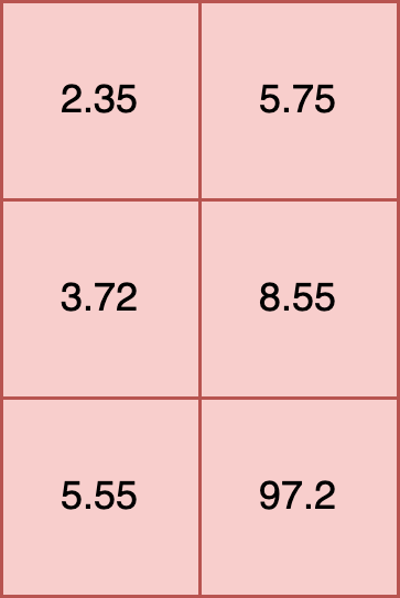
All Inputs Are Tensors
All inputs into an ONNX model must be tensors. This requires that the shape of each element is the same. For example, the following is a proper input:
t [
[2.35, 5.75],
[3.72, 8.55],
[5.55, 97.2]
]
Another example is a 2,2,3 tensor, where the shape of each element is (3,), and each element has 2 rows.
t = [
[2.35, 5.75, 19.2],
[3.72, 8.55, 10.5]
],
[
[5.55, 7.2, 15.7],
[9.6, 8.2, 2.3]
]
In this example each element has a shape of (2,). Tensors with elements of different shapes, known as ragged tensors, are not supported. For example:
t = [
[2.35, 5.75],
[3.72, 8.55, 10.5],
[5.55, 97.2]
])
**INVALID SHAPE**
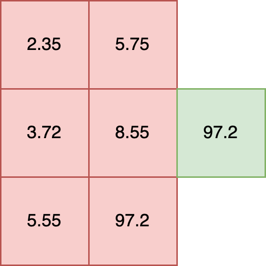
For models that require ragged tensor or other shapes, see other data formatting options such as Bring Your Own Predict models.
Data Type Consistency
All inputs into an ONNX model must have the same internal data type. For example, the following is valid because all of the data types within each element are float32.
t = [
[2.35, 5.75],
[3.72, 8.55],
[5.55, 97.2]
]
The following is invalid, as it mixes floats and strings in each element:
t = [
[2.35, "Bob"],
[3.72, "Nancy"],
[5.55, "Wani"]
]
The following inputs are valid, as each data type is consistent within the elements.
df = pd.DataFrame({
"t": [
[2.35, 5.75, 19.2],
[5.55, 7.2, 15.7],
],
"s": [
["Bob", "Nancy", "Wani"],
["Jason", "Rita", "Phoebe"]
]
})
df
| t | s | |
|---|---|---|
| 0 | [2.35, 5.75, 19.2] | [Bob, Nancy, Wani] |
| 1 | [5.55, 7.2, 15.7] | [Jason, Rita, Phoebe] |
| Parameter | Description |
|---|---|
| Web Site | https://www.tensorflow.org/ |
| Supported Libraries | tensorflow==2.9.3 |
| Framework | Framework.TENSORFLOW aka tensorflow |
| Runtime | Native aka tensorflow |
| Supported File Types | SavedModel format as .zip file |
IMPORTANT NOTE
These requirements are <strong>not</strong> for Tensorflow Keras models, only for non-Keras Tensorflow models in the SavedModel format. For Tensorflow Keras deployment in Wallaroo, see the Tensorflow Keras requirements.
TensorFlow File Format
TensorFlow models are .zip file of the SavedModel format. For example, the Aloha sample TensorFlow model is stored in the directory alohacnnlstm:
├── saved_model.pb
└── variables
├── variables.data-00000-of-00002
├── variables.data-00001-of-00002
└── variables.index
This is compressed into the .zip file alohacnnlstm.zip with the following command:
zip -r alohacnnlstm.zip alohacnnlstm/
ML models that meet the Tensorflow and SavedModel format will run as Wallaroo Native runtimes by default.
See the SavedModel guide for full details.
| Parameter | Description |
|---|---|
| Web Site | https://www.python.org/ |
| Supported Libraries | python==3.8 |
| Framework | Framework.PYTHON aka python |
| Runtime | Native aka python |
Python models uploaded to Wallaroo are executed as a native runtime.
Note that Python models - aka “Python steps” - are standalone python scripts that use the python libraries natively supported by the Wallaroo platform. These are used for either simple model deployment (such as ARIMA Statsmodels), or data formatting such as the postprocessing steps. A Wallaroo Python model will be composed of one Python script that matches the Wallaroo requirements.
This is contrasted with Arbitrary Python models, also known as Bring Your Own Predict (BYOP) allow for custom model deployments with supporting scripts and artifacts. These are used with pre-trained models (PyTorch, Tensorflow, etc) along with whatever supporting artifacts they require. Supporting artifacts can include other Python modules, model files, etc. These are zipped with all scripts, artifacts, and a requirements.txt file that indicates what other Python models need to be imported that are outside of the typical Wallaroo platform.
Python Models Requirements
Python models uploaded to Wallaroo are Python scripts that must include the wallaroo_json method as the entry point for the Wallaroo engine to use it as a Pipeline step.
This method receives the results of the previous Pipeline step, and its return value will be used in the next Pipeline step.
If the Python model is the first step in the pipeline, then it will be receiving the inference request data (for example: a preprocessing step). If it is the last step in the pipeline, then it will be the data returned from the inference request.
In the example below, the Python model is used as a post processing step for another ML model. The Python model expects to receive data from a ML Model who’s output is a DataFrame with the column dense_2. It then extracts the values of that column as a list, selects the first element, and returns a DataFrame with that element as the value of the column output.
def wallaroo_json(data: pd.DataFrame):
print(data)
return [{"output": [data["dense_2"].to_list()[0][0]]}]
In line with other Wallaroo inference results, the outputs of a Python step that returns a pandas DataFrame or Arrow Table will be listed in the out. metadata, with all inference outputs listed as out.{variable 1}, out.{variable 2}, etc. In the example above, this results the output field as the out.output field in the Wallaroo inference result.
| time | in.tensor | out.output | check_failures | |
|---|---|---|---|---|
| 0 | 2023-06-20 20:23:28.395 | [0.6878518042, 0.1760734021, -0.869514083, 0.3.. | [12.886651039123535] | 0 |
| Parameter | Description |
|---|---|
| Web Site | https://huggingface.co/models |
| Supported Libraries |
|
| Frameworks | The following Hugging Face pipelines are supported by Wallaroo.
|
| Runtime | Containerized flight |
During the model upload process, the Wallaroo instance will attempt to convert the model to a Native Wallaroo Runtime. If unsuccessful based , it will create a Wallaroo Containerized Runtime for the model. See the model deployment section for details on how to configure pipeline resources based on the model’s runtime.
Hugging Face Schemas
Input and output schemas for each Hugging Face pipeline are defined below. Note that adding additional inputs not specified below will raise errors, except for the following:
Framework.HUGGING_FACE_IMAGE_TO_TEXTFramework.HUGGING_FACE_TEXT_CLASSIFICATIONFramework.HUGGING_FACE_SUMMARIZATIONFramework.HUGGING_FACE_TRANSLATION
Additional inputs added to these Hugging Face pipelines will be added as key/pair value arguments to the model’s generate method. If the argument is not required, then the model will default to the values coded in the original Hugging Face model’s source code.
See the Hugging Face Pipeline documentation for more details on each pipeline and framework.
| Wallaroo Framework | Reference |
|---|---|
Framework.HUGGING_FACE_FEATURE_EXTRACTION |
Schemas:
input_schema = pa.schema([
pa.field('inputs', pa.string())
])
output_schema = pa.schema([
pa.field('output', pa.list_(
pa.list_(
pa.float64(),
list_size=128
),
))
])
| Wallaroo Framework | Reference |
|---|---|
Framework.HUGGING_FACE_IMAGE_CLASSIFICATION |
Schemas:
input_schema = pa.schema([
pa.field('inputs', pa.list_(
pa.list_(
pa.list_(
pa.int64(),
list_size=3
),
list_size=100
),
list_size=100
)),
pa.field('top_k', pa.int64()),
])
output_schema = pa.schema([
pa.field('score', pa.list_(pa.float64(), list_size=2)),
pa.field('label', pa.list_(pa.string(), list_size=2)),
])
| Wallaroo Framework | Reference |
|---|---|
Framework.HUGGING_FACE_IMAGE_SEGMENTATION |
Schemas:
input_schema = pa.schema([
pa.field('inputs',
pa.list_(
pa.list_(
pa.list_(
pa.int64(),
list_size=3
),
list_size=100
),
list_size=100
)),
pa.field('threshold', pa.float64()),
pa.field('mask_threshold', pa.float64()),
pa.field('overlap_mask_area_threshold', pa.float64()),
])
output_schema = pa.schema([
pa.field('score', pa.list_(pa.float64())),
pa.field('label', pa.list_(pa.string())),
pa.field('mask',
pa.list_(
pa.list_(
pa.list_(
pa.int64(),
list_size=100
),
list_size=100
),
)),
])
| Wallaroo Framework | Reference |
|---|---|
Framework.HUGGING_FACE_IMAGE_TO_TEXT |
Any parameter that is not part of the required inputs list will be forwarded to the model as a key/pair value to the underlying models generate method. If the additional input is not supported by the model, an error will be returned.
Schemas:
input_schema = pa.schema([
pa.field('inputs', pa.list_( #required
pa.list_(
pa.list_(
pa.int64(),
list_size=3
),
list_size=100
),
list_size=100
)),
# pa.field('max_new_tokens', pa.int64()), # optional
])
output_schema = pa.schema([
pa.field('generated_text', pa.list_(pa.string())),
])
| Wallaroo Framework | Reference |
|---|---|
Framework.HUGGING_FACE_OBJECT_DETECTION |
Schemas:
input_schema = pa.schema([
pa.field('inputs',
pa.list_(
pa.list_(
pa.list_(
pa.int64(),
list_size=3
),
list_size=100
),
list_size=100
)),
pa.field('threshold', pa.float64()),
])
output_schema = pa.schema([
pa.field('score', pa.list_(pa.float64())),
pa.field('label', pa.list_(pa.string())),
pa.field('box',
pa.list_( # dynamic output, i.e. dynamic number of boxes per input image, each sublist contains the 4 box coordinates
pa.list_(
pa.int64(),
list_size=4
),
),
),
])
| Wallaroo Framework | Reference |
|---|---|
Framework.HUGGING_FACE_QUESTION_ANSWERING |
Schemas:
input_schema = pa.schema([
pa.field('question', pa.string()),
pa.field('context', pa.string()),
pa.field('top_k', pa.int64()),
pa.field('doc_stride', pa.int64()),
pa.field('max_answer_len', pa.int64()),
pa.field('max_seq_len', pa.int64()),
pa.field('max_question_len', pa.int64()),
pa.field('handle_impossible_answer', pa.bool_()),
pa.field('align_to_words', pa.bool_()),
])
output_schema = pa.schema([
pa.field('score', pa.float64()),
pa.field('start', pa.int64()),
pa.field('end', pa.int64()),
pa.field('answer', pa.string()),
])
| Wallaroo Framework | Reference |
|---|---|
Framework.HUGGING_FACE_STABLE_DIFFUSION_TEXT_2_IMG |
Schemas:
input_schema = pa.schema([
pa.field('prompt', pa.string()),
pa.field('height', pa.int64()),
pa.field('width', pa.int64()),
pa.field('num_inference_steps', pa.int64()), # optional
pa.field('guidance_scale', pa.float64()), # optional
pa.field('negative_prompt', pa.string()), # optional
pa.field('num_images_per_prompt', pa.string()), # optional
pa.field('eta', pa.float64()) # optional
])
output_schema = pa.schema([
pa.field('images', pa.list_(
pa.list_(
pa.list_(
pa.int64(),
list_size=3
),
list_size=128
),
list_size=128
)),
])
| Wallaroo Framework | Reference |
|---|---|
Framework.HUGGING_FACE_SUMMARIZATION |
Any parameter that is not part of the required inputs list will be forwarded to the model as a key/pair value to the underlying models generate method. If the additional input is not supported by the model, an error will be returned.
Schemas:
input_schema = pa.schema([
pa.field('inputs', pa.string()),
pa.field('return_text', pa.bool_()),
pa.field('return_tensors', pa.bool_()),
pa.field('clean_up_tokenization_spaces', pa.bool_()),
# pa.field('extra_field', pa.int64()), # every extra field you specify will be forwarded as a key/value pair
])
output_schema = pa.schema([
pa.field('summary_text', pa.string()),
])
| Wallaroo Framework | Reference |
|---|---|
Framework.HUGGING_FACE_TEXT_CLASSIFICATION |
Schemas
input_schema = pa.schema([
pa.field('inputs', pa.string()), # required
pa.field('top_k', pa.int64()), # optional
pa.field('function_to_apply', pa.string()), # optional
])
output_schema = pa.schema([
pa.field('label', pa.list_(pa.string(), list_size=2)), # list with a number of items same as top_k, list_size can be skipped but may lead in worse performance
pa.field('score', pa.list_(pa.float64(), list_size=2)), # list with a number of items same as top_k, list_size can be skipped but may lead in worse performance
])
| Wallaroo Framework | Reference |
|---|---|
Framework.HUGGING_FACE_TRANSLATION |
Any parameter that is not part of the required inputs list will be forwarded to the model as a key/pair value to the underlying models generate method. If the additional input is not supported by the model, an error will be returned.
Schemas:
input_schema = pa.schema([
pa.field('inputs', pa.string()), # required
pa.field('return_tensors', pa.bool_()), # optional
pa.field('return_text', pa.bool_()), # optional
pa.field('clean_up_tokenization_spaces', pa.bool_()), # optional
pa.field('src_lang', pa.string()), # optional
pa.field('tgt_lang', pa.string()), # optional
# pa.field('extra_field', pa.int64()), # every extra field you specify will be forwarded as a key/value pair
])
output_schema = pa.schema([
pa.field('translation_text', pa.string()),
])
| Wallaroo Framework | Reference |
|---|---|
Framework.HUGGING_FACE_ZERO_SHOT_CLASSIFICATION |
Schemas:
input_schema = pa.schema([
pa.field('inputs', pa.string()), # required
pa.field('candidate_labels', pa.list_(pa.string(), list_size=2)), # required
pa.field('hypothesis_template', pa.string()), # optional
pa.field('multi_label', pa.bool_()), # optional
])
output_schema = pa.schema([
pa.field('sequence', pa.string()),
pa.field('scores', pa.list_(pa.float64(), list_size=2)), # same as number of candidate labels, list_size can be skipped by may result in slightly worse performance
pa.field('labels', pa.list_(pa.string(), list_size=2)), # same as number of candidate labels, list_size can be skipped by may result in slightly worse performance
])
| Wallaroo Framework | Reference |
|---|---|
Framework.HUGGING_FACE_ZERO_SHOT_IMAGE_CLASSIFICATION |
Schemas:
input_schema = pa.schema([
pa.field('inputs', # required
pa.list_(
pa.list_(
pa.list_(
pa.int64(),
list_size=3
),
list_size=100
),
list_size=100
)),
pa.field('candidate_labels', pa.list_(pa.string(), list_size=2)), # required
pa.field('hypothesis_template', pa.string()), # optional
])
output_schema = pa.schema([
pa.field('score', pa.list_(pa.float64(), list_size=2)), # same as number of candidate labels
pa.field('label', pa.list_(pa.string(), list_size=2)), # same as number of candidate labels
])
| Wallaroo Framework | Reference |
|---|---|
Framework.HUGGING_FACE_ZERO_SHOT_OBJECT_DETECTION |
Schemas:
input_schema = pa.schema([
pa.field('images',
pa.list_(
pa.list_(
pa.list_(
pa.int64(),
list_size=3
),
list_size=640
),
list_size=480
)),
pa.field('candidate_labels', pa.list_(pa.string(), list_size=3)),
pa.field('threshold', pa.float64()),
# pa.field('top_k', pa.int64()), # we want the model to return exactly the number of predictions, we shouldn't specify this
])
output_schema = pa.schema([
pa.field('score', pa.list_(pa.float64())), # variable output, depending on detected objects
pa.field('label', pa.list_(pa.string())), # variable output, depending on detected objects
pa.field('box',
pa.list_( # dynamic output, i.e. dynamic number of boxes per input image, each sublist contains the 4 box coordinates
pa.list_(
pa.int64(),
list_size=4
),
),
),
])
| Wallaroo Framework | Reference |
|---|---|
Framework.HUGGING_FACE_SENTIMENT_ANALYSIS | Hugging Face Sentiment Analysis |
| Wallaroo Framework | Reference |
|---|---|
Framework.HUGGING_FACE_TEXT_GENERATION |
Any parameter that is not part of the required inputs list will be forwarded to the model as a key/pair value to the underlying models generate method. If the additional input is not supported by the model, an error will be returned.
input_schema = pa.schema([
pa.field('inputs', pa.string()),
pa.field('return_tensors', pa.bool_()), # optional
pa.field('return_text', pa.bool_()), # optional
pa.field('return_full_text', pa.bool_()), # optional
pa.field('clean_up_tokenization_spaces', pa.bool_()), # optional
pa.field('prefix', pa.string()), # optional
pa.field('handle_long_generation', pa.string()), # optional
# pa.field('extra_field', pa.int64()), # every extra field you specify will be forwarded as a key/value pair
])
output_schema = pa.schema([
pa.field('generated_text', pa.list_(pa.string(), list_size=1))
])
| Wallaroo Framework | Reference |
|---|---|
Framework.HUGGING_FACE_AUTOMATIC_SPEECH_RECOGNITION |
Sample input and output schema.
input_schema = pa.schema([
pa.field('inputs', pa.list_(pa.float32())), # required: the audio stored in numpy arrays of shape (num_samples,) and data type `float32`
pa.field('return_timestamps', pa.string()) # optional: return start & end times for each predicted chunk
])
output_schema = pa.schema([
pa.field('text', pa.string()), # required: the output text corresponding to the audio input
pa.field('chunks', pa.list_(pa.struct([('text', pa.string()), ('timestamp', pa.list_(pa.float32()))]))), # required (if `return_timestamps` is set), start & end times for each predicted chunk
])
| Parameter | Description |
|---|---|
| Web Site | https://pytorch.org/ |
| Supported Libraries |
|
| Framework | Framework.PYTORCH aka pytorch |
| Supported File Types | pt ot pth in TorchScript format |
| Runtime | onnx/flight |
- IMPORTANT NOTE: The PyTorch model must be in TorchScript format. scripting (i.e.
torch.jit.script()is always recommended over tracing (i.e.torch.jit.trace()). From the PyTorch documentation: “Scripting preserves dynamic control flow and is valid for inputs of different sizes.” For more details, see TorchScript-based ONNX Exporter: Tracing vs Scripting.
During the model upload process, the Wallaroo instance will attempt to convert the model to a Native Wallaroo Runtime. If unsuccessful based , it will create a Wallaroo Containerized Runtime for the model. See the model deployment section for details on how to configure pipeline resources based on the model’s runtime.
- IMPORTANT CONFIGURATION NOTE: For PyTorch input schemas, the floats must be
pyarrow.float32()for the PyTorch model to be converted to the Native Wallaroo Runtime during the upload process.
Sci-kit Learn aka SKLearn.
| Parameter | Description |
|---|---|
| Web Site | https://scikit-learn.org/stable/index.html |
| Supported Libraries |
|
| Framework | Framework.SKLEARN aka sklearn |
| Runtime | onnx / flight |
During the model upload process, the Wallaroo instance will attempt to convert the model to a Native Wallaroo Runtime. If unsuccessful based , it will create a Wallaroo Containerized Runtime for the model. See the model deployment section for details on how to configure pipeline resources based on the model’s runtime.
SKLearn Schema Inputs
SKLearn schema follows a different format than other models. To prevent inputs from being out of order, the inputs should be submitted in a single row in the order the model is trained to accept, with all of the data types being the same. For example, the following DataFrame has 4 columns, each column a float.
| sepal length (cm) | sepal width (cm) | petal length (cm) | petal width (cm) | |
|---|---|---|---|---|
| 0 | 5.1 | 3.5 | 1.4 | 0.2 |
| 1 | 4.9 | 3.0 | 1.4 | 0.2 |
For submission to an SKLearn model, the data input schema will be a single array with 4 float values.
input_schema = pa.schema([
pa.field('inputs', pa.list_(pa.float64(), list_size=4))
])
When submitting as an inference, the DataFrame is converted to rows with the column data expressed as a single array. The data must be in the same order as the model expects, which is why the data is submitted as a single array rather than JSON labeled columns: this insures that the data is submitted in the exact order as the model is trained to accept.
Original DataFrame:
| sepal length (cm) | sepal width (cm) | petal length (cm) | petal width (cm) | |
|---|---|---|---|---|
| 0 | 5.1 | 3.5 | 1.4 | 0.2 |
| 1 | 4.9 | 3.0 | 1.4 | 0.2 |
Converted DataFrame:
| inputs | |
|---|---|
| 0 | [5.1, 3.5, 1.4, 0.2] |
| 1 | [4.9, 3.0, 1.4, 0.2] |
SKLearn Schema Outputs
Outputs for SKLearn that are meant to be predictions or probabilities when output by the model are labeled in the output schema for the model when uploaded to Wallaroo. For example, a model that outputs either 1 or 0 as its output would have the output schema as follows:
output_schema = pa.schema([
pa.field('predictions', pa.int32())
])
When used in Wallaroo, the inference result is contained in the out metadata as out.predictions.
pipeline.infer(dataframe)
| time | in.inputs | out.predictions | check_failures | |
|---|---|---|---|---|
| 0 | 2023-07-05 15:11:29.776 | [5.1, 3.5, 1.4, 0.2] | 0 | 0 |
| 1 | 2023-07-05 15:11:29.776 | [4.9, 3.0, 1.4, 0.2] | 0 | 0 |
| Parameter | Description |
|---|---|
| Web Site | https://www.tensorflow.org/api_docs/python/tf/keras/Model |
| Supported Libraries |
|
| Framework | Framework.KERAS aka keras |
| Supported File Types | SavedModel format as .zip file and HDF5 format |
| Runtime | onnx/flight |
During the model upload process, the Wallaroo instance will attempt to convert the model to a Native Wallaroo Runtime. If unsuccessful based , it will create a Wallaroo Containerized Runtime for the model. See the model deployment section for details on how to configure pipeline resources based on the model’s runtime.
TensorFlow Keras SavedModel Format
TensorFlow Keras SavedModel models are .zip file of the SavedModel format. For example, the Aloha sample TensorFlow model is stored in the directory alohacnnlstm:
├── saved_model.pb
└── variables
├── variables.data-00000-of-00002
├── variables.data-00001-of-00002
└── variables.index
This is compressed into the .zip file alohacnnlstm.zip with the following command:
zip -r alohacnnlstm.zip alohacnnlstm/
See the SavedModel guide for full details.
TensorFlow Keras H5 Format
Wallaroo supports the H5 for Tensorflow Keras models.
| Parameter | Description |
|---|---|
| Web Site | https://xgboost.ai/ |
| Supported Libraries |
|
| Framework | Framework.XGBOOST aka xgboost |
| Supported File Types | pickle (XGB files are not supported.) |
| Runtime | onnx / flight |
During the model upload process, the Wallaroo instance will attempt to convert the model to a Native Wallaroo Runtime. If unsuccessful based , it will create a Wallaroo Containerized Runtime for the model. See the model deployment section for details on how to configure pipeline resources based on the model’s runtime.
XGBoost Schema Inputs
XGBoost schema follows a different format than other models. To prevent inputs from being out of order, the inputs should be submitted in a single row in the order the model is trained to accept, with all of the data types being the same. If a model is originally trained to accept inputs of different data types, it will need to be retrained to only accept one data type for each column - typically pa.float64() is a good choice.
For example, the following DataFrame has 4 columns, each column a float.
| sepal length (cm) | sepal width (cm) | petal length (cm) | petal width (cm) | |
|---|---|---|---|---|
| 0 | 5.1 | 3.5 | 1.4 | 0.2 |
| 1 | 4.9 | 3.0 | 1.4 | 0.2 |
For submission to an XGBoost model, the data input schema will be a single array with 4 float values.
input_schema = pa.schema([
pa.field('inputs', pa.list_(pa.float64(), list_size=4))
])
When submitting as an inference, the DataFrame is converted to rows with the column data expressed as a single array. The data must be in the same order as the model expects, which is why the data is submitted as a single array rather than JSON labeled columns: this insures that the data is submitted in the exact order as the model is trained to accept.
Original DataFrame:
| sepal length (cm) | sepal width (cm) | petal length (cm) | petal width (cm) | |
|---|---|---|---|---|
| 0 | 5.1 | 3.5 | 1.4 | 0.2 |
| 1 | 4.9 | 3.0 | 1.4 | 0.2 |
Converted DataFrame:
| inputs | |
|---|---|
| 0 | [5.1, 3.5, 1.4, 0.2] |
| 1 | [4.9, 3.0, 1.4, 0.2] |
XGBoost Schema Outputs
Outputs for XGBoost are labeled based on the trained model outputs. For this example, the output is simply a single output listed as output. In the Wallaroo inference result, it is grouped with the metadata out as out.output.
output_schema = pa.schema([
pa.field('output', pa.int32())
])
pipeline.infer(dataframe)
| time | in.inputs | out.output | check_failures | |
|---|---|---|---|---|
| 0 | 2023-07-05 15:11:29.776 | [5.1, 3.5, 1.4, 0.2] | 0 | 0 |
| 1 | 2023-07-05 15:11:29.776 | [4.9, 3.0, 1.4, 0.2] | 0 | 0 |
| Parameter | Description |
|---|---|
| Web Site | https://www.python.org/ |
| Supported Libraries | python==3.8 |
| Framework | Framework.CUSTOM aka custom |
| Runtime | Containerized aka flight |
Arbitrary Python models, also known as Bring Your Own Predict (BYOP) allow for custom model deployments with supporting scripts and artifacts. These are used with pre-trained models (PyTorch, Tensorflow, etc) along with whatever supporting artifacts they require. Supporting artifacts can include other Python modules, model files, etc. These are zipped with all scripts, artifacts, and a requirements.txt file that indicates what other Python models need to be imported that are outside of the typical Wallaroo platform.
Contrast this with Wallaroo Python models - aka “Python steps”. These are standalone python scripts that use the python libraries natively supported by the Wallaroo platform. These are used for either simple model deployment (such as ARIMA Statsmodels), or data formatting such as the postprocessing steps. A Wallaroo Python model will be composed of one Python script that matches the Wallaroo requirements.
Arbitrary Python File Requirements
Arbitrary Python (BYOP) models are uploaded to Wallaroo via a ZIP file with the following components:
| Artifact | Type | Description |
|---|---|---|
Python scripts aka .py files with classes that extend mac.inference.Inference and mac.inference.creation.InferenceBuilder | Python Script | Extend the classes mac.inference.Inference and mac.inference.creation.InferenceBuilder. These are included with the Wallaroo SDK. Further details are in Arbitrary Python Script Requirements. Note that there is no specified naming requirements for the classes that extend mac.inference.Inference and mac.inference.creation.InferenceBuilder - any qualified class name is sufficient as long as these two classes are extended as defined below. |
requirements.txt | Python requirements file | This sets the Python libraries used for the arbitrary python model. These libraries should be targeted for Python 3.8 compliance. These requirements and the versions of libraries should be exactly the same between creating the model and deploying it in Wallaroo. This insures that the script and methods will function exactly the same as during the model creation process. |
| Other artifacts | Files | Other models, files, and other artifacts used in support of this model. |
For example, the if the arbitrary python model will be known as vgg_clustering, the contents may be in the following structure, with vgg_clustering as the storage directory:
vgg_clustering\
feature_extractor.h5
kmeans.pkl
custom_inference.py
requirements.txt
Note the inclusion of the custom_inference.py file. This file name is not required - any Python script or scripts that extend the classes listed above are sufficient. This Python script could have been named vgg_custom_model.py or any other name as long as it includes the extension of the classes listed above.
The sample arbitrary python model file is created with the command zip -r vgg_clustering.zip vgg_clustering/.
Wallaroo Arbitrary Python uses the Wallaroo SDK mac module, included in the Wallaroo SDK 2023.2.1 and above. See the Wallaroo SDK Install Guides for instructions on installing the Wallaroo SDK.
Arbitrary Python Script Requirements
The entry point of the arbitrary python model is any python script that extends the following classes. These are included with the Wallaroo SDK. The required methods that must be overridden are specified in each section below.
mac.inference.Inferenceinterface serves model inferences based on submitted input some input. Its purpose is to serve inferences for any supported arbitrary model framework (e.g.scikit,kerasetc.).classDiagram class Inference { <<Abstract>> +model Optional[Any] +expected_model_types()* Set +predict(input_data: InferenceData)* InferenceData -raise_error_if_model_is_not_assigned() None -raise_error_if_model_is_wrong_type() None }mac.inference.creation.InferenceBuilderbuilds a concreteInference, i.e. instantiates anInferenceobject, loads the appropriate model and assigns the model to to the Inference object.classDiagram class InferenceBuilder { +create(config InferenceConfig) * Inference -inference()* Any }
mac.inference.Inference
mac.inference.Inference Objects
| Object | Type | Description |
|---|---|---|
model (Required) | [Any] | One or more objects that match the expected_model_types. This can be a ML Model (for inference use), a string (for data conversion), etc. See Arbitrary Python Examples for examples. |
mac.inference.Inference Methods
| Method | Returns | Description |
|---|---|---|
expected_model_types (Required) | Set | Returns a Set of models expected for the inference as defined by the developer. Typically this is a set of one. Wallaroo checks the expected model types to verify that the model submitted through the InferenceBuilder method matches what this Inference class expects. |
_predict (input_data: mac.types.InferenceData) (Required) | mac.types.InferenceData | The entry point for the Wallaroo inference with the following input and output parameters that are defined when the model is updated.
InferenceDataValidationError exception is raised when the input data does not match mac.types.InferenceData. |
raise_error_if_model_is_not_assigned | N/A | Error when a model is not set to Inference. |
raise_error_if_model_is_wrong_type | N/A | Error when the model does not match the expected_model_types. |
IMPORTANT NOTE
Verify that the inputs and outputs match the InferenceData input and output types: a Dictionary of numpy arrays defined by the input_schema and output_schema parameters when uploading the model to the Wallaroo instance. The following code is an example of a Dictionary of numpy arrays.
preds = self.model.predict(data)
preds = preds.numpy()
rows, _ = preds.shape
preds = preds.reshape((rows,))
return {"prediction": preds} # a Dictionary of numpy arrays.
The example, the expected_model_types can be defined for the KMeans model.
from sklearn.cluster import KMeans
class SampleClass(mac.inference.Inference):
@property
def expected_model_types(self) -> Set[Any]:
return {KMeans}
mac.inference.creation.InferenceBuilder
InferenceBuilder builds a concrete Inference, i.e. instantiates an Inference object, loads the appropriate model and assigns the model to the Inference.
classDiagram
class InferenceBuilder {
+create(config InferenceConfig) * Inference
-inference()* Any
}Each model that is included requires its own InferenceBuilder. InferenceBuilder loads one model, then submits it to the Inference class when created. The Inference class checks this class against its expected_model_types() Set.
mac.inference.creation.InferenceBuilder Methods
| Method | Returns | Description |
|---|---|---|
create(config mac.config.inference.CustomInferenceConfig) (Required) | The custom Inference instance. | Creates an Inference subclass, then assigns a model and attributes. The CustomInferenceConfig is used to retrieve the config.model_path, which is a pathlib.Path object pointing to the folder where the model artifacts are saved. Every artifact loaded must be relative to config.model_path. This is set when the arbitrary python .zip file is uploaded and the environment for running it in Wallaroo is set. For example: loading the artifact vgg_clustering\feature_extractor.h5 would be set with config.model_path \ feature_extractor.h5. The model loaded must match an existing module. For our example, this is from sklearn.cluster import KMeans, and this must match the Inference expected_model_types. |
inference | custom Inference instance. | Returns the instantiated custom Inference object created from the create method. |
Arbitrary Python Runtime
Arbitrary Python always run in the containerized model runtime.
| Parameter | Description |
|---|---|
| Web Site | https://mlflow.org |
| Supported Libraries | mlflow==1.3.0 |
| Runtime | Containerized aka mlflow |
For models that do not fall under the supported model frameworks, organizations can use containerized MLFlow ML Models.
This guide details how to add ML Models from a model registry service into Wallaroo.
Wallaroo supports both public and private containerized model registries. See the Wallaroo Private Containerized Model Container Registry Guide for details on how to configure a Wallaroo instance with a private model registry.
Wallaroo users can register their trained MLFlow ML Models from a containerized model container registry into their Wallaroo instance and perform inferences with it through a Wallaroo pipeline.
As of this time, Wallaroo only supports MLFlow 1.30.0 containerized models. For information on how to containerize an MLFlow model, see the MLFlow Documentation.
Wallaroo supports both public and private containerized model registries. See the Wallaroo Private Containerized Model Container Registry Guide for details on how to configure a Wallaroo instance with a private model registry.
List Wallaroo Frameworks
Wallaroo frameworks are listed from the Wallaroo.Framework class. The following demonstrates listing all available supported frameworks.
from wallaroo.framework import Framework
[e.value for e in Framework]
['onnx',
'tensorflow',
'python',
'keras',
'sklearn',
'pytorch',
'xgboost',
'hugging-face-feature-extraction',
'hugging-face-image-classification',
'hugging-face-image-segmentation',
'hugging-face-image-to-text',
'hugging-face-object-detection',
'hugging-face-question-answering',
'hugging-face-stable-diffusion-text-2-img',
'hugging-face-summarization',
'hugging-face-text-classification',
'hugging-face-translation',
'hugging-face-zero-shot-classification',
'hugging-face-zero-shot-image-classification',
'hugging-face-zero-shot-object-detection',
'hugging-face-sentiment-analysis',
'hugging-face-text-generation']
2.1.1 - Model Registry Service with Wallaroo SDK Demonstration
How to use the Wallaroo SDK with Model Registry Services
This tutorial can be downloaded as part of the Wallaroo Tutorials repository.
MLFLow Registry Model Upload Demonstration
Wallaroo users can register their trained machine learning models from a model registry into their Wallaroo instance and perform inferences with it through a Wallaroo pipeline.
This guide details how to add ML Models from a model registry service into a Wallaroo instance.
Artifact Requirements
Models are uploaded to the Wallaroo instance as the specific artifact - the “file” or other data that represents the file itself. This must comply with the Wallaroo model requirements framework and version or it will not be deployed.
This tutorial will:
- Create a Wallaroo workspace and pipeline.
- Show how to connect a Wallaroo Registry that connects to a Model Registry Service.
- Use the registry connection details to upload a sample model to Wallaroo.
- Perform a sample inference.
Prerequisites
- A Wallaroo version 2023.2.1 or above instance.
- A Model (aka Artifact) Registry Service
References
Tutorial Steps
Import Libraries
We’ll start with importing the libraries we need for the tutorial.
import os
import wallaroo
Connect to the Wallaroo Instance through the User Interface
The next step is to connect to Wallaroo through the Wallaroo client. The Python library is included in the Wallaroo install and available through the Jupyter Hub interface provided with your Wallaroo environment.
This is accomplished using the wallaroo.Client() command, which provides a URL to grant the SDK permission to your specific Wallaroo environment. When displayed, enter the URL into a browser and confirm permissions. Store the connection into a variable that can be referenced later.
If logging into the Wallaroo instance through the internal JupyterHub service, use wl = wallaroo.Client(). For more information on Wallaroo Client settings, see the Client Connection guide.
wl=wallaroo.Client()
Connect to Model Registry
The Wallaroo Registry stores the URL and authentication token to the Model Registry service, with the assigned name. Note that in this demonstration all URLs and token are examples.
registry = wl.create_model_registry(name="JeffRegistry45",
token="dapi67c8c0b04606f730e78b7ae5e3221015-3",
url="https://sample.registry.service.azuredatabricks.net")
registry
| Field | Value |
|---|---|
| Name | JeffRegistry45 |
| URL | https://sample.registry.service.azuredatabricks.net |
| Workspaces | john.hummel@wallaroo.ai - Default Workspace |
| Created At | 2023-17-Jul 19:54:49 |
| Updated At | 2023-17-Jul 19:54:49 |
List Model Registries
Registries associated with a workspace are listed with the Wallaroo.Client.list_model_registries() method.
# List all registries in this workspace
registries = wl.list_model_registries()
registries
| name | registry url | created at | updated at |
|---|---|---|---|
| JeffRegistry45 | https://sample.registry.service.azuredatabricks.net | 2023-17-Jul 17:56:52 | 2023-17-Jul 17:56:52 |
| JeffRegistry45 | https://sample.registry.service.azuredatabricks.net | 2023-17-Jul 19:54:49 | 2023-17-Jul 19:54:49 |
Create Workspace
For this demonstration, we will create a random Wallaroo workspace, then attach our registry to the workspace so it is accessible by other workspace users.
Add Registry to Workspace
Registries are assigned to a Wallaroo workspace with the Wallaroo.registry.add_registry_to_workspace method. This allows members of the workspace to access the registry connection. A registry can be associated with one or more workspaces.
Add Registry to Workspace Parameters
| Parameter | Type | Description |
|---|---|---|
name | string (Required) | The numerical identifier of the workspace. |
# Make a random new workspace
import math
import random
num = math.floor(random.random()* 1000)
workspace_id = wl.create_workspace(f"test{num}").id()
registry.add_registry_to_workspace(workspace_id=workspace_id)
| Field | Value |
|---|---|
| Name | JeffRegistry45 |
| URL | https://sample.registry.service.azuredatabricks.net |
| Workspaces | test68, john.hummel@wallaroo.ai - Default Workspace |
| Created At | 2023-17-Jul 19:54:49 |
| Updated At | 2023-17-Jul 19:54:49 |
Remove Registry from Workspace
Registries are removed from a Wallaroo workspace with the Registry remove_registry_from_workspace method.
Remove Registry from Workspace Parameters
| Parameter | Type | Description |
|---|---|---|
workspace_id | Integer (Required) | The numerical identifier of the workspace. |
registry.remove_registry_from_workspace(workspace_id=workspace_id)
| Field | Value |
|---|---|
| Name | JeffRegistry45 |
| URL | https://sample.registry.service.azuredatabricks.net |
| Workspaces | john.hummel@wallaroo.ai - Default Workspace |
| Created At | 2023-17-Jul 19:54:49 |
| Updated At | 2023-17-Jul 19:54:49 |
List Models in a Registry
A List of models available to the Wallaroo instance through the MLFlow Registry is performed with the Wallaroo.Registry.list_models() method.
registry_models = registry.list_models()
registry_models
| Name | Registry User | Versions | Created At | Updated At |
| logreg1 | gib.bhojraj@wallaroo.ai | 1 | 2023-06-Jul 14:36:54 | 2023-06-Jul 14:36:56 |
| sidekick-test | gib.bhojraj@wallaroo.ai | 1 | 2023-11-Jul 14:42:14 | 2023-11-Jul 14:42:14 |
| testmodel | gib.bhojraj@wallaroo.ai | 1 | 2023-16-Jun 12:38:42 | 2023-06-Jul 15:03:41 |
| testmodel2 | gib.bhojraj@wallaroo.ai | 1 | 2023-16-Jun 12:41:04 | 2023-29-Jun 18:08:33 |
| verified-working | gib.bhojraj@wallaroo.ai | 1 | 2023-11-Jul 16:18:03 | 2023-11-Jul 16:57:54 |
| wine_quality | gib.bhojraj@wallaroo.ai | 2 | 2023-16-Jun 13:05:53 | 2023-16-Jun 13:09:57 |
Select Model from Registry
Registry models are selected from the Wallaroo.Registry.list_models() method, then specifying the model to use.
single_registry_model = registry_models[4]
single_registry_model
| Name | verified-working |
| Registry User | gib.bhojraj@wallaroo.ai |
| Versions | 1 |
| Created At | 2023-11-Jul 16:18:03 |
| Updated At | 2023-11-Jul 16:57:54 |
List Model Versions
The Registry Model attribute versions shows the complete list of versions for the particular model.
single_registry_model.versions()
| Name | Version | Description |
| verified-working | 3 | None |
List Model Version Artifacts
Artifacts belonging to a MLFlow registry model are listed with the Model Version list_artifacts() method. This returns all artifacts for the model.
single_registry_model.versions()[1].list_artifacts()
| File Name | File Size | Full Path |
|---|---|---|
| MLmodel | 559B | https://sample.registry.service.azuredatabricks.net/api/2.0/dbfs/read?path=/databricks/mlflow-registry/9168792a16cb40a88de6959ef31e42a2/models/√erified-working/MLmodel |
| conda.yaml | 182B | https://sample.registry.service.azuredatabricks.net/api/2.0/dbfs/read?path=/databricks/mlflow-registry/9168792a16cb40a88de6959ef31e42a2/models/√erified-working/conda.yaml |
| model.pkl | 829B | https://sample.registry.service.azuredatabricks.net/api/2.0/dbfs/read?path=/databricks/mlflow-registry/9168792a16cb40a88de6959ef31e42a2/models/√erified-working/model.pkl |
| python_env.yaml | 122B | https://sample.registry.service.azuredatabricks.net/api/2.0/dbfs/read?path=/databricks/mlflow-registry/9168792a16cb40a88de6959ef31e42a2/models/√erified-working/python_env.yaml |
| requirements.txt | 73B | https://sample.registry.service.azuredatabricks.net/api/2.0/dbfs/read?path=/databricks/mlflow-registry/9168792a16cb40a88de6959ef31e42a2/models/√erified-working/requirements.txt |
Configure Data Schemas
To upload a ML Model to Wallaroo, the input and output schemas must be defined in pyarrow.lib.Schema format.
from wallaroo.framework import Framework
import pyarrow as pa
input_schema = pa.schema([
pa.field('inputs', pa.list_(pa.float64(), list_size=4))
])
output_schema = pa.schema([
pa.field('predictions', pa.int32()),
pa.field('probabilities', pa.list_(pa.float64(), list_size=3))
])
Upload a Model from a Registry
Models uploaded to the Wallaroo workspace are uploaded from a MLFlow Registry with the Wallaroo.Registry.upload method.
Upload a Model from a Registry Parameters
| Parameter | Type | Description |
|---|---|---|
name | string (Required) | The name to assign the model once uploaded. Model names are unique within a workspace. Models assigned the same name as an existing model will be uploaded as a new model version. |
path | string (Required) | The full path to the model artifact in the registry. |
framework | string (Required) | The Wallaroo model Framework. See Model Uploads and Registrations Supported Frameworks |
input_schema | pyarrow.lib.Schema (Required for non-native runtimes) | The input schema in Apache Arrow schema format. |
output_schema | pyarrow.lib.Schema (Required for non-native runtimes) | The output schema in Apache Arrow schema format. |
model = registry.upload_model(
name="verified-working",
path="https://sample.registry.service.azuredatabricks.net/api/2.0/dbfs/read?path=/databricks/mlflow-registry/9168792a16cb40a88de6959ef31e42a2/models/√erified-working/model.pkl",
framework=Framework.SKLEARN,
input_schema=input_schema,
output_schema=output_schema)
model
| Name | verified-working |
| Version | cf194b65-65b2-4d42-a4e2-6ca6fa5bfc42 |
| File Name | model.pkl |
| SHA | 5f4c25b0b564ab9fe0ea437424323501a460aa74463e81645a6419be67933ca4 |
| Status | pending_conversion |
| Image Path | None |
| Updated At | 2023-17-Jul 17:57:23 |
Verify the Model Status
Once uploaded, the model will undergo conversion. The following will loop through the model status until it is ready. Once ready, it is available for deployment.
import time
while model.status() != "ready" and model.status() != "error":
print(model.status())
time.sleep(3)
print(model.status())
pending_conversion
pending_conversion
pending_conversion
pending_conversion
pending_conversion
pending_conversion
pending_conversion
pending_conversion
pending_conversion
pending_conversion
converting
converting
converting
converting
converting
converting
converting
converting
converting
converting
converting
converting
converting
converting
converting
ready
Model Runtime
Once uploaded and converted, the model runtime is derived. This determines whether to allocate resources to pipeline’s native runtime environment or containerized runtime environment. For more details, see the Wallaroo SDK Essentials Guide: Pipeline Deployment Configuration guide.
model.config().runtime()
'mlflow'
Deploy Pipeline
The model is uploaded and ready for use. We’ll add it as a step in our pipeline, then deploy the pipeline. For this example we’re allocated 0.5 cpu to the runtime environment and 1 CPU to the containerized runtime environment.
import os, json
from wallaroo.deployment_config import DeploymentConfigBuilder
deployment_config = DeploymentConfigBuilder().cpus(0.5).sidekick_cpus(model, 1).build()
pipeline = wl.build_pipeline("jefftest1")
pipeline = pipeline.add_model_step(model)
deployment = pipeline.deploy(deployment_config=deployment_config)
pipeline.status()
{'status': 'Running',
'details': [],
'engines': [{'ip': '10.244.3.148',
'name': 'engine-86c7fc5c95-8kwh5',
'status': 'Running',
'reason': None,
'details': [],
'pipeline_statuses': {'pipelines': [{'id': 'jefftest1',
'status': 'Running'}]},
'model_statuses': {'models': [{'name': 'verified-working',
'version': 'cf194b65-65b2-4d42-a4e2-6ca6fa5bfc42',
'sha': '5f4c25b0b564ab9fe0ea437424323501a460aa74463e81645a6419be67933ca4',
'status': 'Running'}]}}],
'engine_lbs': [{'ip': '10.244.4.203',
'name': 'engine-lb-584f54c899-tpv5b',
'status': 'Running',
'reason': None,
'details': []}],
'sidekicks': [{'ip': '10.244.0.225',
'name': 'engine-sidekick-verified-working-43-74f957566d-9zdfh',
'status': 'Running',
'reason': None,
'details': [],
'statuses': '\n'}]}
Run Inference
A sample inference will be run. First the pandas DataFrame used for the inference is created, then the inference run through the pipeline’s infer method.
import pandas as pd
from sklearn.datasets import load_iris
data = load_iris(as_frame=True)
X = data['data'].values
dataframe = pd.DataFrame({"inputs": data['data'][:2].values.tolist()})
dataframe
| inputs | |
|---|---|
| 0 | [5.1, 3.5, 1.4, 0.2] |
| 1 | [4.9, 3.0, 1.4, 0.2] |
deployment.infer(dataframe)
| time | in.inputs | out.predictions | out.probabilities | check_failures | |
|---|---|---|---|---|---|
| 0 | 2023-07-17 17:59:18.840 | [5.1, 3.5, 1.4, 0.2] | 0 | [0.981814913291491, 0.018185072312411506, 1.43... | 0 |
| 1 | 2023-07-17 17:59:18.840 | [4.9, 3.0, 1.4, 0.2] | 0 | [0.9717552971628304, 0.02824467272952288, 3.01... | 0 |
Undeploy Pipelines
With the tutorial complete, the pipeline is undeployed to return the resources back to the cluster.
pipeline.undeploy()
| name | jefftest1 |
|---|---|
| created | 2023-07-17 17:59:05.922172+00:00 |
| last_updated | 2023-07-17 17:59:06.684060+00:00 |
| deployed | False |
| tags | |
| versions | c2cca319-fcad-47b2-9de0-ad5b2852d1a2, f1e6d1b5-96ee-46a1-bfdf-174310ff4270 |
| steps | verified-working |
2.2 - Wallaroo SDK Upload Tutorials: Arbitrary Python
How to upload different Arbitrary Python models to Wallaroo.
The following tutorials cover how to upload sample arbitrary python models into a Wallaroo instance.
| Parameter | Description |
|---|---|
| Web Site | https://www.python.org/ |
| Supported Libraries | python==3.8 |
| Framework | Framework.CUSTOM aka custom |
| Runtime | Containerized aka flight |
Arbitrary Python models, also known as Bring Your Own Predict (BYOP) allow for custom model deployments with supporting scripts and artifacts. These are used with pre-trained models (PyTorch, Tensorflow, etc) along with whatever supporting artifacts they require. Supporting artifacts can include other Python modules, model files, etc. These are zipped with all scripts, artifacts, and a requirements.txt file that indicates what other Python models need to be imported that are outside of the typical Wallaroo platform.
Contrast this with Wallaroo Python models - aka “Python steps”. These are standalone python scripts that use the python libraries natively supported by the Wallaroo platform. These are used for either simple model deployment (such as ARIMA Statsmodels), or data formatting such as the postprocessing steps. A Wallaroo Python model will be composed of one Python script that matches the Wallaroo requirements.
Arbitrary Python File Requirements
Arbitrary Python (BYOP) models are uploaded to Wallaroo via a ZIP file with the following components:
| Artifact | Type | Description |
|---|---|---|
Python scripts aka .py files with classes that extend mac.inference.Inference and mac.inference.creation.InferenceBuilder | Python Script | Extend the classes mac.inference.Inference and mac.inference.creation.InferenceBuilder. These are included with the Wallaroo SDK. Further details are in Arbitrary Python Script Requirements. Note that there is no specified naming requirements for the classes that extend mac.inference.Inference and mac.inference.creation.InferenceBuilder - any qualified class name is sufficient as long as these two classes are extended as defined below. |
requirements.txt | Python requirements file | This sets the Python libraries used for the arbitrary python model. These libraries should be targeted for Python 3.8 compliance. These requirements and the versions of libraries should be exactly the same between creating the model and deploying it in Wallaroo. This insures that the script and methods will function exactly the same as during the model creation process. |
| Other artifacts | Files | Other models, files, and other artifacts used in support of this model. |
For example, the if the arbitrary python model will be known as vgg_clustering, the contents may be in the following structure, with vgg_clustering as the storage directory:
vgg_clustering\
feature_extractor.h5
kmeans.pkl
custom_inference.py
requirements.txt
Note the inclusion of the custom_inference.py file. This file name is not required - any Python script or scripts that extend the classes listed above are sufficient. This Python script could have been named vgg_custom_model.py or any other name as long as it includes the extension of the classes listed above.
The sample arbitrary python model file is created with the command zip -r vgg_clustering.zip vgg_clustering/.
Wallaroo Arbitrary Python uses the Wallaroo SDK mac module, included in the Wallaroo SDK 2023.2.1 and above. See the Wallaroo SDK Install Guides for instructions on installing the Wallaroo SDK.
Arbitrary Python Script Requirements
The entry point of the arbitrary python model is any python script that extends the following classes. These are included with the Wallaroo SDK. The required methods that must be overridden are specified in each section below.
mac.inference.Inferenceinterface serves model inferences based on submitted input some input. Its purpose is to serve inferences for any supported arbitrary model framework (e.g.scikit,kerasetc.).classDiagram class Inference { <<Abstract>> +model Optional[Any] +expected_model_types()* Set +predict(input_data: InferenceData)* InferenceData -raise_error_if_model_is_not_assigned() None -raise_error_if_model_is_wrong_type() None }mac.inference.creation.InferenceBuilderbuilds a concreteInference, i.e. instantiates anInferenceobject, loads the appropriate model and assigns the model to to the Inference object.classDiagram class InferenceBuilder { +create(config InferenceConfig) * Inference -inference()* Any }
mac.inference.Inference
mac.inference.Inference Objects
| Object | Type | Description |
|---|---|---|
model (Required) | [Any] | One or more objects that match the expected_model_types. This can be a ML Model (for inference use), a string (for data conversion), etc. See Arbitrary Python Examples for examples. |
mac.inference.Inference Methods
| Method | Returns | Description |
|---|---|---|
expected_model_types (Required) | Set | Returns a Set of models expected for the inference as defined by the developer. Typically this is a set of one. Wallaroo checks the expected model types to verify that the model submitted through the InferenceBuilder method matches what this Inference class expects. |
_predict (input_data: mac.types.InferenceData) (Required) | mac.types.InferenceData | The entry point for the Wallaroo inference with the following input and output parameters that are defined when the model is updated.
InferenceDataValidationError exception is raised when the input data does not match mac.types.InferenceData. |
raise_error_if_model_is_not_assigned | N/A | Error when a model is not set to Inference. |
raise_error_if_model_is_wrong_type | N/A | Error when the model does not match the expected_model_types. |
IMPORTANT NOTE
Verify that the inputs and outputs match the InferenceData input and output types: a Dictionary of numpy arrays defined by the input_schema and output_schema parameters when uploading the model to the Wallaroo instance. The following code is an example of a Dictionary of numpy arrays.
preds = self.model.predict(data)
preds = preds.numpy()
rows, _ = preds.shape
preds = preds.reshape((rows,))
return {"prediction": preds} # a Dictionary of numpy arrays.
The example, the expected_model_types can be defined for the KMeans model.
from sklearn.cluster import KMeans
class SampleClass(mac.inference.Inference):
@property
def expected_model_types(self) -> Set[Any]:
return {KMeans}
mac.inference.creation.InferenceBuilder
InferenceBuilder builds a concrete Inference, i.e. instantiates an Inference object, loads the appropriate model and assigns the model to the Inference.
classDiagram
class InferenceBuilder {
+create(config InferenceConfig) * Inference
-inference()* Any
}Each model that is included requires its own InferenceBuilder. InferenceBuilder loads one model, then submits it to the Inference class when created. The Inference class checks this class against its expected_model_types() Set.
mac.inference.creation.InferenceBuilder Methods
| Method | Returns | Description |
|---|---|---|
create(config mac.config.inference.CustomInferenceConfig) (Required) | The custom Inference instance. | Creates an Inference subclass, then assigns a model and attributes. The CustomInferenceConfig is used to retrieve the config.model_path, which is a pathlib.Path object pointing to the folder where the model artifacts are saved. Every artifact loaded must be relative to config.model_path. This is set when the arbitrary python .zip file is uploaded and the environment for running it in Wallaroo is set. For example: loading the artifact vgg_clustering\feature_extractor.h5 would be set with config.model_path \ feature_extractor.h5. The model loaded must match an existing module. For our example, this is from sklearn.cluster import KMeans, and this must match the Inference expected_model_types. |
inference | custom Inference instance. | Returns the instantiated custom Inference object created from the create method. |
Arbitrary Python Runtime
Arbitrary Python always run in the containerized model runtime.
2.2.1 - Wallaroo SDK Upload Arbitrary Python Tutorial: Generate VGG16 Model
How to generate a VGG166 model for arbitrary python model deployment in Wallaroo.
This tutorial can be downloaded as part of the Wallaroo Tutorials repository.
Wallaroo SDK Upload Arbitrary Python Tutorial: Generate Model
This tutorial demonstrates how to use arbitrary python as a ML Model in Wallaroo. Arbitrary Python allows organizations to use Python scripts that require specific libraries and artifacts as models in the Wallaroo engine. This allows for highly flexible use of ML models with supporting scripts.
Tutorial Goals
This tutorial is split into two parts:
- Wallaroo SDK Upload Arbitrary Python Tutorial: Generate Model: Train a dummy
KMeansmodel for clustering images using a pre-trainedVGG16model oncifar10as a feature extractor. The Python entry points used for Wallaroo deployment will be added and described.- A copy of the arbitrary Python model
models/model-auto-conversion-BYOP-vgg16-clustering.zipis included in this tutorial, so this step can be skipped.
- A copy of the arbitrary Python model
- Arbitrary Python Tutorial Deploy Model in Wallaroo Upload and Deploy: Deploys the
KMeansmodel in an arbitrary Python package in Wallaroo, and perform sample inferences. The filemodels/model-auto-conversion-BYOP-vgg16-clustering.zipis provided so users can go right to testing deployment.
Arbitrary Python Script Requirements
The entry point of the arbitrary python model is any python script that must include the following.
class ImageClustering(Inference): The default inference class. This is used to perform the actual inferences. Wallaroo uses the_predictmethod to receive the inference data and call the appropriate functions for the inference.def __init__: Used to initialize this class and load in any other classes or other required settings.def expected_model_types: Used by Wallaroo to anticipate what model types are used by the script.def model(self, model): Defines the model used for the inference. Accepts the model instance used in the inference.self._raise_error_if_model_is_wrong_type(model): Returns the error if the wrong model type is used. This verifies that only the anticipated model type is used for the inference.self._model = model: Sets the submitted model as the model for this class, provided_raise_error_if_model_is_wrong_typeis not raised.
def _predict(self, input_data: InferenceData): This is the entry point for Wallaroo to perform the inference. This will receive the inference data, then perform whatever steps and return a dictionary of numpy arrays.
class ImageClusteringBuilder(InferenceBuilder): Loads the model and prepares it for inferencing.def inference(self) -> ImageClustering: Sets the inference class being used for the inferences.def create(self, config: CustomInferenceConfig) -> ImageClustering: Creates an inference subclass, assigning the model and any attributes required for it to function.
All other methods used for the functioning of these classes are optional, as long as they meet the requirements listed above.
Tutorial Prerequisites
- A Wallaroo version 2023.2.1 or above instance.
References
VGG16 Model Training Steps
This process will train a dummy KMeans model for clustering images using a pre-trained VGG16 model on cifar10 as a feature extractor. This model consists of the following elements:
- All elements are stored in the folder
models/vgg16_clustering. This will be converted to the zip filemodel-auto-conversion-BYOP-vgg16-clustering.zip. models/vgg16_clusteringwill contain the following:- All necessary model artifacts
- One or multiple Python files implementing the classes
InferenceandInferenceBuilder. The implemented classes can have any naming they desire as long as they inherit from the appropriate base classes. - a
requirements.txtfile with all necessary pip requirements to successfully run the inference
Import Libraries
The first step is to import the libraries we’ll be using. These are included by default in the Wallaroo instance’s JupyterHub service.
import numpy as np
import pandas as pd
import json
import os
import pickle
import pyarrow as pa
import tensorflow as tf
import warnings
warnings.filterwarnings('ignore')
from sklearn.cluster import KMeans
from tensorflow.keras.datasets import cifar10
from tensorflow.keras import Model
from tensorflow.keras.layers import Flatten
2023-07-07 16:16:26.511340: W tensorflow/stream_executor/platform/default/dso_loader.cc:64] Could not load dynamic library 'libcudart.so.11.0'; dlerror: libcudart.so.11.0: cannot open shared object file: No such file or directory
2023-07-07 16:16:26.511369: I tensorflow/stream_executor/cuda/cudart_stub.cc:29] Ignore above cudart dlerror if you do not have a GPU set up on your machine.
Variables
We’ll use these variables in later steps rather than hard code them in. In this case, the directory where we’ll store our artifacts.
model_directory = './models/vgg16_clustering'
Load Data Set
In this section, we will load our sample data and shape it.
# Load and preprocess the CIFAR-10 dataset
(X_train, y_train), (X_test, y_test) = cifar10.load_data()
# Normalize the pixel values to be between 0 and 1
X_train = X_train / 255.0
X_test = X_test / 255.0
X_train.shape
(50000, 32, 32, 3)
Train KMeans with VGG16 as feature extractor
Now we will train our model.
pretrained_model = tf.keras.applications.VGG16(include_top=False,
weights='imagenet',
input_shape=(32, 32, 3)
)
embedding_model = Model(inputs=pretrained_model.input,
outputs=Flatten()(pretrained_model.output))
2023-07-07 16:16:30.207936: W tensorflow/stream_executor/platform/default/dso_loader.cc:64] Could not load dynamic library 'libcuda.so.1'; dlerror: libcuda.so.1: cannot open shared object file: No such file or directory
2023-07-07 16:16:30.207966: W tensorflow/stream_executor/cuda/cuda_driver.cc:269] failed call to cuInit: UNKNOWN ERROR (303)
2023-07-07 16:16:30.207987: I tensorflow/stream_executor/cuda/cuda_diagnostics.cc:156] kernel driver does not appear to be running on this host (jupyter-john-2ehummel-40wallaroo-2eai): /proc/driver/nvidia/version does not exist
2023-07-07 16:16:30.208169: I tensorflow/core/platform/cpu_feature_guard.cc:151] This TensorFlow binary is optimized with oneAPI Deep Neural Network Library (oneDNN) to use the following CPU instructions in performance-critical operations: AVX2 AVX512F FMA
To enable them in other operations, rebuild TensorFlow with the appropriate compiler flags.
X_train_embeddings = embedding_model.predict(X_train[:100])
X_test_embeddings = embedding_model.predict(X_test[:100])
kmeans = KMeans(n_clusters=2, random_state=0).fit(X_train_embeddings)
Save Models
Let’s first create the directory where the model artifacts will be saved:
os.makedirs(model_directory, exist_ok=True)
And now save the two models:
with open(f'{model_directory}/kmeans.pkl', 'wb') as fp:
pickle.dump(kmeans, fp)
embedding_model.save(f'{model_directory}/feature_extractor.h5')
WARNING:tensorflow:Compiled the loaded model, but the compiled metrics have yet to be built. `model.compile_metrics` will be empty until you train or evaluate the model.
All needed model artifacts have been now saved under our model directory.
Sample Arbitrary Python Script
The following shows an example of extending the Inference and InferenceBuilder classes for our specific model. This script is located in our model directory under ./models/vgg16_clustering.
"""This module features an example implementation of a custom Inference and its
corresponding InferenceBuilder."""
import pathlib
import pickle
from typing import Any, Set
import tensorflow as tf
from mac.config.inference import CustomInferenceConfig
from mac.inference import Inference
from mac.inference.creation import InferenceBuilder
from mac.types import InferenceData
from sklearn.cluster import KMeans
class ImageClustering(Inference):
"""Inference class for image clustering, that uses
a pre-trained VGG16 model on cifar10 as a feature extractor
and performs clustering on a trained KMeans model.
Attributes:
- feature_extractor: The embedding model we will use
as a feature extractor (i.e. a trained VGG16).
- expected_model_types: A set of model instance types that are expected by this inference.
- model: The model on which the inference is calculated.
"""
def __init__(self, feature_extractor: tf.keras.Model):
self.feature_extractor = feature_extractor
super().__init__()
@property
def expected_model_types(self) -> Set[Any]:
return {KMeans}
@Inference.model.setter # type: ignore
def model(self, model) -> None:
"""Sets the model on which the inference is calculated.
:param model: A model instance on which the inference is calculated.
:raises TypeError: If the model is not an instance of expected_model_types
(i.e. KMeans).
"""
self._raise_error_if_model_is_wrong_type(model) # this will make sure an error will be raised if the model is of wrong type
self._model = model
def _predict(self, input_data: InferenceData) -> InferenceData:
"""Calculates the inference on the given input data.
This is the core function that each subclass needs to implement
in order to calculate the inference.
:param input_data: The input data on which the inference is calculated.
It is of type InferenceData, meaning it comes as a dictionary of numpy
arrays.
:raises InferenceDataValidationError: If the input data is not valid.
Ideally, every subclass should raise this error if the input data is not valid.
:return: The output of the model, that is a dictionary of numpy arrays.
"""
# input_data maps to the input_schema we have defined
# with PyArrow, coming as a dictionary of numpy arrays
inputs = input_data["images"]
# Forward inputs to the models
embeddings = self.feature_extractor(inputs)
predictions = self.model.predict(embeddings.numpy())
# Return predictions as dictionary of numpy arrays
return {"predictions": predictions}
class ImageClusteringBuilder(InferenceBuilder):
"""InferenceBuilder subclass for ImageClustering, that loads
a pre-trained VGG16 model on cifar10 as a feature extractor
and a trained KMeans model, and creates an ImageClustering object."""
@property
def inference(self) -> ImageClustering:
return ImageClustering
def create(self, config: CustomInferenceConfig) -> ImageClustering:
"""Creates an Inference subclass and assigns a model and additionally
needed attributes to it.
:param config: Custom inference configuration. In particular, we're
interested in `config.model_path` that is a pathlib.Path object
pointing to the folder where the model artifacts are saved.
Every artifact we need to load from this folder has to be
relative to `config.model_path`.
:return: A custom Inference instance.
"""
feature_extractor = self._load_feature_extractor(
config.model_path / "feature_extractor.h5"
)
inference = self.inference(feature_extractor)
model = self._load_model(config.model_path / "kmeans.pkl")
inference.model = model
return inference
def _load_feature_extractor(
self, file_path: pathlib.Path
) -> tf.keras.Model:
return tf.keras.models.load_model(file_path)
def _load_model(self, file_path: pathlib.Path) -> KMeans:
with open(file_path.as_posix(), "rb") as fp:
model = pickle.load(fp)
return model
Create Requirements File
As a last step we need to create a requirements.txt file and save it under our vgg_clustering/. The file should contain all the necessary pip requirements needed to run the inference. It will have this data inside.
- IMPORTANT NOTE: Verify that the library versions match the required model versions and libraries for Wallaroo. Otherwise the deployed models
tensorflow==2.8.0
scikit-learn==1.2.2
Zip model folder
Assuming we have stored the following files inside out model directory models/vgg_clustering/:
feature_extractor.h5kmeans.pklcustom_inference.pyrequirements.txt
Now we will zip the file. This is performed with the zip command and the -r option to zip the contents of the entire directory.
zip -r model-auto-conversion-BYOP-vgg16-clustering.zip vgg16_clustering/
The arbitrary Python custom model can now be uploaded to the Wallaroo instance.
2.2.2 - Wallaroo SDK Upload Arbitrary Python Tutorial: Deploy VGG16 Model
How to deploy a VGG166 model as a arbitrary python model in Wallaroo.
This tutorial can be downloaded as part of the Wallaroo Tutorials repository.
Arbitrary Python Tutorial Deploy Model in Wallaroo Upload and Deploy
This tutorial demonstrates how to use arbitrary python as a ML Model in Wallaroo. Arbitrary Python allows organizations to use Python scripts that require specific libraries and artifacts as models in the Wallaroo engine. This allows for highly flexible use of ML models with supporting scripts.
Tutorial Goals
This tutorial is split into two parts:
- Wallaroo SDK Upload Arbitrary Python Tutorial: Generate Model: Train a dummy
KMeansmodel for clustering images using a pre-trainedVGG16model oncifar10as a feature extractor. The Python entry points used for Wallaroo deployment will be added and described.- A copy of the arbitrary Python model
models/model-auto-conversion-BYOP-vgg16-clustering.zipis included in this tutorial, so this step can be skipped.
- A copy of the arbitrary Python model
- Arbitrary Python Tutorial Deploy Model in Wallaroo Upload and Deploy: Deploys the
KMeansmodel in an arbitrary Python package in Wallaroo, and perform sample inferences. The filemodels/model-auto-conversion-BYOP-vgg16-clustering.zipis provided so users can go right to testing deployment.
Arbitrary Python Script Requirements
The entry point of the arbitrary python model is any python script that must include the following.
class ImageClustering(Inference): The default inference class. This is used to perform the actual inferences. Wallaroo uses the_predictmethod to receive the inference data and call the appropriate functions for the inference.def __init__: Used to initialize this class and load in any other classes or other required settings.def expected_model_types: Used by Wallaroo to anticipate what model types are used by the script.def model(self, model): Defines the model used for the inference. Accepts the model instance used in the inference.self._raise_error_if_model_is_wrong_type(model): Returns the error if the wrong model type is used. This verifies that only the anticipated model type is used for the inference.self._model = model: Sets the submitted model as the model for this class, provided_raise_error_if_model_is_wrong_typeis not raised.
def _predict(self, input_data: InferenceData): This is the entry point for Wallaroo to perform the inference. This will receive the inference data, then perform whatever steps and return a dictionary of numpy arrays.
class ImageClusteringBuilder(InferenceBuilder): Loads the model and prepares it for inferencing.def inference(self) -> ImageClustering: Sets the inference class being used for the inferences.def create(self, config: CustomInferenceConfig) -> ImageClustering: Creates an inference subclass, assigning the model and any attributes required for it to function.
All other methods used for the functioning of these classes are optional, as long as they meet the requirements listed above.
Tutorial Prerequisites
- A Wallaroo version 2023.2.1 or above instance.
References
Tutorial Steps
Import Libraries
The first step is to import the libraries we’ll be using. These are included by default in the Wallaroo instance’s JupyterHub service.
import numpy as np
import pandas as pd
import json
import os
import pickle
import pyarrow as pa
import tensorflow as tf
import wallaroo
from sklearn.cluster import KMeans
from tensorflow.keras.datasets import cifar10
from tensorflow.keras import Model
from tensorflow.keras.layers import Flatten
from wallaroo.pipeline import Pipeline
from wallaroo.deployment_config import DeploymentConfigBuilder
from wallaroo.framework import Framework
from wallaroo.object import EntityNotFoundError
Open a Connection to Wallaroo
The next step is connect to Wallaroo through the Wallaroo client. The Python library is included in the Wallaroo install and available through the Jupyter Hub interface provided with your Wallaroo environment.
This is accomplished using the wallaroo.Client() command, which provides a URL to grant the SDK permission to your specific Wallaroo environment. When displayed, enter the URL into a browser and confirm permissions. Store the connection into a variable that can be referenced later.
If logging into the Wallaroo instance through the internal JupyterHub service, use wl = wallaroo.Client(). If logging in externally, update the wallarooPrefix and wallarooSuffix variables with the proper DNS information. For more information on Wallaroo DNS settings, see the Wallaroo DNS Integration Guide.
wl = wallaroo.Client()
Set Variables and Helper Functions
We’ll set the name of our workspace, pipeline, models and files. Workspace names must be unique across the Wallaroo workspace. For this, we’ll add in a randomly generated 4 characters to the workspace name to prevent collisions with other users’ workspaces. If running this tutorial, we recommend hard coding the workspace name so it will function in the same workspace each time it’s run.
We’ll set up some helper functions that will either use existing workspaces and pipelines, or create them if they do not already exist.
# import string
# import random
# # make a random 4 character suffix to prevent overwriting other user's workspaces
# suffix= ''.join(random.choice(string.ascii_lowercase) for i in range(4))
suffix=''
workspace_name = f'vgg16-clustering-workspace{suffix}'
pipeline_name = f'vgg16-clustering-pipeline'
model_name = 'vgg16-clustering'
model_file_name = './models/model-auto-conversion-BYOP-vgg16-clustering.zip'
def get_workspace(name):
workspace = None
for ws in wl.list_workspaces():
if ws.name() == name:
workspace= ws
if(workspace == None):
workspace = wl.create_workspace(name)
return workspace
def get_pipeline(name):
try:
pipeline = wl.pipelines_by_name(name)[0]
except EntityNotFoundError:
pipeline = wl.build_pipeline(name)
return pipeline
Create Workspace and Pipeline
We will now create the Wallaroo workspace to store our model and set it as the current workspace. Future commands will default to this workspace for pipeline creation, model uploads, etc. We’ll create our Wallaroo pipeline that is used to deploy our arbitrary Python model.
workspace = get_workspace(workspace_name)
wl.set_current_workspace(workspace)
pipeline = get_pipeline(pipeline_name)
Upload Arbitrary Python Model
Arbitrary Python models are uploaded to Wallaroo through the Wallaroo Client upload_model method.
Upload Arbitrary Python Model Parameters
The following parameters are required for Arbitrary Python models. Note that while some fields are considered as optional for the upload_model method, they are required for proper uploading of a Arbitrary Python model to Wallaroo.
| Parameter | Type | Description |
|---|---|---|
name | string (Required) | The name of the model. Model names are unique per workspace. Models that are uploaded with the same name are assigned as a new version of the model. |
path | string (Required) | The path to the model file being uploaded. |
framework | string (Upload Method Optional, Arbitrary Python model Required) | Set as Framework.CUSTOM. |
input_schema | pyarrow.lib.Schema (Upload Method Optional, Arbitrary Python model Required) | The input schema in Apache Arrow schema format. |
output_schema | pyarrow.lib.Schema (Upload Method Optional, Arbitrary Python model Required) | The output schema in Apache Arrow schema format. |
convert_wait | bool (Upload Method Optional, Arbitrary Python model Optional) (Default: True) |
|
Once the upload process starts, the model is containerized by the Wallaroo instance. This process may take up to 10 minutes.
Upload Arbitrary Python Model Return
The following is returned with a successful model upload and conversion.
| Field | Type | Description |
|---|---|---|
name | string | The name of the model. |
version | string | The model version as a unique UUID. |
file_name | string | The file name of the model as stored in Wallaroo. |
image_path | string | The image used to deploy the model in the Wallaroo engine. |
last_update_time | DateTime | When the model was last updated. |
For our example, we’ll start with setting the input_schema and output_schema that is expected by our ImageClustering._predict() method.
input_schema = pa.schema([
pa.field('images', pa.list_(
pa.list_(
pa.list_(
pa.int64(),
list_size=3
),
list_size=32
),
list_size=32
)),
])
output_schema = pa.schema([
pa.field('predictions', pa.int64()),
])
Upload Model
Now we’ll upload our model. The framework is Framework.CUSTOM for arbitrary Python models, and we’ll specify the input and output schemas for the upload.
model = wl.upload_model(model_name,
model_file_name,
framework=Framework.CUSTOM,
input_schema=input_schema,
output_schema=output_schema,
convert_wait=True)
model
Waiting for model loading - this will take up to 10.0min.
Model is pending loading to a container runtime..
Model is attempting loading to a container runtime..........................successful
Ready
| Name | vgg16-clustering |
| Version | 49e8e007-27ae-49da-8a69-6ed5c4aec890 |
| File Name | model-auto-conversion-BYOP-vgg16-clustering.zip |
| SHA | 7bb3362b1768c92ea7e593451b2b8913d3b7616c19fd8d25b73fb6990f9283e0 |
| Status | ready |
| Image Path | proxy.replicated.com/proxy/wallaroo/ghcr.io/wallaroolabs/mlflow-deploy:v2023.4.0-main-4005 |
| Architecture | None |
| Updated At | 2023-20-Oct 15:40:13 |
model.config().runtime()
'flight'
Deploy Pipeline
The model is uploaded and ready for use. We’ll add it as a step in our pipeline, then deploy the pipeline. For this example we’re allocated 0.25 cpu and 4 Gi RAM to the pipeline through the pipeline’s deployment configuration.
pipeline.add_model_step(model)
| name | vgg16-clustering-pipeline |
|---|---|
| created | 2023-10-20 15:37:53.960266+00:00 |
| last_updated | 2023-10-20 15:37:53.960266+00:00 |
| deployed | (none) |
| tags | |
| versions | a7cc9967-3311-4540-93d6-9ea30fa48cd5 |
| steps | |
| published | False |
deployment_config = DeploymentConfigBuilder() \
.cpus(0.25).memory('4Gi') \
.build()
pipeline.deploy(deployment_config=deployment_config)
pipeline.status()
pipeline.status()
{'status': 'Error',
'details': [],
'engines': [{'ip': '10.244.3.130',
'name': 'engine-6fcbccd45c-wrrfq',
'status': 'Running',
'reason': None,
'details': [],
'pipeline_statuses': {'pipelines': [{'id': 'vgg16-clustering-pipeline',
'status': 'Running'}]},
'model_statuses': {'models': [{'name': 'vgg16-clustering',
'version': '49e8e007-27ae-49da-8a69-6ed5c4aec890',
'sha': '7bb3362b1768c92ea7e593451b2b8913d3b7616c19fd8d25b73fb6990f9283e0',
'status': 'Running'}]}}],
'engine_lbs': [{'ip': '10.244.2.188',
'name': 'engine-lb-584f54c899-ssbjw',
'status': 'Running',
'reason': None,
'details': []}],
'sidekicks': [{'ip': '10.244.3.129',
'name': 'engine-sidekick-vgg16-clustering-55-7bcb767b67-ljl6k',
'status': 'Running',
'reason': None,
'details': [],
'statuses': None}]}
Run inference
Everything is in place - we’ll now run a sample inference with some toy data. In this case we’re randomly generating some values in the data shape the model expects, then submitting an inference request through our deployed pipeline.
input_data = {
"images": [np.random.randint(0, 256, (32, 32, 3), dtype=np.uint8)] * 2,
}
dataframe = pd.DataFrame(input_data)
dataframe
| images | |
|---|---|
| 0 | [[[181, 128, 112], [109, 189, 153], [127, 171,... |
| 1 | [[[181, 128, 112], [109, 189, 153], [127, 171,... |
pipeline.infer(dataframe, timeout=10000)
| time | in.images | out.predictions | check_failures | |
|---|---|---|---|---|
| 0 | 2023-10-20 15:41:48.657 | [181, 128, 112, 109, 189, 153, 127, 171, 206, ... | 1 | 0 |
| 1 | 2023-10-20 15:41:48.657 | [181, 128, 112, 109, 189, 153, 127, 171, 206, ... | 1 | 0 |
Undeploy Pipelines
The inference is successful, so we will undeploy the pipeline and return the resources back to the cluster.
pipeline.undeploy()
2.3 - Wallaroo SDK Upload Tutorials: Hugging Face
How to upload different Hugging Face models to Wallaroo.
The following tutorials cover how to upload sample Hugging Face models. The complete list of supported Hugging Face pipelines are as follows.
| Parameter | Description |
|---|---|
| Web Site | https://huggingface.co/models |
| Supported Libraries |
|
| Frameworks | The following Hugging Face pipelines are supported by Wallaroo.
|
| Runtime | Containerized flight |
During the model upload process, the Wallaroo instance will attempt to convert the model to a Native Wallaroo Runtime. If unsuccessful based , it will create a Wallaroo Containerized Runtime for the model. See the model deployment section for details on how to configure pipeline resources based on the model’s runtime.
Hugging Face Schemas
Input and output schemas for each Hugging Face pipeline are defined below. Note that adding additional inputs not specified below will raise errors, except for the following:
Framework.HUGGING_FACE_IMAGE_TO_TEXTFramework.HUGGING_FACE_TEXT_CLASSIFICATIONFramework.HUGGING_FACE_SUMMARIZATIONFramework.HUGGING_FACE_TRANSLATION
Additional inputs added to these Hugging Face pipelines will be added as key/pair value arguments to the model’s generate method. If the argument is not required, then the model will default to the values coded in the original Hugging Face model’s source code.
See the Hugging Face Pipeline documentation for more details on each pipeline and framework.
| Wallaroo Framework | Reference |
|---|---|
Framework.HUGGING_FACE_FEATURE_EXTRACTION |
Schemas:
input_schema = pa.schema([
pa.field('inputs', pa.string())
])
output_schema = pa.schema([
pa.field('output', pa.list_(
pa.list_(
pa.float64(),
list_size=128
),
))
])
| Wallaroo Framework | Reference |
|---|---|
Framework.HUGGING_FACE_IMAGE_CLASSIFICATION |
Schemas:
input_schema = pa.schema([
pa.field('inputs', pa.list_(
pa.list_(
pa.list_(
pa.int64(),
list_size=3
),
list_size=100
),
list_size=100
)),
pa.field('top_k', pa.int64()),
])
output_schema = pa.schema([
pa.field('score', pa.list_(pa.float64(), list_size=2)),
pa.field('label', pa.list_(pa.string(), list_size=2)),
])
| Wallaroo Framework | Reference |
|---|---|
Framework.HUGGING_FACE_IMAGE_SEGMENTATION |
Schemas:
input_schema = pa.schema([
pa.field('inputs',
pa.list_(
pa.list_(
pa.list_(
pa.int64(),
list_size=3
),
list_size=100
),
list_size=100
)),
pa.field('threshold', pa.float64()),
pa.field('mask_threshold', pa.float64()),
pa.field('overlap_mask_area_threshold', pa.float64()),
])
output_schema = pa.schema([
pa.field('score', pa.list_(pa.float64())),
pa.field('label', pa.list_(pa.string())),
pa.field('mask',
pa.list_(
pa.list_(
pa.list_(
pa.int64(),
list_size=100
),
list_size=100
),
)),
])
| Wallaroo Framework | Reference |
|---|---|
Framework.HUGGING_FACE_IMAGE_TO_TEXT |
Any parameter that is not part of the required inputs list will be forwarded to the model as a key/pair value to the underlying models generate method. If the additional input is not supported by the model, an error will be returned.
Schemas:
input_schema = pa.schema([
pa.field('inputs', pa.list_( #required
pa.list_(
pa.list_(
pa.int64(),
list_size=3
),
list_size=100
),
list_size=100
)),
# pa.field('max_new_tokens', pa.int64()), # optional
])
output_schema = pa.schema([
pa.field('generated_text', pa.list_(pa.string())),
])
| Wallaroo Framework | Reference |
|---|---|
Framework.HUGGING_FACE_OBJECT_DETECTION |
Schemas:
input_schema = pa.schema([
pa.field('inputs',
pa.list_(
pa.list_(
pa.list_(
pa.int64(),
list_size=3
),
list_size=100
),
list_size=100
)),
pa.field('threshold', pa.float64()),
])
output_schema = pa.schema([
pa.field('score', pa.list_(pa.float64())),
pa.field('label', pa.list_(pa.string())),
pa.field('box',
pa.list_( # dynamic output, i.e. dynamic number of boxes per input image, each sublist contains the 4 box coordinates
pa.list_(
pa.int64(),
list_size=4
),
),
),
])
| Wallaroo Framework | Reference |
|---|---|
Framework.HUGGING_FACE_QUESTION_ANSWERING |
Schemas:
input_schema = pa.schema([
pa.field('question', pa.string()),
pa.field('context', pa.string()),
pa.field('top_k', pa.int64()),
pa.field('doc_stride', pa.int64()),
pa.field('max_answer_len', pa.int64()),
pa.field('max_seq_len', pa.int64()),
pa.field('max_question_len', pa.int64()),
pa.field('handle_impossible_answer', pa.bool_()),
pa.field('align_to_words', pa.bool_()),
])
output_schema = pa.schema([
pa.field('score', pa.float64()),
pa.field('start', pa.int64()),
pa.field('end', pa.int64()),
pa.field('answer', pa.string()),
])
| Wallaroo Framework | Reference |
|---|---|
Framework.HUGGING_FACE_STABLE_DIFFUSION_TEXT_2_IMG |
Schemas:
input_schema = pa.schema([
pa.field('prompt', pa.string()),
pa.field('height', pa.int64()),
pa.field('width', pa.int64()),
pa.field('num_inference_steps', pa.int64()), # optional
pa.field('guidance_scale', pa.float64()), # optional
pa.field('negative_prompt', pa.string()), # optional
pa.field('num_images_per_prompt', pa.string()), # optional
pa.field('eta', pa.float64()) # optional
])
output_schema = pa.schema([
pa.field('images', pa.list_(
pa.list_(
pa.list_(
pa.int64(),
list_size=3
),
list_size=128
),
list_size=128
)),
])
| Wallaroo Framework | Reference |
|---|---|
Framework.HUGGING_FACE_SUMMARIZATION |
Any parameter that is not part of the required inputs list will be forwarded to the model as a key/pair value to the underlying models generate method. If the additional input is not supported by the model, an error will be returned.
Schemas:
input_schema = pa.schema([
pa.field('inputs', pa.string()),
pa.field('return_text', pa.bool_()),
pa.field('return_tensors', pa.bool_()),
pa.field('clean_up_tokenization_spaces', pa.bool_()),
# pa.field('extra_field', pa.int64()), # every extra field you specify will be forwarded as a key/value pair
])
output_schema = pa.schema([
pa.field('summary_text', pa.string()),
])
| Wallaroo Framework | Reference |
|---|---|
Framework.HUGGING_FACE_TEXT_CLASSIFICATION |
Schemas
input_schema = pa.schema([
pa.field('inputs', pa.string()), # required
pa.field('top_k', pa.int64()), # optional
pa.field('function_to_apply', pa.string()), # optional
])
output_schema = pa.schema([
pa.field('label', pa.list_(pa.string(), list_size=2)), # list with a number of items same as top_k, list_size can be skipped but may lead in worse performance
pa.field('score', pa.list_(pa.float64(), list_size=2)), # list with a number of items same as top_k, list_size can be skipped but may lead in worse performance
])
| Wallaroo Framework | Reference |
|---|---|
Framework.HUGGING_FACE_TRANSLATION |
Any parameter that is not part of the required inputs list will be forwarded to the model as a key/pair value to the underlying models generate method. If the additional input is not supported by the model, an error will be returned.
Schemas:
input_schema = pa.schema([
pa.field('inputs', pa.string()), # required
pa.field('return_tensors', pa.bool_()), # optional
pa.field('return_text', pa.bool_()), # optional
pa.field('clean_up_tokenization_spaces', pa.bool_()), # optional
pa.field('src_lang', pa.string()), # optional
pa.field('tgt_lang', pa.string()), # optional
# pa.field('extra_field', pa.int64()), # every extra field you specify will be forwarded as a key/value pair
])
output_schema = pa.schema([
pa.field('translation_text', pa.string()),
])
| Wallaroo Framework | Reference |
|---|---|
Framework.HUGGING_FACE_ZERO_SHOT_CLASSIFICATION |
Schemas:
input_schema = pa.schema([
pa.field('inputs', pa.string()), # required
pa.field('candidate_labels', pa.list_(pa.string(), list_size=2)), # required
pa.field('hypothesis_template', pa.string()), # optional
pa.field('multi_label', pa.bool_()), # optional
])
output_schema = pa.schema([
pa.field('sequence', pa.string()),
pa.field('scores', pa.list_(pa.float64(), list_size=2)), # same as number of candidate labels, list_size can be skipped by may result in slightly worse performance
pa.field('labels', pa.list_(pa.string(), list_size=2)), # same as number of candidate labels, list_size can be skipped by may result in slightly worse performance
])
| Wallaroo Framework | Reference |
|---|---|
Framework.HUGGING_FACE_ZERO_SHOT_IMAGE_CLASSIFICATION |
Schemas:
input_schema = pa.schema([
pa.field('inputs', # required
pa.list_(
pa.list_(
pa.list_(
pa.int64(),
list_size=3
),
list_size=100
),
list_size=100
)),
pa.field('candidate_labels', pa.list_(pa.string(), list_size=2)), # required
pa.field('hypothesis_template', pa.string()), # optional
])
output_schema = pa.schema([
pa.field('score', pa.list_(pa.float64(), list_size=2)), # same as number of candidate labels
pa.field('label', pa.list_(pa.string(), list_size=2)), # same as number of candidate labels
])
| Wallaroo Framework | Reference |
|---|---|
Framework.HUGGING_FACE_ZERO_SHOT_OBJECT_DETECTION |
Schemas:
input_schema = pa.schema([
pa.field('images',
pa.list_(
pa.list_(
pa.list_(
pa.int64(),
list_size=3
),
list_size=640
),
list_size=480
)),
pa.field('candidate_labels', pa.list_(pa.string(), list_size=3)),
pa.field('threshold', pa.float64()),
# pa.field('top_k', pa.int64()), # we want the model to return exactly the number of predictions, we shouldn't specify this
])
output_schema = pa.schema([
pa.field('score', pa.list_(pa.float64())), # variable output, depending on detected objects
pa.field('label', pa.list_(pa.string())), # variable output, depending on detected objects
pa.field('box',
pa.list_( # dynamic output, i.e. dynamic number of boxes per input image, each sublist contains the 4 box coordinates
pa.list_(
pa.int64(),
list_size=4
),
),
),
])
| Wallaroo Framework | Reference |
|---|---|
Framework.HUGGING_FACE_SENTIMENT_ANALYSIS | Hugging Face Sentiment Analysis |
| Wallaroo Framework | Reference |
|---|---|
Framework.HUGGING_FACE_TEXT_GENERATION |
Any parameter that is not part of the required inputs list will be forwarded to the model as a key/pair value to the underlying models generate method. If the additional input is not supported by the model, an error will be returned.
input_schema = pa.schema([
pa.field('inputs', pa.string()),
pa.field('return_tensors', pa.bool_()), # optional
pa.field('return_text', pa.bool_()), # optional
pa.field('return_full_text', pa.bool_()), # optional
pa.field('clean_up_tokenization_spaces', pa.bool_()), # optional
pa.field('prefix', pa.string()), # optional
pa.field('handle_long_generation', pa.string()), # optional
# pa.field('extra_field', pa.int64()), # every extra field you specify will be forwarded as a key/value pair
])
output_schema = pa.schema([
pa.field('generated_text', pa.list_(pa.string(), list_size=1))
])
| Wallaroo Framework | Reference |
|---|---|
Framework.HUGGING_FACE_AUTOMATIC_SPEECH_RECOGNITION |
Sample input and output schema.
input_schema = pa.schema([
pa.field('inputs', pa.list_(pa.float32())), # required: the audio stored in numpy arrays of shape (num_samples,) and data type `float32`
pa.field('return_timestamps', pa.string()) # optional: return start & end times for each predicted chunk
])
output_schema = pa.schema([
pa.field('text', pa.string()), # required: the output text corresponding to the audio input
pa.field('chunks', pa.list_(pa.struct([('text', pa.string()), ('timestamp', pa.list_(pa.float32()))]))), # required (if `return_timestamps` is set), start & end times for each predicted chunk
])
2.3.1 - Wallaroo API Upload Tutorial: Hugging Face Zero Shot Classification
How to upload a Hugging Face Zero Shot Classification model to Wallaroo via the MLOps API.
The Wallaroo 101 tutorial can be downloaded as part of the Wallaroo Tutorials repository.
Wallaroo Model Upload via MLops API: Hugging Face Zero Shot Classification
The following tutorial demonstrates how to upload a Hugging Face Zero Shot model to a Wallaroo instance.
Tutorial Goals
Demonstrate the following:
- Upload a Hugging Face Zero Shot Model to a Wallaroo instance.
- Create a pipeline and add the model as a pipeline step.
- Perform a sample inference.
Prerequisites
- A Wallaroo version 2023.2.1 or above instance
References
- Wallaroo MLOps API Essentials Guide: Model Upload and Registrations
- Wallaroo API Connection Guide
- DNS Integration Guide
Tutorial Steps
Import Libraries
import json
import os
import requests
import base64
import wallaroo
from wallaroo.pipeline import Pipeline
from wallaroo.deployment_config import DeploymentConfigBuilder
from wallaroo.framework import Framework
import pyarrow as pa
import numpy as np
import pandas as pd
Connect to Wallaroo
To perform the various Wallaroo MLOps API requests, we will use the Wallaroo SDK to generate the necessary tokens. For details on other methods of requesting and using authentication tokens with the Wallaroo MLOps API, see the Wallaroo API Connection Guide.
This is accomplished using the wallaroo.Client() command, which provides a URL to grant the SDK permission to your specific Wallaroo environment. When displayed, enter the URL into a browser and confirm permissions. Store the connection into a variable that can be referenced later.
If logging into the Wallaroo instance through the internal JupyterHub service, use wl = wallaroo.Client(). For more information on Wallaroo Client settings, see the Client Connection guide.
wl = wallaroo.Client()
Variables
The following variables will be set for the rest of the tutorial to set the following:
- Wallaroo Workspace
- Wallaroo Pipeline
- Wallaroo Model name and path
- Wallaroo Model Framework
- The DNS prefix and suffix for the Wallaroo instance.
To allow this tutorial to be run multiple times or by multiple users in the same Wallaroo instance, a random 4 character prefix will be added to the workspace, pipeline, and model.
Verify that the DNS prefix and suffix match the Wallaroo instance used for this tutorial. See the DNS Integration Guide for more details.
import string
import random
# make a random 4 character suffix to prevent overwriting other user's workspaces
suffix= ''.join(random.choice(string.ascii_lowercase) for i in range(4))
workspace_name = f'hugging-face-zero-shot-api{suffix}'
pipeline_name = f'hugging-face-zero-shot'
model_name = f'zero-shot-classification'
model_file_name = "./models/model-auto-conversion_hugging-face_dummy-pipelines_zero-shot-classification-pipeline.zip"
framework = "hugging-face-zero-shot-classification"
wallarooPrefix = "YOUR PREFIX."
wallarooPrefix = "YOUR SUFFIX"
APIURL=f"https://{wallarooPrefix}api.{wallarooSuffix}"
APIURL
'https://doc-test.api.wallarooexample.ai'
Create the Workspace
In a production environment, the Wallaroo workspace that contains the pipeline and models would be created and deployed. We will quickly recreate those steps using the MLOps API.
Workspaces are created through the MLOps API with the /v1/api/workspaces/create command. This requires the workspace name be provided, and that the workspace not already exist in the Wallaroo instance.
Reference: MLOps API Create Workspace
# Retrieve the token
headers = wl.auth.auth_header()
# set Content-Type type
headers['Content-Type']='application/json'
# Create workspace
apiRequest = f"{APIURL}/v1/api/workspaces/create"
data = {
"workspace_name": workspace_name
}
response = requests.post(apiRequest, json=data, headers=headers, verify=True).json()
display(response)
# Stored for future examples
workspaceId = response['workspace_id']
{'workspace_id': 9}
Upload the Model
- Endpoint:
/v1/api/models/upload_and_convert
- Headers:
- Content-Type:
multipart/form-data
- Content-Type:
- Parameters
- name (String Required): The model name.
- visibility (String Required): Either
publicorprivate. - workspace_id (String Required): The numerical ID of the workspace to upload the model to.
- conversion (String Required): The conversion parameters that include the following:
- framework (String Required): The framework of the model being uploaded. See the list of supported models for more details.
- python_version (String Required): The version of Python required for model.
- requirements (String Required): Required libraries. Can be
[]if the requirements are default Wallaroo JupyterHub libraries. - input_schema (String Optional): The input schema from the Apache Arrow
pyarrow.lib.Schemaformat, encoded withbase64.b64encode. Only required for non-native runtime models. - output_schema (String Optional): The output schema from the Apache Arrow
pyarrow.lib.Schemaformat, encoded withbase64.b64encode. Only required for non-native runtime models.
Set the Schemas
The input and output schemas will be defined according to the Wallaroo Hugging Face schema requirements. The inputs are then base64 encoded for attachment in the API request.
input_schema = pa.schema([
pa.field('inputs', pa.string()), # required
pa.field('candidate_labels', pa.list_(pa.string(), list_size=2)), # required
pa.field('hypothesis_template', pa.string()), # optional
pa.field('multi_label', pa.bool_()), # optional
])
output_schema = pa.schema([
pa.field('sequence', pa.string()),
pa.field('scores', pa.list_(pa.float64(), list_size=2)), # same as number of candidate labels, list_size can be skipped by may result in slightly worse performance
pa.field('labels', pa.list_(pa.string(), list_size=2)), # same as number of candidate labels, list_size can be skipped by may result in slightly worse performance
])
encoded_input_schema = base64.b64encode(
bytes(input_schema.serialize())
).decode("utf8")
encoded_output_schema = base64.b64encode(
bytes(output_schema.serialize())
).decode("utf8")
Build the Request
We will now build the request to include the required data. We will be using the workspaceId returned when we created our workspace in a previous step, specifying the input and output schemas, and the framework.
metadata = {
"name": model_name,
"visibility": "private",
"workspace_id": workspaceId,
"conversion": {
"framework": framework,
"python_version": "3.8",
"requirements": []
},
"input_schema": encoded_input_schema,
"output_schema": encoded_output_schema,
}
Upload Model API Request
Now we will make our upload and convert request. The model is is stored for the next set of steps.
headers = wl.auth.auth_header()
files = {
'metadata': (None, json.dumps(metadata), "application/json"),
'file': (model_name, open(model_file_name,'rb'),'application/octet-stream')
}
response = requests.post(f'{APIURL}/v1/api/models/upload_and_convert',
headers=headers,
files=files)
print(response.json())
{'insert_models': {'returning': [{'models': [{'id': 9}]}]}}
# Get the model details
# Retrieve the token
headers = wl.auth.auth_header()
# set Content-Type type
headers['Content-Type']='application/json'
apiRequest = f"{APIURL}/v1/api/models/list_versions"
data = {
"model_id": model_name,
"models_pk_id" : modelId
}
status = None
while status != 'ready':
response = requests.post(apiRequest, json=data, headers=headers, verify=True).json()
# verify we have the right version
display(model)
model = next(model for model in response if model["id"] == modelId)
display(model)
status = model['status']
{'sha': '3dcc14dd925489d4f0a3960e90a7ab5917ab685ce955beca8924aa7bb9a69398',
'models_pk_id': 7,
'model_version': '284a2e7c-679a-40cc-9121-2747b81a0228',
'owner_id': '""',
'model_id': 'zero-shot-classification',
'id': 7,
'file_name': 'zero-shot-classification',
'image_path': 'proxy.replicated.com/proxy/wallaroo/ghcr.io/wallaroolabs/mlflow-deploy:v2023.3.0-main-3509',
'status': 'ready'}
{‘sha’: ‘3dcc14dd925489d4f0a3960e90a7ab5917ab685ce955beca8924aa7bb9a69398’,
‘models_pk_id’: 7,
‘model_version’: ‘284a2e7c-679a-40cc-9121-2747b81a0228’,
‘owner_id’: ‘""’,
‘model_id’: ‘zero-shot-classification’,
‘id’: 7,
‘file_name’: ‘zero-shot-classification’,
‘image_path’: ‘proxy.replicated.com/proxy/wallaroo/ghcr.io/wallaroolabs/mlflow-deploy:v2023.3.0-main-3509’,
‘status’: ‘ready’}
Model Upload Complete
With that, the model upload is complete and can be deployed into a Wallaroo pipeline.
2.3.2 - Wallaroo SDK Upload Tutorial: Hugging Face Zero Shot Classification
How to upload a Hugging Face Zero Shot Classification model to Wallaroo via the Wallaroo SDK.
The Wallaroo 101 tutorial can be downloaded as part of the Wallaroo Tutorials repository.
Wallaroo Model Upload via the Wallaroo SDK: Hugging Face Zero Shot Classification
The following tutorial demonstrates how to upload a Hugging Face Zero Shot model to a Wallaroo instance.
Tutorial Goals
Demonstrate the following:
- Upload a Hugging Face Zero Shot Model to a Wallaroo instance.
- Create a pipeline and add the model as a pipeline step.
- Perform a sample inference.
Prerequisites
- A Wallaroo version 2023.2.1 or above instance.
References
- Wallaroo MLOps API Essentials Guide: Model Upload and Registrations
- Wallaroo API Connection Guide
- DNS Integration Guide
Tutorial Steps
Import Libraries
The first step is to import the libraries we’ll be using. These are included by default in the Wallaroo instance’s JupyterHub service.
import json
import os
import wallaroo
from wallaroo.pipeline import Pipeline
from wallaroo.deployment_config import DeploymentConfigBuilder
from wallaroo.framework import Framework
from wallaroo.object import EntityNotFoundError
import os
os.environ["MODELS_ENABLED"] = "true"
import pyarrow as pa
import numpy as np
import pandas as pd
Open a Connection to Wallaroo
The next step is connect to Wallaroo through the Wallaroo client. The Python library is included in the Wallaroo install and available through the Jupyter Hub interface provided with your Wallaroo environment.
This is accomplished using the wallaroo.Client() command, which provides a URL to grant the SDK permission to your specific Wallaroo environment. When displayed, enter the URL into a browser and confirm permissions. Store the connection into a variable that can be referenced later.
If logging into the Wallaroo instance through the internal JupyterHub service, use wl = wallaroo.Client(). If logging in externally, update the wallarooPrefix and wallarooSuffix variables with the proper DNS information. For more information on Wallaroo DNS settings, see the Wallaroo DNS Integration Guide.
wl = wallaroo.Client()
Set Variables and Helper Functions
We’ll set the name of our workspace, pipeline, models and files. Workspace names must be unique across the Wallaroo workspace. For this, we’ll add in a randomly generated 4 characters to the workspace name to prevent collisions with other users’ workspaces. If running this tutorial, we recommend hard coding the workspace name so it will function in the same workspace each time it’s run.
We’ll set up some helper functions that will either use existing workspaces and pipelines, or create them if they do not already exist.
def get_workspace(name):
workspace = None
for ws in wl.list_workspaces():
if ws.name() == name:
workspace= ws
if(workspace == None):
workspace = wl.create_workspace(name)
return workspace
def get_pipeline(name):
try:
pipeline = wl.pipelines_by_name(name)[0]
except EntityNotFoundError:
pipeline = wl.build_pipeline(name)
return pipeline
import string
import random
# make a random 4 character suffix to prevent overwriting other user's workspaces
suffix= ''.join(random.choice(string.ascii_lowercase) for i in range(4))
suffix=''
workspace_name = f'hf-zero-shot-classification{suffix}'
pipeline_name = f'hf-zero-shot-classification'
model_name = 'hf-zero-shot-classification'
model_file_name = './models/model-auto-conversion_hugging-face_dummy-pipelines_zero-shot-classification-pipeline.zip'
Create Workspace and Pipeline
We will now create the Wallaroo workspace to store our model and set it as the current workspace. Future commands will default to this workspace for pipeline creation, model uploads, etc. We’ll create our Wallaroo pipeline to deploy our model.
workspace = get_workspace(workspace_name)
wl.set_current_workspace(workspace)
pipeline = get_pipeline(pipeline_name)
Configure Data Schemas
The following parameters are required for Hugging Face models. Note that while some fields are considered as optional for the upload_model method, they are required for proper uploading of a Hugging Face model to Wallaroo.
| Parameter | Type | Description |
|---|---|---|
name | string (Required) | The name of the model. Model names are unique per workspace. Models that are uploaded with the same name are assigned as a new version of the model. |
path | string (Required) | The path to the model file being uploaded. |
framework | string (Upload Method Optional, Hugging Face model Required) | Set as the framework. |
input_schema | pyarrow.lib.Schema (Upload Method Optional, Hugging Face model Required) | The input schema in Apache Arrow schema format. |
output_schema | pyarrow.lib.Schema (Upload Method Optional, Hugging Face model Required) | The output schema in Apache Arrow schema format. |
convert_wait | bool (Upload Method Optional, Hugging Face model Optional) (Default: True) |
|
The input and output schemas will be configured for the data inputs and outputs. More information on the available inputs under the official 🤗 Hugging Face source code.
input_schema = pa.schema([
pa.field('inputs', pa.string()), # required
pa.field('candidate_labels', pa.list_(pa.string(), list_size=2)), # required
pa.field('hypothesis_template', pa.string()), # optional
pa.field('multi_label', pa.bool_()), # optional
])
output_schema = pa.schema([
pa.field('sequence', pa.string()),
pa.field('scores', pa.list_(pa.float64(), list_size=2)), # same as number of candidate labels, list_size can be skipped by may result in slightly worse performance
pa.field('labels', pa.list_(pa.string(), list_size=2)), # same as number of candidate labels, list_size can be skipped by may result in slightly worse performance
])
Upload Model
The model will be uploaded with the framework set as Framework.HUGGING_FACE_ZERO_SHOT_CLASSIFICATION.
framework=Framework.HUGGING_FACE_ZERO_SHOT_CLASSIFICATION
model = wl.upload_model(model_name,
model_file_name,
framework=framework,
input_schema=input_schema,
output_schema=output_schema,
convert_wait=True)
model
Waiting for model loading - this will take up to 10.0min.
Model is pending loading to a container runtime..
Model is attempting loading to a container runtime................................................successful
Ready
| Name | hf-zero-shot-classification |
| Version | 6953b047-bfea-424e-9496-348b1f57039f |
| File Name | model-auto-conversion_hugging-face_dummy-pipelines_zero-shot-classification-pipeline.zip |
| SHA | 3dcc14dd925489d4f0a3960e90a7ab5917ab685ce955beca8924aa7bb9a69398 |
| Status | ready |
| Image Path | proxy.replicated.com/proxy/wallaroo/ghcr.io/wallaroolabs/mlflow-deploy:v2023.4.0-main-4005 |
| Architecture | None |
| Updated At | 2023-20-Oct 15:50:58 |
model.config().runtime()
'flight'
Deploy Pipeline
The model is uploaded and ready for use. We’ll add it as a step in our pipeline, then deploy the pipeline. For this example we’re allocated 0.25 cpu and 4 Gi RAM to the pipeline through the pipeline’s deployment configuration.
deployment_config = DeploymentConfigBuilder() \
.cpus(0.25).memory('1Gi') \
.build()
pipeline = get_pipeline(pipeline_name)
# clear the pipeline if used previously
pipeline.undeploy()
pipeline.clear()
pipeline.add_model_step(model)
pipeline.deploy(deployment_config=deployment_config)
pipeline.status()
Run Inference
A sample inference will be run. First the pandas DataFrame used for the inference is created, then the inference run through the pipeline’s infer method.
input_data = {
"inputs": ["this is a test", "this is another test"], # required
"candidate_labels": [["english", "german"], ["english", "german"]], # optional: using the defaults, similar to not passing this parameter
"hypothesis_template": ["This example is {}.", "This example is {}."], # optional: using the defaults, similar to not passing this parameter
"multi_label": [False, False], # optional: using the defaults, similar to not passing this parameter
}
dataframe = pd.DataFrame(input_data)
dataframe
| inputs | candidate_labels | hypothesis_template | multi_label | |
|---|---|---|---|---|
| 0 | this is a test | [english, german] | This example is {}. | False |
| 1 | this is another test | [english, german] | This example is {}. | False |
%time
pipeline.infer(dataframe)
CPU times: user 2 µs, sys: 0 ns, total: 2 µs
Wall time: 5.48 µs
| time | in.candidate_labels | in.hypothesis_template | in.inputs | in.multi_label | out.labels | out.scores | out.sequence | check_failures | |
|---|---|---|---|---|---|---|---|---|---|
| 0 | 2023-10-20 15:52:07.129 | [english, german] | This example is {}. | this is a test | False | [english, german] | [0.504054605960846, 0.49594545364379883] | this is a test | 0 |
| 1 | 2023-10-20 15:52:07.129 | [english, german] | This example is {}. | this is another test | False | [english, german] | [0.5037839412689209, 0.4962160289287567] | this is another test | 0 |
Undeploy Pipelines
With the tutorial complete, the pipeline is undeployed to return the resources back to the cluster.
pipeline.undeploy()
Waiting for undeployment - this will take up to 45s ........................................ ok
| name | hf-zero-shot-classification |
|---|---|
| created | 2023-10-20 15:46:51.341680+00:00 |
| last_updated | 2023-10-20 15:51:04.118540+00:00 |
| deployed | False |
| tags | |
| versions | d63a6bd8-7bf0-4af1-a22a-ca19c72bde52, 66b81ce8-8ab5-4634-8e6b-5534f328ef34 |
| steps | hf-zero-shot-classification |
| published | False |
2.4 - Wallaroo SDK Upload Tutorials: Python Step Shape
How to upload different Python Step Shape models to Wallaroo.
The following tutorials cover how to upload sample Python Step Shape models into a Wallaroo instance.
Python scripts are uploaded to Wallaroo and and treated like an ML Models in Pipeline steps. These will be referred to as Python steps.
Python steps can include:
- Preprocessing steps to prepare the data received to be handed to ML Model deployed as another Pipeline step.
- Postprocessing steps to take data output by a ML Model as part of a Pipeline step, and prepare the data to be received by some other data store or entity.
- A model contained within a Python script.
In all of these, the requirements for uploading a Python script as a ML Model in Wallaroo are the same.
| Parameter | Description |
|---|---|
| Web Site | https://www.python.org/ |
| Supported Libraries | python==3.8 |
| Framework | Framework.PYTHON aka python |
| Runtime | Native aka python |
Python models uploaded to Wallaroo are executed as a native runtime.
Note that Python models - aka “Python steps” - are standalone python scripts that use the python libraries natively supported by the Wallaroo platform. These are used for either simple model deployment (such as ARIMA Statsmodels), or data formatting such as the postprocessing steps. A Wallaroo Python model will be composed of one Python script that matches the Wallaroo requirements.
This is contrasted with Arbitrary Python models, also known as Bring Your Own Predict (BYOP) allow for custom model deployments with supporting scripts and artifacts. These are used with pre-trained models (PyTorch, Tensorflow, etc) along with whatever supporting artifacts they require. Supporting artifacts can include other Python modules, model files, etc. These are zipped with all scripts, artifacts, and a requirements.txt file that indicates what other Python models need to be imported that are outside of the typical Wallaroo platform.
Python Models Requirements
Python models uploaded to Wallaroo are Python scripts that must include the wallaroo_json method as the entry point for the Wallaroo engine to use it as a Pipeline step.
This method receives the results of the previous Pipeline step, and its return value will be used in the next Pipeline step.
If the Python model is the first step in the pipeline, then it will be receiving the inference request data (for example: a preprocessing step). If it is the last step in the pipeline, then it will be the data returned from the inference request.
In the example below, the Python model is used as a post processing step for another ML model. The Python model expects to receive data from a ML Model who’s output is a DataFrame with the column dense_2. It then extracts the values of that column as a list, selects the first element, and returns a DataFrame with that element as the value of the column output.
def wallaroo_json(data: pd.DataFrame):
print(data)
return [{"output": [data["dense_2"].to_list()[0][0]]}]
In line with other Wallaroo inference results, the outputs of a Python step that returns a pandas DataFrame or Arrow Table will be listed in the out. metadata, with all inference outputs listed as out.{variable 1}, out.{variable 2}, etc. In the example above, this results the output field as the out.output field in the Wallaroo inference result.
| time | in.tensor | out.output | check_failures | |
|---|---|---|---|---|
| 0 | 2023-06-20 20:23:28.395 | [0.6878518042, 0.1760734021, -0.869514083, 0.3.. | [12.886651039123535] | 0 |
2.4.1 - Python Model Shape Upload to Wallaroo with the Wallaroo SDK
How to upload a Python Step Shape model to Wallaroo via the SDK
This tutorial can be downloaded as part of the Wallaroo Tutorials repository.
Python Model Upload to Wallaroo
Python scripts can be deployed to Wallaroo as Python Models. These are treated like other models, and are used for:
- ML Models: Models written entirely in Python script.
- Data Formatting: Typically preprocess or post process modules that shape incoming data into what a ML model expects, or receives data output by a ML model and changes the data for other processes to accept.
Models are added to Wallaroo pipelines as pipeline steps, with the data from the previous step submitted to the next one. Python steps require the entry method wallaroo_json. These methods should be structured to receive and send pandas DataFrames as the inputs and outputs.
This allows inference requests to a Wallaroo pipeline to receive pandas DataFrames or Apache Arrow tables, and return the same for consistent results.
This tutorial will:
- Create a Wallaroo workspace and pipeline.
- Upload the sample Python model and ONNX model.
- Demonstrate the outputs of the ONNX model to an inference request.
- Demonstrate the functionality of the Python model in reshaping data after an inference request.
- Use both the ONNX model and the Python model together as pipeline steps to perform an inference request and export the data for use.
Prerequisites
- A Wallaroo version 2023.2.1 or above instance.
References
Tutorial Steps
Import Libraries
We’ll start with importing the libraries we need for the tutorial. The main libraries used are:
- Wallaroo: To connect with the Wallaroo instance and perform the MLOps commands.
pyarrow: Used for formatting the data.pandas: Used for pandas DataFrame tables.
import wallaroo
from wallaroo.object import EntityNotFoundError
from wallaroo.framework import Framework
from wallaroo.deployment_config import DeploymentConfigBuilder
import pandas as pd
#import os
# import json
import pyarrow as pa
Connect to the Wallaroo Instance through the User Interface
The next step is to connect to Wallaroo through the Wallaroo client. The Python library is included in the Wallaroo install and available through the Jupyter Hub interface provided with your Wallaroo environment.
This is accomplished using the wallaroo.Client() command, which provides a URL to grant the SDK permission to your specific Wallaroo environment. When displayed, enter the URL into a browser and confirm permissions. Store the connection into a variable that can be referenced later.
If logging into the Wallaroo instance through the internal JupyterHub service, use wl = wallaroo.Client(). For more information on Wallaroo Client settings, see the Client Connection guide.
# Login through local Wallaroo instance
wl = wallaroo.Client()
Set Variables and Helper Functions
We’ll set the name of our workspace, pipeline, models and files. Workspace names must be unique across the Wallaroo workspace. For this, we’ll add in a randomly generated 4 characters to the workspace name to prevent collisions with other users’ workspaces. If running this tutorial, we recommend hard coding the workspace name so it will function in the same workspace each time it’s run.
We’ll set up some helper functions that will either use existing workspaces and pipelines, or create them if they do not already exist.
import string
import random
# make a random 4 character suffix to prevent overwriting other user's workspaces
suffix= ''.join(random.choice(string.ascii_lowercase) for i in range(4))
suffix='jch'
workspace_name = f'python-demo{suffix}'
pipeline_name = f'python-step-demo-pipeline'
onnx_model_name = 'house-price-sample'
onnx_model_file_name = './models/house_price_keras.onnx'
python_model_name = 'python-step'
python_model_file_name = './models/step.py'
def get_workspace(name):
workspace = None
for ws in wl.list_workspaces():
if ws.name() == name:
workspace= ws
if(workspace == None):
workspace = wl.create_workspace(name)
return workspace
def get_pipeline(name):
try:
pipeline = wl.pipelines_by_name(name)[0]
except EntityNotFoundError:
pipeline = wl.build_pipeline(name)
return pipeline
Create a New Workspace
For our tutorial, we’ll create the workspace, set it as the current workspace, then the pipeline we’ll add our models to.
Create New Workspace References
- Wallaroo SDK Essentials Guide: Workspace Management
- Wallaroo SDK Essentials Guide: Pipeline Management
workspace = get_workspace(workspace_name)
wl.set_current_workspace(workspace)
pipeline = get_pipeline(pipeline_name)
pipeline
Model Descriptions
We have two models we’ll be using.
./models/house_price_keras.onnx: A ML model trained to forecast hour prices based on inputs. This forecast is stored in the columndense_2../models/step.py: A Python script that accepts the data from the house price model, and reformats the output. We’ll be using it as a post-processing step.
For the Python step, it contains the method wallaroo_json as the entry point used by Wallaroo when deployed as a pipeline step. Our sample script has the following:
# take a dataframe output of the house price model, and reformat the `dense_2`
# column as `output`
def wallaroo_json(data: pd.DataFrame):
print(data)
return [{"output": [data["dense_2"].to_list()[0][0]]}]
As seen from the description, all those function will do it take the DataFrame output of the house price model, and output a DataFrame replacing the first element in the list from column dense_2 with output.
Upload Models
Both of these models will be uploaded to our current workspace using the method upload_model(name, path, framework).configure(framework, input_schema, output_schema).
- For
./models/house_price_keras.onnx, we will specify it asFramework.ONNX. We do not need to specify the input and output schemas. - For
./models/step.py, we will set the input and output schemas in the requiredpyarrow.lib.Schemaformat.
Upload Model References
- Wallaroo SDK Essentials Guide: Model Uploads and Registrations: ONNX
- Wallaroo SDK Essentials Guide: Model Uploads and Registrations: Python Models
house_price_model = (wl.upload_model(onnx_model_name,
onnx_model_file_name,
framework=Framework.ONNX)
.configure('onnx',
tensor_fields=["tensor"]
)
)
input_schema = pa.schema([
pa.field('dense_2', pa.list_(pa.float64()))
])
output_schema = pa.schema([
pa.field('output', pa.list_(pa.float64()))
])
step = (wl.upload_model(python_model_name,
python_model_file_name,
framework=Framework.PYTHON)
.configure(
'python',
input_schema=input_schema,
output_schema=output_schema
)
)
Pipeline Steps
With our models uploaded, we’ll perform different configurations of the pipeline steps.
First we’ll add just the house price model to the pipeline, deploy it, and submit a sample inference.
# used to restrict the resources needed for this demonstration
deployment_config = DeploymentConfigBuilder() \
.cpus(0.25).memory('1Gi') \
.build()
# clear the pipeline if this tutorial was run before
pipeline.undeploy()
pipeline.clear()
pipeline.add_model_step(house_price_model).deploy(deployment_config=deployment_config)
## sample inference data
data = pd.DataFrame.from_dict({"tensor": [[0.6878518042239091,
0.17607340208535074,
-0.8695140830357148,
0.34638762962802144,
-0.0916270832672289,
-0.022063226781124278,
-0.13969884765926363,
1.002792335666138,
-0.3067449033633758,
0.9272000630461978,
0.28326687982544635,
0.35935375728372815,
-0.682562654045523,
0.532642794275658,
-0.22705189652659302,
0.5743846356405602,
-0.18805086358065454
]]})
results = pipeline.infer(data)
display(results)
Inference with Pipeline Step
Our inference result had the results in the out.dense_2 column. We’ll clear the pipeline, then add in as the pipeline step just the Python postprocessing step we’ve created. Then for our inference request, we’ll just submit the output of the house price model. Our result should be the first element in the array returned in the out.output column.
pipeline.clear()
pipeline.add_model_step(step)
pipeline.deploy(deployment_config=deployment_config)
data = pd.DataFrame.from_dict({"dense_2": [12.886651]})
python_result = pipeline.infer(data)
display(python_result)
Putting Both Models Together
Now we’ll do one last pipeline deployment with 2 steps:
- First the house price model that outputs the inference result into
dense_2. - Second the python step so it will accept the output of the house price model, and reshape it into
output.
import datetime
inference_start = datetime.datetime.now()
pipeline.undeploy()
pipeline.clear()
pipeline.add_model_step(house_price_model)
pipeline.add_model_step(step)
pipeline.deploy(deployment_config=deployment_config)
pipeline.status()
data = pd.DataFrame.from_dict({"tensor": [[0.6878518042239091,
0.17607340208535074,
-0.8695140830357148,
0.34638762962802144,
-0.0916270832672289,
-0.022063226781124278,
-0.13969884765926363,
1.002792335666138,
-0.3067449033633758,
0.9272000630461978,
0.28326687982544635,
0.35935375728372815,
-0.682562654045523,
0.532642794275658,
-0.22705189652659302,
0.5743846356405602,
-0.18805086358065454
]]})
results = pipeline.infer(data)
display(results)
Pipeline Logs
As the data was exported by the pipeline step as a pandas DataFrame, it will be reflected in the pipeline logs. We’ll retrieve the most recent log from our most recent inference.
inference_end = datetime.datetime.now()
pipeline.logs(start_datetime=inference_start, end_datetime=inference_end)
Undeploy the Pipeline
With our tutorial complete, we’ll undeploy the pipeline and return the resources back to the cluster.
This process demonstrated how to structure a postprocessing Python script as a Wallaroo Pipeline step. This can be used for pre or post processing, Python based models, and other use cases.
pipeline.undeploy()
2.5 - Wallaroo SDK Upload Tutorials: Pytorch
How to upload different Pytorch models to Wallaroo.
The following tutorials cover how to upload sample Pytorch models.
| Parameter | Description |
|---|---|
| Web Site | https://pytorch.org/ |
| Supported Libraries |
|
| Framework | Framework.PYTORCH aka pytorch |
| Supported File Types | pt ot pth in TorchScript format |
| Runtime | onnx/flight |
- IMPORTANT NOTE: The PyTorch model must be in TorchScript format. scripting (i.e.
torch.jit.script()is always recommended over tracing (i.e.torch.jit.trace()). From the PyTorch documentation: “Scripting preserves dynamic control flow and is valid for inputs of different sizes.” For more details, see TorchScript-based ONNX Exporter: Tracing vs Scripting.
During the model upload process, the Wallaroo instance will attempt to convert the model to a Native Wallaroo Runtime. If unsuccessful based , it will create a Wallaroo Containerized Runtime for the model. See the model deployment section for details on how to configure pipeline resources based on the model’s runtime.
- IMPORTANT CONFIGURATION NOTE: For PyTorch input schemas, the floats must be
pyarrow.float32()for the PyTorch model to be converted to the Native Wallaroo Runtime during the upload process.
2.5.1 - Wallaroo SDK Upload Tutorial: Pytorch Single IO
How to upload a Pytorch model with single input/output to Wallaroo
This tutorial can be downloaded as part of the Wallaroo Tutorials repository.
Wallaroo Model Upload via the Wallaroo SDK: Pytorch Single Input Output
The following tutorial demonstrates how to upload a Pytorch Single Input Output model to a Wallaroo instance.
Tutorial Goals
Demonstrate the following:
- Upload a Pytorch Single Input Output to a Wallaroo instance.
- Create a pipeline and add the model as a pipeline step.
- Perform a sample inference.
Prerequisites
- A Wallaroo version 2023.2.1 or above instance.
References
- Wallaroo MLOps API Essentials Guide: Model Upload and Registrations
- Wallaroo API Connection Guide
- DNS Integration Guide
Tutorial Steps
Import Libraries
The first step is to import the libraries we’ll be using. These are included by default in the Wallaroo instance’s JupyterHub service.
import json
import os
import pickle
import wallaroo
from wallaroo.pipeline import Pipeline
from wallaroo.deployment_config import DeploymentConfigBuilder
from wallaroo.object import EntityNotFoundError
from wallaroo.framework import Framework
import pyarrow as pa
import numpy as np
import pandas as pd
Open a Connection to Wallaroo
The next step is connect to Wallaroo through the Wallaroo client. The Python library is included in the Wallaroo install and available through the Jupyter Hub interface provided with your Wallaroo environment.
This is accomplished using the wallaroo.Client() command, which provides a URL to grant the SDK permission to your specific Wallaroo environment. When displayed, enter the URL into a browser and confirm permissions. Store the connection into a variable that can be referenced later.
If logging into the Wallaroo instance through the internal JupyterHub service, use wl = wallaroo.Client(). If logging in externally, update the wallarooPrefix and wallarooSuffix variables with the proper DNS information. For more information on Wallaroo DNS settings, see the Wallaroo DNS Integration Guide.
wl = wallaroo.Client()
Set Variables and Helper Functions
We’ll set the name of our workspace, pipeline, models and files. Workspace names must be unique across the Wallaroo workspace. For this, we’ll add in a randomly generated 4 characters to the workspace name to prevent collisions with other users’ workspaces. If running this tutorial, we recommend hard coding the workspace name so it will function in the same workspace each time it’s run.
We’ll set up some helper functions that will either use existing workspaces and pipelines, or create them if they do not already exist.
def get_workspace(name):
workspace = None
for ws in wl.list_workspaces():
if ws.name() == name:
workspace= ws
if(workspace == None):
workspace = wl.create_workspace(name)
return workspace
def get_pipeline(name):
try:
pipeline = wl.pipelines_by_name(name)[0]
except EntityNotFoundError:
pipeline = wl.build_pipeline(name)
return pipeline
import string
import random
# make a random 4 character suffix to prevent overwriting other user's workspaces
suffix= ''.join(random.choice(string.ascii_lowercase) for i in range(4))
suffix=''
workspace_name = f'pytorch-single-io{suffix}'
pipeline_name = 'pytorch-single-io'
model_name = 'pytorch-single-io'
model_file_name = "./models/model-auto-conversion_pytorch_single_io_model.pt"
Create Workspace and Pipeline
We will now create the Wallaroo workspace to store our model and set it as the current workspace. Future commands will default to this workspace for pipeline creation, model uploads, etc. We’ll create our Wallaroo pipeline to deploy our model.
workspace = get_workspace(workspace_name)
wl.set_current_workspace(workspace)
pipeline = get_pipeline(pipeline_name)
Configure Data Schemas
The following parameters are required for PyTorch models. Note that while some fields are considered as optional for the upload_model method, they are required for proper uploading of a PyTorch model to Wallaroo.
| Parameter | Type | Description |
|---|---|---|
name | string (Required) | The name of the model. Model names are unique per workspace. Models that are uploaded with the same name are assigned as a new version of the model. |
path | string (Required) | The path to the model file being uploaded. |
framework | string (Upload Method Optional, PyTorch model Required) | Set as the Framework.PyTorch. |
input_schema | pyarrow.lib.Schema (Upload Method Optional, PyTorch model Required) | The input schema in Apache Arrow schema format. Note that float values must be pyarrow.float32(). |
output_schema | pyarrow.lib.Schema (Upload Method Optional, PyTorch model Required) | The output schema in Apache Arrow schema format. Note that float values must be pyarrow.float32(). |
convert_wait | bool (Upload Method Optional, PyTorch model Optional) (Default: True) |
|
Once the upload process starts, the model is containerized by the Wallaroo instance. This process may take up to 10 minutes.
input_schema = pa.schema([
pa.field('input', pa.list_(pa.float32(), list_size=10))
])
output_schema = pa.schema([
pa.field('output', pa.list_(pa.float32(), list_size=1))
])
Upload Model
The model will be uploaded with the framework set as Framework.PYTORCH.
model = wl.upload_model(model_name,
model_file_name,
framework=Framework.PYTORCH,
input_schema=input_schema,
output_schema=output_schema
)
model
Waiting for model loading - this will take up to 10.0min.
Model is pending loading to a native runtime..
Ready
| Name | pytorch-single-io |
| Version | 7e8be792-3b25-4be0-b0b8-e687e501f8df |
| File Name | model-auto-conversion_pytorch_single_io_model.pt |
| SHA | 23bdbafc51c3df7ac84e5f8b2833c592d7da2b27715a7da3e45bf732ea85b8bb |
| Status | ready |
| Image Path | None |
| Architecture | None |
| Updated At | 2023-23-Oct 19:14:00 |
model.config().runtime()
'onnx'
Deploy Pipeline
The model is uploaded and ready for use. We’ll add it as a step in our pipeline, then deploy the pipeline. For this example we’re allocated 0.25 cpu and 4 Gi RAM to the pipeline through the pipeline’s deployment configuration.
deployment_config = DeploymentConfigBuilder() \
.cpus(0.25).memory('1Gi') \
.build()
# clear the pipeline if it was used before
pipeline.undeploy()
pipeline.clear()
pipeline.add_model_step(model)
pipeline.deploy(deployment_config=deployment_config)
ok
Waiting for deployment - this will take up to 45s ................................... ok
| name | pytorch-single-io |
|---|---|
| created | 2023-10-19 21:44:22.896716+00:00 |
| last_updated | 2023-10-23 19:14:02.453910+00:00 |
| deployed | True |
| tags | |
| versions | 8221fbd5-2dc6-4761-82a7-1744aa05d81a, 0f430725-0252-4585-80ea-ec0e2028316d, 64edbfa5-d1bb-44e2-beb2-c6ee87d1a4d9 |
| steps | pytorch-single-io |
| published | False |
Run Inference
A sample inference will be run. First the pandas DataFrame used for the inference is created, then the inference run through the pipeline’s infer method.
mock_inference_data = np.random.rand(10, 10)
mock_dataframe = pd.DataFrame({"input": mock_inference_data.tolist()})
pipeline.infer(mock_dataframe)
| time | in.input | out.output | check_failures | |
|---|---|---|---|---|
| 0 | 2023-10-23 19:14:39.424 | [0.4474957532, 0.1724440529, 0.9187094437, 0.7... | [-0.07964326] | 0 |
| 1 | 2023-10-23 19:14:39.424 | [0.4042578849, 0.0492679987, 0.8344617226, 0.0... | [0.04861839] | 0 |
| 2 | 2023-10-23 19:14:39.424 | [0.5826077484, 0.1242290539, 0.8257548413, 0.2... | [-0.040291503] | 0 |
| 3 | 2023-10-23 19:14:39.424 | [0.5482710709, 0.8289840296, 0.4642728375, 0.8... | [-0.1577661] | 0 |
| 4 | 2023-10-23 19:14:39.424 | [0.7409150425, 0.093049813, 0.7461292107, 0.70... | [-0.07514663] | 0 |
| 5 | 2023-10-23 19:14:39.424 | [0.1703855753, 0.7154656468, 0.7717122989, 0.5... | [-0.027950048] | 0 |
| 6 | 2023-10-23 19:14:39.424 | [0.8858337747, 0.3015204777, 0.5810049274, 0.9... | [-0.20391503] | 0 |
| 7 | 2023-10-23 19:14:39.424 | [0.0857726256, 0.17188405, 0.1614009234, 0.095... | [-0.058097966] | 0 |
| 8 | 2023-10-23 19:14:39.424 | [0.0874623336, 0.1636057129, 0.5464519563, 0.0... | [-0.027925014] | 0 |
| 9 | 2023-10-23 19:14:39.424 | [0.4850890686, 0.7002499257, 0.6851349698, 0.0... | [0.088012084] | 0 |
Undeploy Pipelines
With the tutorial complete, the pipeline is undeployed to return the resources back to the cluster.
pipeline.undeploy()
Waiting for undeployment - this will take up to 45s .................................... ok
| name | pytorch-single-io |
|---|---|
| created | 2023-10-19 21:44:22.896716+00:00 |
| last_updated | 2023-10-23 19:14:02.453910+00:00 |
| deployed | False |
| tags | |
| versions | 8221fbd5-2dc6-4761-82a7-1744aa05d81a, 0f430725-0252-4585-80ea-ec0e2028316d, 64edbfa5-d1bb-44e2-beb2-c6ee87d1a4d9 |
| steps | pytorch-single-io |
| published | False |
2.5.2 - Wallaroo SDK Upload Tutorial: Pytorch Multiple IO
How to upload a Pytorch model with Multiple input/output to Wallaroo
This tutorial can be downloaded as part of the Wallaroo Tutorials repository.
Wallaroo Model Upload via the Wallaroo SDK: Pytorch Multiple Input Output
The following tutorial demonstrates how to upload a Pytorch Multiple Input Output model to a Wallaroo instance.
Tutorial Goals
Demonstrate the following:
- Upload a Pytorch Multiple Input Output to a Wallaroo instance.
- Create a pipeline and add the model as a pipeline step.
- Perform a sample inference.
Prerequisites
- A Wallaroo version 2023.2.1 or above instance.
References
- Wallaroo MLOps API Essentials Guide: Model Upload and Registrations
- Wallaroo API Connection Guide
- DNS Integration Guide
Tutorial Steps
Import Libraries
The first step is to import the libraries we’ll be using. These are included by default in the Wallaroo instance’s JupyterHub service.
import json
import os
import pickle
import wallaroo
from wallaroo.pipeline import Pipeline
from wallaroo.deployment_config import DeploymentConfigBuilder
from wallaroo.object import EntityNotFoundError
from wallaroo.framework import Framework
import pyarrow as pa
import numpy as np
import pandas as pd
Open a Connection to Wallaroo
The next step is connect to Wallaroo through the Wallaroo client. The Python library is included in the Wallaroo install and available through the Jupyter Hub interface provided with your Wallaroo environment.
This is accomplished using the wallaroo.Client() command, which provides a URL to grant the SDK permission to your specific Wallaroo environment. When displayed, enter the URL into a browser and confirm permissions. Store the connection into a variable that can be referenced later.
If logging into the Wallaroo instance through the internal JupyterHub service, use wl = wallaroo.Client(). If logging in externally, update the wallarooPrefix and wallarooSuffix variables with the proper DNS information. For more information on Wallaroo DNS settings, see the Wallaroo DNS Integration Guide.
wl = wallaroo.Client()
Set Variables and Helper Functions
We’ll set the name of our workspace, pipeline, models and files. Workspace names must be unique across the Wallaroo workspace. For this, we’ll add in a randomly generated 4 characters to the workspace name to prevent collisions with other users’ workspaces. If running this tutorial, we recommend hard coding the workspace name so it will function in the same workspace each time it’s run.
We’ll set up some helper functions that will either use existing workspaces and pipelines, or create them if they do not already exist.
def get_workspace(name):
workspace = None
for ws in wl.list_workspaces():
if ws.name() == name:
workspace= ws
if(workspace == None):
workspace = wl.create_workspace(name)
return workspace
def get_pipeline(name):
try:
pipeline = wl.pipelines_by_name(name)[0]
except EntityNotFoundError:
pipeline = wl.build_pipeline(name)
return pipeline
import string
import random
# make a random 4 character suffix to prevent overwriting other user's workspaces
suffix= ''.join(random.choice(string.ascii_lowercase) for i in range(4))
suffix=''
workspace_name = f'pytorch-multi-io{suffix}'
pipeline_name = f'pytorch-multi-io'
model_name = 'pytorch-multi-io'
model_file_name = "./models/model-auto-conversion_pytorch_multi_io_model.pt"
Create Workspace and Pipeline
We will now create the Wallaroo workspace to store our model and set it as the current workspace. Future commands will default to this workspace for pipeline creation, model uploads, etc. We’ll create our Wallaroo pipeline to deploy our model.
workspace = get_workspace(workspace_name)
wl.set_current_workspace(workspace)
pipeline = get_pipeline(pipeline_name)
Configure Data Schemas
The following parameters are required for PyTorch models. Note that while some fields are considered as optional for the upload_model method, they are required for proper uploading of a PyTorch model to Wallaroo.
| Parameter | Type | Description |
|---|---|---|
name | string (Required) | The name of the model. Model names are unique per workspace. Models that are uploaded with the same name are assigned as a new version of the model. |
path | string (Required) | The path to the model file being uploaded. |
framework | string (Upload Method Optional, PyTorch model Required) | Set as the Framework.PyTorch. |
input_schema | pyarrow.lib.Schema (Upload Method Optional, PyTorch model Required) | The input schema in Apache Arrow schema format. Note that float values must be pyarrow.float32(). |
output_schema | pyarrow.lib.Schema (Upload Method Optional, PyTorch model Required) | The output schema in Apache Arrow schema format. Note that float values must be pyarrow.float32(). |
convert_wait | bool (Upload Method Optional, PyTorch model Optional) (Default: True) |
|
Once the upload process starts, the model is containerized by the Wallaroo instance. This process may take up to 10 minutes.
input_schema = pa.schema([
pa.field('input_1', pa.list_(pa.float32(), list_size=10)),
pa.field('input_2', pa.list_(pa.float32(), list_size=5))
])
output_schema = pa.schema([
pa.field('output_1', pa.list_(pa.float32(), list_size=3)),
pa.field('output_2', pa.list_(pa.float32(), list_size=2))
])
Upload Model
The model will be uploaded with the framework set as Framework.PYTORCH.
model = wl.upload_model(model_name,
model_file_name,
framework=Framework.PYTORCH,
input_schema=input_schema,
output_schema=output_schema
)
model
Waiting for model loading - this will take up to 10.0min.
Model is pending loading to a native runtime..
Ready
| Name | pytorch-multi-io |
| Version | f8df148e-a006-42c5-ac99-796f115897b8 |
| File Name | model-auto-conversion_pytorch_multi_io_model.pt |
| SHA | 792db9ee9f41aded3c1d4705f50ccdedd21cafb8b6232c03e4a849b6da1050a8 |
| Status | ready |
| Image Path | None |
| Architecture | None |
| Updated At | 2023-23-Oct 19:08:41 |
model.config().runtime()
'onnx'
Deploy Pipeline
The model is uploaded and ready for use. We’ll add it as a step in our pipeline, then deploy the pipeline. For this example we’re allocated 0.25 cpu and 4 Gi RAM to the pipeline through the pipeline’s deployment configuration.
deployment_config = DeploymentConfigBuilder() \
.cpus(0.25).memory('1Gi') \
.build()
# clear the pipeline if it was used before
pipeline.clear()
pipeline.add_model_step(model)
pipeline.deploy(deployment_config=deployment_config)
pipeline.status()
Waiting for deployment - this will take up to 45s .................................. ok
{'status': 'Running',
'details': [],
'engines': [{'ip': '10.244.3.164',
'name': 'engine-8549d6985f-qfgsp',
'status': 'Running',
'reason': None,
'details': [],
'pipeline_statuses': {'pipelines': [{'id': 'pytorch-multi-io',
'status': 'Running'}]},
'model_statuses': {'models': [{'name': 'pytorch-multi-io',
'version': 'f8df148e-a006-42c5-ac99-796f115897b8',
'sha': '792db9ee9f41aded3c1d4705f50ccdedd21cafb8b6232c03e4a849b6da1050a8',
'status': 'Running'}]}}],
'engine_lbs': [{'ip': '10.244.2.215',
'name': 'engine-lb-584f54c899-n8t26',
'status': 'Running',
'reason': None,
'details': []}],
'sidekicks': []}
Run Inference
A sample inference will be run. First the pandas DataFrame used for the inference is created, then the inference run through the pipeline’s infer method.
mock_inference_data = [np.random.rand(10, 10), np.random.rand(10, 5)]
mock_dataframe = pd.DataFrame(
{
"input_1": mock_inference_data[0].tolist(),
"input_2": mock_inference_data[1].tolist(),
}
)
pipeline.infer(mock_dataframe)
| time | in.input_1 | in.input_2 | out.output_1 | out.output_2 | check_failures | |
|---|---|---|---|---|---|---|
| 0 | 2023-10-23 19:09:20.035 | [0.5520269716, 0.353031825, 0.5972010785, 0.77... | [0.2850280321, 0.8368284642, 0.532692657, 0.53... | [-0.12692596, -0.048615545, 0.16396174] | [0.037088655, -0.07631089] | 0 |
| 1 | 2023-10-23 19:09:20.035 | [0.665654034, 0.2721328048, 0.611313055, 0.742... | [0.2229083231, 0.0462179945, 0.6249161412, 0.4... | [0.05110594, -0.0646694, 0.26961502] | [0.14888486, -0.011880934] | 0 |
| 2 | 2023-10-23 19:09:20.035 | [0.7482700902, 0.867766789, 0.7562958282, 0.14... | [0.5123290316, 0.619602395, 0.6079586226, 0.67... | [0.025596283, -0.04604797, 0.33752537] | [0.20393606, 0.020352483] | 0 |
| 3 | 2023-10-23 19:09:20.035 | [0.7405163748, 0.8286719088, 0.165741416, 0.89... | [0.3027072867, 0.3416387734, 0.2969483802, 0.1... | [0.007636443, -0.09208804, 0.23095742] | [0.09487003, 0.08022867] | 0 |
| 4 | 2023-10-23 19:09:20.035 | [0.1383739731, 0.1535340384, 0.5779792315, 0.0... | [0.3376164512, 0.969855208, 0.1542470748, 0.25... | [-0.14555773, 0.1504708, 0.07537982] | [0.049346283, -0.15848272] | 0 |
| 5 | 2023-10-23 19:09:20.035 | [0.6635943228, 0.1642769142, 0.5543163791, 0.4... | [0.822826152, 0.4580905361, 0.9199056247, 0.64... | [-0.018602632, -0.057865076, 0.31042594] | [-0.028693462, -0.06809359] | 0 |
| 6 | 2023-10-23 19:09:20.035 | [0.4162411861, 0.0306481021, 0.9126412322, 0.8... | [0.8228113533, 0.351936158, 0.5182544133, 0.74... | [0.030514084, -0.063929394, 0.24837358] | [-0.05689506, 0.047190517] | 0 |
| 7 | 2023-10-23 19:09:20.035 | [0.5263343174, 0.3983799972, 0.6999939214, 0.6... | [0.3230482528, 0.2033379246, 0.6991399275, 0.0... | [-0.008261979, 0.06275801, 0.16552104] | [0.15914191, 0.044295207] | 0 |
| 8 | 2023-10-23 19:09:20.035 | [0.5231957471, 0.2019007135, 0.7899041536, 0.2... | [0.633605919, 0.1939292389, 0.0518512061, 0.28... | [0.0014905855, 0.072615415, 0.21212187] | [0.16694427, -0.0021356493] | 0 |
| 9 | 2023-10-23 19:09:20.035 | [0.0287641209, 0.9260014076, 0.540519311, 0.10... | [0.9722058029, 0.8047130284, 0.671538585, 0.61... | [-0.07756777, -0.11604313, 0.25187707] | [-0.014747229, 0.03463669] | 0 |
Undeploy Pipelines
With the tutorial complete, the pipeline is undeployed to return the resources back to the cluster.
pipeline.undeploy()
Waiting for undeployment - this will take up to 45s .................................... ok
| name | pytorch-multi-io |
|---|---|
| created | 2023-10-19 21:47:11.881873+00:00 |
| last_updated | 2023-10-23 19:08:43.867731+00:00 |
| deployed | False |
| tags | |
| versions | 75b823f2-7f60-4423-ae54-3a52c0de67c4, 39168af2-bd41-49f8-8f5e-b1aba608ee68, d543d8ac-ba93-4dd5-a8d4-8bd2b405eb18, c55a8525-f108-404a-b0da-2f78f2ea2e34, c0358f0b-22b1-431f-8eee-73eef2ce8bbc |
| steps | pytorch-multi-io |
| published | False |
2.6 - Wallaroo SDK Upload Tutorials: SKLearn
How to upload different SKLearn models to Wallaroo.
The following tutorials cover how to upload sample SKLearn models.
Sci-kit Learn aka SKLearn.
| Parameter | Description |
|---|---|
| Web Site | https://scikit-learn.org/stable/index.html |
| Supported Libraries |
|
| Framework | Framework.SKLEARN aka sklearn |
| Runtime | onnx / flight |
During the model upload process, the Wallaroo instance will attempt to convert the model to a Native Wallaroo Runtime. If unsuccessful based , it will create a Wallaroo Containerized Runtime for the model. See the model deployment section for details on how to configure pipeline resources based on the model’s runtime.
SKLearn Schema Inputs
SKLearn schema follows a different format than other models. To prevent inputs from being out of order, the inputs should be submitted in a single row in the order the model is trained to accept, with all of the data types being the same. For example, the following DataFrame has 4 columns, each column a float.
| sepal length (cm) | sepal width (cm) | petal length (cm) | petal width (cm) | |
|---|---|---|---|---|
| 0 | 5.1 | 3.5 | 1.4 | 0.2 |
| 1 | 4.9 | 3.0 | 1.4 | 0.2 |
For submission to an SKLearn model, the data input schema will be a single array with 4 float values.
input_schema = pa.schema([
pa.field('inputs', pa.list_(pa.float64(), list_size=4))
])
When submitting as an inference, the DataFrame is converted to rows with the column data expressed as a single array. The data must be in the same order as the model expects, which is why the data is submitted as a single array rather than JSON labeled columns: this insures that the data is submitted in the exact order as the model is trained to accept.
Original DataFrame:
| sepal length (cm) | sepal width (cm) | petal length (cm) | petal width (cm) | |
|---|---|---|---|---|
| 0 | 5.1 | 3.5 | 1.4 | 0.2 |
| 1 | 4.9 | 3.0 | 1.4 | 0.2 |
Converted DataFrame:
| inputs | |
|---|---|
| 0 | [5.1, 3.5, 1.4, 0.2] |
| 1 | [4.9, 3.0, 1.4, 0.2] |
SKLearn Schema Outputs
Outputs for SKLearn that are meant to be predictions or probabilities when output by the model are labeled in the output schema for the model when uploaded to Wallaroo. For example, a model that outputs either 1 or 0 as its output would have the output schema as follows:
output_schema = pa.schema([
pa.field('predictions', pa.int32())
])
When used in Wallaroo, the inference result is contained in the out metadata as out.predictions.
pipeline.infer(dataframe)
| time | in.inputs | out.predictions | check_failures | |
|---|---|---|---|---|
| 0 | 2023-07-05 15:11:29.776 | [5.1, 3.5, 1.4, 0.2] | 0 | 0 |
| 1 | 2023-07-05 15:11:29.776 | [4.9, 3.0, 1.4, 0.2] | 0 | 0 |
2.6.1 - Wallaroo SDK Upload Tutorial: SKLearn Clustering Kmeans
How to upload a SKLearn Clustering Kmeans to Wallaroo
This tutorial can be downloaded as part of the Wallaroo Tutorials repository.
Wallaroo Model Upload via the Wallaroo SDK: SKLearn Clustering KMeans
The following tutorial demonstrates how to upload a SKLearn Clustering KMeans model to a Wallaroo instance.
Tutorial Goals
Demonstrate the following:
- Upload a SKLearn Clustering KMeans model to a Wallaroo instance.
- Create a pipeline and add the model as a pipeline step.
- Perform a sample inference.
Prerequisites
- A Wallaroo version 2023.2.1 or above instance.
References
- Wallaroo MLOps API Essentials Guide: Model Upload and Registrations
- Wallaroo API Connection Guide
- DNS Integration Guide
Tutorial Steps
Import Libraries
The first step is to import the libraries we’ll be using. These are included by default in the Wallaroo instance’s JupyterHub service.
import json
import os
import pickle
import wallaroo
from wallaroo.pipeline import Pipeline
from wallaroo.deployment_config import DeploymentConfigBuilder
from wallaroo.object import EntityNotFoundError
from wallaroo.framework import Framework
import os
os.environ["MODELS_ENABLED"] = "true"
import pyarrow as pa
import numpy as np
import pandas as pd
Open a Connection to Wallaroo
The next step is connect to Wallaroo through the Wallaroo client. The Python library is included in the Wallaroo install and available through the Jupyter Hub interface provided with your Wallaroo environment.
This is accomplished using the wallaroo.Client() command, which provides a URL to grant the SDK permission to your specific Wallaroo environment. When displayed, enter the URL into a browser and confirm permissions. Store the connection into a variable that can be referenced later.
If logging into the Wallaroo instance through the internal JupyterHub service, use wl = wallaroo.Client(). If logging in externally, update the wallarooPrefix and wallarooSuffix variables with the proper DNS information. For more information on Wallaroo DNS settings, see the Wallaroo DNS Integration Guide.
wl = wallaroo.Client()
Set Variables and Helper Functions
We’ll set the name of our workspace, pipeline, models and files. Workspace names must be unique across the Wallaroo workspace. For this, we’ll add in a randomly generated 4 characters to the workspace name to prevent collisions with other users’ workspaces. If running this tutorial, we recommend hard coding the workspace name so it will function in the same workspace each time it’s run.
We’ll set up some helper functions that will either use existing workspaces and pipelines, or create them if they do not already exist.
def get_workspace(name):
workspace = None
for ws in wl.list_workspaces():
if ws.name() == name:
workspace= ws
if(workspace == None):
workspace = wl.create_workspace(name)
return workspace
def get_pipeline(name):
try:
pipeline = wl.pipelines_by_name(name)[0]
except EntityNotFoundError:
pipeline = wl.build_pipeline(name)
return pipeline
import string
import random
# make a random 4 character suffix to prevent overwriting other user's workspaces
suffix= ''.join(random.choice(string.ascii_lowercase) for i in range(4))
suffix=''
workspace_name = f'sklearn-clustering-kmeans{suffix}'
pipeline_name = f'sklearn-clustering-kmeans'
model_name = 'sklearn-clustering-kmeans'
model_file_name = "models/model-auto-conversion_sklearn_kmeans.pkl"
Create Workspace and Pipeline
We will now create the Wallaroo workspace to store our model and set it as the current workspace. Future commands will default to this workspace for pipeline creation, model uploads, etc. We’ll create our Wallaroo pipeline to deploy our model.
workspace = get_workspace(workspace_name)
wl.set_current_workspace(workspace)
pipeline = get_pipeline(pipeline_name)
Configure Data Schemas
SKLearn models are uploaded to Wallaroo through the Wallaroo Client upload_model method.
Upload SKLearn Model Parameters
The following parameters are required for SKLearn models. Note that while some fields are considered as optional for the upload_model method, they are required for proper uploading of a SKLearn model to Wallaroo.
| Parameter | Type | Description |
|---|---|---|
name | string (Required) | The name of the model. Model names are unique per workspace. Models that are uploaded with the same name are assigned as a new version of the model. |
path | string (Required) | The path to the model file being uploaded. |
framework | string (Upload Method Optional, SKLearn model Required) | Set as the Framework.SKLEARN. |
input_schema | pyarrow.lib.Schema (Upload Method Optional, SKLearn model Required) | The input schema in Apache Arrow schema format. |
output_schema | pyarrow.lib.Schema (Upload Method Optional, SKLearn model Required) | The output schema in Apache Arrow schema format. |
convert_wait | bool (Upload Method Optional, SKLearn model Optional) (Default: True) |
|
Once the upload process starts, the model is containerized by the Wallaroo instance. This process may take up to 10 minutes.
input_schema = pa.schema([
pa.field('inputs', pa.list_(pa.float64(), list_size=4))
])
output_schema = pa.schema([
pa.field('predictions', pa.int32())
])
Upload Model
The model will be uploaded with the framework set as Framework.SKLEARN.
model = wl.upload_model(model_name,
model_file_name,
framework=Framework.SKLEARN,
input_schema=input_schema,
output_schema=output_schema,
)
model
Waiting for model loading - this will take up to 10.0min.
Model is pending loading to a native runtime..
Model is attempting loading to a native runtime..incompatible
Model is pending loading to a container runtime..
Model is attempting loading to a container runtime..............successful
Ready
| Name | sklearn-clustering-kmeans |
| Version | 34e40a39-41a1-42b9-a13f-7d49f0c52830 |
| File Name | model-auto-conversion_sklearn_kmeans.pkl |
| SHA | b378a614854619dd573ec65b9b4ac73d0b397d50a048e733d96b68c5fdbec896 |
| Status | ready |
| Image Path | proxy.replicated.com/proxy/wallaroo/ghcr.io/wallaroolabs/mlflow-deploy:v2023.4.0-main-4005 |
| Architecture | None |
| Updated At | 2023-20-Oct 21:04:46 |
model.config().runtime()
'flight'
Deploy Pipeline
The model is uploaded and ready for use. We’ll add it as a step in our pipeline, then deploy the pipeline. For this example we’re allocated 0.25 cpu and 4 Gi RAM to the pipeline through the pipeline’s deployment configuration.
deployment_config = DeploymentConfigBuilder() \
.cpus(0.25).memory('1Gi') \
.build()
# clear the pipeline if it was used before
pipeline.undeploy()
pipeline.clear()
pipeline.add_model_step(model)
pipeline.deploy(deployment_config=deployment_config)
Inference
SKLearn models must have all of the data as one line to prevent columns from being read out of order when submitting in JSON. The following will take in the data, convert the rows into a single inputs for the table, then perform the inference. From the output_schema we have defined the output as predictions which will be displayed in our inference result output as out.predictions.
data = pd.read_json('./data/test-sklearn-kmeans.json')
display(data)
# move the column values to a single array input
mock_dataframe = pd.DataFrame({"inputs": data[:2].values.tolist()})
display(mock_dataframe)
| sepal length (cm) | sepal width (cm) | petal length (cm) | petal width (cm) | |
|---|---|---|---|---|
| 0 | 5.1 | 3.5 | 1.4 | 0.2 |
| 1 | 4.9 | 3.0 | 1.4 | 0.2 |
| inputs | |
|---|---|
| 0 | [5.1, 3.5, 1.4, 0.2] |
| 1 | [4.9, 3.0, 1.4, 0.2] |
result = pipeline.infer(mock_dataframe)
display(result)
| time | in.inputs | out.predictions | check_failures | |
|---|---|---|---|---|
| 0 | 2023-10-20 21:08:04.496 | [5.1, 3.5, 1.4, 0.2] | 1 | 0 |
| 1 | 2023-10-20 21:08:04.496 | [4.9, 3.0, 1.4, 0.2] | 1 | 0 |
Undeploy Pipelines
With the tutorial complete, the pipeline is undeployed to return the resources back to the cluster.
pipeline.undeploy()
Waiting for undeployment - this will take up to 45s ..................................... ok
| name | sklearn-clustering-kmeans |
|---|---|
| created | 2023-10-20 20:47:07.107730+00:00 |
| last_updated | 2023-10-20 21:05:30.043676+00:00 |
| deployed | False |
| tags | |
| versions | 7df8f5d9-01db-40ae-bd47-2a871db46058, afbe6d0e-ecb6-47e0-9982-2eb1228f82a2, 35562729-c690-4da2-a1fd-37a760b3909f, d9bf604a-0310-4783-ae52-c6606eb3e228, f33e9409-c562-404c-a09e-a0d6d8e63d1a, a4caed26-a5d7-4d08-9c84-11be2f2c02e8 |
| steps | sklearn-clustering-kmeans |
| published | False |
2.6.2 - Wallaroo SDK Upload Tutorial: SKLearn Clustering SVM
How to upload a SKLearn Clustering SVM to Wallaroo
This tutorial can be downloaded as part of the Wallaroo Tutorials repository.
Wallaroo Model Upload via the Wallaroo SDK: Sklearn Clustering SVM
The following tutorial demonstrates how to upload a SKLearn Clustering Support Vector Machine(SVM) model to a Wallaroo instance.
Tutorial Goals
Demonstrate the following:
- Upload a Sklearn Clustering SVM model to a Wallaroo instance.
- Create a pipeline and add the model as a pipeline step.
- Perform a sample inference.
Prerequisites
- A Wallaroo version 2023.2.1 or above instance.
References
- Wallaroo MLOps API Essentials Guide: Model Upload and Registrations
- Wallaroo API Connection Guide
- DNS Integration Guide
Tutorial Steps
Import Libraries
The first step is to import the libraries we’ll be using. These are included by default in the Wallaroo instance’s JupyterHub service.
import json
import os
import pickle
import wallaroo
from wallaroo.pipeline import Pipeline
from wallaroo.deployment_config import DeploymentConfigBuilder
from wallaroo.object import EntityNotFoundError
from wallaroo.framework import Framework
import os
os.environ["MODELS_ENABLED"] = "true"
import pyarrow as pa
import numpy as np
import pandas as pd
Open a Connection to Wallaroo
The next step is connect to Wallaroo through the Wallaroo client. The Python library is included in the Wallaroo install and available through the Jupyter Hub interface provided with your Wallaroo environment.
This is accomplished using the wallaroo.Client() command, which provides a URL to grant the SDK permission to your specific Wallaroo environment. When displayed, enter the URL into a browser and confirm permissions. Store the connection into a variable that can be referenced later.
If logging into the Wallaroo instance through the internal JupyterHub service, use wl = wallaroo.Client(). If logging in externally, update the wallarooPrefix and wallarooSuffix variables with the proper DNS information. For more information on Wallaroo DNS settings, see the Wallaroo DNS Integration Guide.
wl = wallaroo.Client()
Set Variables and Helper Functions
We’ll set the name of our workspace, pipeline, models and files. Workspace names must be unique across the Wallaroo workspace. For this, we’ll add in a randomly generated 4 characters to the workspace name to prevent collisions with other users’ workspaces. If running this tutorial, we recommend hard coding the workspace name so it will function in the same workspace each time it’s run.
We’ll set up some helper functions that will either use existing workspaces and pipelines, or create them if they do not already exist.
def get_workspace(name):
workspace = None
for ws in wl.list_workspaces():
if ws.name() == name:
workspace= ws
if(workspace == None):
workspace = wl.create_workspace(name)
return workspace
def get_pipeline(name):
try:
pipeline = wl.pipelines_by_name(name)[0]
except EntityNotFoundError:
pipeline = wl.build_pipeline(name)
return pipeline
import string
import random
# make a random 4 character suffix to prevent overwriting other user's workspaces
suffix= ''.join(random.choice(string.ascii_lowercase) for i in range(4))
suffix=''
workspace_name = f'sklearn-clustering-svm{suffix}'
pipeline_name = f'sklearn-clustering-svm'
model_name = 'sklearn-clustering-svm'
model_file_name = './models/model-auto-conversion_sklearn_svm_pipeline.pkl'
Create Workspace and Pipeline
We will now create the Wallaroo workspace to store our model and set it as the current workspace. Future commands will default to this workspace for pipeline creation, model uploads, etc. We’ll create our Wallaroo pipeline to deploy our model.
workspace = get_workspace(workspace_name)
wl.set_current_workspace(workspace)
pipeline = get_pipeline(pipeline_name)
Configure Data Schemas
SKLearn models are uploaded to Wallaroo through the Wallaroo Client upload_model method.
Upload SKLearn Model Parameters
The following parameters are required for SKLearn models. Note that while some fields are considered as optional for the upload_model method, they are required for proper uploading of a SKLearn model to Wallaroo.
| Parameter | Type | Description |
|---|---|---|
name | string (Required) | The name of the model. Model names are unique per workspace. Models that are uploaded with the same name are assigned as a new version of the model. |
path | string (Required) | The path to the model file being uploaded. |
framework | string (Upload Method Optional, SKLearn model Required) | Set as the Framework.SKLEARN. |
input_schema | pyarrow.lib.Schema (Upload Method Optional, SKLearn model Required) | The input schema in Apache Arrow schema format. |
output_schema | pyarrow.lib.Schema (Upload Method Optional, SKLearn model Required) | The output schema in Apache Arrow schema format. |
convert_wait | bool (Upload Method Optional, SKLearn model Optional) (Default: True) |
|
Once the upload process starts, the model is containerized by the Wallaroo instance. This process may take up to 10 minutes.
input_schema = pa.schema([
pa.field('inputs', pa.list_(pa.float64(), list_size=4))
])
output_schema = pa.schema([
pa.field('predictions', pa.int32())
])
Upload Model
The model will be uploaded with the framework set as Framework.SKLEARN.
model = wl.upload_model(model_name,
model_file_name,
framework=Framework.SKLEARN,
input_schema=input_schema,
output_schema=output_schema)
model
Waiting for model loading - this will take up to 10.0min.
Model is pending loading to a native runtime..
Model is attempting loading to a native runtime..incompatible
Model is pending loading to a container runtime.
Model is attempting loading to a container runtime.........successful
Ready
| Name | sklearn-clustering-svm |
| Version | 9e9f6913-999d-4a19-894c-ecc372debcaf |
| File Name | model-auto-conversion_sklearn_svm_pipeline.pkl |
| SHA | c6eec69d96f7eeb3db034600dea6b12da1d2b832c39252ec4942d02f68f52f40 |
| Status | ready |
| Image Path | proxy.replicated.com/proxy/wallaroo/ghcr.io/wallaroolabs/mlflow-deploy:v2023.4.0-main-4005 |
| Architecture | None |
| Updated At | 2023-20-Oct 21:10:50 |
model.config().runtime()
'flight'
Deploy Pipeline
The model is uploaded and ready for use. We’ll add it as a step in our pipeline, then deploy the pipeline. For this example we’re allocated 0.25 cpu and 4 Gi RAM to the pipeline through the pipeline’s deployment configuration.
deployment_config = DeploymentConfigBuilder() \
.cpus(0.25).memory('1Gi') \
.build()
# clear the pipeline if it was used before
pipeline.undeploy()
pipeline.clear()
pipeline.add_model_step(model)
pipeline.deploy(deployment_config=deployment_config)
ok
Waiting for deployment - this will take up to 45s ...........................................
*** An error occurred while deploying your pipeline.
Deployment failed. See status for details.
Status: {'status': 'Error', 'details': [], 'engines': [{'ip': '10.244.3.151', 'name': 'engine-8444db4dcb-md57f', 'status': 'Running', 'reason': None, 'details': [], 'pipeline_statuses': {'pipelines': [{'id': 'sklearn-clustering-svm', 'status': 'Running'}]}, 'model_statuses': {'models': [{'name': 'sklearn-clustering-svm', 'version': '9e9f6913-999d-4a19-894c-ecc372debcaf', 'sha': 'c6eec69d96f7eeb3db034600dea6b12da1d2b832c39252ec4942d02f68f52f40', 'status': 'Running'}]}}], 'engine_lbs': [{'ip': '10.244.2.207', 'name': 'engine-lb-584f54c899-nkj9h', 'status': 'Running', 'reason': None, 'details': []}], 'sidekicks': [{'ip': '10.244.3.150', 'name': 'engine-sidekick-sklearn-clustering-svm-71-59bc7cf755-vkq92', 'status': 'Running', 'reason': None, 'details': [], 'statuses': None}]}
Inference
SKLearn models must have all of the data as one line to prevent columns from being read out of order when submitting in JSON. The following will take in the data, convert the rows into a single inputs for the table, then perform the inference. From the output_schema we have defined the output as predictions which will be displayed in our inference result output as out.predictions.
data = pd.read_json('./data/test_cluster-svm.json')
display(data)
# move the column values to a single array input
dataframe = pd.DataFrame({"inputs": data[:2].values.tolist()})
display(dataframe)
| sepal length (cm) | sepal width (cm) | petal length (cm) | petal width (cm) | |
|---|---|---|---|---|
| 0 | 5.1 | 3.5 | 1.4 | 0.2 |
| 1 | 4.9 | 3.0 | 1.4 | 0.2 |
| inputs | |
|---|---|
| 0 | [5.1, 3.5, 1.4, 0.2] |
| 1 | [4.9, 3.0, 1.4, 0.2] |
pipeline.infer(dataframe)
| time | in.inputs | out.predictions | check_failures | |
|---|---|---|---|---|
| 0 | 2023-10-20 21:11:44.879 | [5.1, 3.5, 1.4, 0.2] | 0 | 0 |
| 1 | 2023-10-20 21:11:44.879 | [4.9, 3.0, 1.4, 0.2] | 0 | 0 |
Undeploy Pipelines
With the tutorial complete, the pipeline is undeployed to return the resources back to the cluster.
pipeline.undeploy()
Waiting for undeployment - this will take up to 45s ..................................... ok
| name | sklearn-clustering-svm |
|---|---|
| created | 2023-10-20 21:00:38.923149+00:00 |
| last_updated | 2023-10-20 21:10:52.412340+00:00 |
| deployed | False |
| tags | |
| versions | bf6b7315-b5c8-47fe-b088-ded36b18a3c6, 1758d8ac-6f86-4863-b194-1d7baf20fc1f, 8a5fbd0d-028a-478d-990d-4aa34a8e2b1b |
| steps | sklearn-clustering-svm |
| published | False |
2.6.3 - Wallaroo SDK Upload Tutorial: SKLearn Linear Regression
How to upload a SKLearn Linear Regression model to Wallaroo
This tutorial can be downloaded as part of the Wallaroo Tutorials repository.
Wallaroo Model Upload via the Wallaroo SDK: SKLearn Linear Regression
The following tutorial demonstrates how to upload a SKLearn Linear Regression model to a Wallaroo instance.
Tutorial Goals
Demonstrate the following:
- Upload a SKLearn Linear Regression model to a Wallaroo instance.
- Create a pipeline and add the model as a pipeline step.
- Perform a sample inference.
Prerequisites
- A Wallaroo version 2023.2.1 or above instance.
References
- Wallaroo MLOps API Essentials Guide: Model Upload and Registrations
- Wallaroo API Connection Guide
- DNS Integration Guide
Tutorial Steps
Import Libraries
The first step is to import the libraries we’ll be using. These are included by default in the Wallaroo instance’s JupyterHub service.
import json
import os
import pickle
import wallaroo
from wallaroo.pipeline import Pipeline
from wallaroo.deployment_config import DeploymentConfigBuilder
from wallaroo.object import EntityNotFoundError
from wallaroo.framework import Framework
import os
os.environ["MODELS_ENABLED"] = "true"
import pyarrow as pa
import numpy as np
import pandas as pd
Open a Connection to Wallaroo
The next step is connect to Wallaroo through the Wallaroo client. The Python library is included in the Wallaroo install and available through the Jupyter Hub interface provided with your Wallaroo environment.
This is accomplished using the wallaroo.Client() command, which provides a URL to grant the SDK permission to your specific Wallaroo environment. When displayed, enter the URL into a browser and confirm permissions. Store the connection into a variable that can be referenced later.
If logging into the Wallaroo instance through the internal JupyterHub service, use wl = wallaroo.Client(). If logging in externally, update the wallarooPrefix and wallarooSuffix variables with the proper DNS information. For more information on Wallaroo DNS settings, see the Wallaroo DNS Integration Guide.
wl = wallaroo.Client()
Set Variables and Helper Functions
We’ll set the name of our workspace, pipeline, models and files. Workspace names must be unique across the Wallaroo workspace. For this, we’ll add in a randomly generated 4 characters to the workspace name to prevent collisions with other users’ workspaces. If running this tutorial, we recommend hard coding the workspace name so it will function in the same workspace each time it’s run.
We’ll set up some helper functions that will either use existing workspaces and pipelines, or create them if they do not already exist.
def get_workspace(name):
workspace = None
for ws in wl.list_workspaces():
if ws.name() == name:
workspace= ws
if(workspace == None):
workspace = wl.create_workspace(name)
return workspace
def get_pipeline(name):
try:
pipeline = wl.pipelines_by_name(name)[0]
except EntityNotFoundError:
pipeline = wl.build_pipeline(name)
return pipeline
import string
import random
# make a random 4 character suffix to prevent overwriting other user's workspaces
suffix= ''.join(random.choice(string.ascii_lowercase) for i in range(4))
suffix=''
workspace_name = f'sklearn-linear-regression{suffix}'
pipeline_name = f'sklearn-linear-regression'
model_name = 'sklearn-linear-regression'
model_file_name = 'models/model-auto-conversion_sklearn_linreg_diabetes.pkl'
Create Workspace and Pipeline
We will now create the Wallaroo workspace to store our model and set it as the current workspace. Future commands will default to this workspace for pipeline creation, model uploads, etc. We’ll create our Wallaroo pipeline to deploy our model.
workspace = get_workspace(workspace_name)
wl.set_current_workspace(workspace)
pipeline = get_pipeline(pipeline_name)
Configure Data Schemas
SKLearn models are uploaded to Wallaroo through the Wallaroo Client upload_model method.
Upload SKLearn Model Parameters
The following parameters are required for SKLearn models. Note that while some fields are considered as optional for the upload_model method, they are required for proper uploading of a SKLearn model to Wallaroo.
| Parameter | Type | Description |
|---|---|---|
name | string (Required) | The name of the model. Model names are unique per workspace. Models that are uploaded with the same name are assigned as a new version of the model. |
path | string (Required) | The path to the model file being uploaded. |
framework | string (Upload Method Optional, SKLearn model Required) | Set as the Framework.SKLEARN. |
input_schema | pyarrow.lib.Schema (Upload Method Optional, SKLearn model Required) | The input schema in Apache Arrow schema format. |
output_schema | pyarrow.lib.Schema (Upload Method Optional, SKLearn model Required) | The output schema in Apache Arrow schema format. |
convert_wait | bool (Upload Method Optional, SKLearn model Optional) (Default: True) |
|
Once the upload process starts, the model is containerized by the Wallaroo instance. This process may take up to 10 minutes.
input_schema = pa.schema([
pa.field('inputs', pa.list_(pa.float64(), list_size=10))
])
output_schema = pa.schema([
pa.field('predictions', pa.float32())
])
Upload Model
The model will be uploaded with the framework set as Framework.SKLEARN.
model = wl.upload_model(model_name,
model_file_name,
framework=Framework.SKLEARN,
input_schema=input_schema,
output_schema=output_schema)
model
Waiting for model loading - this will take up to 10.0min.
Model is pending loading to a native runtime..
Model is attempting loading to a native runtime..incompatible
Model is pending loading to a container runtime.
Model is attempting loading to a container runtime...........successful
Ready
| Name | sklearn-linear-regression |
| Version | 44d45548-b606-4c53-a741-072a8948b26c |
| File Name | model-auto-conversion_sklearn_linreg_diabetes.pkl |
| SHA | 6a9085e2d65bf0379934651d2272d3c6c4e020e36030933d85df3a8d15135a45 |
| Status | ready |
| Image Path | proxy.replicated.com/proxy/wallaroo/ghcr.io/wallaroolabs/mlflow-deploy:v2023.4.0-main-4005 |
| Architecture | None |
| Updated At | 2023-20-Oct 21:12:03 |
model.config().runtime()
'flight'
Deploy Pipeline
The model is uploaded and ready for use. We’ll add it as a step in our pipeline, then deploy the pipeline. For this example we’re allocated 0.25 cpu and 4 Gi RAM to the pipeline through the pipeline’s deployment configuration.
deployment_config = DeploymentConfigBuilder() \
.cpus(0.25).memory('1Gi') \
.build()
# clear the pipeline if it was used before
pipeline.undeploy()
pipeline.clear()
pipeline.add_model_step(model)
pipeline.deploy(deployment_config=deployment_config)
Inference
SKLearn models must have all of the data as one line to prevent columns from being read out of order when submitting in JSON. The following will take in the data, convert the rows into a single inputs for the table, then perform the inference. From the output_schema we have defined the output as predictions which will be displayed in our inference result output as out.predictions.
data = pd.read_json('data/test_linear_regression_data.json')
display(data)
# move the column values to a single array input
dataframe = pd.DataFrame({"inputs": data[:2].values.tolist()})
display(dataframe)
| age | sex | bmi | bp | s1 | s2 | s3 | s4 | s5 | s6 | |
|---|---|---|---|---|---|---|---|---|---|---|
| 0 | 0.038076 | 0.050680 | 0.061696 | 0.021872 | -0.044223 | -0.034821 | -0.043401 | -0.002592 | 0.019907 | -0.017646 |
| 1 | -0.001882 | -0.044642 | -0.051474 | -0.026328 | -0.008449 | -0.019163 | 0.074412 | -0.039493 | -0.068332 | -0.092204 |
| inputs | |
|---|---|
| 0 | [0.0380759064, 0.0506801187, 0.0616962065, 0.0... |
| 1 | [-0.0018820165, -0.0446416365, -0.051474061200... |
pipeline.infer(dataframe)
| time | in.inputs | out.predictions | check_failures | |
|---|---|---|---|---|
| 0 | 2023-10-20 21:13:02.803 | [0.0380759064, 0.0506801187, 0.0616962065, 0.0... | 206.116677 | 0 |
| 1 | 2023-10-20 21:13:02.803 | [-0.0018820165, -0.0446416365, -0.0514740612, ... | 68.071033 | 0 |
Undeploy Pipelines
With the tutorial complete, the pipeline is undeployed to return the resources back to the cluster.
pipeline.undeploy()
Waiting for undeployment - this will take up to 45s ...................................... ok
| name | sklearn-linear-regression |
|---|---|
| created | 2023-10-20 21:10:45.329449+00:00 |
| last_updated | 2023-10-20 21:12:08.793882+00:00 |
| deployed | False |
| tags | |
| versions | 96565b51-c90c-4d0d-bee8-8c1a777af534, 682a9e09-a139-4546-a469-969be071ffcb |
| steps | sklearn-linear-regression |
| published | False |
2.6.4 - Wallaroo SDK Upload Tutorial: SKLearn Logistic Regression
How to upload a SKLearn Logistic Regression to Wallaroo
This tutorial can be downloaded as part of the Wallaroo Tutorials repository.
Wallaroo Model Upload via the Wallaroo SDK: SKLearn Logistic Regression
The following tutorial demonstrates how to upload a SKLearn Logistic Regression model to a Wallaroo instance.
Tutorial Goals
Demonstrate the following:
- Upload a SKLearn Logistic Regression model to a Wallaroo instance.
- Create a pipeline and add the model as a pipeline step.
- Perform a sample inference.
Prerequisites
- A Wallaroo version 2023.2.1 or above instance.
References
- Wallaroo MLOps API Essentials Guide: Model Upload and Registrations
- Wallaroo API Connection Guide
- DNS Integration Guide
Tutorial Steps
Import Libraries
The first step is to import the libraries we’ll be using. These are included by default in the Wallaroo instance’s JupyterHub service.
import json
import os
import pickle
import wallaroo
from wallaroo.pipeline import Pipeline
from wallaroo.deployment_config import DeploymentConfigBuilder
from wallaroo.object import EntityNotFoundError
from wallaroo.framework import Framework
import os
os.environ["MODELS_ENABLED"] = "true"
import pyarrow as pa
import numpy as np
import pandas as pd
Open a Connection to Wallaroo
The next step is connect to Wallaroo through the Wallaroo client. The Python library is included in the Wallaroo install and available through the Jupyter Hub interface provided with your Wallaroo environment.
This is accomplished using the wallaroo.Client() command, which provides a URL to grant the SDK permission to your specific Wallaroo environment. When displayed, enter the URL into a browser and confirm permissions. Store the connection into a variable that can be referenced later.
If logging into the Wallaroo instance through the internal JupyterHub service, use wl = wallaroo.Client(). If logging in externally, update the wallarooPrefix and wallarooSuffix variables with the proper DNS information. For more information on Wallaroo DNS settings, see the Wallaroo DNS Integration Guide.
wl = wallaroo.Client()
Set Variables and Helper Functions
We’ll set the name of our workspace, pipeline, models and files. Workspace names must be unique across the Wallaroo workspace. For this, we’ll add in a randomly generated 4 characters to the workspace name to prevent collisions with other users’ workspaces. If running this tutorial, we recommend hard coding the workspace name so it will function in the same workspace each time it’s run.
We’ll set up some helper functions that will either use existing workspaces and pipelines, or create them if they do not already exist.
def get_workspace(name):
workspace = None
for ws in wl.list_workspaces():
if ws.name() == name:
workspace= ws
if(workspace == None):
workspace = wl.create_workspace(name)
return workspace
def get_pipeline(name):
try:
pipeline = wl.pipelines_by_name(name)[0]
except EntityNotFoundError:
pipeline = wl.build_pipeline(name)
return pipeline
import string
import random
# make a random 4 character suffix to prevent overwriting other user's workspaces
suffix= ''.join(random.choice(string.ascii_lowercase) for i in range(4))
suffix=''
workspace_name = f'sklearn-logistic-regression{suffix}'
pipeline_name = f'sklearn-logistic-regression'
model_name = 'sklearn-logistic-regression'
model_file_name = 'models/logreg.pkl'
Create Workspace and Pipeline
We will now create the Wallaroo workspace to store our model and set it as the current workspace. Future commands will default to this workspace for pipeline creation, model uploads, etc. We’ll create our Wallaroo pipeline to deploy our model.
workspace = get_workspace(workspace_name)
wl.set_current_workspace(workspace)
pipeline = get_pipeline(pipeline_name)
Configure Data Schemas
SKLearn models are uploaded to Wallaroo through the Wallaroo Client upload_model method.
Upload SKLearn Model Parameters
The following parameters are required for SKLearn models. Note that while some fields are considered as optional for the upload_model method, they are required for proper uploading of a SKLearn model to Wallaroo.
| Parameter | Type | Description |
|---|---|---|
name | string (Required) | The name of the model. Model names are unique per workspace. Models that are uploaded with the same name are assigned as a new version of the model. |
path | string (Required) | The path to the model file being uploaded. |
framework | string (Upload Method Optional, SKLearn model Required) | Set as the Framework.SKLEARN. |
input_schema | pyarrow.lib.Schema (Upload Method Optional, SKLearn model Required) | The input schema in Apache Arrow schema format. |
output_schema | pyarrow.lib.Schema (Upload Method Optional, SKLearn model Required) | The output schema in Apache Arrow schema format. |
convert_wait | bool (Upload Method Optional, SKLearn model Optional) (Default: True) |
|
Once the upload process starts, the model is containerized by the Wallaroo instance. This process may take up to 10 minutes.
input_schema = pa.schema([
pa.field('inputs', pa.list_(pa.float64(), list_size=4))
])
output_schema = pa.schema([
pa.field('predictions', pa.int32()),
pa.field('probabilities', pa.list_(pa.float64(), list_size=3))
])
Upload Model
The model will be uploaded with the framework set as Framework.SKLEARN.
model = wl.upload_model(model_name,
model_file_name,
framework=Framework.SKLEARN,
input_schema=input_schema,
output_schema=output_schema)
model
Waiting for model loading - this will take up to 10.0min.
Model is pending loading to a native runtime..
Model is attempting loading to a native runtime..incompatible
Model is pending loading to a container runtime.
Model is attempting loading to a container runtime...........successful
Ready
| Name | sklearn-logistic-regression |
| Version | 56627137-162a-4437-a417-5f7af8c4241d |
| File Name | logreg.pkl |
| SHA | 9302df6cc64a2c0d12daa257657f07f9db0bb2072bb3fb92396500b21358e0b9 |
| Status | ready |
| Image Path | proxy.replicated.com/proxy/wallaroo/ghcr.io/wallaroolabs/mlflow-deploy:v2023.4.0-main-4005 |
| Architecture | None |
| Updated At | 2023-20-Oct 21:11:53 |
model.config().runtime()
'flight'
Deploy Pipeline
The model is uploaded and ready for use. We’ll add it as a step in our pipeline, then deploy the pipeline. For this example we’re allocated 0.25 cpu and 4 Gi RAM to the pipeline through the pipeline’s deployment configuration.
deployment_config = DeploymentConfigBuilder() \
.cpus(0.25).memory('1Gi') \
.build()
# clear the pipeline if it was used before
pipeline.undeploy()
pipeline.clear()
pipeline.add_model_step(model)
pipeline.deploy(deployment_config=deployment_config)
Inference
SKLearn models must have all of the data as one line to prevent columns from being read out of order when submitting in JSON. The following will take in the data, convert the rows into a single inputs for the table, then perform the inference. From the output_schema we have defined the output as predictions which will be displayed in our inference result output as out.predictions.
data = pd.read_json('data/test_logreg_data.json')
display(data)
# move the column values to a single array input
dataframe = pd.DataFrame({"inputs": data[:2].values.tolist()})
display(dataframe)
| sepal length (cm) | sepal width (cm) | petal length (cm) | petal width (cm) | |
|---|---|---|---|---|
| 0 | 5.1 | 3.5 | 1.4 | 0.2 |
| 1 | 4.9 | 3.0 | 1.4 | 0.2 |
| inputs | |
|---|---|
| 0 | [5.1, 3.5, 1.4, 0.2] |
| 1 | [4.9, 3.0, 1.4, 0.2] |
pipeline.infer(dataframe)
| time | in.inputs | out.predictions | out.probabilities | check_failures | |
|---|---|---|---|---|---|
| 0 | 2023-10-20 21:12:53.100 | [5.1, 3.5, 1.4, 0.2] | 0 | [0.9815821465852236, 0.018417838912958125, 1.4... | 0 |
| 1 | 2023-10-20 21:12:53.100 | [4.9, 3.0, 1.4, 0.2] | 0 | [0.9713374799347873, 0.028662489870060148, 3.0... | 0 |
Undeploy Pipelines
With the tutorial complete, the pipeline is undeployed to return the resources back to the cluster.
pipeline.undeploy()
Waiting for undeployment - this will take up to 45s .................................... ok
| name | sklearn-logistic-regression |
|---|---|
| created | 2023-10-20 21:10:37.789707+00:00 |
| last_updated | 2023-10-20 21:11:58.541031+00:00 |
| deployed | False |
| tags | |
| versions | b8170bfd-fafb-44ce-a62c-c82c6da46f4c, 7b233ca1-b1bb-4448-a948-b8fbb1481b75 |
| steps | sklearn-logistic-regression |
| published | False |
2.6.5 - Wallaroo SDK Upload Tutorial: SKLearn SVM PCA
How to upload a SKLearn SVM PCA to Wallaroo
This tutorial can be downloaded as part of the Wallaroo Tutorials repository.
Wallaroo Model Upload via the Wallaroo SDK: Sklearn Clustering SVM PCA
The following tutorial demonstrates how to upload a SKLearn Clustering Support Vector Machine(SVM) Principal Component Analysis (PCA) model to a Wallaroo instance.
Tutorial Goals
Demonstrate the following:
- Upload a Sklearn Clustering SVM PCA model to a Wallaroo instance.
- Create a pipeline and add the model as a pipeline step.
- Perform a sample inference.
Prerequisites
- A Wallaroo version 2023.2.1 or above instance.
References
- Wallaroo MLOps API Essentials Guide: Model Upload and Registrations
- Wallaroo API Connection Guide
- DNS Integration Guide
Tutorial Steps
Import Libraries
The first step is to import the libraries we’ll be using. These are included by default in the Wallaroo instance’s JupyterHub service.
import json
import os
import pickle
import wallaroo
from wallaroo.pipeline import Pipeline
from wallaroo.deployment_config import DeploymentConfigBuilder
from wallaroo.object import EntityNotFoundError
from wallaroo.framework import Framework
import os
os.environ["MODELS_ENABLED"] = "true"
import pyarrow as pa
import numpy as np
import pandas as pd
Open a Connection to Wallaroo
The next step is connect to Wallaroo through the Wallaroo client. The Python library is included in the Wallaroo install and available through the Jupyter Hub interface provided with your Wallaroo environment.
This is accomplished using the wallaroo.Client() command, which provides a URL to grant the SDK permission to your specific Wallaroo environment. When displayed, enter the URL into a browser and confirm permissions. Store the connection into a variable that can be referenced later.
If logging into the Wallaroo instance through the internal JupyterHub service, use wl = wallaroo.Client(). If logging in externally, update the wallarooPrefix and wallarooSuffix variables with the proper DNS information. For more information on Wallaroo DNS settings, see the Wallaroo DNS Integration Guide.
wl = wallaroo.Client()
Set Variables and Helper Functions
We’ll set the name of our workspace, pipeline, models and files. Workspace names must be unique across the Wallaroo workspace. For this, we’ll add in a randomly generated 4 characters to the workspace name to prevent collisions with other users’ workspaces. If running this tutorial, we recommend hard coding the workspace name so it will function in the same workspace each time it’s run.
We’ll set up some helper functions that will either use existing workspaces and pipelines, or create them if they do not already exist.
def get_workspace(name):
workspace = None
for ws in wl.list_workspaces():
if ws.name() == name:
workspace= ws
if(workspace == None):
workspace = wl.create_workspace(name)
return workspace
def get_pipeline(name):
try:
pipeline = wl.pipelines_by_name(name)[0]
except EntityNotFoundError:
pipeline = wl.build_pipeline(name)
return pipeline
import string
import random
# make a random 4 character suffix to prevent overwriting other user's workspaces
suffix= ''.join(random.choice(string.ascii_lowercase) for i in range(4))
suffix=''
workspace_name = f'sklearn-clustering-svm-pca{suffix}'
pipeline_name = f'sklearn-clustering-svm-pca'
model_name = 'sklearn-clustering-svm-pca'
model_file_name = 'models/model-auto-conversion_sklearn_svm_pca_pipeline.pkl'
Create Workspace and Pipeline
We will now create the Wallaroo workspace to store our model and set it as the current workspace. Future commands will default to this workspace for pipeline creation, model uploads, etc. We’ll create our Wallaroo pipeline to deploy our model.
workspace = get_workspace(workspace_name)
wl.set_current_workspace(workspace)
pipeline = get_pipeline(pipeline_name)
Configure Data Schemas
SKLearn models are uploaded to Wallaroo through the Wallaroo Client upload_model method.
Upload SKLearn Model Parameters
The following parameters are required for SKLearn models. Note that while some fields are considered as optional for the upload_model method, they are required for proper uploading of a SKLearn model to Wallaroo.
| Parameter | Type | Description |
|---|---|---|
name | string (Required) | The name of the model. Model names are unique per workspace. Models that are uploaded with the same name are assigned as a new version of the model. |
path | string (Required) | The path to the model file being uploaded. |
framework | string (Upload Method Optional, SKLearn model Required) | Set as the Framework.SKLEARN. |
input_schema | pyarrow.lib.Schema (Upload Method Optional, SKLearn model Required) | The input schema in Apache Arrow schema format. |
output_schema | pyarrow.lib.Schema (Upload Method Optional, SKLearn model Required) | The output schema in Apache Arrow schema format. |
convert_wait | bool (Upload Method Optional, SKLearn model Optional) (Default: True) |
|
Once the upload process starts, the model is containerized by the Wallaroo instance. This process may take up to 10 minutes.
input_schema = pa.schema([
pa.field('inputs', pa.list_(pa.float64(), list_size=4))
])
output_schema = pa.schema([
pa.field('predictions', pa.int32())
])
Upload Model
The model will be uploaded with the framework set as Framework.SKLEARN.
model = wl.upload_model(model_name,
model_file_name,
framework=Framework.SKLEARN,
input_schema=input_schema,
output_schema=output_schema)
model
Waiting for model loading - this will take up to 10.0min.
Model is pending loading to a native runtime..
Model is attempting loading to a native runtime..incompatible
Model is pending loading to a container runtime.
Model is attempting loading to a container runtime.............successful
Ready
| Name | sklearn-clustering-svm-pca |
| Version | 8568d7b1-1f50-48c8-839b-00b6d0dfb734 |
| File Name | model-auto-conversion_sklearn_svm_pca_pipeline.pkl |
| SHA | 524b05d22f13fa4ce5feaf07b86710b447f0c80a02601be86ee5b6bc748fe7fd |
| Status | ready |
| Image Path | proxy.replicated.com/proxy/wallaroo/ghcr.io/wallaroolabs/mlflow-deploy:v2023.4.0-main-4005 |
| Architecture | None |
| Updated At | 2023-20-Oct 21:06:26 |
model.config().runtime()
'flight'
Deploy Pipeline
The model is uploaded and ready for use. We’ll add it as a step in our pipeline, then deploy the pipeline. For this example we’re allocated 0.25 cpu and 4 Gi RAM to the pipeline through the pipeline’s deployment configuration.
deployment_config = DeploymentConfigBuilder() \
.cpus(0.25).memory('1Gi') \
.build()
# clear the pipeline if it was used before
pipeline.undeploy()
pipeline.clear()
pipeline.add_model_step(model)
pipeline.deploy(deployment_config=deployment_config)
Inference
SKLearn models must have all of the data as one line to prevent columns from being read out of order when submitting in JSON. The following will take in the data, convert the rows into a single inputs for the table, then perform the inference. From the output_schema we have defined the output as predictions which will be displayed in our inference result output as out.predictions.
data = pd.read_json('data/test-sklearn-kmeans.json')
display(data)
# move the column values to a single array input
dataframe = pd.DataFrame({"inputs": data[:2].values.tolist()})
display(dataframe)
| sepal length (cm) | sepal width (cm) | petal length (cm) | petal width (cm) | |
|---|---|---|---|---|
| 0 | 5.1 | 3.5 | 1.4 | 0.2 |
| 1 | 4.9 | 3.0 | 1.4 | 0.2 |
| inputs | |
|---|---|
| 0 | [5.1, 3.5, 1.4, 0.2] |
| 1 | [4.9, 3.0, 1.4, 0.2] |
pipeline.infer(dataframe)
| time | in.inputs | out.predictions | check_failures | |
|---|---|---|---|---|
| 0 | 2023-10-20 21:08:35.188 | [5.1, 3.5, 1.4, 0.2] | 0 | 0 |
| 1 | 2023-10-20 21:08:35.188 | [4.9, 3.0, 1.4, 0.2] | 0 | 0 |
Undeploy Pipelines
With the tutorial complete, the pipeline is undeployed to return the resources back to the cluster.
pipeline.undeploy()
Waiting for undeployment - this will take up to 45s ...................................... ok
| name | sklearn-clustering-svm-pca |
|---|---|
| created | 2023-10-20 20:49:31.399831+00:00 |
| last_updated | 2023-10-20 21:06:27.900292+00:00 |
| deployed | False |
| tags | |
| versions | 4f174cb4-a314-4f62-9960-e1bb7dcb8782, 0b7b909b-10e1-4ae4-a2e9-6c07d020fe27, 984f5d05-2799-4d36-a0eb-deb076c1d1be, 76968e9f-774e-4730-9c84-3c4143b5e123 |
| steps | sklearn-clustering-svm-pca |
| published | False |
2.7 - Wallaroo SDK Upload Tutorials: Tensorflow
How to upload different Tensorflow models to Wallaroo.
The following tutorials cover how to upload sample Tensorflow models.
| Parameter | Description |
|---|---|
| Web Site | https://www.tensorflow.org/ |
| Supported Libraries | tensorflow==2.9.3 |
| Framework | Framework.TENSORFLOW aka tensorflow |
| Runtime | Native aka tensorflow |
| Supported File Types | SavedModel format as .zip file |
IMPORTANT NOTE
These requirements are not for Tensorflow Keras models, only for non-Keras Tensorflow models in the SavedModel format. For Tensorflow Keras deployment in Wallaroo, see the Tensorflow Keras requirements.TensorFlow File Format
TensorFlow models are .zip file of the SavedModel format. For example, the Aloha sample TensorFlow model is stored in the directory alohacnnlstm:
├── saved_model.pb
└── variables
├── variables.data-00000-of-00002
├── variables.data-00001-of-00002
└── variables.index
This is compressed into the .zip file alohacnnlstm.zip with the following command:
zip -r alohacnnlstm.zip alohacnnlstm/
ML models that meet the Tensorflow and SavedModel format will run as Wallaroo Native runtimes by default.
See the SavedModel guide for full details.
2.7.1 - Wallaroo SDK Upload Tutorial: Tensorflow Aloha
How to upload the Tensorflow Aloha model to Wallaroo
This tutorial and the assets can be downloaded as part of the Wallaroo Tutorials repository.
Wallaroo SDK Upload Tutorial: Tensorflow
In this notebook we will walk through uploading a Tensorflow model to a Wallaroo instance and performing sample inferences. For this example we will be using an open source model that uses an Aloha CNN LSTM model for classifying Domain names as being either legitimate or being used for nefarious purposes such as malware distribution.
Prerequisites
- An installed Wallaroo instance.
- The following Python libraries installed:
Tutorial Goals
For our example, we will perform the following:
- Create a workspace for our work.
- Upload the Aloha model.
- Create a pipeline that can ingest our submitted data, submit it to the model, and export the results.
All sample data and models are available through the Wallaroo Quick Start Guide Samples repository.
Connect to the Wallaroo Instance
The first step is to connect to Wallaroo through the Wallaroo client. The Python library is included in the Wallaroo install and available through the Jupyter Hub interface provided with your Wallaroo environment.
This is accomplished using the wallaroo.Client() command, which provides a URL to grant the SDK permission to your specific Wallaroo environment. When displayed, enter the URL into a browser and confirm permissions. Store the connection into a variable that can be referenced later.
If logging into the Wallaroo instance through the internal JupyterHub service, use wl = wallaroo.Client(). For more information on Wallaroo Client settings, see the Client Connection guide.e/wallaroo-sdk-essentials-client/).
import wallaroo
from wallaroo.object import EntityNotFoundError
from wallaroo.framework import Framework
# to display dataframe tables
from IPython.display import display
# used to display dataframe information without truncating
import os
os.environ["MODELS_ENABLED"] = "true"
import pandas as pd
pd.set_option('display.max_colwidth', None)
import pyarrow as pa
# Login through local Wallaroo instance
wl = wallaroo.Client()
Create the Workspace
We will create a workspace to work in and call it the “alohaworkspace”, then set it as current workspace environment. We’ll also create our pipeline in advance as alohapipeline. The model name and the model file will be specified for use in later steps.
To allow this tutorial to be run multiple times or by multiple users in the same Wallaroo instance, a random 4 character prefix will be added to the workspace, pipeline, and model.
import string
import random
# make a random 4 character suffix to verify uniqueness in tutorials
suffix= ''.join(random.choice(string.ascii_lowercase) for i in range(4))
suffix=''
workspace_name = f'tensorflowuploadexampleworkspace{suffix}'
pipeline_name = f'tensorflowuploadexample{suffix}'
model_name = f'tensorflowuploadexample{suffix}'
model_file_name = './models/alohacnnlstm.zip'
def get_workspace(name):
workspace = None
for ws in wl.list_workspaces():
if ws.name() == name:
workspace= ws
if(workspace == None):
workspace = wl.create_workspace(name)
return workspace
def get_pipeline(name):
try:
pipeline = wl.pipelines_by_name(name)[0]
except EntityNotFoundError:
pipeline = wl.build_pipeline(name)
return pipeline
workspace = get_workspace(workspace_name)
wl.set_current_workspace(workspace)
aloha_pipeline = get_pipeline(pipeline_name)
aloha_pipeline
| name | tensorflowuploadexample |
|---|---|
| created | 2023-10-20 21:15:17.379310+00:00 |
| last_updated | 2023-10-20 21:15:17.379310+00:00 |
| deployed | (none) |
| tags | |
| versions | dce97e55-97d7-4bf9-8c75-8f9115e40e23 |
| steps | |
| published | False |
We can verify the workspace is created the current default workspace with the get_current_workspace() command.
wl.get_current_workspace()
{'name': 'tensorflowuploadexampleworkspace', 'id': 83, 'archived': False, 'created_by': '420ff140-d2a0-4425-9c12-cac5ed602472', 'created_at': '2023-10-20T21:15:17.207568+00:00', 'models': [], 'pipelines': [{'name': 'tensorflowuploadexample', 'create_time': datetime.datetime(2023, 10, 20, 21, 15, 17, 379310, tzinfo=tzutc()), 'definition': '[]'}]}
Upload the Models
Now we will upload our models. Note that for this example we are applying the model from a .ZIP file. The Aloha model is a protobuf file that has been defined for evaluating web pages, and we will configure it to use data in the tensorflow format.
The following parameters are required for TensorFlow models. Tensorflow models are native runtimes in Wallaroo, so the input_schema and output_schema parameters are optional.
| Parameter | Type | Description |
|---|---|---|
name | string (Required) | The name of the model. Model names are unique per workspace. Models that are uploaded with the same name are assigned as a new version of the model. |
path | string (Required) | The path to the model file being uploaded. |
framework | string (Required) | Set as the Framework.TENSORFLOW. |
input_schema | pyarrow.lib.Schema (Optional) | The input schema in Apache Arrow schema format. |
output_schema | pyarrow.lib.Schema (Optional) | The output schema in Apache Arrow schema format. |
convert_wait | bool (Optional) (Default: True) | Not required for native runtimes.
|
TensorFlow File Format
TensorFlow models are .zip file of the SavedModel format. For example, the Aloha sample TensorFlow model is stored in the directory alohacnnlstm:
├── saved_model.pb
└── variables
├── variables.data-00000-of-00002
├── variables.data-00001-of-00002
└── variables.index
This is compressed into the .zip file alohacnnlstm.zip with the following command:
zip -r alohacnnlstm.zip alohacnnlstm/
model = wl.upload_model(model_name, model_file_name, Framework.TENSORFLOW).configure("tensorflow")
model.config().runtime()
'tensorflow'
Deploy a model
Now that we have a model that we want to use we will create a deployment for it.
We will tell the deployment we are using a tensorflow model and give the deployment name and the configuration we want for the deployment.
aloha_pipeline.add_model_step(model)
| name | tensorflowuploadexample |
|---|---|
| created | 2023-10-20 21:15:17.379310+00:00 |
| last_updated | 2023-10-20 21:15:17.379310+00:00 |
| deployed | (none) |
| tags | |
| versions | dce97e55-97d7-4bf9-8c75-8f9115e40e23 |
| steps | |
| published | False |
aloha_pipeline.deploy()
Waiting for deployment - this will take up to 45s ........ ok
| name | tensorflowuploadexample |
|---|---|
| created | 2023-10-20 21:15:17.379310+00:00 |
| last_updated | 2023-10-20 21:15:17.786848+00:00 |
| deployed | True |
| tags | |
| versions | ceffdd27-2887-4a32-ba90-4eec496aafb1, dce97e55-97d7-4bf9-8c75-8f9115e40e23 |
| steps | tensorflowuploadexample |
| published | False |
We can verify that the pipeline is running and list what models are associated with it.
aloha_pipeline.status()
{'status': 'Running',
'details': [],
'engines': [{'ip': '10.244.0.33',
'name': 'engine-69b5b9c587-cg8rx',
'status': 'Running',
'reason': None,
'details': [],
'pipeline_statuses': {'pipelines': [{'id': 'tensorflowuploadexample',
'status': 'Running'}]},
'model_statuses': {'models': [{'name': 'tensorflowuploadexample',
'version': '5d6ca253-93b4-4f16-b117-6d116450b108',
'sha': 'd71d9ffc61aaac58c2b1ed70a2db13d1416fb9d3f5b891e5e4e2e97180fe22f8',
'status': 'Running'}]}}],
'engine_lbs': [{'ip': '10.244.2.210',
'name': 'engine-lb-584f54c899-z5pcp',
'status': 'Running',
'reason': None,
'details': []}],
'sidekicks': []}
Interferences
Infer 1 row
Now that the pipeline is deployed and our Aloha model is in place, we’ll perform a smoke test to verify the pipeline is up and running properly. We’ll use the infer_from_file command to load a single encoded URL into the inference engine and print the results back out.
The result should tell us that the tokenized URL is legitimate (0) or fraud (1). This sample data should return close to 1 in out.main.
smoke_test = pd.DataFrame.from_records(
[
{
"text_input":[
0,
0,
0,
0,
0,
0,
0,
0,
0,
0,
0,
0,
0,
0,
0,
0,
0,
0,
0,
0,
0,
0,
0,
0,
0,
0,
0,
0,
0,
0,
0,
0,
0,
0,
0,
0,
0,
0,
0,
0,
28,
16,
32,
23,
29,
32,
30,
19,
26,
17
]
}
]
)
result = aloha_pipeline.infer(smoke_test)
display(result.loc[:, ["time","out.main"]])
| time | out.main | |
|---|---|---|
| 0 | 2023-10-20 21:15:26.393 | [0.997564] |
Undeploy Pipeline
When finished with our tests, we will undeploy the pipeline so we have the Kubernetes resources back for other tasks. Note that if the deployment variable is unchanged aloha_pipeline.deploy() will restart the inference engine in the same configuration as before.
aloha_pipeline.undeploy()
Waiting for undeployment - this will take up to 45s ..................................... ok
| name | tensorflowuploadexample |
|---|---|
| created | 2023-10-20 21:15:17.379310+00:00 |
| last_updated | 2023-10-20 21:15:17.786848+00:00 |
| deployed | False |
| tags | |
| versions | ceffdd27-2887-4a32-ba90-4eec496aafb1, dce97e55-97d7-4bf9-8c75-8f9115e40e23 |
| steps | tensorflowuploadexample |
| published | False |
2.8 - Wallaroo SDK Upload Tutorials: Tensorflow Keras
How to upload different Tensorflow Keras models to Wallaroo.
The following tutorials cover how to upload sample Tensorflow Keras models.
| Parameter | Description |
|---|---|
| Web Site | https://www.tensorflow.org/api_docs/python/tf/keras/Model |
| Supported Libraries |
|
| Framework | Framework.KERAS aka keras |
| Supported File Types | SavedModel format as .zip file and HDF5 format |
| Runtime | onnx/flight |
During the model upload process, the Wallaroo instance will attempt to convert the model to a Native Wallaroo Runtime. If unsuccessful based , it will create a Wallaroo Containerized Runtime for the model. See the model deployment section for details on how to configure pipeline resources based on the model’s runtime.
TensorFlow Keras SavedModel Format
TensorFlow Keras SavedModel models are .zip file of the SavedModel format. For example, the Aloha sample TensorFlow model is stored in the directory alohacnnlstm:
├── saved_model.pb
└── variables
├── variables.data-00000-of-00002
├── variables.data-00001-of-00002
└── variables.index
This is compressed into the .zip file alohacnnlstm.zip with the following command:
zip -r alohacnnlstm.zip alohacnnlstm/
See the SavedModel guide for full details.
TensorFlow Keras H5 Format
Wallaroo supports the H5 for Tensorflow Keras models.
2.8.1 - Wallaroo SDK Upload Tutorial: Keras Sequential Single IO
How to upload a Keras Sequential Single IO model to Wallaroo via the Wallaroo SDK
This tutorial can be downloaded as part of the Wallaroo Tutorials repository.
Wallaroo Model Upload via the Wallaroo SDK: TensorFlow keras Sequential Single IO
The following tutorial demonstrates how to upload a TensorFlow keras Sequential Single IO model to a Wallaroo instance.
Tutorial Goals
Demonstrate the following:
- Upload a TensorFlow keras Sequential Single IO to a Wallaroo instance.
- Create a pipeline and add the model as a pipeline step.
- Perform a sample inference.
Prerequisites
- A Wallaroo version 2023.2.1 or above instance.
References
- Wallaroo MLOps API Essentials Guide: Model Upload and Registrations
- Wallaroo API Connection Guide
- DNS Integration Guide
Tutorial Steps
Import Libraries
The first step is to import the libraries we’ll be using. These are included by default in the Wallaroo instance’s JupyterHub service.
import json
import os
import pickle
import wallaroo
from wallaroo.pipeline import Pipeline
from wallaroo.deployment_config import DeploymentConfigBuilder
from wallaroo.framework import Framework
from wallaroo.object import EntityNotFoundError
import os
os.environ["MODELS_ENABLED"] = "true"
import pyarrow as pa
import numpy as np
import pandas as pd
from sklearn.datasets import load_iris
from sklearn.linear_model import LogisticRegression
import datetime
Open a Connection to Wallaroo
The next step is connect to Wallaroo through the Wallaroo client. The Python library is included in the Wallaroo install and available through the Jupyter Hub interface provided with your Wallaroo environment.
This is accomplished using the wallaroo.Client() command, which provides a URL to grant the SDK permission to your specific Wallaroo environment. When displayed, enter the URL into a browser and confirm permissions. Store the connection into a variable that can be referenced later.
If logging into the Wallaroo instance through the internal JupyterHub service, use wl = wallaroo.Client(). If logging in externally, update the wallarooPrefix and wallarooSuffix variables with the proper DNS information. For more information on Wallaroo DNS settings, see the Wallaroo DNS Integration Guide.
wl = wallaroo.Client()
Set Variables and Helper Functions
We’ll set the name of our workspace, pipeline, models and files. Workspace names must be unique across the Wallaroo workspace. For this, we’ll add in a randomly generated 4 characters to the workspace name to prevent collisions with other users’ workspaces. If running this tutorial, we recommend hard coding the workspace name so it will function in the same workspace each time it’s run.
We’ll set up some helper functions that will either use existing workspaces and pipelines, or create them if they do not already exist.
def get_workspace(name):
workspace = None
for ws in wl.list_workspaces():
if ws.name() == name:
workspace= ws
if(workspace == None):
workspace = wl.create_workspace(name)
return workspace
def get_pipeline(name):
try:
pipeline = wl.pipelines_by_name(name)[0]
except EntityNotFoundError:
pipeline = wl.build_pipeline(name)
return pipeline
import string
import random
# make a random 4 character suffix to prevent overwriting other user's workspaces
suffix= ''.join(random.choice(string.ascii_lowercase) for i in range(4))
suffix=''
workspace_name = f'keras-sequential-single-io{suffix}'
pipeline_name = f'keras-sequential-single-io'
model_name = 'keras-sequential-single-io'
model_file_name = 'models/model-auto-conversion_keras_single_io_keras_sequential_model.h5'
Create Workspace and Pipeline
We will now create the Wallaroo workspace to store our model and set it as the current workspace. Future commands will default to this workspace for pipeline creation, model uploads, etc. We’ll create our Wallaroo pipeline to deploy our model.
workspace = get_workspace(workspace_name)
wl.set_current_workspace(workspace)
pipeline = get_pipeline(pipeline_name)
Configure Data Schemas
The following parameters are required for TensorFlow keras models. Note that while some fields are considered as optional for the upload_model method, they are required for proper uploading of a TensorFlow Keras model to Wallaroo.
| Parameter | Type | Description |
|---|---|---|
name | string (Required) | The name of the model. Model names are unique per workspace. Models that are uploaded with the same name are assigned as a new version of the model. |
path | string (Required) | The path to the model file being uploaded. |
framework | string (Upload Method Optional, TensorFlow keras model Required) | Set as the Framework.KERAS. |
input_schema | pyarrow.lib.Schema (Upload Method Optional, TensorFlow Keras model Required) | The input schema in Apache Arrow schema format. |
output_schema | pyarrow.lib.Schema (Upload Method Optional, TensorFlow Keras model Required) | The output schema in Apache Arrow schema format. |
convert_wait | bool (Upload Method Optional, TensorFlow model Optional) (Default: True) |
|
Once the upload process starts, the model is containerized by the Wallaroo instance. This process may take up to 10 minutes.
input_schema = pa.schema([
pa.field('input', pa.list_(pa.float64(), list_size=10))
])
output_schema = pa.schema([
pa.field('output', pa.list_(pa.float64(), list_size=32))
])
Upload Model
The model will be uploaded with the framework set as Framework.KERAS.
framework=Framework.KERAS
model = wl.upload_model(model_name,
model_file_name,
framework=framework,
input_schema=input_schema,
output_schema=output_schema)
model
Waiting for model loading - this will take up to 10.0min.
Model is pending loading to a native runtime.
Model is pending loading to a container runtime..
Model is attempting loading to a container runtime.....................successful
Ready
| Name | keras-sequential-single-io |
| Version | 3aa90e63-f61b-4418-a70a-1631edfcb7e6 |
| File Name | model-auto-conversion_keras_single_io_keras_sequential_model.h5 |
| SHA | f7e49538e38bebe066ce8df97bac8be239ae8c7d2733e500c8cd633706ae95a8 |
| Status | ready |
| Image Path | proxy.replicated.com/proxy/wallaroo/ghcr.io/wallaroolabs/mlflow-deploy:v2023.4.0-main-4005 |
| Architecture | None |
| Updated At | 2023-20-Oct 17:52:05 |
model.config().runtime()
'flight'
Deploy Pipeline
The model is uploaded and ready for use. We’ll add it as a step in our pipeline, then deploy the pipeline. For this example we’re allocated 0.25 cpu and 4 Gi RAM to the pipeline through the pipeline’s deployment configuration.
deployment_config = DeploymentConfigBuilder() \
.cpus(0.25).memory('1Gi') \
.build()
# clear the pipeline if used in a previous tutorial
pipeline.undeploy()
pipeline.clear()
pipeline.add_model_step(model)
pipeline.deploy(deployment_config=deployment_config)
pipeline.status()
Run Inference
A sample inference will be run. First the pandas DataFrame used for the inference is created, then the inference run through the pipeline’s infer method.
input_data = np.random.rand(10, 10)
mock_dataframe = pd.DataFrame({
"input": input_data.tolist()
})
mock_dataframe
| input | |
|---|---|
| 0 | [0.1991693928323468, 0.7669068394222905, 0.310... |
| 1 | [0.5845813884987883, 0.9974851461171536, 0.641... |
| 2 | [0.932340919861926, 0.5378812209722794, 0.1672... |
| 3 | [0.40557019984163867, 0.49709830678629907, 0.6... |
| 4 | [0.044116334060004925, 0.8634686667900255, 0.2... |
| 5 | [0.9516672781081118, 0.5804880585685775, 0.858... |
| 6 | [0.6956141885467453, 0.7382529966340766, 0.392... |
| 7 | [0.21926011010552227, 0.6843926552276196, 0.78... |
| 8 | [0.9941171972816318, 0.45451319048527616, 0.95... |
| 9 | [0.3712231387032263, 0.08633906733980612, 0.87... |
pipeline.infer(mock_dataframe)
| time | in.input | out.output | check_failures | |
|---|---|---|---|---|
| 0 | 2023-10-20 17:58:27.143 | [0.1991693928, 0.7669068394, 0.3105885385, 0.2... | [0.028634641, 0.023895813, 0.040356454, 0.0244... | 0 |
| 1 | 2023-10-20 17:58:27.143 | [0.5845813885, 0.9974851461, 0.6415301842, 0.8... | [0.039276116, 0.01871082, 0.047833905, 0.01654... | 0 |
| 2 | 2023-10-20 17:58:27.143 | [0.9323409199, 0.537881221, 0.1672841103, 0.79... | [0.016344877, 0.039013684, 0.03176823, 0.03096... | 0 |
| 3 | 2023-10-20 17:58:27.143 | [0.4055701998, 0.4970983068, 0.6517088712, 0.2... | [0.03115139, 0.019364284, 0.03944681, 0.024314... | 0 |
| 4 | 2023-10-20 17:58:27.143 | [0.0441163341, 0.8634686668, 0.212879749, 0.62... | [0.024984468, 0.031172493, 0.06482109, 0.02364... | 0 |
| 5 | 2023-10-20 17:58:27.143 | [0.9516672781, 0.5804880586, 0.8585948355, 0.8... | [0.03174607, 0.024760708, 0.051566537, 0.02118... | 0 |
| 6 | 2023-10-20 17:58:27.143 | [0.6956141885, 0.7382529966, 0.3924137787, 0.9... | [0.031668007, 0.025940748, 0.06299812, 0.02237... | 0 |
| 7 | 2023-10-20 17:58:27.143 | [0.2192601101, 0.6843926552, 0.78983548, 0.939... | [0.03280156, 0.025590684, 0.0276087, 0.0241528... | 0 |
| 8 | 2023-10-20 17:58:27.143 | [0.9941171973, 0.4545131905, 0.95580094, 0.179... | [0.024180355, 0.02735067, 0.051267277, 0.03041... | 0 |
| 9 | 2023-10-20 17:58:27.143 | [0.3712231387, 0.0863390673, 0.8778721234, 0.0... | [0.02604158, 0.02733598, 0.04093318, 0.0291493... | 0 |
Undeploy Pipelines
With the tutorial complete, the pipeline is undeployed to return the resources back to the cluster.
pipeline.undeploy()
Waiting for undeployment - this will take up to 45s .............
2.9 - Wallaroo SDK Upload Tutorials: XGBoost
How to upload different XGBoost models to Wallaroo.
The following tutorials cover how to upload sample XGBoost models.
| Parameter | Description |
|---|---|
| Web Site | https://xgboost.ai/ |
| Supported Libraries |
|
| Framework | Framework.XGBOOST aka xgboost |
| Supported File Types | pickle (XGB files are not supported.) |
| Runtime | onnx / flight |
During the model upload process, the Wallaroo instance will attempt to convert the model to a Native Wallaroo Runtime. If unsuccessful based , it will create a Wallaroo Containerized Runtime for the model. See the model deployment section for details on how to configure pipeline resources based on the model’s runtime.
XGBoost Schema Inputs
XGBoost schema follows a different format than other models. To prevent inputs from being out of order, the inputs should be submitted in a single row in the order the model is trained to accept, with all of the data types being the same. If a model is originally trained to accept inputs of different data types, it will need to be retrained to only accept one data type for each column - typically pa.float64() is a good choice.
For example, the following DataFrame has 4 columns, each column a float.
| sepal length (cm) | sepal width (cm) | petal length (cm) | petal width (cm) | |
|---|---|---|---|---|
| 0 | 5.1 | 3.5 | 1.4 | 0.2 |
| 1 | 4.9 | 3.0 | 1.4 | 0.2 |
For submission to an XGBoost model, the data input schema will be a single array with 4 float values.
input_schema = pa.schema([
pa.field('inputs', pa.list_(pa.float64(), list_size=4))
])
When submitting as an inference, the DataFrame is converted to rows with the column data expressed as a single array. The data must be in the same order as the model expects, which is why the data is submitted as a single array rather than JSON labeled columns: this insures that the data is submitted in the exact order as the model is trained to accept.
Original DataFrame:
| sepal length (cm) | sepal width (cm) | petal length (cm) | petal width (cm) | |
|---|---|---|---|---|
| 0 | 5.1 | 3.5 | 1.4 | 0.2 |
| 1 | 4.9 | 3.0 | 1.4 | 0.2 |
Converted DataFrame:
| inputs | |
|---|---|
| 0 | [5.1, 3.5, 1.4, 0.2] |
| 1 | [4.9, 3.0, 1.4, 0.2] |
XGBoost Schema Outputs
Outputs for XGBoost are labeled based on the trained model outputs. For this example, the output is simply a single output listed as output. In the Wallaroo inference result, it is grouped with the metadata out as out.output.
output_schema = pa.schema([
pa.field('output', pa.int32())
])
pipeline.infer(dataframe)
| time | in.inputs | out.output | check_failures | |
|---|---|---|---|---|
| 0 | 2023-07-05 15:11:29.776 | [5.1, 3.5, 1.4, 0.2] | 0 | 0 |
| 1 | 2023-07-05 15:11:29.776 | [4.9, 3.0, 1.4, 0.2] | 0 | 0 |
2.9.1 - Wallaroo SDK Upload Tutorial: RF Regressor Tutorial
How to upload a RF Regressor Tutorial to Wallaroo
This tutorial can be downloaded as part of the Wallaroo Tutorials repository.
Wallaroo Model Upload via the Wallaroo SDK: XGBoost RF Regressor
The following tutorial demonstrates how to upload a XGBoost RF Regressor model to a Wallaroo instance.
Tutorial Goals
Demonstrate the following:
- Upload a XGBoost RF Regressor model to a Wallaroo instance.
- Create a pipeline and add the model as a pipeline step.
- Perform a sample inference.
Prerequisites
- A Wallaroo version 2023.2.1 or above instance.
References
- Wallaroo MLOps API Essentials Guide: Model Upload and Registrations
- Wallaroo API Connection Guide
- DNS Integration Guide
Tutorial Steps
Import Libraries
The first step is to import the libraries we’ll be using. These are included by default in the Wallaroo instance’s JupyterHub service.
import json
import os
import pickle
import wallaroo
from wallaroo.pipeline import Pipeline
from wallaroo.deployment_config import DeploymentConfigBuilder
from wallaroo.object import EntityNotFoundError
from wallaroo.framework import Framework
import os
os.environ["MODELS_ENABLED"] = "true"
import pyarrow as pa
import numpy as np
import pandas as pd
Open a Connection to Wallaroo
The next step is connect to Wallaroo through the Wallaroo client. The Python library is included in the Wallaroo install and available through the Jupyter Hub interface provided with your Wallaroo environment.
This is accomplished using the wallaroo.Client() command, which provides a URL to grant the SDK permission to your specific Wallaroo environment. When displayed, enter the URL into a browser and confirm permissions. Store the connection into a variable that can be referenced later.
If logging into the Wallaroo instance through the internal JupyterHub service, use wl = wallaroo.Client(). If logging in externally, update the wallarooPrefix and wallarooSuffix variables with the proper DNS information. For more information on Wallaroo DNS settings, see the Wallaroo DNS Integration Guide.
wl = wallaroo.Client()
Set Variables and Helper Functions
We’ll set the name of our workspace, pipeline, models and files. Workspace names must be unique across the Wallaroo workspace. For this, we’ll add in a randomly generated 4 characters to the workspace name to prevent collisions with other users’ workspaces. If running this tutorial, we recommend hard coding the workspace name so it will function in the same workspace each time it’s run.
We’ll set up some helper functions that will either use existing workspaces and pipelines, or create them if they do not already exist.
def get_workspace(name):
workspace = None
for ws in wl.list_workspaces():
if ws.name() == name:
workspace= ws
if(workspace == None):
workspace = wl.create_workspace(name)
return workspace
def get_pipeline(name):
try:
pipeline = wl.pipelines_by_name(name)[0]
except EntityNotFoundError:
pipeline = wl.build_pipeline(name)
return pipeline
import string
import random
# make a random 4 character suffix to prevent overwriting other user's workspaces
suffix= ''.join(random.choice(string.ascii_lowercase) for i in range(4))
suffix=''
workspace_name = f'xgboost-rf-regressor{suffix}'
pipeline_name = f'xgboost-rf-regressor'
model_name = 'xgboost-rf-regressor'
model_file_name = 'models/model-auto-conversion_xgboost_xgb_rf_regressor_diabetes.pkl'
Create Workspace and Pipeline
We will now create the Wallaroo workspace to store our model and set it as the current workspace. Future commands will default to this workspace for pipeline creation, model uploads, etc. We’ll create our Wallaroo pipeline to deploy our model.
workspace = get_workspace(workspace_name)
wl.set_current_workspace(workspace)
pipeline = get_pipeline(pipeline_name)
Configure Data Schemas
XGBoost models are uploaded to Wallaroo through the Wallaroo Client upload_model method.
Upload XGBoost Model Parameters
The following parameters are required for XGBoost models. Note that while some fields are considered as optional for the upload_model method, they are required for proper uploading of a XGBoost model to Wallaroo.
| Parameter | Type | Description |
|---|---|---|
name | string (Required) | The name of the model. Model names are unique per workspace. Models that are uploaded with the same name are assigned as a new version of the model. |
path | string (Required) | The path to the model file being uploaded. |
framework | string (Upload Method Optional, SKLearn model Required) | Set as the Framework.XGBOOST. |
input_schema | pyarrow.lib.Schema (Upload Method Optional, SKLearn model Required) | The input schema in Apache Arrow schema format. |
output_schema | pyarrow.lib.Schema (Upload Method Optional, SKLearn model Required) | The output schema in Apache Arrow schema format. |
convert_wait | bool (Upload Method Optional, SKLearn model Optional) (Default: True) |
|
Once the upload process starts, the model is containerized by the Wallaroo instance. This process may take up to 10 minutes.
XGBoost Schema Inputs
XGBoost schema follows a different format than other models. To prevent inputs from being out of order, the inputs should be submitted in a single row in the order the model is trained to accept, with all of the data types being the same. If a model is originally trained to accept inputs of different data types, it will need to be retrained to only accept one data type for each column - typically pa.float64() is a good choice.
For example, the following DataFrame has 4 columns, each column a float.
| sepal length (cm) | sepal width (cm) | petal length (cm) | petal width (cm) | |
|---|---|---|---|---|
| 0 | 5.1 | 3.5 | 1.4 | 0.2 |
| 1 | 4.9 | 3.0 | 1.4 | 0.2 |
For submission to an XGBoost model, the data input schema will be a single array with 4 float values.
input_schema = pa.schema([
pa.field('inputs', pa.list_(pa.float64(), list_size=4))
])
When submitting as an inference, the DataFrame is converted to rows with the column data expressed as a single array. The data must be in the same order as the model expects, which is why the data is submitted as a single array rather than JSON labeled columns: this insures that the data is submitted in the exact order as the model is trained to accept.
Original DataFrame:
| sepal length (cm) | sepal width (cm) | petal length (cm) | petal width (cm) | |
|---|---|---|---|---|
| 0 | 5.1 | 3.5 | 1.4 | 0.2 |
| 1 | 4.9 | 3.0 | 1.4 | 0.2 |
Converted DataFrame:
| inputs | |
|---|---|
| 0 | [5.1, 3.5, 1.4, 0.2] |
| 1 | [4.9, 3.0, 1.4, 0.2] |
XGBoost Schema Outputs
Outputs for XGBoost are labeled based on the trained model outputs. For this example, the output is simply a single output listed as output. In the Wallaroo inference result, it is grouped with the metadata out as out.output.
output_schema = pa.schema([
pa.field('output', pa.int32())
])
pipeline.infer(dataframe)
| time | in.inputs | out.output | check_failures | |
|---|---|---|---|---|
| 0 | 2023-07-05 15:11:29.776 | [5.1, 3.5, 1.4, 0.2] | 0 | 0 |
| 1 | 2023-07-05 15:11:29.776 | [4.9, 3.0, 1.4, 0.2] | 0 | 0 |
input_schema = pa.schema([
pa.field('inputs', pa.list_(pa.float64(), list_size=10))
])
output_schema = pa.schema([
pa.field('output', pa.float64())
])
Upload Model
The model will be uploaded with the framework set as Framework.XGBOOST.
model = wl.upload_model(model_name,
model_file_name,
framework=Framework.XGBOOST,
input_schema=input_schema,
output_schema=output_schema)
model
model.config().runtime()
'flight'
Deploy Pipeline
The model is uploaded and ready for use. We’ll add it as a step in our pipeline, then deploy the pipeline. For this example we’re allocated 0.25 cpu and 4 Gi RAM to the pipeline through the pipeline’s deployment configuration.
deployment_config = DeploymentConfigBuilder() \
.cpus(0.25).memory('1Gi') \
.build()
# clear the pipeline if it was used before
pipeline.undeploy()
pipeline.clear()
pipeline.add_model_step(model)
pipeline.deploy(deployment_config=deployment_config)
Run Inference
A sample inference will be run. First the pandas DataFrame used for the inference is created, then the inference run through the pipeline’s infer method.
data = pd.read_json('./data/test_xgb_rf-regressor.json')
display(data)
dataframe = pd.DataFrame({"inputs": data[:2].values.tolist()})
display(dataframe)
pipeline.infer(dataframe)
| age | sex | bmi | bp | s1 | s2 | s3 | s4 | s5 | s6 | |
|---|---|---|---|---|---|---|---|---|---|---|
| 0 | 0.038076 | 0.050680 | 0.061696 | 0.021872 | -0.044223 | -0.034821 | -0.043401 | -0.002592 | 0.019907 | -0.017646 |
| 1 | -0.001882 | -0.044642 | -0.051474 | -0.026328 | -0.008449 | -0.019163 | 0.074412 | -0.039493 | -0.068332 | -0.092204 |
| inputs | |
|---|---|
| 0 | [0.0380759064, 0.0506801187, 0.0616962065, 0.0... |
| 1 | [-0.0018820165, -0.0446416365, -0.051474061200... |
| time | in.inputs | out.output | check_failures | |
|---|---|---|---|---|
| 0 | 2023-10-20 21:25:41.653 | [0.0380759064, 0.0506801187, 0.0616962065, 0.0... | 166.61877 | 0 |
| 1 | 2023-10-20 21:25:41.653 | [-0.0018820165, -0.0446416365, -0.0514740612, ... | 76.18958 | 0 |
Undeploy Pipelines
With the tutorial complete, the pipeline is undeployed to return the resources back to the cluster.
pipeline.undeploy()
Waiting for undeployment - this will take up to 45s ......................................... ok
| name | xgboost-rf-regressor |
|---|---|
| created | 2023-10-20 21:18:03.238552+00:00 |
| last_updated | 2023-10-20 21:22:34.399963+00:00 |
| deployed | False |
| tags | |
| versions | d7d97f0e-8078-401f-aec7-bb33fae69c83, 165e0dd6-5ca4-4bc7-a6ae-8941ce05321c |
| steps | xgboost-rf-regressor |
| published | False |
2.9.2 - Wallaroo SDK Upload Tutorial: XGBoost Classification
How to upload a XGBoost Classification to Wallaroo
This tutorial can be downloaded as part of the Wallaroo Tutorials repository.
Wallaroo Model Upload via the Wallaroo SDK: XGBoost Classification
The following tutorial demonstrates how to upload a XGBoost Classification model to a Wallaroo instance.
Tutorial Goals
Demonstrate the following:
- Upload a XGBoost Classification model to a Wallaroo instance.
- Create a pipeline and add the model as a pipeline step.
- Perform a sample inference.
Prerequisites
- A Wallaroo version 2023.2.1 or above instance.
References
- Wallaroo MLOps API Essentials Guide: Model Upload and Registrations
- Wallaroo API Connection Guide
- DNS Integration Guide
Tutorial Steps
Import Libraries
The first step is to import the libraries we’ll be using. These are included by default in the Wallaroo instance’s JupyterHub service.
import json
import os
import pickle
import wallaroo
from wallaroo.pipeline import Pipeline
from wallaroo.deployment_config import DeploymentConfigBuilder
from wallaroo.object import EntityNotFoundError
from wallaroo.framework import Framework
import os
os.environ["MODELS_ENABLED"] = "true"
import pyarrow as pa
import numpy as np
import pandas as pd
Open a Connection to Wallaroo
The next step is connect to Wallaroo through the Wallaroo client. The Python library is included in the Wallaroo install and available through the Jupyter Hub interface provided with your Wallaroo environment.
This is accomplished using the wallaroo.Client() command, which provides a URL to grant the SDK permission to your specific Wallaroo environment. When displayed, enter the URL into a browser and confirm permissions. Store the connection into a variable that can be referenced later.
If logging into the Wallaroo instance through the internal JupyterHub service, use wl = wallaroo.Client(). If logging in externally, update the wallarooPrefix and wallarooSuffix variables with the proper DNS information. For more information on Wallaroo DNS settings, see the Wallaroo DNS Integration Guide.
wl = wallaroo.Client()
Set Variables and Helper Functions
We’ll set the name of our workspace, pipeline, models and files. Workspace names must be unique across the Wallaroo workspace. For this, we’ll add in a randomly generated 4 characters to the workspace name to prevent collisions with other users’ workspaces. If running this tutorial, we recommend hard coding the workspace name so it will function in the same workspace each time it’s run.
We’ll set up some helper functions that will either use existing workspaces and pipelines, or create them if they do not already exist.
def get_workspace(name):
workspace = None
for ws in wl.list_workspaces():
if ws.name() == name:
workspace= ws
if(workspace == None):
workspace = wl.create_workspace(name)
return workspace
def get_pipeline(name):
try:
pipeline = wl.pipelines_by_name(name)[0]
except EntityNotFoundError:
pipeline = wl.build_pipeline(name)
return pipeline
import string
import random
# make a random 4 character suffix to prevent overwriting other user's workspaces
suffix= ''.join(random.choice(string.ascii_lowercase) for i in range(4))
suffix=''
workspace_name = f'xgboost-classification{suffix}'
pipeline_name = f'xgboost-classification'
model_name = 'xgboost-classification'
model_file_name = './models/model-auto-conversion_xgboost_xgb_classification_iris.pkl'
Create Workspace and Pipeline
We will now create the Wallaroo workspace to store our model and set it as the current workspace. Future commands will default to this workspace for pipeline creation, model uploads, etc. We’ll create our Wallaroo pipeline to deploy our model.
workspace = get_workspace(workspace_name)
wl.set_current_workspace(workspace)
pipeline = get_pipeline(pipeline_name)
Configure Data Schemas
XGBoost models are uploaded to Wallaroo through the Wallaroo Client upload_model method.
Upload XGBoost Model Parameters
The following parameters are required for XGBoost models. Note that while some fields are considered as optional for the upload_model method, they are required for proper uploading of a XGBoost model to Wallaroo.
| Parameter | Type | Description |
|---|---|---|
name | string (Required) | The name of the model. Model names are unique per workspace. Models that are uploaded with the same name are assigned as a new version of the model. |
path | string (Required) | The path to the model file being uploaded. |
framework | string (Upload Method Optional, SKLearn model Required) | Set as the Framework.XGBOOST. |
input_schema | pyarrow.lib.Schema (Upload Method Optional, SKLearn model Required) | The input schema in Apache Arrow schema format. |
output_schema | pyarrow.lib.Schema (Upload Method Optional, SKLearn model Required) | The output schema in Apache Arrow schema format. |
convert_wait | bool (Upload Method Optional, SKLearn model Optional) (Default: True) |
|
Once the upload process starts, the model is containerized by the Wallaroo instance. This process may take up to 10 minutes.
XGBoost Schema Inputs
XGBoost schema follows a different format than other models. To prevent inputs from being out of order, the inputs should be submitted in a single row in the order the model is trained to accept, with all of the data types being the same. If a model is originally trained to accept inputs of different data types, it will need to be retrained to only accept one data type for each column - typically pa.float64() is a good choice.
For example, the following DataFrame has 4 columns, each column a float.
| sepal length (cm) | sepal width (cm) | petal length (cm) | petal width (cm) | |
|---|---|---|---|---|
| 0 | 5.1 | 3.5 | 1.4 | 0.2 |
| 1 | 4.9 | 3.0 | 1.4 | 0.2 |
For submission to an XGBoost model, the data input schema will be a single array with 4 float values.
input_schema = pa.schema([
pa.field('inputs', pa.list_(pa.float64(), list_size=4))
])
When submitting as an inference, the DataFrame is converted to rows with the column data expressed as a single array. The data must be in the same order as the model expects, which is why the data is submitted as a single array rather than JSON labeled columns: this insures that the data is submitted in the exact order as the model is trained to accept.
Original DataFrame:
| sepal length (cm) | sepal width (cm) | petal length (cm) | petal width (cm) | |
|---|---|---|---|---|
| 0 | 5.1 | 3.5 | 1.4 | 0.2 |
| 1 | 4.9 | 3.0 | 1.4 | 0.2 |
Converted DataFrame:
| inputs | |
|---|---|
| 0 | [5.1, 3.5, 1.4, 0.2] |
| 1 | [4.9, 3.0, 1.4, 0.2] |
XGBoost Schema Outputs
Outputs for XGBoost are labeled based on the trained model outputs. For this example, the output is simply a single output listed as output. In the Wallaroo inference result, it is grouped with the metadata out as out.output.
output_schema = pa.schema([
pa.field('output', pa.int32())
])
pipeline.infer(dataframe)
| time | in.inputs | out.output | check_failures | |
|---|---|---|---|---|
| 0 | 2023-07-05 15:11:29.776 | [5.1, 3.5, 1.4, 0.2] | 0 | 0 |
| 1 | 2023-07-05 15:11:29.776 | [4.9, 3.0, 1.4, 0.2] | 0 | 0 |
input_schema = pa.schema([
pa.field('inputs', pa.list_(pa.float64(), list_size=4))
])
output_schema = pa.schema([
pa.field('output', pa.float64())
])
Upload Model
The model will be uploaded with the framework set as Framework.XGBOOST.
model = wl.upload_model(model_name,
model_file_name,
framework=Framework.XGBOOST,
input_schema=input_schema,
output_schema=output_schema)
model
Waiting for model loading - this will take up to 10.0min.
Model is pending loading to a native runtime..
Model is attempting loading to a native runtime..incompatible
Model is pending loading to a container runtime.
Model is attempting loading to a container runtime............successful
Ready
| Name | xgboost-classification |
| Version | 7d116e96-1b77-44b4-b689-3355263ac042 |
| File Name | model-auto-conversion_xgboost_xgb_classification_iris.pkl |
| SHA | 4a1844c460e8c8503207305fb807e3a28e788062588925021807c54ee80cc7f9 |
| Status | ready |
| Image Path | proxy.replicated.com/proxy/wallaroo/ghcr.io/wallaroolabs/mlflow-deploy:v2023.4.0-main-4005 |
| Architecture | None |
| Updated At | 2023-20-Oct 21:23:59 |
model.config().runtime()
'flight'
Deploy Pipeline
The model is uploaded and ready for use. We’ll add it as a step in our pipeline, then deploy the pipeline. For this example we’re allocated 0.25 cpu and 4 Gi RAM to the pipeline through the pipeline’s deployment configuration.
deployment_config = DeploymentConfigBuilder() \
.cpus(0.25).memory('1Gi') \
.build()
# clear the pipeline if it was used before
pipeline.undeploy()
pipeline.clear()
pipeline.add_model_step(model)
pipeline.deploy(deployment_config=deployment_config)
Run Inference
A sample inference will be run. First the pandas DataFrame used for the inference is created, then the inference run through the pipeline’s infer method.
data = pd.read_json('data/test-xgboost-classification-data.json')
display(data)
dataframe = pd.DataFrame({"inputs": data[:2].values.tolist()})
display(dataframe)
results = pipeline.infer(dataframe)
display(results)
| sepal length (cm) | sepal width (cm) | petal length (cm) | petal width (cm) | |
|---|---|---|---|---|
| 0 | 5.1 | 3.5 | 1.4 | 0.2 |
| 1 | 4.9 | 3.0 | 1.4 | 0.2 |
| inputs | |
|---|---|
| 0 | [5.1, 3.5, 1.4, 0.2] |
| 1 | [4.9, 3.0, 1.4, 0.2] |
| time | in.inputs | out.output | check_failures | |
|---|---|---|---|---|
| 0 | 2023-10-20 21:25:56.406 | [5.1, 3.5, 1.4, 0.2] | 0 | 0 |
| 1 | 2023-10-20 21:25:56.406 | [4.9, 3.0, 1.4, 0.2] | 0 | 0 |
Undeploy Pipelines
With the tutorial complete, the pipeline is undeployed to return the resources back to the cluster.
pipeline.undeploy()
Waiting for undeployment - this will take up to 45s ..................................... ok
| name | xgboost-classification |
|---|---|
| created | 2023-10-20 21:17:45.439768+00:00 |
| last_updated | 2023-10-20 21:25:04.938567+00:00 |
| deployed | False |
| tags | |
| versions | c3659936-2f53-46f3-85b7-22563d396e95, 00973faf-6767-4584-9dbf-b0efbb55ae52 |
| steps | xgboost-classification |
| published | False |
2.9.3 - Wallaroo SDK Upload Tutorial: XGBoost Regressor
How to upload a XGBoost Regressor to Wallaroo
This tutorial can be downloaded as part of the Wallaroo Tutorials repository.
Wallaroo Model Upload via the Wallaroo SDK: XGBoost Regressor
The following tutorial demonstrates how to upload a XGBoost Regressor model to a Wallaroo instance.
Tutorial Goals
Demonstrate the following:
- Upload a XGBoost Regressor model to a Wallaroo instance.
- Create a pipeline and add the model as a pipeline step.
- Perform a sample inference.
Prerequisites
- A Wallaroo version 2023.2.1 or above instance.
References
- Wallaroo MLOps API Essentials Guide: Model Upload and Registrations
- Wallaroo API Connection Guide
- DNS Integration Guide
Tutorial Steps
Import Libraries
The first step is to import the libraries we’ll be using. These are included by default in the Wallaroo instance’s JupyterHub service.
import json
import os
import pickle
import wallaroo
from wallaroo.pipeline import Pipeline
from wallaroo.deployment_config import DeploymentConfigBuilder
from wallaroo.object import EntityNotFoundError
from wallaroo.framework import Framework
import os
os.environ["MODELS_ENABLED"] = "true"
import pyarrow as pa
import numpy as np
import pandas as pd
Open a Connection to Wallaroo
The next step is connect to Wallaroo through the Wallaroo client. The Python library is included in the Wallaroo install and available through the Jupyter Hub interface provided with your Wallaroo environment.
This is accomplished using the wallaroo.Client() command, which provides a URL to grant the SDK permission to your specific Wallaroo environment. When displayed, enter the URL into a browser and confirm permissions. Store the connection into a variable that can be referenced later.
If logging into the Wallaroo instance through the internal JupyterHub service, use wl = wallaroo.Client(). If logging in externally, update the wallarooPrefix and wallarooSuffix variables with the proper DNS information. For more information on Wallaroo DNS settings, see the Wallaroo DNS Integration Guide.
wl = wallaroo.Client()
Set Variables and Helper Functions
We’ll set the name of our workspace, pipeline, models and files. Workspace names must be unique across the Wallaroo workspace. For this, we’ll add in a randomly generated 4 characters to the workspace name to prevent collisions with other users’ workspaces. If running this tutorial, we recommend hard coding the workspace name so it will function in the same workspace each time it’s run.
We’ll set up some helper functions that will either use existing workspaces and pipelines, or create them if they do not already exist.
def get_workspace(name):
workspace = None
for ws in wl.list_workspaces():
if ws.name() == name:
workspace= ws
if(workspace == None):
workspace = wl.create_workspace(name)
return workspace
def get_pipeline(name):
try:
pipeline = wl.pipelines_by_name(name)[0]
except EntityNotFoundError:
pipeline = wl.build_pipeline(name)
return pipeline
import string
import random
# make a random 4 character suffix to prevent overwriting other user's workspaces
suffix= ''.join(random.choice(string.ascii_lowercase) for i in range(4))
suffix=''
workspace_name = f'xgboost-regressor{suffix}'
pipeline_name = f'xgboost-regressor'
model_name = 'xgboost-regressor'
model_file_name = 'models/model-auto-conversion_xgboost_xgb_regressor_diabetes.pkl'
Create Workspace and Pipeline
We will now create the Wallaroo workspace to store our model and set it as the current workspace. Future commands will default to this workspace for pipeline creation, model uploads, etc. We’ll create our Wallaroo pipeline to deploy our model.
workspace = get_workspace(workspace_name)
wl.set_current_workspace(workspace)
pipeline = get_pipeline(pipeline_name)
Configure Data Schemas
XGBoost models are uploaded to Wallaroo through the Wallaroo Client upload_model method.
Upload XGBoost Model Parameters
The following parameters are required for XGBoost models. Note that while some fields are considered as optional for the upload_model method, they are required for proper uploading of a XGBoost model to Wallaroo.
| Parameter | Type | Description |
|---|---|---|
name | string (Required) | The name of the model. Model names are unique per workspace. Models that are uploaded with the same name are assigned as a new version of the model. |
path | string (Required) | The path to the model file being uploaded. |
framework | string (Upload Method Optional, SKLearn model Required) | Set as the Framework.XGBOOST. |
input_schema | pyarrow.lib.Schema (Upload Method Optional, SKLearn model Required) | The input schema in Apache Arrow schema format. |
output_schema | pyarrow.lib.Schema (Upload Method Optional, SKLearn model Required) | The output schema in Apache Arrow schema format. |
convert_wait | bool (Upload Method Optional, SKLearn model Optional) (Default: True) |
|
Once the upload process starts, the model is containerized by the Wallaroo instance. This process may take up to 10 minutes.
XGBoost Schema Inputs
XGBoost schema follows a different format than other models. To prevent inputs from being out of order, the inputs should be submitted in a single row in the order the model is trained to accept, with all of the data types being the same. If a model is originally trained to accept inputs of different data types, it will need to be retrained to only accept one data type for each column - typically pa.float64() is a good choice.
For example, the following DataFrame has 4 columns, each column a float.
| sepal length (cm) | sepal width (cm) | petal length (cm) | petal width (cm) | |
|---|---|---|---|---|
| 0 | 5.1 | 3.5 | 1.4 | 0.2 |
| 1 | 4.9 | 3.0 | 1.4 | 0.2 |
For submission to an XGBoost model, the data input schema will be a single array with 4 float values.
input_schema = pa.schema([
pa.field('inputs', pa.list_(pa.float64(), list_size=4))
])
When submitting as an inference, the DataFrame is converted to rows with the column data expressed as a single array. The data must be in the same order as the model expects, which is why the data is submitted as a single array rather than JSON labeled columns: this insures that the data is submitted in the exact order as the model is trained to accept.
Original DataFrame:
| sepal length (cm) | sepal width (cm) | petal length (cm) | petal width (cm) | |
|---|---|---|---|---|
| 0 | 5.1 | 3.5 | 1.4 | 0.2 |
| 1 | 4.9 | 3.0 | 1.4 | 0.2 |
Converted DataFrame:
| inputs | |
|---|---|
| 0 | [5.1, 3.5, 1.4, 0.2] |
| 1 | [4.9, 3.0, 1.4, 0.2] |
XGBoost Schema Outputs
Outputs for XGBoost are labeled based on the trained model outputs. For this example, the output is simply a single output listed as output. In the Wallaroo inference result, it is grouped with the metadata out as out.output.
output_schema = pa.schema([
pa.field('output', pa.int32())
])
pipeline.infer(dataframe)
| time | in.inputs | out.output | check_failures | |
|---|---|---|---|---|
| 0 | 2023-07-05 15:11:29.776 | [5.1, 3.5, 1.4, 0.2] | 0 | 0 |
| 1 | 2023-07-05 15:11:29.776 | [4.9, 3.0, 1.4, 0.2] | 0 | 0 |
input_schema = pa.schema([
pa.field('inputs', pa.list_(pa.float64(), list_size=10))
])
output_schema = pa.schema([
pa.field('output', pa.float64())
])
Upload Model
The model will be uploaded with the framework set as Framework.XGBOOST.
model = wl.upload_model(model_name,
model_file_name,
framework=Framework.XGBOOST,
input_schema=input_schema,
output_schema=output_schema)
model
Waiting for model loading - this will take up to 10.0min.
Model is pending loading to a native runtime...........
Model is pending loading to a container runtime......
Model is attempting loading to a container runtime................successful
Ready
| Name | xgboost-regressor |
| Version | c7db517c-0e25-49ac-9189-da8dba06b929 |
| File Name | model-auto-conversion_xgboost_xgb_regressor_diabetes.pkl |
| SHA | 17e2e4e635b287f1234ed7c59a8447faebf4d69d7974749113233d0007b08e29 |
| Status | ready |
| Image Path | proxy.replicated.com/proxy/wallaroo/ghcr.io/wallaroolabs/mlflow-deploy:v2023.4.0-main-4005 |
| Architecture | None |
| Updated At | 2023-20-Oct 21:20:47 |
model.config().runtime()
'flight'
Deploy Pipeline
The model is uploaded and ready for use. We’ll add it as a step in our pipeline, then deploy the pipeline. For this example we’re allocated 0.25 cpu and 4 Gi RAM to the pipeline through the pipeline’s deployment configuration.
deployment_config = DeploymentConfigBuilder() \
.cpus(0.25).memory('1Gi') \
.build()
# clear the pipeline if it was used before
pipeline.undeploy()
pipeline.clear()
pipeline.add_model_step(model)
pipeline.deploy(deployment_config=deployment_config)
Run Inference
A sample inference will be run. First the pandas DataFrame used for the inference is created, then the inference run through the pipeline’s infer method.
data = pd.read_json('./data/test_xgb_regressor.json')
display(data)
dataframe = pd.DataFrame({"inputs": data[:2].values.tolist()})
display(dataframe)
results = pipeline.infer(dataframe)
display(results)
| age | sex | bmi | bp | s1 | s2 | s3 | s4 | s5 | s6 | |
|---|---|---|---|---|---|---|---|---|---|---|
| 0 | 0.038076 | 0.050680 | 0.061696 | 0.021872 | -0.044223 | -0.034821 | -0.043401 | -0.002592 | 0.019907 | -0.017646 |
| 1 | -0.001882 | -0.044642 | -0.051474 | -0.026328 | -0.008449 | -0.019163 | 0.074412 | -0.039493 | -0.068332 | -0.092204 |
| inputs | |
|---|---|
| 0 | [0.0380759064, 0.0506801187, 0.0616962065, 0.0... |
| 1 | [-0.0018820165, -0.0446416365, -0.051474061200... |
| time | in.inputs | out.output | check_failures | |
|---|---|---|---|---|
| 0 | 2023-10-20 21:21:57.555 | [0.0380759064, 0.0506801187, 0.0616962065, 0.0... | 151.00136 | 0 |
| 1 | 2023-10-20 21:21:57.555 | [-0.0018820165, -0.0446416365, -0.0514740612, ... | 74.99957 | 0 |
Undeploy Pipelines
With the tutorial complete, the pipeline is undeployed to return the resources back to the cluster.
pipeline.undeploy()
Waiting for undeployment - this will take up to 45s .................................... ok
| name | xgboost-regressor |
|---|---|
| created | 2023-10-20 21:17:53.229541+00:00 |
| last_updated | 2023-10-20 21:20:48.730760+00:00 |
| deployed | False |
| tags | |
| versions | 09ccbdb0-20a6-4952-9976-f6cbaeeaf12b, 3a7a1aa3-0c22-4839-a1a4-9739e3e187e3 |
| steps | xgboost-regressor |
| published | False |
2.9.4 - Wallaroo SDK Upload Tutorial: XGBoost RF Classification
How to upload a XGBoost RF Classification to Wallaroo
This tutorial can be downloaded as part of the Wallaroo Tutorials repository.
Wallaroo Model Upload via the Wallaroo SDK: XGBoost RF Classification
The following tutorial demonstrates how to upload a XGBoost RF Classification model to a Wallaroo instance.
Tutorial Goals
Demonstrate the following:
- Upload a XGBoost RF Classification model to a Wallaroo instance.
- Create a pipeline and add the model as a pipeline step.
- Perform a sample inference.
Prerequisites
- A Wallaroo version 2023.2.1 or above instance.
References
- Wallaroo MLOps API Essentials Guide: Model Upload and Registrations
- Wallaroo API Connection Guide
- DNS Integration Guide
Tutorial Steps
Import Libraries
The first step is to import the libraries we’ll be using. These are included by default in the Wallaroo instance’s JupyterHub service.
import json
import os
import pickle
import wallaroo
from wallaroo.pipeline import Pipeline
from wallaroo.deployment_config import DeploymentConfigBuilder
from wallaroo.object import EntityNotFoundError
from wallaroo.framework import Framework
import os
os.environ["MODELS_ENABLED"] = "true"
import pyarrow as pa
import numpy as np
import pandas as pd
Open a Connection to Wallaroo
The next step is connect to Wallaroo through the Wallaroo client. The Python library is included in the Wallaroo install and available through the Jupyter Hub interface provided with your Wallaroo environment.
This is accomplished using the wallaroo.Client() command, which provides a URL to grant the SDK permission to your specific Wallaroo environment. When displayed, enter the URL into a browser and confirm permissions. Store the connection into a variable that can be referenced later.
If logging into the Wallaroo instance through the internal JupyterHub service, use wl = wallaroo.Client(). If logging in externally, update the wallarooPrefix and wallarooSuffix variables with the proper DNS information. For more information on Wallaroo DNS settings, see the Wallaroo DNS Integration Guide.
wl = wallaroo.Client()
Set Variables and Helper Functions
We’ll set the name of our workspace, pipeline, models and files. Workspace names must be unique across the Wallaroo workspace. For this, we’ll add in a randomly generated 4 characters to the workspace name to prevent collisions with other users’ workspaces. If running this tutorial, we recommend hard coding the workspace name so it will function in the same workspace each time it’s run.
We’ll set up some helper functions that will either use existing workspaces and pipelines, or create them if they do not already exist.
def get_workspace(name):
workspace = None
for ws in wl.list_workspaces():
if ws.name() == name:
workspace= ws
if(workspace == None):
workspace = wl.create_workspace(name)
return workspace
def get_pipeline(name):
try:
pipeline = wl.pipelines_by_name(name)[0]
except EntityNotFoundError:
pipeline = wl.build_pipeline(name)
return pipeline
import string
import random
# make a random 4 character suffix to prevent overwriting other user's workspaces
suffix= ''.join(random.choice(string.ascii_lowercase) for i in range(4))
suffix=''
workspace_name = f'xgboost-rf-classification{suffix}'
pipeline_name = f'xgboost-rf-classification'
model_name = 'xgboost-rf-classification'
model_file_name = './models/model-auto-conversion_xgboost_xgb_rf_classification_iris.pkl'
Create Workspace and Pipeline
We will now create the Wallaroo workspace to store our model and set it as the current workspace. Future commands will default to this workspace for pipeline creation, model uploads, etc. We’ll create our Wallaroo pipeline to deploy our model.
workspace = get_workspace(workspace_name)
wl.set_current_workspace(workspace)
pipeline = get_pipeline(pipeline_name)
Configure Data Schemas
XGBoost models are uploaded to Wallaroo through the Wallaroo Client upload_model method.
Upload XGBoost Model Parameters
The following parameters are required for XGBoost models. Note that while some fields are considered as optional for the upload_model method, they are required for proper uploading of a XGBoost model to Wallaroo.
| Parameter | Type | Description |
|---|---|---|
name | string (Required) | The name of the model. Model names are unique per workspace. Models that are uploaded with the same name are assigned as a new version of the model. |
path | string (Required) | The path to the model file being uploaded. |
framework | string (Upload Method Optional, SKLearn model Required) | Set as the Framework.XGBOOST. |
input_schema | pyarrow.lib.Schema (Upload Method Optional, SKLearn model Required) | The input schema in Apache Arrow schema format. |
output_schema | pyarrow.lib.Schema (Upload Method Optional, SKLearn model Required) | The output schema in Apache Arrow schema format. |
convert_wait | bool (Upload Method Optional, SKLearn model Optional) (Default: True) |
|
Once the upload process starts, the model is containerized by the Wallaroo instance. This process may take up to 10 minutes.
XGBoost Schema Inputs
XGBoost schema follows a different format than other models. To prevent inputs from being out of order, the inputs should be submitted in a single row in the order the model is trained to accept, with all of the data types being the same. If a model is originally trained to accept inputs of different data types, it will need to be retrained to only accept one data type for each column - typically pa.float64() is a good choice.
For example, the following DataFrame has 4 columns, each column a float.
| sepal length (cm) | sepal width (cm) | petal length (cm) | petal width (cm) | |
|---|---|---|---|---|
| 0 | 5.1 | 3.5 | 1.4 | 0.2 |
| 1 | 4.9 | 3.0 | 1.4 | 0.2 |
For submission to an XGBoost model, the data input schema will be a single array with 4 float values.
input_schema = pa.schema([
pa.field('inputs', pa.list_(pa.float64(), list_size=4))
])
When submitting as an inference, the DataFrame is converted to rows with the column data expressed as a single array. The data must be in the same order as the model expects, which is why the data is submitted as a single array rather than JSON labeled columns: this insures that the data is submitted in the exact order as the model is trained to accept.
Original DataFrame:
| sepal length (cm) | sepal width (cm) | petal length (cm) | petal width (cm) | |
|---|---|---|---|---|
| 0 | 5.1 | 3.5 | 1.4 | 0.2 |
| 1 | 4.9 | 3.0 | 1.4 | 0.2 |
Converted DataFrame:
| inputs | |
|---|---|
| 0 | [5.1, 3.5, 1.4, 0.2] |
| 1 | [4.9, 3.0, 1.4, 0.2] |
XGBoost Schema Outputs
Outputs for XGBoost are labeled based on the trained model outputs. For this example, the output is simply a single output listed as output. In the Wallaroo inference result, it is grouped with the metadata out as out.output.
output_schema = pa.schema([
pa.field('output', pa.int32())
])
pipeline.infer(dataframe)
| time | in.inputs | out.output | check_failures | |
|---|---|---|---|---|
| 0 | 2023-07-05 15:11:29.776 | [5.1, 3.5, 1.4, 0.2] | 0 | 0 |
| 1 | 2023-07-05 15:11:29.776 | [4.9, 3.0, 1.4, 0.2] | 0 | 0 |
input_schema = pa.schema([
pa.field('inputs', pa.list_(pa.float64(), list_size=4))
])
output_schema = pa.schema([
pa.field('output', pa.float64())
])
Upload Model
The model will be uploaded with the framework set as Framework.XGBOOST.
model = wl.upload_model(model_name,
model_file_name,
framework=Framework.XGBOOST,
input_schema=input_schema,
output_schema=output_schema)
model
Waiting for model loading - this will take up to 10.0min.
Model is pending loading to a native runtime.............
Model is attempting loading to a native runtime..incompatible
Model is pending loading to a container runtime.Please log into the following URL in a web browser:
https://product-uat-ee.keycloak.wallarooexample.ai/auth/realms/master/device?user_code=CYBR-VWUQ
Login successful!
Ready
| Name | xgboost-rf-classification |
| Version | 4462b788-99b7-4a02-b346-a4ab47293791 |
| File Name | model-auto-conversion_xgboost_xgb_rf_classification_iris.pkl |
| SHA | 2aeb56c084a279770abdd26d14caba949159698c1a5d260d2aafe73090e6cb03 |
| Status | ready |
| Image Path | proxy.replicated.com/proxy/wallaroo/ghcr.io/wallaroolabs/mlflow-deploy:v2023.4.0-main-4005 |
| Architecture | None |
| Updated At | 2023-20-Oct 21:20:57 |
model.config().runtime()
'flight'
Deploy Pipeline
The model is uploaded and ready for use. We’ll add it as a step in our pipeline, then deploy the pipeline. For this example we’re allocated 0.25 cpu and 4 Gi RAM to the pipeline through the pipeline’s deployment configuration.
deployment_config = DeploymentConfigBuilder() \
.cpus(0.25).memory('1Gi') \
.build()
# clear the pipeline if it was used before
pipeline.undeploy()
pipeline.clear()
pipeline.add_model_step(model)
pipeline.deploy(deployment_config=deployment_config)
Run Inference
A sample inference will be run. First the pandas DataFrame used for the inference is created, then the inference run through the pipeline’s infer method.
data = pd.read_json('./data/test-xgboost-rf-classification-data.json')
data
dataframe = pd.DataFrame({"inputs": data[:2].values.tolist()})
dataframe
pipeline.infer(dataframe)
| time | in.inputs | out.output | check_failures | |
|---|---|---|---|---|
| 0 | 2023-10-20 21:25:28.029 | [5.1, 3.5, 1.4, 0.2] | 0 | 0 |
| 1 | 2023-10-20 21:25:28.029 | [4.9, 3.0, 1.4, 0.2] | 0 | 0 |
Undeploy Pipelines
With the tutorial complete, the pipeline is undeployed to return the resources back to the cluster.
pipeline.undeploy()
Waiting for undeployment - this will take up to 45s ........................................ ok
| name | xgboost-rf-classification |
|---|---|
| created | 2023-10-20 21:17:57.183979+00:00 |
| last_updated | 2023-10-20 21:22:13.552727+00:00 |
| deployed | False |
| tags | |
| versions | cee7509c-3060-423d-933d-f2da5841bef7, a4bc3896-3d85-4dda-ad64-4171cbf2c0b8 |
| steps | xgboost-rf-classification |
| published | False |
2.10 - Model Conversion Tutorials
How to convert ML models into a Wallaroo compatible format.
Wallaroo pipelines support the ONNX standard. The following guides offer tips on converting a ML model to ONNX.
See the Wallaroo ML Models Upload and Registrations tutorials for guides on uploading different model frameworks into a Wallaroo instance.
These sample guides and their machine language models can be downloaded from the Wallaroo Tutorials Repository.
2.10.1 - PyTorch to ONNX Outside Wallaroo
How to convert PyTorch ML models into the ONNX format.
This tutorial and the assets can be downloaded as part of the Wallaroo Tutorials repository.
How to Convert PyTorch to ONNX
The following tutorial is a brief example of how to convert a PyTorth (aka sk-learn) ML model to ONNX. This allows organizations that have trained sk-learn models to convert them and use them with Wallaroo.
This tutorial assumes that you have a Wallaroo instance and are running this Notebook from the Wallaroo Jupyter Hub service. This sample code is based on the guide Convert your PyTorch model to ONNX.
This tutorial provides the following:
pytorchbikeshare.pt: a RandomForestRegressor PyTorch model. This model has a total of 58 inputs, and uses the classBikeShareRegressor.
Prerequisites
- An installed Wallaroo instance.
- The following Python libraries installed:
ostorch
Conversion Process
Libraries
The first step is to import our libraries we will be using. For this example, the PyTorth torch library will be imported into this kernel.
# the Pytorch libraries
# Import into this kernel
import torch
import torch.onnx
Load the Model
To load a PyTorch model into a variable, the model’s class has to be defined. For out example we are using the BikeShareRegressor class as defined below.
class BikeShareRegressor(torch.nn.Module):
def __init__(self):
super(BikeShareRegressor, self).__init__()
self.net = nn.Sequential(nn.Linear(input_size, l1),
torch.nn.ReLU(),
torch.nn.Dropout(p=dropout),
nn.BatchNorm1d(l1),
nn.Linear(l1, l2),
torch.nn.ReLU(),
torch.nn.Dropout(p=dropout),
nn.BatchNorm1d(l2),
nn.Linear(l2, output_size))
def forward(self, x):
return self.net(x)
Now we will load the model into the variable pytorch_tobe_converted.
# load the Pytorch model
model = torch.load("./pytorch_bikesharingmodel.pt")
Convert_ONNX Inputs
Now we will define our method Convert_ONNX() which has the following inputs:
PyTorchModel: the PyTorch we are converting.
modelInputs: the model input or tuple for multiple inputs.
onnxPath: The location to save the onnx file.
opset_version: The ONNX version to export to.
input_names: Array of the model’s input names.
output_names: Array of the model’s output names.
dynamic_axes: Sets variable length axes in the format, replacing the
batch_sizeas necessary:{'modelInput' : { 0 : 'batch_size'}, 'modelOutput' : {0 : 'batch_size'}}export_params: Whether to store the trained parameter weight inside the model file. Defaults to
True.do_constant_folding: Sets whether to execute constant folding for optimization. Defaults to
True.
#Function to Convert to ONNX
def Convert_ONNX():
# set the model to inference mode
model.eval()
# Export the model
torch.onnx.export(model, # model being run
dummy_input, # model input (or a tuple for multiple inputs)
pypath, # where to save the model
export_params=True, # store the trained parameter weights inside the model file
opset_version=15, # the ONNX version to export the model to
do_constant_folding=True, # whether to execute constant folding for optimization
input_names = ['modelInput'], # the model's input names
output_names = ['modelOutput'], # the model's output names
dynamic_axes = {'modelInput' : {0 : 'batch_size'}, 'modelOutput' : {0 : 'batch_size'}} # variable length axes
)
print(" ")
print('Model has been converted to ONNX')
Convert the Model
We’ll now set our variables and run our conversion. For out example, the input_size is known to be 58, and the device value we’ll derive from torch.cuda. We’ll also set the ONNX version for exporting to 15.
pypath = "pytorchbikeshare.onnx"
input_size = 58
if torch.cuda.is_available():
device = 'cuda'
else:
device = 'cpu'
onnx_opset_version = 15
# Set up some dummy input tensor for the model
dummy_input = torch.randn(1, input_size, requires_grad=True).to(device)
Convert_ONNX()
================ Diagnostic Run torch.onnx.export version 2.0.0 ================
verbose: False, log level: Level.ERROR
======================= 0 NONE 0 NOTE 0 WARNING 0 ERROR ========================
Model has been converted to ONNX
Conclusion
And now our conversion is complete. Please feel free to use this sample code in your own projects.
2.10.2 - XGBoost Convert to ONNX
How to convert XGBoost to ONNX using the onnxmltools.convert library
This tutorial and the assets can be downloaded as part of the Wallaroo Tutorials repository.
How to Convert XGBoost to ONNX
The following tutorial is a brief example of how to convert a XGBoost ML model to the ONNX standard. This allows organizations that have trained XGBoost models to convert them and use them with Wallaroo.
This tutorial assumes that you have a Wallaroo instance and are running this Notebook from the Wallaroo Jupyter Hub service.
This tutorial provides the following:
housing_model_xgb.pkl: A pretrained model used as part of the Notebooks in Production tutorial. This model has a total of 18 columns.
Conversion Process
Libraries
The first step is to import our libraries we will be using.
import onnx
import pickle
from onnxmltools.convert import convert_xgboost
from skl2onnx.common.data_types import FloatTensorType, DoubleTensorType
Set Variables
The following variables are required to be known before the process can be started:
- number of columns: The number of columns used by the model.
- TARGET_OPSET: Verify the TARGET_OPSET value taht will be used in the conversion process matches the current Wallaroo model uploads requirements.
# set the number of columns
ncols = 18
TARGET_OPSET = 15
Load the XGBoost Model
Next we will load our model that has been saved in the pickle format and unpickle it.
# load the xgboost model
with open("housing_model_xgb.pkl", "rb") as f:
xgboost_model = pickle.load(f)
Conversion Inputs
The convert_xgboost method has the following format and requires the following inputs:
convert_xgboost({XGBoost Model},
{XGBoost Model Type},
[
('input',
{Tensor Data Type}([None, {ncols}]))
],
target_opset={TARGET_OPSET})
- XGBoost Model: The XGBoost Model to convert.
- XGBoost Model Type: The type of XGBoost model. In this example is it a
tree-based classifier. - Tensor Data Type: Either
FloatTensorTypeorDoubleTensorTypefrom theskl2onnx.common.data_typeslibrary. - ncols: Number of columns in the model.
- TARGET_OPSET: The target opset which can be derived in code showed below.
Convert the Model
With all of our data in place we can now convert our XBBoost model to ONNX using the convert_xgboost method.
onnx_model_converted = convert_xgboost(xgboost_model, 'tree-based classifier',
[('input', FloatTensorType([None, ncols]))],
target_opset=TARGET_OPSET)
Save the Model
With the model converted to ONNX, we can now save it and use it in a Wallaroo pipeline.
onnx.save_model(onnx_model_converted, "housing_model_xgb.onnx")
3 - Wallaroo Observability
Tutorials focused on Observability
3.1 - Wallaroo Edge Computer Vision Observability
A demonstration on observability with computer vision deployed on edge devices.
This tutorial and the assets can be downloaded as part of the Wallaroo Tutorials repository.
Computer Vision for Object Detection in Retail
The following tutorial demonstrates using Wallaroo for observability of edge deployments of computer vision models.
Introduction
This tutorial focuses on the resnet50 computer vision model. By default, this provides the following outputs from receiving an image converted to tensor values:
boxes: The bounding boxes for detected objects.classes: The class of the detected object (bottle, coat, person, etc).confidences: The confidence the model has that the detected model is the class.
For this demonstration, the model is modified with Wallaroo Bring Your Own Predict (BYOP) to add two additional fields:
avg_px_intensity: the average pixel intensity checks the input to determine the average value of the Red/Green/Blue pixel values. This is used as a benchmark to determine if the two images are significantly different. For example, an all white photo would have anavg_px_intensityof1, while an all blank photo would have a value of0.avg_confidence: The average confidence of all detected objects.
This demonstration will use avg_confidence to demonstrate observability in our edge deployed computer vision model.
Prerequisites
- A Wallaroo Ops instance 2023.4 and above with [edge deployment enabled](Edge Deployment Registry Guide).
- An x64 edge device with Docker installed, recommended with at least 8 cores.
In order for the wallaroo tutorial notebooks to run properly, the videos directory must contain these models in the models directory.
To download the Wallaroo Computer Vision models, use the following link:
https://storage.googleapis.com/wallaroo-public-data/cv-demo-models/cv-retail-models.zip
Unzip the contents into the directory models.
The following models are required to run the tutorial:
onnx==1.12.0
onnxruntime==1.12.1
torchvision
torch
matplotlib==3.5.0
opencv-python
imutils
pytz
ipywidgets
To run this tutorial outside of a Wallaroo Ops center, the Wallaroo SDK is available and is installed via pip with:
pip install wallaroo==2023.4.1
References
Steps
Import Libraries
The following libraries are used to execute this tutorial. The utils.py provides additional helper methods for rendering the images into tensor fields and other useful tasks.
# preload needed libraries
import wallaroo
from wallaroo.object import EntityNotFoundError
from wallaroo.framework import Framework
from IPython.display import display
from IPython.display import Image
import pandas as pd
import json
import datetime
import time
import cv2
import matplotlib.pyplot as plt
import string
import random
import pyarrow as pa
import sys
import asyncio
import numpy as np
import utils
pd.set_option('display.max_colwidth', None)
import datetime
# api based inference request
import requests
Connect to the Wallaroo Instance
The first step is to connect to Wallaroo through the Wallaroo client. The Python library is included in the Wallaroo install and available through the Jupyter Hub interface provided with your Wallaroo environment.
This is accomplished using the wallaroo.Client() command, which provides a URL to grant the SDK permission to your specific Wallaroo environment. When displayed, enter the URL into a browser and confirm permissions. Store the connection into a variable that can be referenced later.
If logging into the Wallaroo instance through the internal JupyterHub service, use wl = wallaroo.Client(). For more information on Wallaroo Client settings, see the Client Connection guide.
The option request_timeout provides additional time for the Wallaroo model upload process to complete.
wl = wallaroo.Client(request_timeout=600)
Create Workspace
We will create a workspace to manage our pipeline and models. The following variables will set the name of our sample workspace then set it as the current workspace.
Workspace names must be unique. The following helper function will either create a new workspace, or retrieve an existing one with the same name. Verify that a pre-existing workspace has been shared with the targeted user.
Set the variables workspace_name to ensure a unique workspace name if required.
The workspace will then be set as the Current Workspace. Model uploads and
def get_workspace(name, client):
workspace = None
for ws in client.list_workspaces():
if ws.name() == name:
workspace= ws
if(workspace == None):
workspace = client.create_workspace(name)
return workspace
workspace_name = "cv-retail-edge-observability"
model_name = "resnet-with-intensity"
model_file_name = "./models/model-with-pixel-intensity.zip"
pipeline_name = "retail-inv-tracker-edge-obs"
workspace = get_workspace(workspace_name, wl)
wl.set_current_workspace(workspace)
{'name': 'cv-retail-edge-observability', 'id': 8, 'archived': False, 'created_by': 'cc3619bb-2cec-4a44-9333-55a0dc6b3997', 'created_at': '2024-01-10T17:37:38.659309+00:00', 'models': [], 'pipelines': []}
Upload Model
The model is uploaded as a BYOP model, where the model, Python script and other artifacts are included in a .zip file. This requires the input and output schemas for the model specified in Apache Arrow Schema format.
input_schema = pa.schema([
pa.field('tensor', pa.list_(
pa.list_(
pa.list_(
pa.float32(), # images are normalized
list_size=640
),
list_size=480
),
list_size=3
)),
])
output_schema = pa.schema([
pa.field('boxes', pa.list_(pa.list_(pa.float32(), list_size=4))),
pa.field('classes', pa.list_(pa.int64())),
pa.field('confidences', pa.list_(pa.float32())),
pa.field('avg_px_intensity', pa.list_(pa.float32())),
pa.field('avg_confidence', pa.list_(pa.float32())),
])
model = wl.upload_model(model_name,
model_file_name,
framework=Framework.CUSTOM,
input_schema=input_schema,
output_schema=output_schema)
Waiting for model loading - this will take up to 10.0min.
Model is pending loading to a container runtime......
Model is attempting loading to a container runtime.............successful
Ready
Deploy Pipeline
Next we configure the hardware we want to use for deployment. If we plan on eventually deploying to edge, this is a good way to simulate edge hardware conditions. The BYOP model is deployed as a Wallaroo Containerized Runtime, so the hardware allocation is performed through the sidekick options.
deployment_config = wallaroo.DeploymentConfigBuilder() \
.replica_count(1) \
.cpus(1) \
.memory("2Gi") \
.sidekick_cpus(model, 1) \
.sidekick_memory(model, '6Gi') \
.build()
We create the pipeline with the wallaroo.client.build_pipeline method, and assign our model as a model pipeline step. Once complete, we will deploy the pipeline to allocate resources from the Kuberntes cluster hosting the Wallaroo Ops to the pipeline.
pipeline = wl.build_pipeline(pipeline_name)
pipeline.clear()
pipeline.add_model_step(model)
pipeline.deploy(deployment_config = deployment_config)
| name | retail-inv-tracker-edge-obs |
|---|---|
| created | 2024-01-10 17:50:59.035145+00:00 |
| last_updated | 2024-01-10 17:50:59.700103+00:00 |
| deployed | True |
| arch | None |
| tags | |
| versions | d0c2ed1c-3691-49f1-8fc8-e6510e4c39f8, 773099d3-6d64-4a92-b5a7-f614a916965d |
| steps | resnet-with-intensity |
| published | False |
Monitoring for Model Drift
For this example, we want to track the average confidence of object predictions and get alerted if we see a drop in confidence.
We will convert a set of images to pandas DataFrames with the images converted to tensor values. The first set of images baseline_images as well formed images. The second set blurred_images are the same photos intentionally blurred for our observability demonstration.
baseline_images = [
"./data/images/input/example/dairy_bottles.png",
"./data/images/input/example/dairy_products.png",
"./data/images/input/example/product_cheeses.png"
]
blurred_images = [
"./data/images/input/example/blurred-dairy_bottles.png",
"./data/images/input/example/blurred-dairy_products.png",
"./data/images/input/example/blurred-product_cheeses.png"
]
baseline_images_list = utils.processImages(baseline_images)
blurred_images_list = utils.processImages(blurred_images)
The Wallaroo SDK is capable of using numpy arrays in a pandas DataFrame for inference requests. Our demonstration will focus on using API calls for inference requests, so we will flatten the numpy array and use that value for our inference inputs. The following examples show using a baseline and blurred image for inference requests and the sample outputs.
# baseline image
df_test = pd.DataFrame({'tensor': wallaroo.utils.flatten_np_array_columns(baseline_images_list[0], 'tensor')})
df_test
| tensor | |
|---|---|
| 0 | [0.9372549, 0.9529412, 0.9490196, 0.94509804, 0.94509804, 0.94509804, 0.94509804, 0.94509804, 0.94509804, 0.94509804, 0.94509804, 0.94509804, 0.94509804, 0.94509804, 0.94509804, 0.94509804, 0.94509804, 0.94509804, 0.9490196, 0.9490196, 0.9529412, 0.9529412, 0.9490196, 0.9607843, 0.96862745, 0.9647059, 0.96862745, 0.9647059, 0.95686275, 0.9607843, 0.9647059, 0.9647059, 0.9607843, 0.9647059, 0.972549, 0.95686275, 0.9607843, 0.91764706, 0.95686275, 0.91764706, 0.8784314, 0.89411765, 0.84313726, 0.8784314, 0.8627451, 0.8509804, 0.9254902, 0.84705883, 0.96862745, 0.89411765, 0.81960785, 0.8509804, 0.92941177, 0.8666667, 0.8784314, 0.8666667, 0.9647059, 0.9764706, 0.98039216, 0.9764706, 0.972549, 0.972549, 0.972549, 0.972549, 0.972549, 0.972549, 0.98039216, 0.89411765, 0.48235294, 0.4627451, 0.43137255, 0.27058825, 0.25882354, 0.29411766, 0.34509805, 0.36862746, 0.4117647, 0.45490196, 0.4862745, 0.5254902, 0.56078434, 0.6039216, 0.64705884, 0.6862745, 0.72156864, 0.74509805, 0.7490196, 0.7882353, 0.8666667, 0.98039216, 0.9882353, 0.96862745, 0.9647059, 0.96862745, 0.972549, 0.9647059, 0.9607843, 0.9607843, 0.9607843, 0.9607843, ...] |
result = pipeline.infer(df_test,
dataset=['time', 'out.avg_confidence','out.avg_px_intensity','out.boxes','out.classes','out.confidences','check_failures','metadata'])
result
| time | out.avg_confidence | out.avg_px_intensity | out.boxes | out.classes | out.confidences | metadata.partition | |
|---|---|---|---|---|---|---|---|
| 0 | 2024-01-10 17:53:50.655 | [0.35880384] | [0.425382] | [[2.1511102, 193.98323, 76.26535, 475.40292], [610.82245, 98.606316, 639.8868, 232.27054], [544.2867, 98.726524, 581.28845, 230.20497], [454.99344, 113.08567, 484.78464, 210.1282], [502.58884, 331.87665, 551.2269, 476.49182], [538.54254, 292.1205, 587.46545, 468.1288], [578.5417, 99.70756, 617.2247, 233.57082], [548.552, 191.84564, 577.30585, 238.47737], [459.83328, 344.29712, 505.42633, 456.7118], [483.47168, 110.56585, 514.0936, 205.00156], [262.1222, 190.36658, 323.4903, 405.20584], [511.6675, 104.53834, 547.01715, 228.23663], [75.39197, 205.62312, 168.49893, 453.44086], [362.50656, 173.16858, 398.66956, 371.8243], [490.42468, 337.627, 534.1234, 461.0242], [351.3856, 169.14897, 390.7583, 244.06992], [525.19824, 291.73895, 570.5553, 417.6439], [563.4224, 285.3889, 609.30853, 452.25943], [425.57935, 366.24915, 480.63535, 474.54], [154.538, 198.0377, 227.64284, 439.84412], [597.02893, 273.60458, 637.2067, 439.03214], [473.88763, 293.41992, 519.7537, 349.2304], [262.77597, 192.03581, 313.3096, 258.3466], [521.1493, 152.89026, 534.8596, 246.52365], [389.89633, 178.07867, 431.87555, 360.59323], [215.99901, 179.52965, 280.2847, 421.9092], [523.6454, 310.7387, 560.36487, 473.57968], [151.7131, 191.41077, 228.71013, 443.32187], [0.50784916, 14.856098, 504.5198, 405.7277], [443.83676, 340.1249, 532.83734, 475.77713], [472.37848, 329.13092, 494.03647, 352.5906], [572.41455, 286.26132, 601.8677, 384.5899], [532.7721, 189.89102, 551.9026, 241.76051], [564.0309, 105.75121, 597.0351, 225.32579], [551.25854, 287.16034, 590.9206, 405.71548], [70.46805, 0.39822236, 92.786545, 84.40113], [349.44534, 3.6184297, 392.61484, 98.43363], [64.40484, 215.14934, 104.09457, 436.50797], [615.1218, 269.46683, 633.30853, 306.03452], [238.31851, 0.73957217, 290.2898, 91.30623], [449.37347, 337.39554, 480.13208, 369.35126], [74.95623, 191.84235, 164.21284, 457.00143], [391.96646, 6.255016, 429.23056, 100.72327], [597.48663, 276.6981, 618.0615, 298.62778], [384.51172, 171.95828, 407.01276, 205.28722], [341.5734, 179.8058, 365.88345, 208.57889], [555.0278, 288.62695, 582.6162, 358.0912], [615.92035, 264.9265, 632.3316, 280.2552], [297.95154, 0.5227982, 347.18744, 95.13106], [311.64868, 203.67934, 369.6169, 392.58063], [163.10356, 0.0, 227.67468, 86.49685], [68.518974, 1.870926, 161.25877, 82.89816], [593.6093, 103.263596, 617.124, 200.96545], [263.3115, 200.12204, 275.699, 234.26517], [592.2285, 279.66064, 619.70496, 379.14764], [597.7549, 269.6543, 618.5473, 286.25214], [478.04306, 204.36165, 530.00745, 239.35196], [501.34528, 289.28003, 525.766, 333.00262], [462.4777, 336.92056, 491.32016, 358.18915], [254.40384, 203.89566, 273.66177, 237.13142], [307.96042, 154.70946, 440.4545, 386.88065], [195.53915, 187.13596, 367.6518, 404.91095], [77.52113, 2.9323518, 160.15236, 81.59642], [577.648, 283.4004, 601.4359, 307.41882], [516.63873, 129.74504, 540.40936, 242.17572], [543.2536, 253.38689, 631.3576, 466.62567], [271.1358, 45.97066, 640.0, 456.88235], [568.77203, 188.66449, 595.866, 235.05397], [400.997, 169.88531, 419.35645, 185.80077], [473.9581, 328.07736, 493.2316, 339.41437], [602.9851, 376.39505, 633.74243, 438.61758], [480.95963, 117.62996, 525.08826, 242.74872], [215.71178, 194.87447, 276.59906, 414.3832], [462.2966, 331.94638, 493.14175, 347.97647], [543.94977, 196.90623, 556.04315, 238.99141], [386.8205, 446.6134, 428.81064, 480.00003], [152.22516, 0.0, 226.98564, 85.44817], [616.91815, 246.15547, 630.8656, 273.48447], [576.33356, 100.67465, 601.9629, 183.61014], [260.99304, 202.73479, 319.40524, 304.172], [333.5814, 169.75925, 390.9659, 278.09406], [286.26767, 3.700516, 319.3962, 88.77158], [532.5545, 209.36183, 552.58417, 240.08965], [572.99915, 207.65208, 595.62415, 235.46635], [6.2744417, 0.5994095, 96.04993, 81.27411], [203.32298, 188.94266, 227.27435, 254.29417], [513.7689, 154.48575, 531.3786, 245.21616], [547.53815, 369.9145, 583.13916, 470.30206], [316.64532, 252.80664, 336.65454, 272.82834], [234.79965, 0.0003570557, 298.05707, 92.014496], [523.0663, 195.29694, 534.485, 242.23671], [467.7621, 202.35623, 536.2362, 245.53342], [146.07208, 0.9752747, 178.93895, 83.210175], [18.780663, 1.0261598, 249.98721, 88.49467], [600.9064, 270.41983, 625.3632, 297.94083], [556.40955, 287.84702, 580.2647, 322.64728], [80.6706, 161.22787, 638.6261, 480.00003], [455.98315, 334.6629, 480.16724, 349.97784], [613.9905, 267.98065, 635.95807, 375.1775], [345.75964, 2.459102, 395.91183, 99.68698]] | [44, 44, 44, 44, 44, 44, 44, 44, 44, 44, 44, 44, 44, 44, 44, 44, 44, 44, 44, 44, 44, 44, 44, 44, 44, 44, 44, 86, 82, 44, 44, 44, 44, 44, 44, 84, 84, 44, 44, 44, 44, 86, 84, 44, 44, 44, 44, 44, 84, 44, 44, 84, 44, 44, 44, 44, 51, 44, 44, 44, 44, 44, 44, 44, 44, 44, 82, 44, 44, 44, 44, 44, 86, 44, 44, 1, 84, 44, 44, 44, 44, 84, 47, 47, 84, 14, 44, 44, 53, 84, 47, 47, 44, 84, 44, 44, 82, 44, 44, 44] | [0.9965358, 0.9883404, 0.9700247, 0.9696426, 0.96478045, 0.96037567, 0.9542889, 0.9467539, 0.946524, 0.94484967, 0.93611854, 0.91653466, 0.9133634, 0.8874814, 0.84405905, 0.825526, 0.82326967, 0.81740034, 0.7956525, 0.78669065, 0.7731486, 0.75193685, 0.7360918, 0.7009186, 0.6932351, 0.65077204, 0.63243586, 0.57877576, 0.5023476, 0.50163734, 0.44628552, 0.42804396, 0.4253787, 0.39086252, 0.36836442, 0.3473236, 0.32950658, 0.3105372, 0.29076362, 0.28558296, 0.26680034, 0.26302803, 0.25444376, 0.24568668, 0.2353662, 0.23321979, 0.22612995, 0.22483191, 0.22332378, 0.21442991, 0.20122288, 0.19754867, 0.19439234, 0.19083925, 0.1871393, 0.17646024, 0.16628945, 0.16326219, 0.14825206, 0.13694529, 0.12920643, 0.12815322, 0.122357555, 0.121289656, 0.116281696, 0.11498632, 0.111848116, 0.11016138, 0.1095062, 0.1039151, 0.10385688, 0.097573474, 0.09632071, 0.09557622, 0.091599144, 0.09062039, 0.08262358, 0.08223499, 0.07993951, 0.07989185, 0.078758545, 0.078201495, 0.07737936, 0.07690251, 0.07593444, 0.07503418, 0.07482597, 0.068981, 0.06841128, 0.06764157, 0.065750405, 0.064908616, 0.061884128, 0.06010121, 0.0578873, 0.05717648, 0.056616478, 0.056017116, 0.05458274, 0.053669468] | engine-fc59fccbc-bs2sg |
# example of an inference from a bad photo
df_test = pd.DataFrame({'tensor': wallaroo.utils.flatten_np_array_columns(blurred_images_list[0], 'tensor')})
result = pipeline.infer(df_test, dataset=['time', 'out.avg_confidence','out.avg_px_intensity','out.boxes','out.classes','out.confidences','check_failures','metadata'])
result
| time | out.avg_confidence | out.avg_px_intensity | out.boxes | out.classes | out.confidences | metadata.partition | |
|---|---|---|---|---|---|---|---|
| 0 | 2024-01-10 17:53:59.016 | [0.29440108] | [0.42540666] | [[1.104647, 203.48311, 81.29011, 472.4321], [67.34002, 195.64558, 163.41652, 470.1668], [218.88916, 180.21216, 281.3725, 422.2332], [156.47955, 189.82559, 227.1866, 443.35718], [393.81195, 172.34473, 434.30322, 363.96057], [266.56137, 201.46182, 326.2503, 406.3162], [542.941, 99.440956, 588.42365, 229.33481], [426.12668, 260.50723, 638.6193, 476.10742], [511.26102, 106.84715, 546.8103, 243.0127], [0.0, 68.56848, 482.48538, 472.53766], [347.34027, 0.0, 401.10968, 97.51968], [289.03827, 0.32189485, 347.78888, 93.458755], [91.05826, 183.34473, 207.86084, 469.46518], [613.1202, 102.11072, 639.4794, 228.7474], [369.04257, 177.80518, 419.34775, 371.53873], [512.19727, 92.89032, 548.08636, 239.37686], [458.50125, 115.80958, 485.57538, 236.75961], [571.35834, 102.115395, 620.06, 230.47636], [481.23752, 105.288246, 516.5597, 246.37486], [74.288246, 0.4324219, 162.55719, 80.09118], [566.6188, 102.72982, 623.63257, 226.31448], [14.5338335, 0.0, 410.35077, 100.371155], [67.72321, 186.76591, 144.67079, 272.91965], [171.88432, 1.3620621, 220.8489, 82.6873], [455.16003, 109.83146, 486.36246, 243.25917], [320.3717, 211.61632, 373.62762, 397.29614], [476.53476, 105.55374, 517.4519, 240.22443], [530.3071, 97.575066, 617.83466, 235.27464], [146.26923, 184.24777, 186.76619, 459.51907], [610.5376, 99.28521, 638.6954, 235.62247], [316.39325, 194.10446, 375.8869, 401.48578], [540.51245, 105.909325, 584.589, 239.12834], [460.5496, 313.47333, 536.9969, 447.4658], [222.15643, 206.45018, 282.35947, 423.1165], [80.06503, 0.0, 157.40846, 79.61287], [396.70865, 235.83214, 638.7461, 473.58328], [494.6364, 115.012085, 520.81445, 241.98145], [432.90045, 145.19109, 464.7877, 264.47726], [200.3818, 181.47552, 232.85869, 429.13736], [50.631256, 161.2574, 321.71106, 465.66733], [545.57556, 106.189095, 593.3653, 227.64984], [338.0726, 1.0913361, 413.84973, 101.5233], [364.8136, 178.95511, 410.21368, 373.15686], [392.6712, 173.77844, 434.40182, 370.18982], [361.36926, 175.07799, 397.51382, 371.78812], [158.44263, 182.24762, 228.91519, 445.61328], [282.683, 0.0, 348.24307, 92.91383], [0.0, 194.40187, 640.0, 474.7329], [276.38458, 260.773, 326.8054, 407.18048], [528.4028, 105.582886, 561.3014, 239.953], [506.40353, 115.89468, 526.7106, 233.26082], [20.692535, 4.8851624, 441.1723, 215.57448], [193.52037, 188.48592, 329.2185, 428.5391], [1.6791562, 122.02866, 481.69287, 463.82855], [255.57025, 0.0, 396.8555, 100.11973], [457.83475, 91.354, 534.8592, 250.44174], [313.2646, 156.99405, 445.05853, 389.01157], [344.55948, 0.0, 370.23212, 94.05032], [24.93765, 11.427448, 439.70956, 184.92136], [433.3421, 132.6041, 471.16473, 259.3983]] | [44, 44, 44, 44, 44, 44, 44, 61, 90, 82, 44, 84, 44, 47, 44, 44, 90, 44, 44, 84, 47, 84, 44, 84, 44, 84, 90, 44, 44, 44, 44, 90, 61, 84, 44, 67, 90, 44, 44, 44, 47, 84, 84, 84, 44, 86, 44, 67, 84, 90, 90, 82, 44, 78, 84, 44, 44, 44, 78, 84] | [0.99679935, 0.9928388, 0.95979476, 0.94534546, 0.76680815, 0.7245405, 0.6529537, 0.6196737, 0.61694986, 0.6146526, 0.52818304, 0.51962215, 0.51650614, 0.50039023, 0.48194215, 0.48113948, 0.4220569, 0.35743266, 0.3185851, 0.31218198, 0.3114053, 0.29015902, 0.2836629, 0.24364658, 0.23470096, 0.23113059, 0.20228004, 0.19990075, 0.19283496, 0.18304716, 0.17492934, 0.16523221, 0.1606256, 0.15927774, 0.14796422, 0.1388699, 0.1340389, 0.13308196, 0.11703869, 0.10279331, 0.10200763, 0.0987304, 0.09823867, 0.09219642, 0.09162199, 0.088787705, 0.08765345, 0.080090344, 0.07868707, 0.07560313, 0.07533865, 0.07433937, 0.07159829, 0.069288105, 0.065867245, 0.06332389, 0.057103153, 0.05622299, 0.052092217, 0.05025773] | engine-fc59fccbc-bs2sg |
Inference Request via API
The following code performs the same inference request through the pipeline’s inference URL. This is used to demonstrate how the API inference result appears, which is used for the later examples.
headers = wl.auth.auth_header()
headers['Content-Type'] = 'application/json; format=pandas-records'
deploy_url = pipeline._deployment._url()
response = requests.post(
deploy_url,
headers=headers,
data=df_test.to_json(orient="records")
)
display(pd.DataFrame(response.json()))
| time | out | metadata | |
|---|---|---|---|
| 0 | 1704909276772 | {'avg_confidence': [0.29440108], 'avg_px_intensity': [0.42540666], 'boxes': [[1.104647, 203.48311, 81.29011, 472.4321], [67.34002, 195.64558, 163.41652, 470.1668], [218.88916, 180.21216, 281.3725, 422.2332], [156.47955, 189.82559, 227.1866, 443.35718], [393.81195, 172.34473, 434.30322, 363.96057], [266.56137, 201.46182, 326.2503, 406.3162], [542.941, 99.440956, 588.42365, 229.33481], [426.12668, 260.50723, 638.6193, 476.10742], [511.26102, 106.84715, 546.8103, 243.0127], [0.0, 68.56848, 482.48538, 472.53766], [347.34027, 0.0, 401.10968, 97.51968], [289.03827, 0.32189485, 347.78888, 93.458755], [91.05826, 183.34473, 207.86084, 469.46518], [613.1202, 102.11072, 639.4794, 228.7474], [369.04257, 177.80518, 419.34775, 371.53873], [512.19727, 92.89032, 548.08636, 239.37686], [458.50125, 115.80958, 485.57538, 236.75961], [571.35834, 102.115395, 620.06, 230.47636], [481.23752, 105.288246, 516.5597, 246.37486], [74.288246, 0.4324219, 162.55719, 80.09118], [566.6188, 102.72982, 623.63257, 226.31448], [14.5338335, 0.0, 410.35077, 100.371155], [67.72321, 186.76591, 144.67079, 272.91965], [171.88432, 1.3620621, 220.8489, 82.6873], [455.16003, 109.83146, 486.36246, 243.25917], [320.3717, 211.61632, 373.62762, 397.29614], [476.53476, 105.55374, 517.4519, 240.22443], [530.3071, 97.575066, 617.83466, 235.27464], [146.26923, 184.24777, 186.76619, 459.51907], [610.5376, 99.28521, 638.6954, 235.62247], [316.39325, 194.10446, 375.8869, 401.48578], [540.51245, 105.909325, 584.589, 239.12834], [460.5496, 313.47333, 536.9969, 447.4658], [222.15643, 206.45018, 282.35947, 423.1165], [80.06503, 0.0, 157.40846, 79.61287], [396.70865, 235.83214, 638.7461, 473.58328], [494.6364, 115.012085, 520.81445, 241.98145], [432.90045, 145.19109, 464.7877, 264.47726], [200.3818, 181.47552, 232.85869, 429.13736], [50.631256, 161.2574, 321.71106, 465.66733], [545.57556, 106.189095, 593.3653, 227.64984], [338.0726, 1.0913361, 413.84973, 101.5233], [364.8136, 178.95511, 410.21368, 373.15686], [392.6712, 173.77844, 434.40182, 370.18982], [361.36926, 175.07799, 397.51382, 371.78812], [158.44263, 182.24762, 228.91519, 445.61328], [282.683, 0.0, 348.24307, 92.91383], [0.0, 194.40187, 640.0, 474.7329], [276.38458, 260.773, 326.8054, 407.18048], [528.4028, 105.582886, 561.3014, 239.953], [506.40353, 115.89468, 526.7106, 233.26082], [20.692535, 4.8851624, 441.1723, 215.57448], [193.52037, 188.48592, 329.2185, 428.5391], [1.6791562, 122.02866, 481.69287, 463.82855], [255.57025, 0.0, 396.8555, 100.11973], [457.83475, 91.354, 534.8592, 250.44174], [313.2646, 156.99405, 445.05853, 389.01157], [344.55948, 0.0, 370.23212, 94.05032], [24.93765, 11.427448, 439.70956, 184.92136], [433.3421, 132.6041, 471.16473, 259.3983]], 'classes': [44, 44, 44, 44, 44, 44, 44, 61, 90, 82, 44, 84, 44, 47, 44, 44, 90, 44, 44, 84, 47, 84, 44, 84, 44, 84, 90, 44, 44, 44, 44, 90, 61, 84, 44, 67, 90, 44, 44, 44, 47, 84, 84, 84, 44, 86, 44, 67, 84, 90, 90, 82, 44, 78, 84, 44, 44, 44, 78, 84], 'confidences': [0.99679935, 0.9928388, 0.95979476, 0.94534546, 0.76680815, 0.7245405, 0.6529537, 0.6196737, 0.61694986, 0.6146526, 0.52818304, 0.51962215, 0.51650614, 0.50039023, 0.48194215, 0.48113948, 0.4220569, 0.35743266, 0.3185851, 0.31218198, 0.3114053, 0.29015902, 0.2836629, 0.24364658, 0.23470096, 0.23113059, 0.20228004, 0.19990075, 0.19283496, 0.18304716, 0.17492934, 0.16523221, 0.1606256, 0.15927774, 0.14796422, 0.1388699, 0.1340389, 0.13308196, 0.11703869, 0.10279331, 0.10200763, 0.0987304, 0.09823867, 0.09219642, 0.09162199, 0.088787705, 0.08765345, 0.080090344, 0.07868707, 0.07560313, 0.07533865, 0.07433937, 0.07159829, 0.069288105, 0.065867245, 0.06332389, 0.057103153, 0.05622299, 0.052092217, 0.05025773]} | {'last_model': '{"model_name":"resnet-with-intensity","model_sha":"6d58039b1a02c5cce85646292965d29056deabdfcc6b18c34adf566922c212b0"}', 'pipeline_version': '', 'elapsed': [146497846, 6506643289], 'dropped': [], 'partition': 'engine-fc59fccbc-bs2sg'} |
Store the Ops Pipeline Partition
Wallaroo pipeline logs include the metadata.partition field that indicates what instance of the pipeline performed the inference. This partition name updates each time a new pipeline version is created; modifying the pipeline steps and other actions changes the pipeline version.
ops_partition = result.loc[0, 'metadata.partition']
ops_partition
'engine-fc59fccbc-bs2sg'
API Inference Helper Functions
The following helper functions are set up to perform inferences through either the Wallaroo Ops pipeline, or an edge deployed version of the pipeline.
For this example, update the hostname testboy.local to the hostname of the deployed edge device.
import requests
def ops_pipeline_inference(df):
df_flattened = pd.DataFrame({'tensor': wallaroo.utils.flatten_np_array_columns(df, 'tensor')})
# api based inference request
headers = wl.auth.auth_header()
headers['Content-Type'] = 'application/json; format=pandas-records'
deploy_url = pipeline._deployment._url()
response = requests.post(
deploy_url,
headers=headers,
data=df_flattened.to_json(orient="records")
)
display(pd.DataFrame(response.json()).loc[:, ['time', 'metadata']])
def edge_pipeline_inference(df):
df_flattened = pd.DataFrame({'tensor': wallaroo.utils.flatten_np_array_columns(df, 'tensor')})
# api based inference request
# headers = wl.auth.auth_header()
headers = {
'Content-Type': 'application/json; format=pandas-records'
}
deploy_url = 'http://testboy.local:8080/pipelines/retail-inv-tracker-edge-obs'
response = requests.post(
deploy_url,
headers=headers,
data=df_flattened.to_json(orient="records")
)
display(pd.DataFrame(response.json()).loc[:, ['time', 'out', 'metadata']])
Edge Deployment
We can now deploy the pipeline to an edge device. This will require the following steps:
- Publish the pipeline: Publishes the pipeline to the OCI registry.
- Add Edge: Add the edge location to the pipeline publish.
- Deploy Edge: Deploy the edge device with the edge location settings.
pup = pipeline.publish()
Waiting for pipeline publish... It may take up to 600 sec.
Pipeline is Publishing......Published.
display(pup)
| ID | 5 |
| Pipeline Version | c2dd2c7d-618d-497f-8515-3aa1469d7985 |
| Status | Published |
| Engine URL | ghcr.io/wallaroolabs/doc-samples/engines/proxy/wallaroo/ghcr.io/wallaroolabs/standalone-mini:v2023.4.1-4351 |
| Pipeline URL | ghcr.io/wallaroolabs/doc-samples/pipelines/retail-inv-tracker-edge-obs:c2dd2c7d-618d-497f-8515-3aa1469d7985 |
| Helm Chart URL | oci://ghcr.io/wallaroolabs/doc-samples/charts/retail-inv-tracker-edge-obs |
| Helm Chart Reference | ghcr.io/wallaroolabs/doc-samples/charts@sha256:306df0921321c299d0b04c8e0499ab0678082a197da97676e280e5d752ab415b |
| Helm Chart Version | 0.0.1-c2dd2c7d-618d-497f-8515-3aa1469d7985 |
| Engine Config | {'engine': {'resources': {'limits': {'cpu': 4.0, 'memory': '3Gi'}, 'requests': {'cpu': 4.0, 'memory': '3Gi'}, 'arch': 'x86', 'gpu': False}}, 'engineAux': {}, 'enginelb': {'resources': {'limits': {'cpu': 1.0, 'memory': '512Mi'}, 'requests': {'cpu': 0.2, 'memory': '512Mi'}, 'arch': 'x86', 'gpu': False}}} |
| User Images | [] |
| Created By | john.hummel@wallaroo.ai |
| Created At | 2024-01-10 18:09:25.001491+00:00 |
| Updated At | 2024-01-10 18:09:25.001491+00:00 |
| Docker Run Variables | {} |
Add Edge
The edge location is added with the publish.add_edge(name) method. This returns the OCI registration information, and the EDGE_BUNDLE information. The EDGE_BUNDLE data is a base64 encoded set of parameters for the pipeline that the edge device is associated with.
Edge names must be unique. Update the edge name below if required.
edge_name = 'cv-observability-demo-sample'
edge_publish = pup.add_edge(edge_name)
display(edge_publish)
| ID | 5 |
| Pipeline Version | c2dd2c7d-618d-497f-8515-3aa1469d7985 |
| Status | Published |
| Engine URL | ghcr.io/wallaroolabs/doc-samples/engines/proxy/wallaroo/ghcr.io/wallaroolabs/standalone-mini:v2023.4.1-4351 |
| Pipeline URL | ghcr.io/wallaroolabs/doc-samples/pipelines/retail-inv-tracker-edge-obs:c2dd2c7d-618d-497f-8515-3aa1469d7985 |
| Helm Chart URL | oci://ghcr.io/wallaroolabs/doc-samples/charts/retail-inv-tracker-edge-obs |
| Helm Chart Reference | ghcr.io/wallaroolabs/doc-samples/charts@sha256:306df0921321c299d0b04c8e0499ab0678082a197da97676e280e5d752ab415b |
| Helm Chart Version | 0.0.1-c2dd2c7d-618d-497f-8515-3aa1469d7985 |
| Engine Config | {'engine': {'resources': {'limits': {'cpu': 4.0, 'memory': '3Gi'}, 'requests': {'cpu': 4.0, 'memory': '3Gi'}, 'arch': 'x86', 'gpu': False}}, 'engineAux': {}, 'enginelb': {'resources': {'limits': {'cpu': 1.0, 'memory': '512Mi'}, 'requests': {'cpu': 0.2, 'memory': '512Mi'}, 'arch': 'x86', 'gpu': False}}} |
| User Images | [] |
| Created By | john.hummel@wallaroo.ai |
| Created At | 2024-01-10 18:09:25.001491+00:00 |
| Updated At | 2024-01-10 18:09:25.001491+00:00 |
| Docker Run Variables | {'EDGE_BUNDLE': 'abcde'} |
DevOps Deployment
The edge deployment is performed with docker run, docker compose, or helm installations. The following command generates the docker run command, with the following values provided by the DevOps Engineer:
$REGISTRYURL$REGISTRYUSERNAME$REGISTRYPASSWORD
Before deploying, create the ./data directory that is used to store the authentication credentials.
# create docker run
docker_command = f'''
docker run -p 8080:8080 \\
-v ./data:/persist \\
-e DEBUG=true \\
-e OCI_REGISTRY=$REGISTRYURL \\
-e EDGE_BUNDLE={edge_publish.docker_run_variables['EDGE_BUNDLE']} \\
-e CONFIG_CPUS=6 \\
-e OCI_USERNAME=$REGISTRYUSERNAME \\
-e OCI_PASSWORD=$REGISTRYPASSWORD \\
-e PIPELINE_URL={edge_publish.pipeline_url} \\
{edge_publish.engine_url}
'''
print(docker_command)
docker run -p 8080:8080 \
-v ./data:/persist \
-e DEBUG=true \
-e OCI_REGISTRY=$REGISTRYURL \
-e EDGE_BUNDLE=ZXhwb3J0IEJVTkRMRV9WRVJTSU9OPTEKZXhwb3J0IEVER0VfTkFNRT1jdi1vYnNlcnZhYmlsaXR5LWRlbW8tc2FtcGxlCmV4cG9ydCBKT0lOX1RPS0VOPWQxN2E0NzJlLTYzNjQtNDcxMi05MWUyLWRhNzUzMjQ1MzNiYwpleHBvcnQgT1BTQ0VOVEVSX0hPU1Q9ZG9jLXRlc3QuZWRnZS53YWxsYXJvb2NvbW11bml0eS5uaW5qYQpleHBvcnQgUElQRUxJTkVfVVJMPWdoY3IuaW8vd2FsbGFyb29sYWJzL2RvYy1zYW1wbGVzL3BpcGVsaW5lcy9yZXRhaWwtaW52LXRyYWNrZXItZWRnZS1vYnM6YzJkZDJjN2QtNjE4ZC00OTdmLTg1MTUtM2FhMTQ2OWQ3OTg1CmV4cG9ydCBXT1JLU1BBQ0VfSUQ9OA== \
-e CONFIG_CPUS=6 \
-e OCI_USERNAME=$REGISTRYUSERNAME \
-e OCI_PASSWORD=$REGISTRYPASSWORD \
-e PIPELINE_URL=ghcr.io/wallaroolabs/doc-samples/pipelines/retail-inv-tracker-edge-obs:c2dd2c7d-618d-497f-8515-3aa1469d7985 \
ghcr.io/wallaroolabs/doc-samples/engines/proxy/wallaroo/ghcr.io/wallaroolabs/standalone-mini:v2023.4.1-4351
Verify Logs
Before we perform inferences on the edge deployment, we’ll collect the pipeline logs and display the current partitions. These should only include the Wallaroo Ops pipeline.
logs = pipeline.logs(dataset=['time', 'metadata'])
ops_locations = [pd.unique(logs['metadata.partition']).tolist()][0]
display(ops_locations)
ops_location = ops_locations[0]
Warning: The inference log is above the allowable limit and the following columns may have been suppressed for various rows in the logs: ['in.tensor']. To review the dropped columns for an individual inference’s suppressed data, include dataset=["metadata"] in the log request.
['engine-fc59fccbc-bs2sg']
Drift Detection Example
The following uses our baseline and blurred data to create observability values. We start with creating a set of baseline images inference results through our deployed Ops pipeline, storing the start and end dates.
baseline_start = datetime.datetime.now(datetime.timezone.utc)
for i in range(10):
for good_image in baseline_images_list:
ops_pipeline_inference(good_image)
time.sleep(10)
baseline_end = datetime.datetime.now(datetime.timezone.utc)
Build Assay with Baseline
We will use the baseline values to create our assay, specifying the start and end dates to use for the baseline values. From there we will run an interactive assay to view the current values against the baseline. Since they are just the baseline values, everything should be fine.
For our assay window, we will set the locations to both the Ops pipeline and the edge deployed pipeline. This gathers the pipeline log values from both partitions for the assay.
# create baseline from numpy
assay_name_from_dates = "average confidence drift detection example"
step_name = "resnet-with-intensity"
assay_builder_from_dates = wl.build_assay(assay_name_from_dates,
pipeline,
step_name,
iopath="output avg_confidence 0",
baseline_start=baseline_start,
baseline_end=baseline_end)
# assay from recent updates
assay_builder_from_dates = assay_builder_from_dates.add_run_until(baseline_end)
# View 1 minute intervals
# just ops
(assay_builder_from_dates
.window_builder()
.add_width(minutes=1)
.add_interval(minutes=1)
.add_start(baseline_start)
.add_location_filter([ops_partition, edge_name])
)
<wallaroo.assay_config.WindowBuilder at 0x14850dd00>
assay_config = assay_builder_from_dates.build()
assay_results = assay_config.interactive_run()
print(f"Generated {len(assay_results)} analyses")
assay_results.chart_scores()
Generated 6 analyses
Set Observability Data
The next set of inferences will send all blurred image data to the edge deployed pipeline, and all good to the Ops pipeline. By the end, we will be able to demonstrate viewing the assay results to show detecting the blurred images causing more and more scores outside of the baseline.
Every so often we will rerun the interactive assay to show the updated results.
assay_window_start = datetime.datetime.now(datetime.timezone.utc)
for i in range(1):
for bad_image in blurred_images_list:
edge_pipeline_inference(bad_image)
for i in range(9):
for good_image in baseline_images_list:
ops_pipeline_inference(good_image)
# assay window from dates
assay_window_end = datetime.datetime.now(datetime.timezone.utc)
assay_builder_from_dates = assay_builder_from_dates.add_run_until(assay_window_end)
# View 1 minute intervals
# just combined
(assay_builder_from_dates
.window_builder()
.add_width(minutes=6)
.add_interval(minutes=6)
.add_start(assay_window_start)
.add_location_filter([ops_partition, edge_name])
)
<wallaroo.assay_config.WindowBuilder at 0x14850dd00>
assay_config = assay_builder_from_dates.build()
assay_results = assay_config.interactive_run()
print(f"Generated {len(assay_results)} analyses")
assay_results.chart_scores()
Generated 1 analyses
for i in range(8):
for good_image in baseline_images_list:
ops_pipeline_inference(good_image)
for i in range(2):
for bad_image in blurred_images_list:
edge_pipeline_inference(bad_image)
for i in range(7):
print(i)
for good_image in baseline_images_list:
ops_pipeline_inference(good_image)
for i in range(3):
print(i)
for bad_image in blurred_images_list:
edge_pipeline_inference(bad_image)
for i in range(6):
print(i)
for good_image in baseline_images_list:
ops_pipeline_inference(good_image)
for i in range(4):
print(i)
for bad_image in blurred_images_list:
edge_pipeline_inference(bad_image)
# assay window from dates
assay_window_end = datetime.datetime.now(datetime.timezone.utc)
assay_builder_from_dates = assay_builder_from_dates.add_run_until(assay_window_end)
# View 1 minute intervals
# just combined
(assay_builder_from_dates
.window_builder()
.add_width(minutes=7)
.add_interval(minutes=7)
.add_start(assay_window_start)
.add_location_filter([ops_partition, edge_name])
)
<wallaroo.assay_config.WindowBuilder at 0x14850dd00>
assay_config = assay_builder_from_dates.build()
assay_results = assay_config.interactive_run()
print(f"Generated {len(assay_results)} analyses")
assay_results.chart_scores()
Generated 7 analyses
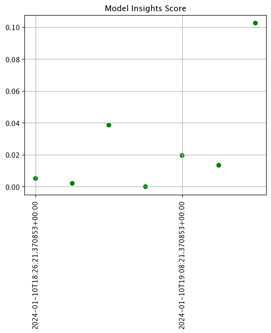
for i in range(5):
print(i)
for good_image in baseline_images_list:
ops_pipeline_inference(good_image)
for i in range(5):
print(i)
for bad_image in blurred_images_list:
edge_pipeline_inference(bad_image)
for i in range(4):
print(i)
for good_image in baseline_images_list:
ops_pipeline_inference(good_image)
for i in range(6):
print(i)
for bad_image in blurred_images_list:
edge_pipeline_inference(bad_image)
for i in range(3):
print(i)
for good_image in baseline_images_list:
ops_pipeline_inference(good_image)
for i in range(7):
print(i)
for bad_image in blurred_images_list:
edge_pipeline_inference(bad_image)
for i in range(2):
print(i)
for good_image in baseline_images_list:
ops_pipeline_inference(good_image)
for i in range(8):
print(i)
for bad_image in blurred_images_list:
edge_pipeline_inference(bad_image)
for i in range(1):
print(i)
for good_image in baseline_images_list:
ops_pipeline_inference(good_image)
for i in range(9):
print(i)
for bad_image in blurred_images_list:
edge_pipeline_inference(bad_image)
for i in range(10):
print(i)
for bad_image in blurred_images_list:
edge_pipeline_inference(bad_image)
# assay window from dates
assay_window_end = datetime.datetime.now(datetime.timezone.utc)
assay_builder_from_dates = assay_builder_from_dates.add_run_until(assay_window_end)
# just combined
(assay_builder_from_dates
.window_builder()
.add_width(minutes=6)
.add_interval(minutes=6)
.add_start(assay_window_start)
.add_location_filter([ops_partition, edge_name])
)
<wallaroo.assay_config.WindowBuilder at 0x14850dd00>
assay_config = assay_builder_from_dates.build()
assay_results = assay_config.interactive_run()
print(f"Generated {len(assay_results)} analyses")
assay_results.chart_scores()
Generated 16 analyses
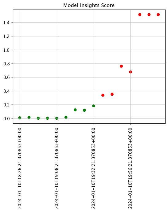
If we isolate to just the Ops center pipeline, we see a different result.
# assay window from dates
assay_window_end = datetime.datetime.now(datetime.timezone.utc)
assay_builder_from_dates = assay_builder_from_dates.add_run_until(assay_window_end)
# just combined
(assay_builder_from_dates
.window_builder()
.add_width(minutes=6)
.add_interval(minutes=6)
.add_start(assay_window_start)
.add_location_filter([ops_partition])
)
<wallaroo.assay_config.WindowBuilder at 0x14850dd00>
assay_config = assay_builder_from_dates.build()
assay_results = assay_config.interactive_run()
print(f"Generated {len(assay_results)} analyses")
assay_results.chart_scores()
Generated 13 analyses
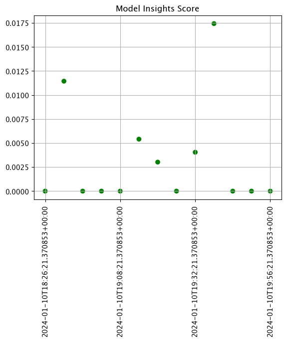
If we isolate to only the edge location, we see where the out of baseline scores are coming from.
# assay window from dates
assay_window_end = datetime.datetime.now(datetime.timezone.utc)
assay_builder_from_dates = assay_builder_from_dates.add_run_until(assay_window_end)
# just combined
(assay_builder_from_dates
.window_builder()
.add_width(minutes=6)
.add_interval(minutes=6)
.add_start(assay_window_start)
.add_location_filter([edge_name])
)
<wallaroo.assay_config.WindowBuilder at 0x14850dd00>
assay_config = assay_builder_from_dates.build()
assay_results = assay_config.interactive_run()
print(f"Generated {len(assay_results)} analyses")
assay_results.chart_scores()
Generated 12 analyses
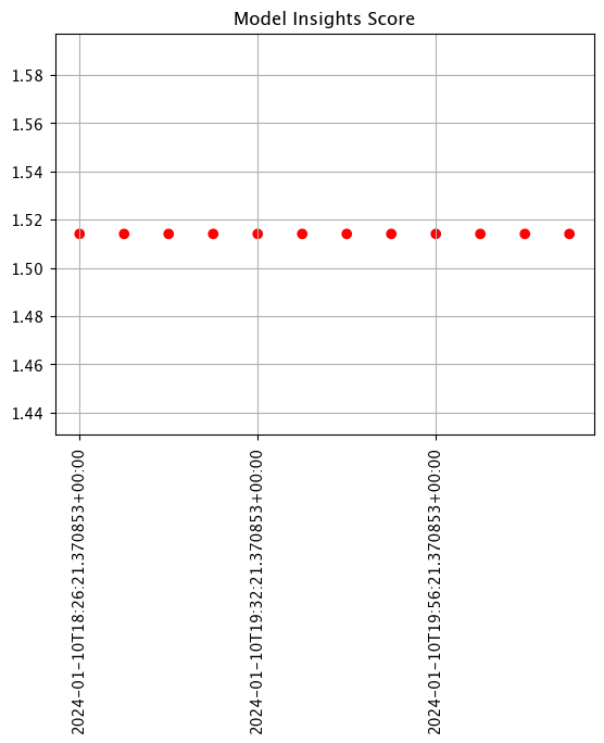
With the demonstration complete, we can shut down the edge deployed pipeline and undeploy the pipeline in the Ops center.
pipeline.undeploy()
| name | retail-inv-tracker-edge-obs |
|---|---|
| created | 2024-01-10 17:50:59.035145+00:00 |
| last_updated | 2024-01-10 18:09:22.128239+00:00 |
| deployed | False |
| arch | None |
| tags | |
| versions | c2dd2c7d-618d-497f-8515-3aa1469d7985, bee8f4f6-b1d3-40e7-9fc5-221db3ff1b87, 79321f4e-ca2d-4be1-8590-8c3be5d8953c, 64c06b04-d8fb-4651-ae5e-886c12a30e94, d0c2ed1c-3691-49f1-8fc8-e6510e4c39f8, 773099d3-6d64-4a92-b5a7-f614a916965d |
| steps | resnet-with-intensity |
| published | True |
3.2 - Wallaroo Model Observability: Anomaly Detection with CCFraud
How to detect anomalous model inputs or outputs using the CCFraud model as an example.
The following tutorials are available from the Wallaroo Tutorials Repository.
Wallaroo Model Observability: Anomaly Detection with CCFraud
The following tutorial demonstrates the use case of detecting anomalies: inference input or output data that does not match typical validations.
Wallaroo provides validations to detect anomalous data from inference inputs and outputs. Validations are added to a Wallaroo pipeline with the wallaroo.pipeline.add_validations method.
Adding validations takes the format:
pipeline.add_validations(
validation_name_01 = polars.col(in|out.{column_name}) EXPRESSION,
validation_name_02 = polars.col(in|out.{column_name}) EXPRESSION
...{additional rules}
)
validation_name: The user provided name of the validation. The names must match Python variable naming requirements.- IMPORTANT NOTE: Using the name
countas a validation name returns an error. Any validation rules namedcountare dropped upon request and a warning returned.
- IMPORTANT NOTE: Using the name
polars.col(in|out.{column_name}): Specifies the input or output for a specific field aka “column” in an inference result. Wallaroo inference requests are in the formatin.{field_name}for inputs, andout.{field_name}for outputs.- More than one field can be selected, as long as they follow the rules of the polars 0.18 Expressions library.
EXPRESSION: The expression to validate. When the expression returns True, that indicates an anomaly detected.
The polars library version 0.18.5 is used to create the validation rule. This is installed by default with the Wallaroo SDK. This provides a powerful range of comparisons to organizations tracking anomalous data from their ML models.
When validations are added to a pipeline, inference request outputs return the following fields:
| Field | Type | Description |
|---|---|---|
| anomaly.count | Integer | The total of all validations that returned True. |
| anomaly.{validation name} | Bool | The output of the validation {validation_name}. |
When validation returns True, an anomaly is detected.
For example, adding the validation fraud to the following pipeline returns anomaly.count of 1 when the validation fraud returns True. The validation fraud returns True when the output field dense_1 at index 0 is greater than 0.9.
sample_pipeline = wallaroo.client.build_pipeline("sample-pipeline")
sample_pipeline.add_model_step(ccfraud_model)
# add the validation
sample_pipeline.add_validations(
fraud=pl.col("out.dense_1").list.get(0) > 0.9,
)
# deploy the pipeline
sample_pipeline.deploy()
# sample inference
display(sample_pipeline.infer_from_file("dev_high_fraud.json", data_format='pandas-records'))
| time | in.tensor | out.dense_1 | anomaly.count | anomaly.fraud | |
|---|---|---|---|---|---|
| 0 | 2024-02-02 16:05:42.152 | [1.0678324729, 18.1555563975, -1.6589551058, 5…] | [0.981199] | 1 | True |
Detecting Anomalies from Inference Request Results
When an inference request is submitted to a Wallaroo pipeline with validations, the following fields are output:
| Field | Type | Description |
|---|---|---|
| anomaly.count | Integer | The total of all validations that returned True. |
| anomaly.{validation name} | Bool | The output of each pipeline validation {validation_name}. |
For example, adding the validation fraud to the following pipeline returns anomaly.count of 1 when the validation fraud returns True.
sample_pipeline = wallaroo.client.build_pipeline("sample-pipeline")
sample_pipeline.add_model_step(ccfraud_model)
# add the validation
sample_pipeline.add_validations(
fraud=pl.col("out.dense_1").list.get(0) > 0.9,
)
# deploy the pipeline
sample_pipeline.deploy()
# sample inference
display(sample_pipeline.infer_from_file("dev_high_fraud.json", data_format='pandas-records'))
| time | in.tensor | out.dense_1 | anomaly.count | anomaly.fraud | |
|---|---|---|---|---|---|
| 0 | 2024-02-02 16:05:42.152 | [1.0678324729, 18.1555563975, -1.6589551058, 5…] | [0.981199] | 1 | True |
Anomaly Detection Demonstration
The following demonstrates how to:
- Upload a ccfraud ML model trained to detect the likelihood of a transaction being fraudulent. This outputs the field
dense_1as an float where the closer to 1, the higher the likelihood of the transaction being fraudulent. - Add the ccfraud model as a pipeline step.
- Add the validation
fraudto detect when the output ofdense_1at index 0 when the values are greater than0.9. - Deploy the pipeline and performing sample inferences on it.
- Perform sample inferences to show when the
fraudvalidation returnsTrueandFalse. - Perform sample inference with different datasets to show enable or disable certain fields from displaying in the inference results.
Prerequisites
- Wallaroo version 2023.4.1 and above.
polarsversion 0.18.5. This is installed by default with the Wallaroo SDK.
Tutorial Steps
Load Libraries
The first step is to import the libraries used in this notebook.
import wallaroo
wallaroo.__version__
'2023.4.1+379cb6b8a'
Connect to the Wallaroo Instance through the User Interface
The next step is to connect to Wallaroo through the Wallaroo client. The Python library is included in the Wallaroo install and available through the Jupyter Hub interface provided with your Wallaroo environment.
This is accomplished using the wallaroo.Client() command, which provides a URL to grant the SDK permission to your specific Wallaroo environment. When displayed, enter the URL into a browser and confirm permissions. Store the connection into a variable that can be referenced later.
If logging into the Wallaroo instance through the internal JupyterHub service, use wl = wallaroo.Client(). For more information on Wallaroo Client settings, see the Client Connection guide.
wl = wallaroo.Client()
Create a New Workspace
We’ll use the SDK below to create our workspace then assign as our current workspace. The current workspace is used by the Wallaroo SDK for where to upload models, create pipelines, etc. We’ll also set up variables for our models and pipelines down the road, so we have one spot to change names to whatever fits your organization’s standards best.
Before starting, verify that the workspace name is unique in your Wallaroo instance.
def get_workspace(name, client):
workspace = None
for ws in client.list_workspaces():
if ws.name() == name:
workspace= ws
if(workspace == None):
workspace = client.create_workspace(name)
return workspace
workspace_name = 'validation-ccfraud-demonstration-jch'
pipeline_name = 'ccfraud-validation-demo'
model_name = 'ccfraud'
model_file_name = './models/ccfraud.onnx'
workspace = get_workspace(workspace_name, wl)
wl.set_current_workspace(workspace)
{'name': 'validation-ccfraud-demonstration-jch', 'id': 19, 'archived': False, 'created_by': 'c97d480f-6064-4537-b18e-40fb1864b4cd', 'created_at': '2024-02-08T16:57:29.044902+00:00', 'models': [{'name': 'ccfraud', 'versions': 2, 'owner_id': '""', 'last_update_time': datetime.datetime(2024, 2, 8, 17, 12, 40, 341069, tzinfo=tzutc()), 'created_at': datetime.datetime(2024, 2, 8, 16, 57, 31, 612826, tzinfo=tzutc())}], 'pipelines': [{'name': 'ccfraud-validation', 'create_time': datetime.datetime(2024, 2, 8, 16, 57, 32, 340043, tzinfo=tzutc()), 'definition': '[]'}]}
Upload the Model
Upload the model to the Wallaroo workspace with the wallaroo.client.upload_model method. Our ccfraud ML model is a Wallaroo Default Runtime of type ONNX, so all we need is the model name, the model file path, and the framework type of wallaroo.framework.Framework.ONNX.
ccfraud_model = (wl.upload_model(model_name,
model_file_name,
framework=wallaroo.framework.Framework.ONNX)
)
Build the Pipeline
Pipelines are build with the wallaroo.client.build_pipeline method, which takes the pipeline name. This will create the pipeline in our default workspace. Note that if there are any existing pipelines with the same name in this workspace, this method will retrieve that pipeline for this SDK session.
Once the pipeline is created, we add the ccfraud model as our pipeline step.
sample_pipeline = wl.build_pipeline(pipeline_name)
sample_pipeline = sample_pipeline.add_model_step(ccfraud_model)
Add Validation
Now we add our validation to our new pipeline. We will give it the following configuration.
- Validation Name:
fraud - Validation Field:
out.dense_1 - Validation Field Index:
0 - Validation Expression: Values greater than
0.9.
The polars library is required for creating the validation. We will import the polars library, then add our validation to the pipeline.
- IMPORTANT NOTE: Validation names must be unique per pipeline. If a validation of the same name is added, both are included in the pipeline validations, but only most recent validation with the same name is displayed with the inference results. Anomalies detected by multiple validations of the same name are added to the
anomaly.countinference result field.
import polars as pl
sample_pipeline = sample_pipeline.add_validations(
fraud=pl.col("out.dense_1").list.get(0) > 0.9
)
Display Pipeline And Validation Steps
The method wallaroo.pipeline.steps() shows the current pipeline steps. The added validations are in the Check field. This is used for demonstration purposes to show the added validation to the pipeline.
sample_pipeline.steps()
[{'ModelInference': {'models': [{'name': 'ccfraud', 'version': 'f1f2ab86-a41d-4601-b14a-b594e3d86c6e', 'sha': 'bc85ce596945f876256f41515c7501c399fd97ebcb9ab3dd41bf03f8937b4507'}]}},
{'Check': {'tree': ['{"Alias":[{"BinaryExpr":{"left":{"Function":{"input":[{"Column":"out.dense_1"},{"Literal":{"Int32":0}}],"function":{"ListExpr":"Get"},"options":{"collect_groups":"ApplyFlat","fmt_str":"","input_wildcard_expansion":false,"auto_explode":true,"cast_to_supertypes":false,"allow_rename":false,"pass_name_to_apply":false,"changes_length":false,"check_lengths":true,"allow_group_aware":true}}},"op":"Gt","right":{"Literal":{"Float64":0.9}}}},"fraud"]}']}}]
Deploy Pipeline
With the pipeline steps set and the validations created, we deploy the pipeline. Because of it’s size, we will only allocate 0.1 cpu from the cluster for the pipeline’s use.
deploy_config = wallaroo.deployment_config.DeploymentConfigBuilder() \
.cpus(0.1)\
.build()
sample_pipeline.deploy(deployment_config=deploy_config)
Waiting for deployment - this will take up to 45s ......... ok
| name | ccfraud-validation-demo |
|---|---|
| created | 2024-02-08 17:47:02.951799+00:00 |
| last_updated | 2024-02-08 17:47:03.074392+00:00 |
| deployed | True |
| arch | None |
| tags | |
| versions | 5d5a2272-5c80-4eb1-9712-0a342febb775, 7baa8bc8-2218-4b09-9436-00a40407a14d |
| steps | ccfraud |
| published | False |
Sample Inferences
Two sample inferences are performed with the method wallaroo.pipeline.infer_from_file that takes either a pandas Record JSON file or an Apache Arrow table as the input.
For our demonstration, we will use the following pandas Record JSON files with the following sample data:
./data/dev_smoke_test.pandas.json: A sample inference that generates a low (lower than 0.01) likelihood of fraud../data/dev_high_fraud.pandas.json: A sample inference that generates a high (higher than 0.90) likelihood of fraud.
The inference request returns a pandas DataFrame.
Each of the inference outputs will include the following fields:
| Field | Type | Description |
|---|---|---|
| time | DateTime | The DateTime of the inference request. |
| in.{input_field_name} | Input Dependent | Each input field submitted is labeled as in.{input_field_name} in the inference request result. For our example, this is tensor, so the input field in the returned inference request is in.tensor. |
| out.{model_output_field_name} | Output Dependent | Each field output by the ML model is labeled as out.{model_output_field_name} in the inference request result. For our example, the ccfraud model returns dense_1 as its output field, so the output field in the returned inference request is out.dense_1. |
| anomaly.count | Integer | The total number of validations that returned True. |
| **anomaly.{validation_name} | Bool | Each validation added to the pipeline is returned as anomaly.{validation_name}, and returns either True if the validation returns True, indicating an anomaly is found, or False for an anomaly for the validation is not found. For our example, we will have anomaly.fraud returned. |
sample_pipeline.infer_from_file("./data/dev_smoke_test.pandas.json")
| time | in.dense_input | out.dense_1 | anomaly.count | anomaly.fraud | |
|---|---|---|---|---|---|
| 0 | 2024-02-08 17:47:12.909 | [1.0678324729, 0.2177810266, -1.7115145262, 0.... | [0.0014974177] | 0 | False |
sample_pipeline.infer_from_file("./data/dev_high_fraud.json")
| time | in.dense_input | out.dense_1 | anomaly.count | anomaly.fraud | |
|---|---|---|---|---|---|
| 0 | 2024-02-08 17:47:12.962 | [1.0678324729, 18.1555563975, -1.6589551058, 5... | [0.981199] | 1 | True |
Other Validation Examples
The following are additional examples of validations.
Multiple Validations
The following uses multiple validations to check for anomalies. We still use fraud which detects outputs that are greater than 0.9. The second validation too_low triggers an anomaly when the out.dense_1 is under 0.05.
After the validations are added, the pipeline is redeployed to “set” them.
sample_pipeline = sample_pipeline.add_validations(
too_low=pl.col("out.dense_1").list.get(0) < 0.001
)
deploy_config = wallaroo.deployment_config.DeploymentConfigBuilder() \
.cpus(0.1)\
.build()
sample_pipeline.undeploy()
sample_pipeline.deploy(deployment_config=deploy_config)
Waiting for undeployment - this will take up to 45s ..................................... ok
Waiting for deployment - this will take up to 45s ......... ok
| name | ccfraud-validation-demo |
|---|---|
| created | 2024-02-08 17:47:02.951799+00:00 |
| last_updated | 2024-02-08 17:47:51.243530+00:00 |
| deployed | True |
| arch | None |
| tags | |
| versions | 54982a2e-180b-4da6-ab50-e2940ec14ff5, 5d5a2272-5c80-4eb1-9712-0a342febb775, 7baa8bc8-2218-4b09-9436-00a40407a14d |
| steps | ccfraud |
| published | False |
sample_pipeline.infer_from_file("./data/dev_smoke_test.pandas.json")
| time | in.dense_input | out.dense_1 | anomaly.count | anomaly.fraud | anomaly.too_low | |
|---|---|---|---|---|---|---|
| 0 | 2024-02-08 17:48:00.996 | [1.0678324729, 0.2177810266, -1.7115145262, 0.... | [0.0014974177] | 0 | False | False |
sample_pipeline.infer_from_file("./data/dev_high_fraud.json")
| time | in.dense_input | out.dense_1 | anomaly.count | anomaly.fraud | anomaly.too_low | |
|---|---|---|---|---|---|---|
| 0 | 2024-02-08 17:48:01.041 | [1.0678324729, 18.1555563975, -1.6589551058, 5... | [0.981199] | 1 | True | False |
Compound Validations
The following combines multiple field checks into a single validation. For this, we will check for values of out.dense_1 that are between 0.05 and 0.9.
Each expression is separated by (). For example:
- Expression 1:
pl.col("out.dense_1").list.get(0) < 0.9 - Expression 2:
pl.col("out.dense_1").list.get(0) > 0.001 - Compound Expression:
(pl.col("out.dense_1").list.get(0) < 0.9) & (pl.col("out.dense_1").list.get(0) > 0.001)
sample_pipeline = sample_pipeline.add_validations(
in_between_2=(pl.col("out.dense_1").list.get(0) < 0.9) & (pl.col("out.dense_1").list.get(0) > 0.001)
)
deploy_config = wallaroo.deployment_config.DeploymentConfigBuilder() \
.cpus(0.1)\
.build()
sample_pipeline.undeploy()
sample_pipeline.deploy(deployment_config=deploy_config)
Waiting for undeployment - this will take up to 45s ..................................... ok
Waiting for deployment - this will take up to 45s ......... ok
| name | ccfraud-validation-demo |
|---|---|
| created | 2024-02-08 17:47:02.951799+00:00 |
| last_updated | 2024-02-08 17:48:39.387256+00:00 |
| deployed | True |
| arch | None |
| tags | |
| versions | 97fb284e-aa10-4192-a072-308a705b969c, 54982a2e-180b-4da6-ab50-e2940ec14ff5, 5d5a2272-5c80-4eb1-9712-0a342febb775, 7baa8bc8-2218-4b09-9436-00a40407a14d |
| steps | ccfraud |
| published | False |
results = sample_pipeline.infer_from_file("./data/cc_data_1k.df.json")
results.loc[results['anomaly.in_between_2'] == True]
| time | in.dense_input | out.dense_1 | anomaly.count | anomaly.fraud | anomaly.in_between_2 | anomaly.too_low | |
|---|---|---|---|---|---|---|---|
| 4 | 2024-02-08 17:48:49.305 | [0.5817662108, 0.097881551, 0.1546819424, 0.47... | [0.0010916889] | 1 | False | True | False |
| 7 | 2024-02-08 17:48:49.305 | [1.0379636346, -0.152987302, -1.0912561862, -0... | [0.0011294782] | 1 | False | True | False |
| 8 | 2024-02-08 17:48:49.305 | [0.1517283662, 0.6589966337, -0.3323713647, 0.... | [0.0018743575] | 1 | False | True | False |
| 9 | 2024-02-08 17:48:49.305 | [-0.1683100246, 0.7070470317, 0.1875234948, -0... | [0.0011520088] | 1 | False | True | False |
| 10 | 2024-02-08 17:48:49.305 | [0.6066235674, 0.0631839305, -0.0802961973, 0.... | [0.0016568303] | 1 | False | True | False |
| ... | ... | ... | ... | ... | ... | ... | ... |
| 982 | 2024-02-08 17:48:49.305 | [-0.0932906169, 0.2837744937, -0.061094265, 0.... | [0.0010192394] | 1 | False | True | False |
| 983 | 2024-02-08 17:48:49.305 | [0.0991458877, 0.5813808183, -0.3863062246, -0... | [0.0020678043] | 1 | False | True | False |
| 992 | 2024-02-08 17:48:49.305 | [1.0458395446, 0.2492453605, -1.5260449285, 0.... | [0.0013128221] | 1 | False | True | False |
| 998 | 2024-02-08 17:48:49.305 | [1.0046377125, 0.0343666504, -1.3512533246, 0.... | [0.0011070371] | 1 | False | True | False |
| 1000 | 2024-02-08 17:48:49.305 | [0.6118805301, 0.1726081102, 0.4310545502, 0.5... | [0.0012498498] | 1 | False | True | False |
179 rows × 7 columns
Specify Dataset
Wallaroo inference requests allow datasets to be excluded or included with the dataset_exclude and dataset parameters.
| Parameter | Type | Description |
|---|---|---|
| dataset_exclude | List(String) | The list of datasets to exclude. Values include:
|
| dataset | List(String) | The list of datasets and fields to include. |
For our example, we will exclude the anomaly dataset, but include the datasets 'time', 'in', 'out', 'anomaly.count'. Note that while we exclude anomaly, we override that with by setting the anomaly field 'anomaly.count' in our dataset parameter.
sample_pipeline.infer_from_file("./data/dev_high_fraud.json",
dataset_exclude=['anomaly'],
dataset=['time', 'in', 'out', 'anomaly.count']
)
| time | in.dense_input | out.dense_1 | anomaly.count | |
|---|---|---|---|---|
| 0 | 2024-02-08 17:48:49.634 | [1.0678324729, 18.1555563975, -1.6589551058, 5... | [0.981199] | 1 |
Undeploy the Pipeline
With the demonstration complete, we undeploy the pipeline and return the resources back to the cluster.
sample_pipeline.undeploy()
Waiting for undeployment - this will take up to 45s ..................................... ok
| name | ccfraud-validation-demo |
|---|---|
| created | 2024-02-08 17:47:02.951799+00:00 |
| last_updated | 2024-02-08 17:48:39.387256+00:00 |
| deployed | False |
| arch | None |
| tags | |
| versions | 97fb284e-aa10-4192-a072-308a705b969c, 54982a2e-180b-4da6-ab50-e2940ec14ff5, 5d5a2272-5c80-4eb1-9712-0a342febb775, 7baa8bc8-2218-4b09-9436-00a40407a14d |
| steps | ccfraud |
| published | False |
3.3 - Wallaroo Model Observability: Anomaly Detection with House Price Prediction
How to detect anomalous model inputs or outputs using the CCFraud model as an example.
The following tutorials are available from the Wallaroo Tutorials Repository.
Wallaroo Model Observability: Anomaly Detection with House Price Prediction
The following tutorial demonstrates the use case of detecting anomalies: inference input or output data that does not match typical validations.
Wallaroo provides validations to detect anomalous data from inference inputs and outputs. Validations are added to a Wallaroo pipeline with the wallaroo.pipeline.add_validations method.
Adding validations takes the format:
pipeline.add_validations(
validation_name_01 = polars.col(in|out.{column_name}) EXPRESSION,
validation_name_02 = polars.col(in|out.{column_name}) EXPRESSION
...{additional rules}
)
validation_name: The user provided name of the validation. The names must match Python variable naming requirements.- IMPORTANT NOTE: Using the name
countas a validation name returns an error. Any validation rules namedcountare dropped upon request and a warning returned.
- IMPORTANT NOTE: Using the name
polars.col(in|out.{column_name}): Specifies the input or output for a specific field aka “column” in an inference result. Wallaroo inference requests are in the formatin.{field_name}for inputs, andout.{field_name}for outputs.- More than one field can be selected, as long as they follow the rules of the polars 0.18 Expressions library.
EXPRESSION: The expression to validate. When the expression returns True, that indicates an anomaly detected.
The polars library version 0.18.5 is used to create the validation rule. This is installed by default with the Wallaroo SDK. This provides a powerful range of comparisons to organizations tracking anomalous data from their ML models.
When validations are added to a pipeline, inference request outputs return the following fields:
| Field | Type | Description |
|---|---|---|
| anomaly.count | Integer | The total of all validations that returned True. |
| anomaly.{validation name} | Bool | The output of the validation {validation_name}. |
When validation returns True, an anomaly is detected.
For example, adding the validation fraud to the following pipeline returns anomaly.count of 1 when the validation fraud returns True. The validation fraud returns True when the output field dense_1 at index 0 is greater than 0.9.
sample_pipeline = wallaroo.client.build_pipeline("sample-pipeline")
sample_pipeline.add_model_step(model)
# add the validation
sample_pipeline.add_validations(
fraud=pl.col("out.dense_1").list.get(0) > 0.9,
)
# deploy the pipeline
sample_pipeline.deploy()
# sample inference
display(sample_pipeline.infer_from_file("dev_high_fraud.json", data_format='pandas-records'))
| time | in.tensor | out.dense_1 | anomaly.count | anomaly.fraud | |
|---|---|---|---|---|---|
| 0 | 2024-02-02 16:05:42.152 | [1.0678324729, 18.1555563975, -1.6589551058, 5…] | [0.981199] | 1 | True |
Detecting Anomalies from Inference Request Results
When an inference request is submitted to a Wallaroo pipeline with validations, the following fields are output:
| Field | Type | Description |
|---|---|---|
| anomaly.count | Integer | The total of all validations that returned True. |
| anomaly.{validation name} | Bool | The output of each pipeline validation {validation_name}. |
For example, adding the validation fraud to the following pipeline returns anomaly.count of 1 when the validation fraud returns True.
sample_pipeline = wallaroo.client.build_pipeline("sample-pipeline")
sample_pipeline.add_model_step(model)
# add the validation
sample_pipeline.add_validations(
fraud=pl.col("out.dense_1").list.get(0) > 0.9,
)
# deploy the pipeline
sample_pipeline.deploy()
# sample inference
display(sample_pipeline.infer_from_file("dev_high_fraud.json", data_format='pandas-records'))
| time | in.tensor | out.dense_1 | anomaly.count | anomaly.fraud | |
|---|---|---|---|---|---|
| 0 | 2024-02-02 16:05:42.152 | [1.0678324729, 18.1555563975, -1.6589551058, 5…] | [0.981199] | 1 | True |
Anomaly Detection Demonstration
The following demonstrates how to:
- Upload a house price ML model trained to predict house prices based on a set of inputs. This outputs the field
variableas an float which is the predicted house price. - Add the house price model as a pipeline step.
- Add the validation
too_highto detect when a house price exceeds a certain value. - Deploy the pipeline and performing sample inferences on it.
- Perform sample inferences to show when the
too_highvalidation returnsTrueandFalse. - Perform sample inference with different datasets to show enable or disable certain fields from displaying in the inference results.
Prerequisites
- Wallaroo version 2023.4.1 and above.
polarsversion 0.18.5. This is installed by default with the Wallaroo SDK.
Tutorial Steps
Load Libraries
The first step is to import the libraries used in this notebook.
import wallaroo
wallaroo.__version__
'2023.4.1+379cb6b8a'
Connect to the Wallaroo Instance through the User Interface
The next step is to connect to Wallaroo through the Wallaroo client. The Python library is included in the Wallaroo install and available through the Jupyter Hub interface provided with your Wallaroo environment.
This is accomplished using the wallaroo.Client() command, which provides a URL to grant the SDK permission to your specific Wallaroo environment. When displayed, enter the URL into a browser and confirm permissions. Store the connection into a variable that can be referenced later.
If logging into the Wallaroo instance through the internal JupyterHub service, use wl = wallaroo.Client(). For more information on Wallaroo Client settings, see the Client Connection guide.
wl = wallaroo.Client()
Create a New Workspace
We’ll use the SDK below to create our workspace then assign as our current workspace. The current workspace is used by the Wallaroo SDK for where to upload models, create pipelines, etc. We’ll also set up variables for our models and pipelines down the road, so we have one spot to change names to whatever fits your organization’s standards best.
Before starting, verify that the workspace name is unique in your Wallaroo instance.
def get_workspace(name, client):
workspace = None
for ws in client.list_workspaces():
if ws.name() == name:
workspace= ws
if(workspace == None):
workspace = client.create_workspace(name)
return workspace
workspace_name = 'validation-house-price-demonstration'
pipeline_name = 'validation-demo'
model_name = 'anomaly-housing-model'
model_file_name = './models/rf_model.onnx'
workspace = get_workspace(workspace_name, wl)
wl.set_current_workspace(workspace)
{'name': 'validation-house-price-demonstration', 'id': 25, 'archived': False, 'created_by': 'c97d480f-6064-4537-b18e-40fb1864b4cd', 'created_at': '2024-02-08T21:52:50.354176+00:00', 'models': [{'name': 'anomaly-housing-model', 'versions': 1, 'owner_id': '""', 'last_update_time': datetime.datetime(2024, 2, 8, 21, 52, 51, 671284, tzinfo=tzutc()), 'created_at': datetime.datetime(2024, 2, 8, 21, 52, 51, 671284, tzinfo=tzutc())}], 'pipelines': [{'name': 'validation-demo', 'create_time': datetime.datetime(2024, 2, 8, 21, 52, 52, 879885, tzinfo=tzutc()), 'definition': '[]'}]}
Upload the Model
Upload the model to the Wallaroo workspace with the wallaroo.client.upload_model method. Our house price ML model is a Wallaroo Default Runtime of type ONNX, so all we need is the model name, the model file path, and the framework type of wallaroo.framework.Framework.ONNX.
model = (wl.upload_model(model_name,
model_file_name,
framework=wallaroo.framework.Framework.ONNX)
)
Build the Pipeline
Pipelines are build with the wallaroo.client.build_pipeline method, which takes the pipeline name. This will create the pipeline in our default workspace. Note that if there are any existing pipelines with the same name in this workspace, this method will retrieve that pipeline for this SDK session.
Once the pipeline is created, we add the ccfraud model as our pipeline step.
sample_pipeline = wl.build_pipeline(pipeline_name)
sample_pipeline.clear()
sample_pipeline = sample_pipeline.add_model_step(model)
import onnx
model = onnx.load(model_file_name)
output =[node.name for node in model.graph.output]
input_all = [node.name for node in model.graph.input]
input_initializer = [node.name for node in model.graph.initializer]
net_feed_input = list(set(input_all) - set(input_initializer))
print('Inputs: ', net_feed_input)
print('Outputs: ', output)
Inputs: ['float_input']
Outputs: ['variable']
Add Validation
Now we add our validation to our new pipeline. We will give it the following configuration.
- Validation Name:
too_high - Validation Field:
out.variable - Validation Field Index:
0 - Validation Expression: Values greater than
1000000.0.
The polars library is required for creating the validation. We will import the polars library, then add our validation to the pipeline.
- IMPORTANT NOTE: Validation names must be unique per pipeline. If a validation of the same name is added, both are included in the pipeline validations, but only most recent validation with the same name is displayed with the inference results. Anomalies detected by multiple validations of the same name are added to the
anomaly.countinference result field.
import polars as pl
sample_pipeline = sample_pipeline.add_validations(
too_high=pl.col("out.variable").list.get(0) > 1000000.0
)
Display Pipeline And Validation Steps
The method wallaroo.pipeline.steps() shows the current pipeline steps. The added validations are in the Check field. This is used for demonstration purposes to show the added validation to the pipeline.
sample_pipeline.steps()
[{'ModelInference': {'models': [{'name': 'anomaly-housing-model', 'version': '9a76a2cf-9ea3-4978-8fd5-005d0280e661', 'sha': 'e22a0831aafd9917f3cc87a15ed267797f80e2afa12ad7d8810ca58f173b8cc6'}]}},
{'Check': {'tree': ['{"Alias":[{"BinaryExpr":{"left":{"Function":{"input":[{"Column":"out.variable"},{"Literal":{"Int32":0}}],"function":{"ListExpr":"Get"},"options":{"collect_groups":"ApplyFlat","fmt_str":"","input_wildcard_expansion":false,"auto_explode":true,"cast_to_supertypes":false,"allow_rename":false,"pass_name_to_apply":false,"changes_length":false,"check_lengths":true,"allow_group_aware":true}}},"op":"Gt","right":{"Literal":{"Float64":1000000.0}}}},"too_high"]}']}}]
Deploy Pipeline
With the pipeline steps set and the validations created, we deploy the pipeline. Because of it’s size, we will only allocate 0.1 cpu from the cluster for the pipeline’s use.
deploy_config = wallaroo.deployment_config.DeploymentConfigBuilder() \
.cpus(0.25)\
.build()
sample_pipeline.deploy(deployment_config=deploy_config)
Waiting for undeployment - this will take up to 45s ..................................... ok
Waiting for deployment - this will take up to 45s ......... ok
| name | validation-demo |
|---|---|
| created | 2024-02-08 21:52:52.879885+00:00 |
| last_updated | 2024-02-08 22:14:13.217863+00:00 |
| deployed | True |
| arch | None |
| tags | |
| versions | 2a8d204a-f359-4f02-b558-950dbab28dc6, 424c7f24-ca65-45af-825f-64d3e9f8e8c8, 190226c9-a536-4457-9851-a68ef968b6fc, e10707fd-75b8-4386-8466-e58dc13d2828, 53b87a42-8498-475a-bf30-73fdebbf85cc |
| steps | anomaly-housing-model |
| published | False |
Sample Inferences
Two sample inferences are performed with the method wallaroo.pipeline.infer_from_file that takes either a pandas Record JSON file or an Apache Arrow table as the input.
For our demonstration, we will use the following pandas Record JSON file with the following sample data:
./data/houseprice_5000_data.json: A sample sets of 5000 houses to generates a range of predicted values.
The inference request returns a pandas DataFrame.
Each of the inference outputs will include the following fields:
| Field | Type | Description |
|---|---|---|
| time | DateTime | The DateTime of the inference request. |
| in.{input_field_name} | Input Dependent | Each input field submitted is labeled as in.{input_field_name} in the inference request result. For our example, this is tensor, so the input field in the returned inference request is in.tensor. |
| out.{model_output_field_name} | Output Dependent | Each field output by the ML model is labeled as out.{model_output_field_name} in the inference request result. For our example, the ccfraud model returns dense_1 as its output field, so the output field in the returned inference request is out.dense_1. |
| anomaly.count | Integer | The total number of validations that returned True. |
| **anomaly.{validation_name} | Bool | Each validation added to the pipeline is returned as anomaly.{validation_name}, and returns either True if the validation returns True, indicating an anomaly is found, or False for an anomaly for the validation is not found. For our example, we will have anomaly.fraud returned. |
results = sample_pipeline.infer_from_file('./data/test-1000.df.json')
# first 20 results
display(results.head(20))
# only results that trigger the anomaly too_high
results.loc[results['anomaly.too_high'] == True]
| time | in.float_input | out.variable | anomaly.count | anomaly.too_high | |
|---|---|---|---|---|---|
| 0 | 2024-02-08 22:14:47.075 | [4.0, 2.5, 2900.0, 5505.0, 2.0, 0.0, 0.0, 3.0,... | [718013.75] | 0 | False |
| 1 | 2024-02-08 22:14:47.075 | [2.0, 2.5, 2170.0, 6361.0, 1.0, 0.0, 2.0, 3.0,... | [615094.56] | 0 | False |
| 2 | 2024-02-08 22:14:47.075 | [3.0, 2.5, 1300.0, 812.0, 2.0, 0.0, 0.0, 3.0, ... | [448627.72] | 0 | False |
| 3 | 2024-02-08 22:14:47.075 | [4.0, 2.5, 2500.0, 8540.0, 2.0, 0.0, 0.0, 3.0,... | [758714.2] | 0 | False |
| 4 | 2024-02-08 22:14:47.075 | [3.0, 1.75, 2200.0, 11520.0, 1.0, 0.0, 0.0, 4.... | [513264.7] | 0 | False |
| 5 | 2024-02-08 22:14:47.075 | [3.0, 2.0, 2140.0, 4923.0, 1.0, 0.0, 0.0, 4.0,... | [668288.0] | 0 | False |
| 6 | 2024-02-08 22:14:47.075 | [4.0, 3.5, 3590.0, 5334.0, 2.0, 0.0, 2.0, 3.0,... | [1004846.5] | 1 | True |
| 7 | 2024-02-08 22:14:47.075 | [3.0, 2.0, 1280.0, 960.0, 2.0, 0.0, 0.0, 3.0, ... | [684577.2] | 0 | False |
| 8 | 2024-02-08 22:14:47.075 | [4.0, 2.5, 2820.0, 15000.0, 2.0, 0.0, 0.0, 4.0... | [727898.1] | 0 | False |
| 9 | 2024-02-08 22:14:47.075 | [3.0, 2.25, 1790.0, 11393.0, 1.0, 0.0, 0.0, 3.... | [559631.1] | 0 | False |
| 10 | 2024-02-08 22:14:47.075 | [3.0, 1.5, 1010.0, 7683.0, 1.5, 0.0, 0.0, 5.0,... | [340764.53] | 0 | False |
| 11 | 2024-02-08 22:14:47.075 | [3.0, 2.0, 1270.0, 1323.0, 3.0, 0.0, 0.0, 3.0,... | [442168.06] | 0 | False |
| 12 | 2024-02-08 22:14:47.075 | [4.0, 1.75, 2070.0, 9120.0, 1.0, 0.0, 0.0, 4.0... | [630865.6] | 0 | False |
| 13 | 2024-02-08 22:14:47.075 | [4.0, 1.0, 1620.0, 4080.0, 1.5, 0.0, 0.0, 3.0,... | [559631.1] | 0 | False |
| 14 | 2024-02-08 22:14:47.075 | [4.0, 3.25, 3990.0, 9786.0, 2.0, 0.0, 0.0, 3.0... | [909441.1] | 0 | False |
| 15 | 2024-02-08 22:14:47.075 | [4.0, 2.0, 1780.0, 19843.0, 1.0, 0.0, 0.0, 3.0... | [313096.0] | 0 | False |
| 16 | 2024-02-08 22:14:47.075 | [4.0, 2.5, 2130.0, 6003.0, 2.0, 0.0, 0.0, 3.0,... | [404040.8] | 0 | False |
| 17 | 2024-02-08 22:14:47.075 | [3.0, 1.75, 1660.0, 10440.0, 1.0, 0.0, 0.0, 3.... | [292859.5] | 0 | False |
| 18 | 2024-02-08 22:14:47.075 | [3.0, 2.5, 2110.0, 4118.0, 2.0, 0.0, 0.0, 3.0,... | [338357.88] | 0 | False |
| 19 | 2024-02-08 22:14:47.075 | [4.0, 2.25, 2200.0, 11250.0, 1.5, 0.0, 0.0, 5.... | [682284.6] | 0 | False |
| time | in.float_input | out.variable | anomaly.count | anomaly.too_high | |
|---|---|---|---|---|---|
| 6 | 2024-02-08 22:14:47.075 | [4.0, 3.5, 3590.0, 5334.0, 2.0, 0.0, 2.0, 3.0,... | [1004846.5] | 1 | True |
| 30 | 2024-02-08 22:14:47.075 | [4.0, 3.0, 3710.0, 20000.0, 2.0, 0.0, 2.0, 5.0... | [1514079.8] | 1 | True |
| 40 | 2024-02-08 22:14:47.075 | [4.0, 4.5, 5120.0, 41327.0, 2.0, 0.0, 0.0, 3.0... | [1204324.8] | 1 | True |
| 63 | 2024-02-08 22:14:47.075 | [4.0, 3.0, 4040.0, 19700.0, 2.0, 0.0, 0.0, 3.0... | [1028923.06] | 1 | True |
| 110 | 2024-02-08 22:14:47.075 | [4.0, 2.5, 3470.0, 20445.0, 2.0, 0.0, 0.0, 4.0... | [1412215.3] | 1 | True |
| 130 | 2024-02-08 22:14:47.075 | [4.0, 2.75, 2620.0, 13777.0, 1.5, 0.0, 2.0, 4.... | [1223839.1] | 1 | True |
| 133 | 2024-02-08 22:14:47.075 | [5.0, 2.25, 3320.0, 13138.0, 1.0, 0.0, 2.0, 4.... | [1108000.1] | 1 | True |
| 154 | 2024-02-08 22:14:47.075 | [4.0, 2.75, 3800.0, 9606.0, 2.0, 0.0, 0.0, 3.0... | [1039781.25] | 1 | True |
| 160 | 2024-02-08 22:14:47.075 | [5.0, 3.5, 4150.0, 13232.0, 2.0, 0.0, 0.0, 3.0... | [1042119.1] | 1 | True |
| 210 | 2024-02-08 22:14:47.075 | [4.0, 3.5, 4300.0, 70407.0, 2.0, 0.0, 0.0, 3.0... | [1115275.0] | 1 | True |
| 239 | 2024-02-08 22:14:47.075 | [4.0, 3.25, 5010.0, 49222.0, 2.0, 0.0, 0.0, 5.... | [1092274.1] | 1 | True |
| 248 | 2024-02-08 22:14:47.075 | [4.0, 3.75, 4410.0, 8112.0, 3.0, 0.0, 4.0, 3.0... | [1967344.1] | 1 | True |
| 255 | 2024-02-08 22:14:47.075 | [4.0, 3.0, 4750.0, 21701.0, 1.5, 0.0, 0.0, 5.0... | [2002393.5] | 1 | True |
| 271 | 2024-02-08 22:14:47.075 | [5.0, 3.25, 5790.0, 13726.0, 2.0, 0.0, 3.0, 3.... | [1189654.4] | 1 | True |
| 281 | 2024-02-08 22:14:47.075 | [3.0, 3.0, 3570.0, 6250.0, 2.0, 0.0, 2.0, 3.0,... | [1124493.3] | 1 | True |
| 282 | 2024-02-08 22:14:47.075 | [3.0, 2.75, 3170.0, 34850.0, 1.0, 0.0, 0.0, 5.... | [1227073.8] | 1 | True |
| 283 | 2024-02-08 22:14:47.075 | [4.0, 2.75, 3260.0, 19542.0, 1.0, 0.0, 0.0, 4.... | [1364650.3] | 1 | True |
| 285 | 2024-02-08 22:14:47.075 | [4.0, 2.75, 4020.0, 18745.0, 2.0, 0.0, 4.0, 4.... | [1322835.9] | 1 | True |
| 323 | 2024-02-08 22:14:47.075 | [3.0, 3.0, 2480.0, 5500.0, 2.0, 0.0, 3.0, 3.0,... | [1100884.1] | 1 | True |
| 351 | 2024-02-08 22:14:47.075 | [5.0, 4.0, 4660.0, 9900.0, 2.0, 0.0, 2.0, 4.0,... | [1058105.0] | 1 | True |
| 360 | 2024-02-08 22:14:47.075 | [4.0, 3.5, 3770.0, 8501.0, 2.0, 0.0, 0.0, 3.0,... | [1169643.0] | 1 | True |
| 398 | 2024-02-08 22:14:47.075 | [3.0, 2.25, 2390.0, 7875.0, 1.0, 0.0, 1.0, 3.0... | [1364149.9] | 1 | True |
| 414 | 2024-02-08 22:14:47.075 | [5.0, 3.5, 5430.0, 10327.0, 2.0, 0.0, 2.0, 3.0... | [1207858.6] | 1 | True |
| 443 | 2024-02-08 22:14:47.075 | [5.0, 4.0, 4360.0, 8030.0, 2.0, 0.0, 0.0, 3.0,... | [1160512.8] | 1 | True |
| 497 | 2024-02-08 22:14:47.075 | [4.0, 2.5, 4090.0, 11225.0, 2.0, 0.0, 0.0, 3.0... | [1048372.4] | 1 | True |
| 513 | 2024-02-08 22:14:47.075 | [4.0, 3.25, 3320.0, 8587.0, 3.0, 0.0, 0.0, 3.0... | [1130661.0] | 1 | True |
| 520 | 2024-02-08 22:14:47.075 | [5.0, 3.75, 4170.0, 8142.0, 2.0, 0.0, 2.0, 3.0... | [1098628.8] | 1 | True |
| 530 | 2024-02-08 22:14:47.075 | [4.0, 4.25, 3500.0, 8750.0, 1.0, 0.0, 4.0, 5.0... | [1140733.8] | 1 | True |
| 535 | 2024-02-08 22:14:47.075 | [4.0, 3.5, 4460.0, 16271.0, 2.0, 0.0, 2.0, 3.0... | [1208638.0] | 1 | True |
| 556 | 2024-02-08 22:14:47.075 | [4.0, 3.5, 4285.0, 9567.0, 2.0, 0.0, 1.0, 5.0,... | [1886959.4] | 1 | True |
| 623 | 2024-02-08 22:14:47.075 | [4.0, 3.25, 4240.0, 25639.0, 2.0, 0.0, 3.0, 3.... | [1156651.3] | 1 | True |
| 624 | 2024-02-08 22:14:47.075 | [4.0, 3.5, 3440.0, 9776.0, 2.0, 0.0, 0.0, 3.0,... | [1124493.3] | 1 | True |
| 634 | 2024-02-08 22:14:47.075 | [4.0, 3.25, 4700.0, 38412.0, 2.0, 0.0, 0.0, 3.... | [1164589.4] | 1 | True |
| 651 | 2024-02-08 22:14:47.075 | [3.0, 3.0, 3920.0, 13085.0, 2.0, 1.0, 4.0, 4.0... | [1452224.5] | 1 | True |
| 658 | 2024-02-08 22:14:47.075 | [3.0, 3.25, 3230.0, 7800.0, 2.0, 0.0, 3.0, 3.0... | [1077279.3] | 1 | True |
| 671 | 2024-02-08 22:14:47.075 | [3.0, 3.5, 3080.0, 6495.0, 2.0, 0.0, 3.0, 3.0,... | [1122811.8] | 1 | True |
| 685 | 2024-02-08 22:14:47.075 | [4.0, 2.5, 4200.0, 35267.0, 2.0, 0.0, 0.0, 3.0... | [1181336.0] | 1 | True |
| 686 | 2024-02-08 22:14:47.075 | [4.0, 3.25, 4160.0, 47480.0, 2.0, 0.0, 0.0, 3.... | [1082353.3] | 1 | True |
| 698 | 2024-02-08 22:14:47.075 | [4.0, 4.5, 5770.0, 10050.0, 1.0, 0.0, 3.0, 5.0... | [1689843.3] | 1 | True |
| 711 | 2024-02-08 22:14:47.075 | [3.0, 2.5, 5403.0, 24069.0, 2.0, 1.0, 4.0, 4.0... | [1946437.3] | 1 | True |
| 720 | 2024-02-08 22:14:47.075 | [5.0, 3.0, 3420.0, 18129.0, 2.0, 0.0, 0.0, 3.0... | [1325961.0] | 1 | True |
| 722 | 2024-02-08 22:14:47.075 | [3.0, 3.25, 4560.0, 13363.0, 1.0, 0.0, 4.0, 3.... | [2005883.1] | 1 | True |
| 726 | 2024-02-08 22:14:47.075 | [5.0, 3.5, 4200.0, 5400.0, 2.0, 0.0, 0.0, 3.0,... | [1052898.0] | 1 | True |
| 737 | 2024-02-08 22:14:47.075 | [4.0, 3.25, 2980.0, 7000.0, 2.0, 0.0, 3.0, 3.0... | [1156206.5] | 1 | True |
| 740 | 2024-02-08 22:14:47.075 | [4.0, 4.5, 6380.0, 88714.0, 2.0, 0.0, 0.0, 3.0... | [1355747.1] | 1 | True |
| 782 | 2024-02-08 22:14:47.075 | [5.0, 4.25, 4860.0, 9453.0, 1.5, 0.0, 1.0, 5.0... | [1910823.8] | 1 | True |
| 798 | 2024-02-08 22:14:47.075 | [4.0, 2.5, 2790.0, 5450.0, 2.0, 0.0, 0.0, 3.0,... | [1097757.4] | 1 | True |
| 818 | 2024-02-08 22:14:47.075 | [4.0, 4.0, 4620.0, 130208.0, 2.0, 0.0, 0.0, 3.... | [1164589.4] | 1 | True |
| 827 | 2024-02-08 22:14:47.075 | [4.0, 2.5, 3340.0, 10422.0, 2.0, 0.0, 0.0, 3.0... | [1103101.4] | 1 | True |
| 828 | 2024-02-08 22:14:47.075 | [5.0, 3.5, 3760.0, 10207.0, 2.0, 0.0, 0.0, 3.0... | [1489624.5] | 1 | True |
| 901 | 2024-02-08 22:14:47.075 | [4.0, 2.25, 4470.0, 60373.0, 2.0, 0.0, 0.0, 3.... | [1208638.0] | 1 | True |
| 912 | 2024-02-08 22:14:47.075 | [3.0, 2.25, 2960.0, 8330.0, 1.0, 0.0, 3.0, 4.0... | [1178314.0] | 1 | True |
| 919 | 2024-02-08 22:14:47.075 | [4.0, 3.25, 5180.0, 19850.0, 2.0, 0.0, 3.0, 3.... | [1295531.3] | 1 | True |
| 941 | 2024-02-08 22:14:47.075 | [4.0, 3.75, 3770.0, 4000.0, 2.5, 0.0, 0.0, 5.0... | [1182821.0] | 1 | True |
| 965 | 2024-02-08 22:14:47.075 | [6.0, 4.0, 5310.0, 12741.0, 2.0, 0.0, 2.0, 3.0... | [2016006.0] | 1 | True |
| 973 | 2024-02-08 22:14:47.075 | [5.0, 2.0, 3540.0, 9970.0, 2.0, 0.0, 3.0, 3.0,... | [1085835.8] | 1 | True |
| 997 | 2024-02-08 22:14:47.075 | [4.0, 3.25, 2910.0, 1880.0, 2.0, 0.0, 3.0, 5.0... | [1060847.5] | 1 | True |
Other Validation Examples
The following are additional examples of validations.
Multiple Validations
The following uses multiple validations to check for anomalies. We still use fraud which detects outputs that are greater than 1000000.0. The second validation too_low triggers an anomaly when the out.variable is under 250000.0.
After the validations are added, the pipeline is redeployed to “set” them.
sample_pipeline = sample_pipeline.add_validations(
too_low=pl.col("out.variable").list.get(0) < 250000.0
)
deploy_config = wallaroo.deployment_config.DeploymentConfigBuilder() \
.cpus(0.1)\
.build()
sample_pipeline.undeploy()
sample_pipeline.deploy(deployment_config=deploy_config)
Waiting for undeployment - this will take up to 45s ..................................... ok
Waiting for deployment - this will take up to 45s .............. ok
| name | validation-demo |
|---|---|
| created | 2024-02-08 21:52:52.879885+00:00 |
| last_updated | 2024-02-08 22:16:50.265231+00:00 |
| deployed | True |
| arch | None |
| tags | |
| versions | 053580e2-f73d-4b63-8c9c-0b5e06be96c2, 2a8d204a-f359-4f02-b558-950dbab28dc6, 424c7f24-ca65-45af-825f-64d3e9f8e8c8, 190226c9-a536-4457-9851-a68ef968b6fc, e10707fd-75b8-4386-8466-e58dc13d2828, 53b87a42-8498-475a-bf30-73fdebbf85cc |
| steps | anomaly-housing-model |
| published | False |
results = sample_pipeline.infer_from_file('./data/test-1000.df.json')
# first 20 results
display(results.head(20))
# only results that trigger the anomaly too_high
results.loc[results['anomaly.too_high'] == True]
# only results that trigger the anomaly too_low
results.loc[results['anomaly.too_low'] == True]
| time | in.float_input | out.variable | anomaly.count | anomaly.too_high | anomaly.too_low | |
|---|---|---|---|---|---|---|
| 0 | 2024-02-08 22:17:23.630 | [4.0, 2.5, 2900.0, 5505.0, 2.0, 0.0, 0.0, 3.0,... | [718013.75] | 0 | False | False |
| 1 | 2024-02-08 22:17:23.630 | [2.0, 2.5, 2170.0, 6361.0, 1.0, 0.0, 2.0, 3.0,... | [615094.56] | 0 | False | False |
| 2 | 2024-02-08 22:17:23.630 | [3.0, 2.5, 1300.0, 812.0, 2.0, 0.0, 0.0, 3.0, ... | [448627.72] | 0 | False | False |
| 3 | 2024-02-08 22:17:23.630 | [4.0, 2.5, 2500.0, 8540.0, 2.0, 0.0, 0.0, 3.0,... | [758714.2] | 0 | False | False |
| 4 | 2024-02-08 22:17:23.630 | [3.0, 1.75, 2200.0, 11520.0, 1.0, 0.0, 0.0, 4.... | [513264.7] | 0 | False | False |
| 5 | 2024-02-08 22:17:23.630 | [3.0, 2.0, 2140.0, 4923.0, 1.0, 0.0, 0.0, 4.0,... | [668288.0] | 0 | False | False |
| 6 | 2024-02-08 22:17:23.630 | [4.0, 3.5, 3590.0, 5334.0, 2.0, 0.0, 2.0, 3.0,... | [1004846.5] | 1 | True | False |
| 7 | 2024-02-08 22:17:23.630 | [3.0, 2.0, 1280.0, 960.0, 2.0, 0.0, 0.0, 3.0, ... | [684577.2] | 0 | False | False |
| 8 | 2024-02-08 22:17:23.630 | [4.0, 2.5, 2820.0, 15000.0, 2.0, 0.0, 0.0, 4.0... | [727898.1] | 0 | False | False |
| 9 | 2024-02-08 22:17:23.630 | [3.0, 2.25, 1790.0, 11393.0, 1.0, 0.0, 0.0, 3.... | [559631.1] | 0 | False | False |
| 10 | 2024-02-08 22:17:23.630 | [3.0, 1.5, 1010.0, 7683.0, 1.5, 0.0, 0.0, 5.0,... | [340764.53] | 0 | False | False |
| 11 | 2024-02-08 22:17:23.630 | [3.0, 2.0, 1270.0, 1323.0, 3.0, 0.0, 0.0, 3.0,... | [442168.06] | 0 | False | False |
| 12 | 2024-02-08 22:17:23.630 | [4.0, 1.75, 2070.0, 9120.0, 1.0, 0.0, 0.0, 4.0... | [630865.6] | 0 | False | False |
| 13 | 2024-02-08 22:17:23.630 | [4.0, 1.0, 1620.0, 4080.0, 1.5, 0.0, 0.0, 3.0,... | [559631.1] | 0 | False | False |
| 14 | 2024-02-08 22:17:23.630 | [4.0, 3.25, 3990.0, 9786.0, 2.0, 0.0, 0.0, 3.0... | [909441.1] | 0 | False | False |
| 15 | 2024-02-08 22:17:23.630 | [4.0, 2.0, 1780.0, 19843.0, 1.0, 0.0, 0.0, 3.0... | [313096.0] | 0 | False | False |
| 16 | 2024-02-08 22:17:23.630 | [4.0, 2.5, 2130.0, 6003.0, 2.0, 0.0, 0.0, 3.0,... | [404040.8] | 0 | False | False |
| 17 | 2024-02-08 22:17:23.630 | [3.0, 1.75, 1660.0, 10440.0, 1.0, 0.0, 0.0, 3.... | [292859.5] | 0 | False | False |
| 18 | 2024-02-08 22:17:23.630 | [3.0, 2.5, 2110.0, 4118.0, 2.0, 0.0, 0.0, 3.0,... | [338357.88] | 0 | False | False |
| 19 | 2024-02-08 22:17:23.630 | [4.0, 2.25, 2200.0, 11250.0, 1.5, 0.0, 0.0, 5.... | [682284.6] | 0 | False | False |
| time | in.float_input | out.variable | anomaly.count | anomaly.too_high | anomaly.too_low | |
|---|---|---|---|---|---|---|
| 21 | 2024-02-08 22:17:23.630 | [2.0, 2.0, 1390.0, 1302.0, 2.0, 0.0, 0.0, 3.0,... | [249227.8] | 1 | False | True |
| 69 | 2024-02-08 22:17:23.630 | [3.0, 1.75, 1050.0, 9871.0, 1.0, 0.0, 0.0, 5.0... | [236238.66] | 1 | False | True |
| 83 | 2024-02-08 22:17:23.630 | [3.0, 1.75, 1070.0, 8100.0, 1.0, 0.0, 0.0, 4.0... | [236238.66] | 1 | False | True |
| 95 | 2024-02-08 22:17:23.630 | [3.0, 2.5, 1340.0, 3011.0, 2.0, 0.0, 0.0, 3.0,... | [244380.27] | 1 | False | True |
| 124 | 2024-02-08 22:17:23.630 | [4.0, 1.5, 1200.0, 10890.0, 1.0, 0.0, 0.0, 5.0... | [241330.19] | 1 | False | True |
| ... | ... | ... | ... | ... | ... | ... |
| 939 | 2024-02-08 22:17:23.630 | [3.0, 1.0, 1150.0, 4800.0, 1.5, 0.0, 0.0, 4.0,... | [240834.92] | 1 | False | True |
| 946 | 2024-02-08 22:17:23.630 | [2.0, 1.0, 780.0, 6250.0, 1.0, 0.0, 0.0, 3.0, ... | [236815.78] | 1 | False | True |
| 948 | 2024-02-08 22:17:23.630 | [1.0, 1.0, 620.0, 8261.0, 1.0, 0.0, 0.0, 3.0, ... | [236815.78] | 1 | False | True |
| 962 | 2024-02-08 22:17:23.630 | [3.0, 1.0, 1190.0, 7500.0, 1.0, 0.0, 0.0, 5.0,... | [241330.19] | 1 | False | True |
| 991 | 2024-02-08 22:17:23.630 | [2.0, 1.0, 870.0, 8487.0, 1.0, 0.0, 0.0, 4.0, ... | [236238.66] | 1 | False | True |
62 rows × 6 columns
Compound Validations
The following combines multiple field checks into a single validation. For this, we will check for values of out.variable that are between 500000 and 1000000.
Each expression is separated by (). For example:
- Expression 1:
pl.col("out.variable").list.get(0) < 1000000.0 - Expression 2:
pl.col("out.variable").list.get(0) > 500000.0 - Compound Expression:
(pl.col("out.variable").list.get(0) < 1000000.0) & (pl.col("out.variable").list.get(0) > 500000.0)
sample_pipeline = sample_pipeline.add_validations(
in_between=(pl.col("out.variable").list.get(0) < 1000000.0) & (pl.col("out.variable").list.get(0) > 500000.0)
)
deploy_config = wallaroo.deployment_config.DeploymentConfigBuilder() \
.cpus(0.1)\
.build()
sample_pipeline.undeploy()
sample_pipeline.deploy(deployment_config=deploy_config)
Waiting for undeployment - this will take up to 45s .................................... ok
Waiting for deployment - this will take up to 45s ............. ok
| name | validation-demo |
|---|---|
| created | 2024-02-08 21:52:52.879885+00:00 |
| last_updated | 2024-02-08 22:18:18.613710+00:00 |
| deployed | True |
| arch | None |
| tags | |
| versions | 016728d7-3948-467f-8ecc-e0594f406884, 053580e2-f73d-4b63-8c9c-0b5e06be96c2, 2a8d204a-f359-4f02-b558-950dbab28dc6, 424c7f24-ca65-45af-825f-64d3e9f8e8c8, 190226c9-a536-4457-9851-a68ef968b6fc, e10707fd-75b8-4386-8466-e58dc13d2828, 53b87a42-8498-475a-bf30-73fdebbf85cc |
| steps | anomaly-housing-model |
| published | False |
results = sample_pipeline.infer_from_file('./data/test-1000.df.json')
results.loc[results['anomaly.in_between'] == True]
| time | in.float_input | out.variable | anomaly.count | anomaly.in_between | anomaly.too_high | anomaly.too_low | |
|---|---|---|---|---|---|---|---|
| 0 | 2024-02-08 22:18:32.886 | [4.0, 2.5, 2900.0, 5505.0, 2.0, 0.0, 0.0, 3.0,... | [718013.75] | 1 | True | False | False |
| 1 | 2024-02-08 22:18:32.886 | [2.0, 2.5, 2170.0, 6361.0, 1.0, 0.0, 2.0, 3.0,... | [615094.56] | 1 | True | False | False |
| 3 | 2024-02-08 22:18:32.886 | [4.0, 2.5, 2500.0, 8540.0, 2.0, 0.0, 0.0, 3.0,... | [758714.2] | 1 | True | False | False |
| 4 | 2024-02-08 22:18:32.886 | [3.0, 1.75, 2200.0, 11520.0, 1.0, 0.0, 0.0, 4.... | [513264.7] | 1 | True | False | False |
| 5 | 2024-02-08 22:18:32.886 | [3.0, 2.0, 2140.0, 4923.0, 1.0, 0.0, 0.0, 4.0,... | [668288.0] | 1 | True | False | False |
| ... | ... | ... | ... | ... | ... | ... | ... |
| 989 | 2024-02-08 22:18:32.886 | [4.0, 2.75, 2500.0, 4950.0, 2.0, 0.0, 0.0, 3.0... | [700271.56] | 1 | True | False | False |
| 993 | 2024-02-08 22:18:32.886 | [3.0, 2.5, 2140.0, 8925.0, 2.0, 0.0, 0.0, 3.0,... | [669645.5] | 1 | True | False | False |
| 995 | 2024-02-08 22:18:32.886 | [3.0, 2.5, 2900.0, 23550.0, 1.0, 0.0, 0.0, 3.0... | [827411.0] | 1 | True | False | False |
| 998 | 2024-02-08 22:18:32.886 | [3.0, 1.75, 2910.0, 37461.0, 1.0, 0.0, 0.0, 4.... | [706823.56] | 1 | True | False | False |
| 999 | 2024-02-08 22:18:32.886 | [3.0, 2.0, 2005.0, 7000.0, 1.0, 0.0, 0.0, 3.0,... | [581003.0] | 1 | True | False | False |
395 rows × 7 columns
Specify Dataset
Wallaroo inference requests allow datasets to be excluded or included with the dataset_exclude and dataset parameters.
| Parameter | Type | Description |
|---|---|---|
| dataset_exclude | List(String) | The list of datasets to exclude. Values include:
|
| dataset | List(String) | The list of datasets and fields to include. |
For our example, we will exclude the anomaly dataset, but include the datasets 'time', 'in', 'out', 'anomaly.count'. Note that while we exclude anomaly, we override that with by setting the anomaly field 'anomaly.count' in our dataset parameter.
sample_pipeline.infer_from_file('./data/test-1000.df.json',
dataset_exclude=['anomaly'],
dataset=['time', 'in', 'out', 'anomaly.count']
)
| time | in.float_input | out.variable | anomaly.count | |
|---|---|---|---|---|
| 0 | 2024-02-08 22:19:04.558 | [4.0, 2.5, 2900.0, 5505.0, 2.0, 0.0, 0.0, 3.0,... | [718013.75] | 1 |
| 1 | 2024-02-08 22:19:04.558 | [2.0, 2.5, 2170.0, 6361.0, 1.0, 0.0, 2.0, 3.0,... | [615094.56] | 1 |
| 2 | 2024-02-08 22:19:04.558 | [3.0, 2.5, 1300.0, 812.0, 2.0, 0.0, 0.0, 3.0, ... | [448627.72] | 0 |
| 3 | 2024-02-08 22:19:04.558 | [4.0, 2.5, 2500.0, 8540.0, 2.0, 0.0, 0.0, 3.0,... | [758714.2] | 1 |
| 4 | 2024-02-08 22:19:04.558 | [3.0, 1.75, 2200.0, 11520.0, 1.0, 0.0, 0.0, 4.... | [513264.7] | 1 |
| ... | ... | ... | ... | ... |
| 995 | 2024-02-08 22:19:04.558 | [3.0, 2.5, 2900.0, 23550.0, 1.0, 0.0, 0.0, 3.0... | [827411.0] | 1 |
| 996 | 2024-02-08 22:19:04.558 | [4.0, 1.75, 2700.0, 7875.0, 1.5, 0.0, 0.0, 4.0... | [441960.38] | 0 |
| 997 | 2024-02-08 22:19:04.558 | [4.0, 3.25, 2910.0, 1880.0, 2.0, 0.0, 3.0, 5.0... | [1060847.5] | 1 |
| 998 | 2024-02-08 22:19:04.558 | [3.0, 1.75, 2910.0, 37461.0, 1.0, 0.0, 0.0, 4.... | [706823.56] | 1 |
| 999 | 2024-02-08 22:19:04.558 | [3.0, 2.0, 2005.0, 7000.0, 1.0, 0.0, 0.0, 3.0,... | [581003.0] | 1 |
1000 rows × 4 columns
Undeploy the Pipeline
With the demonstration complete, we undeploy the pipeline and return the resources back to the cluster.
sample_pipeline.undeploy()
Waiting for undeployment - this will take up to 45s .................................... ok
| name | validation-demo |
|---|---|
| created | 2024-02-08 21:52:52.879885+00:00 |
| last_updated | 2024-02-08 22:18:18.613710+00:00 |
| deployed | False |
| arch | None |
| tags | |
| versions | 016728d7-3948-467f-8ecc-e0594f406884, 053580e2-f73d-4b63-8c9c-0b5e06be96c2, 2a8d204a-f359-4f02-b558-950dbab28dc6, 424c7f24-ca65-45af-825f-64d3e9f8e8c8, 190226c9-a536-4457-9851-a68ef968b6fc, e10707fd-75b8-4386-8466-e58dc13d2828, 53b87a42-8498-475a-bf30-73fdebbf85cc |
| steps | anomaly-housing-model |
| published | False |
3.4 - Wallaroo Edge Observability with Classification Financial Models
A demonstration on publishing an a Classification Financial model with Edge Observability through Wallaroo.
The following tutorial is available on the Wallaroo Github Repository.
Classification Financial Services Edge Deployment Demonstration
This notebook will walk through building Wallaroo pipeline with a a Classification model deployed to detect the likelihood of credit card fraud, then publishing that pipeline to an Open Container Initiative (OCI) Registry where it can be deployed in other Docker and Kubernetes environments.
This demonstration will focus on deployment to the edge. For further examples of using Wallaroo with this computer vision models, see Wallaroo 101.
This demonstration performs the following:
- In Wallaroo Ops:
- Setting up a workspace, pipeline, and model for deriving the price of a house based on inputs.
- Creating an assay from a sample of inferences.
- Display the inference result and upload the assay to the Wallaroo instance where it can be referenced later.
- In a remote aka edge location:
- Deploying the Wallaroo pipeline as a Wallaroo Inference Server deployed on an edge device with observability features.
- In Wallaroo Ops:
- Observe the Wallaroo Ops and remote Wallaroo Inference Server inference results as part of the pipeline logs.
Prerequisites
- A deployed Wallaroo Ops instance.
- A location with Docker or Kubernetes with
helmfor Wallaroo Inference server deployments. - The following Python libraries installed:
References
Data Scientist Pipeline Publish Steps
Load Libraries
The first step is to import the libraries used in this notebook.
import wallaroo
from wallaroo.object import EntityNotFoundError
import pyarrow as pa
import pandas as pd
import requests
# used to display dataframe information without truncating
from IPython.display import display
pd.set_option('display.max_colwidth', None)
Connect to the Wallaroo Instance through the User Interface
The next step is to connect to Wallaroo through the Wallaroo client. The Python library is included in the Wallaroo install and available through the Jupyter Hub interface provided with your Wallaroo environment.
This is accomplished using the wallaroo.Client() command, which provides a URL to grant the SDK permission to your specific Wallaroo environment. When displayed, enter the URL into a browser and confirm permissions. Store the connection into a variable that can be referenced later.
If logging into the Wallaroo instance through the internal JupyterHub service, use wl = wallaroo.Client(). For more information on Wallaroo Client settings, see the Client Connection guide.
wl = wallaroo.Client()
Create a New Workspace
We’ll use the SDK below to create our workspace , assign as our current workspace, then display all of the workspaces we have at the moment. We’ll also set up variables for our models and pipelines down the road, so we have one spot to change names to whatever fits your organization’s standards best.
To allow this tutorial to be run by multiple users in the same Wallaroo instance, a random 4 character prefix will be added to the workspace, pipeline, and model. Feel free to set suffix='' if this is not required.
import string
import random
# make a random 4 character suffix to verify uniqueness in tutorials
random_suffix= ''.join(random.choice(string.ascii_lowercase) for i in range(4))
suffix='jch'
workspace_name = f'edge-observability-demo{suffix}'
pipeline_name = 'edge-observability-pipeline'
xgboost_model_name = 'ccfraud-xgboost'
xgboost_model_file_name = './models/xgboost_ccfraud.onnx'
def get_workspace(name):
workspace = None
for ws in wl.list_workspaces():
if ws.name() == name:
workspace= ws
if(workspace == None):
workspace = wl.create_workspace(name)
return workspace
def get_pipeline(name):
try:
pipeline = wl.pipelines_by_name(name)[0]
except EntityNotFoundError:
pipeline = wl.build_pipeline(name)
return pipeline
workspace = get_workspace(workspace_name)
wl.set_current_workspace(workspace)
{'name': 'edge-observability-demojch', 'id': 14, 'archived': False, 'created_by': 'b3deff28-04d0-41b8-a04f-b5cf610d6ce9', 'created_at': '2023-10-31T20:12:45.456363+00:00', 'models': [], 'pipelines': []}
Upload the Model
When a model is uploaded to a Wallaroo cluster, it is optimized and packaged to make it ready to run as part of a pipeline. In many times, the Wallaroo Server can natively run a model without any Python overhead. In other cases, such as a Python script, a custom Python environment will be automatically generated. This is comparable to the process of “containerizing” a model by adding a small HTTP server and other wrapping around it.
Our pretrained model is in ONNX format, which is specified in the framework parameter.
xgboost_edge_demo_model = wl.upload_model(
xgboost_model_name,
xgboost_model_file_name,
framework=wallaroo.framework.Framework.ONNX,
).configure(tensor_fields=["tensor"])
Reserve Pipeline Resources
Before deploying an inference engine we need to tell wallaroo what resources it will need.
To do this we will use the wallaroo DeploymentConfigBuilder() and fill in the options listed below to determine what the properties of our inference engine will be.
We will be testing this deployment for an edge scenario, so the resource specifications are kept small – what’s the minimum needed to meet the expected load on the planned hardware.
- cpus - 1 => allow the engine to use 4 CPU cores when running the neural net
- memory - 900Mi => each inference engine will have 2 GB of memory, which is plenty for processing a single image at a time.
- arch - we will specify the X86 architecture.
deploy_config = (wallaroo
.DeploymentConfigBuilder()
.replica_count(1)
.cpus(1)
.memory("900Mi")
.build()
)
Simulated Edge Deployment
We will now deploy our pipeline into the current Kubernetes environment using the specified resource constraints. This is a “simulated edge” deploy in that we try to mimic the edge hardware as closely as possible.
pipeline = get_pipeline(pipeline_name)
display(pipeline)
# clear the pipeline if previously run
pipeline.clear()
pipeline.add_model_step(xgboost_edge_demo_model)
pipeline.deploy(deployment_config = deploy_config)
| name | edge-observability-pipeline |
|---|---|
| created | 2023-10-31 20:12:45.895294+00:00 |
| last_updated | 2023-10-31 20:12:45.895294+00:00 |
| deployed | (none) |
| arch | None |
| tags | |
| versions | 5d440e01-f2db-440c-a4f9-cd28bb491b6c |
| steps | |
| published | False |
Waiting for deployment - this will take up to 45s ....... ok
| name | edge-observability-pipeline |
|---|---|
| created | 2023-10-31 20:12:45.895294+00:00 |
| last_updated | 2023-10-31 20:12:46.009712+00:00 |
| deployed | True |
| arch | None |
| tags | |
| versions | 2b335efd-5593-422c-9ee9-52542b59601a, 5d440e01-f2db-440c-a4f9-cd28bb491b6c |
| steps | ccfraud-xgboost |
| published | False |
Run Single Image Inference
A single image, encoded using the Apache Arrow format, is sent to the deployed pipeline. Arrow is used here because, as a binary protocol, there is far lower network and compute overhead than using JSON. The Wallaroo Server engine accepts both JSON, pandas DataFrame, and Apache Arrow formats.
The sample DataFrames and arrow tables are in the ./data directory. We’ll use the Apache Arrow table cc_data_10k.arrow.
Once complete, we’ll display how long the inference request took.
import datetime
import time
deploy_url = pipeline._deployment._url()
headers = wl.auth.auth_header()
headers['Content-Type']='application/vnd.apache.arrow.file'
# headers['Content-Type']='application/json; format=pandas-records'
headers['Accept']='application/json; format=pandas-records'
dataFile = './data/cc_data_1k.arrow'
local_inference_start = datetime.datetime.now()
!curl -X POST {deploy_url} \
-H "Authorization:{headers['Authorization']}" \
-H "Content-Type:{headers['Content-Type']}" \
-H "Accept:{headers['Accept']}" \
--data-binary @{dataFile} > curl_response_xgboost.df.json
% Total % Received % Xferd Average Speed Time Time Time Current
Dload Upload Total Spent Left Speed
100 799k 100 685k 100 114k 39.3M 6733k --:--:-- --:--:-- --:--:-- 45.9M
We will import the inference output, and isolate the metadata partition to store where the inference results are stored in the pipeline logs.
# display the first 20 results
df_results = pd.read_json('./curl_response_xgboost.df.json', orient="records")
# get just the partition
df_results['partition'] = df_results['metadata'].map(lambda x: x['partition'])
# display(df_results.head(20))
display(df_results.head(20).loc[:, ['time', 'out', 'partition']])
| time | out | partition | |
|---|---|---|---|
| 0 | 1698783174953 | {'variable': [1.0094898]} | engine-5d9b58dbd9-v5rvw |
| 1 | 1698783174953 | {'variable': [1.0094898]} | engine-5d9b58dbd9-v5rvw |
| 2 | 1698783174953 | {'variable': [1.0094898]} | engine-5d9b58dbd9-v5rvw |
| 3 | 1698783174953 | {'variable': [1.0094898]} | engine-5d9b58dbd9-v5rvw |
| 4 | 1698783174953 | {'variable': [-1.9073485999999998e-06]} | engine-5d9b58dbd9-v5rvw |
| 5 | 1698783174953 | {'variable': [-4.4882298e-05]} | engine-5d9b58dbd9-v5rvw |
| 6 | 1698783174953 | {'variable': [-9.36985e-05]} | engine-5d9b58dbd9-v5rvw |
| 7 | 1698783174953 | {'variable': [-8.3208084e-05]} | engine-5d9b58dbd9-v5rvw |
| 8 | 1698783174953 | {'variable': [-8.332728999999999e-05]} | engine-5d9b58dbd9-v5rvw |
| 9 | 1698783174953 | {'variable': [0.0004896521599999999]} | engine-5d9b58dbd9-v5rvw |
| 10 | 1698783174953 | {'variable': [0.0006609559]} | engine-5d9b58dbd9-v5rvw |
| 11 | 1698783174953 | {'variable': [7.57277e-05]} | engine-5d9b58dbd9-v5rvw |
| 12 | 1698783174953 | {'variable': [-0.000100553036]} | engine-5d9b58dbd9-v5rvw |
| 13 | 1698783174953 | {'variable': [-0.0005198717]} | engine-5d9b58dbd9-v5rvw |
| 14 | 1698783174953 | {'variable': [-3.695488e-06]} | engine-5d9b58dbd9-v5rvw |
| 15 | 1698783174953 | {'variable': [-0.00010883808]} | engine-5d9b58dbd9-v5rvw |
| 16 | 1698783174953 | {'variable': [-0.00017666817]} | engine-5d9b58dbd9-v5rvw |
| 17 | 1698783174953 | {'variable': [-2.8312206e-05]} | engine-5d9b58dbd9-v5rvw |
| 18 | 1698783174953 | {'variable': [2.1755695e-05]} | engine-5d9b58dbd9-v5rvw |
| 19 | 1698783174953 | {'variable': [-8.493661999999999e-05]} | engine-5d9b58dbd9-v5rvw |
Undeploy Pipeline
With our testing complete, we will undeploy the pipeline and return the resources back to the cluster.
pipeline.undeploy()
Waiting for undeployment - this will take up to 45s .................................... ok
| name | edge-observability-pipeline |
|---|---|
| created | 2023-10-31 20:12:45.895294+00:00 |
| last_updated | 2023-10-31 20:12:46.009712+00:00 |
| deployed | False |
| arch | None |
| tags | |
| versions | 2b335efd-5593-422c-9ee9-52542b59601a, 5d440e01-f2db-440c-a4f9-cd28bb491b6c |
| steps | ccfraud-xgboost |
| published | False |
Publish the Pipeline for Edge Deployment
It worked! For a demo, we’ll take working once as “tested”. So now that we’ve tested our pipeline, we are ready to publish it for edge deployment.
Publishing it means assembling all of the configuration files and model assets and pushing them to an Open Container Initiative (OCI) repository set in the Wallaroo instance as the Edge Registry service. DevOps engineers then retrieve that image and deploy it through Docker, Kubernetes, or similar deployments.
See Edge Deployment Registry Guide for details on adding an OCI Registry Service to Wallaroo as the Edge Deployment Registry.
This is done through the SDK command wallaroo.pipeline.publish(deployment_config) which has the following parameters and returns.
Publish a Pipeline Parameters
The publish method takes the following parameters. The containerized pipeline will be pushed to the Edge registry service with the model, pipeline configurations, and other artifacts needed to deploy the pipeline.
| Parameter | Type | Description |
|---|---|---|
deployment_config | wallaroo.deployment_config.DeploymentConfig (Optional) | Sets the pipeline deployment configuration. For example: For more information on pipeline deployment configuration, see the Wallaroo SDK Essentials Guide: Pipeline Deployment Configuration. |
Publish a Pipeline Returns
| Field | Type | Description |
|---|---|---|
| id | integer | Numerical Wallaroo id of the published pipeline. |
| pipeline version id | integer | Numerical Wallaroo id of the pipeline version published. |
| status | string | The status of the pipeline publication. Values include:
|
| Engine URL | string | The URL of the published pipeline engine in the edge registry. |
| Pipeline URL | string | The URL of the published pipeline in the edge registry. |
| Helm Chart URL | string | The URL of the helm chart for the published pipeline in the edge registry. |
| Helm Chart Reference | string | The help chart reference. |
| Helm Chart Version | string | The version of the Helm Chart of the published pipeline. This is also used as the Docker tag. |
| Engine Config | wallaroo.deployment_config.DeploymentConfig | The pipeline configuration included with the published pipeline. |
| Created At | DateTime | When the published pipeline was created. |
| Updated At | DateTime | When the published pipeline was updated. |
Publish Example
We will now publish the pipeline to our Edge Deployment Registry with the pipeline.publish(deployment_config) command. deployment_config is an optional field that specifies the pipeline deployment. This can be overridden by the DevOps engineer during deployment.
pub=pipeline.publish(deploy_config)
display(pub)
Waiting for pipeline publish... It may take up to 600 sec.
Pipeline is Publishing....Published.
| ID | 2 |
| Pipeline Version | 1a5a21e2-f0e8-4148-9ee2-23c877c0ac90 |
| Status | Published |
| Engine URL | us-central1-docker.pkg.dev/wallaroo-dev-253816/uat/engines/proxy/wallaroo/ghcr.io/wallaroolabs/standalone-mini:v2023.4.0-4092 |
| Pipeline URL | us-central1-docker.pkg.dev/wallaroo-dev-253816/uat/pipelines/edge-observability-pipeline:1a5a21e2-f0e8-4148-9ee2-23c877c0ac90 |
| Helm Chart URL | oci://us-central1-docker.pkg.dev/wallaroo-dev-253816/uat/charts/edge-observability-pipeline |
| Helm Chart Reference | us-central1-docker.pkg.dev/wallaroo-dev-253816/uat/charts@sha256:8bf628174b5ff87d913590d34a4c3d5eaa846b8b2a52bcf6a76295cd588cb6e8 |
| Helm Chart Version | 0.0.1-1a5a21e2-f0e8-4148-9ee2-23c877c0ac90 |
| Engine Config | {'engine': {'resources': {'limits': {'cpu': 1.0, 'memory': '512Mi'}, 'requests': {'cpu': 1.0, 'memory': '512Mi'}}}, 'engineAux': {'images': {}}, 'enginelb': {'resources': {'limits': {'cpu': 1.0, 'memory': '512Mi'}, 'requests': {'cpu': 1.0, 'memory': '512Mi'}}}} |
| User Images | [] |
| Created By | john.hummel@wallaroo.ai |
| Created At | 2023-10-31 20:13:32.751657+00:00 |
| Updated At | 2023-10-31 20:13:32.751657+00:00 |
| Docker Run Variables | {} |
List Published Pipelines
The method wallaroo.client.list_pipelines() shows a list of all pipelines in the Wallaroo instance, and includes the published field that indicates whether the pipeline was published to the registry (True), or has not yet been published (False).
wl.list_pipelines()
| name | created | last_updated | deployed | arch | tags | versions | steps | published |
|---|---|---|---|---|---|---|---|---|
| edge-observability-pipeline | 2023-31-Oct 20:12:45 | 2023-31-Oct 20:13:32 | False | None | 1a5a21e2-f0e8-4148-9ee2-23c877c0ac90, 2b335efd-5593-422c-9ee9-52542b59601a, 5d440e01-f2db-440c-a4f9-cd28bb491b6c | ccfraud-xgboost | True | |
| housepricesagapipeline | 2023-31-Oct 20:04:58 | 2023-31-Oct 20:13:02 | True | None | 0056edf3-730f-452d-a6ed-2dfa47ff5567, 8bc714ea-8257-4512-a102-402baf3143b3, 76006480-b145-4d6a-9e95-9b2e7a4f8d8e | housepricesagacontrol | True |
List Publishes from a Pipeline
All publishes created from a pipeline are displayed with the wallaroo.pipeline.publishes method. The pipeline_version_id is used to know what version of the pipeline was used in that specific publish. This allows for pipelines to be updated over time, and newer versions to be sent and tracked to the Edge Deployment Registry service.
List Publishes Parameters
N/A
List Publishes Returns
A List of the following fields:
| Field | Type | Description |
|---|---|---|
| id | integer | Numerical Wallaroo id of the published pipeline. |
| pipeline_version_id | integer | Numerical Wallaroo id of the pipeline version published. |
| engine_url | string | The URL of the published pipeline engine in the edge registry. |
| pipeline_url | string | The URL of the published pipeline in the edge registry. |
| created_by | string | The email address of the user that published the pipeline. |
| Created At | DateTime | When the published pipeline was created. |
| Updated At | DateTime | When the published pipeline was updated. |
pipeline.publishes()
| id | pipeline_version_name | engine_url | pipeline_url | created_by | created_at | updated_at |
|---|---|---|---|---|---|---|
| 2 | 1a5a21e2-f0e8-4148-9ee2-23c877c0ac90 | us-central1-docker.pkg.dev/wallaroo-dev-253816/uat/engines/proxy/wallaroo/ghcr.io/wallaroolabs/standalone-mini:v2023.4.0-4092 | us-central1-docker.pkg.dev/wallaroo-dev-253816/uat/pipelines/edge-observability-pipeline:1a5a21e2-f0e8-4148-9ee2-23c877c0ac90 | john.hummel@wallaroo.ai | 2023-31-Oct 20:13:32 | 2023-31-Oct 20:13:32 |
DevOps - Pipeline Edge Deployment
Once a pipeline is deployed to the Edge Registry service, it can be deployed in environments such as Docker, Kubernetes, or similar container running services by a DevOps engineer as a Wallaroo Server.
The following guides will demonstrate publishing a Wallaroo Pipeline as a Wallaroo Server.
Add Edge Location
Wallaroo Servers can optionally connect to the Wallaroo Ops instance and transmit their inference results. These are added to the pipeline logs for the published pipeline the Wallaroo Server is associated with.
Wallaroo Servers are added with the wallaroo.pipeline_publish.add_edge(name: string) method. The name is the unique primary key for each edge added to the pipeline publish and must be unique.
This returns a Publish Edge with the following fields:
| Field | Type | Description |
|---|---|---|
id | Integer | The integer ID of the pipeline publish. |
created_at | DateTime | The DateTime of the pipeline publish. |
docker_run_variables | String | The Docker variables in UUID format that include the following: The BUNDLE_VERSION, EDGE_NAME, JOIN_TOKEN_, OPSCENTER_HOST, PIPELINE_URL, and WORKSPACE_ID. |
engine_config | String | The Wallaroo wallaroo.deployment_config.DeploymentConfig for the pipeline. |
pipeline_version_id | Integer | The integer identifier of the pipeline version published. |
status | String | The status of the publish. Published is a successful publish. |
updated_at | DateTime | The DateTime when the pipeline publish was updated. |
user_images | List[String] | User images used in the pipeline publish. |
created_by | String | The UUID of the Wallaroo user that created the pipeline publish. |
engine_url | String | The URL for the published pipeline’s Wallaroo engine in the OCI registry. |
error | String | Any errors logged. |
helm | String | The helm chart, helm reference and helm version. |
pipeline_url | String | The URL for the published pipeline’s container in the OCI registry. |
pipeline_version_name | String | The UUID identifier of the pipeline version published. |
additional_properties | String | Any other identities. |
Two edge publishes will be created so we can demonstrate removing an edge shortly.
edge_01_name = f'edge-ccfraud-observability{random_suffix}'
edge01 = pub.add_edge(edge_01_name)
display(edge01)
edge_02_name = f'edge-ccfraud-observability-02{random_suffix}'
edge02 = pub.add_edge(edge_02_name)
display(edge02)
| ID | 2 |
| Pipeline Version | 1a5a21e2-f0e8-4148-9ee2-23c877c0ac90 |
| Status | Published |
| Engine URL | us-central1-docker.pkg.dev/wallaroo-dev-253816/uat/engines/proxy/wallaroo/ghcr.io/wallaroolabs/standalone-mini:v2023.4.0-4092 |
| Pipeline URL | us-central1-docker.pkg.dev/wallaroo-dev-253816/uat/pipelines/edge-observability-pipeline:1a5a21e2-f0e8-4148-9ee2-23c877c0ac90 |
| Helm Chart URL | oci://us-central1-docker.pkg.dev/wallaroo-dev-253816/uat/charts/edge-observability-pipeline |
| Helm Chart Reference | us-central1-docker.pkg.dev/wallaroo-dev-253816/uat/charts@sha256:8bf628174b5ff87d913590d34a4c3d5eaa846b8b2a52bcf6a76295cd588cb6e8 |
| Helm Chart Version | 0.0.1-1a5a21e2-f0e8-4148-9ee2-23c877c0ac90 |
| Engine Config | {'engine': {'resources': {'limits': {'cpu': 1.0, 'memory': '512Mi'}, 'requests': {'cpu': 1.0, 'memory': '512Mi'}}}, 'engineAux': {'images': {}}, 'enginelb': {'resources': {'limits': {'cpu': 1.0, 'memory': '512Mi'}, 'requests': {'cpu': 1.0, 'memory': '512Mi'}}}} |
| User Images | [] |
| Created By | john.hummel@wallaroo.ai |
| Created At | 2023-10-31 20:13:32.751657+00:00 |
| Updated At | 2023-10-31 20:13:32.751657+00:00 |
| Docker Run Variables | {'EDGE_BUNDLE': 'abcde'} |
pipeline.list_edges()
| ID | Name | Tags | Pipeline Version | SPIFFE ID |
|---|---|---|---|---|
| 898bb58c-77c2-4164-b6cc-f004dc39e125 | edge-ccfraud-observabilityymgy | [] | 6 | wallaroo.ai/ns/deployments/edge/898bb58c-77c2-4164-b6cc-f004dc39e125 |
| 1f35731a-f4f6-4cd0-a23a-c4a326b73277 | edge-ccfraud-observability-02ymgy | [] | 6 | wallaroo.ai/ns/deployments/edge/1f35731a-f4f6-4cd0-a23a-c4a326b73277 |
Remove Edge Location
Wallaroo Servers are removed with the wallaroo.pipeline_publish.remove_edge(name: string) method.
This returns a Publish Edge with the following fields:
| Field | Type | Description |
|---|---|---|
id | Integer | The integer ID of the pipeline publish. |
created_at | DateTime | The DateTime of the pipeline publish. |
docker_run_variables | String | The Docker variables in UUID format that include the following: The BUNDLE_VERSION, EDGE_NAME, JOIN_TOKEN_, OPSCENTER_HOST, PIPELINE_URL, and WORKSPACE_ID. |
engine_config | String | The Wallaroo wallaroo.deployment_config.DeploymentConfig for the pipeline. |
pipeline_version_id | Integer | The integer identifier of the pipeline version published. |
status | String | The status of the publish. Published is a successful publish. |
updated_at | DateTime | The DateTime when the pipeline publish was updated. |
user_images | List[String] | User images used in the pipeline publish. |
created_by | String | The UUID of the Wallaroo user that created the pipeline publish. |
engine_url | String | The URL for the published pipeline’s Wallaroo engine in the OCI registry. |
error | String | Any errors logged. |
helm | String | The helm chart, helm reference and helm version. |
pipeline_url | String | The URL for the published pipeline’s container in the OCI registry. |
pipeline_version_name | String | The UUID identifier of the pipeline version published. |
additional_properties | String | Any other identities. |
Two edge publishes will be created so we can demonstrate removing an edge shortly.
sample = pub.remove_edge(edge_02_name)
display(sample)
None
pipeline.list_edges()
| ID | Name | Tags | Pipeline Version | SPIFFE ID |
|---|---|---|---|---|
| 898bb58c-77c2-4164-b6cc-f004dc39e125 | edge-ccfraud-observabilityymgy | [] | 6 | wallaroo.ai/ns/deployments/edge/898bb58c-77c2-4164-b6cc-f004dc39e125 |
Docker Deployment
First, the DevOps engineer must authenticate to the same OCI Registry service used for the Wallaroo Edge Deployment registry.
For more details, check with the documentation on your artifact service. The following are provided for the three major cloud services:
- Set up authentication for Docker
- Authenticate with an Azure container registry
- Authenticating Amazon ECR Repositories for Docker CLI with Credential Helper
For the deployment, the engine URL is specified with the following environmental variables:
DEBUG(true|false): Whether to include debug output.OCI_REGISTRY: The URL of the registry service.CONFIG_CPUS: The number of CPUs to use.OCI_USERNAME: The edge registry username.OCI_PASSWORD: The edge registry password or token.PIPELINE_URL: The published pipeline URL.
Docker Deployment Example
Using our sample environment, here’s sample deployment using Docker with a computer vision ML model, the same used in the Wallaroo Use Case Tutorials Computer Vision: Retail tutorials.
docker run -p 8080:8080 \
-e DEBUG=true \
-e OCI_REGISTRY={your registry server} \
-e EDGE_BUNDLE={Your edge bundle['EDGE_BUNDLE']}
-e CONFIG_CPUS=1 \
-e OCI_USERNAME=oauth2accesstoken \
-e OCI_PASSWORD={registry token here} \
-e PIPELINE_URL={your registry server}{Your Wallaroo Server pipeline} \
{your registry server}/{Your Wallaroo Server engine}
Docker Compose Deployment
For users who prefer to use docker compose, the following sample compose.yaml file is used to launch the Wallaroo Edge pipeline. This is the same used in the Wallaroo Use Case Tutorials Computer Vision: Retail tutorials.
services:
engine:
image: {Your Engine URL}
ports:
- 8080:8080
environment:
EDGE_BUNDLE: {Your Edge Bundle['EDGE_BUNDLE']}
PIPELINE_URL: {Your Pipeline URL}
OCI_REGISTRY: {Your Edge Registry URL}
OCI_USERNAME: {Your Registry Username}
OCI_PASSWORD: {Your Token or Password}
CONFIG_CPUS: 1
For example:
services:
engine:
image: sample-registry.com/engine:v2023.3.0-main-3707
ports:
- 8080:8080
environment:
PIPELINE_URL: sample-registry.com/pipelines/edge-cv-retail:bf70eaf7-8c11-4b46-b751-916a43b1a555
OCI_REGISTRY: sample-registry.com
OCI_USERNAME: _json_key_base64
OCI_PASSWORD: abc123
CONFIG_CPUS: 1
Docker Compose Deployment Example
The deployment and undeployment is then just a simple docker compose up and docker compose down. The following shows an example of deploying the Wallaroo edge pipeline using docker compose.
docker compose up
[+] Running 1/1
✔ Container cv_data-engine-1 Recreated 0.5s
Attaching to cv_data-engine-1
cv_data-engine-1 | Wallaroo Engine - Standalone mode
cv_data-engine-1 | Login Succeeded
cv_data-engine-1 | Fetching manifest and config for pipeline: sample-registry.com/pipelines/edge-cv-retail:bf70eaf7-8c11-4b46-b751-916a43b1a555
cv_data-engine-1 | Fetching model layers
cv_data-engine-1 | digest: sha256:c6c8869645962e7711132a7e17aced2ac0f60dcdc2c7faa79b2de73847a87984
cv_data-engine-1 | filename: c6c8869645962e7711132a7e17aced2ac0f60dcdc2c7faa79b2de73847a87984
cv_data-engine-1 | name: resnet-50
cv_data-engine-1 | type: model
cv_data-engine-1 | runtime: onnx
cv_data-engine-1 | version: 693e19b5-0dc7-4afb-9922-e3f7feefe66d
cv_data-engine-1 |
cv_data-engine-1 | Fetched
cv_data-engine-1 | Starting engine
cv_data-engine-1 | Looking for preexisting `yaml` files in //modelconfigs
cv_data-engine-1 | Looking for preexisting `yaml` files in //pipelines
Helm Deployment
Published pipelines can be deployed through the use of helm charts.
Helm deployments take up to two steps - the first step is in retrieving the required values.yaml and making updates to override.
- Pull the helm charts from the published pipeline. The two fields are the Helm Chart URL and the Helm Chart version to specify the OCI . This typically takes the format of:
helm pull oci://{published.helm_chart_url} --version {published.helm_chart_version}
- Extract the
tgzfile and copy thevalues.yamland copy the values used to edit engine allocations, etc. The following are required for the deployment to run:
ociRegistry:
registry: {your registry service}
username: {registry username here}
password: {registry token here}
Store this into another file, suc as local-values.yaml.
- Create the namespace to deploy the pipeline to. For example, the namespace
wallaroo-edge-pipelinewould be:
kubectl create -n wallaroo-edge-pipeline
Deploy the
helminstallation withhelm installthrough one of the following options:Specify the
tgzfile that was downloaded and the local values file. For example:helm install --namespace {namespace} --values {local values file} {helm install name} {tgz path}Specify the expended directory from the downloaded
tgzfile.helm install --namespace {namespace} --values {local values file} {helm install name} {helm directory path}Specify the Helm Pipeline Helm Chart and the Pipeline Helm Version.
helm install --namespace {namespace} --values {local values file} {helm install name} oci://{published.helm_chart_url} --version {published.helm_chart_version}
Once deployed, the DevOps engineer will have to forward the appropriate ports to the
svc/engine-svcservice in the specific pipeline. For example, usingkubectl port-forwardto the namespaceccfraudthat would be:kubectl port-forward svc/engine-svc -n ccfraud01 8080 --address 0.0.0.0`
The following code segment generates a docker run template based on the previously published pipeline. Replace the $REGISTRYURL, $REGISTRYUSERNAME and $REGISTRYPASSWORD with your OCI registry values.
docker_command = f'''
docker run -p 8080:8080 \\
-e DEBUG=true \\
-e OCI_REGISTRY=$REGISTRYURL \\
-e EDGE_BUNDLE={edge01.docker_run_variables['EDGE_BUNDLE']} \\
-e CONFIG_CPUS=1 \\
-e OCI_USERNAME=$REGISTRYUSERNAME \\
-e OCI_PASSWORD=$REGISTRYPASSWORD \\
-e PIPELINE_URL={edge01.pipeline_url} \\
{edge01.engine_url}
'''
print(docker_command)
Edge Deployed Pipeline API Endpoints
Once deployed, we can check the pipelines and models available. We’ll use a curl command, but any HTTP based request will work the same way.
The endpoint /pipelines returns:
- id (String): The name of the pipeline.
- status (String): The status as either
Running, orErrorif there are any issues.
For this example, the deployment is made on a machine called localhost. Replace this URL with the URL of you edge deployment.
!curl testboy.local:8080/pipelines
The endpoint /models returns a List of models with the following fields:
- name (String): The model name.
- sha (String): The sha hash value of the ML model.
- status (String): The status of either Running or Error if there are any issues.
- version (String): The model version. This matches the version designation used by Wallaroo to track model versions in UUID format.
!curl testboy.local:8080/models
Edge Inference Endpoint
The inference endpoint takes the following pattern:
/pipelines/{pipeline-name}: Thepipeline-nameis the same as returned from the/pipelinesendpoint asid.
Wallaroo inference endpoint URLs accept the following data inputs through the Content-Type header:
Content-Type: application/vnd.apache.arrow.file: For Apache Arrow tables.Content-Type: application/json; format=pandas-records: For pandas DataFrame in record format.
Once deployed, we can perform an inference through the deployment URL.
The endpoint returns Content-Type: application/json; format=pandas-records by default with the following fields:
- check_failures (List[Integer]): Whether any validation checks were triggered. For more information, see Wallaroo SDK Essentials Guide: Pipeline Management: Anomaly Testing.
- elapsed (List[Integer]): A list of time in nanoseconds for:
- [0] The time to serialize the input.
- [1…n] How long each step took.
- model_name (String): The name of the model used.
- model_version (String): The version of the model in UUID format.
- original_data: The original input data. Returns
nullif the input may be too long for a proper return. - outputs (List): The outputs of the inference result separated by data type, where each data type includes:
- data: The returned values.
- dim (List[Integer]): The dimension shape returned.
- v (Integer): The vector shape of the data.
- pipeline_name (String): The name of the pipeline.
- shadow_data: Any shadow deployed data inferences in the same format as outputs.
- time (Integer): The time since UNIX epoch.
!curl -X POST testboy.local:8080/pipelines/edge-observability-pipeline \
-H "Content-Type: application/vnd.apache.arrow.file" \
--data-binary @./data/cc_data_1k.arrow > curl_response_edge.df.json
# display the first 20 results
df_results = pd.read_json('./curl_response_edge.df.json', orient="records")
# display(df_results.head(20))
display(df_results.head(20).loc[:, ['time', 'out', 'metadata']])
pipeline.export_logs(
limit=30000,
directory='partition-edge-observability',
file_prefix='edge-logs',
dataset=['time', 'out', 'metadata']
)
# display the head 20 results
df_logs = pd.read_json('./partition-edge-observability/edge-logs-1.json', orient="records", lines=True)
# get just the partition
# df_results['partition'] = df_results['metadata'].map(lambda x: x['partition'])
# display(df_results.head(20))
display(df_logs.head(20).loc[:, ['time', 'out.variable', 'metadata.partition']])
display(pd.unique(df_logs['metadata.partition']))
3.5 - Wallaroo Assays Model Insights Tutorial
How to use Wallaroo Assays to monitor the environment and know when to retrain the model based on changes to data.
This tutorial and the assets can be downloaded as part of the Wallaroo Tutorials repository.
Model Drift Observability with Assays
The Model Insights feature lets you monitor how the environment that your model operates within may be changing in ways that affect it’s predictions so that you can intervene (retrain) in an efficient and timely manner. Changes in the inputs, data drift, can occur due to errors in the data processing pipeline or due to changes in the environment such as user preference or behavior.
This notebook focuses on interactive exploration over historical data. After you are comfortable with how your data has behaved historically, you can schedule this same analysis (called an assay) to automatically run periodically, looking for indications of data drift or concept drift.
In this notebook, we will be running a drift assay on an ONNX model pre-trained to predict house prices.
Goal
Model insights monitors the output of the spam classifier model over a designated time window and compares it to an expected baseline distribution. We measure the difference between the window distribution and the baseline distribution; large differences indicate that the behavior of the model (or its inputs) has changed from what we expect. This possibly indicates a change that should be accounted for, possibly by retraining the models.
Resources
This tutorial provides the following:
- Models:
models/rf_model.onnx: The champion model that has been used in this environment for some time.- Various inputs:
smallinputs.df.json: A set of house inputs that tends to generate low house price values.biginputs.df.json: A set of house inputs that tends to generate high house price values.
Prerequisites
- A deployed Wallaroo instance
- The following Python libraries installed:
Steps
- Deploying a sample ML model used to determine house prices based on a set of input parameters.
- Build an assay baseline from a set of baseline start and end dates, and an assay baseline from a numpy array.
- Preview the assay and show different assay configurations.
- Upload the assay.
- View assay results.
- Pause and resume the assay.
Import Libraries
The first step will be to import our libraries, and set variables used through this tutorial.
import wallaroo
from wallaroo.object import EntityNotFoundError
from wallaroo.framework import Framework
from IPython.display import display
# used to display DataFrame information without truncating
from IPython.display import display
import pandas as pd
pd.set_option('display.max_colwidth', None)
import datetime
import time
# used for unique connection names
import string
import random
suffix= ''.join(random.choice(string.ascii_lowercase) for i in range(4))
suffix=''
# used to make a unique workspace
suffix=''
workspace_name = f'assay-demonstration-tutorial{suffix}'
main_pipeline_name = f'assay-demonstration-tutorial'
model_name_control = f'house-price-estimator'
model_file_name_control = './models/rf_model.onnx'
# Set the name of the assay
assay_name=f"house price test{suffix}"
# ignoring warnings for demonstration
import warnings
warnings.filterwarnings('ignore')
# used to display DataFrame information without truncating
from IPython.display import display
import pandas as pd
pd.set_option('display.max_colwidth', None)
def get_workspace(name, client):
workspace = None
for ws in client.list_workspaces():
if ws.name() == name:
workspace= ws
if(workspace == None):
workspace = client.create_workspace(name)
return workspace
Connect to the Wallaroo Instance
The first step is to connect to Wallaroo through the Wallaroo client. The Python library is included in the Wallaroo install and available through the Jupyter Hub interface provided with your Wallaroo environment.
This is accomplished using the wallaroo.Client() command, which provides a URL to grant the SDK permission to your specific Wallaroo environment. When displayed, enter the URL into a browser and confirm permissions. Store the connection into a variable that can be referenced later.
If logging into the Wallaroo instance through the internal JupyterHub service, use wl = wallaroo.Client(). For more information on Wallaroo Client settings, see the Client Connection guide.
# Login through local Wallaroo instance
wl = wallaroo.Client()
wl = wallaroo.Client()
wallarooPrefix = "doc-test."
wallarooSuffix = "wallarooexample.ai"
wl = wallaroo.Client(api_endpoint=f"https://{wallarooPrefix}api.{wallarooSuffix}",
auth_endpoint=f"https://{wallarooPrefix}keycloak.{wallarooSuffix}",
auth_type="sso")
Create Workspace
We will create a workspace to manage our pipeline and models. The following variables will set the name of our sample workspace then set it as the current workspace.
Workspace, pipeline, and model names should be unique to each user, so we’ll add in a randomly generated suffix so multiple people can run this tutorial in a Wallaroo instance without effecting each other.
workspace = get_workspace(workspace_name, wl)
wl.set_current_workspace(workspace)
{'name': 'assay-demonstration-tutorial', 'id': 5, 'archived': False, 'created_by': '755d34dd-e562-454e-82ed-593d6f3244b7', 'created_at': '2024-02-15T16:18:22.083904+00:00', 'models': [], 'pipelines': []}
Upload The Champion Model
For our example, we will upload the champion model that has been trained to derive house prices from a variety of inputs. The model file is rf_model.onnx, and is uploaded with the name house-price-estimator.
housing_model_control = (wl.upload_model(model_name_control,
model_file_name_control,
framework=Framework.ONNX)
.configure(tensor_fields=["tensor"])
)
Build the Pipeline
This pipeline is made to be an example of an existing situation where a model is deployed and being used for inferences in a production environment. We’ll call it assay-demonstration-tutorial, set housing_model_control as a pipeline step, then run a few sample inferences.
This pipeline will be a simple one - just a single pipeline step.
mainpipeline = wl.build_pipeline(main_pipeline_name)
# clear the steps if used before
mainpipeline.clear()
mainpipeline.add_model_step(housing_model_control)
#minimum deployment config
deploy_config = wallaroo.DeploymentConfigBuilder().replica_count(1).cpus(0.5).memory("1Gi").build()
mainpipeline.deploy(deployment_config = deploy_config)
| name | assay-demonstration-tutorial |
|---|---|
| created | 2024-02-15 16:18:25.122619+00:00 |
| last_updated | 2024-02-15 16:18:26.007576+00:00 |
| deployed | True |
| arch | None |
| tags | |
| versions | 53ea84b7-21d0-4aad-9e20-5d8f368abc63, 8de360dd-a086-4b7f-a5ec-84bae69e13ac |
| steps | house-price-estimator |
| published | False |
Testing
We’ll use two inferences as a quick sample test - one that has a house that should be determined around $700k, the other with a house determined to be around $1.5 million.
normal_input = pd.DataFrame.from_records({"tensor": [[4.0, 2.5, 2900.0, 5505.0, 2.0, 0.0, 0.0, 3.0, 8.0, 2900.0, 0.0, 47.6063, -122.02, 2970.0, 5251.0, 12.0, 0.0, 0.0]]})
result = mainpipeline.infer(normal_input)
display(result)
| time | in.tensor | out.variable | check_failures | |
|---|---|---|---|---|
| 0 | 2024-02-15 16:18:42.466 | [4.0, 2.5, 2900.0, 5505.0, 2.0, 0.0, 0.0, 3.0, 8.0, 2900.0, 0.0, 47.6063, -122.02, 2970.0, 5251.0, 12.0, 0.0, 0.0] | [718013.7] | 0 |
large_house_input = pd.DataFrame.from_records({'tensor': [[4.0, 3.0, 3710.0, 20000.0, 2.0, 0.0, 2.0, 5.0, 10.0, 2760.0, 950.0, 47.6696, -122.261, 3970.0, 20000.0, 79.0, 0.0, 0.0]]})
large_house_result = mainpipeline.infer(large_house_input)
display(large_house_result)
| time | in.tensor | out.variable | check_failures | |
|---|---|---|---|---|
| 0 | 2024-02-15 16:18:42.866 | [4.0, 3.0, 3710.0, 20000.0, 2.0, 0.0, 2.0, 5.0, 10.0, 2760.0, 950.0, 47.6696, -122.261, 3970.0, 20000.0, 79.0, 0.0, 0.0] | [1514079.4] | 0 |
Generate Sample Data
Before creating the assays, we must generate data for the assays to build from.
For this example, we will:
- Perform sample inferences based on lower priced houses and use that as our baseline.
- Generate inferences from specific set of high priced houses create inference outputs that will be outside the baseline. This is used in later steps to demonstrate baseline comparison against assay analyses.
Inference Results History Generation
To start the demonstration, we’ll create a baseline of values from houses with small estimated prices and set that as our baseline.
We will save the beginning and end periods of our baseline data to the variables assay_baseline_start and assay_baseline_end.
small_houses_inputs = pd.read_json('./data/smallinputs.df.json')
baseline_size = 500
# Where the baseline data will start
assay_baseline_start = datetime.datetime.now()
# These inputs will be random samples of small priced houses. Around 30,000 is a good number
small_houses = small_houses_inputs.sample(baseline_size, replace=True).reset_index(drop=True)
# Wait 60 seconds to set this data apart from the rest
time.sleep(60)
small_results = mainpipeline.infer(small_houses)
# Set the baseline end
assay_baseline_end = datetime.datetime.now()
Generate Numpy Baseline Values
This process generates a numpy array of the inference results used as baseline data in later steps.
# get the numpy values
# set the results to a non-array value
small_results_baseline_df = small_results.copy()
small_results_baseline_df['variable']=small_results['out.variable'].map(lambda x: x[0])
small_results_baseline_df
# set the numpy array
small_results_baseline = small_results_baseline_df['variable'].to_numpy()
Assay Test Data
The following will generate inference data for us to test against the assay baseline. For this, we will add in house data that generate higher house prices than the baseline data we used earlier.
This process should take 6 minutes to generate the historical data we’ll later use in our assays. We store the DateTime assay_window_start to determine where to start out assay analyses.
# Get a spread of house values
# # Set the start for our assay window period.
assay_window_start = datetime.datetime.now()
time.sleep(65)
inference_size = 1000
# And a spread of large house values
small_houses_inputs = pd.read_json('./data/smallinputs.df.json', orient="records")
small_houses = small_houses_inputs.sample(inference_size, replace=True).reset_index(drop=True)
mainpipeline.infer(small_houses)
time.sleep(65)
# Get a spread of large house values
time.sleep(65)
inference_size = 1000
# And a spread of large house values
big_houses_inputs = pd.read_json('./data/biginputs.df.json', orient="records")
big_houses = big_houses_inputs.sample(inference_size, replace=True).reset_index(drop=True)
mainpipeline.infer(big_houses)
time.sleep(65)
Model Insights via the Wallaroo Dashboard SDK
Assays generated through the Wallaroo SDK can be previewed, configured, and uploaded to the Wallaroo Ops instance. The following is a condensed version of this process. For full details see the Wallaroo SDK Essentials Guide: Assays Management guide.
Model drift detection with assays using the Wallaroo SDK follows this general process.
- Define the Baseline: From either historical inference data for a specific model in a pipeline, or from a pre-determine array of data, a baseline is formed.
- Assay Preview: Once the baseline is formed, we preview the assay and configure the different options until we have the the best method of detecting environment or model drift.
- Create Assay: With the previews and configuration complete, we upload the assay. The assay will perform an analysis on a regular scheduled based on the configuration.
- Get Assay Results: Retrieve the analyses and use them to detect model drift and possible sources.
- Pause/Resume Assay: Pause or restart an assay as needed.
Define the Baseline
Assay baselines are defined with the wallaroo.client.build_assay method. Through this process we define the baseline from either a range of dates or pre-generated values.
wallaroo.client.build_assay take the following parameters:
| Parameter | Type | Description |
|---|---|---|
| assay_name | String (Required) - required | The name of the assay. Assay names must be unique across the Wallaroo instance. |
| pipeline | wallaroo.pipeline.Pipeline (Required) | The pipeline the assay is monitoring. |
| model_name | String (Required) | The name of the model to monitor. |
| iopath | String (Required) | The input/output data for the model being tracked in the format input/output field index. Only one value is tracked for any assay. For example, to track the output of the model’s field house_value at index 0, the iopath is 'output house_value 0. |
| baseline_start | datetime.datetime (Optional) | The start time for the inferences to use as the baseline. Must be included with baseline_end. Cannot be included with baseline_data. |
| baseline_end | datetime.datetime (Optional) | The end time of the baseline window. the baseline. Windows start immediately after the baseline window and are run at regular intervals continuously until the assay is deactivated or deleted. Must be included with baseline_start. Cannot be included with baseline_data.. |
| baseline_data | numpy.array (Optional) | The baseline data in numpy array format. Cannot be included with either baseline_start or baseline_data. |
Baselines are created in one of two ways:
- Date Range: The
baseline_startandbaseline_endretrieves the inference requests and results for the pipeline from the start and end period. This data is summarized and used to create the baseline. - Numpy Values: The
baseline_datasets the baseline from a provided numpy array.
Define the Baseline Example
This example shows two methods of defining the baseline for an assay:
"assays from date baseline": This assay uses historical inference requests to define the baseline. This assay is saved to the variableassay_builder_from_dates."assays from numpy": This assay uses a pre-generated numpy array to define the baseline. This assay is saved to the variableassay_builder_from_numpy.
In both cases, the following parameters are used:
| Parameter | Value |
|---|---|
| assay_name | "assays from date baseline" and "assays from numpy" |
| pipeline | mainpipeline: A pipeline with a ML model that predicts house prices. The output field for this model is variable. |
| model_name | "houseprice-predictor" - the model name set during model upload. |
| iopath | These assays monitor the model’s output field variable at index 0. From this, the iopath setting is "output variable 0". |
The difference between the two assays’ parameters determines how the baseline is generated.
"assays from date baseline": Uses thebaseline_startandbaseline_endto set the time period of inference requests and results to gather data from."assays from numpy": Uses a pre-generated numpy array as for the baseline data.
For each of our assays, we will set the time period of inference data to compare against the baseline data.
# Build the assay, based on the start and end of our baseline time,
# and tracking the output variable index 0
assay_builder_from_dates = wl.build_assay(assay_name="assays from date baseline",
pipeline=mainpipeline,
model_name="house-price-estimator",
iopath="output variable 0",
baseline_start=assay_baseline_start,
baseline_end=assay_baseline_end)
# set the width, interval, and time period
assay_builder_from_dates.add_run_until(datetime.datetime.now())
assay_builder_from_dates.window_builder().add_width(minutes=1).add_interval(minutes=1).add_start(assay_window_start)
assay_config_from_dates = assay_builder_from_dates.build()
assay_results_from_dates = assay_config_from_dates.interactive_run()
# assay builder by baseline
assay_builder_from_numpy = wl.build_assay(assay_name="assays from numpy",
pipeline=mainpipeline,
model_name="house-price-estimator",
iopath="output variable 0",
baseline_data = small_results_baseline)
# set the width, interval, and time period
assay_builder_from_numpy.add_run_until(datetime.datetime.now())
assay_builder_from_numpy.window_builder().add_width(minutes=1).add_interval(minutes=1).add_start(assay_window_start)
assay_config_from_numpy = assay_builder_from_numpy.build()
assay_results_from_numpy = assay_config_from_numpy.interactive_run()
Baseline DataFrame
The method wallaroo.assay_config.AssayBuilder.baseline_dataframe returns a DataFrame of the assay baseline generated from the provided parameters. This includes:
metadata: The inference metadata with the model information, inference time, and other related factors.indata: Each input field assigned with the labelin.{input field name}.outdata: Each output field assigned with the labelout.{output field name}
Note that for assays generated from numpy values, there is only the out data based on the supplied baseline data.
In the following example, the baseline DataFrame is retrieved.
display(assay_builder_from_dates.baseline_dataframe())
| time | metadata | input_tensor_0 | input_tensor_1 | input_tensor_2 | input_tensor_3 | input_tensor_4 | input_tensor_5 | input_tensor_6 | input_tensor_7 | ... | input_tensor_9 | input_tensor_10 | input_tensor_11 | input_tensor_12 | input_tensor_13 | input_tensor_14 | input_tensor_15 | input_tensor_16 | input_tensor_17 | output_variable_0 | |
|---|---|---|---|---|---|---|---|---|---|---|---|---|---|---|---|---|---|---|---|---|---|
| 0 | 1708013922866 | {'last_model': '{"model_name":"house-price-estimator","model_sha":"e22a0831aafd9917f3cc87a15ed267797f80e2afa12ad7d8810ca58f173b8cc6"}', 'pipeline_version': '', 'elapsed': [49610, 341497], 'dropped': [], 'partition': 'engine-58b565bf45-29xnm'} | 4.0 | 3.00 | 3710.0 | 20000.0 | 2.0 | 0.0 | 2.0 | 5.0 | ... | 2760.0 | 950.0 | 47.669600 | -122.261000 | 3970.0 | 20000.0 | 79.0 | 0.0 | 0.0 | 1.514079e+06 |
| 1 | 1708013983808 | {'last_model': '{"model_name":"house-price-estimator","model_sha":"e22a0831aafd9917f3cc87a15ed267797f80e2afa12ad7d8810ca58f173b8cc6"}', 'pipeline_version': '', 'elapsed': [2517407, 2287534], 'dropped': [], 'partition': 'engine-58b565bf45-29xnm'} | 3.0 | 2.50 | 1500.0 | 7420.0 | 1.0 | 0.0 | 0.0 | 3.0 | ... | 1000.0 | 500.0 | 47.723598 | -122.174004 | 1840.0 | 7272.0 | 42.0 | 0.0 | 0.0 | 4.196772e+05 |
| 2 | 1708013983808 | {'last_model': '{"model_name":"house-price-estimator","model_sha":"e22a0831aafd9917f3cc87a15ed267797f80e2afa12ad7d8810ca58f173b8cc6"}', 'pipeline_version': '', 'elapsed': [2517407, 2287534], 'dropped': [], 'partition': 'engine-58b565bf45-29xnm'} | 4.0 | 2.50 | 2009.0 | 5000.0 | 2.0 | 0.0 | 0.0 | 3.0 | ... | 2009.0 | 0.0 | 47.257702 | -122.197998 | 2009.0 | 5182.0 | 0.0 | 0.0 | 0.0 | 3.208637e+05 |
| 3 | 1708013983808 | {'last_model': '{"model_name":"house-price-estimator","model_sha":"e22a0831aafd9917f3cc87a15ed267797f80e2afa12ad7d8810ca58f173b8cc6"}', 'pipeline_version': '', 'elapsed': [2517407, 2287534], 'dropped': [], 'partition': 'engine-58b565bf45-29xnm'} | 3.0 | 1.75 | 1530.0 | 7245.0 | 1.0 | 0.0 | 0.0 | 4.0 | ... | 1530.0 | 0.0 | 47.730999 | -122.191002 | 1530.0 | 7490.0 | 31.0 | 0.0 | 0.0 | 4.319292e+05 |
| 4 | 1708013983808 | {'last_model': '{"model_name":"house-price-estimator","model_sha":"e22a0831aafd9917f3cc87a15ed267797f80e2afa12ad7d8810ca58f173b8cc6"}', 'pipeline_version': '', 'elapsed': [2517407, 2287534], 'dropped': [], 'partition': 'engine-58b565bf45-29xnm'} | 3.0 | 1.75 | 1480.0 | 4800.0 | 2.0 | 0.0 | 0.0 | 4.0 | ... | 1140.0 | 340.0 | 47.656700 | -122.397003 | 1810.0 | 4800.0 | 70.0 | 0.0 | 0.0 | 5.361757e+05 |
| ... | ... | ... | ... | ... | ... | ... | ... | ... | ... | ... | ... | ... | ... | ... | ... | ... | ... | ... | ... | ... | ... |
| 496 | 1708013983808 | {'last_model': '{"model_name":"house-price-estimator","model_sha":"e22a0831aafd9917f3cc87a15ed267797f80e2afa12ad7d8810ca58f173b8cc6"}', 'pipeline_version': '', 'elapsed': [2517407, 2287534], 'dropped': [], 'partition': 'engine-58b565bf45-29xnm'} | 4.0 | 2.25 | 2560.0 | 12100.0 | 1.0 | 0.0 | 0.0 | 4.0 | ... | 1760.0 | 800.0 | 47.631001 | -122.108002 | 2240.0 | 12100.0 | 38.0 | 0.0 | 0.0 | 7.019407e+05 |
| 497 | 1708013983808 | {'last_model': '{"model_name":"house-price-estimator","model_sha":"e22a0831aafd9917f3cc87a15ed267797f80e2afa12ad7d8810ca58f173b8cc6"}', 'pipeline_version': '', 'elapsed': [2517407, 2287534], 'dropped': [], 'partition': 'engine-58b565bf45-29xnm'} | 2.0 | 1.00 | 1160.0 | 5000.0 | 1.0 | 0.0 | 0.0 | 4.0 | ... | 1160.0 | 0.0 | 47.686501 | -122.399002 | 1750.0 | 5000.0 | 77.0 | 0.0 | 0.0 | 4.508677e+05 |
| 498 | 1708013983808 | {'last_model': '{"model_name":"house-price-estimator","model_sha":"e22a0831aafd9917f3cc87a15ed267797f80e2afa12ad7d8810ca58f173b8cc6"}', 'pipeline_version': '', 'elapsed': [2517407, 2287534], 'dropped': [], 'partition': 'engine-58b565bf45-29xnm'} | 4.0 | 2.50 | 1910.0 | 5000.0 | 2.0 | 0.0 | 0.0 | 3.0 | ... | 1910.0 | 0.0 | 47.360802 | -122.036003 | 2020.0 | 5000.0 | 9.0 | 0.0 | 0.0 | 2.962027e+05 |
| 499 | 1708013983808 | {'last_model': '{"model_name":"house-price-estimator","model_sha":"e22a0831aafd9917f3cc87a15ed267797f80e2afa12ad7d8810ca58f173b8cc6"}', 'pipeline_version': '', 'elapsed': [2517407, 2287534], 'dropped': [], 'partition': 'engine-58b565bf45-29xnm'} | 3.0 | 1.50 | 1590.0 | 8911.0 | 1.0 | 0.0 | 0.0 | 3.0 | ... | 1590.0 | 0.0 | 47.739399 | -122.251999 | 1590.0 | 9625.0 | 58.0 | 0.0 | 0.0 | 4.371780e+05 |
| 500 | 1708013983808 | {'last_model': '{"model_name":"house-price-estimator","model_sha":"e22a0831aafd9917f3cc87a15ed267797f80e2afa12ad7d8810ca58f173b8cc6"}', 'pipeline_version': '', 'elapsed': [2517407, 2287534], 'dropped': [], 'partition': 'engine-58b565bf45-29xnm'} | 4.0 | 2.75 | 2640.0 | 4000.0 | 2.0 | 0.0 | 0.0 | 5.0 | ... | 1730.0 | 910.0 | 47.672699 | -122.296997 | 1530.0 | 3740.0 | 89.0 | 0.0 | 0.0 | 7.184457e+05 |
501 rows × 21 columns
assay_builder_from_numpy.baseline_dataframe()
| output_variable_0 | |
|---|---|
| 0 | 419677.20 |
| 1 | 320863.72 |
| 2 | 431929.20 |
| 3 | 536175.70 |
| 4 | 343304.63 |
| ... | ... |
| 495 | 701940.70 |
| 496 | 450867.70 |
| 497 | 296202.70 |
| 498 | 437177.97 |
| 499 | 718445.70 |
500 rows × 1 columns
Baseline Stats
The method wallaroo.assay.AssayAnalysis.baseline_stats() returns a pandas.core.frame.DataFrame of the baseline stats.
The baseline stats for each assay are displayed in the examples below.
assay_results_from_dates[0].baseline_stats()
| Baseline | |
|---|---|
| count | 501 |
| min | 236238.671875 |
| max | 1514079.375 |
| mean | 495193.231786 |
| median | 442168.125 |
| std | 226075.814267 |
| start | None |
| end | None |
assay_results_from_numpy[0].baseline_stats()
| Baseline | |
|---|---|
| count | 500 |
| min | 236238.67 |
| max | 1489624.3 |
| mean | 493155.46054 |
| median | 441840.425 |
| std | 221657.583536 |
| start | None |
| end | None |
Baseline Bins
The method wallaroo.assay.AssayAnalysis.baseline_bins a simple dataframe to with the edge/bin data for a baseline.
assay_results_from_dates[0].baseline_bins()
| b_edges | b_edge_names | b_aggregated_values | b_aggregation | |
|---|---|---|---|---|
| 0 | 2.362387e+05 | left_outlier | 0.000000 | Density |
| 1 | 2.962027e+05 | q_20 | 0.203593 | Density |
| 2 | 4.159643e+05 | q_40 | 0.195609 | Density |
| 3 | 4.640602e+05 | q_60 | 0.203593 | Density |
| 4 | 6.821819e+05 | q_80 | 0.197605 | Density |
| 5 | 1.514079e+06 | q_100 | 0.199601 | Density |
| 6 | inf | right_outlier | 0.000000 | Density |
assay_results_from_numpy[0].baseline_bins()
| b_edges | b_edge_names | b_aggregated_values | b_aggregation | |
|---|---|---|---|---|
| 0 | 236238.67 | left_outlier | 0.000 | Density |
| 1 | 296202.70 | q_20 | 0.204 | Density |
| 2 | 415964.30 | q_40 | 0.196 | Density |
| 3 | 464057.38 | q_60 | 0.200 | Density |
| 4 | 675545.44 | q_80 | 0.200 | Density |
| 5 | 1489624.30 | q_100 | 0.200 | Density |
| 6 | inf | right_outlier | 0.000 | Density |
Baseline Histogram Chart
The method wallaroo.assay_config.AssayBuilder.baseline_histogram returns a histogram chart of the assay baseline generated from the provided parameters.
assay_builder_from_dates.baseline_histogram()
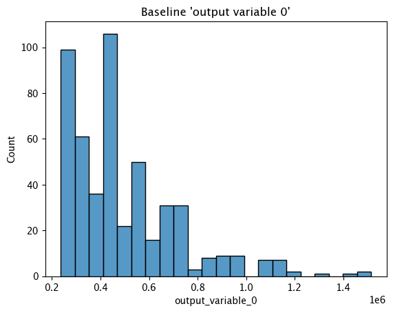
Baseline KDE Chart
The method wallaroo.assay_config.AssayBuilder.baseline_kde returns a Kernel Density Estimation (KDE) chart of the assay baseline generated from the provided parameters.
assay_builder_from_dates.baseline_kde()
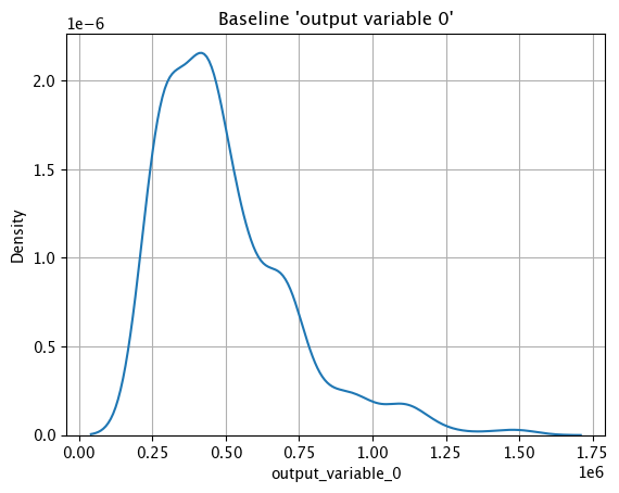
Baseline ECDF Chart
The method wallaroo.assay_config.AssayBuilder.baseline_ecdf returns a Empirical Cumulative Distribution Function (CDF) chart of the assay baseline generated from the provided parameters.
assay_builder_from_dates.baseline_ecdf()
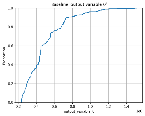
Assay Preview
Now that the baseline is defined, we look at different configuration options and view how the assay baseline and results changes. Once we determine what gives us the best method of determining model drift, we can create the assay.
Analysis List Chart Scores
Analysis List scores show the assay scores for each assay result interval in one chart. Values that are outside of the alert threshold are colored red, while scores within the alert threshold are green.
Assay chart scores are displayed with the method wallaroo.assay.AssayAnalysisList.chart_scores(title: Optional[str] = None), with ability to display an optional title with the chart.
The following example shows retrieving the assay results and displaying the chart scores. From our example, we have two windows - the first should be green, and the second is red showing that values were outside the alert threshold.
# Build the assay, based on the start and end of our baseline time,
# and tracking the output variable index 0
assay_builder_from_dates = wl.build_assay(assay_name="assays from date baseline",
pipeline=mainpipeline,
model_name="house-price-estimator",
iopath="output variable 0",
baseline_start=assay_baseline_start,
baseline_end=assay_baseline_end)
# set the width, interval, and time period
assay_builder_from_dates.add_run_until(datetime.datetime.now())
assay_builder_from_dates.window_builder().add_width(minutes=1).add_interval(minutes=1).add_start(assay_window_start)
assay_config_from_dates = assay_builder_from_dates.build()
assay_results_from_dates = assay_config_from_dates.interactive_run()
assay_results_from_dates.chart_scores()

Analysis Chart
The method wallaroo.assay.AssayAnalysis.chart() displays a comparison between the baseline and an interval of inference data.
This is compared to the Chart Scores, which is a list of all of the inference data split into intervals, while the Analysis Chart shows the breakdown of one set of inference data against the baseline.
Score from the Analysis List Chart Scores and each element from the Analysis List DataFrame generates
The following fields are included.
| Field | Type | Description |
|---|---|---|
| baseline mean | Float | The mean of the baseline values. |
| window mean | Float | The mean of the window values. |
| baseline median | Float | The median of the baseline values. |
| window median | Float | The median of the window values. |
| bin_mode | String | The binning mode used for the assay. |
| aggregation | String | The aggregation mode used for the assay. |
| metric | String | The metric mode used for the assay. |
| weighted | Bool | Whether the bins were manually weighted. |
| score | Float | The score from the assay window. |
| scores | List(Float) | The score from each assay window bin. |
| index | Integer/None | The window index. Interactive assay runs are None. |
# Build the assay, based on the start and end of our baseline time,
# and tracking the output variable index 0
assay_builder_from_dates = wl.build_assay(assay_name="assays from date baseline",
pipeline=mainpipeline,
model_name="house-price-estimator",
iopath="output variable 0",
baseline_start=assay_baseline_start,
baseline_end=assay_baseline_end)
# set the width, interval, and time period
assay_builder_from_dates.add_run_until(datetime.datetime.now())
assay_builder_from_dates.window_builder().add_width(minutes=1).add_interval(minutes=1).add_start(assay_window_start)
assay_config_from_dates = assay_builder_from_dates.build()
assay_results_from_dates = assay_config_from_dates.interactive_run()
assay_results_from_dates[0].chart()
baseline mean = 495193.23178642715
window mean = 517763.394625
baseline median = 442168.125
window median = 448627.8125
bin_mode = Quantile
aggregation = Density
metric = PSI
weighted = False
score = 0.0363497101644573
scores = [0.0, 0.027271477163285655, 0.003847844548034077, 0.000217023993714693, 0.002199485350158766, 0.0028138791092641195, 0.0]
index = None

Analysis List DataFrame
wallaroo.assay.AssayAnalysisList.to_dataframe() returns a DataFrame showing the assay results for each window aka individual analysis. This DataFrame contains the following fields:
| Field | Type | Description |
|---|---|---|
| assay_id | Integer/None | The assay id. Only provided from uploaded and executed assays. |
| name | String/None | The name of the assay. Only provided from uploaded and executed assays. |
| iopath | String/None | The iopath of the assay. Only provided from uploaded and executed assays. |
| score | Float | The assay score. |
| start | DateTime | The DateTime start of the assay window. |
| min | Float | The minimum value in the assay window. |
| max | Float | The maximum value in the assay window. |
| mean | Float | The mean value in the assay window. |
| median | Float | The median value in the assay window. |
| std | Float | The standard deviation value in the assay window. |
| warning_threshold | Float/None | The warning threshold of the assay window. |
| alert_threshold | Float/None | The alert threshold of the assay window. |
| status | String | The assay window status. Values are:
|
For this example, the assay analysis list DataFrame is listed.
From this tutorial, we should have 2 windows of dta to look at, each one minute apart. The first window should show status: OK, with the second window with the very large house prices will show status: alert
# Build the assay, based on the start and end of our baseline time,
# and tracking the output variable index 0
assay_builder_from_dates = wl.build_assay(assay_name="assays from date baseline",
pipeline=mainpipeline,
model_name="house-price-estimator",
iopath="output variable 0",
baseline_start=assay_baseline_start,
baseline_end=assay_baseline_end)
# set the width, interval, and time period
assay_builder_from_dates.add_run_until(datetime.datetime.now())
assay_builder_from_dates.window_builder().add_width(minutes=1).add_interval(minutes=1).add_start(assay_window_start)
assay_config_from_dates = assay_builder_from_dates.build()
assay_results_from_dates = assay_config_from_dates.interactive_run()
assay_results_from_dates.to_dataframe()
| assay_id | name | iopath | score | start | min | max | mean | median | std | warning_threshold | alert_threshold | status | |
|---|---|---|---|---|---|---|---|---|---|---|---|---|---|
| 0 | None | 0.036350 | 2024-02-15T16:20:43.976756+00:00 | 2.362387e+05 | 1489624.250 | 5.177634e+05 | 4.486278e+05 | 227729.030050 | None | 0.25 | Ok | ||
| 1 | None | 8.868614 | 2024-02-15T16:22:43.976756+00:00 | 1.514079e+06 | 2016006.125 | 1.885772e+06 | 1.946438e+06 | 160046.727324 | None | 0.25 | Alert |
Analysis List Full DataFrame
wallaroo.assay.AssayAnalysisList.to_full_dataframe() returns a DataFrame showing all values, including the inputs and outputs from the assay results for each window aka individual analysis. This DataFrame contains the following fields:
pipeline_id warning_threshold bin_index created_at
| Field | Type | Description |
|---|---|---|
| window_start | DateTime | The date and time when the window period began. |
| analyzed_at | DateTime | The date and time when the assay analysis was performed. |
| elapsed_millis | Integer | How long the analysis took to perform in milliseconds. |
| baseline_summary_count | Integer | The number of data elements from the baseline. |
| baseline_summary_min | Float | The minimum value from the baseline summary. |
| baseline_summary_max | Float | The maximum value from the baseline summary. |
| baseline_summary_mean | Float | The mean value of the baseline summary. |
| baseline_summary_median | Float | The median value of the baseline summary. |
| baseline_summary_std | Float | The standard deviation value of the baseline summary. |
| baseline_summary_edges_{0…n} | Float | The baseline summary edges for each baseline edge from 0 to number of edges. |
| summarizer_type | String | The type of summarizer used for the baseline. See wallaroo.assay_config for other summarizer types. |
| summarizer_bin_weights | List / None | If baseline bin weights were provided, the list of those weights. Otherwise, None. |
| summarizer_provided_edges | List / None | If baseline bin edges were provided, the list of those edges. Otherwise, None. |
| status | String | The assay window status. Values are:
|
| id | Integer/None | The id for the window aka analysis. Only provided from uploaded and executed assays. |
| assay_id | Integer/None | The assay id. Only provided from uploaded and executed assays. |
| pipeline_id | Integer/None | The pipeline id. Only provided from uploaded and executed assays. |
| warning_threshold | Float | The warning threshold set for the assay. |
| warning_threshold | Float | The warning threshold set for the assay. |
| bin_index | Integer/None | The bin index for the window aka analysis. |
| created_at | Datetime/None | The date and time the window aka analysis was generated. Only provided from uploaded and executed assays. |
For this example, full DataFrame from an assay preview is generated.
From this tutorial, we should have 2 windows of dta to look at, each one minute apart. The first window should show status: OK, with the second window with the very large house prices will show status: alert
# Build the assay, based on the start and end of our baseline time,
# and tracking the output variable index 0
assay_builder_from_dates = wl.build_assay(assay_name="assays from date baseline",
pipeline=mainpipeline,
model_name="house-price-estimator",
iopath="output variable 0",
baseline_start=assay_baseline_start,
baseline_end=assay_baseline_end)
# set the width, interval, and time period
assay_builder_from_dates.add_run_until(datetime.datetime.now())
assay_builder_from_dates.window_builder().add_width(minutes=1).add_interval(minutes=1).add_start(assay_window_start)
assay_config_from_dates = assay_builder_from_dates.build()
assay_results_from_dates = assay_config_from_dates.interactive_run()
assay_results_from_dates.to_full_dataframe()
| window_start | analyzed_at | elapsed_millis | baseline_summary_count | baseline_summary_min | baseline_summary_max | baseline_summary_mean | baseline_summary_median | baseline_summary_std | baseline_summary_edges_0 | ... | summarizer_type | summarizer_bin_weights | summarizer_provided_edges | status | id | assay_id | pipeline_id | warning_threshold | bin_index | created_at | |
|---|---|---|---|---|---|---|---|---|---|---|---|---|---|---|---|---|---|---|---|---|---|
| 0 | 2024-02-15T16:20:43.976756+00:00 | 2024-02-15T16:26:42.266029+00:00 | 82 | 501 | 236238.671875 | 1514079.375 | 495193.231786 | 442168.125 | 226075.814267 | 236238.671875 | ... | UnivariateContinuous | None | None | Ok | None | None | None | None | None | None |
| 1 | 2024-02-15T16:22:43.976756+00:00 | 2024-02-15T16:26:42.266134+00:00 | 83 | 501 | 236238.671875 | 1514079.375 | 495193.231786 | 442168.125 | 226075.814267 | 236238.671875 | ... | UnivariateContinuous | None | None | Alert | None | None | None | None | None | None |
2 rows × 86 columns
Analysis Compare Basic Stats
The method wallaroo.assay.AssayAnalysis.compare_basic_stats returns a DataFrame comparing one set of inference data against the baseline.
This is compared to the Analysis List DataFrame, which is a list of all of the inference data split into intervals, while the Analysis Compare Basic Stats shows the breakdown of one set of inference data against the baseline.
# Build the assay, based on the start and end of our baseline time,
# and tracking the output variable index 0
assay_builder_from_dates = wl.build_assay(assay_name="assays from date baseline",
pipeline=mainpipeline,
model_name="house-price-estimator",
iopath="output variable 0",
baseline_start=assay_baseline_start,
baseline_end=assay_baseline_end)
# set the width, interval, and time period
assay_builder_from_dates.add_run_until(datetime.datetime.now())
assay_builder_from_dates.window_builder().add_width(minutes=1).add_interval(minutes=1).add_start(assay_window_start)
assay_config_from_dates = assay_builder_from_dates.build()
assay_results_from_dates = assay_config_from_dates.interactive_run()
assay_results_from_dates[0].compare_basic_stats()
| Baseline | Window | diff | pct_diff | |
|---|---|---|---|---|
| count | 501.0 | 1000.0 | 499.000000 | 99.600798 |
| min | 236238.671875 | 236238.671875 | 0.000000 | 0.000000 |
| max | 1514079.375 | 1489624.25 | -24455.125000 | -1.615181 |
| mean | 495193.231786 | 517763.394625 | 22570.162839 | 4.557850 |
| median | 442168.125 | 448627.8125 | 6459.687500 | 1.460912 |
| std | 226075.814267 | 227729.03005 | 1653.215783 | 0.731266 |
| start | None | 2024-02-15T16:20:43.976756+00:00 | NaN | NaN |
| end | None | 2024-02-15T16:21:43.976756+00:00 | NaN | NaN |
Configure Assays
Before creating the assay, configure the assay and continue to preview it until the best method for detecting drift is set. The following options are available.
Score Metric
The score is a distance between the baseline and the analysis window. The larger the score, the greater the difference between the baseline and the analysis window. The following methods are provided determining the score:
PSI(Default) - Population Stability Index (PSI).MAXDIFF: Maximum difference between corresponding bins.SUMDIFF: Mum of differences between corresponding bins.
The metric type used is updated with the wallaroo.assay_config.AssayBuilder.add_metric(metric: wallaroo.assay_config.Metric) method.
The following three charts use each of the metrics. Note how the scores change based on the score type used.
# Build the assay, based on the start and end of our baseline time,
# and tracking the output variable index 0
assay_builder_from_dates = wl.build_assay(assay_name="assays from date baseline",
pipeline=mainpipeline,
model_name="house-price-estimator",
iopath="output variable 0",
baseline_start=assay_baseline_start,
baseline_end=assay_baseline_end)
# set metric PSI mode
assay_builder_from_dates.summarizer_builder.add_metric(wallaroo.assay_config.Metric.PSI)
# set the width, interval, and time period
assay_builder_from_dates.add_run_until(datetime.datetime.now())
assay_builder_from_dates.window_builder().add_width(minutes=1).add_interval(minutes=1).add_start(assay_window_start)
assay_config_from_dates = assay_builder_from_dates.build()
assay_results_from_dates = assay_config_from_dates.interactive_run()
assay_results_from_dates[0].chart()
baseline mean = 495193.23178642715
window mean = 517763.394625
baseline median = 442168.125
window median = 448627.8125
bin_mode = Quantile
aggregation = Density
metric = PSI
weighted = False
score = 0.0363497101644573
scores = [0.0, 0.027271477163285655, 0.003847844548034077, 0.000217023993714693, 0.002199485350158766, 0.0028138791092641195, 0.0]
index = None

# Build the assay, based on the start and end of our baseline time,
# and tracking the output variable index 0
assay_builder_from_dates = wl.build_assay(assay_name="assays from date baseline",
pipeline=mainpipeline,
model_name="house-price-estimator",
iopath="output variable 0",
baseline_start=assay_baseline_start,
baseline_end=assay_baseline_end)
# set metric MAXDIFF mode
assay_builder_from_dates.summarizer_builder.add_metric(wallaroo.assay_config.Metric.MAXDIFF)
# set the width, interval, and time period
assay_builder_from_dates.add_run_until(datetime.datetime.now())
assay_builder_from_dates.window_builder().add_width(minutes=1).add_interval(minutes=1).add_start(assay_window_start)
assay_config_from_dates = assay_builder_from_dates.build()
assay_results_from_dates = assay_config_from_dates.interactive_run()
assay_results_from_dates[0].chart()
baseline mean = 495193.23178642715
window mean = 517763.394625
baseline median = 442168.125
window median = 448627.8125
bin_mode = Quantile
aggregation = Density
metric = MaxDiff
weighted = False
score = 0.06759281437125747
scores = [0.0, 0.06759281437125747, 0.028391217564870255, 0.006592814371257472, 0.02139520958083832, 0.02439920159680639, 0.0]
index = 1

# Build the assay, based on the start and end of our baseline time,
# and tracking the output variable index 0
assay_builder_from_dates = wl.build_assay(assay_name="assays from date baseline",
pipeline=mainpipeline,
model_name="house-price-estimator",
iopath="output variable 0",
baseline_start=assay_baseline_start,
baseline_end=assay_baseline_end)
# set metric SUMDIFF mode
assay_builder_from_dates.summarizer_builder.add_metric(wallaroo.assay_config.Metric.SUMDIFF)
# set the width, interval, and time period
assay_builder_from_dates.add_run_until(datetime.datetime.now())
assay_builder_from_dates.window_builder().add_width(minutes=1).add_interval(minutes=1).add_start(assay_window_start)
assay_config_from_dates = assay_builder_from_dates.build()
assay_results_from_dates = assay_config_from_dates.interactive_run()
assay_results_from_dates[0].chart()
baseline mean = 495193.23178642715
window mean = 517763.394625
baseline median = 442168.125
window median = 448627.8125
bin_mode = Quantile
aggregation = Density
metric = SumDiff
weighted = False
score = 0.07418562874251496
scores = [0.0, 0.06759281437125747, 0.028391217564870255, 0.006592814371257472, 0.02139520958083832, 0.02439920159680639, 0.0]
index = None
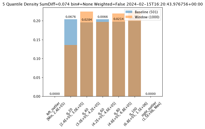
Alert Threshold
Assay alert thresholds are modified with the wallaroo.assay_config.AssayBuilder.add_alert_threshold(alert_threshold: float) method. By default alert thresholds are 0.1.
The following example updates the alert threshold to 0.5.
# Build the assay, based on the start and end of our baseline time,
# and tracking the output variable index 0
assay_builder_from_dates = wl.build_assay(assay_name="assays from date baseline",
pipeline=mainpipeline,
model_name="house-price-estimator",
iopath="output variable 0",
baseline_start=assay_baseline_start,
baseline_end=assay_baseline_end)
assay_builder_from_dates.add_alert_threshold(0.5)
# set the width, interval, and time period
assay_builder_from_dates.add_run_until(datetime.datetime.now())
assay_builder_from_dates.window_builder().add_width(minutes=1).add_interval(minutes=1).add_start(assay_window_start)
assay_config_from_dates = assay_builder_from_dates.build()
assay_results_from_dates = assay_config_from_dates.interactive_run()
assay_results_from_dates.to_dataframe()
| assay_id | name | iopath | score | start | min | max | mean | median | std | warning_threshold | alert_threshold | status | |
|---|---|---|---|---|---|---|---|---|---|---|---|---|---|
| 0 | None | 0.036350 | 2024-02-15T16:20:43.976756+00:00 | 2.362387e+05 | 1489624.250 | 5.177634e+05 | 4.486278e+05 | 227729.030050 | None | 0.5 | Ok | ||
| 1 | None | 8.868614 | 2024-02-15T16:22:43.976756+00:00 | 1.514079e+06 | 2016006.125 | 1.885772e+06 | 1.946438e+06 | 160046.727324 | None | 0.5 | Alert |
Number of Bins
Number of bins sets how the baseline data is partitioned. The total number of bins includes the set number plus the left_outlier and the right_outlier, so the total number of bins will be the total set + 2.
The number of bins is set with the wallaroo.assay_config.UnivariateContinousSummarizerBuilder.add_num_bins(num_bins: int) method.
# Build the assay, based on the start and end of our baseline time,
# and tracking the output variable index 0
assay_builder_from_dates = wl.build_assay(assay_name="assays from date baseline",
pipeline=mainpipeline,
model_name="house-price-estimator",
iopath="output variable 0",
baseline_start=assay_baseline_start,
baseline_end=assay_baseline_end)
# Set the number of bins
# update number of bins here
assay_builder_from_dates.summarizer_builder.add_num_bins(10)
# set the width, interval, and time period
assay_builder_from_dates.add_run_until(datetime.datetime.now())
assay_builder_from_dates.window_builder().add_width(minutes=1).add_interval(minutes=1).add_start(assay_window_start)
assay_config_from_dates = assay_builder_from_dates.build()
assay_results_from_dates = assay_config_from_dates.interactive_run()
assay_results_from_dates[0].chart()
baseline mean = 495193.23178642715
window mean = 517763.394625
baseline median = 442168.125
window median = 448627.8125
bin_mode = Quantile
aggregation = Density
metric = PSI
weighted = False
score = 0.05250979748389363
scores = [0.0, 0.009076998929542533, 0.01924002322223739, 0.0021945246367443406, 0.0016700458183385653, 0.005779503770625584, 0.002393429678215835, 0.002942858220315506, 0.00010651192741915124, 0.00046961759334670583, 0.008636283687108028, 0.0]
index = None
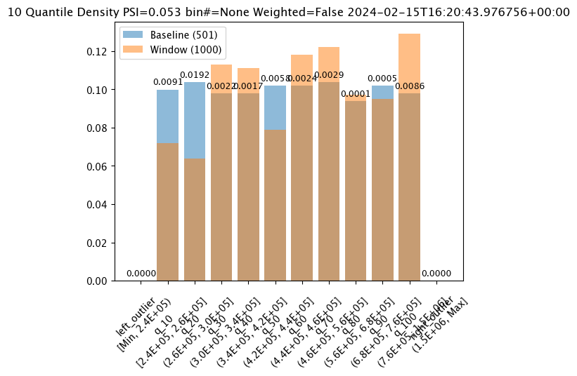
Binning Mode
Binning Mode defines how the bins are separated. Binning modes are modified through the wallaroo.assay_config.UnivariateContinousSummarizerBuilder.add_bin_mode(bin_mode: bin_mode: wallaroo.assay_config.BinMode, edges: Optional[List[float]] = None).
Available bin_mode values from wallaroo.assay_config.Binmode are the following:
QUANTILE(Default): Based on percentages. Ifnum_binsis 5 then quintiles so bins are created at the 20%, 40%, 60%, 80% and 100% points.EQUAL: Evenly spaced bins where each bin is set with the formulamin - max / num_binsPROVIDED: The user provides the edge points for the bins.
If PROVIDED is supplied, then a List of float values must be provided for the edges parameter that matches the number of bins.
The following examples are used to show how each of the binning modes effects the bins.
# Build the assay, based on the start and end of our baseline time,
# and tracking the output variable index 0
assay_builder_from_dates = wl.build_assay(assay_name="assays from date baseline",
pipeline=mainpipeline,
model_name="house-price-estimator",
iopath="output variable 0",
baseline_start=assay_baseline_start,
baseline_end=assay_baseline_end)
# update binning mode here
assay_builder_from_dates.summarizer_builder.add_bin_mode(wallaroo.assay_config.BinMode.QUANTILE)
# set the width, interval, and time period
assay_builder_from_dates.add_run_until(datetime.datetime.now())
assay_builder_from_dates.window_builder().add_width(minutes=1).add_interval(minutes=1).add_start(assay_window_start)
assay_config_from_dates = assay_builder_from_dates.build()
assay_results_from_dates = assay_config_from_dates.interactive_run()
assay_results_from_dates[0].chart()
baseline mean = 495193.23178642715
window mean = 517763.394625
baseline median = 442168.125
window median = 448627.8125
bin_mode = Quantile
aggregation = Density
metric = PSI
weighted = False
score = 0.0363497101644573
scores = [0.0, 0.027271477163285655, 0.003847844548034077, 0.000217023993714693, 0.002199485350158766, 0.0028138791092641195, 0.0]
index = None

# Build the assay, based on the start and end of our baseline time,
# and tracking the output variable index 0
assay_builder_from_dates = wl.build_assay(assay_name="assays from date baseline",
pipeline=mainpipeline,
model_name="house-price-estimator",
iopath="output variable 0",
baseline_start=assay_baseline_start,
baseline_end=assay_baseline_end)
# update binning mode here
assay_builder_from_dates.summarizer_builder.add_bin_mode(wallaroo.assay_config.BinMode.EQUAL)
# set the width, interval, and time period
assay_builder_from_dates.add_run_until(datetime.datetime.now())
assay_builder_from_dates.window_builder().add_width(minutes=1).add_interval(minutes=1).add_start(assay_window_start)
assay_config_from_dates = assay_builder_from_dates.build()
assay_results_from_dates = assay_config_from_dates.interactive_run()
assay_results_from_dates[0].chart()
baseline mean = 495193.23178642715
window mean = 517763.394625
baseline median = 442168.125
window median = 448627.8125
bin_mode = Equal
aggregation = Density
metric = PSI
weighted = False
score = 0.013362603453760629
scores = [0.0, 0.0016737762070682225, 1.1166481947075492e-06, 0.011233704798893194, 1.276169365380064e-07, 0.00045387818266796784, 0.0]
index = None
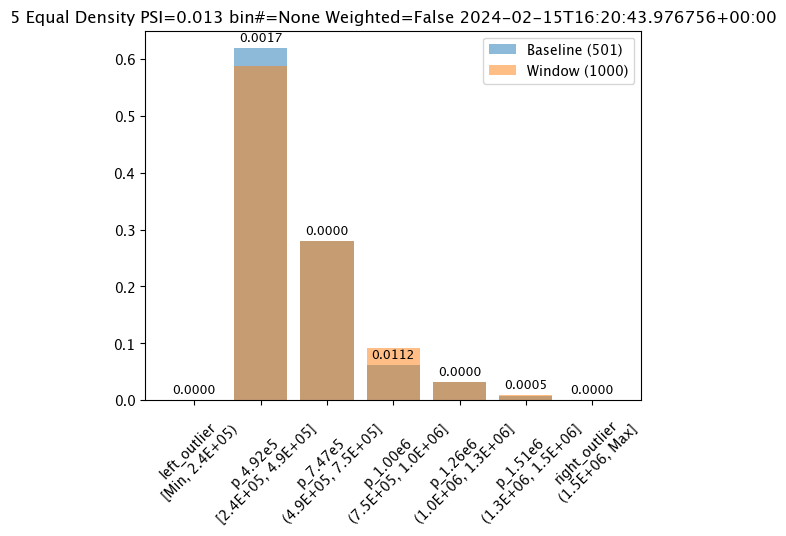
The following example manually sets the bin values.
The values in this dataset run from 200000 to 1500000. We can specify the bins with the BinMode.PROVIDED and specifying a list of floats with the right hand / upper edge of each bin and optionally the lower edge of the smallest bin. If the lowest edge is not specified the threshold for left outliers is taken from the smallest value in the baseline dataset.
# Build the assay, based on the start and end of our baseline time,
# and tracking the output variable index 0
assay_builder_from_dates = wl.build_assay(assay_name="assays from date baseline",
pipeline=mainpipeline,
model_name="house-price-estimator",
iopath="output variable 0",
baseline_start=assay_baseline_start,
baseline_end=assay_baseline_end)
edges = [200000.0, 400000.0, 600000.0, 800000.0, 1500000.0, 2000000.0]
# update binning mode here
assay_builder_from_dates.summarizer_builder.add_bin_mode(wallaroo.assay_config.BinMode.PROVIDED, edges)
# set the width, interval, and time period
assay_builder_from_dates.add_run_until(datetime.datetime.now())
assay_builder_from_dates.window_builder().add_width(minutes=1).add_interval(minutes=1).add_start(assay_window_start)
assay_config_from_dates = assay_builder_from_dates.build()
assay_results_from_dates = assay_config_from_dates.interactive_run()
assay_results_from_dates[0].chart()
baseline mean = 495193.23178642715
window mean = 517763.394625
baseline median = 442168.125
window median = 448627.8125
bin_mode = Provided
aggregation = Density
metric = PSI
weighted = False
score = 0.01005936099521711
scores = [0.0, 0.0030207963288415803, 0.00011480201840874194, 0.00045327555974347976, 0.0037119550613212583, 0.0027585320269020493, 0.0]
index = None
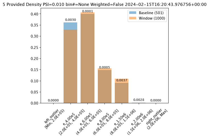
Aggregation Options
Assay aggregation options are modified with the wallaroo.assay_config.AssayBuilder.add_aggregation(aggregation: wallaroo.assay_config.Aggregation) method. The following options are provided:
Aggregation.DENSITY(Default): Count the number/percentage of values that fall in each bin.Aggregation.CUMULATIVE: Empirical Cumulative Density Function style, which keeps a cumulative count of the values/percentages that fall in each bin.
The following example demonstrate the different results between the two.
#Aggregation.DENSITY - the default
# Build the assay, based on the start and end of our baseline time,
# and tracking the output variable index 0
assay_builder_from_dates = wl.build_assay(assay_name="assays from date baseline",
pipeline=mainpipeline,
model_name="house-price-estimator",
iopath="output variable 0",
baseline_start=assay_baseline_start,
baseline_end=assay_baseline_end)
assay_builder_from_dates.summarizer_builder.add_aggregation(wallaroo.assay_config.Aggregation.DENSITY)
# set the width, interval, and time period
assay_builder_from_dates.add_run_until(datetime.datetime.now())
assay_builder_from_dates.window_builder().add_width(minutes=1).add_interval(minutes=1).add_start(assay_window_start)
assay_config_from_dates = assay_builder_from_dates.build()
assay_results_from_dates = assay_config_from_dates.interactive_run()
assay_results_from_dates[0].chart()
baseline mean = 495193.23178642715
window mean = 517763.394625
baseline median = 442168.125
window median = 448627.8125
bin_mode = Quantile
aggregation = Density
metric = PSI
weighted = False
score = 0.0363497101644573
scores = [0.0, 0.027271477163285655, 0.003847844548034077, 0.000217023993714693, 0.002199485350158766, 0.0028138791092641195, 0.0]
index = None
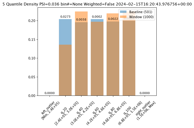
#Aggregation.CUMULATIVE
# Build the assay, based on the start and end of our baseline time,
# and tracking the output variable index 0
assay_builder_from_dates = wl.build_assay(assay_name="assays from date baseline",
pipeline=mainpipeline,
model_name="house-price-estimator",
iopath="output variable 0",
baseline_start=assay_baseline_start,
baseline_end=assay_baseline_end)
assay_builder_from_dates.summarizer_builder.add_aggregation(wallaroo.assay_config.Aggregation.CUMULATIVE)
# set the width, interval, and time period
assay_builder_from_dates.add_run_until(datetime.datetime.now())
assay_builder_from_dates.window_builder().add_width(minutes=1).add_interval(minutes=1).add_start(assay_window_start)
assay_config_from_dates = assay_builder_from_dates.build()
assay_results_from_dates = assay_config_from_dates.interactive_run()
assay_results_from_dates[0].chart()
baseline mean = 495193.23178642715
window mean = 517763.394625
baseline median = 442168.125
window median = 448627.8125
bin_mode = Quantile
aggregation = Cumulative
metric = PSI
weighted = False
score = 0.17698802395209584
scores = [0.0, 0.06759281437125747, 0.03920159680638724, 0.04579441117764471, 0.02439920159680642, 0.0, 0.0]
index = None
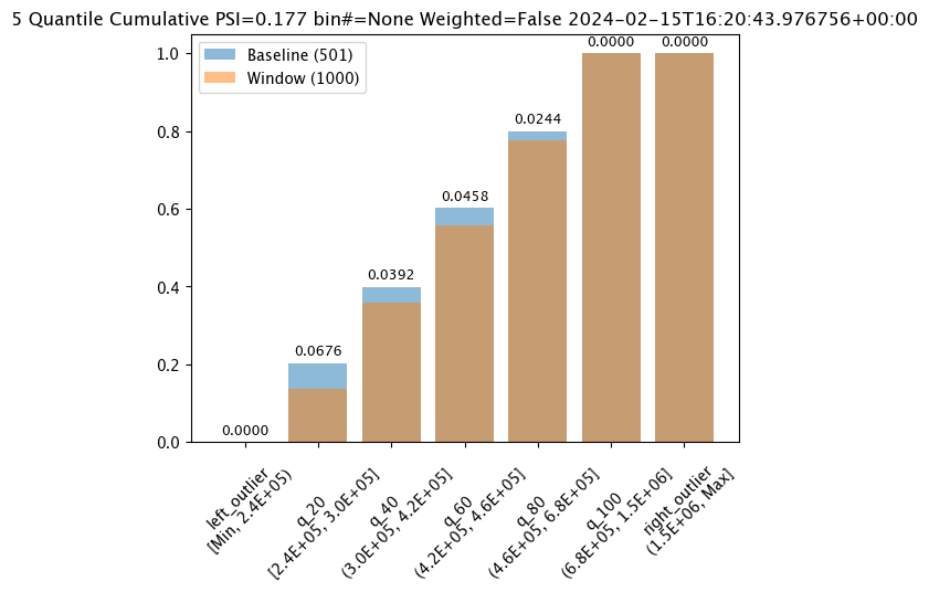
Inference Interval and Inference Width
The inference interval aka window interval sets how often to run the assay analysis. This is set from the wallaroo.assay_config.AssayBuilder.window_builder.add_interval method to collect data expressed in time units: “hours=24”, “minutes=1”, etc.
For example, with an interval of 1 minute, the assay collects data every minute. Within an hour, 60 intervals of data is collected.
We can adjust the interval and see how the assays change based on how frequently they are run.
The width sets the time period from the wallaroo.assay_config.AssayBuilder.window_builder.add_width method to collect data expressed in time units: “hours=24”, “minutes=1”, etc.
For example, an interval of 1 minute and a width of 1 minute collects 1 minutes worth of data every minute. An interval of 1 minute with a width of 5 minutes collects 5 minute of inference data every minute.
By default, the interval and width is 24 hours.
For this example, we’ll adjust the width and interval from 1 minute to 5 minutes and see how the number of analyses and their score changes.
# Build the assay, based on the start and end of our baseline time,
# and tracking the output variable index 0
assay_builder_from_dates = wl.build_assay(assay_name="assays from date baseline",
pipeline=mainpipeline,
model_name="house-price-estimator",
iopath="output variable 0",
baseline_start=assay_baseline_start,
baseline_end=assay_baseline_end)
# set the width, interval, and time period
assay_builder_from_dates.add_run_until(datetime.datetime.now())
assay_builder_from_dates.window_builder().add_width(minutes=1).add_interval(minutes=1).add_start(assay_window_start)
assay_config_from_dates = assay_builder_from_dates.build()
assay_results_from_dates = assay_config_from_dates.interactive_run()
assay_results_from_dates.chart_scores()

# Build the assay, based on the start and end of our baseline time,
# and tracking the output variable index 0
assay_builder_from_dates = wl.build_assay(assay_name="assays from date baseline",
pipeline=mainpipeline,
model_name="house-price-estimator",
iopath="output variable 0",
baseline_start=assay_baseline_start,
baseline_end=assay_baseline_end)
# set the width, interval, and time period
assay_builder_from_dates.add_run_until(datetime.datetime.now())
assay_builder_from_dates.window_builder().add_width(minutes=5).add_interval(minutes=5).add_start(assay_window_start)
assay_config_from_dates = assay_builder_from_dates.build()
assay_results_from_dates = assay_config_from_dates.interactive_run()
assay_results_from_dates.chart_scores()
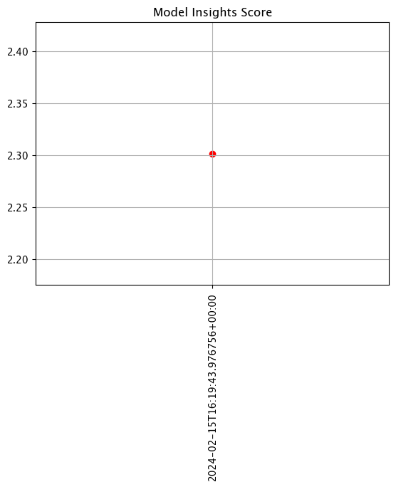
Add Run Until and Add Inference Start
For previewing assays, setting wallaroo.assay_config.AssayBuilder.add_run_until sets the end date and time for collecting inference data. When an assay is uploaded, this setting is no longer valid - assays run at the Inference Interval until the assay is paused.
Setting the wallaroo.assay_config.WindowBuilder.add_start sets the start date and time to collect inference data. When an assay is uploaded, this setting is included, and assay results will be displayed starting from that start date at the Inference Interval until the assay is paused. By default, add_start begins 24 hours after the assay is uploaded unless set in the assay configuration manually.
For the following example, the add_run_until setting is set to datetime.datetime.now() to collect all inference data from assay_window_start up until now, and the second example limits that example to only two minutes of data.
# inference data that includes all of the data until now
assay_builder_from_dates = wl.build_assay(assay_name="assays from date baseline",
pipeline=mainpipeline,
model_name="house-price-estimator",
iopath="output variable 0",
baseline_start=assay_baseline_start,
baseline_end=assay_baseline_end)
# set the width, interval, and time period
assay_builder_from_dates.add_run_until(datetime.datetime.now())
assay_builder_from_dates.window_builder().add_width(minutes=1).add_interval(minutes=1).add_start(assay_window_start)
assay_config_from_dates = assay_builder_from_dates.build()
assay_results_from_dates = assay_config_from_dates.interactive_run()
assay_results_from_dates.chart_scores()
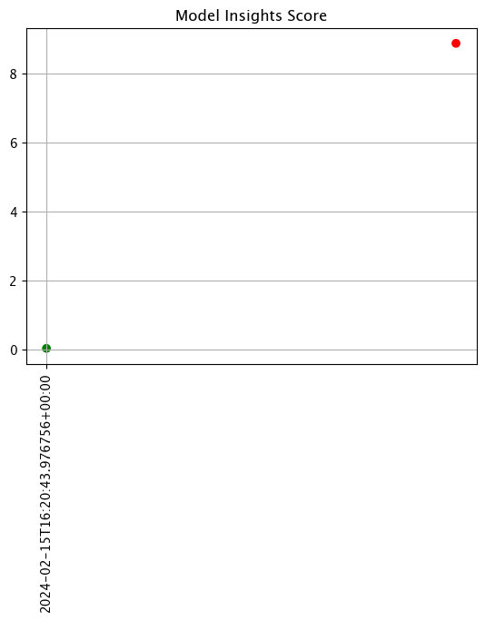
# inference data that includes all of the data until now
assay_builder_from_dates = wl.build_assay(assay_name="assays from date baseline",
pipeline=mainpipeline,
model_name="house-price-estimator",
iopath="output variable 0",
baseline_start=assay_baseline_start,
baseline_end=assay_baseline_end)
# set the width, interval, and time period
assay_builder_from_dates.add_run_until(assay_window_start+datetime.timedelta(seconds=120))
assay_builder_from_dates.window_builder().add_width(minutes=1).add_interval(minutes=1).add_start(assay_window_start)
assay_config_from_dates = assay_builder_from_dates.build()
assay_results_from_dates = assay_config_from_dates.interactive_run()
assay_results_from_dates.chart_scores()
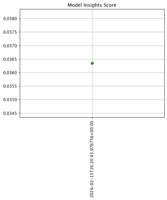
Create Assay
With the assay previewed and configuration options determined, we officially create it by uploading it to the Wallaroo instance.
Once it is uploaded, the assay runs an analysis based on the window width, interval, and the other settings configured.
Assays are uploaded with the wallaroo.assay_config.upload() method. This uploads the assay into the Wallaroo database with the configurations applied and returns the assay id. Note that assay names must be unique across the Wallaroo instance; attempting to upload an assay with the same name as an existing one will return an error.
wallaroo.assay_config.upload() returns the assay id for the assay.
Typically we would just call wallaroo.assay_config.upload() after configuring the assay. For the example below, we will perform the complete configuration in one window to show all of the configuration steps at once before creating the assay.
# Build the assay, based on the start and end of our baseline time,
# and tracking the output variable index 0
assay_builder_from_dates = wl.build_assay(assay_name="assays creation example",
pipeline=mainpipeline,
model_name="house-price-estimator",
iopath="output variable 0",
baseline_start=assay_baseline_start,
baseline_end=assay_baseline_end)
# set the width, interval, and assay start date and time
assay_builder_from_dates.window_builder().add_width(minutes=1).add_interval(minutes=1).add_start(assay_window_start)
# add other options
assay_builder_from_dates.summarizer_builder.add_aggregation(wallaroo.assay_config.Aggregation.CUMULATIVE)
assay_builder_from_dates.summarizer_builder.add_metric(wallaroo.assay_config.Metric.MAXDIFF)
assay_builder_from_dates.add_alert_threshold(0.5)
assay_id = assay_builder_from_dates.upload()
# wait 65 seconds for the first analysis run performed
time.sleep(65)
The assay is now visible through the Wallaroo UI by selecting the workspace, then the pipeline, then Insights.

Get Assay Results
Once an assay is created the assay runs an analysis based on the window width, interval, and the other settings configured.
Assay results are retrieved with the wallaroo.client.get_assay_results method, which takes the following parameters:
| Parameter | Type | Description |
|---|---|---|
| assay_id | Integer (Required) | The numerical id of the assay. |
| start | Datetime.Datetime (Required) | The start date and time of historical data from the pipeline to start analyses from. |
| end | Datetime.Datetime (Required) | The end date and time of historical data from the pipeline to limit analyses to. |
- IMPORTANT NOTE: This process requires that additional historical data is generated from the time the assay is created to when the results are available. To add additional inference data, use the Assay Test Data section above.
assay_results = wl.get_assay_results(assay_id=assay_id,
start=assay_window_start,
end=datetime.datetime.now())
assay_results.chart_scores()
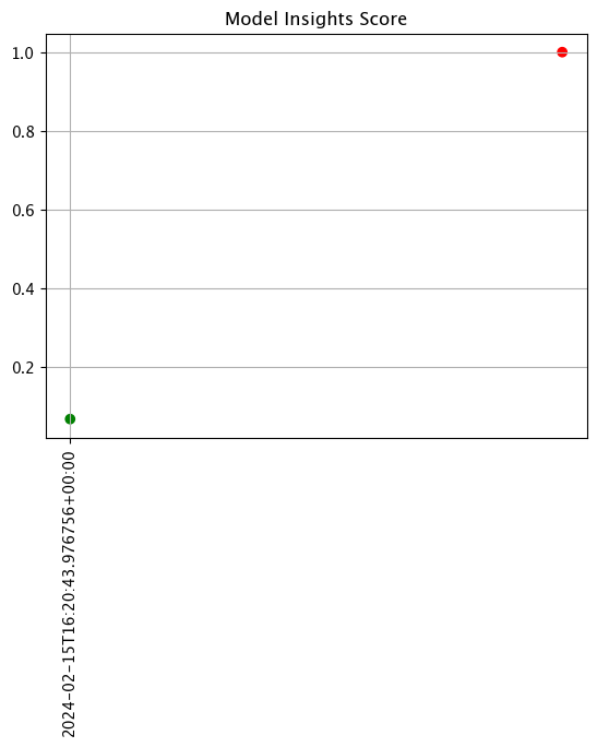
assay_results[0].chart()
baseline mean = 495193.23178642715
window mean = 517763.394625
baseline median = 442168.125
window median = 448627.8125
bin_mode = Quantile
aggregation = Cumulative
metric = MaxDiff
weighted = False
score = 0.067592815
scores = [0.0, 0.06759281437125747, 0.03920159680638724, 0.04579441117764471, 0.02439920159680642, 0.0, 0.0]
index = 1

List and Retrieve Assay
If the assay id is not already know, it is retrieved from the wallaroo.client.list_assays() method. Select the assay to retrieve data for and retrieve its id with wallaroo.assay.Assay._id method.
wl.list_assays()
| name | active | status | warning_threshold | alert_threshold | pipeline_name |
|---|---|---|---|---|---|
| assays creation example | True | {"run_at": "2024-02-15T16:40:53.212979206+00:00", "num_ok": 0, "num_warnings": 0, "num_alerts": 0} | None | 0.5 | assay-demonstration-tutorial |
retrieved_assay = wl.list_assays()[0]
live_assay_results = wl.get_assay_results(assay_id=retrieved_assay._id,
start=assay_window_start,
end=datetime.datetime.now())
live_assay_results.chart_scores()

live_assay_results[0].chart()
baseline mean = 495193.23178642715
window mean = 517763.394625
baseline median = 442168.125
window median = 448627.8125
bin_mode = Quantile
aggregation = Cumulative
metric = MaxDiff
weighted = False
score = 0.067592815
scores = [0.0, 0.06759281437125747, 0.03920159680638724, 0.04579441117764471, 0.02439920159680642, 0.0, 0.0]
index = 1

Pause and Resume Assay
Assays are paused and started with the wallaroo.assay.Assay.turn_off and wallaroo.assay.Assay.turn_on methods.
For the following, we retrieve an assay from the wallaroo instance and pause it, then list the assays to verify its setting Active is False.
display(wl.list_assays())
retrieved_assay = wl.list_assays()[0]
| name | active | status | warning_threshold | alert_threshold | pipeline_name |
|---|---|---|---|---|---|
| assays creation example | True | {"run_at": "2024-02-15T16:40:53.212979206+00:00", "num_ok": 0, "num_warnings": 0, "num_alerts": 0} | None | 0.5 | assay-demonstration-tutorial |
Now we pause the assay, and show the assay list to verify it is no longer active.
retrieved_assay.turn_off()
display(wl.list_assays())
| name | active | status | warning_threshold | alert_threshold | pipeline_name |
|---|---|---|---|---|---|
| assays creation example | False | {"run_at": "2024-02-15T16:40:53.212979206+00:00", "num_ok": 0, "num_warnings": 0, "num_alerts": 0} | None | 0.5 | assay-demonstration-tutorial |
We resume the assay and verify its setting Active is True.
retrieved_assay.turn_on()
display(wl.list_assays())
| name | active | status | warning_threshold | alert_threshold | pipeline_name |
|---|---|---|---|---|---|
| assays creation example | True | {"run_at": "2024-02-15T16:40:53.212979206+00:00", "num_ok": 0, "num_warnings": 0, "num_alerts": 0} | None | 0.5 | assay-demonstration-tutorial |
Undeploy Main Pipeline
With the examples and tutorial complete, we will undeploy the main pipeline and return the resources back to the Wallaroo instance.
mainpipeline.undeploy()
3.6 - Computer Vision Pipeline Logs MLOps API Tutorial
How to retrieve computer vision oriented pipeline logs through the Wallaroo MLOps API.
This tutorial and the assets can be downloaded as part of the Wallaroo Tutorials repository.
Pipeline API Log Tutorial
This tutorial demonstrates Wallaroo Pipeline MLOps API for pipeline log retrieval for Computer Vision based models.
This tutorial will demonstrate how to:
- Select or create a workspace, pipeline and upload the control model, and additional testing models.
- Add a pipeline step with the champion model, then deploy the pipeline and perform sample inferences for computer vision detection.
- Retrieve the logs via the Wallaroo MLOps API. These steps will be simplified to only show the API log retrieval method. See the Wallaroo Documentation site for full details.
- Use the pipeline logs to display metadata data.
- Undeploy the pipeline.
This tutorial provides the following:
- Models:
models/yolov8n.onnx: A pre-trained Yolov8n model.
- Data:
data/dogbike.png: A PNG image with a dog and bicycle.data/dogbike.df.json: A pandas Record format JSON file of the PNG image converted to numpy array values for inference requests.
Prerequisites
- A deployed Wallaroo instance
- The following Python libraries installed:
wallaroo: The Wallaroo SDK. Included with the Wallaroo JupyterHub service by default.
Initial Steps
Import libraries
The first step is to import the libraries needed for this notebook.
import wallaroo
from wallaroo.object import EntityNotFoundError
import pyarrow as pa
from IPython.display import display
# used to display DataFrame information without truncating
from IPython.display import display
import pandas as pd
pd.set_option('display.max_colwidth', None)
import datetime
import requests
Connect to the Wallaroo Instance
The first step is to connect to Wallaroo through the Wallaroo client. The Python library is included in the Wallaroo install and available through the Jupyter Hub interface provided with your Wallaroo environment.
This is accomplished using the wallaroo.Client() command, which provides a URL to grant the SDK permission to your specific Wallaroo environment. When displayed, enter the URL into a browser and confirm permissions. Store the connection into a variable that can be referenced later.
If logging into the Wallaroo instance through the internal JupyterHub service, use wl = wallaroo.Client(). If logging in externally, update the wallarooPrefix and wallarooSuffix variables with the proper DNS information. For more information on Wallaroo Client settings, see the Client Connection guide.
# Login through local Wallaroo instance
wl = wallaroo.Client()
Wallaroo MLOps API URL
API URL
The variable APIURL is used to specify the connection to the Wallaroo instance’s MLOps API URL, and is composed of the Wallaroo DNS prefix and suffix. For full details, see the Wallaroo API Connection Guide
.
For this demonstration, the following Wallaroo SDK methods are used to generate the API authentication Bearer token, and the MLOps API URL.
For full details on connecting to a Wallaroo instance via MLOps API calls, see the Wallaroo API Connection Guide.
These methods are:
wallaroo.client.auth_header(): Returns the authorization Bearer token for a user authenticated through the Wallaroo SDK.wallaroo.client.api_endpoint: Returns the Wallaroo instance’s api endpoint.
display(wl.auth.auth_header())
display(wl.api_endpoint)
{'Authorization': 'Bearer eyJhbGciOiJSUzI1NiIsInR5cCIgOiAiSldUIiwia2lkIiA6ICJzWThabWtGcm9VWDdDSzFiQjEyS1dwWGtaaUk2R01Gd1ZQUHduWmxxbkVRIn0.eyJleHAiOjE3MDMyNjYxOTIsImlhdCI6MTcwMzI2NjEzMiwiYXV0aF90aW1lIjoxNzAzMjY0OTgxLCJqdGkiOiI0NDdmNmU4YS02NTY0LTRhMDQtODBiYy03MDY1YjViMzM4NTQiLCJpc3MiOiJodHRwczovL2RvYy10ZXN0LmtleWNsb2FrLndhbGxhcm9vY29tbXVuaXR5Lm5pbmphL2F1dGgvcmVhbG1zL21hc3RlciIsImF1ZCI6WyJtYXN0ZXItcmVhbG0iLCJhY2NvdW50Il0sInN1YiI6ImNkOGZkMDYzLTYyZmItNDhkYy05NTg5LTFkZTFiMjlkOTZhNyIsInR5cCI6IkJlYXJlciIsImF6cCI6InNkay1jbGllbnQiLCJzZXNzaW9uX3N0YXRlIjoiMTIxNTg0M2UtMThhNy00NzgyLWE0YjgtODQ4YjIyYWQxYzdmIiwiYWNyIjoiMSIsInJlYWxtX2FjY2VzcyI6eyJyb2xlcyI6WyJkZWZhdWx0LXJvbGVzLW1hc3RlciIsIm9mZmxpbmVfYWNjZXNzIiwidW1hX2F1dGhvcml6YXRpb24iXX0sInJlc291cmNlX2FjY2VzcyI6eyJtYXN0ZXItcmVhbG0iOnsicm9sZXMiOlsibWFuYWdlLXVzZXJzIiwidmlldy11c2VycyIsInF1ZXJ5LWdyb3VwcyIsInF1ZXJ5LXVzZXJzIl19LCJhY2NvdW50Ijp7InJvbGVzIjpbIm1hbmFnZS1hY2NvdW50IiwibWFuYWdlLWFjY291bnQtbGlua3MiLCJ2aWV3LXByb2ZpbGUiXX19LCJzY29wZSI6InByb2ZpbGUgb3BlbmlkIGVtYWlsIiwic2lkIjoiMTIxNTg0M2UtMThhNy00NzgyLWE0YjgtODQ4YjIyYWQxYzdmIiwiZW1haWxfdmVyaWZpZWQiOmZhbHNlLCJodHRwczovL2hhc3VyYS5pby9qd3QvY2xhaW1zIjp7IngtaGFzdXJhLXVzZXItaWQiOiJjZDhmZDA2My02MmZiLTQ4ZGMtOTU4OS0xZGUxYjI5ZDk2YTciLCJ4LWhhc3VyYS1kZWZhdWx0LXJvbGUiOiJ1c2VyIiwieC1oYXN1cmEtYWxsb3dlZC1yb2xlcyI6WyJ1c2VyIl0sIngtaGFzdXJhLXVzZXItZ3JvdXBzIjoie30ifSwibmFtZSI6IkpvaG4gSGFuc2FyaWNrIiwicHJlZmVycmVkX3VzZXJuYW1lIjoiam9obi5odW1tZWxAd2FsbGFyb28uYWkiLCJnaXZlbl9uYW1lIjoiSm9obiIsImZhbWlseV9uYW1lIjoiSGFuc2FyaWNrIiwiZW1haWwiOiJqb2huLmh1bW1lbEB3YWxsYXJvby5haSJ9.W4rshsGTfdHrQnfP03zDcKUJSTEXVHb6HGmci5wDjCSUmqVibauaifoPl1b9mC9XR384-mt9CTEoA4k9JR9YntGzVgifQ2FgSvFtLHaTMMdl1BYulmJmnG_1jxheU7bc0XcgaBpTTQprkVn_UNvipIQuTxIwSsRyJzCmTXofQ8MQB5M1UVz2EQij-w9PzNWUbgDQ0K4IueYFK3idF3VWZCrO3ETEQV-xqySc-GoOmS8IQHWgNBb_WD11SjBYj1wrISYj3PgBAalyCc-hxZKDbdtuWGjjjeexqkGr_aTc4DfxQS3VUki4k9pCJEi5riLeOf0eJvRRYT69GrLrIe7IIA'}
Create Workspace
We will create a workspace to manage our pipeline and models. The following variables will set the name of our sample workspace then set it as the current workspace.
IMPORTANT NOTE: Workspace names must be unique across the Wallaroo instance. To verify unique names, the randomization code below is provided to allow the workspace name to be unique. If this is not required, set
suffixto''.References
import string
import random
# make a random 4 character suffix to prevent overwriting other user's workspaces
suffix= ''.join(random.choice(string.ascii_lowercase) for i in range(4))
suffix=''
workspace_name = f'log-api-cv-workspace{suffix}'
main_pipeline_name = 'log-api-cv'
model_name = 'yolov8n'
model_file_name = './models/yolov8n.onnx'
def get_workspace(name, client):
workspace = None
for ws in client.list_workspaces():
if ws.name() == name:
workspace= ws
if(workspace == None):
workspace = client.create_workspace(name)
return workspace
workspace = get_workspace(workspace_name, wl)
wl.set_current_workspace(workspace)
workspace_id = workspace.id()
Upload The Computer Vision Model
For our example, we will upload the Yolov8n model, and set the input field to images.
# Upload Retrained Yolo8 Model
yolov8_model = (wl.upload_model(model_name,
model_file_name,
framework=wallaroo.framework.Framework.ONNX)
.configure(tensor_fields=['images'],
batch_config="single"
)
)
Build the Pipeline
This pipeline is made to be an example of an existing situation where a model is deployed and being used for inferences in a production environment. We’ll call it housepricepipeline, set housingcontrol as a pipeline step, then run a few sample inferences.
mainpipeline = wl.build_pipeline(main_pipeline_name)
# in case this pipeline was run before
mainpipeline.undeploy()
mainpipeline.clear()
mainpipeline.add_model_step(yolov8_model).deploy()
| name | log-api-cv |
|---|---|
| created | 2023-12-22 17:10:06.563220+00:00 |
| last_updated | 2023-12-22 17:55:34.460452+00:00 |
| deployed | True |
| arch | None |
| tags | |
| versions | b1c6d8ea-0259-4a45-aca5-c065a2d59d2d, a8f0adef-5ab9-4695-95eb-e09c256b221c, d174e395-66b5-40bb-bec0-a689e597749f, 4db1d862-0c8d-4394-9009-8aee1324503c, ce598566-83f7-4983-a8e5-4fc779e2c008, b016fb58-d52e-46e1-afc4-31268f471077, 0bd75ecf-1923-42cf-b7e5-6593699465c0 |
| steps | api-sample-model |
| published | False |
Testing
We’ll pass in our DataFrame reference file as an inference request, noting the start and end times for our log retrieval.
dataframe_start = datetime.datetime.now(datetime.timezone.utc)
# run as inference api
# Retrieve the token
headers = wl.auth.auth_header()
# set Content-Type type
headers['Content-Type']='application/json; format=pandas-records'
## Inference through external URL using dataframe
df = pd.read_json('./data/dogbike.df.json')
data = df.to_dict(orient="records")
# submit the request via POST, import as pandas DataFrame
response = pd.DataFrame.from_records(
requests.post(
mainpipeline._deployment._url(),
json=data,
headers=headers)
.json()
)
# just to account for any local versus server time discrepancy
import time
time.sleep(20)
dataframe_end = datetime.datetime.now(datetime.timezone.utc)
# run additional inferences outside the time frame
for i in range(10):
# submit the request via POST, import as pandas DataFrame
response = pd.DataFrame.from_records(
requests.post(
mainpipeline._deployment._url(),
json=data,
headers=headers)
.json()
)
Get Pipeline Logs
Pipeline logs are retrieved through the Wallaroo MLOps API with the following request.
- REQUEST URL
v1/api/pipelines/get_logs
- Headers
- Accept:
application/json; format=pandas-records: For the logs returned as pandas DataFrameapplication/vnd.apache.arrow.file: for the logs returned as Apache Arrow
- Accept:
- PARAMETERS
- pipeline_name (String Required): The name of the pipeline.
- workspace_id (Integer Required): The numerical identifier of the workspace.
- cursor (String Optional): Cursor returned with a previous page of results from a pipeline log request, used to retrieve the next page of information.
- order (String Optional Default:
Desc): The order for log inserts returned. Valid values are:Asc: In chronological order of inserts.Desc: In reverse chronological order of inserts.
- page_size (Integer Optional Default:
1000.): Max records per page. - start_time (String Optional): The start time of the period to retrieve logs for in RFC 3339 format for DateTime. Must be combined with
end_time. - end_time (String Optional): The end time of the period to retrieve logs for in RFC 3339 format for DateTime. Must be combined with
start_time.
- RETURNS
- The logs are returned by default as
'application/json; format=pandas-records'format. To request the logs as Apache Arrow tables, set the submission headerAccepttoapplication/vnd.apache.arrow.file. - Headers:
- x-iteration-cursor: Used to retrieve the next page of results. This is not included if
x-iteration-statusisAll. - x-iteration-status: Informs whether there are more records available outside of this log request parameters.
- All: This page includes all logs available from this request. If
x-iteration-statusisAll, thenx-iteration-cursoris not provided. - SchemaChange: A change in the log schema caused by actions such as pipeline version, etc.
- RecordLimited: The number of records exceeded from the page size, more records can be requested as the next page. There may be more records available to retrieve OR the record limit was reached for this request even if no more records are available in next cursor request.
- ByteLimited: The number of records exceeded the pipeline log limit which is around 100K.
- All: This page includes all logs available from this request. If
- x-iteration-cursor: Used to retrieve the next page of results. This is not included if
- The logs are returned by default as
Get Pipeline Logs Example
For our example, we will retrieve the pipeline logs. FIrst by specifying the date and time, then we will request the logs and continue to show them as long as the cursor has another log to display. Because of the size of the input and outputs, most logs may be constrained by the x-iteration-status as ByteLimited.
# retrieve the authorization token
headers = wl.auth.auth_header()
url = f"{wl.api_endpoint}/v1/api/pipelines/get_logs"
# Standard log retrieval
data = {
'pipeline_name': main_pipeline_name,
'workspace_id': workspace_id,
'start_time': dataframe_start.isoformat(),
'end_time': dataframe_end.isoformat()
}
response = requests.post(url, headers=headers, json=data)
standard_logs = pd.DataFrame.from_records(response.json())
display(len(standard_logs))
display(standard_logs.loc[:, ["time", "out"]])
1
| time | out | |
|---|---|---|
| 0 | 1703267760538 | {'output0': [17.09787, 16.459343, 17.259743, 19.960602, 43.600235, 59.986958, 62.826073, 68.24793, 77.43261, 80.82158, 89.44183, 96.168915, 99.22421, 112.584045, 126.75803, 131.9707, 137.1645, 141.93822, 146.29594, 152.00876, 155.94037, 165.20976, 175.27249, 184.05307, 193.66891, 201.51189, 215.04979, 223.80424, 227.24472, 234.19638, 244.9743, 248.5781, 252.42526, 264.95795, 278.48563, 285.758, 293.1897, 300.48227, 305.47742, 314.46085, 319.89404, 324.83658, 335.99536, 345.1116, 350.31964, 352.41107, 365.44934, 381.30008, 391.52316, 399.29163, 405.78503, 411.33804, 415.93207, 421.6868, 431.67108, 439.9069, 447.71542, 459.38522, 474.13187, 479.32642, 484.49884, 493.5153, 501.29932, 507.7967, 514.26044, 523.1473, 531.3479, 542.5094, 555.619, 557.7229, 564.6408, 571.5525, 572.8373, 587.95703, 604.2997, 609.452, 616.31714, 623.5797, 624.13153, 634.47266, 16.970057, 16.788723, 17.441803, 17.900642, 36.188023, 57.277973, 61.664352, 62.556896, 63.43486, 79.50621, 83.844, 95.983765, 106.166, 115.368454, 123.09253, 124.5821, 128.65866, 139.16113, 142.02315, 143.69855, ...]} |
# retrieve the authorization token
headers = wl.auth.auth_header()
url = f"{wl.api_endpoint}/v1/api/pipelines/get_logs"
# datetime set back one day to get more values
data = {
'pipeline_name': main_pipeline_name,
'workspace_id': workspace_id
}
response = requests.post(url, headers=headers, json=data)
standard_logs = pd.DataFrame.from_records(response.json())
display(standard_logs.loc[:, ["time", "out"]])
cursor = response.headers['x-iteration-cursor']
# if there's another record, get the next one
while 'x-iteration-cursor' in response.headers:
# retrieve the authorization token
headers = wl.auth.auth_header()
url = f"{wl.api_endpoint}/v1/api/pipelines/get_logs"
# datetime set back one day to get more values
data = {
'pipeline_name': main_pipeline_name,
'workspace_id': workspace_id,
'cursor': response.headers['x-iteration-cursor']
}
response = requests.post(url, headers=headers, json=data)
# if there's no response, the logs are done
if response.json() != []:
standard_logs = pd.DataFrame.from_records(response.json())
display(standard_logs.head(5).loc[:, ["time", "out"]])
| time | out | |
|---|---|---|
| 0 | 1703267304746 | {'output0': [17.09787, 16.459343, 17.259743, 19.960602, 43.600235, 59.986958, 62.826073, 68.24793, 77.43261, 80.82158, 89.44183, 96.168915, 99.22421, 112.584045, 126.75803, 131.9707, 137.1645, 141.93822, 146.29594, 152.00876, 155.94037, 165.20976, 175.27249, 184.05307, 193.66891, 201.51189, 215.04979, 223.80424, 227.24472, 234.19638, 244.9743, 248.5781, 252.42526, 264.95795, 278.48563, 285.758, 293.1897, 300.48227, 305.47742, 314.46085, 319.89404, 324.83658, 335.99536, 345.1116, 350.31964, 352.41107, 365.44934, 381.30008, 391.52316, 399.29163, 405.78503, 411.33804, 415.93207, 421.6868, 431.67108, 439.9069, 447.71542, 459.38522, 474.13187, 479.32642, 484.49884, 493.5153, 501.29932, 507.7967, 514.26044, 523.1473, 531.3479, 542.5094, 555.619, 557.7229, 564.6408, 571.5525, 572.8373, 587.95703, 604.2997, 609.452, 616.31714, 623.5797, 624.13153, 634.47266, 16.970057, 16.788723, 17.441803, 17.900642, 36.188023, 57.277973, 61.664352, 62.556896, 63.43486, 79.50621, 83.844, 95.983765, 106.166, 115.368454, 123.09253, 124.5821, 128.65866, 139.16113, 142.02315, 143.69855, ...]} |
| 1 | 1703267414439 | {'output0': [17.09787, 16.459343, 17.259743, 19.960602, 43.600235, 59.986958, 62.826073, 68.24793, 77.43261, 80.82158, 89.44183, 96.168915, 99.22421, 112.584045, 126.75803, 131.9707, 137.1645, 141.93822, 146.29594, 152.00876, 155.94037, 165.20976, 175.27249, 184.05307, 193.66891, 201.51189, 215.04979, 223.80424, 227.24472, 234.19638, 244.9743, 248.5781, 252.42526, 264.95795, 278.48563, 285.758, 293.1897, 300.48227, 305.47742, 314.46085, 319.89404, 324.83658, 335.99536, 345.1116, 350.31964, 352.41107, 365.44934, 381.30008, 391.52316, 399.29163, 405.78503, 411.33804, 415.93207, 421.6868, 431.67108, 439.9069, 447.71542, 459.38522, 474.13187, 479.32642, 484.49884, 493.5153, 501.29932, 507.7967, 514.26044, 523.1473, 531.3479, 542.5094, 555.619, 557.7229, 564.6408, 571.5525, 572.8373, 587.95703, 604.2997, 609.452, 616.31714, 623.5797, 624.13153, 634.47266, 16.970057, 16.788723, 17.441803, 17.900642, 36.188023, 57.277973, 61.664352, 62.556896, 63.43486, 79.50621, 83.844, 95.983765, 106.166, 115.368454, 123.09253, 124.5821, 128.65866, 139.16113, 142.02315, 143.69855, ...]} |
| 2 | 1703267420527 | {'output0': [17.09787, 16.459343, 17.259743, 19.960602, 43.600235, 59.986958, 62.826073, 68.24793, 77.43261, 80.82158, 89.44183, 96.168915, 99.22421, 112.584045, 126.75803, 131.9707, 137.1645, 141.93822, 146.29594, 152.00876, 155.94037, 165.20976, 175.27249, 184.05307, 193.66891, 201.51189, 215.04979, 223.80424, 227.24472, 234.19638, 244.9743, 248.5781, 252.42526, 264.95795, 278.48563, 285.758, 293.1897, 300.48227, 305.47742, 314.46085, 319.89404, 324.83658, 335.99536, 345.1116, 350.31964, 352.41107, 365.44934, 381.30008, 391.52316, 399.29163, 405.78503, 411.33804, 415.93207, 421.6868, 431.67108, 439.9069, 447.71542, 459.38522, 474.13187, 479.32642, 484.49884, 493.5153, 501.29932, 507.7967, 514.26044, 523.1473, 531.3479, 542.5094, 555.619, 557.7229, 564.6408, 571.5525, 572.8373, 587.95703, 604.2997, 609.452, 616.31714, 623.5797, 624.13153, 634.47266, 16.970057, 16.788723, 17.441803, 17.900642, 36.188023, 57.277973, 61.664352, 62.556896, 63.43486, 79.50621, 83.844, 95.983765, 106.166, 115.368454, 123.09253, 124.5821, 128.65866, 139.16113, 142.02315, 143.69855, ...]} |
| 3 | 1703267426032 | {'output0': [17.09787, 16.459343, 17.259743, 19.960602, 43.600235, 59.986958, 62.826073, 68.24793, 77.43261, 80.82158, 89.44183, 96.168915, 99.22421, 112.584045, 126.75803, 131.9707, 137.1645, 141.93822, 146.29594, 152.00876, 155.94037, 165.20976, 175.27249, 184.05307, 193.66891, 201.51189, 215.04979, 223.80424, 227.24472, 234.19638, 244.9743, 248.5781, 252.42526, 264.95795, 278.48563, 285.758, 293.1897, 300.48227, 305.47742, 314.46085, 319.89404, 324.83658, 335.99536, 345.1116, 350.31964, 352.41107, 365.44934, 381.30008, 391.52316, 399.29163, 405.78503, 411.33804, 415.93207, 421.6868, 431.67108, 439.9069, 447.71542, 459.38522, 474.13187, 479.32642, 484.49884, 493.5153, 501.29932, 507.7967, 514.26044, 523.1473, 531.3479, 542.5094, 555.619, 557.7229, 564.6408, 571.5525, 572.8373, 587.95703, 604.2997, 609.452, 616.31714, 623.5797, 624.13153, 634.47266, 16.970057, 16.788723, 17.441803, 17.900642, 36.188023, 57.277973, 61.664352, 62.556896, 63.43486, 79.50621, 83.844, 95.983765, 106.166, 115.368454, 123.09253, 124.5821, 128.65866, 139.16113, 142.02315, 143.69855, ...]} |
| 4 | 1703267432037 | {'output0': [17.09787, 16.459343, 17.259743, 19.960602, 43.600235, 59.986958, 62.826073, 68.24793, 77.43261, 80.82158, 89.44183, 96.168915, 99.22421, 112.584045, 126.75803, 131.9707, 137.1645, 141.93822, 146.29594, 152.00876, 155.94037, 165.20976, 175.27249, 184.05307, 193.66891, 201.51189, 215.04979, 223.80424, 227.24472, 234.19638, 244.9743, 248.5781, 252.42526, 264.95795, 278.48563, 285.758, 293.1897, 300.48227, 305.47742, 314.46085, 319.89404, 324.83658, 335.99536, 345.1116, 350.31964, 352.41107, 365.44934, 381.30008, 391.52316, 399.29163, 405.78503, 411.33804, 415.93207, 421.6868, 431.67108, 439.9069, 447.71542, 459.38522, 474.13187, 479.32642, 484.49884, 493.5153, 501.29932, 507.7967, 514.26044, 523.1473, 531.3479, 542.5094, 555.619, 557.7229, 564.6408, 571.5525, 572.8373, 587.95703, 604.2997, 609.452, 616.31714, 623.5797, 624.13153, 634.47266, 16.970057, 16.788723, 17.441803, 17.900642, 36.188023, 57.277973, 61.664352, 62.556896, 63.43486, 79.50621, 83.844, 95.983765, 106.166, 115.368454, 123.09253, 124.5821, 128.65866, 139.16113, 142.02315, 143.69855, ...]} |
| 5 | 1703267437567 | {'output0': [17.09787, 16.459343, 17.259743, 19.960602, 43.600235, 59.986958, 62.826073, 68.24793, 77.43261, 80.82158, 89.44183, 96.168915, 99.22421, 112.584045, 126.75803, 131.9707, 137.1645, 141.93822, 146.29594, 152.00876, 155.94037, 165.20976, 175.27249, 184.05307, 193.66891, 201.51189, 215.04979, 223.80424, 227.24472, 234.19638, 244.9743, 248.5781, 252.42526, 264.95795, 278.48563, 285.758, 293.1897, 300.48227, 305.47742, 314.46085, 319.89404, 324.83658, 335.99536, 345.1116, 350.31964, 352.41107, 365.44934, 381.30008, 391.52316, 399.29163, 405.78503, 411.33804, 415.93207, 421.6868, 431.67108, 439.9069, 447.71542, 459.38522, 474.13187, 479.32642, 484.49884, 493.5153, 501.29932, 507.7967, 514.26044, 523.1473, 531.3479, 542.5094, 555.619, 557.7229, 564.6408, 571.5525, 572.8373, 587.95703, 604.2997, 609.452, 616.31714, 623.5797, 624.13153, 634.47266, 16.970057, 16.788723, 17.441803, 17.900642, 36.188023, 57.277973, 61.664352, 62.556896, 63.43486, 79.50621, 83.844, 95.983765, 106.166, 115.368454, 123.09253, 124.5821, 128.65866, 139.16113, 142.02315, 143.69855, ...]} |
| 6 | 1703267442644 | {'output0': [17.09787, 16.459343, 17.259743, 19.960602, 43.600235, 59.986958, 62.826073, 68.24793, 77.43261, 80.82158, 89.44183, 96.168915, 99.22421, 112.584045, 126.75803, 131.9707, 137.1645, 141.93822, 146.29594, 152.00876, 155.94037, 165.20976, 175.27249, 184.05307, 193.66891, 201.51189, 215.04979, 223.80424, 227.24472, 234.19638, 244.9743, 248.5781, 252.42526, 264.95795, 278.48563, 285.758, 293.1897, 300.48227, 305.47742, 314.46085, 319.89404, 324.83658, 335.99536, 345.1116, 350.31964, 352.41107, 365.44934, 381.30008, 391.52316, 399.29163, 405.78503, 411.33804, 415.93207, 421.6868, 431.67108, 439.9069, 447.71542, 459.38522, 474.13187, 479.32642, 484.49884, 493.5153, 501.29932, 507.7967, 514.26044, 523.1473, 531.3479, 542.5094, 555.619, 557.7229, 564.6408, 571.5525, 572.8373, 587.95703, 604.2997, 609.452, 616.31714, 623.5797, 624.13153, 634.47266, 16.970057, 16.788723, 17.441803, 17.900642, 36.188023, 57.277973, 61.664352, 62.556896, 63.43486, 79.50621, 83.844, 95.983765, 106.166, 115.368454, 123.09253, 124.5821, 128.65866, 139.16113, 142.02315, 143.69855, ...]} |
| 7 | 1703267449561 | {'output0': [17.09787, 16.459343, 17.259743, 19.960602, 43.600235, 59.986958, 62.826073, 68.24793, 77.43261, 80.82158, 89.44183, 96.168915, 99.22421, 112.584045, 126.75803, 131.9707, 137.1645, 141.93822, 146.29594, 152.00876, 155.94037, 165.20976, 175.27249, 184.05307, 193.66891, 201.51189, 215.04979, 223.80424, 227.24472, 234.19638, 244.9743, 248.5781, 252.42526, 264.95795, 278.48563, 285.758, 293.1897, 300.48227, 305.47742, 314.46085, 319.89404, 324.83658, 335.99536, 345.1116, 350.31964, 352.41107, 365.44934, 381.30008, 391.52316, 399.29163, 405.78503, 411.33804, 415.93207, 421.6868, 431.67108, 439.9069, 447.71542, 459.38522, 474.13187, 479.32642, 484.49884, 493.5153, 501.29932, 507.7967, 514.26044, 523.1473, 531.3479, 542.5094, 555.619, 557.7229, 564.6408, 571.5525, 572.8373, 587.95703, 604.2997, 609.452, 616.31714, 623.5797, 624.13153, 634.47266, 16.970057, 16.788723, 17.441803, 17.900642, 36.188023, 57.277973, 61.664352, 62.556896, 63.43486, 79.50621, 83.844, 95.983765, 106.166, 115.368454, 123.09253, 124.5821, 128.65866, 139.16113, 142.02315, 143.69855, ...]} |
| 8 | 1703267455734 | {'output0': [17.09787, 16.459343, 17.259743, 19.960602, 43.600235, 59.986958, 62.826073, 68.24793, 77.43261, 80.82158, 89.44183, 96.168915, 99.22421, 112.584045, 126.75803, 131.9707, 137.1645, 141.93822, 146.29594, 152.00876, 155.94037, 165.20976, 175.27249, 184.05307, 193.66891, 201.51189, 215.04979, 223.80424, 227.24472, 234.19638, 244.9743, 248.5781, 252.42526, 264.95795, 278.48563, 285.758, 293.1897, 300.48227, 305.47742, 314.46085, 319.89404, 324.83658, 335.99536, 345.1116, 350.31964, 352.41107, 365.44934, 381.30008, 391.52316, 399.29163, 405.78503, 411.33804, 415.93207, 421.6868, 431.67108, 439.9069, 447.71542, 459.38522, 474.13187, 479.32642, 484.49884, 493.5153, 501.29932, 507.7967, 514.26044, 523.1473, 531.3479, 542.5094, 555.619, 557.7229, 564.6408, 571.5525, 572.8373, 587.95703, 604.2997, 609.452, 616.31714, 623.5797, 624.13153, 634.47266, 16.970057, 16.788723, 17.441803, 17.900642, 36.188023, 57.277973, 61.664352, 62.556896, 63.43486, 79.50621, 83.844, 95.983765, 106.166, 115.368454, 123.09253, 124.5821, 128.65866, 139.16113, 142.02315, 143.69855, ...]} |
| 9 | 1703267462641 | {'output0': [17.09787, 16.459343, 17.259743, 19.960602, 43.600235, 59.986958, 62.826073, 68.24793, 77.43261, 80.82158, 89.44183, 96.168915, 99.22421, 112.584045, 126.75803, 131.9707, 137.1645, 141.93822, 146.29594, 152.00876, 155.94037, 165.20976, 175.27249, 184.05307, 193.66891, 201.51189, 215.04979, 223.80424, 227.24472, 234.19638, 244.9743, 248.5781, 252.42526, 264.95795, 278.48563, 285.758, 293.1897, 300.48227, 305.47742, 314.46085, 319.89404, 324.83658, 335.99536, 345.1116, 350.31964, 352.41107, 365.44934, 381.30008, 391.52316, 399.29163, 405.78503, 411.33804, 415.93207, 421.6868, 431.67108, 439.9069, 447.71542, 459.38522, 474.13187, 479.32642, 484.49884, 493.5153, 501.29932, 507.7967, 514.26044, 523.1473, 531.3479, 542.5094, 555.619, 557.7229, 564.6408, 571.5525, 572.8373, 587.95703, 604.2997, 609.452, 616.31714, 623.5797, 624.13153, 634.47266, 16.970057, 16.788723, 17.441803, 17.900642, 36.188023, 57.277973, 61.664352, 62.556896, 63.43486, 79.50621, 83.844, 95.983765, 106.166, 115.368454, 123.09253, 124.5821, 128.65866, 139.16113, 142.02315, 143.69855, ...]} |
| 10 | 1703267468362 | {'output0': [17.09787, 16.459343, 17.259743, 19.960602, 43.600235, 59.986958, 62.826073, 68.24793, 77.43261, 80.82158, 89.44183, 96.168915, 99.22421, 112.584045, 126.75803, 131.9707, 137.1645, 141.93822, 146.29594, 152.00876, 155.94037, 165.20976, 175.27249, 184.05307, 193.66891, 201.51189, 215.04979, 223.80424, 227.24472, 234.19638, 244.9743, 248.5781, 252.42526, 264.95795, 278.48563, 285.758, 293.1897, 300.48227, 305.47742, 314.46085, 319.89404, 324.83658, 335.99536, 345.1116, 350.31964, 352.41107, 365.44934, 381.30008, 391.52316, 399.29163, 405.78503, 411.33804, 415.93207, 421.6868, 431.67108, 439.9069, 447.71542, 459.38522, 474.13187, 479.32642, 484.49884, 493.5153, 501.29932, 507.7967, 514.26044, 523.1473, 531.3479, 542.5094, 555.619, 557.7229, 564.6408, 571.5525, 572.8373, 587.95703, 604.2997, 609.452, 616.31714, 623.5797, 624.13153, 634.47266, 16.970057, 16.788723, 17.441803, 17.900642, 36.188023, 57.277973, 61.664352, 62.556896, 63.43486, 79.50621, 83.844, 95.983765, 106.166, 115.368454, 123.09253, 124.5821, 128.65866, 139.16113, 142.02315, 143.69855, ...]} |
| time | out | |
|---|---|---|
| 0 | 1703267760538 | {'output0': [17.09787, 16.459343, 17.259743, 19.960602, 43.600235, 59.986958, 62.826073, 68.24793, 77.43261, 80.82158, 89.44183, 96.168915, 99.22421, 112.584045, 126.75803, 131.9707, 137.1645, 141.93822, 146.29594, 152.00876, 155.94037, 165.20976, 175.27249, 184.05307, 193.66891, 201.51189, 215.04979, 223.80424, 227.24472, 234.19638, 244.9743, 248.5781, 252.42526, 264.95795, 278.48563, 285.758, 293.1897, 300.48227, 305.47742, 314.46085, 319.89404, 324.83658, 335.99536, 345.1116, 350.31964, 352.41107, 365.44934, 381.30008, 391.52316, 399.29163, 405.78503, 411.33804, 415.93207, 421.6868, 431.67108, 439.9069, 447.71542, 459.38522, 474.13187, 479.32642, 484.49884, 493.5153, 501.29932, 507.7967, 514.26044, 523.1473, 531.3479, 542.5094, 555.619, 557.7229, 564.6408, 571.5525, 572.8373, 587.95703, 604.2997, 609.452, 616.31714, 623.5797, 624.13153, 634.47266, 16.970057, 16.788723, 17.441803, 17.900642, 36.188023, 57.277973, 61.664352, 62.556896, 63.43486, 79.50621, 83.844, 95.983765, 106.166, 115.368454, 123.09253, 124.5821, 128.65866, 139.16113, 142.02315, 143.69855, ...]} |
| 1 | 1703267788432 | {'output0': [17.09787, 16.459343, 17.259743, 19.960602, 43.600235, 59.986958, 62.826073, 68.24793, 77.43261, 80.82158, 89.44183, 96.168915, 99.22421, 112.584045, 126.75803, 131.9707, 137.1645, 141.93822, 146.29594, 152.00876, 155.94037, 165.20976, 175.27249, 184.05307, 193.66891, 201.51189, 215.04979, 223.80424, 227.24472, 234.19638, 244.9743, 248.5781, 252.42526, 264.95795, 278.48563, 285.758, 293.1897, 300.48227, 305.47742, 314.46085, 319.89404, 324.83658, 335.99536, 345.1116, 350.31964, 352.41107, 365.44934, 381.30008, 391.52316, 399.29163, 405.78503, 411.33804, 415.93207, 421.6868, 431.67108, 439.9069, 447.71542, 459.38522, 474.13187, 479.32642, 484.49884, 493.5153, 501.29932, 507.7967, 514.26044, 523.1473, 531.3479, 542.5094, 555.619, 557.7229, 564.6408, 571.5525, 572.8373, 587.95703, 604.2997, 609.452, 616.31714, 623.5797, 624.13153, 634.47266, 16.970057, 16.788723, 17.441803, 17.900642, 36.188023, 57.277973, 61.664352, 62.556896, 63.43486, 79.50621, 83.844, 95.983765, 106.166, 115.368454, 123.09253, 124.5821, 128.65866, 139.16113, 142.02315, 143.69855, ...]} |
| 2 | 1703267794241 | {'output0': [17.09787, 16.459343, 17.259743, 19.960602, 43.600235, 59.986958, 62.826073, 68.24793, 77.43261, 80.82158, 89.44183, 96.168915, 99.22421, 112.584045, 126.75803, 131.9707, 137.1645, 141.93822, 146.29594, 152.00876, 155.94037, 165.20976, 175.27249, 184.05307, 193.66891, 201.51189, 215.04979, 223.80424, 227.24472, 234.19638, 244.9743, 248.5781, 252.42526, 264.95795, 278.48563, 285.758, 293.1897, 300.48227, 305.47742, 314.46085, 319.89404, 324.83658, 335.99536, 345.1116, 350.31964, 352.41107, 365.44934, 381.30008, 391.52316, 399.29163, 405.78503, 411.33804, 415.93207, 421.6868, 431.67108, 439.9069, 447.71542, 459.38522, 474.13187, 479.32642, 484.49884, 493.5153, 501.29932, 507.7967, 514.26044, 523.1473, 531.3479, 542.5094, 555.619, 557.7229, 564.6408, 571.5525, 572.8373, 587.95703, 604.2997, 609.452, 616.31714, 623.5797, 624.13153, 634.47266, 16.970057, 16.788723, 17.441803, 17.900642, 36.188023, 57.277973, 61.664352, 62.556896, 63.43486, 79.50621, 83.844, 95.983765, 106.166, 115.368454, 123.09253, 124.5821, 128.65866, 139.16113, 142.02315, 143.69855, ...]} |
| 3 | 1703267802339 | {'output0': [17.09787, 16.459343, 17.259743, 19.960602, 43.600235, 59.986958, 62.826073, 68.24793, 77.43261, 80.82158, 89.44183, 96.168915, 99.22421, 112.584045, 126.75803, 131.9707, 137.1645, 141.93822, 146.29594, 152.00876, 155.94037, 165.20976, 175.27249, 184.05307, 193.66891, 201.51189, 215.04979, 223.80424, 227.24472, 234.19638, 244.9743, 248.5781, 252.42526, 264.95795, 278.48563, 285.758, 293.1897, 300.48227, 305.47742, 314.46085, 319.89404, 324.83658, 335.99536, 345.1116, 350.31964, 352.41107, 365.44934, 381.30008, 391.52316, 399.29163, 405.78503, 411.33804, 415.93207, 421.6868, 431.67108, 439.9069, 447.71542, 459.38522, 474.13187, 479.32642, 484.49884, 493.5153, 501.29932, 507.7967, 514.26044, 523.1473, 531.3479, 542.5094, 555.619, 557.7229, 564.6408, 571.5525, 572.8373, 587.95703, 604.2997, 609.452, 616.31714, 623.5797, 624.13153, 634.47266, 16.970057, 16.788723, 17.441803, 17.900642, 36.188023, 57.277973, 61.664352, 62.556896, 63.43486, 79.50621, 83.844, 95.983765, 106.166, 115.368454, 123.09253, 124.5821, 128.65866, 139.16113, 142.02315, 143.69855, ...]} |
| 4 | 1703267810346 | {'output0': [17.09787, 16.459343, 17.259743, 19.960602, 43.600235, 59.986958, 62.826073, 68.24793, 77.43261, 80.82158, 89.44183, 96.168915, 99.22421, 112.584045, 126.75803, 131.9707, 137.1645, 141.93822, 146.29594, 152.00876, 155.94037, 165.20976, 175.27249, 184.05307, 193.66891, 201.51189, 215.04979, 223.80424, 227.24472, 234.19638, 244.9743, 248.5781, 252.42526, 264.95795, 278.48563, 285.758, 293.1897, 300.48227, 305.47742, 314.46085, 319.89404, 324.83658, 335.99536, 345.1116, 350.31964, 352.41107, 365.44934, 381.30008, 391.52316, 399.29163, 405.78503, 411.33804, 415.93207, 421.6868, 431.67108, 439.9069, 447.71542, 459.38522, 474.13187, 479.32642, 484.49884, 493.5153, 501.29932, 507.7967, 514.26044, 523.1473, 531.3479, 542.5094, 555.619, 557.7229, 564.6408, 571.5525, 572.8373, 587.95703, 604.2997, 609.452, 616.31714, 623.5797, 624.13153, 634.47266, 16.970057, 16.788723, 17.441803, 17.900642, 36.188023, 57.277973, 61.664352, 62.556896, 63.43486, 79.50621, 83.844, 95.983765, 106.166, 115.368454, 123.09253, 124.5821, 128.65866, 139.16113, 142.02315, 143.69855, ...]} |
| time | out | |
|---|---|---|
| 0 | 1703266176951 | {'output0': [17.09787, 16.459343, 17.259743, 19.960602, 43.600235, 59.986958, 62.826073, 68.24793, 77.43261, 80.82158, 89.44183, 96.168915, 99.22421, 112.584045, 126.75803, 131.9707, 137.1645, 141.93822, 146.29594, 152.00876, 155.94037, 165.20976, 175.27249, 184.05307, 193.66891, 201.51189, 215.04979, 223.80424, 227.24472, 234.19638, 244.9743, 248.5781, 252.42526, 264.95795, 278.48563, 285.758, 293.1897, 300.48227, 305.47742, 314.46085, 319.89404, 324.83658, 335.99536, 345.1116, 350.31964, 352.41107, 365.44934, 381.30008, 391.52316, 399.29163, 405.78503, 411.33804, 415.93207, 421.6868, 431.67108, 439.9069, 447.71542, 459.38522, 474.13187, 479.32642, 484.49884, 493.5153, 501.29932, 507.7967, 514.26044, 523.1473, 531.3479, 542.5094, 555.619, 557.7229, 564.6408, 571.5525, 572.8373, 587.95703, 604.2997, 609.452, 616.31714, 623.5797, 624.13153, 634.47266, 16.970057, 16.788723, 17.441803, 17.900642, 36.188023, 57.277973, 61.664352, 62.556896, 63.43486, 79.50621, 83.844, 95.983765, 106.166, 115.368454, 123.09253, 124.5821, 128.65866, 139.16113, 142.02315, 143.69855, ...]} |
| 1 | 1703266192757 | {'output0': [17.09787, 16.459343, 17.259743, 19.960602, 43.600235, 59.986958, 62.826073, 68.24793, 77.43261, 80.82158, 89.44183, 96.168915, 99.22421, 112.584045, 126.75803, 131.9707, 137.1645, 141.93822, 146.29594, 152.00876, 155.94037, 165.20976, 175.27249, 184.05307, 193.66891, 201.51189, 215.04979, 223.80424, 227.24472, 234.19638, 244.9743, 248.5781, 252.42526, 264.95795, 278.48563, 285.758, 293.1897, 300.48227, 305.47742, 314.46085, 319.89404, 324.83658, 335.99536, 345.1116, 350.31964, 352.41107, 365.44934, 381.30008, 391.52316, 399.29163, 405.78503, 411.33804, 415.93207, 421.6868, 431.67108, 439.9069, 447.71542, 459.38522, 474.13187, 479.32642, 484.49884, 493.5153, 501.29932, 507.7967, 514.26044, 523.1473, 531.3479, 542.5094, 555.619, 557.7229, 564.6408, 571.5525, 572.8373, 587.95703, 604.2997, 609.452, 616.31714, 623.5797, 624.13153, 634.47266, 16.970057, 16.788723, 17.441803, 17.900642, 36.188023, 57.277973, 61.664352, 62.556896, 63.43486, 79.50621, 83.844, 95.983765, 106.166, 115.368454, 123.09253, 124.5821, 128.65866, 139.16113, 142.02315, 143.69855, ...]} |
| 2 | 1703266198591 | {'output0': [17.09787, 16.459343, 17.259743, 19.960602, 43.600235, 59.986958, 62.826073, 68.24793, 77.43261, 80.82158, 89.44183, 96.168915, 99.22421, 112.584045, 126.75803, 131.9707, 137.1645, 141.93822, 146.29594, 152.00876, 155.94037, 165.20976, 175.27249, 184.05307, 193.66891, 201.51189, 215.04979, 223.80424, 227.24472, 234.19638, 244.9743, 248.5781, 252.42526, 264.95795, 278.48563, 285.758, 293.1897, 300.48227, 305.47742, 314.46085, 319.89404, 324.83658, 335.99536, 345.1116, 350.31964, 352.41107, 365.44934, 381.30008, 391.52316, 399.29163, 405.78503, 411.33804, 415.93207, 421.6868, 431.67108, 439.9069, 447.71542, 459.38522, 474.13187, 479.32642, 484.49884, 493.5153, 501.29932, 507.7967, 514.26044, 523.1473, 531.3479, 542.5094, 555.619, 557.7229, 564.6408, 571.5525, 572.8373, 587.95703, 604.2997, 609.452, 616.31714, 623.5797, 624.13153, 634.47266, 16.970057, 16.788723, 17.441803, 17.900642, 36.188023, 57.277973, 61.664352, 62.556896, 63.43486, 79.50621, 83.844, 95.983765, 106.166, 115.368454, 123.09253, 124.5821, 128.65866, 139.16113, 142.02315, 143.69855, ...]} |
| 3 | 1703266205430 | {'output0': [17.09787, 16.459343, 17.259743, 19.960602, 43.600235, 59.986958, 62.826073, 68.24793, 77.43261, 80.82158, 89.44183, 96.168915, 99.22421, 112.584045, 126.75803, 131.9707, 137.1645, 141.93822, 146.29594, 152.00876, 155.94037, 165.20976, 175.27249, 184.05307, 193.66891, 201.51189, 215.04979, 223.80424, 227.24472, 234.19638, 244.9743, 248.5781, 252.42526, 264.95795, 278.48563, 285.758, 293.1897, 300.48227, 305.47742, 314.46085, 319.89404, 324.83658, 335.99536, 345.1116, 350.31964, 352.41107, 365.44934, 381.30008, 391.52316, 399.29163, 405.78503, 411.33804, 415.93207, 421.6868, 431.67108, 439.9069, 447.71542, 459.38522, 474.13187, 479.32642, 484.49884, 493.5153, 501.29932, 507.7967, 514.26044, 523.1473, 531.3479, 542.5094, 555.619, 557.7229, 564.6408, 571.5525, 572.8373, 587.95703, 604.2997, 609.452, 616.31714, 623.5797, 624.13153, 634.47266, 16.970057, 16.788723, 17.441803, 17.900642, 36.188023, 57.277973, 61.664352, 62.556896, 63.43486, 79.50621, 83.844, 95.983765, 106.166, 115.368454, 123.09253, 124.5821, 128.65866, 139.16113, 142.02315, 143.69855, ...]} |
| 4 | 1703266212538 | {'output0': [17.09787, 16.459343, 17.259743, 19.960602, 43.600235, 59.986958, 62.826073, 68.24793, 77.43261, 80.82158, 89.44183, 96.168915, 99.22421, 112.584045, 126.75803, 131.9707, 137.1645, 141.93822, 146.29594, 152.00876, 155.94037, 165.20976, 175.27249, 184.05307, 193.66891, 201.51189, 215.04979, 223.80424, 227.24472, 234.19638, 244.9743, 248.5781, 252.42526, 264.95795, 278.48563, 285.758, 293.1897, 300.48227, 305.47742, 314.46085, 319.89404, 324.83658, 335.99536, 345.1116, 350.31964, 352.41107, 365.44934, 381.30008, 391.52316, 399.29163, 405.78503, 411.33804, 415.93207, 421.6868, 431.67108, 439.9069, 447.71542, 459.38522, 474.13187, 479.32642, 484.49884, 493.5153, 501.29932, 507.7967, 514.26044, 523.1473, 531.3479, 542.5094, 555.619, 557.7229, 564.6408, 571.5525, 572.8373, 587.95703, 604.2997, 609.452, 616.31714, 623.5797, 624.13153, 634.47266, 16.970057, 16.788723, 17.441803, 17.900642, 36.188023, 57.277973, 61.664352, 62.556896, 63.43486, 79.50621, 83.844, 95.983765, 106.166, 115.368454, 123.09253, 124.5821, 128.65866, 139.16113, 142.02315, 143.69855, ...]} |
Undeploy Main Pipeline
With the examples and tutorial complete, we will undeploy the main pipeline and return the resources back to the Wallaroo instance.
mainpipeline.undeploy()
| name | log-api-cv |
|---|---|
| created | 2023-12-22 17:10:06.563220+00:00 |
| last_updated | 2023-12-22 17:55:34.460452+00:00 |
| deployed | False |
| arch | None |
| tags | |
| versions | b1c6d8ea-0259-4a45-aca5-c065a2d59d2d, a8f0adef-5ab9-4695-95eb-e09c256b221c, d174e395-66b5-40bb-bec0-a689e597749f, 4db1d862-0c8d-4394-9009-8aee1324503c, ce598566-83f7-4983-a8e5-4fc779e2c008, b016fb58-d52e-46e1-afc4-31268f471077, 0bd75ecf-1923-42cf-b7e5-6593699465c0 |
| steps | api-sample-model |
| published | False |
3.7 - Wallaroo Edge Observability with Classification Financial Models through API
A demonstration on publishing an a Classification Financial model with Edge Observability through the Wallaroo MLOps API.
The following tutorial is available on the Wallaroo Github Repository.
Classification Financial Services Edge Deployment Demonstration via API
This notebook will walk through building Wallaroo pipeline with a a Classification model deployed to detect the likelihood of credit card fraud, then publishing that pipeline to an Open Container Initiative (OCI) Registry where it can be deployed in other Docker and Kubernetes environments. This example focuses on using the Wallaroo MLOps API to publish the pipeline and retrieve the relevant information.
This demonstration will focus on deployment to the edge. For further examples of using Wallaroo with this computer vision models, see Wallaroo 101.
For this demonstration, logging into the Wallaroo MLOps API will be done through the Wallaroo SDK. For more details on authenticating and connecting to the Wallaroo MLOps API, see the Wallaroo API Connection Guide.
This demonstration performs the following:
- In Wallaroo Ops:
- Setting up a workspace, pipeline, and model for deriving the price of a house based on inputs.
- Creating an assay from a sample of inferences.
- Display the inference result and upload the assay to the Wallaroo instance where it can be referenced later.
- In a remote aka edge location:
- Deploying the Wallaroo pipeline as a Wallaroo Inference Server deployed on an edge device with observability features.
- In Wallaroo Ops:
- Observe the Wallaroo Ops and remote Wallaroo Inference Server inference results as part of the pipeline logs.
Prerequisites
- A deployed Wallaroo Ops instance.
- A location with Docker or Kubernetes with
helmfor Wallaroo Inference server deployments. - The following Python libraries installed:
References
Data Scientist Pipeline Publish Steps
Load Libraries
The first step is to import the libraries used in this notebook.
import wallaroo
from wallaroo.object import EntityNotFoundError
import pyarrow as pa
import pandas as pd
import requests
# used to display dataframe information without truncating
from IPython.display import display
pd.set_option('display.max_colwidth', None)
Connect to the Wallaroo Instance through the User Interface
The next step is to connect to Wallaroo through the Wallaroo client. The Python library is included in the Wallaroo install and available through the Jupyter Hub interface provided with your Wallaroo environment.
This is accomplished using the wallaroo.Client() command, which provides a URL to grant the SDK permission to your specific Wallaroo environment. When displayed, enter the URL into a browser and confirm permissions. Store the connection into a variable that can be referenced later.
If logging into the Wallaroo instance through the internal JupyterHub service, use wl = wallaroo.Client(). For more information on Wallaroo Client settings, see the Client Connection guide.
wl = wallaroo.Client()
Create a New Workspace
We’ll use the SDK below to create our workspace , assign as our current workspace, then display all of the workspaces we have at the moment. We’ll also set up variables for our models and pipelines down the road, so we have one spot to change names to whatever fits your organization’s standards best.
To allow this tutorial to be run by multiple users in the same Wallaroo instance, a random 4 character prefix will be added to the workspace, pipeline, and model. Feel free to set suffix='' if this is not required.
import string
import random
# make a random 4 character suffix to verify uniqueness in tutorials
suffix_random= ''.join(random.choice(string.ascii_lowercase) for i in range(4))
suffix=''
workspace_name = f'edge-publish-api-demo{suffix}'
pipeline_name = 'edge-pipeline'
model_name = 'ccfraud'
model_file_name = './models/xgboost_ccfraud.onnx'
def get_workspace(name):
workspace = None
for ws in wl.list_workspaces():
if ws.name() == name:
workspace= ws
if(workspace == None):
workspace = wl.create_workspace(name)
return workspace
def get_pipeline(name):
try:
pipeline = wl.pipelines_by_name(name)[0]
except EntityNotFoundError:
pipeline = wl.build_pipeline(name)
return pipeline
workspace = get_workspace(workspace_name)
wl.set_current_workspace(workspace)
{'name': 'edge-publish-api-demo', 'id': 21, 'archived': False, 'created_by': 'b3deff28-04d0-41b8-a04f-b5cf610d6ce9', 'created_at': '2023-10-31T20:36:33.093439+00:00', 'models': [], 'pipelines': []}
Upload the Model
When a model is uploaded to a Wallaroo cluster, it is optimized and packaged to make it ready to run as part of a pipeline. In many times, the Wallaroo Server can natively run a model without any Python overhead. In other cases, such as a Python script, a custom Python environment will be automatically generated. This is comparable to the process of “containerizing” a model by adding a small HTTP server and other wrapping around it.
Our pretrained model is in ONNX format, which is specified in the framework parameter.
edge_demo_model = wl.upload_model(
model_name,
model_file_name,
framework=wallaroo.framework.Framework.ONNX,
).configure(tensor_fields=["tensor"])
Reserve Pipeline Resources
Before deploying an inference engine we need to tell wallaroo what resources it will need.
To do this we will use the wallaroo DeploymentConfigBuilder() and fill in the options listed below to determine what the properties of our inference engine will be.
We will be testing this deployment for an edge scenario, so the resource specifications are kept small – what’s the minimum needed to meet the expected load on the planned hardware.
- cpus - 0.5 => allow the engine to use 4 CPU cores when running the neural net
- memory - 900Mi => each inference engine will have 2 GB of memory, which is plenty for processing a single image at a time.
- arch - we will specify the X86 architecture.
deploy_config = (wallaroo
.DeploymentConfigBuilder()
.replica_count(1)
.cpus(1)
.memory("900Mi")
.build()
)
Simulated Edge Deployment
We will now deploy our pipeline into the current Kubernetes environment using the specified resource constraints. This is a “simulated edge” deploy in that we try to mimic the edge hardware as closely as possible.
pipeline = get_pipeline(pipeline_name)
display(pipeline)
pipeline.add_model_step(edge_demo_model)
pipeline.deploy(deployment_config = deploy_config)
| name | edge-pipeline |
|---|---|
| created | 2023-10-31 20:36:33.486078+00:00 |
| last_updated | 2023-10-31 20:36:33.486078+00:00 |
| deployed | (none) |
| arch | None |
| tags | |
| versions | a5752acc-9334-4cac-8b34-471979b55d61 |
| steps | |
| published | False |
Waiting for deployment - this will take up to 45s ............. ok
| name | edge-pipeline |
|---|---|
| created | 2023-10-31 20:36:33.486078+00:00 |
| last_updated | 2023-10-31 20:36:33.629569+00:00 |
| deployed | True |
| arch | None |
| tags | |
| versions | 932e9cd2-978e-40e6-ab84-2ed5e5d63408, a5752acc-9334-4cac-8b34-471979b55d61 |
| steps | ccfraud |
| published | False |
Run Sample Inference
A sample input will not be provided to test the inference.
The sample DataFrames and arrow tables are in the ./data directory. We’ll use the Apache Arrow table cc_data_1k.arrow with 1,000 records.
deploy_url = pipeline._deployment._url()
headers = wl.auth.auth_header()
headers['Content-Type']='application/vnd.apache.arrow.file'
# headers['Content-Type']='application/json; format=pandas-records'
headers['Accept']='application/json; format=pandas-records'
dataFile = './data/cc_data_1k.arrow'
!curl -X POST {deploy_url} \
-H "Authorization:{headers['Authorization']}" \
-H "Content-Type:{headers['Content-Type']}" \
-H "Accept:{headers['Accept']}" \
--data-binary @{dataFile} > curl_response.df.json
% Total % Received % Xferd Average Speed Time Time Time Current
Dload Upload Total Spent Left Speed
100 755k 100 641k 100 114k 44.7M 8176k --:--:-- --:--:-- --:--:-- 52.7M
# display the first 20 results
df_results = pd.read_json('./curl_response.df.json', orient="records")
# get just the partition
df_results['partition'] = df_results['metadata'].map(lambda x: x['partition'])
# display(df_results.head(20))
display(df_results.head(20).loc[:, ['time', 'out', 'partition']])
| time | out | partition | |
|---|---|---|---|
| 0 | 1698784607697 | {'variable': [1.0094898]} | engine-fc7d5c445-bw7hf |
| 1 | 1698784607697 | {'variable': [1.0094898]} | engine-fc7d5c445-bw7hf |
| 2 | 1698784607697 | {'variable': [1.0094898]} | engine-fc7d5c445-bw7hf |
| 3 | 1698784607697 | {'variable': [1.0094898]} | engine-fc7d5c445-bw7hf |
| 4 | 1698784607697 | {'variable': [-1.9073485999999998e-06]} | engine-fc7d5c445-bw7hf |
| 5 | 1698784607697 | {'variable': [-4.4882298e-05]} | engine-fc7d5c445-bw7hf |
| 6 | 1698784607697 | {'variable': [-9.36985e-05]} | engine-fc7d5c445-bw7hf |
| 7 | 1698784607697 | {'variable': [-8.3208084e-05]} | engine-fc7d5c445-bw7hf |
| 8 | 1698784607697 | {'variable': [-8.332728999999999e-05]} | engine-fc7d5c445-bw7hf |
| 9 | 1698784607697 | {'variable': [0.0004896521599999999]} | engine-fc7d5c445-bw7hf |
| 10 | 1698784607697 | {'variable': [0.0006609559]} | engine-fc7d5c445-bw7hf |
| 11 | 1698784607697 | {'variable': [7.57277e-05]} | engine-fc7d5c445-bw7hf |
| 12 | 1698784607697 | {'variable': [-0.000100553036]} | engine-fc7d5c445-bw7hf |
| 13 | 1698784607697 | {'variable': [-0.0005198717]} | engine-fc7d5c445-bw7hf |
| 14 | 1698784607697 | {'variable': [-3.695488e-06]} | engine-fc7d5c445-bw7hf |
| 15 | 1698784607697 | {'variable': [-0.00010883808]} | engine-fc7d5c445-bw7hf |
| 16 | 1698784607697 | {'variable': [-0.00017666817]} | engine-fc7d5c445-bw7hf |
| 17 | 1698784607697 | {'variable': [-2.8312206e-05]} | engine-fc7d5c445-bw7hf |
| 18 | 1698784607697 | {'variable': [2.1755695e-05]} | engine-fc7d5c445-bw7hf |
| 19 | 1698784607697 | {'variable': [-8.493661999999999e-05]} | engine-fc7d5c445-bw7hf |
Undeploy the Pipeline
With the testing complete, we can undeploy the pipeline. Note that deploying and undeploying a pipeline is not required for publishing a pipeline to the Edge Registry - this is done just for this demonstration.
pipeline.undeploy()
Waiting for undeployment - this will take up to 45s .................................... ok
| name | edge-pipeline |
|---|---|
| created | 2023-10-31 20:36:33.486078+00:00 |
| last_updated | 2023-10-31 20:36:33.629569+00:00 |
| deployed | False |
| arch | None |
| tags | |
| versions | 932e9cd2-978e-40e6-ab84-2ed5e5d63408, a5752acc-9334-4cac-8b34-471979b55d61 |
| steps | ccfraud |
| published | False |
Publish the Pipeline for Edge Deployment
It worked! For a demo, we’ll take working once as “tested”. So now that we’ve tested our pipeline, we are ready to publish it for edge deployment.
Publishing it means assembling all of the configuration files and model assets and pushing them to an Open Container Initiative (OCI) repository set in the Wallaroo instance as the Edge Registry service. DevOps engineers then retrieve that image and deploy it through Docker, Kubernetes, or similar deployments.
See Edge Deployment Registry Guide for details on adding an OCI Registry Service to Wallaroo as the Edge Deployment Registry.
This is done through the SDK command wallaroo.pipeline.publish(deployment_config) which has the following parameters and returns.
Publish a Pipeline Endpoint
Pipelines are published as images to the edge registry set in the Enable Wallaroo Edge Registry through the following endpoint.
- Endpoint:
/v1/api/pipelines/publish
- Parameters
- pipeline_id (Integer Required): The numerical id of the pipeline to publish to the edge registry.
- pipeline_version_id (Integer Required): The numerical id of the pipeline’s version to publish to the edge registry.
- model_config_ids (List Optional): The list of model config ids to include.
- Returns
- id (Integer): Numerical Wallaroo id of the published pipeline.
- pipeline_version_id (Integer): Numerical Wallaroo id of the pipeline version published.
- status: The status of the pipeline publish. Values include:
- PendingPublish: The pipeline publication is about to be uploaded or is in the process of being uploaded.
- Published: The pipeline is published and ready for use.
- created_at (String): When the published pipeline was created.
- updated_at (String): When the published pipeline was updated.
- created_by (String): The email address of the Wallaroo user that created the pipeline publish.
- pipeline_url (String): The URL of the published pipeline in the edge registry. May be
nulluntil the status isPublished) - engine_url (String): The URL of the published pipeline engine in the edge registry. May be
nulluntil the status isPublished. - helm (String): The helm chart, helm reference and helm version.
- engine_config (*
wallaroo.deployment_config.DeploymentConfig) | The pipeline configuration included with the published pipeline.
Publish Example
We will now publish the pipeline to our Edge Deployment Registry with the pipeline.publish(deployment_config) command. deployment_config is an optional field that specifies the pipeline deployment. This can be overridden by the DevOps engineer during deployment. For this demonstration, we will be retrieving the most recent pipeline version.
For this, we will require the pipeline version id, the workspace id, and the model config ids (which will be empty as not required).
# get the pipeline version
pipeline_version_id = pipeline.versions()[-1].id()
display(pipeline_version_id)
pipeline_id = pipeline.id()
display(pipeline_id)
headers = {
"Authorization": wl.auth._bearer_token_str(),
"Content-Type": "application/json",
}
url = f"{wl.api_endpoint}/v1/api/pipelines/publish"
response = requests.post(
url,
headers=headers,
json={"pipeline_id": 1,
"pipeline_version_id": pipeline_version_id,
"model_config_ids": [edge_demo_model.id()]
}
)
display(response.json())
7
7
{'id': 3,
'pipeline_version_id': 7,
'pipeline_version_name': 'a5752acc-9334-4cac-8b34-471979b55d61',
'status': 'PendingPublish',
'created_at': '2023-10-31T20:37:25.516351+00:00',
'updated_at': '2023-10-31T20:37:25.516351+00:00',
'created_by': 'b3deff28-04d0-41b8-a04f-b5cf610d6ce9',
'pipeline_url': None,
'engine_url': None,
'helm': None,
'engine_config': {'engine': {'resources': {'limits': {'cpu': 4.0,
'memory': '3Gi'},
'requests': {'cpu': 4.0, 'memory': '3Gi'}}},
'enginelb': {'resources': {'limits': {'cpu': 1.0, 'memory': '512Mi'},
'requests': {'cpu': 0.2, 'memory': '512Mi'}}},
'engineAux': {}},
'error': None,
'user_images': [],
'docker_run_variables': {}}
publish_id = response.json()['id']
display(publish_id)
3
Get Publish Status
The status of a created Wallaroo pipeline publish is available through the following endpoint.
- Endpoint:
/v1/api/pipelines/get_publish_status
- Parameters
- publish_id (Integer Required): The numerical id of the pipeline publish to retrieve.
- Returns
- id (Integer): Numerical Wallaroo id of the published pipeline.
- pipeline_version_id (Integer): Numerical Wallaroo id of the pipeline version published.
- status: The status of the pipeline publish. Values include:
- PendingPublish: The pipeline publication is about to be uploaded or is in the process of being uploaded.
- Published: The pipeline is published and ready for use.
- created_at (String): When the published pipeline was created.
- updated_at (String): When the published pipeline was updated.
- created_by (String): The email address of the Wallaroo user that created the pipeline publish.
- pipeline_url (String): The URL of the published pipeline in the edge registry. May be
nulluntil the status isPublished) - engine_url (String): The URL of the published pipeline engine in the edge registry. May be
nulluntil the status isPublished. - helm: The Helm chart information including the following fields:
- reference (String): The Helm reference.
- chart (String): The Helm chart URL.
- version (String): The Helm chart version.
- engine_config (*
wallaroo.deployment_config.DeploymentConfig) | The pipeline configuration included with the published pipeline.
Get Publish Status Example
The following example shows retrieving the status of a recently created pipeline publish. Once the published status is Published we know the pipeline is ready for deployment.
headers = {
"Authorization": wl.auth._bearer_token_str(),
"Content-Type": "application/json",
}
url = f"{wl.api_endpoint}/v1/api/pipelines/get_publish_status"
response = requests.post(
url,
headers=headers,
json={
"id": publish_id
},
)
display(response.json())
pub = response.json()
{'id': 3,
'pipeline_version_id': 7,
'pipeline_version_name': 'a5752acc-9334-4cac-8b34-471979b55d61',
'status': 'Publishing',
'created_at': '2023-10-31T20:37:25.516351+00:00',
'updated_at': '2023-10-31T20:37:25.516351+00:00',
'created_by': 'b3deff28-04d0-41b8-a04f-b5cf610d6ce9',
'pipeline_url': None,
'engine_url': None,
'helm': None,
'engine_config': {'engine': {'resources': {'limits': {'cpu': 4.0,
'memory': '3Gi'},
'requests': {'cpu': 4.0, 'memory': '3Gi'}}},
'enginelb': {'resources': {'limits': {'cpu': 1.0, 'memory': '512Mi'},
'requests': {'cpu': 0.2, 'memory': '512Mi'}}},
'engineAux': {}},
'error': None,
'user_images': [],
'docker_run_variables': {}}
List Publishes for a Pipeline
A list of publishes created for a specific pipeline is retrieved through the following endpoint.
- Endpoint:
/v1/api/pipelines/list_publishes_for_pipeline
- Parameters
- publish_id (Integer Required): The numerical id of the pipeline to retrieve all publishes for.
- Returns a List of pipeline publishes with the following fields:
- id (Integer): Numerical Wallaroo id of the published pipeline.
- pipeline_version_id (Integer): Numerical Wallaroo id of the pipeline version published.
- status: The status of the pipeline publish. Values include:
PendingPublish: The pipeline publication is about to be uploaded or is in the process of being uploaded.Published: The pipeline is published and ready for use.
- created_at (String): When the published pipeline was created.
- updated_at (String): When the published pipeline was updated.
- created_by (String): The email address of the Wallaroo user that created the pipeline publish.
- pipeline_url (String): The URL of the published pipeline in the edge registry. May be
nulluntil the status isPublished) - engine_url (String): The URL of the published pipeline engine in the edge registry. May be
nulluntil the status isPublished. - helm: The Helm chart information including the following fields:
- reference (String): The Helm reference.
- chart (String): The Helm chart URL.
- version (String): The Helm chart version.
- engine_config (*
wallaroo.deployment_config.DeploymentConfig) | The pipeline configuration included with the published pipeline.
List Publishes for a Pipeline Example
headers = {
"Authorization": wl.auth._bearer_token_str(),
"Content-Type": "application/json",
}
url = f"{wl.api_endpoint}/v1/api/pipelines/list_publishes_for_pipeline"
response = requests.post(
url,
headers=headers,
json={"pipeline_id": pipeline_id},
)
display(response.json())
{'publishes': [{'id': 3,
'pipeline_version_id': 7,
'pipeline_version_name': 'a5752acc-9334-4cac-8b34-471979b55d61',
'status': 'Publishing',
'created_at': '2023-10-31T20:37:25.516351+00:00',
'updated_at': '2023-10-31T20:37:25.516351+00:00',
'created_by': 'b3deff28-04d0-41b8-a04f-b5cf610d6ce9',
'pipeline_url': None,
'engine_url': None,
'helm': None,
'engine_config': {'engine': {'resources': {'limits': {'cpu': 4.0,
'memory': '3Gi'},
'requests': {'cpu': 4.0, 'memory': '3Gi'}}},
'enginelb': {'resources': {'limits': {'cpu': 1.0, 'memory': '512Mi'},
'requests': {'cpu': 0.2, 'memory': '512Mi'}}},
'engineAux': {}},
'error': None,
'user_images': [],
'docker_run_variables': {}}],
'edges': []}
DevOps Deployment
We now have our pipeline published to our Edge Registry service. We can deploy this in a x86 environment running Docker that is logged into the same registry service that we deployed to.
For more details, check with the documentation on your artifact service. The following are provided for the three major cloud services:
- Set up authentication for Docker
- Authenticate with an Azure container registry
- Authenticating Amazon ECR Repositories for Docker CLI with Credential Helper
Add Edge Location
Wallaroo Servers can optionally connect to the Wallaroo Ops instance and transmit their inference results. These are added to the pipeline logs for the published pipeline the Wallaroo Server is associated with.
Add Publish Edge
Edges are added to an existing pipeline publish with the following endpoint.
- Endpoint
/v1/api/pipelines/add_edge_to_publish
- Parameters
- name (String Required): The name of the edge. This must be a unique value across all edges in the Wallaroo instance.
- pipeline_publish_id (Integer Required): The numerical identifier of the pipeline publish to add this edge to.
- tags (List[String] Required): A list of optional tags.
- Returns
- id (Integer): The integer ID of the pipeline publish.
- created_at: (String): The DateTime of the pipeline publish.
- docker_run_variables (String) The Docker variables in base64 encoded format that include the following: The
BUNDLE_VERSION,EDGE_NAME,JOIN_TOKEN_,OPSCENTER_HOST,PIPELINE_URL, andWORKSPACE_ID. - engine_config (String): The Wallaroo
wallaroo.deployment_config.DeploymentConfigfor the pipeline. - pipeline_version_id (Integer): The integer identifier of the pipeline version published.
- status (String): The status of the publish.
Publishedis a successful publish. - updated_at (DateTime): The DateTime when the pipeline publish was updated.
- user_images (List[String]): User images used in the pipeline publish.
- created_by (String): The UUID of the Wallaroo user that created the pipeline publish.
- engine_url (String): The URL for the published pipeline’s Wallaroo engine in the OCI registry.
- error (String): Any errors logged.
- helm (String): The helm chart, helm reference and helm version.
- pipeline_url (String): The URL for the published pipeline’s container in the OCI registry.
- pipeline_version_name (String): The UUID identifier of the pipeline version published.
- additional_properties (String): Any additional properties.
headers = {
"Authorization": wl.auth._bearer_token_str(),
"Content-Type": "application/json",
}
edge_name = f"ccfraud-observability-api{suffix_random}"
url = f"{wl.api_endpoint}/v1/api/pipelines/add_edge_to_publish"
response = requests.post(
url,
headers=headers,
json={
"pipeline_publish_id": publish_id,
"name": edge_name,
"tags": []
}
)
display(response.json())
{'id': 3,
'pipeline_version_id': 7,
'pipeline_version_name': 'a5752acc-9334-4cac-8b34-471979b55d61',
'status': 'Published',
'created_at': '2023-10-31T20:37:25.516351+00:00',
'updated_at': '2023-10-31T20:37:25.516351+00:00',
'created_by': 'b3deff28-04d0-41b8-a04f-b5cf610d6ce9',
'pipeline_url': 'us-central1-docker.pkg.dev/wallaroo-dev-253816/uat/pipelines/edge-pipeline:a5752acc-9334-4cac-8b34-471979b55d61',
'engine_url': 'us-central1-docker.pkg.dev/wallaroo-dev-253816/uat/engines/proxy/wallaroo/ghcr.io/wallaroolabs/standalone-mini:v2023.4.0-4092',
'helm': {'reference': 'us-central1-docker.pkg.dev/wallaroo-dev-253816/uat/charts@sha256:4197aaf0beccfc7f935e93c60338aa043d84dddaf4deaeadb000a5cdb4c7ab33',
'chart': 'us-central1-docker.pkg.dev/wallaroo-dev-253816/uat/charts/edge-pipeline',
'version': '0.0.1-a5752acc-9334-4cac-8b34-471979b55d61',
'values': {'edgeBundle': 'ZXhwb3J0IEJVTkRMRV9WRVJTSU9OPTEKZXhwb3J0IEVER0VfTkFNRT1jY2ZyYXVkLW9ic2VydmFiaWxpdHktYXBpbnZ3aApleHBvcnQgSk9JTl9UT0tFTj1jMmFmNjgxNC0yZGI4LTRmNDgtOGJmMS03NzIwMTkxODhhMzEKZXhwb3J0IE9QU0NFTlRFUl9IT1NUPXByb2R1Y3QtdWF0LWVlLmVkZ2Uud2FsbGFyb29jb21tdW5pdHkubmluamEKZXhwb3J0IFBJUEVMSU5FX1VSTD11cy1jZW50cmFsMS1kb2NrZXIucGtnLmRldi93YWxsYXJvby1kZXYtMjUzODE2L3VhdC9waXBlbGluZXMvZWRnZS1waXBlbGluZTphNTc1MmFjYy05MzM0LTRjYWMtOGIzNC00NzE5NzliNTVkNjEKZXhwb3J0IFdPUktTUEFDRV9JRD0yMQ=='}},
'engine_config': {'engine': {'resources': {'limits': {'cpu': 4.0,
'memory': '3Gi'},
'requests': {'cpu': 4.0, 'memory': '3Gi'}}},
'enginelb': {'resources': {'limits': {'cpu': 1.0, 'memory': '512Mi'},
'requests': {'cpu': 0.2, 'memory': '512Mi'}}},
'engineAux': {}},
'error': None,
'user_images': [],
'docker_run_variables': {'EDGE_BUNDLE': 'abcde'}}
# used for deployment later
edge_location_publish=response.json()
Remove Edge from Publish
Edges are removed from an existing pipeline publish with the following endpoint.
- Endpoint
/v1/api/pipelines/remove_edge_from_publish
- Parameters
- name (String Required): The name of the edge. This must be a unique value across all edges in the Wallaroo instance.
- Returns
- null
# adding another edge to remove
headers = {
"Authorization": wl.auth._bearer_token_str(),
"Content-Type": "application/json",
}
edge_name2 = f"ccfraud-observability-api2{suffix_random}"
url = f"{wl.api_endpoint}/v1/api/pipelines/add_edge_to_publish"
response = requests.post(
url,
headers=headers,
json={
"pipeline_publish_id": publish_id,
"name": edge_name2,
"tags": []
}
)
display(response.json())
{'id': 3,
'pipeline_version_id': 7,
'pipeline_version_name': 'a5752acc-9334-4cac-8b34-471979b55d61',
'status': 'Published',
'created_at': '2023-10-31T20:37:25.516351+00:00',
'updated_at': '2023-10-31T20:37:25.516351+00:00',
'created_by': 'b3deff28-04d0-41b8-a04f-b5cf610d6ce9',
'pipeline_url': 'us-central1-docker.pkg.dev/wallaroo-dev-253816/uat/pipelines/edge-pipeline:a5752acc-9334-4cac-8b34-471979b55d61',
'engine_url': 'us-central1-docker.pkg.dev/wallaroo-dev-253816/uat/engines/proxy/wallaroo/ghcr.io/wallaroolabs/standalone-mini:v2023.4.0-4092',
'helm': {'reference': 'us-central1-docker.pkg.dev/wallaroo-dev-253816/uat/charts@sha256:4197aaf0beccfc7f935e93c60338aa043d84dddaf4deaeadb000a5cdb4c7ab33',
'chart': 'us-central1-docker.pkg.dev/wallaroo-dev-253816/uat/charts/edge-pipeline',
'version': '0.0.1-a5752acc-9334-4cac-8b34-471979b55d61',
'values': {'edgeBundle': 'ZXhwb3J0IEJVTkRMRV9WRVJTSU9OPTEKZXhwb3J0IEVER0VfTkFNRT1jY2ZyYXVkLW9ic2VydmFiaWxpdHktYXBpMm52d2gKZXhwb3J0IEpPSU5fVE9LRU49NDZhODVmZGYtMzYwZC00MjUxLTk2NTEtNTBkYmRiNDFkNTA1CmV4cG9ydCBPUFNDRU5URVJfSE9TVD1wcm9kdWN0LXVhdC1lZS5lZGdlLndhbGxhcm9vY29tbXVuaXR5Lm5pbmphCmV4cG9ydCBQSVBFTElORV9VUkw9dXMtY2VudHJhbDEtZG9ja2VyLnBrZy5kZXYvd2FsbGFyb28tZGV2LTI1MzgxNi91YXQvcGlwZWxpbmVzL2VkZ2UtcGlwZWxpbmU6YTU3NTJhY2MtOTMzNC00Y2FjLThiMzQtNDcxOTc5YjU1ZDYxCmV4cG9ydCBXT1JLU1BBQ0VfSUQ9MjE='}},
'engine_config': {'engine': {'resources': {'limits': {'cpu': 4.0,
'memory': '3Gi'},
'requests': {'cpu': 4.0, 'memory': '3Gi'}}},
'enginelb': {'resources': {'limits': {'cpu': 1.0, 'memory': '512Mi'},
'requests': {'cpu': 0.2, 'memory': '512Mi'}}},
'engineAux': {}},
'error': None,
'user_images': [],
'docker_run_variables': {'EDGE_BUNDLE': 'abcde'}}
edge_name2
'ccfraud-observability-api2nvwh'
# remove the edge
headers = {
"Authorization": wl.auth._bearer_token_str(),
"Content-Type": "application/json",
}
edge_name2 = f"ccfraud-observability-api2{suffix_random}"
url = f"{wl.api_endpoint}/v1/api/pipelines/remove_edge"
response = requests.post(
url,
headers=headers,
json={
"name": "ccfraud-observability-api2nvwh",
}
)
display(response)
<Response [200]>
DevOps - Pipeline Edge Deployment
Once a pipeline is deployed to the Edge Registry service, it can be deployed in environments such as Docker, Kubernetes, or similar container running services by a DevOps engineer.
Docker Deployment
First, the DevOps engineer must authenticate to the same OCI Registry service used for the Wallaroo Edge Deployment registry.
For more details, check with the documentation on your artifact service. The following are provided for the three major cloud services:
- Set up authentication for Docker
- Authenticate with an Azure container registry
- Authenticating Amazon ECR Repositories for Docker CLI with Credential Helper
For the deployment, the engine URL is specified with the following environmental variables:
DEBUG(true|false): Whether to include debug output.OCI_REGISTRY: The URL of the registry service.CONFIG_CPUS: The number of CPUs to use.OCI_USERNAME: The edge registry username.OCI_PASSWORD: The edge registry password or token.PIPELINE_URL: The published pipeline URL.
Docker Deployment Example
Using our sample environment, here’s sample deployment using Docker with a computer vision ML model, the same used in the Wallaroo Use Case Tutorials Computer Vision: Retail tutorials.
docker run -p 8080:8080 \
-e DEBUG=true -e OCI_REGISTRY={your registry server} \
-e CONFIG_CPUS=1 \
-e OCI_USERNAME=oauth2accesstoken \
-e OCI_PASSWORD={registry token here} \
-e PIPELINE_URL={your registry server}/pipelines/edge-cv-retail:bf70eaf7-8c11-4b46-b751-916a43b1a555 \
{your registry server}/engine:v2023.3.0-main-3707
Docker Compose Deployment
For users who prefer to use docker compose, the following sample compose.yaml file is used to launch the Wallaroo Edge pipeline. This is the same used in the Wallaroo Use Case Tutorials Computer Vision: Retail tutorials.
services:
engine:
image: {Your Engine URL}
ports:
- 8080:8080
environment:
PIPELINE_URL: {Your Pipeline URL}
OCI_REGISTRY: {Your Edge Registry URL}
OCI_USERNAME: {Your Registry Username}
OCI_PASSWORD: {Your Token or Password}
CONFIG_CPUS: 1
For example:
services:
engine:
image: sample-registry.com/engine:v2023.3.0-main-3707
ports:
- 8080:8080
environment:
PIPELINE_URL: sample-registry.com/pipelines/edge-cv-retail:bf70eaf7-8c11-4b46-b751-916a43b1a555
OCI_REGISTRY: sample-registry.com
OCI_USERNAME: _json_key_base64
OCI_PASSWORD: abc123
CONFIG_CPUS: 1
Docker Compose Deployment Example
The deployment and undeployment is then just a simple docker compose up and docker compose down. The following shows an example of deploying the Wallaroo edge pipeline using docker compose.
docker compose up
[+] Running 1/1
✔ Container cv_data-engine-1 Recreated 0.5s
Attaching to cv_data-engine-1
cv_data-engine-1 | Wallaroo Engine - Standalone mode
cv_data-engine-1 | Login Succeeded
cv_data-engine-1 | Fetching manifest and config for pipeline: sample-registry.com/pipelines/edge-cv-retail:bf70eaf7-8c11-4b46-b751-916a43b1a555
cv_data-engine-1 | Fetching model layers
cv_data-engine-1 | digest: sha256:c6c8869645962e7711132a7e17aced2ac0f60dcdc2c7faa79b2de73847a87984
cv_data-engine-1 | filename: c6c8869645962e7711132a7e17aced2ac0f60dcdc2c7faa79b2de73847a87984
cv_data-engine-1 | name: resnet-50
cv_data-engine-1 | type: model
cv_data-engine-1 | runtime: onnx
cv_data-engine-1 | version: 693e19b5-0dc7-4afb-9922-e3f7feefe66d
cv_data-engine-1 |
cv_data-engine-1 | Fetched
cv_data-engine-1 | Starting engine
cv_data-engine-1 | Looking for preexisting `yaml` files in //modelconfigs
cv_data-engine-1 | Looking for preexisting `yaml` files in //pipelines
Helm Deployment
Published pipelines can be deployed through the use of helm charts.
Helm deployments take up to two steps - the first step is in retrieving the required values.yaml and making updates to override.
- Pull the helm charts from the published pipeline. The two fields are the Helm Chart URL and the Helm Chart version to specify the OCI . This typically takes the format of:
helm pull oci://{published.helm_chart_url} --version {published.helm_chart_version}
- Extract the
tgzfile and copy thevalues.yamland copy the values used to edit engine allocations, etc. The following are required for the deployment to run:
ociRegistry:
registry: {your registry service}
username: {registry username here}
password: {registry token here}
Store this into another file, suc as local-values.yaml.
- Create the namespace to deploy the pipeline to. For example, the namespace
wallaroo-edge-pipelinewould be:
kubectl create -n wallaroo-edge-pipeline
Deploy the
helminstallation withhelm installthrough one of the following options:Specify the
tgzfile that was downloaded and the local values file. For example:helm install --namespace {namespace} --values {local values file} {helm install name} {tgz path}Specify the expended directory from the downloaded
tgzfile.helm install --namespace {namespace} --values {local values file} {helm install name} {helm directory path}Specify the Helm Pipeline Helm Chart and the Pipeline Helm Version.
helm install --namespace {namespace} --values {local values file} {helm install name} oci://{published.helm_chart_url} --version {published.helm_chart_version}
Once deployed, the DevOps engineer will have to forward the appropriate ports to the
svc/engine-svcservice in the specific pipeline. For example, usingkubectl port-forwardto the namespaceccfraudthat would be:kubectl port-forward svc/engine-svc -n ccfraud01 8080 --address 0.0.0.0`
The following generates a docker run command based on the added edge location example above. Replace $REGISTRYURL, $REGISTRYUSERNAME and $REGISTRYPASSWORD with the appropriate values.
docker_command = f'''
docker run -p 8080:8080 \\
-e DEBUG=true \\
-e OCI_REGISTRY=$REGISTRYURL \\
-e EDGE_BUNDLE={edge_location_publish['docker_run_variables']['EDGE_BUNDLE']} \\
-e CONFIG_CPUS=1 \\
-e OCI_USERNAME=$REGISTRYUSERNAME \\
-e OCI_PASSWORD=$REGISTRYPASSWORD \\
-e PIPELINE_URL={edge_location_publish['pipeline_url']} \\
{edge_location_publish['engine_url']}
'''
print(docker_command)
Edge Deployed Pipeline API Endpoints
Once deployed, we can check the pipelines and models available. We’ll use a curl command, but any HTTP based request will work the same way.
The endpoint /pipelines returns:
- id (String): The name of the pipeline.
- status (String): The status as either
Running, orErrorif there are any issues.
For this example, the deployment is made on a machine called testboy.local. Replace this URL with the URL of you edge deployment.
!curl testboy.local:8080/pipelines
The endpoint /models returns a List of models with the following fields:
- name (String): The model name.
- sha (String): The sha hash value of the ML model.
- status (String): The status of either Running or Error if there are any issues.
- version (String): The model version. This matches the version designation used by Wallaroo to track model versions in UUID format.
!curl testboy.local:8080/models
Edge Inference Endpoint
The inference endpoint takes the following pattern:
/pipelines/{pipeline-name}: Thepipeline-nameis the same as returned from the/pipelinesendpoint asid.
Wallaroo inference endpoint URLs accept the following data inputs through the Content-Type header:
Content-Type: application/vnd.apache.arrow.file: For Apache Arrow tables.Content-Type: application/json; format=pandas-records: For pandas DataFrame in record format.
Once deployed, we can perform an inference through the deployment URL.
The endpoint returns Content-Type: application/json; format=pandas-records by default with the following fields:
- check_failures (List[Integer]): Whether any validation checks were triggered. For more information, see Wallaroo SDK Essentials Guide: Pipeline Management: Anomaly Testing.
- elapsed (List[Integer]): A list of time in nanoseconds for:
- [0] The time to serialize the input.
- [1…n] How long each step took.
- model_name (String): The name of the model used.
- model_version (String): The version of the model in UUID format.
- original_data: The original input data. Returns
nullif the input may be too long for a proper return. - outputs (List): The outputs of the inference result separated by data type, where each data type includes:
- data: The returned values.
- dim (List[Integer]): The dimension shape returned.
- v (Integer): The vector shape of the data.
- pipeline_name (String): The name of the pipeline.
- shadow_data: Any shadow deployed data inferences in the same format as outputs.
- time (Integer): The time since UNIX epoch.
!curl -X POST testboy.local:8080/pipelines/edge-pipeline \
-H "Content-Type: application/vnd.apache.arrow.file" \
--data-binary @./data/cc_data_1k.arrow > curl_response_edge.df.json
# display the first 20 results
df_results = pd.read_json('./curl_response_edge.df.json', orient="records")
# display(df_results.head(20))
display(df_results.head(20).loc[:, ['time', 'out', 'metadata']])
pipeline.export_logs(
limit=30000,
directory='partition-edge-observability',
file_prefix='edge-logs-api',
dataset=['time', 'out', 'metadata']
)
# display the head 20 results
df_logs = pd.read_json('./partition-edge-observability/edge-logs-api-1.json', orient="records", lines=True)
# get just the partition
# df_results['partition'] = df_results['metadata'].map(lambda x: x['partition'])
# display(df_results.head(20))
display(df_logs.head(20).loc[:, ['time', 'out.variable', 'metadata.partition']])
display(pd.unique(df_logs['metadata.partition']))
3.8 - Pipeline Logs MLOps API Tutorial
How to retrieve pipeline logs through the Wallaroo MLOps API.
This tutorial and the assets can be downloaded as part of the Wallaroo Tutorials repository.
Pipeline API Log Tutorial
This tutorial demonstrates Wallaroo Pipeline MLOps API for pipeline log retrieval.
This tutorial will demonstrate how to:
- Select or create a workspace, pipeline and upload the control model, and additional testing models.
- Add a pipeline step with the champion model, then deploy the pipeline and perform sample inferences.
- Retrieve the logs via the Wallaroo MLOps API. These steps will be simplified to only show the API log retrieval method. See the Wallaroo Documentation site for full details.
- Swap out the pipeline step with the champion model with a shadow deploy step that compares the champion model against two competitors.
- Perform sample inferences with a shadow deployed step, then display the log files through the MLOps API for a shadow deployed pipeline.
- Swap out the shadow deployed pipeline step with an A/B pipeline step.
- Perform sample inferences with a A/B pipeline step, then display the log files through the MLOps API for an A/B pipeline step.
- Undeploy the pipeline.
This tutorial provides the following:
- Models:
models/rf_model.onnx: The champion model that has been used in this environment for some time.models/xgb_model.onnxandmodels/gbr_model.onnx: Rival models that will be tested against the champion.
- Data:
data/xtest-1.df.jsonanddata/xtest-1k.df.json: DataFrame JSON inference inputs with 1 input and 1,000 inputs.data/xtest-1k.arrow: Apache Arrow inference inputs with 1 input and 1,000 inputs.
Prerequisites
- A deployed Wallaroo instance
- The following Python libraries installed:
Initial Steps
Import libraries
The first step is to import the libraries needed for this notebook.
import wallaroo
from wallaroo.object import EntityNotFoundError
import pyarrow as pa
from IPython.display import display
# used to display DataFrame information without truncating
from IPython.display import display
import pandas as pd
pd.set_option('display.max_colwidth', None)
import datetime
import requests
Connect to the Wallaroo Instance
The first step is to connect to Wallaroo through the Wallaroo client. The Python library is included in the Wallaroo install and available through the Jupyter Hub interface provided with your Wallaroo environment.
This is accomplished using the wallaroo.Client() command, which provides a URL to grant the SDK permission to your specific Wallaroo environment. When displayed, enter the URL into a browser and confirm permissions. Store the connection into a variable that can be referenced later.
If logging into the Wallaroo instance through the internal JupyterHub service, use wl = wallaroo.Client(). If logging in externally, update the wallarooPrefix and wallarooSuffix variables with the proper DNS information. For more information on Wallaroo Client settings, see the Client Connection guide.
# Login through local Wallaroo instance
wl = wallaroo.Client()
Wallaroo MLOps API URL
API URL
The variable APIURL is used to specify the connection to the Wallaroo instance’s MLOps API URL, and is composed of the Wallaroo DNS prefix and suffix. For full details, see the Wallaroo API Connection Guide
.
For our examples, we will use the Wallaroo SDK to retrieve the API endpoint via the wl.api_endpoint() method.
display(wl.api_endpoint)
'https://doc-test.api.wallarooexample.ai'
Create Workspace
We will create a workspace to manage our pipeline and models. The following variables will set the name of our sample workspace then set it as the current workspace.
workspace_name = 'logapiworkspace'
main_pipeline_name = 'logapipipeline'
model_name_control = 'logapicontrol'
model_file_name_control = './models/rf_model.onnx'
def get_workspace(name, client):
workspace = None
for ws in client.list_workspaces():
if ws.name() == name:
workspace= ws
if(workspace == None):
workspace = client.create_workspace(name)
return workspace
workspace = get_workspace(workspace_name, wl)
wl.set_current_workspace(workspace)
workspace_id = workspace.id()
Standard Pipeline
Upload The Champion Model
For our example, we will upload the champion model that has been trained to derive house prices from a variety of inputs. The model file is rf_model.onnx, and is uploaded with the name housingcontrol.
housing_model_control = (wl.upload_model(model_name_control,
model_file_name_control,
framework=wallaroo.framework.Framework.ONNX)
.configure(tensor_fields=["tensor"])
)
Build the Pipeline
This pipeline is made to be an example of an existing situation where a model is deployed and being used for inferences in a production environment. We’ll call it housepricepipeline, set housingcontrol as a pipeline step, then run a few sample inferences.
mainpipeline = wl.build_pipeline(main_pipeline_name)
mainpipeline.undeploy()
# in case this pipeline was run before
mainpipeline.clear()
mainpipeline.add_model_step(housing_model_control).deploy()
| name | logapipipeline |
|---|---|
| created | 2024-03-07 17:14:00.354660+00:00 |
| last_updated | 2024-03-07 17:14:01.362335+00:00 |
| deployed | True |
| arch | None |
| accel | None |
| tags | |
| versions | c6c4e074-9525-4c51-8496-d2ed4c0ec714, 9739a581-ea94-4ba6-bcef-169e076253d2 |
| steps | logapicontrol |
| published | False |
Testing
We’ll pass in two DataFrame formatted inference requests which are returned as a pandas DataFrame. Then roughly 1,000 inferences as a batch as an Apache Arrow table, which is returned as an arrow table, which we’ll convert into a pandas DataFrame to display the first 20 results.
dataframe_start = datetime.datetime.now(datetime.timezone.utc)
normal_input = pd.DataFrame.from_records({"tensor": [[4.0, 2.5, 2900.0, 5505.0, 2.0, 0.0, 0.0, 3.0, 8.0, 2900.0, 0.0, 47.6063, -122.02, 2970.0, 5251.0, 12.0, 0.0, 0.0]]})
result = mainpipeline.infer(normal_input)
display(result)
large_house_input = pd.DataFrame.from_records({'tensor': [[4.0, 3.0, 3710.0, 20000.0, 2.0, 0.0, 2.0, 5.0, 10.0, 2760.0, 950.0, 47.6696, -122.261, 3970.0, 20000.0, 79.0, 0.0, 0.0]]})
large_house_result = mainpipeline.infer(large_house_input)
display(large_house_result)
import time
time.sleep(10)
dataframe_end = datetime.datetime.now(datetime.timezone.utc)
# generating multiple log entries
batch_inferences = mainpipeline.infer_from_file('./data/xtest-1k.arrow')
batch_inferences = mainpipeline.infer_from_file('./data/xtest-1k.arrow')
batch_inferences = mainpipeline.infer_from_file('./data/xtest-1k.arrow')
large_inference_result = batch_inferences.to_pandas()
display(large_inference_result.head(20))
| time | in.tensor | out.variable | anomaly.count | |
|---|---|---|---|---|
| 0 | 2024-03-07 17:14:17.592 | [4.0, 2.5, 2900.0, 5505.0, 2.0, 0.0, 0.0, 3.0, 8.0, 2900.0, 0.0, 47.6063, -122.02, 2970.0, 5251.0, 12.0, 0.0, 0.0] | [718013.7] | 0 |
| time | in.tensor | out.variable | anomaly.count | |
|---|---|---|---|---|
| 0 | 2024-03-07 17:14:17.811 | [4.0, 3.0, 3710.0, 20000.0, 2.0, 0.0, 2.0, 5.0, 10.0, 2760.0, 950.0, 47.6696, -122.261, 3970.0, 20000.0, 79.0, 0.0, 0.0] | [1514079.4] | 0 |
| time | in.tensor | out.variable | anomaly.count | |
|---|---|---|---|---|
| 0 | 2024-03-07 17:14:28.829 | [4.0, 2.5, 2900.0, 5505.0, 2.0, 0.0, 0.0, 3.0, 8.0, 2900.0, 0.0, 47.6063, -122.02, 2970.0, 5251.0, 12.0, 0.0, 0.0] | [718013.75] | 0 |
| 1 | 2024-03-07 17:14:28.829 | [2.0, 2.5, 2170.0, 6361.0, 1.0, 0.0, 2.0, 3.0, 8.0, 2170.0, 0.0, 47.7109, -122.017, 2310.0, 7419.0, 6.0, 0.0, 0.0] | [615094.56] | 0 |
| 2 | 2024-03-07 17:14:28.829 | [3.0, 2.5, 1300.0, 812.0, 2.0, 0.0, 0.0, 3.0, 8.0, 880.0, 420.0, 47.5893, -122.317, 1300.0, 824.0, 6.0, 0.0, 0.0] | [448627.72] | 0 |
| 3 | 2024-03-07 17:14:28.829 | [4.0, 2.5, 2500.0, 8540.0, 2.0, 0.0, 0.0, 3.0, 9.0, 2500.0, 0.0, 47.5759, -121.994, 2560.0, 8475.0, 24.0, 0.0, 0.0] | [758714.2] | 0 |
| 4 | 2024-03-07 17:14:28.829 | [3.0, 1.75, 2200.0, 11520.0, 1.0, 0.0, 0.0, 4.0, 7.0, 2200.0, 0.0, 47.7659, -122.341, 1690.0, 8038.0, 62.0, 0.0, 0.0] | [513264.7] | 0 |
| 5 | 2024-03-07 17:14:28.829 | [3.0, 2.0, 2140.0, 4923.0, 1.0, 0.0, 0.0, 4.0, 8.0, 1070.0, 1070.0, 47.6902, -122.339, 1470.0, 4923.0, 86.0, 0.0, 0.0] | [668288.0] | 0 |
| 6 | 2024-03-07 17:14:28.829 | [4.0, 3.5, 3590.0, 5334.0, 2.0, 0.0, 2.0, 3.0, 9.0, 3140.0, 450.0, 47.6763, -122.267, 2100.0, 6250.0, 9.0, 0.0, 0.0] | [1004846.5] | 0 |
| 7 | 2024-03-07 17:14:28.829 | [3.0, 2.0, 1280.0, 960.0, 2.0, 0.0, 0.0, 3.0, 9.0, 1040.0, 240.0, 47.602, -122.311, 1280.0, 1173.0, 0.0, 0.0, 0.0] | [684577.2] | 0 |
| 8 | 2024-03-07 17:14:28.829 | [4.0, 2.5, 2820.0, 15000.0, 2.0, 0.0, 0.0, 4.0, 9.0, 2820.0, 0.0, 47.7255, -122.101, 2440.0, 15000.0, 29.0, 0.0, 0.0] | [727898.1] | 0 |
| 9 | 2024-03-07 17:14:28.829 | [3.0, 2.25, 1790.0, 11393.0, 1.0, 0.0, 0.0, 3.0, 8.0, 1790.0, 0.0, 47.6297, -122.099, 2290.0, 11894.0, 36.0, 0.0, 0.0] | [559631.1] | 0 |
| 10 | 2024-03-07 17:14:28.829 | [3.0, 1.5, 1010.0, 7683.0, 1.5, 0.0, 0.0, 5.0, 7.0, 1010.0, 0.0, 47.72, -122.318, 1550.0, 7271.0, 61.0, 0.0, 0.0] | [340764.53] | 0 |
| 11 | 2024-03-07 17:14:28.829 | [3.0, 2.0, 1270.0, 1323.0, 3.0, 0.0, 0.0, 3.0, 8.0, 1270.0, 0.0, 47.6934, -122.342, 1330.0, 1323.0, 8.0, 0.0, 0.0] | [442168.06] | 0 |
| 12 | 2024-03-07 17:14:28.829 | [4.0, 1.75, 2070.0, 9120.0, 1.0, 0.0, 0.0, 4.0, 7.0, 1250.0, 820.0, 47.6045, -122.123, 1650.0, 8400.0, 57.0, 0.0, 0.0] | [630865.6] | 0 |
| 13 | 2024-03-07 17:14:28.829 | [4.0, 1.0, 1620.0, 4080.0, 1.5, 0.0, 0.0, 3.0, 7.0, 1620.0, 0.0, 47.6696, -122.324, 1760.0, 4080.0, 91.0, 0.0, 0.0] | [559631.1] | 0 |
| 14 | 2024-03-07 17:14:28.829 | [4.0, 3.25, 3990.0, 9786.0, 2.0, 0.0, 0.0, 3.0, 9.0, 3990.0, 0.0, 47.6784, -122.026, 3920.0, 8200.0, 10.0, 0.0, 0.0] | [909441.1] | 0 |
| 15 | 2024-03-07 17:14:28.829 | [4.0, 2.0, 1780.0, 19843.0, 1.0, 0.0, 0.0, 3.0, 7.0, 1780.0, 0.0, 47.4414, -122.154, 2210.0, 13500.0, 52.0, 0.0, 0.0] | [313096.0] | 0 |
| 16 | 2024-03-07 17:14:28.829 | [4.0, 2.5, 2130.0, 6003.0, 2.0, 0.0, 0.0, 3.0, 8.0, 2130.0, 0.0, 47.4518, -122.12, 1940.0, 4529.0, 11.0, 0.0, 0.0] | [404040.8] | 0 |
| 17 | 2024-03-07 17:14:28.829 | [3.0, 1.75, 1660.0, 10440.0, 1.0, 0.0, 0.0, 3.0, 7.0, 1040.0, 620.0, 47.4448, -121.77, 1240.0, 10380.0, 36.0, 0.0, 0.0] | [292859.5] | 0 |
| 18 | 2024-03-07 17:14:28.829 | [3.0, 2.5, 2110.0, 4118.0, 2.0, 0.0, 0.0, 3.0, 8.0, 2110.0, 0.0, 47.3878, -122.153, 2110.0, 4044.0, 25.0, 0.0, 0.0] | [338357.88] | 0 |
| 19 | 2024-03-07 17:14:28.829 | [4.0, 2.25, 2200.0, 11250.0, 1.5, 0.0, 0.0, 5.0, 7.0, 1300.0, 900.0, 47.6845, -122.201, 2320.0, 10814.0, 94.0, 0.0, 0.0] | [682284.6] | 0 |
Standard Pipeline Logs
Pipeline logs are retrieved through the Wallaroo MLOps API with the following request.
- REQUEST URL
v1/api/pipelines/get_logs
- Headers
- Accept:
application/json; format=pandas-records: For the logs returned as pandas DataFrameapplication/vnd.apache.arrow.file: for the logs returned as Apache Arrow
- Accept:
- PARAMETERS
- pipeline_name (String Required): The name of the pipeline.
- workspace_id (Integer Required): The numerical identifier of the workspace.
- cursor (String Optional): Cursor returned with a previous page of results from a pipeline log request, used to retrieve the next page of information.
- order (String Optional Default:
Desc): The order for log inserts returned. Valid values are:Asc: In chronological order of inserts.Desc: In reverse chronological order of inserts.
- page_size (Integer Optional Default:
1000.): Max records per page. - start_time (String Optional): The start time of the period to retrieve logs for in RFC 3339 format for DateTime. Must be combined with
end_time. - end_time (String Optional): The end time of the period to retrieve logs for in RFC 3339 format for DateTime. Must be combined with
start_time.
- RETURNS
- The logs are returned by default as
'application/json; format=pandas-records'format. To request the logs as Apache Arrow tables, set the submission headerAccepttoapplication/vnd.apache.arrow.file. - Headers:
- x-iteration-cursor: Used to retrieve the next page of results. This is not included if
x-iteration-statusisAll. - x-iteration-status: Informs whether there are more records available outside of this log request parameters.
- All: This page includes all logs available from this request. If
x-iteration-statusisAll, thenx-iteration-cursoris not provided. - SchemaChange: A change in the log schema caused by actions such as pipeline version, etc.
- RecordLimited: The number of records exceeded from the page size, more records can be requested as the next page. There may be more records available to retrieve OR the record limit was reached for this request even if no more records are available in next cursor request.
- ByteLimited: The number of records exceeded the pipeline log limit which is around 100K.
- All: This page includes all logs available from this request. If
- x-iteration-cursor: Used to retrieve the next page of results. This is not included if
- The logs are returned by default as
# retrieve the authorization token
headers = wl.auth.auth_header()
url = f"{wl.api_endpoint}/v1/api/pipelines/get_logs"
# Standard log retrieval
data = {
'pipeline_name': main_pipeline_name,
'workspace_id': workspace_id
}
response = requests.post(url, headers=headers, json=data)
standard_logs = pd.DataFrame.from_records(response.json())
display(len(standard_logs))
display(standard_logs.head(5).loc[:, ["time", "in", "out"]])
cursor = response.headers['x-iteration-cursor']
2
| time | in | out | |
|---|---|---|---|
| 0 | 1709831657592 | {'tensor': [4.0, 2.5, 2900.0, 5505.0, 2.0, 0.0, 0.0, 3.0, 8.0, 2900.0, 0.0, 47.6063, -122.02, 2970.0, 5251.0, 12.0, 0.0, 0.0]} | {'variable': [718013.7]} |
| 1 | 1709831657811 | {'tensor': [4.0, 3.0, 3710.0, 20000.0, 2.0, 0.0, 2.0, 5.0, 10.0, 2760.0, 950.0, 47.6696, -122.261, 3970.0, 20000.0, 79.0, 0.0, 0.0]} | {'variable': [1514079.4]} |
# Get next page of results as an arrow table
# retrieve the authorization token
headers = wl.auth.auth_header()
headers['Accept']="application/vnd.apache.arrow.file"
url = f"{wl.api_endpoint}/v1/api/pipelines/get_logs"
# Standard log retrieval
data = {
'pipeline_name': main_pipeline_name,
'workspace_id': workspace_id,
'cursor': cursor
}
response = requests.post(url, headers=headers, json=data)
# Arrow table is retrieved
with pa.ipc.open_file(response.content) as reader:
arrow_table = reader.read_all()
# convert to Polars DataFrame and display the first 5 rows
display(arrow_table.to_pandas().head(5).loc[:,["time", "out"]])
| time | out | |
|---|---|---|
| 0 | 1709831668232 | {'variable': [718013.75]} |
| 1 | 1709831668232 | {'variable': [615094.56]} |
| 2 | 1709831668232 | {'variable': [448627.72]} |
| 3 | 1709831668232 | {'variable': [758714.2]} |
| 4 | 1709831668232 | {'variable': [513264.7]} |
# Retrieve logs from specific date/time to only get the two DataFrame input inferences in ascending format
# retrieve the authorization token
headers = wl.auth.auth_header()
url = f"{wl.api_endpoint}/v1/api/pipelines/get_logs"
# Standard log retrieval
data = {
'pipeline_name': main_pipeline_name,
'workspace_id': workspace_id,
'order': 'Asc',
'start_time': f'{dataframe_start.isoformat()}',
'end_time': f'{dataframe_end.isoformat()}'
}
response = requests.post(url, headers=headers, json=data)
standard_logs = pd.DataFrame.from_records(response.json())
display(standard_logs.head(5).loc[:, ["time", "in", "out"]])
display(response.headers)
| time | in | out | |
|---|---|---|---|
| 0 | 1709831657592 | {'tensor': [4.0, 2.5, 2900.0, 5505.0, 2.0, 0.0, 0.0, 3.0, 8.0, 2900.0, 0.0, 47.6063, -122.02, 2970.0, 5251.0, 12.0, 0.0, 0.0]} | {'variable': [718013.7]} |
| 1 | 1709831657811 | {'tensor': [4.0, 3.0, 3710.0, 20000.0, 2.0, 0.0, 2.0, 5.0, 10.0, 2760.0, 950.0, 47.6696, -122.261, 3970.0, 20000.0, 79.0, 0.0, 0.0]} | {'variable': [1514079.4]} |
{'content-type': 'application/json; format=pandas-records', 'x-iteration-status': 'All', 'content-length': '877', 'date': 'Thu, 07 Mar 2024 17:14:29 GMT', 'x-envoy-upstream-service-time': '4', 'server': 'envoy'}
Shadow Deploy Pipelines
Let’s assume that after analyzing the assay information we want to test two challenger models to our control. We do that with the Shadow Deploy pipeline step.
In Shadow Deploy, the pipeline step is added with the add_shadow_deploy method, with the champion model listed first, then an array of challenger models after. All inference data is fed to all models, with the champion results displayed in the out.variable column, and the shadow results in the format out_{model name}.variable. For example, since we named our challenger models housingchallenger01 and housingchallenger02, the columns out_housingchallenger01.variable and out_housingchallenger02.variable have the shadow deployed model results.
For this example, we will remove the previous pipeline step, then replace it with a shadow deploy step with rf_model.onnx as our champion, and models xgb_model.onnx and gbr_model.onnx as the challengers. We’ll deploy the pipeline and prepare it for sample inferences.
# Upload the challenger models
model_name_challenger01 = 'logcontrolchallenger01'
model_file_name_challenger01 = './models/xgb_model.onnx'
model_name_challenger02 = 'logcontrolchallenger02'
model_file_name_challenger02 = './models/gbr_model.onnx'
housing_model_challenger01 = (wl.upload_model(model_name_challenger01,
model_file_name_challenger01,
framework=wallaroo.framework.Framework.ONNX)
.configure(tensor_fields=["tensor"])
)
housing_model_challenger02 = (wl.upload_model(model_name_challenger02,
model_file_name_challenger02,
framework=wallaroo.framework.Framework.ONNX).configure(tensor_fields=["tensor"])
)
# Undeploy the pipeline
mainpipeline.undeploy()
mainpipeline.clear()
# Add the new shadow deploy step with our challenger models
mainpipeline.add_shadow_deploy(housing_model_control, [housing_model_challenger01, housing_model_challenger02])
# Deploy the pipeline with the new shadow step
mainpipeline.deploy()
| name | logapipipeline |
|---|---|
| created | 2024-03-07 17:14:00.354660+00:00 |
| last_updated | 2024-03-07 17:16:26.023654+00:00 |
| deployed | True |
| arch | None |
| accel | None |
| tags | |
| versions | 3690d26a-d9d8-4b48-b0a7-afcac1d7c6b9, c6c4e074-9525-4c51-8496-d2ed4c0ec714, 9739a581-ea94-4ba6-bcef-169e076253d2 |
| steps | logapicontrol |
| published | False |
Shadow Deploy Sample Inference
We’ll now use our same sample data for an inference to our shadow deployed pipeline, then display the first 20 results with just the comparative outputs.
shadow_date_start = datetime.datetime.now(datetime.timezone.utc)
shadow_result = mainpipeline.infer_from_file('./data/xtest-1k.arrow')
shadow_outputs = shadow_result.to_pandas()
display(shadow_outputs.loc[0:20,['out.variable','out_logcontrolchallenger01.variable','out_logcontrolchallenger02.variable']])
shadow_date_end = datetime.datetime.now(datetime.timezone.utc)
| out.variable | out_logcontrolchallenger01.variable | out_logcontrolchallenger02.variable | |
|---|---|---|---|
| 0 | [718013.75] | [659806.0] | [704901.9] |
| 1 | [615094.56] | [732883.5] | [695994.44] |
| 2 | [448627.72] | [419508.84] | [416164.8] |
| 3 | [758714.2] | [634028.8] | [655277.2] |
| 4 | [513264.7] | [427209.44] | [426854.66] |
| 5 | [668288.0] | [615501.9] | [632556.1] |
| 6 | [1004846.5] | [1139732.5] | [1100465.2] |
| 7 | [684577.2] | [498328.88] | [528278.06] |
| 8 | [727898.1] | [722664.4] | [659439.94] |
| 9 | [559631.1] | [525746.44] | [534331.44] |
| 10 | [340764.53] | [376337.1] | [377187.2] |
| 11 | [442168.06] | [382053.12] | [403964.3] |
| 12 | [630865.6] | [505608.97] | [528991.3] |
| 13 | [559631.1] | [603260.5] | [612201.75] |
| 14 | [909441.1] | [969585.4] | [893874.7] |
| 15 | [313096.0] | [313633.75] | [318054.94] |
| 16 | [404040.8] | [360413.56] | [357816.75] |
| 17 | [292859.5] | [316674.94] | [294034.7] |
| 18 | [338357.88] | [299907.44] | [323254.3] |
| 19 | [682284.6] | [811896.75] | [770916.7] |
| 20 | [583765.94] | [573618.5] | [549141.4] |
Shadow Deploy Logs
Pipelines with a shadow deployed step include the shadow inference result in the same format as the inference result: inference results from shadow deployed models are displayed as out_{model name}.{output variable}.
# Retrieve logs from specific date/time to only get the two DataFrame input inferences in ascending format
# retrieve the authorization token
headers = wl.auth.auth_header()
url = f"{wl.api_endpoint}/v1/api/pipelines/get_logs"
# Standard log retrieval
data = {
'pipeline_name': main_pipeline_name,
'workspace_id': workspace_id,
'order': 'Asc',
'start_time': f'{shadow_date_start.isoformat()}',
'end_time': f'{shadow_date_end.isoformat()}'
}
response = requests.post(url, headers=headers, json=data)
standard_logs = pd.DataFrame.from_records(response.json())
display(standard_logs.head(5).loc[:, ["time", "out", "out_logcontrolchallenger01", "out_logcontrolchallenger02"]])
| time | out | out_logcontrolchallenger01 | out_logcontrolchallenger02 | |
|---|---|---|---|---|
| 0 | 1709831801106 | {'variable': [718013.75]} | {'variable': [659806.0]} | {'variable': [704901.9]} |
| 1 | 1709831801106 | {'variable': [615094.56]} | {'variable': [732883.5]} | {'variable': [695994.44]} |
| 2 | 1709831801106 | {'variable': [448627.72]} | {'variable': [419508.84]} | {'variable': [416164.8]} |
| 3 | 1709831801106 | {'variable': [758714.2]} | {'variable': [634028.8]} | {'variable': [655277.2]} |
| 4 | 1709831801106 | {'variable': [513264.7]} | {'variable': [427209.44]} | {'variable': [426854.66]} |
A/B Testing Pipeline
A/B testing allows inference requests to be split between a control model and one or more challenger models. For full details, see the Pipeline Management Guide: A/B Testing.
When the inference results and log entries are displayed, they include the column out._model_split which displays:
| Field | Type | Description |
|---|---|---|
name | String | The model name used for the inference. |
version | String | The version of the model. |
sha | String | The sha hash of the model version. |
For this example, the shadow deployed step will be removed and replaced with an A/B Testing step with the ratio 1:1:1, so the control and each of the challenger models will be split randomly between inference requests. A set of sample inferences will be run, then the pipeline logs displayed.
pipeline = (wl.build_pipeline(“randomsplitpipeline-demo”)
.add_random_split([(2, control), (1, challenger)], “session_id”))
ab_date_start = datetime.datetime.now(datetime.timezone.utc)
mainpipeline.undeploy()
# remove the shadow deploy steps
mainpipeline.clear()
# Add the a/b test step to the pipeline
mainpipeline.add_random_split([(1, housing_model_control), (1, housing_model_challenger01), (1, housing_model_challenger02)], "session_id")
mainpipeline.deploy()
# Perform sample inferences of 20 rows and display the results
abtesting_inputs = pd.read_json('./data/xtest-1k.df.json')
for index, row in abtesting_inputs.sample(20).iterrows():
display(mainpipeline.infer(row.to_frame('tensor').reset_index()).loc[:,["out._model_split", "out.variable"]])
ab_date_end = datetime.datetime.now(datetime.timezone.utc)
| out._model_split | out.variable | |
|---|---|---|
| 0 | [{"name":"logcontrolchallenger01","version":"1ec4c975-95bf-4f83-8ef8-37c76fd2f861","sha":"31e92d6ccb27b041a324a7ac22cf95d9d6cc3aa7e8263a229f7c4aec4938657c"}] | [224316.13] |
| out._model_split | out.variable | |
|---|---|---|
| 0 | [{"name":"logapicontrol","version":"3a4d6449-64d8-482d-b497-a8c9d9092a8c","sha":"e22a0831aafd9917f3cc87a15ed267797f80e2afa12ad7d8810ca58f173b8cc6"}] | [241330.17] |
| out._model_split | out.variable | |
|---|---|---|
| 0 | [{"name":"logapicontrol","version":"3a4d6449-64d8-482d-b497-a8c9d9092a8c","sha":"e22a0831aafd9917f3cc87a15ed267797f80e2afa12ad7d8810ca58f173b8cc6"}] | [675545.44] |
| out._model_split | out.variable | |
|---|---|---|
| 0 | [{"name":"logcontrolchallenger01","version":"1ec4c975-95bf-4f83-8ef8-37c76fd2f861","sha":"31e92d6ccb27b041a324a7ac22cf95d9d6cc3aa7e8263a229f7c4aec4938657c"}] | [391424.6] |
| out._model_split | out.variable | |
|---|---|---|
| 0 | [{"name":"logcontrolchallenger01","version":"1ec4c975-95bf-4f83-8ef8-37c76fd2f861","sha":"31e92d6ccb27b041a324a7ac22cf95d9d6cc3aa7e8263a229f7c4aec4938657c"}] | [767853.5] |
| out._model_split | out.variable | |
|---|---|---|
| 0 | [{"name":"logcontrolchallenger02","version":"5a205da3-a31f-4758-9626-74da277f060e","sha":"ed6065a79d841f7e96307bb20d5ef22840f15da0b587efb51425c7ad60589d6a"}] | [327108.25] |
| out._model_split | out.variable | |
|---|---|---|
| 0 | [{"name":"logapicontrol","version":"3a4d6449-64d8-482d-b497-a8c9d9092a8c","sha":"e22a0831aafd9917f3cc87a15ed267797f80e2afa12ad7d8810ca58f173b8cc6"}] | [338138.0] |
| out._model_split | out.variable | |
|---|---|---|
| 0 | [{"name":"logcontrolchallenger01","version":"1ec4c975-95bf-4f83-8ef8-37c76fd2f861","sha":"31e92d6ccb27b041a324a7ac22cf95d9d6cc3aa7e8263a229f7c4aec4938657c"}] | [220148.0] |
| out._model_split | out.variable | |
|---|---|---|
| 0 | [{"name":"logapicontrol","version":"3a4d6449-64d8-482d-b497-a8c9d9092a8c","sha":"e22a0831aafd9917f3cc87a15ed267797f80e2afa12ad7d8810ca58f173b8cc6"}] | [291799.84] |
| out._model_split | out.variable | |
|---|---|---|
| 0 | [{"name":"logapicontrol","version":"3a4d6449-64d8-482d-b497-a8c9d9092a8c","sha":"e22a0831aafd9917f3cc87a15ed267797f80e2afa12ad7d8810ca58f173b8cc6"}] | [706407.4] |
| out._model_split | out.variable | |
|---|---|---|
| 0 | [{"name":"logcontrolchallenger02","version":"5a205da3-a31f-4758-9626-74da277f060e","sha":"ed6065a79d841f7e96307bb20d5ef22840f15da0b587efb51425c7ad60589d6a"}] | [231846.72] |
| out._model_split | out.variable | |
|---|---|---|
| 0 | [{"name":"logcontrolchallenger01","version":"1ec4c975-95bf-4f83-8ef8-37c76fd2f861","sha":"31e92d6ccb27b041a324a7ac22cf95d9d6cc3aa7e8263a229f7c4aec4938657c"}] | [428174.94] |
| out._model_split | out.variable | |
|---|---|---|
| 0 | [{"name":"logcontrolchallenger02","version":"5a205da3-a31f-4758-9626-74da277f060e","sha":"ed6065a79d841f7e96307bb20d5ef22840f15da0b587efb51425c7ad60589d6a"}] | [728114.44] |
| out._model_split | out.variable | |
|---|---|---|
| 0 | [{"name":"logcontrolchallenger02","version":"5a205da3-a31f-4758-9626-74da277f060e","sha":"ed6065a79d841f7e96307bb20d5ef22840f15da0b587efb51425c7ad60589d6a"}] | [416164.8] |
| out._model_split | out.variable | |
|---|---|---|
| 0 | [{"name":"logapicontrol","version":"3a4d6449-64d8-482d-b497-a8c9d9092a8c","sha":"e22a0831aafd9917f3cc87a15ed267797f80e2afa12ad7d8810ca58f173b8cc6"}] | [879092.9] |
| out._model_split | out.variable | |
|---|---|---|
| 0 | [{"name":"logapicontrol","version":"3a4d6449-64d8-482d-b497-a8c9d9092a8c","sha":"e22a0831aafd9917f3cc87a15ed267797f80e2afa12ad7d8810ca58f173b8cc6"}] | [441465.72] |
| out._model_split | out.variable | |
|---|---|---|
| 0 | [{"name":"logcontrolchallenger02","version":"5a205da3-a31f-4758-9626-74da277f060e","sha":"ed6065a79d841f7e96307bb20d5ef22840f15da0b587efb51425c7ad60589d6a"}] | [1532461.0] |
| out._model_split | out.variable | |
|---|---|---|
| 0 | [{"name":"logapicontrol","version":"3a4d6449-64d8-482d-b497-a8c9d9092a8c","sha":"e22a0831aafd9917f3cc87a15ed267797f80e2afa12ad7d8810ca58f173b8cc6"}] | [448627.8] |
| out._model_split | out.variable | |
|---|---|---|
| 0 | [{"name":"logapicontrol","version":"3a4d6449-64d8-482d-b497-a8c9d9092a8c","sha":"e22a0831aafd9917f3cc87a15ed267797f80e2afa12ad7d8810ca58f173b8cc6"}] | [713485.7] |
| out._model_split | out.variable | |
|---|---|---|
| 0 | [{"name":"logcontrolchallenger01","version":"1ec4c975-95bf-4f83-8ef8-37c76fd2f861","sha":"31e92d6ccb27b041a324a7ac22cf95d9d6cc3aa7e8263a229f7c4aec4938657c"}] | [1720818.0] |
Retrieve A/B Testing Log Files through API
The log files for A/B Testing pipeline inference results contain the model information with the model outputs in the out field.
# Retrieve logs from specific date/time to only get the two DataFrame input inferences in ascending format
# retrieve the authorization token
headers = wl.auth.auth_header()
url = f"{wl.api_endpoint}/v1/api/pipelines/get_logs"
# Standard log retrieval
data = {
'pipeline_name': main_pipeline_name,
'workspace_id': workspace_id,
'order': 'Asc',
'start_time': f'{ab_date_start.isoformat()}',
'end_time': f'{ab_date_end.isoformat()}'
}
response = requests.post(url, headers=headers, json=data)
standard_logs = pd.DataFrame.from_records(response.json())
display(standard_logs.head(5).loc[:, ["time", "out"]])
| time | out | |
|---|---|---|
| 0 | 1709831883585 | {'_model_split': ['{"name":"logcontrolchallenger01","version":"1ec4c975-95bf-4f83-8ef8-37c76fd2f861","sha":"31e92d6ccb27b041a324a7ac22cf95d9d6cc3aa7e8263a229f7c4aec4938657c"}'], 'variable': [224316.13]} |
| 1 | 1709831883828 | {'_model_split': ['{"name":"logapicontrol","version":"3a4d6449-64d8-482d-b497-a8c9d9092a8c","sha":"e22a0831aafd9917f3cc87a15ed267797f80e2afa12ad7d8810ca58f173b8cc6"}'], 'variable': [241330.17]} |
| 2 | 1709831884044 | {'_model_split': ['{"name":"logapicontrol","version":"3a4d6449-64d8-482d-b497-a8c9d9092a8c","sha":"e22a0831aafd9917f3cc87a15ed267797f80e2afa12ad7d8810ca58f173b8cc6"}'], 'variable': [675545.44]} |
| 3 | 1709831884273 | {'_model_split': ['{"name":"logcontrolchallenger01","version":"1ec4c975-95bf-4f83-8ef8-37c76fd2f861","sha":"31e92d6ccb27b041a324a7ac22cf95d9d6cc3aa7e8263a229f7c4aec4938657c"}'], 'variable': [391424.6]} |
| 4 | 1709831884465 | {'_model_split': ['{"name":"logcontrolchallenger01","version":"1ec4c975-95bf-4f83-8ef8-37c76fd2f861","sha":"31e92d6ccb27b041a324a7ac22cf95d9d6cc3aa7e8263a229f7c4aec4938657c"}'], 'variable': [767853.5]} |
Undeploy Main Pipeline
With the examples and tutorial complete, we will undeploy the main pipeline and return the resources back to the Wallaroo instance.
mainpipeline.undeploy()
| name | logapipipeline |
|---|---|
| created | 2024-03-07 17:14:00.354660+00:00 |
| last_updated | 2024-03-07 17:17:33.498224+00:00 |
| deployed | False |
| arch | None |
| accel | None |
| tags | |
| versions | 7fba4700-0076-48d8-924c-bbc18d030f47, 3690d26a-d9d8-4b48-b0a7-afcac1d7c6b9, c6c4e074-9525-4c51-8496-d2ed4c0ec714, 9739a581-ea94-4ba6-bcef-169e076253d2 |
| steps | logapicontrol |
| published | False |
3.9 - Pipeline Logs Tutorial
How to retrieve pipeline logs as DataFrame, Apache Arrow tables, and saved to files.
This tutorial and the assets can be downloaded as part of the Wallaroo Tutorials repository.
Pipeline Log Tutorial
This tutorial demonstrates Wallaroo Pipeline logs and
This tutorial will demonstrate how to:
- Select or create a workspace, pipeline and upload the control model, then additional models for A/B Testing and Shadow Deploy.
- Add a pipeline step with the champion model, then deploy the pipeline and perform sample inferences.
- Display the various log types for a standard deployed pipeline.
- Swap out the pipeline step with the champion model with a shadow deploy step that compares the champion model against two competitors.
- Perform sample inferences with a shadow deployed step, then display the log files for a shadow deployed pipeline.
- Swap out the shadow deployed pipeline step with an A/B pipeline step.
- Perform sample inferences with a A/B pipeline step, then display the log files for an A/B pipeline step.
- Undeploy the pipeline.
This tutorial provides the following:
- Models:
models/rf_model.onnx: The champion model that has been used in this environment for some time.models/xgb_model.onnxandmodels/gbr_model.onnx: Rival models that will be tested against the champion.
- Data:
data/xtest-1.df.jsonanddata/xtest-1k.df.json: DataFrame JSON inference inputs with 1 input and 1,000 inputs.data/xtest-1k.arrow: Apache Arrow inference inputs with 1 input and 1,000 inputs.
Prerequisites
- A deployed Wallaroo instance
- The following Python libraries installed:
Initial Steps
Import libraries
The first step is to import the libraries needed for this notebook.
import wallaroo
from wallaroo.object import EntityNotFoundError
import pyarrow as pa
from IPython.display import display
# used to display DataFrame information without truncating
from IPython.display import display
import pandas as pd
pd.set_option('display.max_colwidth', None)
import datetime
import os
Connect to the Wallaroo Instance
The first step is to connect to Wallaroo through the Wallaroo client. The Python library is included in the Wallaroo install and available through the Jupyter Hub interface provided with your Wallaroo environment.
This is accomplished using the wallaroo.Client() command, which provides a URL to grant the SDK permission to your specific Wallaroo environment. When displayed, enter the URL into a browser and confirm permissions. Store the connection into a variable that can be referenced later.
If logging into the Wallaroo instance through the internal JupyterHub service, use wl = wallaroo.Client(). For more information on Wallaroo Client settings, see the Client Connection guide.
# Login through local Wallaroo instance
wl = wallaroo.Client()
Create Workspace
We will create a workspace to manage our pipeline and models. The following variables will set the name of our sample workspace then set it as the current workspace.
workspace_name = 'logworkspace'
main_pipeline_name = 'logpipeline-test'
model_name_control = 'logcontrol'
model_file_name_control = './models/rf_model.onnx'
def get_workspace(name):
workspace = None
for ws in wl.list_workspaces():
if ws.name() == name:
workspace= ws
if(workspace == None):
workspace = wl.create_workspace(name)
return workspace
workspace = get_workspace(workspace_name)
wl.set_current_workspace(workspace)
{'name': 'logworkspace', 'id': 27, 'archived': False, 'created_by': 'c97d480f-6064-4537-b18e-40fb1864b4cd', 'created_at': '2024-02-09T16:21:07.131681+00:00', 'models': [], 'pipelines': []}
Standard Pipeline
Upload The Champion Model
For our example, we will upload the champion model that has been trained to derive house prices from a variety of inputs. The model file is rf_model.onnx, and is uploaded with the name housingcontrol.
housing_model_control = (wl.upload_model(model_name_control,
model_file_name_control,
framework=wallaroo.framework.Framework.ONNX)
.configure(tensor_fields=["tensor"])
)
Build the Pipeline
This pipeline is made to be an example of an existing situation where a model is deployed and being used for inferences in a production environment. We’ll call it housepricepipeline, set housingcontrol as a pipeline step, then run a few sample inferences.
mainpipeline = wl.build_pipeline(main_pipeline_name)
# in case this pipeline was run before
mainpipeline.clear()
mainpipeline.add_model_step(housing_model_control)
deploy_config = wallaroo.deployment_config.DeploymentConfigBuilder() \
.cpus(0.25)\
.build()
mainpipeline.deploy(deployment_config=deploy_config)
Waiting for deployment - this will take up to 45s .......... ok
| name | logpipeline-test |
|---|---|
| created | 2024-02-09 16:21:09.406182+00:00 |
| last_updated | 2024-02-09 16:30:53.067304+00:00 |
| deployed | True |
| arch | None |
| tags | |
| versions | e2b9d903-4015-4d09-902b-9150a7196cea, 9df38be1-d2f4-4be1-9022-8f0570a238b9, 3078b49f-3eff-48d1-8d9b-a8780b329ecc, 21bff9df-828f-40e7-8a22-449a2e636b44, f78a7030-bd25-4bf7-ba0d-a18cfe3790e0, 10c1ac25-d626-4413-8d5d-1bed42d0e65c, b179b693-b6b6-4ff9-b2a4-2a639d88bc9b, da7b9cf0-81e8-452b-8b70-689406dc9548, a9a9b62c-9d37-427f-99af-67725558bf9b, 1c14591a-96b4-4059-bb63-2d2bc4e308d5, add660ac-0ebf-4a24-bb6d-6cdc875866c8 |
| steps | logcontrol |
| published | False |
Testing
We’ll use two inferences as a quick sample test - one that has a house that should be determined around \$700k, the other with a house determined to be around \$1.5 million. We’ll also save the start and end periods for these events to for later log functionality.
dataframe_start = datetime.datetime.now()
normal_input = pd.DataFrame.from_records({"tensor": [
[
4.0,
2.5,
2900.0,
5505.0,
2.0,
0.0,
0.0,
3.0,
8.0,
2900.0,
0.0,
47.6063,
-122.02,
2970.0,
5251.0,
12.0,
0.0,
0.0
]
]
}
)
result = mainpipeline.infer(normal_input)
display(result)
| time | in.tensor | out.variable | anomaly.count | |
|---|---|---|---|---|
| 0 | 2024-02-09 16:31:04.817 | [4.0, 2.5, 2900.0, 5505.0, 2.0, 0.0, 0.0, 3.0, 8.0, 2900.0, 0.0, 47.6063, -122.02, 2970.0, 5251.0, 12.0, 0.0, 0.0] | [718013.7] | 0 |
large_house_input = pd.DataFrame.from_records(
{
'tensor': [
[
4.0,
3.0,
3710.0,
20000.0,
2.0,
0.0,
2.0,
5.0,
10.0,
2760.0,
950.0,
47.6696,
-122.261,
3970.0,
20000.0,
79.0,
0.0,
0.0
]
]
}
)
large_house_result = mainpipeline.infer(large_house_input)
display(large_house_result)
import time
time.sleep(10)
dataframe_end = datetime.datetime.now()
| time | in.tensor | out.variable | anomaly.count | |
|---|---|---|---|---|
| 0 | 2024-02-09 16:31:04.917 | [4.0, 3.0, 3710.0, 20000.0, 2.0, 0.0, 2.0, 5.0, 10.0, 2760.0, 950.0, 47.6696, -122.261, 3970.0, 20000.0, 79.0, 0.0, 0.0] | [1514079.4] | 0 |
As one last sample, we’ll run through roughly 1,000 inferences at once and show a few of the results. For this example we’ll use an Apache Arrow table, which has a smaller file size compared to uploading a pandas DataFrame JSON file. The inference result is returned as an arrow table, which we’ll convert into a pandas DataFrame to display the first 20 results.
batch_inferences = mainpipeline.infer_from_file('./data/xtest-1k.arrow')
large_inference_result = batch_inferences.to_pandas()
display(large_inference_result.head(20))
| time | in.tensor | out.variable | anomaly.count | |
|---|---|---|---|---|
| 0 | 2024-02-09 16:31:15.018 | [4.0, 2.5, 2900.0, 5505.0, 2.0, 0.0, 0.0, 3.0, 8.0, 2900.0, 0.0, 47.6063, -122.02, 2970.0, 5251.0, 12.0, 0.0, 0.0] | [718013.75] | 0 |
| 1 | 2024-02-09 16:31:15.018 | [2.0, 2.5, 2170.0, 6361.0, 1.0, 0.0, 2.0, 3.0, 8.0, 2170.0, 0.0, 47.7109, -122.017, 2310.0, 7419.0, 6.0, 0.0, 0.0] | [615094.56] | 0 |
| 2 | 2024-02-09 16:31:15.018 | [3.0, 2.5, 1300.0, 812.0, 2.0, 0.0, 0.0, 3.0, 8.0, 880.0, 420.0, 47.5893, -122.317, 1300.0, 824.0, 6.0, 0.0, 0.0] | [448627.72] | 0 |
| 3 | 2024-02-09 16:31:15.018 | [4.0, 2.5, 2500.0, 8540.0, 2.0, 0.0, 0.0, 3.0, 9.0, 2500.0, 0.0, 47.5759, -121.994, 2560.0, 8475.0, 24.0, 0.0, 0.0] | [758714.2] | 0 |
| 4 | 2024-02-09 16:31:15.018 | [3.0, 1.75, 2200.0, 11520.0, 1.0, 0.0, 0.0, 4.0, 7.0, 2200.0, 0.0, 47.7659, -122.341, 1690.0, 8038.0, 62.0, 0.0, 0.0] | [513264.7] | 0 |
| 5 | 2024-02-09 16:31:15.018 | [3.0, 2.0, 2140.0, 4923.0, 1.0, 0.0, 0.0, 4.0, 8.0, 1070.0, 1070.0, 47.6902, -122.339, 1470.0, 4923.0, 86.0, 0.0, 0.0] | [668288.0] | 0 |
| 6 | 2024-02-09 16:31:15.018 | [4.0, 3.5, 3590.0, 5334.0, 2.0, 0.0, 2.0, 3.0, 9.0, 3140.0, 450.0, 47.6763, -122.267, 2100.0, 6250.0, 9.0, 0.0, 0.0] | [1004846.5] | 0 |
| 7 | 2024-02-09 16:31:15.018 | [3.0, 2.0, 1280.0, 960.0, 2.0, 0.0, 0.0, 3.0, 9.0, 1040.0, 240.0, 47.602, -122.311, 1280.0, 1173.0, 0.0, 0.0, 0.0] | [684577.2] | 0 |
| 8 | 2024-02-09 16:31:15.018 | [4.0, 2.5, 2820.0, 15000.0, 2.0, 0.0, 0.0, 4.0, 9.0, 2820.0, 0.0, 47.7255, -122.101, 2440.0, 15000.0, 29.0, 0.0, 0.0] | [727898.1] | 0 |
| 9 | 2024-02-09 16:31:15.018 | [3.0, 2.25, 1790.0, 11393.0, 1.0, 0.0, 0.0, 3.0, 8.0, 1790.0, 0.0, 47.6297, -122.099, 2290.0, 11894.0, 36.0, 0.0, 0.0] | [559631.1] | 0 |
| 10 | 2024-02-09 16:31:15.018 | [3.0, 1.5, 1010.0, 7683.0, 1.5, 0.0, 0.0, 5.0, 7.0, 1010.0, 0.0, 47.72, -122.318, 1550.0, 7271.0, 61.0, 0.0, 0.0] | [340764.53] | 0 |
| 11 | 2024-02-09 16:31:15.018 | [3.0, 2.0, 1270.0, 1323.0, 3.0, 0.0, 0.0, 3.0, 8.0, 1270.0, 0.0, 47.6934, -122.342, 1330.0, 1323.0, 8.0, 0.0, 0.0] | [442168.06] | 0 |
| 12 | 2024-02-09 16:31:15.018 | [4.0, 1.75, 2070.0, 9120.0, 1.0, 0.0, 0.0, 4.0, 7.0, 1250.0, 820.0, 47.6045, -122.123, 1650.0, 8400.0, 57.0, 0.0, 0.0] | [630865.6] | 0 |
| 13 | 2024-02-09 16:31:15.018 | [4.0, 1.0, 1620.0, 4080.0, 1.5, 0.0, 0.0, 3.0, 7.0, 1620.0, 0.0, 47.6696, -122.324, 1760.0, 4080.0, 91.0, 0.0, 0.0] | [559631.1] | 0 |
| 14 | 2024-02-09 16:31:15.018 | [4.0, 3.25, 3990.0, 9786.0, 2.0, 0.0, 0.0, 3.0, 9.0, 3990.0, 0.0, 47.6784, -122.026, 3920.0, 8200.0, 10.0, 0.0, 0.0] | [909441.1] | 0 |
| 15 | 2024-02-09 16:31:15.018 | [4.0, 2.0, 1780.0, 19843.0, 1.0, 0.0, 0.0, 3.0, 7.0, 1780.0, 0.0, 47.4414, -122.154, 2210.0, 13500.0, 52.0, 0.0, 0.0] | [313096.0] | 0 |
| 16 | 2024-02-09 16:31:15.018 | [4.0, 2.5, 2130.0, 6003.0, 2.0, 0.0, 0.0, 3.0, 8.0, 2130.0, 0.0, 47.4518, -122.12, 1940.0, 4529.0, 11.0, 0.0, 0.0] | [404040.8] | 0 |
| 17 | 2024-02-09 16:31:15.018 | [3.0, 1.75, 1660.0, 10440.0, 1.0, 0.0, 0.0, 3.0, 7.0, 1040.0, 620.0, 47.4448, -121.77, 1240.0, 10380.0, 36.0, 0.0, 0.0] | [292859.5] | 0 |
| 18 | 2024-02-09 16:31:15.018 | [3.0, 2.5, 2110.0, 4118.0, 2.0, 0.0, 0.0, 3.0, 8.0, 2110.0, 0.0, 47.3878, -122.153, 2110.0, 4044.0, 25.0, 0.0, 0.0] | [338357.88] | 0 |
| 19 | 2024-02-09 16:31:15.018 | [4.0, 2.25, 2200.0, 11250.0, 1.5, 0.0, 0.0, 5.0, 7.0, 1300.0, 900.0, 47.6845, -122.201, 2320.0, 10814.0, 94.0, 0.0, 0.0] | [682284.6] | 0 |
Standard Pipeline Logs
Pipeline logs with standard pipeline steps are retrieved either with:
- Pipeline
logswhich returns either a pandas DataFrame or Apache Arrow table. - Pipeline
export_logswhich saves the logs either a pandas DataFrame JSON file or Apache Arrow table.
For full details, see the Wallaroo Documentation Pipeline Log Management guide.
Pipeline Log Method
The Pipeline logs method includes the following parameters. For a complete list, see the Wallaroo SDK Essentials Guide: Pipeline Log Management.
| Parameter | Type | Description |
|---|---|---|
limit | Int (Optional) | Limits how many log records to display. Defaults to 100. If there are more pipeline logs than are being displayed, the Warning message Pipeline log record limit exceeded will be displayed. For example, if 100 log files were requested and there are a total of 1,000, the warning message will be displayed. |
start_datetime and end_datetime | DateTime (Optional) | Limits logs to all logs between the start and end DateTime parameters. Both parameters must be provided. Submitting a logs() request with only start_datetime or end_datetime will generate an exception.If start_datetime and end_datetime are provided as parameters, then the records are returned in chronological order, with the oldest record displayed first. |
dataset | List (OPTIONAL) | The datasets to be returned. The datasets available are:
metadata.elapsed: IMPORTANT NOTE: See Metadata Requests Restrictionsfor specifications on how this dataset can be used with other datasets.
|
arrow | Boolean (Optional) | Defaults to False. If arrow is set to True, then the logs are returned as an Apache Arrow table. If arrow=False, then the logs are returned as a pandas DataFrame. |
Pipeline Log Warnings
If the total number of logs the either the set limit or 10 MB in file size, the following warning is returned:
Warning: There are more logs available. Please set a larger limit or request a file using export_logs.
If the total number of logs requested either through the limit or through the start_datetime and end_datetime request is greater than 10 MB in size, the following error is displayed:
Warning: Pipeline log size limit exceeded. Only displaying 509 log messages. Please request a file using export_logs.
The following examples demonstrate displaying the logs, then displaying the logs between the control_model_start and control_model_end periods, then again retrieved as an Arrow table with the logs limited to only 5 entries.
# pipeline log retrieval - reverse chronological order
regular_logs = mainpipeline.logs()
display("Standard Logs")
display(len(regular_logs))
display(regular_logs)
# Display metadata
metadatalogs = mainpipeline.logs(dataset=["time", "out.variable", "metadata"])
display("Metadata Logs")
# Only showing the pipeline version for space reasons
display(metadatalogs.loc[:, ["time", "out.variable", "metadata.pipeline_version"]])
# Display logs restricted by date and limit
display("Logs restricted by date")
arrow_logs = mainpipeline.logs(start_datetime=dataframe_start, end_datetime=dataframe_end, limit=50)
display(len(arrow_logs))
display(arrow_logs)
# # pipeline log retrieval limited to arrow tables
display(mainpipeline.logs(arrow=True))
Pipeline log schema has changed over the logs requested 1 newest records retrieved successfully, newest record seen was at <datetime>. Please request additional records separately
'Standard Logs'
1
| time | in.tensor | out.variable | anomaly.count | |
|---|---|---|---|---|
| 0 | 2024-02-09 16:28:44.753 | [4.0, 2.5, 2900.0, 5505.0, 2.0, 0.0, 0.0, 3.0, 8.0, 2900.0, 0.0, 47.6063, -122.02, 2970.0, 5251.0, 12.0, 0.0, 0.0] | [718013.7] | 0 |
Pipeline log schema has changed over the logs requested 1 newest records retrieved successfully, newest record seen was at <datetime>. Please request additional records separately
'Metadata Logs'
| time | out.variable | metadata.pipeline_version | |
|---|---|---|---|
| 0 | 2024-02-09 16:28:44.753 | [718013.7] | 21bff9df-828f-40e7-8a22-449a2e636b44 |
'Logs restricted by date'
2
| time | in.tensor | out.variable | anomaly.count | |
|---|---|---|---|---|
| 0 | 2024-02-09 16:31:04.817 | [4.0, 2.5, 2900.0, 5505.0, 2.0, 0.0, 0.0, 3.0, 8.0, 2900.0, 0.0, 47.6063, -122.02, 2970.0, 5251.0, 12.0, 0.0, 0.0] | [718013.7] | 0 |
| 1 | 2024-02-09 16:31:04.917 | [4.0, 3.0, 3710.0, 20000.0, 2.0, 0.0, 2.0, 5.0, 10.0, 2760.0, 950.0, 47.6696, -122.261, 3970.0, 20000.0, 79.0, 0.0, 0.0] | [1514079.4] | 0 |
Pipeline log schema has changed over the logs requested 1 newest records retrieved successfully, newest record seen was at <datetime>. Please request additional records separately
pyarrow.Table
time: timestamp[ms]
in.tensor: list<item: double> not null
child 0, item: double
out.variable: list<inner: float not null> not null
child 0, inner: float not null
anomaly.count: uint32 not null
----
time: [[2024-02-09 16:28:44.753]]
in.tensor: [[[4,2.5,2900,5505,2,...,2970,5251,12,0,0]]]
out.variable: [[[718013.7]]]
anomaly.count: [[0]]
result = mainpipeline.infer(normal_input, dataset=["*", "metadata.pipeline_version"])
display(result)
| time | in.tensor | out.variable | anomaly.count | metadata.pipeline_version | |
|---|---|---|---|---|---|
| 0 | 2024-02-09 16:31:30.617 | [4.0, 2.5, 2900.0, 5505.0, 2.0, 0.0, 0.0, 3.0, 8.0, 2900.0, 0.0, 47.6063, -122.02, 2970.0, 5251.0, 12.0, 0.0, 0.0] | [718013.7] | 0 |
The following displays the pipeline metadata logs.
Standard Pipeline Steps Log Requests
Effected pipeline steps:
add_model_stepreplace_with_model_step
For log file requests, the following metadata dataset requests for standard pipeline steps are available:
metadata
These must be paired with specific columns. * is not available when paired with metadata.
in: All input fields.out: All output fields.time: The DateTime the inference request was made.in.{input_fields}: Any input fields (tensor, etc.)out.{output_fields}: Any output fields (out.house_price,out.variable, etc.)anomaly.count: Any anomalies detected from validations.anomaly.{validation}: The validation that triggered the anomaly detection and whether it isTrue(indicating an anomaly was detected) orFalse.
The following requests the metadata, and displays the output variable and last model from the metadata.
# Display metadata
metadatalogs = mainpipeline.logs(dataset=['time', "out","metadata"])
display("Metadata Logs")
display(metadatalogs.loc[:, ['time', 'out.variable', 'metadata.last_model']])
Pipeline log schema has changed over the logs requested 2 newest records retrieved successfully, newest record seen was at <datetime>. Please request additional records separately
'Metadata Logs'
| time | out.variable | metadata.last_model | |
|---|---|---|---|
| 0 | 2024-02-09 16:28:44.753 | [718013.7] | {"model_name":"logcontrol","model_sha":"e22a0831aafd9917f3cc87a15ed267797f80e2afa12ad7d8810ca58f173b8cc6"} |
| 1 | 2024-02-09 16:31:30.617 | [718013.7] | {"model_name":"logcontrol","model_sha":"e22a0831aafd9917f3cc87a15ed267797f80e2afa12ad7d8810ca58f173b8cc6"} |
Pipeline Limits
In a previous step we performed 10,000 inferences at once. If we attempt to pull them at once, we’ll likely run into the size limit for this pipeline and receive the following warning message indicating that the pipeline size limits were exceeded and we should use export_logs instead.
Warning: Pipeline log size limit exceeded. Only displaying 1000 log messages (of 10000 requested). Please request a file using export_logs.
logs = mainpipeline.logs(limit=10000)
display(logs)
Pipeline log schema has changed over the logs requested 2 newest records retrieved successfully, newest record seen was at <datetime>. Please request additional records separately
| time | in.tensor | out.variable | anomaly.count | |
|---|---|---|---|---|
| 0 | 2024-02-09 16:28:44.753 | [4.0, 2.5, 2900.0, 5505.0, 2.0, 0.0, 0.0, 3.0, 8.0, 2900.0, 0.0, 47.6063, -122.02, 2970.0, 5251.0, 12.0, 0.0, 0.0] | [718013.7] | 0 |
| 1 | 2024-02-09 16:31:30.617 | [4.0, 2.5, 2900.0, 5505.0, 2.0, 0.0, 0.0, 3.0, 8.0, 2900.0, 0.0, 47.6063, -122.02, 2970.0, 5251.0, 12.0, 0.0, 0.0] | [718013.7] | 0 |
Pipeline export_logs Method
The Pipeline method export_logs returns the Pipeline records as either a DataFrame JSON file, or an Apache Arrow table file. For a complete list, see the Wallaroo SDK Essentials Guide: Pipeline Log Management.
The export_logs method takes the following parameters:
| Parameter | Type | Description |
|---|---|---|
directory | String (Optional) (Default: logs) | Logs are exported to a file from current working directory to directory. |
data_size_limit | String (Optional) ((Default: 100MB) | The maximum size for the exported data in bytes. Note that file size is approximate to the request; a request of 10MiB may return 10.3MB of data. The fields are in the format “{size as number} {unit value}”, and can include a space so “10 MiB” and “10MiB” are the same. The accepted unit values are:
|
file_prefix | String (Optional) (Default: The name of the pipeline) | The name of the exported files. By default, this will the name of the pipeline and is segmented by pipeline version between the limits or the start and end period. For example: ’logpipeline-1.json`, etc. |
limit | Int (Optional) | Limits how many log records to display. Defaults to 100. If there are more pipeline logs than are being displayed, the Warning message Pipeline log record limit exceeded will be displayed. For example, if 100 log files were requested and there are a total of 1,000, the warning message will be displayed. |
start and end | DateTime (Optional) | Limits logs to all logs between the start and end DateTime parameters. Both parameters must be provided. Submitting a logs() request with only start or end will generate an exception.If start and end are provided as parameters, then the records are returned in chronological order, with the oldest record displayed first. |
dataset | List (OPTIONAL) | The datasets to be returned. The datasets available are:
metadata.elapsed: IMPORTANT NOTE: See Metadata Requests Restrictionsfor specifications on how this dataset can be used with other datasets.
|
arrow | Boolean (Optional) | Defaults to False. If arrow is set to True, then the logs are returned as an Apache Arrow table. If arrow=False, then the logs are returned as JSON in pandas DataFrame format. |
The following examples demonstrate saving a DataFrame version of the mainpipeline logs, then an Arrow version.
# Save the DataFrame version of the log file
mainpipeline.export_logs()
display(os.listdir('./logs'))
mainpipeline.export_logs(arrow=True)
display(os.listdir('./logs'))
Warning: There are more logs available. Please set a larger limit to export more data.
Note: The logs with different schemas are written to separate files in the provided directory.
[’logpipeline-test-1.arrow’,
’logpipeline-test-2.arrow’,
’logpipeline-test-2.json’,
’logpipeline-1.json’,
’logpipeline-test-1.json’,
’logpipeline-1.arrow']
Warning: There are more logs available. Please set a larger limit to export more data.
Note: The logs with different schemas are written to separate files in the provided directory.
[’logpipeline-test-1.arrow’,
’logpipeline-test-2.arrow’,
’logpipeline-test-2.json’,
’logpipeline-1.json’,
’logpipeline-test-1.json’,
’logpipeline-1.arrow’]
Shadow Deploy Pipelines
Let’s assume that after analyzing the assay information we want to test two challenger models to our control. We do that with the Shadow Deploy pipeline step.
In Shadow Deploy, the pipeline step is added with the add_shadow_deploy method, with the champion model listed first, then an array of challenger models after. All inference data is fed to all models, with the champion results displayed in the out.variable column, and the shadow results in the format out_{model name}.variable. For example, since we named our challenger models housingchallenger01 and housingchallenger02, the columns out_housingchallenger01.variable and out_housingchallenger02.variable have the shadow deployed model results.
For this example, we will remove the previous pipeline step, then replace it with a shadow deploy step with rf_model.onnx as our champion, and models xgb_model.onnx and gbr_model.onnx as the challengers. We’ll deploy the pipeline and prepare it for sample inferences.
# Upload the challenger models
model_name_challenger01 = 'logcontrolchallenger01'
model_file_name_challenger01 = './models/xgb_model.onnx'
model_name_challenger02 = 'logcontrolchallenger02'
model_file_name_challenger02 = './models/gbr_model.onnx'
housing_model_challenger01 = (wl.upload_model(model_name_challenger01,
model_file_name_challenger01,
framework=wallaroo.framework.Framework.ONNX)
.configure(tensor_fields=["tensor"])
)
housing_model_challenger02 = (wl.upload_model(model_name_challenger02,
model_file_name_challenger02,
framework=wallaroo.framework.Framework.ONNX)
.configure(tensor_fields=["tensor"])
)
# Undeploy the pipeline
mainpipeline.undeploy()
mainpipeline.clear()
# Add the new shadow deploy step with our challenger models
mainpipeline.add_shadow_deploy(housing_model_control, [housing_model_challenger01, housing_model_challenger02])
# Deploy the pipeline with the new shadow step
deploy_config = wallaroo.deployment_config.DeploymentConfigBuilder() \
.cpus(0.25)\
.build()
mainpipeline.deploy(deployment_config=deploy_config)
Waiting for undeployment - this will take up to 45s ................................... ok
Waiting for deployment - this will take up to 45s ........ ok
| name | logpipeline-test |
|---|---|
| created | 2024-02-09 16:21:09.406182+00:00 |
| last_updated | 2024-02-09 16:33:08.547068+00:00 |
| deployed | True |
| arch | None |
| tags | |
| versions | e143a2d5-5641-4dcc-8ae4-786fd777a30a, e2b9d903-4015-4d09-902b-9150a7196cea, 9df38be1-d2f4-4be1-9022-8f0570a238b9, 3078b49f-3eff-48d1-8d9b-a8780b329ecc, 21bff9df-828f-40e7-8a22-449a2e636b44, f78a7030-bd25-4bf7-ba0d-a18cfe3790e0, 10c1ac25-d626-4413-8d5d-1bed42d0e65c, b179b693-b6b6-4ff9-b2a4-2a639d88bc9b, da7b9cf0-81e8-452b-8b70-689406dc9548, a9a9b62c-9d37-427f-99af-67725558bf9b, 1c14591a-96b4-4059-bb63-2d2bc4e308d5, add660ac-0ebf-4a24-bb6d-6cdc875866c8 |
| steps | logcontrol |
| published | False |
Shadow Deploy Sample Inference
We’ll now use our same sample data for an inference to our shadow deployed pipeline, then display the first 20 results with just the comparative outputs.
shadow_date_start = datetime.datetime.now()
shadow_result = mainpipeline.infer_from_file('./data/xtest-1k.arrow')
shadow_outputs = shadow_result.to_pandas()
display(shadow_outputs.loc[0:20,['out.variable','out_logcontrolchallenger01.variable','out_logcontrolchallenger02.variable']])
shadow_date_end = datetime.datetime.now()
| out.variable | out_logcontrolchallenger01.variable | out_logcontrolchallenger02.variable | |
|---|---|---|---|
| 0 | [718013.75] | [659806.0] | [704901.9] |
| 1 | [615094.56] | [732883.5] | [695994.44] |
| 2 | [448627.72] | [419508.84] | [416164.8] |
| 3 | [758714.2] | [634028.8] | [655277.2] |
| 4 | [513264.7] | [427209.44] | [426854.66] |
| 5 | [668288.0] | [615501.9] | [632556.1] |
| 6 | [1004846.5] | [1139732.5] | [1100465.2] |
| 7 | [684577.2] | [498328.88] | [528278.06] |
| 8 | [727898.1] | [722664.4] | [659439.94] |
| 9 | [559631.1] | [525746.44] | [534331.44] |
| 10 | [340764.53] | [376337.1] | [377187.2] |
| 11 | [442168.06] | [382053.12] | [403964.3] |
| 12 | [630865.6] | [505608.97] | [528991.3] |
| 13 | [559631.1] | [603260.5] | [612201.75] |
| 14 | [909441.1] | [969585.4] | [893874.7] |
| 15 | [313096.0] | [313633.75] | [318054.94] |
| 16 | [404040.8] | [360413.56] | [357816.75] |
| 17 | [292859.5] | [316674.94] | [294034.7] |
| 18 | [338357.88] | [299907.44] | [323254.3] |
| 19 | [682284.6] | [811896.75] | [770916.7] |
| 20 | [583765.94] | [573618.5] | [549141.4] |
Shadow Deploy Logs
Pipelines with a shadow deployed step include the shadow inference result in the same format as the inference result: inference results from shadow deployed models are displayed as out_{model name}.{output variable}.
# display logs with shadow deployed steps
display(mainpipeline.logs(start_datetime=shadow_date_start, end_datetime=shadow_date_end).loc[:, ["time", "out.variable", "out_logcontrolchallenger01.variable", "out_logcontrolchallenger02.variable"]])
Warning: Pipeline log size limit exceeded. Please request logs using export_logs
| time | out.variable | out_logcontrolchallenger01.variable | out_logcontrolchallenger02.variable | |
|---|---|---|---|---|
| 0 | 2024-02-09 16:33:18.093 | [718013.75] | [659806.0] | [704901.9] |
| 1 | 2024-02-09 16:33:18.093 | [615094.56] | [732883.5] | [695994.44] |
| 2 | 2024-02-09 16:33:18.093 | [448627.72] | [419508.84] | [416164.8] |
| 3 | 2024-02-09 16:33:18.093 | [758714.2] | [634028.8] | [655277.2] |
| 4 | 2024-02-09 16:33:18.093 | [513264.7] | [427209.44] | [426854.66] |
| ... | ... | ... | ... | ... |
| 495 | 2024-02-09 16:33:18.093 | [873315.0] | [779848.6] | [771244.75] |
| 496 | 2024-02-09 16:33:18.093 | [721143.6] | [607252.1] | [610430.56] |
| 497 | 2024-02-09 16:33:18.093 | [1048372.4] | [844343.56] | [900959.4] |
| 498 | 2024-02-09 16:33:18.093 | [244566.38] | [251694.84] | [246188.81] |
| 499 | 2024-02-09 16:33:18.093 | [518869.0] | [482136.66] | [547725.56] |
500 rows × 4 columns
For log file requests, the following metadata dataset requests for testing pipeline steps are available:
metadata
These must be paired with specific columns. * is not available when paired with metadata.
in: All input fields.out: All output fields.time: The DateTime the inference request was made.in.{input_fields}: Any input fields (tensor, etc.).out.{output_fields}: Any output fields matching the specificoutput_field(out.house_price,out.variable, etc.).out_: All shadow deployed challenger steps Any output fields matching the specificoutput_field(out.house_price,out.variable, etc.).anomaly.count: Any anomalies detected from validations.anomaly.{validation}: The validation that triggered the anomaly detection and whether it isTrue(indicating an anomaly was detected) orFalse.
The following example retrieves the logs from a pipeline with shadow deployed models, and displays the specific shadow deployed model outputs and the metadata.elasped field.
# display logs with shadow deployed steps
display(mainpipeline.logs(start_datetime=shadow_date_start, end_datetime=shadow_date_end).loc[:, ["time",
"out.variable",
"out_logcontrolchallenger01.variable",
"out_logcontrolchallenger02.variable"
]
])
Warning: Pipeline log size limit exceeded. Please request logs using export_logs
| time | out.variable | out_logcontrolchallenger01.variable | out_logcontrolchallenger02.variable | |
|---|---|---|---|---|
| 0 | 2024-02-09 16:33:18.093 | [718013.75] | [659806.0] | [704901.9] |
| 1 | 2024-02-09 16:33:18.093 | [615094.56] | [732883.5] | [695994.44] |
| 2 | 2024-02-09 16:33:18.093 | [448627.72] | [419508.84] | [416164.8] |
| 3 | 2024-02-09 16:33:18.093 | [758714.2] | [634028.8] | [655277.2] |
| 4 | 2024-02-09 16:33:18.093 | [513264.7] | [427209.44] | [426854.66] |
| ... | ... | ... | ... | ... |
| 495 | 2024-02-09 16:33:18.093 | [873315.0] | [779848.6] | [771244.75] |
| 496 | 2024-02-09 16:33:18.093 | [721143.6] | [607252.1] | [610430.56] |
| 497 | 2024-02-09 16:33:18.093 | [1048372.4] | [844343.56] | [900959.4] |
| 498 | 2024-02-09 16:33:18.093 | [244566.38] | [251694.84] | [246188.81] |
| 499 | 2024-02-09 16:33:18.093 | [518869.0] | [482136.66] | [547725.56] |
500 rows × 4 columns
metadatalogs = mainpipeline.logs(dataset=["time",
"out_logcontrolchallenger01.variable",
"out_logcontrolchallenger02.variable",
"metadata",
'anomaly.count'
],
start_datetime=shadow_date_start,
end_datetime=shadow_date_end
)
display(metadatalogs.loc[:, ['out_logcontrolchallenger01.variable',
'out_logcontrolchallenger02.variable',
'metadata.elapsed',
'anomaly.count'
]
])
Warning: Pipeline log size limit exceeded. Please request logs using export_logs
| out_logcontrolchallenger01.variable | out_logcontrolchallenger02.variable | metadata.elapsed | anomaly.count | |
|---|---|---|---|---|
| 0 | [659806.0] | [704901.9] | [325472, 124071] | 0 |
| 1 | [732883.5] | [695994.44] | [325472, 124071] | 0 |
| 2 | [419508.84] | [416164.8] | [325472, 124071] | 0 |
| 3 | [634028.8] | [655277.2] | [325472, 124071] | 0 |
| 4 | [427209.44] | [426854.66] | [325472, 124071] | 0 |
| ... | ... | ... | ... | ... |
| 495 | [779848.6] | [771244.75] | [325472, 124071] | 0 |
| 496 | [607252.1] | [610430.56] | [325472, 124071] | 0 |
| 497 | [844343.56] | [900959.4] | [325472, 124071] | 0 |
| 498 | [251694.84] | [246188.81] | [325472, 124071] | 0 |
| 499 | [482136.66] | [547725.56] | [325472, 124071] | 0 |
500 rows × 4 columns
The following demonstrates exporting the shadow deployed logs to the directory shadow.
# Save shadow deployed log files as pandas DataFrame
mainpipeline.export_logs(directory="shadow", file_prefix="shadowdeploylogs")
display(os.listdir('./shadow'))
Warning: There are more logs available. Please set a larger limit to export more data.
Note: The logs with different schemas are written to separate files in the provided directory.
[‘shadowdeploylogs-2.json’, ‘shadowdeploylogs-1.json’]
A/B Testing Pipeline
A/B testing allows inference requests to be split between a control model and one or more challenger models. For full details, see the Pipeline Management Guide: A/B Testing.
When the inference results and log entries are displayed, they include the column out._model_split which displays:
| Field | Type | Description |
|---|---|---|
name | String | The model name used for the inference. |
version | String | The version of the model. |
sha | String | The sha hash of the model version. |
For this example, the shadow deployed step will be removed and replaced with an A/B Testing step with the ratio 1:1:1, so the control and each of the challenger models will be split randomly between inference requests. A set of sample inferences will be run, then the pipeline logs displayed.
pipeline = (wl.build_pipeline(“randomsplitpipeline-demo”)
.add_random_split([(2, control), (1, challenger)], “session_id”))
mainpipeline.undeploy()
# remove the shadow deploy steps
mainpipeline.clear()
# Add the a/b test step to the pipeline
mainpipeline.add_random_split([(1, housing_model_control), (1, housing_model_challenger01), (1, housing_model_challenger02)], "session_id")
deploy_config = wallaroo.deployment_config.DeploymentConfigBuilder() \
.cpus(0.25)\
.build()
mainpipeline.deploy(deployment_config=deploy_config)
# Perform sample inferences of 20 rows and display the results
ab_date_start = datetime.datetime.now()
abtesting_inputs = pd.read_json('./data/xtest-1k.df.json')
for index, row in abtesting_inputs.sample(20).iterrows():
display(mainpipeline.infer(row.to_frame('tensor').reset_index()).loc[:,["out._model_split", "out.variable"]])
ab_date_end = datetime.datetime.now()
Waiting for undeployment - this will take up to 45s ..................................... ok
Waiting for deployment - this will take up to 45s ......... ok
| out._model_split | out.variable | |
|---|---|---|
| 0 | [{"name":"logcontrolchallenger01","version":"5b63884e-3f09-4e90-9f09-213350b9c445","sha":"31e92d6ccb27b041a324a7ac22cf95d9d6cc3aa7e8263a229f7c4aec4938657c"}] | [300542.5] |
| out._model_split | out.variable | |
|---|---|---|
| 0 | [{"name":"logcontrolchallenger01","version":"5b63884e-3f09-4e90-9f09-213350b9c445","sha":"31e92d6ccb27b041a324a7ac22cf95d9d6cc3aa7e8263a229f7c4aec4938657c"}] | [580584.3] |
| out._model_split | out.variable | |
|---|---|---|
| 0 | [{"name":"logcontrol","version":"1f93edce-3f3e-4d29-be29-6a4e9303da05","sha":"e22a0831aafd9917f3cc87a15ed267797f80e2afa12ad7d8810ca58f173b8cc6"}] | [447162.84] |
| out._model_split | out.variable | |
|---|---|---|
| 0 | [{"name":"logcontrol","version":"1f93edce-3f3e-4d29-be29-6a4e9303da05","sha":"e22a0831aafd9917f3cc87a15ed267797f80e2afa12ad7d8810ca58f173b8cc6"}] | [581002.94] |
| out._model_split | out.variable | |
|---|---|---|
| 0 | [{"name":"logcontrolchallenger01","version":"5b63884e-3f09-4e90-9f09-213350b9c445","sha":"31e92d6ccb27b041a324a7ac22cf95d9d6cc3aa7e8263a229f7c4aec4938657c"}] | [944906.25] |
| out._model_split | out.variable | |
|---|---|---|
| 0 | [{"name":"logcontrolchallenger02","version":"6fc54099-7151-48d7-9e57-6d989fb9bb1c","sha":"ed6065a79d841f7e96307bb20d5ef22840f15da0b587efb51425c7ad60589d6a"}] | [488997.9] |
| out._model_split | out.variable | |
|---|---|---|
| 0 | [{"name":"logcontrol","version":"1f93edce-3f3e-4d29-be29-6a4e9303da05","sha":"e22a0831aafd9917f3cc87a15ed267797f80e2afa12ad7d8810ca58f173b8cc6"}] | [373955.94] |
| out._model_split | out.variable | |
|---|---|---|
| 0 | [{"name":"logcontrolchallenger01","version":"5b63884e-3f09-4e90-9f09-213350b9c445","sha":"31e92d6ccb27b041a324a7ac22cf95d9d6cc3aa7e8263a229f7c4aec4938657c"}] | [868765.4] |
| out._model_split | out.variable | |
|---|---|---|
| 0 | [{"name":"logcontrolchallenger02","version":"6fc54099-7151-48d7-9e57-6d989fb9bb1c","sha":"ed6065a79d841f7e96307bb20d5ef22840f15da0b587efb51425c7ad60589d6a"}] | [499459.2] |
| out._model_split | out.variable | |
|---|---|---|
| 0 | [{"name":"logcontrol","version":"1f93edce-3f3e-4d29-be29-6a4e9303da05","sha":"e22a0831aafd9917f3cc87a15ed267797f80e2afa12ad7d8810ca58f173b8cc6"}] | [559631.06] |
| out._model_split | out.variable | |
|---|---|---|
| 0 | [{"name":"logcontrolchallenger01","version":"5b63884e-3f09-4e90-9f09-213350b9c445","sha":"31e92d6ccb27b041a324a7ac22cf95d9d6cc3aa7e8263a229f7c4aec4938657c"}] | [344156.25] |
| out._model_split | out.variable | |
|---|---|---|
| 0 | [{"name":"logcontrolchallenger02","version":"6fc54099-7151-48d7-9e57-6d989fb9bb1c","sha":"ed6065a79d841f7e96307bb20d5ef22840f15da0b587efb51425c7ad60589d6a"}] | [296829.75] |
| out._model_split | out.variable | |
|---|---|---|
| 0 | [{"name":"logcontrolchallenger02","version":"6fc54099-7151-48d7-9e57-6d989fb9bb1c","sha":"ed6065a79d841f7e96307bb20d5ef22840f15da0b587efb51425c7ad60589d6a"}] | [532923.94] |
| out._model_split | out.variable | |
|---|---|---|
| 0 | [{"name":"logcontrolchallenger02","version":"6fc54099-7151-48d7-9e57-6d989fb9bb1c","sha":"ed6065a79d841f7e96307bb20d5ef22840f15da0b587efb51425c7ad60589d6a"}] | [878232.2] |
| out._model_split | out.variable | |
|---|---|---|
| 0 | [{"name":"logcontrolchallenger02","version":"6fc54099-7151-48d7-9e57-6d989fb9bb1c","sha":"ed6065a79d841f7e96307bb20d5ef22840f15da0b587efb51425c7ad60589d6a"}] | [996693.6] |
| out._model_split | out.variable | |
|---|---|---|
| 0 | [{"name":"logcontrolchallenger02","version":"6fc54099-7151-48d7-9e57-6d989fb9bb1c","sha":"ed6065a79d841f7e96307bb20d5ef22840f15da0b587efb51425c7ad60589d6a"}] | [544343.3] |
| out._model_split | out.variable | |
|---|---|---|
| 0 | [{"name":"logcontrol","version":"1f93edce-3f3e-4d29-be29-6a4e9303da05","sha":"e22a0831aafd9917f3cc87a15ed267797f80e2afa12ad7d8810ca58f173b8cc6"}] | [379076.28] |
| out._model_split | out.variable | |
|---|---|---|
| 0 | [{"name":"logcontrolchallenger01","version":"5b63884e-3f09-4e90-9f09-213350b9c445","sha":"31e92d6ccb27b041a324a7ac22cf95d9d6cc3aa7e8263a229f7c4aec4938657c"}] | [585684.3] |
| out._model_split | out.variable | |
|---|---|---|
| 0 | [{"name":"logcontrolchallenger01","version":"5b63884e-3f09-4e90-9f09-213350b9c445","sha":"31e92d6ccb27b041a324a7ac22cf95d9d6cc3aa7e8263a229f7c4aec4938657c"}] | [573976.44] |
| out._model_split | out.variable | |
|---|---|---|
| 0 | [{"name":"logcontrol","version":"1f93edce-3f3e-4d29-be29-6a4e9303da05","sha":"e22a0831aafd9917f3cc87a15ed267797f80e2afa12ad7d8810ca58f173b8cc6"}] | [310164.06] |
## Get the logs with the a/b testing information
metadatalogs = mainpipeline.logs(dataset=["time",
"out",
"metadata"
]
)
display(metadatalogs.loc[:, ['out.variable', 'metadata.last_model']])
Pipeline log schema has changed over the logs requested 2 newest records retrieved successfully, newest record seen was at <datetime>. Please request additional records separately
| out.variable | metadata.last_model | |
|---|---|---|
| 0 | [718013.7] | {"model_name":"logcontrol","model_sha":"e22a0831aafd9917f3cc87a15ed267797f80e2afa12ad7d8810ca58f173b8cc6"} |
| 1 | [718013.7] | {"model_name":"logcontrol","model_sha":"e22a0831aafd9917f3cc87a15ed267797f80e2afa12ad7d8810ca58f173b8cc6"} |
# Save a/b testing log files as DataFrame
mainpipeline.export_logs(directory="abtesting",
file_prefix="abtests",
start_datetime=ab_date_start,
end_datetime=ab_date_end)
display(os.listdir('./abtesting'))
['abtests-1.json']
The following exports the metadata with the log files.
# Save a/b testing log files as DataFrame
mainpipeline.export_logs(directory="abtesting-metadata",
file_prefix="abtests",
start_datetime=ab_date_start,
end_datetime=ab_date_end,
dataset=["time", "out", "metadata"])
display(os.listdir('./abtesting-metadata'))
['abtests-1.json']
Anomaly Detection Logs
Wallaroo provides validations to detect anomalous data from inference inputs and outputs. Validations are added to a Wallaroo pipeline with the wallaroo.pipeline.add_validations method.
Adding validations takes the format:
pipeline.add_validations(
validation_name_01 = polars.col(in|out.{column_name}) EXPRESSION,
validation_name_02 = polars.col(in|out.{column_name}) EXPRESSION
...{additional rules}
)
validation_name: The user provided name of the validation. The names must match Python variable naming requirements.- IMPORTANT NOTE: Using the name
countas a validation name returns an error. Any validation rules namedcountare dropped upon request and an error returned.
- IMPORTANT NOTE: Using the name
polars.col(in|out.{column_name}): Specifies the input or output for a specific field aka “column” in an inference result. Wallaroo inference requests are in the formatin.{field_name}for inputs, andout.{field_name}for outputs.- More than one field can be selected, as long as they follow the rules of the polars 0.18 Expressions library.
EXPRESSION: The expression to validate. When the expression returns True, that indicates an anomaly detected.
The polars library version 0.18.5 is used to create the validation rule. This is installed by default with the Wallaroo SDK. This provides a powerful range of comparisons to organizations tracking anomalous data from their ML models.
When validations are added to a pipeline, inference request outputs return the following fields:
| Field | Type | Description |
|---|---|---|
| anomaly.count | Integer | The total of all validations that returned True. |
| anomaly.{validation name} | Bool | The output of the validation {validation_name}. |
When validation returns True, an anomaly is detected.
For example, adding the validation fraud to the following pipeline returns anomaly.count of 1 when the validation fraud returns True. The validation fraud returns True when the output field dense_1 at index 0 is greater than 0.9.
sample_pipeline = wallaroo.client.build_pipeline("sample-pipeline")
sample_pipeline.add_model_step(model)
# add the validation
sample_pipeline.add_validations(
fraud=pl.col("out.dense_1").list.get(0) > 0.9,
)
# deploy the pipeline
sample_pipeline.deploy()
# sample inference
display(sample_pipeline.infer_from_file("dev_high_fraud.json", data_format='pandas-records'))
| time | in.tensor | out.dense_1 | anomaly.count | anomaly.fraud | |
|---|---|---|---|---|---|
| 0 | 2024-02-02 16:05:42.152 | [1.0678324729, 18.1555563975, -1.6589551058, 5…] | [0.981199] | 1 | True |
Anomaly Detection Inference Requests Example
For this example, we create the validation rule too_high which detects houses with a value greater than 1,000,000 and show the output for houses that trigger that validation.
For these examples we’ll create a new pipeline to ensure the logs are “clean” for the samples.
import polars as pl
mainpipeline.undeploy()
mainpipeline.clear()
mainpipeline.add_model_step(housing_model_control)
mainpipeline.add_validations(
too_high=pl.col("out.variable").list.get(0) > 1000000.0
)
deploy_config = wallaroo.deployment_config.DeploymentConfigBuilder() \
.cpus(0.25)\
.build()
mainpipeline.deploy(deployment_config=deploy_config)
Waiting for undeployment - this will take up to 45s ...................................... ok
Waiting for deployment - this will take up to 45s ......... ok
| name | logpipeline-test |
|---|---|
| created | 2024-02-09 16:21:09.406182+00:00 |
| last_updated | 2024-02-09 16:53:37.061953+00:00 |
| deployed | True |
| arch | None |
| tags | |
| versions | 764c7706-c996-42e9-90ff-87b1b496f98d, 05c46dbc-9d72-40d5-bc4c-7fee7bc3e971, 9a4d76f5-9905-4063-8bf8-47e103987515, d5e4882a-3c17-4965-b059-66432a50a3cd, 00b3d5e7-4644-4138-b73d-b0511b3c9e2a, e143a2d5-5641-4dcc-8ae4-786fd777a30a, e2b9d903-4015-4d09-902b-9150a7196cea, 9df38be1-d2f4-4be1-9022-8f0570a238b9, 3078b49f-3eff-48d1-8d9b-a8780b329ecc, 21bff9df-828f-40e7-8a22-449a2e636b44, f78a7030-bd25-4bf7-ba0d-a18cfe3790e0, 10c1ac25-d626-4413-8d5d-1bed42d0e65c, b179b693-b6b6-4ff9-b2a4-2a639d88bc9b, da7b9cf0-81e8-452b-8b70-689406dc9548, a9a9b62c-9d37-427f-99af-67725558bf9b, 1c14591a-96b4-4059-bb63-2d2bc4e308d5, add660ac-0ebf-4a24-bb6d-6cdc875866c8 |
| steps | logcontrol |
| published | False |
import datetime
import time
import pytz
inference_start = datetime.datetime.now(pytz.utc)
# adding sleep to ensure log distinction
time.sleep(15)
results = mainpipeline.infer_from_file('./data/test-1000.df.json')
inference_end = datetime.datetime.now(pytz.utc)
# first 20 results
display(results.head(20))
# only results that trigger the anomaly too_high
results.loc[results['anomaly.too_high'] == True]
| time | in.tensor | out.variable | anomaly.count | anomaly.too_high | |
|---|---|---|---|---|---|
| 0 | 2024-02-09 16:54:02.507 | [4.0, 2.5, 2900.0, 5505.0, 2.0, 0.0, 0.0, 3.0, 8.0, 2900.0, 0.0, 47.6063, -122.02, 2970.0, 5251.0, 12.0, 0.0, 0.0] | [718013.75] | 0 | False |
| 1 | 2024-02-09 16:54:02.507 | [2.0, 2.5, 2170.0, 6361.0, 1.0, 0.0, 2.0, 3.0, 8.0, 2170.0, 0.0, 47.7109, -122.017, 2310.0, 7419.0, 6.0, 0.0, 0.0] | [615094.56] | 0 | False |
| 2 | 2024-02-09 16:54:02.507 | [3.0, 2.5, 1300.0, 812.0, 2.0, 0.0, 0.0, 3.0, 8.0, 880.0, 420.0, 47.5893, -122.317, 1300.0, 824.0, 6.0, 0.0, 0.0] | [448627.72] | 0 | False |
| 3 | 2024-02-09 16:54:02.507 | [4.0, 2.5, 2500.0, 8540.0, 2.0, 0.0, 0.0, 3.0, 9.0, 2500.0, 0.0, 47.5759, -121.994, 2560.0, 8475.0, 24.0, 0.0, 0.0] | [758714.2] | 0 | False |
| 4 | 2024-02-09 16:54:02.507 | [3.0, 1.75, 2200.0, 11520.0, 1.0, 0.0, 0.0, 4.0, 7.0, 2200.0, 0.0, 47.7659, -122.341, 1690.0, 8038.0, 62.0, 0.0, 0.0] | [513264.7] | 0 | False |
| 5 | 2024-02-09 16:54:02.507 | [3.0, 2.0, 2140.0, 4923.0, 1.0, 0.0, 0.0, 4.0, 8.0, 1070.0, 1070.0, 47.6902, -122.339, 1470.0, 4923.0, 86.0, 0.0, 0.0] | [668288.0] | 0 | False |
| 6 | 2024-02-09 16:54:02.507 | [4.0, 3.5, 3590.0, 5334.0, 2.0, 0.0, 2.0, 3.0, 9.0, 3140.0, 450.0, 47.6763, -122.267, 2100.0, 6250.0, 9.0, 0.0, 0.0] | [1004846.5] | 1 | True |
| 7 | 2024-02-09 16:54:02.507 | [3.0, 2.0, 1280.0, 960.0, 2.0, 0.0, 0.0, 3.0, 9.0, 1040.0, 240.0, 47.602, -122.311, 1280.0, 1173.0, 0.0, 0.0, 0.0] | [684577.2] | 0 | False |
| 8 | 2024-02-09 16:54:02.507 | [4.0, 2.5, 2820.0, 15000.0, 2.0, 0.0, 0.0, 4.0, 9.0, 2820.0, 0.0, 47.7255, -122.101, 2440.0, 15000.0, 29.0, 0.0, 0.0] | [727898.1] | 0 | False |
| 9 | 2024-02-09 16:54:02.507 | [3.0, 2.25, 1790.0, 11393.0, 1.0, 0.0, 0.0, 3.0, 8.0, 1790.0, 0.0, 47.6297, -122.099, 2290.0, 11894.0, 36.0, 0.0, 0.0] | [559631.1] | 0 | False |
| 10 | 2024-02-09 16:54:02.507 | [3.0, 1.5, 1010.0, 7683.0, 1.5, 0.0, 0.0, 5.0, 7.0, 1010.0, 0.0, 47.72, -122.318, 1550.0, 7271.0, 61.0, 0.0, 0.0] | [340764.53] | 0 | False |
| 11 | 2024-02-09 16:54:02.507 | [3.0, 2.0, 1270.0, 1323.0, 3.0, 0.0, 0.0, 3.0, 8.0, 1270.0, 0.0, 47.6934, -122.342, 1330.0, 1323.0, 8.0, 0.0, 0.0] | [442168.06] | 0 | False |
| 12 | 2024-02-09 16:54:02.507 | [4.0, 1.75, 2070.0, 9120.0, 1.0, 0.0, 0.0, 4.0, 7.0, 1250.0, 820.0, 47.6045, -122.123, 1650.0, 8400.0, 57.0, 0.0, 0.0] | [630865.6] | 0 | False |
| 13 | 2024-02-09 16:54:02.507 | [4.0, 1.0, 1620.0, 4080.0, 1.5, 0.0, 0.0, 3.0, 7.0, 1620.0, 0.0, 47.6696, -122.324, 1760.0, 4080.0, 91.0, 0.0, 0.0] | [559631.1] | 0 | False |
| 14 | 2024-02-09 16:54:02.507 | [4.0, 3.25, 3990.0, 9786.0, 2.0, 0.0, 0.0, 3.0, 9.0, 3990.0, 0.0, 47.6784, -122.026, 3920.0, 8200.0, 10.0, 0.0, 0.0] | [909441.1] | 0 | False |
| 15 | 2024-02-09 16:54:02.507 | [4.0, 2.0, 1780.0, 19843.0, 1.0, 0.0, 0.0, 3.0, 7.0, 1780.0, 0.0, 47.4414, -122.154, 2210.0, 13500.0, 52.0, 0.0, 0.0] | [313096.0] | 0 | False |
| 16 | 2024-02-09 16:54:02.507 | [4.0, 2.5, 2130.0, 6003.0, 2.0, 0.0, 0.0, 3.0, 8.0, 2130.0, 0.0, 47.4518, -122.12, 1940.0, 4529.0, 11.0, 0.0, 0.0] | [404040.8] | 0 | False |
| 17 | 2024-02-09 16:54:02.507 | [3.0, 1.75, 1660.0, 10440.0, 1.0, 0.0, 0.0, 3.0, 7.0, 1040.0, 620.0, 47.4448, -121.77, 1240.0, 10380.0, 36.0, 0.0, 0.0] | [292859.5] | 0 | False |
| 18 | 2024-02-09 16:54:02.507 | [3.0, 2.5, 2110.0, 4118.0, 2.0, 0.0, 0.0, 3.0, 8.0, 2110.0, 0.0, 47.3878, -122.153, 2110.0, 4044.0, 25.0, 0.0, 0.0] | [338357.88] | 0 | False |
| 19 | 2024-02-09 16:54:02.507 | [4.0, 2.25, 2200.0, 11250.0, 1.5, 0.0, 0.0, 5.0, 7.0, 1300.0, 900.0, 47.6845, -122.201, 2320.0, 10814.0, 94.0, 0.0, 0.0] | [682284.6] | 0 | False |
| time | in.tensor | out.variable | anomaly.count | anomaly.too_high | |
|---|---|---|---|---|---|
| 6 | 2024-02-09 16:54:02.507 | [4.0, 3.5, 3590.0, 5334.0, 2.0, 0.0, 2.0, 3.0, 9.0, 3140.0, 450.0, 47.6763, -122.267, 2100.0, 6250.0, 9.0, 0.0, 0.0] | [1004846.5] | 1 | True |
| 30 | 2024-02-09 16:54:02.507 | [4.0, 3.0, 3710.0, 20000.0, 2.0, 0.0, 2.0, 5.0, 10.0, 2760.0, 950.0, 47.6696, -122.261, 3970.0, 20000.0, 79.0, 0.0, 0.0] | [1514079.8] | 1 | True |
| 40 | 2024-02-09 16:54:02.507 | [4.0, 4.5, 5120.0, 41327.0, 2.0, 0.0, 0.0, 3.0, 10.0, 3290.0, 1830.0, 47.7009, -122.059, 3360.0, 82764.0, 6.0, 0.0, 0.0] | [1204324.8] | 1 | True |
| 63 | 2024-02-09 16:54:02.507 | [4.0, 3.0, 4040.0, 19700.0, 2.0, 0.0, 0.0, 3.0, 11.0, 4040.0, 0.0, 47.7205, -122.127, 3930.0, 21887.0, 27.0, 0.0, 0.0] | [1028923.06] | 1 | True |
| 110 | 2024-02-09 16:54:02.507 | [4.0, 2.5, 3470.0, 20445.0, 2.0, 0.0, 0.0, 4.0, 10.0, 3470.0, 0.0, 47.547, -122.219, 3360.0, 21950.0, 51.0, 0.0, 0.0] | [1412215.3] | 1 | True |
| 130 | 2024-02-09 16:54:02.507 | [4.0, 2.75, 2620.0, 13777.0, 1.5, 0.0, 2.0, 4.0, 9.0, 1720.0, 900.0, 47.58, -122.285, 3530.0, 9287.0, 88.0, 0.0, 0.0] | [1223839.1] | 1 | True |
| 133 | 2024-02-09 16:54:02.507 | [5.0, 2.25, 3320.0, 13138.0, 1.0, 0.0, 2.0, 4.0, 9.0, 1900.0, 1420.0, 47.759, -122.269, 2820.0, 13138.0, 51.0, 0.0, 0.0] | [1108000.1] | 1 | True |
| 154 | 2024-02-09 16:54:02.507 | [4.0, 2.75, 3800.0, 9606.0, 2.0, 0.0, 0.0, 3.0, 9.0, 3800.0, 0.0, 47.7368, -122.208, 3400.0, 9677.0, 6.0, 0.0, 0.0] | [1039781.25] | 1 | True |
| 160 | 2024-02-09 16:54:02.507 | [5.0, 3.5, 4150.0, 13232.0, 2.0, 0.0, 0.0, 3.0, 11.0, 4150.0, 0.0, 47.3417, -122.182, 3840.0, 15121.0, 9.0, 0.0, 0.0] | [1042119.1] | 1 | True |
| 210 | 2024-02-09 16:54:02.507 | [4.0, 3.5, 4300.0, 70407.0, 2.0, 0.0, 0.0, 3.0, 10.0, 2710.0, 1590.0, 47.4472, -122.092, 3520.0, 26727.0, 22.0, 0.0, 0.0] | [1115275.0] | 1 | True |
| 239 | 2024-02-09 16:54:02.507 | [4.0, 3.25, 5010.0, 49222.0, 2.0, 0.0, 0.0, 5.0, 9.0, 3710.0, 1300.0, 47.5489, -122.092, 3140.0, 54014.0, 36.0, 0.0, 0.0] | [1092274.1] | 1 | True |
| 248 | 2024-02-09 16:54:02.507 | [4.0, 3.75, 4410.0, 8112.0, 3.0, 0.0, 4.0, 3.0, 11.0, 3570.0, 840.0, 47.5888, -122.392, 2770.0, 5750.0, 12.0, 0.0, 0.0] | [1967344.1] | 1 | True |
| 255 | 2024-02-09 16:54:02.507 | [4.0, 3.0, 4750.0, 21701.0, 1.5, 0.0, 0.0, 5.0, 11.0, 4750.0, 0.0, 47.6454, -122.218, 3120.0, 18551.0, 38.0, 0.0, 0.0] | [2002393.5] | 1 | True |
| 271 | 2024-02-09 16:54:02.507 | [5.0, 3.25, 5790.0, 13726.0, 2.0, 0.0, 3.0, 3.0, 10.0, 4430.0, 1360.0, 47.5388, -122.114, 5790.0, 13726.0, 0.0, 0.0, 0.0] | [1189654.4] | 1 | True |
| 281 | 2024-02-09 16:54:02.507 | [3.0, 3.0, 3570.0, 6250.0, 2.0, 0.0, 2.0, 3.0, 10.0, 2710.0, 860.0, 47.5624, -122.399, 2550.0, 7596.0, 30.0, 0.0, 0.0] | [1124493.3] | 1 | True |
| 282 | 2024-02-09 16:54:02.507 | [3.0, 2.75, 3170.0, 34850.0, 1.0, 0.0, 0.0, 5.0, 9.0, 3170.0, 0.0, 47.6611, -122.169, 3920.0, 36740.0, 58.0, 0.0, 0.0] | [1227073.8] | 1 | True |
| 283 | 2024-02-09 16:54:02.507 | [4.0, 2.75, 3260.0, 19542.0, 1.0, 0.0, 0.0, 4.0, 10.0, 2170.0, 1090.0, 47.6245, -122.236, 3480.0, 19863.0, 46.0, 0.0, 0.0] | [1364650.3] | 1 | True |
| 285 | 2024-02-09 16:54:02.507 | [4.0, 2.75, 4020.0, 18745.0, 2.0, 0.0, 4.0, 4.0, 10.0, 2830.0, 1190.0, 47.6042, -122.21, 3150.0, 20897.0, 26.0, 0.0, 0.0] | [1322835.9] | 1 | True |
| 323 | 2024-02-09 16:54:02.507 | [3.0, 3.0, 2480.0, 5500.0, 2.0, 0.0, 3.0, 3.0, 10.0, 1730.0, 750.0, 47.6466, -122.404, 2950.0, 5670.0, 64.0, 1.0, 55.0] | [1100884.1] | 1 | True |
| 351 | 2024-02-09 16:54:02.507 | [5.0, 4.0, 4660.0, 9900.0, 2.0, 0.0, 2.0, 4.0, 9.0, 2600.0, 2060.0, 47.5135, -122.2, 3380.0, 9900.0, 35.0, 0.0, 0.0] | [1058105.0] | 1 | True |
| 360 | 2024-02-09 16:54:02.507 | [4.0, 3.5, 3770.0, 8501.0, 2.0, 0.0, 0.0, 3.0, 10.0, 3770.0, 0.0, 47.6744, -122.196, 1520.0, 9660.0, 6.0, 0.0, 0.0] | [1169643.0] | 1 | True |
| 398 | 2024-02-09 16:54:02.507 | [3.0, 2.25, 2390.0, 7875.0, 1.0, 0.0, 1.0, 3.0, 10.0, 1980.0, 410.0, 47.6515, -122.278, 3720.0, 9075.0, 66.0, 0.0, 0.0] | [1364149.9] | 1 | True |
| 414 | 2024-02-09 16:54:02.507 | [5.0, 3.5, 5430.0, 10327.0, 2.0, 0.0, 2.0, 3.0, 10.0, 4010.0, 1420.0, 47.5476, -122.116, 4340.0, 10324.0, 7.0, 0.0, 0.0] | [1207858.6] | 1 | True |
| 443 | 2024-02-09 16:54:02.507 | [5.0, 4.0, 4360.0, 8030.0, 2.0, 0.0, 0.0, 3.0, 10.0, 4360.0, 0.0, 47.5923, -121.973, 3570.0, 6185.0, 0.0, 0.0, 0.0] | [1160512.8] | 1 | True |
| 497 | 2024-02-09 16:54:02.507 | [4.0, 2.5, 4090.0, 11225.0, 2.0, 0.0, 0.0, 3.0, 10.0, 4090.0, 0.0, 47.581, -121.971, 3510.0, 8762.0, 9.0, 0.0, 0.0] | [1048372.4] | 1 | True |
| 513 | 2024-02-09 16:54:02.507 | [4.0, 3.25, 3320.0, 8587.0, 3.0, 0.0, 0.0, 3.0, 11.0, 2950.0, 370.0, 47.691, -122.337, 1860.0, 5668.0, 6.0, 0.0, 0.0] | [1130661.0] | 1 | True |
| 520 | 2024-02-09 16:54:02.507 | [5.0, 3.75, 4170.0, 8142.0, 2.0, 0.0, 2.0, 3.0, 10.0, 4170.0, 0.0, 47.5354, -122.181, 3030.0, 7980.0, 9.0, 0.0, 0.0] | [1098628.8] | 1 | True |
| 530 | 2024-02-09 16:54:02.507 | [4.0, 4.25, 3500.0, 8750.0, 1.0, 0.0, 4.0, 5.0, 9.0, 2140.0, 1360.0, 47.7222, -122.367, 3110.0, 8750.0, 63.0, 0.0, 0.0] | [1140733.8] | 1 | True |
| 535 | 2024-02-09 16:54:02.507 | [4.0, 3.5, 4460.0, 16271.0, 2.0, 0.0, 2.0, 3.0, 11.0, 4460.0, 0.0, 47.5862, -121.97, 4540.0, 17122.0, 13.0, 0.0, 0.0] | [1208638.0] | 1 | True |
| 556 | 2024-02-09 16:54:02.507 | [4.0, 3.5, 4285.0, 9567.0, 2.0, 0.0, 1.0, 5.0, 10.0, 3485.0, 800.0, 47.6434, -122.409, 2960.0, 6902.0, 68.0, 0.0, 0.0] | [1886959.4] | 1 | True |
| 623 | 2024-02-09 16:54:02.507 | [4.0, 3.25, 4240.0, 25639.0, 2.0, 0.0, 3.0, 3.0, 10.0, 3550.0, 690.0, 47.3241, -122.378, 3590.0, 24967.0, 25.0, 0.0, 0.0] | [1156651.3] | 1 | True |
| 624 | 2024-02-09 16:54:02.507 | [4.0, 3.5, 3440.0, 9776.0, 2.0, 0.0, 0.0, 3.0, 10.0, 3440.0, 0.0, 47.5374, -122.216, 2400.0, 11000.0, 9.0, 0.0, 0.0] | [1124493.3] | 1 | True |
| 634 | 2024-02-09 16:54:02.507 | [4.0, 3.25, 4700.0, 38412.0, 2.0, 0.0, 0.0, 3.0, 10.0, 3420.0, 1280.0, 47.6445, -122.167, 3640.0, 35571.0, 36.0, 0.0, 0.0] | [1164589.4] | 1 | True |
| 651 | 2024-02-09 16:54:02.507 | [3.0, 3.0, 3920.0, 13085.0, 2.0, 1.0, 4.0, 4.0, 11.0, 3920.0, 0.0, 47.5716, -122.204, 3450.0, 13287.0, 18.0, 0.0, 0.0] | [1452224.5] | 1 | True |
| 658 | 2024-02-09 16:54:02.507 | [3.0, 3.25, 3230.0, 7800.0, 2.0, 0.0, 3.0, 3.0, 10.0, 3230.0, 0.0, 47.6348, -122.403, 3030.0, 6600.0, 9.0, 0.0, 0.0] | [1077279.3] | 1 | True |
| 671 | 2024-02-09 16:54:02.507 | [3.0, 3.5, 3080.0, 6495.0, 2.0, 0.0, 3.0, 3.0, 11.0, 2530.0, 550.0, 47.6321, -122.393, 4120.0, 8620.0, 18.0, 1.0, 10.0] | [1122811.8] | 1 | True |
| 685 | 2024-02-09 16:54:02.507 | [4.0, 2.5, 4200.0, 35267.0, 2.0, 0.0, 0.0, 3.0, 11.0, 4200.0, 0.0, 47.7108, -122.071, 3540.0, 22234.0, 24.0, 0.0, 0.0] | [1181336.0] | 1 | True |
| 686 | 2024-02-09 16:54:02.507 | [4.0, 3.25, 4160.0, 47480.0, 2.0, 0.0, 0.0, 3.0, 10.0, 4160.0, 0.0, 47.7266, -122.115, 3400.0, 40428.0, 19.0, 0.0, 0.0] | [1082353.3] | 1 | True |
| 698 | 2024-02-09 16:54:02.507 | [4.0, 4.5, 5770.0, 10050.0, 1.0, 0.0, 3.0, 5.0, 9.0, 3160.0, 2610.0, 47.677, -122.275, 2950.0, 6700.0, 65.0, 0.0, 0.0] | [1689843.3] | 1 | True |
| 711 | 2024-02-09 16:54:02.507 | [3.0, 2.5, 5403.0, 24069.0, 2.0, 1.0, 4.0, 4.0, 12.0, 5403.0, 0.0, 47.4169, -122.348, 3980.0, 104374.0, 39.0, 0.0, 0.0] | [1946437.3] | 1 | True |
| 720 | 2024-02-09 16:54:02.507 | [5.0, 3.0, 3420.0, 18129.0, 2.0, 0.0, 0.0, 3.0, 9.0, 2540.0, 880.0, 47.5333, -122.217, 3750.0, 16316.0, 62.0, 1.0, 53.0] | [1325961.0] | 1 | True |
| 722 | 2024-02-09 16:54:02.507 | [3.0, 3.25, 4560.0, 13363.0, 1.0, 0.0, 4.0, 3.0, 11.0, 2760.0, 1800.0, 47.6205, -122.214, 4060.0, 13362.0, 20.0, 0.0, 0.0] | [2005883.1] | 1 | True |
| 726 | 2024-02-09 16:54:02.507 | [5.0, 3.5, 4200.0, 5400.0, 2.0, 0.0, 0.0, 3.0, 9.0, 3140.0, 1060.0, 47.7077, -122.12, 3300.0, 5564.0, 2.0, 0.0, 0.0] | [1052898.0] | 1 | True |
| 737 | 2024-02-09 16:54:02.507 | [4.0, 3.25, 2980.0, 7000.0, 2.0, 0.0, 3.0, 3.0, 10.0, 2140.0, 840.0, 47.5933, -122.292, 2200.0, 4800.0, 114.0, 1.0, 114.0] | [1156206.5] | 1 | True |
| 740 | 2024-02-09 16:54:02.507 | [4.0, 4.5, 6380.0, 88714.0, 2.0, 0.0, 0.0, 3.0, 12.0, 6380.0, 0.0, 47.5592, -122.015, 3040.0, 7113.0, 8.0, 0.0, 0.0] | [1355747.1] | 1 | True |
| 782 | 2024-02-09 16:54:02.507 | [5.0, 4.25, 4860.0, 9453.0, 1.5, 0.0, 1.0, 5.0, 10.0, 3100.0, 1760.0, 47.6196, -122.286, 3150.0, 8557.0, 109.0, 0.0, 0.0] | [1910823.8] | 1 | True |
| 798 | 2024-02-09 16:54:02.507 | [4.0, 2.5, 2790.0, 5450.0, 2.0, 0.0, 0.0, 3.0, 10.0, 1930.0, 860.0, 47.6453, -122.303, 2320.0, 5450.0, 89.0, 1.0, 75.0] | [1097757.4] | 1 | True |
| 818 | 2024-02-09 16:54:02.507 | [4.0, 4.0, 4620.0, 130208.0, 2.0, 0.0, 0.0, 3.0, 10.0, 4620.0, 0.0, 47.5885, -121.939, 4620.0, 131007.0, 1.0, 0.0, 0.0] | [1164589.4] | 1 | True |
| 827 | 2024-02-09 16:54:02.507 | [4.0, 2.5, 3340.0, 10422.0, 2.0, 0.0, 0.0, 3.0, 10.0, 3340.0, 0.0, 47.6515, -122.197, 1770.0, 9490.0, 18.0, 0.0, 0.0] | [1103101.4] | 1 | True |
| 828 | 2024-02-09 16:54:02.507 | [5.0, 3.5, 3760.0, 10207.0, 2.0, 0.0, 0.0, 3.0, 10.0, 3150.0, 610.0, 47.5605, -122.225, 3550.0, 12118.0, 46.0, 0.0, 0.0] | [1489624.5] | 1 | True |
| 901 | 2024-02-09 16:54:02.507 | [4.0, 2.25, 4470.0, 60373.0, 2.0, 0.0, 0.0, 3.0, 11.0, 4470.0, 0.0, 47.7289, -122.127, 3210.0, 40450.0, 26.0, 0.0, 0.0] | [1208638.0] | 1 | True |
| 912 | 2024-02-09 16:54:02.507 | [3.0, 2.25, 2960.0, 8330.0, 1.0, 0.0, 3.0, 4.0, 10.0, 2260.0, 700.0, 47.7035, -122.385, 2960.0, 8840.0, 62.0, 0.0, 0.0] | [1178314.0] | 1 | True |
| 919 | 2024-02-09 16:54:02.507 | [4.0, 3.25, 5180.0, 19850.0, 2.0, 0.0, 3.0, 3.0, 12.0, 3540.0, 1640.0, 47.562, -122.162, 3160.0, 9750.0, 9.0, 0.0, 0.0] | [1295531.3] | 1 | True |
| 941 | 2024-02-09 16:54:02.507 | [4.0, 3.75, 3770.0, 4000.0, 2.5, 0.0, 0.0, 5.0, 9.0, 2890.0, 880.0, 47.6157, -122.287, 2800.0, 5000.0, 98.0, 0.0, 0.0] | [1182821.0] | 1 | True |
| 965 | 2024-02-09 16:54:02.507 | [6.0, 4.0, 5310.0, 12741.0, 2.0, 0.0, 2.0, 3.0, 10.0, 3600.0, 1710.0, 47.5696, -122.213, 4190.0, 12632.0, 48.0, 0.0, 0.0] | [2016006.0] | 1 | True |
| 973 | 2024-02-09 16:54:02.507 | [5.0, 2.0, 3540.0, 9970.0, 2.0, 0.0, 3.0, 3.0, 9.0, 3540.0, 0.0, 47.7108, -122.277, 2280.0, 7195.0, 44.0, 0.0, 0.0] | [1085835.8] | 1 | True |
| 997 | 2024-02-09 16:54:02.507 | [4.0, 3.25, 2910.0, 1880.0, 2.0, 0.0, 3.0, 5.0, 9.0, 1830.0, 1080.0, 47.616, -122.282, 3100.0, 8200.0, 100.0, 0.0, 0.0] | [1060847.5] | 1 | True |
### Anomaly Detection Logs
Pipeline logs retrieves with `wallaroo.pipeline.logs` include the `anomaly` dataset.
logs = mainpipeline.logs(limit=1000)
display(logs)
display(logs.loc[logs['anomaly.too_high'] == True])
Warning: There are more logs available. Please set a larger limit or request a file using export_logs.
| time | in.tensor | out.variable | anomaly.count | anomaly.too_high | |
|---|---|---|---|---|---|
| 0 | 2024-02-09 16:49:26.521 | [3.0, 2.0, 2005.0, 7000.0, 1.0, 0.0, 0.0, 3.0, 7.0, 1605.0, 400.0, 47.6039, -122.298, 1750.0, 4500.0, 34.0, 0.0, 0.0] | [581003.0] | 0 | False |
| 1 | 2024-02-09 16:49:26.521 | [3.0, 1.75, 2910.0, 37461.0, 1.0, 0.0, 0.0, 4.0, 7.0, 1530.0, 1380.0, 47.7015, -122.164, 2520.0, 18295.0, 47.0, 0.0, 0.0] | [706823.56] | 0 | False |
| 2 | 2024-02-09 16:49:26.521 | [4.0, 3.25, 2910.0, 1880.0, 2.0, 0.0, 3.0, 5.0, 9.0, 1830.0, 1080.0, 47.616, -122.282, 3100.0, 8200.0, 100.0, 0.0, 0.0] | [1060847.5] | 1 | True |
| 3 | 2024-02-09 16:49:26.521 | [4.0, 1.75, 2700.0, 7875.0, 1.5, 0.0, 0.0, 4.0, 8.0, 2700.0, 0.0, 47.454, -122.144, 2220.0, 7875.0, 46.0, 0.0, 0.0] | [441960.38] | 0 | False |
| 4 | 2024-02-09 16:49:26.521 | [3.0, 2.5, 2900.0, 23550.0, 1.0, 0.0, 0.0, 3.0, 10.0, 1490.0, 1410.0, 47.5708, -122.153, 2900.0, 19604.0, 27.0, 0.0, 0.0] | [827411.0] | 0 | False |
| ... | ... | ... | ... | ... | ... |
| 995 | 2024-02-09 16:49:26.521 | [3.0, 1.75, 2200.0, 11520.0, 1.0, 0.0, 0.0, 4.0, 7.0, 2200.0, 0.0, 47.7659, -122.341, 1690.0, 8038.0, 62.0, 0.0, 0.0] | [513264.7] | 0 | False |
| 996 | 2024-02-09 16:49:26.521 | [4.0, 2.5, 2500.0, 8540.0, 2.0, 0.0, 0.0, 3.0, 9.0, 2500.0, 0.0, 47.5759, -121.994, 2560.0, 8475.0, 24.0, 0.0, 0.0] | [758714.2] | 0 | False |
| 997 | 2024-02-09 16:49:26.521 | [3.0, 2.5, 1300.0, 812.0, 2.0, 0.0, 0.0, 3.0, 8.0, 880.0, 420.0, 47.5893, -122.317, 1300.0, 824.0, 6.0, 0.0, 0.0] | [448627.72] | 0 | False |
| 998 | 2024-02-09 16:49:26.521 | [2.0, 2.5, 2170.0, 6361.0, 1.0, 0.0, 2.0, 3.0, 8.0, 2170.0, 0.0, 47.7109, -122.017, 2310.0, 7419.0, 6.0, 0.0, 0.0] | [615094.56] | 0 | False |
| 999 | 2024-02-09 16:49:26.521 | [4.0, 2.5, 2900.0, 5505.0, 2.0, 0.0, 0.0, 3.0, 8.0, 2900.0, 0.0, 47.6063, -122.02, 2970.0, 5251.0, 12.0, 0.0, 0.0] | [718013.75] | 0 | False |
1000 rows × 5 columns
| time | in.tensor | out.variable | anomaly.count | anomaly.too_high | |
|---|---|---|---|---|---|
| 2 | 2024-02-09 16:49:26.521 | [4.0, 3.25, 2910.0, 1880.0, 2.0, 0.0, 3.0, 5.0, 9.0, 1830.0, 1080.0, 47.616, -122.282, 3100.0, 8200.0, 100.0, 0.0, 0.0] | [1060847.5] | 1 | True |
| 26 | 2024-02-09 16:49:26.521 | [5.0, 2.0, 3540.0, 9970.0, 2.0, 0.0, 3.0, 3.0, 9.0, 3540.0, 0.0, 47.7108, -122.277, 2280.0, 7195.0, 44.0, 0.0, 0.0] | [1085835.8] | 1 | True |
| 34 | 2024-02-09 16:49:26.521 | [6.0, 4.0, 5310.0, 12741.0, 2.0, 0.0, 2.0, 3.0, 10.0, 3600.0, 1710.0, 47.5696, -122.213, 4190.0, 12632.0, 48.0, 0.0, 0.0] | [2016006.0] | 1 | True |
| 58 | 2024-02-09 16:49:26.521 | [4.0, 3.75, 3770.0, 4000.0, 2.5, 0.0, 0.0, 5.0, 9.0, 2890.0, 880.0, 47.6157, -122.287, 2800.0, 5000.0, 98.0, 0.0, 0.0] | [1182821.0] | 1 | True |
| 80 | 2024-02-09 16:49:26.521 | [4.0, 3.25, 5180.0, 19850.0, 2.0, 0.0, 3.0, 3.0, 12.0, 3540.0, 1640.0, 47.562, -122.162, 3160.0, 9750.0, 9.0, 0.0, 0.0] | [1295531.2] | 1 | True |
| 87 | 2024-02-09 16:49:26.521 | [3.0, 2.25, 2960.0, 8330.0, 1.0, 0.0, 3.0, 4.0, 10.0, 2260.0, 700.0, 47.7035, -122.385, 2960.0, 8840.0, 62.0, 0.0, 0.0] | [1178314.0] | 1 | True |
| 98 | 2024-02-09 16:49:26.521 | [4.0, 2.25, 4470.0, 60373.0, 2.0, 0.0, 0.0, 3.0, 11.0, 4470.0, 0.0, 47.7289, -122.127, 3210.0, 40450.0, 26.0, 0.0, 0.0] | [1208638.0] | 1 | True |
| 171 | 2024-02-09 16:49:26.521 | [5.0, 3.5, 3760.0, 10207.0, 2.0, 0.0, 0.0, 3.0, 10.0, 3150.0, 610.0, 47.5605, -122.225, 3550.0, 12118.0, 46.0, 0.0, 0.0] | [1489624.5] | 1 | True |
| 172 | 2024-02-09 16:49:26.521 | [4.0, 2.5, 3340.0, 10422.0, 2.0, 0.0, 0.0, 3.0, 10.0, 3340.0, 0.0, 47.6515, -122.197, 1770.0, 9490.0, 18.0, 0.0, 0.0] | [1103101.4] | 1 | True |
| 181 | 2024-02-09 16:49:26.521 | [4.0, 4.0, 4620.0, 130208.0, 2.0, 0.0, 0.0, 3.0, 10.0, 4620.0, 0.0, 47.5885, -121.939, 4620.0, 131007.0, 1.0, 0.0, 0.0] | [1164589.4] | 1 | True |
| 201 | 2024-02-09 16:49:26.521 | [4.0, 2.5, 2790.0, 5450.0, 2.0, 0.0, 0.0, 3.0, 10.0, 1930.0, 860.0, 47.6453, -122.303, 2320.0, 5450.0, 89.0, 1.0, 75.0] | [1097757.4] | 1 | True |
| 217 | 2024-02-09 16:49:26.521 | [5.0, 4.25, 4860.0, 9453.0, 1.5, 0.0, 1.0, 5.0, 10.0, 3100.0, 1760.0, 47.6196, -122.286, 3150.0, 8557.0, 109.0, 0.0, 0.0] | [1910823.8] | 1 | True |
| 259 | 2024-02-09 16:49:26.521 | [4.0, 4.5, 6380.0, 88714.0, 2.0, 0.0, 0.0, 3.0, 12.0, 6380.0, 0.0, 47.5592, -122.015, 3040.0, 7113.0, 8.0, 0.0, 0.0] | [1355747.1] | 1 | True |
| 262 | 2024-02-09 16:49:26.521 | [4.0, 3.25, 2980.0, 7000.0, 2.0, 0.0, 3.0, 3.0, 10.0, 2140.0, 840.0, 47.5933, -122.292, 2200.0, 4800.0, 114.0, 1.0, 114.0] | [1156206.5] | 1 | True |
| 273 | 2024-02-09 16:49:26.521 | [5.0, 3.5, 4200.0, 5400.0, 2.0, 0.0, 0.0, 3.0, 9.0, 3140.0, 1060.0, 47.7077, -122.12, 3300.0, 5564.0, 2.0, 0.0, 0.0] | [1052898.0] | 1 | True |
| 277 | 2024-02-09 16:49:26.521 | [3.0, 3.25, 4560.0, 13363.0, 1.0, 0.0, 4.0, 3.0, 11.0, 2760.0, 1800.0, 47.6205, -122.214, 4060.0, 13362.0, 20.0, 0.0, 0.0] | [2005883.1] | 1 | True |
| 279 | 2024-02-09 16:49:26.521 | [5.0, 3.0, 3420.0, 18129.0, 2.0, 0.0, 0.0, 3.0, 9.0, 2540.0, 880.0, 47.5333, -122.217, 3750.0, 16316.0, 62.0, 1.0, 53.0] | [1325961.0] | 1 | True |
| 288 | 2024-02-09 16:49:26.521 | [3.0, 2.5, 5403.0, 24069.0, 2.0, 1.0, 4.0, 4.0, 12.0, 5403.0, 0.0, 47.4169, -122.348, 3980.0, 104374.0, 39.0, 0.0, 0.0] | [1946437.2] | 1 | True |
| 301 | 2024-02-09 16:49:26.521 | [4.0, 4.5, 5770.0, 10050.0, 1.0, 0.0, 3.0, 5.0, 9.0, 3160.0, 2610.0, 47.677, -122.275, 2950.0, 6700.0, 65.0, 0.0, 0.0] | [1689843.2] | 1 | True |
| 313 | 2024-02-09 16:49:26.521 | [4.0, 3.25, 4160.0, 47480.0, 2.0, 0.0, 0.0, 3.0, 10.0, 4160.0, 0.0, 47.7266, -122.115, 3400.0, 40428.0, 19.0, 0.0, 0.0] | [1082353.2] | 1 | True |
| 314 | 2024-02-09 16:49:26.521 | [4.0, 2.5, 4200.0, 35267.0, 2.0, 0.0, 0.0, 3.0, 11.0, 4200.0, 0.0, 47.7108, -122.071, 3540.0, 22234.0, 24.0, 0.0, 0.0] | [1181336.0] | 1 | True |
| 328 | 2024-02-09 16:49:26.521 | [3.0, 3.5, 3080.0, 6495.0, 2.0, 0.0, 3.0, 3.0, 11.0, 2530.0, 550.0, 47.6321, -122.393, 4120.0, 8620.0, 18.0, 1.0, 10.0] | [1122811.8] | 1 | True |
| 341 | 2024-02-09 16:49:26.521 | [3.0, 3.25, 3230.0, 7800.0, 2.0, 0.0, 3.0, 3.0, 10.0, 3230.0, 0.0, 47.6348, -122.403, 3030.0, 6600.0, 9.0, 0.0, 0.0] | [1077279.2] | 1 | True |
| 348 | 2024-02-09 16:49:26.521 | [3.0, 3.0, 3920.0, 13085.0, 2.0, 1.0, 4.0, 4.0, 11.0, 3920.0, 0.0, 47.5716, -122.204, 3450.0, 13287.0, 18.0, 0.0, 0.0] | [1452224.5] | 1 | True |
| 365 | 2024-02-09 16:49:26.521 | [4.0, 3.25, 4700.0, 38412.0, 2.0, 0.0, 0.0, 3.0, 10.0, 3420.0, 1280.0, 47.6445, -122.167, 3640.0, 35571.0, 36.0, 0.0, 0.0] | [1164589.4] | 1 | True |
| 375 | 2024-02-09 16:49:26.521 | [4.0, 3.5, 3440.0, 9776.0, 2.0, 0.0, 0.0, 3.0, 10.0, 3440.0, 0.0, 47.5374, -122.216, 2400.0, 11000.0, 9.0, 0.0, 0.0] | [1124493.2] | 1 | True |
| 376 | 2024-02-09 16:49:26.521 | [4.0, 3.25, 4240.0, 25639.0, 2.0, 0.0, 3.0, 3.0, 10.0, 3550.0, 690.0, 47.3241, -122.378, 3590.0, 24967.0, 25.0, 0.0, 0.0] | [1156651.2] | 1 | True |
| 443 | 2024-02-09 16:49:26.521 | [4.0, 3.5, 4285.0, 9567.0, 2.0, 0.0, 1.0, 5.0, 10.0, 3485.0, 800.0, 47.6434, -122.409, 2960.0, 6902.0, 68.0, 0.0, 0.0] | [1886959.4] | 1 | True |
| 464 | 2024-02-09 16:49:26.521 | [4.0, 3.5, 4460.0, 16271.0, 2.0, 0.0, 2.0, 3.0, 11.0, 4460.0, 0.0, 47.5862, -121.97, 4540.0, 17122.0, 13.0, 0.0, 0.0] | [1208638.0] | 1 | True |
| 469 | 2024-02-09 16:49:26.521 | [4.0, 4.25, 3500.0, 8750.0, 1.0, 0.0, 4.0, 5.0, 9.0, 2140.0, 1360.0, 47.7222, -122.367, 3110.0, 8750.0, 63.0, 0.0, 0.0] | [1140733.8] | 1 | True |
| 479 | 2024-02-09 16:49:26.521 | [5.0, 3.75, 4170.0, 8142.0, 2.0, 0.0, 2.0, 3.0, 10.0, 4170.0, 0.0, 47.5354, -122.181, 3030.0, 7980.0, 9.0, 0.0, 0.0] | [1098628.8] | 1 | True |
| 486 | 2024-02-09 16:49:26.521 | [4.0, 3.25, 3320.0, 8587.0, 3.0, 0.0, 0.0, 3.0, 11.0, 2950.0, 370.0, 47.691, -122.337, 1860.0, 5668.0, 6.0, 0.0, 0.0] | [1130661.0] | 1 | True |
| 502 | 2024-02-09 16:49:26.521 | [4.0, 2.5, 4090.0, 11225.0, 2.0, 0.0, 0.0, 3.0, 10.0, 4090.0, 0.0, 47.581, -121.971, 3510.0, 8762.0, 9.0, 0.0, 0.0] | [1048372.4] | 1 | True |
| 556 | 2024-02-09 16:49:26.521 | [5.0, 4.0, 4360.0, 8030.0, 2.0, 0.0, 0.0, 3.0, 10.0, 4360.0, 0.0, 47.5923, -121.973, 3570.0, 6185.0, 0.0, 0.0, 0.0] | [1160512.8] | 1 | True |
| 585 | 2024-02-09 16:49:26.521 | [5.0, 3.5, 5430.0, 10327.0, 2.0, 0.0, 2.0, 3.0, 10.0, 4010.0, 1420.0, 47.5476, -122.116, 4340.0, 10324.0, 7.0, 0.0, 0.0] | [1207858.6] | 1 | True |
| 601 | 2024-02-09 16:49:26.521 | [3.0, 2.25, 2390.0, 7875.0, 1.0, 0.0, 1.0, 3.0, 10.0, 1980.0, 410.0, 47.6515, -122.278, 3720.0, 9075.0, 66.0, 0.0, 0.0] | [1364149.9] | 1 | True |
| 639 | 2024-02-09 16:49:26.521 | [4.0, 3.5, 3770.0, 8501.0, 2.0, 0.0, 0.0, 3.0, 10.0, 3770.0, 0.0, 47.6744, -122.196, 1520.0, 9660.0, 6.0, 0.0, 0.0] | [1169643.0] | 1 | True |
| 648 | 2024-02-09 16:49:26.521 | [5.0, 4.0, 4660.0, 9900.0, 2.0, 0.0, 2.0, 4.0, 9.0, 2600.0, 2060.0, 47.5135, -122.2, 3380.0, 9900.0, 35.0, 0.0, 0.0] | [1058105.0] | 1 | True |
| 676 | 2024-02-09 16:49:26.521 | [3.0, 3.0, 2480.0, 5500.0, 2.0, 0.0, 3.0, 3.0, 10.0, 1730.0, 750.0, 47.6466, -122.404, 2950.0, 5670.0, 64.0, 1.0, 55.0] | [1100884.1] | 1 | True |
| 714 | 2024-02-09 16:49:26.521 | [4.0, 2.75, 4020.0, 18745.0, 2.0, 0.0, 4.0, 4.0, 10.0, 2830.0, 1190.0, 47.6042, -122.21, 3150.0, 20897.0, 26.0, 0.0, 0.0] | [1322835.9] | 1 | True |
| 716 | 2024-02-09 16:49:26.521 | [4.0, 2.75, 3260.0, 19542.0, 1.0, 0.0, 0.0, 4.0, 10.0, 2170.0, 1090.0, 47.6245, -122.236, 3480.0, 19863.0, 46.0, 0.0, 0.0] | [1364650.2] | 1 | True |
| 717 | 2024-02-09 16:49:26.521 | [3.0, 2.75, 3170.0, 34850.0, 1.0, 0.0, 0.0, 5.0, 9.0, 3170.0, 0.0, 47.6611, -122.169, 3920.0, 36740.0, 58.0, 0.0, 0.0] | [1227073.8] | 1 | True |
| 718 | 2024-02-09 16:49:26.521 | [3.0, 3.0, 3570.0, 6250.0, 2.0, 0.0, 2.0, 3.0, 10.0, 2710.0, 860.0, 47.5624, -122.399, 2550.0, 7596.0, 30.0, 0.0, 0.0] | [1124493.2] | 1 | True |
| 728 | 2024-02-09 16:49:26.521 | [5.0, 3.25, 5790.0, 13726.0, 2.0, 0.0, 3.0, 3.0, 10.0, 4430.0, 1360.0, 47.5388, -122.114, 5790.0, 13726.0, 0.0, 0.0, 0.0] | [1189654.4] | 1 | True |
| 744 | 2024-02-09 16:49:26.521 | [4.0, 3.0, 4750.0, 21701.0, 1.5, 0.0, 0.0, 5.0, 11.0, 4750.0, 0.0, 47.6454, -122.218, 3120.0, 18551.0, 38.0, 0.0, 0.0] | [2002393.5] | 1 | True |
| 751 | 2024-02-09 16:49:26.521 | [4.0, 3.75, 4410.0, 8112.0, 3.0, 0.0, 4.0, 3.0, 11.0, 3570.0, 840.0, 47.5888, -122.392, 2770.0, 5750.0, 12.0, 0.0, 0.0] | [1967344.1] | 1 | True |
| 760 | 2024-02-09 16:49:26.521 | [4.0, 3.25, 5010.0, 49222.0, 2.0, 0.0, 0.0, 5.0, 9.0, 3710.0, 1300.0, 47.5489, -122.092, 3140.0, 54014.0, 36.0, 0.0, 0.0] | [1092274.1] | 1 | True |
| 789 | 2024-02-09 16:49:26.521 | [4.0, 3.5, 4300.0, 70407.0, 2.0, 0.0, 0.0, 3.0, 10.0, 2710.0, 1590.0, 47.4472, -122.092, 3520.0, 26727.0, 22.0, 0.0, 0.0] | [1115275.0] | 1 | True |
| 839 | 2024-02-09 16:49:26.521 | [5.0, 3.5, 4150.0, 13232.0, 2.0, 0.0, 0.0, 3.0, 11.0, 4150.0, 0.0, 47.3417, -122.182, 3840.0, 15121.0, 9.0, 0.0, 0.0] | [1042119.1] | 1 | True |
| 845 | 2024-02-09 16:49:26.521 | [4.0, 2.75, 3800.0, 9606.0, 2.0, 0.0, 0.0, 3.0, 9.0, 3800.0, 0.0, 47.7368, -122.208, 3400.0, 9677.0, 6.0, 0.0, 0.0] | [1039781.25] | 1 | True |
| 866 | 2024-02-09 16:49:26.521 | [5.0, 2.25, 3320.0, 13138.0, 1.0, 0.0, 2.0, 4.0, 9.0, 1900.0, 1420.0, 47.759, -122.269, 2820.0, 13138.0, 51.0, 0.0, 0.0] | [1108000.1] | 1 | True |
| 869 | 2024-02-09 16:49:26.521 | [4.0, 2.75, 2620.0, 13777.0, 1.5, 0.0, 2.0, 4.0, 9.0, 1720.0, 900.0, 47.58, -122.285, 3530.0, 9287.0, 88.0, 0.0, 0.0] | [1223839.1] | 1 | True |
| 889 | 2024-02-09 16:49:26.521 | [4.0, 2.5, 3470.0, 20445.0, 2.0, 0.0, 0.0, 4.0, 10.0, 3470.0, 0.0, 47.547, -122.219, 3360.0, 21950.0, 51.0, 0.0, 0.0] | [1412215.2] | 1 | True |
| 936 | 2024-02-09 16:49:26.521 | [4.0, 3.0, 4040.0, 19700.0, 2.0, 0.0, 0.0, 3.0, 11.0, 4040.0, 0.0, 47.7205, -122.127, 3930.0, 21887.0, 27.0, 0.0, 0.0] | [1028923.06] | 1 | True |
| 959 | 2024-02-09 16:49:26.521 | [4.0, 4.5, 5120.0, 41327.0, 2.0, 0.0, 0.0, 3.0, 10.0, 3290.0, 1830.0, 47.7009, -122.059, 3360.0, 82764.0, 6.0, 0.0, 0.0] | [1204324.8] | 1 | True |
| 969 | 2024-02-09 16:49:26.521 | [4.0, 3.0, 3710.0, 20000.0, 2.0, 0.0, 2.0, 5.0, 10.0, 2760.0, 950.0, 47.6696, -122.261, 3970.0, 20000.0, 79.0, 0.0, 0.0] | [1514079.8] | 1 | True |
| 993 | 2024-02-09 16:49:26.521 | [4.0, 3.5, 3590.0, 5334.0, 2.0, 0.0, 2.0, 3.0, 9.0, 3140.0, 450.0, 47.6763, -122.267, 2100.0, 6250.0, 9.0, 0.0, 0.0] | [1004846.5] | 1 | True |
Undeploy Main Pipeline
With the examples and tutorial complete, we will undeploy the main pipeline and return the resources back to the Wallaroo instance.
mainpipeline.undeploy()
Waiting for undeployment - this will take up to 45s ..................................... ok
| name | logpipeline-test |
|---|---|
| created | 2024-02-09 16:21:09.406182+00:00 |
| last_updated | 2024-02-09 16:53:37.061953+00:00 |
| deployed | False |
| arch | None |
| tags | |
| versions | 764c7706-c996-42e9-90ff-87b1b496f98d, 05c46dbc-9d72-40d5-bc4c-7fee7bc3e971, 9a4d76f5-9905-4063-8bf8-47e103987515, d5e4882a-3c17-4965-b059-66432a50a3cd, 00b3d5e7-4644-4138-b73d-b0511b3c9e2a, e143a2d5-5641-4dcc-8ae4-786fd777a30a, e2b9d903-4015-4d09-902b-9150a7196cea, 9df38be1-d2f4-4be1-9022-8f0570a238b9, 3078b49f-3eff-48d1-8d9b-a8780b329ecc, 21bff9df-828f-40e7-8a22-449a2e636b44, f78a7030-bd25-4bf7-ba0d-a18cfe3790e0, 10c1ac25-d626-4413-8d5d-1bed42d0e65c, b179b693-b6b6-4ff9-b2a4-2a639d88bc9b, da7b9cf0-81e8-452b-8b70-689406dc9548, a9a9b62c-9d37-427f-99af-67725558bf9b, 1c14591a-96b4-4059-bb63-2d2bc4e308d5, add660ac-0ebf-4a24-bb6d-6cdc875866c8 |
| steps | logcontrol |
| published | False |
3.10 - Wallaroo Edge Observability with Wallaroo Assays
A demonstration on deploying a Wallaroo Pipeline as a Wallaroo Server edge deployment, and using the inference data for assays.
This tutorial and the assets can be downloaded as part of the Wallaroo Tutorials repository.
Wallaroo Edge Observability with Assays Tutorial
This notebook is designed to demonstrate the Wallaroo Edge Observability with Wallaroo Assays. This notebook will walk through the process of:
- In Wallaroo Ops:
- Setting up a workspace, pipeline, and model for deriving the price of a house based on inputs.
- Creating an assay from a sample of inferences.
- Display the inference result and upload the assay to the Wallaroo instance where it can be referenced later.
- In a remote aka edge location:
- Deploying the Wallaroo pipeline as a Wallaroo Inference Server deployed on an edge device with observability features.
- In Wallaroo Ops:
- Updating the assay to use the edge location’s inferences for assays.
This tutorial provides the following:
- Models:
models/rf_model.onnx: The champion model that has been used in this environment for some time.models/xgb_model.onnxandmodels/gbr_model.onnx: Rival models that will be tested against the champion.
- Data:
data/xtest-1.df.jsonanddata/xtest-1k.df.json: DataFrame JSON inference inputs with 1 input and 1,000 inputs.data/xtest-1k.arrow: Apache Arrow inference inputs with 1 input and 1,000 inputs.
Prerequisites
- A deployed Wallaroo Ops instance.
- A location with Docker or Kubernetes with
helmfor Wallaroo Inference server deployments. - The following Python libraries installed:
References
# used for unique workspace names
import string
import random
suffix= ''.join(random.choice(string.ascii_lowercase) for i in range(4))
suffix='jch'
workspace_name = f'edge-observability-{suffix}'
main_pipeline_name = 'houseprice-estimation-edge'
model_name_control = 'housepricesagacontrol'
model_file_name_control = './models/rf_model.onnx'
# Set the name of the assay
edge_name=f"house-price-edge-{suffix}"
def get_workspace(name, client):
workspace = None
for ws in wl.list_workspaces():
if ws.name() == name:
workspace= ws
if(workspace == None):
workspace = wl.create_workspace(name)
return workspace
def get_pipeline(name, workspace):
pipelines = workspace.pipelines()
pipe_filter = filter(lambda x: x.name() == name, pipelines)
pipes = list(pipe_filter)
# we can't have a pipe in the workspace with the same name, so it's always the first
if pipes:
pipeline = pipes[0]
else:
pipeline = wl.build_pipeline(name)
return pipeline
Initial Steps
Import libraries
The first step is to import the libraries needed for this notebook.
import wallaroo
from wallaroo.object import EntityNotFoundError
from wallaroo.framework import Framework
from IPython.display import display
# used to display DataFrame information without truncating
from IPython.display import display
import pandas as pd
pd.set_option('display.max_colwidth', None)
import datetime
import time
Connect to the Wallaroo Instance
The first step is to connect to Wallaroo through the Wallaroo client. The Python library is included in the Wallaroo install and available through the Jupyter Hub interface provided with your Wallaroo environment.
This is accomplished using the wallaroo.Client() command, which provides a URL to grant the SDK permission to your specific Wallaroo environment. When displayed, enter the URL into a browser and confirm permissions. Store the connection into a variable that can be referenced later.
If logging into the Wallaroo instance through the internal JupyterHub service, use wl = wallaroo.Client(). For more information on Wallaroo Client settings, see the Client Connection guide.
# Login through local Wallaroo instance
wl = wallaroo.Client()
Create Workspace
We will create a workspace to manage our pipeline and models. The following variables will set the name of our sample workspace then set it as the current workspace.
Workspace, pipeline, and model names should be unique to each user, so we’ll add in a randomly generated suffix so multiple people can run this tutorial in a Wallaroo instance without effecting each other.
workspace = get_workspace(workspace_name, wl)
wl.set_current_workspace(workspace)
{'name': 'edge-observability-jch', 'id': 11, 'archived': False, 'created_by': '93dc3434-cf57-47b4-a3e4-b2168b1fd7e1', 'created_at': '2023-12-12T18:03:20.250521+00:00', 'models': [], 'pipelines': []}
Upload The Champion Model
For our example, we will upload the champion model that has been trained to derive house prices from a variety of inputs. The model file is rf_model.onnx, and is uploaded with the name housingcontrol.
housing_model_control = (wl.upload_model(model_name_control,
model_file_name_control,
framework=Framework.ONNX)
.configure(tensor_fields=["tensor"])
)
Standard Pipeline Steps
Build the Pipeline
This pipeline is made to be an example of an existing situation where a model is deployed and being used for inferences in a production environment. We’ll call it housepricepipeline, set housingcontrol as a pipeline step, then run a few sample inferences.
This pipeline will be a simple one - just a single pipeline step.
mainpipeline = get_pipeline(main_pipeline_name, workspace)
mainpipeline.clear()
mainpipeline.add_model_step(housing_model_control)
#minimum deployment config
deploy_config = wallaroo.DeploymentConfigBuilder().replica_count(1).cpus(0.5).memory("1Gi").build()
mainpipeline.deploy(deployment_config = deploy_config)
| name | houseprice-estimation-edge |
|---|---|
| created | 2023-12-12 18:03:28.275490+00:00 |
| last_updated | 2023-12-12 18:03:29.206241+00:00 |
| deployed | True |
| arch | None |
| tags | |
| versions | 66d73202-0c8c-4468-b589-67286a2f5dd6, be11e14c-1565-4d68-8bf5-f9eebd7cd458 |
| steps | housepricesagacontrol |
| published | False |
Testing
We’ll use two inferences as a quick sample test - one that has a house that should be determined around $700k, the other with a house determined to be around $1.5 million. We’ll also save the start and end periods for these events to for later log functionality.
normal_input = pd.DataFrame.from_records({"tensor": [[4.0, 2.5, 2900.0, 5505.0, 2.0, 0.0, 0.0, 3.0, 8.0, 2900.0, 0.0, 47.6063, -122.02, 2970.0, 5251.0, 12.0, 0.0, 0.0]]})
result = mainpipeline.infer(normal_input)
display(result)
| time | in.tensor | out.variable | check_failures | |
|---|---|---|---|---|
| 0 | 2023-12-12 18:03:46.251 | [4.0, 2.5, 2900.0, 5505.0, 2.0, 0.0, 0.0, 3.0, 8.0, 2900.0, 0.0, 47.6063, -122.02, 2970.0, 5251.0, 12.0, 0.0, 0.0] | [718013.7] | 0 |
large_house_input = pd.DataFrame.from_records({'tensor': [[4.0, 3.0, 3710.0, 20000.0, 2.0, 0.0, 2.0, 5.0, 10.0, 2760.0, 950.0, 47.6696, -122.261, 3970.0, 20000.0, 79.0, 0.0, 0.0]]})
large_house_result = mainpipeline.infer(large_house_input)
display(large_house_result)
| time | in.tensor | out.variable | check_failures | |
|---|---|---|---|---|
| 0 | 2023-12-12 18:03:46.644 | [4.0, 3.0, 3710.0, 20000.0, 2.0, 0.0, 2.0, 5.0, 10.0, 2760.0, 950.0, 47.6696, -122.261, 3970.0, 20000.0, 79.0, 0.0, 0.0] | [1514079.4] | 0 |
Assays
Wallaroo assays provide a method for detecting input or model drift. These can be triggered either when unexpected input is provided for the inference, or when the model needs to be retrained from changing environment conditions.
Wallaroo assays can track either an input field and its index, or an output field and its index. For full details, see the Wallaroo Assays Management Guide.
For this example, we will:
- Perform sample inferences based on lower priced houses.
- Create an assay with the baseline set off those lower priced houses.
- Generate inferences spread across all house values, plus specific set of high priced houses to trigger the assay alert.
- Run an interactive assay to show the detection of values outside the established baseline.
Assay Generation
To start the demonstration, we’ll create a baseline of values from houses with small estimated prices and set that as our baseline. Assays are typically run on a 24 hours interval based on a 24 hour window of data, but we’ll bypass that by setting our baseline time even shorter.
small_houses_inputs = pd.read_json('./data/smallinputs.df.json')
baseline_size = 500
# Where the baseline data will start
assay_baseline_start = datetime.datetime.now()
# These inputs will be random samples of small priced houses. Around 30,000 is a good number
small_houses = small_houses_inputs.sample(baseline_size, replace=True).reset_index(drop=True)
# Wait 30 seconds to set this data apart from the rest
time.sleep(30)
small_results = mainpipeline.infer(small_houses)
# Set the baseline end
assay_baseline_end = datetime.datetime.now()
display(small_results)
| time | in.tensor | out.variable | check_failures | |
|---|---|---|---|---|
| 0 | 2023-12-12 18:04:57.444 | [2.0, 1.0, 830.0, 26329.0, 1.0, 1.0, 3.0, 4.0, 6.0, 830.0, 0.0, 47.4011993408, -122.4250030518, 2030.0, 27338.0, 86.0, 0.0, 0.0] | [379398.28] | 0 |
| 1 | 2023-12-12 18:04:57.444 | [5.0, 1.75, 2660.0, 10637.0, 1.5, 0.0, 0.0, 5.0, 7.0, 1670.0, 990.0, 47.6944999695, -122.2919998169, 1570.0, 6825.0, 92.0, 0.0, 0.0] | [716776.56] | 0 |
| 2 | 2023-12-12 18:04:57.444 | [3.0, 1.75, 1630.0, 15600.0, 1.0, 0.0, 0.0, 3.0, 7.0, 1630.0, 0.0, 47.6800003052, -122.1650009155, 1830.0, 10850.0, 56.0, 0.0, 0.0] | [559631.06] | 0 |
| 3 | 2023-12-12 18:04:57.444 | [3.0, 1.0, 1980.0, 3243.0, 1.5, 0.0, 0.0, 3.0, 8.0, 1980.0, 0.0, 47.6428985596, -122.327003479, 1380.0, 1249.0, 102.0, 0.0, 0.0] | [577149.0] | 0 |
| 4 | 2023-12-12 18:04:57.444 | [4.0, 2.5, 2230.0, 4372.0, 2.0, 0.0, 0.0, 5.0, 8.0, 1540.0, 690.0, 47.6697998047, -122.3339996338, 2020.0, 4372.0, 79.0, 0.0, 0.0] | [682284.56] | 0 |
| ... | ... | ... | ... | ... |
| 495 | 2023-12-12 18:04:57.444 | [3.0, 2.75, 2050.0, 3320.0, 1.5, 0.0, 0.0, 4.0, 7.0, 1580.0, 470.0, 47.6719017029, -122.3010025024, 1760.0, 4150.0, 87.0, 0.0, 0.0] | [630865.5] | 0 |
| 496 | 2023-12-12 18:04:57.444 | [3.0, 2.5, 1520.0, 4170.0, 2.0, 0.0, 0.0, 3.0, 7.0, 1520.0, 0.0, 47.3842010498, -122.0400009155, 1560.0, 4237.0, 10.0, 0.0, 0.0] | [261886.94] | 0 |
| 497 | 2023-12-12 18:04:57.444 | [3.0, 1.75, 1460.0, 7800.0, 1.0, 0.0, 0.0, 2.0, 7.0, 1040.0, 420.0, 47.3035011292, -122.3820037842, 1310.0, 7865.0, 36.0, 0.0, 0.0] | [300480.3] | 0 |
| 498 | 2023-12-12 18:04:57.444 | [4.0, 1.75, 2320.0, 9240.0, 1.0, 0.0, 0.0, 3.0, 7.0, 1160.0, 1160.0, 47.4908981323, -122.2570037842, 2130.0, 7320.0, 55.0, 1.0, 55.0] | [404676.1] | 0 |
| 499 | 2023-12-12 18:04:57.444 | [5.0, 3.0, 2170.0, 2440.0, 1.5, 0.0, 0.0, 4.0, 8.0, 1450.0, 720.0, 47.6724014282, -122.3170013428, 2070.0, 4000.0, 103.0, 0.0, 0.0] | [675545.44] | 0 |
500 rows × 4 columns
Derive Numpy Values
For our assay, we will create it using the inference results and collect them into one numpy array.
# get the numpy values
# set the results to a non-array value
small_results_baseline_df = small_results.copy()
small_results_baseline_df['variable']=small_results['out.variable'].map(lambda x: x[0])
small_results_baseline_df
| time | in.tensor | out.variable | check_failures | variable | |
|---|---|---|---|---|---|
| 0 | 2023-12-12 18:04:57.444 | [2.0, 1.0, 830.0, 26329.0, 1.0, 1.0, 3.0, 4.0, 6.0, 830.0, 0.0, 47.4011993408, -122.4250030518, 2030.0, 27338.0, 86.0, 0.0, 0.0] | [379398.28] | 0 | 379398.28 |
| 1 | 2023-12-12 18:04:57.444 | [5.0, 1.75, 2660.0, 10637.0, 1.5, 0.0, 0.0, 5.0, 7.0, 1670.0, 990.0, 47.6944999695, -122.2919998169, 1570.0, 6825.0, 92.0, 0.0, 0.0] | [716776.56] | 0 | 716776.56 |
| 2 | 2023-12-12 18:04:57.444 | [3.0, 1.75, 1630.0, 15600.0, 1.0, 0.0, 0.0, 3.0, 7.0, 1630.0, 0.0, 47.6800003052, -122.1650009155, 1830.0, 10850.0, 56.0, 0.0, 0.0] | [559631.06] | 0 | 559631.06 |
| 3 | 2023-12-12 18:04:57.444 | [3.0, 1.0, 1980.0, 3243.0, 1.5, 0.0, 0.0, 3.0, 8.0, 1980.0, 0.0, 47.6428985596, -122.327003479, 1380.0, 1249.0, 102.0, 0.0, 0.0] | [577149.0] | 0 | 577149.00 |
| 4 | 2023-12-12 18:04:57.444 | [4.0, 2.5, 2230.0, 4372.0, 2.0, 0.0, 0.0, 5.0, 8.0, 1540.0, 690.0, 47.6697998047, -122.3339996338, 2020.0, 4372.0, 79.0, 0.0, 0.0] | [682284.56] | 0 | 682284.56 |
| ... | ... | ... | ... | ... | ... |
| 495 | 2023-12-12 18:04:57.444 | [3.0, 2.75, 2050.0, 3320.0, 1.5, 0.0, 0.0, 4.0, 7.0, 1580.0, 470.0, 47.6719017029, -122.3010025024, 1760.0, 4150.0, 87.0, 0.0, 0.0] | [630865.5] | 0 | 630865.50 |
| 496 | 2023-12-12 18:04:57.444 | [3.0, 2.5, 1520.0, 4170.0, 2.0, 0.0, 0.0, 3.0, 7.0, 1520.0, 0.0, 47.3842010498, -122.0400009155, 1560.0, 4237.0, 10.0, 0.0, 0.0] | [261886.94] | 0 | 261886.94 |
| 497 | 2023-12-12 18:04:57.444 | [3.0, 1.75, 1460.0, 7800.0, 1.0, 0.0, 0.0, 2.0, 7.0, 1040.0, 420.0, 47.3035011292, -122.3820037842, 1310.0, 7865.0, 36.0, 0.0, 0.0] | [300480.3] | 0 | 300480.30 |
| 498 | 2023-12-12 18:04:57.444 | [4.0, 1.75, 2320.0, 9240.0, 1.0, 0.0, 0.0, 3.0, 7.0, 1160.0, 1160.0, 47.4908981323, -122.2570037842, 2130.0, 7320.0, 55.0, 1.0, 55.0] | [404676.1] | 0 | 404676.10 |
| 499 | 2023-12-12 18:04:57.444 | [5.0, 3.0, 2170.0, 2440.0, 1.5, 0.0, 0.0, 4.0, 8.0, 1450.0, 720.0, 47.6724014282, -122.3170013428, 2070.0, 4000.0, 103.0, 0.0, 0.0] | [675545.44] | 0 | 675545.44 |
500 rows × 5 columns
# get the numpy values
small_results_baseline = small_results_baseline_df['variable'].to_numpy()
small_results_baseline
array([ 379398.28, 716776.56, 559631.06, 577149. , 682284.56,
950176.7 , 675545.44, 559631.06, 256630.36, 340764.53,
559631.06, 246088.6 , 241852.33, 1322835.6 , 317132.63,
435628.72, 519346.94, 252192.9 , 536371.2 , 559631.06,
575724.7 , 559452.94, 725572.56, 252192.9 , 274207.16,
703282.7 , 758714.3 , 827411.25, 736751.3 , 657905.75,
548006.06, 557391.25, 448180.78, 451058.3 , 381737.6 ,
502022.94, 411000.13, 488736.22, 716558.56, 430252.3 ,
450867.7 , 416774.6 , 559631.06, 682181.9 , 879092.9 ,
555231.94, 391459.97, 244380.27, 236238.67, 328513.6 ,
252539.6 , 879092.9 , 358668.2 , 291903.97, 365436.22,
320863.72, 713485.7 , 284336.47, 448627.8 , 439977.53,
758714.3 , 721518.44, 701940.7 , 879092.9 , 559631.06,
435628.72, 303002.25, 551223.44, 447162.84, 536371.2 ,
244380.27, 873848.44, 725572.56, 557391.25, 725184.1 ,
1077279.1 , 554921.94, 706407.4 , 673288.6 , 448627.8 ,
557391.25, 581002.94, 380009.28, 435628.72, 513264.66,
572709.94, 637377. , 448627.8 , 557391.25, 284336.47,
283759.94, 292859.44, 703282.7 , 258377. , 450867.7 ,
700294.25, 557391.25, 448627.8 , 380009.28, 287576.4 ,
701940.7 , 981676.7 , 557391.25, 341649.34, 450867.7 ,
1100884.3 , 365436.22, 448627.8 , 519346.94, 293808.03,
368504.3 , 437177.97, 423382.72, 448627.8 , 241330.17,
712309.9 , 244380.27, 236238.67, 987157.25, 713979. ,
288798.1 , 904378.7 , 400561.2 , 448627.8 , 904378.7 ,
424966.6 , 758714.3 , 450867.7 , 641162.2 , 473287.25,
557391.25, 278475.66, 559631.06, 736751.3 , 404676.1 ,
313096. , 447951.56, 275408.03, 431992.22, 450996.34,
718445.7 , 296411.7 , 450867.7 , 435628.72, 682284.56,
450867.7 , 1295531.8 , 757403.4 , 559631.06, 435628.72,
363491.63, 713358.8 , 404676.1 , 447162.84, 450867.7 ,
559631.06, 630865.5 , 597475.75, 999203.06, 236238.67,
544392.06, 365436.22, 559631.06, 437177.97, 1052897.9 ,
700294.25, 266405.63, 559452.94, 448627.8 , 268856.88,
448627.8 , 713979. , 435628.72, 391459.97, 276709.06,
765468.9 , 637377. , 846775.06, 536371.2 , 437177.97,
581002.94, 435628.72, 700271.56, 415964.3 , 513083.8 ,
431929.2 , 236238.67, 291857.06, 448627.8 , 457449.06,
442168.13, 236238.67, 711565.44, 291239.75, 725875.94,
831483.56, 448627.8 , 426066.38, 701940.7 , 829775.3 ,
431992.22, 308049.63, 553463.25, 300446.66, 291239.75,
553463.25, 439977.53, 873848.44, 713979. , 448627.8 ,
919031.5 , 1052897.9 , 765468.9 , 431992.22, 437177.97,
536371.2 , 379752.2 , 713485.7 , 446769. , 837085.5 ,
536371.2 , 837085.5 , 552992.06, 450867.7 , 642519.7 ,
381737.6 , 536371.2 , 713485.7 , 442168.13, 303002.25,
363491.63, 263051.63, 437177.97, 448627.8 , 846775.06,
553463.25, 523152.63, 379752.2 , 665791.5 , 475270.97,
758714.3 , 725184.1 , 448627.8 , 437177.97, 236238.67,
383833.88, 559631.06, 244351.92, 713485.7 , 450867.7 ,
416774.6 , 575285.1 , 630865.5 , 701940.7 , 290323.1 ,
284845.34, 554921.94, 581002.94, 519346.94, 340764.53,
338357.88, 340764.53, 421402.1 , 453195.8 , 999203.06,
448627.8 , 236238.67, 274207.16, 266405.63, 536371.2 ,
251194.58, 917346.2 , 349102.75, 947561.9 , 431992.22,
291239.75, 252192.9 , 448627.8 , 385561.78, 1122811.6 ,
317765.63, 725875.94, 784103.56, 422481.5 , 447951.56,
241657.14, 267013.97, 597475.75, 458858.44, 322015.03,
536371.2 , 725572.56, 448627.8 , 538436.75, 538436.75,
349102.75, 288798.1 , 448627.8 , 557391.25, 448627.8 ,
431992.22, 544392.06, 1160512.8 , 416774.6 , 300988.8 ,
310992.94, 555231.94, 421306.6 , 630865.5 , 278475.66,
656923.44, 921695.4 , 442168.13, 680620.7 , 236238.67,
324875.06, 628260.9 , 274207.16, 759983.6 , 252192.9 ,
290323.1 , 424966.6 , 450867.7 , 448627.8 , 450867.7 ,
400561.2 , 557391.25, 921695.4 , 303002.25, 274207.16,
450867.7 , 1100884.3 , 475270.97, 886958.6 , 573403.2 ,
557391.25, 873848.44, 379076.28, 464057.38, 261201.22,
246525.2 , 437177.97, 252539.6 , 1060847.5 , 532234.1 ,
947561.9 , 713485.7 , 424966.6 , 400561.2 , 1295531.8 ,
435628.72, 333878.22, 573403.2 , 517771.6 , 450996.34,
434534.22, 682284.56, 831483.56, 554921.94, 544392.06,
937359.6 , 1077279.1 , 332134.97, 391459.97, 718013.7 ,
448627.8 , 303002.25, 424966.6 , 348616.63, 758714.3 ,
532234.1 , 469038.13, 435628.72, 334257.7 , 309800.8 ,
274207.16, 516278.63, 559631.06, 276709.06, 718445.7 ,
437177.97, 437177.97, 675545.44, 559923.9 , 303002.25,
404551.03, 432908.6 , 687786.44, 292859.44, 411000.13,
252192.9 , 1108000. , 921695.4 , 1124493. , 542342. ,
293808.03, 448627.8 , 453195.8 , 383833.88, 630865.5 ,
380009.28, 340764.53, 758714.3 , 450867.7 , 435628.72,
276709.06, 421402.1 , 340764.53, 886958.6 , 447162.84,
475270.97, 442856.4 , 1082353.1 , 416774.6 , 785664.75,
383833.88, 403520.16, 404040.78, 921561.56, 437177.97,
482485.6 , 244380.27, 340764.53, 266405.63, 718588.94,
450867.7 , 332134.97, 563844.44, 701940.7 , 784103.56,
277145.63, 418823.38, 784103.56, 450996.34, 426066.38,
758714.3 , 1227073.8 , 332134.97, 290323.1 , 559631.06,
277145.63, 701940.7 , 291857.06, 404484.53, 418823.38,
236238.67, 380009.28, 342604.47, 542342. , 243585.28,
516278.63, 448627.8 , 594678.75, 431929.2 , 291239.75,
349102.75, 723934.9 , 559631.06, 517121.56, 423382.72,
296202.7 , 435628.72, 252192.9 , 1039781.2 , 450867.7 ,
303936.78, 393833.97, 403520.16, 276709.06, 284845.34,
320863.72, 308049.63, 267013.97, 701940.7 , 291239.75,
919031.5 , 461279.1 , 450867.7 , 557391.25, 726181.75,
700271.56, 400561.2 , 542342. , 788215.2 , 450996.34,
675545.44, 340764.53, 765468.9 , 536371.2 , 435628.72,
846775.06, 765468.9 , 641162.2 , 779810.06, 683845.75,
630865.5 , 261886.94, 300480.3 , 404676.1 , 675545.44])
Create Assay from Numpy Values
Assays are created with the wallaroo.client.build_assay method. We provide the following parameters:
- The unique name of the assay
- The pipeline
- The name of the model to track inference data from
- The model name
- The iopath (the fields output by the model to track)
- The baseline data - our derived numpy array.
assay_baseline_from_numpy_name = "assays from numpy for edge"
# assay builder by baseline
assay_builder_from_numpy = wl.build_assay(assay_name=assay_baseline_from_numpy_name,
pipeline=mainpipeline,
model_name=model_name_control,
iopath="output variable 0",
baseline_data = small_results_baseline)
We’ll display the histogram of the current baseline, which came directly from the previous inference results.
# assay_builder_from_numpy.window_builder().add_width(minutes=1)
# assay_builder_from_numpy.window_builder().add_start(assay_baseline_start)
<wallaroo.assay_config.WindowBuilder at 0x177b80c40>
# assay_config_from_numpy = assay_builder_from_numpy.build()
# assay_analysis_from_numpy = assay_config_from_numpy.interactive_run()
# get the histogram from the numpy baseline
assay_builder_from_numpy.baseline_histogram()
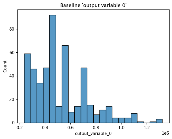
Assay Testing
Now we’ll perform some inferences with a spread of values, then a larger set with a set of larger house values to trigger our assay alert. We’ll use our assay created from the numpy baseline values to demonstrate.
Because our assay windows are 1 minutes, we’ll need to stagger our inference values to be set into the proper windows. This will take about 4 minutes.
# Get a spread of house values
# Set the start for our assay window period.
assay_window_start = datetime.datetime.now()
time.sleep(35)
regular_houses_inputs = pd.read_json('./data/xtest-1k.df.json', orient="records")
inference_size = 1000
regular_houses = regular_houses_inputs.sample(inference_size, replace=True).reset_index(drop=True)
# And a spread of large house values
time.sleep(65)
big_houses_inputs = pd.read_json('./data/biginputs.df.json', orient="records")
big_houses = big_houses_inputs.sample(inference_size, replace=True).reset_index(drop=True)
mainpipeline.infer(big_houses)
# End our assay window period
assay_window_end = datetime.datetime.now()
Assay Configuration
Because we are using a short amount of data, we’ll shorten the window and interval to just 1 minute each, and narrow the window to when we started our set of inferences to when we finish.
assay_builder_from_numpy.add_run_until(assay_window_end)
assay_builder_from_numpy.window_builder().add_width(minutes=1).add_interval(minutes=1).add_start(assay_window_start)
assay_config_from_dates = assay_builder_from_numpy.build()
assay_analysis_from_numpy = assay_config_from_numpy.interactive_run()
# Show how many assay windows were analyzed, then show the chart
print(f"Generated {len(assay_analysis_from_numpy)} analyses")
assay_analysis_from_numpy.chart_scores()
Generated 2 analyses

# Display the results as a DataFrame - we're mainly interested in the score and whether the
# alert threshold was triggered
display(assay_analysis_from_numpy.to_dataframe().loc[:, ["score", "start", "alert_threshold", "status"]])
| score | start | alert_threshold | status | |
|---|---|---|---|---|
| 0 | 0.002769 | 2023-12-12T18:04:26.569377+00:00 | 0.25 | Ok |
| 1 | 8.869974 | 2023-12-12T18:05:26.569377+00:00 | 0.25 | Alert |
Undeploy Main Pipeline
With the examples and tutorial complete, we will undeploy the main pipeline and return the resources back to the Wallaroo instance.
mainpipeline.undeploy()
| name | houseprice-estimation-edge |
|---|---|
| created | 2023-12-12 18:03:28.275490+00:00 |
| last_updated | 2023-12-12 18:03:29.206241+00:00 |
| deployed | False |
| arch | None |
| tags | |
| versions | 66d73202-0c8c-4468-b589-67286a2f5dd6, be11e14c-1565-4d68-8bf5-f9eebd7cd458 |
| steps | housepricesagacontrol |
| published | False |
Edge Deployment
We can now deploy the pipeline to an edge device. This will require the following steps:
- Publish the pipeline: Publishes the pipeline to the OCI registry.
- Add Edge: Add the edge location to the pipeline publish.
- Deploy Edge: Deploy the edge device with the edge location settings.
Publish Pipeline
Publishing the pipeline uses the pipeline publish() command, which returns the OCI registry information.
assay_pub = mainpipeline.publish()
Waiting for pipeline publish... It may take up to 600 sec.
Pipeline is Publishing....Published.
Add Edge
The edge location is added with the publish.add_edge(name) method. This returns the OCI registration information, and the EDGE_BUNDLE information. The EDGE_BUNDLE data is a base64 encoded set of parameters for the pipeline that the edge device is associated with.
display(edge_name)
edge_publish = assay_pub.add_edge(edge_name)
display(edge_publish)
'house-price-edge-jch'
| ID | 3 |
| Pipeline Version | 210d54bf-2788-4e61-be63-31a57738ce15 |
| Status | Published |
| Engine URL | ghcr.io/wallaroolabs/doc-samples/engines/proxy/wallaroo/ghcr.io/wallaroolabs/standalone-mini:v2023.4.0-4103 |
| Pipeline URL | ghcr.io/wallaroolabs/doc-samples/pipelines/houseprice-estimation-edge:210d54bf-2788-4e61-be63-31a57738ce15 |
| Helm Chart URL | oci://ghcr.io/wallaroolabs/doc-samples/charts/houseprice-estimation-edge |
| Helm Chart Reference | ghcr.io/wallaroolabs/doc-samples/charts@sha256:a075005a0aca85006392b49edcb0066f17261f32ace3796e87e2a753d78f42d3 |
| Helm Chart Version | 0.0.1-210d54bf-2788-4e61-be63-31a57738ce15 |
| Engine Config | {'engine': {'resources': {'limits': {'cpu': 4.0, 'memory': '3Gi'}, 'requests': {'cpu': 4.0, 'memory': '3Gi'}}}, 'engineAux': {}, 'enginelb': {'resources': {'limits': {'cpu': 1.0, 'memory': '512Mi'}, 'requests': {'cpu': 0.2, 'memory': '512Mi'}}}} |
| User Images | [] |
| Created By | john.hansarick@wallaroo.ai |
| Created At | 2023-12-12 18:16:53.829858+00:00 |
| Updated At | 2023-12-12 18:16:53.829858+00:00 |
| Docker Run Variables | {'EDGE_BUNDLE': 'abcde'} |
DevOps Deployment
The edge deployment is performed with docker run, docker compose, or helm installations. The following command generates the docker run command, with the following values provided by the DevOps Engineer:
$REGISTRYURL$REGISTRYUSERNAME$REGISTRYPASSWORD
Before deploying, create the ./data directory that is used to store the authentication credentials.
# create docker run
docker_command = f'''
docker run -p 8080:8080 \\
-v ./data:/persist \\
-e DEBUG=true \\
-e OCI_REGISTRY=$REGISTRYURL \\
-e EDGE_BUNDLE={edge_publish.docker_run_variables['EDGE_BUNDLE']} \\
-e CONFIG_CPUS=1 \\
-e OCI_USERNAME=$REGISTRYUSERNAME \\
-e OCI_PASSWORD=$REGISTRYPASSWORD \\
-e PIPELINE_URL={edge_publish.pipeline_url} \\
{edge_publish.engine_url}
'''
print(docker_command)
docker run -p 8080:8080 \
-v ./data:/persist \
-e DEBUG=true \
-e OCI_REGISTRY=$REGISTRYURL \
-e EDGE_BUNDLE=ZXhwb3J0IEJVTkRMRV9WRVJTSU9OPTEKZXhwb3J0IEVER0VfTkFNRT1ob3VzZS1wcmljZS1lZGdlLWpjaApleHBvcnQgSk9JTl9UT0tFTj05MzNjNDIyNy0wZWYxLTQxODQtYTkyZS1lMWFiYzNkM2Y0M2YKZXhwb3J0IE9QU0NFTlRFUl9IT1NUPWRvYy10ZXN0LmVkZ2Uud2FsbGFyb29jb21tdW5pdHkubmluamEKZXhwb3J0IFBJUEVMSU5FX1VSTD1naGNyLmlvL3dhbGxhcm9vbGFicy9kb2Mtc2FtcGxlcy9waXBlbGluZXMvaG91c2VwcmljZS1lc3RpbWF0aW9uLWVkZ2U6MjEwZDU0YmYtMjc4OC00ZTYxLWJlNjMtMzFhNTc3MzhjZTE1CmV4cG9ydCBXT1JLU1BBQ0VfSUQ9MTE= \
-e CONFIG_CPUS=1 \
-e OCI_USERNAME=$REGISTRYUSERNAME \
-e OCI_PASSWORD=$REGISTRYPASSWORD \
-e PIPELINE_URL=ghcr.io/wallaroolabs/doc-samples/pipelines/houseprice-estimation-edge:210d54bf-2788-4e61-be63-31a57738ce15 \
ghcr.io/wallaroolabs/doc-samples/engines/proxy/wallaroo/ghcr.io/wallaroolabs/standalone-mini:v2023.4.0-4103
Verify Logs
Before we perform inferences on the edge deployment, we’ll collect the pipeline logs and display the current partitions. These should only include the Wallaroo Ops pipeline.
logs = mainpipeline.logs(dataset=['time', 'out.variable', 'metadata'])
ops_locations = [pd.unique(logs['metadata.partition']).tolist()][0]
display(ops_locations)
ops_location = ops_locations[0]
Warning: There are more logs available. Please set a larger limit or request a file using export_logs.
['engine-6c9f97965b-pgjrw']
Edge Inferences
We will perform sample inference on our edge location, then verify that the inference results are added to our pipeline logs with the name of our edge location. For these example, the edge location is on the hostname testboy.local.
edge_datetime_start = datetime.datetime.now()
!curl testboy.local:8080/pipelines
{"pipelines":[{"id":"houseprice-estimation-edge","status":"Running"}]}
!curl -X POST testboy.local:8080/pipelines/{main_pipeline_name} \
-H "Content-Type: Content-Type: application/json; format=pandas-records" \
--data @./data/xtest-1k.df.json
[{"time":1702405553622,"in":{"tensor":[4.0,2.5,2900.0,5505.0,2.0,0.0,0.0,3.0,8.0,2900.0,0.0,47.6063,-122.02,2970.0,5251.0,12.0,0.0,0.0]},"out":{"variable":[718013.7]},"check_failures":[],"metadata":{"last_model":"{\"model_name\":\"housepricesagacontrol\",\"model_sha\":\"e22a0831aafd9917f3cc87a15ed267797f80e2afa12ad7d8810ca58f173b8cc6\"}","pipeline_version":"","elapsed":[5708247,1425087],"dropped":[],"partition":"house-price-edge-jch"}},{"time":1702405553622,"in":{"tensor":[2.0,2.5,2170.0,6361.0,1.0,0.0,2.0,3.0,8.0,2170.0,0.0,47.7109,-122.017,2310.0,7419.0,6.0,0.0,0.0]},"out":{"variable":[615094.56]},"check_failures":[],"metadata":{"last_model":"{\"model_name\":\"housepricesagacontrol\",\"model_sha\":\"e22a0831aafd9917f3cc87a15ed267797f80e2afa12ad7d8810ca58f173b8cc6\"}","pipeline_version":"","elapsed":[5708247,1425087],"dropped":[],"partition":"house-price-edge-jch"}},{"time":1702405553622,"in":{"tensor":[3.0,2.5,1300.0,812.0,2.0,0.0,0.0,3.0,8.0,880.0,420.0,47.5893,-122.317,1300.0,824.0,6.0,0.0,0.0]},"out":{"variable":[448627.7]},"check_failures":[],"metadata":{"last_model":"{\"model_name\":\"housepricesagacontrol\",\"model_sha\":\"e22a0831aafd9917f3cc87a15ed267797f80e2afa12ad7d8810ca58f173b8cc6\"}","pipeline_version":"","elapsed":[5708247,1425087],"dropped":[],"partition":"house-price-edge-jch"}},{"time":1702405553622,"in":{"tensor":[4.0,2.5,2500.0,8540.0,2.0,0.0,0.0,3.0,9.0,2500.0,0.0,47.5759,-121.994,2560.0,8475.0,24.0,0.0,0.0]},"out":{"variable":[758714.2]},"check_failures":[],"metadata":{"last_model":"{\"model_name\":\"housepricesagacontrol\",\"model_sha\":\"e22a0831aafd9917f3cc87a15ed267797f80e2afa12ad7d8810ca58f173b8cc6\"}","pipeline_version":"","elapsed":[5708247,1425087],"dropped":[],"partition":"house-price-edge-jch"}},{"time":1702405553622,"in":{"tensor":[3.0,1.75,2200.0,11520.0,1.0,0.0,0.0,4.0,7.0,2200.0,0.0,47.7659,-122.341,1690.0,8038.0,62.0,0.0,0.0]},"out":{"variable":[513264.63]},"check_failures":[],"metadata":{"last_model":"{\"model_name\":\"housepricesagacontrol\",\"model_sha\":\"e22a0831aafd9917f3cc87a15ed267797f80e2afa12ad7d8810ca58f173b8cc6\"}","pipeline_version":"","elapsed":[5708247,1425087],"dropped":[],"partition":"house-price-edge-jch"}},{"time":1702405553622,"in":{"tensor":[3.0,2.0,2140.0,4923.0,1.0,0.0,0.0,4.0,8.0,1070.0,1070.0,47.6902,-122.339,1470.0,4923.0,86.0,0.0,0.0]},"out":{"variable":[668287.94]},"check_failures":[],"metadata":{"last_model":"{\"model_name\":\"housepricesagacontrol\",\"model_sha\":\"e22a0831aafd9917f3cc87a15ed267797f80e2afa12ad7d8810ca58f173b8cc6\"}","pipeline_version":"","elapsed":[5708247,1425087],"dropped":[],"partition":"house-price-edge-jch"}},{"time":1702405553622,"in":{"tensor":[4.0,3.5,3590.0,5334.0,2.0,0.0,2.0,3.0,9.0,3140.0,450.0,47.6763,-122.267,2100.0,6250.0,9.0,0.0,0.0]},"out":{"variable":[1004846.6]},"check_failures":[],"metadata":{"last_model":"{\"model_name\":\"housepricesagacontrol\",\"model_sha\":\"e22a0831aafd9917f3cc87a15ed267797f80e2afa12ad7d8810ca58f173b8cc6\"}","pipeline_version":"","elapsed":[5708247,1425087],"dropped":[],"partition":"house-price-edge-jch"}},{"time":1702405553622,"in":{"tensor":[3.0,2.0,1280.0,960.0,2.0,0.0,0.0,3.0,9.0,1040.0,240.0,47.602,-122.311,1280.0,1173.0,0.0,0.0,0.0]},"out":{"variable":[684577.1]},"check_failures":[],"metadata":{"last_model":"{\"model_name\":\"housepricesagacontrol\",\"model_sha\":\"e22a0831aafd9917f3cc87a15ed267797f80e2afa12ad7d8810ca58f173b8cc6\"}","pipeline_version":"","elapsed":[5708247,1425087],"dropped":[],"partition":"house-price-edge-jch"}},{"time":1702405553622,"in":{"tensor":[4.0,2.5,2820.0,15000.0,2.0,0.0,0.0,4.0,9.0,2820.0,0.0,47.7255,-122.101,2440.0,15000.0,29.0,0.0,0.0]},"out":{"variable":[727898.1]},"check_failures":[],"metadata":{"last_model":"{\"model_name\":\"housepricesagacontrol\",\"model_sha\":\"e22a0831aafd9917f3cc87a15ed267797f80e2afa12ad7d8810ca58f173b8cc6\"}","pipeline_version":"","elapsed":[5708247,1425087],"dropped":[],"partition":"house-price-edge-jch"}},{"time":1702405553622,"in":{"tensor":[3.0,2.25,1790.0,11393.0,1.0,0.0,0.0,3.0,8.0,1790.0,0.0,47.6297,-122.099,2290.0,11894.0,36.0,0.0,0.0]},"out":{"variable":[559631.1]},"check_failures":[],"metadata":{"last_model":"{\"model_name\":\"housepricesagacontrol\",\"model_sha\":\"e22a0831aafd9917f3cc87a15ed267797f80e2afa12ad7d8810ca58f173b8cc6\"}","pipeline_version":"","elapsed":[5708247,1425087],"dropped":[],"partition":"house-price-edge-jch"}},{"time":1702405553622,"in":{"tensor":[3.0,1.5,1010.0,7683.0,1.5,0.0,0.0,5.0,7.0,1010.0,0.0,47.72,-122.318,1550.0,7271.0,61.0,0.0,0.0]},"out":{"variable":[340764.53]},"check_failures":[],"metadata":{"last_model":"{\"model_name\":\"housepricesagacontrol\",\"model_sha\":\"e22a0831aafd9917f3cc87a15ed267797f80e2afa12ad7d8810ca58f173b8cc6\"}","pipeline_version":"","elapsed":[5708247,1425087],"dropped":[],"partition":"house-price-edge-jch"}},{"time":1702405553622,"in":{"tensor":[3.0,2.0,1270.0,1323.0,3.0,0.0,0.0,3.0,8.0,1270.0,0.0,47.6934,-122.342,1330.0,1323.0,8.0,0.0,0.0]},"out":{"variable":[442168.06]},"check_failures":[],"metadata":{"last_model":"{\"model_name\":\"housepricesagacontrol\",\"model_sha\":\"e22a0831aafd9917f3cc87a15ed267797f80e2afa12ad7d8810ca58f173b8cc6\"}","pipeline_version":"","elapsed":[5708247,1425087],"dropped":[],"partition":"house-price-edge-jch"}},{"time":1702405553622,"in":{"tensor":[4.0,1.75,2070.0,9120.0,1.0,0.0,0.0,4.0,7.0,1250.0,820.0,47.6045,-122.123,1650.0,8400.0,57.0,0.0,0.0]},"out":{"variable":[630865.6]},"check_failures":[],"metadata":{"last_model":"{\"model_name\":\"housepricesagacontrol\",\"model_sha\":\"e22a0831aafd9917f3cc87a15ed267797f80e2afa12ad7d8810ca58f173b8cc6\"}","pipeline_version":"","elapsed":[5708247,1425087],"dropped":[],"partition":"house-price-edge-jch"}},{"time":1702405553622,"in":{"tensor":[4.0,1.0,1620.0,4080.0,1.5,0.0,0.0,3.0,7.0,1620.0,0.0,47.6696,-122.324,1760.0,4080.0,91.0,0.0,0.0]},"out":{"variable":[559631.1]},"check_failures":[],"metadata":{"last_model":"{\"model_name\":\"housepricesagacontrol\",\"model_sha\":\"e22a0831aafd9917f3cc87a15ed267797f80e2afa12ad7d8810ca58f173b8cc6\"}","pipeline_version":"","elapsed":[5708247,1425087],"dropped":[],"partition":"house-price-edge-jch"}},{"time":1702405553622,"in":{"tensor":[4.0,3.25,3990.0,9786.0,2.0,0.0,0.0,3.0,9.0,3990.0,0.0,47.6784,-122.026,3920.0,8200.0,10.0,0.0,0.0]},"out":{"variable":[909441.1]},"check_failures":[],"metadata":{"last_model":"{\"model_name\":\"housepricesagacontrol\",\"model_sha\":\"e22a0831aafd9917f3cc87a15ed267797f80e2afa12ad7d8810ca58f173b8cc6\"}","pipeline_version":"","elapsed":[5708247,1425087],"dropped":[],"partition":"house-price-edge-jch"}},{"time":1702405553622,"in":{"tensor":[4.0,2.0,1780.0,19843.0,1.0,0.0,0.0,3.0,7.0,1780.0,0.0,47.4414,-122.154,2210.0,13500.0,52.0,0.0,0.0]},"out":{"variable":[313096.0]},"check_failures":[],"metadata":{"last_model":"{\"model_name\":\"housepricesagacontrol\",\"model_sha\":\"e22a0831aafd9917f3cc87a15ed267797f80e2afa12ad7d8810ca58f173b8cc6\"}","pipeline_version":"","elapsed":[5708247,1425087],"dropped":[],"partition":"house-price-edge-jch"}},{"time":1702405553622,"in":{"tensor":[4.0,2.5,2130.0,6003.0,2.0,0.0,0.0,3.0,8.0,2130.0,0.0,47.4518,-122.12,1940.0,4529.0,11.0,0.0,0.0]},"out":{"variable":[404040.8]},"check_failures":[],"metadata":{"last_model":"{\"model_name\":\"housepricesagacontrol\",\"model_sha\":\"e22a0831aafd9917f3cc87a15ed267797f80e2afa12ad7d8810ca58f173b8cc6\"}","pipeline_version":"","elapsed":[5708247,1425087],"dropped":[],"partition":"house-price-edge-jch"}},{"time":1702405553622,"in":{"tensor":[3.0,1.75,1660.0,10440.0,1.0,0.0,0.0,3.0,7.0,1040.0,620.0,47.4448,-121.77,1240.0,10380.0,36.0,0.0,0.0]},"out":{"variable":[292859.5]},"check_failures":[],"metadata":{"last_model":"{\"model_name\":\"housepricesagacontrol\",\"model_sha\":\"e22a0831aafd9917f3cc87a15ed267797f80e2afa12ad7d8810ca58f173b8cc6\"}","pipeline_version":"","elapsed":[5708247,1425087],"dropped":[],"partition":"house-price-edge-jch"}},{"time":1702405553622,"in":{"tensor":[3.0,2.5,2110.0,4118.0,2.0,0.0,0.0,3.0,8.0,2110.0,0.0,47.3878,-122.153,2110.0,4044.0,25.0,0.0,0.0]},"out":{"variable":[338357.88]},"check_failures":[],"metadata":{"last_model":"{\"model_name\":\"housepricesagacontrol\",\"model_sha\":\"e22a0831aafd9917f3cc87a15ed267797f80e2afa12ad7d8810ca58f173b8cc6\"}","pipeline_version":"","elapsed":[5708247,1425087],"dropped":[],"partition":"house-price-edge-jch"}},{"time":1702405553622,"in":{"tensor":[4.0,2.25,2200.0,11250.0,1.5,0.0,0.0,5.0,7.0,1300.0,900.0,47.6845,-122.201,2320.0,10814.0,94.0,0.0,0.0]},"out":{"variable":[682284.5]},"check_failures":[],"metadata":{"last_model":"{\"model_name\":\"housepricesagacontrol\",\"model_sha\":\"e22a0831aafd9917f3cc87a15ed267797f80e2afa12ad7d8810ca58f173b8cc6\"}","pipeline_version":"","elapsed":[5708247,1425087],"dropped":[],"partition":"house-price-edge-jch"}},{"time":1702405553622,"in":{"tensor":[4.0,2.25,2020.0,10260.0,2.0,0.0,0.0,4.0,7.0,2020.0,0.0,47.6801,-122.114,2020.0,10311.0,31.0,0.0,0.0]},"out":{"variable":[583765.94]},"check_failures":[],"metadata":{"last_model":"{\"model_name\":\"housepricesagacontrol\",\"model_sha\":\"e22a0831aafd9917f3cc87a15ed267797f80e2afa12ad7d8810ca58f173b8cc6\"}","pipeline_version":"","elapsed":[5708247,1425087],"dropped":[],"partition":"house-price-edge-jch"}},{"time":1702405553622,"in":{"tensor":[2.0,2.0,1390.0,1302.0,2.0,0.0,0.0,3.0,7.0,1390.0,0.0,47.3089,-122.33,1390.0,1302.0,28.0,0.0,0.0]},"out":{"variable":[249227.78]},"check_failures":[],"metadata":{"last_model":"{\"model_name\":\"housepricesagacontrol\",\"model_sha\":\"e22a0831aafd9917f3cc87a15ed267797f80e2afa12ad7d8810ca58f173b8cc6\"}","pipeline_version":"","elapsed":[5708247,1425087],"dropped":[],"partition":"house-price-edge-jch"}},{"time":1702405553622,"in":{"tensor":[4.0,1.75,1400.0,7920.0,1.0,0.0,0.0,3.0,7.0,1400.0,0.0,47.4658,-122.184,1910.0,7700.0,52.0,0.0,0.0]},"out":{"variable":[267013.97]},"check_failures":[],"metadata":{"last_model":"{\"model_name\":\"housepricesagacontrol\",\"model_sha\":\"e22a0831aafd9917f3cc87a15ed267797f80e2afa12ad7d8810ca58f173b8cc6\"}","pipeline_version":"","elapsed":[5708247,1425087],"dropped":[],"partition":"house-price-edge-jch"}},{"time":1702405553622,"in":{"tensor":[2.0,2.5,1370.0,1140.0,2.0,0.0,0.0,3.0,8.0,1080.0,290.0,47.7055,-122.342,1340.0,1050.0,5.0,0.0,0.0]},"out":{"variable":[342604.44]},"check_failures":[],"metadata":{"last_model":"{\"model_name\":\"housepricesagacontrol\",\"model_sha\":\"e22a0831aafd9917f3cc87a15ed267797f80e2afa12ad7d8810ca58f173b8cc6\"}","pipeline_version":"","elapsed":[5708247,1425087],"dropped":[],"partition":"house-price-edge-jch"}},{"time":1702405553622,"in":{"tensor":[4.0,2.5,2390.0,6976.0,2.0,0.0,0.0,3.0,7.0,2390.0,0.0,47.4807,-122.182,2390.0,6346.0,11.0,0.0,0.0]},"out":{"variable":[410291.75]},"check_failures":[],"metadata":{"last_model":"{\"model_name\":\"housepricesagacontrol\",\"model_sha\":\"e22a0831aafd9917f3cc87a15ed267797f80e2afa12ad7d8810ca58f173b8cc6\"}","pipeline_version":"","elapsed":[5708247,1425087],"dropped":[],"partition":"house-price-edge-jch"}},{"time":1702405553622,"in":{"tensor":[5.0,3.0,2170.0,2440.0,1.5,0.0,0.0,4.0,8.0,1450.0,720.0,47.6724,-122.317,2070.0,4000.0,103.0,0.0,0.0]},"out":{"variable":[675545.4]},"check_failures":[],"metadata":{"last_model":"{\"model_name\":\"housepricesagacontrol\",\"model_sha\":\"e22a0831aafd9917f3cc87a15ed267797f80e2afa12ad7d8810ca58f173b8cc6\"}","pipeline_version":"","elapsed":[5708247,1425087],"dropped":[],"partition":"house-price-edge-jch"}},{"time":1702405553622,"in":{"tensor":[2.0,1.0,1370.0,9460.0,1.0,0.0,0.0,3.0,6.0,1370.0,0.0,47.6238,-122.191,1690.0,9930.0,65.0,0.0,0.0]},"out":{"variable":[449699.75]},"check_failures":[],"metadata":{"last_model":"{\"model_name\":\"housepricesagacontrol\",\"model_sha\":\"e22a0831aafd9917f3cc87a15ed267797f80e2afa12ad7d8810ca58f173b8cc6\"}","pipeline_version":"","elapsed":[5708247,1425087],"dropped":[],"partition":"house-price-edge-jch"}},{"time":1702405553622,"in":{"tensor":[4.0,2.5,2270.0,5000.0,2.0,0.0,0.0,3.0,9.0,2270.0,0.0,47.6916,-122.37,1210.0,5000.0,0.0,0.0,0.0]},"out":{"variable":[756046.0]},"check_failures":[],"metadata":{"last_model":"{\"model_name\":\"housepricesagacontrol\",\"model_sha\":\"e22a0831aafd9917f3cc87a15ed267797f80e2afa12ad7d8810ca58f173b8cc6\"}","pipeline_version":"","elapsed":[5708247,1425087],"dropped":[],"partition":"house-price-edge-jch"}},{"time":1702405553622,"in":{"tensor":[3.0,3.0,1330.0,1379.0,2.0,0.0,0.0,4.0,8.0,1120.0,210.0,47.6126,-122.313,1810.0,1770.0,9.0,0.0,0.0]},"out":{"variable":[450867.56]},"check_failures":[],"metadata":{"last_model":"{\"model_name\":\"housepricesagacontrol\",\"model_sha\":\"e22a0831aafd9917f3cc87a15ed267797f80e2afa12ad7d8810ca58f173b8cc6\"}","pipeline_version":"","elapsed":[5708247,1425087],"dropped":[],"partition":"house-price-edge-jch"}},{"time":1702405553622,"in":{"tensor":[5.0,1.75,2490.0,24969.0,1.0,0.0,2.0,4.0,8.0,1540.0,950.0,47.336,-122.35,2790.0,15600.0,55.0,0.0,0.0]},"out":{"variable":[392724.16]},"check_failures":[],"metadata":{"last_model":"{\"model_name\":\"housepricesagacontrol\",\"model_sha\":\"e22a0831aafd9917f3cc87a15ed267797f80e2afa12ad7d8810ca58f173b8cc6\"}","pipeline_version":"","elapsed":[5708247,1425087],"dropped":[],"partition":"house-price-edge-jch"}},{"time":1702405553622,"in":{"tensor":[4.0,3.0,3710.0,20000.0,2.0,0.0,2.0,5.0,10.0,2760.0,950.0,47.6696,-122.261,3970.0,20000.0,79.0,0.0,0.0]},"out":{"variable":[1514079.6]},"check_failures":[],"metadata":{"last_model":"{\"model_name\":\"housepricesagacontrol\",\"model_sha\":\"e22a0831aafd9917f3cc87a15ed267797f80e2afa12ad7d8810ca58f173b8cc6\"}","pipeline_version":"","elapsed":[5708247,1425087],"dropped":[],"partition":"house-price-edge-jch"}},{"time":1702405553622,"in":{"tensor":[3.0,2.25,2800.0,17300.0,1.0,0.0,0.0,4.0,8.0,1420.0,1380.0,47.5716,-122.128,2140.0,12650.0,44.0,0.0,0.0]},"out":{"variable":[706407.25]},"check_failures":[],"metadata":{"last_model":"{\"model_name\":\"housepricesagacontrol\",\"model_sha\":\"e22a0831aafd9917f3cc87a15ed267797f80e2afa12ad7d8810ca58f173b8cc6\"}","pipeline_version":"","elapsed":[5708247,1425087],"dropped":[],"partition":"house-price-edge-jch"}},{"time":1702405553622,"in":{"tensor":[3.0,1.75,1790.0,50529.0,1.0,0.0,0.0,5.0,7.0,1090.0,700.0,47.3511,-122.073,1940.0,50529.0,50.0,0.0,0.0]},"out":{"variable":[291904.0]},"check_failures":[],"metadata":{"last_model":"{\"model_name\":\"housepricesagacontrol\",\"model_sha\":\"e22a0831aafd9917f3cc87a15ed267797f80e2afa12ad7d8810ca58f173b8cc6\"}","pipeline_version":"","elapsed":[5708247,1425087],"dropped":[],"partition":"house-price-edge-jch"}},{"time":1702405553622,"in":{"tensor":[3.0,1.5,1340.0,11744.0,1.0,0.0,0.0,2.0,7.0,1340.0,0.0,47.4947,-122.36,2020.0,13673.0,64.0,0.0,0.0]},"out":{"variable":[259657.52]},"check_failures":[],"metadata":{"last_model":"{\"model_name\":\"housepricesagacontrol\",\"model_sha\":\"e22a0831aafd9917f3cc87a15ed267797f80e2afa12ad7d8810ca58f173b8cc6\"}","pipeline_version":"","elapsed":[5708247,1425087],"dropped":[],"partition":"house-price-edge-jch"}},{"time":1702405553622,"in":{"tensor":[3.0,2.5,2110.0,7434.0,2.0,0.0,0.0,4.0,7.0,2110.0,0.0,47.3935,-122.169,2100.0,7749.0,36.0,0.0,0.0]},"out":{"variable":[335398.94]},"check_failures":[],"metadata":{"last_model":"{\"model_name\":\"housepricesagacontrol\",\"model_sha\":\"e22a0831aafd9917f3cc87a15ed267797f80e2afa12ad7d8810ca58f173b8cc6\"}","pipeline_version":"","elapsed":[5708247,1425087],"dropped":[],"partition":"house-price-edge-jch"}},{"time":1702405553622,"in":{"tensor":[4.0,2.5,2440.0,3600.0,2.5,0.0,0.0,4.0,8.0,2440.0,0.0,47.6298,-122.362,2440.0,5440.0,112.0,0.0,0.0]},"out":{"variable":[713978.94]},"check_failures":[],"metadata":{"last_model":"{\"model_name\":\"housepricesagacontrol\",\"model_sha\":\"e22a0831aafd9917f3cc87a15ed267797f80e2afa12ad7d8810ca58f173b8cc6\"}","pipeline_version":"","elapsed":[5708247,1425087],"dropped":[],"partition":"house-price-edge-jch"}},{"time":1702405553622,"in":{"tensor":[4.0,2.75,2100.0,11894.0,1.0,0.0,0.0,4.0,8.0,1720.0,380.0,47.6006,-122.194,2390.0,9450.0,46.0,0.0,0.0]},"out":{"variable":[642519.75]},"check_failures":[],"metadata":{"last_model":"{\"model_name\":\"housepricesagacontrol\",\"model_sha\":\"e22a0831aafd9917f3cc87a15ed267797f80e2afa12ad7d8810ca58f173b8cc6\"}","pipeline_version":"","elapsed":[5708247,1425087],"dropped":[],"partition":"house-price-edge-jch"}},{"time":1702405553622,"in":{"tensor":[3.0,2.25,1280.0,959.0,3.0,0.0,0.0,3.0,8.0,1280.0,0.0,47.6914,-122.343,1130.0,1126.0,9.0,0.0,0.0]},"out":{"variable":[446768.88]},"check_failures":[],"metadata":{"last_model":"{\"model_name\":\"housepricesagacontrol\",\"model_sha\":\"e22a0831aafd9917f3cc87a15ed267797f80e2afa12ad7d8810ca58f173b8cc6\"}","pipeline_version":"","elapsed":[5708247,1425087],"dropped":[],"partition":"house-price-edge-jch"}},{"time":1702405553622,"in":{"tensor":[3.0,1.5,1740.0,9038.0,1.0,0.0,0.0,4.0,7.0,1740.0,0.0,47.5897,-122.136,1390.0,9770.0,59.0,0.0,0.0]},"out":{"variable":[557391.25]},"check_failures":[],"metadata":{"last_model":"{\"model_name\":\"housepricesagacontrol\",\"model_sha\":\"e22a0831aafd9917f3cc87a15ed267797f80e2afa12ad7d8810ca58f173b8cc6\"}","pipeline_version":"","elapsed":[5708247,1425087],"dropped":[],"partition":"house-price-edge-jch"}},{"time":1702405553622,"in":{"tensor":[2.0,2.5,1860.0,3504.0,2.0,0.0,0.0,3.0,7.0,1860.0,0.0,47.776,-122.239,1860.0,4246.0,14.0,0.0,0.0]},"out":{"variable":[438514.2]},"check_failures":[],"metadata":{"last_model":"{\"model_name\":\"housepricesagacontrol\",\"model_sha\":\"e22a0831aafd9917f3cc87a15ed267797f80e2afa12ad7d8810ca58f173b8cc6\"}","pipeline_version":"","elapsed":[5708247,1425087],"dropped":[],"partition":"house-price-edge-jch"}},{"time":1702405553622,"in":{"tensor":[4.0,4.5,5120.0,41327.0,2.0,0.0,0.0,3.0,10.0,3290.0,1830.0,47.7009,-122.059,3360.0,82764.0,6.0,0.0,0.0]},"out":{"variable":[1204324.9]},"check_failures":[],"metadata":{"last_model":"{\"model_name\":\"housepricesagacontrol\",\"model_sha\":\"e22a0831aafd9917f3cc87a15ed267797f80e2afa12ad7d8810ca58f173b8cc6\"}","pipeline_version":"","elapsed":[5708247,1425087],"dropped":[],"partition":"house-price-edge-jch"}},{"time":1702405553622,"in":{"tensor":[2.0,1.0,670.0,11505.0,1.0,0.0,0.0,3.0,5.0,670.0,0.0,47.499,-122.157,2180.0,11505.0,12.0,0.0,0.0]},"out":{"variable":[251194.61]},"check_failures":[],"metadata":{"last_model":"{\"model_name\":\"housepricesagacontrol\",\"model_sha\":\"e22a0831aafd9917f3cc87a15ed267797f80e2afa12ad7d8810ca58f173b8cc6\"}","pipeline_version":"","elapsed":[5708247,1425087],"dropped":[],"partition":"house-price-edge-jch"}},{"time":1702405553622,"in":{"tensor":[3.0,2.5,2370.0,4200.0,2.0,0.0,0.0,3.0,8.0,2370.0,0.0,47.3699,-122.019,2370.0,4370.0,1.0,0.0,0.0]},"out":{"variable":[349102.75]},"check_failures":[],"metadata":{"last_model":"{\"model_name\":\"housepricesagacontrol\",\"model_sha\":\"e22a0831aafd9917f3cc87a15ed267797f80e2afa12ad7d8810ca58f173b8cc6\"}","pipeline_version":"","elapsed":[5708247,1425087],"dropped":[],"partition":"house-price-edge-jch"}},{"time":1702405553622,"in":{"tensor":[5.0,2.75,2580.0,7865.0,1.0,0.0,0.0,4.0,8.0,1480.0,1100.0,47.6208,-122.139,2140.0,8400.0,51.0,0.0,0.0]},"out":{"variable":[701940.6]},"check_failures":[],"metadata":{"last_model":"{\"model_name\":\"housepricesagacontrol\",\"model_sha\":\"e22a0831aafd9917f3cc87a15ed267797f80e2afa12ad7d8810ca58f173b8cc6\"}","pipeline_version":"","elapsed":[5708247,1425087],"dropped":[],"partition":"house-price-edge-jch"}},{"time":1702405553622,"in":{"tensor":[3.0,2.25,998.0,904.0,2.0,0.0,0.0,3.0,7.0,798.0,200.0,47.6983,-122.367,998.0,1110.0,7.0,0.0,0.0]},"out":{"variable":[400561.06]},"check_failures":[],"metadata":{"last_model":"{\"model_name\":\"housepricesagacontrol\",\"model_sha\":\"e22a0831aafd9917f3cc87a15ed267797f80e2afa12ad7d8810ca58f173b8cc6\"}","pipeline_version":"","elapsed":[5708247,1425087],"dropped":[],"partition":"house-price-edge-jch"}},{"time":1702405553622,"in":{"tensor":[4.0,2.5,2930.0,7806.0,2.0,0.0,0.0,3.0,9.0,2930.0,0.0,47.6219,-122.024,2600.0,6051.0,9.0,0.0,0.0]},"out":{"variable":[779809.94]},"check_failures":[],"metadata":{"last_model":"{\"model_name\":\"housepricesagacontrol\",\"model_sha\":\"e22a0831aafd9917f3cc87a15ed267797f80e2afa12ad7d8810ca58f173b8cc6\"}","pipeline_version":"","elapsed":[5708247,1425087],"dropped":[],"partition":"house-price-edge-jch"}},{"time":1702405553622,"in":{"tensor":[3.0,1.75,1120.0,4000.0,1.0,0.0,0.0,4.0,7.0,870.0,250.0,47.6684,-122.368,1470.0,4000.0,98.0,0.0,0.0]},"out":{"variable":[448627.7]},"check_failures":[],"metadata":{"last_model":"{\"model_name\":\"housepricesagacontrol\",\"model_sha\":\"e22a0831aafd9917f3cc87a15ed267797f80e2afa12ad7d8810ca58f173b8cc6\"}","pipeline_version":"","elapsed":[5708247,1425087],"dropped":[],"partition":"house-price-edge-jch"}},{"time":1702405553622,"in":{"tensor":[4.0,1.0,2000.0,4800.0,2.0,0.0,0.0,4.0,7.0,2000.0,0.0,47.6583,-122.351,1260.0,1452.0,104.0,0.0,0.0]},"out":{"variable":[581002.94]},"check_failures":[],"metadata":{"last_model":"{\"model_name\":\"housepricesagacontrol\",\"model_sha\":\"e22a0831aafd9917f3cc87a15ed267797f80e2afa12ad7d8810ca58f173b8cc6\"}","pipeline_version":"","elapsed":[5708247,1425087],"dropped":[],"partition":"house-price-edge-jch"}},{"time":1702405553622,"in":{"tensor":[4.0,2.5,1520.0,3370.0,2.0,0.0,0.0,3.0,8.0,1520.0,0.0,47.5696,-122.004,1860.0,4486.0,21.0,0.0,0.0]},"out":{"variable":[535229.2]},"check_failures":[],"metadata":{"last_model":"{\"model_name\":\"housepricesagacontrol\",\"model_sha\":\"e22a0831aafd9917f3cc87a15ed267797f80e2afa12ad7d8810ca58f173b8cc6\"}","pipeline_version":"","elapsed":[5708247,1425087],"dropped":[],"partition":"house-price-edge-jch"}},{"time":1702405553622,"in":{"tensor":[4.0,2.5,2920.0,9904.0,2.0,0.0,0.0,4.0,9.0,2920.0,0.0,47.5759,-121.995,1810.0,5617.0,24.0,0.0,0.0]},"out":{"variable":[778197.5]},"check_failures":[],"metadata":{"last_model":"{\"model_name\":\"housepricesagacontrol\",\"model_sha\":\"e22a0831aafd9917f3cc87a15ed267797f80e2afa12ad7d8810ca58f173b8cc6\"}","pipeline_version":"","elapsed":[5708247,1425087],"dropped":[],"partition":"house-price-edge-jch"}},{"time":1702405553622,"in":{"tensor":[3.0,2.0,1850.0,8208.0,1.0,0.0,0.0,4.0,7.0,1180.0,670.0,47.3109,-122.362,1790.0,8174.0,44.0,0.0,0.0]},"out":{"variable":[291261.94]},"check_failures":[],"metadata":{"last_model":"{\"model_name\":\"housepricesagacontrol\",\"model_sha\":\"e22a0831aafd9917f3cc87a15ed267797f80e2afa12ad7d8810ca58f173b8cc6\"}","pipeline_version":"","elapsed":[5708247,1425087],"dropped":[],"partition":"house-price-edge-jch"}},{"time":1702405553622,"in":{"tensor":[4.0,2.5,3430.0,35120.0,2.0,0.0,0.0,3.0,10.0,3430.0,0.0,47.6484,-122.182,3920.0,35230.0,31.0,0.0,0.0]},"out":{"variable":[950176.56]},"check_failures":[],"metadata":{"last_model":"{\"model_name\":\"housepricesagacontrol\",\"model_sha\":\"e22a0831aafd9917f3cc87a15ed267797f80e2afa12ad7d8810ca58f173b8cc6\"}","pipeline_version":"","elapsed":[5708247,1425087],"dropped":[],"partition":"house-price-edge-jch"}},{"time":1702405553622,"in":{"tensor":[4.0,2.0,1530.0,6375.0,2.0,0.0,0.0,3.0,7.0,1530.0,0.0,47.4692,-122.162,1500.0,8712.0,72.0,1.0,41.0]},"out":{"variable":[289359.53]},"check_failures":[],"metadata":{"last_model":"{\"model_name\":\"housepricesagacontrol\",\"model_sha\":\"e22a0831aafd9917f3cc87a15ed267797f80e2afa12ad7d8810ca58f173b8cc6\"}","pipeline_version":"","elapsed":[5708247,1425087],"dropped":[],"partition":"house-price-edge-jch"}},{"time":1702405553622,"in":{"tensor":[3.0,2.25,1640.0,8400.0,1.0,0.0,0.0,3.0,8.0,1180.0,460.0,47.3733,-122.289,1600.0,8120.0,46.0,0.0,0.0]},"out":{"variable":[277145.72]},"check_failures":[],"metadata":{"last_model":"{\"model_name\":\"housepricesagacontrol\",\"model_sha\":\"e22a0831aafd9917f3cc87a15ed267797f80e2afa12ad7d8810ca58f173b8cc6\"}","pipeline_version":"","elapsed":[5708247,1425087],"dropped":[],"partition":"house-price-edge-jch"}},{"time":1702405553622,"in":{"tensor":[3.0,2.0,1540.0,8400.0,1.0,0.0,0.0,3.0,7.0,1180.0,360.0,47.6554,-122.129,1550.0,8760.0,46.0,0.0,0.0]},"out":{"variable":[552992.06]},"check_failures":[],"metadata":{"last_model":"{\"model_name\":\"housepricesagacontrol\",\"model_sha\":\"e22a0831aafd9917f3cc87a15ed267797f80e2afa12ad7d8810ca58f173b8cc6\"}","pipeline_version":"","elapsed":[5708247,1425087],"dropped":[],"partition":"house-price-edge-jch"}},{"time":1702405553622,"in":{"tensor":[4.0,2.5,1850.0,8310.0,1.0,0.0,0.0,3.0,7.0,1200.0,650.0,47.7717,-122.29,1840.0,10080.0,53.0,0.0,0.0]},"out":{"variable":[437753.3]},"check_failures":[],"metadata":{"last_model":"{\"model_name\":\"housepricesagacontrol\",\"model_sha\":\"e22a0831aafd9917f3cc87a15ed267797f80e2afa12ad7d8810ca58f173b8cc6\"}","pipeline_version":"","elapsed":[5708247,1425087],"dropped":[],"partition":"house-price-edge-jch"}},{"time":1702405553622,"in":{"tensor":[3.0,1.75,1530.0,7245.0,1.0,0.0,0.0,4.0,7.0,1530.0,0.0,47.731,-122.191,1530.0,7490.0,31.0,0.0,0.0]},"out":{"variable":[431929.03]},"check_failures":[],"metadata":{"last_model":"{\"model_name\":\"housepricesagacontrol\",\"model_sha\":\"e22a0831aafd9917f3cc87a15ed267797f80e2afa12ad7d8810ca58f173b8cc6\"}","pipeline_version":"","elapsed":[5708247,1425087],"dropped":[],"partition":"house-price-edge-jch"}},{"time":1702405553622,"in":{"tensor":[4.0,2.5,2610.0,5866.0,2.0,0.0,0.0,3.0,8.0,2610.0,0.0,47.3441,-122.04,2480.0,5188.0,9.0,0.0,0.0]},"out":{"variable":[358668.13]},"check_failures":[],"metadata":{"last_model":"{\"model_name\":\"housepricesagacontrol\",\"model_sha\":\"e22a0831aafd9917f3cc87a15ed267797f80e2afa12ad7d8810ca58f173b8cc6\"}","pipeline_version":"","elapsed":[5708247,1425087],"dropped":[],"partition":"house-price-edge-jch"}},{"time":1702405553622,"in":{"tensor":[4.0,2.5,1710.0,5000.0,1.0,0.0,0.0,3.0,8.0,1110.0,600.0,47.6772,-122.285,1750.0,5304.0,36.0,0.0,0.0]},"out":{"variable":[559631.1]},"check_failures":[],"metadata":{"last_model":"{\"model_name\":\"housepricesagacontrol\",\"model_sha\":\"e22a0831aafd9917f3cc87a15ed267797f80e2afa12ad7d8810ca58f173b8cc6\"}","pipeline_version":"","elapsed":[5708247,1425087],"dropped":[],"partition":"house-price-edge-jch"}},{"time":1702405553622,"in":{"tensor":[5.0,2.5,3470.0,12003.0,2.0,0.0,0.0,3.0,8.0,3470.0,0.0,47.624,-122.048,2220.0,12283.0,37.0,0.0,0.0]},"out":{"variable":[732736.0]},"check_failures":[],"metadata":{"last_model":"{\"model_name\":\"housepricesagacontrol\",\"model_sha\":\"e22a0831aafd9917f3cc87a15ed267797f80e2afa12ad7d8810ca58f173b8cc6\"}","pipeline_version":"","elapsed":[5708247,1425087],"dropped":[],"partition":"house-price-edge-jch"}},{"time":1702405553622,"in":{"tensor":[3.0,2.0,1020.0,1204.0,2.0,0.0,0.0,3.0,7.0,720.0,300.0,47.5445,-122.376,1360.0,1506.0,10.0,0.0,0.0]},"out":{"variable":[435628.56]},"check_failures":[],"metadata":{"last_model":"{\"model_name\":\"housepricesagacontrol\",\"model_sha\":\"e22a0831aafd9917f3cc87a15ed267797f80e2afa12ad7d8810ca58f173b8cc6\"}","pipeline_version":"","elapsed":[5708247,1425087],"dropped":[],"partition":"house-price-edge-jch"}},{"time":1702405553622,"in":{"tensor":[3.0,2.75,2870.0,6600.0,2.0,0.0,2.0,3.0,8.0,2870.0,0.0,47.5745,-122.113,2570.0,7925.0,30.0,0.0,0.0]},"out":{"variable":[710023.7]},"check_failures":[],"metadata":{"last_model":"{\"model_name\":\"housepricesagacontrol\",\"model_sha\":\"e22a0831aafd9917f3cc87a15ed267797f80e2afa12ad7d8810ca58f173b8cc6\"}","pipeline_version":"","elapsed":[5708247,1425087],"dropped":[],"partition":"house-price-edge-jch"}},{"time":1702405553622,"in":{"tensor":[2.0,2.0,1440.0,4666.0,1.0,0.0,0.0,3.0,8.0,1440.0,0.0,47.709,-122.019,1510.0,4595.0,5.0,0.0,0.0]},"out":{"variable":[359614.63]},"check_failures":[],"metadata":{"last_model":"{\"model_name\":\"housepricesagacontrol\",\"model_sha\":\"e22a0831aafd9917f3cc87a15ed267797f80e2afa12ad7d8810ca58f173b8cc6\"}","pipeline_version":"","elapsed":[5708247,1425087],"dropped":[],"partition":"house-price-edge-jch"}},{"time":1702405553622,"in":{"tensor":[4.0,3.0,4040.0,19700.0,2.0,0.0,0.0,3.0,11.0,4040.0,0.0,47.7205,-122.127,3930.0,21887.0,27.0,0.0,0.0]},"out":{"variable":[1028923.06]},"check_failures":[],"metadata":{"last_model":"{\"model_name\":\"housepricesagacontrol\",\"model_sha\":\"e22a0831aafd9917f3cc87a15ed267797f80e2afa12ad7d8810ca58f173b8cc6\"}","pipeline_version":"","elapsed":[5708247,1425087],"dropped":[],"partition":"house-price-edge-jch"}},{"time":1702405553622,"in":{"tensor":[6.0,4.5,3300.0,7480.0,2.0,0.0,0.0,3.0,8.0,3300.0,0.0,47.6796,-122.104,2470.0,7561.0,34.0,0.0,0.0]},"out":{"variable":[725572.5]},"check_failures":[],"metadata":{"last_model":"{\"model_name\":\"housepricesagacontrol\",\"model_sha\":\"e22a0831aafd9917f3cc87a15ed267797f80e2afa12ad7d8810ca58f173b8cc6\"}","pipeline_version":"","elapsed":[5708247,1425087],"dropped":[],"partition":"house-price-edge-jch"}},{"time":1702405553622,"in":{"tensor":[3.0,1.5,1670.0,3852.0,2.0,0.0,3.0,4.0,8.0,1670.0,0.0,47.6411,-122.371,2320.0,4572.0,87.0,0.0,0.0]},"out":{"variable":[559631.1]},"check_failures":[],"metadata":{"last_model":"{\"model_name\":\"housepricesagacontrol\",\"model_sha\":\"e22a0831aafd9917f3cc87a15ed267797f80e2afa12ad7d8810ca58f173b8cc6\"}","pipeline_version":"","elapsed":[5708247,1425087],"dropped":[],"partition":"house-price-edge-jch"}},{"time":1702405553622,"in":{"tensor":[4.0,2.5,1700.0,6031.0,2.0,0.0,0.0,3.0,8.0,1700.0,0.0,47.3582,-122.191,1930.0,6035.0,20.0,0.0,0.0]},"out":{"variable":[290323.1]},"check_failures":[],"metadata":{"last_model":"{\"model_name\":\"housepricesagacontrol\",\"model_sha\":\"e22a0831aafd9917f3cc87a15ed267797f80e2afa12ad7d8810ca58f173b8cc6\"}","pipeline_version":"","elapsed":[5708247,1425087],"dropped":[],"partition":"house-price-edge-jch"}},{"time":1702405553622,"in":{"tensor":[4.0,2.5,3220.0,7873.0,2.0,0.0,0.0,3.0,10.0,3220.0,0.0,47.5849,-122.03,2610.0,8023.0,21.0,0.0,0.0]},"out":{"variable":[886958.5]},"check_failures":[],"metadata":{"last_model":"{\"model_name\":\"housepricesagacontrol\",\"model_sha\":\"e22a0831aafd9917f3cc87a15ed267797f80e2afa12ad7d8810ca58f173b8cc6\"}","pipeline_version":"","elapsed":[5708247,1425087],"dropped":[],"partition":"house-price-edge-jch"}},{"time":1702405553622,"in":{"tensor":[5.0,3.25,3030.0,20446.0,2.0,0.0,2.0,3.0,9.0,2130.0,900.0,47.6133,-122.106,2890.0,20908.0,38.0,0.0,0.0]},"out":{"variable":[811666.5]},"check_failures":[],"metadata":{"last_model":"{\"model_name\":\"housepricesagacontrol\",\"model_sha\":\"e22a0831aafd9917f3cc87a15ed267797f80e2afa12ad7d8810ca58f173b8cc6\"}","pipeline_version":"","elapsed":[5708247,1425087],"dropped":[],"partition":"house-price-edge-jch"}},{"time":1702405553622,"in":{"tensor":[3.0,1.75,1050.0,9871.0,1.0,0.0,0.0,5.0,7.0,1050.0,0.0,47.3816,-122.087,1300.0,10794.0,46.0,0.0,0.0]},"out":{"variable":[236238.66]},"check_failures":[],"metadata":{"last_model":"{\"model_name\":\"housepricesagacontrol\",\"model_sha\":\"e22a0831aafd9917f3cc87a15ed267797f80e2afa12ad7d8810ca58f173b8cc6\"}","pipeline_version":"","elapsed":[5708247,1425087],"dropped":[],"partition":"house-price-edge-jch"}},{"time":1702405553622,"in":{"tensor":[3.0,1.5,2230.0,6000.0,1.0,0.0,1.0,3.0,8.0,1260.0,970.0,47.5373,-122.395,2120.0,7200.0,47.0,0.0,0.0]},"out":{"variable":[683845.6]},"check_failures":[],"metadata":{"last_model":"{\"model_name\":\"housepricesagacontrol\",\"model_sha\":\"e22a0831aafd9917f3cc87a15ed267797f80e2afa12ad7d8810ca58f173b8cc6\"}","pipeline_version":"","elapsed":[5708247,1425087],"dropped":[],"partition":"house-price-edge-jch"}},{"time":1702405553622,"in":{"tensor":[4.0,2.5,2710.0,6474.0,2.0,0.0,0.0,3.0,8.0,2710.0,0.0,47.5383,-121.878,2870.0,6968.0,11.0,0.0,0.0]},"out":{"variable":[717470.06]},"check_failures":[],"metadata":{"last_model":"{\"model_name\":\"housepricesagacontrol\",\"model_sha\":\"e22a0831aafd9917f3cc87a15ed267797f80e2afa12ad7d8810ca58f173b8cc6\"}","pipeline_version":"","elapsed":[5708247,1425087],"dropped":[],"partition":"house-price-edge-jch"}},{"time":1702405553622,"in":{"tensor":[4.0,2.5,3490.0,18521.0,2.0,0.0,0.0,4.0,9.0,3490.0,0.0,47.7406,-122.07,2850.0,18521.0,24.0,0.0,0.0]},"out":{"variable":[873314.94]},"check_failures":[],"metadata":{"last_model":"{\"model_name\":\"housepricesagacontrol\",\"model_sha\":\"e22a0831aafd9917f3cc87a15ed267797f80e2afa12ad7d8810ca58f173b8cc6\"}","pipeline_version":"","elapsed":[5708247,1425087],"dropped":[],"partition":"house-price-edge-jch"}},{"time":1702405553622,"in":{"tensor":[2.0,1.0,720.0,5820.0,1.0,0.0,1.0,5.0,6.0,720.0,0.0,47.7598,-122.255,952.0,5820.0,65.0,0.0,0.0]},"out":{"variable":[340764.53]},"check_failures":[],"metadata":{"last_model":"{\"model_name\":\"housepricesagacontrol\",\"model_sha\":\"e22a0831aafd9917f3cc87a15ed267797f80e2afa12ad7d8810ca58f173b8cc6\"}","pipeline_version":"","elapsed":[5708247,1425087],"dropped":[],"partition":"house-price-edge-jch"}},{"time":1702405553622,"in":{"tensor":[4.0,1.75,2100.0,11942.0,1.0,0.0,0.0,3.0,7.0,1030.0,1070.0,47.55,-122.356,1170.0,6986.0,50.0,0.0,0.0]},"out":{"variable":[642519.75]},"check_failures":[],"metadata":{"last_model":"{\"model_name\":\"housepricesagacontrol\",\"model_sha\":\"e22a0831aafd9917f3cc87a15ed267797f80e2afa12ad7d8810ca58f173b8cc6\"}","pipeline_version":"","elapsed":[5708247,1425087],"dropped":[],"partition":"house-price-edge-jch"}},{"time":1702405553622,"in":{"tensor":[5.0,3.5,3240.0,6919.0,2.0,0.0,0.0,3.0,8.0,2760.0,480.0,47.4779,-122.122,2970.0,5690.0,0.0,0.0,0.0]},"out":{"variable":[464811.22]},"check_failures":[],"metadata":{"last_model":"{\"model_name\":\"housepricesagacontrol\",\"model_sha\":\"e22a0831aafd9917f3cc87a15ed267797f80e2afa12ad7d8810ca58f173b8cc6\"}","pipeline_version":"","elapsed":[5708247,1425087],"dropped":[],"partition":"house-price-edge-jch"}},{"time":1702405553622,"in":{"tensor":[2.0,1.0,1410.0,5000.0,1.0,0.0,2.0,4.0,7.0,940.0,470.0,47.5531,-122.379,1450.0,5000.0,97.0,0.0,0.0]},"out":{"variable":[437929.72]},"check_failures":[],"metadata":{"last_model":"{\"model_name\":\"housepricesagacontrol\",\"model_sha\":\"e22a0831aafd9917f3cc87a15ed267797f80e2afa12ad7d8810ca58f173b8cc6\"}","pipeline_version":"","elapsed":[5708247,1425087],"dropped":[],"partition":"house-price-edge-jch"}},{"time":1702405553622,"in":{"tensor":[3.0,2.75,2300.0,5090.0,2.0,0.0,0.0,3.0,8.0,1700.0,600.0,47.545,-122.36,1530.0,9100.0,7.0,0.0,0.0]},"out":{"variable":[686890.9]},"check_failures":[],"metadata":{"last_model":"{\"model_name\":\"housepricesagacontrol\",\"model_sha\":\"e22a0831aafd9917f3cc87a15ed267797f80e2afa12ad7d8810ca58f173b8cc6\"}","pipeline_version":"","elapsed":[5708247,1425087],"dropped":[],"partition":"house-price-edge-jch"}},{"time":1702405553622,"in":{"tensor":[4.0,2.5,2410.0,7140.0,2.0,0.0,0.0,3.0,8.0,2410.0,0.0,47.6329,-122.021,2350.0,7140.0,21.0,0.0,0.0]},"out":{"variable":[701940.6]},"check_failures":[],"metadata":{"last_model":"{\"model_name\":\"housepricesagacontrol\",\"model_sha\":\"e22a0831aafd9917f3cc87a15ed267797f80e2afa12ad7d8810ca58f173b8cc6\"}","pipeline_version":"","elapsed":[5708247,1425087],"dropped":[],"partition":"house-price-edge-jch"}},{"time":1702405553622,"in":{"tensor":[4.0,1.75,1920.0,7455.0,1.0,0.0,0.0,4.0,7.0,960.0,960.0,47.7106,-122.286,1920.0,7455.0,75.0,1.0,25.0]},"out":{"variable":[447162.75]},"check_failures":[],"metadata":{"last_model":"{\"model_name\":\"housepricesagacontrol\",\"model_sha\":\"e22a0831aafd9917f3cc87a15ed267797f80e2afa12ad7d8810ca58f173b8cc6\"}","pipeline_version":"","elapsed":[5708247,1425087],"dropped":[],"partition":"house-price-edge-jch"}},{"time":1702405553622,"in":{"tensor":[4.0,1.75,1670.0,9886.0,1.0,0.0,0.0,5.0,7.0,1670.0,0.0,47.7249,-122.287,2590.0,9997.0,67.0,0.0,0.0]},"out":{"variable":[437177.88]},"check_failures":[],"metadata":{"last_model":"{\"model_name\":\"housepricesagacontrol\",\"model_sha\":\"e22a0831aafd9917f3cc87a15ed267797f80e2afa12ad7d8810ca58f173b8cc6\"}","pipeline_version":"","elapsed":[5708247,1425087],"dropped":[],"partition":"house-price-edge-jch"}},{"time":1702405553622,"in":{"tensor":[3.0,2.5,1880.0,5500.0,2.0,0.0,0.0,4.0,7.0,1880.0,0.0,47.657,-122.393,1230.0,5500.0,67.0,1.0,60.0]},"out":{"variable":[561604.7]},"check_failures":[],"metadata":{"last_model":"{\"model_name\":\"housepricesagacontrol\",\"model_sha\":\"e22a0831aafd9917f3cc87a15ed267797f80e2afa12ad7d8810ca58f173b8cc6\"}","pipeline_version":"","elapsed":[5708247,1425087],"dropped":[],"partition":"house-price-edge-jch"}},{"time":1702405553622,"in":{"tensor":[3.0,1.75,1270.0,10790.0,1.0,0.0,0.0,3.0,7.0,1270.0,0.0,47.6647,-122.177,1270.0,10790.0,58.0,0.0,0.0]},"out":{"variable":[448627.7]},"check_failures":[],"metadata":{"last_model":"{\"model_name\":\"housepricesagacontrol\",\"model_sha\":\"e22a0831aafd9917f3cc87a15ed267797f80e2afa12ad7d8810ca58f173b8cc6\"}","pipeline_version":"","elapsed":[5708247,1425087],"dropped":[],"partition":"house-price-edge-jch"}},{"time":1702405553622,"in":{"tensor":[3.0,1.75,1070.0,8100.0,1.0,0.0,0.0,4.0,6.0,1070.0,0.0,47.2853,-122.22,1260.0,8100.0,57.0,0.0,0.0]},"out":{"variable":[236238.66]},"check_failures":[],"metadata":{"last_model":"{\"model_name\":\"housepricesagacontrol\",\"model_sha\":\"e22a0831aafd9917f3cc87a15ed267797f80e2afa12ad7d8810ca58f173b8cc6\"}","pipeline_version":"","elapsed":[5708247,1425087],"dropped":[],"partition":"house-price-edge-jch"}},{"time":1702405553622,"in":{"tensor":[3.0,2.5,2480.0,4950.0,2.0,0.0,0.0,3.0,7.0,2480.0,0.0,47.4389,-122.116,2230.0,5298.0,11.0,0.0,0.0]},"out":{"variable":[397183.3]},"check_failures":[],"metadata":{"last_model":"{\"model_name\":\"housepricesagacontrol\",\"model_sha\":\"e22a0831aafd9917f3cc87a15ed267797f80e2afa12ad7d8810ca58f173b8cc6\"}","pipeline_version":"","elapsed":[5708247,1425087],"dropped":[],"partition":"house-price-edge-jch"}},{"time":1702405553622,"in":{"tensor":[3.0,1.0,1400.0,4914.0,1.5,0.0,0.0,3.0,7.0,1400.0,0.0,47.681,-122.364,1400.0,3744.0,85.0,0.0,0.0]},"out":{"variable":[448627.7]},"check_failures":[],"metadata":{"last_model":"{\"model_name\":\"housepricesagacontrol\",\"model_sha\":\"e22a0831aafd9917f3cc87a15ed267797f80e2afa12ad7d8810ca58f173b8cc6\"}","pipeline_version":"","elapsed":[5708247,1425087],"dropped":[],"partition":"house-price-edge-jch"}},{"time":1702405553622,"in":{"tensor":[4.0,2.5,3190.0,4980.0,2.0,0.0,0.0,3.0,9.0,3190.0,0.0,47.3657,-122.034,2830.0,6720.0,10.0,0.0,0.0]},"out":{"variable":[511200.13]},"check_failures":[],"metadata":{"last_model":"{\"model_name\":\"housepricesagacontrol\",\"model_sha\":\"e22a0831aafd9917f3cc87a15ed267797f80e2afa12ad7d8810ca58f173b8cc6\"}","pipeline_version":"","elapsed":[5708247,1425087],"dropped":[],"partition":"house-price-edge-jch"}},{"time":1702405553622,"in":{"tensor":[3.0,1.0,1700.0,4400.0,1.5,0.0,0.0,4.0,8.0,1700.0,0.0,47.612,-122.292,1610.0,4180.0,108.0,0.0,0.0]},"out":{"variable":[557391.25]},"check_failures":[],"metadata":{"last_model":"{\"model_name\":\"housepricesagacontrol\",\"model_sha\":\"e22a0831aafd9917f3cc87a15ed267797f80e2afa12ad7d8810ca58f173b8cc6\"}","pipeline_version":"","elapsed":[5708247,1425087],"dropped":[],"partition":"house-price-edge-jch"}},{"time":1702405553622,"in":{"tensor":[2.0,2.5,1620.0,14467.0,2.0,0.0,0.0,3.0,7.0,1620.0,0.0,47.6306,-122.035,1470.0,13615.0,33.0,0.0,0.0]},"out":{"variable":[557391.25]},"check_failures":[],"metadata":{"last_model":"{\"model_name\":\"housepricesagacontrol\",\"model_sha\":\"e22a0831aafd9917f3cc87a15ed267797f80e2afa12ad7d8810ca58f173b8cc6\"}","pipeline_version":"","elapsed":[5708247,1425087],"dropped":[],"partition":"house-price-edge-jch"}},{"time":1702405553622,"in":{"tensor":[3.0,2.5,2160.0,8809.0,1.0,0.0,0.0,3.0,9.0,1540.0,620.0,47.6994,-122.349,930.0,5420.0,0.0,0.0,0.0]},"out":{"variable":[726181.8]},"check_failures":[],"metadata":{"last_model":"{\"model_name\":\"housepricesagacontrol\",\"model_sha\":\"e22a0831aafd9917f3cc87a15ed267797f80e2afa12ad7d8810ca58f173b8cc6\"}","pipeline_version":"","elapsed":[5708247,1425087],"dropped":[],"partition":"house-price-edge-jch"}},{"time":1702405553622,"in":{"tensor":[2.0,1.0,1060.0,7868.0,1.0,0.0,0.0,3.0,7.0,1060.0,0.0,47.7414,-122.295,1530.0,10728.0,63.0,0.0,0.0]},"out":{"variable":[340764.53]},"check_failures":[],"metadata":{"last_model":"{\"model_name\":\"housepricesagacontrol\",\"model_sha\":\"e22a0831aafd9917f3cc87a15ed267797f80e2afa12ad7d8810ca58f173b8cc6\"}","pipeline_version":"","elapsed":[5708247,1425087],"dropped":[],"partition":"house-price-edge-jch"}},{"time":1702405553622,"in":{"tensor":[2.0,2.25,2320.0,18919.0,2.0,1.0,4.0,4.0,8.0,2320.0,0.0,47.3905,-122.462,1610.0,18919.0,39.0,0.0,0.0]},"out":{"variable":[491385.94]},"check_failures":[],"metadata":{"last_model":"{\"model_name\":\"housepricesagacontrol\",\"model_sha\":\"e22a0831aafd9917f3cc87a15ed267797f80e2afa12ad7d8810ca58f173b8cc6\"}","pipeline_version":"","elapsed":[5708247,1425087],"dropped":[],"partition":"house-price-edge-jch"}},{"time":1702405553622,"in":{"tensor":[6.0,3.75,3190.0,4700.0,2.0,0.0,0.0,3.0,8.0,3190.0,0.0,47.3724,-122.105,2680.0,5640.0,12.0,0.0,0.0]},"out":{"variable":[383833.94]},"check_failures":[],"metadata":{"last_model":"{\"model_name\":\"housepricesagacontrol\",\"model_sha\":\"e22a0831aafd9917f3cc87a15ed267797f80e2afa12ad7d8810ca58f173b8cc6\"}","pipeline_version":"","elapsed":[5708247,1425087],"dropped":[],"partition":"house-price-edge-jch"}},{"time":1702405553622,"in":{"tensor":[6.0,2.0,1900.0,8240.0,1.0,0.0,0.0,2.0,7.0,1200.0,700.0,47.7037,-122.296,1900.0,8240.0,51.0,0.0,0.0]},"out":{"variable":[458858.38]},"check_failures":[],"metadata":{"last_model":"{\"model_name\":\"housepricesagacontrol\",\"model_sha\":\"e22a0831aafd9917f3cc87a15ed267797f80e2afa12ad7d8810ca58f173b8cc6\"}","pipeline_version":"","elapsed":[5708247,1425087],"dropped":[],"partition":"house-price-edge-jch"}},{"time":1702405553622,"in":{"tensor":[4.0,3.25,3940.0,27591.0,2.0,0.0,3.0,3.0,9.0,3440.0,500.0,47.5157,-122.116,3420.0,29170.0,14.0,0.0,0.0]},"out":{"variable":[736751.25]},"check_failures":[],"metadata":{"last_model":"{\"model_name\":\"housepricesagacontrol\",\"model_sha\":\"e22a0831aafd9917f3cc87a15ed267797f80e2afa12ad7d8810ca58f173b8cc6\"}","pipeline_version":"","elapsed":[5708247,1425087],"dropped":[],"partition":"house-price-edge-jch"}},{"time":1702405553622,"in":{"tensor":[3.0,2.5,1340.0,3011.0,2.0,0.0,0.0,3.0,7.0,1340.0,0.0,47.3839,-122.038,1060.0,3232.0,19.0,0.0,0.0]},"out":{"variable":[244380.27]},"check_failures":[],"metadata":{"last_model":"{\"model_name\":\"housepricesagacontrol\",\"model_sha\":\"e22a0831aafd9917f3cc87a15ed267797f80e2afa12ad7d8810ca58f173b8cc6\"}","pipeline_version":"","elapsed":[5708247,1425087],"dropped":[],"partition":"house-price-edge-jch"}},{"time":1702405553622,"in":{"tensor":[4.0,2.0,2280.0,8339.0,1.0,0.0,0.0,4.0,7.0,1220.0,1060.0,47.6986,-122.297,1970.0,8340.0,61.0,0.0,0.0]},"out":{"variable":[665791.44]},"check_failures":[],"metadata":{"last_model":"{\"model_name\":\"housepricesagacontrol\",\"model_sha\":\"e22a0831aafd9917f3cc87a15ed267797f80e2afa12ad7d8810ca58f173b8cc6\"}","pipeline_version":"","elapsed":[5708247,1425087],"dropped":[],"partition":"house-price-edge-jch"}},{"time":1702405553622,"in":{"tensor":[3.0,2.25,2510.0,12013.0,2.0,0.0,0.0,3.0,8.0,2510.0,0.0,47.3473,-122.314,1870.0,8017.0,27.0,0.0,0.0]},"out":{"variable":[352864.06]},"check_failures":[],"metadata":{"last_model":"{\"model_name\":\"housepricesagacontrol\",\"model_sha\":\"e22a0831aafd9917f3cc87a15ed267797f80e2afa12ad7d8810ca58f173b8cc6\"}","pipeline_version":"","elapsed":[5708247,1425087],"dropped":[],"partition":"house-price-edge-jch"}},{"time":1702405553622,"in":{"tensor":[5.0,1.5,1750.0,12491.0,1.0,0.0,0.0,3.0,6.0,1390.0,360.0,47.6995,-122.174,1560.0,12473.0,54.0,0.0,0.0]},"out":{"variable":[467742.97]},"check_failures":[],"metadata":{"last_model":"{\"model_name\":\"housepricesagacontrol\",\"model_sha\":\"e22a0831aafd9917f3cc87a15ed267797f80e2afa12ad7d8810ca58f173b8cc6\"}","pipeline_version":"","elapsed":[5708247,1425087],"dropped":[],"partition":"house-price-edge-jch"}},{"time":1702405553622,"in":{"tensor":[3.0,1.0,1590.0,4600.0,1.5,0.0,0.0,4.0,7.0,1290.0,300.0,47.6807,-122.399,1770.0,4350.0,88.0,0.0,0.0]},"out":{"variable":[559631.1]},"check_failures":[],"metadata":{"last_model":"{\"model_name\":\"housepricesagacontrol\",\"model_sha\":\"e22a0831aafd9917f3cc87a15ed267797f80e2afa12ad7d8810ca58f173b8cc6\"}","pipeline_version":"","elapsed":[5708247,1425087],"dropped":[],"partition":"house-price-edge-jch"}},{"time":1702405553622,"in":{"tensor":[3.0,1.75,1740.0,3060.0,1.0,0.0,0.0,5.0,8.0,950.0,790.0,47.6816,-122.31,1800.0,3960.0,84.0,1.0,84.0]},"out":{"variable":[559631.1]},"check_failures":[],"metadata":{"last_model":"{\"model_name\":\"housepricesagacontrol\",\"model_sha\":\"e22a0831aafd9917f3cc87a15ed267797f80e2afa12ad7d8810ca58f173b8cc6\"}","pipeline_version":"","elapsed":[5708247,1425087],"dropped":[],"partition":"house-price-edge-jch"}},{"time":1702405553622,"in":{"tensor":[4.0,2.25,2570.0,11070.0,2.0,0.0,0.0,4.0,8.0,2570.0,0.0,47.4507,-122.152,2210.0,9600.0,49.0,0.0,0.0]},"out":{"variable":[427942.7]},"check_failures":[],"metadata":{"last_model":"{\"model_name\":\"housepricesagacontrol\",\"model_sha\":\"e22a0831aafd9917f3cc87a15ed267797f80e2afa12ad7d8810ca58f173b8cc6\"}","pipeline_version":"","elapsed":[5708247,1425087],"dropped":[],"partition":"house-price-edge-jch"}},{"time":1702405553622,"in":{"tensor":[4.0,2.25,2420.0,11120.0,1.0,0.0,2.0,4.0,8.0,1620.0,800.0,47.4954,-122.366,2210.0,8497.0,63.0,0.0,0.0]},"out":{"variable":[447951.6]},"check_failures":[],"metadata":{"last_model":"{\"model_name\":\"housepricesagacontrol\",\"model_sha\":\"e22a0831aafd9917f3cc87a15ed267797f80e2afa12ad7d8810ca58f173b8cc6\"}","pipeline_version":"","elapsed":[5708247,1425087],"dropped":[],"partition":"house-price-edge-jch"}},{"time":1702405553622,"in":{"tensor":[4.0,2.5,2632.0,4117.0,2.0,0.0,0.0,3.0,8.0,2632.0,0.0,47.3428,-122.278,2040.0,5195.0,1.0,0.0,0.0]},"out":{"variable":[368504.25]},"check_failures":[],"metadata":{"last_model":"{\"model_name\":\"housepricesagacontrol\",\"model_sha\":\"e22a0831aafd9917f3cc87a15ed267797f80e2afa12ad7d8810ca58f173b8cc6\"}","pipeline_version":"","elapsed":[5708247,1425087],"dropped":[],"partition":"house-price-edge-jch"}},{"time":1702405553622,"in":{"tensor":[3.0,1.0,1440.0,11330.0,1.0,0.0,0.0,3.0,7.0,1440.0,0.0,47.4742,-122.265,1580.0,10100.0,50.0,0.0,0.0]},"out":{"variable":[263051.63]},"check_failures":[],"metadata":{"last_model":"{\"model_name\":\"housepricesagacontrol\",\"model_sha\":\"e22a0831aafd9917f3cc87a15ed267797f80e2afa12ad7d8810ca58f173b8cc6\"}","pipeline_version":"","elapsed":[5708247,1425087],"dropped":[],"partition":"house-price-edge-jch"}},{"time":1702405553622,"in":{"tensor":[2.0,2.25,1630.0,1686.0,2.0,0.0,0.0,3.0,10.0,1330.0,300.0,47.6113,-122.314,1570.0,2580.0,0.0,0.0,0.0]},"out":{"variable":[917346.3]},"check_failures":[],"metadata":{"last_model":"{\"model_name\":\"housepricesagacontrol\",\"model_sha\":\"e22a0831aafd9917f3cc87a15ed267797f80e2afa12ad7d8810ca58f173b8cc6\"}","pipeline_version":"","elapsed":[5708247,1425087],"dropped":[],"partition":"house-price-edge-jch"}},{"time":1702405553622,"in":{"tensor":[5.0,2.5,2600.0,3839.0,2.0,0.0,0.0,3.0,7.0,2600.0,0.0,47.4324,-122.145,2180.0,4800.0,9.0,0.0,0.0]},"out":{"variable":[400676.47]},"check_failures":[],"metadata":{"last_model":"{\"model_name\":\"housepricesagacontrol\",\"model_sha\":\"e22a0831aafd9917f3cc87a15ed267797f80e2afa12ad7d8810ca58f173b8cc6\"}","pipeline_version":"","elapsed":[5708247,1425087],"dropped":[],"partition":"house-price-edge-jch"}},{"time":1702405553622,"in":{"tensor":[4.0,2.75,3160.0,8429.0,1.0,0.0,3.0,4.0,7.0,1620.0,1540.0,47.511,-122.251,1760.0,6780.0,33.0,0.0,0.0]},"out":{"variable":[480989.66]},"check_failures":[],"metadata":{"last_model":"{\"model_name\":\"housepricesagacontrol\",\"model_sha\":\"e22a0831aafd9917f3cc87a15ed267797f80e2afa12ad7d8810ca58f173b8cc6\"}","pipeline_version":"","elapsed":[5708247,1425087],"dropped":[],"partition":"house-price-edge-jch"}},{"time":1702405553622,"in":{"tensor":[3.0,2.25,1480.0,5400.0,2.0,0.0,0.0,4.0,8.0,1480.0,0.0,47.6095,-122.296,1280.0,3600.0,100.0,0.0,0.0]},"out":{"variable":[533935.94]},"check_failures":[],"metadata":{"last_model":"{\"model_name\":\"housepricesagacontrol\",\"model_sha\":\"e22a0831aafd9917f3cc87a15ed267797f80e2afa12ad7d8810ca58f173b8cc6\"}","pipeline_version":"","elapsed":[5708247,1425087],"dropped":[],"partition":"house-price-edge-jch"}},{"time":1702405553622,"in":{"tensor":[3.0,1.75,2040.0,12065.0,1.0,0.0,0.0,3.0,8.0,2040.0,0.0,47.3756,-122.044,2010.0,11717.0,27.0,0.0,0.0]},"out":{"variable":[328513.6]},"check_failures":[],"metadata":{"last_model":"{\"model_name\":\"housepricesagacontrol\",\"model_sha\":\"e22a0831aafd9917f3cc87a15ed267797f80e2afa12ad7d8810ca58f173b8cc6\"}","pipeline_version":"","elapsed":[5708247,1425087],"dropped":[],"partition":"house-price-edge-jch"}},{"time":1702405553622,"in":{"tensor":[4.0,2.5,3470.0,20445.0,2.0,0.0,0.0,4.0,10.0,3470.0,0.0,47.547,-122.219,3360.0,21950.0,51.0,0.0,0.0]},"out":{"variable":[1412215.4]},"check_failures":[],"metadata":{"last_model":"{\"model_name\":\"housepricesagacontrol\",\"model_sha\":\"e22a0831aafd9917f3cc87a15ed267797f80e2afa12ad7d8810ca58f173b8cc6\"}","pipeline_version":"","elapsed":[5708247,1425087],"dropped":[],"partition":"house-price-edge-jch"}},{"time":1702405553622,"in":{"tensor":[3.0,2.0,1400.0,6380.0,1.0,0.0,0.0,4.0,7.0,700.0,700.0,47.7015,-122.316,1690.0,5800.0,91.0,0.0,0.0]},"out":{"variable":[394707.13]},"check_failures":[],"metadata":{"last_model":"{\"model_name\":\"housepricesagacontrol\",\"model_sha\":\"e22a0831aafd9917f3cc87a15ed267797f80e2afa12ad7d8810ca58f173b8cc6\"}","pipeline_version":"","elapsed":[5708247,1425087],"dropped":[],"partition":"house-price-edge-jch"}},{"time":1702405553622,"in":{"tensor":[4.0,2.0,1610.0,8976.0,1.0,0.0,0.0,4.0,8.0,1610.0,0.0,47.6011,-122.192,1930.0,8976.0,48.0,0.0,0.0]},"out":{"variable":[559631.1]},"check_failures":[],"metadata":{"last_model":"{\"model_name\":\"housepricesagacontrol\",\"model_sha\":\"e22a0831aafd9917f3cc87a15ed267797f80e2afa12ad7d8810ca58f173b8cc6\"}","pipeline_version":"","elapsed":[5708247,1425087],"dropped":[],"partition":"house-price-edge-jch"}},{"time":1702405553622,"in":{"tensor":[3.0,2.5,1850.0,8770.0,2.0,0.0,0.0,3.0,8.0,1850.0,0.0,47.2091,-122.009,2350.0,8606.0,18.0,0.0,0.0]},"out":{"variable":[291857.1]},"check_failures":[],"metadata":{"last_model":"{\"model_name\":\"housepricesagacontrol\",\"model_sha\":\"e22a0831aafd9917f3cc87a15ed267797f80e2afa12ad7d8810ca58f173b8cc6\"}","pipeline_version":"","elapsed":[5708247,1425087],"dropped":[],"partition":"house-price-edge-jch"}},{"time":1702405553622,"in":{"tensor":[4.0,1.5,2170.0,9948.0,2.0,0.0,0.0,3.0,7.0,2170.0,0.0,47.4263,-122.331,1500.0,9750.0,62.0,0.0,0.0]},"out":{"variable":[371795.6]},"check_failures":[],"metadata":{"last_model":"{\"model_name\":\"housepricesagacontrol\",\"model_sha\":\"e22a0831aafd9917f3cc87a15ed267797f80e2afa12ad7d8810ca58f173b8cc6\"}","pipeline_version":"","elapsed":[5708247,1425087],"dropped":[],"partition":"house-price-edge-jch"}},{"time":1702405553622,"in":{"tensor":[5.0,2.25,1950.0,8086.0,1.0,0.0,0.0,3.0,7.0,1130.0,820.0,47.3179,-122.331,1670.0,8550.0,35.0,0.0,0.0]},"out":{"variable":[312429.8]},"check_failures":[],"metadata":{"last_model":"{\"model_name\":\"housepricesagacontrol\",\"model_sha\":\"e22a0831aafd9917f3cc87a15ed267797f80e2afa12ad7d8810ca58f173b8cc6\"}","pipeline_version":"","elapsed":[5708247,1425087],"dropped":[],"partition":"house-price-edge-jch"}},{"time":1702405553622,"in":{"tensor":[3.0,1.75,2080.0,87991.0,1.0,0.0,0.0,3.0,6.0,1040.0,1040.0,47.6724,-121.865,2080.0,84300.0,44.0,0.0,0.0]},"out":{"variable":[632114.7]},"check_failures":[],"metadata":{"last_model":"{\"model_name\":\"housepricesagacontrol\",\"model_sha\":\"e22a0831aafd9917f3cc87a15ed267797f80e2afa12ad7d8810ca58f173b8cc6\"}","pipeline_version":"","elapsed":[5708247,1425087],"dropped":[],"partition":"house-price-edge-jch"}},{"time":1702405553622,"in":{"tensor":[4.0,2.0,2580.0,4500.0,2.0,0.0,0.0,4.0,9.0,1850.0,730.0,47.6245,-122.316,2590.0,4100.0,110.0,0.0,0.0]},"out":{"variable":[964052.56]},"check_failures":[],"metadata":{"last_model":"{\"model_name\":\"housepricesagacontrol\",\"model_sha\":\"e22a0831aafd9917f3cc87a15ed267797f80e2afa12ad7d8810ca58f173b8cc6\"}","pipeline_version":"","elapsed":[5708247,1425087],"dropped":[],"partition":"house-price-edge-jch"}},{"time":1702405553622,"in":{"tensor":[4.0,2.0,2240.0,7725.0,1.0,0.0,0.0,5.0,7.0,1120.0,1120.0,47.5331,-122.365,1340.0,6300.0,58.0,0.0,0.0]},"out":{"variable":[423382.75]},"check_failures":[],"metadata":{"last_model":"{\"model_name\":\"housepricesagacontrol\",\"model_sha\":\"e22a0831aafd9917f3cc87a15ed267797f80e2afa12ad7d8810ca58f173b8cc6\"}","pipeline_version":"","elapsed":[5708247,1425087],"dropped":[],"partition":"house-price-edge-jch"}},{"time":1702405553622,"in":{"tensor":[2.0,1.0,800.0,1200.0,2.0,0.0,0.0,3.0,7.0,800.0,0.0,47.6969,-122.347,806.0,1200.0,15.0,0.0,0.0]},"out":{"variable":[404484.38]},"check_failures":[],"metadata":{"last_model":"{\"model_name\":\"housepricesagacontrol\",\"model_sha\":\"e22a0831aafd9917f3cc87a15ed267797f80e2afa12ad7d8810ca58f173b8cc6\"}","pipeline_version":"","elapsed":[5708247,1425087],"dropped":[],"partition":"house-price-edge-jch"}},{"time":1702405553622,"in":{"tensor":[3.0,1.0,1980.0,3243.0,1.5,0.0,0.0,3.0,8.0,1980.0,0.0,47.6429,-122.327,1380.0,1249.0,102.0,0.0,0.0]},"out":{"variable":[577149.0]},"check_failures":[],"metadata":{"last_model":"{\"model_name\":\"housepricesagacontrol\",\"model_sha\":\"e22a0831aafd9917f3cc87a15ed267797f80e2afa12ad7d8810ca58f173b8cc6\"}","pipeline_version":"","elapsed":[5708247,1425087],"dropped":[],"partition":"house-price-edge-jch"}},{"time":1702405553622,"in":{"tensor":[3.0,3.5,1280.0,1257.0,2.0,0.0,0.0,3.0,8.0,1040.0,240.0,47.6721,-122.374,1280.0,1249.0,14.0,0.0,0.0]},"out":{"variable":[448627.7]},"check_failures":[],"metadata":{"last_model":"{\"model_name\":\"housepricesagacontrol\",\"model_sha\":\"e22a0831aafd9917f3cc87a15ed267797f80e2afa12ad7d8810ca58f173b8cc6\"}","pipeline_version":"","elapsed":[5708247,1425087],"dropped":[],"partition":"house-price-edge-jch"}},{"time":1702405553622,"in":{"tensor":[3.0,1.75,2000.0,14733.0,1.0,0.0,0.0,4.0,8.0,2000.0,0.0,47.6001,-122.178,2620.0,14733.0,57.0,0.0,0.0]},"out":{"variable":[581002.94]},"check_failures":[],"metadata":{"last_model":"{\"model_name\":\"housepricesagacontrol\",\"model_sha\":\"e22a0831aafd9917f3cc87a15ed267797f80e2afa12ad7d8810ca58f173b8cc6\"}","pipeline_version":"","elapsed":[5708247,1425087],"dropped":[],"partition":"house-price-edge-jch"}},{"time":1702405553622,"in":{"tensor":[2.0,2.25,1350.0,1493.0,2.0,0.0,0.0,3.0,8.0,1050.0,300.0,47.5421,-122.388,1250.0,1202.0,7.0,0.0,0.0]},"out":{"variable":[435628.56]},"check_failures":[],"metadata":{"last_model":"{\"model_name\":\"housepricesagacontrol\",\"model_sha\":\"e22a0831aafd9917f3cc87a15ed267797f80e2afa12ad7d8810ca58f173b8cc6\"}","pipeline_version":"","elapsed":[5708247,1425087],"dropped":[],"partition":"house-price-edge-jch"}},{"time":1702405553622,"in":{"tensor":[4.0,1.5,1200.0,10890.0,1.0,0.0,0.0,5.0,7.0,1200.0,0.0,47.3423,-122.088,1250.0,10139.0,42.0,0.0,0.0]},"out":{"variable":[241330.19]},"check_failures":[],"metadata":{"last_model":"{\"model_name\":\"housepricesagacontrol\",\"model_sha\":\"e22a0831aafd9917f3cc87a15ed267797f80e2afa12ad7d8810ca58f173b8cc6\"}","pipeline_version":"","elapsed":[5708247,1425087],"dropped":[],"partition":"house-price-edge-jch"}},{"time":1702405553622,"in":{"tensor":[3.0,1.75,1850.0,7684.0,1.0,0.0,0.0,3.0,8.0,1320.0,530.0,47.2975,-122.37,1940.0,7630.0,35.0,0.0,0.0]},"out":{"variable":[291857.1]},"check_failures":[],"metadata":{"last_model":"{\"model_name\":\"housepricesagacontrol\",\"model_sha\":\"e22a0831aafd9917f3cc87a15ed267797f80e2afa12ad7d8810ca58f173b8cc6\"}","pipeline_version":"","elapsed":[5708247,1425087],"dropped":[],"partition":"house-price-edge-jch"}},{"time":1702405553622,"in":{"tensor":[2.0,1.5,1440.0,725.0,2.0,0.0,0.0,3.0,8.0,1100.0,340.0,47.5607,-122.378,1440.0,4255.0,3.0,0.0,0.0]},"out":{"variable":[447192.13]},"check_failures":[],"metadata":{"last_model":"{\"model_name\":\"housepricesagacontrol\",\"model_sha\":\"e22a0831aafd9917f3cc87a15ed267797f80e2afa12ad7d8810ca58f173b8cc6\"}","pipeline_version":"","elapsed":[5708247,1425087],"dropped":[],"partition":"house-price-edge-jch"}},{"time":1702405553622,"in":{"tensor":[3.0,1.0,1040.0,4240.0,1.0,0.0,0.0,4.0,7.0,860.0,180.0,47.6768,-122.367,1170.0,4240.0,90.0,0.0,0.0]},"out":{"variable":[448627.7]},"check_failures":[],"metadata":{"last_model":"{\"model_name\":\"housepricesagacontrol\",\"model_sha\":\"e22a0831aafd9917f3cc87a15ed267797f80e2afa12ad7d8810ca58f173b8cc6\"}","pipeline_version":"","elapsed":[5708247,1425087],"dropped":[],"partition":"house-price-edge-jch"}},{"time":1702405553622,"in":{"tensor":[2.0,1.5,1088.0,1360.0,2.0,0.0,0.0,3.0,7.0,1088.0,0.0,47.7094,-122.213,1098.0,1469.0,31.0,0.0,0.0]},"out":{"variable":[340764.53]},"check_failures":[],"metadata":{"last_model":"{\"model_name\":\"housepricesagacontrol\",\"model_sha\":\"e22a0831aafd9917f3cc87a15ed267797f80e2afa12ad7d8810ca58f173b8cc6\"}","pipeline_version":"","elapsed":[5708247,1425087],"dropped":[],"partition":"house-price-edge-jch"}},{"time":1702405553622,"in":{"tensor":[3.0,1.75,1260.0,15000.0,1.5,0.0,0.0,4.0,7.0,1260.0,0.0,47.2737,-122.153,2400.0,21715.0,32.0,0.0,0.0]},"out":{"variable":[254622.98]},"check_failures":[],"metadata":{"last_model":"{\"model_name\":\"housepricesagacontrol\",\"model_sha\":\"e22a0831aafd9917f3cc87a15ed267797f80e2afa12ad7d8810ca58f173b8cc6\"}","pipeline_version":"","elapsed":[5708247,1425087],"dropped":[],"partition":"house-price-edge-jch"}},{"time":1702405553622,"in":{"tensor":[4.0,2.75,2620.0,13777.0,1.5,0.0,2.0,4.0,9.0,1720.0,900.0,47.58,-122.285,3530.0,9287.0,88.0,0.0,0.0]},"out":{"variable":[1223838.8]},"check_failures":[],"metadata":{"last_model":"{\"model_name\":\"housepricesagacontrol\",\"model_sha\":\"e22a0831aafd9917f3cc87a15ed267797f80e2afa12ad7d8810ca58f173b8cc6\"}","pipeline_version":"","elapsed":[5708247,1425087],"dropped":[],"partition":"house-price-edge-jch"}},{"time":1702405553622,"in":{"tensor":[4.0,1.75,2260.0,41236.0,1.0,0.0,0.0,4.0,8.0,1690.0,570.0,47.5528,-122.034,3080.0,30240.0,53.0,0.0,0.0]},"out":{"variable":[695842.7]},"check_failures":[],"metadata":{"last_model":"{\"model_name\":\"housepricesagacontrol\",\"model_sha\":\"e22a0831aafd9917f3cc87a15ed267797f80e2afa12ad7d8810ca58f173b8cc6\"}","pipeline_version":"","elapsed":[5708247,1425087],"dropped":[],"partition":"house-price-edge-jch"}},{"time":1702405553622,"in":{"tensor":[3.0,2.0,1640.0,9234.0,1.0,0.0,0.0,5.0,7.0,1060.0,580.0,47.5162,-122.274,2230.0,10354.0,47.0,0.0,0.0]},"out":{"variable":[332134.94]},"check_failures":[],"metadata":{"last_model":"{\"model_name\":\"housepricesagacontrol\",\"model_sha\":\"e22a0831aafd9917f3cc87a15ed267797f80e2afa12ad7d8810ca58f173b8cc6\"}","pipeline_version":"","elapsed":[5708247,1425087],"dropped":[],"partition":"house-price-edge-jch"}},{"time":1702405553622,"in":{"tensor":[5.0,2.25,3320.0,13138.0,1.0,0.0,2.0,4.0,9.0,1900.0,1420.0,47.759,-122.269,2820.0,13138.0,51.0,0.0,0.0]},"out":{"variable":[1108000.1]},"check_failures":[],"metadata":{"last_model":"{\"model_name\":\"housepricesagacontrol\",\"model_sha\":\"e22a0831aafd9917f3cc87a15ed267797f80e2afa12ad7d8810ca58f173b8cc6\"}","pipeline_version":"","elapsed":[5708247,1425087],"dropped":[],"partition":"house-price-edge-jch"}},{"time":1702405553622,"in":{"tensor":[2.0,1.0,1320.0,1824.0,1.5,0.0,0.0,4.0,6.0,1320.0,0.0,47.585,-122.294,1320.0,4000.0,105.0,0.0,0.0]},"out":{"variable":[448627.7]},"check_failures":[],"metadata":{"last_model":"{\"model_name\":\"housepricesagacontrol\",\"model_sha\":\"e22a0831aafd9917f3cc87a15ed267797f80e2afa12ad7d8810ca58f173b8cc6\"}","pipeline_version":"","elapsed":[5708247,1425087],"dropped":[],"partition":"house-price-edge-jch"}},{"time":1702405553622,"in":{"tensor":[4.0,2.5,2250.0,10160.0,2.0,0.0,0.0,5.0,8.0,2250.0,0.0,47.5645,-122.219,2660.0,10125.0,48.0,0.0,0.0]},"out":{"variable":[684559.5]},"check_failures":[],"metadata":{"last_model":"{\"model_name\":\"housepricesagacontrol\",\"model_sha\":\"e22a0831aafd9917f3cc87a15ed267797f80e2afa12ad7d8810ca58f173b8cc6\"}","pipeline_version":"","elapsed":[5708247,1425087],"dropped":[],"partition":"house-price-edge-jch"}},{"time":1702405553622,"in":{"tensor":[3.0,2.5,1740.0,3690.0,2.0,0.0,0.0,3.0,8.0,1740.0,0.0,47.5345,-121.867,2100.0,4944.0,14.0,0.0,0.0]},"out":{"variable":[517771.6]},"check_failures":[],"metadata":{"last_model":"{\"model_name\":\"housepricesagacontrol\",\"model_sha\":\"e22a0831aafd9917f3cc87a15ed267797f80e2afa12ad7d8810ca58f173b8cc6\"}","pipeline_version":"","elapsed":[5708247,1425087],"dropped":[],"partition":"house-price-edge-jch"}},{"time":1702405553622,"in":{"tensor":[3.0,2.5,1730.0,4286.0,2.0,0.0,0.0,3.0,7.0,1730.0,0.0,47.432,-122.329,1780.0,4343.0,16.0,0.0,0.0]},"out":{"variable":[310164.06]},"check_failures":[],"metadata":{"last_model":"{\"model_name\":\"housepricesagacontrol\",\"model_sha\":\"e22a0831aafd9917f3cc87a15ed267797f80e2afa12ad7d8810ca58f173b8cc6\"}","pipeline_version":"","elapsed":[5708247,1425087],"dropped":[],"partition":"house-price-edge-jch"}},{"time":1702405553622,"in":{"tensor":[1.0,1.0,1020.0,3200.0,1.0,0.0,0.0,3.0,7.0,1020.0,0.0,47.6361,-122.343,1670.0,3480.0,87.0,0.0,0.0]},"out":{"variable":[449699.75]},"check_failures":[],"metadata":{"last_model":"{\"model_name\":\"housepricesagacontrol\",\"model_sha\":\"e22a0831aafd9917f3cc87a15ed267797f80e2afa12ad7d8810ca58f173b8cc6\"}","pipeline_version":"","elapsed":[5708247,1425087],"dropped":[],"partition":"house-price-edge-jch"}},{"time":1702405553622,"in":{"tensor":[3.0,2.5,1420.0,1438.0,2.0,0.0,0.0,3.0,9.0,1280.0,140.0,47.6265,-122.323,1490.0,1439.0,11.0,0.0,0.0]},"out":{"variable":[684577.1]},"check_failures":[],"metadata":{"last_model":"{\"model_name\":\"housepricesagacontrol\",\"model_sha\":\"e22a0831aafd9917f3cc87a15ed267797f80e2afa12ad7d8810ca58f173b8cc6\"}","pipeline_version":"","elapsed":[5708247,1425087],"dropped":[],"partition":"house-price-edge-jch"}},{"time":1702405553622,"in":{"tensor":[3.0,2.0,1180.0,1800.0,2.0,0.0,2.0,3.0,8.0,1180.0,0.0,47.6168,-122.301,1500.0,1948.0,21.0,0.0,0.0]},"out":{"variable":[448627.7]},"check_failures":[],"metadata":{"last_model":"{\"model_name\":\"housepricesagacontrol\",\"model_sha\":\"e22a0831aafd9917f3cc87a15ed267797f80e2afa12ad7d8810ca58f173b8cc6\"}","pipeline_version":"","elapsed":[5708247,1425087],"dropped":[],"partition":"house-price-edge-jch"}},{"time":1702405553622,"in":{"tensor":[4.0,2.5,2800.0,12831.0,2.0,0.0,0.0,3.0,8.0,2800.0,0.0,47.7392,-121.966,2810.0,10235.0,13.0,0.0,0.0]},"out":{"variable":[536371.2]},"check_failures":[],"metadata":{"last_model":"{\"model_name\":\"housepricesagacontrol\",\"model_sha\":\"e22a0831aafd9917f3cc87a15ed267797f80e2afa12ad7d8810ca58f173b8cc6\"}","pipeline_version":"","elapsed":[5708247,1425087],"dropped":[],"partition":"house-price-edge-jch"}},{"time":1702405553622,"in":{"tensor":[3.0,1.75,1320.0,9675.0,1.5,0.0,0.0,4.0,7.0,1320.0,0.0,47.5695,-121.902,1160.0,9675.0,44.0,0.0,0.0]},"out":{"variable":[438346.25]},"check_failures":[],"metadata":{"last_model":"{\"model_name\":\"housepricesagacontrol\",\"model_sha\":\"e22a0831aafd9917f3cc87a15ed267797f80e2afa12ad7d8810ca58f173b8cc6\"}","pipeline_version":"","elapsed":[5708247,1425087],"dropped":[],"partition":"house-price-edge-jch"}},{"time":1702405553622,"in":{"tensor":[3.0,1.75,1380.0,4590.0,1.0,0.0,0.0,2.0,7.0,930.0,450.0,47.6841,-122.293,1320.0,4692.0,64.0,0.0,0.0]},"out":{"variable":[448627.7]},"check_failures":[],"metadata":{"last_model":"{\"model_name\":\"housepricesagacontrol\",\"model_sha\":\"e22a0831aafd9917f3cc87a15ed267797f80e2afa12ad7d8810ca58f173b8cc6\"}","pipeline_version":"","elapsed":[5708247,1425087],"dropped":[],"partition":"house-price-edge-jch"}},{"time":1702405553622,"in":{"tensor":[3.0,1.0,1340.0,4000.0,1.5,0.0,0.0,4.0,7.0,1340.0,0.0,47.6652,-122.288,1510.0,4000.0,87.0,0.0,0.0]},"out":{"variable":[448627.7]},"check_failures":[],"metadata":{"last_model":"{\"model_name\":\"housepricesagacontrol\",\"model_sha\":\"e22a0831aafd9917f3cc87a15ed267797f80e2afa12ad7d8810ca58f173b8cc6\"}","pipeline_version":"","elapsed":[5708247,1425087],"dropped":[],"partition":"house-price-edge-jch"}},{"time":1702405553622,"in":{"tensor":[3.0,2.0,1580.0,14398.0,1.0,0.0,0.0,3.0,7.0,1080.0,500.0,47.6328,-122.174,1650.0,14407.0,34.0,0.0,0.0]},"out":{"variable":[558463.3]},"check_failures":[],"metadata":{"last_model":"{\"model_name\":\"housepricesagacontrol\",\"model_sha\":\"e22a0831aafd9917f3cc87a15ed267797f80e2afa12ad7d8810ca58f173b8cc6\"}","pipeline_version":"","elapsed":[5708247,1425087],"dropped":[],"partition":"house-price-edge-jch"}},{"time":1702405553622,"in":{"tensor":[2.0,1.0,920.0,43560.0,1.0,0.0,0.0,4.0,5.0,920.0,0.0,47.5245,-121.931,1530.0,11875.0,91.0,0.0,0.0]},"out":{"variable":[243300.83]},"check_failures":[],"metadata":{"last_model":"{\"model_name\":\"housepricesagacontrol\",\"model_sha\":\"e22a0831aafd9917f3cc87a15ed267797f80e2afa12ad7d8810ca58f173b8cc6\"}","pipeline_version":"","elapsed":[5708247,1425087],"dropped":[],"partition":"house-price-edge-jch"}},{"time":1702405553622,"in":{"tensor":[3.0,1.75,1720.0,37363.0,1.0,0.0,0.0,4.0,8.0,1350.0,370.0,47.6608,-122.035,2740.0,40635.0,41.0,0.0,0.0]},"out":{"variable":[559631.1]},"check_failures":[],"metadata":{"last_model":"{\"model_name\":\"housepricesagacontrol\",\"model_sha\":\"e22a0831aafd9917f3cc87a15ed267797f80e2afa12ad7d8810ca58f173b8cc6\"}","pipeline_version":"","elapsed":[5708247,1425087],"dropped":[],"partition":"house-price-edge-jch"}},{"time":1702405553622,"in":{"tensor":[4.0,3.0,2940.0,5763.0,1.0,0.0,0.0,5.0,8.0,1640.0,1300.0,47.5589,-122.295,2020.0,7320.0,59.0,0.0,0.0]},"out":{"variable":[727968.44]},"check_failures":[],"metadata":{"last_model":"{\"model_name\":\"housepricesagacontrol\",\"model_sha\":\"e22a0831aafd9917f3cc87a15ed267797f80e2afa12ad7d8810ca58f173b8cc6\"}","pipeline_version":"","elapsed":[5708247,1425087],"dropped":[],"partition":"house-price-edge-jch"}},{"time":1702405553622,"in":{"tensor":[4.0,1.5,1730.0,10396.0,1.0,0.0,0.0,3.0,7.0,1730.0,0.0,47.4497,-122.168,1510.0,10396.0,51.0,0.0,0.0]},"out":{"variable":[300988.88]},"check_failures":[],"metadata":{"last_model":"{\"model_name\":\"housepricesagacontrol\",\"model_sha\":\"e22a0831aafd9917f3cc87a15ed267797f80e2afa12ad7d8810ca58f173b8cc6\"}","pipeline_version":"","elapsed":[5708247,1425087],"dropped":[],"partition":"house-price-edge-jch"}},{"time":1702405553622,"in":{"tensor":[3.0,1.0,1320.0,11090.0,1.0,0.0,0.0,3.0,7.0,1320.0,0.0,47.7748,-122.304,1320.0,8319.0,59.0,0.0,0.0]},"out":{"variable":[341649.3]},"check_failures":[],"metadata":{"last_model":"{\"model_name\":\"housepricesagacontrol\",\"model_sha\":\"e22a0831aafd9917f3cc87a15ed267797f80e2afa12ad7d8810ca58f173b8cc6\"}","pipeline_version":"","elapsed":[5708247,1425087],"dropped":[],"partition":"house-price-edge-jch"}},{"time":1702405553622,"in":{"tensor":[3.0,2.5,2250.0,8076.0,2.0,0.0,0.0,3.0,8.0,2250.0,0.0,47.3667,-122.041,2180.0,7244.0,19.0,0.0,0.0]},"out":{"variable":[343304.66]},"check_failures":[],"metadata":{"last_model":"{\"model_name\":\"housepricesagacontrol\",\"model_sha\":\"e22a0831aafd9917f3cc87a15ed267797f80e2afa12ad7d8810ca58f173b8cc6\"}","pipeline_version":"","elapsed":[5708247,1425087],"dropped":[],"partition":"house-price-edge-jch"}},{"time":1702405553622,"in":{"tensor":[2.0,1.75,2260.0,280962.0,2.0,0.0,2.0,3.0,9.0,1890.0,370.0,47.6359,-121.94,2860.0,219542.0,9.0,0.0,0.0]},"out":{"variable":[735392.8]},"check_failures":[],"metadata":{"last_model":"{\"model_name\":\"housepricesagacontrol\",\"model_sha\":\"e22a0831aafd9917f3cc87a15ed267797f80e2afa12ad7d8810ca58f173b8cc6\"}","pipeline_version":"","elapsed":[5708247,1425087],"dropped":[],"partition":"house-price-edge-jch"}},{"time":1702405553622,"in":{"tensor":[4.0,2.25,2210.0,14073.0,1.0,0.0,0.0,3.0,8.0,1630.0,580.0,47.4774,-122.142,2340.0,11340.0,37.0,0.0,0.0]},"out":{"variable":[416774.66]},"check_failures":[],"metadata":{"last_model":"{\"model_name\":\"housepricesagacontrol\",\"model_sha\":\"e22a0831aafd9917f3cc87a15ed267797f80e2afa12ad7d8810ca58f173b8cc6\"}","pipeline_version":"","elapsed":[5708247,1425087],"dropped":[],"partition":"house-price-edge-jch"}},{"time":1702405553622,"in":{"tensor":[4.0,2.75,3800.0,9606.0,2.0,0.0,0.0,3.0,9.0,3800.0,0.0,47.7368,-122.208,3400.0,9677.0,6.0,0.0,0.0]},"out":{"variable":[1039781.1]},"check_failures":[],"metadata":{"last_model":"{\"model_name\":\"housepricesagacontrol\",\"model_sha\":\"e22a0831aafd9917f3cc87a15ed267797f80e2afa12ad7d8810ca58f173b8cc6\"}","pipeline_version":"","elapsed":[5708247,1425087],"dropped":[],"partition":"house-price-edge-jch"}},{"time":1702405553622,"in":{"tensor":[4.0,1.0,1200.0,43560.0,1.0,0.0,0.0,3.0,5.0,1200.0,0.0,47.3375,-122.123,1400.0,54450.0,46.0,0.0,0.0]},"out":{"variable":[242656.47]},"check_failures":[],"metadata":{"last_model":"{\"model_name\":\"housepricesagacontrol\",\"model_sha\":\"e22a0831aafd9917f3cc87a15ed267797f80e2afa12ad7d8810ca58f173b8cc6\"}","pipeline_version":"","elapsed":[5708247,1425087],"dropped":[],"partition":"house-price-edge-jch"}},{"time":1702405553622,"in":{"tensor":[3.0,2.0,1380.0,5198.0,1.0,0.0,0.0,4.0,7.0,1380.0,0.0,47.5514,-122.357,1320.0,6827.0,33.0,0.0,0.0]},"out":{"variable":[435628.56]},"check_failures":[],"metadata":{"last_model":"{\"model_name\":\"housepricesagacontrol\",\"model_sha\":\"e22a0831aafd9917f3cc87a15ed267797f80e2afa12ad7d8810ca58f173b8cc6\"}","pipeline_version":"","elapsed":[5708247,1425087],"dropped":[],"partition":"house-price-edge-jch"}},{"time":1702405553622,"in":{"tensor":[3.0,1.75,1480.0,8165.0,1.0,0.0,0.0,4.0,7.0,1480.0,0.0,47.3624,-122.079,1450.0,7939.0,30.0,0.0,0.0]},"out":{"variable":[256845.56]},"check_failures":[],"metadata":{"last_model":"{\"model_name\":\"housepricesagacontrol\",\"model_sha\":\"e22a0831aafd9917f3cc87a15ed267797f80e2afa12ad7d8810ca58f173b8cc6\"}","pipeline_version":"","elapsed":[5708247,1425087],"dropped":[],"partition":"house-price-edge-jch"}},{"time":1702405553622,"in":{"tensor":[3.0,2.25,1890.0,9646.0,1.0,0.0,0.0,3.0,8.0,1890.0,0.0,47.4838,-122.299,1580.0,9488.0,49.0,0.0,0.0]},"out":{"variable":[307947.7]},"check_failures":[],"metadata":{"last_model":"{\"model_name\":\"housepricesagacontrol\",\"model_sha\":\"e22a0831aafd9917f3cc87a15ed267797f80e2afa12ad7d8810ca58f173b8cc6\"}","pipeline_version":"","elapsed":[5708247,1425087],"dropped":[],"partition":"house-price-edge-jch"}},{"time":1702405553622,"in":{"tensor":[3.0,1.75,1260.0,11224.0,1.0,0.0,0.0,5.0,7.0,1260.0,0.0,47.7444,-122.321,1570.0,11052.0,67.0,0.0,0.0]},"out":{"variable":[340764.53]},"check_failures":[],"metadata":{"last_model":"{\"model_name\":\"housepricesagacontrol\",\"model_sha\":\"e22a0831aafd9917f3cc87a15ed267797f80e2afa12ad7d8810ca58f173b8cc6\"}","pipeline_version":"","elapsed":[5708247,1425087],"dropped":[],"partition":"house-price-edge-jch"}},{"time":1702405553622,"in":{"tensor":[5.0,3.5,4150.0,13232.0,2.0,0.0,0.0,3.0,11.0,4150.0,0.0,47.3417,-122.182,3840.0,15121.0,9.0,0.0,0.0]},"out":{"variable":[1042119.1]},"check_failures":[],"metadata":{"last_model":"{\"model_name\":\"housepricesagacontrol\",\"model_sha\":\"e22a0831aafd9917f3cc87a15ed267797f80e2afa12ad7d8810ca58f173b8cc6\"}","pipeline_version":"","elapsed":[5708247,1425087],"dropped":[],"partition":"house-price-edge-jch"}},{"time":1702405553622,"in":{"tensor":[5.0,3.0,3070.0,8474.0,2.0,0.0,0.0,3.0,9.0,3070.0,0.0,47.6852,-122.184,3070.0,8527.0,3.0,0.0,0.0]},"out":{"variable":[837085.44]},"check_failures":[],"metadata":{"last_model":"{\"model_name\":\"housepricesagacontrol\",\"model_sha\":\"e22a0831aafd9917f3cc87a15ed267797f80e2afa12ad7d8810ca58f173b8cc6\"}","pipeline_version":"","elapsed":[5708247,1425087],"dropped":[],"partition":"house-price-edge-jch"}},{"time":1702405553622,"in":{"tensor":[3.0,2.25,2160.0,9540.0,2.0,0.0,0.0,3.0,8.0,2160.0,0.0,47.7668,-122.243,1720.0,12593.0,36.0,0.0,0.0]},"out":{"variable":[513083.88]},"check_failures":[],"metadata":{"last_model":"{\"model_name\":\"housepricesagacontrol\",\"model_sha\":\"e22a0831aafd9917f3cc87a15ed267797f80e2afa12ad7d8810ca58f173b8cc6\"}","pipeline_version":"","elapsed":[5708247,1425087],"dropped":[],"partition":"house-price-edge-jch"}},{"time":1702405553622,"in":{"tensor":[3.0,1.75,1280.0,10716.0,1.0,0.0,0.0,4.0,7.0,1280.0,0.0,47.4755,-122.145,1440.0,9870.0,45.0,0.0,0.0]},"out":{"variable":[243585.28]},"check_failures":[],"metadata":{"last_model":"{\"model_name\":\"housepricesagacontrol\",\"model_sha\":\"e22a0831aafd9917f3cc87a15ed267797f80e2afa12ad7d8810ca58f173b8cc6\"}","pipeline_version":"","elapsed":[5708247,1425087],"dropped":[],"partition":"house-price-edge-jch"}},{"time":1702405553622,"in":{"tensor":[4.0,2.25,2190.0,3746.0,2.0,0.0,0.0,3.0,8.0,2190.0,0.0,47.3896,-122.034,2200.0,3591.0,9.0,0.0,0.0]},"out":{"variable":[341472.13]},"check_failures":[],"metadata":{"last_model":"{\"model_name\":\"housepricesagacontrol\",\"model_sha\":\"e22a0831aafd9917f3cc87a15ed267797f80e2afa12ad7d8810ca58f173b8cc6\"}","pipeline_version":"","elapsed":[5708247,1425087],"dropped":[],"partition":"house-price-edge-jch"}},{"time":1702405553622,"in":{"tensor":[1.0,1.0,930.0,7129.0,1.0,0.0,0.0,3.0,6.0,930.0,0.0,47.7234,-122.333,1300.0,8075.0,66.0,0.0,0.0]},"out":{"variable":[340764.53]},"check_failures":[],"metadata":{"last_model":"{\"model_name\":\"housepricesagacontrol\",\"model_sha\":\"e22a0831aafd9917f3cc87a15ed267797f80e2afa12ad7d8810ca58f173b8cc6\"}","pipeline_version":"","elapsed":[5708247,1425087],"dropped":[],"partition":"house-price-edge-jch"}},{"time":1702405553622,"in":{"tensor":[2.0,1.0,720.0,8040.0,1.0,0.0,0.0,3.0,6.0,720.0,0.0,47.4662,-122.359,2300.0,9500.0,71.0,0.0,0.0]},"out":{"variable":[251194.61]},"check_failures":[],"metadata":{"last_model":"{\"model_name\":\"housepricesagacontrol\",\"model_sha\":\"e22a0831aafd9917f3cc87a15ed267797f80e2afa12ad7d8810ca58f173b8cc6\"}","pipeline_version":"","elapsed":[5708247,1425087],"dropped":[],"partition":"house-price-edge-jch"}},{"time":1702405553622,"in":{"tensor":[3.0,1.0,1120.0,7250.0,1.0,0.0,0.0,4.0,7.0,1120.0,0.0,47.7143,-122.211,1340.0,7302.0,42.0,0.0,0.0]},"out":{"variable":[340764.53]},"check_failures":[],"metadata":{"last_model":"{\"model_name\":\"housepricesagacontrol\",\"model_sha\":\"e22a0831aafd9917f3cc87a15ed267797f80e2afa12ad7d8810ca58f173b8cc6\"}","pipeline_version":"","elapsed":[5708247,1425087],"dropped":[],"partition":"house-price-edge-jch"}},{"time":1702405553622,"in":{"tensor":[4.0,1.5,1760.0,6150.0,1.5,0.0,0.0,3.0,7.0,1760.0,0.0,47.3871,-122.224,1760.0,8276.0,63.0,0.0,0.0]},"out":{"variable":[289684.22]},"check_failures":[],"metadata":{"last_model":"{\"model_name\":\"housepricesagacontrol\",\"model_sha\":\"e22a0831aafd9917f3cc87a15ed267797f80e2afa12ad7d8810ca58f173b8cc6\"}","pipeline_version":"","elapsed":[5708247,1425087],"dropped":[],"partition":"house-price-edge-jch"}},{"time":1702405553622,"in":{"tensor":[4.0,2.25,1920.0,8259.0,2.0,0.0,0.0,4.0,8.0,1920.0,0.0,47.5616,-122.088,2030.0,8910.0,35.0,0.0,0.0]},"out":{"variable":[553463.4]},"check_failures":[],"metadata":{"last_model":"{\"model_name\":\"housepricesagacontrol\",\"model_sha\":\"e22a0831aafd9917f3cc87a15ed267797f80e2afa12ad7d8810ca58f173b8cc6\"}","pipeline_version":"","elapsed":[5708247,1425087],"dropped":[],"partition":"house-price-edge-jch"}},{"time":1702405553622,"in":{"tensor":[5.0,2.75,2590.0,6120.0,2.0,0.0,0.0,3.0,8.0,2590.0,0.0,47.6667,-122.327,1390.0,3060.0,105.0,0.0,0.0]},"out":{"variable":[715530.0]},"check_failures":[],"metadata":{"last_model":"{\"model_name\":\"housepricesagacontrol\",\"model_sha\":\"e22a0831aafd9917f3cc87a15ed267797f80e2afa12ad7d8810ca58f173b8cc6\"}","pipeline_version":"","elapsed":[5708247,1425087],"dropped":[],"partition":"house-price-edge-jch"}},{"time":1702405553622,"in":{"tensor":[2.0,2.5,1650.0,2710.0,2.0,0.0,2.0,3.0,8.0,1650.0,0.0,47.5173,-121.878,1760.0,2992.0,6.0,0.0,0.0]},"out":{"variable":[354512.44]},"check_failures":[],"metadata":{"last_model":"{\"model_name\":\"housepricesagacontrol\",\"model_sha\":\"e22a0831aafd9917f3cc87a15ed267797f80e2afa12ad7d8810ca58f173b8cc6\"}","pipeline_version":"","elapsed":[5708247,1425087],"dropped":[],"partition":"house-price-edge-jch"}},{"time":1702405553622,"in":{"tensor":[2.0,1.5,1280.0,8710.0,1.0,0.0,0.0,3.0,7.0,1280.0,0.0,47.4472,-122.16,1520.0,9375.0,47.0,0.0,0.0]},"out":{"variable":[245070.97]},"check_failures":[],"metadata":{"last_model":"{\"model_name\":\"housepricesagacontrol\",\"model_sha\":\"e22a0831aafd9917f3cc87a15ed267797f80e2afa12ad7d8810ca58f173b8cc6\"}","pipeline_version":"","elapsed":[5708247,1425087],"dropped":[],"partition":"house-price-edge-jch"}},{"time":1702405553622,"in":{"tensor":[3.0,1.0,1420.0,11040.0,1.0,0.0,0.0,4.0,7.0,1420.0,0.0,47.5969,-122.14,1530.0,8208.0,54.0,0.0,0.0]},"out":{"variable":[453195.78]},"check_failures":[],"metadata":{"last_model":"{\"model_name\":\"housepricesagacontrol\",\"model_sha\":\"e22a0831aafd9917f3cc87a15ed267797f80e2afa12ad7d8810ca58f173b8cc6\"}","pipeline_version":"","elapsed":[5708247,1425087],"dropped":[],"partition":"house-price-edge-jch"}},{"time":1702405553622,"in":{"tensor":[3.0,2.5,2330.0,33750.0,2.0,0.0,0.0,3.0,9.0,2330.0,0.0,47.4787,-121.723,2270.0,35000.0,32.0,1.0,18.0]},"out":{"variable":[521639.2]},"check_failures":[],"metadata":{"last_model":"{\"model_name\":\"housepricesagacontrol\",\"model_sha\":\"e22a0831aafd9917f3cc87a15ed267797f80e2afa12ad7d8810ca58f173b8cc6\"}","pipeline_version":"","elapsed":[5708247,1425087],"dropped":[],"partition":"house-price-edge-jch"}},{"time":1702405553622,"in":{"tensor":[3.0,1.75,1790.0,12000.0,1.0,0.0,0.0,3.0,7.0,1040.0,750.0,47.3945,-122.313,1840.0,12000.0,54.0,0.0,0.0]},"out":{"variable":[291872.63]},"check_failures":[],"metadata":{"last_model":"{\"model_name\":\"housepricesagacontrol\",\"model_sha\":\"e22a0831aafd9917f3cc87a15ed267797f80e2afa12ad7d8810ca58f173b8cc6\"}","pipeline_version":"","elapsed":[5708247,1425087],"dropped":[],"partition":"house-price-edge-jch"}},{"time":1702405553622,"in":{"tensor":[5.0,3.0,3520.0,36558.0,2.0,0.0,0.0,4.0,8.0,2100.0,1420.0,47.4658,-122.007,3000.0,36558.0,29.0,0.0,0.0]},"out":{"variable":[475971.53]},"check_failures":[],"metadata":{"last_model":"{\"model_name\":\"housepricesagacontrol\",\"model_sha\":\"e22a0831aafd9917f3cc87a15ed267797f80e2afa12ad7d8810ca58f173b8cc6\"}","pipeline_version":"","elapsed":[5708247,1425087],"dropped":[],"partition":"house-price-edge-jch"}},{"time":1702405553622,"in":{"tensor":[4.0,1.75,2090.0,7416.0,1.0,0.0,0.0,4.0,7.0,1050.0,1040.0,47.4107,-122.179,1710.0,7527.0,44.0,0.0,0.0]},"out":{"variable":[349619.6]},"check_failures":[],"metadata":{"last_model":"{\"model_name\":\"housepricesagacontrol\",\"model_sha\":\"e22a0831aafd9917f3cc87a15ed267797f80e2afa12ad7d8810ca58f173b8cc6\"}","pipeline_version":"","elapsed":[5708247,1425087],"dropped":[],"partition":"house-price-edge-jch"}},{"time":1702405553622,"in":{"tensor":[3.0,1.75,1760.0,6300.0,1.0,0.0,0.0,3.0,7.0,1060.0,700.0,47.5003,-122.26,1340.0,7300.0,52.0,0.0,0.0]},"out":{"variable":[300446.72]},"check_failures":[],"metadata":{"last_model":"{\"model_name\":\"housepricesagacontrol\",\"model_sha\":\"e22a0831aafd9917f3cc87a15ed267797f80e2afa12ad7d8810ca58f173b8cc6\"}","pipeline_version":"","elapsed":[5708247,1425087],"dropped":[],"partition":"house-price-edge-jch"}},{"time":1702405553622,"in":{"tensor":[4.0,2.75,1610.0,11201.0,1.0,0.0,0.0,5.0,7.0,1020.0,590.0,47.7024,-122.198,1610.0,9000.0,32.0,0.0,0.0]},"out":{"variable":[465401.9]},"check_failures":[],"metadata":{"last_model":"{\"model_name\":\"housepricesagacontrol\",\"model_sha\":\"e22a0831aafd9917f3cc87a15ed267797f80e2afa12ad7d8810ca58f173b8cc6\"}","pipeline_version":"","elapsed":[5708247,1425087],"dropped":[],"partition":"house-price-edge-jch"}},{"time":1702405553622,"in":{"tensor":[4.0,2.5,2630.0,48706.0,2.0,0.0,0.0,3.0,8.0,2630.0,0.0,47.775,-122.125,2680.0,48706.0,28.0,0.0,0.0]},"out":{"variable":[536371.2]},"check_failures":[],"metadata":{"last_model":"{\"model_name\":\"housepricesagacontrol\",\"model_sha\":\"e22a0831aafd9917f3cc87a15ed267797f80e2afa12ad7d8810ca58f173b8cc6\"}","pipeline_version":"","elapsed":[5708247,1425087],"dropped":[],"partition":"house-price-edge-jch"}},{"time":1702405553622,"in":{"tensor":[3.0,1.5,1570.0,10824.0,2.0,0.0,0.0,3.0,7.0,1570.0,0.0,47.54,-122.275,1530.0,8125.0,107.0,0.0,0.0]},"out":{"variable":[544392.1]},"check_failures":[],"metadata":{"last_model":"{\"model_name\":\"housepricesagacontrol\",\"model_sha\":\"e22a0831aafd9917f3cc87a15ed267797f80e2afa12ad7d8810ca58f173b8cc6\"}","pipeline_version":"","elapsed":[5708247,1425087],"dropped":[],"partition":"house-price-edge-jch"}},{"time":1702405553622,"in":{"tensor":[5.0,2.25,2910.0,9454.0,1.0,0.0,1.0,3.0,8.0,1910.0,1000.0,47.5871,-122.173,2400.0,10690.0,42.0,0.0,0.0]},"out":{"variable":[711565.44]},"check_failures":[],"metadata":{"last_model":"{\"model_name\":\"housepricesagacontrol\",\"model_sha\":\"e22a0831aafd9917f3cc87a15ed267797f80e2afa12ad7d8810ca58f173b8cc6\"}","pipeline_version":"","elapsed":[5708247,1425087],"dropped":[],"partition":"house-price-edge-jch"}},{"time":1702405553622,"in":{"tensor":[4.0,1.75,2120.0,7620.0,2.0,0.0,0.0,3.0,8.0,2120.0,0.0,47.457,-122.346,1820.0,7620.0,43.0,1.0,31.0]},"out":{"variable":[404040.8]},"check_failures":[],"metadata":{"last_model":"{\"model_name\":\"housepricesagacontrol\",\"model_sha\":\"e22a0831aafd9917f3cc87a15ed267797f80e2afa12ad7d8810ca58f173b8cc6\"}","pipeline_version":"","elapsed":[5708247,1425087],"dropped":[],"partition":"house-price-edge-jch"}},{"time":1702405553622,"in":{"tensor":[3.0,2.0,2320.0,9420.0,1.0,0.0,0.0,5.0,7.0,2320.0,0.0,47.5133,-122.196,2030.0,9420.0,62.0,0.0,0.0]},"out":{"variable":[413013.4]},"check_failures":[],"metadata":{"last_model":"{\"model_name\":\"housepricesagacontrol\",\"model_sha\":\"e22a0831aafd9917f3cc87a15ed267797f80e2afa12ad7d8810ca58f173b8cc6\"}","pipeline_version":"","elapsed":[5708247,1425087],"dropped":[],"partition":"house-price-edge-jch"}},{"time":1702405553622,"in":{"tensor":[3.0,1.5,1010.0,1546.0,2.0,0.0,0.0,3.0,8.0,1010.0,0.0,47.5998,-122.311,1010.0,1517.0,44.0,1.0,43.0]},"out":{"variable":[448627.7]},"check_failures":[],"metadata":{"last_model":"{\"model_name\":\"housepricesagacontrol\",\"model_sha\":\"e22a0831aafd9917f3cc87a15ed267797f80e2afa12ad7d8810ca58f173b8cc6\"}","pipeline_version":"","elapsed":[5708247,1425087],"dropped":[],"partition":"house-price-edge-jch"}},{"time":1702405553622,"in":{"tensor":[5.0,2.75,2730.0,5820.0,2.0,0.0,0.0,3.0,8.0,2730.0,0.0,47.4856,-122.154,2730.0,5700.0,0.0,0.0,0.0]},"out":{"variable":[457449.13]},"check_failures":[],"metadata":{"last_model":"{\"model_name\":\"housepricesagacontrol\",\"model_sha\":\"e22a0831aafd9917f3cc87a15ed267797f80e2afa12ad7d8810ca58f173b8cc6\"}","pipeline_version":"","elapsed":[5708247,1425087],"dropped":[],"partition":"house-price-edge-jch"}},{"time":1702405553622,"in":{"tensor":[2.0,1.0,870.0,7227.0,1.0,0.0,0.0,3.0,7.0,870.0,0.0,47.7288,-122.331,1250.0,7252.0,66.0,0.0,0.0]},"out":{"variable":[340764.53]},"check_failures":[],"metadata":{"last_model":"{\"model_name\":\"housepricesagacontrol\",\"model_sha\":\"e22a0831aafd9917f3cc87a15ed267797f80e2afa12ad7d8810ca58f173b8cc6\"}","pipeline_version":"","elapsed":[5708247,1425087],"dropped":[],"partition":"house-price-edge-jch"}},{"time":1702405553622,"in":{"tensor":[2.0,1.0,820.0,681.0,3.0,0.0,0.0,3.0,8.0,820.0,0.0,47.6619,-122.352,820.0,1156.0,8.0,0.0,0.0]},"out":{"variable":[448627.7]},"check_failures":[],"metadata":{"last_model":"{\"model_name\":\"housepricesagacontrol\",\"model_sha\":\"e22a0831aafd9917f3cc87a15ed267797f80e2afa12ad7d8810ca58f173b8cc6\"}","pipeline_version":"","elapsed":[5708247,1425087],"dropped":[],"partition":"house-price-edge-jch"}},{"time":1702405553622,"in":{"tensor":[4.0,2.75,2450.0,4187.0,2.0,0.0,2.0,3.0,8.0,2450.0,0.0,47.5471,-122.016,2320.0,4187.0,4.0,0.0,0.0]},"out":{"variable":[705013.4]},"check_failures":[],"metadata":{"last_model":"{\"model_name\":\"housepricesagacontrol\",\"model_sha\":\"e22a0831aafd9917f3cc87a15ed267797f80e2afa12ad7d8810ca58f173b8cc6\"}","pipeline_version":"","elapsed":[5708247,1425087],"dropped":[],"partition":"house-price-edge-jch"}},{"time":1702405553622,"in":{"tensor":[3.0,2.5,3380.0,7074.0,2.0,0.0,0.0,3.0,8.0,2200.0,1180.0,47.7462,-121.978,2060.0,6548.0,15.0,0.0,0.0]},"out":{"variable":[597475.75]},"check_failures":[],"metadata":{"last_model":"{\"model_name\":\"housepricesagacontrol\",\"model_sha\":\"e22a0831aafd9917f3cc87a15ed267797f80e2afa12ad7d8810ca58f173b8cc6\"}","pipeline_version":"","elapsed":[5708247,1425087],"dropped":[],"partition":"house-price-edge-jch"}},{"time":1702405553622,"in":{"tensor":[2.0,1.0,1050.0,6250.0,1.0,0.0,0.0,4.0,6.0,840.0,210.0,47.5024,-122.333,1310.0,12500.0,72.0,0.0,0.0]},"out":{"variable":[236238.66]},"check_failures":[],"metadata":{"last_model":"{\"model_name\":\"housepricesagacontrol\",\"model_sha\":\"e22a0831aafd9917f3cc87a15ed267797f80e2afa12ad7d8810ca58f173b8cc6\"}","pipeline_version":"","elapsed":[5708247,1425087],"dropped":[],"partition":"house-price-edge-jch"}},{"time":1702405553622,"in":{"tensor":[2.0,1.0,770.0,4800.0,1.0,0.0,0.0,3.0,7.0,770.0,0.0,47.527,-122.383,1390.0,4800.0,71.0,0.0,0.0]},"out":{"variable":[313906.47]},"check_failures":[],"metadata":{"last_model":"{\"model_name\":\"housepricesagacontrol\",\"model_sha\":\"e22a0831aafd9917f3cc87a15ed267797f80e2afa12ad7d8810ca58f173b8cc6\"}","pipeline_version":"","elapsed":[5708247,1425087],"dropped":[],"partition":"house-price-edge-jch"}},{"time":1702405553622,"in":{"tensor":[3.0,2.0,1600.0,7350.0,1.0,0.0,0.0,4.0,7.0,1600.0,0.0,47.6977,-122.126,1600.0,7200.0,35.0,0.0,0.0]},"out":{"variable":[469038.03]},"check_failures":[],"metadata":{"last_model":"{\"model_name\":\"housepricesagacontrol\",\"model_sha\":\"e22a0831aafd9917f3cc87a15ed267797f80e2afa12ad7d8810ca58f173b8cc6\"}","pipeline_version":"","elapsed":[5708247,1425087],"dropped":[],"partition":"house-price-edge-jch"}},{"time":1702405553622,"in":{"tensor":[3.0,1.75,1930.0,13350.0,1.0,0.0,0.0,3.0,8.0,1930.0,0.0,47.3317,-122.365,2270.0,13350.0,48.0,0.0,0.0]},"out":{"variable":[306159.4]},"check_failures":[],"metadata":{"last_model":"{\"model_name\":\"housepricesagacontrol\",\"model_sha\":\"e22a0831aafd9917f3cc87a15ed267797f80e2afa12ad7d8810ca58f173b8cc6\"}","pipeline_version":"","elapsed":[5708247,1425087],"dropped":[],"partition":"house-price-edge-jch"}},{"time":1702405553622,"in":{"tensor":[3.0,1.75,1330.0,13102.0,1.0,0.0,0.0,3.0,7.0,1330.0,0.0,47.3172,-122.322,1270.0,11475.0,46.0,0.0,0.0]},"out":{"variable":[244380.27]},"check_failures":[],"metadata":{"last_model":"{\"model_name\":\"housepricesagacontrol\",\"model_sha\":\"e22a0831aafd9917f3cc87a15ed267797f80e2afa12ad7d8810ca58f173b8cc6\"}","pipeline_version":"","elapsed":[5708247,1425087],"dropped":[],"partition":"house-price-edge-jch"}},{"time":1702405553622,"in":{"tensor":[4.0,2.75,2640.0,4000.0,2.0,0.0,0.0,5.0,8.0,1730.0,910.0,47.6727,-122.297,1530.0,3740.0,89.0,0.0,0.0]},"out":{"variable":[718445.6]},"check_failures":[],"metadata":{"last_model":"{\"model_name\":\"housepricesagacontrol\",\"model_sha\":\"e22a0831aafd9917f3cc87a15ed267797f80e2afa12ad7d8810ca58f173b8cc6\"}","pipeline_version":"","elapsed":[5708247,1425087],"dropped":[],"partition":"house-price-edge-jch"}},{"time":1702405553622,"in":{"tensor":[2.0,1.0,850.0,2340.0,1.0,0.0,0.0,3.0,7.0,850.0,0.0,47.6707,-122.328,1300.0,3000.0,92.0,0.0,0.0]},"out":{"variable":[448627.7]},"check_failures":[],"metadata":{"last_model":"{\"model_name\":\"housepricesagacontrol\",\"model_sha\":\"e22a0831aafd9917f3cc87a15ed267797f80e2afa12ad7d8810ca58f173b8cc6\"}","pipeline_version":"","elapsed":[5708247,1425087],"dropped":[],"partition":"house-price-edge-jch"}},{"time":1702405553622,"in":{"tensor":[3.0,2.25,2070.0,7995.0,1.0,0.0,0.0,3.0,7.0,1350.0,720.0,47.403,-122.175,1620.0,6799.0,28.0,0.0,0.0]},"out":{"variable":[349100.53]},"check_failures":[],"metadata":{"last_model":"{\"model_name\":\"housepricesagacontrol\",\"model_sha\":\"e22a0831aafd9917f3cc87a15ed267797f80e2afa12ad7d8810ca58f173b8cc6\"}","pipeline_version":"","elapsed":[5708247,1425087],"dropped":[],"partition":"house-price-edge-jch"}},{"time":1702405553622,"in":{"tensor":[3.0,2.5,1680.0,4226.0,2.0,0.0,0.0,3.0,8.0,1680.0,0.0,47.3684,-122.123,1800.0,5559.0,12.0,0.0,0.0]},"out":{"variable":[289727.94]},"check_failures":[],"metadata":{"last_model":"{\"model_name\":\"housepricesagacontrol\",\"model_sha\":\"e22a0831aafd9917f3cc87a15ed267797f80e2afa12ad7d8810ca58f173b8cc6\"}","pipeline_version":"","elapsed":[5708247,1425087],"dropped":[],"partition":"house-price-edge-jch"}},{"time":1702405553622,"in":{"tensor":[2.0,2.0,1350.0,2560.0,1.0,0.0,0.0,4.0,8.0,1350.0,0.0,47.6338,-122.106,1800.0,2560.0,41.0,0.0,0.0]},"out":{"variable":[450867.56]},"check_failures":[],"metadata":{"last_model":"{\"model_name\":\"housepricesagacontrol\",\"model_sha\":\"e22a0831aafd9917f3cc87a15ed267797f80e2afa12ad7d8810ca58f173b8cc6\"}","pipeline_version":"","elapsed":[5708247,1425087],"dropped":[],"partition":"house-price-edge-jch"}},{"time":1702405553622,"in":{"tensor":[4.0,2.75,3010.0,7215.0,2.0,0.0,0.0,3.0,9.0,3010.0,0.0,47.6952,-122.178,3010.0,7215.0,0.0,0.0,0.0]},"out":{"variable":[795841.06]},"check_failures":[],"metadata":{"last_model":"{\"model_name\":\"housepricesagacontrol\",\"model_sha\":\"e22a0831aafd9917f3cc87a15ed267797f80e2afa12ad7d8810ca58f173b8cc6\"}","pipeline_version":"","elapsed":[5708247,1425087],"dropped":[],"partition":"house-price-edge-jch"}},{"time":1702405553622,"in":{"tensor":[3.0,1.5,1260.0,10350.0,1.0,0.0,0.0,3.0,7.0,1260.0,0.0,47.6357,-122.123,1800.0,10350.0,55.0,0.0,0.0]},"out":{"variable":[450867.56]},"check_failures":[],"metadata":{"last_model":"{\"model_name\":\"housepricesagacontrol\",\"model_sha\":\"e22a0831aafd9917f3cc87a15ed267797f80e2afa12ad7d8810ca58f173b8cc6\"}","pipeline_version":"","elapsed":[5708247,1425087],"dropped":[],"partition":"house-price-edge-jch"}},{"time":1702405553622,"in":{"tensor":[2.0,1.75,1930.0,5570.0,1.0,0.0,0.0,3.0,8.0,1930.0,0.0,47.7173,-122.034,1810.0,5178.0,9.0,0.0,0.0]},"out":{"variable":[444885.5]},"check_failures":[],"metadata":{"last_model":"{\"model_name\":\"housepricesagacontrol\",\"model_sha\":\"e22a0831aafd9917f3cc87a15ed267797f80e2afa12ad7d8810ca58f173b8cc6\"}","pipeline_version":"","elapsed":[5708247,1425087],"dropped":[],"partition":"house-price-edge-jch"}},{"time":1702405553622,"in":{"tensor":[4.0,2.5,1850.0,7850.0,2.0,0.0,0.0,3.0,8.0,1850.0,0.0,47.6914,-122.103,1830.0,8140.0,29.0,0.0,0.0]},"out":{"variable":[550183.94]},"check_failures":[],"metadata":{"last_model":"{\"model_name\":\"housepricesagacontrol\",\"model_sha\":\"e22a0831aafd9917f3cc87a15ed267797f80e2afa12ad7d8810ca58f173b8cc6\"}","pipeline_version":"","elapsed":[5708247,1425087],"dropped":[],"partition":"house-price-edge-jch"}},{"time":1702405553622,"in":{"tensor":[4.0,1.5,1100.0,11824.0,1.0,0.0,0.0,4.0,7.0,1100.0,0.0,47.5704,-122.141,1380.0,11796.0,60.0,0.0,0.0]},"out":{"variable":[438346.25]},"check_failures":[],"metadata":{"last_model":"{\"model_name\":\"housepricesagacontrol\",\"model_sha\":\"e22a0831aafd9917f3cc87a15ed267797f80e2afa12ad7d8810ca58f173b8cc6\"}","pipeline_version":"","elapsed":[5708247,1425087],"dropped":[],"partition":"house-price-edge-jch"}},{"time":1702405553622,"in":{"tensor":[4.0,2.75,2910.0,6334.0,2.0,0.0,0.0,3.0,8.0,2910.0,0.0,47.4826,-121.771,2790.0,6352.0,1.0,0.0,0.0]},"out":{"variable":[463718.4]},"check_failures":[],"metadata":{"last_model":"{\"model_name\":\"housepricesagacontrol\",\"model_sha\":\"e22a0831aafd9917f3cc87a15ed267797f80e2afa12ad7d8810ca58f173b8cc6\"}","pipeline_version":"","elapsed":[5708247,1425087],"dropped":[],"partition":"house-price-edge-jch"}},{"time":1702405553622,"in":{"tensor":[3.0,2.25,2060.0,7080.0,2.0,0.0,0.0,3.0,9.0,1800.0,260.0,47.6455,-122.409,3070.0,7500.0,75.0,0.0,0.0]},"out":{"variable":[904204.2]},"check_failures":[],"metadata":{"last_model":"{\"model_name\":\"housepricesagacontrol\",\"model_sha\":\"e22a0831aafd9917f3cc87a15ed267797f80e2afa12ad7d8810ca58f173b8cc6\"}","pipeline_version":"","elapsed":[5708247,1425087],"dropped":[],"partition":"house-price-edge-jch"}},{"time":1702405553622,"in":{"tensor":[4.0,2.75,2700.0,37011.0,2.0,0.0,0.0,3.0,9.0,2700.0,0.0,47.3496,-122.088,2700.0,37457.0,30.0,0.0,0.0]},"out":{"variable":[490051.8]},"check_failures":[],"metadata":{"last_model":"{\"model_name\":\"housepricesagacontrol\",\"model_sha\":\"e22a0831aafd9917f3cc87a15ed267797f80e2afa12ad7d8810ca58f173b8cc6\"}","pipeline_version":"","elapsed":[5708247,1425087],"dropped":[],"partition":"house-price-edge-jch"}},{"time":1702405553622,"in":{"tensor":[4.0,2.0,1990.0,4740.0,1.0,0.0,0.0,3.0,7.0,1080.0,910.0,47.6112,-122.303,1560.0,2370.0,89.0,0.0,0.0]},"out":{"variable":[581002.94]},"check_failures":[],"metadata":{"last_model":"{\"model_name\":\"housepricesagacontrol\",\"model_sha\":\"e22a0831aafd9917f3cc87a15ed267797f80e2afa12ad7d8810ca58f173b8cc6\"}","pipeline_version":"","elapsed":[5708247,1425087],"dropped":[],"partition":"house-price-edge-jch"}},{"time":1702405553622,"in":{"tensor":[4.0,3.5,4300.0,70407.0,2.0,0.0,0.0,3.0,10.0,2710.0,1590.0,47.4472,-122.092,3520.0,26727.0,22.0,0.0,0.0]},"out":{"variable":[1115274.9]},"check_failures":[],"metadata":{"last_model":"{\"model_name\":\"housepricesagacontrol\",\"model_sha\":\"e22a0831aafd9917f3cc87a15ed267797f80e2afa12ad7d8810ca58f173b8cc6\"}","pipeline_version":"","elapsed":[5708247,1425087],"dropped":[],"partition":"house-price-edge-jch"}},{"time":1702405553622,"in":{"tensor":[3.0,2.0,1680.0,81893.0,1.0,0.0,0.0,3.0,7.0,1680.0,0.0,47.3248,-122.179,2480.0,38637.0,23.0,0.0,0.0]},"out":{"variable":[290987.34]},"check_failures":[],"metadata":{"last_model":"{\"model_name\":\"housepricesagacontrol\",\"model_sha\":\"e22a0831aafd9917f3cc87a15ed267797f80e2afa12ad7d8810ca58f173b8cc6\"}","pipeline_version":"","elapsed":[5708247,1425087],"dropped":[],"partition":"house-price-edge-jch"}},{"time":1702405553622,"in":{"tensor":[4.0,2.25,2040.0,12000.0,1.0,0.0,0.0,4.0,7.0,1300.0,740.0,47.7362,-122.241,1930.0,12000.0,52.0,0.0,0.0]},"out":{"variable":[477541.8]},"check_failures":[],"metadata":{"last_model":"{\"model_name\":\"housepricesagacontrol\",\"model_sha\":\"e22a0831aafd9917f3cc87a15ed267797f80e2afa12ad7d8810ca58f173b8cc6\"}","pipeline_version":"","elapsed":[5708247,1425087],"dropped":[],"partition":"house-price-edge-jch"}},{"time":1702405553622,"in":{"tensor":[4.0,1.75,2190.0,125452.0,1.0,0.0,2.0,3.0,9.0,2190.0,0.0,47.2703,-122.069,3000.0,125017.0,46.0,0.0,0.0]},"out":{"variable":[656707.06]},"check_failures":[],"metadata":{"last_model":"{\"model_name\":\"housepricesagacontrol\",\"model_sha\":\"e22a0831aafd9917f3cc87a15ed267797f80e2afa12ad7d8810ca58f173b8cc6\"}","pipeline_version":"","elapsed":[5708247,1425087],"dropped":[],"partition":"house-price-edge-jch"}},{"time":1702405553622,"in":{"tensor":[3.0,1.75,2220.0,11646.0,1.0,0.0,0.0,3.0,7.0,1270.0,950.0,47.7762,-122.27,1490.0,10003.0,64.0,0.0,0.0]},"out":{"variable":[513264.63]},"check_failures":[],"metadata":{"last_model":"{\"model_name\":\"housepricesagacontrol\",\"model_sha\":\"e22a0831aafd9917f3cc87a15ed267797f80e2afa12ad7d8810ca58f173b8cc6\"}","pipeline_version":"","elapsed":[5708247,1425087],"dropped":[],"partition":"house-price-edge-jch"}},{"time":1702405553622,"in":{"tensor":[3.0,2.5,1680.0,11193.0,2.0,0.0,0.0,3.0,8.0,1680.0,0.0,47.4482,-122.125,2080.0,8084.0,30.0,0.0,0.0]},"out":{"variable":[311515.1]},"check_failures":[],"metadata":{"last_model":"{\"model_name\":\"housepricesagacontrol\",\"model_sha\":\"e22a0831aafd9917f3cc87a15ed267797f80e2afa12ad7d8810ca58f173b8cc6\"}","pipeline_version":"","elapsed":[5708247,1425087],"dropped":[],"partition":"house-price-edge-jch"}},{"time":1702405553622,"in":{"tensor":[5.0,2.75,3460.0,7977.0,2.0,0.0,0.0,3.0,9.0,3460.0,0.0,47.5908,-122.062,3390.0,6630.0,3.0,0.0,0.0]},"out":{"variable":[879092.6]},"check_failures":[],"metadata":{"last_model":"{\"model_name\":\"housepricesagacontrol\",\"model_sha\":\"e22a0831aafd9917f3cc87a15ed267797f80e2afa12ad7d8810ca58f173b8cc6\"}","pipeline_version":"","elapsed":[5708247,1425087],"dropped":[],"partition":"house-price-edge-jch"}},{"time":1702405553622,"in":{"tensor":[4.0,2.5,2717.0,4513.0,2.0,0.0,0.0,3.0,8.0,2717.0,0.0,47.3373,-122.266,2550.0,4841.0,9.0,0.0,0.0]},"out":{"variable":[371040.2]},"check_failures":[],"metadata":{"last_model":"{\"model_name\":\"housepricesagacontrol\",\"model_sha\":\"e22a0831aafd9917f3cc87a15ed267797f80e2afa12ad7d8810ca58f173b8cc6\"}","pipeline_version":"","elapsed":[5708247,1425087],"dropped":[],"partition":"house-price-edge-jch"}},{"time":1702405553622,"in":{"tensor":[2.0,0.75,1020.0,1076.0,2.0,0.0,0.0,3.0,7.0,1020.0,0.0,47.5941,-122.299,1020.0,1357.0,6.0,0.0,0.0]},"out":{"variable":[448627.7]},"check_failures":[],"metadata":{"last_model":"{\"model_name\":\"housepricesagacontrol\",\"model_sha\":\"e22a0831aafd9917f3cc87a15ed267797f80e2afa12ad7d8810ca58f173b8cc6\"}","pipeline_version":"","elapsed":[5708247,1425087],"dropped":[],"partition":"house-price-edge-jch"}},{"time":1702405553622,"in":{"tensor":[3.0,2.25,1490.0,4522.0,2.0,0.0,0.0,3.0,7.0,1490.0,0.0,47.7611,-122.233,1580.0,4667.0,5.0,0.0,0.0]},"out":{"variable":[417980.06]},"check_failures":[],"metadata":{"last_model":"{\"model_name\":\"housepricesagacontrol\",\"model_sha\":\"e22a0831aafd9917f3cc87a15ed267797f80e2afa12ad7d8810ca58f173b8cc6\"}","pipeline_version":"","elapsed":[5708247,1425087],"dropped":[],"partition":"house-price-edge-jch"}},{"time":1702405553622,"in":{"tensor":[2.0,1.0,840.0,7020.0,1.5,0.0,0.0,4.0,7.0,840.0,0.0,47.5513,-122.394,1310.0,7072.0,72.0,0.0,0.0]},"out":{"variable":[435628.56]},"check_failures":[],"metadata":{"last_model":"{\"model_name\":\"housepricesagacontrol\",\"model_sha\":\"e22a0831aafd9917f3cc87a15ed267797f80e2afa12ad7d8810ca58f173b8cc6\"}","pipeline_version":"","elapsed":[5708247,1425087],"dropped":[],"partition":"house-price-edge-jch"}},{"time":1702405553622,"in":{"tensor":[4.0,1.5,1970.0,4590.0,2.5,0.0,0.0,3.0,7.0,1970.0,0.0,47.666,-122.332,1900.0,4590.0,105.0,0.0,0.0]},"out":{"variable":[572710.0]},"check_failures":[],"metadata":{"last_model":"{\"model_name\":\"housepricesagacontrol\",\"model_sha\":\"e22a0831aafd9917f3cc87a15ed267797f80e2afa12ad7d8810ca58f173b8cc6\"}","pipeline_version":"","elapsed":[5708247,1425087],"dropped":[],"partition":"house-price-edge-jch"}},{"time":1702405553622,"in":{"tensor":[2.0,1.0,820.0,3700.0,1.0,0.0,0.0,5.0,7.0,820.0,0.0,47.588,-122.251,1750.0,9000.0,46.0,0.0,0.0]},"out":{"variable":[450867.56]},"check_failures":[],"metadata":{"last_model":"{\"model_name\":\"housepricesagacontrol\",\"model_sha\":\"e22a0831aafd9917f3cc87a15ed267797f80e2afa12ad7d8810ca58f173b8cc6\"}","pipeline_version":"","elapsed":[5708247,1425087],"dropped":[],"partition":"house-price-edge-jch"}},{"time":1702405553622,"in":{"tensor":[4.0,2.5,2701.0,4500.0,2.0,0.0,0.0,3.0,9.0,2701.0,0.0,47.2586,-122.194,2570.0,4800.0,0.0,0.0,0.0]},"out":{"variable":[467855.44]},"check_failures":[],"metadata":{"last_model":"{\"model_name\":\"housepricesagacontrol\",\"model_sha\":\"e22a0831aafd9917f3cc87a15ed267797f80e2afa12ad7d8810ca58f173b8cc6\"}","pipeline_version":"","elapsed":[5708247,1425087],"dropped":[],"partition":"house-price-edge-jch"}},{"time":1702405553622,"in":{"tensor":[3.0,2.5,1340.0,8867.0,2.0,0.0,0.0,3.0,8.0,1340.0,0.0,47.724,-122.327,1630.0,7287.0,30.0,0.0,0.0]},"out":{"variable":[342604.44]},"check_failures":[],"metadata":{"last_model":"{\"model_name\":\"housepricesagacontrol\",\"model_sha\":\"e22a0831aafd9917f3cc87a15ed267797f80e2afa12ad7d8810ca58f173b8cc6\"}","pipeline_version":"","elapsed":[5708247,1425087],"dropped":[],"partition":"house-price-edge-jch"}},{"time":1702405553622,"in":{"tensor":[4.0,2.75,2420.0,10200.0,1.0,0.0,0.0,3.0,8.0,1220.0,1200.0,47.72,-122.236,2240.0,9750.0,53.0,0.0,0.0]},"out":{"variable":[538316.4]},"check_failures":[],"metadata":{"last_model":"{\"model_name\":\"housepricesagacontrol\",\"model_sha\":\"e22a0831aafd9917f3cc87a15ed267797f80e2afa12ad7d8810ca58f173b8cc6\"}","pipeline_version":"","elapsed":[5708247,1425087],"dropped":[],"partition":"house-price-edge-jch"}},{"time":1702405553622,"in":{"tensor":[2.0,1.0,1340.0,7788.0,1.0,0.0,2.0,3.0,7.0,1340.0,0.0,47.5094,-122.244,2550.0,7788.0,67.0,0.0,0.0]},"out":{"variable":[278475.63]},"check_failures":[],"metadata":{"last_model":"{\"model_name\":\"housepricesagacontrol\",\"model_sha\":\"e22a0831aafd9917f3cc87a15ed267797f80e2afa12ad7d8810ca58f173b8cc6\"}","pipeline_version":"","elapsed":[5708247,1425087],"dropped":[],"partition":"house-price-edge-jch"}},{"time":1702405553622,"in":{"tensor":[2.0,1.0,940.0,9839.0,1.0,0.0,0.0,3.0,6.0,940.0,0.0,47.5379,-122.386,1330.0,8740.0,104.0,0.0,0.0]},"out":{"variable":[435628.56]},"check_failures":[],"metadata":{"last_model":"{\"model_name\":\"housepricesagacontrol\",\"model_sha\":\"e22a0831aafd9917f3cc87a15ed267797f80e2afa12ad7d8810ca58f173b8cc6\"}","pipeline_version":"","elapsed":[5708247,1425087],"dropped":[],"partition":"house-price-edge-jch"}},{"time":1702405553622,"in":{"tensor":[3.0,4.0,2080.0,2250.0,3.0,0.0,4.0,3.0,8.0,2080.0,0.0,47.6598,-122.355,2080.0,2250.0,17.0,0.0,0.0]},"out":{"variable":[656923.5]},"check_failures":[],"metadata":{"last_model":"{\"model_name\":\"housepricesagacontrol\",\"model_sha\":\"e22a0831aafd9917f3cc87a15ed267797f80e2afa12ad7d8810ca58f173b8cc6\"}","pipeline_version":"","elapsed":[5708247,1425087],"dropped":[],"partition":"house-price-edge-jch"}},{"time":1702405553622,"in":{"tensor":[3.0,1.5,1810.0,8232.0,1.0,0.0,0.0,3.0,8.0,1810.0,0.0,47.3195,-122.273,2260.0,8491.0,27.0,0.0,0.0]},"out":{"variable":[291239.75]},"check_failures":[],"metadata":{"last_model":"{\"model_name\":\"housepricesagacontrol\",\"model_sha\":\"e22a0831aafd9917f3cc87a15ed267797f80e2afa12ad7d8810ca58f173b8cc6\"}","pipeline_version":"","elapsed":[5708247,1425087],"dropped":[],"partition":"house-price-edge-jch"}},{"time":1702405553622,"in":{"tensor":[3.0,1.0,1030.0,3000.0,1.0,0.0,0.0,3.0,7.0,830.0,200.0,47.6813,-122.317,1830.0,3000.0,90.0,0.0,0.0]},"out":{"variable":[450867.56]},"check_failures":[],"metadata":{"last_model":"{\"model_name\":\"housepricesagacontrol\",\"model_sha\":\"e22a0831aafd9917f3cc87a15ed267797f80e2afa12ad7d8810ca58f173b8cc6\"}","pipeline_version":"","elapsed":[5708247,1425087],"dropped":[],"partition":"house-price-edge-jch"}},{"time":1702405553622,"in":{"tensor":[2.0,1.5,1170.0,5248.0,1.0,0.0,0.0,5.0,6.0,1170.0,0.0,47.5318,-122.374,1170.0,5120.0,74.0,0.0,0.0]},"out":{"variable":[260266.5]},"check_failures":[],"metadata":{"last_model":"{\"model_name\":\"housepricesagacontrol\",\"model_sha\":\"e22a0831aafd9917f3cc87a15ed267797f80e2afa12ad7d8810ca58f173b8cc6\"}","pipeline_version":"","elapsed":[5708247,1425087],"dropped":[],"partition":"house-price-edge-jch"}},{"time":1702405553622,"in":{"tensor":[3.0,2.5,2830.0,3750.0,3.0,0.0,0.0,3.0,10.0,2830.0,0.0,47.6799,-122.385,1780.0,5000.0,0.0,0.0,0.0]},"out":{"variable":[937359.6]},"check_failures":[],"metadata":{"last_model":"{\"model_name\":\"housepricesagacontrol\",\"model_sha\":\"e22a0831aafd9917f3cc87a15ed267797f80e2afa12ad7d8810ca58f173b8cc6\"}","pipeline_version":"","elapsed":[5708247,1425087],"dropped":[],"partition":"house-price-edge-jch"}},{"time":1702405553622,"in":{"tensor":[4.0,2.25,3310.0,8540.0,1.0,0.0,4.0,4.0,9.0,1660.0,1650.0,47.5603,-122.158,3450.0,9566.0,41.0,0.0,0.0]},"out":{"variable":[921561.5]},"check_failures":[],"metadata":{"last_model":"{\"model_name\":\"housepricesagacontrol\",\"model_sha\":\"e22a0831aafd9917f3cc87a15ed267797f80e2afa12ad7d8810ca58f173b8cc6\"}","pipeline_version":"","elapsed":[5708247,1425087],"dropped":[],"partition":"house-price-edge-jch"}},{"time":1702405553622,"in":{"tensor":[1.0,2.0,3000.0,204732.0,2.5,0.0,2.0,3.0,8.0,3000.0,0.0,47.6331,-121.945,2330.0,213008.0,35.0,0.0,0.0]},"out":{"variable":[716558.5]},"check_failures":[],"metadata":{"last_model":"{\"model_name\":\"housepricesagacontrol\",\"model_sha\":\"e22a0831aafd9917f3cc87a15ed267797f80e2afa12ad7d8810ca58f173b8cc6\"}","pipeline_version":"","elapsed":[5708247,1425087],"dropped":[],"partition":"house-price-edge-jch"}},{"time":1702405553622,"in":{"tensor":[2.0,1.0,900.0,5000.0,1.0,0.0,0.0,3.0,7.0,900.0,0.0,47.6883,-122.395,1280.0,5000.0,70.0,0.0,0.0]},"out":{"variable":[448627.7]},"check_failures":[],"metadata":{"last_model":"{\"model_name\":\"housepricesagacontrol\",\"model_sha\":\"e22a0831aafd9917f3cc87a15ed267797f80e2afa12ad7d8810ca58f173b8cc6\"}","pipeline_version":"","elapsed":[5708247,1425087],"dropped":[],"partition":"house-price-edge-jch"}},{"time":1702405553622,"in":{"tensor":[4.0,2.25,2580.0,7344.0,2.0,0.0,0.0,3.0,8.0,2580.0,0.0,47.5647,-122.09,2390.0,7507.0,37.0,0.0,0.0]},"out":{"variable":[701940.6]},"check_failures":[],"metadata":{"last_model":"{\"model_name\":\"housepricesagacontrol\",\"model_sha\":\"e22a0831aafd9917f3cc87a15ed267797f80e2afa12ad7d8810ca58f173b8cc6\"}","pipeline_version":"","elapsed":[5708247,1425087],"dropped":[],"partition":"house-price-edge-jch"}},{"time":1702405553622,"in":{"tensor":[3.0,2.5,1990.0,4040.0,1.5,0.0,0.0,5.0,8.0,1390.0,600.0,47.6867,-122.354,1180.0,3030.0,88.0,0.0,0.0]},"out":{"variable":[581002.94]},"check_failures":[],"metadata":{"last_model":"{\"model_name\":\"housepricesagacontrol\",\"model_sha\":\"e22a0831aafd9917f3cc87a15ed267797f80e2afa12ad7d8810ca58f173b8cc6\"}","pipeline_version":"","elapsed":[5708247,1425087],"dropped":[],"partition":"house-price-edge-jch"}},{"time":1702405553622,"in":{"tensor":[3.0,2.5,1440.0,1102.0,3.0,0.0,0.0,3.0,8.0,1440.0,0.0,47.6995,-122.346,1440.0,1434.0,6.0,0.0,0.0]},"out":{"variable":[408956.34]},"check_failures":[],"metadata":{"last_model":"{\"model_name\":\"housepricesagacontrol\",\"model_sha\":\"e22a0831aafd9917f3cc87a15ed267797f80e2afa12ad7d8810ca58f173b8cc6\"}","pipeline_version":"","elapsed":[5708247,1425087],"dropped":[],"partition":"house-price-edge-jch"}},{"time":1702405553622,"in":{"tensor":[4.0,3.25,5010.0,49222.0,2.0,0.0,0.0,5.0,9.0,3710.0,1300.0,47.5489,-122.092,3140.0,54014.0,36.0,0.0,0.0]},"out":{"variable":[1092274.0]},"check_failures":[],"metadata":{"last_model":"{\"model_name\":\"housepricesagacontrol\",\"model_sha\":\"e22a0831aafd9917f3cc87a15ed267797f80e2afa12ad7d8810ca58f173b8cc6\"}","pipeline_version":"","elapsed":[5708247,1425087],"dropped":[],"partition":"house-price-edge-jch"}},{"time":1702405553622,"in":{"tensor":[4.0,1.5,1770.0,5750.0,2.0,0.0,0.0,3.0,7.0,1770.0,0.0,47.5621,-122.394,970.0,5750.0,67.0,0.0,0.0]},"out":{"variable":[544392.1]},"check_failures":[],"metadata":{"last_model":"{\"model_name\":\"housepricesagacontrol\",\"model_sha\":\"e22a0831aafd9917f3cc87a15ed267797f80e2afa12ad7d8810ca58f173b8cc6\"}","pipeline_version":"","elapsed":[5708247,1425087],"dropped":[],"partition":"house-price-edge-jch"}},{"time":1702405553622,"in":{"tensor":[4.0,2.25,1790.0,7203.0,1.0,0.0,0.0,4.0,7.0,1110.0,680.0,47.7709,-122.294,2270.0,9000.0,41.0,0.0,0.0]},"out":{"variable":[437177.88]},"check_failures":[],"metadata":{"last_model":"{\"model_name\":\"housepricesagacontrol\",\"model_sha\":\"e22a0831aafd9917f3cc87a15ed267797f80e2afa12ad7d8810ca58f173b8cc6\"}","pipeline_version":"","elapsed":[5708247,1425087],"dropped":[],"partition":"house-price-edge-jch"}},{"time":1702405553622,"in":{"tensor":[4.0,3.25,2470.0,4760.0,1.5,0.0,0.0,5.0,9.0,1890.0,580.0,47.6331,-122.31,2470.0,4760.0,108.0,0.0,0.0]},"out":{"variable":[957189.6]},"check_failures":[],"metadata":{"last_model":"{\"model_name\":\"housepricesagacontrol\",\"model_sha\":\"e22a0831aafd9917f3cc87a15ed267797f80e2afa12ad7d8810ca58f173b8cc6\"}","pipeline_version":"","elapsed":[5708247,1425087],"dropped":[],"partition":"house-price-edge-jch"}},{"time":1702405553622,"in":{"tensor":[3.0,1.75,2060.0,5721.0,1.0,0.0,2.0,3.0,9.0,1140.0,920.0,47.5268,-122.388,2060.0,8124.0,50.0,0.0,0.0]},"out":{"variable":[764936.7]},"check_failures":[],"metadata":{"last_model":"{\"model_name\":\"housepricesagacontrol\",\"model_sha\":\"e22a0831aafd9917f3cc87a15ed267797f80e2afa12ad7d8810ca58f173b8cc6\"}","pipeline_version":"","elapsed":[5708247,1425087],"dropped":[],"partition":"house-price-edge-jch"}},{"time":1702405553622,"in":{"tensor":[2.0,2.25,1240.0,720.0,2.0,0.0,0.0,3.0,7.0,1150.0,90.0,47.5322,-122.072,1260.0,810.0,7.0,0.0,0.0]},"out":{"variable":[258321.64]},"check_failures":[],"metadata":{"last_model":"{\"model_name\":\"housepricesagacontrol\",\"model_sha\":\"e22a0831aafd9917f3cc87a15ed267797f80e2afa12ad7d8810ca58f173b8cc6\"}","pipeline_version":"","elapsed":[5708247,1425087],"dropped":[],"partition":"house-price-edge-jch"}},{"time":1702405553622,"in":{"tensor":[5.0,4.0,4100.0,8120.0,2.0,0.0,0.0,3.0,9.0,4100.0,0.0,47.6917,-122.02,4100.0,7625.0,3.0,0.0,0.0]},"out":{"variable":[987974.8]},"check_failures":[],"metadata":{"last_model":"{\"model_name\":\"housepricesagacontrol\",\"model_sha\":\"e22a0831aafd9917f3cc87a15ed267797f80e2afa12ad7d8810ca58f173b8cc6\"}","pipeline_version":"","elapsed":[5708247,1425087],"dropped":[],"partition":"house-price-edge-jch"}},{"time":1702405553622,"in":{"tensor":[3.0,1.0,1680.0,7910.0,1.0,0.0,0.0,3.0,7.0,1680.0,0.0,47.5085,-122.385,1330.0,7910.0,66.0,0.0,0.0]},"out":{"variable":[323856.3]},"check_failures":[],"metadata":{"last_model":"{\"model_name\":\"housepricesagacontrol\",\"model_sha\":\"e22a0831aafd9917f3cc87a15ed267797f80e2afa12ad7d8810ca58f173b8cc6\"}","pipeline_version":"","elapsed":[5708247,1425087],"dropped":[],"partition":"house-price-edge-jch"}},{"time":1702405553622,"in":{"tensor":[3.0,1.0,1400.0,6600.0,1.0,0.0,0.0,3.0,6.0,1280.0,120.0,47.4845,-122.331,1730.0,6600.0,60.0,0.0,0.0]},"out":{"variable":[259955.61]},"check_failures":[],"metadata":{"last_model":"{\"model_name\":\"housepricesagacontrol\",\"model_sha\":\"e22a0831aafd9917f3cc87a15ed267797f80e2afa12ad7d8810ca58f173b8cc6\"}","pipeline_version":"","elapsed":[5708247,1425087],"dropped":[],"partition":"house-price-edge-jch"}},{"time":1702405553622,"in":{"tensor":[4.0,3.75,4410.0,8112.0,3.0,0.0,4.0,3.0,11.0,3570.0,840.0,47.5888,-122.392,2770.0,5750.0,12.0,0.0,0.0]},"out":{"variable":[1967344.1]},"check_failures":[],"metadata":{"last_model":"{\"model_name\":\"housepricesagacontrol\",\"model_sha\":\"e22a0831aafd9917f3cc87a15ed267797f80e2afa12ad7d8810ca58f173b8cc6\"}","pipeline_version":"","elapsed":[5708247,1425087],"dropped":[],"partition":"house-price-edge-jch"}},{"time":1702405553622,"in":{"tensor":[3.0,3.75,3710.0,34412.0,2.0,0.0,0.0,3.0,10.0,2910.0,800.0,47.5888,-122.04,2390.0,34412.0,36.0,0.0,0.0]},"out":{"variable":[924823.6]},"check_failures":[],"metadata":{"last_model":"{\"model_name\":\"housepricesagacontrol\",\"model_sha\":\"e22a0831aafd9917f3cc87a15ed267797f80e2afa12ad7d8810ca58f173b8cc6\"}","pipeline_version":"","elapsed":[5708247,1425087],"dropped":[],"partition":"house-price-edge-jch"}},{"time":1702405553622,"in":{"tensor":[4.0,2.5,3450.0,35100.0,2.0,0.0,0.0,3.0,10.0,3450.0,0.0,47.7302,-122.106,3110.0,35894.0,27.0,0.0,0.0]},"out":{"variable":[921695.2]},"check_failures":[],"metadata":{"last_model":"{\"model_name\":\"housepricesagacontrol\",\"model_sha\":\"e22a0831aafd9917f3cc87a15ed267797f80e2afa12ad7d8810ca58f173b8cc6\"}","pipeline_version":"","elapsed":[5708247,1425087],"dropped":[],"partition":"house-price-edge-jch"}},{"time":1702405553622,"in":{"tensor":[3.0,1.5,1810.0,5080.0,1.0,0.0,0.0,3.0,7.0,1030.0,780.0,47.6819,-122.287,1780.0,7620.0,57.0,0.0,0.0]},"out":{"variable":[559631.1]},"check_failures":[],"metadata":{"last_model":"{\"model_name\":\"housepricesagacontrol\",\"model_sha\":\"e22a0831aafd9917f3cc87a15ed267797f80e2afa12ad7d8810ca58f173b8cc6\"}","pipeline_version":"","elapsed":[5708247,1425087],"dropped":[],"partition":"house-price-edge-jch"}},{"time":1702405553622,"in":{"tensor":[3.0,2.75,1850.0,16960.0,1.0,0.0,2.0,4.0,8.0,1850.0,0.0,47.7128,-122.365,2470.0,13761.0,61.0,0.0,0.0]},"out":{"variable":[440821.3]},"check_failures":[],"metadata":{"last_model":"{\"model_name\":\"housepricesagacontrol\",\"model_sha\":\"e22a0831aafd9917f3cc87a15ed267797f80e2afa12ad7d8810ca58f173b8cc6\"}","pipeline_version":"","elapsed":[5708247,1425087],"dropped":[],"partition":"house-price-edge-jch"}},{"time":1702405553622,"in":{"tensor":[3.0,2.0,1570.0,6300.0,1.0,0.0,0.0,3.0,7.0,820.0,750.0,47.5565,-122.275,1510.0,4281.0,61.0,1.0,52.0]},"out":{"variable":[544392.1]},"check_failures":[],"metadata":{"last_model":"{\"model_name\":\"housepricesagacontrol\",\"model_sha\":\"e22a0831aafd9917f3cc87a15ed267797f80e2afa12ad7d8810ca58f173b8cc6\"}","pipeline_version":"","elapsed":[5708247,1425087],"dropped":[],"partition":"house-price-edge-jch"}},{"time":1702405553622,"in":{"tensor":[3.0,1.75,2140.0,13260.0,1.0,0.0,0.0,3.0,7.0,1240.0,900.0,47.5074,-122.353,1640.0,13260.0,66.0,0.0,0.0]},"out":{"variable":[388243.13]},"check_failures":[],"metadata":{"last_model":"{\"model_name\":\"housepricesagacontrol\",\"model_sha\":\"e22a0831aafd9917f3cc87a15ed267797f80e2afa12ad7d8810ca58f173b8cc6\"}","pipeline_version":"","elapsed":[5708247,1425087],"dropped":[],"partition":"house-price-edge-jch"}},{"time":1702405553622,"in":{"tensor":[4.0,3.0,4750.0,21701.0,1.5,0.0,0.0,5.0,11.0,4750.0,0.0,47.6454,-122.218,3120.0,18551.0,38.0,0.0,0.0]},"out":{"variable":[2002393.9]},"check_failures":[],"metadata":{"last_model":"{\"model_name\":\"housepricesagacontrol\",\"model_sha\":\"e22a0831aafd9917f3cc87a15ed267797f80e2afa12ad7d8810ca58f173b8cc6\"}","pipeline_version":"","elapsed":[5708247,1425087],"dropped":[],"partition":"house-price-edge-jch"}},{"time":1702405553622,"in":{"tensor":[3.0,2.5,1270.0,2509.0,2.0,0.0,0.0,3.0,8.0,1270.0,0.0,47.5357,-122.365,1420.0,2206.0,10.0,0.0,0.0]},"out":{"variable":[431992.1]},"check_failures":[],"metadata":{"last_model":"{\"model_name\":\"housepricesagacontrol\",\"model_sha\":\"e22a0831aafd9917f3cc87a15ed267797f80e2afa12ad7d8810ca58f173b8cc6\"}","pipeline_version":"","elapsed":[5708247,1425087],"dropped":[],"partition":"house-price-edge-jch"}},{"time":1702405553622,"in":{"tensor":[3.0,2.5,2030.0,4867.0,2.0,0.0,0.0,3.0,7.0,2030.0,0.0,47.3747,-122.128,2030.0,5000.0,12.0,0.0,0.0]},"out":{"variable":[327625.28]},"check_failures":[],"metadata":{"last_model":"{\"model_name\":\"housepricesagacontrol\",\"model_sha\":\"e22a0831aafd9917f3cc87a15ed267797f80e2afa12ad7d8810ca58f173b8cc6\"}","pipeline_version":"","elapsed":[5708247,1425087],"dropped":[],"partition":"house-price-edge-jch"}},{"time":1702405553622,"in":{"tensor":[3.0,2.5,1520.0,4170.0,2.0,0.0,0.0,3.0,7.0,1520.0,0.0,47.3842,-122.04,1560.0,4237.0,10.0,0.0,0.0]},"out":{"variable":[261886.9]},"check_failures":[],"metadata":{"last_model":"{\"model_name\":\"housepricesagacontrol\",\"model_sha\":\"e22a0831aafd9917f3cc87a15ed267797f80e2afa12ad7d8810ca58f173b8cc6\"}","pipeline_version":"","elapsed":[5708247,1425087],"dropped":[],"partition":"house-price-edge-jch"}},{"time":1702405553622,"in":{"tensor":[4.0,2.25,1570.0,499571.0,1.0,0.0,3.0,4.0,7.0,1570.0,0.0,47.1808,-122.023,1700.0,181708.0,42.0,0.0,0.0]},"out":{"variable":[303082.13]},"check_failures":[],"metadata":{"last_model":"{\"model_name\":\"housepricesagacontrol\",\"model_sha\":\"e22a0831aafd9917f3cc87a15ed267797f80e2afa12ad7d8810ca58f173b8cc6\"}","pipeline_version":"","elapsed":[5708247,1425087],"dropped":[],"partition":"house-price-edge-jch"}},{"time":1702405553622,"in":{"tensor":[5.0,3.25,2500.0,7620.0,1.0,0.0,3.0,3.0,7.0,1250.0,1250.0,47.5298,-122.344,2020.0,7620.0,53.0,0.0,0.0]},"out":{"variable":[474010.38]},"check_failures":[],"metadata":{"last_model":"{\"model_name\":\"housepricesagacontrol\",\"model_sha\":\"e22a0831aafd9917f3cc87a15ed267797f80e2afa12ad7d8810ca58f173b8cc6\"}","pipeline_version":"","elapsed":[5708247,1425087],"dropped":[],"partition":"house-price-edge-jch"}},{"time":1702405553622,"in":{"tensor":[5.0,2.25,3070.0,64033.0,1.0,0.0,0.0,3.0,9.0,2730.0,340.0,47.3238,-122.292,1560.0,28260.0,31.0,0.0,0.0]},"out":{"variable":[536388.3]},"check_failures":[],"metadata":{"last_model":"{\"model_name\":\"housepricesagacontrol\",\"model_sha\":\"e22a0831aafd9917f3cc87a15ed267797f80e2afa12ad7d8810ca58f173b8cc6\"}","pipeline_version":"","elapsed":[5708247,1425087],"dropped":[],"partition":"house-price-edge-jch"}},{"time":1702405553622,"in":{"tensor":[5.0,3.5,3060.0,8862.0,2.0,0.0,0.0,3.0,8.0,3060.0,0.0,47.5322,-122.185,2680.0,8398.0,26.0,0.0,0.0]},"out":{"variable":[481600.25]},"check_failures":[],"metadata":{"last_model":"{\"model_name\":\"housepricesagacontrol\",\"model_sha\":\"e22a0831aafd9917f3cc87a15ed267797f80e2afa12ad7d8810ca58f173b8cc6\"}","pipeline_version":"","elapsed":[5708247,1425087],"dropped":[],"partition":"house-price-edge-jch"}},{"time":1702405553622,"in":{"tensor":[4.0,1.5,1250.0,8400.0,1.0,0.0,0.0,3.0,7.0,960.0,290.0,47.7505,-122.315,1560.0,8400.0,64.0,0.0,0.0]},"out":{"variable":[340764.53]},"check_failures":[],"metadata":{"last_model":"{\"model_name\":\"housepricesagacontrol\",\"model_sha\":\"e22a0831aafd9917f3cc87a15ed267797f80e2afa12ad7d8810ca58f173b8cc6\"}","pipeline_version":"","elapsed":[5708247,1425087],"dropped":[],"partition":"house-price-edge-jch"}},{"time":1702405553622,"in":{"tensor":[3.0,2.0,1670.0,8800.0,1.0,0.0,0.0,4.0,7.0,1150.0,520.0,47.6096,-122.132,2020.0,8250.0,53.0,0.0,0.0]},"out":{"variable":[559631.1]},"check_failures":[],"metadata":{"last_model":"{\"model_name\":\"housepricesagacontrol\",\"model_sha\":\"e22a0831aafd9917f3cc87a15ed267797f80e2afa12ad7d8810ca58f173b8cc6\"}","pipeline_version":"","elapsed":[5708247,1425087],"dropped":[],"partition":"house-price-edge-jch"}},{"time":1702405553622,"in":{"tensor":[5.0,3.25,4115.0,7910.0,2.0,0.0,0.0,3.0,9.0,4115.0,0.0,47.6847,-122.016,3950.0,6765.0,0.0,0.0,0.0]},"out":{"variable":[988481.9]},"check_failures":[],"metadata":{"last_model":"{\"model_name\":\"housepricesagacontrol\",\"model_sha\":\"e22a0831aafd9917f3cc87a15ed267797f80e2afa12ad7d8810ca58f173b8cc6\"}","pipeline_version":"","elapsed":[5708247,1425087],"dropped":[],"partition":"house-price-edge-jch"}},{"time":1702405553622,"in":{"tensor":[4.0,3.0,2680.0,15438.0,2.0,0.0,2.0,3.0,8.0,2680.0,0.0,47.6109,-122.226,4480.0,14406.0,113.0,1.0,54.0]},"out":{"variable":[747075.75]},"check_failures":[],"metadata":{"last_model":"{\"model_name\":\"housepricesagacontrol\",\"model_sha\":\"e22a0831aafd9917f3cc87a15ed267797f80e2afa12ad7d8810ca58f173b8cc6\"}","pipeline_version":"","elapsed":[5708247,1425087],"dropped":[],"partition":"house-price-edge-jch"}},{"time":1702405553622,"in":{"tensor":[3.0,1.75,1150.0,6600.0,1.5,0.0,0.0,4.0,6.0,1150.0,0.0,47.6709,-122.185,1530.0,6600.0,44.0,0.0,0.0]},"out":{"variable":[448627.7]},"check_failures":[],"metadata":{"last_model":"{\"model_name\":\"housepricesagacontrol\",\"model_sha\":\"e22a0831aafd9917f3cc87a15ed267797f80e2afa12ad7d8810ca58f173b8cc6\"}","pipeline_version":"","elapsed":[5708247,1425087],"dropped":[],"partition":"house-price-edge-jch"}},{"time":1702405553622,"in":{"tensor":[3.0,1.75,1650.0,1180.0,3.0,0.0,0.0,3.0,8.0,1650.0,0.0,47.6636,-122.319,1720.0,1960.0,0.0,0.0,0.0]},"out":{"variable":[559631.1]},"check_failures":[],"metadata":{"last_model":"{\"model_name\":\"housepricesagacontrol\",\"model_sha\":\"e22a0831aafd9917f3cc87a15ed267797f80e2afa12ad7d8810ca58f173b8cc6\"}","pipeline_version":"","elapsed":[5708247,1425087],"dropped":[],"partition":"house-price-edge-jch"}},{"time":1702405553622,"in":{"tensor":[3.0,2.25,1850.0,2575.0,2.0,0.0,0.0,3.0,9.0,1850.0,0.0,47.5525,-122.273,1080.0,4120.0,1.0,0.0,0.0]},"out":{"variable":[723935.0]},"check_failures":[],"metadata":{"last_model":"{\"model_name\":\"housepricesagacontrol\",\"model_sha\":\"e22a0831aafd9917f3cc87a15ed267797f80e2afa12ad7d8810ca58f173b8cc6\"}","pipeline_version":"","elapsed":[5708247,1425087],"dropped":[],"partition":"house-price-edge-jch"}},{"time":1702405553622,"in":{"tensor":[4.0,2.0,1560.0,3840.0,1.0,0.0,0.0,4.0,6.0,960.0,600.0,47.6882,-122.365,1560.0,4800.0,90.0,0.0,0.0]},"out":{"variable":[557391.25]},"check_failures":[],"metadata":{"last_model":"{\"model_name\":\"housepricesagacontrol\",\"model_sha\":\"e22a0831aafd9917f3cc87a15ed267797f80e2afa12ad7d8810ca58f173b8cc6\"}","pipeline_version":"","elapsed":[5708247,1425087],"dropped":[],"partition":"house-price-edge-jch"}},{"time":1702405553622,"in":{"tensor":[5.0,3.25,5790.0,13726.0,2.0,0.0,3.0,3.0,10.0,4430.0,1360.0,47.5388,-122.114,5790.0,13726.0,0.0,0.0,0.0]},"out":{"variable":[1189654.5]},"check_failures":[],"metadata":{"last_model":"{\"model_name\":\"housepricesagacontrol\",\"model_sha\":\"e22a0831aafd9917f3cc87a15ed267797f80e2afa12ad7d8810ca58f173b8cc6\"}","pipeline_version":"","elapsed":[5708247,1425087],"dropped":[],"partition":"house-price-edge-jch"}},{"time":1702405553622,"in":{"tensor":[4.0,2.5,2070.0,2992.0,2.0,0.0,0.0,3.0,8.0,2070.0,0.0,47.4496,-122.12,1900.0,2957.0,13.0,0.0,0.0]},"out":{"variable":[400536.1]},"check_failures":[],"metadata":{"last_model":"{\"model_name\":\"housepricesagacontrol\",\"model_sha\":\"e22a0831aafd9917f3cc87a15ed267797f80e2afa12ad7d8810ca58f173b8cc6\"}","pipeline_version":"","elapsed":[5708247,1425087],"dropped":[],"partition":"house-price-edge-jch"}},{"time":1702405553622,"in":{"tensor":[3.0,1.0,980.0,6380.0,1.0,0.0,0.0,3.0,7.0,760.0,220.0,47.692,-122.308,1390.0,6380.0,73.0,0.0,0.0]},"out":{"variable":[444933.2]},"check_failures":[],"metadata":{"last_model":"{\"model_name\":\"housepricesagacontrol\",\"model_sha\":\"e22a0831aafd9917f3cc87a15ed267797f80e2afa12ad7d8810ca58f173b8cc6\"}","pipeline_version":"","elapsed":[5708247,1425087],"dropped":[],"partition":"house-price-edge-jch"}},{"time":1702405553622,"in":{"tensor":[5.0,1.75,2110.0,5000.0,1.5,0.0,0.0,4.0,7.0,1250.0,860.0,47.6745,-122.287,1720.0,5000.0,69.0,0.0,0.0]},"out":{"variable":[656396.2]},"check_failures":[],"metadata":{"last_model":"{\"model_name\":\"housepricesagacontrol\",\"model_sha\":\"e22a0831aafd9917f3cc87a15ed267797f80e2afa12ad7d8810ca58f173b8cc6\"}","pipeline_version":"","elapsed":[5708247,1425087],"dropped":[],"partition":"house-price-edge-jch"}},{"time":1702405553622,"in":{"tensor":[2.0,1.0,740.0,6250.0,1.0,0.0,0.0,3.0,6.0,740.0,0.0,47.506,-122.335,980.0,6957.0,72.0,0.0,0.0]},"out":{"variable":[236238.66]},"check_failures":[],"metadata":{"last_model":"{\"model_name\":\"housepricesagacontrol\",\"model_sha\":\"e22a0831aafd9917f3cc87a15ed267797f80e2afa12ad7d8810ca58f173b8cc6\"}","pipeline_version":"","elapsed":[5708247,1425087],"dropped":[],"partition":"house-price-edge-jch"}},{"time":1702405553622,"in":{"tensor":[3.0,1.0,1140.0,5258.0,1.5,0.0,0.0,3.0,6.0,1140.0,0.0,47.5122,-122.383,1140.0,5280.0,103.0,0.0,0.0]},"out":{"variable":[312719.84]},"check_failures":[],"metadata":{"last_model":"{\"model_name\":\"housepricesagacontrol\",\"model_sha\":\"e22a0831aafd9917f3cc87a15ed267797f80e2afa12ad7d8810ca58f173b8cc6\"}","pipeline_version":"","elapsed":[5708247,1425087],"dropped":[],"partition":"house-price-edge-jch"}},{"time":1702405553622,"in":{"tensor":[3.0,1.0,2298.0,10140.0,1.0,0.0,0.0,3.0,7.0,2298.0,0.0,47.6909,-122.083,2580.0,24724.0,46.0,0.0,0.0]},"out":{"variable":[683869.56]},"check_failures":[],"metadata":{"last_model":"{\"model_name\":\"housepricesagacontrol\",\"model_sha\":\"e22a0831aafd9917f3cc87a15ed267797f80e2afa12ad7d8810ca58f173b8cc6\"}","pipeline_version":"","elapsed":[5708247,1425087],"dropped":[],"partition":"house-price-edge-jch"}},{"time":1702405553622,"in":{"tensor":[3.0,1.0,890.0,9465.0,1.0,0.0,0.0,3.0,6.0,890.0,0.0,47.4388,-122.328,1590.0,9147.0,57.0,0.0,0.0]},"out":{"variable":[240212.23]},"check_failures":[],"metadata":{"last_model":"{\"model_name\":\"housepricesagacontrol\",\"model_sha\":\"e22a0831aafd9917f3cc87a15ed267797f80e2afa12ad7d8810ca58f173b8cc6\"}","pipeline_version":"","elapsed":[5708247,1425087],"dropped":[],"partition":"house-price-edge-jch"}},{"time":1702405553622,"in":{"tensor":[4.0,2.5,1950.0,5451.0,2.0,0.0,0.0,3.0,7.0,1950.0,0.0,47.4341,-122.144,2240.0,6221.0,10.0,0.0,0.0]},"out":{"variable":[350049.28]},"check_failures":[],"metadata":{"last_model":"{\"model_name\":\"housepricesagacontrol\",\"model_sha\":\"e22a0831aafd9917f3cc87a15ed267797f80e2afa12ad7d8810ca58f173b8cc6\"}","pipeline_version":"","elapsed":[5708247,1425087],"dropped":[],"partition":"house-price-edge-jch"}},{"time":1702405553622,"in":{"tensor":[2.0,1.0,830.0,26329.0,1.0,1.0,3.0,4.0,6.0,830.0,0.0,47.4012,-122.425,2030.0,27338.0,86.0,0.0,0.0]},"out":{"variable":[379398.38]},"check_failures":[],"metadata":{"last_model":"{\"model_name\":\"housepricesagacontrol\",\"model_sha\":\"e22a0831aafd9917f3cc87a15ed267797f80e2afa12ad7d8810ca58f173b8cc6\"}","pipeline_version":"","elapsed":[5708247,1425087],"dropped":[],"partition":"house-price-edge-jch"}},{"time":1702405553622,"in":{"tensor":[3.0,3.0,3570.0,6250.0,2.0,0.0,2.0,3.0,10.0,2710.0,860.0,47.5624,-122.399,2550.0,7596.0,30.0,0.0,0.0]},"out":{"variable":[1124493.1]},"check_failures":[],"metadata":{"last_model":"{\"model_name\":\"housepricesagacontrol\",\"model_sha\":\"e22a0831aafd9917f3cc87a15ed267797f80e2afa12ad7d8810ca58f173b8cc6\"}","pipeline_version":"","elapsed":[5708247,1425087],"dropped":[],"partition":"house-price-edge-jch"}},{"time":1702405553622,"in":{"tensor":[3.0,2.75,3170.0,34850.0,1.0,0.0,0.0,5.0,9.0,3170.0,0.0,47.6611,-122.169,3920.0,36740.0,58.0,0.0,0.0]},"out":{"variable":[1227073.8]},"check_failures":[],"metadata":{"last_model":"{\"model_name\":\"housepricesagacontrol\",\"model_sha\":\"e22a0831aafd9917f3cc87a15ed267797f80e2afa12ad7d8810ca58f173b8cc6\"}","pipeline_version":"","elapsed":[5708247,1425087],"dropped":[],"partition":"house-price-edge-jch"}},{"time":1702405553622,"in":{"tensor":[4.0,2.75,3260.0,19542.0,1.0,0.0,0.0,4.0,10.0,2170.0,1090.0,47.6245,-122.236,3480.0,19863.0,46.0,0.0,0.0]},"out":{"variable":[1364650.3]},"check_failures":[],"metadata":{"last_model":"{\"model_name\":\"housepricesagacontrol\",\"model_sha\":\"e22a0831aafd9917f3cc87a15ed267797f80e2afa12ad7d8810ca58f173b8cc6\"}","pipeline_version":"","elapsed":[5708247,1425087],"dropped":[],"partition":"house-price-edge-jch"}},{"time":1702405553622,"in":{"tensor":[2.0,1.75,1210.0,4141.0,1.0,0.0,0.0,4.0,7.0,910.0,300.0,47.686,-122.382,1310.0,4141.0,72.0,0.0,0.0]},"out":{"variable":[448627.7]},"check_failures":[],"metadata":{"last_model":"{\"model_name\":\"housepricesagacontrol\",\"model_sha\":\"e22a0831aafd9917f3cc87a15ed267797f80e2afa12ad7d8810ca58f173b8cc6\"}","pipeline_version":"","elapsed":[5708247,1425087],"dropped":[],"partition":"house-price-edge-jch"}},{"time":1702405553622,"in":{"tensor":[4.0,2.75,4020.0,18745.0,2.0,0.0,4.0,4.0,10.0,2830.0,1190.0,47.6042,-122.21,3150.0,20897.0,26.0,0.0,0.0]},"out":{"variable":[1322835.8]},"check_failures":[],"metadata":{"last_model":"{\"model_name\":\"housepricesagacontrol\",\"model_sha\":\"e22a0831aafd9917f3cc87a15ed267797f80e2afa12ad7d8810ca58f173b8cc6\"}","pipeline_version":"","elapsed":[5708247,1425087],"dropped":[],"partition":"house-price-edge-jch"}},{"time":1702405553622,"in":{"tensor":[3.0,1.75,1930.0,10183.0,1.0,0.0,0.0,4.0,8.0,1480.0,450.0,47.5624,-122.135,2320.0,10000.0,39.0,0.0,0.0]},"out":{"variable":[559453.0]},"check_failures":[],"metadata":{"last_model":"{\"model_name\":\"housepricesagacontrol\",\"model_sha\":\"e22a0831aafd9917f3cc87a15ed267797f80e2afa12ad7d8810ca58f173b8cc6\"}","pipeline_version":"","elapsed":[5708247,1425087],"dropped":[],"partition":"house-price-edge-jch"}},{"time":1702405553622,"in":{"tensor":[3.0,1.0,1240.0,5758.0,1.5,0.0,0.0,4.0,6.0,960.0,280.0,47.5675,-122.396,1460.0,5750.0,105.0,0.0,0.0]},"out":{"variable":[437002.72]},"check_failures":[],"metadata":{"last_model":"{\"model_name\":\"housepricesagacontrol\",\"model_sha\":\"e22a0831aafd9917f3cc87a15ed267797f80e2afa12ad7d8810ca58f173b8cc6\"}","pipeline_version":"","elapsed":[5708247,1425087],"dropped":[],"partition":"house-price-edge-jch"}},{"time":1702405553622,"in":{"tensor":[3.0,2.5,1730.0,4102.0,3.0,1.0,4.0,3.0,8.0,1730.0,0.0,47.645,-122.084,2340.0,16994.0,19.0,0.0,0.0]},"out":{"variable":[559631.1]},"check_failures":[],"metadata":{"last_model":"{\"model_name\":\"housepricesagacontrol\",\"model_sha\":\"e22a0831aafd9917f3cc87a15ed267797f80e2afa12ad7d8810ca58f173b8cc6\"}","pipeline_version":"","elapsed":[5708247,1425087],"dropped":[],"partition":"house-price-edge-jch"}},{"time":1702405553622,"in":{"tensor":[4.0,2.5,2160.0,10987.0,1.0,0.0,0.0,4.0,8.0,1440.0,720.0,47.6333,-122.034,1280.0,11617.0,34.0,1.0,22.0]},"out":{"variable":[673288.6]},"check_failures":[],"metadata":{"last_model":"{\"model_name\":\"housepricesagacontrol\",\"model_sha\":\"e22a0831aafd9917f3cc87a15ed267797f80e2afa12ad7d8810ca58f173b8cc6\"}","pipeline_version":"","elapsed":[5708247,1425087],"dropped":[],"partition":"house-price-edge-jch"}},{"time":1702405553622,"in":{"tensor":[3.0,1.5,1770.0,30689.0,1.0,0.0,4.0,3.0,9.0,1770.0,0.0,47.7648,-122.37,2650.0,30280.0,62.0,0.0,0.0]},"out":{"variable":[836230.3]},"check_failures":[],"metadata":{"last_model":"{\"model_name\":\"housepricesagacontrol\",\"model_sha\":\"e22a0831aafd9917f3cc87a15ed267797f80e2afa12ad7d8810ca58f173b8cc6\"}","pipeline_version":"","elapsed":[5708247,1425087],"dropped":[],"partition":"house-price-edge-jch"}},{"time":1702405553622,"in":{"tensor":[5.0,2.5,3001.0,5710.0,2.0,0.0,0.0,3.0,8.0,3001.0,0.0,47.3727,-122.177,2340.0,5980.0,8.0,0.0,0.0]},"out":{"variable":[379076.34]},"check_failures":[],"metadata":{"last_model":"{\"model_name\":\"housepricesagacontrol\",\"model_sha\":\"e22a0831aafd9917f3cc87a15ed267797f80e2afa12ad7d8810ca58f173b8cc6\"}","pipeline_version":"","elapsed":[5708247,1425087],"dropped":[],"partition":"house-price-edge-jch"}},{"time":1702405553622,"in":{"tensor":[2.0,1.0,962.0,1992.0,2.0,0.0,0.0,3.0,7.0,962.0,0.0,47.6911,-122.313,1130.0,1992.0,3.0,0.0,0.0]},"out":{"variable":[446768.88]},"check_failures":[],"metadata":{"last_model":"{\"model_name\":\"housepricesagacontrol\",\"model_sha\":\"e22a0831aafd9917f3cc87a15ed267797f80e2afa12ad7d8810ca58f173b8cc6\"}","pipeline_version":"","elapsed":[5708247,1425087],"dropped":[],"partition":"house-price-edge-jch"}},{"time":1702405553622,"in":{"tensor":[3.0,2.5,2350.0,5100.0,2.0,0.0,0.0,3.0,8.0,2350.0,0.0,47.3512,-122.008,2350.0,5363.0,11.0,0.0,0.0]},"out":{"variable":[349102.75]},"check_failures":[],"metadata":{"last_model":"{\"model_name\":\"housepricesagacontrol\",\"model_sha\":\"e22a0831aafd9917f3cc87a15ed267797f80e2afa12ad7d8810ca58f173b8cc6\"}","pipeline_version":"","elapsed":[5708247,1425087],"dropped":[],"partition":"house-price-edge-jch"}},{"time":1702405553622,"in":{"tensor":[3.0,1.75,1750.0,14400.0,1.0,0.0,0.0,4.0,7.0,1750.0,0.0,47.4535,-122.361,2030.0,14400.0,63.0,0.0,0.0]},"out":{"variable":[313096.0]},"check_failures":[],"metadata":{"last_model":"{\"model_name\":\"housepricesagacontrol\",\"model_sha\":\"e22a0831aafd9917f3cc87a15ed267797f80e2afa12ad7d8810ca58f173b8cc6\"}","pipeline_version":"","elapsed":[5708247,1425087],"dropped":[],"partition":"house-price-edge-jch"}},{"time":1702405553622,"in":{"tensor":[3.0,2.5,1620.0,1171.0,3.0,0.0,4.0,3.0,8.0,1470.0,150.0,47.6681,-122.355,1620.0,1505.0,6.0,0.0,0.0]},"out":{"variable":[557391.25]},"check_failures":[],"metadata":{"last_model":"{\"model_name\":\"housepricesagacontrol\",\"model_sha\":\"e22a0831aafd9917f3cc87a15ed267797f80e2afa12ad7d8810ca58f173b8cc6\"}","pipeline_version":"","elapsed":[5708247,1425087],"dropped":[],"partition":"house-price-edge-jch"}},{"time":1702405553622,"in":{"tensor":[2.0,1.0,1410.0,5101.0,1.5,0.0,0.0,3.0,8.0,1410.0,0.0,47.6872,-122.333,1410.0,4224.0,87.0,0.0,0.0]},"out":{"variable":[450928.88]},"check_failures":[],"metadata":{"last_model":"{\"model_name\":\"housepricesagacontrol\",\"model_sha\":\"e22a0831aafd9917f3cc87a15ed267797f80e2afa12ad7d8810ca58f173b8cc6\"}","pipeline_version":"","elapsed":[5708247,1425087],"dropped":[],"partition":"house-price-edge-jch"}},{"time":1702405553622,"in":{"tensor":[2.0,1.0,990.0,8140.0,1.0,0.0,0.0,1.0,6.0,990.0,0.0,47.5828,-122.382,2150.0,5000.0,105.0,0.0,0.0]},"out":{"variable":[450867.56]},"check_failures":[],"metadata":{"last_model":"{\"model_name\":\"housepricesagacontrol\",\"model_sha\":\"e22a0831aafd9917f3cc87a15ed267797f80e2afa12ad7d8810ca58f173b8cc6\"}","pipeline_version":"","elapsed":[5708247,1425087],"dropped":[],"partition":"house-price-edge-jch"}},{"time":1702405553622,"in":{"tensor":[3.0,2.5,2690.0,7000.0,2.0,0.0,0.0,5.0,7.0,1840.0,850.0,47.6784,-122.277,1800.0,6435.0,71.0,0.0,0.0]},"out":{"variable":[718445.6]},"check_failures":[],"metadata":{"last_model":"{\"model_name\":\"housepricesagacontrol\",\"model_sha\":\"e22a0831aafd9917f3cc87a15ed267797f80e2afa12ad7d8810ca58f173b8cc6\"}","pipeline_version":"","elapsed":[5708247,1425087],"dropped":[],"partition":"house-price-edge-jch"}},{"time":1702405553622,"in":{"tensor":[4.0,2.5,2240.0,4616.0,2.0,0.0,0.0,3.0,7.0,1840.0,400.0,47.5118,-122.194,2260.0,5200.0,14.0,0.0,0.0]},"out":{"variable":[407385.34]},"check_failures":[],"metadata":{"last_model":"{\"model_name\":\"housepricesagacontrol\",\"model_sha\":\"e22a0831aafd9917f3cc87a15ed267797f80e2afa12ad7d8810ca58f173b8cc6\"}","pipeline_version":"","elapsed":[5708247,1425087],"dropped":[],"partition":"house-price-edge-jch"}},{"time":1702405553622,"in":{"tensor":[2.0,1.0,810.0,4080.0,1.0,0.0,0.0,4.0,6.0,810.0,0.0,47.5337,-122.379,1400.0,4080.0,73.0,0.0,0.0]},"out":{"variable":[375011.88]},"check_failures":[],"metadata":{"last_model":"{\"model_name\":\"housepricesagacontrol\",\"model_sha\":\"e22a0831aafd9917f3cc87a15ed267797f80e2afa12ad7d8810ca58f173b8cc6\"}","pipeline_version":"","elapsed":[5708247,1425087],"dropped":[],"partition":"house-price-edge-jch"}},{"time":1702405553622,"in":{"tensor":[3.0,1.75,1240.0,10956.0,1.0,0.0,0.0,3.0,6.0,1240.0,0.0,47.3705,-122.15,1240.0,8137.0,27.0,0.0,0.0]},"out":{"variable":[243063.13]},"check_failures":[],"metadata":{"last_model":"{\"model_name\":\"housepricesagacontrol\",\"model_sha\":\"e22a0831aafd9917f3cc87a15ed267797f80e2afa12ad7d8810ca58f173b8cc6\"}","pipeline_version":"","elapsed":[5708247,1425087],"dropped":[],"partition":"house-price-edge-jch"}},{"time":1702405553622,"in":{"tensor":[4.0,2.5,2550.0,7555.0,2.0,0.0,0.0,3.0,8.0,2550.0,0.0,47.2614,-122.29,2550.0,6800.0,13.0,0.0,0.0]},"out":{"variable":[353912.0]},"check_failures":[],"metadata":{"last_model":"{\"model_name\":\"housepricesagacontrol\",\"model_sha\":\"e22a0831aafd9917f3cc87a15ed267797f80e2afa12ad7d8810ca58f173b8cc6\"}","pipeline_version":"","elapsed":[5708247,1425087],"dropped":[],"partition":"house-price-edge-jch"}},{"time":1702405553622,"in":{"tensor":[2.0,1.0,770.0,6731.0,1.0,0.0,0.0,4.0,6.0,770.0,0.0,47.7505,-122.312,1120.0,9212.0,72.0,0.0,0.0]},"out":{"variable":[340764.53]},"check_failures":[],"metadata":{"last_model":"{\"model_name\":\"housepricesagacontrol\",\"model_sha\":\"e22a0831aafd9917f3cc87a15ed267797f80e2afa12ad7d8810ca58f173b8cc6\"}","pipeline_version":"","elapsed":[5708247,1425087],"dropped":[],"partition":"house-price-edge-jch"}},{"time":1702405553622,"in":{"tensor":[4.0,3.5,3450.0,7832.0,2.0,0.0,0.0,3.0,10.0,3450.0,0.0,47.5637,-122.123,3220.0,8567.0,7.0,0.0,0.0]},"out":{"variable":[921695.2]},"check_failures":[],"metadata":{"last_model":"{\"model_name\":\"housepricesagacontrol\",\"model_sha\":\"e22a0831aafd9917f3cc87a15ed267797f80e2afa12ad7d8810ca58f173b8cc6\"}","pipeline_version":"","elapsed":[5708247,1425087],"dropped":[],"partition":"house-price-edge-jch"}},{"time":1702405553622,"in":{"tensor":[3.0,2.5,1660.0,2890.0,2.0,0.0,0.0,3.0,7.0,1660.0,0.0,47.5434,-122.293,1540.0,2890.0,14.0,0.0,0.0]},"out":{"variable":[544392.1]},"check_failures":[],"metadata":{"last_model":"{\"model_name\":\"housepricesagacontrol\",\"model_sha\":\"e22a0831aafd9917f3cc87a15ed267797f80e2afa12ad7d8810ca58f173b8cc6\"}","pipeline_version":"","elapsed":[5708247,1425087],"dropped":[],"partition":"house-price-edge-jch"}},{"time":1702405553622,"in":{"tensor":[4.0,2.0,1450.0,5456.0,1.0,0.0,0.0,5.0,7.0,1450.0,0.0,47.5442,-122.297,980.0,6100.0,63.0,0.0,0.0]},"out":{"variable":[451058.16]},"check_failures":[],"metadata":{"last_model":"{\"model_name\":\"housepricesagacontrol\",\"model_sha\":\"e22a0831aafd9917f3cc87a15ed267797f80e2afa12ad7d8810ca58f173b8cc6\"}","pipeline_version":"","elapsed":[5708247,1425087],"dropped":[],"partition":"house-price-edge-jch"}},{"time":1702405553622,"in":{"tensor":[2.0,1.0,1170.0,6543.0,1.0,0.0,0.0,3.0,7.0,1170.0,0.0,47.537,-122.385,1550.0,7225.0,101.0,0.0,0.0]},"out":{"variable":[434534.06]},"check_failures":[],"metadata":{"last_model":"{\"model_name\":\"housepricesagacontrol\",\"model_sha\":\"e22a0831aafd9917f3cc87a15ed267797f80e2afa12ad7d8810ca58f173b8cc6\"}","pipeline_version":"","elapsed":[5708247,1425087],"dropped":[],"partition":"house-price-edge-jch"}},{"time":1702405553622,"in":{"tensor":[4.0,2.5,2750.0,11830.0,2.0,0.0,0.0,3.0,9.0,2750.0,0.0,47.4698,-122.121,2310.0,11830.0,0.0,0.0,0.0]},"out":{"variable":[515844.28]},"check_failures":[],"metadata":{"last_model":"{\"model_name\":\"housepricesagacontrol\",\"model_sha\":\"e22a0831aafd9917f3cc87a15ed267797f80e2afa12ad7d8810ca58f173b8cc6\"}","pipeline_version":"","elapsed":[5708247,1425087],"dropped":[],"partition":"house-price-edge-jch"}},{"time":1702405553622,"in":{"tensor":[3.0,2.0,2060.0,2900.0,1.5,0.0,0.0,5.0,8.0,1330.0,730.0,47.5897,-122.292,1910.0,3900.0,84.0,0.0,0.0]},"out":{"variable":[630865.6]},"check_failures":[],"metadata":{"last_model":"{\"model_name\":\"housepricesagacontrol\",\"model_sha\":\"e22a0831aafd9917f3cc87a15ed267797f80e2afa12ad7d8810ca58f173b8cc6\"}","pipeline_version":"","elapsed":[5708247,1425087],"dropped":[],"partition":"house-price-edge-jch"}},{"time":1702405553622,"in":{"tensor":[3.0,1.75,2350.0,20820.0,1.0,0.0,0.0,4.0,8.0,1800.0,550.0,47.6095,-122.059,2040.0,10800.0,36.0,0.0,0.0]},"out":{"variable":[700294.1]},"check_failures":[],"metadata":{"last_model":"{\"model_name\":\"housepricesagacontrol\",\"model_sha\":\"e22a0831aafd9917f3cc87a15ed267797f80e2afa12ad7d8810ca58f173b8cc6\"}","pipeline_version":"","elapsed":[5708247,1425087],"dropped":[],"partition":"house-price-edge-jch"}},{"time":1702405553622,"in":{"tensor":[3.0,1.0,1160.0,3700.0,1.5,0.0,0.0,3.0,7.0,1160.0,0.0,47.5651,-122.359,1340.0,3750.0,105.0,0.0,0.0]},"out":{"variable":[435628.56]},"check_failures":[],"metadata":{"last_model":"{\"model_name\":\"housepricesagacontrol\",\"model_sha\":\"e22a0831aafd9917f3cc87a15ed267797f80e2afa12ad7d8810ca58f173b8cc6\"}","pipeline_version":"","elapsed":[5708247,1425087],"dropped":[],"partition":"house-price-edge-jch"}},{"time":1702405553622,"in":{"tensor":[3.0,2.0,2070.0,9600.0,1.0,0.0,1.0,3.0,7.0,1590.0,480.0,47.616,-122.239,3000.0,16215.0,68.0,0.0,0.0]},"out":{"variable":[636559.6]},"check_failures":[],"metadata":{"last_model":"{\"model_name\":\"housepricesagacontrol\",\"model_sha\":\"e22a0831aafd9917f3cc87a15ed267797f80e2afa12ad7d8810ca58f173b8cc6\"}","pipeline_version":"","elapsed":[5708247,1425087],"dropped":[],"partition":"house-price-edge-jch"}},{"time":1702405553622,"in":{"tensor":[4.0,2.5,2490.0,5812.0,2.0,0.0,0.0,3.0,8.0,2490.0,0.0,47.3875,-122.155,2690.0,6012.0,14.0,0.0,0.0]},"out":{"variable":[352272.5]},"check_failures":[],"metadata":{"last_model":"{\"model_name\":\"housepricesagacontrol\",\"model_sha\":\"e22a0831aafd9917f3cc87a15ed267797f80e2afa12ad7d8810ca58f173b8cc6\"}","pipeline_version":"","elapsed":[5708247,1425087],"dropped":[],"partition":"house-price-edge-jch"}},{"time":1702405553622,"in":{"tensor":[2.0,1.0,980.0,3800.0,1.0,0.0,0.0,3.0,7.0,980.0,0.0,47.6903,-122.34,1520.0,5010.0,89.0,0.0,0.0]},"out":{"variable":[448627.7]},"check_failures":[],"metadata":{"last_model":"{\"model_name\":\"housepricesagacontrol\",\"model_sha\":\"e22a0831aafd9917f3cc87a15ed267797f80e2afa12ad7d8810ca58f173b8cc6\"}","pipeline_version":"","elapsed":[5708247,1425087],"dropped":[],"partition":"house-price-edge-jch"}},{"time":1702405553622,"in":{"tensor":[2.0,1.0,1130.0,2640.0,1.0,0.0,0.0,4.0,8.0,1130.0,0.0,47.6438,-122.357,1680.0,3200.0,87.0,0.0,0.0]},"out":{"variable":[449699.75]},"check_failures":[],"metadata":{"last_model":"{\"model_name\":\"housepricesagacontrol\",\"model_sha\":\"e22a0831aafd9917f3cc87a15ed267797f80e2afa12ad7d8810ca58f173b8cc6\"}","pipeline_version":"","elapsed":[5708247,1425087],"dropped":[],"partition":"house-price-edge-jch"}},{"time":1702405553622,"in":{"tensor":[3.0,0.75,1240.0,4000.0,1.0,0.0,0.0,4.0,7.0,1240.0,0.0,47.6239,-122.297,1460.0,4000.0,47.0,0.0,0.0]},"out":{"variable":[448627.7]},"check_failures":[],"metadata":{"last_model":"{\"model_name\":\"housepricesagacontrol\",\"model_sha\":\"e22a0831aafd9917f3cc87a15ed267797f80e2afa12ad7d8810ca58f173b8cc6\"}","pipeline_version":"","elapsed":[5708247,1425087],"dropped":[],"partition":"house-price-edge-jch"}},{"time":1702405553622,"in":{"tensor":[3.0,2.5,1400.0,2036.0,2.0,0.0,0.0,3.0,7.0,1400.0,0.0,47.5516,-122.382,1500.0,2036.0,11.0,0.0,0.0]},"out":{"variable":[435628.56]},"check_failures":[],"metadata":{"last_model":"{\"model_name\":\"housepricesagacontrol\",\"model_sha\":\"e22a0831aafd9917f3cc87a15ed267797f80e2afa12ad7d8810ca58f173b8cc6\"}","pipeline_version":"","elapsed":[5708247,1425087],"dropped":[],"partition":"house-price-edge-jch"}},{"time":1702405553622,"in":{"tensor":[3.0,2.5,1530.0,8500.0,1.0,0.0,0.0,5.0,7.0,1030.0,500.0,47.3592,-122.046,1850.0,8140.0,19.0,0.0,0.0]},"out":{"variable":[281411.13]},"check_failures":[],"metadata":{"last_model":"{\"model_name\":\"housepricesagacontrol\",\"model_sha\":\"e22a0831aafd9917f3cc87a15ed267797f80e2afa12ad7d8810ca58f173b8cc6\"}","pipeline_version":"","elapsed":[5708247,1425087],"dropped":[],"partition":"house-price-edge-jch"}},{"time":1702405553622,"in":{"tensor":[3.0,2.5,1830.0,8133.0,1.0,0.0,0.0,3.0,8.0,1390.0,440.0,47.7478,-122.247,2310.0,11522.0,19.0,0.0,0.0]},"out":{"variable":[437177.88]},"check_failures":[],"metadata":{"last_model":"{\"model_name\":\"housepricesagacontrol\",\"model_sha\":\"e22a0831aafd9917f3cc87a15ed267797f80e2afa12ad7d8810ca58f173b8cc6\"}","pipeline_version":"","elapsed":[5708247,1425087],"dropped":[],"partition":"house-price-edge-jch"}},{"time":1702405553622,"in":{"tensor":[3.0,2.5,2570.0,10431.0,2.0,0.0,0.0,3.0,9.0,2570.0,0.0,47.4188,-122.213,2590.0,10078.0,25.0,0.0,0.0]},"out":{"variable":[482485.63]},"check_failures":[],"metadata":{"last_model":"{\"model_name\":\"housepricesagacontrol\",\"model_sha\":\"e22a0831aafd9917f3cc87a15ed267797f80e2afa12ad7d8810ca58f173b8cc6\"}","pipeline_version":"","elapsed":[5708247,1425087],"dropped":[],"partition":"house-price-edge-jch"}},{"time":1702405553622,"in":{"tensor":[3.0,1.75,1760.0,4125.0,1.5,0.0,3.0,4.0,7.0,1760.0,0.0,47.6748,-122.352,1760.0,4000.0,87.0,0.0,0.0]},"out":{"variable":[559631.1]},"check_failures":[],"metadata":{"last_model":"{\"model_name\":\"housepricesagacontrol\",\"model_sha\":\"e22a0831aafd9917f3cc87a15ed267797f80e2afa12ad7d8810ca58f173b8cc6\"}","pipeline_version":"","elapsed":[5708247,1425087],"dropped":[],"partition":"house-price-edge-jch"}},{"time":1702405553622,"in":{"tensor":[4.0,2.5,2990.0,5669.0,2.0,0.0,0.0,3.0,8.0,2990.0,0.0,47.6119,-122.011,3110.0,5058.0,11.0,0.0,0.0]},"out":{"variable":[728707.6]},"check_failures":[],"metadata":{"last_model":"{\"model_name\":\"housepricesagacontrol\",\"model_sha\":\"e22a0831aafd9917f3cc87a15ed267797f80e2afa12ad7d8810ca58f173b8cc6\"}","pipeline_version":"","elapsed":[5708247,1425087],"dropped":[],"partition":"house-price-edge-jch"}},{"time":1702405553622,"in":{"tensor":[3.0,3.0,2480.0,5500.0,2.0,0.0,3.0,3.0,10.0,1730.0,750.0,47.6466,-122.404,2950.0,5670.0,64.0,1.0,55.0]},"out":{"variable":[1100884.1]},"check_failures":[],"metadata":{"last_model":"{\"model_name\":\"housepricesagacontrol\",\"model_sha\":\"e22a0831aafd9917f3cc87a15ed267797f80e2afa12ad7d8810ca58f173b8cc6\"}","pipeline_version":"","elapsed":[5708247,1425087],"dropped":[],"partition":"house-price-edge-jch"}},{"time":1702405553622,"in":{"tensor":[3.0,1.5,1240.0,8410.0,1.0,0.0,0.0,5.0,6.0,1240.0,0.0,47.753,-122.328,1630.0,8410.0,67.0,0.0,0.0]},"out":{"variable":[340764.53]},"check_failures":[],"metadata":{"last_model":"{\"model_name\":\"housepricesagacontrol\",\"model_sha\":\"e22a0831aafd9917f3cc87a15ed267797f80e2afa12ad7d8810ca58f173b8cc6\"}","pipeline_version":"","elapsed":[5708247,1425087],"dropped":[],"partition":"house-price-edge-jch"}},{"time":1702405553622,"in":{"tensor":[5.0,2.5,2720.0,5000.0,1.5,0.0,0.0,4.0,7.0,1530.0,1190.0,47.6827,-122.376,1210.0,5000.0,75.0,0.0,0.0]},"out":{"variable":[718445.6]},"check_failures":[],"metadata":{"last_model":"{\"model_name\":\"housepricesagacontrol\",\"model_sha\":\"e22a0831aafd9917f3cc87a15ed267797f80e2afa12ad7d8810ca58f173b8cc6\"}","pipeline_version":"","elapsed":[5708247,1425087],"dropped":[],"partition":"house-price-edge-jch"}},{"time":1702405553622,"in":{"tensor":[4.0,2.5,3880.0,14550.0,2.0,0.0,0.0,3.0,10.0,3880.0,0.0,47.6378,-122.04,3240.0,14045.0,27.0,0.0,0.0]},"out":{"variable":[946325.5]},"check_failures":[],"metadata":{"last_model":"{\"model_name\":\"housepricesagacontrol\",\"model_sha\":\"e22a0831aafd9917f3cc87a15ed267797f80e2afa12ad7d8810ca58f173b8cc6\"}","pipeline_version":"","elapsed":[5708247,1425087],"dropped":[],"partition":"house-price-edge-jch"}},{"time":1702405553622,"in":{"tensor":[3.0,2.5,2460.0,38794.0,2.0,0.0,0.0,3.0,9.0,2460.0,0.0,47.7602,-122.022,2470.0,51400.0,16.0,0.0,0.0]},"out":{"variable":[721143.56]},"check_failures":[],"metadata":{"last_model":"{\"model_name\":\"housepricesagacontrol\",\"model_sha\":\"e22a0831aafd9917f3cc87a15ed267797f80e2afa12ad7d8810ca58f173b8cc6\"}","pipeline_version":"","elapsed":[5708247,1425087],"dropped":[],"partition":"house-price-edge-jch"}},{"time":1702405553622,"in":{"tensor":[2.0,1.0,920.0,4095.0,1.0,0.0,0.0,4.0,6.0,920.0,0.0,47.5484,-122.278,1460.0,4945.0,100.0,0.0,0.0]},"out":{"variable":[435628.56]},"check_failures":[],"metadata":{"last_model":"{\"model_name\":\"housepricesagacontrol\",\"model_sha\":\"e22a0831aafd9917f3cc87a15ed267797f80e2afa12ad7d8810ca58f173b8cc6\"}","pipeline_version":"","elapsed":[5708247,1425087],"dropped":[],"partition":"house-price-edge-jch"}},{"time":1702405553622,"in":{"tensor":[2.0,1.75,2330.0,7280.0,1.0,0.0,0.0,3.0,7.0,1450.0,880.0,47.4282,-122.28,1830.0,12178.0,33.0,0.0,0.0]},"out":{"variable":[392393.9]},"check_failures":[],"metadata":{"last_model":"{\"model_name\":\"housepricesagacontrol\",\"model_sha\":\"e22a0831aafd9917f3cc87a15ed267797f80e2afa12ad7d8810ca58f173b8cc6\"}","pipeline_version":"","elapsed":[5708247,1425087],"dropped":[],"partition":"house-price-edge-jch"}},{"time":1702405553622,"in":{"tensor":[4.0,2.0,1900.0,8160.0,1.0,0.0,0.0,3.0,7.0,1900.0,0.0,47.2114,-121.986,1280.0,6532.0,40.0,0.0,0.0]},"out":{"variable":[287576.44]},"check_failures":[],"metadata":{"last_model":"{\"model_name\":\"housepricesagacontrol\",\"model_sha\":\"e22a0831aafd9917f3cc87a15ed267797f80e2afa12ad7d8810ca58f173b8cc6\"}","pipeline_version":"","elapsed":[5708247,1425087],"dropped":[],"partition":"house-price-edge-jch"}},{"time":1702405553622,"in":{"tensor":[4.0,3.5,3820.0,17745.0,2.0,0.0,2.0,3.0,8.0,2440.0,1380.0,47.557,-122.295,2520.0,9640.0,59.0,0.0,0.0]},"out":{"variable":[785664.7]},"check_failures":[],"metadata":{"last_model":"{\"model_name\":\"housepricesagacontrol\",\"model_sha\":\"e22a0831aafd9917f3cc87a15ed267797f80e2afa12ad7d8810ca58f173b8cc6\"}","pipeline_version":"","elapsed":[5708247,1425087],"dropped":[],"partition":"house-price-edge-jch"}},{"time":1702405553622,"in":{"tensor":[5.0,3.0,2840.0,7199.0,1.0,0.0,0.0,3.0,7.0,1710.0,1130.0,47.5065,-122.275,2210.0,10800.0,11.0,0.0,0.0]},"out":{"variable":[432908.6]},"check_failures":[],"metadata":{"last_model":"{\"model_name\":\"housepricesagacontrol\",\"model_sha\":\"e22a0831aafd9917f3cc87a15ed267797f80e2afa12ad7d8810ca58f173b8cc6\"}","pipeline_version":"","elapsed":[5708247,1425087],"dropped":[],"partition":"house-price-edge-jch"}},{"time":1702405553622,"in":{"tensor":[3.0,1.75,1580.0,507038.0,1.0,0.0,2.0,4.0,7.0,1580.0,0.0,47.2303,-121.936,2040.0,210394.0,29.0,0.0,0.0]},"out":{"variable":[311536.88]},"check_failures":[],"metadata":{"last_model":"{\"model_name\":\"housepricesagacontrol\",\"model_sha\":\"e22a0831aafd9917f3cc87a15ed267797f80e2afa12ad7d8810ca58f173b8cc6\"}","pipeline_version":"","elapsed":[5708247,1425087],"dropped":[],"partition":"house-price-edge-jch"}},{"time":1702405553622,"in":{"tensor":[4.0,2.5,2650.0,18295.0,2.0,0.0,0.0,3.0,8.0,2650.0,0.0,47.6075,-122.154,2230.0,19856.0,28.0,0.0,0.0]},"out":{"variable":[706407.25]},"check_failures":[],"metadata":{"last_model":"{\"model_name\":\"housepricesagacontrol\",\"model_sha\":\"e22a0831aafd9917f3cc87a15ed267797f80e2afa12ad7d8810ca58f173b8cc6\"}","pipeline_version":"","elapsed":[5708247,1425087],"dropped":[],"partition":"house-price-edge-jch"}},{"time":1702405553622,"in":{"tensor":[3.0,2.0,1260.0,8092.0,1.0,0.0,0.0,3.0,7.0,1260.0,0.0,47.3635,-122.054,1950.0,8092.0,28.0,0.0,0.0]},"out":{"variable":[253958.77]},"check_failures":[],"metadata":{"last_model":"{\"model_name\":\"housepricesagacontrol\",\"model_sha\":\"e22a0831aafd9917f3cc87a15ed267797f80e2afa12ad7d8810ca58f173b8cc6\"}","pipeline_version":"","elapsed":[5708247,1425087],"dropped":[],"partition":"house-price-edge-jch"}},{"time":1702405553622,"in":{"tensor":[3.0,1.75,1960.0,8136.0,1.0,0.0,0.0,3.0,7.0,980.0,980.0,47.5208,-122.364,1070.0,7480.0,66.0,0.0,0.0]},"out":{"variable":[365436.22]},"check_failures":[],"metadata":{"last_model":"{\"model_name\":\"housepricesagacontrol\",\"model_sha\":\"e22a0831aafd9917f3cc87a15ed267797f80e2afa12ad7d8810ca58f173b8cc6\"}","pipeline_version":"","elapsed":[5708247,1425087],"dropped":[],"partition":"house-price-edge-jch"}},{"time":1702405553622,"in":{"tensor":[3.0,2.5,2210.0,7620.0,2.0,0.0,0.0,3.0,8.0,2210.0,0.0,47.6938,-122.13,1920.0,7440.0,20.0,0.0,0.0]},"out":{"variable":[677870.8]},"check_failures":[],"metadata":{"last_model":"{\"model_name\":\"housepricesagacontrol\",\"model_sha\":\"e22a0831aafd9917f3cc87a15ed267797f80e2afa12ad7d8810ca58f173b8cc6\"}","pipeline_version":"","elapsed":[5708247,1425087],"dropped":[],"partition":"house-price-edge-jch"}},{"time":1702405553622,"in":{"tensor":[5.0,3.25,3160.0,10587.0,1.0,0.0,0.0,5.0,7.0,2190.0,970.0,47.7238,-122.165,2200.0,7761.0,55.0,0.0,0.0]},"out":{"variable":[573403.06]},"check_failures":[],"metadata":{"last_model":"{\"model_name\":\"housepricesagacontrol\",\"model_sha\":\"e22a0831aafd9917f3cc87a15ed267797f80e2afa12ad7d8810ca58f173b8cc6\"}","pipeline_version":"","elapsed":[5708247,1425087],"dropped":[],"partition":"house-price-edge-jch"}},{"time":1702405553622,"in":{"tensor":[4.0,2.25,2280.0,7500.0,1.0,0.0,0.0,4.0,7.0,1140.0,1140.0,47.4182,-122.332,1660.0,8000.0,51.0,0.0,0.0]},"out":{"variable":[380461.7]},"check_failures":[],"metadata":{"last_model":"{\"model_name\":\"housepricesagacontrol\",\"model_sha\":\"e22a0831aafd9917f3cc87a15ed267797f80e2afa12ad7d8810ca58f173b8cc6\"}","pipeline_version":"","elapsed":[5708247,1425087],"dropped":[],"partition":"house-price-edge-jch"}},{"time":1702405553622,"in":{"tensor":[4.0,2.5,2870.0,6658.0,2.0,0.0,0.0,3.0,8.0,2870.0,0.0,47.5394,-121.878,2770.0,6658.0,11.0,0.0,0.0]},"out":{"variable":[713358.75]},"check_failures":[],"metadata":{"last_model":"{\"model_name\":\"housepricesagacontrol\",\"model_sha\":\"e22a0831aafd9917f3cc87a15ed267797f80e2afa12ad7d8810ca58f173b8cc6\"}","pipeline_version":"","elapsed":[5708247,1425087],"dropped":[],"partition":"house-price-edge-jch"}},{"time":1702405553622,"in":{"tensor":[4.0,3.0,2570.0,4000.0,2.0,0.0,0.0,3.0,8.0,1750.0,820.0,47.6743,-122.313,1970.0,4000.0,105.0,1.0,105.0]},"out":{"variable":[713978.94]},"check_failures":[],"metadata":{"last_model":"{\"model_name\":\"housepricesagacontrol\",\"model_sha\":\"e22a0831aafd9917f3cc87a15ed267797f80e2afa12ad7d8810ca58f173b8cc6\"}","pipeline_version":"","elapsed":[5708247,1425087],"dropped":[],"partition":"house-price-edge-jch"}},{"time":1702405553622,"in":{"tensor":[3.0,1.0,1220.0,3000.0,1.5,0.0,0.0,3.0,6.0,1220.0,0.0,47.6506,-122.346,1350.0,3000.0,114.0,0.0,0.0]},"out":{"variable":[448627.7]},"check_failures":[],"metadata":{"last_model":"{\"model_name\":\"housepricesagacontrol\",\"model_sha\":\"e22a0831aafd9917f3cc87a15ed267797f80e2afa12ad7d8810ca58f173b8cc6\"}","pipeline_version":"","elapsed":[5708247,1425087],"dropped":[],"partition":"house-price-edge-jch"}},{"time":1702405553622,"in":{"tensor":[3.0,1.5,1140.0,1069.0,3.0,0.0,0.0,3.0,8.0,1140.0,0.0,47.6907,-122.342,1230.0,1276.0,10.0,0.0,0.0]},"out":{"variable":[446768.88]},"check_failures":[],"metadata":{"last_model":"{\"model_name\":\"housepricesagacontrol\",\"model_sha\":\"e22a0831aafd9917f3cc87a15ed267797f80e2afa12ad7d8810ca58f173b8cc6\"}","pipeline_version":"","elapsed":[5708247,1425087],"dropped":[],"partition":"house-price-edge-jch"}},{"time":1702405553622,"in":{"tensor":[3.0,1.0,1700.0,6356.0,1.5,0.0,0.0,3.0,7.0,1700.0,0.0,47.5677,-122.281,2080.0,6000.0,107.0,0.0,0.0]},"out":{"variable":[548006.1]},"check_failures":[],"metadata":{"last_model":"{\"model_name\":\"housepricesagacontrol\",\"model_sha\":\"e22a0831aafd9917f3cc87a15ed267797f80e2afa12ad7d8810ca58f173b8cc6\"}","pipeline_version":"","elapsed":[5708247,1425087],"dropped":[],"partition":"house-price-edge-jch"}},{"time":1702405553622,"in":{"tensor":[3.0,1.5,1280.0,4366.0,2.0,0.0,0.0,4.0,6.0,1280.0,0.0,47.335,-122.215,1280.0,4366.0,29.0,0.0,0.0]},"out":{"variable":[243063.13]},"check_failures":[],"metadata":{"last_model":"{\"model_name\":\"housepricesagacontrol\",\"model_sha\":\"e22a0831aafd9917f3cc87a15ed267797f80e2afa12ad7d8810ca58f173b8cc6\"}","pipeline_version":"","elapsed":[5708247,1425087],"dropped":[],"partition":"house-price-edge-jch"}},{"time":1702405553622,"in":{"tensor":[2.0,2.75,1465.0,972.0,2.0,0.0,0.0,3.0,7.0,1050.0,415.0,47.621,-122.298,1480.0,1430.0,8.0,0.0,0.0]},"out":{"variable":[498579.4]},"check_failures":[],"metadata":{"last_model":"{\"model_name\":\"housepricesagacontrol\",\"model_sha\":\"e22a0831aafd9917f3cc87a15ed267797f80e2afa12ad7d8810ca58f173b8cc6\"}","pipeline_version":"","elapsed":[5708247,1425087],"dropped":[],"partition":"house-price-edge-jch"}},{"time":1702405553622,"in":{"tensor":[7.0,3.25,4340.0,8521.0,2.0,0.0,0.0,3.0,7.0,2550.0,1790.0,47.52,-122.338,1890.0,8951.0,28.0,0.0,0.0]},"out":{"variable":[474651.25]},"check_failures":[],"metadata":{"last_model":"{\"model_name\":\"housepricesagacontrol\",\"model_sha\":\"e22a0831aafd9917f3cc87a15ed267797f80e2afa12ad7d8810ca58f173b8cc6\"}","pipeline_version":"","elapsed":[5708247,1425087],"dropped":[],"partition":"house-price-edge-jch"}},{"time":1702405553622,"in":{"tensor":[4.0,2.75,2640.0,3750.0,2.0,0.0,0.0,5.0,7.0,1840.0,800.0,47.6783,-122.363,1690.0,5000.0,103.0,0.0,0.0]},"out":{"variable":[718445.6]},"check_failures":[],"metadata":{"last_model":"{\"model_name\":\"housepricesagacontrol\",\"model_sha\":\"e22a0831aafd9917f3cc87a15ed267797f80e2afa12ad7d8810ca58f173b8cc6\"}","pipeline_version":"","elapsed":[5708247,1425087],"dropped":[],"partition":"house-price-edge-jch"}},{"time":1702405553622,"in":{"tensor":[3.0,1.75,1397.0,18000.0,1.0,0.0,0.0,3.0,7.0,1397.0,0.0,47.3388,-122.166,1950.0,31294.0,49.0,1.0,49.0]},"out":{"variable":[261201.19]},"check_failures":[],"metadata":{"last_model":"{\"model_name\":\"housepricesagacontrol\",\"model_sha\":\"e22a0831aafd9917f3cc87a15ed267797f80e2afa12ad7d8810ca58f173b8cc6\"}","pipeline_version":"","elapsed":[5708247,1425087],"dropped":[],"partition":"house-price-edge-jch"}},{"time":1702405553622,"in":{"tensor":[3.0,2.0,1590.0,87120.0,1.0,0.0,3.0,3.0,8.0,1590.0,0.0,47.2241,-122.072,2780.0,183161.0,16.0,0.0,0.0]},"out":{"variable":[318011.44]},"check_failures":[],"metadata":{"last_model":"{\"model_name\":\"housepricesagacontrol\",\"model_sha\":\"e22a0831aafd9917f3cc87a15ed267797f80e2afa12ad7d8810ca58f173b8cc6\"}","pipeline_version":"","elapsed":[5708247,1425087],"dropped":[],"partition":"house-price-edge-jch"}},{"time":1702405553622,"in":{"tensor":[5.0,4.0,4660.0,9900.0,2.0,0.0,2.0,4.0,9.0,2600.0,2060.0,47.5135,-122.2,3380.0,9900.0,35.0,0.0,0.0]},"out":{"variable":[1058105.0]},"check_failures":[],"metadata":{"last_model":"{\"model_name\":\"housepricesagacontrol\",\"model_sha\":\"e22a0831aafd9917f3cc87a15ed267797f80e2afa12ad7d8810ca58f173b8cc6\"}","pipeline_version":"","elapsed":[5708247,1425087],"dropped":[],"partition":"house-price-edge-jch"}},{"time":1702405553622,"in":{"tensor":[2.0,2.25,1260.0,1312.0,3.0,0.0,0.0,3.0,8.0,1260.0,0.0,47.6538,-122.356,1300.0,1312.0,7.0,0.0,0.0]},"out":{"variable":[448627.7]},"check_failures":[],"metadata":{"last_model":"{\"model_name\":\"housepricesagacontrol\",\"model_sha\":\"e22a0831aafd9917f3cc87a15ed267797f80e2afa12ad7d8810ca58f173b8cc6\"}","pipeline_version":"","elapsed":[5708247,1425087],"dropped":[],"partition":"house-price-edge-jch"}},{"time":1702405553622,"in":{"tensor":[2.0,1.0,930.0,6098.0,1.0,0.0,0.0,4.0,6.0,930.0,0.0,47.5289,-122.03,1730.0,9000.0,95.0,0.0,0.0]},"out":{"variable":[246901.17]},"check_failures":[],"metadata":{"last_model":"{\"model_name\":\"housepricesagacontrol\",\"model_sha\":\"e22a0831aafd9917f3cc87a15ed267797f80e2afa12ad7d8810ca58f173b8cc6\"}","pipeline_version":"","elapsed":[5708247,1425087],"dropped":[],"partition":"house-price-edge-jch"}},{"time":1702405553622,"in":{"tensor":[1.0,1.0,1230.0,3774.0,1.0,0.0,0.0,4.0,6.0,830.0,400.0,47.6886,-122.354,1300.0,3774.0,90.0,0.0,0.0]},"out":{"variable":[448627.7]},"check_failures":[],"metadata":{"last_model":"{\"model_name\":\"housepricesagacontrol\",\"model_sha\":\"e22a0831aafd9917f3cc87a15ed267797f80e2afa12ad7d8810ca58f173b8cc6\"}","pipeline_version":"","elapsed":[5708247,1425087],"dropped":[],"partition":"house-price-edge-jch"}},{"time":1702405553622,"in":{"tensor":[3.0,2.25,1470.0,1703.0,2.0,0.0,0.0,3.0,8.0,1470.0,0.0,47.5478,-121.999,1380.0,1107.0,9.0,0.0,0.0]},"out":{"variable":[504122.38]},"check_failures":[],"metadata":{"last_model":"{\"model_name\":\"housepricesagacontrol\",\"model_sha\":\"e22a0831aafd9917f3cc87a15ed267797f80e2afa12ad7d8810ca58f173b8cc6\"}","pipeline_version":"","elapsed":[5708247,1425087],"dropped":[],"partition":"house-price-edge-jch"}},{"time":1702405553622,"in":{"tensor":[3.0,2.5,2120.0,5277.0,2.0,0.0,0.0,3.0,7.0,2120.0,0.0,47.6811,-122.034,2370.0,5257.0,10.0,0.0,0.0]},"out":{"variable":[657905.8]},"check_failures":[],"metadata":{"last_model":"{\"model_name\":\"housepricesagacontrol\",\"model_sha\":\"e22a0831aafd9917f3cc87a15ed267797f80e2afa12ad7d8810ca58f173b8cc6\"}","pipeline_version":"","elapsed":[5708247,1425087],"dropped":[],"partition":"house-price-edge-jch"}},{"time":1702405553622,"in":{"tensor":[3.0,2.5,1780.0,2778.0,2.0,0.0,0.0,3.0,8.0,1530.0,250.0,47.5487,-122.372,1380.0,1998.0,7.0,0.0,0.0]},"out":{"variable":[544392.1]},"check_failures":[],"metadata":{"last_model":"{\"model_name\":\"housepricesagacontrol\",\"model_sha\":\"e22a0831aafd9917f3cc87a15ed267797f80e2afa12ad7d8810ca58f173b8cc6\"}","pipeline_version":"","elapsed":[5708247,1425087],"dropped":[],"partition":"house-price-edge-jch"}},{"time":1702405553622,"in":{"tensor":[4.0,2.5,1860.0,3840.0,1.5,0.0,0.0,3.0,7.0,1170.0,690.0,47.6886,-122.359,1400.0,3840.0,87.0,1.0,86.0]},"out":{"variable":[560013.4]},"check_failures":[],"metadata":{"last_model":"{\"model_name\":\"housepricesagacontrol\",\"model_sha\":\"e22a0831aafd9917f3cc87a15ed267797f80e2afa12ad7d8810ca58f173b8cc6\"}","pipeline_version":"","elapsed":[5708247,1425087],"dropped":[],"partition":"house-price-edge-jch"}},{"time":1702405553622,"in":{"tensor":[4.0,2.75,1700.0,7495.0,1.0,0.0,0.0,4.0,7.0,1200.0,500.0,47.7589,-122.354,1650.0,7495.0,51.0,0.0,0.0]},"out":{"variable":[437177.88]},"check_failures":[],"metadata":{"last_model":"{\"model_name\":\"housepricesagacontrol\",\"model_sha\":\"e22a0831aafd9917f3cc87a15ed267797f80e2afa12ad7d8810ca58f173b8cc6\"}","pipeline_version":"","elapsed":[5708247,1425087],"dropped":[],"partition":"house-price-edge-jch"}},{"time":1702405553622,"in":{"tensor":[4.0,3.5,3770.0,8501.0,2.0,0.0,0.0,3.0,10.0,3770.0,0.0,47.6744,-122.196,1520.0,9660.0,6.0,0.0,0.0]},"out":{"variable":[1169643.0]},"check_failures":[],"metadata":{"last_model":"{\"model_name\":\"housepricesagacontrol\",\"model_sha\":\"e22a0831aafd9917f3cc87a15ed267797f80e2afa12ad7d8810ca58f173b8cc6\"}","pipeline_version":"","elapsed":[5708247,1425087],"dropped":[],"partition":"house-price-edge-jch"}},{"time":1702405553622,"in":{"tensor":[3.0,2.5,1740.0,30886.0,2.0,0.0,0.0,3.0,8.0,1740.0,0.0,47.46,-121.707,1740.0,39133.0,22.0,0.0,0.0]},"out":{"variable":[306037.66]},"check_failures":[],"metadata":{"last_model":"{\"model_name\":\"housepricesagacontrol\",\"model_sha\":\"e22a0831aafd9917f3cc87a15ed267797f80e2afa12ad7d8810ca58f173b8cc6\"}","pipeline_version":"","elapsed":[5708247,1425087],"dropped":[],"partition":"house-price-edge-jch"}},{"time":1702405553622,"in":{"tensor":[3.0,1.0,980.0,9135.0,1.0,0.0,0.0,3.0,7.0,980.0,0.0,47.3496,-122.289,1780.0,9135.0,59.0,0.0,0.0]},"out":{"variable":[247640.27]},"check_failures":[],"metadata":{"last_model":"{\"model_name\":\"housepricesagacontrol\",\"model_sha\":\"e22a0831aafd9917f3cc87a15ed267797f80e2afa12ad7d8810ca58f173b8cc6\"}","pipeline_version":"","elapsed":[5708247,1425087],"dropped":[],"partition":"house-price-edge-jch"}},{"time":1702405553622,"in":{"tensor":[3.0,2.5,1680.0,5000.0,2.0,0.0,0.0,3.0,8.0,1680.0,0.0,47.3196,-122.395,1720.0,5000.0,27.0,0.0,0.0]},"out":{"variable":[296411.75]},"check_failures":[],"metadata":{"last_model":"{\"model_name\":\"housepricesagacontrol\",\"model_sha\":\"e22a0831aafd9917f3cc87a15ed267797f80e2afa12ad7d8810ca58f173b8cc6\"}","pipeline_version":"","elapsed":[5708247,1425087],"dropped":[],"partition":"house-price-edge-jch"}},{"time":1702405553622,"in":{"tensor":[3.0,2.0,2330.0,4950.0,1.5,0.0,0.0,3.0,6.0,1430.0,900.0,47.5585,-122.29,1160.0,5115.0,114.0,0.0,0.0]},"out":{"variable":[689450.25]},"check_failures":[],"metadata":{"last_model":"{\"model_name\":\"housepricesagacontrol\",\"model_sha\":\"e22a0831aafd9917f3cc87a15ed267797f80e2afa12ad7d8810ca58f173b8cc6\"}","pipeline_version":"","elapsed":[5708247,1425087],"dropped":[],"partition":"house-price-edge-jch"}},{"time":1702405553622,"in":{"tensor":[3.0,1.75,1630.0,1526.0,3.0,0.0,0.0,3.0,8.0,1630.0,0.0,47.6536,-122.354,1570.0,1274.0,0.0,0.0,0.0]},"out":{"variable":[557391.25]},"check_failures":[],"metadata":{"last_model":"{\"model_name\":\"housepricesagacontrol\",\"model_sha\":\"e22a0831aafd9917f3cc87a15ed267797f80e2afa12ad7d8810ca58f173b8cc6\"}","pipeline_version":"","elapsed":[5708247,1425087],"dropped":[],"partition":"house-price-edge-jch"}},{"time":1702405553622,"in":{"tensor":[3.0,2.5,2040.0,3810.0,2.0,0.0,0.0,3.0,8.0,2040.0,0.0,47.3537,-122.0,2370.0,4590.0,9.0,0.0,0.0]},"out":{"variable":[328513.6]},"check_failures":[],"metadata":{"last_model":"{\"model_name\":\"housepricesagacontrol\",\"model_sha\":\"e22a0831aafd9917f3cc87a15ed267797f80e2afa12ad7d8810ca58f173b8cc6\"}","pipeline_version":"","elapsed":[5708247,1425087],"dropped":[],"partition":"house-price-edge-jch"}},{"time":1702405553622,"in":{"tensor":[5.0,2.0,2280.0,5750.0,1.0,0.0,0.0,4.0,8.0,1140.0,1140.0,47.5672,-122.39,1780.0,5750.0,64.0,0.0,0.0]},"out":{"variable":[682284.5]},"check_failures":[],"metadata":{"last_model":"{\"model_name\":\"housepricesagacontrol\",\"model_sha\":\"e22a0831aafd9917f3cc87a15ed267797f80e2afa12ad7d8810ca58f173b8cc6\"}","pipeline_version":"","elapsed":[5708247,1425087],"dropped":[],"partition":"house-price-edge-jch"}},{"time":1702405553622,"in":{"tensor":[3.0,1.75,1350.0,10125.0,1.0,0.0,0.0,3.0,8.0,1350.0,0.0,47.3334,-122.298,1520.0,9720.0,48.0,0.0,0.0]},"out":{"variable":[248495.05]},"check_failures":[],"metadata":{"last_model":"{\"model_name\":\"housepricesagacontrol\",\"model_sha\":\"e22a0831aafd9917f3cc87a15ed267797f80e2afa12ad7d8810ca58f173b8cc6\"}","pipeline_version":"","elapsed":[5708247,1425087],"dropped":[],"partition":"house-price-edge-jch"}},{"time":1702405553622,"in":{"tensor":[5.0,2.0,2050.0,10200.0,1.0,0.0,0.0,3.0,6.0,1430.0,620.0,47.4136,-122.333,1940.0,8625.0,58.0,0.0,0.0]},"out":{"variable":[355371.1]},"check_failures":[],"metadata":{"last_model":"{\"model_name\":\"housepricesagacontrol\",\"model_sha\":\"e22a0831aafd9917f3cc87a15ed267797f80e2afa12ad7d8810ca58f173b8cc6\"}","pipeline_version":"","elapsed":[5708247,1425087],"dropped":[],"partition":"house-price-edge-jch"}},{"time":1702405553622,"in":{"tensor":[3.0,1.75,1480.0,4800.0,2.0,0.0,0.0,4.0,7.0,1140.0,340.0,47.6567,-122.397,1810.0,4800.0,70.0,0.0,0.0]},"out":{"variable":[536175.75]},"check_failures":[],"metadata":{"last_model":"{\"model_name\":\"housepricesagacontrol\",\"model_sha\":\"e22a0831aafd9917f3cc87a15ed267797f80e2afa12ad7d8810ca58f173b8cc6\"}","pipeline_version":"","elapsed":[5708247,1425087],"dropped":[],"partition":"house-price-edge-jch"}},{"time":1702405553622,"in":{"tensor":[5.0,2.5,2990.0,15085.0,2.0,0.0,0.0,3.0,9.0,2990.0,0.0,47.746,-122.218,3150.0,13076.0,8.0,0.0,0.0]},"out":{"variable":[810731.1]},"check_failures":[],"metadata":{"last_model":"{\"model_name\":\"housepricesagacontrol\",\"model_sha\":\"e22a0831aafd9917f3cc87a15ed267797f80e2afa12ad7d8810ca58f173b8cc6\"}","pipeline_version":"","elapsed":[5708247,1425087],"dropped":[],"partition":"house-price-edge-jch"}},{"time":1702405553622,"in":{"tensor":[2.0,1.0,1450.0,4500.0,1.5,0.0,0.0,4.0,7.0,1450.0,0.0,47.6739,-122.396,1470.0,5000.0,93.0,0.0,0.0]},"out":{"variable":[464057.3]},"check_failures":[],"metadata":{"last_model":"{\"model_name\":\"housepricesagacontrol\",\"model_sha\":\"e22a0831aafd9917f3cc87a15ed267797f80e2afa12ad7d8810ca58f173b8cc6\"}","pipeline_version":"","elapsed":[5708247,1425087],"dropped":[],"partition":"house-price-edge-jch"}},{"time":1702405553622,"in":{"tensor":[3.0,1.5,1200.0,2002.0,2.0,0.0,0.0,3.0,8.0,1200.0,0.0,47.4659,-122.189,1270.0,1848.0,48.0,0.0,0.0]},"out":{"variable":[241852.31]},"check_failures":[],"metadata":{"last_model":"{\"model_name\":\"housepricesagacontrol\",\"model_sha\":\"e22a0831aafd9917f3cc87a15ed267797f80e2afa12ad7d8810ca58f173b8cc6\"}","pipeline_version":"","elapsed":[5708247,1425087],"dropped":[],"partition":"house-price-edge-jch"}},{"time":1702405553622,"in":{"tensor":[6.0,2.75,3500.0,5150.0,2.0,0.0,0.0,5.0,8.0,2430.0,1070.0,47.6842,-122.363,1430.0,3860.0,105.0,0.0,0.0]},"out":{"variable":[784103.5]},"check_failures":[],"metadata":{"last_model":"{\"model_name\":\"housepricesagacontrol\",\"model_sha\":\"e22a0831aafd9917f3cc87a15ed267797f80e2afa12ad7d8810ca58f173b8cc6\"}","pipeline_version":"","elapsed":[5708247,1425087],"dropped":[],"partition":"house-price-edge-jch"}},{"time":1702405553622,"in":{"tensor":[4.0,2.5,2190.0,4944.0,2.0,0.0,0.0,3.0,8.0,2190.0,0.0,47.5341,-121.866,2190.0,5108.0,16.0,0.0,0.0]},"out":{"variable":[598725.06]},"check_failures":[],"metadata":{"last_model":"{\"model_name\":\"housepricesagacontrol\",\"model_sha\":\"e22a0831aafd9917f3cc87a15ed267797f80e2afa12ad7d8810ca58f173b8cc6\"}","pipeline_version":"","elapsed":[5708247,1425087],"dropped":[],"partition":"house-price-edge-jch"}},{"time":1702405553622,"in":{"tensor":[3.0,2.5,2630.0,4611.0,2.0,0.0,0.0,3.0,8.0,2630.0,0.0,47.5322,-121.868,2220.0,5250.0,14.0,0.0,0.0]},"out":{"variable":[470087.56]},"check_failures":[],"metadata":{"last_model":"{\"model_name\":\"housepricesagacontrol\",\"model_sha\":\"e22a0831aafd9917f3cc87a15ed267797f80e2afa12ad7d8810ca58f173b8cc6\"}","pipeline_version":"","elapsed":[5708247,1425087],"dropped":[],"partition":"house-price-edge-jch"}},{"time":1702405553622,"in":{"tensor":[4.0,2.5,2550.0,5395.0,2.0,0.0,0.0,3.0,8.0,2550.0,0.0,47.5355,-121.874,2850.0,6109.0,14.0,0.0,0.0]},"out":{"variable":[699002.56]},"check_failures":[],"metadata":{"last_model":"{\"model_name\":\"housepricesagacontrol\",\"model_sha\":\"e22a0831aafd9917f3cc87a15ed267797f80e2afa12ad7d8810ca58f173b8cc6\"}","pipeline_version":"","elapsed":[5708247,1425087],"dropped":[],"partition":"house-price-edge-jch"}},{"time":1702405553622,"in":{"tensor":[6.0,3.75,2930.0,14980.0,2.0,0.0,3.0,3.0,9.0,2930.0,0.0,47.5441,-122.117,3210.0,10787.0,1.0,0.0,0.0]},"out":{"variable":[788215.1]},"check_failures":[],"metadata":{"last_model":"{\"model_name\":\"housepricesagacontrol\",\"model_sha\":\"e22a0831aafd9917f3cc87a15ed267797f80e2afa12ad7d8810ca58f173b8cc6\"}","pipeline_version":"","elapsed":[5708247,1425087],"dropped":[],"partition":"house-price-edge-jch"}},{"time":1702405553622,"in":{"tensor":[5.0,2.5,1630.0,20750.0,1.0,0.0,0.0,4.0,7.0,1100.0,530.0,47.3657,-122.113,1630.0,8640.0,40.0,0.0,0.0]},"out":{"variable":[278094.97]},"check_failures":[],"metadata":{"last_model":"{\"model_name\":\"housepricesagacontrol\",\"model_sha\":\"e22a0831aafd9917f3cc87a15ed267797f80e2afa12ad7d8810ca58f173b8cc6\"}","pipeline_version":"","elapsed":[5708247,1425087],"dropped":[],"partition":"house-price-edge-jch"}},{"time":1702405553622,"in":{"tensor":[5.0,1.75,2320.0,7700.0,1.0,0.0,0.0,5.0,7.0,1290.0,1030.0,47.3426,-122.285,1740.0,7210.0,52.0,0.0,0.0]},"out":{"variable":[347191.7]},"check_failures":[],"metadata":{"last_model":"{\"model_name\":\"housepricesagacontrol\",\"model_sha\":\"e22a0831aafd9917f3cc87a15ed267797f80e2afa12ad7d8810ca58f173b8cc6\"}","pipeline_version":"","elapsed":[5708247,1425087],"dropped":[],"partition":"house-price-edge-jch"}},{"time":1702405553622,"in":{"tensor":[2.0,2.5,1900.0,5065.0,2.0,0.0,0.0,3.0,8.0,1900.0,0.0,47.7175,-122.034,1350.0,4664.0,10.0,0.0,0.0]},"out":{"variable":[441512.63]},"check_failures":[],"metadata":{"last_model":"{\"model_name\":\"housepricesagacontrol\",\"model_sha\":\"e22a0831aafd9917f3cc87a15ed267797f80e2afa12ad7d8810ca58f173b8cc6\"}","pipeline_version":"","elapsed":[5708247,1425087],"dropped":[],"partition":"house-price-edge-jch"}},{"time":1702405553622,"in":{"tensor":[3.0,1.75,1020.0,7020.0,1.5,0.0,0.0,4.0,7.0,1020.0,0.0,47.7362,-122.314,1020.0,5871.0,61.0,0.0,0.0]},"out":{"variable":[340764.53]},"check_failures":[],"metadata":{"last_model":"{\"model_name\":\"housepricesagacontrol\",\"model_sha\":\"e22a0831aafd9917f3cc87a15ed267797f80e2afa12ad7d8810ca58f173b8cc6\"}","pipeline_version":"","elapsed":[5708247,1425087],"dropped":[],"partition":"house-price-edge-jch"}},{"time":1702405553622,"in":{"tensor":[3.0,1.5,1280.0,16738.0,1.5,0.0,0.0,4.0,5.0,1280.0,0.0,47.3895,-122.023,1590.0,16317.0,82.0,0.0,0.0]},"out":{"variable":[246525.2]},"check_failures":[],"metadata":{"last_model":"{\"model_name\":\"housepricesagacontrol\",\"model_sha\":\"e22a0831aafd9917f3cc87a15ed267797f80e2afa12ad7d8810ca58f173b8cc6\"}","pipeline_version":"","elapsed":[5708247,1425087],"dropped":[],"partition":"house-price-edge-jch"}},{"time":1702405553622,"in":{"tensor":[4.0,2.5,3500.0,7048.0,2.0,0.0,0.0,3.0,9.0,3500.0,0.0,47.6811,-122.025,3920.0,7864.0,9.0,0.0,0.0]},"out":{"variable":[879092.6]},"check_failures":[],"metadata":{"last_model":"{\"model_name\":\"housepricesagacontrol\",\"model_sha\":\"e22a0831aafd9917f3cc87a15ed267797f80e2afa12ad7d8810ca58f173b8cc6\"}","pipeline_version":"","elapsed":[5708247,1425087],"dropped":[],"partition":"house-price-edge-jch"}},{"time":1702405553622,"in":{"tensor":[3.0,2.25,1810.0,8158.0,1.0,0.0,0.0,3.0,8.0,1450.0,360.0,47.6258,-122.038,1740.0,9532.0,30.0,0.0,0.0]},"out":{"variable":[559631.1]},"check_failures":[],"metadata":{"last_model":"{\"model_name\":\"housepricesagacontrol\",\"model_sha\":\"e22a0831aafd9917f3cc87a15ed267797f80e2afa12ad7d8810ca58f173b8cc6\"}","pipeline_version":"","elapsed":[5708247,1425087],"dropped":[],"partition":"house-price-edge-jch"}},{"time":1702405553622,"in":{"tensor":[4.0,1.0,1220.0,5120.0,1.5,0.0,0.0,5.0,6.0,1220.0,0.0,47.205,-121.996,1540.0,7670.0,75.0,0.0,0.0]},"out":{"variable":[244351.94]},"check_failures":[],"metadata":{"last_model":"{\"model_name\":\"housepricesagacontrol\",\"model_sha\":\"e22a0831aafd9917f3cc87a15ed267797f80e2afa12ad7d8810ca58f173b8cc6\"}","pipeline_version":"","elapsed":[5708247,1425087],"dropped":[],"partition":"house-price-edge-jch"}},{"time":1702405553622,"in":{"tensor":[3.0,3.25,1720.0,1587.0,2.5,0.0,2.0,3.0,9.0,1410.0,310.0,47.6187,-122.299,1490.0,1620.0,11.0,0.0,0.0]},"out":{"variable":[725184.25]},"check_failures":[],"metadata":{"last_model":"{\"model_name\":\"housepricesagacontrol\",\"model_sha\":\"e22a0831aafd9917f3cc87a15ed267797f80e2afa12ad7d8810ca58f173b8cc6\"}","pipeline_version":"","elapsed":[5708247,1425087],"dropped":[],"partition":"house-price-edge-jch"}},{"time":1702405553622,"in":{"tensor":[3.0,2.0,1270.0,1333.0,3.0,0.0,0.0,3.0,8.0,1270.0,0.0,47.6933,-122.342,1330.0,1333.0,9.0,0.0,0.0]},"out":{"variable":[442168.06]},"check_failures":[],"metadata":{"last_model":"{\"model_name\":\"housepricesagacontrol\",\"model_sha\":\"e22a0831aafd9917f3cc87a15ed267797f80e2afa12ad7d8810ca58f173b8cc6\"}","pipeline_version":"","elapsed":[5708247,1425087],"dropped":[],"partition":"house-price-edge-jch"}},{"time":1702405553622,"in":{"tensor":[3.0,1.75,1250.0,3880.0,1.0,0.0,0.0,4.0,7.0,750.0,500.0,47.6869,-122.392,1240.0,3880.0,70.0,0.0,0.0]},"out":{"variable":[448627.7]},"check_failures":[],"metadata":{"last_model":"{\"model_name\":\"housepricesagacontrol\",\"model_sha\":\"e22a0831aafd9917f3cc87a15ed267797f80e2afa12ad7d8810ca58f173b8cc6\"}","pipeline_version":"","elapsed":[5708247,1425087],"dropped":[],"partition":"house-price-edge-jch"}},{"time":1702405553622,"in":{"tensor":[4.0,2.5,3710.0,7491.0,2.0,0.0,0.0,3.0,9.0,3710.0,0.0,47.5596,-122.016,3040.0,7491.0,12.0,0.0,0.0]},"out":{"variable":[879092.6]},"check_failures":[],"metadata":{"last_model":"{\"model_name\":\"housepricesagacontrol\",\"model_sha\":\"e22a0831aafd9917f3cc87a15ed267797f80e2afa12ad7d8810ca58f173b8cc6\"}","pipeline_version":"","elapsed":[5708247,1425087],"dropped":[],"partition":"house-price-edge-jch"}},{"time":1702405553622,"in":{"tensor":[3.0,1.5,1500.0,10227.0,1.0,0.0,0.0,4.0,7.0,1000.0,500.0,47.2043,-121.996,1490.0,7670.0,69.0,0.0,0.0]},"out":{"variable":[256845.56]},"check_failures":[],"metadata":{"last_model":"{\"model_name\":\"housepricesagacontrol\",\"model_sha\":\"e22a0831aafd9917f3cc87a15ed267797f80e2afa12ad7d8810ca58f173b8cc6\"}","pipeline_version":"","elapsed":[5708247,1425087],"dropped":[],"partition":"house-price-edge-jch"}},{"time":1702405553622,"in":{"tensor":[2.0,1.5,1160.0,1269.0,2.0,0.0,0.0,3.0,7.0,970.0,190.0,47.6608,-122.335,1700.0,3150.0,9.0,0.0,0.0]},"out":{"variable":[450867.56]},"check_failures":[],"metadata":{"last_model":"{\"model_name\":\"housepricesagacontrol\",\"model_sha\":\"e22a0831aafd9917f3cc87a15ed267797f80e2afa12ad7d8810ca58f173b8cc6\"}","pipeline_version":"","elapsed":[5708247,1425087],"dropped":[],"partition":"house-price-edge-jch"}},{"time":1702405553622,"in":{"tensor":[3.0,2.5,2000.0,7414.0,2.0,0.0,0.0,4.0,7.0,2000.0,0.0,47.3508,-122.057,2000.0,7414.0,21.0,0.0,0.0]},"out":{"variable":[320863.75]},"check_failures":[],"metadata":{"last_model":"{\"model_name\":\"housepricesagacontrol\",\"model_sha\":\"e22a0831aafd9917f3cc87a15ed267797f80e2afa12ad7d8810ca58f173b8cc6\"}","pipeline_version":"","elapsed":[5708247,1425087],"dropped":[],"partition":"house-price-edge-jch"}},{"time":1702405553622,"in":{"tensor":[3.0,1.75,1880.0,11700.0,1.0,0.0,0.0,4.0,7.0,1880.0,0.0,47.3213,-122.187,2230.0,35200.0,46.0,0.0,0.0]},"out":{"variable":[296253.94]},"check_failures":[],"metadata":{"last_model":"{\"model_name\":\"housepricesagacontrol\",\"model_sha\":\"e22a0831aafd9917f3cc87a15ed267797f80e2afa12ad7d8810ca58f173b8cc6\"}","pipeline_version":"","elapsed":[5708247,1425087],"dropped":[],"partition":"house-price-edge-jch"}},{"time":1702405553622,"in":{"tensor":[3.0,3.25,1710.0,2171.0,2.0,0.0,0.0,3.0,7.0,1400.0,310.0,47.5434,-122.368,1380.0,1300.0,0.0,0.0,0.0]},"out":{"variable":[544392.1]},"check_failures":[],"metadata":{"last_model":"{\"model_name\":\"housepricesagacontrol\",\"model_sha\":\"e22a0831aafd9917f3cc87a15ed267797f80e2afa12ad7d8810ca58f173b8cc6\"}","pipeline_version":"","elapsed":[5708247,1425087],"dropped":[],"partition":"house-price-edge-jch"}},{"time":1702405553622,"in":{"tensor":[3.0,1.5,2240.0,3800.0,2.0,0.0,0.0,3.0,8.0,1370.0,870.0,47.6887,-122.307,1690.0,4275.0,85.0,0.0,0.0]},"out":{"variable":[682284.5]},"check_failures":[],"metadata":{"last_model":"{\"model_name\":\"housepricesagacontrol\",\"model_sha\":\"e22a0831aafd9917f3cc87a15ed267797f80e2afa12ad7d8810ca58f173b8cc6\"}","pipeline_version":"","elapsed":[5708247,1425087],"dropped":[],"partition":"house-price-edge-jch"}},{"time":1702405553622,"in":{"tensor":[4.0,3.25,2720.0,4000.0,2.0,0.0,1.0,3.0,10.0,2070.0,650.0,47.5554,-122.267,1450.0,4000.0,0.0,0.0,0.0]},"out":{"variable":[941029.0]},"check_failures":[],"metadata":{"last_model":"{\"model_name\":\"housepricesagacontrol\",\"model_sha\":\"e22a0831aafd9917f3cc87a15ed267797f80e2afa12ad7d8810ca58f173b8cc6\"}","pipeline_version":"","elapsed":[5708247,1425087],"dropped":[],"partition":"house-price-edge-jch"}},{"time":1702405553622,"in":{"tensor":[3.0,2.25,2390.0,7875.0,1.0,0.0,1.0,3.0,10.0,1980.0,410.0,47.6515,-122.278,3720.0,9075.0,66.0,0.0,0.0]},"out":{"variable":[1364149.9]},"check_failures":[],"metadata":{"last_model":"{\"model_name\":\"housepricesagacontrol\",\"model_sha\":\"e22a0831aafd9917f3cc87a15ed267797f80e2afa12ad7d8810ca58f173b8cc6\"}","pipeline_version":"","elapsed":[5708247,1425087],"dropped":[],"partition":"house-price-edge-jch"}},{"time":1702405553622,"in":{"tensor":[3.0,2.75,2050.0,3320.0,1.5,0.0,0.0,4.0,7.0,1580.0,470.0,47.6719,-122.301,1760.0,4150.0,87.0,0.0,0.0]},"out":{"variable":[630865.6]},"check_failures":[],"metadata":{"last_model":"{\"model_name\":\"housepricesagacontrol\",\"model_sha\":\"e22a0831aafd9917f3cc87a15ed267797f80e2afa12ad7d8810ca58f173b8cc6\"}","pipeline_version":"","elapsed":[5708247,1425087],"dropped":[],"partition":"house-price-edge-jch"}},{"time":1702405553622,"in":{"tensor":[2.0,2.5,1100.0,1737.0,2.0,0.0,0.0,3.0,8.0,1100.0,0.0,47.4499,-122.189,1610.0,2563.0,8.0,0.0,0.0]},"out":{"variable":[241657.14]},"check_failures":[],"metadata":{"last_model":"{\"model_name\":\"housepricesagacontrol\",\"model_sha\":\"e22a0831aafd9917f3cc87a15ed267797f80e2afa12ad7d8810ca58f173b8cc6\"}","pipeline_version":"","elapsed":[5708247,1425087],"dropped":[],"partition":"house-price-edge-jch"}},{"time":1702405553622,"in":{"tensor":[1.0,0.75,770.0,4600.0,1.0,0.0,0.0,4.0,6.0,770.0,0.0,47.5565,-122.377,1550.0,4600.0,104.0,0.0,0.0]},"out":{"variable":[435628.56]},"check_failures":[],"metadata":{"last_model":"{\"model_name\":\"housepricesagacontrol\",\"model_sha\":\"e22a0831aafd9917f3cc87a15ed267797f80e2afa12ad7d8810ca58f173b8cc6\"}","pipeline_version":"","elapsed":[5708247,1425087],"dropped":[],"partition":"house-price-edge-jch"}},{"time":1702405553622,"in":{"tensor":[3.0,2.25,2920.0,6300.0,1.0,0.0,0.0,3.0,8.0,1710.0,1210.0,47.7065,-122.37,1940.0,6300.0,58.0,0.0,0.0]},"out":{"variable":[719351.6]},"check_failures":[],"metadata":{"last_model":"{\"model_name\":\"housepricesagacontrol\",\"model_sha\":\"e22a0831aafd9917f3cc87a15ed267797f80e2afa12ad7d8810ca58f173b8cc6\"}","pipeline_version":"","elapsed":[5708247,1425087],"dropped":[],"partition":"house-price-edge-jch"}},{"time":1702405553622,"in":{"tensor":[4.0,2.5,3340.0,34238.0,1.0,0.0,0.0,4.0,8.0,2060.0,1280.0,47.7654,-122.076,2400.0,36590.0,37.0,0.0,0.0]},"out":{"variable":[597475.75]},"check_failures":[],"metadata":{"last_model":"{\"model_name\":\"housepricesagacontrol\",\"model_sha\":\"e22a0831aafd9917f3cc87a15ed267797f80e2afa12ad7d8810ca58f173b8cc6\"}","pipeline_version":"","elapsed":[5708247,1425087],"dropped":[],"partition":"house-price-edge-jch"}},{"time":1702405553622,"in":{"tensor":[5.0,4.25,4110.0,42755.0,2.0,0.0,2.0,3.0,10.0,2970.0,1140.0,47.3375,-122.337,2730.0,12750.0,14.0,0.0,0.0]},"out":{"variable":[900814.5]},"check_failures":[],"metadata":{"last_model":"{\"model_name\":\"housepricesagacontrol\",\"model_sha\":\"e22a0831aafd9917f3cc87a15ed267797f80e2afa12ad7d8810ca58f173b8cc6\"}","pipeline_version":"","elapsed":[5708247,1425087],"dropped":[],"partition":"house-price-edge-jch"}},{"time":1702405553622,"in":{"tensor":[3.0,3.0,1560.0,1466.0,3.0,0.0,0.0,3.0,8.0,1560.0,0.0,47.6604,-122.352,1530.0,2975.0,8.0,0.0,0.0]},"out":{"variable":[557391.25]},"check_failures":[],"metadata":{"last_model":"{\"model_name\":\"housepricesagacontrol\",\"model_sha\":\"e22a0831aafd9917f3cc87a15ed267797f80e2afa12ad7d8810ca58f173b8cc6\"}","pipeline_version":"","elapsed":[5708247,1425087],"dropped":[],"partition":"house-price-edge-jch"}},{"time":1702405553622,"in":{"tensor":[3.0,2.25,1900.0,7225.0,1.0,0.0,0.0,3.0,8.0,1220.0,680.0,47.6394,-122.113,1900.0,7399.0,44.0,0.0,0.0]},"out":{"variable":[563844.5]},"check_failures":[],"metadata":{"last_model":"{\"model_name\":\"housepricesagacontrol\",\"model_sha\":\"e22a0831aafd9917f3cc87a15ed267797f80e2afa12ad7d8810ca58f173b8cc6\"}","pipeline_version":"","elapsed":[5708247,1425087],"dropped":[],"partition":"house-price-edge-jch"}},{"time":1702405553622,"in":{"tensor":[2.0,1.0,1480.0,6210.0,1.0,0.0,0.0,3.0,7.0,1080.0,400.0,47.774,-122.351,1290.0,7509.0,64.0,0.0,0.0]},"out":{"variable":[415964.2]},"check_failures":[],"metadata":{"last_model":"{\"model_name\":\"housepricesagacontrol\",\"model_sha\":\"e22a0831aafd9917f3cc87a15ed267797f80e2afa12ad7d8810ca58f173b8cc6\"}","pipeline_version":"","elapsed":[5708247,1425087],"dropped":[],"partition":"house-price-edge-jch"}},{"time":1702405553622,"in":{"tensor":[2.0,1.0,1070.0,5000.0,1.0,0.0,0.0,3.0,7.0,1070.0,0.0,47.6666,-122.331,1710.0,5000.0,91.0,0.0,0.0]},"out":{"variable":[450867.56]},"check_failures":[],"metadata":{"last_model":"{\"model_name\":\"housepricesagacontrol\",\"model_sha\":\"e22a0831aafd9917f3cc87a15ed267797f80e2afa12ad7d8810ca58f173b8cc6\"}","pipeline_version":"","elapsed":[5708247,1425087],"dropped":[],"partition":"house-price-edge-jch"}},{"time":1702405553622,"in":{"tensor":[3.0,2.0,2080.0,11375.0,1.0,0.0,0.0,3.0,8.0,2080.0,0.0,47.214,-121.993,1080.0,12899.0,12.0,0.0,0.0]},"out":{"variable":[337248.4]},"check_failures":[],"metadata":{"last_model":"{\"model_name\":\"housepricesagacontrol\",\"model_sha\":\"e22a0831aafd9917f3cc87a15ed267797f80e2afa12ad7d8810ca58f173b8cc6\"}","pipeline_version":"","elapsed":[5708247,1425087],"dropped":[],"partition":"house-price-edge-jch"}},{"time":1702405553622,"in":{"tensor":[2.0,1.5,1670.0,9880.0,1.0,0.0,0.0,4.0,7.0,1670.0,0.0,47.4864,-122.348,1670.0,9807.0,73.0,1.0,22.0]},"out":{"variable":[299854.8]},"check_failures":[],"metadata":{"last_model":"{\"model_name\":\"housepricesagacontrol\",\"model_sha\":\"e22a0831aafd9917f3cc87a15ed267797f80e2afa12ad7d8810ca58f173b8cc6\"}","pipeline_version":"","elapsed":[5708247,1425087],"dropped":[],"partition":"house-price-edge-jch"}},{"time":1702405553622,"in":{"tensor":[4.0,1.75,1920.0,7500.0,1.0,0.0,0.0,4.0,7.0,1920.0,0.0,47.4222,-122.318,1490.0,8000.0,52.0,0.0,0.0]},"out":{"variable":[303936.8]},"check_failures":[],"metadata":{"last_model":"{\"model_name\":\"housepricesagacontrol\",\"model_sha\":\"e22a0831aafd9917f3cc87a15ed267797f80e2afa12ad7d8810ca58f173b8cc6\"}","pipeline_version":"","elapsed":[5708247,1425087],"dropped":[],"partition":"house-price-edge-jch"}},{"time":1702405553622,"in":{"tensor":[3.0,2.25,2780.0,6000.0,1.0,0.0,3.0,4.0,9.0,1670.0,1110.0,47.6442,-122.406,2780.0,6000.0,66.0,0.0,0.0]},"out":{"variable":[998351.1]},"check_failures":[],"metadata":{"last_model":"{\"model_name\":\"housepricesagacontrol\",\"model_sha\":\"e22a0831aafd9917f3cc87a15ed267797f80e2afa12ad7d8810ca58f173b8cc6\"}","pipeline_version":"","elapsed":[5708247,1425087],"dropped":[],"partition":"house-price-edge-jch"}},{"time":1702405553622,"in":{"tensor":[4.0,2.5,2990.0,6037.0,2.0,0.0,0.0,3.0,9.0,2990.0,0.0,47.4766,-121.735,2990.0,5992.0,2.0,0.0,0.0]},"out":{"variable":[524275.44]},"check_failures":[],"metadata":{"last_model":"{\"model_name\":\"housepricesagacontrol\",\"model_sha\":\"e22a0831aafd9917f3cc87a15ed267797f80e2afa12ad7d8810ca58f173b8cc6\"}","pipeline_version":"","elapsed":[5708247,1425087],"dropped":[],"partition":"house-price-edge-jch"}},{"time":1702405553622,"in":{"tensor":[5.0,3.5,5430.0,10327.0,2.0,0.0,2.0,3.0,10.0,4010.0,1420.0,47.5476,-122.116,4340.0,10324.0,7.0,0.0,0.0]},"out":{"variable":[1207858.8]},"check_failures":[],"metadata":{"last_model":"{\"model_name\":\"housepricesagacontrol\",\"model_sha\":\"e22a0831aafd9917f3cc87a15ed267797f80e2afa12ad7d8810ca58f173b8cc6\"}","pipeline_version":"","elapsed":[5708247,1425087],"dropped":[],"partition":"house-price-edge-jch"}},{"time":1702405553622,"in":{"tensor":[3.0,2.5,1980.0,4500.0,2.0,0.0,0.0,3.0,7.0,1980.0,0.0,47.3671,-122.113,2200.0,4500.0,2.0,0.0,0.0]},"out":{"variable":[320395.44]},"check_failures":[],"metadata":{"last_model":"{\"model_name\":\"housepricesagacontrol\",\"model_sha\":\"e22a0831aafd9917f3cc87a15ed267797f80e2afa12ad7d8810ca58f173b8cc6\"}","pipeline_version":"","elapsed":[5708247,1425087],"dropped":[],"partition":"house-price-edge-jch"}},{"time":1702405553622,"in":{"tensor":[3.0,1.5,1240.0,12400.0,1.0,0.0,0.0,3.0,7.0,1240.0,0.0,47.607,-122.132,1640.0,9600.0,56.0,0.0,0.0]},"out":{"variable":[449699.75]},"check_failures":[],"metadata":{"last_model":"{\"model_name\":\"housepricesagacontrol\",\"model_sha\":\"e22a0831aafd9917f3cc87a15ed267797f80e2afa12ad7d8810ca58f173b8cc6\"}","pipeline_version":"","elapsed":[5708247,1425087],"dropped":[],"partition":"house-price-edge-jch"}},{"time":1702405553622,"in":{"tensor":[3.0,2.5,2360.0,4080.0,2.0,0.0,0.0,3.0,7.0,2360.0,0.0,47.6825,-122.038,2290.0,4080.0,11.0,0.0,0.0]},"out":{"variable":[701940.6]},"check_failures":[],"metadata":{"last_model":"{\"model_name\":\"housepricesagacontrol\",\"model_sha\":\"e22a0831aafd9917f3cc87a15ed267797f80e2afa12ad7d8810ca58f173b8cc6\"}","pipeline_version":"","elapsed":[5708247,1425087],"dropped":[],"partition":"house-price-edge-jch"}},{"time":1702405553622,"in":{"tensor":[5.0,2.5,3260.0,24300.0,1.5,0.0,1.0,4.0,8.0,2310.0,950.0,47.7587,-122.274,2390.0,32057.0,64.0,0.0,0.0]},"out":{"variable":[611431.06]},"check_failures":[],"metadata":{"last_model":"{\"model_name\":\"housepricesagacontrol\",\"model_sha\":\"e22a0831aafd9917f3cc87a15ed267797f80e2afa12ad7d8810ca58f173b8cc6\"}","pipeline_version":"","elapsed":[5708247,1425087],"dropped":[],"partition":"house-price-edge-jch"}},{"time":1702405553622,"in":{"tensor":[4.0,2.5,2280.0,27441.0,2.0,0.0,0.0,3.0,8.0,2280.0,0.0,47.7628,-122.123,2350.0,35020.0,18.0,0.0,0.0]},"out":{"variable":[519346.94]},"check_failures":[],"metadata":{"last_model":"{\"model_name\":\"housepricesagacontrol\",\"model_sha\":\"e22a0831aafd9917f3cc87a15ed267797f80e2afa12ad7d8810ca58f173b8cc6\"}","pipeline_version":"","elapsed":[5708247,1425087],"dropped":[],"partition":"house-price-edge-jch"}},{"time":1702405553622,"in":{"tensor":[3.0,1.0,1480.0,4200.0,1.5,0.0,0.0,3.0,7.0,1480.0,0.0,47.6147,-122.298,1460.0,3600.0,89.0,0.0,0.0]},"out":{"variable":[533935.94]},"check_failures":[],"metadata":{"last_model":"{\"model_name\":\"housepricesagacontrol\",\"model_sha\":\"e22a0831aafd9917f3cc87a15ed267797f80e2afa12ad7d8810ca58f173b8cc6\"}","pipeline_version":"","elapsed":[5708247,1425087],"dropped":[],"partition":"house-price-edge-jch"}},{"time":1702405553622,"in":{"tensor":[3.0,2.5,1710.0,1664.0,2.0,0.0,0.0,5.0,8.0,1300.0,410.0,47.6456,-122.383,1470.0,5400.0,11.0,0.0,0.0]},"out":{"variable":[557391.25]},"check_failures":[],"metadata":{"last_model":"{\"model_name\":\"housepricesagacontrol\",\"model_sha\":\"e22a0831aafd9917f3cc87a15ed267797f80e2afa12ad7d8810ca58f173b8cc6\"}","pipeline_version":"","elapsed":[5708247,1425087],"dropped":[],"partition":"house-price-edge-jch"}},{"time":1702405553622,"in":{"tensor":[3.0,3.5,2800.0,7694.0,1.0,0.0,0.0,3.0,9.0,2800.0,0.0,47.7095,-122.022,2420.0,7694.0,10.0,0.0,0.0]},"out":{"variable":[759983.5]},"check_failures":[],"metadata":{"last_model":"{\"model_name\":\"housepricesagacontrol\",\"model_sha\":\"e22a0831aafd9917f3cc87a15ed267797f80e2afa12ad7d8810ca58f173b8cc6\"}","pipeline_version":"","elapsed":[5708247,1425087],"dropped":[],"partition":"house-price-edge-jch"}},{"time":1702405553622,"in":{"tensor":[3.0,0.75,1080.0,5025.0,1.0,0.0,0.0,3.0,5.0,1080.0,0.0,47.4936,-122.335,1370.0,6000.0,66.0,0.0,0.0]},"out":{"variable":[236238.66]},"check_failures":[],"metadata":{"last_model":"{\"model_name\":\"housepricesagacontrol\",\"model_sha\":\"e22a0831aafd9917f3cc87a15ed267797f80e2afa12ad7d8810ca58f173b8cc6\"}","pipeline_version":"","elapsed":[5708247,1425087],"dropped":[],"partition":"house-price-edge-jch"}},{"time":1702405553622,"in":{"tensor":[4.0,2.75,2840.0,8800.0,2.0,0.0,0.0,3.0,9.0,2840.0,0.0,47.7029,-122.171,1840.0,7700.0,6.0,0.0,0.0]},"out":{"variable":[765468.75]},"check_failures":[],"metadata":{"last_model":"{\"model_name\":\"housepricesagacontrol\",\"model_sha\":\"e22a0831aafd9917f3cc87a15ed267797f80e2afa12ad7d8810ca58f173b8cc6\"}","pipeline_version":"","elapsed":[5708247,1425087],"dropped":[],"partition":"house-price-edge-jch"}},{"time":1702405553622,"in":{"tensor":[4.0,1.75,2000.0,8700.0,1.0,0.0,0.0,5.0,7.0,1010.0,990.0,47.374,-122.141,1490.0,7350.0,39.0,0.0,0.0]},"out":{"variable":[317551.3]},"check_failures":[],"metadata":{"last_model":"{\"model_name\":\"housepricesagacontrol\",\"model_sha\":\"e22a0831aafd9917f3cc87a15ed267797f80e2afa12ad7d8810ca58f173b8cc6\"}","pipeline_version":"","elapsed":[5708247,1425087],"dropped":[],"partition":"house-price-edge-jch"}},{"time":1702405553622,"in":{"tensor":[3.0,1.0,1410.0,7700.0,1.0,0.0,0.0,3.0,7.0,980.0,430.0,47.4577,-122.171,1510.0,7700.0,52.0,0.0,0.0]},"out":{"variable":[257630.27]},"check_failures":[],"metadata":{"last_model":"{\"model_name\":\"housepricesagacontrol\",\"model_sha\":\"e22a0831aafd9917f3cc87a15ed267797f80e2afa12ad7d8810ca58f173b8cc6\"}","pipeline_version":"","elapsed":[5708247,1425087],"dropped":[],"partition":"house-price-edge-jch"}},{"time":1702405553622,"in":{"tensor":[3.0,1.0,1000.0,4171.0,1.0,0.0,0.0,3.0,7.0,1000.0,0.0,47.6834,-122.097,1090.0,3479.0,29.0,0.0,0.0]},"out":{"variable":[448627.7]},"check_failures":[],"metadata":{"last_model":"{\"model_name\":\"housepricesagacontrol\",\"model_sha\":\"e22a0831aafd9917f3cc87a15ed267797f80e2afa12ad7d8810ca58f173b8cc6\"}","pipeline_version":"","elapsed":[5708247,1425087],"dropped":[],"partition":"house-price-edge-jch"}},{"time":1702405553622,"in":{"tensor":[2.0,1.0,1150.0,4000.0,1.0,0.0,0.0,3.0,7.0,1150.0,0.0,47.6575,-122.394,1150.0,4288.0,67.0,0.0,0.0]},"out":{"variable":[448627.7]},"check_failures":[],"metadata":{"last_model":"{\"model_name\":\"housepricesagacontrol\",\"model_sha\":\"e22a0831aafd9917f3cc87a15ed267797f80e2afa12ad7d8810ca58f173b8cc6\"}","pipeline_version":"","elapsed":[5708247,1425087],"dropped":[],"partition":"house-price-edge-jch"}},{"time":1702405553622,"in":{"tensor":[3.0,2.0,1050.0,18304.0,1.0,0.0,0.0,4.0,7.0,1050.0,0.0,47.3206,-122.269,1690.0,15675.0,61.0,0.0,0.0]},"out":{"variable":[241809.89]},"check_failures":[],"metadata":{"last_model":"{\"model_name\":\"housepricesagacontrol\",\"model_sha\":\"e22a0831aafd9917f3cc87a15ed267797f80e2afa12ad7d8810ca58f173b8cc6\"}","pipeline_version":"","elapsed":[5708247,1425087],"dropped":[],"partition":"house-price-edge-jch"}},{"time":1702405553622,"in":{"tensor":[4.0,2.25,2580.0,21115.0,2.0,0.0,0.0,4.0,9.0,2580.0,0.0,47.5566,-122.219,2690.0,10165.0,37.0,0.0,0.0]},"out":{"variable":[793214.3]},"check_failures":[],"metadata":{"last_model":"{\"model_name\":\"housepricesagacontrol\",\"model_sha\":\"e22a0831aafd9917f3cc87a15ed267797f80e2afa12ad7d8810ca58f173b8cc6\"}","pipeline_version":"","elapsed":[5708247,1425087],"dropped":[],"partition":"house-price-edge-jch"}},{"time":1702405553622,"in":{"tensor":[3.0,1.75,1750.0,5200.0,1.0,0.0,1.0,4.0,8.0,1750.0,0.0,47.6995,-122.383,2060.0,5200.0,58.0,0.0,0.0]},"out":{"variable":[467742.97]},"check_failures":[],"metadata":{"last_model":"{\"model_name\":\"housepricesagacontrol\",\"model_sha\":\"e22a0831aafd9917f3cc87a15ed267797f80e2afa12ad7d8810ca58f173b8cc6\"}","pipeline_version":"","elapsed":[5708247,1425087],"dropped":[],"partition":"house-price-edge-jch"}},{"time":1702405553622,"in":{"tensor":[5.0,3.0,3410.0,9600.0,1.0,0.0,0.0,4.0,8.0,1870.0,1540.0,47.6358,-122.103,2390.0,9679.0,46.0,0.0,0.0]},"out":{"variable":[732736.0]},"check_failures":[],"metadata":{"last_model":"{\"model_name\":\"housepricesagacontrol\",\"model_sha\":\"e22a0831aafd9917f3cc87a15ed267797f80e2afa12ad7d8810ca58f173b8cc6\"}","pipeline_version":"","elapsed":[5708247,1425087],"dropped":[],"partition":"house-price-edge-jch"}},{"time":1702405553622,"in":{"tensor":[2.0,2.5,1500.0,3608.0,2.0,0.0,0.0,3.0,8.0,1500.0,0.0,47.5472,-121.994,2080.0,2686.0,9.0,0.0,0.0]},"out":{"variable":[525737.75]},"check_failures":[],"metadata":{"last_model":"{\"model_name\":\"housepricesagacontrol\",\"model_sha\":\"e22a0831aafd9917f3cc87a15ed267797f80e2afa12ad7d8810ca58f173b8cc6\"}","pipeline_version":"","elapsed":[5708247,1425087],"dropped":[],"partition":"house-price-edge-jch"}},{"time":1702405553622,"in":{"tensor":[2.0,1.5,901.0,1245.0,3.0,0.0,0.0,3.0,7.0,901.0,0.0,47.6774,-122.325,1138.0,1137.0,13.0,0.0,0.0]},"out":{"variable":[448627.7]},"check_failures":[],"metadata":{"last_model":"{\"model_name\":\"housepricesagacontrol\",\"model_sha\":\"e22a0831aafd9917f3cc87a15ed267797f80e2afa12ad7d8810ca58f173b8cc6\"}","pipeline_version":"","elapsed":[5708247,1425087],"dropped":[],"partition":"house-price-edge-jch"}},{"time":1702405553622,"in":{"tensor":[5.0,2.75,2130.0,6222.0,1.0,0.0,0.0,3.0,7.0,1300.0,830.0,47.5272,-122.276,2130.0,6222.0,23.0,0.0,0.0]},"out":{"variable":[391460.0]},"check_failures":[],"metadata":{"last_model":"{\"model_name\":\"housepricesagacontrol\",\"model_sha\":\"e22a0831aafd9917f3cc87a15ed267797f80e2afa12ad7d8810ca58f173b8cc6\"}","pipeline_version":"","elapsed":[5708247,1425087],"dropped":[],"partition":"house-price-edge-jch"}},{"time":1702405553622,"in":{"tensor":[4.0,2.25,2640.0,8800.0,1.0,0.0,0.0,3.0,8.0,1620.0,1020.0,47.7552,-122.148,2500.0,11700.0,35.0,0.0,0.0]},"out":{"variable":[536371.2]},"check_failures":[],"metadata":{"last_model":"{\"model_name\":\"housepricesagacontrol\",\"model_sha\":\"e22a0831aafd9917f3cc87a15ed267797f80e2afa12ad7d8810ca58f173b8cc6\"}","pipeline_version":"","elapsed":[5708247,1425087],"dropped":[],"partition":"house-price-edge-jch"}},{"time":1702405553622,"in":{"tensor":[3.0,2.5,2100.0,2200.0,2.0,0.0,0.0,4.0,7.0,1500.0,600.0,47.614,-122.294,1750.0,4400.0,96.0,0.0,0.0]},"out":{"variable":[642519.75]},"check_failures":[],"metadata":{"last_model":"{\"model_name\":\"housepricesagacontrol\",\"model_sha\":\"e22a0831aafd9917f3cc87a15ed267797f80e2afa12ad7d8810ca58f173b8cc6\"}","pipeline_version":"","elapsed":[5708247,1425087],"dropped":[],"partition":"house-price-edge-jch"}},{"time":1702405553622,"in":{"tensor":[3.0,2.0,1080.0,9225.0,1.0,0.0,0.0,2.0,7.0,1080.0,0.0,47.4842,-122.346,1410.0,9840.0,59.0,0.0,0.0]},"out":{"variable":[236238.66]},"check_failures":[],"metadata":{"last_model":"{\"model_name\":\"housepricesagacontrol\",\"model_sha\":\"e22a0831aafd9917f3cc87a15ed267797f80e2afa12ad7d8810ca58f173b8cc6\"}","pipeline_version":"","elapsed":[5708247,1425087],"dropped":[],"partition":"house-price-edge-jch"}},{"time":1702405553622,"in":{"tensor":[4.0,2.25,2590.0,12600.0,2.0,0.0,0.0,3.0,9.0,2590.0,0.0,47.5566,-122.162,2620.0,11050.0,36.0,0.0,0.0]},"out":{"variable":[758714.2]},"check_failures":[],"metadata":{"last_model":"{\"model_name\":\"housepricesagacontrol\",\"model_sha\":\"e22a0831aafd9917f3cc87a15ed267797f80e2afa12ad7d8810ca58f173b8cc6\"}","pipeline_version":"","elapsed":[5708247,1425087],"dropped":[],"partition":"house-price-edge-jch"}},{"time":1702405553622,"in":{"tensor":[4.0,1.75,2180.0,7876.0,1.0,0.0,0.0,4.0,7.0,1290.0,890.0,47.5157,-122.191,1960.0,7225.0,38.0,0.0,0.0]},"out":{"variable":[395096.0]},"check_failures":[],"metadata":{"last_model":"{\"model_name\":\"housepricesagacontrol\",\"model_sha\":\"e22a0831aafd9917f3cc87a15ed267797f80e2afa12ad7d8810ca58f173b8cc6\"}","pipeline_version":"","elapsed":[5708247,1425087],"dropped":[],"partition":"house-price-edge-jch"}},{"time":1702405553622,"in":{"tensor":[2.0,1.0,810.0,5100.0,1.0,0.0,0.0,3.0,6.0,810.0,0.0,47.7317,-122.343,1500.0,5100.0,59.0,0.0,0.0]},"out":{"variable":[340764.53]},"check_failures":[],"metadata":{"last_model":"{\"model_name\":\"housepricesagacontrol\",\"model_sha\":\"e22a0831aafd9917f3cc87a15ed267797f80e2afa12ad7d8810ca58f173b8cc6\"}","pipeline_version":"","elapsed":[5708247,1425087],"dropped":[],"partition":"house-price-edge-jch"}},{"time":1702405553622,"in":{"tensor":[3.0,2.5,2430.0,88426.0,1.0,0.0,0.0,4.0,7.0,1570.0,860.0,47.4828,-121.718,1560.0,56827.0,29.0,0.0,0.0]},"out":{"variable":[418823.38]},"check_failures":[],"metadata":{"last_model":"{\"model_name\":\"housepricesagacontrol\",\"model_sha\":\"e22a0831aafd9917f3cc87a15ed267797f80e2afa12ad7d8810ca58f173b8cc6\"}","pipeline_version":"","elapsed":[5708247,1425087],"dropped":[],"partition":"house-price-edge-jch"}},{"time":1702405553622,"in":{"tensor":[5.0,4.0,4360.0,8030.0,2.0,0.0,0.0,3.0,10.0,4360.0,0.0,47.5923,-121.973,3570.0,6185.0,0.0,0.0,0.0]},"out":{"variable":[1160512.8]},"check_failures":[],"metadata":{"last_model":"{\"model_name\":\"housepricesagacontrol\",\"model_sha\":\"e22a0831aafd9917f3cc87a15ed267797f80e2afa12ad7d8810ca58f173b8cc6\"}","pipeline_version":"","elapsed":[5708247,1425087],"dropped":[],"partition":"house-price-edge-jch"}},{"time":1702405553622,"in":{"tensor":[3.0,3.5,3190.0,29982.0,1.0,0.0,3.0,4.0,8.0,2630.0,560.0,47.458,-122.368,2600.0,19878.0,74.0,0.0,0.0]},"out":{"variable":[509102.56]},"check_failures":[],"metadata":{"last_model":"{\"model_name\":\"housepricesagacontrol\",\"model_sha\":\"e22a0831aafd9917f3cc87a15ed267797f80e2afa12ad7d8810ca58f173b8cc6\"}","pipeline_version":"","elapsed":[5708247,1425087],"dropped":[],"partition":"house-price-edge-jch"}},{"time":1702405553622,"in":{"tensor":[3.0,2.75,2210.0,4000.0,2.0,0.0,0.0,3.0,8.0,2210.0,0.0,47.6954,-122.017,2230.0,4674.0,6.0,0.0,0.0]},"out":{"variable":[673519.5]},"check_failures":[],"metadata":{"last_model":"{\"model_name\":\"housepricesagacontrol\",\"model_sha\":\"e22a0831aafd9917f3cc87a15ed267797f80e2afa12ad7d8810ca58f173b8cc6\"}","pipeline_version":"","elapsed":[5708247,1425087],"dropped":[],"partition":"house-price-edge-jch"}},{"time":1702405553622,"in":{"tensor":[3.0,2.25,1453.0,2225.0,2.0,0.0,0.0,4.0,8.0,1453.0,0.0,47.5429,-122.188,1860.0,2526.0,29.0,0.0,0.0]},"out":{"variable":[453298.0]},"check_failures":[],"metadata":{"last_model":"{\"model_name\":\"housepricesagacontrol\",\"model_sha\":\"e22a0831aafd9917f3cc87a15ed267797f80e2afa12ad7d8810ca58f173b8cc6\"}","pipeline_version":"","elapsed":[5708247,1425087],"dropped":[],"partition":"house-price-edge-jch"}},{"time":1702405553622,"in":{"tensor":[3.0,2.5,1790.0,3962.0,2.0,0.0,0.0,3.0,8.0,1790.0,0.0,47.6894,-122.391,1340.0,3960.0,22.0,0.0,0.0]},"out":{"variable":[554922.0]},"check_failures":[],"metadata":{"last_model":"{\"model_name\":\"housepricesagacontrol\",\"model_sha\":\"e22a0831aafd9917f3cc87a15ed267797f80e2afa12ad7d8810ca58f173b8cc6\"}","pipeline_version":"","elapsed":[5708247,1425087],"dropped":[],"partition":"house-price-edge-jch"}},{"time":1702405553622,"in":{"tensor":[2.0,1.0,730.0,5040.0,1.0,0.0,0.0,3.0,6.0,730.0,0.0,47.5387,-122.374,790.0,5040.0,87.0,0.0,0.0]},"out":{"variable":[435628.56]},"check_failures":[],"metadata":{"last_model":"{\"model_name\":\"housepricesagacontrol\",\"model_sha\":\"e22a0831aafd9917f3cc87a15ed267797f80e2afa12ad7d8810ca58f173b8cc6\"}","pipeline_version":"","elapsed":[5708247,1425087],"dropped":[],"partition":"house-price-edge-jch"}},{"time":1702405553622,"in":{"tensor":[4.0,3.75,2690.0,4000.0,2.0,0.0,3.0,4.0,9.0,2120.0,570.0,47.6418,-122.372,2830.0,4000.0,105.0,1.0,80.0]},"out":{"variable":[999203.2]},"check_failures":[],"metadata":{"last_model":"{\"model_name\":\"housepricesagacontrol\",\"model_sha\":\"e22a0831aafd9917f3cc87a15ed267797f80e2afa12ad7d8810ca58f173b8cc6\"}","pipeline_version":"","elapsed":[5708247,1425087],"dropped":[],"partition":"house-price-edge-jch"}},{"time":1702405553622,"in":{"tensor":[3.0,1.0,1240.0,10800.0,1.0,0.0,0.0,5.0,7.0,1240.0,0.0,47.5233,-122.185,1810.0,10800.0,55.0,0.0,0.0]},"out":{"variable":[268856.88]},"check_failures":[],"metadata":{"last_model":"{\"model_name\":\"housepricesagacontrol\",\"model_sha\":\"e22a0831aafd9917f3cc87a15ed267797f80e2afa12ad7d8810ca58f173b8cc6\"}","pipeline_version":"","elapsed":[5708247,1425087],"dropped":[],"partition":"house-price-edge-jch"}},{"time":1702405553622,"in":{"tensor":[3.0,1.0,1300.0,8284.0,1.0,0.0,0.0,3.0,7.0,1300.0,0.0,47.3327,-122.306,1360.0,7848.0,46.0,0.0,0.0]},"out":{"variable":[243560.81]},"check_failures":[],"metadata":{"last_model":"{\"model_name\":\"housepricesagacontrol\",\"model_sha\":\"e22a0831aafd9917f3cc87a15ed267797f80e2afa12ad7d8810ca58f173b8cc6\"}","pipeline_version":"","elapsed":[5708247,1425087],"dropped":[],"partition":"house-price-edge-jch"}},{"time":1702405553622,"in":{"tensor":[3.0,2.0,1340.0,8505.0,1.0,0.0,0.0,3.0,6.0,1340.0,0.0,47.4727,-122.297,1370.0,9000.0,83.0,0.0,0.0]},"out":{"variable":[246026.86]},"check_failures":[],"metadata":{"last_model":"{\"model_name\":\"housepricesagacontrol\",\"model_sha\":\"e22a0831aafd9917f3cc87a15ed267797f80e2afa12ad7d8810ca58f173b8cc6\"}","pipeline_version":"","elapsed":[5708247,1425087],"dropped":[],"partition":"house-price-edge-jch"}},{"time":1702405553622,"in":{"tensor":[1.0,1.0,900.0,4368.0,1.0,0.0,0.0,5.0,6.0,900.0,0.0,47.2107,-121.99,1290.0,5000.0,100.0,1.0,35.0]},"out":{"variable":[236238.66]},"check_failures":[],"metadata":{"last_model":"{\"model_name\":\"housepricesagacontrol\",\"model_sha\":\"e22a0831aafd9917f3cc87a15ed267797f80e2afa12ad7d8810ca58f173b8cc6\"}","pipeline_version":"","elapsed":[5708247,1425087],"dropped":[],"partition":"house-price-edge-jch"}},{"time":1702405553622,"in":{"tensor":[4.0,1.75,2120.0,9706.0,1.0,0.0,0.0,3.0,7.0,1370.0,750.0,47.4939,-122.297,1730.0,11337.0,49.0,0.0,0.0]},"out":{"variable":[385561.78]},"check_failures":[],"metadata":{"last_model":"{\"model_name\":\"housepricesagacontrol\",\"model_sha\":\"e22a0831aafd9917f3cc87a15ed267797f80e2afa12ad7d8810ca58f173b8cc6\"}","pipeline_version":"","elapsed":[5708247,1425087],"dropped":[],"partition":"house-price-edge-jch"}},{"time":1702405553622,"in":{"tensor":[4.0,3.25,2500.0,5801.0,1.5,0.0,0.0,3.0,8.0,1960.0,540.0,47.632,-122.29,3670.0,7350.0,88.0,0.0,0.0]},"out":{"variable":[739536.3]},"check_failures":[],"metadata":{"last_model":"{\"model_name\":\"housepricesagacontrol\",\"model_sha\":\"e22a0831aafd9917f3cc87a15ed267797f80e2afa12ad7d8810ca58f173b8cc6\"}","pipeline_version":"","elapsed":[5708247,1425087],"dropped":[],"partition":"house-price-edge-jch"}},{"time":1702405553622,"in":{"tensor":[3.0,1.75,1670.0,5400.0,2.0,0.0,0.0,5.0,8.0,1670.0,0.0,47.635,-122.284,2100.0,5400.0,102.0,0.0,0.0]},"out":{"variable":[559631.1]},"check_failures":[],"metadata":{"last_model":"{\"model_name\":\"housepricesagacontrol\",\"model_sha\":\"e22a0831aafd9917f3cc87a15ed267797f80e2afa12ad7d8810ca58f173b8cc6\"}","pipeline_version":"","elapsed":[5708247,1425087],"dropped":[],"partition":"house-price-edge-jch"}},{"time":1702405553622,"in":{"tensor":[3.0,1.75,1200.0,9266.0,1.0,0.0,0.0,4.0,7.0,1200.0,0.0,47.314,-122.208,1200.0,9266.0,54.0,0.0,0.0]},"out":{"variable":[241330.19]},"check_failures":[],"metadata":{"last_model":"{\"model_name\":\"housepricesagacontrol\",\"model_sha\":\"e22a0831aafd9917f3cc87a15ed267797f80e2afa12ad7d8810ca58f173b8cc6\"}","pipeline_version":"","elapsed":[5708247,1425087],"dropped":[],"partition":"house-price-edge-jch"}},{"time":1702405553622,"in":{"tensor":[3.0,1.75,1330.0,36537.0,1.0,0.0,0.0,4.0,7.0,1330.0,0.0,47.3126,-122.129,1650.0,35100.0,26.0,0.0,0.0]},"out":{"variable":[249455.83]},"check_failures":[],"metadata":{"last_model":"{\"model_name\":\"housepricesagacontrol\",\"model_sha\":\"e22a0831aafd9917f3cc87a15ed267797f80e2afa12ad7d8810ca58f173b8cc6\"}","pipeline_version":"","elapsed":[5708247,1425087],"dropped":[],"partition":"house-price-edge-jch"}},{"time":1702405553622,"in":{"tensor":[5.0,2.5,2340.0,5670.0,2.0,0.0,0.0,3.0,7.0,2340.0,0.0,47.4913,-122.152,2190.0,4869.0,5.0,0.0,0.0]},"out":{"variable":[407019.03]},"check_failures":[],"metadata":{"last_model":"{\"model_name\":\"housepricesagacontrol\",\"model_sha\":\"e22a0831aafd9917f3cc87a15ed267797f80e2afa12ad7d8810ca58f173b8cc6\"}","pipeline_version":"","elapsed":[5708247,1425087],"dropped":[],"partition":"house-price-edge-jch"}},{"time":1702405553622,"in":{"tensor":[3.0,2.5,2160.0,4297.0,2.0,0.0,0.0,3.0,9.0,2160.0,0.0,47.5476,-122.012,2160.0,3968.0,15.0,0.0,0.0]},"out":{"variable":[723867.6]},"check_failures":[],"metadata":{"last_model":"{\"model_name\":\"housepricesagacontrol\",\"model_sha\":\"e22a0831aafd9917f3cc87a15ed267797f80e2afa12ad7d8810ca58f173b8cc6\"}","pipeline_version":"","elapsed":[5708247,1425087],"dropped":[],"partition":"house-price-edge-jch"}},{"time":1702405553622,"in":{"tensor":[2.0,1.0,1120.0,8661.0,1.0,0.0,0.0,3.0,7.0,1120.0,0.0,47.7034,-122.307,1470.0,7205.0,68.0,0.0,0.0]},"out":{"variable":[340764.53]},"check_failures":[],"metadata":{"last_model":"{\"model_name\":\"housepricesagacontrol\",\"model_sha\":\"e22a0831aafd9917f3cc87a15ed267797f80e2afa12ad7d8810ca58f173b8cc6\"}","pipeline_version":"","elapsed":[5708247,1425087],"dropped":[],"partition":"house-price-edge-jch"}},{"time":1702405553622,"in":{"tensor":[2.0,1.0,1350.0,8220.0,1.0,0.0,0.0,3.0,7.0,1060.0,290.0,47.7224,-122.358,1540.0,8280.0,66.0,0.0,0.0]},"out":{"variable":[342604.44]},"check_failures":[],"metadata":{"last_model":"{\"model_name\":\"housepricesagacontrol\",\"model_sha\":\"e22a0831aafd9917f3cc87a15ed267797f80e2afa12ad7d8810ca58f173b8cc6\"}","pipeline_version":"","elapsed":[5708247,1425087],"dropped":[],"partition":"house-price-edge-jch"}},{"time":1702405553622,"in":{"tensor":[4.0,2.5,2800.0,9538.0,2.0,0.0,0.0,3.0,8.0,2800.0,0.0,47.2675,-122.307,1970.0,7750.0,21.0,0.0,0.0]},"out":{"variable":[375104.94]},"check_failures":[],"metadata":{"last_model":"{\"model_name\":\"housepricesagacontrol\",\"model_sha\":\"e22a0831aafd9917f3cc87a15ed267797f80e2afa12ad7d8810ca58f173b8cc6\"}","pipeline_version":"","elapsed":[5708247,1425087],"dropped":[],"partition":"house-price-edge-jch"}},{"time":1702405553622,"in":{"tensor":[3.0,2.25,1260.0,1488.0,3.0,0.0,0.0,3.0,7.0,1260.0,0.0,47.7071,-122.336,1190.0,1095.0,5.0,0.0,0.0]},"out":{"variable":[340764.53]},"check_failures":[],"metadata":{"last_model":"{\"model_name\":\"housepricesagacontrol\",\"model_sha\":\"e22a0831aafd9917f3cc87a15ed267797f80e2afa12ad7d8810ca58f173b8cc6\"}","pipeline_version":"","elapsed":[5708247,1425087],"dropped":[],"partition":"house-price-edge-jch"}},{"time":1702405553622,"in":{"tensor":[4.0,2.25,1990.0,7712.0,1.0,0.0,0.0,3.0,8.0,1210.0,780.0,47.5688,-122.087,1720.0,7393.0,41.0,0.0,0.0]},"out":{"variable":[575724.75]},"check_failures":[],"metadata":{"last_model":"{\"model_name\":\"housepricesagacontrol\",\"model_sha\":\"e22a0831aafd9917f3cc87a15ed267797f80e2afa12ad7d8810ca58f173b8cc6\"}","pipeline_version":"","elapsed":[5708247,1425087],"dropped":[],"partition":"house-price-edge-jch"}},{"time":1702405553622,"in":{"tensor":[3.0,1.75,2330.0,16300.0,2.0,0.0,0.0,3.0,9.0,2330.0,0.0,47.7037,-122.24,2330.0,16300.0,51.0,0.0,0.0]},"out":{"variable":[920796.0]},"check_failures":[],"metadata":{"last_model":"{\"model_name\":\"housepricesagacontrol\",\"model_sha\":\"e22a0831aafd9917f3cc87a15ed267797f80e2afa12ad7d8810ca58f173b8cc6\"}","pipeline_version":"","elapsed":[5708247,1425087],"dropped":[],"partition":"house-price-edge-jch"}},{"time":1702405553622,"in":{"tensor":[9.0,3.0,3680.0,4400.0,2.0,0.0,0.0,3.0,7.0,2830.0,850.0,47.6374,-122.324,1960.0,2450.0,107.0,0.0,0.0]},"out":{"variable":[784103.5]},"check_failures":[],"metadata":{"last_model":"{\"model_name\":\"housepricesagacontrol\",\"model_sha\":\"e22a0831aafd9917f3cc87a15ed267797f80e2afa12ad7d8810ca58f173b8cc6\"}","pipeline_version":"","elapsed":[5708247,1425087],"dropped":[],"partition":"house-price-edge-jch"}},{"time":1702405553622,"in":{"tensor":[3.0,2.25,2340.0,6183.0,1.0,0.0,0.0,3.0,7.0,1210.0,1130.0,47.6979,-122.31,1970.0,6183.0,85.0,0.0,0.0]},"out":{"variable":[676904.8]},"check_failures":[],"metadata":{"last_model":"{\"model_name\":\"housepricesagacontrol\",\"model_sha\":\"e22a0831aafd9917f3cc87a15ed267797f80e2afa12ad7d8810ca58f173b8cc6\"}","pipeline_version":"","elapsed":[5708247,1425087],"dropped":[],"partition":"house-price-edge-jch"}},{"time":1702405553622,"in":{"tensor":[4.0,1.75,2140.0,159865.0,1.0,0.0,0.0,4.0,7.0,1140.0,1000.0,47.4235,-122.218,1830.0,15569.0,54.0,0.0,0.0]},"out":{"variable":[385957.0]},"check_failures":[],"metadata":{"last_model":"{\"model_name\":\"housepricesagacontrol\",\"model_sha\":\"e22a0831aafd9917f3cc87a15ed267797f80e2afa12ad7d8810ca58f173b8cc6\"}","pipeline_version":"","elapsed":[5708247,1425087],"dropped":[],"partition":"house-price-edge-jch"}},{"time":1702405553622,"in":{"tensor":[3.0,3.25,3080.0,12100.0,2.0,0.0,0.0,3.0,8.0,2080.0,1000.0,47.695,-122.399,2100.0,6581.0,30.0,0.0,0.0]},"out":{"variable":[756699.7]},"check_failures":[],"metadata":{"last_model":"{\"model_name\":\"housepricesagacontrol\",\"model_sha\":\"e22a0831aafd9917f3cc87a15ed267797f80e2afa12ad7d8810ca58f173b8cc6\"}","pipeline_version":"","elapsed":[5708247,1425087],"dropped":[],"partition":"house-price-edge-jch"}},{"time":1702405553622,"in":{"tensor":[4.0,2.5,3190.0,24170.0,2.0,0.0,0.0,3.0,10.0,3190.0,0.0,47.6209,-122.052,2110.0,26321.0,13.0,0.0,0.0]},"out":{"variable":[886958.5]},"check_failures":[],"metadata":{"last_model":"{\"model_name\":\"housepricesagacontrol\",\"model_sha\":\"e22a0831aafd9917f3cc87a15ed267797f80e2afa12ad7d8810ca58f173b8cc6\"}","pipeline_version":"","elapsed":[5708247,1425087],"dropped":[],"partition":"house-price-edge-jch"}},{"time":1702405553622,"in":{"tensor":[4.0,2.5,2570.0,7221.0,1.0,0.0,0.0,4.0,8.0,1570.0,1000.0,47.6921,-122.387,2440.0,7274.0,57.0,0.0,0.0]},"out":{"variable":[713978.94]},"check_failures":[],"metadata":{"last_model":"{\"model_name\":\"housepricesagacontrol\",\"model_sha\":\"e22a0831aafd9917f3cc87a15ed267797f80e2afa12ad7d8810ca58f173b8cc6\"}","pipeline_version":"","elapsed":[5708247,1425087],"dropped":[],"partition":"house-price-edge-jch"}},{"time":1702405553622,"in":{"tensor":[4.0,2.5,2830.0,5932.0,2.0,0.0,0.0,3.0,9.0,2830.0,0.0,47.6479,-122.408,2840.0,5593.0,0.0,0.0,0.0]},"out":{"variable":[800304.06]},"check_failures":[],"metadata":{"last_model":"{\"model_name\":\"housepricesagacontrol\",\"model_sha\":\"e22a0831aafd9917f3cc87a15ed267797f80e2afa12ad7d8810ca58f173b8cc6\"}","pipeline_version":"","elapsed":[5708247,1425087],"dropped":[],"partition":"house-price-edge-jch"}},{"time":1702405553622,"in":{"tensor":[3.0,1.75,1440.0,11787.0,1.0,0.0,0.0,3.0,8.0,1440.0,0.0,47.6276,-122.033,2190.0,11787.0,31.0,0.0,0.0]},"out":{"variable":[462431.13]},"check_failures":[],"metadata":{"last_model":"{\"model_name\":\"housepricesagacontrol\",\"model_sha\":\"e22a0831aafd9917f3cc87a15ed267797f80e2afa12ad7d8810ca58f173b8cc6\"}","pipeline_version":"","elapsed":[5708247,1425087],"dropped":[],"partition":"house-price-edge-jch"}},{"time":1702405553622,"in":{"tensor":[4.0,3.5,3740.0,41458.0,2.0,0.0,2.0,3.0,11.0,3740.0,0.0,47.7375,-122.139,3750.0,38325.0,14.0,0.0,0.0]},"out":{"variable":[957666.2]},"check_failures":[],"metadata":{"last_model":"{\"model_name\":\"housepricesagacontrol\",\"model_sha\":\"e22a0831aafd9917f3cc87a15ed267797f80e2afa12ad7d8810ca58f173b8cc6\"}","pipeline_version":"","elapsed":[5708247,1425087],"dropped":[],"partition":"house-price-edge-jch"}},{"time":1702405553622,"in":{"tensor":[3.0,2.5,1680.0,4584.0,2.0,0.0,0.0,3.0,7.0,1680.0,0.0,47.4794,-122.182,2160.0,4621.0,11.0,0.0,0.0]},"out":{"variable":[311515.1]},"check_failures":[],"metadata":{"last_model":"{\"model_name\":\"housepricesagacontrol\",\"model_sha\":\"e22a0831aafd9917f3cc87a15ed267797f80e2afa12ad7d8810ca58f173b8cc6\"}","pipeline_version":"","elapsed":[5708247,1425087],"dropped":[],"partition":"house-price-edge-jch"}},{"time":1702405553622,"in":{"tensor":[3.0,2.25,3230.0,17833.0,2.0,0.0,0.0,4.0,9.0,3230.0,0.0,47.5683,-122.188,3690.0,17162.0,41.0,0.0,0.0]},"out":{"variable":[937281.8]},"check_failures":[],"metadata":{"last_model":"{\"model_name\":\"housepricesagacontrol\",\"model_sha\":\"e22a0831aafd9917f3cc87a15ed267797f80e2afa12ad7d8810ca58f173b8cc6\"}","pipeline_version":"","elapsed":[5708247,1425087],"dropped":[],"partition":"house-price-edge-jch"}},{"time":1702405553622,"in":{"tensor":[3.0,2.5,1800.0,4357.0,2.0,0.0,0.0,3.0,8.0,1800.0,0.0,47.5337,-121.841,1800.0,3663.0,2.0,0.0,0.0]},"out":{"variable":[450996.3]},"check_failures":[],"metadata":{"last_model":"{\"model_name\":\"housepricesagacontrol\",\"model_sha\":\"e22a0831aafd9917f3cc87a15ed267797f80e2afa12ad7d8810ca58f173b8cc6\"}","pipeline_version":"","elapsed":[5708247,1425087],"dropped":[],"partition":"house-price-edge-jch"}},{"time":1702405553622,"in":{"tensor":[3.0,2.0,1460.0,11481.0,1.0,0.0,0.0,2.0,7.0,1170.0,290.0,47.4493,-121.777,1540.0,9680.0,19.0,0.0,0.0]},"out":{"variable":[266405.6]},"check_failures":[],"metadata":{"last_model":"{\"model_name\":\"housepricesagacontrol\",\"model_sha\":\"e22a0831aafd9917f3cc87a15ed267797f80e2afa12ad7d8810ca58f173b8cc6\"}","pipeline_version":"","elapsed":[5708247,1425087],"dropped":[],"partition":"house-price-edge-jch"}},{"time":1702405553622,"in":{"tensor":[4.0,2.75,3470.0,212639.0,2.0,0.0,0.0,3.0,7.0,2070.0,1400.0,47.7066,-121.968,2370.0,233917.0,21.0,0.0,0.0]},"out":{"variable":[727923.2]},"check_failures":[],"metadata":{"last_model":"{\"model_name\":\"housepricesagacontrol\",\"model_sha\":\"e22a0831aafd9917f3cc87a15ed267797f80e2afa12ad7d8810ca58f173b8cc6\"}","pipeline_version":"","elapsed":[5708247,1425087],"dropped":[],"partition":"house-price-edge-jch"}},{"time":1702405553622,"in":{"tensor":[3.0,2.5,3310.0,5300.0,2.0,0.0,2.0,3.0,8.0,2440.0,870.0,47.5178,-122.389,2140.0,7500.0,6.0,0.0,0.0]},"out":{"variable":[480151.44]},"check_failures":[],"metadata":{"last_model":"{\"model_name\":\"housepricesagacontrol\",\"model_sha\":\"e22a0831aafd9917f3cc87a15ed267797f80e2afa12ad7d8810ca58f173b8cc6\"}","pipeline_version":"","elapsed":[5708247,1425087],"dropped":[],"partition":"house-price-edge-jch"}},{"time":1702405553622,"in":{"tensor":[4.0,1.5,1770.0,6014.0,1.5,0.0,0.0,4.0,7.0,1240.0,530.0,47.5773,-122.393,1740.0,6014.0,68.0,0.0,0.0]},"out":{"variable":[559631.1]},"check_failures":[],"metadata":{"last_model":"{\"model_name\":\"housepricesagacontrol\",\"model_sha\":\"e22a0831aafd9917f3cc87a15ed267797f80e2afa12ad7d8810ca58f173b8cc6\"}","pipeline_version":"","elapsed":[5708247,1425087],"dropped":[],"partition":"house-price-edge-jch"}},{"time":1702405553622,"in":{"tensor":[3.0,2.0,1560.0,1020.0,3.0,0.0,0.0,3.0,8.0,1560.0,0.0,47.605,-122.304,1560.0,1728.0,0.0,0.0,0.0]},"out":{"variable":[557391.25]},"check_failures":[],"metadata":{"last_model":"{\"model_name\":\"housepricesagacontrol\",\"model_sha\":\"e22a0831aafd9917f3cc87a15ed267797f80e2afa12ad7d8810ca58f173b8cc6\"}","pipeline_version":"","elapsed":[5708247,1425087],"dropped":[],"partition":"house-price-edge-jch"}},{"time":1702405553622,"in":{"tensor":[3.0,2.0,1350.0,14200.0,1.0,0.0,0.0,3.0,7.0,1350.0,0.0,47.7315,-121.972,2100.0,15101.0,25.0,0.0,0.0]},"out":{"variable":[342604.44]},"check_failures":[],"metadata":{"last_model":"{\"model_name\":\"housepricesagacontrol\",\"model_sha\":\"e22a0831aafd9917f3cc87a15ed267797f80e2afa12ad7d8810ca58f173b8cc6\"}","pipeline_version":"","elapsed":[5708247,1425087],"dropped":[],"partition":"house-price-edge-jch"}},{"time":1702405553622,"in":{"tensor":[3.0,1.5,1840.0,5000.0,1.5,0.0,0.0,5.0,7.0,1340.0,500.0,47.6652,-122.362,1840.0,5000.0,99.0,0.0,0.0]},"out":{"variable":[559631.1]},"check_failures":[],"metadata":{"last_model":"{\"model_name\":\"housepricesagacontrol\",\"model_sha\":\"e22a0831aafd9917f3cc87a15ed267797f80e2afa12ad7d8810ca58f173b8cc6\"}","pipeline_version":"","elapsed":[5708247,1425087],"dropped":[],"partition":"house-price-edge-jch"}},{"time":1702405553622,"in":{"tensor":[3.0,1.75,2480.0,10804.0,1.0,0.0,0.0,3.0,8.0,1800.0,680.0,47.7721,-122.367,2480.0,10400.0,38.0,0.0,0.0]},"out":{"variable":[536371.2]},"check_failures":[],"metadata":{"last_model":"{\"model_name\":\"housepricesagacontrol\",\"model_sha\":\"e22a0831aafd9917f3cc87a15ed267797f80e2afa12ad7d8810ca58f173b8cc6\"}","pipeline_version":"","elapsed":[5708247,1425087],"dropped":[],"partition":"house-price-edge-jch"}},{"time":1702405553622,"in":{"tensor":[3.0,1.5,1030.0,8414.0,1.0,0.0,0.0,4.0,7.0,1030.0,0.0,47.7654,-122.297,1750.0,8414.0,47.0,0.0,0.0]},"out":{"variable":[340764.53]},"check_failures":[],"metadata":{"last_model":"{\"model_name\":\"housepricesagacontrol\",\"model_sha\":\"e22a0831aafd9917f3cc87a15ed267797f80e2afa12ad7d8810ca58f173b8cc6\"}","pipeline_version":"","elapsed":[5708247,1425087],"dropped":[],"partition":"house-price-edge-jch"}},{"time":1702405553622,"in":{"tensor":[4.0,2.75,2450.0,15002.0,1.0,0.0,0.0,5.0,9.0,2450.0,0.0,47.4268,-122.343,2650.0,15055.0,40.0,0.0,0.0]},"out":{"variable":[508746.75]},"check_failures":[],"metadata":{"last_model":"{\"model_name\":\"housepricesagacontrol\",\"model_sha\":\"e22a0831aafd9917f3cc87a15ed267797f80e2afa12ad7d8810ca58f173b8cc6\"}","pipeline_version":"","elapsed":[5708247,1425087],"dropped":[],"partition":"house-price-edge-jch"}},{"time":1702405553622,"in":{"tensor":[2.0,1.0,1010.0,4000.0,1.0,0.0,0.0,3.0,6.0,1010.0,0.0,47.5536,-122.267,1040.0,4000.0,103.0,0.0,0.0]},"out":{"variable":[435628.56]},"check_failures":[],"metadata":{"last_model":"{\"model_name\":\"housepricesagacontrol\",\"model_sha\":\"e22a0831aafd9917f3cc87a15ed267797f80e2afa12ad7d8810ca58f173b8cc6\"}","pipeline_version":"","elapsed":[5708247,1425087],"dropped":[],"partition":"house-price-edge-jch"}},{"time":1702405553622,"in":{"tensor":[3.0,2.5,1330.0,1200.0,3.0,0.0,0.0,3.0,7.0,1330.0,0.0,47.7034,-122.344,1330.0,1206.0,12.0,0.0,0.0]},"out":{"variable":[342604.44]},"check_failures":[],"metadata":{"last_model":"{\"model_name\":\"housepricesagacontrol\",\"model_sha\":\"e22a0831aafd9917f3cc87a15ed267797f80e2afa12ad7d8810ca58f173b8cc6\"}","pipeline_version":"","elapsed":[5708247,1425087],"dropped":[],"partition":"house-price-edge-jch"}},{"time":1702405553622,"in":{"tensor":[2.0,1.75,2770.0,19700.0,2.0,0.0,0.0,3.0,8.0,1780.0,990.0,47.7581,-122.365,2360.0,9700.0,31.0,0.0,0.0]},"out":{"variable":[536371.2]},"check_failures":[],"metadata":{"last_model":"{\"model_name\":\"housepricesagacontrol\",\"model_sha\":\"e22a0831aafd9917f3cc87a15ed267797f80e2afa12ad7d8810ca58f173b8cc6\"}","pipeline_version":"","elapsed":[5708247,1425087],"dropped":[],"partition":"house-price-edge-jch"}},{"time":1702405553622,"in":{"tensor":[3.0,1.75,1900.0,5520.0,1.0,0.0,0.0,3.0,7.0,1280.0,620.0,47.5549,-122.292,1330.0,5196.0,32.0,0.0,0.0]},"out":{"variable":[551223.5]},"check_failures":[],"metadata":{"last_model":"{\"model_name\":\"housepricesagacontrol\",\"model_sha\":\"e22a0831aafd9917f3cc87a15ed267797f80e2afa12ad7d8810ca58f173b8cc6\"}","pipeline_version":"","elapsed":[5708247,1425087],"dropped":[],"partition":"house-price-edge-jch"}},{"time":1702405553622,"in":{"tensor":[2.0,2.5,1470.0,2034.0,2.0,0.0,0.0,4.0,8.0,1470.0,0.0,47.6213,-122.153,1510.0,2055.0,29.0,0.0,0.0]},"out":{"variable":[517121.53]},"check_failures":[],"metadata":{"last_model":"{\"model_name\":\"housepricesagacontrol\",\"model_sha\":\"e22a0831aafd9917f3cc87a15ed267797f80e2afa12ad7d8810ca58f173b8cc6\"}","pipeline_version":"","elapsed":[5708247,1425087],"dropped":[],"partition":"house-price-edge-jch"}},{"time":1702405553622,"in":{"tensor":[4.0,3.5,2770.0,8763.0,2.0,0.0,0.0,3.0,8.0,2100.0,670.0,47.2625,-122.308,2030.0,7242.0,18.0,0.0,0.0]},"out":{"variable":[373955.94]},"check_failures":[],"metadata":{"last_model":"{\"model_name\":\"housepricesagacontrol\",\"model_sha\":\"e22a0831aafd9917f3cc87a15ed267797f80e2afa12ad7d8810ca58f173b8cc6\"}","pipeline_version":"","elapsed":[5708247,1425087],"dropped":[],"partition":"house-price-edge-jch"}},{"time":1702405553622,"in":{"tensor":[4.0,2.5,3550.0,35689.0,2.0,0.0,0.0,4.0,9.0,3550.0,0.0,47.7503,-122.074,3350.0,35711.0,23.0,0.0,0.0]},"out":{"variable":[873314.94]},"check_failures":[],"metadata":{"last_model":"{\"model_name\":\"housepricesagacontrol\",\"model_sha\":\"e22a0831aafd9917f3cc87a15ed267797f80e2afa12ad7d8810ca58f173b8cc6\"}","pipeline_version":"","elapsed":[5708247,1425087],"dropped":[],"partition":"house-price-edge-jch"}},{"time":1702405553622,"in":{"tensor":[4.0,2.5,2510.0,47044.0,2.0,0.0,0.0,3.0,9.0,2510.0,0.0,47.7699,-122.085,2600.0,42612.0,27.0,0.0,0.0]},"out":{"variable":[721143.56]},"check_failures":[],"metadata":{"last_model":"{\"model_name\":\"housepricesagacontrol\",\"model_sha\":\"e22a0831aafd9917f3cc87a15ed267797f80e2afa12ad7d8810ca58f173b8cc6\"}","pipeline_version":"","elapsed":[5708247,1425087],"dropped":[],"partition":"house-price-edge-jch"}},{"time":1702405553622,"in":{"tensor":[4.0,2.5,4090.0,11225.0,2.0,0.0,0.0,3.0,10.0,4090.0,0.0,47.581,-121.971,3510.0,8762.0,9.0,0.0,0.0]},"out":{"variable":[1048372.4]},"check_failures":[],"metadata":{"last_model":"{\"model_name\":\"housepricesagacontrol\",\"model_sha\":\"e22a0831aafd9917f3cc87a15ed267797f80e2afa12ad7d8810ca58f173b8cc6\"}","pipeline_version":"","elapsed":[5708247,1425087],"dropped":[],"partition":"house-price-edge-jch"}},{"time":1702405553622,"in":{"tensor":[2.0,1.0,720.0,5000.0,1.0,0.0,0.0,5.0,6.0,720.0,0.0,47.5195,-122.374,810.0,5000.0,63.0,0.0,0.0]},"out":{"variable":[244566.4]},"check_failures":[],"metadata":{"last_model":"{\"model_name\":\"housepricesagacontrol\",\"model_sha\":\"e22a0831aafd9917f3cc87a15ed267797f80e2afa12ad7d8810ca58f173b8cc6\"}","pipeline_version":"","elapsed":[5708247,1425087],"dropped":[],"partition":"house-price-edge-jch"}},{"time":1702405553622,"in":{"tensor":[4.0,2.75,2930.0,22000.0,1.0,0.0,3.0,4.0,9.0,1580.0,1350.0,47.3227,-122.384,2930.0,9758.0,36.0,0.0,0.0]},"out":{"variable":[518869.0]},"check_failures":[],"metadata":{"last_model":"{\"model_name\":\"housepricesagacontrol\",\"model_sha\":\"e22a0831aafd9917f3cc87a15ed267797f80e2afa12ad7d8810ca58f173b8cc6\"}","pipeline_version":"","elapsed":[5708247,1425087],"dropped":[],"partition":"house-price-edge-jch"}},{"time":1702405553622,"in":{"tensor":[2.0,1.0,850.0,5000.0,1.0,0.0,0.0,3.0,6.0,850.0,0.0,47.3817,-122.314,1160.0,5000.0,39.0,0.0,0.0]},"out":{"variable":[236238.66]},"check_failures":[],"metadata":{"last_model":"{\"model_name\":\"housepricesagacontrol\",\"model_sha\":\"e22a0831aafd9917f3cc87a15ed267797f80e2afa12ad7d8810ca58f173b8cc6\"}","pipeline_version":"","elapsed":[5708247,1425087],"dropped":[],"partition":"house-price-edge-jch"}},{"time":1702405553622,"in":{"tensor":[3.0,2.5,1570.0,1433.0,3.0,0.0,0.0,3.0,8.0,1570.0,0.0,47.6858,-122.336,1570.0,2652.0,4.0,0.0,0.0]},"out":{"variable":[557391.25]},"check_failures":[],"metadata":{"last_model":"{\"model_name\":\"housepricesagacontrol\",\"model_sha\":\"e22a0831aafd9917f3cc87a15ed267797f80e2afa12ad7d8810ca58f173b8cc6\"}","pipeline_version":"","elapsed":[5708247,1425087],"dropped":[],"partition":"house-price-edge-jch"}},{"time":1702405553622,"in":{"tensor":[3.0,2.5,2390.0,15669.0,2.0,0.0,0.0,3.0,9.0,2390.0,0.0,47.7446,-122.193,2640.0,12500.0,24.0,0.0,0.0]},"out":{"variable":[741973.7]},"check_failures":[],"metadata":{"last_model":"{\"model_name\":\"housepricesagacontrol\",\"model_sha\":\"e22a0831aafd9917f3cc87a15ed267797f80e2afa12ad7d8810ca58f173b8cc6\"}","pipeline_version":"","elapsed":[5708247,1425087],"dropped":[],"partition":"house-price-edge-jch"}},{"time":1702405553622,"in":{"tensor":[3.0,0.75,920.0,20412.0,1.0,1.0,2.0,5.0,6.0,920.0,0.0,47.4781,-122.49,1162.0,54705.0,64.0,0.0,0.0]},"out":{"variable":[338418.8]},"check_failures":[],"metadata":{"last_model":"{\"model_name\":\"housepricesagacontrol\",\"model_sha\":\"e22a0831aafd9917f3cc87a15ed267797f80e2afa12ad7d8810ca58f173b8cc6\"}","pipeline_version":"","elapsed":[5708247,1425087],"dropped":[],"partition":"house-price-edge-jch"}},{"time":1702405553622,"in":{"tensor":[4.0,2.5,2800.0,246114.0,2.0,0.0,0.0,3.0,9.0,2800.0,0.0,47.6586,-121.962,2750.0,60351.0,15.0,0.0,0.0]},"out":{"variable":[765468.75]},"check_failures":[],"metadata":{"last_model":"{\"model_name\":\"housepricesagacontrol\",\"model_sha\":\"e22a0831aafd9917f3cc87a15ed267797f80e2afa12ad7d8810ca58f173b8cc6\"}","pipeline_version":"","elapsed":[5708247,1425087],"dropped":[],"partition":"house-price-edge-jch"}},{"time":1702405553622,"in":{"tensor":[2.0,1.0,1120.0,9912.0,1.0,0.0,0.0,4.0,6.0,1120.0,0.0,47.3735,-122.43,1540.0,9750.0,34.0,0.0,0.0]},"out":{"variable":[309800.72]},"check_failures":[],"metadata":{"last_model":"{\"model_name\":\"housepricesagacontrol\",\"model_sha\":\"e22a0831aafd9917f3cc87a15ed267797f80e2afa12ad7d8810ca58f173b8cc6\"}","pipeline_version":"","elapsed":[5708247,1425087],"dropped":[],"partition":"house-price-edge-jch"}},{"time":1702405553622,"in":{"tensor":[3.0,3.5,2760.0,4500.0,2.0,0.0,0.0,3.0,9.0,2120.0,640.0,47.6529,-122.372,1950.0,6000.0,10.0,0.0,0.0]},"out":{"variable":[798189.0]},"check_failures":[],"metadata":{"last_model":"{\"model_name\":\"housepricesagacontrol\",\"model_sha\":\"e22a0831aafd9917f3cc87a15ed267797f80e2afa12ad7d8810ca58f173b8cc6\"}","pipeline_version":"","elapsed":[5708247,1425087],"dropped":[],"partition":"house-price-edge-jch"}},{"time":1702405553622,"in":{"tensor":[4.0,1.75,2710.0,11400.0,1.0,0.0,0.0,4.0,9.0,1430.0,1280.0,47.561,-122.153,2640.0,11000.0,38.0,0.0,0.0]},"out":{"variable":[772047.94]},"check_failures":[],"metadata":{"last_model":"{\"model_name\":\"housepricesagacontrol\",\"model_sha\":\"e22a0831aafd9917f3cc87a15ed267797f80e2afa12ad7d8810ca58f173b8cc6\"}","pipeline_version":"","elapsed":[5708247,1425087],"dropped":[],"partition":"house-price-edge-jch"}},{"time":1702405553622,"in":{"tensor":[3.0,2.5,1700.0,7496.0,2.0,0.0,0.0,3.0,8.0,1700.0,0.0,47.432,-122.189,2280.0,7496.0,20.0,0.0,0.0]},"out":{"variable":[310992.97]},"check_failures":[],"metadata":{"last_model":"{\"model_name\":\"housepricesagacontrol\",\"model_sha\":\"e22a0831aafd9917f3cc87a15ed267797f80e2afa12ad7d8810ca58f173b8cc6\"}","pipeline_version":"","elapsed":[5708247,1425087],"dropped":[],"partition":"house-price-edge-jch"}},{"time":1702405553622,"in":{"tensor":[4.0,3.5,3420.0,33106.0,2.0,0.0,0.0,3.0,9.0,3420.0,0.0,47.3554,-121.986,3420.0,36590.0,10.0,0.0,0.0]},"out":{"variable":[539867.06]},"check_failures":[],"metadata":{"last_model":"{\"model_name\":\"housepricesagacontrol\",\"model_sha\":\"e22a0831aafd9917f3cc87a15ed267797f80e2afa12ad7d8810ca58f173b8cc6\"}","pipeline_version":"","elapsed":[5708247,1425087],"dropped":[],"partition":"house-price-edge-jch"}},{"time":1702405553622,"in":{"tensor":[4.0,1.0,1060.0,5750.0,1.0,0.0,0.0,3.0,6.0,950.0,110.0,47.6562,-122.389,1790.0,5857.0,110.0,0.0,0.0]},"out":{"variable":[450867.56]},"check_failures":[],"metadata":{"last_model":"{\"model_name\":\"housepricesagacontrol\",\"model_sha\":\"e22a0831aafd9917f3cc87a15ed267797f80e2afa12ad7d8810ca58f173b8cc6\"}","pipeline_version":"","elapsed":[5708247,1425087],"dropped":[],"partition":"house-price-edge-jch"}},{"time":1702405553622,"in":{"tensor":[4.0,2.75,2720.0,54048.0,2.0,0.0,0.0,3.0,8.0,2720.0,0.0,47.7181,-122.089,2580.0,37721.0,30.0,0.0,0.0]},"out":{"variable":[546009.8]},"check_failures":[],"metadata":{"last_model":"{\"model_name\":\"housepricesagacontrol\",\"model_sha\":\"e22a0831aafd9917f3cc87a15ed267797f80e2afa12ad7d8810ca58f173b8cc6\"}","pipeline_version":"","elapsed":[5708247,1425087],"dropped":[],"partition":"house-price-edge-jch"}},{"time":1702405553622,"in":{"tensor":[4.0,2.5,2740.0,43101.0,2.0,0.0,0.0,3.0,9.0,2740.0,0.0,47.7649,-122.049,2740.0,33447.0,21.0,0.0,0.0]},"out":{"variable":[727898.1]},"check_failures":[],"metadata":{"last_model":"{\"model_name\":\"housepricesagacontrol\",\"model_sha\":\"e22a0831aafd9917f3cc87a15ed267797f80e2afa12ad7d8810ca58f173b8cc6\"}","pipeline_version":"","elapsed":[5708247,1425087],"dropped":[],"partition":"house-price-edge-jch"}},{"time":1702405553622,"in":{"tensor":[4.0,3.25,3320.0,8587.0,3.0,0.0,0.0,3.0,11.0,2950.0,370.0,47.691,-122.337,1860.0,5668.0,6.0,0.0,0.0]},"out":{"variable":[1130661.0]},"check_failures":[],"metadata":{"last_model":"{\"model_name\":\"housepricesagacontrol\",\"model_sha\":\"e22a0831aafd9917f3cc87a15ed267797f80e2afa12ad7d8810ca58f173b8cc6\"}","pipeline_version":"","elapsed":[5708247,1425087],"dropped":[],"partition":"house-price-edge-jch"}},{"time":1702405553622,"in":{"tensor":[4.0,2.5,3130.0,13202.0,2.0,0.0,0.0,3.0,10.0,3130.0,0.0,47.5878,-121.976,2840.0,10470.0,19.0,0.0,0.0]},"out":{"variable":[879083.4]},"check_failures":[],"metadata":{"last_model":"{\"model_name\":\"housepricesagacontrol\",\"model_sha\":\"e22a0831aafd9917f3cc87a15ed267797f80e2afa12ad7d8810ca58f173b8cc6\"}","pipeline_version":"","elapsed":[5708247,1425087],"dropped":[],"partition":"house-price-edge-jch"}},{"time":1702405553622,"in":{"tensor":[2.0,1.75,1370.0,5125.0,1.0,0.0,0.0,5.0,6.0,1370.0,0.0,47.6926,-122.346,1200.0,5100.0,70.0,0.0,0.0]},"out":{"variable":[444933.2]},"check_failures":[],"metadata":{"last_model":"{\"model_name\":\"housepricesagacontrol\",\"model_sha\":\"e22a0831aafd9917f3cc87a15ed267797f80e2afa12ad7d8810ca58f173b8cc6\"}","pipeline_version":"","elapsed":[5708247,1425087],"dropped":[],"partition":"house-price-edge-jch"}},{"time":1702405553622,"in":{"tensor":[4.0,2.5,2040.0,5508.0,2.0,0.0,0.0,4.0,8.0,2040.0,0.0,47.5719,-122.007,2130.0,5496.0,18.0,0.0,0.0]},"out":{"variable":[627853.44]},"check_failures":[],"metadata":{"last_model":"{\"model_name\":\"housepricesagacontrol\",\"model_sha\":\"e22a0831aafd9917f3cc87a15ed267797f80e2afa12ad7d8810ca58f173b8cc6\"}","pipeline_version":"","elapsed":[5708247,1425087],"dropped":[],"partition":"house-price-edge-jch"}},{"time":1702405553622,"in":{"tensor":[4.0,2.5,3140.0,12792.0,2.0,0.0,0.0,4.0,9.0,3140.0,0.0,47.3863,-122.156,2510.0,12792.0,37.0,0.0,0.0]},"out":{"variable":[513583.1]},"check_failures":[],"metadata":{"last_model":"{\"model_name\":\"housepricesagacontrol\",\"model_sha\":\"e22a0831aafd9917f3cc87a15ed267797f80e2afa12ad7d8810ca58f173b8cc6\"}","pipeline_version":"","elapsed":[5708247,1425087],"dropped":[],"partition":"house-price-edge-jch"}},{"time":1702405553622,"in":{"tensor":[4.0,1.0,1190.0,7620.0,1.5,0.0,0.0,3.0,6.0,1190.0,0.0,47.5281,-122.348,1060.0,7320.0,88.0,0.0,0.0]},"out":{"variable":[247792.72]},"check_failures":[],"metadata":{"last_model":"{\"model_name\":\"housepricesagacontrol\",\"model_sha\":\"e22a0831aafd9917f3cc87a15ed267797f80e2afa12ad7d8810ca58f173b8cc6\"}","pipeline_version":"","elapsed":[5708247,1425087],"dropped":[],"partition":"house-price-edge-jch"}},{"time":1702405553622,"in":{"tensor":[4.0,2.5,2927.0,12171.0,2.0,0.0,0.0,3.0,10.0,2927.0,0.0,47.5948,-121.983,2967.0,12166.0,17.0,0.0,0.0]},"out":{"variable":[829775.25]},"check_failures":[],"metadata":{"last_model":"{\"model_name\":\"housepricesagacontrol\",\"model_sha\":\"e22a0831aafd9917f3cc87a15ed267797f80e2afa12ad7d8810ca58f173b8cc6\"}","pipeline_version":"","elapsed":[5708247,1425087],"dropped":[],"partition":"house-price-edge-jch"}},{"time":1702405553622,"in":{"tensor":[5.0,3.75,4170.0,8142.0,2.0,0.0,2.0,3.0,10.0,4170.0,0.0,47.5354,-122.181,3030.0,7980.0,9.0,0.0,0.0]},"out":{"variable":[1098628.6]},"check_failures":[],"metadata":{"last_model":"{\"model_name\":\"housepricesagacontrol\",\"model_sha\":\"e22a0831aafd9917f3cc87a15ed267797f80e2afa12ad7d8810ca58f173b8cc6\"}","pipeline_version":"","elapsed":[5708247,1425087],"dropped":[],"partition":"house-price-edge-jch"}},{"time":1702405553622,"in":{"tensor":[3.0,2.5,2520.0,5000.0,3.0,0.0,0.0,3.0,9.0,2520.0,0.0,47.5664,-122.359,1130.0,5000.0,24.0,0.0,0.0]},"out":{"variable":[793214.3]},"check_failures":[],"metadata":{"last_model":"{\"model_name\":\"housepricesagacontrol\",\"model_sha\":\"e22a0831aafd9917f3cc87a15ed267797f80e2afa12ad7d8810ca58f173b8cc6\"}","pipeline_version":"","elapsed":[5708247,1425087],"dropped":[],"partition":"house-price-edge-jch"}},{"time":1702405553622,"in":{"tensor":[5.0,3.5,2738.0,6031.0,2.0,0.0,0.0,3.0,8.0,2738.0,0.0,47.2962,-122.35,2738.0,5201.0,0.0,0.0,0.0]},"out":{"variable":[371040.2]},"check_failures":[],"metadata":{"last_model":"{\"model_name\":\"housepricesagacontrol\",\"model_sha\":\"e22a0831aafd9917f3cc87a15ed267797f80e2afa12ad7d8810ca58f173b8cc6\"}","pipeline_version":"","elapsed":[5708247,1425087],"dropped":[],"partition":"house-price-edge-jch"}},{"time":1702405553622,"in":{"tensor":[3.0,2.0,1110.0,8724.0,1.0,0.0,0.0,4.0,7.0,1110.0,0.0,47.3056,-122.206,1390.0,7750.0,24.0,0.0,0.0]},"out":{"variable":[236238.66]},"check_failures":[],"metadata":{"last_model":"{\"model_name\":\"housepricesagacontrol\",\"model_sha\":\"e22a0831aafd9917f3cc87a15ed267797f80e2afa12ad7d8810ca58f173b8cc6\"}","pipeline_version":"","elapsed":[5708247,1425087],"dropped":[],"partition":"house-price-edge-jch"}},{"time":1702405553622,"in":{"tensor":[3.0,1.5,1180.0,1231.0,3.0,0.0,0.0,3.0,7.0,1180.0,0.0,47.6845,-122.315,1280.0,3360.0,7.0,0.0,0.0]},"out":{"variable":[448627.7]},"check_failures":[],"metadata":{"last_model":"{\"model_name\":\"housepricesagacontrol\",\"model_sha\":\"e22a0831aafd9917f3cc87a15ed267797f80e2afa12ad7d8810ca58f173b8cc6\"}","pipeline_version":"","elapsed":[5708247,1425087],"dropped":[],"partition":"house-price-edge-jch"}},{"time":1702405553622,"in":{"tensor":[3.0,1.0,910.0,6000.0,1.0,0.0,0.0,2.0,6.0,910.0,0.0,47.5065,-122.338,1090.0,6957.0,58.0,0.0,0.0]},"out":{"variable":[236238.66]},"check_failures":[],"metadata":{"last_model":"{\"model_name\":\"housepricesagacontrol\",\"model_sha\":\"e22a0831aafd9917f3cc87a15ed267797f80e2afa12ad7d8810ca58f173b8cc6\"}","pipeline_version":"","elapsed":[5708247,1425087],"dropped":[],"partition":"house-price-edge-jch"}},{"time":1702405553622,"in":{"tensor":[4.0,1.5,1540.0,7168.0,1.0,0.0,0.0,3.0,7.0,1160.0,380.0,47.455,-122.198,1540.0,7176.0,51.0,0.0,0.0]},"out":{"variable":[293808.06]},"check_failures":[],"metadata":{"last_model":"{\"model_name\":\"housepricesagacontrol\",\"model_sha\":\"e22a0831aafd9917f3cc87a15ed267797f80e2afa12ad7d8810ca58f173b8cc6\"}","pipeline_version":"","elapsed":[5708247,1425087],"dropped":[],"partition":"house-price-edge-jch"}},{"time":1702405553622,"in":{"tensor":[4.0,2.0,1570.0,9415.0,2.0,0.0,0.0,4.0,7.0,1570.0,0.0,47.3168,-122.174,1550.0,8978.0,30.0,0.0,0.0]},"out":{"variable":[276709.1]},"check_failures":[],"metadata":{"last_model":"{\"model_name\":\"housepricesagacontrol\",\"model_sha\":\"e22a0831aafd9917f3cc87a15ed267797f80e2afa12ad7d8810ca58f173b8cc6\"}","pipeline_version":"","elapsed":[5708247,1425087],"dropped":[],"partition":"house-price-edge-jch"}},{"time":1702405553622,"in":{"tensor":[4.0,2.5,2160.0,9682.0,2.0,0.0,0.0,3.0,8.0,2160.0,0.0,47.4106,-122.204,1770.0,9600.0,15.0,0.0,0.0]},"out":{"variable":[363491.66]},"check_failures":[],"metadata":{"last_model":"{\"model_name\":\"housepricesagacontrol\",\"model_sha\":\"e22a0831aafd9917f3cc87a15ed267797f80e2afa12ad7d8810ca58f173b8cc6\"}","pipeline_version":"","elapsed":[5708247,1425087],"dropped":[],"partition":"house-price-edge-jch"}},{"time":1702405553622,"in":{"tensor":[3.0,1.0,1190.0,9199.0,1.0,0.0,0.0,3.0,7.0,1190.0,0.0,47.4258,-122.322,1190.0,9364.0,59.0,0.0,0.0]},"out":{"variable":[241330.19]},"check_failures":[],"metadata":{"last_model":"{\"model_name\":\"housepricesagacontrol\",\"model_sha\":\"e22a0831aafd9917f3cc87a15ed267797f80e2afa12ad7d8810ca58f173b8cc6\"}","pipeline_version":"","elapsed":[5708247,1425087],"dropped":[],"partition":"house-price-edge-jch"}},{"time":1702405553622,"in":{"tensor":[4.0,4.25,3500.0,8750.0,1.0,0.0,4.0,5.0,9.0,2140.0,1360.0,47.7222,-122.367,3110.0,8750.0,63.0,0.0,0.0]},"out":{"variable":[1140733.8]},"check_failures":[],"metadata":{"last_model":"{\"model_name\":\"housepricesagacontrol\",\"model_sha\":\"e22a0831aafd9917f3cc87a15ed267797f80e2afa12ad7d8810ca58f173b8cc6\"}","pipeline_version":"","elapsed":[5708247,1425087],"dropped":[],"partition":"house-price-edge-jch"}},{"time":1702405553622,"in":{"tensor":[4.0,1.75,2230.0,9625.0,1.0,0.0,4.0,3.0,8.0,1180.0,1050.0,47.508,-122.244,2300.0,8211.0,59.0,0.0,0.0]},"out":{"variable":[473591.84]},"check_failures":[],"metadata":{"last_model":"{\"model_name\":\"housepricesagacontrol\",\"model_sha\":\"e22a0831aafd9917f3cc87a15ed267797f80e2afa12ad7d8810ca58f173b8cc6\"}","pipeline_version":"","elapsed":[5708247,1425087],"dropped":[],"partition":"house-price-edge-jch"}},{"time":1702405553622,"in":{"tensor":[4.0,2.5,2420.0,9147.0,2.0,0.0,0.0,3.0,10.0,2420.0,0.0,47.3221,-122.322,1400.0,7200.0,16.0,0.0,0.0]},"out":{"variable":[559139.4]},"check_failures":[],"metadata":{"last_model":"{\"model_name\":\"housepricesagacontrol\",\"model_sha\":\"e22a0831aafd9917f3cc87a15ed267797f80e2afa12ad7d8810ca58f173b8cc6\"}","pipeline_version":"","elapsed":[5708247,1425087],"dropped":[],"partition":"house-price-edge-jch"}},{"time":1702405553622,"in":{"tensor":[3.0,2.5,1750.0,7208.0,2.0,0.0,0.0,3.0,8.0,1750.0,0.0,47.4315,-122.192,2050.0,7524.0,20.0,0.0,0.0]},"out":{"variable":[311909.63]},"check_failures":[],"metadata":{"last_model":"{\"model_name\":\"housepricesagacontrol\",\"model_sha\":\"e22a0831aafd9917f3cc87a15ed267797f80e2afa12ad7d8810ca58f173b8cc6\"}","pipeline_version":"","elapsed":[5708247,1425087],"dropped":[],"partition":"house-price-edge-jch"}},{"time":1702405553622,"in":{"tensor":[5.0,1.75,2330.0,6450.0,1.0,0.0,1.0,3.0,8.0,1330.0,1000.0,47.4959,-122.367,2330.0,8258.0,57.0,0.0,0.0]},"out":{"variable":[448720.22]},"check_failures":[],"metadata":{"last_model":"{\"model_name\":\"housepricesagacontrol\",\"model_sha\":\"e22a0831aafd9917f3cc87a15ed267797f80e2afa12ad7d8810ca58f173b8cc6\"}","pipeline_version":"","elapsed":[5708247,1425087],"dropped":[],"partition":"house-price-edge-jch"}},{"time":1702405553622,"in":{"tensor":[4.0,3.5,4460.0,16271.0,2.0,0.0,2.0,3.0,11.0,4460.0,0.0,47.5862,-121.97,4540.0,17122.0,13.0,0.0,0.0]},"out":{"variable":[1208638.1]},"check_failures":[],"metadata":{"last_model":"{\"model_name\":\"housepricesagacontrol\",\"model_sha\":\"e22a0831aafd9917f3cc87a15ed267797f80e2afa12ad7d8810ca58f173b8cc6\"}","pipeline_version":"","elapsed":[5708247,1425087],"dropped":[],"partition":"house-price-edge-jch"}},{"time":1702405553622,"in":{"tensor":[3.0,2.75,3010.0,1842.0,2.0,0.0,0.0,3.0,9.0,3010.0,0.0,47.5836,-121.994,2950.0,4200.0,3.0,0.0,0.0]},"out":{"variable":[795841.06]},"check_failures":[],"metadata":{"last_model":"{\"model_name\":\"housepricesagacontrol\",\"model_sha\":\"e22a0831aafd9917f3cc87a15ed267797f80e2afa12ad7d8810ca58f173b8cc6\"}","pipeline_version":"","elapsed":[5708247,1425087],"dropped":[],"partition":"house-price-edge-jch"}},{"time":1702405553622,"in":{"tensor":[2.0,1.5,1780.0,4750.0,1.0,0.0,0.0,4.0,7.0,1080.0,700.0,47.6859,-122.395,1690.0,5962.0,67.0,0.0,0.0]},"out":{"variable":[558463.3]},"check_failures":[],"metadata":{"last_model":"{\"model_name\":\"housepricesagacontrol\",\"model_sha\":\"e22a0831aafd9917f3cc87a15ed267797f80e2afa12ad7d8810ca58f173b8cc6\"}","pipeline_version":"","elapsed":[5708247,1425087],"dropped":[],"partition":"house-price-edge-jch"}},{"time":1702405553622,"in":{"tensor":[3.0,2.5,1650.0,2201.0,3.0,0.0,0.0,3.0,8.0,1650.0,0.0,47.7108,-122.333,1650.0,1965.0,8.0,0.0,0.0]},"out":{"variable":[439977.38]},"check_failures":[],"metadata":{"last_model":"{\"model_name\":\"housepricesagacontrol\",\"model_sha\":\"e22a0831aafd9917f3cc87a15ed267797f80e2afa12ad7d8810ca58f173b8cc6\"}","pipeline_version":"","elapsed":[5708247,1425087],"dropped":[],"partition":"house-price-edge-jch"}},{"time":1702405553622,"in":{"tensor":[4.0,2.25,2370.0,11310.0,1.0,0.0,0.0,3.0,8.0,1550.0,820.0,47.7684,-122.289,1890.0,8621.0,47.0,0.0,0.0]},"out":{"variable":[536371.2]},"check_failures":[],"metadata":{"last_model":"{\"model_name\":\"housepricesagacontrol\",\"model_sha\":\"e22a0831aafd9917f3cc87a15ed267797f80e2afa12ad7d8810ca58f173b8cc6\"}","pipeline_version":"","elapsed":[5708247,1425087],"dropped":[],"partition":"house-price-edge-jch"}},{"time":1702405553622,"in":{"tensor":[3.0,3.0,1520.0,1884.0,3.0,0.0,0.0,3.0,8.0,1520.0,0.0,47.7176,-122.284,1360.0,1939.0,5.0,0.0,0.0]},"out":{"variable":[424966.44]},"check_failures":[],"metadata":{"last_model":"{\"model_name\":\"housepricesagacontrol\",\"model_sha\":\"e22a0831aafd9917f3cc87a15ed267797f80e2afa12ad7d8810ca58f173b8cc6\"}","pipeline_version":"","elapsed":[5708247,1425087],"dropped":[],"partition":"house-price-edge-jch"}},{"time":1702405553622,"in":{"tensor":[2.0,2.0,1300.0,4659.0,1.0,0.0,0.0,3.0,8.0,1300.0,0.0,47.7132,-122.033,1640.0,4780.0,9.0,0.0,0.0]},"out":{"variable":[340764.53]},"check_failures":[],"metadata":{"last_model":"{\"model_name\":\"housepricesagacontrol\",\"model_sha\":\"e22a0831aafd9917f3cc87a15ed267797f80e2afa12ad7d8810ca58f173b8cc6\"}","pipeline_version":"","elapsed":[5708247,1425087],"dropped":[],"partition":"house-price-edge-jch"}},{"time":1702405553622,"in":{"tensor":[3.0,2.5,2074.0,4900.0,2.0,0.0,0.0,3.0,8.0,2074.0,0.0,47.7327,-122.233,1840.0,7382.0,17.0,0.0,0.0]},"out":{"variable":[483519.2]},"check_failures":[],"metadata":{"last_model":"{\"model_name\":\"housepricesagacontrol\",\"model_sha\":\"e22a0831aafd9917f3cc87a15ed267797f80e2afa12ad7d8810ca58f173b8cc6\"}","pipeline_version":"","elapsed":[5708247,1425087],"dropped":[],"partition":"house-price-edge-jch"}},{"time":1702405553622,"in":{"tensor":[4.0,2.5,3200.0,6691.0,2.0,0.0,0.0,3.0,7.0,3200.0,0.0,47.367,-122.031,2610.0,6510.0,13.0,0.0,0.0]},"out":{"variable":[383833.94]},"check_failures":[],"metadata":{"last_model":"{\"model_name\":\"housepricesagacontrol\",\"model_sha\":\"e22a0831aafd9917f3cc87a15ed267797f80e2afa12ad7d8810ca58f173b8cc6\"}","pipeline_version":"","elapsed":[5708247,1425087],"dropped":[],"partition":"house-price-edge-jch"}},{"time":1702405553622,"in":{"tensor":[3.0,1.0,1060.0,12690.0,1.0,0.0,0.0,3.0,7.0,1060.0,0.0,47.6736,-122.167,1920.0,10200.0,45.0,0.0,0.0]},"out":{"variable":[450867.56]},"check_failures":[],"metadata":{"last_model":"{\"model_name\":\"housepricesagacontrol\",\"model_sha\":\"e22a0831aafd9917f3cc87a15ed267797f80e2afa12ad7d8810ca58f173b8cc6\"}","pipeline_version":"","elapsed":[5708247,1425087],"dropped":[],"partition":"house-price-edge-jch"}},{"time":1702405553622,"in":{"tensor":[2.0,1.75,1740.0,7290.0,1.0,0.0,0.0,3.0,8.0,1280.0,460.0,47.6461,-122.397,1820.0,6174.0,64.0,0.0,0.0]},"out":{"variable":[559631.1]},"check_failures":[],"metadata":{"last_model":"{\"model_name\":\"housepricesagacontrol\",\"model_sha\":\"e22a0831aafd9917f3cc87a15ed267797f80e2afa12ad7d8810ca58f173b8cc6\"}","pipeline_version":"","elapsed":[5708247,1425087],"dropped":[],"partition":"house-price-edge-jch"}},{"time":1702405553622,"in":{"tensor":[4.0,2.25,2490.0,8700.0,1.0,0.0,0.0,3.0,7.0,1890.0,600.0,47.7397,-122.324,1470.0,7975.0,39.0,0.0,0.0]},"out":{"variable":[530288.94]},"check_failures":[],"metadata":{"last_model":"{\"model_name\":\"housepricesagacontrol\",\"model_sha\":\"e22a0831aafd9917f3cc87a15ed267797f80e2afa12ad7d8810ca58f173b8cc6\"}","pipeline_version":"","elapsed":[5708247,1425087],"dropped":[],"partition":"house-price-edge-jch"}},{"time":1702405553622,"in":{"tensor":[3.0,1.75,1050.0,7854.0,1.0,0.0,0.0,4.0,7.0,1050.0,0.0,47.3011,-122.369,1360.0,7668.0,40.0,0.0,0.0]},"out":{"variable":[239734.06]},"check_failures":[],"metadata":{"last_model":"{\"model_name\":\"housepricesagacontrol\",\"model_sha\":\"e22a0831aafd9917f3cc87a15ed267797f80e2afa12ad7d8810ca58f173b8cc6\"}","pipeline_version":"","elapsed":[5708247,1425087],"dropped":[],"partition":"house-price-edge-jch"}},{"time":1702405553622,"in":{"tensor":[4.0,1.5,1800.0,6750.0,1.5,0.0,0.0,4.0,7.0,1800.0,0.0,47.6868,-122.285,1420.0,5900.0,64.0,0.0,0.0]},"out":{"variable":[557391.25]},"check_failures":[],"metadata":{"last_model":"{\"model_name\":\"housepricesagacontrol\",\"model_sha\":\"e22a0831aafd9917f3cc87a15ed267797f80e2afa12ad7d8810ca58f173b8cc6\"}","pipeline_version":"","elapsed":[5708247,1425087],"dropped":[],"partition":"house-price-edge-jch"}},{"time":1702405553622,"in":{"tensor":[4.0,2.5,2570.0,6466.0,2.0,0.0,0.0,3.0,9.0,2570.0,0.0,47.3324,-122.17,2520.0,6667.0,15.0,0.0,0.0]},"out":{"variable":[464060.25]},"check_failures":[],"metadata":{"last_model":"{\"model_name\":\"housepricesagacontrol\",\"model_sha\":\"e22a0831aafd9917f3cc87a15ed267797f80e2afa12ad7d8810ca58f173b8cc6\"}","pipeline_version":"","elapsed":[5708247,1425087],"dropped":[],"partition":"house-price-edge-jch"}},{"time":1702405553622,"in":{"tensor":[3.0,1.5,1590.0,21600.0,1.5,0.0,0.0,4.0,7.0,1590.0,0.0,47.2159,-121.966,1780.0,21600.0,44.0,0.0,0.0]},"out":{"variable":[283759.94]},"check_failures":[],"metadata":{"last_model":"{\"model_name\":\"housepricesagacontrol\",\"model_sha\":\"e22a0831aafd9917f3cc87a15ed267797f80e2afa12ad7d8810ca58f173b8cc6\"}","pipeline_version":"","elapsed":[5708247,1425087],"dropped":[],"partition":"house-price-edge-jch"}},{"time":1702405553622,"in":{"tensor":[2.0,1.5,1400.0,1650.0,3.0,0.0,0.0,3.0,7.0,1400.0,0.0,47.7222,-122.29,1430.0,1650.0,15.0,0.0,0.0]},"out":{"variable":[342604.44]},"check_failures":[],"metadata":{"last_model":"{\"model_name\":\"housepricesagacontrol\",\"model_sha\":\"e22a0831aafd9917f3cc87a15ed267797f80e2afa12ad7d8810ca58f173b8cc6\"}","pipeline_version":"","elapsed":[5708247,1425087],"dropped":[],"partition":"house-price-edge-jch"}},{"time":1702405553622,"in":{"tensor":[4.0,2.5,3010.0,7953.0,2.0,0.0,0.0,3.0,9.0,3010.0,0.0,47.522,-122.19,2670.0,6202.0,14.0,0.0,0.0]},"out":{"variable":[660749.5]},"check_failures":[],"metadata":{"last_model":"{\"model_name\":\"housepricesagacontrol\",\"model_sha\":\"e22a0831aafd9917f3cc87a15ed267797f80e2afa12ad7d8810ca58f173b8cc6\"}","pipeline_version":"","elapsed":[5708247,1425087],"dropped":[],"partition":"house-price-edge-jch"}},{"time":1702405553622,"in":{"tensor":[3.0,1.0,1280.0,9000.0,1.5,0.0,0.0,4.0,6.0,1280.0,0.0,47.4915,-122.338,1430.0,4500.0,60.0,0.0,0.0]},"out":{"variable":[243585.28]},"check_failures":[],"metadata":{"last_model":"{\"model_name\":\"housepricesagacontrol\",\"model_sha\":\"e22a0831aafd9917f3cc87a15ed267797f80e2afa12ad7d8810ca58f173b8cc6\"}","pipeline_version":"","elapsed":[5708247,1425087],"dropped":[],"partition":"house-price-edge-jch"}},{"time":1702405553622,"in":{"tensor":[3.0,2.0,1270.0,6760.0,1.0,0.0,0.0,5.0,7.0,1270.0,0.0,47.7381,-122.179,1550.0,5734.0,42.0,0.0,0.0]},"out":{"variable":[340764.53]},"check_failures":[],"metadata":{"last_model":"{\"model_name\":\"housepricesagacontrol\",\"model_sha\":\"e22a0831aafd9917f3cc87a15ed267797f80e2afa12ad7d8810ca58f173b8cc6\"}","pipeline_version":"","elapsed":[5708247,1425087],"dropped":[],"partition":"house-price-edge-jch"}},{"time":1702405553622,"in":{"tensor":[5.0,2.75,2160.0,7200.0,1.5,0.0,0.0,3.0,7.0,1220.0,940.0,47.5576,-122.273,1900.0,7200.0,59.0,0.0,0.0]},"out":{"variable":[673288.6]},"check_failures":[],"metadata":{"last_model":"{\"model_name\":\"housepricesagacontrol\",\"model_sha\":\"e22a0831aafd9917f3cc87a15ed267797f80e2afa12ad7d8810ca58f173b8cc6\"}","pipeline_version":"","elapsed":[5708247,1425087],"dropped":[],"partition":"house-price-edge-jch"}},{"time":1702405553622,"in":{"tensor":[4.0,3.5,4285.0,9567.0,2.0,0.0,1.0,5.0,10.0,3485.0,800.0,47.6434,-122.409,2960.0,6902.0,68.0,0.0,0.0]},"out":{"variable":[1886959.4]},"check_failures":[],"metadata":{"last_model":"{\"model_name\":\"housepricesagacontrol\",\"model_sha\":\"e22a0831aafd9917f3cc87a15ed267797f80e2afa12ad7d8810ca58f173b8cc6\"}","pipeline_version":"","elapsed":[5708247,1425087],"dropped":[],"partition":"house-price-edge-jch"}},{"time":1702405553622,"in":{"tensor":[5.0,2.75,2060.0,8906.0,1.0,0.0,0.0,4.0,7.0,1220.0,840.0,47.5358,-122.289,1840.0,8906.0,36.0,0.0,0.0]},"out":{"variable":[627884.3]},"check_failures":[],"metadata":{"last_model":"{\"model_name\":\"housepricesagacontrol\",\"model_sha\":\"e22a0831aafd9917f3cc87a15ed267797f80e2afa12ad7d8810ca58f173b8cc6\"}","pipeline_version":"","elapsed":[5708247,1425087],"dropped":[],"partition":"house-price-edge-jch"}},{"time":1702405553622,"in":{"tensor":[4.0,3.25,2670.0,5001.0,1.0,0.0,0.0,3.0,9.0,1640.0,1030.0,47.5666,-122.293,1610.0,5001.0,1.0,0.0,0.0]},"out":{"variable":[793214.3]},"check_failures":[],"metadata":{"last_model":"{\"model_name\":\"housepricesagacontrol\",\"model_sha\":\"e22a0831aafd9917f3cc87a15ed267797f80e2afa12ad7d8810ca58f173b8cc6\"}","pipeline_version":"","elapsed":[5708247,1425087],"dropped":[],"partition":"house-price-edge-jch"}},{"time":1702405553622,"in":{"tensor":[4.0,2.5,2380.0,13550.0,2.0,0.0,0.0,3.0,7.0,2380.0,0.0,47.4486,-122.288,1230.0,9450.0,15.0,0.0,0.0]},"out":{"variable":[397096.1]},"check_failures":[],"metadata":{"last_model":"{\"model_name\":\"housepricesagacontrol\",\"model_sha\":\"e22a0831aafd9917f3cc87a15ed267797f80e2afa12ad7d8810ca58f173b8cc6\"}","pipeline_version":"","elapsed":[5708247,1425087],"dropped":[],"partition":"house-price-edge-jch"}},{"time":1702405553622,"in":{"tensor":[5.0,2.75,3600.0,9437.0,2.0,0.0,0.0,3.0,9.0,3600.0,0.0,47.4822,-122.131,3550.0,9421.0,0.0,0.0,0.0]},"out":{"variable":[542342.0]},"check_failures":[],"metadata":{"last_model":"{\"model_name\":\"housepricesagacontrol\",\"model_sha\":\"e22a0831aafd9917f3cc87a15ed267797f80e2afa12ad7d8810ca58f173b8cc6\"}","pipeline_version":"","elapsed":[5708247,1425087],"dropped":[],"partition":"house-price-edge-jch"}},{"time":1702405553622,"in":{"tensor":[1.0,1.0,1090.0,32010.0,1.0,0.0,0.0,4.0,6.0,1090.0,0.0,47.6928,-121.87,1870.0,25346.0,56.0,0.0,0.0]},"out":{"variable":[444407.88]},"check_failures":[],"metadata":{"last_model":"{\"model_name\":\"housepricesagacontrol\",\"model_sha\":\"e22a0831aafd9917f3cc87a15ed267797f80e2afa12ad7d8810ca58f173b8cc6\"}","pipeline_version":"","elapsed":[5708247,1425087],"dropped":[],"partition":"house-price-edge-jch"}},{"time":1702405553622,"in":{"tensor":[4.0,2.0,1700.0,6375.0,1.0,0.0,0.0,4.0,7.0,850.0,850.0,47.6973,-122.295,1470.0,8360.0,65.0,0.0,0.0]},"out":{"variable":[469038.03]},"check_failures":[],"metadata":{"last_model":"{\"model_name\":\"housepricesagacontrol\",\"model_sha\":\"e22a0831aafd9917f3cc87a15ed267797f80e2afa12ad7d8810ca58f173b8cc6\"}","pipeline_version":"","elapsed":[5708247,1425087],"dropped":[],"partition":"house-price-edge-jch"}},{"time":1702405553622,"in":{"tensor":[5.0,2.0,2000.0,4211.0,1.5,0.0,2.0,4.0,7.0,1280.0,720.0,47.6283,-122.301,1680.0,4000.0,106.0,0.0,0.0]},"out":{"variable":[582564.1]},"check_failures":[],"metadata":{"last_model":"{\"model_name\":\"housepricesagacontrol\",\"model_sha\":\"e22a0831aafd9917f3cc87a15ed267797f80e2afa12ad7d8810ca58f173b8cc6\"}","pipeline_version":"","elapsed":[5708247,1425087],"dropped":[],"partition":"house-price-edge-jch"}},{"time":1702405553622,"in":{"tensor":[3.0,2.25,1780.0,9969.0,1.0,0.0,0.0,3.0,8.0,1450.0,330.0,47.7286,-122.168,1950.0,7974.0,29.0,0.0,0.0]},"out":{"variable":[437177.88]},"check_failures":[],"metadata":{"last_model":"{\"model_name\":\"housepricesagacontrol\",\"model_sha\":\"e22a0831aafd9917f3cc87a15ed267797f80e2afa12ad7d8810ca58f173b8cc6\"}","pipeline_version":"","elapsed":[5708247,1425087],"dropped":[],"partition":"house-price-edge-jch"}},{"time":1702405553622,"in":{"tensor":[3.0,1.75,2190.0,6450.0,1.0,0.0,0.0,3.0,8.0,1480.0,710.0,47.5284,-122.391,2190.0,6450.0,58.0,0.0,0.0]},"out":{"variable":[421402.2]},"check_failures":[],"metadata":{"last_model":"{\"model_name\":\"housepricesagacontrol\",\"model_sha\":\"e22a0831aafd9917f3cc87a15ed267797f80e2afa12ad7d8810ca58f173b8cc6\"}","pipeline_version":"","elapsed":[5708247,1425087],"dropped":[],"partition":"house-price-edge-jch"}},{"time":1702405553622,"in":{"tensor":[3.0,2.25,2220.0,10530.0,1.0,0.0,0.0,4.0,8.0,1700.0,520.0,47.6383,-122.098,2500.0,10014.0,41.0,0.0,0.0]},"out":{"variable":[680620.7]},"check_failures":[],"metadata":{"last_model":"{\"model_name\":\"housepricesagacontrol\",\"model_sha\":\"e22a0831aafd9917f3cc87a15ed267797f80e2afa12ad7d8810ca58f173b8cc6\"}","pipeline_version":"","elapsed":[5708247,1425087],"dropped":[],"partition":"house-price-edge-jch"}},{"time":1702405553622,"in":{"tensor":[2.0,1.5,1940.0,4400.0,1.0,0.0,0.0,3.0,7.0,970.0,970.0,47.6371,-122.279,1480.0,3080.0,92.0,0.0,0.0]},"out":{"variable":[567502.2]},"check_failures":[],"metadata":{"last_model":"{\"model_name\":\"housepricesagacontrol\",\"model_sha\":\"e22a0831aafd9917f3cc87a15ed267797f80e2afa12ad7d8810ca58f173b8cc6\"}","pipeline_version":"","elapsed":[5708247,1425087],"dropped":[],"partition":"house-price-edge-jch"}},{"time":1702405553622,"in":{"tensor":[3.0,1.5,2120.0,6290.0,1.0,0.0,0.0,4.0,8.0,1220.0,900.0,47.5658,-122.318,1620.0,5400.0,65.0,0.0,0.0]},"out":{"variable":[657905.8]},"check_failures":[],"metadata":{"last_model":"{\"model_name\":\"housepricesagacontrol\",\"model_sha\":\"e22a0831aafd9917f3cc87a15ed267797f80e2afa12ad7d8810ca58f173b8cc6\"}","pipeline_version":"","elapsed":[5708247,1425087],"dropped":[],"partition":"house-price-edge-jch"}},{"time":1702405553622,"in":{"tensor":[3.0,2.5,2242.0,4800.0,2.0,0.0,0.0,3.0,8.0,2242.0,0.0,47.2581,-122.2,2009.0,4800.0,2.0,0.0,0.0]},"out":{"variable":[343304.66]},"check_failures":[],"metadata":{"last_model":"{\"model_name\":\"housepricesagacontrol\",\"model_sha\":\"e22a0831aafd9917f3cc87a15ed267797f80e2afa12ad7d8810ca58f173b8cc6\"}","pipeline_version":"","elapsed":[5708247,1425087],"dropped":[],"partition":"house-price-edge-jch"}},{"time":1702405553622,"in":{"tensor":[2.0,1.0,770.0,5040.0,1.0,0.0,0.0,3.0,5.0,770.0,0.0,47.5964,-122.299,1330.0,2580.0,85.0,0.0,0.0]},"out":{"variable":[448627.7]},"check_failures":[],"metadata":{"last_model":"{\"model_name\":\"housepricesagacontrol\",\"model_sha\":\"e22a0831aafd9917f3cc87a15ed267797f80e2afa12ad7d8810ca58f173b8cc6\"}","pipeline_version":"","elapsed":[5708247,1425087],"dropped":[],"partition":"house-price-edge-jch"}},{"time":1702405553622,"in":{"tensor":[5.0,3.0,3320.0,5354.0,2.0,0.0,0.0,3.0,9.0,3320.0,0.0,47.6542,-122.331,2330.0,4040.0,11.0,0.0,0.0]},"out":{"variable":[974485.4]},"check_failures":[],"metadata":{"last_model":"{\"model_name\":\"housepricesagacontrol\",\"model_sha\":\"e22a0831aafd9917f3cc87a15ed267797f80e2afa12ad7d8810ca58f173b8cc6\"}","pipeline_version":"","elapsed":[5708247,1425087],"dropped":[],"partition":"house-price-edge-jch"}},{"time":1702405553622,"in":{"tensor":[3.0,1.0,840.0,9480.0,1.0,0.0,0.0,3.0,6.0,840.0,0.0,47.3277,-122.341,840.0,9420.0,55.0,0.0,0.0]},"out":{"variable":[236238.66]},"check_failures":[],"metadata":{"last_model":"{\"model_name\":\"housepricesagacontrol\",\"model_sha\":\"e22a0831aafd9917f3cc87a15ed267797f80e2afa12ad7d8810ca58f173b8cc6\"}","pipeline_version":"","elapsed":[5708247,1425087],"dropped":[],"partition":"house-price-edge-jch"}},{"time":1702405553622,"in":{"tensor":[4.0,2.0,2000.0,5000.0,1.5,0.0,0.0,5.0,7.0,2000.0,0.0,47.5787,-122.293,2200.0,5000.0,90.0,0.0,0.0]},"out":{"variable":[581002.94]},"check_failures":[],"metadata":{"last_model":"{\"model_name\":\"housepricesagacontrol\",\"model_sha\":\"e22a0831aafd9917f3cc87a15ed267797f80e2afa12ad7d8810ca58f173b8cc6\"}","pipeline_version":"","elapsed":[5708247,1425087],"dropped":[],"partition":"house-price-edge-jch"}},{"time":1702405553622,"in":{"tensor":[2.0,1.0,800.0,6016.0,1.0,0.0,0.0,3.0,6.0,800.0,0.0,47.6913,-122.369,1470.0,3734.0,72.0,0.0,0.0]},"out":{"variable":[446768.88]},"check_failures":[],"metadata":{"last_model":"{\"model_name\":\"housepricesagacontrol\",\"model_sha\":\"e22a0831aafd9917f3cc87a15ed267797f80e2afa12ad7d8810ca58f173b8cc6\"}","pipeline_version":"","elapsed":[5708247,1425087],"dropped":[],"partition":"house-price-edge-jch"}},{"time":1702405553622,"in":{"tensor":[3.0,2.25,2300.0,35287.0,2.0,0.0,0.0,3.0,8.0,2300.0,0.0,47.2477,-121.937,1760.0,47916.0,38.0,0.0,0.0]},"out":{"variable":[400628.5]},"check_failures":[],"metadata":{"last_model":"{\"model_name\":\"housepricesagacontrol\",\"model_sha\":\"e22a0831aafd9917f3cc87a15ed267797f80e2afa12ad7d8810ca58f173b8cc6\"}","pipeline_version":"","elapsed":[5708247,1425087],"dropped":[],"partition":"house-price-edge-jch"}},{"time":1702405553622,"in":{"tensor":[5.0,4.0,1680.0,7268.0,1.0,0.0,0.0,3.0,8.0,1370.0,310.0,47.5571,-122.356,2040.0,8259.0,7.0,0.0,0.0]},"out":{"variable":[546632.0]},"check_failures":[],"metadata":{"last_model":"{\"model_name\":\"housepricesagacontrol\",\"model_sha\":\"e22a0831aafd9917f3cc87a15ed267797f80e2afa12ad7d8810ca58f173b8cc6\"}","pipeline_version":"","elapsed":[5708247,1425087],"dropped":[],"partition":"house-price-edge-jch"}},{"time":1702405553622,"in":{"tensor":[3.0,1.5,1180.0,10277.0,1.0,0.0,0.0,3.0,6.0,1180.0,0.0,47.488,-121.787,1680.0,11104.0,31.0,0.0,0.0]},"out":{"variable":[246775.17]},"check_failures":[],"metadata":{"last_model":"{\"model_name\":\"housepricesagacontrol\",\"model_sha\":\"e22a0831aafd9917f3cc87a15ed267797f80e2afa12ad7d8810ca58f173b8cc6\"}","pipeline_version":"","elapsed":[5708247,1425087],"dropped":[],"partition":"house-price-edge-jch"}},{"time":1702405553622,"in":{"tensor":[4.0,1.0,1460.0,3840.0,1.5,0.0,0.0,3.0,8.0,1340.0,120.0,47.533,-122.347,990.0,4200.0,87.0,0.0,0.0]},"out":{"variable":[288798.13]},"check_failures":[],"metadata":{"last_model":"{\"model_name\":\"housepricesagacontrol\",\"model_sha\":\"e22a0831aafd9917f3cc87a15ed267797f80e2afa12ad7d8810ca58f173b8cc6\"}","pipeline_version":"","elapsed":[5708247,1425087],"dropped":[],"partition":"house-price-edge-jch"}},{"time":1702405553622,"in":{"tensor":[3.0,1.5,1540.0,3570.0,1.5,0.0,0.0,5.0,7.0,1490.0,50.0,47.6692,-122.325,1620.0,4080.0,84.0,0.0,0.0]},"out":{"variable":[552992.06]},"check_failures":[],"metadata":{"last_model":"{\"model_name\":\"housepricesagacontrol\",\"model_sha\":\"e22a0831aafd9917f3cc87a15ed267797f80e2afa12ad7d8810ca58f173b8cc6\"}","pipeline_version":"","elapsed":[5708247,1425087],"dropped":[],"partition":"house-price-edge-jch"}},{"time":1702405553622,"in":{"tensor":[2.0,1.0,870.0,4600.0,1.0,0.0,0.0,4.0,7.0,870.0,0.0,47.5274,-122.379,930.0,4600.0,72.0,0.0,0.0]},"out":{"variable":[313906.47]},"check_failures":[],"metadata":{"last_model":"{\"model_name\":\"housepricesagacontrol\",\"model_sha\":\"e22a0831aafd9917f3cc87a15ed267797f80e2afa12ad7d8810ca58f173b8cc6\"}","pipeline_version":"","elapsed":[5708247,1425087],"dropped":[],"partition":"house-price-edge-jch"}},{"time":1702405553622,"in":{"tensor":[2.0,2.0,2010.0,3797.0,1.5,0.0,0.0,3.0,7.0,1450.0,560.0,47.5596,-122.315,1660.0,4650.0,92.0,1.0,82.0]},"out":{"variable":[578362.9]},"check_failures":[],"metadata":{"last_model":"{\"model_name\":\"housepricesagacontrol\",\"model_sha\":\"e22a0831aafd9917f3cc87a15ed267797f80e2afa12ad7d8810ca58f173b8cc6\"}","pipeline_version":"","elapsed":[5708247,1425087],"dropped":[],"partition":"house-price-edge-jch"}},{"time":1702405553622,"in":{"tensor":[4.0,2.75,1790.0,47250.0,1.0,0.0,0.0,3.0,7.0,1220.0,570.0,47.5302,-121.746,1250.0,43791.0,27.0,0.0,0.0]},"out":{"variable":[323826.7]},"check_failures":[],"metadata":{"last_model":"{\"model_name\":\"housepricesagacontrol\",\"model_sha\":\"e22a0831aafd9917f3cc87a15ed267797f80e2afa12ad7d8810ca58f173b8cc6\"}","pipeline_version":"","elapsed":[5708247,1425087],"dropped":[],"partition":"house-price-edge-jch"}},{"time":1702405553622,"in":{"tensor":[4.0,2.5,2230.0,4372.0,2.0,0.0,0.0,5.0,8.0,1540.0,690.0,47.6698,-122.334,2020.0,4372.0,79.0,0.0,0.0]},"out":{"variable":[682284.5]},"check_failures":[],"metadata":{"last_model":"{\"model_name\":\"housepricesagacontrol\",\"model_sha\":\"e22a0831aafd9917f3cc87a15ed267797f80e2afa12ad7d8810ca58f173b8cc6\"}","pipeline_version":"","elapsed":[5708247,1425087],"dropped":[],"partition":"house-price-edge-jch"}},{"time":1702405553622,"in":{"tensor":[3.0,2.0,1310.0,9855.0,1.0,0.0,0.0,3.0,7.0,1310.0,0.0,47.7296,-122.241,1310.0,8370.0,52.0,0.0,0.0]},"out":{"variable":[340764.53]},"check_failures":[],"metadata":{"last_model":"{\"model_name\":\"housepricesagacontrol\",\"model_sha\":\"e22a0831aafd9917f3cc87a15ed267797f80e2afa12ad7d8810ca58f173b8cc6\"}","pipeline_version":"","elapsed":[5708247,1425087],"dropped":[],"partition":"house-price-edge-jch"}},{"time":1702405553622,"in":{"tensor":[4.0,3.0,2170.0,2500.0,2.0,0.0,0.0,3.0,8.0,1710.0,460.0,47.6742,-122.303,2170.0,4080.0,17.0,0.0,0.0]},"out":{"variable":[675545.4]},"check_failures":[],"metadata":{"last_model":"{\"model_name\":\"housepricesagacontrol\",\"model_sha\":\"e22a0831aafd9917f3cc87a15ed267797f80e2afa12ad7d8810ca58f173b8cc6\"}","pipeline_version":"","elapsed":[5708247,1425087],"dropped":[],"partition":"house-price-edge-jch"}},{"time":1702405553622,"in":{"tensor":[3.0,2.25,1180.0,14258.0,2.0,0.0,0.0,3.0,7.0,1180.0,0.0,47.7112,-122.238,1860.0,10390.0,27.0,0.0,0.0]},"out":{"variable":[340764.53]},"check_failures":[],"metadata":{"last_model":"{\"model_name\":\"housepricesagacontrol\",\"model_sha\":\"e22a0831aafd9917f3cc87a15ed267797f80e2afa12ad7d8810ca58f173b8cc6\"}","pipeline_version":"","elapsed":[5708247,1425087],"dropped":[],"partition":"house-price-edge-jch"}},{"time":1702405553622,"in":{"tensor":[3.0,2.0,1910.0,5040.0,1.5,0.0,0.0,3.0,8.0,1910.0,0.0,47.6312,-122.061,1980.0,4275.0,43.0,0.0,0.0]},"out":{"variable":[563844.5]},"check_failures":[],"metadata":{"last_model":"{\"model_name\":\"housepricesagacontrol\",\"model_sha\":\"e22a0831aafd9917f3cc87a15ed267797f80e2afa12ad7d8810ca58f173b8cc6\"}","pipeline_version":"","elapsed":[5708247,1425087],"dropped":[],"partition":"house-price-edge-jch"}},{"time":1702405553622,"in":{"tensor":[2.0,0.75,900.0,3527.0,1.0,0.0,0.0,3.0,6.0,900.0,0.0,47.5083,-122.336,1220.0,4080.0,76.0,0.0,0.0]},"out":{"variable":[236815.78]},"check_failures":[],"metadata":{"last_model":"{\"model_name\":\"housepricesagacontrol\",\"model_sha\":\"e22a0831aafd9917f3cc87a15ed267797f80e2afa12ad7d8810ca58f173b8cc6\"}","pipeline_version":"","elapsed":[5708247,1425087],"dropped":[],"partition":"house-price-edge-jch"}},{"time":1702405553622,"in":{"tensor":[4.0,2.25,2180.0,8000.0,1.0,0.0,0.0,4.0,9.0,1630.0,550.0,47.317,-122.378,2310.0,8000.0,39.0,0.0,0.0]},"out":{"variable":[444141.97]},"check_failures":[],"metadata":{"last_model":"{\"model_name\":\"housepricesagacontrol\",\"model_sha\":\"e22a0831aafd9917f3cc87a15ed267797f80e2afa12ad7d8810ca58f173b8cc6\"}","pipeline_version":"","elapsed":[5708247,1425087],"dropped":[],"partition":"house-price-edge-jch"}},{"time":1702405553622,"in":{"tensor":[3.0,2.75,1670.0,3330.0,1.5,0.0,0.0,4.0,7.0,1670.0,0.0,47.6551,-122.36,1370.0,5000.0,89.0,0.0,0.0]},"out":{"variable":[557391.25]},"check_failures":[],"metadata":{"last_model":"{\"model_name\":\"housepricesagacontrol\",\"model_sha\":\"e22a0831aafd9917f3cc87a15ed267797f80e2afa12ad7d8810ca58f173b8cc6\"}","pipeline_version":"","elapsed":[5708247,1425087],"dropped":[],"partition":"house-price-edge-jch"}},{"time":1702405553622,"in":{"tensor":[4.0,2.5,3250.0,8970.0,2.0,0.0,0.0,3.0,10.0,3250.0,0.0,47.5862,-122.037,3240.0,8449.0,20.0,0.0,0.0]},"out":{"variable":[886958.5]},"check_failures":[],"metadata":{"last_model":"{\"model_name\":\"housepricesagacontrol\",\"model_sha\":\"e22a0831aafd9917f3cc87a15ed267797f80e2afa12ad7d8810ca58f173b8cc6\"}","pipeline_version":"","elapsed":[5708247,1425087],"dropped":[],"partition":"house-price-edge-jch"}},{"time":1702405553622,"in":{"tensor":[3.0,2.0,1720.0,5525.0,1.0,0.0,2.0,5.0,7.0,960.0,760.0,47.559,-122.298,1760.0,5525.0,73.0,0.0,0.0]},"out":{"variable":[546632.0]},"check_failures":[],"metadata":{"last_model":"{\"model_name\":\"housepricesagacontrol\",\"model_sha\":\"e22a0831aafd9917f3cc87a15ed267797f80e2afa12ad7d8810ca58f173b8cc6\"}","pipeline_version":"","elapsed":[5708247,1425087],"dropped":[],"partition":"house-price-edge-jch"}},{"time":1702405553622,"in":{"tensor":[3.0,1.0,1060.0,10228.0,1.0,0.0,0.0,3.0,7.0,1060.0,0.0,47.7481,-122.3,1570.0,10228.0,66.0,0.0,0.0]},"out":{"variable":[340764.53]},"check_failures":[],"metadata":{"last_model":"{\"model_name\":\"housepricesagacontrol\",\"model_sha\":\"e22a0831aafd9917f3cc87a15ed267797f80e2afa12ad7d8810ca58f173b8cc6\"}","pipeline_version":"","elapsed":[5708247,1425087],"dropped":[],"partition":"house-price-edge-jch"}},{"time":1702405553622,"in":{"tensor":[4.0,2.5,2640.0,8625.0,2.0,0.0,0.0,3.0,8.0,2640.0,0.0,47.4598,-122.15,2240.0,8700.0,27.0,0.0,0.0]},"out":{"variable":[441465.78]},"check_failures":[],"metadata":{"last_model":"{\"model_name\":\"housepricesagacontrol\",\"model_sha\":\"e22a0831aafd9917f3cc87a15ed267797f80e2afa12ad7d8810ca58f173b8cc6\"}","pipeline_version":"","elapsed":[5708247,1425087],"dropped":[],"partition":"house-price-edge-jch"}},{"time":1702405553622,"in":{"tensor":[3.0,1.0,1440.0,27505.0,1.0,0.0,0.0,3.0,8.0,1440.0,0.0,47.7553,-122.37,2430.0,16400.0,64.0,0.0,0.0]},"out":{"variable":[359614.63]},"check_failures":[],"metadata":{"last_model":"{\"model_name\":\"housepricesagacontrol\",\"model_sha\":\"e22a0831aafd9917f3cc87a15ed267797f80e2afa12ad7d8810ca58f173b8cc6\"}","pipeline_version":"","elapsed":[5708247,1425087],"dropped":[],"partition":"house-price-edge-jch"}},{"time":1702405553622,"in":{"tensor":[4.0,3.0,3120.0,157875.0,2.0,0.0,0.0,4.0,8.0,3120.0,0.0,47.444,-122.187,1580.0,7050.0,38.0,0.0,0.0]},"out":{"variable":[448180.78]},"check_failures":[],"metadata":{"last_model":"{\"model_name\":\"housepricesagacontrol\",\"model_sha\":\"e22a0831aafd9917f3cc87a15ed267797f80e2afa12ad7d8810ca58f173b8cc6\"}","pipeline_version":"","elapsed":[5708247,1425087],"dropped":[],"partition":"house-price-edge-jch"}},{"time":1702405553622,"in":{"tensor":[3.0,2.5,1730.0,7442.0,2.0,0.0,0.0,3.0,7.0,1730.0,0.0,47.3507,-122.178,1630.0,6458.0,27.0,0.0,0.0]},"out":{"variable":[285253.16]},"check_failures":[],"metadata":{"last_model":"{\"model_name\":\"housepricesagacontrol\",\"model_sha\":\"e22a0831aafd9917f3cc87a15ed267797f80e2afa12ad7d8810ca58f173b8cc6\"}","pipeline_version":"","elapsed":[5708247,1425087],"dropped":[],"partition":"house-price-edge-jch"}},{"time":1702405553622,"in":{"tensor":[4.0,1.75,1540.0,7200.0,1.0,0.0,0.0,3.0,7.0,1260.0,280.0,47.3424,-122.308,1540.0,8416.0,48.0,0.0,0.0]},"out":{"variable":[275408.03]},"check_failures":[],"metadata":{"last_model":"{\"model_name\":\"housepricesagacontrol\",\"model_sha\":\"e22a0831aafd9917f3cc87a15ed267797f80e2afa12ad7d8810ca58f173b8cc6\"}","pipeline_version":"","elapsed":[5708247,1425087],"dropped":[],"partition":"house-price-edge-jch"}},{"time":1702405553622,"in":{"tensor":[3.0,1.0,1220.0,8040.0,1.5,0.0,0.0,3.0,7.0,1220.0,0.0,47.7133,-122.308,1360.0,8040.0,50.0,0.0,0.0]},"out":{"variable":[340764.53]},"check_failures":[],"metadata":{"last_model":"{\"model_name\":\"housepricesagacontrol\",\"model_sha\":\"e22a0831aafd9917f3cc87a15ed267797f80e2afa12ad7d8810ca58f173b8cc6\"}","pipeline_version":"","elapsed":[5708247,1425087],"dropped":[],"partition":"house-price-edge-jch"}},{"time":1702405553622,"in":{"tensor":[3.0,2.0,1460.0,9759.0,1.0,0.0,0.0,5.0,7.0,1460.0,0.0,47.6644,-122.144,1620.0,8421.0,42.0,0.0,0.0]},"out":{"variable":[498579.4]},"check_failures":[],"metadata":{"last_model":"{\"model_name\":\"housepricesagacontrol\",\"model_sha\":\"e22a0831aafd9917f3cc87a15ed267797f80e2afa12ad7d8810ca58f173b8cc6\"}","pipeline_version":"","elapsed":[5708247,1425087],"dropped":[],"partition":"house-price-edge-jch"}},{"time":1702405553622,"in":{"tensor":[2.0,1.0,1650.0,9780.0,1.0,0.0,0.0,3.0,7.0,950.0,700.0,47.6549,-122.394,1650.0,5458.0,72.0,0.0,0.0]},"out":{"variable":[558463.3]},"check_failures":[],"metadata":{"last_model":"{\"model_name\":\"housepricesagacontrol\",\"model_sha\":\"e22a0831aafd9917f3cc87a15ed267797f80e2afa12ad7d8810ca58f173b8cc6\"}","pipeline_version":"","elapsed":[5708247,1425087],"dropped":[],"partition":"house-price-edge-jch"}},{"time":1702405553622,"in":{"tensor":[3.0,1.75,1700.0,7532.0,1.0,0.0,0.0,3.0,7.0,1700.0,0.0,47.355,-122.176,1690.0,7405.0,27.0,0.0,0.0]},"out":{"variable":[284336.5]},"check_failures":[],"metadata":{"last_model":"{\"model_name\":\"housepricesagacontrol\",\"model_sha\":\"e22a0831aafd9917f3cc87a15ed267797f80e2afa12ad7d8810ca58f173b8cc6\"}","pipeline_version":"","elapsed":[5708247,1425087],"dropped":[],"partition":"house-price-edge-jch"}},{"time":1702405553622,"in":{"tensor":[3.0,2.25,2206.0,82031.0,1.0,0.0,2.0,3.0,6.0,866.0,1340.0,47.6302,-122.069,2590.0,53024.0,31.0,0.0,0.0]},"out":{"variable":[682181.8]},"check_failures":[],"metadata":{"last_model":"{\"model_name\":\"housepricesagacontrol\",\"model_sha\":\"e22a0831aafd9917f3cc87a15ed267797f80e2afa12ad7d8810ca58f173b8cc6\"}","pipeline_version":"","elapsed":[5708247,1425087],"dropped":[],"partition":"house-price-edge-jch"}},{"time":1702405553622,"in":{"tensor":[2.0,1.0,750.0,4000.0,1.0,0.0,0.0,4.0,6.0,750.0,0.0,47.5547,-122.272,1120.0,5038.0,89.0,0.0,0.0]},"out":{"variable":[435628.56]},"check_failures":[],"metadata":{"last_model":"{\"model_name\":\"housepricesagacontrol\",\"model_sha\":\"e22a0831aafd9917f3cc87a15ed267797f80e2afa12ad7d8810ca58f173b8cc6\"}","pipeline_version":"","elapsed":[5708247,1425087],"dropped":[],"partition":"house-price-edge-jch"}},{"time":1702405553622,"in":{"tensor":[3.0,1.0,1100.0,5400.0,1.5,0.0,0.0,3.0,7.0,1100.0,0.0,47.6604,-122.396,1770.0,4400.0,106.0,0.0,0.0]},"out":{"variable":[450867.56]},"check_failures":[],"metadata":{"last_model":"{\"model_name\":\"housepricesagacontrol\",\"model_sha\":\"e22a0831aafd9917f3cc87a15ed267797f80e2afa12ad7d8810ca58f173b8cc6\"}","pipeline_version":"","elapsed":[5708247,1425087],"dropped":[],"partition":"house-price-edge-jch"}},{"time":1702405553622,"in":{"tensor":[4.0,2.5,2340.0,8990.0,2.0,0.0,0.0,3.0,8.0,2340.0,0.0,47.3781,-122.03,2980.0,6718.0,11.0,0.0,0.0]},"out":{"variable":[349102.75]},"check_failures":[],"metadata":{"last_model":"{\"model_name\":\"housepricesagacontrol\",\"model_sha\":\"e22a0831aafd9917f3cc87a15ed267797f80e2afa12ad7d8810ca58f173b8cc6\"}","pipeline_version":"","elapsed":[5708247,1425087],"dropped":[],"partition":"house-price-edge-jch"}},{"time":1702405553622,"in":{"tensor":[4.0,2.5,2120.0,3220.0,2.0,0.0,0.0,3.0,9.0,2120.0,0.0,47.6662,-122.083,2120.0,3547.0,9.0,0.0,0.0]},"out":{"variable":[713948.4]},"check_failures":[],"metadata":{"last_model":"{\"model_name\":\"housepricesagacontrol\",\"model_sha\":\"e22a0831aafd9917f3cc87a15ed267797f80e2afa12ad7d8810ca58f173b8cc6\"}","pipeline_version":"","elapsed":[5708247,1425087],"dropped":[],"partition":"house-price-edge-jch"}},{"time":1702405553622,"in":{"tensor":[3.0,2.5,2520.0,53143.0,1.5,0.0,0.0,3.0,7.0,2520.0,0.0,47.743,-121.925,2020.0,56628.0,26.0,0.0,0.0]},"out":{"variable":[530288.94]},"check_failures":[],"metadata":{"last_model":"{\"model_name\":\"housepricesagacontrol\",\"model_sha\":\"e22a0831aafd9917f3cc87a15ed267797f80e2afa12ad7d8810ca58f173b8cc6\"}","pipeline_version":"","elapsed":[5708247,1425087],"dropped":[],"partition":"house-price-edge-jch"}},{"time":1702405553622,"in":{"tensor":[5.0,2.5,2960.0,8968.0,1.0,0.0,0.0,4.0,8.0,1640.0,1320.0,47.6233,-122.102,1890.0,9077.0,49.0,0.0,0.0]},"out":{"variable":[713485.7]},"check_failures":[],"metadata":{"last_model":"{\"model_name\":\"housepricesagacontrol\",\"model_sha\":\"e22a0831aafd9917f3cc87a15ed267797f80e2afa12ad7d8810ca58f173b8cc6\"}","pipeline_version":"","elapsed":[5708247,1425087],"dropped":[],"partition":"house-price-edge-jch"}},{"time":1702405553622,"in":{"tensor":[4.0,1.0,1510.0,7200.0,1.5,0.0,0.0,4.0,7.0,1510.0,0.0,47.761,-122.307,1950.0,10656.0,60.0,0.0,0.0]},"out":{"variable":[421306.5]},"check_failures":[],"metadata":{"last_model":"{\"model_name\":\"housepricesagacontrol\",\"model_sha\":\"e22a0831aafd9917f3cc87a15ed267797f80e2afa12ad7d8810ca58f173b8cc6\"}","pipeline_version":"","elapsed":[5708247,1425087],"dropped":[],"partition":"house-price-edge-jch"}},{"time":1702405553622,"in":{"tensor":[4.0,1.75,2350.0,18800.0,1.0,0.0,2.0,3.0,8.0,2350.0,0.0,47.5904,-122.177,3050.0,14640.0,55.0,0.0,0.0]},"out":{"variable":[718588.9]},"check_failures":[],"metadata":{"last_model":"{\"model_name\":\"housepricesagacontrol\",\"model_sha\":\"e22a0831aafd9917f3cc87a15ed267797f80e2afa12ad7d8810ca58f173b8cc6\"}","pipeline_version":"","elapsed":[5708247,1425087],"dropped":[],"partition":"house-price-edge-jch"}},{"time":1702405553622,"in":{"tensor":[4.0,2.5,1980.0,6566.0,2.0,0.0,0.0,3.0,8.0,1980.0,0.0,47.3809,-122.097,2590.0,6999.0,11.0,0.0,0.0]},"out":{"variable":[320395.44]},"check_failures":[],"metadata":{"last_model":"{\"model_name\":\"housepricesagacontrol\",\"model_sha\":\"e22a0831aafd9917f3cc87a15ed267797f80e2afa12ad7d8810ca58f173b8cc6\"}","pipeline_version":"","elapsed":[5708247,1425087],"dropped":[],"partition":"house-price-edge-jch"}},{"time":1702405553622,"in":{"tensor":[3.0,2.5,2170.0,3200.0,1.5,0.0,0.0,5.0,7.0,1280.0,890.0,47.6543,-122.347,1180.0,1224.0,91.0,0.0,0.0]},"out":{"variable":[675545.4]},"check_failures":[],"metadata":{"last_model":"{\"model_name\":\"housepricesagacontrol\",\"model_sha\":\"e22a0831aafd9917f3cc87a15ed267797f80e2afa12ad7d8810ca58f173b8cc6\"}","pipeline_version":"","elapsed":[5708247,1425087],"dropped":[],"partition":"house-price-edge-jch"}},{"time":1702405553622,"in":{"tensor":[3.0,3.5,3940.0,11632.0,2.0,0.0,0.0,3.0,10.0,3940.0,0.0,47.438,-122.344,2015.0,11632.0,0.0,0.0,0.0]},"out":{"variable":[655009.6]},"check_failures":[],"metadata":{"last_model":"{\"model_name\":\"housepricesagacontrol\",\"model_sha\":\"e22a0831aafd9917f3cc87a15ed267797f80e2afa12ad7d8810ca58f173b8cc6\"}","pipeline_version":"","elapsed":[5708247,1425087],"dropped":[],"partition":"house-price-edge-jch"}},{"time":1702405553622,"in":{"tensor":[3.0,2.5,1390.0,2815.0,2.0,0.0,0.0,3.0,8.0,1390.0,0.0,47.566,-122.366,1390.0,3700.0,16.0,0.0,0.0]},"out":{"variable":[435628.56]},"check_failures":[],"metadata":{"last_model":"{\"model_name\":\"housepricesagacontrol\",\"model_sha\":\"e22a0831aafd9917f3cc87a15ed267797f80e2afa12ad7d8810ca58f173b8cc6\"}","pipeline_version":"","elapsed":[5708247,1425087],"dropped":[],"partition":"house-price-edge-jch"}},{"time":1702405553622,"in":{"tensor":[3.0,2.0,1400.0,7384.0,1.0,0.0,0.0,3.0,7.0,1150.0,250.0,47.4655,-122.174,1820.0,7992.0,35.0,0.0,0.0]},"out":{"variable":[267013.97]},"check_failures":[],"metadata":{"last_model":"{\"model_name\":\"housepricesagacontrol\",\"model_sha\":\"e22a0831aafd9917f3cc87a15ed267797f80e2afa12ad7d8810ca58f173b8cc6\"}","pipeline_version":"","elapsed":[5708247,1425087],"dropped":[],"partition":"house-price-edge-jch"}},{"time":1702405553622,"in":{"tensor":[3.0,2.5,2780.0,32880.0,1.0,0.0,0.0,3.0,9.0,2780.0,0.0,47.4798,-121.727,2780.0,40091.0,21.0,0.0,0.0]},"out":{"variable":[533212.75]},"check_failures":[],"metadata":{"last_model":"{\"model_name\":\"housepricesagacontrol\",\"model_sha\":\"e22a0831aafd9917f3cc87a15ed267797f80e2afa12ad7d8810ca58f173b8cc6\"}","pipeline_version":"","elapsed":[5708247,1425087],"dropped":[],"partition":"house-price-edge-jch"}},{"time":1702405553622,"in":{"tensor":[3.0,2.5,1250.0,1150.0,2.0,0.0,0.0,3.0,8.0,1080.0,170.0,47.5582,-122.363,1250.0,1150.0,6.0,0.0,0.0]},"out":{"variable":[435628.56]},"check_failures":[],"metadata":{"last_model":"{\"model_name\":\"housepricesagacontrol\",\"model_sha\":\"e22a0831aafd9917f3cc87a15ed267797f80e2afa12ad7d8810ca58f173b8cc6\"}","pipeline_version":"","elapsed":[5708247,1425087],"dropped":[],"partition":"house-price-edge-jch"}},{"time":1702405553622,"in":{"tensor":[3.0,1.75,2360.0,8290.0,1.0,0.0,0.0,4.0,7.0,1180.0,1180.0,47.6738,-122.281,1880.0,7670.0,65.0,0.0,0.0]},"out":{"variable":[713978.94]},"check_failures":[],"metadata":{"last_model":"{\"model_name\":\"housepricesagacontrol\",\"model_sha\":\"e22a0831aafd9917f3cc87a15ed267797f80e2afa12ad7d8810ca58f173b8cc6\"}","pipeline_version":"","elapsed":[5708247,1425087],"dropped":[],"partition":"house-price-edge-jch"}},{"time":1702405553622,"in":{"tensor":[4.0,2.5,3070.0,6923.0,2.0,0.0,0.0,3.0,9.0,3070.0,0.0,47.669,-122.172,2190.0,9218.0,5.0,0.0,0.0]},"out":{"variable":[831483.5]},"check_failures":[],"metadata":{"last_model":"{\"model_name\":\"housepricesagacontrol\",\"model_sha\":\"e22a0831aafd9917f3cc87a15ed267797f80e2afa12ad7d8810ca58f173b8cc6\"}","pipeline_version":"","elapsed":[5708247,1425087],"dropped":[],"partition":"house-price-edge-jch"}},{"time":1702405553622,"in":{"tensor":[4.0,2.5,2370.0,10631.0,2.0,0.0,0.0,3.0,8.0,2370.0,0.0,47.3473,-122.302,2200.0,8297.0,15.0,0.0,0.0]},"out":{"variable":[349102.75]},"check_failures":[],"metadata":{"last_model":"{\"model_name\":\"housepricesagacontrol\",\"model_sha\":\"e22a0831aafd9917f3cc87a15ed267797f80e2afa12ad7d8810ca58f173b8cc6\"}","pipeline_version":"","elapsed":[5708247,1425087],"dropped":[],"partition":"house-price-edge-jch"}},{"time":1702405553622,"in":{"tensor":[3.0,1.0,1780.0,7800.0,1.0,0.0,0.0,3.0,7.0,1060.0,720.0,47.4932,-122.263,1450.0,7800.0,57.0,0.0,0.0]},"out":{"variable":[300446.72]},"check_failures":[],"metadata":{"last_model":"{\"model_name\":\"housepricesagacontrol\",\"model_sha\":\"e22a0831aafd9917f3cc87a15ed267797f80e2afa12ad7d8810ca58f173b8cc6\"}","pipeline_version":"","elapsed":[5708247,1425087],"dropped":[],"partition":"house-price-edge-jch"}},{"time":1702405553622,"in":{"tensor":[4.0,3.25,4240.0,25639.0,2.0,0.0,3.0,3.0,10.0,3550.0,690.0,47.3241,-122.378,3590.0,24967.0,25.0,0.0,0.0]},"out":{"variable":[1156651.3]},"check_failures":[],"metadata":{"last_model":"{\"model_name\":\"housepricesagacontrol\",\"model_sha\":\"e22a0831aafd9917f3cc87a15ed267797f80e2afa12ad7d8810ca58f173b8cc6\"}","pipeline_version":"","elapsed":[5708247,1425087],"dropped":[],"partition":"house-price-edge-jch"}},{"time":1702405553622,"in":{"tensor":[4.0,3.5,3440.0,9776.0,2.0,0.0,0.0,3.0,10.0,3440.0,0.0,47.5374,-122.216,2400.0,11000.0,9.0,0.0,0.0]},"out":{"variable":[1124493.1]},"check_failures":[],"metadata":{"last_model":"{\"model_name\":\"housepricesagacontrol\",\"model_sha\":\"e22a0831aafd9917f3cc87a15ed267797f80e2afa12ad7d8810ca58f173b8cc6\"}","pipeline_version":"","elapsed":[5708247,1425087],"dropped":[],"partition":"house-price-edge-jch"}},{"time":1702405553622,"in":{"tensor":[2.0,3.25,1400.0,1243.0,3.0,0.0,0.0,3.0,8.0,1400.0,0.0,47.6534,-122.353,1400.0,1335.0,14.0,0.0,0.0]},"out":{"variable":[448627.7]},"check_failures":[],"metadata":{"last_model":"{\"model_name\":\"housepricesagacontrol\",\"model_sha\":\"e22a0831aafd9917f3cc87a15ed267797f80e2afa12ad7d8810ca58f173b8cc6\"}","pipeline_version":"","elapsed":[5708247,1425087],"dropped":[],"partition":"house-price-edge-jch"}},{"time":1702405553622,"in":{"tensor":[4.0,2.75,2020.0,7070.0,1.0,0.0,0.0,5.0,7.0,1010.0,1010.0,47.5202,-122.378,1390.0,6000.0,56.0,0.0,0.0]},"out":{"variable":[379752.2]},"check_failures":[],"metadata":{"last_model":"{\"model_name\":\"housepricesagacontrol\",\"model_sha\":\"e22a0831aafd9917f3cc87a15ed267797f80e2afa12ad7d8810ca58f173b8cc6\"}","pipeline_version":"","elapsed":[5708247,1425087],"dropped":[],"partition":"house-price-edge-jch"}},{"time":1702405553622,"in":{"tensor":[3.0,1.5,2070.0,5386.0,1.0,0.0,0.0,4.0,7.0,1140.0,930.0,47.6896,-122.374,1770.0,5386.0,66.0,0.0,0.0]},"out":{"variable":[628260.94]},"check_failures":[],"metadata":{"last_model":"{\"model_name\":\"housepricesagacontrol\",\"model_sha\":\"e22a0831aafd9917f3cc87a15ed267797f80e2afa12ad7d8810ca58f173b8cc6\"}","pipeline_version":"","elapsed":[5708247,1425087],"dropped":[],"partition":"house-price-edge-jch"}},{"time":1702405553622,"in":{"tensor":[4.0,2.5,2570.0,7980.0,2.0,0.0,0.0,3.0,9.0,2570.0,0.0,47.6378,-122.065,2760.0,6866.0,16.0,0.0,0.0]},"out":{"variable":[758714.2]},"check_failures":[],"metadata":{"last_model":"{\"model_name\":\"housepricesagacontrol\",\"model_sha\":\"e22a0831aafd9917f3cc87a15ed267797f80e2afa12ad7d8810ca58f173b8cc6\"}","pipeline_version":"","elapsed":[5708247,1425087],"dropped":[],"partition":"house-price-edge-jch"}},{"time":1702405553622,"in":{"tensor":[2.0,1.0,1290.0,3140.0,2.0,0.0,0.0,3.0,7.0,1290.0,0.0,47.6971,-122.026,1290.0,2628.0,6.0,0.0,0.0]},"out":{"variable":[400561.06]},"check_failures":[],"metadata":{"last_model":"{\"model_name\":\"housepricesagacontrol\",\"model_sha\":\"e22a0831aafd9917f3cc87a15ed267797f80e2afa12ad7d8810ca58f173b8cc6\"}","pipeline_version":"","elapsed":[5708247,1425087],"dropped":[],"partition":"house-price-edge-jch"}},{"time":1702405553622,"in":{"tensor":[3.0,3.0,2230.0,12968.0,2.0,0.0,0.0,3.0,9.0,2230.0,0.0,47.6271,-122.197,2260.0,10160.0,25.0,0.0,0.0]},"out":{"variable":[757403.5]},"check_failures":[],"metadata":{"last_model":"{\"model_name\":\"housepricesagacontrol\",\"model_sha\":\"e22a0831aafd9917f3cc87a15ed267797f80e2afa12ad7d8810ca58f173b8cc6\"}","pipeline_version":"","elapsed":[5708247,1425087],"dropped":[],"partition":"house-price-edge-jch"}},{"time":1702405553622,"in":{"tensor":[3.0,1.5,1110.0,9762.0,1.0,0.0,0.0,4.0,7.0,1110.0,0.0,47.676,-122.15,1900.0,9720.0,51.0,0.0,0.0]},"out":{"variable":[450867.56]},"check_failures":[],"metadata":{"last_model":"{\"model_name\":\"housepricesagacontrol\",\"model_sha\":\"e22a0831aafd9917f3cc87a15ed267797f80e2afa12ad7d8810ca58f173b8cc6\"}","pipeline_version":"","elapsed":[5708247,1425087],"dropped":[],"partition":"house-price-edge-jch"}},{"time":1702405553622,"in":{"tensor":[3.0,1.5,1220.0,1086.0,3.0,0.0,0.0,3.0,8.0,1220.0,0.0,47.7049,-122.353,1220.0,1422.0,7.0,0.0,0.0]},"out":{"variable":[340764.53]},"check_failures":[],"metadata":{"last_model":"{\"model_name\":\"housepricesagacontrol\",\"model_sha\":\"e22a0831aafd9917f3cc87a15ed267797f80e2afa12ad7d8810ca58f173b8cc6\"}","pipeline_version":"","elapsed":[5708247,1425087],"dropped":[],"partition":"house-price-edge-jch"}},{"time":1702405553622,"in":{"tensor":[4.0,2.5,2160.0,3139.0,1.0,0.0,0.0,3.0,7.0,1080.0,1080.0,47.6662,-122.338,1650.0,3740.0,74.0,0.0,0.0]},"out":{"variable":[673288.6]},"check_failures":[],"metadata":{"last_model":"{\"model_name\":\"housepricesagacontrol\",\"model_sha\":\"e22a0831aafd9917f3cc87a15ed267797f80e2afa12ad7d8810ca58f173b8cc6\"}","pipeline_version":"","elapsed":[5708247,1425087],"dropped":[],"partition":"house-price-edge-jch"}},{"time":1702405553622,"in":{"tensor":[4.0,3.25,4700.0,38412.0,2.0,0.0,0.0,3.0,10.0,3420.0,1280.0,47.6445,-122.167,3640.0,35571.0,36.0,0.0,0.0]},"out":{"variable":[1164589.4]},"check_failures":[],"metadata":{"last_model":"{\"model_name\":\"housepricesagacontrol\",\"model_sha\":\"e22a0831aafd9917f3cc87a15ed267797f80e2afa12ad7d8810ca58f173b8cc6\"}","pipeline_version":"","elapsed":[5708247,1425087],"dropped":[],"partition":"house-price-edge-jch"}},{"time":1702405553622,"in":{"tensor":[3.0,2.5,1880.0,4499.0,2.0,0.0,0.0,3.0,8.0,1880.0,0.0,47.5664,-121.999,2130.0,5114.0,22.0,0.0,0.0]},"out":{"variable":[553463.4]},"check_failures":[],"metadata":{"last_model":"{\"model_name\":\"housepricesagacontrol\",\"model_sha\":\"e22a0831aafd9917f3cc87a15ed267797f80e2afa12ad7d8810ca58f173b8cc6\"}","pipeline_version":"","elapsed":[5708247,1425087],"dropped":[],"partition":"house-price-edge-jch"}},{"time":1702405553622,"in":{"tensor":[3.0,2.5,2160.0,15817.0,2.0,0.0,0.0,3.0,8.0,2160.0,0.0,47.4166,-122.183,1990.0,15817.0,16.0,0.0,0.0]},"out":{"variable":[404551.0]},"check_failures":[],"metadata":{"last_model":"{\"model_name\":\"housepricesagacontrol\",\"model_sha\":\"e22a0831aafd9917f3cc87a15ed267797f80e2afa12ad7d8810ca58f173b8cc6\"}","pipeline_version":"","elapsed":[5708247,1425087],"dropped":[],"partition":"house-price-edge-jch"}},{"time":1702405553622,"in":{"tensor":[3.0,2.75,2340.0,16500.0,1.0,0.0,0.0,4.0,8.0,1500.0,840.0,47.5952,-122.051,2210.0,15251.0,42.0,0.0,0.0]},"out":{"variable":[687786.44]},"check_failures":[],"metadata":{"last_model":"{\"model_name\":\"housepricesagacontrol\",\"model_sha\":\"e22a0831aafd9917f3cc87a15ed267797f80e2afa12ad7d8810ca58f173b8cc6\"}","pipeline_version":"","elapsed":[5708247,1425087],"dropped":[],"partition":"house-price-edge-jch"}},{"time":1702405553622,"in":{"tensor":[2.0,1.5,960.0,1829.0,2.0,0.0,0.0,3.0,7.0,960.0,0.0,47.6032,-122.308,1470.0,1829.0,10.0,0.0,0.0]},"out":{"variable":[448627.7]},"check_failures":[],"metadata":{"last_model":"{\"model_name\":\"housepricesagacontrol\",\"model_sha\":\"e22a0831aafd9917f3cc87a15ed267797f80e2afa12ad7d8810ca58f173b8cc6\"}","pipeline_version":"","elapsed":[5708247,1425087],"dropped":[],"partition":"house-price-edge-jch"}},{"time":1702405553622,"in":{"tensor":[3.0,2.5,1270.0,1062.0,2.0,0.0,0.0,3.0,8.0,1060.0,210.0,47.6568,-122.321,1260.0,1112.0,7.0,0.0,0.0]},"out":{"variable":[448627.7]},"check_failures":[],"metadata":{"last_model":"{\"model_name\":\"housepricesagacontrol\",\"model_sha\":\"e22a0831aafd9917f3cc87a15ed267797f80e2afa12ad7d8810ca58f173b8cc6\"}","pipeline_version":"","elapsed":[5708247,1425087],"dropped":[],"partition":"house-price-edge-jch"}},{"time":1702405553622,"in":{"tensor":[4.0,2.5,2560.0,5800.0,2.0,0.0,0.0,3.0,9.0,2560.0,0.0,47.3474,-122.025,3040.0,5800.0,10.0,0.0,0.0]},"out":{"variable":[464060.25]},"check_failures":[],"metadata":{"last_model":"{\"model_name\":\"housepricesagacontrol\",\"model_sha\":\"e22a0831aafd9917f3cc87a15ed267797f80e2afa12ad7d8810ca58f173b8cc6\"}","pipeline_version":"","elapsed":[5708247,1425087],"dropped":[],"partition":"house-price-edge-jch"}},{"time":1702405553622,"in":{"tensor":[3.0,1.0,1090.0,4000.0,1.5,0.0,0.0,4.0,7.0,1090.0,0.0,47.6846,-122.386,1520.0,4000.0,70.0,0.0,0.0]},"out":{"variable":[448627.7]},"check_failures":[],"metadata":{"last_model":"{\"model_name\":\"housepricesagacontrol\",\"model_sha\":\"e22a0831aafd9917f3cc87a15ed267797f80e2afa12ad7d8810ca58f173b8cc6\"}","pipeline_version":"","elapsed":[5708247,1425087],"dropped":[],"partition":"house-price-edge-jch"}},{"time":1702405553622,"in":{"tensor":[3.0,1.75,1610.0,14000.0,1.0,0.0,0.0,4.0,7.0,1050.0,560.0,47.3429,-122.036,1550.0,10080.0,38.0,0.0,0.0]},"out":{"variable":[276709.1]},"check_failures":[],"metadata":{"last_model":"{\"model_name\":\"housepricesagacontrol\",\"model_sha\":\"e22a0831aafd9917f3cc87a15ed267797f80e2afa12ad7d8810ca58f173b8cc6\"}","pipeline_version":"","elapsed":[5708247,1425087],"dropped":[],"partition":"house-price-edge-jch"}},{"time":1702405553622,"in":{"tensor":[3.0,2.5,1578.0,7340.0,2.0,0.0,0.0,3.0,7.0,1578.0,0.0,47.3771,-122.186,1850.0,7200.0,4.0,0.0,0.0]},"out":{"variable":[284081.56]},"check_failures":[],"metadata":{"last_model":"{\"model_name\":\"housepricesagacontrol\",\"model_sha\":\"e22a0831aafd9917f3cc87a15ed267797f80e2afa12ad7d8810ca58f173b8cc6\"}","pipeline_version":"","elapsed":[5708247,1425087],"dropped":[],"partition":"house-price-edge-jch"}},{"time":1702405553622,"in":{"tensor":[3.0,2.5,1370.0,22326.0,2.0,0.0,0.0,3.0,7.0,1370.0,0.0,47.4469,-121.775,1580.0,10920.0,21.0,0.0,0.0]},"out":{"variable":[252192.89]},"check_failures":[],"metadata":{"last_model":"{\"model_name\":\"housepricesagacontrol\",\"model_sha\":\"e22a0831aafd9917f3cc87a15ed267797f80e2afa12ad7d8810ca58f173b8cc6\"}","pipeline_version":"","elapsed":[5708247,1425087],"dropped":[],"partition":"house-price-edge-jch"}},{"time":1702405553622,"in":{"tensor":[4.0,1.5,1780.0,14810.0,1.0,0.0,0.0,4.0,8.0,1180.0,600.0,47.3581,-122.288,1450.0,6728.0,65.0,0.0,0.0]},"out":{"variable":[281823.16]},"check_failures":[],"metadata":{"last_model":"{\"model_name\":\"housepricesagacontrol\",\"model_sha\":\"e22a0831aafd9917f3cc87a15ed267797f80e2afa12ad7d8810ca58f173b8cc6\"}","pipeline_version":"","elapsed":[5708247,1425087],"dropped":[],"partition":"house-price-edge-jch"}},{"time":1702405553622,"in":{"tensor":[3.0,1.75,1630.0,15600.0,1.0,0.0,0.0,3.0,7.0,1630.0,0.0,47.68,-122.165,1830.0,10850.0,56.0,0.0,0.0]},"out":{"variable":[559631.1]},"check_failures":[],"metadata":{"last_model":"{\"model_name\":\"housepricesagacontrol\",\"model_sha\":\"e22a0831aafd9917f3cc87a15ed267797f80e2afa12ad7d8810ca58f173b8cc6\"}","pipeline_version":"","elapsed":[5708247,1425087],"dropped":[],"partition":"house-price-edge-jch"}},{"time":1702405553622,"in":{"tensor":[3.0,1.0,1100.0,17334.0,1.0,0.0,0.0,3.0,7.0,1100.0,0.0,47.3003,-122.27,1530.0,18694.0,36.0,0.0,0.0]},"out":{"variable":[238078.05]},"check_failures":[],"metadata":{"last_model":"{\"model_name\":\"housepricesagacontrol\",\"model_sha\":\"e22a0831aafd9917f3cc87a15ed267797f80e2afa12ad7d8810ca58f173b8cc6\"}","pipeline_version":"","elapsed":[5708247,1425087],"dropped":[],"partition":"house-price-edge-jch"}},{"time":1702405553622,"in":{"tensor":[2.0,1.0,950.0,11835.0,1.0,0.0,0.0,3.0,5.0,950.0,0.0,47.7494,-122.237,1690.0,12586.0,82.0,0.0,0.0]},"out":{"variable":[340764.53]},"check_failures":[],"metadata":{"last_model":"{\"model_name\":\"housepricesagacontrol\",\"model_sha\":\"e22a0831aafd9917f3cc87a15ed267797f80e2afa12ad7d8810ca58f173b8cc6\"}","pipeline_version":"","elapsed":[5708247,1425087],"dropped":[],"partition":"house-price-edge-jch"}},{"time":1702405553622,"in":{"tensor":[3.0,3.0,1390.0,1080.0,2.0,0.0,0.0,3.0,7.0,1140.0,250.0,47.5325,-122.282,1450.0,1461.0,9.0,0.0,0.0]},"out":{"variable":[271309.13]},"check_failures":[],"metadata":{"last_model":"{\"model_name\":\"housepricesagacontrol\",\"model_sha\":\"e22a0831aafd9917f3cc87a15ed267797f80e2afa12ad7d8810ca58f173b8cc6\"}","pipeline_version":"","elapsed":[5708247,1425087],"dropped":[],"partition":"house-price-edge-jch"}},{"time":1702405553622,"in":{"tensor":[3.0,1.75,2150.0,13789.0,1.0,0.0,0.0,4.0,8.0,1610.0,540.0,47.7591,-122.295,2150.0,15480.0,48.0,0.0,0.0]},"out":{"variable":[508926.25]},"check_failures":[],"metadata":{"last_model":"{\"model_name\":\"housepricesagacontrol\",\"model_sha\":\"e22a0831aafd9917f3cc87a15ed267797f80e2afa12ad7d8810ca58f173b8cc6\"}","pipeline_version":"","elapsed":[5708247,1425087],"dropped":[],"partition":"house-price-edge-jch"}},{"time":1702405553622,"in":{"tensor":[3.0,3.0,3920.0,13085.0,2.0,1.0,4.0,4.0,11.0,3920.0,0.0,47.5716,-122.204,3450.0,13287.0,18.0,0.0,0.0]},"out":{"variable":[1452224.5]},"check_failures":[],"metadata":{"last_model":"{\"model_name\":\"housepricesagacontrol\",\"model_sha\":\"e22a0831aafd9917f3cc87a15ed267797f80e2afa12ad7d8810ca58f173b8cc6\"}","pipeline_version":"","elapsed":[5708247,1425087],"dropped":[],"partition":"house-price-edge-jch"}},{"time":1702405553622,"in":{"tensor":[4.0,2.5,2720.0,8000.0,1.0,0.0,0.0,4.0,7.0,1360.0,1360.0,47.5237,-122.391,1790.0,8000.0,60.0,0.0,0.0]},"out":{"variable":[434958.8]},"check_failures":[],"metadata":{"last_model":"{\"model_name\":\"housepricesagacontrol\",\"model_sha\":\"e22a0831aafd9917f3cc87a15ed267797f80e2afa12ad7d8810ca58f173b8cc6\"}","pipeline_version":"","elapsed":[5708247,1425087],"dropped":[],"partition":"house-price-edge-jch"}},{"time":1702405553622,"in":{"tensor":[3.0,1.75,1200.0,9085.0,1.0,0.0,0.0,4.0,7.0,1200.0,0.0,47.2795,-122.353,1200.0,9085.0,46.0,0.0,0.0]},"out":{"variable":[241330.19]},"check_failures":[],"metadata":{"last_model":"{\"model_name\":\"housepricesagacontrol\",\"model_sha\":\"e22a0831aafd9917f3cc87a15ed267797f80e2afa12ad7d8810ca58f173b8cc6\"}","pipeline_version":"","elapsed":[5708247,1425087],"dropped":[],"partition":"house-price-edge-jch"}},{"time":1702405553622,"in":{"tensor":[1.0,1.0,1310.0,8667.0,1.5,0.0,0.0,1.0,6.0,1310.0,0.0,47.6059,-122.313,1130.0,4800.0,96.0,0.0,0.0]},"out":{"variable":[448627.7]},"check_failures":[],"metadata":{"last_model":"{\"model_name\":\"housepricesagacontrol\",\"model_sha\":\"e22a0831aafd9917f3cc87a15ed267797f80e2afa12ad7d8810ca58f173b8cc6\"}","pipeline_version":"","elapsed":[5708247,1425087],"dropped":[],"partition":"house-price-edge-jch"}},{"time":1702405553622,"in":{"tensor":[4.0,2.75,2400.0,3844.0,1.0,0.0,0.0,5.0,7.0,1200.0,1200.0,47.7027,-122.347,1100.0,3844.0,40.0,0.0,0.0]},"out":{"variable":[712309.8]},"check_failures":[],"metadata":{"last_model":"{\"model_name\":\"housepricesagacontrol\",\"model_sha\":\"e22a0831aafd9917f3cc87a15ed267797f80e2afa12ad7d8810ca58f173b8cc6\"}","pipeline_version":"","elapsed":[5708247,1425087],"dropped":[],"partition":"house-price-edge-jch"}},{"time":1702405553622,"in":{"tensor":[3.0,2.0,2160.0,15788.0,1.0,0.0,0.0,3.0,8.0,2160.0,0.0,47.6227,-122.207,2260.0,9787.0,63.0,0.0,0.0]},"out":{"variable":[673288.6]},"check_failures":[],"metadata":{"last_model":"{\"model_name\":\"housepricesagacontrol\",\"model_sha\":\"e22a0831aafd9917f3cc87a15ed267797f80e2afa12ad7d8810ca58f173b8cc6\"}","pipeline_version":"","elapsed":[5708247,1425087],"dropped":[],"partition":"house-price-edge-jch"}},{"time":1702405553622,"in":{"tensor":[4.0,2.75,2280.0,15347.0,1.0,0.0,0.0,5.0,7.0,2280.0,0.0,47.5218,-122.164,2280.0,15347.0,54.0,0.0,0.0]},"out":{"variable":[416617.4]},"check_failures":[],"metadata":{"last_model":"{\"model_name\":\"housepricesagacontrol\",\"model_sha\":\"e22a0831aafd9917f3cc87a15ed267797f80e2afa12ad7d8810ca58f173b8cc6\"}","pipeline_version":"","elapsed":[5708247,1425087],"dropped":[],"partition":"house-price-edge-jch"}},{"time":1702405553622,"in":{"tensor":[3.0,3.25,3230.0,7800.0,2.0,0.0,3.0,3.0,10.0,3230.0,0.0,47.6348,-122.403,3030.0,6600.0,9.0,0.0,0.0]},"out":{"variable":[1077279.3]},"check_failures":[],"metadata":{"last_model":"{\"model_name\":\"housepricesagacontrol\",\"model_sha\":\"e22a0831aafd9917f3cc87a15ed267797f80e2afa12ad7d8810ca58f173b8cc6\"}","pipeline_version":"","elapsed":[5708247,1425087],"dropped":[],"partition":"house-price-edge-jch"}},{"time":1702405553622,"in":{"tensor":[4.0,2.5,2210.0,8465.0,1.0,0.0,0.0,3.0,8.0,1490.0,720.0,47.2647,-122.221,2210.0,7917.0,24.0,0.0,0.0]},"out":{"variable":[338137.97]},"check_failures":[],"metadata":{"last_model":"{\"model_name\":\"housepricesagacontrol\",\"model_sha\":\"e22a0831aafd9917f3cc87a15ed267797f80e2afa12ad7d8810ca58f173b8cc6\"}","pipeline_version":"","elapsed":[5708247,1425087],"dropped":[],"partition":"house-price-edge-jch"}},{"time":1702405553622,"in":{"tensor":[4.0,2.25,2380.0,16236.0,1.0,0.0,0.0,3.0,7.0,1540.0,840.0,47.6126,-122.12,2230.0,8925.0,53.0,0.0,0.0]},"out":{"variable":[701940.6]},"check_failures":[],"metadata":{"last_model":"{\"model_name\":\"housepricesagacontrol\",\"model_sha\":\"e22a0831aafd9917f3cc87a15ed267797f80e2afa12ad7d8810ca58f173b8cc6\"}","pipeline_version":"","elapsed":[5708247,1425087],"dropped":[],"partition":"house-price-edge-jch"}},{"time":1702405553622,"in":{"tensor":[2.0,1.0,1080.0,4000.0,1.0,0.0,0.0,3.0,7.0,1080.0,0.0,47.6902,-122.387,1530.0,4240.0,75.0,0.0,0.0]},"out":{"variable":[448627.7]},"check_failures":[],"metadata":{"last_model":"{\"model_name\":\"housepricesagacontrol\",\"model_sha\":\"e22a0831aafd9917f3cc87a15ed267797f80e2afa12ad7d8810ca58f173b8cc6\"}","pipeline_version":"","elapsed":[5708247,1425087],"dropped":[],"partition":"house-price-edge-jch"}},{"time":1702405553622,"in":{"tensor":[3.0,2.5,2950.0,10254.0,2.0,0.0,0.0,3.0,9.0,2950.0,0.0,47.4888,-122.14,2800.0,9323.0,8.0,0.0,0.0]},"out":{"variable":[523152.7]},"check_failures":[],"metadata":{"last_model":"{\"model_name\":\"housepricesagacontrol\",\"model_sha\":\"e22a0831aafd9917f3cc87a15ed267797f80e2afa12ad7d8810ca58f173b8cc6\"}","pipeline_version":"","elapsed":[5708247,1425087],"dropped":[],"partition":"house-price-edge-jch"}},{"time":1702405553622,"in":{"tensor":[3.0,2.5,2100.0,5060.0,2.0,0.0,0.0,3.0,7.0,2100.0,0.0,47.563,-122.298,1520.0,2468.0,8.0,0.0,0.0]},"out":{"variable":[642519.75]},"check_failures":[],"metadata":{"last_model":"{\"model_name\":\"housepricesagacontrol\",\"model_sha\":\"e22a0831aafd9917f3cc87a15ed267797f80e2afa12ad7d8810ca58f173b8cc6\"}","pipeline_version":"","elapsed":[5708247,1425087],"dropped":[],"partition":"house-price-edge-jch"}},{"time":1702405553622,"in":{"tensor":[4.0,1.0,1540.0,115434.0,1.5,0.0,0.0,4.0,7.0,1540.0,0.0,47.4163,-122.22,2027.0,23522.0,91.0,0.0,0.0]},"out":{"variable":[301714.75]},"check_failures":[],"metadata":{"last_model":"{\"model_name\":\"housepricesagacontrol\",\"model_sha\":\"e22a0831aafd9917f3cc87a15ed267797f80e2afa12ad7d8810ca58f173b8cc6\"}","pipeline_version":"","elapsed":[5708247,1425087],"dropped":[],"partition":"house-price-edge-jch"}},{"time":1702405553622,"in":{"tensor":[3.0,2.0,940.0,5000.0,1.0,0.0,0.0,3.0,7.0,880.0,60.0,47.6771,-122.398,1420.0,5000.0,74.0,0.0,0.0]},"out":{"variable":[448627.7]},"check_failures":[],"metadata":{"last_model":"{\"model_name\":\"housepricesagacontrol\",\"model_sha\":\"e22a0831aafd9917f3cc87a15ed267797f80e2afa12ad7d8810ca58f173b8cc6\"}","pipeline_version":"","elapsed":[5708247,1425087],"dropped":[],"partition":"house-price-edge-jch"}},{"time":1702405553622,"in":{"tensor":[2.0,2.25,1620.0,1841.0,2.0,0.0,0.0,3.0,8.0,1540.0,80.0,47.5483,-122.004,1530.0,1831.0,10.0,0.0,0.0]},"out":{"variable":[544392.1]},"check_failures":[],"metadata":{"last_model":"{\"model_name\":\"housepricesagacontrol\",\"model_sha\":\"e22a0831aafd9917f3cc87a15ed267797f80e2afa12ad7d8810ca58f173b8cc6\"}","pipeline_version":"","elapsed":[5708247,1425087],"dropped":[],"partition":"house-price-edge-jch"}},{"time":1702405553622,"in":{"tensor":[4.0,3.5,3180.0,12528.0,2.0,0.0,1.0,4.0,9.0,2060.0,1120.0,47.7058,-122.379,2850.0,11410.0,36.0,0.0,0.0]},"out":{"variable":[944006.9]},"check_failures":[],"metadata":{"last_model":"{\"model_name\":\"housepricesagacontrol\",\"model_sha\":\"e22a0831aafd9917f3cc87a15ed267797f80e2afa12ad7d8810ca58f173b8cc6\"}","pipeline_version":"","elapsed":[5708247,1425087],"dropped":[],"partition":"house-price-edge-jch"}},{"time":1702405553622,"in":{"tensor":[4.0,1.5,1810.0,6583.0,1.0,0.0,0.0,3.0,7.0,1500.0,310.0,47.7273,-122.351,860.0,8670.0,47.0,0.0,0.0]},"out":{"variable":[437177.88]},"check_failures":[],"metadata":{"last_model":"{\"model_name\":\"housepricesagacontrol\",\"model_sha\":\"e22a0831aafd9917f3cc87a15ed267797f80e2afa12ad7d8810ca58f173b8cc6\"}","pipeline_version":"","elapsed":[5708247,1425087],"dropped":[],"partition":"house-price-edge-jch"}},{"time":1702405553622,"in":{"tensor":[5.0,3.0,3230.0,5167.0,1.5,0.0,0.0,4.0,8.0,2000.0,1230.0,47.7053,-122.34,1509.0,1626.0,106.0,0.0,0.0]},"out":{"variable":[756699.7]},"check_failures":[],"metadata":{"last_model":"{\"model_name\":\"housepricesagacontrol\",\"model_sha\":\"e22a0831aafd9917f3cc87a15ed267797f80e2afa12ad7d8810ca58f173b8cc6\"}","pipeline_version":"","elapsed":[5708247,1425087],"dropped":[],"partition":"house-price-edge-jch"}},{"time":1702405553622,"in":{"tensor":[3.0,1.75,1540.0,9154.0,1.0,0.0,0.0,3.0,8.0,1540.0,0.0,47.6207,-122.042,1990.0,10273.0,31.0,0.0,0.0]},"out":{"variable":[555231.94]},"check_failures":[],"metadata":{"last_model":"{\"model_name\":\"housepricesagacontrol\",\"model_sha\":\"e22a0831aafd9917f3cc87a15ed267797f80e2afa12ad7d8810ca58f173b8cc6\"}","pipeline_version":"","elapsed":[5708247,1425087],"dropped":[],"partition":"house-price-edge-jch"}},{"time":1702405553622,"in":{"tensor":[3.0,3.5,3080.0,6495.0,2.0,0.0,3.0,3.0,11.0,2530.0,550.0,47.6321,-122.393,4120.0,8620.0,18.0,1.0,10.0]},"out":{"variable":[1122811.6]},"check_failures":[],"metadata":{"last_model":"{\"model_name\":\"housepricesagacontrol\",\"model_sha\":\"e22a0831aafd9917f3cc87a15ed267797f80e2afa12ad7d8810ca58f173b8cc6\"}","pipeline_version":"","elapsed":[5708247,1425087],"dropped":[],"partition":"house-price-edge-jch"}},{"time":1702405553622,"in":{"tensor":[3.0,1.0,1420.0,7420.0,1.5,0.0,0.0,3.0,6.0,1420.0,0.0,47.4949,-122.239,1290.0,6600.0,70.0,0.0,0.0]},"out":{"variable":[256630.31]},"check_failures":[],"metadata":{"last_model":"{\"model_name\":\"housepricesagacontrol\",\"model_sha\":\"e22a0831aafd9917f3cc87a15ed267797f80e2afa12ad7d8810ca58f173b8cc6\"}","pipeline_version":"","elapsed":[5708247,1425087],"dropped":[],"partition":"house-price-edge-jch"}},{"time":1702405553622,"in":{"tensor":[3.0,1.0,1020.0,5410.0,1.0,0.0,0.0,4.0,7.0,880.0,140.0,47.6924,-122.31,1580.0,5376.0,86.0,0.0,0.0]},"out":{"variable":[444933.2]},"check_failures":[],"metadata":{"last_model":"{\"model_name\":\"housepricesagacontrol\",\"model_sha\":\"e22a0831aafd9917f3cc87a15ed267797f80e2afa12ad7d8810ca58f173b8cc6\"}","pipeline_version":"","elapsed":[5708247,1425087],"dropped":[],"partition":"house-price-edge-jch"}},{"time":1702405553622,"in":{"tensor":[3.0,2.5,2480.0,6112.0,2.0,0.0,0.0,3.0,7.0,2480.0,0.0,47.4387,-122.114,3220.0,6727.0,10.0,0.0,0.0]},"out":{"variable":[400456.03]},"check_failures":[],"metadata":{"last_model":"{\"model_name\":\"housepricesagacontrol\",\"model_sha\":\"e22a0831aafd9917f3cc87a15ed267797f80e2afa12ad7d8810ca58f173b8cc6\"}","pipeline_version":"","elapsed":[5708247,1425087],"dropped":[],"partition":"house-price-edge-jch"}},{"time":1702405553622,"in":{"tensor":[3.0,2.0,1770.0,7251.0,1.0,0.0,0.0,4.0,8.0,1770.0,0.0,47.4087,-122.17,2560.0,7210.0,24.0,0.0,0.0]},"out":{"variable":[294203.56]},"check_failures":[],"metadata":{"last_model":"{\"model_name\":\"housepricesagacontrol\",\"model_sha\":\"e22a0831aafd9917f3cc87a15ed267797f80e2afa12ad7d8810ca58f173b8cc6\"}","pipeline_version":"","elapsed":[5708247,1425087],"dropped":[],"partition":"house-price-edge-jch"}},{"time":1702405553622,"in":{"tensor":[2.0,1.0,820.0,5100.0,1.0,0.0,0.0,4.0,6.0,820.0,0.0,47.5175,-122.205,2270.0,5100.0,60.0,0.0,0.0]},"out":{"variable":[258377.03]},"check_failures":[],"metadata":{"last_model":"{\"model_name\":\"housepricesagacontrol\",\"model_sha\":\"e22a0831aafd9917f3cc87a15ed267797f80e2afa12ad7d8810ca58f173b8cc6\"}","pipeline_version":"","elapsed":[5708247,1425087],"dropped":[],"partition":"house-price-edge-jch"}},{"time":1702405553622,"in":{"tensor":[3.0,2.25,2420.0,7548.0,1.0,0.0,0.0,4.0,8.0,1370.0,1050.0,47.3112,-122.376,2150.0,8000.0,47.0,0.0,0.0]},"out":{"variable":[350835.88]},"check_failures":[],"metadata":{"last_model":"{\"model_name\":\"housepricesagacontrol\",\"model_sha\":\"e22a0831aafd9917f3cc87a15ed267797f80e2afa12ad7d8810ca58f173b8cc6\"}","pipeline_version":"","elapsed":[5708247,1425087],"dropped":[],"partition":"house-price-edge-jch"}},{"time":1702405553622,"in":{"tensor":[6.0,4.5,3500.0,8504.0,2.0,0.0,0.0,3.0,7.0,3500.0,0.0,47.7349,-122.295,1550.0,8460.0,35.0,0.0,0.0]},"out":{"variable":[637376.94]},"check_failures":[],"metadata":{"last_model":"{\"model_name\":\"housepricesagacontrol\",\"model_sha\":\"e22a0831aafd9917f3cc87a15ed267797f80e2afa12ad7d8810ca58f173b8cc6\"}","pipeline_version":"","elapsed":[5708247,1425087],"dropped":[],"partition":"house-price-edge-jch"}},{"time":1702405553622,"in":{"tensor":[4.0,2.5,2701.0,5821.0,2.0,0.0,0.0,3.0,7.0,2701.0,0.0,47.2873,-122.177,2566.0,5843.0,1.0,0.0,0.0]},"out":{"variable":[371040.2]},"check_failures":[],"metadata":{"last_model":"{\"model_name\":\"housepricesagacontrol\",\"model_sha\":\"e22a0831aafd9917f3cc87a15ed267797f80e2afa12ad7d8810ca58f173b8cc6\"}","pipeline_version":"","elapsed":[5708247,1425087],"dropped":[],"partition":"house-price-edge-jch"}},{"time":1702405553622,"in":{"tensor":[3.0,2.25,1620.0,997.0,2.5,0.0,0.0,3.0,8.0,1540.0,80.0,47.54,-122.026,1620.0,1068.0,4.0,0.0,0.0]},"out":{"variable":[544392.1]},"check_failures":[],"metadata":{"last_model":"{\"model_name\":\"housepricesagacontrol\",\"model_sha\":\"e22a0831aafd9917f3cc87a15ed267797f80e2afa12ad7d8810ca58f173b8cc6\"}","pipeline_version":"","elapsed":[5708247,1425087],"dropped":[],"partition":"house-price-edge-jch"}},{"time":1702405553622,"in":{"tensor":[4.0,3.25,2050.0,5000.0,2.0,0.0,0.0,4.0,8.0,1370.0,680.0,47.6235,-122.298,1720.0,5000.0,27.0,0.0,0.0]},"out":{"variable":[630865.6]},"check_failures":[],"metadata":{"last_model":"{\"model_name\":\"housepricesagacontrol\",\"model_sha\":\"e22a0831aafd9917f3cc87a15ed267797f80e2afa12ad7d8810ca58f173b8cc6\"}","pipeline_version":"","elapsed":[5708247,1425087],"dropped":[],"partition":"house-price-edge-jch"}},{"time":1702405553622,"in":{"tensor":[4.0,2.25,2400.0,7738.0,1.5,0.0,0.0,3.0,8.0,2400.0,0.0,47.4562,-122.33,2170.0,8452.0,50.0,0.0,0.0]},"out":{"variable":[424253.22]},"check_failures":[],"metadata":{"last_model":"{\"model_name\":\"housepricesagacontrol\",\"model_sha\":\"e22a0831aafd9917f3cc87a15ed267797f80e2afa12ad7d8810ca58f173b8cc6\"}","pipeline_version":"","elapsed":[5708247,1425087],"dropped":[],"partition":"house-price-edge-jch"}},{"time":1702405553622,"in":{"tensor":[2.0,1.0,710.0,4618.0,1.0,0.0,1.0,3.0,5.0,710.0,0.0,47.64,-122.394,1810.0,4988.0,90.0,0.0,0.0]},"out":{"variable":[450867.56]},"check_failures":[],"metadata":{"last_model":"{\"model_name\":\"housepricesagacontrol\",\"model_sha\":\"e22a0831aafd9917f3cc87a15ed267797f80e2afa12ad7d8810ca58f173b8cc6\"}","pipeline_version":"","elapsed":[5708247,1425087],"dropped":[],"partition":"house-price-edge-jch"}},{"time":1702405553622,"in":{"tensor":[3.0,1.75,1720.0,6000.0,1.0,0.0,2.0,3.0,7.0,1000.0,720.0,47.4999,-122.223,1690.0,6000.0,60.0,0.0,0.0]},"out":{"variable":[332793.6]},"check_failures":[],"metadata":{"last_model":"{\"model_name\":\"housepricesagacontrol\",\"model_sha\":\"e22a0831aafd9917f3cc87a15ed267797f80e2afa12ad7d8810ca58f173b8cc6\"}","pipeline_version":"","elapsed":[5708247,1425087],"dropped":[],"partition":"house-price-edge-jch"}},{"time":1702405553622,"in":{"tensor":[4.0,2.5,4200.0,35267.0,2.0,0.0,0.0,3.0,11.0,4200.0,0.0,47.7108,-122.071,3540.0,22234.0,24.0,0.0,0.0]},"out":{"variable":[1181336.1]},"check_failures":[],"metadata":{"last_model":"{\"model_name\":\"housepricesagacontrol\",\"model_sha\":\"e22a0831aafd9917f3cc87a15ed267797f80e2afa12ad7d8810ca58f173b8cc6\"}","pipeline_version":"","elapsed":[5708247,1425087],"dropped":[],"partition":"house-price-edge-jch"}},{"time":1702405553622,"in":{"tensor":[4.0,3.25,4160.0,47480.0,2.0,0.0,0.0,3.0,10.0,4160.0,0.0,47.7266,-122.115,3400.0,40428.0,19.0,0.0,0.0]},"out":{"variable":[1082353.1]},"check_failures":[],"metadata":{"last_model":"{\"model_name\":\"housepricesagacontrol\",\"model_sha\":\"e22a0831aafd9917f3cc87a15ed267797f80e2afa12ad7d8810ca58f173b8cc6\"}","pipeline_version":"","elapsed":[5708247,1425087],"dropped":[],"partition":"house-price-edge-jch"}},{"time":1702405553622,"in":{"tensor":[3.0,2.25,1500.0,7482.0,1.0,0.0,0.0,4.0,7.0,1210.0,290.0,47.4619,-122.187,1480.0,7308.0,46.0,0.0,0.0]},"out":{"variable":[265691.34]},"check_failures":[],"metadata":{"last_model":"{\"model_name\":\"housepricesagacontrol\",\"model_sha\":\"e22a0831aafd9917f3cc87a15ed267797f80e2afa12ad7d8810ca58f173b8cc6\"}","pipeline_version":"","elapsed":[5708247,1425087],"dropped":[],"partition":"house-price-edge-jch"}},{"time":1702405553622,"in":{"tensor":[3.0,1.5,1720.0,8100.0,2.0,0.0,0.0,3.0,8.0,1720.0,0.0,47.6746,-122.4,2210.0,8100.0,107.0,0.0,0.0]},"out":{"variable":[559631.1]},"check_failures":[],"metadata":{"last_model":"{\"model_name\":\"housepricesagacontrol\",\"model_sha\":\"e22a0831aafd9917f3cc87a15ed267797f80e2afa12ad7d8810ca58f173b8cc6\"}","pipeline_version":"","elapsed":[5708247,1425087],"dropped":[],"partition":"house-price-edge-jch"}},{"time":1702405553622,"in":{"tensor":[3.0,2.25,1590.0,11745.0,1.0,0.0,0.0,3.0,7.0,1090.0,500.0,47.3553,-122.28,1540.0,12530.0,36.0,0.0,0.0]},"out":{"variable":[276046.53]},"check_failures":[],"metadata":{"last_model":"{\"model_name\":\"housepricesagacontrol\",\"model_sha\":\"e22a0831aafd9917f3cc87a15ed267797f80e2afa12ad7d8810ca58f173b8cc6\"}","pipeline_version":"","elapsed":[5708247,1425087],"dropped":[],"partition":"house-price-edge-jch"}},{"time":1702405553622,"in":{"tensor":[3.0,2.5,2860.0,4500.0,2.0,0.0,2.0,3.0,8.0,1980.0,880.0,47.6463,-122.371,2310.0,4500.0,99.0,0.0,0.0]},"out":{"variable":[721518.4]},"check_failures":[],"metadata":{"last_model":"{\"model_name\":\"housepricesagacontrol\",\"model_sha\":\"e22a0831aafd9917f3cc87a15ed267797f80e2afa12ad7d8810ca58f173b8cc6\"}","pipeline_version":"","elapsed":[5708247,1425087],"dropped":[],"partition":"house-price-edge-jch"}},{"time":1702405553622,"in":{"tensor":[3.0,2.25,2120.0,6710.0,1.0,0.0,0.0,5.0,7.0,1420.0,700.0,47.7461,-122.324,1880.0,6960.0,55.0,0.0,0.0]},"out":{"variable":[494083.5]},"check_failures":[],"metadata":{"last_model":"{\"model_name\":\"housepricesagacontrol\",\"model_sha\":\"e22a0831aafd9917f3cc87a15ed267797f80e2afa12ad7d8810ca58f173b8cc6\"}","pipeline_version":"","elapsed":[5708247,1425087],"dropped":[],"partition":"house-price-edge-jch"}},{"time":1702405553622,"in":{"tensor":[3.0,2.5,2660.0,4975.0,2.0,0.0,0.0,3.0,8.0,2660.0,0.0,47.5487,-122.272,1840.0,6653.0,0.0,0.0,0.0]},"out":{"variable":[718445.6]},"check_failures":[],"metadata":{"last_model":"{\"model_name\":\"housepricesagacontrol\",\"model_sha\":\"e22a0831aafd9917f3cc87a15ed267797f80e2afa12ad7d8810ca58f173b8cc6\"}","pipeline_version":"","elapsed":[5708247,1425087],"dropped":[],"partition":"house-price-edge-jch"}},{"time":1702405553622,"in":{"tensor":[2.0,2.5,980.0,1020.0,3.0,0.0,0.0,3.0,8.0,980.0,0.0,47.6844,-122.387,980.0,1023.0,6.0,0.0,0.0]},"out":{"variable":[448627.7]},"check_failures":[],"metadata":{"last_model":"{\"model_name\":\"housepricesagacontrol\",\"model_sha\":\"e22a0831aafd9917f3cc87a15ed267797f80e2afa12ad7d8810ca58f173b8cc6\"}","pipeline_version":"","elapsed":[5708247,1425087],"dropped":[],"partition":"house-price-edge-jch"}},{"time":1702405553622,"in":{"tensor":[4.0,2.5,2040.0,5616.0,2.0,0.0,0.0,3.0,8.0,2040.0,0.0,47.7737,-122.238,2380.0,4737.0,2.0,0.0,0.0]},"out":{"variable":[481460.63]},"check_failures":[],"metadata":{"last_model":"{\"model_name\":\"housepricesagacontrol\",\"model_sha\":\"e22a0831aafd9917f3cc87a15ed267797f80e2afa12ad7d8810ca58f173b8cc6\"}","pipeline_version":"","elapsed":[5708247,1425087],"dropped":[],"partition":"house-price-edge-jch"}},{"time":1702405553622,"in":{"tensor":[3.0,1.75,1360.0,9603.0,1.0,0.0,0.0,3.0,7.0,1360.0,0.0,47.3959,-122.309,2240.0,10605.0,52.0,0.0,0.0]},"out":{"variable":[257407.33]},"check_failures":[],"metadata":{"last_model":"{\"model_name\":\"housepricesagacontrol\",\"model_sha\":\"e22a0831aafd9917f3cc87a15ed267797f80e2afa12ad7d8810ca58f173b8cc6\"}","pipeline_version":"","elapsed":[5708247,1425087],"dropped":[],"partition":"house-price-edge-jch"}},{"time":1702405553622,"in":{"tensor":[5.0,3.5,3450.0,28324.0,1.0,0.0,0.0,5.0,8.0,2350.0,1100.0,47.6991,-122.196,2640.0,14978.0,42.0,0.0,0.0]},"out":{"variable":[782434.4]},"check_failures":[],"metadata":{"last_model":"{\"model_name\":\"housepricesagacontrol\",\"model_sha\":\"e22a0831aafd9917f3cc87a15ed267797f80e2afa12ad7d8810ca58f173b8cc6\"}","pipeline_version":"","elapsed":[5708247,1425087],"dropped":[],"partition":"house-price-edge-jch"}},{"time":1702405553622,"in":{"tensor":[2.0,1.75,1810.0,4220.0,2.0,0.0,0.0,3.0,8.0,1810.0,0.0,47.7177,-122.034,1350.0,4479.0,10.0,0.0,0.0]},"out":{"variable":[437177.88]},"check_failures":[],"metadata":{"last_model":"{\"model_name\":\"housepricesagacontrol\",\"model_sha\":\"e22a0831aafd9917f3cc87a15ed267797f80e2afa12ad7d8810ca58f173b8cc6\"}","pipeline_version":"","elapsed":[5708247,1425087],"dropped":[],"partition":"house-price-edge-jch"}},{"time":1702405553622,"in":{"tensor":[4.0,4.5,5770.0,10050.0,1.0,0.0,3.0,5.0,9.0,3160.0,2610.0,47.677,-122.275,2950.0,6700.0,65.0,0.0,0.0]},"out":{"variable":[1689843.4]},"check_failures":[],"metadata":{"last_model":"{\"model_name\":\"housepricesagacontrol\",\"model_sha\":\"e22a0831aafd9917f3cc87a15ed267797f80e2afa12ad7d8810ca58f173b8cc6\"}","pipeline_version":"","elapsed":[5708247,1425087],"dropped":[],"partition":"house-price-edge-jch"}},{"time":1702405553622,"in":{"tensor":[4.0,1.5,1720.0,6417.0,1.0,0.0,0.0,3.0,7.0,1720.0,0.0,47.7268,-122.311,1430.0,6240.0,61.0,0.0,0.0]},"out":{"variable":[437177.88]},"check_failures":[],"metadata":{"last_model":"{\"model_name\":\"housepricesagacontrol\",\"model_sha\":\"e22a0831aafd9917f3cc87a15ed267797f80e2afa12ad7d8810ca58f173b8cc6\"}","pipeline_version":"","elapsed":[5708247,1425087],"dropped":[],"partition":"house-price-edge-jch"}},{"time":1702405553622,"in":{"tensor":[4.0,1.0,1470.0,18581.0,1.5,0.0,0.0,3.0,6.0,1470.0,0.0,47.4336,-122.197,1770.0,18581.0,90.0,0.0,0.0]},"out":{"variable":[275884.4]},"check_failures":[],"metadata":{"last_model":"{\"model_name\":\"housepricesagacontrol\",\"model_sha\":\"e22a0831aafd9917f3cc87a15ed267797f80e2afa12ad7d8810ca58f173b8cc6\"}","pipeline_version":"","elapsed":[5708247,1425087],"dropped":[],"partition":"house-price-edge-jch"}},{"time":1702405553622,"in":{"tensor":[3.0,1.75,2340.0,10495.0,1.0,0.0,0.0,4.0,8.0,2340.0,0.0,47.5386,-122.226,3120.0,11068.0,47.0,0.0,0.0]},"out":{"variable":[704672.25]},"check_failures":[],"metadata":{"last_model":"{\"model_name\":\"housepricesagacontrol\",\"model_sha\":\"e22a0831aafd9917f3cc87a15ed267797f80e2afa12ad7d8810ca58f173b8cc6\"}","pipeline_version":"","elapsed":[5708247,1425087],"dropped":[],"partition":"house-price-edge-jch"}},{"time":1702405553622,"in":{"tensor":[2.0,1.75,2080.0,8112.0,1.0,1.0,4.0,4.0,8.0,1040.0,1040.0,47.7134,-122.277,2030.0,8408.0,75.0,1.0,45.0]},"out":{"variable":[987157.4]},"check_failures":[],"metadata":{"last_model":"{\"model_name\":\"housepricesagacontrol\",\"model_sha\":\"e22a0831aafd9917f3cc87a15ed267797f80e2afa12ad7d8810ca58f173b8cc6\"}","pipeline_version":"","elapsed":[5708247,1425087],"dropped":[],"partition":"house-price-edge-jch"}},{"time":1702405553622,"in":{"tensor":[3.0,1.75,1360.0,16000.0,1.0,0.0,0.0,3.0,7.0,1360.0,0.0,47.7583,-122.306,1360.0,12939.0,36.0,0.0,0.0]},"out":{"variable":[342604.44]},"check_failures":[],"metadata":{"last_model":"{\"model_name\":\"housepricesagacontrol\",\"model_sha\":\"e22a0831aafd9917f3cc87a15ed267797f80e2afa12ad7d8810ca58f173b8cc6\"}","pipeline_version":"","elapsed":[5708247,1425087],"dropped":[],"partition":"house-price-edge-jch"}},{"time":1702405553622,"in":{"tensor":[2.0,1.5,1080.0,6760.0,1.0,0.0,2.0,3.0,6.0,1080.0,0.0,47.7008,-122.386,2080.0,5800.0,91.0,0.0,0.0]},"out":{"variable":[392867.25]},"check_failures":[],"metadata":{"last_model":"{\"model_name\":\"housepricesagacontrol\",\"model_sha\":\"e22a0831aafd9917f3cc87a15ed267797f80e2afa12ad7d8810ca58f173b8cc6\"}","pipeline_version":"","elapsed":[5708247,1425087],"dropped":[],"partition":"house-price-edge-jch"}},{"time":1702405553622,"in":{"tensor":[4.0,1.0,1750.0,68841.0,1.0,0.0,0.0,3.0,7.0,1750.0,0.0,47.4442,-122.081,1550.0,32799.0,72.0,0.0,0.0]},"out":{"variable":[303002.3]},"check_failures":[],"metadata":{"last_model":"{\"model_name\":\"housepricesagacontrol\",\"model_sha\":\"e22a0831aafd9917f3cc87a15ed267797f80e2afa12ad7d8810ca58f173b8cc6\"}","pipeline_version":"","elapsed":[5708247,1425087],"dropped":[],"partition":"house-price-edge-jch"}},{"time":1702405553622,"in":{"tensor":[1.0,1.0,670.0,5750.0,1.0,0.0,0.0,3.0,7.0,670.0,0.0,47.5624,-122.394,1170.0,5750.0,73.0,1.0,69.0]},"out":{"variable":[435628.56]},"check_failures":[],"metadata":{"last_model":"{\"model_name\":\"housepricesagacontrol\",\"model_sha\":\"e22a0831aafd9917f3cc87a15ed267797f80e2afa12ad7d8810ca58f173b8cc6\"}","pipeline_version":"","elapsed":[5708247,1425087],"dropped":[],"partition":"house-price-edge-jch"}},{"time":1702405553622,"in":{"tensor":[3.0,3.0,2990.0,9773.0,2.0,0.0,0.0,4.0,8.0,2990.0,0.0,47.6344,-122.174,2230.0,11553.0,42.0,0.0,0.0]},"out":{"variable":[713485.7]},"check_failures":[],"metadata":{"last_model":"{\"model_name\":\"housepricesagacontrol\",\"model_sha\":\"e22a0831aafd9917f3cc87a15ed267797f80e2afa12ad7d8810ca58f173b8cc6\"}","pipeline_version":"","elapsed":[5708247,1425087],"dropped":[],"partition":"house-price-edge-jch"}},{"time":1702405553622,"in":{"tensor":[3.0,2.0,1360.0,9688.0,1.0,0.0,0.0,4.0,7.0,1360.0,0.0,47.2574,-122.31,1390.0,9685.0,31.0,0.0,0.0]},"out":{"variable":[247009.34]},"check_failures":[],"metadata":{"last_model":"{\"model_name\":\"housepricesagacontrol\",\"model_sha\":\"e22a0831aafd9917f3cc87a15ed267797f80e2afa12ad7d8810ca58f173b8cc6\"}","pipeline_version":"","elapsed":[5708247,1425087],"dropped":[],"partition":"house-price-edge-jch"}},{"time":1702405553622,"in":{"tensor":[4.0,1.0,2500.0,35802.0,1.5,0.0,0.0,3.0,7.0,2500.0,0.0,47.6488,-122.153,2880.0,40510.0,59.0,0.0,0.0]},"out":{"variable":[713003.44]},"check_failures":[],"metadata":{"last_model":"{\"model_name\":\"housepricesagacontrol\",\"model_sha\":\"e22a0831aafd9917f3cc87a15ed267797f80e2afa12ad7d8810ca58f173b8cc6\"}","pipeline_version":"","elapsed":[5708247,1425087],"dropped":[],"partition":"house-price-edge-jch"}},{"time":1702405553622,"in":{"tensor":[3.0,1.75,2300.0,41900.0,1.0,0.0,0.0,4.0,8.0,1310.0,990.0,47.477,-122.292,1160.0,8547.0,76.0,0.0,0.0]},"out":{"variable":[430252.34]},"check_failures":[],"metadata":{"last_model":"{\"model_name\":\"housepricesagacontrol\",\"model_sha\":\"e22a0831aafd9917f3cc87a15ed267797f80e2afa12ad7d8810ca58f173b8cc6\"}","pipeline_version":"","elapsed":[5708247,1425087],"dropped":[],"partition":"house-price-edge-jch"}},{"time":1702405553622,"in":{"tensor":[3.0,2.5,5403.0,24069.0,2.0,1.0,4.0,4.0,12.0,5403.0,0.0,47.4169,-122.348,3980.0,104374.0,39.0,0.0,0.0]},"out":{"variable":[1946437.1]},"check_failures":[],"metadata":{"last_model":"{\"model_name\":\"housepricesagacontrol\",\"model_sha\":\"e22a0831aafd9917f3cc87a15ed267797f80e2afa12ad7d8810ca58f173b8cc6\"}","pipeline_version":"","elapsed":[5708247,1425087],"dropped":[],"partition":"house-price-edge-jch"}},{"time":1702405553622,"in":{"tensor":[3.0,1.0,1530.0,4944.0,1.0,0.0,0.0,3.0,7.0,1530.0,0.0,47.6857,-122.341,1500.0,4944.0,64.0,0.0,0.0]},"out":{"variable":[550275.25]},"check_failures":[],"metadata":{"last_model":"{\"model_name\":\"housepricesagacontrol\",\"model_sha\":\"e22a0831aafd9917f3cc87a15ed267797f80e2afa12ad7d8810ca58f173b8cc6\"}","pipeline_version":"","elapsed":[5708247,1425087],"dropped":[],"partition":"house-price-edge-jch"}},{"time":1702405553622,"in":{"tensor":[2.0,1.75,1120.0,758.0,2.0,0.0,0.0,3.0,7.0,1120.0,0.0,47.5325,-122.072,1150.0,758.0,2.0,0.0,0.0]},"out":{"variable":[247726.44]},"check_failures":[],"metadata":{"last_model":"{\"model_name\":\"housepricesagacontrol\",\"model_sha\":\"e22a0831aafd9917f3cc87a15ed267797f80e2afa12ad7d8810ca58f173b8cc6\"}","pipeline_version":"","elapsed":[5708247,1425087],"dropped":[],"partition":"house-price-edge-jch"}},{"time":1702405553622,"in":{"tensor":[4.0,2.5,2350.0,6958.0,2.0,0.0,0.0,3.0,9.0,2350.0,0.0,47.3321,-122.172,2480.0,6395.0,16.0,0.0,0.0]},"out":{"variable":[461279.13]},"check_failures":[],"metadata":{"last_model":"{\"model_name\":\"housepricesagacontrol\",\"model_sha\":\"e22a0831aafd9917f3cc87a15ed267797f80e2afa12ad7d8810ca58f173b8cc6\"}","pipeline_version":"","elapsed":[5708247,1425087],"dropped":[],"partition":"house-price-edge-jch"}},{"time":1702405553622,"in":{"tensor":[5.0,2.0,2300.0,7897.0,2.5,0.0,0.0,4.0,8.0,2300.0,0.0,47.7556,-122.356,2030.0,7902.0,59.0,0.0,0.0]},"out":{"variable":[523576.2]},"check_failures":[],"metadata":{"last_model":"{\"model_name\":\"housepricesagacontrol\",\"model_sha\":\"e22a0831aafd9917f3cc87a15ed267797f80e2afa12ad7d8810ca58f173b8cc6\"}","pipeline_version":"","elapsed":[5708247,1425087],"dropped":[],"partition":"house-price-edge-jch"}},{"time":1702405553622,"in":{"tensor":[4.0,2.5,2130.0,9100.0,1.0,0.0,0.0,3.0,8.0,1290.0,840.0,47.3815,-122.169,1770.0,7700.0,36.0,0.0,0.0]},"out":{"variable":[334257.66]},"check_failures":[],"metadata":{"last_model":"{\"model_name\":\"housepricesagacontrol\",\"model_sha\":\"e22a0831aafd9917f3cc87a15ed267797f80e2afa12ad7d8810ca58f173b8cc6\"}","pipeline_version":"","elapsed":[5708247,1425087],"dropped":[],"partition":"house-price-edge-jch"}},{"time":1702405553622,"in":{"tensor":[3.0,2.0,1560.0,7000.0,1.0,0.0,0.0,4.0,7.0,1560.0,0.0,47.3355,-122.284,1560.0,7200.0,46.0,0.0,0.0]},"out":{"variable":[276709.1]},"check_failures":[],"metadata":{"last_model":"{\"model_name\":\"housepricesagacontrol\",\"model_sha\":\"e22a0831aafd9917f3cc87a15ed267797f80e2afa12ad7d8810ca58f173b8cc6\"}","pipeline_version":"","elapsed":[5708247,1425087],"dropped":[],"partition":"house-price-edge-jch"}},{"time":1702405553622,"in":{"tensor":[5.0,2.5,2030.0,8400.0,1.0,0.0,0.0,3.0,7.0,1330.0,700.0,47.6713,-122.152,1920.0,8400.0,47.0,0.0,0.0]},"out":{"variable":[595497.4]},"check_failures":[],"metadata":{"last_model":"{\"model_name\":\"housepricesagacontrol\",\"model_sha\":\"e22a0831aafd9917f3cc87a15ed267797f80e2afa12ad7d8810ca58f173b8cc6\"}","pipeline_version":"","elapsed":[5708247,1425087],"dropped":[],"partition":"house-price-edge-jch"}},{"time":1702405553622,"in":{"tensor":[2.0,1.0,660.0,6509.0,1.0,0.0,0.0,4.0,5.0,660.0,0.0,47.4938,-122.171,970.0,5713.0,63.0,0.0,0.0]},"out":{"variable":[236238.66]},"check_failures":[],"metadata":{"last_model":"{\"model_name\":\"housepricesagacontrol\",\"model_sha\":\"e22a0831aafd9917f3cc87a15ed267797f80e2afa12ad7d8810ca58f173b8cc6\"}","pipeline_version":"","elapsed":[5708247,1425087],"dropped":[],"partition":"house-price-edge-jch"}},{"time":1702405553622,"in":{"tensor":[5.0,3.0,3420.0,18129.0,2.0,0.0,0.0,3.0,9.0,2540.0,880.0,47.5333,-122.217,3750.0,16316.0,62.0,1.0,53.0]},"out":{"variable":[1325960.9]},"check_failures":[],"metadata":{"last_model":"{\"model_name\":\"housepricesagacontrol\",\"model_sha\":\"e22a0831aafd9917f3cc87a15ed267797f80e2afa12ad7d8810ca58f173b8cc6\"}","pipeline_version":"","elapsed":[5708247,1425087],"dropped":[],"partition":"house-price-edge-jch"}},{"time":1702405553622,"in":{"tensor":[3.0,2.5,2460.0,4399.0,2.0,0.0,0.0,3.0,7.0,2460.0,0.0,47.5415,-121.884,2060.0,4399.0,7.0,0.0,0.0]},"out":{"variable":[701940.6]},"check_failures":[],"metadata":{"last_model":"{\"model_name\":\"housepricesagacontrol\",\"model_sha\":\"e22a0831aafd9917f3cc87a15ed267797f80e2afa12ad7d8810ca58f173b8cc6\"}","pipeline_version":"","elapsed":[5708247,1425087],"dropped":[],"partition":"house-price-edge-jch"}},{"time":1702405553622,"in":{"tensor":[3.0,3.25,4560.0,13363.0,1.0,0.0,4.0,3.0,11.0,2760.0,1800.0,47.6205,-122.214,4060.0,13362.0,20.0,0.0,0.0]},"out":{"variable":[2005883.4]},"check_failures":[],"metadata":{"last_model":"{\"model_name\":\"housepricesagacontrol\",\"model_sha\":\"e22a0831aafd9917f3cc87a15ed267797f80e2afa12ad7d8810ca58f173b8cc6\"}","pipeline_version":"","elapsed":[5708247,1425087],"dropped":[],"partition":"house-price-edge-jch"}},{"time":1702405553622,"in":{"tensor":[4.0,1.75,2670.0,189486.0,2.0,0.0,4.0,3.0,8.0,2670.0,0.0,47.2585,-122.061,2190.0,218610.0,42.0,0.0,0.0]},"out":{"variable":[495822.56]},"check_failures":[],"metadata":{"last_model":"{\"model_name\":\"housepricesagacontrol\",\"model_sha\":\"e22a0831aafd9917f3cc87a15ed267797f80e2afa12ad7d8810ca58f173b8cc6\"}","pipeline_version":"","elapsed":[5708247,1425087],"dropped":[],"partition":"house-price-edge-jch"}},{"time":1702405553622,"in":{"tensor":[3.0,1.75,1350.0,2325.0,3.0,0.0,0.0,3.0,7.0,1350.0,0.0,47.6965,-122.35,1520.0,1652.0,16.0,0.0,0.0]},"out":{"variable":[422481.38]},"check_failures":[],"metadata":{"last_model":"{\"model_name\":\"housepricesagacontrol\",\"model_sha\":\"e22a0831aafd9917f3cc87a15ed267797f80e2afa12ad7d8810ca58f173b8cc6\"}","pipeline_version":"","elapsed":[5708247,1425087],"dropped":[],"partition":"house-price-edge-jch"}},{"time":1702405553622,"in":{"tensor":[4.0,2.5,3670.0,54450.0,2.0,0.0,0.0,3.0,10.0,3670.0,0.0,47.6211,-122.016,2900.0,49658.0,15.0,0.0,0.0]},"out":{"variable":[921695.2]},"check_failures":[],"metadata":{"last_model":"{\"model_name\":\"housepricesagacontrol\",\"model_sha\":\"e22a0831aafd9917f3cc87a15ed267797f80e2afa12ad7d8810ca58f173b8cc6\"}","pipeline_version":"","elapsed":[5708247,1425087],"dropped":[],"partition":"house-price-edge-jch"}},{"time":1702405553622,"in":{"tensor":[5.0,3.5,4200.0,5400.0,2.0,0.0,0.0,3.0,9.0,3140.0,1060.0,47.7077,-122.12,3300.0,5564.0,2.0,0.0,0.0]},"out":{"variable":[1052897.8]},"check_failures":[],"metadata":{"last_model":"{\"model_name\":\"housepricesagacontrol\",\"model_sha\":\"e22a0831aafd9917f3cc87a15ed267797f80e2afa12ad7d8810ca58f173b8cc6\"}","pipeline_version":"","elapsed":[5708247,1425087],"dropped":[],"partition":"house-price-edge-jch"}},{"time":1702405553622,"in":{"tensor":[4.0,2.25,1810.0,9240.0,2.0,0.0,0.0,3.0,7.0,1810.0,0.0,47.4362,-122.187,1660.0,9240.0,54.0,0.0,0.0]},"out":{"variable":[303866.03]},"check_failures":[],"metadata":{"last_model":"{\"model_name\":\"housepricesagacontrol\",\"model_sha\":\"e22a0831aafd9917f3cc87a15ed267797f80e2afa12ad7d8810ca58f173b8cc6\"}","pipeline_version":"","elapsed":[5708247,1425087],"dropped":[],"partition":"house-price-edge-jch"}},{"time":1702405553622,"in":{"tensor":[2.0,1.0,700.0,5829.0,1.0,0.0,0.0,3.0,6.0,700.0,0.0,47.6958,-122.357,1160.0,6700.0,70.0,0.0,0.0]},"out":{"variable":[432971.75]},"check_failures":[],"metadata":{"last_model":"{\"model_name\":\"housepricesagacontrol\",\"model_sha\":\"e22a0831aafd9917f3cc87a15ed267797f80e2afa12ad7d8810ca58f173b8cc6\"}","pipeline_version":"","elapsed":[5708247,1425087],"dropped":[],"partition":"house-price-edge-jch"}},{"time":1702405553622,"in":{"tensor":[4.0,2.5,3220.0,38448.0,2.0,0.0,0.0,3.0,10.0,3220.0,0.0,47.6854,-122.053,3090.0,38448.0,21.0,0.0,0.0]},"out":{"variable":[886958.5]},"check_failures":[],"metadata":{"last_model":"{\"model_name\":\"housepricesagacontrol\",\"model_sha\":\"e22a0831aafd9917f3cc87a15ed267797f80e2afa12ad7d8810ca58f173b8cc6\"}","pipeline_version":"","elapsed":[5708247,1425087],"dropped":[],"partition":"house-price-edge-jch"}},{"time":1702405553622,"in":{"tensor":[4.0,2.0,1520.0,7983.0,1.0,0.0,0.0,5.0,7.0,1520.0,0.0,47.7357,-122.193,1520.0,7783.0,47.0,0.0,0.0]},"out":{"variable":[424966.44]},"check_failures":[],"metadata":{"last_model":"{\"model_name\":\"housepricesagacontrol\",\"model_sha\":\"e22a0831aafd9917f3cc87a15ed267797f80e2afa12ad7d8810ca58f173b8cc6\"}","pipeline_version":"","elapsed":[5708247,1425087],"dropped":[],"partition":"house-price-edge-jch"}},{"time":1702405553622,"in":{"tensor":[4.0,2.5,1910.0,5000.0,2.0,0.0,0.0,3.0,7.0,1910.0,0.0,47.3608,-122.036,2020.0,5000.0,9.0,0.0,0.0]},"out":{"variable":[296202.75]},"check_failures":[],"metadata":{"last_model":"{\"model_name\":\"housepricesagacontrol\",\"model_sha\":\"e22a0831aafd9917f3cc87a15ed267797f80e2afa12ad7d8810ca58f173b8cc6\"}","pipeline_version":"","elapsed":[5708247,1425087],"dropped":[],"partition":"house-price-edge-jch"}},{"time":1702405553622,"in":{"tensor":[3.0,2.5,2840.0,216493.0,2.0,0.0,0.0,3.0,9.0,2840.0,0.0,47.702,-121.892,2820.0,175111.0,23.0,0.0,0.0]},"out":{"variable":[765468.75]},"check_failures":[],"metadata":{"last_model":"{\"model_name\":\"housepricesagacontrol\",\"model_sha\":\"e22a0831aafd9917f3cc87a15ed267797f80e2afa12ad7d8810ca58f173b8cc6\"}","pipeline_version":"","elapsed":[5708247,1425087],"dropped":[],"partition":"house-price-edge-jch"}},{"time":1702405553622,"in":{"tensor":[5.0,2.75,3430.0,15119.0,2.0,0.0,0.0,3.0,10.0,3430.0,0.0,47.5678,-122.032,3430.0,12045.0,17.0,0.0,0.0]},"out":{"variable":[919031.3]},"check_failures":[],"metadata":{"last_model":"{\"model_name\":\"housepricesagacontrol\",\"model_sha\":\"e22a0831aafd9917f3cc87a15ed267797f80e2afa12ad7d8810ca58f173b8cc6\"}","pipeline_version":"","elapsed":[5708247,1425087],"dropped":[],"partition":"house-price-edge-jch"}},{"time":1702405553622,"in":{"tensor":[3.0,2.5,1760.0,5390.0,1.0,0.0,0.0,3.0,8.0,1760.0,0.0,47.3482,-122.042,2310.0,5117.0,0.0,0.0,0.0]},"out":{"variable":[291239.75]},"check_failures":[],"metadata":{"last_model":"{\"model_name\":\"housepricesagacontrol\",\"model_sha\":\"e22a0831aafd9917f3cc87a15ed267797f80e2afa12ad7d8810ca58f173b8cc6\"}","pipeline_version":"","elapsed":[5708247,1425087],"dropped":[],"partition":"house-price-edge-jch"}},{"time":1702405553622,"in":{"tensor":[2.0,2.25,1110.0,1290.0,3.0,0.0,0.0,3.0,8.0,1110.0,0.0,47.6968,-122.34,1360.0,1251.0,8.0,0.0,0.0]},"out":{"variable":[405552.56]},"check_failures":[],"metadata":{"last_model":"{\"model_name\":\"housepricesagacontrol\",\"model_sha\":\"e22a0831aafd9917f3cc87a15ed267797f80e2afa12ad7d8810ca58f173b8cc6\"}","pipeline_version":"","elapsed":[5708247,1425087],"dropped":[],"partition":"house-price-edge-jch"}},{"time":1702405553622,"in":{"tensor":[3.0,2.5,1350.0,941.0,3.0,0.0,0.0,3.0,9.0,1350.0,0.0,47.6265,-122.364,1640.0,1369.0,8.0,0.0,0.0]},"out":{"variable":[684577.1]},"check_failures":[],"metadata":{"last_model":"{\"model_name\":\"housepricesagacontrol\",\"model_sha\":\"e22a0831aafd9917f3cc87a15ed267797f80e2afa12ad7d8810ca58f173b8cc6\"}","pipeline_version":"","elapsed":[5708247,1425087],"dropped":[],"partition":"house-price-edge-jch"}},{"time":1702405553622,"in":{"tensor":[4.0,3.25,2980.0,7000.0,2.0,0.0,3.0,3.0,10.0,2140.0,840.0,47.5933,-122.292,2200.0,4800.0,114.0,1.0,114.0]},"out":{"variable":[1156206.5]},"check_failures":[],"metadata":{"last_model":"{\"model_name\":\"housepricesagacontrol\",\"model_sha\":\"e22a0831aafd9917f3cc87a15ed267797f80e2afa12ad7d8810ca58f173b8cc6\"}","pipeline_version":"","elapsed":[5708247,1425087],"dropped":[],"partition":"house-price-edge-jch"}},{"time":1702405553622,"in":{"tensor":[3.0,3.0,2260.0,1834.0,2.0,0.0,0.0,3.0,8.0,1660.0,600.0,47.6111,-122.308,2260.0,1834.0,12.0,0.0,0.0]},"out":{"variable":[682284.5]},"check_failures":[],"metadata":{"last_model":"{\"model_name\":\"housepricesagacontrol\",\"model_sha\":\"e22a0831aafd9917f3cc87a15ed267797f80e2afa12ad7d8810ca58f173b8cc6\"}","pipeline_version":"","elapsed":[5708247,1425087],"dropped":[],"partition":"house-price-edge-jch"}},{"time":1702405553622,"in":{"tensor":[5.0,3.25,3400.0,7452.0,2.0,0.0,0.0,3.0,10.0,3400.0,0.0,47.6141,-122.136,2650.0,8749.0,15.0,0.0,0.0]},"out":{"variable":[911794.4]},"check_failures":[],"metadata":{"last_model":"{\"model_name\":\"housepricesagacontrol\",\"model_sha\":\"e22a0831aafd9917f3cc87a15ed267797f80e2afa12ad7d8810ca58f173b8cc6\"}","pipeline_version":"","elapsed":[5708247,1425087],"dropped":[],"partition":"house-price-edge-jch"}},{"time":1702405553622,"in":{"tensor":[4.0,4.5,6380.0,88714.0,2.0,0.0,0.0,3.0,12.0,6380.0,0.0,47.5592,-122.015,3040.0,7113.0,8.0,0.0,0.0]},"out":{"variable":[1355747.1]},"check_failures":[],"metadata":{"last_model":"{\"model_name\":\"housepricesagacontrol\",\"model_sha\":\"e22a0831aafd9917f3cc87a15ed267797f80e2afa12ad7d8810ca58f173b8cc6\"}","pipeline_version":"","elapsed":[5708247,1425087],"dropped":[],"partition":"house-price-edge-jch"}},{"time":1702405553622,"in":{"tensor":[4.0,3.75,3180.0,9889.0,2.0,0.0,0.0,3.0,9.0,2500.0,680.0,47.6853,-122.204,2910.0,8558.0,2.0,0.0,0.0]},"out":{"variable":[946050.25]},"check_failures":[],"metadata":{"last_model":"{\"model_name\":\"housepricesagacontrol\",\"model_sha\":\"e22a0831aafd9917f3cc87a15ed267797f80e2afa12ad7d8810ca58f173b8cc6\"}","pipeline_version":"","elapsed":[5708247,1425087],"dropped":[],"partition":"house-price-edge-jch"}},{"time":1702405553622,"in":{"tensor":[4.0,3.0,3130.0,12381.0,2.0,0.0,0.0,3.0,9.0,3130.0,0.0,47.5599,-122.118,3250.0,10049.0,20.0,0.0,0.0]},"out":{"variable":[836480.94]},"check_failures":[],"metadata":{"last_model":"{\"model_name\":\"housepricesagacontrol\",\"model_sha\":\"e22a0831aafd9917f3cc87a15ed267797f80e2afa12ad7d8810ca58f173b8cc6\"}","pipeline_version":"","elapsed":[5708247,1425087],"dropped":[],"partition":"house-price-edge-jch"}},{"time":1702405553622,"in":{"tensor":[3.0,2.0,1470.0,7694.0,1.0,0.0,0.0,4.0,7.0,1470.0,0.0,47.3539,-122.054,1580.0,7480.0,23.0,0.0,0.0]},"out":{"variable":[259333.95]},"check_failures":[],"metadata":{"last_model":"{\"model_name\":\"housepricesagacontrol\",\"model_sha\":\"e22a0831aafd9917f3cc87a15ed267797f80e2afa12ad7d8810ca58f173b8cc6\"}","pipeline_version":"","elapsed":[5708247,1425087],"dropped":[],"partition":"house-price-edge-jch"}},{"time":1702405553622,"in":{"tensor":[5.0,3.25,2360.0,3873.0,2.0,0.0,0.0,3.0,8.0,1990.0,370.0,47.5635,-122.299,1720.0,3071.0,8.0,0.0,0.0]},"out":{"variable":[713978.94]},"check_failures":[],"metadata":{"last_model":"{\"model_name\":\"housepricesagacontrol\",\"model_sha\":\"e22a0831aafd9917f3cc87a15ed267797f80e2afa12ad7d8810ca58f173b8cc6\"}","pipeline_version":"","elapsed":[5708247,1425087],"dropped":[],"partition":"house-price-edge-jch"}},{"time":1702405553622,"in":{"tensor":[4.0,4.0,2790.0,16117.0,2.0,0.0,0.0,4.0,9.0,2790.0,0.0,47.6033,-122.155,2740.0,25369.0,15.0,0.0,0.0]},"out":{"variable":[765468.75]},"check_failures":[],"metadata":{"last_model":"{\"model_name\":\"housepricesagacontrol\",\"model_sha\":\"e22a0831aafd9917f3cc87a15ed267797f80e2afa12ad7d8810ca58f173b8cc6\"}","pipeline_version":"","elapsed":[5708247,1425087],"dropped":[],"partition":"house-price-edge-jch"}},{"time":1702405553622,"in":{"tensor":[4.0,2.5,2600.0,4506.0,2.0,0.0,0.0,3.0,9.0,2600.0,0.0,47.5146,-122.188,2470.0,6041.0,9.0,0.0,0.0]},"out":{"variable":[575285.2]},"check_failures":[],"metadata":{"last_model":"{\"model_name\":\"housepricesagacontrol\",\"model_sha\":\"e22a0831aafd9917f3cc87a15ed267797f80e2afa12ad7d8810ca58f173b8cc6\"}","pipeline_version":"","elapsed":[5708247,1425087],"dropped":[],"partition":"house-price-edge-jch"}},{"time":1702405553622,"in":{"tensor":[4.0,3.5,3270.0,15704.0,2.0,0.0,0.0,3.0,9.0,2110.0,1160.0,47.6256,-122.042,3020.0,8582.0,24.0,0.0,0.0]},"out":{"variable":[846775.0]},"check_failures":[],"metadata":{"last_model":"{\"model_name\":\"housepricesagacontrol\",\"model_sha\":\"e22a0831aafd9917f3cc87a15ed267797f80e2afa12ad7d8810ca58f173b8cc6\"}","pipeline_version":"","elapsed":[5708247,1425087],"dropped":[],"partition":"house-price-edge-jch"}},{"time":1702405553622,"in":{"tensor":[4.0,2.5,2810.0,6146.0,2.0,0.0,0.0,3.0,9.0,2810.0,0.0,47.4045,-122.208,2810.0,6180.0,16.0,0.0,0.0]},"out":{"variable":[488736.25]},"check_failures":[],"metadata":{"last_model":"{\"model_name\":\"housepricesagacontrol\",\"model_sha\":\"e22a0831aafd9917f3cc87a15ed267797f80e2afa12ad7d8810ca58f173b8cc6\"}","pipeline_version":"","elapsed":[5708247,1425087],"dropped":[],"partition":"house-price-edge-jch"}},{"time":1702405553622,"in":{"tensor":[3.0,1.0,1480.0,5600.0,1.0,0.0,0.0,4.0,6.0,940.0,540.0,47.5045,-122.27,1350.0,11100.0,67.0,0.0,0.0]},"out":{"variable":[267890.16]},"check_failures":[],"metadata":{"last_model":"{\"model_name\":\"housepricesagacontrol\",\"model_sha\":\"e22a0831aafd9917f3cc87a15ed267797f80e2afa12ad7d8810ca58f173b8cc6\"}","pipeline_version":"","elapsed":[5708247,1425087],"dropped":[],"partition":"house-price-edge-jch"}},{"time":1702405553622,"in":{"tensor":[4.0,1.75,2320.0,9240.0,1.0,0.0,0.0,3.0,7.0,1160.0,1160.0,47.4909,-122.257,2130.0,7320.0,55.0,1.0,55.0]},"out":{"variable":[404676.1]},"check_failures":[],"metadata":{"last_model":"{\"model_name\":\"housepricesagacontrol\",\"model_sha\":\"e22a0831aafd9917f3cc87a15ed267797f80e2afa12ad7d8810ca58f173b8cc6\"}","pipeline_version":"","elapsed":[5708247,1425087],"dropped":[],"partition":"house-price-edge-jch"}},{"time":1702405553622,"in":{"tensor":[4.0,1.75,1880.0,12150.0,1.0,0.0,0.0,3.0,7.0,1280.0,600.0,47.3272,-122.363,1980.0,9680.0,38.0,0.0,0.0]},"out":{"variable":[293560.13]},"check_failures":[],"metadata":{"last_model":"{\"model_name\":\"housepricesagacontrol\",\"model_sha\":\"e22a0831aafd9917f3cc87a15ed267797f80e2afa12ad7d8810ca58f173b8cc6\"}","pipeline_version":"","elapsed":[5708247,1425087],"dropped":[],"partition":"house-price-edge-jch"}},{"time":1702405553622,"in":{"tensor":[2.0,2.5,1785.0,779.0,2.0,0.0,0.0,3.0,7.0,1595.0,190.0,47.5959,-122.198,1780.0,794.0,39.0,0.0,0.0]},"out":{"variable":[559631.1]},"check_failures":[],"metadata":{"last_model":"{\"model_name\":\"housepricesagacontrol\",\"model_sha\":\"e22a0831aafd9917f3cc87a15ed267797f80e2afa12ad7d8810ca58f173b8cc6\"}","pipeline_version":"","elapsed":[5708247,1425087],"dropped":[],"partition":"house-price-edge-jch"}},{"time":1702405553622,"in":{"tensor":[4.0,2.5,2590.0,9530.0,1.0,0.0,0.0,4.0,8.0,1640.0,950.0,47.7752,-122.285,2710.0,10970.0,36.0,0.0,0.0]},"out":{"variable":[536371.2]},"check_failures":[],"metadata":{"last_model":"{\"model_name\":\"housepricesagacontrol\",\"model_sha\":\"e22a0831aafd9917f3cc87a15ed267797f80e2afa12ad7d8810ca58f173b8cc6\"}","pipeline_version":"","elapsed":[5708247,1425087],"dropped":[],"partition":"house-price-edge-jch"}},{"time":1702405553622,"in":{"tensor":[4.0,1.75,1910.0,8775.0,1.0,0.0,0.0,3.0,7.0,1210.0,700.0,47.7396,-122.247,2210.0,8778.0,59.0,0.0,0.0]},"out":{"variable":[438821.44]},"check_failures":[],"metadata":{"last_model":"{\"model_name\":\"housepricesagacontrol\",\"model_sha\":\"e22a0831aafd9917f3cc87a15ed267797f80e2afa12ad7d8810ca58f173b8cc6\"}","pipeline_version":"","elapsed":[5708247,1425087],"dropped":[],"partition":"house-price-edge-jch"}},{"time":1702405553622,"in":{"tensor":[5.0,2.5,1900.0,7843.0,2.0,0.0,0.0,5.0,7.0,1900.0,0.0,47.6273,-122.123,1900.0,7350.0,49.0,0.0,0.0]},"out":{"variable":[563844.5]},"check_failures":[],"metadata":{"last_model":"{\"model_name\":\"housepricesagacontrol\",\"model_sha\":\"e22a0831aafd9917f3cc87a15ed267797f80e2afa12ad7d8810ca58f173b8cc6\"}","pipeline_version":"","elapsed":[5708247,1425087],"dropped":[],"partition":"house-price-edge-jch"}},{"time":1702405553622,"in":{"tensor":[4.0,2.5,2440.0,5001.0,2.0,0.0,0.0,3.0,8.0,2440.0,0.0,47.5108,-122.193,2260.0,5001.0,9.0,0.0,0.0]},"out":{"variable":[444931.3]},"check_failures":[],"metadata":{"last_model":"{\"model_name\":\"housepricesagacontrol\",\"model_sha\":\"e22a0831aafd9917f3cc87a15ed267797f80e2afa12ad7d8810ca58f173b8cc6\"}","pipeline_version":"","elapsed":[5708247,1425087],"dropped":[],"partition":"house-price-edge-jch"}},{"time":1702405553622,"in":{"tensor":[3.0,1.0,1670.0,4005.0,1.5,0.0,0.0,4.0,7.0,1170.0,500.0,47.6878,-122.38,1240.0,4005.0,75.0,0.0,0.0]},"out":{"variable":[557391.25]},"check_failures":[],"metadata":{"last_model":"{\"model_name\":\"housepricesagacontrol\",\"model_sha\":\"e22a0831aafd9917f3cc87a15ed267797f80e2afa12ad7d8810ca58f173b8cc6\"}","pipeline_version":"","elapsed":[5708247,1425087],"dropped":[],"partition":"house-price-edge-jch"}},{"time":1702405553622,"in":{"tensor":[4.0,2.5,2810.0,6481.0,2.0,0.0,0.0,3.0,9.0,2810.0,0.0,47.333,-122.172,2660.0,6958.0,17.0,0.0,0.0]},"out":{"variable":[475271.03]},"check_failures":[],"metadata":{"last_model":"{\"model_name\":\"housepricesagacontrol\",\"model_sha\":\"e22a0831aafd9917f3cc87a15ed267797f80e2afa12ad7d8810ca58f173b8cc6\"}","pipeline_version":"","elapsed":[5708247,1425087],"dropped":[],"partition":"house-price-edge-jch"}},{"time":1702405553622,"in":{"tensor":[6.0,2.5,2590.0,10890.0,1.0,0.0,0.0,4.0,7.0,1340.0,1250.0,47.4126,-122.165,2474.0,10454.0,44.0,0.0,0.0]},"out":{"variable":[383253.88]},"check_failures":[],"metadata":{"last_model":"{\"model_name\":\"housepricesagacontrol\",\"model_sha\":\"e22a0831aafd9917f3cc87a15ed267797f80e2afa12ad7d8810ca58f173b8cc6\"}","pipeline_version":"","elapsed":[5708247,1425087],"dropped":[],"partition":"house-price-edge-jch"}},{"time":1702405553622,"in":{"tensor":[4.0,2.25,2200.0,6967.0,2.0,0.0,0.0,3.0,8.0,2200.0,0.0,47.7355,-122.202,1970.0,7439.0,29.0,0.0,0.0]},"out":{"variable":[519346.94]},"check_failures":[],"metadata":{"last_model":"{\"model_name\":\"housepricesagacontrol\",\"model_sha\":\"e22a0831aafd9917f3cc87a15ed267797f80e2afa12ad7d8810ca58f173b8cc6\"}","pipeline_version":"","elapsed":[5708247,1425087],"dropped":[],"partition":"house-price-edge-jch"}},{"time":1702405553622,"in":{"tensor":[3.0,2.5,1520.0,1304.0,2.0,0.0,0.0,3.0,8.0,1180.0,340.0,47.5446,-122.385,1270.0,1718.0,8.0,0.0,0.0]},"out":{"variable":[530271.7]},"check_failures":[],"metadata":{"last_model":"{\"model_name\":\"housepricesagacontrol\",\"model_sha\":\"e22a0831aafd9917f3cc87a15ed267797f80e2afa12ad7d8810ca58f173b8cc6\"}","pipeline_version":"","elapsed":[5708247,1425087],"dropped":[],"partition":"house-price-edge-jch"}},{"time":1702405553622,"in":{"tensor":[4.0,2.0,1580.0,9600.0,1.0,0.0,0.0,5.0,7.0,1050.0,530.0,47.4091,-122.313,1710.0,9600.0,49.0,0.0,0.0]},"out":{"variable":[281058.72]},"check_failures":[],"metadata":{"last_model":"{\"model_name\":\"housepricesagacontrol\",\"model_sha\":\"e22a0831aafd9917f3cc87a15ed267797f80e2afa12ad7d8810ca58f173b8cc6\"}","pipeline_version":"","elapsed":[5708247,1425087],"dropped":[],"partition":"house-price-edge-jch"}},{"time":1702405553622,"in":{"tensor":[2.0,1.0,1160.0,5000.0,1.0,0.0,0.0,4.0,8.0,1160.0,0.0,47.6865,-122.399,1750.0,5000.0,77.0,0.0,0.0]},"out":{"variable":[450867.56]},"check_failures":[],"metadata":{"last_model":"{\"model_name\":\"housepricesagacontrol\",\"model_sha\":\"e22a0831aafd9917f3cc87a15ed267797f80e2afa12ad7d8810ca58f173b8cc6\"}","pipeline_version":"","elapsed":[5708247,1425087],"dropped":[],"partition":"house-price-edge-jch"}},{"time":1702405553622,"in":{"tensor":[5.0,2.75,2770.0,6116.0,1.0,0.0,0.0,3.0,7.0,1490.0,1280.0,47.4847,-122.291,1920.0,6486.0,35.0,0.0,0.0]},"out":{"variable":[429876.34]},"check_failures":[],"metadata":{"last_model":"{\"model_name\":\"housepricesagacontrol\",\"model_sha\":\"e22a0831aafd9917f3cc87a15ed267797f80e2afa12ad7d8810ca58f173b8cc6\"}","pipeline_version":"","elapsed":[5708247,1425087],"dropped":[],"partition":"house-price-edge-jch"}},{"time":1702405553622,"in":{"tensor":[3.0,1.0,1260.0,7897.0,1.0,0.0,0.0,3.0,7.0,1260.0,0.0,47.1946,-122.003,1560.0,8285.0,35.0,0.0,0.0]},"out":{"variable":[246088.6]},"check_failures":[],"metadata":{"last_model":"{\"model_name\":\"housepricesagacontrol\",\"model_sha\":\"e22a0831aafd9917f3cc87a15ed267797f80e2afa12ad7d8810ca58f173b8cc6\"}","pipeline_version":"","elapsed":[5708247,1425087],"dropped":[],"partition":"house-price-edge-jch"}},{"time":1702405553622,"in":{"tensor":[3.0,1.75,1700.0,8481.0,2.0,0.0,0.0,3.0,7.0,1700.0,0.0,47.2623,-122.305,1830.0,6600.0,21.0,0.0,0.0]},"out":{"variable":[290323.1]},"check_failures":[],"metadata":{"last_model":"{\"model_name\":\"housepricesagacontrol\",\"model_sha\":\"e22a0831aafd9917f3cc87a15ed267797f80e2afa12ad7d8810ca58f173b8cc6\"}","pipeline_version":"","elapsed":[5708247,1425087],"dropped":[],"partition":"house-price-edge-jch"}},{"time":1702405553622,"in":{"tensor":[4.0,2.5,1890.0,6962.0,2.0,0.0,0.0,3.0,8.0,1890.0,0.0,47.3328,-122.187,2170.0,6803.0,17.0,0.0,0.0]},"out":{"variable":[293560.13]},"check_failures":[],"metadata":{"last_model":"{\"model_name\":\"housepricesagacontrol\",\"model_sha\":\"e22a0831aafd9917f3cc87a15ed267797f80e2afa12ad7d8810ca58f173b8cc6\"}","pipeline_version":"","elapsed":[5708247,1425087],"dropped":[],"partition":"house-price-edge-jch"}},{"time":1702405553622,"in":{"tensor":[4.0,2.5,2070.0,8685.0,2.0,0.0,0.0,3.0,7.0,2070.0,0.0,47.4697,-122.267,2170.0,9715.0,9.0,0.0,0.0]},"out":{"variable":[380009.28]},"check_failures":[],"metadata":{"last_model":"{\"model_name\":\"housepricesagacontrol\",\"model_sha\":\"e22a0831aafd9917f3cc87a15ed267797f80e2afa12ad7d8810ca58f173b8cc6\"}","pipeline_version":"","elapsed":[5708247,1425087],"dropped":[],"partition":"house-price-edge-jch"}},{"time":1702405553622,"in":{"tensor":[2.0,1.0,1010.0,6000.0,1.0,0.0,0.0,4.0,6.0,1010.0,0.0,47.771,-122.353,1610.0,7313.0,70.0,0.0,0.0]},"out":{"variable":[340764.53]},"check_failures":[],"metadata":{"last_model":"{\"model_name\":\"housepricesagacontrol\",\"model_sha\":\"e22a0831aafd9917f3cc87a15ed267797f80e2afa12ad7d8810ca58f173b8cc6\"}","pipeline_version":"","elapsed":[5708247,1425087],"dropped":[],"partition":"house-price-edge-jch"}},{"time":1702405553622,"in":{"tensor":[4.0,2.0,1540.0,5920.0,1.5,0.0,0.0,5.0,7.0,1540.0,0.0,47.7148,-122.301,1630.0,6216.0,79.0,0.0,0.0]},"out":{"variable":[433900.7]},"check_failures":[],"metadata":{"last_model":"{\"model_name\":\"housepricesagacontrol\",\"model_sha\":\"e22a0831aafd9917f3cc87a15ed267797f80e2afa12ad7d8810ca58f173b8cc6\"}","pipeline_version":"","elapsed":[5708247,1425087],"dropped":[],"partition":"house-price-edge-jch"}},{"time":1702405553622,"in":{"tensor":[3.0,2.5,1553.0,1991.0,3.0,0.0,0.0,3.0,8.0,1553.0,0.0,47.7049,-122.34,1509.0,2431.0,0.0,0.0,0.0]},"out":{"variable":[449229.88]},"check_failures":[],"metadata":{"last_model":"{\"model_name\":\"housepricesagacontrol\",\"model_sha\":\"e22a0831aafd9917f3cc87a15ed267797f80e2afa12ad7d8810ca58f173b8cc6\"}","pipeline_version":"","elapsed":[5708247,1425087],"dropped":[],"partition":"house-price-edge-jch"}},{"time":1702405553622,"in":{"tensor":[4.0,1.0,1820.0,5500.0,1.5,0.0,0.0,3.0,6.0,1820.0,0.0,47.5185,-122.363,1140.0,5500.0,68.0,0.0,0.0]},"out":{"variable":[322015.06]},"check_failures":[],"metadata":{"last_model":"{\"model_name\":\"housepricesagacontrol\",\"model_sha\":\"e22a0831aafd9917f3cc87a15ed267797f80e2afa12ad7d8810ca58f173b8cc6\"}","pipeline_version":"","elapsed":[5708247,1425087],"dropped":[],"partition":"house-price-edge-jch"}},{"time":1702405553622,"in":{"tensor":[3.0,1.5,1780.0,10196.0,1.0,0.0,0.0,4.0,7.0,1270.0,510.0,47.3375,-122.291,1320.0,7875.0,48.0,0.0,0.0]},"out":{"variable":[281823.16]},"check_failures":[],"metadata":{"last_model":"{\"model_name\":\"housepricesagacontrol\",\"model_sha\":\"e22a0831aafd9917f3cc87a15ed267797f80e2afa12ad7d8810ca58f173b8cc6\"}","pipeline_version":"","elapsed":[5708247,1425087],"dropped":[],"partition":"house-price-edge-jch"}},{"time":1702405553622,"in":{"tensor":[3.0,1.5,1760.0,4000.0,2.0,0.0,0.0,3.0,8.0,1760.0,0.0,47.6401,-122.32,1760.0,4000.0,92.0,0.0,0.0]},"out":{"variable":[559631.1]},"check_failures":[],"metadata":{"last_model":"{\"model_name\":\"housepricesagacontrol\",\"model_sha\":\"e22a0831aafd9917f3cc87a15ed267797f80e2afa12ad7d8810ca58f173b8cc6\"}","pipeline_version":"","elapsed":[5708247,1425087],"dropped":[],"partition":"house-price-edge-jch"}},{"time":1702405553622,"in":{"tensor":[3.0,1.75,1628.0,286355.0,1.0,0.0,0.0,3.0,7.0,1628.0,0.0,47.2558,-122.122,1490.0,216344.0,19.0,0.0,0.0]},"out":{"variable":[274207.16]},"check_failures":[],"metadata":{"last_model":"{\"model_name\":\"housepricesagacontrol\",\"model_sha\":\"e22a0831aafd9917f3cc87a15ed267797f80e2afa12ad7d8810ca58f173b8cc6\"}","pipeline_version":"","elapsed":[5708247,1425087],"dropped":[],"partition":"house-price-edge-jch"}},{"time":1702405553622,"in":{"tensor":[3.0,2.5,1300.0,1331.0,3.0,0.0,0.0,3.0,8.0,1300.0,0.0,47.6607,-122.352,1450.0,5270.0,8.0,0.0,0.0]},"out":{"variable":[448627.7]},"check_failures":[],"metadata":{"last_model":"{\"model_name\":\"housepricesagacontrol\",\"model_sha\":\"e22a0831aafd9917f3cc87a15ed267797f80e2afa12ad7d8810ca58f173b8cc6\"}","pipeline_version":"","elapsed":[5708247,1425087],"dropped":[],"partition":"house-price-edge-jch"}},{"time":1702405553622,"in":{"tensor":[3.0,1.75,2180.0,7700.0,1.0,0.0,0.0,3.0,8.0,1480.0,700.0,47.7594,-122.361,2180.0,7604.0,53.0,0.0,0.0]},"out":{"variable":[516278.66]},"check_failures":[],"metadata":{"last_model":"{\"model_name\":\"housepricesagacontrol\",\"model_sha\":\"e22a0831aafd9917f3cc87a15ed267797f80e2afa12ad7d8810ca58f173b8cc6\"}","pipeline_version":"","elapsed":[5708247,1425087],"dropped":[],"partition":"house-price-edge-jch"}},{"time":1702405553622,"in":{"tensor":[3.0,2.25,1500.0,1312.0,3.0,0.0,0.0,3.0,8.0,1500.0,0.0,47.6534,-122.346,1500.0,1282.0,7.0,0.0,0.0]},"out":{"variable":[536497.06]},"check_failures":[],"metadata":{"last_model":"{\"model_name\":\"housepricesagacontrol\",\"model_sha\":\"e22a0831aafd9917f3cc87a15ed267797f80e2afa12ad7d8810ca58f173b8cc6\"}","pipeline_version":"","elapsed":[5708247,1425087],"dropped":[],"partition":"house-price-edge-jch"}},{"time":1702405553622,"in":{"tensor":[3.0,3.25,1450.0,1468.0,2.0,0.0,0.0,3.0,8.0,1100.0,350.0,47.5664,-122.37,1450.0,1478.0,5.0,0.0,0.0]},"out":{"variable":[451058.16]},"check_failures":[],"metadata":{"last_model":"{\"model_name\":\"housepricesagacontrol\",\"model_sha\":\"e22a0831aafd9917f3cc87a15ed267797f80e2afa12ad7d8810ca58f173b8cc6\"}","pipeline_version":"","elapsed":[5708247,1425087],"dropped":[],"partition":"house-price-edge-jch"}},{"time":1702405553622,"in":{"tensor":[3.0,2.5,1400.0,4800.0,1.0,0.0,0.0,3.0,7.0,1200.0,200.0,47.6865,-122.379,1440.0,3840.0,93.0,0.0,0.0]},"out":{"variable":[448627.7]},"check_failures":[],"metadata":{"last_model":"{\"model_name\":\"housepricesagacontrol\",\"model_sha\":\"e22a0831aafd9917f3cc87a15ed267797f80e2afa12ad7d8810ca58f173b8cc6\"}","pipeline_version":"","elapsed":[5708247,1425087],"dropped":[],"partition":"house-price-edge-jch"}},{"time":1702405553622,"in":{"tensor":[4.0,2.5,2009.0,5000.0,2.0,0.0,0.0,3.0,8.0,2009.0,0.0,47.2577,-122.198,2009.0,5182.0,0.0,0.0,0.0]},"out":{"variable":[320863.75]},"check_failures":[],"metadata":{"last_model":"{\"model_name\":\"housepricesagacontrol\",\"model_sha\":\"e22a0831aafd9917f3cc87a15ed267797f80e2afa12ad7d8810ca58f173b8cc6\"}","pipeline_version":"","elapsed":[5708247,1425087],"dropped":[],"partition":"house-price-edge-jch"}},{"time":1702405553622,"in":{"tensor":[5.0,4.25,4860.0,9453.0,1.5,0.0,1.0,5.0,10.0,3100.0,1760.0,47.6196,-122.286,3150.0,8557.0,109.0,0.0,0.0]},"out":{"variable":[1910823.8]},"check_failures":[],"metadata":{"last_model":"{\"model_name\":\"housepricesagacontrol\",\"model_sha\":\"e22a0831aafd9917f3cc87a15ed267797f80e2afa12ad7d8810ca58f173b8cc6\"}","pipeline_version":"","elapsed":[5708247,1425087],"dropped":[],"partition":"house-price-edge-jch"}},{"time":1702405553622,"in":{"tensor":[3.0,2.0,1780.0,5720.0,1.0,0.0,0.0,5.0,7.0,980.0,800.0,47.6794,-122.351,1620.0,5050.0,89.0,0.0,0.0]},"out":{"variable":[557391.25]},"check_failures":[],"metadata":{"last_model":"{\"model_name\":\"housepricesagacontrol\",\"model_sha\":\"e22a0831aafd9917f3cc87a15ed267797f80e2afa12ad7d8810ca58f173b8cc6\"}","pipeline_version":"","elapsed":[5708247,1425087],"dropped":[],"partition":"house-price-edge-jch"}},{"time":1702405553622,"in":{"tensor":[5.0,1.75,2180.0,9178.0,1.0,0.0,0.0,3.0,7.0,1140.0,1040.0,47.4364,-122.28,2140.0,9261.0,51.0,0.0,0.0]},"out":{"variable":[382005.6]},"check_failures":[],"metadata":{"last_model":"{\"model_name\":\"housepricesagacontrol\",\"model_sha\":\"e22a0831aafd9917f3cc87a15ed267797f80e2afa12ad7d8810ca58f173b8cc6\"}","pipeline_version":"","elapsed":[5708247,1425087],"dropped":[],"partition":"house-price-edge-jch"}},{"time":1702405553622,"in":{"tensor":[5.0,2.75,2980.0,9838.0,1.0,0.0,0.0,3.0,7.0,1710.0,1270.0,47.3807,-122.222,2240.0,9838.0,47.0,0.0,0.0]},"out":{"variable":[379076.34]},"check_failures":[],"metadata":{"last_model":"{\"model_name\":\"housepricesagacontrol\",\"model_sha\":\"e22a0831aafd9917f3cc87a15ed267797f80e2afa12ad7d8810ca58f173b8cc6\"}","pipeline_version":"","elapsed":[5708247,1425087],"dropped":[],"partition":"house-price-edge-jch"}},{"time":1702405553622,"in":{"tensor":[3.0,1.75,1520.0,12282.0,1.0,0.0,0.0,3.0,8.0,1220.0,300.0,47.7516,-122.299,1860.0,13500.0,36.0,0.0,0.0]},"out":{"variable":[424966.44]},"check_failures":[],"metadata":{"last_model":"{\"model_name\":\"housepricesagacontrol\",\"model_sha\":\"e22a0831aafd9917f3cc87a15ed267797f80e2afa12ad7d8810ca58f173b8cc6\"}","pipeline_version":"","elapsed":[5708247,1425087],"dropped":[],"partition":"house-price-edge-jch"}},{"time":1702405553622,"in":{"tensor":[4.0,2.5,2630.0,5701.0,2.0,0.0,0.0,3.0,7.0,2630.0,0.0,47.375,-122.16,2770.0,5939.0,4.0,0.0,0.0]},"out":{"variable":[368504.25]},"check_failures":[],"metadata":{"last_model":"{\"model_name\":\"housepricesagacontrol\",\"model_sha\":\"e22a0831aafd9917f3cc87a15ed267797f80e2afa12ad7d8810ca58f173b8cc6\"}","pipeline_version":"","elapsed":[5708247,1425087],"dropped":[],"partition":"house-price-edge-jch"}},{"time":1702405553622,"in":{"tensor":[4.0,2.5,2270.0,11500.0,1.0,0.0,0.0,3.0,8.0,1540.0,730.0,47.7089,-122.241,2020.0,10918.0,47.0,0.0,0.0]},"out":{"variable":[625990.0]},"check_failures":[],"metadata":{"last_model":"{\"model_name\":\"housepricesagacontrol\",\"model_sha\":\"e22a0831aafd9917f3cc87a15ed267797f80e2afa12ad7d8810ca58f173b8cc6\"}","pipeline_version":"","elapsed":[5708247,1425087],"dropped":[],"partition":"house-price-edge-jch"}},{"time":1702405553622,"in":{"tensor":[5.0,2.5,2380.0,8204.0,1.0,0.0,0.0,3.0,8.0,1540.0,840.0,47.7,-122.287,2270.0,8204.0,58.0,0.0,0.0]},"out":{"variable":[712309.8]},"check_failures":[],"metadata":{"last_model":"{\"model_name\":\"housepricesagacontrol\",\"model_sha\":\"e22a0831aafd9917f3cc87a15ed267797f80e2afa12ad7d8810ca58f173b8cc6\"}","pipeline_version":"","elapsed":[5708247,1425087],"dropped":[],"partition":"house-price-edge-jch"}},{"time":1702405553622,"in":{"tensor":[3.0,2.5,1500.0,7420.0,1.0,0.0,0.0,3.0,7.0,1000.0,500.0,47.7236,-122.174,1840.0,7272.0,42.0,0.0,0.0]},"out":{"variable":[419677.06]},"check_failures":[],"metadata":{"last_model":"{\"model_name\":\"housepricesagacontrol\",\"model_sha\":\"e22a0831aafd9917f3cc87a15ed267797f80e2afa12ad7d8810ca58f173b8cc6\"}","pipeline_version":"","elapsed":[5708247,1425087],"dropped":[],"partition":"house-price-edge-jch"}},{"time":1702405553622,"in":{"tensor":[3.0,1.75,1620.0,12825.0,1.0,0.0,0.0,3.0,8.0,1340.0,280.0,47.3321,-122.323,2076.0,11200.0,53.0,0.0,0.0]},"out":{"variable":[284081.56]},"check_failures":[],"metadata":{"last_model":"{\"model_name\":\"housepricesagacontrol\",\"model_sha\":\"e22a0831aafd9917f3cc87a15ed267797f80e2afa12ad7d8810ca58f173b8cc6\"}","pipeline_version":"","elapsed":[5708247,1425087],"dropped":[],"partition":"house-price-edge-jch"}},{"time":1702405553622,"in":{"tensor":[3.0,1.5,1580.0,5000.0,1.0,0.0,0.0,3.0,8.0,1290.0,290.0,47.687,-122.386,1570.0,4500.0,75.0,0.0,0.0]},"out":{"variable":[557391.25]},"check_failures":[],"metadata":{"last_model":"{\"model_name\":\"housepricesagacontrol\",\"model_sha\":\"e22a0831aafd9917f3cc87a15ed267797f80e2afa12ad7d8810ca58f173b8cc6\"}","pipeline_version":"","elapsed":[5708247,1425087],"dropped":[],"partition":"house-price-edge-jch"}},{"time":1702405553622,"in":{"tensor":[3.0,1.5,1590.0,8911.0,1.0,0.0,0.0,3.0,7.0,1590.0,0.0,47.7394,-122.252,1590.0,9625.0,58.0,0.0,0.0]},"out":{"variable":[437177.88]},"check_failures":[],"metadata":{"last_model":"{\"model_name\":\"housepricesagacontrol\",\"model_sha\":\"e22a0831aafd9917f3cc87a15ed267797f80e2afa12ad7d8810ca58f173b8cc6\"}","pipeline_version":"","elapsed":[5708247,1425087],"dropped":[],"partition":"house-price-edge-jch"}},{"time":1702405553622,"in":{"tensor":[5.0,1.75,2660.0,10637.0,1.5,0.0,0.0,5.0,7.0,1670.0,990.0,47.6945,-122.292,1570.0,6825.0,92.0,0.0,0.0]},"out":{"variable":[716776.5]},"check_failures":[],"metadata":{"last_model":"{\"model_name\":\"housepricesagacontrol\",\"model_sha\":\"e22a0831aafd9917f3cc87a15ed267797f80e2afa12ad7d8810ca58f173b8cc6\"}","pipeline_version":"","elapsed":[5708247,1425087],"dropped":[],"partition":"house-price-edge-jch"}},{"time":1702405553622,"in":{"tensor":[3.0,1.5,1780.0,16000.0,1.0,0.0,0.0,2.0,7.0,1240.0,540.0,47.419,-122.322,1860.0,9775.0,54.0,0.0,0.0]},"out":{"variable":[308049.63]},"check_failures":[],"metadata":{"last_model":"{\"model_name\":\"housepricesagacontrol\",\"model_sha\":\"e22a0831aafd9917f3cc87a15ed267797f80e2afa12ad7d8810ca58f173b8cc6\"}","pipeline_version":"","elapsed":[5708247,1425087],"dropped":[],"partition":"house-price-edge-jch"}},{"time":1702405553622,"in":{"tensor":[3.0,2.75,2600.0,12860.0,1.0,0.0,0.0,3.0,7.0,1350.0,1250.0,47.695,-121.918,2260.0,12954.0,49.0,0.0,0.0]},"out":{"variable":[703282.56]},"check_failures":[],"metadata":{"last_model":"{\"model_name\":\"housepricesagacontrol\",\"model_sha\":\"e22a0831aafd9917f3cc87a15ed267797f80e2afa12ad7d8810ca58f173b8cc6\"}","pipeline_version":"","elapsed":[5708247,1425087],"dropped":[],"partition":"house-price-edge-jch"}},{"time":1702405553622,"in":{"tensor":[3.0,2.0,1460.0,2610.0,2.0,0.0,0.0,3.0,8.0,1460.0,0.0,47.6864,-122.345,1320.0,3000.0,27.0,0.0,0.0]},"out":{"variable":[498579.4]},"check_failures":[],"metadata":{"last_model":"{\"model_name\":\"housepricesagacontrol\",\"model_sha\":\"e22a0831aafd9917f3cc87a15ed267797f80e2afa12ad7d8810ca58f173b8cc6\"}","pipeline_version":"","elapsed":[5708247,1425087],"dropped":[],"partition":"house-price-edge-jch"}},{"time":1702405553622,"in":{"tensor":[4.0,2.5,2790.0,5450.0,2.0,0.0,0.0,3.0,10.0,1930.0,860.0,47.6453,-122.303,2320.0,5450.0,89.0,1.0,75.0]},"out":{"variable":[1097757.3]},"check_failures":[],"metadata":{"last_model":"{\"model_name\":\"housepricesagacontrol\",\"model_sha\":\"e22a0831aafd9917f3cc87a15ed267797f80e2afa12ad7d8810ca58f173b8cc6\"}","pipeline_version":"","elapsed":[5708247,1425087],"dropped":[],"partition":"house-price-edge-jch"}},{"time":1702405553622,"in":{"tensor":[3.0,2.25,2370.0,9619.0,1.0,0.0,0.0,4.0,8.0,1650.0,720.0,47.6366,-122.099,1960.0,9712.0,41.0,0.0,0.0]},"out":{"variable":[701940.6]},"check_failures":[],"metadata":{"last_model":"{\"model_name\":\"housepricesagacontrol\",\"model_sha\":\"e22a0831aafd9917f3cc87a15ed267797f80e2afa12ad7d8810ca58f173b8cc6\"}","pipeline_version":"","elapsed":[5708247,1425087],"dropped":[],"partition":"house-price-edge-jch"}},{"time":1702405553622,"in":{"tensor":[4.0,2.5,2340.0,8248.0,2.0,0.0,0.0,3.0,8.0,2340.0,0.0,47.6314,-122.03,2140.0,9963.0,25.0,0.0,0.0]},"out":{"variable":[687786.44]},"check_failures":[],"metadata":{"last_model":"{\"model_name\":\"housepricesagacontrol\",\"model_sha\":\"e22a0831aafd9917f3cc87a15ed267797f80e2afa12ad7d8810ca58f173b8cc6\"}","pipeline_version":"","elapsed":[5708247,1425087],"dropped":[],"partition":"house-price-edge-jch"}},{"time":1702405553622,"in":{"tensor":[3.0,2.25,3280.0,79279.0,1.0,0.0,0.0,3.0,10.0,3280.0,0.0,47.3207,-122.293,1860.0,24008.0,13.0,0.0,0.0]},"out":{"variable":[634865.75]},"check_failures":[],"metadata":{"last_model":"{\"model_name\":\"housepricesagacontrol\",\"model_sha\":\"e22a0831aafd9917f3cc87a15ed267797f80e2afa12ad7d8810ca58f173b8cc6\"}","pipeline_version":"","elapsed":[5708247,1425087],"dropped":[],"partition":"house-price-edge-jch"}},{"time":1702405553622,"in":{"tensor":[4.0,2.5,3260.0,5974.0,2.0,0.0,1.0,3.0,9.0,2820.0,440.0,47.6772,-122.267,2260.0,6780.0,8.0,0.0,0.0]},"out":{"variable":[947562.0]},"check_failures":[],"metadata":{"last_model":"{\"model_name\":\"housepricesagacontrol\",\"model_sha\":\"e22a0831aafd9917f3cc87a15ed267797f80e2afa12ad7d8810ca58f173b8cc6\"}","pipeline_version":"","elapsed":[5708247,1425087],"dropped":[],"partition":"house-price-edge-jch"}},{"time":1702405553622,"in":{"tensor":[4.0,1.75,2180.0,4431.0,1.5,0.0,0.0,3.0,8.0,2020.0,160.0,47.636,-122.302,1890.0,4400.0,103.0,0.0,0.0]},"out":{"variable":[675545.4]},"check_failures":[],"metadata":{"last_model":"{\"model_name\":\"housepricesagacontrol\",\"model_sha\":\"e22a0831aafd9917f3cc87a15ed267797f80e2afa12ad7d8810ca58f173b8cc6\"}","pipeline_version":"","elapsed":[5708247,1425087],"dropped":[],"partition":"house-price-edge-jch"}},{"time":1702405553622,"in":{"tensor":[3.0,3.0,2110.0,7794.0,1.0,0.0,0.0,3.0,6.0,2110.0,0.0,47.4005,-122.293,1330.0,10044.0,33.0,0.0,0.0]},"out":{"variable":[349668.47]},"check_failures":[],"metadata":{"last_model":"{\"model_name\":\"housepricesagacontrol\",\"model_sha\":\"e22a0831aafd9917f3cc87a15ed267797f80e2afa12ad7d8810ca58f173b8cc6\"}","pipeline_version":"","elapsed":[5708247,1425087],"dropped":[],"partition":"house-price-edge-jch"}},{"time":1702405553622,"in":{"tensor":[3.0,2.25,1960.0,1585.0,2.0,0.0,0.0,3.0,7.0,1750.0,210.0,47.5414,-122.288,1760.0,1958.0,11.0,0.0,0.0]},"out":{"variable":[559453.0]},"check_failures":[],"metadata":{"last_model":"{\"model_name\":\"housepricesagacontrol\",\"model_sha\":\"e22a0831aafd9917f3cc87a15ed267797f80e2afa12ad7d8810ca58f173b8cc6\"}","pipeline_version":"","elapsed":[5708247,1425087],"dropped":[],"partition":"house-price-edge-jch"}},{"time":1702405553622,"in":{"tensor":[4.0,2.25,3190.0,52953.0,2.0,0.0,0.0,4.0,10.0,3190.0,0.0,47.5933,-122.075,3190.0,51400.0,35.0,0.0,0.0]},"out":{"variable":[886958.5]},"check_failures":[],"metadata":{"last_model":"{\"model_name\":\"housepricesagacontrol\",\"model_sha\":\"e22a0831aafd9917f3cc87a15ed267797f80e2afa12ad7d8810ca58f173b8cc6\"}","pipeline_version":"","elapsed":[5708247,1425087],"dropped":[],"partition":"house-price-edge-jch"}},{"time":1702405553622,"in":{"tensor":[3.0,2.0,1740.0,18000.0,1.0,0.0,0.0,3.0,7.0,1230.0,510.0,47.7397,-122.242,1740.0,11250.0,25.0,0.0,0.0]},"out":{"variable":[437177.88]},"check_failures":[],"metadata":{"last_model":"{\"model_name\":\"housepricesagacontrol\",\"model_sha\":\"e22a0831aafd9917f3cc87a15ed267797f80e2afa12ad7d8810ca58f173b8cc6\"}","pipeline_version":"","elapsed":[5708247,1425087],"dropped":[],"partition":"house-price-edge-jch"}},{"time":1702405553622,"in":{"tensor":[3.0,1.5,2060.0,15050.0,1.5,0.0,0.0,4.0,7.0,2060.0,0.0,47.3321,-122.373,1900.0,15674.0,76.0,0.0,0.0]},"out":{"variable":[355736.1]},"check_failures":[],"metadata":{"last_model":"{\"model_name\":\"housepricesagacontrol\",\"model_sha\":\"e22a0831aafd9917f3cc87a15ed267797f80e2afa12ad7d8810ca58f173b8cc6\"}","pipeline_version":"","elapsed":[5708247,1425087],"dropped":[],"partition":"house-price-edge-jch"}},{"time":1702405553622,"in":{"tensor":[3.0,2.5,2590.0,7720.0,2.0,0.0,0.0,3.0,9.0,2590.0,0.0,47.659,-122.146,2600.0,9490.0,26.0,0.0,0.0]},"out":{"variable":[758714.2]},"check_failures":[],"metadata":{"last_model":"{\"model_name\":\"housepricesagacontrol\",\"model_sha\":\"e22a0831aafd9917f3cc87a15ed267797f80e2afa12ad7d8810ca58f173b8cc6\"}","pipeline_version":"","elapsed":[5708247,1425087],"dropped":[],"partition":"house-price-edge-jch"}},{"time":1702405553622,"in":{"tensor":[5.0,2.0,1900.0,6000.0,1.5,0.0,0.0,4.0,6.0,1900.0,0.0,47.6831,-122.186,2110.0,8400.0,95.0,0.0,0.0]},"out":{"variable":[563844.5]},"check_failures":[],"metadata":{"last_model":"{\"model_name\":\"housepricesagacontrol\",\"model_sha\":\"e22a0831aafd9917f3cc87a15ed267797f80e2afa12ad7d8810ca58f173b8cc6\"}","pipeline_version":"","elapsed":[5708247,1425087],"dropped":[],"partition":"house-price-edge-jch"}},{"time":1702405553622,"in":{"tensor":[3.0,2.5,2590.0,35640.0,1.0,0.0,0.0,3.0,9.0,2590.0,0.0,47.5516,-122.03,2590.0,31200.0,28.0,0.0,0.0]},"out":{"variable":[758714.2]},"check_failures":[],"metadata":{"last_model":"{\"model_name\":\"housepricesagacontrol\",\"model_sha\":\"e22a0831aafd9917f3cc87a15ed267797f80e2afa12ad7d8810ca58f173b8cc6\"}","pipeline_version":"","elapsed":[5708247,1425087],"dropped":[],"partition":"house-price-edge-jch"}},{"time":1702405553622,"in":{"tensor":[3.0,1.75,1820.0,78408.0,1.0,0.0,0.0,3.0,6.0,1220.0,600.0,47.3364,-122.128,1340.0,78408.0,65.0,0.0,0.0]},"out":{"variable":[281823.16]},"check_failures":[],"metadata":{"last_model":"{\"model_name\":\"housepricesagacontrol\",\"model_sha\":\"e22a0831aafd9917f3cc87a15ed267797f80e2afa12ad7d8810ca58f173b8cc6\"}","pipeline_version":"","elapsed":[5708247,1425087],"dropped":[],"partition":"house-price-edge-jch"}},{"time":1702405553622,"in":{"tensor":[2.0,1.75,2330.0,10143.0,1.0,0.0,2.0,4.0,7.0,1220.0,1110.0,47.4899,-122.359,2560.0,9750.0,61.0,0.0,0.0]},"out":{"variable":[422508.75]},"check_failures":[],"metadata":{"last_model":"{\"model_name\":\"housepricesagacontrol\",\"model_sha\":\"e22a0831aafd9917f3cc87a15ed267797f80e2afa12ad7d8810ca58f173b8cc6\"}","pipeline_version":"","elapsed":[5708247,1425087],"dropped":[],"partition":"house-price-edge-jch"}},{"time":1702405553622,"in":{"tensor":[4.0,1.5,3520.0,4933.0,1.5,0.0,0.0,4.0,8.0,2270.0,1250.0,47.5655,-122.315,1710.0,5400.0,86.0,0.0,0.0]},"out":{"variable":[784103.5]},"check_failures":[],"metadata":{"last_model":"{\"model_name\":\"housepricesagacontrol\",\"model_sha\":\"e22a0831aafd9917f3cc87a15ed267797f80e2afa12ad7d8810ca58f173b8cc6\"}","pipeline_version":"","elapsed":[5708247,1425087],"dropped":[],"partition":"house-price-edge-jch"}},{"time":1702405553622,"in":{"tensor":[3.0,1.0,1400.0,1581.0,1.5,0.0,0.0,5.0,8.0,1400.0,0.0,47.6221,-122.314,1860.0,3861.0,105.0,0.0,0.0]},"out":{"variable":[450867.56]},"check_failures":[],"metadata":{"last_model":"{\"model_name\":\"housepricesagacontrol\",\"model_sha\":\"e22a0831aafd9917f3cc87a15ed267797f80e2afa12ad7d8810ca58f173b8cc6\"}","pipeline_version":"","elapsed":[5708247,1425087],"dropped":[],"partition":"house-price-edge-jch"}},{"time":1702405553622,"in":{"tensor":[4.0,1.5,1940.0,6386.0,1.0,0.0,0.0,3.0,7.0,1140.0,800.0,47.5533,-122.285,1340.0,6165.0,60.0,0.0,0.0]},"out":{"variable":[558381.0]},"check_failures":[],"metadata":{"last_model":"{\"model_name\":\"housepricesagacontrol\",\"model_sha\":\"e22a0831aafd9917f3cc87a15ed267797f80e2afa12ad7d8810ca58f173b8cc6\"}","pipeline_version":"","elapsed":[5708247,1425087],"dropped":[],"partition":"house-price-edge-jch"}},{"time":1702405553622,"in":{"tensor":[4.0,2.5,3620.0,42580.0,2.0,0.0,0.0,3.0,10.0,3620.0,0.0,47.7204,-122.115,2950.0,33167.0,30.0,0.0,0.0]},"out":{"variable":[921695.2]},"check_failures":[],"metadata":{"last_model":"{\"model_name\":\"housepricesagacontrol\",\"model_sha\":\"e22a0831aafd9917f3cc87a15ed267797f80e2afa12ad7d8810ca58f173b8cc6\"}","pipeline_version":"","elapsed":[5708247,1425087],"dropped":[],"partition":"house-price-edge-jch"}},{"time":1702405553622,"in":{"tensor":[4.0,4.0,4620.0,130208.0,2.0,0.0,0.0,3.0,10.0,4620.0,0.0,47.5885,-121.939,4620.0,131007.0,1.0,0.0,0.0]},"out":{"variable":[1164589.4]},"check_failures":[],"metadata":{"last_model":"{\"model_name\":\"housepricesagacontrol\",\"model_sha\":\"e22a0831aafd9917f3cc87a15ed267797f80e2afa12ad7d8810ca58f173b8cc6\"}","pipeline_version":"","elapsed":[5708247,1425087],"dropped":[],"partition":"house-price-edge-jch"}},{"time":1702405553622,"in":{"tensor":[3.0,2.25,1560.0,35026.0,1.0,0.0,0.0,3.0,7.0,1290.0,270.0,47.3023,-122.069,1660.0,35160.0,30.0,0.0,0.0]},"out":{"variable":[278759.22]},"check_failures":[],"metadata":{"last_model":"{\"model_name\":\"housepricesagacontrol\",\"model_sha\":\"e22a0831aafd9917f3cc87a15ed267797f80e2afa12ad7d8810ca58f173b8cc6\"}","pipeline_version":"","elapsed":[5708247,1425087],"dropped":[],"partition":"house-price-edge-jch"}},{"time":1702405553622,"in":{"tensor":[4.0,2.5,2770.0,63118.0,2.0,0.0,0.0,3.0,9.0,2770.0,0.0,47.6622,-121.961,2770.0,44224.0,17.0,0.0,0.0]},"out":{"variable":[765468.75]},"check_failures":[],"metadata":{"last_model":"{\"model_name\":\"housepricesagacontrol\",\"model_sha\":\"e22a0831aafd9917f3cc87a15ed267797f80e2afa12ad7d8810ca58f173b8cc6\"}","pipeline_version":"","elapsed":[5708247,1425087],"dropped":[],"partition":"house-price-edge-jch"}},{"time":1702405553622,"in":{"tensor":[3.0,2.5,1660.0,10763.0,2.0,0.0,0.0,3.0,7.0,1660.0,0.0,47.3812,-122.029,2010.0,7983.0,20.0,0.0,0.0]},"out":{"variable":[284845.38]},"check_failures":[],"metadata":{"last_model":"{\"model_name\":\"housepricesagacontrol\",\"model_sha\":\"e22a0831aafd9917f3cc87a15ed267797f80e2afa12ad7d8810ca58f173b8cc6\"}","pipeline_version":"","elapsed":[5708247,1425087],"dropped":[],"partition":"house-price-edge-jch"}},{"time":1702405553622,"in":{"tensor":[2.0,1.0,1070.0,8130.0,1.0,0.0,0.0,3.0,7.0,1070.0,0.0,47.697,-122.37,1360.0,7653.0,73.0,0.0,0.0]},"out":{"variable":[403520.0]},"check_failures":[],"metadata":{"last_model":"{\"model_name\":\"housepricesagacontrol\",\"model_sha\":\"e22a0831aafd9917f3cc87a15ed267797f80e2afa12ad7d8810ca58f173b8cc6\"}","pipeline_version":"","elapsed":[5708247,1425087],"dropped":[],"partition":"house-price-edge-jch"}},{"time":1702405553622,"in":{"tensor":[3.0,2.5,2420.0,4750.0,2.0,0.0,0.0,3.0,8.0,2420.0,0.0,47.3663,-122.122,2690.0,4750.0,12.0,0.0,0.0]},"out":{"variable":[350835.88]},"check_failures":[],"metadata":{"last_model":"{\"model_name\":\"housepricesagacontrol\",\"model_sha\":\"e22a0831aafd9917f3cc87a15ed267797f80e2afa12ad7d8810ca58f173b8cc6\"}","pipeline_version":"","elapsed":[5708247,1425087],"dropped":[],"partition":"house-price-edge-jch"}},{"time":1702405553622,"in":{"tensor":[2.0,1.0,560.0,7560.0,1.0,0.0,0.0,3.0,6.0,560.0,0.0,47.5271,-122.375,990.0,7560.0,70.0,0.0,0.0]},"out":{"variable":[253679.61]},"check_failures":[],"metadata":{"last_model":"{\"model_name\":\"housepricesagacontrol\",\"model_sha\":\"e22a0831aafd9917f3cc87a15ed267797f80e2afa12ad7d8810ca58f173b8cc6\"}","pipeline_version":"","elapsed":[5708247,1425087],"dropped":[],"partition":"house-price-edge-jch"}},{"time":1702405553622,"in":{"tensor":[2.0,2.0,1651.0,18200.0,1.0,0.0,0.0,3.0,6.0,1651.0,0.0,47.4621,-122.461,1510.0,89595.0,68.0,0.0,0.0]},"out":{"variable":[316231.78]},"check_failures":[],"metadata":{"last_model":"{\"model_name\":\"housepricesagacontrol\",\"model_sha\":\"e22a0831aafd9917f3cc87a15ed267797f80e2afa12ad7d8810ca58f173b8cc6\"}","pipeline_version":"","elapsed":[5708247,1425087],"dropped":[],"partition":"house-price-edge-jch"}},{"time":1702405553622,"in":{"tensor":[3.0,1.0,1000.0,16376.0,1.0,0.0,0.0,3.0,7.0,1000.0,0.0,47.4825,-122.108,1420.0,16192.0,55.0,0.0,0.0]},"out":{"variable":[236238.66]},"check_failures":[],"metadata":{"last_model":"{\"model_name\":\"housepricesagacontrol\",\"model_sha\":\"e22a0831aafd9917f3cc87a15ed267797f80e2afa12ad7d8810ca58f173b8cc6\"}","pipeline_version":"","elapsed":[5708247,1425087],"dropped":[],"partition":"house-price-edge-jch"}},{"time":1702405553622,"in":{"tensor":[4.0,2.5,3340.0,10422.0,2.0,0.0,0.0,3.0,10.0,3340.0,0.0,47.6515,-122.197,1770.0,9490.0,18.0,0.0,0.0]},"out":{"variable":[1103101.4]},"check_failures":[],"metadata":{"last_model":"{\"model_name\":\"housepricesagacontrol\",\"model_sha\":\"e22a0831aafd9917f3cc87a15ed267797f80e2afa12ad7d8810ca58f173b8cc6\"}","pipeline_version":"","elapsed":[5708247,1425087],"dropped":[],"partition":"house-price-edge-jch"}},{"time":1702405553622,"in":{"tensor":[5.0,3.5,3760.0,10207.0,2.0,0.0,0.0,3.0,10.0,3150.0,610.0,47.5605,-122.225,3550.0,12118.0,46.0,0.0,0.0]},"out":{"variable":[1489624.4]},"check_failures":[],"metadata":{"last_model":"{\"model_name\":\"housepricesagacontrol\",\"model_sha\":\"e22a0831aafd9917f3cc87a15ed267797f80e2afa12ad7d8810ca58f173b8cc6\"}","pipeline_version":"","elapsed":[5708247,1425087],"dropped":[],"partition":"house-price-edge-jch"}},{"time":1702405553622,"in":{"tensor":[3.0,2.25,2020.0,3600.0,2.0,0.0,0.0,3.0,8.0,2020.0,0.0,47.6678,-122.165,2070.0,3699.0,16.0,0.0,0.0]},"out":{"variable":[583765.94]},"check_failures":[],"metadata":{"last_model":"{\"model_name\":\"housepricesagacontrol\",\"model_sha\":\"e22a0831aafd9917f3cc87a15ed267797f80e2afa12ad7d8810ca58f173b8cc6\"}","pipeline_version":"","elapsed":[5708247,1425087],"dropped":[],"partition":"house-price-edge-jch"}},{"time":1702405553622,"in":{"tensor":[4.0,1.75,1540.0,5120.0,1.0,0.0,0.0,5.0,6.0,770.0,770.0,47.5359,-122.372,1080.0,5120.0,71.0,0.0,0.0]},"out":{"variable":[538436.75]},"check_failures":[],"metadata":{"last_model":"{\"model_name\":\"housepricesagacontrol\",\"model_sha\":\"e22a0831aafd9917f3cc87a15ed267797f80e2afa12ad7d8810ca58f173b8cc6\"}","pipeline_version":"","elapsed":[5708247,1425087],"dropped":[],"partition":"house-price-edge-jch"}},{"time":1702405553622,"in":{"tensor":[4.0,2.75,2330.0,7642.0,1.0,0.0,0.0,3.0,8.0,1800.0,530.0,47.2946,-122.37,2320.0,7933.0,24.0,0.0,0.0]},"out":{"variable":[348323.88]},"check_failures":[],"metadata":{"last_model":"{\"model_name\":\"housepricesagacontrol\",\"model_sha\":\"e22a0831aafd9917f3cc87a15ed267797f80e2afa12ad7d8810ca58f173b8cc6\"}","pipeline_version":"","elapsed":[5708247,1425087],"dropped":[],"partition":"house-price-edge-jch"}},{"time":1702405553622,"in":{"tensor":[5.0,3.5,2700.0,11675.0,1.5,0.0,2.0,4.0,6.0,1950.0,750.0,47.7172,-122.349,2160.0,8114.0,66.0,0.0,0.0]},"out":{"variable":[559923.9]},"check_failures":[],"metadata":{"last_model":"{\"model_name\":\"housepricesagacontrol\",\"model_sha\":\"e22a0831aafd9917f3cc87a15ed267797f80e2afa12ad7d8810ca58f173b8cc6\"}","pipeline_version":"","elapsed":[5708247,1425087],"dropped":[],"partition":"house-price-edge-jch"}},{"time":1702405553622,"in":{"tensor":[2.0,1.0,700.0,8100.0,1.0,0.0,0.0,3.0,6.0,700.0,0.0,47.7492,-122.311,1230.0,8100.0,65.0,0.0,0.0]},"out":{"variable":[340764.53]},"check_failures":[],"metadata":{"last_model":"{\"model_name\":\"housepricesagacontrol\",\"model_sha\":\"e22a0831aafd9917f3cc87a15ed267797f80e2afa12ad7d8810ca58f173b8cc6\"}","pipeline_version":"","elapsed":[5708247,1425087],"dropped":[],"partition":"house-price-edge-jch"}},{"time":1702405553622,"in":{"tensor":[4.0,2.0,1890.0,4500.0,1.5,0.0,0.0,3.0,7.0,1490.0,400.0,47.6684,-122.356,1640.0,4010.0,108.0,1.0,86.0]},"out":{"variable":[562676.7]},"check_failures":[],"metadata":{"last_model":"{\"model_name\":\"housepricesagacontrol\",\"model_sha\":\"e22a0831aafd9917f3cc87a15ed267797f80e2afa12ad7d8810ca58f173b8cc6\"}","pipeline_version":"","elapsed":[5708247,1425087],"dropped":[],"partition":"house-price-edge-jch"}},{"time":1702405553622,"in":{"tensor":[2.0,2.25,1061.0,2884.0,2.0,0.0,0.0,3.0,7.0,1061.0,0.0,47.346,-122.218,1481.0,2887.0,2.0,0.0,0.0]},"out":{"variable":[236238.66]},"check_failures":[],"metadata":{"last_model":"{\"model_name\":\"housepricesagacontrol\",\"model_sha\":\"e22a0831aafd9917f3cc87a15ed267797f80e2afa12ad7d8810ca58f173b8cc6\"}","pipeline_version":"","elapsed":[5708247,1425087],"dropped":[],"partition":"house-price-edge-jch"}},{"time":1702405553622,"in":{"tensor":[4.0,2.25,2060.0,5649.0,1.0,0.0,0.0,5.0,8.0,1360.0,700.0,47.6496,-122.407,2060.0,5626.0,73.0,0.0,0.0]},"out":{"variable":[630865.6]},"check_failures":[],"metadata":{"last_model":"{\"model_name\":\"housepricesagacontrol\",\"model_sha\":\"e22a0831aafd9917f3cc87a15ed267797f80e2afa12ad7d8810ca58f173b8cc6\"}","pipeline_version":"","elapsed":[5708247,1425087],"dropped":[],"partition":"house-price-edge-jch"}},{"time":1702405553622,"in":{"tensor":[3.0,1.5,1390.0,10530.0,1.0,0.0,0.0,3.0,7.0,1390.0,0.0,47.7025,-122.196,1750.0,10530.0,54.0,0.0,0.0]},"out":{"variable":[376762.28]},"check_failures":[],"metadata":{"last_model":"{\"model_name\":\"housepricesagacontrol\",\"model_sha\":\"e22a0831aafd9917f3cc87a15ed267797f80e2afa12ad7d8810ca58f173b8cc6\"}","pipeline_version":"","elapsed":[5708247,1425087],"dropped":[],"partition":"house-price-edge-jch"}},{"time":1702405553622,"in":{"tensor":[3.0,2.5,1730.0,3600.0,2.0,0.0,0.0,3.0,8.0,1730.0,0.0,47.5014,-122.34,2030.0,3600.0,0.0,0.0,0.0]},"out":{"variable":[317132.63]},"check_failures":[],"metadata":{"last_model":"{\"model_name\":\"housepricesagacontrol\",\"model_sha\":\"e22a0831aafd9917f3cc87a15ed267797f80e2afa12ad7d8810ca58f173b8cc6\"}","pipeline_version":"","elapsed":[5708247,1425087],"dropped":[],"partition":"house-price-edge-jch"}},{"time":1702405553622,"in":{"tensor":[2.0,1.0,1550.0,7713.0,1.0,0.0,0.0,3.0,7.0,1550.0,0.0,47.7005,-122.358,1340.0,6350.0,84.0,1.0,49.0]},"out":{"variable":[465299.84]},"check_failures":[],"metadata":{"last_model":"{\"model_name\":\"housepricesagacontrol\",\"model_sha\":\"e22a0831aafd9917f3cc87a15ed267797f80e2afa12ad7d8810ca58f173b8cc6\"}","pipeline_version":"","elapsed":[5708247,1425087],"dropped":[],"partition":"house-price-edge-jch"}},{"time":1702405553622,"in":{"tensor":[3.0,1.5,1840.0,10125.0,1.0,0.0,0.0,4.0,8.0,1220.0,620.0,47.5607,-122.217,2320.0,10160.0,55.0,0.0,0.0]},"out":{"variable":[546632.0]},"check_failures":[],"metadata":{"last_model":"{\"model_name\":\"housepricesagacontrol\",\"model_sha\":\"e22a0831aafd9917f3cc87a15ed267797f80e2afa12ad7d8810ca58f173b8cc6\"}","pipeline_version":"","elapsed":[5708247,1425087],"dropped":[],"partition":"house-price-edge-jch"}},{"time":1702405553622,"in":{"tensor":[2.0,1.0,630.0,6000.0,1.0,0.0,0.0,3.0,6.0,630.0,0.0,47.4973,-122.221,1470.0,6840.0,71.0,1.0,62.0]},"out":{"variable":[236238.66]},"check_failures":[],"metadata":{"last_model":"{\"model_name\":\"housepricesagacontrol\",\"model_sha\":\"e22a0831aafd9917f3cc87a15ed267797f80e2afa12ad7d8810ca58f173b8cc6\"}","pipeline_version":"","elapsed":[5708247,1425087],"dropped":[],"partition":"house-price-edge-jch"}},{"time":1702405553622,"in":{"tensor":[4.0,2.5,1620.0,8125.0,2.0,0.0,0.0,4.0,7.0,1620.0,0.0,47.6255,-122.059,1480.0,8120.0,32.0,0.0,0.0]},"out":{"variable":[557391.25]},"check_failures":[],"metadata":{"last_model":"{\"model_name\":\"housepricesagacontrol\",\"model_sha\":\"e22a0831aafd9917f3cc87a15ed267797f80e2afa12ad7d8810ca58f173b8cc6\"}","pipeline_version":"","elapsed":[5708247,1425087],"dropped":[],"partition":"house-price-edge-jch"}},{"time":1702405553622,"in":{"tensor":[3.0,1.75,1760.0,12874.0,1.0,0.0,0.0,4.0,7.0,1230.0,530.0,47.5906,-122.167,1950.0,10240.0,47.0,0.0,0.0]},"out":{"variable":[559631.1]},"check_failures":[],"metadata":{"last_model":"{\"model_name\":\"housepricesagacontrol\",\"model_sha\":\"e22a0831aafd9917f3cc87a15ed267797f80e2afa12ad7d8810ca58f173b8cc6\"}","pipeline_version":"","elapsed":[5708247,1425087],"dropped":[],"partition":"house-price-edge-jch"}},{"time":1702405553622,"in":{"tensor":[3.0,2.25,1230.0,11601.0,1.0,0.0,0.0,4.0,7.0,910.0,320.0,47.1955,-121.991,1820.0,8465.0,23.0,0.0,0.0]},"out":{"variable":[253408.2]},"check_failures":[],"metadata":{"last_model":"{\"model_name\":\"housepricesagacontrol\",\"model_sha\":\"e22a0831aafd9917f3cc87a15ed267797f80e2afa12ad7d8810ca58f173b8cc6\"}","pipeline_version":"","elapsed":[5708247,1425087],"dropped":[],"partition":"house-price-edge-jch"}},{"time":1702405553622,"in":{"tensor":[3.0,1.75,1460.0,7800.0,1.0,0.0,0.0,2.0,7.0,1040.0,420.0,47.3035,-122.382,1310.0,7865.0,36.0,0.0,0.0]},"out":{"variable":[300480.25]},"check_failures":[],"metadata":{"last_model":"{\"model_name\":\"housepricesagacontrol\",\"model_sha\":\"e22a0831aafd9917f3cc87a15ed267797f80e2afa12ad7d8810ca58f173b8cc6\"}","pipeline_version":"","elapsed":[5708247,1425087],"dropped":[],"partition":"house-price-edge-jch"}},{"time":1702405553622,"in":{"tensor":[2.0,2.0,1494.0,19271.0,2.0,1.0,4.0,3.0,7.0,1494.0,0.0,47.4728,-122.497,1494.0,43583.0,71.0,1.0,54.0]},"out":{"variable":[359947.7]},"check_failures":[],"metadata":{"last_model":"{\"model_name\":\"housepricesagacontrol\",\"model_sha\":\"e22a0831aafd9917f3cc87a15ed267797f80e2afa12ad7d8810ca58f173b8cc6\"}","pipeline_version":"","elapsed":[5708247,1425087],"dropped":[],"partition":"house-price-edge-jch"}},{"time":1702405553622,"in":{"tensor":[4.0,2.75,3340.0,5677.0,2.0,0.0,0.0,3.0,9.0,3340.0,0.0,47.709,-122.118,3240.0,5643.0,4.0,0.0,0.0]},"out":{"variable":[857574.4]},"check_failures":[],"metadata":{"last_model":"{\"model_name\":\"housepricesagacontrol\",\"model_sha\":\"e22a0831aafd9917f3cc87a15ed267797f80e2afa12ad7d8810ca58f173b8cc6\"}","pipeline_version":"","elapsed":[5708247,1425087],"dropped":[],"partition":"house-price-edge-jch"}},{"time":1702405553622,"in":{"tensor":[4.0,2.5,2930.0,5973.0,2.0,0.0,0.0,3.0,10.0,2930.0,0.0,47.3846,-122.186,3038.0,7095.0,7.0,0.0,0.0]},"out":{"variable":[594678.75]},"check_failures":[],"metadata":{"last_model":"{\"model_name\":\"housepricesagacontrol\",\"model_sha\":\"e22a0831aafd9917f3cc87a15ed267797f80e2afa12ad7d8810ca58f173b8cc6\"}","pipeline_version":"","elapsed":[5708247,1425087],"dropped":[],"partition":"house-price-edge-jch"}},{"time":1702405553622,"in":{"tensor":[3.0,1.0,1310.0,18135.0,1.0,0.0,0.0,3.0,7.0,1310.0,0.0,47.6065,-122.113,2150.0,18135.0,67.0,0.0,0.0]},"out":{"variable":[450867.56]},"check_failures":[],"metadata":{"last_model":"{\"model_name\":\"housepricesagacontrol\",\"model_sha\":\"e22a0831aafd9917f3cc87a15ed267797f80e2afa12ad7d8810ca58f173b8cc6\"}","pipeline_version":"","elapsed":[5708247,1425087],"dropped":[],"partition":"house-price-edge-jch"}},{"time":1702405553622,"in":{"tensor":[2.0,1.75,1260.0,5300.0,1.0,0.0,0.0,4.0,7.0,840.0,420.0,47.6809,-122.348,1280.0,3000.0,64.0,0.0,0.0]},"out":{"variable":[448627.7]},"check_failures":[],"metadata":{"last_model":"{\"model_name\":\"housepricesagacontrol\",\"model_sha\":\"e22a0831aafd9917f3cc87a15ed267797f80e2afa12ad7d8810ca58f173b8cc6\"}","pipeline_version":"","elapsed":[5708247,1425087],"dropped":[],"partition":"house-price-edge-jch"}},{"time":1702405553622,"in":{"tensor":[3.0,1.0,1000.0,10560.0,1.0,0.0,0.0,3.0,7.0,1000.0,0.0,47.3217,-122.317,1190.0,9375.0,60.0,0.0,0.0]},"out":{"variable":[236238.66]},"check_failures":[],"metadata":{"last_model":"{\"model_name\":\"housepricesagacontrol\",\"model_sha\":\"e22a0831aafd9917f3cc87a15ed267797f80e2afa12ad7d8810ca58f173b8cc6\"}","pipeline_version":"","elapsed":[5708247,1425087],"dropped":[],"partition":"house-price-edge-jch"}},{"time":1702405553622,"in":{"tensor":[3.0,2.0,1790.0,6800.0,1.0,0.0,0.0,4.0,7.0,1240.0,550.0,47.728,-122.339,1470.0,6800.0,51.0,0.0,0.0]},"out":{"variable":[437177.88]},"check_failures":[],"metadata":{"last_model":"{\"model_name\":\"housepricesagacontrol\",\"model_sha\":\"e22a0831aafd9917f3cc87a15ed267797f80e2afa12ad7d8810ca58f173b8cc6\"}","pipeline_version":"","elapsed":[5708247,1425087],"dropped":[],"partition":"house-price-edge-jch"}},{"time":1702405553622,"in":{"tensor":[2.0,2.5,1830.0,1988.0,2.0,0.0,0.0,3.0,9.0,1530.0,300.0,47.5779,-122.409,1800.0,2467.0,3.0,0.0,0.0]},"out":{"variable":[725184.25]},"check_failures":[],"metadata":{"last_model":"{\"model_name\":\"housepricesagacontrol\",\"model_sha\":\"e22a0831aafd9917f3cc87a15ed267797f80e2afa12ad7d8810ca58f173b8cc6\"}","pipeline_version":"","elapsed":[5708247,1425087],"dropped":[],"partition":"house-price-edge-jch"}},{"time":1702405553622,"in":{"tensor":[4.0,2.5,2240.0,8664.0,1.0,0.0,0.0,5.0,8.0,1470.0,770.0,47.6621,-122.189,2210.0,8860.0,39.0,0.0,0.0]},"out":{"variable":[682284.5]},"check_failures":[],"metadata":{"last_model":"{\"model_name\":\"housepricesagacontrol\",\"model_sha\":\"e22a0831aafd9917f3cc87a15ed267797f80e2afa12ad7d8810ca58f173b8cc6\"}","pipeline_version":"","elapsed":[5708247,1425087],"dropped":[],"partition":"house-price-edge-jch"}},{"time":1702405553622,"in":{"tensor":[2.0,1.5,1320.0,10800.0,1.0,0.0,0.0,4.0,8.0,1320.0,0.0,47.7145,-122.367,2120.0,12040.0,67.0,0.0,0.0]},"out":{"variable":[341649.3]},"check_failures":[],"metadata":{"last_model":"{\"model_name\":\"housepricesagacontrol\",\"model_sha\":\"e22a0831aafd9917f3cc87a15ed267797f80e2afa12ad7d8810ca58f173b8cc6\"}","pipeline_version":"","elapsed":[5708247,1425087],"dropped":[],"partition":"house-price-edge-jch"}},{"time":1702405553622,"in":{"tensor":[3.0,1.0,1610.0,8500.0,1.5,0.0,0.0,3.0,7.0,1610.0,0.0,47.3717,-122.297,1070.0,8750.0,56.0,0.0,0.0]},"out":{"variable":[274207.16]},"check_failures":[],"metadata":{"last_model":"{\"model_name\":\"housepricesagacontrol\",\"model_sha\":\"e22a0831aafd9917f3cc87a15ed267797f80e2afa12ad7d8810ca58f173b8cc6\"}","pipeline_version":"","elapsed":[5708247,1425087],"dropped":[],"partition":"house-price-edge-jch"}},{"time":1702405553622,"in":{"tensor":[3.0,1.75,1390.0,13200.0,2.0,0.0,0.0,3.0,7.0,1390.0,0.0,47.4429,-121.771,1430.0,10725.0,35.0,0.0,0.0]},"out":{"variable":[252539.56]},"check_failures":[],"metadata":{"last_model":"{\"model_name\":\"housepricesagacontrol\",\"model_sha\":\"e22a0831aafd9917f3cc87a15ed267797f80e2afa12ad7d8810ca58f173b8cc6\"}","pipeline_version":"","elapsed":[5708247,1425087],"dropped":[],"partition":"house-price-edge-jch"}},{"time":1702405553622,"in":{"tensor":[3.0,1.0,1430.0,3455.0,1.0,0.0,0.0,3.0,7.0,980.0,450.0,47.6873,-122.336,1450.0,4599.0,67.0,0.0,0.0]},"out":{"variable":[453195.78]},"check_failures":[],"metadata":{"last_model":"{\"model_name\":\"housepricesagacontrol\",\"model_sha\":\"e22a0831aafd9917f3cc87a15ed267797f80e2afa12ad7d8810ca58f173b8cc6\"}","pipeline_version":"","elapsed":[5708247,1425087],"dropped":[],"partition":"house-price-edge-jch"}},{"time":1702405553622,"in":{"tensor":[4.0,2.25,2350.0,7210.0,1.5,0.0,0.0,4.0,7.0,2350.0,0.0,47.7407,-122.183,1930.0,7519.0,42.0,0.0,0.0]},"out":{"variable":[529302.44]},"check_failures":[],"metadata":{"last_model":"{\"model_name\":\"housepricesagacontrol\",\"model_sha\":\"e22a0831aafd9917f3cc87a15ed267797f80e2afa12ad7d8810ca58f173b8cc6\"}","pipeline_version":"","elapsed":[5708247,1425087],"dropped":[],"partition":"house-price-edge-jch"}},{"time":1702405553622,"in":{"tensor":[4.0,2.5,1750.0,6397.0,2.0,0.0,0.0,3.0,7.0,1750.0,0.0,47.3082,-122.358,1940.0,6502.0,27.0,0.0,0.0]},"out":{"variable":[291239.75]},"check_failures":[],"metadata":{"last_model":"{\"model_name\":\"housepricesagacontrol\",\"model_sha\":\"e22a0831aafd9917f3cc87a15ed267797f80e2afa12ad7d8810ca58f173b8cc6\"}","pipeline_version":"","elapsed":[5708247,1425087],"dropped":[],"partition":"house-price-edge-jch"}},{"time":1702405553622,"in":{"tensor":[3.0,2.5,1690.0,4500.0,1.5,0.0,1.0,4.0,8.0,1690.0,0.0,47.5841,-122.383,2140.0,7200.0,86.0,0.0,0.0]},"out":{"variable":[559631.1]},"check_failures":[],"metadata":{"last_model":"{\"model_name\":\"housepricesagacontrol\",\"model_sha\":\"e22a0831aafd9917f3cc87a15ed267797f80e2afa12ad7d8810ca58f173b8cc6\"}","pipeline_version":"","elapsed":[5708247,1425087],"dropped":[],"partition":"house-price-edge-jch"}},{"time":1702405553622,"in":{"tensor":[3.0,1.75,1260.0,8614.0,1.0,0.0,0.0,4.0,7.0,1260.0,0.0,47.3586,-122.056,1600.0,8614.0,29.0,0.0,0.0]},"out":{"variable":[246525.2]},"check_failures":[],"metadata":{"last_model":"{\"model_name\":\"housepricesagacontrol\",\"model_sha\":\"e22a0831aafd9917f3cc87a15ed267797f80e2afa12ad7d8810ca58f173b8cc6\"}","pipeline_version":"","elapsed":[5708247,1425087],"dropped":[],"partition":"house-price-edge-jch"}},{"time":1702405553622,"in":{"tensor":[3.0,2.5,1480.0,8381.0,1.0,0.0,0.0,4.0,7.0,1480.0,0.0,47.7078,-122.288,1710.0,8050.0,46.0,0.0,0.0]},"out":{"variable":[421153.03]},"check_failures":[],"metadata":{"last_model":"{\"model_name\":\"housepricesagacontrol\",\"model_sha\":\"e22a0831aafd9917f3cc87a15ed267797f80e2afa12ad7d8810ca58f173b8cc6\"}","pipeline_version":"","elapsed":[5708247,1425087],"dropped":[],"partition":"house-price-edge-jch"}},{"time":1702405553622,"in":{"tensor":[4.0,3.5,3660.0,4903.0,2.0,0.0,0.0,3.0,9.0,2760.0,900.0,47.7184,-122.156,3630.0,4992.0,0.0,0.0,0.0]},"out":{"variable":[873848.2]},"check_failures":[],"metadata":{"last_model":"{\"model_name\":\"housepricesagacontrol\",\"model_sha\":\"e22a0831aafd9917f3cc87a15ed267797f80e2afa12ad7d8810ca58f173b8cc6\"}","pipeline_version":"","elapsed":[5708247,1425087],"dropped":[],"partition":"house-price-edge-jch"}},{"time":1702405553622,"in":{"tensor":[4.0,2.0,2180.0,6000.0,1.5,0.0,0.0,3.0,8.0,2060.0,120.0,47.5958,-122.306,1370.0,4500.0,88.0,0.0,0.0]},"out":{"variable":[675545.4]},"check_failures":[],"metadata":{"last_model":"{\"model_name\":\"housepricesagacontrol\",\"model_sha\":\"e22a0831aafd9917f3cc87a15ed267797f80e2afa12ad7d8810ca58f173b8cc6\"}","pipeline_version":"","elapsed":[5708247,1425087],"dropped":[],"partition":"house-price-edge-jch"}},{"time":1702405553622,"in":{"tensor":[2.0,1.75,1670.0,6460.0,1.0,0.0,0.0,3.0,8.0,1670.0,0.0,47.7123,-122.027,2170.0,6254.0,10.0,0.0,0.0]},"out":{"variable":[437177.88]},"check_failures":[],"metadata":{"last_model":"{\"model_name\":\"housepricesagacontrol\",\"model_sha\":\"e22a0831aafd9917f3cc87a15ed267797f80e2afa12ad7d8810ca58f173b8cc6\"}","pipeline_version":"","elapsed":[5708247,1425087],"dropped":[],"partition":"house-price-edge-jch"}},{"time":1702405553622,"in":{"tensor":[3.0,1.0,970.0,7503.0,1.0,0.0,0.0,4.0,6.0,970.0,0.0,47.4688,-122.163,1230.0,9504.0,48.0,0.0,0.0]},"out":{"variable":[236238.66]},"check_failures":[],"metadata":{"last_model":"{\"model_name\":\"housepricesagacontrol\",\"model_sha\":\"e22a0831aafd9917f3cc87a15ed267797f80e2afa12ad7d8810ca58f173b8cc6\"}","pipeline_version":"","elapsed":[5708247,1425087],"dropped":[],"partition":"house-price-edge-jch"}},{"time":1702405553622,"in":{"tensor":[3.0,1.0,1780.0,6840.0,2.0,0.0,0.0,4.0,6.0,1780.0,0.0,47.727,-122.3,1410.0,7200.0,67.0,0.0,0.0]},"out":{"variable":[437177.88]},"check_failures":[],"metadata":{"last_model":"{\"model_name\":\"housepricesagacontrol\",\"model_sha\":\"e22a0831aafd9917f3cc87a15ed267797f80e2afa12ad7d8810ca58f173b8cc6\"}","pipeline_version":"","elapsed":[5708247,1425087],"dropped":[],"partition":"house-price-edge-jch"}},{"time":1702405553622,"in":{"tensor":[3.0,1.75,1720.0,4050.0,1.0,0.0,0.0,5.0,7.0,860.0,860.0,47.6782,-122.314,1720.0,4410.0,108.0,0.0,0.0]},"out":{"variable":[559631.1]},"check_failures":[],"metadata":{"last_model":"{\"model_name\":\"housepricesagacontrol\",\"model_sha\":\"e22a0831aafd9917f3cc87a15ed267797f80e2afa12ad7d8810ca58f173b8cc6\"}","pipeline_version":"","elapsed":[5708247,1425087],"dropped":[],"partition":"house-price-edge-jch"}},{"time":1702405553622,"in":{"tensor":[3.0,1.75,1680.0,8100.0,1.0,0.0,2.0,3.0,8.0,1680.0,0.0,47.7212,-122.364,1880.0,7750.0,65.0,0.0,0.0]},"out":{"variable":[437177.88]},"check_failures":[],"metadata":{"last_model":"{\"model_name\":\"housepricesagacontrol\",\"model_sha\":\"e22a0831aafd9917f3cc87a15ed267797f80e2afa12ad7d8810ca58f173b8cc6\"}","pipeline_version":"","elapsed":[5708247,1425087],"dropped":[],"partition":"house-price-edge-jch"}},{"time":1702405553622,"in":{"tensor":[3.0,2.5,2714.0,17936.0,2.0,0.0,0.0,3.0,9.0,2714.0,0.0,47.3185,-122.275,2590.0,18386.0,10.0,0.0,0.0]},"out":{"variable":[487028.0]},"check_failures":[],"metadata":{"last_model":"{\"model_name\":\"housepricesagacontrol\",\"model_sha\":\"e22a0831aafd9917f3cc87a15ed267797f80e2afa12ad7d8810ca58f173b8cc6\"}","pipeline_version":"","elapsed":[5708247,1425087],"dropped":[],"partition":"house-price-edge-jch"}},{"time":1702405553622,"in":{"tensor":[3.0,2.25,1700.0,1481.0,3.0,0.0,0.0,3.0,8.0,1700.0,0.0,47.6598,-122.349,1560.0,1350.0,12.0,0.0,0.0]},"out":{"variable":[557391.25]},"check_failures":[],"metadata":{"last_model":"{\"model_name\":\"housepricesagacontrol\",\"model_sha\":\"e22a0831aafd9917f3cc87a15ed267797f80e2afa12ad7d8810ca58f173b8cc6\"}","pipeline_version":"","elapsed":[5708247,1425087],"dropped":[],"partition":"house-price-edge-jch"}},{"time":1702405553622,"in":{"tensor":[4.0,2.0,1870.0,6000.0,1.5,0.0,0.0,3.0,7.0,1870.0,0.0,47.7155,-122.315,1520.0,7169.0,58.0,0.0,0.0]},"out":{"variable":[442856.3]},"check_failures":[],"metadata":{"last_model":"{\"model_name\":\"housepricesagacontrol\",\"model_sha\":\"e22a0831aafd9917f3cc87a15ed267797f80e2afa12ad7d8810ca58f173b8cc6\"}","pipeline_version":"","elapsed":[5708247,1425087],"dropped":[],"partition":"house-price-edge-jch"}},{"time":1702405553622,"in":{"tensor":[4.0,2.5,2030.0,5754.0,2.0,0.0,0.0,3.0,8.0,2030.0,0.0,47.3542,-122.137,2030.0,5784.0,14.0,0.0,0.0]},"out":{"variable":[327625.28]},"check_failures":[],"metadata":{"last_model":"{\"model_name\":\"housepricesagacontrol\",\"model_sha\":\"e22a0831aafd9917f3cc87a15ed267797f80e2afa12ad7d8810ca58f173b8cc6\"}","pipeline_version":"","elapsed":[5708247,1425087],"dropped":[],"partition":"house-price-edge-jch"}},{"time":1702405553622,"in":{"tensor":[4.0,2.5,2420.0,10603.0,1.0,0.0,0.0,5.0,7.0,1210.0,1210.0,47.7397,-122.259,1750.0,10800.0,56.0,0.0,0.0]},"out":{"variable":[530288.94]},"check_failures":[],"metadata":{"last_model":"{\"model_name\":\"housepricesagacontrol\",\"model_sha\":\"e22a0831aafd9917f3cc87a15ed267797f80e2afa12ad7d8810ca58f173b8cc6\"}","pipeline_version":"","elapsed":[5708247,1425087],"dropped":[],"partition":"house-price-edge-jch"}},{"time":1702405553622,"in":{"tensor":[3.0,2.0,1340.0,4320.0,1.0,0.0,0.0,3.0,5.0,920.0,420.0,47.299,-122.228,980.0,6480.0,102.0,1.0,81.0]},"out":{"variable":[244380.27]},"check_failures":[],"metadata":{"last_model":"{\"model_name\":\"housepricesagacontrol\",\"model_sha\":\"e22a0831aafd9917f3cc87a15ed267797f80e2afa12ad7d8810ca58f173b8cc6\"}","pipeline_version":"","elapsed":[5708247,1425087],"dropped":[],"partition":"house-price-edge-jch"}},{"time":1702405553622,"in":{"tensor":[3.0,2.5,2230.0,3939.0,2.0,0.0,0.0,3.0,8.0,2230.0,0.0,47.73,-122.335,2230.0,4200.0,1.0,0.0,0.0]},"out":{"variable":[519346.94]},"check_failures":[],"metadata":{"last_model":"{\"model_name\":\"housepricesagacontrol\",\"model_sha\":\"e22a0831aafd9917f3cc87a15ed267797f80e2afa12ad7d8810ca58f173b8cc6\"}","pipeline_version":"","elapsed":[5708247,1425087],"dropped":[],"partition":"house-price-edge-jch"}},{"time":1702405553622,"in":{"tensor":[4.0,1.5,1860.0,12197.0,1.0,0.0,0.0,3.0,7.0,1860.0,0.0,47.729,-122.235,1510.0,11761.0,50.0,0.0,0.0]},"out":{"variable":[438514.2]},"check_failures":[],"metadata":{"last_model":"{\"model_name\":\"housepricesagacontrol\",\"model_sha\":\"e22a0831aafd9917f3cc87a15ed267797f80e2afa12ad7d8810ca58f173b8cc6\"}","pipeline_version":"","elapsed":[5708247,1425087],"dropped":[],"partition":"house-price-edge-jch"}},{"time":1702405553622,"in":{"tensor":[3.0,2.75,1120.0,881.0,3.0,0.0,0.0,3.0,8.0,1120.0,0.0,47.6914,-122.343,1120.0,1087.0,15.0,0.0,0.0]},"out":{"variable":[446768.88]},"check_failures":[],"metadata":{"last_model":"{\"model_name\":\"housepricesagacontrol\",\"model_sha\":\"e22a0831aafd9917f3cc87a15ed267797f80e2afa12ad7d8810ca58f173b8cc6\"}","pipeline_version":"","elapsed":[5708247,1425087],"dropped":[],"partition":"house-price-edge-jch"}},{"time":1702405553622,"in":{"tensor":[4.0,1.75,2340.0,5940.0,1.0,0.0,0.0,3.0,8.0,1290.0,1050.0,47.6789,-122.281,1930.0,5940.0,61.0,0.0,0.0]},"out":{"variable":[689450.25]},"check_failures":[],"metadata":{"last_model":"{\"model_name\":\"housepricesagacontrol\",\"model_sha\":\"e22a0831aafd9917f3cc87a15ed267797f80e2afa12ad7d8810ca58f173b8cc6\"}","pipeline_version":"","elapsed":[5708247,1425087],"dropped":[],"partition":"house-price-edge-jch"}},{"time":1702405553622,"in":{"tensor":[3.0,2.25,1970.0,35100.0,2.0,0.0,0.0,4.0,9.0,1970.0,0.0,47.4635,-121.991,2340.0,35100.0,37.0,0.0,0.0]},"out":{"variable":[484757.22]},"check_failures":[],"metadata":{"last_model":"{\"model_name\":\"housepricesagacontrol\",\"model_sha\":\"e22a0831aafd9917f3cc87a15ed267797f80e2afa12ad7d8810ca58f173b8cc6\"}","pipeline_version":"","elapsed":[5708247,1425087],"dropped":[],"partition":"house-price-edge-jch"}},{"time":1702405553622,"in":{"tensor":[5.0,2.5,2620.0,8050.0,1.0,0.0,0.0,3.0,8.0,1520.0,1100.0,47.6919,-122.115,2030.0,7676.0,39.0,0.0,0.0]},"out":{"variable":[706407.25]},"check_failures":[],"metadata":{"last_model":"{\"model_name\":\"housepricesagacontrol\",\"model_sha\":\"e22a0831aafd9917f3cc87a15ed267797f80e2afa12ad7d8810ca58f173b8cc6\"}","pipeline_version":"","elapsed":[5708247,1425087],"dropped":[],"partition":"house-price-edge-jch"}},{"time":1702405553622,"in":{"tensor":[4.0,2.5,1960.0,7230.0,2.0,0.0,0.0,3.0,8.0,1960.0,0.0,47.2855,-122.36,1850.0,7208.0,12.0,0.0,0.0]},"out":{"variable":[317765.7]},"check_failures":[],"metadata":{"last_model":"{\"model_name\":\"housepricesagacontrol\",\"model_sha\":\"e22a0831aafd9917f3cc87a15ed267797f80e2afa12ad7d8810ca58f173b8cc6\"}","pipeline_version":"","elapsed":[5708247,1425087],"dropped":[],"partition":"house-price-edge-jch"}},{"time":1702405553622,"in":{"tensor":[3.0,2.25,1190.0,1022.0,3.0,0.0,0.0,3.0,8.0,1190.0,0.0,47.6972,-122.349,1210.0,1171.0,17.0,0.0,0.0]},"out":{"variable":[400561.06]},"check_failures":[],"metadata":{"last_model":"{\"model_name\":\"housepricesagacontrol\",\"model_sha\":\"e22a0831aafd9917f3cc87a15ed267797f80e2afa12ad7d8810ca58f173b8cc6\"}","pipeline_version":"","elapsed":[5708247,1425087],"dropped":[],"partition":"house-price-edge-jch"}},{"time":1702405553622,"in":{"tensor":[4.0,2.25,2130.0,11900.0,2.0,0.0,0.0,3.0,9.0,2130.0,0.0,47.6408,-122.058,2590.0,11900.0,38.0,0.0,0.0]},"out":{"variable":[730767.9]},"check_failures":[],"metadata":{"last_model":"{\"model_name\":\"housepricesagacontrol\",\"model_sha\":\"e22a0831aafd9917f3cc87a15ed267797f80e2afa12ad7d8810ca58f173b8cc6\"}","pipeline_version":"","elapsed":[5708247,1425087],"dropped":[],"partition":"house-price-edge-jch"}},{"time":1702405553622,"in":{"tensor":[4.0,1.75,2420.0,8400.0,1.0,0.0,0.0,5.0,7.0,1620.0,800.0,47.5017,-122.165,1660.0,8400.0,50.0,0.0,0.0]},"out":{"variable":[411000.16]},"check_failures":[],"metadata":{"last_model":"{\"model_name\":\"housepricesagacontrol\",\"model_sha\":\"e22a0831aafd9917f3cc87a15ed267797f80e2afa12ad7d8810ca58f173b8cc6\"}","pipeline_version":"","elapsed":[5708247,1425087],"dropped":[],"partition":"house-price-edge-jch"}},{"time":1702405553622,"in":{"tensor":[4.0,2.5,2230.0,8560.0,2.0,0.0,0.0,3.0,8.0,2230.0,0.0,47.4877,-122.143,2400.0,7756.0,12.0,0.0,0.0]},"out":{"variable":[429339.13]},"check_failures":[],"metadata":{"last_model":"{\"model_name\":\"housepricesagacontrol\",\"model_sha\":\"e22a0831aafd9917f3cc87a15ed267797f80e2afa12ad7d8810ca58f173b8cc6\"}","pipeline_version":"","elapsed":[5708247,1425087],"dropped":[],"partition":"house-price-edge-jch"}},{"time":1702405553622,"in":{"tensor":[3.0,3.5,1690.0,1765.0,2.0,0.0,0.0,3.0,8.0,1370.0,320.0,47.6536,-122.34,1690.0,1694.0,8.0,0.0,0.0]},"out":{"variable":[558463.3]},"check_failures":[],"metadata":{"last_model":"{\"model_name\":\"housepricesagacontrol\",\"model_sha\":\"e22a0831aafd9917f3cc87a15ed267797f80e2afa12ad7d8810ca58f173b8cc6\"}","pipeline_version":"","elapsed":[5708247,1425087],"dropped":[],"partition":"house-price-edge-jch"}},{"time":1702405553622,"in":{"tensor":[4.0,2.5,4060.0,8547.0,2.0,0.0,0.0,3.0,9.0,2790.0,1270.0,47.3694,-122.056,2810.0,8313.0,7.0,0.0,0.0]},"out":{"variable":[634262.5]},"check_failures":[],"metadata":{"last_model":"{\"model_name\":\"housepricesagacontrol\",\"model_sha\":\"e22a0831aafd9917f3cc87a15ed267797f80e2afa12ad7d8810ca58f173b8cc6\"}","pipeline_version":"","elapsed":[5708247,1425087],"dropped":[],"partition":"house-price-edge-jch"}},{"time":1702405553622,"in":{"tensor":[3.0,2.0,1620.0,8400.0,1.0,0.0,0.0,3.0,7.0,1180.0,440.0,47.6574,-122.128,2120.0,8424.0,46.0,0.0,0.0]},"out":{"variable":[559631.1]},"check_failures":[],"metadata":{"last_model":"{\"model_name\":\"housepricesagacontrol\",\"model_sha\":\"e22a0831aafd9917f3cc87a15ed267797f80e2afa12ad7d8810ca58f173b8cc6\"}","pipeline_version":"","elapsed":[5708247,1425087],"dropped":[],"partition":"house-price-edge-jch"}},{"time":1702405553622,"in":{"tensor":[4.0,2.25,2130.0,8499.0,1.0,0.0,0.0,4.0,7.0,1600.0,530.0,47.3657,-122.21,1890.0,11368.0,39.0,0.0,0.0]},"out":{"variable":[334257.66]},"check_failures":[],"metadata":{"last_model":"{\"model_name\":\"housepricesagacontrol\",\"model_sha\":\"e22a0831aafd9917f3cc87a15ed267797f80e2afa12ad7d8810ca58f173b8cc6\"}","pipeline_version":"","elapsed":[5708247,1425087],"dropped":[],"partition":"house-price-edge-jch"}},{"time":1702405553622,"in":{"tensor":[3.0,2.5,2100.0,4440.0,2.0,0.0,4.0,3.0,7.0,2100.0,0.0,47.5865,-122.397,2100.0,6000.0,70.0,0.0,0.0]},"out":{"variable":[672052.4]},"check_failures":[],"metadata":{"last_model":"{\"model_name\":\"housepricesagacontrol\",\"model_sha\":\"e22a0831aafd9917f3cc87a15ed267797f80e2afa12ad7d8810ca58f173b8cc6\"}","pipeline_version":"","elapsed":[5708247,1425087],"dropped":[],"partition":"house-price-edge-jch"}},{"time":1702405553622,"in":{"tensor":[5.0,1.0,1460.0,11726.0,1.5,0.0,0.0,3.0,6.0,1290.0,170.0,47.5039,-122.361,1460.0,10450.0,78.0,0.0,0.0]},"out":{"variable":[266253.56]},"check_failures":[],"metadata":{"last_model":"{\"model_name\":\"housepricesagacontrol\",\"model_sha\":\"e22a0831aafd9917f3cc87a15ed267797f80e2afa12ad7d8810ca58f173b8cc6\"}","pipeline_version":"","elapsed":[5708247,1425087],"dropped":[],"partition":"house-price-edge-jch"}},{"time":1702405553622,"in":{"tensor":[2.0,1.0,1210.0,8400.0,1.0,0.0,0.0,3.0,8.0,780.0,430.0,47.6503,-122.393,1860.0,6000.0,14.0,0.0,0.0]},"out":{"variable":[450867.56]},"check_failures":[],"metadata":{"last_model":"{\"model_name\":\"housepricesagacontrol\",\"model_sha\":\"e22a0831aafd9917f3cc87a15ed267797f80e2afa12ad7d8810ca58f173b8cc6\"}","pipeline_version":"","elapsed":[5708247,1425087],"dropped":[],"partition":"house-price-edge-jch"}},{"time":1702405553622,"in":{"tensor":[2.0,1.0,910.0,6490.0,1.0,0.0,0.0,3.0,7.0,910.0,0.0,47.6892,-122.306,1040.0,6490.0,72.0,0.0,0.0]},"out":{"variable":[448627.7]},"check_failures":[],"metadata":{"last_model":"{\"model_name\":\"housepricesagacontrol\",\"model_sha\":\"e22a0831aafd9917f3cc87a15ed267797f80e2afa12ad7d8810ca58f173b8cc6\"}","pipeline_version":"","elapsed":[5708247,1425087],"dropped":[],"partition":"house-price-edge-jch"}},{"time":1702405553622,"in":{"tensor":[4.0,2.5,2790.0,5423.0,2.0,0.0,0.0,3.0,9.0,2790.0,0.0,47.6085,-122.017,2450.0,6453.0,15.0,0.0,0.0]},"out":{"variable":[765468.75]},"check_failures":[],"metadata":{"last_model":"{\"model_name\":\"housepricesagacontrol\",\"model_sha\":\"e22a0831aafd9917f3cc87a15ed267797f80e2afa12ad7d8810ca58f173b8cc6\"}","pipeline_version":"","elapsed":[5708247,1425087],"dropped":[],"partition":"house-price-edge-jch"}},{"time":1702405553622,"in":{"tensor":[3.0,2.5,1810.0,1585.0,3.0,0.0,0.0,3.0,7.0,1810.0,0.0,47.6957,-122.376,1560.0,1586.0,1.0,0.0,0.0]},"out":{"variable":[502022.9]},"check_failures":[],"metadata":{"last_model":"{\"model_name\":\"housepricesagacontrol\",\"model_sha\":\"e22a0831aafd9917f3cc87a15ed267797f80e2afa12ad7d8810ca58f173b8cc6\"}","pipeline_version":"","elapsed":[5708247,1425087],"dropped":[],"partition":"house-price-edge-jch"}},{"time":1702405553622,"in":{"tensor":[3.0,3.5,1970.0,5079.0,2.0,0.0,0.0,3.0,8.0,1680.0,290.0,47.5816,-122.296,1940.0,6000.0,7.0,0.0,0.0]},"out":{"variable":[572710.0]},"check_failures":[],"metadata":{"last_model":"{\"model_name\":\"housepricesagacontrol\",\"model_sha\":\"e22a0831aafd9917f3cc87a15ed267797f80e2afa12ad7d8810ca58f173b8cc6\"}","pipeline_version":"","elapsed":[5708247,1425087],"dropped":[],"partition":"house-price-edge-jch"}},{"time":1702405553622,"in":{"tensor":[4.0,2.5,2641.0,8615.0,2.0,0.0,0.0,3.0,7.0,2641.0,0.0,47.4038,-122.213,2641.0,8091.0,16.0,0.0,0.0]},"out":{"variable":[384215.06]},"check_failures":[],"metadata":{"last_model":"{\"model_name\":\"housepricesagacontrol\",\"model_sha\":\"e22a0831aafd9917f3cc87a15ed267797f80e2afa12ad7d8810ca58f173b8cc6\"}","pipeline_version":"","elapsed":[5708247,1425087],"dropped":[],"partition":"house-price-edge-jch"}},{"time":1702405553622,"in":{"tensor":[3.0,1.0,1150.0,3000.0,1.0,0.0,0.0,5.0,6.0,1150.0,0.0,47.6867,-122.345,1460.0,3200.0,108.0,0.0,0.0]},"out":{"variable":[448627.7]},"check_failures":[],"metadata":{"last_model":"{\"model_name\":\"housepricesagacontrol\",\"model_sha\":\"e22a0831aafd9917f3cc87a15ed267797f80e2afa12ad7d8810ca58f173b8cc6\"}","pipeline_version":"","elapsed":[5708247,1425087],"dropped":[],"partition":"house-price-edge-jch"}},{"time":1702405553622,"in":{"tensor":[4.0,2.25,4470.0,60373.0,2.0,0.0,0.0,3.0,11.0,4470.0,0.0,47.7289,-122.127,3210.0,40450.0,26.0,0.0,0.0]},"out":{"variable":[1208638.1]},"check_failures":[],"metadata":{"last_model":"{\"model_name\":\"housepricesagacontrol\",\"model_sha\":\"e22a0831aafd9917f3cc87a15ed267797f80e2afa12ad7d8810ca58f173b8cc6\"}","pipeline_version":"","elapsed":[5708247,1425087],"dropped":[],"partition":"house-price-edge-jch"}},{"time":1702405553622,"in":{"tensor":[4.0,1.75,1720.0,8750.0,1.0,0.0,0.0,3.0,7.0,860.0,860.0,47.726,-122.21,1790.0,8750.0,43.0,0.0,0.0]},"out":{"variable":[437177.88]},"check_failures":[],"metadata":{"last_model":"{\"model_name\":\"housepricesagacontrol\",\"model_sha\":\"e22a0831aafd9917f3cc87a15ed267797f80e2afa12ad7d8810ca58f173b8cc6\"}","pipeline_version":"","elapsed":[5708247,1425087],"dropped":[],"partition":"house-price-edge-jch"}},{"time":1702405553622,"in":{"tensor":[3.0,2.5,2830.0,6000.0,1.0,0.0,3.0,3.0,9.0,1730.0,1100.0,47.5751,-122.378,2040.0,5300.0,60.0,0.0,0.0]},"out":{"variable":[981676.6]},"check_failures":[],"metadata":{"last_model":"{\"model_name\":\"housepricesagacontrol\",\"model_sha\":\"e22a0831aafd9917f3cc87a15ed267797f80e2afa12ad7d8810ca58f173b8cc6\"}","pipeline_version":"","elapsed":[5708247,1425087],"dropped":[],"partition":"house-price-edge-jch"}},{"time":1702405553622,"in":{"tensor":[2.0,1.5,1070.0,1236.0,2.0,0.0,0.0,3.0,8.0,1000.0,70.0,47.5619,-122.382,1170.0,1888.0,10.0,0.0,0.0]},"out":{"variable":[435628.56]},"check_failures":[],"metadata":{"last_model":"{\"model_name\":\"housepricesagacontrol\",\"model_sha\":\"e22a0831aafd9917f3cc87a15ed267797f80e2afa12ad7d8810ca58f173b8cc6\"}","pipeline_version":"","elapsed":[5708247,1425087],"dropped":[],"partition":"house-price-edge-jch"}},{"time":1702405553622,"in":{"tensor":[2.0,1.5,1090.0,1183.0,3.0,0.0,0.0,3.0,8.0,1090.0,0.0,47.6974,-122.349,1110.0,1384.0,6.0,0.0,0.0]},"out":{"variable":[400561.06]},"check_failures":[],"metadata":{"last_model":"{\"model_name\":\"housepricesagacontrol\",\"model_sha\":\"e22a0831aafd9917f3cc87a15ed267797f80e2afa12ad7d8810ca58f173b8cc6\"}","pipeline_version":"","elapsed":[5708247,1425087],"dropped":[],"partition":"house-price-edge-jch"}},{"time":1702405553622,"in":{"tensor":[4.0,3.25,3270.0,6027.0,2.0,0.0,0.0,3.0,10.0,3270.0,0.0,47.6346,-122.063,3270.0,6546.0,13.0,0.0,0.0]},"out":{"variable":[889377.4]},"check_failures":[],"metadata":{"last_model":"{\"model_name\":\"housepricesagacontrol\",\"model_sha\":\"e22a0831aafd9917f3cc87a15ed267797f80e2afa12ad7d8810ca58f173b8cc6\"}","pipeline_version":"","elapsed":[5708247,1425087],"dropped":[],"partition":"house-price-edge-jch"}},{"time":1702405553622,"in":{"tensor":[4.0,3.0,2410.0,8284.0,1.0,0.0,0.0,5.0,7.0,1210.0,1200.0,47.7202,-122.22,2050.0,7940.0,45.0,0.0,0.0]},"out":{"variable":[532234.1]},"check_failures":[],"metadata":{"last_model":"{\"model_name\":\"housepricesagacontrol\",\"model_sha\":\"e22a0831aafd9917f3cc87a15ed267797f80e2afa12ad7d8810ca58f173b8cc6\"}","pipeline_version":"","elapsed":[5708247,1425087],"dropped":[],"partition":"house-price-edge-jch"}},{"time":1702405553622,"in":{"tensor":[4.0,2.5,2490.0,12929.0,2.0,0.0,0.0,3.0,9.0,2490.0,0.0,47.6161,-122.021,2440.0,12929.0,31.0,0.0,0.0]},"out":{"variable":[758714.2]},"check_failures":[],"metadata":{"last_model":"{\"model_name\":\"housepricesagacontrol\",\"model_sha\":\"e22a0831aafd9917f3cc87a15ed267797f80e2afa12ad7d8810ca58f173b8cc6\"}","pipeline_version":"","elapsed":[5708247,1425087],"dropped":[],"partition":"house-price-edge-jch"}},{"time":1702405553622,"in":{"tensor":[3.0,1.75,2050.0,4080.0,2.0,0.0,0.0,3.0,8.0,2050.0,0.0,47.6698,-122.325,1890.0,4080.0,23.0,0.0,0.0]},"out":{"variable":[630865.6]},"check_failures":[],"metadata":{"last_model":"{\"model_name\":\"housepricesagacontrol\",\"model_sha\":\"e22a0831aafd9917f3cc87a15ed267797f80e2afa12ad7d8810ca58f173b8cc6\"}","pipeline_version":"","elapsed":[5708247,1425087],"dropped":[],"partition":"house-price-edge-jch"}},{"time":1702405553622,"in":{"tensor":[3.0,2.5,2540.0,5237.0,2.0,0.0,0.0,3.0,8.0,2540.0,0.0,47.5492,-122.276,1800.0,4097.0,3.0,0.0,0.0]},"out":{"variable":[713978.94]},"check_failures":[],"metadata":{"last_model":"{\"model_name\":\"housepricesagacontrol\",\"model_sha\":\"e22a0831aafd9917f3cc87a15ed267797f80e2afa12ad7d8810ca58f173b8cc6\"}","pipeline_version":"","elapsed":[5708247,1425087],"dropped":[],"partition":"house-price-edge-jch"}},{"time":1702405553622,"in":{"tensor":[3.0,1.75,1850.0,8667.0,1.0,0.0,0.0,4.0,7.0,880.0,970.0,47.7025,-122.198,1450.0,10530.0,32.0,0.0,0.0]},"out":{"variable":[467484.22]},"check_failures":[],"metadata":{"last_model":"{\"model_name\":\"housepricesagacontrol\",\"model_sha\":\"e22a0831aafd9917f3cc87a15ed267797f80e2afa12ad7d8810ca58f173b8cc6\"}","pipeline_version":"","elapsed":[5708247,1425087],"dropped":[],"partition":"house-price-edge-jch"}},{"time":1702405553622,"in":{"tensor":[3.0,2.25,2960.0,8330.0,1.0,0.0,3.0,4.0,10.0,2260.0,700.0,47.7035,-122.385,2960.0,8840.0,62.0,0.0,0.0]},"out":{"variable":[1178314.0]},"check_failures":[],"metadata":{"last_model":"{\"model_name\":\"housepricesagacontrol\",\"model_sha\":\"e22a0831aafd9917f3cc87a15ed267797f80e2afa12ad7d8810ca58f173b8cc6\"}","pipeline_version":"","elapsed":[5708247,1425087],"dropped":[],"partition":"house-price-edge-jch"}},{"time":1702405553622,"in":{"tensor":[4.0,1.75,1670.0,13125.0,1.0,0.0,0.0,5.0,8.0,1670.0,0.0,47.6315,-122.101,2360.0,12500.0,42.0,0.0,0.0]},"out":{"variable":[559631.1]},"check_failures":[],"metadata":{"last_model":"{\"model_name\":\"housepricesagacontrol\",\"model_sha\":\"e22a0831aafd9917f3cc87a15ed267797f80e2afa12ad7d8810ca58f173b8cc6\"}","pipeline_version":"","elapsed":[5708247,1425087],"dropped":[],"partition":"house-price-edge-jch"}},{"time":1702405553622,"in":{"tensor":[4.0,2.5,2240.0,5500.0,2.0,0.0,0.0,3.0,8.0,2240.0,0.0,47.496,-122.169,700.0,5500.0,1.0,0.0,0.0]},"out":{"variable":[426066.44]},"check_failures":[],"metadata":{"last_model":"{\"model_name\":\"housepricesagacontrol\",\"model_sha\":\"e22a0831aafd9917f3cc87a15ed267797f80e2afa12ad7d8810ca58f173b8cc6\"}","pipeline_version":"","elapsed":[5708247,1425087],"dropped":[],"partition":"house-price-edge-jch"}},{"time":1702405553622,"in":{"tensor":[3.0,2.25,1850.0,7151.0,2.0,0.0,0.0,3.0,7.0,1850.0,0.0,47.2843,-122.352,1710.0,6827.0,26.0,0.0,0.0]},"out":{"variable":[285870.5]},"check_failures":[],"metadata":{"last_model":"{\"model_name\":\"housepricesagacontrol\",\"model_sha\":\"e22a0831aafd9917f3cc87a15ed267797f80e2afa12ad7d8810ca58f173b8cc6\"}","pipeline_version":"","elapsed":[5708247,1425087],"dropped":[],"partition":"house-price-edge-jch"}},{"time":1702405553622,"in":{"tensor":[3.0,1.5,1330.0,9548.0,1.0,0.0,0.0,5.0,7.0,1330.0,0.0,47.3675,-122.11,1420.0,9548.0,47.0,0.0,0.0]},"out":{"variable":[244380.27]},"check_failures":[],"metadata":{"last_model":"{\"model_name\":\"housepricesagacontrol\",\"model_sha\":\"e22a0831aafd9917f3cc87a15ed267797f80e2afa12ad7d8810ca58f173b8cc6\"}","pipeline_version":"","elapsed":[5708247,1425087],"dropped":[],"partition":"house-price-edge-jch"}},{"time":1702405553622,"in":{"tensor":[2.0,1.0,870.0,3121.0,1.0,0.0,0.0,4.0,7.0,870.0,0.0,47.6659,-122.369,1570.0,1777.0,91.0,0.0,0.0]},"out":{"variable":[448627.7]},"check_failures":[],"metadata":{"last_model":"{\"model_name\":\"housepricesagacontrol\",\"model_sha\":\"e22a0831aafd9917f3cc87a15ed267797f80e2afa12ad7d8810ca58f173b8cc6\"}","pipeline_version":"","elapsed":[5708247,1425087],"dropped":[],"partition":"house-price-edge-jch"}},{"time":1702405553622,"in":{"tensor":[3.0,1.5,1430.0,9600.0,1.0,0.0,0.0,4.0,7.0,1430.0,0.0,47.4737,-122.15,1590.0,10240.0,48.0,0.0,0.0]},"out":{"variable":[260603.86]},"check_failures":[],"metadata":{"last_model":"{\"model_name\":\"housepricesagacontrol\",\"model_sha\":\"e22a0831aafd9917f3cc87a15ed267797f80e2afa12ad7d8810ca58f173b8cc6\"}","pipeline_version":"","elapsed":[5708247,1425087],"dropped":[],"partition":"house-price-edge-jch"}},{"time":1702405553622,"in":{"tensor":[4.0,3.25,5180.0,19850.0,2.0,0.0,3.0,3.0,12.0,3540.0,1640.0,47.562,-122.162,3160.0,9750.0,9.0,0.0,0.0]},"out":{"variable":[1295531.3]},"check_failures":[],"metadata":{"last_model":"{\"model_name\":\"housepricesagacontrol\",\"model_sha\":\"e22a0831aafd9917f3cc87a15ed267797f80e2afa12ad7d8810ca58f173b8cc6\"}","pipeline_version":"","elapsed":[5708247,1425087],"dropped":[],"partition":"house-price-edge-jch"}},{"time":1702405553622,"in":{"tensor":[3.0,2.75,2200.0,7000.0,1.0,0.0,0.0,4.0,7.0,1280.0,920.0,47.4574,-122.169,1670.0,7000.0,37.0,0.0,0.0]},"out":{"variable":[381737.6]},"check_failures":[],"metadata":{"last_model":"{\"model_name\":\"housepricesagacontrol\",\"model_sha\":\"e22a0831aafd9917f3cc87a15ed267797f80e2afa12ad7d8810ca58f173b8cc6\"}","pipeline_version":"","elapsed":[5708247,1425087],"dropped":[],"partition":"house-price-edge-jch"}},{"time":1702405553622,"in":{"tensor":[4.0,1.75,2430.0,7559.0,1.0,0.0,0.0,4.0,8.0,1580.0,850.0,47.7206,-122.11,1980.0,8750.0,34.0,0.0,0.0]},"out":{"variable":[538316.4]},"check_failures":[],"metadata":{"last_model":"{\"model_name\":\"housepricesagacontrol\",\"model_sha\":\"e22a0831aafd9917f3cc87a15ed267797f80e2afa12ad7d8810ca58f173b8cc6\"}","pipeline_version":"","elapsed":[5708247,1425087],"dropped":[],"partition":"house-price-edge-jch"}},{"time":1702405553622,"in":{"tensor":[5.0,1.75,2340.0,9148.0,2.0,0.0,0.0,3.0,7.0,2340.0,0.0,47.4232,-122.324,1390.0,10019.0,57.0,0.0,0.0]},"out":{"variable":[385982.16]},"check_failures":[],"metadata":{"last_model":"{\"model_name\":\"housepricesagacontrol\",\"model_sha\":\"e22a0831aafd9917f3cc87a15ed267797f80e2afa12ad7d8810ca58f173b8cc6\"}","pipeline_version":"","elapsed":[5708247,1425087],"dropped":[],"partition":"house-price-edge-jch"}},{"time":1702405553622,"in":{"tensor":[2.0,2.0,1870.0,4751.0,1.0,0.0,0.0,3.0,8.0,1870.0,0.0,47.7082,-122.015,2170.0,5580.0,8.0,0.0,0.0]},"out":{"variable":[451035.7]},"check_failures":[],"metadata":{"last_model":"{\"model_name\":\"housepricesagacontrol\",\"model_sha\":\"e22a0831aafd9917f3cc87a15ed267797f80e2afa12ad7d8810ca58f173b8cc6\"}","pipeline_version":"","elapsed":[5708247,1425087],"dropped":[],"partition":"house-price-edge-jch"}},{"time":1702405553622,"in":{"tensor":[3.0,2.5,2020.0,11935.0,1.0,0.0,0.0,4.0,9.0,2020.0,0.0,47.632,-122.092,2410.0,12350.0,38.0,0.0,0.0]},"out":{"variable":[716173.8]},"check_failures":[],"metadata":{"last_model":"{\"model_name\":\"housepricesagacontrol\",\"model_sha\":\"e22a0831aafd9917f3cc87a15ed267797f80e2afa12ad7d8810ca58f173b8cc6\"}","pipeline_version":"","elapsed":[5708247,1425087],"dropped":[],"partition":"house-price-edge-jch"}},{"time":1702405553622,"in":{"tensor":[3.0,1.0,1130.0,7920.0,1.0,0.0,0.0,3.0,7.0,1130.0,0.0,47.4852,-122.125,1390.0,8580.0,54.0,0.0,0.0]},"out":{"variable":[239033.16]},"check_failures":[],"metadata":{"last_model":"{\"model_name\":\"housepricesagacontrol\",\"model_sha\":\"e22a0831aafd9917f3cc87a15ed267797f80e2afa12ad7d8810ca58f173b8cc6\"}","pipeline_version":"","elapsed":[5708247,1425087],"dropped":[],"partition":"house-price-edge-jch"}},{"time":1702405553622,"in":{"tensor":[4.0,1.5,2190.0,13660.0,1.0,0.0,3.0,3.0,8.0,2190.0,0.0,47.7658,-122.37,2520.0,20500.0,62.0,0.0,0.0]},"out":{"variable":[522414.94]},"check_failures":[],"metadata":{"last_model":"{\"model_name\":\"housepricesagacontrol\",\"model_sha\":\"e22a0831aafd9917f3cc87a15ed267797f80e2afa12ad7d8810ca58f173b8cc6\"}","pipeline_version":"","elapsed":[5708247,1425087],"dropped":[],"partition":"house-price-edge-jch"}},{"time":1702405553622,"in":{"tensor":[4.0,2.5,2800.0,5900.0,1.0,0.0,0.0,3.0,8.0,1660.0,1140.0,47.6809,-122.286,2580.0,5900.0,51.0,0.0,0.0]},"out":{"variable":[718445.6]},"check_failures":[],"metadata":{"last_model":"{\"model_name\":\"housepricesagacontrol\",\"model_sha\":\"e22a0831aafd9917f3cc87a15ed267797f80e2afa12ad7d8810ca58f173b8cc6\"}","pipeline_version":"","elapsed":[5708247,1425087],"dropped":[],"partition":"house-price-edge-jch"}},{"time":1702405553622,"in":{"tensor":[2.0,1.0,650.0,5400.0,1.0,0.0,0.0,3.0,6.0,650.0,0.0,47.6185,-122.295,1310.0,4906.0,64.0,0.0,0.0]},"out":{"variable":[448627.7]},"check_failures":[],"metadata":{"last_model":"{\"model_name\":\"housepricesagacontrol\",\"model_sha\":\"e22a0831aafd9917f3cc87a15ed267797f80e2afa12ad7d8810ca58f173b8cc6\"}","pipeline_version":"","elapsed":[5708247,1425087],"dropped":[],"partition":"house-price-edge-jch"}},{"time":1702405553622,"in":{"tensor":[3.0,1.5,1120.0,6653.0,1.0,0.0,0.0,4.0,7.0,1120.0,0.0,47.7321,-122.334,1580.0,7355.0,78.0,0.0,0.0]},"out":{"variable":[340764.53]},"check_failures":[],"metadata":{"last_model":"{\"model_name\":\"housepricesagacontrol\",\"model_sha\":\"e22a0831aafd9917f3cc87a15ed267797f80e2afa12ad7d8810ca58f173b8cc6\"}","pipeline_version":"","elapsed":[5708247,1425087],"dropped":[],"partition":"house-price-edge-jch"}},{"time":1702405553622,"in":{"tensor":[3.0,1.75,1340.0,10276.0,1.0,0.0,0.0,4.0,7.0,1340.0,0.0,47.7207,-122.222,2950.0,7987.0,53.0,0.0,0.0]},"out":{"variable":[342604.44]},"check_failures":[],"metadata":{"last_model":"{\"model_name\":\"housepricesagacontrol\",\"model_sha\":\"e22a0831aafd9917f3cc87a15ed267797f80e2afa12ad7d8810ca58f173b8cc6\"}","pipeline_version":"","elapsed":[5708247,1425087],"dropped":[],"partition":"house-price-edge-jch"}},{"time":1702405553622,"in":{"tensor":[3.0,1.0,1580.0,8206.0,1.0,0.0,0.0,3.0,7.0,1100.0,480.0,47.3676,-122.312,1600.0,8196.0,52.0,0.0,0.0]},"out":{"variable":[277145.72]},"check_failures":[],"metadata":{"last_model":"{\"model_name\":\"housepricesagacontrol\",\"model_sha\":\"e22a0831aafd9917f3cc87a15ed267797f80e2afa12ad7d8810ca58f173b8cc6\"}","pipeline_version":"","elapsed":[5708247,1425087],"dropped":[],"partition":"house-price-edge-jch"}},{"time":1702405553622,"in":{"tensor":[6.0,2.5,3180.0,9375.0,1.0,0.0,0.0,4.0,8.0,1590.0,1590.0,47.5707,-122.129,2670.0,9625.0,47.0,0.0,0.0]},"out":{"variable":[725875.94]},"check_failures":[],"metadata":{"last_model":"{\"model_name\":\"housepricesagacontrol\",\"model_sha\":\"e22a0831aafd9917f3cc87a15ed267797f80e2afa12ad7d8810ca58f173b8cc6\"}","pipeline_version":"","elapsed":[5708247,1425087],"dropped":[],"partition":"house-price-edge-jch"}},{"time":1702405553622,"in":{"tensor":[4.0,2.5,2030.0,4997.0,2.0,0.0,0.0,3.0,8.0,2030.0,0.0,47.393,-122.184,2095.0,5500.0,10.0,0.0,0.0]},"out":{"variable":[332104.94]},"check_failures":[],"metadata":{"last_model":"{\"model_name\":\"housepricesagacontrol\",\"model_sha\":\"e22a0831aafd9917f3cc87a15ed267797f80e2afa12ad7d8810ca58f173b8cc6\"}","pipeline_version":"","elapsed":[5708247,1425087],"dropped":[],"partition":"house-price-edge-jch"}},{"time":1702405553622,"in":{"tensor":[3.0,1.0,1100.0,5132.0,1.0,0.0,0.0,3.0,6.0,840.0,260.0,47.7011,-122.336,1280.0,5132.0,66.0,0.0,0.0]},"out":{"variable":[392867.25]},"check_failures":[],"metadata":{"last_model":"{\"model_name\":\"housepricesagacontrol\",\"model_sha\":\"e22a0831aafd9917f3cc87a15ed267797f80e2afa12ad7d8810ca58f173b8cc6\"}","pipeline_version":"","elapsed":[5708247,1425087],"dropped":[],"partition":"house-price-edge-jch"}},{"time":1702405553622,"in":{"tensor":[2.0,1.0,970.0,2970.0,1.0,0.0,0.0,3.0,7.0,970.0,0.0,47.6233,-122.319,1670.0,3000.0,104.0,0.0,0.0]},"out":{"variable":[449699.75]},"check_failures":[],"metadata":{"last_model":"{\"model_name\":\"housepricesagacontrol\",\"model_sha\":\"e22a0831aafd9917f3cc87a15ed267797f80e2afa12ad7d8810ca58f173b8cc6\"}","pipeline_version":"","elapsed":[5708247,1425087],"dropped":[],"partition":"house-price-edge-jch"}},{"time":1702405553622,"in":{"tensor":[2.0,1.0,1190.0,11400.0,1.0,0.0,0.0,3.0,7.0,1190.0,0.0,47.5012,-122.265,1410.0,11400.0,63.0,0.0,0.0]},"out":{"variable":[242591.38]},"check_failures":[],"metadata":{"last_model":"{\"model_name\":\"housepricesagacontrol\",\"model_sha\":\"e22a0831aafd9917f3cc87a15ed267797f80e2afa12ad7d8810ca58f173b8cc6\"}","pipeline_version":"","elapsed":[5708247,1425087],"dropped":[],"partition":"house-price-edge-jch"}},{"time":1702405553622,"in":{"tensor":[4.0,2.25,1920.0,8910.0,1.0,0.0,0.0,4.0,8.0,1200.0,720.0,47.5897,-122.156,2250.0,8800.0,45.0,0.0,0.0]},"out":{"variable":[563844.5]},"check_failures":[],"metadata":{"last_model":"{\"model_name\":\"housepricesagacontrol\",\"model_sha\":\"e22a0831aafd9917f3cc87a15ed267797f80e2afa12ad7d8810ca58f173b8cc6\"}","pipeline_version":"","elapsed":[5708247,1425087],"dropped":[],"partition":"house-price-edge-jch"}},{"time":1702405553622,"in":{"tensor":[4.0,1.75,2250.0,13515.0,1.0,0.0,0.0,4.0,8.0,2150.0,100.0,47.3789,-122.229,2150.0,12508.0,74.0,0.0,0.0]},"out":{"variable":[348616.63]},"check_failures":[],"metadata":{"last_model":"{\"model_name\":\"housepricesagacontrol\",\"model_sha\":\"e22a0831aafd9917f3cc87a15ed267797f80e2afa12ad7d8810ca58f173b8cc6\"}","pipeline_version":"","elapsed":[5708247,1425087],"dropped":[],"partition":"house-price-edge-jch"}},{"time":1702405553622,"in":{"tensor":[3.0,1.0,1150.0,4800.0,1.5,0.0,0.0,4.0,6.0,1150.0,0.0,47.3101,-122.212,1310.0,9510.0,76.0,0.0,0.0]},"out":{"variable":[240834.94]},"check_failures":[],"metadata":{"last_model":"{\"model_name\":\"housepricesagacontrol\",\"model_sha\":\"e22a0831aafd9917f3cc87a15ed267797f80e2afa12ad7d8810ca58f173b8cc6\"}","pipeline_version":"","elapsed":[5708247,1425087],"dropped":[],"partition":"house-price-edge-jch"}},{"time":1702405553622,"in":{"tensor":[2.0,2.25,1660.0,2128.0,2.0,0.0,0.0,4.0,8.0,1660.0,0.0,47.7528,-122.252,1640.0,2128.0,41.0,0.0,0.0]},"out":{"variable":[437177.88]},"check_failures":[],"metadata":{"last_model":"{\"model_name\":\"housepricesagacontrol\",\"model_sha\":\"e22a0831aafd9917f3cc87a15ed267797f80e2afa12ad7d8810ca58f173b8cc6\"}","pipeline_version":"","elapsed":[5708247,1425087],"dropped":[],"partition":"house-price-edge-jch"}},{"time":1702405553622,"in":{"tensor":[4.0,3.75,3770.0,4000.0,2.5,0.0,0.0,5.0,9.0,2890.0,880.0,47.6157,-122.287,2800.0,5000.0,98.0,0.0,0.0]},"out":{"variable":[1182820.9]},"check_failures":[],"metadata":{"last_model":"{\"model_name\":\"housepricesagacontrol\",\"model_sha\":\"e22a0831aafd9917f3cc87a15ed267797f80e2afa12ad7d8810ca58f173b8cc6\"}","pipeline_version":"","elapsed":[5708247,1425087],"dropped":[],"partition":"house-price-edge-jch"}},{"time":1702405553622,"in":{"tensor":[2.0,1.0,1070.0,3000.0,1.0,0.0,0.0,4.0,7.0,870.0,200.0,47.6828,-122.353,1890.0,3300.0,89.0,0.0,0.0]},"out":{"variable":[450867.56]},"check_failures":[],"metadata":{"last_model":"{\"model_name\":\"housepricesagacontrol\",\"model_sha\":\"e22a0831aafd9917f3cc87a15ed267797f80e2afa12ad7d8810ca58f173b8cc6\"}","pipeline_version":"","elapsed":[5708247,1425087],"dropped":[],"partition":"house-price-edge-jch"}},{"time":1702405553622,"in":{"tensor":[3.0,2.75,3860.0,12786.0,2.0,0.0,0.0,4.0,10.0,3860.0,0.0,47.549,-122.141,2820.0,14636.0,30.0,0.0,0.0]},"out":{"variable":[946325.5]},"check_failures":[],"metadata":{"last_model":"{\"model_name\":\"housepricesagacontrol\",\"model_sha\":\"e22a0831aafd9917f3cc87a15ed267797f80e2afa12ad7d8810ca58f173b8cc6\"}","pipeline_version":"","elapsed":[5708247,1425087],"dropped":[],"partition":"house-price-edge-jch"}},{"time":1702405553622,"in":{"tensor":[4.0,2.5,2160.0,5298.0,2.5,0.0,0.0,4.0,9.0,2160.0,0.0,47.6106,-122.31,1720.0,2283.0,112.0,0.0,0.0]},"out":{"variable":[904378.75]},"check_failures":[],"metadata":{"last_model":"{\"model_name\":\"housepricesagacontrol\",\"model_sha\":\"e22a0831aafd9917f3cc87a15ed267797f80e2afa12ad7d8810ca58f173b8cc6\"}","pipeline_version":"","elapsed":[5708247,1425087],"dropped":[],"partition":"house-price-edge-jch"}},{"time":1702405553622,"in":{"tensor":[3.0,2.25,2120.0,9297.0,2.0,0.0,0.0,4.0,8.0,2120.0,0.0,47.5561,-122.154,2620.0,10352.0,33.0,0.0,0.0]},"out":{"variable":[657905.8]},"check_failures":[],"metadata":{"last_model":"{\"model_name\":\"housepricesagacontrol\",\"model_sha\":\"e22a0831aafd9917f3cc87a15ed267797f80e2afa12ad7d8810ca58f173b8cc6\"}","pipeline_version":"","elapsed":[5708247,1425087],"dropped":[],"partition":"house-price-edge-jch"}},{"time":1702405553622,"in":{"tensor":[2.0,1.0,780.0,6250.0,1.0,0.0,0.0,3.0,6.0,780.0,0.0,47.5099,-122.33,1280.0,7100.0,73.0,0.0,0.0]},"out":{"variable":[236815.78]},"check_failures":[],"metadata":{"last_model":"{\"model_name\":\"housepricesagacontrol\",\"model_sha\":\"e22a0831aafd9917f3cc87a15ed267797f80e2afa12ad7d8810ca58f173b8cc6\"}","pipeline_version":"","elapsed":[5708247,1425087],"dropped":[],"partition":"house-price-edge-jch"}},{"time":1702405553622,"in":{"tensor":[4.0,2.0,2160.0,4800.0,2.0,0.0,0.0,4.0,7.0,1290.0,870.0,47.4777,-122.212,1570.0,4800.0,86.0,0.0,0.0]},"out":{"variable":[384558.4]},"check_failures":[],"metadata":{"last_model":"{\"model_name\":\"housepricesagacontrol\",\"model_sha\":\"e22a0831aafd9917f3cc87a15ed267797f80e2afa12ad7d8810ca58f173b8cc6\"}","pipeline_version":"","elapsed":[5708247,1425087],"dropped":[],"partition":"house-price-edge-jch"}},{"time":1702405553622,"in":{"tensor":[1.0,1.0,620.0,8261.0,1.0,0.0,0.0,3.0,5.0,620.0,0.0,47.5138,-122.364,1180.0,8244.0,75.0,0.0,0.0]},"out":{"variable":[236815.78]},"check_failures":[],"metadata":{"last_model":"{\"model_name\":\"housepricesagacontrol\",\"model_sha\":\"e22a0831aafd9917f3cc87a15ed267797f80e2afa12ad7d8810ca58f173b8cc6\"}","pipeline_version":"","elapsed":[5708247,1425087],"dropped":[],"partition":"house-price-edge-jch"}},{"time":1702405553622,"in":{"tensor":[1.0,1.0,390.0,2000.0,1.0,0.0,0.0,4.0,6.0,390.0,0.0,47.6938,-122.347,1340.0,5100.0,95.0,0.0,0.0]},"out":{"variable":[442168.06]},"check_failures":[],"metadata":{"last_model":"{\"model_name\":\"housepricesagacontrol\",\"model_sha\":\"e22a0831aafd9917f3cc87a15ed267797f80e2afa12ad7d8810ca58f173b8cc6\"}","pipeline_version":"","elapsed":[5708247,1425087],"dropped":[],"partition":"house-price-edge-jch"}},{"time":1702405553622,"in":{"tensor":[3.0,1.0,1600.0,3200.0,1.5,0.0,0.0,3.0,7.0,1600.0,0.0,47.653,-122.331,1860.0,3420.0,105.0,0.0,0.0]},"out":{"variable":[559631.1]},"check_failures":[],"metadata":{"last_model":"{\"model_name\":\"housepricesagacontrol\",\"model_sha\":\"e22a0831aafd9917f3cc87a15ed267797f80e2afa12ad7d8810ca58f173b8cc6\"}","pipeline_version":"","elapsed":[5708247,1425087],"dropped":[],"partition":"house-price-edge-jch"}},{"time":1702405553622,"in":{"tensor":[2.0,1.0,980.0,5110.0,1.0,0.0,0.0,4.0,7.0,780.0,200.0,47.7002,-122.314,1430.0,5110.0,75.0,0.0,0.0]},"out":{"variable":[393833.94]},"check_failures":[],"metadata":{"last_model":"{\"model_name\":\"housepricesagacontrol\",\"model_sha\":\"e22a0831aafd9917f3cc87a15ed267797f80e2afa12ad7d8810ca58f173b8cc6\"}","pipeline_version":"","elapsed":[5708247,1425087],"dropped":[],"partition":"house-price-edge-jch"}},{"time":1702405553622,"in":{"tensor":[3.0,2.0,2100.0,31550.0,1.0,0.0,0.0,3.0,8.0,2100.0,0.0,47.6907,-121.917,1860.0,18452.0,4.0,0.0,0.0]},"out":{"variable":[641162.25]},"check_failures":[],"metadata":{"last_model":"{\"model_name\":\"housepricesagacontrol\",\"model_sha\":\"e22a0831aafd9917f3cc87a15ed267797f80e2afa12ad7d8810ca58f173b8cc6\"}","pipeline_version":"","elapsed":[5708247,1425087],"dropped":[],"partition":"house-price-edge-jch"}},{"time":1702405553622,"in":{"tensor":[3.0,2.25,1460.0,1353.0,2.0,0.0,0.0,3.0,8.0,1050.0,410.0,47.5774,-122.412,1690.0,3776.0,2.0,0.0,0.0]},"out":{"variable":[499651.47]},"check_failures":[],"metadata":{"last_model":"{\"model_name\":\"housepricesagacontrol\",\"model_sha\":\"e22a0831aafd9917f3cc87a15ed267797f80e2afa12ad7d8810ca58f173b8cc6\"}","pipeline_version":"","elapsed":[5708247,1425087],"dropped":[],"partition":"house-price-edge-jch"}},{"time":1702405553622,"in":{"tensor":[3.0,1.75,1360.0,18123.0,1.0,0.0,0.0,3.0,8.0,1360.0,0.0,47.4716,-121.756,1570.0,16817.0,31.0,0.0,0.0]},"out":{"variable":[252192.89]},"check_failures":[],"metadata":{"last_model":"{\"model_name\":\"housepricesagacontrol\",\"model_sha\":\"e22a0831aafd9917f3cc87a15ed267797f80e2afa12ad7d8810ca58f173b8cc6\"}","pipeline_version":"","elapsed":[5708247,1425087],"dropped":[],"partition":"house-price-edge-jch"}},{"time":1702405553622,"in":{"tensor":[3.0,2.25,2110.0,7350.0,1.0,0.0,0.0,3.0,8.0,1530.0,580.0,47.3088,-122.341,2640.0,7777.0,34.0,0.0,0.0]},"out":{"variable":[333878.22]},"check_failures":[],"metadata":{"last_model":"{\"model_name\":\"housepricesagacontrol\",\"model_sha\":\"e22a0831aafd9917f3cc87a15ed267797f80e2afa12ad7d8810ca58f173b8cc6\"}","pipeline_version":"","elapsed":[5708247,1425087],"dropped":[],"partition":"house-price-edge-jch"}},{"time":1702405553622,"in":{"tensor":[3.0,1.75,1700.0,5750.0,1.5,0.0,2.0,5.0,7.0,1450.0,250.0,47.5643,-122.38,1700.0,5750.0,89.0,0.0,0.0]},"out":{"variable":[546632.0]},"check_failures":[],"metadata":{"last_model":"{\"model_name\":\"housepricesagacontrol\",\"model_sha\":\"e22a0831aafd9917f3cc87a15ed267797f80e2afa12ad7d8810ca58f173b8cc6\"}","pipeline_version":"","elapsed":[5708247,1425087],"dropped":[],"partition":"house-price-edge-jch"}},{"time":1702405553622,"in":{"tensor":[4.0,2.5,1820.0,3899.0,2.0,0.0,0.0,3.0,7.0,1820.0,0.0,47.735,-121.985,1820.0,3899.0,16.0,0.0,0.0]},"out":{"variable":[437177.88]},"check_failures":[],"metadata":{"last_model":"{\"model_name\":\"housepricesagacontrol\",\"model_sha\":\"e22a0831aafd9917f3cc87a15ed267797f80e2afa12ad7d8810ca58f173b8cc6\"}","pipeline_version":"","elapsed":[5708247,1425087],"dropped":[],"partition":"house-price-edge-jch"}},{"time":1702405553622,"in":{"tensor":[4.0,2.5,1560.0,4350.0,2.0,0.0,0.0,3.0,7.0,1560.0,0.0,47.5025,-122.186,1560.0,4350.0,11.0,0.0,0.0]},"out":{"variable":[298900.9]},"check_failures":[],"metadata":{"last_model":"{\"model_name\":\"housepricesagacontrol\",\"model_sha\":\"e22a0831aafd9917f3cc87a15ed267797f80e2afa12ad7d8810ca58f173b8cc6\"}","pipeline_version":"","elapsed":[5708247,1425087],"dropped":[],"partition":"house-price-edge-jch"}},{"time":1702405553622,"in":{"tensor":[3.0,2.25,2510.0,6339.0,1.5,0.0,2.0,5.0,8.0,1810.0,700.0,47.6496,-122.391,1820.0,5741.0,82.0,0.0,0.0]},"out":{"variable":[717051.75]},"check_failures":[],"metadata":{"last_model":"{\"model_name\":\"housepricesagacontrol\",\"model_sha\":\"e22a0831aafd9917f3cc87a15ed267797f80e2afa12ad7d8810ca58f173b8cc6\"}","pipeline_version":"","elapsed":[5708247,1425087],"dropped":[],"partition":"house-price-edge-jch"}},{"time":1702405553622,"in":{"tensor":[2.0,1.0,1640.0,5200.0,1.0,0.0,0.0,4.0,7.0,1040.0,600.0,47.6426,-122.403,1780.0,5040.0,77.0,0.0,0.0]},"out":{"variable":[559631.1]},"check_failures":[],"metadata":{"last_model":"{\"model_name\":\"housepricesagacontrol\",\"model_sha\":\"e22a0831aafd9917f3cc87a15ed267797f80e2afa12ad7d8810ca58f173b8cc6\"}","pipeline_version":"","elapsed":[5708247,1425087],"dropped":[],"partition":"house-price-edge-jch"}},{"time":1702405553622,"in":{"tensor":[3.0,1.0,1580.0,7424.0,1.0,0.0,0.0,3.0,7.0,1010.0,570.0,47.4607,-122.171,1710.0,7772.0,52.0,0.0,0.0]},"out":{"variable":[296494.97]},"check_failures":[],"metadata":{"last_model":"{\"model_name\":\"housepricesagacontrol\",\"model_sha\":\"e22a0831aafd9917f3cc87a15ed267797f80e2afa12ad7d8810ca58f173b8cc6\"}","pipeline_version":"","elapsed":[5708247,1425087],"dropped":[],"partition":"house-price-edge-jch"}},{"time":1702405553622,"in":{"tensor":[3.0,1.0,1190.0,7500.0,1.0,0.0,0.0,5.0,7.0,1190.0,0.0,47.3248,-122.142,1200.0,9750.0,46.0,0.0,0.0]},"out":{"variable":[241330.19]},"check_failures":[],"metadata":{"last_model":"{\"model_name\":\"housepricesagacontrol\",\"model_sha\":\"e22a0831aafd9917f3cc87a15ed267797f80e2afa12ad7d8810ca58f173b8cc6\"}","pipeline_version":"","elapsed":[5708247,1425087],"dropped":[],"partition":"house-price-edge-jch"}},{"time":1702405553622,"in":{"tensor":[4.0,2.5,2160.0,7000.0,2.0,0.0,0.0,4.0,9.0,2160.0,0.0,47.5659,-122.013,2300.0,7440.0,25.0,0.0,0.0]},"out":{"variable":[723867.6]},"check_failures":[],"metadata":{"last_model":"{\"model_name\":\"housepricesagacontrol\",\"model_sha\":\"e22a0831aafd9917f3cc87a15ed267797f80e2afa12ad7d8810ca58f173b8cc6\"}","pipeline_version":"","elapsed":[5708247,1425087],"dropped":[],"partition":"house-price-edge-jch"}},{"time":1702405553622,"in":{"tensor":[3.0,1.5,2220.0,8994.0,1.0,0.0,0.0,4.0,8.0,1110.0,1110.0,47.5473,-122.172,2220.0,8994.0,52.0,0.0,0.0]},"out":{"variable":[680620.7]},"check_failures":[],"metadata":{"last_model":"{\"model_name\":\"housepricesagacontrol\",\"model_sha\":\"e22a0831aafd9917f3cc87a15ed267797f80e2afa12ad7d8810ca58f173b8cc6\"}","pipeline_version":"","elapsed":[5708247,1425087],"dropped":[],"partition":"house-price-edge-jch"}},{"time":1702405553622,"in":{"tensor":[6.0,4.0,5310.0,12741.0,2.0,0.0,2.0,3.0,10.0,3600.0,1710.0,47.5696,-122.213,4190.0,12632.0,48.0,0.0,0.0]},"out":{"variable":[2016006.1]},"check_failures":[],"metadata":{"last_model":"{\"model_name\":\"housepricesagacontrol\",\"model_sha\":\"e22a0831aafd9917f3cc87a15ed267797f80e2afa12ad7d8810ca58f173b8cc6\"}","pipeline_version":"","elapsed":[5708247,1425087],"dropped":[],"partition":"house-price-edge-jch"}},{"time":1702405553622,"in":{"tensor":[4.0,1.0,1330.0,2400.0,1.5,0.0,0.0,4.0,6.0,1330.0,0.0,47.65,-122.34,1330.0,4400.0,114.0,0.0,0.0]},"out":{"variable":[448627.7]},"check_failures":[],"metadata":{"last_model":"{\"model_name\":\"housepricesagacontrol\",\"model_sha\":\"e22a0831aafd9917f3cc87a15ed267797f80e2afa12ad7d8810ca58f173b8cc6\"}","pipeline_version":"","elapsed":[5708247,1425087],"dropped":[],"partition":"house-price-edge-jch"}},{"time":1702405553622,"in":{"tensor":[4.0,3.0,3750.0,11025.0,2.0,0.0,0.0,3.0,10.0,3750.0,0.0,47.6367,-122.059,2930.0,12835.0,38.0,0.0,0.0]},"out":{"variable":[950677.94]},"check_failures":[],"metadata":{"last_model":"{\"model_name\":\"housepricesagacontrol\",\"model_sha\":\"e22a0831aafd9917f3cc87a15ed267797f80e2afa12ad7d8810ca58f173b8cc6\"}","pipeline_version":"","elapsed":[5708247,1425087],"dropped":[],"partition":"house-price-edge-jch"}},{"time":1702405553622,"in":{"tensor":[4.0,2.5,2460.0,6454.0,2.0,0.0,0.0,3.0,7.0,2460.0,0.0,47.5381,-121.89,2320.0,4578.0,9.0,0.0,0.0]},"out":{"variable":[701940.6]},"check_failures":[],"metadata":{"last_model":"{\"model_name\":\"housepricesagacontrol\",\"model_sha\":\"e22a0831aafd9917f3cc87a15ed267797f80e2afa12ad7d8810ca58f173b8cc6\"}","pipeline_version":"","elapsed":[5708247,1425087],"dropped":[],"partition":"house-price-edge-jch"}},{"time":1702405553622,"in":{"tensor":[3.0,2.5,1600.0,2231.0,2.0,0.0,0.0,3.0,7.0,1600.0,0.0,47.3314,-122.29,1600.0,2962.0,11.0,0.0,0.0]},"out":{"variable":[277145.72]},"check_failures":[],"metadata":{"last_model":"{\"model_name\":\"housepricesagacontrol\",\"model_sha\":\"e22a0831aafd9917f3cc87a15ed267797f80e2afa12ad7d8810ca58f173b8cc6\"}","pipeline_version":"","elapsed":[5708247,1425087],"dropped":[],"partition":"house-price-edge-jch"}},{"time":1702405553622,"in":{"tensor":[3.0,2.5,2370.0,5353.0,2.0,0.0,0.0,3.0,8.0,2370.0,0.0,47.7333,-121.975,2130.0,6850.0,5.0,0.0,0.0]},"out":{"variable":[536371.2]},"check_failures":[],"metadata":{"last_model":"{\"model_name\":\"housepricesagacontrol\",\"model_sha\":\"e22a0831aafd9917f3cc87a15ed267797f80e2afa12ad7d8810ca58f173b8cc6\"}","pipeline_version":"","elapsed":[5708247,1425087],"dropped":[],"partition":"house-price-edge-jch"}},{"time":1702405553622,"in":{"tensor":[2.0,1.75,1740.0,4736.0,1.5,0.0,2.0,4.0,7.0,1040.0,700.0,47.5994,-122.287,2020.0,4215.0,107.0,0.0,0.0]},"out":{"variable":[559631.1]},"check_failures":[],"metadata":{"last_model":"{\"model_name\":\"housepricesagacontrol\",\"model_sha\":\"e22a0831aafd9917f3cc87a15ed267797f80e2afa12ad7d8810ca58f173b8cc6\"}","pipeline_version":"","elapsed":[5708247,1425087],"dropped":[],"partition":"house-price-edge-jch"}},{"time":1702405553622,"in":{"tensor":[3.0,1.75,1540.0,1044.0,3.0,0.0,0.0,3.0,8.0,1540.0,0.0,47.6765,-122.32,1580.0,3090.0,0.0,0.0,0.0]},"out":{"variable":[552992.06]},"check_failures":[],"metadata":{"last_model":"{\"model_name\":\"housepricesagacontrol\",\"model_sha\":\"e22a0831aafd9917f3cc87a15ed267797f80e2afa12ad7d8810ca58f173b8cc6\"}","pipeline_version":"","elapsed":[5708247,1425087],"dropped":[],"partition":"house-price-edge-jch"}},{"time":1702405553622,"in":{"tensor":[5.0,2.0,3540.0,9970.0,2.0,0.0,3.0,3.0,9.0,3540.0,0.0,47.7108,-122.277,2280.0,7195.0,44.0,0.0,0.0]},"out":{"variable":[1085835.8]},"check_failures":[],"metadata":{"last_model":"{\"model_name\":\"housepricesagacontrol\",\"model_sha\":\"e22a0831aafd9917f3cc87a15ed267797f80e2afa12ad7d8810ca58f173b8cc6\"}","pipeline_version":"","elapsed":[5708247,1425087],"dropped":[],"partition":"house-price-edge-jch"}},{"time":1702405553622,"in":{"tensor":[5.0,2.75,3230.0,13572.0,1.0,0.0,2.0,3.0,8.0,1880.0,1350.0,47.4393,-122.347,2910.0,15292.0,50.0,0.0,0.0]},"out":{"variable":[473287.38]},"check_failures":[],"metadata":{"last_model":"{\"model_name\":\"housepricesagacontrol\",\"model_sha\":\"e22a0831aafd9917f3cc87a15ed267797f80e2afa12ad7d8810ca58f173b8cc6\"}","pipeline_version":"","elapsed":[5708247,1425087],"dropped":[],"partition":"house-price-edge-jch"}},{"time":1702405553622,"in":{"tensor":[2.0,1.0,960.0,4920.0,1.0,0.0,0.0,3.0,6.0,960.0,0.0,47.6946,-122.362,1010.0,5040.0,72.0,0.0,0.0]},"out":{"variable":[441284.0]},"check_failures":[],"metadata":{"last_model":"{\"model_name\":\"housepricesagacontrol\",\"model_sha\":\"e22a0831aafd9917f3cc87a15ed267797f80e2afa12ad7d8810ca58f173b8cc6\"}","pipeline_version":"","elapsed":[5708247,1425087],"dropped":[],"partition":"house-price-edge-jch"}},{"time":1702405553622,"in":{"tensor":[4.0,1.75,2800.0,49149.0,1.0,0.0,0.0,4.0,7.0,1400.0,1400.0,47.4649,-122.034,2560.0,61419.0,36.0,0.0,0.0]},"out":{"variable":[439212.06]},"check_failures":[],"metadata":{"last_model":"{\"model_name\":\"housepricesagacontrol\",\"model_sha\":\"e22a0831aafd9917f3cc87a15ed267797f80e2afa12ad7d8810ca58f173b8cc6\"}","pipeline_version":"","elapsed":[5708247,1425087],"dropped":[],"partition":"house-price-edge-jch"}},{"time":1702405553622,"in":{"tensor":[4.0,2.25,2560.0,12100.0,1.0,0.0,0.0,4.0,8.0,1760.0,800.0,47.631,-122.108,2240.0,12100.0,38.0,0.0,0.0]},"out":{"variable":[701940.6]},"check_failures":[],"metadata":{"last_model":"{\"model_name\":\"housepricesagacontrol\",\"model_sha\":\"e22a0831aafd9917f3cc87a15ed267797f80e2afa12ad7d8810ca58f173b8cc6\"}","pipeline_version":"","elapsed":[5708247,1425087],"dropped":[],"partition":"house-price-edge-jch"}},{"time":1702405553622,"in":{"tensor":[4.0,2.5,2040.0,9225.0,1.0,0.0,0.0,5.0,8.0,1610.0,430.0,47.636,-122.097,1730.0,9225.0,46.0,0.0,0.0]},"out":{"variable":[627853.44]},"check_failures":[],"metadata":{"last_model":"{\"model_name\":\"housepricesagacontrol\",\"model_sha\":\"e22a0831aafd9917f3cc87a15ed267797f80e2afa12ad7d8810ca58f173b8cc6\"}","pipeline_version":"","elapsed":[5708247,1425087],"dropped":[],"partition":"house-price-edge-jch"}},{"time":1702405553622,"in":{"tensor":[4.0,2.75,2010.0,7000.0,2.0,0.0,0.0,5.0,8.0,2010.0,0.0,47.6607,-122.396,1420.0,4400.0,113.0,0.0,0.0]},"out":{"variable":[583765.94]},"check_failures":[],"metadata":{"last_model":"{\"model_name\":\"housepricesagacontrol\",\"model_sha\":\"e22a0831aafd9917f3cc87a15ed267797f80e2afa12ad7d8810ca58f173b8cc6\"}","pipeline_version":"","elapsed":[5708247,1425087],"dropped":[],"partition":"house-price-edge-jch"}},{"time":1702405553622,"in":{"tensor":[3.0,2.75,2890.0,12130.0,2.0,0.0,3.0,4.0,10.0,2830.0,60.0,47.6505,-122.203,2415.0,11538.0,27.0,0.0,0.0]},"out":{"variable":[987149.56]},"check_failures":[],"metadata":{"last_model":"{\"model_name\":\"housepricesagacontrol\",\"model_sha\":\"e22a0831aafd9917f3cc87a15ed267797f80e2afa12ad7d8810ca58f173b8cc6\"}","pipeline_version":"","elapsed":[5708247,1425087],"dropped":[],"partition":"house-price-edge-jch"}},{"time":1702405553622,"in":{"tensor":[2.0,1.0,1170.0,7142.0,1.0,0.0,0.0,3.0,7.0,1170.0,0.0,47.7497,-122.313,1170.0,7615.0,63.0,0.0,0.0]},"out":{"variable":[340764.53]},"check_failures":[],"metadata":{"last_model":"{\"model_name\":\"housepricesagacontrol\",\"model_sha\":\"e22a0831aafd9917f3cc87a15ed267797f80e2afa12ad7d8810ca58f173b8cc6\"}","pipeline_version":"","elapsed":[5708247,1425087],"dropped":[],"partition":"house-price-edge-jch"}},{"time":1702405553622,"in":{"tensor":[4.0,2.5,1980.0,5909.0,2.0,0.0,0.0,3.0,8.0,1980.0,0.0,47.3913,-122.185,2550.0,5487.0,11.0,0.0,0.0]},"out":{"variable":[324875.06]},"check_failures":[],"metadata":{"last_model":"{\"model_name\":\"housepricesagacontrol\",\"model_sha\":\"e22a0831aafd9917f3cc87a15ed267797f80e2afa12ad7d8810ca58f173b8cc6\"}","pipeline_version":"","elapsed":[5708247,1425087],"dropped":[],"partition":"house-price-edge-jch"}},{"time":1702405553622,"in":{"tensor":[3.0,1.75,1890.0,93218.0,1.0,0.0,0.0,4.0,7.0,1890.0,0.0,47.2568,-122.07,1690.0,172062.0,50.0,0.0,0.0]},"out":{"variable":[291799.88]},"check_failures":[],"metadata":{"last_model":"{\"model_name\":\"housepricesagacontrol\",\"model_sha\":\"e22a0831aafd9917f3cc87a15ed267797f80e2afa12ad7d8810ca58f173b8cc6\"}","pipeline_version":"","elapsed":[5708247,1425087],"dropped":[],"partition":"house-price-edge-jch"}},{"time":1702405553622,"in":{"tensor":[2.0,1.0,1430.0,3000.0,1.5,0.0,0.0,3.0,7.0,1300.0,130.0,47.6415,-122.303,1750.0,4000.0,85.0,0.0,0.0]},"out":{"variable":[455435.63]},"check_failures":[],"metadata":{"last_model":"{\"model_name\":\"housepricesagacontrol\",\"model_sha\":\"e22a0831aafd9917f3cc87a15ed267797f80e2afa12ad7d8810ca58f173b8cc6\"}","pipeline_version":"","elapsed":[5708247,1425087],"dropped":[],"partition":"house-price-edge-jch"}},{"time":1702405553622,"in":{"tensor":[4.0,2.5,2230.0,5650.0,2.0,0.0,0.0,3.0,7.0,2230.0,0.0,47.5073,-122.168,1590.0,7241.0,3.0,0.0,0.0]},"out":{"variable":[401263.84]},"check_failures":[],"metadata":{"last_model":"{\"model_name\":\"housepricesagacontrol\",\"model_sha\":\"e22a0831aafd9917f3cc87a15ed267797f80e2afa12ad7d8810ca58f173b8cc6\"}","pipeline_version":"","elapsed":[5708247,1425087],"dropped":[],"partition":"house-price-edge-jch"}},{"time":1702405553622,"in":{"tensor":[2.0,1.0,1380.0,4390.0,1.0,0.0,0.0,4.0,8.0,880.0,500.0,47.6947,-122.323,1390.0,5234.0,83.0,0.0,0.0]},"out":{"variable":[441284.0]},"check_failures":[],"metadata":{"last_model":"{\"model_name\":\"housepricesagacontrol\",\"model_sha\":\"e22a0831aafd9917f3cc87a15ed267797f80e2afa12ad7d8810ca58f173b8cc6\"}","pipeline_version":"","elapsed":[5708247,1425087],"dropped":[],"partition":"house-price-edge-jch"}},{"time":1702405553622,"in":{"tensor":[5.0,3.0,2230.0,6551.0,1.0,0.0,0.0,3.0,7.0,1330.0,900.0,47.487,-122.32,2230.0,9476.0,1.0,0.0,0.0]},"out":{"variable":[399760.3]},"check_failures":[],"metadata":{"last_model":"{\"model_name\":\"housepricesagacontrol\",\"model_sha\":\"e22a0831aafd9917f3cc87a15ed267797f80e2afa12ad7d8810ca58f173b8cc6\"}","pipeline_version":"","elapsed":[5708247,1425087],"dropped":[],"partition":"house-price-edge-jch"}},{"time":1702405553622,"in":{"tensor":[3.0,2.5,2010.0,2287.0,2.0,0.0,0.0,3.0,8.0,1390.0,620.0,47.5517,-121.998,1690.0,1662.0,0.0,0.0,0.0]},"out":{"variable":[578362.9]},"check_failures":[],"metadata":{"last_model":"{\"model_name\":\"housepricesagacontrol\",\"model_sha\":\"e22a0831aafd9917f3cc87a15ed267797f80e2afa12ad7d8810ca58f173b8cc6\"}","pipeline_version":"","elapsed":[5708247,1425087],"dropped":[],"partition":"house-price-edge-jch"}},{"time":1702405553622,"in":{"tensor":[4.0,2.75,2500.0,4950.0,2.0,0.0,0.0,3.0,8.0,2500.0,0.0,47.6964,-122.017,2500.0,4950.0,4.0,0.0,0.0]},"out":{"variable":[700271.5]},"check_failures":[],"metadata":{"last_model":"{\"model_name\":\"housepricesagacontrol\",\"model_sha\":\"e22a0831aafd9917f3cc87a15ed267797f80e2afa12ad7d8810ca58f173b8cc6\"}","pipeline_version":"","elapsed":[5708247,1425087],"dropped":[],"partition":"house-price-edge-jch"}},{"time":1702405553622,"in":{"tensor":[3.0,1.75,1600.0,9579.0,1.0,0.0,0.0,3.0,8.0,1180.0,420.0,47.7662,-122.159,1750.0,9829.0,38.0,0.0,0.0]},"out":{"variable":[437177.88]},"check_failures":[],"metadata":{"last_model":"{\"model_name\":\"housepricesagacontrol\",\"model_sha\":\"e22a0831aafd9917f3cc87a15ed267797f80e2afa12ad7d8810ca58f173b8cc6\"}","pipeline_version":"","elapsed":[5708247,1425087],"dropped":[],"partition":"house-price-edge-jch"}},{"time":1702405553622,"in":{"tensor":[2.0,1.0,870.0,8487.0,1.0,0.0,0.0,4.0,6.0,870.0,0.0,47.4955,-122.239,1350.0,6850.0,71.0,0.0,0.0]},"out":{"variable":[236238.66]},"check_failures":[],"metadata":{"last_model":"{\"model_name\":\"housepricesagacontrol\",\"model_sha\":\"e22a0831aafd9917f3cc87a15ed267797f80e2afa12ad7d8810ca58f173b8cc6\"}","pipeline_version":"","elapsed":[5708247,1425087],"dropped":[],"partition":"house-price-edge-jch"}},{"time":1702405553622,"in":{"tensor":[4.0,2.5,1690.0,7260.0,1.0,0.0,0.0,3.0,7.0,1080.0,610.0,47.3001,-122.368,1690.0,7700.0,36.0,0.0,0.0]},"out":{"variable":[284336.5]},"check_failures":[],"metadata":{"last_model":"{\"model_name\":\"housepricesagacontrol\",\"model_sha\":\"e22a0831aafd9917f3cc87a15ed267797f80e2afa12ad7d8810ca58f173b8cc6\"}","pipeline_version":"","elapsed":[5708247,1425087],"dropped":[],"partition":"house-price-edge-jch"}},{"time":1702405553622,"in":{"tensor":[3.0,2.5,2140.0,8925.0,2.0,0.0,0.0,3.0,8.0,2140.0,0.0,47.6314,-122.027,2310.0,8956.0,23.0,0.0,0.0]},"out":{"variable":[669645.44]},"check_failures":[],"metadata":{"last_model":"{\"model_name\":\"housepricesagacontrol\",\"model_sha\":\"e22a0831aafd9917f3cc87a15ed267797f80e2afa12ad7d8810ca58f173b8cc6\"}","pipeline_version":"","elapsed":[5708247,1425087],"dropped":[],"partition":"house-price-edge-jch"}},{"time":1702405553622,"in":{"tensor":[3.0,1.75,1300.0,10030.0,1.0,0.0,0.0,4.0,7.0,1300.0,0.0,47.7359,-122.192,1520.0,7713.0,48.0,0.0,0.0]},"out":{"variable":[340764.53]},"check_failures":[],"metadata":{"last_model":"{\"model_name\":\"housepricesagacontrol\",\"model_sha\":\"e22a0831aafd9917f3cc87a15ed267797f80e2afa12ad7d8810ca58f173b8cc6\"}","pipeline_version":"","elapsed":[5708247,1425087],"dropped":[],"partition":"house-price-edge-jch"}},{"time":1702405553622,"in":{"tensor":[3.0,2.5,2900.0,23550.0,1.0,0.0,0.0,3.0,10.0,1490.0,1410.0,47.5708,-122.153,2900.0,19604.0,27.0,0.0,0.0]},"out":{"variable":[827411.1]},"check_failures":[],"metadata":{"last_model":"{\"model_name\":\"housepricesagacontrol\",\"model_sha\":\"e22a0831aafd9917f3cc87a15ed267797f80e2afa12ad7d8810ca58f173b8cc6\"}","pipeline_version":"","elapsed":[5708247,1425087],"dropped":[],"partition":"house-price-edge-jch"}},{"time":1702405553622,"in":{"tensor":[4.0,1.75,2700.0,7875.0,1.5,0.0,0.0,4.0,8.0,2700.0,0.0,47.454,-122.144,2220.0,7875.0,46.0,0.0,0.0]},"out":{"variable":[441960.38]},"check_failures":[],"metadata":{"last_model":"{\"model_name\":\"housepricesagacontrol\",\"model_sha\":\"e22a0831aafd9917f3cc87a15ed267797f80e2afa12ad7d8810ca58f173b8cc6\"}","pipeline_version":"","elapsed":[5708247,1425087],"dropped":[],"partition":"house-price-edge-jch"}},{"time":1702405553622,"in":{"tensor":[4.0,3.25,2910.0,1880.0,2.0,0.0,3.0,5.0,9.0,1830.0,1080.0,47.616,-122.282,3100.0,8200.0,100.0,0.0,0.0]},"out":{"variable":[1060847.5]},"check_failures":[],"metadata":{"last_model":"{\"model_name\":\"housepricesagacontrol\",\"model_sha\":\"e22a0831aafd9917f3cc87a15ed267797f80e2afa12ad7d8810ca58f173b8cc6\"}","pipeline_version":"","elapsed":[5708247,1425087],"dropped":[],"partition":"house-price-edge-jch"}},{"time":1702405553622,"in":{"tensor":[3.0,1.75,2910.0,37461.0,1.0,0.0,0.0,4.0,7.0,1530.0,1380.0,47.7015,-122.164,2520.0,18295.0,47.0,0.0,0.0]},"out":{"variable":[706823.5]},"check_failures":[],"metadata":{"last_model":"{\"model_name\":\"housepricesagacontrol\",\"model_sha\":\"e22a0831aafd9917f3cc87a15ed267797f80e2afa12ad7d8810ca58f173b8cc6\"}","pipeline_version":"","elapsed":[5708247,1425087],"dropped":[],"partition":"house-price-edge-jch"}},{"time":1702405553622,"in":{"tensor":[3.0,2.0,2005.0,7000.0,1.0,0.0,0.0,3.0,7.0,1605.0,400.0,47.6039,-122.298,1750.0,4500.0,34.0,0.0,0.0]},"out":{"variable":[581002.94]},"check_failures":[],"metadata":{"last_model":"{\"model_name\":\"housepricesagacontrol\",\"model_sha\":\"e22a0831aafd9917f3cc87a15ed267797f80e2afa12ad7d8810ca58f173b8cc6\"}","pipeline_version":"","elapsed":[5708247,1425087],"dropped":[],"partition":"house-price-edge-jch"}}]
time.sleep(10)
edge_datetime_end = datetime.datetime.now()
logs = mainpipeline.logs(start_datetime = edge_datetime_start,
end_datetime = edge_datetime_end,
dataset=['time', 'out.variable', 'metadata'])
edge_locations = [pd.unique(logs['metadata.partition']).tolist()][0]
print(edge_locations)
Warning: Pipeline log size limit exceeded. Please request logs using export_logs
['house-price-edge-jch']
Edge Observability
We can now update our assay to include separate edge locations and display the results using the wallaroo.assay_config.AssayBuilder.window_builder.add_location_filter(). We’ll start by just including our Wallaroo Ops pipeline, with the dates limited to the start of of the Ops Pipeline inferences to include the edge inference results.
assay_builder_from_numpy.add_run_until(edge_datetime_end)
assay_builder_from_numpy.window_builder().add_width(minutes=1).add_interval(minutes=1).add_start(assay_window_start).add_location_filter([ops_location])
assay_config_from_numpy = assay_builder_from_numpy.build()
assay_analysis_from_numpy = assay_config_from_numpy.interactive_run()
# Show how many assay windows were analyzed, then show the chart
print(f"Generated {len(assay_analysis_from_numpy)} analyses")
assay_analysis_from_numpy.chart_scores()
Generated 1 analyses
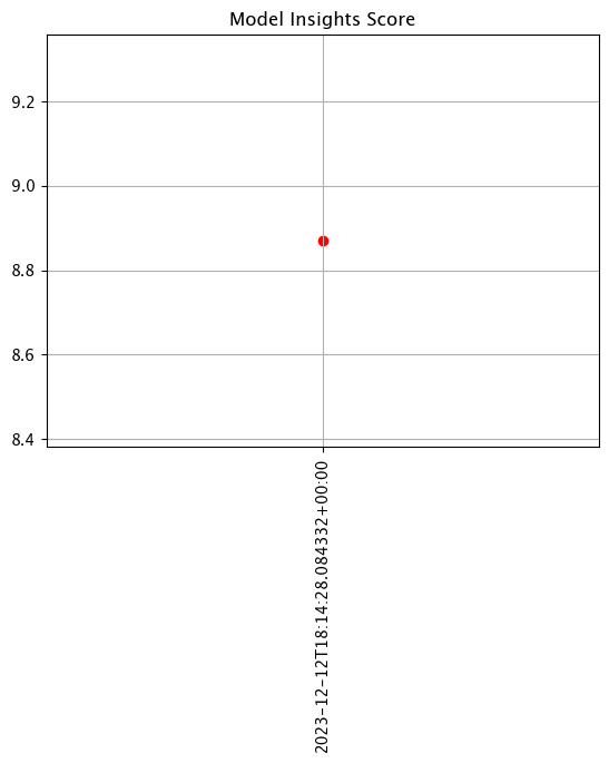
Now we’ll update with for just the edge location.
assay_builder_from_numpy.add_run_until(edge_datetime_end)
(assay_builder_from_numpy
.window_builder()
.add_width(minutes=1)
.add_interval(minutes=1)
.add_start(assay_window_start)
.add_location_filter([edge_name]))
assay_config_from_numpy = assay_builder_from_numpy.build()
assay_analysis_from_numpy = assay_config_from_numpy.interactive_run()
# Show how many assay windows were analyzed, then show the chart
print(f"Generated {len(assay_analysis_from_numpy)} analyses")
assay_analysis_from_numpy.chart_scores()
Generated 1 analyses
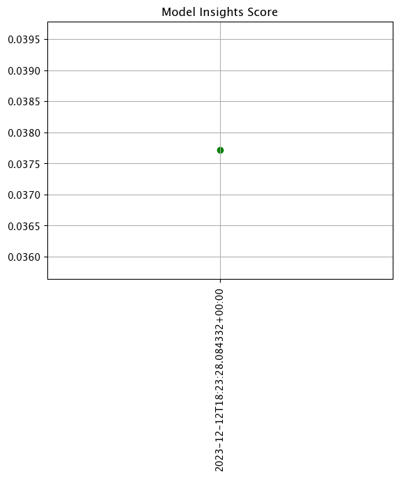
And finally we will use both locations in a cumulative assay window.
assay_builder_from_numpy.add_run_until(edge_datetime_end)
(assay_builder_from_numpy
.window_builder()
.add_width(minutes=1)
.add_interval(minutes=1)
.add_start(assay_window_start)
.add_location_filter([ops_location, edge_name]))
assay_config_from_numpy = assay_builder_from_numpy.build()
assay_analysis_from_numpy = assay_config_from_numpy.interactive_run()
# Show how many assay windows were analyzed, then show the chart
print(f"Generated {len(assay_analysis_from_numpy)} analyses")
assay_analysis_from_numpy.chart_scores()
Generated 2 analyses
3.11 - House Price Testing Life Cycle
A comprehensive tutorial on different testing and model comparison techniques for house price prediction.
This tutorial and the assets can be downloaded as part of the Wallaroo Tutorials repository.
House Price Testing Life Cycle Comprehensive Tutorial
This tutorial simulates using Wallaroo for testing a model for inference outliers, potential model drift, and methods to test competitive models against each other and deploy the final version to use. This demonstrates using assays to detect model or data drift, then Wallaroo Shadow Deploy to compare different models to determine which one is most fit for an organization’s needs. These features allow organizations to monitor model performance and accuracy then swap out models as needed.
- IMPORTANT NOTE: This tutorial assumes that the House Price Model Life Cycle Preparation notebook was run before this notebook, and that the workspace, pipeline and models used are the same. This is critical for the section on Assays below. If the preparation notebook has not been run, skip the Assays section as there will be no historical data for the assays to function on.
This tutorial will demonstrate how to:
- Select or create a workspace, pipeline and upload the champion model.
- Add a pipeline step with the champion model, then deploy the pipeline and perform sample inferences.
- Create an assay and set a baseline, then demonstrate inferences that trigger the assay alert threshold.
- Swap out the pipeline step with the champion model with a shadow deploy step that compares the champion model against two competitors.
- Evaluate the results of the champion versus competitor models.
- Change the pipeline step from a shadow deploy step to an A/B testing step, and show the different results.
- Change the A/B testing step back to standard pipeline step with the original control model, then demonstrate hot swapping the control model with a challenger model without undeploying the pipeline.
- Undeploy the pipeline.
This tutorial provides the following:
- Models:
models/rf_model.onnx: The champion model that has been used in this environment for some time.models/xgb_model.onnxandmodels/gbr_model.onnx: Rival models that will be tested against the champion.
- Data:
data/xtest-1.df.jsonanddata/xtest-1k.df.json: DataFrame JSON inference inputs with 1 input and 1,000 inputs.data/xtest-1k.arrow: Apache Arrow inference inputs with 1 input and 1,000 inputs.
Prerequisites
- A deployed Wallaroo instance
- The following Python libraries installed:
Initial Steps
Import libraries
The first step is to import the libraries needed for this notebook.
import wallaroo
from wallaroo.object import EntityNotFoundError
from wallaroo.framework import Framework
from IPython.display import display
# used to display DataFrame information without truncating
from IPython.display import display
import pandas as pd
pd.set_option('display.max_colwidth', None)
import datetime
import time
# used for unique connection names
import string
import random
suffix= ''.join(random.choice(string.ascii_lowercase) for i in range(4))
suffix='baselines'
import json
Connect to the Wallaroo Instance
The first step is to connect to Wallaroo through the Wallaroo client. The Python library is included in the Wallaroo install and available through the Jupyter Hub interface provided with your Wallaroo environment.
This is accomplished using the wallaroo.Client() command, which provides a URL to grant the SDK permission to your specific Wallaroo environment. When displayed, enter the URL into a browser and confirm permissions. Store the connection into a variable that can be referenced later.
If logging into the Wallaroo instance through the internal JupyterHub service, use wl = wallaroo.Client(). For more information on Wallaroo Client settings, see the Client Connection guide.
# Login through local Wallaroo instance
wl = wallaroo.Client()
Create Workspace
We will create a workspace to manage our pipeline and models. The following variables will set the name of our sample workspace then set it as the current workspace.
Workspace, pipeline, and model names should be unique to each user, so we’ll add in a randomly generated suffix so multiple people can run this tutorial in a Wallaroo instance without effecting each other.
workspace_name = f'housepricesagaworkspace{suffix}'
main_pipeline_name = f'housepricesagapipeline'
model_name_control = f'housepricesagacontrol'
model_file_name_control = './models/rf_model.onnx'
def get_workspace(name):
workspace = None
for ws in wl.list_workspaces():
if ws.name() == name:
workspace= ws
if(workspace == None):
workspace = wl.create_workspace(name)
return workspace
def get_pipeline(name, workspace):
pipelines = workspace.pipelines()
pipe_filter = filter(lambda x: x.name() == name, pipelines)
pipes = list(pipe_filter)
# we can't have a pipe in the workspace with the same name, so it's always the first
if pipes:
pipeline = pipes[0]
else:
pipeline = wl.build_pipeline(name)
return pipeline
workspace = get_workspace(workspace_name)
wl.set_current_workspace(workspace)
{'name': 'housepricesagaworkspacebaselines', 'id': 87, 'archived': False, 'created_by': 'd6a42dd8-1da9-4405-bb80-7c4b42e38b52', 'created_at': '2023-10-31T16:56:03.395454+00:00', 'models': [], 'pipelines': []}
Upload The Champion Model
For our example, we will upload the champion model that has been trained to derive house prices from a variety of inputs. The model file is rf_model.onnx, and is uploaded with the name housingcontrol.
housing_model_control = (wl.upload_model(model_name_control,
model_file_name_control,
framework=Framework.ONNX)
.configure(tensor_fields=["tensor"])
)
Standard Pipeline Steps
Build the Pipeline
This pipeline is made to be an example of an existing situation where a model is deployed and being used for inferences in a production environment. We’ll call it housepricepipeline, set housingcontrol as a pipeline step, then run a few sample inferences.
This pipeline will be a simple one - just a single pipeline step.
mainpipeline = get_pipeline(main_pipeline_name, workspace)
# clearing from previous runs and verifying it is undeployed
mainpipeline.clear()
mainpipeline.undeploy()
mainpipeline.add_model_step(housing_model_control)
#minimum deployment config
deploy_config = wallaroo.DeploymentConfigBuilder().replica_count(1).cpus(0.5).memory("1Gi").build()
mainpipeline.deploy(deployment_config = deploy_config)
Waiting for deployment - this will take up to 45s ............. ok
| name | housepricesagapipeline |
|---|---|
| created | 2023-10-31 16:56:07.345831+00:00 |
| last_updated | 2023-10-31 16:56:07.444932+00:00 |
| deployed | True |
| tags | |
| versions | 2ea0cc42-c955-4fc3-bac9-7a2c7c22ddc1, dca84ab2-274a-4391-95dd-a99bda7621e1 |
| steps | housepricesagacontrol |
| published | False |
Testing
We’ll use two inferences as a quick sample test - one that has a house that should be determined around $700k, the other with a house determined to be around $1.5 million. We’ll also save the start and end periods for these events to for later log functionality.
normal_input = pd.DataFrame.from_records({"tensor": [[4.0, 2.5, 2900.0, 5505.0, 2.0, 0.0, 0.0, 3.0, 8.0, 2900.0, 0.0, 47.6063, -122.02, 2970.0, 5251.0, 12.0, 0.0, 0.0]]})
result = mainpipeline.infer(normal_input)
display(result)
| time | in.tensor | out.variable | check_failures | |
|---|---|---|---|---|
| 0 | 2023-10-31 16:57:07.307 | [4.0, 2.5, 2900.0, 5505.0, 2.0, 0.0, 0.0, 3.0, 8.0, 2900.0, 0.0, 47.6063, -122.02, 2970.0, 5251.0, 12.0, 0.0, 0.0] | [718013.7] | 0 |
large_house_input = pd.DataFrame.from_records({'tensor': [[4.0, 3.0, 3710.0, 20000.0, 2.0, 0.0, 2.0, 5.0, 10.0, 2760.0, 950.0, 47.6696, -122.261, 3970.0, 20000.0, 79.0, 0.0, 0.0]]})
large_house_result = mainpipeline.infer(large_house_input)
display(large_house_result)
| time | in.tensor | out.variable | check_failures | |
|---|---|---|---|---|
| 0 | 2023-10-31 16:57:07.746 | [4.0, 3.0, 3710.0, 20000.0, 2.0, 0.0, 2.0, 5.0, 10.0, 2760.0, 950.0, 47.6696, -122.261, 3970.0, 20000.0, 79.0, 0.0, 0.0] | [1514079.4] | 0 |
As one last sample, we’ll run through roughly 1,000 inferences at once and show a few of the results. For this example we’ll use an Apache Arrow table, which has a smaller file size compared to uploading a pandas DataFrame JSON file. The inference result is returned as an arrow table, which we’ll convert into a pandas DataFrame to display the first 20 results.
time.sleep(5)
control_model_start = datetime.datetime.now()
batch_inferences = mainpipeline.infer_from_file('./data/xtest-1k.arrow')
large_inference_result = batch_inferences.to_pandas()
display(large_inference_result.head(20))
| time | in.tensor | out.variable | check_failures | |
|---|---|---|---|---|
| 0 | 2023-10-31 16:57:13.771 | [4.0, 2.5, 2900.0, 5505.0, 2.0, 0.0, 0.0, 3.0, 8.0, 2900.0, 0.0, 47.6063, -122.02, 2970.0, 5251.0, 12.0, 0.0, 0.0] | [718013.7] | 0 |
| 1 | 2023-10-31 16:57:13.771 | [2.0, 2.5, 2170.0, 6361.0, 1.0, 0.0, 2.0, 3.0, 8.0, 2170.0, 0.0, 47.7109, -122.017, 2310.0, 7419.0, 6.0, 0.0, 0.0] | [615094.6] | 0 |
| 2 | 2023-10-31 16:57:13.771 | [3.0, 2.5, 1300.0, 812.0, 2.0, 0.0, 0.0, 3.0, 8.0, 880.0, 420.0, 47.5893, -122.317, 1300.0, 824.0, 6.0, 0.0, 0.0] | [448627.8] | 0 |
| 3 | 2023-10-31 16:57:13.771 | [4.0, 2.5, 2500.0, 8540.0, 2.0, 0.0, 0.0, 3.0, 9.0, 2500.0, 0.0, 47.5759, -121.994, 2560.0, 8475.0, 24.0, 0.0, 0.0] | [758714.3] | 0 |
| 4 | 2023-10-31 16:57:13.771 | [3.0, 1.75, 2200.0, 11520.0, 1.0, 0.0, 0.0, 4.0, 7.0, 2200.0, 0.0, 47.7659, -122.341, 1690.0, 8038.0, 62.0, 0.0, 0.0] | [513264.66] | 0 |
| 5 | 2023-10-31 16:57:13.771 | [3.0, 2.0, 2140.0, 4923.0, 1.0, 0.0, 0.0, 4.0, 8.0, 1070.0, 1070.0, 47.6902, -122.339, 1470.0, 4923.0, 86.0, 0.0, 0.0] | [668287.94] | 0 |
| 6 | 2023-10-31 16:57:13.771 | [4.0, 3.5, 3590.0, 5334.0, 2.0, 0.0, 2.0, 3.0, 9.0, 3140.0, 450.0, 47.6763, -122.267, 2100.0, 6250.0, 9.0, 0.0, 0.0] | [1004846.56] | 0 |
| 7 | 2023-10-31 16:57:13.771 | [3.0, 2.0, 1280.0, 960.0, 2.0, 0.0, 0.0, 3.0, 9.0, 1040.0, 240.0, 47.602, -122.311, 1280.0, 1173.0, 0.0, 0.0, 0.0] | [684577.25] | 0 |
| 8 | 2023-10-31 16:57:13.771 | [4.0, 2.5, 2820.0, 15000.0, 2.0, 0.0, 0.0, 4.0, 9.0, 2820.0, 0.0, 47.7255, -122.101, 2440.0, 15000.0, 29.0, 0.0, 0.0] | [727898.25] | 0 |
| 9 | 2023-10-31 16:57:13.771 | [3.0, 2.25, 1790.0, 11393.0, 1.0, 0.0, 0.0, 3.0, 8.0, 1790.0, 0.0, 47.6297, -122.099, 2290.0, 11894.0, 36.0, 0.0, 0.0] | [559631.06] | 0 |
| 10 | 2023-10-31 16:57:13.771 | [3.0, 1.5, 1010.0, 7683.0, 1.5, 0.0, 0.0, 5.0, 7.0, 1010.0, 0.0, 47.72, -122.318, 1550.0, 7271.0, 61.0, 0.0, 0.0] | [340764.53] | 0 |
| 11 | 2023-10-31 16:57:13.771 | [3.0, 2.0, 1270.0, 1323.0, 3.0, 0.0, 0.0, 3.0, 8.0, 1270.0, 0.0, 47.6934, -122.342, 1330.0, 1323.0, 8.0, 0.0, 0.0] | [442168.12] | 0 |
| 12 | 2023-10-31 16:57:13.771 | [4.0, 1.75, 2070.0, 9120.0, 1.0, 0.0, 0.0, 4.0, 7.0, 1250.0, 820.0, 47.6045, -122.123, 1650.0, 8400.0, 57.0, 0.0, 0.0] | [630865.5] | 0 |
| 13 | 2023-10-31 16:57:13.771 | [4.0, 1.0, 1620.0, 4080.0, 1.5, 0.0, 0.0, 3.0, 7.0, 1620.0, 0.0, 47.6696, -122.324, 1760.0, 4080.0, 91.0, 0.0, 0.0] | [559631.06] | 0 |
| 14 | 2023-10-31 16:57:13.771 | [4.0, 3.25, 3990.0, 9786.0, 2.0, 0.0, 0.0, 3.0, 9.0, 3990.0, 0.0, 47.6784, -122.026, 3920.0, 8200.0, 10.0, 0.0, 0.0] | [909441.25] | 0 |
| 15 | 2023-10-31 16:57:13.771 | [4.0, 2.0, 1780.0, 19843.0, 1.0, 0.0, 0.0, 3.0, 7.0, 1780.0, 0.0, 47.4414, -122.154, 2210.0, 13500.0, 52.0, 0.0, 0.0] | [313096.0] | 0 |
| 16 | 2023-10-31 16:57:13.771 | [4.0, 2.5, 2130.0, 6003.0, 2.0, 0.0, 0.0, 3.0, 8.0, 2130.0, 0.0, 47.4518, -122.12, 1940.0, 4529.0, 11.0, 0.0, 0.0] | [404040.78] | 0 |
| 17 | 2023-10-31 16:57:13.771 | [3.0, 1.75, 1660.0, 10440.0, 1.0, 0.0, 0.0, 3.0, 7.0, 1040.0, 620.0, 47.4448, -121.77, 1240.0, 10380.0, 36.0, 0.0, 0.0] | [292859.44] | 0 |
| 18 | 2023-10-31 16:57:13.771 | [3.0, 2.5, 2110.0, 4118.0, 2.0, 0.0, 0.0, 3.0, 8.0, 2110.0, 0.0, 47.3878, -122.153, 2110.0, 4044.0, 25.0, 0.0, 0.0] | [338357.88] | 0 |
| 19 | 2023-10-31 16:57:13.771 | [4.0, 2.25, 2200.0, 11250.0, 1.5, 0.0, 0.0, 5.0, 7.0, 1300.0, 900.0, 47.6845, -122.201, 2320.0, 10814.0, 94.0, 0.0, 0.0] | [682284.56] | 0 |
Graph of Prices
Here’s a distribution plot of the inferences to view the values, with the X axis being the house price in millions, and the Y axis the number of houses fitting in a bin grouping. The majority of houses are in the $250,000 to $500,000 range, with some outliers in the far end.
import matplotlib.pyplot as plt
houseprices = pd.DataFrame({'sell_price': large_inference_result['out.variable'].apply(lambda x: x[0])})
houseprices.hist(column='sell_price', bins=75, grid=False, figsize=(12,8))
plt.axvline(x=0, color='gray', ls='--')
_ = plt.title('Distribution of predicted home sales price')
time.sleep(5)
control_model_end = datetime.datetime.now()
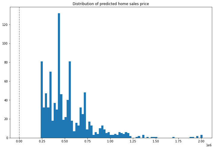
Pipeline Logs
Pipeline logs with standard pipeline steps are retrieved either with:
- Pipeline
logswhich returns either a pandas DataFrame or Apache Arrow table. - Pipeline
export_logswhich saves the logs either a pandas DataFrame JSON file or Apache Arrow table.
For full details, see the Wallaroo Documentation Pipeline Log Management guide.
Pipeline Log Methods
The Pipeline logs method accepts the following parameters.
| Parameter | Type | Description |
|---|---|---|
limit | Int (Optional) | Limits how many log records to display. Defaults to 100. If there are more pipeline logs than are being displayed, the Warning message Pipeline log record limit exceeded will be displayed. For example, if 100 log files were requested and there are a total of 1,000, the warning message will be displayed. |
start_datetimert and end_datetime | DateTime (Optional) | Limits logs to all logs between the start_datetime and end_datetime DateTime parameters. Both parameters must be provided. Submitting a logs() request with only start_datetime or end_datetime will generate an exception.If start_datetime and end_datetime are provided as parameters, then the records are returned in chronological order, with the oldest record displayed first. |
arrow | Boolean (Optional) | Defaults to False. If arrow is set to True, then the logs are returned as an Apache Arrow table. If arrow=False, then the logs are returned as a pandas DataFrame. |
The following examples demonstrate displaying the logs, then displaying the logs between the control_model_start and control_model_end periods, then again retrieved as an Arrow table.
# pipeline log retrieval - reverse chronological order
display(mainpipeline.logs())
# pipeline log retrieval between two dates - chronological order
display(mainpipeline.logs(start_datetime=control_model_start, end_datetime=control_model_end))
# pipeline log retrieval limited to the last 5 an an arrow table
display(mainpipeline.logs(arrow=True))
Warning: There are more logs available. Please set a larger limit or request a file using export_logs.
| time | in.tensor | out.variable | check_failures | |
|---|---|---|---|---|
| 0 | 2023-10-31 16:57:13.771 | [3.0, 2.0, 2005.0, 7000.0, 1.0, 0.0, 0.0, 3.0, 7.0, 1605.0, 400.0, 47.6039, -122.298, 1750.0, 4500.0, 34.0, 0.0, 0.0] | [581002.94] | 0 |
| 1 | 2023-10-31 16:57:13.771 | [3.0, 1.75, 2910.0, 37461.0, 1.0, 0.0, 0.0, 4.0, 7.0, 1530.0, 1380.0, 47.7015, -122.164, 2520.0, 18295.0, 47.0, 0.0, 0.0] | [706823.6] | 0 |
| 2 | 2023-10-31 16:57:13.771 | [4.0, 3.25, 2910.0, 1880.0, 2.0, 0.0, 3.0, 5.0, 9.0, 1830.0, 1080.0, 47.616, -122.282, 3100.0, 8200.0, 100.0, 0.0, 0.0] | [1060847.5] | 0 |
| 3 | 2023-10-31 16:57:13.771 | [4.0, 1.75, 2700.0, 7875.0, 1.5, 0.0, 0.0, 4.0, 8.0, 2700.0, 0.0, 47.454, -122.144, 2220.0, 7875.0, 46.0, 0.0, 0.0] | [441960.3] | 0 |
| 4 | 2023-10-31 16:57:13.771 | [3.0, 2.5, 2900.0, 23550.0, 1.0, 0.0, 0.0, 3.0, 10.0, 1490.0, 1410.0, 47.5708, -122.153, 2900.0, 19604.0, 27.0, 0.0, 0.0] | [827411.25] | 0 |
| ... | ... | ... | ... | ... |
| 95 | 2023-10-31 16:57:13.771 | [2.0, 1.5, 1070.0, 1236.0, 2.0, 0.0, 0.0, 3.0, 8.0, 1000.0, 70.0, 47.5619, -122.382, 1170.0, 1888.0, 10.0, 0.0, 0.0] | [435628.72] | 0 |
| 96 | 2023-10-31 16:57:13.771 | [3.0, 2.5, 2830.0, 6000.0, 1.0, 0.0, 3.0, 3.0, 9.0, 1730.0, 1100.0, 47.5751, -122.378, 2040.0, 5300.0, 60.0, 0.0, 0.0] | [981676.7] | 0 |
| 97 | 2023-10-31 16:57:13.771 | [4.0, 1.75, 1720.0, 8750.0, 1.0, 0.0, 0.0, 3.0, 7.0, 860.0, 860.0, 47.726, -122.21, 1790.0, 8750.0, 43.0, 0.0, 0.0] | [437177.97] | 0 |
| 98 | 2023-10-31 16:57:13.771 | [4.0, 2.25, 4470.0, 60373.0, 2.0, 0.0, 0.0, 3.0, 11.0, 4470.0, 0.0, 47.7289, -122.127, 3210.0, 40450.0, 26.0, 0.0, 0.0] | [1208638.1] | 0 |
| 99 | 2023-10-31 16:57:13.771 | [3.0, 1.0, 1150.0, 3000.0, 1.0, 0.0, 0.0, 5.0, 6.0, 1150.0, 0.0, 47.6867, -122.345, 1460.0, 3200.0, 108.0, 0.0, 0.0] | [448627.8] | 0 |
100 rows × 4 columns
Warning: Pipeline log size limit exceeded. Please request logs using export_logs
| time | in.tensor | out.variable | check_failures | |
|---|---|---|---|---|
| 0 | 2023-10-31 16:57:13.771 | [4.0, 2.5, 2900.0, 5505.0, 2.0, 0.0, 0.0, 3.0, 8.0, 2900.0, 0.0, 47.6063, -122.02, 2970.0, 5251.0, 12.0, 0.0, 0.0] | [718013.7] | 0 |
| 1 | 2023-10-31 16:57:13.771 | [2.0, 2.5, 2170.0, 6361.0, 1.0, 0.0, 2.0, 3.0, 8.0, 2170.0, 0.0, 47.7109, -122.017, 2310.0, 7419.0, 6.0, 0.0, 0.0] | [615094.6] | 0 |
| 2 | 2023-10-31 16:57:13.771 | [3.0, 2.5, 1300.0, 812.0, 2.0, 0.0, 0.0, 3.0, 8.0, 880.0, 420.0, 47.5893, -122.317, 1300.0, 824.0, 6.0, 0.0, 0.0] | [448627.8] | 0 |
| 3 | 2023-10-31 16:57:13.771 | [4.0, 2.5, 2500.0, 8540.0, 2.0, 0.0, 0.0, 3.0, 9.0, 2500.0, 0.0, 47.5759, -121.994, 2560.0, 8475.0, 24.0, 0.0, 0.0] | [758714.3] | 0 |
| 4 | 2023-10-31 16:57:13.771 | [3.0, 1.75, 2200.0, 11520.0, 1.0, 0.0, 0.0, 4.0, 7.0, 2200.0, 0.0, 47.7659, -122.341, 1690.0, 8038.0, 62.0, 0.0, 0.0] | [513264.66] | 0 |
| ... | ... | ... | ... | ... |
| 495 | 2023-10-31 16:57:13.771 | [4.0, 2.5, 3550.0, 35689.0, 2.0, 0.0, 0.0, 4.0, 9.0, 3550.0, 0.0, 47.7503, -122.074, 3350.0, 35711.0, 23.0, 0.0, 0.0] | [873315.2] | 0 |
| 496 | 2023-10-31 16:57:13.771 | [4.0, 2.5, 2510.0, 47044.0, 2.0, 0.0, 0.0, 3.0, 9.0, 2510.0, 0.0, 47.7699, -122.085, 2600.0, 42612.0, 27.0, 0.0, 0.0] | [721143.6] | 0 |
| 497 | 2023-10-31 16:57:13.771 | [4.0, 2.5, 4090.0, 11225.0, 2.0, 0.0, 0.0, 3.0, 10.0, 4090.0, 0.0, 47.581, -121.971, 3510.0, 8762.0, 9.0, 0.0, 0.0] | [1048372.44] | 0 |
| 498 | 2023-10-31 16:57:13.771 | [2.0, 1.0, 720.0, 5000.0, 1.0, 0.0, 0.0, 5.0, 6.0, 720.0, 0.0, 47.5195, -122.374, 810.0, 5000.0, 63.0, 0.0, 0.0] | [244566.39] | 0 |
| 499 | 2023-10-31 16:57:13.771 | [4.0, 2.75, 2930.0, 22000.0, 1.0, 0.0, 3.0, 4.0, 9.0, 1580.0, 1350.0, 47.3227, -122.384, 2930.0, 9758.0, 36.0, 0.0, 0.0] | [518869.03] | 0 |
500 rows × 4 columns
Warning: There are more logs available. Please set a larger limit or request a file using export_logs.
pyarrow.Table
time: timestamp[ms]
in.tensor: list<item: float> not null
child 0, item: float
out.variable: list<inner: float not null> not null
child 0, inner: float not null
check_failures: int8
----
time: [[2023-10-31 16:57:13.771,2023-10-31 16:57:13.771,2023-10-31 16:57:13.771,2023-10-31 16:57:13.771,2023-10-31 16:57:13.771,...,2023-10-31 16:57:13.771,2023-10-31 16:57:13.771,2023-10-31 16:57:13.771,2023-10-31 16:57:13.771,2023-10-31 16:57:13.771]]
in.tensor: [[[3,2,2005,7000,1,...,1750,4500,34,0,0],[3,1.75,2910,37461,1,...,2520,18295,47,0,0],...,[4,2.25,4470,60373,2,...,3210,40450,26,0,0],[3,1,1150,3000,1,...,1460,3200,108,0,0]]]
out.variable: [[[581002.94],[706823.6],...,[1208638.1],[448627.8]]]
check_failures: [[0,0,0,0,0,...,0,0,0,0,0]]
Anomaly Detection through Validations
Anomaly detection allows organizations to set validation parameters in a pipeline. A validation is added to a pipeline to test data based on an expression, and flag any inferences where the validation failed inference result and the pipeline logs.
Validations are added through the Pipeline add_validation(name, validation) command which uses the following parameters:
| Parameter | Type | Description |
|---|---|---|
| name | String (Required) | The name of the validation. |
| Validation | Expression (Required) | The validation test command in the format model_name.outputs][field][index] {Operation} {Value}. |
For this example, we want to detect the outputs of housing_model_control and validate that values are less than 1,500,000. Any outputs greater than that will trigger a check_failure which is shown in the output.
## Add the validation to the pipeline
mainpipeline = mainpipeline.add_validation('price too high', housing_model_control.outputs[0][0] < 1500000.0)
#minimum deployment config
deploy_config = wallaroo.DeploymentConfigBuilder().replica_count(1).cpus(0.5).memory("1Gi").build()
mainpipeline.deploy(deployment_config = deploy_config)
ok
| name | housepricesagapipeline |
|---|---|
| created | 2023-10-31 16:56:07.345831+00:00 |
| last_updated | 2023-10-31 16:57:24.026392+00:00 |
| deployed | True |
| tags | |
| versions | f7e0deaf-63a2-491a-8ff9-e8148d3cabcb, 2ea0cc42-c955-4fc3-bac9-7a2c7c22ddc1, dca84ab2-274a-4391-95dd-a99bda7621e1 |
| steps | housepricesagacontrol |
| published | False |
Validation Testing
Two validations will be tested:
- One that should return a house value lower than 1,500,000. The validation will pass so
check_failurewill be 0. - The other than should return a house value greater than 1,500,000. The validation will fail, so
check_failurewill be 1.
validation_start = datetime.datetime.now()
# Small value home
normal_input = pd.DataFrame.from_records({
"tensor": [[
3.0,
2.25,
1620.0,
997.0,
2.5,
0.0,
0.0,
3.0,
8.0,
1540.0,
80.0,
47.5400009155,
-122.0260009766,
1620.0,
1068.0,
4.0,
0.0,
0.0
]]
}
)
small_result = mainpipeline.infer(normal_input)
display(small_result.loc[:,["time", "out.variable", "check_failures"]])
| time | out.variable | check_failures | |
|---|---|---|---|
| 0 | 2023-10-31 16:57:26.205 | [544392.06] | 0 |
# Big value home
big_input = pd.DataFrame.from_records({
"tensor": [[
4.0,
4.5,
5770.0,
10050.0,
1.0,
0.0,
3.0,
5.0,
9.0,
3160.0,
2610.0,
47.6769981384,
-122.2750015259,
2950.0,
6700.0,
65.0,
0.0,
0.0
]]
}
)
big_result = mainpipeline.infer(big_input)
display(big_result.loc[:,["time", "out.variable", "check_failures"]])
| time | out.variable | check_failures | |
|---|---|---|---|
| 0 | 2023-10-31 16:57:27.138 | [1689843.1] | 1 |
Anomaly Results
We’ll run through our previous batch, this time showing only those results outside of the validation, and a graph showing where the anomalies are against the other results.
batch_inferences = mainpipeline.infer_from_file('./data/xtest-1k.arrow')
large_inference_result = batch_inferences.to_pandas()
# Display only the anomalous results
display(large_inference_result[large_inference_result["check_failures"] > 0].loc[:,["time", "out.variable", "check_failures"]])
| time | out.variable | check_failures | |
|---|---|---|---|
| 30 | 2023-10-31 16:57:28.974 | [1514079.4] | 1 |
| 248 | 2023-10-31 16:57:28.974 | [1967344.1] | 1 |
| 255 | 2023-10-31 16:57:28.974 | [2002393.6] | 1 |
| 556 | 2023-10-31 16:57:28.974 | [1886959.2] | 1 |
| 698 | 2023-10-31 16:57:28.974 | [1689843.1] | 1 |
| 711 | 2023-10-31 16:57:28.974 | [1946437.8] | 1 |
| 722 | 2023-10-31 16:57:28.974 | [2005883.1] | 1 |
| 782 | 2023-10-31 16:57:28.974 | [1910824.0] | 1 |
| 965 | 2023-10-31 16:57:28.974 | [2016006.1] | 1 |
import matplotlib.pyplot as plt
houseprices = pd.DataFrame({'sell_price': large_inference_result['out.variable'].apply(lambda x: x[0])})
houseprices.hist(column='sell_price', bins=75, grid=False, figsize=(12,8))
plt.axvline(x=1500000, color='red', ls='--')
_ = plt.title('Distribution of predicted home sales price')
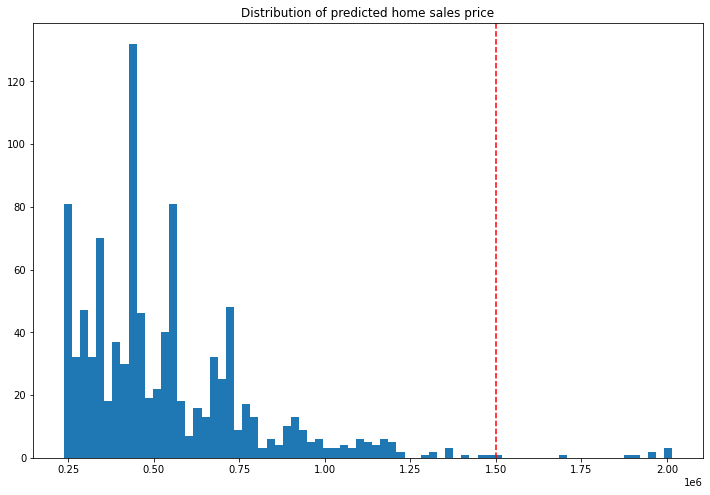
Assays
Wallaroo assays provide a method for detecting input or model drift. These can be triggered either when unexpected input is provided for the inference, or when the model needs to be retrained from changing environment conditions.
Wallaroo assays can track either an input field and its index, or an output field and its index. For full details, see the Wallaroo Assays Management Guide.
For this example, we will:
- Perform sample inferences based on lower priced houses.
- Create an assay with the baseline set off those lower priced houses.
- Generate inferences spread across all house values, plus specific set of high priced houses to trigger the assay alert.
- Run an interactive assay to show the detection of values outside the established baseline.
Assay Generation
To start the demonstration, we’ll create a baseline of values from houses with small estimated prices and set that as our baseline. Assays are typically run on a 24 hours interval based on a 24 hour window of data, but we’ll bypass that by setting our baseline time even shorter.
small_houses_inputs = pd.read_json('./data/smallinputs.df.json')
baseline_size = 500
# Where the baseline data will start
baseline_start = datetime.datetime.now()
# These inputs will be random samples of small priced houses. Around 30,000 is a good number
small_houses = small_houses_inputs.sample(baseline_size, replace=True).reset_index(drop=True)
small_results = mainpipeline.infer(small_houses)
# Set the baseline end
baseline_end = datetime.datetime.now()
# turn the inference results into a numpy array for the baseline
# set the results to a non-array value
small_results_baseline_df = small_results.copy()
small_results_baseline_df['variable']=small_results['out.variable'].map(lambda x: x[0])
# get the numpy values
small_results_baseline = small_results_baseline_df['variable'].to_numpy()
assay_baseline_from_numpy_name = "house price saga assay from numpy"
# assay builder by baseline
assay_builder_from_numpy = wl.build_assay(assay_name=assay_baseline_from_numpy_name,
pipeline=mainpipeline,
model_name=model_name_control,
iopath="output variable 0",
baseline_data = small_results_baseline)
# set the width from the recent results
assay_builder_from_numpy.window_builder().add_width(minutes=1)
assay_config_from_numpy = assay_builder_from_numpy.build()
assay_analysis_from_numpy = assay_config_from_numpy.interactive_run()
# get the histogram from the numpy baseline
assay_builder_from_numpy.baseline_histogram()
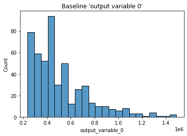
# show the baseline stats
assay_analysis_from_numpy[0].baseline_stats()
| Baseline | |
|---|---|
| count | 500 |
| min | 236238.67 |
| max | 1489624.3 |
| mean | 513762.85694 |
| median | 448627.8 |
| std | 235726.284713 |
| start | None |
| end | None |
Now we’ll perform some inferences with a spread of values, then a larger set with a set of larger house values to trigger our assay alert.
Because our assay windows are 1 minutes, we’ll need to stagger our inference values to be set into the proper windows. This will take about 4 minutes.
By default, assay start date is set to 24 hours from when the assay was created. For this example, we will set the assay.window_builder.add_start to set the assay window to start at the beginning of our data, and assay.add_run_until to set the time period to stop gathering data from.
# Get a spread of house values
time.sleep(35)
# regular_houses_inputs = pd.read_json('./data/xtest-1k.df.json', orient="records")
inference_size = 1000
# regular_houses = regular_houses_inputs.sample(inference_size, replace=True).reset_index(drop=True)
# And a spread of large house values
big_houses_inputs = pd.read_json('./data/biginputs.df.json', orient="records")
big_houses = big_houses_inputs.sample(inference_size, replace=True).reset_index(drop=True)
# Set the start for our assay window period.
assay_window_start = datetime.datetime.now()
mainpipeline.infer(big_houses)
# End our assay window period
time.sleep(35)
assay_window_end = datetime.datetime.now()
assay_builder_from_numpy.add_run_until(assay_window_end)
assay_builder_from_numpy.window_builder().add_width(minutes=1).add_interval(minutes=1).add_start(assay_window_start)
assay_config_from_dates = assay_builder_from_numpy.build()
assay_analysis_from_numpy = assay_config_from_numpy.interactive_run()
# Show how many assay windows were analyzed, then show the chart
print(f"Generated {len(assay_analysis_from_numpy)} analyses")
assay_analysis_from_numpy.chart_scores()
Generated 5 analyses
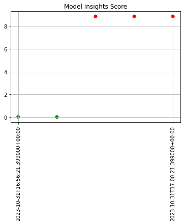
# Display the results as a DataFrame - we're mainly interested in the score and whether the
# alert threshold was triggered
display(assay_analysis_from_numpy.to_dataframe().loc[:, ["score", "start", "alert_threshold", "status"]])
| score | start | alert_threshold | status | |
|---|---|---|---|---|
| 0 | 0.016079 | 2023-10-31T16:56:21.399000+00:00 | 0.25 | Ok |
| 1 | 0.006042 | 2023-10-31T16:57:21.399000+00:00 | 0.25 | Ok |
| 2 | 8.868832 | 2023-10-31T16:58:21.399000+00:00 | 0.25 | Alert |
| 3 | 8.868832 | 2023-10-31T16:59:21.399000+00:00 | 0.25 | Alert |
| 4 | 8.868832 | 2023-10-31T17:00:21.399000+00:00 | 0.25 | Alert |
assay_builder_from_numpy.upload()
18
The assay is now visible through the Wallaroo UI by selecting the workspace, then the pipeline, then Insights.
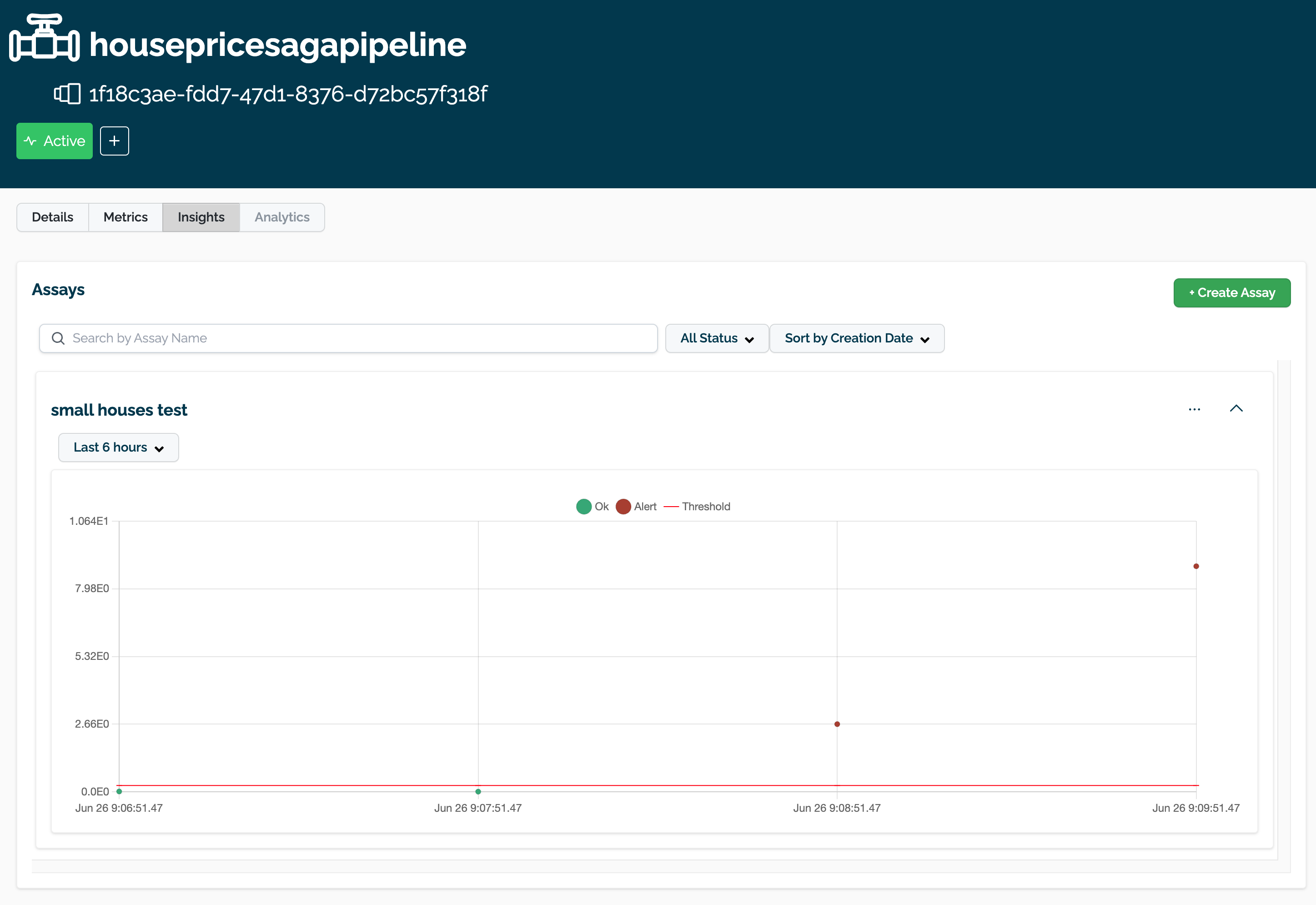
Shadow Deploy
Let’s assume that after analyzing the assay information we want to test two challenger models to our control. We do that with the Shadow Deploy pipeline step.
In Shadow Deploy, the pipeline step is added with the add_shadow_deploy method, with the champion model listed first, then an array of challenger models after. All inference data is fed to all models, with the champion results displayed in the out.variable column, and the shadow results in the format out_{model name}.variable. For example, since we named our challenger models housingchallenger01 and housingchallenger02, the columns out_housingchallenger01.variable and out_housingchallenger02.variable have the shadow deployed model results.
For this example, we will remove the previous pipeline step, then replace it with a shadow deploy step with rf_model.onnx as our champion, and models xgb_model.onnx and gbr_model.onnx as the challengers. We’ll deploy the pipeline and prepare it for sample inferences.
# Upload the challenger models
model_name_challenger01 = 'housingchallenger01'
model_file_name_challenger01 = './models/xgb_model.onnx'
model_name_challenger02 = 'housingchallenger02'
model_file_name_challenger02 = './models/gbr_model.onnx'
housing_model_challenger01 = (wl.upload_model(model_name_challenger01,
model_file_name_challenger01,
framework=Framework.ONNX)
.configure(tensor_fields=["tensor"])
)
housing_model_challenger02 = (wl.upload_model(model_name_challenger02,
model_file_name_challenger02,
framework=Framework.ONNX)
.configure(tensor_fields=["tensor"])
)
# Undeploy the pipeline
mainpipeline.undeploy()
mainpipeline.clear()
# Add the new shadow deploy step with our challenger models
mainpipeline.add_shadow_deploy(housing_model_control, [housing_model_challenger01, housing_model_challenger02])
# Deploy the pipeline with the new shadow step
#minimum deployment config
deploy_config = wallaroo.DeploymentConfigBuilder().replica_count(1).cpus(0.5).memory("1Gi").build()
mainpipeline.deploy(deployment_config = deploy_config)
Waiting for undeployment - this will take up to 45s ................................... ok
Waiting for deployment - this will take up to 45s ................................. ok
| name | housepricesagapipeline |
|---|---|
| created | 2023-10-31 16:56:07.345831+00:00 |
| last_updated | 2023-10-31 17:04:57.709641+00:00 |
| deployed | True |
| tags | |
| versions | 44d28e3e-094f-4507-8aa1-909c1f151dd5, b9f46ba3-3f14-4e5b-989e-e0b8d166392f, f7e0deaf-63a2-491a-8ff9-e8148d3cabcb, 2ea0cc42-c955-4fc3-bac9-7a2c7c22ddc1, dca84ab2-274a-4391-95dd-a99bda7621e1 |
| steps | housepricesagacontrol |
| published | False |
Shadow Deploy Sample Inference
We’ll now use our same sample data for an inference to our shadow deployed pipeline, then display the first 20 results with just the comparative outputs.
shadow_result = mainpipeline.infer_from_file('./data/xtest-1k.arrow')
shadow_outputs = shadow_result.to_pandas()
display(shadow_outputs.loc[0:20,['out.variable','out_housingchallenger01.variable','out_housingchallenger02.variable']])
| out.variable | out_housingchallenger01.variable | out_housingchallenger02.variable | |
|---|---|---|---|
| 0 | [718013.7] | [659806.0] | [704901.9] |
| 1 | [615094.6] | [732883.5] | [695994.44] |
| 2 | [448627.8] | [419508.84] | [416164.8] |
| 3 | [758714.3] | [634028.75] | [655277.2] |
| 4 | [513264.66] | [427209.47] | [426854.66] |
| 5 | [668287.94] | [615501.9] | [632556.06] |
| 6 | [1004846.56] | [1139732.4] | [1100465.2] |
| 7 | [684577.25] | [498328.88] | [528278.06] |
| 8 | [727898.25] | [722664.4] | [659439.94] |
| 9 | [559631.06] | [525746.44] | [534331.44] |
| 10 | [340764.53] | [376337.06] | [377187.2] |
| 11 | [442168.12] | [382053.12] | [403964.3] |
| 12 | [630865.5] | [505608.97] | [528991.3] |
| 13 | [559631.06] | [603260.5] | [612201.75] |
| 14 | [909441.25] | [969585.44] | [893874.7] |
| 15 | [313096.0] | [313633.7] | [318054.94] |
| 16 | [404040.78] | [360413.62] | [357816.7] |
| 17 | [292859.44] | [316674.88] | [294034.62] |
| 18 | [338357.88] | [299907.47] | [323254.28] |
| 19 | [682284.56] | [811896.75] | [770916.6] |
| 20 | [583765.94] | [573618.5] | [549141.4] |
A/B Testing
A/B Testing is another method of comparing and testing models. Like shadow deploy, multiple models are compared against the champion or control models. The difference is that instead of submitting the inference data to all models, then tracking the outputs of all of the models, the inference inputs are off of a ratio and other conditions.
For this example, we’ll be using a 1:1:1 ratio with a random split between the champion model and the two challenger models. Each time an inference request is made, there is a random equal chance of any one of them being selected.
When the inference results and log entries are displayed, they include the column out._model_split which displays:
| Field | Type | Description |
|---|---|---|
name | String | The model name used for the inference. |
version | String | The version of the model. |
sha | String | The sha hash of the model version. |
This is used to determine which model was used for the inference request.
# remove the shadow deploy steps
mainpipeline.clear()
# Add the a/b test step to the pipeline
mainpipeline.add_random_split([(1, housing_model_control), (1, housing_model_challenger01), (1, housing_model_challenger02)], "session_id")
mainpipeline.deploy()
# Perform sample inferences of 20 rows and display the results
ab_date_start = datetime.datetime.now()
abtesting_inputs = pd.read_json('./data/xtest-1k.df.json')
df = pd.DataFrame(columns=["model", "value"])
for index, row in abtesting_inputs.sample(20).iterrows():
result = mainpipeline.infer(row.to_frame('tensor').reset_index())
value = result.loc[0]["out.variable"]
model = json.loads(result.loc[0]["out._model_split"][0])['name']
df = df.append({'model': model, 'value': value}, ignore_index=True)
display(df)
ab_date_end = datetime.datetime.now()
ok
| model | value | |
|---|---|---|
| 0 | housingchallenger01 | [278554.44] |
| 1 | housingchallenger02 | [615955.3] |
| 2 | housepricesagacontrol | [1092273.9] |
| 3 | housepricesagacontrol | [683845.75] |
| 4 | housepricesagacontrol | [682284.56] |
| 5 | housepricesagacontrol | [247792.75] |
| 6 | housingchallenger02 | [315142.44] |
| 7 | housingchallenger02 | [530408.94] |
| 8 | housepricesagacontrol | [340764.53] |
| 9 | housepricesagacontrol | [421153.16] |
| 10 | housingchallenger01 | [395150.63] |
| 11 | housingchallenger02 | [544343.3] |
| 12 | housingchallenger01 | [395284.4] |
| 13 | housepricesagacontrol | [701940.7] |
| 14 | housepricesagacontrol | [448627.8] |
| 15 | housepricesagacontrol | [320863.72] |
| 16 | housingchallenger01 | [558485.3] |
| 17 | housingchallenger02 | [236329.28] |
| 18 | housepricesagacontrol | [559631.06] |
| 19 | housingchallenger01 | [281437.56] |
Model Swap
Now that we’ve completed our testing, we can swap our deployed model in the original housepricingpipeline with one we feel works better.
We’ll start by removing the A/B Testing pipeline step, then going back to the single pipeline step with the champion model and perform a test inference.
When going from a testing step such as A/B Testing or Shadow Deploy, it is best to undeploy the pipeline, change the steps, then deploy the pipeline. In a production environment, there should be two pipelines: One for production, the other for testing models. Since this example uses one pipeline for simplicity, we will undeploy our main pipeline and reset it back to a one-step pipeline with the current champion model as our pipeline step.
Once done, we’ll perform the hot swap with the model gbr_model.onnx, which was labeled housing_model_challenger02 in a previous step. We’ll do an inference with the same data as used with the challenger model. Note that previously, the inference through the original model returned [718013.7].
mainpipeline.undeploy()
# remove the shadow deploy steps
mainpipeline.clear()
mainpipeline.add_model_step(housing_model_control).deploy()
# Inference test
normal_input = pd.DataFrame.from_records({"tensor": [[4.0,
2.25,
2200.0,
11250.0,
1.5,
0.0,
0.0,
5.0,
7.0,
1300.0,
900.0,
47.6845,
-122.201,
2320.0,
10814.0,
94.0,
0.0,
0.0]]})
controlresult = mainpipeline.infer(normal_input)
display(controlresult)
ok
Waiting for deployment - this will take up to 45s ........ ok
| time | in.tensor | out.variable | check_failures | |
|---|---|---|---|---|
| 0 | 2023-10-31 17:08:19.579 | [4.0, 2.25, 2200.0, 11250.0, 1.5, 0.0, 0.0, 5.0, 7.0, 1300.0, 900.0, 47.6845, -122.201, 2320.0, 10814.0, 94.0, 0.0, 0.0] | [682284.56] | 0 |
Now we’ll “hot swap” the control model. We don’t have to deploy the pipeline - we can just swap the model out in that pipeline step and continue with only a millisecond or two lost while the swap was performed.
# Perform hot swap
mainpipeline.replace_with_model_step(0, housing_model_challenger02).deploy()
# wait a moment for the database to be updated. The swap is near instantaneous but database writes may take a moment
import time
time.sleep(15)
# inference after model swap
normal_input = pd.DataFrame.from_records({"tensor": [[4.0,
2.25,
2200.0,
11250.0,
1.5,
0.0,
0.0,
5.0,
7.0,
1300.0,
900.0,
47.6845,
-122.201,
2320.0,
10814.0,
94.0,
0.0,
0.0]]})
challengerresult = mainpipeline.infer(normal_input)
display(challengerresult)
ok
| time | in.tensor | out.variable | check_failures | |
|---|---|---|---|---|
| 0 | 2023-10-31 17:09:23.932 | [4.0, 2.25, 2200.0, 11250.0, 1.5, 0.0, 0.0, 5.0, 7.0, 1300.0, 900.0, 47.6845, -122.201, 2320.0, 10814.0, 94.0, 0.0, 0.0] | [770916.6] | 0 |
# Display the difference between the two
display(f'Original model output: {controlresult.loc[0]["out.variable"]}')
display(f'Hot swapped model output: {challengerresult.loc[0]["out.variable"]}')
'Original model output: [682284.56]'
‘Hot swapped model output: [770916.6]’
Undeploy Main Pipeline
With the examples and tutorial complete, we will undeploy the main pipeline and return the resources back to the Wallaroo instance.
mainpipeline.undeploy()
Waiting for undeployment - this will take up to 45s ...................................... ok
| name | housepricesagapipeline |
|---|---|
| created | 2023-10-31 16:56:07.345831+00:00 |
| last_updated | 2023-10-31 17:09:08.758964+00:00 |
| deployed | False |
| tags | |
| versions | 51034ba5-b58e-4475-908d-ec8fae069745, cd0f20e9-6923-4e6f-8114-1137676da5c5, 58274aab-0045-4557-a740-7d085af8574d, 4cf4f0dc-2c42-4f8b-975c-1f5c5d939a98, c5ae5a56-1c7f-4a94-9d4e-f08bf35e7f4f, f652a9d8-a4f6-428a-9b36-b29eec6b5198, 0e7d9d77-02d7-4c13-8062-9c77492145f8, 42b97784-fc16-43be-b89e-2d3dad20dd2b, 7d35285a-f8af-4bed-855b-60258c3435ee, 8b0dc4bb-3340-44f9-85d6-fbd091e19412, 06169fed-59e9-41f8-9dbd-0fc9f80ebb73, 44d28e3e-094f-4507-8aa1-909c1f151dd5, b9f46ba3-3f14-4e5b-989e-e0b8d166392f, f7e0deaf-63a2-491a-8ff9-e8148d3cabcb, 2ea0cc42-c955-4fc3-bac9-7a2c7c22ddc1, dca84ab2-274a-4391-95dd-a99bda7621e1 |
| steps | housepricesagacontrol |
| published | False |
4 - Model Cookbooks
Sample model deployment tutorials for Wallaroo
Recipes for deploying common models in Wallaroo.
4.1 - Aloha Quick Tutorial
The Aloha Quick Start Guide demonstrates how to use Wallaroo to determine malicious web sites from their URL.
This tutorial and the assets can be downloaded as part of the Wallaroo Tutorials repository.
Aloha Demo
In this notebook we will walk through a simple pipeline deployment to inference on a model. For this example we will be using an open source model that uses an Aloha CNN LSTM model for classifying Domain names as being either legitimate or being used for nefarious purposes such as malware distribution.
Prerequisites
- An installed Wallaroo instance.
- The following Python libraries installed:
Tutorial Goals
For our example, we will perform the following:
- Create a workspace for our work.
- Upload the Aloha model.
- Create a pipeline that can ingest our submitted data, submit it to the model, and export the results
- Run a sample inference through our pipeline by loading a file
- Run a sample inference through our pipeline’s URL and store the results in a file.
All sample data and models are available through the Wallaroo Quick Start Guide Samples repository.
Connect to the Wallaroo Instance
The first step is to connect to Wallaroo through the Wallaroo client. The Python library is included in the Wallaroo install and available through the Jupyter Hub interface provided with your Wallaroo environment.
This is accomplished using the wallaroo.Client() command, which provides a URL to grant the SDK permission to your specific Wallaroo environment. When displayed, enter the URL into a browser and confirm permissions. Store the connection into a variable that can be referenced later.
If logging into the Wallaroo instance through the internal JupyterHub service, use wl = wallaroo.Client(). For more information on Wallaroo Client settings, see the Client Connection guide.e/wallaroo-sdk-essentials-client/).
import wallaroo
from wallaroo.object import EntityNotFoundError
# to display dataframe tables
from IPython.display import display
# used to display dataframe information without truncating
import pandas as pd
pd.set_option('display.max_colwidth', None)
import pyarrow as pa
# Login through local Wallaroo instance
wl = wallaroo.Client()
Create the Workspace
We will create a workspace to work in and call it the “alohaworkspace”, then set it as current workspace environment. We’ll also create our pipeline in advance as alohapipeline. The model name and the model file will be specified for use in later steps.
To allow this tutorial to be run multiple times or by multiple users in the same Wallaroo instance, a random 4 character prefix will be added to the workspace, pipeline, and model.
import string
import random
# make a random 4 character suffix to verify uniqueness in tutorials
suffix= ''.join(random.choice(string.ascii_lowercase) for i in range(4))
workspace_name = f'alohaworkspace{suffix}'
pipeline_name = f'alohapipeline{suffix}'
model_name = f'alohamodel{suffix}'
model_file_name = './alohacnnlstm.zip'
def get_workspace(name):
workspace = None
for ws in wl.list_workspaces():
if ws.name() == name:
workspace= ws
if(workspace == None):
workspace = wl.create_workspace(name)
return workspace
def get_pipeline(name):
try:
pipeline = wl.pipelines_by_name(name)[0]
except EntityNotFoundError:
pipeline = wl.build_pipeline(name)
return pipeline
wl.list_workspaces()[0:5]
[{'name': 'john.hummel@wallaroo.ai - Default Workspace', 'id': 1, 'archived': False, 'created_by': 'db364f8c-b866-4865-96b7-0b65662cb384', 'created_at': '2023-08-24T16:55:38.589652+00:00', 'models': [{'name': 'hf-summarization-demoyns2', 'versions': 1, 'owner_id': '""', 'last_update_time': datetime.datetime(2023, 8, 25, 15, 49, 36, 877913, tzinfo=tzutc()), 'created_at': datetime.datetime(2023, 8, 25, 15, 49, 36, 877913, tzinfo=tzutc())}], 'pipelines': [{'name': 'hf-summarization-pipeline-edge', 'create_time': datetime.datetime(2023, 8, 25, 15, 52, 2, 329988, tzinfo=tzutc()), 'definition': '[]'}]},
{'name': 'edge-publish-demojohn', 'id': 5, 'archived': False, 'created_by': 'db364f8c-b866-4865-96b7-0b65662cb384', 'created_at': '2023-08-24T16:57:29.048825+00:00', 'models': [{'name': 'ccfraud', 'versions': 1, 'owner_id': '""', 'last_update_time': datetime.datetime(2023, 8, 24, 16, 57, 29, 410708, tzinfo=tzutc()), 'created_at': datetime.datetime(2023, 8, 24, 16, 57, 29, 410708, tzinfo=tzutc())}], 'pipelines': [{'name': 'edge-pipeline', 'create_time': datetime.datetime(2023, 8, 24, 16, 57, 29, 486951, tzinfo=tzutc()), 'definition': '[]'}]},
{'name': 'workshop-workspace-sample', 'id': 6, 'archived': False, 'created_by': 'db364f8c-b866-4865-96b7-0b65662cb384', 'created_at': '2023-08-24T21:01:46.66355+00:00', 'models': [{'name': 'house-price-prime', 'versions': 2, 'owner_id': '""', 'last_update_time': datetime.datetime(2023, 8, 24, 21, 9, 13, 887924, tzinfo=tzutc()), 'created_at': datetime.datetime(2023, 8, 24, 21, 8, 35, 654241, tzinfo=tzutc())}], 'pipelines': [{'name': 'houseprice-estimator', 'create_time': datetime.datetime(2023, 8, 24, 21, 16, 0, 405934, tzinfo=tzutc()), 'definition': '[]'}]},
{'name': 'john-is-nice', 'id': 7, 'archived': False, 'created_by': 'db364f8c-b866-4865-96b7-0b65662cb384', 'created_at': '2023-08-24T21:05:57.618824+00:00', 'models': [], 'pipelines': []},
{'name': 'edge-hf-summarization', 'id': 8, 'archived': False, 'created_by': 'db364f8c-b866-4865-96b7-0b65662cb384', 'created_at': '2023-08-25T18:43:02.41099+00:00', 'models': [{'name': 'hf-summarization', 'versions': 1, 'owner_id': '""', 'last_update_time': datetime.datetime(2023, 8, 25, 18, 49, 26, 195772, tzinfo=tzutc()), 'created_at': datetime.datetime(2023, 8, 25, 18, 49, 26, 195772, tzinfo=tzutc())}], 'pipelines': [{'name': 'edge-hf-summarization', 'create_time': datetime.datetime(2023, 8, 25, 18, 53, 19, 465175, tzinfo=tzutc()), 'definition': '[]'}]}]
workspace = get_workspace(workspace_name)
wl.set_current_workspace(workspace)
aloha_pipeline = get_pipeline(pipeline_name)
aloha_pipeline
| name | alohapipelineudjo |
|---|---|
| created | 2023-08-28 17:10:05.043499+00:00 |
| last_updated | 2023-08-28 17:10:05.043499+00:00 |
| deployed | (none) |
| tags | |
| versions | e3f6ddff-9a25-48cc-9f94-fbc7bd67db29 |
| steps | |
| published | False |
We can verify the workspace is created the current default workspace with the get_current_workspace() command.
wl.get_current_workspace()
{'name': 'alohaworkspaceudjo', 'id': 13, 'archived': False, 'created_by': 'db364f8c-b866-4865-96b7-0b65662cb384', 'created_at': '2023-08-28T17:10:04.351972+00:00', 'models': [], 'pipelines': [{'name': 'alohapipelineudjo', 'create_time': datetime.datetime(2023, 8, 28, 17, 10, 5, 43499, tzinfo=tzutc()), 'definition': '[]'}]}
Upload the Models
Now we will upload our models. Note that for this example we are applying the model from a .ZIP file. The Aloha model is a protobuf file that has been defined for evaluating web pages, and we will configure it to use data in the tensorflow format.
from wallaroo.framework import Framework
model = wl.upload_model(model_name,
model_file_name,
framework=Framework.TENSORFLOW
)
Deploy a model
Now that we have a model that we want to use we will create a deployment for it.
We will tell the deployment we are using a tensorflow model and give the deployment name and the configuration we want for the deployment.
To do this, we’ll create our pipeline that can ingest the data, pass the data to our Aloha model, and give us a final output. We’ll call our pipeline aloha-test-demo, then deploy it so it’s ready to receive data. The deployment process usually takes about 45 seconds.
- Note: If you receive an error that the pipeline could not be deployed because there are not enough resources, undeploy any other pipelines and deploy this one again. This command can quickly undeploy all pipelines to regain resources. We recommend not running this command in a production environment since it will cancel any running pipelines:
for p in wl.list_pipelines(): p.undeploy()
aloha_pipeline.add_model_step(model)
| name | alohapipelineudjo |
|---|---|
| created | 2023-08-28 17:10:05.043499+00:00 |
| last_updated | 2023-08-28 17:10:05.043499+00:00 |
| deployed | (none) |
| tags | |
| versions | e3f6ddff-9a25-48cc-9f94-fbc7bd67db29 |
| steps | |
| published | False |
aloha_pipeline.deploy()
| name | alohapipelineudjo |
|---|---|
| created | 2023-08-28 17:10:05.043499+00:00 |
| last_updated | 2023-08-28 17:10:10.176032+00:00 |
| deployed | True |
| tags | |
| versions | 750fec3b-f178-4abd-9643-2208e0fd1fbd, e3f6ddff-9a25-48cc-9f94-fbc7bd67db29 |
| steps | alohamodeludjo |
| published | False |
We can verify that the pipeline is running and list what models are associated with it.
aloha_pipeline.status()
{'status': 'Running',
'details': [],
'engines': [{'ip': '10.244.3.99',
'name': 'engine-7f6ccf6879-hmw2p',
'status': 'Running',
'reason': None,
'details': [],
'pipeline_statuses': {'pipelines': [{'id': 'alohapipelineudjo',
'status': 'Running'}]},
'model_statuses': {'models': [{'name': 'alohamodeludjo',
'version': 'b99dd290-870d-425e-8835-953decd402be',
'sha': 'd71d9ffc61aaac58c2b1ed70a2db13d1416fb9d3f5b891e5e4e2e97180fe22f8',
'status': 'Running'}]}}],
'engine_lbs': [{'ip': '10.244.4.114',
'name': 'engine-lb-584f54c899-4g6rh',
'status': 'Running',
'reason': None,
'details': []}],
'sidekicks': []}
Interferences
Infer 1 row
Now that the pipeline is deployed and our Aloha model is in place, we’ll perform a smoke test to verify the pipeline is up and running properly. We’ll use the infer_from_file command to load a single encoded URL into the inference engine and print the results back out.
The result should tell us that the tokenized URL is legitimate (0) or fraud (1). This sample data should return close to 1 in out.main.
smoke_test = pd.DataFrame.from_records(
[
{
"text_input":[
0,
0,
0,
0,
0,
0,
0,
0,
0,
0,
0,
0,
0,
0,
0,
0,
0,
0,
0,
0,
0,
0,
0,
0,
0,
0,
0,
0,
0,
0,
0,
0,
0,
0,
0,
0,
0,
0,
0,
0,
28,
16,
32,
23,
29,
32,
30,
19,
26,
17
]
}
]
)
result = aloha_pipeline.infer(smoke_test)
display(result.loc[:, ["time","out.main"]])
| time | out.main | |
|---|---|---|
| 0 | 2023-08-28 17:10:27.482 | [0.997564] |
Infer From File
This time, we’ll give it a bigger set of data to infer. ./data/data_1k.arrow is an Apache Arrow table with 1,000 records in it. Once submitted, we’ll turn the result into a DataFrame and display the first five results.
result = aloha_pipeline.infer_from_file('./data/data_1k.arrow')
display(result.to_pandas().loc[:, ["time","out.main"]])
| time | out.main | |
|---|---|---|
| 0 | 2023-08-28 17:10:28.399 | [0.997564] |
| 1 | 2023-08-28 17:10:28.399 | [0.9885122] |
| 2 | 2023-08-28 17:10:28.399 | [0.9993358] |
| 3 | 2023-08-28 17:10:28.399 | [0.99999857] |
| 4 | 2023-08-28 17:10:28.399 | [0.9984837] |
| ... | ... | ... |
| 995 | 2023-08-28 17:10:28.399 | [0.9999754] |
| 996 | 2023-08-28 17:10:28.399 | [0.9999727] |
| 997 | 2023-08-28 17:10:28.399 | [0.66066873] |
| 998 | 2023-08-28 17:10:28.399 | [0.9998954] |
| 999 | 2023-08-28 17:10:28.399 | [0.99999803] |
1000 rows × 2 columns
outputs = result.to_pandas()
display(outputs.loc[:5, ["time","out.main"]])
| time | out.main | |
|---|---|---|
| 0 | 2023-08-28 17:10:28.399 | [0.997564] |
| 1 | 2023-08-28 17:10:28.399 | [0.9885122] |
| 2 | 2023-08-28 17:10:28.399 | [0.9993358] |
| 3 | 2023-08-28 17:10:28.399 | [0.99999857] |
| 4 | 2023-08-28 17:10:28.399 | [0.9984837] |
| 5 | 2023-08-28 17:10:28.399 | [1.0] |
Batch Inference
Now that our smoke test is successful, let’s really give it some data. We have two inference files we can use:
data_1k.arrow: Contains 10,000 inferencesdata_25k.arrow: Contains 25,000 inferences
When Apache Arrow tables are submitted to a Wallaroo Pipeline, the inference is processed natively as an Arrow table, and the results are returned as an Arrow table. This allows for faster data processing than with JSON files or DataFrame objects.
We’ll pipe the data_25k.arrow file through the aloha_pipeline deployment URL, and place the results in a file named response.arrow. We’ll also display the time this takes. Note that for larger batches of 50,000 inferences or more can be difficult to view in Jupyter Hub because of its size, so we’ll only display the first five rows.
- IMPORTANT NOTE: The
_deployment._url()method will return an internal URL when using Python commands from within the Wallaroo instance - for example, the Wallaroo JupyterHub service. When connecting via an external connection,_deployment._url()returns an external URL. External URL connections requires the authentication be included in the HTTP request, and that Model Endpoints Guide external endpoints are enabled in the Wallaroo configuration options.
inference_url = aloha_pipeline._deployment._url()
inference_url
'https://doc-test.api.wallarooexample.ai/v1/api/pipelines/infer/alohapipelineudjo-15/alohapipelineudjo'
connection =wl.mlops().__dict__
token = connection['token']
dataFile="./data/data_25k.arrow"
contentType="application/vnd.apache.arrow.file"
!curl -X POST {inference_url} -H "Authorization: Bearer {token}" -H "Content-Type:{contentType}" --data-binary @{dataFile} > curl_response.df
% Total % Received % Xferd Average Speed Time Time Time Current
Dload Upload Total Spent Left Speed
100 25.9M 100 21.1M 100 4874k 1740k 391k 0:00:12 0:00:12 --:--:-- 4647k
cc_data_from_file = pd.read_json('./curl_response.df', orient="records")
display(cc_data_from_file.head(5).loc[:5, ["time","out"]])
| time | out | |
|---|---|---|
| 0 | 1693242632007 | {'banjori': [0.0015195821], 'corebot': [0.9829147500000001], 'cryptolocker': [0.012099549000000001], 'dircrypt': [4.7591115e-05], 'gozi': [2.0289428e-05], 'kraken': [0.00031977256999999996], 'locky': [0.011029262000000001], 'main': [0.997564], 'matsnu': [0.010341609], 'pykspa': [0.008038961], 'qakbot': [0.016155055], 'ramdo': [0.00623623], 'ramnit': [0.0009985747000000001], 'simda': [1.7933434e-26], 'suppobox': [1.388995e-27]} |
| 1 | 1693242632007 | {'banjori': [7.447196e-18], 'corebot': [6.7359245e-08], 'cryptolocker': [0.1708199], 'dircrypt': [1.3220122000000002e-09], 'gozi': [1.2758705999999999e-24], 'kraken': [0.22559543], 'locky': [0.34209849999999997], 'main': [0.99999994], 'matsnu': [0.3080186], 'pykspa': [0.1828217], 'qakbot': [3.8022549999999994e-11], 'ramdo': [0.2062254], 'ramnit': [0.15215826], 'simda': [1.1701982e-30], 'suppobox': [3.1514454e-38]} |
| 2 | 1693242632007 | {'banjori': [2.8598648999999997e-21], 'corebot': [9.302004000000001e-08], 'cryptolocker': [0.04445298], 'dircrypt': [6.1637580000000004e-09], 'gozi': [8.3496755e-23], 'kraken': [0.48234479999999996], 'locky': [0.26332903], 'main': [1.0], 'matsnu': [0.29800338], 'pykspa': [0.22361776], 'qakbot': [1.5238920999999999e-06], 'ramdo': [0.32820392], 'ramnit': [0.029332489000000003], 'simda': [1.1995622e-31], 'suppobox': [0.0]} |
| 3 | 1693242632007 | {'banjori': [2.1387213e-15], 'corebot': [3.8817485e-10], 'cryptolocker': [0.045599736], 'dircrypt': [1.9090386e-07], 'gozi': [1.3140123e-25], 'kraken': [0.59542626], 'locky': [0.17374137], 'main': [0.9999996999999999], 'matsnu': [0.23151578], 'pykspa': [0.17591679999999998], 'qakbot': [1.0876152e-09], 'ramdo': [0.21832279999999998], 'ramnit': [0.0128692705], 'simda': [6.1588803e-28], 'suppobox': [1.4386237e-35]} |
| 4 | 1693242632007 | {'banjori': [9.453342500000001e-15], 'corebot': [7.091151e-10], 'cryptolocker': [0.049815163], 'dircrypt': [5.2914135e-09], 'gozi': [7.4132087e-19], 'kraken': [1.5504574999999998e-13], 'locky': [1.079181e-15], 'main': [0.9999988999999999], 'matsnu': [1.5003075e-15], 'pykspa': [0.33075705], 'qakbot': [2.6258850000000004e-07], 'ramdo': [0.5036279], 'ramnit': [0.020393765], 'simda': [0.0], 'suppobox': [2.3292326e-38]} |
Undeploy Pipeline
When finished with our tests, we will undeploy the pipeline so we have the Kubernetes resources back for other tasks. Note that if the deployment variable is unchanged aloha_pipeline.deploy() will restart the inference engine in the same configuration as before.
aloha_pipeline.undeploy()
| name | alohapipelineudjo |
|---|---|
| created | 2023-08-28 17:10:05.043499+00:00 |
| last_updated | 2023-08-28 17:10:10.176032+00:00 |
| deployed | False |
| tags | |
| versions | 750fec3b-f178-4abd-9643-2208e0fd1fbd, e3f6ddff-9a25-48cc-9f94-fbc7bd67db29 |
| steps | alohamodeludjo |
| published | False |
4.2 - Computer Vision Tutorials
How to use Wallaroo with computer vision models to detect objects in images.
This tutorial and the assets can be downloaded as part of the Wallaroo Tutorials repository.
Step 00: Introduction and Setup
This tutorial demonstrates how to use the Wallaroo to detect objects in images through the following models:
- rnn mobilenet: A single stage object detector that performs fast inferences. Mobilenet is typically good at identifying objects at a distance.
- resnet50: A dual stage object detector with slower inferencing but but is able to detect objects that are closer to each other.
This tutorial series will demonstrate the following:
- How to deploy a Wallaroo pipeline with trained rnn mobilenet model and perform sample inferences to detect objects in pictures, then display those objects.
- How to deploy a Wallaroo pipeline with a trained resnet50 model and perform sample inferences to detect objects in pictures, then display those objects.
- Use the Wallaroo feature shadow deploy to have both models perform inferences, then select the inference result with the higher confidence and show the objects detected.
This tutorial assumes that users have installed the Wallaroo SDK or are running these tutorials from within their Wallaroo instance’s JupyterHub service.
This demonstration should be run within a Wallaroo JupyterHub instance for best results.
Prerequisites
The included OpenCV class is included in this demonstration as CVDemoUtils.py, and requires the following dependencies:
- ffmpeg
- libsm
- libxext
Internal JupyterHub Service
To install these dependencies in the Wallaroo JupyterHub service, use the following commands from a terminal shell via the following procedure:
Launch the JupyterHub Service within the Wallaroo install.
Select File->New->Terminal.
Enter the following:
sudo apt-get updatesudo apt-get install ffmpeg libsm6 libxext6 -y
External SDK Users
For users using the Wallaroo SDK to connect with a remote Wallaroo instance, the following commands will install the required dependancies:
For Linux users, this can be installed with:
sudo apt-get update
sudo apt-get install ffmpeg libsm6 libxext6 -y
MacOS users can prepare their environments using a package manager such as Brew with the following:
brew install ffmpeg libsm libxext
Libraries and Dependencies
- This repository may use large file sizes for the models. Use the Wallaroo Tutorials Releases to download a .zip file of the most recent computer vision tutorial that includes the models.
- Import the following Python libraries into your environment:
These can be installed by running the command below in the Wallaroo JupyterHub service. Note the use of pip install torch --no-cache-dir for low memory environments.
!pip install torchvision
!pip install torch --no-cache-dir
!pip install opencv-python
!pip install onnx
!pip install onnxruntime
!pip install imutils
!pip install pytz
!pip install ipywidgets
Requirement already satisfied: torchvision in /opt/homebrew/anaconda3/envs/wallaroosdk.2023.4.0/lib/python3.8/site-packages (0.14.1)
Requirement already satisfied: typing-extensions in /opt/homebrew/anaconda3/envs/wallaroosdk.2023.4.0/lib/python3.8/site-packages (from torchvision) (4.5.0)
Requirement already satisfied: numpy in /opt/homebrew/anaconda3/envs/wallaroosdk.2023.4.0/lib/python3.8/site-packages (from torchvision) (1.22.3)
Requirement already satisfied: requests in /opt/homebrew/anaconda3/envs/wallaroosdk.2023.4.0/lib/python3.8/site-packages (from torchvision) (2.25.1)
Requirement already satisfied: torch in /opt/homebrew/anaconda3/envs/wallaroosdk.2023.4.0/lib/python3.8/site-packages (from torchvision) (1.13.1)
Requirement already satisfied: pillow!=8.3.*,>=5.3.0 in /opt/homebrew/anaconda3/envs/wallaroosdk.2023.4.0/lib/python3.8/site-packages (from torchvision) (10.1.0)
Requirement already satisfied: chardet<5,>=3.0.2 in /opt/homebrew/anaconda3/envs/wallaroosdk.2023.4.0/lib/python3.8/site-packages (from requests->torchvision) (4.0.0)
Requirement already satisfied: idna<3,>=2.5 in /opt/homebrew/anaconda3/envs/wallaroosdk.2023.4.0/lib/python3.8/site-packages (from requests->torchvision) (2.10)
Requirement already satisfied: urllib3<1.27,>=1.21.1 in /opt/homebrew/anaconda3/envs/wallaroosdk.2023.4.0/lib/python3.8/site-packages (from requests->torchvision) (1.26.18)
Requirement already satisfied: certifi>=2017.4.17 in /opt/homebrew/anaconda3/envs/wallaroosdk.2023.4.0/lib/python3.8/site-packages (from requests->torchvision) (2023.7.22)
Requirement already satisfied: torch in /opt/homebrew/anaconda3/envs/wallaroosdk.2023.4.0/lib/python3.8/site-packages (1.13.1)
Requirement already satisfied: typing-extensions in /opt/homebrew/anaconda3/envs/wallaroosdk.2023.4.0/lib/python3.8/site-packages (from torch) (4.5.0)
Requirement already satisfied: opencv-python in /Users/johnhansarick/.local/lib/python3.8/site-packages (4.8.1.78)
Requirement already satisfied: numpy>=1.21.0 in /opt/homebrew/anaconda3/envs/wallaroosdk.2023.4.0/lib/python3.8/site-packages (from opencv-python) (1.22.3)
Requirement already satisfied: onnx in /opt/homebrew/anaconda3/envs/wallaroosdk.2023.4.0/lib/python3.8/site-packages (1.15.0)
Requirement already satisfied: numpy in /opt/homebrew/anaconda3/envs/wallaroosdk.2023.4.0/lib/python3.8/site-packages (from onnx) (1.22.3)
Requirement already satisfied: protobuf>=3.20.2 in /opt/homebrew/anaconda3/envs/wallaroosdk.2023.4.0/lib/python3.8/site-packages (from onnx) (4.24.4)
Collecting onnxruntime
Using cached onnxruntime-1.16.1-cp38-cp38-macosx_11_0_arm64.whl.metadata (4.1 kB)
Collecting coloredlogs (from onnxruntime)
Using cached coloredlogs-15.0.1-py2.py3-none-any.whl (46 kB)
Requirement already satisfied: flatbuffers in /opt/homebrew/anaconda3/envs/wallaroosdk.2023.4.0/lib/python3.8/site-packages (from onnxruntime) (1.12)
Requirement already satisfied: numpy>=1.21.6 in /opt/homebrew/anaconda3/envs/wallaroosdk.2023.4.0/lib/python3.8/site-packages (from onnxruntime) (1.22.3)
Requirement already satisfied: packaging in /opt/homebrew/anaconda3/envs/wallaroosdk.2023.4.0/lib/python3.8/site-packages (from onnxruntime) (23.1)
Requirement already satisfied: protobuf in /opt/homebrew/anaconda3/envs/wallaroosdk.2023.4.0/lib/python3.8/site-packages (from onnxruntime) (4.24.4)
Collecting sympy (from onnxruntime)
Using cached sympy-1.12-py3-none-any.whl (5.7 MB)
Collecting humanfriendly>=9.1 (from coloredlogs->onnxruntime)
Using cached humanfriendly-10.0-py2.py3-none-any.whl (86 kB)
Collecting mpmath>=0.19 (from sympy->onnxruntime)
Using cached mpmath-1.3.0-py3-none-any.whl (536 kB)
Using cached onnxruntime-1.16.1-cp38-cp38-macosx_11_0_arm64.whl (6.1 MB)
Installing collected packages: mpmath, sympy, humanfriendly, coloredlogs, onnxruntime
Successfully installed coloredlogs-15.0.1 humanfriendly-10.0 mpmath-1.3.0 onnxruntime-1.16.1 sympy-1.12
Collecting imutils
Using cached imutils-0.5.4-py3-none-any.whl
Installing collected packages: imutils
Successfully installed imutils-0.5.4
Requirement already satisfied: pytz in /opt/homebrew/anaconda3/envs/wallaroosdk.2023.4.0/lib/python3.8/site-packages (2023.3.post1)
Collecting ipywidgets
Using cached ipywidgets-8.1.1-py3-none-any.whl.metadata (2.4 kB)
Collecting comm>=0.1.3 (from ipywidgets)
Using cached comm-0.1.4-py3-none-any.whl.metadata (4.2 kB)
Requirement already satisfied: ipython>=6.1.0 in /opt/homebrew/anaconda3/envs/wallaroosdk.2023.4.0/lib/python3.8/site-packages (from ipywidgets) (7.24.1)
Requirement already satisfied: traitlets>=4.3.1 in /opt/homebrew/anaconda3/envs/wallaroosdk.2023.4.0/lib/python3.8/site-packages (from ipywidgets) (5.12.0)
Collecting widgetsnbextension~=4.0.9 (from ipywidgets)
Using cached widgetsnbextension-4.0.9-py3-none-any.whl.metadata (1.6 kB)
Collecting jupyterlab-widgets~=3.0.9 (from ipywidgets)
Using cached jupyterlab_widgets-3.0.9-py3-none-any.whl.metadata (4.1 kB)
Requirement already satisfied: setuptools>=18.5 in /opt/homebrew/anaconda3/envs/wallaroosdk.2023.4.0/lib/python3.8/site-packages (from ipython>=6.1.0->ipywidgets) (68.0.0)
Requirement already satisfied: jedi>=0.16 in /opt/homebrew/anaconda3/envs/wallaroosdk.2023.4.0/lib/python3.8/site-packages (from ipython>=6.1.0->ipywidgets) (0.18.1)
Requirement already satisfied: decorator in /opt/homebrew/anaconda3/envs/wallaroosdk.2023.4.0/lib/python3.8/site-packages (from ipython>=6.1.0->ipywidgets) (5.1.1)
Requirement already satisfied: pickleshare in /opt/homebrew/anaconda3/envs/wallaroosdk.2023.4.0/lib/python3.8/site-packages (from ipython>=6.1.0->ipywidgets) (0.7.5)
Requirement already satisfied: prompt-toolkit!=3.0.0,!=3.0.1,<3.1.0,>=2.0.0 in /opt/homebrew/anaconda3/envs/wallaroosdk.2023.4.0/lib/python3.8/site-packages (from ipython>=6.1.0->ipywidgets) (3.0.36)
Requirement already satisfied: pygments in /opt/homebrew/anaconda3/envs/wallaroosdk.2023.4.0/lib/python3.8/site-packages (from ipython>=6.1.0->ipywidgets) (2.15.1)
Requirement already satisfied: backcall in /opt/homebrew/anaconda3/envs/wallaroosdk.2023.4.0/lib/python3.8/site-packages (from ipython>=6.1.0->ipywidgets) (0.2.0)
Requirement already satisfied: matplotlib-inline in /opt/homebrew/anaconda3/envs/wallaroosdk.2023.4.0/lib/python3.8/site-packages (from ipython>=6.1.0->ipywidgets) (0.1.6)
Requirement already satisfied: pexpect>4.3 in /opt/homebrew/anaconda3/envs/wallaroosdk.2023.4.0/lib/python3.8/site-packages (from ipython>=6.1.0->ipywidgets) (4.8.0)
Requirement already satisfied: appnope in /opt/homebrew/anaconda3/envs/wallaroosdk.2023.4.0/lib/python3.8/site-packages (from ipython>=6.1.0->ipywidgets) (0.1.2)
Requirement already satisfied: parso<0.9.0,>=0.8.0 in /opt/homebrew/anaconda3/envs/wallaroosdk.2023.4.0/lib/python3.8/site-packages (from jedi>=0.16->ipython>=6.1.0->ipywidgets) (0.8.3)
Requirement already satisfied: ptyprocess>=0.5 in /opt/homebrew/anaconda3/envs/wallaroosdk.2023.4.0/lib/python3.8/site-packages (from pexpect>4.3->ipython>=6.1.0->ipywidgets) (0.7.0)
Requirement already satisfied: wcwidth in /opt/homebrew/anaconda3/envs/wallaroosdk.2023.4.0/lib/python3.8/site-packages (from prompt-toolkit!=3.0.0,!=3.0.1,<3.1.0,>=2.0.0->ipython>=6.1.0->ipywidgets) (0.2.5)
Using cached ipywidgets-8.1.1-py3-none-any.whl (139 kB)
Using cached comm-0.1.4-py3-none-any.whl (6.6 kB)
Using cached jupyterlab_widgets-3.0.9-py3-none-any.whl (214 kB)
Using cached widgetsnbextension-4.0.9-py3-none-any.whl (2.3 MB)
Installing collected packages: widgetsnbextension, jupyterlab-widgets, comm, ipywidgets
Attempting uninstall: comm
Found existing installation: comm 0.1.2
Uninstalling comm-0.1.2:
Successfully uninstalled comm-0.1.2
Successfully installed comm-0.1.4 ipywidgets-8.1.1 jupyterlab-widgets-3.0.9 widgetsnbextension-4.0.9
The rest of the tutorials will rely on these libraries and applications, so finish their installation before running the tutorials in this series.
Models for Wallaroo Computer Vision Tutorials
In order for the wallaroo tutorial notebooks to run properly, the videos directory must contain these models in the models directory.
To download the Wallaroo Computer Vision models, use the following link:
https://storage.googleapis.com/wallaroo-public-data/cv-demo-models/cv-retail-models.zip
Unzip the contents into the directory models.
Directory contents
- coco_classes.pickle - contain the 80 COCO classifications used by resnet50 and mobilenet object detectors.
- frcnn-resent.pt - PyTorch resnet50 model
- frcnn-resnet.pt.onnx - PyTorch resnet50 model converted to onnx
- mobilenet.pt - PyTorch mobilenet model
- mobilenet.pt.onnx - PyTorch mobilenet model converted to onnx
4.2.1 - Step 01: Detecting Objects Using mobilenet
This tutorial and the assets can be downloaded as part of the Wallaroo Tutorials repository.
Step 01: Detecting Objects Using mobilenet
The following tutorial demonstrates how to use a trained mobilenet model deployed in Wallaroo to detect objects. This process will use the following steps:
- Create a Wallaroo workspace and pipeline.
- Upload a trained mobilenet ML model and add it as a pipeline step.
- Deploy the pipeline.
- Perform an inference on a sample image.
- Draw the detected objects, their bounding boxes, their classifications, and the confidence of the classifications on the provided image.
- Review our results.
Steps
Import Libraries
The first step will be to import our libraries. Please check with Step 00: Introduction and Setup and verify that the necessary libraries and applications are added to your environment.
import torch
import pickle
import wallaroo
from wallaroo.object import EntityNotFoundError
from wallaroo.framework import Framework
import numpy as np
import json
import requests
import time
import pandas as pd
from CVDemoUtils import CVDemo
# used to display dataframe information without truncating
from IPython.display import display
import pandas as pd
pd.set_option('display.max_colwidth', None)
# used for unique connection names
import string
import random
suffix= ''.join(random.choice(string.ascii_lowercase) for i in range(4))
suffix=''
Connect to the Wallaroo Instance
The first step is to connect to Wallaroo through the Wallaroo client. The Python library is included in the Wallaroo install and available through the Jupyter Hub interface provided with your Wallaroo environment.
This is accomplished using the wallaroo.Client() command, which provides a URL to grant the SDK permission to your specific Wallaroo environment. When displayed, enter the URL into a browser and confirm permissions. Store the connection into a variable that can be referenced later.
If logging into the Wallaroo instance through the internal JupyterHub service, use wl = wallaroo.Client(). For more information on Wallaroo Client settings, see the Client Connection guide.
# Login through local service
wl = wallaroo.Client()
Set Variables
The following variables and methods are used later to create or connect to an existing workspace, pipeline, and model.
workspace_name = f'mobilenetworkspacetest{suffix}'
pipeline_name = f'mobilenetpipeline{suffix}'
model_name = f'mobilenet{suffix}'
model_file_name = 'models/mobilenet.pt.onnx'
def get_workspace(name):
workspace = None
for ws in wl.list_workspaces():
if ws.name() == name:
workspace= ws
if(workspace == None):
workspace = wl.create_workspace(name)
return workspace
def get_pipeline(name):
try:
pipeline = wl.pipelines_by_name(name)[0]
except EntityNotFoundError:
pipeline = wl.build_pipeline(name)
return pipeline
Create Workspace
The workspace will be created or connected to, and set as the default workspace for this session. Once that is done, then all models and pipelines will be set in that workspace.
workspace = get_workspace(workspace_name)
wl.set_current_workspace(workspace)
wl.get_current_workspace()
{'name': 'mobilenetworkspacetest', 'id': 8, 'archived': False, 'created_by': '1b26fc10-d0f9-4f92-a1a2-ab342b3d069e', 'created_at': '2023-10-30T18:15:15.756292+00:00', 'models': [], 'pipelines': []}
Create Pipeline and Upload Model
We will now create or connect to an existing pipeline as named in the variables above.
pipeline = get_pipeline(pipeline_name)
mobilenet_model = wl.upload_model(model_name, model_file_name, framework=Framework.ONNX).configure(batch_config="single", tensor_fields=["tensor"])
Deploy Pipeline
With the model uploaded, we can add it is as a step in the pipeline, then deploy it. Once deployed, resources from the Wallaroo instance will be reserved and the pipeline will be ready to use the model to perform inference requests.
pipeline.add_model_step(mobilenet_model)
pipeline.deploy()
| name | mobilenetpipeline |
|---|---|
| created | 2023-10-30 18:15:17.969988+00:00 |
| last_updated | 2023-10-30 18:15:25.186553+00:00 |
| deployed | True |
| arch | None |
| tags | |
| versions | 7a1d84f9-13f7-405a-a4d0-5ec7de59f03e, b236b83b-1755-41d9-a2ae-804c040b9038 |
| steps | mobilenet |
| published | False |
Prepare input image
Next we will load a sample image and resize it to the width and height required for the object detector. Once complete, it the image will be converted to a numpy ndim array and added to a dictionary.
# The size the image will be resized to
width = 640
height = 480
# Only objects that have a confidence > confidence_target will be displayed on the image
cvDemo = CVDemo()
imagePath = 'data/images/input/example/dairy_bottles.png'
# The image width and height needs to be set to what the model was trained for. In this case 640x480.
tensor, resizedImage = cvDemo.loadImageAndResize(imagePath, width, height)
# get npArray from the tensorFloat
npArray = tensor.cpu().numpy()
#creates a dictionary with the wallaroo "tensor" key and the numpy ndim array representing image as the value.
dictData = {"tensor":[npArray]}
dataframedata = pd.DataFrame(dictData)
Run Inference
With that done, we can have the model detect the objects on the image by running an inference through the pipeline, and storing the results for the next step.
startTime = time.time()
# pass the dataframe in
#infResults = pipeline.infer(dataframedata, dataset=["*", "metadata.elapsed"])
infResults = pipeline.infer_from_file('./data/dairy_bottles.df.json', dataset=["*", "metadata.elapsed"])
endTime = time.time()
Draw the Inference Results
With our inference results, we can take them and use the Wallaroo CVDemo class and draw them onto the original image. The bounding boxes and the confidence value will only be drawn on images where the model returned a 90% confidence rate in the object’s identity.
df = pd.DataFrame(columns=['classification','confidence','x','y','width','height'])
pd.options.mode.chained_assignment = None # default='warn'
pd.options.display.float_format = '{:.2%}'.format
# Points to where all the inference results are
boxList = infResults.loc[0]["out.boxes"]
# # reshape this to an array of bounding box coordinates converted to ints
boxA = np.array(boxList)
boxes = boxA.reshape(-1, 4)
boxes = boxes.astype(int)
df[['x', 'y','width','height']] = pd.DataFrame(boxes)
classes = infResults.loc[0]["out.classes"]
confidences = infResults.loc[0]["out.confidences"]
infResults = {
'model_name' : model_name,
'pipeline_name' : pipeline_name,
'width': width,
'height': height,
'image' : resizedImage,
'boxes' : boxes,
'classes' : classes,
'confidences' : confidences,
'confidence-target' : 0.90,
'inference-time': (endTime-startTime),
'onnx-time' : int(infResults.loc[0]["metadata.elapsed"][1]) / 1e+9,
'color':(255,0,0)
}
image = cvDemo.drawAndDisplayDetectedObjectsWithClassification(infResults)
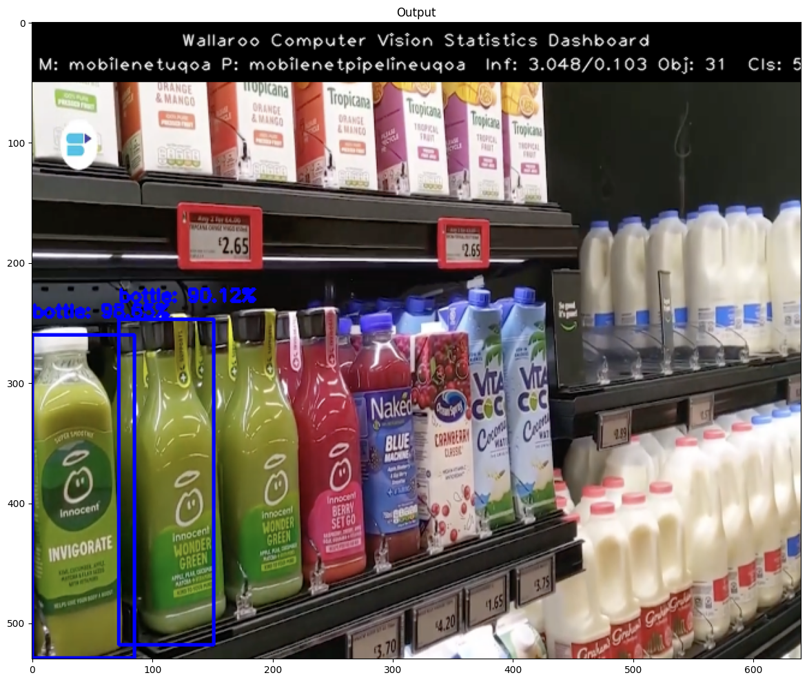
Extract the Inference Information
To show what is going on in the background, we’ll extract the inference results create a dataframe with columns representing the classification, confidence, and bounding boxes of the objects identified.
idx = 0
for idx in range(0,len(classes)):
df['classification'][idx] = cvDemo.CLASSES[classes[idx]] # Classes contains the 80 different COCO classificaitons
df['confidence'][idx] = confidences[idx]
df
| classification | confidence | x | y | width | height | |
|---|---|---|---|---|---|---|
| 0 | bottle | 98.65% | 0 | 210 | 85 | 479 |
| 1 | bottle | 90.12% | 72 | 197 | 151 | 468 |
| 2 | bottle | 60.78% | 211 | 184 | 277 | 420 |
| 3 | bottle | 59.22% | 143 | 203 | 216 | 448 |
| 4 | refrigerator | 53.73% | 13 | 41 | 640 | 480 |
| 5 | bottle | 45.13% | 106 | 206 | 159 | 463 |
| 6 | bottle | 43.73% | 278 | 1 | 321 | 93 |
| 7 | bottle | 43.09% | 462 | 104 | 510 | 224 |
| 8 | bottle | 40.85% | 310 | 1 | 352 | 94 |
| 9 | bottle | 39.19% | 528 | 268 | 636 | 475 |
| 10 | bottle | 35.76% | 220 | 0 | 258 | 90 |
| 11 | bottle | 31.81% | 552 | 96 | 600 | 233 |
| 12 | bottle | 26.45% | 349 | 0 | 404 | 98 |
| 13 | bottle | 23.06% | 450 | 264 | 619 | 472 |
| 14 | bottle | 20.48% | 261 | 193 | 307 | 408 |
| 15 | bottle | 17.46% | 509 | 101 | 544 | 235 |
| 16 | bottle | 17.31% | 592 | 100 | 633 | 239 |
| 17 | bottle | 16.00% | 475 | 297 | 551 | 468 |
| 18 | bottle | 14.91% | 368 | 163 | 423 | 362 |
| 19 | book | 13.66% | 120 | 0 | 175 | 81 |
| 20 | book | 13.32% | 72 | 0 | 143 | 85 |
| 21 | bottle | 12.22% | 271 | 200 | 305 | 274 |
| 22 | book | 12.13% | 161 | 0 | 213 | 85 |
| 23 | bottle | 11.96% | 162 | 0 | 214 | 83 |
| 24 | bottle | 11.53% | 310 | 190 | 367 | 397 |
| 25 | bottle | 9.62% | 396 | 166 | 441 | 360 |
| 26 | cake | 8.65% | 439 | 256 | 640 | 473 |
| 27 | bottle | 7.84% | 544 | 375 | 636 | 472 |
| 28 | vase | 7.23% | 272 | 2 | 306 | 96 |
| 29 | bottle | 6.28% | 453 | 303 | 524 | 463 |
| 30 | bottle | 5.28% | 609 | 94 | 635 | 211 |
Undeploy the Pipeline
With the inference complete, we can undeploy the pipeline and return the resources back to the Wallaroo instance.
pipeline.undeploy()
| name | mobilenetpipeline |
|---|---|
| created | 2023-10-30 18:15:17.969988+00:00 |
| last_updated | 2023-10-30 18:15:25.186553+00:00 |
| deployed | False |
| arch | None |
| tags | |
| versions | 7a1d84f9-13f7-405a-a4d0-5ec7de59f03e, b236b83b-1755-41d9-a2ae-804c040b9038 |
| steps | mobilenet |
| published | False |
4.2.2 - Step 02: Detecting Objects Using resnet50
This tutorial and the assets can be downloaded as part of the Wallaroo Tutorials repository.
Step 02: Detecting Objects Using resnet50
The following tutorial demonstrates how to use a trained mobilenet model deployed in Wallaroo to detect objects. This process will use the following steps:
- Create a Wallaroo workspace and pipeline.
- Upload a trained resnet50 ML model and add it as a pipeline step.
- Deploy the pipeline.
- Perform an inference on a sample image.
- Draw the detected objects, their bounding boxes, their classifications, and the confidence of the classifications on the provided image.
- Review our results.
Steps
Import Libraries
The first step will be to import our libraries. Please check with Step 00: Introduction and Setup and verify that the necessary libraries and applications are added to your environment.
import torch
import pickle
import wallaroo
from wallaroo.object import EntityNotFoundError
from wallaroo.framework import Framework
import numpy as np
import json
import requests
import time
import pandas as pd
from CVDemoUtils import CVDemo
# used to display dataframe information without truncating
from IPython.display import display
import pandas as pd
pd.set_option('display.max_colwidth', None)
# used for unique connection names
import string
import random
suffix= ''.join(random.choice(string.ascii_lowercase) for i in range(4))
Connect to the Wallaroo Instance
The first step is to connect to Wallaroo through the Wallaroo client. The Python library is included in the Wallaroo install and available through the Jupyter Hub interface provided with your Wallaroo environment.
This is accomplished using the wallaroo.Client() command, which provides a URL to grant the SDK permission to your specific Wallaroo environment. When displayed, enter the URL into a browser and confirm permissions. Store the connection into a variable that can be referenced later.
If logging into the Wallaroo instance through the internal JupyterHub service, use wl = wallaroo.Client(). For more information on Wallaroo Client settings, see the Client Connection guide.
# Login through local service
wl = wallaroo.Client()
wl = wallaroo.Client()
Set Variables
The following variables and methods are used later to create or connect to an existing workspace, pipeline, and model. This example has both the resnet model, and a post process script.
workspace_name = f'resnetworkspace{suffix}'
pipeline_name = f'resnetnetpipeline{suffix}'
model_name = f'resnet50{suffix}'
model_file_name = 'models/frcnn-resnet.pt.onnx'
def get_workspace(name):
workspace = None
for ws in wl.list_workspaces():
if ws.name() == name:
workspace= ws
if(workspace == None):
workspace = wl.create_workspace(name)
return workspace
def get_pipeline(name):
try:
pipeline = wl.pipelines_by_name(name)[0]
except EntityNotFoundError:
pipeline = wl.build_pipeline(name)
return pipeline
Create Workspace
The workspace will be created or connected to, and set as the default workspace for this session. Once that is done, then all models and pipelines will be set in that workspace.
workspace = get_workspace(workspace_name)
wl.set_current_workspace(workspace)
wl.get_current_workspace()
{'name': 'resnetworkspacestck', 'id': 9, 'archived': False, 'created_by': '6236ad2a-7eb8-4bbc-a8c9-39ce92767bad', 'created_at': '2023-10-24T16:52:27.179962+00:00', 'models': [], 'pipelines': []}
Create Pipeline and Upload Model
We will now create or connect to an existing pipeline as named in the variables above.
pipeline = get_pipeline(pipeline_name)
resnet_model = wl.upload_model(model_name, model_file_name, framework=Framework.ONNX).configure(batch_config="single", tensor_fields=["tensor"])
Deploy Pipeline
With the model uploaded, we can add it is as a step in the pipeline, then deploy it. Once deployed, resources from the Wallaroo instance will be reserved and the pipeline will be ready to use the model to perform inference requests.
pipeline.add_model_step(resnet_model)
| name | resnetnetpipelinestck |
|---|---|
| created | 2023-10-24 16:52:29.027087+00:00 |
| last_updated | 2023-10-24 16:52:29.027087+00:00 |
| deployed | (none) |
| tags | |
| versions | 6e3874c5-e1bb-4847-a60d-2c42b7bc0a7e |
| steps | |
| published | False |
pipeline.deploy()
| name | resnetnetpipelinestck |
|---|---|
| created | 2023-10-24 16:52:29.027087+00:00 |
| last_updated | 2023-10-24 16:52:40.680056+00:00 |
| deployed | True |
| tags | |
| versions | 52cb9d23-29cc-431f-9b08-d95d337b5bea, 6e3874c5-e1bb-4847-a60d-2c42b7bc0a7e |
| steps | resnet50stck |
| published | False |
Test the pipeline by running inference on a sample image
Prepare input image
Next we will load a sample image and resize it to the width and height required for the object detector.
We will convert the image to a numpy ndim array and add it do a dictionary
#The size the image will be resized to
width = 640
height = 480
cvDemo = CVDemo()
imagePath = 'data/images/input/example/dairy_bottles.png'
# The image width and height needs to be set to what the model was trained for. In this case 640x480.
tensor, resizedImage = cvDemo.loadImageAndResize(imagePath, width, height)
# get npArray from the tensorFloat
npArray = tensor.cpu().numpy()
dictData = {"tensor":[npArray]}
dataframedata = pd.DataFrame(dictData)
Run Inference
With that done, we can have the model detect the objects on the image by running an inference through the pipeline, and storing the results for the next step.
IMPORTANT NOTE: If necessary, add timeout=60 to the infer method if more time is needed to upload the data file for the inference request.
startTime = time.time()
# pass the dataframe in
# infResults = pipeline.infer(dataframedata, dataset=["*", "metadata.elapsed"])
infResults = pipeline.infer_from_file('./data/dairy_bottles.df.json', dataset=["*", "metadata.elapsed"])
endTime = time.time()
Draw the Inference Results
With our inference results, we can take them and use the Wallaroo CVDemo class and draw them onto the original image. The bounding boxes and the confidence value will only be drawn on images where the model returned a 50% confidence rate in the object’s identity.
df = pd.DataFrame(columns=['classification','confidence','x','y','width','height'])
pd.options.mode.chained_assignment = None # default='warn'
pd.options.display.float_format = '{:.2%}'.format
# Points to where all the inference results are
boxList = infResults.loc[0]["out.boxes"]
# # reshape this to an array of bounding box coordinates converted to ints
boxA = np.array(boxList)
boxes = boxA.reshape(-1, 4)
boxes = boxes.astype(int)
df[['x', 'y','width','height']] = pd.DataFrame(boxes)
classes = infResults.loc[0]["out.classes"]
confidences = infResults.loc[0]["out.confidences"]
infResults = {
'model_name' : model_name,
'pipeline_name' : pipeline_name,
'width': width,
'height': height,
'image' : resizedImage,
'boxes' : boxes,
'classes' : classes,
'confidences' : confidences,
'confidence-target' : 0.90,
'inference-time': (endTime-startTime),
'onnx-time' : int(infResults.loc[0]["metadata.elapsed"][1]) / 1e+9,
'color':(255,0,0)
}
image = cvDemo.drawAndDisplayDetectedObjectsWithClassification(infResults)
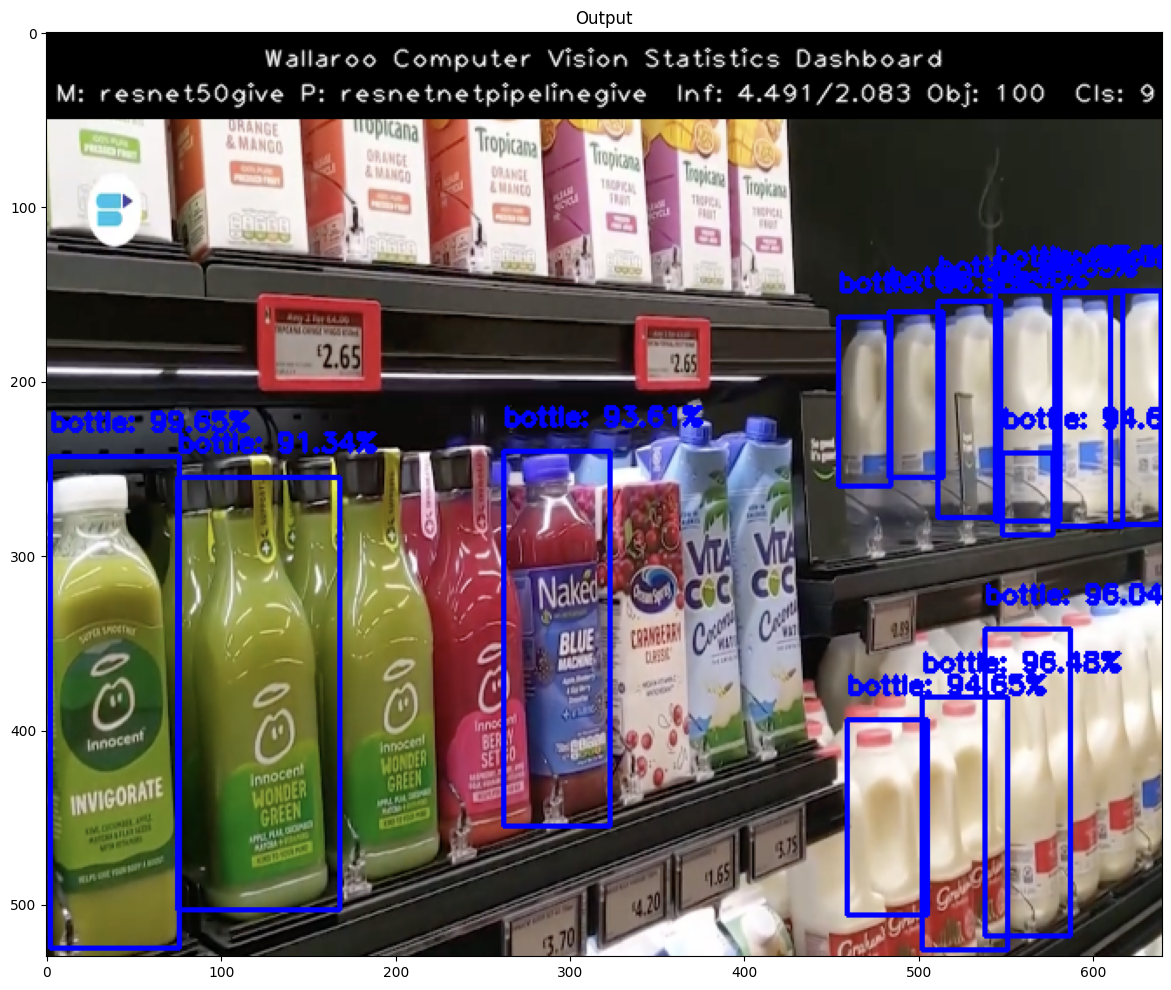
Extract the Inference Information
To show what is going on in the background, we’ll extract the inference results create a dataframe with columns representing the classification, confidence, and bounding boxes of the objects identified.
idx = 0
for idx in range(0,len(classes)):
cocoClasses = cvDemo.getCocoClasses()
df['classification'][idx] = cocoClasses[classes[idx]] # Classes contains the 80 different COCO classificaitons
df['confidence'][idx] = confidences[idx]
df
| classification | confidence | x | y | width | height | |
|---|---|---|---|---|---|---|
| 0 | bottle | 99.65% | 2 | 193 | 76 | 475 |
| 1 | bottle | 98.83% | 610 | 98 | 639 | 232 |
| 2 | bottle | 97.00% | 544 | 98 | 581 | 230 |
| 3 | bottle | 96.96% | 454 | 113 | 484 | 210 |
| 4 | bottle | 96.48% | 502 | 331 | 551 | 476 |
| ... | ... | ... | ... | ... | ... | ... |
| 95 | bottle | 5.72% | 556 | 287 | 580 | 322 |
| 96 | refrigerator | 5.66% | 80 | 161 | 638 | 480 |
| 97 | bottle | 5.60% | 455 | 334 | 480 | 349 |
| 98 | bottle | 5.46% | 613 | 267 | 635 | 375 |
| 99 | bottle | 5.37% | 345 | 2 | 395 | 99 |
100 rows × 6 columns
Undeploy the Pipeline
With the inference complete, we can undeploy the pipeline and return the resources back to the Wallaroo instance.
pipeline.undeploy()
| name | resnetnetpipelinestck |
|---|---|
| created | 2023-10-24 16:52:29.027087+00:00 |
| last_updated | 2023-10-24 16:52:40.680056+00:00 |
| deployed | False |
| tags | |
| versions | 52cb9d23-29cc-431f-9b08-d95d337b5bea, 6e3874c5-e1bb-4847-a60d-2c42b7bc0a7e |
| steps | resnet50stck |
| published | False |
4.2.3 - Step 03: mobilenet and resnet50 Shadow Deploy
This tutorial and the assets can be downloaded as part of the Wallaroo Tutorials repository.
Step 03: Detecting Objects Using Shadow Deploy
The following tutorial demonstrates how to use two trained models, one based on the resnet50, the other on mobilenet, deployed in Wallaroo to detect objects. This builds on the previous tutorials in this series, Step 01: Detecting Objects Using mobilenet" and “Step 02: Detecting Objects Using resnet50”.
For this tutorial, the Wallaroo feature Shadow Deploy will be used to submit inference requests to both models at once. The mobilnet object detector is the control and the faster-rcnn object detector is the challenger. The results between the two will be compared for their confidence, and that confidence will be used to draw bounding boxes around identified objects.
This process will use the following steps:
- Create a Wallaroo workspace and pipeline.
- Upload a trained resnet50 ML model and trained mobilenet model and add them as a shadow deployed step with the mobilenet as the control model.
- Deploy the pipeline.
- Perform an inference on a sample image.
- Based on the
- Draw the detected objects, their bounding boxes, their classifications, and the confidence of the classifications on the provided image.
- Review our results.
Steps
Import Libraries
The first step will be to import our libraries. Please check with Step 00: Introduction and Setup and verify that the necessary libraries and applications are added to your environment.
import torch
import pickle
import wallaroo
from wallaroo.object import EntityNotFoundError
from wallaroo.framework import Framework
import numpy as np
import json
import requests
import time
import pandas as pd
from CVDemoUtils import CVDemo
# used to display dataframe information without truncating
from IPython.display import display
import pandas as pd
pd.set_option('display.max_colwidth', None)
# used for unique connection names
import string
import random
suffix= ''.join(random.choice(string.ascii_lowercase) for i in range(4))
Connect to the Wallaroo Instance
The first step is to connect to Wallaroo through the Wallaroo client. The Python library is included in the Wallaroo install and available through the Jupyter Hub interface provided with your Wallaroo environment.
This is accomplished using the wallaroo.Client() command, which provides a URL to grant the SDK permission to your specific Wallaroo environment. When displayed, enter the URL into a browser and confirm permissions. Store the connection into a variable that can be referenced later.
If logging into the Wallaroo instance through the internal JupyterHub service, use wl = wallaroo.Client(). For more information on Wallaroo Client settings, see the Client Connection guide.
# Login through local service
wl = wallaroo.Client()
wl = wallaroo.Client()
Set Variables
The following variables and methods are used later to create or connect to an existing workspace, pipeline, and model. This example has both the resnet model, and a post process script.
workspace_name = f'shadowimageworkspacetest{suffix}'
pipeline_name = f'shadowimagepipelinetest{suffix}'
control_model_name = f'mobilenet{suffix}'
control_model_file_name = 'models/mobilenet.pt.onnx'
challenger_model_name = f'resnet50{suffix}'
challenger_model_file_name = 'models/frcnn-resnet.pt.onnx'
def get_workspace(name):
workspace = None
for ws in wl.list_workspaces():
if ws.name() == name:
workspace= ws
if(workspace == None):
workspace = wl.create_workspace(name)
return workspace
def get_pipeline(name):
try:
pipeline = wl.pipelines_by_name(name)[0]
except EntityNotFoundError:
pipeline = wl.build_pipeline(name)
return pipeline
Create Workspace
The workspace will be created or connected to, and set as the default workspace for this session. Once that is done, then all models and pipelines will be set in that workspace.
workspace = get_workspace(workspace_name)
wl.set_current_workspace(workspace)
wl.get_current_workspace()
{'name': 'shadowimageworkspacetestkpld', 'id': 10, 'archived': False, 'created_by': '6236ad2a-7eb8-4bbc-a8c9-39ce92767bad', 'created_at': '2023-10-24T17:05:03.040658+00:00', 'models': [], 'pipelines': []}
Create Pipeline and Upload Model
We will now create or connect to an existing pipeline as named in the variables above, then upload each of the models.
pipeline = get_pipeline(pipeline_name)
control = wl.upload_model(control_model_name, control_model_file_name, framework=Framework.ONNX).configure(batch_config="single", tensor_fields=["tensor"])
challenger = wl.upload_model(challenger_model_name, challenger_model_file_name, framework=Framework.ONNX).configure(batch_config="single", tensor_fields=["tensor"])
Shadow Deploy Pipeline
For this step, rather than deploying each model into a separate step, both will be deployed into a single step as a Shadow Deploy step. This will take the inference input data and process it through both pipelines at the same time. The inference results for the control will be stored in it’s ['outputs'] array, while the results for the challenger are stored the ['shadow_data'] array.
pipeline.add_shadow_deploy(control, [challenger])
| name | shadowimagepipelinetestkpld |
|---|---|
| created | 2023-10-24 17:05:04.926467+00:00 |
| last_updated | 2023-10-24 17:05:04.926467+00:00 |
| deployed | (none) |
| tags | |
| versions | 2f6bee8b-bf31-41cf-b7d2-d4912bfdcca8 |
| steps | |
| published | False |
pipeline.deploy()
| name | shadowimagepipelinetestkpld |
|---|---|
| created | 2023-10-24 17:05:04.926467+00:00 |
| last_updated | 2023-10-24 17:05:22.613731+00:00 |
| deployed | True |
| tags | |
| versions | 433aa539-cb64-4733-85d3-68f6f769dd36, 2f6bee8b-bf31-41cf-b7d2-d4912bfdcca8 |
| steps | mobilenetkpld |
| published | False |
pipeline.status()
{'status': 'Running',
'details': [],
'engines': [{'ip': '10.244.3.35',
'name': 'engine-5888d5b5d6-2dvlb',
'status': 'Running',
'reason': None,
'details': [],
'pipeline_statuses': {'pipelines': [{'id': 'shadowimagepipelinetestkpld',
'status': 'Running'}]},
'model_statuses': {'models': [{'name': 'mobilenetkpld',
'version': 'be97c0ef-afb1-4835-9f94-ec6534fa9c07',
'sha': '9044c970ee061cc47e0c77e20b05e884be37f2a20aa9c0c3ce1993dbd486a830',
'status': 'Running'},
{'name': 'resnet50kpld',
'version': 'f0967b5f-4b17-4dbd-b1d6-49b3339f041b',
'sha': '43326e50af639105c81372346fb9ddf453fea0fe46648b2053c375360d9c1647',
'status': 'Running'}]}}],
'engine_lbs': [{'ip': '10.244.4.58',
'name': 'engine-lb-584f54c899-hl4lx',
'status': 'Running',
'reason': None,
'details': []}],
'sidekicks': []}
Prepare input image
Next we will load a sample image and resize it to the width and height required for the object detector.
We will convert the image to a numpy ndim array and add it do a dictionary
imagePath = 'data/images/input/example/store-front.png'
# The image width and height needs to be set to what the model was trained for. In this case 640x480.
cvDemo = CVDemo()
# The size the image will be resized to meet the input requirements of the object detector
width = 640
height = 480
tensor, controlImage = cvDemo.loadImageAndResize(imagePath, width, height)
challengerImage = controlImage.copy()
# get npArray from the tensorFloat
npArray = tensor.cpu().numpy()
#creates a dictionary with the wallaroo "tensor" key and the numpy ndim array representing image as the value.
# dictData = {"tensor": npArray.tolist()}
dictData = {"tensor":[npArray]}
dataframedata = pd.DataFrame(dictData)
Run Inference using Shadow Deployment
Now lets have the model detect the objects on the image by running inference and extracting the results
startTime = time.time()
infResults = pipeline.infer_from_file('./data/dairy_bottles.df.json', dataset=["*", "metadata.elapsed"])
#infResults = pipeline.infer(dataframedata, dataset=["*", "metadata.elapsed"])
endTime = time.time()
Extract Control Inference Results
First we’ll extract the inference result data for the control model and map it onto the image.
df = pd.DataFrame(columns=['classification','confidence','x','y','width','height'])
pd.options.mode.chained_assignment = None # default='warn'
pd.options.display.float_format = '{:.2%}'.format
# Points to where all the inference results are
# boxList = infResults[0]["out.output"]
boxList = infResults.loc[0]["out.boxes"]
# # reshape this to an array of bounding box coordinates converted to ints
boxA = np.array(boxList)
controlBoxes = boxA.reshape(-1, 4)
controlBoxes = controlBoxes.astype(int)
df[['x', 'y','width','height']] = pd.DataFrame(controlBoxes)
controlClasses = infResults.loc[0]["out.classes"]
controlConfidences = infResults.loc[0]["out.confidences"]
results = {
'model_name' : control.name(),
'pipeline_name' : pipeline.name(),
'width': width,
'height': height,
'image' : controlImage,
'boxes' : controlBoxes,
'classes' : controlClasses,
'confidences' : controlConfidences,
'confidence-target' : 0.9,
'color':CVDemo.RED, # color to draw bounding boxes and the text in the statistics
'inference-time': (endTime-startTime),
'onnx-time' : 0,
}
cvDemo.drawAndDisplayDetectedObjectsWithClassification(results)
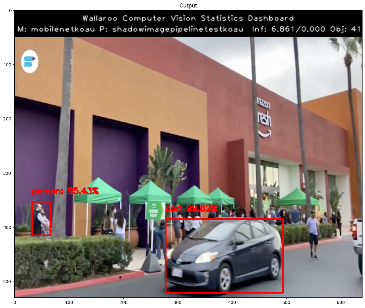
Display the Control Results
Here we will use the Wallaroo CVDemo helper class to draw the control model results on the image.
The full results will be displayed in a dataframe with columns representing the classification, confidence, and bounding boxes of the objects identified.
Once extracted from the results we will want to reshape the flattened array into an array with 4 elements (x,y,width,height).
idx = 0
cocoClasses = cvDemo.getCocoClasses()
for idx in range(0,len(controlClasses)):
df['classification'][idx] = cocoClasses[controlClasses[idx]] # Classes contains the 80 different COCO classificaitons
df['confidence'][idx] = controlConfidences[idx]
df
| classification | confidence | x | y | width | height | |
|---|---|---|---|---|---|---|
| 0 | bottle | 98.65% | 0 | 210 | 85 | 479 |
| 1 | bottle | 90.12% | 72 | 197 | 151 | 468 |
| 2 | bottle | 60.78% | 211 | 184 | 277 | 420 |
| 3 | bottle | 59.22% | 143 | 203 | 216 | 448 |
| 4 | refrigerator | 53.73% | 13 | 41 | 640 | 480 |
| 5 | bottle | 45.13% | 106 | 206 | 159 | 463 |
| 6 | bottle | 43.73% | 278 | 1 | 321 | 93 |
| 7 | bottle | 43.09% | 462 | 104 | 510 | 224 |
| 8 | bottle | 40.85% | 310 | 1 | 352 | 94 |
| 9 | bottle | 39.19% | 528 | 268 | 636 | 475 |
| 10 | bottle | 35.76% | 220 | 0 | 258 | 90 |
| 11 | bottle | 31.81% | 552 | 96 | 600 | 233 |
| 12 | bottle | 26.45% | 349 | 0 | 404 | 98 |
| 13 | bottle | 23.06% | 450 | 264 | 619 | 472 |
| 14 | bottle | 20.48% | 261 | 193 | 307 | 408 |
| 15 | bottle | 17.46% | 509 | 101 | 544 | 235 |
| 16 | bottle | 17.31% | 592 | 100 | 633 | 239 |
| 17 | bottle | 16.00% | 475 | 297 | 551 | 468 |
| 18 | bottle | 14.91% | 368 | 163 | 423 | 362 |
| 19 | book | 13.66% | 120 | 0 | 175 | 81 |
| 20 | book | 13.32% | 72 | 0 | 143 | 85 |
| 21 | bottle | 12.22% | 271 | 200 | 305 | 274 |
| 22 | book | 12.13% | 161 | 0 | 213 | 85 |
| 23 | bottle | 11.96% | 162 | 0 | 214 | 83 |
| 24 | bottle | 11.53% | 310 | 190 | 367 | 397 |
| 25 | bottle | 9.62% | 396 | 166 | 441 | 360 |
| 26 | cake | 8.65% | 439 | 256 | 640 | 473 |
| 27 | bottle | 7.84% | 544 | 375 | 636 | 472 |
| 28 | vase | 7.23% | 272 | 2 | 306 | 96 |
| 29 | bottle | 6.28% | 453 | 303 | 524 | 463 |
| 30 | bottle | 5.28% | 609 | 94 | 635 | 211 |
Display the Challenger Results
Here we will use the Wallaroo CVDemo helper class to draw the challenger model results on the input image.
challengerDf = pd.DataFrame(columns=['classification','confidence','x','y','width','height'])
pd.options.mode.chained_assignment = None # default='warn'
pd.options.display.float_format = '{:.2%}'.format
# Points to where all the inference results are
boxList = infResults.loc[0][f"out_{challenger_model_name}.boxes"]
# outputs = results['outputs']
# boxes = outputs[0]
# # reshape this to an array of bounding box coordinates converted to ints
# boxList = boxes['Float']['data']
boxA = np.array(boxList)
challengerBoxes = boxA.reshape(-1, 4)
challengerBoxes = challengerBoxes.astype(int)
challengerDf[['x', 'y','width','height']] = pd.DataFrame(challengerBoxes)
challengerClasses = infResults.loc[0][f"out_{challenger_model_name}.classes"]
challengerConfidences = infResults.loc[0][f"out_{challenger_model_name}.confidences"]
results = {
'model_name' : challenger.name(),
'pipeline_name' : pipeline.name(),
'width': width,
'height': height,
'image' : challengerImage,
'boxes' : challengerBoxes,
'classes' : challengerClasses,
'confidences' : challengerConfidences,
'confidence-target' : 0.9,
'color':CVDemo.RED, # color to draw bounding boxes and the text in the statistics
'inference-time': (endTime-startTime),
'onnx-time' : 0,
}
cvDemo.drawAndDisplayDetectedObjectsWithClassification(results)
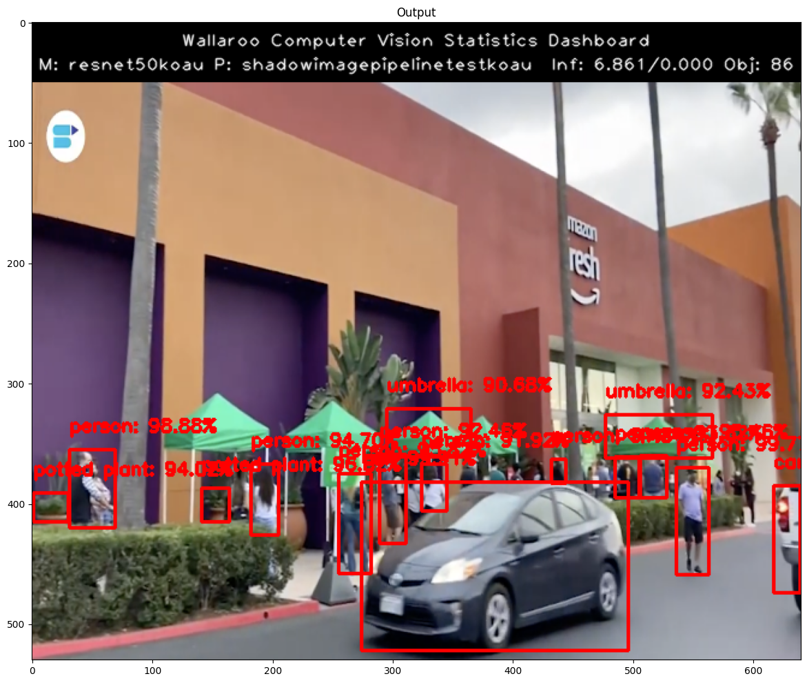
Display Challenger Results
The inference results for the objects detected by the challenger model will be displayed including the confidence values. Once extracted from the results we will want to reshape the flattened array into an array with 4 elements (x,y,width,height).
idx = 0
for idx in range(0,len(challengerClasses)):
challengerDf['classification'][idx] = cvDemo.CLASSES[challengerClasses[idx]] # Classes contains the 80 different COCO classificaitons
challengerDf['confidence'][idx] = challengerConfidences[idx]
challengerDf
| classification | confidence | x | y | width | height | |
|---|---|---|---|---|---|---|
| 0 | bottle | 99.65% | 2 | 193 | 76 | 475 |
| 1 | bottle | 98.83% | 610 | 98 | 639 | 232 |
| 2 | bottle | 97.00% | 544 | 98 | 581 | 230 |
| 3 | bottle | 96.96% | 454 | 113 | 484 | 210 |
| 4 | bottle | 96.48% | 502 | 331 | 551 | 476 |
| ... | ... | ... | ... | ... | ... | ... |
| 95 | bottle | 5.72% | 556 | 287 | 580 | 322 |
| 96 | refrigerator | 5.66% | 80 | 161 | 638 | 480 |
| 97 | bottle | 5.60% | 455 | 334 | 480 | 349 |
| 98 | bottle | 5.46% | 613 | 267 | 635 | 375 |
| 99 | bottle | 5.37% | 345 | 2 | 395 | 99 |
100 rows × 6 columns
pipeline.undeploy()
| name | shadowimagepipelinetestkpld |
|---|---|
| created | 2023-10-24 17:05:04.926467+00:00 |
| last_updated | 2023-10-24 17:05:22.613731+00:00 |
| deployed | False |
| tags | |
| versions | 433aa539-cb64-4733-85d3-68f6f769dd36, 2f6bee8b-bf31-41cf-b7d2-d4912bfdcca8 |
| steps | mobilenetkpld |
| published | False |
Conclusion
Notice the difference in the control confidence and the challenger confidence. Clearly we can see in this example the challenger resnet50 model is performing better than the control mobilenet model. This is likely due to the fact that frcnn resnet50 model is a 2 stage object detector vs the frcnn mobilenet is a single stage detector.
This completes using Wallaroo’s shadow deployment feature to compare different computer vision models.
4.3 - Computer Vision: Yolov8n Demonstration
How to use Wallaroo with the Yolov8n computer vision model to detect objects in images.
The following tutorial is available on the Wallaroo Github Repository.
Computer Vision Yolov8n Deployment in Wallaroo
The Yolov8 computer vision model is used for fast recognition of objects in images. This tutorial demonstrates how to deploy a Yolov8n pre-trained model into a Wallaroo Ops server and perform inferences on it.
For this tutorial, the helper module CVDemoUtils and WallarooUtils are used to transform a sample image into a pandas DataFrame. This DataFrame is then submitted to the Yolov8n model deployed in Wallaroo.
This demonstration follows these steps:
- Upload the Yolo8 model to Wallaroo
- Add the Yolo8 model as a Wallaroo pipeline step
- Deploy the Wallaroo pipeline and allocate cluster resources to the pipeline
- Perform sample inferences
- Undeploy and return the resources
References
- Wallaroo Workspaces: Workspaces are environments were users upload models, create pipelines and other artifacts. The workspace should be considered the fundamental area where work is done. Workspaces are shared with other users to give them access to the same models, pipelines, etc.
- Wallaroo Model Upload and Registration: ML Models are uploaded to Wallaroo through the SDK or the MLOps API to a workspace. ML models include default runtimes (ONNX, Python Step, and TensorFlow) that are run directly through the Wallaroo engine, and containerized runtimes (Hugging Face, PyTorch, etc) that are run through in a container through the Wallaroo engine.
- Wallaroo Pipelines: Pipelines are used to deploy models for inferencing. Each model is a pipeline step in a pipelines, where the inputs of the previous step are fed into the next. Pipeline steps can be ML models, Python scripts, or Arbitrary Python (these contain necessary models and artifacts for running a model).
Steps
Load Libraries
The first step is loading the required libraries including the Wallaroo Python module.
# Import Wallaroo Python SDK
import wallaroo
from wallaroo.object import EntityNotFoundError
from wallaroo.framework import Framework
from CVDemoUtils import CVDemo
from WallarooUtils import Util
cvDemo = CVDemo()
util = Util()
# used to display DataFrame information without truncating
from IPython.display import display
import pandas as pd
pd.set_option('display.max_colwidth', None)
Connect to the Wallaroo Instance through the User Interface
The next step is to connect to Wallaroo through the Wallaroo client. The Python library is included in the Wallaroo install and available through the Jupyter Hub interface provided with your Wallaroo environment.
This is accomplished using the wallaroo.Client() command, which provides a URL to grant the SDK permission to your specific Wallaroo environment. When displayed, enter the URL into a browser and confirm permissions. Store the connection into a variable that can be referenced later.
If logging into the Wallaroo instance through the internal JupyterHub service, use wl = wallaroo.Client(). For more information on Wallaroo Client settings, see the Client Connection guide.
wl = wallaroo.Client()
Create a New Workspace
We’ll use the SDK below to create our workspace , assign as our current workspace, then display all of the workspaces we have at the moment. We’ll also set up variables for our models and pipelines down the road, so we have one spot to change names to whatever fits your organization’s standards best.
To allow this tutorial to be run by multiple users in the same Wallaroo instance, a random 4 character prefix will be added to the workspace, pipeline, and model. Feel free to set suffix='' if this is not required.
# import string
# import random
# # make a random 4 character suffix to verify uniqueness in tutorials
# suffix= ''.join(random.choice(string.ascii_lowercase) for i in range(4))
suffix = ''
model_name = 'yolov8n'
model_filename = 'models/yolov8n.onnx'
pipeline_name = 'yolo8demonstration'
workspace_name = f'yolo8-demonstration{suffix}'
def get_workspace(name):
workspace = None
for ws in wl.list_workspaces():
if ws.name() == name:
workspace= ws
if(workspace == None):
workspace = wl.create_workspace(name)
return workspace
Upload the Model
When a model is uploaded to a Wallaroo cluster, it is optimized and packaged to make it ready to run as part of a pipeline. In many times, the Wallaroo Server can natively run a model without any Python overhead. In other cases, such as a Python script, a custom Python environment will be automatically generated. This is comparable to the process of “containerizing” a model by adding a small HTTP server and other wrapping around it.
Our pretrained model is in ONNX format, which is specified in the framework parameter. For this model, the tensor fields are set to images to match the input parameters, and the batch configuration is set to single - only one record will be submitted at a time.
# Upload Retrained Yolo8 Model
yolov8_model = (wl.upload_model(model_name,
model_filename,
framework=Framework.ONNX)
.configure(tensor_fields=['images'],
batch_config="single"
)
)
Pipeline Deployment Configuration
For our pipeline we set the deployment configuration to only use 1 cpu and 1 GiB of RAM.
deployment_config = wallaroo.DeploymentConfigBuilder() \
.replica_count(1) \
.cpus(1) \
.memory("1Gi") \
.build()
Build and Deploy the Pipeline
Now we build our pipeline and set our Yolo8 model as a pipeline step, then deploy the pipeline using the deployment configuration above.
pipeline = wl.build_pipeline(pipeline_name) \
.add_model_step(yolov8_model)
pipeline.deploy(deployment_config=deployment_config)
| name | yolo8demonstration |
|---|---|
| created | 2023-10-19 15:33:26.144685+00:00 |
| last_updated | 2023-10-19 15:33:27.154726+00:00 |
| deployed | True |
| tags | |
| versions | 39b02242-de8b-46cd-849e-8a896226a84a, bed60f2a-ddd6-4a48-a9fd-debe6b1e1bca |
| steps | yolov8n |
| published | False |
Convert Image to DataFrame
The sample image dogbike.png was converted to a DataFrame using the cvDemo helper modules. The converted DataFrame is stored as ./data/dogbike.df.json to save time.
The code sample below demonstrates how to use this module to convert the sample image to a DataFrame.
# convert the image to a tensor
width, height = 640, 640
tensor1, resizedImage1 = cvDemo.loadImageAndResize('dogbike.png', width, height)
tensor1.flatten()
# add the tensor to a DataFrame and save the DataFrame in pandas record format
df = util.convert_data(tensor1,'images')
df.to_json("data.json", orient = 'records')
# convert the image to a tensor
width, height = 640, 640
tensor1, resizedImage1 = cvDemo.loadImageAndResize('./data/dogbike.png', width, height)
tensor1.flatten()
# add the tensor to a DataFrame and save the DataFrame in pandas record format
df = util.convert_data(tensor1,'images')
df.to_json("data.json", orient = 'records')
Inference Request
We submit the DataFrame to the pipeline using wallaroo.pipeline.infer_from_file, and store the results in the variable inf1.
inf1 = pipeline.infer_from_file('./data/dogbike.df.json')
Display Bounding Boxes
Using our helper method cvDemo we’ll identify the objects detected in the photo and their bounding boxes. Only objects with a confidence threshold of 50% or more are shown.
inf1.loc[:, ['out.output0']]
| out.output0 | |
|---|---|
| 0 | [17.09787, 16.459343, 17.259743, 19.960602, 43.600235, 59.986958, 62.826073, 68.24793, 77.43261, 80.82158, 89.44183, 96.168915, 99.22421, 112.584045, 126.75803, 131.9707, 137.1645, 141.93822, 146.29594, 152.00876, 155.94037, 165.20976, 175.27249, 184.05307, 193.66891, 201.51189, 215.04979, 223.80424, 227.24472, 234.19638, 244.9743, 248.5781, 252.42526, 264.95795, 278.48563, 285.758, 293.1897, 300.48227, 305.47742, 314.46085, 319.89404, 324.83658, 335.99536, 345.1116, 350.31964, 352.41107, 365.44934, 381.30008, 391.52316, 399.29163, 405.78503, 411.33804, 415.93207, 421.6868, 431.67108, 439.9069, 447.71542, 459.38522, 474.13187, 479.32642, 484.49884, 493.5153, 501.29932, 507.7967, 514.26044, 523.1473, 531.3479, 542.5094, 555.619, 557.7229, 564.6408, 571.5525, 572.8373, 587.95703, 604.2997, 609.452, 616.31714, 623.5797, 624.13153, 634.47266, 16.970057, 16.788723, 17.441803, 17.900642, 36.188023, 57.277973, 61.664352, 62.556896, 63.43486, 79.50621, 83.844, 95.983765, 106.166, 115.368454, 123.09253, 124.5821, 128.65866, 139.16113, 142.02315, 143.69855, ...] |
confidence_thres = 0.50
iou_thres = 0.25
cvDemo.drawYolo8Boxes(inf1, resizedImage1, width, height, confidence_thres, iou_thres, draw=True)
Score: 86.47% | Class: Dog | Bounding Box: [108, 250, 149, 356]
Score: 81.13% | Class: Bicycle | Bounding Box: [97, 149, 375, 323]
Score: 63.16% | Class: Car | Bounding Box: [390, 85, 186, 108]
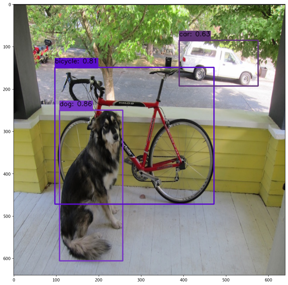
array([[[ 34, 34, 34],
[ 35, 35, 35],
[ 33, 33, 33],
...,
[ 33, 33, 33],
[ 33, 33, 33],
[ 35, 35, 35]],
[[ 33, 33, 33],
[ 34, 34, 34],
[ 34, 34, 34],
...,
[ 34, 34, 34],
[ 33, 33, 33],
[ 34, 34, 34]],
[[ 53, 54, 48],
[ 54, 55, 49],
[ 54, 55, 49],
...,
[153, 178, 111],
[151, 183, 108],
[159, 176, 99]],
...,
[[159, 167, 178],
[159, 165, 177],
[158, 163, 175],
...,
[126, 127, 121],
[127, 125, 120],
[128, 120, 117]],
[[160, 168, 179],
[156, 162, 174],
[152, 157, 169],
...,
[126, 127, 121],
[129, 127, 122],
[127, 118, 116]],
[[155, 163, 174],
[155, 162, 174],
[152, 158, 170],
...,
[127, 127, 121],
[130, 126, 122],
[128, 119, 116]]], dtype=uint8)
Inference Through Pipeline API
Another method of performing an inference using the pipeline’s deployment url.
Performing an inference through an API requires the following:
- The authentication token to authorize the connection to the pipeline.
- The pipeline’s inference URL.
- Inference data to sent to the pipeline - in JSON, DataFrame records format, or Apache Arrow.
Full details are available through the Wallaroo API Connection Guide on how retrieve an authorization token and perform inferences through the pipeline’s API.
For this demonstration we’ll submit the pandas record, request a pandas record as the return, and set the authorization header. The results will be stored in the file curl_response.df.
deploy_url = pipeline._deployment._url()
headers = wl.auth.auth_header()
headers['Content-Type']='application/json; format=pandas-records'
headers['Accept']='application/json; format=pandas-records'
!curl -X POST {deploy_url} \
-H "Authorization:{headers['Authorization']}" \
-H "Content-Type:application/json; format=pandas-records" \
-H "Accept:application/json; format=pandas-records" \
--data @./data/dogbike.df.json > curl_response.df
% Total % Received % Xferd Average Speed Time Time Time Current
Dload Upload Total Spent Left Speed
100 38.0M 100 22.9M 100 15.0M 5624k 3701k 0:00:04 0:00:04 --:--:-- 9334k
pipeline.undeploy()
| name | yolo8demonstration |
|---|---|
| created | 2023-10-11 14:37:32.252497+00:00 |
| last_updated | 2023-10-11 14:59:03.213137+00:00 |
| deployed | False |
| tags | |
| versions | 2a3933c4-52db-40c6-b80f-9031664fd08a, 95bbabf1-1f15-4e4b-9e67-f7730c2b2cbd, 6c672144-ed4f-4505-97eb-a5b1763af847, 7149e0bc-089b-4d57-9a0b-5d4f4a9a4097, 329e394b-5105-4dc3-b0ff-5411623fc139, 7acaea4e-6ae3-426b-9f97-5e3dcc39c48e, a8b2c009-e7b5-4b96-81b9-40447797a05f, 09952a45-2401-4ebd-8e85-c678365b64a7, d870a558-10ef-448e-b00d-068c10c7e82b, fa531e16-1706-43c4-98d9-e0dd6355fe6f, 4c0b535e-b39b-40f4-82a7-34965b2f7c2a, 3507964d-382f-4e1c-84c7-64c5e27f819c, 9971f8dd-a17b-4d6a-ab72-d786d4990fab, b92a035f-903c-4039-8303-8ceb979a53c2 |
| steps | yolov8n |
| published | False |
4.4 - Computer Vision: Image Detection for Health Care
How to use Wallaroo with computer vision models to detect mitochondria from images of cells.
This tutorial can be found on the Wallaroo Tutorials Github Repository.
Image Detection for Health Care Computer Vision Tutorial Part 00: Prerequisites
The following tutorial demonstrates how to use Wallaroo to detect mitochondria from high resolution images. For this example we will be using a high resolution 1536x2048 image that is broken down into “patches” of 256x256 images that can be quickly analyzed.
Mitochondria are known as the “powerhouse” of the cell, and having a healthy amount of mitochondria indicates that a patient has enough energy to live a healthy life, or may have underlying issues that a doctor can check for.
Scanning high resolution images of patient cells can be used to count how many mitochondria a patient has, but the process is laborious. The following ML Model is trained to examine an image of cells, then detect which structures are mitochondria. This is used to speed up the process of testing patients and determining next steps.
Prerequisites
The included TiffImagesUtils class is included in this demonstration as CVDemoUtils.py, and requires the following dependencies:
- ffmpeg
- libsm
- libxext
Internal JupyterHub Service
To install these dependencies in the Wallaroo JupyterHub service, use the following commands from a terminal shell via the following procedure:
Launch the JupyterHub Service within the Wallaroo install.
Select File->New->Terminal.
Enter the following:
sudo apt-get updatesudo apt-get install ffmpeg libsm6 libxext6 -y
External SDK Users
For users using the Wallaroo SDK to connect with a remote Wallaroo instance, the following commands will install the required dependancies:
For Linux users, this can be installed with:
sudo apt-get update
sudo apt-get install ffmpeg libsm6 libxext6 -y
MacOS users can prepare their environments using a package manager such as Brew with the following:
brew install ffmpeg libsm libxext
### Libraries and Dependencies
1. This repository may use large file sizes for the models. If necessary, install [Git Large File Storage (LFS)](https://git-lfs.com) or use the [Wallaroo Tutorials Releases](https://github.com/WallarooLabs/Wallaroo_Tutorials/releases) to download a .zip file of the most recent computer vision tutorial that includes the models.
1. Import the following Python libraries into your environment:
1. [torch](https://pypi.org/project/torch/)
1. [wallaroo](https://pypi.org/project/wallaroo/)
1. [torchvision](https://pypi.org/project/torchvision/)
1. [opencv-python](https://pypi.org/project/opencv-python/)
1. [onnx](https://pypi.org/project/onnx/)
1. [onnxruntime](https://pypi.org/project/onnxruntime/)
1. [imutils](https://pypi.org/project/imutils/)
1. [pytz](https://pypi.org/project/pytz/)
1. [ipywidgets](https://pypi.org/project/ipywidgets/)
These can be installed by running the command below in the Wallaroo JupyterHub service. Note the use of `pip install torch --no-cache-dir` for low memory environments.
```python
!pip install torchvision==0.15.2
!pip install torch==2.0.1 --no-cache-dir
!pip install opencv-python==4.7.0.72
!pip install onnx==1.12.0
!pip install onnxruntime==1.15.0
!pip install imutils==0.5.4
!pip install pytz
!pip install ipywidgets==8.0.6
!pip install patchify==0.2.3
!pip install tifffile==2023.4.12
!pip install piexif==1.1.3
Requirement already satisfied: torchvision==0.15.2 in /opt/conda/lib/python3.9/site-packages (0.15.2)
Requirement already satisfied: requests in /opt/conda/lib/python3.9/site-packages (from torchvision==0.15.2) (2.25.1)
Requirement already satisfied: pillow!=8.3.*,>=5.3.0 in /opt/conda/lib/python3.9/site-packages (from torchvision==0.15.2) (9.2.0)
Requirement already satisfied: torch==2.0.1 in /opt/conda/lib/python3.9/site-packages (from torchvision==0.15.2) (2.0.1)
Requirement already satisfied: numpy in /opt/conda/lib/python3.9/site-packages (from torchvision==0.15.2) (1.22.3)
Requirement already satisfied: nvidia-cuda-nvrtc-cu11==11.7.99 in /opt/conda/lib/python3.9/site-packages (from torch==2.0.1->torchvision==0.15.2) (11.7.99)
Requirement already satisfied: filelock in /opt/conda/lib/python3.9/site-packages (from torch==2.0.1->torchvision==0.15.2) (3.12.0)
Requirement already satisfied: jinja2 in /opt/conda/lib/python3.9/site-packages (from torch==2.0.1->torchvision==0.15.2) (3.1.2)
Requirement already satisfied: nvidia-cufft-cu11==10.9.0.58 in /opt/conda/lib/python3.9/site-packages (from torch==2.0.1->torchvision==0.15.2) (10.9.0.58)
Requirement already satisfied: nvidia-cudnn-cu11==8.5.0.96 in /opt/conda/lib/python3.9/site-packages (from torch==2.0.1->torchvision==0.15.2) (8.5.0.96)
Requirement already satisfied: nvidia-cublas-cu11==11.10.3.66 in /opt/conda/lib/python3.9/site-packages (from torch==2.0.1->torchvision==0.15.2) (11.10.3.66)
Requirement already satisfied: nvidia-cusparse-cu11==11.7.4.91 in /opt/conda/lib/python3.9/site-packages (from torch==2.0.1->torchvision==0.15.2) (11.7.4.91)
Requirement already satisfied: networkx in /opt/conda/lib/python3.9/site-packages (from torch==2.0.1->torchvision==0.15.2) (3.1)
Requirement already satisfied: nvidia-nccl-cu11==2.14.3 in /opt/conda/lib/python3.9/site-packages (from torch==2.0.1->torchvision==0.15.2) (2.14.3)
Requirement already satisfied: nvidia-curand-cu11==10.2.10.91 in /opt/conda/lib/python3.9/site-packages (from torch==2.0.1->torchvision==0.15.2) (10.2.10.91)
Requirement already satisfied: triton==2.0.0 in /opt/conda/lib/python3.9/site-packages (from torch==2.0.1->torchvision==0.15.2) (2.0.0)
Requirement already satisfied: nvidia-nvtx-cu11==11.7.91 in /opt/conda/lib/python3.9/site-packages (from torch==2.0.1->torchvision==0.15.2) (11.7.91)
Requirement already satisfied: typing-extensions in /opt/conda/lib/python3.9/site-packages (from torch==2.0.1->torchvision==0.15.2) (4.3.0)
Requirement already satisfied: sympy in /opt/conda/lib/python3.9/site-packages (from torch==2.0.1->torchvision==0.15.2) (1.12)
Requirement already satisfied: nvidia-cusolver-cu11==11.4.0.1 in /opt/conda/lib/python3.9/site-packages (from torch==2.0.1->torchvision==0.15.2) (11.4.0.1)
Requirement already satisfied: nvidia-cuda-cupti-cu11==11.7.101 in /opt/conda/lib/python3.9/site-packages (from torch==2.0.1->torchvision==0.15.2) (11.7.101)
Requirement already satisfied: nvidia-cuda-runtime-cu11==11.7.99 in /opt/conda/lib/python3.9/site-packages (from torch==2.0.1->torchvision==0.15.2) (11.7.99)
Requirement already satisfied: wheel in /opt/conda/lib/python3.9/site-packages (from nvidia-cublas-cu11==11.10.3.66->torch==2.0.1->torchvision==0.15.2) (0.37.1)
Requirement already satisfied: setuptools in /opt/conda/lib/python3.9/site-packages (from nvidia-cublas-cu11==11.10.3.66->torch==2.0.1->torchvision==0.15.2) (62.3.2)
Requirement already satisfied: cmake in /opt/conda/lib/python3.9/site-packages (from triton==2.0.0->torch==2.0.1->torchvision==0.15.2) (3.26.4)
Requirement already satisfied: lit in /opt/conda/lib/python3.9/site-packages (from triton==2.0.0->torch==2.0.1->torchvision==0.15.2) (16.0.5.post0)
Requirement already satisfied: urllib3<1.27,>=1.21.1 in /opt/conda/lib/python3.9/site-packages (from requests->torchvision==0.15.2) (1.26.9)
Requirement already satisfied: certifi>=2017.4.17 in /opt/conda/lib/python3.9/site-packages (from requests->torchvision==0.15.2) (2022.5.18.1)
Requirement already satisfied: idna<3,>=2.5 in /opt/conda/lib/python3.9/site-packages (from requests->torchvision==0.15.2) (2.10)
Requirement already satisfied: chardet<5,>=3.0.2 in /opt/conda/lib/python3.9/site-packages (from requests->torchvision==0.15.2) (4.0.0)
Requirement already satisfied: MarkupSafe>=2.0 in /opt/conda/lib/python3.9/site-packages (from jinja2->torch==2.0.1->torchvision==0.15.2) (2.1.1)
Requirement already satisfied: mpmath>=0.19 in /opt/conda/lib/python3.9/site-packages (from sympy->torch==2.0.1->torchvision==0.15.2) (1.3.0)
Requirement already satisfied: torch==2.0.1 in /opt/conda/lib/python3.9/site-packages (2.0.1)
Requirement already satisfied: jinja2 in /opt/conda/lib/python3.9/site-packages (from torch==2.0.1) (3.1.2)
Requirement already satisfied: nvidia-cusparse-cu11==11.7.4.91 in /opt/conda/lib/python3.9/site-packages (from torch==2.0.1) (11.7.4.91)
Requirement already satisfied: networkx in /opt/conda/lib/python3.9/site-packages (from torch==2.0.1) (3.1)
Requirement already satisfied: nvidia-cuda-nvrtc-cu11==11.7.99 in /opt/conda/lib/python3.9/site-packages (from torch==2.0.1) (11.7.99)
Requirement already satisfied: nvidia-curand-cu11==10.2.10.91 in /opt/conda/lib/python3.9/site-packages (from torch==2.0.1) (10.2.10.91)
Requirement already satisfied: triton==2.0.0 in /opt/conda/lib/python3.9/site-packages (from torch==2.0.1) (2.0.0)
Requirement already satisfied: nvidia-cuda-runtime-cu11==11.7.99 in /opt/conda/lib/python3.9/site-packages (from torch==2.0.1) (11.7.99)
Requirement already satisfied: nvidia-cufft-cu11==10.9.0.58 in /opt/conda/lib/python3.9/site-packages (from torch==2.0.1) (10.9.0.58)
Requirement already satisfied: nvidia-nccl-cu11==2.14.3 in /opt/conda/lib/python3.9/site-packages (from torch==2.0.1) (2.14.3)
Requirement already satisfied: filelock in /opt/conda/lib/python3.9/site-packages (from torch==2.0.1) (3.12.0)
Requirement already satisfied: nvidia-cuda-cupti-cu11==11.7.101 in /opt/conda/lib/python3.9/site-packages (from torch==2.0.1) (11.7.101)
Requirement already satisfied: nvidia-cublas-cu11==11.10.3.66 in /opt/conda/lib/python3.9/site-packages (from torch==2.0.1) (11.10.3.66)
Requirement already satisfied: sympy in /opt/conda/lib/python3.9/site-packages (from torch==2.0.1) (1.12)
Requirement already satisfied: nvidia-cudnn-cu11==8.5.0.96 in /opt/conda/lib/python3.9/site-packages (from torch==2.0.1) (8.5.0.96)
Requirement already satisfied: nvidia-cusolver-cu11==11.4.0.1 in /opt/conda/lib/python3.9/site-packages (from torch==2.0.1) (11.4.0.1)
Requirement already satisfied: nvidia-nvtx-cu11==11.7.91 in /opt/conda/lib/python3.9/site-packages (from torch==2.0.1) (11.7.91)
Requirement already satisfied: typing-extensions in /opt/conda/lib/python3.9/site-packages (from torch==2.0.1) (4.3.0)
Requirement already satisfied: setuptools in /opt/conda/lib/python3.9/site-packages (from nvidia-cublas-cu11==11.10.3.66->torch==2.0.1) (62.3.2)
Requirement already satisfied: wheel in /opt/conda/lib/python3.9/site-packages (from nvidia-cublas-cu11==11.10.3.66->torch==2.0.1) (0.37.1)
Requirement already satisfied: cmake in /opt/conda/lib/python3.9/site-packages (from triton==2.0.0->torch==2.0.1) (3.26.4)
Requirement already satisfied: lit in /opt/conda/lib/python3.9/site-packages (from triton==2.0.0->torch==2.0.1) (16.0.5.post0)
Requirement already satisfied: MarkupSafe>=2.0 in /opt/conda/lib/python3.9/site-packages (from jinja2->torch==2.0.1) (2.1.1)
Requirement already satisfied: mpmath>=0.19 in /opt/conda/lib/python3.9/site-packages (from sympy->torch==2.0.1) (1.3.0)
Requirement already satisfied: opencv-python==4.7.0.72 in /opt/conda/lib/python3.9/site-packages (4.7.0.72)
Requirement already satisfied: numpy>=1.19.3 in /opt/conda/lib/python3.9/site-packages (from opencv-python==4.7.0.72) (1.22.3)
Requirement already satisfied: onnx==1.12.0 in /opt/conda/lib/python3.9/site-packages (1.12.0)
Requirement already satisfied: typing-extensions>=3.6.2.1 in /opt/conda/lib/python3.9/site-packages (from onnx==1.12.0) (4.3.0)
Requirement already satisfied: protobuf<=3.20.1,>=3.12.2 in /opt/conda/lib/python3.9/site-packages (from onnx==1.12.0) (3.19.5)
Requirement already satisfied: numpy>=1.16.6 in /opt/conda/lib/python3.9/site-packages (from onnx==1.12.0) (1.22.3)
Requirement already satisfied: onnxruntime==1.15.0 in /opt/conda/lib/python3.9/site-packages (1.15.0)
Requirement already satisfied: packaging in /opt/conda/lib/python3.9/site-packages (from onnxruntime==1.15.0) (21.3)
Requirement already satisfied: flatbuffers in /opt/conda/lib/python3.9/site-packages (from onnxruntime==1.15.0) (1.12)
Requirement already satisfied: protobuf in /opt/conda/lib/python3.9/site-packages (from onnxruntime==1.15.0) (3.19.5)
Requirement already satisfied: numpy>=1.21.6 in /opt/conda/lib/python3.9/site-packages (from onnxruntime==1.15.0) (1.22.3)
Requirement already satisfied: coloredlogs in /opt/conda/lib/python3.9/site-packages (from onnxruntime==1.15.0) (15.0.1)
Requirement already satisfied: sympy in /opt/conda/lib/python3.9/site-packages (from onnxruntime==1.15.0) (1.12)
Requirement already satisfied: humanfriendly>=9.1 in /opt/conda/lib/python3.9/site-packages (from coloredlogs->onnxruntime==1.15.0) (10.0)
Requirement already satisfied: pyparsing!=3.0.5,>=2.0.2 in /opt/conda/lib/python3.9/site-packages (from packaging->onnxruntime==1.15.0) (3.0.9)
Requirement already satisfied: mpmath>=0.19 in /opt/conda/lib/python3.9/site-packages (from sympy->onnxruntime==1.15.0) (1.3.0)
Requirement already satisfied: imutils==0.5.4 in /opt/conda/lib/python3.9/site-packages (0.5.4)
Requirement already satisfied: pytz in /opt/conda/lib/python3.9/site-packages (2022.1)
Requirement already satisfied: ipywidgets==8.0.6 in /opt/conda/lib/python3.9/site-packages (8.0.6)
Requirement already satisfied: jupyterlab-widgets~=3.0.7 in /opt/conda/lib/python3.9/site-packages (from ipywidgets==8.0.6) (3.0.7)
Requirement already satisfied: ipython>=6.1.0 in /opt/conda/lib/python3.9/site-packages (from ipywidgets==8.0.6) (7.24.1)
Requirement already satisfied: ipykernel>=4.5.1 in /opt/conda/lib/python3.9/site-packages (from ipywidgets==8.0.6) (6.13.0)
Requirement already satisfied: traitlets>=4.3.1 in /opt/conda/lib/python3.9/site-packages (from ipywidgets==8.0.6) (5.2.1.post0)
Requirement already satisfied: widgetsnbextension~=4.0.7 in /opt/conda/lib/python3.9/site-packages (from ipywidgets==8.0.6) (4.0.7)
Requirement already satisfied: psutil in /opt/conda/lib/python3.9/site-packages (from ipykernel>=4.5.1->ipywidgets==8.0.6) (5.9.1)
Requirement already satisfied: matplotlib-inline>=0.1 in /opt/conda/lib/python3.9/site-packages (from ipykernel>=4.5.1->ipywidgets==8.0.6) (0.1.3)
Requirement already satisfied: debugpy>=1.0 in /opt/conda/lib/python3.9/site-packages (from ipykernel>=4.5.1->ipywidgets==8.0.6) (1.6.0)
Requirement already satisfied: nest-asyncio in /opt/conda/lib/python3.9/site-packages (from ipykernel>=4.5.1->ipywidgets==8.0.6) (1.5.5)
Requirement already satisfied: packaging in /opt/conda/lib/python3.9/site-packages (from ipykernel>=4.5.1->ipywidgets==8.0.6) (21.3)
Requirement already satisfied: tornado>=6.1 in /opt/conda/lib/python3.9/site-packages (from ipykernel>=4.5.1->ipywidgets==8.0.6) (6.1)
Requirement already satisfied: jupyter-client>=6.1.12 in /opt/conda/lib/python3.9/site-packages (from ipykernel>=4.5.1->ipywidgets==8.0.6) (7.3.1)
Requirement already satisfied: pexpect>4.3 in /opt/conda/lib/python3.9/site-packages (from ipython>=6.1.0->ipywidgets==8.0.6) (4.8.0)
Requirement already satisfied: backcall in /opt/conda/lib/python3.9/site-packages (from ipython>=6.1.0->ipywidgets==8.0.6) (0.2.0)
Requirement already satisfied: jedi>=0.16 in /opt/conda/lib/python3.9/site-packages (from ipython>=6.1.0->ipywidgets==8.0.6) (0.18.1)
Requirement already satisfied: pickleshare in /opt/conda/lib/python3.9/site-packages (from ipython>=6.1.0->ipywidgets==8.0.6) (0.7.5)
Requirement already satisfied: decorator in /opt/conda/lib/python3.9/site-packages (from ipython>=6.1.0->ipywidgets==8.0.6) (5.1.1)
Requirement already satisfied: prompt-toolkit!=3.0.0,!=3.0.1,<3.1.0,>=2.0.0 in /opt/conda/lib/python3.9/site-packages (from ipython>=6.1.0->ipywidgets==8.0.6) (3.0.29)
Requirement already satisfied: setuptools>=18.5 in /opt/conda/lib/python3.9/site-packages (from ipython>=6.1.0->ipywidgets==8.0.6) (62.3.2)
Requirement already satisfied: pygments in /opt/conda/lib/python3.9/site-packages (from ipython>=6.1.0->ipywidgets==8.0.6) (2.12.0)
Requirement already satisfied: parso<0.9.0,>=0.8.0 in /opt/conda/lib/python3.9/site-packages (from jedi>=0.16->ipython>=6.1.0->ipywidgets==8.0.6) (0.8.3)
Requirement already satisfied: entrypoints in /opt/conda/lib/python3.9/site-packages (from jupyter-client>=6.1.12->ipykernel>=4.5.1->ipywidgets==8.0.6) (0.4)
Requirement already satisfied: python-dateutil>=2.8.2 in /opt/conda/lib/python3.9/site-packages (from jupyter-client>=6.1.12->ipykernel>=4.5.1->ipywidgets==8.0.6) (2.8.2)
Requirement already satisfied: jupyter-core>=4.9.2 in /opt/conda/lib/python3.9/site-packages (from jupyter-client>=6.1.12->ipykernel>=4.5.1->ipywidgets==8.0.6) (4.10.0)
Requirement already satisfied: pyzmq>=22.3 in /opt/conda/lib/python3.9/site-packages (from jupyter-client>=6.1.12->ipykernel>=4.5.1->ipywidgets==8.0.6) (23.0.0)
Requirement already satisfied: ptyprocess>=0.5 in /opt/conda/lib/python3.9/site-packages (from pexpect>4.3->ipython>=6.1.0->ipywidgets==8.0.6) (0.7.0)
Requirement already satisfied: wcwidth in /opt/conda/lib/python3.9/site-packages (from prompt-toolkit!=3.0.0,!=3.0.1,<3.1.0,>=2.0.0->ipython>=6.1.0->ipywidgets==8.0.6) (0.2.5)
Requirement already satisfied: pyparsing!=3.0.5,>=2.0.2 in /opt/conda/lib/python3.9/site-packages (from packaging->ipykernel>=4.5.1->ipywidgets==8.0.6) (3.0.9)
Requirement already satisfied: six>=1.5 in /opt/conda/lib/python3.9/site-packages (from python-dateutil>=2.8.2->jupyter-client>=6.1.12->ipykernel>=4.5.1->ipywidgets==8.0.6) (1.16.0)
Requirement already satisfied: patchify==0.2.3 in /opt/conda/lib/python3.9/site-packages (0.2.3)
Requirement already satisfied: numpy<2,>=1 in /opt/conda/lib/python3.9/site-packages (from patchify==0.2.3) (1.22.3)
Requirement already satisfied: tifffile==2023.4.12 in /opt/conda/lib/python3.9/site-packages (2023.4.12)
Requirement already satisfied: numpy in /opt/conda/lib/python3.9/site-packages (from tifffile==2023.4.12) (1.22.3)
Requirement already satisfied: piexif==1.1.3 in /opt/conda/lib/python3.9/site-packages (1.1.3)
Wallaroo SDK
The Wallaroo SDK is provided by default with the Wallaroo instance’s JupyterHub service. To install the Wallaroo SDK manually, it is provided from the Python Package Index and is installed with pip. Verify that the same version of the Wallaroo SDK is the same version as the Wallaroo instance. For example for Wallaroo release 2023.2, the SDK install command is:
pip install wallaroo==2023.4.1
See the Wallaroo SDK Install Guides for full details.
4.4.1 - Computer Vision: Image Detection for Health Care
How to use Wallaroo with computer vision models to detect mitochondria from images of cells.
This tutorial can be found on the Wallaroo Tutorials Github Repository.
Image Detection for Health Care Computer Vision Tutorial Part 01: Mitochondria Detection
The following tutorial demonstrates how to use Wallaroo to detect mitochondria from high resolution images. For this example we will be using a high resolution 1536x2048 image that is broken down into “patches” of 256x256 images that can be quickly analyzed.
Mitochondria are known as the “powerhouse” of the cell, and having a healthy amount of mitochondria indicates that a patient has enough energy to live a healthy life, or may have underling issues that a doctor can check for.
Scanning high resolution images of patient cells can be used to count how many mitochondria a patient has, but the process is laborious. The following ML Model is trained to examine an image of cells, then detect which structures are mitochondria. This is used to speed up the process of testing patients and determining next steps.
Tutorial Goals
This tutorial will perform the following:
- Upload and deploy the
mitochondria_epochs_15.onnxmodel to a Wallaroo pipeline. - Randomly select from from a selection of 256x256 images that were originally part of a larger 1536x2048 image.
- Convert the images into a numpy array inserted into a pandas DataFrame.
- Submit the DataFrame to the Wallaroo pipeline and use the results to create a mask image of where the model detects mitochondria.
- Compare the original image against a map of “ground truth” and the model’s mask image.
- Undeploy the pipeline and return the resources back to the Wallaroo instance.
Prerequisites
Complete the steps from Mitochondria Detection Computer Vision Tutorial Part 00: Prerequisites.
Mitochondria Computer Vision Detection Steps
Import Libraries
The first step is to import the necessary libraries. Included with this tutorial are the following custom modules:
tiff_utils: Organizes the tiff images to perform random image selections and other tasks.
Note that tensorflow may return warnings depending on the environment.
import json
import IPython.display as display
import time
import matplotlib.pyplot as plt
from IPython.display import clear_output, display
from lib.TiffImageUtils import TiffUtils
import tifffile as tiff
import pandas as pd
import wallaroo
from wallaroo.object import EntityNotFoundError
import numpy as np
from matplotlib import pyplot as plt
import cv2
from keras.utils import normalize
tiff_utils = TiffUtils()
# used for unique connection names
import string
import random
suffix= ''.join(random.choice(string.ascii_lowercase) for i in range(4))
# ignoring warnings for demonstration
import warnings
warnings.filterwarnings('ignore')
Open a Connection to Wallaroo
The next step is connect to Wallaroo through the Wallaroo client. The Python library is included in the Wallaroo install and available through the Jupyter Hub interface provided with your Wallaroo environment.
This is accomplished using the wallaroo.Client() command, which provides a URL to grant the SDK permission to your specific Wallaroo environment. When displayed, enter the URL into a browser and confirm permissions. Store the connection into a variable that can be referenced later.
If logging into the Wallaroo instance through the internal JupyterHub service, use wl = wallaroo.Client(). If logging in externally, update the wallarooPrefix and wallarooSuffix variables with the proper DNS information. For more information on Wallaroo DNS settings, see the Wallaroo DNS Integration Guide.
wl = wallaroo.Client()
Create Workspace and Pipeline
We will create a workspace to manage our pipeline and models. The following variables will set the name of our sample workspace then set it as the current workspace.
Workspace, pipeline, and model names should be unique to each Wallaroo instance, so we’ll add in a randomly generated suffix so multiple people can run this tutorial in a Wallaroo instance without affecting each other.
workspace_name = f'biolabsworkspace{suffix}'
pipeline_name = f'biolabspipeline{suffix}'
model_name = f'biolabsmodel{suffix}'
model_file_name = 'models/mitochondria_epochs_15.onnx'
def get_workspace(name):
workspace = None
for ws in wl.list_workspaces():
if ws.name() == name:
workspace= ws
if(workspace == None):
workspace = wl.create_workspace(name)
return workspace
def get_pipeline(name):
try:
pipeline = wl.pipelines_by_name(name)[0]
except EntityNotFoundError:
pipeline = wl.build_pipeline(name)
return pipeline
workspace = get_workspace(workspace_name)
wl.set_current_workspace(workspace)
pipeline = get_pipeline(pipeline_name)
pipeline
| name | biolabspipelinebspy |
|---|---|
| created | 2023-07-14 15:28:32.639523+00:00 |
| last_updated | 2023-07-14 15:28:32.639523+00:00 |
| deployed | (none) |
| tags | |
| versions | c70dbdfe-e380-41b0-9da6-97bbfae90554 |
| steps |
Upload the Models
Now we will:
- Upload our model.
- Apply it as a step in our pipeline.
- Create a pipeline deployment with enough memory to perform the inferences.
- Deploy the pipeline.
deployment_config = wallaroo.DeploymentConfigBuilder().replica_count(1).cpus(1).memory("2Gi").build()
model = (wl.upload_model(model_name,
model_file_name,
framework=wallaroo.framework.Framework.ONNX)
.configure(tensor_fields=["tensor"])
)
pipeline = wl.build_pipeline(pipeline_name) \
.add_model_step(model) \
.deploy(deployment_config = deployment_config)
Retrieve Image and Convert to Data
The next step is to process the image into a numpy array that the model is trained to detect from.
We start by retrieving all the patch images from a recorded time series tiff recorded on one of our microscopes.
sample_mitochondria_patches_path = "./patches/ms-01-atl-3-22-23_9-50"
patches = tiff_utils.get_all_patches(sample_mitochondria_patches_path)
Randomly we will retrieve a 256x256 patch image and use it to do our semantic segmentation prediction.
We’ll then convert it into a numpy array and insert into a DataFrame for a single inference.
The following helper function loadImageAndConvertTiff is used to convert the image into a numpy, then insert that into the DataFrame. This allows a later command to take the randomly grabbed image perform the process on other images.
def loadImageAndConvertTiff(imagePath, width, height):
img = cv2.imread(imagePath, 0)
imgNorm = np.expand_dims(normalize(np.array(img), axis=1),2)
imgNorm=imgNorm[:,:,0][:,:,None]
imgNorm=np.expand_dims(imgNorm, 0)
resizedImage = None
#creates a dictionary with the wallaroo "tensor" key and the numpy ndim array representing image as the value.
dictData = {"tensor":[imgNorm]}
dataframedata = pd.DataFrame(dictData)
# display(dataframedata)
return dataframedata, resizedImage
def run_semantic_segmentation_inference(pipeline, input_tiff_image, width, height, threshold):
tensor, resizedImage = loadImageAndConvertTiff(input_tiff_image, width, height)
# print(tensor)
# #
# # run inference on the 256x256 patch image get the predicted mitochandria mask
# #
output = pipeline.infer(tensor)
# print(output)
# # Obtain the flattened predicted mitochandria mask result
list1d = output.loc[0]["out.conv2d_37"]
np1d = np.array(list1d)
# # unflatten it
predicted_mask = np1d.reshape(1,width,height,1)
# # perform the element-wise comaprison operation using the threshold provided
predicted_mask = (predicted_mask[0,:,:,0] > threshold).astype(np.uint8)
# return predicted_mask
return predicted_mask
Infer and Display Results
We will now perform our inferences and display the results. This results in a predicted mask showing us where the mitochondria cells are located.
- The first image is the input image.
- The 2nd image is the ground truth. The mask was created by a human who identified the mitochondria cells in the input image
- The 3rd image is the predicted mask after running inference on the Wallaroo pipeline.
We’ll perform this 10 times to show how quickly the inferences can be submitted.
for x in range(10):
# get a sample 256x256 mitochondria image
random_patch = tiff_utils.get_random_patch_sample(patches)
# build the path to the image
patch_image_path = sample_mitochondria_patches_path + "/images/" + random_patch['patch_image_file']
# run inference in order to get the predicted 256x256 mask
predicted_mask = run_semantic_segmentation_inference(pipeline, patch_image_path, 256,256, 0.2)
# # plot the results
test_image = random_patch['patch_image'][:,:,0]
test_image_title = f"Testing Image - {random_patch['index']}"
ground_truth_image = random_patch['patch_mask'][:,:,0]
ground_truth_image_title = "Ground Truth Mask"
predicted_mask_title = 'Predicted Mask'
tiff_utils.plot_test_results(test_image, test_image_title, \
ground_truth_image, ground_truth_image_title, \
predicted_mask, predicted_mask_title)
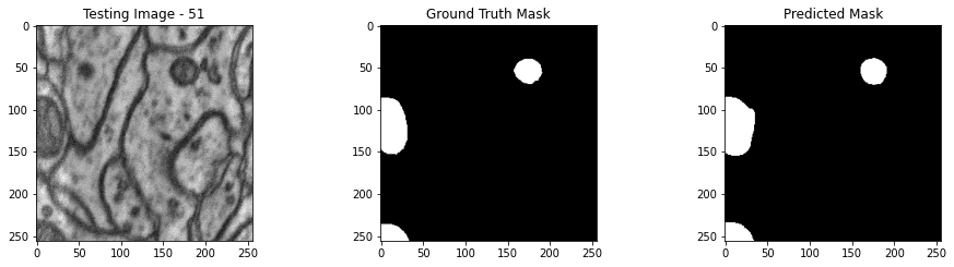
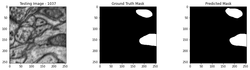
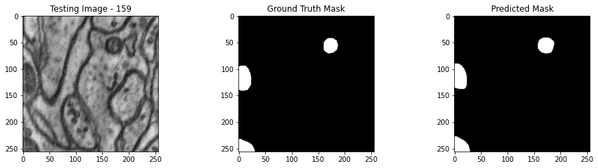
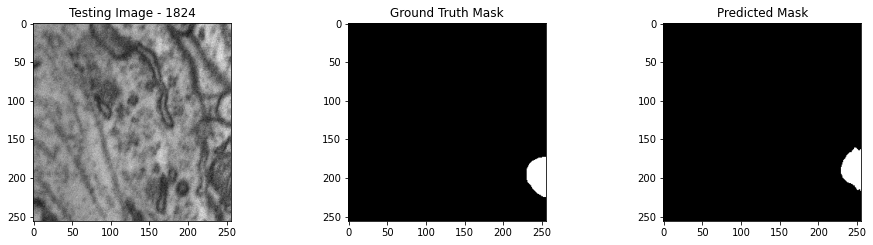
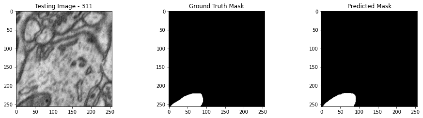
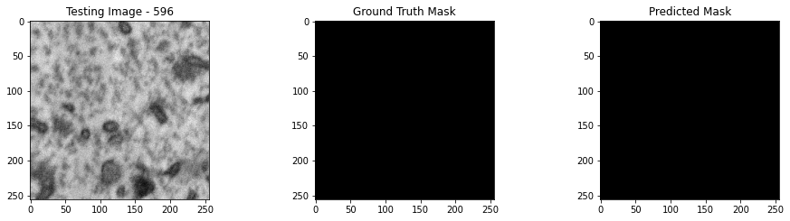
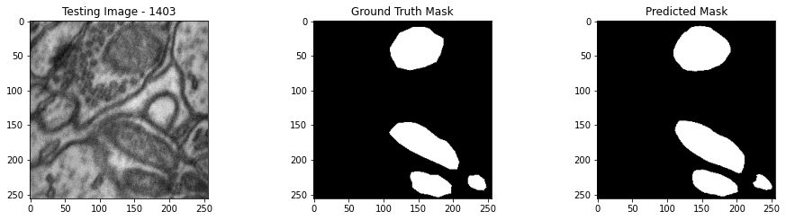
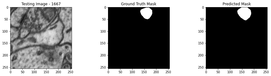
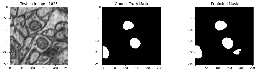
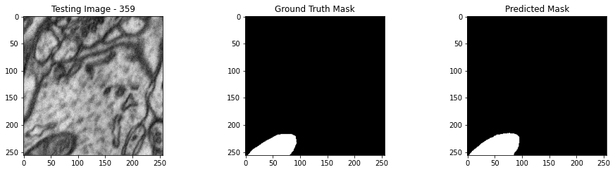
Complete Tutorial
With the demonstration complete, the pipeline is undeployed and the resources returned back to the Wallaroo instance.
pipeline.undeploy()
| name | biolabspipelinebspy |
|---|---|
| created | 2023-07-14 15:28:32.639523+00:00 |
| last_updated | 2023-07-14 15:28:38.163950+00:00 |
| deployed | False |
| tags | |
| versions | 0460ef47-3de3-43b2-8f62-16e76be8ce93, ef41bc7b-8213-4dd4-a1b9-54ac1253c652, c70dbdfe-e380-41b0-9da6-97bbfae90554 |
| steps | biolabsmodelbspy |
4.4.2 - Computer Vision: Image Detection for Health Care
How to use Wallaroo with computer vision models to detect mitochondria from images of cells.
This tutorial can be found on the Wallaroo Tutorials Github Repository.
Image Detection for Health Care Computer Vision Tutorial Part 02: External Data Connection Stores
The first example in this tutorial series showed selecting from 10 random images of cells and detecting mitochondria from within them.
This tutorial will expand on that by using a Wallaroo connection to retrieve a high resolution 1536x2048 image, break it down into 256x256 “patches” that can be quickly analyzed.
Wallaroo connections are definitions set by MLOps engineers that are used by other Wallaroo users for connection information to a data source. For this example, the data source will be a GitHub URL, but they could be Google BigQuery databases, Kafka topics, or any number of user defined examples.
Tutorial Goals
This tutorial will perform the following:
- Upload and deploy the
mitochondria_epochs_15.onnxmodel to a Wallaroo pipeline. - Create a Wallaroo connection pointing to a location for a high resolution image of cells.
- Break down the image into 256x256 images based on the how the model was trained to detect mitochondria.
- Convert the images into a numpy array inserted into a pandas DataFrame.
- Submit the DataFrame to the Wallaroo pipeline and use the results to create a mask image of where the model detects mitochondria.
- Compare the original image against a map of “ground truth” and the model’s mask image.
- Undeploy the pipeline and return the resources back to the Wallaroo instance.
Prerequisites
Prerequisites
Complete the steps from Mitochondria Detection Computer Vision Tutorial Part 00: Prerequisites.
Mitochondria Computer Vision Detection Steps
Import Libraries
The first step is to import the necessary libraries. Included with this tutorial are the following custom modules:
tiff_utils: Organizes the tiff images to perform random image selections and other tasks.
import json
import IPython.display as display
import time
import matplotlib.pyplot as plt
from IPython.display import clear_output, display
from lib.TiffImageUtils import TiffUtils
import tifffile as tiff
import pandas as pd
import wallaroo
from wallaroo.object import EntityNotFoundError, RequiredAttributeMissing
import numpy as np
from matplotlib import pyplot as plt
import cv2
from keras.utils import normalize
tiff_utils = TiffUtils()
# used for unique connection names
import string
import random
suffix= ''.join(random.choice(string.ascii_lowercase) for i in range(4))
# ignoring warnings for demonstration
import warnings
warnings.filterwarnings('ignore')
Open a Connection to Wallaroo
The next step is connect to Wallaroo through the Wallaroo client. The Python library is included in the Wallaroo install and available through the Jupyter Hub interface provided with your Wallaroo environment.
This is accomplished using the wallaroo.Client() command, which provides a URL to grant the SDK permission to your specific Wallaroo environment. When displayed, enter the URL into a browser and confirm permissions. Store the connection into a variable that can be referenced later.
If logging into the Wallaroo instance through the internal JupyterHub service, use wl = wallaroo.Client(). If logging in externally, update the wallarooPrefix and wallarooSuffix variables with the proper DNS information. For more information on Wallaroo DNS settings, see the Wallaroo DNS Integration Guide.
wl = wallaroo.Client()
Create Workspace and Pipeline
We will create a workspace to manage our pipeline and models. The following variables will set the name of our sample workspace then set it as the current workspace.
Workspace, pipeline, and model names should be unique to each Wallaroo instance, so we’ll add in a randomly generated suffix so multiple people can run this tutorial in a Wallaroo instance without effecting each other.
workspace_name = f'biolabsconnectionworkspace{suffix}'
pipeline_name = f'biolabsconnectionpipeline{suffix}'
model_name = f'biolabsconnectionmodel{suffix}'
model_file_name = 'models/mitochondria_epochs_15.onnx'
def get_workspace(name):
workspace = None
for ws in wl.list_workspaces():
if ws.name() == name:
workspace= ws
if(workspace == None):
workspace = wl.create_workspace(name)
return workspace
def get_pipeline(name):
try:
pipeline = wl.pipelines_by_name(name)[0]
except EntityNotFoundError:
pipeline = wl.build_pipeline(name)
return pipeline
workspace = get_workspace(workspace_name)
wl.set_current_workspace(workspace)
pipeline = get_pipeline(pipeline_name)
pipeline
| name | biolabsconnectionpipelinepdrv |
|---|---|
| created | 2023-07-14 15:29:16.969523+00:00 |
| last_updated | 2023-07-14 15:29:16.969523+00:00 |
| deployed | (none) |
| tags | |
| versions | 79d3b6ca-823f-406d-bf23-88a23b49ff1b |
| steps |
Upload the Models
Now we will:
- Upload our model.
- Apply it as a step in our pipeline.
- Create a pipeline deployment with enough memory to perform the inferences.
- Deploy the pipeline.
deployment_config = wallaroo.DeploymentConfigBuilder().replica_count(1).cpus(1).memory("2Gi").build()
model = (wl.upload_model(model_name,
model_file_name,
framework=wallaroo.framework.Framework.ONNX)
.configure(tensor_fields=["tensor"])
)
pipeline = wl.build_pipeline(pipeline_name) \
.add_model_step(model) \
.deploy(deployment_config = deployment_config)
Create the Wallaroo Connection
The Wallaroo connection will point to the location of our high resolution images:
- One the cell photos to be retrieved
- The other “ground truth” masks that are mapped compared against the model’s predictions.
The images will be retrieved, then parsed into a series of 256x256 images.
image_connection_name = f'mitochondria_image_source{suffix}'
image_connection_type = "HTTP"
image_connection_argument = {
'cell_images':'https://storage.googleapis.com/wallaroo-public-data/csa_demo/computer-vision/examples/medical/bio-labs/atl-lab/images/ms-01-atl-3-22-23_9-50.tiff',
'ground_truth_masks': 'https://storage.googleapis.com/wallaroo-public-data/csa_demo/computer-vision/examples/medical/bio-labs/atl-lab/masks/ms-01-atl-3-22-23_9-50-masks.tiff'
}
connection = wl.create_connection(image_connection_name, image_connection_type, image_connection_argument)
Retrieve Images
We’ll use our new connection to reach out, retrieve the images and store them locally for processing. The information is stored in the details() method for the connection, which is hidden by default when showing the connection, but the data can be retrieved when necessary.
inference_source_connection = wl.get_connection(name=image_connection_name)
display(inference_source_connection)
| Field | Value |
|---|---|
| Name | mitochondria_image_sourcepdrv |
| Connection Type | HTTP |
| Details | ***** |
| Created At | 2023-07-14T15:32:00.930954+00:00 |
| Linked Workspaces | [] |
patches_dict = tiff_utils.build_patches("downloaded_patches",
(256,256),
256,
inference_source_connection.details()['cell_images'],
inference_source_connection.details()['ground_truth_masks'] )
created dir downloaded_patches/ms-01-atl-3-22-23_9-50
saving file downloaded_patches/ms-01-atl-3-22-23_9-50/ms-01-atl-3-22-23_9-50.tiff
Retrieve Image and Convert to Data
The next step is to process the image into a numpy array that the model is trained to detect from.
We start by retrieving all the patch images from a recorded time series tiff recorded on one of our microscopes.
sample_mitochondria_patches_path = "./downloaded_patches/ms-01-atl-3-22-23_9-50"
patches = tiff_utils.get_all_patches(sample_mitochondria_patches_path)
Randomly we will retrieve a 256x256 patch image and use it to do our semantic segmentation prediction.
We’ll then convert it into a numpy array and insert into a DataFrame for a single inference.
The following helper function loadImageAndConvertTiff is used to convert the image into a numpy, then insert that into the DataFrame. This allows a later command to take the randomly grabbed image perform the process on other images.
def loadImageAndConvertTiff(imagePath, width, height):
img = cv2.imread(imagePath, 0)
imgNorm = np.expand_dims(normalize(np.array(img), axis=1),2)
imgNorm=imgNorm[:,:,0][:,:,None]
imgNorm=np.expand_dims(imgNorm, 0)
resizedImage = None
#creates a dictionary with the wallaroo "tensor" key and the numpy ndim array representing image as the value.
dictData = {"tensor":[imgNorm]}
dataframedata = pd.DataFrame(dictData)
# display(dataframedata)
return dataframedata, resizedImage
def run_semantic_segmentation_inference(pipeline, input_tiff_image, width, height, threshold):
tensor, resizedImage = loadImageAndConvertTiff(input_tiff_image, width, height)
# print(tensor)
# #
# # run inference on the 256x256 patch image get the predicted mitochandria mask
# #
output = pipeline.infer(tensor)
# print(output)
# # Obtain the flattened predicted mitochandria mask result
list1d = output.loc[0]["out.conv2d_37"]
np1d = np.array(list1d)
# # unflatten it
predicted_mask = np1d.reshape(1,width,height,1)
# # perform the element-wise comaprison operation using the threshold provided
predicted_mask = (predicted_mask[0,:,:,0] > threshold).astype(np.uint8)
# return predicted_mask
return predicted_mask
Infer and Display Results
We will now perform our inferences and display the results. This results in a predicted mask showing us where the mitochondria cells are located.
- The first image is the input image.
- The 2nd image is the ground truth. The mask was created by a human who identified the mitochondria cells in the input image
- The 3rd image is the predicted mask after running inference on the Wallaroo pipeline.
We’ll perform this 10 times to show how quickly the inferences can be submitted.
for x in range(10):
# get a sample 256x256 mitochondria image
random_patch = tiff_utils.get_random_patch_sample(patches)
# build the path to the image
patch_image_path = sample_mitochondria_patches_path + "/images/" + random_patch['patch_image_file']
# run inference in order to get the predicted 256x256 mask
predicted_mask = run_semantic_segmentation_inference(pipeline, patch_image_path, 256,256, 0.2)
# # plot the results
test_image = random_patch['patch_image'][:,:,0]
test_image_title = f"Testing Image - {random_patch['index']}"
ground_truth_image = random_patch['patch_mask'][:,:,0]
ground_truth_image_title = "Ground Truth Mask"
predicted_mask_title = 'Predicted Mask'
tiff_utils.plot_test_results(test_image, test_image_title, \
ground_truth_image, ground_truth_image_title, \
predicted_mask, predicted_mask_title)
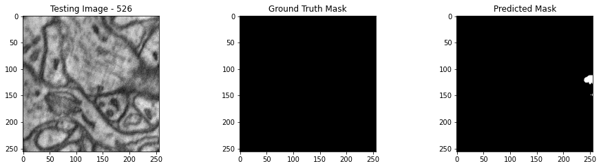
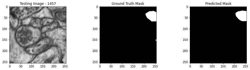
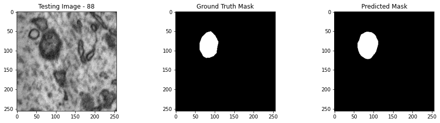
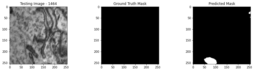
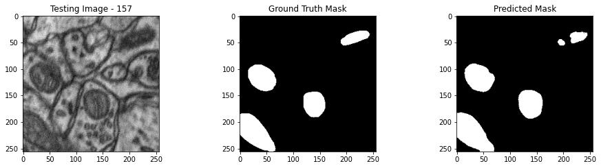
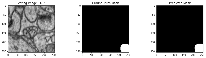
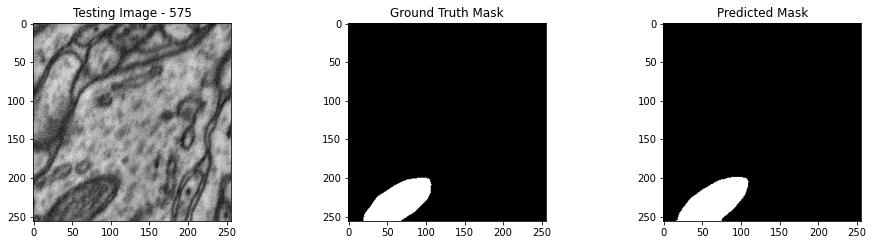
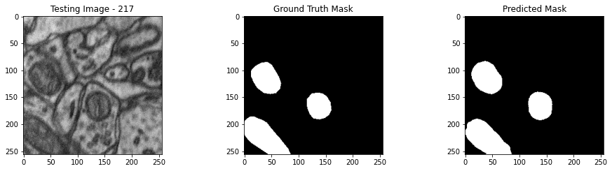
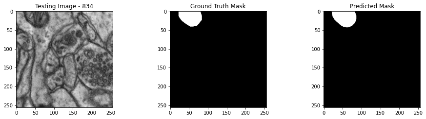
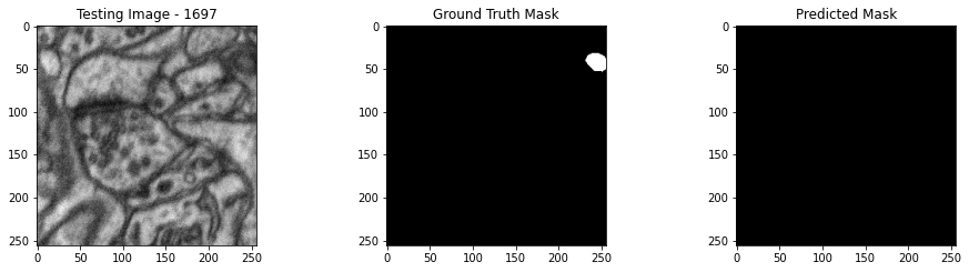
Complete Tutorial
With the demonstration complete, the pipeline is undeployed and the resources returned back to the Wallaroo instance.
pipeline.undeploy()
| name | biolabsconnectionpipelinepdrv |
|---|---|
| created | 2023-07-14 15:29:16.969523+00:00 |
| last_updated | 2023-07-14 15:29:23.004729+00:00 |
| deployed | False |
| tags | |
| versions | 0daae212-f578-4723-a0e5-edbcfa548976, 143eb35c-8606-471c-8053-230640249ad6, 79d3b6ca-823f-406d-bf23-88a23b49ff1b |
| steps | biolabsconnectionmodelpdrv |
4.5 - CLIP ViT-B/32 Transformer Demonstration with Wallaroo
The CLIP ViT-B/32 Transformer Demonstration with Wallaroo deployment.
This tutorial and the assets can be downloaded as part of the Wallaroo Tutorials repository.
CLIP ViT-B/32 Transformer Demonstration with Wallaroo
The following tutorial demonstrates deploying and performing sample inferences with the Hugging Face CLIP ViT-B/32 Transformer model.
Prerequisites
This tutorial is geared towards the Wallaroo version 2023.2.1 and above. The model clip-vit-base-patch-32.zip must be downloaded and placed into the ./models directory. This is available from the following URL:
https://storage.googleapis.com/wallaroo-public-data/hf-clip-vit-b32/clip-vit-base-patch-32.zip
If performing this tutorial from outside the Wallaroo JupyterHub environment, install the Wallaroo SDK.
Steps
Imports
The first step is to import the libraries used for the example.
import json
import os
import requests
import wallaroo
from wallaroo.pipeline import Pipeline
from wallaroo.deployment_config import DeploymentConfigBuilder
from wallaroo.framework import Framework
from wallaroo.object import EntityNotFoundError
import pyarrow as pa
import numpy as np
import pandas as pd
from PIL import Image
Connect to the Wallaroo Instance
The first step is to connect to Wallaroo through the Wallaroo client. The Python library is included in the Wallaroo install and available through the Jupyter Hub interface provided with your Wallaroo environment.
This is accomplished using the wallaroo.Client() command, which provides a URL to grant the SDK permission to your specific Wallaroo environment. When displayed, enter the URL into a browser and confirm permissions. Store the connection into a variable that can be referenced later.
If logging into the Wallaroo instance through the internal JupyterHub service, use wl = wallaroo.Client(). For more information on Wallaroo Client settings, see the Client Connection guide.
wl = wallaroo.Client()
Set Workspace and Pipeline
The next step is to create the Wallaroo workspace and pipeline used for the inference requests.
- References
# return the workspace called <name> through the Wallaroo client.
def get_workspace(name, client):
workspace = None
for ws in client.list_workspaces():
if ws.name() == name:
workspace= ws
return workspace
# if no workspaces were found
if workspace==None:
workspace = wl.create_workspace(name)
return workspace
# create the workspace and pipeline
workspace_name = 'clip-demo'
pipeline_name = 'clip-demo'
workspace = get_workspace(workspace_name, wl)
wl.set_current_workspace(workspace)
display(wl.get_current_workspace())
pipeline = wl.build_pipeline(pipeline_name)
pipeline
{'name': 'clip-demo', 'id': 8, 'archived': False, 'created_by': '12ea09d1-0f49-405e-bed1-27eb6d10fde4', 'created_at': '2023-11-20T18:57:53.667873+00:00', 'models': [], 'pipelines': [{'name': 'clip-demo', 'create_time': datetime.datetime(2023, 11, 20, 18, 57, 55, 550690, tzinfo=tzutc()), 'definition': '[]'}]}
| name | clip-demo |
|---|---|
| created | 2023-11-20 18:57:55.550690+00:00 |
| last_updated | 2023-11-20 18:57:55.550690+00:00 |
| deployed | (none) |
| arch | None |
| tags | |
| versions | ff0e4846-f0f9-4fb0-bc06-d6daa21797bf |
| steps | |
| published | False |
Configure and Upload Model
The 🤗 Hugging Face model is uploaded to Wallaroo by defining the input and output schema, and specifying the model’s framework as wallaroo.framework.Framework.HUGGING_FACE_ZERO_SHOT_IMAGE_CLASSIFICATION.
The data schemas are defined in Apache PyArrow Schema format.
The model is converted to the Wallaroo Containerized runtime after the upload is complete.
input_schema = pa.schema([
pa.field('inputs', # required, fixed image dimensions
pa.list_(
pa.list_(
pa.list_(
pa.int64(),
list_size=3
),
list_size=640
),
list_size=480
)),
pa.field('candidate_labels', pa.list_(pa.string(), list_size=4)), # required, equivalent to `options` in the provided demo
])
output_schema = pa.schema([
pa.field('score', pa.list_(pa.float64(), list_size=4)), # has to be same as number of candidate labels
pa.field('label', pa.list_(pa.string(), list_size=4)), # has to be same as number of candidate labels
])
Upload Model
model = wl.upload_model('clip-vit', './models/clip-vit-base-patch-32.zip',
framework=Framework.HUGGING_FACE_ZERO_SHOT_IMAGE_CLASSIFICATION,
input_schema=input_schema,
output_schema=output_schema)
model
Waiting for model loading - this will take up to 10.0min.
Model is pending loading to a container runtime..
Model is attempting loading to a container runtime............................................................successful
Ready
| Name | clip-vit |
| Version | 57594cc7-7db1-43c3-b21a-6dcaba846f26 |
| File Name | clip-vit-base-patch-32.zip |
| SHA | 4efc24685a14e1682301cc0085b9db931aeb5f3f8247854bedc6863275ed0646 |
| Status | ready |
| Image Path | proxy.replicated.com/proxy/wallaroo/ghcr.io/wallaroolabs/mlflow-deploy:v2023.4.0-4103 |
| Architecture | None |
| Updated At | 2023-20-Nov 20:51:44 |
Deploy Pipeline
With the model uploaded and prepared, we add the model as a pipeline step and deploy it. For this example, we will allocate 4 Gi of RAM and 1 CPU to the model’s use through the pipeline deployment configuration.
deployment_config = wallaroo.DeploymentConfigBuilder() \
.cpus(.25).memory('1Gi') \
.sidekick_memory(model, '4Gi') \
.sidekick_cpus(model, 1.0) \
.build()
The pipeline is deployed with the specified engine deployment.
Because the model is converted to the Wallaroo Containerized Runtime, the deployment step may timeout with the status still as Starting. If this occurs, wait an additional 60 seconds, then run the pipeline.status() cell. Once the status is Running, the rest of the tutorial can proceed.
pipeline.clear()
pipeline.add_model_step(model)
pipeline.deploy(deployment_config=deployment_config)
| name | clip-demo |
|---|---|
| created | 2023-11-20 18:57:55.550690+00:00 |
| last_updated | 2023-11-20 20:51:59.304917+00:00 |
| deployed | True |
| arch | None |
| tags | |
| versions | 7a6168c2-f807-465f-a122-33fe7b5d8a3d, ff0e4846-f0f9-4fb0-bc06-d6daa21797bf |
| steps | clip-vit |
| published | False |
pipeline.status()
{'status': 'Running',
'details': [],
'engines': [{'ip': '10.244.3.140',
'name': 'engine-bb48bb959-2xctn',
'status': 'Running',
'reason': None,
'details': [],
'pipeline_statuses': {'pipelines': [{'id': 'clip-demo',
'status': 'Running'}]},
'model_statuses': {'models': [{'name': 'clip-vit',
'version': '57594cc7-7db1-43c3-b21a-6dcaba846f26',
'sha': '4efc24685a14e1682301cc0085b9db931aeb5f3f8247854bedc6863275ed0646',
'status': 'Running'}]}}],
'engine_lbs': [{'ip': '10.244.4.152',
'name': 'engine-lb-584f54c899-gcbpj',
'status': 'Running',
'reason': None,
'details': []}],
'sidekicks': [{'ip': '10.244.3.139',
'name': 'engine-sidekick-clip-vit-11-75c5666b69-tqfbk',
'status': 'Running',
'reason': None,
'details': [],
'statuses': '\n'}]}
Run Inference
We verify the pipeline is deployed by checking the status().
The sample images in the ./data directory are converted into numpy arrays, and the candidate labels added as inputs. Both are set as DataFrame arrays where the field inputs are the image values, and candidate_labels the labels.
image_paths = [
"./data/bear-in-tree.jpg",
"./data/elephant-and-zebras.jpg",
"./data/horse-and-dogs.jpg",
"./data/kittens.jpg",
"./data/remote-monitor.jpg"
]
images = []
for iu in image_paths:
image = Image.open(iu)
image = image.resize((640, 480)) # fixed image dimensions
images.append(np.array(image))
dataframe = pd.DataFrame({"images": images})
input_data = {
"inputs": images,
"candidate_labels": [["cat", "dog", "horse", "elephant"]] * 5,
}
dataframe = pd.DataFrame(input_data)
dataframe
| inputs | candidate_labels | |
|---|---|---|
| 0 | [[[60, 62, 61], [62, 64, 63], [67, 69, 68], [7... | [cat, dog, horse, elephant] |
| 1 | [[[228, 235, 241], [229, 236, 242], [230, 237,... | [cat, dog, horse, elephant] |
| 2 | [[[177, 177, 177], [177, 177, 177], [177, 177,... | [cat, dog, horse, elephant] |
| 3 | [[[140, 25, 56], [144, 25, 67], [146, 24, 73],... | [cat, dog, horse, elephant] |
| 4 | [[[24, 20, 11], [22, 18, 9], [18, 14, 5], [21,... | [cat, dog, horse, elephant] |
Inference Outputs
The inference is run, and the labels with their corresponding confidence values for each label are mapped to out.label and out.score for each image.
results = pipeline.infer(dataframe,timeout=600,dataset=["in", "out", "metadata.elapsed", "time", "check_failures"])
pd.set_option('display.max_colwidth', None)
display(results.loc[:, ['out.label', 'out.score']])
| out.label | out.score | |
|---|---|---|
| 0 | [elephant, dog, horse, cat] | [0.4146825075149536, 0.3483847379684448, 0.1285749077796936, 0.10835790634155273] |
| 1 | [elephant, horse, dog, cat] | [0.9981434345245361, 0.001765866531059146, 6.823801231803373e-05, 2.2441448891186155e-05] |
| 2 | [horse, dog, elephant, cat] | [0.7596800923347473, 0.217111736536026, 0.020392831414937973, 0.0028152535669505596] |
| 3 | [cat, dog, elephant, horse] | [0.9870228171348572, 0.0066468678414821625, 0.0032716328278183937, 0.003058753442019224] |
| 4 | [dog, horse, cat, elephant] | [0.5713965892791748, 0.17229433357715607, 0.15523898601531982, 0.1010700911283493] |
Undeploy Pipelines
With the tutorial complete, the pipeline is undeployed and the resources returned back to the cluster.
pipeline.undeploy()
| name | clip-demo |
|---|---|
| created | 2023-11-20 18:57:55.550690+00:00 |
| last_updated | 2023-11-20 20:51:59.304917+00:00 |
| deployed | False |
| arch | None |
| tags | |
| versions | 7a6168c2-f807-465f-a122-33fe7b5d8a3d, ff0e4846-f0f9-4fb0-bc06-d6daa21797bf |
| steps | clip-vit |
| published | False |
4.6 - Containerized MLFlow Tutorial
The Containerized MLFlow Tutorial demonstrates how to use Wallaroo with containerized MLFlow models.
Setting Private Registry Configuration in Wallaroo
Configure Via Kots
If Wallaroo was installed via kots, use the following procedure to add the private model registry information.
Launch the Wallaroo Administrative Dashboard through a terminal linked to the Kubernetes cluster. Replace the namespace with the one used in your installation.
kubectl kots admin-console --namespace wallarooLaunch the dashboard, by default at
http://localhost:8800.From the admin dashboard, select Config -> Private Model Container Registry.
Enable Provide private container registry credentials for model images.
Provide the following:
- Registry URL: The URL of the Containerized Model Container Registry. Typically in the format
host:port. In this example, the registry for GitHub is used. NOTE: When setting the URL for the Containerized Model Container Registry, only the actual service address is needed. For example: with the full URL of the model asghcr.io/wallaroolabs/wallaroo_tutorials/mlflow-statsmodels-example:2022.4, the URL would beghcr.io/wallaroolabs. - email: The email address of the user authenticating to the registry service.
- username: The username of the user authentication to the registry service.
- password: The password of the user authentication or token to the registry service.
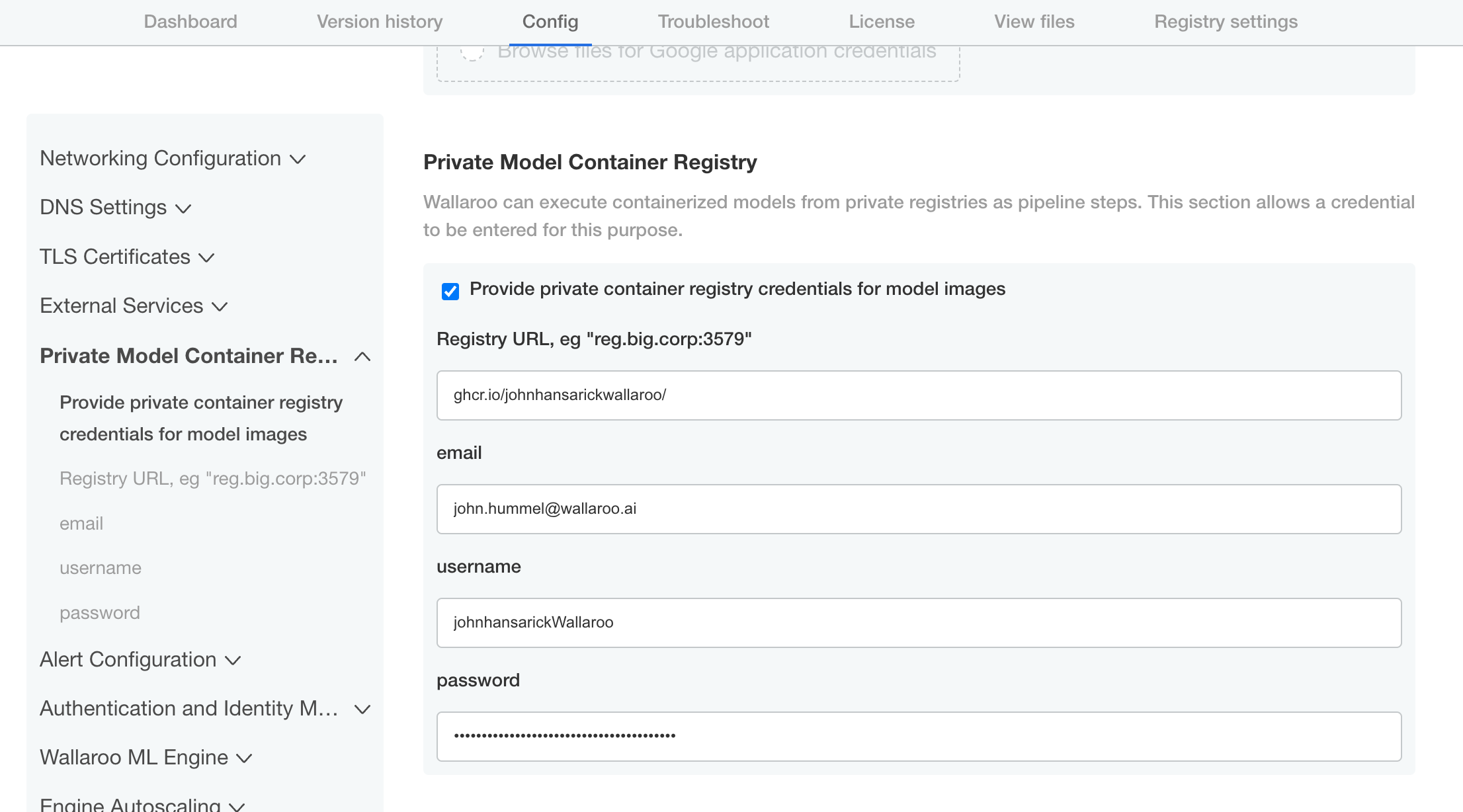
- Registry URL: The URL of the Containerized Model Container Registry. Typically in the format
Scroll down and select Save config.
Deploy the new version.
Once complete, the Wallaroo instance will be able to authenticate to the Containerized Model Container Registry and retrieve the images.
Configure via Helm
During either the installation process or updates, set the following in the
local-values.yamlfile:privateModelRegistry:enabled: truesecretName:model-registry-secretregistry: The URL of the private registry.email: The email address of the user authenticating to the registry service.username: The username of the user authentication to the registry service.password: The password of the user authentication to the registry service.
For example:
# Other settings - DNS entries, etc. # The private registry settings privateModelRegistry: enabled: true secretName: model-registry-secret registry: "YOUR REGISTRY URL:YOUR REGISTRY PORT" email: "YOUR EMAIL ADDRESS" username: "YOUR USERNAME" password: "Your Password here"
Install or update the Wallaroo instance via Helm as per the Wallaroo Helm Install instructions.
Once complete, the Wallaroo instance will be able to authenticate to the registry service and retrieve the images.
This tutorial and the assets can be downloaded as part of the Wallaroo Tutorials repository.
MLFlow Inference with Wallaroo Tutorial
Wallaroo users can register their trained MLFlow ML Models from a containerized model container registry into their Wallaroo instance and perform inferences with it through a Wallaroo pipeline.
As of this time, Wallaroo only supports MLFlow 1.3.0 containerized models. For information on how to containerize an MLFlow model, see the MLFlow Documentation.
This tutorial assumes that you have a Wallaroo instance, and have either your own containerized model or use the one from the reference and are running this Notebook from the Wallaroo Jupyter Hub service.
See the Wallaroo Private Containerized Model Container Registry Guide for details on how to configure a Wallaroo instance with a private model registry.
MLFlow Data Formats
When using containerized MLFlow models with Wallaroo, the inputs and outputs must be named. For example, the following output:
[-12.045839810372835]
Would need to be wrapped with the data values named:
[{"prediction": -12.045839810372835}]
A short sample code for wrapping data may be:
output_df = pd.DataFrame(prediction, columns=["prediction"])
return output_df
MLFlow Models and Wallaroo
MLFlow models are composed of two parts: the model, and the flavors. When submitting a MLFlow model to Wallaroo, both aspects must be part of the ML Model included in the container. For full information about MLFlow model structure, see the MLFlow Documentation.
Wallaroo registers the models from container registries. Organizations will either have to make their containers available in a public or through a private Containerized Model Container Registry service. For examples on setting up a private container registry service, see the Docker Documentation “Deploy a registry server”. For more details on setting up a container registry in a cloud environment, see the related documentation for your preferred cloud provider:
- Google Cloud Platform Container Registry
- Amazon Web Services Elastic Container Registry
- Microsoft Azure Container Registry
For this example, we will be using the MLFlow containers that was registered in a GitHub container registry service in MLFlow Creation Tutorial Part 03: Container Registration. The address of those containers are:
- postprocess: ghcr.io/johnhansarickwallaroo/mlflowtests/mlflow-postprocess-example . Used for format data after the statsmodel inferences.
- statsmodel: ghcr.io/johnhansarickwallaroo/mlflowtests/mlflow-statsmodels-example . The statsmodel generated in MLFlow Creation Tutorial Part 01: Model Creation.
Prerequisites
Before uploading and running an inference with a MLFlow model in Wallaroo the following will be required:
- MLFlow Input Schema: The input schema with the fields and data types for each MLFlow model type uploaded to Wallaroo. In the examples below, the data types are imported using the
pyarrowlibrary. - An installed Wallaroo instance.
- The following Python libraries installed:
oswallaroo: The Wallaroo SDK. Included with the Wallaroo JupyterHub service by default.
IMPORTANT NOTE: Wallaroo supports MLFlow 1.3.0. Please ensure the MLFlow models used in Wallaroo meet this specification.
MLFlow Inference Steps
To register a containerized MLFlow ML Model into Wallaroo, use the following general step:
- Import Libraries
- Connect to Wallaroo
- Set MLFlow Input Schemas
- Register MLFlow Model
- Create Pipeline and Add Model Steps
- Run Inference
Import Libraries
We start by importing the libraries we will need to connect to Wallaroo and use our MLFlow models. This includes the wallaroo libraries, pyarrow for data types, and the json library for handling JSON data.
import wallaroo
from wallaroo.object import EntityNotFoundError
import pyarrow as pa
import pandas as pd
Connect to the Wallaroo Instance
The first step is to connect to Wallaroo through the Wallaroo client. The Python library is included in the Wallaroo install and available through the Jupyter Hub interface provided with your Wallaroo environment.
This is accomplished using the wallaroo.Client() command, which provides a URL to grant the SDK permission to your specific Wallaroo environment. When displayed, enter the URL into a browser and confirm permissions. Store the connection into a variable that can be referenced later.
If logging into the Wallaroo instance through the internal JupyterHub service, use wl = wallaroo.Client(). For more information on Wallaroo Client settings, see the Client Connection guide.
# Login through local Wallaroo instance
wl = wallaroo.Client()
def get_workspace(name):
workspace = None
for ws in wl.list_workspaces():
if ws.name() == name:
workspace= ws
if(workspace == None):
workspace = wl.create_workspace(name)
return workspace
def get_pipeline(name):
try:
pipeline = wl.pipelines_by_name(name)[0]
except EntityNotFoundError:
pipeline = wl.build_pipeline(name)
return pipeline
prefix = 'mlflow'
workspace_name= f"{prefix}statsmodelworkspace"
pipeline_name = f"{prefix}statsmodelpipeline"
mlflowworkspace = get_workspace(workspace_name)
wl.set_current_workspace(mlflowworkspace)
pipeline = get_pipeline(pipeline_name)
Set MLFlow Input Schemas
Set the MLFlow input schemas through the pyarrow library. In the examples below, the input schemas for both the MLFlow model statsmodels-test and the statsmodels-test-postprocess model.
sm_input_schema = pa.schema([
pa.field('temp', pa.float32()),
pa.field('holiday', pa.uint8()),
pa.field('workingday', pa.uint8()),
pa.field('windspeed', pa.float32())
])
pp_input_schema = pa.schema([
pa.field('predicted_mean', pa.float32())
])
Register MLFlow Model
Use the register_model_image method to register the Docker container containing the MLFlow models.
statsmodelUrl = "ghcr.io/wallaroolabs/wallaroo_tutorials/mlflow-statsmodels-example:2023.1"
postprocessUrl = "ghcr.io/wallaroolabs/wallaroo_tutorials/mlflow-postprocess-example:2023.1"
sm_model = wl.register_model_image(
name=f"{prefix}statmodels",
image=f"{statsmodelUrl}"
).configure("mlflow", input_schema=sm_input_schema, output_schema=pp_input_schema)
pp_model = wl.register_model_image(
name=f"{prefix}postprocess",
image=f"{postprocessUrl}"
).configure("mlflow", input_schema=pp_input_schema, output_schema=pp_input_schema)
Create Pipeline and Add Model Steps
With the models registered, we can add the MLFlow models as steps in the pipeline. Once ready, we will deploy the pipeline so it is available for submitting data for running inferences.
pipeline.add_model_step(sm_model)
pipeline.add_model_step(pp_model)
| name | mlflowstatsmodelpipeline |
|---|---|
| created | 2023-07-14 15:32:52.546581+00:00 |
| last_updated | 2023-07-14 15:32:52.546581+00:00 |
| deployed | (none) |
| tags | |
| versions | efa60e66-b2b7-4bb2-bc37-dd9ea7377467 |
| steps |
from wallaroo.deployment_config import DeploymentConfigBuilder
deployment_config = DeploymentConfigBuilder() \
.cpus(0.25).memory('1Gi') \
.sidekick_env(sm_model, {"GUNICORN_CMD_ARGS": "--timeout=180 --workers=1"}) \
.sidekick_env(pp_model, {"GUNICORN_CMD_ARGS": "--timeout=180 --workers=1"}) \
.build()
pipeline.deploy(deployment_config=deployment_config)
| name | mlflowstatsmodelpipeline |
|---|---|
| created | 2023-07-14 15:32:52.546581+00:00 |
| last_updated | 2023-07-14 15:35:09.901078+00:00 |
| deployed | True |
| tags | |
| versions | 2f8e9483-a9ad-436e-9068-7826cd8166c4, 539aae6b-4437-4f8c-8be0-db9ef11e80fb, efa60e66-b2b7-4bb2-bc37-dd9ea7377467 |
| steps | mlflowstatmodels |
pipeline.status()
{'status': 'Running',
'details': [],
'engines': [{'ip': '10.244.3.142',
'name': 'engine-c55d468-qgk48',
'status': 'Running',
'reason': None,
'details': [],
'pipeline_statuses': {'pipelines': [{'id': 'mlflowstatsmodelpipeline',
'status': 'Running'}]},
'model_statuses': {'models': [{'name': 'mlflowpostprocess',
'version': 'b7cd3426-825a-467d-8616-011ae8901d23',
'sha': '825ebae48014d297134930028ab0e823bc0d9551334b9a4402c87a714e8156b2',
'status': 'Running'},
{'name': 'mlflowstatmodels',
'version': '1a547bbb-36c7-4b5c-93a8-f357e3542d6f',
'sha': '3afd13d9c5070679e284050cd099e84aa2e5cb7c08a788b21d6cb2397615d018',
'status': 'Running'}]}}],
'engine_lbs': [{'ip': '10.244.4.188',
'name': 'engine-lb-584f54c899-xhdmq',
'status': 'Running',
'reason': None,
'details': []}],
'sidekicks': [{'ip': '10.244.0.72',
'name': 'engine-sidekick-mlflowstatmodels-27-786dc6b47c-bprqb',
'status': 'Running',
'reason': None,
'details': [],
'statuses': '\n'},
{'ip': '10.244.0.73',
'name': 'engine-sidekick-mlflowpostprocess-28-9fff54995-2n2nn',
'status': 'Running',
'reason': None,
'details': [],
'statuses': '\n'}]}
Run Inference
Once the pipeline is running, we can submit our data to the pipeline and return our results. Once finished, we will undeploy the pipeline to return the resources back to the cluster.
# Initial container run may need extra time to finish deploying - adding 90 second timeout to compensate
results = pipeline.infer_from_file('./resources/bike_day_eval_engine.df.json', timeout=90)
display(results.loc[:,["out.predicted_mean"]])
| out.predicted_mean | |
|---|---|
| 0 | 0.281983 |
| 1 | 0.658847 |
| 2 | 0.572368 |
| 3 | 0.619873 |
| 4 | -1.217801 |
| 5 | -1.849156 |
| 6 | 0.933885 |
pipeline.undeploy()
| name | mlflowstatsmodelpipeline |
|---|---|
| created | 2023-07-14 15:32:52.546581+00:00 |
| last_updated | 2023-07-14 15:32:56.591792+00:00 |
| deployed | False |
| tags | |
| versions | 539aae6b-4437-4f8c-8be0-db9ef11e80fb, efa60e66-b2b7-4bb2-bc37-dd9ea7377467 |
| steps | mlflowstatmodels |
4.7 - Custom Inference Computer Vision Upload, Auto Packaging, and Deploy Tutorial
The uploading and auto packaging a Custom Inference aka Arbitrary Python computer vision model in Wallaroo.
This tutorial and the assets can be downloaded as part of the Wallaroo Tutorials repository.
Custom Inference Computer Vision Upload, Auto Packaging, and Deploy Tutorial
The following tutorial demonstrates using Wallaroo deploying Bring Your Own Predict aka Arbitrary Python in a Wallaroo instance. The model is auto packaged upon uploading. Once ready, the model is deployed and sample inferences performed on it.
Introduction
This tutorial focuses on the Resnet50 computer vision model. By default, this provides the following outputs from receiving an image converted to tensor values:
boxes: The bounding boxes for detected objects.classes: The class of the detected object (bottle, coat, person, etc).confidences: The confidence the model has that the detected model is the class.
For this demonstration, the model is modified with Wallaroo Bring Your Own Predict (BYOP) to add two additional fields:
avg_px_intensity: the average pixel intensity checks the input to determine the average value of the Red/Green/Blue pixel values. This is used as a benchmark to determine if the two images are significantly different. For example, an all white photo would have anavg_px_intensityof1, while an all blank photo would have a value of0.avg_confidence: The average confidence of all detected objects.
Prerequisites
- A Wallaroo Ops instance 2023.4 and above
To download the Wallaroo Computer Vision models, use the following link:
https://storage.googleapis.com/wallaroo-public-data/cv-demo-models/cv-retail-models.zip
Unzip the contents into the directory models.
The following libraries are required to run the tutorial:
onnx==1.12.0
onnxruntime==1.12.1
torchvision
torch
matplotlib==3.5.0
opencv-python
imutils
pytz
ipywidgets
To run this tutorial outside of a Wallaroo Ops center, the Wallaroo SDK is available and is installed via pip with:
pip install wallaroo==2023.4.1
Steps
Import Libraries
The following libraries are used to execute this tutorial. The utils.py provides additional helper methods for rendering the images into tensor fields and other useful tasks.
# preload needed libraries
import wallaroo
from wallaroo.object import EntityNotFoundError
from wallaroo.framework import Framework
from IPython.display import display
from IPython.display import Image
import pandas as pd
import json
import datetime
import time
import cv2
import matplotlib.pyplot as plt
import string
import random
import pyarrow as pa
import sys
import asyncio
import numpy as np
import utils
pd.set_option('display.max_colwidth', None)
import datetime
# api based inference request
import requests
import utils
# ignoring warnings for demonstration
import warnings
warnings.filterwarnings('ignore')
Connect to the Wallaroo Instance
The first step is to connect to Wallaroo through the Wallaroo client. The Python library is included in the Wallaroo install and available through the Jupyter Hub interface provided with your Wallaroo environment.
This is accomplished using the wallaroo.Client() command, which provides a URL to grant the SDK permission to your specific Wallaroo environment. When displayed, enter the URL into a browser and confirm permissions. Store the connection into a variable that can be referenced later.
If logging into the Wallaroo instance through the internal JupyterHub service, use wl = wallaroo.Client(). For more information on Wallaroo Client settings, see the Client Connection guide.
The option request_timeout provides additional time for the Wallaroo model upload process to complete.
wl = wallaroo.Client(request_timeout=600)
Create Workspace
We will create a workspace to manage our pipeline and models. The following variables will set the name of our sample workspace then set it as the current workspace.
Workspace names must be unique. The following helper function will either create a new workspace, or retrieve an existing one with the same name. Verify that a pre-existing workspace has been shared with the targeted user.
Set the variables workspace_name to ensure a unique workspace name if required.
The workspace will then be set as the Current Workspace. Model uploads and pipeline creation through the SDK are set in the current workspace.
def get_workspace(name, client):
workspace = None
for ws in client.list_workspaces():
if ws.name() == name:
workspace= ws
if(workspace == None):
workspace = client.create_workspace(name)
return workspace
workspace_name = "cv-retail-edge-observability"
model_name = "resnet-with-intensity"
model_file_name = "./models/model-with-pixel-intensity.zip"
pipeline_name = "retail-inv-tracker-edge-obs"
workspace = get_workspace(workspace_name, wl)
wl.set_current_workspace(workspace)
{'name': 'cv-retail-edge-observability', 'id': 12, 'archived': False, 'created_by': 'a762b468-4c2d-49dd-a9c7-7335e531741c', 'created_at': '2024-02-27T16:51:56.017038+00:00', 'models': [{'name': 'resnet-with-intensity', 'versions': 1, 'owner_id': '""', 'last_update_time': datetime.datetime(2024, 2, 27, 16, 53, 13, 935887, tzinfo=tzutc()), 'created_at': datetime.datetime(2024, 2, 27, 16, 53, 13, 935887, tzinfo=tzutc())}], 'pipelines': [{'name': 'retail-inv-tracker-edge-obs', 'create_time': datetime.datetime(2024, 2, 27, 16, 56, 20, 567978, tzinfo=tzutc()), 'definition': '[]'}]}
Upload Model
The model is uploaded as a BYOP (Bring Your Own Predict) aka Aribitrary model, where the model, Python script and other artifacts are included in a .zip file. This requires the input and output schemas for the model specified in Apache Arrow Schema format.
The contents of the Wallaroo BYOP script includes the following to load the model, and add additional fields. By default the frcnn-resnet model outputs the following fields:
- boxes: A List of the the bounding boxes of each detected object.
- classes: A List of the class of each detected object.
- confidences: A confidence score of how likely the object is what class was detected.
The model-with-pixel-intensity.zip BYOP model uses that class, then adds in the following fields.
- avg_px_intensity: The average pixel intensidy of the image. This provides a way of determining if the same pictures from the same camera has significant changes. For example, a security camera would have a different pixel intensity in one picture where the light was on, versus one one when the lights were off.
- avg_confidence: An average of all of the confidences output by the model. This is used for observability and track model drift.
The following predict method is used in the BYOP model.
def _predict(self, input_data: InferenceData):
# Parse inputs
inputs = input_data["tensor"]
# Pass to onnx model
# `dynamic_axes` hasn't been set in torch.onnx.export()
# that is used in CVDemoUtils.loadPytorchAndConvertToOnnx()
# therefore we cannot do batch inference
ort_sess = ort.InferenceSession(self._model.SerializeToString())
outputs = ort_sess.run(None, {"data": inputs.astype(np.float32)})
boxes, classes, confidences = outputs
# Calculate input derivatives
avg_px_intensity = np.mean(inputs[0])
# Calculate output derivatives
avg_confidence = np.mean(confidences)
# batch size isn't specified in the onnx session output
# but we need to return a batch of outputs
return {
"boxes": np.array([boxes]),
"classes": np.array([classes]),
"confidences": np.array([confidences]),
"avg_px_intensity": np.array([[avg_px_intensity]]),
"avg_confidence": np.array([[avg_confidence]]),
}
For full details on Wallaroo BYOP models, see Wallaroo SDK Essentials Guide: Model Uploads and Registrations: Arbitrary Python.
The following sets the input/output schemas in Apache pyarrow format, and uploads the models. Once uploaded, it is automatically
input_schema = pa.schema([
pa.field('tensor', pa.list_(
pa.list_(
pa.list_(
pa.float32(), # images are normalized
list_size=640
),
list_size=480
),
list_size=3
)),
])
output_schema = pa.schema([
pa.field('boxes', pa.list_(pa.list_(pa.float32(), list_size=4))),
pa.field('classes', pa.list_(pa.int64())),
pa.field('confidences', pa.list_(pa.float32())),
pa.field('avg_px_intensity', pa.list_(pa.float32())),
pa.field('avg_confidence', pa.list_(pa.float32())),
])
model = wl.upload_model(model_name,
model_file_name,
framework=Framework.CUSTOM,
input_schema=input_schema,
output_schema=output_schema)
Waiting for model loading - this will take up to 10.0min.
Model is pending loading to a container runtime..
Model is attempting loading to a container runtime........................successful
Ready
Deploy Pipeline
Next we configure the hardware we want to use for deployment. If we plan on eventually deploying to edge, this is a good way to simulate edge hardware conditions. The BYOP model is deployed as a Wallaroo Containerized Runtime, so the hardware allocation is performed through the sidekick options.
deployment_config = wallaroo.DeploymentConfigBuilder() \
.replica_count(1) \
.cpus(1) \
.memory("2Gi") \
.sidekick_cpus(model, 1) \
.sidekick_memory(model, '6Gi') \
.build()
We create the pipeline with the wallaroo.client.build_pipeline method, and assign our model as a model pipeline step. Once complete, we will deploy the pipeline to allocate resources from the Kuberntes cluster hosting the Wallaroo Ops to the pipeline.
pipeline = wl.build_pipeline(pipeline_name)
pipeline.clear()
pipeline.add_model_step(model)
pipeline.deploy(deployment_config = deployment_config)
Waiting for deployment - this will take up to 600s ................... ok
| name | retail-inv-tracker-edge-obs |
|---|---|
| created | 2024-02-27 16:56:20.567978+00:00 |
| last_updated | 2024-02-27 17:55:07.307761+00:00 |
| deployed | True |
| arch | None |
| tags | |
| versions | 0e234ea5-ca90-40ea-abfb-a295941c606d, ecf277ed-d20f-481e-8dfe-9dc6937071f9, 21a90743-e121-485e-934f-754f335f4ea3, b4c9256f-719e-4d4c-b167-df32decec0aa |
| steps | resnet-with-intensity |
| published | False |
Sample Inferences
We’ll perform some sample inferences and display the outputs. For each image, we’ll use the inference result to draw the bounding boxes for all objects with a confidence value higher than 50%. We’ll display the average confidence across all detected objects after the bounding box image.
For more details on performing inferences, see Wallaroo SDK Essentials Guide: Inference Management.
width, height = 640, 480
baseline_images = [
"./data/images/input/example/dairy_bottles.png",
"./data/images/input/example/dairy_products.png",
"./data/images/input/example/product_cheeses.png"
]
for sample_image in baseline_images:
dfImage, resizedImage = utils.loadImageAndConvertToDataframe(sample_image, width, height)
startTime = time.time()
infResults = pipeline.infer(dfImage, timeout=300)
endTime = time.time()
elapsed = 1.0
results = {
'model_name' : model_name,
'pipeline_name' : pipeline_name,
'width': width,
'height': height,
'image' : resizedImage,
'inf-results' : infResults,
'confidence-target' : 0.50,
'inference-time': (endTime-startTime),
'onnx-time' : int(elapsed) / 1e+9,
'classes_file': "./models/coco_classes.pickle",
'color': 'BLUE'
}
image = utils.drawDetectedObjectsFromInference(results)
display(infResults.loc[:, ['out.avg_confidence']])
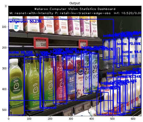
| out.avg_confidence | |
|---|---|
| 0 | [0.3588039] |
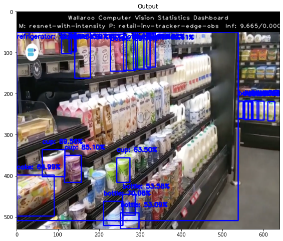
| out.avg_confidence | |
|---|---|
| 0 | [0.2970887] |
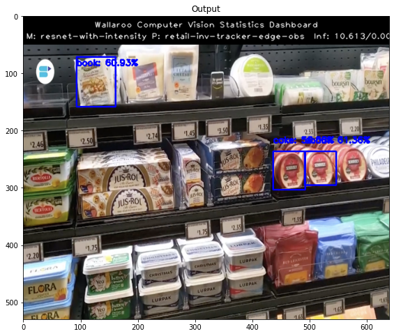
| out.avg_confidence | |
|---|---|
| 0 | [0.1656933] |
The Wallaroo SDK is capable of using numpy arrays in a pandas DataFrame for inference requests. Our demonstration will focus on using API calls for inference requests, so we will flatten the numpy array and use that value for our inference inputs. The following examples show using a baseline and blurred image for inference requests and the sample outputs.
pipeline.undeploy()
Waiting for undeployment - this will take up to 600s ...................................... ok
| name | retail-inv-tracker-edge-obs |
|---|---|
| created | 2024-02-27 16:56:20.567978+00:00 |
| last_updated | 2024-02-27 17:55:07.307761+00:00 |
| deployed | False |
| arch | None |
| tags | |
| versions | 0e234ea5-ca90-40ea-abfb-a295941c606d, ecf277ed-d20f-481e-8dfe-9dc6937071f9, 21a90743-e121-485e-934f-754f335f4ea3, b4c9256f-719e-4d4c-b167-df32decec0aa |
| steps | resnet-with-intensity |
| published | False |
4.8 - Demand Curve Quick Start Guide
The Demand Curve Quick Start Guide demonstrates how to use Wallaroo to chart a demand curve based on submitted data. This example uses a model plus preprocess and postprocessing steps.
This tutorial and the assets can be downloaded as part of the Wallaroo Tutorials repository.
Demand Curve Pipeline Tutorial
This worksheet demonstrates a Wallaroo pipeline with data preprocessing, a model, and data postprocessing.
The model is a “demand curve” that predicts the expected number of units of a product that will be sold to a customer as a function of unit price and facts about the customer. Such models can be used for price optimization or sales volume forecasting. This is purely a “toy” demonstration, but is useful for detailing the process of working with models and pipelines.
Data preprocessing is required to create the features used by the model. Simple postprocessing prevents nonsensical estimates (e.g. negative units sold).
Prerequisites
- An installed Wallaroo instance.
- The following Python libraries installed:
oswallaroo: The Wallaroo SDK. Included with the Wallaroo JupyterHub service by default.
import json
import wallaroo
from wallaroo.object import EntityNotFoundError
import pandas
import numpy
import conversion
from wallaroo.object import EntityNotFoundError
import pyarrow as pa
# used to display dataframe information without truncating
from IPython.display import display
import pandas as pd
pd.set_option('display.max_colwidth', None)
# ignoring warnings for demonstration
import warnings
warnings.filterwarnings('ignore')
Connect to the Wallaroo Instance
The first step is to connect to Wallaroo through the Wallaroo client. The Python library is included in the Wallaroo install and available through the Jupyter Hub interface provided with your Wallaroo environment.
This is accomplished using the wallaroo.Client() command, which provides a URL to grant the SDK permission to your specific Wallaroo environment. When displayed, enter the URL into a browser and confirm permissions. Store the connection into a variable that can be referenced later.
If logging into the Wallaroo instance through the internal JupyterHub service, use wl = wallaroo.Client(). For more information on Wallaroo Client settings, see the Client Connection guide.
# Login through local Wallaroo instance
wl = wallaroo.Client()
Now that the Wallaroo client has been initialized, we can create the workspace and call it demandcurveworkspace, then set it as our current workspace. We’ll also create our pipeline so it’s ready when we add our models to it.
We’ll set some variables and methods to create our workspace, pipelines and models. Note that as of the July 2022 release of Wallaroo, workspace names must be unique. Pipelines with the same name will be created as a new version when built.
workspace_name = 'demandcurveworkspace'
pipeline_name = 'demandcurvepipeline'
model_name = 'demandcurvemodel'
model_file_name = './models/demand_curve_v1.onnx'
def get_workspace(name, client):
workspace = None
for ws in client.list_workspaces():
if ws.name() == name:
workspace= ws
if(workspace == None):
workspace = client.create_workspace(name)
return workspace
workspace = get_workspace(workspace_name, wl)
wl.set_current_workspace(workspace)
demandcurve_pipeline = wl.build_pipeline(pipeline_name)
demandcurve_pipeline
| name | demandcurvepipeline |
|---|---|
| created | 2024-03-13 19:22:55.459643+00:00 |
| last_updated | 2024-03-13 19:23:42.945824+00:00 |
| deployed | (none) |
| arch | None |
| tags | |
| versions | cf5f73c5-9725-49e7-a55c-530737653959, 5be24e45-8175-4b73-a091-d397d7bc5514 |
| steps | |
| published | False |
With our workspace established, we’ll upload three models:
./models/preprocess_dc_byop.zip: A preprocess model step that formats the data into a tensor that the model can inference from../models/demand_curve_v1.onnx: Our demand_curve model. We’ll store the upload configuration intodemand_curve_model../models/postprocess_dc_byop.zip: A postprocess model step that will zero out any negative values and return the output variable as “prediction”.
Note that the order we upload our models isn’t important - we’ll be establishing the actual process of moving data from one model to the next when we set up our pipeline.
demand_curve_model = wl.upload_model(model_name,
model_file_name,
framework=wallaroo.framework.Framework.ONNX).configure(tensor_fields=["tensor"])
input_schema = pa.schema([
pa.field('Date', pa.string()),
pa.field('cust_known', pa.bool_()),
pa.field('StockCode', pa.int32()),
pa.field('UnitPrice', pa.float32()),
pa.field('UnitsSold', pa.int32())
])
output_schema = pa.schema([
pa.field('tensor', pa.list_(pa.float64()))
])
preprocess_step = wl.upload_model('curve-preprocess',
'./models/preprocess_dc_byop.zip',
framework=wallaroo.framework.Framework.CUSTOM,
input_schema=input_schema,
output_schema=output_schema)
Waiting for model loading - this will take up to 10.0min.
Model is pending loading to a container runtime..
Model is attempting loading to a container runtime........successful
Ready
input_schema = pa.schema([
pa.field('variable', pa.list_(pa.float64()))
])
output_schema = pa.schema([
pa.field('prediction', pa.list_(pa.float64()))
])
postprocess_step = wl.upload_model('curve-postprocess',
'./models/postprocess_dc_byop.zip',
framework=wallaroo.framework.Framework.CUSTOM,
input_schema=input_schema,
output_schema=output_schema)
Waiting for model loading - this will take up to 10.0min.
Model is pending loading to a container runtime..
Model is attempting loading to a container runtime........successful
Ready
With our models uploaded, we’re going to create our own pipeline and give it three steps:
- The preprocess step to put the data into a tensor format.
- Then we apply the data to our
demand_curve_model. - And finally, we prepare our data for output with the
module_post.
# now make a pipeline
demandcurve_pipeline.undeploy()
demandcurve_pipeline.clear()
demandcurve_pipeline.add_model_step(preprocess_step)
demandcurve_pipeline.add_model_step(demand_curve_model)
demandcurve_pipeline.add_model_step(postprocess_step)
| name | demandcurvepipeline |
|---|---|
| created | 2024-03-13 19:22:55.459643+00:00 |
| last_updated | 2024-03-13 19:23:42.945824+00:00 |
| deployed | (none) |
| arch | None |
| tags | |
| versions | cf5f73c5-9725-49e7-a55c-530737653959, 5be24e45-8175-4b73-a091-d397d7bc5514 |
| steps | |
| published | False |
And with that - let’s deploy our model pipeline. This usually takes about 45 seconds for the deployment to finish.
deploy_config = wallaroo.DeploymentConfigBuilder().replica_count(1).cpus(1).memory("1Gi").build()
demandcurve_pipeline.deploy(deployment_config=deploy_config)
Waiting for deployment - this will take up to 45s ............. ok
| name | demandcurvepipeline |
|---|---|
| created | 2024-03-13 19:22:55.459643+00:00 |
| last_updated | 2024-03-13 19:25:24.927731+00:00 |
| deployed | True |
| arch | None |
| tags | |
| versions | c2baa959-f50c-468e-875e-b3d14972d400, cf5f73c5-9725-49e7-a55c-530737653959, 5be24e45-8175-4b73-a091-d397d7bc5514 |
| steps | curve-preprocess |
| published | False |
We can check the status of our pipeline to make sure everything was set up correctly:
demandcurve_pipeline.status()
{'status': 'Running',
'details': [],
'engines': [{'ip': '10.28.0.139',
'name': 'engine-7b76dd59dd-kjvhm',
'status': 'Running',
'reason': None,
'details': [],
'pipeline_statuses': {'pipelines': [{'id': 'demandcurvepipeline',
'status': 'Running'}]},
'model_statuses': {'models': [{'name': 'curve-postprocess',
'version': '9fd8b767-943e-477a-8a7f-f0424eb7a438',
'sha': 'cf4cb335761e2bd5f238bd13f70e777f1fcc1eb31837ebea9cf3eb55c8faeb2f',
'status': 'Running'},
{'name': 'demandcurvemodel',
'version': 'df1251a5-3fa3-4aff-9633-5a5577f40a3f',
'sha': '2820b42c9e778ae259918315f25afc8685ecab9967bad0a3d241e6191b414a0d',
'status': 'Running'},
{'name': 'curve-preprocess',
'version': 'e82604bb-5e6e-45a7-9147-6e7eb209b8ef',
'sha': '22d6886115cbf667cfb7dbd394730625e09d0f8a8ff853848a7edebdb3c26f01',
'status': 'Running'}]}}],
'engine_lbs': [{'ip': '10.28.2.108',
'name': 'engine-lb-d7cc8fc9c-2l2l2',
'status': 'Running',
'reason': None,
'details': []}],
'sidekicks': [{'ip': '10.28.0.138',
'name': 'engine-sidekick-curve-preprocess-6-86cdc949f7-2khcl',
'status': 'Running',
'reason': None,
'details': [],
'statuses': '\n'},
{'ip': '10.28.2.107',
'name': 'engine-sidekick-curve-postprocess-7-55c99ff755-c5w25',
'status': 'Running',
'reason': None,
'details': [],
'statuses': '\n'}]}
Everything is ready. Let’s feed our pipeline some data. We have some information prepared with the daily_purchasses.csv spreadsheet. We’ll start with just one row to make sure that everything is working correctly.
# read in some purchase data
purchases = pandas.read_csv('daily_purchases.csv')
# start with a one-row data frame for testing
subsamp_raw = purchases.iloc[0:1,: ]
subsamp_raw
| Date | cust_known | StockCode | UnitPrice | UnitsSold | |
|---|---|---|---|---|---|
| 0 | 2010-12-01 | False | 21928 | 4.21 | 1 |
result = demandcurve_pipeline.infer(subsamp_raw)
display(result)
| time | in.Date | in.StockCode | in.UnitPrice | in.UnitsSold | in.cust_known | out.prediction | anomaly.count | |
|---|---|---|---|---|---|---|---|---|
| 0 | 2024-03-13 19:25:39.152 | 2010-12-01 | 21928 | 4.21 | 1 | False | [6.680255142999893] | 0 |
We can see from the out.prediction field that the demand curve has a predicted slope of 6.68 from our sample data. We can isolate that by specifying just the data output below.
display(result.loc[0, ['out.prediction']][0])
[6.680255142999893]
Bulk Inference
The initial test went perfectly. Now let’s throw some more data into our pipeline. We’ll draw 10 random rows from our spreadsheet, perform an inference from that, and then display the results and the logs showing the pipeline’s actions.
ix = numpy.random.choice(purchases.shape[0], size=10, replace=False)
converted = conversion.pandas_to_dict(purchases.iloc[ix,: ])
test_df = pd.DataFrame(converted['query'], columns=converted['colnames'])
display(test_df)
output = demandcurve_pipeline.infer(test_df)
display(output)
| Date | cust_known | StockCode | UnitPrice | UnitsSold | |
|---|---|---|---|---|---|
| 0 | 2011-02-15 | True | 85099C | 1.95 | 15 |
| 1 | 2011-04-14 | True | 23201 | 2.08 | 20 |
| 2 | 2011-04-20 | True | 85099B | 2.08 | 110 |
| 3 | 2011-08-19 | True | 21931 | 2.08 | 20 |
| 4 | 2011-09-21 | True | 22386 | 2.08 | 23 |
| 5 | 2011-09-12 | True | 85099C | 2.08 | 10 |
| 6 | 2011-11-30 | False | 21929 | 2.08 | 10 |
| 7 | 2011-01-21 | True | 85099C | 1.95 | 6 |
| 8 | 2011-11-25 | True | 23202 | 2.08 | 2 |
| 9 | 2011-09-29 | True | 22386 | 2.08 | 52 |
| time | in.Date | in.StockCode | in.UnitPrice | in.UnitsSold | in.cust_known | out.prediction | anomaly.count | |
|---|---|---|---|---|---|---|---|---|
| 0 | 2024-03-13 19:25:39.258 | 2011-02-15 | 85099C | 1.95 | 15 | True | [40.57067616108544] | 0 |
| 1 | 2024-03-13 19:25:39.258 | 2011-04-14 | 23201 | 2.08 | 20 | True | [33.125327529877765] | 0 |
| 2 | 2024-03-13 19:25:39.258 | 2011-04-20 | 85099B | 2.08 | 110 | True | [33.125327529877765] | 0 |
| 3 | 2024-03-13 19:25:39.258 | 2011-08-19 | 21931 | 2.08 | 20 | True | [33.125327529877765] | 0 |
| 4 | 2024-03-13 19:25:39.258 | 2011-09-21 | 22386 | 2.08 | 23 | True | [33.125327529877765] | 0 |
| 5 | 2024-03-13 19:25:39.258 | 2011-09-12 | 85099C | 2.08 | 10 | True | [33.125327529877765] | 0 |
| 6 | 2024-03-13 19:25:39.258 | 2011-11-30 | 21929 | 2.08 | 10 | False | [9.110871233285868] | 0 |
| 7 | 2024-03-13 19:25:39.258 | 2011-01-21 | 85099C | 1.95 | 6 | True | [40.57067616108544] | 0 |
| 8 | 2024-03-13 19:25:39.258 | 2011-11-25 | 23202 | 2.08 | 2 | True | [33.125327529877765] | 0 |
| 9 | 2024-03-13 19:25:39.258 | 2011-09-29 | 22386 | 2.08 | 52 | True | [33.125327529877765] | 0 |
Undeploy the Pipeline
Once we’ve finished with our demand curve demo, we’ll undeploy the pipeline and give the resources back to our Kubernetes cluster.
demandcurve_pipeline.undeploy()
Waiting for undeployment - this will take up to 45s .................................... ok
| name | demandcurvepipeline |
|---|---|
| created | 2024-03-13 19:22:55.459643+00:00 |
| last_updated | 2024-03-13 19:25:24.927731+00:00 |
| deployed | False |
| arch | None |
| tags | |
| versions | c2baa959-f50c-468e-875e-b3d14972d400, cf5f73c5-9725-49e7-a55c-530737653959, 5be24e45-8175-4b73-a091-d397d7bc5514 |
| steps | curve-preprocess |
| published | False |
Thank you for being a part of this demonstration. If you have additional questions, please feel free to contact us at Wallaroo.
4.9 - IMDB Tutorial
The IMDB Tutorial demonstrates how to use Wallaroo to determine if reviews are positive or negative.
This tutorial and the assets can be downloaded as part of the Wallaroo Tutorials repository.
IMDB Sample
The following example demonstrates how to use Wallaroo with chained models. In this example, we will be using information from the IMDB (Internet Movie DataBase) with a sentiment model to detect whether a given review is positive or negative. Imagine using this to automatically scan Tweets regarding your product and finding either customers who need help or have nice things to say about your product.
Note that this example is considered a “toy” model - only the first 100 words in the review were tokenized, and the embedding is very small.
The following example is based on the Large Movie Review Dataset, and sample data can be downloaded from the aclIMDB dataset.
Prerequisites
- An installed Wallaroo instance.
- The following Python libraries installed:
import wallaroo
from wallaroo.object import EntityNotFoundError
# to display dataframe tables
from IPython.display import display
# used to display dataframe information without truncating
import pandas as pd
pd.set_option('display.max_colwidth', None)
import pyarrow as pa
print(wallaroo.__version__)
2023.2.1rc2
Connect to the Wallaroo Instance
The first step is to connect to Wallaroo through the Wallaroo client. The Python library is included in the Wallaroo install and available through the Jupyter Hub interface provided with your Wallaroo environment.
This is accomplished using the wallaroo.Client() command, which provides a URL to grant the SDK permission to your specific Wallaroo environment. When displayed, enter the URL into a browser and confirm permissions. Store the connection into a variable that can be referenced later.
If logging into the Wallaroo instance through the internal JupyterHub service, use wl = wallaroo.Client(). For more information on Wallaroo Client settings, see the Client Connection guide.
# Login through local Wallaroo instance
wl = wallaroo.Client()
To test this model, we will perform the following:
- Create a workspace for our models.
- Upload two models:
embedder: Takes pre-tokenized text documents (model input: 100 integers/datum; output 800 numbers/datum) and creates an embedding from them.sentiment: The second model classifies the resulting embeddings from 0 to 1, which 0 being an unfavorable review, 1 being a favorable review.
- Create a pipeline that will take incoming data and pass it to the embedder, which will pass the output to the sentiment model, and then export the final result.
- To test it, we will use information that has already been tokenized and submit it to our pipeline and gauge the results.
Just for the sake of this tutorial, we’ll use the SDK below to create our workspace , assign as our current workspace, then display all of the workspaces we have at the moment. We’ll also set up for our models and pipelines down the road, so we have one spot to change names to whatever fits your organization’s standards best.
To allow this tutorial to be run multiple times or by multiple users in the same Wallaroo instance, a random 4 character prefix will be added to the workspace, pipeline, and model.
When we create our new workspace, we’ll save it in the Python variable workspace so we can refer to it as needed.
First we’ll create a workspace for our environment, and call it imdbworkspace. We’ll also set up our pipeline so it’s ready for our models.
import string
import random
# make a random 4 character prefix
prefix= ''.join(random.choice(string.ascii_lowercase) for i in range(4))
workspace_name = f'{prefix}imdbworkspace'
pipeline_name = f'{prefix}imdbpipeline'
def get_workspace(name):
workspace = None
for ws in wl.list_workspaces():
if ws.name() == name:
workspace= ws
if(workspace == None):
workspace = wl.create_workspace(name)
return workspace
def get_pipeline(name):
try:
pipeline = wl.pipelines_by_name(name)[0]
except EntityNotFoundError:
pipeline = wl.build_pipeline(name)
return pipeline
workspace = get_workspace(workspace_name)
wl.set_current_workspace(workspace)
imdb_pipeline = get_pipeline(pipeline_name)
imdb_pipeline
| name | bggqimdbpipeline |
|---|---|
| created | 2023-07-14 15:29:46.732165+00:00 |
| last_updated | 2023-07-14 15:29:46.732165+00:00 |
| deployed | (none) |
| tags | |
| versions | 844d5e89-1cb8-44a3-b9ff-2dbf1e75db27 |
| steps |
Just to make sure, let’s list our current workspace. If everything is going right, it will show us we’re in the imdb-workspace.
wl.get_current_workspace()
{'name': 'bggqimdbworkspace', 'id': 21, 'archived': False, 'created_by': '4e296632-35b3-460e-85fe-565e311bc566', 'created_at': '2023-07-14T15:29:45.662776+00:00', 'models': [], 'pipelines': [{'name': 'bggqimdbpipeline', 'create_time': datetime.datetime(2023, 7, 14, 15, 29, 46, 732165, tzinfo=tzutc()), 'definition': '[]'}]}
Now we’ll upload our two models:
embedder.onnx: This will be used to embed the tokenized documents for evaluation.sentiment_model.onnx: This will be used to analyze the review and determine if it is a positive or negative review. The closer to 0, the more likely it is a negative review, while the closer to 1 the more likely it is to be a positive review.
embedder = (wl.upload_model(f'{prefix}embedder-o',
'./embedder.onnx',
framework=wallaroo.framework.Framework.ONNX)
.configure(tensor_fields=["tensor"])
)
smodel = (wl.upload_model(f'{prefix}smodel-o',
'./sentiment_model.onnx',
framework=wallaroo.framework.Framework.ONNX)
.configure(runtime="onnx", tensor_fields=["flatten_1"])
)
With our models uploaded, now we’ll create our pipeline that will contain two steps:
- First, it runs the data through the embedder.
- Second, it applies it to our sentiment model.
# now make a pipeline
imdb_pipeline.add_model_step(embedder)
imdb_pipeline.add_model_step(smodel)
| name | bggqimdbpipeline |
|---|---|
| created | 2023-07-14 15:29:46.732165+00:00 |
| last_updated | 2023-07-14 15:29:46.732165+00:00 |
| deployed | (none) |
| tags | |
| versions | 844d5e89-1cb8-44a3-b9ff-2dbf1e75db27 |
| steps |
Now that we have our pipeline set up with the steps, we can deploy the pipeline.
imdb_pipeline.deploy()
| name | bggqimdbpipeline |
|---|---|
| created | 2023-07-14 15:29:46.732165+00:00 |
| last_updated | 2023-07-14 15:29:52.678281+00:00 |
| deployed | True |
| tags | |
| versions | 8fd7b44a-f5d3-4291-b741-db398c478537, 844d5e89-1cb8-44a3-b9ff-2dbf1e75db27 |
| steps | bggqembedder-o |
We’ll check the pipeline status to verify it’s deployed and the models are ready.
imdb_pipeline.status()
{'status': 'Running',
'details': [],
'engines': [{'ip': '10.244.3.140',
'name': 'engine-6cb454f6bb-4fz9b',
'status': 'Running',
'reason': None,
'details': [],
'pipeline_statuses': {'pipelines': [{'id': 'bggqimdbpipeline',
'status': 'Running'}]},
'model_statuses': {'models': [{'name': 'bggqsmodel-o',
'version': 'aaca7ea2-b6d6-471f-9c5f-ea194de3112b',
'sha': '3473ea8700fbf1a1a8bfb112554a0dde8aab36758030dcde94a9357a83fd5650',
'status': 'Running'},
{'name': 'bggqembedder-o',
'version': '2ef7af8b-1ad6-4ae9-b126-f836a05e9e37',
'sha': 'd083fd87fa84451904f71ab8b9adfa88580beb92ca77c046800f79780a20b7e4',
'status': 'Running'}]}}],
'engine_lbs': [{'ip': '10.244.4.186',
'name': 'engine-lb-584f54c899-5zpkl',
'status': 'Running',
'reason': None,
'details': []}],
'sidekicks': []}
To test this out, we’ll start with a single piece of information from our data directory.
singleton = pd.DataFrame.from_records(
[
{
"tensor":[
1607.0,
2635.0,
5749.0,
199.0,
49.0,
351.0,
16.0,
2919.0,
159.0,
5092.0,
2457.0,
8.0,
11.0,
1252.0,
507.0,
42.0,
287.0,
316.0,
15.0,
65.0,
136.0,
2.0,
133.0,
16.0,
4311.0,
131.0,
286.0,
153.0,
5.0,
2826.0,
175.0,
54.0,
548.0,
48.0,
1.0,
17.0,
9.0,
183.0,
1.0,
111.0,
15.0,
1.0,
17.0,
284.0,
982.0,
18.0,
28.0,
211.0,
1.0,
1382.0,
8.0,
146.0,
1.0,
19.0,
12.0,
9.0,
13.0,
21.0,
1898.0,
122.0,
14.0,
70.0,
14.0,
9.0,
97.0,
25.0,
74.0,
1.0,
189.0,
12.0,
9.0,
6.0,
31.0,
3.0,
244.0,
2497.0,
3659.0,
2.0,
665.0,
2497.0,
63.0,
180.0,
1.0,
17.0,
6.0,
287.0,
3.0,
646.0,
44.0,
15.0,
161.0,
50.0,
71.0,
438.0,
351.0,
31.0,
5749.0,
2.0,
0.0,
0.0
]
}
]
)
results = imdb_pipeline.infer(singleton)
display(results)
| time | in.tensor | out.dense_1 | check_failures | |
|---|---|---|---|---|
| 0 | 2023-07-14 15:30:09.930 | [1607.0, 2635.0, 5749.0, 199.0, 49.0, 351.0, 16.0, 2919.0, 159.0, 5092.0, 2457.0, 8.0, 11.0, 1252.0, 507.0, 42.0, 287.0, 316.0, 15.0, 65.0, 136.0, 2.0, 133.0, 16.0, 4311.0, 131.0, 286.0, 153.0, 5.0, 2826.0, 175.0, 54.0, 548.0, 48.0, 1.0, 17.0, 9.0, 183.0, 1.0, 111.0, 15.0, 1.0, 17.0, 284.0, 982.0, 18.0, 28.0, 211.0, 1.0, 1382.0, 8.0, 146.0, 1.0, 19.0, 12.0, 9.0, 13.0, 21.0, 1898.0, 122.0, 14.0, 70.0, 14.0, 9.0, 97.0, 25.0, 74.0, 1.0, 189.0, 12.0, 9.0, 6.0, 31.0, 3.0, 244.0, 2497.0, 3659.0, 2.0, 665.0, 2497.0, 63.0, 180.0, 1.0, 17.0, 6.0, 287.0, 3.0, 646.0, 44.0, 15.0, 161.0, 50.0, 71.0, 438.0, 351.0, 31.0, 5749.0, 2.0, 0.0, 0.0] | [0.37142318] | 0 |
Since that works, let’s load up all 50,000 rows and do a full inference on each of them via an Apache Arrow file. Wallaroo pipeline inferences use Apache Arrow as their core data type, making this inference fast.
We’ll do a demonstration with a pandas DataFrame and display the first 5 results.
results = imdb_pipeline.infer_from_file('./data/test_data_50K.arrow')
# using pandas DataFrame
outputs = results.to_pandas()
display(outputs.loc[:5, ["time","out.dense_1"]])
| time | out.dense_1 | |
|---|---|---|
| 0 | 2023-07-14 15:30:17.404 | [0.8980188] |
| 1 | 2023-07-14 15:30:17.404 | [0.056596935] |
| 2 | 2023-07-14 15:30:17.404 | [0.9260802] |
| 3 | 2023-07-14 15:30:17.404 | [0.926919] |
| 4 | 2023-07-14 15:30:17.404 | [0.6618577] |
| 5 | 2023-07-14 15:30:17.404 | [0.48736304] |
Undeploy
With our pipeline’s work done, we’ll undeploy it and give our Kubernetes environment back its resources.
imdb_pipeline.undeploy()
| name | bggqimdbpipeline |
|---|---|
| created | 2023-07-14 15:29:46.732165+00:00 |
| last_updated | 2023-07-14 15:29:52.678281+00:00 |
| deployed | False |
| tags | |
| versions | 8fd7b44a-f5d3-4291-b741-db398c478537, 844d5e89-1cb8-44a3-b9ff-2dbf1e75db27 |
| steps | bggqembedder-o |
And there is our example. Please feel free to contact us at Wallaroo for if you have any questions.
4.10 - whisper-large-v2 Demonstration with Wallaroo
The whisper-large-v2 Demonstration with Wallaroo deployment.
This tutorial can be downloaded as part of the Wallaroo Tutorials repository.
Whisper Demo
The following tutorial demonstrates deploying the openai/whisper-large-v2 on a Wallaroo pipeline and performing inferences on it using the BYOP feature.
Data Prepartions
For this example, the following Python libraries were used:
These can be installed with the following command:
pip install librosa datasets --user
For these libraries, a sample of audio files was retrieved and converted using the following code.
import librosa
from datasets import load_dataset
# load the sample dataset and retrieve the audio files
dataset = load_dataset("Narsil/asr_dummy")
# the following is used to play them
audio_1, sr_1 = librosa.load(dataset["test"][0]["file"])
audio_2, sr_2 = librosa.load(dataset["test"][1]["file"])
audio_files = [(audio_1, sr_1), (audio_2, sr_2)]
# convert the audio files to numpy values in a DataFrame
input_data = {
"inputs": [audio_1, audio_2],
"return_timestamps": ["word", "word"],
}
dataframe = pd.DataFrame(input_data)
# the following will provide a UI to play the audio file samples
def display_audio(audio: np.array, sr: int) -> None:
IPython.display.display(Audio(data=audio, rate=sr))
for audio, sr in audio_files:
display_audio(audio, sr)
The resulting pandas DataFrame can either be submitted directly to a deployed Wallaroo pipeline using wallaroo.pipeline.infer, or the DataFrame exported to a pandas Record file in pandas JSON format, and used for an inference request using wallaroo.pipeline.infer_from_file.
For this example, the audio files are pre-converted to a JSON pandas Record table file, and used for the inference result. This removes the requirements to add additional Python libraries to a virtual environment or Wallaroo JupyterHub service. The code above is provided as an example of converting the dataset audio into values for inference requests.
Tutorial Steps
Import Libraries
The first step is to import the libraries we’ll be using. These are included by default in the Wallaroo instance’s JupyterHub service or are installed with the Wallaroo SDK.
- References
import json
import os
import wallaroo
from wallaroo.pipeline import Pipeline
from wallaroo.deployment_config import DeploymentConfigBuilder
from wallaroo.framework import Framework
import pyarrow as pa
import numpy as np
import pandas as pd
# ignoring warnings for demonstration
import warnings
warnings.filterwarnings('ignore')
wallaroo.__version__
'2023.4.0+5d935fefc'
Open a Connection to Wallaroo
The next step is connect to Wallaroo through the Wallaroo client. The Python library is included in the Wallaroo install and available through the Jupyter Hub interface provided with your Wallaroo environment.
This is accomplished using the wallaroo.Client() command, which provides a URL to grant the SDK permission to your specific Wallaroo environment. When displayed, enter the URL into a browser and confirm permissions. Store the connection into a variable that can be referenced later.
If logging into the Wallaroo instance through the internal JupyterHub service, use wl = wallaroo.Client(). If logging in externally, update the wallarooPrefix and wallarooSuffix variables with the proper DNS information. For more information on Wallaroo DNS settings, see the Wallaroo DNS Integration Guide.
For this tutorial, the request_timeout option is increased to allow the model conversion and pipeline deployment to proceed without any warning messages.
wl = wallaroo.Client(request_timeout=600)
Set Variables and Helper Functions
We’ll set the name of our workspace, pipeline, models and files. Workspace names must be unique across the Wallaroo workspace. For this, we’ll add in a randomly generated 4 characters to the workspace name to prevent collisions with other users’ workspaces. If running this tutorial, we recommend hard coding the workspace name so it will function in the same workspace each time it’s run.
We’ll set up some helper functions that will either use existing workspaces and pipelines, or create them if they do not already exist.
def get_workspace(name, client):
workspace = None
for ws in wl.list_workspaces():
if ws.name() == name:
workspace= ws
if(workspace == None):
workspace = wl.create_workspace(name)
return workspace
The names for our workspace, pipeline, model, and model files are set here to make updating this tutorial easier.
- IMPORTANT NOTE: Workspace names must be unique across the Wallaroo instance. To verify unique names, the randomization code below is provided to allow the workspace name to be unique. If this is not required, set
suffixto''.
import string
import random
# make a random 4 character suffix to prevent overwriting other user's workspaces
suffix= ''.join(random.choice(string.ascii_lowercase) for i in range(4))
suffix=''
workspace_name = f'whisper-tiny-demo{suffix}'
pipeline_name = 'whisper-hf-byop'
model_name = 'whisper-byop'
model_file_name = './models/model-auto-conversion_hugging-face_complex-pipelines_asr-whisper-tiny.zip'
Create Workspace and Pipeline
We will now create the Wallaroo workspace to store our model and set it as the current workspace. Future commands will default to this workspace for pipeline creation, model uploads, etc. We’ll create our Wallaroo pipeline that is used to deploy our arbitrary Python model.
workspace = get_workspace(workspace_name, wl)
wl.set_current_workspace(workspace)
pipeline = wl.build_pipeline(pipeline_name)
display(wl.get_current_workspace())
{'name': 'whisper-tiny-demojch', 'id': 32, 'archived': False, 'created_by': '9aa81a1f-952f-435e-b77d-504dd0215914', 'created_at': '2023-12-19T15:51:28.027575+00:00', 'models': [], 'pipelines': [{'name': 'whisper-hf-byop', 'create_time': datetime.datetime(2023, 12, 19, 15, 51, 28, 50715, tzinfo=tzutc()), 'definition': '[]'}]}
Configure & Upload Model
For this example, we will use the openai/whisper-tiny model for the automatic-speech-recognition pipeline task from the official 🤗 Hugging Face hub.
To manually create an automatic-speech-recognition pipeline from the 🤗 Hugging Face hub link above:
- Download the original model from the the official
🤗 Hugging Facehub.
from transformers import pipeline
pipe = pipeline("automatic-speech-recognition", model="openai/whisper-tiny")
pipe.save_pretrained("asr-whisper-tiny/")
As a last step, you can zip the folder containing all needed files as follows:
zip -r asr-whisper-tiny.zip asr-whisper-tiny/
Configure PyArrow Schema
You can find more info on the available inputs for the automatic-speech-recognition pipeline under the official source code from 🤗 Hugging Face.
The input and output schemas are defined in Apache pyarrow Schema format.
The model is then uploaded with the wallaroo.client.model_upload method, where we define:
- The name to assign the model.
- The model file path.
- The input and output schemas.
The model is uploaded to the Wallaroo instance, where it is containerized to run with the Wallaroo Inference Engine.
- References
input_schema = pa.schema([
pa.field('inputs', pa.list_(pa.float32())), # required: the audio stored in numpy arrays of shape (num_samples,) and data type `float32`
pa.field('return_timestamps', pa.string()) # optional: return start & end times for each predicted chunk
])
output_schema = pa.schema([
pa.field('text', pa.string()), # required: the output text corresponding to the audio input
pa.field('chunks', pa.list_(pa.struct([('text', pa.string()), ('timestamp', pa.list_(pa.float32()))]))), # required (if `return_timestamps` is set), start & end times for each predicted chunk
])
model = wl.upload_model(model_name,
model_file_name,
framework=Framework.HUGGING_FACE_AUTOMATIC_SPEECH_RECOGNITION,
input_schema=input_schema,
output_schema=output_schema)
model
Waiting for model loading - this will take up to 10.0min.
Model is pending loading to a container runtime..
Model is attempting loading to a container runtime............................................successful
Ready
| Name | whisper-byop |
| Version | 6c36e84e-297c-4eec-9c38-9d7fb4e4e9db |
| File Name | model-auto-conversion_hugging-face_complex-pipelines_asr-whisper-tiny.zip |
| SHA | ddd57c9c8d3ed5417783ebb7101421aa1e79429365d20326155c9c02ae1e8a13 |
| Status | ready |
| Image Path | proxy.replicated.com/proxy/wallaroo/ghcr.io/wallaroolabs/mlflow-deploy:v2023.4.0-4297 |
| Architecture | None |
| Updated At | 2023-19-Dec 15:55:27 |
Deploy Pipeline
The model is deployed with the wallaroo.pipeline.deploy(deployment_config) command. For the deployment configuration, we set the containerized aka sidekick memory to 8 GB to accommodate the size of the model, and CPUs to at least 4. To optimize performance, a GPU could be assigned to the containerized model.
- References
deployment_config = DeploymentConfigBuilder() \
.cpus(0.25).memory('1Gi') \
.sidekick_memory(model, '8Gi') \
.sidekick_cpus(model, 4.0) \
.build()
pipeline = wl.build_pipeline(pipeline_name)
pipeline.add_model_step(model)
pipeline.deploy(deployment_config=deployment_config)
ok
| name | whisper-hf-byop |
|---|---|
| created | 2023-12-19 15:51:28.050715+00:00 |
| last_updated | 2023-12-19 16:03:12.950146+00:00 |
| deployed | True |
| arch | None |
| tags | |
| versions | f03d5844-0a71-4791-bac9-b265680d0239, c9492252-e9c1-4e16-af96-4a9c9be2690a, 7579cda5-b36e-4b9b-a30e-1d544f03b9f8, 510b93fa-8389-4055-ae64-3e0e52016f88, 2e035d66-81d4-40f3-8e23-0b711953a176 |
| steps | whisper-byop |
| published | False |
After a couple of minutes we verify the pipeline deployment was successful.
pipeline.status()
{'status': 'Running',
'details': [],
'engines': [{'ip': '10.244.9.7',
'name': 'engine-65499bc68b-v2vbk',
'status': 'Running',
'reason': None,
'details': [],
'pipeline_statuses': {'pipelines': [{'id': 'whisper-hf-byop',
'status': 'Running'}]},
'model_statuses': {'models': [{'name': 'whisper-byop',
'version': '6c36e84e-297c-4eec-9c38-9d7fb4e4e9db',
'sha': 'ddd57c9c8d3ed5417783ebb7101421aa1e79429365d20326155c9c02ae1e8a13',
'status': 'Running'}]}}],
'engine_lbs': [{'ip': '10.244.2.112',
'name': 'engine-lb-584f54c899-zlmqq',
'status': 'Running',
'reason': None,
'details': []}],
'sidekicks': [{'ip': '10.244.9.6',
'name': 'engine-sidekick-whisper-byop-16-6d5c4cd7f7-mfcpg',
'status': 'Running',
'reason': None,
'details': [],
'statuses': '\n'}]}
Run inference on the example dataset
We perform a sample inference with the provided DataFrame, and display the results.
%%time
result = pipeline.infer_from_file('./data/sound-examples.df.json', timeout=10000)
CPU times: user 138 ms, sys: 12.4 ms, total: 150 ms
Wall time: 6.02 s
display(result)
| time | in.inputs | in.return_timestamps | out.chunks | out.text | check_failures | |
|---|---|---|---|---|---|---|
| 0 | 2023-12-19 16:03:18.686 | [0.0003229662, 0.0003370901, 0.0002854846, 0.0... | word | [{'text': ' He', 'timestamp': [0.0, 1.08]}, {'... | He hoped there would be Stu for dinner, turni... | 0 |
| 1 | 2023-12-19 16:03:18.686 | [0.0010076478, 0.0012469155, 0.0008045971, 0.0... | word | [{'text': ' Stuff', 'timestamp': [29.78, 29.78... | Stuff it into you. His belly calcled him. | 0 |
Evaluate results
Let’s compare the results side by side with the audio inputs.
for transcription in result['out.text'].values:
print(f"Transcription: {transcription}\n")
Transcription: He hoped there would be Stu for dinner, turnips and carrots and bruised potatoes and fat mutton pieces to be ladled out in thick, peppered, flour-fat and sauce.
Transcription: Stuff it into you. His belly calcled him.
Undeploy Pipelines
With the demonstration complete, we undeploy the pipelines to return the resources back to the Wallaroo instance.
pipeline.undeploy()
ok
| name | whisper-hf-byop |
|---|---|
| created | 2023-12-19 15:51:28.050715+00:00 |
| last_updated | 2023-12-19 16:03:12.950146+00:00 |
| deployed | False |
| arch | None |
| tags | |
| versions | f03d5844-0a71-4791-bac9-b265680d0239, c9492252-e9c1-4e16-af96-4a9c9be2690a, 7579cda5-b36e-4b9b-a30e-1d544f03b9f8, 510b93fa-8389-4055-ae64-3e0e52016f88, 2e035d66-81d4-40f3-8e23-0b711953a176 |
| steps | whisper-byop |
| published | False |
5 - Wallaroo Edge Deployment Tutorials
Tutorials on how to publish Wallaroo pipelines for edge deployments.
The following tutorials demonstrate how to publish a Wallaroo pipeline to an Open Container Registry (OCI) and deploy it to an Edge device.
5.1 - Wallaroo Edge Computer Vision For Health Care Imaging Demonstration: Preparation
A demonstration on publishing a CV model for health care images based Wallaroo pipeline to Edge devices.
The following tutorial is available on the Wallaroo Github Repository.
Image Detection for Health Care Computer Vision Tutorial Part 00: Prerequisites
The following tutorial demonstrates how to use Wallaroo to detect mitochondria from high resolution images. For this example we will be using a high resolution 1536x2048 image that is broken down into “patches” of 256x256 images that can be quickly analyzed.
Mitochondria are known as the “powerhouse” of the cell, and having a healthy amount of mitochondria indicates that a patient has enough energy to live a healthy life, or may have underlying issues that a doctor can check for.
Scanning high resolution images of patient cells can be used to count how many mitochondria a patient has, but the process is laborious. The following ML Model is trained to examine an image of cells, then detect which structures are mitochondria. This is used to speed up the process of testing patients and determining next steps.
Prerequisites
The included TiffImagesUtils class is included in this demonstration as CVDemoUtils.py, and requires the following dependencies:
- ffmpeg
- libsm
- libxext
Internal JupyterHub Service
To install these dependencies in the Wallaroo JupyterHub service, use the following commands from a terminal shell via the following procedure:
Launch the JupyterHub Service within the Wallaroo install.
Select File->New->Terminal.
Enter the following:
sudo apt-get updatesudo apt-get install ffmpeg libsm6 libxext6 -y
External SDK Users
For users using the Wallaroo SDK to connect with a remote Wallaroo instance, the following commands will install the required dependancies:
For Linux users, this can be installed with:
sudo apt-get update
sudo apt-get install ffmpeg libsm6 libxext6 -y
MacOS users can prepare their environments using a package manager such as Brew with the following:
brew install ffmpeg libsm libxext
### Libraries and Dependencies
1. This repository may use large file sizes for the models. If necessary, install [Git Large File Storage (LFS)](https://git-lfs.com) or use the [Wallaroo Tutorials Releases](https://github.com/WallarooLabs/Wallaroo_Tutorials/releases) to download a .zip file of the most recent computer vision tutorial that includes the models.
1. Import the following Python libraries into your environment:
1. [torch](https://pypi.org/project/torch/)
1. [wallaroo](https://pypi.org/project/wallaroo/)
1. [torchvision](https://pypi.org/project/torchvision/)
1. [opencv-python](https://pypi.org/project/opencv-python/)
1. [onnx](https://pypi.org/project/onnx/)
1. [onnxruntime](https://pypi.org/project/onnxruntime/)
1. [imutils](https://pypi.org/project/imutils/)
1. [pytz](https://pypi.org/project/pytz/)
1. [ipywidgets](https://pypi.org/project/ipywidgets/)
These can be installed by running the command below in the Wallaroo JupyterHub service. Note the use of `pip install torch --no-cache-dir` for low memory environments.
```python
!pip install torchvision==0.15.2
!pip install torch==2.0.1 --no-cache-dir
!pip install opencv-python==4.7.0.72
!pip install onnx==1.12.0
!pip install onnxruntime==1.15.0
!pip install imutils==0.5.4
!pip install pytz
!pip install ipywidgets==8.0.6
!pip install patchify==0.2.3
!pip install tifffile==2023.4.12
!pip install piexif==1.1.3
Requirement already satisfied: torchvision==0.15.2 in /opt/conda/lib/python3.9/site-packages (0.15.2)
Requirement already satisfied: requests in /opt/conda/lib/python3.9/site-packages (from torchvision==0.15.2) (2.25.1)
Requirement already satisfied: pillow!=8.3.*,>=5.3.0 in /opt/conda/lib/python3.9/site-packages (from torchvision==0.15.2) (9.2.0)
Requirement already satisfied: torch==2.0.1 in /opt/conda/lib/python3.9/site-packages (from torchvision==0.15.2) (2.0.1)
Requirement already satisfied: numpy in /opt/conda/lib/python3.9/site-packages (from torchvision==0.15.2) (1.22.3)
Requirement already satisfied: nvidia-cuda-nvrtc-cu11==11.7.99 in /opt/conda/lib/python3.9/site-packages (from torch==2.0.1->torchvision==0.15.2) (11.7.99)
Requirement already satisfied: filelock in /opt/conda/lib/python3.9/site-packages (from torch==2.0.1->torchvision==0.15.2) (3.12.0)
Requirement already satisfied: jinja2 in /opt/conda/lib/python3.9/site-packages (from torch==2.0.1->torchvision==0.15.2) (3.1.2)
Requirement already satisfied: nvidia-cufft-cu11==10.9.0.58 in /opt/conda/lib/python3.9/site-packages (from torch==2.0.1->torchvision==0.15.2) (10.9.0.58)
Requirement already satisfied: nvidia-cudnn-cu11==8.5.0.96 in /opt/conda/lib/python3.9/site-packages (from torch==2.0.1->torchvision==0.15.2) (8.5.0.96)
Requirement already satisfied: nvidia-cublas-cu11==11.10.3.66 in /opt/conda/lib/python3.9/site-packages (from torch==2.0.1->torchvision==0.15.2) (11.10.3.66)
Requirement already satisfied: nvidia-cusparse-cu11==11.7.4.91 in /opt/conda/lib/python3.9/site-packages (from torch==2.0.1->torchvision==0.15.2) (11.7.4.91)
Requirement already satisfied: networkx in /opt/conda/lib/python3.9/site-packages (from torch==2.0.1->torchvision==0.15.2) (3.1)
Requirement already satisfied: nvidia-nccl-cu11==2.14.3 in /opt/conda/lib/python3.9/site-packages (from torch==2.0.1->torchvision==0.15.2) (2.14.3)
Requirement already satisfied: nvidia-curand-cu11==10.2.10.91 in /opt/conda/lib/python3.9/site-packages (from torch==2.0.1->torchvision==0.15.2) (10.2.10.91)
Requirement already satisfied: triton==2.0.0 in /opt/conda/lib/python3.9/site-packages (from torch==2.0.1->torchvision==0.15.2) (2.0.0)
Requirement already satisfied: nvidia-nvtx-cu11==11.7.91 in /opt/conda/lib/python3.9/site-packages (from torch==2.0.1->torchvision==0.15.2) (11.7.91)
Requirement already satisfied: typing-extensions in /opt/conda/lib/python3.9/site-packages (from torch==2.0.1->torchvision==0.15.2) (4.3.0)
Requirement already satisfied: sympy in /opt/conda/lib/python3.9/site-packages (from torch==2.0.1->torchvision==0.15.2) (1.12)
Requirement already satisfied: nvidia-cusolver-cu11==11.4.0.1 in /opt/conda/lib/python3.9/site-packages (from torch==2.0.1->torchvision==0.15.2) (11.4.0.1)
Requirement already satisfied: nvidia-cuda-cupti-cu11==11.7.101 in /opt/conda/lib/python3.9/site-packages (from torch==2.0.1->torchvision==0.15.2) (11.7.101)
Requirement already satisfied: nvidia-cuda-runtime-cu11==11.7.99 in /opt/conda/lib/python3.9/site-packages (from torch==2.0.1->torchvision==0.15.2) (11.7.99)
Requirement already satisfied: wheel in /opt/conda/lib/python3.9/site-packages (from nvidia-cublas-cu11==11.10.3.66->torch==2.0.1->torchvision==0.15.2) (0.37.1)
Requirement already satisfied: setuptools in /opt/conda/lib/python3.9/site-packages (from nvidia-cublas-cu11==11.10.3.66->torch==2.0.1->torchvision==0.15.2) (62.3.2)
Requirement already satisfied: cmake in /opt/conda/lib/python3.9/site-packages (from triton==2.0.0->torch==2.0.1->torchvision==0.15.2) (3.26.4)
Requirement already satisfied: lit in /opt/conda/lib/python3.9/site-packages (from triton==2.0.0->torch==2.0.1->torchvision==0.15.2) (16.0.5.post0)
Requirement already satisfied: urllib3<1.27,>=1.21.1 in /opt/conda/lib/python3.9/site-packages (from requests->torchvision==0.15.2) (1.26.9)
Requirement already satisfied: certifi>=2017.4.17 in /opt/conda/lib/python3.9/site-packages (from requests->torchvision==0.15.2) (2022.5.18.1)
Requirement already satisfied: idna<3,>=2.5 in /opt/conda/lib/python3.9/site-packages (from requests->torchvision==0.15.2) (2.10)
Requirement already satisfied: chardet<5,>=3.0.2 in /opt/conda/lib/python3.9/site-packages (from requests->torchvision==0.15.2) (4.0.0)
Requirement already satisfied: MarkupSafe>=2.0 in /opt/conda/lib/python3.9/site-packages (from jinja2->torch==2.0.1->torchvision==0.15.2) (2.1.1)
Requirement already satisfied: mpmath>=0.19 in /opt/conda/lib/python3.9/site-packages (from sympy->torch==2.0.1->torchvision==0.15.2) (1.3.0)
Requirement already satisfied: torch==2.0.1 in /opt/conda/lib/python3.9/site-packages (2.0.1)
Requirement already satisfied: jinja2 in /opt/conda/lib/python3.9/site-packages (from torch==2.0.1) (3.1.2)
Requirement already satisfied: nvidia-cusparse-cu11==11.7.4.91 in /opt/conda/lib/python3.9/site-packages (from torch==2.0.1) (11.7.4.91)
Requirement already satisfied: networkx in /opt/conda/lib/python3.9/site-packages (from torch==2.0.1) (3.1)
Requirement already satisfied: nvidia-cuda-nvrtc-cu11==11.7.99 in /opt/conda/lib/python3.9/site-packages (from torch==2.0.1) (11.7.99)
Requirement already satisfied: nvidia-curand-cu11==10.2.10.91 in /opt/conda/lib/python3.9/site-packages (from torch==2.0.1) (10.2.10.91)
Requirement already satisfied: triton==2.0.0 in /opt/conda/lib/python3.9/site-packages (from torch==2.0.1) (2.0.0)
Requirement already satisfied: nvidia-cuda-runtime-cu11==11.7.99 in /opt/conda/lib/python3.9/site-packages (from torch==2.0.1) (11.7.99)
Requirement already satisfied: nvidia-cufft-cu11==10.9.0.58 in /opt/conda/lib/python3.9/site-packages (from torch==2.0.1) (10.9.0.58)
Requirement already satisfied: nvidia-nccl-cu11==2.14.3 in /opt/conda/lib/python3.9/site-packages (from torch==2.0.1) (2.14.3)
Requirement already satisfied: filelock in /opt/conda/lib/python3.9/site-packages (from torch==2.0.1) (3.12.0)
Requirement already satisfied: nvidia-cuda-cupti-cu11==11.7.101 in /opt/conda/lib/python3.9/site-packages (from torch==2.0.1) (11.7.101)
Requirement already satisfied: nvidia-cublas-cu11==11.10.3.66 in /opt/conda/lib/python3.9/site-packages (from torch==2.0.1) (11.10.3.66)
Requirement already satisfied: sympy in /opt/conda/lib/python3.9/site-packages (from torch==2.0.1) (1.12)
Requirement already satisfied: nvidia-cudnn-cu11==8.5.0.96 in /opt/conda/lib/python3.9/site-packages (from torch==2.0.1) (8.5.0.96)
Requirement already satisfied: nvidia-cusolver-cu11==11.4.0.1 in /opt/conda/lib/python3.9/site-packages (from torch==2.0.1) (11.4.0.1)
Requirement already satisfied: nvidia-nvtx-cu11==11.7.91 in /opt/conda/lib/python3.9/site-packages (from torch==2.0.1) (11.7.91)
Requirement already satisfied: typing-extensions in /opt/conda/lib/python3.9/site-packages (from torch==2.0.1) (4.3.0)
Requirement already satisfied: setuptools in /opt/conda/lib/python3.9/site-packages (from nvidia-cublas-cu11==11.10.3.66->torch==2.0.1) (62.3.2)
Requirement already satisfied: wheel in /opt/conda/lib/python3.9/site-packages (from nvidia-cublas-cu11==11.10.3.66->torch==2.0.1) (0.37.1)
Requirement already satisfied: cmake in /opt/conda/lib/python3.9/site-packages (from triton==2.0.0->torch==2.0.1) (3.26.4)
Requirement already satisfied: lit in /opt/conda/lib/python3.9/site-packages (from triton==2.0.0->torch==2.0.1) (16.0.5.post0)
Requirement already satisfied: MarkupSafe>=2.0 in /opt/conda/lib/python3.9/site-packages (from jinja2->torch==2.0.1) (2.1.1)
Requirement already satisfied: mpmath>=0.19 in /opt/conda/lib/python3.9/site-packages (from sympy->torch==2.0.1) (1.3.0)
Requirement already satisfied: opencv-python==4.7.0.72 in /opt/conda/lib/python3.9/site-packages (4.7.0.72)
Requirement already satisfied: numpy>=1.19.3 in /opt/conda/lib/python3.9/site-packages (from opencv-python==4.7.0.72) (1.22.3)
Requirement already satisfied: onnx==1.12.0 in /opt/conda/lib/python3.9/site-packages (1.12.0)
Requirement already satisfied: typing-extensions>=3.6.2.1 in /opt/conda/lib/python3.9/site-packages (from onnx==1.12.0) (4.3.0)
Requirement already satisfied: protobuf<=3.20.1,>=3.12.2 in /opt/conda/lib/python3.9/site-packages (from onnx==1.12.0) (3.19.5)
Requirement already satisfied: numpy>=1.16.6 in /opt/conda/lib/python3.9/site-packages (from onnx==1.12.0) (1.22.3)
Requirement already satisfied: onnxruntime==1.15.0 in /opt/conda/lib/python3.9/site-packages (1.15.0)
Requirement already satisfied: packaging in /opt/conda/lib/python3.9/site-packages (from onnxruntime==1.15.0) (21.3)
Requirement already satisfied: flatbuffers in /opt/conda/lib/python3.9/site-packages (from onnxruntime==1.15.0) (1.12)
Requirement already satisfied: protobuf in /opt/conda/lib/python3.9/site-packages (from onnxruntime==1.15.0) (3.19.5)
Requirement already satisfied: numpy>=1.21.6 in /opt/conda/lib/python3.9/site-packages (from onnxruntime==1.15.0) (1.22.3)
Requirement already satisfied: coloredlogs in /opt/conda/lib/python3.9/site-packages (from onnxruntime==1.15.0) (15.0.1)
Requirement already satisfied: sympy in /opt/conda/lib/python3.9/site-packages (from onnxruntime==1.15.0) (1.12)
Requirement already satisfied: humanfriendly>=9.1 in /opt/conda/lib/python3.9/site-packages (from coloredlogs->onnxruntime==1.15.0) (10.0)
Requirement already satisfied: pyparsing!=3.0.5,>=2.0.2 in /opt/conda/lib/python3.9/site-packages (from packaging->onnxruntime==1.15.0) (3.0.9)
Requirement already satisfied: mpmath>=0.19 in /opt/conda/lib/python3.9/site-packages (from sympy->onnxruntime==1.15.0) (1.3.0)
Requirement already satisfied: imutils==0.5.4 in /opt/conda/lib/python3.9/site-packages (0.5.4)
Requirement already satisfied: pytz in /opt/conda/lib/python3.9/site-packages (2022.1)
Requirement already satisfied: ipywidgets==8.0.6 in /opt/conda/lib/python3.9/site-packages (8.0.6)
Requirement already satisfied: jupyterlab-widgets~=3.0.7 in /opt/conda/lib/python3.9/site-packages (from ipywidgets==8.0.6) (3.0.7)
Requirement already satisfied: ipython>=6.1.0 in /opt/conda/lib/python3.9/site-packages (from ipywidgets==8.0.6) (7.24.1)
Requirement already satisfied: ipykernel>=4.5.1 in /opt/conda/lib/python3.9/site-packages (from ipywidgets==8.0.6) (6.13.0)
Requirement already satisfied: traitlets>=4.3.1 in /opt/conda/lib/python3.9/site-packages (from ipywidgets==8.0.6) (5.2.1.post0)
Requirement already satisfied: widgetsnbextension~=4.0.7 in /opt/conda/lib/python3.9/site-packages (from ipywidgets==8.0.6) (4.0.7)
Requirement already satisfied: psutil in /opt/conda/lib/python3.9/site-packages (from ipykernel>=4.5.1->ipywidgets==8.0.6) (5.9.1)
Requirement already satisfied: matplotlib-inline>=0.1 in /opt/conda/lib/python3.9/site-packages (from ipykernel>=4.5.1->ipywidgets==8.0.6) (0.1.3)
Requirement already satisfied: debugpy>=1.0 in /opt/conda/lib/python3.9/site-packages (from ipykernel>=4.5.1->ipywidgets==8.0.6) (1.6.0)
Requirement already satisfied: nest-asyncio in /opt/conda/lib/python3.9/site-packages (from ipykernel>=4.5.1->ipywidgets==8.0.6) (1.5.5)
Requirement already satisfied: packaging in /opt/conda/lib/python3.9/site-packages (from ipykernel>=4.5.1->ipywidgets==8.0.6) (21.3)
Requirement already satisfied: tornado>=6.1 in /opt/conda/lib/python3.9/site-packages (from ipykernel>=4.5.1->ipywidgets==8.0.6) (6.1)
Requirement already satisfied: jupyter-client>=6.1.12 in /opt/conda/lib/python3.9/site-packages (from ipykernel>=4.5.1->ipywidgets==8.0.6) (7.3.1)
Requirement already satisfied: pexpect>4.3 in /opt/conda/lib/python3.9/site-packages (from ipython>=6.1.0->ipywidgets==8.0.6) (4.8.0)
Requirement already satisfied: backcall in /opt/conda/lib/python3.9/site-packages (from ipython>=6.1.0->ipywidgets==8.0.6) (0.2.0)
Requirement already satisfied: jedi>=0.16 in /opt/conda/lib/python3.9/site-packages (from ipython>=6.1.0->ipywidgets==8.0.6) (0.18.1)
Requirement already satisfied: pickleshare in /opt/conda/lib/python3.9/site-packages (from ipython>=6.1.0->ipywidgets==8.0.6) (0.7.5)
Requirement already satisfied: decorator in /opt/conda/lib/python3.9/site-packages (from ipython>=6.1.0->ipywidgets==8.0.6) (5.1.1)
Requirement already satisfied: prompt-toolkit!=3.0.0,!=3.0.1,<3.1.0,>=2.0.0 in /opt/conda/lib/python3.9/site-packages (from ipython>=6.1.0->ipywidgets==8.0.6) (3.0.29)
Requirement already satisfied: setuptools>=18.5 in /opt/conda/lib/python3.9/site-packages (from ipython>=6.1.0->ipywidgets==8.0.6) (62.3.2)
Requirement already satisfied: pygments in /opt/conda/lib/python3.9/site-packages (from ipython>=6.1.0->ipywidgets==8.0.6) (2.12.0)
Requirement already satisfied: parso<0.9.0,>=0.8.0 in /opt/conda/lib/python3.9/site-packages (from jedi>=0.16->ipython>=6.1.0->ipywidgets==8.0.6) (0.8.3)
Requirement already satisfied: entrypoints in /opt/conda/lib/python3.9/site-packages (from jupyter-client>=6.1.12->ipykernel>=4.5.1->ipywidgets==8.0.6) (0.4)
Requirement already satisfied: python-dateutil>=2.8.2 in /opt/conda/lib/python3.9/site-packages (from jupyter-client>=6.1.12->ipykernel>=4.5.1->ipywidgets==8.0.6) (2.8.2)
Requirement already satisfied: jupyter-core>=4.9.2 in /opt/conda/lib/python3.9/site-packages (from jupyter-client>=6.1.12->ipykernel>=4.5.1->ipywidgets==8.0.6) (4.10.0)
Requirement already satisfied: pyzmq>=22.3 in /opt/conda/lib/python3.9/site-packages (from jupyter-client>=6.1.12->ipykernel>=4.5.1->ipywidgets==8.0.6) (23.0.0)
Requirement already satisfied: ptyprocess>=0.5 in /opt/conda/lib/python3.9/site-packages (from pexpect>4.3->ipython>=6.1.0->ipywidgets==8.0.6) (0.7.0)
Requirement already satisfied: wcwidth in /opt/conda/lib/python3.9/site-packages (from prompt-toolkit!=3.0.0,!=3.0.1,<3.1.0,>=2.0.0->ipython>=6.1.0->ipywidgets==8.0.6) (0.2.5)
Requirement already satisfied: pyparsing!=3.0.5,>=2.0.2 in /opt/conda/lib/python3.9/site-packages (from packaging->ipykernel>=4.5.1->ipywidgets==8.0.6) (3.0.9)
Requirement already satisfied: six>=1.5 in /opt/conda/lib/python3.9/site-packages (from python-dateutil>=2.8.2->jupyter-client>=6.1.12->ipykernel>=4.5.1->ipywidgets==8.0.6) (1.16.0)
Requirement already satisfied: patchify==0.2.3 in /opt/conda/lib/python3.9/site-packages (0.2.3)
Requirement already satisfied: numpy<2,>=1 in /opt/conda/lib/python3.9/site-packages (from patchify==0.2.3) (1.22.3)
Requirement already satisfied: tifffile==2023.4.12 in /opt/conda/lib/python3.9/site-packages (2023.4.12)
Requirement already satisfied: numpy in /opt/conda/lib/python3.9/site-packages (from tifffile==2023.4.12) (1.22.3)
Requirement already satisfied: piexif==1.1.3 in /opt/conda/lib/python3.9/site-packages (1.1.3)
Wallaroo SDK
The Wallaroo SDK is provided by default with the Wallaroo instance’s JupyterHub service. To install the Wallaroo SDK manually, it is provided from the Python Package Index and is installed with pip. Verify that the same version of the Wallaroo SDK is the same version as the Wallaroo instance. For example for Wallaroo release 2023.2, the SDK install command is:
pip install wallaroo==2023.3.0
See the Wallaroo SDK Install Guides for full details.
5.1.1 - Wallaroo Edge Computer Vision For Health Care Imaging Demonstration: Preparation
A demonstration on publishing a CV model based Wallaroo pipeline to Edge devices.
The following tutorial is available on the Wallaroo Github Repository.
Computer Vision Healthcare Images Edge Deployment Demonstration
The following tutorial demonstrates how to use Wallaroo to detect mitochondria from high resolution images, publish the Wallaroo pipeline to an Open Container Initiative (OCI) Registry, and deploy it in an edge system. For this example we will be using a high resolution 1536x2048 image that is broken down into “patches” of 256x256 images that can be quickly analyzed.
Mitochondria are known as the “powerhouse” of the cell, and having a healthy amount of mitochondria indicates that a patient has enough energy to live a healthy life, or may have underling issues that a doctor can check for.
Scanning high resolution images of patient cells can be used to count how many mitochondria a patient has, but the process is laborious. The following ML Model is trained to examine an image of cells, then detect which structures are mitochondria. This is used to speed up the process of testing patients and determining next steps.
Tutorial Goals
This tutorial will perform the following:
- As a Data Scientist in the Wallaroo Ops instance:
- Upload and deploy the
mitochondria_epochs_15.onnxmodel to a Wallaroo pipeline. - Randomly select from from a selection of 256x256 images that were originally part of a larger 1536x2048 image.
- Convert the images into a numpy array inserted into a pandas DataFrame.
- Submit the DataFrame to the Wallaroo pipeline and use the results to create a mask image of where the model detects mitochondria.
- Compare the original image against a map of “ground truth” and the model’s mask image.
- Undeploy the pipeline and return the resources back to the Wallaroo instance.
- Publish the pipeline to an Edge deployment registry.
- Display different pipeline publishes functions.
- Upload and deploy the
- As a DevOps Engineer in a remote aka edge device:
- Deploy the published pipeline as a Wallaroo Inference Server through a Docker based deployment.
- Perform inference requests using the same data samples as in the Wallaroo deployed pipeline.
- Display the results.
References
Prerequisites
Complete the steps from Mitochondria Detection Computer Vision Tutorial Part 00: Prerequisites.
Mitochondria Computer Vision Detection Steps
Import Libraries
The first step is to import the necessary libraries. Included with this tutorial are the following custom modules:
tiff_utils: Organizes the tiff images to perform random image selections and other tasks.
Note that tensorflow may return warnings depending on the environment.
import json
import IPython.display as display
import time
import matplotlib.pyplot as plt
from IPython.display import clear_output, display
from lib.TiffImageUtils import TiffUtils
import tifffile as tiff
import requests
import pandas as pd
import wallaroo
from wallaroo.object import EntityNotFoundError
from wallaroo.framework import Framework
import numpy as np
from matplotlib import pyplot as plt
import cv2
from tensorflow.keras.utils import normalize
tiff_utils = TiffUtils()
# used for unique connection names
import string
import random
suffix= ''.join(random.choice(string.ascii_lowercase) for i in range(4))
# ignoring warnings for demonstration
import warnings
warnings.filterwarnings('ignore')
Open a Connection to Wallaroo
The next step is connect to Wallaroo through the Wallaroo client. The Python library is included in the Wallaroo install and available through the Jupyter Hub interface provided with your Wallaroo environment.
This is accomplished using the wallaroo.Client() command, which provides a URL to grant the SDK permission to your specific Wallaroo environment. When displayed, enter the URL into a browser and confirm permissions. Store the connection into a variable that can be referenced later.
If logging into the Wallaroo instance through the internal JupyterHub service, use wl = wallaroo.Client(). If logging in externally, update the wallarooPrefix and wallarooSuffix variables with the proper DNS information. For more information on Wallaroo DNS settings, see the Wallaroo DNS Integration Guide.
wl = wallaroo.Client()
Create Workspace and Pipeline
We will create a workspace to manage our pipeline and models. The following variables will set the name of our sample workspace then set it as the current workspace.
Workspace, pipeline, and model names should be unique to each Wallaroo instance, so we’ll add in a randomly generated suffix so multiple people can run this tutorial in a Wallaroo instance without affecting each other.
workspace_name = f'edgebiolabsworkspace{suffix}'
pipeline_name = f'edgebiolabspipeline'
model_name = f'edgebiolabsmodel'
model_file_name = 'models/mitochondria_epochs_15.onnx'
def get_workspace(name):
workspace = None
for ws in wl.list_workspaces():
if ws.name() == name:
workspace= ws
if(workspace == None):
workspace = wl.create_workspace(name)
return workspace
def get_pipeline(name):
try:
pipeline = wl.pipelines_by_name(name)[0]
except EntityNotFoundError:
pipeline = wl.build_pipeline(name)
return pipeline
workspace = get_workspace(workspace_name)
wl.set_current_workspace(workspace)
pipeline = get_pipeline(pipeline_name)
pipeline
| name | edgebiolabspipeline |
|---|---|
| created | 2023-09-08 18:50:52.714306+00:00 |
| last_updated | 2023-09-08 18:54:59.685240+00:00 |
| deployed | False |
| tags | |
| versions | 59a163a3-e9c7-4213-88bf-d732bcae7dbd, d608aa0f-4961-496f-b57c-ce02299b4e39, bf426f14-e3c4-4450-81d4-e833026505a9, b56f68b5-ae1d-49dc-b640-c964b10b117f, 951e4096-b3d7-426d-9eee-2b763d4a0558, e36b6b52-5652-440e-b856-89e42782b62f, 46ad2f62-987f-459d-8283-f495300647fa, 9c283c94-0ecd-4160-998e-b462d03008e1, 78b125a9-5311-46e7-adc8-5794f9ca29f0 |
| steps | edgebiolabsmodel |
| published | True |
Upload the Models
Now we will:
- Upload our model.
- Apply it as a step in our pipeline.
- Create a pipeline deployment with enough memory to perform the inferences.
- Deploy the pipeline.
model = wl.upload_model(model_name, model_file_name, framework=Framework.ONNX)
Reserve Pipeline Resources
Before deploying an inference engine we need to tell wallaroo what resources it will need.
To do this we will use the wallaroo DeploymentConfigBuilder() and fill in the options listed below to determine what the properties of our inference engine will be.
We will be testing this deployment for an edge scenario, so the resource specifications are kept small – what’s the minimum needed to meet the expected load on the planned hardware.
- cpus - 4 => allow the engine to use 4 CPU cores when running the neural net
- memory - 8Gi => each inference engine will have 8 GB of memory, which is plenty for processing a single image at a time.
deployment_config = wallaroo.DeploymentConfigBuilder().replica_count(1).cpus(4).memory("8Gi").build()
pipeline = wl.build_pipeline(pipeline_name) \
.clear() \
.add_model_step(model) \
.deploy(deployment_config = deployment_config)
pipeline.deploy()
| name | edgebiolabspipeline |
|---|---|
| created | 2023-09-08 18:50:52.714306+00:00 |
| last_updated | 2023-09-08 19:02:06.905356+00:00 |
| deployed | True |
| tags | |
| versions | b411c8aa-8368-484f-a615-d2a2bce634ca, 0321956b-098c-47eb-8f4c-3bd90e443f2d, 88bcc7a5-d618-4c72-90e5-651f1e252db9, d2425979-98ac-468c-83db-dd4f542e7217, 59a163a3-e9c7-4213-88bf-d732bcae7dbd, d608aa0f-4961-496f-b57c-ce02299b4e39, bf426f14-e3c4-4450-81d4-e833026505a9, b56f68b5-ae1d-49dc-b640-c964b10b117f, 951e4096-b3d7-426d-9eee-2b763d4a0558, e36b6b52-5652-440e-b856-89e42782b62f, 46ad2f62-987f-459d-8283-f495300647fa, 9c283c94-0ecd-4160-998e-b462d03008e1, 78b125a9-5311-46e7-adc8-5794f9ca29f0 |
| steps | edgebiolabsmodel |
| published | True |
pipeline.status()
{'status': 'Running',
'details': [],
'engines': [{'ip': '10.244.3.161',
'name': 'engine-5577857f96-z52g4',
'status': 'Running',
'reason': None,
'details': [],
'pipeline_statuses': {'pipelines': [{'id': 'edgebiolabspipeline',
'status': 'Running'}]},
'model_statuses': {'models': [{'name': 'edgebiolabsmodel',
'version': 'd023bbc7-9c4d-44b8-92a8-27c0b1e9bcb4',
'sha': 'e80fcdaf563a183b0c32c027dcb3890a64e1764d6d7dcd29524cd270dd42e7bd',
'status': 'Running'}]}}],
'engine_lbs': [{'ip': '10.244.4.193',
'name': 'engine-lb-584f54c899-gswpx',
'status': 'Running',
'reason': None,
'details': []}],
'sidekicks': []}
Retrieve Image and Convert to Data
The next step is to process the image into a numpy array that the model is trained to detect from.
We start by retrieving all the patch images from a recorded time series tiff recorded on one of our microscopes.
For this tutorial, we will be using the path ./patches/condensed, with a more limited number of images to save on local memory.
sample_mitochondria_patches_path = "./patches/condensed"
patches = tiff_utils.get_all_patches(sample_mitochondria_patches_path)
Randomly we will retrieve a 256x256 patch image and use it to do our semantic segmentation prediction.
We’ll then convert it into a numpy array and insert into a DataFrame for a single inference.
The following helper function loadImageAndConvertTiff is used to convert the image into a numpy, then insert that into the DataFrame. This allows a later command to take the randomly grabbed image perform the process on other images.
def loadImageAndConvertTiff(imagePath, width, height):
img = cv2.imread(imagePath, 0)
imgNorm = np.expand_dims(normalize(np.array(img), axis=1),2)
imgNorm=imgNorm[:,:,0][:,:,None]
imgNorm=np.expand_dims(imgNorm, 0)
resizedImage = None
#creates a dictionary with the wallaroo "tensor" key and the numpy ndim array representing image as the value.
dictData = {"tensor":[imgNorm]}
dataframedata = pd.DataFrame(dictData)
# display(dataframedata)
return dataframedata, resizedImage
def run_semantic_segmentation_inference(pipeline, input_tiff_image, width, height, threshold):
tensor, resizedImage = loadImageAndConvertTiff(input_tiff_image, width, height)
# print(tensor)
# #
# # run inference on the 256x256 patch image get the predicted mitochandria mask
# #
output = pipeline.infer(tensor)
# print(output)
# # Obtain the flattened predicted mitochandria mask result
list1d = output.loc[0]["out.conv2d_37"]
np1d = np.array(list1d)
# # unflatten it
predicted_mask = np1d.reshape(1,width,height,1)
# # perform the element-wise comaprison operation using the threshold provided
predicted_mask = (predicted_mask[0,:,:,0] > threshold).astype(np.uint8)
# return predicted_mask
return predicted_mask
Infer and Display Results
We will now perform our inferences and display the results. This results in a predicted mask showing us where the mitochondria cells are located.
- The first image is the input image.
- The 2nd image is the ground truth. The mask was created by a human who identified the mitochondria cells in the input image
- The 3rd image is the predicted mask after running inference on the Wallaroo pipeline.
We’ll perform this 10 times to show how quickly the inferences can be submitted.
random_patches = []
for x in range(10):
random_patches.append(tiff_utils.get_random_patch_sample(patches))
for random_patch in random_patches:
# get a sample 256x256 mitochondria image
# random_patch = tiff_utils.get_random_patch_sample(patches)
# build the path to the image
patch_image_path = sample_mitochondria_patches_path + "/images/" + random_patch['patch_image_file']
# run inference in order to get the predicted 256x256 mask
predicted_mask = run_semantic_segmentation_inference(pipeline, patch_image_path, 256,256, 0.2)
# # plot the results
test_image = random_patch['patch_image'][:,:,0]
test_image_title = f"Testing Image - {random_patch['index']}"
ground_truth_image = random_patch['patch_mask'][:,:,0]
ground_truth_image_title = "Ground Truth Mask"
predicted_mask_title = 'Predicted Mask'
tiff_utils.plot_test_results(test_image, test_image_title, \
ground_truth_image, ground_truth_image_title, \
predicted_mask, predicted_mask_title)
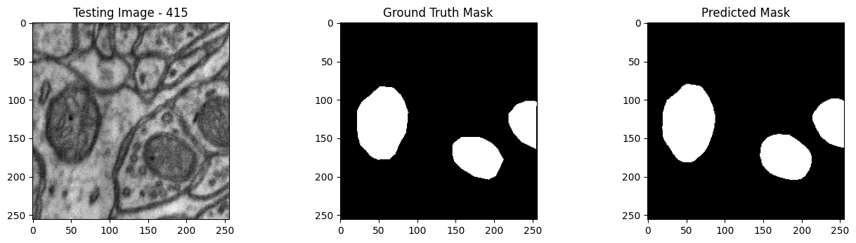


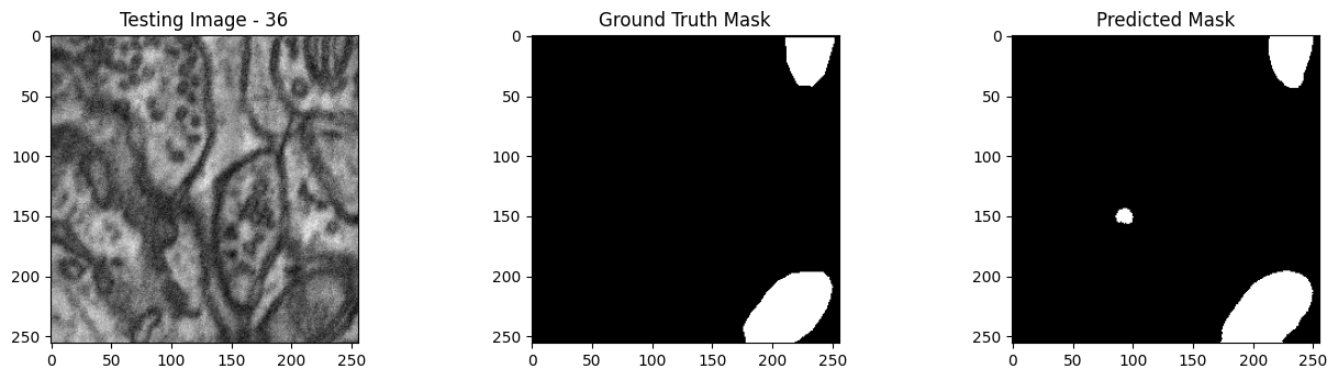
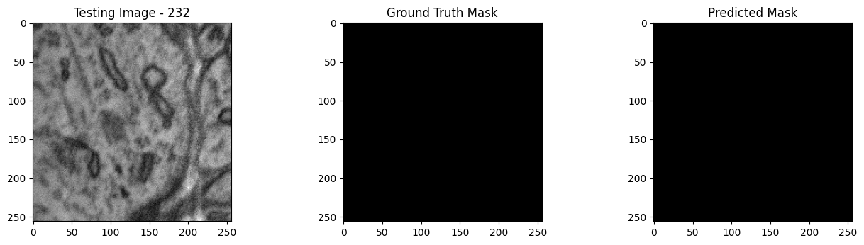


Undeploy Pipeline
With the experiment complete, we will undeploy the pipeline.
pipeline.undeploy()
| name | edgebiolabspipeline |
|---|---|
| created | 2023-09-08 18:50:52.714306+00:00 |
| last_updated | 2023-09-08 18:59:30.140145+00:00 |
| deployed | False |
| tags | |
| versions | 0321956b-098c-47eb-8f4c-3bd90e443f2d, 88bcc7a5-d618-4c72-90e5-651f1e252db9, d2425979-98ac-468c-83db-dd4f542e7217, 59a163a3-e9c7-4213-88bf-d732bcae7dbd, d608aa0f-4961-496f-b57c-ce02299b4e39, bf426f14-e3c4-4450-81d4-e833026505a9, b56f68b5-ae1d-49dc-b640-c964b10b117f, 951e4096-b3d7-426d-9eee-2b763d4a0558, e36b6b52-5652-440e-b856-89e42782b62f, 46ad2f62-987f-459d-8283-f495300647fa, 9c283c94-0ecd-4160-998e-b462d03008e1, 78b125a9-5311-46e7-adc8-5794f9ca29f0 |
| steps | edgebiolabsmodel |
| published | True |
Publish the Pipeline for Edge Deployment
It worked! For a demo, we’ll take working once as “tested”. So now that we’ve tested our pipeline, we are ready to publish it for edge deployment.
Publishing it means assembling all of the configuration files and model assets and pushing them to an Open Container Initiative (OCI) repository set in the Wallaroo instance as the Edge Registry service. DevOps engineers then retrieve that image and deploy it through Docker, Kubernetes, or similar deployments.
See Edge Deployment Registry Guide for details on adding an OCI Registry Service to Wallaroo as the Edge Deployment Registry.
This is done through the SDK command wallaroo.pipeline.publish(deployment_config) which has the following parameters and returns.
Publish a Pipeline Parameters
The publish method takes the following parameters. The containerized pipeline will be pushed to the Edge registry service with the model, pipeline configurations, and other artifacts needed to deploy the pipeline.
| Parameter | Type | Description |
|---|---|---|
deployment_config | wallaroo.deployment_config.DeploymentConfig (Optional) | Sets the pipeline deployment configuration. For example: For more information on pipeline deployment configuration, see the Wallaroo SDK Essentials Guide: Pipeline Deployment Configuration. |
Publish a Pipeline Returns
| Field | Type | Description |
|---|---|---|
| id | integer | Numerical Wallaroo id of the published pipeline. |
| pipeline version id | integer | Numerical Wallaroo id of the pipeline version published. |
| status | string | The status of the pipeline publication. Values include:
|
| Engine URL | string | The URL of the published pipeline engine in the edge registry. |
| Pipeline URL | string | The URL of the published pipeline in the edge registry. |
| Helm Chart URL | string | The URL of the helm chart for the published pipeline in the edge registry. |
| Helm Chart Reference | string | The help chart reference. |
| Helm Chart Version | string | The version of the Helm Chart of the published pipeline. This is also used as the Docker tag. |
| Engine Config | wallaroo.deployment_config.DeploymentConfig | The pipeline configuration included with the published pipeline. |
| Created At | DateTime | When the published pipeline was created. |
| Updated At | DateTime | When the published pipeline was updated. |
Publish Example
We will now publish the pipeline to our Edge Deployment Registry with the pipeline.publish(deployment_config) command. deployment_config is an optional field that specifies the pipeline deployment. This can be overridden by the DevOps engineer during deployment.
pub=pipeline.publish(deployment_config)
pub
Waiting for pipeline publish... It may take up to 600 sec.
Pipeline is Publishing...Published.
| ID | 11 |
| Pipeline Version | 59a163a3-e9c7-4213-88bf-d732bcae7dbd |
| Status | Published |
| Engine URL | ghcr.io/wallaroolabs/doc-samples/engines/proxy/wallaroo/ghcr.io/wallaroolabs/standalone-mini:v2023.3.0-3798 |
| Pipeline URL | ghcr.io/wallaroolabs/doc-samples/pipelines/edgebiolabspipeline:59a163a3-e9c7-4213-88bf-d732bcae7dbd |
| Helm Chart URL | ghcr.io/wallaroolabs/doc-samples/charts/edgebiolabspipeline |
| Helm Chart Reference | ghcr.io/wallaroolabs/doc-samples/charts@sha256:5d2a7b51c608133c6718a40d3dd589612260fd2f629de472ba13e7f95553fada |
| Helm Chart Version | 0.0.1-59a163a3-e9c7-4213-88bf-d732bcae7dbd |
| Engine Config | {'engine': {'resources': {'limits': {'cpu': 1.0, 'memory': '512Mi'}, 'requests': {'cpu': 1.0, 'memory': '512Mi'}}}, 'engineAux': {'images': {}}, 'enginelb': {'resources': {'limits': {'cpu': 1.0, 'memory': '512Mi'}, 'requests': {'cpu': 1.0, 'memory': '512Mi'}}}} |
| User Images | [] |
| Created By | john.hummel@wallaroo.ai |
| Created At | 2023-09-08 18:54:59.802486+00:00 |
| Updated At | 2023-09-08 18:54:59.802486+00:00 |
List Published Pipeline
The method wallaroo.client.list_pipelines() shows a list of all pipelines in the Wallaroo instance, and includes the published field that indicates whether the pipeline was published to the registry (True), or has not yet been published (False).
wl.list_pipelines()
| name | created | last_updated | deployed | tags | versions | steps | published |
|---|---|---|---|---|---|---|---|
| edgebiolabspipeline | 2023-08-Sep 18:50:52 | 2023-08-Sep 18:54:04 | True | d608aa0f-4961-496f-b57c-ce02299b4e39, bf426f14-e3c4-4450-81d4-e833026505a9, b56f68b5-ae1d-49dc-b640-c964b10b117f, 951e4096-b3d7-426d-9eee-2b763d4a0558, e36b6b52-5652-440e-b856-89e42782b62f, 46ad2f62-987f-459d-8283-f495300647fa, 9c283c94-0ecd-4160-998e-b462d03008e1, 78b125a9-5311-46e7-adc8-5794f9ca29f0 | edgebiolabsmodel | True | |
| edge-cv-demo | 2023-08-Sep 18:25:24 | 2023-08-Sep 18:37:14 | False | 69a912fb-47da-4049-98d5-aa024e7d66b2, 482fc033-00a6-42e7-b359-90611b76f74d, 32805f9a-40eb-4366-b444-635ab466ef76, b412ff15-c87b-46ea-8d96-48868b7867f0, aaf2c947-af26-4b0e-9819-f8aca5657017, 7ad0a22c-6472-4390-8f33-a8b3eccc7877, c73bbf20-8fe3-4714-be5e-e35773fe4779, fc431a83-22dc-43db-8610-cde3095af584 | resnet-50 | True | |
| edge-pipeline | 2023-08-Sep 17:30:28 | 2023-08-Sep 18:21:00 | False | 2d8f9e1d-dc65-4e90-a5ce-ee619162d8cd, 1ea2d089-1127-464d-a980-e087d1f052e2 | ccfraud | True | |
| edge-pipeline | 2023-08-Sep 17:24:44 | 2023-08-Sep 17:24:59 | False | 873582f4-4b39-4a69-a2b9-536a0e29927c, 079cf5a1-7e95-4cb7-ae40-381b538371db | ccfraud | True | |
| edge-pipeline-classification-cybersecurity | 2023-08-Sep 15:40:28 | 2023-08-Sep 15:45:22 | False | 60222730-4fb5-4179-b8bf-fa53762fecd1, 86040216-0bbb-4715-b08f-da461857c515, 34204277-bdbd-4ae2-9ce9-86dabe4be5f5, 729ccaa2-41b5-4c8f-89f4-fe1e98f2b303, 216bb86b-f6e8-498f-b8a5-020347355715 | aloha | True | |
| edge-pipeline | 2023-08-Sep 15:36:03 | 2023-08-Sep 15:36:03 | False | 83b49e9e-f43d-4459-bb2a-7fa144352307, 73a5d31f-75f5-42c4-9a9d-3ee524113b6c | aloha | False | |
| vgg16-clustering-pipeline | 2023-08-Sep 14:52:44 | 2023-08-Sep 14:56:09 | False | 50d6586a-0661-4f26-802d-c71da2ceea2e, d94e44b3-7ff6-4138-8b76-be1795cb6690, 8d2a8143-2255-408a-bd09-e3008a5bde0b | vgg16-clustering | True |
List Publishes from a Pipeline
All publishes created from a pipeline are displayed with the wallaroo.pipeline.publishes method. The pipeline_version_id is used to know what version of the pipeline was used in that specific publish. This allows for pipelines to be updated over time, and newer versions to be sent and tracked to the Edge Deployment Registry service.
List Publishes Parameters
N/A
List Publishes Returns
A List of the following fields:
| Field | Type | Description |
|---|---|---|
| id | integer | Numerical Wallaroo id of the published pipeline. |
| pipeline_version_id | integer | Numerical Wallaroo id of the pipeline version published. |
| engine_url | string | The URL of the published pipeline engine in the edge registry. |
| pipeline_url | string | The URL of the published pipeline in the edge registry. |
| created_by | string | The email address of the user that published the pipeline. |
| Created At | DateTime | When the published pipeline was created. |
| Updated At | DateTime | When the published pipeline was updated. |
pipeline.publishes()
| id | pipeline_version_name | engine_url | pipeline_url | created_by | created_at | updated_at |
|---|---|---|---|---|---|---|
| 10 | d608aa0f-4961-496f-b57c-ce02299b4e39 | ghcr.io/wallaroolabs/doc-samples/engines/proxy/wallaroo/ghcr.io/wallaroolabs/standalone-mini:v2023.3.0-3798 | ghcr.io/wallaroolabs/doc-samples/pipelines/edgebiolabspipeline:d608aa0f-4961-496f-b57c-ce02299b4e39 | john.hummel@wallaroo.ai | 2023-08-Sep 18:54:04 | 2023-08-Sep 18:54:04 |
Undeploy Pipeline
With the testing complete, the pipeline is undeployed and the resources returned back to the Wallaroo instance.
pipeline.undeploy()
Waiting for undeployment - this will take up to 45s .................................... ok
| name | edgebiolabspipeline |
|---|---|
| created | 2023-09-08 18:50:52.714306+00:00 |
| last_updated | 2023-09-08 18:54:04.264810+00:00 |
| deployed | False |
| tags | |
| versions | d608aa0f-4961-496f-b57c-ce02299b4e39, bf426f14-e3c4-4450-81d4-e833026505a9, b56f68b5-ae1d-49dc-b640-c964b10b117f, 951e4096-b3d7-426d-9eee-2b763d4a0558, e36b6b52-5652-440e-b856-89e42782b62f, 46ad2f62-987f-459d-8283-f495300647fa, 9c283c94-0ecd-4160-998e-b462d03008e1, 78b125a9-5311-46e7-adc8-5794f9ca29f0 |
| steps | edgebiolabsmodel |
| published | False |
DevOps - Pipeline Edge Deployment
Once a pipeline is deployed to the Edge Registry service, it can be deployed in environments such as Docker, Kubernetes, or similar container running services by a DevOps engineer.
Docker Deployment
First, the DevOps engineer must authenticate to the same OCI Registry service used for the Wallaroo Edge Deployment registry.
For more details, check with the documentation on your artifact service. The following are provided for the three major cloud services:
- Set up authentication for Docker
- Authenticate with an Azure container registry
- Authenticating Amazon ECR Repositories for Docker CLI with Credential Helper
For the deployment, the engine URL is specified with the following environmental variables:
DEBUG(true|false): Whether to include debug output.OCI_REGISTRY: The URL of the registry service.CONFIG_CPUS: The number of CPUs to use.OCI_USERNAME: The edge registry username.OCI_PASSWORD: The edge registry password or token.PIPELINE_URL: The published pipeline URL.
Docker Deployment Example
Using our sample environment, here’s sample deployment using Docker with a computer vision ML model, the same used in the Wallaroo Use Case Tutorials Computer Vision: Retail tutorials.
For docker run commands, the persistent volume for storing session data is stored with -v ./data:/persist. Updated as required for your deployments.
docker run -p 8080:8080 \
-v ./data:/persist \
-e DEBUG=true -e OCI_REGISTRY={your registry server} \
-e CONFIG_CPUS=4 \
-e OCI_USERNAME=oauth2accesstoken \
-e OCI_PASSWORD={registry token here} \
-e PIPELINE_URL={your registry server}/pipelines/edge-cv-retail:bf70eaf7-8c11-4b46-b751-916a43b1a555 \
{your registry server}/engine:v2023.3.0-main-3707
Docker Compose Deployment
For users who prefer to use docker compose, the following sample compose.yaml file is used to launch the Wallaroo Edge pipeline. This is the same used in the Wallaroo Use Case Tutorials Computer Vision: Retail tutorials. The session and other data is stored with the volumes entry to add a persistent volume.
services:
engine:
image: {Your Engine URL}
ports:
- 8080:8080
volumes:
- ./data:/persist
environment:
PIPELINE_URL: {Your Pipeline URL}
OCI_REGISTRY: {Your Edge Registry URL}
OCI_USERNAME: {Your Registry Username}
OCI_PASSWORD: {Your Token or Password}
CONFIG_CPUS: 1
For example:
services:
engine:
image: sample-registry.com/engine:v2023.3.0-main-3707
ports:
- 8080:8080
environment:
PIPELINE_URL: sample-registry.com/pipelines/edge-cv-retail:bf70eaf7-8c11-4b46-b751-916a43b1a555
OCI_REGISTRY: sample-registry.com
OCI_USERNAME: _json_key_base64
OCI_PASSWORD: abc123
CONFIG_CPUS: 1
Docker Compose Deployment Example
The deployment and undeployment is then just a simple docker compose up and docker compose down. The following shows an example of deploying the Wallaroo edge pipeline using docker compose.
docker compose up
[+] Running 1/1
✔ Container cv_data-engine-1 Recreated 0.5s
Attaching to cv_data-engine-1
cv_data-engine-1 | Wallaroo Engine - Standalone mode
cv_data-engine-1 | Login Succeeded
cv_data-engine-1 | Fetching manifest and config for pipeline: sample-registry.com/pipelines/edge-cv-retail:bf70eaf7-8c11-4b46-b751-916a43b1a555
cv_data-engine-1 | Fetching model layers
cv_data-engine-1 | digest: sha256:c6c8869645962e7711132a7e17aced2ac0f60dcdc2c7faa79b2de73847a87984
cv_data-engine-1 | filename: c6c8869645962e7711132a7e17aced2ac0f60dcdc2c7faa79b2de73847a87984
cv_data-engine-1 | name: resnet-50
cv_data-engine-1 | type: model
cv_data-engine-1 | runtime: onnx
cv_data-engine-1 | version: 693e19b5-0dc7-4afb-9922-e3f7feefe66d
cv_data-engine-1 |
cv_data-engine-1 | Fetched
cv_data-engine-1 | Starting engine
cv_data-engine-1 | Looking for preexisting `yaml` files in //modelconfigs
cv_data-engine-1 | Looking for preexisting `yaml` files in //pipelines
Helm Deployment
Published pipelines can be deployed through the use of helm charts.
Helm deployments take up to two steps - the first step is in retrieving the required values.yaml and making updates to override.
- Pull the helm charts from the published pipeline. The two fields are the Helm Chart URL and the Helm Chart version to specify the OCI . This typically takes the format of:
helm pull oci://{published.helm_chart_url} --version {published.helm_chart_version}
- Extract the
tgzfile and copy thevalues.yamland copy the values used to edit engine allocations, etc. The following are required for the deployment to run:
ociRegistry:
registry: {your registry service}
username: {registry username here}
password: {registry token here}
Store this into another file, suc as local-values.yaml.
- Create the namespace to deploy the pipeline to. For example, the namespace
wallaroo-edge-pipelinewould be:
kubectl create -n wallaroo-edge-pipeline
Deploy the
helminstallation withhelm installthrough one of the following options:Specify the
tgzfile that was downloaded and the local values file. For example:helm install --namespace {namespace} --values {local values file} {helm install name} {tgz path}Specify the expended directory from the downloaded
tgzfile.helm install --namespace {namespace} --values {local values file} {helm install name} {helm directory path}Specify the Helm Pipeline Helm Chart and the Pipeline Helm Version.
helm install --namespace {namespace} --values {local values file} {helm install name} oci://{published.helm_chart_url} --version {published.helm_chart_version}
Once deployed, the DevOps engineer will have to forward the appropriate ports to the
svc/engine-svcservice in the specific pipeline. For example, usingkubectl port-forwardto the namespaceccfraudthat would be:kubectl port-forward svc/engine-svc -n ccfraud01 8080 --address 0.0.0.0`
The following code segment generates a docker compose template based on the previously published pipeline.
docker_compose = f'''
services:
engine:
image: {pub.engine_url}
ports:
- 8080:8080
volumes:
- ./data:/persist
environment:
PIPELINE_URL: {pub.pipeline_url}
OCI_USERNAME: YOUR USERNAME
OCI_PASSWORD: YOUR PASSWORD OR TOKEN
OCI_REGISTRY: ghcr.io
CONFIG_CPUS: 4
'''
print(docker_compose)
services:
engine:
image: ghcr.io/wallaroolabs/doc-samples/engines/proxy/wallaroo/ghcr.io/wallaroolabs/standalone-mini:v2023.3.0-3798
ports:
- 8080:8080
environment:
PIPELINE_URL: ghcr.io/wallaroolabs/doc-samples/pipelines/edgebiolabspipeline:d608aa0f-4961-496f-b57c-ce02299b4e39
OCI_USERNAME: YOUR USERNAME
OCI_PASSWORD: YOUR PASSWORD OR TOKEN
OCI_REGISTRY: ghcr.io
CONFIG_CPUS: 4
Edge Deployed Pipeline API Endpoints
Once deployed, we can check the pipelines and models available. We’ll use a curl command, but any HTTP based request will work the same way.
The endpoint /pipelines returns:
- id (String): The name of the pipeline.
- status (String): The status as either
Running, orErrorif there are any issues.
For this example, the deployment is made on a machine called testboy.local. Replace this URL with the URL of you edge deployment.
!curl testboy.local:8080/pipelines
{"pipelines":[{"id":"edgebiolabspipeline","status":"Running"}]}
The endpoint /models returns a List of models with the following fields:
- name (String): The model name.
- sha (String): The sha hash value of the ML model.
- status (String): The status of either Running or Error if there are any issues.
- version (String): The model version. This matches the version designation used by Wallaroo to track model versions in UUID format.
!curl testboy.local:8080/models
{"models":[{"name":"edgebiolabsmodel","sha":"e80fcdaf563a183b0c32c027dcb3890a64e1764d6d7dcd29524cd270dd42e7bd","status":"Running","version":"37b76f7a-cef3-4dfb-8bed-c0779c0e668c"}]}
Edge Inference Endpoint
The inference endpoint takes the following pattern:
/pipelines/{pipeline-name}: Thepipeline-nameis the same as returned from the/pipelinesendpoint asid.
Wallaroo inference endpoint URLs accept the following data inputs through the Content-Type header:
Content-Type: application/vnd.apache.arrow.file: For Apache Arrow tables.Content-Type: application/json; format=pandas-records: For pandas DataFrame in record format.
Once deployed, we can perform an inference through the deployment URL.
The endpoint returns Content-Type: application/json; format=pandas-records by default with the following fields:
- check_failures (List[Integer]): Whether any validation checks were triggered. For more information, see Wallaroo SDK Essentials Guide: Pipeline Management: Anomaly Testing.
- elapsed (List[Integer]): A list of time in nanoseconds for:
- [0] The time to serialize the input.
- [1…n] How long each step took.
- model_name (String): The name of the model used.
- model_version (String): The version of the model in UUID format.
- original_data: The original input data. Returns
nullif the input may be too long for a proper return. - outputs (List): The outputs of the inference result separated by data type, where each data type includes:
- data: The returned values.
- dim (List[Integer]): The dimension shape returned.
- v (Integer): The vector shape of the data.
- pipeline_name (String): The name of the pipeline.
- shadow_data: Any shadow deployed data inferences in the same format as outputs.
- time (Integer): The time since UNIX epoch.
We’ll repeat our process above - only this time through the Python requests library to our locally deployed pipeline.
def loadImageAndConvertTiffList(imagePath, width, height):
img = cv2.imread(imagePath, 0)
imgNorm = np.expand_dims(normalize(np.array(img), axis=1),2)
imgNorm=imgNorm[:,:,0][:,:,None]
imgNorm=np.expand_dims(imgNorm, 0)
resizedImage = None
#creates a dictionary with the wallaroo "tensor" key and the numpy ndim array representing image as the value.
dictData = {"tensor":imgNorm.tolist()}
dataframedata = pd.DataFrame(dictData)
# display(dataframedata)
return dataframedata, resizedImage
def run_semantic_segmentation_inference_requests(pipeline_url, input_tiff_image, width, height, threshold):
tensor, resizedImage = loadImageAndConvertTiffList(input_tiff_image, width, height)
# print(tensor)
# #
# # run inference on the 256x256 patch image get the predicted mitochondria mask
# #
# set the content type and accept headers
headers = {
'Content-Type': 'application/json; format=pandas-records'
}
data = tensor.to_json(orient="records")
# print(data)
# print(pipeline_url)
response = requests.post(
pipeline_url,
headers=headers,
data=data,
verify=True
)
# list1d = response.json()[0]['outputs'][0]['Float']['data']
output = pd.DataFrame(response.json())
# display(output)
list1d = output.loc[0]["outputs"][0]['Float']['data']
# output = pipeline.infer(tensor)
# print(output)
# # Obtain the flattened predicted mitochandria mask result
# list1d = output.loc[0]["out.conv2d_37"]
np1d = np.array(list1d)
# # # unflatten it
predicted_mask = np1d.reshape(1,width,height,1)
# # # perform the element-wise comaprison operation using the threshold provided
predicted_mask = (predicted_mask[0,:,:,0] > threshold).astype(np.uint8)
# # return predicted_mask
return predicted_mask
# set this to your deployed pipeline's URL
host = 'http://testboy.local:8080'
deployurl = f'{host}/pipelines/edgebiolabspipeline'
for random_patch in random_patches:
# build the path to the image
patch_image_path = sample_mitochondria_patches_path + "/images/" + random_patch['patch_image_file']
# run inference in order to get the predicted 256x256 mask
predicted_mask = run_semantic_segmentation_inference_requests(deployurl, patch_image_path, 256,256, 0.2)
# # plot the results
test_image = random_patch['patch_image'][:,:,0]
test_image_title = f"Testing Image - {random_patch['index']}"
ground_truth_image = random_patch['patch_mask'][:,:,0]
ground_truth_image_title = "Ground Truth Mask"
predicted_mask_title = 'Predicted Mask'
tiff_utils.plot_test_results(test_image, test_image_title, \
ground_truth_image, ground_truth_image_title, \
predicted_mask, predicted_mask_title)

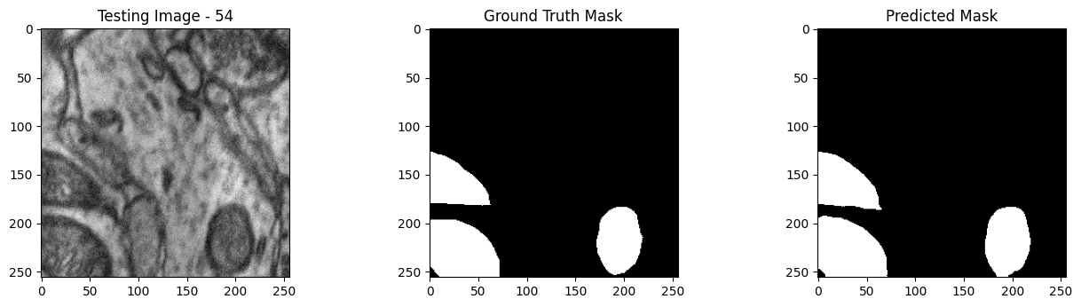
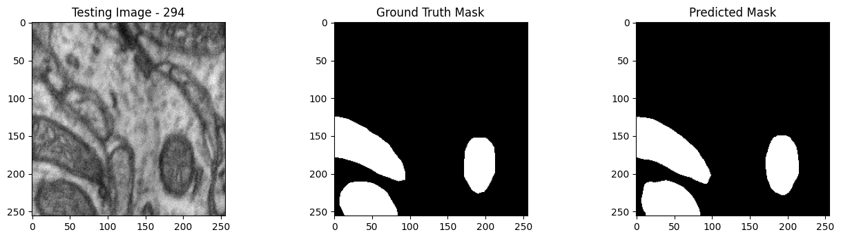
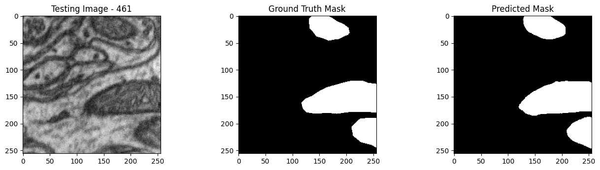


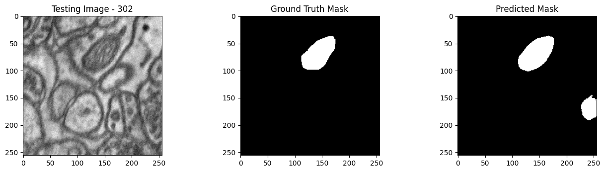
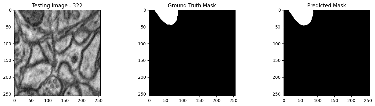
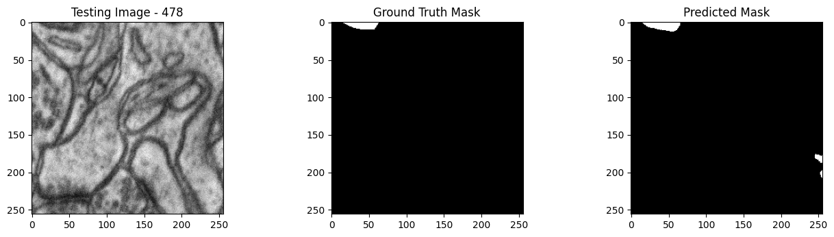
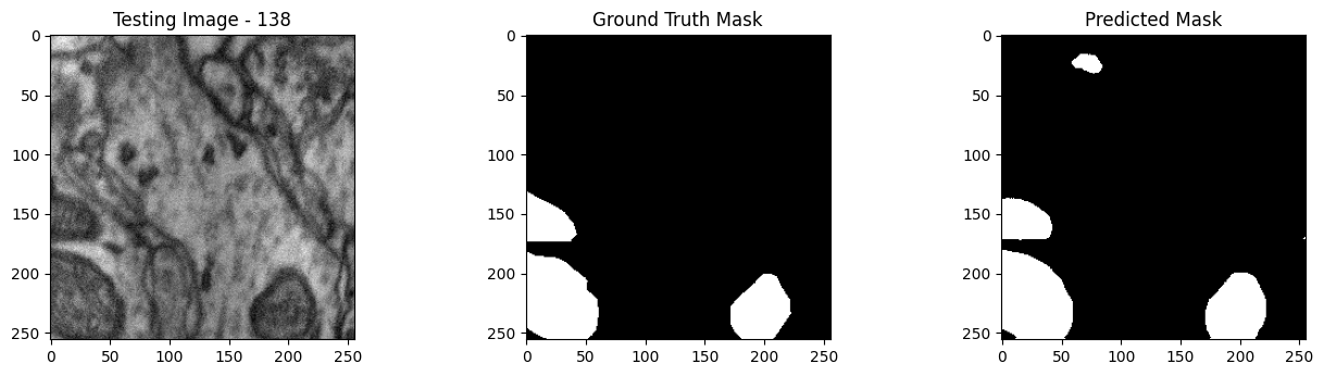
5.2 - Wallaroo Edge Classification Financial Services Deployment via MLOps API Demonstration
A demonstration on publishing a classification financial services model for edge deployment via the Wallaroo MLOps API.
The following tutorial is available on the Wallaroo Github Repository.
Classification Financial Services Edge Deployment Demonstration via API
This notebook will walk through building Wallaroo pipeline with a a Classification model deployed to detect the likelihood of credit card fraud, then publishing that pipeline to an Open Container Initiative (OCI) Registry where it can be deployed in other Docker and Kubernetes environments. This example uses the Wallaroo MLOps API.
This demonstration will focus on deployment to the edge.
This demonstration performs the following:
- As a Data Scientist in Wallaroo Ops:
- Upload a computer vision model to Wallaroo, deploy it in a Wallaroo pipeline, then perform a sample inference.
- Publish the pipeline to an Open Container Initiative (OCI) Registry service. This is configured in the Wallaroo instance. See Edge Deployment Registry Guide for details on adding an OCI Registry Service to Wallaroo as the Edge Deployment Registry. This demonstration uses a GitHub repository - see Introduction to GitHub Packages for setting up your own package repository using GitHub, which can then be used with this tutorial.
- View the pipeline publish details.
- As a DevOps Engineer in a remote aka edge device:
- Deploy the published pipeline as a Wallaroo Inference Server. This example will use Docker.
- Perform a sample inference through the Wallaroo Inference Server with the same data used in the data scientist example.
References
Data Scientist Pipeline Publish Steps
Load Libraries
The first step is to import the libraries used in this notebook.
import wallaroo
from wallaroo.object import EntityNotFoundError
import pyarrow as pa
import pandas as pd
import requests
# used to display dataframe information without truncating
from IPython.display import display
pd.set_option('display.max_colwidth', None)
Connect to the Wallaroo Instance through the User Interface
The next step is to connect to Wallaroo through the Wallaroo client. The Python library is included in the Wallaroo install and available through the Jupyter Hub interface provided with your Wallaroo environment.
This is accomplished using the wallaroo.Client() command, which provides a URL to grant the SDK permission to your specific Wallaroo environment. When displayed, enter the URL into a browser and confirm permissions. Store the connection into a variable that can be referenced later.
If logging into the Wallaroo instance through the internal JupyterHub service, use wl = wallaroo.Client(). For more information on Wallaroo Client settings, see the Client Connection guide.
wl = wallaroo.Client()
Create a New Workspace
We’ll use the SDK below to create our workspace , assign as our current workspace, then display all of the workspaces we have at the moment. We’ll also set up variables for our models and pipelines down the road, so we have one spot to change names to whatever fits your organization’s standards best.
To allow this tutorial to be run by multiple users in the same Wallaroo instance, a random 4 character prefix will be added to the workspace, pipeline, and model. Feel free to set suffix='' if this is not required.
import string
import random
# make a random 4 character suffix to verify uniqueness in tutorials
suffix= ''.join(random.choice(string.ascii_lowercase) for i in range(4))
workspace_name = f'edge-publish-api-demo{suffix}'
pipeline_name = 'edge-pipeline'
model_name = 'ccfraud'
model_file_name = './models/xgboost_ccfraud.onnx'
def get_workspace(name):
workspace = None
for ws in wl.list_workspaces():
if ws.name() == name:
workspace= ws
if(workspace == None):
workspace = wl.create_workspace(name)
return workspace
def get_pipeline(name):
try:
pipeline = wl.pipelines_by_name(name)[0]
except EntityNotFoundError:
pipeline = wl.build_pipeline(name)
return pipeline
workspace = get_workspace(workspace_name)
wl.set_current_workspace(workspace)
{'name': 'edge-publish-api-demozbnv', 'id': 27, 'archived': False, 'created_by': 'aa707604-ec80-495a-a9a1-87774c8086d5', 'created_at': '2023-09-19T19:44:20.31345+00:00', 'models': [], 'pipelines': []}
Upload the Model
When a model is uploaded to a Wallaroo cluster, it is optimized and packaged to make it ready to run as part of a pipeline. In many times, the Wallaroo Server can natively run a model without any Python overhead. In other cases, such as a Python script, a custom Python environment will be automatically generated. This is comparable to the process of “containerizing” a model by adding a small HTTP server and other wrapping around it.
Our pretrained model is in ONNX format, which is specified in the framework parameter.
edge_demo_model = wl.upload_model(
model_name,
model_file_name,
framework=wallaroo.framework.Framework.ONNX,
).configure(tensor_fields=["tensor"])
Reserve Pipeline Resources
Before deploying an inference engine we need to tell wallaroo what resources it will need.
To do this we will use the wallaroo DeploymentConfigBuilder() and fill in the options listed below to determine what the properties of our inference engine will be.
We will be testing this deployment for an edge scenario, so the resource specifications are kept small – what’s the minimum needed to meet the expected load on the planned hardware.
- cpus - 0.5 => allow the engine to use 4 CPU cores when running the neural net
- memory - 900Mi => each inference engine will have 2 GB of memory, which is plenty for processing a single image at a time.
- arch - we will specify the X86 architecture.
deploy_config = (wallaroo
.DeploymentConfigBuilder()
.replica_count(1)
.cpus(1)
.memory("900Mi")
.build()
)
Simulated Edge Deployment
We will now deploy our pipeline into the current Kubernetes environment using the specified resource constraints. This is a “simulated edge” deploy in that we try to mimic the edge hardware as closely as possible.
pipeline = get_pipeline(pipeline_name)
display(pipeline)
pipeline.add_model_step(edge_demo_model)
pipeline.deploy(deployment_config = deploy_config)
| name | edge-pipeline |
|---|---|
| created | 2023-09-19 19:38:20.298800+00:00 |
| last_updated | 2023-09-19 19:41:15.049021+00:00 |
| deployed | False |
| tags | |
| versions | de226e15-5500-4b26-9c80-ee089e196585, 15be4514-3459-462c-a633-153511608d4a |
| steps | ccfraud-xgboost |
| published | False |
| name | edge-pipeline |
|---|---|
| created | 2023-09-19 19:44:25.627257+00:00 |
| last_updated | 2023-09-19 19:44:25.627257+00:00 |
| deployed | True |
| tags | |
| versions | ed209209-c8dc-4d9b-b381-1255e1d57800 |
| steps | ccfraud |
| published | False |
Run Single Image Inference
A single image, encoded using the Apache Arrow format, is sent to the deployed pipeline. Arrow is used here because, as a binary protocol, there is far lower network and compute overhead than using JSON. The Wallaroo Server engine accepts both JSON, pandas DataFrame, and Apache Arrow formats.
The sample DataFrames and arrow tables are in the ./data directory. We’ll use the Apache Arrow table cc_data_10k.arrow.
Once complete, we’ll display how long the inference request took.
deploy_url = pipeline._deployment._url()
headers = wl.auth.auth_header()
headers['Content-Type']='application/vnd.apache.arrow.file'
# headers['Content-Type']='application/json; format=pandas-records'
headers['Accept']='application/json; format=pandas-records'
dataFile = './data/cc_data_10k.arrow'
!curl -X POST {deploy_url} \
-H "Authorization:{headers['Authorization']}" \
-H "Content-Type:{headers['Content-Type']}" \
-H "Accept:{headers['Accept']}" \
--data-binary @{dataFile} > curl_response.df.json
% Total % Received % Xferd Average Speed Time Time Time Current
Dload Upload Total Spent Left Speed
100 7731k 100 6568k 100 1162k 2343k 414k 0:00:02 0:00:02 --:--:-- 2761k
Undeploy the Pipeline
With the testing complete, we can undeploy the pipeline. Note that deploying and undeploying a pipeline is not required for publishing a pipeline to the Edge Registry - this is done just for this demonstration.
pipeline.undeploy()
| name | edge-pipeline |
|---|---|
| created | 2023-09-19 19:44:25.627257+00:00 |
| last_updated | 2023-09-19 19:44:25.627257+00:00 |
| deployed | False |
| tags | |
| versions | ed209209-c8dc-4d9b-b381-1255e1d57800 |
| steps | ccfraud |
| published | False |
Publish the Pipeline for Edge Deployment
It worked! For a demo, we’ll take working once as “tested”. So now that we’ve tested our pipeline, we are ready to publish it for edge deployment.
Publishing it means assembling all of the configuration files and model assets and pushing them to an Open Container Initiative (OCI) repository set in the Wallaroo instance as the Edge Registry service. DevOps engineers then retrieve that image and deploy it through Docker, Kubernetes, or similar deployments.
See Edge Deployment Registry Guide for details on adding an OCI Registry Service to Wallaroo as the Edge Deployment Registry.
This is done through the SDK command wallaroo.pipeline.publish(deployment_config) which has the following parameters and returns.
Publish a Pipeline Endpoint
Pipelines are published as images to the edge registry set in the Enable Wallaroo Edge Registry through the following endpoint.
- Endpoint:
/v1/api/pipelines/publish
- Parameters
- pipeline_id (Integer Required): The numerical id of the pipeline to publish to the edge registry.
- pipeline_version_id (Integer Required): The numerical id of the pipeline’s version to publish to the edge registry.
- model_config_ids (List Optional): The list of model config ids to include.
- Returns
- id (Integer): Numerical Wallaroo id of the published pipeline.
- pipeline_version_id (Integer): Numerical Wallaroo id of the pipeline version published.
- status: The status of the pipeline publish. Values include:
- PendingPublish: The pipeline publication is about to be uploaded or is in the process of being uploaded.
- Published: The pipeline is published and ready for use.
- created_at (String): When the published pipeline was created.
- updated_at (String): When the published pipeline was updated.
- created_by (String): The email address of the Wallaroo user that created the pipeline publish.
- pipeline_url (String): The URL of the published pipeline in the edge registry. May be
nulluntil the status isPublished) - engine_url (String): The URL of the published pipeline engine in the edge registry. May be
nulluntil the status isPublished. - helm: ???
- engine_config (*
wallaroo.deployment_config.DeploymentConfig) | The pipeline configuration included with the published pipeline.
Publish Example
We will now publish the pipeline to our Edge Deployment Registry with the pipeline.publish(deployment_config) command. deployment_config is an optional field that specifies the pipeline deployment. This can be overridden by the DevOps engineer during deployment. For this demonstration, we will be retrieving the most recent pipeline version.
For this, we will require the pipeline version id, the workspace id, and the model config ids (which will be empty as not required).
# get the pipeline version
pipeline_version_id = pipeline.versions()[-1].id()
display(pipeline_version_id)
pipeline_id = pipeline.id()
display(pipeline_id)
headers = {
"Authorization": wl.auth._bearer_token_str(),
"Content-Type": "application/json",
}
url = f"{wl.api_endpoint}/v1/api/pipelines/publish"
response = requests.post(
url,
headers=headers,
json={"pipeline_id": 1,
"pipeline_version_id": pipeline_version_id,
"model_config_ids": [edge_demo_model.id()]
}
)
display(response.json())
13
13
{'id': 8,
'pipeline_version_id': 13,
'pipeline_version_name': '1ea2d089-1127-464d-a980-e087d1f052e2',
'status': 'PendingPublish',
'created_at': '2023-09-08T18:21:51.987293+00:00',
'updated_at': '2023-09-08T18:21:51.987293+00:00',
'created_by': 'aa707604-ec80-495a-a9a1-87774c8086d5',
'pipeline_url': None,
'engine_url': None,
'helm': None,
'engine_config': {'engine': {'resources': {'limits': {'cpu': 4.0,
'memory': '3Gi'},
'requests': {'cpu': 4.0, 'memory': '3Gi'}}},
'enginelb': {'resources': {'limits': {'cpu': 1.0, 'memory': '512Mi'},
'requests': {'cpu': 0.2, 'memory': '512Mi'}}},
'engineAux': {}},
'error': None,
'user_images': []}
publish_id = response.json()['id']
display(publish_id)
8
Get Publish Status
The status of a created Wallaroo pipeline publish is available through the following endpoint.
- Endpoint:
/v1/api/pipelines/get_publish_status
- Parameters
- publish_id (Integer Required): The numerical id of the pipeline publish to retrieve.
- Returns
- id (Integer): Numerical Wallaroo id of the published pipeline.
- pipeline_version_id (Integer): Numerical Wallaroo id of the pipeline version published.
- status: The status of the pipeline publish. Values include:
- PendingPublish: The pipeline publication is about to be uploaded or is in the process of being uploaded.
- Published: The pipeline is published and ready for use.
- created_at (String): When the published pipeline was created.
- updated_at (String): When the published pipeline was updated.
- created_by (String): The email address of the Wallaroo user that created the pipeline publish.
- pipeline_url (String): The URL of the published pipeline in the edge registry. May be
nulluntil the status isPublished) - engine_url (String): The URL of the published pipeline engine in the edge registry. May be
nulluntil the status isPublished. - helm: The Helm chart information including the following fields:
- reference (String): The Helm reference.
- chart (String): The Helm chart URL.
- version (String): The Helm chart version.
- engine_config (*
wallaroo.deployment_config.DeploymentConfig) | The pipeline configuration included with the published pipeline.
Get Publish Status Example
The following example shows retrieving the status of a recently created pipeline publish. Once the published status is Published we know the pipeline is ready for deployment.
headers = {
"Authorization": wl.auth._bearer_token_str(),
"Content-Type": "application/json",
}
url = f"{wl.api_endpoint}/v1/api/pipelines/get_publish_status"
response = requests.post(
url,
headers=headers,
json={
"id": publish_id
},
)
display(response.json())
pub = response.json()
{'id': 8,
'pipeline_version_id': 13,
'pipeline_version_name': '1ea2d089-1127-464d-a980-e087d1f052e2',
'status': 'Published',
'created_at': '2023-09-08T18:21:51.987293+00:00',
'updated_at': '2023-09-08T18:21:51.987293+00:00',
'created_by': 'aa707604-ec80-495a-a9a1-87774c8086d5',
'pipeline_url': 'ghcr.io/wallaroolabs/doc-samples/pipelines/edge-pipeline:1ea2d089-1127-464d-a980-e087d1f052e2',
'engine_url': 'ghcr.io/wallaroolabs/doc-samples/engines/proxy/wallaroo/ghcr.io/wallaroolabs/standalone-mini:v2023.3.0-3798',
'helm': {'reference': 'ghcr.io/wallaroolabs/doc-samples/charts@sha256:1c19b448ae2adc33c39a954665bba079377a4a4a5bf73f81ebcc4a067eeb3fde',
'chart': 'ghcr.io/wallaroolabs/doc-samples/charts/edge-pipeline',
'version': '0.0.1-1ea2d089-1127-464d-a980-e087d1f052e2'},
'engine_config': {'engine': {'resources': {'limits': {'cpu': 4.0,
'memory': '3Gi'},
'requests': {'cpu': 4.0, 'memory': '3Gi'}}},
'enginelb': {'resources': {'limits': {'cpu': 1.0, 'memory': '512Mi'},
'requests': {'cpu': 0.2, 'memory': '512Mi'}}},
'engineAux': {}},
'error': None,
'user_images': []}
List Publishes for a Pipeline
A list of publishes created for a specific pipeline is retrieved through the following endpoint.
- Endpoint:
/v1/api/pipelines/list_publishes_for_pipeline
- Parameters
- publish_id (Integer Required): The numerical id of the pipeline to retrieve all publishes for.
- Returns a List of pipeline publishes with the following fields:
- id (Integer): Numerical Wallaroo id of the published pipeline.
- pipeline_version_id (Integer): Numerical Wallaroo id of the pipeline version published.
- status: The status of the pipeline publish. Values include:
PendingPublish: The pipeline publication is about to be uploaded or is in the process of being uploaded.Published: The pipeline is published and ready for use.
- created_at (String): When the published pipeline was created.
- updated_at (String): When the published pipeline was updated.
- created_by (String): The email address of the Wallaroo user that created the pipeline publish.
- pipeline_url (String): The URL of the published pipeline in the edge registry. May be
nulluntil the status isPublished) - engine_url (String): The URL of the published pipeline engine in the edge registry. May be
nulluntil the status isPublished. - helm: The Helm chart information including the following fields:
- reference (String): The Helm reference.
- chart (String): The Helm chart URL.
- version (String): The Helm chart version.
- engine_config (*
wallaroo.deployment_config.DeploymentConfig) | The pipeline configuration included with the published pipeline.
List Publishes for a Pipeline Example
headers = {
"Authorization": wl.auth._bearer_token_str(),
"Content-Type": "application/json",
}
url = f"{wl.api_endpoint}/v1/api/pipelines/list_publishes_for_pipeline"
response = requests.post(
url,
headers=headers,
json={"pipeline_id": pipeline_id},
)
display(response.json())
{'pipelines': [{'id': 7,
'pipeline_version_id': 13,
'pipeline_version_name': '1ea2d089-1127-464d-a980-e087d1f052e2',
'status': 'Published',
'created_at': '2023-09-08T18:17:12.975417+00:00',
'updated_at': '2023-09-08T18:17:12.975417+00:00',
'created_by': 'aa707604-ec80-495a-a9a1-87774c8086d5',
'pipeline_url': 'ghcr.io/wallaroolabs/doc-samples/pipelines/edge-pipeline:1ea2d089-1127-464d-a980-e087d1f052e2',
'engine_url': 'ghcr.io/wallaroolabs/doc-samples/engines/proxy/wallaroo/ghcr.io/wallaroolabs/standalone-mini:v2023.3.0-3798',
'helm': {'reference': 'ghcr.io/wallaroolabs/doc-samples/charts@sha256:6e6b2fa3b595b2add4bf177588a131d4493b9c38999ee22a00a34af41332f307',
'chart': 'ghcr.io/wallaroolabs/doc-samples/charts/edge-pipeline',
'version': '0.0.1-1ea2d089-1127-464d-a980-e087d1f052e2'},
'engine_config': {'engine': {'resources': {'limits': {'cpu': 4.0,
'memory': '3Gi'},
'requests': {'cpu': 4.0, 'memory': '3Gi'}}},
'enginelb': {'resources': {'limits': {'cpu': 1.0, 'memory': '512Mi'},
'requests': {'cpu': 0.2, 'memory': '512Mi'}}},
'engineAux': {}},
'error': None,
'user_images': []},
{'id': 5,
'pipeline_version_id': 13,
'pipeline_version_name': '1ea2d089-1127-464d-a980-e087d1f052e2',
'status': 'Error',
'created_at': '2023-09-08T17:44:10.957028+00:00',
'updated_at': '2023-09-08T17:44:10.957028+00:00',
'created_by': 'aa707604-ec80-495a-a9a1-87774c8086d5',
'pipeline_url': None,
'engine_url': None,
'helm': None,
'engine_config': {'engine': {'resources': {'limits': {'cpu': 4.0,
'memory': '3Gi'},
'requests': {'cpu': 4.0, 'memory': '3Gi'}}},
'enginelb': {'resources': {'limits': {'cpu': 1.0, 'memory': '512Mi'},
'requests': {'cpu': 0.2, 'memory': '512Mi'}}},
'engineAux': {}},
'error': 'Authentication failure: ',
'user_images': []},
{'id': 4,
'pipeline_version_id': 13,
'pipeline_version_name': '1ea2d089-1127-464d-a980-e087d1f052e2',
'status': 'Published',
'created_at': '2023-09-08T17:31:35.735893+00:00',
'updated_at': '2023-09-08T17:31:35.735893+00:00',
'created_by': 'aa707604-ec80-495a-a9a1-87774c8086d5',
'pipeline_url': 'ghcr.io/wallaroolabs/doc-samples/pipelines/edge-pipeline:1ea2d089-1127-464d-a980-e087d1f052e2',
'engine_url': 'ghcr.io/wallaroolabs/doc-samples/engines/proxy/wallaroo/ghcr.io/wallaroolabs/standalone-mini:v2023.3.0-3798',
'helm': {'reference': 'ghcr.io/wallaroolabs/doc-samples/charts@sha256:819e7476614f99e5d83069fccac4b7eef347b891915625c39978b94718c116e7',
'chart': 'ghcr.io/wallaroolabs/doc-samples/charts/edge-pipeline',
'version': '0.0.1-1ea2d089-1127-464d-a980-e087d1f052e2'},
'engine_config': {'engine': {'resources': {'limits': {'cpu': 4.0,
'memory': '3Gi'},
'requests': {'cpu': 4.0, 'memory': '3Gi'}}},
'enginelb': {'resources': {'limits': {'cpu': 1.0, 'memory': '512Mi'},
'requests': {'cpu': 0.2, 'memory': '512Mi'}}},
'engineAux': {}},
'error': None,
'user_images': []},
{'id': 6,
'pipeline_version_id': 13,
'pipeline_version_name': '1ea2d089-1127-464d-a980-e087d1f052e2',
'status': 'Published',
'created_at': '2023-09-08T18:07:42.61758+00:00',
'updated_at': '2023-09-08T18:07:42.61758+00:00',
'created_by': 'aa707604-ec80-495a-a9a1-87774c8086d5',
'pipeline_url': 'ghcr.io/wallaroolabs/doc-samples/pipelines/edge-pipeline:1ea2d089-1127-464d-a980-e087d1f052e2',
'engine_url': 'ghcr.io/wallaroolabs/doc-samples/engines/proxy/wallaroo/ghcr.io/wallaroolabs/standalone-mini:v2023.3.0-3798',
'helm': {'reference': 'ghcr.io/wallaroolabs/doc-samples/charts@sha256:be785f7bbc91a4cad8d5fa15893e1a198e507242e801e40322d5d61ee537906e',
'chart': 'ghcr.io/wallaroolabs/doc-samples/charts/edge-pipeline',
'version': '0.0.1-1ea2d089-1127-464d-a980-e087d1f052e2'},
'engine_config': {'engine': {'resources': {'limits': {'cpu': 4.0,
'memory': '3Gi'},
'requests': {'cpu': 4.0, 'memory': '3Gi'}}},
'enginelb': {'resources': {'limits': {'cpu': 1.0, 'memory': '512Mi'},
'requests': {'cpu': 0.2, 'memory': '512Mi'}}},
'engineAux': {}},
'error': None,
'user_images': []},
{'id': 8,
'pipeline_version_id': 13,
'pipeline_version_name': '1ea2d089-1127-464d-a980-e087d1f052e2',
'status': 'Publishing',
'created_at': '2023-09-08T18:21:51.987293+00:00',
'updated_at': '2023-09-08T18:21:51.987293+00:00',
'created_by': 'aa707604-ec80-495a-a9a1-87774c8086d5',
'pipeline_url': None,
'engine_url': None,
'helm': None,
'engine_config': {'engine': {'resources': {'limits': {'cpu': 4.0,
'memory': '3Gi'},
'requests': {'cpu': 4.0, 'memory': '3Gi'}}},
'enginelb': {'resources': {'limits': {'cpu': 1.0, 'memory': '512Mi'},
'requests': {'cpu': 0.2, 'memory': '512Mi'}}},
'engineAux': {}},
'error': None,
'user_images': []}]}
DevOps Deployment
We now have our pipeline published to our Edge Registry service. We can deploy this in a x86 environment running Docker that is logged into the same registry service that we deployed to.
For more details, check with the documentation on your artifact service. The following are provided for the three major cloud services:
- Set up authentication for Docker
- Authenticate with an Azure container registry
- Authenticating Amazon ECR Repositories for Docker CLI with Credential Helper
DevOps - Pipeline Edge Deployment
Once a pipeline is deployed to the Edge Registry service, it can be deployed in environments such as Docker, Kubernetes, or similar container running services by a DevOps engineer.
Docker Deployment
First, the DevOps engineer must authenticate to the same OCI Registry service used for the Wallaroo Edge Deployment registry.
For more details, check with the documentation on your artifact service. The following are provided for the three major cloud services:
- Set up authentication for Docker
- Authenticate with an Azure container registry
- Authenticating Amazon ECR Repositories for Docker CLI with Credential Helper
For the deployment, the engine URL is specified with the following environmental variables:
DEBUG(true|false): Whether to include debug output.OCI_REGISTRY: The URL of the registry service.CONFIG_CPUS: The number of CPUs to use.OCI_USERNAME: The edge registry username.OCI_PASSWORD: The edge registry password or token.PIPELINE_URL: The published pipeline URL.
Docker Deployment Example
Using our sample environment, here’s sample deployment using Docker with a computer vision ML model, the same used in the Wallaroo Use Case Tutorials Computer Vision: Retail tutorials.
docker run -p 8080:8080 \
-e DEBUG=true -e OCI_REGISTRY={your registry server} \
-e CONFIG_CPUS=1 \
-e OCI_USERNAME=oauth2accesstoken \
-e OCI_PASSWORD={registry token here} \
-e PIPELINE_URL={your registry server}/pipelines/edge-cv-retail:bf70eaf7-8c11-4b46-b751-916a43b1a555 \
{your registry server}/engine:v2023.3.0-main-3707
Docker Compose Deployment
For users who prefer to use docker compose, the following sample compose.yaml file is used to launch the Wallaroo Edge pipeline. This is the same used in the Wallaroo Use Case Tutorials Computer Vision: Retail tutorials.
services:
engine:
image: {Your Engine URL}
ports:
- 8080:8080
environment:
PIPELINE_URL: {Your Pipeline URL}
OCI_REGISTRY: {Your Edge Registry URL}
OCI_USERNAME: {Your Registry Username}
OCI_PASSWORD: {Your Token or Password}
CONFIG_CPUS: 1
For example:
services:
engine:
image: sample-registry.com/engine:v2023.3.0-main-3707
ports:
- 8080:8080
environment:
PIPELINE_URL: sample-registry.com/pipelines/edge-cv-retail:bf70eaf7-8c11-4b46-b751-916a43b1a555
OCI_REGISTRY: sample-registry.com
OCI_USERNAME: _json_key_base64
OCI_PASSWORD: abc123
CONFIG_CPUS: 1
Docker Compose Deployment Example
The deployment and undeployment is then just a simple docker compose up and docker compose down. The following shows an example of deploying the Wallaroo edge pipeline using docker compose.
docker compose up
[+] Running 1/1
✔ Container cv_data-engine-1 Recreated 0.5s
Attaching to cv_data-engine-1
cv_data-engine-1 | Wallaroo Engine - Standalone mode
cv_data-engine-1 | Login Succeeded
cv_data-engine-1 | Fetching manifest and config for pipeline: sample-registry.com/pipelines/edge-cv-retail:bf70eaf7-8c11-4b46-b751-916a43b1a555
cv_data-engine-1 | Fetching model layers
cv_data-engine-1 | digest: sha256:c6c8869645962e7711132a7e17aced2ac0f60dcdc2c7faa79b2de73847a87984
cv_data-engine-1 | filename: c6c8869645962e7711132a7e17aced2ac0f60dcdc2c7faa79b2de73847a87984
cv_data-engine-1 | name: resnet-50
cv_data-engine-1 | type: model
cv_data-engine-1 | runtime: onnx
cv_data-engine-1 | version: 693e19b5-0dc7-4afb-9922-e3f7feefe66d
cv_data-engine-1 |
cv_data-engine-1 | Fetched
cv_data-engine-1 | Starting engine
cv_data-engine-1 | Looking for preexisting `yaml` files in //modelconfigs
cv_data-engine-1 | Looking for preexisting `yaml` files in //pipelines
Helm Deployment
Published pipelines can be deployed through the use of helm charts.
Helm deployments take up to two steps - the first step is in retrieving the required values.yaml and making updates to override.
- Pull the helm charts from the published pipeline. The two fields are the Helm Chart URL and the Helm Chart version to specify the OCI . This typically takes the format of:
helm pull oci://{published.helm_chart_url} --version {published.helm_chart_version}
- Extract the
tgzfile and copy thevalues.yamland copy the values used to edit engine allocations, etc. The following are required for the deployment to run:
ociRegistry:
registry: {your registry service}
username: {registry username here}
password: {registry token here}
Store this into another file, suc as local-values.yaml.
- Create the namespace to deploy the pipeline to. For example, the namespace
wallaroo-edge-pipelinewould be:
kubectl create -n wallaroo-edge-pipeline
Deploy the
helminstallation withhelm installthrough one of the following options:Specify the
tgzfile that was downloaded and the local values file. For example:helm install --namespace {namespace} --values {local values file} {helm install name} {tgz path}Specify the expended directory from the downloaded
tgzfile.helm install --namespace {namespace} --values {local values file} {helm install name} {helm directory path}Specify the Helm Pipeline Helm Chart and the Pipeline Helm Version.
helm install --namespace {namespace} --values {local values file} {helm install name} oci://{published.helm_chart_url} --version {published.helm_chart_version}
Once deployed, the DevOps engineer will have to forward the appropriate ports to the
svc/engine-svcservice in the specific pipeline. For example, usingkubectl port-forwardto the namespaceccfraudthat would be:kubectl port-forward svc/engine-svc -n ccfraud01 8080 --address 0.0.0.0`
docker_compose = f'''
services:
engine:
image: {pub['engine_url']}
ports:
- 8080:8080
environment:
PIPELINE_URL: {pub['pipeline_url']}
OCI_USERNAME: YOUR USERNAME
OCI_PASSWORD: YOUR PASSWORD OR TOKEN
OCI_REGISTRY: ghcr.io
CONFIG_CPUS: 1
'''
print(docker_compose)
services:
engine:
image: ghcr.io/wallaroolabs/doc-samples/engines/proxy/wallaroo/ghcr.io/wallaroolabs/standalone-mini:v2023.3.0-3798
ports:
- 8080:8080
environment:
PIPELINE_URL: ghcr.io/wallaroolabs/doc-samples/pipelines/edge-pipeline:1ea2d089-1127-464d-a980-e087d1f052e2
OCI_USERNAME: YOUR USERNAME
OCI_PASSWORD: YOUR PASSWORD OR TOKEN
OCI_REGISTRY: ghcr.io
CONFIG_CPUS: 4
Edge Deployed Pipeline API Endpoints
Once deployed, we can check the pipelines and models available. We’ll use a curl command, but any HTTP based request will work the same way.
The endpoint /pipelines returns:
- id (String): The name of the pipeline.
- status (String): The status as either
Running, orErrorif there are any issues.
For this example, the deployment is made on a machine called testboy.local. Replace this URL with the URL of you edge deployment.
!curl testboy.local:8080/pipelines
{"pipelines":[{"id":"edge-pipeline","status":"Running"}]}
The endpoint /models returns a List of models with the following fields:
- name (String): The model name.
- sha (String): The sha hash value of the ML model.
- status (String): The status of either Running or Error if there are any issues.
- version (String): The model version. This matches the version designation used by Wallaroo to track model versions in UUID format.
!curl testboy.local:8080/models
{"models":[{"name":"ccfraud","sha":"054810e3e3ebbdd34438d9c1a08ed6a6680ef10bf97b9223f78ebf38e14b3b52","status":"Running","version":"4b28d9f8-31ad-4f4b-a262-a2196530c3d0"}]}
Edge Inference Endpoint
The inference endpoint takes the following pattern:
/pipelines/{pipeline-name}: Thepipeline-nameis the same as returned from the/pipelinesendpoint asid.
Wallaroo inference endpoint URLs accept the following data inputs through the Content-Type header:
Content-Type: application/vnd.apache.arrow.file: For Apache Arrow tables.Content-Type: application/json; format=pandas-records: For pandas DataFrame in record format.
Once deployed, we can perform an inference through the deployment URL.
The endpoint returns Content-Type: application/json; format=pandas-records by default with the following fields:
- check_failures (List[Integer]): Whether any validation checks were triggered. For more information, see Wallaroo SDK Essentials Guide: Pipeline Management: Anomaly Testing.
- elapsed (List[Integer]): A list of time in nanoseconds for:
- [0] The time to serialize the input.
- [1…n] How long each step took.
- model_name (String): The name of the model used.
- model_version (String): The version of the model in UUID format.
- original_data: The original input data. Returns
nullif the input may be too long for a proper return. - outputs (List): The outputs of the inference result separated by data type, where each data type includes:
- data: The returned values.
- dim (List[Integer]): The dimension shape returned.
- v (Integer): The vector shape of the data.
- pipeline_name (String): The name of the pipeline.
- shadow_data: Any shadow deployed data inferences in the same format as outputs.
- time (Integer): The time since UNIX epoch.
!curl -X POST testboy.local:8080/pipelines/edge-pipeline -H "Content-Type: application/vnd.apache.arrow.file" --data-binary @./data/cc_data_10k.arrow
[{"check_failures":[],"elapsed":[1831692,4085791],"model_name":"ccfraud","model_version":"4b28d9f8-31ad-4f4b-a262-a2196530c3d0","original_data":null,"outputs":[{"Float":{"data":[1.0094895362854004,1.0094895362854004,1.0094895362854004,1.0094895362854004,-1.8477439880371094e-6,-0.00004494190216064453,-0.00009369850158691406,-0.0000832676887512207,-0.00008344650268554688,0.0004897117614746094,0.0006609857082366943,0.00007578730583190918,-0.00010061264038085938,-0.000519871711730957,-3.7550926208496094e-6,-0.00010895729064941406,-0.00017696619033813477,-0.000028371810913085938,0.00002181529998779297,-0.00008505582809448242,-0.000049233436584472656,0.00020524859428405762,0.00001677870750427246,-0.00008910894393920898,0.00008806586265563965,0.0002167224884033203,-0.00003045797348022461,-0.0001615285873413086,-0.00007712841033935547,-8.046627044677734e-6,-0.000048100948333740234,-0.00013583898544311523,-0.000014126300811767578,-0.00015842914581298828,-0.00004863739013671875,0.0000731050968170166,-7.212162017822266e-6,0.0005553662776947021,7.420778274536133e-6,9.000301361083984e-6,0.00011602044105529785,0.00005555152893066406,-0.00020551681518554688,0.0006919503211975098,-0.00003838539123535156,-0.00010466575622558594,0.000025719404220581055,0.00022289156913757324,-0.00014388561248779297,0.00006046891212463379,0.0006777942180633545,-0.0006906390190124512,-0.000011146068572998047,-0.0000692605972290039,-4.172325134277344e-6,0.00008225440979003906,0.0013971328735351562,-0.00010895729064941406,-0.00002586841583251953,-0.00024509429931640625,0.0001341700553894043,0.0000641942024230957,-0.00023108720779418945,0.00012108683586120605,-0.000026285648345947266,-0.00005835294723510742,-0.000056803226470947266,0.0002706944942474365,-9.298324584960938e-6,0.0013747215270996094,0.00010889768600463867,0.0001391768455505371,0.00033020973205566406,-2.9206275939941406e-6,0.00009962916374206543,-0.000033855438232421875,-0.00003886222839355469,0.00020307302474975586,0.00041168928146362305,0.00003641843795776367,0.0007800459861755371,-0.00003427267074584961,-0.0003724098205566406,6.556510925292969e-7,-0.000026047229766845703,-0.00004279613494873047,-0.00003844499588012695,0.0000171661376953125,0.000019282102584838867,0.00004598498344421387,-0.00011116266250610352,0.0008075833320617676,0.0003064572811126709,-0.000026226043701171875,0.00022932887077331543,-0.00015473365783691406,0.000012218952178955078,0.0007858872413635254,0.0010485351085662842,-0.000953972339630127,0.00006034970283508301,-0.00013965368270874023,0.00014868378639221191,-0.0000960230827331543,0.00022268295288085938,-0.00002372264862060547,0.00015243887901306152,0.000058531761169433594,-0.00020366907119750977,-0.00003266334533691406,0.000046372413635253906,0.0003497898578643799,-0.00004309415817260742,-0.00007253885269165039,0.00013744831085205078,-0.00005334615707397461,0.00008705258369445801,0.00015547871589660645,0.00010827183723449707,0.00015839934349060059,-0.000951230525970459,0.0005430281162261963,0.0006096959114074707,0.00005373358726501465,0.00014838576316833496,-5.543231964111328e-6,-0.000038564205169677734,0.0002301037311553955,0.0002828240394592285,0.0000254213809967041,0.00009182095527648926,0.00012382864952087402,0.000030219554901123047,-0.0001442432403564453,-0.0010399818420410156,0.000041604042053222656,0.00030282139778137207,0.0004699230194091797,0.00001004338264465332,-8.761882781982422e-6,0.0006243288516998291,-0.00013703107833862305,0.0004756748676300049,0.00006377696990966797,0.00004094839096069336,-0.00004678964614868164,-0.000261843204498291,0.000060230493545532227,-0.00003314018249511719,-0.00006818771362304688,-0.000022351741790771484,0.0002624392509460449,0.00011542439460754395,-0.0001252889633178711,0.00009205937385559082,0.000047087669372558594,-0.00013875961303710938,0.00016242265701293945,0.00018420815467834473,0.0000667572021484375,-0.00004190206527709961,1.0031051635742188,8.374452590942383e-6,-0.000011146068572998047,-0.00010162591934204102,-0.000054776668548583984,-0.00003916025161743164,0.00008448958396911621,0.0006806254386901855,0.00007832050323486328,-0.00006818771362304688,7.957220077514648e-6,0.000030159950256347656,1.4007091522216797e-6,0.000012487173080444336,0.00011420249938964844,0.000038564205169677734,-0.00006175041198730469,0.00010338425636291504,0.0006650686264038086,6.705522537231445e-6,0.0000705718994140625,-0.00001341104507446289,-0.00016045570373535156,-0.00001436471939086914,8.821487426757812e-6,-0.00004565715789794922,0.00005206465721130371,0.0000788569450378418,-0.00005453824996948242,-0.00010496377944946289,-0.000057578086853027344,0.000014543533325195312,0.00007987022399902344,0.00005200505256652832,-0.00004106760025024414,0.00017750263214111328,0.00004857778549194336,0.00022241473197937012,5.8710575103759766e-6,0.00012260675430297852,-0.00009238719940185547,-0.00009495019912719727,-0.00006073713302612305,-0.0000603795051574707,-0.00002372264862060547,0.0003605782985687256,0.00006362795829772949,0.0001945197582244873,-0.00007486343383789062,0.0003400444984436035,0.0001691877841949463,-0.00011646747589111328,-0.00003045797348022461,1.4007091522216797e-6,0.00003993511199951172,-0.00004845857620239258,0.00029987096786499023,-0.00008589029312133789,0.00002962350845336914,-8.165836334228516e-6,-0.00006395578384399414,0.000011980533599853516,-0.000048041343688964844,0.000013172626495361328,0.00007236003875732422,-0.00003057718276977539,0.0001099705696105957,0.00006970763206481934,0.0026289522647857666,0.00034049153327941895,0.00022974610328674316,-0.00011205673217773438,0.00008842349052429199,0.0001296699047088623,-0.00002199411392211914,-0.00011396408081054688,1.6391277313232422e-6,-0.00009763240814208984,7.0035457611083984e-6,-0.00025451183319091797,0.00005170702934265137,-0.0003129243850708008,0.0002517402172088623,-0.00006282329559326172,-0.00003266334533691406,0.000010371208190917969,-0.00007551908493041992,0.000017523765563964844,0.0002104043960571289,0.00024232268333435059,0.00011464953422546387,0.000016510486602783203,-0.00013703107833862305,0.0002478361129760742,0.00009262561798095703,-0.00012320280075073242,0.00013723969459533691,-0.0001881122589111328,-0.00006717443466186523,-0.000027894973754882812,0.0001271665096282959,0.00034058094024658203,-0.000050067901611328125,-0.00013691186904907227,-0.00003516674041748047,-0.0000673532485961914,-0.000025987625122070312,-0.0007557272911071777,0.00003692507743835449,0.000291287899017334,0.000023066997528076172,0.00007557868957519531,-0.00021779537200927734,0.0001627206802368164,0.00006014108657836914,0.0001519322395324707,8.255243301391602e-6,0.000011712312698364258,0.00004503130912780762,-0.00007915496826171875,0.00009515881538391113,-0.00006175041198730469,0.00008749961853027344,-0.000049233436584472656,0.000013053417205810547,-0.00006175041198730469,-0.00009000301361083984,0.000032454729080200195,0.000038743019104003906,0.00017514824867248535,0.000022619962692260742,0.00015926361083984375,-0.00010162591934204102,0.00005957484245300293,0.00046065449714660645,-4.172325134277344e-6,0.00011304020881652832,-0.00002872943878173828,-0.0000616908073425293,-2.9206275939941406e-6,0.00009137392044067383,-0.0000407099723815918,0.00010654330253601074,0.00010898709297180176,0.00014150142669677734,-0.00004857778549194336,0.00007382035255432129,-7.092952728271484e-6,-0.000019490718841552734,0.0000254213809967041,0.00002682209014892578,0.0014048218727111816,0.00003522634506225586,0.001670747995376587,-0.00003314018249511719,-0.000051140785217285156,0.00006148219108581543,-0.0001386404037475586,0.00016745924949645996,-0.00005173683166503906,-0.00012826919555664062,-0.00011724233627319336,-0.000025033950805664062,-0.00008755922317504883,-0.00004583597183227539,-0.00014722347259521484,-0.00033473968505859375,-0.00005125999450683594,-0.0013584494590759277,0.00020137429237365723,-0.00010502338409423828,-0.0004221796989440918,-0.00008535385131835938,0.00017812848091125488,0.000019818544387817383,0.00001385807991027832,-0.00004857778549194336,-0.00006175041198730469,-0.00001996755599975586,0.0003409385681152344,-0.00009971857070922852,0.000023305416107177734,-0.00009584426879882812,0.0004963576793670654,-0.00014019012451171875,0.00020310282707214355,-0.000027120113372802734,-1.1920928955078125e-6,0.00012561678886413574,-0.00004220008850097656,0.00016936659812927246,-0.000019848346710205078,-0.00004404783248901367,-0.0001474618911743164,0.00023934245109558105,-0.00006943941116333008,0.000010371208190917969,-1.7881393432617188e-7,-0.0016776323318481445,-0.000028133392333984375,-9.298324584960938e-6,0.00020357966423034668,0.00007766485214233398,-0.00005346536636352539,0.00007814168930053711,-0.00009500980377197266,-0.00001996755599975586,-0.00004202127456665039,0.0030659139156341553,0.00007766485214233398,0.000040590763092041016,0.00007304549217224121,0.00021648406982421875,-8.344650268554688e-7,0.00035637617111206055,0.0003491342067718506,-0.00001150369644165039,-0.000049233436584472656,-0.00007539987564086914,-5.364418029785156e-7,-0.00007033348083496094,0.001573026180267334,0.000011712312698364258,-0.00008821487426757812,-0.00008380413055419922,0.000051409006118774414,0.000037342309951782227,-0.00006765127182006836,0.0005421638488769531,-0.00006622076034545898,0.000021398067474365234,-0.00003415346145629883,-0.00016832351684570312,-0.000049054622650146484,-9.298324584960938e-6,-0.00004029273986816406,-0.00024503469467163086,-0.00015115737915039062,0.00006666779518127441,0.00016412138938903809,0.000011980533599853516,-9.000301361083984e-6,-0.000019788742065429688,0.000352710485458374,-0.000037670135498046875,0.0000426173210144043,0.0003161132335662842,0.0002676844596862793,0.0002047419548034668,-0.000017583370208740234,-0.000268399715423584,9.000301361083984e-6,-0.00011771917343139648,-0.00002872943878173828,0.00005939602851867676,0.0005748867988586426,0.0002168118953704834,0.00011768937110900879,-0.00001823902130126953,-0.00009167194366455078,0.00010922551155090332,-0.00003254413604736328,0.00010541081428527832,0.0013660788536071777,-0.0002314448356628418,-5.424022674560547e-6,0.00002041459083557129,0.00013369321823120117,-0.000019073486328125,0.0004660487174987793,-0.000048279762268066406,-5.900859832763672e-6,0.002194702625274658,-0.00008296966552734375,0.00016680359840393066,-0.000052928924560546875,-2.9206275939941406e-6,-0.00010597705841064453,0.00006327033042907715,0.000562518835067749,-0.0007330179214477539,-0.000021457672119140625,-0.00008469820022583008,0.000058084726333618164,0.00005015730857849121,0.00018325448036193848,-0.000030279159545898438,-0.00006848573684692383,-0.00001341104507446289,-0.00003254413604736328,0.0006752610206604004,-0.0003809928894042969,0.0001696944236755371,-6.4373016357421875e-6,0.00015291571617126465,-0.00004929304122924805,-0.000013887882232666016,0.0006453394889831543,-0.00008928775787353516,0.00009682774543762207,-0.00008690357208251953,7.748603820800781e-6,-0.0000540614128112793,0.0001620650291442871,0.00020524859428405762,0.00006130337715148926,-0.000011026859283447266,-0.00006645917892456055,0.00038427114486694336,-0.000010609626770019531,-0.00019943714141845703,0.00016736984252929688,-0.00006848573684692383,-0.0010878443717956543,-0.000021457672119140625,0.0006114840507507324,0.0007844865322113037,0.00006723403930664062,-0.000011205673217773438,0.000056415796279907227,0.000023305416107177734,-0.00003266334533691406,-0.00007069110870361328,-0.000011682510375976562,0.000032275915145874023,-0.0000623464584350586,0.00015985965728759766,-0.00010776519775390625,-0.00004285573959350586,0.0002612173557281494,0.000039130449295043945,0.000017911195755004883,-3.933906555175781e-6,-0.00007611513137817383,0.00012165307998657227,-0.00003266334533691406,-0.00007635354995727539,0.001859515905380249,-0.00006598234176635742,-0.0002478361129760742,0.0005283355712890625,-0.00015586614608764648,-0.00007998943328857422,-0.0000374913215637207,0.00015607476234436035,0.00005653500556945801,-0.0001461505889892578,-0.0001703500747680664,-0.00011497735977172852,0.00015872716903686523,0.00003629922866821289,0.0005819499492645264,0.0002072751522064209,-0.00010275840759277344,0.0006814897060394287,0.000024944543838500977,-0.00006175041198730469,-0.00010985136032104492,-0.00032955408096313477,-0.00007462501525878906,-2.980232238769531e-7,0.00002390146255493164,-0.00041353702545166016,0.00014549493789672852,-0.0004501938819885254,-0.00006175041198730469,0.00004735589027404785,0.00018990039825439453,2.5331974029541016e-6,0.000028908252716064453,-0.0004271268844604492,-0.0007519125938415527,-0.0019210577011108398,-0.00004029273986816406,-0.00004220008850097656,0.000060886144638061523,0.000553429126739502,-0.00003975629806518555,0.00006702542304992676,0.0007629990577697754,-0.00008744001388549805,-0.000056684017181396484,0.0006085634231567383,-0.00003838539123535156,-0.000047087669372558594,0.00039055943489074707,0.0005201399326324463,4.202127456665039e-6,-0.00007230043411254883,0.0000667572021484375,-0.000045299530029296875,0.00008890032768249512,-0.00012606382369995117,0.0001658797264099121,-0.00003999471664428711,-0.00005936622619628906,-0.0002568960189819336,0.00007066130638122559,-0.00006455183029174805,-0.00031310319900512695,-0.000053763389587402344,-0.000041484832763671875,0.00022780895233154297,-0.00007712841033935547,0.00035378336906433105,0.0008490979671478271,-0.00001150369644165039,8.64267349243164e-6,-0.0001227855682373047,0.001187354326248169,0.00001341104507446289,7.152557373046875e-6,0.000040590763092041016,0.000037044286727905273,0.0020221471786499023,-0.00005513429641723633,-0.0001303553581237793,-0.00005453824996948242,-0.000057756900787353516,-8.761882781982422e-6,-0.00004869699478149414,-0.00009393692016601562,-0.0000922083854675293,0.00021260976791381836,-0.0002377629280090332,-0.00012499094009399414,0.00007683038711547852,0.00019982457160949707,-0.000031113624572753906,0.00007963180541992188,-0.00003254413604736328,0.000024139881134033203,0.00015729665756225586,0.001053154468536377,-0.0001131892204284668,0.00010439753532409668,0.0004248321056365967,-0.0000712275505065918,0.00003272294998168945,0.002625793218612671,0.00015535950660705566,0.000023305416107177734,-0.00006729364395141602,-0.00006306171417236328,-0.00016045570373535156,7.957220077514648e-6,-0.000017583370208740234,0.00002905726432800293,0.00007387995719909668,0.000056415796279907227,-0.00016051530838012695,0.0006984174251556396,0.0016936957836151123,-0.00003266334533691406,-0.00005233287811279297,-0.00001609325408935547,-0.0002071857452392578,-0.0002918839454650879,-0.000048279762268066406,-0.000021696090698242188,-0.00003999471664428711,-5.900859832763672e-6,0.00012260675430297852,0.00006961822509765625,-1.8477439880371094e-6,0.008613228797912598,0.0001391768455505371,-0.000044465065002441406,0.00011470913887023926,0.0001399517059326172,0.00003293156623840332,-0.00003415346145629883,-0.00022113323211669922,0.0002512037754058838,-0.00013506412506103516,-0.0010699033737182617,-0.0001405477523803711,0.000040590763092041016,-5.602836608886719e-6,0.0005582273006439209,0.00010216236114501953,-0.0002544522285461426,-0.00005161762237548828,-0.00002092123031616211,0.00002625584602355957,0.00004920363426208496,-0.00022113323211669922,-0.00003147125244140625,-0.000047087669372558594,0.0012041926383972168,2.2649765014648438e-6,0.000011056661605834961,0.00008317828178405762,0.0002574622631072998,-0.000056743621826171875,-0.00005841255187988281,0.00032591819763183594,-0.00013452768325805664,-0.000017583370208740234,-0.00011199712753295898,0.000055283308029174805,0.00007304549217224121,0.00005412101745605469,0.00010669231414794922,0.000015676021575927734,-1.8477439880371094e-6,-0.00014919042587280273,0.00005990266799926758,7.450580596923828e-7,0.00020956993103027344,-0.00013208389282226562,0.00017517805099487305,0.0000667572021484375,0.000014871358871459961,-0.000052034854888916016,0.000058531761169433594,-0.000039577484130859375,0.00005969405174255371,0.000035136938095092773,-0.00007867813110351562,0.00006723403930664062,-0.00006264448165893555,-0.00003260374069213867,-0.00004947185516357422,-0.000027954578399658203,0.00025528669357299805,-0.00003266334533691406,0.00017511844635009766,-0.000018656253814697266,0.00038802623748779297,8.374452590942383e-6,0.00008296966552734375,-0.00006264448165893555,0.0012904107570648193,0.00015109777450561523,0.0011358857154846191,-0.00008356571197509766,-0.00017273426055908203,-0.00008046627044677734,-0.00008004903793334961,0.0001869797706604004,0.00008097290992736816,-0.000054836273193359375,0.00011780858039855957,-0.00011783838272094727,-8.52346420288086e-6,-0.000012159347534179688,4.559755325317383e-6,-0.000052869319915771484,-0.00032824277877807617,0.00022241473197937012,0.00011655688285827637,0.00021776556968688965,0.00009191036224365234,0.00001677870750427246,0.00020399689674377441,-0.00002765655517578125,0.00003337860107421875,0.0008656978607177734,0.00002753734588623047,-0.000021219253540039062,-0.000021159648895263672,0.00013762712478637695,0.00005939602851867676,-0.00024515390396118164,0.00006103515625,0.000015109777450561523,0.00004920363426208496,-0.00008690357208251953,0.0004245340824127197,-0.00003463029861450195,-4.649162292480469e-6,-0.0003299117088317871,-0.00007665157318115234,-0.00011205673217773438,-0.000059723854064941406,-0.0001443028450012207,0.0013949573040008545,7.62939453125e-6,0.0007587075233459473,0.000040590763092041016,0.00013449788093566895,0.0005497932434082031,-0.00003904104232788086,0.000059217214584350586,-0.0000578761100769043,-0.00016045570373535156,-0.00003451108932495117,0.00005283951759338379,-0.00013113021850585938,0.00005415081977844238,-0.000855565071105957,0.000051409006118774414,-0.00004279613494873047,0.000138014554977417,-0.000050067901611328125,-0.00006276369094848633,-0.0003508329391479492,0.00016322731971740723,-9.715557098388672e-6,0.00006318092346191406,-0.000015974044799804688,-0.000057756900787353516,0.0001418590545654297,-3.6954879760742188e-6,0.0001640617847442627,0.0005311965942382812,-0.0006833672523498535,7.778406143188477e-6,-0.0001595616340637207,0.0004950761795043945,0.00011652708053588867,-0.00012344121932983398,7.420778274536133e-6,0.0005854666233062744,0.000058323144912719727,0.0004997849464416504,0.00010451674461364746,-0.0000445246696472168,-0.00005638599395751953,-0.0000807642936706543,0.00039327144622802734,-0.00002372264862060547,-0.00008660554885864258,-7.748603820800781e-7,0.00026237964630126953,-0.00011301040649414062,0.00016757845878601074,-0.00010389089584350586,0.00034815073013305664,-0.000040590763092041016,0.00032773613929748535,0.000030249357223510742,-0.00039887428283691406,-0.00003319978713989258,-0.00010836124420166016,0.0000152587890625,-0.00001245737075805664,-0.000012814998626708984,0.00008043646812438965,-0.00006759166717529297,0.004439592361450195,-0.00006645917892456055,0.0006435513496398926,-0.00003653764724731445,-0.0002791285514831543,-0.00016379356384277344,0.000012874603271484375,0.0005150735378265381,-0.00006687641143798828,0.00005841255187988281,0.00005939602851867676,-0.000022709369659423828,0.00006777048110961914,0.0012004077434539795,0.00008353590965270996,-0.00009953975677490234,-0.00007104873657226562,0.0002047717571258545,0.000015944242477416992,0.00017377734184265137,-0.00009417533874511719,0.00018593668937683105,0.000523298978805542,-0.0006039142608642578,0.00020459294319152832,0.0019805729389190674,0.0000222623348236084,0.00005188584327697754,-0.00030815601348876953,0.000050067901611328125,0.000056415796279907227,0.00018021464347839355,0.000042110681533813477,0.00010761618614196777,7.778406143188477e-6,0.000010877847671508789,0.000011056661605834961,0.000010371208190917969,-5.4836273193359375e-6,0.000012248754501342773,0.00014084577560424805,0.000020951032638549805,0.00031754374504089355,0.0004915893077850342,-0.00018334388732910156,0.000017583370208740234,-0.00047284364700317383,0.00005391240119934082,0.00005137920379638672,0.000029385089874267578,0.000026464462280273438,0.00008949637413024902,0.00022846460342407227,0.0002377331256866455,9.000301361083984e-6,0.00024303793907165527,-0.0001838207244873047,0.0002231597900390625,-8.881092071533203e-6,9.59634780883789e-6,-0.0001849532127380371,-0.0003368854522705078,0.00008615851402282715,0.00004723668098449707,0.0006887316703796387,-0.00006175041198730469,7.12275505065918e-6,0.00015872716903686523,0.000011056661605834961,0.00006052851676940918,0.0005851984024047852,0.00016483664512634277,0.0009807050228118896,0.00011464953422546387,0.00007292628288269043,-0.00011301040649414062,-0.00006622076034545898,0.00011947751045227051,0.00007915496826171875,-0.000058591365814208984,0.00007042288780212402,-0.000049233436584472656,-0.000026226043701171875,0.000024259090423583984,0.0003885626792907715,0.00011587142944335938,0.00012484192848205566,0.00009378790855407715,-0.00008535385131835938,0.000039517879486083984,0.001344531774520874,-0.00008475780487060547,0.00007766485214233398,0.001497119665145874,-0.0002904534339904785,0.0001322329044342041,0.0004950761795043945,-0.00003403425216674805,-0.0000553131103515625,-0.00015795230865478516,0.0005057156085968018,-0.00040262937545776367,0.0008079111576080322,0.0001640021800994873,-0.00012570619583129883,0.00005409121513366699,-0.00014066696166992188,-0.00006854534149169922,-0.00002104043960571289,0.00006321072578430176,-0.000432431697845459,0.000056415796279907227,0.00020197033882141113,0.00005334615707397461,-0.0020911097526550293,0.000041425228118896484,0.00004228949546813965,3.8743019104003906e-7,0.0009822249412536621,-0.0005515813827514648,0.0005631446838378906,-0.00010466575622558594,-0.00007265806198120117,-0.00005745887756347656,0.00025767087936401367,0.000044733285903930664,0.00003701448440551758,0.000035643577575683594,0.00011068582534790039,-0.00001239776611328125,0.00023868680000305176,-0.00008052587509155273,0.00021761655807495117,-0.00013256072998046875,0.00004029273986816406,-0.00008046627044677734,0.000011593103408813477,-0.000050127506256103516,-0.00005918741226196289,0.9965696334838867,-0.0008934736251831055,1.1026859283447266e-6,0.0003985166549682617,0.000039130449295043945,0.0010131001472473145,0.0005317330360412598,0.00009769201278686523,-0.00022274255752563477,-0.00003910064697265625,-0.00134962797164917,0.0003387928009033203,0.0001786649227142334,0.00005182623863220215,0.00018659234046936035,-0.00004595518112182617,-0.00006395578384399414,0.0004660487174987793,-0.000030875205993652344,0.0004372894763946533,0.0001856684684753418,-0.000020742416381835938,0.0000648796558380127,-0.000017344951629638672,-0.0008408427238464355,-0.00008678436279296875,0.00031766295433044434,-0.00012040138244628906,0.0004812479019165039,0.00007590651512145996,0.0000616610050201416,-0.0011248588562011719,-0.0001601576805114746,-0.00020951032638549805,0.00026991963386535645,0.00071677565574646,0.00007534027099609375,0.00004082918167114258,0.0001093745231628418,0.00005581974983215332,0.00005221366882324219,0.00020304322242736816,-0.000045299530029296875,-0.0001806020736694336,-0.000043392181396484375,0.00014150142669677734,-0.0000985860824584961,0.0005464255809783936,-2.980232238769531e-7,0.00006115436553955078,0.00010135769844055176,0.0002200603485107422,-4.470348358154297e-6,0.00002962350845336914,-0.00005924701690673828,-0.00014603137969970703,-0.00018286705017089844,-0.00006002187728881836,-0.00003254413604736328,0.00022280216217041016,-7.450580596923828e-6,-0.00003910064697265625,-0.00002467632293701172,0.0000826418399810791,0.00003764033317565918,-0.00025969743728637695,0.00010520219802856445,-0.000037670135498046875,-0.00009328126907348633,-0.00005120038986206055,-0.00017708539962768555,-0.000033736228942871094,-0.00014472007751464844,0.00023701786994934082,-0.00009149312973022461,0.000011056661605834961,-0.00046384334564208984,-0.00008732080459594727,0.00008612871170043945,0.0000991523265838623,0.00006970763206481934,0.00001767277717590332,-0.00005990266799926758,-0.00013267993927001953,-0.00009244680404663086,-8.881092071533203e-6,0.00005564093589782715,0.0001270771026611328,-0.000025391578674316406,-0.000013470649719238281,-0.00007164478302001953,0.00007304549217224121,0.0016810297966003418,0.000013053417205810547,-0.0001380443572998047,-0.0000985264778137207,1.2814998626708984e-6,0.0001932382583618164,0.00007447600364685059,0.00010457634925842285,0.00022715330123901367,-0.00007086992263793945,0.00008016824722290039,0.00007963180541992188,0.0008942782878875732,0.00005227327346801758,-0.0000584721565246582,-0.00028645992279052734,0.00008612871170043945,-0.00025194883346557617,0.05461674928665161,-0.00025266408920288086,-0.000024378299713134766,-7.510185241699219e-6,-0.00009459257125854492,-0.000060558319091796875,0.0007780492305755615,-6.377696990966797e-6,0.000046581029891967773,-0.00010734796524047852,0.0003878474235534668,0.000015109777450561523,-0.00006884336471557617,4.559755325317383e-6,-0.00010710954666137695,0.00014281272888183594,-0.00002866983413696289,0.000023424625396728516,0.000027447938919067383,0.0000470578670501709,-0.0000788569450378418,9.804964065551758e-6,0.00013846158981323242,-6.67572021484375e-6,0.00003123283386230469,0.0000921785831451416,0.0017957985401153564,-3.4570693969726562e-6,0.0001793503761291504,-0.0001347661018371582,-0.00006681680679321289,0.00018611550331115723,-0.0003120303153991699,0.00001385807991027832,-0.00009882450103759766,0.00001430511474609375,-0.00009208917617797852,0.00044852495193481445,0.00010320544242858887,0.00008630752563476562,-0.000025987625122070312,0.0000432133674621582,0.00002893805503845215,0.000034689903259277344,0.00007456541061401367,-0.0000623464584350586,-0.000054836273193359375,0.000035762786865234375,-0.00030434131622314453,-0.00012695789337158203,0.0007923245429992676,0.000057131052017211914,-0.0000883936882019043,-0.0007992386817932129,0.0002683103084564209,-0.000022470951080322266,-0.00013816356658935547,0.000043392181396484375,0.00003573298454284668,-0.000022709369659423828,-0.00010758638381958008,0.00010839104652404785,-0.0006168484687805176,0.00002378225326538086,0.0010581612586975098,-0.00011301040649414062,0.000038743019104003906,0.00009745359420776367,-0.00005918741226196289,0.00003796815872192383,0.00005251169204711914,0.00003549456596374512,0.00013241171836853027,0.000029832124710083008,0.0005008280277252197,0.00013044476509094238,-0.00005823373794555664,0.00003713369369506836,-0.00020927190780639648,-0.000043511390686035156,-0.00010758638381958008,0.000254213809967041,-0.00010579824447631836,0.0005966722965240479,-0.000020325183868408203,0.00003841519355773926,0.00031119585037231445,-0.0000438690185546875,0.000035136938095092773,-0.0001201629638671875,-0.00035393238067626953,0.00008487701416015625,0.00010117888450622559,-0.00012099742889404297,-0.000011086463928222656,0.0002905428409576416,5.990266799926758e-6,0.00007233023643493652,0.0000254213809967041,0.00016224384307861328,9.000301361083984e-6,-0.00007069110870361328,8.07642936706543e-6,2.5331974029541016e-6,0.0002567172050476074,0.00037658214569091797,0.0007415115833282471,-0.00009274482727050781,-0.00004857778549194336,0.00006911158561706543,1.6391277313232422e-6,-0.00006753206253051758,-0.0001570582389831543,6.258487701416016e-7,0.00044411420822143555,0.00022205710411071777,0.00008234381675720215,-0.00008207559585571289,-0.00003993511199951172,-0.00015431642532348633,-0.00007092952728271484,-0.00003802776336669922,-0.00001043081283569336,0.00007665157318115234,-0.00008052587509155273,0.0012735426425933838,-0.00010704994201660156,-0.00006395578384399414,0.00014200806617736816,0.00019243359565734863,0.0003650188446044922,-0.00015676021575927734,-0.0001327991485595703,-0.00003618001937866211,-0.0002758502960205078,0.0002887248992919922,0.00001531839370727539,0.00037932395935058594,-0.000046253204345703125,0.00007557868957519531,0.00018683075904846191,0.00008445978164672852,0.00010889768600463867,-0.00003701448440551758,0.000038743019104003906,-0.000024080276489257812,0.000013887882232666016,-0.0003847479820251465,-0.0001946091651916504,0.0003078281879425049,-0.000532686710357666,-0.0000597834587097168,-9.298324584960938e-6,0.00012245774269104004,-0.000048041343688964844,-0.0001233220100402832,0.00014397501945495605,-0.00013715028762817383,-0.0000654458999633789,-0.00011771917343139648,6.0498714447021484e-6,0.00008001923561096191,-0.00014531612396240234,-0.000024080276489257812,0.000036090612411499023,0.0000432431697845459,0.000018537044525146484,0.00006395578384399414,0.00002065300941467285,0.000240325927734375,0.000087738037109375,-0.000045359134674072266,0.00011369585990905762,-0.0001334547996520996,0.00005602836608886719,-0.00020819902420043945,0.00023692846298217773,0.00022268295288085938,0.00026100873947143555,0.000026553869247436523,0.00026983022689819336,0.0006432831287384033,-0.00019663572311401367,9.000301361083984e-6,2.950429916381836e-6,-0.00003618001937866211,0.0000374913215637207,0.000051409006118774414,0.0000368654727935791,-0.00003314018249511719,-4.231929779052734e-6,0.00020650029182434082,0.0067882537841796875,0.000614553689956665,0.00006252527236938477,-0.00024521350860595703,0.00004652142524719238,0.0000374913215637207,0.0000292360782623291,-0.00017023086547851562,0.000021219253540039062,0.00003173947334289551,0.00035330653190612793,0.000043720006942749023,0.0003228485584259033,0.00002256035804748535,-0.00004607439041137695,-0.00012320280075073242,-0.00002288818359375,0.0010229051113128662,0.00033783912658691406,0.00012692809104919434,-0.0000445246696472168,-0.002033054828643799,-0.000016570091247558594,-0.000024080276489257812,7.450580596923828e-7,-0.00009244680404663086,-0.00002872943878173828,0.000045925378799438477,0.00020948052406311035,0.000028759241104125977,-0.00008106231689453125,-0.00008225440979003906,-0.00009226799011230469,0.001526951789855957,0.0002525150775909424,0.0000934898853302002,0.000021785497665405273,0.00003635883331298828,-0.00011616945266723633,-3.5762786865234375e-7,-0.000011861324310302734,-0.0001595020294189453,-0.00011324882507324219,0.00008627772331237793,-0.00008016824722290039,-0.000013172626495361328,0.00017192959785461426,0.00002256035804748535,0.00016412138938903809,0.00030094385147094727,0.000453263521194458,-0.00003629922866821289,0.00024771690368652344,0.00014773011207580566,0.00005561113357543945,0.00021791458129882812,-0.0008637905120849609,-0.00028645992279052734,0.00016963481903076172,0.00014382600784301758,-0.0000355839729309082,-0.00007271766662597656,-0.000039696693420410156,0.00042185187339782715,-0.0001277327537536621,0.00010651350021362305,0.00011748075485229492,0.000010341405868530273,0.00026029348373413086,-0.00004673004150390625,0.000049442052841186523,0.00020179152488708496,0.0004972517490386963,-8.344650268554688e-7,-0.0000324249267578125,-0.00012195110321044922,-0.0002346634864807129,0.027543574571609497,-0.00003826618194580078,0.00069427490234375,0.00011149048805236816,0.0011579692363739014,-7.748603820800781e-7,-0.00008410215377807617,0.00003764033317565918,-0.0002167820930480957,-0.0000674128532409668,0.00007963180541992188,-0.000020205974578857422,0.00011652708053588867,-0.00011205673217773438,0.00008043646812438965,0.000025719404220581055,-0.00005650520324707031,-0.00010031461715698242,0.00018548965454101562,0.0004343390464782715,-0.0013698339462280273,-0.0000349879264831543,-0.000056743621826171875,-0.00012737512588500977,0.00003451108932495117,2.7120113372802734e-6,-0.00020575523376464844,0.00004076957702636719,-0.0006015896797180176,0.00015437602996826172,0.0008349120616912842,0.0001945197582244873,-0.00005829334259033203,-8.702278137207031e-6,-0.00018787384033203125,0.0000292360782623291,-0.00011152029037475586,7.12275505065918e-6,0.0002987086772918701,-0.00005638599395751953,0.00027498602867126465,0.000728905200958252,-0.00008463859558105469,-0.00003838539123535156,-0.000026881694793701172,-0.0001131296157836914,0.00023311376571655273,0.0004515647888183594,0.0003565847873687744,-0.00006210803985595703,-0.000038564205169677734,-0.00004851818084716797,0.00019636750221252441,-0.00021922588348388672,-0.0005775094032287598,-0.00014197826385498047,-0.0003151893615722656,0.00031945109367370605,-0.00012916326522827148,0.000028789043426513672,-0.0001887679100036621,-0.00002765655517578125,-0.00004088878631591797,-0.00008440017700195312,0.00016936659812927246,-6.735324859619141e-6,-0.00008678436279296875,-0.00019371509552001953,0.000032395124435424805,0.0003720521926879883,0.0001099705696105957,0.00023880600929260254,3.0100345611572266e-6,-0.000023365020751953125,0.0003075599670410156,-0.00003719329833984375,0.000012755393981933594,-6.973743438720703e-6,0.0004925727844238281,0.0029455721378326416,-0.00004857778549194336,-0.000024378299713134766,0.00009498000144958496,-0.00005429983139038086,0.00014922022819519043,-8.344650268554688e-7,-0.00029540061950683594,0.00003409385681152344,-0.0001957416534423828,0.00013998150825500488,-0.00014954805374145508,0.0005075633525848389,0.00006839632987976074,0.00011086463928222656,-0.00008225440979003906,-0.00007736682891845703,-0.00007003545761108398,0.0014379322528839111,-0.00006175041198730469,0.00008720159530639648,0.000015050172805786133,-0.00013118982315063477,0.000018417835235595703,0.00009056925773620605,-0.000024080276489257812,0.00008001923561096191,-0.000010609626770019531,-0.00006765127182006836,-0.00019156932830810547,0.00008907914161682129,-0.00011724233627319336,-0.00007748603820800781,0.000030159950256347656,-0.00007534027099609375,0.000015348196029663086,0.0001620650291442871,0.0000775754451751709,-0.00008744001388549805,0.00007915496826171875,9.5367431640625e-7,-0.00002950429916381836,-0.00002294778823852539,-5.602836608886719e-6,0.0001963973045349121,-0.00017023086547851562,0.9967000484466553,-0.000037550926208496094,0.0006068944931030273,0.0001443624496459961,0.00042444467544555664,0.00006428360939025879,0.00021776556968688965,0.000058144330978393555,-0.00028693675994873047,0.00014826655387878418,-0.000026047229766845703,-0.00010216236114501953,0.00004938244819641113,0.00011131167411804199,9.387731552124023e-6,-0.000019371509552001953,-0.00004607439041137695,0.000048220157623291016,-0.001156926155090332,0.000020891427993774414,0.00017017126083374023,0.00019875168800354004,0.0018985569477081299,0.00008001923561096191,0.0010929703712463379,0.154680997133255,0.0005657970905303955,0.000012755393981933594,-0.00043082237243652344,0.0001297295093536377,-0.00008207559585571289,0.00007709860801696777,0.0000966191291809082,0.00007274746894836426,-0.001146554946899414,0.00011739134788513184,-0.00013238191604614258,-0.0001913905143737793,0.00008887052536010742,0.00006902217864990234,-0.000024497509002685547,-0.0000940561294555664,-0.000012874603271484375,-0.00011169910430908203,0.00038999319076538086,-0.00003916025161743164,-0.00001800060272216797,0.0003387928009033203,0.00006175041198730469,0.0000374913215637207,-0.00001138448715209961,0.00020208954811096191,-0.00008541345596313477,-7.569789886474609e-6,0.00003319978713989258,0.00036835670471191406,-0.00013768672943115234,0.0003140568733215332,-0.00008815526962280273,0.0001620650291442871,0.000976651906967163,-0.000013947486877441406,0.000026941299438476562,0.00029969215393066406,-0.00006395578384399414,0.000014871358871459961,0.00014859437942504883,0.000020056962966918945,-0.00030672550201416016,0.0010245144367218018,-0.0003267526626586914,-0.00011140108108520508,0.0011615157127380371,-0.00011718273162841797,0.0000985264778137207,0.000024378299713134766,0.00008615851402282715,5.424022674560547e-6,0.002024620771408081,0.00003439188003540039,-0.00006747245788574219,0.00002950429916381836,-0.0000413060188293457,0.00018870830535888672,-0.0002791285514831543,-0.00004267692565917969,-0.00005435943603515625,-0.00010776519775390625,-0.000033020973205566406,-0.00008845329284667969,0.00009512901306152344,-0.00018095970153808594,-0.00004857778549194336,-0.0010918974876403809,-0.0001881122589111328,0.0075664222240448,9.000301361083984e-6,-0.000016868114471435547,-0.00021779537200927734,-0.001434326171875,-0.0027778148651123047,0.00044727325439453125,0.00026535987854003906,0.00010380148887634277,0.000030249357223510742,-1.8477439880371094e-6,-0.0007334351539611816,0.00047472119331359863,0.00011298060417175293,-0.000056743621826171875,0.000027626752853393555,0.00006008148193359375,-0.000022351741790771484,0.00018861889839172363,0.00016796588897705078,0.000024646520614624023,0.00007963180541992188,0.00019913911819458008,0.000015079975128173828,-0.00014269351959228516,-0.00006449222564697266,-0.00009500980377197266,-0.000010907649993896484,0.00002968311309814453,0.0000400543212890625,-0.000039517879486083984,0.000038743019104003906,0.00032004714012145996,-6.67572021484375e-6,0.00007176399230957031,0.00001704692840576172,-0.0002359151840209961,0.00014191865921020508,-1.0132789611816406e-6,0.00008615851402282715,-0.000026226043701171875,0.00022917985916137695,0.0011649727821350098,-0.00019347667694091797,0.00004279613494873047,0.000057578086853027344,0.0001570582389831543,0.00008317828178405762,0.00012189149856567383,-0.00005173683166503906,0.00006130337715148926,0.0000870823860168457,-0.000025510787963867188,0.00005564093589782715,9.000301361083984e-6,0.0007108449935913086,0.00001189112663269043,6.318092346191406e-6,-0.00011050701141357422,0.0003285408020019531,0.00014346837997436523,0.0005007386207580566,0.0013189911842346191,0.00011494755744934082,0.0000298917293548584,-0.00005835294723510742,-0.00015538930892944336,-0.00004571676254272461,0.00003361701965332031,-0.0012104511260986328,-0.0006108880043029785,-0.00008046627044677734,-1.1920928955078125e-6,0.000764697790145874,0.00023993849754333496,9.000301361083984e-6,-0.000018775463104248047,0.0002613663673400879,0.000019371509552001953,-0.00007963180541992188,0.00010201334953308105,0.0001761317253112793,-0.00004965066909790039,-0.00009638071060180664,-0.00006020069122314453,0.00004076957702636719,0.0028809010982513428,-0.00011599063873291016,-0.00009584426879882812,0.0002518892288208008,-0.00004947185516357422,-0.000014424324035644531,0.0003661811351776123,-0.000048279762268066406,-0.00019544363021850586,-0.00003123283386230469,-0.00012040138244628906,0.000058531761169433594,0.0007878541946411133,-0.00006729364395141602,0.00015464425086975098,0.0040565431118011475,0.010540366172790527,-0.00017505884170532227,0.00028565526008605957,0.0002708137035369873,-0.00008952617645263672,-0.00015491247177124023,-0.000025391578674316406,0.00009751319885253906,0.00012350082397460938,0.043460071086883545,0.00017508864402770996,-0.0000521540641784668,-0.00038617849349975586,0.00015288591384887695,0.00002613663673400879,0.00034695863723754883,-0.00004404783248901367,-0.00004756450653076172,0.00019782781600952148,-0.00003653764724731445,0.00001239776611328125,0.00009447336196899414,-0.000028908252716064453,-0.000043511390686035156,0.00004112720489501953,0.00011664628982543945,-0.00002968311309814453,-0.0001703500747680664,0.00013118982315063477,0.00009867548942565918,0.0001633763313293457,0.000398486852645874,0.00011405348777770996,0.0003980100154876709,1.4007091522216797e-6,0.000033855438232421875,-0.00011557340621948242,0.0002936720848083496,0.000779271125793457,0.000026404857635498047,-0.00020331144332885742,-0.000048041343688964844,-6.4373016357421875e-6,0.008365094661712646,-0.00015693902969360352,-0.000024080276489257812,4.4405460357666016e-6,0.0007870495319366455,-0.00003790855407714844,-0.0001285076141357422,0.00006031990051269531,0.000016003847122192383,-0.000027894973754882812,-0.00015842914581298828,0.0001645982265472412,0.00008752942085266113,-0.000011682510375976562,-0.000029027462005615234,-0.00006395578384399414,0.000050693750381469727,-0.0000858306884765625,0.0001055002212524414,-0.0001589655876159668,0.00016683340072631836,-0.00012737512588500977,0.00038319826126098633,0.00006195902824401855,0.00009962916374206543,-0.000010251998901367188,-0.00020039081573486328,0.0001786947250366211,-0.00009244680404663086,0.00011485815048217773,-0.000027120113372802734,0.00004926323890686035,0.00012367963790893555,0.0002468526363372803,0.00003394484519958496,-1.1920928955078125e-6,0.000858992338180542,-0.00019210577011108398,-0.00013643503189086914,-0.00012564659118652344,-0.000011622905731201172,-0.00015854835510253906,0.0004056692123413086,-0.00018334388732910156,-0.00022542476654052734,0.0001500546932220459,-0.00010734796524047852,0.00005969405174255371,-0.000011324882507324219,-0.00004011392593383789,0.000025600194931030273,-0.0000400543212890625,0.000035136938095092773,-0.00003647804260253906,-0.0003993511199951172,-0.000049233436584472656,-0.00011545419692993164,0.0002484321594238281,0.000026047229766845703,0.00006702542304992676,-0.00006622076034545898,0.0009613633155822754,0.0013696849346160889,0.00020167231559753418,-0.00012028217315673828,-0.00008851289749145508,-0.00020676851272583008,0.00008502602577209473,-0.000011801719665527344,0.000317990779876709,0.000665128231048584,0.00013375282287597656,0.0004343390464782715,0.00001093745231628418,-0.0001596212387084961,-0.00008612871170043945,0.00017517805099487305,-0.00005459785461425781,0.000058531761169433594,-0.00009298324584960938,0.0012864172458648682,0.00033909082412719727,-0.00017970800399780273,0.00020179152488708496,-0.00011914968490600586,-0.0001284480094909668,-0.0000814199447631836,0.00029847025871276855,0.0008998215198516846,-0.0001628398895263672,0.00006130337715148926,-0.00011068582534790039,-0.00003528594970703125,-0.00007200241088867188,-0.00008702278137207031,-0.000020205974578857422,0.00026658177375793457,0.00007709860801696777,-2.3245811462402344e-6,-0.000029027462005615234,-0.00003820657730102539,0.000058531761169433594,0.004237085580825806,-0.000017881393432617188,-0.0003762245178222656,0.0008556246757507324,0.00069388747215271,0.00015649199485778809,-0.0001525282859802246,0.001047968864440918,0.00002378225326538086,0.000010341405868530273,-0.00008046627044677734,0.0004799962043762207,0.0001958608627319336,0.00007483363151550293,-0.00006920099258422852,0.00037670135498046875,4.500150680541992e-6,0.000035256147384643555,0.00033289194107055664,-0.000518500804901123,0.00001531839370727539,0.0007495582103729248,0.003031790256500244,-0.0006960034370422363,-0.000038683414459228516,0.0026393234729766846,-0.00007712841033935547,0.00016796588897705078,0.000051409006118774414,-0.00008410215377807617,-0.00005173683166503906,-0.0000635385513305664,6.0498714447021484e-6,0.8936001062393188,0.0005476176738739014,0.0002326667308807373,-0.000022470951080322266,-0.000033795833587646484,-0.00012952089309692383,0.000030666589736938477,0.00006395578384399414,-0.000011026859283447266,0.0004271566867828369,-0.00007003545761108398,0.0005788505077362061,-3.6954879760742188e-6,0.0010002553462982178,-5.066394805908203e-6,0.0007869601249694824,-0.00011456012725830078,-0.000038564205169677734,0.0002301633358001709,0.00014123320579528809,0.017958015203475952,0.0001849532127380371,0.00001239776611328125,0.00007030367851257324,0.0001246631145477295,-0.00005894899368286133,0.0000298917293548584,0.00012505054473876953,4.0531158447265625e-6,-0.00003606081008911133,-0.00016695261001586914,-6.67572021484375e-6,0.0006988346576690674,0.000027894973754882812,0.00002276897430419922,-7.152557373046875e-7,0.000042110681533813477,-0.00010985136032104492,-0.00011301040649414062,0.000016689300537109375,0.00018543004989624023,0.00034111738204956055,0.0008606314659118652,0.0009454786777496338,0.0007196664810180664,4.202127456665039e-6,-0.0001297593116760254,-0.000021219253540039062,-0.0001621842384338379,8.344650268554688e-7,0.00011432170867919922,0.0009383261203765869,0.00008916854858398438,0.000058531761169433594,0.0003771185874938965,-0.00010651350021362305,0.00001093745231628418,1.8775463104248047e-6,-0.0001761317253112793,0.0004426538944244385,0.00027370452880859375,0.00039201974868774414,-0.0003674626350402832,-0.0003153085708618164,0.000010102987289428711,-0.00013369321823120117,0.00024148821830749512,0.000015407800674438477,0.00017279386520385742,0.0000832676887512207,0.002135723829269409,0.00007715821266174316,-0.0000349879264831543,0.00023192167282104492,0.00028568506240844727,-0.00015795230865478516,-0.0000654458999633789,-0.00022071599960327148,0.00044667720794677734,0.00007644295692443848,-6.67572021484375e-6,-0.00006335973739624023,-0.0001137852668762207,0.00010028481483459473,0.000016123056411743164,-0.00007981061935424805,0.00008377432823181152,0.011123120784759521,-0.00013840198516845703,0.00005194544792175293,0.00010839104652404785,0.00010395050048828125,-0.0005806088447570801,-0.00006633996963500977,-0.0002085566520690918,-0.00002181529998779297,-0.00008040666580200195,3.4868717193603516e-6,0.00006341934204101562,0.00023093819618225098,0.000038743019104003906,-0.00006854534149169922,0.0005142092704772949,-0.00001621246337890625,-0.000054001808166503906,-0.00008946657180786133,0.00005874037742614746,0.00007092952728271484,-0.001827538013458252,-0.00013679265975952148,0.00018870830535888672,0.010084807872772217,-9.238719940185547e-6,-0.0002111196517944336,0.00006368756294250488,0.00003993511199951172,0.00006252527236938477,0.0001863241195678711,0.0001519620418548584,0.00002816319465637207,0.00006130337715148926,0.000012993812561035156,0.000012993812561035156,0.00008702278137207031,0.000046312808990478516,0.000014424324035644531,0.00012442469596862793,-0.00020807981491088867,-0.0001684427261352539,-0.0001462697982788086,0.00069388747215271,0.0006012320518493652,-0.00001239776611328125,0.0014383792877197266,-1.1920928955078125e-6,0.00001475214958190918,0.00015789270401000977,-0.0001875758171081543,0.000039964914321899414,-0.00011199712753295898,-0.000019669532775878906,0.00024232268333435059,0.000021666288375854492,-4.172325134277344e-7,0.000011324882507324219,-0.00030481815338134766,5.036592483520508e-6,0.0007088780403137207,0.00007387995719909668,0.00009843707084655762,-0.00002199411392211914,-5.900859832763672e-6,0.00023573637008666992,0.0001842975616455078,0.00003018975257873535,0.00033274292945861816,0.0007373392581939697,-0.00006592273712158203,-0.00006097555160522461,-0.0002460479736328125,0.00005227327346801758,-0.00020807981491088867,-0.00022727251052856445,0.00006154179573059082,-0.00012892484664916992,0.00019687414169311523,0.00020778179168701172,0.000026553869247436523,-0.0001799464225769043,-0.0010570287704467773,-0.000057578086853027344,-0.0002110004425048828,-0.000013053417205810547,0.00011229515075683594,0.00003835558891296387,0.000030606985092163086,0.00013208389282226562,0.00019729137420654297,-9.715557098388672e-6,0.0002485215663909912,-0.0001227855682373047,-0.0007824897766113281,0.00008702278137207031,0.00001481175422668457,0.000023484230041503906,0.0006262362003326416,0.000057578086853027344,0.0005315840244293213,-0.0002250075340270996,0.00026085972785949707,2.0563602447509766e-6,0.000030159950256347656,0.0003808140754699707,-0.00004786252975463867,-0.00008052587509155273,-0.00007528066635131836,-0.000018656253814697266,-0.00027441978454589844,0.00011155009269714355,0.00012674927711486816,-0.00007134675979614258,-0.000019311904907226562,-0.00004190206527709961,0.00005218386650085449,-0.00008022785186767578,0.0005297660827636719,0.0001685023307800293,0.0005402266979217529,0.0002015829086303711,-0.000017404556274414062,0.00007066130638122559,-4.172325134277344e-7,0.0005934238433837891,0.000011473894119262695,-0.00004076957702636719,0.00006029009819030762,-0.000010013580322265625,0.00010073184967041016,0.00003984570503234863,0.00022920966148376465,0.0024115145206451416,-0.00005793571472167969,0.0013051927089691162,7.450580596923828e-7,-0.00005441904067993164,0.00023892521858215332,-0.00013750791549682617,0.00003984570503234863,0.002346545457839966,0.000324249267578125,0.000024437904357910156,-0.00013142824172973633,0.00003892183303833008,0.00010889768600463867,0.00005200505256652832,-0.00006455183029174805,0.000030249357223510742,-0.000020205974578857422,-0.000019311904907226562,0.000023186206817626953,-0.00018471479415893555,-0.000019550323486328125,-0.000057578086853027344,0.00004062056541442871,-0.00013709068298339844,0.00003597140312194824,-0.000014066696166992188,-0.00006526708602905273,-0.001025378704071045,0.000022023916244506836,-0.0000349879264831543,0.000110626220703125,0.00045052170753479004,0.000044405460357666016,1.4007091522216797e-6,0.00016960501670837402,-0.0000362396240234375,-0.0000349879264831543,0.0032159090042114258,0.00006186962127685547,-0.000015556812286376953,-0.000056803226470947266,0.00006112456321716309,0.0006106197834014893,0.0017672181129455566,0.00019782781600952148,-0.00005447864532470703,-0.00003635883331298828,-0.0000673532485961914,0.00011646747589111328,-0.00004297494888305664,0.00035262107849121094,1.0619900226593018,0.00009250640869140625,-0.00001436471939086914,0.000394672155380249,0.000048160552978515625,-0.00003314018249511719,-0.00011593103408813477,-0.00006526708602905273,0.00039830803871154785,-0.00007086992263793945,-0.00010657310485839844,-7.152557373046875e-6,-0.00017023086547851562,0.00004971027374267578,-0.000010251998901367188,-0.00010728836059570312,0.00009590387344360352,0.00024506449699401855,0.0007878541946411133,0.0008027851581573486,0.0002652406692504883,0.0035292208194732666,0.000035136938095092773,5.27501106262207e-6,-0.00004380941390991211,3.6954879760742188e-6,0.000825345516204834,0.000056415796279907227,0.0000368654727935791,0.000023752450942993164,0.000047594308853149414,-0.000049173831939697266,0.00006639957427978516,-0.00010716915130615234,0.0035226941108703613,0.00006175041198730469,-0.00012737512588500977,0.00006598234176635742,0.0002738535404205322,0.00039207935333251953,-0.00010776519775390625,1.4603137969970703e-6,-0.000034868717193603516,-5.602836608886719e-6,0.0008271932601928711,0.0011271238327026367,0.00007414817810058594,-0.00008690357208251953,-0.00013023614883422852,-0.000012516975402832031,-0.000010013580322265625,0.0003142356872558594,0.00004938244819641113,0.00005391240119934082,-0.00008928775787353516,-0.00009548664093017578,-0.00007891654968261719,0.00007733702659606934,0.00007578730583190918,-0.00014632940292358398,-0.00005984306335449219,0.00009587407112121582,0.00035181641578674316,0.00020828843116760254,0.0017824769020080566,0.00004026293754577637,-4.76837158203125e-6,-0.00011199712753295898,0.12756288051605225,-0.000017583370208740234,0.000024259090423583984,0.000016629695892333984,-0.00003707408905029297,0.0008746087551116943,-0.00011199712753295898,0.00040861964225769043,-4.76837158203125e-7,-0.00020879507064819336,0.00030365586280822754,0.000016629695892333984,0.1076585054397583,0.00023797154426574707,-0.00004583597183227539,-0.00015795230865478516,-0.00004982948303222656,0.0007281899452209473,0.000010371208190917969,0.0010360777378082275,-0.00017273426055908203,0.0032575130462646484,-0.00001519918441772461,0.0002186894416809082,8.612871170043945e-6,0.0005216300487518311,0.00021606683731079102,-0.00002110004425048828,0.0001283586025238037,0.00022223591804504395,-0.00004857778549194336,-0.0001881122589111328,0.0000597536563873291,0.0038232803344726562,0.000036329030990600586,0.000050067901611328125,-0.00011175870895385742,0.0004247426986694336,0.0001347661018371582,-0.0003660917282104492,0.00011494755744934082,0.00001677870750427246,0.0000508725643157959,-0.00014972686767578125,-0.00006711483001708984,8.046627044677734e-7,6.079673767089844e-6,0.0006443560123443604,-0.000895380973815918,0.00007414817810058594,0.000016450881958007812,0.000024259090423583984,0.00011652708053588867,5.21540641784668e-6,-0.0003024935722351074,0.00023239850997924805,-0.00008893013000488281,0.000017911195755004883,0.0001634359359741211,-0.00008887052536010742,0.9734111428260803,0.0002053678035736084,7.4803829193115234e-6,0.00009077787399291992,0.00004404783248901367,-0.00011587142944335938,-9.715557098388672e-6,0.0000820457935333252,0.00004464387893676758,0.0004744529724121094,0.00018477439880371094,0.00002256035804748535,-0.00013113021850585938,-0.00011754035949707031,-0.00008052587509155273,0.0002047419548034668,-0.00002199411392211914,-0.00008207559585571289,-0.0002079606056213379,0.0008832812309265137,0.0005734264850616455,-0.000028908252716064453,-0.00007867813110351562,0.0024368762969970703,-0.000026702880859375,-0.00003886222839355469,-0.000052869319915771484,-0.0001652836799621582,0.0000413060188293457,0.00018960237503051758,-0.00005990266799926758,-3.635883331298828e-6,0.0008790791034698486,0.00005221366882324219,-0.000057816505432128906,0.00013810396194458008,0.00001677870750427246,0.00019720196723937988,0.00014147162437438965,0.00014963746070861816,0.0002613663673400879,0.0003415048122406006,0.00030046701431274414,0.00003293156623840332,-0.000041365623474121094,0.00026100873947143555,-6.67572021484375e-6,0.0004042387008666992,0.000020235776901245117,-3.337860107421875e-6,-0.00007331371307373047,1.043081283569336e-6,0.0000883638858795166,0.00012674927711486816,-0.0000209808349609375,0.00003394484519958496,-0.000021159648895263672,-0.00005441904067993164,0.00005742907524108887,-0.0005972981452941895,0.00005561113357543945,-9.000301361083984e-6,0.006903797388076782,-4.172325134277344e-6,0.00033742189407348633,0.0001710057258605957,0.00003865361213684082,-0.0001525282859802246,0.9974905252456665,-0.00004029273986816406,0.000056415796279907227,0.00044333934783935547,0.00006967782974243164,0.0000165402889251709,0.0006504356861114502,-0.00004887580871582031,-0.00006645917892456055,-0.000034809112548828125,-0.00046938657760620117,3.129243850708008e-6,-0.00009107589721679688,1.4007091522216797e-6,-0.00007069110870361328,0.00001385807991027832,-0.00004309415817260742,0.0006239712238311768,0.00011008977890014648,-0.00008857250213623047,-0.0004779696464538574,0.0004957020282745361,-0.0001442432403564453,0.000028789043426513672,0.000456392765045166,0.0000641942024230957,0.00013530254364013672,-0.000024318695068359375,-0.00007855892181396484,-0.000014781951904296875,0.00006315112113952637,0.0006995499134063721,-0.00031757354736328125,-0.00014728307723999023,0.00005939602851867676,-0.00007969141006469727,-0.001058816909790039,-0.0001881122589111328,-0.00004845857620239258,0.000030159950256347656,-0.0004247426986694336,0.00045120716094970703,0.000015020370483398438,-0.00006318092346191406,0.00005283951759338379,-0.000011146068572998047,0.0005142092704772949,0.0001881122589111328,-0.0001881718635559082,-0.00007277727127075195,-0.0002948641777038574,-9.000301361083984e-6,-1.9073486328125e-6,0.000028401613235473633,-0.00014644861221313477,-0.00013703107833862305,-0.000056684017181396484,-0.00010842084884643555,-0.0004646182060241699,-0.000102996826171875,4.231929779052734e-6,-0.000023424625396728516,-1.7881393432617188e-7,0.000010341405868530273,0.0007184743881225586,-0.00002092123031616211,9.834766387939453e-6,0.0001685023307800293,-0.00002950429916381836,0.0006702244281768799,0.0005649030208587646,-0.00002199411392211914,-0.00011110305786132812,0.000023037195205688477,8.821487426757812e-6,0.0003498494625091553,-0.00015431642532348633,0.00010326504707336426,-0.00014632940292358398,0.00025522708892822266,0.0032204389572143555,0.00011679530143737793,-0.00008755922317504883,0.0000374913215637207,0.0003311336040496826,0.0001462399959564209,0.0000254213809967041,-0.0001582503318786621,0.0009517073631286621,0.000087738037109375,0.0003178417682647705,0.000042110681533813477,0.00004026293754577637,-0.000038564205169677734,0.0006361007690429688,-0.00011330842971801758,0.0029163658618927,-0.000045418739318847656,0.0003847479820251465,-0.00003319978713989258,0.0011823773384094238,0.000311434268951416,0.00003463029861450195,-0.0001729726791381836,0.0003287196159362793,0.000029087066650390625,-0.00006622076034545898,0.00009587407112121582,0.00009065866470336914,0.00006052851676940918,0.00010856986045837402,0.00020235776901245117,0.0000998377799987793,-0.00003713369369506836,0.00008705258369445801,-0.00007992982864379883,0.00013169646263122559,0.00009611248970031738,0.00011464953422546387,-0.00002568960189819336,0.0000851750373840332,-0.00003916025161743164,0.000036597251892089844,-0.00006252527236938477,0.000043720006942749023,-0.00008547306060791016,0.00018227100372314453,0.00001710653305053711,0.00011155009269714355,-0.00003129243850708008,-0.000368654727935791,0.0006187558174133301,0.0011155307292938232,-0.000024080276489257812,0.00030797719955444336,-0.0001914501190185547,0.0004277229309082031,-0.00012737512588500977,-0.0002066493034362793,2.4139881134033203e-6,8.881092071533203e-6,0.000042319297790527344,-0.00002378225326538086,-0.00002199411392211914,0.00005799531936645508,-0.000011444091796875,0.0002620816230773926,-0.00005030632019042969,0.00021731853485107422,0.000015616416931152344,-0.0006544589996337891,0.00006628036499023438,0.0000985264778137207,0.003493964672088623,-8.165836334228516e-6,-0.00015461444854736328,0.000052541494369506836,-0.00007992982864379883,0.00018545985221862793,-0.00012421607971191406,-0.00002199411392211914,0.0015419721603393555,0.000019341707229614258,-0.00011849403381347656,0.000026553869247436523,-0.0007675886154174805,-0.0001742243766784668,-0.000095367431640625,-0.00008732080459594727,-0.000030040740966796875,0.0001175999641418457,0.00012806057929992676,0.0003839433193206787,0.00009930133819580078,0.0000947117805480957,-0.00012826919555664062,7.18235969543457e-6,-0.00001239776611328125,-2.9206275939941406e-6,0.0001825094223022461,0.0012904107570648193,-0.000033855438232421875,-0.000043392181396484375,0.000018149614334106445,0.00011816620826721191,-0.000045180320739746094,0.00007483363151550293,-0.00014019012451171875,0.00011527538299560547,8.493661880493164e-6,0.00003692507743835449,-0.00018072128295898438,0.000174790620803833,0.0002377033233642578,-0.00012725591659545898,0.0004902184009552002,0.00019782781600952148,-0.00007712841033935547,0.00003451108932495117,-0.000014066696166992188,-0.00003153085708618164,0.0002040266990661621,0.00008314847946166992,0.00008538365364074707,0.0002777278423309326,-8.702278137207031e-6,0.0000444948673248291,0.0005512535572052002,0.0000629425048828125,0.0000788271427154541,0.00009694695472717285,-0.00011515617370605469,0.0014816522598266602,0.000038564205169677734,0.0000584721565246582,-0.0001838207244873047,-0.00013184547424316406,0.00003764033317565918,0.000025928020477294922,0.0014185309410095215,0.005668759346008301,0.0001741945743560791,0.00002244114875793457,-0.00006669759750366211,0.000014215707778930664,-0.000011324882507324219,0.000014424324035644531,-0.00004678964614868164,-0.00009888410568237305,-0.0003344416618347168,0.00008416175842285156,-0.0001856088638305664,-0.0001392960548400879,0.00006565451622009277,7.927417755126953e-6,0.000036329030990600586,0.0000623166561126709,0.000045418739318847656,6.5267086029052734e-6,0.00011798739433288574,0.0004588961601257324,0.000057756900787353516,-0.00012052059173583984,-0.00006216764450073242,0.00021329522132873535,-0.000019550323486328125,0.00009959936141967773,0.000044286251068115234,-0.00009971857070922852,-0.00007146596908569336,0.0003497004508972168,-0.00005251169204711914,0.00006815791130065918,-0.00007098913192749023,0.00008368492126464844,-0.0001462697982788086,-0.000033974647521972656,-0.00034922361373901367,-0.00010734796524047852,-0.0001258254051208496,0.000057369470596313477,0.00017198920249938965,0.00013169646263122559,0.00007414817810058594,0.0001640915870666504,-0.0002257823944091797,0.005791991949081421,-0.00005823373794555664,-0.00008744001388549805,0.00008434057235717773,-0.00006175041198730469,7.778406143188477e-6,0.00005221366882324219,-0.000049173831939697266,-0.00003653764724731445,-0.00004279613494873047,-0.00006842613220214844,-0.00003987550735473633,-0.00003719329833984375,-0.00010436773300170898,-0.0011246204376220703,0.00016412138938903809,-0.00008273124694824219,-0.000021636486053466797,0.000018298625946044922,0.00003764033317565918,0.0001226961612701416,0.000026613473892211914,0.0030987560749053955,0.00020113587379455566,-0.00003451108932495117,0.0001100003719329834,-0.0004731416702270508,-0.000050067901611328125,0.00003102421760559082,0.00003412365913391113,0.0003573894500732422,0.0002791881561279297,-0.00011855363845825195,0.0007666647434234619,0.0001017153263092041,0.00023862719535827637,0.00011515617370605469,0.00005060434341430664,-0.00009882450103759766,4.470348358154297e-7,-4.410743713378906e-6,9.268522262573242e-6,-0.00003999471664428711,0.00009268522262573242,0.00012925267219543457,-0.00004220008850097656,-0.000301361083984375,-0.00015079975128173828,-0.0007612109184265137,0.00037863850593566895,-0.0004073977470397949,0.00015079975128173828,0.0006333589553833008,-0.0007686614990234375,0.000026792287826538086,7.361173629760742e-6,0.000050127506256103516,2.8312206268310547e-6,-0.00008749961853027344,-0.0000324249267578125,0.00019407272338867188,0.00024762749671936035,0.00004571676254272461,0.00011712312698364258,0.00005397200584411621,0.00010839104652404785,0.0008359551429748535,9.03010368347168e-6,0.00006598234176635742,-0.00003415346145629883,0.000048547983169555664,-0.00008368492126464844,-0.000051140785217285156,0.000041365623474121094,-0.0004463791847229004,0.00008970499038696289,-0.00019037723541259766,0.000027865171432495117,0.000026464462280273438,4.0531158447265625e-6,0.00002822279930114746,0.000028431415557861328,0.0000470280647277832,0.0004690587520599365,0.0006783604621887207,-0.0019513368606567383,0.0003542304039001465,0.00010097026824951172,0.000059932470321655273,0.00002244114875793457,0.0002982020378112793,-0.0002421736717224121,6.0498714447021484e-6,-0.00006395578384399414,-0.00004279613494873047,0.0001965165138244629,-0.00005453824996948242,0.002518951892852783,-0.00003510713577270508,0.0003229677677154541,0.00019979476928710938,-0.0000311732292175293,-0.00015813112258911133,0.00026303529739379883,-0.00008207559585571289,-0.00008422136306762695,0.00008893013000488281,-8.761882781982422e-6,0.00012424588203430176,0.00017595291137695312,-0.00017631053924560547,0.00011661648750305176,0.00025513768196105957,-5.900859832763672e-6,-0.00003254413604736328,-0.00008386373519897461,-0.000021219253540039062,0.000013530254364013672,0.00004404783248901367,0.000026464462280273438,-0.00002199411392211914,-0.000018477439880371094,-0.00003349781036376953,0.0000591278076171875,-0.0001285076141357422,-0.00006175041198730469,0.00419965386390686,-9.298324584960938e-6,-4.76837158203125e-7,0.02366921305656433,-0.00014764070510864258,0.00003865361213684082,0.0006722211837768555,1.1920928955078125e-6,0.00006508827209472656,-0.00004124641418457031,0.00012549757957458496,0.00016948580741882324,0.0003511011600494385,0.00024831295013427734,-0.00003075599670410156,0.00006020069122314453,0.00043195486068725586,-0.00006717443466186523,0.000011056661605834961,0.00013685226440429688,0.0001811981201171875,-0.0001817941665649414,0.000046700239181518555,-0.000042557716369628906,0.0007190406322479248,0.00007387995719909668,-0.0001125335693359375,-0.00020551681518554688,-0.0001201629638671875,0.00023061037063598633,-0.00004029273986816406,0.0006503760814666748,-0.000011444091796875,-0.000049114227294921875,-0.00009161233901977539,0.00011014938354492188,0.0006431937217712402,0.00013631582260131836,0.00030800700187683105,-0.000035703182220458984,0.00042307376861572266,0.00001704692840576172,-6.139278411865234e-6,-0.00003719329833984375,-0.00015109777450561523,0.0007800459861755371,-0.000010013580322265625,-0.000016391277313232422,-3.159046173095703e-6,-6.854534149169922e-6,0.00009801983833312988,-0.00027698278427124023,-0.0009726285934448242,0.0000603795051574707,0.0780571699142456,-8.761882781982422e-6,0.00010889768600463867,0.00007176399230957031,-0.0002097487449645996,-8.881092071533203e-6,-0.00004935264587402344,0.0000959932804107666,0.00016182661056518555,0.00007233023643493652,-0.00010526180267333984,-0.00012558698654174805,0.00006464123725891113,-0.00014764070510864258,-4.76837158203125e-7,0.00040012598037719727,0.00023105740547180176,-0.0006964206695556641,0.000051409006118774414,-0.00036275386810302734,0.00020626187324523926,0.00009906291961669922,0.000018209218978881836,0.000051409006118774414,0.0006341040134429932,-0.000019490718841552734,0.00009489059448242188,0.00006598234176635742,0.00033792853355407715,-0.00021773576736450195,0.00006175041198730469,-0.000013947486877441406,-0.000057756900787353516,-0.00002467632293701172,0.0000298917293548584,0.00014725327491760254,0.0008530914783477783,-0.000037729740142822266,-0.00003808736801147461,0.000011056661605834961,0.0006226301193237305,4.857778549194336e-6,0.00023725628852844238,-0.00003218650817871094,-4.172325134277344e-7,-0.0007373690605163574,-0.0006991028785705566,0.00042510032653808594,-6.854534149169922e-6,0.0004521608352661133,0.00021156668663024902,4.559755325317383e-6,0.00005885958671569824,0.00007572770118713379,-0.00002008676528930664,0.0002707242965698242,-0.00010836124420166016,-0.00006312131881713867,0.00003999471664428711,-0.0001684427261352539,7.897615432739258e-6,-0.00012195110321044922,-0.00003337860107421875,-0.00008690357208251953,-0.0001525282859802246,-0.00008660554885864258,0.00004106760025024414,-0.00009059906005859375,-0.0035704374313354492,0.00008428096771240234,-0.00002676248550415039,0.0007460415363311768,-0.0000979304313659668,0.00019490718841552734,0.00032955408096313477,0.00007387995719909668,-0.0005390048027038574,-0.00021779537200927734,0.00023952126502990723,0.00018212199211120605,-0.00014096498489379883,0.00039449334144592285,-0.00001150369644165039,0.0001328885555267334,0.0006299912929534912,0.0002498626708984375,-0.00002276897430419922,0.0002829134464263916,0.00003361701965332031,-0.00012880563735961914,-0.00008368492126464844,0.000023305416107177734,0.00011664628982543945,0.00012311339378356934,0.0000394284725189209,-0.0001837611198425293,0.00008669495582580566,0.0001951456069946289,0.000295490026473999,-0.000021636486053466797,0.0013923346996307373,0.00007387995719909668,-8.64267349243164e-6,-0.00006413459777832031,0.000027060508728027344,-0.0000845193862915039,0.00023791193962097168,-0.0001266002655029297,0.0013642311096191406,-0.00005644559860229492,0.00014549493789672852,-0.000040590763092041016,0.000017255544662475586,-0.00009125471115112305,-0.000053882598876953125,-0.00020688772201538086,0.0005757808685302734,0.00035181641578674316,0.00004363059997558594,-0.00003123283386230469,0.00004076957702636719,-0.00008213520050048828,0.002743750810623169,-0.00016045570373535156,-0.000047147274017333984,-0.00024056434631347656,4.857778549194336e-6,-0.000017583370208740234,0.00015601515769958496,-0.00007367134094238281,0.000011056661605834961,-0.0006039142608642578,0.000010371208190917969,-0.00009161233901977539,0.00018018484115600586,-0.000011444091796875,0.00021630525588989258,-0.0001932382583618164,-0.00007426738739013672,0.007965683937072754,0.00011470913887023926,0.0002378225326538086,0.00033220648765563965,0.00036135315895080566,0.0001703202724456787,-0.000041544437408447266,0.00018107891082763672,-0.00007337331771850586,0.0002760589122772217,-0.0000845193862915039,-0.00008690357208251953,-0.000056803226470947266,-0.00005030632019042969,0.0001678466796875,0.00032269954681396484,0.00044152140617370605,0.00013574957847595215,0.000012367963790893555,2.950429916381836e-6,0.000057756900787353516,-0.00007712841033935547,0.00019782781600952148,-0.0003985762596130371,-0.00007098913192749023,-0.00018709897994995117,-0.000040650367736816406,0.000028789043426513672,-0.00012737512588500977,0.00014415383338928223,3.7550926208496094e-6,4.32133674621582e-6,0.00005894899368286133,-0.000029146671295166016,-0.00006175041198730469,-0.00001728534698486328,-7.152557373046875e-6,-0.0002174973487854004,-0.00008821487426757812,0.00002568960189819336,0.0003406405448913574,-0.00011032819747924805,-0.0002161264419555664,-0.00017577409744262695,-0.00011622905731201172,-0.00001996755599975586,0.0006383657455444336,-4.351139068603516e-6,-0.000053763389587402344,-0.00002378225326538086,0.00002816319465637207,0.0004792213439941406,-0.0001766681671142578,-0.00013905763626098633,0.00005409121513366699,-0.00006175041198730469,0.0005030930042266846,0.0008121132850646973,0.000056415796279907227,0.0006763637065887451,-0.000019848346710205078,-0.00009638071060180664,0.0000591278076171875,0.00010889768600463867,0.0006135702133178711,-0.0001137852668762207,0.00020501017570495605,0.00007596611976623535,0.000035136938095092773,0.000023305416107177734,0.00012189149856567383,-0.00008630752563476562,-0.0001010894775390625,-5.125999450683594e-6,0.0012150108814239502,0.00009274482727050781,-0.00004857778549194336,-0.000049233436584472656,-0.0001296401023864746,0.00007963180541992188,-0.00014764070510864258,-0.00002765655517578125,-0.00003314018249511719,0.000027239322662353516,0.0000667572021484375,-0.00022369623184204102,-0.000010013580322265625,0.000021249055862426758,-0.00013720989227294922,-0.00008207559585571289,0.0002193450927734375,-0.0002903938293457031,0.000045418739318847656,-0.00030428171157836914,-0.000010013580322265625,0.0005785822868347168,0.0005546808242797852,0.00007075071334838867,0.004621356725692749,-0.000036716461181640625,-0.00010591745376586914,0.00002512335777282715,0.0003387928009033203,0.0000718832015991211,0.00010204315185546875,0.00010895729064941406,0.00009271502494812012,0.00018197298049926758,-0.00006031990051269531,-0.00018489360809326172,0.0003101825714111328,-0.000032067298889160156,0.000037789344787597656,-0.00003814697265625,-0.002085864543914795,0.0002537667751312256,-0.000010609626770019531,0.00005042552947998047,0.000035762786865234375,-0.00005429983139038086,-0.00006413459777832031,-0.00008386373519897461,0.0004372894763946533,-0.000022172927856445312,-0.00016987323760986328,0.00014039874076843262,-0.00007969141006469727,-0.00003987550735473633,0.00024050474166870117,0.005055904388427734,0.001671910285949707,-0.00009959936141967773,-0.0000438690185546875,-0.00019782781600952148,0.0002580881118774414,-0.00013589859008789062,-0.00020301342010498047,0.00004106760025024414,0.00009933114051818848,-0.000053882598876953125,0.0025929510593414307,0.00036391615867614746,0.000033736228942871094,-0.00005835294723510742,7.927417755126953e-6,-0.00010579824447631836,-0.00008720159530639648,-3.933906555175781e-6,0.1276165246963501,0.00021758675575256348,-0.00010198354721069336,0.00001874566078186035,-0.000032961368560791016,0.0001640915870666504,-0.00008744001388549805,-0.00004208087921142578,0.00045368075370788574,-0.0002079606056213379,0.00004410743713378906,0.00012853741645812988,0.000026792287826538086,-0.00022047758102416992,0.000029385089874267578,-0.000013947486877441406,-0.00009304285049438477,0.00006154179573059082,0.0004672408103942871,-0.000014960765838623047,-0.00011289119720458984,-0.00003886222839355469,0.000010371208190917969,0.0001246929168701172,0.00011479854583740234,-0.00003600120544433594,-0.00037670135498046875,-0.00006574392318725586,0.0002937018871307373,-0.0000940561294555664,-1.1920928955078125e-6,-0.00005745887756347656,-0.00004309415817260742,0.000027894973754882812,-0.00010162591934204102,-0.00010275840759277344,0.00023615360260009766,0.00016704201698303223,-0.00014346837997436523,0.00006008148193359375,5.632638931274414e-6,-0.000017583370208740234,0.009659171104431152,0.0003736913204193115,-0.0003110170364379883,0.000014454126358032227,0.00022345781326293945,-0.00001704692840576172,-0.0000762939453125,0.000573277473449707,0.005822688341140747,0.000023871660232543945,-0.00002110004425048828,-0.00022226572036743164,0.00009772181510925293,0.00018203258514404297,-1.9669532775878906e-6,-0.00009453296661376953,-0.00005239248275756836,-2.086162567138672e-6,0.000019341707229614258,0.0000718235969543457,0.00005459785461425781,-0.00020551681518554688,0.00006598234176635742,0.0000985562801361084,0.0008968114852905273,-0.0000286102294921875,0.0006791055202484131,-0.00004029273986816406,-0.000039696693420410156,-0.00023359060287475586,0.000038176774978637695,-0.00012683868408203125,0.00013190507888793945,0.00014445185661315918,-0.0001309514045715332,4.798173904418945e-6,0.00006467103958129883,0.0001265406608581543,-2.6226043701171875e-6,-0.000023424625396728516,0.000037729740142822266,4.976987838745117e-6,0.002126544713973999,0.0005249381065368652,0.00006413459777832031,-0.00008350610733032227,-0.0002409815788269043,0.00020271539688110352,0.000024259090423583984,0.00012478232383728027,-0.00004500150680541992,-0.00023049116134643555,0.00021314620971679688,-0.000017404556274414062,3.6656856536865234e-6,0.00045368075370788574,-0.0000890493392944336,0.00022998452186584473,0.000058531761169433594,0.0007298290729522705,0.00005328655242919922,-0.00017076730728149414,-0.00011658668518066406,0.0006191432476043701,-0.00009560585021972656,6.5267086029052734e-6,-0.0001398324966430664,-0.00001043081283569336,0.0002633631229400635,0.00019493699073791504,0.00017637014389038086,-0.00009912252426147461,-0.00007408857345581055,-0.00010037422180175781,0.00024712085723876953,-0.00021344423294067383,0.000861048698425293,-0.000010073184967041016,-0.0000814199447631836,-0.00003904104232788086,8.374452590942383e-6,-0.00004011392593383789,0.00010991096496582031,0.00010779500007629395,-0.000050902366638183594,-0.00010770559310913086,0.0003357529640197754,0.00007778406143188477,0.00008699297904968262,0.00046202540397644043,-0.00016075372695922852,-0.00002294778823852539,0.0010742545127868652,0.0005284547805786133,0.000024646520614624023,0.0006504356861114502,0.00011712312698364258,0.00003865361213684082,-0.00008863210678100586,0.00009441375732421875,0.00018411874771118164,0.000039517879486083984,0.00011152029037475586,-0.00013297796249389648,0.000039637088775634766,0.00019237399101257324,0.000012993812561035156,9.59634780883789e-6,0.000058531761169433594,0.000014901161193847656,-0.000030100345611572266,-1.9073486328125e-6,-0.00012737512588500977,0.000038743019104003906,0.0005559623241424561,0.0021409690380096436,0.000024616718292236328,-0.00005745887756347656,-0.00004976987838745117,-0.0001424551010131836,0.000054001808166503906,-0.00006395578384399414,0.00018909573554992676,-0.00014507770538330078,0.00008353590965270996,-0.00010162591934204102,0.0005299746990203857,0.000017434358596801758,-0.00013780593872070312,-0.00014072656631469727,-0.000015854835510253906,-0.00002002716064453125,-0.00005441904067993164,-1.2516975402832031e-6,-0.000016927719116210938,0.00016480684280395508,0.00041171908378601074,-0.00017559528350830078,0.00014159083366394043,0.0002429187297821045,0.00021860003471374512,-0.00004029273986816406,0.0004150867462158203,-0.00004762411117553711,0.00006383657455444336,0.0002942979335784912,7.748603820800781e-6,0.00003960728645324707,0.000027388334274291992,-0.00003790855407714844,0.000011056661605834961,0.00011265277862548828,0.00005778670310974121,-0.0013222098350524902,0.00001099705696105957,-8.344650268554688e-6,0.0022065937519073486,0.005291998386383057,-0.00006622076034545898,-0.004418075084686279,-0.00006097555160522461,-0.00009429454803466797,0.0013254880905151367,-0.00014674663543701172,0.0004911422729492188,-0.00014281272888183594,0.0002702474594116211,0.000017255544662475586,0.0000254213809967041,0.00034558773040771484,-0.000010967254638671875,-0.000010013580322265625,0.000045418739318847656,-0.00013244152069091797,-0.000020444393157958984,-0.000016570091247558594,0.0003484487533569336,5.066394805908203e-7,0.00019156932830810547,-0.00009006261825561523,-0.00022393465042114258,0.00016388297080993652,-0.0002777576446533203,0.0001341402530670166,0.000038743019104003906,-0.00003641843795776367,0.00017714500427246094,0.000025719404220581055,0.0001552104949951172,-1.7881393432617188e-6,0.00006213784217834473,0.0001316070556640625,0.00010982155799865723,0.0008836090564727783,0.00007787346839904785,0.00007542967796325684,0.000048279762268066406,0.00006008148193359375,0.00003764033317565918,0.0001601874828338623,-0.0001499652862548828,0.00003916025161743164,0.0000546872615814209,0.00011843442916870117,0.00001665949821472168,0.00003987550735473633,-0.00019466876983642578,0.0000254213809967041,-0.000049054622650146484,0.00027313828468322754,-0.000080108642578125,-0.00006765127182006836,0.0003840327262878418,-0.000056684017181396484,0.00001677870750427246,-0.00010341405868530273,0.00016221404075622559,0.000048220157623291016,-0.00010126829147338867,-0.00016075372695922852,-0.0001227259635925293,-0.00010311603546142578,-0.000022709369659423828,-0.00015342235565185547,0.000052362680435180664,-4.470348358154297e-6,0.00012236833572387695,-0.00016045570373535156,0.00007578730583190918,-0.00023990869522094727,-0.0001914501190185547,-0.00008279085159301758,-0.00007343292236328125,-0.0008326172828674316,-0.00001823902130126953,-0.0007087588310241699,-0.00010222196578979492,-0.0041945576667785645,-0.00006508827209472656,0.0008530318737030029,0.0009375810623168945,0.000019341707229614258,-0.000024139881134033203,0.0012004971504211426,0.00011548399925231934,0.0001895427703857422,0.0004284381866455078,-0.00008600950241088867,0.00010529160499572754,0.00011485815048217773,-6.67572021484375e-6,0.00008240342140197754,-0.00004380941390991211,0.00015813112258911133,0.0005284547805786133,0.0008274614810943604,0.00005117058753967285,0.000456392765045166,-0.00001436471939086914,0.00013241171836853027,-0.00004076957702636719,-0.00002199411392211914,-0.00012421607971191406,-0.00017023086547851562,0.00014799833297729492,-0.00013178586959838867,0.00009930133819580078,0.00009962916374206543,0.000015109777450561523,0.000029087066650390625,-0.00010603666305541992,-0.00008636713027954102,-0.0001437067985534668,-0.00013703107833862305,0.00001239776611328125,0.00003311038017272949,0.00003993511199951172,-0.00020122528076171875,0.00010249018669128418,0.00008651614189147949,-0.00002574920654296875,0.00043967366218566895,-9.715557098388672e-6,-0.00009042024612426758,-0.00006175041198730469,-0.00009500980377197266,0.000014275312423706055,0.00021925568580627441,-0.0000514984130859375,0.0006403326988220215,0.0000622868537902832,-0.00042569637298583984,-0.00005894899368286133,0.0002613663673400879,0.000448375940322876,-0.00004220008850097656,0.000045418739318847656,-2.980232238769531e-7,-0.000032782554626464844,-0.0000826716423034668,-0.0000832676887512207,0.00008875131607055664,0.0010144412517547607,0.00007578730583190918,-0.000018775463104248047,0.0031089186668395996,0.0005257129669189453,-0.00007152557373046875,0.0001252591609954834,0.00026038289070129395,0.0001265406608581543,-8.64267349243164e-6,-0.00002372264862060547,0.0017885863780975342,-0.00002378225326538086,-0.00006216764450073242,-0.00016635656356811523,0.0001195371150970459,0.000011086463928222656,0.00010848045349121094,-0.000054836273193359375,-0.00009459257125854492,-0.000056743621826171875,-0.00026619434356689453,0.00003841519355773926,-0.000041425228118896484,0.0000298917293548584,-0.0001856088638305664,-0.0007587671279907227,-0.00013715028762817383,0.0009095072746276855,-0.00016045570373535156,0.0002684295177459717,0.00003266334533691406,0.0001531839370727539,0.00005778670310974121,0.0009407997131347656,0.000041037797927856445,-0.00020772218704223633,-0.00006699562072753906,-0.00013840198516845703,-0.000037729740142822266,0.007404327392578125,-0.0000489354133605957,-0.00009745359420776367,-0.00019782781600952148,0.00002422928810119629,-0.0000731348991394043,-0.000246584415435791,-0.00012737512588500977,-0.00004947185516357422,-0.00019246339797973633,0.000010371208190917969,-0.000010311603546142578,-0.00005835294723510742,-0.000025033950805664062,0.00011652708053588867,0.00020635128021240234,0.00003999471664428711,-0.00011289119720458984,0.000047653913497924805,-0.0002627372741699219,3.9637088775634766e-6,0.0006329715251922607,-9.298324584960938e-6,-0.00035500526428222656,0.000019282102584838867,-2.9206275939941406e-6,5.811452865600586e-6,-0.000036716461181640625,-0.000010013580322265625,0.00047320127487182617,0.00015267729759216309,-0.000027000904083251953,-0.000020384788513183594,-0.00043839216232299805,-2.3245811462402344e-6,0.0001836717128753662,0.000034689903259277344,-0.00006896257400512695,-0.00014281272888183594,-0.000012576580047607422,0.0006558001041412354,0.000038743019104003906,0.00003680586814880371,0.000013887882232666016,0.000016808509826660156,0.0010871589183807373,0.00023862719535827637,-0.000014781951904296875,7.331371307373047e-6,0.0004343390464782715,0.00017532706260681152,-0.00014132261276245117,0.00009936094284057617,-0.00005650520324707031,0.0003961622714996338,0.001109689474105835,0.00007915496826171875,0.0015815496444702148,-0.00012099742889404297,0.00034859776496887207,-0.00006216764450073242,0.000041037797927856445,-0.000010073184967041016,0.0000374913215637207,-0.00012218952178955078,-0.00007218122482299805,0.00019782781600952148,-4.351139068603516e-6,0.00044402480125427246,0.0006433725357055664,-0.000164031982421875,-0.000027239322662353516,-0.00007367134094238281,0.0009597539901733398,0.0008310377597808838,0.0003269612789154053,0.00029164552688598633,-0.00005835294723510742,0.000046312808990478516,-0.0001901388168334961,-0.0001137852668762207,0.0001596212387084961,-0.00008690357208251953,0.00008615851402282715,-0.00006622076034545898,0.00004038214683532715,-0.000043392181396484375,-0.00003224611282348633,-0.00027424097061157227,0.000021755695343017578,-0.00025856494903564453,-0.00005030632019042969,-0.000028848648071289062,-0.00002676248550415039,0.002356022596359253,0.00012424588203430176,0.000011056661605834961,-0.0003839731216430664,0.00004902482032775879,-0.00006556510925292969,0.00018784403800964355,-0.000029981136322021484,0.00039759278297424316,-0.000019550323486328125,0.00013276934623718262,0.0014253556728363037,0.00017648935317993164,-0.00003403425216674805,-0.00009924173355102539,0.0005148947238922119,-0.00010776519775390625,0.0000642538070678711,0.00032836198806762695,-0.00007903575897216797,-0.00002580881118774414,0.00012630224227905273,0.00017440319061279297,-0.000024557113647460938,-0.000024080276489257812,0.0000298917293548584,0.0000737607479095459,-0.00001627206802368164,0.00005397200584411621,-0.00011873245239257812,0.0010547041893005371,0.00504755973815918,3.9637088775634766e-6,0.00007963180541992188,0.00014579296112060547,-6.67572021484375e-6,-0.00004363059997558594,0.00010699033737182617,-0.000011861324310302734,-1.0728836059570312e-6,0.0002949833869934082,1.6391277313232422e-6,0.00010704994201660156,0.00006654858589172363,0.0003961622714996338,-0.00005173683166503906,0.000043720006942749023,-0.0001462697982788086,0.00003275275230407715,0.000058531761169433594,0.00005939602851867676,0.00007456541061401367,0.00045618414878845215,-0.0001575946807861328,0.00008717179298400879,0.0003941953182220459,0.000011712312698364258,0.0001697540283203125,-0.00004029273986816406,-0.00040012598037719727,-0.00021249055862426758,0.0012807250022888184,0.0003603994846343994,-0.000024318695068359375,-0.0001163482666015625,0.0001614093780517578,0.00005111098289489746,-0.000023126602172851562,-0.00003319978713989258,-0.00007158517837524414,0.0001348555088043213,-0.00008016824722290039,0.000023305416107177734,0.00172463059425354,3.0100345611572266e-6,-0.00006341934204101562,-0.000052869319915771484,0.00009086728096008301,0.00005131959915161133,0.000155717134475708,9.238719940185547e-6,0.00033912062644958496,-0.0003822445869445801,-0.00011461973190307617,-6.4373016357421875e-6,-0.00006645917892456055,0.000029742717742919922,-0.00003170967102050781,-0.00015968084335327148,0.00020307302474975586,0.000038743019104003906,-0.00006651878356933594,0.00023052096366882324,3.0100345611572266e-6,7.569789886474609e-6,0.0002987980842590332,0.0002408921718597412,-0.000018358230590820312,0.00035384297370910645,-0.00005805492401123047,0.00001093745231628418,0.000039517879486083984,-1.1920928955078125e-6,-0.00010836124420166016,-0.000011265277862548828,0.0075265467166900635,0.00006008148193359375,0.00023564696311950684,0.00014477968215942383,0.00006341934204101562,0.000039517879486083984,0.0003508925437927246,-0.00013762712478637695,0.00025907158851623535,-0.00006514787673950195,0.000032007694244384766,0.0004564225673675537,0.0006086826324462891,0.0004254281520843506,-0.00008046627044677734,-8.881092071533203e-6,0.00007167458534240723,-0.0016456246376037598,-0.00007790327072143555,-0.000043392181396484375,-0.00006961822509765625,0.00016257166862487793,-0.00021779537200927734,0.00003185868263244629,-0.00006175041198730469,0.0011184215545654297,-0.0002079606056213379,0.00008448958396911621,0.000530540943145752,-0.000014543533325195312,-0.00006097555160522461,0.0005841255187988281,-0.000056743621826171875,0.000029087066650390625,0.00009694695472717285,0.00007542967796325684,0.00006911158561706543,0.00010526180267333984,-3.933906555175781e-6,0.0000655055046081543,-0.000023066997528076172,0.0005117058753967285,0.00013065338134765625,0.0002790391445159912,0.000026971101760864258,-0.00017827749252319336,-0.00005930662155151367,3.0100345611572266e-6,0.0002098679542541504,0.0014828145503997803,0.0008340179920196533,0.000054776668548583984,-0.0000349879264831543,0.000046372413635253906,-0.00006031990051269531,0.00008016824722290039,-8.761882781982422e-6,-0.00015115737915039062,-2.9206275939941406e-6,0.00020006299018859863,-0.00011605024337768555,-0.00004887580871582031,-0.000793159008026123,0.000043720006942749023,-8.761882781982422e-6,0.000028640031814575195,-0.00011551380157470703,0.00001239776611328125,0.00069388747215271,0.0001379847526550293,-0.0001615285873413086,0.000049442052841186523,-0.00006645917892456055,0.0002759993076324463,0.000010281801223754883,-0.00016045570373535156,0.0001392662525177002,0.0001501142978668213,0.0000959634780883789,0.00001093745231628418,-0.00022524595260620117,0.00020828843116760254,-0.00002199411392211914,0.000026553869247436523,-0.000037670135498046875,-0.00011289119720458984,0.00009638071060180664,-0.00004029273986816406,-0.00016045570373535156,-0.000058710575103759766,0.0020170211791992188,-0.00002092123031616211,-0.000017583370208740234,-0.00013118982315063477,-0.00004947185516357422,0.00006341934204101562,0.00012055039405822754,-0.00012302398681640625,-0.000021457672119140625,-0.00006717443466186523,0.000012993812561035156,0.0004381239414215088,-0.000050902366638183594,0.0006940066814422607,-0.00003445148468017578,0.31808745861053467,0.00021842122077941895,0.00020116567611694336,-0.000010609626770019531,-0.00012761354446411133,-0.0000393986701965332,-0.00002372264862060547,0.00011542439460754395,0.0001888275146484375,0.00020968914031982422,-0.00011175870895385742,0.000043839216232299805,-0.00029855966567993164,-0.00004309415817260742,0.0026486217975616455,0.00005194544792175293,-0.00005990266799926758,-0.00005239248275756836,0.00018993020057678223,0.00013309717178344727,0.000011056661605834961,-0.0000400543212890625,-0.00017023086547851562,7.063150405883789e-6,-0.00004869699478149414,-0.00008690357208251953,0.0005363523960113525,-0.00006455183029174805,0.0005677938461303711,0.000020176172256469727,-0.00001049041748046875,-0.000037789344787597656,-0.0003898739814758301,0.00005176663398742676,0.000051349401473999023,0.000028371810913085938,-0.00004583597183227539,0.00012484192848205566,0.0001392662525177002,0.00009062886238098145,-2.980232238769531e-7,0.000825732946395874,0.00014868378639221191,0.0001696944236755371,0.00018829107284545898,-0.00004786252975463867,0.00045999884605407715,0.00005123019218444824,0.00005391240119934082,0.0005907714366912842,-0.0006937384605407715,-0.00002199411392211914,0.000032275915145874023,0.00013822317123413086,-0.00022518634796142578,-0.000017881393432617188,0.00003266334533691406,-0.00014150142669677734,-3.2782554626464844e-6,4.500150680541992e-6,0.0006263852119445801,0.00007930397987365723,0.0001112520694732666,-0.00003904104232788086,-0.00016045570373535156,0.00007933378219604492,0.0001265108585357666,0.00009196996688842773,-0.00007623434066772461,-0.000011622905731201172,-6.4373016357421875e-6,9.000301361083984e-6,7.778406143188477e-6,0.000364452600479126,-0.00016021728515625,0.00030490756034851074,-0.00002872943878173828,-0.00003331899642944336,9.119510650634766e-6,0.00033020973205566406,0.00008895993232727051,0.000352710485458374,0.00006687641143798828,0.00025537610054016113,0.00009340047836303711,1.4603137969970703e-6,0.000014573335647583008,-0.0001131892204284668,0.0005371570587158203,0.0002281665802001953,0.0003352165222167969,0.000035136938095092773,0.0000196993350982666,-0.00003075599670410156,-0.00007712841033935547,0.00006508827209472656,-0.00014221668243408203,0.00028651952743530273,0.000026464462280273438,-0.000043511390686035156,0.00011664628982543945,0.00005182623863220215,-0.00006175041198730469,-0.00011557340621948242,-0.00047981739044189453,-0.00005501508712768555,-0.00005173683166503906,0.00020486116409301758,-0.00009000301361083984,0.0001334846019744873,0.000046133995056152344,-0.00011199712753295898,0.000057309865951538086,0.000055164098739624023,-0.00007021427154541016,-0.00008213520050048828,-0.0005948543548583984,0.0004595518112182617,-0.0000502467155456543,-0.00011968612670898438,2.950429916381836e-6,3.9637088775634766e-6,-0.00010091066360473633,0.00020685791969299316,-0.0019667744636535645,0.000039637088775634766,-0.00001728534698486328,0.0007398128509521484,0.0004901885986328125,-0.00007021427154541016,0.0005512535572052002,-0.000010132789611816406,0.00010564923286437988,0.000029206275939941406,0.0009828805923461914,0.0007458925247192383,0.00022298097610473633,-0.00008064508438110352,-0.00031441450119018555,0.00004622340202331543,0.00025957822799682617,-0.00017589330673217773,0.0002530217170715332,0.00017854571342468262,0.00012221932411193848,0.0001150369644165039,-0.00015735626220703125,-1.1920928955078125e-6,-0.0000400543212890625,0.00012242794036865234,0.0001138448715209961,-0.000016391277313232422,-0.00007069110870361328,0.00003865361213684082,0.000045746564865112305,-0.00006562471389770508,-1.1920928955078125e-6,-0.0001297593116760254,-0.00014013051986694336,0.00009170174598693848,0.000030606985092163086,-0.0001080632209777832,0.000028371810913085938,0.000012010335922241211,-0.0001329183578491211,0.000016689300537109375,-1.0132789611816406e-6,0.00016051530838012695,-0.000010609626770019531,0.00017687678337097168,-0.000010013580322265625,0.00021722912788391113,-0.000056803226470947266,0.0001640021800994873,-0.00030559301376342773,0.0006647408008575439,-0.00004082918167114258,-0.0000826120376586914,0.00009205937385559082,0.00014761090278625488,0.00012445449829101562,0.000043392181396484375,0.0001557767391204834,-0.00008088350296020508,-0.00012415647506713867,-0.00014013051986694336,-0.0001677870750427246,-0.00018537044525146484,-0.000011146068572998047,0.0007800459861755371,-0.00008296966552734375,-0.00006592273712158203,0.00004845857620239258,0.00006705522537231445,-0.0005903244018554688,-0.0001881122589111328,-0.00032401084899902344,0.00023132562637329102,-0.00021779537200927734,-0.00002199411392211914,0.000045418739318847656,0.00012093782424926758,-0.00009196996688842773,-0.00003314018249511719,0.00002378225326538086,-2.1457672119140625e-6,0.00002434849739074707,0.000023096799850463867,0.00009694695472717285,-0.00002104043960571289,0.000026464462280273438,2.86102294921875e-6,-0.00007140636444091797,0.000024259090423583984,-0.00019347667694091797,0.0002339184284210205,-0.000038564205169677734,-0.00010156631469726562,1.4007091522216797e-6,0.0004532933235168457,0.00003993511199951172,-0.00002372264862060547,0.00023031234741210938,-0.00005310773849487305,0.0019401609897613525,-0.0000908970832824707,-0.00007098913192749023,0.000051409006118774414,0.0001361370086669922,-0.00006884336471557617,0.00025540590286254883,9.000301361083984e-6,-0.00013500452041625977,-0.00018036365509033203,-0.00011593103408813477,0.0003141164779663086,-0.00003451108932495117,-0.00003719329833984375,0.0000254213809967041,-0.000011265277862548828,0.00027486681938171387,0.0018061399459838867,-0.00009322166442871094,-0.000010728836059570312,0.00004583597183227539,0.00020867586135864258,-0.00015163421630859375,0.00027063488960266113,0.000049740076065063477,-0.00010204315185546875,-0.000045180320739746094,-0.00002950429916381836,-0.000029027462005615234,0.00020259618759155273,-0.00017505884170532227,0.00008845329284667969,0.0005846619606018066,0.0005157291889190674,-0.00006103515625,0.00015610456466674805,-0.00013703107833862305,3.5762786865234375e-7,0.0007618069648742676,0.00023725628852844238,-0.00003898143768310547,-0.0000324249267578125,0.00040727853775024414,0.00007739663124084473,0.00003522634506225586,0.00022685527801513672,0.0033787190914154053,-0.00036269426345825195,2.8908252716064453e-6,0.0005964338779449463,0.000030159950256347656,-0.000011146068572998047,0.0003689229488372803,0.000046193599700927734,0.0002911686897277832,-0.000018775463104248047,0.00004985928535461426,0.00003018975257873535,-0.00044041872024536133,-0.0007075667381286621,0.0002326369285583496,0.0000254213809967041,1.6689300537109375e-6,-2.86102294921875e-6,0.002922743558883667,-0.0001590251922607422,-0.00007975101470947266,0.0000165402889251709,-0.00005894899368286133,0.0000241696834564209,-0.00008285045623779297,-0.00003612041473388672,0.000056803226470947266,0.00016754865646362305,-0.00010323524475097656,-0.00005453824996948242,-0.00046634674072265625,-0.00002950429916381836,0.00010889768600463867,-0.000020205974578857422,-0.000038683414459228516,0.000038743019104003906,-0.00006711483001708984,0.000011712312698364258,0.00028818845748901367,-4.351139068603516e-6,0.0013106167316436768,0.00014477968215942383,-0.00007921457290649414,-0.00005549192428588867,-0.0002855658531188965,-0.000302731990814209,0.00023311376571655273,-0.00013703107833862305,0.0002963542938232422,0.00005352497100830078,0.0005941689014434814,0.00018492341041564941,0.00011709332466125488,-0.000010848045349121094,-0.00010895729064941406,-0.00002008676528930664,0.004773199558258057,0.00023868680000305176,-0.00005537271499633789,0.0000432431697845459,0.000025153160095214844,0.0002657175064086914,0.000039517879486083984,-0.0001901388168334961,-0.00006175041198730469,0.00013053417205810547,-0.00004029273986816406,0.00022920966148376465,0.000652313232421875,0.0000298917293548584,0.0001093745231628418,-0.00008291006088256836,-0.00021922588348388672,-0.00018644332885742188,0.0009926557540893555,3.844499588012695e-6,-0.00004309415817260742,-0.00003129243850708008,-0.000057578086853027344,0.00003692507743835449,0.00011393427848815918,0.00007620453834533691,0.0002695620059967041,-0.0001327991485595703,0.00013884902000427246,0.00017318129539489746,0.0004583001136779785,-0.000033855438232421875,0.00013649463653564453,-0.00007337331771850586,0.00005182623863220215,-3.159046173095703e-6,1.430511474609375e-6,0.0002072751522064209,0.0000890195369720459,-0.0001570582389831543,-0.00008368492126464844,0.00007593631744384766,0.0000731348991394043,-0.00006175041198730469,0.0001754164695739746,0.0003961622714996338,0.000012993812561035156,0.000051409006118774414,-0.000052809715270996094,0.00003629922866821289,-0.00012046098709106445,-0.0001901388168334961,0.00003853440284729004,0.00005778670310974121,0.00012105703353881836,-0.0000883340835571289,0.00013235211372375488,0.0000991523265838623,-0.0001532435417175293,0.0011962652206420898,-0.00002682209014892578,-0.00001728534698486328,0.00014254450798034668,0.00013458728790283203,-0.000037550926208496094,0.00031632184982299805,0.0001742243766784668,0.00003337860107421875,-0.00003904104232788086,0.00009271502494812012,-0.0020911097526550293,0.00009137392044067383,0.0010845959186553955,-0.00023037195205688477,-0.000053882598876953125,-7.867813110351562e-6,-0.0001334547996520996,0.001875549554824829,0.0003803372383117676,-0.000019371509552001953,0.0000603795051574707,-0.00013530254364013672,-0.000046372413635253906,-0.00001823902130126953,0.000056415796279907227,0.00006154179573059082,0.0004950761795043945,0.00016075372695922852,-5.781650543212891e-6,0.000038743019104003906,-0.00023627281188964844,-0.000018715858459472656,-0.002343416213989258,-0.000057756900787353516,-0.00019466876983642578,-0.00003224611282348633,0.0002512037754058838,-0.00028067827224731445,-0.00011289119720458984,0.00023931264877319336,1.0003868341445923,-0.00007772445678710938,0.00023344159126281738,0.000018298625946044922,-1.1920928955078125e-6,0.00023511052131652832,-0.00030601024627685547,-0.0002751350402832031,0.000011056661605834961,-0.00021910667419433594,-1.8477439880371094e-6,0.00003764033317565918,-0.00006860494613647461,0.00011625885963439941,-0.0000514984130859375,-0.00010776519775390625,0.00008913874626159668,-0.00008744001388549805,-0.000051140785217285156,-0.00014150142669677734,0.000258713960647583,0.00348818302154541,0.0001920759677886963,0.0002257227897644043,0.00007304549217224121,-0.000048279762268066406,0.00004595518112182617,-0.00006258487701416016,-0.00010573863983154297,-0.00015670061111450195,0.0012691020965576172,0.00011026859283447266,0.0004897117614746094,-0.00019496679306030273,-0.00003635883331298828,0.000314176082611084,-7.62939453125e-6,0.00010415911674499512,-0.00012421607971191406,0.00010469555854797363,-0.000039696693420410156,7.18235969543457e-6,-0.00011962652206420898,0.000039637088775634766,-0.0002091526985168457,0.0000673532485961914,-0.00047576427459716797,0.00011664628982543945,-0.00003838539123535156,-0.00004696846008300781,-0.00017017126083374023,-0.000046133995056152344,-0.00009375810623168945,-0.00004470348358154297,0.0020770132541656494,-0.00001233816146850586,0.00012215971946716309,0.00010439753532409668,0.001260519027709961,-0.000017940998077392578,-0.00004214048385620117,1.5497207641601562e-6,0.00010895729064941406,-0.000020563602447509766,0.00019845366477966309,0.0000692605972290039,-0.00003814697265625,-7.152557373046875e-7,-0.00015026330947875977,-0.000029146671295166016,-0.00006175041198730469,-0.000041425228118896484,-0.0000693202018737793,-0.00008690357208251953,-0.000010013580322265625,7.12275505065918e-6,0.0000591278076171875,-0.000030338764190673828,0.0009763538837432861,-0.00006210803985595703,0.00011539459228515625,0.001177668571472168,-0.00014126300811767578,-0.00006943941116333008,-0.000021457672119140625,-0.00008189678192138672,0.0008236169815063477,-1.1920928955078125e-6,0.00010150671005249023,0.0000781714916229248,-0.00004011392593383789,0.000014871358871459961,7.12275505065918e-6,0.000028848648071289062,-0.0001347661018371582,-0.000010728836059570312,0.0001010596752166748,-0.00027108192443847656,0.00003764033317565918,0.000012636184692382812,0.001036524772644043,1.0087215900421143,0.00008603930473327637,-0.00013768672943115234,-0.00037223100662231445,-0.0005692839622497559,-4.0531158447265625e-6,0.000015944242477416992,-0.00008183717727661133,0.00005397200584411621,0.00005391240119934082,0.0005032718181610107,-0.000045180320739746094,0.00021025538444519043,0.00003045797348022461,-0.00008016824722290039,-0.000021278858184814453,0.0008064806461334229,-0.00007969141006469727,-0.00014507770538330078,0.000764697790145874,-0.00006896257400512695,-0.000029742717742919922,-0.0015646815299987793,0.00011652708053588867,-0.000023424625396728516,0.00001099705696105957,-0.00014096498489379883,-0.0011262297630310059,0.00007939338684082031,-0.0004246234893798828,-0.0003229975700378418,-0.0001869797706604004,0.0002937018871307373,0.00003102421760559082,-2.9206275939941406e-6,-0.000033795833587646484,0.00009039044380187988,-0.00004976987838745117,-0.00067901611328125,2.1457672119140625e-6,-0.0003625154495239258,-0.000010132789611816406,-0.00013023614883422852,0.00004336237907409668,-0.00018399953842163086,0.000020056962966918945,0.000033527612686157227,-0.00005745887756347656,-0.00013870000839233398,0.000061005353927612305,0.0004118680953979492,0.0001633763313293457,0.0001640915870666504,0.000041037797927856445,0.00021582841873168945,0.00004589557647705078,0.00035059452056884766,-0.0006142854690551758,-0.00008296966552734375,0.00010183453559875488,-0.0001697540283203125,0.0002747476100921631,0.00038185715675354004,0.00004190206527709961,-0.00011289119720458984,-0.000056684017181396484,8.672475814819336e-6,-0.00008285045623779297,0.000041931867599487305,-0.00005620718002319336,-0.000013828277587890625,0.00022047758102416992,-4.351139068603516e-6,-0.00010949373245239258,0.0002484321594238281,0.00010889768600463867,-0.00005888938903808594,-0.00007700920104980469,0.00007578730583190918,-0.00018459558486938477,0.00042000412940979004,-0.00001138448715209961,-0.000059723854064941406,0.00004139542579650879,-0.00012451410293579102,0.00001436471939086914,-0.00004947185516357422,-9.179115295410156e-6,-0.00009208917617797852,0.00018027424812316895,-0.00003510713577270508,0.000011056661605834961,-0.00006455183029174805,0.00010117888450622559,-0.0000730752944946289,0.0003085136413574219,-0.0001093745231628418,0.00018098950386047363,0.000013768672943115234,0.00002446770668029785,-0.0003123283386230469,-0.00011402368545532227,0.000039190053939819336,0.000024139881134033203,0.00015014410018920898,0.00012633204460144043,0.000341564416885376,-0.00013881921768188477,-0.000045180320739746094,0.000043958425521850586,-0.00010228157043457031,-0.00010758638381958008,0.00009515881538391113,-4.351139068603516e-6,0.0002936720848083496,0.000529944896697998,-0.00017201900482177734,-0.00012052059173583984,-0.000049591064453125,0.00006121397018432617,-0.000046312808990478516,0.00016757845878601074,0.0000661313533782959,0.000015079975128173828,0.00004929304122924805,-0.00009250640869140625,0.00010690093040466309,0.00016096234321594238,0.00005218386650085449,-0.00013786554336547852,-0.00045883655548095703,-0.00004935264587402344,-0.0004392862319946289,0.00006970763206481934,0.00029528141021728516,-0.000047147274017333984,-0.0002980232238769531,0.00006908178329467773,-0.000021159648895263672,-0.00002372264862060547,-0.00002968311309814453,-0.000016391277313232422,-0.00007551908493041992,0.00009009242057800293,0.000193864107131958,-0.00046765804290771484,0.00023192167282104492,-0.00011664628982543945,-0.00030690431594848633,0.000059604644775390625,-0.00007367134094238281,-0.00003600120544433594,-0.00010567903518676758,-0.000056803226470947266,-0.00011146068572998047,-0.000019848346710205078,0.00005778670310974121,-0.00011724233627319336,0.00002625584602355957,-0.000050961971282958984,-0.000021398067474365234,-0.00010007619857788086,0.00018808245658874512,-1.8477439880371094e-6,-0.000019788742065429688,-0.00009888410568237305,-0.00017023086547851562,-0.00020825862884521484,-0.000057816505432128906,1.6391277313232422e-6,-0.00001615285873413086,0.0005757808685302734,7.748603820800781e-6,0.0002982020378112793,-0.00003451108932495117,0.00038295984268188477,0.00037348270416259766,-0.00014138221740722656,0.00047150254249572754,-0.00019234418869018555,0.000023245811462402344,0.00006395578384399414,-0.00003552436828613281,0.00009647011756896973,0.0005761981010437012,0.00031745433807373047,0.00015947222709655762,-0.000052869319915771484,0.0005498528480529785,-0.00009524822235107422,-0.000030040740966796875,0.00012150406837463379,0.000021845102310180664,-0.00007903575897216797,0.00009292364120483398,-6.496906280517578e-6,0.000029921531677246094,-0.00006598234176635742,-0.00029212236404418945,0.00029605627059936523,-0.00004476308822631836,9.000301361083984e-6,-0.00015228986740112305,0.0002498328685760498,-0.000021457672119140625,0.0003685951232910156,0.00014898180961608887,0.00009989738464355469,-0.00012737512588500977,0.00017708539962768555,-0.00017136335372924805,0.00008615851402282715,0.00015044212341308594,0.00007304549217224121,0.00012728571891784668,-0.00003600120544433594,-0.00007331371307373047,-0.0001888871192932129,-0.00010734796524047852,-0.00005900859832763672,-8.761882781982422e-6,0.00018960237503051758,-0.00021272897720336914,0.0005817413330078125,9.804964065551758e-6,0.000014960765838623047,0.00008615851402282715,-0.0000209808349609375,0.0007527768611907959,-0.00004220008850097656,-0.00037235021591186523,0.00021222233772277832,0.00033485889434814453,0.0000686347484588623,-0.00008279085159301758,0.00004413723945617676,0.00034230947494506836,0.00015610456466674805,-0.000028908252716064453,2.2649765014648438e-6,-0.00003349781036376953,-0.0002072453498840332,-0.00011301040649414062,0.00014516711235046387,-4.172325134277344e-6,0.0002345740795135498,0.00027808547019958496,-0.00017023086547851562,-3.993511199951172e-6,0.0003819465637207031,0.00044855475425720215,-0.00005161762237548828,-0.00019669532775878906,-0.00005030632019042969,0.0003578066825866699,-0.000017344951629638672,0.0005161166191101074,-0.000014603137969970703,0.00008550286293029785,0.0001817643642425537,9.000301361083984e-6,0.00008258223533630371,-8.165836334228516e-6,0.00001099705696105957,0.0001971721649169922,-0.00004839897155761719,0.00006598234176635742,0.00010657310485839844,0.0001900196075439453,-0.00016456842422485352,-0.00003325939178466797,-0.000011265277862548828,0.0004184246063232422,-0.00007653236389160156,-0.00005555152893066406,-0.00017207860946655273,0.00004303455352783203,-0.00006151199340820312,0.0015815496444702148,0.0007964670658111572,-0.0002117156982421875,-0.000015854835510253906,-0.0001703500747680664,-0.000047147274017333984,-0.0001582503318786621,0.00002637505531311035,0.00022432208061218262,-0.000016570091247558594,0.0004343390464782715,0.00020334124565124512,-0.00012981891632080078,0.000038743019104003906,-0.00022560358047485352,0.000038623809814453125,-5.185604095458984e-6,0.00019499659538269043,-0.00006216764450073242,0.00027042627334594727,0.00024017691612243652,-0.0000851750373840332,-0.000020742416381835938,0.002068042755126953,-9.894371032714844e-6,0.00007963180541992188,0.0006750524044036865,0.0003387928009033203,0.00006112456321716309,-0.000027120113372802734,-0.0000654458999633789,-0.0001513361930847168,0.00003173947334289551,0.00007697939872741699,0.00004163384437561035,-0.000056803226470947266,0.000038743019104003906,-0.00022876262664794922,-0.0000661611557006836,-0.0001723766326904297,0.000017702579498291016,0.00015524029731750488,-0.00010985136032104492,-0.00006914138793945312,0.000056415796279907227,-0.00004416704177856445,-0.00002199411392211914,-0.00007027387619018555,0.00028079748153686523,-0.00001150369644165039,0.0002453327178955078,-0.00006818771362304688,0.0002784430980682373,-8.64267349243164e-6,-0.00006556510925292969,-0.000011146068572998047,0.00018805265426635742,0.00004252791404724121,-0.00014019012451171875,0.00025513768196105957,-0.000032007694244384766,-0.00004470348358154297,-0.00001615285873413086,0.0000731050968170166,-0.0002339482307434082,0.0000330805778503418,-0.000010907649993896484,0.0001723170280456543,-0.00004082918167114258,0.000033855438232421875,0.0008778572082519531,-0.00022464990615844727,0.0001614391803741455,-0.00010865926742553711,-5.364418029785156e-6,0.0000165402889251709,0.00005760788917541504,0.00008916854858398438,0.00008800625801086426,0.00047728419303894043,0.0001607835292816162,-0.00018334388732910156,-0.00008702278137207031,0.000030487775802612305,0.00002664327621459961,0.00008702278137207031,-0.0009887218475341797,-0.00010830163955688477,0.00008445978164672852,-0.00012737512588500977,0.0006105601787567139,0.000024199485778808594,-0.00021070241928100586,-0.00006306171417236328,0.00008878111839294434,-0.000024497509002685547,-0.00011301040649414062,-0.00006771087646484375,0.000011593103408813477,-0.00002092123031616211,2.384185791015625e-7,-0.00017023086547851562,-0.00010502338409423828,0.0005835294723510742,-0.000049233436584472656,-0.0003432631492614746,0.0001869499683380127,-0.00009679794311523438,-0.000095367431640625,-0.00029212236404418945,0.00001195073127746582,-0.000087738037109375,0.00003781914710998535,0.00011262297630310059,-0.00007319450378417969,2.4139881134033203e-6,-0.00026106834411621094,-0.00011718273162841797,0.00018864870071411133,-0.000020384788513183594,0.00003629922866821289,0.0010464191436767578,0.0001621842384338379,0.00003224611282348633,0.0007508397102355957,0.00022852420806884766,-0.000052869319915771484,0.00011625885963439941,0.00027117133140563965,-0.00010395050048828125,-0.00007355213165283203,0.00006175041198730469,0.00014325976371765137,-0.000020444393157958984,-0.000026464462280273438,-0.00006175041198730469,0.00013712048530578613,-0.00006824731826782227,3.1888484954833984e-6,0.0001779496669769287,0.004655003547668457,-0.000024080276489257812,-0.000011265277862548828,0.0011660456657409668,0.000012755393981933594,-0.00007414817810058594,0.00005173683166503906,1.0184556245803833,-0.00008571147918701172,0.00037360191345214844,0.0007800459861755371,-0.00007420778274536133,0.000027000904083251953,-0.000028371810913085938,0.00011163949966430664,0.000022023916244506836,0.000745624303817749,-0.00014597177505493164,0.0000292360782623291,5.8710575103759766e-6,-0.0001119375228881836,0.00011757016181945801,0.00006508827209472656,-0.000024080276489257812,-0.0013048648834228516,-0.000053882598876953125,0.0001825094223022461,-0.00005710124969482422,0.00004652142524719238,0.00024560093879699707,-0.00004416704177856445,-0.00016045570373535156,-0.00005036592483520508,-0.00022214651107788086,-0.00012415647506713867,0.00006556510925292969,-0.00012761354446411133,0.00004076957702636719,-0.00013822317123413086,0.0005757808685302734,-0.00010836124420166016,0.000033855438232421875,8.851289749145508e-6,0.00005117058753967285,0.00009268522262573242,4.976987838745117e-6,0.0002751648426055908,-0.00007146596908569336,-9.715557098388672e-6,-0.000335693359375,-0.00006729364395141602,0.00011745095252990723,-0.00003415346145629883,0.00010973215103149414,0.00025710463523864746,-0.00009584426879882812,0.0002416670322418213,-0.00003600120544433594,-0.000030040740966796875,-0.00011265277862548828,0.00019824504852294922,-0.00005328655242919922,-0.000022709369659423828,0.0006711781024932861,0.0011954307556152344,-0.00022047758102416992,-0.00003445148468017578,0.0001779496669769287,-0.00013595819473266602,-0.000034689903259277344,0.000028759241104125977,0.0000241696834564209,0.00006532669067382812,0.00010141730308532715,0.00005391240119934082,9.000301361083984e-6,0.0014383792877197266,-1.7881393432617188e-7,0.00001800060272216797,0.00009328126907348633,-0.00018334388732910156,-0.000011146068572998047,-0.00017023086547851562,-0.00006347894668579102,0.0001862049102783203,-0.0000349879264831543,0.0000298917293548584,-0.00013190507888793945,-0.00006830692291259766,-9.298324584960938e-6,-0.0000565648078918457,0.00002580881118774414,0.00036770105361938477,0.00025725364685058594,0.000027358531951904297,0.00026607513427734375,0.00031816959381103516,-0.000018537044525146484,-0.00002002716064453125,0.000022470951080322266,-1.8477439880371094e-6,0.000015228986740112305,-4.470348358154297e-6,0.00011917948722839355,0.000028759241104125977,-0.001032710075378418,8.255243301391602e-6,-0.00007712841033935547,0.00010132789611816406,-0.000023245811462402344,0.0000559687614440918,-0.00015044212341308594,0.000010162591934204102,0.000064849853515625,-0.00002759695053100586,-0.00021564960479736328,-4.351139068603516e-6,-0.00004494190216064453,-0.000026702880859375,0.00011646747589111328,0.00008419156074523926,-2.1457672119140625e-6,0.00020053982734680176,0.0003184080123901367,0.001975119113922119,0.000016242265701293945,-2.384185791015625e-6,0.0001666545867919922,0.0012909173965454102,0.0002301037311553955,0.00019985437393188477,0.0000909268856048584,-6.67572021484375e-6,-0.000048220157623291016,8.374452590942383e-6,-0.00005829334259033203,0.000010639429092407227,-0.000041544437408447266,0.00020751357078552246,-0.00004786252975463867,0.00004312396049499512,-0.000059604644775390625,4.082918167114258e-6,0.00035640597343444824,-0.00006622076034545898,0.0002644360065460205,-0.00013625621795654297,-0.0000349879264831543,0.0023232102394104004,0.00009521842002868652,-0.0007143020629882812,0.000013738870620727539,0.00011783838272094727,-9.715557098388672e-6,7.450580596923828e-7,0.00007832050323486328,-0.000021159648895263672,0.0015623271465301514,0.0000209808349609375,0.000045418739318847656,-0.00008744001388549805,0.0003101825714111328,0.00022277235984802246,0.00002300739288330078,0.00004509091377258301,-0.00011146068572998047,-0.00005745887756347656,-3.159046173095703e-6,-0.0001410841941833496,0.000024050474166870117,-0.00004857778549194336,-0.0005680322647094727,0.00028651952743530273,-5.4836273193359375e-6,0.00037658214569091797,-0.0014178156852722168,-0.00008702278137207031,0.0004526674747467041,0.00004699826240539551,0.0000623166561126709,1.2814998626708984e-6,-0.00004112720489501953,-0.0009093880653381348,0.0000832676887512207,0.00014960765838623047,0.00007271766662597656,0.00001621246337890625,-0.00003600120544433594,0.000030606985092163086,-0.0005013942718505859,-0.00007253885269165039,-0.00007981061935424805,-0.000011861324310302734,-0.0001266002655029297,0.0007370710372924805,-0.00005441904067993164,-0.000012159347534179688,0.00016859173774719238,0.000017911195755004883,-2.9206275939941406e-6,0.00043386220932006836,0.0009403526782989502,0.00022208690643310547,-0.00007641315460205078,0.000056415796279907227,-0.00008422136306762695,-0.0000400543212890625,-0.00012761354446411133,-0.00004363059997558594,-0.00005882978439331055,0.000314176082611084,-0.00034880638122558594,0.000736624002456665,0.00003692507743835449,-0.00023359060287475586,-0.00010353326797485352,-0.000030994415283203125,3.0100345611572266e-6,0.00006923079490661621,-0.00006985664367675781,-0.00009584426879882812,-0.0002275705337524414,0.008132874965667725,-0.00003075599670410156,0.00007027387619018555,0.0000667870044708252,0.00020256638526916504,0.00020548701286315918,0.00020930171012878418,-0.00003743171691894531,-0.00010627508163452148,0.000017434358596801758,0.0013747215270996094,0.00020185112953186035,-0.0006191730499267578,0.0001004338264465332,0.0003573298454284668,0.00017917156219482422,-0.000012576580047607422,0.00002187490463256836,-0.00009495019912719727,0.006038188934326172,-0.00014197826385498047,0.0001494884490966797,0.00009745359420776367,0.00006222724914550781,0.0001672506332397461,2.1457672119140625e-6,0.00008213520050048828,-0.000035762786865234375,-0.000044465065002441406,-0.00030875205993652344,0.00048103928565979004,-0.000011861324310302734,0.004509329795837402,-0.000025987625122070312,-0.0001837015151977539,-0.00009161233901977539,-0.00013208389282226562,0.00008907914161682129,0.000038683414459228516,0.00005182623863220215,-0.000052869319915771484,-0.00007712841033935547,0.0004075765609741211,0.0003998279571533203,-0.000015139579772949219,0.0015786290168762207,0.000087738037109375,0.00003471970558166504,0.01565346121788025,-0.000039696693420410156,-0.0006622672080993652,0.0002645254135131836,-0.00004309415817260742,0.000038117170333862305,2.592802047729492e-6,0.00014901161193847656,0.0012169480323791504,0.00009399652481079102,-0.00028514862060546875,-0.000043511390686035156,0.0001658797264099121,0.0002593696117401123,-0.0003453493118286133,0.0002817809581756592,-0.00010091066360473633,0.0001391768455505371,-0.00013524293899536133,0.0005136430263519287,0.000026941299438476562,-0.000023603439331054688,-0.00011515617370605469,-0.000022709369659423828,0.00024405121803283691,-0.00004029273986816406,-0.00009453296661376953,-0.00004935264587402344,-0.00006175041198730469,0.0004950761795043945,-4.410743713378906e-6,0.0001182854175567627,-0.000047087669372558594,-0.0006338357925415039,0.000014841556549072266,0.00009498000144958496,-0.000025331974029541016,0.00020390748977661133,0.00019618868827819824,-0.000110626220703125,-0.00021350383758544922,-0.000041425228118896484,-0.00016671419143676758,0.00010725855827331543,-0.00009161233901977539,0.0006235837936401367,0.000038564205169677734,0.00014349818229675293,0.00025275349617004395,0.000040590763092041016,0.000046372413635253906,-0.0002009868621826172,-0.0000998377799987793,-0.00005173683166503906,-0.0012410283088684082,-0.00015562772750854492,-0.00003331899642944336,0.000051409006118774414,0.00008615851402282715,-0.000018477439880371094,0.0002484321594238281,-0.0005284547805786133,-9.119510650634766e-6,-0.0006968379020690918,-0.0018134713172912598,0.00033420324325561523,0.0009375810623168945,0.00008639693260192871,-0.00003224611282348633,-0.00006753206253051758,-0.0000654458999633789,-0.0001646280288696289,-1.0132789611816406e-6,0.0001569688320159912,-0.000152587890625,0.000691533088684082,0.000035136938095092773,-0.00004792213439941406,-0.00010138750076293945,0.0009407997131347656,0.000014126300811767578,-0.0001901388168334961,-0.00006395578384399414,-0.000054895877838134766,-0.00004076957702636719,-0.00010764598846435547,-3.814697265625e-6,-0.00002288818359375,0.0001666247844696045,-0.0007026791572570801,-0.0001354813575744629,0.000032901763916015625,-0.0002918839454650879,-0.00026732683181762695,0.0000788271427154541,0.00007236003875732422,-0.00003075599670410156,-0.00016379356384277344,0.0005104243755340576,-0.00005054473876953125,0.00005695223808288574,0.00009319186210632324,-0.00006687641143798828,-0.00002676248550415039,0.0003406405448913574,-0.000024616718292236328,-0.00001239776611328125,0.00006940960884094238,-8.881092071533203e-6,0.00018364191055297852,-0.00008589029312133789,0.00007167458534240723,-0.000058710575103759766,0.00006338953971862793,0.00003999471664428711,0.000029385089874267578,-0.000039517879486083984,0.00005799531936645508,0.0001818537712097168,0.00014662742614746094,0.00007233023643493652,-0.00002199411392211914,-0.0005834698677062988,0.00042945146560668945,-0.00012171268463134766,0.0010508298873901367,0.000253140926361084,0.00001633167266845703,0.003268212080001831,-0.0001995563507080078,0.00012764334678649902,-0.000020265579223632812,0.00008416175842285156,0.00006148219108581543,-0.00020772218704223633,-0.0000584721565246582,0.00003457069396972656,-0.00009375810623168945,-0.000017583370208740234,0.0003961622714996338,-0.00004458427429199219,0.000023871660232543945,-4.172325134277344e-7,0.00010845065116882324,-0.00007265806198120117,-0.00016707181930541992,-0.00019305944442749023,-0.000056743621826171875,-0.00015097856521606445,0.00006970763206481934,0.00008317828178405762,0.0003469884395599365,1.996755599975586e-6,-0.00001436471939086914,0.0002905428409576416,0.000056415796279907227,0.00023725628852844238,-0.000018656253814697266,0.00004407763481140137,0.000015616416931152344,-0.00007277727127075195,-0.00012737512588500977,0.000021219253540039062,-4.5299530029296875e-6,0.00006276369094848633,-0.000049233436584472656,0.00015547871589660645,4.738569259643555e-6,-0.0000317692756652832,-0.0003103017807006836,0.00011944770812988281,0.0002357959747314453,0.00017708539962768555,1.0132789611816406e-6,0.00015714764595031738,0.00044605135917663574,0.001745760440826416,0.00017067790031433105,-0.00003701448440551758,0.00009927153587341309,-0.000049233436584472656,0.0000559687614440918,-0.00006568431854248047,0.000038564205169677734,-0.00003933906555175781,-0.00005525350570678711,0.0009301304817199707,9.506940841674805e-6,-0.00004583597183227539,0.00013443827629089355,0.00021663308143615723,0.00045797228813171387,-0.00009399652481079102,-0.00008690357208251953,0.000030368566513061523,-0.00003629922866821289,0.00006639957427978516,-0.00011289119720458984,0.00004920363426208496,-5.900859832763672e-6,-0.00014275312423706055,0.0003736913204193115,-0.00002199411392211914,0.000051409006118774414,-0.00007224082946777344,0.0013731718063354492,0.00010889768600463867,0.00010135769844055176,-0.00002849102020263672,-0.000023543834686279297,0.00004076957702636719,-0.00011652708053588867,0.00031125545501708984,-0.00005823373794555664,0.00020232796669006348,-0.00014209747314453125,-0.0002467632293701172,-0.000011920928955078125,0.00011223554611206055,0.00016552209854125977,0.0002835690975189209,-0.00011557340621948242,-0.00005745887756347656,0.00017219781875610352,-0.0001932382583618164,0.00007531046867370605,-0.00009310245513916016,0.000031441450119018555,0.000021636486053466797,-0.0015183687210083008,0.000039130449295043945,0.0003643035888671875,0.0006225109100341797,-0.00015246868133544922,0.00025784969329833984,-8.344650268554688e-7,0.00001755356788635254,0.000690847635269165,-0.00003916025161743164,-0.00007992982864379883,-0.000051975250244140625,9.387731552124023e-6,-0.000022590160369873047,-0.0002574324607849121,-0.000018656253814697266,-0.000056684017181396484,0.0001271069049835205,-0.00014573335647583008,-0.00003719329833984375,-0.00008064508438110352,0.00021025538444519043,0.00011226534843444824,0.00007295608520507812,0.00018340349197387695,-0.00005930662155151367,0.00005397200584411621,-0.00016945600509643555,-0.00006246566772460938,0.00017708539962768555,-0.00012969970703125,-4.172325134277344e-7,-0.000019311904907226562,0.0007363259792327881,0.000053495168685913086,-4.470348358154297e-6,0.000633925199508667,0.00041431188583374023,0.0007370710372924805,-0.00011199712753295898,-0.00001436471939086914,-4.708766937255859e-6,0.00013169646263122559,-0.000024378299713134766,0.00045868754386901855,0.00017780065536499023,0.000019341707229614258,0.0004343390464782715,-0.00007712841033935547,0.0005020499229431152,-0.000029146671295166016,0.0003037452697753906,-5.900859832763672e-6,0.000791698694229126,0.0006575286388397217,0.0003026723861694336,-0.00010496377944946289,0.0005331635475158691,-0.00007730722427368164,0.00016680359840393066,0.00005137920379638672,0.0000667572021484375,-0.00006508827209472656,-0.00003260374069213867,-4.5299530029296875e-6,-0.0000889897346496582,0.000038743019104003906,-0.0000400543212890625,0.002375096082687378,0.00045040249824523926,0.00009498000144958496,0.00007349252700805664,-0.00008213520050048828,-0.00010579824447631836,0.00001093745231628418,-0.0000870823860168457,-1.8477439880371094e-6,0.00007167458534240723,-0.0000922083854675293,-0.00024390220642089844,0.00007447600364685059,-0.000058710575103759766,-0.0001602768898010254,0.00016641616821289062,-0.00010836124420166016,0.00013372302055358887,-0.00009149312973022461,0.00027292966842651367,-0.00012767314910888672,0.00002434849739074707,0.0004812479019165039,-0.0001665949821472168,-0.00020843744277954102,-0.00008279085159301758,-0.00004279613494873047,-4.887580871582031e-6,0.00002917647361755371,-0.00007253885269165039,0.00006443262100219727,-0.000030338764190673828,-0.000053882598876953125,0.000016689300537109375,0.000012993812561035156,-0.0001703500747680664,-0.0004162788391113281,0.00006872415542602539,0.0003026127815246582,-0.00004357099533081055,-0.00014406442642211914,0.00007665157318115234,-0.00009500980377197266,-0.00021857023239135742,-0.00003081560134887695,-0.0000445246696472168,-0.0000616312026977539,-0.00016796588897705078,-0.00008291006088256836,0.00007832050323486328,0.0002586841583251953,0.00008979439735412598,0.0009567439556121826,0.000018298625946044922,-0.00008577108383178711,-4.351139068603516e-6,0.00005221366882324219,0.00002440810203552246,0.00025784969329833984,0.00034424662590026855,0.0007106661796569824,-0.000039517879486083984,-0.00004839897155761719,0.0008143782615661621,0.000033736228942871094,0.0005916953086853027,0.00006979703903198242,0.00024002790451049805,-0.000011980533599853516,-0.00008720159530639648,-0.000042557716369628906,0.000025719404220581055,0.00008431077003479004,-0.00007545948028564453,0.0004744529724121094,-1.1920928955078125e-6,0.00014135241508483887,0.0006210207939147949,0.00005447864532470703,0.00009572505950927734,-0.00003427267074584961,-0.0002523660659790039,-0.00007528066635131836,-0.00007873773574829102,0.00018456578254699707,-0.00002849102020263672,0.00016793608665466309,0.00014126300811767578,-0.0001621842384338379,0.0000991523265838623,0.00008505582809448242,-0.00009924173355102539,-0.00002199411392211914,0.0001697242259979248,0.00019738078117370605,-0.00011289119720458984,0.0003445744514465332,0.000010371208190917969,-0.00001043081283569336,-0.00007712841033935547,0.00044852495193481445,0.00007581710815429688,-0.00003135204315185547,-0.00005054473876953125,0.00021505355834960938,0.00004571676254272461,0.00034737586975097656,0.001233607530593872,0.0034908950328826904,0.00019380450248718262,0.00010254979133605957,-0.0000731348991394043,-0.00006389617919921875,-0.00041353702545166016,0.0004018247127532959,-0.00001919269561767578,-0.00003904104232788086,0.000010907649993896484,0.000015616416931152344,0.00021257996559143066,-0.00011783838272094727,-0.0001525282859802246,0.0005863010883331299,-0.00005650520324707031,0.0016044080257415771,0.0007280409336090088,-0.00003415346145629883,0.00006479024887084961,0.00003647804260253906,-1.0132789611816406e-6,0.00331878662109375,0.00018584728240966797,-0.0001266002655029297,0.00007387995719909668,-0.0001450181007385254,-0.00005429983139038086,-0.00003314018249511719,0.00020366907119750977,0.00015464425086975098,-0.0001919865608215332,-3.4570693969726562e-6,0.0008941292762756348,0.00003764033317565918,-0.00011074542999267578,-9.5367431640625e-6,-0.000019848346710205078,-0.000040531158447265625,0.0001944899559020996,0.00006598234176635742,0.00021183490753173828,0.00017893314361572266,-0.000018656253814697266,-0.00003170967102050781,-0.000016570091247558594,0.00011718273162841797,-0.0000661611557006836,0.0005636215209960938,-0.00020551681518554688,0.00001239776611328125,-0.000030219554901123047,-0.000049054622650146484,0.00022983551025390625,-9.953975677490234e-6,0.00018644332885742188,-0.00011301040649414062,-0.00008922815322875977,-0.00003314018249511719,-4.708766937255859e-6,0.00025451183319091797,-0.0000871419906616211,0.0019747912883758545,-1.9073486328125e-6,-0.00008744001388549805,0.00006052851676940918,-0.00006431341171264648,0.00009340047836303711,0.00002816319465637207,0.00010371208190917969,-0.00015461444854736328,-0.00006788969039916992,-0.00015854835510253906,0.00001677870750427246,-0.00031685829162597656,0.0003161132335662842,0.00002434849739074707,-0.00008726119995117188,-8.761882781982422e-6,-8.165836334228516e-6,-0.00007331371307373047,0.00006127357482910156,0.00010761618614196777,-0.00009655952453613281,0.00007089972496032715,-0.00002008676528930664,-0.0000883936882019043,-0.0015284419059753418,-0.000029027462005615234,-0.0000553131103515625,-0.000035643577575683594,0.00007304549217224121,-0.00008505582809448242,-0.000021457672119140625,0.0007075071334838867,0.0006789565086364746,0.000456392765045166,0.00012284517288208008,-0.000038683414459228516,0.00019156932830810547,-0.00019437074661254883,0.00008249282836914062,0.0003375411033630371,-0.00005835294723510742,0.00031509995460510254,0.00009432435035705566,0.00005537271499633789,0.000024050474166870117,-0.000012576580047607422,-0.00004607439041137695,0.00020706653594970703,-0.0001412034034729004,-0.00006747245788574219,-0.000013530254364013672,-0.0002846717834472656,0.0003459751605987549,-0.00003629922866821289,0.00007578730583190918,3.0100345611572266e-6,-0.00016516447067260742,0.00005996227264404297,0.00017410516738891602,-0.00004029273986816406,0.000038743019104003906,0.00011733174324035645,-0.000052094459533691406,0.0000470578670501709,-0.00004202127456665039,-0.00009638071060180664,0.000014781951904296875,0.00020831823348999023,-0.000049173831939697266,0.00007414817810058594,0.00013425946235656738,-2.9206275939941406e-6,0.000015735626220703125,-0.00006890296936035156,0.00011691451072692871,0.00019782781600952148,0.0005104243755340576,0.00003865361213684082,0.00027999281883239746,-0.00008302927017211914,-0.00005459785461425781,0.00018349289894104004,0.00012221932411193848,-0.00002002716064453125,-0.00014919042587280273,0.00003489851951599121,0.0006216168403625488,0.000015527009963989258,-0.00003415346145629883,0.00023815035820007324,0.00012725591659545898,0.00027939677238464355,-0.0005019903182983398,-5.7220458984375e-6,-0.00012624263763427734,0.000048220157623291016,-0.000060558319091796875,0.0012943148612976074,0.000290602445602417,0.00011017918586730957,0.00069388747215271,0.00046250224113464355,-0.00016045570373535156,0.00014725327491760254,-0.00008231401443481445,0.00003507733345031738,0.00016671419143676758,0.00019800662994384766,-0.000024497509002685547,-0.000011444091796875,-0.00013893842697143555,6.556510925292969e-7,0.00031763315200805664,0.00008019804954528809,-0.00003463029861450195,-0.00002568960189819336,0.000016510486602783203,-0.000056684017181396484,0.0000775754451751709,-0.00006175041198730469,-0.000057756900787353516,-0.000011086463928222656,0.0008706450462341309,0.0029019713401794434,0.00003764033317565918,0.0000787973403930664,-0.000622093677520752,-0.00010496377944946289,-0.0000928640365600586,-0.0000413060188293457,0.0003961622714996338,0.000021398067474365234,0.0021159350872039795,0.00012260675430297852,0.000011056661605834961,0.00015023350715637207,-0.0000152587890625,-0.0000718235969543457,-0.00006175041198730469,0.00021412968635559082,-0.00002771615982055664,0.00034818053245544434,0.00005179643630981445,0.00014328956604003906,-0.00001436471939086914,0.000011533498764038086,0.00004461407661437988,0.0010148286819458008,-0.00044095516204833984,0.00005930662155151367,0.00012424588203430176,0.00017374753952026367,0.000027239322662353516,-0.000015854835510253906,-0.0001779794692993164,-0.0001703500747680664,-0.00003641843795776367,-0.000501096248626709,0.000033915042877197266,-0.000023126602172851562,-0.00017392635345458984,-0.00024455785751342773,0.000012695789337158203,0.00010254979133605957,0.00022581219673156738,-0.00020331144332885742,0.00006467103958129883,0.000020116567611694336,0.000028371810913085938,-0.000022292137145996094,4.947185516357422e-6,-0.0020492076873779297,-0.00033789873123168945,0.0005476772785186768,0.0001449286937713623,-0.00018030405044555664,0.00001430511474609375,-0.00012612342834472656,-0.00003415346145629883,-0.0000870823860168457,0.0002937018871307373,-0.0000349879264831543,-0.0001552104949951172,-0.00009775161743164062,-0.00009745359420776367,-0.0000998377799987793,-0.00005519390106201172,-0.00021386146545410156,0.0001386702060699463,-0.00016045570373535156,-0.00016897916793823242,-0.00021785497665405273,-0.00003629922866821289,-0.00006532669067382812,-0.00003707408905029297,-0.000016570091247558594,0.00001341104507446289,-0.00013709068298339844,0.00012189149856567383,0.0004172325134277344,0.00012424588203430176,0.0004999637603759766,0.0003396272659301758,-1.7881393432617188e-7,0.00019559264183044434,0.0003254115581512451,0.00012314319610595703,-7.152557373046875e-7,0.0000393986701965332,0.00005227327346801758,0.0005920231342315674,0.00006046891212463379,0.0025355517864227295,-0.000019609928131103516,-0.00016045570373535156,0.00011229515075683594,0.00013574957847595215,-0.00001239776611328125,-0.001196146011352539,-0.00010091066360473633,-0.00006115436553955078,-0.0001633763313293457,0.0000374913215637207,0.0009527802467346191,-0.00005233287811279297,0.000020742416381835938,0.00003185868263244629,-0.00007992982864379883,0.00006851553916931152,0.0008163750171661377,-0.00004029273986816406,-0.00006753206253051758,0.000055670738220214844,-0.000054836273193359375,-0.00013619661331176758,0.00004073977470397949,-0.00016170740127563477,-0.000023603439331054688,0.00003692507743835449,-0.000015974044799804688,-0.000064849853515625,-0.000020205974578857422,-0.00018471479415893555,0.00005289912223815918,0.000029206275939941406,0.0005042850971221924,-0.00002372264862060547,0.000031501054763793945,-0.0000699758529663086,0.00006937980651855469,-0.000010967254638671875,-0.000012159347534179688,-0.00005352497100830078,0.00012969970703125,-0.0001939535140991211,0.00023260712623596191,-0.00013703107833862305,0.0007418990135192871,0.0001774430274963379,-0.00001138448715209961,0.0005669891834259033,-0.00020372867584228516,-0.00011360645294189453,-0.0004036426544189453,0.0002683699131011963,0.00008317828178405762,0.9982490539550781,-0.00003159046173095703,0.0000794827938079834,0.000030159950256347656,0.00006723403930664062,0.0002326667308807373,0.00028130412101745605,-0.00008690357208251953,-0.00003254413604736328,0.00014853477478027344,0.00019237399101257324,-0.0001525282859802246,-0.00004029273986816406,-0.00008219480514526367,0.00004073977470397949,-0.00026857852935791016,-0.00002676248550415039,0.0004950761795043945,0.00018399953842163086,-0.00010925531387329102,0.000031501054763793945,0.00005397200584411621,-0.00009196996688842773,0.00011867284774780273,-0.00023734569549560547,0.0005757808685302734,-0.00003820657730102539,-0.00008022785186767578,-0.00004678964614868164,0.0003374814987182617,0.00017368793487548828,0.005341857671737671,0.0004132390022277832,3.0100345611572266e-6,-0.00003743171691894531,0.00009438395500183105,-0.000025451183319091797,-0.00002676248550415039,-0.00006461143493652344,-0.00006252527236938477,0.0005765557289123535,0.0003794431686401367,0.0007134974002838135,-0.00008434057235717773,-0.00002944469451904297,6.705522537231445e-6,-0.00018095970153808594,-0.00005173683166503906,-0.00008213520050048828,-0.00007301568984985352,0.00007209181785583496,0.00005742907524108887,0.00007131695747375488,-0.00003713369369506836,-0.00001800060272216797,-0.00006252527236938477,0.001881331205368042,0.00014215707778930664,-0.00003135204315185547,0.0002148449420928955,0.00006568431854248047,0.00035387277603149414,-0.00007873773574829102,0.000028192996978759766,0.00005143880844116211,-0.00004947185516357422,-4.708766937255859e-6,-0.00011724233627319336,-0.00017279386520385742,0.0003218650817871094,0.00007027387619018555,0.0010507702827453613,-0.00003516674041748047,-0.0001551508903503418,0.000010371208190917969,-0.000052928924560546875,0.00015753507614135742,-0.00002104043960571289,0.00010910630226135254,0.000029653310775756836,0.00006970763206481934,-0.00010573863983154297,-0.000017583370208740234,-0.00003719329833984375,0.0000254213809967041,0.0002377927303314209,-0.0000623464584350586,0.00006598234176635742,-0.0001646876335144043,-0.00021213293075561523,0.00007516145706176758,-0.000011682510375976562,0.00014448165893554688,-0.00006461143493652344,-0.00011008977890014648,0.00003409385681152344,-0.00006508827209472656,0.00030478835105895996,-0.00006908178329467773,0.00008019804954528809,6.288290023803711e-6,-0.00006395578384399414,0.00013574957847595215,-0.0014451146125793457,0.0002944469451904297,0.0007665753364562988,-0.0000674128532409668,-0.00009429454803466797,-0.00009495019912719727,-0.00006985664367675781,-0.00003415346145629883,-0.000027894973754882812,3.0100345611572266e-6,0.000011980533599853516,-4.887580871582031e-6,-0.00011050701141357422,0.000017255544662475586,0.00017723441123962402,0.00014168024063110352,0.00004234910011291504,0.000010371208190917969,7.420778274536133e-6,0.00011211633682250977,-0.000054836273193359375,0.000010341405868530273,0.0005360245704650879,-0.00013458728790283203,0.00025856494903564453,0.00009080767631530762,-9.000301361083984e-6,0.0000890493392944336,0.00019064545631408691,-0.00008910894393920898,0.00014853477478027344,-0.00003635883331298828,0.00016242265701293945,-0.00005239248275756836,0.00008001923561096191,-0.00010758638381958008,-0.0000845789909362793,0.00004073977470397949,-0.000032067298889160156,0.00010263919830322266,0.0001736283302307129,-0.00006031990051269531,-0.000055849552154541016,-0.00013685226440429688,-1.8477439880371094e-6,0.0003005862236022949,0.00010749697685241699,0.0002478659152984619,0.00010216236114501953,0.00007539987564086914,0.000018298625946044922,0.0003535151481628418,0.001056283712387085,0.0002512037754058838,0.00043824315071105957,0.00007683038711547852,-0.00008720159530639648,-0.00003421306610107422,-0.000044226646423339844,5.0067901611328125e-6,0.0005072951316833496,0.00020000338554382324,-0.00003743171691894531,0.00009906291961669922,-4.5299530029296875e-6,-0.0003857612609863281,-0.0001341104507446289,-0.00013375282287597656,0.00004082918167114258,7.927417755126953e-6,0.0002798140048980713,-5.9604644775390625e-6,-0.00036919116973876953,0.0003961622714996338,0.0004210174083709717,0.000039130449295043945,-0.00005173683166503906,-0.00010585784912109375,-0.0003153085708618164,-0.00002187490463256836,0.0006359219551086426,0.000046581029891967773,-0.00016021728515625,0.0002995133399963379,-0.000017583370208740234,-0.000058710575103759766,0.00069388747215271,-0.00010985136032104492,-0.00007265806198120117,0.000027626752853393555,0.00014674663543701172,0.00011977553367614746,-0.00003904104232788086,-0.0003095865249633789,-0.0012875199317932129,0.00009936094284057617,-0.0001055598258972168,0.00010502338409423828,-0.00012916326522827148,-0.00006580352783203125,-0.000036835670471191406,-0.00040352344512939453,0.0003783702850341797,0.00022852420806884766,-0.00011360645294189453,-0.000017344951629638672,0.00010395050048828125,0.000045180320739746094,0.00007352232933044434,-0.0001583695411682129,0.00025984644889831543,0.000030159950256347656,0.000032395124435424805,-0.0003198981285095215,-0.00013685226440429688,-0.00016045570373535156,-0.0001366734504699707,-0.00019478797912597656,0.0004964768886566162,0.00008374452590942383,0.00014212727546691895,0.00006148219108581543,-0.0001081228256225586,0.0003496110439300537,-0.0000641942024230957,-0.0001380443572998047,-0.0002747178077697754,0.0003039538860321045,-0.00002372264862060547,0.000052362680435180664,-0.0001373291015625,0.00008845329284667969,0.0001893937587738037,-0.00014919042587280273,0.0003407001495361328,0.0002008974552154541,0.000020772218704223633,-0.000017583370208740234,0.002543121576309204,-0.0000769495964050293,0.00005391240119934082,0.0013007521629333496,-0.000110626220703125,-0.00011175870895385742,0.0002054274082183838,0.00009196996688842773,0.00018215179443359375,-1.0132789611816406e-6,-4.172325134277344e-7,-0.00008016824722290039,0.00019499659538269043,-0.0001957416534423828,0.0005024075508117676,-0.00039070844650268555,0.00013369321823120117,-0.0002683401107788086,-0.000020205974578857422,0.00009194016456604004,-0.00004678964614868164,-0.00005418062210083008,0.000024050474166870117,-0.000018656253814697266,-0.00006192922592163086,-0.00009465217590332031,4.410743713378906e-6,-0.0006210803985595703,-0.000041425228118896484,9.000301361083984e-6,-0.000038564205169677734,-0.00004363059997558594,0.010011762380599976,0.000047087669372558594,-0.000563502311706543,0.0000565648078918457,0.00042000412940979004,0.000020891427993774414,0.0000254213809967041,0.000028789043426513672,0.00026300549507141113,0.00006628036499023438,-0.00006020069122314453,0.00008556246757507324,0.00021919608116149902,-1.8477439880371094e-6,-0.00004029273986816406,4.887580871582031e-6,-0.0000622868537902832,0.00004842877388000488,-0.0001881122589111328,-0.00016826391220092773,0.0003993511199951172,0.0004056692123413086,0.0004363059997558594,-0.000030040740966796875,-0.00023216009140014648,0.00009003281593322754,-0.00003129243850708008,0.00006923079490661621,0.001544266939163208,0.00011652708053588867,0.0008057951927185059,-0.00010228157043457031,-0.000016033649444580078,-0.000058770179748535156,0.0001341402530670166,-0.00008380413055419922,2.8312206268310547e-6,0.0007148683071136475,0.00013715028762817383,0.0005553662776947021,-0.0001957416534423828,-0.00018423795700073242,0.00004824995994567871,-0.00011515617370605469,-0.00013315677642822266,-0.000054836273193359375,0.00003600120544433594,-0.00006622076034545898,-0.00005269050598144531,0.00019630789756774902,0.00008428096771240234,0.00017192959785461426,0.00015661120414733887,-0.00003904104232788086,-0.0000349879264831543,7.450580596923828e-7,-0.00015807151794433594,-0.0001551508903503418,-0.000052034854888916016,-0.00011754035949707031,-0.00017017126083374023,0.00011813640594482422,-0.00011283159255981445,-0.0000775456428527832,0.00010439753532409668,0.00012809038162231445,-0.0024405717849731445,-0.0001983642578125,7.420778274536133e-6,-0.000024437904357910156,-0.0000654458999633789,-0.000019550323486328125,0.000258028507232666,0.00016862154006958008,-0.000014483928680419922,0.00019562244415283203,0.000010162591934204102,-0.000047087669372558594,0.00021085143089294434,-0.0001570582389831543,0.000010371208190917969,0.00007039308547973633,0.000028371810913085938,0.0001391768455505371,-0.000027000904083251953,-0.00010538101196289062,0.00003272294998168945,-0.000057816505432128906,-0.00007039308547973633,0.0000686347484588623,-0.0004304051399230957,0.00031310319900512695,0.000042885541915893555,0.00025522708892822266,0.0002071857452392578,-0.00011366605758666992,-0.00021141767501831055,-0.00001436471939086914,-8.404254913330078e-6,0.000011712312698364258,-0.00019615888595581055,-0.00011944770812988281,0.0000788569450378418,-0.000054717063903808594,0.000058531761169433594,-0.00012940168380737305,-0.00006574392318725586,-0.000056743621826171875,0.00023260712623596191,-0.00001901388168334961,-0.00005030632019042969,0.00008800625801086426,1.1026859283447266e-6,-0.00006341934204101562,0.00022155046463012695,-0.0001532435417175293,-0.000020384788513183594,-0.00006890296936035156,0.000023096799850463867,-0.00013840198516845703,-0.000536501407623291,-0.00005173683166503906,-0.0001353621482849121,0.0004343390464782715,-4.76837158203125e-7,0.000028759241104125977,0.00010117888450622559,-0.000032007694244384766,-0.00005412101745605469,0.0003924369812011719,0.00002968311309814453,0.001584172248840332,0.00003987550735473633,0.000038743019104003906,0.000023245811462402344,0.00009647011756896973,0.00003960728645324707,0.0000222623348236084,0.00008881092071533203,0.00002378225326538086,-0.00007086992263793945,-0.00021779537200927734,0.0000444948673248291,0.00017899274826049805,-0.000017762184143066406,-0.00011992454528808594,-0.00008279085159301758,-0.00002473592758178711,0.00035321712493896484,-0.00015366077423095703,-0.00006669759750366211,-0.0003434419631958008,-0.00009638071060180664,0.00010889768600463867,-0.0009215474128723145,-0.000095367431640625,0.00005695223808288574,-0.00006753206253051758,-0.0001232624053955078,0.00021132826805114746,-0.0000388026237487793,0.00019437074661254883,0.0004216134548187256,-0.00005060434341430664,-0.000038504600524902344,-0.00019729137420654297,0.000014871358871459961,0.0001697242259979248,-0.00012242794036865234,0.00006148219108581543,0.00010439753532409668,0.000038743019104003906,-0.00006645917892456055,-0.000993490219116211,-9.417533874511719e-6,-0.0002676248550415039,0.0008746087551116943,-0.0002282261848449707,0.00041100382804870605,0.00023886561393737793,0.000025600194931030273,0.00014716386795043945,-0.00003069639205932617,9.000301361083984e-6,0.00009498000144958496,-0.00006175041198730469,-0.0001620650291442871,-0.00007915496826171875,0.00046196579933166504,0.00024452805519104004,-0.0006332993507385254,-0.000058710575103759766,0.000229567289352417,-0.00015503168106079102,-0.00011074542999267578,0.00009018182754516602,-0.00003629922866821289,0.000026464462280273438,1.6391277313232422e-6,-0.00020939111709594727,0.0009377896785736084,-0.00005173683166503906,-0.00006175041198730469,-0.00001055002212524414,-0.00015288591384887695,0.00005939602851867676,0.00011205673217773438,0.00029355287551879883,-0.00003135204315185547,0.0001773238182067871,0.00025767087936401367,0.00009372830390930176,-0.00016200542449951172,0.000031888484954833984,0.0002639591693878174,-0.00009340047836303711,0.00012746453285217285,0.0000648200511932373,2.086162567138672e-6,0.0005631446838378906,0.0005607306957244873,-0.00010031461715698242,0.00003764033317565918,4.857778549194336e-6,-2.384185791015625e-6,-0.00003147125244140625,0.000037342309951782227,0.00046899914741516113,-0.0001881122589111328,-0.00002378225326538086,0.00022533535957336426,-0.00010222196578979492,-0.0001856088638305664,0.004445403814315796,0.00011831521987915039,0.00006854534149169922,0.00043892860412597656,-0.000025331974029541016,0.00007414817810058594,0.000044912099838256836,6.5267086029052734e-6,-0.00003975629806518555,0.00483354926109314,-0.0001405477523803711,0.001049637794494629,-0.00003814697265625,0.0000667572021484375,0.00008094310760498047,0.13219475746154785,-0.00004583597183227539,0.000024944543838500977,1.2218952178955078e-6,-0.0003809928894042969,-0.0001366734504699707,-0.000039458274841308594,0.00005963444709777832,-5.4836273193359375e-6,-0.00008744001388549805,-0.00004029273986816406,0.000269472599029541,-0.00018537044525146484,0.000868380069732666,-0.00003451108932495117,-0.0005341768264770508,0.00044968724250793457,0.00010225176811218262,-0.0006827712059020996,0.00023040175437927246,-0.0002516508102416992,-0.00019741058349609375,0.0005765259265899658,0.000043720006942749023,-0.00021034479141235352,-0.00013935565948486328,0.00001800060272216797,-0.00015020370483398438,0.0000673532485961914,-0.00005739927291870117,-0.0007472038269042969,-0.00008922815322875977,0.0038232803344726562,-0.00022333860397338867,0.0005257129669189453,-0.00010859966278076172,0.0005566179752349854,-0.000022709369659423828,0.0005068182945251465,-0.00007420778274536133,0.00017830729484558105,-0.000015437602996826172,0.00003999471664428711,0.00025767087936401367,-0.00020295381546020508,0.0004501938819885254,-0.000033855438232421875,0.00008213520050048828,-0.00008630752563476562,-0.0004252195358276367,0.0002453923225402832,-0.00011897087097167969,0.00004729628562927246,-0.00014853477478027344,0.00002276897430419922,-0.00008165836334228516,0.00018352270126342773,-0.00001519918441772461,-0.000018775463104248047,0.00028392672538757324,0.00014269351959228516,-0.00007832050323486328,-0.00008046627044677734,-0.00020003318786621094,0.00022771954536437988,-0.00008744001388549805,0.0003317892551422119,-0.0001538395881652832,0.057941943407058716,-0.0000540614128112793,-6.854534149169922e-6,0.0002981424331665039,0.0006600022315979004,2.175569534301758e-6,-0.00004279613494873047,0.0001805424690246582,0.0002238750457763672,-0.00010377168655395508,-0.00010758638381958008,0.00005173683166503906,0.00011226534843444824,0.002223074436187744,-0.0000521540641784668,0.000045418739318847656,-1.3709068298339844e-6,-0.00006699562072753906,0.002326279878616333,-0.00017404556274414062,-0.00006657838821411133,-0.00008594989776611328,-0.0001812577247619629,-3.2782554626464844e-6,-0.000056743621826171875,-0.0001201629638671875,-4.351139068603516e-6,0.00019437074661254883,0.00007891654968261719,0.0002682805061340332,-0.00006622076034545898,0.000013768672943115234,-0.000046253204345703125,-0.00006264448165893555,-0.00006091594696044922,0.00006282329559326172,0.00007766485214233398,0.00007176399230957031,0.00028651952743530273,0.00006943941116333008,0.00014799833297729492,-0.00007653236389160156,0.000027239322662353516,1.1622905731201172e-6,-0.00040662288665771484,-0.000056743621826171875,-0.0000311732292175293,0.00024214386940002441,3.9637088775634766e-6,0.00008538365364074707,-4.0531158447265625e-6,-0.00015288591384887695,-2.980232238769531e-7,5.27501106262207e-6,3.606081008911133e-6,0.0007158517837524414,-0.000010311603546142578,-0.00002372264862060547,0.00017067790031433105,-0.0000400543212890625,0.00005397200584411621,-0.0024381279945373535,-0.00005918741226196289,0.0001601874828338623,-0.000038564205169677734,0.00022390484809875488,-1.8477439880371094e-6,0.00018903613090515137,-0.00011897087097167969,0.00011143088340759277,0.000040978193283081055,-0.000023543834686279297,-0.00007778406143188477,-0.000035822391510009766,-0.0001538395881652832,0.0022835135459899902,0.00008317828178405762,0.00024303793907165527,-0.00004583597183227539,-0.00011557340621948242,-0.00003057718276977539,0.0005976855754852295,0.0001868605613708496,-0.000030159950256347656,0.0010381340980529785,0.0003961622714996338,-0.00012230873107910156,-0.00008016824722290039,5.3942203521728516e-6,-4.172325134277344e-6,0.00004073977470397949,0.0003234744071960449,-0.0001957416534423828,-0.00022143125534057617,-0.00006031990051269531,-0.00027370452880859375,-0.0005246400833129883,0.00018540024757385254,0.00015920400619506836,0.000014126300811767578,0.0007292628288269043,-0.0001138448715209961,-8.761882781982422e-6,0.0001436173915863037,0.0005272328853607178,8.07642936706543e-6,-0.00008505582809448242,-0.0001131296157836914,0.0001850128173828125,-0.0005409717559814453,8.374452590942383e-6,-0.00012993812561035156,0.00005227327346801758,0.00023493170738220215,-0.000010013580322265625,0.0005335509777069092,-0.0009971261024475098,0.000058531761169433594,0.00016388297080993652,-0.00007826089859008789,-0.00014406442642211914,-0.00008606910705566406,-0.00005710124969482422,8.13603401184082e-6,-0.00010228157043457031,0.00045350193977355957,0.00008615851402282715,0.000042378902435302734,0.000041037797927856445,0.0007783770561218262,0.000022143125534057617,0.00012698769569396973,8.881092071533203e-6,6.5267086029052734e-6,-0.00004029273986816406,0.000520169734954834,-7.748603820800781e-6,0.00049629807472229,-0.00010061264038085938,0.0000432431697845459,0.00019535422325134277,0.00012513995170593262,-0.00020647048950195312,0.00006797909736633301,-0.00011068582534790039,0.00010889768600463867,0.00033164024353027344,0.00023192167282104492,-0.00013256072998046875,-6.973743438720703e-6,0.0008689761161804199,-0.00020873546600341797,-0.0005592703819274902,-0.0008193850517272949,-0.00014632940292358398,0.0035699307918548584,0.00001093745231628418,-0.000033855438232421875,7.450580596923828e-7,0.00017216801643371582,-0.00012201070785522461,-0.00015419721603393555,0.00006914138793945312,0.00008615851402282715,-0.00001609325408935547,-0.00020545721054077148,0.000023424625396728516,-0.0003399848937988281,0.0002790987491607666,0.00020954012870788574,-0.00022619962692260742,-0.00010585784912109375,-0.00014126300811767578,0.00021925568580627441,0.00010654330253601074,-8.165836334228516e-6,0.000011861324310302734,-0.000018835067749023438,-0.00009387731552124023,-0.00017023086547851562,-0.00008887052536010742,-0.000045180320739746094,-0.0000578761100769043,-0.00010532140731811523,-0.00002962350845336914,0.0003961622714996338,0.00007709860801696777,0.0001310110092163086,0.0006149709224700928,-0.00004941225051879883,0.0021272003650665283,-0.0019513368606567383,-9.5367431640625e-7,0.00004649162292480469,-0.00013703107833862305,-0.00006896257400512695,-0.00004404783248901367,0.00105208158493042,0.000021219253540039062,0.0001634359359741211,-0.000029146671295166016,6.556510925292969e-7,0.000025898218154907227,0.00020524859428405762,-0.0000699758529663086,0.00015664100646972656,0.000049620866775512695,-0.00012737512588500977,-0.00007092952728271484,0.00001531839370727539,0.0001443922519683838,-0.00002199411392211914,-0.00048094987869262695,0.0003666877746582031,0.0008790791034698486,0.00003764033317565918,0.00040596723556518555,-0.00001913309097290039,-0.000164031982421875,0.0003998279571533203,0.00015872716903686523,0.000011056661605834961,0.00007909536361694336,-0.00042551755905151367,0.0008502006530761719,0.0001825094223022461,-0.0001703500747680664,0.00015458464622497559,0.0009667277336120605,-0.00003713369369506836,0.000011056661605834961,-0.000017583370208740234,-0.000019550323486328125,0.006336987018585205,0.007716506719589233,-0.000060558319091796875,-0.00046563148498535156,-0.000021398067474365234,3.159046173095703e-6,-0.00006175041198730469,-0.000026047229766845703,-0.00016266107559204102,0.00003427267074584961,0.000021249055862426758,0.000017464160919189453,-0.00007712841033935547,-0.00006198883056640625,0.00003403425216674805,-0.0001488327980041504,-0.0008047223091125488,-0.0001487135887145996,0.0001182854175567627,-0.0001570582389831543,0.000026553869247436523,-0.000046253204345703125,-0.00006794929504394531,0.000467449426651001,-0.00001728534698486328,0.0007198452949523926,0.0005600154399871826,0.0001703202724456787,-3.4570693969726562e-6,9.268522262573242e-6,-0.00017023086547851562,0.00009498000144958496,-0.000053882598876953125,-0.000015437602996826172,-0.00003713369369506836,-0.00014060735702514648,-0.00012987852096557617,-0.00012540817260742188,0.00007596611976623535,0.00016921758651733398,-0.000733792781829834,-0.00006395578384399414,0.00010836124420166016,-0.00010949373245239258,0.00002148747444152832,0.0008379220962524414,0.00015464425086975098,0.00003960728645324707,0.0000388026237487793,-0.000056803226470947266,-0.00012099742889404297,-0.000057578086853027344,-0.00008106231689453125,0.000030368566513061523,-0.00015985965728759766,0.00004073977470397949,-0.000021159648895263672,-1.1920928955078125e-6,0.00001823902130126953,-0.00003266334533691406,0.00037348270416259766,0.0005197227001190186,0.00001385807991027832,-0.00003314018249511719,-0.00010818243026733398,0.00001239776611328125,-0.00017023086547851562,-0.000018358230590820312,-0.00007712841033935547,-0.000022709369659423828,-0.0006039142608642578,-0.000043392181396484375,-0.00007069110870361328,0.00008478760719299316,-0.0000998377799987793,0.00015524029731750488,0.0005228817462921143,0.00004678964614868164,0.0004112124443054199,0.00015211105346679688,0.00017282366752624512,-0.000015854835510253906,0.00017970800399780273,-0.0002338886260986328,-0.00004875659942626953,0.00012189149856567383,-0.00019186735153198242,-0.0001329183578491211,-0.00006097555160522461,0.00007423758506774902,0.00005742907524108887,0.00017562508583068848,0.0013796091079711914,0.00033664703369140625,-0.000016987323760986328,-0.000038683414459228516,0.00020039081573486328,0.0002664327621459961,-0.00004094839096069336,-0.00005793571472167969,0.0007998347282409668,-0.0007587671279907227,0.0003706514835357666,0.00016298890113830566,-0.000043272972106933594,0.0006051063537597656,0.00046697258949279785,-0.00006455183029174805,9.000301361083984e-6,0.000012993812561035156,0.00003018975257873535,0.0005589127540588379,-0.00014215707778930664,0.00015872716903686523,-0.00008779764175415039,-0.00009006261825561523,0.0002161860466003418,0.00022464990615844727,-0.00025272369384765625,4.380941390991211e-6,-0.00008052587509155273,0.000056415796279907227,0.00015798211097717285,-0.00016582012176513672,0.00014010071754455566,0.00006541609764099121,-0.00012862682342529297,0.00022962689399719238,-0.00002199411392211914,0.00006973743438720703,-0.00021779537200927734,0.00006774067878723145,0.00002625584602355957,0.00015872716903686523,-0.00006562471389770508,0.0001645982265472412,-0.00012576580047607422,0.00013142824172973633,0.00002244114875793457,0.00003477931022644043,0.000012874603271484375,-0.00007033348083496094,0.00007238984107971191,-0.0001887679100036621,0.0005559623241424561,-0.00010228157043457031,-0.00016158819198608398,0.00011771917343139648,-0.000023186206817626953,0.0005960166454315186,-1.9073486328125e-6,0.000950247049331665,0.0005960762500762939,0.00021028518676757812,-5.900859832763672e-6,0.00040844082832336426,-0.00018680095672607422,-0.000028192996978759766,-0.00007516145706176758,0.00005060434341430664,0.00020366907119750977,0.00007587671279907227,5.751848220825195e-6,-0.000014901161193847656,4.32133674621582e-6,0.000012993812561035156,-0.000014960765838623047,-0.00007396936416625977,0.000633925199508667,0.00005301833152770996,-0.00010913610458374023,0.000038743019104003906,-0.00011056661605834961,-0.00012195110321044922,-0.00003415346145629883,0.00010636448860168457,0.00011131167411804199,-0.000030338764190673828,-0.00012737512588500977,-0.00013899803161621094,0.00021544098854064941,-0.00011920928955078125,-0.000352323055267334,0.000038743019104003906,-0.00007605552673339844,-0.00005918741226196289,-0.00002664327621459961,0.00018867850303649902,-0.00012761354446411133,-0.0002658963203430176,-0.0006397366523742676,0.0001265406608581543,-0.000010728836059570312,0.00025013089179992676,-0.00008654594421386719,0.00015467405319213867,-0.0000654458999633789,-0.0002295374870300293,0.0002403557300567627,-0.00008088350296020508,-9.298324584960938e-6,-0.00003445148468017578,-0.00008064508438110352,-0.00001138448715209961,0.00010183453559875488,-0.0000972747802734375,0.000027239322662353516,0.000559687614440918,0.00008431077003479004,-0.00007355213165283203,-0.00010949373245239258,0.00006008148193359375,0.000467449426651001,-0.00013703107833862305,0.00136488676071167,0.00007575750350952148,0.00023040175437927246,-0.00012052059173583984,-0.00003075599670410156,-4.470348358154297e-6,-0.0000699162483215332,-0.000013828277587890625,-0.00006097555160522461,-0.000016808509826660156,0.00006362795829772949,-0.00005441904067993164,0.00010076165199279785,0.006914019584655762,0.00006920099258422852,0.002264171838760376,0.00020942091941833496,0.0002709031105041504,0.00014269351959228516,-0.00026673078536987305,-0.0003134012222290039,0.00012299418449401855,0.000012218952178955078,1.4007091522216797e-6,-0.0003294944763183594,0.00047957897186279297,-6.556510925292969e-7,-0.00007200241088867188,0.00006598234176635742,0.00008529424667358398,0.00009623169898986816,-0.00002199411392211914,-0.000010311603546142578,-0.00003349781036376953,-0.00006896257400512695,-0.00041359663009643555,0.00023192167282104492,0.00005224347114562988,0.00014269351959228516,0.00014451146125793457,0.00010910630226135254,-0.00005060434341430664,0.0000686347484588623,0.00001704692840576172,-0.00019299983978271484,-0.00021827220916748047,1.6391277313232422e-6,-0.000010013580322265625,0.000021070241928100586,-0.00002467632293701172,-0.00006276369094848633,0.00015947222709655762,-0.00018310546875,0.0002459883689880371,-0.00003153085708618164,0.00008282065391540527,-0.00010484457015991211,-0.0001137852668762207,0.0006563067436218262,-0.000047087669372558594,-0.000026702880859375,0.00021448731422424316,-0.00002008676528930664,0.00008797645568847656,0.0004285573959350586,-0.0007088184356689453,-0.00004583597183227539,-0.000021159648895263672,0.00015297532081604004,0.000025600194931030273,0.00012603402137756348,-0.00006878376007080078,-0.0005119442939758301,0.0005408525466918945,-0.0818401575088501,-0.00007712841033935547,-0.000038564205169677734,-0.00015056133270263672,0.0002593100070953369,0.000012993812561035156,0.00019538402557373047,-0.000017404556274414062,0.00011843442916870117,-0.00016808509826660156,0.000058531761169433594,0.00003898143768310547,0.9946230053901672,-0.00021260976791381836,-0.000027060508728027344,-5.0067901611328125e-6,1.4007091522216797e-6,-0.00011301040649414062,-0.00012767314910888672,-0.00005882978439331055,0.0004710257053375244,0.0003961622714996338,-0.00008755922317504883,-0.000020503997802734375,0.0002022385597229004,-0.0005088448524475098,-0.0000362396240234375,0.00001570582389831543,-0.00004023313522338867,-0.0001798868179321289,0.00006130337715148926,0.0010404884815216064,-0.00001728534698486328,0.000056415796279907227,0.00009718537330627441,-0.00015538930892944336,-0.000022172927856445312,0.000011056661605834961,9.000301361083984e-6,-0.000035643577575683594,0.0002047419548034668,-0.00001728534698486328,-0.00017654895782470703,-0.00007009506225585938,-0.000038564205169677734,-0.000032782554626464844,9.000301361083984e-6,0.0001233220100402832,0.000056415796279907227,-0.0002918839454650879,-0.000020265579223632812,0.00005733966827392578,0.015246808528900146,-0.00013583898544311523,0.00008380413055419922,-0.000035762786865234375,-4.351139068603516e-6,0.00044971704483032227,-0.00004798173904418945,0.00012293457984924316,-4.172325134277344e-6,0.0003853440284729004,-0.000021219253540039062,-1.8477439880371094e-6,0.00003361701965332031,-0.00016897916793823242,-4.172325134277344e-7,-0.00012797117233276367,0.00003039836883544922,2.086162567138672e-6,-0.00002014636993408203,-4.76837158203125e-7,0.0005034506320953369,0.00020524859428405762,0.000016808509826660156,0.00033670663833618164,-0.00005888938903808594,-0.0001309514045715332,0.0016042888164520264,0.00008019804954528809,0.0002541542053222656,0.000050067901611328125,0.000044226646423339844,-6.4373016357421875e-6,0.0000152587890625,0.00010904669761657715,0.0000985562801361084,0.0007128715515136719,0.0005147159099578857,0.000511467456817627,0.004290968179702759,-0.00002372264862060547,-0.000020205974578857422,-0.0001424551010131836,0.013300418853759766,-0.00008016824722290039,0.00007787346839904785,0.00005397200584411621,0.00003272294998168945,0.000725090503692627,-0.00003141164779663086,0.0008202195167541504,-0.00004690885543823242,0.00005561113357543945,0.0025506317615509033,-0.00004607439041137695,0.00006148219108581543,0.002022981643676758,-0.00026875734329223633,0.00011095404624938965,-0.000095367431640625,-0.0001685619354248047,0.00024014711380004883,0.00021031498908996582,0.00004407763481140137,0.12746703624725342,-7.152557373046875e-6,0.000027626752853393555,0.00020936131477355957,0.0008980333805084229,-0.00005161762237548828,0.00007638335227966309,0.00015753507614135742,-0.00014835596084594727,-0.00026673078536987305,-0.00001823902130126953,0.00005397200584411621,0.000012993812561035156,0.00006833672523498535,0.0005921721458435059,-0.000014066696166992188,0.00009113550186157227,0.000057756900787353516,-0.00001990795135498047,-0.0001017451286315918,0.0000966191291809082,0.00015839934349060059,0.000017255544662475586,-0.00021719932556152344,-0.0006619095802307129,-0.000014066696166992188,0.000048995018005371094,0.00004735589027404785,9.804964065551758e-6,0.000562518835067749,0.000019222497940063477,-0.000046312808990478516,0.0002987086772918701,-0.00007146596908569336,0.0004367232322692871,0.0004172325134277344,0.0008178651332855225,-0.00001990795135498047,0.0001468658447265625,0.00015524029731750488,0.000013619661331176758,0.000909954309463501,0.0003000795841217041,0.00005391240119934082,0.000027686357498168945,0.00008553266525268555,0.0004825294017791748,0.0004414021968841553,0.00012305378913879395,-0.00018274784088134766,-0.0000597834587097168,-0.000028133392333984375,0.00001677870750427246,-0.000058710575103759766,0.0002970099449157715,-0.00007170438766479492,-9.834766387939453e-6,-0.00021976232528686523,0.00003781914710998535,0.0007458031177520752,-0.00003927946090698242,0.00018164515495300293,0.000043720006942749023,-1.1920928955078125e-6,-0.00007522106170654297,0.00014898180961608887,-0.0004697442054748535,-0.000022709369659423828,-0.00011175870895385742,-0.00021779537200927734,-0.00004208087921142578,-0.0008678436279296875,-0.00004655122756958008,-0.000051915645599365234,-0.00047701597213745117,0.00006970763206481934,0.00017517805099487305,0.00028651952743530273,0.00008323788642883301,-0.00010102987289428711,-0.000027239322662353516,0.0000909268856048584,0.000011980533599853516,0.000125885009765625,-0.00011652708053588867,0.00019749999046325684,0.00007611513137817383,-0.000018656253814697266,0.00011652708053588867,0.0005821287631988525,-0.00011301040649414062,-0.00014507770538330078,0.00002568960189819336,0.00009796023368835449,0.00008976459503173828,-0.00019371509552001953,-0.00010651350021362305,0.00003376603126525879,-0.00006639957427978516,-0.000054955482482910156,-0.00001996755599975586,-0.000029146671295166016,-0.000014185905456542969,0.0000750124454498291,0.00012254714965820312,4.380941390991211e-6,0.00017067790031433105,-0.0001659393310546875,0.0008691251277923584,0.00030940771102905273,0.000029265880584716797,0.00009939074516296387,-0.00016796588897705078,-0.00020372867584228516,0.0000705420970916748,0.000013649463653564453,0.0005805790424346924,-0.000029146671295166016,-0.000036716461181640625,-0.00014138221740722656,0.000012993812561035156,-0.00004470348358154297,-0.00013822317123413086,0.00005778670310974121,0.000028192996978759766,-0.000049233436584472656,-0.00012493133544921875,0.00007006525993347168,0.00004076957702636719,0.00021457672119140625,0.0007081329822540283,0.0001525580883026123,-0.0000782012939453125,-9.000301361083984e-6,0.00006175041198730469,0.00009942054748535156,0.00014168024063110352,0.0011730194091796875,0.0005993843078613281,0.0013566315174102783,-0.00005996227264404297,0.000056415796279907227,0.0008396506309509277,0.00018545985221862793,-0.00006687641143798828,-0.00007778406143188477,-8.761882781982422e-6,-0.00003719329833984375,0.00012248754501342773,-0.00017726421356201172,9.000301361083984e-6,0.00019550323486328125,0.00022223591804504395,0.0005774497985839844,0.00018456578254699707,-6.973743438720703e-6,-0.00003904104232788086,-0.000011444091796875,-0.00010198354721069336,0.00016608834266662598,0.00006911158561706543,-0.000011742115020751953,-0.00010186433792114258,-0.00017511844635009766,-0.000017583370208740234,-0.000020503997802734375,0.00004869699478149414,0.0010079145431518555,-0.000051081180572509766,3.8743019104003906e-7,-0.00003463029861450195,-0.00008165836334228516,0.000055402517318725586,0.000267714262008667,0.00009608268737792969,-0.000015556812286376953,0.00005123019218444824,0.00006148219108581543,0.00010654330253601074,0.00022852420806884766,0.000026166439056396484,-0.0007342696189880371,-6.67572021484375e-6,-0.00022089481353759766,0.00042191147804260254,0.0001310110092163086,-0.00006687641143798828,-0.000011265277862548828,-0.00006753206253051758,-0.0000508427619934082,0.00021961331367492676,-0.00023293495178222656,-4.172325134277344e-7,-0.00011324882507324219,0.000038564205169677734,0.0000737309455871582,-0.00007653236389160156,-0.0006166696548461914,7.12275505065918e-6,0.00033032894134521484,0.00016942620277404785,-0.000022649765014648438,0.00018334388732910156,-0.00006145238876342773,-0.000050067901611328125,0.00002625584602355957,0.00003123283386230469,0.00018072128295898438,0.00008052587509155273,-0.0004754066467285156,0.000010371208190917969,0.00008305907249450684,0.000045418739318847656,-0.0001729726791381836,0.00035893917083740234,-0.00014954805374145508,-0.00008004903793334961,0.0018134713172912598,0.0000655055046081543,0.00018146634101867676,0.008831173181533813,0.000033855438232421875,0.00026041269302368164,-0.000016868114471435547,0.00005060434341430664,0.0009828805923461914,0.00003865361213684082,-0.00007063150405883789,-0.0000521540641784668,0.00016570091247558594,-9.357929229736328e-6,0.000024050474166870117,0.00007608532905578613,-0.0003326535224914551,0.00003489851951599121,-0.000024080276489257812,-0.00008368492126464844,0.0013796091079711914,0.00013628602027893066,0.0009992420673370361,0.00034043192863464355,-0.000016868114471435547,-0.00008594989776611328,0.00002804398536682129,-0.0000654458999633789,0.000011056661605834961,0.0005057156085968018,0.00007075071334838867,-0.00016051530838012695,0.0003680288791656494,1.0169150829315186,0.0009958446025848389,0.00012248754501342773,0.000011473894119262695,-0.00016045570373535156,9.804964065551758e-6,-3.159046173095703e-6,0.00002905726432800293,-0.00008445978164672852,-0.0001704096794128418,0.00013208389282226562,0.0004481673240661621,-0.000010788440704345703,0.0001666545867919922,-5.364418029785156e-6,0.00020319223403930664,0.00031632184982299805,0.000016123056411743164,-0.0009534955024719238,-0.000011146068572998047,0.00007578730583190918,0.00034043192863464355,-0.00005555152893066406,-0.000019311904907226562,-0.00005453824996948242,0.0000565648078918457,0.00009748339653015137,0.000046372413635253906,-6.616115570068359e-6,0.00008755922317504883,0.000058531761169433594,-0.00009918212890625,0.00005710124969482422,-0.000033855438232421875,0.00012084841728210449,0.00013390183448791504,0.000038743019104003906,-0.00001996755599975586,0.00041791796684265137,0.000012367963790893555,0.00008895993232727051,-0.00005030632019042969,-0.000039637088775634766,0.000046581029891967773,0.0002066195011138916,-0.00014191865921020508,-0.000043392181396484375,-0.000056803226470947266,1.7583370208740234e-6,0.0008179843425750732,-0.00009053945541381836,0.00011742115020751953,0.00001800060272216797,0.0000998377799987793,0.0003027617931365967,8.255243301391602e-6,0.00006747245788574219,-0.00004404783248901367,0.00006747245788574219,0.00002378225326538086,-0.000050067901611328125,0.002916872501373291,0.00007715821266174316,-8.702278137207031e-6,0.0001239478588104248,0.0003362894058227539,-0.00012737512588500977,0.0002575814723968506,0.00020679831504821777,0.0000629127025604248,-0.000020265579223632812,0.00011938810348510742,0.00016376376152038574,-0.00009548664093017578,0.00018173456192016602,-3.0994415283203125e-6,0.0002288222312927246,-0.00007897615432739258,-0.0000896453857421875,-0.00002872943878173828,-0.00013458728790283203,0.0004019737243652344,0.00004076957702636719,1.4603137969970703e-6,2.294778823852539e-6,-0.00020939111709594727,-0.00011926889419555664,-0.00007367134094238281,-0.00008422136306762695,-0.00006842613220214844,0.0001277625560760498,0.00011008977890014648,-0.0007248520851135254,-1.1920928955078125e-6,-0.0008009672164916992,-0.00007086992263793945,-0.00005060434341430664,0.000010371208190917969,-0.000033795833587646484,-0.000016570091247558594,0.00011980533599853516,8.672475814819336e-6,-0.00011366605758666992,0.00006592273712158203,0.00014677643775939941,-0.00003463029861450195,-0.000054895877838134766,-0.00003641843795776367,0.00019949674606323242,-0.0001175999641418457,-5.364418029785156e-6,0.00043147802352905273,-0.0000667572021484375,-0.00017017126083374023,0.00006628036499023438,-0.00005537271499633789,0.00015592575073242188,3.4570693969726562e-6,-0.00009840726852416992,-0.000022292137145996094,0.0001361370086669922,0.013528138399124146,0.00022861361503601074,-0.00004172325134277344,-0.00012195110321044922,-0.0003387928009033203,-0.000014483928680419922,-0.00014269351959228516,-0.00002199411392211914,-0.00001245737075805664,-0.00004756450653076172,0.00023040175437927246,0.00016990303993225098,0.00010439753532409668,0.000035762786865234375,-0.001922905445098877,0.0001723766326904297,-0.00006085634231567383,0.00007987022399902344,0.00004521012306213379,0.00012955069541931152,0.00002905726432800293,0.0001906752586364746,-0.0001856088638305664,0.000053048133850097656,0.00034543871879577637,8.255243301391602e-6,0.00007835030555725098,-8.761882781982422e-6,0.0005578398704528809,0.0005292892456054688,0.00002181529998779297,-0.000029146671295166016,-0.000052928924560546875,-6.67572021484375e-6,-0.00006908178329467773,-0.0008179545402526855,0.00019174814224243164,0.0005420148372650146,-0.00003314018249511719,0.0000254213809967041,0.00019183754920959473,-0.0001868605613708496,0.0000445246696472168,0.000035762786865234375,-0.00002193450927734375,0.00016632676124572754,0.00013124942779541016,-0.000038564205169677734,-0.00001436471939086914,-0.000016570091247558594,-0.00005334615707397461,0.000014036893844604492,0.00001749396324157715,-0.00004756450653076172,-0.00005930662155151367,-0.0006089210510253906,0.000011354684829711914,-0.000010311603546142578,-0.00007712841033935547,0.0006487071514129639,0.00024050474166870117,-4.351139068603516e-6,-0.0015180110931396484,-0.0009155869483947754,-0.00014215707778930664,0.000035703182220458984,-0.000034689903259277344,0.00007450580596923828,-0.000017344951629638672,-0.00007474422454833984,3.993511199951172e-6,5.811452865600586e-6,0.000010371208190917969,0.00006261467933654785,0.0001252889633178711,0.000174790620803833,9.804964065551758e-6,0.0002758800983428955,0.0001074075698852539,0.00008916854858398438,0.00014472007751464844,-0.00020068883895874023,0.00020259618759155273,4.172325134277344e-7,0.0000794827938079834,-0.000064849853515625,-0.00017255544662475586,0.00013151764869689941,-0.00010609626770019531,0.00013527274131774902,0.0001513659954071045,0.000027179718017578125,-0.0000349879264831543,0.00007739663124084473,0.00014960765838623047,0.0006583929061889648,0.000014871358871459961,0.00010129809379577637,-0.00011914968490600586,-0.0000858306884765625,0.00011596083641052246,-0.00002872943878173828,0.00010901689529418945,-0.0001341104507446289,0.00012615323066711426,0.00022974610328674316,0.000048786401748657227,0.000038743019104003906,-0.0000960230827331543,0.00008982419967651367,-0.00010281801223754883,-0.0000692605972290039,-0.00036346912384033203,0.00008627772331237793,-0.000024259090423583984,-0.000025331974029541016,-0.00003457069396972656,0.00020942091941833496,0.00048425793647766113,-4.351139068603516e-6,0.000016510486602783203,0.000027239322662353516,-0.0001876354217529297,-0.00007069110870361328,-0.00032526254653930664,0.00008615851402282715,0.00001806020736694336,0.000015616416931152344,0.00013127923011779785,4.202127456665039e-6,-0.000010371208190917969,-0.00004035234451293945,0.00007793307304382324,0.0002174675464630127,0.00040850043296813965,-0.0002181529998779297,-0.000091552734375,0.0002613663673400879,-7.152557373046875e-6,0.00020423531532287598,-0.0001952052116394043,9.000301361083984e-6,0.0005810856819152832,0.0003395676612854004,0.0004992187023162842,0.000045418739318847656,0.00004348158836364746,-0.0000833272933959961,-0.00009161233901977539,-0.00006812810897827148,-0.000031113624572753906,3.8743019104003906e-7,0.00011494755744934082,0.0000603795051574707,-0.00004416704177856445,0.00003281235694885254,0.00033986568450927734,0.00006383657455444336,-0.00005620718002319336,2.682209014892578e-7,0.00008705258369445801,-0.00007927417755126953,-0.000012814998626708984,0.00010257959365844727,-0.00003981590270996094,-0.00018310546875,-0.000213623046875,-4.351139068603516e-6,0.00011643767356872559,-0.00001609325408935547,-0.00014907121658325195,0.00006276369094848633,-0.0001627206802368164,0.000013709068298339844,-0.00006824731826782227,-0.00016045570373535156,0.0004941225051879883,-0.00015270709991455078,8.940696716308594e-6,0.00019058585166931152,-0.00005346536636352539,-0.00013059377670288086,0.00005397200584411621,-0.00005030632019042969,0.00001093745231628418,-0.00022792816162109375,0.000045418739318847656,-0.00004178285598754883,0.0006841123104095459,-0.00003123283386230469,-0.0001881122589111328,-0.0003580451011657715,-0.00004011392593383789,0.00006213784217834473,0.00003221631050109863,0.00023192167282104492,-0.00015503168106079102,0.00009775161743164062,0.00013145804405212402,0.0014584064483642578,0.00005882978439331055,0.00004920363426208496,0.00011429190635681152,0.00037354230880737305,-0.00014263391494750977,-0.00004744529724121094,0.00003382563591003418,0.0004837512969970703,0.00007414817810058594,-0.00007408857345581055,0.00003832578659057617,-0.00021082162857055664,0.000024884939193725586,-0.00003343820571899414,-0.00003832578659057617,-0.00021141767501831055,-0.0006555914878845215,-0.000016987323760986328,0.00004741549491882324,0.00045236945152282715,-0.00017547607421875,-0.00003701448440551758,0.0013471543788909912,0.000014901161193847656,0.00006192922592163086,0.0005710422992706299,0.0000661611557006836,0.0004977881908416748,-0.00007647275924682617,-0.00004309415817260742,0.0002600252628326416,0.00010073184967041016,-0.00001710653305053711,-0.00008440017700195312,0.0005197525024414062,0.00008231401443481445,-0.00007277727127075195,0.00016951560974121094,-0.00004857778549194336,-0.00007134675979614258,0.00007086992263793945,0.000025033950805664062,-0.000263214111328125,-0.00008690357208251953,-0.00003743171691894531,0.0001201629638671875,-0.00006389617919921875,-0.00001150369644165039,0.0001971721649169922,-0.00014531612396240234,4.6193599700927734e-6,0.0009101629257202148,-0.00010675191879272461,-0.00001519918441772461,9.000301361083984e-6,0.0007276237010955811,-0.00001800060272216797,0.00001424551010131836,-0.00014597177505493164,0.00008320808410644531,0.00008916854858398438,0.00028568506240844727,0.000064849853515625,0.00008448958396911621,0.00006839632987976074,0.0004825294017791748,-0.000018656253814697266,0.00021466612815856934,0.00011664628982543945,-0.00010687112808227539,-0.000037550926208496094,-0.00004857778549194336,0.00009647011756896973,-0.00008690357208251953,0.0010027587413787842,0.000019341707229614258,0.00019797682762145996,0.000012636184692382812,-0.000027894973754882812,-7.212162017822266e-6,0.000048220157623291016,-0.00010406970977783203,-0.00008851289749145508,-0.00008016824722290039,0.0000603795051574707,-0.000037550926208496094,0.00015613436698913574,-0.00010776519775390625,0.000051081180572509766,0.00010076165199279785,-0.00010228157043457031,0.00006154179573059082,0.24085110425949097,0.000043720006942749023,0.0008274614810943604,0.0007616877555847168,0.00016689300537109375,-0.000022470951080322266,0.00048360228538513184,0.0009475946426391602,0.00007614493370056152,0.00006341934204101562,-0.00003653764724731445,0.0001742243766784668,-0.00002759695053100586,-0.00001728534698486328,0.00028958916664123535,0.0007108449935913086,0.000028371810913085938,0.0013771355152130127,0.0003933906555175781,-0.00009351968765258789,1.00663423538208,-0.000047087669372558594,0.000058531761169433594,0.00022852420806884766,-0.0003345608711242676,-0.0000426173210144043,-8.881092071533203e-6,0.00003865361213684082,0.00015360116958618164,-0.00004857778549194336,-0.00028514862060546875,-0.00011426210403442383,-0.00009948015213012695,0.0015321969985961914,-0.00009989738464355469,-0.0000616908073425293,-0.00005030632019042969,-0.00004595518112182617,-0.000023245811462402344,-0.00015866756439208984,0.00006917119026184082,-0.00004857778549194336,0.00009378790855407715,0.00009736418724060059,-0.00003403425216674805,0.0000393986701965332,-0.0004393458366394043,8.881092071533203e-6,0.006521761417388916,0.00007078051567077637,-0.00011086463928222656,-0.000020742416381835938,-0.000052928924560546875,0.0005249083042144775,-0.00007712841033935547,0.0006239712238311768,-0.0004038810729980469,-0.000010013580322265625,-0.00006282329559326172,-0.00004029273986816406,-0.00011038780212402344,0.0005570054054260254,-0.00010156631469726562,-0.00008910894393920898,0.0002657175064086914,0.0005540847778320312,-0.00004678964614868164,0.00025850534439086914,-0.00024884939193725586,-0.00006431341171264648,0.0003064572811126709,-0.0002155303955078125,-0.00002104043960571289,-0.00031888484954833984,-0.00013679265975952148,-0.0000622868537902832,0.00028389692306518555,0.00009655952453613281,-0.00002282857894897461,-0.00003618001937866211,-0.00008422136306762695,-0.00004750490188598633,0.00012701749801635742,3.904104232788086e-6,0.00002562999725341797,0.00010117888450622559,0.00020074844360351562,0.00011652708053588867,5.692243576049805e-6,0.00008380413055419922,-0.000039637088775634766,0.000058531761169433594,-0.00002199411392211914,0.000050961971282958984,-0.00002771615982055664,0.000060051679611206055,7.4803829193115234e-6,0.00014272332191467285,-0.00008958578109741211,0.00392875075340271,0.0004343390464782715,-0.00002199411392211914,0.00005081295967102051,-0.00008887052536010742,-0.0004735589027404785,-7.927417755126953e-6,-0.000022292137145996094,0.000023573637008666992,0.000779271125793457,-0.0002735257148742676,0.00048482418060302734,-0.0006555914878845215,-0.000040650367736816406,0.00008657574653625488,0.000023126602172851562,-0.00009882450103759766,-0.000014126300811767578,0.0003637373447418213,-0.00002777576446533203,0.0001296699047088623,0.00023025274276733398,9.119510650634766e-6,-0.00029927492141723633,2.3245811462402344e-6,0.0007958710193634033,0.00016960501670837402,-0.00001728534698486328,0.00004506111145019531,-0.00007098913192749023,-0.000057816505432128906,0.00018838047981262207,0.000195235013961792,-0.00010335445404052734,-0.00005120038986206055,-0.0000776052474975586,-0.00012874603271484375,0.0016920268535614014,0.00010675191879272461,-6.973743438720703e-6,0.00003451108932495117,0.00006300210952758789,0.0019163787364959717,-4.112720489501953e-6,0.002390265464782715,-0.0003840923309326172,-0.0001817941665649414,0.00009113550186157227,0.0001379251480102539,-0.00011640787124633789,-0.00006645917892456055,0.00013333559036254883,-0.000060558319091796875,-0.00017112493515014648,0.00010120868682861328,-0.00042426586151123047,0.000037103891372680664,-0.0001405477523803711,-0.00014019012451171875,-0.00007462501525878906,-0.00024968385696411133,-0.000049233436584472656,-0.0001405477523803711,0.000056415796279907227,9.000301361083984e-6,0.00003993511199951172,0.00001239776611328125,-0.00007069110870361328,-9.059906005859375e-6,-0.00004094839096069336,-0.00012576580047607422,0.018777430057525635,0.00011894106864929199,0.00069388747215271,-0.00001823902130126953,0.00001093745231628418,0.0000667572021484375,-0.0000400543212890625,-0.00006884336471557617,-0.00008690357208251953,-0.00003314018249511719,0.00001430511474609375,0.0005803704261779785,0.000010371208190917969,0.00017067790031433105,-0.000013589859008789062,-0.000056743621826171875,-0.00008815526962280273,-0.000014066696166992188,0.00008505582809448242,0.000050634145736694336,0.000024139881134033203,0.0008490979671478271,0.00017750263214111328,0.00007915496826171875,-0.00011360645294189453,-0.00004190206527709961,-8.761882781982422e-6,-0.000056743621826171875,0.00003865361213684082,0.00018668174743652344,0.0008532404899597168,0.00014790892601013184,0.00047284364700317383,3.0100345611572266e-6,0.00009655952453613281,-0.00004839897155761719,0.000059098005294799805,0.00009956955909729004,0.00030544400215148926,0.00003165006637573242,0.000017434358596801758,-0.000017523765563964844,-0.00005793571472167969,0.001047968864440918,0.00009465217590332031,0.00024816393852233887,0.00017002224922180176,0.00008615851402282715,-0.00003445148468017578,-0.00006526708602905273,-7.987022399902344e-6,0.00013142824172973633,0.0001468658447265625,0.000035256147384643555,0.00019124150276184082,0.000015020370483398438,0.0010741055011749268,-0.0002079606056213379,0.00037550926208496094,2.950429916381836e-6,0.00007387995719909668,0.0008202195167541504,-0.000026166439056396484,-0.00001996755599975586,0.00002467632293701172,-6.973743438720703e-6,-3.5762786865234375e-7,0.00003764033317565918,0.00020417571067810059,-0.00002759695053100586,0.00015658140182495117,0.0000254213809967041,0.00003471970558166504,0.0018803775310516357,0.000028699636459350586,-0.00005835294723510742,0.0006657242774963379,0.00028845667839050293,-0.00003451108932495117,0.000022202730178833008,0.000012993812561035156,0.0001277625560760498,-0.00002676248550415039,0.0006513595581054688,-0.00006455183029174805,0.00005742907524108887,-0.00008845329284667969,0.000028431415557861328,-0.00010287761688232422,0.00014960765838623047,0.00004920363426208496,0.00006255507469177246,-0.000025451183319091797,-0.00005507469177246094,0.00025960803031921387,-0.0001582503318786621,0.0001391768455505371,0.000026553869247436523,-0.000020444393157958984,-0.00006175041198730469,0.00014406442642211914,-0.000045239925384521484,-0.00007462501525878906,-8.285045623779297e-6,0.00011652708053588867,0.000048220157623291016,0.0001087486743927002,0.000362396240234375,0.000057756900787353516,-0.000013053417205810547,-0.00003892183303833008,0.000038743019104003906,-0.00008213520050048828,-3.2782554626464844e-6,-0.00004988908767700195,-0.00010949373245239258,-0.00009262561798095703,0.0007047653198242188,0.00002378225326538086,-0.0015631914138793945,-0.00020551681518554688,0.000019282102584838867,-0.00014209747314453125,0.00003808736801147461,0.0004210174083709717,-0.000049114227294921875,0.00006949901580810547,-0.0005925893783569336,0.000012874603271484375,0.0022576749324798584,-0.0000922083854675293,-0.00012195110321044922,0.0003439486026763916,0.0008502006530761719,-0.00007063150405883789,0.00010779500007629395,-0.00002187490463256836,0.00001677870750427246,0.0004817545413970947,-0.0001620650291442871,0.0001125633716583252,0.00009492039680480957,-0.00006526708602905273,0.00020369887351989746,-0.00017017126083374023,-0.00023412704467773438,-0.00007712841033935547,-0.0001042485237121582,-0.00005620718002319336,0.00006467103958129883,-0.00009775161743164062,-0.00003653764724731445,-0.00011467933654785156,0.000049620866775512695,-3.4570693969726562e-6,-0.00005459785461425781,0.00009372830390930176,-0.0001856088638305664,-0.00021570920944213867,-0.0010913610458374023,0.000012695789337158203,8.374452590942383e-6,0.000023424625396728516,-0.000060498714447021484,-0.0013421177864074707,0.000043839216232299805,0.0008884966373443604,-0.000010788440704345703,-0.00015497207641601562,0.00012156367301940918,-0.0000731348991394043,0.00003993511199951172,-0.00011920928955078125,0.0001449882984161377,-0.0012600421905517578,0.00012201070785522461,-0.0001856088638305664,-0.000016748905181884766,0.00012800097465515137,0.00010028481483459473,-0.000052869319915771484,-0.00009584426879882812,0.00012189149856567383,0.0001691877841949463,-0.000027060508728027344,6.5267086029052734e-6,-0.0001442432403564453,-0.00010985136032104492,-0.0002060532569885254,-0.000019550323486328125,-0.0002707839012145996,0.0002828538417816162,0.00018236041069030762,-0.0001004934310913086,-0.000034689903259277344,1.0057635307312012,-0.00010985136032104492,-0.00004696846008300781,0.0002869069576263428,0.00022551417350769043,0.00007578730583190918,0.0004032254219055176,0.00004920363426208496,-0.00018781423568725586,0.0006343722343444824,0.000022739171981811523,0.000021576881408691406,-0.00004583597183227539,9.000301361083984e-6,5.632638931274414e-6,0.00020518898963928223,0.000058531761169433594,0.00006604194641113281,-0.0000349879264831543,0.0001703202724456787,0.00002378225326538086,0.000253140926361084,2.950429916381836e-6,0.000641554594039917,-0.00006645917892456055,-0.00017023086547851562,0.0005999505519866943,-0.00009644031524658203,-0.00015288591384887695,0.0003879964351654053,0.00036898255348205566,0.00011867284774780273,-0.000045180320739746094,0.00006410479545593262,-8.344650268554688e-7,-0.000011444091796875,-0.00013887882232666016,0.00005221366882324219,0.0002218782901763916,-3.814697265625e-6,-6.854534149169922e-6,0.00011652708053588867,-0.0008159279823303223,-0.000047087669372558594,-0.00014019012451171875,0.0001620948314666748,0.00032073259353637695,0.00013828277587890625,-0.0001391768455505371,0.00001704692840576172,-0.00006210803985595703,0.00008952617645263672,0.000057250261306762695,2.384185791015625e-7,0.00004076957702636719,0.00004920363426208496,0.00010147690773010254,0.000021845102310180664,0.00005391240119934082,-0.00005030632019042969,0.00002434849739074707,-0.0008249282836914062,-0.00006175041198730469,0.00017502903938293457,-0.000030159950256347656,-1.4901161193847656e-6,-0.00042253732681274414,0.00022470951080322266,-0.00013685226440429688,-0.00024008750915527344,-0.00005835294723510742,-0.0007074475288391113,0.000436246395111084,0.00024381279945373535,-0.000030338764190673828,-2.7418136596679688e-6,-0.00014466047286987305,-0.00008440017700195312,0.000028371810913085938,0.00005123019218444824,0.00007855892181396484,-0.00008034706115722656,0.000503838062286377,-0.00004839897155761719,-0.00024306774139404297,0.00009509921073913574,-0.00011080503463745117,-0.0000616908073425293,-0.00016045570373535156,0.0005100667476654053,0.00007930397987365723,-0.00006204843521118164,0.00012955069541931152,-0.00022536516189575195,-0.000260770320892334,-0.0001093745231628418,-0.00008702278137207031,-0.000046312808990478516,0.00009867548942565918,-0.00004857778549194336,-0.00002294778823852539,0.00019916892051696777,-0.0001615285873413086,0.00016197562217712402,0.0001246631145477295,-0.00002199411392211914,7.152557373046875e-6,0.0008274614810943604,0.0000432431697845459,-0.00006395578384399414,9.268522262573242e-6,-0.0001302957534790039,0.00012037158012390137,-0.000013053417205810547,0.00005885958671569824,-0.000021219253540039062,0.0000699460506439209,-5.424022674560547e-6,0.00017067790031433105,0.0007844865322113037,0.0009587407112121582,0.00005939602851867676,-9.834766387939453e-6,0.00006371736526489258,-0.0001291036605834961,0.00010150671005249023,-0.000024497509002685547,0.0007259845733642578,0.00008615851402282715,0.00009062886238098145,0.00015103816986083984,4.738569259643555e-6,0.00007370114326477051,0.0006429553031921387,-0.0000712275505065918,-0.00013935565948486328,-0.000059664249420166016,0.000045686960220336914,-0.00006431341171264648,-0.00009435415267944336,-0.00014597177505493164,0.000056415796279907227,0.001337975263595581,0.00024375319480895996,0.0000896155834197998,-0.0009056329727172852,-0.00009584426879882812,0.000058531761169433594,-0.00011289119720458984,-0.00006753206253051758,0.00009524822235107422,0.00003382563591003418,0.00023323297500610352,-0.00007170438766479492,-0.0000349879264831543,0.00007081031799316406,-0.00003737211227416992,0.000030249357223510742,0.00003471970558166504,0.0004837512969970703,0.00003409385681152344,-0.0002751350402832031,0.0003699958324432373,-0.0000483393669128418,0.00013592839241027832,-7.569789886474609e-6,-0.0000985264778137207,-0.00014066696166992188,-0.00001436471939086914,0.0026037395000457764,0.000031560659408569336,-0.00002199411392211914,-6.973743438720703e-6,0.043460071086883545,-0.00004798173904418945,0.0001481771469116211,0.00006276369094848633,8.821487426757812e-6,0.00038239359855651855,-0.00012058019638061523,-0.00034493207931518555,0.0004201829433441162,-0.000865638256072998,2.4139881134033203e-6,0.0008160769939422607,0.00003865361213684082,0.0006165206432342529,0.00014516711235046387,0.0000591278076171875,0.0001316666603088379,-0.0000832676887512207,-0.000019848346710205078,0.00009459257125854492,-0.00003224611282348633,9.000301361083984e-6,0.0001494288444519043,-0.00012958049774169922,0.00019791722297668457,-0.0000502467155456543,0.00002625584602355957,0.00008845329284667969,0.0003808140754699707,-0.00008922815322875977,0.000026464462280273438,-0.000024080276489257812,0.00005555152893066406,-0.00010818243026733398,0.005840659141540527,0.00006917119026184082,0.018185466527938843,0.00003597140312194824,0.00007387995719909668,-0.00006395578384399414,-0.0014110803604125977,0.000050067901611328125,0.00005650520324707031,0.0002716183662414551,0.00033342838287353516,-0.0001412034034729004,0.00008213520050048828,0.00003981590270996094,-0.0005708932876586914,9.000301361083984e-6,0.00028270483016967773,-0.00005984306335449219,0.0003808140754699707,-0.000023603439331054688,0.0002480745315551758,-0.000049054622650146484,-0.00002968311309814453,-0.00014603137969970703,-0.00006115436553955078,-0.00010830163955688477,-0.000012934207916259766,0.02489343285560608,-0.000023603439331054688,0.0001017153263092041,-0.00019598007202148438,-0.00009185075759887695,0.000576406717300415,-0.0001856088638305664,-0.0001214146614074707,-0.000037789344787597656,0.0005100667476654053,-9.238719940185547e-6,-0.00006949901580810547,0.00034043192863464355,0.00014740228652954102,-0.0004163980484008789,-0.00010114908218383789,0.0008478164672851562,-0.00017750263214111328,0.0006039440631866455,0.000058531761169433594,-0.00007486343383789062,0.00009062886238098145,-0.0002072453498840332,-0.00003349781036376953,0.00028890371322631836,0.0003801584243774414,0.00009810924530029297,-0.00010150671005249023,-0.0000349879264831543,0.0003846883773803711,0.00009149312973022461,0.00017404556274414062,-0.00019508600234985352,0.0005627572536468506,0.000010371208190917969,0.00023886561393737793,0.00003153085708618164,-0.00007712841033935547,-0.00004094839096069336,-0.00016766786575317383,0.002607375383377075,-0.00006127357482910156,0.00009170174598693848,-0.0000438690185546875,0.0006996691226959229,-0.00008600950241088867,0.00001099705696105957,-0.0061203837394714355,0.00002244114875793457,-0.00001633167266845703,-7.152557373046875e-6,-0.0000603795051574707,0.00007280707359313965,0.000028371810913085938,0.000054389238357543945,0.00007528066635131836,0.000742793083190918,-0.00004756450653076172,0.00039759278297424316,-0.00005984306335449219,0.00003471970558166504,0.00004073977470397949,0.00019174814224243164,-0.0002849102020263672,-0.00012683868408203125,0.00018459558486938477,0.0002662837505340576,0.000028789043426513672,-0.00007092952728271484,0.0000692903995513916,0.000033855438232421875,2.115964889526367e-6,0.001211404800415039,0.000516742467880249,0.00006413459777832031,0.00014278292655944824,0.00014868378639221191,-0.00003170967102050781,0.0004006028175354004,-0.0001335740089416504,0.000015556812286376953,-0.0001423358917236328,-0.000018656253814697266,-0.00004220008850097656,0.0005996823310852051,0.00014984607696533203,0.0001055598258972168,5.662441253662109e-7,-0.00007253885269165039,0.0005622208118438721,0.00008475780487060547,0.00018468499183654785,0.00011229515075683594,0.00009846687316894531,-0.00004935264587402344,-0.000030338764190673828,0.0002955198287963867,0.0005402266979217529,0.000039249658584594727,-0.0004259943962097168,0.00010475516319274902,2.0563602447509766e-6,-0.0002486109733581543,-3.159046173095703e-6,0.0011923909187316895,0.00010666251182556152,0.0008148849010467529,0.00012037158012390137,9.000301361083984e-6,-0.00005030632019042969,0.00014477968215942383,0.00011515617370605469,0.000058531761169433594,-0.000023543834686279297,0.00003933906555175781,0.000011056661605834961,0.000026941299438476562,0.00038617849349975586,-0.0017943382263183594,-3.933906555175781e-6,0.0006118714809417725,0.00010117888450622559,0.00001239776611328125,0.00011548399925231934,-0.00012636184692382812,-0.000031828880310058594,0.0005104243755340576,0.0005698502063751221,-4.172325134277344e-6,-0.0008103847503662109,0.000038743019104003906,-0.00011330842971801758,-0.00006514787673950195,0.0007437169551849365,-0.0001932382583618164,-0.00006794929504394531,-0.00011754035949707031,0.00011664628982543945,-1.1920928955078125e-6,-0.00006091594696044922,-0.000059485435485839844,0.00023102760314941406,-0.000016868114471435547,-0.0001901388168334961,0.0006360709667205811,0.0001341402530670166,-0.00008922815322875977,-0.00008285045623779297,0.0004464089870452881,-0.00007957220077514648,-0.00006514787673950195,0.000136643648147583,0.00021713972091674805,0.000053495168685913086,-0.00003141164779663086,-0.00005030632019042969,-0.00003403425216674805,-0.00002568960189819336,-0.000037670135498046875,0.00007700920104980469,0.00014585256576538086,0.00006148219108581543,-0.0001271963119506836,0.007077038288116455,0.0003961622714996338,-0.00001609325408935547,0.00039145350456237793,-0.0000438690185546875,-0.0006629824638366699,-1.0132789611816406e-6,0.00004938244819641113,-0.00009042024612426758,0.0002466440200805664,-0.00003325939178466797,-0.000029981136322021484,0.0011116862297058105,0.0002804696559906006,0.000012874603271484375,0.00014960765838623047,0.00021731853485107422,0.00006002187728881836,3.0100345611572266e-6,0.00032272934913635254,0.00002428889274597168,0.00019437074661254883,-0.00016045570373535156,0.0004839301109313965,0.00015267729759216309,-0.000037729740142822266,-5.364418029785156e-7,-0.0000845193862915039,0.000039249658584594727,0.000028580427169799805,-0.00002181529998779297,0.00010338425636291504,0.0001869797706604004,-0.000039637088775634766,9.506940841674805e-6,-0.00004273653030395508,-0.00004875659942626953,0.000673443078994751,-0.000039696693420410156,-0.000046312808990478516,-0.00004947185516357422,-0.000017821788787841797,-0.0002772212028503418,0.000010371208190917969,0.0004965364933013916,-5.7220458984375e-6,0.00003764033317565918,0.0010091662406921387,0.00008118152618408203,-0.0002276301383972168,-1.5497207641601562e-6,-0.00010770559310913086,-0.0001621842384338379,0.00018164515495300293,-0.00012642145156860352,-0.00003719329833984375,0.0005890429019927979,0.00022581219673156738,-0.000054836273193359375,0.007965683937072754,-0.0006231069564819336,0.00035697221755981445,0.0002924799919128418,-0.0006958842277526855,-0.0009298920631408691,-0.00014466047286987305,0.00008615851402282715,-0.00017249584197998047,0.0003498494625091553,-3.874301910400391e-6,0.0015297234058380127,0.00010132789611816406,-0.00011777877807617188,0.00009736418724060059,0.00007578730583190918,0.0007616877555847168,-0.00006753206253051758,0.00005361437797546387,0.00009202957153320312,0.0005225539207458496,-0.0018393993377685547,-0.00012236833572387695,0.000051409006118774414,-0.00003218650817871094,-0.00002181529998779297,-0.00012958049774169922,0.00007414817810058594,-0.00012171268463134766,-0.00010353326797485352,-0.000056684017181396484,0.00007835030555725098,-0.00004947185516357422,-0.00008744001388549805,0.00010788440704345703,0.000016033649444580078,9.000301361083984e-6,0.00015559792518615723,0.00017210841178894043,0.00001284480094909668,0.000014126300811767578,-0.0006039142608642578,-0.0000966191291809082,0.00013887882232666016,7.420778274536133e-6,0.0007370710372924805,-0.00041162967681884766,0.0013432800769805908,-0.00008314847946166992,-0.00025534629821777344,-0.00017070770263671875,-0.000011444091796875,0.000051081180572509766,-0.000010013580322265625,2.652406692504883e-6,-0.005954623222351074,-0.00006031990051269531,-0.00009053945541381836,-0.00014483928680419922,-0.00004786252975463867,-0.00013637542724609375,0.00023549795150756836,-0.00002110004425048828,0.00007471442222595215,-0.00015842914581298828,0.000024259090423583984,-0.000018775463104248047,0.00002625584602355957,-0.000023424625396728516,-0.000689089298248291,0.00017774105072021484,-0.00014728307723999023,-0.00006765127182006836,0.00011491775512695312,-0.00003123283386230469,-0.000029921531677246094,-0.00010079145431518555,0.00001385807991027832,-0.00004982948303222656,-0.000024497509002685547,-0.00016045570373535156,-0.00005513429641723633,0.00001239776611328125,-0.00003266334533691406,-0.00012737512588500977,-0.0000730752944946289,-0.0001570582389831543,0.00004750490188598633,0.0001545548439025879,-0.00003445148468017578,0.00014987587928771973,-0.0002503395080566406,-0.0009137392044067383,0.0001284480094909668,0.00001862645149230957,0.0006805360317230225,-0.0000324249267578125,0.000013649463653564453,-0.00005650520324707031,0.000016301870346069336,0.0003192424774169922,0.00013053417205810547,-0.00008165836334228516,0.0009419023990631104,0.00040602684020996094,-0.00002199411392211914,0.00011464953422546387,-0.00008606910705566406,0.00007387995719909668,-0.000029027462005615234,0.000013500452041625977,0.0002733170986175537,0.00010901689529418945,0.00003865361213684082,-0.00025922060012817383,0.000332564115524292,-0.00008600950241088867,-0.000051021575927734375,0.00006115436553955078,-0.000013947486877441406,-0.00013059377670288086,4.0531158447265625e-6,0.0013551712036132812,0.00007918477058410645,-0.0003018975257873535,-0.000027894973754882812,0.0001423954963684082,-0.00017511844635009766,-0.000013887882232666016,-0.00002491474151611328,0.00008809566497802734,-0.000032067298889160156,-0.00005882978439331055,-4.172325134277344e-7,0.0015513896942138672,-0.00008195638656616211,0.00034555792808532715,-8.046627044677734e-6,0.00040343403816223145,-0.0001507401466369629,-0.0001570582389831543,0.00014802813529968262,-0.00002199411392211914,0.0001379251480102539,0.00003573298454284668,-0.00005984306335449219,0.000037103891372680664,4.798173904418945e-6,-0.000050902366638183594,-0.000010371208190917969,0.0005042850971221924,0.00009682774543762207,0.00003084540367126465,-0.000039458274841308594,-0.000036597251892089844,0.0000966191291809082,0.00015118718147277832,-0.000021457672119140625,-2.9206275939941406e-6,0.00002905726432800293,0.000015676021575927734,-0.00007712841033935547,0.00004038214683532715,-0.00008577108383178711,0.0002937018871307373,-0.0001856088638305664,-0.00004363059997558594,0.0010742545127868652,0.00001677870750427246,-0.000056803226470947266,-0.0008009672164916992,-0.00003224611282348633,0.000023305416107177734,-0.00007891654968261719,-0.0003096461296081543,-0.000046193599700927734,-0.00008052587509155273,0.0007198750972747803,0.00037926435470581055,-0.00009447336196899414,-0.00002110004425048828,0.00008052587509155273,0.00004789233207702637,-0.00004696846008300781,0.00003203749656677246,0.00030928850173950195,0.000697702169418335,-0.00002372264862060547,0.06425303220748901,-0.000050067901611328125,-0.00002562999725341797,0.000022023916244506836,-0.00008243322372436523,0.00006148219108581543,0.0003598630428314209,0.00005716085433959961,0.000030159950256347656,-0.00013971328735351562,-0.000010013580322265625,-0.000023126602172851562,0.00011402368545532227,0.00005173683166503906,0.0004018247127532959,-0.00006836652755737305,0.002896130084991455,-0.0014400482177734375,0.00006410479545593262,0.0006135702133178711,0.00003173947334289551,0.00022464990615844727,-0.00009161233901977539,0.00006130337715148926,0.000051409006118774414,0.0008941590785980225,0.0000667870044708252,-0.00013017654418945312,0.00014495849609375,0.0004546940326690674,-0.00006973743438720703,0.0005207955837249756,-0.000023186206817626953,0.0007666945457458496,-0.000058531761169433594,0.0005284547805786133,0.00008365511894226074,0.00017940998077392578,0.0004743635654449463,-8.046627044677734e-6,-0.00003451108932495117,-0.000013828277587890625,0.00011068582534790039,7.957220077514648e-6,-0.0003020167350769043,0.00011512637138366699,0.00012958049774169922,0.00004971027374267578,-0.000042498111724853516,-0.00003653764724731445,0.000038743019104003906,0.000364452600479126,-0.00002586841583251953,9.804964065551758e-6,-7.152557373046875e-7,0.00010889768600463867,-0.00007712841033935547,0.00018233060836791992,0.0001685023307800293,-0.00002008676528930664,-0.00020885467529296875,2.0563602447509766e-6,-0.00039952993392944336,-0.0004531741142272949,-0.00017505884170532227,-7.212162017822266e-6,0.000039637088775634766,0.0001379847526550293,0.0023800134658813477,-0.00011831521987915039,-0.00021392107009887695,0.000041812658309936523,0.00020119547843933105,-0.0000388026237487793,-0.00008046627044677734,0.00028461217880249023,2.2649765014648438e-6,-0.00006854534149169922,-0.00003653764724731445,-2.384185791015625e-7,0.0015007257461547852,0.00003403425216674805,-4.172325134277344e-7,-0.00025194883346557617,-0.0001634359359741211,0.000026464462280273438,0.00047579407691955566,-0.00010406970977783203,0.00006499886512756348,0.0001907050609588623,-0.0000349879264831543,0.00001773238182067871,8.64267349243164e-6,0.00015556812286376953,-0.00003212690353393555,-0.00008314847946166992,0.00007447600364685059,0.000036388635635375977,0.00011304020881652832,0.00006300210952758789,-0.000048041343688964844,-0.000029206275939941406,0.00001800060272216797,0.00019785761833190918,0.0001703202724456787,0.000756382942199707,0.000034689903259277344,0.0003623366355895996,0.00003045797348022461,-0.00022208690643310547,-0.000010013580322265625,0.00008738040924072266,0.0005178153514862061,-1.8477439880371094e-6,0.0000667572021484375,0.000014841556549072266,-0.00009316205978393555,0.0001500546932220459,0.0006135702133178711,-0.00011789798736572266,-0.00006020069122314453,-0.00029790401458740234,0.00009870529174804688,-0.0001398324966430664,-0.0001659393310546875,-0.00017523765563964844,-0.00003796815872192383,-0.00008434057235717773,0.00019782781600952148,0.0002377927303314209,0.000015020370483398438,0.0008573532104492188,0.00002726912498474121,-0.000056684017181396484,-0.00002199411392211914,0.000304490327835083,-0.00029844045639038086,-0.00003075599670410156,-0.00002384185791015625,0.00008612871170043945,-0.00002014636993408203,-0.000310361385345459,-0.00006639957427978516,-9.298324584960938e-6,0.00039836764335632324,0.00003471970558166504,-0.000016868114471435547,-0.0001704096794128418,0.00007709860801696777,-0.00010645389556884766,-0.000011742115020751953,-0.000037670135498046875,0.0012444853782653809,0.00011923909187316895,-0.00006759166717529297,0.00007286667823791504,-0.00020998716354370117,-0.00011098384857177734,0.0009254515171051025,0.00005194544792175293,0.00007608532905578613,-0.000020444393157958984,0.000010371208190917969,-0.000011444091796875,-0.00020247697830200195,-0.00014090538024902344,0.0000718533992767334,0.00010910630226135254,0.0004372894763946533,0.00010880827903747559,-0.0001780390739440918,0.00004750490188598633,-0.00021201372146606445,-0.000059723854064941406,0.00013527274131774902,-4.351139068603516e-6,-0.00006842613220214844,-0.00012612342834472656,-0.00004380941390991211,-0.00014191865921020508,0.0001443624496459961,0.0009068548679351807,0.00007417798042297363,0.0005512535572052002,0.00020453333854675293,0.0005907714366912842,0.00006407499313354492,0.00025513768196105957,0.000030368566513061523,0.00018325448036193848,-0.000038504600524902344,0.000053763389587402344,0.000030666589736938477,0.000696718692779541,0.005731731653213501,-0.00018388032913208008,-5.364418029785156e-7,-7.3909759521484375e-6,0.00045669078826904297,-0.00008273124694824219,-0.000016629695892333984,-0.00010758638381958008,0.00003516674041748047,-6.079673767089844e-6,0.0000750124454498291,0.0006246566772460938,0.000034928321838378906,0.00004404783248901367,-1.3113021850585938e-6,-0.0004152059555053711,0.00003489851951599121,0.0003535151481628418,0.000053048133850097656,-0.00015753507614135742,-0.000022709369659423828,-0.00006884336471557617,-0.0001703500747680664,0.00027549266815185547,-0.00007462501525878906,0.00029927492141723633,-0.00004762411117553711,-0.00005751848220825195,-0.00015288591384887695,-0.00016164779663085938,9.864568710327148e-6,-7.152557373046875e-6,0.0001741945743560791,0.00012704730033874512,0.000012218952178955078,-0.00040078163146972656,0.0005661845207214355,-0.00046765804290771484,-0.00011426210403442383,0.0007196664810180664,0.0038198530673980713,5.334615707397461e-6,-0.00010627508163452148,-0.00005161762237548828,0.00009450316429138184,-7.62939453125e-6,0.0000940859317779541,0.00013890862464904785,0.00002771615982055664,-0.0001342296600341797,0.00007939338684082031,0.0001564323902130127,0.00011545419692993164,-0.0001703500747680664,0.000036597251892089844,-2.8014183044433594e-6,0.00005638599395751953,-0.00017583370208740234,-0.000029861927032470703,0.0008274614810943604,0.000296175479888916,0.00023090839385986328,-0.000013828277587890625,-0.00003451108932495117,-0.000058710575103759766,0.00016948580741882324,0.0008798539638519287,0.0001639723777770996,0.000056415796279907227,-0.00012421607971191406,-0.00007098913192749023,0.000044673681259155273,0.00010895729064941406,0.00011211633682250977,-0.00010091066360473633,-0.00017511844635009766,0.000013649463653564453,0.00027573108673095703,7.450580596923828e-7,-0.00012576580047607422,0.00003948807716369629,0.0008201301097869873,-0.00012749433517456055,-0.00007975101470947266,0.00001385807991027832,0.000011056661605834961,0.000030428171157836914,-0.0000871419906616211,-0.00004029273986816406,0.0002804696559906006,-0.000017642974853515625,0.0006674528121948242,-0.000022470951080322266,-0.00011676549911499023,-0.0001652836799621582,-0.00018084049224853516,0.000031888484954833984,0.00005906820297241211,-0.00006663799285888672,0.0004044175148010254,-0.0001537799835205078,-0.00006145238876342773,-0.0001876354217529297,-0.000019371509552001953,0.00027257204055786133,-0.00007659196853637695,-0.0000890493392944336,0.00011923909187316895,0.0002047419548034668,-0.00002199411392211914,-0.00023299455642700195,0.00006496906280517578,0.00009188055992126465,0.000016808509826660156,-0.000018775463104248047,-0.00020056962966918945,0.0000852346420288086,-0.0002595186233520508,0.00001385807991027832,-0.000031948089599609375,0.00007042288780212402,-0.00012749433517456055,0.00034108757972717285,0.00016623735427856445,7.450580596923828e-7,0.00018277764320373535,0.0003961622714996338,0.00005397200584411621,0.0008328855037689209,-0.0005686283111572266,0.000037044286727905273,-0.00004029273986816406,5.125999450683594e-6,0.00005459785461425781,0.0006996393203735352,-0.00008279085159301758,0.001502305269241333,0.0002681314945220947,-0.0000330805778503418,-0.00040465593338012695,0.00010895729064941406,0.000039249658584594727,-0.000058591365814208984,-0.000021159648895263672,0.0007207393646240234,-0.0000317692756652832,-0.00011199712753295898,0.000019669532775878906,0.0003737211227416992,-0.00008684396743774414,0.000029921531677246094,0.00017893314361572266,0.00001138448715209961,0.00013449788093566895,0.000024259090423583984,-9.119510650634766e-6,-0.0000871419906616211,-0.000026226043701171875,0.0004980862140655518,0.000013053417205810547,-0.00001519918441772461,0.000024110078811645508,-0.00002372264862060547,0.00019982457160949707,0.00008615851402282715,-0.0002275705337524414,0.00010186433792114258,-0.000018656253814697266,0.00009170174598693848,0.0001640915870666504,0.001059025526046753,6.9141387939453125e-6,0.550259530544281,-0.0013703703880310059,0.00026300549507141113,0.0010390281677246094,0.00003719329833984375,0.0000254213809967041,0.00006413459777832031,0.00011309981346130371,-0.00001531839370727539,-0.00004470348358154297,-0.00011557340621948242,0.0011613667011260986,0.00018411874771118164,-0.00015556812286376953,0.00013557076454162598,3.2186508178710938e-6,0.0003574788570404053,0.0003961622714996338,-0.00011301040649414062,0.0006579756736755371,-4.172325134277344e-7,0.0008565187454223633,-0.0003151893615722656,-0.000038564205169677734,-0.00003504753112792969,0.00006574392318725586,-0.00007528066635131836,0.00024232268333435059,0.00008574128150939941,0.00003361701965332031,0.00003764033317565918,0.00008150935173034668,0.0001379251480102539,0.00010889768600463867,0.00011911988258361816,0.00013524293899536133,-0.00004112720489501953,0.00007021427154541016,-0.00001728534698486328,0.00005391240119934082,-0.0000966191291809082,0.0003961622714996338,0.00005137920379638672,0.00006857514381408691,-0.00007385015487670898,-6.4373016357421875e-6,-0.00012534856796264648,-0.00001424551010131836,0.00022464990615844727,0.00023424625396728516,0.0006609857082366943,-0.00008493661880493164,0.000015348196029663086,-4.172325134277344e-7,-0.00002491474151611328,-0.0001703500747680664,0.0006894767284393311,0.000025033950805664062,3.9637088775634766e-6,-0.00004786252975463867,-0.00012224912643432617,-0.0001480579376220703,0.00007709860801696777,0.0001703202724456787,-0.00008040666580200195,-0.00005453824996948242,0.000013053417205810547,0.05007743835449219,-0.00009185075759887695,0.000016123056411743164,0.00002199411392211914,-0.000018656253814697266,-0.00019800662994384766,-0.0001266002655029297,-0.00011777877807617188,0.00045058131217956543,-0.0000565648078918457,0.000011712312698364258,-0.000011920928955078125,-0.000014901161193847656,-0.00011092424392700195,-0.0002231597900390625,-0.000041425228118896484,0.00002428889274597168,-0.0003917813301086426,-0.00007712841033935547,0.00010204315185546875,0.00008615851402282715,-0.00011742115020751953,0.0003961622714996338,0.0002047717571258545,0.0001895129680633545,-0.0001627206802368164,-0.0000336766242980957,0.00007066130638122559,8.851289749145508e-6,0.0003610849380493164,-0.000011742115020751953,-0.00008004903793334961,0.00015470385551452637,0.0004972219467163086,-0.000058531761169433594,-0.000039696693420410156,-0.000020682811737060547,-0.00004369020462036133,0.0014047622680664062,-1.8477439880371094e-6,0.0004950761795043945,0.00012597441673278809,-0.00011599063873291016,-0.00007367134094238281,0.00004062056541442871,-0.000014901161193847656,0.00007793307304382324,-0.000046312808990478516,0.0010656416416168213,0.00040012598037719727,0.000849306583404541,-0.00020384788513183594,0.0000432431697845459,-0.00004029273986816406,0.000016689300537109375,0.00040596723556518555,0.0007940232753753662,-0.00014144182205200195,-0.005874931812286377,0.00009113550186157227,2.8908252716064453e-6,-0.00016045570373535156,-0.000046193599700927734,-0.00005835294723510742,0.00006178021430969238,-0.000018596649169921875,0.00010889768600463867,-0.00027680397033691406,0.00010779500007629395,-0.00027441978454589844,-0.00008445978164672852,0.00009268522262573242,-0.00017279386520385742,0.00006467103958129883,0.0004950761795043945,0.0000775754451751709,0.0000374913215637207,0.00022345781326293945,0.00012093782424926758,0.0003274977207183838,0.000019669532775878906,0.00033020973205566406,-0.00003504753112792969,-0.0000871419906616211,0.000017523765563964844,-0.0006068944931030273,0.000061005353927612305,-0.000095367431640625,0.0000756680965423584,0.00001341104507446289,-0.0009786486625671387,-0.000012934207916259766,0.0000349581241607666,-0.0003701448440551758,0.000010371208190917969,-5.9604644775390625e-6,0.00003406405448913574,-0.000041425228118896484,-8.761882781982422e-6,0.000030159950256347656,0.00046899914741516113,-0.00006318092346191406,-0.0002562999725341797,0.00007158517837524414,0.0002543032169342041,-0.000037670135498046875,-0.00010693073272705078,-0.000022649765014648438,0.00003960728645324707,-0.000018477439880371094,0.00010392069816589355,0.00022241473197937012,0.0004367232322692871,0.00011566281318664551,0.00013458728790283203,-0.0009288191795349121,0.00008669495582580566,0.00008428096771240234,-0.00005173683166503906,-0.00001996755599975586,0.0021333694458007812,-0.000039696693420410156,-5.066394805908203e-6,-4.172325134277344e-6,0.00011241436004638672,-0.00016045570373535156,0.0005744993686676025,-0.0015993714332580566,-0.00021839141845703125,0.00008684396743774414,0.00004920363426208496,-0.000052869319915771484,-0.000020384788513183594,-0.0004373788833618164,-0.00005835294723510742,-0.0000712275505065918,0.000742793083190918,7.12275505065918e-6,0.00014385581016540527,0.00009700655937194824,0.00003826618194580078,-0.0017909407615661621,-0.00033468008041381836,0.000041872262954711914,0.000052869319915771484,0.000033229589462280273,-0.00010007619857788086,0.0005438625812530518,-0.001097559928894043,-0.0002574324607849121,0.0006753504276275635,0.00013458728790283203,-0.0001221299171447754,-0.0001068115234375,0.00042429566383361816,0.0006009042263031006,0.00032508373260498047,0.000013172626495361328,0.00008678436279296875,-0.00009131431579589844,0.0000616610050201416,0.00018781423568725586,-0.000056684017181396484,0.005434244871139526,-0.00016295909881591797,1.6391277313232422e-6,-0.00034165382385253906,0.004350781440734863,-0.00008690357208251953,0.00006189942359924316,-0.0001798868179321289,0.0005969405174255371,-0.0000317692756652832,-0.000016868114471435547,0.0014499127864837646,0.000045418739318847656,0.00012728571891784668,0.0001658797264099121,0.0006530582904815674,0.000023245811462402344,0.000054776668548583984,-0.00016069412231445312,-0.00011217594146728516,0.00007176399230957031,-0.000024318695068359375,0.000026017427444458008,3.9637088775634766e-6,-0.0001450181007385254,3.9637088775634766e-6,-0.0002853870391845703,-0.000087738037109375,-0.0000711679458618164,-0.00011432170867919922,0.0000686347484588623,-0.0000464320182800293,-0.00010776519775390625,-0.00006765127182006836,0.0004754364490509033,0.00004595518112182617,-0.00006890296936035156,0.0005850493907928467,-0.00008744001388549805,-0.00007069110870361328,-2.4437904357910156e-6,0.00005805492401123047,0.00031641125679016113,-0.000041425228118896484,0.00003764033317565918,0.0010000765323638916,0.00014406442642211914,0.00011867284774780273,-0.0003510713577270508,-0.00006175041198730469,-0.000059604644775390625,-0.0006822347640991211,0.00040149688720703125,0.00035181641578674316,0.0001086890697479248,0.0005919337272644043,-9.298324584960938e-6,-0.00008887052536010742,-0.000012576580047607422,0.00003489851951599121,-0.000023663043975830078,-0.000011146068572998047,-0.00019347667694091797,0.00006115436553955078,0.000059098005294799805,0.00012683868408203125,-0.000016748905181884766,0.00016137957572937012,0.00034555792808532715,-0.00006031990051269531,0.00004026293754577637,-5.602836608886719e-6,0.0001049339771270752,0.0007477998733520508,0.0003269612789154053,-9.000301361083984e-6,0.0007869601249694824,-0.00004464387893676758,0.00022143125534057617,6.288290023803711e-6,-0.00004887580871582031,-9.953975677490234e-6,0.00002905726432800293,-0.00016939640045166016,-0.0001137852668762207,-0.0006788372993469238,-0.000053822994232177734,-0.00016885995864868164,0.00022745132446289062,-0.000016808509826660156,-0.0008813738822937012,-0.0000794529914855957,-0.00006848573684692383,1.0053213834762573,0.00005036592483520508,0.0002967417240142822,-0.00007337331771850586,-0.00008976459503173828,-0.0001399517059326172,6.854534149169922e-6,-0.000016570091247558594,0.0001411139965057373,-0.000043392181396484375,0.0002351999282836914,-0.00013822317123413086,-0.00008910894393920898,-0.0002574324607849121,0.000050634145736694336,0.00001621246337890625,0.00004062056541442871,-0.00005745887756347656,-0.00010639429092407227,-0.000020623207092285156,0.00013136863708496094,0.00020235776901245117,-0.0001925826072692871,0.000913769006729126,0.00016289949417114258,-0.00006896257400512695,-0.0001348257064819336,0.00009226799011230469,-0.0000705718994140625,0.00003471970558166504,0.0000298917293548584,0.0001112222671508789,0.0004158318042755127,0.0008469820022583008,0.00019982457160949707,0.000058531761169433594,-0.00009304285049438477,0.00010889768600463867,-0.00006109476089477539,0.00020065903663635254,-0.00009244680404663086,0.0009026229381561279,-0.00008744001388549805,-0.00008374452590942383,0.0001289844512939453,0.0001412034034729004,0.0006379783153533936,0.00024580955505371094,-0.0001399517059326172,0.00045603513717651367,0.000038564205169677734,0.00003463029861450195,0.00024336576461791992,0.000011533498764038086,0.00012996792793273926,0.00009161233901977539,-0.000049054622650146484,0.000013768672943115234,-0.000039637088775634766,-0.000012874603271484375,-0.00013893842697143555,-0.00005030632019042969,0.0029011666774749756,0.00017622113227844238,-0.0001895427703857422,0.000030159950256347656,0.0001614093780517578,-0.0001315474510192871,0.00016948580741882324,-0.0000641942024230957,-1.1920928955078125e-7,0.000038743019104003906,0.00001677870750427246,0.00006395578384399414,0.00024193525314331055,0.00001704692840576172,0.0001290440559387207,-0.00013250112533569336,0.0001328885555267334,-0.00005990266799926758,0.0009530782699584961,-0.00003737211227416992,0.00011879205703735352,-0.00004857778549194336,0.00023424625396728516,0.00014987587928771973,1.341104507446289e-6,0.00009950995445251465,-0.0006316900253295898,-0.000024318695068359375,-0.0001887679100036621,0.00003555417060852051,-0.00010031461715698242,0.00020363926887512207,0.001071631908416748,0.000025719404220581055,-0.00015312433242797852,0.00007069110870361328,-2.9206275939941406e-6,3.635883331298828e-6,0.00008845329284667969,-0.00009316205978393555,-0.000024080276489257812,0.00016251206398010254,-0.00022178888320922852,0.000054836273193359375,0.0012392103672027588,0.00026172399520874023,-0.00013691186904907227,-7.510185241699219e-6,-0.00001615285873413086,0.000030159950256347656,0.0003439784049987793,7.778406143188477e-6,0.00012189149856567383,0.0004372894763946533,-0.004754066467285156,-0.000037670135498046875,-0.00001823902130126953,-0.000095367431640625,0.0002976953983306885,0.00007987022399902344,-0.000095367431640625,-0.0000286102294921875,-0.00007665157318115234,-0.00001436471939086914,-0.00018084049224853516,-0.00005918741226196289,-0.00010216236114501953,0.0033968687057495117,0.00006374716758728027,-0.00006371736526489258,-0.000015497207641601562,-0.0002683401107788086,0.0002593696117401123,0.000024080276489257812,0.00011664628982543945,0.0001049339771270752,0.00007963180541992188,-0.0000947713851928711,0.00019308924674987793,7.778406143188477e-6,-0.00006431341171264648,-0.000225067138671875,-0.00004184246063232422,-0.00019377470016479492,-0.000011622905731201172,-0.00006175041198730469,0.000010371208190917969,-0.00021135807037353516,-0.00006175041198730469,3.4868717193603516e-6,0.000058531761169433594,0.000702202320098877,-0.0000966191291809082,-0.00011718273162841797,0.000013738870620727539,-0.00008422136306762695,0.00007742643356323242,-4.172325134277344e-7,-1.1920928955078125e-6,0.000056415796279907227,0.00007918477058410645,0.00035059452056884766,-0.00007766485214233398,-0.000020205974578857422,0.0005331635475158691,-0.0000546574592590332,0.00043022632598876953,0.00006148219108581543,0.00007614493370056152,-0.00014507770538330078,0.00018468499183654785,0.0005929470062255859,0.000373154878616333,-0.00005835294723510742,-0.000015437602996826172,0.0013747215270996094,-0.000013828277587890625,-0.00008934736251831055,0.000050634145736694336,1.817941665649414e-6,0.000056624412536621094,7.12275505065918e-6,0.00017049908638000488,0.0000292360782623291,0.00009498000144958496,-0.0008346438407897949,0.00006598234176635742,-0.0009838342666625977,0.00009682774543762207,0.00009846687316894531,-0.00016045570373535156,-0.000020682811737060547,0.00003808736801147461,0.00010439753532409668,0.00012499094009399414,0.00007447600364685059,-0.00008386373519897461,0.000044673681259155273,0.00006115436553955078,-0.00013870000839233398,-0.00006175041198730469,0.00043317675590515137,0.000038743019104003906,0.00001385807991027832,-0.000044345855712890625,0.00022846460342407227,-0.00015550851821899414,0.0006593763828277588,0.0004057586193084717,0.0000966787338256836,0.000028342008590698242,-0.000042557716369628906,-0.00019371509552001953,-0.00005370378494262695,0.04569914937019348,0.000011056661605834961,0.00008675456047058105,0.00008410215377807617,0.000030159950256347656,0.0005034506320953369,-0.00011730194091796875,0.0007529854774475098,0.00004190206527709961,-0.00001609325408935547,-0.00001436471939086914,-0.00005841255187988281,0.00007608532905578613,0.0010043978691101074,-0.00021779537200927734,0.0017265081405639648,0.00008234381675720215,0.00034672021865844727,-0.00008767843246459961,-0.00017696619033813477,-0.0000654458999633789,-0.00012701749801635742,0.00006195902824401855,-0.000021576881408691406,-0.000017583370208740234,0.000053316354751586914,0.0004355311393737793,-0.00007617473602294922,-0.002789020538330078,0.011596471071243286,0.00008779764175415039,0.00044164061546325684,0.0001531839370727539,0.000048667192459106445,0.00001677870750427246,-0.00006622076034545898,0.000038743019104003906,-0.000018775463104248047,-0.0001881122589111328,0.00019782781600952148,0.00003764033317565918,-0.00017660856246948242,0.00008177757263183594,-0.00034618377685546875,-0.000058710575103759766,0.0006584823131561279,-0.0002532005310058594,0.00021073222160339355,0.00014516711235046387,0.00011813640594482422,-0.00003641843795776367,0.0010380446910858154,0.000011593103408813477,-6.973743438720703e-6,-0.00002199411392211914,-0.000014007091522216797,0.00005996227264404297,0.000012487173080444336,-0.000032782554626464844,0.00011220574378967285,-0.00013571977615356445,0.00019812583923339844,-0.000012874603271484375,-0.00043958425521850586,-0.00007092952728271484,-0.00018072128295898438,0.00014585256576538086,-0.00008189678192138672,-0.00021409988403320312,0.00171700119972229,-8.761882781982422e-6,0.0003184974193572998,0.0005669295787811279,-0.000014781951904296875,-0.0003084540367126465,0.00004062056541442871,-0.00004190206527709961,-0.00008487701416015625,0.0001283884048461914,-0.0002701282501220703,0.00016894936561584473,-0.000034868717193603516,0.0036369264125823975,0.00011771917343139648,-0.0002466440200805664,-0.00008732080459594727,0.00003454089164733887,0.000045418739318847656,-0.000036716461181640625,0.0002453029155731201,0.00013437867164611816,0.00023099780082702637,0.0010644197463989258,3.993511199951172e-6,-0.000036597251892089844,0.0007998347282409668,0.00007387995719909668,2.5331974029541016e-6,0.00010323524475097656,-0.0001049041748046875,0.0010041296482086182,-0.02607262134552002,-0.000019609928131103516,0.000018298625946044922,0.00021958351135253906,-0.00009161233901977539,0.00004652142524719238,-0.00030618906021118164,0.00026607513427734375,0.9759286642074585,0.0001678466796875,0.00005778670310974121,-0.00003838539123535156,0.1501309871673584,-0.00001424551010131836,-0.00018012523651123047,2.1457672119140625e-6,-0.00018012523651123047,0.0001347661018371582,0.00010010600090026855,7.867813110351562e-6,-0.000055909156799316406,0.00006034970283508301,0.00007128715515136719,0.00027117133140563965,8.374452590942383e-6,-0.00004029273986816406,-0.00011199712753295898,0.0002613663673400879,-0.000010013580322265625,0.00035321712493896484,-0.00005882978439331055,0.00034818053245544434,0.00021058320999145508,-0.00006222724914550781,0.0001042783260345459,0.0005699694156646729,0.000016510486602783203,0.0005570054054260254,0.00007387995719909668,-0.000037670135498046875,0.000026464462280273438,0.00016441941261291504,1.8775463104248047e-6,0.00006970763206481934,0.00012162327766418457,0.000011056661605834961,0.00018593668937683105,-0.00008165836334228516,-0.00003212690353393555,-0.00004887580871582031,0.0007893145084381104,-0.0001633167266845703,-0.00013697147369384766,-0.0001380443572998047,0.0005807280540466309,0.00007909536361694336,-0.000014126300811767578,0.0002624094486236572,-0.00009489059448242188,-0.00010722875595092773,0.00004369020462036133,0.00010323524475097656,-0.00002092123031616211,9.804964065551758e-6,-0.000028133392333984375,-0.000011146068572998047,0.011081278324127197,0.00010761618614196777,-0.00011301040649414062,-0.00004857778549194336,0.00010439753532409668,0.00002893805503845215,-0.0010860562324523926,-0.00003415346145629883,-0.00009453296661376953,0.000141143798828125,-0.00011914968490600586,-6.973743438720703e-6,-0.000036656856536865234,0.00009080767631530762,-0.0001361370086669922,-3.159046173095703e-6,0.00002250075340270996,0.000017255544662475586,-0.000024080276489257812,-0.0000972747802734375,0.00008705258369445801,-0.0000788569450378418,-0.00005078315734863281,0.0000743567943572998,0.00019621849060058594,-0.00006967782974243164,0.0007491409778594971,-0.00006395578384399414,-0.0000737309455871582,0.0013224780559539795,-0.0002516508102416992,-0.0000521540641784668,-0.00019508600234985352,-0.00015151500701904297,0.001351773738861084,0.00009173154830932617,-0.00008744001388549805,-0.0001621842384338379,-0.00021922588348388672,-0.00029927492141723633,-0.00005316734313964844,-3.635883331298828e-6,-0.00017023086547851562,0.00009468197822570801,0.00008127093315124512,-0.00008630752563476562,-0.00007474422454833984,-0.00034499168395996094,0.000046759843826293945,0.00012165307998657227,0.00041747093200683594,-0.0001156926155090332,9.000301361083984e-6,0.00085410475730896,-0.0003705024719238281,0.0009673833847045898,-0.00012570619583129883,0.000760197639465332,-0.00015598535537719727,0.00018960237503051758,0.00010690093040466309,0.0003711581230163574,-0.00025218725204467773,0.00003516674041748047,-0.000011324882507324219,4.0531158447265625e-6,-0.000022292137145996094,-0.00003170967102050781,-0.000051915645599365234,-0.00006693601608276367,0.00009062886238098145,0.0001035928726196289,0.00016069412231445312,0.0002837181091308594,0.00011771917343139648,-0.000019669532775878906,0.00014135241508483887,0.001089245080947876,0.00003203749656677246,-0.00008922815322875977,0.0008187592029571533,-0.000302731990814209,0.00029337406158447266,-7.152557373046875e-6,0.00008806586265563965,-0.0003051161766052246,-0.00006645917892456055,-0.00003635883331298828,-0.00014162063598632812,-0.00002372264862060547,-0.000036597251892089844,0.0007529258728027344,0.00007665157318115234,-0.000025451183319091797,-0.000040531158447265625,0.00007104873657226562,-0.00011175870895385742,-0.000030934810638427734,7.599592208862305e-6,0.000049054622650146484,-0.00004607439041137695,0.00012770295143127441,0.000044345855712890625,-0.000010609626770019531,-0.00011438131332397461,0.0004245340824127197,-0.00006753206253051758,0.00015914440155029297,0.0013771355152130127,-0.00003415346145629883,0.00005841255187988281,-0.00014597177505493164,-0.00005984306335449219,0.0005838274955749512,-0.00009143352508544922,9.000301361083984e-6,0.00005742907524108887,-0.000025331974029541016,0.0006593763828277588,-9.238719940185547e-6,0.00001868605613708496,3.725290298461914e-6,0.00015681982040405273,0.0002709031105041504,-0.00002199411392211914,0.00002586841583251953,0.00019541382789611816,0.00006467103958129883,-0.00004655122756958008,-0.0001233220100402832,0.0007963180541992188,8.374452590942383e-6,-0.0000749826431274414,0.00012382864952087402,-0.00012737512588500977,0.00013071298599243164,0.00003337860107421875,-6.67572021484375e-6,0.00010180473327636719,-0.00008857250213623047,0.00005391240119934082,-0.0001329183578491211,-0.00012195110321044922,-0.0008754730224609375,-0.00001728534698486328,-0.000043392181396484375,-0.00010722875595092773,-0.00004583597183227539,-0.00015968084335327148,-0.00048410892486572266,0.0002460479736328125,-0.00011199712753295898,-0.00003981590270996094,-0.00017434358596801758,-0.000024437904357910156,-0.0002771615982055664,-0.00015795230865478516,-0.0000985860824584961,0.00013819336891174316,0.00004661083221435547,-0.00007891654968261719,5.334615707397461e-6,0.00004073977470397949,0.0000444948673248291,3.9637088775634766e-6,-0.00009739398956298828,-0.000056624412536621094,-0.0000883936882019043,0.003315061330795288,-0.00010287761688232422,0.00015798211097717285,0.00004312396049499512,-0.0001278519630432129,0.0006258785724639893,0.0006172060966491699,0.0006260275840759277,-0.0000661611557006836,-0.0001258254051208496,0.0002942383289337158,0.00002467632293701172,-0.0000362396240234375,0.0002967715263366699,0.0005104243755340576,0.0003930330276489258,0.00009003281593322754,0.0005249977111816406,-0.000024080276489257812,-0.000039577484130859375,-0.000059485435485839844,-0.00010609626770019531,0.00006970763206481934,-0.00005549192428588867,-4.172325134277344e-7,-0.000028192996978759766,0.0006927251815795898,0.000064849853515625,0.00017240643501281738,0.0003860592842102051,0.00001099705696105957,0.0005478560924530029,-1.7881393432617188e-6,-0.00004792213439941406,0.0031849443912506104,-0.00006020069122314453,-0.000021755695343017578,0.0016826987266540527,0.00017067790031433105,0.0003650486469268799,0.0019600093364715576,-0.001213669776916504,-0.000054001808166503906,-0.00012058019638061523,1.7881393432617188e-6,0.00003865361213684082,-0.00034630298614501953,-0.00019556283950805664,-0.00009453296661376953,-0.00010150671005249023,-0.00010442733764648438,0.002476811408996582,-0.000011444091796875,-0.00016421079635620117,-0.00012880563735961914,-0.0001335740089416504,0.0002416372299194336,0.00014317035675048828,2.652406692504883e-6,-0.00006979703903198242,0.000023424625396728516,9.47713851928711e-6,-0.00004029273986816406,-0.00014132261276245117,0.00008127093315124512,0.00019726157188415527,0.00019049644470214844,0.000029772520065307617,-0.00004947185516357422,2.294778823852539e-6,0.0001945197582244873,0.00005608797073364258,-0.00007086992263793945,0.00015664100646972656,-0.00001728534698486328,-0.000020205974578857422,0.000058531761169433594,-0.00001239776611328125,0.000026166439056396484,-0.00029355287551879883,0.0001042485237121582,0.000020265579223632812,0.00023192167282104492,-0.000047087669372558594,-0.00003904104232788086,-0.00008589029312133789,0.000013738870620727539,-1.1920928955078125e-6,-0.00001537799835205078,0.000012993812561035156,0.000030606985092163086,0.000954747200012207,-0.00002568960189819336,-0.00020951032638549805,0.00015994906425476074,-0.00007778406143188477,-0.00006812810897827148,7.063150405883789e-6,2.1457672119140625e-6,-0.00005429983139038086,0.000034928321838378906,0.0004165470600128174,-0.00015497207641601562,-0.00004267692565917969,-0.00015878677368164062,0.000013947486877441406,0.0006739795207977295,0.0003508925437927246,-0.00004673004150390625,0.0004112124443054199,0.00015872716903686523,-0.0000941157341003418,0.00008428096771240234,0.00010097026824951172,0.0005241334438323975,-0.000014126300811767578,0.00022220611572265625,0.0001366734504699707,0.0002944469451904297,-0.00004589557647705078,0.00006970763206481934,-0.00006103515625,-0.000152587890625,-0.000011146068572998047,-0.0001881718635559082,0.000042110681533813477,0.00005695223808288574,0.00003364682197570801,0.0000432431697845459,-0.0007026791572570801,0.00012311339378356934,-0.00003844499588012695,0.0004939138889312744,0.00022718310356140137,-1.5497207641601562e-6,0.0006563067436218262,-0.00007462501525878906,-0.000056684017181396484,0.00039136409759521484,0.000058978796005249023,0.0002917349338531494,0.00001946091651916504,0.00001093745231628418,0.00020778179168701172,0.00025895237922668457,0.00011643767356872559,0.000163346529006958,-0.0001633763313293457,0.00005924701690673828,-9.000301361083984e-6,0.0005913972854614258,-0.00007712841033935547,0.0006880760192871094,-0.00010514259338378906,-0.00007265806198120117,-0.0001366734504699707,-4.351139068603516e-6,-0.00004655122756958008,0.00035053491592407227,0.00002849102020263672,0.00016480684280395508,0.00023156404495239258,-0.00006395578384399414,-6.973743438720703e-6,0.00018343329429626465,-0.0001551508903503418,0.00020942091941833496,-0.00002276897430419922,-0.00002300739288330078,0.00024211406707763672,0.00007909536361694336,0.00007602572441101074,-0.00004947185516357422,-0.00010538101196289062,-0.000049114227294921875,-0.00025194883346557617,-9.298324584960938e-6,0.000029087066650390625,0.0001468658447265625,0.00008505582809448242,-0.0001957416534423828,-0.0000864267349243164,-0.00007539987564086914,-0.0003122091293334961,0.00018867850303649902,0.00016611814498901367,0.00003993511199951172,0.00007963180541992188,-0.000095367431640625,0.00007385015487670898,-7.152557373046875e-6,-0.000031828880310058594,0.000011056661605834961,0.00006145238876342773,0.000027924776077270508,0.00003218650817871094,-0.000020444393157958984,0.000010281801223754883,0.00013840198516845703,0.00013649463653564453,0.00010675191879272461,-0.00002586841583251953,0.00009930133819580078,0.00047284364700317383,-4.172325134277344e-6,-0.000024080276489257812,-0.00030034780502319336,0.00020995736122131348,0.00015553832054138184,0.0005878210067749023,-0.00019359588623046875,-0.00014448165893554688,-9.298324584960938e-6,-0.00004845857620239258,0.00018483400344848633,0.000025719404220581055,-0.0009467601776123047,-0.0001487135887145996,-0.000038564205169677734,0.0000578463077545166,0.00016960501670837402,0.000764697790145874,-0.00006091594696044922,0.0008490979671478271,0.00026607513427734375,0.00004622340202331543,-5.245208740234375e-6,-0.00009161233901977539,-0.0000922083854675293,0.000026464462280273438,-0.00006783008575439453,0.00045120716094970703,-0.00012105703353881836,-0.000056743621826171875,-0.000019550323486328125,0.00001385807991027832,0.00006276369094848633,0.000033855438232421875,0.00012692809104919434,-2.682209014892578e-6,-0.0017408132553100586,-0.00017219781875610352,-0.00020843744277954102,7.867813110351562e-6,-0.000052928924560546875,0.00013169646263122559,-0.00021910667419433594,-0.0001297593116760254,0.00011372566223144531,0.0000254213809967041,0.0004188418388366699,-0.00006753206253051758,-0.000038564205169677734,0.0003267228603363037,0.000027239322662353516,-0.0002333521842956543,0.0003903210163116455,-0.00010091066360473633,-8.165836334228516e-6,0.0003724992275238037,0.00019043684005737305,-0.00009942054748535156,0.0000489354133605957,0.0002484321594238281,-0.00010961294174194336,0.00008615851402282715,0.000418931245803833,0.0005750060081481934,0.00014188885688781738,-0.00006395578384399414,-0.0010715126991271973,0.000030249357223510742,-0.000038564205169677734,-0.00011688470840454102,0.0006131529808044434,0.00012955069541931152,0.000339508056640625,0.00006148219108581543,0.000047773122787475586,-0.00004404783248901367,0.0000890493392944336,-0.00016045570373535156,0.000012487173080444336,0.0011903643608093262,-0.0003783702850341797,0.0000775754451751709,-0.000026226043701171875,-0.00008785724639892578,-0.000047087669372558594,0.0008422434329986572,-0.00007736682891845703,-0.00006848573684692383,0.00009179115295410156,0.00010085105895996094,0.00008597970008850098,0.000010371208190917969,0.00011652708053588867,-0.0001112222671508789,-1.1920928955078125e-6,-0.00017017126083374023,-0.00020551681518554688,0.0007346570491790771,0.00004076957702636719,-0.00026047229766845703,-0.000025212764739990234,0.00014421343803405762,0.00004780292510986328,0.000058531761169433594,-0.000041425228118896484,-0.00005692243576049805,0.0004298985004425049,-6.198883056640625e-6,-0.00007581710815429688,-0.0001499652862548828,0.0002675354480743408,0.00011977553367614746,-0.00010728836059570312,0.00017654895782470703,0.0004202425479888916,7.18235969543457e-6,-0.0007015466690063477,0.00023221969604492188,-0.00011599063873291016,0.0005787014961242676,0.000038564205169677734,0.0013332366943359375,-0.004218101501464844,-0.000020205974578857422,-4.172325134277344e-7,0.00010704994201660156,0.0016810297966003418,-0.00013256072998046875,0.0001659989356994629,-0.00014466047286987305,0.00007575750350952148,-0.00006264448165893555,-0.00001811981201171875,0.00021409988403320312,-0.00001150369644165039,-0.00006753206253051758,-0.000038683414459228516,-9.59634780883789e-6,-0.00025784969329833984,0.0006210207939147949,-0.00017577409744262695,0.00010445713996887207,-0.000010728836059570312,0.00013047456741333008,0.000013828277587890625,-0.000041544437408447266,0.0007458925247192383,-0.0000858306884765625,-0.000037729740142822266,-0.000018656253814697266,0.0002232193946838379,0.00007909536361694336,-4.351139068603516e-6,-0.00012737512588500977,0.00021025538444519043,0.0001736283302307129,0.0003789961338043213,-4.351139068603516e-6,0.00015872716903686523,-0.0005110502243041992,0.00003865361213684082,-0.0001786947250366211,0.0001609325408935547,0.00024062395095825195,0.000043720006942749023,-0.0000349879264831543,0.000023156404495239258,-0.00011533498764038086,-0.000030994415283203125,0.0000368654727935791,0.000024259090423583984,-3.4570693969726562e-6,0.0002097487449645996,-0.00016707181930541992,-0.000050067901611328125,-0.00008952617645263672,-0.00010228157043457031,1.0005313158035278,-0.000054717063903808594,-0.00016546249389648438,-0.00009500980377197266,0.0001690685749053955,-0.00002199411392211914,0.00006073713302612305,0.00019568204879760742,-0.000016987323760986328,-0.0010405778884887695,0.00020575523376464844,0.000033020973205566406,-0.00007766485214233398,-0.00010836124420166016,0.00009387731552124023,0.000021636486053466797,-0.00002372264862060547,0.00006508827209472656,-0.00004225969314575195,0.00033912062644958496,-0.00004857778549194336,-0.00014191865921020508,-0.0000438690185546875,-0.0001957416534423828,-0.00045299530029296875,-0.0004190206527709961,-0.00016444921493530273,-0.00011032819747924805,-0.000043511390686035156,-0.00003999471664428711,0.00002518296241760254,-0.000018298625946044922,0.00048103928565979004,-0.0000903010368347168,-0.000016808509826660156,-0.00013184547424316406,0.0003961622714996338,0.0000934302806854248,-0.00014221668243408203,-0.000047266483306884766,0.0003228485584259033,-0.00004583597183227539,0.00020706653594970703,-0.00004851818084716797,-0.000032901763916015625,0.00004941225051879883,-0.0002129673957824707,0.00007614493370056152,0.00008949637413024902,0.00005409121513366699,0.000012993812561035156,0.0005127489566802979,-9.715557098388672e-6,0.00006970763206481934,0.0001710653305053711,0.00005334615707397461,-0.00026023387908935547,-0.000010609626770019531,0.006366103887557983,0.000048220157623291016,-0.00006979703903198242,0.0000693202018737793,0.0006429851055145264,-5.900859832763672e-6,0.000010371208190917969,-0.00034821033477783203,0.000018537044525146484,-0.00017952919006347656,-0.0001266002655029297,0.0000254213809967041,0.00009113550186157227,0.000034481287002563477,0.0001353621482849121,0.00001430511474609375,-0.00022977590560913086,-0.00010877847671508789,0.0005900561809539795,0.000016689300537109375],"dim":[10254,1],"v":1}}],"pipeline_name":"edge-pipeline","shadow_data":{},"time":1694197368155}]
!curl -X POST testboy.local:8080/pipelines/edge-pipeline -H "Content-Type: application/json; format=pandas-records" --data-binary @./data/cc_data_10k.df.json
[{"check_failures":[],"elapsed":[82181917,4328729],"model_name":"ccfraud","model_version":"4b28d9f8-31ad-4f4b-a262-a2196530c3d0","original_data":null,"outputs":[{"Float":{"data":[1.0094895362854004,1.0094895362854004,1.0094895362854004,1.0094895362854004,-1.8477439880371094e-6,-0.00004494190216064453,-0.00009369850158691406,-0.0000832676887512207,-0.00008344650268554688,0.0004897117614746094,0.0006609857082366943,0.00007578730583190918,-0.00010061264038085938,-0.000519871711730957,-3.7550926208496094e-6,-0.00010895729064941406,-0.00017696619033813477,-0.000028371810913085938,0.00002181529998779297,-0.00008505582809448242,-0.000049233436584472656,0.00020524859428405762,0.00001677870750427246,-0.00008910894393920898,0.00008806586265563965,0.0002167224884033203,-0.00003045797348022461,-0.0001615285873413086,-0.00007712841033935547,-8.046627044677734e-6,-0.000048100948333740234,-0.00013583898544311523,-0.000014126300811767578,-0.00015842914581298828,-0.00004863739013671875,0.0000731050968170166,-7.212162017822266e-6,0.0005553662776947021,7.420778274536133e-6,9.000301361083984e-6,0.00011602044105529785,0.00005555152893066406,-0.00020551681518554688,0.0006919503211975098,-0.00003838539123535156,-0.00010466575622558594,0.000025719404220581055,0.00022289156913757324,-0.00014388561248779297,0.00006046891212463379,0.0006777942180633545,-0.0006906390190124512,-0.000011146068572998047,-0.0000692605972290039,-4.172325134277344e-6,0.00008225440979003906,0.0013971328735351562,-0.00010895729064941406,-0.00002586841583251953,-0.00024509429931640625,0.0001341700553894043,0.0000641942024230957,-0.00023108720779418945,0.00012108683586120605,-0.000026285648345947266,-0.00005835294723510742,-0.000056803226470947266,0.0002706944942474365,-9.298324584960938e-6,0.0013747215270996094,0.00010889768600463867,0.0001391768455505371,0.00033020973205566406,-2.9206275939941406e-6,0.00009962916374206543,-0.000033855438232421875,-0.00003886222839355469,0.00020307302474975586,0.00041168928146362305,0.00003641843795776367,0.0007800459861755371,-0.00003427267074584961,-0.0003724098205566406,6.556510925292969e-7,-0.000026047229766845703,-0.00004279613494873047,-0.00003844499588012695,0.0000171661376953125,0.000019282102584838867,0.00004598498344421387,-0.00011116266250610352,0.0008075833320617676,0.0003064572811126709,-0.000026226043701171875,0.00022932887077331543,-0.00015473365783691406,0.000012218952178955078,0.0007858872413635254,0.0010485351085662842,-0.000953972339630127,0.00006034970283508301,-0.00013965368270874023,0.00014868378639221191,-0.0000960230827331543,0.00022268295288085938,-0.00002372264862060547,0.00015243887901306152,0.000058531761169433594,-0.00020366907119750977,-0.00003266334533691406,0.000046372413635253906,0.0003497898578643799,-0.00004309415817260742,-0.00007253885269165039,0.00013744831085205078,-0.00005334615707397461,0.00008705258369445801,0.00015547871589660645,0.00010827183723449707,0.00015839934349060059,-0.000951230525970459,0.0005430281162261963,0.0006096959114074707,0.00005373358726501465,0.00014838576316833496,-5.543231964111328e-6,-0.000038564205169677734,0.0002301037311553955,0.0002828240394592285,0.0000254213809967041,0.00009182095527648926,0.00012382864952087402,0.000030219554901123047,-0.0001442432403564453,-0.0010399818420410156,0.000041604042053222656,0.00030282139778137207,0.0004699230194091797,0.00001004338264465332,-8.761882781982422e-6,0.0006243288516998291,-0.00013703107833862305,0.0004756748676300049,0.00006377696990966797,0.00004094839096069336,-0.00004678964614868164,-0.000261843204498291,0.000060230493545532227,-0.00003314018249511719,-0.00006818771362304688,-0.000022351741790771484,0.0002624392509460449,0.00011542439460754395,-0.0001252889633178711,0.00009205937385559082,0.000047087669372558594,-0.00013875961303710938,0.00016242265701293945,0.00018420815467834473,0.0000667572021484375,-0.00004190206527709961,1.0031051635742188,8.374452590942383e-6,-0.000011146068572998047,-0.00010162591934204102,-0.000054776668548583984,-0.00003916025161743164,0.00008448958396911621,0.0006806254386901855,0.00007832050323486328,-0.00006818771362304688,7.957220077514648e-6,0.000030159950256347656,1.4007091522216797e-6,0.000012487173080444336,0.00011420249938964844,0.000038564205169677734,-0.00006175041198730469,0.00010338425636291504,0.0006650686264038086,6.705522537231445e-6,0.0000705718994140625,-0.00001341104507446289,-0.00016045570373535156,-0.00001436471939086914,8.821487426757812e-6,-0.00004565715789794922,0.00005206465721130371,0.0000788569450378418,-0.00005453824996948242,-0.00010496377944946289,-0.000057578086853027344,0.000014543533325195312,0.00007987022399902344,0.00005200505256652832,-0.00004106760025024414,0.00017750263214111328,0.00004857778549194336,0.00022241473197937012,5.8710575103759766e-6,0.00012260675430297852,-0.00009238719940185547,-0.00009495019912719727,-0.00006073713302612305,-0.0000603795051574707,-0.00002372264862060547,0.0003605782985687256,0.00006362795829772949,0.0001945197582244873,-0.00007486343383789062,0.0003400444984436035,0.0001691877841949463,-0.00011646747589111328,-0.00003045797348022461,1.4007091522216797e-6,0.00003993511199951172,-0.00004845857620239258,0.00029987096786499023,-0.00008589029312133789,0.00002962350845336914,-8.165836334228516e-6,-0.00006395578384399414,0.000011980533599853516,-0.000048041343688964844,0.000013172626495361328,0.00007236003875732422,-0.00003057718276977539,0.0001099705696105957,0.00006970763206481934,0.0026289522647857666,0.00034049153327941895,0.00022974610328674316,-0.00011205673217773438,0.00008842349052429199,0.0001296699047088623,-0.00002199411392211914,-0.00011396408081054688,1.6391277313232422e-6,-0.00009763240814208984,7.0035457611083984e-6,-0.00025451183319091797,0.00005170702934265137,-0.0003129243850708008,0.0002517402172088623,-0.00006282329559326172,-0.00003266334533691406,0.000010371208190917969,-0.00007551908493041992,0.000017523765563964844,0.0002104043960571289,0.00024232268333435059,0.00011464953422546387,0.000016510486602783203,-0.00013703107833862305,0.0002478361129760742,0.00009262561798095703,-0.00012320280075073242,0.00013723969459533691,-0.0001881122589111328,-0.00006717443466186523,-0.000027894973754882812,0.0001271665096282959,0.00034058094024658203,-0.000050067901611328125,-0.00013691186904907227,-0.00003516674041748047,-0.0000673532485961914,-0.000025987625122070312,-0.0007557272911071777,0.00003692507743835449,0.000291287899017334,0.000023066997528076172,0.00007557868957519531,-0.00021779537200927734,0.0001627206802368164,0.00006014108657836914,0.0001519322395324707,8.255243301391602e-6,0.000011712312698364258,0.00004503130912780762,-0.00007915496826171875,0.00009515881538391113,-0.00006175041198730469,0.00008749961853027344,-0.000049233436584472656,0.000013053417205810547,-0.00006175041198730469,-0.00009000301361083984,0.000032454729080200195,0.000038743019104003906,0.00017514824867248535,0.000022619962692260742,0.00015926361083984375,-0.00010162591934204102,0.00005957484245300293,0.00046065449714660645,-4.172325134277344e-6,0.00011304020881652832,-0.00002872943878173828,-0.0000616908073425293,-2.9206275939941406e-6,0.00009137392044067383,-0.0000407099723815918,0.00010654330253601074,0.00010898709297180176,0.00014150142669677734,-0.00004857778549194336,0.00007382035255432129,-7.092952728271484e-6,-0.000019490718841552734,0.0000254213809967041,0.00002682209014892578,0.0014048218727111816,0.00003522634506225586,0.001670747995376587,-0.00003314018249511719,-0.000051140785217285156,0.00006148219108581543,-0.0001386404037475586,0.00016745924949645996,-0.00005173683166503906,-0.00012826919555664062,-0.00011724233627319336,-0.000025033950805664062,-0.00008755922317504883,-0.00004583597183227539,-0.00014722347259521484,-0.00033473968505859375,-0.00005125999450683594,-0.0013584494590759277,0.00020137429237365723,-0.00010502338409423828,-0.0004221796989440918,-0.00008535385131835938,0.00017812848091125488,0.000019818544387817383,0.00001385807991027832,-0.00004857778549194336,-0.00006175041198730469,-0.00001996755599975586,0.0003409385681152344,-0.00009971857070922852,0.000023305416107177734,-0.00009584426879882812,0.0004963576793670654,-0.00014019012451171875,0.00020310282707214355,-0.000027120113372802734,-1.1920928955078125e-6,0.00012561678886413574,-0.00004220008850097656,0.00016936659812927246,-0.000019848346710205078,-0.00004404783248901367,-0.0001474618911743164,0.00023934245109558105,-0.00006943941116333008,0.000010371208190917969,-1.7881393432617188e-7,-0.0016776323318481445,-0.000028133392333984375,-9.298324584960938e-6,0.00020357966423034668,0.00007766485214233398,-0.00005346536636352539,0.00007814168930053711,-0.00009500980377197266,-0.00001996755599975586,-0.00004202127456665039,0.0030659139156341553,0.00007766485214233398,0.000040590763092041016,0.00007304549217224121,0.00021648406982421875,-8.344650268554688e-7,0.00035637617111206055,0.0003491342067718506,-0.00001150369644165039,-0.000049233436584472656,-0.00007539987564086914,-5.364418029785156e-7,-0.00007033348083496094,0.001573026180267334,0.000011712312698364258,-0.00008821487426757812,-0.00008380413055419922,0.000051409006118774414,0.000037342309951782227,-0.00006765127182006836,0.0005421638488769531,-0.00006622076034545898,0.000021398067474365234,-0.00003415346145629883,-0.00016832351684570312,-0.000049054622650146484,-9.298324584960938e-6,-0.00004029273986816406,-0.00024503469467163086,-0.00015115737915039062,0.00006666779518127441,0.00016412138938903809,0.000011980533599853516,-9.000301361083984e-6,-0.000019788742065429688,0.000352710485458374,-0.000037670135498046875,0.0000426173210144043,0.0003161132335662842,0.0002676844596862793,0.0002047419548034668,-0.000017583370208740234,-0.000268399715423584,9.000301361083984e-6,-0.00011771917343139648,-0.00002872943878173828,0.00005939602851867676,0.0005748867988586426,0.0002168118953704834,0.00011768937110900879,-0.00001823902130126953,-0.00009167194366455078,0.00010922551155090332,-0.00003254413604736328,0.00010541081428527832,0.0013660788536071777,-0.0002314448356628418,-5.424022674560547e-6,0.00002041459083557129,0.00013369321823120117,-0.000019073486328125,0.0004660487174987793,-0.000048279762268066406,-5.900859832763672e-6,0.002194702625274658,-0.00008296966552734375,0.00016680359840393066,-0.000052928924560546875,-2.9206275939941406e-6,-0.00010597705841064453,0.00006327033042907715,0.000562518835067749,-0.0007330179214477539,-0.000021457672119140625,-0.00008469820022583008,0.000058084726333618164,0.00005015730857849121,0.00018325448036193848,-0.000030279159545898438,-0.00006848573684692383,-0.00001341104507446289,-0.00003254413604736328,0.0006752610206604004,-0.0003809928894042969,0.0001696944236755371,-6.4373016357421875e-6,0.00015291571617126465,-0.00004929304122924805,-0.000013887882232666016,0.0006453394889831543,-0.00008928775787353516,0.00009682774543762207,-0.00008690357208251953,7.748603820800781e-6,-0.0000540614128112793,0.0001620650291442871,0.00020524859428405762,0.00006130337715148926,-0.000011026859283447266,-0.00006645917892456055,0.00038427114486694336,-0.000010609626770019531,-0.00019943714141845703,0.00016736984252929688,-0.00006848573684692383,-0.0010878443717956543,-0.000021457672119140625,0.0006114840507507324,0.0007844865322113037,0.00006723403930664062,-0.000011205673217773438,0.000056415796279907227,0.000023305416107177734,-0.00003266334533691406,-0.00007069110870361328,-0.000011682510375976562,0.000032275915145874023,-0.0000623464584350586,0.00015985965728759766,-0.00010776519775390625,-0.00004285573959350586,0.0002612173557281494,0.000039130449295043945,0.000017911195755004883,-3.933906555175781e-6,-0.00007611513137817383,0.00012165307998657227,-0.00003266334533691406,-0.00007635354995727539,0.001859515905380249,-0.00006598234176635742,-0.0002478361129760742,0.0005283355712890625,-0.00015586614608764648,-0.00007998943328857422,-0.0000374913215637207,0.00015607476234436035,0.00005653500556945801,-0.0001461505889892578,-0.0001703500747680664,-0.00011497735977172852,0.00015872716903686523,0.00003629922866821289,0.0005819499492645264,0.0002072751522064209,-0.00010275840759277344,0.0006814897060394287,0.000024944543838500977,-0.00006175041198730469,-0.00010985136032104492,-0.00032955408096313477,-0.00007462501525878906,-2.980232238769531e-7,0.00002390146255493164,-0.00041353702545166016,0.00014549493789672852,-0.0004501938819885254,-0.00006175041198730469,0.00004735589027404785,0.00018990039825439453,2.5331974029541016e-6,0.000028908252716064453,-0.0004271268844604492,-0.0007519125938415527,-0.0019210577011108398,-0.00004029273986816406,-0.00004220008850097656,0.000060886144638061523,0.000553429126739502,-0.00003975629806518555,0.00006702542304992676,0.0007629990577697754,-0.00008744001388549805,-0.000056684017181396484,0.0006085634231567383,-0.00003838539123535156,-0.000047087669372558594,0.00039055943489074707,0.0005201399326324463,4.202127456665039e-6,-0.00007230043411254883,0.0000667572021484375,-0.000045299530029296875,0.00008890032768249512,-0.00012606382369995117,0.0001658797264099121,-0.00003999471664428711,-0.00005936622619628906,-0.0002568960189819336,0.00007066130638122559,-0.00006455183029174805,-0.00031310319900512695,-0.000053763389587402344,-0.000041484832763671875,0.00022780895233154297,-0.00007712841033935547,0.00035378336906433105,0.0008490979671478271,-0.00001150369644165039,8.64267349243164e-6,-0.0001227855682373047,0.001187354326248169,0.00001341104507446289,7.152557373046875e-6,0.000040590763092041016,0.000037044286727905273,0.0020221471786499023,-0.00005513429641723633,-0.0001303553581237793,-0.00005453824996948242,-0.000057756900787353516,-8.761882781982422e-6,-0.00004869699478149414,-0.00009393692016601562,-0.0000922083854675293,0.00021260976791381836,-0.0002377629280090332,-0.00012499094009399414,0.00007683038711547852,0.00019982457160949707,-0.000031113624572753906,0.00007963180541992188,-0.00003254413604736328,0.000024139881134033203,0.00015729665756225586,0.001053154468536377,-0.0001131892204284668,0.00010439753532409668,0.0004248321056365967,-0.0000712275505065918,0.00003272294998168945,0.002625793218612671,0.00015535950660705566,0.000023305416107177734,-0.00006729364395141602,-0.00006306171417236328,-0.00016045570373535156,7.957220077514648e-6,-0.000017583370208740234,0.00002905726432800293,0.00007387995719909668,0.000056415796279907227,-0.00016051530838012695,0.0006984174251556396,0.0016936957836151123,-0.00003266334533691406,-0.00005233287811279297,-0.00001609325408935547,-0.0002071857452392578,-0.0002918839454650879,-0.000048279762268066406,-0.000021696090698242188,-0.00003999471664428711,-5.900859832763672e-6,0.00012260675430297852,0.00006961822509765625,-1.8477439880371094e-6,0.008613228797912598,0.0001391768455505371,-0.000044465065002441406,0.00011470913887023926,0.0001399517059326172,0.00003293156623840332,-0.00003415346145629883,-0.00022113323211669922,0.0002512037754058838,-0.00013506412506103516,-0.0010699033737182617,-0.0001405477523803711,0.000040590763092041016,-5.602836608886719e-6,0.0005582273006439209,0.00010216236114501953,-0.0002544522285461426,-0.00005161762237548828,-0.00002092123031616211,0.00002625584602355957,0.00004920363426208496,-0.00022113323211669922,-0.00003147125244140625,-0.000047087669372558594,0.0012041926383972168,2.2649765014648438e-6,0.000011056661605834961,0.00008317828178405762,0.0002574622631072998,-0.000056743621826171875,-0.00005841255187988281,0.00032591819763183594,-0.00013452768325805664,-0.000017583370208740234,-0.00011199712753295898,0.000055283308029174805,0.00007304549217224121,0.00005412101745605469,0.00010669231414794922,0.000015676021575927734,-1.8477439880371094e-6,-0.00014919042587280273,0.00005990266799926758,7.450580596923828e-7,0.00020956993103027344,-0.00013208389282226562,0.00017517805099487305,0.0000667572021484375,0.000014871358871459961,-0.000052034854888916016,0.000058531761169433594,-0.000039577484130859375,0.00005969405174255371,0.000035136938095092773,-0.00007867813110351562,0.00006723403930664062,-0.00006264448165893555,-0.00003260374069213867,-0.00004947185516357422,-0.000027954578399658203,0.00025528669357299805,-0.00003266334533691406,0.00017511844635009766,-0.000018656253814697266,0.00038802623748779297,8.374452590942383e-6,0.00008296966552734375,-0.00006264448165893555,0.0012904107570648193,0.00015109777450561523,0.0011358857154846191,-0.00008356571197509766,-0.00017273426055908203,-0.00008046627044677734,-0.00008004903793334961,0.0001869797706604004,0.00008097290992736816,-0.000054836273193359375,0.00011780858039855957,-0.00011783838272094727,-8.52346420288086e-6,-0.000012159347534179688,4.559755325317383e-6,-0.000052869319915771484,-0.00032824277877807617,0.00022241473197937012,0.00011655688285827637,0.00021776556968688965,0.00009191036224365234,0.00001677870750427246,0.00020399689674377441,-0.00002765655517578125,0.00003337860107421875,0.0008656978607177734,0.00002753734588623047,-0.000021219253540039062,-0.000021159648895263672,0.00013762712478637695,0.00005939602851867676,-0.00024515390396118164,0.00006103515625,0.000015109777450561523,0.00004920363426208496,-0.00008690357208251953,0.0004245340824127197,-0.00003463029861450195,-4.649162292480469e-6,-0.0003299117088317871,-0.00007665157318115234,-0.00011205673217773438,-0.000059723854064941406,-0.0001443028450012207,0.0013949573040008545,7.62939453125e-6,0.0007587075233459473,0.000040590763092041016,0.00013449788093566895,0.0005497932434082031,-0.00003904104232788086,0.000059217214584350586,-0.0000578761100769043,-0.00016045570373535156,-0.00003451108932495117,0.00005283951759338379,-0.00013113021850585938,0.00005415081977844238,-0.000855565071105957,0.000051409006118774414,-0.00004279613494873047,0.000138014554977417,-0.000050067901611328125,-0.00006276369094848633,-0.0003508329391479492,0.00016322731971740723,-9.715557098388672e-6,0.00006318092346191406,-0.000015974044799804688,-0.000057756900787353516,0.0001418590545654297,-3.6954879760742188e-6,0.0001640617847442627,0.0005311965942382812,-0.0006833672523498535,7.778406143188477e-6,-0.0001595616340637207,0.0004950761795043945,0.00011652708053588867,-0.00012344121932983398,7.420778274536133e-6,0.0005854666233062744,0.000058323144912719727,0.0004997849464416504,0.00010451674461364746,-0.0000445246696472168,-0.00005638599395751953,-0.0000807642936706543,0.00039327144622802734,-0.00002372264862060547,-0.00008660554885864258,-7.748603820800781e-7,0.00026237964630126953,-0.00011301040649414062,0.00016757845878601074,-0.00010389089584350586,0.00034815073013305664,-0.000040590763092041016,0.00032773613929748535,0.000030249357223510742,-0.00039887428283691406,-0.00003319978713989258,-0.00010836124420166016,0.0000152587890625,-0.00001245737075805664,-0.000012814998626708984,0.00008043646812438965,-0.00006759166717529297,0.004439592361450195,-0.00006645917892456055,0.0006435513496398926,-0.00003653764724731445,-0.0002791285514831543,-0.00016379356384277344,0.000012874603271484375,0.0005150735378265381,-0.00006687641143798828,0.00005841255187988281,0.00005939602851867676,-0.000022709369659423828,0.00006777048110961914,0.0012004077434539795,0.00008353590965270996,-0.00009953975677490234,-0.00007104873657226562,0.0002047717571258545,0.000015944242477416992,0.00017377734184265137,-0.00009417533874511719,0.00018593668937683105,0.000523298978805542,-0.0006039142608642578,0.00020459294319152832,0.0019805729389190674,0.0000222623348236084,0.00005188584327697754,-0.00030815601348876953,0.000050067901611328125,0.000056415796279907227,0.00018021464347839355,0.000042110681533813477,0.00010761618614196777,7.778406143188477e-6,0.000010877847671508789,0.000011056661605834961,0.000010371208190917969,-5.4836273193359375e-6,0.000012248754501342773,0.00014084577560424805,0.000020951032638549805,0.00031754374504089355,0.0004915893077850342,-0.00018334388732910156,0.000017583370208740234,-0.00047284364700317383,0.00005391240119934082,0.00005137920379638672,0.000029385089874267578,0.000026464462280273438,0.00008949637413024902,0.00022846460342407227,0.0002377331256866455,9.000301361083984e-6,0.00024303793907165527,-0.0001838207244873047,0.0002231597900390625,-8.881092071533203e-6,9.59634780883789e-6,-0.0001849532127380371,-0.0003368854522705078,0.00008615851402282715,0.00004723668098449707,0.0006887316703796387,-0.00006175041198730469,7.12275505065918e-6,0.00015872716903686523,0.000011056661605834961,0.00006052851676940918,0.0005851984024047852,0.00016483664512634277,0.0009807050228118896,0.00011464953422546387,0.00007292628288269043,-0.00011301040649414062,-0.00006622076034545898,0.00011947751045227051,0.00007915496826171875,-0.000058591365814208984,0.00007042288780212402,-0.000049233436584472656,-0.000026226043701171875,0.000024259090423583984,0.0003885626792907715,0.00011587142944335938,0.00012484192848205566,0.00009378790855407715,-0.00008535385131835938,0.000039517879486083984,0.001344531774520874,-0.00008475780487060547,0.00007766485214233398,0.001497119665145874,-0.0002904534339904785,0.0001322329044342041,0.0004950761795043945,-0.00003403425216674805,-0.0000553131103515625,-0.00015795230865478516,0.0005057156085968018,-0.00040262937545776367,0.0008079111576080322,0.0001640021800994873,-0.00012570619583129883,0.00005409121513366699,-0.00014066696166992188,-0.00006854534149169922,-0.00002104043960571289,0.00006321072578430176,-0.000432431697845459,0.000056415796279907227,0.00020197033882141113,0.00005334615707397461,-0.0020911097526550293,0.000041425228118896484,0.00004228949546813965,3.8743019104003906e-7,0.0009822249412536621,-0.0005515813827514648,0.0005631446838378906,-0.00010466575622558594,-0.00007265806198120117,-0.00005745887756347656,0.00025767087936401367,0.000044733285903930664,0.00003701448440551758,0.000035643577575683594,0.00011068582534790039,-0.00001239776611328125,0.00023868680000305176,-0.00008052587509155273,0.00021761655807495117,-0.00013256072998046875,0.00004029273986816406,-0.00008046627044677734,0.000011593103408813477,-0.000050127506256103516,-0.00005918741226196289,0.9965696334838867,-0.0008934736251831055,1.1026859283447266e-6,0.0003985166549682617,0.000039130449295043945,0.0010131001472473145,0.0005317330360412598,0.00009769201278686523,-0.00022274255752563477,-0.00003910064697265625,-0.00134962797164917,0.0003387928009033203,0.0001786649227142334,0.00005182623863220215,0.00018659234046936035,-0.00004595518112182617,-0.00006395578384399414,0.0004660487174987793,-0.000030875205993652344,0.0004372894763946533,0.0001856684684753418,-0.000020742416381835938,0.0000648796558380127,-0.000017344951629638672,-0.0008408427238464355,-0.00008678436279296875,0.00031766295433044434,-0.00012040138244628906,0.0004812479019165039,0.00007590651512145996,0.0000616610050201416,-0.0011248588562011719,-0.0001601576805114746,-0.00020951032638549805,0.00026991963386535645,0.00071677565574646,0.00007534027099609375,0.00004082918167114258,0.0001093745231628418,0.00005581974983215332,0.00005221366882324219,0.00020304322242736816,-0.000045299530029296875,-0.0001806020736694336,-0.000043392181396484375,0.00014150142669677734,-0.0000985860824584961,0.0005464255809783936,-2.980232238769531e-7,0.00006115436553955078,0.00010135769844055176,0.0002200603485107422,-4.470348358154297e-6,0.00002962350845336914,-0.00005924701690673828,-0.00014603137969970703,-0.00018286705017089844,-0.00006002187728881836,-0.00003254413604736328,0.00022280216217041016,-7.450580596923828e-6,-0.00003910064697265625,-0.00002467632293701172,0.0000826418399810791,0.00003764033317565918,-0.00025969743728637695,0.00010520219802856445,-0.000037670135498046875,-0.00009328126907348633,-0.00005120038986206055,-0.00017708539962768555,-0.000033736228942871094,-0.00014472007751464844,0.00023701786994934082,-0.00009149312973022461,0.000011056661605834961,-0.00046384334564208984,-0.00008732080459594727,0.00008612871170043945,0.0000991523265838623,0.00006970763206481934,0.00001767277717590332,-0.00005990266799926758,-0.00013267993927001953,-0.00009244680404663086,-8.881092071533203e-6,0.00005564093589782715,0.0001270771026611328,-0.000025391578674316406,-0.000013470649719238281,-0.00007164478302001953,0.00007304549217224121,0.0016810297966003418,0.000013053417205810547,-0.0001380443572998047,-0.0000985264778137207,1.2814998626708984e-6,0.0001932382583618164,0.00007447600364685059,0.00010457634925842285,0.00022715330123901367,-0.00007086992263793945,0.00008016824722290039,0.00007963180541992188,0.0008942782878875732,0.00005227327346801758,-0.0000584721565246582,-0.00028645992279052734,0.00008612871170043945,-0.00025194883346557617,0.05461674928665161,-0.00025266408920288086,-0.000024378299713134766,-7.510185241699219e-6,-0.00009459257125854492,-0.000060558319091796875,0.0007780492305755615,-6.377696990966797e-6,0.000046581029891967773,-0.00010734796524047852,0.0003878474235534668,0.000015109777450561523,-0.00006884336471557617,4.559755325317383e-6,-0.00010710954666137695,0.00014281272888183594,-0.00002866983413696289,0.000023424625396728516,0.000027447938919067383,0.0000470578670501709,-0.0000788569450378418,9.804964065551758e-6,0.00013846158981323242,-6.67572021484375e-6,0.00003123283386230469,0.0000921785831451416,0.0017957985401153564,-3.4570693969726562e-6,0.0001793503761291504,-0.0001347661018371582,-0.00006681680679321289,0.00018611550331115723,-0.0003120303153991699,0.00001385807991027832,-0.00009882450103759766,0.00001430511474609375,-0.00009208917617797852,0.00044852495193481445,0.00010320544242858887,0.00008630752563476562,-0.000025987625122070312,0.0000432133674621582,0.00002893805503845215,0.000034689903259277344,0.00007456541061401367,-0.0000623464584350586,-0.000054836273193359375,0.000035762786865234375,-0.00030434131622314453,-0.00012695789337158203,0.0007923245429992676,0.000057131052017211914,-0.0000883936882019043,-0.0007992386817932129,0.0002683103084564209,-0.000022470951080322266,-0.00013816356658935547,0.000043392181396484375,0.00003573298454284668,-0.000022709369659423828,-0.00010758638381958008,0.00010839104652404785,-0.0006168484687805176,0.00002378225326538086,0.0010581612586975098,-0.00011301040649414062,0.000038743019104003906,0.00009745359420776367,-0.00005918741226196289,0.00003796815872192383,0.00005251169204711914,0.00003549456596374512,0.00013241171836853027,0.000029832124710083008,0.0005008280277252197,0.00013044476509094238,-0.00005823373794555664,0.00003713369369506836,-0.00020927190780639648,-0.000043511390686035156,-0.00010758638381958008,0.000254213809967041,-0.00010579824447631836,0.0005966722965240479,-0.000020325183868408203,0.00003841519355773926,0.00031119585037231445,-0.0000438690185546875,0.000035136938095092773,-0.0001201629638671875,-0.00035393238067626953,0.00008487701416015625,0.00010117888450622559,-0.00012099742889404297,-0.000011086463928222656,0.0002905428409576416,5.990266799926758e-6,0.00007233023643493652,0.0000254213809967041,0.00016224384307861328,9.000301361083984e-6,-0.00007069110870361328,8.07642936706543e-6,2.5331974029541016e-6,0.0002567172050476074,0.00037658214569091797,0.0007415115833282471,-0.00009274482727050781,-0.00004857778549194336,0.00006911158561706543,1.6391277313232422e-6,-0.00006753206253051758,-0.0001570582389831543,6.258487701416016e-7,0.00044411420822143555,0.00022205710411071777,0.00008234381675720215,-0.00008207559585571289,-0.00003993511199951172,-0.00015431642532348633,-0.00007092952728271484,-0.00003802776336669922,-0.00001043081283569336,0.00007665157318115234,-0.00008052587509155273,0.0012735426425933838,-0.00010704994201660156,-0.00006395578384399414,0.00014200806617736816,0.00019243359565734863,0.0003650188446044922,-0.00015676021575927734,-0.0001327991485595703,-0.00003618001937866211,-0.0002758502960205078,0.0002887248992919922,0.00001531839370727539,0.00037932395935058594,-0.000046253204345703125,0.00007557868957519531,0.00018683075904846191,0.00008445978164672852,0.00010889768600463867,-0.00003701448440551758,0.000038743019104003906,-0.000024080276489257812,0.000013887882232666016,-0.0003847479820251465,-0.0001946091651916504,0.0003078281879425049,-0.000532686710357666,-0.0000597834587097168,-9.298324584960938e-6,0.00012245774269104004,-0.000048041343688964844,-0.0001233220100402832,0.00014397501945495605,-0.00013715028762817383,-0.0000654458999633789,-0.00011771917343139648,6.0498714447021484e-6,0.00008001923561096191,-0.00014531612396240234,-0.000024080276489257812,0.000036090612411499023,0.0000432431697845459,0.000018537044525146484,0.00006395578384399414,0.00002065300941467285,0.000240325927734375,0.000087738037109375,-0.000045359134674072266,0.00011369585990905762,-0.0001334547996520996,0.00005602836608886719,-0.00020819902420043945,0.00023692846298217773,0.00022268295288085938,0.00026100873947143555,0.000026553869247436523,0.00026983022689819336,0.0006432831287384033,-0.00019663572311401367,9.000301361083984e-6,2.950429916381836e-6,-0.00003618001937866211,0.0000374913215637207,0.000051409006118774414,0.0000368654727935791,-0.00003314018249511719,-4.231929779052734e-6,0.00020650029182434082,0.0067882537841796875,0.000614553689956665,0.00006252527236938477,-0.00024521350860595703,0.00004652142524719238,0.0000374913215637207,0.0000292360782623291,-0.00017023086547851562,0.000021219253540039062,0.00003173947334289551,0.00035330653190612793,0.000043720006942749023,0.0003228485584259033,0.00002256035804748535,-0.00004607439041137695,-0.00012320280075073242,-0.00002288818359375,0.0010229051113128662,0.00033783912658691406,0.00012692809104919434,-0.0000445246696472168,-0.002033054828643799,-0.000016570091247558594,-0.000024080276489257812,7.450580596923828e-7,-0.00009244680404663086,-0.00002872943878173828,0.000045925378799438477,0.00020948052406311035,0.000028759241104125977,-0.00008106231689453125,-0.00008225440979003906,-0.00009226799011230469,0.001526951789855957,0.0002525150775909424,0.0000934898853302002,0.000021785497665405273,0.00003635883331298828,-0.00011616945266723633,-3.5762786865234375e-7,-0.000011861324310302734,-0.0001595020294189453,-0.00011324882507324219,0.00008627772331237793,-0.00008016824722290039,-0.000013172626495361328,0.00017192959785461426,0.00002256035804748535,0.00016412138938903809,0.00030094385147094727,0.000453263521194458,-0.00003629922866821289,0.00024771690368652344,0.00014773011207580566,0.00005561113357543945,0.00021791458129882812,-0.0008637905120849609,-0.00028645992279052734,0.00016963481903076172,0.00014382600784301758,-0.0000355839729309082,-0.00007271766662597656,-0.000039696693420410156,0.00042185187339782715,-0.0001277327537536621,0.00010651350021362305,0.00011748075485229492,0.000010341405868530273,0.00026029348373413086,-0.00004673004150390625,0.000049442052841186523,0.00020179152488708496,0.0004972517490386963,-8.344650268554688e-7,-0.0000324249267578125,-0.00012195110321044922,-0.0002346634864807129,0.027543574571609497,-0.00003826618194580078,0.00069427490234375,0.00011149048805236816,0.0011579692363739014,-7.748603820800781e-7,-0.00008410215377807617,0.00003764033317565918,-0.0002167820930480957,-0.0000674128532409668,0.00007963180541992188,-0.000020205974578857422,0.00011652708053588867,-0.00011205673217773438,0.00008043646812438965,0.000025719404220581055,-0.00005650520324707031,-0.00010031461715698242,0.00018548965454101562,0.0004343390464782715,-0.0013698339462280273,-0.0000349879264831543,-0.000056743621826171875,-0.00012737512588500977,0.00003451108932495117,2.7120113372802734e-6,-0.00020575523376464844,0.00004076957702636719,-0.0006015896797180176,0.00015437602996826172,0.0008349120616912842,0.0001945197582244873,-0.00005829334259033203,-8.702278137207031e-6,-0.00018787384033203125,0.0000292360782623291,-0.00011152029037475586,7.12275505065918e-6,0.0002987086772918701,-0.00005638599395751953,0.00027498602867126465,0.000728905200958252,-0.00008463859558105469,-0.00003838539123535156,-0.000026881694793701172,-0.0001131296157836914,0.00023311376571655273,0.0004515647888183594,0.0003565847873687744,-0.00006210803985595703,-0.000038564205169677734,-0.00004851818084716797,0.00019636750221252441,-0.00021922588348388672,-0.0005775094032287598,-0.00014197826385498047,-0.0003151893615722656,0.00031945109367370605,-0.00012916326522827148,0.000028789043426513672,-0.0001887679100036621,-0.00002765655517578125,-0.00004088878631591797,-0.00008440017700195312,0.00016936659812927246,-6.735324859619141e-6,-0.00008678436279296875,-0.00019371509552001953,0.000032395124435424805,0.0003720521926879883,0.0001099705696105957,0.00023880600929260254,3.0100345611572266e-6,-0.000023365020751953125,0.0003075599670410156,-0.00003719329833984375,0.000012755393981933594,-6.973743438720703e-6,0.0004925727844238281,0.0029455721378326416,-0.00004857778549194336,-0.000024378299713134766,0.00009498000144958496,-0.00005429983139038086,0.00014922022819519043,-8.344650268554688e-7,-0.00029540061950683594,0.00003409385681152344,-0.0001957416534423828,0.00013998150825500488,-0.00014954805374145508,0.0005075633525848389,0.00006839632987976074,0.00011086463928222656,-0.00008225440979003906,-0.00007736682891845703,-0.00007003545761108398,0.0014379322528839111,-0.00006175041198730469,0.00008720159530639648,0.000015050172805786133,-0.00013118982315063477,0.000018417835235595703,0.00009056925773620605,-0.000024080276489257812,0.00008001923561096191,-0.000010609626770019531,-0.00006765127182006836,-0.00019156932830810547,0.00008907914161682129,-0.00011724233627319336,-0.00007748603820800781,0.000030159950256347656,-0.00007534027099609375,0.000015348196029663086,0.0001620650291442871,0.0000775754451751709,-0.00008744001388549805,0.00007915496826171875,9.5367431640625e-7,-0.00002950429916381836,-0.00002294778823852539,-5.602836608886719e-6,0.0001963973045349121,-0.00017023086547851562,0.9967000484466553,-0.000037550926208496094,0.0006068944931030273,0.0001443624496459961,0.00042444467544555664,0.00006428360939025879,0.00021776556968688965,0.000058144330978393555,-0.00028693675994873047,0.00014826655387878418,-0.000026047229766845703,-0.00010216236114501953,0.00004938244819641113,0.00011131167411804199,9.387731552124023e-6,-0.000019371509552001953,-0.00004607439041137695,0.000048220157623291016,-0.001156926155090332,0.000020891427993774414,0.00017017126083374023,0.00019875168800354004,0.0018985569477081299,0.00008001923561096191,0.0010929703712463379,0.154680997133255,0.0005657970905303955,0.000012755393981933594,-0.00043082237243652344,0.0001297295093536377,-0.00008207559585571289,0.00007709860801696777,0.0000966191291809082,0.00007274746894836426,-0.001146554946899414,0.00011739134788513184,-0.00013238191604614258,-0.0001913905143737793,0.00008887052536010742,0.00006902217864990234,-0.000024497509002685547,-0.0000940561294555664,-0.000012874603271484375,-0.00011169910430908203,0.00038999319076538086,-0.00003916025161743164,-0.00001800060272216797,0.0003387928009033203,0.00006175041198730469,0.0000374913215637207,-0.00001138448715209961,0.00020208954811096191,-0.00008541345596313477,-7.569789886474609e-6,0.00003319978713989258,0.00036835670471191406,-0.00013768672943115234,0.0003140568733215332,-0.00008815526962280273,0.0001620650291442871,0.000976651906967163,-0.000013947486877441406,0.000026941299438476562,0.00029969215393066406,-0.00006395578384399414,0.000014871358871459961,0.00014859437942504883,0.000020056962966918945,-0.00030672550201416016,0.0010245144367218018,-0.0003267526626586914,-0.00011140108108520508,0.0011615157127380371,-0.00011718273162841797,0.0000985264778137207,0.000024378299713134766,0.00008615851402282715,5.424022674560547e-6,0.002024620771408081,0.00003439188003540039,-0.00006747245788574219,0.00002950429916381836,-0.0000413060188293457,0.00018870830535888672,-0.0002791285514831543,-0.00004267692565917969,-0.00005435943603515625,-0.00010776519775390625,-0.000033020973205566406,-0.00008845329284667969,0.00009512901306152344,-0.00018095970153808594,-0.00004857778549194336,-0.0010918974876403809,-0.0001881122589111328,0.0075664222240448,9.000301361083984e-6,-0.000016868114471435547,-0.00021779537200927734,-0.001434326171875,-0.0027778148651123047,0.00044727325439453125,0.00026535987854003906,0.00010380148887634277,0.000030249357223510742,-1.8477439880371094e-6,-0.0007334351539611816,0.00047472119331359863,0.00011298060417175293,-0.000056743621826171875,0.000027626752853393555,0.00006008148193359375,-0.000022351741790771484,0.00018861889839172363,0.00016796588897705078,0.000024646520614624023,0.00007963180541992188,0.00019913911819458008,0.000015079975128173828,-0.00014269351959228516,-0.00006449222564697266,-0.00009500980377197266,-0.000010907649993896484,0.00002968311309814453,0.0000400543212890625,-0.000039517879486083984,0.000038743019104003906,0.00032004714012145996,-6.67572021484375e-6,0.00007176399230957031,0.00001704692840576172,-0.0002359151840209961,0.00014191865921020508,-1.0132789611816406e-6,0.00008615851402282715,-0.000026226043701171875,0.00022917985916137695,0.0011649727821350098,-0.00019347667694091797,0.00004279613494873047,0.000057578086853027344,0.0001570582389831543,0.00008317828178405762,0.00012189149856567383,-0.00005173683166503906,0.00006130337715148926,0.0000870823860168457,-0.000025510787963867188,0.00005564093589782715,9.000301361083984e-6,0.0007108449935913086,0.00001189112663269043,6.318092346191406e-6,-0.00011050701141357422,0.0003285408020019531,0.00014346837997436523,0.0005007386207580566,0.0013189911842346191,0.00011494755744934082,0.0000298917293548584,-0.00005835294723510742,-0.00015538930892944336,-0.00004571676254272461,0.00003361701965332031,-0.0012104511260986328,-0.0006108880043029785,-0.00008046627044677734,-1.1920928955078125e-6,0.000764697790145874,0.00023993849754333496,9.000301361083984e-6,-0.000018775463104248047,0.0002613663673400879,0.000019371509552001953,-0.00007963180541992188,0.00010201334953308105,0.0001761317253112793,-0.00004965066909790039,-0.00009638071060180664,-0.00006020069122314453,0.00004076957702636719,0.0028809010982513428,-0.00011599063873291016,-0.00009584426879882812,0.0002518892288208008,-0.00004947185516357422,-0.000014424324035644531,0.0003661811351776123,-0.000048279762268066406,-0.00019544363021850586,-0.00003123283386230469,-0.00012040138244628906,0.000058531761169433594,0.0007878541946411133,-0.00006729364395141602,0.00015464425086975098,0.0040565431118011475,0.010540366172790527,-0.00017505884170532227,0.00028565526008605957,0.0002708137035369873,-0.00008952617645263672,-0.00015491247177124023,-0.000025391578674316406,0.00009751319885253906,0.00012350082397460938,0.043460071086883545,0.00017508864402770996,-0.0000521540641784668,-0.00038617849349975586,0.00015288591384887695,0.00002613663673400879,0.00034695863723754883,-0.00004404783248901367,-0.00004756450653076172,0.00019782781600952148,-0.00003653764724731445,0.00001239776611328125,0.00009447336196899414,-0.000028908252716064453,-0.000043511390686035156,0.00004112720489501953,0.00011664628982543945,-0.00002968311309814453,-0.0001703500747680664,0.00013118982315063477,0.00009867548942565918,0.0001633763313293457,0.000398486852645874,0.00011405348777770996,0.0003980100154876709,1.4007091522216797e-6,0.000033855438232421875,-0.00011557340621948242,0.0002936720848083496,0.000779271125793457,0.000026404857635498047,-0.00020331144332885742,-0.000048041343688964844,-6.4373016357421875e-6,0.008365094661712646,-0.00015693902969360352,-0.000024080276489257812,4.4405460357666016e-6,0.0007870495319366455,-0.00003790855407714844,-0.0001285076141357422,0.00006031990051269531,0.000016003847122192383,-0.000027894973754882812,-0.00015842914581298828,0.0001645982265472412,0.00008752942085266113,-0.000011682510375976562,-0.000029027462005615234,-0.00006395578384399414,0.000050693750381469727,-0.0000858306884765625,0.0001055002212524414,-0.0001589655876159668,0.00016683340072631836,-0.00012737512588500977,0.00038319826126098633,0.00006195902824401855,0.00009962916374206543,-0.000010251998901367188,-0.00020039081573486328,0.0001786947250366211,-0.00009244680404663086,0.00011485815048217773,-0.000027120113372802734,0.00004926323890686035,0.00012367963790893555,0.0002468526363372803,0.00003394484519958496,-1.1920928955078125e-6,0.000858992338180542,-0.00019210577011108398,-0.00013643503189086914,-0.00012564659118652344,-0.000011622905731201172,-0.00015854835510253906,0.0004056692123413086,-0.00018334388732910156,-0.00022542476654052734,0.0001500546932220459,-0.00010734796524047852,0.00005969405174255371,-0.000011324882507324219,-0.00004011392593383789,0.000025600194931030273,-0.0000400543212890625,0.000035136938095092773,-0.00003647804260253906,-0.0003993511199951172,-0.000049233436584472656,-0.00011545419692993164,0.0002484321594238281,0.000026047229766845703,0.00006702542304992676,-0.00006622076034545898,0.0009613633155822754,0.0013696849346160889,0.00020167231559753418,-0.00012028217315673828,-0.00008851289749145508,-0.00020676851272583008,0.00008502602577209473,-0.000011801719665527344,0.000317990779876709,0.000665128231048584,0.00013375282287597656,0.0004343390464782715,0.00001093745231628418,-0.0001596212387084961,-0.00008612871170043945,0.00017517805099487305,-0.00005459785461425781,0.000058531761169433594,-0.00009298324584960938,0.0012864172458648682,0.00033909082412719727,-0.00017970800399780273,0.00020179152488708496,-0.00011914968490600586,-0.0001284480094909668,-0.0000814199447631836,0.00029847025871276855,0.0008998215198516846,-0.0001628398895263672,0.00006130337715148926,-0.00011068582534790039,-0.00003528594970703125,-0.00007200241088867188,-0.00008702278137207031,-0.000020205974578857422,0.00026658177375793457,0.00007709860801696777,-2.3245811462402344e-6,-0.000029027462005615234,-0.00003820657730102539,0.000058531761169433594,0.004237085580825806,-0.000017881393432617188,-0.0003762245178222656,0.0008556246757507324,0.00069388747215271,0.00015649199485778809,-0.0001525282859802246,0.001047968864440918,0.00002378225326538086,0.000010341405868530273,-0.00008046627044677734,0.0004799962043762207,0.0001958608627319336,0.00007483363151550293,-0.00006920099258422852,0.00037670135498046875,4.500150680541992e-6,0.000035256147384643555,0.00033289194107055664,-0.000518500804901123,0.00001531839370727539,0.0007495582103729248,0.003031790256500244,-0.0006960034370422363,-0.000038683414459228516,0.0026393234729766846,-0.00007712841033935547,0.00016796588897705078,0.000051409006118774414,-0.00008410215377807617,-0.00005173683166503906,-0.0000635385513305664,6.0498714447021484e-6,0.8936001062393188,0.0005476176738739014,0.0002326667308807373,-0.000022470951080322266,-0.000033795833587646484,-0.00012952089309692383,0.000030666589736938477,0.00006395578384399414,-0.000011026859283447266,0.0004271566867828369,-0.00007003545761108398,0.0005788505077362061,-3.6954879760742188e-6,0.0010002553462982178,-5.066394805908203e-6,0.0007869601249694824,-0.00011456012725830078,-0.000038564205169677734,0.0002301633358001709,0.00014123320579528809,0.017958015203475952,0.0001849532127380371,0.00001239776611328125,0.00007030367851257324,0.0001246631145477295,-0.00005894899368286133,0.0000298917293548584,0.00012505054473876953,4.0531158447265625e-6,-0.00003606081008911133,-0.00016695261001586914,-6.67572021484375e-6,0.0006988346576690674,0.000027894973754882812,0.00002276897430419922,-7.152557373046875e-7,0.000042110681533813477,-0.00010985136032104492,-0.00011301040649414062,0.000016689300537109375,0.00018543004989624023,0.00034111738204956055,0.0008606314659118652,0.0009454786777496338,0.0007196664810180664,4.202127456665039e-6,-0.0001297593116760254,-0.000021219253540039062,-0.0001621842384338379,8.344650268554688e-7,0.00011432170867919922,0.0009383261203765869,0.00008916854858398438,0.000058531761169433594,0.0003771185874938965,-0.00010651350021362305,0.00001093745231628418,1.8775463104248047e-6,-0.0001761317253112793,0.0004426538944244385,0.00027370452880859375,0.00039201974868774414,-0.0003674626350402832,-0.0003153085708618164,0.000010102987289428711,-0.00013369321823120117,0.00024148821830749512,0.000015407800674438477,0.00017279386520385742,0.0000832676887512207,0.002135723829269409,0.00007715821266174316,-0.0000349879264831543,0.00023192167282104492,0.00028568506240844727,-0.00015795230865478516,-0.0000654458999633789,-0.00022071599960327148,0.00044667720794677734,0.00007644295692443848,-6.67572021484375e-6,-0.00006335973739624023,-0.0001137852668762207,0.00010028481483459473,0.000016123056411743164,-0.00007981061935424805,0.00008377432823181152,0.011123120784759521,-0.00013840198516845703,0.00005194544792175293,0.00010839104652404785,0.00010395050048828125,-0.0005806088447570801,-0.00006633996963500977,-0.0002085566520690918,-0.00002181529998779297,-0.00008040666580200195,3.4868717193603516e-6,0.00006341934204101562,0.00023093819618225098,0.000038743019104003906,-0.00006854534149169922,0.0005142092704772949,-0.00001621246337890625,-0.000054001808166503906,-0.00008946657180786133,0.00005874037742614746,0.00007092952728271484,-0.001827538013458252,-0.00013679265975952148,0.00018870830535888672,0.010084807872772217,-9.238719940185547e-6,-0.0002111196517944336,0.00006368756294250488,0.00003993511199951172,0.00006252527236938477,0.0001863241195678711,0.0001519620418548584,0.00002816319465637207,0.00006130337715148926,0.000012993812561035156,0.000012993812561035156,0.00008702278137207031,0.000046312808990478516,0.000014424324035644531,0.00012442469596862793,-0.00020807981491088867,-0.0001684427261352539,-0.0001462697982788086,0.00069388747215271,0.0006012320518493652,-0.00001239776611328125,0.0014383792877197266,-1.1920928955078125e-6,0.00001475214958190918,0.00015789270401000977,-0.0001875758171081543,0.000039964914321899414,-0.00011199712753295898,-0.000019669532775878906,0.00024232268333435059,0.000021666288375854492,-4.172325134277344e-7,0.000011324882507324219,-0.00030481815338134766,5.036592483520508e-6,0.0007088780403137207,0.00007387995719909668,0.00009843707084655762,-0.00002199411392211914,-5.900859832763672e-6,0.00023573637008666992,0.0001842975616455078,0.00003018975257873535,0.00033274292945861816,0.0007373392581939697,-0.00006592273712158203,-0.00006097555160522461,-0.0002460479736328125,0.00005227327346801758,-0.00020807981491088867,-0.00022727251052856445,0.00006154179573059082,-0.00012892484664916992,0.00019687414169311523,0.00020778179168701172,0.000026553869247436523,-0.0001799464225769043,-0.0010570287704467773,-0.000057578086853027344,-0.0002110004425048828,-0.000013053417205810547,0.00011229515075683594,0.00003835558891296387,0.000030606985092163086,0.00013208389282226562,0.00019729137420654297,-9.715557098388672e-6,0.0002485215663909912,-0.0001227855682373047,-0.0007824897766113281,0.00008702278137207031,0.00001481175422668457,0.000023484230041503906,0.0006262362003326416,0.000057578086853027344,0.0005315840244293213,-0.0002250075340270996,0.00026085972785949707,2.0563602447509766e-6,0.000030159950256347656,0.0003808140754699707,-0.00004786252975463867,-0.00008052587509155273,-0.00007528066635131836,-0.000018656253814697266,-0.00027441978454589844,0.00011155009269714355,0.00012674927711486816,-0.00007134675979614258,-0.000019311904907226562,-0.00004190206527709961,0.00005218386650085449,-0.00008022785186767578,0.0005297660827636719,0.0001685023307800293,0.0005402266979217529,0.0002015829086303711,-0.000017404556274414062,0.00007066130638122559,-4.172325134277344e-7,0.0005934238433837891,0.000011473894119262695,-0.00004076957702636719,0.00006029009819030762,-0.000010013580322265625,0.00010073184967041016,0.00003984570503234863,0.00022920966148376465,0.0024115145206451416,-0.00005793571472167969,0.0013051927089691162,7.450580596923828e-7,-0.00005441904067993164,0.00023892521858215332,-0.00013750791549682617,0.00003984570503234863,0.002346545457839966,0.000324249267578125,0.000024437904357910156,-0.00013142824172973633,0.00003892183303833008,0.00010889768600463867,0.00005200505256652832,-0.00006455183029174805,0.000030249357223510742,-0.000020205974578857422,-0.000019311904907226562,0.000023186206817626953,-0.00018471479415893555,-0.000019550323486328125,-0.000057578086853027344,0.00004062056541442871,-0.00013709068298339844,0.00003597140312194824,-0.000014066696166992188,-0.00006526708602905273,-0.001025378704071045,0.000022023916244506836,-0.0000349879264831543,0.000110626220703125,0.00045052170753479004,0.000044405460357666016,1.4007091522216797e-6,0.00016960501670837402,-0.0000362396240234375,-0.0000349879264831543,0.0032159090042114258,0.00006186962127685547,-0.000015556812286376953,-0.000056803226470947266,0.00006112456321716309,0.0006106197834014893,0.0017672181129455566,0.00019782781600952148,-0.00005447864532470703,-0.00003635883331298828,-0.0000673532485961914,0.00011646747589111328,-0.00004297494888305664,0.00035262107849121094,1.0619900226593018,0.00009250640869140625,-0.00001436471939086914,0.000394672155380249,0.000048160552978515625,-0.00003314018249511719,-0.00011593103408813477,-0.00006526708602905273,0.00039830803871154785,-0.00007086992263793945,-0.00010657310485839844,-7.152557373046875e-6,-0.00017023086547851562,0.00004971027374267578,-0.000010251998901367188,-0.00010728836059570312,0.00009590387344360352,0.00024506449699401855,0.0007878541946411133,0.0008027851581573486,0.0002652406692504883,0.0035292208194732666,0.000035136938095092773,5.27501106262207e-6,-0.00004380941390991211,3.6954879760742188e-6,0.000825345516204834,0.000056415796279907227,0.0000368654727935791,0.000023752450942993164,0.000047594308853149414,-0.000049173831939697266,0.00006639957427978516,-0.00010716915130615234,0.0035226941108703613,0.00006175041198730469,-0.00012737512588500977,0.00006598234176635742,0.0002738535404205322,0.00039207935333251953,-0.00010776519775390625,1.4603137969970703e-6,-0.000034868717193603516,-5.602836608886719e-6,0.0008271932601928711,0.0011271238327026367,0.00007414817810058594,-0.00008690357208251953,-0.00013023614883422852,-0.000012516975402832031,-0.000010013580322265625,0.0003142356872558594,0.00004938244819641113,0.00005391240119934082,-0.00008928775787353516,-0.00009548664093017578,-0.00007891654968261719,0.00007733702659606934,0.00007578730583190918,-0.00014632940292358398,-0.00005984306335449219,0.00009587407112121582,0.00035181641578674316,0.00020828843116760254,0.0017824769020080566,0.00004026293754577637,-4.76837158203125e-6,-0.00011199712753295898,0.12756288051605225,-0.000017583370208740234,0.000024259090423583984,0.000016629695892333984,-0.00003707408905029297,0.0008746087551116943,-0.00011199712753295898,0.00040861964225769043,-4.76837158203125e-7,-0.00020879507064819336,0.00030365586280822754,0.000016629695892333984,0.1076585054397583,0.00023797154426574707,-0.00004583597183227539,-0.00015795230865478516,-0.00004982948303222656,0.0007281899452209473,0.000010371208190917969,0.0010360777378082275,-0.00017273426055908203,0.0032575130462646484,-0.00001519918441772461,0.0002186894416809082,8.612871170043945e-6,0.0005216300487518311,0.00021606683731079102,-0.00002110004425048828,0.0001283586025238037,0.00022223591804504395,-0.00004857778549194336,-0.0001881122589111328,0.0000597536563873291,0.0038232803344726562,0.000036329030990600586,0.000050067901611328125,-0.00011175870895385742,0.0004247426986694336,0.0001347661018371582,-0.0003660917282104492,0.00011494755744934082,0.00001677870750427246,0.0000508725643157959,-0.00014972686767578125,-0.00006711483001708984,8.046627044677734e-7,6.079673767089844e-6,0.0006443560123443604,-0.000895380973815918,0.00007414817810058594,0.000016450881958007812,0.000024259090423583984,0.00011652708053588867,5.21540641784668e-6,-0.0003024935722351074,0.00023239850997924805,-0.00008893013000488281,0.000017911195755004883,0.0001634359359741211,-0.00008887052536010742,0.9734111428260803,0.0002053678035736084,7.4803829193115234e-6,0.00009077787399291992,0.00004404783248901367,-0.00011587142944335938,-9.715557098388672e-6,0.0000820457935333252,0.00004464387893676758,0.0004744529724121094,0.00018477439880371094,0.00002256035804748535,-0.00013113021850585938,-0.00011754035949707031,-0.00008052587509155273,0.0002047419548034668,-0.00002199411392211914,-0.00008207559585571289,-0.0002079606056213379,0.0008832812309265137,0.0005734264850616455,-0.000028908252716064453,-0.00007867813110351562,0.0024368762969970703,-0.000026702880859375,-0.00003886222839355469,-0.000052869319915771484,-0.0001652836799621582,0.0000413060188293457,0.00018960237503051758,-0.00005990266799926758,-3.635883331298828e-6,0.0008790791034698486,0.00005221366882324219,-0.000057816505432128906,0.00013810396194458008,0.00001677870750427246,0.00019720196723937988,0.00014147162437438965,0.00014963746070861816,0.0002613663673400879,0.0003415048122406006,0.00030046701431274414,0.00003293156623840332,-0.000041365623474121094,0.00026100873947143555,-6.67572021484375e-6,0.0004042387008666992,0.000020235776901245117,-3.337860107421875e-6,-0.00007331371307373047,1.043081283569336e-6,0.0000883638858795166,0.00012674927711486816,-0.0000209808349609375,0.00003394484519958496,-0.000021159648895263672,-0.00005441904067993164,0.00005742907524108887,-0.0005972981452941895,0.00005561113357543945,-9.000301361083984e-6,0.006903797388076782,-4.172325134277344e-6,0.00033742189407348633,0.0001710057258605957,0.00003865361213684082,-0.0001525282859802246,0.9974905252456665,-0.00004029273986816406,0.000056415796279907227,0.00044333934783935547,0.00006967782974243164,0.0000165402889251709,0.0006504356861114502,-0.00004887580871582031,-0.00006645917892456055,-0.000034809112548828125,-0.00046938657760620117,3.129243850708008e-6,-0.00009107589721679688,1.4007091522216797e-6,-0.00007069110870361328,0.00001385807991027832,-0.00004309415817260742,0.0006239712238311768,0.00011008977890014648,-0.00008857250213623047,-0.0004779696464538574,0.0004957020282745361,-0.0001442432403564453,0.000028789043426513672,0.000456392765045166,0.0000641942024230957,0.00013530254364013672,-0.000024318695068359375,-0.00007855892181396484,-0.000014781951904296875,0.00006315112113952637,0.0006995499134063721,-0.00031757354736328125,-0.00014728307723999023,0.00005939602851867676,-0.00007969141006469727,-0.001058816909790039,-0.0001881122589111328,-0.00004845857620239258,0.000030159950256347656,-0.0004247426986694336,0.00045120716094970703,0.000015020370483398438,-0.00006318092346191406,0.00005283951759338379,-0.000011146068572998047,0.0005142092704772949,0.0001881122589111328,-0.0001881718635559082,-0.00007277727127075195,-0.0002948641777038574,-9.000301361083984e-6,-1.9073486328125e-6,0.000028401613235473633,-0.00014644861221313477,-0.00013703107833862305,-0.000056684017181396484,-0.00010842084884643555,-0.0004646182060241699,-0.000102996826171875,4.231929779052734e-6,-0.000023424625396728516,-1.7881393432617188e-7,0.000010341405868530273,0.0007184743881225586,-0.00002092123031616211,9.834766387939453e-6,0.0001685023307800293,-0.00002950429916381836,0.0006702244281768799,0.0005649030208587646,-0.00002199411392211914,-0.00011110305786132812,0.000023037195205688477,8.821487426757812e-6,0.0003498494625091553,-0.00015431642532348633,0.00010326504707336426,-0.00014632940292358398,0.00025522708892822266,0.0032204389572143555,0.00011679530143737793,-0.00008755922317504883,0.0000374913215637207,0.0003311336040496826,0.0001462399959564209,0.0000254213809967041,-0.0001582503318786621,0.0009517073631286621,0.000087738037109375,0.0003178417682647705,0.000042110681533813477,0.00004026293754577637,-0.000038564205169677734,0.0006361007690429688,-0.00011330842971801758,0.0029163658618927,-0.000045418739318847656,0.0003847479820251465,-0.00003319978713989258,0.0011823773384094238,0.000311434268951416,0.00003463029861450195,-0.0001729726791381836,0.0003287196159362793,0.000029087066650390625,-0.00006622076034545898,0.00009587407112121582,0.00009065866470336914,0.00006052851676940918,0.00010856986045837402,0.00020235776901245117,0.0000998377799987793,-0.00003713369369506836,0.00008705258369445801,-0.00007992982864379883,0.00013169646263122559,0.00009611248970031738,0.00011464953422546387,-0.00002568960189819336,0.0000851750373840332,-0.00003916025161743164,0.000036597251892089844,-0.00006252527236938477,0.000043720006942749023,-0.00008547306060791016,0.00018227100372314453,0.00001710653305053711,0.00011155009269714355,-0.00003129243850708008,-0.000368654727935791,0.0006187558174133301,0.0011155307292938232,-0.000024080276489257812,0.00030797719955444336,-0.0001914501190185547,0.0004277229309082031,-0.00012737512588500977,-0.0002066493034362793,2.4139881134033203e-6,8.881092071533203e-6,0.000042319297790527344,-0.00002378225326538086,-0.00002199411392211914,0.00005799531936645508,-0.000011444091796875,0.0002620816230773926,-0.00005030632019042969,0.00021731853485107422,0.000015616416931152344,-0.0006544589996337891,0.00006628036499023438,0.0000985264778137207,0.003493964672088623,-8.165836334228516e-6,-0.00015461444854736328,0.000052541494369506836,-0.00007992982864379883,0.00018545985221862793,-0.00012421607971191406,-0.00002199411392211914,0.0015419721603393555,0.000019341707229614258,-0.00011849403381347656,0.000026553869247436523,-0.0007675886154174805,-0.0001742243766784668,-0.000095367431640625,-0.00008732080459594727,-0.000030040740966796875,0.0001175999641418457,0.00012806057929992676,0.0003839433193206787,0.00009930133819580078,0.0000947117805480957,-0.00012826919555664062,7.18235969543457e-6,-0.00001239776611328125,-2.9206275939941406e-6,0.0001825094223022461,0.0012904107570648193,-0.000033855438232421875,-0.000043392181396484375,0.000018149614334106445,0.00011816620826721191,-0.000045180320739746094,0.00007483363151550293,-0.00014019012451171875,0.00011527538299560547,8.493661880493164e-6,0.00003692507743835449,-0.00018072128295898438,0.000174790620803833,0.0002377033233642578,-0.00012725591659545898,0.0004902184009552002,0.00019782781600952148,-0.00007712841033935547,0.00003451108932495117,-0.000014066696166992188,-0.00003153085708618164,0.0002040266990661621,0.00008314847946166992,0.00008538365364074707,0.0002777278423309326,-8.702278137207031e-6,0.0000444948673248291,0.0005512535572052002,0.0000629425048828125,0.0000788271427154541,0.00009694695472717285,-0.00011515617370605469,0.0014816522598266602,0.000038564205169677734,0.0000584721565246582,-0.0001838207244873047,-0.00013184547424316406,0.00003764033317565918,0.000025928020477294922,0.0014185309410095215,0.005668759346008301,0.0001741945743560791,0.00002244114875793457,-0.00006669759750366211,0.000014215707778930664,-0.000011324882507324219,0.000014424324035644531,-0.00004678964614868164,-0.00009888410568237305,-0.0003344416618347168,0.00008416175842285156,-0.0001856088638305664,-0.0001392960548400879,0.00006565451622009277,7.927417755126953e-6,0.000036329030990600586,0.0000623166561126709,0.000045418739318847656,6.5267086029052734e-6,0.00011798739433288574,0.0004588961601257324,0.000057756900787353516,-0.00012052059173583984,-0.00006216764450073242,0.00021329522132873535,-0.000019550323486328125,0.00009959936141967773,0.000044286251068115234,-0.00009971857070922852,-0.00007146596908569336,0.0003497004508972168,-0.00005251169204711914,0.00006815791130065918,-0.00007098913192749023,0.00008368492126464844,-0.0001462697982788086,-0.000033974647521972656,-0.00034922361373901367,-0.00010734796524047852,-0.0001258254051208496,0.000057369470596313477,0.00017198920249938965,0.00013169646263122559,0.00007414817810058594,0.0001640915870666504,-0.0002257823944091797,0.005791991949081421,-0.00005823373794555664,-0.00008744001388549805,0.00008434057235717773,-0.00006175041198730469,7.778406143188477e-6,0.00005221366882324219,-0.000049173831939697266,-0.00003653764724731445,-0.00004279613494873047,-0.00006842613220214844,-0.00003987550735473633,-0.00003719329833984375,-0.00010436773300170898,-0.0011246204376220703,0.00016412138938903809,-0.00008273124694824219,-0.000021636486053466797,0.000018298625946044922,0.00003764033317565918,0.0001226961612701416,0.000026613473892211914,0.0030987560749053955,0.00020113587379455566,-0.00003451108932495117,0.0001100003719329834,-0.0004731416702270508,-0.000050067901611328125,0.00003102421760559082,0.00003412365913391113,0.0003573894500732422,0.0002791881561279297,-0.00011855363845825195,0.0007666647434234619,0.0001017153263092041,0.00023862719535827637,0.00011515617370605469,0.00005060434341430664,-0.00009882450103759766,4.470348358154297e-7,-4.410743713378906e-6,9.268522262573242e-6,-0.00003999471664428711,0.00009268522262573242,0.00012925267219543457,-0.00004220008850097656,-0.000301361083984375,-0.00015079975128173828,-0.0007612109184265137,0.00037863850593566895,-0.0004073977470397949,0.00015079975128173828,0.0006333589553833008,-0.0007686614990234375,0.000026792287826538086,7.361173629760742e-6,0.000050127506256103516,2.8312206268310547e-6,-0.00008749961853027344,-0.0000324249267578125,0.00019407272338867188,0.00024762749671936035,0.00004571676254272461,0.00011712312698364258,0.00005397200584411621,0.00010839104652404785,0.0008359551429748535,9.03010368347168e-6,0.00006598234176635742,-0.00003415346145629883,0.000048547983169555664,-0.00008368492126464844,-0.000051140785217285156,0.000041365623474121094,-0.0004463791847229004,0.00008970499038696289,-0.00019037723541259766,0.000027865171432495117,0.000026464462280273438,4.0531158447265625e-6,0.00002822279930114746,0.000028431415557861328,0.0000470280647277832,0.0004690587520599365,0.0006783604621887207,-0.0019513368606567383,0.0003542304039001465,0.00010097026824951172,0.000059932470321655273,0.00002244114875793457,0.0002982020378112793,-0.0002421736717224121,6.0498714447021484e-6,-0.00006395578384399414,-0.00004279613494873047,0.0001965165138244629,-0.00005453824996948242,0.002518951892852783,-0.00003510713577270508,0.0003229677677154541,0.00019979476928710938,-0.0000311732292175293,-0.00015813112258911133,0.00026303529739379883,-0.00008207559585571289,-0.00008422136306762695,0.00008893013000488281,-8.761882781982422e-6,0.00012424588203430176,0.00017595291137695312,-0.00017631053924560547,0.00011661648750305176,0.00025513768196105957,-5.900859832763672e-6,-0.00003254413604736328,-0.00008386373519897461,-0.000021219253540039062,0.000013530254364013672,0.00004404783248901367,0.000026464462280273438,-0.00002199411392211914,-0.000018477439880371094,-0.00003349781036376953,0.0000591278076171875,-0.0001285076141357422,-0.00006175041198730469,0.00419965386390686,-9.298324584960938e-6,-4.76837158203125e-7,0.02366921305656433,-0.00014764070510864258,0.00003865361213684082,0.0006722211837768555,1.1920928955078125e-6,0.00006508827209472656,-0.00004124641418457031,0.00012549757957458496,0.00016948580741882324,0.0003511011600494385,0.00024831295013427734,-0.00003075599670410156,0.00006020069122314453,0.00043195486068725586,-0.00006717443466186523,0.000011056661605834961,0.00013685226440429688,0.0001811981201171875,-0.0001817941665649414,0.000046700239181518555,-0.000042557716369628906,0.0007190406322479248,0.00007387995719909668,-0.0001125335693359375,-0.00020551681518554688,-0.0001201629638671875,0.00023061037063598633,-0.00004029273986816406,0.0006503760814666748,-0.000011444091796875,-0.000049114227294921875,-0.00009161233901977539,0.00011014938354492188,0.0006431937217712402,0.00013631582260131836,0.00030800700187683105,-0.000035703182220458984,0.00042307376861572266,0.00001704692840576172,-6.139278411865234e-6,-0.00003719329833984375,-0.00015109777450561523,0.0007800459861755371,-0.000010013580322265625,-0.000016391277313232422,-3.159046173095703e-6,-6.854534149169922e-6,0.00009801983833312988,-0.00027698278427124023,-0.0009726285934448242,0.0000603795051574707,0.0780571699142456,-8.761882781982422e-6,0.00010889768600463867,0.00007176399230957031,-0.0002097487449645996,-8.881092071533203e-6,-0.00004935264587402344,0.0000959932804107666,0.00016182661056518555,0.00007233023643493652,-0.00010526180267333984,-0.00012558698654174805,0.00006464123725891113,-0.00014764070510864258,-4.76837158203125e-7,0.00040012598037719727,0.00023105740547180176,-0.0006964206695556641,0.000051409006118774414,-0.00036275386810302734,0.00020626187324523926,0.00009906291961669922,0.000018209218978881836,0.000051409006118774414,0.0006341040134429932,-0.000019490718841552734,0.00009489059448242188,0.00006598234176635742,0.00033792853355407715,-0.00021773576736450195,0.00006175041198730469,-0.000013947486877441406,-0.000057756900787353516,-0.00002467632293701172,0.0000298917293548584,0.00014725327491760254,0.0008530914783477783,-0.000037729740142822266,-0.00003808736801147461,0.000011056661605834961,0.0006226301193237305,4.857778549194336e-6,0.00023725628852844238,-0.00003218650817871094,-4.172325134277344e-7,-0.0007373690605163574,-0.0006991028785705566,0.00042510032653808594,-6.854534149169922e-6,0.0004521608352661133,0.00021156668663024902,4.559755325317383e-6,0.00005885958671569824,0.00007572770118713379,-0.00002008676528930664,0.0002707242965698242,-0.00010836124420166016,-0.00006312131881713867,0.00003999471664428711,-0.0001684427261352539,7.897615432739258e-6,-0.00012195110321044922,-0.00003337860107421875,-0.00008690357208251953,-0.0001525282859802246,-0.00008660554885864258,0.00004106760025024414,-0.00009059906005859375,-0.0035704374313354492,0.00008428096771240234,-0.00002676248550415039,0.0007460415363311768,-0.0000979304313659668,0.00019490718841552734,0.00032955408096313477,0.00007387995719909668,-0.0005390048027038574,-0.00021779537200927734,0.00023952126502990723,0.00018212199211120605,-0.00014096498489379883,0.00039449334144592285,-0.00001150369644165039,0.0001328885555267334,0.0006299912929534912,0.0002498626708984375,-0.00002276897430419922,0.0002829134464263916,0.00003361701965332031,-0.00012880563735961914,-0.00008368492126464844,0.000023305416107177734,0.00011664628982543945,0.00012311339378356934,0.0000394284725189209,-0.0001837611198425293,0.00008669495582580566,0.0001951456069946289,0.000295490026473999,-0.000021636486053466797,0.0013923346996307373,0.00007387995719909668,-8.64267349243164e-6,-0.00006413459777832031,0.000027060508728027344,-0.0000845193862915039,0.00023791193962097168,-0.0001266002655029297,0.0013642311096191406,-0.00005644559860229492,0.00014549493789672852,-0.000040590763092041016,0.000017255544662475586,-0.00009125471115112305,-0.000053882598876953125,-0.00020688772201538086,0.0005757808685302734,0.00035181641578674316,0.00004363059997558594,-0.00003123283386230469,0.00004076957702636719,-0.00008213520050048828,0.002743750810623169,-0.00016045570373535156,-0.000047147274017333984,-0.00024056434631347656,4.857778549194336e-6,-0.000017583370208740234,0.00015601515769958496,-0.00007367134094238281,0.000011056661605834961,-0.0006039142608642578,0.000010371208190917969,-0.00009161233901977539,0.00018018484115600586,-0.000011444091796875,0.00021630525588989258,-0.0001932382583618164,-0.00007426738739013672,0.007965683937072754,0.00011470913887023926,0.0002378225326538086,0.00033220648765563965,0.00036135315895080566,0.0001703202724456787,-0.000041544437408447266,0.00018107891082763672,-0.00007337331771850586,0.0002760589122772217,-0.0000845193862915039,-0.00008690357208251953,-0.000056803226470947266,-0.00005030632019042969,0.0001678466796875,0.00032269954681396484,0.00044152140617370605,0.00013574957847595215,0.000012367963790893555,2.950429916381836e-6,0.000057756900787353516,-0.00007712841033935547,0.00019782781600952148,-0.0003985762596130371,-0.00007098913192749023,-0.00018709897994995117,-0.000040650367736816406,0.000028789043426513672,-0.00012737512588500977,0.00014415383338928223,3.7550926208496094e-6,4.32133674621582e-6,0.00005894899368286133,-0.000029146671295166016,-0.00006175041198730469,-0.00001728534698486328,-7.152557373046875e-6,-0.0002174973487854004,-0.00008821487426757812,0.00002568960189819336,0.0003406405448913574,-0.00011032819747924805,-0.0002161264419555664,-0.00017577409744262695,-0.00011622905731201172,-0.00001996755599975586,0.0006383657455444336,-4.351139068603516e-6,-0.000053763389587402344,-0.00002378225326538086,0.00002816319465637207,0.0004792213439941406,-0.0001766681671142578,-0.00013905763626098633,0.00005409121513366699,-0.00006175041198730469,0.0005030930042266846,0.0008121132850646973,0.000056415796279907227,0.0006763637065887451,-0.000019848346710205078,-0.00009638071060180664,0.0000591278076171875,0.00010889768600463867,0.0006135702133178711,-0.0001137852668762207,0.00020501017570495605,0.00007596611976623535,0.000035136938095092773,0.000023305416107177734,0.00012189149856567383,-0.00008630752563476562,-0.0001010894775390625,-5.125999450683594e-6,0.0012150108814239502,0.00009274482727050781,-0.00004857778549194336,-0.000049233436584472656,-0.0001296401023864746,0.00007963180541992188,-0.00014764070510864258,-0.00002765655517578125,-0.00003314018249511719,0.000027239322662353516,0.0000667572021484375,-0.00022369623184204102,-0.000010013580322265625,0.000021249055862426758,-0.00013720989227294922,-0.00008207559585571289,0.0002193450927734375,-0.0002903938293457031,0.000045418739318847656,-0.00030428171157836914,-0.000010013580322265625,0.0005785822868347168,0.0005546808242797852,0.00007075071334838867,0.004621356725692749,-0.000036716461181640625,-0.00010591745376586914,0.00002512335777282715,0.0003387928009033203,0.0000718832015991211,0.00010204315185546875,0.00010895729064941406,0.00009271502494812012,0.00018197298049926758,-0.00006031990051269531,-0.00018489360809326172,0.0003101825714111328,-0.000032067298889160156,0.000037789344787597656,-0.00003814697265625,-0.002085864543914795,0.0002537667751312256,-0.000010609626770019531,0.00005042552947998047,0.000035762786865234375,-0.00005429983139038086,-0.00006413459777832031,-0.00008386373519897461,0.0004372894763946533,-0.000022172927856445312,-0.00016987323760986328,0.00014039874076843262,-0.00007969141006469727,-0.00003987550735473633,0.00024050474166870117,0.005055904388427734,0.001671910285949707,-0.00009959936141967773,-0.0000438690185546875,-0.00019782781600952148,0.0002580881118774414,-0.00013589859008789062,-0.00020301342010498047,0.00004106760025024414,0.00009933114051818848,-0.000053882598876953125,0.0025929510593414307,0.00036391615867614746,0.000033736228942871094,-0.00005835294723510742,7.927417755126953e-6,-0.00010579824447631836,-0.00008720159530639648,-3.933906555175781e-6,0.1276165246963501,0.00021758675575256348,-0.00010198354721069336,0.00001874566078186035,-0.000032961368560791016,0.0001640915870666504,-0.00008744001388549805,-0.00004208087921142578,0.00045368075370788574,-0.0002079606056213379,0.00004410743713378906,0.00012853741645812988,0.000026792287826538086,-0.00022047758102416992,0.000029385089874267578,-0.000013947486877441406,-0.00009304285049438477,0.00006154179573059082,0.0004672408103942871,-0.000014960765838623047,-0.00011289119720458984,-0.00003886222839355469,0.000010371208190917969,0.0001246929168701172,0.00011479854583740234,-0.00003600120544433594,-0.00037670135498046875,-0.00006574392318725586,0.0002937018871307373,-0.0000940561294555664,-1.1920928955078125e-6,-0.00005745887756347656,-0.00004309415817260742,0.000027894973754882812,-0.00010162591934204102,-0.00010275840759277344,0.00023615360260009766,0.00016704201698303223,-0.00014346837997436523,0.00006008148193359375,5.632638931274414e-6,-0.000017583370208740234,0.009659171104431152,0.0003736913204193115,-0.0003110170364379883,0.000014454126358032227,0.00022345781326293945,-0.00001704692840576172,-0.0000762939453125,0.000573277473449707,0.005822688341140747,0.000023871660232543945,-0.00002110004425048828,-0.00022226572036743164,0.00009772181510925293,0.00018203258514404297,-1.9669532775878906e-6,-0.00009453296661376953,-0.00005239248275756836,-2.086162567138672e-6,0.000019341707229614258,0.0000718235969543457,0.00005459785461425781,-0.00020551681518554688,0.00006598234176635742,0.0000985562801361084,0.0008968114852905273,-0.0000286102294921875,0.0006791055202484131,-0.00004029273986816406,-0.000039696693420410156,-0.00023359060287475586,0.000038176774978637695,-0.00012683868408203125,0.00013190507888793945,0.00014445185661315918,-0.0001309514045715332,4.798173904418945e-6,0.00006467103958129883,0.0001265406608581543,-2.6226043701171875e-6,-0.000023424625396728516,0.000037729740142822266,4.976987838745117e-6,0.002126544713973999,0.0005249381065368652,0.00006413459777832031,-0.00008350610733032227,-0.0002409815788269043,0.00020271539688110352,0.000024259090423583984,0.00012478232383728027,-0.00004500150680541992,-0.00023049116134643555,0.00021314620971679688,-0.000017404556274414062,3.6656856536865234e-6,0.00045368075370788574,-0.0000890493392944336,0.00022998452186584473,0.000058531761169433594,0.0007298290729522705,0.00005328655242919922,-0.00017076730728149414,-0.00011658668518066406,0.0006191432476043701,-0.00009560585021972656,6.5267086029052734e-6,-0.0001398324966430664,-0.00001043081283569336,0.0002633631229400635,0.00019493699073791504,0.00017637014389038086,-0.00009912252426147461,-0.00007408857345581055,-0.00010037422180175781,0.00024712085723876953,-0.00021344423294067383,0.000861048698425293,-0.000010073184967041016,-0.0000814199447631836,-0.00003904104232788086,8.374452590942383e-6,-0.00004011392593383789,0.00010991096496582031,0.00010779500007629395,-0.000050902366638183594,-0.00010770559310913086,0.0003357529640197754,0.00007778406143188477,0.00008699297904968262,0.00046202540397644043,-0.00016075372695922852,-0.00002294778823852539,0.0010742545127868652,0.0005284547805786133,0.000024646520614624023,0.0006504356861114502,0.00011712312698364258,0.00003865361213684082,-0.00008863210678100586,0.00009441375732421875,0.00018411874771118164,0.000039517879486083984,0.00011152029037475586,-0.00013297796249389648,0.000039637088775634766,0.00019237399101257324,0.000012993812561035156,9.59634780883789e-6,0.000058531761169433594,0.000014901161193847656,-0.000030100345611572266,-1.9073486328125e-6,-0.00012737512588500977,0.000038743019104003906,0.0005559623241424561,0.0021409690380096436,0.000024616718292236328,-0.00005745887756347656,-0.00004976987838745117,-0.0001424551010131836,0.000054001808166503906,-0.00006395578384399414,0.00018909573554992676,-0.00014507770538330078,0.00008353590965270996,-0.00010162591934204102,0.0005299746990203857,0.000017434358596801758,-0.00013780593872070312,-0.00014072656631469727,-0.000015854835510253906,-0.00002002716064453125,-0.00005441904067993164,-1.2516975402832031e-6,-0.000016927719116210938,0.00016480684280395508,0.00041171908378601074,-0.00017559528350830078,0.00014159083366394043,0.0002429187297821045,0.00021860003471374512,-0.00004029273986816406,0.0004150867462158203,-0.00004762411117553711,0.00006383657455444336,0.0002942979335784912,7.748603820800781e-6,0.00003960728645324707,0.000027388334274291992,-0.00003790855407714844,0.000011056661605834961,0.00011265277862548828,0.00005778670310974121,-0.0013222098350524902,0.00001099705696105957,-8.344650268554688e-6,0.0022065937519073486,0.005291998386383057,-0.00006622076034545898,-0.004418075084686279,-0.00006097555160522461,-0.00009429454803466797,0.0013254880905151367,-0.00014674663543701172,0.0004911422729492188,-0.00014281272888183594,0.0002702474594116211,0.000017255544662475586,0.0000254213809967041,0.00034558773040771484,-0.000010967254638671875,-0.000010013580322265625,0.000045418739318847656,-0.00013244152069091797,-0.000020444393157958984,-0.000016570091247558594,0.0003484487533569336,5.066394805908203e-7,0.00019156932830810547,-0.00009006261825561523,-0.00022393465042114258,0.00016388297080993652,-0.0002777576446533203,0.0001341402530670166,0.000038743019104003906,-0.00003641843795776367,0.00017714500427246094,0.000025719404220581055,0.0001552104949951172,-1.7881393432617188e-6,0.00006213784217834473,0.0001316070556640625,0.00010982155799865723,0.0008836090564727783,0.00007787346839904785,0.00007542967796325684,0.000048279762268066406,0.00006008148193359375,0.00003764033317565918,0.0001601874828338623,-0.0001499652862548828,0.00003916025161743164,0.0000546872615814209,0.00011843442916870117,0.00001665949821472168,0.00003987550735473633,-0.00019466876983642578,0.0000254213809967041,-0.000049054622650146484,0.00027313828468322754,-0.000080108642578125,-0.00006765127182006836,0.0003840327262878418,-0.000056684017181396484,0.00001677870750427246,-0.00010341405868530273,0.00016221404075622559,0.000048220157623291016,-0.00010126829147338867,-0.00016075372695922852,-0.0001227259635925293,-0.00010311603546142578,-0.000022709369659423828,-0.00015342235565185547,0.000052362680435180664,-4.470348358154297e-6,0.00012236833572387695,-0.00016045570373535156,0.00007578730583190918,-0.00023990869522094727,-0.0001914501190185547,-0.00008279085159301758,-0.00007343292236328125,-0.0008326172828674316,-0.00001823902130126953,-0.0007087588310241699,-0.00010222196578979492,-0.0041945576667785645,-0.00006508827209472656,0.0008530318737030029,0.0009375810623168945,0.000019341707229614258,-0.000024139881134033203,0.0012004971504211426,0.00011548399925231934,0.0001895427703857422,0.0004284381866455078,-0.00008600950241088867,0.00010529160499572754,0.00011485815048217773,-6.67572021484375e-6,0.00008240342140197754,-0.00004380941390991211,0.00015813112258911133,0.0005284547805786133,0.0008274614810943604,0.00005117058753967285,0.000456392765045166,-0.00001436471939086914,0.00013241171836853027,-0.00004076957702636719,-0.00002199411392211914,-0.00012421607971191406,-0.00017023086547851562,0.00014799833297729492,-0.00013178586959838867,0.00009930133819580078,0.00009962916374206543,0.000015109777450561523,0.000029087066650390625,-0.00010603666305541992,-0.00008636713027954102,-0.0001437067985534668,-0.00013703107833862305,0.00001239776611328125,0.00003311038017272949,0.00003993511199951172,-0.00020122528076171875,0.00010249018669128418,0.00008651614189147949,-0.00002574920654296875,0.00043967366218566895,-9.715557098388672e-6,-0.00009042024612426758,-0.00006175041198730469,-0.00009500980377197266,0.000014275312423706055,0.00021925568580627441,-0.0000514984130859375,0.0006403326988220215,0.0000622868537902832,-0.00042569637298583984,-0.00005894899368286133,0.0002613663673400879,0.000448375940322876,-0.00004220008850097656,0.000045418739318847656,-2.980232238769531e-7,-0.000032782554626464844,-0.0000826716423034668,-0.0000832676887512207,0.00008875131607055664,0.0010144412517547607,0.00007578730583190918,-0.000018775463104248047,0.0031089186668395996,0.0005257129669189453,-0.00007152557373046875,0.0001252591609954834,0.00026038289070129395,0.0001265406608581543,-8.64267349243164e-6,-0.00002372264862060547,0.0017885863780975342,-0.00002378225326538086,-0.00006216764450073242,-0.00016635656356811523,0.0001195371150970459,0.000011086463928222656,0.00010848045349121094,-0.000054836273193359375,-0.00009459257125854492,-0.000056743621826171875,-0.00026619434356689453,0.00003841519355773926,-0.000041425228118896484,0.0000298917293548584,-0.0001856088638305664,-0.0007587671279907227,-0.00013715028762817383,0.0009095072746276855,-0.00016045570373535156,0.0002684295177459717,0.00003266334533691406,0.0001531839370727539,0.00005778670310974121,0.0009407997131347656,0.000041037797927856445,-0.00020772218704223633,-0.00006699562072753906,-0.00013840198516845703,-0.000037729740142822266,0.007404327392578125,-0.0000489354133605957,-0.00009745359420776367,-0.00019782781600952148,0.00002422928810119629,-0.0000731348991394043,-0.000246584415435791,-0.00012737512588500977,-0.00004947185516357422,-0.00019246339797973633,0.000010371208190917969,-0.000010311603546142578,-0.00005835294723510742,-0.000025033950805664062,0.00011652708053588867,0.00020635128021240234,0.00003999471664428711,-0.00011289119720458984,0.000047653913497924805,-0.0002627372741699219,3.9637088775634766e-6,0.0006329715251922607,-9.298324584960938e-6,-0.00035500526428222656,0.000019282102584838867,-2.9206275939941406e-6,5.811452865600586e-6,-0.000036716461181640625,-0.000010013580322265625,0.00047320127487182617,0.00015267729759216309,-0.000027000904083251953,-0.000020384788513183594,-0.00043839216232299805,-2.3245811462402344e-6,0.0001836717128753662,0.000034689903259277344,-0.00006896257400512695,-0.00014281272888183594,-0.000012576580047607422,0.0006558001041412354,0.000038743019104003906,0.00003680586814880371,0.000013887882232666016,0.000016808509826660156,0.0010871589183807373,0.00023862719535827637,-0.000014781951904296875,7.331371307373047e-6,0.0004343390464782715,0.00017532706260681152,-0.00014132261276245117,0.00009936094284057617,-0.00005650520324707031,0.0003961622714996338,0.001109689474105835,0.00007915496826171875,0.0015815496444702148,-0.00012099742889404297,0.00034859776496887207,-0.00006216764450073242,0.000041037797927856445,-0.000010073184967041016,0.0000374913215637207,-0.00012218952178955078,-0.00007218122482299805,0.00019782781600952148,-4.351139068603516e-6,0.00044402480125427246,0.0006433725357055664,-0.000164031982421875,-0.000027239322662353516,-0.00007367134094238281,0.0009597539901733398,0.0008310377597808838,0.0003269612789154053,0.00029164552688598633,-0.00005835294723510742,0.000046312808990478516,-0.0001901388168334961,-0.0001137852668762207,0.0001596212387084961,-0.00008690357208251953,0.00008615851402282715,-0.00006622076034545898,0.00004038214683532715,-0.000043392181396484375,-0.00003224611282348633,-0.00027424097061157227,0.000021755695343017578,-0.00025856494903564453,-0.00005030632019042969,-0.000028848648071289062,-0.00002676248550415039,0.002356022596359253,0.00012424588203430176,0.000011056661605834961,-0.0003839731216430664,0.00004902482032775879,-0.00006556510925292969,0.00018784403800964355,-0.000029981136322021484,0.00039759278297424316,-0.000019550323486328125,0.00013276934623718262,0.0014253556728363037,0.00017648935317993164,-0.00003403425216674805,-0.00009924173355102539,0.0005148947238922119,-0.00010776519775390625,0.0000642538070678711,0.00032836198806762695,-0.00007903575897216797,-0.00002580881118774414,0.00012630224227905273,0.00017440319061279297,-0.000024557113647460938,-0.000024080276489257812,0.0000298917293548584,0.0000737607479095459,-0.00001627206802368164,0.00005397200584411621,-0.00011873245239257812,0.0010547041893005371,0.00504755973815918,3.9637088775634766e-6,0.00007963180541992188,0.00014579296112060547,-6.67572021484375e-6,-0.00004363059997558594,0.00010699033737182617,-0.000011861324310302734,-1.0728836059570312e-6,0.0002949833869934082,1.6391277313232422e-6,0.00010704994201660156,0.00006654858589172363,0.0003961622714996338,-0.00005173683166503906,0.000043720006942749023,-0.0001462697982788086,0.00003275275230407715,0.000058531761169433594,0.00005939602851867676,0.00007456541061401367,0.00045618414878845215,-0.0001575946807861328,0.00008717179298400879,0.0003941953182220459,0.000011712312698364258,0.0001697540283203125,-0.00004029273986816406,-0.00040012598037719727,-0.00021249055862426758,0.0012807250022888184,0.0003603994846343994,-0.000024318695068359375,-0.0001163482666015625,0.0001614093780517578,0.00005111098289489746,-0.000023126602172851562,-0.00003319978713989258,-0.00007158517837524414,0.0001348555088043213,-0.00008016824722290039,0.000023305416107177734,0.00172463059425354,3.0100345611572266e-6,-0.00006341934204101562,-0.000052869319915771484,0.00009086728096008301,0.00005131959915161133,0.000155717134475708,9.238719940185547e-6,0.00033912062644958496,-0.0003822445869445801,-0.00011461973190307617,-6.4373016357421875e-6,-0.00006645917892456055,0.000029742717742919922,-0.00003170967102050781,-0.00015968084335327148,0.00020307302474975586,0.000038743019104003906,-0.00006651878356933594,0.00023052096366882324,3.0100345611572266e-6,7.569789886474609e-6,0.0002987980842590332,0.0002408921718597412,-0.000018358230590820312,0.00035384297370910645,-0.00005805492401123047,0.00001093745231628418,0.000039517879486083984,-1.1920928955078125e-6,-0.00010836124420166016,-0.000011265277862548828,0.0075265467166900635,0.00006008148193359375,0.00023564696311950684,0.00014477968215942383,0.00006341934204101562,0.000039517879486083984,0.0003508925437927246,-0.00013762712478637695,0.00025907158851623535,-0.00006514787673950195,0.000032007694244384766,0.0004564225673675537,0.0006086826324462891,0.0004254281520843506,-0.00008046627044677734,-8.881092071533203e-6,0.00007167458534240723,-0.0016456246376037598,-0.00007790327072143555,-0.000043392181396484375,-0.00006961822509765625,0.00016257166862487793,-0.00021779537200927734,0.00003185868263244629,-0.00006175041198730469,0.0011184215545654297,-0.0002079606056213379,0.00008448958396911621,0.000530540943145752,-0.000014543533325195312,-0.00006097555160522461,0.0005841255187988281,-0.000056743621826171875,0.000029087066650390625,0.00009694695472717285,0.00007542967796325684,0.00006911158561706543,0.00010526180267333984,-3.933906555175781e-6,0.0000655055046081543,-0.000023066997528076172,0.0005117058753967285,0.00013065338134765625,0.0002790391445159912,0.000026971101760864258,-0.00017827749252319336,-0.00005930662155151367,3.0100345611572266e-6,0.0002098679542541504,0.0014828145503997803,0.0008340179920196533,0.000054776668548583984,-0.0000349879264831543,0.000046372413635253906,-0.00006031990051269531,0.00008016824722290039,-8.761882781982422e-6,-0.00015115737915039062,-2.9206275939941406e-6,0.00020006299018859863,-0.00011605024337768555,-0.00004887580871582031,-0.000793159008026123,0.000043720006942749023,-8.761882781982422e-6,0.000028640031814575195,-0.00011551380157470703,0.00001239776611328125,0.00069388747215271,0.0001379847526550293,-0.0001615285873413086,0.000049442052841186523,-0.00006645917892456055,0.0002759993076324463,0.000010281801223754883,-0.00016045570373535156,0.0001392662525177002,0.0001501142978668213,0.0000959634780883789,0.00001093745231628418,-0.00022524595260620117,0.00020828843116760254,-0.00002199411392211914,0.000026553869247436523,-0.000037670135498046875,-0.00011289119720458984,0.00009638071060180664,-0.00004029273986816406,-0.00016045570373535156,-0.000058710575103759766,0.0020170211791992188,-0.00002092123031616211,-0.000017583370208740234,-0.00013118982315063477,-0.00004947185516357422,0.00006341934204101562,0.00012055039405822754,-0.00012302398681640625,-0.000021457672119140625,-0.00006717443466186523,0.000012993812561035156,0.0004381239414215088,-0.000050902366638183594,0.0006940066814422607,-0.00003445148468017578,0.31808745861053467,0.00021842122077941895,0.00020116567611694336,-0.000010609626770019531,-0.00012761354446411133,-0.0000393986701965332,-0.00002372264862060547,0.00011542439460754395,0.0001888275146484375,0.00020968914031982422,-0.00011175870895385742,0.000043839216232299805,-0.00029855966567993164,-0.00004309415817260742,0.0026486217975616455,0.00005194544792175293,-0.00005990266799926758,-0.00005239248275756836,0.00018993020057678223,0.00013309717178344727,0.000011056661605834961,-0.0000400543212890625,-0.00017023086547851562,7.063150405883789e-6,-0.00004869699478149414,-0.00008690357208251953,0.0005363523960113525,-0.00006455183029174805,0.0005677938461303711,0.000020176172256469727,-0.00001049041748046875,-0.000037789344787597656,-0.0003898739814758301,0.00005176663398742676,0.000051349401473999023,0.000028371810913085938,-0.00004583597183227539,0.00012484192848205566,0.0001392662525177002,0.00009062886238098145,-2.980232238769531e-7,0.000825732946395874,0.00014868378639221191,0.0001696944236755371,0.00018829107284545898,-0.00004786252975463867,0.00045999884605407715,0.00005123019218444824,0.00005391240119934082,0.0005907714366912842,-0.0006937384605407715,-0.00002199411392211914,0.000032275915145874023,0.00013822317123413086,-0.00022518634796142578,-0.000017881393432617188,0.00003266334533691406,-0.00014150142669677734,-3.2782554626464844e-6,4.500150680541992e-6,0.0006263852119445801,0.00007930397987365723,0.0001112520694732666,-0.00003904104232788086,-0.00016045570373535156,0.00007933378219604492,0.0001265108585357666,0.00009196996688842773,-0.00007623434066772461,-0.000011622905731201172,-6.4373016357421875e-6,9.000301361083984e-6,7.778406143188477e-6,0.000364452600479126,-0.00016021728515625,0.00030490756034851074,-0.00002872943878173828,-0.00003331899642944336,9.119510650634766e-6,0.00033020973205566406,0.00008895993232727051,0.000352710485458374,0.00006687641143798828,0.00025537610054016113,0.00009340047836303711,1.4603137969970703e-6,0.000014573335647583008,-0.0001131892204284668,0.0005371570587158203,0.0002281665802001953,0.0003352165222167969,0.000035136938095092773,0.0000196993350982666,-0.00003075599670410156,-0.00007712841033935547,0.00006508827209472656,-0.00014221668243408203,0.00028651952743530273,0.000026464462280273438,-0.000043511390686035156,0.00011664628982543945,0.00005182623863220215,-0.00006175041198730469,-0.00011557340621948242,-0.00047981739044189453,-0.00005501508712768555,-0.00005173683166503906,0.00020486116409301758,-0.00009000301361083984,0.0001334846019744873,0.000046133995056152344,-0.00011199712753295898,0.000057309865951538086,0.000055164098739624023,-0.00007021427154541016,-0.00008213520050048828,-0.0005948543548583984,0.0004595518112182617,-0.0000502467155456543,-0.00011968612670898438,2.950429916381836e-6,3.9637088775634766e-6,-0.00010091066360473633,0.00020685791969299316,-0.0019667744636535645,0.000039637088775634766,-0.00001728534698486328,0.0007398128509521484,0.0004901885986328125,-0.00007021427154541016,0.0005512535572052002,-0.000010132789611816406,0.00010564923286437988,0.000029206275939941406,0.0009828805923461914,0.0007458925247192383,0.00022298097610473633,-0.00008064508438110352,-0.00031441450119018555,0.00004622340202331543,0.00025957822799682617,-0.00017589330673217773,0.0002530217170715332,0.00017854571342468262,0.00012221932411193848,0.0001150369644165039,-0.00015735626220703125,-1.1920928955078125e-6,-0.0000400543212890625,0.00012242794036865234,0.0001138448715209961,-0.000016391277313232422,-0.00007069110870361328,0.00003865361213684082,0.000045746564865112305,-0.00006562471389770508,-1.1920928955078125e-6,-0.0001297593116760254,-0.00014013051986694336,0.00009170174598693848,0.000030606985092163086,-0.0001080632209777832,0.000028371810913085938,0.000012010335922241211,-0.0001329183578491211,0.000016689300537109375,-1.0132789611816406e-6,0.00016051530838012695,-0.000010609626770019531,0.00017687678337097168,-0.000010013580322265625,0.00021722912788391113,-0.000056803226470947266,0.0001640021800994873,-0.00030559301376342773,0.0006647408008575439,-0.00004082918167114258,-0.0000826120376586914,0.00009205937385559082,0.00014761090278625488,0.00012445449829101562,0.000043392181396484375,0.0001557767391204834,-0.00008088350296020508,-0.00012415647506713867,-0.00014013051986694336,-0.0001677870750427246,-0.00018537044525146484,-0.000011146068572998047,0.0007800459861755371,-0.00008296966552734375,-0.00006592273712158203,0.00004845857620239258,0.00006705522537231445,-0.0005903244018554688,-0.0001881122589111328,-0.00032401084899902344,0.00023132562637329102,-0.00021779537200927734,-0.00002199411392211914,0.000045418739318847656,0.00012093782424926758,-0.00009196996688842773,-0.00003314018249511719,0.00002378225326538086,-2.1457672119140625e-6,0.00002434849739074707,0.000023096799850463867,0.00009694695472717285,-0.00002104043960571289,0.000026464462280273438,2.86102294921875e-6,-0.00007140636444091797,0.000024259090423583984,-0.00019347667694091797,0.0002339184284210205,-0.000038564205169677734,-0.00010156631469726562,1.4007091522216797e-6,0.0004532933235168457,0.00003993511199951172,-0.00002372264862060547,0.00023031234741210938,-0.00005310773849487305,0.0019401609897613525,-0.0000908970832824707,-0.00007098913192749023,0.000051409006118774414,0.0001361370086669922,-0.00006884336471557617,0.00025540590286254883,9.000301361083984e-6,-0.00013500452041625977,-0.00018036365509033203,-0.00011593103408813477,0.0003141164779663086,-0.00003451108932495117,-0.00003719329833984375,0.0000254213809967041,-0.000011265277862548828,0.00027486681938171387,0.0018061399459838867,-0.00009322166442871094,-0.000010728836059570312,0.00004583597183227539,0.00020867586135864258,-0.00015163421630859375,0.00027063488960266113,0.000049740076065063477,-0.00010204315185546875,-0.000045180320739746094,-0.00002950429916381836,-0.000029027462005615234,0.00020259618759155273,-0.00017505884170532227,0.00008845329284667969,0.0005846619606018066,0.0005157291889190674,-0.00006103515625,0.00015610456466674805,-0.00013703107833862305,3.5762786865234375e-7,0.0007618069648742676,0.00023725628852844238,-0.00003898143768310547,-0.0000324249267578125,0.00040727853775024414,0.00007739663124084473,0.00003522634506225586,0.00022685527801513672,0.0033787190914154053,-0.00036269426345825195,2.8908252716064453e-6,0.0005964338779449463,0.000030159950256347656,-0.000011146068572998047,0.0003689229488372803,0.000046193599700927734,0.0002911686897277832,-0.000018775463104248047,0.00004985928535461426,0.00003018975257873535,-0.00044041872024536133,-0.0007075667381286621,0.0002326369285583496,0.0000254213809967041,1.6689300537109375e-6,-2.86102294921875e-6,0.002922743558883667,-0.0001590251922607422,-0.00007975101470947266,0.0000165402889251709,-0.00005894899368286133,0.0000241696834564209,-0.00008285045623779297,-0.00003612041473388672,0.000056803226470947266,0.00016754865646362305,-0.00010323524475097656,-0.00005453824996948242,-0.00046634674072265625,-0.00002950429916381836,0.00010889768600463867,-0.000020205974578857422,-0.000038683414459228516,0.000038743019104003906,-0.00006711483001708984,0.000011712312698364258,0.00028818845748901367,-4.351139068603516e-6,0.0013106167316436768,0.00014477968215942383,-0.00007921457290649414,-0.00005549192428588867,-0.0002855658531188965,-0.000302731990814209,0.00023311376571655273,-0.00013703107833862305,0.0002963542938232422,0.00005352497100830078,0.0005941689014434814,0.00018492341041564941,0.00011709332466125488,-0.000010848045349121094,-0.00010895729064941406,-0.00002008676528930664,0.004773199558258057,0.00023868680000305176,-0.00005537271499633789,0.0000432431697845459,0.000025153160095214844,0.0002657175064086914,0.000039517879486083984,-0.0001901388168334961,-0.00006175041198730469,0.00013053417205810547,-0.00004029273986816406,0.00022920966148376465,0.000652313232421875,0.0000298917293548584,0.0001093745231628418,-0.00008291006088256836,-0.00021922588348388672,-0.00018644332885742188,0.0009926557540893555,3.844499588012695e-6,-0.00004309415817260742,-0.00003129243850708008,-0.000057578086853027344,0.00003692507743835449,0.00011393427848815918,0.00007620453834533691,0.0002695620059967041,-0.0001327991485595703,0.00013884902000427246,0.00017318129539489746,0.0004583001136779785,-0.000033855438232421875,0.00013649463653564453,-0.00007337331771850586,0.00005182623863220215,-3.159046173095703e-6,1.430511474609375e-6,0.0002072751522064209,0.0000890195369720459,-0.0001570582389831543,-0.00008368492126464844,0.00007593631744384766,0.0000731348991394043,-0.00006175041198730469,0.0001754164695739746,0.0003961622714996338,0.000012993812561035156,0.000051409006118774414,-0.000052809715270996094,0.00003629922866821289,-0.00012046098709106445,-0.0001901388168334961,0.00003853440284729004,0.00005778670310974121,0.00012105703353881836,-0.0000883340835571289,0.00013235211372375488,0.0000991523265838623,-0.0001532435417175293,0.0011962652206420898,-0.00002682209014892578,-0.00001728534698486328,0.00014254450798034668,0.00013458728790283203,-0.000037550926208496094,0.00031632184982299805,0.0001742243766784668,0.00003337860107421875,-0.00003904104232788086,0.00009271502494812012,-0.0020911097526550293,0.00009137392044067383,0.0010845959186553955,-0.00023037195205688477,-0.000053882598876953125,-7.867813110351562e-6,-0.0001334547996520996,0.001875549554824829,0.0003803372383117676,-0.000019371509552001953,0.0000603795051574707,-0.00013530254364013672,-0.000046372413635253906,-0.00001823902130126953,0.000056415796279907227,0.00006154179573059082,0.0004950761795043945,0.00016075372695922852,-5.781650543212891e-6,0.000038743019104003906,-0.00023627281188964844,-0.000018715858459472656,-0.002343416213989258,-0.000057756900787353516,-0.00019466876983642578,-0.00003224611282348633,0.0002512037754058838,-0.00028067827224731445,-0.00011289119720458984,0.00023931264877319336,1.0003868341445923,-0.00007772445678710938,0.00023344159126281738,0.000018298625946044922,-1.1920928955078125e-6,0.00023511052131652832,-0.00030601024627685547,-0.0002751350402832031,0.000011056661605834961,-0.00021910667419433594,-1.8477439880371094e-6,0.00003764033317565918,-0.00006860494613647461,0.00011625885963439941,-0.0000514984130859375,-0.00010776519775390625,0.00008913874626159668,-0.00008744001388549805,-0.000051140785217285156,-0.00014150142669677734,0.000258713960647583,0.00348818302154541,0.0001920759677886963,0.0002257227897644043,0.00007304549217224121,-0.000048279762268066406,0.00004595518112182617,-0.00006258487701416016,-0.00010573863983154297,-0.00015670061111450195,0.0012691020965576172,0.00011026859283447266,0.0004897117614746094,-0.00019496679306030273,-0.00003635883331298828,0.000314176082611084,-7.62939453125e-6,0.00010415911674499512,-0.00012421607971191406,0.00010469555854797363,-0.000039696693420410156,7.18235969543457e-6,-0.00011962652206420898,0.000039637088775634766,-0.0002091526985168457,0.0000673532485961914,-0.00047576427459716797,0.00011664628982543945,-0.00003838539123535156,-0.00004696846008300781,-0.00017017126083374023,-0.000046133995056152344,-0.00009375810623168945,-0.00004470348358154297,0.0020770132541656494,-0.00001233816146850586,0.00012215971946716309,0.00010439753532409668,0.001260519027709961,-0.000017940998077392578,-0.00004214048385620117,1.5497207641601562e-6,0.00010895729064941406,-0.000020563602447509766,0.00019845366477966309,0.0000692605972290039,-0.00003814697265625,-7.152557373046875e-7,-0.00015026330947875977,-0.000029146671295166016,-0.00006175041198730469,-0.000041425228118896484,-0.0000693202018737793,-0.00008690357208251953,-0.000010013580322265625,7.12275505065918e-6,0.0000591278076171875,-0.000030338764190673828,0.0009763538837432861,-0.00006210803985595703,0.00011539459228515625,0.001177668571472168,-0.00014126300811767578,-0.00006943941116333008,-0.000021457672119140625,-0.00008189678192138672,0.0008236169815063477,-1.1920928955078125e-6,0.00010150671005249023,0.0000781714916229248,-0.00004011392593383789,0.000014871358871459961,7.12275505065918e-6,0.000028848648071289062,-0.0001347661018371582,-0.000010728836059570312,0.0001010596752166748,-0.00027108192443847656,0.00003764033317565918,0.000012636184692382812,0.001036524772644043,1.0087215900421143,0.00008603930473327637,-0.00013768672943115234,-0.00037223100662231445,-0.0005692839622497559,-4.0531158447265625e-6,0.000015944242477416992,-0.00008183717727661133,0.00005397200584411621,0.00005391240119934082,0.0005032718181610107,-0.000045180320739746094,0.00021025538444519043,0.00003045797348022461,-0.00008016824722290039,-0.000021278858184814453,0.0008064806461334229,-0.00007969141006469727,-0.00014507770538330078,0.000764697790145874,-0.00006896257400512695,-0.000029742717742919922,-0.0015646815299987793,0.00011652708053588867,-0.000023424625396728516,0.00001099705696105957,-0.00014096498489379883,-0.0011262297630310059,0.00007939338684082031,-0.0004246234893798828,-0.0003229975700378418,-0.0001869797706604004,0.0002937018871307373,0.00003102421760559082,-2.9206275939941406e-6,-0.000033795833587646484,0.00009039044380187988,-0.00004976987838745117,-0.00067901611328125,2.1457672119140625e-6,-0.0003625154495239258,-0.000010132789611816406,-0.00013023614883422852,0.00004336237907409668,-0.00018399953842163086,0.000020056962966918945,0.000033527612686157227,-0.00005745887756347656,-0.00013870000839233398,0.000061005353927612305,0.0004118680953979492,0.0001633763313293457,0.0001640915870666504,0.000041037797927856445,0.00021582841873168945,0.00004589557647705078,0.00035059452056884766,-0.0006142854690551758,-0.00008296966552734375,0.00010183453559875488,-0.0001697540283203125,0.0002747476100921631,0.00038185715675354004,0.00004190206527709961,-0.00011289119720458984,-0.000056684017181396484,8.672475814819336e-6,-0.00008285045623779297,0.000041931867599487305,-0.00005620718002319336,-0.000013828277587890625,0.00022047758102416992,-4.351139068603516e-6,-0.00010949373245239258,0.0002484321594238281,0.00010889768600463867,-0.00005888938903808594,-0.00007700920104980469,0.00007578730583190918,-0.00018459558486938477,0.00042000412940979004,-0.00001138448715209961,-0.000059723854064941406,0.00004139542579650879,-0.00012451410293579102,0.00001436471939086914,-0.00004947185516357422,-9.179115295410156e-6,-0.00009208917617797852,0.00018027424812316895,-0.00003510713577270508,0.000011056661605834961,-0.00006455183029174805,0.00010117888450622559,-0.0000730752944946289,0.0003085136413574219,-0.0001093745231628418,0.00018098950386047363,0.000013768672943115234,0.00002446770668029785,-0.0003123283386230469,-0.00011402368545532227,0.000039190053939819336,0.000024139881134033203,0.00015014410018920898,0.00012633204460144043,0.000341564416885376,-0.00013881921768188477,-0.000045180320739746094,0.000043958425521850586,-0.00010228157043457031,-0.00010758638381958008,0.00009515881538391113,-4.351139068603516e-6,0.0002936720848083496,0.000529944896697998,-0.00017201900482177734,-0.00012052059173583984,-0.000049591064453125,0.00006121397018432617,-0.000046312808990478516,0.00016757845878601074,0.0000661313533782959,0.000015079975128173828,0.00004929304122924805,-0.00009250640869140625,0.00010690093040466309,0.00016096234321594238,0.00005218386650085449,-0.00013786554336547852,-0.00045883655548095703,-0.00004935264587402344,-0.0004392862319946289,0.00006970763206481934,0.00029528141021728516,-0.000047147274017333984,-0.0002980232238769531,0.00006908178329467773,-0.000021159648895263672,-0.00002372264862060547,-0.00002968311309814453,-0.000016391277313232422,-0.00007551908493041992,0.00009009242057800293,0.000193864107131958,-0.00046765804290771484,0.00023192167282104492,-0.00011664628982543945,-0.00030690431594848633,0.000059604644775390625,-0.00007367134094238281,-0.00003600120544433594,-0.00010567903518676758,-0.000056803226470947266,-0.00011146068572998047,-0.000019848346710205078,0.00005778670310974121,-0.00011724233627319336,0.00002625584602355957,-0.000050961971282958984,-0.000021398067474365234,-0.00010007619857788086,0.00018808245658874512,-1.8477439880371094e-6,-0.000019788742065429688,-0.00009888410568237305,-0.00017023086547851562,-0.00020825862884521484,-0.000057816505432128906,1.6391277313232422e-6,-0.00001615285873413086,0.0005757808685302734,7.748603820800781e-6,0.0002982020378112793,-0.00003451108932495117,0.00038295984268188477,0.00037348270416259766,-0.00014138221740722656,0.00047150254249572754,-0.00019234418869018555,0.000023245811462402344,0.00006395578384399414,-0.00003552436828613281,0.00009647011756896973,0.0005761981010437012,0.00031745433807373047,0.00015947222709655762,-0.000052869319915771484,0.0005498528480529785,-0.00009524822235107422,-0.000030040740966796875,0.00012150406837463379,0.000021845102310180664,-0.00007903575897216797,0.00009292364120483398,-6.496906280517578e-6,0.000029921531677246094,-0.00006598234176635742,-0.00029212236404418945,0.00029605627059936523,-0.00004476308822631836,9.000301361083984e-6,-0.00015228986740112305,0.0002498328685760498,-0.000021457672119140625,0.0003685951232910156,0.00014898180961608887,0.00009989738464355469,-0.00012737512588500977,0.00017708539962768555,-0.00017136335372924805,0.00008615851402282715,0.00015044212341308594,0.00007304549217224121,0.00012728571891784668,-0.00003600120544433594,-0.00007331371307373047,-0.0001888871192932129,-0.00010734796524047852,-0.00005900859832763672,-8.761882781982422e-6,0.00018960237503051758,-0.00021272897720336914,0.0005817413330078125,9.804964065551758e-6,0.000014960765838623047,0.00008615851402282715,-0.0000209808349609375,0.0007527768611907959,-0.00004220008850097656,-0.00037235021591186523,0.00021222233772277832,0.00033485889434814453,0.0000686347484588623,-0.00008279085159301758,0.00004413723945617676,0.00034230947494506836,0.00015610456466674805,-0.000028908252716064453,2.2649765014648438e-6,-0.00003349781036376953,-0.0002072453498840332,-0.00011301040649414062,0.00014516711235046387,-4.172325134277344e-6,0.0002345740795135498,0.00027808547019958496,-0.00017023086547851562,-3.993511199951172e-6,0.0003819465637207031,0.00044855475425720215,-0.00005161762237548828,-0.00019669532775878906,-0.00005030632019042969,0.0003578066825866699,-0.000017344951629638672,0.0005161166191101074,-0.000014603137969970703,0.00008550286293029785,0.0001817643642425537,9.000301361083984e-6,0.00008258223533630371,-8.165836334228516e-6,0.00001099705696105957,0.0001971721649169922,-0.00004839897155761719,0.00006598234176635742,0.00010657310485839844,0.0001900196075439453,-0.00016456842422485352,-0.00003325939178466797,-0.000011265277862548828,0.0004184246063232422,-0.00007653236389160156,-0.00005555152893066406,-0.00017207860946655273,0.00004303455352783203,-0.00006151199340820312,0.0015815496444702148,0.0007964670658111572,-0.0002117156982421875,-0.000015854835510253906,-0.0001703500747680664,-0.000047147274017333984,-0.0001582503318786621,0.00002637505531311035,0.00022432208061218262,-0.000016570091247558594,0.0004343390464782715,0.00020334124565124512,-0.00012981891632080078,0.000038743019104003906,-0.00022560358047485352,0.000038623809814453125,-5.185604095458984e-6,0.00019499659538269043,-0.00006216764450073242,0.00027042627334594727,0.00024017691612243652,-0.0000851750373840332,-0.000020742416381835938,0.002068042755126953,-9.894371032714844e-6,0.00007963180541992188,0.0006750524044036865,0.0003387928009033203,0.00006112456321716309,-0.000027120113372802734,-0.0000654458999633789,-0.0001513361930847168,0.00003173947334289551,0.00007697939872741699,0.00004163384437561035,-0.000056803226470947266,0.000038743019104003906,-0.00022876262664794922,-0.0000661611557006836,-0.0001723766326904297,0.000017702579498291016,0.00015524029731750488,-0.00010985136032104492,-0.00006914138793945312,0.000056415796279907227,-0.00004416704177856445,-0.00002199411392211914,-0.00007027387619018555,0.00028079748153686523,-0.00001150369644165039,0.0002453327178955078,-0.00006818771362304688,0.0002784430980682373,-8.64267349243164e-6,-0.00006556510925292969,-0.000011146068572998047,0.00018805265426635742,0.00004252791404724121,-0.00014019012451171875,0.00025513768196105957,-0.000032007694244384766,-0.00004470348358154297,-0.00001615285873413086,0.0000731050968170166,-0.0002339482307434082,0.0000330805778503418,-0.000010907649993896484,0.0001723170280456543,-0.00004082918167114258,0.000033855438232421875,0.0008778572082519531,-0.00022464990615844727,0.0001614391803741455,-0.00010865926742553711,-5.364418029785156e-6,0.0000165402889251709,0.00005760788917541504,0.00008916854858398438,0.00008800625801086426,0.00047728419303894043,0.0001607835292816162,-0.00018334388732910156,-0.00008702278137207031,0.000030487775802612305,0.00002664327621459961,0.00008702278137207031,-0.0009887218475341797,-0.00010830163955688477,0.00008445978164672852,-0.00012737512588500977,0.0006105601787567139,0.000024199485778808594,-0.00021070241928100586,-0.00006306171417236328,0.00008878111839294434,-0.000024497509002685547,-0.00011301040649414062,-0.00006771087646484375,0.000011593103408813477,-0.00002092123031616211,2.384185791015625e-7,-0.00017023086547851562,-0.00010502338409423828,0.0005835294723510742,-0.000049233436584472656,-0.0003432631492614746,0.0001869499683380127,-0.00009679794311523438,-0.000095367431640625,-0.00029212236404418945,0.00001195073127746582,-0.000087738037109375,0.00003781914710998535,0.00011262297630310059,-0.00007319450378417969,2.4139881134033203e-6,-0.00026106834411621094,-0.00011718273162841797,0.00018864870071411133,-0.000020384788513183594,0.00003629922866821289,0.0010464191436767578,0.0001621842384338379,0.00003224611282348633,0.0007508397102355957,0.00022852420806884766,-0.000052869319915771484,0.00011625885963439941,0.00027117133140563965,-0.00010395050048828125,-0.00007355213165283203,0.00006175041198730469,0.00014325976371765137,-0.000020444393157958984,-0.000026464462280273438,-0.00006175041198730469,0.00013712048530578613,-0.00006824731826782227,3.1888484954833984e-6,0.0001779496669769287,0.004655003547668457,-0.000024080276489257812,-0.000011265277862548828,0.0011660456657409668,0.000012755393981933594,-0.00007414817810058594,0.00005173683166503906,1.0184556245803833,-0.00008571147918701172,0.00037360191345214844,0.0007800459861755371,-0.00007420778274536133,0.000027000904083251953,-0.000028371810913085938,0.00011163949966430664,0.000022023916244506836,0.000745624303817749,-0.00014597177505493164,0.0000292360782623291,5.8710575103759766e-6,-0.0001119375228881836,0.00011757016181945801,0.00006508827209472656,-0.000024080276489257812,-0.0013048648834228516,-0.000053882598876953125,0.0001825094223022461,-0.00005710124969482422,0.00004652142524719238,0.00024560093879699707,-0.00004416704177856445,-0.00016045570373535156,-0.00005036592483520508,-0.00022214651107788086,-0.00012415647506713867,0.00006556510925292969,-0.00012761354446411133,0.00004076957702636719,-0.00013822317123413086,0.0005757808685302734,-0.00010836124420166016,0.000033855438232421875,8.851289749145508e-6,0.00005117058753967285,0.00009268522262573242,4.976987838745117e-6,0.0002751648426055908,-0.00007146596908569336,-9.715557098388672e-6,-0.000335693359375,-0.00006729364395141602,0.00011745095252990723,-0.00003415346145629883,0.00010973215103149414,0.00025710463523864746,-0.00009584426879882812,0.0002416670322418213,-0.00003600120544433594,-0.000030040740966796875,-0.00011265277862548828,0.00019824504852294922,-0.00005328655242919922,-0.000022709369659423828,0.0006711781024932861,0.0011954307556152344,-0.00022047758102416992,-0.00003445148468017578,0.0001779496669769287,-0.00013595819473266602,-0.000034689903259277344,0.000028759241104125977,0.0000241696834564209,0.00006532669067382812,0.00010141730308532715,0.00005391240119934082,9.000301361083984e-6,0.0014383792877197266,-1.7881393432617188e-7,0.00001800060272216797,0.00009328126907348633,-0.00018334388732910156,-0.000011146068572998047,-0.00017023086547851562,-0.00006347894668579102,0.0001862049102783203,-0.0000349879264831543,0.0000298917293548584,-0.00013190507888793945,-0.00006830692291259766,-9.298324584960938e-6,-0.0000565648078918457,0.00002580881118774414,0.00036770105361938477,0.00025725364685058594,0.000027358531951904297,0.00026607513427734375,0.00031816959381103516,-0.000018537044525146484,-0.00002002716064453125,0.000022470951080322266,-1.8477439880371094e-6,0.000015228986740112305,-4.470348358154297e-6,0.00011917948722839355,0.000028759241104125977,-0.001032710075378418,8.255243301391602e-6,-0.00007712841033935547,0.00010132789611816406,-0.000023245811462402344,0.0000559687614440918,-0.00015044212341308594,0.000010162591934204102,0.000064849853515625,-0.00002759695053100586,-0.00021564960479736328,-4.351139068603516e-6,-0.00004494190216064453,-0.000026702880859375,0.00011646747589111328,0.00008419156074523926,-2.1457672119140625e-6,0.00020053982734680176,0.0003184080123901367,0.001975119113922119,0.000016242265701293945,-2.384185791015625e-6,0.0001666545867919922,0.0012909173965454102,0.0002301037311553955,0.00019985437393188477,0.0000909268856048584,-6.67572021484375e-6,-0.000048220157623291016,8.374452590942383e-6,-0.00005829334259033203,0.000010639429092407227,-0.000041544437408447266,0.00020751357078552246,-0.00004786252975463867,0.00004312396049499512,-0.000059604644775390625,4.082918167114258e-6,0.00035640597343444824,-0.00006622076034545898,0.0002644360065460205,-0.00013625621795654297,-0.0000349879264831543,0.0023232102394104004,0.00009521842002868652,-0.0007143020629882812,0.000013738870620727539,0.00011783838272094727,-9.715557098388672e-6,7.450580596923828e-7,0.00007832050323486328,-0.000021159648895263672,0.0015623271465301514,0.0000209808349609375,0.000045418739318847656,-0.00008744001388549805,0.0003101825714111328,0.00022277235984802246,0.00002300739288330078,0.00004509091377258301,-0.00011146068572998047,-0.00005745887756347656,-3.159046173095703e-6,-0.0001410841941833496,0.000024050474166870117,-0.00004857778549194336,-0.0005680322647094727,0.00028651952743530273,-5.4836273193359375e-6,0.00037658214569091797,-0.0014178156852722168,-0.00008702278137207031,0.0004526674747467041,0.00004699826240539551,0.0000623166561126709,1.2814998626708984e-6,-0.00004112720489501953,-0.0009093880653381348,0.0000832676887512207,0.00014960765838623047,0.00007271766662597656,0.00001621246337890625,-0.00003600120544433594,0.000030606985092163086,-0.0005013942718505859,-0.00007253885269165039,-0.00007981061935424805,-0.000011861324310302734,-0.0001266002655029297,0.0007370710372924805,-0.00005441904067993164,-0.000012159347534179688,0.00016859173774719238,0.000017911195755004883,-2.9206275939941406e-6,0.00043386220932006836,0.0009403526782989502,0.00022208690643310547,-0.00007641315460205078,0.000056415796279907227,-0.00008422136306762695,-0.0000400543212890625,-0.00012761354446411133,-0.00004363059997558594,-0.00005882978439331055,0.000314176082611084,-0.00034880638122558594,0.000736624002456665,0.00003692507743835449,-0.00023359060287475586,-0.00010353326797485352,-0.000030994415283203125,3.0100345611572266e-6,0.00006923079490661621,-0.00006985664367675781,-0.00009584426879882812,-0.0002275705337524414,0.008132874965667725,-0.00003075599670410156,0.00007027387619018555,0.0000667870044708252,0.00020256638526916504,0.00020548701286315918,0.00020930171012878418,-0.00003743171691894531,-0.00010627508163452148,0.000017434358596801758,0.0013747215270996094,0.00020185112953186035,-0.0006191730499267578,0.0001004338264465332,0.0003573298454284668,0.00017917156219482422,-0.000012576580047607422,0.00002187490463256836,-0.00009495019912719727,0.006038188934326172,-0.00014197826385498047,0.0001494884490966797,0.00009745359420776367,0.00006222724914550781,0.0001672506332397461,2.1457672119140625e-6,0.00008213520050048828,-0.000035762786865234375,-0.000044465065002441406,-0.00030875205993652344,0.00048103928565979004,-0.000011861324310302734,0.004509329795837402,-0.000025987625122070312,-0.0001837015151977539,-0.00009161233901977539,-0.00013208389282226562,0.00008907914161682129,0.000038683414459228516,0.00005182623863220215,-0.000052869319915771484,-0.00007712841033935547,0.0004075765609741211,0.0003998279571533203,-0.000015139579772949219,0.0015786290168762207,0.000087738037109375,0.00003471970558166504,0.01565346121788025,-0.000039696693420410156,-0.0006622672080993652,0.0002645254135131836,-0.00004309415817260742,0.000038117170333862305,2.592802047729492e-6,0.00014901161193847656,0.0012169480323791504,0.00009399652481079102,-0.00028514862060546875,-0.000043511390686035156,0.0001658797264099121,0.0002593696117401123,-0.0003453493118286133,0.0002817809581756592,-0.00010091066360473633,0.0001391768455505371,-0.00013524293899536133,0.0005136430263519287,0.000026941299438476562,-0.000023603439331054688,-0.00011515617370605469,-0.000022709369659423828,0.00024405121803283691,-0.00004029273986816406,-0.00009453296661376953,-0.00004935264587402344,-0.00006175041198730469,0.0004950761795043945,-4.410743713378906e-6,0.0001182854175567627,-0.000047087669372558594,-0.0006338357925415039,0.000014841556549072266,0.00009498000144958496,-0.000025331974029541016,0.00020390748977661133,0.00019618868827819824,-0.000110626220703125,-0.00021350383758544922,-0.000041425228118896484,-0.00016671419143676758,0.00010725855827331543,-0.00009161233901977539,0.0006235837936401367,0.000038564205169677734,0.00014349818229675293,0.00025275349617004395,0.000040590763092041016,0.000046372413635253906,-0.0002009868621826172,-0.0000998377799987793,-0.00005173683166503906,-0.0012410283088684082,-0.00015562772750854492,-0.00003331899642944336,0.000051409006118774414,0.00008615851402282715,-0.000018477439880371094,0.0002484321594238281,-0.0005284547805786133,-9.119510650634766e-6,-0.0006968379020690918,-0.0018134713172912598,0.00033420324325561523,0.0009375810623168945,0.00008639693260192871,-0.00003224611282348633,-0.00006753206253051758,-0.0000654458999633789,-0.0001646280288696289,-1.0132789611816406e-6,0.0001569688320159912,-0.000152587890625,0.000691533088684082,0.000035136938095092773,-0.00004792213439941406,-0.00010138750076293945,0.0009407997131347656,0.000014126300811767578,-0.0001901388168334961,-0.00006395578384399414,-0.000054895877838134766,-0.00004076957702636719,-0.00010764598846435547,-3.814697265625e-6,-0.00002288818359375,0.0001666247844696045,-0.0007026791572570801,-0.0001354813575744629,0.000032901763916015625,-0.0002918839454650879,-0.00026732683181762695,0.0000788271427154541,0.00007236003875732422,-0.00003075599670410156,-0.00016379356384277344,0.0005104243755340576,-0.00005054473876953125,0.00005695223808288574,0.00009319186210632324,-0.00006687641143798828,-0.00002676248550415039,0.0003406405448913574,-0.000024616718292236328,-0.00001239776611328125,0.00006940960884094238,-8.881092071533203e-6,0.00018364191055297852,-0.00008589029312133789,0.00007167458534240723,-0.000058710575103759766,0.00006338953971862793,0.00003999471664428711,0.000029385089874267578,-0.000039517879486083984,0.00005799531936645508,0.0001818537712097168,0.00014662742614746094,0.00007233023643493652,-0.00002199411392211914,-0.0005834698677062988,0.00042945146560668945,-0.00012171268463134766,0.0010508298873901367,0.000253140926361084,0.00001633167266845703,0.003268212080001831,-0.0001995563507080078,0.00012764334678649902,-0.000020265579223632812,0.00008416175842285156,0.00006148219108581543,-0.00020772218704223633,-0.0000584721565246582,0.00003457069396972656,-0.00009375810623168945,-0.000017583370208740234,0.0003961622714996338,-0.00004458427429199219,0.000023871660232543945,-4.172325134277344e-7,0.00010845065116882324,-0.00007265806198120117,-0.00016707181930541992,-0.00019305944442749023,-0.000056743621826171875,-0.00015097856521606445,0.00006970763206481934,0.00008317828178405762,0.0003469884395599365,1.996755599975586e-6,-0.00001436471939086914,0.0002905428409576416,0.000056415796279907227,0.00023725628852844238,-0.000018656253814697266,0.00004407763481140137,0.000015616416931152344,-0.00007277727127075195,-0.00012737512588500977,0.000021219253540039062,-4.5299530029296875e-6,0.00006276369094848633,-0.000049233436584472656,0.00015547871589660645,4.738569259643555e-6,-0.0000317692756652832,-0.0003103017807006836,0.00011944770812988281,0.0002357959747314453,0.00017708539962768555,1.0132789611816406e-6,0.00015714764595031738,0.00044605135917663574,0.001745760440826416,0.00017067790031433105,-0.00003701448440551758,0.00009927153587341309,-0.000049233436584472656,0.0000559687614440918,-0.00006568431854248047,0.000038564205169677734,-0.00003933906555175781,-0.00005525350570678711,0.0009301304817199707,9.506940841674805e-6,-0.00004583597183227539,0.00013443827629089355,0.00021663308143615723,0.00045797228813171387,-0.00009399652481079102,-0.00008690357208251953,0.000030368566513061523,-0.00003629922866821289,0.00006639957427978516,-0.00011289119720458984,0.00004920363426208496,-5.900859832763672e-6,-0.00014275312423706055,0.0003736913204193115,-0.00002199411392211914,0.000051409006118774414,-0.00007224082946777344,0.0013731718063354492,0.00010889768600463867,0.00010135769844055176,-0.00002849102020263672,-0.000023543834686279297,0.00004076957702636719,-0.00011652708053588867,0.00031125545501708984,-0.00005823373794555664,0.00020232796669006348,-0.00014209747314453125,-0.0002467632293701172,-0.000011920928955078125,0.00011223554611206055,0.00016552209854125977,0.0002835690975189209,-0.00011557340621948242,-0.00005745887756347656,0.00017219781875610352,-0.0001932382583618164,0.00007531046867370605,-0.00009310245513916016,0.000031441450119018555,0.000021636486053466797,-0.0015183687210083008,0.000039130449295043945,0.0003643035888671875,0.0006225109100341797,-0.00015246868133544922,0.00025784969329833984,-8.344650268554688e-7,0.00001755356788635254,0.000690847635269165,-0.00003916025161743164,-0.00007992982864379883,-0.000051975250244140625,9.387731552124023e-6,-0.000022590160369873047,-0.0002574324607849121,-0.000018656253814697266,-0.000056684017181396484,0.0001271069049835205,-0.00014573335647583008,-0.00003719329833984375,-0.00008064508438110352,0.00021025538444519043,0.00011226534843444824,0.00007295608520507812,0.00018340349197387695,-0.00005930662155151367,0.00005397200584411621,-0.00016945600509643555,-0.00006246566772460938,0.00017708539962768555,-0.00012969970703125,-4.172325134277344e-7,-0.000019311904907226562,0.0007363259792327881,0.000053495168685913086,-4.470348358154297e-6,0.000633925199508667,0.00041431188583374023,0.0007370710372924805,-0.00011199712753295898,-0.00001436471939086914,-4.708766937255859e-6,0.00013169646263122559,-0.000024378299713134766,0.00045868754386901855,0.00017780065536499023,0.000019341707229614258,0.0004343390464782715,-0.00007712841033935547,0.0005020499229431152,-0.000029146671295166016,0.0003037452697753906,-5.900859832763672e-6,0.000791698694229126,0.0006575286388397217,0.0003026723861694336,-0.00010496377944946289,0.0005331635475158691,-0.00007730722427368164,0.00016680359840393066,0.00005137920379638672,0.0000667572021484375,-0.00006508827209472656,-0.00003260374069213867,-4.5299530029296875e-6,-0.0000889897346496582,0.000038743019104003906,-0.0000400543212890625,0.002375096082687378,0.00045040249824523926,0.00009498000144958496,0.00007349252700805664,-0.00008213520050048828,-0.00010579824447631836,0.00001093745231628418,-0.0000870823860168457,-1.8477439880371094e-6,0.00007167458534240723,-0.0000922083854675293,-0.00024390220642089844,0.00007447600364685059,-0.000058710575103759766,-0.0001602768898010254,0.00016641616821289062,-0.00010836124420166016,0.00013372302055358887,-0.00009149312973022461,0.00027292966842651367,-0.00012767314910888672,0.00002434849739074707,0.0004812479019165039,-0.0001665949821472168,-0.00020843744277954102,-0.00008279085159301758,-0.00004279613494873047,-4.887580871582031e-6,0.00002917647361755371,-0.00007253885269165039,0.00006443262100219727,-0.000030338764190673828,-0.000053882598876953125,0.000016689300537109375,0.000012993812561035156,-0.0001703500747680664,-0.0004162788391113281,0.00006872415542602539,0.0003026127815246582,-0.00004357099533081055,-0.00014406442642211914,0.00007665157318115234,-0.00009500980377197266,-0.00021857023239135742,-0.00003081560134887695,-0.0000445246696472168,-0.0000616312026977539,-0.00016796588897705078,-0.00008291006088256836,0.00007832050323486328,0.0002586841583251953,0.00008979439735412598,0.0009567439556121826,0.000018298625946044922,-0.00008577108383178711,-4.351139068603516e-6,0.00005221366882324219,0.00002440810203552246,0.00025784969329833984,0.00034424662590026855,0.0007106661796569824,-0.000039517879486083984,-0.00004839897155761719,0.0008143782615661621,0.000033736228942871094,0.0005916953086853027,0.00006979703903198242,0.00024002790451049805,-0.000011980533599853516,-0.00008720159530639648,-0.000042557716369628906,0.000025719404220581055,0.00008431077003479004,-0.00007545948028564453,0.0004744529724121094,-1.1920928955078125e-6,0.00014135241508483887,0.0006210207939147949,0.00005447864532470703,0.00009572505950927734,-0.00003427267074584961,-0.0002523660659790039,-0.00007528066635131836,-0.00007873773574829102,0.00018456578254699707,-0.00002849102020263672,0.00016793608665466309,0.00014126300811767578,-0.0001621842384338379,0.0000991523265838623,0.00008505582809448242,-0.00009924173355102539,-0.00002199411392211914,0.0001697242259979248,0.00019738078117370605,-0.00011289119720458984,0.0003445744514465332,0.000010371208190917969,-0.00001043081283569336,-0.00007712841033935547,0.00044852495193481445,0.00007581710815429688,-0.00003135204315185547,-0.00005054473876953125,0.00021505355834960938,0.00004571676254272461,0.00034737586975097656,0.001233607530593872,0.0034908950328826904,0.00019380450248718262,0.00010254979133605957,-0.0000731348991394043,-0.00006389617919921875,-0.00041353702545166016,0.0004018247127532959,-0.00001919269561767578,-0.00003904104232788086,0.000010907649993896484,0.000015616416931152344,0.00021257996559143066,-0.00011783838272094727,-0.0001525282859802246,0.0005863010883331299,-0.00005650520324707031,0.0016044080257415771,0.0007280409336090088,-0.00003415346145629883,0.00006479024887084961,0.00003647804260253906,-1.0132789611816406e-6,0.00331878662109375,0.00018584728240966797,-0.0001266002655029297,0.00007387995719909668,-0.0001450181007385254,-0.00005429983139038086,-0.00003314018249511719,0.00020366907119750977,0.00015464425086975098,-0.0001919865608215332,-3.4570693969726562e-6,0.0008941292762756348,0.00003764033317565918,-0.00011074542999267578,-9.5367431640625e-6,-0.000019848346710205078,-0.000040531158447265625,0.0001944899559020996,0.00006598234176635742,0.00021183490753173828,0.00017893314361572266,-0.000018656253814697266,-0.00003170967102050781,-0.000016570091247558594,0.00011718273162841797,-0.0000661611557006836,0.0005636215209960938,-0.00020551681518554688,0.00001239776611328125,-0.000030219554901123047,-0.000049054622650146484,0.00022983551025390625,-9.953975677490234e-6,0.00018644332885742188,-0.00011301040649414062,-0.00008922815322875977,-0.00003314018249511719,-4.708766937255859e-6,0.00025451183319091797,-0.0000871419906616211,0.0019747912883758545,-1.9073486328125e-6,-0.00008744001388549805,0.00006052851676940918,-0.00006431341171264648,0.00009340047836303711,0.00002816319465637207,0.00010371208190917969,-0.00015461444854736328,-0.00006788969039916992,-0.00015854835510253906,0.00001677870750427246,-0.00031685829162597656,0.0003161132335662842,0.00002434849739074707,-0.00008726119995117188,-8.761882781982422e-6,-8.165836334228516e-6,-0.00007331371307373047,0.00006127357482910156,0.00010761618614196777,-0.00009655952453613281,0.00007089972496032715,-0.00002008676528930664,-0.0000883936882019043,-0.0015284419059753418,-0.000029027462005615234,-0.0000553131103515625,-0.000035643577575683594,0.00007304549217224121,-0.00008505582809448242,-0.000021457672119140625,0.0007075071334838867,0.0006789565086364746,0.000456392765045166,0.00012284517288208008,-0.000038683414459228516,0.00019156932830810547,-0.00019437074661254883,0.00008249282836914062,0.0003375411033630371,-0.00005835294723510742,0.00031509995460510254,0.00009432435035705566,0.00005537271499633789,0.000024050474166870117,-0.000012576580047607422,-0.00004607439041137695,0.00020706653594970703,-0.0001412034034729004,-0.00006747245788574219,-0.000013530254364013672,-0.0002846717834472656,0.0003459751605987549,-0.00003629922866821289,0.00007578730583190918,3.0100345611572266e-6,-0.00016516447067260742,0.00005996227264404297,0.00017410516738891602,-0.00004029273986816406,0.000038743019104003906,0.00011733174324035645,-0.000052094459533691406,0.0000470578670501709,-0.00004202127456665039,-0.00009638071060180664,0.000014781951904296875,0.00020831823348999023,-0.000049173831939697266,0.00007414817810058594,0.00013425946235656738,-2.9206275939941406e-6,0.000015735626220703125,-0.00006890296936035156,0.00011691451072692871,0.00019782781600952148,0.0005104243755340576,0.00003865361213684082,0.00027999281883239746,-0.00008302927017211914,-0.00005459785461425781,0.00018349289894104004,0.00012221932411193848,-0.00002002716064453125,-0.00014919042587280273,0.00003489851951599121,0.0006216168403625488,0.000015527009963989258,-0.00003415346145629883,0.00023815035820007324,0.00012725591659545898,0.00027939677238464355,-0.0005019903182983398,-5.7220458984375e-6,-0.00012624263763427734,0.000048220157623291016,-0.000060558319091796875,0.0012943148612976074,0.000290602445602417,0.00011017918586730957,0.00069388747215271,0.00046250224113464355,-0.00016045570373535156,0.00014725327491760254,-0.00008231401443481445,0.00003507733345031738,0.00016671419143676758,0.00019800662994384766,-0.000024497509002685547,-0.000011444091796875,-0.00013893842697143555,6.556510925292969e-7,0.00031763315200805664,0.00008019804954528809,-0.00003463029861450195,-0.00002568960189819336,0.000016510486602783203,-0.000056684017181396484,0.0000775754451751709,-0.00006175041198730469,-0.000057756900787353516,-0.000011086463928222656,0.0008706450462341309,0.0029019713401794434,0.00003764033317565918,0.0000787973403930664,-0.000622093677520752,-0.00010496377944946289,-0.0000928640365600586,-0.0000413060188293457,0.0003961622714996338,0.000021398067474365234,0.0021159350872039795,0.00012260675430297852,0.000011056661605834961,0.00015023350715637207,-0.0000152587890625,-0.0000718235969543457,-0.00006175041198730469,0.00021412968635559082,-0.00002771615982055664,0.00034818053245544434,0.00005179643630981445,0.00014328956604003906,-0.00001436471939086914,0.000011533498764038086,0.00004461407661437988,0.0010148286819458008,-0.00044095516204833984,0.00005930662155151367,0.00012424588203430176,0.00017374753952026367,0.000027239322662353516,-0.000015854835510253906,-0.0001779794692993164,-0.0001703500747680664,-0.00003641843795776367,-0.000501096248626709,0.000033915042877197266,-0.000023126602172851562,-0.00017392635345458984,-0.00024455785751342773,0.000012695789337158203,0.00010254979133605957,0.00022581219673156738,-0.00020331144332885742,0.00006467103958129883,0.000020116567611694336,0.000028371810913085938,-0.000022292137145996094,4.947185516357422e-6,-0.0020492076873779297,-0.00033789873123168945,0.0005476772785186768,0.0001449286937713623,-0.00018030405044555664,0.00001430511474609375,-0.00012612342834472656,-0.00003415346145629883,-0.0000870823860168457,0.0002937018871307373,-0.0000349879264831543,-0.0001552104949951172,-0.00009775161743164062,-0.00009745359420776367,-0.0000998377799987793,-0.00005519390106201172,-0.00021386146545410156,0.0001386702060699463,-0.00016045570373535156,-0.00016897916793823242,-0.00021785497665405273,-0.00003629922866821289,-0.00006532669067382812,-0.00003707408905029297,-0.000016570091247558594,0.00001341104507446289,-0.00013709068298339844,0.00012189149856567383,0.0004172325134277344,0.00012424588203430176,0.0004999637603759766,0.0003396272659301758,-1.7881393432617188e-7,0.00019559264183044434,0.0003254115581512451,0.00012314319610595703,-7.152557373046875e-7,0.0000393986701965332,0.00005227327346801758,0.0005920231342315674,0.00006046891212463379,0.0025355517864227295,-0.000019609928131103516,-0.00016045570373535156,0.00011229515075683594,0.00013574957847595215,-0.00001239776611328125,-0.001196146011352539,-0.00010091066360473633,-0.00006115436553955078,-0.0001633763313293457,0.0000374913215637207,0.0009527802467346191,-0.00005233287811279297,0.000020742416381835938,0.00003185868263244629,-0.00007992982864379883,0.00006851553916931152,0.0008163750171661377,-0.00004029273986816406,-0.00006753206253051758,0.000055670738220214844,-0.000054836273193359375,-0.00013619661331176758,0.00004073977470397949,-0.00016170740127563477,-0.000023603439331054688,0.00003692507743835449,-0.000015974044799804688,-0.000064849853515625,-0.000020205974578857422,-0.00018471479415893555,0.00005289912223815918,0.000029206275939941406,0.0005042850971221924,-0.00002372264862060547,0.000031501054763793945,-0.0000699758529663086,0.00006937980651855469,-0.000010967254638671875,-0.000012159347534179688,-0.00005352497100830078,0.00012969970703125,-0.0001939535140991211,0.00023260712623596191,-0.00013703107833862305,0.0007418990135192871,0.0001774430274963379,-0.00001138448715209961,0.0005669891834259033,-0.00020372867584228516,-0.00011360645294189453,-0.0004036426544189453,0.0002683699131011963,0.00008317828178405762,0.9982490539550781,-0.00003159046173095703,0.0000794827938079834,0.000030159950256347656,0.00006723403930664062,0.0002326667308807373,0.00028130412101745605,-0.00008690357208251953,-0.00003254413604736328,0.00014853477478027344,0.00019237399101257324,-0.0001525282859802246,-0.00004029273986816406,-0.00008219480514526367,0.00004073977470397949,-0.00026857852935791016,-0.00002676248550415039,0.0004950761795043945,0.00018399953842163086,-0.00010925531387329102,0.000031501054763793945,0.00005397200584411621,-0.00009196996688842773,0.00011867284774780273,-0.00023734569549560547,0.0005757808685302734,-0.00003820657730102539,-0.00008022785186767578,-0.00004678964614868164,0.0003374814987182617,0.00017368793487548828,0.005341857671737671,0.0004132390022277832,3.0100345611572266e-6,-0.00003743171691894531,0.00009438395500183105,-0.000025451183319091797,-0.00002676248550415039,-0.00006461143493652344,-0.00006252527236938477,0.0005765557289123535,0.0003794431686401367,0.0007134974002838135,-0.00008434057235717773,-0.00002944469451904297,6.705522537231445e-6,-0.00018095970153808594,-0.00005173683166503906,-0.00008213520050048828,-0.00007301568984985352,0.00007209181785583496,0.00005742907524108887,0.00007131695747375488,-0.00003713369369506836,-0.00001800060272216797,-0.00006252527236938477,0.001881331205368042,0.00014215707778930664,-0.00003135204315185547,0.0002148449420928955,0.00006568431854248047,0.00035387277603149414,-0.00007873773574829102,0.000028192996978759766,0.00005143880844116211,-0.00004947185516357422,-4.708766937255859e-6,-0.00011724233627319336,-0.00017279386520385742,0.0003218650817871094,0.00007027387619018555,0.0010507702827453613,-0.00003516674041748047,-0.0001551508903503418,0.000010371208190917969,-0.000052928924560546875,0.00015753507614135742,-0.00002104043960571289,0.00010910630226135254,0.000029653310775756836,0.00006970763206481934,-0.00010573863983154297,-0.000017583370208740234,-0.00003719329833984375,0.0000254213809967041,0.0002377927303314209,-0.0000623464584350586,0.00006598234176635742,-0.0001646876335144043,-0.00021213293075561523,0.00007516145706176758,-0.000011682510375976562,0.00014448165893554688,-0.00006461143493652344,-0.00011008977890014648,0.00003409385681152344,-0.00006508827209472656,0.00030478835105895996,-0.00006908178329467773,0.00008019804954528809,6.288290023803711e-6,-0.00006395578384399414,0.00013574957847595215,-0.0014451146125793457,0.0002944469451904297,0.0007665753364562988,-0.0000674128532409668,-0.00009429454803466797,-0.00009495019912719727,-0.00006985664367675781,-0.00003415346145629883,-0.000027894973754882812,3.0100345611572266e-6,0.000011980533599853516,-4.887580871582031e-6,-0.00011050701141357422,0.000017255544662475586,0.00017723441123962402,0.00014168024063110352,0.00004234910011291504,0.000010371208190917969,7.420778274536133e-6,0.00011211633682250977,-0.000054836273193359375,0.000010341405868530273,0.0005360245704650879,-0.00013458728790283203,0.00025856494903564453,0.00009080767631530762,-9.000301361083984e-6,0.0000890493392944336,0.00019064545631408691,-0.00008910894393920898,0.00014853477478027344,-0.00003635883331298828,0.00016242265701293945,-0.00005239248275756836,0.00008001923561096191,-0.00010758638381958008,-0.0000845789909362793,0.00004073977470397949,-0.000032067298889160156,0.00010263919830322266,0.0001736283302307129,-0.00006031990051269531,-0.000055849552154541016,-0.00013685226440429688,-1.8477439880371094e-6,0.0003005862236022949,0.00010749697685241699,0.0002478659152984619,0.00010216236114501953,0.00007539987564086914,0.000018298625946044922,0.0003535151481628418,0.001056283712387085,0.0002512037754058838,0.00043824315071105957,0.00007683038711547852,-0.00008720159530639648,-0.00003421306610107422,-0.000044226646423339844,5.0067901611328125e-6,0.0005072951316833496,0.00020000338554382324,-0.00003743171691894531,0.00009906291961669922,-4.5299530029296875e-6,-0.0003857612609863281,-0.0001341104507446289,-0.00013375282287597656,0.00004082918167114258,7.927417755126953e-6,0.0002798140048980713,-5.9604644775390625e-6,-0.00036919116973876953,0.0003961622714996338,0.0004210174083709717,0.000039130449295043945,-0.00005173683166503906,-0.00010585784912109375,-0.0003153085708618164,-0.00002187490463256836,0.0006359219551086426,0.000046581029891967773,-0.00016021728515625,0.0002995133399963379,-0.000017583370208740234,-0.000058710575103759766,0.00069388747215271,-0.00010985136032104492,-0.00007265806198120117,0.000027626752853393555,0.00014674663543701172,0.00011977553367614746,-0.00003904104232788086,-0.0003095865249633789,-0.0012875199317932129,0.00009936094284057617,-0.0001055598258972168,0.00010502338409423828,-0.00012916326522827148,-0.00006580352783203125,-0.000036835670471191406,-0.00040352344512939453,0.0003783702850341797,0.00022852420806884766,-0.00011360645294189453,-0.000017344951629638672,0.00010395050048828125,0.000045180320739746094,0.00007352232933044434,-0.0001583695411682129,0.00025984644889831543,0.000030159950256347656,0.000032395124435424805,-0.0003198981285095215,-0.00013685226440429688,-0.00016045570373535156,-0.0001366734504699707,-0.00019478797912597656,0.0004964768886566162,0.00008374452590942383,0.00014212727546691895,0.00006148219108581543,-0.0001081228256225586,0.0003496110439300537,-0.0000641942024230957,-0.0001380443572998047,-0.0002747178077697754,0.0003039538860321045,-0.00002372264862060547,0.000052362680435180664,-0.0001373291015625,0.00008845329284667969,0.0001893937587738037,-0.00014919042587280273,0.0003407001495361328,0.0002008974552154541,0.000020772218704223633,-0.000017583370208740234,0.002543121576309204,-0.0000769495964050293,0.00005391240119934082,0.0013007521629333496,-0.000110626220703125,-0.00011175870895385742,0.0002054274082183838,0.00009196996688842773,0.00018215179443359375,-1.0132789611816406e-6,-4.172325134277344e-7,-0.00008016824722290039,0.00019499659538269043,-0.0001957416534423828,0.0005024075508117676,-0.00039070844650268555,0.00013369321823120117,-0.0002683401107788086,-0.000020205974578857422,0.00009194016456604004,-0.00004678964614868164,-0.00005418062210083008,0.000024050474166870117,-0.000018656253814697266,-0.00006192922592163086,-0.00009465217590332031,4.410743713378906e-6,-0.0006210803985595703,-0.000041425228118896484,9.000301361083984e-6,-0.000038564205169677734,-0.00004363059997558594,0.010011762380599976,0.000047087669372558594,-0.000563502311706543,0.0000565648078918457,0.00042000412940979004,0.000020891427993774414,0.0000254213809967041,0.000028789043426513672,0.00026300549507141113,0.00006628036499023438,-0.00006020069122314453,0.00008556246757507324,0.00021919608116149902,-1.8477439880371094e-6,-0.00004029273986816406,4.887580871582031e-6,-0.0000622868537902832,0.00004842877388000488,-0.0001881122589111328,-0.00016826391220092773,0.0003993511199951172,0.0004056692123413086,0.0004363059997558594,-0.000030040740966796875,-0.00023216009140014648,0.00009003281593322754,-0.00003129243850708008,0.00006923079490661621,0.001544266939163208,0.00011652708053588867,0.0008057951927185059,-0.00010228157043457031,-0.000016033649444580078,-0.000058770179748535156,0.0001341402530670166,-0.00008380413055419922,2.8312206268310547e-6,0.0007148683071136475,0.00013715028762817383,0.0005553662776947021,-0.0001957416534423828,-0.00018423795700073242,0.00004824995994567871,-0.00011515617370605469,-0.00013315677642822266,-0.000054836273193359375,0.00003600120544433594,-0.00006622076034545898,-0.00005269050598144531,0.00019630789756774902,0.00008428096771240234,0.00017192959785461426,0.00015661120414733887,-0.00003904104232788086,-0.0000349879264831543,7.450580596923828e-7,-0.00015807151794433594,-0.0001551508903503418,-0.000052034854888916016,-0.00011754035949707031,-0.00017017126083374023,0.00011813640594482422,-0.00011283159255981445,-0.0000775456428527832,0.00010439753532409668,0.00012809038162231445,-0.0024405717849731445,-0.0001983642578125,7.420778274536133e-6,-0.000024437904357910156,-0.0000654458999633789,-0.000019550323486328125,0.000258028507232666,0.00016862154006958008,-0.000014483928680419922,0.00019562244415283203,0.000010162591934204102,-0.000047087669372558594,0.00021085143089294434,-0.0001570582389831543,0.000010371208190917969,0.00007039308547973633,0.000028371810913085938,0.0001391768455505371,-0.000027000904083251953,-0.00010538101196289062,0.00003272294998168945,-0.000057816505432128906,-0.00007039308547973633,0.0000686347484588623,-0.0004304051399230957,0.00031310319900512695,0.000042885541915893555,0.00025522708892822266,0.0002071857452392578,-0.00011366605758666992,-0.00021141767501831055,-0.00001436471939086914,-8.404254913330078e-6,0.000011712312698364258,-0.00019615888595581055,-0.00011944770812988281,0.0000788569450378418,-0.000054717063903808594,0.000058531761169433594,-0.00012940168380737305,-0.00006574392318725586,-0.000056743621826171875,0.00023260712623596191,-0.00001901388168334961,-0.00005030632019042969,0.00008800625801086426,1.1026859283447266e-6,-0.00006341934204101562,0.00022155046463012695,-0.0001532435417175293,-0.000020384788513183594,-0.00006890296936035156,0.000023096799850463867,-0.00013840198516845703,-0.000536501407623291,-0.00005173683166503906,-0.0001353621482849121,0.0004343390464782715,-4.76837158203125e-7,0.000028759241104125977,0.00010117888450622559,-0.000032007694244384766,-0.00005412101745605469,0.0003924369812011719,0.00002968311309814453,0.001584172248840332,0.00003987550735473633,0.000038743019104003906,0.000023245811462402344,0.00009647011756896973,0.00003960728645324707,0.0000222623348236084,0.00008881092071533203,0.00002378225326538086,-0.00007086992263793945,-0.00021779537200927734,0.0000444948673248291,0.00017899274826049805,-0.000017762184143066406,-0.00011992454528808594,-0.00008279085159301758,-0.00002473592758178711,0.00035321712493896484,-0.00015366077423095703,-0.00006669759750366211,-0.0003434419631958008,-0.00009638071060180664,0.00010889768600463867,-0.0009215474128723145,-0.000095367431640625,0.00005695223808288574,-0.00006753206253051758,-0.0001232624053955078,0.00021132826805114746,-0.0000388026237487793,0.00019437074661254883,0.0004216134548187256,-0.00005060434341430664,-0.000038504600524902344,-0.00019729137420654297,0.000014871358871459961,0.0001697242259979248,-0.00012242794036865234,0.00006148219108581543,0.00010439753532409668,0.000038743019104003906,-0.00006645917892456055,-0.000993490219116211,-9.417533874511719e-6,-0.0002676248550415039,0.0008746087551116943,-0.0002282261848449707,0.00041100382804870605,0.00023886561393737793,0.000025600194931030273,0.00014716386795043945,-0.00003069639205932617,9.000301361083984e-6,0.00009498000144958496,-0.00006175041198730469,-0.0001620650291442871,-0.00007915496826171875,0.00046196579933166504,0.00024452805519104004,-0.0006332993507385254,-0.000058710575103759766,0.000229567289352417,-0.00015503168106079102,-0.00011074542999267578,0.00009018182754516602,-0.00003629922866821289,0.000026464462280273438,1.6391277313232422e-6,-0.00020939111709594727,0.0009377896785736084,-0.00005173683166503906,-0.00006175041198730469,-0.00001055002212524414,-0.00015288591384887695,0.00005939602851867676,0.00011205673217773438,0.00029355287551879883,-0.00003135204315185547,0.0001773238182067871,0.00025767087936401367,0.00009372830390930176,-0.00016200542449951172,0.000031888484954833984,0.0002639591693878174,-0.00009340047836303711,0.00012746453285217285,0.0000648200511932373,2.086162567138672e-6,0.0005631446838378906,0.0005607306957244873,-0.00010031461715698242,0.00003764033317565918,4.857778549194336e-6,-2.384185791015625e-6,-0.00003147125244140625,0.000037342309951782227,0.00046899914741516113,-0.0001881122589111328,-0.00002378225326538086,0.00022533535957336426,-0.00010222196578979492,-0.0001856088638305664,0.004445403814315796,0.00011831521987915039,0.00006854534149169922,0.00043892860412597656,-0.000025331974029541016,0.00007414817810058594,0.000044912099838256836,6.5267086029052734e-6,-0.00003975629806518555,0.00483354926109314,-0.0001405477523803711,0.001049637794494629,-0.00003814697265625,0.0000667572021484375,0.00008094310760498047,0.13219475746154785,-0.00004583597183227539,0.000024944543838500977,1.2218952178955078e-6,-0.0003809928894042969,-0.0001366734504699707,-0.000039458274841308594,0.00005963444709777832,-5.4836273193359375e-6,-0.00008744001388549805,-0.00004029273986816406,0.000269472599029541,-0.00018537044525146484,0.000868380069732666,-0.00003451108932495117,-0.0005341768264770508,0.00044968724250793457,0.00010225176811218262,-0.0006827712059020996,0.00023040175437927246,-0.0002516508102416992,-0.00019741058349609375,0.0005765259265899658,0.000043720006942749023,-0.00021034479141235352,-0.00013935565948486328,0.00001800060272216797,-0.00015020370483398438,0.0000673532485961914,-0.00005739927291870117,-0.0007472038269042969,-0.00008922815322875977,0.0038232803344726562,-0.00022333860397338867,0.0005257129669189453,-0.00010859966278076172,0.0005566179752349854,-0.000022709369659423828,0.0005068182945251465,-0.00007420778274536133,0.00017830729484558105,-0.000015437602996826172,0.00003999471664428711,0.00025767087936401367,-0.00020295381546020508,0.0004501938819885254,-0.000033855438232421875,0.00008213520050048828,-0.00008630752563476562,-0.0004252195358276367,0.0002453923225402832,-0.00011897087097167969,0.00004729628562927246,-0.00014853477478027344,0.00002276897430419922,-0.00008165836334228516,0.00018352270126342773,-0.00001519918441772461,-0.000018775463104248047,0.00028392672538757324,0.00014269351959228516,-0.00007832050323486328,-0.00008046627044677734,-0.00020003318786621094,0.00022771954536437988,-0.00008744001388549805,0.0003317892551422119,-0.0001538395881652832,0.057941943407058716,-0.0000540614128112793,-6.854534149169922e-6,0.0002981424331665039,0.0006600022315979004,2.175569534301758e-6,-0.00004279613494873047,0.0001805424690246582,0.0002238750457763672,-0.00010377168655395508,-0.00010758638381958008,0.00005173683166503906,0.00011226534843444824,0.002223074436187744,-0.0000521540641784668,0.000045418739318847656,-1.3709068298339844e-6,-0.00006699562072753906,0.002326279878616333,-0.00017404556274414062,-0.00006657838821411133,-0.00008594989776611328,-0.0001812577247619629,-3.2782554626464844e-6,-0.000056743621826171875,-0.0001201629638671875,-4.351139068603516e-6,0.00019437074661254883,0.00007891654968261719,0.0002682805061340332,-0.00006622076034545898,0.000013768672943115234,-0.000046253204345703125,-0.00006264448165893555,-0.00006091594696044922,0.00006282329559326172,0.00007766485214233398,0.00007176399230957031,0.00028651952743530273,0.00006943941116333008,0.00014799833297729492,-0.00007653236389160156,0.000027239322662353516,1.1622905731201172e-6,-0.00040662288665771484,-0.000056743621826171875,-0.0000311732292175293,0.00024214386940002441,3.9637088775634766e-6,0.00008538365364074707,-4.0531158447265625e-6,-0.00015288591384887695,-2.980232238769531e-7,5.27501106262207e-6,3.606081008911133e-6,0.0007158517837524414,-0.000010311603546142578,-0.00002372264862060547,0.00017067790031433105,-0.0000400543212890625,0.00005397200584411621,-0.0024381279945373535,-0.00005918741226196289,0.0001601874828338623,-0.000038564205169677734,0.00022390484809875488,-1.8477439880371094e-6,0.00018903613090515137,-0.00011897087097167969,0.00011143088340759277,0.000040978193283081055,-0.000023543834686279297,-0.00007778406143188477,-0.000035822391510009766,-0.0001538395881652832,0.0022835135459899902,0.00008317828178405762,0.00024303793907165527,-0.00004583597183227539,-0.00011557340621948242,-0.00003057718276977539,0.0005976855754852295,0.0001868605613708496,-0.000030159950256347656,0.0010381340980529785,0.0003961622714996338,-0.00012230873107910156,-0.00008016824722290039,5.3942203521728516e-6,-4.172325134277344e-6,0.00004073977470397949,0.0003234744071960449,-0.0001957416534423828,-0.00022143125534057617,-0.00006031990051269531,-0.00027370452880859375,-0.0005246400833129883,0.00018540024757385254,0.00015920400619506836,0.000014126300811767578,0.0007292628288269043,-0.0001138448715209961,-8.761882781982422e-6,0.0001436173915863037,0.0005272328853607178,8.07642936706543e-6,-0.00008505582809448242,-0.0001131296157836914,0.0001850128173828125,-0.0005409717559814453,8.374452590942383e-6,-0.00012993812561035156,0.00005227327346801758,0.00023493170738220215,-0.000010013580322265625,0.0005335509777069092,-0.0009971261024475098,0.000058531761169433594,0.00016388297080993652,-0.00007826089859008789,-0.00014406442642211914,-0.00008606910705566406,-0.00005710124969482422,8.13603401184082e-6,-0.00010228157043457031,0.00045350193977355957,0.00008615851402282715,0.000042378902435302734,0.000041037797927856445,0.0007783770561218262,0.000022143125534057617,0.00012698769569396973,8.881092071533203e-6,6.5267086029052734e-6,-0.00004029273986816406,0.000520169734954834,-7.748603820800781e-6,0.00049629807472229,-0.00010061264038085938,0.0000432431697845459,0.00019535422325134277,0.00012513995170593262,-0.00020647048950195312,0.00006797909736633301,-0.00011068582534790039,0.00010889768600463867,0.00033164024353027344,0.00023192167282104492,-0.00013256072998046875,-6.973743438720703e-6,0.0008689761161804199,-0.00020873546600341797,-0.0005592703819274902,-0.0008193850517272949,-0.00014632940292358398,0.0035699307918548584,0.00001093745231628418,-0.000033855438232421875,7.450580596923828e-7,0.00017216801643371582,-0.00012201070785522461,-0.00015419721603393555,0.00006914138793945312,0.00008615851402282715,-0.00001609325408935547,-0.00020545721054077148,0.000023424625396728516,-0.0003399848937988281,0.0002790987491607666,0.00020954012870788574,-0.00022619962692260742,-0.00010585784912109375,-0.00014126300811767578,0.00021925568580627441,0.00010654330253601074,-8.165836334228516e-6,0.000011861324310302734,-0.000018835067749023438,-0.00009387731552124023,-0.00017023086547851562,-0.00008887052536010742,-0.000045180320739746094,-0.0000578761100769043,-0.00010532140731811523,-0.00002962350845336914,0.0003961622714996338,0.00007709860801696777,0.0001310110092163086,0.0006149709224700928,-0.00004941225051879883,0.0021272003650665283,-0.0019513368606567383,-9.5367431640625e-7,0.00004649162292480469,-0.00013703107833862305,-0.00006896257400512695,-0.00004404783248901367,0.00105208158493042,0.000021219253540039062,0.0001634359359741211,-0.000029146671295166016,6.556510925292969e-7,0.000025898218154907227,0.00020524859428405762,-0.0000699758529663086,0.00015664100646972656,0.000049620866775512695,-0.00012737512588500977,-0.00007092952728271484,0.00001531839370727539,0.0001443922519683838,-0.00002199411392211914,-0.00048094987869262695,0.0003666877746582031,0.0008790791034698486,0.00003764033317565918,0.00040596723556518555,-0.00001913309097290039,-0.000164031982421875,0.0003998279571533203,0.00015872716903686523,0.000011056661605834961,0.00007909536361694336,-0.00042551755905151367,0.0008502006530761719,0.0001825094223022461,-0.0001703500747680664,0.00015458464622497559,0.0009667277336120605,-0.00003713369369506836,0.000011056661605834961,-0.000017583370208740234,-0.000019550323486328125,0.006336987018585205,0.007716506719589233,-0.000060558319091796875,-0.00046563148498535156,-0.000021398067474365234,3.159046173095703e-6,-0.00006175041198730469,-0.000026047229766845703,-0.00016266107559204102,0.00003427267074584961,0.000021249055862426758,0.000017464160919189453,-0.00007712841033935547,-0.00006198883056640625,0.00003403425216674805,-0.0001488327980041504,-0.0008047223091125488,-0.0001487135887145996,0.0001182854175567627,-0.0001570582389831543,0.000026553869247436523,-0.000046253204345703125,-0.00006794929504394531,0.000467449426651001,-0.00001728534698486328,0.0007198452949523926,0.0005600154399871826,0.0001703202724456787,-3.4570693969726562e-6,9.268522262573242e-6,-0.00017023086547851562,0.00009498000144958496,-0.000053882598876953125,-0.000015437602996826172,-0.00003713369369506836,-0.00014060735702514648,-0.00012987852096557617,-0.00012540817260742188,0.00007596611976623535,0.00016921758651733398,-0.000733792781829834,-0.00006395578384399414,0.00010836124420166016,-0.00010949373245239258,0.00002148747444152832,0.0008379220962524414,0.00015464425086975098,0.00003960728645324707,0.0000388026237487793,-0.000056803226470947266,-0.00012099742889404297,-0.000057578086853027344,-0.00008106231689453125,0.000030368566513061523,-0.00015985965728759766,0.00004073977470397949,-0.000021159648895263672,-1.1920928955078125e-6,0.00001823902130126953,-0.00003266334533691406,0.00037348270416259766,0.0005197227001190186,0.00001385807991027832,-0.00003314018249511719,-0.00010818243026733398,0.00001239776611328125,-0.00017023086547851562,-0.000018358230590820312,-0.00007712841033935547,-0.000022709369659423828,-0.0006039142608642578,-0.000043392181396484375,-0.00007069110870361328,0.00008478760719299316,-0.0000998377799987793,0.00015524029731750488,0.0005228817462921143,0.00004678964614868164,0.0004112124443054199,0.00015211105346679688,0.00017282366752624512,-0.000015854835510253906,0.00017970800399780273,-0.0002338886260986328,-0.00004875659942626953,0.00012189149856567383,-0.00019186735153198242,-0.0001329183578491211,-0.00006097555160522461,0.00007423758506774902,0.00005742907524108887,0.00017562508583068848,0.0013796091079711914,0.00033664703369140625,-0.000016987323760986328,-0.000038683414459228516,0.00020039081573486328,0.0002664327621459961,-0.00004094839096069336,-0.00005793571472167969,0.0007998347282409668,-0.0007587671279907227,0.0003706514835357666,0.00016298890113830566,-0.000043272972106933594,0.0006051063537597656,0.00046697258949279785,-0.00006455183029174805,9.000301361083984e-6,0.000012993812561035156,0.00003018975257873535,0.0005589127540588379,-0.00014215707778930664,0.00015872716903686523,-0.00008779764175415039,-0.00009006261825561523,0.0002161860466003418,0.00022464990615844727,-0.00025272369384765625,4.380941390991211e-6,-0.00008052587509155273,0.000056415796279907227,0.00015798211097717285,-0.00016582012176513672,0.00014010071754455566,0.00006541609764099121,-0.00012862682342529297,0.00022962689399719238,-0.00002199411392211914,0.00006973743438720703,-0.00021779537200927734,0.00006774067878723145,0.00002625584602355957,0.00015872716903686523,-0.00006562471389770508,0.0001645982265472412,-0.00012576580047607422,0.00013142824172973633,0.00002244114875793457,0.00003477931022644043,0.000012874603271484375,-0.00007033348083496094,0.00007238984107971191,-0.0001887679100036621,0.0005559623241424561,-0.00010228157043457031,-0.00016158819198608398,0.00011771917343139648,-0.000023186206817626953,0.0005960166454315186,-1.9073486328125e-6,0.000950247049331665,0.0005960762500762939,0.00021028518676757812,-5.900859832763672e-6,0.00040844082832336426,-0.00018680095672607422,-0.000028192996978759766,-0.00007516145706176758,0.00005060434341430664,0.00020366907119750977,0.00007587671279907227,5.751848220825195e-6,-0.000014901161193847656,4.32133674621582e-6,0.000012993812561035156,-0.000014960765838623047,-0.00007396936416625977,0.000633925199508667,0.00005301833152770996,-0.00010913610458374023,0.000038743019104003906,-0.00011056661605834961,-0.00012195110321044922,-0.00003415346145629883,0.00010636448860168457,0.00011131167411804199,-0.000030338764190673828,-0.00012737512588500977,-0.00013899803161621094,0.00021544098854064941,-0.00011920928955078125,-0.000352323055267334,0.000038743019104003906,-0.00007605552673339844,-0.00005918741226196289,-0.00002664327621459961,0.00018867850303649902,-0.00012761354446411133,-0.0002658963203430176,-0.0006397366523742676,0.0001265406608581543,-0.000010728836059570312,0.00025013089179992676,-0.00008654594421386719,0.00015467405319213867,-0.0000654458999633789,-0.0002295374870300293,0.0002403557300567627,-0.00008088350296020508,-9.298324584960938e-6,-0.00003445148468017578,-0.00008064508438110352,-0.00001138448715209961,0.00010183453559875488,-0.0000972747802734375,0.000027239322662353516,0.000559687614440918,0.00008431077003479004,-0.00007355213165283203,-0.00010949373245239258,0.00006008148193359375,0.000467449426651001,-0.00013703107833862305,0.00136488676071167,0.00007575750350952148,0.00023040175437927246,-0.00012052059173583984,-0.00003075599670410156,-4.470348358154297e-6,-0.0000699162483215332,-0.000013828277587890625,-0.00006097555160522461,-0.000016808509826660156,0.00006362795829772949,-0.00005441904067993164,0.00010076165199279785,0.006914019584655762,0.00006920099258422852,0.002264171838760376,0.00020942091941833496,0.0002709031105041504,0.00014269351959228516,-0.00026673078536987305,-0.0003134012222290039,0.00012299418449401855,0.000012218952178955078,1.4007091522216797e-6,-0.0003294944763183594,0.00047957897186279297,-6.556510925292969e-7,-0.00007200241088867188,0.00006598234176635742,0.00008529424667358398,0.00009623169898986816,-0.00002199411392211914,-0.000010311603546142578,-0.00003349781036376953,-0.00006896257400512695,-0.00041359663009643555,0.00023192167282104492,0.00005224347114562988,0.00014269351959228516,0.00014451146125793457,0.00010910630226135254,-0.00005060434341430664,0.0000686347484588623,0.00001704692840576172,-0.00019299983978271484,-0.00021827220916748047,1.6391277313232422e-6,-0.000010013580322265625,0.000021070241928100586,-0.00002467632293701172,-0.00006276369094848633,0.00015947222709655762,-0.00018310546875,0.0002459883689880371,-0.00003153085708618164,0.00008282065391540527,-0.00010484457015991211,-0.0001137852668762207,0.0006563067436218262,-0.000047087669372558594,-0.000026702880859375,0.00021448731422424316,-0.00002008676528930664,0.00008797645568847656,0.0004285573959350586,-0.0007088184356689453,-0.00004583597183227539,-0.000021159648895263672,0.00015297532081604004,0.000025600194931030273,0.00012603402137756348,-0.00006878376007080078,-0.0005119442939758301,0.0005408525466918945,-0.0818401575088501,-0.00007712841033935547,-0.000038564205169677734,-0.00015056133270263672,0.0002593100070953369,0.000012993812561035156,0.00019538402557373047,-0.000017404556274414062,0.00011843442916870117,-0.00016808509826660156,0.000058531761169433594,0.00003898143768310547,0.9946230053901672,-0.00021260976791381836,-0.000027060508728027344,-5.0067901611328125e-6,1.4007091522216797e-6,-0.00011301040649414062,-0.00012767314910888672,-0.00005882978439331055,0.0004710257053375244,0.0003961622714996338,-0.00008755922317504883,-0.000020503997802734375,0.0002022385597229004,-0.0005088448524475098,-0.0000362396240234375,0.00001570582389831543,-0.00004023313522338867,-0.0001798868179321289,0.00006130337715148926,0.0010404884815216064,-0.00001728534698486328,0.000056415796279907227,0.00009718537330627441,-0.00015538930892944336,-0.000022172927856445312,0.000011056661605834961,9.000301361083984e-6,-0.000035643577575683594,0.0002047419548034668,-0.00001728534698486328,-0.00017654895782470703,-0.00007009506225585938,-0.000038564205169677734,-0.000032782554626464844,9.000301361083984e-6,0.0001233220100402832,0.000056415796279907227,-0.0002918839454650879,-0.000020265579223632812,0.00005733966827392578,0.015246808528900146,-0.00013583898544311523,0.00008380413055419922,-0.000035762786865234375,-4.351139068603516e-6,0.00044971704483032227,-0.00004798173904418945,0.00012293457984924316,-4.172325134277344e-6,0.0003853440284729004,-0.000021219253540039062,-1.8477439880371094e-6,0.00003361701965332031,-0.00016897916793823242,-4.172325134277344e-7,-0.00012797117233276367,0.00003039836883544922,2.086162567138672e-6,-0.00002014636993408203,-4.76837158203125e-7,0.0005034506320953369,0.00020524859428405762,0.000016808509826660156,0.00033670663833618164,-0.00005888938903808594,-0.0001309514045715332,0.0016042888164520264,0.00008019804954528809,0.0002541542053222656,0.000050067901611328125,0.000044226646423339844,-6.4373016357421875e-6,0.0000152587890625,0.00010904669761657715,0.0000985562801361084,0.0007128715515136719,0.0005147159099578857,0.000511467456817627,0.004290968179702759,-0.00002372264862060547,-0.000020205974578857422,-0.0001424551010131836,0.013300418853759766,-0.00008016824722290039,0.00007787346839904785,0.00005397200584411621,0.00003272294998168945,0.000725090503692627,-0.00003141164779663086,0.0008202195167541504,-0.00004690885543823242,0.00005561113357543945,0.0025506317615509033,-0.00004607439041137695,0.00006148219108581543,0.002022981643676758,-0.00026875734329223633,0.00011095404624938965,-0.000095367431640625,-0.0001685619354248047,0.00024014711380004883,0.00021031498908996582,0.00004407763481140137,0.12746703624725342,-7.152557373046875e-6,0.000027626752853393555,0.00020936131477355957,0.0008980333805084229,-0.00005161762237548828,0.00007638335227966309,0.00015753507614135742,-0.00014835596084594727,-0.00026673078536987305,-0.00001823902130126953,0.00005397200584411621,0.000012993812561035156,0.00006833672523498535,0.0005921721458435059,-0.000014066696166992188,0.00009113550186157227,0.000057756900787353516,-0.00001990795135498047,-0.0001017451286315918,0.0000966191291809082,0.00015839934349060059,0.000017255544662475586,-0.00021719932556152344,-0.0006619095802307129,-0.000014066696166992188,0.000048995018005371094,0.00004735589027404785,9.804964065551758e-6,0.000562518835067749,0.000019222497940063477,-0.000046312808990478516,0.0002987086772918701,-0.00007146596908569336,0.0004367232322692871,0.0004172325134277344,0.0008178651332855225,-0.00001990795135498047,0.0001468658447265625,0.00015524029731750488,0.000013619661331176758,0.000909954309463501,0.0003000795841217041,0.00005391240119934082,0.000027686357498168945,0.00008553266525268555,0.0004825294017791748,0.0004414021968841553,0.00012305378913879395,-0.00018274784088134766,-0.0000597834587097168,-0.000028133392333984375,0.00001677870750427246,-0.000058710575103759766,0.0002970099449157715,-0.00007170438766479492,-9.834766387939453e-6,-0.00021976232528686523,0.00003781914710998535,0.0007458031177520752,-0.00003927946090698242,0.00018164515495300293,0.000043720006942749023,-1.1920928955078125e-6,-0.00007522106170654297,0.00014898180961608887,-0.0004697442054748535,-0.000022709369659423828,-0.00011175870895385742,-0.00021779537200927734,-0.00004208087921142578,-0.0008678436279296875,-0.00004655122756958008,-0.000051915645599365234,-0.00047701597213745117,0.00006970763206481934,0.00017517805099487305,0.00028651952743530273,0.00008323788642883301,-0.00010102987289428711,-0.000027239322662353516,0.0000909268856048584,0.000011980533599853516,0.000125885009765625,-0.00011652708053588867,0.00019749999046325684,0.00007611513137817383,-0.000018656253814697266,0.00011652708053588867,0.0005821287631988525,-0.00011301040649414062,-0.00014507770538330078,0.00002568960189819336,0.00009796023368835449,0.00008976459503173828,-0.00019371509552001953,-0.00010651350021362305,0.00003376603126525879,-0.00006639957427978516,-0.000054955482482910156,-0.00001996755599975586,-0.000029146671295166016,-0.000014185905456542969,0.0000750124454498291,0.00012254714965820312,4.380941390991211e-6,0.00017067790031433105,-0.0001659393310546875,0.0008691251277923584,0.00030940771102905273,0.000029265880584716797,0.00009939074516296387,-0.00016796588897705078,-0.00020372867584228516,0.0000705420970916748,0.000013649463653564453,0.0005805790424346924,-0.000029146671295166016,-0.000036716461181640625,-0.00014138221740722656,0.000012993812561035156,-0.00004470348358154297,-0.00013822317123413086,0.00005778670310974121,0.000028192996978759766,-0.000049233436584472656,-0.00012493133544921875,0.00007006525993347168,0.00004076957702636719,0.00021457672119140625,0.0007081329822540283,0.0001525580883026123,-0.0000782012939453125,-9.000301361083984e-6,0.00006175041198730469,0.00009942054748535156,0.00014168024063110352,0.0011730194091796875,0.0005993843078613281,0.0013566315174102783,-0.00005996227264404297,0.000056415796279907227,0.0008396506309509277,0.00018545985221862793,-0.00006687641143798828,-0.00007778406143188477,-8.761882781982422e-6,-0.00003719329833984375,0.00012248754501342773,-0.00017726421356201172,9.000301361083984e-6,0.00019550323486328125,0.00022223591804504395,0.0005774497985839844,0.00018456578254699707,-6.973743438720703e-6,-0.00003904104232788086,-0.000011444091796875,-0.00010198354721069336,0.00016608834266662598,0.00006911158561706543,-0.000011742115020751953,-0.00010186433792114258,-0.00017511844635009766,-0.000017583370208740234,-0.000020503997802734375,0.00004869699478149414,0.0010079145431518555,-0.000051081180572509766,3.8743019104003906e-7,-0.00003463029861450195,-0.00008165836334228516,0.000055402517318725586,0.000267714262008667,0.00009608268737792969,-0.000015556812286376953,0.00005123019218444824,0.00006148219108581543,0.00010654330253601074,0.00022852420806884766,0.000026166439056396484,-0.0007342696189880371,-6.67572021484375e-6,-0.00022089481353759766,0.00042191147804260254,0.0001310110092163086,-0.00006687641143798828,-0.000011265277862548828,-0.00006753206253051758,-0.0000508427619934082,0.00021961331367492676,-0.00023293495178222656,-4.172325134277344e-7,-0.00011324882507324219,0.000038564205169677734,0.0000737309455871582,-0.00007653236389160156,-0.0006166696548461914,7.12275505065918e-6,0.00033032894134521484,0.00016942620277404785,-0.000022649765014648438,0.00018334388732910156,-0.00006145238876342773,-0.000050067901611328125,0.00002625584602355957,0.00003123283386230469,0.00018072128295898438,0.00008052587509155273,-0.0004754066467285156,0.000010371208190917969,0.00008305907249450684,0.000045418739318847656,-0.0001729726791381836,0.00035893917083740234,-0.00014954805374145508,-0.00008004903793334961,0.0018134713172912598,0.0000655055046081543,0.00018146634101867676,0.008831173181533813,0.000033855438232421875,0.00026041269302368164,-0.000016868114471435547,0.00005060434341430664,0.0009828805923461914,0.00003865361213684082,-0.00007063150405883789,-0.0000521540641784668,0.00016570091247558594,-9.357929229736328e-6,0.000024050474166870117,0.00007608532905578613,-0.0003326535224914551,0.00003489851951599121,-0.000024080276489257812,-0.00008368492126464844,0.0013796091079711914,0.00013628602027893066,0.0009992420673370361,0.00034043192863464355,-0.000016868114471435547,-0.00008594989776611328,0.00002804398536682129,-0.0000654458999633789,0.000011056661605834961,0.0005057156085968018,0.00007075071334838867,-0.00016051530838012695,0.0003680288791656494,1.0169150829315186,0.0009958446025848389,0.00012248754501342773,0.000011473894119262695,-0.00016045570373535156,9.804964065551758e-6,-3.159046173095703e-6,0.00002905726432800293,-0.00008445978164672852,-0.0001704096794128418,0.00013208389282226562,0.0004481673240661621,-0.000010788440704345703,0.0001666545867919922,-5.364418029785156e-6,0.00020319223403930664,0.00031632184982299805,0.000016123056411743164,-0.0009534955024719238,-0.000011146068572998047,0.00007578730583190918,0.00034043192863464355,-0.00005555152893066406,-0.000019311904907226562,-0.00005453824996948242,0.0000565648078918457,0.00009748339653015137,0.000046372413635253906,-6.616115570068359e-6,0.00008755922317504883,0.000058531761169433594,-0.00009918212890625,0.00005710124969482422,-0.000033855438232421875,0.00012084841728210449,0.00013390183448791504,0.000038743019104003906,-0.00001996755599975586,0.00041791796684265137,0.000012367963790893555,0.00008895993232727051,-0.00005030632019042969,-0.000039637088775634766,0.000046581029891967773,0.0002066195011138916,-0.00014191865921020508,-0.000043392181396484375,-0.000056803226470947266,1.7583370208740234e-6,0.0008179843425750732,-0.00009053945541381836,0.00011742115020751953,0.00001800060272216797,0.0000998377799987793,0.0003027617931365967,8.255243301391602e-6,0.00006747245788574219,-0.00004404783248901367,0.00006747245788574219,0.00002378225326538086,-0.000050067901611328125,0.002916872501373291,0.00007715821266174316,-8.702278137207031e-6,0.0001239478588104248,0.0003362894058227539,-0.00012737512588500977,0.0002575814723968506,0.00020679831504821777,0.0000629127025604248,-0.000020265579223632812,0.00011938810348510742,0.00016376376152038574,-0.00009548664093017578,0.00018173456192016602,-3.0994415283203125e-6,0.0002288222312927246,-0.00007897615432739258,-0.0000896453857421875,-0.00002872943878173828,-0.00013458728790283203,0.0004019737243652344,0.00004076957702636719,1.4603137969970703e-6,2.294778823852539e-6,-0.00020939111709594727,-0.00011926889419555664,-0.00007367134094238281,-0.00008422136306762695,-0.00006842613220214844,0.0001277625560760498,0.00011008977890014648,-0.0007248520851135254,-1.1920928955078125e-6,-0.0008009672164916992,-0.00007086992263793945,-0.00005060434341430664,0.000010371208190917969,-0.000033795833587646484,-0.000016570091247558594,0.00011980533599853516,8.672475814819336e-6,-0.00011366605758666992,0.00006592273712158203,0.00014677643775939941,-0.00003463029861450195,-0.000054895877838134766,-0.00003641843795776367,0.00019949674606323242,-0.0001175999641418457,-5.364418029785156e-6,0.00043147802352905273,-0.0000667572021484375,-0.00017017126083374023,0.00006628036499023438,-0.00005537271499633789,0.00015592575073242188,3.4570693969726562e-6,-0.00009840726852416992,-0.000022292137145996094,0.0001361370086669922,0.013528138399124146,0.00022861361503601074,-0.00004172325134277344,-0.00012195110321044922,-0.0003387928009033203,-0.000014483928680419922,-0.00014269351959228516,-0.00002199411392211914,-0.00001245737075805664,-0.00004756450653076172,0.00023040175437927246,0.00016990303993225098,0.00010439753532409668,0.000035762786865234375,-0.001922905445098877,0.0001723766326904297,-0.00006085634231567383,0.00007987022399902344,0.00004521012306213379,0.00012955069541931152,0.00002905726432800293,0.0001906752586364746,-0.0001856088638305664,0.000053048133850097656,0.00034543871879577637,8.255243301391602e-6,0.00007835030555725098,-8.761882781982422e-6,0.0005578398704528809,0.0005292892456054688,0.00002181529998779297,-0.000029146671295166016,-0.000052928924560546875,-6.67572021484375e-6,-0.00006908178329467773,-0.0008179545402526855,0.00019174814224243164,0.0005420148372650146,-0.00003314018249511719,0.0000254213809967041,0.00019183754920959473,-0.0001868605613708496,0.0000445246696472168,0.000035762786865234375,-0.00002193450927734375,0.00016632676124572754,0.00013124942779541016,-0.000038564205169677734,-0.00001436471939086914,-0.000016570091247558594,-0.00005334615707397461,0.000014036893844604492,0.00001749396324157715,-0.00004756450653076172,-0.00005930662155151367,-0.0006089210510253906,0.000011354684829711914,-0.000010311603546142578,-0.00007712841033935547,0.0006487071514129639,0.00024050474166870117,-4.351139068603516e-6,-0.0015180110931396484,-0.0009155869483947754,-0.00014215707778930664,0.000035703182220458984,-0.000034689903259277344,0.00007450580596923828,-0.000017344951629638672,-0.00007474422454833984,3.993511199951172e-6,5.811452865600586e-6,0.000010371208190917969,0.00006261467933654785,0.0001252889633178711,0.000174790620803833,9.804964065551758e-6,0.0002758800983428955,0.0001074075698852539,0.00008916854858398438,0.00014472007751464844,-0.00020068883895874023,0.00020259618759155273,4.172325134277344e-7,0.0000794827938079834,-0.000064849853515625,-0.00017255544662475586,0.00013151764869689941,-0.00010609626770019531,0.00013527274131774902,0.0001513659954071045,0.000027179718017578125,-0.0000349879264831543,0.00007739663124084473,0.00014960765838623047,0.0006583929061889648,0.000014871358871459961,0.00010129809379577637,-0.00011914968490600586,-0.0000858306884765625,0.00011596083641052246,-0.00002872943878173828,0.00010901689529418945,-0.0001341104507446289,0.00012615323066711426,0.00022974610328674316,0.000048786401748657227,0.000038743019104003906,-0.0000960230827331543,0.00008982419967651367,-0.00010281801223754883,-0.0000692605972290039,-0.00036346912384033203,0.00008627772331237793,-0.000024259090423583984,-0.000025331974029541016,-0.00003457069396972656,0.00020942091941833496,0.00048425793647766113,-4.351139068603516e-6,0.000016510486602783203,0.000027239322662353516,-0.0001876354217529297,-0.00007069110870361328,-0.00032526254653930664,0.00008615851402282715,0.00001806020736694336,0.000015616416931152344,0.00013127923011779785,4.202127456665039e-6,-0.000010371208190917969,-0.00004035234451293945,0.00007793307304382324,0.0002174675464630127,0.00040850043296813965,-0.0002181529998779297,-0.000091552734375,0.0002613663673400879,-7.152557373046875e-6,0.00020423531532287598,-0.0001952052116394043,9.000301361083984e-6,0.0005810856819152832,0.0003395676612854004,0.0004992187023162842,0.000045418739318847656,0.00004348158836364746,-0.0000833272933959961,-0.00009161233901977539,-0.00006812810897827148,-0.000031113624572753906,3.8743019104003906e-7,0.00011494755744934082,0.0000603795051574707,-0.00004416704177856445,0.00003281235694885254,0.00033986568450927734,0.00006383657455444336,-0.00005620718002319336,2.682209014892578e-7,0.00008705258369445801,-0.00007927417755126953,-0.000012814998626708984,0.00010257959365844727,-0.00003981590270996094,-0.00018310546875,-0.000213623046875,-4.351139068603516e-6,0.00011643767356872559,-0.00001609325408935547,-0.00014907121658325195,0.00006276369094848633,-0.0001627206802368164,0.000013709068298339844,-0.00006824731826782227,-0.00016045570373535156,0.0004941225051879883,-0.00015270709991455078,8.940696716308594e-6,0.00019058585166931152,-0.00005346536636352539,-0.00013059377670288086,0.00005397200584411621,-0.00005030632019042969,0.00001093745231628418,-0.00022792816162109375,0.000045418739318847656,-0.00004178285598754883,0.0006841123104095459,-0.00003123283386230469,-0.0001881122589111328,-0.0003580451011657715,-0.00004011392593383789,0.00006213784217834473,0.00003221631050109863,0.00023192167282104492,-0.00015503168106079102,0.00009775161743164062,0.00013145804405212402,0.0014584064483642578,0.00005882978439331055,0.00004920363426208496,0.00011429190635681152,0.00037354230880737305,-0.00014263391494750977,-0.00004744529724121094,0.00003382563591003418,0.0004837512969970703,0.00007414817810058594,-0.00007408857345581055,0.00003832578659057617,-0.00021082162857055664,0.000024884939193725586,-0.00003343820571899414,-0.00003832578659057617,-0.00021141767501831055,-0.0006555914878845215,-0.000016987323760986328,0.00004741549491882324,0.00045236945152282715,-0.00017547607421875,-0.00003701448440551758,0.0013471543788909912,0.000014901161193847656,0.00006192922592163086,0.0005710422992706299,0.0000661611557006836,0.0004977881908416748,-0.00007647275924682617,-0.00004309415817260742,0.0002600252628326416,0.00010073184967041016,-0.00001710653305053711,-0.00008440017700195312,0.0005197525024414062,0.00008231401443481445,-0.00007277727127075195,0.00016951560974121094,-0.00004857778549194336,-0.00007134675979614258,0.00007086992263793945,0.000025033950805664062,-0.000263214111328125,-0.00008690357208251953,-0.00003743171691894531,0.0001201629638671875,-0.00006389617919921875,-0.00001150369644165039,0.0001971721649169922,-0.00014531612396240234,4.6193599700927734e-6,0.0009101629257202148,-0.00010675191879272461,-0.00001519918441772461,9.000301361083984e-6,0.0007276237010955811,-0.00001800060272216797,0.00001424551010131836,-0.00014597177505493164,0.00008320808410644531,0.00008916854858398438,0.00028568506240844727,0.000064849853515625,0.00008448958396911621,0.00006839632987976074,0.0004825294017791748,-0.000018656253814697266,0.00021466612815856934,0.00011664628982543945,-0.00010687112808227539,-0.000037550926208496094,-0.00004857778549194336,0.00009647011756896973,-0.00008690357208251953,0.0010027587413787842,0.000019341707229614258,0.00019797682762145996,0.000012636184692382812,-0.000027894973754882812,-7.212162017822266e-6,0.000048220157623291016,-0.00010406970977783203,-0.00008851289749145508,-0.00008016824722290039,0.0000603795051574707,-0.000037550926208496094,0.00015613436698913574,-0.00010776519775390625,0.000051081180572509766,0.00010076165199279785,-0.00010228157043457031,0.00006154179573059082,0.24085110425949097,0.000043720006942749023,0.0008274614810943604,0.0007616877555847168,0.00016689300537109375,-0.000022470951080322266,0.00048360228538513184,0.0009475946426391602,0.00007614493370056152,0.00006341934204101562,-0.00003653764724731445,0.0001742243766784668,-0.00002759695053100586,-0.00001728534698486328,0.00028958916664123535,0.0007108449935913086,0.000028371810913085938,0.0013771355152130127,0.0003933906555175781,-0.00009351968765258789,1.00663423538208,-0.000047087669372558594,0.000058531761169433594,0.00022852420806884766,-0.0003345608711242676,-0.0000426173210144043,-8.881092071533203e-6,0.00003865361213684082,0.00015360116958618164,-0.00004857778549194336,-0.00028514862060546875,-0.00011426210403442383,-0.00009948015213012695,0.0015321969985961914,-0.00009989738464355469,-0.0000616908073425293,-0.00005030632019042969,-0.00004595518112182617,-0.000023245811462402344,-0.00015866756439208984,0.00006917119026184082,-0.00004857778549194336,0.00009378790855407715,0.00009736418724060059,-0.00003403425216674805,0.0000393986701965332,-0.0004393458366394043,8.881092071533203e-6,0.006521761417388916,0.00007078051567077637,-0.00011086463928222656,-0.000020742416381835938,-0.000052928924560546875,0.0005249083042144775,-0.00007712841033935547,0.0006239712238311768,-0.0004038810729980469,-0.000010013580322265625,-0.00006282329559326172,-0.00004029273986816406,-0.00011038780212402344,0.0005570054054260254,-0.00010156631469726562,-0.00008910894393920898,0.0002657175064086914,0.0005540847778320312,-0.00004678964614868164,0.00025850534439086914,-0.00024884939193725586,-0.00006431341171264648,0.0003064572811126709,-0.0002155303955078125,-0.00002104043960571289,-0.00031888484954833984,-0.00013679265975952148,-0.0000622868537902832,0.00028389692306518555,0.00009655952453613281,-0.00002282857894897461,-0.00003618001937866211,-0.00008422136306762695,-0.00004750490188598633,0.00012701749801635742,3.904104232788086e-6,0.00002562999725341797,0.00010117888450622559,0.00020074844360351562,0.00011652708053588867,5.692243576049805e-6,0.00008380413055419922,-0.000039637088775634766,0.000058531761169433594,-0.00002199411392211914,0.000050961971282958984,-0.00002771615982055664,0.000060051679611206055,7.4803829193115234e-6,0.00014272332191467285,-0.00008958578109741211,0.00392875075340271,0.0004343390464782715,-0.00002199411392211914,0.00005081295967102051,-0.00008887052536010742,-0.0004735589027404785,-7.927417755126953e-6,-0.000022292137145996094,0.000023573637008666992,0.000779271125793457,-0.0002735257148742676,0.00048482418060302734,-0.0006555914878845215,-0.000040650367736816406,0.00008657574653625488,0.000023126602172851562,-0.00009882450103759766,-0.000014126300811767578,0.0003637373447418213,-0.00002777576446533203,0.0001296699047088623,0.00023025274276733398,9.119510650634766e-6,-0.00029927492141723633,2.3245811462402344e-6,0.0007958710193634033,0.00016960501670837402,-0.00001728534698486328,0.00004506111145019531,-0.00007098913192749023,-0.000057816505432128906,0.00018838047981262207,0.000195235013961792,-0.00010335445404052734,-0.00005120038986206055,-0.0000776052474975586,-0.00012874603271484375,0.0016920268535614014,0.00010675191879272461,-6.973743438720703e-6,0.00003451108932495117,0.00006300210952758789,0.0019163787364959717,-4.112720489501953e-6,0.002390265464782715,-0.0003840923309326172,-0.0001817941665649414,0.00009113550186157227,0.0001379251480102539,-0.00011640787124633789,-0.00006645917892456055,0.00013333559036254883,-0.000060558319091796875,-0.00017112493515014648,0.00010120868682861328,-0.00042426586151123047,0.000037103891372680664,-0.0001405477523803711,-0.00014019012451171875,-0.00007462501525878906,-0.00024968385696411133,-0.000049233436584472656,-0.0001405477523803711,0.000056415796279907227,9.000301361083984e-6,0.00003993511199951172,0.00001239776611328125,-0.00007069110870361328,-9.059906005859375e-6,-0.00004094839096069336,-0.00012576580047607422,0.018777430057525635,0.00011894106864929199,0.00069388747215271,-0.00001823902130126953,0.00001093745231628418,0.0000667572021484375,-0.0000400543212890625,-0.00006884336471557617,-0.00008690357208251953,-0.00003314018249511719,0.00001430511474609375,0.0005803704261779785,0.000010371208190917969,0.00017067790031433105,-0.000013589859008789062,-0.000056743621826171875,-0.00008815526962280273,-0.000014066696166992188,0.00008505582809448242,0.000050634145736694336,0.000024139881134033203,0.0008490979671478271,0.00017750263214111328,0.00007915496826171875,-0.00011360645294189453,-0.00004190206527709961,-8.761882781982422e-6,-0.000056743621826171875,0.00003865361213684082,0.00018668174743652344,0.0008532404899597168,0.00014790892601013184,0.00047284364700317383,3.0100345611572266e-6,0.00009655952453613281,-0.00004839897155761719,0.000059098005294799805,0.00009956955909729004,0.00030544400215148926,0.00003165006637573242,0.000017434358596801758,-0.000017523765563964844,-0.00005793571472167969,0.001047968864440918,0.00009465217590332031,0.00024816393852233887,0.00017002224922180176,0.00008615851402282715,-0.00003445148468017578,-0.00006526708602905273,-7.987022399902344e-6,0.00013142824172973633,0.0001468658447265625,0.000035256147384643555,0.00019124150276184082,0.000015020370483398438,0.0010741055011749268,-0.0002079606056213379,0.00037550926208496094,2.950429916381836e-6,0.00007387995719909668,0.0008202195167541504,-0.000026166439056396484,-0.00001996755599975586,0.00002467632293701172,-6.973743438720703e-6,-3.5762786865234375e-7,0.00003764033317565918,0.00020417571067810059,-0.00002759695053100586,0.00015658140182495117,0.0000254213809967041,0.00003471970558166504,0.0018803775310516357,0.000028699636459350586,-0.00005835294723510742,0.0006657242774963379,0.00028845667839050293,-0.00003451108932495117,0.000022202730178833008,0.000012993812561035156,0.0001277625560760498,-0.00002676248550415039,0.0006513595581054688,-0.00006455183029174805,0.00005742907524108887,-0.00008845329284667969,0.000028431415557861328,-0.00010287761688232422,0.00014960765838623047,0.00004920363426208496,0.00006255507469177246,-0.000025451183319091797,-0.00005507469177246094,0.00025960803031921387,-0.0001582503318786621,0.0001391768455505371,0.000026553869247436523,-0.000020444393157958984,-0.00006175041198730469,0.00014406442642211914,-0.000045239925384521484,-0.00007462501525878906,-8.285045623779297e-6,0.00011652708053588867,0.000048220157623291016,0.0001087486743927002,0.000362396240234375,0.000057756900787353516,-0.000013053417205810547,-0.00003892183303833008,0.000038743019104003906,-0.00008213520050048828,-3.2782554626464844e-6,-0.00004988908767700195,-0.00010949373245239258,-0.00009262561798095703,0.0007047653198242188,0.00002378225326538086,-0.0015631914138793945,-0.00020551681518554688,0.000019282102584838867,-0.00014209747314453125,0.00003808736801147461,0.0004210174083709717,-0.000049114227294921875,0.00006949901580810547,-0.0005925893783569336,0.000012874603271484375,0.0022576749324798584,-0.0000922083854675293,-0.00012195110321044922,0.0003439486026763916,0.0008502006530761719,-0.00007063150405883789,0.00010779500007629395,-0.00002187490463256836,0.00001677870750427246,0.0004817545413970947,-0.0001620650291442871,0.0001125633716583252,0.00009492039680480957,-0.00006526708602905273,0.00020369887351989746,-0.00017017126083374023,-0.00023412704467773438,-0.00007712841033935547,-0.0001042485237121582,-0.00005620718002319336,0.00006467103958129883,-0.00009775161743164062,-0.00003653764724731445,-0.00011467933654785156,0.000049620866775512695,-3.4570693969726562e-6,-0.00005459785461425781,0.00009372830390930176,-0.0001856088638305664,-0.00021570920944213867,-0.0010913610458374023,0.000012695789337158203,8.374452590942383e-6,0.000023424625396728516,-0.000060498714447021484,-0.0013421177864074707,0.000043839216232299805,0.0008884966373443604,-0.000010788440704345703,-0.00015497207641601562,0.00012156367301940918,-0.0000731348991394043,0.00003993511199951172,-0.00011920928955078125,0.0001449882984161377,-0.0012600421905517578,0.00012201070785522461,-0.0001856088638305664,-0.000016748905181884766,0.00012800097465515137,0.00010028481483459473,-0.000052869319915771484,-0.00009584426879882812,0.00012189149856567383,0.0001691877841949463,-0.000027060508728027344,6.5267086029052734e-6,-0.0001442432403564453,-0.00010985136032104492,-0.0002060532569885254,-0.000019550323486328125,-0.0002707839012145996,0.0002828538417816162,0.00018236041069030762,-0.0001004934310913086,-0.000034689903259277344,1.0057635307312012,-0.00010985136032104492,-0.00004696846008300781,0.0002869069576263428,0.00022551417350769043,0.00007578730583190918,0.0004032254219055176,0.00004920363426208496,-0.00018781423568725586,0.0006343722343444824,0.000022739171981811523,0.000021576881408691406,-0.00004583597183227539,9.000301361083984e-6,5.632638931274414e-6,0.00020518898963928223,0.000058531761169433594,0.00006604194641113281,-0.0000349879264831543,0.0001703202724456787,0.00002378225326538086,0.000253140926361084,2.950429916381836e-6,0.000641554594039917,-0.00006645917892456055,-0.00017023086547851562,0.0005999505519866943,-0.00009644031524658203,-0.00015288591384887695,0.0003879964351654053,0.00036898255348205566,0.00011867284774780273,-0.000045180320739746094,0.00006410479545593262,-8.344650268554688e-7,-0.000011444091796875,-0.00013887882232666016,0.00005221366882324219,0.0002218782901763916,-3.814697265625e-6,-6.854534149169922e-6,0.00011652708053588867,-0.0008159279823303223,-0.000047087669372558594,-0.00014019012451171875,0.0001620948314666748,0.00032073259353637695,0.00013828277587890625,-0.0001391768455505371,0.00001704692840576172,-0.00006210803985595703,0.00008952617645263672,0.000057250261306762695,2.384185791015625e-7,0.00004076957702636719,0.00004920363426208496,0.00010147690773010254,0.000021845102310180664,0.00005391240119934082,-0.00005030632019042969,0.00002434849739074707,-0.0008249282836914062,-0.00006175041198730469,0.00017502903938293457,-0.000030159950256347656,-1.4901161193847656e-6,-0.00042253732681274414,0.00022470951080322266,-0.00013685226440429688,-0.00024008750915527344,-0.00005835294723510742,-0.0007074475288391113,0.000436246395111084,0.00024381279945373535,-0.000030338764190673828,-2.7418136596679688e-6,-0.00014466047286987305,-0.00008440017700195312,0.000028371810913085938,0.00005123019218444824,0.00007855892181396484,-0.00008034706115722656,0.000503838062286377,-0.00004839897155761719,-0.00024306774139404297,0.00009509921073913574,-0.00011080503463745117,-0.0000616908073425293,-0.00016045570373535156,0.0005100667476654053,0.00007930397987365723,-0.00006204843521118164,0.00012955069541931152,-0.00022536516189575195,-0.000260770320892334,-0.0001093745231628418,-0.00008702278137207031,-0.000046312808990478516,0.00009867548942565918,-0.00004857778549194336,-0.00002294778823852539,0.00019916892051696777,-0.0001615285873413086,0.00016197562217712402,0.0001246631145477295,-0.00002199411392211914,7.152557373046875e-6,0.0008274614810943604,0.0000432431697845459,-0.00006395578384399414,9.268522262573242e-6,-0.0001302957534790039,0.00012037158012390137,-0.000013053417205810547,0.00005885958671569824,-0.000021219253540039062,0.0000699460506439209,-5.424022674560547e-6,0.00017067790031433105,0.0007844865322113037,0.0009587407112121582,0.00005939602851867676,-9.834766387939453e-6,0.00006371736526489258,-0.0001291036605834961,0.00010150671005249023,-0.000024497509002685547,0.0007259845733642578,0.00008615851402282715,0.00009062886238098145,0.00015103816986083984,4.738569259643555e-6,0.00007370114326477051,0.0006429553031921387,-0.0000712275505065918,-0.00013935565948486328,-0.000059664249420166016,0.000045686960220336914,-0.00006431341171264648,-0.00009435415267944336,-0.00014597177505493164,0.000056415796279907227,0.001337975263595581,0.00024375319480895996,0.0000896155834197998,-0.0009056329727172852,-0.00009584426879882812,0.000058531761169433594,-0.00011289119720458984,-0.00006753206253051758,0.00009524822235107422,0.00003382563591003418,0.00023323297500610352,-0.00007170438766479492,-0.0000349879264831543,0.00007081031799316406,-0.00003737211227416992,0.000030249357223510742,0.00003471970558166504,0.0004837512969970703,0.00003409385681152344,-0.0002751350402832031,0.0003699958324432373,-0.0000483393669128418,0.00013592839241027832,-7.569789886474609e-6,-0.0000985264778137207,-0.00014066696166992188,-0.00001436471939086914,0.0026037395000457764,0.000031560659408569336,-0.00002199411392211914,-6.973743438720703e-6,0.043460071086883545,-0.00004798173904418945,0.0001481771469116211,0.00006276369094848633,8.821487426757812e-6,0.00038239359855651855,-0.00012058019638061523,-0.00034493207931518555,0.0004201829433441162,-0.000865638256072998,2.4139881134033203e-6,0.0008160769939422607,0.00003865361213684082,0.0006165206432342529,0.00014516711235046387,0.0000591278076171875,0.0001316666603088379,-0.0000832676887512207,-0.000019848346710205078,0.00009459257125854492,-0.00003224611282348633,9.000301361083984e-6,0.0001494288444519043,-0.00012958049774169922,0.00019791722297668457,-0.0000502467155456543,0.00002625584602355957,0.00008845329284667969,0.0003808140754699707,-0.00008922815322875977,0.000026464462280273438,-0.000024080276489257812,0.00005555152893066406,-0.00010818243026733398,0.005840659141540527,0.00006917119026184082,0.018185466527938843,0.00003597140312194824,0.00007387995719909668,-0.00006395578384399414,-0.0014110803604125977,0.000050067901611328125,0.00005650520324707031,0.0002716183662414551,0.00033342838287353516,-0.0001412034034729004,0.00008213520050048828,0.00003981590270996094,-0.0005708932876586914,9.000301361083984e-6,0.00028270483016967773,-0.00005984306335449219,0.0003808140754699707,-0.000023603439331054688,0.0002480745315551758,-0.000049054622650146484,-0.00002968311309814453,-0.00014603137969970703,-0.00006115436553955078,-0.00010830163955688477,-0.000012934207916259766,0.02489343285560608,-0.000023603439331054688,0.0001017153263092041,-0.00019598007202148438,-0.00009185075759887695,0.000576406717300415,-0.0001856088638305664,-0.0001214146614074707,-0.000037789344787597656,0.0005100667476654053,-9.238719940185547e-6,-0.00006949901580810547,0.00034043192863464355,0.00014740228652954102,-0.0004163980484008789,-0.00010114908218383789,0.0008478164672851562,-0.00017750263214111328,0.0006039440631866455,0.000058531761169433594,-0.00007486343383789062,0.00009062886238098145,-0.0002072453498840332,-0.00003349781036376953,0.00028890371322631836,0.0003801584243774414,0.00009810924530029297,-0.00010150671005249023,-0.0000349879264831543,0.0003846883773803711,0.00009149312973022461,0.00017404556274414062,-0.00019508600234985352,0.0005627572536468506,0.000010371208190917969,0.00023886561393737793,0.00003153085708618164,-0.00007712841033935547,-0.00004094839096069336,-0.00016766786575317383,0.002607375383377075,-0.00006127357482910156,0.00009170174598693848,-0.0000438690185546875,0.0006996691226959229,-0.00008600950241088867,0.00001099705696105957,-0.0061203837394714355,0.00002244114875793457,-0.00001633167266845703,-7.152557373046875e-6,-0.0000603795051574707,0.00007280707359313965,0.000028371810913085938,0.000054389238357543945,0.00007528066635131836,0.000742793083190918,-0.00004756450653076172,0.00039759278297424316,-0.00005984306335449219,0.00003471970558166504,0.00004073977470397949,0.00019174814224243164,-0.0002849102020263672,-0.00012683868408203125,0.00018459558486938477,0.0002662837505340576,0.000028789043426513672,-0.00007092952728271484,0.0000692903995513916,0.000033855438232421875,2.115964889526367e-6,0.001211404800415039,0.000516742467880249,0.00006413459777832031,0.00014278292655944824,0.00014868378639221191,-0.00003170967102050781,0.0004006028175354004,-0.0001335740089416504,0.000015556812286376953,-0.0001423358917236328,-0.000018656253814697266,-0.00004220008850097656,0.0005996823310852051,0.00014984607696533203,0.0001055598258972168,5.662441253662109e-7,-0.00007253885269165039,0.0005622208118438721,0.00008475780487060547,0.00018468499183654785,0.00011229515075683594,0.00009846687316894531,-0.00004935264587402344,-0.000030338764190673828,0.0002955198287963867,0.0005402266979217529,0.000039249658584594727,-0.0004259943962097168,0.00010475516319274902,2.0563602447509766e-6,-0.0002486109733581543,-3.159046173095703e-6,0.0011923909187316895,0.00010666251182556152,0.0008148849010467529,0.00012037158012390137,9.000301361083984e-6,-0.00005030632019042969,0.00014477968215942383,0.00011515617370605469,0.000058531761169433594,-0.000023543834686279297,0.00003933906555175781,0.000011056661605834961,0.000026941299438476562,0.00038617849349975586,-0.0017943382263183594,-3.933906555175781e-6,0.0006118714809417725,0.00010117888450622559,0.00001239776611328125,0.00011548399925231934,-0.00012636184692382812,-0.000031828880310058594,0.0005104243755340576,0.0005698502063751221,-4.172325134277344e-6,-0.0008103847503662109,0.000038743019104003906,-0.00011330842971801758,-0.00006514787673950195,0.0007437169551849365,-0.0001932382583618164,-0.00006794929504394531,-0.00011754035949707031,0.00011664628982543945,-1.1920928955078125e-6,-0.00006091594696044922,-0.000059485435485839844,0.00023102760314941406,-0.000016868114471435547,-0.0001901388168334961,0.0006360709667205811,0.0001341402530670166,-0.00008922815322875977,-0.00008285045623779297,0.0004464089870452881,-0.00007957220077514648,-0.00006514787673950195,0.000136643648147583,0.00021713972091674805,0.000053495168685913086,-0.00003141164779663086,-0.00005030632019042969,-0.00003403425216674805,-0.00002568960189819336,-0.000037670135498046875,0.00007700920104980469,0.00014585256576538086,0.00006148219108581543,-0.0001271963119506836,0.007077038288116455,0.0003961622714996338,-0.00001609325408935547,0.00039145350456237793,-0.0000438690185546875,-0.0006629824638366699,-1.0132789611816406e-6,0.00004938244819641113,-0.00009042024612426758,0.0002466440200805664,-0.00003325939178466797,-0.000029981136322021484,0.0011116862297058105,0.0002804696559906006,0.000012874603271484375,0.00014960765838623047,0.00021731853485107422,0.00006002187728881836,3.0100345611572266e-6,0.00032272934913635254,0.00002428889274597168,0.00019437074661254883,-0.00016045570373535156,0.0004839301109313965,0.00015267729759216309,-0.000037729740142822266,-5.364418029785156e-7,-0.0000845193862915039,0.000039249658584594727,0.000028580427169799805,-0.00002181529998779297,0.00010338425636291504,0.0001869797706604004,-0.000039637088775634766,9.506940841674805e-6,-0.00004273653030395508,-0.00004875659942626953,0.000673443078994751,-0.000039696693420410156,-0.000046312808990478516,-0.00004947185516357422,-0.000017821788787841797,-0.0002772212028503418,0.000010371208190917969,0.0004965364933013916,-5.7220458984375e-6,0.00003764033317565918,0.0010091662406921387,0.00008118152618408203,-0.0002276301383972168,-1.5497207641601562e-6,-0.00010770559310913086,-0.0001621842384338379,0.00018164515495300293,-0.00012642145156860352,-0.00003719329833984375,0.0005890429019927979,0.00022581219673156738,-0.000054836273193359375,0.007965683937072754,-0.0006231069564819336,0.00035697221755981445,0.0002924799919128418,-0.0006958842277526855,-0.0009298920631408691,-0.00014466047286987305,0.00008615851402282715,-0.00017249584197998047,0.0003498494625091553,-3.874301910400391e-6,0.0015297234058380127,0.00010132789611816406,-0.00011777877807617188,0.00009736418724060059,0.00007578730583190918,0.0007616877555847168,-0.00006753206253051758,0.00005361437797546387,0.00009202957153320312,0.0005225539207458496,-0.0018393993377685547,-0.00012236833572387695,0.000051409006118774414,-0.00003218650817871094,-0.00002181529998779297,-0.00012958049774169922,0.00007414817810058594,-0.00012171268463134766,-0.00010353326797485352,-0.000056684017181396484,0.00007835030555725098,-0.00004947185516357422,-0.00008744001388549805,0.00010788440704345703,0.000016033649444580078,9.000301361083984e-6,0.00015559792518615723,0.00017210841178894043,0.00001284480094909668,0.000014126300811767578,-0.0006039142608642578,-0.0000966191291809082,0.00013887882232666016,7.420778274536133e-6,0.0007370710372924805,-0.00041162967681884766,0.0013432800769805908,-0.00008314847946166992,-0.00025534629821777344,-0.00017070770263671875,-0.000011444091796875,0.000051081180572509766,-0.000010013580322265625,2.652406692504883e-6,-0.005954623222351074,-0.00006031990051269531,-0.00009053945541381836,-0.00014483928680419922,-0.00004786252975463867,-0.00013637542724609375,0.00023549795150756836,-0.00002110004425048828,0.00007471442222595215,-0.00015842914581298828,0.000024259090423583984,-0.000018775463104248047,0.00002625584602355957,-0.000023424625396728516,-0.000689089298248291,0.00017774105072021484,-0.00014728307723999023,-0.00006765127182006836,0.00011491775512695312,-0.00003123283386230469,-0.000029921531677246094,-0.00010079145431518555,0.00001385807991027832,-0.00004982948303222656,-0.000024497509002685547,-0.00016045570373535156,-0.00005513429641723633,0.00001239776611328125,-0.00003266334533691406,-0.00012737512588500977,-0.0000730752944946289,-0.0001570582389831543,0.00004750490188598633,0.0001545548439025879,-0.00003445148468017578,0.00014987587928771973,-0.0002503395080566406,-0.0009137392044067383,0.0001284480094909668,0.00001862645149230957,0.0006805360317230225,-0.0000324249267578125,0.000013649463653564453,-0.00005650520324707031,0.000016301870346069336,0.0003192424774169922,0.00013053417205810547,-0.00008165836334228516,0.0009419023990631104,0.00040602684020996094,-0.00002199411392211914,0.00011464953422546387,-0.00008606910705566406,0.00007387995719909668,-0.000029027462005615234,0.000013500452041625977,0.0002733170986175537,0.00010901689529418945,0.00003865361213684082,-0.00025922060012817383,0.000332564115524292,-0.00008600950241088867,-0.000051021575927734375,0.00006115436553955078,-0.000013947486877441406,-0.00013059377670288086,4.0531158447265625e-6,0.0013551712036132812,0.00007918477058410645,-0.0003018975257873535,-0.000027894973754882812,0.0001423954963684082,-0.00017511844635009766,-0.000013887882232666016,-0.00002491474151611328,0.00008809566497802734,-0.000032067298889160156,-0.00005882978439331055,-4.172325134277344e-7,0.0015513896942138672,-0.00008195638656616211,0.00034555792808532715,-8.046627044677734e-6,0.00040343403816223145,-0.0001507401466369629,-0.0001570582389831543,0.00014802813529968262,-0.00002199411392211914,0.0001379251480102539,0.00003573298454284668,-0.00005984306335449219,0.000037103891372680664,4.798173904418945e-6,-0.000050902366638183594,-0.000010371208190917969,0.0005042850971221924,0.00009682774543762207,0.00003084540367126465,-0.000039458274841308594,-0.000036597251892089844,0.0000966191291809082,0.00015118718147277832,-0.000021457672119140625,-2.9206275939941406e-6,0.00002905726432800293,0.000015676021575927734,-0.00007712841033935547,0.00004038214683532715,-0.00008577108383178711,0.0002937018871307373,-0.0001856088638305664,-0.00004363059997558594,0.0010742545127868652,0.00001677870750427246,-0.000056803226470947266,-0.0008009672164916992,-0.00003224611282348633,0.000023305416107177734,-0.00007891654968261719,-0.0003096461296081543,-0.000046193599700927734,-0.00008052587509155273,0.0007198750972747803,0.00037926435470581055,-0.00009447336196899414,-0.00002110004425048828,0.00008052587509155273,0.00004789233207702637,-0.00004696846008300781,0.00003203749656677246,0.00030928850173950195,0.000697702169418335,-0.00002372264862060547,0.06425303220748901,-0.000050067901611328125,-0.00002562999725341797,0.000022023916244506836,-0.00008243322372436523,0.00006148219108581543,0.0003598630428314209,0.00005716085433959961,0.000030159950256347656,-0.00013971328735351562,-0.000010013580322265625,-0.000023126602172851562,0.00011402368545532227,0.00005173683166503906,0.0004018247127532959,-0.00006836652755737305,0.002896130084991455,-0.0014400482177734375,0.00006410479545593262,0.0006135702133178711,0.00003173947334289551,0.00022464990615844727,-0.00009161233901977539,0.00006130337715148926,0.000051409006118774414,0.0008941590785980225,0.0000667870044708252,-0.00013017654418945312,0.00014495849609375,0.0004546940326690674,-0.00006973743438720703,0.0005207955837249756,-0.000023186206817626953,0.0007666945457458496,-0.000058531761169433594,0.0005284547805786133,0.00008365511894226074,0.00017940998077392578,0.0004743635654449463,-8.046627044677734e-6,-0.00003451108932495117,-0.000013828277587890625,0.00011068582534790039,7.957220077514648e-6,-0.0003020167350769043,0.00011512637138366699,0.00012958049774169922,0.00004971027374267578,-0.000042498111724853516,-0.00003653764724731445,0.000038743019104003906,0.000364452600479126,-0.00002586841583251953,9.804964065551758e-6,-7.152557373046875e-7,0.00010889768600463867,-0.00007712841033935547,0.00018233060836791992,0.0001685023307800293,-0.00002008676528930664,-0.00020885467529296875,2.0563602447509766e-6,-0.00039952993392944336,-0.0004531741142272949,-0.00017505884170532227,-7.212162017822266e-6,0.000039637088775634766,0.0001379847526550293,0.0023800134658813477,-0.00011831521987915039,-0.00021392107009887695,0.000041812658309936523,0.00020119547843933105,-0.0000388026237487793,-0.00008046627044677734,0.00028461217880249023,2.2649765014648438e-6,-0.00006854534149169922,-0.00003653764724731445,-2.384185791015625e-7,0.0015007257461547852,0.00003403425216674805,-4.172325134277344e-7,-0.00025194883346557617,-0.0001634359359741211,0.000026464462280273438,0.00047579407691955566,-0.00010406970977783203,0.00006499886512756348,0.0001907050609588623,-0.0000349879264831543,0.00001773238182067871,8.64267349243164e-6,0.00015556812286376953,-0.00003212690353393555,-0.00008314847946166992,0.00007447600364685059,0.000036388635635375977,0.00011304020881652832,0.00006300210952758789,-0.000048041343688964844,-0.000029206275939941406,0.00001800060272216797,0.00019785761833190918,0.0001703202724456787,0.000756382942199707,0.000034689903259277344,0.0003623366355895996,0.00003045797348022461,-0.00022208690643310547,-0.000010013580322265625,0.00008738040924072266,0.0005178153514862061,-1.8477439880371094e-6,0.0000667572021484375,0.000014841556549072266,-0.00009316205978393555,0.0001500546932220459,0.0006135702133178711,-0.00011789798736572266,-0.00006020069122314453,-0.00029790401458740234,0.00009870529174804688,-0.0001398324966430664,-0.0001659393310546875,-0.00017523765563964844,-0.00003796815872192383,-0.00008434057235717773,0.00019782781600952148,0.0002377927303314209,0.000015020370483398438,0.0008573532104492188,0.00002726912498474121,-0.000056684017181396484,-0.00002199411392211914,0.000304490327835083,-0.00029844045639038086,-0.00003075599670410156,-0.00002384185791015625,0.00008612871170043945,-0.00002014636993408203,-0.000310361385345459,-0.00006639957427978516,-9.298324584960938e-6,0.00039836764335632324,0.00003471970558166504,-0.000016868114471435547,-0.0001704096794128418,0.00007709860801696777,-0.00010645389556884766,-0.000011742115020751953,-0.000037670135498046875,0.0012444853782653809,0.00011923909187316895,-0.00006759166717529297,0.00007286667823791504,-0.00020998716354370117,-0.00011098384857177734,0.0009254515171051025,0.00005194544792175293,0.00007608532905578613,-0.000020444393157958984,0.000010371208190917969,-0.000011444091796875,-0.00020247697830200195,-0.00014090538024902344,0.0000718533992767334,0.00010910630226135254,0.0004372894763946533,0.00010880827903747559,-0.0001780390739440918,0.00004750490188598633,-0.00021201372146606445,-0.000059723854064941406,0.00013527274131774902,-4.351139068603516e-6,-0.00006842613220214844,-0.00012612342834472656,-0.00004380941390991211,-0.00014191865921020508,0.0001443624496459961,0.0009068548679351807,0.00007417798042297363,0.0005512535572052002,0.00020453333854675293,0.0005907714366912842,0.00006407499313354492,0.00025513768196105957,0.000030368566513061523,0.00018325448036193848,-0.000038504600524902344,0.000053763389587402344,0.000030666589736938477,0.000696718692779541,0.005731731653213501,-0.00018388032913208008,-5.364418029785156e-7,-7.3909759521484375e-6,0.00045669078826904297,-0.00008273124694824219,-0.000016629695892333984,-0.00010758638381958008,0.00003516674041748047,-6.079673767089844e-6,0.0000750124454498291,0.0006246566772460938,0.000034928321838378906,0.00004404783248901367,-1.3113021850585938e-6,-0.0004152059555053711,0.00003489851951599121,0.0003535151481628418,0.000053048133850097656,-0.00015753507614135742,-0.000022709369659423828,-0.00006884336471557617,-0.0001703500747680664,0.00027549266815185547,-0.00007462501525878906,0.00029927492141723633,-0.00004762411117553711,-0.00005751848220825195,-0.00015288591384887695,-0.00016164779663085938,9.864568710327148e-6,-7.152557373046875e-6,0.0001741945743560791,0.00012704730033874512,0.000012218952178955078,-0.00040078163146972656,0.0005661845207214355,-0.00046765804290771484,-0.00011426210403442383,0.0007196664810180664,0.0038198530673980713,5.334615707397461e-6,-0.00010627508163452148,-0.00005161762237548828,0.00009450316429138184,-7.62939453125e-6,0.0000940859317779541,0.00013890862464904785,0.00002771615982055664,-0.0001342296600341797,0.00007939338684082031,0.0001564323902130127,0.00011545419692993164,-0.0001703500747680664,0.000036597251892089844,-2.8014183044433594e-6,0.00005638599395751953,-0.00017583370208740234,-0.000029861927032470703,0.0008274614810943604,0.000296175479888916,0.00023090839385986328,-0.000013828277587890625,-0.00003451108932495117,-0.000058710575103759766,0.00016948580741882324,0.0008798539638519287,0.0001639723777770996,0.000056415796279907227,-0.00012421607971191406,-0.00007098913192749023,0.000044673681259155273,0.00010895729064941406,0.00011211633682250977,-0.00010091066360473633,-0.00017511844635009766,0.000013649463653564453,0.00027573108673095703,7.450580596923828e-7,-0.00012576580047607422,0.00003948807716369629,0.0008201301097869873,-0.00012749433517456055,-0.00007975101470947266,0.00001385807991027832,0.000011056661605834961,0.000030428171157836914,-0.0000871419906616211,-0.00004029273986816406,0.0002804696559906006,-0.000017642974853515625,0.0006674528121948242,-0.000022470951080322266,-0.00011676549911499023,-0.0001652836799621582,-0.00018084049224853516,0.000031888484954833984,0.00005906820297241211,-0.00006663799285888672,0.0004044175148010254,-0.0001537799835205078,-0.00006145238876342773,-0.0001876354217529297,-0.000019371509552001953,0.00027257204055786133,-0.00007659196853637695,-0.0000890493392944336,0.00011923909187316895,0.0002047419548034668,-0.00002199411392211914,-0.00023299455642700195,0.00006496906280517578,0.00009188055992126465,0.000016808509826660156,-0.000018775463104248047,-0.00020056962966918945,0.0000852346420288086,-0.0002595186233520508,0.00001385807991027832,-0.000031948089599609375,0.00007042288780212402,-0.00012749433517456055,0.00034108757972717285,0.00016623735427856445,7.450580596923828e-7,0.00018277764320373535,0.0003961622714996338,0.00005397200584411621,0.0008328855037689209,-0.0005686283111572266,0.000037044286727905273,-0.00004029273986816406,5.125999450683594e-6,0.00005459785461425781,0.0006996393203735352,-0.00008279085159301758,0.001502305269241333,0.0002681314945220947,-0.0000330805778503418,-0.00040465593338012695,0.00010895729064941406,0.000039249658584594727,-0.000058591365814208984,-0.000021159648895263672,0.0007207393646240234,-0.0000317692756652832,-0.00011199712753295898,0.000019669532775878906,0.0003737211227416992,-0.00008684396743774414,0.000029921531677246094,0.00017893314361572266,0.00001138448715209961,0.00013449788093566895,0.000024259090423583984,-9.119510650634766e-6,-0.0000871419906616211,-0.000026226043701171875,0.0004980862140655518,0.000013053417205810547,-0.00001519918441772461,0.000024110078811645508,-0.00002372264862060547,0.00019982457160949707,0.00008615851402282715,-0.0002275705337524414,0.00010186433792114258,-0.000018656253814697266,0.00009170174598693848,0.0001640915870666504,0.001059025526046753,6.9141387939453125e-6,0.550259530544281,-0.0013703703880310059,0.00026300549507141113,0.0010390281677246094,0.00003719329833984375,0.0000254213809967041,0.00006413459777832031,0.00011309981346130371,-0.00001531839370727539,-0.00004470348358154297,-0.00011557340621948242,0.0011613667011260986,0.00018411874771118164,-0.00015556812286376953,0.00013557076454162598,3.2186508178710938e-6,0.0003574788570404053,0.0003961622714996338,-0.00011301040649414062,0.0006579756736755371,-4.172325134277344e-7,0.0008565187454223633,-0.0003151893615722656,-0.000038564205169677734,-0.00003504753112792969,0.00006574392318725586,-0.00007528066635131836,0.00024232268333435059,0.00008574128150939941,0.00003361701965332031,0.00003764033317565918,0.00008150935173034668,0.0001379251480102539,0.00010889768600463867,0.00011911988258361816,0.00013524293899536133,-0.00004112720489501953,0.00007021427154541016,-0.00001728534698486328,0.00005391240119934082,-0.0000966191291809082,0.0003961622714996338,0.00005137920379638672,0.00006857514381408691,-0.00007385015487670898,-6.4373016357421875e-6,-0.00012534856796264648,-0.00001424551010131836,0.00022464990615844727,0.00023424625396728516,0.0006609857082366943,-0.00008493661880493164,0.000015348196029663086,-4.172325134277344e-7,-0.00002491474151611328,-0.0001703500747680664,0.0006894767284393311,0.000025033950805664062,3.9637088775634766e-6,-0.00004786252975463867,-0.00012224912643432617,-0.0001480579376220703,0.00007709860801696777,0.0001703202724456787,-0.00008040666580200195,-0.00005453824996948242,0.000013053417205810547,0.05007743835449219,-0.00009185075759887695,0.000016123056411743164,0.00002199411392211914,-0.000018656253814697266,-0.00019800662994384766,-0.0001266002655029297,-0.00011777877807617188,0.00045058131217956543,-0.0000565648078918457,0.000011712312698364258,-0.000011920928955078125,-0.000014901161193847656,-0.00011092424392700195,-0.0002231597900390625,-0.000041425228118896484,0.00002428889274597168,-0.0003917813301086426,-0.00007712841033935547,0.00010204315185546875,0.00008615851402282715,-0.00011742115020751953,0.0003961622714996338,0.0002047717571258545,0.0001895129680633545,-0.0001627206802368164,-0.0000336766242980957,0.00007066130638122559,8.851289749145508e-6,0.0003610849380493164,-0.000011742115020751953,-0.00008004903793334961,0.00015470385551452637,0.0004972219467163086,-0.000058531761169433594,-0.000039696693420410156,-0.000020682811737060547,-0.00004369020462036133,0.0014047622680664062,-1.8477439880371094e-6,0.0004950761795043945,0.00012597441673278809,-0.00011599063873291016,-0.00007367134094238281,0.00004062056541442871,-0.000014901161193847656,0.00007793307304382324,-0.000046312808990478516,0.0010656416416168213,0.00040012598037719727,0.000849306583404541,-0.00020384788513183594,0.0000432431697845459,-0.00004029273986816406,0.000016689300537109375,0.00040596723556518555,0.0007940232753753662,-0.00014144182205200195,-0.005874931812286377,0.00009113550186157227,2.8908252716064453e-6,-0.00016045570373535156,-0.000046193599700927734,-0.00005835294723510742,0.00006178021430969238,-0.000018596649169921875,0.00010889768600463867,-0.00027680397033691406,0.00010779500007629395,-0.00027441978454589844,-0.00008445978164672852,0.00009268522262573242,-0.00017279386520385742,0.00006467103958129883,0.0004950761795043945,0.0000775754451751709,0.0000374913215637207,0.00022345781326293945,0.00012093782424926758,0.0003274977207183838,0.000019669532775878906,0.00033020973205566406,-0.00003504753112792969,-0.0000871419906616211,0.000017523765563964844,-0.0006068944931030273,0.000061005353927612305,-0.000095367431640625,0.0000756680965423584,0.00001341104507446289,-0.0009786486625671387,-0.000012934207916259766,0.0000349581241607666,-0.0003701448440551758,0.000010371208190917969,-5.9604644775390625e-6,0.00003406405448913574,-0.000041425228118896484,-8.761882781982422e-6,0.000030159950256347656,0.00046899914741516113,-0.00006318092346191406,-0.0002562999725341797,0.00007158517837524414,0.0002543032169342041,-0.000037670135498046875,-0.00010693073272705078,-0.000022649765014648438,0.00003960728645324707,-0.000018477439880371094,0.00010392069816589355,0.00022241473197937012,0.0004367232322692871,0.00011566281318664551,0.00013458728790283203,-0.0009288191795349121,0.00008669495582580566,0.00008428096771240234,-0.00005173683166503906,-0.00001996755599975586,0.0021333694458007812,-0.000039696693420410156,-5.066394805908203e-6,-4.172325134277344e-6,0.00011241436004638672,-0.00016045570373535156,0.0005744993686676025,-0.0015993714332580566,-0.00021839141845703125,0.00008684396743774414,0.00004920363426208496,-0.000052869319915771484,-0.000020384788513183594,-0.0004373788833618164,-0.00005835294723510742,-0.0000712275505065918,0.000742793083190918,7.12275505065918e-6,0.00014385581016540527,0.00009700655937194824,0.00003826618194580078,-0.0017909407615661621,-0.00033468008041381836,0.000041872262954711914,0.000052869319915771484,0.000033229589462280273,-0.00010007619857788086,0.0005438625812530518,-0.001097559928894043,-0.0002574324607849121,0.0006753504276275635,0.00013458728790283203,-0.0001221299171447754,-0.0001068115234375,0.00042429566383361816,0.0006009042263031006,0.00032508373260498047,0.000013172626495361328,0.00008678436279296875,-0.00009131431579589844,0.0000616610050201416,0.00018781423568725586,-0.000056684017181396484,0.005434244871139526,-0.00016295909881591797,1.6391277313232422e-6,-0.00034165382385253906,0.004350781440734863,-0.00008690357208251953,0.00006189942359924316,-0.0001798868179321289,0.0005969405174255371,-0.0000317692756652832,-0.000016868114471435547,0.0014499127864837646,0.000045418739318847656,0.00012728571891784668,0.0001658797264099121,0.0006530582904815674,0.000023245811462402344,0.000054776668548583984,-0.00016069412231445312,-0.00011217594146728516,0.00007176399230957031,-0.000024318695068359375,0.000026017427444458008,3.9637088775634766e-6,-0.0001450181007385254,3.9637088775634766e-6,-0.0002853870391845703,-0.000087738037109375,-0.0000711679458618164,-0.00011432170867919922,0.0000686347484588623,-0.0000464320182800293,-0.00010776519775390625,-0.00006765127182006836,0.0004754364490509033,0.00004595518112182617,-0.00006890296936035156,0.0005850493907928467,-0.00008744001388549805,-0.00007069110870361328,-2.4437904357910156e-6,0.00005805492401123047,0.00031641125679016113,-0.000041425228118896484,0.00003764033317565918,0.0010000765323638916,0.00014406442642211914,0.00011867284774780273,-0.0003510713577270508,-0.00006175041198730469,-0.000059604644775390625,-0.0006822347640991211,0.00040149688720703125,0.00035181641578674316,0.0001086890697479248,0.0005919337272644043,-9.298324584960938e-6,-0.00008887052536010742,-0.000012576580047607422,0.00003489851951599121,-0.000023663043975830078,-0.000011146068572998047,-0.00019347667694091797,0.00006115436553955078,0.000059098005294799805,0.00012683868408203125,-0.000016748905181884766,0.00016137957572937012,0.00034555792808532715,-0.00006031990051269531,0.00004026293754577637,-5.602836608886719e-6,0.0001049339771270752,0.0007477998733520508,0.0003269612789154053,-9.000301361083984e-6,0.0007869601249694824,-0.00004464387893676758,0.00022143125534057617,6.288290023803711e-6,-0.00004887580871582031,-9.953975677490234e-6,0.00002905726432800293,-0.00016939640045166016,-0.0001137852668762207,-0.0006788372993469238,-0.000053822994232177734,-0.00016885995864868164,0.00022745132446289062,-0.000016808509826660156,-0.0008813738822937012,-0.0000794529914855957,-0.00006848573684692383,1.0053213834762573,0.00005036592483520508,0.0002967417240142822,-0.00007337331771850586,-0.00008976459503173828,-0.0001399517059326172,6.854534149169922e-6,-0.000016570091247558594,0.0001411139965057373,-0.000043392181396484375,0.0002351999282836914,-0.00013822317123413086,-0.00008910894393920898,-0.0002574324607849121,0.000050634145736694336,0.00001621246337890625,0.00004062056541442871,-0.00005745887756347656,-0.00010639429092407227,-0.000020623207092285156,0.00013136863708496094,0.00020235776901245117,-0.0001925826072692871,0.000913769006729126,0.00016289949417114258,-0.00006896257400512695,-0.0001348257064819336,0.00009226799011230469,-0.0000705718994140625,0.00003471970558166504,0.0000298917293548584,0.0001112222671508789,0.0004158318042755127,0.0008469820022583008,0.00019982457160949707,0.000058531761169433594,-0.00009304285049438477,0.00010889768600463867,-0.00006109476089477539,0.00020065903663635254,-0.00009244680404663086,0.0009026229381561279,-0.00008744001388549805,-0.00008374452590942383,0.0001289844512939453,0.0001412034034729004,0.0006379783153533936,0.00024580955505371094,-0.0001399517059326172,0.00045603513717651367,0.000038564205169677734,0.00003463029861450195,0.00024336576461791992,0.000011533498764038086,0.00012996792793273926,0.00009161233901977539,-0.000049054622650146484,0.000013768672943115234,-0.000039637088775634766,-0.000012874603271484375,-0.00013893842697143555,-0.00005030632019042969,0.0029011666774749756,0.00017622113227844238,-0.0001895427703857422,0.000030159950256347656,0.0001614093780517578,-0.0001315474510192871,0.00016948580741882324,-0.0000641942024230957,-1.1920928955078125e-7,0.000038743019104003906,0.00001677870750427246,0.00006395578384399414,0.00024193525314331055,0.00001704692840576172,0.0001290440559387207,-0.00013250112533569336,0.0001328885555267334,-0.00005990266799926758,0.0009530782699584961,-0.00003737211227416992,0.00011879205703735352,-0.00004857778549194336,0.00023424625396728516,0.00014987587928771973,1.341104507446289e-6,0.00009950995445251465,-0.0006316900253295898,-0.000024318695068359375,-0.0001887679100036621,0.00003555417060852051,-0.00010031461715698242,0.00020363926887512207,0.001071631908416748,0.000025719404220581055,-0.00015312433242797852,0.00007069110870361328,-2.9206275939941406e-6,3.635883331298828e-6,0.00008845329284667969,-0.00009316205978393555,-0.000024080276489257812,0.00016251206398010254,-0.00022178888320922852,0.000054836273193359375,0.0012392103672027588,0.00026172399520874023,-0.00013691186904907227,-7.510185241699219e-6,-0.00001615285873413086,0.000030159950256347656,0.0003439784049987793,7.778406143188477e-6,0.00012189149856567383,0.0004372894763946533,-0.004754066467285156,-0.000037670135498046875,-0.00001823902130126953,-0.000095367431640625,0.0002976953983306885,0.00007987022399902344,-0.000095367431640625,-0.0000286102294921875,-0.00007665157318115234,-0.00001436471939086914,-0.00018084049224853516,-0.00005918741226196289,-0.00010216236114501953,0.0033968687057495117,0.00006374716758728027,-0.00006371736526489258,-0.000015497207641601562,-0.0002683401107788086,0.0002593696117401123,0.000024080276489257812,0.00011664628982543945,0.0001049339771270752,0.00007963180541992188,-0.0000947713851928711,0.00019308924674987793,7.778406143188477e-6,-0.00006431341171264648,-0.000225067138671875,-0.00004184246063232422,-0.00019377470016479492,-0.000011622905731201172,-0.00006175041198730469,0.000010371208190917969,-0.00021135807037353516,-0.00006175041198730469,3.4868717193603516e-6,0.000058531761169433594,0.000702202320098877,-0.0000966191291809082,-0.00011718273162841797,0.000013738870620727539,-0.00008422136306762695,0.00007742643356323242,-4.172325134277344e-7,-1.1920928955078125e-6,0.000056415796279907227,0.00007918477058410645,0.00035059452056884766,-0.00007766485214233398,-0.000020205974578857422,0.0005331635475158691,-0.0000546574592590332,0.00043022632598876953,0.00006148219108581543,0.00007614493370056152,-0.00014507770538330078,0.00018468499183654785,0.0005929470062255859,0.000373154878616333,-0.00005835294723510742,-0.000015437602996826172,0.0013747215270996094,-0.000013828277587890625,-0.00008934736251831055,0.000050634145736694336,1.817941665649414e-6,0.000056624412536621094,7.12275505065918e-6,0.00017049908638000488,0.0000292360782623291,0.00009498000144958496,-0.0008346438407897949,0.00006598234176635742,-0.0009838342666625977,0.00009682774543762207,0.00009846687316894531,-0.00016045570373535156,-0.000020682811737060547,0.00003808736801147461,0.00010439753532409668,0.00012499094009399414,0.00007447600364685059,-0.00008386373519897461,0.000044673681259155273,0.00006115436553955078,-0.00013870000839233398,-0.00006175041198730469,0.00043317675590515137,0.000038743019104003906,0.00001385807991027832,-0.000044345855712890625,0.00022846460342407227,-0.00015550851821899414,0.0006593763828277588,0.0004057586193084717,0.0000966787338256836,0.000028342008590698242,-0.000042557716369628906,-0.00019371509552001953,-0.00005370378494262695,0.04569914937019348,0.000011056661605834961,0.00008675456047058105,0.00008410215377807617,0.000030159950256347656,0.0005034506320953369,-0.00011730194091796875,0.0007529854774475098,0.00004190206527709961,-0.00001609325408935547,-0.00001436471939086914,-0.00005841255187988281,0.00007608532905578613,0.0010043978691101074,-0.00021779537200927734,0.0017265081405639648,0.00008234381675720215,0.00034672021865844727,-0.00008767843246459961,-0.00017696619033813477,-0.0000654458999633789,-0.00012701749801635742,0.00006195902824401855,-0.000021576881408691406,-0.000017583370208740234,0.000053316354751586914,0.0004355311393737793,-0.00007617473602294922,-0.002789020538330078,0.011596471071243286,0.00008779764175415039,0.00044164061546325684,0.0001531839370727539,0.000048667192459106445,0.00001677870750427246,-0.00006622076034545898,0.000038743019104003906,-0.000018775463104248047,-0.0001881122589111328,0.00019782781600952148,0.00003764033317565918,-0.00017660856246948242,0.00008177757263183594,-0.00034618377685546875,-0.000058710575103759766,0.0006584823131561279,-0.0002532005310058594,0.00021073222160339355,0.00014516711235046387,0.00011813640594482422,-0.00003641843795776367,0.0010380446910858154,0.000011593103408813477,-6.973743438720703e-6,-0.00002199411392211914,-0.000014007091522216797,0.00005996227264404297,0.000012487173080444336,-0.000032782554626464844,0.00011220574378967285,-0.00013571977615356445,0.00019812583923339844,-0.000012874603271484375,-0.00043958425521850586,-0.00007092952728271484,-0.00018072128295898438,0.00014585256576538086,-0.00008189678192138672,-0.00021409988403320312,0.00171700119972229,-8.761882781982422e-6,0.0003184974193572998,0.0005669295787811279,-0.000014781951904296875,-0.0003084540367126465,0.00004062056541442871,-0.00004190206527709961,-0.00008487701416015625,0.0001283884048461914,-0.0002701282501220703,0.00016894936561584473,-0.000034868717193603516,0.0036369264125823975,0.00011771917343139648,-0.0002466440200805664,-0.00008732080459594727,0.00003454089164733887,0.000045418739318847656,-0.000036716461181640625,0.0002453029155731201,0.00013437867164611816,0.00023099780082702637,0.0010644197463989258,3.993511199951172e-6,-0.000036597251892089844,0.0007998347282409668,0.00007387995719909668,2.5331974029541016e-6,0.00010323524475097656,-0.0001049041748046875,0.0010041296482086182,-0.02607262134552002,-0.000019609928131103516,0.000018298625946044922,0.00021958351135253906,-0.00009161233901977539,0.00004652142524719238,-0.00030618906021118164,0.00026607513427734375,0.9759286642074585,0.0001678466796875,0.00005778670310974121,-0.00003838539123535156,0.1501309871673584,-0.00001424551010131836,-0.00018012523651123047,2.1457672119140625e-6,-0.00018012523651123047,0.0001347661018371582,0.00010010600090026855,7.867813110351562e-6,-0.000055909156799316406,0.00006034970283508301,0.00007128715515136719,0.00027117133140563965,8.374452590942383e-6,-0.00004029273986816406,-0.00011199712753295898,0.0002613663673400879,-0.000010013580322265625,0.00035321712493896484,-0.00005882978439331055,0.00034818053245544434,0.00021058320999145508,-0.00006222724914550781,0.0001042783260345459,0.0005699694156646729,0.000016510486602783203,0.0005570054054260254,0.00007387995719909668,-0.000037670135498046875,0.000026464462280273438,0.00016441941261291504,1.8775463104248047e-6,0.00006970763206481934,0.00012162327766418457,0.000011056661605834961,0.00018593668937683105,-0.00008165836334228516,-0.00003212690353393555,-0.00004887580871582031,0.0007893145084381104,-0.0001633167266845703,-0.00013697147369384766,-0.0001380443572998047,0.0005807280540466309,0.00007909536361694336,-0.000014126300811767578,0.0002624094486236572,-0.00009489059448242188,-0.00010722875595092773,0.00004369020462036133,0.00010323524475097656,-0.00002092123031616211,9.804964065551758e-6,-0.000028133392333984375,-0.000011146068572998047,0.011081278324127197,0.00010761618614196777,-0.00011301040649414062,-0.00004857778549194336,0.00010439753532409668,0.00002893805503845215,-0.0010860562324523926,-0.00003415346145629883,-0.00009453296661376953,0.000141143798828125,-0.00011914968490600586,-6.973743438720703e-6,-0.000036656856536865234,0.00009080767631530762,-0.0001361370086669922,-3.159046173095703e-6,0.00002250075340270996,0.000017255544662475586,-0.000024080276489257812,-0.0000972747802734375,0.00008705258369445801,-0.0000788569450378418,-0.00005078315734863281,0.0000743567943572998,0.00019621849060058594,-0.00006967782974243164,0.0007491409778594971,-0.00006395578384399414,-0.0000737309455871582,0.0013224780559539795,-0.0002516508102416992,-0.0000521540641784668,-0.00019508600234985352,-0.00015151500701904297,0.001351773738861084,0.00009173154830932617,-0.00008744001388549805,-0.0001621842384338379,-0.00021922588348388672,-0.00029927492141723633,-0.00005316734313964844,-3.635883331298828e-6,-0.00017023086547851562,0.00009468197822570801,0.00008127093315124512,-0.00008630752563476562,-0.00007474422454833984,-0.00034499168395996094,0.000046759843826293945,0.00012165307998657227,0.00041747093200683594,-0.0001156926155090332,9.000301361083984e-6,0.00085410475730896,-0.0003705024719238281,0.0009673833847045898,-0.00012570619583129883,0.000760197639465332,-0.00015598535537719727,0.00018960237503051758,0.00010690093040466309,0.0003711581230163574,-0.00025218725204467773,0.00003516674041748047,-0.000011324882507324219,4.0531158447265625e-6,-0.000022292137145996094,-0.00003170967102050781,-0.000051915645599365234,-0.00006693601608276367,0.00009062886238098145,0.0001035928726196289,0.00016069412231445312,0.0002837181091308594,0.00011771917343139648,-0.000019669532775878906,0.00014135241508483887,0.001089245080947876,0.00003203749656677246,-0.00008922815322875977,0.0008187592029571533,-0.000302731990814209,0.00029337406158447266,-7.152557373046875e-6,0.00008806586265563965,-0.0003051161766052246,-0.00006645917892456055,-0.00003635883331298828,-0.00014162063598632812,-0.00002372264862060547,-0.000036597251892089844,0.0007529258728027344,0.00007665157318115234,-0.000025451183319091797,-0.000040531158447265625,0.00007104873657226562,-0.00011175870895385742,-0.000030934810638427734,7.599592208862305e-6,0.000049054622650146484,-0.00004607439041137695,0.00012770295143127441,0.000044345855712890625,-0.000010609626770019531,-0.00011438131332397461,0.0004245340824127197,-0.00006753206253051758,0.00015914440155029297,0.0013771355152130127,-0.00003415346145629883,0.00005841255187988281,-0.00014597177505493164,-0.00005984306335449219,0.0005838274955749512,-0.00009143352508544922,9.000301361083984e-6,0.00005742907524108887,-0.000025331974029541016,0.0006593763828277588,-9.238719940185547e-6,0.00001868605613708496,3.725290298461914e-6,0.00015681982040405273,0.0002709031105041504,-0.00002199411392211914,0.00002586841583251953,0.00019541382789611816,0.00006467103958129883,-0.00004655122756958008,-0.0001233220100402832,0.0007963180541992188,8.374452590942383e-6,-0.0000749826431274414,0.00012382864952087402,-0.00012737512588500977,0.00013071298599243164,0.00003337860107421875,-6.67572021484375e-6,0.00010180473327636719,-0.00008857250213623047,0.00005391240119934082,-0.0001329183578491211,-0.00012195110321044922,-0.0008754730224609375,-0.00001728534698486328,-0.000043392181396484375,-0.00010722875595092773,-0.00004583597183227539,-0.00015968084335327148,-0.00048410892486572266,0.0002460479736328125,-0.00011199712753295898,-0.00003981590270996094,-0.00017434358596801758,-0.000024437904357910156,-0.0002771615982055664,-0.00015795230865478516,-0.0000985860824584961,0.00013819336891174316,0.00004661083221435547,-0.00007891654968261719,5.334615707397461e-6,0.00004073977470397949,0.0000444948673248291,3.9637088775634766e-6,-0.00009739398956298828,-0.000056624412536621094,-0.0000883936882019043,0.003315061330795288,-0.00010287761688232422,0.00015798211097717285,0.00004312396049499512,-0.0001278519630432129,0.0006258785724639893,0.0006172060966491699,0.0006260275840759277,-0.0000661611557006836,-0.0001258254051208496,0.0002942383289337158,0.00002467632293701172,-0.0000362396240234375,0.0002967715263366699,0.0005104243755340576,0.0003930330276489258,0.00009003281593322754,0.0005249977111816406,-0.000024080276489257812,-0.000039577484130859375,-0.000059485435485839844,-0.00010609626770019531,0.00006970763206481934,-0.00005549192428588867,-4.172325134277344e-7,-0.000028192996978759766,0.0006927251815795898,0.000064849853515625,0.00017240643501281738,0.0003860592842102051,0.00001099705696105957,0.0005478560924530029,-1.7881393432617188e-6,-0.00004792213439941406,0.0031849443912506104,-0.00006020069122314453,-0.000021755695343017578,0.0016826987266540527,0.00017067790031433105,0.0003650486469268799,0.0019600093364715576,-0.001213669776916504,-0.000054001808166503906,-0.00012058019638061523,1.7881393432617188e-6,0.00003865361213684082,-0.00034630298614501953,-0.00019556283950805664,-0.00009453296661376953,-0.00010150671005249023,-0.00010442733764648438,0.002476811408996582,-0.000011444091796875,-0.00016421079635620117,-0.00012880563735961914,-0.0001335740089416504,0.0002416372299194336,0.00014317035675048828,2.652406692504883e-6,-0.00006979703903198242,0.000023424625396728516,9.47713851928711e-6,-0.00004029273986816406,-0.00014132261276245117,0.00008127093315124512,0.00019726157188415527,0.00019049644470214844,0.000029772520065307617,-0.00004947185516357422,2.294778823852539e-6,0.0001945197582244873,0.00005608797073364258,-0.00007086992263793945,0.00015664100646972656,-0.00001728534698486328,-0.000020205974578857422,0.000058531761169433594,-0.00001239776611328125,0.000026166439056396484,-0.00029355287551879883,0.0001042485237121582,0.000020265579223632812,0.00023192167282104492,-0.000047087669372558594,-0.00003904104232788086,-0.00008589029312133789,0.000013738870620727539,-1.1920928955078125e-6,-0.00001537799835205078,0.000012993812561035156,0.000030606985092163086,0.000954747200012207,-0.00002568960189819336,-0.00020951032638549805,0.00015994906425476074,-0.00007778406143188477,-0.00006812810897827148,7.063150405883789e-6,2.1457672119140625e-6,-0.00005429983139038086,0.000034928321838378906,0.0004165470600128174,-0.00015497207641601562,-0.00004267692565917969,-0.00015878677368164062,0.000013947486877441406,0.0006739795207977295,0.0003508925437927246,-0.00004673004150390625,0.0004112124443054199,0.00015872716903686523,-0.0000941157341003418,0.00008428096771240234,0.00010097026824951172,0.0005241334438323975,-0.000014126300811767578,0.00022220611572265625,0.0001366734504699707,0.0002944469451904297,-0.00004589557647705078,0.00006970763206481934,-0.00006103515625,-0.000152587890625,-0.000011146068572998047,-0.0001881718635559082,0.000042110681533813477,0.00005695223808288574,0.00003364682197570801,0.0000432431697845459,-0.0007026791572570801,0.00012311339378356934,-0.00003844499588012695,0.0004939138889312744,0.00022718310356140137,-1.5497207641601562e-6,0.0006563067436218262,-0.00007462501525878906,-0.000056684017181396484,0.00039136409759521484,0.000058978796005249023,0.0002917349338531494,0.00001946091651916504,0.00001093745231628418,0.00020778179168701172,0.00025895237922668457,0.00011643767356872559,0.000163346529006958,-0.0001633763313293457,0.00005924701690673828,-9.000301361083984e-6,0.0005913972854614258,-0.00007712841033935547,0.0006880760192871094,-0.00010514259338378906,-0.00007265806198120117,-0.0001366734504699707,-4.351139068603516e-6,-0.00004655122756958008,0.00035053491592407227,0.00002849102020263672,0.00016480684280395508,0.00023156404495239258,-0.00006395578384399414,-6.973743438720703e-6,0.00018343329429626465,-0.0001551508903503418,0.00020942091941833496,-0.00002276897430419922,-0.00002300739288330078,0.00024211406707763672,0.00007909536361694336,0.00007602572441101074,-0.00004947185516357422,-0.00010538101196289062,-0.000049114227294921875,-0.00025194883346557617,-9.298324584960938e-6,0.000029087066650390625,0.0001468658447265625,0.00008505582809448242,-0.0001957416534423828,-0.0000864267349243164,-0.00007539987564086914,-0.0003122091293334961,0.00018867850303649902,0.00016611814498901367,0.00003993511199951172,0.00007963180541992188,-0.000095367431640625,0.00007385015487670898,-7.152557373046875e-6,-0.000031828880310058594,0.000011056661605834961,0.00006145238876342773,0.000027924776077270508,0.00003218650817871094,-0.000020444393157958984,0.000010281801223754883,0.00013840198516845703,0.00013649463653564453,0.00010675191879272461,-0.00002586841583251953,0.00009930133819580078,0.00047284364700317383,-4.172325134277344e-6,-0.000024080276489257812,-0.00030034780502319336,0.00020995736122131348,0.00015553832054138184,0.0005878210067749023,-0.00019359588623046875,-0.00014448165893554688,-9.298324584960938e-6,-0.00004845857620239258,0.00018483400344848633,0.000025719404220581055,-0.0009467601776123047,-0.0001487135887145996,-0.000038564205169677734,0.0000578463077545166,0.00016960501670837402,0.000764697790145874,-0.00006091594696044922,0.0008490979671478271,0.00026607513427734375,0.00004622340202331543,-5.245208740234375e-6,-0.00009161233901977539,-0.0000922083854675293,0.000026464462280273438,-0.00006783008575439453,0.00045120716094970703,-0.00012105703353881836,-0.000056743621826171875,-0.000019550323486328125,0.00001385807991027832,0.00006276369094848633,0.000033855438232421875,0.00012692809104919434,-2.682209014892578e-6,-0.0017408132553100586,-0.00017219781875610352,-0.00020843744277954102,7.867813110351562e-6,-0.000052928924560546875,0.00013169646263122559,-0.00021910667419433594,-0.0001297593116760254,0.00011372566223144531,0.0000254213809967041,0.0004188418388366699,-0.00006753206253051758,-0.000038564205169677734,0.0003267228603363037,0.000027239322662353516,-0.0002333521842956543,0.0003903210163116455,-0.00010091066360473633,-8.165836334228516e-6,0.0003724992275238037,0.00019043684005737305,-0.00009942054748535156,0.0000489354133605957,0.0002484321594238281,-0.00010961294174194336,0.00008615851402282715,0.000418931245803833,0.0005750060081481934,0.00014188885688781738,-0.00006395578384399414,-0.0010715126991271973,0.000030249357223510742,-0.000038564205169677734,-0.00011688470840454102,0.0006131529808044434,0.00012955069541931152,0.000339508056640625,0.00006148219108581543,0.000047773122787475586,-0.00004404783248901367,0.0000890493392944336,-0.00016045570373535156,0.000012487173080444336,0.0011903643608093262,-0.0003783702850341797,0.0000775754451751709,-0.000026226043701171875,-0.00008785724639892578,-0.000047087669372558594,0.0008422434329986572,-0.00007736682891845703,-0.00006848573684692383,0.00009179115295410156,0.00010085105895996094,0.00008597970008850098,0.000010371208190917969,0.00011652708053588867,-0.0001112222671508789,-1.1920928955078125e-6,-0.00017017126083374023,-0.00020551681518554688,0.0007346570491790771,0.00004076957702636719,-0.00026047229766845703,-0.000025212764739990234,0.00014421343803405762,0.00004780292510986328,0.000058531761169433594,-0.000041425228118896484,-0.00005692243576049805,0.0004298985004425049,-6.198883056640625e-6,-0.00007581710815429688,-0.0001499652862548828,0.0002675354480743408,0.00011977553367614746,-0.00010728836059570312,0.00017654895782470703,0.0004202425479888916,7.18235969543457e-6,-0.0007015466690063477,0.00023221969604492188,-0.00011599063873291016,0.0005787014961242676,0.000038564205169677734,0.0013332366943359375,-0.004218101501464844,-0.000020205974578857422,-4.172325134277344e-7,0.00010704994201660156,0.0016810297966003418,-0.00013256072998046875,0.0001659989356994629,-0.00014466047286987305,0.00007575750350952148,-0.00006264448165893555,-0.00001811981201171875,0.00021409988403320312,-0.00001150369644165039,-0.00006753206253051758,-0.000038683414459228516,-9.59634780883789e-6,-0.00025784969329833984,0.0006210207939147949,-0.00017577409744262695,0.00010445713996887207,-0.000010728836059570312,0.00013047456741333008,0.000013828277587890625,-0.000041544437408447266,0.0007458925247192383,-0.0000858306884765625,-0.000037729740142822266,-0.000018656253814697266,0.0002232193946838379,0.00007909536361694336,-4.351139068603516e-6,-0.00012737512588500977,0.00021025538444519043,0.0001736283302307129,0.0003789961338043213,-4.351139068603516e-6,0.00015872716903686523,-0.0005110502243041992,0.00003865361213684082,-0.0001786947250366211,0.0001609325408935547,0.00024062395095825195,0.000043720006942749023,-0.0000349879264831543,0.000023156404495239258,-0.00011533498764038086,-0.000030994415283203125,0.0000368654727935791,0.000024259090423583984,-3.4570693969726562e-6,0.0002097487449645996,-0.00016707181930541992,-0.000050067901611328125,-0.00008952617645263672,-0.00010228157043457031,1.0005313158035278,-0.000054717063903808594,-0.00016546249389648438,-0.00009500980377197266,0.0001690685749053955,-0.00002199411392211914,0.00006073713302612305,0.00019568204879760742,-0.000016987323760986328,-0.0010405778884887695,0.00020575523376464844,0.000033020973205566406,-0.00007766485214233398,-0.00010836124420166016,0.00009387731552124023,0.000021636486053466797,-0.00002372264862060547,0.00006508827209472656,-0.00004225969314575195,0.00033912062644958496,-0.00004857778549194336,-0.00014191865921020508,-0.0000438690185546875,-0.0001957416534423828,-0.00045299530029296875,-0.0004190206527709961,-0.00016444921493530273,-0.00011032819747924805,-0.000043511390686035156,-0.00003999471664428711,0.00002518296241760254,-0.000018298625946044922,0.00048103928565979004,-0.0000903010368347168,-0.000016808509826660156,-0.00013184547424316406,0.0003961622714996338,0.0000934302806854248,-0.00014221668243408203,-0.000047266483306884766,0.0003228485584259033,-0.00004583597183227539,0.00020706653594970703,-0.00004851818084716797,-0.000032901763916015625,0.00004941225051879883,-0.0002129673957824707,0.00007614493370056152,0.00008949637413024902,0.00005409121513366699,0.000012993812561035156,0.0005127489566802979,-9.715557098388672e-6,0.00006970763206481934,0.0001710653305053711,0.00005334615707397461,-0.00026023387908935547,-0.000010609626770019531,0.006366103887557983,0.000048220157623291016,-0.00006979703903198242,0.0000693202018737793,0.0006429851055145264,-5.900859832763672e-6,0.000010371208190917969,-0.00034821033477783203,0.000018537044525146484,-0.00017952919006347656,-0.0001266002655029297,0.0000254213809967041,0.00009113550186157227,0.000034481287002563477,0.0001353621482849121,0.00001430511474609375,-0.00022977590560913086,-0.00010877847671508789,0.0005900561809539795,0.000016689300537109375],"dim":[10254,1],"v":1}}],"pipeline_name":"edge-pipeline","shadow_data":{},"time":1694197369398}]
5.3 - Wallaroo Edge Classification Financial Services Deployment Demonstration
A demonstration on publishing a classification financial services model for edge deployment via the Wallaroo SDK.
The following tutorial is available on the Wallaroo Github Repository.
Classification Financial Services Edge Deployment Demonstration
This notebook will walk through building Wallaroo pipeline with a a Classification model deployed to detect the likelihood of credit card fraud, then publishing that pipeline to an Open Container Initiative (OCI) Registry where it can be deployed in other Docker and Kubernetes environments.
This demonstration will focus on deployment to the edge.
This demonstration will perform the following:
- As a Data Scientist in Wallaroo Ops:
- Upload a computer vision model to Wallaroo, deploy it in a Wallaroo pipeline, then perform a sample inference.
- Publish the pipeline to an Open Container Initiative (OCI) Registry service. This is configured in the Wallaroo instance. See Edge Deployment Registry Guide for details on adding an OCI Registry Service to Wallaroo as the Edge Deployment Registry. This demonstration uses a GitHub repository - see Introduction to GitHub Packages for setting up your own package repository using GitHub, which can then be used with this tutorial.
- View the pipeline publish details.
- As a DevOps Engineer in a remote aka edge device:
- Deploy the published pipeline as a Wallaroo Inference Server. This example will use Docker.
- Perform a sample inference through the Wallaroo Inference Server with the same data used in the data scientist example.
References
Data Scientist Pipeline Publish Steps
Load Libraries
The first step is to import the libraries used in this notebook.
import wallaroo
from wallaroo.object import EntityNotFoundError
import pyarrow as pa
import pandas as pd
import requests
# used to display dataframe information without truncating
from IPython.display import display
pd.set_option('display.max_colwidth', None)
Connect to the Wallaroo Instance through the User Interface
The next step is to connect to Wallaroo through the Wallaroo client. The Python library is included in the Wallaroo install and available through the Jupyter Hub interface provided with your Wallaroo environment.
This is accomplished using the wallaroo.Client() command, which provides a URL to grant the SDK permission to your specific Wallaroo environment. When displayed, enter the URL into a browser and confirm permissions. Store the connection into a variable that can be referenced later.
If logging into the Wallaroo instance through the internal JupyterHub service, use wl = wallaroo.Client(). For more information on Wallaroo Client settings, see the Client Connection guide.
wl = wallaroo.Client()
Create a New Workspace
We’ll use the SDK below to create our workspace , assign as our current workspace, then display all of the workspaces we have at the moment. We’ll also set up variables for our models and pipelines down the road, so we have one spot to change names to whatever fits your organization’s standards best.
To allow this tutorial to be run by multiple users in the same Wallaroo instance, a random 4 character prefix will be added to the workspace, pipeline, and model. Feel free to set suffix='' if this is not required.
import string
import random
# make a random 4 character suffix to verify uniqueness in tutorials
suffix= ''.join(random.choice(string.ascii_lowercase) for i in range(4))
suffix=''
workspace_name = f'edge-publish-demo{suffix}'
pipeline_name = 'edge-pipeline'
xgboost_model_name = 'ccfraud-xgboost'
xgboost_model_file_name = './models/xgboost_ccfraud.onnx'
keras_model_name = 'ccfraud-keras'
keras_model_file_name = './models/keras_ccfraud.onnx'
def get_workspace(name):
workspace = None
for ws in wl.list_workspaces():
if ws.name() == name:
workspace= ws
if(workspace == None):
workspace = wl.create_workspace(name)
return workspace
def get_pipeline(name):
try:
pipeline = wl.pipelines_by_name(name)[0]
except EntityNotFoundError:
pipeline = wl.build_pipeline(name)
return pipeline
workspace = get_workspace(workspace_name)
wl.set_current_workspace(workspace)
{'name': 'edge-publish-demo', 'id': 5, 'archived': False, 'created_by': '1b26fc10-d0f9-4f92-a1a2-ab342b3d069e', 'created_at': '2023-10-29T23:33:31.225119+00:00', 'models': [], 'pipelines': []}
Upload the Model
When a model is uploaded to a Wallaroo cluster, it is optimized and packaged to make it ready to run as part of a pipeline. In many times, the Wallaroo Server can natively run a model without any Python overhead. In other cases, such as a Python script, a custom Python environment will be automatically generated. This is comparable to the process of “containerizing” a model by adding a small HTTP server and other wrapping around it.
Our pretrained model is in ONNX format, which is specified in the framework parameter.
xgboost_edge_demo_model = wl.upload_model(
xgboost_model_name,
xgboost_model_file_name,
framework=wallaroo.framework.Framework.ONNX,
).configure(tensor_fields=["tensor"])
keras_edge_demo_model = wl.upload_model(
keras_model_name,
keras_model_file_name,
framework=wallaroo.framework.Framework.ONNX,
).configure(tensor_fields=["tensor"])
Reserve Pipeline Resources
Before deploying an inference engine we need to tell wallaroo what resources it will need.
To do this we will use the wallaroo DeploymentConfigBuilder() and fill in the options listed below to determine what the properties of our inference engine will be.
We will be testing this deployment for an edge scenario, so the resource specifications are kept small – what’s the minimum needed to meet the expected load on the planned hardware.
- cpus - 1 => allow the engine to use 4 CPU cores when running the neural net
- memory - 900Mi => each inference engine will have 2 GB of memory, which is plenty for processing a single image at a time.
- arch - we will specify the X86 architecture.
deploy_config = (wallaroo
.DeploymentConfigBuilder()
.replica_count(1)
.cpus(1)
.memory("900Mi")
.build()
)
Simulated Edge Deployment
We will now deploy our pipeline into the current Kubernetes environment using the specified resource constraints. This is a “simulated edge” deploy in that we try to mimic the edge hardware as closely as possible.
pipeline = get_pipeline(pipeline_name)
display(pipeline)
# clear the pipeline if previously run
pipeline.clear()
pipeline.add_model_step(xgboost_edge_demo_model)
pipeline.deploy(deployment_config = deploy_config)
| name | edge-pipeline |
|---|---|
| created | 2023-10-29 23:33:35.884674+00:00 |
| last_updated | 2023-10-29 23:33:35.884674+00:00 |
| deployed | (none) |
| arch | None |
| tags | |
| versions | 642d3781-600b-452d-8cea-a8aafe08da17 |
| steps | |
| published | False |
| name | edge-pipeline |
|---|---|
| created | 2023-10-29 23:33:35.884674+00:00 |
| last_updated | 2023-10-29 23:33:37.744245+00:00 |
| deployed | True |
| arch | None |
| tags | |
| versions | f388c109-8d57-4ed2-9806-aa13f854576b, 642d3781-600b-452d-8cea-a8aafe08da17 |
| steps | ccfraud-xgboost |
| published | False |
xgboost_pipeline_version = pipeline.versions()[0]
xgboost_pipeline_version
| name | edge-pipeline |
| version | f388c109-8d57-4ed2-9806-aa13f854576b |
| creation_time | 2023-29-Oct 23:33:37 |
| last_updated_time | 2023-29-Oct 23:33:37 |
| deployed | False |
| tags | |
| steps | ccfraud-xgboost |
Run Single Image Inference
A single image, encoded using the Apache Arrow format, is sent to the deployed pipeline. Arrow is used here because, as a binary protocol, there is far lower network and compute overhead than using JSON. The Wallaroo Server engine accepts both JSON, pandas DataFrame, and Apache Arrow formats.
The sample DataFrames and arrow tables are in the ./data directory. We’ll use the Apache Arrow table cc_data_10k.arrow.
Once complete, we’ll display how long the inference request took.
deploy_url = pipeline._deployment._url()
headers = wl.auth.auth_header()
headers['Content-Type']='application/vnd.apache.arrow.file'
# headers['Content-Type']='application/json; format=pandas-records'
headers['Accept']='application/json; format=pandas-records'
dataFile = './data/cc_data_10k.arrow'
!curl -X POST {deploy_url} \
-H "Authorization:{headers['Authorization']}" \
-H "Content-Type:{headers['Content-Type']}" \
-H "Accept:{headers['Accept']}" \
--data-binary @{dataFile} > curl_response_xgboost.df.json
% Total % Received % Xferd Average Speed Time Time Time Current
Dload Upload Total Spent Left Speed
0 0 0 0 0 0 0 0 --:--:-- --:--:-- --:--:-- 0100 7841k 100 6679k 100 1162k 3282k 571k 0:00:02 0:00:02 --:--:-- 3862k
Redeploy with Keras version
We will now redeploy the pipeline with the converted keras version of our model, then set that version of the pipeline.
# clear the pipeline if previously run
pipeline.clear()
pipeline.add_model_step(keras_edge_demo_model)
pipeline.deploy(deployment_config = deploy_config)
# give a moment to verify the model swap
import time
time.sleep(10)
keras_pipeline_version = pipeline.versions()[0]
keras_pipeline_version
| name | edge-pipeline |
| version | 3e77697e-7957-42e6-a796-72a6155e3b6e |
| creation_time | 2023-30-Oct 13:54:17 |
| last_updated_time | 2023-30-Oct 13:54:17 |
| deployed | False |
| tags | |
| steps | ccfraud-keras |
deploy_url = pipeline._deployment._url()
headers = wl.auth.auth_header()
headers['Content-Type']='application/vnd.apache.arrow.file'
# headers['Content-Type']='application/json; format=pandas-records'
headers['Accept']='application/json; format=pandas-records'
dataFile = './data/cc_data_10k.arrow'
import datetime
local_inference_start = datetime.datetime.now()
!curl -X POST {deploy_url} \
-H "Authorization:{headers['Authorization']}" \
-H "Content-Type:{headers['Content-Type']}" \
-H "Accept:{headers['Accept']}" \
--data-binary @{dataFile} > curl_response_keras.df.json
% Total % Received % Xferd Average Speed Time Time Time Current
Dload Upload Total Spent Left Speed
100 8141k 100 6979k 100 1162k 3636k 605k 0:00:01 0:00:01 --:--:-- 4249k
Undeploy Pipeline
With our testing complete, we will undeploy the pipeline and return the resources back to the cluster.
pipeline.undeploy()
| name | edge-pipeline |
|---|---|
| created | 2023-10-29 23:33:35.884674+00:00 |
| last_updated | 2023-10-29 23:34:07.750085+00:00 |
| deployed | False |
| arch | None |
| tags | |
| versions | 60fb5c6e-db3e-497d-afc8-ccc149beba4a, f388c109-8d57-4ed2-9806-aa13f854576b, 642d3781-600b-452d-8cea-a8aafe08da17 |
| steps | ccfraud-xgboost |
| published | False |
Publish the Pipeline for Edge Deployment
It worked! For a demo, we’ll take working once as “tested”. So now that we’ve tested our pipeline, we are ready to publish it for edge deployment.
Publishing it means assembling all of the configuration files and model assets and pushing them to an Open Container Initiative (OCI) repository set in the Wallaroo instance as the Edge Registry service. DevOps engineers then retrieve that image and deploy it through Docker, Kubernetes, or similar deployments.
See Edge Deployment Registry Guide for details on adding an OCI Registry Service to Wallaroo as the Edge Deployment Registry.
This is done through the SDK command wallaroo.pipeline.publish(deployment_config) which has the following parameters and returns.
Publish a Pipeline Parameters
The publish method takes the following parameters. The containerized pipeline will be pushed to the Edge registry service with the model, pipeline configurations, and other artifacts needed to deploy the pipeline.
| Parameter | Type | Description |
|---|---|---|
deployment_config | wallaroo.deployment_config.DeploymentConfig (Optional) | Sets the pipeline deployment configuration. For example: For more information on pipeline deployment configuration, see the Wallaroo SDK Essentials Guide: Pipeline Deployment Configuration. |
Publish a Pipeline Returns
| Field | Type | Description |
|---|---|---|
| id | integer | Numerical Wallaroo id of the published pipeline. |
| pipeline version id | integer | Numerical Wallaroo id of the pipeline version published. |
| status | string | The status of the pipeline publication. Values include:
|
| Engine URL | string | The URL of the published pipeline engine in the edge registry. |
| Pipeline URL | string | The URL of the published pipeline in the edge registry. |
| Helm Chart URL | string | The URL of the helm chart for the published pipeline in the edge registry. |
| Helm Chart Reference | string | The help chart reference. |
| Helm Chart Version | string | The version of the Helm Chart of the published pipeline. This is also used as the Docker tag. |
| Engine Config | wallaroo.deployment_config.DeploymentConfig | The pipeline configuration included with the published pipeline. |
| Created At | DateTime | When the published pipeline was created. |
| Updated At | DateTime | When the published pipeline was updated. |
Publish Example
We will now publish the pipeline to our Edge Deployment Registry with the pipeline.publish(deployment_config) command. deployment_config is an optional field that specifies the pipeline deployment. This can be overridden by the DevOps engineer during deployment.
xgb_pub=xgboost_pipeline_version.publish(deploy_config)
display(xgb_pub)
keras_pub=keras_pipeline_version.publish(deploy_config)
display(keras_pub)
Waiting for pipeline publish... It may take up to 600 sec.
Pipeline is Publishing...Published.
| ID | 1 |
| Pipeline Version | f388c109-8d57-4ed2-9806-aa13f854576b |
| Status | Published |
| Engine URL | ghcr.io/wallaroolabs/doc-samples/engines/proxy/wallaroo/ghcr.io/wallaroolabs/standalone-mini:v2023.4.0-main-4079 |
| Pipeline URL | ghcr.io/wallaroolabs/doc-samples/pipelines/edge-pipeline:f388c109-8d57-4ed2-9806-aa13f854576b |
| Helm Chart URL | oci://ghcr.io/wallaroolabs/doc-samples/charts/edge-pipeline |
| Helm Chart Reference | ghcr.io/wallaroolabs/doc-samples/charts@sha256:429aae187be641c22de5a333c737219a5ffaf908ac3673781cdf83f4ebbf7abc |
| Helm Chart Version | 0.0.1-f388c109-8d57-4ed2-9806-aa13f854576b |
| Engine Config | {'engine': {'resources': {'limits': {'cpu': 1.0, 'memory': '512Mi'}, 'requests': {'cpu': 1.0, 'memory': '512Mi'}}}, 'engineAux': {'images': {}}, 'enginelb': {'resources': {'limits': {'cpu': 1.0, 'memory': '512Mi'}, 'requests': {'cpu': 1.0, 'memory': '512Mi'}}}} |
| User Images | [] |
| Created By | john.hummel@wallaroo.ai |
| Created At | 2023-10-29 23:35:03.508703+00:00 |
| Updated At | 2023-10-29 23:35:03.508703+00:00 |
| Docker Run Variables | {} |
Waiting for pipeline publish... It may take up to 600 sec.
Pipeline is Publishing...Published.
| ID | 2 |
| Pipeline Version | 60fb5c6e-db3e-497d-afc8-ccc149beba4a |
| Status | Published |
| Engine URL | ghcr.io/wallaroolabs/doc-samples/engines/proxy/wallaroo/ghcr.io/wallaroolabs/standalone-mini:v2023.4.0-main-4079 |
| Pipeline URL | ghcr.io/wallaroolabs/doc-samples/pipelines/edge-pipeline:60fb5c6e-db3e-497d-afc8-ccc149beba4a |
| Helm Chart URL | oci://ghcr.io/wallaroolabs/doc-samples/charts/edge-pipeline |
| Helm Chart Reference | ghcr.io/wallaroolabs/doc-samples/charts@sha256:2de830d875ac8e60984c391091e5fdc981ad74e56925545c99b5e5b222c612bc |
| Helm Chart Version | 0.0.1-60fb5c6e-db3e-497d-afc8-ccc149beba4a |
| Engine Config | {'engine': {'resources': {'limits': {'cpu': 1.0, 'memory': '512Mi'}, 'requests': {'cpu': 1.0, 'memory': '512Mi'}}}, 'engineAux': {'images': {}}, 'enginelb': {'resources': {'limits': {'cpu': 1.0, 'memory': '512Mi'}, 'requests': {'cpu': 1.0, 'memory': '512Mi'}}}} |
| User Images | [] |
| Created By | john.hummel@wallaroo.ai |
| Created At | 2023-10-29 23:35:21.956532+00:00 |
| Updated At | 2023-10-29 23:35:21.956532+00:00 |
| Docker Run Variables | {} |
display(pipeline)
| name | edge-pipeline |
|---|---|
| created | 2023-10-29 23:33:35.884674+00:00 |
| last_updated | 2023-10-29 23:34:07.750085+00:00 |
| deployed | False |
| arch | None |
| tags | |
| versions | 60fb5c6e-db3e-497d-afc8-ccc149beba4a, f388c109-8d57-4ed2-9806-aa13f854576b, 642d3781-600b-452d-8cea-a8aafe08da17 |
| steps | ccfraud-xgboost |
| published | False |
List Published Pipelines
The method wallaroo.client.list_pipelines() shows a list of all pipelines in the Wallaroo instance, and includes the published field that indicates whether the pipeline was published to the registry (True), or has not yet been published (False).
wl.list_pipelines()
| name | created | last_updated | deployed | arch | tags | versions | steps | published |
|---|---|---|---|---|---|---|---|---|
| edge-pipeline | 2023-29-Oct 23:33:35 | 2023-29-Oct 23:34:07 | False | None | 60fb5c6e-db3e-497d-afc8-ccc149beba4a, f388c109-8d57-4ed2-9806-aa13f854576b, 642d3781-600b-452d-8cea-a8aafe08da17 | ccfraud-xgboost | True |
List Publishes from a Pipeline
All publishes created from a pipeline are displayed with the wallaroo.pipeline.publishes method. The pipeline_version_id is used to know what version of the pipeline was used in that specific publish. This allows for pipelines to be updated over time, and newer versions to be sent and tracked to the Edge Deployment Registry service.
List Publishes Parameters
N/A
List Publishes Returns
A List of the following fields:
| Field | Type | Description |
|---|---|---|
| id | integer | Numerical Wallaroo id of the published pipeline. |
| pipeline_version_id | integer | Numerical Wallaroo id of the pipeline version published. |
| engine_url | string | The URL of the published pipeline engine in the edge registry. |
| pipeline_url | string | The URL of the published pipeline in the edge registry. |
| created_by | string | The email address of the user that published the pipeline. |
| Created At | DateTime | When the published pipeline was created. |
| Updated At | DateTime | When the published pipeline was updated. |
pipeline.publishes()
| id | pipeline_version_name | engine_url | pipeline_url | created_by | created_at | updated_at |
|---|---|---|---|---|---|---|
| 1 | f388c109-8d57-4ed2-9806-aa13f854576b | ghcr.io/wallaroolabs/doc-samples/engines/proxy/wallaroo/ghcr.io/wallaroolabs/standalone-mini:v2023.4.0-main-4079 | ghcr.io/wallaroolabs/doc-samples/pipelines/edge-pipeline:f388c109-8d57-4ed2-9806-aa13f854576b | john.hummel@wallaroo.ai | 2023-29-Oct 23:35:03 | 2023-29-Oct 23:35:03 |
| 2 | 60fb5c6e-db3e-497d-afc8-ccc149beba4a | ghcr.io/wallaroolabs/doc-samples/engines/proxy/wallaroo/ghcr.io/wallaroolabs/standalone-mini:v2023.4.0-main-4079 | ghcr.io/wallaroolabs/doc-samples/pipelines/edge-pipeline:60fb5c6e-db3e-497d-afc8-ccc149beba4a | john.hummel@wallaroo.ai | 2023-29-Oct 23:35:21 | 2023-29-Oct 23:35:21 |
DevOps - Pipeline Edge Deployment
Once a pipeline is deployed to the Edge Registry service, it can be deployed in environments such as Docker, Kubernetes, or similar container running services by a DevOps engineer as a Wallaroo Server.
The following guides will demonstrate publishing a Wallaroo Pipeline as a Wallaroo Server.
Add Edge Location
Wallaroo Servers can optionally connect to the Wallaroo Ops instance and transmit their inference results. These are added to the pipeline logs for the published pipeline the Wallaroo Server is associated with.
Wallaroo Servers are added with the wallaroo.pipeline_publish.add_edge(name: string) method. The name is the unique primary key for each edge added to the pipeline publish and must be unique.
This returns a Publish Edge with the following fields:
| Field | Type | Description |
|---|---|---|
id | Integer | The integer ID of the pipeline publish. |
created_at | DateTime | The DateTime of the pipeline publish. |
docker_run_variables | String | The Docker variables in UUID format that include the following: The BUNDLE_VERSION, EDGE_NAME, JOIN_TOKEN_, OPSCENTER_HOST, PIPELINE_URL, and WORKSPACE_ID. |
engine_config | String | The Wallaroo wallaroo.deployment_config.DeploymentConfig for the pipeline. |
pipeline_version_id | Integer | The integer identifier of the pipeline version published. |
status | String | The status of the publish. Published is a successful publish. |
updated_at | DateTime | The DateTime when the pipeline publish was updated. |
user_images | List[String] | User images used in the pipeline publish. |
created_by | String | The UUID of the Wallaroo user that created the pipeline publish. |
engine_url | String | The URL for the published pipeline’s Wallaroo engine in the OCI registry. |
error | String | Any errors logged. |
helm | String | The helm chart, helm reference and helm version. |
pipeline_url | String | The URL for the published pipeline’s container in the OCI registry. |
pipeline_version_name | String | The UUID identifier of the pipeline version published. |
additional_properties | String | Any other identities. |
xgb_edge = xgb_pub.add_edge("xgb-ccfraud-edge-publish")
display(xgb_edge)
keras_edge = keras_pub.add_edge("keras-ccfraud-publish")
display(keras_edge)
PipelinePublish(created_at=datetime.datetime(2023, 10, 29, 23, 35, 3, 508703, tzinfo=tzutc()), docker_run_variables={'EDGE_BUNDLE': 'abcde'}, engine_config={'engine': {'resources': {'limits': {'cpu': 1.0, 'memory': '512Mi'}, 'requests': {'cpu': 1.0, 'memory': '512Mi'}}}, 'engineAux': {'images': {}}, 'enginelb': {'resources': {'limits': {'cpu': 1.0, 'memory': '512Mi'}, 'requests': {'cpu': 1.0, 'memory': '512Mi'}}}}, id=1, pipeline_version_id=2, status='Published', updated_at=datetime.datetime(2023, 10, 29, 23, 35, 3, 508703, tzinfo=tzutc()), user_images=[], created_by='1b26fc10-d0f9-4f92-a1a2-ab342b3d069e', engine_url='ghcr.io/wallaroolabs/doc-samples/engines/proxy/wallaroo/ghcr.io/wallaroolabs/standalone-mini:v2023.4.0-main-4079', error=None, helm={'reference': 'ghcr.io/wallaroolabs/doc-samples/charts@sha256:429aae187be641c22de5a333c737219a5ffaf908ac3673781cdf83f4ebbf7abc', 'values': {'edgeBundle': 'ZXhwb3J0IEJVTkRMRV9WRVJTSU9OPTEKZXhwb3J0IEVER0VfTkFNRT14Z2ItY2NmcmF1ZC1lZGdlLXRlc3QKZXhwb3J0IEpPSU5fVE9LRU49MzE0OGFkYTUtMjg1YS00ZmNhLWIzYjgtYjUwYTQ4ZDc1MTFiCmV4cG9ydCBPUFNDRU5URVJfSE9TVD1kb2MtdGVzdC5lZGdlLndhbGxhcm9vY29tbXVuaXR5Lm5pbmphCmV4cG9ydCBQSVBFTElORV9VUkw9Z2hjci5pby93YWxsYXJvb2xhYnMvZG9jLXNhbXBsZXMvcGlwZWxpbmVzL2VkZ2UtcGlwZWxpbmU6ZjM4OGMxMDktOGQ1Ny00ZWQyLTk4MDYtYWExM2Y4NTQ1NzZiCmV4cG9ydCBXT1JLU1BBQ0VfSUQ9NQ=='}, 'chart': 'ghcr.io/wallaroolabs/doc-samples/charts/edge-pipeline', 'version': '0.0.1-f388c109-8d57-4ed2-9806-aa13f854576b'}, pipeline_url='ghcr.io/wallaroolabs/doc-samples/pipelines/edge-pipeline:f388c109-8d57-4ed2-9806-aa13f854576b', pipeline_version_name='f388c109-8d57-4ed2-9806-aa13f854576b', additional_properties={})
| ID | 2 |
| Pipeline Version | 60fb5c6e-db3e-497d-afc8-ccc149beba4a |
| Status | Published |
| Engine URL | ghcr.io/wallaroolabs/doc-samples/engines/proxy/wallaroo/ghcr.io/wallaroolabs/standalone-mini:v2023.4.0-main-4079 |
| Pipeline URL | ghcr.io/wallaroolabs/doc-samples/pipelines/edge-pipeline:60fb5c6e-db3e-497d-afc8-ccc149beba4a |
| Helm Chart URL | oci://ghcr.io/wallaroolabs/doc-samples/charts/edge-pipeline |
| Helm Chart Reference | ghcr.io/wallaroolabs/doc-samples/charts@sha256:2de830d875ac8e60984c391091e5fdc981ad74e56925545c99b5e5b222c612bc |
| Helm Chart Version | 0.0.1-60fb5c6e-db3e-497d-afc8-ccc149beba4a |
| Engine Config | {'engine': {'resources': {'limits': {'cpu': 1.0, 'memory': '512Mi'}, 'requests': {'cpu': 1.0, 'memory': '512Mi'}}}, 'engineAux': {'images': {}}, 'enginelb': {'resources': {'limits': {'cpu': 1.0, 'memory': '512Mi'}, 'requests': {'cpu': 1.0, 'memory': '512Mi'}}}} |
| User Images | [] |
| Created By | john.hummel@wallaroo.ai |
| Created At | 2023-10-29 23:35:21.956532+00:00 |
| Updated At | 2023-10-29 23:35:21.956532+00:00 |
| Docker Run Variables | {'EDGE_BUNDLE': 'abcde'} |
DevOps - Pipeline Edge Deployment
Once a pipeline is deployed to the Edge Registry service, it can be deployed in environments such as Docker, Kubernetes, or similar container running services by a DevOps engineer.
Docker Deployment
First, the DevOps engineer must authenticate to the same OCI Registry service used for the Wallaroo Edge Deployment registry.
For more details, check with the documentation on your artifact service. The following are provided for the three major cloud services:
- Set up authentication for Docker
- Authenticate with an Azure container registry
- Authenticating Amazon ECR Repositories for Docker CLI with Credential Helper
For the deployment, the engine URL is specified with the following environmental variables:
DEBUG(true|false): Whether to include debug output.OCI_REGISTRY: The URL of the registry service.CONFIG_CPUS: The number of CPUs to use.OCI_USERNAME: The edge registry username.OCI_PASSWORD: The edge registry password or token.PIPELINE_URL: The published pipeline URL.
Docker Deployment Example
Using our sample environment, here’s sample deployment using Docker with a computer vision ML model, the same used in the Wallaroo Use Case Tutorials Computer Vision: Retail tutorials.
For docker run commands, the persistent volume for storing session data is stored with -v ./data:/persist. Updated as required for your deployments.
docker run -p 8080:8080 \
-v ./data:/persist \
-e DEBUG=true -e OCI_REGISTRY={your registry server} \
-e CONFIG_CPUS=4 \
-e OCI_USERNAME=oauth2accesstoken \
-e OCI_PASSWORD={registry token here} \
-e PIPELINE_URL={your registry server}/pipelines/edge-cv-retail:bf70eaf7-8c11-4b46-b751-916a43b1a555 \
{your registry server}/engine:v2023.3.0-main-3707
Docker Compose Deployment
For users who prefer to use docker compose, the following sample compose.yaml file is used to launch the Wallaroo Edge pipeline. This is the same used in the Wallaroo Use Case Tutorials Computer Vision: Retail tutorials. The session and other data is stored with the volumes entry to add a persistent volume.
services:
engine:
image: {Your Engine URL}
ports:
- 8080:8080
volumes:
- ./data:/persist
environment:
PIPELINE_URL: {Your Pipeline URL}
OCI_REGISTRY: {Your Edge Registry URL}
OCI_USERNAME: {Your Registry Username}
OCI_PASSWORD: {Your Token or Password}
CONFIG_CPUS: 1
For example:
services:
engine:
image: sample-registry.com/engine:v2023.3.0-main-3707
ports:
- 8080:8080
environment:
PIPELINE_URL: sample-registry.com/pipelines/edge-cv-retail:bf70eaf7-8c11-4b46-b751-916a43b1a555
OCI_REGISTRY: sample-registry.com
OCI_USERNAME: _json_key_base64
OCI_PASSWORD: abc123
CONFIG_CPUS: 1
Docker Compose Deployment Example
The deployment and undeployment is then just a simple docker compose up and docker compose down. The following shows an example of deploying the Wallaroo edge pipeline using docker compose.
docker compose up
[+] Running 1/1
✔ Container cv_data-engine-1 Recreated 0.5s
Attaching to cv_data-engine-1
cv_data-engine-1 | Wallaroo Engine - Standalone mode
cv_data-engine-1 | Login Succeeded
cv_data-engine-1 | Fetching manifest and config for pipeline: sample-registry.com/pipelines/edge-cv-retail:bf70eaf7-8c11-4b46-b751-916a43b1a555
cv_data-engine-1 | Fetching model layers
cv_data-engine-1 | digest: sha256:c6c8869645962e7711132a7e17aced2ac0f60dcdc2c7faa79b2de73847a87984
cv_data-engine-1 | filename: c6c8869645962e7711132a7e17aced2ac0f60dcdc2c7faa79b2de73847a87984
cv_data-engine-1 | name: resnet-50
cv_data-engine-1 | type: model
cv_data-engine-1 | runtime: onnx
cv_data-engine-1 | version: 693e19b5-0dc7-4afb-9922-e3f7feefe66d
cv_data-engine-1 |
cv_data-engine-1 | Fetched
cv_data-engine-1 | Starting engine
cv_data-engine-1 | Looking for preexisting `yaml` files in //modelconfigs
cv_data-engine-1 | Looking for preexisting `yaml` files in //pipelines
Helm Deployment
Published pipelines can be deployed through the use of helm charts.
Helm deployments take up to two steps - the first step is in retrieving the required values.yaml and making updates to override.
- Pull the helm charts from the published pipeline. The two fields are the Helm Chart URL and the Helm Chart version to specify the OCI . This typically takes the format of:
helm pull oci://{published.helm_chart_url} --version {published.helm_chart_version}
- Extract the
tgzfile and copy thevalues.yamland copy the values used to edit engine allocations, etc. The following are required for the deployment to run:
ociRegistry:
registry: {your registry service}
username: {registry username here}
password: {registry token here}
Store this into another file, suc as local-values.yaml.
- Create the namespace to deploy the pipeline to. For example, the namespace
wallaroo-edge-pipelinewould be:
kubectl create -n wallaroo-edge-pipeline
Deploy the
helminstallation withhelm installthrough one of the following options:Specify the
tgzfile that was downloaded and the local values file. For example:helm install --namespace {namespace} --values {local values file} {helm install name} {tgz path}Specify the expended directory from the downloaded
tgzfile.helm install --namespace {namespace} --values {local values file} {helm install name} {helm directory path}Specify the Helm Pipeline Helm Chart and the Pipeline Helm Version.
helm install --namespace {namespace} --values {local values file} {helm install name} oci://{published.helm_chart_url} --version {published.helm_chart_version}
Once deployed, the DevOps engineer will have to forward the appropriate ports to the
svc/engine-svcservice in the specific pipeline. For example, usingkubectl port-forwardto the namespaceccfraudthat would be:kubectl port-forward svc/engine-svc -n ccfraud01 8080 --address 0.0.0.0`
The following code segment generates a docker compose template based on the previously published pipeline.
xgboost_docker_compose = f'''
services:
engine:
image: {xgb_edge.engine_url}
ports:
- 8080:8080
volumes:
- ./data:/persist
environment:
PIPELINE_URL: {xgb_edge.pipeline_url}
OCI_USERNAME: YOUR USERNAME
OCI_PASSWORD: YOUR PASSWORD OR TOKEN
OCI_REGISTRY: ghcr.io
CONFIG_CPUS: 1
'''
print(xgboost_docker_compose)
services:
engine:
image: ghcr.io/wallaroolabs/doc-samples/engines/proxy/wallaroo/ghcr.io/wallaroolabs/standalone-mini:v2023.4.0-main-4079
ports:
- 8080:8080
environment:
PIPELINE_URL: ghcr.io/wallaroolabs/doc-samples/pipelines/edge-pipeline:f388c109-8d57-4ed2-9806-aa13f854576b
OCI_USERNAME: YOUR USERNAME
OCI_PASSWORD: YOUR PASSWORD OR TOKEN
OCI_REGISTRY: ghcr.io
CONFIG_CPUS: 1
Edge Deployed Pipeline API Endpoints
Once deployed, we can check the pipelines and models available. We’ll use a curl command, but any HTTP based request will work the same way.
The endpoint /pipelines returns:
- id (String): The name of the pipeline.
- status (String): The status as either
Running, orErrorif there are any issues.
For this example, the deployment is made on a machine called localhost. Replace this URL with the URL of you edge deployment.
!curl testboy.local:8080/pipelines
{"pipelines":[{"id":"edge-pipeline","status":"Running"}]}
The endpoint /models returns a List of models with the following fields:
- name (String): The model name.
- sha (String): The sha hash value of the ML model.
- status (String): The status of either Running or Error if there are any issues.
- version (String): The model version. This matches the version designation used by Wallaroo to track model versions in UUID format.
!curl testboy.local:8080/models
{"models":[{"name":"ccfraud-xgboost","version":"d7970a71-9982-4c5c-9535-2677a4d87597","sha":"054810e3e3ebbdd34438d9c1a08ed6a6680ef10bf97b9223f78ebf38e14b3b52","status":"Running"}]}
Edge Inference Endpoint
The inference endpoint takes the following pattern:
/pipelines/{pipeline-name}: Thepipeline-nameis the same as returned from the/pipelinesendpoint asid.
Wallaroo inference endpoint URLs accept the following data inputs through the Content-Type header:
Content-Type: application/vnd.apache.arrow.file: For Apache Arrow tables.Content-Type: application/json; format=pandas-records: For pandas DataFrame in record format.
Once deployed, we can perform an inference through the deployment URL.
The endpoint returns Content-Type: application/json; format=pandas-records by default with the following fields:
- check_failures (List[Integer]): Whether any validation checks were triggered. For more information, see Wallaroo SDK Essentials Guide: Pipeline Management: Anomaly Testing.
- elapsed (List[Integer]): A list of time in nanoseconds for:
- [0] The time to serialize the input.
- [1…n] How long each step took.
- model_name (String): The name of the model used.
- model_version (String): The version of the model in UUID format.
- original_data: The original input data. Returns
nullif the input may be too long for a proper return. - outputs (List): The outputs of the inference result separated by data type, where each data type includes:
- data: The returned values.
- dim (List[Integer]): The dimension shape returned.
- v (Integer): The vector shape of the data.
- pipeline_name (String): The name of the pipeline.
- shadow_data: Any shadow deployed data inferences in the same format as outputs.
- time (Integer): The time since UNIX epoch.
!curl -X POST testboy.local:8080/pipelines/edge-pipeline -H "Content-Type: application/vnd.apache.arrow.file" --data-binary @./data/cc_data_10k.arrow
[{"time":1698625326953,"in":{"tensor":[-1.0603298,2.3544967,-3.5638788,5.138735,-1.2308457,-0.76878244,-3.5881228,1.8880838,-3.2789674,-3.9563255,4.099344,-5.653918,-0.8775733,-9.131571,-0.6093538,-3.7480276,-5.0309124,-0.8748149,1.9870535,0.7005486,0.9204423,-0.10414918,0.32295644,-0.74181414,0.038412016,1.0993439,1.2603409,-0.14662448,-1.4463212]},"out":{"variable":[1.0094895]},"check_failures":[],"metadata":{"last_model":"{\"model_name\":\"ccfraud-xgboost\",\"model_sha\":\"054810e3e3ebbdd34438d9c1a08ed6a6680ef10bf97b9223f78ebf38e14b3b52\"}","pipeline_version":"","elapsed":[1659376,6982620],"dropped":[],"partition":"xgb-ccfraud-edge-test"}},{"time":1698625326953,"in":{"tensor":[-1.0603298,2.3544967,-3.5638788,5.138735,-1.2308457,-0.76878244,-3.5881228,1.8880838,-3.2789674,-3.9563255,4.099344,-5.653918,-0.8775733,-9.131571,-0.6093538,-3.7480276,-5.0309124,-0.8748149,1.9870535,0.7005486,0.9204423,-0.10414918,0.32295644,-0.74181414,0.038412016,1.0993439,1.2603409,-0.14662448,-1.4463212]},"out":{"variable":[1.0094895]},"check_failures":[],"metadata":{"last_model":"{\"model_name\":\"ccfraud-xgboost\",\"model_sha\":\"054810e3e3ebbdd34438d9c1a08ed6a6680ef10bf97b9223f78ebf38e14b3b52\"}","pipeline_version":"","elapsed":[1659376,6982620],"dropped":[],"partition":"xgb-ccfraud-edge-test"}},{"time":1698625326953,"in":{"tensor":[-1.0603298,2.3544967,-3.5638788,5.138735,-1.2308457,-0.76878244,-3.5881228,1.8880838,-3.2789674,-3.9563255,4.099344,-5.653918,-0.8775733,-9.131571,-0.6093538,-3.7480276,-5.0309124,-0.8748149,1.9870535,0.7005486,0.9204423,-0.10414918,0.32295644,-0.74181414,0.038412016,1.0993439,1.2603409,-0.14662448,-1.4463212]},"out":{"variable":[1.0094895]},"check_failures":[],"metadata":{"last_model":"{\"model_name\":\"ccfraud-xgboost\",\"model_sha\":\"054810e3e3ebbdd34438d9c1a08ed6a6680ef10bf97b9223f78ebf38e14b3b52\"}","pipeline_version":"","elapsed":[1659376,6982620],"dropped":[],"partition":"xgb-ccfraud-edge-test"}},{"time":1698625326953,"in":{"tensor":[-1.0603298,2.3544967,-3.5638788,5.138735,-1.2308457,-0.76878244,-3.5881228,1.8880838,-3.2789674,-3.9563255,4.099344,-5.653918,-0.8775733,-9.131571,-0.6093538,-3.7480276,-5.0309124,-0.8748149,1.9870535,0.7005486,0.9204423,-0.10414918,0.32295644,-0.74181414,0.038412016,1.0993439,1.2603409,-0.14662448,-1.4463212]},"out":{"variable":[1.0094895]},"check_failures":[],"metadata":{"last_model":"{\"model_name\":\"ccfraud-xgboost\",\"model_sha\":\"054810e3e3ebbdd34438d9c1a08ed6a6680ef10bf97b9223f78ebf38e14b3b52\"}","pipeline_version":"","elapsed":[1659376,6982620],"dropped":[],"partition":"xgb-ccfraud-edge-test"}},{"time":1698625326953,"in":{"tensor":[0.5817662,0.09788155,0.15468194,0.4754102,-0.19788623,-0.45043448,0.016654044,-0.025607055,0.09205616,-0.27839172,0.059329946,-0.019658541,-0.42250833,-0.12175389,1.5473095,0.23916228,0.3553975,-0.76851654,-0.7000849,-0.11900433,-0.3450517,-1.1065114,0.25234112,0.020944182,0.21992674,0.25406894,-0.04502251,0.10867739,0.25471792]},"out":{"variable":[-1.847744e-6]},"check_failures":[],"metadata":{"last_model":"{\"model_name\":\"ccfraud-xgboost\",\"model_sha\":\"054810e3e3ebbdd34438d9c1a08ed6a6680ef10bf97b9223f78ebf38e14b3b52\"}","pipeline_version":"","elapsed":[1659376,6982620],"dropped":[],"partition":"xgb-ccfraud-edge-test"}},{"time":1698625326953,"in":{"tensor":[-0.76212734,0.88547015,0.52358085,-0.8139744,0.37932405,0.15606533,0.54512995,0.078592725,0.41439685,0.49140525,0.0774391,1.050105,0.990144,-0.61424834,-1.526074,0.20533247,-1.0185637,0.049098693,0.69641846,0.5948332,-0.39343628,-0.5922493,-0.3953093,-1.3310426,0.6287441,0.8665526,0.79746735,1.1174343,-0.67007166]},"out":{"variable":[-0.000044941902]},"check_failures":[],"metadata":{"last_model":"{\"model_name\":\"ccfraud-xgboost\",\"model_sha\":\"054810e3e3ebbdd34438d9c1a08ed6a6680ef10bf97b9223f78ebf38e14b3b52\"}","pipeline_version":"","elapsed":[1659376,6982620],"dropped":[],"partition":"xgb-ccfraud-edge-test"}},{"time":1698625326953,"in":{"tensor":[-0.283683,0.22813416,1.0358809,1.0311414,0.6485054,0.6993339,0.18276672,0.09897462,-0.5734488,0.59289277,0.30856374,0.153387,-0.36283478,-0.28650546,-1.1380446,-0.22071175,-0.12060339,-0.2325247,0.86751795,-0.008132303,-0.015330415,0.4169238,-0.42490253,-0.9834452,-1.1175903,2.1076703,-0.33619502,-0.34695736,0.01930767]},"out":{"variable":[-0.0000936985]},"check_failures":[],"metadata":{"last_model":"{\"model_name\":\"ccfraud-xgboost\",\"model_sha\":\"054810e3e3ebbdd34438d9c1a08ed6a6680ef10bf97b9223f78ebf38e14b3b52\"}","pipeline_version":"","elapsed":[1659376,6982620],"dropped":[],"partition":"xgb-ccfraud-edge-test"}},{"time":1698625326953,"in":{"tensor":[1.0379636,-0.1529873,-1.0912561,-0.0033339828,0.4804282,0.11207085,0.02331577,0.0009213038,0.402173,0.21207537,-0.14628042,0.4424477,-0.4641602,0.49842563,-0.8230271,0.31683883,-0.9050441,0.0710365,1.1111388,-0.2157914,-0.37375912,-1.0330075,0.31447208,-0.51092434,-0.16859105,0.59183246,-0.22317928,-0.22871533,-0.086894475]},"out":{"variable":[-0.00008326769]},"check_failures":[],"metadata":{"last_model":"{\"model_name\":\"ccfraud-xgboost\",\"model_sha\":\"054810e3e3ebbdd34438d9c1a08ed6a6680ef10bf97b9223f78ebf38e14b3b52\"}","pipeline_version":"","elapsed":[1659376,6982620],"dropped":[],"partition":"xgb-ccfraud-edge-test"}},{"time":1698625326953,"in":{"tensor":[0.15172836,0.65899664,-0.33237135,0.7285872,0.6430272,-0.03610513,0.22015305,-1.4928732,-0.58958066,0.22272511,0.44437298,0.8411556,-0.2412913,0.8986829,-0.98663074,-0.89193016,-0.08788759,0.116333246,1.1469567,-0.54174703,2.232136,-0.16792713,-0.80712235,-0.6379227,1.9121889,-0.5565545,0.6528274,0.8163898,-0.2281615]},"out":{"variable":[-0.0000834465]},"check_failures":[],"metadata":{"last_model":"{\"model_name\":\"ccfraud-xgboost\",\"model_sha\":\"054810e3e3ebbdd34438d9c1a08ed6a6680ef10bf97b9223f78ebf38e14b3b52\"}","pipeline_version":"","elapsed":[1659376,6982620],"dropped":[],"partition":"xgb-ccfraud-edge-test"}},{"time":1698625326953,"in":{"tensor":[-0.16831003,0.70704705,0.1875235,-0.3885407,0.8190382,-0.22649299,0.92044693,-0.1362741,-0.33363444,-0.31742817,1.1903479,0.17742921,-0.56816316,-0.8907064,-0.5603226,0.08978318,0.41875258,0.3406269,0.7358794,0.21623169,-0.40908328,-0.87360895,-0.11287065,1.0027862,-0.9404916,0.34471446,0.09082339,0.033859488,-1.5295522]},"out":{"variable":[0.00048971176]},"check_failures":[],"metadata":{"last_model":"{\"model_name\":\"ccfraud-xgboost\",\"model_sha\":\"054810e3e3ebbdd34438d9c1a08ed6a6680ef10bf97b9223f78ebf38e14b3b52\"}","pipeline_version":"","elapsed":[1659376,6982620],"dropped":[],"partition":"xgb-ccfraud-edge-test"}},{"time":1698625326953,"in":{"tensor":[0.6066236,0.06318393,-0.080296196,0.69552624,-0.17752558,-0.37571582,-0.10034784,-0.0020206973,0.68594426,-0.65828407,-0.99951875,-0.53400946,-1.1303344,-1.4048094,-0.09533161,0.34286508,1.1376277,0.4248309,0.23163849,-0.114537075,-0.30158636,-0.67313415,-0.27232176,-0.39252278,1.1115261,0.9205382,-0.028059,0.13116439,0.21520226]},"out":{"variable":[0.0006609857]},"check_failures":[],"metadata":{"last_model":"{\"model_name\":\"ccfraud-xgboost\",\"model_sha\":\"054810e3e3ebbdd34438d9c1a08ed6a6680ef10bf97b9223f78ebf38e14b3b52\"}","pipeline_version":"","elapsed":[1659376,6982620],"dropped":[],"partition":"xgb-ccfraud-edge-test"}},{"time":1698625326953,"in":{"tensor":[0.60226053,0.033541884,0.073849276,0.18511786,-0.30548555,-0.79402184,0.16549419,-0.13036002,-0.18841587,0.06659758,1.4810975,0.6472122,-0.6703197,0.7565687,0.21340588,0.15054758,-0.43123785,-0.018295193,0.28519955,-0.107650906,0.0068242825,-0.10765891,-0.07880265,0.94753283,0.8413388,1.1769861,-0.20262122,-0.0006311265,0.18515596]},"out":{"variable":[0.000075787306]},"check_failures":[],"metadata":{"last_model":"{\"model_name\":\"ccfraud-xgboost\",\"model_sha\":\"054810e3e3ebbdd34438d9c1a08ed6a6680ef10bf97b9223f78ebf38e14b3b52\"}","pipeline_version":"","elapsed":[1659376,6982620],"dropped":[],"partition":"xgb-ccfraud-edge-test"}},{"time":1698625326953,"in":{"tensor":[-1.2004162,-0.02934247,0.6002674,-1.0581166,0.8618826,0.91735643,0.07531515,0.22061892,1.2188735,-0.38865238,-0.60951257,0.19650432,-0.26614958,-0.63791335,0.48339835,-0.49855313,-0.30642432,-1.4524497,-3.11407,-1.0750208,0.3341224,1.5687761,-0.5201671,-0.53177613,-0.38329494,-0.98468643,-2.8976276,-0.5073512,-0.32526934]},"out":{"variable":[-0.00010061264]},"check_failures":[],"metadata":{"last_model":"{\"model_name\":\"ccfraud-xgboost\",\"model_sha\":\"054810e3e3ebbdd34438d9c1a08ed6a6680ef10bf97b9223f78ebf38e14b3b52\"}","pipeline_version":"","elapsed":[1659376,6982620],"dropped":[],"partition":"xgb-ccfraud-edge-test"}},{"time":1698625326953,"in":{"tensor":[-2.8427358,2.8260143,-1.5953345,-0.29916728,-1.549522,1.6401772,-3.282195,0.48630285,0.35768014,0.32223722,0.27108464,2.002559,-1.2151492,2.2835338,-0.41484657,-0.6786231,2.6106102,-1.646885,-1.6080123,0.9995474,-0.46652016,0.831605,1.2855679,-2.3561878,0.21079384,1.1256707,1.153819,1.0332061,-1.4715525]},"out":{"variable":[-0.0005198717]},"check_failures":[],"metadata":{"last_model":"{\"model_name\":\"ccfraud-xgboost\",\"model_sha\":\"054810e3e3ebbdd34438d9c1a08ed6a6680ef10bf97b9223f78ebf38e14b3b52\"}","pipeline_version":"","elapsed":[1659376,6982620],"dropped":[],"partition":"xgb-ccfraud-edge-test"}},{"time":1698625326953,"in":{"tensor":[0.3702517,-0.5595652,0.6757256,0.6920586,-1.0975951,-0.38643262,-0.24648264,-0.030465499,0.68886346,-0.2568824,-0.31262127,0.4177154,0.08658273,-0.23586535,0.7111355,0.2937196,-0.21506658,-0.037999824,-0.5299305,0.4921897,0.3506791,0.49341124,-0.36453056,1.3046787,0.3883792,1.0901335,-0.09818759,0.22211438,1.2586007]},"out":{"variable":[-3.7550926e-6]},"check_failures":[],"metadata":{"last_model":"{\"model_name\":\"ccfraud-xgboost\",\"model_sha\":\"054810e3e3ebbdd34438d9c1a08ed6a6680ef10bf97b9223f78ebf38e14b3b52\"}","pipeline_version":"","elapsed":[1659376,6982620],"dropped":[],"partition":"xgb-ccfraud-edge-test"}},{"time":1698625326953,"in":{"tensor":[1.0740601,-0.5004444,-0.66651046,-0.51379544,-0.22180252,0.17340112,-0.60049874,0.010577019,-0.48169973,0.8861571,0.1852977,0.8741914,1.1965272,-0.10993397,-0.60576683,-1.1254346,-0.7830481,1.9148498,-0.3837604,-0.6387752,-0.48532954,-0.5961116,0.4123371,0.17603698,-0.5173803,1.1181809,-0.093431875,-0.17569223,-0.25514305]},"out":{"variable":[-0.00010895729]},"check_failures":[],"metadata":{"last_model":"{\"model_name\":\"ccfraud-xgboost\",\"model_sha\":\"054810e3e3ebbdd34438d9c1a08ed6a6680ef10bf97b9223f78ebf38e14b3b52\"}","pipeline_version":"","elapsed":[1659376,6982620],"dropped":[],"partition":"xgb-ccfraud-edge-test"}},{"time":1698625326953,"in":{"tensor":[-0.3389502,0.4600634,1.5422134,0.026738992,0.11589317,0.5045447,0.051636267,0.26452863,1.2691985,-1.014758,0.79324645,-2.0832021,1.2439083,1.1713997,-2.061609,0.77830386,-0.37469184,1.3187634,-0.5760758,-0.25636935,-0.20084627,-0.15239857,-0.5701108,-0.985294,0.365404,-1.1771123,0.21818152,0.28223863,-0.6710689]},"out":{"variable":[-0.00017696619]},"check_failures":[],"metadata":{"last_model":"{\"model_name\":\"ccfraud-xgboost\",\"model_sha\":\"054810e3e3ebbdd34438d9c1a08ed6a6680ef10bf97b9223f78ebf38e14b3b52\"}","pipeline_version":"","elapsed":[1659376,6982620],"dropped":[],"partition":"xgb-ccfraud-edge-test"}},{"time":1698625326953,"in":{"tensor":[-0.1743934,0.5772186,0.8490727,-0.10389066,0.025234297,-0.48115987,0.49339873,0.049350295,-0.13110694,-0.22817178,-1.0658146,-1.0302883,-1.4343836,0.43495497,1.1462514,0.45912603,-0.5472936,0.01727497,0.26316148,0.014584183,-0.38746545,-1.1470861,-0.10807207,-0.30417433,-0.3364263,0.22170973,0.6161929,0.36431053,-1.1844814]},"out":{"variable":[-0.000028371811]},"check_failures":[],"metadata":{"last_model":"{\"model_name\":\"ccfraud-xgboost\",\"model_sha\":\"054810e3e3ebbdd34438d9c1a08ed6a6680ef10bf97b9223f78ebf38e14b3b52\"}","pipeline_version":"","elapsed":[1659376,6982620],"dropped":[],"partition":"xgb-ccfraud-edge-test"}},{"time":1698625326953,"in":{"tensor":[-0.23329744,0.6800385,1.5082537,1.9026657,-0.41825768,0.6195861,0.2622513,-0.08355818,-0.41426057,0.5189396,0.3581939,-2.8619535,3.0848026,1.0557985,0.78585243,0.3180247,1.0839174,0.20266233,1.725372,0.4795673,-0.004384384,0.42990956,-0.21948867,0.13709909,-0.6193371,5.7056184,-0.38162833,0.084742144,0.8207671]},"out":{"variable":[0.0000218153]},"check_failures":[],"metadata":{"last_model":"{\"model_name\":\"ccfraud-xgboost\",\"model_sha\":\"054810e3e3ebbdd34438d9c1a08ed6a6680ef10bf97b9223f78ebf38e14b3b52\"}","pipeline_version":"","elapsed":[1659376,6982620],"dropped":[],"partition":"xgb-ccfraud-edge-test"}},{"time":1698625326953,"in":{"tensor":[-0.15769207,0.5255561,0.5355834,-0.39210808,0.52396876,0.3137754,0.4081535,0.22581166,-0.32123488,-0.08560486,-0.44397104,-0.62804425,-1.0677764,0.513629,0.4487001,1.0692428,-1.3535799,1.0473038,1.1965669,0.113832705,-0.42031947,-1.2798508,-0.37998196,-2.4444578,-0.062201664,0.34116963,0.60303295,0.29572552,-0.62350035]},"out":{"variable":[-0.00008505583]},"check_failures":[],"metadata":{"last_model":"{\"model_name\":\"ccfraud-xgboost\",\"model_sha\":\"054810e3e3ebbdd34438d9c1a08ed6a6680ef10bf97b9223f78ebf38e14b3b52\"}","pipeline_version":"","elapsed":[1659376,6982620],"dropped":[],"partition":"xgb-ccfraud-edge-test"}},{"time":1698625326953,"in":{"tensor":[0.5821285,0.11040553,0.0005528572,0.35847768,0.0009258978,-0.5660805,0.3656323,-0.17896397,-0.2540332,-0.111036815,0.10153065,0.59766275,0.4702092,0.44627196,1.0536294,-0.32146043,0.008732998,-1.611796,-0.3327905,-0.019228207,-0.44908717,-1.4274566,0.23963836,0.13922943,0.4135984,0.3334319,-0.13388844,0.05674168,0.48595673]},"out":{"variable":[-0.000049233437]},"check_failures":[],"metadata":{"last_model":"{\"model_name\":\"ccfraud-xgboost\",\"model_sha\":\"054810e3e3ebbdd34438d9c1a08ed6a6680ef10bf97b9223f78ebf38e14b3b52\"}","pipeline_version":"","elapsed":[1659376,6982620],"dropped":[],"partition":"xgb-ccfraud-edge-test"}},{"time":1698625326953,"in":{"tensor":[-0.033359002,0.72533965,-0.39032695,-0.57826084,0.8241545,-0.23701255,0.7091515,0.058850326,-0.11442173,-0.31060484,0.7264095,0.51079,0.09124316,-0.94494075,-1.0101439,0.6696019,-0.02739022,0.45038506,0.2018647,0.22970165,-0.47412914,-1.1301442,0.0881565,0.2847339,-0.65968096,0.2495022,0.783842,0.425271,-1.5295522]},"out":{"variable":[0.0002052486]},"check_failures":[],"metadata":{"last_model":"{\"model_name\":\"ccfraud-xgboost\",\"model_sha\":\"054810e3e3ebbdd34438d9c1a08ed6a6680ef10bf97b9223f78ebf38e14b3b52\"}","pipeline_version":"","elapsed":[1659376,6982620],"dropped":[],"partition":"xgb-ccfraud-edge-test"}},{"time":1698625326953,"in":{"tensor":[0.99612063,-0.070714645,-0.07580351,0.3752228,-0.41034186,-0.52060634,-0.40363136,-0.1552825,2.2485933,-0.54327786,0.37805024,-1.6682525,2.3059323,1.4362261,0.33281872,0.11231401,0.11676064,0.16790277,-0.5310204,-0.3375144,-0.3548673,-0.457869,0.6405079,-0.20685208,-0.72970647,-1.9848061,0.09086494,-0.09237451,-1.0974333]},"out":{"variable":[0.000016778708]},"check_failures":[],"metadata":{"last_model":"{\"model_name\":\"ccfraud-xgboost\",\"model_sha\":\"054810e3e3ebbdd34438d9c1a08ed6a6680ef10bf97b9223f78ebf38e14b3b52\"}","pipeline_version":"","elapsed":[1659376,6982620],"dropped":[],"partition":"xgb-ccfraud-edge-test"}},{"time":1698625326953,"in":{"tensor":[0.6669038,0.17050995,-0.04743854,-0.040669218,0.022141378,-0.75510395,0.3490489,-0.30295718,-0.24399875,-0.15230541,-0.3251254,0.8622393,1.5689608,0.11790669,0.78979915,0.21099047,-0.5235865,-1.1954296,0.56621826,0.060217664,-0.63206226,-1.8353984,0.22661482,-0.121596515,0.41619003,1.3380167,-0.2317967,0.018291943,-0.2108207]},"out":{"variable":[-0.000089108944]},"check_failures":[],"metadata":{"last_model":"{\"model_name\":\"ccfraud-xgboost\",\"model_sha\":\"054810e3e3ebbdd34438d9c1a08ed6a6680ef10bf97b9223f78ebf38e14b3b52\"}","pipeline_version":"","elapsed":[1659376,6982620],"dropped":[],"partition":"xgb-ccfraud-edge-test"}},{"time":1698625326953,"in":{"tensor":[0.5954254,0.17489225,0.31999162,1.0054677,-0.15581167,-0.286586,-0.10086249,-0.039709914,1.3330976,-0.2638555,0.48460796,-3.0550597,0.1049866,2.1513402,0.67382073,-0.11722081,0.7147723,-0.044274203,-1.2792548,-0.39961994,-0.093944766,0.053350925,-0.08236118,-0.030950304,1.0073503,-0.58883727,-0.012973003,0.041281264,-0.32977784]},"out":{"variable":[0.00008806586]},"check_failures":[],"metadata":{"last_model":"{\"model_name\":\"ccfraud-xgboost\",\"model_sha\":\"054810e3e3ebbdd34438d9c1a08ed6a6680ef10bf97b9223f78ebf38e14b3b52\"}","pipeline_version":"","elapsed":[1659376,6982620],"dropped":[],"partition":"xgb-ccfraud-edge-test"}},{"time":1698625326953,"in":{"tensor":[-0.074469365,0.37593755,-0.09396072,-0.6793986,1.2705146,-0.7267386,0.9701613,-0.30211186,-0.04602417,-0.87128747,-0.89274573,-0.19904386,0.108983606,-1.2071698,-0.7052919,0.49317724,-0.038857777,-0.21248332,-0.76329535,-0.024139723,-0.3506034,-0.8706072,0.19725423,0.6212804,-1.8726408,-0.2064993,-0.03891397,0.11459169,-1.1314558]},"out":{"variable":[0.00021672249]},"check_failures":[],"metadata":{"last_model":"{\"model_name\":\"ccfraud-xgboost\",\"model_sha\":\"054810e3e3ebbdd34438d9c1a08ed6a6680ef10bf97b9223f78ebf38e14b3b52\"}","pipeline_version":"","elapsed":[1659376,6982620],"dropped":[],"partition":"xgb-ccfraud-edge-test"}},{"time":1698625326953,"in":{"tensor":[0.51475286,-0.3092386,0.22029838,0.36593595,-0.15539129,0.5975108,-0.2690881,0.10788912,0.3656514,-0.11393402,-0.025603244,1.3775673,1.6224706,-0.46968126,-0.7431822,0.58465815,-1.0572315,0.7425235,0.85720456,0.3786567,0.15444985,0.42633918,-0.69590676,-1.5441769,1.2422347,1.154927,-0.040456727,0.07043687,0.95274866]},"out":{"variable":[-0.000030457973]},"check_failures":[],"metadata":{"last_model":"{\"model_name\":\"ccfraud-xgboost\",\"model_sha\":\"054810e3e3ebbdd34438d9c1a08ed6a6680ef10bf97b9223f78ebf38e14b3b52\"}","pipeline_version":"","elapsed":[1659376,6982620],"dropped":[],"partition":"xgb-ccfraud-edge-test"}},{"time":1698625326953,"in":{"tensor":[-0.5004119,0.5710679,-0.7004768,-1.5298942,0.12268347,-0.80238277,0.54073256,0.31670657,-2.3045022,-0.12975,0.32722455,0.1891089,0.8425429,0.92003644,-1.4378879,1.0624661,0.15808496,-1.0738219,1.2437011,-0.13637821,0.7573873,1.6388302,-0.77358794,-0.6830007,1.1140363,0.1257924,-0.762906,-0.2095035,0.5154124]},"out":{"variable":[-0.00016152859]},"check_failures":[],"metadata":{"last_model":"{\"model_name\":\"ccfraud-xgboost\",\"model_sha\":\"054810e3e3ebbdd34438d9c1a08ed6a6680ef10bf97b9223f78ebf38e14b3b52\"}","pipeline_version":"","elapsed":[1659376,6982620],"dropped":[],"partition":"xgb-ccfraud-edge-test"}},{"time":1698625326953,"in":{"tensor":[1.0361011,-0.0008696652,-0.8793289,0.30460158,0.302969,-0.47644886,0.26861066,-0.28461778,0.33633572,0.03239887,-1.1434221,0.9609175,1.5005987,-0.04658469,-0.3294648,-0.22124499,-0.5470983,-1.0241195,0.40660042,-0.1433458,-0.3594086,-0.7389766,0.30195162,-1.1330311,-0.05679121,0.28008136,-0.12770282,-0.1886957,-0.12277038]},"out":{"variable":[-0.00007712841]},"check_failures":[],"metadata":{"last_model":"{\"model_name\":\"ccfraud-xgboost\",\"model_sha\":\"054810e3e3ebbdd34438d9c1a08ed6a6680ef10bf97b9223f78ebf38e14b3b52\"}","pipeline_version":"","elapsed":[1659376,6982620],"dropped":[],"partition":"xgb-ccfraud-edge-test"}},{"time":1698625326953,"in":{"tensor":[-0.13422932,0.5885044,0.80135125,-0.07490599,0.3626415,-0.17195533,0.7418286,-0.111020304,-0.23384224,-0.31246865,-0.19419037,-0.18489185,0.18830508,-0.64466375,1.3046483,0.12006991,0.058584124,-0.5700201,-0.39254862,0.27264023,-0.41642466,-0.8678752,-0.037809055,-0.5754679,-0.37952748,0.19561274,0.21978469,-0.40128627,0.055890076]},"out":{"variable":[-8.046627e-6]},"check_failures":[],"metadata":{"last_model":"{\"model_name\":\"ccfraud-xgboost\",\"model_sha\":\"054810e3e3ebbdd34438d9c1a08ed6a6680ef10bf97b9223f78ebf38e14b3b52\"}","pipeline_version":"","elapsed":[1659376,6982620],"dropped":[],"partition":"xgb-ccfraud-edge-test"}},{"time":1698625326953,"in":{"tensor":[1.0314611,0.18661475,-0.967565,0.44167465,0.40123245,-0.6225398,0.13929072,-0.29931846,1.4711267,-0.67946875,0.54191273,-1.9156077,2.5038748,0.45306006,-0.6905032,0.26368704,1.3335655,-0.14759238,-0.2126412,-0.17631707,-0.69113004,-1.4972259,0.59784335,0.8760902,-0.49113128,0.26358107,-0.21342155,-0.09587891,-0.37781358]},"out":{"variable":[-0.00004810095]},"check_failures":[],"metadata":{"last_model":"{\"model_name\":\"ccfraud-xgboost\",\"model_sha\":\"054810e3e3ebbdd34438d9c1a08ed6a6680ef10bf97b9223f78ebf38e14b3b52\"}","pipeline_version":"","elapsed":[1659376,6982620],"dropped":[],"partition":"xgb-ccfraud-edge-test"}},{"time":1698625326953,"in":{"tensor":[-0.4420377,0.70992273,0.8526703,-0.3780673,-0.10406473,-0.78370506,0.4876154,0.21822539,-0.7070515,-0.9084344,-0.4420285,0.66874325,1.036011,0.27246788,0.23919359,0.6503611,-0.62461114,-0.7028171,-0.7871962,-0.15783228,-0.2558803,-1.099625,0.20530012,0.64365214,-0.717324,-0.18070129,-0.1780591,0.17653853,0.020056294]},"out":{"variable":[-0.00013583899]},"check_failures":[],"metadata":{"last_model":"{\"model_name\":\"ccfraud-xgboost\",\"model_sha\":\"054810e3e3ebbdd34438d9c1a08ed6a6680ef10bf97b9223f78ebf38e14b3b52\"}","pipeline_version":"","elapsed":[1659376,6982620],"dropped":[],"partition":"xgb-ccfraud-edge-test"}},{"time":1698625326953,"in":{"tensor":[1.0306029,-0.09875048,-0.68291265,0.30232325,-0.19940884,-0.9453841,0.08499421,-0.20793322,0.6594562,0.10821571,-0.93291414,-0.30435157,-1.34386,0.5728035,0.20170537,-0.054253343,-0.22846897,-0.8118632,0.1884637,-0.41211322,-0.42214048,-1.1464952,0.629538,0.0039466782,-0.6541092,0.41312608,-0.19946055,-0.18813345,-1.1816916]},"out":{"variable":[-0.000014126301]},"check_failures":[],"metadata":{"last_model":"{\"model_name\":\"ccfraud-xgboost\",\"model_sha\":\"054810e3e3ebbdd34438d9c1a08ed6a6680ef10bf97b9223f78ebf38e14b3b52\"}","pipeline_version":"","elapsed":[1659376,6982620],"dropped":[],"partition":"xgb-ccfraud-edge-test"}},{"time":1698625326953,"in":{"tensor":[1.007577,-1.2756438,0.052199654,-1.0390975,-1.0037422,1.5008411,-1.8225068,0.5232013,-0.13956119,1.00567,-0.82002836,0.056978673,0.96111614,-1.424962,-0.42690384,-1.7077422,1.776169,-1.64683,-1.3404515,-0.55016273,-0.16402969,0.6213204,0.69167477,-0.57686794,-1.2334156,-0.26107687,0.3177277,-0.08192411,0.43552563]},"out":{"variable":[-0.00015842915]},"check_failures":[],"metadata":{"last_model":"{\"model_name\":\"ccfraud-xgboost\",\"model_sha\":\"054810e3e3ebbdd34438d9c1a08ed6a6680ef10bf97b9223f78ebf38e14b3b52\"}","pipeline_version":"","elapsed":[1659376,6982620],"dropped":[],"partition":"xgb-ccfraud-edge-test"}},{"time":1698625326953,"in":{"tensor":[-0.48582304,-0.14729187,0.35816598,-1.6885973,-0.4470823,-0.75880635,-0.010562288,0.22244935,-2.5852776,0.6018767,-0.42555508,-0.46751463,1.0372912,0.025901966,-0.27149382,-0.7914221,0.8986041,-1.092402,-1.1911633,-0.1370313,-0.4152627,-1.0700476,0.45595267,0.007989334,-0.48485753,-1.2643088,0.56480473,0.24773492,0.6446368]},"out":{"variable":[-0.00004863739]},"check_failures":[],"metadata":{"last_model":"{\"model_name\":\"ccfraud-xgboost\",\"model_sha\":\"054810e3e3ebbdd34438d9c1a08ed6a6680ef10bf97b9223f78ebf38e14b3b52\"}","pipeline_version":"","elapsed":[1659376,6982620],"dropped":[],"partition":"xgb-ccfraud-edge-test"}},{"time":1698625326953,"in":{"tensor":[0.6719022,-0.44460213,0.79218847,-0.3198164,-1.1308395,-0.27766076,-0.8503603,-0.026196625,-0.17820448,0.364,-0.41236642,0.33826545,1.4787014,-1.0856503,-0.25773624,1.0686611,0.4525188,-1.7047869,0.8341226,0.21043377,0.1873332,0.754514,-0.04977306,0.74019474,0.77633053,-0.41497615,0.14399616,0.108015284,-0.09124021]},"out":{"variable":[0.0000731051]},"check_failures":[],"metadata":{"last_model":"{\"model_name\":\"ccfraud-xgboost\",\"model_sha\":\"054810e3e3ebbdd34438d9c1a08ed6a6680ef10bf97b9223f78ebf38e14b3b52\"}","pipeline_version":"","elapsed":[1659376,6982620],"dropped":[],"partition":"xgb-ccfraud-edge-test"}},{"time":1698625326953,"in":{"tensor":[-0.027644986,0.6927756,-0.3744034,-0.9896722,1.2325599,-0.7477088,1.6407014,-0.6010297,-0.26091084,0.36366898,1.0811771,0.6362178,0.11709348,0.32945287,-0.9119542,-0.7531078,-1.0245882,0.017916724,0.15700781,0.3440068,0.22805093,1.4617734,-0.51095223,1.3767855,-0.58434385,-0.044870585,0.40692645,-0.36447504,-1.2598414]},"out":{"variable":[-7.212162e-6]},"check_failures":[],"metadata":{"last_model":"{\"model_name\":\"ccfraud-xgboost\",\"model_sha\":\"054810e3e3ebbdd34438d9c1a08ed6a6680ef10bf97b9223f78ebf38e14b3b52\"}","pipeline_version":"","elapsed":[1659376,6982620],"dropped":[],"partition":"xgb-ccfraud-edge-test"}},{"time":1698625326953,"in":{"tensor":[-0.33849305,-0.13500771,1.7730489,-1.4961599,-0.34101033,0.37117592,-0.22251745,0.11046108,-0.79085475,0.010071582,0.3306484,0.3338637,1.0332386,-0.83958596,-0.20955653,-0.3044533,-1.4219615,2.692535,-1.8691269,-0.4193306,-0.19612584,0.24102248,-0.64378464,-0.76351833,0.35536942,1.3054847,-0.32719943,-0.5214081,-0.09374062]},"out":{"variable":[0.0005553663]},"check_failures":[],"metadata":{"last_model":"{\"model_name\":\"ccfraud-xgboost\",\"model_sha\":\"054810e3e3ebbdd34438d9c1a08ed6a6680ef10bf97b9223f78ebf38e14b3b52\"}","pipeline_version":"","elapsed":[1659376,6982620],"dropped":[],"partition":"xgb-ccfraud-edge-test"}},{"time":1698625326953,"in":{"tensor":[0.52267814,0.036006145,0.2738333,0.7483428,-0.0033877767,0.3459734,-0.115472645,0.21920173,-0.19877009,0.12277823,1.655873,0.8679093,-0.37739736,0.64327353,0.88965786,-0.20127699,-0.179129,-0.5057351,-1.1407791,-0.1906826,0.21697514,0.5973547,-0.077911556,-0.48722494,0.79134905,-0.5984862,0.10031427,0.049455747,0.32705066]},"out":{"variable":[7.4207783e-6]},"check_failures":[],"metadata":{"last_model":"{\"model_name\":\"ccfraud-xgboost\",\"model_sha\":\"054810e3e3ebbdd34438d9c1a08ed6a6680ef10bf97b9223f78ebf38e14b3b52\"}","pipeline_version":"","elapsed":[1659376,6982620],"dropped":[],"partition":"xgb-ccfraud-edge-test"}},{"time":1698625326953,"in":{"tensor":[0.6185856,0.34090105,0.08412882,0.8725068,-0.1154328,-1.1185576,0.52028066,-0.35715264,-0.40566456,0.02396761,0.25290665,0.79102546,0.68367773,0.459202,0.603323,-0.46382555,-0.18119508,-0.73712283,-0.573938,-0.14438094,0.0683933,0.29591873,-0.15163279,1.5982271,1.5469022,-0.6865121,-0.013013052,0.07001095,-0.46808773]},"out":{"variable":[9.000301e-6]},"check_failures":[],"metadata":{"last_model":"{\"model_name\":\"ccfraud-xgboost\",\"model_sha\":\"054810e3e3ebbdd34438d9c1a08ed6a6680ef10bf97b9223f78ebf38e14b3b52\"}","pipeline_version":"","elapsed":[1659376,6982620],"dropped":[],"partition":"xgb-ccfraud-edge-test"}},{"time":1698625326953,"in":{"tensor":[-0.29456955,0.5039031,-0.46312508,-0.68134534,1.932976,0.74935853,1.0001631,0.23807919,-1.0362839,-1.0531306,1.0889661,0.2753463,-0.26749498,-0.5164911,-0.31937155,-0.8311938,1.2842605,-0.8138568,-0.7115981,-0.0002541351,0.16696844,0.49970558,-0.925282,-1.62521,2.202248,1.9290973,-0.33548838,-0.27462542,0.08953561]},"out":{"variable":[0.00011602044]},"check_failures":[],"metadata":{"last_model":"{\"model_name\":\"ccfraud-xgboost\",\"model_sha\":\"054810e3e3ebbdd34438d9c1a08ed6a6680ef10bf97b9223f78ebf38e14b3b52\"}","pipeline_version":"","elapsed":[1659376,6982620],"dropped":[],"partition":"xgb-ccfraud-edge-test"}},{"time":1698625326953,"in":{"tensor":[-0.5793514,0.8547056,0.5166598,0.50257796,-0.13937335,-0.123254366,0.78104424,-0.072188996,0.11953018,0.6905212,-0.37262413,-0.6905693,-1.15098,0.29400635,1.6156033,-0.7158769,0.08556172,-0.29346612,0.041613758,0.05882849,0.05740167,0.7156543,-0.22662836,0.0918381,-0.597546,-0.7613067,-0.6684053,-0.73902005,0.6656158]},"out":{"variable":[0.00005555153]},"check_failures":[],"metadata":{"last_model":"{\"model_name\":\"ccfraud-xgboost\",\"model_sha\":\"054810e3e3ebbdd34438d9c1a08ed6a6680ef10bf97b9223f78ebf38e14b3b52\"}","pipeline_version":"","elapsed":[1659376,6982620],"dropped":[],"partition":"xgb-ccfraud-edge-test"}},{"time":1698625326953,"in":{"tensor":[1.0246421,-0.23369452,-1.6049889,-0.5273757,1.7727455,2.560767,-0.3777702,0.6641135,0.34544936,0.08902053,0.01741484,0.3818606,-0.21193688,0.5128641,0.5087733,-0.19911586,-0.41372743,-1.1382835,0.027134586,-0.19951296,-0.4054614,-1.1788813,0.6686829,1.1594225,-0.49801883,0.45251983,-0.1324238,-0.2004146,-1.1314558]},"out":{"variable":[-0.00020551682]},"check_failures":[],"metadata":{"last_model":"{\"model_name\":\"ccfraud-xgboost\",\"model_sha\":\"054810e3e3ebbdd34438d9c1a08ed6a6680ef10bf97b9223f78ebf38e14b3b52\"}","pipeline_version":"","elapsed":[1659376,6982620],"dropped":[],"partition":"xgb-ccfraud-edge-test"}},{"time":1698625326953,"in":{"tensor":[-0.3402047,0.644565,0.8896255,2.6472554,1.0157524,-0.13542937,0.504462,0.08606625,-1.9542389,0.9993264,-0.69987595,-1.118151,-1.0718848,0.75938535,0.5740441,-0.06601672,0.10441203,-0.6224725,-0.79556227,0.05257674,0.21671192,0.29545137,-0.09172077,0.0636362,-0.37953526,0.3449625,0.22984676,0.4705718,-1.4715525]},"out":{"variable":[0.0006919503]},"check_failures":[],"metadata":{"last_model":"{\"model_name\":\"ccfraud-xgboost\",\"model_sha\":\"054810e3e3ebbdd34438d9c1a08ed6a6680ef10bf97b9223f78ebf38e14b3b52\"}","pipeline_version":"","elapsed":[1659376,6982620],"dropped":[],"partition":"xgb-ccfraud-edge-test"}},{"time":1698625326953,"in":{"tensor":[-0.60463995,0.8141915,-0.16562629,-0.3988339,0.20737772,-0.25510556,-0.31725058,-3.0687628,-0.08647843,-0.53498375,-0.94415015,0.44413695,-0.11936536,0.40570155,-0.4541627,-0.008570938,-0.26652277,-0.9149926,-0.31702644,0.31708196,-1.0394453,-0.5051802,0.8504295,-0.2105558,-1.1844435,0.0885613,-1.7341104,-1.3068029,-1.1314558]},"out":{"variable":[-0.00003838539]},"check_failures":[],"metadata":{"last_model":"{\"model_name\":\"ccfraud-xgboost\",\"model_sha\":\"054810e3e3ebbdd34438d9c1a08ed6a6680ef10bf97b9223f78ebf38e14b3b52\"}","pipeline_version":"","elapsed":[1659376,6982620],"dropped":[],"partition":"xgb-ccfraud-edge-test"}},{"time":1698625326953,"in":{"tensor":[0.94668794,-0.30250782,-0.7231718,-0.12039799,0.48631474,1.1768568,-0.4806291,0.34574488,0.68462926,-0.05672474,0.8148851,1.3929603,0.940003,-0.0036565077,0.0546098,0.5494183,-1.1186925,0.42909333,0.42614788,0.1245732,-0.2316319,-0.91602325,0.80179214,5.164035,-0.67310375,-1.7194444,-0.008652115,0.00929943,0.6132738]},"out":{"variable":[-0.000104665756]},"check_failures":[],"metadata":{"last_model":"{\"model_name\":\"ccfraud-xgboost\",\"model_sha\":\"054810e3e3ebbdd34438d9c1a08ed6a6680ef10bf97b9223f78ebf38e14b3b52\"}","pipeline_version":"","elapsed":[1659376,6982620],"dropped":[],"partition":"xgb-ccfraud-edge-test"}},{"time":1698625326953,"in":{"tensor":[0.6166255,0.27559885,0.29702562,0.8404177,-0.25075212,-0.8530978,0.24719335,-0.25163543,-0.1830764,-0.004660569,0.07414015,0.79523575,0.9094898,0.22845097,0.85687095,-0.109738566,-0.40711185,-0.42787918,-0.62255675,-0.12446008,0.08049597,0.35358018,-0.10843366,1.2466713,1.3014777,-0.7258652,0.045437448,0.09036175,-0.9261797]},"out":{"variable":[0.000025719404]},"check_failures":[],"metadata":{"last_model":"{\"model_name\":\"ccfraud-xgboost\",\"model_sha\":\"054810e3e3ebbdd34438d9c1a08ed6a6680ef10bf97b9223f78ebf38e14b3b52\"}","pipeline_version":"","elapsed":[1659376,6982620],"dropped":[],"partition":"xgb-ccfraud-edge-test"}},{"time":1698625326953,"in":{"tensor":[0.7084081,-0.8053309,-0.79905105,0.28826204,-0.4588184,-0.46348107,0.22184815,-0.11378863,0.80081373,-0.13805357,0.74048156,0.9025996,-0.93280524,0.543895,-0.9113684,-0.37141538,-0.23388559,-0.12602918,0.55899745,0.41282284,0.09291294,-0.41102946,-0.04458023,0.034805607,-0.48140344,-0.28342846,-0.21467893,-0.03933142,1.372891]},"out":{"variable":[0.00022289157]},"check_failures":[],"metadata":{"last_model":"{\"model_name\":\"ccfraud-xgboost\",\"model_sha\":\"054810e3e3ebbdd34438d9c1a08ed6a6680ef10bf97b9223f78ebf38e14b3b52\"}","pipeline_version":"","elapsed":[1659376,6982620],"dropped":[],"partition":"xgb-ccfraud-edge-test"}},{"time":1698625326953,"in":{"tensor":[-0.11000314,-0.6286341,1.3735621,-0.9407906,-1.150655,0.18967041,-0.88745034,0.24066988,-1.4029988,0.8756156,-0.921804,-1.3620982,-0.46435636,-0.79149973,0.23192993,-1.244281,1.4747531,0.017335173,0.4492968,-0.19581892,-0.07788745,0.3805544,0.3501471,0.07088893,-1.4621772,-0.3509148,0.54920745,0.56801844,0.5154124]},"out":{"variable":[-0.00014388561]},"check_failures":[],"metadata":{"last_model":"{\"model_name\":\"ccfraud-xgboost\",\"model_sha\":\"054810e3e3ebbdd34438d9c1a08ed6a6680ef10bf97b9223f78ebf38e14b3b52\"}","pipeline_version":"","elapsed":[1659376,6982620],"dropped":[],"partition":"xgb-ccfraud-edge-test"}},{"time":1698625326953,"in":{"tensor":[0.9578437,-0.7819938,-0.06803381,-0.5758641,-0.880874,0.039043684,-1.0870211,0.039117772,0.9878377,0.44996592,2.0645015,-2.1650045,2.365025,1.0974602,-0.46434292,2.1107874,0.29423833,-0.17550361,0.31163704,0.29148263,0.30895975,0.791647,0.41834316,1.1891418,-1.0588971,-0.80493844,-0.06266303,-0.06771341,0.8915709]},"out":{"variable":[0.000060468912]},"check_failures":[],"metadata":{"last_model":"{\"model_name\":\"ccfraud-xgboost\",\"model_sha\":\"054810e3e3ebbdd34438d9c1a08ed6a6680ef10bf97b9223f78ebf38e14b3b52\"}","pipeline_version":"","elapsed":[1659376,6982620],"dropped":[],"partition":"xgb-ccfraud-edge-test"}},{"time":1698625326953,"in":{"tensor":[-0.7247012,0.43901405,0.03716368,-2.672608,-0.15507026,-1.0138491,0.23802023,0.49859545,1.0861815,-2.57987,-1.4233127,1.2690924,0.8043437,0.40797368,-0.12345773,-0.31520417,-0.5239938,-0.030428886,0.13662022,-0.56576055,-0.051799066,-0.32205275,-0.26541823,-0.7281586,0.8474823,-2.4832094,-0.52650446,-0.26464006,-0.62805796]},"out":{"variable":[0.0006777942]},"check_failures":[],"metadata":{"last_model":"{\"model_name\":\"ccfraud-xgboost\",\"model_sha\":\"054810e3e3ebbdd34438d9c1a08ed6a6680ef10bf97b9223f78ebf38e14b3b52\"}","pipeline_version":"","elapsed":[1659376,6982620],"dropped":[],"partition":"xgb-ccfraud-edge-test"}},{"time":1698625326953,"in":{"tensor":[-0.1742012,0.93297577,1.5799085,2.960386,0.20045139,1.066977,0.12653728,0.25683317,-2.0864387,1.2354602,0.49014026,0.15680143,1.1591066,-0.0055863876,0.58619636,0.56888354,-0.50426465,1.3357729,1.6958,0.4338778,0.35231304,1.0875124,-0.72694385,-0.5204005,0.36302385,1.1696186,0.28920355,0.2815605,-0.294803]},"out":{"variable":[-0.000690639]},"check_failures":[],"metadata":{"last_model":"{\"model_name\":\"ccfraud-xgboost\",\"model_sha\":\"054810e3e3ebbdd34438d9c1a08ed6a6680ef10bf97b9223f78ebf38e14b3b52\"}","pipeline_version":"","elapsed":[1659376,6982620],"dropped":[],"partition":"xgb-ccfraud-edge-test"}},{"time":1698625326953,"in":{"tensor":[1.1600057,-0.43975842,-1.5776229,-1.7067107,0.044663128,-1.2864543,0.29110515,-0.5594357,0.0043151765,0.04044862,-1.1776679,0.36642218,0.9189486,0.5322241,0.86092794,-2.7597094,-0.14471778,1.288976,0.42803714,-0.71674013,-0.39814246,-0.20529328,-0.08998662,-1.1444333,0.8708352,-0.06862742,-0.08085636,-0.23053841,-0.117155835]},"out":{"variable":[-0.000011146069]},"check_failures":[],"metadata":{"last_model":"{\"model_name\":\"ccfraud-xgboost\",\"model_sha\":\"054810e3e3ebbdd34438d9c1a08ed6a6680ef10bf97b9223f78ebf38e14b3b52\"}","pipeline_version":"","elapsed":[1659376,6982620],"dropped":[],"partition":"xgb-ccfraud-edge-test"}},{"time":1698625326953,"in":{"tensor":[0.60867727,0.0597078,-0.03318536,0.71328473,0.32770127,0.6238328,-0.06352046,0.19744666,0.14384875,0.06027274,0.055396,0.58792543,-0.4562196,0.29291338,-0.736126,-0.19361705,-0.43345505,-0.039802656,0.4533605,-0.22971326,-0.18549135,-0.28477624,-0.35493696,-1.9395752,1.4873317,-0.52729803,0.07346704,-0.0137021765,-0.60218596]},"out":{"variable":[-0.0000692606]},"check_failures":[],"metadata":{"last_model":"{\"model_name\":\"ccfraud-xgboost\",\"model_sha\":\"054810e3e3ebbdd34438d9c1a08ed6a6680ef10bf97b9223f78ebf38e14b3b52\"}","pipeline_version":"","elapsed":[1659376,6982620],"dropped":[],"partition":"xgb-ccfraud-edge-test"}},{"time":1698625326953,"in":{"tensor":[0.65136075,0.15627314,-0.095367424,0.21329188,0.174881,-0.056076527,-0.032090064,0.028439451,-0.12086888,-0.08695515,0.55258167,0.42162228,0.14308424,-0.1151436,0.5391978,1.1404953,-0.753732,0.7307476,0.6609372,-0.057985786,-0.43592715,-1.335792,-0.03372154,-1.5098197,0.64694303,0.3110473,-0.077319466,0.03606177,-1.1314558]},"out":{"variable":[-4.172325e-6]},"check_failures":[],"metadata":{"last_model":"{\"model_name\":\"ccfraud-xgboost\",\"model_sha\":\"054810e3e3ebbdd34438d9c1a08ed6a6680ef10bf97b9223f78ebf38e14b3b52\"}","pipeline_version":"","elapsed":[1659376,6982620],"dropped":[],"partition":"xgb-ccfraud-edge-test"}},{"time":1698625326953,"in":{"tensor":[0.40640867,-0.8154939,0.32489723,0.22541288,-0.3909808,1.669351,-0.8972766,0.6716937,-0.39986846,0.59228086,1.0935515,-0.039444603,-1.7089468,0.46108723,1.0339919,-2.5992353,1.0043337,0.42681405,-2.8426926,-0.6250609,-0.03565909,0.3400744,-0.13941957,-2.3573554,0.21053523,-0.20722468,0.24955489,0.09781243,1.0503175]},"out":{"variable":[0.00008225441]},"check_failures":[],"metadata":{"last_model":"{\"model_name\":\"ccfraud-xgboost\",\"model_sha\":\"054810e3e3ebbdd34438d9c1a08ed6a6680ef10bf97b9223f78ebf38e14b3b52\"}","pipeline_version":"","elapsed":[1659376,6982620],"dropped":[],"partition":"xgb-ccfraud-edge-test"}},{"time":1698625326953,"in":{"tensor":[1.0398185,0.4499805,-2.1638885,0.29786998,1.1850207,-1.1026144,0.9064961,-0.40351295,-0.27279615,-0.75452846,1.7728862,0.90725404,0.26863846,-1.4262757,-0.5601091,-0.32117972,1.6885883,1.1310759,0.0034914182,-0.18834141,0.32543263,1.2665215,-0.42086452,0.9744932,1.7301925,-0.50936246,-0.06252456,-0.08952658,-1.4715525]},"out":{"variable":[0.0013971329]},"check_failures":[],"metadata":{"last_model":"{\"model_name\":\"ccfraud-xgboost\",\"model_sha\":\"054810e3e3ebbdd34438d9c1a08ed6a6680ef10bf97b9223f78ebf38e14b3b52\"}","pipeline_version":"","elapsed":[1659376,6982620],"dropped":[],"partition":"xgb-ccfraud-edge-test"}},{"time":1698625326953,"in":{"tensor":[0.9078252,-0.9216494,-1.0211432,-0.59053355,-0.2192534,0.3123963,-0.36988005,0.01370762,-0.17451715,0.66275257,-0.34188685,0.27409822,0.14956559,0.23874973,-0.27562907,-1.1945304,-0.8539761,2.3778658,-0.0663595,-0.2280562,-0.40891144,-1.0242757,0.017456034,-0.64179134,-0.35497814,-0.089505106,-0.10611148,-0.074143946,1.1746398]},"out":{"variable":[-0.00010895729]},"check_failures":[],"metadata":{"last_model":"{\"model_name\":\"ccfraud-xgboost\",\"model_sha\":\"054810e3e3ebbdd34438d9c1a08ed6a6680ef10bf97b9223f78ebf38e14b3b52\"}","pipeline_version":"","elapsed":[1659376,6982620],"dropped":[],"partition":"xgb-ccfraud-edge-test"}},{"time":1698625326953,"in":{"tensor":[0.7148348,-0.19658315,-0.03542437,-0.4184073,-0.60872376,-1.208125,-0.024374668,-0.33625272,-1.0217501,0.62333167,0.012650335,-0.7035528,-0.3081852,0.21956435,0.47286355,0.7203184,0.6242633,-1.9501064,0.63924176,0.045633934,0.2864189,0.696573,-0.19725062,1.2577627,1.4151516,-0.2155497,-0.08082878,0.025014816,-0.12277038]},"out":{"variable":[-0.000025868416]},"check_failures":[],"metadata":{"last_model":"{\"model_name\":\"ccfraud-xgboost\",\"model_sha\":\"054810e3e3ebbdd34438d9c1a08ed6a6680ef10bf97b9223f78ebf38e14b3b52\"}","pipeline_version":"","elapsed":[1659376,6982620],"dropped":[],"partition":"xgb-ccfraud-edge-test"}},{"time":1698625326953,"in":{"tensor":[-0.19821471,0.45367005,-0.094271526,-0.6562033,0.80770916,0.2518348,0.0026958978,-2.5127144,-0.035390027,-0.29509434,-0.31673437,-0.20119208,-1.5167359,0.513414,-0.979101,0.53931856,-1.1914109,0.32436764,0.645322,0.6371052,-2.2239695,-0.40491754,0.41240084,-1.9543031,-1.0945872,0.1979445,-1.1862322,-1.2610627,-1.1314558]},"out":{"variable":[-0.0002450943]},"check_failures":[],"metadata":{"last_model":"{\"model_name\":\"ccfraud-xgboost\",\"model_sha\":\"054810e3e3ebbdd34438d9c1a08ed6a6680ef10bf97b9223f78ebf38e14b3b52\"}","pipeline_version":"","elapsed":[1659376,6982620],"dropped":[],"partition":"xgb-ccfraud-edge-test"}},{"time":1698625326953,"in":{"tensor":[-1.1934927,1.7999614,-0.99726284,-1.2368212,0.6247128,-1.361777,1.6718268,-0.7008239,1.8290436,3.0480232,-0.39743865,-0.1965994,-0.36360553,-0.499294,0.10369832,-1.2739304,-0.73955965,-0.82316864,-0.65558845,1.883495,-0.23786138,1.0475591,-0.26195443,-0.017215958,0.36620578,0.15018484,2.6267586,1.684709,-0.45952678]},"out":{"variable":[0.00013417006]},"check_failures":[],"metadata":{"last_model":"{\"model_name\":\"ccfraud-xgboost\",\"model_sha\":\"054810e3e3ebbdd34438d9c1a08ed6a6680ef10bf97b9223f78ebf38e14b3b52\"}","pipeline_version":"","elapsed":[1659376,6982620],"dropped":[],"partition":"xgb-ccfraud-edge-test"}},{"time":1698625326953,"in":{"tensor":[1.0513806,-0.05070194,-0.9231041,0.23807824,0.16724059,-0.5724856,-0.050337873,-0.19268669,2.1157546,-0.35388142,-0.38086817,-3.3954206,-0.3570176,2.364637,0.44441336,-0.13446382,0.23050372,0.8893171,-0.33300525,-0.518904,0.09724908,0.6785876,0.038203117,0.6242077,0.5729388,-0.9665964,-0.09567412,-0.18126501,-1.4715525]},"out":{"variable":[0.0000641942]},"check_failures":[],"metadata":{"last_model":"{\"model_name\":\"ccfraud-xgboost\",\"model_sha\":\"054810e3e3ebbdd34438d9c1a08ed6a6680ef10bf97b9223f78ebf38e14b3b52\"}","pipeline_version":"","elapsed":[1659376,6982620],"dropped":[],"partition":"xgb-ccfraud-edge-test"}},{"time":1698625326953,"in":{"tensor":[-1.5500023,2.2164023,-2.2540143,-0.85903513,-0.49679193,-1.3039801,-0.37092945,1.7977607,-0.5659127,-0.26808125,-1.5253491,1.3230457,1.0747721,2.1093495,-0.44600645,-0.055986676,0.5383262,-0.33970243,-0.36334217,-0.007291557,0.48361436,1.043016,0.25887668,1.3091998,0.29084986,0.18367183,0.42229056,0.6266772,-0.8002631]},"out":{"variable":[-0.00023108721]},"check_failures":[],"metadata":{"last_model":"{\"model_name\":\"ccfraud-xgboost\",\"model_sha\":\"054810e3e3ebbdd34438d9c1a08ed6a6680ef10bf97b9223f78ebf38e14b3b52\"}","pipeline_version":"","elapsed":[1659376,6982620],"dropped":[],"partition":"xgb-ccfraud-edge-test"}},{"time":1698625326953,"in":{"tensor":[0.8272847,-0.8497372,0.14599037,0.42146483,-0.64799607,1.4182218,-1.1739733,0.4799617,2.1358082,-0.3797778,-0.6316113,1.8223383,1.0493128,-1.3265485,-2.2342553,-0.019538682,-0.58162963,0.91293114,0.92923665,0.18067831,0.25989205,1.1706747,-0.12206057,-0.2107799,-0.18886028,-0.3443547,0.20887747,-0.02935861,0.9760885]},"out":{"variable":[0.000121086836]},"check_failures":[],"metadata":{"last_model":"{\"model_name\":\"ccfraud-xgboost\",\"model_sha\":\"054810e3e3ebbdd34438d9c1a08ed6a6680ef10bf97b9223f78ebf38e14b3b52\"}","pipeline_version":"","elapsed":[1659376,6982620],"dropped":[],"partition":"xgb-ccfraud-edge-test"}},{"time":1698625326953,"in":{"tensor":[1.0029567,-1.1641067,-0.75389594,-1.1302117,-0.94026,-0.38723668,-0.72180104,-0.11347545,-1.0649049,1.3535244,-1.2348872,-1.4908267,-0.69630337,-0.03415544,0.37932837,-0.16452534,0.38929617,-0.22685698,0.096368775,-0.18982457,-0.7719026,-2.362488,0.76353294,0.5594695,-1.3496937,-1.4810923,-0.08279883,-0.018073488,1.1124923]},"out":{"variable":[-0.000026285648]},"check_failures":[],"metadata":{"last_model":"{\"model_name\":\"ccfraud-xgboost\",\"model_sha\":\"054810e3e3ebbdd34438d9c1a08ed6a6680ef10bf97b9223f78ebf38e14b3b52\"}","pipeline_version":"","elapsed":[1659376,6982620],"dropped":[],"partition":"xgb-ccfraud-edge-test"}},{"time":1698625326953,"in":{"tensor":[1.1165904,-0.88979423,-0.56199324,-1.1732104,-0.90042365,-0.3875642,-0.89612484,-0.11711092,-1.3476461,1.5294131,0.49057257,0.040222544,0.82767165,-0.33602074,-0.9850302,-0.33233342,0.12463891,0.5165509,0.31073546,-0.46636176,-0.19351271,0.07738729,0.3273115,-0.5881644,-0.39412883,-0.40845436,0.01814801,-0.17146167,0.29793903]},"out":{"variable":[-0.000058352947]},"check_failures":[],"metadata":{"last_model":"{\"model_name\":\"ccfraud-xgboost\",\"model_sha\":\"054810e3e3ebbdd34438d9c1a08ed6a6680ef10bf97b9223f78ebf38e14b3b52\"}","pipeline_version":"","elapsed":[1659376,6982620],"dropped":[],"partition":"xgb-ccfraud-edge-test"}},{"time":1698625326953,"in":{"tensor":[-0.15322654,0.6244314,-0.1209648,-0.53450245,0.2157519,-0.4321906,0.4339824,0.3693675,-0.36371636,-0.40467808,0.31083965,0.6515377,-0.39962682,0.71987367,-1.132618,0.31105438,-0.5962314,-0.14836673,0.3157052,-0.196004,-0.25589892,-0.7720738,0.17800812,-0.70592695,-0.90628636,0.31002125,0.27730393,0.07463476,-0.3706612]},"out":{"variable":[-0.000056803226]},"check_failures":[],"metadata":{"last_model":"{\"model_name\":\"ccfraud-xgboost\",\"model_sha\":\"054810e3e3ebbdd34438d9c1a08ed6a6680ef10bf97b9223f78ebf38e14b3b52\"}","pipeline_version":"","elapsed":[1659376,6982620],"dropped":[],"partition":"xgb-ccfraud-edge-test"}},{"time":1698625326953,"in":{"tensor":[1.0360516,0.052017014,-1.1257493,0.27382582,0.32471985,-0.6003988,0.1367499,-0.15815286,0.5128118,-0.31593555,-0.7695735,-0.20819008,-0.4744561,-0.7471976,0.2968824,0.42927992,0.513113,-0.20173265,0.14006405,-0.22544585,-0.52193075,-1.4407357,0.56525207,0.5995545,-0.4862951,0.37679797,-0.17047775,-0.09086978,-0.37836802]},"out":{"variable":[0.0002706945]},"check_failures":[],"metadata":{"last_model":"{\"model_name\":\"ccfraud-xgboost\",\"model_sha\":\"054810e3e3ebbdd34438d9c1a08ed6a6680ef10bf97b9223f78ebf38e14b3b52\"}","pipeline_version":"","elapsed":[1659376,6982620],"dropped":[],"partition":"xgb-ccfraud-edge-test"}},{"time":1698625326953,"in":{"tensor":[0.96497935,-0.3863988,-0.14685744,0.30387026,-0.7070686,-0.2943077,-0.63996094,0.12523495,1.0553573,0.20708261,0.53560543,0.26112777,-1.4793875,0.27964312,-0.26375496,0.56142205,-0.6689834,0.7876176,-0.009940588,-0.35167953,0.33015203,1.0954077,0.25857994,0.16242284,-0.59987336,1.2228471,-0.09630159,-0.17936482,-0.07047866]},"out":{"variable":[-9.298325e-6]},"check_failures":[],"metadata":{"last_model":"{\"model_name\":\"ccfraud-xgboost\",\"model_sha\":\"054810e3e3ebbdd34438d9c1a08ed6a6680ef10bf97b9223f78ebf38e14b3b52\"}","pipeline_version":"","elapsed":[1659376,6982620],"dropped":[],"partition":"xgb-ccfraud-edge-test"}},{"time":1698625326953,"in":{"tensor":[1.0283948,-0.50010335,-0.8045749,-0.45763847,-0.45089743,-0.41784936,-0.6984818,-0.06078952,-0.013373192,0.040237937,-0.28363886,-0.6362405,0.512298,-2.2049675,0.4274729,1.8306406,1.5593114,-0.5918711,0.18088546,0.22200799,0.36679444,1.0169828,0.17667453,0.9692576,-0.26870188,-0.2501365,0.045052715,0.019954333,0.6000607]},"out":{"variable":[0.0013747215]},"check_failures":[],"metadata":{"last_model":"{\"model_name\":\"ccfraud-xgboost\",\"model_sha\":\"054810e3e3ebbdd34438d9c1a08ed6a6680ef10bf97b9223f78ebf38e14b3b52\"}","pipeline_version":"","elapsed":[1659376,6982620],"dropped":[],"partition":"xgb-ccfraud-edge-test"}},{"time":1698625326953,"in":{"tensor":[0.5839988,0.08818812,0.16022153,0.6791485,-0.1397902,-0.28828844,0.04180085,-0.017322326,-0.14104171,0.16161403,0.9272068,0.581768,-0.32430947,0.6017938,0.36357462,0.4639167,-0.91324043,0.71676904,-0.017831141,-0.10126527,0.15871751,0.3576531,-0.3155439,-0.017780414,1.2909594,-0.6092459,0.013264191,0.05073722,0.29936457]},"out":{"variable":[0.000108897686]},"check_failures":[],"metadata":{"last_model":"{\"model_name\":\"ccfraud-xgboost\",\"model_sha\":\"054810e3e3ebbdd34438d9c1a08ed6a6680ef10bf97b9223f78ebf38e14b3b52\"}","pipeline_version":"","elapsed":[1659376,6982620],"dropped":[],"partition":"xgb-ccfraud-edge-test"}},{"time":1698625326953,"in":{"tensor":[-0.3448633,-0.0006880299,1.4598507,0.8738877,-0.9702002,0.2747665,0.56325173,0.10841333,0.3813232,-0.7492839,-0.8874189,0.5537743,0.31623194,-0.8380593,-1.0910876,-0.5095562,0.1358853,0.09915004,-0.20348169,0.4870386,0.45189366,1.2937768,0.36332592,1.2559824,0.60108715,-0.37843505,0.08877559,0.18898317,1.1959703]},"out":{"variable":[0.00013917685]},"check_failures":[],"metadata":{"last_model":"{\"model_name\":\"ccfraud-xgboost\",\"model_sha\":\"054810e3e3ebbdd34438d9c1a08ed6a6680ef10bf97b9223f78ebf38e14b3b52\"}","pipeline_version":"","elapsed":[1659376,6982620],"dropped":[],"partition":"xgb-ccfraud-edge-test"}},{"time":1698625326953,"in":{"tensor":[1.0094414,0.0016912592,-2.0826907,0.08242537,2.283993,2.345197,0.1733799,0.4854711,-0.29207417,0.34627765,0.017937623,0.16152546,-0.29654905,1.045158,0.65412205,-0.54664296,-0.5892495,-0.6186257,-0.6413421,-0.21952276,0.17997117,0.44025627,0.0246596,1.1653653,0.968066,-0.9610184,-0.04595894,-0.19947153,0.13172783]},"out":{"variable":[0.00033020973]},"check_failures":[],"metadata":{"last_model":"{\"model_name\":\"ccfraud-xgboost\",\"model_sha\":\"054810e3e3ebbdd34438d9c1a08ed6a6680ef10bf97b9223f78ebf38e14b3b52\"}","pipeline_version":"","elapsed":[1659376,6982620],"dropped":[],"partition":"xgb-ccfraud-edge-test"}},{"time":1698625326953,"in":{"tensor":[-0.148475,0.5546832,0.089572415,-0.4923147,0.8445123,-0.42848697,1.1912234,-0.16235271,-0.7851067,-0.49551207,0.3802734,0.7044582,0.05631164,0.47176096,-1.7347403,-0.43641686,-0.58393204,-0.17616591,0.4346926,-0.11083318,0.14771725,0.5283655,-0.57481515,-0.5705527,0.25621232,0.70332,0.13268556,0.38694197,0.0678129]},"out":{"variable":[-2.9206276e-6]},"check_failures":[],"metadata":{"last_model":"{\"model_name\":\"ccfraud-xgboost\",\"model_sha\":\"054810e3e3ebbdd34438d9c1a08ed6a6680ef10bf97b9223f78ebf38e14b3b52\"}","pipeline_version":"","elapsed":[1659376,6982620],"dropped":[],"partition":"xgb-ccfraud-edge-test"}},{"time":1698625326953,"in":{"tensor":[1.0067044,0.06525351,-1.0105762,0.23266701,0.3181265,-0.42365462,0.07312798,-0.060292356,0.17203979,-0.18758042,1.3298776,0.9369835,0.0154508045,-0.65129423,-0.52428406,0.43973875,0.3892509,0.05604527,0.25172257,-0.20149235,-0.40869093,-1.0873387,0.62600404,1.0152674,-0.61112356,0.30587363,-0.15714155,-0.11415194,-1.5295522]},"out":{"variable":[0.000099629164]},"check_failures":[],"metadata":{"last_model":"{\"model_name\":\"ccfraud-xgboost\",\"model_sha\":\"054810e3e3ebbdd34438d9c1a08ed6a6680ef10bf97b9223f78ebf38e14b3b52\"}","pipeline_version":"","elapsed":[1659376,6982620],"dropped":[],"partition":"xgb-ccfraud-edge-test"}},{"time":1698625326953,"in":{"tensor":[-0.6930886,1.7479811,-1.4000895,0.49078366,0.8122338,1.5843946,-2.7687342,-8.620631,-1.650252,-0.9346162,0.120150775,1.9147236,0.5287652,2.1729066,-0.523327,0.11210456,-0.17067173,0.54646873,0.47639912,1.9356036,-1.8196851,1.2368977,0.4161591,-0.4086207,1.6507792,-0.6684774,0.44037408,1.244297,-1.4715525]},"out":{"variable":[-0.00003385544]},"check_failures":[],"metadata":{"last_model":"{\"model_name\":\"ccfraud-xgboost\",\"model_sha\":\"054810e3e3ebbdd34438d9c1a08ed6a6680ef10bf97b9223f78ebf38e14b3b52\"}","pipeline_version":"","elapsed":[1659376,6982620],"dropped":[],"partition":"xgb-ccfraud-edge-test"}},{"time":1698625326953,"in":{"tensor":[-0.26380944,0.5934398,0.16700879,-0.029171763,-0.08458823,-0.4709148,0.40464753,0.297373,-0.6610835,-0.2466001,0.6037069,0.117235094,-1.0017588,0.9821401,-0.08864123,0.4347924,-0.52752054,0.5371435,0.47867316,-0.35618353,0.15291359,0.12698588,0.075058594,-0.011101131,-0.3987958,0.5346696,-0.596092,-0.2161907,0.35327896]},"out":{"variable":[-0.00003886223]},"check_failures":[],"metadata":{"last_model":"{\"model_name\":\"ccfraud-xgboost\",\"model_sha\":\"054810e3e3ebbdd34438d9c1a08ed6a6680ef10bf97b9223f78ebf38e14b3b52\"}","pipeline_version":"","elapsed":[1659376,6982620],"dropped":[],"partition":"xgb-ccfraud-edge-test"}},{"time":1698625326953,"in":{"tensor":[0.64517164,0.06330705,0.07065827,0.485248,-0.30630746,-0.78429204,0.13470374,-0.15521558,0.30481046,-0.060132373,-0.7339756,-0.36101192,-1.3515954,0.45839986,0.20225334,-0.30956936,0.071177974,-0.54892254,0.1710059,-0.27675158,-0.116803415,-0.21160455,-0.14700751,0.70331603,1.1967795,1.1534057,-0.15220031,0.0034743906,-4.9137397]},"out":{"variable":[0.00020307302]},"check_failures":[],"metadata":{"last_model":"{\"model_name\":\"ccfraud-xgboost\",\"model_sha\":\"054810e3e3ebbdd34438d9c1a08ed6a6680ef10bf97b9223f78ebf38e14b3b52\"}","pipeline_version":"","elapsed":[1659376,6982620],"dropped":[],"partition":"xgb-ccfraud-edge-test"}},{"time":1698625326953,"in":{"tensor":[1.023437,0.12781274,-1.2116096,0.43755856,0.22811304,-1.1448352,0.37560534,-0.29449996,0.5985989,-0.47720173,-0.49782467,-0.20796058,-1.0350022,-0.5918026,0.29581657,-0.22121657,0.9550632,-0.06483592,-0.094665475,-0.37169895,-0.23855415,-0.47410372,0.25446752,-0.24801677,0.21975517,-0.7652798,-0.042194836,-0.0984193,-0.6065519]},"out":{"variable":[0.00041168928]},"check_failures":[],"metadata":{"last_model":"{\"model_name\":\"ccfraud-xgboost\",\"model_sha\":\"054810e3e3ebbdd34438d9c1a08ed6a6680ef10bf97b9223f78ebf38e14b3b52\"}","pipeline_version":"","elapsed":[1659376,6982620],"dropped":[],"partition":"xgb-ccfraud-edge-test"}},{"time":1698625326953,"in":{"tensor":[-1.1705726,1.2395738,1.1057427,-1.2384332,-0.07045262,-0.798891,0.9450354,-0.2537069,1.3734581,1.444832,-0.34883866,-0.5807431,-0.968872,-0.8501834,0.2900462,0.79239446,-1.4424073,-0.586058,-2.337502,1.2052011,-0.77022755,-1.2499186,-0.2880109,0.49467137,1.1503161,-0.008970669,1.4366127,0.4068035,-0.52353555]},"out":{"variable":[0.000036418438]},"check_failures":[],"metadata":{"last_model":"{\"model_name\":\"ccfraud-xgboost\",\"model_sha\":\"054810e3e3ebbdd34438d9c1a08ed6a6680ef10bf97b9223f78ebf38e14b3b52\"}","pipeline_version":"","elapsed":[1659376,6982620],"dropped":[],"partition":"xgb-ccfraud-edge-test"}},{"time":1698625326953,"in":{"tensor":[0.62297827,0.44547284,-0.21132462,0.96000874,0.061184894,-0.94052446,0.2623985,-0.19594418,-0.089151174,-0.5947376,0.12327805,-0.15455322,-0.12658584,-1.3421412,1.1936092,0.6644329,1.0224009,0.7299436,-0.7784733,-0.13325949,-0.09581758,-0.19425553,-0.20132817,0.40955222,1.3237214,-0.6752282,0.07973182,0.19077782,-1.4715525]},"out":{"variable":[0.000780046]},"check_failures":[],"metadata":{"last_model":"{\"model_name\":\"ccfraud-xgboost\",\"model_sha\":\"054810e3e3ebbdd34438d9c1a08ed6a6680ef10bf97b9223f78ebf38e14b3b52\"}","pipeline_version":"","elapsed":[1659376,6982620],"dropped":[],"partition":"xgb-ccfraud-edge-test"}},{"time":1698625326953,"in":{"tensor":[-0.32550326,-0.51330674,0.7884673,-0.39067483,0.07563433,0.006876687,-0.33530998,0.23527406,-1.1405036,0.45050484,0.6967619,-0.68416333,-1.241514,0.06314602,-0.5900585,0.028553912,1.2218946,-1.2913625,2.6297846,0.5703874,0.41180748,0.86460394,0.102152266,-0.51224524,-0.3307508,-0.08030071,0.2710487,0.42843825,0.61870253]},"out":{"variable":[-0.00003427267]},"check_failures":[],"metadata":{"last_model":"{\"model_name\":\"ccfraud-xgboost\",\"model_sha\":\"054810e3e3ebbdd34438d9c1a08ed6a6680ef10bf97b9223f78ebf38e14b3b52\"}","pipeline_version":"","elapsed":[1659376,6982620],"dropped":[],"partition":"xgb-ccfraud-edge-test"}},{"time":1698625326953,"in":{"tensor":[-3.1432586,-4.8084426,0.43431962,0.19937694,0.15280256,-0.25853953,-0.4534528,0.93729454,-0.76347053,-0.7935255,0.85124534,0.36224416,-0.26355937,-0.024485543,-1.2639619,0.9129851,1.1610098,-1.5016345,-0.4116014,4.4778275,1.5464432,-0.08948777,3.0812159,-0.57934844,1.1108155,-0.71460325,0.026061593,-2.232068,1.8951424]},"out":{"variable":[-0.00037240982]},"check_failures":[],"metadata":{"last_model":"{\"model_name\":\"ccfraud-xgboost\",\"model_sha\":\"054810e3e3ebbdd34438d9c1a08ed6a6680ef10bf97b9223f78ebf38e14b3b52\"}","pipeline_version":"","elapsed":[1659376,6982620],"dropped":[],"partition":"xgb-ccfraud-edge-test"}},{"time":1698625326953,"in":{"tensor":[0.45806733,-0.4486505,0.62416965,0.2672319,-0.92049414,-0.31681767,-0.29784665,-0.07165539,0.61905634,-0.32404685,-0.3409596,0.9407661,1.3722541,-0.55371404,0.6307163,0.3621278,-0.3551864,-0.25435424,-0.14972518,0.4654964,0.2551355,0.5054015,-0.3147537,0.85902184,0.37553895,2.2441685,-0.14851606,0.15692548,1.0955055]},"out":{"variable":[6.556511e-7]},"check_failures":[],"metadata":{"last_model":"{\"model_name\":\"ccfraud-xgboost\",\"model_sha\":\"054810e3e3ebbdd34438d9c1a08ed6a6680ef10bf97b9223f78ebf38e14b3b52\"}","pipeline_version":"","elapsed":[1659376,6982620],"dropped":[],"partition":"xgb-ccfraud-edge-test"}},{"time":1698625326953,"in":{"tensor":[0.6157557,0.30677524,0.38229346,0.6891872,-0.29851493,-0.90145403,0.05513312,-0.28026918,1.0599539,-0.5912061,1.2595305,-1.814965,2.4568846,1.0709493,0.2801298,0.35773048,0.9217877,-0.22805092,-0.66136485,-0.10319468,-0.5606506,-1.2803702,0.30012745,1.0420117,0.329558,0.06769688,-0.11850305,0.105558515,-0.37781358]},"out":{"variable":[-0.00002604723]},"check_failures":[],"metadata":{"last_model":"{\"model_name\":\"ccfraud-xgboost\",\"model_sha\":\"054810e3e3ebbdd34438d9c1a08ed6a6680ef10bf97b9223f78ebf38e14b3b52\"}","pipeline_version":"","elapsed":[1659376,6982620],"dropped":[],"partition":"xgb-ccfraud-edge-test"}},{"time":1698625326953,"in":{"tensor":[1.0894713,-0.6212789,-0.45476985,-0.65818,-0.6399456,-0.33420837,-0.74753845,-0.12483573,0.06465545,0.6425924,-1.2913105,-0.3861289,0.9475,-0.64938223,0.16205005,1.4748582,-0.1638622,-1.1650383,0.86215097,0.08249035,0.40552068,1.2876736,0.06002892,-1.0125995,-0.07539045,-0.10474145,0.020468026,-0.14960553,0.2056732]},"out":{"variable":[-0.000042796135]},"check_failures":[],"metadata":{"last_model":"{\"model_name\":\"ccfraud-xgboost\",\"model_sha\":\"054810e3e3ebbdd34438d9c1a08ed6a6680ef10bf97b9223f78ebf38e14b3b52\"}","pipeline_version":"","elapsed":[1659376,6982620],"dropped":[],"partition":"xgb-ccfraud-edge-test"}},{"time":1698625326953,"in":{"tensor":[-0.35404125,0.39953873,1.1055785,0.3772724,0.19348593,-0.16252497,0.45216063,0.014741699,-0.40643665,-0.37107873,-0.069205076,0.56822896,1.0256374,-0.09629154,1.2331958,-0.05734968,-0.37372273,-0.6846023,-0.7008524,-0.13784634,-0.123156056,-0.25256068,0.5192861,0.07652259,-0.20732841,-1.3150871,-0.003753117,0.014258158,0.14237471]},"out":{"variable":[-0.000038444996]},"check_failures":[],"metadata":{"last_model":"{\"model_name\":\"ccfraud-xgboost\",\"model_sha\":\"054810e3e3ebbdd34438d9c1a08ed6a6680ef10bf97b9223f78ebf38e14b3b52\"}","pipeline_version":"","elapsed":[1659376,6982620],"dropped":[],"partition":"xgb-ccfraud-edge-test"}},{"time":1698625326953,"in":{"tensor":[-0.44567707,0.7631072,0.83562374,-0.8098843,-0.3747502,-1.1609323,0.44382963,0.18140951,-0.47496918,-0.83238924,0.03938486,0.83701026,1.0108913,0.2015056,0.19335629,0.40393892,-0.35809648,-0.80326223,-1.0734161,-0.059552,0.044871744,0.097564615,0.00013772,1.6694957,-0.55677336,1.5043166,0.3290079,0.39505994,-1.6081295]},"out":{"variable":[0.000017166138]},"check_failures":[],"metadata":{"last_model":"{\"model_name\":\"ccfraud-xgboost\",\"model_sha\":\"054810e3e3ebbdd34438d9c1a08ed6a6680ef10bf97b9223f78ebf38e14b3b52\"}","pipeline_version":"","elapsed":[1659376,6982620],"dropped":[],"partition":"xgb-ccfraud-edge-test"}},{"time":1698625326953,"in":{"tensor":[-0.72196597,0.8628525,0.36469334,-0.55456734,-0.48466533,-0.40479872,-0.14245647,0.9058309,-0.11645763,-0.5063773,0.11524953,0.06542112,-1.8459545,1.0129483,-0.9329025,0.6551635,-0.25803858,0.3708997,0.20242861,-0.22632368,-0.18132034,-0.734923,0.020441955,-0.043431506,-0.30365995,0.64234716,0.34293133,0.31517282,-0.7812248]},"out":{"variable":[0.000019282103]},"check_failures":[],"metadata":{"last_model":"{\"model_name\":\"ccfraud-xgboost\",\"model_sha\":\"054810e3e3ebbdd34438d9c1a08ed6a6680ef10bf97b9223f78ebf38e14b3b52\"}","pipeline_version":"","elapsed":[1659376,6982620],"dropped":[],"partition":"xgb-ccfraud-edge-test"}},{"time":1698625326953,"in":{"tensor":[-0.34952134,0.45278054,1.0276297,0.9102638,0.23779574,-0.18802728,0.5176187,-0.021749107,-0.38453627,-0.24044909,-0.23894186,0.5990427,0.40921015,-0.10575796,-0.047694616,-1.3794469,0.67373294,-1.0392612,0.43076044,-0.059512205,0.06565183,0.52735394,0.06450649,0.7042185,-0.20926823,-0.6564943,0.14262976,0.49645364,-0.11682753]},"out":{"variable":[0.000045984983]},"check_failures":[],"metadata":{"last_model":"{\"model_name\":\"ccfraud-xgboost\",\"model_sha\":\"054810e3e3ebbdd34438d9c1a08ed6a6680ef10bf97b9223f78ebf38e14b3b52\"}","pipeline_version":"","elapsed":[1659376,6982620],"dropped":[],"partition":"xgb-ccfraud-edge-test"}},{"time":1698625326953,"in":{"tensor":[-0.15074556,0.8508504,-0.41546398,-0.6253506,0.9289268,-1.2462205,1.4150939,-0.5247626,0.7729946,-0.514589,0.34017417,-1.8915675,2.6701417,1.8811682,-1.0967721,-0.9376899,0.3495488,-0.4216374,-0.5605204,0.12878163,0.12086331,1.1574837,-0.35301936,0.010842327,-0.45936367,0.10993795,1.1742148,1.0838649,0.020554755]},"out":{"variable":[-0.00011116266]},"check_failures":[],"metadata":{"last_model":"{\"model_name\":\"ccfraud-xgboost\",\"model_sha\":\"054810e3e3ebbdd34438d9c1a08ed6a6680ef10bf97b9223f78ebf38e14b3b52\"}","pipeline_version":"","elapsed":[1659376,6982620],"dropped":[],"partition":"xgb-ccfraud-edge-test"}},{"time":1698625326953,"in":{"tensor":[-1.240204,0.85862607,-0.17213379,-0.12620355,-0.3924482,-0.4780368,-0.003166953,0.8879785,0.6207316,-0.24525404,-1.924788,0.56733567,-0.3646492,0.13180363,-2.2005544,-0.60098785,0.6219754,-0.98528457,0.6595469,-0.11380898,-0.63124794,-0.976438,0.27329367,-0.17487253,0.41248184,0.2622759,0.56013465,-0.339052,0.21570763]},"out":{"variable":[0.00080758333]},"check_failures":[],"metadata":{"last_model":"{\"model_name\":\"ccfraud-xgboost\",\"model_sha\":\"054810e3e3ebbdd34438d9c1a08ed6a6680ef10bf97b9223f78ebf38e14b3b52\"}","pipeline_version":"","elapsed":[1659376,6982620],"dropped":[],"partition":"xgb-ccfraud-edge-test"}},{"time":1698625326953,"in":{"tensor":[0.65720016,-0.15714228,0.27721357,-0.3343326,-0.695895,-0.7537114,-0.40291205,-0.1078564,-0.87076473,0.1409322,0.90127915,-0.0717557,0.7444853,-1.2139266,1.1036155,1.1663399,1.5803206,-2.209768,-0.1119068,0.14033322,-0.10397076,-0.39129636,0.3576384,0.88124907,0.22097662,-1.0031936,0.09913531,0.16180193,-0.12277038]},"out":{"variable":[0.00030645728]},"check_failures":[],"metadata":{"last_model":"{\"model_name\":\"ccfraud-xgboost\",\"model_sha\":\"054810e3e3ebbdd34438d9c1a08ed6a6680ef10bf97b9223f78ebf38e14b3b52\"}","pipeline_version":"","elapsed":[1659376,6982620],"dropped":[],"partition":"xgb-ccfraud-edge-test"}},{"time":1698625326953,"in":{"tensor":[-0.32505253,0.11316505,0.7014305,-1.665271,0.19137834,-1.029649,0.5583702,-0.21881153,-1.3954788,-0.22466235,-0.870605,-1.3090354,-0.45502967,-0.006228645,-0.24195594,1.1824324,-0.029553356,-1.3454218,-0.14634174,0.07756119,0.6051771,1.4580672,-1.0504755,0.14319086,2.053668,0.22143225,-0.10182848,0.10936588,-0.3247709]},"out":{"variable":[-0.000026226044]},"check_failures":[],"metadata":{"last_model":"{\"model_name\":\"ccfraud-xgboost\",\"model_sha\":\"054810e3e3ebbdd34438d9c1a08ed6a6680ef10bf97b9223f78ebf38e14b3b52\"}","pipeline_version":"","elapsed":[1659376,6982620],"dropped":[],"partition":"xgb-ccfraud-edge-test"}},{"time":1698625326953,"in":{"tensor":[0.49476388,-0.24497701,0.7161278,0.46020445,-0.20190193,1.3496764,-0.75516796,0.5572065,0.78390706,-0.38208753,0.2560026,0.8743176,0.10978895,-0.31097427,1.3895504,-1.2488933,1.1626137,-2.581986,-1.9849579,-0.27659848,0.0464384,0.5845176,0.27012426,-1.5321276,-0.10376887,0.9158579,0.20829149,0.055177517,-0.05083516]},"out":{"variable":[0.00022932887]},"check_failures":[],"metadata":{"last_model":"{\"model_name\":\"ccfraud-xgboost\",\"model_sha\":\"054810e3e3ebbdd34438d9c1a08ed6a6680ef10bf97b9223f78ebf38e14b3b52\"}","pipeline_version":"","elapsed":[1659376,6982620],"dropped":[],"partition":"xgb-ccfraud-edge-test"}},{"time":1698625326953,"in":{"tensor":[-2.2223341,0.09377436,-0.29833117,-1.9050652,-0.5327907,-0.579311,0.33763847,0.43191597,2.1225212,1.1439016,0.371997,0.33154923,-0.7776107,-0.3336491,-0.17345014,1.2436544,-1.5528721,0.81871533,-1.138649,0.29498476,-0.4712971,0.61665714,-0.38523558,-0.6038977,1.055463,1.1335166,1.0688181,2.2894523,0.63753915]},"out":{"variable":[-0.00015473366]},"check_failures":[],"metadata":{"last_model":"{\"model_name\":\"ccfraud-xgboost\",\"model_sha\":\"054810e3e3ebbdd34438d9c1a08ed6a6680ef10bf97b9223f78ebf38e14b3b52\"}","pipeline_version":"","elapsed":[1659376,6982620],"dropped":[],"partition":"xgb-ccfraud-edge-test"}},{"time":1698625326953,"in":{"tensor":[0.6122214,-0.2273847,0.37621588,-1.0234898,-0.77858496,-0.8321627,-0.25674912,-0.06303685,0.9462675,-0.76819676,1.8148937,1.4721625,0.16528866,0.37993893,1.2534641,-0.106285036,-0.48836663,0.34227017,1.0859296,-0.03173502,-0.1056097,-0.28390142,0.14197159,0.9256126,0.41079247,-0.37652817,0.015971718,0.06630902,0.020554755]},"out":{"variable":[0.000012218952]},"check_failures":[],"metadata":{"last_model":"{\"model_name\":\"ccfraud-xgboost\",\"model_sha\":\"054810e3e3ebbdd34438d9c1a08ed6a6680ef10bf97b9223f78ebf38e14b3b52\"}","pipeline_version":"","elapsed":[1659376,6982620],"dropped":[],"partition":"xgb-ccfraud-edge-test"}},{"time":1698625326953,"in":{"tensor":[-1.6841452,-5.789682,-1.9894754,0.5071515,-2.616194,0.28221557,2.2221587,-0.75004727,-1.8035654,0.18076852,-1.4578086,-1.1895887,0.45675206,0.28772724,0.047505334,-0.42452088,0.7706858,0.65827835,-0.5695006,6.479072,1.7959756,-2.3049762,-4.255991,-0.5557565,-0.33283404,-0.59151745,-1.1685308,1.4323391,2.4471438]},"out":{"variable":[0.00078588724]},"check_failures":[],"metadata":{"last_model":"{\"model_name\":\"ccfraud-xgboost\",\"model_sha\":\"054810e3e3ebbdd34438d9c1a08ed6a6680ef10bf97b9223f78ebf38e14b3b52\"}","pipeline_version":"","elapsed":[1659376,6982620],"dropped":[],"partition":"xgb-ccfraud-edge-test"}},{"time":1698625326953,"in":{"tensor":[-0.641909,0.044589568,-0.4326139,-0.6006386,-0.4891395,0.08342015,2.4794302,-0.37002283,-0.3994748,-1.3475499,0.67942053,-0.4516392,-1.1650956,-0.53547657,-0.30254695,1.0195829,-0.2976019,1.6583208,-0.8429524,-0.23139806,0.34439224,1.0269362,-0.30121985,-0.697071,0.87575126,-0.38738453,0.4947078,0.013714577,1.6456571]},"out":{"variable":[0.0010485351]},"check_failures":[],"metadata":{"last_model":"{\"model_name\":\"ccfraud-xgboost\",\"model_sha\":\"054810e3e3ebbdd34438d9c1a08ed6a6680ef10bf97b9223f78ebf38e14b3b52\"}","pipeline_version":"","elapsed":[1659376,6982620],"dropped":[],"partition":"xgb-ccfraud-edge-test"}},{"time":1698625326953,"in":{"tensor":[0.3666812,0.70935714,-1.4573687,0.14731137,1.4050584,-0.96273905,1.0431169,-0.37117875,0.3451711,-1.1482538,-0.6879756,-1.1734898,-0.64827704,-3.1121616,1.0381902,0.45948142,2.2886617,1.974509,0.4237357,0.24068312,-0.21273835,-0.021529904,-0.37036592,-2.2865314,-0.08352744,-0.9402497,0.29118317,-0.55021757,-0.15714271]},"out":{"variable":[-0.00095397234]},"check_failures":[],"metadata":{"last_model":"{\"model_name\":\"ccfraud-xgboost\",\"model_sha\":\"054810e3e3ebbdd34438d9c1a08ed6a6680ef10bf97b9223f78ebf38e14b3b52\"}","pipeline_version":"","elapsed":[1659376,6982620],"dropped":[],"partition":"xgb-ccfraud-edge-test"}},{"time":1698625326953,"in":{"tensor":[-0.37781167,-0.15779713,0.25268927,-0.66309905,0.4070335,0.34646434,1.0090923,0.099034525,-0.113406666,-0.9438933,0.024142126,0.40941507,-0.39780855,0.18456985,-1.1743118,-0.054708116,-0.6902458,0.40883788,0.9919395,0.58958596,-0.08138142,-0.8155854,0.2373859,0.10343247,1.9772078,0.0703374,-0.5510172,-0.3676219,1.1922607]},"out":{"variable":[0.000060349703]},"check_failures":[],"metadata":{"last_model":"{\"model_name\":\"ccfraud-xgboost\",\"model_sha\":\"054810e3e3ebbdd34438d9c1a08ed6a6680ef10bf97b9223f78ebf38e14b3b52\"}","pipeline_version":"","elapsed":[1659376,6982620],"dropped":[],"partition":"xgb-ccfraud-edge-test"}},{"time":1698625326953,"in":{"tensor":[-0.5441515,0.6152366,-0.10289302,-0.7942758,1.9625087,2.5010896,0.057151157,1.0853031,-0.90893376,-0.8080815,-0.50732493,-0.16735895,-0.14387766,0.73483986,0.55275285,0.70427376,-1.0803332,0.53350884,-0.58099544,-0.09560036,0.10906082,-0.24187681,-0.6832408,1.6533536,1.6738994,-0.8081848,-0.22057012,-0.092476815,-0.720346]},"out":{"variable":[-0.00013965368]},"check_failures":[],"metadata":{"last_model":"{\"model_name\":\"ccfraud-xgboost\",\"model_sha\":\"054810e3e3ebbdd34438d9c1a08ed6a6680ef10bf97b9223f78ebf38e14b3b52\"}","pipeline_version":"","elapsed":[1659376,6982620],"dropped":[],"partition":"xgb-ccfraud-edge-test"}},{"time":1698625326953,"in":{"tensor":[1.0696515,0.014507447,-1.3482268,0.20223963,0.4565883,-0.85343415,0.4966129,-0.3343277,0.244725,0.17578913,-1.0643429,-0.2923822,-0.9742293,0.7601266,-0.22124547,-0.6228462,-0.1146819,-0.6925598,0.23430914,-0.35380158,0.10163232,0.46872598,0.014047208,1.198947,0.7404084,1.419368,-0.30591792,-0.24611983,-1.6081295]},"out":{"variable":[0.00014868379]},"check_failures":[],"metadata":{"last_model":"{\"model_name\":\"ccfraud-xgboost\",\"model_sha\":\"054810e3e3ebbdd34438d9c1a08ed6a6680ef10bf97b9223f78ebf38e14b3b52\"}","pipeline_version":"","elapsed":[1659376,6982620],"dropped":[],"partition":"xgb-ccfraud-edge-test"}},{"time":1698625326953,"in":{"tensor":[0.80790323,-0.8051961,-0.18980138,0.1972532,-0.13420944,1.9351873,-1.1146904,0.7489111,1.8221754,-0.29659572,0.15492351,0.8215013,-1.1076905,-0.261424,-0.27097616,-0.61488175,0.2164164,-0.53377783,-0.5200865,-0.17525129,0.13959989,0.6140323,0.32465035,-1.6171831,-0.9440577,-0.6020581,0.21750563,-0.0924018,0.8753511]},"out":{"variable":[-0.00009602308]},"check_failures":[],"metadata":{"last_model":"{\"model_name\":\"ccfraud-xgboost\",\"model_sha\":\"054810e3e3ebbdd34438d9c1a08ed6a6680ef10bf97b9223f78ebf38e14b3b52\"}","pipeline_version":"","elapsed":[1659376,6982620],"dropped":[],"partition":"xgb-ccfraud-edge-test"}},{"time":1698625326953,"in":{"tensor":[-0.35396942,0.32112306,0.061537277,-2.5152493,0.66438824,-1.2965348,1.375183,-0.2864154,0.39272085,-1.9082564,0.9163809,0.75573885,-1.2486575,0.982343,-0.62997246,-1.6671562,-0.15490368,0.25186017,1.117486,-0.21968432,0.30973464,1.0025579,-1.2897661,0.09919758,2.938793,-1.129847,-0.03394987,0.04847691,-0.12277038]},"out":{"variable":[0.00022268295]},"check_failures":[],"metadata":{"last_model":"{\"model_name\":\"ccfraud-xgboost\",\"model_sha\":\"054810e3e3ebbdd34438d9c1a08ed6a6680ef10bf97b9223f78ebf38e14b3b52\"}","pipeline_version":"","elapsed":[1659376,6982620],"dropped":[],"partition":"xgb-ccfraud-edge-test"}},{"time":1698625326953,"in":{"tensor":[0.97652495,-0.26174754,0.09181025,0.33056983,-0.70650005,-0.3006284,-0.641592,0.016955689,1.308832,-0.16884343,-0.70004684,0.80343455,0.7866465,-0.37036607,0.97142965,0.37299755,-0.73845077,0.14268512,-0.50183654,-0.23970778,0.124138206,0.67013156,0.47472227,-0.023213899,-0.7240052,-0.84313494,0.15396784,-0.06881064,-0.4781521]},"out":{"variable":[-0.000023722649]},"check_failures":[],"metadata":{"last_model":"{\"model_name\":\"ccfraud-xgboost\",\"model_sha\":\"054810e3e3ebbdd34438d9c1a08ed6a6680ef10bf97b9223f78ebf38e14b3b52\"}","pipeline_version":"","elapsed":[1659376,6982620],"dropped":[],"partition":"xgb-ccfraud-edge-test"}},{"time":1698625326953,"in":{"tensor":[-0.24763511,0.60520244,0.34350523,-1.0970064,0.35389203,-0.81279844,0.9604792,-0.34691626,0.3073683,-0.05020096,-0.29324085,-0.124218374,-0.38008448,0.049778756,0.6023698,-0.64371085,-0.16814284,-0.87833387,0.85755944,0.35981956,-0.42234632,-0.819155,0.0419441,1.9376324,-1.0215174,1.0435874,0.2628272,0.1652052,-0.67007166]},"out":{"variable":[0.00015243888]},"check_failures":[],"metadata":{"last_model":"{\"model_name\":\"ccfraud-xgboost\",\"model_sha\":\"054810e3e3ebbdd34438d9c1a08ed6a6680ef10bf97b9223f78ebf38e14b3b52\"}","pipeline_version":"","elapsed":[1659376,6982620],"dropped":[],"partition":"xgb-ccfraud-edge-test"}},{"time":1698625326953,"in":{"tensor":[0.91567427,-0.23599257,-0.41529298,0.87440324,-0.20878991,-0.048423197,-0.25621465,0.0888458,0.6104404,0.32930437,0.31403923,0.3920183,-1.0242871,0.49224848,-0.2667299,0.4768336,-0.9450724,0.7396573,-0.2103346,-0.2557186,0.14149043,0.35415876,0.17919956,-0.7620164,-0.2103475,-1.3828881,0.05250925,-0.11919002,0.60625]},"out":{"variable":[0.00005853176]},"check_failures":[],"metadata":{"last_model":"{\"model_name\":\"ccfraud-xgboost\",\"model_sha\":\"054810e3e3ebbdd34438d9c1a08ed6a6680ef10bf97b9223f78ebf38e14b3b52\"}","pipeline_version":"","elapsed":[1659376,6982620],"dropped":[],"partition":"xgb-ccfraud-edge-test"}},{"time":1698625326953,"in":{"tensor":[-2.203346,1.9512372,-0.3815071,0.4845231,-1.6287969,-0.5688235,-0.77811146,1.6527306,0.3839854,1.1954474,-0.9455631,0.44013345,0.14861841,0.9672333,1.5642717,0.38760495,0.47640234,0.59427416,0.05211308,0.8511595,0.055669844,0.5053812,-0.51093805,0.6555955,1.8629833,-0.17281301,0.9133791,0.57116383,0.37146658]},"out":{"variable":[-0.00020366907]},"check_failures":[],"metadata":{"last_model":"{\"model_name\":\"ccfraud-xgboost\",\"model_sha\":\"054810e3e3ebbdd34438d9c1a08ed6a6680ef10bf97b9223f78ebf38e14b3b52\"}","pipeline_version":"","elapsed":[1659376,6982620],"dropped":[],"partition":"xgb-ccfraud-edge-test"}},{"time":1698625326953,"in":{"tensor":[-0.3907216,-0.11443611,0.61000633,-1.3264343,0.21237898,-0.3434833,0.28923175,-0.08283319,-1.5154959,0.2815609,0.315299,0.2680696,0.83668554,0.029232183,-0.5364617,-0.8672706,-0.9740495,1.991349,-0.843762,-0.56356704,-0.370894,-0.597008,-0.29253548,-0.7742779,-0.34434888,1.8164117,-0.216035,0.4061744,0.56790584]},"out":{"variable":[-0.000032663345]},"check_failures":[],"metadata":{"last_model":"{\"model_name\":\"ccfraud-xgboost\",\"model_sha\":\"054810e3e3ebbdd34438d9c1a08ed6a6680ef10bf97b9223f78ebf38e14b3b52\"}","pipeline_version":"","elapsed":[1659376,6982620],"dropped":[],"partition":"xgb-ccfraud-edge-test"}},{"time":1698625326953,"in":{"tensor":[-0.10320781,0.61225337,0.66988355,0.32533777,0.34676388,-0.49612176,0.67862046,-0.16458817,-0.75804275,-0.17822708,-0.78246295,-0.24389096,0.3104913,0.34448373,1.2258805,-0.40750176,-0.11168737,-0.03339658,1.5041876,0.15737292,0.030622648,0.13145113,-0.42614838,-0.11839828,-0.1554094,1.002091,0.1962257,0.38566944,-1.128947]},"out":{"variable":[0.000046372414]},"check_failures":[],"metadata":{"last_model":"{\"model_name\":\"ccfraud-xgboost\",\"model_sha\":\"054810e3e3ebbdd34438d9c1a08ed6a6680ef10bf97b9223f78ebf38e14b3b52\"}","pipeline_version":"","elapsed":[1659376,6982620],"dropped":[],"partition":"xgb-ccfraud-edge-test"}},{"time":1698625326953,"in":{"tensor":[0.03158651,0.7073561,0.05271951,0.7521642,0.48698682,-0.20862205,0.5512501,-0.123686396,-0.54834235,-0.22184575,-0.51695764,-0.6265251,-0.27457622,-0.6863605,1.6351842,-0.91162276,1.6949204,0.30243638,3.4729908,0.33993217,-0.34255168,-0.8926091,0.059882253,0.9827193,-1.4692708,1.1690625,0.059697572,0.67433405,-0.4447317]},"out":{"variable":[0.00034978986]},"check_failures":[],"metadata":{"last_model":"{\"model_name\":\"ccfraud-xgboost\",\"model_sha\":\"054810e3e3ebbdd34438d9c1a08ed6a6680ef10bf97b9223f78ebf38e14b3b52\"}","pipeline_version":"","elapsed":[1659376,6982620],"dropped":[],"partition":"xgb-ccfraud-edge-test"}},{"time":1698625326953,"in":{"tensor":[0.63630617,0.0396446,0.3189589,0.16722152,-0.07512588,0.23571725,-0.3009451,0.076262474,-0.0029134874,0.052198138,0.5462857,1.1612104,1.5297629,-0.05514538,0.6056906,1.1731461,-1.4560297,0.7228766,0.4923261,0.0538672,-0.13571484,-0.3593005,-0.12601791,-1.3446137,0.6334768,0.5463975,-0.01399827,0.032251075,-0.58008015]},"out":{"variable":[-0.000043094158]},"check_failures":[],"metadata":{"last_model":"{\"model_name\":\"ccfraud-xgboost\",\"model_sha\":\"054810e3e3ebbdd34438d9c1a08ed6a6680ef10bf97b9223f78ebf38e14b3b52\"}","pipeline_version":"","elapsed":[1659376,6982620],"dropped":[],"partition":"xgb-ccfraud-edge-test"}},{"time":1698625326953,"in":{"tensor":[-1.2420869,-2.0213368,1.853098,-0.60043097,0.9751416,-0.41342512,-2.1394536,0.69058657,0.29009214,-0.14337616,-0.7375136,-0.28909943,-1.1077663,-1.2198427,-3.139459,1.0425665,0.45571125,-0.4739344,1.5841076,0.9798972,0.489427,0.5999177,0.09835733,-0.8035502,1.3199797,-0.19049874,-0.023101807,0.32842126,0.24687178]},"out":{"variable":[-0.00007253885]},"check_failures":[],"metadata":{"last_model":"{\"model_name\":\"ccfraud-xgboost\",\"model_sha\":\"054810e3e3ebbdd34438d9c1a08ed6a6680ef10bf97b9223f78ebf38e14b3b52\"}","pipeline_version":"","elapsed":[1659376,6982620],"dropped":[],"partition":"xgb-ccfraud-edge-test"}},{"time":1698625326953,"in":{"tensor":[-0.10303153,0.5943716,0.08790886,-0.1280867,0.87358177,0.027016928,0.6234108,0.09824452,-0.64158726,-0.63306487,0.65813637,-0.18889768,-0.8795502,-0.4982066,-0.07256062,0.1161638,0.6638667,0.7388907,1.8058076,0.08797578,-0.35747364,-1.0883584,-0.19156995,0.1902372,-0.67702997,0.7341228,0.19747177,0.48181635,-1.3447926]},"out":{"variable":[0.00013744831]},"check_failures":[],"metadata":{"last_model":"{\"model_name\":\"ccfraud-xgboost\",\"model_sha\":\"054810e3e3ebbdd34438d9c1a08ed6a6680ef10bf97b9223f78ebf38e14b3b52\"}","pipeline_version":"","elapsed":[1659376,6982620],"dropped":[],"partition":"xgb-ccfraud-edge-test"}},{"time":1698625326953,"in":{"tensor":[-0.34450135,-0.13552621,0.15972175,-0.42331323,1.035538,0.10726383,0.58630043,0.07524388,0.3921433,-0.1289986,-0.3537291,-0.54249686,-1.6942695,0.28274733,0.7338426,-1.1598202,0.52483547,-2.3684096,-1.4554056,-0.3825931,-0.3794687,-0.36231154,1.3388882,-1.7288159,-1.2600151,0.4646216,0.20185968,-0.6677603,-0.37781358]},"out":{"variable":[-0.000053346157]},"check_failures":[],"metadata":{"last_model":"{\"model_name\":\"ccfraud-xgboost\",\"model_sha\":\"054810e3e3ebbdd34438d9c1a08ed6a6680ef10bf97b9223f78ebf38e14b3b52\"}","pipeline_version":"","elapsed":[1659376,6982620],"dropped":[],"partition":"xgb-ccfraud-edge-test"}},{"time":1698625326953,"in":{"tensor":[-0.34649882,0.7334384,-0.35986373,-0.50315946,0.77546406,-0.6990059,1.0969853,0.095113896,-0.6575289,-0.97290903,-1.2506928,-0.18873776,-0.67897654,0.995447,-0.5335172,-0.9119666,0.06050993,-0.38025418,0.08182577,-0.2741495,0.34785122,0.8407776,-0.6563234,1.1806592,1.2830148,-0.19195896,-0.16975655,0.13533136,0.18102135]},"out":{"variable":[0.000087052584]},"check_failures":[],"metadata":{"last_model":"{\"model_name\":\"ccfraud-xgboost\",\"model_sha\":\"054810e3e3ebbdd34438d9c1a08ed6a6680ef10bf97b9223f78ebf38e14b3b52\"}","pipeline_version":"","elapsed":[1659376,6982620],"dropped":[],"partition":"xgb-ccfraud-edge-test"}},{"time":1698625326953,"in":{"tensor":[-0.6980023,-0.06919675,-1.0044445,-0.67222637,1.6882895,-1.108569,0.85583925,-0.14913176,-0.0054758745,-0.9304424,-1.151369,0.11601458,0.43900165,-1.1267804,-1.5242294,0.50839055,0.10793613,-0.34693336,-1.4776282,-0.92078424,-0.18256883,0.2047916,0.82093245,0.38073188,-0.27621,0.41270947,-0.7211784,-1.018704,-0.67007166]},"out":{"variable":[0.00015547872]},"check_failures":[],"metadata":{"last_model":"{\"model_name\":\"ccfraud-xgboost\",\"model_sha\":\"054810e3e3ebbdd34438d9c1a08ed6a6680ef10bf97b9223f78ebf38e14b3b52\"}","pipeline_version":"","elapsed":[1659376,6982620],"dropped":[],"partition":"xgb-ccfraud-edge-test"}},{"time":1698625326953,"in":{"tensor":[-0.43313634,0.56031096,1.2341641,-0.81657267,-0.155337,-0.5728288,0.4231441,-0.108390234,1.7498944,-0.39430043,0.7272938,-3.5394642,-0.59465706,1.5783019,0.29864782,0.17665638,0.52310616,-0.48051953,-1.7184769,-0.006376478,-0.37617424,-0.5297311,0.016609928,0.5098777,-1.0302722,1.3623112,0.09053205,0.002526251,-1.2831589]},"out":{"variable":[0.00010827184]},"check_failures":[],"metadata":{"last_model":"{\"model_name\":\"ccfraud-xgboost\",\"model_sha\":\"054810e3e3ebbdd34438d9c1a08ed6a6680ef10bf97b9223f78ebf38e14b3b52\"}","pipeline_version":"","elapsed":[1659376,6982620],"dropped":[],"partition":"xgb-ccfraud-edge-test"}},{"time":1698625326953,"in":{"tensor":[1.007201,0.13645937,-0.9202689,0.3783499,0.37710753,-0.38601792,0.002492396,-0.13085103,1.3165518,-0.5179097,2.263691,-1.508446,1.7347921,0.7984468,-1.3416958,0.4035117,1.2151212,0.37014702,-0.0020757976,-0.24967398,-0.61453444,-1.339348,0.6432508,0.9163604,-0.6515853,0.2254818,-0.22163048,-0.133302,-1.1314558]},"out":{"variable":[0.00015839934]},"check_failures":[],"metadata":{"last_model":"{\"model_name\":\"ccfraud-xgboost\",\"model_sha\":\"054810e3e3ebbdd34438d9c1a08ed6a6680ef10bf97b9223f78ebf38e14b3b52\"}","pipeline_version":"","elapsed":[1659376,6982620],"dropped":[],"partition":"xgb-ccfraud-edge-test"}},{"time":1698625326953,"in":{"tensor":[-0.4036348,1.2107258,0.9568508,3.0187874,0.24423143,0.9966495,0.362624,0.526708,-2.117767,0.9493931,-1.276038,-0.15291493,1.1596184,0.21959092,0.4825963,0.0485669,0.32380214,-0.35782814,2.0668252,0.6071638,-0.63895863,-1.9895066,0.24946254,0.66316324,0.05810341,-0.06317391,0.48090005,0.3504047,0.5659923]},"out":{"variable":[-0.0009512305]},"check_failures":[],"metadata":{"last_model":"{\"model_name\":\"ccfraud-xgboost\",\"model_sha\":\"054810e3e3ebbdd34438d9c1a08ed6a6680ef10bf97b9223f78ebf38e14b3b52\"}","pipeline_version":"","elapsed":[1659376,6982620],"dropped":[],"partition":"xgb-ccfraud-edge-test"}},{"time":1698625326953,"in":{"tensor":[-0.8496019,0.076114945,0.67175025,2.4917326,0.41658783,0.0013426022,0.8109498,-0.45572186,0.6136663,1.1225997,0.7139421,-3.022622,1.0618671,1.3674318,-0.08488994,-1.0844668,1.4193019,-0.5695434,0.613086,-1.108496,-0.5281941,0.7974469,1.3318782,0.642051,-1.1299167,0.3223963,0.45291492,-0.33152592,0.90267795]},"out":{"variable":[0.0005430281]},"check_failures":[],"metadata":{"last_model":"{\"model_name\":\"ccfraud-xgboost\",\"model_sha\":\"054810e3e3ebbdd34438d9c1a08ed6a6680ef10bf97b9223f78ebf38e14b3b52\"}","pipeline_version":"","elapsed":[1659376,6982620],"dropped":[],"partition":"xgb-ccfraud-edge-test"}},{"time":1698625326953,"in":{"tensor":[-0.4962418,0.5863098,1.8261855,2.0021725,-0.6176448,0.28405127,-0.28879648,0.35280088,-0.3818951,0.9666164,-0.86287284,-1.5228239,-1.5400064,0.06094632,2.332185,0.696271,-0.20070083,1.265723,0.48254907,0.48224527,0.27152613,0.91837007,-0.2665046,0.5830632,0.05782883,0.8786249,1.1408392,0.81375283,0.34073055]},"out":{"variable":[0.0006096959]},"check_failures":[],"metadata":{"last_model":"{\"model_name\":\"ccfraud-xgboost\",\"model_sha\":\"054810e3e3ebbdd34438d9c1a08ed6a6680ef10bf97b9223f78ebf38e14b3b52\"}","pipeline_version":"","elapsed":[1659376,6982620],"dropped":[],"partition":"xgb-ccfraud-edge-test"}},{"time":1698625326953,"in":{"tensor":[0.015577531,0.402047,0.09158985,-0.5537872,0.35478958,-0.42233232,0.6339015,0.08589823,-0.0056510405,-0.16537777,0.2028556,-0.30490544,-1.9876884,0.7053495,-0.90717286,0.2535762,-0.6887005,0.025550772,0.33520502,-0.18797892,-0.3406939,-0.9295563,0.10041979,-0.7732041,-1.0531871,0.3155695,0.5611994,0.2599139,-0.6335827]},"out":{"variable":[0.000053733587]},"check_failures":[],"metadata":{"last_model":"{\"model_name\":\"ccfraud-xgboost\",\"model_sha\":\"054810e3e3ebbdd34438d9c1a08ed6a6680ef10bf97b9223f78ebf38e14b3b52\"}","pipeline_version":"","elapsed":[1659376,6982620],"dropped":[],"partition":"xgb-ccfraud-edge-test"}},{"time":1698625326953,"in":{"tensor":[1.0681666,-0.3598415,-1.1335441,-1.5336708,-0.109344326,-1.0459073,0.07671712,-0.22377343,1.9302654,-1.0610626,-0.66218215,0.16928901,-1.3888832,0.82631826,1.6925385,-1.1798086,-0.049565926,-0.2631745,1.4708657,-0.36758056,-0.3334348,-0.81192607,0.50041497,0.8973034,0.012055018,-2.3184657,0.036777463,-0.13564955,-0.49750078]},"out":{"variable":[0.00014838576]},"check_failures":[],"metadata":{"last_model":"{\"model_name\":\"ccfraud-xgboost\",\"model_sha\":\"054810e3e3ebbdd34438d9c1a08ed6a6680ef10bf97b9223f78ebf38e14b3b52\"}","pipeline_version":"","elapsed":[1659376,6982620],"dropped":[],"partition":"xgb-ccfraud-edge-test"}},{"time":1698625326953,"in":{"tensor":[0.624508,-0.014635298,0.41528863,-0.138519,-0.48895985,-0.5119162,-0.1962946,-0.049643226,-0.0043893754,-0.05283958,1.5794761,1.3234447,0.8586361,0.1764921,0.49705353,0.625347,-0.7453709,-0.008654954,0.38812518,-0.0022448811,-0.10192696,-0.28649795,0.13891642,0.6625173,0.22720586,1.8267663,-0.1735321,0.012792528,-1.0482622]},"out":{"variable":[-5.543232e-6]},"check_failures":[],"metadata":{"last_model":"{\"model_name\":\"ccfraud-xgboost\",\"model_sha\":\"054810e3e3ebbdd34438d9c1a08ed6a6680ef10bf97b9223f78ebf38e14b3b52\"}","pipeline_version":"","elapsed":[1659376,6982620],"dropped":[],"partition":"xgb-ccfraud-edge-test"}},{"time":1698625326953,"in":{"tensor":[0.67533773,0.067221,-0.085494876,-0.056897514,-0.034815967,-0.60758865,0.22562605,-0.27026367,0.12188828,-0.24679129,-0.7052927,0.82296693,1.330081,-0.12691543,0.034973346,-0.2755219,-0.2170589,-0.8643444,0.6969386,0.015563853,-0.15164861,-0.15099531,-0.2803717,-0.02355598,1.2670856,2.3754947,-0.22019377,-0.02280941,-0.6977244]},"out":{"variable":[-0.000038564205]},"check_failures":[],"metadata":{"last_model":"{\"model_name\":\"ccfraud-xgboost\",\"model_sha\":\"054810e3e3ebbdd34438d9c1a08ed6a6680ef10bf97b9223f78ebf38e14b3b52\"}","pipeline_version":"","elapsed":[1659376,6982620],"dropped":[],"partition":"xgb-ccfraud-edge-test"}},{"time":1698625326953,"in":{"tensor":[-0.007092835,0.8330026,0.7969699,1.9214635,0.47481993,-0.09470018,1.0192305,-0.19499792,-1.2324048,0.98479354,-1.151882,-1.1424726,-1.0317839,0.1690399,-0.43951026,1.4303277,-1.3486071,-0.600305,-2.0942087,-0.32835394,-0.56981945,-1.8271298,0.5150707,-0.21671556,-1.8589263,-1.5463668,-0.5897947,-0.5319441,0.35327896]},"out":{"variable":[0.00023010373]},"check_failures":[],"metadata":{"last_model":"{\"model_name\":\"ccfraud-xgboost\",\"model_sha\":\"054810e3e3ebbdd34438d9c1a08ed6a6680ef10bf97b9223f78ebf38e14b3b52\"}","pipeline_version":"","elapsed":[1659376,6982620],"dropped":[],"partition":"xgb-ccfraud-edge-test"}},{"time":1698625326953,"in":{"tensor":[-3.9609478,-3.7791169,-0.00717723,3.0479558,3.1335287,-1.4981002,1.8326122,-1.057817,-0.5110744,1.8676206,-1.062889,-1.0860057,-0.14474203,-0.87401515,-1.1263527,1.2283014,-1.6066318,-0.9614599,-1.063694,-5.612676,-2.5783448,0.92082155,7.8417997,-0.13192731,5.2494707,0.7815079,3.2692704,-1.3719102,1.1759158]},"out":{"variable":[0.00028282404]},"check_failures":[],"metadata":{"last_model":"{\"model_name\":\"ccfraud-xgboost\",\"model_sha\":\"054810e3e3ebbdd34438d9c1a08ed6a6680ef10bf97b9223f78ebf38e14b3b52\"}","pipeline_version":"","elapsed":[1659376,6982620],"dropped":[],"partition":"xgb-ccfraud-edge-test"}},{"time":1698625326953,"in":{"tensor":[1.0166998,-0.11145296,-0.7691983,0.15045892,0.040898677,-0.5029033,0.050743453,-0.10749972,0.329915,0.23229375,0.51997125,0.7124046,-0.46873802,0.5712678,-0.6402995,0.25076652,-0.73420197,-0.19747388,0.7253603,-0.2868139,-0.36691582,-0.99691206,0.49353573,-0.71304065,-0.5579064,0.42045665,-0.19928284,-0.22303578,-0.37781358]},"out":{"variable":[0.000025421381]},"check_failures":[],"metadata":{"last_model":"{\"model_name\":\"ccfraud-xgboost\",\"model_sha\":\"054810e3e3ebbdd34438d9c1a08ed6a6680ef10bf97b9223f78ebf38e14b3b52\"}","pipeline_version":"","elapsed":[1659376,6982620],"dropped":[],"partition":"xgb-ccfraud-edge-test"}},{"time":1698625326953,"in":{"tensor":[-0.07013723,0.6896473,-0.062857345,0.36883214,1.1726754,0.13670649,1.242254,-0.2866504,-0.16307849,0.8483467,0.11933747,-0.6502339,-1.9649718,0.50225693,-0.7609376,-1.0918624,-0.41336092,0.54345083,1.5170501,0.33823794,-0.040458024,0.72772616,-0.6301427,0.30640054,0.046545956,-0.9165848,0.49095678,-0.48138332,-1.128947]},"out":{"variable":[0.000091820955]},"check_failures":[],"metadata":{"last_model":"{\"model_name\":\"ccfraud-xgboost\",\"model_sha\":\"054810e3e3ebbdd34438d9c1a08ed6a6680ef10bf97b9223f78ebf38e14b3b52\"}","pipeline_version":"","elapsed":[1659376,6982620],"dropped":[],"partition":"xgb-ccfraud-edge-test"}},{"time":1698625326953,"in":{"tensor":[-0.41869414,0.24937308,0.9987356,0.1456583,0.98339915,2.1264324,0.45717543,-0.70199275,1.4594795,2.3479588,1.1869236,-0.7682315,-1.1836745,-1.3235142,2.3508782,-2.095596,0.24520382,-0.19850911,2.521019,0.63355714,0.1846212,1.9133826,-0.71435386,-1.4839697,-1.8133695,1.756643,-4.682096,-3.145647,-0.17195074]},"out":{"variable":[0.00012382865]},"check_failures":[],"metadata":{"last_model":"{\"model_name\":\"ccfraud-xgboost\",\"model_sha\":\"054810e3e3ebbdd34438d9c1a08ed6a6680ef10bf97b9223f78ebf38e14b3b52\"}","pipeline_version":"","elapsed":[1659376,6982620],"dropped":[],"partition":"xgb-ccfraud-edge-test"}},{"time":1698625326953,"in":{"tensor":[-0.5132502,0.44653964,1.4221953,-1.4179376,-0.5274335,-0.59487647,0.22042102,0.11878492,1.3315885,-1.1960324,-0.64669055,0.24035206,-0.52288973,-0.33747968,0.7969244,-0.34291828,-0.40402833,0.36617512,-0.025037289,0.16995017,-0.06306178,0.2384105,-0.5874529,0.6317631,1.1771098,-1.5511972,1.1069388,0.63173443,-1.4715525]},"out":{"variable":[0.000030219555]},"check_failures":[],"metadata":{"last_model":"{\"model_name\":\"ccfraud-xgboost\",\"model_sha\":\"054810e3e3ebbdd34438d9c1a08ed6a6680ef10bf97b9223f78ebf38e14b3b52\"}","pipeline_version":"","elapsed":[1659376,6982620],"dropped":[],"partition":"xgb-ccfraud-edge-test"}},{"time":1698625326953,"in":{"tensor":[-0.06515063,-0.28604308,1.184669,-0.9600884,-1.0872529,-0.18241417,-0.25647765,-0.022641422,-2.33079,0.994993,0.07957874,-0.78523344,0.9429098,-0.4395869,1.3463886,-1.2114706,1.3168896,-0.41504097,0.47606826,0.0031979482,-0.21865234,-0.22677417,0.5694002,0.58214116,-1.4310421,-0.6858401,0.44494992,0.5212204,0.7198808]},"out":{"variable":[-0.00014424324]},"check_failures":[],"metadata":{"last_model":"{\"model_name\":\"ccfraud-xgboost\",\"model_sha\":\"054810e3e3ebbdd34438d9c1a08ed6a6680ef10bf97b9223f78ebf38e14b3b52\"}","pipeline_version":"","elapsed":[1659376,6982620],"dropped":[],"partition":"xgb-ccfraud-edge-test"}},{"time":1698625326953,"in":{"tensor":[-0.19791354,-0.76604533,0.9991777,-1.4592263,-1.0882018,2.0935044,-1.3507578,0.62762725,0.09219399,0.90485716,-1.4341503,-0.30058596,0.6075253,-2.1047537,-1.5005188,-2.1693122,2.0320692,-1.1605159,-0.8439784,-0.6596543,0.16036236,2.159364,0.5909655,-0.505427,-3.036541,-0.0972293,0.9622131,0.89943933,0.6784175]},"out":{"variable":[-0.0010399818]},"check_failures":[],"metadata":{"last_model":"{\"model_name\":\"ccfraud-xgboost\",\"model_sha\":\"054810e3e3ebbdd34438d9c1a08ed6a6680ef10bf97b9223f78ebf38e14b3b52\"}","pipeline_version":"","elapsed":[1659376,6982620],"dropped":[],"partition":"xgb-ccfraud-edge-test"}},{"time":1698625326953,"in":{"tensor":[-0.042386994,0.35797852,-0.5046952,-0.45141232,1.2307148,1.0656356,0.37516916,0.43587467,0.08134237,-1.0364234,1.0782677,0.11889183,-1.123918,-1.4850953,-0.63876057,-0.45921975,1.8372345,-0.43444335,-1.2771169,-0.36552137,0.1942517,0.8593426,-0.098672196,-1.3985329,-0.6352201,1.2979261,-0.20199023,-0.027059888,-0.031107176]},"out":{"variable":[0.000041604042]},"check_failures":[],"metadata":{"last_model":"{\"model_name\":\"ccfraud-xgboost\",\"model_sha\":\"054810e3e3ebbdd34438d9c1a08ed6a6680ef10bf97b9223f78ebf38e14b3b52\"}","pipeline_version":"","elapsed":[1659376,6982620],"dropped":[],"partition":"xgb-ccfraud-edge-test"}},{"time":1698625326953,"in":{"tensor":[-0.05067118,0.7472755,-0.92419463,-0.655544,1.7742766,0.18710597,1.2268269,-0.052173015,-0.7500653,-0.8460983,-0.21012914,-0.19388478,0.094337314,-0.53775877,0.66050905,-0.95503706,1.3156105,-1.4231248,-1.594966,-0.28038326,0.38928732,1.2883853,-0.25723577,-0.98624593,-1.2031139,1.2147114,0.10679516,0.6960247,-1.128947]},"out":{"variable":[0.0003028214]},"check_failures":[],"metadata":{"last_model":"{\"model_name\":\"ccfraud-xgboost\",\"model_sha\":\"054810e3e3ebbdd34438d9c1a08ed6a6680ef10bf97b9223f78ebf38e14b3b52\"}","pipeline_version":"","elapsed":[1659376,6982620],"dropped":[],"partition":"xgb-ccfraud-edge-test"}},{"time":1698625326953,"in":{"tensor":[1.0289187,0.13998175,-1.1677085,0.29921752,0.4485223,-0.6085497,0.24523173,-0.21150145,0.5500346,-0.54772377,-0.5629051,0.43393683,0.52911276,-1.0367523,0.3283449,0.15356457,0.55087817,-0.037670318,0.14762755,-0.16912188,-0.47064605,-1.1764339,0.46010542,0.57139033,-0.06753103,-1.2438974,-0.002140208,-0.040878437,-0.32526934]},"out":{"variable":[0.00046992302]},"check_failures":[],"metadata":{"last_model":"{\"model_name\":\"ccfraud-xgboost\",\"model_sha\":\"054810e3e3ebbdd34438d9c1a08ed6a6680ef10bf97b9223f78ebf38e14b3b52\"}","pipeline_version":"","elapsed":[1659376,6982620],"dropped":[],"partition":"xgb-ccfraud-edge-test"}},{"time":1698625326953,"in":{"tensor":[-0.09975136,-0.83834267,-1.3290595,-1.1714381,0.28237757,-1.2703339,0.04051715,-0.041841827,-2.4850235,1.0618812,-1.4339432,-1.5659198,-0.4623467,0.75027555,-0.6078919,-1.6500818,1.2852315,0.10340682,0.69968957,-0.008750697,0.51340276,1.2402755,0.10008076,1.1552914,0.15254162,0.5468807,-0.34683427,-0.7558924,0.83859015]},"out":{"variable":[0.000010043383]},"check_failures":[],"metadata":{"last_model":"{\"model_name\":\"ccfraud-xgboost\",\"model_sha\":\"054810e3e3ebbdd34438d9c1a08ed6a6680ef10bf97b9223f78ebf38e14b3b52\"}","pipeline_version":"","elapsed":[1659376,6982620],"dropped":[],"partition":"xgb-ccfraud-edge-test"}},{"time":1698625326953,"in":{"tensor":[0.5600773,-0.0980379,0.62461346,0.31843543,-0.5959768,-0.057851817,-0.45885903,0.21626188,0.21716392,0.05156667,1.6056486,0.5490469,-0.91136837,0.49350905,1.0444901,0.5201299,-0.41951638,-0.05047543,-0.5399009,-0.19801642,-0.005783148,-0.1211439,0.25753918,0.34429625,-0.04526568,0.66339684,-0.027809367,0.050388064,-0.12310262]},"out":{"variable":[-8.761883e-6]},"check_failures":[],"metadata":{"last_model":"{\"model_name\":\"ccfraud-xgboost\",\"model_sha\":\"054810e3e3ebbdd34438d9c1a08ed6a6680ef10bf97b9223f78ebf38e14b3b52\"}","pipeline_version":"","elapsed":[1659376,6982620],"dropped":[],"partition":"xgb-ccfraud-edge-test"}},{"time":1698625326953,"in":{"tensor":[-0.6151195,1.4468527,-0.24110444,0.4735369,0.14880311,-0.22195247,-2.6154795,-6.776945,-1.3956449,-2.2108183,0.44725305,1.4323734,0.6570531,-0.2910563,0.5208947,0.9401685,1.7143991,0.104351155,-1.3010758,2.570124,-5.3617,1.083495,-0.96363825,1.0546505,1.3957907,0.72146684,-0.027021786,1.1052352,-1.6081295]},"out":{"variable":[0.00062432885]},"check_failures":[],"metadata":{"last_model":"{\"model_name\":\"ccfraud-xgboost\",\"model_sha\":\"054810e3e3ebbdd34438d9c1a08ed6a6680ef10bf97b9223f78ebf38e14b3b52\"}","pipeline_version":"","elapsed":[1659376,6982620],"dropped":[],"partition":"xgb-ccfraud-edge-test"}},{"time":1698625326953,"in":{"tensor":[0.64622235,-0.33425376,-0.34172156,-1.2163298,1.0337584,2.6902826,-0.98580813,0.7344797,2.6371138,-1.2313017,0.7493048,-1.861047,1.6855975,1.4410383,0.76968753,-0.17468373,0.0958692,1.0768352,0.8958528,-0.01887283,-0.2886721,-0.3959933,-0.11157247,1.5937057,1.2238166,-1.4676676,0.16059536,0.086176775,-0.2402068]},"out":{"variable":[-0.00013703108]},"check_failures":[],"metadata":{"last_model":"{\"model_name\":\"ccfraud-xgboost\",\"model_sha\":\"054810e3e3ebbdd34438d9c1a08ed6a6680ef10bf97b9223f78ebf38e14b3b52\"}","pipeline_version":"","elapsed":[1659376,6982620],"dropped":[],"partition":"xgb-ccfraud-edge-test"}},{"time":1698625326953,"in":{"tensor":[0.6370201,-0.81059104,-0.92458725,0.51084816,-0.29325792,-0.1691108,0.1154979,-0.10394993,0.7496299,-0.58635885,-0.6030766,0.30116266,0.67050123,-1.2951716,0.7457987,1.0355107,0.29188016,0.25324774,-0.31101596,0.9297205,-0.14823033,-1.5403088,0.123509996,0.63531774,-1.3093114,0.12076032,-0.23051727,0.19124043,1.5129868]},"out":{"variable":[0.00047567487]},"check_failures":[],"metadata":{"last_model":"{\"model_name\":\"ccfraud-xgboost\",\"model_sha\":\"054810e3e3ebbdd34438d9c1a08ed6a6680ef10bf97b9223f78ebf38e14b3b52\"}","pipeline_version":"","elapsed":[1659376,6982620],"dropped":[],"partition":"xgb-ccfraud-edge-test"}},{"time":1698625326953,"in":{"tensor":[-0.18105938,0.2716027,0.79561543,0.11200964,-0.14547753,-0.050223514,0.42549372,-0.11385825,0.2333407,-0.5178551,-0.8080389,0.8683277,1.7541639,-0.53985983,0.57750916,-0.6130728,-0.2608308,0.30782318,0.8932886,0.13849504,0.51850915,1.8872771,-0.2527231,0.008665864,-0.90267295,-0.16669782,0.34500986,0.7214825,0.7267497]},"out":{"variable":[0.00006377697]},"check_failures":[],"metadata":{"last_model":"{\"model_name\":\"ccfraud-xgboost\",\"model_sha\":\"054810e3e3ebbdd34438d9c1a08ed6a6680ef10bf97b9223f78ebf38e14b3b52\"}","pipeline_version":"","elapsed":[1659376,6982620],"dropped":[],"partition":"xgb-ccfraud-edge-test"}},{"time":1698625326953,"in":{"tensor":[-0.17543319,0.62266093,0.81201714,0.06464697,0.09172283,-0.3465695,0.319307,0.11818016,0.86115277,-0.5719533,1.7396882,-3.125838,-0.42506218,1.6517721,-0.32045782,0.83022016,0.5635581,1.2077504,0.1633292,-0.039665855,-0.5603646,-1.4090091,-0.015406081,-0.29200563,-0.45046934,0.08932434,0.47773865,0.24426301,-0.3800351]},"out":{"variable":[0.00004094839]},"check_failures":[],"metadata":{"last_model":"{\"model_name\":\"ccfraud-xgboost\",\"model_sha\":\"054810e3e3ebbdd34438d9c1a08ed6a6680ef10bf97b9223f78ebf38e14b3b52\"}","pipeline_version":"","elapsed":[1659376,6982620],"dropped":[],"partition":"xgb-ccfraud-edge-test"}},{"time":1698625326953,"in":{"tensor":[0.7163932,-0.5804451,-0.37275228,-1.2981738,0.7598307,2.7245047,-1.2904809,0.7792005,-0.5048466,0.59579647,-0.061709914,-0.75772846,0.35995317,-0.32428804,1.4083403,2.0107586,-0.50496906,-0.47853592,0.73808634,0.296514,0.4551037,1.0382544,-0.23249254,1.7471482,1.1329678,-0.07121285,0.09260166,0.071862094,-0.15892518]},"out":{"variable":[-0.000046789646]},"check_failures":[],"metadata":{"last_model":"{\"model_name\":\"ccfraud-xgboost\",\"model_sha\":\"054810e3e3ebbdd34438d9c1a08ed6a6680ef10bf97b9223f78ebf38e14b3b52\"}","pipeline_version":"","elapsed":[1659376,6982620],"dropped":[],"partition":"xgb-ccfraud-edge-test"}},{"time":1698625326953,"in":{"tensor":[-1.5344303,1.8314029,-1.3770344,-0.7064345,0.31689867,5.9994183,-7.4237957,-14.101677,-0.99200934,-3.6784985,-0.75597763,1.9633418,-1.6060214,2.9214795,0.8102392,1.5508366,0.33291999,0.59618914,-1.7712402,5.8049154,-12.055762,4.0980234,2.1796858,0.9506344,-0.027077725,-0.7445239,-0.01833101,1.5878187,0.083205536]},"out":{"variable":[-0.0002618432]},"check_failures":[],"metadata":{"last_model":"{\"model_name\":\"ccfraud-xgboost\",\"model_sha\":\"054810e3e3ebbdd34438d9c1a08ed6a6680ef10bf97b9223f78ebf38e14b3b52\"}","pipeline_version":"","elapsed":[1659376,6982620],"dropped":[],"partition":"xgb-ccfraud-edge-test"}},{"time":1698625326953,"in":{"tensor":[0.5652518,0.060955457,0.15120931,0.7283598,-0.015254927,0.08973499,-0.052538525,0.12821244,-0.13615425,0.18676127,1.0522664,0.38964167,-0.8276381,0.7234188,0.6548833,0.20715943,-0.5822694,0.243491,-0.52645445,-0.19851169,0.18390569,0.45390812,-0.24009714,-0.5332874,1.1112797,-0.51265204,0.04428738,0.03487627,0.22090007]},"out":{"variable":[0.000060230494]},"check_failures":[],"metadata":{"last_model":"{\"model_name\":\"ccfraud-xgboost\",\"model_sha\":\"054810e3e3ebbdd34438d9c1a08ed6a6680ef10bf97b9223f78ebf38e14b3b52\"}","pipeline_version":"","elapsed":[1659376,6982620],"dropped":[],"partition":"xgb-ccfraud-edge-test"}},{"time":1698625326953,"in":{"tensor":[-0.34245193,0.21240608,0.7035243,0.1338626,0.5737958,0.41180936,1.3231026,-0.18260017,-0.23775774,-0.6346285,-1.2238379,0.4765557,1.0886642,-0.544808,-0.9134128,-0.49023452,-0.55965805,-0.8277658,-0.83109176,0.41758612,0.0277592,0.20780125,0.108060695,-1.2784563,0.3252651,-1.0505395,-0.1664733,-0.23459843,1.0719161]},"out":{"variable":[-0.000033140182]},"check_failures":[],"metadata":{"last_model":"{\"model_name\":\"ccfraud-xgboost\",\"model_sha\":\"054810e3e3ebbdd34438d9c1a08ed6a6680ef10bf97b9223f78ebf38e14b3b52\"}","pipeline_version":"","elapsed":[1659376,6982620],"dropped":[],"partition":"xgb-ccfraud-edge-test"}},{"time":1698625326953,"in":{"tensor":[-0.23768641,0.17765276,0.89532334,-0.63921213,-0.36381057,-0.6876042,0.71566397,-0.065808386,-0.05677575,-0.7149858,-0.59809446,-0.40799457,-0.6525562,0.16983515,0.61285084,0.78720385,-0.7513424,-0.32746583,-0.77865034,0.09291849,-0.06470175,-0.6231603,0.7033088,0.6235828,-1.8810459,0.9778163,0.09705408,0.5758385,0.8647558]},"out":{"variable":[-0.00006818771]},"check_failures":[],"metadata":{"last_model":"{\"model_name\":\"ccfraud-xgboost\",\"model_sha\":\"054810e3e3ebbdd34438d9c1a08ed6a6680ef10bf97b9223f78ebf38e14b3b52\"}","pipeline_version":"","elapsed":[1659376,6982620],"dropped":[],"partition":"xgb-ccfraud-edge-test"}},{"time":1698625326953,"in":{"tensor":[-0.09370771,0.6353041,0.6475039,0.23990566,0.5948508,0.16200095,0.52552056,0.014879477,0.5179362,-0.53106487,0.96642756,-2.5369618,1.2548864,1.9705017,-0.6643146,0.5408451,-0.37075332,1.4630089,0.36827806,-0.12565541,-0.10705322,-0.062722735,-0.6233428,-1.5271796,0.6584218,-0.7243753,-0.0007764899,0.0007149781,-0.2155996]},"out":{"variable":[-0.000022351742]},"check_failures":[],"metadata":{"last_model":"{\"model_name\":\"ccfraud-xgboost\",\"model_sha\":\"054810e3e3ebbdd34438d9c1a08ed6a6680ef10bf97b9223f78ebf38e14b3b52\"}","pipeline_version":"","elapsed":[1659376,6982620],"dropped":[],"partition":"xgb-ccfraud-edge-test"}},{"time":1698625326953,"in":{"tensor":[0.4962513,-0.01292896,0.453878,0.8365503,0.10807635,1.0088292,-0.2737665,0.41086537,0.36592814,-0.31407228,0.5509316,1.0358148,-0.09623202,0.07523173,0.95834416,-1.8618245,1.4203975,-3.071678,-2.0229788,-0.37908044,-0.15561834,-0.0047062403,0.3434873,-1.0800492,0.32516733,-0.8640486,0.26433867,0.06181914,-0.34251982]},"out":{"variable":[0.00026243925]},"check_failures":[],"metadata":{"last_model":"{\"model_name\":\"ccfraud-xgboost\",\"model_sha\":\"054810e3e3ebbdd34438d9c1a08ed6a6680ef10bf97b9223f78ebf38e14b3b52\"}","pipeline_version":"","elapsed":[1659376,6982620],"dropped":[],"partition":"xgb-ccfraud-edge-test"}},{"time":1698625326953,"in":{"tensor":[-0.63321537,0.332214,0.7904723,1.0089909,0.28348762,-0.07465995,0.4199683,-0.011259269,0.009703579,0.2593379,-0.60607046,-0.030861333,-0.46487236,-0.042985827,0.36154586,-1.3414634,0.68980587,-0.770631,0.98460925,-0.23137166,-0.11726607,0.3620542,0.2644723,0.1486038,-0.07752672,-0.49714866,0.20959003,0.8896676,0.22006623]},"out":{"variable":[0.000115424395]},"check_failures":[],"metadata":{"last_model":"{\"model_name\":\"ccfraud-xgboost\",\"model_sha\":\"054810e3e3ebbdd34438d9c1a08ed6a6680ef10bf97b9223f78ebf38e14b3b52\"}","pipeline_version":"","elapsed":[1659376,6982620],"dropped":[],"partition":"xgb-ccfraud-edge-test"}},{"time":1698625326953,"in":{"tensor":[-0.039035864,-0.7788331,1.8615133,-1.6810204,-1.6294335,0.8134441,-1.6754797,-0.27106458,-0.53050613,0.29360852,-0.07530103,0.6562024,0.8776378,-1.8636124,-3.5361645,-0.44273227,0.6132756,0.6462755,-0.5275895,-0.6357167,0.9064162,0.28029346,-0.82306963,0.21243303,2.974872,0.31561807,0.37553054,0.43962368,-0.09061707]},"out":{"variable":[-0.00012528896]},"check_failures":[],"metadata":{"last_model":"{\"model_name\":\"ccfraud-xgboost\",\"model_sha\":\"054810e3e3ebbdd34438d9c1a08ed6a6680ef10bf97b9223f78ebf38e14b3b52\"}","pipeline_version":"","elapsed":[1659376,6982620],"dropped":[],"partition":"xgb-ccfraud-edge-test"}},{"time":1698625326953,"in":{"tensor":[-0.31296852,0.6102944,0.22086306,-0.48236713,0.75632304,-0.40524328,0.66078156,0.061854277,-0.42120242,-0.649268,1.1271422,0.24211878,-0.6317541,-0.77394295,-0.72282386,0.5271657,0.34214061,0.35763484,0.2517112,0.048608985,-0.53299737,-1.5648072,-0.40693954,1.0897814,1.2476653,0.60541207,-0.093715034,-0.20274107,-0.40808472]},"out":{"variable":[0.000092059374]},"check_failures":[],"metadata":{"last_model":"{\"model_name\":\"ccfraud-xgboost\",\"model_sha\":\"054810e3e3ebbdd34438d9c1a08ed6a6680ef10bf97b9223f78ebf38e14b3b52\"}","pipeline_version":"","elapsed":[1659376,6982620],"dropped":[],"partition":"xgb-ccfraud-edge-test"}},{"time":1698625326953,"in":{"tensor":[-0.30441427,0.77899253,0.8916766,0.11558801,0.1992652,-0.23935771,0.4841831,0.04185934,-0.74684066,-0.11216586,1.2883775,0.59456307,0.47370148,-0.2852143,0.6244259,0.39214134,-0.13252717,0.62547654,1.2954476,0.32513905,-0.2781384,-0.7771964,-0.224399,-0.05235607,-0.35024747,0.3713972,0.44062382,0.5335245,-1.5295522]},"out":{"variable":[0.00004708767]},"check_failures":[],"metadata":{"last_model":"{\"model_name\":\"ccfraud-xgboost\",\"model_sha\":\"054810e3e3ebbdd34438d9c1a08ed6a6680ef10bf97b9223f78ebf38e14b3b52\"}","pipeline_version":"","elapsed":[1659376,6982620],"dropped":[],"partition":"xgb-ccfraud-edge-test"}},{"time":1698625326953,"in":{"tensor":[-1.1507574,0.8476338,0.16150331,1.4097083,0.19116493,0.8082102,0.026386915,0.4776007,-0.5534558,1.0444354,-1.7871153,-0.58274996,0.5833879,0.08995817,1.3224716,0.8262346,-0.6559656,0.34223792,-0.18557762,-0.75269324,0.180472,0.96628773,0.33826265,-2.1878529,-0.35750479,0.3366277,-2.106407,0.19171508,0.50572336]},"out":{"variable":[-0.00013875961]},"check_failures":[],"metadata":{"last_model":"{\"model_name\":\"ccfraud-xgboost\",\"model_sha\":\"054810e3e3ebbdd34438d9c1a08ed6a6680ef10bf97b9223f78ebf38e14b3b52\"}","pipeline_version":"","elapsed":[1659376,6982620],"dropped":[],"partition":"xgb-ccfraud-edge-test"}},{"time":1698625326953,"in":{"tensor":[0.9447129,-0.9088783,-0.08004891,-0.6223434,-1.0437993,-0.01627114,-1.0117898,0.06586261,0.012949011,0.70239526,0.7408085,0.60106206,1.1571827,-0.6694521,-0.35399768,1.9522189,-0.46482506,-0.59282476,0.9135915,0.3803335,0.4657038,1.0812685,0.20323412,-0.5082496,-0.8589204,-0.5604301,0.037378155,-0.07266068,0.94067514]},"out":{"variable":[0.00016242266]},"check_failures":[],"metadata":{"last_model":"{\"model_name\":\"ccfraud-xgboost\",\"model_sha\":\"054810e3e3ebbdd34438d9c1a08ed6a6680ef10bf97b9223f78ebf38e14b3b52\"}","pipeline_version":"","elapsed":[1659376,6982620],"dropped":[],"partition":"xgb-ccfraud-edge-test"}},{"time":1698625326953,"in":{"tensor":[-0.40361664,0.8250025,0.63465697,0.8800988,0.80077,-0.32457745,0.90377533,-0.07130887,-1.4101083,0.4772436,0.5098403,-0.14124772,-0.8017995,0.63772315,-1.172272,0.8623847,-1.2301586,0.32148325,-1.2374487,-0.40274113,0.18953298,0.24880408,-0.5539031,-0.052412637,0.0007664164,-0.32046384,-0.43284562,0.341723,-0.55100614]},"out":{"variable":[0.00018420815]},"check_failures":[],"metadata":{"last_model":"{\"model_name\":\"ccfraud-xgboost\",\"model_sha\":\"054810e3e3ebbdd34438d9c1a08ed6a6680ef10bf97b9223f78ebf38e14b3b52\"}","pipeline_version":"","elapsed":[1659376,6982620],"dropped":[],"partition":"xgb-ccfraud-edge-test"}},{"time":1698625326953,"in":{"tensor":[0.096339956,0.58147305,-0.4862017,-0.6312694,1.0266491,0.021998785,0.68212354,0.10550454,-0.17577016,-0.5690277,0.11162937,0.025500294,-0.35509676,-0.7981297,-0.9140623,0.9112712,-0.22032243,0.77190524,0.5147532,0.0383781,-0.49464908,-1.309385,-0.041745294,-0.70122766,-0.6456053,0.31785563,0.5185251,0.21055712,-1.1314558]},"out":{"variable":[0.0000667572]},"check_failures":[],"metadata":{"last_model":"{\"model_name\":\"ccfraud-xgboost\",\"model_sha\":\"054810e3e3ebbdd34438d9c1a08ed6a6680ef10bf97b9223f78ebf38e14b3b52\"}","pipeline_version":"","elapsed":[1659376,6982620],"dropped":[],"partition":"xgb-ccfraud-edge-test"}},{"time":1698625326953,"in":{"tensor":[0.9660632,-0.099467,-0.16487207,1.1299655,-0.32142097,-0.21405038,-0.20714872,0.009192798,1.0772419,-0.0003262721,-1.2542716,0.6002593,-0.48552066,-0.20586549,-1.2615278,-0.5372464,0.030809607,-1.0974909,0.17643246,-0.42459765,-0.7239013,-1.6932003,0.78953063,-0.18608718,-0.6449588,-2.2724013,0.13309067,-0.090184785,-0.6760854]},"out":{"variable":[-0.000041902065]},"check_failures":[],"metadata":{"last_model":"{\"model_name\":\"ccfraud-xgboost\",\"model_sha\":\"054810e3e3ebbdd34438d9c1a08ed6a6680ef10bf97b9223f78ebf38e14b3b52\"}","pipeline_version":"","elapsed":[1659376,6982620],"dropped":[],"partition":"xgb-ccfraud-edge-test"}},{"time":1698625326953,"in":{"tensor":[-9.716793,9.174981,-14.450761,8.653825,-11.039951,0.6602411,-22.825525,-9.919395,-8.064324,-16.737926,4.852197,-12.563343,-1.0762653,-7.524591,-3.2938414,-9.62102,-15.6501045,-7.089741,1.7687134,5.044906,-11.365625,4.5987034,4.4777045,0.31702697,-2.2731977,0.07944675,-10.052058,-2.024108,-1.0611985]},"out":{"variable":[1.0031052]},"check_failures":[],"metadata":{"last_model":"{\"model_name\":\"ccfraud-xgboost\",\"model_sha\":\"054810e3e3ebbdd34438d9c1a08ed6a6680ef10bf97b9223f78ebf38e14b3b52\"}","pipeline_version":"","elapsed":[1659376,6982620],"dropped":[],"partition":"xgb-ccfraud-edge-test"}},{"time":1698625326953,"in":{"tensor":[0.026135422,0.4854458,0.07742221,-0.5856312,0.50345665,-0.39223027,0.7373208,-0.010549182,-0.23366739,-0.2025601,0.31686947,0.5522615,-0.19058183,0.33389145,-1.1588466,0.2748608,-0.9271389,-0.067767866,0.47932637,-0.02763812,-0.33493146,-0.8001028,0.01757679,-0.8551527,-0.8739431,0.31178072,0.5816261,0.26871246,-0.7236631]},"out":{"variable":[8.374453e-6]},"check_failures":[],"metadata":{"last_model":"{\"model_name\":\"ccfraud-xgboost\",\"model_sha\":\"054810e3e3ebbdd34438d9c1a08ed6a6680ef10bf97b9223f78ebf38e14b3b52\"}","pipeline_version":"","elapsed":[1659376,6982620],"dropped":[],"partition":"xgb-ccfraud-edge-test"}},{"time":1698625326953,"in":{"tensor":[-0.5035388,0.43133423,1.0779041,0.29621336,0.1902087,-0.24297222,0.8276933,-0.005508135,-0.22035095,-0.65062433,-0.4757259,0.2452065,-0.43566188,-0.06451121,-0.8015065,-0.7304022,0.1443875,-1.1274464,-1.2575345,-0.33348075,0.0063372226,0.21457137,-0.0387095,0.66572034,0.55183005,-1.0127882,0.006639597,0.29512012,0.5060995]},"out":{"variable":[-0.000011146069]},"check_failures":[],"metadata":{"last_model":"{\"model_name\":\"ccfraud-xgboost\",\"model_sha\":\"054810e3e3ebbdd34438d9c1a08ed6a6680ef10bf97b9223f78ebf38e14b3b52\"}","pipeline_version":"","elapsed":[1659376,6982620],"dropped":[],"partition":"xgb-ccfraud-edge-test"}},{"time":1698625326953,"in":{"tensor":[0.9205421,-1.4181021,-0.008021056,-1.1478736,-1.2973152,0.86006975,-1.6830168,0.3876726,-0.5291381,1.2267222,-0.40465087,-0.9555774,0.12772314,-0.59823745,2.1328301,-0.5431249,0.967347,-0.6180075,-2.3564394,-0.34263378,0.34894946,1.3507525,0.45173988,-1.9308896,-1.6351296,-0.05289878,0.22855343,-0.03838326,1.0280699]},"out":{"variable":[-0.00010162592]},"check_failures":[],"metadata":{"last_model":"{\"model_name\":\"ccfraud-xgboost\",\"model_sha\":\"054810e3e3ebbdd34438d9c1a08ed6a6680ef10bf97b9223f78ebf38e14b3b52\"}","pipeline_version":"","elapsed":[1659376,6982620],"dropped":[],"partition":"xgb-ccfraud-edge-test"}},{"time":1698625326953,"in":{"tensor":[0.99644214,-0.25079274,-0.26455033,0.2831915,-0.1938317,0.3329961,-0.739537,0.14021114,2.3340871,-0.30065247,1.1011533,-1.8555433,1.1522436,1.5446601,-0.90938807,0.45777604,-0.18696342,1.5343878,0.012669372,-0.345875,0.14166674,0.9966966,0.14265884,0.38450876,-0.06806194,-0.44543636,0.0020921829,-0.16050293,-1.0253842]},"out":{"variable":[-0.00005477667]},"check_failures":[],"metadata":{"last_model":"{\"model_name\":\"ccfraud-xgboost\",\"model_sha\":\"054810e3e3ebbdd34438d9c1a08ed6a6680ef10bf97b9223f78ebf38e14b3b52\"}","pipeline_version":"","elapsed":[1659376,6982620],"dropped":[],"partition":"xgb-ccfraud-edge-test"}},{"time":1698625326953,"in":{"tensor":[1.022316,-0.1422795,-0.69597256,0.1942461,0.04209362,-0.30178,-0.15157506,-0.14737453,1.9936354,-0.33987063,1.1090275,-1.5423613,1.3140817,1.7358984,-2.0076425,-0.38665238,0.316822,0.61824155,0.6711688,-0.3681838,-0.07567705,0.5196112,-0.025283724,-0.84151244,0.3976321,0.3443505,-0.14728269,-0.2563978,-0.8770449]},"out":{"variable":[-0.00003916025]},"check_failures":[],"metadata":{"last_model":"{\"model_name\":\"ccfraud-xgboost\",\"model_sha\":\"054810e3e3ebbdd34438d9c1a08ed6a6680ef10bf97b9223f78ebf38e14b3b52\"}","pipeline_version":"","elapsed":[1659376,6982620],"dropped":[],"partition":"xgb-ccfraud-edge-test"}},{"time":1698625326953,"in":{"tensor":[0.95579004,-0.4114725,-0.30901483,0.21643412,-0.54423046,-0.14111458,-0.5810262,0.145916,1.4008216,-0.03993682,0.14033753,0.1989881,-1.6672229,0.39518747,0.021141056,0.30064636,-0.83953035,1.3252788,0.28154033,-0.35975263,0.36663735,1.2049836,0.036665995,-0.6141275,-0.021464426,-0.9964987,0.09985376,-0.13933997,0.28271946]},"out":{"variable":[0.000084489584]},"check_failures":[],"metadata":{"last_model":"{\"model_name\":\"ccfraud-xgboost\",\"model_sha\":\"054810e3e3ebbdd34438d9c1a08ed6a6680ef10bf97b9223f78ebf38e14b3b52\"}","pipeline_version":"","elapsed":[1659376,6982620],"dropped":[],"partition":"xgb-ccfraud-edge-test"}},{"time":1698625326953,"in":{"tensor":[-0.6144058,-0.3667142,0.80899996,-2.4011064,0.0883493,-1.30282,0.7712114,-0.121778905,1.2499074,-2.3564768,0.24168013,1.4443115,0.33924723,-0.031797606,0.1483903,-1.3513834,-0.0044872984,-1.0917873,-0.98031896,0.16861492,0.13589863,0.15250836,0.42523736,0.99714386,0.39132228,-2.5901675,0.21848589,0.46855095,0.9048362]},"out":{"variable":[0.00068062544]},"check_failures":[],"metadata":{"last_model":"{\"model_name\":\"ccfraud-xgboost\",\"model_sha\":\"054810e3e3ebbdd34438d9c1a08ed6a6680ef10bf97b9223f78ebf38e14b3b52\"}","pipeline_version":"","elapsed":[1659376,6982620],"dropped":[],"partition":"xgb-ccfraud-edge-test"}},{"time":1698625326953,"in":{"tensor":[0.37713185,-0.606436,0.9555134,1.1998816,-0.8533266,1.1849388,-0.84399205,0.5194017,1.3508803,-0.2744901,0.089326136,1.1754771,-0.7192227,-0.7620587,-2.150057,-0.54279256,0.29384524,0.04591992,0.2319917,0.12082868,0.09998521,0.48544446,-0.4102694,-0.4438192,0.8246815,-0.42638326,0.21421728,0.15693249,1.0469002]},"out":{"variable":[0.0000783205]},"check_failures":[],"metadata":{"last_model":"{\"model_name\":\"ccfraud-xgboost\",\"model_sha\":\"054810e3e3ebbdd34438d9c1a08ed6a6680ef10bf97b9223f78ebf38e14b3b52\"}","pipeline_version":"","elapsed":[1659376,6982620],"dropped":[],"partition":"xgb-ccfraud-edge-test"}},{"time":1698625326953,"in":{"tensor":[1.1431706,-0.40118954,-1.1921073,-0.84815276,0.07946817,-0.53954136,-0.1534735,-0.25032765,-0.55675846,0.7731696,-1.2180969,-1.0116149,-0.06704443,0.18396613,0.39968216,1.2400148,-0.077041216,-1.700493,1.1964427,-0.0032937564,-0.010794346,-0.19584943,0.28665134,0.023483258,0.08323576,-0.6263714,-0.14381444,-0.18803652,-0.06838975]},"out":{"variable":[-0.00006818771]},"check_failures":[],"metadata":{"last_model":"{\"model_name\":\"ccfraud-xgboost\",\"model_sha\":\"054810e3e3ebbdd34438d9c1a08ed6a6680ef10bf97b9223f78ebf38e14b3b52\"}","pipeline_version":"","elapsed":[1659376,6982620],"dropped":[],"partition":"xgb-ccfraud-edge-test"}},{"time":1698625326953,"in":{"tensor":[0.53691137,0.1615138,0.27704138,0.75650436,-0.18914805,-0.58120614,0.30432448,-0.121915124,-0.47400096,0.08641574,1.7182245,1.4766457,0.6424163,0.5489061,0.071125805,0.2404118,-0.6922906,-0.3974039,0.12049846,0.040608093,-0.5012563,-1.7240939,0.31275645,0.78400165,0.39651957,-1.8393565,0.0012847469,0.11485602,0.6074019]},"out":{"variable":[7.95722e-6]},"check_failures":[],"metadata":{"last_model":"{\"model_name\":\"ccfraud-xgboost\",\"model_sha\":\"054810e3e3ebbdd34438d9c1a08ed6a6680ef10bf97b9223f78ebf38e14b3b52\"}","pipeline_version":"","elapsed":[1659376,6982620],"dropped":[],"partition":"xgb-ccfraud-edge-test"}},{"time":1698625326953,"in":{"tensor":[-0.29696056,0.28432682,0.01753533,-0.7417366,0.9904609,-0.5126595,1.1532594,-0.13370731,-0.43148392,-0.8586658,0.68373895,0.99314904,0.019878497,0.56265986,-1.4329294,-0.9135526,-0.46949154,0.13457231,0.6762901,0.11384775,0.26959,0.67001307,-0.32385546,1.3131881,0.83586764,-1.1387258,0.19296925,0.4527704,0.58061326]},"out":{"variable":[0.00003015995]},"check_failures":[],"metadata":{"last_model":"{\"model_name\":\"ccfraud-xgboost\",\"model_sha\":\"054810e3e3ebbdd34438d9c1a08ed6a6680ef10bf97b9223f78ebf38e14b3b52\"}","pipeline_version":"","elapsed":[1659376,6982620],"dropped":[],"partition":"xgb-ccfraud-edge-test"}},{"time":1698625326953,"in":{"tensor":[0.98220336,-0.3794518,0.26710355,0.26650357,-0.96485114,-0.25123274,-0.9109511,0.078435995,1.3778362,-0.020886604,-0.8497873,0.42986414,0.48368365,-0.529511,0.97808546,0.8884695,-0.8225289,0.37621686,-0.59865665,-0.21246374,0.28696892,1.1103185,0.44418606,0.1620628,-1.066217,1.2865146,0.009355983,-0.09855077,-0.5876217]},"out":{"variable":[1.4007092e-6]},"check_failures":[],"metadata":{"last_model":"{\"model_name\":\"ccfraud-xgboost\",\"model_sha\":\"054810e3e3ebbdd34438d9c1a08ed6a6680ef10bf97b9223f78ebf38e14b3b52\"}","pipeline_version":"","elapsed":[1659376,6982620],"dropped":[],"partition":"xgb-ccfraud-edge-test"}},{"time":1698625326953,"in":{"tensor":[0.7336518,-0.53680676,0.15496297,-1.0162406,-0.9602257,-0.7823733,-0.5013507,-0.18178068,-2.1968675,1.4238482,1.5121672,0.034904823,0.46773416,0.09713131,-0.4178048,-0.50092804,0.497745,-0.17620447,0.30166167,-0.39601922,-0.6807004,-1.6070775,0.37686202,0.79170495,0.3542204,-1.1565837,0.007213803,0.052367195,0.118398204]},"out":{"variable":[0.000012487173]},"check_failures":[],"metadata":{"last_model":"{\"model_name\":\"ccfraud-xgboost\",\"model_sha\":\"054810e3e3ebbdd34438d9c1a08ed6a6680ef10bf97b9223f78ebf38e14b3b52\"}","pipeline_version":"","elapsed":[1659376,6982620],"dropped":[],"partition":"xgb-ccfraud-edge-test"}},{"time":1698625326953,"in":{"tensor":[0.057446666,0.6204658,-0.25877103,-0.39669847,0.75448364,-0.5422803,0.8386387,-0.09258818,-0.1413428,-0.76065195,-0.54046595,0.20191215,0.6138046,-1.1450751,-0.2874063,0.28003013,0.43021446,-0.41001663,-0.367389,0.11535191,-0.445027,-1.0899992,0.22660321,0.851532,-0.76510584,0.24171847,0.5405356,0.28210828,-0.13828774]},"out":{"variable":[0.0001142025]},"check_failures":[],"metadata":{"last_model":"{\"model_name\":\"ccfraud-xgboost\",\"model_sha\":\"054810e3e3ebbdd34438d9c1a08ed6a6680ef10bf97b9223f78ebf38e14b3b52\"}","pipeline_version":"","elapsed":[1659376,6982620],"dropped":[],"partition":"xgb-ccfraud-edge-test"}},{"time":1698625326953,"in":{"tensor":[0.6436247,-0.094664104,0.042029504,-0.23859678,-0.24409209,-0.3348694,-0.14671941,0.0149980765,0.16042197,0.010917545,0.6800887,0.10536402,-0.9197079,0.62332463,0.652294,0.7819026,-0.8395958,0.43772194,0.77403563,-0.10070182,-0.15039182,-0.5824226,-0.0753456,-0.53255606,0.5087863,2.0385187,-0.24326093,-0.032577768,-0.113230385]},"out":{"variable":[0.000038564205]},"check_failures":[],"metadata":{"last_model":"{\"model_name\":\"ccfraud-xgboost\",\"model_sha\":\"054810e3e3ebbdd34438d9c1a08ed6a6680ef10bf97b9223f78ebf38e14b3b52\"}","pipeline_version":"","elapsed":[1659376,6982620],"dropped":[],"partition":"xgb-ccfraud-edge-test"}},{"time":1698625326953,"in":{"tensor":[1.032032,0.020631349,-0.64803797,0.28384617,-0.02585241,-0.8977417,0.22926731,-0.33166817,0.3034958,0.040342715,-0.49831504,1.0740385,1.2901131,0.04119102,-0.1135813,-0.19189829,-0.39811152,-1.1924865,0.1666752,-0.19283132,-0.38098752,-0.8478783,0.5760011,0.1238962,-0.48459804,0.39512628,-0.15756206,-0.17068473,-1.3447926]},"out":{"variable":[-0.00006175041]},"check_failures":[],"metadata":{"last_model":"{\"model_name\":\"ccfraud-xgboost\",\"model_sha\":\"054810e3e3ebbdd34438d9c1a08ed6a6680ef10bf97b9223f78ebf38e14b3b52\"}","pipeline_version":"","elapsed":[1659376,6982620],"dropped":[],"partition":"xgb-ccfraud-edge-test"}},{"time":1698625326953,"in":{"tensor":[-0.9426126,0.24024116,1.4722956,-0.7749833,-0.72734416,0.14526586,-0.7267402,0.0817133,0.104242876,-0.7596618,1.0859582,0.0006000206,-1.5948939,0.4578334,0.7603409,1.2860445,-0.5311071,0.70316344,-1.431975,-0.7995607,1.4989059,0.72704846,0.20817861,0.39087513,0.014312203,2.1144822,-0.35939693,-0.20215213,0.17007108]},"out":{"variable":[0.00010338426]},"check_failures":[],"metadata":{"last_model":"{\"model_name\":\"ccfraud-xgboost\",\"model_sha\":\"054810e3e3ebbdd34438d9c1a08ed6a6680ef10bf97b9223f78ebf38e14b3b52\"}","pipeline_version":"","elapsed":[1659376,6982620],"dropped":[],"partition":"xgb-ccfraud-edge-test"}},{"time":1698625326953,"in":{"tensor":[-0.8519274,0.6468087,1.0893382,1.1405199,-0.12057789,1.2224385,-1.9374669,-4.22542,0.32795796,-1.0791616,-1.261267,1.0883032,-0.6929639,-0.22059108,-1.8795936,-1.433411,1.33822,-1.2420305,0.8489434,1.4351516,-3.9811664,0.63964665,0.53676534,0.096271954,-1.3408823,-1.2082797,-0.17953306,0.23754437,-1.1264509]},"out":{"variable":[0.0006650686]},"check_failures":[],"metadata":{"last_model":"{\"model_name\":\"ccfraud-xgboost\",\"model_sha\":\"054810e3e3ebbdd34438d9c1a08ed6a6680ef10bf97b9223f78ebf38e14b3b52\"}","pipeline_version":"","elapsed":[1659376,6982620],"dropped":[],"partition":"xgb-ccfraud-edge-test"}},{"time":1698625326953,"in":{"tensor":[-0.03466457,0.0006392458,-0.6936112,-2.273699,0.16147688,-0.01265282,0.64256126,-1.5849874,0.89975816,-1.4807647,0.63078576,1.9157279,0.7577966,0.35575044,-1.4109794,-0.19466722,-1.0139995,-0.35080698,-0.24069351,-0.7017639,1.8824837,-1.3241786,-1.0099277,0.46130526,0.8895118,-1.3283274,0.8899546,0.7844705,1.2743347]},"out":{"variable":[6.7055225e-6]},"check_failures":[],"metadata":{"last_model":"{\"model_name\":\"ccfraud-xgboost\",\"model_sha\":\"054810e3e3ebbdd34438d9c1a08ed6a6680ef10bf97b9223f78ebf38e14b3b52\"}","pipeline_version":"","elapsed":[1659376,6982620],"dropped":[],"partition":"xgb-ccfraud-edge-test"}},{"time":1698625326953,"in":{"tensor":[-0.7780536,-0.48288044,0.76115566,-0.36920482,0.5234653,2.2090285,1.6718963,-0.22015874,0.48934433,-0.3106765,0.99013644,0.30644208,-0.43106392,-0.555326,0.75724995,-1.3415456,-0.03204044,-1.0252688,0.9413389,-0.25102296,-0.8142208,-0.80073553,0.62619966,-1.675094,0.5469011,-1.6421009,-0.8908563,-1.9767263,1.4309946]},"out":{"variable":[0.0000705719]},"check_failures":[],"metadata":{"last_model":"{\"model_name\":\"ccfraud-xgboost\",\"model_sha\":\"054810e3e3ebbdd34438d9c1a08ed6a6680ef10bf97b9223f78ebf38e14b3b52\"}","pipeline_version":"","elapsed":[1659376,6982620],"dropped":[],"partition":"xgb-ccfraud-edge-test"}},{"time":1698625326953,"in":{"tensor":[-0.057825413,0.05893363,0.970961,-1.2136621,0.24838153,0.095774226,0.6357848,-0.54188216,1.2501783,-0.22543502,-1.010197,-0.34501615,0.05201417,-1.0536964,0.75163466,-0.4127534,-0.78563535,0.3837154,0.92001116,0.23619816,0.20465367,1.4590259,-0.5913823,0.95212454,-0.9866301,1.4417284,-1.5168432,-1.549991,0.13013098]},"out":{"variable":[-0.000013411045]},"check_failures":[],"metadata":{"last_model":"{\"model_name\":\"ccfraud-xgboost\",\"model_sha\":\"054810e3e3ebbdd34438d9c1a08ed6a6680ef10bf97b9223f78ebf38e14b3b52\"}","pipeline_version":"","elapsed":[1659376,6982620],"dropped":[],"partition":"xgb-ccfraud-edge-test"}},{"time":1698625326953,"in":{"tensor":[-0.11061211,0.23580259,0.08035138,-1.3302735,1.6035502,2.606979,-0.055889435,0.76201093,-0.32043502,-0.53715354,-0.14366218,-0.26853,0.023635944,0.17684005,1.3336165,0.6969116,-0.9542737,0.25814348,0.698078,0.19625936,-0.1387654,-0.69852906,-0.12259554,1.7436068,-0.34647357,1.8121955,-0.05419219,0.14939417,-0.1106305]},"out":{"variable":[-0.0001604557]},"check_failures":[],"metadata":{"last_model":"{\"model_name\":\"ccfraud-xgboost\",\"model_sha\":\"054810e3e3ebbdd34438d9c1a08ed6a6680ef10bf97b9223f78ebf38e14b3b52\"}","pipeline_version":"","elapsed":[1659376,6982620],"dropped":[],"partition":"xgb-ccfraud-edge-test"}},{"time":1698625326953,"in":{"tensor":[1.0315067,-0.044792242,-0.6671143,0.29389673,-0.12156318,-0.92414665,0.14923851,-0.26322863,0.50023997,0.077965416,-0.7384921,0.31228533,-0.16555318,0.33491305,0.06061792,-0.11587217,-0.30437097,-0.9822091,0.17882599,-0.31475353,-0.40396118,-1.0127006,0.6060081,0.05758457,-0.5780815,0.40513438,-0.18058938,-0.1804791,-1.3447926]},"out":{"variable":[-0.000014364719]},"check_failures":[],"metadata":{"last_model":"{\"model_name\":\"ccfraud-xgboost\",\"model_sha\":\"054810e3e3ebbdd34438d9c1a08ed6a6680ef10bf97b9223f78ebf38e14b3b52\"}","pipeline_version":"","elapsed":[1659376,6982620],"dropped":[],"partition":"xgb-ccfraud-edge-test"}},{"time":1698625326953,"in":{"tensor":[0.55938303,-0.20476279,0.11501405,-0.036525324,-0.42782706,-0.5428184,-0.006735398,-0.036691017,0.3495647,-0.20387664,-0.20070378,-0.42291257,-1.3603435,0.6188104,1.597464,-0.011305869,0.11532832,-1.0752207,-0.2577475,-0.051114675,-0.24115096,-0.99970686,0.16782565,0.14777607,0.0509115,1.8023206,-0.23520592,0.04482798,0.70497006]},"out":{"variable":[8.821487e-6]},"check_failures":[],"metadata":{"last_model":"{\"model_name\":\"ccfraud-xgboost\",\"model_sha\":\"054810e3e3ebbdd34438d9c1a08ed6a6680ef10bf97b9223f78ebf38e14b3b52\"}","pipeline_version":"","elapsed":[1659376,6982620],"dropped":[],"partition":"xgb-ccfraud-edge-test"}},{"time":1698625326953,"in":{"tensor":[-0.3748133,1.0172347,-0.8246426,-0.3825784,0.15846044,-0.66898537,0.2200614,0.6542187,-0.119254045,-0.84865177,-1.0984921,-0.08450914,-0.32716304,-0.36722887,-0.27100426,0.68295664,0.7744226,-0.05312514,-0.2802854,-0.13207406,-0.41871083,-1.3257909,0.36330158,0.75378793,-0.61024535,0.26900366,0.20650919,0.023143215,-0.03221369]},"out":{"variable":[-0.000045657158]},"check_failures":[],"metadata":{"last_model":"{\"model_name\":\"ccfraud-xgboost\",\"model_sha\":\"054810e3e3ebbdd34438d9c1a08ed6a6680ef10bf97b9223f78ebf38e14b3b52\"}","pipeline_version":"","elapsed":[1659376,6982620],"dropped":[],"partition":"xgb-ccfraud-edge-test"}},{"time":1698625326953,"in":{"tensor":[-0.43719643,0.71107477,0.41660857,0.8788482,-0.36348084,0.42502242,0.5010722,0.45428517,-0.1616157,-0.21872734,-1.4057918,-0.69881475,-1.5322028,0.58192,0.4346782,-0.95974356,0.7765743,-0.32101357,1.1295204,-0.08827484,-0.05143579,0.047899496,-0.09751412,-0.77085376,-0.08226419,-0.40277138,0.49387157,0.33468163,0.89588875]},"out":{"variable":[0.000052064657]},"check_failures":[],"metadata":{"last_model":"{\"model_name\":\"ccfraud-xgboost\",\"model_sha\":\"054810e3e3ebbdd34438d9c1a08ed6a6680ef10bf97b9223f78ebf38e14b3b52\"}","pipeline_version":"","elapsed":[1659376,6982620],"dropped":[],"partition":"xgb-ccfraud-edge-test"}},{"time":1698625326953,"in":{"tensor":[-0.9596824,1.3361752,0.10212318,1.6359912,0.10172501,-0.17387643,1.6160562,-0.76302695,0.6172578,4.3698454,1.697403,-0.43229875,-0.9815488,-0.6211888,0.47812393,-0.7545076,-0.6842934,0.1811527,0.9415792,1.6435285,-0.5795853,0.83523047,0.21194363,0.83061105,-1.288688,0.017366054,1.7769742,1.0490522,0.8147322]},"out":{"variable":[0.000078856945]},"check_failures":[],"metadata":{"last_model":"{\"model_name\":\"ccfraud-xgboost\",\"model_sha\":\"054810e3e3ebbdd34438d9c1a08ed6a6680ef10bf97b9223f78ebf38e14b3b52\"}","pipeline_version":"","elapsed":[1659376,6982620],"dropped":[],"partition":"xgb-ccfraud-edge-test"}},{"time":1698625326953,"in":{"tensor":[-0.37330273,0.02889486,1.2293843,1.0765073,-0.099674515,0.66895354,0.19325846,0.3261291,-0.1254537,-0.28707927,0.7382339,0.9722134,-0.2553308,-0.1901206,-1.2020866,-1.238029,0.6291343,-0.029014278,1.4114093,0.40428147,0.23213564,0.7695315,0.22455302,0.07103677,-0.32672253,-0.42799604,0.4053285,0.49212968,0.8876963]},"out":{"variable":[-0.00005453825]},"check_failures":[],"metadata":{"last_model":"{\"model_name\":\"ccfraud-xgboost\",\"model_sha\":\"054810e3e3ebbdd34438d9c1a08ed6a6680ef10bf97b9223f78ebf38e14b3b52\"}","pipeline_version":"","elapsed":[1659376,6982620],"dropped":[],"partition":"xgb-ccfraud-edge-test"}},{"time":1698625326953,"in":{"tensor":[-0.11567145,-0.09817339,-0.23531494,-0.67155486,-0.96213543,-0.47995737,1.1048756,-0.4064569,-1.1339458,0.7362134,1.1036443,-0.95687705,-1.8946065,0.374504,-1.0114515,0.12260737,0.98968935,-1.3290621,2.3675563,-0.37164173,0.2905998,1.0461236,-0.2087384,0.9615079,0.5085289,0.14036715,-0.81587905,-0.31540182,1.2544314]},"out":{"variable":[-0.00010496378]},"check_failures":[],"metadata":{"last_model":"{\"model_name\":\"ccfraud-xgboost\",\"model_sha\":\"054810e3e3ebbdd34438d9c1a08ed6a6680ef10bf97b9223f78ebf38e14b3b52\"}","pipeline_version":"","elapsed":[1659376,6982620],"dropped":[],"partition":"xgb-ccfraud-edge-test"}},{"time":1698625326953,"in":{"tensor":[-0.2675692,0.2468928,0.8025902,-0.6869181,0.36487558,0.37360796,0.41403228,0.13506007,0.028290028,-0.80314255,-0.18268669,0.8096155,1.0379223,-0.2501242,-0.501432,0.6143349,-1.4779279,1.4348116,0.29273275,0.14479426,0.5071113,1.5251875,-0.71024245,-1.6511724,0.5847587,-0.19221157,0.30249476,0.39108005,0.52446383]},"out":{"variable":[-0.000057578087]},"check_failures":[],"metadata":{"last_model":"{\"model_name\":\"ccfraud-xgboost\",\"model_sha\":\"054810e3e3ebbdd34438d9c1a08ed6a6680ef10bf97b9223f78ebf38e14b3b52\"}","pipeline_version":"","elapsed":[1659376,6982620],"dropped":[],"partition":"xgb-ccfraud-edge-test"}},{"time":1698625326953,"in":{"tensor":[0.60133475,-0.41191438,0.29538515,-1.0147591,-0.63885105,-0.2787245,-0.3780258,-0.09253489,1.549929,-1.0896044,-0.8367803,1.302886,1.852981,-0.5959501,1.3315438,-0.28187245,-0.53241533,0.35242292,1.189737,0.25721127,0.16504344,0.73324686,-0.4925393,-0.5659365,1.2045816,0.31687778,0.09640302,0.10690672,0.6794143]},"out":{"variable":[0.000014543533]},"check_failures":[],"metadata":{"last_model":"{\"model_name\":\"ccfraud-xgboost\",\"model_sha\":\"054810e3e3ebbdd34438d9c1a08ed6a6680ef10bf97b9223f78ebf38e14b3b52\"}","pipeline_version":"","elapsed":[1659376,6982620],"dropped":[],"partition":"xgb-ccfraud-edge-test"}},{"time":1698625326953,"in":{"tensor":[-0.42192614,-0.33883575,0.646594,-1.6572089,-0.6507218,0.24078013,-0.7026065,0.500399,-1.3757061,0.4080664,-2.693479,-1.0212157,0.5509248,-0.9842151,-2.1304078,-0.51564676,0.6208506,0.3325703,0.26515266,-0.22716063,-0.34986344,-0.3300349,-0.38908473,-1.6898289,0.60952973,-0.33879805,0.6277939,0.22528571,0.39433593]},"out":{"variable":[0.000079870224]},"check_failures":[],"metadata":{"last_model":"{\"model_name\":\"ccfraud-xgboost\",\"model_sha\":\"054810e3e3ebbdd34438d9c1a08ed6a6680ef10bf97b9223f78ebf38e14b3b52\"}","pipeline_version":"","elapsed":[1659376,6982620],"dropped":[],"partition":"xgb-ccfraud-edge-test"}},{"time":1698625326953,"in":{"tensor":[-0.61722803,0.057598293,0.085135795,-0.42680368,1.4926289,-1.6413672,0.8720465,-0.44753188,-0.85630226,-0.4168169,-0.59628755,0.10401529,0.45694423,0.49718815,-0.045522798,-0.47305623,-0.370751,-0.7899678,-0.06273646,-0.32052717,0.08971693,0.3475212,-1.2933494,0.28535563,2.2656114,1.8976586,-0.38644508,-0.5162129,0.23405515]},"out":{"variable":[0.000052005053]},"check_failures":[],"metadata":{"last_model":"{\"model_name\":\"ccfraud-xgboost\",\"model_sha\":\"054810e3e3ebbdd34438d9c1a08ed6a6680ef10bf97b9223f78ebf38e14b3b52\"}","pipeline_version":"","elapsed":[1659376,6982620],"dropped":[],"partition":"xgb-ccfraud-edge-test"}},{"time":1698625326953,"in":{"tensor":[0.55547446,-0.5578197,0.046647344,-0.30124092,-0.78804517,-0.6045289,-0.11018329,-0.1589646,-0.99865913,0.6542651,1.1328303,0.73656446,0.09630521,0.2617538,-0.8298058,-1.8501482,0.1612054,1.2562712,-0.36349332,-0.3045468,-0.4241503,-0.8527586,-0.17111288,0.99982214,0.6401826,2.1626966,-0.2394092,0.04881938,0.9713816]},"out":{"variable":[-0.0000410676]},"check_failures":[],"metadata":{"last_model":"{\"model_name\":\"ccfraud-xgboost\",\"model_sha\":\"054810e3e3ebbdd34438d9c1a08ed6a6680ef10bf97b9223f78ebf38e14b3b52\"}","pipeline_version":"","elapsed":[1659376,6982620],"dropped":[],"partition":"xgb-ccfraud-edge-test"}},{"time":1698625326953,"in":{"tensor":[1.0498861,-0.7179652,-0.19536088,-0.61641175,-1.0741817,-0.5018439,-0.97476953,0.12027994,0.15510547,0.84946674,0.64436865,-0.96522385,-2.3545537,0.2586463,-0.25408927,1.7180475,0.05885575,-0.87148756,1.1057636,-0.23291089,-0.018186748,-0.2683909,0.72418404,-0.038181514,-1.186978,-1.0370256,-0.023803161,-0.15980971,-0.14518814]},"out":{"variable":[0.00017750263]},"check_failures":[],"metadata":{"last_model":"{\"model_name\":\"ccfraud-xgboost\",\"model_sha\":\"054810e3e3ebbdd34438d9c1a08ed6a6680ef10bf97b9223f78ebf38e14b3b52\"}","pipeline_version":"","elapsed":[1659376,6982620],"dropped":[],"partition":"xgb-ccfraud-edge-test"}},{"time":1698625326953,"in":{"tensor":[-0.3744885,-0.04910625,1.2633525,0.37989056,0.4174639,0.79024535,0.44674155,0.13609311,0.78411704,-0.7817453,-1.9090014,0.5782225,0.2033957,-1.2175093,-2.602118,-0.9495967,0.07208961,-1.1959659,-0.13320814,0.16049127,-0.45157918,-0.77569354,0.15904322,-1.3203603,-0.3522168,-1.4720621,0.019794447,-0.1806851,0.7461095]},"out":{"variable":[0.000048577785]},"check_failures":[],"metadata":{"last_model":"{\"model_name\":\"ccfraud-xgboost\",\"model_sha\":\"054810e3e3ebbdd34438d9c1a08ed6a6680ef10bf97b9223f78ebf38e14b3b52\"}","pipeline_version":"","elapsed":[1659376,6982620],"dropped":[],"partition":"xgb-ccfraud-edge-test"}},{"time":1698625326953,"in":{"tensor":[-0.87480044,1.035719,-0.46141744,1.877796,1.2370762,0.73312354,0.3139368,-1.3363276,-1.4456414,1.7332872,-0.73356915,0.020271596,0.83247304,0.30263358,-1.3300858,1.4850961,-1.7691162,1.0170189,-0.6725416,-1.5515385,2.4132288,0.9163327,0.859896,-2.3347554,-1.2983892,0.07776995,-0.8622587,-0.63155276,-0.006050044]},"out":{"variable":[0.00022241473]},"check_failures":[],"metadata":{"last_model":"{\"model_name\":\"ccfraud-xgboost\",\"model_sha\":\"054810e3e3ebbdd34438d9c1a08ed6a6680ef10bf97b9223f78ebf38e14b3b52\"}","pipeline_version":"","elapsed":[1659376,6982620],"dropped":[],"partition":"xgb-ccfraud-edge-test"}},{"time":1698625326953,"in":{"tensor":[-0.07027758,0.5473334,0.50852275,-0.37263438,0.4101344,-0.5208976,0.60620385,-0.022850731,-0.55492026,-0.53632027,1.0803891,0.9236414,0.71215445,-0.34455338,-0.54922783,1.0088613,-0.8501173,0.41358486,-0.5662035,-0.13783556,-0.082800634,-0.31460723,0.29195073,-0.07638508,-2.3762352,-0.54051054,0.4622298,0.75023055,-1.1314558]},"out":{"variable":[5.8710575e-6]},"check_failures":[],"metadata":{"last_model":"{\"model_name\":\"ccfraud-xgboost\",\"model_sha\":\"054810e3e3ebbdd34438d9c1a08ed6a6680ef10bf97b9223f78ebf38e14b3b52\"}","pipeline_version":"","elapsed":[1659376,6982620],"dropped":[],"partition":"xgb-ccfraud-edge-test"}},{"time":1698625326953,"in":{"tensor":[0.79978853,-1.457888,-0.6498637,-1.6420239,-1.090201,-0.030987967,-0.76283985,0.021318523,0.91191095,-0.044850264,-0.02032481,0.5264269,0.3156769,0.09951193,1.4367197,-0.9568178,-1.1051998,3.215062,0.23274927,0.09557167,-0.12875248,-0.5225499,-0.10473661,-1.8882287,-0.9970617,-0.67886114,0.010385598,0.024151256,1.3940873]},"out":{"variable":[0.00012260675]},"check_failures":[],"metadata":{"last_model":"{\"model_name\":\"ccfraud-xgboost\",\"model_sha\":\"054810e3e3ebbdd34438d9c1a08ed6a6680ef10bf97b9223f78ebf38e14b3b52\"}","pipeline_version":"","elapsed":[1659376,6982620],"dropped":[],"partition":"xgb-ccfraud-edge-test"}},{"time":1698625326953,"in":{"tensor":[0.9776763,-0.38311794,0.009725483,0.09987809,-0.6384926,0.15809615,-0.890842,0.26263124,1.085884,0.15769221,0.699007,0.58636653,-0.64645004,0.016542064,0.19889365,1.0121714,-0.9623785,0.7713396,-0.020258565,-0.2659727,0.09285124,0.3446938,0.6403619,1.2772934,-1.2090478,0.8857435,-0.06418815,-0.12739612,-1.4715525]},"out":{"variable":[-0.0000923872]},"check_failures":[],"metadata":{"last_model":"{\"model_name\":\"ccfraud-xgboost\",\"model_sha\":\"054810e3e3ebbdd34438d9c1a08ed6a6680ef10bf97b9223f78ebf38e14b3b52\"}","pipeline_version":"","elapsed":[1659376,6982620],"dropped":[],"partition":"xgb-ccfraud-edge-test"}},{"time":1698625326953,"in":{"tensor":[1.0529541,-0.05846553,-1.033918,-0.05848659,0.57056606,0.14267439,0.05281656,-0.047734477,0.19313131,0.19719367,0.109356545,1.0982395,0.9190123,0.26087615,-0.68656355,0.44030657,-1.1258999,-0.0703873,1.055136,-0.13148735,-0.42361885,-1.1061308,0.39355338,-0.5649378,-0.26166558,0.43086928,-0.19066559,-0.21827514,-1.1314558]},"out":{"variable":[-0.0000949502]},"check_failures":[],"metadata":{"last_model":"{\"model_name\":\"ccfraud-xgboost\",\"model_sha\":\"054810e3e3ebbdd34438d9c1a08ed6a6680ef10bf97b9223f78ebf38e14b3b52\"}","pipeline_version":"","elapsed":[1659376,6982620],"dropped":[],"partition":"xgb-ccfraud-edge-test"}},{"time":1698625326953,"in":{"tensor":[-2.9382257,3.4720275,-2.2075899,-2.11131,0.45395815,-0.77850527,1.4677883,-0.29021755,4.5045,7.640847,1.1149977,-0.11711722,-1.2152356,-1.5320182,-0.17802376,-1.363308,-1.4811751,-0.21741803,-0.58825254,4.560245,-1.120773,0.7057121,-0.18256727,0.22558102,1.5688797,-0.18975165,2.0611167,-2.1730971,-1.2831589]},"out":{"variable":[-0.000060737133]},"check_failures":[],"metadata":{"last_model":"{\"model_name\":\"ccfraud-xgboost\",\"model_sha\":\"054810e3e3ebbdd34438d9c1a08ed6a6680ef10bf97b9223f78ebf38e14b3b52\"}","pipeline_version":"","elapsed":[1659376,6982620],"dropped":[],"partition":"xgb-ccfraud-edge-test"}},{"time":1698625326953,"in":{"tensor":[0.58095473,0.04497785,-0.26009056,0.40777752,0.8754403,1.4411992,-0.1337674,0.4074851,0.104006395,-0.13536131,-0.736092,-0.16104737,-0.31874627,0.54051614,2.3657432,-0.8875982,0.34047362,-1.8526311,-1.7316071,-0.34476998,0.06849848,0.43389976,-0.23131709,-3.969316,1.0446057,-0.23013404,0.18936849,-0.01947603,-0.5792492]},"out":{"variable":[-0.000060379505]},"check_failures":[],"metadata":{"last_model":"{\"model_name\":\"ccfraud-xgboost\",\"model_sha\":\"054810e3e3ebbdd34438d9c1a08ed6a6680ef10bf97b9223f78ebf38e14b3b52\"}","pipeline_version":"","elapsed":[1659376,6982620],"dropped":[],"partition":"xgb-ccfraud-edge-test"}},{"time":1698625326953,"in":{"tensor":[0.98512655,-0.22233845,-0.12285737,0.3709922,-0.55513185,-0.4480664,-0.42143548,-0.09340022,1.1776236,-0.16457832,-0.7881357,0.9619797,1.0373242,-0.37939158,0.39928874,0.023575148,-0.61534953,0.11414123,-0.30512446,-0.20547336,0.28463596,1.2265918,0.19504417,0.15278453,-0.122270495,-0.45225084,0.109883755,-0.096110456,-0.19444658]},"out":{"variable":[-0.000023722649]},"check_failures":[],"metadata":{"last_model":"{\"model_name\":\"ccfraud-xgboost\",\"model_sha\":\"054810e3e3ebbdd34438d9c1a08ed6a6680ef10bf97b9223f78ebf38e14b3b52\"}","pipeline_version":"","elapsed":[1659376,6982620],"dropped":[],"partition":"xgb-ccfraud-edge-test"}},{"time":1698625326953,"in":{"tensor":[-0.4555051,-0.5622967,-0.20749955,-0.293333,-0.7542408,2.1131992,0.5157393,0.78473246,-0.02303209,-0.8848111,0.85149974,0.4391649,0.057136714,0.74586874,2.8798072,-1.3456384,1.0552962,0.38246402,2.7878354,1.429019,0.9530281,1.8493648,1.7868131,-1.5256659,-1.8067783,2.0298874,-0.015024883,0.47166452,1.5729451]},"out":{"variable":[0.0003605783]},"check_failures":[],"metadata":{"last_model":"{\"model_name\":\"ccfraud-xgboost\",\"model_sha\":\"054810e3e3ebbdd34438d9c1a08ed6a6680ef10bf97b9223f78ebf38e14b3b52\"}","pipeline_version":"","elapsed":[1659376,6982620],"dropped":[],"partition":"xgb-ccfraud-edge-test"}},{"time":1698625326953,"in":{"tensor":[-0.2640314,0.6378787,-0.31572032,-0.72438025,1.1276792,0.15106153,0.72758764,0.034546725,-0.16062328,-0.541739,-0.078216545,-0.5383595,-1.2694101,-0.6342451,-0.7334693,0.7911269,-0.108264014,0.8580975,0.68874156,-0.28171515,-0.33211583,-1.2030114,-0.051138803,-0.9124603,-1.1064517,0.22960745,-0.70468867,0.5373631,-1.1314558]},"out":{"variable":[0.00006362796]},"check_failures":[],"metadata":{"last_model":"{\"model_name\":\"ccfraud-xgboost\",\"model_sha\":\"054810e3e3ebbdd34438d9c1a08ed6a6680ef10bf97b9223f78ebf38e14b3b52\"}","pipeline_version":"","elapsed":[1659376,6982620],"dropped":[],"partition":"xgb-ccfraud-edge-test"}},{"time":1698625326953,"in":{"tensor":[0.023773335,-2.158751,0.07794338,-0.56970775,-1.9279746,-0.24521953,-0.29502365,-0.1623694,-1.7801702,1.1166345,1.3626953,-0.09500124,0.65645295,-0.12962157,0.22058861,0.08322387,0.24888006,1.0588449,-0.57739353,1.5510622,0.6183983,-0.0029997677,-1.0839704,0.9390388,0.038998544,-0.4363562,-0.22289386,0.47225353,1.8223041]},"out":{"variable":[0.00019451976]},"check_failures":[],"metadata":{"last_model":"{\"model_name\":\"ccfraud-xgboost\",\"model_sha\":\"054810e3e3ebbdd34438d9c1a08ed6a6680ef10bf97b9223f78ebf38e14b3b52\"}","pipeline_version":"","elapsed":[1659376,6982620],"dropped":[],"partition":"xgb-ccfraud-edge-test"}},{"time":1698625326953,"in":{"tensor":[-1.2371281,1.2686206,0.06012614,-0.43499315,-0.8387208,-0.75279874,-0.5658508,0.40298665,0.13975279,-0.4283796,-1.232651,0.16779457,-0.90989816,0.89051586,-0.31297216,0.40547314,0.34124792,-0.43506715,-0.3482653,-0.52432114,0.8357867,-1.0948557,0.6002699,0.595828,-0.05220912,0.65028524,0.1928396,0.2863806,-1.4715525]},"out":{"variable":[-0.000074863434]},"check_failures":[],"metadata":{"last_model":"{\"model_name\":\"ccfraud-xgboost\",\"model_sha\":\"054810e3e3ebbdd34438d9c1a08ed6a6680ef10bf97b9223f78ebf38e14b3b52\"}","pipeline_version":"","elapsed":[1659376,6982620],"dropped":[],"partition":"xgb-ccfraud-edge-test"}},{"time":1698625326953,"in":{"tensor":[-0.13884607,0.8461788,0.32786924,1.8992364,1.0704585,0.09872997,1.1962215,-0.19688688,-1.515495,1.2155677,-0.16262598,-0.85627335,-1.8114268,0.46915734,-2.3945308,0.6477388,-1.0964174,0.08810902,-1.2069676,-0.37592784,-0.0138672935,-0.08693092,-0.6266057,-0.6797133,0.84693766,0.0002360298,-1.3043473,-0.8919366,-0.09909601]},"out":{"variable":[0.0003400445]},"check_failures":[],"metadata":{"last_model":"{\"model_name\":\"ccfraud-xgboost\",\"model_sha\":\"054810e3e3ebbdd34438d9c1a08ed6a6680ef10bf97b9223f78ebf38e14b3b52\"}","pipeline_version":"","elapsed":[1659376,6982620],"dropped":[],"partition":"xgb-ccfraud-edge-test"}},{"time":1698625326953,"in":{"tensor":[0.17058216,0.028536081,0.6319238,-0.88255745,-0.07608515,0.19198433,-0.25662372,0.13442743,2.6302714,-1.4985437,-0.31153277,-2.1920037,1.7153178,1.142237,0.60542834,-0.5436091,0.49994242,0.58282906,0.41071498,-0.20268983,-0.13855274,0.26099938,0.0015736277,-1.6660583,-0.68189055,-1.6003495,0.14066859,-0.20264533,-0.2402068]},"out":{"variable":[0.00016918778]},"check_failures":[],"metadata":{"last_model":"{\"model_name\":\"ccfraud-xgboost\",\"model_sha\":\"054810e3e3ebbdd34438d9c1a08ed6a6680ef10bf97b9223f78ebf38e14b3b52\"}","pipeline_version":"","elapsed":[1659376,6982620],"dropped":[],"partition":"xgb-ccfraud-edge-test"}},{"time":1698625326953,"in":{"tensor":[-0.504391,0.73777646,0.53567225,-0.66366875,0.43127453,-0.33140254,0.62315667,0.30944338,-0.9828605,-0.8873485,0.39405963,0.9331494,0.48203602,0.5789516,-1.1159042,0.29212523,-0.6221838,-0.116143644,0.69462293,-0.14173272,-0.2876597,-1.0879779,-0.5683489,-0.65857875,1.080895,0.6693852,-0.41807294,-0.14013243,-1.1314558]},"out":{"variable":[-0.000116467476]},"check_failures":[],"metadata":{"last_model":"{\"model_name\":\"ccfraud-xgboost\",\"model_sha\":\"054810e3e3ebbdd34438d9c1a08ed6a6680ef10bf97b9223f78ebf38e14b3b52\"}","pipeline_version":"","elapsed":[1659376,6982620],"dropped":[],"partition":"xgb-ccfraud-edge-test"}},{"time":1698625326953,"in":{"tensor":[-0.079416595,0.22305514,1.0641241,-0.2073746,0.089409165,0.81812805,-0.18736435,0.25781965,0.31906456,-0.53519064,-1.5911409,0.115599126,1.0615381,-0.6794195,0.9325978,-0.2886938,0.023091452,-0.18941331,1.8850979,0.22329937,-0.078526065,0.17336443,-0.31725392,-2.0569613,-1.1677669,2.4095314,0.33699387,0.42823035,-1.4715525]},"out":{"variable":[-0.000030457973]},"check_failures":[],"metadata":{"last_model":"{\"model_name\":\"ccfraud-xgboost\",\"model_sha\":\"054810e3e3ebbdd34438d9c1a08ed6a6680ef10bf97b9223f78ebf38e14b3b52\"}","pipeline_version":"","elapsed":[1659376,6982620],"dropped":[],"partition":"xgb-ccfraud-edge-test"}},{"time":1698625326953,"in":{"tensor":[1.0272241,-0.1609381,-0.37616804,0.21176991,-0.12666656,-0.08408357,-0.4926231,-0.03519834,2.500255,-0.50816625,-0.76372975,-2.7372212,1.1029711,1.6534648,0.5838343,0.5280991,-0.22575511,0.774933,-0.029992942,-0.39526543,-0.46764132,-0.8874581,0.43731764,-2.0273192,-0.55534047,-1.8422027,0.06316991,-0.13238628,-0.48155257]},"out":{"variable":[1.4007092e-6]},"check_failures":[],"metadata":{"last_model":"{\"model_name\":\"ccfraud-xgboost\",\"model_sha\":\"054810e3e3ebbdd34438d9c1a08ed6a6680ef10bf97b9223f78ebf38e14b3b52\"}","pipeline_version":"","elapsed":[1659376,6982620],"dropped":[],"partition":"xgb-ccfraud-edge-test"}},{"time":1698625326953,"in":{"tensor":[0.7493133,-0.6457158,0.51398194,-0.94942504,-1.2999086,-0.5981501,-0.94574255,-0.15642355,-1.5676754,1.2519706,-0.36459506,-0.5059861,1.3555673,-0.6430831,0.8027219,-0.23916706,0.38744083,0.2752468,-0.55907613,-0.34302297,-0.04811635,0.4666752,-0.037340477,0.6848636,0.7559839,-0.17863435,0.12733011,0.10081014,-0.06630956]},"out":{"variable":[0.000039935112]},"check_failures":[],"metadata":{"last_model":"{\"model_name\":\"ccfraud-xgboost\",\"model_sha\":\"054810e3e3ebbdd34438d9c1a08ed6a6680ef10bf97b9223f78ebf38e14b3b52\"}","pipeline_version":"","elapsed":[1659376,6982620],"dropped":[],"partition":"xgb-ccfraud-edge-test"}},{"time":1698625326953,"in":{"tensor":[-0.70510894,1.1311347,-0.67654926,-0.52636516,0.41285652,-0.045849033,0.6303626,-0.4623783,1.4360635,3.0032058,1.0567311,0.44638133,0.36547232,-0.48260307,1.3277439,-1.3996412,-0.17149916,0.14979245,4.207201,1.6259438,-0.5873302,-0.27666566,0.6915871,0.36639857,-2.846889,1.4224191,0.9330692,1.1883284,-1.4715525]},"out":{"variable":[-0.000048458576]},"check_failures":[],"metadata":{"last_model":"{\"model_name\":\"ccfraud-xgboost\",\"model_sha\":\"054810e3e3ebbdd34438d9c1a08ed6a6680ef10bf97b9223f78ebf38e14b3b52\"}","pipeline_version":"","elapsed":[1659376,6982620],"dropped":[],"partition":"xgb-ccfraud-edge-test"}},{"time":1698625326953,"in":{"tensor":[-0.38873205,0.9862606,1.1004801,2.0394275,-0.49418837,0.29402286,-0.03114568,0.48730162,-1.1706665,0.6329511,-0.16765234,-0.006486437,0.49178421,0.34167382,1.7552575,-0.113536455,0.43881977,-0.120866045,0.06294623,0.14865369,0.4106237,1.2374008,0.09597589,0.70807004,-1.1315006,0.5068037,0.500991,0.5160048,0.34073055]},"out":{"variable":[0.00029987097]},"check_failures":[],"metadata":{"last_model":"{\"model_name\":\"ccfraud-xgboost\",\"model_sha\":\"054810e3e3ebbdd34438d9c1a08ed6a6680ef10bf97b9223f78ebf38e14b3b52\"}","pipeline_version":"","elapsed":[1659376,6982620],"dropped":[],"partition":"xgb-ccfraud-edge-test"}},{"time":1698625326953,"in":{"tensor":[-0.0895354,0.2747897,-1.3269261,-0.85702354,1.7202952,2.7357712,0.10354675,1.1213715,-0.18416303,-1.137562,-0.1139713,-0.070236504,-0.25630474,-0.7031534,0.23038189,0.64024544,0.517211,0.30745843,-0.91006845,0.04081058,0.16528422,0.015637184,0.7972435,0.9812566,-1.6894653,0.14169143,-0.07304279,0.22280113,0.9192365]},"out":{"variable":[-0.00008589029]},"check_failures":[],"metadata":{"last_model":"{\"model_name\":\"ccfraud-xgboost\",\"model_sha\":\"054810e3e3ebbdd34438d9c1a08ed6a6680ef10bf97b9223f78ebf38e14b3b52\"}","pipeline_version":"","elapsed":[1659376,6982620],"dropped":[],"partition":"xgb-ccfraud-edge-test"}},{"time":1698625326953,"in":{"tensor":[-0.23174286,0.71172273,0.935554,0.036587216,-0.10367637,-0.89602643,0.67841476,-0.18549606,0.08632093,0.048555687,-0.011859021,-0.7325255,-1.2572842,-0.43460435,1.148339,0.2652107,0.10384275,-0.13790174,-0.28872338,0.28572434,-0.47037408,-1.0320265,0.023566993,1.0312322,-0.41898984,0.066469416,0.43515345,-0.19337332,-1.1314558]},"out":{"variable":[0.000029623508]},"check_failures":[],"metadata":{"last_model":"{\"model_name\":\"ccfraud-xgboost\",\"model_sha\":\"054810e3e3ebbdd34438d9c1a08ed6a6680ef10bf97b9223f78ebf38e14b3b52\"}","pipeline_version":"","elapsed":[1659376,6982620],"dropped":[],"partition":"xgb-ccfraud-edge-test"}},{"time":1698625326953,"in":{"tensor":[-0.19464228,-0.39292228,1.1997778,-1.980106,-0.3706063,-0.12219544,-0.20507134,-0.07496683,-1.9588293,0.87272465,0.22442006,-1.106409,-0.40943703,-0.54247946,-0.9707445,-0.31838483,0.04232233,1.0033797,0.33945042,-0.27260754,-0.22760361,0.00584501,-0.72952443,-0.6290092,0.9245763,-0.13519605,-0.30172655,-0.55655354,-0.4359365]},"out":{"variable":[-8.165836e-6]},"check_failures":[],"metadata":{"last_model":"{\"model_name\":\"ccfraud-xgboost\",\"model_sha\":\"054810e3e3ebbdd34438d9c1a08ed6a6680ef10bf97b9223f78ebf38e14b3b52\"}","pipeline_version":"","elapsed":[1659376,6982620],"dropped":[],"partition":"xgb-ccfraud-edge-test"}},{"time":1698625326953,"in":{"tensor":[0.028254757,0.52404493,0.19367702,-0.4205457,0.29251862,-0.85508174,0.83201027,-0.16197646,-0.03962646,-0.35447866,-0.9028299,0.06618064,-0.11999717,0.14907517,-0.43729153,-0.10731252,-0.44743216,-0.85179746,-0.10884844,-0.053696856,-0.3601733,-0.82482,0.1450089,0.05017592,-0.9346624,0.28523377,0.5926961,0.31722027,-0.6710689]},"out":{"variable":[-0.000063955784]},"check_failures":[],"metadata":{"last_model":"{\"model_name\":\"ccfraud-xgboost\",\"model_sha\":\"054810e3e3ebbdd34438d9c1a08ed6a6680ef10bf97b9223f78ebf38e14b3b52\"}","pipeline_version":"","elapsed":[1659376,6982620],"dropped":[],"partition":"xgb-ccfraud-edge-test"}},{"time":1698625326953,"in":{"tensor":[0.9937453,-0.26482645,-0.26345178,-0.035500288,-0.36722213,-0.12717077,-0.49208334,0.08845641,0.9729035,-0.030954631,0.6062839,1.060514,0.03883779,0.13823512,0.055622026,0.51655114,-0.94509387,0.3332396,0.49835274,-0.2710472,-0.23051204,-0.49602252,0.59605443,-0.8354348,-0.9334064,-0.56326693,0.016880061,-0.15312852,-1.2375667]},"out":{"variable":[0.000011980534]},"check_failures":[],"metadata":{"last_model":"{\"model_name\":\"ccfraud-xgboost\",\"model_sha\":\"054810e3e3ebbdd34438d9c1a08ed6a6680ef10bf97b9223f78ebf38e14b3b52\"}","pipeline_version":"","elapsed":[1659376,6982620],"dropped":[],"partition":"xgb-ccfraud-edge-test"}},{"time":1698625326953,"in":{"tensor":[0.0005400723,0.45793864,0.26657763,-0.52837676,0.35916114,-0.65022314,0.80419505,-0.076798625,-0.3468157,-0.38173294,0.63935906,0.4571436,-0.7916305,0.5520385,-1.2873863,0.080522425,-0.6975268,-0.17204022,0.24424131,-0.30222464,-0.12841436,-0.36087492,0.22397389,0.091467515,-2.233609,0.009341159,0.38600814,0.6893692,-1.1844814]},"out":{"variable":[-0.000048041344]},"check_failures":[],"metadata":{"last_model":"{\"model_name\":\"ccfraud-xgboost\",\"model_sha\":\"054810e3e3ebbdd34438d9c1a08ed6a6680ef10bf97b9223f78ebf38e14b3b52\"}","pipeline_version":"","elapsed":[1659376,6982620],"dropped":[],"partition":"xgb-ccfraud-edge-test"}},{"time":1698625326953,"in":{"tensor":[1.050937,-0.1913252,-1.0727888,-0.03779896,0.37840617,0.09014328,-0.10614838,0.08892638,0.58651286,0.27202258,-0.37098345,-0.42522553,-1.9921391,0.8485534,-0.3380257,0.592508,-0.93838483,0.35041264,1.0790362,-0.3726265,-0.46872097,-1.4365169,0.45202917,-0.6974743,-0.4493407,0.45066312,-0.23718485,-0.23730956,-0.9261797]},"out":{"variable":[0.0000131726265]},"check_failures":[],"metadata":{"last_model":"{\"model_name\":\"ccfraud-xgboost\",\"model_sha\":\"054810e3e3ebbdd34438d9c1a08ed6a6680ef10bf97b9223f78ebf38e14b3b52\"}","pipeline_version":"","elapsed":[1659376,6982620],"dropped":[],"partition":"xgb-ccfraud-edge-test"}},{"time":1698625326953,"in":{"tensor":[-0.55913126,0.3578491,1.3216528,-1.0101683,-0.21336083,-0.4426514,0.019227045,-0.5371627,0.49920928,-1.1365923,1.0234174,0.698725,-1.1759546,0.27760383,-0.38207862,-0.18037811,-0.4265725,0.7091261,0.110726155,-0.48212212,1.1790452,-0.027570931,-1.2587948,0.8882185,0.9114978,-1.3072788,0.37514004,0.21796656,0.44549796]},"out":{"variable":[0.00007236004]},"check_failures":[],"metadata":{"last_model":"{\"model_name\":\"ccfraud-xgboost\",\"model_sha\":\"054810e3e3ebbdd34438d9c1a08ed6a6680ef10bf97b9223f78ebf38e14b3b52\"}","pipeline_version":"","elapsed":[1659376,6982620],"dropped":[],"partition":"xgb-ccfraud-edge-test"}},{"time":1698625326953,"in":{"tensor":[-0.34676284,0.27968433,-0.27183825,-0.44050178,0.15435588,0.5178135,0.8152559,0.5342062,-0.23196803,-0.8113405,-0.44479337,0.3253059,-0.27915847,0.6187816,0.45797008,-0.9572227,0.733952,-2.3911705,-1.5777879,0.15373205,-0.046427354,-0.38203216,1.1019996,-1.803183,-1.1972886,0.48798868,0.2668481,0.11998405,1.1152403]},"out":{"variable":[-0.000030577183]},"check_failures":[],"metadata":{"last_model":"{\"model_name\":\"ccfraud-xgboost\",\"model_sha\":\"054810e3e3ebbdd34438d9c1a08ed6a6680ef10bf97b9223f78ebf38e14b3b52\"}","pipeline_version":"","elapsed":[1659376,6982620],"dropped":[],"partition":"xgb-ccfraud-edge-test"}},{"time":1698625326953,"in":{"tensor":[-0.3245652,0.055756725,-0.52230656,0.15428959,1.5283887,-0.6181937,1.3424742,-0.23073936,-0.83108795,-0.39100236,-1.5999,-0.68742466,-0.46232614,0.80318475,-0.1112605,-0.21174768,-0.8585561,0.13266818,-0.42503923,0.38065445,0.38996422,0.44777364,-0.081860796,0.08963308,1.9332044,-0.8363705,-0.3019306,-0.048222862,0.990055]},"out":{"variable":[0.00010997057]},"check_failures":[],"metadata":{"last_model":"{\"model_name\":\"ccfraud-xgboost\",\"model_sha\":\"054810e3e3ebbdd34438d9c1a08ed6a6680ef10bf97b9223f78ebf38e14b3b52\"}","pipeline_version":"","elapsed":[1659376,6982620],"dropped":[],"partition":"xgb-ccfraud-edge-test"}},{"time":1698625326953,"in":{"tensor":[0.021994803,-1.404507,0.33461228,0.45386267,-0.9851596,0.8549969,-0.16695584,0.31785053,0.7786437,-0.4769469,1.2339575,1.1341945,-0.5993542,-0.06480496,-0.4631324,-0.43170106,0.55262935,-1.0117502,-0.26045486,1.2340516,0.27249628,-0.57471985,-0.58419514,-0.3505937,-0.48062482,1.8505651,-0.26884586,0.29901975,1.673756]},"out":{"variable":[0.00006970763]},"check_failures":[],"metadata":{"last_model":"{\"model_name\":\"ccfraud-xgboost\",\"model_sha\":\"054810e3e3ebbdd34438d9c1a08ed6a6680ef10bf97b9223f78ebf38e14b3b52\"}","pipeline_version":"","elapsed":[1659376,6982620],"dropped":[],"partition":"xgb-ccfraud-edge-test"}},{"time":1698625326953,"in":{"tensor":[-1.8135428,-1.7366868,-0.13119562,-2.0360696,-1.7190639,-0.12608047,2.7124286,-0.688825,1.898554,-2.3523204,-0.90392375,-0.1347131,-1.4999632,-0.053164847,0.3978897,-0.17071179,-0.5870372,-0.32750893,0.2571896,-1.4801545,-1.1037257,-1.7458876,-2.3033342,0.24204992,0.77923596,-2.822574,1.0820153,-4.586494,1.8757458]},"out":{"variable":[0.0026289523]},"check_failures":[],"metadata":{"last_model":"{\"model_name\":\"ccfraud-xgboost\",\"model_sha\":\"054810e3e3ebbdd34438d9c1a08ed6a6680ef10bf97b9223f78ebf38e14b3b52\"}","pipeline_version":"","elapsed":[1659376,6982620],"dropped":[],"partition":"xgb-ccfraud-edge-test"}},{"time":1698625326953,"in":{"tensor":[-0.58555275,1.4687641,-1.3163561,0.02622199,-0.340552,-0.7818548,-1.0255779,-1.4559677,-0.7075419,-1.6420248,-0.8048744,1.0425074,0.9811542,0.25018278,0.4096237,0.5915588,1.1322534,0.8260055,-0.5351622,0.2615958,-1.097707,1.9477854,0.3994318,-0.04033485,-0.53437537,-0.40042964,-1.525094,-0.4148343,-1.2697012]},"out":{"variable":[0.00034049153]},"check_failures":[],"metadata":{"last_model":"{\"model_name\":\"ccfraud-xgboost\",\"model_sha\":\"054810e3e3ebbdd34438d9c1a08ed6a6680ef10bf97b9223f78ebf38e14b3b52\"}","pipeline_version":"","elapsed":[1659376,6982620],"dropped":[],"partition":"xgb-ccfraud-edge-test"}},{"time":1698625326953,"in":{"tensor":[0.026170073,0.75537086,0.19891597,0.6085848,0.33211967,-0.8543947,0.98650724,-0.38538572,-0.16389102,0.65357864,-0.4221681,-0.20588827,-0.21382649,0.26018333,0.7913616,-0.737765,-0.279401,-0.15375492,0.44344613,0.31377316,0.068711184,0.81725615,-0.006572395,0.64968634,-1.3117281,-0.9056473,0.9241383,0.23186143,-0.51763135]},"out":{"variable":[0.0002297461]},"check_failures":[],"metadata":{"last_model":"{\"model_name\":\"ccfraud-xgboost\",\"model_sha\":\"054810e3e3ebbdd34438d9c1a08ed6a6680ef10bf97b9223f78ebf38e14b3b52\"}","pipeline_version":"","elapsed":[1659376,6982620],"dropped":[],"partition":"xgb-ccfraud-edge-test"}},{"time":1698625326953,"in":{"tensor":[-0.6864495,0.9927781,0.4725019,-0.07988436,-0.5145362,-0.5239274,-0.08501074,0.79372835,-0.7224033,-0.24404001,0.9977226,0.9104216,-0.011136606,0.9455985,0.09852007,0.69616723,-0.349896,0.27356628,0.32646877,0.028592931,-0.1688403,-0.7683547,0.14327256,0.4995074,-0.23965028,0.12989582,0.29568213,0.110651635,-0.23435546]},"out":{"variable":[-0.00011205673]},"check_failures":[],"metadata":{"last_model":"{\"model_name\":\"ccfraud-xgboost\",\"model_sha\":\"054810e3e3ebbdd34438d9c1a08ed6a6680ef10bf97b9223f78ebf38e14b3b52\"}","pipeline_version":"","elapsed":[1659376,6982620],"dropped":[],"partition":"xgb-ccfraud-edge-test"}},{"time":1698625326953,"in":{"tensor":[0.27456146,-1.1546742,-0.1142991,-0.26183873,-1.0389129,-0.60759413,0.23442067,-0.28623793,-0.849587,0.28540793,0.12024583,0.5580522,0.7489955,0.034965016,0.19335385,-2.4679556,0.92303157,-0.109952174,-1.2943213,0.47692958,-0.19585559,-0.977211,-0.45359173,1.184315,0.15045507,2.9369574,-0.38378248,0.2249505,1.5436916]},"out":{"variable":[0.00008842349]},"check_failures":[],"metadata":{"last_model":"{\"model_name\":\"ccfraud-xgboost\",\"model_sha\":\"054810e3e3ebbdd34438d9c1a08ed6a6680ef10bf97b9223f78ebf38e14b3b52\"}","pipeline_version":"","elapsed":[1659376,6982620],"dropped":[],"partition":"xgb-ccfraud-edge-test"}},{"time":1698625326953,"in":{"tensor":[1.0241461,-0.69362295,-0.3026812,-0.68763906,-0.75999415,-0.19490464,-0.81283593,0.036769096,-0.1670395,0.761038,0.74514985,0.24496207,0.25784877,-0.2639835,-0.46629357,1.6635028,-0.21300156,-1.1706666,1.1775403,0.092644416,0.02398736,-0.084881626,0.53461653,-0.7111439,-0.97255296,-0.99839646,0.0049056383,-0.13679056,0.50591147]},"out":{"variable":[0.0001296699]},"check_failures":[],"metadata":{"last_model":"{\"model_name\":\"ccfraud-xgboost\",\"model_sha\":\"054810e3e3ebbdd34438d9c1a08ed6a6680ef10bf97b9223f78ebf38e14b3b52\"}","pipeline_version":"","elapsed":[1659376,6982620],"dropped":[],"partition":"xgb-ccfraud-edge-test"}},{"time":1698625326953,"in":{"tensor":[0.9852597,-0.23388433,-0.30052277,0.07285012,-0.27561125,-0.1362039,-0.3741656,0.013314148,0.58158636,0.1296951,0.6490712,1.3821245,0.99089915,-0.050688576,-0.27983788,0.7835451,-1.0949323,0.065516904,0.5245938,-0.106167965,-0.31057277,-0.8003192,0.61329645,-0.81305057,-1.1182971,0.49176303,-0.10409719,-0.16093403,0.0678129]},"out":{"variable":[-0.000021994114]},"check_failures":[],"metadata":{"last_model":"{\"model_name\":\"ccfraud-xgboost\",\"model_sha\":\"054810e3e3ebbdd34438d9c1a08ed6a6680ef10bf97b9223f78ebf38e14b3b52\"}","pipeline_version":"","elapsed":[1659376,6982620],"dropped":[],"partition":"xgb-ccfraud-edge-test"}},{"time":1698625326953,"in":{"tensor":[-1.2341301,1.7220931,-1.9364468,-0.6184228,-0.2996142,-0.22546808,-0.76868933,1.9047459,-0.25264072,-0.47780466,-0.5025555,0.8978279,0.037922055,0.51540357,-1.0580138,1.5145986,0.68756115,0.9087909,0.32966,-0.010094534,-0.37516758,-1.5224645,0.39557862,-0.71994716,-0.044166643,0.37485448,0.06705622,-0.0986446,-0.03221369]},"out":{"variable":[-0.00011396408]},"check_failures":[],"metadata":{"last_model":"{\"model_name\":\"ccfraud-xgboost\",\"model_sha\":\"054810e3e3ebbdd34438d9c1a08ed6a6680ef10bf97b9223f78ebf38e14b3b52\"}","pipeline_version":"","elapsed":[1659376,6982620],"dropped":[],"partition":"xgb-ccfraud-edge-test"}},{"time":1698625326953,"in":{"tensor":[0.92455214,-0.69174236,-0.32606596,-0.38946402,-0.8960946,-0.57112086,-0.55905706,-0.0076792683,1.7887379,-0.38540247,-1.0948927,-0.3363738,-1.4715971,0.102654934,0.9754888,0.0780435,-0.23499407,0.17921753,0.18816344,-0.11456579,0.26891625,0.7421146,0.17367157,-0.07548724,-0.7343192,1.5258307,-0.13868031,-0.11825307,0.8322803]},"out":{"variable":[1.6391277e-6]},"check_failures":[],"metadata":{"last_model":"{\"model_name\":\"ccfraud-xgboost\",\"model_sha\":\"054810e3e3ebbdd34438d9c1a08ed6a6680ef10bf97b9223f78ebf38e14b3b52\"}","pipeline_version":"","elapsed":[1659376,6982620],"dropped":[],"partition":"xgb-ccfraud-edge-test"}},{"time":1698625326953,"in":{"tensor":[-0.59147114,0.14960356,1.2765076,-0.6301926,-0.5175978,-0.048906013,-0.31465113,0.66163015,0.5721951,-1.2694186,-1.1654223,-0.19236353,-1.4816169,-0.07167183,-0.7143931,-0.03468342,0.43876815,-0.92146415,-0.6823814,-0.32682252,-0.10626344,-0.44412553,-0.031132432,0.17565747,-0.4646564,1.6817468,-0.23753369,-0.035017107,-0.05083516]},"out":{"variable":[-0.00009763241]},"check_failures":[],"metadata":{"last_model":"{\"model_name\":\"ccfraud-xgboost\",\"model_sha\":\"054810e3e3ebbdd34438d9c1a08ed6a6680ef10bf97b9223f78ebf38e14b3b52\"}","pipeline_version":"","elapsed":[1659376,6982620],"dropped":[],"partition":"xgb-ccfraud-edge-test"}},{"time":1698625326953,"in":{"tensor":[0.71478856,-0.8134204,0.7895396,-0.9853766,-1.6478633,-0.3329393,-1.3712679,0.14044999,-1.348021,1.4300563,1.1212792,-0.8246497,-0.7889408,-0.16827287,0.48027164,0.2849521,0.20842567,1.2236861,-0.36138648,-0.5186,-0.046882972,0.28231016,0.17289615,0.81450135,0.15806912,-0.40484667,0.13588476,0.08532737,-0.3247709]},"out":{"variable":[7.0035458e-6]},"check_failures":[],"metadata":{"last_model":"{\"model_name\":\"ccfraud-xgboost\",\"model_sha\":\"054810e3e3ebbdd34438d9c1a08ed6a6680ef10bf97b9223f78ebf38e14b3b52\"}","pipeline_version":"","elapsed":[1659376,6982620],"dropped":[],"partition":"xgb-ccfraud-edge-test"}},{"time":1698625326953,"in":{"tensor":[0.50462717,-0.81328714,0.52561074,-0.6068964,-0.50690377,1.6083552,-1.2179449,0.6463759,-0.30612266,0.41110212,1.7217023,0.34888026,-0.097536966,-0.3493323,0.8783507,0.254479,1.3194827,-2.7289858,-0.8712185,0.13801217,0.6918601,1.9972855,-0.15477742,-2.1657193,0.23605965,0.15999238,0.23969574,0.043288134,0.76435333]},"out":{"variable":[-0.00025451183]},"check_failures":[],"metadata":{"last_model":"{\"model_name\":\"ccfraud-xgboost\",\"model_sha\":\"054810e3e3ebbdd34438d9c1a08ed6a6680ef10bf97b9223f78ebf38e14b3b52\"}","pipeline_version":"","elapsed":[1659376,6982620],"dropped":[],"partition":"xgb-ccfraud-edge-test"}},{"time":1698625326953,"in":{"tensor":[-0.85682,0.65837866,-0.09527622,-1.8197559,-1.0263243,-0.2975121,-1.0542961,1.0539945,1.5460361,-1.4995211,-1.6593435,0.22566709,-0.6622834,0.57577604,1.2717942,0.37709945,-0.15466735,0.92130405,0.60608834,-0.7383229,0.45616257,0.43761426,0.08004723,0.76556534,-0.6896114,-0.8691272,-2.6610367,-0.4688155,-1.2763846]},"out":{"variable":[0.00005170703]},"check_failures":[],"metadata":{"last_model":"{\"model_name\":\"ccfraud-xgboost\",\"model_sha\":\"054810e3e3ebbdd34438d9c1a08ed6a6680ef10bf97b9223f78ebf38e14b3b52\"}","pipeline_version":"","elapsed":[1659376,6982620],"dropped":[],"partition":"xgb-ccfraud-edge-test"}},{"time":1698625326953,"in":{"tensor":[0.64557093,-0.37696648,-0.38341013,2.5553613,0.5983093,2.106421,-0.26013476,0.6216943,-0.60093516,1.1016389,0.5074759,0.5053402,-0.5015178,0.26302668,-0.92442274,0.46824667,-0.24870777,-1.673698,-2.4693787,0.13844003,-0.24518341,-1.3589789,0.6144488,-1.5567306,-1.5900856,-0.9437954,-0.010269686,-0.016395034,1.259161]},"out":{"variable":[-0.00031292439]},"check_failures":[],"metadata":{"last_model":"{\"model_name\":\"ccfraud-xgboost\",\"model_sha\":\"054810e3e3ebbdd34438d9c1a08ed6a6680ef10bf97b9223f78ebf38e14b3b52\"}","pipeline_version":"","elapsed":[1659376,6982620],"dropped":[],"partition":"xgb-ccfraud-edge-test"}},{"time":1698625326953,"in":{"tensor":[-0.87400275,-0.095353074,0.7594758,-0.5632026,-0.14779583,0.20426947,-0.0021931222,0.5571379,-1.3607019,-0.101572454,-0.004276647,-0.3006151,-1.210906,0.5628317,-1.0047711,-0.91333956,-0.58114237,2.4451737,-1.9738456,-0.85232633,-0.2816311,-0.76337606,-0.46641472,1.0011128,1.2356218,-1.4310747,-0.3830117,-0.17311788,0.84195495]},"out":{"variable":[0.00025174022]},"check_failures":[],"metadata":{"last_model":"{\"model_name\":\"ccfraud-xgboost\",\"model_sha\":\"054810e3e3ebbdd34438d9c1a08ed6a6680ef10bf97b9223f78ebf38e14b3b52\"}","pipeline_version":"","elapsed":[1659376,6982620],"dropped":[],"partition":"xgb-ccfraud-edge-test"}},{"time":1698625326953,"in":{"tensor":[-0.54342294,0.8999125,1.3019522,0.6326547,-0.30904824,-0.27934757,0.15973152,0.42543182,-0.8305787,-0.45774364,0.3606232,0.93002856,1.2174835,0.2922984,1.5810837,-0.45408106,0.37511355,-0.7767556,-0.100893624,0.17518175,-0.081579335,-0.22268285,-0.044532113,0.98279005,0.21341115,-0.98555815,0.5801967,0.26522923,-0.67007166]},"out":{"variable":[-0.000062823296]},"check_failures":[],"metadata":{"last_model":"{\"model_name\":\"ccfraud-xgboost\",\"model_sha\":\"054810e3e3ebbdd34438d9c1a08ed6a6680ef10bf97b9223f78ebf38e14b3b52\"}","pipeline_version":"","elapsed":[1659376,6982620],"dropped":[],"partition":"xgb-ccfraud-edge-test"}},{"time":1698625326953,"in":{"tensor":[-0.4333952,0.12628986,0.31891012,-1.3127077,0.054118156,-0.3863106,0.14149718,0.38003477,-1.8455247,-0.0795047,1.0139916,-0.06097076,-0.14246841,0.56725454,-0.7188639,1.241369,0.27235097,-1.841899,0.4080197,0.063416995,0.14809145,-0.24251036,0.1253598,-0.5660542,-0.48777065,-1.2738725,-0.08621725,0.036906764,0.3896078]},"out":{"variable":[-0.000032663345]},"check_failures":[],"metadata":{"last_model":"{\"model_name\":\"ccfraud-xgboost\",\"model_sha\":\"054810e3e3ebbdd34438d9c1a08ed6a6680ef10bf97b9223f78ebf38e14b3b52\"}","pipeline_version":"","elapsed":[1659376,6982620],"dropped":[],"partition":"xgb-ccfraud-edge-test"}},{"time":1698625326953,"in":{"tensor":[0.60997057,0.19495697,0.34509844,0.7869995,-0.30039948,-0.66528964,0.10516495,-0.13452162,0.037154134,-0.012173393,-0.31388953,0.20869824,-0.05945466,0.37625125,1.145208,0.25829324,-0.5356123,-0.36233935,-0.36244935,-0.16742568,-0.31336716,-0.96846837,0.17745855,0.5688185,0.6996451,-1.3035716,0.04869041,0.10831801,-0.20412812]},"out":{"variable":[0.000010371208]},"check_failures":[],"metadata":{"last_model":"{\"model_name\":\"ccfraud-xgboost\",\"model_sha\":\"054810e3e3ebbdd34438d9c1a08ed6a6680ef10bf97b9223f78ebf38e14b3b52\"}","pipeline_version":"","elapsed":[1659376,6982620],"dropped":[],"partition":"xgb-ccfraud-edge-test"}},{"time":1698625326953,"in":{"tensor":[-0.49593475,0.46339306,1.0581524,0.20130014,-0.5445944,-0.3108115,-0.095865056,0.46189862,0.11915388,-0.61731195,-1.04052,0.26511616,0.06187524,-0.12345235,-0.2307106,-0.03871586,0.08099709,0.07370121,0.09389374,0.11372428,0.26023382,0.8702616,-0.20538318,0.73836577,-0.14928624,0.9401187,0.56667584,0.3486558,0.22090007]},"out":{"variable":[-0.000075519085]},"check_failures":[],"metadata":{"last_model":"{\"model_name\":\"ccfraud-xgboost\",\"model_sha\":\"054810e3e3ebbdd34438d9c1a08ed6a6680ef10bf97b9223f78ebf38e14b3b52\"}","pipeline_version":"","elapsed":[1659376,6982620],"dropped":[],"partition":"xgb-ccfraud-edge-test"}},{"time":1698625326953,"in":{"tensor":[-0.3963997,0.35309282,1.3065103,0.0116475895,0.32669583,-0.39961645,0.24189675,0.08341473,-0.18488595,-0.6148622,-1.0288373,-0.19770145,0.10594852,-0.03505799,0.7924947,0.83788306,-1.1429902,0.39836726,-0.9643038,-0.040405713,0.028539026,-0.14903918,-0.25474384,-0.27506363,0.048164945,-1.2869227,0.25273496,0.4023105,-1.0153226]},"out":{"variable":[0.000017523766]},"check_failures":[],"metadata":{"last_model":"{\"model_name\":\"ccfraud-xgboost\",\"model_sha\":\"054810e3e3ebbdd34438d9c1a08ed6a6680ef10bf97b9223f78ebf38e14b3b52\"}","pipeline_version":"","elapsed":[1659376,6982620],"dropped":[],"partition":"xgb-ccfraud-edge-test"}},{"time":1698625326953,"in":{"tensor":[-0.32969826,-0.9354542,-0.8773886,-2.2667582,0.88260365,2.4230475,0.8585714,0.4532451,-0.9307019,-0.6068106,-0.063299395,-0.18660423,0.2763895,0.56167346,1.8044704,-2.465957,-0.009637125,1.7899947,1.6151708,0.89458734,-0.5944285,-2.2821333,1.6672051,1.5279914,0.36975464,-0.46426147,-0.2706668,0.12868717,1.4966499]},"out":{"variable":[0.0002104044]},"check_failures":[],"metadata":{"last_model":"{\"model_name\":\"ccfraud-xgboost\",\"model_sha\":\"054810e3e3ebbdd34438d9c1a08ed6a6680ef10bf97b9223f78ebf38e14b3b52\"}","pipeline_version":"","elapsed":[1659376,6982620],"dropped":[],"partition":"xgb-ccfraud-edge-test"}},{"time":1698625326953,"in":{"tensor":[1.0287297,0.06786782,-1.0719906,0.3038361,0.2770041,-0.67723596,0.15870504,-0.18355915,0.457569,-0.32487,-0.5519911,0.022066789,-0.1855573,-0.8004113,0.24331336,0.35088924,0.5702551,-0.32103103,0.04847506,-0.20414037,-0.4989538,-1.3565445,0.597601,0.9309587,-0.5143732,0.35021123,-0.16519038,-0.08217723,-0.33128977]},"out":{"variable":[0.00024232268]},"check_failures":[],"metadata":{"last_model":"{\"model_name\":\"ccfraud-xgboost\",\"model_sha\":\"054810e3e3ebbdd34438d9c1a08ed6a6680ef10bf97b9223f78ebf38e14b3b52\"}","pipeline_version":"","elapsed":[1659376,6982620],"dropped":[],"partition":"xgb-ccfraud-edge-test"}},{"time":1698625326953,"in":{"tensor":[0.056345057,0.6055362,-0.20216641,-0.45339823,0.662006,-0.43915346,0.71747524,0.03581374,-0.27881393,-0.57843876,1.0807579,0.51746446,-0.26348427,-0.78893423,-1.0320998,0.5505273,0.1988589,0.32280776,0.014800729,0.022895752,-0.39206403,-1.0068301,0.18732482,1.0891019,-0.89632213,0.18008985,0.5244857,0.24702616,-0.8350908]},"out":{"variable":[0.000114649534]},"check_failures":[],"metadata":{"last_model":"{\"model_name\":\"ccfraud-xgboost\",\"model_sha\":\"054810e3e3ebbdd34438d9c1a08ed6a6680ef10bf97b9223f78ebf38e14b3b52\"}","pipeline_version":"","elapsed":[1659376,6982620],"dropped":[],"partition":"xgb-ccfraud-edge-test"}},{"time":1698625326953,"in":{"tensor":[-0.57004184,-0.05651829,0.85692954,-0.5263865,-0.035888232,-0.29577586,0.3687953,0.14940664,0.15942575,-0.32319835,0.6924861,0.20286025,-1.0824163,0.21153711,-0.45049512,0.6235839,-0.7981027,0.21465302,0.018235566,0.08642358,-0.20814152,-0.71493983,0.40834936,-0.044120785,-1.2752492,0.4005418,0.44381166,0.9512349,0.8920477]},"out":{"variable":[0.000016510487]},"check_failures":[],"metadata":{"last_model":"{\"model_name\":\"ccfraud-xgboost\",\"model_sha\":\"054810e3e3ebbdd34438d9c1a08ed6a6680ef10bf97b9223f78ebf38e14b3b52\"}","pipeline_version":"","elapsed":[1659376,6982620],"dropped":[],"partition":"xgb-ccfraud-edge-test"}},{"time":1698625326953,"in":{"tensor":[0.118203074,-0.5966733,-0.09688826,-2.1448643,1.0667362,2.9288318,-1.1103258,0.86893725,-2.019902,1.0460545,-0.056959834,-1.160683,0.47803274,-0.2907765,1.4403213,-0.56014174,0.48262334,0.18943666,0.6283446,-0.10312573,-0.36820605,-0.8050767,0.40338448,1.0536126,-1.2637774,-0.61127263,0.2939895,0.17006326,-0.12277038]},"out":{"variable":[-0.00013703108]},"check_failures":[],"metadata":{"last_model":"{\"model_name\":\"ccfraud-xgboost\",\"model_sha\":\"054810e3e3ebbdd34438d9c1a08ed6a6680ef10bf97b9223f78ebf38e14b3b52\"}","pipeline_version":"","elapsed":[1659376,6982620],"dropped":[],"partition":"xgb-ccfraud-edge-test"}},{"time":1698625326953,"in":{"tensor":[-0.56344116,0.5435422,0.9903859,0.2815058,-0.29870394,0.08888102,0.49510115,-0.21998173,0.71769804,0.6736617,-0.7878391,0.5283589,1.3557912,-1.1350511,0.18214151,-0.51277167,-0.26497838,-0.026943946,0.9985674,0.53873503,-0.0142519325,1.0935297,-0.22677603,0.22706424,-0.38499093,1.0369613,0.5292067,0.6881509,0.6446368]},"out":{"variable":[0.0002478361]},"check_failures":[],"metadata":{"last_model":"{\"model_name\":\"ccfraud-xgboost\",\"model_sha\":\"054810e3e3ebbdd34438d9c1a08ed6a6680ef10bf97b9223f78ebf38e14b3b52\"}","pipeline_version":"","elapsed":[1659376,6982620],"dropped":[],"partition":"xgb-ccfraud-edge-test"}},{"time":1698625326953,"in":{"tensor":[0.9665073,-0.92595565,0.15274537,-0.5683558,-1.3703831,-0.1940762,-1.1523914,-0.0015368158,0.4045779,0.56255597,-1.014616,0.49349725,1.6324834,-0.87416786,0.79869545,-0.7318929,-0.55741334,1.7643596,-1.2719698,-0.37872058,-0.16967402,0.18554795,0.44189432,-0.07067551,-1.5086378,2.563158,-0.07379012,-0.061801057,0.82489896]},"out":{"variable":[0.00009262562]},"check_failures":[],"metadata":{"last_model":"{\"model_name\":\"ccfraud-xgboost\",\"model_sha\":\"054810e3e3ebbdd34438d9c1a08ed6a6680ef10bf97b9223f78ebf38e14b3b52\"}","pipeline_version":"","elapsed":[1659376,6982620],"dropped":[],"partition":"xgb-ccfraud-edge-test"}},{"time":1698625326953,"in":{"tensor":[-0.31851622,0.2342646,0.38012752,-1.0438775,-0.591788,-1.1234126,0.0717775,0.22746235,-0.98814595,0.01703173,-0.77795404,-0.9735064,-1.1041222,0.19225055,-1.0494034,0.83616424,0.74756056,-1.771189,0.04527986,-0.019370666,0.43981436,1.1234852,-0.037147846,1.2131087,-0.54468346,-0.71716964,0.63754404,0.4985903,0.020554755]},"out":{"variable":[-0.0001232028]},"check_failures":[],"metadata":{"last_model":"{\"model_name\":\"ccfraud-xgboost\",\"model_sha\":\"054810e3e3ebbdd34438d9c1a08ed6a6680ef10bf97b9223f78ebf38e14b3b52\"}","pipeline_version":"","elapsed":[1659376,6982620],"dropped":[],"partition":"xgb-ccfraud-edge-test"}},{"time":1698625326953,"in":{"tensor":[0.7537163,-0.502144,-0.025982862,-0.9450924,-0.797967,-0.80257314,-0.40381393,-0.2556844,-2.0363941,1.289827,0.08593273,-0.6548711,0.45854416,-0.008494326,0.522417,-1.319292,1.19823,-0.962738,-0.7552385,-0.5028354,-0.17213431,0.11716804,-0.006546774,0.68566656,1.1006901,-0.15302071,0.032825865,0.029694686,-0.3247709]},"out":{"variable":[0.0001372397]},"check_failures":[],"metadata":{"last_model":"{\"model_name\":\"ccfraud-xgboost\",\"model_sha\":\"054810e3e3ebbdd34438d9c1a08ed6a6680ef10bf97b9223f78ebf38e14b3b52\"}","pipeline_version":"","elapsed":[1659376,6982620],"dropped":[],"partition":"xgb-ccfraud-edge-test"}},{"time":1698625326953,"in":{"tensor":[-0.2346543,0.29531157,-0.614929,-0.69934946,1.3563194,2.6527371,0.17957607,1.0308064,-0.67552155,-0.5796202,-0.36260316,-0.083374545,0.02829175,0.6902143,0.9025405,0.6835563,-0.8219015,0.23772322,0.37806883,0.2754911,-0.054435965,-0.9127555,0.6625818,1.6298712,-0.46922326,0.16210671,-0.37065563,-0.06221719,0.9695308]},"out":{"variable":[-0.00018811226]},"check_failures":[],"metadata":{"last_model":"{\"model_name\":\"ccfraud-xgboost\",\"model_sha\":\"054810e3e3ebbdd34438d9c1a08ed6a6680ef10bf97b9223f78ebf38e14b3b52\"}","pipeline_version":"","elapsed":[1659376,6982620],"dropped":[],"partition":"xgb-ccfraud-edge-test"}},{"time":1698625326953,"in":{"tensor":[0.64178634,0.063203245,0.48312414,0.09396538,-0.49652275,-0.72341275,-0.1982366,-0.2257311,1.4201431,-0.52557564,0.8029807,-1.9880441,2.3118312,1.4976511,0.49184373,0.38814592,0.38786373,-0.22928594,-0.22524849,-0.08158945,-0.3808915,-0.73919785,0.17949839,0.663284,0.21862708,1.7822931,-0.23661894,0.026330784,-0.4359365]},"out":{"variable":[-0.000067174435]},"check_failures":[],"metadata":{"last_model":"{\"model_name\":\"ccfraud-xgboost\",\"model_sha\":\"054810e3e3ebbdd34438d9c1a08ed6a6680ef10bf97b9223f78ebf38e14b3b52\"}","pipeline_version":"","elapsed":[1659376,6982620],"dropped":[],"partition":"xgb-ccfraud-edge-test"}},{"time":1698625326953,"in":{"tensor":[0.56509316,-0.6720332,-0.002468641,-0.4537378,-0.7699589,-0.54197973,-0.27028224,-0.15464543,-0.5904466,0.5213563,-0.84445125,-1.2270734,-0.5795813,0.03982168,0.95537776,1.4769754,0.13319755,-1.2423604,0.834352,0.5004837,0.2802925,0.10558603,-0.42251387,-0.23720297,0.9197249,-0.39210397,-0.08902994,0.1304586,1.1196772]},"out":{"variable":[-0.000027894974]},"check_failures":[],"metadata":{"last_model":"{\"model_name\":\"ccfraud-xgboost\",\"model_sha\":\"054810e3e3ebbdd34438d9c1a08ed6a6680ef10bf97b9223f78ebf38e14b3b52\"}","pipeline_version":"","elapsed":[1659376,6982620],"dropped":[],"partition":"xgb-ccfraud-edge-test"}},{"time":1698625326953,"in":{"tensor":[1.0139385,-0.37939706,-0.6592345,0.52067745,-0.41875026,-0.5870754,-0.19066809,-0.2242134,-0.4495707,0.9378403,-1.2099476,-0.16823299,-0.02204024,0.19041444,-0.08889124,-2.0007677,-0.129797,1.5771443,-1.6919348,-0.80960596,-0.025187165,0.7563668,-0.024499314,-0.059769902,0.5019544,-0.64754766,0.07816997,-0.11793113,0.47706842]},"out":{"variable":[0.00012716651]},"check_failures":[],"metadata":{"last_model":"{\"model_name\":\"ccfraud-xgboost\",\"model_sha\":\"054810e3e3ebbdd34438d9c1a08ed6a6680ef10bf97b9223f78ebf38e14b3b52\"}","pipeline_version":"","elapsed":[1659376,6982620],"dropped":[],"partition":"xgb-ccfraud-edge-test"}},{"time":1698625326953,"in":{"tensor":[-1.3332767,-1.9358386,-0.24083115,-1.3478733,-0.40143174,1.3517057,1.2431964,-0.21182159,0.5818917,0.8620838,0.39024147,-1.9043826,-3.3759143,-0.42195678,-0.4726669,1.0421528,0.23566473,-2.485979,-0.3261831,-1.2392411,-0.8313663,-0.27275312,0.3726126,-2.808185,-2.3450854,-1.4356278,0.93232846,1.1097252,1.7257429]},"out":{"variable":[0.00034058094]},"check_failures":[],"metadata":{"last_model":"{\"model_name\":\"ccfraud-xgboost\",\"model_sha\":\"054810e3e3ebbdd34438d9c1a08ed6a6680ef10bf97b9223f78ebf38e14b3b52\"}","pipeline_version":"","elapsed":[1659376,6982620],"dropped":[],"partition":"xgb-ccfraud-edge-test"}},{"time":1698625326953,"in":{"tensor":[-0.41023874,0.99496156,-0.739032,-0.43307137,0.19489953,-0.47324967,0.10855521,0.77667385,-0.40595612,-0.70783055,0.855681,0.85697424,-0.15170085,-0.20727228,-1.0432392,0.74224436,0.63165885,0.29276615,-0.119286105,-0.11323079,-0.31300053,-1.0446423,0.37628093,0.9831932,-0.74108106,0.21130301,0.20823906,-0.006510473,-0.37781358]},"out":{"variable":[-0.0000500679]},"check_failures":[],"metadata":{"last_model":"{\"model_name\":\"ccfraud-xgboost\",\"model_sha\":\"054810e3e3ebbdd34438d9c1a08ed6a6680ef10bf97b9223f78ebf38e14b3b52\"}","pipeline_version":"","elapsed":[1659376,6982620],"dropped":[],"partition":"xgb-ccfraud-edge-test"}},{"time":1698625326953,"in":{"tensor":[-1.2572544,-1.1651825,1.0103682,-0.5761603,2.3768108,-2.1109014,-0.17883159,-0.13223806,-0.026294943,-0.71147674,-1.0259243,-0.27118564,-0.8557956,0.15482375,-0.78707653,0.20192066,-0.83760786,-0.8279427,-1.2344042,0.65856975,-0.18842669,-1.5522482,0.25440514,0.0012339614,1.3765223,0.22932988,-0.84361374,-0.43663993,-0.43655962]},"out":{"variable":[-0.00013691187]},"check_failures":[],"metadata":{"last_model":"{\"model_name\":\"ccfraud-xgboost\",\"model_sha\":\"054810e3e3ebbdd34438d9c1a08ed6a6680ef10bf97b9223f78ebf38e14b3b52\"}","pipeline_version":"","elapsed":[1659376,6982620],"dropped":[],"partition":"xgb-ccfraud-edge-test"}},{"time":1698625326953,"in":{"tensor":[-0.14664206,0.5461294,0.28938726,0.32032794,1.0736771,0.72254086,0.7649485,0.13136995,-1.0498016,-0.08568323,0.0618089,0.48100007,0.8187501,0.49839997,0.47930846,0.04143409,-0.86461496,0.16906503,1.5221925,0.24548629,-0.349926,-1.1643136,0.0039569894,-2.937852,-0.712077,-1.2721962,0.37955958,0.46215615,0.46649426]},"out":{"variable":[-0.00003516674]},"check_failures":[],"metadata":{"last_model":"{\"model_name\":\"ccfraud-xgboost\",\"model_sha\":\"054810e3e3ebbdd34438d9c1a08ed6a6680ef10bf97b9223f78ebf38e14b3b52\"}","pipeline_version":"","elapsed":[1659376,6982620],"dropped":[],"partition":"xgb-ccfraud-edge-test"}},{"time":1698625326953,"in":{"tensor":[-0.09694356,0.6274198,0.065692306,-0.60183674,0.4902895,-0.46696383,0.7704164,-0.054791033,-0.19784337,0.04886095,0.63236666,1.1116968,0.73265517,0.079938546,-1.2668705,0.15134658,-0.9338461,-0.2861967,0.3623781,0.2014456,-0.3512601,-0.68443525,0.03496039,-0.5542411,-0.7576833,0.29546458,0.86828256,0.46404326,-0.714866]},"out":{"variable":[-0.00006735325]},"check_failures":[],"metadata":{"last_model":"{\"model_name\":\"ccfraud-xgboost\",\"model_sha\":\"054810e3e3ebbdd34438d9c1a08ed6a6680ef10bf97b9223f78ebf38e14b3b52\"}","pipeline_version":"","elapsed":[1659376,6982620],"dropped":[],"partition":"xgb-ccfraud-edge-test"}},{"time":1698625326953,"in":{"tensor":[-1.271781,-0.20806351,0.68556386,2.6083646,1.8990557,0.48637557,0.41534534,-0.027058477,-1.3828459,1.0575471,-1.9726133,-0.6022816,0.72174317,-0.42241585,-0.9344679,0.28567314,-0.54500574,-0.14339343,0.34145927,-1.1781807,-0.36761966,0.504638,0.9073686,-0.07655872,2.3436239,0.96130866,0.092329934,-0.05728045,-0.2962123]},"out":{"variable":[-0.000025987625]},"check_failures":[],"metadata":{"last_model":"{\"model_name\":\"ccfraud-xgboost\",\"model_sha\":\"054810e3e3ebbdd34438d9c1a08ed6a6680ef10bf97b9223f78ebf38e14b3b52\"}","pipeline_version":"","elapsed":[1659376,6982620],"dropped":[],"partition":"xgb-ccfraud-edge-test"}},{"time":1698625326953,"in":{"tensor":[0.85387325,-0.035113312,-0.45779705,2.316782,0.55507785,1.2395663,-0.24627261,0.3079921,-0.77942127,1.3811835,-0.58262664,-0.18416311,0.10943941,0.28971466,-0.3512575,2.3923533,-2.11845,0.84057623,-1.2562633,0.064312644,-0.20480503,-1.221106,0.3663087,-1.4575852,-0.9482013,-0.8003833,-0.08530457,-0.058144256,0.95359176]},"out":{"variable":[-0.0007557273]},"check_failures":[],"metadata":{"last_model":"{\"model_name\":\"ccfraud-xgboost\",\"model_sha\":\"054810e3e3ebbdd34438d9c1a08ed6a6680ef10bf97b9223f78ebf38e14b3b52\"}","pipeline_version":"","elapsed":[1659376,6982620],"dropped":[],"partition":"xgb-ccfraud-edge-test"}},{"time":1698625326953,"in":{"tensor":[-0.39437166,0.5737686,1.0973568,-0.42659473,0.08741034,-0.74107355,1.0887496,-0.1450669,-0.73076004,-0.80563986,-0.3662037,-0.045975987,-0.06305929,0.280373,0.3839235,0.42071062,-0.6202516,-0.9002094,-0.5046502,0.06078403,-0.5759145,-2.0739312,0.16785702,0.550107,0.21268113,-0.22681747,-0.14253283,0.20745802,0.60701823]},"out":{"variable":[0.000036925077]},"check_failures":[],"metadata":{"last_model":"{\"model_name\":\"ccfraud-xgboost\",\"model_sha\":\"054810e3e3ebbdd34438d9c1a08ed6a6680ef10bf97b9223f78ebf38e14b3b52\"}","pipeline_version":"","elapsed":[1659376,6982620],"dropped":[],"partition":"xgb-ccfraud-edge-test"}},{"time":1698625326953,"in":{"tensor":[0.47755882,-0.30456114,0.9076215,1.1901526,-0.87917,0.23196515,-0.49373418,0.11269802,1.1672765,-0.37954062,-1.0947591,1.2280344,0.8865807,-1.0554689,-1.457472,-0.6372354,0.2001193,-0.2561333,0.07686725,0.11937561,0.15925348,0.87710166,-0.45252147,0.7850953,1.3410865,-0.3136791,0.195715,0.1706763,0.82608736]},"out":{"variable":[0.0002912879]},"check_failures":[],"metadata":{"last_model":"{\"model_name\":\"ccfraud-xgboost\",\"model_sha\":\"054810e3e3ebbdd34438d9c1a08ed6a6680ef10bf97b9223f78ebf38e14b3b52\"}","pipeline_version":"","elapsed":[1659376,6982620],"dropped":[],"partition":"xgb-ccfraud-edge-test"}},{"time":1698625326953,"in":{"tensor":[-0.2624375,0.95039105,-0.79862845,0.070421375,0.39791992,-0.100715734,1.0923505,-0.554793,-1.0413796,-0.21588981,0.66217965,0.6813981,-0.24204719,1.1949394,-0.9965851,-0.054423533,-0.6374568,0.23999336,-0.5189555,-0.75034946,1.4226108,0.53939897,-0.06934615,1.1430298,0.5076283,-1.2552487,-0.35204637,-0.36143145,0.9253118]},"out":{"variable":[0.000023066998]},"check_failures":[],"metadata":{"last_model":"{\"model_name\":\"ccfraud-xgboost\",\"model_sha\":\"054810e3e3ebbdd34438d9c1a08ed6a6680ef10bf97b9223f78ebf38e14b3b52\"}","pipeline_version":"","elapsed":[1659376,6982620],"dropped":[],"partition":"xgb-ccfraud-edge-test"}},{"time":1698625326953,"in":{"tensor":[0.74309236,-1.1360765,-1.3659133,-0.31697398,-0.05510013,0.30354518,0.0771493,-0.14345145,-0.5889447,0.6723373,-0.10323043,0.70164335,1.1599303,0.29843572,-0.22821093,-1.4807732,-0.89772975,2.5312746,-0.5951392,0.29153907,0.2286126,0.3830473,-0.690561,-0.53031576,0.42102197,-0.09321109,-0.15066937,0.005246718,1.4849261]},"out":{"variable":[0.00007557869]},"check_failures":[],"metadata":{"last_model":"{\"model_name\":\"ccfraud-xgboost\",\"model_sha\":\"054810e3e3ebbdd34438d9c1a08ed6a6680ef10bf97b9223f78ebf38e14b3b52\"}","pipeline_version":"","elapsed":[1659376,6982620],"dropped":[],"partition":"xgb-ccfraud-edge-test"}},{"time":1698625326953,"in":{"tensor":[0.9715927,-1.0074064,-1.2793629,-1.3050267,0.89302516,2.8565977,-1.2001816,0.77601475,-0.05551261,0.6321982,-0.03125117,-0.42202225,0.14838491,-0.27748406,0.6437577,1.2099953,0.059900604,-1.476472,0.3518233,0.3556361,0.53293735,1.1614227,0.1480285,1.2411255,-0.27847478,-0.16239236,0.019124636,-0.101962365,0.91312766]},"out":{"variable":[-0.00021779537]},"check_failures":[],"metadata":{"last_model":"{\"model_name\":\"ccfraud-xgboost\",\"model_sha\":\"054810e3e3ebbdd34438d9c1a08ed6a6680ef10bf97b9223f78ebf38e14b3b52\"}","pipeline_version":"","elapsed":[1659376,6982620],"dropped":[],"partition":"xgb-ccfraud-edge-test"}},{"time":1698625326953,"in":{"tensor":[-0.554544,0.21217194,1.4944106,0.86200845,-1.0309328,1.3444974,1.140352,0.026922408,-0.13477954,-0.03875256,1.2901274,0.911831,0.52112,-0.59575516,0.13877977,-0.53305334,-0.015350809,0.26805562,1.0072583,0.43554515,-0.047316402,0.6470708,0.1549845,0.07875069,0.43497533,-0.44176272,0.59468055,-0.53935945,1.402867]},"out":{"variable":[0.00016272068]},"check_failures":[],"metadata":{"last_model":"{\"model_name\":\"ccfraud-xgboost\",\"model_sha\":\"054810e3e3ebbdd34438d9c1a08ed6a6680ef10bf97b9223f78ebf38e14b3b52\"}","pipeline_version":"","elapsed":[1659376,6982620],"dropped":[],"partition":"xgb-ccfraud-edge-test"}},{"time":1698625326953,"in":{"tensor":[-0.66233283,0.34287632,-0.5099037,-0.557326,-0.09503889,0.53647524,-0.18484458,-1.9051114,-0.022738228,-1.5871085,-1.9476122,0.062307887,-0.7302696,0.77986985,-0.58264405,0.12773752,-0.10930183,-0.23592688,0.18810534,0.47233397,-1.9657952,-0.24991252,-0.792547,0.0694901,0.20652884,-0.19101119,-0.010423729,-0.6032811,1.2905225]},"out":{"variable":[0.000060141087]},"check_failures":[],"metadata":{"last_model":"{\"model_name\":\"ccfraud-xgboost\",\"model_sha\":\"054810e3e3ebbdd34438d9c1a08ed6a6680ef10bf97b9223f78ebf38e14b3b52\"}","pipeline_version":"","elapsed":[1659376,6982620],"dropped":[],"partition":"xgb-ccfraud-edge-test"}},{"time":1698625326953,"in":{"tensor":[1.0317533,-0.640189,-0.5906166,-0.7296532,-0.5864549,-0.48525193,-0.5194148,-0.050863765,-0.38526016,0.8282722,0.6606703,-0.2707166,-0.65455115,0.21644047,-0.33342528,1.696701,-0.22389211,-1.3351474,1.467283,0.05922716,-0.2864538,-1.2163949,0.6821811,-0.82762396,-1.104271,-1.4179587,-0.08489375,-0.14844473,0.62064844]},"out":{"variable":[0.00015193224]},"check_failures":[],"metadata":{"last_model":"{\"model_name\":\"ccfraud-xgboost\",\"model_sha\":\"054810e3e3ebbdd34438d9c1a08ed6a6680ef10bf97b9223f78ebf38e14b3b52\"}","pipeline_version":"","elapsed":[1659376,6982620],"dropped":[],"partition":"xgb-ccfraud-edge-test"}},{"time":1698625326953,"in":{"tensor":[0.5655352,-0.025493506,0.28787827,0.29818597,-0.15085207,0.19468209,-0.24039471,0.26893118,0.016719835,0.062809326,1.6117878,0.31019095,-1.53732,0.86036325,1.1168782,-0.018977495,-0.009988718,-0.8600188,-0.6767501,-0.32609695,-0.2320359,-0.7721354,0.35950884,-0.5770153,-0.029534766,0.2927502,-0.033316683,0.0068661734,-0.62350035]},"out":{"variable":[8.255243e-6]},"check_failures":[],"metadata":{"last_model":"{\"model_name\":\"ccfraud-xgboost\",\"model_sha\":\"054810e3e3ebbdd34438d9c1a08ed6a6680ef10bf97b9223f78ebf38e14b3b52\"}","pipeline_version":"","elapsed":[1659376,6982620],"dropped":[],"partition":"xgb-ccfraud-edge-test"}},{"time":1698625326953,"in":{"tensor":[0.5617133,0.05577652,0.26641405,0.9126355,-0.108611256,0.11666766,-0.049055535,0.14580952,0.10117778,0.061601546,1.0319822,0.8519731,-0.8808086,0.41000682,-0.8012341,-0.56073636,0.060213394,-0.45526418,-0.09281374,-0.2791943,-0.07785955,-0.01804447,-0.11080618,0.025334047,1.1725057,-0.6775404,0.0703854,0.026091909,-0.2172028]},"out":{"variable":[0.000011712313]},"check_failures":[],"metadata":{"last_model":"{\"model_name\":\"ccfraud-xgboost\",\"model_sha\":\"054810e3e3ebbdd34438d9c1a08ed6a6680ef10bf97b9223f78ebf38e14b3b52\"}","pipeline_version":"","elapsed":[1659376,6982620],"dropped":[],"partition":"xgb-ccfraud-edge-test"}},{"time":1698625326953,"in":{"tensor":[-0.34165576,-0.21196085,1.3650376,-1.2454269,-0.58495617,0.36677527,-0.3310495,0.31435424,1.9663275,-1.6836226,0.8876698,2.0061026,-0.10278765,-0.70535034,-0.93931574,-2.776928,1.3861423,-0.10012801,3.705539,0.026773082,-0.11595655,0.5392507,-0.122508295,0.1531541,0.08575863,-1.423002,0.3397986,0.36338875,-0.25514305]},"out":{"variable":[0.00004503131]},"check_failures":[],"metadata":{"last_model":"{\"model_name\":\"ccfraud-xgboost\",\"model_sha\":\"054810e3e3ebbdd34438d9c1a08ed6a6680ef10bf97b9223f78ebf38e14b3b52\"}","pipeline_version":"","elapsed":[1659376,6982620],"dropped":[],"partition":"xgb-ccfraud-edge-test"}},{"time":1698625326953,"in":{"tensor":[0.97310054,-0.19781582,-1.0177106,-0.03824423,0.57473004,0.60633165,-0.16795814,0.24014585,0.5012114,0.078110985,0.86748236,0.43155107,-1.0443937,0.94182837,1.0925268,-0.7008268,-0.12433468,-0.60968924,-0.9799155,-0.49619052,0.46486753,1.6030746,0.022669604,-2.7264504,0.11696243,0.028929612,0.0483339,-0.26504588,-1.4715525]},"out":{"variable":[-0.00007915497]},"check_failures":[],"metadata":{"last_model":"{\"model_name\":\"ccfraud-xgboost\",\"model_sha\":\"054810e3e3ebbdd34438d9c1a08ed6a6680ef10bf97b9223f78ebf38e14b3b52\"}","pipeline_version":"","elapsed":[1659376,6982620],"dropped":[],"partition":"xgb-ccfraud-edge-test"}},{"time":1698625326953,"in":{"tensor":[0.50027955,-0.6053833,0.3873899,0.41083652,-0.771512,0.26188582,-0.5067921,0.08438784,-0.38951826,0.5278067,-1.0107617,-0.0981065,0.18938765,-0.18876441,0.6758528,-1.8116918,0.11565664,1.3680363,-1.7219195,-0.35360765,-0.20879619,-0.15506665,-0.32889402,-0.4963734,0.84916294,-0.38405958,0.1527516,0.17662072,1.0503175]},"out":{"variable":[0.000095158815]},"check_failures":[],"metadata":{"last_model":"{\"model_name\":\"ccfraud-xgboost\",\"model_sha\":\"054810e3e3ebbdd34438d9c1a08ed6a6680ef10bf97b9223f78ebf38e14b3b52\"}","pipeline_version":"","elapsed":[1659376,6982620],"dropped":[],"partition":"xgb-ccfraud-edge-test"}},{"time":1698625326953,"in":{"tensor":[1.0543123,0.002139032,-0.8176466,0.17917971,0.18918623,-0.62482446,0.20712793,-0.28879938,0.36871153,0.046372037,-1.0789888,0.7659979,1.2057079,0.04196583,-0.039712887,0.024040626,-0.64519113,-0.92090476,0.46379027,-0.18341541,-0.44160408,-1.0310695,0.44608563,-0.9411638,-0.3363232,0.47719252,-0.16247822,-0.19235466,-1.5295522]},"out":{"variable":[-0.00006175041]},"check_failures":[],"metadata":{"last_model":"{\"model_name\":\"ccfraud-xgboost\",\"model_sha\":\"054810e3e3ebbdd34438d9c1a08ed6a6680ef10bf97b9223f78ebf38e14b3b52\"}","pipeline_version":"","elapsed":[1659376,6982620],"dropped":[],"partition":"xgb-ccfraud-edge-test"}},{"time":1698625326953,"in":{"tensor":[0.92362124,-0.6371131,-0.32932842,0.25298545,-0.13281867,1.3727736,-0.9550823,0.43636936,-0.25509942,0.8722762,0.49962536,0.98933834,0.77174467,-0.14012659,0.14189501,-2.0314858,-0.016885828,1.1075692,-2.407934,-0.7964778,-0.003747219,0.9605694,0.208768,-2.7841222,-0.4840916,-0.7807505,0.3034104,-0.13472743,0.5088182]},"out":{"variable":[0.00008749962]},"check_failures":[],"metadata":{"last_model":"{\"model_name\":\"ccfraud-xgboost\",\"model_sha\":\"054810e3e3ebbdd34438d9c1a08ed6a6680ef10bf97b9223f78ebf38e14b3b52\"}","pipeline_version":"","elapsed":[1659376,6982620],"dropped":[],"partition":"xgb-ccfraud-edge-test"}},{"time":1698625326953,"in":{"tensor":[0.6270216,0.15897165,-0.08835315,0.3236748,0.17418092,-0.34467787,0.2926763,-0.11750966,-0.16475746,-0.07632765,-0.409494,0.22102462,0.13339874,0.4901404,1.1444069,-0.12752502,-0.19309205,-1.3408192,-0.12407393,-0.12725285,-0.5406598,-1.6167866,0.20392399,-0.7562723,0.53469473,0.15372443,-0.10386672,0.027633088,-0.020445524]},"out":{"variable":[-0.000049233437]},"check_failures":[],"metadata":{"last_model":"{\"model_name\":\"ccfraud-xgboost\",\"model_sha\":\"054810e3e3ebbdd34438d9c1a08ed6a6680ef10bf97b9223f78ebf38e14b3b52\"}","pipeline_version":"","elapsed":[1659376,6982620],"dropped":[],"partition":"xgb-ccfraud-edge-test"}},{"time":1698625326953,"in":{"tensor":[-0.36446762,0.76850355,0.61983305,0.80642366,0.028327852,0.40897307,0.11950659,0.606274,-0.59484583,-0.12394951,0.56817746,0.68068767,-0.5085411,0.6039379,-0.51249224,-0.8912395,0.51525533,0.025119347,1.4100637,0.020985829,0.042118877,0.37597716,-0.24755183,-0.5244724,-0.118736334,-0.44648468,0.721215,0.41217685,-0.36848098]},"out":{"variable":[0.000013053417]},"check_failures":[],"metadata":{"last_model":"{\"model_name\":\"ccfraud-xgboost\",\"model_sha\":\"054810e3e3ebbdd34438d9c1a08ed6a6680ef10bf97b9223f78ebf38e14b3b52\"}","pipeline_version":"","elapsed":[1659376,6982620],"dropped":[],"partition":"xgb-ccfraud-edge-test"}},{"time":1698625326953,"in":{"tensor":[1.0556401,-0.010138154,-0.8396306,0.16942526,0.2006174,-0.59738296,0.19615597,-0.27595085,0.39978188,0.0511525,-1.1727538,0.63910705,1.0194006,0.07805439,-0.010147264,0.057466,-0.66121536,-0.8648498,0.49784958,-0.19416563,-0.45018917,-1.0723243,0.43356594,-1.0675423,-0.33200952,0.4872842,-0.16634864,-0.19533296,-1.1314558]},"out":{"variable":[-0.00006175041]},"check_failures":[],"metadata":{"last_model":"{\"model_name\":\"ccfraud-xgboost\",\"model_sha\":\"054810e3e3ebbdd34438d9c1a08ed6a6680ef10bf97b9223f78ebf38e14b3b52\"}","pipeline_version":"","elapsed":[1659376,6982620],"dropped":[],"partition":"xgb-ccfraud-edge-test"}},{"time":1698625326953,"in":{"tensor":[-1.0279068,0.44309914,0.21217045,-0.12919104,-0.8413216,0.22757664,-0.5845741,-0.31254038,0.3393126,0.24095368,0.69603485,0.66787386,0.39219272,0.3881751,2.0247636,-0.45140624,0.37917882,1.4037957,4.1805053,-0.9425907,1.3054186,1.1732855,0.65993726,-0.38630342,-0.7776193,2.301368,-1.876308,-0.8774044,0.63753915]},"out":{"variable":[-0.00009000301]},"check_failures":[],"metadata":{"last_model":"{\"model_name\":\"ccfraud-xgboost\",\"model_sha\":\"054810e3e3ebbdd34438d9c1a08ed6a6680ef10bf97b9223f78ebf38e14b3b52\"}","pipeline_version":"","elapsed":[1659376,6982620],"dropped":[],"partition":"xgb-ccfraud-edge-test"}},{"time":1698625326953,"in":{"tensor":[-0.37374926,-0.1443156,1.3063692,-0.14363812,-0.52319974,0.8770158,-0.0112277,0.4370708,-1.1189381,0.19667648,0.81043756,-0.2367154,-1.3093823,0.19996746,0.07686823,-2.1271322,0.41426829,1.6889273,-1.676543,-0.4730789,-0.006370117,0.4764985,0.118936464,-0.6146011,-0.07225941,-0.4135337,0.33193764,0.34130254,0.8876963]},"out":{"variable":[0.00003245473]},"check_failures":[],"metadata":{"last_model":"{\"model_name\":\"ccfraud-xgboost\",\"model_sha\":\"054810e3e3ebbdd34438d9c1a08ed6a6680ef10bf97b9223f78ebf38e14b3b52\"}","pipeline_version":"","elapsed":[1659376,6982620],"dropped":[],"partition":"xgb-ccfraud-edge-test"}},{"time":1698625326953,"in":{"tensor":[-0.42018047,0.67593426,0.19075933,0.46633613,0.5398184,-0.0018310738,0.5114808,0.1565003,-0.8616974,-0.34305456,-1.5312456,0.5620954,2.2739298,0.16044761,0.9776299,0.13930765,-0.7435198,0.46741074,1.2089499,-0.022873502,0.16060981,0.5806398,0.05270781,-1.6055436,0.17674416,-0.5176989,-0.03837809,0.14739685,0.36589286]},"out":{"variable":[0.00003874302]},"check_failures":[],"metadata":{"last_model":"{\"model_name\":\"ccfraud-xgboost\",\"model_sha\":\"054810e3e3ebbdd34438d9c1a08ed6a6680ef10bf97b9223f78ebf38e14b3b52\"}","pipeline_version":"","elapsed":[1659376,6982620],"dropped":[],"partition":"xgb-ccfraud-edge-test"}},{"time":1698625326953,"in":{"tensor":[-0.76129955,1.0001675,1.11813,1.5275759,-0.17112827,0.17074643,-0.23575625,-1.9421448,-0.31927264,0.4860482,-0.97965926,-0.26369926,-1.0737542,-0.11847297,-1.1844511,-0.0759939,0.23352148,-0.38371193,-0.7282764,-1.080532,3.1651788,-0.86519295,0.5223054,1.0880644,0.32289037,0.046548724,-0.1428914,0.19880444,-1.6081295]},"out":{"variable":[0.00017514825]},"check_failures":[],"metadata":{"last_model":"{\"model_name\":\"ccfraud-xgboost\",\"model_sha\":\"054810e3e3ebbdd34438d9c1a08ed6a6680ef10bf97b9223f78ebf38e14b3b52\"}","pipeline_version":"","elapsed":[1659376,6982620],"dropped":[],"partition":"xgb-ccfraud-edge-test"}},{"time":1698625326953,"in":{"tensor":[1.1203542,-0.8631996,-0.41414878,-1.2116127,-0.86390567,-0.047044072,-1.0836647,-0.00898055,-1.3421079,1.4915359,0.91048235,0.49414235,1.5070597,-0.5824403,-0.8946644,-0.3855693,0.19782959,0.37773526,-0.009960088,-0.4459178,-0.111219384,0.39985776,0.50029385,1.1854198,-0.5159271,-0.4740646,0.06579553,-0.13510807,-0.23394012]},"out":{"variable":[0.000022619963]},"check_failures":[],"metadata":{"last_model":"{\"model_name\":\"ccfraud-xgboost\",\"model_sha\":\"054810e3e3ebbdd34438d9c1a08ed6a6680ef10bf97b9223f78ebf38e14b3b52\"}","pipeline_version":"","elapsed":[1659376,6982620],"dropped":[],"partition":"xgb-ccfraud-edge-test"}},{"time":1698625326953,"in":{"tensor":[-2.0170026,2.633176,-1.5361191,-1.5500134,0.5542654,-1.0468057,1.425054,-0.5061191,4.1788583,4.9787493,1.7711005,-2.4546814,0.60320956,0.72984964,-1.2847825,-1.0063882,-0.48226136,0.3324785,-0.53991765,3.2070718,-0.78410625,0.46335846,-0.24343987,-1.0073837,1.1763492,0.18562476,4.8145466,3.3800619,-0.45627287]},"out":{"variable":[0.00015926361]},"check_failures":[],"metadata":{"last_model":"{\"model_name\":\"ccfraud-xgboost\",\"model_sha\":\"054810e3e3ebbdd34438d9c1a08ed6a6680ef10bf97b9223f78ebf38e14b3b52\"}","pipeline_version":"","elapsed":[1659376,6982620],"dropped":[],"partition":"xgb-ccfraud-edge-test"}},{"time":1698625326953,"in":{"tensor":[-0.7490746,0.90667427,0.33678982,-0.91839707,-0.6483425,-0.5885599,-0.26514712,0.85265476,0.22635084,-0.44372827,-0.5980814,-0.027285153,-0.7267297,0.6196983,0.8794273,0.66354316,-0.051396303,-0.7837578,-1.4708805,-0.06627111,-0.09515415,-0.3993745,0.2829088,0.12856144,-0.37526017,1.5901912,0.36765456,0.18082346,-0.82140595]},"out":{"variable":[-0.00010162592]},"check_failures":[],"metadata":{"last_model":"{\"model_name\":\"ccfraud-xgboost\",\"model_sha\":\"054810e3e3ebbdd34438d9c1a08ed6a6680ef10bf97b9223f78ebf38e14b3b52\"}","pipeline_version":"","elapsed":[1659376,6982620],"dropped":[],"partition":"xgb-ccfraud-edge-test"}},{"time":1698625326953,"in":{"tensor":[0.93179846,-0.1269796,-1.7868549,0.3628392,0.62740225,-0.80881375,0.6893944,-0.33965608,0.1967167,-0.317895,-0.83914274,-0.548616,-0.9736149,-0.42917293,-0.002329458,-0.17659375,0.910903,-0.07294651,-0.0390189,0.07339039,0.121142484,0.10332327,-0.26553556,0.62514114,0.66451097,1.4250902,-0.3291816,-0.09401809,0.999677]},"out":{"variable":[0.000059574842]},"check_failures":[],"metadata":{"last_model":"{\"model_name\":\"ccfraud-xgboost\",\"model_sha\":\"054810e3e3ebbdd34438d9c1a08ed6a6680ef10bf97b9223f78ebf38e14b3b52\"}","pipeline_version":"","elapsed":[1659376,6982620],"dropped":[],"partition":"xgb-ccfraud-edge-test"}},{"time":1698625326953,"in":{"tensor":[-0.15894917,0.42520687,0.21617427,0.14721264,0.42706344,-0.0022018347,-0.13418393,-0.5979669,0.393345,-0.81155854,-0.67825854,0.1409754,0.7573765,-1.4951892,1.0241284,0.04606139,0.7757969,1.283001,0.5429092,-0.21120982,1.523267,1.4736176,0.28040197,0.91038996,-1.6750001,-0.278578,0.98480535,0.86979306,-1.0173187]},"out":{"variable":[0.0004606545]},"check_failures":[],"metadata":{"last_model":"{\"model_name\":\"ccfraud-xgboost\",\"model_sha\":\"054810e3e3ebbdd34438d9c1a08ed6a6680ef10bf97b9223f78ebf38e14b3b52\"}","pipeline_version":"","elapsed":[1659376,6982620],"dropped":[],"partition":"xgb-ccfraud-edge-test"}},{"time":1698625326953,"in":{"tensor":[0.65149325,0.15614101,-0.09757602,0.21161294,0.17885728,-0.049612783,-0.032993358,0.029997123,-0.12097904,-0.08707084,0.5512753,0.42036545,0.1434147,-0.11543972,0.5402187,1.141437,-0.7546755,0.7320011,0.6617238,-0.057211556,-0.43617895,-1.3375701,-0.03279761,-1.4885371,0.64787024,0.30987716,-0.07755211,0.03643762,-1.1314558]},"out":{"variable":[-4.172325e-6]},"check_failures":[],"metadata":{"last_model":"{\"model_name\":\"ccfraud-xgboost\",\"model_sha\":\"054810e3e3ebbdd34438d9c1a08ed6a6680ef10bf97b9223f78ebf38e14b3b52\"}","pipeline_version":"","elapsed":[1659376,6982620],"dropped":[],"partition":"xgb-ccfraud-edge-test"}},{"time":1698625326953,"in":{"tensor":[0.030675879,-0.62068856,-0.21244445,-2.0005164,0.45228365,-0.5003901,-0.344839,-0.019884428,-2.1211836,1.1415831,-0.070950374,-1.1094586,-0.2889804,0.13621137,-1.052833,-0.27827197,-0.20104031,1.2205058,-0.06392246,-0.39155424,0.3851536,1.4049044,-0.0012081967,0.30579138,-1.7008549,-0.3284647,0.5469844,0.8043918,-3.719023]},"out":{"variable":[0.00011304021]},"check_failures":[],"metadata":{"last_model":"{\"model_name\":\"ccfraud-xgboost\",\"model_sha\":\"054810e3e3ebbdd34438d9c1a08ed6a6680ef10bf97b9223f78ebf38e14b3b52\"}","pipeline_version":"","elapsed":[1659376,6982620],"dropped":[],"partition":"xgb-ccfraud-edge-test"}},{"time":1698625326953,"in":{"tensor":[1.0939361,-1.1310618,-0.21086231,-1.2595234,-1.1726071,0.28837442,-1.500286,0.15714306,-0.73507214,1.4776713,-0.2713894,-0.4906959,0.47885886,-0.6669389,-0.34555337,0.5410447,-0.39565292,1.4078943,0.33311218,-0.41092977,-0.17638357,0.03504779,0.32967475,-1.8101703,-0.9094727,-0.44381624,0.115060076,-0.12756695,0.5126368]},"out":{"variable":[-0.000028729439]},"check_failures":[],"metadata":{"last_model":"{\"model_name\":\"ccfraud-xgboost\",\"model_sha\":\"054810e3e3ebbdd34438d9c1a08ed6a6680ef10bf97b9223f78ebf38e14b3b52\"}","pipeline_version":"","elapsed":[1659376,6982620],"dropped":[],"partition":"xgb-ccfraud-edge-test"}},{"time":1698625326953,"in":{"tensor":[0.95596826,-0.27228567,-0.78467435,-0.078043155,0.12871864,-0.04674008,-0.07114887,0.013440224,0.28777632,0.20022254,0.55994636,0.6428633,-0.068272516,0.56264806,0.29245457,0.956448,-1.2001036,-0.012421337,0.66794246,0.009103224,-0.5679628,-2.0439672,0.7578439,0.050256167,-1.3004525,-0.002053027,-0.2329042,-0.13049914,0.7242684]},"out":{"variable":[-0.00006169081]},"check_failures":[],"metadata":{"last_model":"{\"model_name\":\"ccfraud-xgboost\",\"model_sha\":\"054810e3e3ebbdd34438d9c1a08ed6a6680ef10bf97b9223f78ebf38e14b3b52\"}","pipeline_version":"","elapsed":[1659376,6982620],"dropped":[],"partition":"xgb-ccfraud-edge-test"}},{"time":1698625326953,"in":{"tensor":[1.0078411,-0.16823807,-0.62156385,0.32713777,-0.08864102,-0.36278686,-0.1394697,-0.08314424,0.73363763,0.08891333,-1.0097697,0.0032089306,-0.38528922,0.2090567,0.38741452,0.17619921,-0.5162003,-0.29181132,-0.10240981,-0.24083175,-0.06301605,-0.10738702,0.41678795,1.1114804,-0.35196456,0.40771216,-0.12843272,-0.13383296,0.06690582]},"out":{"variable":[-2.9206276e-6]},"check_failures":[],"metadata":{"last_model":"{\"model_name\":\"ccfraud-xgboost\",\"model_sha\":\"054810e3e3ebbdd34438d9c1a08ed6a6680ef10bf97b9223f78ebf38e14b3b52\"}","pipeline_version":"","elapsed":[1659376,6982620],"dropped":[],"partition":"xgb-ccfraud-edge-test"}},{"time":1698625326953,"in":{"tensor":[0.6021896,0.11291446,0.24728635,0.4523253,-0.41108823,-0.6772719,-0.086427316,0.02368647,-0.012744721,-0.052405283,1.5098958,0.12215568,-1.524123,0.25645912,0.6009783,0.7680677,-0.09758257,0.4082554,0.030329354,-0.23239589,-0.33332342,-1.1485014,0.28796718,0.7456788,0.2061003,0.143924,-0.096200086,0.071231104,-0.9261797]},"out":{"variable":[0.00009137392]},"check_failures":[],"metadata":{"last_model":"{\"model_name\":\"ccfraud-xgboost\",\"model_sha\":\"054810e3e3ebbdd34438d9c1a08ed6a6680ef10bf97b9223f78ebf38e14b3b52\"}","pipeline_version":"","elapsed":[1659376,6982620],"dropped":[],"partition":"xgb-ccfraud-edge-test"}},{"time":1698625326953,"in":{"tensor":[-0.7576029,-0.17826562,0.84991944,2.3627975,2.0833833,-0.37171802,-0.17335857,0.15166712,-0.3686594,0.4629059,0.6773205,-2.0376678,1.9038012,1.5423584,-3.7472773,0.6876181,-0.2686609,0.6141134,-1.5792178,0.29254654,0.2805836,0.56595016,0.05618734,-0.66898775,-0.1316155,-0.03524048,0.12203781,0.6118021,-0.2957421]},"out":{"variable":[-0.000040709972]},"check_failures":[],"metadata":{"last_model":"{\"model_name\":\"ccfraud-xgboost\",\"model_sha\":\"054810e3e3ebbdd34438d9c1a08ed6a6680ef10bf97b9223f78ebf38e14b3b52\"}","pipeline_version":"","elapsed":[1659376,6982620],"dropped":[],"partition":"xgb-ccfraud-edge-test"}},{"time":1698625326953,"in":{"tensor":[1.0022286,0.046741493,-1.0165722,0.23677401,0.30109075,-0.42615694,0.066671886,-0.051509395,0.19965951,-0.18410262,1.2956308,0.82834923,-0.1916764,-0.6082716,-0.4987634,0.45127928,0.402797,0.087201364,0.2516309,-0.20658895,-0.40812355,-1.1142619,0.6232851,1.0061893,-0.6277037,0.30629066,-0.16254723,-0.11302655,-0.62350035]},"out":{"variable":[0.0001065433]},"check_failures":[],"metadata":{"last_model":"{\"model_name\":\"ccfraud-xgboost\",\"model_sha\":\"054810e3e3ebbdd34438d9c1a08ed6a6680ef10bf97b9223f78ebf38e14b3b52\"}","pipeline_version":"","elapsed":[1659376,6982620],"dropped":[],"partition":"xgb-ccfraud-edge-test"}},{"time":1698625326953,"in":{"tensor":[0.31685263,-0.5426332,-0.120422535,0.5652247,-0.36778995,-0.45835328,0.5042849,-0.2492424,-0.042041782,-0.19456114,-0.6221548,0.301849,0.6359385,0.29044417,1.0696234,0.42320365,-0.6289938,-0.37060398,-0.042950563,0.8586162,-0.027394654,-1.1700276,-0.5000915,-0.14803031,0.513889,0.34230706,-0.2500909,0.23763889,1.4542799]},"out":{"variable":[0.00010898709]},"check_failures":[],"metadata":{"last_model":"{\"model_name\":\"ccfraud-xgboost\",\"model_sha\":\"054810e3e3ebbdd34438d9c1a08ed6a6680ef10bf97b9223f78ebf38e14b3b52\"}","pipeline_version":"","elapsed":[1659376,6982620],"dropped":[],"partition":"xgb-ccfraud-edge-test"}},{"time":1698625326953,"in":{"tensor":[0.6547837,-0.38056514,-0.2714988,-0.7198564,-0.12990785,-0.19531532,-0.081040956,-0.13480352,-1.2360532,0.66705096,0.618526,0.12081435,0.87913764,0.096036285,-0.18527849,1.6190628,-0.38329893,-1.2861814,1.8568522,0.4340188,-0.23505324,-1.1622422,-0.18219155,-1.428195,0.88992405,-1.0029508,-0.08755994,0.03731337,0.81740665]},"out":{"variable":[0.00014150143]},"check_failures":[],"metadata":{"last_model":"{\"model_name\":\"ccfraud-xgboost\",\"model_sha\":\"054810e3e3ebbdd34438d9c1a08ed6a6680ef10bf97b9223f78ebf38e14b3b52\"}","pipeline_version":"","elapsed":[1659376,6982620],"dropped":[],"partition":"xgb-ccfraud-edge-test"}},{"time":1698625326953,"in":{"tensor":[0.035935964,0.5235385,0.15180169,-0.4477025,0.34319302,-0.7852776,0.8281797,-0.151579,-0.023583813,-0.35304302,-1.047064,-0.010862816,-0.14170611,0.14910147,-0.41912845,-0.05361986,-0.50882465,-0.7846746,-0.03499764,-0.054406513,-0.3761622,-0.8699499,0.10879983,-0.21420471,-0.89877915,0.30562544,0.59231144,0.31143898,-0.7236631]},"out":{"variable":[-0.000048577785]},"check_failures":[],"metadata":{"last_model":"{\"model_name\":\"ccfraud-xgboost\",\"model_sha\":\"054810e3e3ebbdd34438d9c1a08ed6a6680ef10bf97b9223f78ebf38e14b3b52\"}","pipeline_version":"","elapsed":[1659376,6982620],"dropped":[],"partition":"xgb-ccfraud-edge-test"}},{"time":1698625326953,"in":{"tensor":[-3.1965551,3.3725674,-1.0012158,-1.8604388,-1.2848662,-0.8022696,-0.35492298,0.7613442,5.638249,6.1892843,1.8572991,-2.849097,-0.8492388,0.5383778,-0.32385984,0.6596929,-0.27676564,0.53960925,-1.6572998,4.10284,-1.3384422,-1.6569775,0.63580585,-0.3492476,1.9596938,1.6808519,6.5645585,5.0535426,-1.6016251]},"out":{"variable":[0.00007382035]},"check_failures":[],"metadata":{"last_model":"{\"model_name\":\"ccfraud-xgboost\",\"model_sha\":\"054810e3e3ebbdd34438d9c1a08ed6a6680ef10bf97b9223f78ebf38e14b3b52\"}","pipeline_version":"","elapsed":[1659376,6982620],"dropped":[],"partition":"xgb-ccfraud-edge-test"}},{"time":1698625326953,"in":{"tensor":[0.085277535,1.0496517,0.23345682,3.2325666,0.13149445,0.07339147,0.19549939,0.3346774,-1.9483362,1.2949452,-1.2153969,-1.285389,-0.94294965,1.0331293,1.1999658,-0.01004369,0.38571975,0.39651042,1.0008668,-0.104277305,0.40410113,1.0054502,-0.2703128,-0.05949489,-0.028303102,1.2258924,-0.33451298,-0.38451976,-1.4715525]},"out":{"variable":[-7.0929527e-6]},"check_failures":[],"metadata":{"last_model":"{\"model_name\":\"ccfraud-xgboost\",\"model_sha\":\"054810e3e3ebbdd34438d9c1a08ed6a6680ef10bf97b9223f78ebf38e14b3b52\"}","pipeline_version":"","elapsed":[1659376,6982620],"dropped":[],"partition":"xgb-ccfraud-edge-test"}},{"time":1698625326953,"in":{"tensor":[0.5280223,-0.79121464,0.18626256,-0.54047906,-0.86798346,0.015774325,-0.65582913,0.20160295,-0.5221527,0.6669682,0.95800656,-1.2170448,-2.285935,0.5171701,0.80089855,1.5613385,0.27271274,-0.972344,0.61868185,0.27926636,0.31157473,0.13137402,-0.17696434,-0.6157741,0.3224608,-0.53178376,-0.044777136,0.08975653,1.0565847]},"out":{"variable":[-0.000019490719]},"check_failures":[],"metadata":{"last_model":"{\"model_name\":\"ccfraud-xgboost\",\"model_sha\":\"054810e3e3ebbdd34438d9c1a08ed6a6680ef10bf97b9223f78ebf38e14b3b52\"}","pipeline_version":"","elapsed":[1659376,6982620],"dropped":[],"partition":"xgb-ccfraud-edge-test"}},{"time":1698625326953,"in":{"tensor":[0.9918547,-0.19815744,-0.64198124,0.2615658,-0.06395787,-0.17266078,-0.22442152,0.06755164,0.5459662,0.26501915,0.686325,0.32589298,-1.3169512,0.6277646,-0.3106496,0.24334058,-0.59244114,0.21315973,0.13225743,-0.34275594,0.032391045,0.11806498,0.42405522,1.1547,-0.39874116,0.44153383,-0.15057933,-0.18365075,-0.3247709]},"out":{"variable":[0.000025421381]},"check_failures":[],"metadata":{"last_model":"{\"model_name\":\"ccfraud-xgboost\",\"model_sha\":\"054810e3e3ebbdd34438d9c1a08ed6a6680ef10bf97b9223f78ebf38e14b3b52\"}","pipeline_version":"","elapsed":[1659376,6982620],"dropped":[],"partition":"xgb-ccfraud-edge-test"}},{"time":1698625326953,"in":{"tensor":[0.6144071,-0.13770771,0.28327554,-0.21731262,-0.3575244,-0.03741815,-0.37484637,0.17718357,0.2777734,-0.04061893,1.1856323,0.27204832,-1.0679897,0.58140695,1.0356935,0.507682,-0.43855906,-0.12959062,0.11253125,-0.19521569,-0.12504284,-0.43470177,0.16248362,-0.47302234,0.046321124,1.9422344,-0.16551875,-0.021494245,-1.1679729]},"out":{"variable":[0.00002682209]},"check_failures":[],"metadata":{"last_model":"{\"model_name\":\"ccfraud-xgboost\",\"model_sha\":\"054810e3e3ebbdd34438d9c1a08ed6a6680ef10bf97b9223f78ebf38e14b3b52\"}","pipeline_version":"","elapsed":[1659376,6982620],"dropped":[],"partition":"xgb-ccfraud-edge-test"}},{"time":1698625326953,"in":{"tensor":[0.5618252,0.11274863,0.97041935,2.0706148,-0.5538467,0.32775933,-0.43982458,0.13743803,0.28739166,0.32636896,-1.1763864,0.7402984,0.67969656,-0.89351416,-1.7376325,-0.015603959,-0.043500617,-0.46509454,-0.71187043,-0.17902511,0.04010433,0.66165775,-0.22772627,0.76607925,1.2389213,0.43412772,0.12639226,0.10039241,-4.9137397]},"out":{"variable":[0.0014048219]},"check_failures":[],"metadata":{"last_model":"{\"model_name\":\"ccfraud-xgboost\",\"model_sha\":\"054810e3e3ebbdd34438d9c1a08ed6a6680ef10bf97b9223f78ebf38e14b3b52\"}","pipeline_version":"","elapsed":[1659376,6982620],"dropped":[],"partition":"xgb-ccfraud-edge-test"}},{"time":1698625326953,"in":{"tensor":[-0.65755117,1.03699,0.7974193,-0.23619764,-0.26713836,-0.5735992,0.4386448,0.13034905,0.15438321,0.986123,1.4319265,0.3793818,-0.7618272,0.21434209,0.2787456,0.30718395,-0.63829285,0.13004321,0.13421193,0.7620466,-0.3982083,-0.8328767,0.088493295,0.7964553,-0.12251362,0.12655593,1.6390494,1.1313875,-1.1314558]},"out":{"variable":[0.000035226345]},"check_failures":[],"metadata":{"last_model":"{\"model_name\":\"ccfraud-xgboost\",\"model_sha\":\"054810e3e3ebbdd34438d9c1a08ed6a6680ef10bf97b9223f78ebf38e14b3b52\"}","pipeline_version":"","elapsed":[1659376,6982620],"dropped":[],"partition":"xgb-ccfraud-edge-test"}},{"time":1698625326953,"in":{"tensor":[1.0707095,-0.5851405,-1.5863774,-1.2106283,1.2161646,2.627351,-1.2460921,0.79134035,-0.10129054,0.09799845,0.43420896,-0.7283433,0.038777515,-1.9478506,0.80844593,1.7722731,1.4645786,-0.6688239,0.09716317,0.12309394,0.31938812,0.9107162,0.27152064,1.0010285,-0.19952591,-0.13661052,0.11688366,-0.050935153,-0.327769]},"out":{"variable":[0.001670748]},"check_failures":[],"metadata":{"last_model":"{\"model_name\":\"ccfraud-xgboost\",\"model_sha\":\"054810e3e3ebbdd34438d9c1a08ed6a6680ef10bf97b9223f78ebf38e14b3b52\"}","pipeline_version":"","elapsed":[1659376,6982620],"dropped":[],"partition":"xgb-ccfraud-edge-test"}},{"time":1698625326953,"in":{"tensor":[1.0896978,-0.42059976,-0.7450079,-0.554665,-0.39277422,-0.917362,-0.14586459,-0.3631266,-0.4802285,0.6347975,-0.590909,0.2491767,1.287036,-0.38436764,-0.70540226,0.6159226,0.41205552,-2.4112155,1.1264604,0.075175114,-0.017505536,0.06508133,0.3419993,0.014545232,-0.05073654,-0.6846983,-0.07023956,-0.16514067,0.2056732]},"out":{"variable":[-0.000033140182]},"check_failures":[],"metadata":{"last_model":"{\"model_name\":\"ccfraud-xgboost\",\"model_sha\":\"054810e3e3ebbdd34438d9c1a08ed6a6680ef10bf97b9223f78ebf38e14b3b52\"}","pipeline_version":"","elapsed":[1659376,6982620],"dropped":[],"partition":"xgb-ccfraud-edge-test"}},{"time":1698625326953,"in":{"tensor":[-1.4112158,-0.7317565,1.5448335,-0.10291723,-0.045369178,0.5413959,-0.8216076,0.51561356,1.6363803,-0.653864,-1.9255171,0.58997303,0.5454826,-1.6943052,-1.7836442,-0.01450281,-0.046232056,0.07530096,0.5234855,-0.70087284,-0.25400224,0.8917043,0.280211,1.1798387,1.3312104,1.7293316,-0.26321214,-0.7127004,0.05658574]},"out":{"variable":[-0.000051140785]},"check_failures":[],"metadata":{"last_model":"{\"model_name\":\"ccfraud-xgboost\",\"model_sha\":\"054810e3e3ebbdd34438d9c1a08ed6a6680ef10bf97b9223f78ebf38e14b3b52\"}","pipeline_version":"","elapsed":[1659376,6982620],"dropped":[],"partition":"xgb-ccfraud-edge-test"}},{"time":1698625326953,"in":{"tensor":[0.55885386,0.11748578,0.3690559,0.85204613,-0.3316524,-0.46552876,0.03764373,-0.04317125,-0.2559515,0.19132124,1.4578874,0.9646398,0.012181668,0.5198439,0.27052546,0.3729843,-0.75731766,0.43198815,-0.33953443,-0.083561964,0.1643126,0.37263346,-0.14753522,0.8859181,1.0450337,-0.74842584,0.026487887,0.07957265,0.32705066]},"out":{"variable":[0.00006148219]},"check_failures":[],"metadata":{"last_model":"{\"model_name\":\"ccfraud-xgboost\",\"model_sha\":\"054810e3e3ebbdd34438d9c1a08ed6a6680ef10bf97b9223f78ebf38e14b3b52\"}","pipeline_version":"","elapsed":[1659376,6982620],"dropped":[],"partition":"xgb-ccfraud-edge-test"}},{"time":1698625326953,"in":{"tensor":[-1.1559612,-0.9372394,-0.2510951,0.85766274,2.8705084,2.2563667,-1.006877,1.3446819,-0.70078033,-0.14013164,-1.2247277,0.04712357,-0.16623552,0.2970077,-1.5343828,0.83293015,-0.848666,0.19121954,-1.1323038,0.6850248,0.36789292,-0.36214134,0.040163357,1.6857582,-0.63298166,-0.4970026,0.1849215,-0.72535807,0.42090806]},"out":{"variable":[-0.0001386404]},"check_failures":[],"metadata":{"last_model":"{\"model_name\":\"ccfraud-xgboost\",\"model_sha\":\"054810e3e3ebbdd34438d9c1a08ed6a6680ef10bf97b9223f78ebf38e14b3b52\"}","pipeline_version":"","elapsed":[1659376,6982620],"dropped":[],"partition":"xgb-ccfraud-edge-test"}},{"time":1698625326953,"in":{"tensor":[0.49022973,-0.5842228,0.6372614,0.601589,-1.2713072,-0.5064469,-0.45635897,-0.054976337,-0.36859357,0.5796658,-0.5368751,-0.17001338,-0.48343873,-0.054797698,0.39088976,-1.7483476,0.20295501,1.6313186,-1.6904565,-0.39545098,-0.17418605,-0.14462644,-0.17934774,1.473628,0.7257076,-0.55464,0.10723053,0.21189582,1.0503175]},"out":{"variable":[0.00016745925]},"check_failures":[],"metadata":{"last_model":"{\"model_name\":\"ccfraud-xgboost\",\"model_sha\":\"054810e3e3ebbdd34438d9c1a08ed6a6680ef10bf97b9223f78ebf38e14b3b52\"}","pipeline_version":"","elapsed":[1659376,6982620],"dropped":[],"partition":"xgb-ccfraud-edge-test"}},{"time":1698625326953,"in":{"tensor":[1.0319393,0.014945794,-0.998666,0.44211867,0.15146118,-1.0358278,0.46059737,-0.38888794,0.2779879,0.117855795,-0.8318591,0.43226063,0.036635716,0.40878063,-0.53701645,-0.66762924,-0.108455434,-0.9615465,0.16534154,-0.28801042,-0.029178832,0.1903297,0.115164615,0.1626397,0.426857,0.77520853,-0.20815247,-0.2168539,-0.16648197]},"out":{"variable":[-0.00005173683]},"check_failures":[],"metadata":{"last_model":"{\"model_name\":\"ccfraud-xgboost\",\"model_sha\":\"054810e3e3ebbdd34438d9c1a08ed6a6680ef10bf97b9223f78ebf38e14b3b52\"}","pipeline_version":"","elapsed":[1659376,6982620],"dropped":[],"partition":"xgb-ccfraud-edge-test"}},{"time":1698625326953,"in":{"tensor":[0.4723317,0.07240848,0.5604368,1.8650813,0.16818507,1.3118975,-0.33877286,0.5138387,-0.12497983,0.31346467,0.113175124,0.23848611,-1.0212089,0.11604612,0.26851073,-1.3837184,1.3852347,-2.9148858,-2.8457954,-0.4702361,0.076871306,0.61103314,0.16924304,-1.0653348,0.464141,0.3871417,0.17534062,0.03689114,-0.2594941]},"out":{"variable":[-0.0001282692]},"check_failures":[],"metadata":{"last_model":"{\"model_name\":\"ccfraud-xgboost\",\"model_sha\":\"054810e3e3ebbdd34438d9c1a08ed6a6680ef10bf97b9223f78ebf38e14b3b52\"}","pipeline_version":"","elapsed":[1659376,6982620],"dropped":[],"partition":"xgb-ccfraud-edge-test"}},{"time":1698625326953,"in":{"tensor":[-0.7542945,0.16121592,0.5180939,-0.9582453,1.4790239,0.6266637,0.45228276,0.29338193,-0.3494477,-0.6439761,0.60584694,0.2791689,-1.0731604,0.45975584,-0.6044539,-0.6129868,-0.017803226,-1.6203082,-1.0244306,-0.70646113,-0.29961634,-0.6892398,-0.9869086,-2.707736,0.82164586,0.8565372,-0.33485925,-0.20421302,0.084521815]},"out":{"variable":[-0.000117242336]},"check_failures":[],"metadata":{"last_model":"{\"model_name\":\"ccfraud-xgboost\",\"model_sha\":\"054810e3e3ebbdd34438d9c1a08ed6a6680ef10bf97b9223f78ebf38e14b3b52\"}","pipeline_version":"","elapsed":[1659376,6982620],"dropped":[],"partition":"xgb-ccfraud-edge-test"}},{"time":1698625326953,"in":{"tensor":[-0.7049737,0.35312852,0.7671032,0.67593604,0.37538677,0.62025815,-0.03576441,0.5677953,-0.6765809,-0.36441618,-1.3895085,0.23534314,1.7204183,0.102989554,2.007829,0.15763536,-0.36750156,0.5175095,0.8265393,0.7475971,0.3002901,0.550032,-0.43439436,-2.152737,1.0703497,0.00699108,0.56892896,-0.029642843,0.7414422]},"out":{"variable":[-0.00002503395]},"check_failures":[],"metadata":{"last_model":"{\"model_name\":\"ccfraud-xgboost\",\"model_sha\":\"054810e3e3ebbdd34438d9c1a08ed6a6680ef10bf97b9223f78ebf38e14b3b52\"}","pipeline_version":"","elapsed":[1659376,6982620],"dropped":[],"partition":"xgb-ccfraud-edge-test"}},{"time":1698625326953,"in":{"tensor":[0.9928438,-0.30747035,-0.43876752,-0.0076863775,-0.1608767,0.18411408,-0.5078,0.16916503,0.7818736,0.16330491,0.3270566,0.51633716,-0.5164663,0.24082504,-0.04248033,0.9137774,-1.0475969,0.35309768,0.5801201,-0.19496587,-0.34907714,-1.0680317,0.6960978,0.26410097,-1.1655436,0.43942985,-0.14027771,-0.15151484,0.04367493]},"out":{"variable":[-0.00008755922]},"check_failures":[],"metadata":{"last_model":"{\"model_name\":\"ccfraud-xgboost\",\"model_sha\":\"054810e3e3ebbdd34438d9c1a08ed6a6680ef10bf97b9223f78ebf38e14b3b52\"}","pipeline_version":"","elapsed":[1659376,6982620],"dropped":[],"partition":"xgb-ccfraud-edge-test"}},{"time":1698625326953,"in":{"tensor":[1.0578196,-0.5750745,-0.31895903,-0.26809686,-0.8307052,-0.45442548,-0.6689444,-0.11317067,0.3411286,0.50424427,-1.1979347,0.3626864,0.48822966,-0.39774078,-0.3079224,-2.13712,0.11824849,1.3554963,-0.93562615,-0.8304769,-0.24205457,0.44484198,0.24833667,0.015705833,-0.116427206,0.47038078,0.07799368,-0.1388586,-0.67007166]},"out":{"variable":[-0.000045835972]},"check_failures":[],"metadata":{"last_model":"{\"model_name\":\"ccfraud-xgboost\",\"model_sha\":\"054810e3e3ebbdd34438d9c1a08ed6a6680ef10bf97b9223f78ebf38e14b3b52\"}","pipeline_version":"","elapsed":[1659376,6982620],"dropped":[],"partition":"xgb-ccfraud-edge-test"}},{"time":1698625326953,"in":{"tensor":[-0.62636876,0.72449976,1.1183474,-0.4323033,0.07417415,-0.12166391,0.39375314,0.52684516,-0.4146318,-1.1375607,0.1854955,0.81094795,-0.53660315,0.2782662,-2.2224522,0.76727986,-0.9646222,0.13058807,-1.2922169,-0.5173077,-0.22375105,-0.85879993,-0.5151962,-0.07170814,1.2803898,-1.613199,-0.25581867,-0.04492675,-1.4715525]},"out":{"variable":[-0.00014722347]},"check_failures":[],"metadata":{"last_model":"{\"model_name\":\"ccfraud-xgboost\",\"model_sha\":\"054810e3e3ebbdd34438d9c1a08ed6a6680ef10bf97b9223f78ebf38e14b3b52\"}","pipeline_version":"","elapsed":[1659376,6982620],"dropped":[],"partition":"xgb-ccfraud-edge-test"}},{"time":1698625326953,"in":{"tensor":[-2.133672,-2.5055912,0.75623393,-0.15503213,1.6325073,-1.2876177,-1.3707936,0.8327969,0.29260093,-1.2109478,0.1754873,0.47825006,-1.0382559,0.64977914,-0.5234035,0.7631536,-0.70104873,1.2974097,-0.5822929,1.6131097,0.96974427,0.21512114,-0.2421347,1.3192556,1.3019974,0.13954002,-0.21875201,-2.040212,0.98987705]},"out":{"variable":[-0.00033473969]},"check_failures":[],"metadata":{"last_model":"{\"model_name\":\"ccfraud-xgboost\",\"model_sha\":\"054810e3e3ebbdd34438d9c1a08ed6a6680ef10bf97b9223f78ebf38e14b3b52\"}","pipeline_version":"","elapsed":[1659376,6982620],"dropped":[],"partition":"xgb-ccfraud-edge-test"}},{"time":1698625326953,"in":{"tensor":[0.60394996,-0.093129836,0.15831801,-0.020799503,-0.49709976,-0.8940035,0.07266221,-0.18241425,0.25305864,-0.17464128,-0.29559192,-0.1123494,-0.5840232,0.43079925,1.2272276,0.27482268,-0.25216976,-0.6569127,0.19359072,-0.009157742,-0.2876792,-1.0566971,0.13624,0.6924045,0.25677758,1.7416996,-0.2524005,0.047479272,0.52663356]},"out":{"variable":[-0.000051259995]},"check_failures":[],"metadata":{"last_model":"{\"model_name\":\"ccfraud-xgboost\",\"model_sha\":\"054810e3e3ebbdd34438d9c1a08ed6a6680ef10bf97b9223f78ebf38e14b3b52\"}","pipeline_version":"","elapsed":[1659376,6982620],"dropped":[],"partition":"xgb-ccfraud-edge-test"}},{"time":1698625326953,"in":{"tensor":[-3.1387491,-2.8851776,0.34868616,3.4726198,2.6942842,-2.340842,-2.450074,0.74780285,-1.1784192,0.6882408,-0.1638522,0.9506278,0.83931214,1.0123854,0.9825628,-0.6808463,1.4084853,-1.0660697,0.79192406,-0.30782536,0.017112575,-0.39827445,-4.191461,1.5247763,-0.30809528,0.7120137,2.7948687,-5.525591,-0.1712181]},"out":{"variable":[-0.0013584495]},"check_failures":[],"metadata":{"last_model":"{\"model_name\":\"ccfraud-xgboost\",\"model_sha\":\"054810e3e3ebbdd34438d9c1a08ed6a6680ef10bf97b9223f78ebf38e14b3b52\"}","pipeline_version":"","elapsed":[1659376,6982620],"dropped":[],"partition":"xgb-ccfraud-edge-test"}},{"time":1698625326953,"in":{"tensor":[0.014394264,0.5025992,-0.5630567,-0.34541503,0.9524683,-0.6958989,1.0054272,-0.17703776,-0.2345891,-0.7422234,-0.53062975,0.3474395,0.94000995,-1.1872673,-0.50165635,0.12704617,0.5031444,-0.3361007,-0.4289551,0.270884,-0.1759931,-0.3734943,0.46060395,0.8837891,-1.5112666,0.29391667,0.7775298,0.6996891,0.4888846]},"out":{"variable":[0.00020137429]},"check_failures":[],"metadata":{"last_model":"{\"model_name\":\"ccfraud-xgboost\",\"model_sha\":\"054810e3e3ebbdd34438d9c1a08ed6a6680ef10bf97b9223f78ebf38e14b3b52\"}","pipeline_version":"","elapsed":[1659376,6982620],"dropped":[],"partition":"xgb-ccfraud-edge-test"}},{"time":1698625326953,"in":{"tensor":[-0.1043814,0.5864509,-0.12548175,-0.34171844,0.6536675,-0.41169956,0.7964755,-0.34812087,-0.055915225,-0.013424491,-1.1902393,0.60810894,1.5409491,-0.2564562,-0.22083345,-0.27275974,-0.6242407,-0.84538287,0.77107626,-0.18459153,-0.20732738,-0.5607052,0.3050474,-1.1454569,-1.58938,0.2836364,-1.1065693,0.3762936,-1.1314558]},"out":{"variable":[-0.000105023384]},"check_failures":[],"metadata":{"last_model":"{\"model_name\":\"ccfraud-xgboost\",\"model_sha\":\"054810e3e3ebbdd34438d9c1a08ed6a6680ef10bf97b9223f78ebf38e14b3b52\"}","pipeline_version":"","elapsed":[1659376,6982620],"dropped":[],"partition":"xgb-ccfraud-edge-test"}},{"time":1698625326953,"in":{"tensor":[-2.921963,-3.7995636,0.43616855,-0.9201538,3.221366,-1.4183276,-2.2655513,1.2068757,0.55321604,-1.384428,0.5764264,0.9209556,-0.63114494,0.9052076,0.70852864,0.428774,-0.29646856,-0.6759677,-1.9659057,2.282373,0.68456715,-1.3376057,-0.039762944,-2.7092123,0.34269416,0.7104769,0.44904754,-2.9283834,0.82241404]},"out":{"variable":[-0.0004221797]},"check_failures":[],"metadata":{"last_model":"{\"model_name\":\"ccfraud-xgboost\",\"model_sha\":\"054810e3e3ebbdd34438d9c1a08ed6a6680ef10bf97b9223f78ebf38e14b3b52\"}","pipeline_version":"","elapsed":[1659376,6982620],"dropped":[],"partition":"xgb-ccfraud-edge-test"}},{"time":1698625326953,"in":{"tensor":[-0.73427653,-0.0063370992,1.3814569,1.1100281,0.873199,-0.2833246,-0.063921355,0.1218674,1.1579005,-0.716867,-0.28291664,-1.9020277,2.036405,1.0655347,-1.6809975,-1.1604221,1.272442,-0.4766746,1.3323134,0.64499784,-0.8284462,-2.0716794,0.21536098,-0.35475248,0.861227,-1.6867374,0.6952964,0.51656026,0.34386486]},"out":{"variable":[-0.00008535385]},"check_failures":[],"metadata":{"last_model":"{\"model_name\":\"ccfraud-xgboost\",\"model_sha\":\"054810e3e3ebbdd34438d9c1a08ed6a6680ef10bf97b9223f78ebf38e14b3b52\"}","pipeline_version":"","elapsed":[1659376,6982620],"dropped":[],"partition":"xgb-ccfraud-edge-test"}},{"time":1698625326953,"in":{"tensor":[-0.69191694,0.03105195,1.7585188,0.38784355,-1.0876664,1.952408,-1.8581388,-1.5770186,-0.23917568,-0.22589585,-0.53301686,0.58052635,-0.7154136,-0.77209204,-2.1528792,-2.0608733,0.6703863,2.7876158,0.35769066,0.15736268,-2.024892,0.9410931,-0.8705118,1.1584668,0.38483092,-0.51481646,0.3188738,0.38638532,0.82241404]},"out":{"variable":[0.00017812848]},"check_failures":[],"metadata":{"last_model":"{\"model_name\":\"ccfraud-xgboost\",\"model_sha\":\"054810e3e3ebbdd34438d9c1a08ed6a6680ef10bf97b9223f78ebf38e14b3b52\"}","pipeline_version":"","elapsed":[1659376,6982620],"dropped":[],"partition":"xgb-ccfraud-edge-test"}},{"time":1698625326953,"in":{"tensor":[-0.28040764,0.3438626,0.6583479,-0.277627,0.046079814,-0.6136638,1.154573,-0.14910425,-0.9166162,-0.5244546,1.451795,1.1227324,0.70323557,0.3150733,-0.75737935,0.3464449,-0.902279,-0.02878255,-0.6890076,0.24964248,0.24184565,0.30849886,0.21024801,0.9346033,0.2541198,0.31080288,-0.18367703,0.09082703,0.94419926]},"out":{"variable":[0.000019818544]},"check_failures":[],"metadata":{"last_model":"{\"model_name\":\"ccfraud-xgboost\",\"model_sha\":\"054810e3e3ebbdd34438d9c1a08ed6a6680ef10bf97b9223f78ebf38e14b3b52\"}","pipeline_version":"","elapsed":[1659376,6982620],"dropped":[],"partition":"xgb-ccfraud-edge-test"}},{"time":1698625326953,"in":{"tensor":[0.6066989,-0.31691545,0.09570787,-1.1656791,-0.43741465,-0.2695086,-0.31555548,0.06237735,1.0483156,-0.80067563,1.4379547,1.1302953,-0.11425466,0.4597705,1.603448,-0.40701118,-0.34675676,0.4258638,0.74214655,-0.05695365,0.3174449,1.032784,-0.31185278,-0.38916683,1.0148495,0.34045085,0.041770447,0.017741367,0.21266764]},"out":{"variable":[0.00001385808]},"check_failures":[],"metadata":{"last_model":"{\"model_name\":\"ccfraud-xgboost\",\"model_sha\":\"054810e3e3ebbdd34438d9c1a08ed6a6680ef10bf97b9223f78ebf38e14b3b52\"}","pipeline_version":"","elapsed":[1659376,6982620],"dropped":[],"partition":"xgb-ccfraud-edge-test"}},{"time":1698625326953,"in":{"tensor":[0.033205863,0.5484152,0.1803971,-0.44557482,0.37399217,-0.748312,0.83480155,-0.15507306,-0.09085269,-0.3699982,-0.8548933,0.27540612,0.29993212,0.0662617,-0.4287717,-0.16920106,-0.44250363,-0.9880696,-0.16332397,-0.03902831,-0.3571213,-0.7646131,0.11155777,-0.14799902,-0.92077816,0.30341372,0.61092997,0.31417832,-1.5295522]},"out":{"variable":[-0.000048577785]},"check_failures":[],"metadata":{"last_model":"{\"model_name\":\"ccfraud-xgboost\",\"model_sha\":\"054810e3e3ebbdd34438d9c1a08ed6a6680ef10bf97b9223f78ebf38e14b3b52\"}","pipeline_version":"","elapsed":[1659376,6982620],"dropped":[],"partition":"xgb-ccfraud-edge-test"}},{"time":1698625326953,"in":{"tensor":[1.0357804,-0.030584998,-0.703949,0.26542708,-0.037382286,-0.84716207,0.17201343,-0.27569804,0.45075798,0.06631546,-0.8026948,0.48952386,0.2985172,0.23763703,0.021158224,-0.08734155,-0.39689863,-0.9844256,0.24797066,-0.26779696,-0.41010964,-1.0044069,0.56146806,-0.18470503,-0.51117796,0.42185208,-0.1748315,-0.18177612,-0.9788407]},"out":{"variable":[-0.00006175041]},"check_failures":[],"metadata":{"last_model":"{\"model_name\":\"ccfraud-xgboost\",\"model_sha\":\"054810e3e3ebbdd34438d9c1a08ed6a6680ef10bf97b9223f78ebf38e14b3b52\"}","pipeline_version":"","elapsed":[1659376,6982620],"dropped":[],"partition":"xgb-ccfraud-edge-test"}},{"time":1698625326953,"in":{"tensor":[0.0040785586,0.4739451,0.2217686,-0.49499595,0.30103898,-0.58410335,0.7042268,0.0022100117,-0.20989215,-0.19759516,0.7821417,0.5282612,-0.7284099,0.46141666,-1.0999792,0.04828419,-0.6040352,-0.32806408,0.13159911,-0.103370085,-0.284821,-0.672676,0.14768234,-0.019708628,-1.0753895,0.25378832,0.5863837,0.2813622,-1.128947]},"out":{"variable":[-0.000019967556]},"check_failures":[],"metadata":{"last_model":"{\"model_name\":\"ccfraud-xgboost\",\"model_sha\":\"054810e3e3ebbdd34438d9c1a08ed6a6680ef10bf97b9223f78ebf38e14b3b52\"}","pipeline_version":"","elapsed":[1659376,6982620],"dropped":[],"partition":"xgb-ccfraud-edge-test"}},{"time":1698625326953,"in":{"tensor":[-0.5461141,0.2831484,1.8399392,0.3280123,-0.7443969,0.308194,-0.21688785,0.31739163,1.2091833,-0.51438093,-1.6195059,-0.24496935,-1.5730202,-0.99943125,-1.7937454,-0.77556473,0.66225487,-0.31998903,0.9322491,-0.041573882,-0.27385318,-0.24749163,-0.4972161,0.6843129,0.5649777,0.862287,0.13139218,0.45028993,-0.078618966]},"out":{"variable":[0.00034093857]},"check_failures":[],"metadata":{"last_model":"{\"model_name\":\"ccfraud-xgboost\",\"model_sha\":\"054810e3e3ebbdd34438d9c1a08ed6a6680ef10bf97b9223f78ebf38e14b3b52\"}","pipeline_version":"","elapsed":[1659376,6982620],"dropped":[],"partition":"xgb-ccfraud-edge-test"}},{"time":1698625326953,"in":{"tensor":[0.5327624,-0.39724216,0.6187685,0.34023345,-0.70675516,0.32843733,-0.48113796,0.2067009,1.0425875,-0.36066094,0.24860619,1.5243818,-0.058927763,-0.70830023,-2.7867858,-0.5456107,0.32622755,-0.7251594,1.6864743,0.052451234,-0.59595424,-1.3597924,0.03038018,0.11700858,0.3999822,1.6701798,-0.10710849,0.034055065,0.6221401]},"out":{"variable":[-0.00009971857]},"check_failures":[],"metadata":{"last_model":"{\"model_name\":\"ccfraud-xgboost\",\"model_sha\":\"054810e3e3ebbdd34438d9c1a08ed6a6680ef10bf97b9223f78ebf38e14b3b52\"}","pipeline_version":"","elapsed":[1659376,6982620],"dropped":[],"partition":"xgb-ccfraud-edge-test"}},{"time":1698625326953,"in":{"tensor":[0.58151037,-0.08156121,0.30044296,0.57926327,-0.37438938,-0.19377328,-0.12533005,0.06744933,0.5822143,-0.17496276,-0.6480043,-0.17398354,-1.434996,0.24832328,0.20254342,-0.57561094,0.44413412,-1.154082,-0.16861327,-0.26692572,-0.29083177,-0.7023279,0.08402241,0.09720408,0.6357944,0.62369365,-0.049123242,0.03998536,0.12267825]},"out":{"variable":[0.000023305416]},"check_failures":[],"metadata":{"last_model":"{\"model_name\":\"ccfraud-xgboost\",\"model_sha\":\"054810e3e3ebbdd34438d9c1a08ed6a6680ef10bf97b9223f78ebf38e14b3b52\"}","pipeline_version":"","elapsed":[1659376,6982620],"dropped":[],"partition":"xgb-ccfraud-edge-test"}},{"time":1698625326953,"in":{"tensor":[0.99090207,-0.13901879,-0.8049346,0.1926562,0.09214786,-0.43558365,0.12297822,-0.12981671,0.27614796,0.18698,0.639174,1.0867969,0.06828528,0.42848116,-0.9548376,-0.040823754,-0.5692929,-0.4412603,0.66870815,-0.19957907,-0.2717843,-0.67584574,0.37758386,-0.63990825,-0.3773395,0.5760218,-0.1968581,-0.21810336,0.22620386]},"out":{"variable":[-0.00009584427]},"check_failures":[],"metadata":{"last_model":"{\"model_name\":\"ccfraud-xgboost\",\"model_sha\":\"054810e3e3ebbdd34438d9c1a08ed6a6680ef10bf97b9223f78ebf38e14b3b52\"}","pipeline_version":"","elapsed":[1659376,6982620],"dropped":[],"partition":"xgb-ccfraud-edge-test"}},{"time":1698625326953,"in":{"tensor":[-0.50669396,-0.47864392,-0.28576347,1.0222135,0.34820333,-0.29977462,1.0299945,-0.11386139,-0.80090594,-0.46012306,1.0285836,-0.15116431,-0.25480667,-0.28226063,1.7047181,-0.6345983,1.1731126,2.182661,3.2926996,1.6362938,0.8309192,1.4132749,1.0359597,-0.7121565,-0.07350011,0.61764437,0.15685496,0.7349212,1.4536488]},"out":{"variable":[0.0004963577]},"check_failures":[],"metadata":{"last_model":"{\"model_name\":\"ccfraud-xgboost\",\"model_sha\":\"054810e3e3ebbdd34438d9c1a08ed6a6680ef10bf97b9223f78ebf38e14b3b52\"}","pipeline_version":"","elapsed":[1659376,6982620],"dropped":[],"partition":"xgb-ccfraud-edge-test"}},{"time":1698625326953,"in":{"tensor":[-0.088016756,-0.31262437,0.72661597,-0.29954094,-0.6432482,0.683784,0.23975007,0.35387126,0.8477261,-0.7227674,0.028855631,0.41997322,-1.1885867,-0.4367707,-2.0311115,0.29861838,-0.44173187,0.38302281,0.36928767,0.24604282,-0.0032821563,-0.22871713,0.9861284,1.2274253,-1.3438205,0.5902594,-0.103097156,0.066773646,1.1345428]},"out":{"variable":[-0.00014019012]},"check_failures":[],"metadata":{"last_model":"{\"model_name\":\"ccfraud-xgboost\",\"model_sha\":\"054810e3e3ebbdd34438d9c1a08ed6a6680ef10bf97b9223f78ebf38e14b3b52\"}","pipeline_version":"","elapsed":[1659376,6982620],"dropped":[],"partition":"xgb-ccfraud-edge-test"}},{"time":1698625326953,"in":{"tensor":[0.5452848,-0.8318203,0.6455974,-0.21100476,-1.2422522,0.115636386,-0.92835087,0.21291222,0.3045167,0.30091417,-0.81769466,-0.9844351,-1.5441513,-0.5498919,-0.27410388,0.59185964,1.210907,-2.0849378,0.65882117,0.188427,0.1085103,0.1363231,-0.064331025,0.1008553,0.41982922,-0.45602113,0.090130046,0.1293774,0.9200563]},"out":{"variable":[0.00020310283]},"check_failures":[],"metadata":{"last_model":"{\"model_name\":\"ccfraud-xgboost\",\"model_sha\":\"054810e3e3ebbdd34438d9c1a08ed6a6680ef10bf97b9223f78ebf38e14b3b52\"}","pipeline_version":"","elapsed":[1659376,6982620],"dropped":[],"partition":"xgb-ccfraud-edge-test"}},{"time":1698625326953,"in":{"tensor":[-0.33645052,1.0916951,-0.6369608,0.5278749,0.1324195,-0.51135164,0.24804436,0.5446735,-0.57172745,0.061754636,-1.6276205,0.016887382,0.39242622,1.0013254,0.7247901,-0.050873492,-0.21341431,0.3176639,0.8962666,-0.010843935,0.16552411,0.5174368,-0.004071275,-1.0244191,-0.9048753,-0.7100333,0.75476426,0.43519446,-0.12310262]},"out":{"variable":[-0.000027120113]},"check_failures":[],"metadata":{"last_model":"{\"model_name\":\"ccfraud-xgboost\",\"model_sha\":\"054810e3e3ebbdd34438d9c1a08ed6a6680ef10bf97b9223f78ebf38e14b3b52\"}","pipeline_version":"","elapsed":[1659376,6982620],"dropped":[],"partition":"xgb-ccfraud-edge-test"}},{"time":1698625326953,"in":{"tensor":[0.0358461,0.51486427,0.17119105,-0.4324547,0.28818154,-0.8288279,0.80865574,-0.13931046,0.019647254,-0.34312525,-1.0311865,-0.17004102,-0.51513267,0.22617505,-0.38353282,-0.06324112,-0.45031372,-0.76711357,-0.07190737,-0.09421333,-0.37582985,-0.8878563,0.12662753,-0.086007535,-0.9453019,0.29717574,0.5886707,0.31110182,-0.9295225]},"out":{"variable":[-1.1920929e-6]},"check_failures":[],"metadata":{"last_model":"{\"model_name\":\"ccfraud-xgboost\",\"model_sha\":\"054810e3e3ebbdd34438d9c1a08ed6a6680ef10bf97b9223f78ebf38e14b3b52\"}","pipeline_version":"","elapsed":[1659376,6982620],"dropped":[],"partition":"xgb-ccfraud-edge-test"}},{"time":1698625326953,"in":{"tensor":[0.4839669,-0.35052,0.46275467,0.42673123,-0.73978823,-0.30579376,-0.26412135,0.0023385042,0.5359812,-0.125552,-0.7454411,-0.3029525,-0.44292796,0.14052108,1.6654351,0.90749586,-0.7409236,0.30123848,-0.3500114,0.25303736,0.07426963,-0.29207066,-0.17059673,0.07330608,0.23738207,0.82605445,-0.10269934,0.1593456,1.0424671]},"out":{"variable":[0.00012561679]},"check_failures":[],"metadata":{"last_model":"{\"model_name\":\"ccfraud-xgboost\",\"model_sha\":\"054810e3e3ebbdd34438d9c1a08ed6a6680ef10bf97b9223f78ebf38e14b3b52\"}","pipeline_version":"","elapsed":[1659376,6982620],"dropped":[],"partition":"xgb-ccfraud-edge-test"}},{"time":1698625326953,"in":{"tensor":[-0.20842989,-0.3861093,1.0890716,-1.6740862,-0.5142645,-0.9503269,-0.33077633,-0.07605513,-2.0577648,0.7206743,-0.70001125,-1.2289861,0.07852386,-0.36809546,-0.0018628951,-0.12950973,0.25982028,-0.09402396,-0.89376783,-0.39478603,-0.4433786,-1.0725276,0.2985505,0.48189312,-1.0114393,-1.4114523,0.30321196,0.48917702,-0.48704207]},"out":{"variable":[-0.00004220009]},"check_failures":[],"metadata":{"last_model":"{\"model_name\":\"ccfraud-xgboost\",\"model_sha\":\"054810e3e3ebbdd34438d9c1a08ed6a6680ef10bf97b9223f78ebf38e14b3b52\"}","pipeline_version":"","elapsed":[1659376,6982620],"dropped":[],"partition":"xgb-ccfraud-edge-test"}},{"time":1698625326953,"in":{"tensor":[0.4549098,-1.1963265,0.105847165,-0.932173,-1.1947993,-0.25331175,-0.47450268,-0.139965,-2.0283446,1.2613294,1.1382515,0.23379873,1.4245563,-0.23817462,-0.09176826,0.017560838,0.07269147,0.3946513,0.19205934,0.49546897,-0.3168654,-1.4193581,-0.19697005,-0.031602517,0.10379409,-1.0593722,-0.05592568,0.23093635,1.401918]},"out":{"variable":[0.0001693666]},"check_failures":[],"metadata":{"last_model":"{\"model_name\":\"ccfraud-xgboost\",\"model_sha\":\"054810e3e3ebbdd34438d9c1a08ed6a6680ef10bf97b9223f78ebf38e14b3b52\"}","pipeline_version":"","elapsed":[1659376,6982620],"dropped":[],"partition":"xgb-ccfraud-edge-test"}},{"time":1698625326953,"in":{"tensor":[-1.1524371,1.7309575,-1.1174126,0.6283713,0.24490993,-0.004298197,0.06396447,1.2748276,-1.5642136,-1.1762056,0.112184554,0.4421444,-0.43913567,0.3480778,-0.7537043,0.09501801,1.9016523,1.3600488,1.4463634,-0.605326,0.29152325,-0.027971622,-0.80325687,0.16684432,2.2782218,-0.51425755,-2.3689833,-0.6165272,0.29708177]},"out":{"variable":[-0.000019848347]},"check_failures":[],"metadata":{"last_model":"{\"model_name\":\"ccfraud-xgboost\",\"model_sha\":\"054810e3e3ebbdd34438d9c1a08ed6a6680ef10bf97b9223f78ebf38e14b3b52\"}","pipeline_version":"","elapsed":[1659376,6982620],"dropped":[],"partition":"xgb-ccfraud-edge-test"}},{"time":1698625326953,"in":{"tensor":[0.9811656,0.16919757,-0.7008121,0.95456624,0.084449716,-1.0605279,0.4730124,-0.3614363,-0.060908698,0.2558517,-0.1540111,0.7385815,0.535823,0.56105644,0.41112146,-0.3139475,-0.44287094,-0.90023136,-0.7590715,-0.2813022,-0.10139134,-0.2315087,0.4484869,0.59957206,-0.004876557,-1.7267015,-0.010822894,-0.114533186,0.11138968]},"out":{"variable":[-0.000044047832]},"check_failures":[],"metadata":{"last_model":"{\"model_name\":\"ccfraud-xgboost\",\"model_sha\":\"054810e3e3ebbdd34438d9c1a08ed6a6680ef10bf97b9223f78ebf38e14b3b52\"}","pipeline_version":"","elapsed":[1659376,6982620],"dropped":[],"partition":"xgb-ccfraud-edge-test"}},{"time":1698625326953,"in":{"tensor":[0.6328707,-0.21346892,-0.46642426,-0.60353297,1.2467247,2.649914,-0.78985417,0.66137576,1.4143221,-0.41107473,0.86760557,-2.4900858,1.8153958,1.6498071,0.829134,0.9049415,-0.23206036,0.7273091,-0.04883781,0.12451339,-0.14650422,-0.35590956,-0.11344071,1.7034023,0.6955589,2.1545315,-0.22680396,0.020083578,0.35327896]},"out":{"variable":[-0.00014746189]},"check_failures":[],"metadata":{"last_model":"{\"model_name\":\"ccfraud-xgboost\",\"model_sha\":\"054810e3e3ebbdd34438d9c1a08ed6a6680ef10bf97b9223f78ebf38e14b3b52\"}","pipeline_version":"","elapsed":[1659376,6982620],"dropped":[],"partition":"xgb-ccfraud-edge-test"}},{"time":1698625326953,"in":{"tensor":[-1.4307511,0.06367266,0.23013651,-1.7841815,-0.7369689,-0.41563883,0.03617748,-1.127399,2.4455516,-3.1719768,0.77979934,-2.297142,1.9388748,-0.99524367,0.9116332,1.8472605,1.877301,2.3218946,-2.0354166,-1.077633,1.852435,-0.54415005,-1.3848861,-0.43315455,1.127518,-0.5201162,1.8582197,-1.2240765,1.3697784]},"out":{"variable":[0.00023934245]},"check_failures":[],"metadata":{"last_model":"{\"model_name\":\"ccfraud-xgboost\",\"model_sha\":\"054810e3e3ebbdd34438d9c1a08ed6a6680ef10bf97b9223f78ebf38e14b3b52\"}","pipeline_version":"","elapsed":[1659376,6982620],"dropped":[],"partition":"xgb-ccfraud-edge-test"}},{"time":1698625326953,"in":{"tensor":[-0.34209853,-0.86475956,1.0056993,-1.4920774,0.01711476,0.2583716,-0.5542769,0.07195169,-2.0123394,1.1370602,0.1936102,-1.3355137,-0.5147384,-0.40218833,-0.112109326,-0.75465953,0.50127995,1.233689,1.6514721,0.28665626,-0.124107756,-0.05494138,-0.20574568,0.2948107,0.77263737,0.16825752,-0.33149683,-0.46150106,0.63753915]},"out":{"variable":[-0.00006943941]},"check_failures":[],"metadata":{"last_model":"{\"model_name\":\"ccfraud-xgboost\",\"model_sha\":\"054810e3e3ebbdd34438d9c1a08ed6a6680ef10bf97b9223f78ebf38e14b3b52\"}","pipeline_version":"","elapsed":[1659376,6982620],"dropped":[],"partition":"xgb-ccfraud-edge-test"}},{"time":1698625326953,"in":{"tensor":[0.5448087,0.077366844,0.14302534,0.8391812,-0.22565825,-0.6942139,0.31104994,-0.23219794,-0.11235584,-0.028573481,-0.28121936,0.46063522,0.53956467,0.3179255,0.9479766,0.032591637,-0.5098914,-0.2169948,-0.50067294,0.08473351,0.11654962,0.15631872,-0.30100408,0.6880174,1.2951825,-0.7002409,-0.00252282,0.12459456,0.7685898]},"out":{"variable":[0.000010371208]},"check_failures":[],"metadata":{"last_model":"{\"model_name\":\"ccfraud-xgboost\",\"model_sha\":\"054810e3e3ebbdd34438d9c1a08ed6a6680ef10bf97b9223f78ebf38e14b3b52\"}","pipeline_version":"","elapsed":[1659376,6982620],"dropped":[],"partition":"xgb-ccfraud-edge-test"}},{"time":1698625326953,"in":{"tensor":[1.1135218,-0.88378245,-0.48067105,-1.1812274,-0.89481205,-0.2530228,-0.9615006,-0.0940655,-1.3558613,1.499196,0.6137668,0.38046446,1.4574422,-0.52183044,-0.9636288,-0.3624702,0.11706243,0.41675338,0.1755759,-0.4326162,-0.14156322,0.30606702,0.32709256,-0.655845,-0.4203272,-0.3651652,0.0540908,-0.1655938,0.22256358]},"out":{"variable":[-1.7881393e-7]},"check_failures":[],"metadata":{"last_model":"{\"model_name\":\"ccfraud-xgboost\",\"model_sha\":\"054810e3e3ebbdd34438d9c1a08ed6a6680ef10bf97b9223f78ebf38e14b3b52\"}","pipeline_version":"","elapsed":[1659376,6982620],"dropped":[],"partition":"xgb-ccfraud-edge-test"}},{"time":1698625326953,"in":{"tensor":[0.19561814,1.5498228,-1.1370057,3.663856,0.70507455,-0.45236272,0.5139346,0.109670624,-1.8400809,0.6231657,-0.016614275,-0.2760269,1.2861642,-2.8472712,0.29534507,0.7141156,3.1083467,1.0304128,0.7226966,0.21541896,-0.26282337,-0.56801087,0.42886108,-0.38128448,-1.1491841,0.36655784,-0.2871523,-0.21897389,-0.11748436]},"out":{"variable":[-0.0016776323]},"check_failures":[],"metadata":{"last_model":"{\"model_name\":\"ccfraud-xgboost\",\"model_sha\":\"054810e3e3ebbdd34438d9c1a08ed6a6680ef10bf97b9223f78ebf38e14b3b52\"}","pipeline_version":"","elapsed":[1659376,6982620],"dropped":[],"partition":"xgb-ccfraud-edge-test"}},{"time":1698625326953,"in":{"tensor":[-0.32701865,0.26011977,1.0235871,0.65757895,0.22551113,0.85529304,1.1337882,-0.07319424,0.025791055,-0.55674183,-2.0561643,-0.22329944,0.017214516,-0.5689774,-0.74409366,-0.80455637,-0.07870199,-0.3474763,2.0410082,0.6110289,-0.73904836,-1.9748571,0.08839438,-1.9291935,0.9611005,-1.5831894,-0.25720558,-0.43469912,1.0917474]},"out":{"variable":[-0.000028133392]},"check_failures":[],"metadata":{"last_model":"{\"model_name\":\"ccfraud-xgboost\",\"model_sha\":\"054810e3e3ebbdd34438d9c1a08ed6a6680ef10bf97b9223f78ebf38e14b3b52\"}","pipeline_version":"","elapsed":[1659376,6982620],"dropped":[],"partition":"xgb-ccfraud-edge-test"}},{"time":1698625326953,"in":{"tensor":[0.9808836,-0.42744198,-0.33155742,0.096002795,-0.527253,-0.14958334,-0.6052595,0.08519909,1.532744,-0.15691994,-1.275988,-0.33880726,-1.1930265,0.034953345,0.766121,0.22920871,-0.5014442,0.5172512,-0.12217835,-0.26942873,0.30503526,1.0176458,0.20656121,1.1274927,-0.26010433,0.32416683,-0.011895857,-0.10140459,0.29865232]},"out":{"variable":[-9.298325e-6]},"check_failures":[],"metadata":{"last_model":"{\"model_name\":\"ccfraud-xgboost\",\"model_sha\":\"054810e3e3ebbdd34438d9c1a08ed6a6680ef10bf97b9223f78ebf38e14b3b52\"}","pipeline_version":"","elapsed":[1659376,6982620],"dropped":[],"partition":"xgb-ccfraud-edge-test"}},{"time":1698625326953,"in":{"tensor":[0.33831018,-0.80112994,0.5258543,0.33763587,-1.1046722,-0.20388225,-0.2242231,-0.0009192895,1.0642879,-0.5050702,-0.7944045,0.46687368,-0.17974786,-0.45228443,-0.2778676,-0.08731579,0.1886399,-0.63807726,0.46956906,0.64322764,-0.09021338,-0.824356,-0.27972478,0.78697646,0.057557993,1.8844374,-0.221138,0.20982644,1.3574708]},"out":{"variable":[0.00020357966]},"check_failures":[],"metadata":{"last_model":"{\"model_name\":\"ccfraud-xgboost\",\"model_sha\":\"054810e3e3ebbdd34438d9c1a08ed6a6680ef10bf97b9223f78ebf38e14b3b52\"}","pipeline_version":"","elapsed":[1659376,6982620],"dropped":[],"partition":"xgb-ccfraud-edge-test"}},{"time":1698625326953,"in":{"tensor":[0.6273707,-0.24699719,0.5785352,-0.5210102,-0.93080527,-0.62798566,-0.4858552,0.003849089,1.6946146,-0.93465394,-0.50546414,0.43680313,-0.59887993,-0.031775706,1.4528809,-0.47370002,-0.12426805,0.321265,0.69517237,-0.21084799,-0.02705834,0.2180137,-0.039273847,0.65064704,0.92755336,-1.4132998,0.21415003,0.11748593,-1.4715525]},"out":{"variable":[0.00007766485]},"check_failures":[],"metadata":{"last_model":"{\"model_name\":\"ccfraud-xgboost\",\"model_sha\":\"054810e3e3ebbdd34438d9c1a08ed6a6680ef10bf97b9223f78ebf38e14b3b52\"}","pipeline_version":"","elapsed":[1659376,6982620],"dropped":[],"partition":"xgb-ccfraud-edge-test"}},{"time":1698625326953,"in":{"tensor":[1.0488445,-0.7071629,-0.2517261,-0.60153383,-0.99856204,-0.4662829,-0.9320437,0.047078706,0.040819265,0.84389585,0.73151046,-0.4424088,-1.176758,-0.019714413,-0.44350985,1.5365286,-0.002899815,-0.60916626,0.8740497,-0.119676515,0.5105867,1.4366156,0.2589804,0.12579289,-0.4483865,-0.22612672,-0.012206356,-0.1743622,0.01930767]},"out":{"variable":[-0.000053465366]},"check_failures":[],"metadata":{"last_model":"{\"model_name\":\"ccfraud-xgboost\",\"model_sha\":\"054810e3e3ebbdd34438d9c1a08ed6a6680ef10bf97b9223f78ebf38e14b3b52\"}","pipeline_version":"","elapsed":[1659376,6982620],"dropped":[],"partition":"xgb-ccfraud-edge-test"}},{"time":1698625326953,"in":{"tensor":[0.56388664,-1.4594076,-0.23211557,-1.3035213,0.069104,3.403348,-1.6508595,0.9187032,-0.5317421,0.887128,-1.1920892,-0.41995302,0.1776777,-1.3427001,-2.1727805,-1.0934019,1.0435075,-0.006266059,1.0981497,0.15669745,-0.5675393,-1.2712479,-0.22238679,1.6967643,0.8792487,-0.44350988,0.15391293,0.1797756,1.1551479]},"out":{"variable":[0.00007814169]},"check_failures":[],"metadata":{"last_model":"{\"model_name\":\"ccfraud-xgboost\",\"model_sha\":\"054810e3e3ebbdd34438d9c1a08ed6a6680ef10bf97b9223f78ebf38e14b3b52\"}","pipeline_version":"","elapsed":[1659376,6982620],"dropped":[],"partition":"xgb-ccfraud-edge-test"}},{"time":1698625326953,"in":{"tensor":[1.0071692,-0.7294063,0.024093032,-0.35091215,-1.0517058,0.04958746,-1.1168184,0.14895481,0.074169576,0.8512247,0.30598056,0.5785295,0.39755523,-0.27628294,-0.03314141,-0.6020965,-0.8474693,2.384599,-0.8524588,-0.6732846,-0.37995732,-0.38181856,0.57403815,-0.5994266,-1.3462751,1.0023037,0.0058388105,-0.121809095,0.31062427]},"out":{"variable":[-0.000095009804]},"check_failures":[],"metadata":{"last_model":"{\"model_name\":\"ccfraud-xgboost\",\"model_sha\":\"054810e3e3ebbdd34438d9c1a08ed6a6680ef10bf97b9223f78ebf38e14b3b52\"}","pipeline_version":"","elapsed":[1659376,6982620],"dropped":[],"partition":"xgb-ccfraud-edge-test"}},{"time":1698625326953,"in":{"tensor":[-0.8536866,-0.1982735,-0.22345485,-2.0284224,1.7125351,2.301018,-0.30264002,0.44614655,-0.8499627,0.78749186,-0.10220622,-0.9857264,0.11296014,-0.41887197,0.46371067,1.8078959,-0.679505,-1.292594,0.67611396,-0.4396967,-0.041642804,-0.4157448,0.34235576,1.6368109,-0.13617435,-1.3606584,-2.1798759,1.5665449,-0.6750781]},"out":{"variable":[-0.000019967556]},"check_failures":[],"metadata":{"last_model":"{\"model_name\":\"ccfraud-xgboost\",\"model_sha\":\"054810e3e3ebbdd34438d9c1a08ed6a6680ef10bf97b9223f78ebf38e14b3b52\"}","pipeline_version":"","elapsed":[1659376,6982620],"dropped":[],"partition":"xgb-ccfraud-edge-test"}},{"time":1698625326953,"in":{"tensor":[0.5173284,-0.9564931,0.042498764,-1.3742487,-1.0650961,-0.5479063,-0.31357944,-0.21157926,0.45071015,-0.4039675,-0.84483045,0.7224981,1.2142859,-0.32275602,1.0160329,-2.2885654,0.091984935,1.5813675,0.26380768,0.01577114,-0.3903151,-0.7741799,-0.43050477,-0.11753552,0.86090744,0.017629242,0.029960573,0.18695118,1.2174633]},"out":{"variable":[-0.000042021275]},"check_failures":[],"metadata":{"last_model":"{\"model_name\":\"ccfraud-xgboost\",\"model_sha\":\"054810e3e3ebbdd34438d9c1a08ed6a6680ef10bf97b9223f78ebf38e14b3b52\"}","pipeline_version":"","elapsed":[1659376,6982620],"dropped":[],"partition":"xgb-ccfraud-edge-test"}},{"time":1698625326953,"in":{"tensor":[0.19377403,0.74125904,-1.5767598,-0.39925835,1.4745885,-1.3927937,1.2903535,-0.29531774,-0.11909805,-1.4273542,-0.7473774,-1.4671634,-2.0247402,-2.2032738,-0.9593992,0.7020514,2.0409477,1.0907795,-1.375599,-0.42288846,0.2133583,0.7132304,0.08648467,0.7226979,-2.8013103,0.49847022,0.65680957,1.2446765,-1.6081295]},"out":{"variable":[0.003065914]},"check_failures":[],"metadata":{"last_model":"{\"model_name\":\"ccfraud-xgboost\",\"model_sha\":\"054810e3e3ebbdd34438d9c1a08ed6a6680ef10bf97b9223f78ebf38e14b3b52\"}","pipeline_version":"","elapsed":[1659376,6982620],"dropped":[],"partition":"xgb-ccfraud-edge-test"}},{"time":1698625326953,"in":{"tensor":[0.6086837,-0.25681296,0.71428466,-0.42887923,-1.1501818,-0.86890006,-0.49945608,-0.0049559665,1.7180864,-0.9245976,-0.11127794,0.39291403,-1.1082689,0.08463507,1.4599776,-0.6256406,0.121594645,0.17588264,0.44944367,-0.2683224,0.014645712,0.30710554,0.08283164,1.5228803,0.765391,-1.4784825,0.20926982,0.1316798,-1.4715525]},"out":{"variable":[0.00007766485]},"check_failures":[],"metadata":{"last_model":"{\"model_name\":\"ccfraud-xgboost\",\"model_sha\":\"054810e3e3ebbdd34438d9c1a08ed6a6680ef10bf97b9223f78ebf38e14b3b52\"}","pipeline_version":"","elapsed":[1659376,6982620],"dropped":[],"partition":"xgb-ccfraud-edge-test"}},{"time":1698625326953,"in":{"tensor":[0.9676365,-0.33272693,-0.73439544,0.083831325,-0.19326523,-0.43215367,-0.080170736,-0.029941369,0.93823063,-0.0099789845,0.23298979,0.41329786,-1.5283302,0.5814314,-0.8908769,-0.17838411,-0.432478,0.16463387,0.9430692,-0.2887497,-0.17253351,-0.4332611,0.25402763,-0.60778093,-0.21326298,-0.18255661,-0.11772019,-0.19292423,0.47706842]},"out":{"variable":[0.000040590763]},"check_failures":[],"metadata":{"last_model":"{\"model_name\":\"ccfraud-xgboost\",\"model_sha\":\"054810e3e3ebbdd34438d9c1a08ed6a6680ef10bf97b9223f78ebf38e14b3b52\"}","pipeline_version":"","elapsed":[1659376,6982620],"dropped":[],"partition":"xgb-ccfraud-edge-test"}},{"time":1698625326953,"in":{"tensor":[0.7565355,-0.62474966,0.3334189,-1.0409073,-1.0518885,-0.45553395,-0.8147891,-0.15590578,-1.654952,1.2330763,-0.70785826,-0.59355026,1.4027708,-0.56459016,0.7664152,-0.09429473,0.23167932,0.0021385592,-0.078152664,-0.29622445,-0.5302798,-1.0553327,0.1737164,-0.2623125,0.42470977,-0.7907354,0.10338388,0.10180958,0.2056732]},"out":{"variable":[0.00007304549]},"check_failures":[],"metadata":{"last_model":"{\"model_name\":\"ccfraud-xgboost\",\"model_sha\":\"054810e3e3ebbdd34438d9c1a08ed6a6680ef10bf97b9223f78ebf38e14b3b52\"}","pipeline_version":"","elapsed":[1659376,6982620],"dropped":[],"partition":"xgb-ccfraud-edge-test"}},{"time":1698625326953,"in":{"tensor":[0.59024245,-0.21822393,0.73053974,-0.41928625,-0.901611,-0.42546284,-0.61990446,0.037333697,2.5765324,-1.1228012,2.278101,-1.1988015,1.118487,1.6095259,-0.16216661,-0.36090723,0.49376798,1.1291542,0.7014629,-0.21714747,-0.13304786,0.18056759,-0.017439986,0.80912524,0.77853477,-1.5586803,0.13837811,0.07889091,-0.2402068]},"out":{"variable":[0.00021648407]},"check_failures":[],"metadata":{"last_model":"{\"model_name\":\"ccfraud-xgboost\",\"model_sha\":\"054810e3e3ebbdd34438d9c1a08ed6a6680ef10bf97b9223f78ebf38e14b3b52\"}","pipeline_version":"","elapsed":[1659376,6982620],"dropped":[],"partition":"xgb-ccfraud-edge-test"}},{"time":1698625326953,"in":{"tensor":[-0.16008238,0.84180796,0.9828359,1.5998131,0.20784584,-0.248758,1.0210767,-0.14401658,-1.5893523,0.31310165,-0.33515975,0.24387527,1.131458,0.17879888,0.4371285,0.2861733,-0.45896816,-0.77835184,0.05177854,0.24328789,-0.42995113,-1.4984094,0.5781511,0.5447324,-1.4251534,-1.0372571,0.30396003,0.57315665,0.6336246]},"out":{"variable":[-8.34465e-7]},"check_failures":[],"metadata":{"last_model":"{\"model_name\":\"ccfraud-xgboost\",\"model_sha\":\"054810e3e3ebbdd34438d9c1a08ed6a6680ef10bf97b9223f78ebf38e14b3b52\"}","pipeline_version":"","elapsed":[1659376,6982620],"dropped":[],"partition":"xgb-ccfraud-edge-test"}},{"time":1698625326953,"in":{"tensor":[-0.12877305,0.7106307,0.86166596,2.2816784,0.99862987,0.056951214,0.88239735,-0.21029973,-1.37007,0.8593709,-1.3443589,-0.06837471,0.744158,-0.43542874,-1.911844,0.021037009,-0.58350044,-0.60732824,-1.2932527,-0.0064322352,0.23709846,1.105159,-0.38705045,0.018199807,-0.664943,0.11325906,0.031138545,-0.059488993,-4.9137397]},"out":{"variable":[0.00035637617]},"check_failures":[],"metadata":{"last_model":"{\"model_name\":\"ccfraud-xgboost\",\"model_sha\":\"054810e3e3ebbdd34438d9c1a08ed6a6680ef10bf97b9223f78ebf38e14b3b52\"}","pipeline_version":"","elapsed":[1659376,6982620],"dropped":[],"partition":"xgb-ccfraud-edge-test"}},{"time":1698625326953,"in":{"tensor":[1.0229911,-1.039204,0.25171968,-0.40975168,-1.1424831,0.9952645,-1.6890548,0.36919376,1.4174274,0.29384577,-2.1363606,0.047538236,0.7618006,-1.9170855,-1.8962407,0.9378965,0.5415965,-1.1721966,1.3470123,0.10194218,0.36437944,1.643841,0.092886314,0.18996249,-0.25146607,0.062015146,0.21516374,-0.07715443,0.33902454]},"out":{"variable":[0.0003491342]},"check_failures":[],"metadata":{"last_model":"{\"model_name\":\"ccfraud-xgboost\",\"model_sha\":\"054810e3e3ebbdd34438d9c1a08ed6a6680ef10bf97b9223f78ebf38e14b3b52\"}","pipeline_version":"","elapsed":[1659376,6982620],"dropped":[],"partition":"xgb-ccfraud-edge-test"}},{"time":1698625326953,"in":{"tensor":[-0.7219621,1.032202,0.5412305,-0.8217639,-0.6382927,-1.2173231,0.13891838,0.54734415,-0.455035,-0.75680447,-0.08265535,1.005579,1.0725662,0.4520984,0.16593258,0.515811,-0.17676437,-0.7772813,-1.1170233,-0.0329597,0.06301263,0.05205519,0.116615444,1.6609747,-0.4122589,1.5188379,0.27971616,0.38734144,-1.6081295]},"out":{"variable":[-0.000011503696]},"check_failures":[],"metadata":{"last_model":"{\"model_name\":\"ccfraud-xgboost\",\"model_sha\":\"054810e3e3ebbdd34438d9c1a08ed6a6680ef10bf97b9223f78ebf38e14b3b52\"}","pipeline_version":"","elapsed":[1659376,6982620],"dropped":[],"partition":"xgb-ccfraud-edge-test"}},{"time":1698625326953,"in":{"tensor":[0.54189795,-0.16730179,0.5087144,0.0063486523,-0.555253,-0.16513857,-0.31176066,0.118476644,0.07232313,-0.049831033,1.8406396,1.066661,0.0498906,0.33889234,0.8838449,0.42459276,-0.35439688,-0.5052963,-0.2499651,0.009563907,-0.102697894,-0.4739732,0.28186026,0.42443344,-0.25231883,1.6175048,-0.1456956,0.045330018,0.48281458]},"out":{"variable":[-0.000049233437]},"check_failures":[],"metadata":{"last_model":"{\"model_name\":\"ccfraud-xgboost\",\"model_sha\":\"054810e3e3ebbdd34438d9c1a08ed6a6680ef10bf97b9223f78ebf38e14b3b52\"}","pipeline_version":"","elapsed":[1659376,6982620],"dropped":[],"partition":"xgb-ccfraud-edge-test"}},{"time":1698625326953,"in":{"tensor":[-0.56913507,0.7142175,0.41424692,-0.5177358,0.85880524,0.8939661,0.54802597,0.5151507,-0.114132755,-0.7143045,-0.49008283,-0.10477979,-0.9529956,0.50754917,1.0068684,-1.7260517,1.0328668,-2.0637555,-0.46146774,-0.094441034,-0.2936917,-0.5455414,-0.38898206,-0.6587089,0.95009863,-0.589636,-0.2666775,-0.55336857,-0.5751151]},"out":{"variable":[-0.000075399876]},"check_failures":[],"metadata":{"last_model":"{\"model_name\":\"ccfraud-xgboost\",\"model_sha\":\"054810e3e3ebbdd34438d9c1a08ed6a6680ef10bf97b9223f78ebf38e14b3b52\"}","pipeline_version":"","elapsed":[1659376,6982620],"dropped":[],"partition":"xgb-ccfraud-edge-test"}},{"time":1698625326953,"in":{"tensor":[0.5580223,-0.38684186,0.671856,0.1652055,-0.86976326,0.060931265,-0.63319045,0.23062053,1.2649873,-0.40597495,-0.7948678,-0.14515343,-1.560196,-0.21622378,0.12056683,-0.38532728,0.58255607,-1.0433768,0.13268922,-0.18563196,-0.28377432,-0.6271989,0.18431531,0.19334042,0.009915044,2.0097318,-0.08554493,0.051721882,0.36589286]},"out":{"variable":[-5.364418e-7]},"check_failures":[],"metadata":{"last_model":"{\"model_name\":\"ccfraud-xgboost\",\"model_sha\":\"054810e3e3ebbdd34438d9c1a08ed6a6680ef10bf97b9223f78ebf38e14b3b52\"}","pipeline_version":"","elapsed":[1659376,6982620],"dropped":[],"partition":"xgb-ccfraud-edge-test"}},{"time":1698625326953,"in":{"tensor":[-0.273063,0.60507894,0.54903144,-1.0444117,0.7004806,-0.8975952,1.2958343,-0.50103027,-0.117255874,-0.59171724,-0.7573776,0.5889392,0.94941324,-0.3876398,-1.2907693,0.15630728,-1.1225793,-1.2002696,-1.4124913,-0.22816291,-0.2823578,-0.6865267,-0.18315315,0.09678343,-0.6817086,-0.21281976,-0.9473483,-0.17883366,-1.1314558]},"out":{"variable":[-0.00007033348]},"check_failures":[],"metadata":{"last_model":"{\"model_name\":\"ccfraud-xgboost\",\"model_sha\":\"054810e3e3ebbdd34438d9c1a08ed6a6680ef10bf97b9223f78ebf38e14b3b52\"}","pipeline_version":"","elapsed":[1659376,6982620],"dropped":[],"partition":"xgb-ccfraud-edge-test"}},{"time":1698625326953,"in":{"tensor":[-1.4317441,-0.10859734,1.9224424,3.7498577,0.08849701,1.999625,-1.6108174,-1.7334645,1.6457098,1.3790746,-1.1604286,-3.102465,1.116549,-0.030078804,-1.6050417,-0.28750673,1.5924542,0.9672748,1.8976058,-1.4519583,2.478982,-0.5399358,-0.90485495,0.9806909,0.30780247,1.2665339,0.85746187,1.0649362,1.0288277]},"out":{"variable":[0.0015730262]},"check_failures":[],"metadata":{"last_model":"{\"model_name\":\"ccfraud-xgboost\",\"model_sha\":\"054810e3e3ebbdd34438d9c1a08ed6a6680ef10bf97b9223f78ebf38e14b3b52\"}","pipeline_version":"","elapsed":[1659376,6982620],"dropped":[],"partition":"xgb-ccfraud-edge-test"}},{"time":1698625326953,"in":{"tensor":[0.46448064,-0.1490328,0.109177664,0.92147326,-0.038735487,0.295352,0.10188351,0.1090078,0.028639868,-0.0001286554,0.84985805,1.0638324,-0.20649175,0.29616994,-0.8318749,-0.4696896,-0.10767869,-0.389322,0.0089491345,0.08814824,-0.00270101,-0.115487576,-0.36657998,-0.5049333,1.213252,-0.6637991,0.026768295,0.081664264,0.93756104]},"out":{"variable":[0.000011712313]},"check_failures":[],"metadata":{"last_model":"{\"model_name\":\"ccfraud-xgboost\",\"model_sha\":\"054810e3e3ebbdd34438d9c1a08ed6a6680ef10bf97b9223f78ebf38e14b3b52\"}","pipeline_version":"","elapsed":[1659376,6982620],"dropped":[],"partition":"xgb-ccfraud-edge-test"}},{"time":1698625326953,"in":{"tensor":[-0.13924652,0.5127776,1.2523133,0.033306662,0.048932727,-0.47027418,0.74108136,-0.22540209,-0.4632341,-0.31120598,0.4558214,0.44819394,0.63866234,-0.13440235,1.0932077,-0.43995836,-0.0743158,-1.0655433,-0.7458743,0.060447194,0.00153169,0.27165046,-0.10127281,1.0568498,-0.4884461,0.38292715,-0.3033826,-0.502171,-0.2444288]},"out":{"variable":[-0.000088214874]},"check_failures":[],"metadata":{"last_model":"{\"model_name\":\"ccfraud-xgboost\",\"model_sha\":\"054810e3e3ebbdd34438d9c1a08ed6a6680ef10bf97b9223f78ebf38e14b3b52\"}","pipeline_version":"","elapsed":[1659376,6982620],"dropped":[],"partition":"xgb-ccfraud-edge-test"}},{"time":1698625326953,"in":{"tensor":[-0.21039869,0.46414143,1.2136085,-0.2928632,0.5303891,0.4686353,0.38105127,-0.065875486,1.4303977,-1.009239,-0.43081322,-3.0703151,1.4149256,1.3097321,0.8593567,-0.07906792,0.09054794,0.9287115,0.9542502,0.1345056,-0.49747264,-0.9083372,-0.56133324,-0.25139412,0.69443744,-1.4672647,-0.21949501,-0.454331,-0.26520786]},"out":{"variable":[-0.00008380413]},"check_failures":[],"metadata":{"last_model":"{\"model_name\":\"ccfraud-xgboost\",\"model_sha\":\"054810e3e3ebbdd34438d9c1a08ed6a6680ef10bf97b9223f78ebf38e14b3b52\"}","pipeline_version":"","elapsed":[1659376,6982620],"dropped":[],"partition":"xgb-ccfraud-edge-test"}},{"time":1698625326953,"in":{"tensor":[0.86854786,-0.5576279,-0.04653325,0.41754314,-0.8332872,-0.2544965,-0.55612165,0.035248715,1.5076379,-0.20890604,-1.1227943,0.22666487,-0.28469634,-0.19557214,0.7848675,0.42437157,-0.68011117,0.37247267,-0.25854114,-0.0004122317,0.12426348,0.25253585,0.28018397,-0.22446023,-0.7883241,-0.8855759,0.075290516,-0.015269869,0.9454074]},"out":{"variable":[0.000051409006]},"check_failures":[],"metadata":{"last_model":"{\"model_name\":\"ccfraud-xgboost\",\"model_sha\":\"054810e3e3ebbdd34438d9c1a08ed6a6680ef10bf97b9223f78ebf38e14b3b52\"}","pipeline_version":"","elapsed":[1659376,6982620],"dropped":[],"partition":"xgb-ccfraud-edge-test"}},{"time":1698625326953,"in":{"tensor":[-0.35833833,0.26995933,1.5840404,-1.3997886,-0.39853004,-0.5633511,0.37396425,-0.059319522,1.3319507,-1.2725265,-0.63121176,-0.0059548113,-0.827932,-0.4225007,0.8483939,-0.39548892,-0.49584123,0.39493987,0.022998676,0.06853692,-0.09928879,0.2721631,-0.6716585,0.61706644,1.0117898,-1.6164994,0.44915345,-0.26261526,-1.4715525]},"out":{"variable":[0.00003734231]},"check_failures":[],"metadata":{"last_model":"{\"model_name\":\"ccfraud-xgboost\",\"model_sha\":\"054810e3e3ebbdd34438d9c1a08ed6a6680ef10bf97b9223f78ebf38e14b3b52\"}","pipeline_version":"","elapsed":[1659376,6982620],"dropped":[],"partition":"xgb-ccfraud-edge-test"}},{"time":1698625326953,"in":{"tensor":[-0.42898628,-3.4670095,-1.3752508,0.2688778,-1.4059353,0.8317625,0.9142682,-0.14967604,1.3525543,-1.0284227,0.2514421,1.9228767,1.5008744,-0.29562327,-1.0092913,0.2566506,-0.57631576,0.3929557,0.9423187,3.9532552,0.92142314,-1.6164545,-1.767848,0.3911275,-1.8442447,0.46667698,-0.7370639,0.6652878,2.1749668]},"out":{"variable":[-0.00006765127]},"check_failures":[],"metadata":{"last_model":"{\"model_name\":\"ccfraud-xgboost\",\"model_sha\":\"054810e3e3ebbdd34438d9c1a08ed6a6680ef10bf97b9223f78ebf38e14b3b52\"}","pipeline_version":"","elapsed":[1659376,6982620],"dropped":[],"partition":"xgb-ccfraud-edge-test"}},{"time":1698625326953,"in":{"tensor":[-0.56257385,-0.10285684,1.4479767,-0.012164886,-0.15621522,-0.11989812,-0.2008525,0.14477862,-1.2047822,0.35203055,-0.66880226,-0.7660345,-0.38307354,0.017291944,1.4091121,-1.6275209,0.025752252,1.6363989,-1.8374547,-0.57053524,-0.18934068,-0.11877062,-0.20539713,0.0047338787,0.4381048,-0.50799966,-0.13501468,0.5924761,0.35327896]},"out":{"variable":[0.00054216385]},"check_failures":[],"metadata":{"last_model":"{\"model_name\":\"ccfraud-xgboost\",\"model_sha\":\"054810e3e3ebbdd34438d9c1a08ed6a6680ef10bf97b9223f78ebf38e14b3b52\"}","pipeline_version":"","elapsed":[1659376,6982620],"dropped":[],"partition":"xgb-ccfraud-edge-test"}},{"time":1698625326953,"in":{"tensor":[1.1412851,-0.37303826,-1.0914092,-0.834671,0.08965884,-0.43307385,-0.20325206,-0.31691992,-0.683369,0.7382391,-0.9495627,-0.03496356,1.9757395,-0.3491287,0.25687134,1.1526908,-0.24705793,-1.44925,0.8529658,0.16535026,0.55179757,1.681262,-0.13433011,0.30701545,0.71557605,0.14478351,-0.08901963,-0.18523507,-0.12277038]},"out":{"variable":[-0.00006622076]},"check_failures":[],"metadata":{"last_model":"{\"model_name\":\"ccfraud-xgboost\",\"model_sha\":\"054810e3e3ebbdd34438d9c1a08ed6a6680ef10bf97b9223f78ebf38e14b3b52\"}","pipeline_version":"","elapsed":[1659376,6982620],"dropped":[],"partition":"xgb-ccfraud-edge-test"}},{"time":1698625326953,"in":{"tensor":[0.81720185,-0.5472907,0.042295963,0.7442043,-0.21330054,1.568544,-1.0693254,0.64533573,1.1313303,0.14544111,0.5939729,0.70751476,-0.4392248,-0.008225324,1.1040527,0.31768435,-0.54570943,0.10312967,-1.767959,-0.23881108,0.5302346,1.6247793,0.23221064,-2.7934432,-0.9801488,-0.99330324,0.29424173,-0.087996334,0.7414422]},"out":{"variable":[0.000021398067]},"check_failures":[],"metadata":{"last_model":"{\"model_name\":\"ccfraud-xgboost\",\"model_sha\":\"054810e3e3ebbdd34438d9c1a08ed6a6680ef10bf97b9223f78ebf38e14b3b52\"}","pipeline_version":"","elapsed":[1659376,6982620],"dropped":[],"partition":"xgb-ccfraud-edge-test"}},{"time":1698625326953,"in":{"tensor":[0.6517805,0.18634357,0.21381664,0.3472072,-0.11024541,-0.510307,0.1064399,-0.18450055,-0.075215854,-0.07546786,-0.47242525,0.7002304,1.3654487,0.027299825,1.0475315,0.444813,-0.74289155,-0.5701156,0.076644935,-0.019218484,-0.386704,-1.0715168,0.12010184,-0.16647379,0.612062,0.252535,-0.062251616,0.06056362,-1.1314558]},"out":{"variable":[-0.00003415346]},"check_failures":[],"metadata":{"last_model":"{\"model_name\":\"ccfraud-xgboost\",\"model_sha\":\"054810e3e3ebbdd34438d9c1a08ed6a6680ef10bf97b9223f78ebf38e14b3b52\"}","pipeline_version":"","elapsed":[1659376,6982620],"dropped":[],"partition":"xgb-ccfraud-edge-test"}},{"time":1698625326953,"in":{"tensor":[-0.09822761,-0.37976554,1.2531289,-1.1289282,-0.68826073,0.50668585,-0.8526917,0.3216593,-2.3246694,1.183327,1.4979358,-0.47371796,0.35051838,-0.2344366,1.0641469,-1.1664381,1.2179383,0.27338767,0.32383564,-0.21529062,0.22178136,1.22295,-0.07144733,-0.49613455,-1.063429,0.056303665,0.51020867,0.41437632,-0.44854912]},"out":{"variable":[-0.00016832352]},"check_failures":[],"metadata":{"last_model":"{\"model_name\":\"ccfraud-xgboost\",\"model_sha\":\"054810e3e3ebbdd34438d9c1a08ed6a6680ef10bf97b9223f78ebf38e14b3b52\"}","pipeline_version":"","elapsed":[1659376,6982620],"dropped":[],"partition":"xgb-ccfraud-edge-test"}},{"time":1698625326953,"in":{"tensor":[-1.3320454,-0.87150204,1.380035,0.3169653,1.4327163,-0.7056724,-0.9960338,0.19234475,1.639417,-0.45724478,2.004892,-0.6809728,2.3094962,0.7895524,-2.9340873,-0.6277438,0.88290995,-0.54387426,-0.53322977,-0.54626566,-0.3420567,0.19997613,-0.6891225,0.49669647,-0.16562939,0.6672705,0.38410833,1.401641,-3.719023]},"out":{"variable":[-0.000049054623]},"check_failures":[],"metadata":{"last_model":"{\"model_name\":\"ccfraud-xgboost\",\"model_sha\":\"054810e3e3ebbdd34438d9c1a08ed6a6680ef10bf97b9223f78ebf38e14b3b52\"}","pipeline_version":"","elapsed":[1659376,6982620],"dropped":[],"partition":"xgb-ccfraud-edge-test"}},{"time":1698625326953,"in":{"tensor":[0.949225,-0.34683028,-0.21035793,0.43377668,-0.660956,-0.5545689,-0.4287006,-0.05090144,1.018481,0.09673124,-0.9239505,-0.19476171,-0.6578484,0.12552458,1.0293018,0.6164637,-0.7043093,0.2974334,-0.6059135,-0.19290766,0.29108152,0.8187443,0.2605065,0.09570829,-0.6325909,0.72474307,-0.073772006,-0.1049394,0.5595321]},"out":{"variable":[-9.298325e-6]},"check_failures":[],"metadata":{"last_model":"{\"model_name\":\"ccfraud-xgboost\",\"model_sha\":\"054810e3e3ebbdd34438d9c1a08ed6a6680ef10bf97b9223f78ebf38e14b3b52\"}","pipeline_version":"","elapsed":[1659376,6982620],"dropped":[],"partition":"xgb-ccfraud-edge-test"}},{"time":1698625326953,"in":{"tensor":[0.6642334,-0.3068025,0.3651124,-0.45838347,-0.7577136,-0.60142833,-0.41432676,-0.092474215,-0.8031265,0.5103969,0.3530934,-0.30048925,0.22563984,-0.08182342,1.0826107,0.86908025,0.71500415,-2.512574,0.14321637,0.08186194,0.0152525315,-0.117208876,0.26353627,0.66171736,0.38080153,-0.8494625,0.043442592,0.08039051,0.08910162]},"out":{"variable":[-0.00004029274]},"check_failures":[],"metadata":{"last_model":"{\"model_name\":\"ccfraud-xgboost\",\"model_sha\":\"054810e3e3ebbdd34438d9c1a08ed6a6680ef10bf97b9223f78ebf38e14b3b52\"}","pipeline_version":"","elapsed":[1659376,6982620],"dropped":[],"partition":"xgb-ccfraud-edge-test"}},{"time":1698625326953,"in":{"tensor":[-0.19979861,0.75495493,-0.62304604,1.4051274,2.824569,3.2247317,0.74632204,0.7147897,-1.9130785,0.8658516,-0.70468897,-0.6448076,-0.48296225,0.5489496,-1.2312982,0.0116042085,-0.5818099,-0.79639816,-1.2563564,-0.20806944,0.12861525,0.2728371,-0.012802417,1.1357012,-0.37983385,0.04286283,0.12416628,0.4967118,0.10238241]},"out":{"variable":[-0.0002450347]},"check_failures":[],"metadata":{"last_model":"{\"model_name\":\"ccfraud-xgboost\",\"model_sha\":\"054810e3e3ebbdd34438d9c1a08ed6a6680ef10bf97b9223f78ebf38e14b3b52\"}","pipeline_version":"","elapsed":[1659376,6982620],"dropped":[],"partition":"xgb-ccfraud-edge-test"}},{"time":1698625326953,"in":{"tensor":[-0.37236404,-0.5984607,-0.2053288,-2.9708996,0.83280146,2.5060875,-0.22728395,0.600561,0.11356344,-0.5128682,-0.33818817,-0.112181686,0.3767865,-0.19144465,1.5590018,-1.2305826,-1.0219831,2.4471107,-0.43700424,-0.8996482,-0.45293736,-0.40574136,0.7594676,1.6514822,-1.254601,-0.68170357,0.33653355,0.29086214,0.93613553]},"out":{"variable":[-0.00015115738]},"check_failures":[],"metadata":{"last_model":"{\"model_name\":\"ccfraud-xgboost\",\"model_sha\":\"054810e3e3ebbdd34438d9c1a08ed6a6680ef10bf97b9223f78ebf38e14b3b52\"}","pipeline_version":"","elapsed":[1659376,6982620],"dropped":[],"partition":"xgb-ccfraud-edge-test"}},{"time":1698625326953,"in":{"tensor":[0.31256005,-1.6994014,-0.66810817,0.60758406,-0.7825334,0.6633052,0.09705358,0.0803809,1.3506474,-0.52541465,0.22805148,1.6460193,0.6052664,-0.24967429,-1.1792039,0.0015682003,-0.6317365,0.54389936,0.6504242,1.6194696,0.32219434,-0.80907273,-0.559191,0.6067635,-0.85847074,-1.9984826,-0.13692069,0.2842759,1.7888757]},"out":{"variable":[0.000066667795]},"check_failures":[],"metadata":{"last_model":"{\"model_name\":\"ccfraud-xgboost\",\"model_sha\":\"054810e3e3ebbdd34438d9c1a08ed6a6680ef10bf97b9223f78ebf38e14b3b52\"}","pipeline_version":"","elapsed":[1659376,6982620],"dropped":[],"partition":"xgb-ccfraud-edge-test"}},{"time":1698625326953,"in":{"tensor":[-3.5368297,-4.8527308,-0.6349805,-0.6221586,4.149817,-2.2012258,-2.635407,0.6008612,-0.9557033,0.20599881,0.8811278,0.848872,1.162595,0.53880614,-0.1964697,1.3235612,0.21694732,-2.4085932,-1.6309456,-0.051542636,0.75594336,1.1954107,-4.6134768,-2.1511552,-0.13386792,-0.0661429,2.9709425,-5.2534904,0.6694232]},"out":{"variable":[0.00016412139]},"check_failures":[],"metadata":{"last_model":"{\"model_name\":\"ccfraud-xgboost\",\"model_sha\":\"054810e3e3ebbdd34438d9c1a08ed6a6680ef10bf97b9223f78ebf38e14b3b52\"}","pipeline_version":"","elapsed":[1659376,6982620],"dropped":[],"partition":"xgb-ccfraud-edge-test"}},{"time":1698625326953,"in":{"tensor":[0.5110315,-0.10074984,-0.24237971,-0.06167957,0.455842,0.52105683,0.198282,0.12946844,-0.25979397,-0.2779904,0.8218889,0.86689216,0.60622716,0.5015642,1.9494771,-1.5535337,1.1492603,-3.1828225,-1.8129715,-0.051817477,0.16185254,0.5407689,-0.027969882,-1.4260868,0.45550907,2.4556952,-0.12726913,-0.024944669,0.6580511]},"out":{"variable":[0.000011980534]},"check_failures":[],"metadata":{"last_model":"{\"model_name\":\"ccfraud-xgboost\",\"model_sha\":\"054810e3e3ebbdd34438d9c1a08ed6a6680ef10bf97b9223f78ebf38e14b3b52\"}","pipeline_version":"","elapsed":[1659376,6982620],"dropped":[],"partition":"xgb-ccfraud-edge-test"}},{"time":1698625326953,"in":{"tensor":[-0.44806015,0.55593,1.1967486,0.6875278,-0.28237644,0.2680497,0.07828841,0.23608257,0.5014749,0.14008383,-0.7532644,-0.15968569,-0.66899467,-0.30988562,0.586351,-0.8666182,0.41335946,-0.15018597,0.22662501,0.20455739,0.20050184,1.1536701,-0.29197538,0.15616363,-0.15343207,-0.29800197,1.0435895,0.9109994,0.10680166]},"out":{"variable":[-9.000301e-6]},"check_failures":[],"metadata":{"last_model":"{\"model_name\":\"ccfraud-xgboost\",\"model_sha\":\"054810e3e3ebbdd34438d9c1a08ed6a6680ef10bf97b9223f78ebf38e14b3b52\"}","pipeline_version":"","elapsed":[1659376,6982620],"dropped":[],"partition":"xgb-ccfraud-edge-test"}},{"time":1698625326953,"in":{"tensor":[-0.45127627,0.6447391,0.7406999,0.17918243,-0.23440461,-0.3715317,0.24932662,0.44069213,-0.18472491,-0.59423333,-0.5790723,0.12083318,-0.8391253,0.38589728,-0.30245048,-0.8596258,0.7852046,-1.1075677,-0.14747128,-0.11785161,-0.0093638,0.13759765,-0.05331908,0.6977706,-0.29855105,0.6655932,0.528281,0.36798128,-0.23435546]},"out":{"variable":[-0.000019788742]},"check_failures":[],"metadata":{"last_model":"{\"model_name\":\"ccfraud-xgboost\",\"model_sha\":\"054810e3e3ebbdd34438d9c1a08ed6a6680ef10bf97b9223f78ebf38e14b3b52\"}","pipeline_version":"","elapsed":[1659376,6982620],"dropped":[],"partition":"xgb-ccfraud-edge-test"}},{"time":1698625326953,"in":{"tensor":[0.784042,-0.37635043,-1.133959,0.45998344,-0.068942964,-0.84610337,0.41701135,-0.31858447,0.7276644,-0.8653677,-0.22124799,0.92221195,1.017871,-1.6349995,-0.20576686,-0.12331145,1.2296844,-0.18119712,-0.0385375,0.46565613,-0.12061892,-0.6409154,-0.0331041,-0.15341024,-0.234197,-0.23546915,-0.102739505,0.07679909,1.2642156]},"out":{"variable":[0.0003527105]},"check_failures":[],"metadata":{"last_model":"{\"model_name\":\"ccfraud-xgboost\",\"model_sha\":\"054810e3e3ebbdd34438d9c1a08ed6a6680ef10bf97b9223f78ebf38e14b3b52\"}","pipeline_version":"","elapsed":[1659376,6982620],"dropped":[],"partition":"xgb-ccfraud-edge-test"}},{"time":1698625326953,"in":{"tensor":[0.98782104,-0.259221,-0.3317905,0.12848625,-0.14781685,0.32477757,-0.5611216,0.1322735,0.95565087,-0.021028789,0.45697728,1.4753146,1.096612,-0.23139675,-0.28957513,0.4212711,-1.1186934,0.91375595,0.28515148,-0.13544835,0.30463088,1.1936741,0.14150453,0.5437389,-0.022375476,-0.5000026,0.08906007,-0.121956825,-0.32526934]},"out":{"variable":[-0.000037670135]},"check_failures":[],"metadata":{"last_model":"{\"model_name\":\"ccfraud-xgboost\",\"model_sha\":\"054810e3e3ebbdd34438d9c1a08ed6a6680ef10bf97b9223f78ebf38e14b3b52\"}","pipeline_version":"","elapsed":[1659376,6982620],"dropped":[],"partition":"xgb-ccfraud-edge-test"}},{"time":1698625326953,"in":{"tensor":[0.18705499,0.8827422,0.75881684,3.2513695,0.35461,0.30961645,0.42648917,-0.018534752,-1.6726751,1.3444442,-0.9672681,0.10736597,1.2615831,-0.031446446,0.066444635,-0.21574728,0.1108955,-0.5948256,1.6964679,0.23755665,-0.38835764,-0.9496169,0.8382221,-0.0320418,-3.7809746,-0.7636957,0.843598,1.003468,-0.3717549]},"out":{"variable":[0.00004261732]},"check_failures":[],"metadata":{"last_model":"{\"model_name\":\"ccfraud-xgboost\",\"model_sha\":\"054810e3e3ebbdd34438d9c1a08ed6a6680ef10bf97b9223f78ebf38e14b3b52\"}","pipeline_version":"","elapsed":[1659376,6982620],"dropped":[],"partition":"xgb-ccfraud-edge-test"}},{"time":1698625326953,"in":{"tensor":[0.5589085,0.33368027,0.2150314,1.9329443,0.07312045,0.16631354,-0.056976307,0.1246043,-0.46015754,0.20367883,0.7300953,0.57971954,-0.10527432,-1.1723026,-1.6207296,0.8297949,0.3931873,0.6885709,-0.46475884,-0.12099522,-0.14484918,-0.22714348,-0.26805514,-0.12547763,1.2303209,0.16434416,0.03507342,0.116128474,-0.115843914]},"out":{"variable":[0.00031611323]},"check_failures":[],"metadata":{"last_model":"{\"model_name\":\"ccfraud-xgboost\",\"model_sha\":\"054810e3e3ebbdd34438d9c1a08ed6a6680ef10bf97b9223f78ebf38e14b3b52\"}","pipeline_version":"","elapsed":[1659376,6982620],"dropped":[],"partition":"xgb-ccfraud-edge-test"}},{"time":1698625326953,"in":{"tensor":[-0.6541555,0.96791106,0.59316504,-0.71448123,0.04698899,-0.53463876,0.4598826,-0.10256299,0.77661526,-0.4968776,-0.40238303,0.08357013,0.2834275,-1.7656857,0.5048789,0.4505062,0.42788202,0.28539732,-0.46012777,0.18642467,-0.24929996,-0.72993815,-0.079717115,-0.24990685,-0.5176023,-0.65471864,-0.48819935,0.8754159,-1.1652739]},"out":{"variable":[0.00026768446]},"check_failures":[],"metadata":{"last_model":"{\"model_name\":\"ccfraud-xgboost\",\"model_sha\":\"054810e3e3ebbdd34438d9c1a08ed6a6680ef10bf97b9223f78ebf38e14b3b52\"}","pipeline_version":"","elapsed":[1659376,6982620],"dropped":[],"partition":"xgb-ccfraud-edge-test"}},{"time":1698625326953,"in":{"tensor":[0.747895,-0.61456853,-0.14121795,-0.9329513,-0.9301579,-1.0301431,-0.37309328,-0.30204192,-1.844265,1.3458396,-0.62768674,-1.5141473,-0.7334874,0.2093529,0.43090072,-0.81096476,0.8298476,-0.10882402,-0.15957081,-0.4468229,-0.22701724,-0.30071786,-0.1628099,0.5970384,1.2140009,-0.17199278,-0.04696904,0.043228697,0.47706842]},"out":{"variable":[0.00020474195]},"check_failures":[],"metadata":{"last_model":"{\"model_name\":\"ccfraud-xgboost\",\"model_sha\":\"054810e3e3ebbdd34438d9c1a08ed6a6680ef10bf97b9223f78ebf38e14b3b52\"}","pipeline_version":"","elapsed":[1659376,6982620],"dropped":[],"partition":"xgb-ccfraud-edge-test"}},{"time":1698625326953,"in":{"tensor":[0.5599219,0.253142,0.700486,1.7038338,-0.2969891,0.044170458,-0.22605686,0.09883113,-0.7211297,0.73767066,1.156637,0.79583424,0.5227149,0.18190467,0.0029443547,1.2352905,-1.1740441,0.6556671,-1.163284,-0.11011024,0.27682623,0.740438,-0.12943617,0.5847247,0.81088614,0.15973255,0.021933617,0.07844966,-0.29339767]},"out":{"variable":[-0.00001758337]},"check_failures":[],"metadata":{"last_model":"{\"model_name\":\"ccfraud-xgboost\",\"model_sha\":\"054810e3e3ebbdd34438d9c1a08ed6a6680ef10bf97b9223f78ebf38e14b3b52\"}","pipeline_version":"","elapsed":[1659376,6982620],"dropped":[],"partition":"xgb-ccfraud-edge-test"}},{"time":1698625326953,"in":{"tensor":[0.5417945,0.09856644,-0.6740924,-0.37645444,1.7246383,2.5371308,-0.091487415,0.5358353,0.031543095,0.3336556,-0.024113916,-0.144523,0.06761806,0.09384695,1.382631,0.40028533,-1.0165285,0.11588178,0.8896637,0.12356534,-0.34698418,-0.95526105,0.6263323,1.6244442,-1.966234,-0.08873988,-0.53624636,-1.1080254,-0.5876217]},"out":{"variable":[-0.00026839972]},"check_failures":[],"metadata":{"last_model":"{\"model_name\":\"ccfraud-xgboost\",\"model_sha\":\"054810e3e3ebbdd34438d9c1a08ed6a6680ef10bf97b9223f78ebf38e14b3b52\"}","pipeline_version":"","elapsed":[1659376,6982620],"dropped":[],"partition":"xgb-ccfraud-edge-test"}},{"time":1698625326953,"in":{"tensor":[0.40851438,-0.17571221,0.28687918,1.0013801,-0.40106186,-0.36945286,0.22261839,-0.07891865,-0.049576014,-0.06525696,0.14831196,0.39488775,-0.0000452915,0.41912055,1.3660458,-0.14177567,-0.1065729,-0.805958,-1.2028494,0.25307575,0.11814571,-0.18102065,-0.14634944,0.6351558,0.61440456,-0.945798,0.0076485304,0.1954222,1.1372516]},"out":{"variable":[9.000301e-6]},"check_failures":[],"metadata":{"last_model":"{\"model_name\":\"ccfraud-xgboost\",\"model_sha\":\"054810e3e3ebbdd34438d9c1a08ed6a6680ef10bf97b9223f78ebf38e14b3b52\"}","pipeline_version":"","elapsed":[1659376,6982620],"dropped":[],"partition":"xgb-ccfraud-edge-test"}},{"time":1698625326953,"in":{"tensor":[-0.24382854,0.15880994,1.5030168,0.029587485,-0.6138183,-0.06923435,0.046541676,0.05801811,-1.3368529,0.20220952,-0.13815208,0.22128522,0.5210597,-0.31772,0.31698203,-2.9699392,1.2921262,0.2932375,0.15073763,-0.35255873,-0.725236,-1.2444428,0.06764094,1.0003035,-0.24379523,0.9576521,0.19409439,0.26892486,0.10428117]},"out":{"variable":[-0.00011771917]},"check_failures":[],"metadata":{"last_model":"{\"model_name\":\"ccfraud-xgboost\",\"model_sha\":\"054810e3e3ebbdd34438d9c1a08ed6a6680ef10bf97b9223f78ebf38e14b3b52\"}","pipeline_version":"","elapsed":[1659376,6982620],"dropped":[],"partition":"xgb-ccfraud-edge-test"}},{"time":1698625326953,"in":{"tensor":[1.046779,0.18634894,-1.1681517,0.8595401,0.63996345,-0.5442632,0.56884414,-0.34984624,0.08006731,0.21493831,-1.3861369,0.58454347,0.80850613,0.3154642,-0.6377377,-0.6574197,-0.48971295,-0.6327466,0.04415994,-0.30654988,0.012819302,0.43755952,-0.14993335,-1.1531831,1.1278251,-0.92548573,-0.024401074,-0.20566495,-1.4715525]},"out":{"variable":[-0.000028729439]},"check_failures":[],"metadata":{"last_model":"{\"model_name\":\"ccfraud-xgboost\",\"model_sha\":\"054810e3e3ebbdd34438d9c1a08ed6a6680ef10bf97b9223f78ebf38e14b3b52\"}","pipeline_version":"","elapsed":[1659376,6982620],"dropped":[],"partition":"xgb-ccfraud-edge-test"}},{"time":1698625326953,"in":{"tensor":[1.0638788,-0.06909635,-1.0994297,0.018368624,0.33769378,-0.41450256,0.08989934,-0.16594584,0.81019723,-0.058843795,-1.4271538,-0.3611905,-0.6401823,0.61544114,1.1294857,-0.0426215,-0.84347296,0.52803165,0.091019884,-0.33670893,0.29032314,0.9851544,-0.09184813,0.1343789,0.7994365,-0.84613335,-0.011292551,-0.16472964,-1.4715525]},"out":{"variable":[0.00005939603]},"check_failures":[],"metadata":{"last_model":"{\"model_name\":\"ccfraud-xgboost\",\"model_sha\":\"054810e3e3ebbdd34438d9c1a08ed6a6680ef10bf97b9223f78ebf38e14b3b52\"}","pipeline_version":"","elapsed":[1659376,6982620],"dropped":[],"partition":"xgb-ccfraud-edge-test"}},{"time":1698625326953,"in":{"tensor":[1.0046517,0.17911306,-1.756173,0.8201515,1.0703621,-0.03796653,0.42672557,-0.05104685,0.066999935,-0.1452913,0.06817298,-0.2027772,-1.257549,-0.64831096,-0.9210619,0.3516007,0.5045866,1.2000304,0.3009936,-0.25801936,-0.07167438,-0.1290803,-0.23089394,-0.86113054,1.0430354,-0.9814003,-0.049235553,-0.11762013,0.27917445]},"out":{"variable":[0.0005748868]},"check_failures":[],"metadata":{"last_model":"{\"model_name\":\"ccfraud-xgboost\",\"model_sha\":\"054810e3e3ebbdd34438d9c1a08ed6a6680ef10bf97b9223f78ebf38e14b3b52\"}","pipeline_version":"","elapsed":[1659376,6982620],"dropped":[],"partition":"xgb-ccfraud-edge-test"}},{"time":1698625326953,"in":{"tensor":[-0.42596126,-0.69389373,0.8069772,-1.3558767,0.2281616,-0.1569321,0.06000173,-0.025119096,2.4212477,-1.4752398,1.654246,-1.9519603,0.81548023,1.4331185,-0.34114084,-0.7096068,0.3615113,1.6453226,1.2083025,0.6283391,0.45378673,1.4808537,0.34506544,1.1265539,-0.5136652,-0.31384832,-0.17538767,-0.103736654,1.0210968]},"out":{"variable":[0.0002168119]},"check_failures":[],"metadata":{"last_model":"{\"model_name\":\"ccfraud-xgboost\",\"model_sha\":\"054810e3e3ebbdd34438d9c1a08ed6a6680ef10bf97b9223f78ebf38e14b3b52\"}","pipeline_version":"","elapsed":[1659376,6982620],"dropped":[],"partition":"xgb-ccfraud-edge-test"}},{"time":1698625326953,"in":{"tensor":[0.5303885,-0.0009526012,0.6542948,0.7871681,-0.44284496,-0.014240132,-0.2634731,0.05533918,0.23481569,-0.120029025,-0.005728697,0.8149274,1.1107583,-0.103913285,1.6545726,0.24727614,-0.48044237,-0.42408714,-1.1798973,0.016131237,0.11888039,0.32827675,0.012513888,0.146626,0.5310298,-0.88304454,0.16358602,0.15562916,0.5327304]},"out":{"variable":[0.00011768937]},"check_failures":[],"metadata":{"last_model":"{\"model_name\":\"ccfraud-xgboost\",\"model_sha\":\"054810e3e3ebbdd34438d9c1a08ed6a6680ef10bf97b9223f78ebf38e14b3b52\"}","pipeline_version":"","elapsed":[1659376,6982620],"dropped":[],"partition":"xgb-ccfraud-edge-test"}},{"time":1698625326953,"in":{"tensor":[-0.26787978,0.20254089,0.8867175,-0.60115486,-0.50321007,-0.21951897,0.55691504,-0.026086086,0.69997424,-0.8614321,-1.2788708,-0.4935003,-0.9948738,-0.14493966,0.20097983,0.15297738,-0.5727681,0.49517152,-0.31684756,-0.26600865,0.35624906,1.1661623,-0.30211043,0.10438082,-0.57968515,0.14949156,0.1605844,0.42742553,0.8623244]},"out":{"variable":[-0.000018239021]},"check_failures":[],"metadata":{"last_model":"{\"model_name\":\"ccfraud-xgboost\",\"model_sha\":\"054810e3e3ebbdd34438d9c1a08ed6a6680ef10bf97b9223f78ebf38e14b3b52\"}","pipeline_version":"","elapsed":[1659376,6982620],"dropped":[],"partition":"xgb-ccfraud-edge-test"}},{"time":1698625326953,"in":{"tensor":[-2.015072,1.4337864,0.08651045,-1.1796279,-2.535724,-0.4013369,-2.1394036,2.418461,-0.7834827,0.18042475,-1.0044813,0.6761038,0.6746248,1.0495914,1.1493511,-0.27640945,0.92682475,1.5688058,-2.8655765,-0.46606714,-0.025389697,0.040655512,0.22036743,0.6756351,0.5548384,2.2708156,0.1509316,0.106075615,-0.045971774]},"out":{"variable":[-0.000091671944]},"check_failures":[],"metadata":{"last_model":"{\"model_name\":\"ccfraud-xgboost\",\"model_sha\":\"054810e3e3ebbdd34438d9c1a08ed6a6680ef10bf97b9223f78ebf38e14b3b52\"}","pipeline_version":"","elapsed":[1659376,6982620],"dropped":[],"partition":"xgb-ccfraud-edge-test"}},{"time":1698625326953,"in":{"tensor":[0.60645735,-0.24596356,0.56828135,-0.56246275,-0.7443417,-0.25206012,-0.51105386,0.086793646,1.5973787,-0.9917331,-0.18015134,0.8841544,0.07960025,-0.1439462,1.6463542,-0.8358176,0.14402473,-0.30901036,0.246316,-0.19395566,0.021567862,0.4545985,-0.0038938008,0.15175393,0.8347574,-1.3560437,0.26529387,0.111238554,-1.4715525]},"out":{"variable":[0.00010922551]},"check_failures":[],"metadata":{"last_model":"{\"model_name\":\"ccfraud-xgboost\",\"model_sha\":\"054810e3e3ebbdd34438d9c1a08ed6a6680ef10bf97b9223f78ebf38e14b3b52\"}","pipeline_version":"","elapsed":[1659376,6982620],"dropped":[],"partition":"xgb-ccfraud-edge-test"}},{"time":1698625326953,"in":{"tensor":[0.5500744,-0.12172099,0.51418865,0.8542207,-0.32711187,0.5611633,-0.45229942,0.31595564,0.65918505,-0.07007247,0.520601,0.7806206,-0.9571668,0.0076292334,-0.99831283,-0.41195893,0.0005125047,-0.020130618,0.09305883,-0.26390252,0.011951161,0.369472,-0.22091565,-0.49616125,1.1302053,-0.50047064,0.15125285,0.041962985,-0.09061707]},"out":{"variable":[-0.000032544136]},"check_failures":[],"metadata":{"last_model":"{\"model_name\":\"ccfraud-xgboost\",\"model_sha\":\"054810e3e3ebbdd34438d9c1a08ed6a6680ef10bf97b9223f78ebf38e14b3b52\"}","pipeline_version":"","elapsed":[1659376,6982620],"dropped":[],"partition":"xgb-ccfraud-edge-test"}},{"time":1698625326953,"in":{"tensor":[-0.043720435,0.6501044,-0.35816124,-0.13040593,0.2541911,-0.51713914,0.25716737,0.35552418,-0.12947987,-0.990645,0.5025407,0.29089126,-0.69957757,-0.47582796,-0.45130688,0.4835115,0.51244545,1.4263492,0.5774184,-0.3251313,0.16406615,0.4341316,-0.05584865,-0.7698897,-1.1751443,-0.80516034,0.073136255,0.19269538,-0.67911977]},"out":{"variable":[0.000105410814]},"check_failures":[],"metadata":{"last_model":"{\"model_name\":\"ccfraud-xgboost\",\"model_sha\":\"054810e3e3ebbdd34438d9c1a08ed6a6680ef10bf97b9223f78ebf38e14b3b52\"}","pipeline_version":"","elapsed":[1659376,6982620],"dropped":[],"partition":"xgb-ccfraud-edge-test"}},{"time":1698625326953,"in":{"tensor":[0.61406106,0.6837973,-1.0367945,1.1933132,0.4732405,-1.4228706,0.5417103,-0.21865927,-0.12902421,-1.3158659,0.45481494,-1.6046748,-2.2809453,-3.0030684,1.4243929,1.2686884,3.2104027,1.9127715,-1.0285792,-0.18895228,-0.31447318,-0.9741178,-0.32736436,-0.013852284,1.4995314,-0.5949006,0.051903952,0.30868307,-0.12443382]},"out":{"variable":[0.0013660789]},"check_failures":[],"metadata":{"last_model":"{\"model_name\":\"ccfraud-xgboost\",\"model_sha\":\"054810e3e3ebbdd34438d9c1a08ed6a6680ef10bf97b9223f78ebf38e14b3b52\"}","pipeline_version":"","elapsed":[1659376,6982620],"dropped":[],"partition":"xgb-ccfraud-edge-test"}},{"time":1698625326953,"in":{"tensor":[-1.9559067,-2.7262986,1.7660677,-0.37402788,2.5797544,-2.6273434,-2.538438,0.506085,2.4719899,-1.423032,1.7999226,-1.8840861,-0.21747601,1.9311707,-0.45501387,-0.24588652,0.43132615,1.5912141,0.14759366,1.249968,0.4300896,-0.28963763,1.0121473,0.6994925,1.0995483,-1.7200484,-0.2427323,0.48392713,-0.2402068]},"out":{"variable":[-0.00023144484]},"check_failures":[],"metadata":{"last_model":"{\"model_name\":\"ccfraud-xgboost\",\"model_sha\":\"054810e3e3ebbdd34438d9c1a08ed6a6680ef10bf97b9223f78ebf38e14b3b52\"}","pipeline_version":"","elapsed":[1659376,6982620],"dropped":[],"partition":"xgb-ccfraud-edge-test"}},{"time":1698625326953,"in":{"tensor":[-0.31056345,-0.02088271,0.6162847,-1.4848392,0.588834,-0.3538503,0.8996678,-0.34920684,-1.4919189,0.021179013,-1.4196781,-1.2124062,0.5821387,-0.39207274,-0.04022617,1.4643303,-0.511159,-1.6313746,1.0132935,0.58634216,-0.23492847,-1.0175501,-0.35792547,-1.7393792,1.3081398,-0.9918381,-0.50482565,-0.5415194,0.7533157]},"out":{"variable":[-5.4240227e-6]},"check_failures":[],"metadata":{"last_model":"{\"model_name\":\"ccfraud-xgboost\",\"model_sha\":\"054810e3e3ebbdd34438d9c1a08ed6a6680ef10bf97b9223f78ebf38e14b3b52\"}","pipeline_version":"","elapsed":[1659376,6982620],"dropped":[],"partition":"xgb-ccfraud-edge-test"}},{"time":1698625326953,"in":{"tensor":[0.7794785,-0.4716169,-0.2428437,-1.0955852,-0.4094312,-0.40002882,-0.34628713,-0.2681455,-2.148866,1.2573161,-0.4640534,-0.29755893,1.8329177,-0.30660856,0.44621748,-1.1003217,0.7639317,-0.8043184,-0.3627093,-0.3503535,-0.22705923,0.03065373,-0.22372605,-0.70556957,1.3956211,-0.05201719,0.047091946,0.013062393,-0.12277038]},"out":{"variable":[0.00002041459]},"check_failures":[],"metadata":{"last_model":"{\"model_name\":\"ccfraud-xgboost\",\"model_sha\":\"054810e3e3ebbdd34438d9c1a08ed6a6680ef10bf97b9223f78ebf38e14b3b52\"}","pipeline_version":"","elapsed":[1659376,6982620],"dropped":[],"partition":"xgb-ccfraud-edge-test"}},{"time":1698625326953,"in":{"tensor":[-0.20426303,-0.08725104,1.5346355,-1.2525892,-0.5550498,-0.5356119,-0.022031121,-0.14123331,-0.71280694,0.11058161,-0.52322733,-1.2478925,-0.27414036,-0.71493286,0.59167236,1.7499793,-0.3010467,-0.8415128,-0.3821591,0.21131817,0.57984513,1.6586752,-0.4967819,0.6867448,0.07595696,-0.4710428,-0.17544867,-0.3443521,0.020305587]},"out":{"variable":[0.00013369322]},"check_failures":[],"metadata":{"last_model":"{\"model_name\":\"ccfraud-xgboost\",\"model_sha\":\"054810e3e3ebbdd34438d9c1a08ed6a6680ef10bf97b9223f78ebf38e14b3b52\"}","pipeline_version":"","elapsed":[1659376,6982620],"dropped":[],"partition":"xgb-ccfraud-edge-test"}},{"time":1698625326953,"in":{"tensor":[-0.3448245,0.81573474,0.5408765,0.7346126,0.23709342,0.57919765,0.1376208,0.5879105,-0.68864185,-0.13985613,0.39864376,1.0236814,0.43216354,0.40353492,-0.58833027,-0.8205812,0.31020004,0.034658577,1.5746845,0.08718506,0.016430909,0.38229868,-0.37473702,-1.0646628,0.023883337,-0.4071086,0.7406489,0.40509343,-1.4715525]},"out":{"variable":[-0.000019073486]},"check_failures":[],"metadata":{"last_model":"{\"model_name\":\"ccfraud-xgboost\",\"model_sha\":\"054810e3e3ebbdd34438d9c1a08ed6a6680ef10bf97b9223f78ebf38e14b3b52\"}","pipeline_version":"","elapsed":[1659376,6982620],"dropped":[],"partition":"xgb-ccfraud-edge-test"}},{"time":1698625326953,"in":{"tensor":[0.6928313,-0.54283327,-1.3507615,0.55261314,-0.029534156,-0.9755313,0.6695657,-0.43710327,0.36179304,-0.5814734,-0.29931036,0.50408405,1.003571,-0.84744215,0.9267118,0.2728958,0.3456839,0.6215789,-0.6192544,0.7690441,0.5686992,0.8182549,-0.6186887,-0.22847386,0.33811212,-0.27943397,-0.16097407,0.1093007,1.4612949]},"out":{"variable":[0.00046604872]},"check_failures":[],"metadata":{"last_model":"{\"model_name\":\"ccfraud-xgboost\",\"model_sha\":\"054810e3e3ebbdd34438d9c1a08ed6a6680ef10bf97b9223f78ebf38e14b3b52\"}","pipeline_version":"","elapsed":[1659376,6982620],"dropped":[],"partition":"xgb-ccfraud-edge-test"}},{"time":1698625326953,"in":{"tensor":[0.67525,-0.13489915,-0.14169277,-0.038657732,0.18220443,0.5371583,-0.23526935,0.0448367,-1.3030964,0.81099343,0.30276486,0.8765028,1.6995839,0.14094453,0.29751998,-1.3666382,-0.79859084,1.8289243,-0.8728486,-0.55399424,-0.4471387,-0.5347744,-0.32442293,-2.270199,1.3331263,-0.48509362,0.13314885,0.017497916,-0.07831509]},"out":{"variable":[-0.000048279762]},"check_failures":[],"metadata":{"last_model":"{\"model_name\":\"ccfraud-xgboost\",\"model_sha\":\"054810e3e3ebbdd34438d9c1a08ed6a6680ef10bf97b9223f78ebf38e14b3b52\"}","pipeline_version":"","elapsed":[1659376,6982620],"dropped":[],"partition":"xgb-ccfraud-edge-test"}},{"time":1698625326953,"in":{"tensor":[0.7654364,-0.7346069,0.382279,-1.0203303,-1.2523582,-0.4054608,-1.0669118,-0.04202421,-1.2884969,1.2945962,-1.081303,-1.5711184,-0.28784487,-0.33486524,1.0675358,0.03857209,0.2850273,0.7146129,-0.31050676,-0.46860442,-0.14196281,0.07912051,-0.083023235,-0.25862867,0.7201507,-0.14313313,0.10277979,0.07556422,-0.08442811]},"out":{"variable":[-5.90086e-6]},"check_failures":[],"metadata":{"last_model":"{\"model_name\":\"ccfraud-xgboost\",\"model_sha\":\"054810e3e3ebbdd34438d9c1a08ed6a6680ef10bf97b9223f78ebf38e14b3b52\"}","pipeline_version":"","elapsed":[1659376,6982620],"dropped":[],"partition":"xgb-ccfraud-edge-test"}},{"time":1698625326953,"in":{"tensor":[-1.1398312,-1.0846909,0.72210693,1.9714613,-6.119024,4.32999,6.442244,-1.1120163,1.4617938,-1.5653719,-0.2603921,-3.0244713,1.5493705,-0.54329896,-3.2513957,0.80892307,0.20951147,0.48708907,-2.009199,0.38693112,-0.22803628,1.0790483,1.9455023,1.215409,0.5382169,-0.0003729869,0.99561703,-2.373814,2.292802]},"out":{"variable":[0.0021947026]},"check_failures":[],"metadata":{"last_model":"{\"model_name\":\"ccfraud-xgboost\",\"model_sha\":\"054810e3e3ebbdd34438d9c1a08ed6a6680ef10bf97b9223f78ebf38e14b3b52\"}","pipeline_version":"","elapsed":[1659376,6982620],"dropped":[],"partition":"xgb-ccfraud-edge-test"}},{"time":1698625326953,"in":{"tensor":[-0.32463637,0.42260692,0.9220475,-0.25306934,0.5561304,1.1163805,0.18708621,0.60679024,-0.52165765,-0.27240613,2.0882518,0.6160735,-0.85630727,0.6251053,1.4368973,-0.9437085,0.6852206,-2.0050862,-1.5473005,-0.06864402,-0.082469836,-0.084547505,0.22205211,-1.7813827,-1.0596464,0.38145182,0.78585714,0.31127533,-0.3817078]},"out":{"variable":[-0.000082969666]},"check_failures":[],"metadata":{"last_model":"{\"model_name\":\"ccfraud-xgboost\",\"model_sha\":\"054810e3e3ebbdd34438d9c1a08ed6a6680ef10bf97b9223f78ebf38e14b3b52\"}","pipeline_version":"","elapsed":[1659376,6982620],"dropped":[],"partition":"xgb-ccfraud-edge-test"}},{"time":1698625326953,"in":{"tensor":[-0.1669966,0.8217334,-0.3406229,-0.10935706,0.40937033,-1.0707632,0.6539408,0.056516014,-0.47792065,-1.1327465,-0.5627643,0.21137753,0.7009056,-0.58892417,0.6020469,0.066647716,0.67667866,0.8268759,-0.12558404,-0.16913992,0.5430075,1.5803866,-0.34584835,0.004506726,-0.8281053,-0.34011817,0.2704531,0.5444362,-0.4440983]},"out":{"variable":[0.0001668036]},"check_failures":[],"metadata":{"last_model":"{\"model_name\":\"ccfraud-xgboost\",\"model_sha\":\"054810e3e3ebbdd34438d9c1a08ed6a6680ef10bf97b9223f78ebf38e14b3b52\"}","pipeline_version":"","elapsed":[1659376,6982620],"dropped":[],"partition":"xgb-ccfraud-edge-test"}},{"time":1698625326953,"in":{"tensor":[-0.6665607,0.7786838,0.35234177,-1.0893766,-0.09148742,-0.20480917,0.13195309,0.4181039,0.013531827,-0.059766106,0.9653753,0.45126948,-0.60337096,0.4446224,0.032434285,0.60241055,-0.66341907,-0.2530582,-0.80189276,-0.23249754,0.04404228,-0.026504204,-0.03034211,-0.474948,-0.6451969,1.438551,-2.2789629,-1.5888654,-1.1872867]},"out":{"variable":[-0.000052928925]},"check_failures":[],"metadata":{"last_model":"{\"model_name\":\"ccfraud-xgboost\",\"model_sha\":\"054810e3e3ebbdd34438d9c1a08ed6a6680ef10bf97b9223f78ebf38e14b3b52\"}","pipeline_version":"","elapsed":[1659376,6982620],"dropped":[],"partition":"xgb-ccfraud-edge-test"}},{"time":1698625326953,"in":{"tensor":[1.0666413,-0.10551917,-1.3532625,0.1182357,0.536551,-0.34084615,0.28049263,-0.16979286,0.563996,0.12688601,-1.7768072,-0.7319189,-1.455529,0.6714044,-0.15476866,-0.33313277,-0.281265,-0.51476616,0.56506366,-0.3520577,-0.14186455,-0.2862461,0.06312067,-0.12423545,0.46483845,1.2070118,-0.27430302,-0.24389201,-0.23435546]},"out":{"variable":[-2.9206276e-6]},"check_failures":[],"metadata":{"last_model":"{\"model_name\":\"ccfraud-xgboost\",\"model_sha\":\"054810e3e3ebbdd34438d9c1a08ed6a6680ef10bf97b9223f78ebf38e14b3b52\"}","pipeline_version":"","elapsed":[1659376,6982620],"dropped":[],"partition":"xgb-ccfraud-edge-test"}},{"time":1698625326953,"in":{"tensor":[-0.10115694,-0.30772308,1.728668,-0.073657244,-0.6660478,1.1580538,-0.346574,0.060037117,0.8075922,0.3272384,-2.2899423,-0.39182827,-0.3706895,-1.9097323,-2.2399943,-2.080716,-0.15099627,2.1067073,-1.1684762,-0.6431127,-0.34938928,0.7113932,-0.26289603,1.054213,-1.1763861,-1.3277802,-0.26992813,-0.7415464,0.47706842]},"out":{"variable":[-0.00010597706]},"check_failures":[],"metadata":{"last_model":"{\"model_name\":\"ccfraud-xgboost\",\"model_sha\":\"054810e3e3ebbdd34438d9c1a08ed6a6680ef10bf97b9223f78ebf38e14b3b52\"}","pipeline_version":"","elapsed":[1659376,6982620],"dropped":[],"partition":"xgb-ccfraud-edge-test"}},{"time":1698625326953,"in":{"tensor":[-0.32832983,0.3548677,1.3286189,0.19666794,0.10451808,-0.23520257,0.22424743,-0.13409348,-0.026649937,0.12430463,-0.5933215,-0.14407462,0.6663507,-0.41729322,1.7492586,0.2877127,-0.6436037,0.22000234,0.8433576,0.38126734,-0.23847955,-0.34205523,-0.4526343,-0.15870352,0.32042682,0.7421349,-0.084320895,-0.55058897,0.007429915]},"out":{"variable":[0.00006327033]},"check_failures":[],"metadata":{"last_model":"{\"model_name\":\"ccfraud-xgboost\",\"model_sha\":\"054810e3e3ebbdd34438d9c1a08ed6a6680ef10bf97b9223f78ebf38e14b3b52\"}","pipeline_version":"","elapsed":[1659376,6982620],"dropped":[],"partition":"xgb-ccfraud-edge-test"}},{"time":1698625326953,"in":{"tensor":[0.5904529,0.023717819,-0.14981446,0.5209326,0.10697119,0.3476408,-0.2794465,0.26116735,0.49106216,-0.5360622,0.5906824,0.053042263,-1.3493572,-1.1642128,-0.5482646,0.33519235,1.0599263,0.61010146,0.2896625,-0.18986371,-0.23515959,-0.43588635,-0.27621317,-1.5199654,0.9898053,0.9890778,0.0074584777,0.06811022,-0.22123353]},"out":{"variable":[0.00056251884]},"check_failures":[],"metadata":{"last_model":"{\"model_name\":\"ccfraud-xgboost\",\"model_sha\":\"054810e3e3ebbdd34438d9c1a08ed6a6680ef10bf97b9223f78ebf38e14b3b52\"}","pipeline_version":"","elapsed":[1659376,6982620],"dropped":[],"partition":"xgb-ccfraud-edge-test"}},{"time":1698625326953,"in":{"tensor":[-0.37118217,0.5112266,2.2560916,3.479966,-0.35982007,2.2387474,-0.32875183,0.22292586,0.9317112,0.7448833,-1.0945519,-2.703808,2.4871323,-0.29844844,-1.9119571,-0.4814973,1.2969524,0.89429414,1.872029,0.29674533,-0.16086131,0.77320105,-0.6899687,0.80741215,0.23798342,1.1335677,-0.5041684,-0.3308995,0.8467702]},"out":{"variable":[-0.0007330179]},"check_failures":[],"metadata":{"last_model":"{\"model_name\":\"ccfraud-xgboost\",\"model_sha\":\"054810e3e3ebbdd34438d9c1a08ed6a6680ef10bf97b9223f78ebf38e14b3b52\"}","pipeline_version":"","elapsed":[1659376,6982620],"dropped":[],"partition":"xgb-ccfraud-edge-test"}},{"time":1698625326953,"in":{"tensor":[1.0006105,0.21834902,-1.206359,0.9183851,0.6563959,-0.7434926,0.6117225,-0.40213773,0.7417257,0.16030374,1.5594428,-1.7738217,1.470409,2.5300138,-1.4181088,-0.25677314,-0.04512834,0.5731386,-0.23616916,-0.3254046,0.09808224,0.64712036,-0.21520956,-0.6529798,1.042264,-0.94345546,-0.1865411,-0.24562792,0.3133999]},"out":{"variable":[-0.000021457672]},"check_failures":[],"metadata":{"last_model":"{\"model_name\":\"ccfraud-xgboost\",\"model_sha\":\"054810e3e3ebbdd34438d9c1a08ed6a6680ef10bf97b9223f78ebf38e14b3b52\"}","pipeline_version":"","elapsed":[1659376,6982620],"dropped":[],"partition":"xgb-ccfraud-edge-test"}},{"time":1698625326953,"in":{"tensor":[-0.7774828,-0.58799815,0.01471206,-0.56828225,0.6967038,-0.73047465,-0.19946739,0.26212135,-1.3668872,-0.15880695,-1.5178674,-0.09059159,0.89768845,0.44809672,0.3435856,-2.0247517,-0.0070907716,2.0926013,-0.55016816,0.017292814,0.26257905,0.56714565,-0.46668997,0.84403855,0.8159219,0.082618855,0.037739325,-0.4666638,0.5595321]},"out":{"variable":[-0.0000846982]},"check_failures":[],"metadata":{"last_model":"{\"model_name\":\"ccfraud-xgboost\",\"model_sha\":\"054810e3e3ebbdd34438d9c1a08ed6a6680ef10bf97b9223f78ebf38e14b3b52\"}","pipeline_version":"","elapsed":[1659376,6982620],"dropped":[],"partition":"xgb-ccfraud-edge-test"}},{"time":1698625326953,"in":{"tensor":[0.066407405,0.0011676752,-0.07354451,-0.89523256,-0.30047512,-0.67302245,0.6521537,-0.26871595,-1.0268834,-0.33940047,-0.42917338,-0.46930692,1.1844925,-1.8038821,-0.3620137,1.2113601,1.3130064,-0.9293194,0.8641808,0.56904453,0.4981294,1.2955055,0.6102633,-0.040716976,-2.188829,-0.70468366,0.61042166,0.9675064,0.9990483]},"out":{"variable":[0.000058084726]},"check_failures":[],"metadata":{"last_model":"{\"model_name\":\"ccfraud-xgboost\",\"model_sha\":\"054810e3e3ebbdd34438d9c1a08ed6a6680ef10bf97b9223f78ebf38e14b3b52\"}","pipeline_version":"","elapsed":[1659376,6982620],"dropped":[],"partition":"xgb-ccfraud-edge-test"}},{"time":1698625326953,"in":{"tensor":[-0.4332132,0.73367155,0.85372925,0.7422788,0.040948253,-0.35756415,0.467779,0.16361494,-0.7617788,-0.023496376,0.97537005,0.44552603,-0.8261053,0.62440413,-0.5343024,-0.6353647,0.10025426,0.40416232,1.180273,-0.1268482,0.15648648,0.53321767,-0.6207826,0.9247602,0.5027677,-0.51641107,-0.7428343,-0.70677006,-1.4715525]},"out":{"variable":[0.00005015731]},"check_failures":[],"metadata":{"last_model":"{\"model_name\":\"ccfraud-xgboost\",\"model_sha\":\"054810e3e3ebbdd34438d9c1a08ed6a6680ef10bf97b9223f78ebf38e14b3b52\"}","pipeline_version":"","elapsed":[1659376,6982620],"dropped":[],"partition":"xgb-ccfraud-edge-test"}},{"time":1698625326953,"in":{"tensor":[-0.24588174,1.0269283,-0.86318964,0.6162781,0.9947726,-0.012736461,0.93677616,0.32658896,-0.99459064,-0.6085859,0.23233514,0.017482938,-0.52563286,-0.5013811,-0.9172422,-0.14079744,1.1077914,1.4531902,1.4045703,0.17691477,0.12888369,0.42888105,-0.3608482,-0.06916896,0.2909631,-0.8040156,0.7323384,0.6643691,0.51568913]},"out":{"variable":[0.00018325448]},"check_failures":[],"metadata":{"last_model":"{\"model_name\":\"ccfraud-xgboost\",\"model_sha\":\"054810e3e3ebbdd34438d9c1a08ed6a6680ef10bf97b9223f78ebf38e14b3b52\"}","pipeline_version":"","elapsed":[1659376,6982620],"dropped":[],"partition":"xgb-ccfraud-edge-test"}},{"time":1698625326953,"in":{"tensor":[0.6862346,-0.31211275,0.12811945,-0.45353585,-0.7026005,-0.8786082,-0.24372588,-0.24967796,-0.84381664,0.5722378,-0.21353328,-0.5477901,0.3080595,-0.08429121,0.6964898,1.1002192,0.3253847,-1.638261,0.6326522,0.18732087,0.32024845,0.74122137,-0.23856843,0.69424444,1.2013001,-0.2473296,-0.03171395,0.061214976,0.4007647]},"out":{"variable":[-0.00003027916]},"check_failures":[],"metadata":{"last_model":"{\"model_name\":\"ccfraud-xgboost\",\"model_sha\":\"054810e3e3ebbdd34438d9c1a08ed6a6680ef10bf97b9223f78ebf38e14b3b52\"}","pipeline_version":"","elapsed":[1659376,6982620],"dropped":[],"partition":"xgb-ccfraud-edge-test"}},{"time":1698625326953,"in":{"tensor":[-0.15868008,0.4988303,0.034891456,-0.3348351,0.69792646,0.38447708,0.4616673,0.09244908,0.44065407,-1.025883,0.23053251,1.0057315,0.49618316,-1.7953259,-2.3319213,-0.31664267,0.62740993,1.1140949,0.40914363,-0.14364043,0.39936143,1.5848742,-0.8172481,0.35779503,0.8803357,-0.007565019,-0.42665285,0.17621297,-0.273229]},"out":{"variable":[-0.00006848574]},"check_failures":[],"metadata":{"last_model":"{\"model_name\":\"ccfraud-xgboost\",\"model_sha\":\"054810e3e3ebbdd34438d9c1a08ed6a6680ef10bf97b9223f78ebf38e14b3b52\"}","pipeline_version":"","elapsed":[1659376,6982620],"dropped":[],"partition":"xgb-ccfraud-edge-test"}},{"time":1698625326953,"in":{"tensor":[-0.84404635,0.08586424,1.0229127,0.54219836,0.47436747,-0.03683953,0.06820749,0.3291389,-0.6191151,-0.08235244,0.44241095,0.14074112,-0.19204381,0.46220186,0.94090813,0.57654554,-0.8387108,1.1067699,1.5138458,-0.17942724,-0.287329,-0.5623917,1.0670847,-0.9621155,0.76723504,-0.93908125,-0.49017715,-1.0094265,-0.12310262]},"out":{"variable":[-0.000013411045]},"check_failures":[],"metadata":{"last_model":"{\"model_name\":\"ccfraud-xgboost\",\"model_sha\":\"054810e3e3ebbdd34438d9c1a08ed6a6680ef10bf97b9223f78ebf38e14b3b52\"}","pipeline_version":"","elapsed":[1659376,6982620],"dropped":[],"partition":"xgb-ccfraud-edge-test"}},{"time":1698625326953,"in":{"tensor":[0.66461694,0.17548542,0.122162774,0.29063067,0.0025789223,-0.3643569,0.0903409,-0.1584386,-0.03204987,-0.07034612,-0.7953626,0.5034576,1.2613978,0.039290562,1.094249,0.5642394,-0.8724726,-0.41536897,0.23778497,-0.02136723,-0.42106158,-1.1763214,0.052541416,-0.74385023,0.6889277,0.2974067,-0.06542506,0.047999408,-1.5295522]},"out":{"variable":[-0.000032544136]},"check_failures":[],"metadata":{"last_model":"{\"model_name\":\"ccfraud-xgboost\",\"model_sha\":\"054810e3e3ebbdd34438d9c1a08ed6a6680ef10bf97b9223f78ebf38e14b3b52\"}","pipeline_version":"","elapsed":[1659376,6982620],"dropped":[],"partition":"xgb-ccfraud-edge-test"}},{"time":1698625326953,"in":{"tensor":[-0.5467449,0.46248302,0.014632727,1.3227452,1.8613024,-1.5018373,0.5533794,-0.25638455,-0.9573891,-1.3324686,1.356869,-0.54751265,0.03720982,-3.624831,1.8504937,0.027418727,3.8595018,1.2673293,-0.18936914,0.68292814,-0.03337527,-0.15157637,-0.2538681,0.13709529,0.44437638,-0.397898,-0.09250871,-0.010496457,-1.4715525]},"out":{"variable":[0.000675261]},"check_failures":[],"metadata":{"last_model":"{\"model_name\":\"ccfraud-xgboost\",\"model_sha\":\"054810e3e3ebbdd34438d9c1a08ed6a6680ef10bf97b9223f78ebf38e14b3b52\"}","pipeline_version":"","elapsed":[1659376,6982620],"dropped":[],"partition":"xgb-ccfraud-edge-test"}},{"time":1698625326953,"in":{"tensor":[-4.794283,-7.9236293,0.8728188,0.058917377,4.0148535,-3.9561062,-4.135564,0.19050688,-0.30258346,1.5122585,-1.0410197,-0.9707434,0.6958038,-0.83391833,1.4763967,0.969537,-0.31003273,1.1336033,-1.3382045,0.1936426,-0.11581204,-0.08878749,0.7461956,-0.06673671,1.3567985,0.06388944,2.296291,2.840601,1.8350313]},"out":{"variable":[-0.0003809929]},"check_failures":[],"metadata":{"last_model":"{\"model_name\":\"ccfraud-xgboost\",\"model_sha\":\"054810e3e3ebbdd34438d9c1a08ed6a6680ef10bf97b9223f78ebf38e14b3b52\"}","pipeline_version":"","elapsed":[1659376,6982620],"dropped":[],"partition":"xgb-ccfraud-edge-test"}},{"time":1698625326953,"in":{"tensor":[-0.3640885,0.69794065,1.2121627,0.14840508,0.36682105,-0.07718234,0.525782,-0.026605263,-0.53070545,-0.44529644,-1.0284276,0.08957998,1.04021,-0.123360105,1.0855274,0.4689613,-0.9530756,0.19374368,0.24788505,0.063638724,-0.2261976,-0.78596556,-0.49917012,-0.81707114,0.6573945,-1.1439776,-0.15994222,0.29992384,-2.5243063]},"out":{"variable":[0.00016969442]},"check_failures":[],"metadata":{"last_model":"{\"model_name\":\"ccfraud-xgboost\",\"model_sha\":\"054810e3e3ebbdd34438d9c1a08ed6a6680ef10bf97b9223f78ebf38e14b3b52\"}","pipeline_version":"","elapsed":[1659376,6982620],"dropped":[],"partition":"xgb-ccfraud-edge-test"}},{"time":1698625326953,"in":{"tensor":[0.40947565,-0.4849933,0.3432927,0.2054029,-0.66914487,-0.15240182,-0.15480554,0.041520502,0.20412815,-0.079726495,1.0830333,0.7178074,0.0027630462,0.31984606,0.80499804,0.9752529,-0.9602155,0.59719926,0.19161437,0.49156114,0.084604,-0.4957612,-0.22719723,0.06373841,0.08876494,0.88158613,-0.1751427,0.15474522,1.2152262]},"out":{"variable":[-6.4373016e-6]},"check_failures":[],"metadata":{"last_model":"{\"model_name\":\"ccfraud-xgboost\",\"model_sha\":\"054810e3e3ebbdd34438d9c1a08ed6a6680ef10bf97b9223f78ebf38e14b3b52\"}","pipeline_version":"","elapsed":[1659376,6982620],"dropped":[],"partition":"xgb-ccfraud-edge-test"}},{"time":1698625326953,"in":{"tensor":[-0.65156424,0.42882764,0.35913593,-0.00887912,-0.30934,0.028455073,0.91072154,0.28573707,-0.99716634,-0.5277476,1.2271397,0.5462919,-0.40972513,0.933076,0.18991166,-0.019082382,-0.08140768,-0.16538496,0.006099212,-0.24044617,0.21212621,0.3375135,-0.23078144,0.086937964,-0.11081289,0.6717847,-0.1742019,-0.338167,1.1528174]},"out":{"variable":[0.00015291572]},"check_failures":[],"metadata":{"last_model":"{\"model_name\":\"ccfraud-xgboost\",\"model_sha\":\"054810e3e3ebbdd34438d9c1a08ed6a6680ef10bf97b9223f78ebf38e14b3b52\"}","pipeline_version":"","elapsed":[1659376,6982620],"dropped":[],"partition":"xgb-ccfraud-edge-test"}},{"time":1698625326953,"in":{"tensor":[-0.44112137,0.6148637,1.0368223,0.29623237,-0.24755734,0.028174467,0.4029295,0.17733869,-0.15555859,-0.4437378,-1.2855865,-0.29249793,-0.40202674,-0.034339163,0.19711886,-0.39359725,0.21416876,-0.24307829,1.6441725,-0.008765405,-0.39062783,-0.9531013,-0.297952,-0.2294486,0.4287396,0.64486444,-0.8861457,-0.7407658,0.42446446]},"out":{"variable":[-0.00004929304]},"check_failures":[],"metadata":{"last_model":"{\"model_name\":\"ccfraud-xgboost\",\"model_sha\":\"054810e3e3ebbdd34438d9c1a08ed6a6680ef10bf97b9223f78ebf38e14b3b52\"}","pipeline_version":"","elapsed":[1659376,6982620],"dropped":[],"partition":"xgb-ccfraud-edge-test"}},{"time":1698625326953,"in":{"tensor":[0.5266777,-1.9075747,-0.17144014,-0.25019816,-1.523923,0.7315422,-0.87074256,0.21373956,0.6120117,0.35074803,0.22475314,1.294267,0.73110026,-0.8939002,-1.8506076,-1.4760911,0.09621123,1.6108974,-0.36465037,0.67441785,-0.15499173,-0.8980808,-0.039741945,1.3089402,-1.7548969,2.176616,-0.2664032,0.1411835,1.6418141]},"out":{"variable":[-0.000013887882]},"check_failures":[],"metadata":{"last_model":"{\"model_name\":\"ccfraud-xgboost\",\"model_sha\":\"054810e3e3ebbdd34438d9c1a08ed6a6680ef10bf97b9223f78ebf38e14b3b52\"}","pipeline_version":"","elapsed":[1659376,6982620],"dropped":[],"partition":"xgb-ccfraud-edge-test"}},{"time":1698625326953,"in":{"tensor":[0.8943464,0.20672365,-0.5993105,2.771453,0.24529609,-0.37958345,0.4309551,-0.15230745,-0.84241664,1.3079551,-1.3497957,-0.8787327,-1.3965646,0.6817614,-0.9326428,0.7473115,-0.65318984,-0.710242,-1.6950957,-0.29722536,-0.155398,-0.76565593,0.32525668,-0.07719337,-0.20891403,-0.3763086,-0.18670374,-0.11502491,0.74992734]},"out":{"variable":[0.0006453395]},"check_failures":[],"metadata":{"last_model":"{\"model_name\":\"ccfraud-xgboost\",\"model_sha\":\"054810e3e3ebbdd34438d9c1a08ed6a6680ef10bf97b9223f78ebf38e14b3b52\"}","pipeline_version":"","elapsed":[1659376,6982620],"dropped":[],"partition":"xgb-ccfraud-edge-test"}},{"time":1698625326953,"in":{"tensor":[-0.20369062,0.45983893,1.1289785,-0.017646745,-0.15887928,0.14419165,0.3401944,-0.097804755,1.0318707,-0.7675623,-0.07162918,-2.30634,3.0603552,1.0064034,0.44479364,0.83432245,-0.23977983,0.7071396,-0.15757698,0.020727767,-0.1637389,-0.113248125,-0.10208713,-0.77484345,-0.26588592,0.72704935,-0.24592848,-0.011902429,0.69792]},"out":{"variable":[-0.00008928776]},"check_failures":[],"metadata":{"last_model":"{\"model_name\":\"ccfraud-xgboost\",\"model_sha\":\"054810e3e3ebbdd34438d9c1a08ed6a6680ef10bf97b9223f78ebf38e14b3b52\"}","pipeline_version":"","elapsed":[1659376,6982620],"dropped":[],"partition":"xgb-ccfraud-edge-test"}},{"time":1698625326953,"in":{"tensor":[-0.19237417,-0.19401182,0.5617931,-1.8861284,0.21104272,0.53862053,-0.0058770343,0.23885879,-0.8469873,-0.12596168,-0.3304014,-0.7492857,-0.1955372,-0.40861174,-1.1518328,2.0251198,-0.80526555,-0.23139174,0.52885056,0.20635465,0.5518787,1.2974209,-0.46716812,-0.58127415,0.2002328,-0.34655297,0.21447563,0.3968538,0.52455443]},"out":{"variable":[0.000096827745]},"check_failures":[],"metadata":{"last_model":"{\"model_name\":\"ccfraud-xgboost\",\"model_sha\":\"054810e3e3ebbdd34438d9c1a08ed6a6680ef10bf97b9223f78ebf38e14b3b52\"}","pipeline_version":"","elapsed":[1659376,6982620],"dropped":[],"partition":"xgb-ccfraud-edge-test"}},{"time":1698625326953,"in":{"tensor":[1.0639726,0.0036069006,-0.9524047,0.07545899,0.44300288,-0.24187218,0.16917257,-0.21134192,0.3377488,0.03461932,-1.1745331,0.78898853,1.4529146,-0.02207289,-0.0050622495,0.08632283,-0.7388691,-0.857651,0.5371947,-0.120534524,-0.45810384,-1.120237,0.4764341,0.09802046,-0.2545762,0.42161793,-0.17180306,-0.17288207,-1.5295522]},"out":{"variable":[-0.00008690357]},"check_failures":[],"metadata":{"last_model":"{\"model_name\":\"ccfraud-xgboost\",\"model_sha\":\"054810e3e3ebbdd34438d9c1a08ed6a6680ef10bf97b9223f78ebf38e14b3b52\"}","pipeline_version":"","elapsed":[1659376,6982620],"dropped":[],"partition":"xgb-ccfraud-edge-test"}},{"time":1698625326953,"in":{"tensor":[0.57950664,0.020530127,0.10363564,0.92875075,-0.015281051,0.07846574,0.030760584,0.060362663,0.41096357,-0.08677101,-1.1110302,-0.17633745,-1.0609363,0.2562295,0.051853325,-0.5977072,0.16445105,-0.7947503,-0.22647744,-0.24579854,-0.18177925,-0.35599834,-0.22160123,-0.7536636,1.3177102,-0.5790334,0.06282971,0.05129285,0.28271946]},"out":{"variable":[7.748604e-6]},"check_failures":[],"metadata":{"last_model":"{\"model_name\":\"ccfraud-xgboost\",\"model_sha\":\"054810e3e3ebbdd34438d9c1a08ed6a6680ef10bf97b9223f78ebf38e14b3b52\"}","pipeline_version":"","elapsed":[1659376,6982620],"dropped":[],"partition":"xgb-ccfraud-edge-test"}},{"time":1698625326953,"in":{"tensor":[-0.7326512,0.25695896,1.4323287,0.98984945,-0.6829634,0.076972514,-0.3636143,0.6937025,-0.32595274,-0.22168298,0.83329755,0.402075,-0.77501184,0.40971586,0.38218367,0.096923634,0.046406914,1.3236668,1.0751115,0.48806015,0.43707106,0.94345504,-0.18248376,0.9000085,0.6172712,-0.15793094,0.54916203,0.052416902,0.7057263]},"out":{"variable":[-0.000054061413]},"check_failures":[],"metadata":{"last_model":"{\"model_name\":\"ccfraud-xgboost\",\"model_sha\":\"054810e3e3ebbdd34438d9c1a08ed6a6680ef10bf97b9223f78ebf38e14b3b52\"}","pipeline_version":"","elapsed":[1659376,6982620],"dropped":[],"partition":"xgb-ccfraud-edge-test"}},{"time":1698625326953,"in":{"tensor":[0.58953375,-0.9601348,0.10877235,-0.8965879,-1.132536,-0.40999547,-0.6136139,-0.10886281,-1.6549785,1.2026435,-0.3209576,-1.124267,-0.121460676,-0.07247408,1.0058895,-0.74495715,0.9410849,-0.44996834,-0.81031334,-0.094665304,-0.1301205,-0.35482183,-0.12164717,0.08335942,0.49507266,-0.38477266,0.015151083,0.1460036,1.0998068]},"out":{"variable":[0.00016206503]},"check_failures":[],"metadata":{"last_model":"{\"model_name\":\"ccfraud-xgboost\",\"model_sha\":\"054810e3e3ebbdd34438d9c1a08ed6a6680ef10bf97b9223f78ebf38e14b3b52\"}","pipeline_version":"","elapsed":[1659376,6982620],"dropped":[],"partition":"xgb-ccfraud-edge-test"}},{"time":1698625326953,"in":{"tensor":[-0.272355,0.89303684,-0.5806552,-0.6850405,0.8665526,-0.13077645,0.6542146,0.11462873,0.2604972,0.23526227,0.6273658,0.41990268,-0.0034289362,-1.0693392,-0.89010066,0.63012576,-0.057549253,0.40143037,0.13382204,0.54873466,-0.57262015,-1.225487,0.10673459,-0.14950415,-0.44535133,0.3058259,1.2954675,0.851396,-0.99963504]},"out":{"variable":[0.0002052486]},"check_failures":[],"metadata":{"last_model":"{\"model_name\":\"ccfraud-xgboost\",\"model_sha\":\"054810e3e3ebbdd34438d9c1a08ed6a6680ef10bf97b9223f78ebf38e14b3b52\"}","pipeline_version":"","elapsed":[1659376,6982620],"dropped":[],"partition":"xgb-ccfraud-edge-test"}},{"time":1698625326953,"in":{"tensor":[0.08809529,0.7155285,-0.5602064,-0.3236124,1.0905492,-0.63335305,1.3323807,-0.41310093,-0.48624936,-0.38834852,-0.88889486,0.69673467,1.2317073,0.30100146,-0.6178488,-1.3379083,-0.19253787,-0.61866415,0.5512,-0.11679108,0.4546933,1.6117926,-0.34239557,1.1577255,-0.9551583,-0.49237323,0.25161126,0.7979889,-0.8187135]},"out":{"variable":[0.00006130338]},"check_failures":[],"metadata":{"last_model":"{\"model_name\":\"ccfraud-xgboost\",\"model_sha\":\"054810e3e3ebbdd34438d9c1a08ed6a6680ef10bf97b9223f78ebf38e14b3b52\"}","pipeline_version":"","elapsed":[1659376,6982620],"dropped":[],"partition":"xgb-ccfraud-edge-test"}},{"time":1698625326953,"in":{"tensor":[0.48479894,-0.31194305,1.034723,1.1340613,-1.0544261,0.14635997,-0.71048653,0.19926554,1.1168445,-0.18279865,-0.99249303,0.23749301,-0.2930046,-0.57106435,0.21348552,0.30908224,-0.32192245,0.49816212,-0.5734934,0.021617256,0.30243704,0.96588856,-0.29849628,0.69259506,0.8139393,-0.37482777,0.18748346,0.18837352,0.7831401]},"out":{"variable":[-0.000011026859]},"check_failures":[],"metadata":{"last_model":"{\"model_name\":\"ccfraud-xgboost\",\"model_sha\":\"054810e3e3ebbdd34438d9c1a08ed6a6680ef10bf97b9223f78ebf38e14b3b52\"}","pipeline_version":"","elapsed":[1659376,6982620],"dropped":[],"partition":"xgb-ccfraud-edge-test"}},{"time":1698625326953,"in":{"tensor":[0.9801352,-0.3339392,0.14423792,0.39797658,-0.8007516,-0.270965,-0.8590374,0.038942892,2.5515845,-0.31462258,-0.13478622,-2.7958453,0.6142143,1.3923392,0.22840926,0.7239704,0.23119158,0.4723,-0.69015074,-0.3809464,-0.17470092,-0.049857408,0.5962843,-0.2622709,-1.2742826,0.93672943,-0.11477287,-0.13782953,-0.09217639]},"out":{"variable":[-0.00006645918]},"check_failures":[],"metadata":{"last_model":"{\"model_name\":\"ccfraud-xgboost\",\"model_sha\":\"054810e3e3ebbdd34438d9c1a08ed6a6680ef10bf97b9223f78ebf38e14b3b52\"}","pipeline_version":"","elapsed":[1659376,6982620],"dropped":[],"partition":"xgb-ccfraud-edge-test"}},{"time":1698625326953,"in":{"tensor":[0.93636453,0.32935166,0.14945923,2.761171,0.20080778,0.5896874,-0.35764143,0.057529535,0.5709942,0.8480289,-0.13688664,-2.0791638,2.9318643,1.1074904,-1.295157,1.3783666,-0.34603998,-0.26020828,-2.2518914,-0.27456018,-0.47238708,-1.0154386,0.80154705,0.7933815,-1.0119507,-0.92286086,-0.03613978,-0.060538705,-0.22980571]},"out":{"variable":[0.00038427114]},"check_failures":[],"metadata":{"last_model":"{\"model_name\":\"ccfraud-xgboost\",\"model_sha\":\"054810e3e3ebbdd34438d9c1a08ed6a6680ef10bf97b9223f78ebf38e14b3b52\"}","pipeline_version":"","elapsed":[1659376,6982620],"dropped":[],"partition":"xgb-ccfraud-edge-test"}},{"time":1698625326953,"in":{"tensor":[-0.72805136,-0.29575163,1.1922735,-0.5614668,0.17195079,-0.94891244,0.075077936,0.2073219,-0.17375526,-0.38043278,1.1788642,-0.0064928033,-1.4732934,0.51823974,0.11777597,0.90433294,-0.7992047,0.297953,-0.36119846,0.5384976,-0.049343728,-0.86631936,0.6645512,0.81834275,-0.6647842,1.217887,0.41075593,0.5617712,0.76435333]},"out":{"variable":[-0.000010609627]},"check_failures":[],"metadata":{"last_model":"{\"model_name\":\"ccfraud-xgboost\",\"model_sha\":\"054810e3e3ebbdd34438d9c1a08ed6a6680ef10bf97b9223f78ebf38e14b3b52\"}","pipeline_version":"","elapsed":[1659376,6982620],"dropped":[],"partition":"xgb-ccfraud-edge-test"}},{"time":1698625326953,"in":{"tensor":[-1.0990392,1.5355124,-0.16191997,-0.14969143,-0.2932257,-0.07378073,-0.62415206,-1.3514493,-0.24271876,-0.2096293,-1.0722734,0.5382956,1.0714009,-0.0480813,0.851452,0.91337293,0.19011584,0.17108032,0.17673568,-0.61062396,2.836126,-2.2592876,0.6010886,-0.92187285,0.21795447,0.26034665,-0.06284865,-0.015440968,-0.28827843]},"out":{"variable":[-0.00019943714]},"check_failures":[],"metadata":{"last_model":"{\"model_name\":\"ccfraud-xgboost\",\"model_sha\":\"054810e3e3ebbdd34438d9c1a08ed6a6680ef10bf97b9223f78ebf38e14b3b52\"}","pipeline_version":"","elapsed":[1659376,6982620],"dropped":[],"partition":"xgb-ccfraud-edge-test"}},{"time":1698625326953,"in":{"tensor":[-0.45640823,-0.6804614,0.67949307,0.8778399,1.3497597,-0.8459463,-0.44319528,0.114512466,-0.16100417,0.41766652,1.1483731,-0.1895067,-1.8196748,0.7812357,0.86714596,-0.45845595,-0.20130661,0.4540834,0.33782783,0.40692222,0.41679808,0.7426262,0.50525355,-0.05271438,-1.1565832,-0.8254574,-0.23246455,-0.3808445,-0.63265765]},"out":{"variable":[0.00016736984]},"check_failures":[],"metadata":{"last_model":"{\"model_name\":\"ccfraud-xgboost\",\"model_sha\":\"054810e3e3ebbdd34438d9c1a08ed6a6680ef10bf97b9223f78ebf38e14b3b52\"}","pipeline_version":"","elapsed":[1659376,6982620],"dropped":[],"partition":"xgb-ccfraud-edge-test"}},{"time":1698625326953,"in":{"tensor":[0.61247534,0.13456579,-0.0132220695,0.6991205,0.4344781,0.6572597,0.01590616,0.12802683,-0.062012214,0.022077931,0.30528304,1.3844492,1.0686488,-0.015878433,-0.9180182,-0.272659,-0.5328978,-0.2594635,0.44291174,-0.10986551,-0.16442603,-0.11161152,-0.38061014,-1.8498403,1.5885823,-0.53818333,0.0988482,-0.0048575024,-1.0173187]},"out":{"variable":[-0.00006848574]},"check_failures":[],"metadata":{"last_model":"{\"model_name\":\"ccfraud-xgboost\",\"model_sha\":\"054810e3e3ebbdd34438d9c1a08ed6a6680ef10bf97b9223f78ebf38e14b3b52\"}","pipeline_version":"","elapsed":[1659376,6982620],"dropped":[],"partition":"xgb-ccfraud-edge-test"}},{"time":1698625326953,"in":{"tensor":[-0.14769867,1.2107072,-0.38449892,0.69024116,1.1057849,-0.9642498,1.122316,-0.13622922,-0.88592714,-1.7601955,0.7767947,-0.8520588,-0.52023005,-3.4314306,1.162829,0.69683814,3.4054186,1.3307784,-1.289194,-0.056785792,-0.082757406,-0.110774554,-0.45436037,-0.44758207,-0.23437434,-0.77889156,0.48625967,0.74890107,-1.4715525]},"out":{"variable":[-0.0010878444]},"check_failures":[],"metadata":{"last_model":"{\"model_name\":\"ccfraud-xgboost\",\"model_sha\":\"054810e3e3ebbdd34438d9c1a08ed6a6680ef10bf97b9223f78ebf38e14b3b52\"}","pipeline_version":"","elapsed":[1659376,6982620],"dropped":[],"partition":"xgb-ccfraud-edge-test"}},{"time":1698625326953,"in":{"tensor":[0.62324005,0.11314292,0.4077564,0.49884716,-0.5377257,-0.9087219,0.010939816,-0.13525376,0.14156711,-0.024982437,-0.08061289,-0.0658072,-0.7590031,0.47685602,1.2180014,0.27847284,-0.27541363,-0.6033773,-0.29325375,-0.22278051,-0.34384584,-1.0835004,0.33863416,1.1265842,0.27540138,0.16074431,-0.090467565,0.073079236,-1.4765549]},"out":{"variable":[-0.000021457672]},"check_failures":[],"metadata":{"last_model":"{\"model_name\":\"ccfraud-xgboost\",\"model_sha\":\"054810e3e3ebbdd34438d9c1a08ed6a6680ef10bf97b9223f78ebf38e14b3b52\"}","pipeline_version":"","elapsed":[1659376,6982620],"dropped":[],"partition":"xgb-ccfraud-edge-test"}},{"time":1698625326953,"in":{"tensor":[-0.38066745,0.10927689,1.5237278,0.7130245,-0.3741826,1.9302983,-0.03750917,0.64017344,0.74105936,-0.7912506,-0.1752632,0.8619404,-0.22069316,-0.91709703,-0.4401918,-2.1457481,1.7250289,-2.3809655,-1.8597442,-0.33833084,0.36995015,1.841423,-0.05650693,-0.9660309,-0.16025147,-0.13460098,0.24037121,-0.002447353,0.87847733]},"out":{"variable":[0.00061148405]},"check_failures":[],"metadata":{"last_model":"{\"model_name\":\"ccfraud-xgboost\",\"model_sha\":\"054810e3e3ebbdd34438d9c1a08ed6a6680ef10bf97b9223f78ebf38e14b3b52\"}","pipeline_version":"","elapsed":[1659376,6982620],"dropped":[],"partition":"xgb-ccfraud-edge-test"}},{"time":1698625326953,"in":{"tensor":[0.9927917,0.24483883,-1.5234396,1.0527378,0.7317695,-0.6752619,0.5559199,-0.24579161,0.17656362,-0.30964774,-0.7140641,-0.32633737,-0.83061224,-0.8941114,-0.28479433,-0.1902398,1.1300116,0.19119895,-0.48866218,-0.26446435,-0.05143421,0.0019234524,-0.02896885,0.7695968,0.9006321,-1.0651342,-0.029942436,-0.05223893,0.30488548]},"out":{"variable":[0.00078448653]},"check_failures":[],"metadata":{"last_model":"{\"model_name\":\"ccfraud-xgboost\",\"model_sha\":\"054810e3e3ebbdd34438d9c1a08ed6a6680ef10bf97b9223f78ebf38e14b3b52\"}","pipeline_version":"","elapsed":[1659376,6982620],"dropped":[],"partition":"xgb-ccfraud-edge-test"}},{"time":1698625326953,"in":{"tensor":[-0.38428915,0.60458535,-0.6254724,-0.81420803,0.6546973,-1.0975611,1.3720233,-0.26675564,-0.13269877,0.2881122,0.81479293,0.1435939,-1.281036,0.98987347,-0.7494727,-0.5808617,-0.61079633,0.102399714,0.0073232353,0.045202,0.27354577,1.3045743,-0.38533255,0.079069905,-0.5445795,0.17718232,1.6123914,1.2515284,0.69200015]},"out":{"variable":[0.00006723404]},"check_failures":[],"metadata":{"last_model":"{\"model_name\":\"ccfraud-xgboost\",\"model_sha\":\"054810e3e3ebbdd34438d9c1a08ed6a6680ef10bf97b9223f78ebf38e14b3b52\"}","pipeline_version":"","elapsed":[1659376,6982620],"dropped":[],"partition":"xgb-ccfraud-edge-test"}},{"time":1698625326953,"in":{"tensor":[0.5919326,-1.0860525,-2.2065375,-0.17519471,1.6407869,2.5335913,0.33880663,0.46133134,0.047001168,0.0003805925,0.022323303,0.23955825,-0.15079924,0.8399729,0.699913,-0.3070667,-0.44652602,-0.65964085,-0.4584842,1.0340766,0.47702345,-0.057553254,-0.50334024,1.2837341,0.041751012,0.7662826,-0.36672866,0.021586364,1.5912083]},"out":{"variable":[-0.000011205673]},"check_failures":[],"metadata":{"last_model":"{\"model_name\":\"ccfraud-xgboost\",\"model_sha\":\"054810e3e3ebbdd34438d9c1a08ed6a6680ef10bf97b9223f78ebf38e14b3b52\"}","pipeline_version":"","elapsed":[1659376,6982620],"dropped":[],"partition":"xgb-ccfraud-edge-test"}},{"time":1698625326953,"in":{"tensor":[0.5518794,0.071355425,0.33153918,1.0597014,-0.25664696,-0.2631268,0.08704187,-0.019243667,0.25286117,-0.10815842,-0.2630409,0.50733584,-0.41231877,0.14607218,-0.10843225,-0.90788335,0.4524398,-1.2272309,-0.61882526,-0.21573754,-0.09522108,-0.055981763,-0.059651446,0.68700457,1.1598792,-0.69110787,0.07813688,0.08296647,0.27140594]},"out":{"variable":[0.000056415796]},"check_failures":[],"metadata":{"last_model":"{\"model_name\":\"ccfraud-xgboost\",\"model_sha\":\"054810e3e3ebbdd34438d9c1a08ed6a6680ef10bf97b9223f78ebf38e14b3b52\"}","pipeline_version":"","elapsed":[1659376,6982620],"dropped":[],"partition":"xgb-ccfraud-edge-test"}},{"time":1698625326953,"in":{"tensor":[0.56854594,-0.072105125,0.38717178,0.6330342,-0.4804501,-0.3292553,-0.10958532,0.0432285,0.53925836,-0.18046147,-0.33375514,0.019305602,-1.3278434,0.23541173,0.15749112,-0.6912244,0.56913155,-1.3042319,-0.32513052,-0.26195672,-0.25700462,-0.6018357,0.14972602,0.68137467,0.5617328,0.5786281,-0.046463717,0.052978653,0.15565613]},"out":{"variable":[0.000023305416]},"check_failures":[],"metadata":{"last_model":"{\"model_name\":\"ccfraud-xgboost\",\"model_sha\":\"054810e3e3ebbdd34438d9c1a08ed6a6680ef10bf97b9223f78ebf38e14b3b52\"}","pipeline_version":"","elapsed":[1659376,6982620],"dropped":[],"partition":"xgb-ccfraud-edge-test"}},{"time":1698625326953,"in":{"tensor":[-0.113584094,-0.1298182,0.00862747,-2.534057,0.25695208,-0.6830352,0.5968632,-0.37632284,0.24945351,-0.33414337,-1.340186,-0.21968588,0.14531884,-0.27581748,0.11047857,-2.669041,-0.32617703,1.8866614,-0.43645,-0.4753092,-0.088882014,1.0513349,-0.4479554,0.8560259,0.028600825,-0.15757294,0.339861,0.069296695,-0.11847123]},"out":{"variable":[-0.000032663345]},"check_failures":[],"metadata":{"last_model":"{\"model_name\":\"ccfraud-xgboost\",\"model_sha\":\"054810e3e3ebbdd34438d9c1a08ed6a6680ef10bf97b9223f78ebf38e14b3b52\"}","pipeline_version":"","elapsed":[1659376,6982620],"dropped":[],"partition":"xgb-ccfraud-edge-test"}},{"time":1698625326953,"in":{"tensor":[1.0189637,-0.3441218,-0.46631038,0.04475667,-0.11387293,0.39706504,-0.62945265,0.153105,0.9808007,0.1667135,-0.49161834,0.5490736,0.22869176,-0.12702538,-0.28008988,1.0174052,-1.3844247,1.1354996,0.6666075,-0.18056855,0.16939746,0.7424694,-0.01947327,-2.2348583,-0.24422275,1.308578,-0.06707078,-0.21238609,-0.25514305]},"out":{"variable":[-0.00007069111]},"check_failures":[],"metadata":{"last_model":"{\"model_name\":\"ccfraud-xgboost\",\"model_sha\":\"054810e3e3ebbdd34438d9c1a08ed6a6680ef10bf97b9223f78ebf38e14b3b52\"}","pipeline_version":"","elapsed":[1659376,6982620],"dropped":[],"partition":"xgb-ccfraud-edge-test"}},{"time":1698625326953,"in":{"tensor":[0.5598683,0.025600413,0.7033564,1.150992,-0.47126904,0.09461064,-0.26297605,0.09803797,0.6489722,-0.23498118,-0.4133442,1.1391991,0.4466148,-0.51935065,-0.896434,-1.071308,0.59030867,-1.2673252,-0.4753021,-0.2349932,-0.08376912,0.33384222,-0.04637427,0.73144627,1.1484864,-0.5766333,0.18894865,0.092358336,-1.4715525]},"out":{"variable":[-0.00001168251]},"check_failures":[],"metadata":{"last_model":"{\"model_name\":\"ccfraud-xgboost\",\"model_sha\":\"054810e3e3ebbdd34438d9c1a08ed6a6680ef10bf97b9223f78ebf38e14b3b52\"}","pipeline_version":"","elapsed":[1659376,6982620],"dropped":[],"partition":"xgb-ccfraud-edge-test"}},{"time":1698625326953,"in":{"tensor":[0.87921077,-1.4861712,-0.8495408,-1.301496,-0.4903706,1.3326181,-1.1582184,0.41061816,-1.043774,1.3470652,0.5091489,-0.60631675,-0.47231376,-0.07457064,0.23034225,-0.9209556,0.9173965,-0.47595438,-0.98059106,-0.12854914,0.07477755,0.25778577,0.19507058,-1.6525482,-1.0002269,-0.23543113,0.044426676,-0.08563969,1.2330447]},"out":{"variable":[0.000032275915]},"check_failures":[],"metadata":{"last_model":"{\"model_name\":\"ccfraud-xgboost\",\"model_sha\":\"054810e3e3ebbdd34438d9c1a08ed6a6680ef10bf97b9223f78ebf38e14b3b52\"}","pipeline_version":"","elapsed":[1659376,6982620],"dropped":[],"partition":"xgb-ccfraud-edge-test"}},{"time":1698625326953,"in":{"tensor":[0.6278637,-0.08514092,-0.09027357,-0.38620377,-0.0675438,-0.35476226,0.07959514,-0.056041718,-0.103018515,-0.033961665,0.77718836,0.53572315,-0.14765425,0.56844527,0.39471406,0.80475515,-0.8420762,-0.32991147,1.253589,0.06761285,-0.7258316,-2.4130101,0.2763599,-0.8755091,-0.1118147,1.9149836,-0.3353847,-0.020290291,0.44358334]},"out":{"variable":[-0.00006234646]},"check_failures":[],"metadata":{"last_model":"{\"model_name\":\"ccfraud-xgboost\",\"model_sha\":\"054810e3e3ebbdd34438d9c1a08ed6a6680ef10bf97b9223f78ebf38e14b3b52\"}","pipeline_version":"","elapsed":[1659376,6982620],"dropped":[],"partition":"xgb-ccfraud-edge-test"}},{"time":1698625326953,"in":{"tensor":[1.043391,0.018290311,-1.1345313,0.27678555,0.2577115,-0.62275004,0.06702324,-0.10426008,0.6635679,-0.2839346,-0.9526784,-0.7889033,-1.5849863,-0.52527773,0.42848882,0.4860093,0.58426243,-0.04348482,0.15253583,-0.34000757,-0.54620427,-1.5603752,0.6004353,0.5483364,-0.55184823,0.3862042,-0.18430087,-0.102772124,-1.5295522]},"out":{"variable":[0.00015985966]},"check_failures":[],"metadata":{"last_model":"{\"model_name\":\"ccfraud-xgboost\",\"model_sha\":\"054810e3e3ebbdd34438d9c1a08ed6a6680ef10bf97b9223f78ebf38e14b3b52\"}","pipeline_version":"","elapsed":[1659376,6982620],"dropped":[],"partition":"xgb-ccfraud-edge-test"}},{"time":1698625326953,"in":{"tensor":[0.8969894,-0.5078295,-0.048810314,0.3389056,-0.6845951,0.106666826,-0.7295286,0.21014935,1.0608426,0.16189337,0.4127828,0.49458542,-0.69787556,0.09152897,0.20385945,1.0097097,-1.0412853,0.83175397,-0.07647343,-0.10869767,0.12890412,0.25114,0.38158557,-0.6913512,-1.1289773,0.34857634,-0.03457512,-0.105512254,0.72855747]},"out":{"variable":[-0.0001077652]},"check_failures":[],"metadata":{"last_model":"{\"model_name\":\"ccfraud-xgboost\",\"model_sha\":\"054810e3e3ebbdd34438d9c1a08ed6a6680ef10bf97b9223f78ebf38e14b3b52\"}","pipeline_version":"","elapsed":[1659376,6982620],"dropped":[],"partition":"xgb-ccfraud-edge-test"}},{"time":1698625326953,"in":{"tensor":[-1.13642,1.2766683,0.1663613,-1.2896764,-0.4189952,-0.20562878,-0.08122715,0.6709762,0.9803598,1.2562785,1.0636332,0.5656301,-0.56426996,0.06931504,0.2283964,0.7210122,-0.7277922,-0.24519913,-1.1439939,0.9899218,-0.30742395,-0.43558842,0.19734307,-0.5336029,0.112446435,1.6352612,1.9372566,1.294746,-0.8067744]},"out":{"variable":[-0.00004285574]},"check_failures":[],"metadata":{"last_model":"{\"model_name\":\"ccfraud-xgboost\",\"model_sha\":\"054810e3e3ebbdd34438d9c1a08ed6a6680ef10bf97b9223f78ebf38e14b3b52\"}","pipeline_version":"","elapsed":[1659376,6982620],"dropped":[],"partition":"xgb-ccfraud-edge-test"}},{"time":1698625326953,"in":{"tensor":[-0.036019344,0.5524549,-0.23178868,-0.98445386,0.909018,-0.5948978,0.99424887,-0.05446427,-0.32544902,-1.0436757,0.88921815,0.725715,-0.043206207,-0.82456094,-2.0118806,0.97425354,-0.36931852,0.17912328,-1.3962271,-0.33063906,-0.16570395,-0.54551935,0.38888943,1.0943054,-2.4743311,-0.55657274,0.4336998,0.8837596,-0.23435546]},"out":{"variable":[0.00026121736]},"check_failures":[],"metadata":{"last_model":"{\"model_name\":\"ccfraud-xgboost\",\"model_sha\":\"054810e3e3ebbdd34438d9c1a08ed6a6680ef10bf97b9223f78ebf38e14b3b52\"}","pipeline_version":"","elapsed":[1659376,6982620],"dropped":[],"partition":"xgb-ccfraud-edge-test"}},{"time":1698625326953,"in":{"tensor":[0.9949023,-0.23532298,-0.19334143,0.24388044,-0.6060306,-0.5959727,-0.4473551,0.013053463,1.3851476,-0.15918945,-0.89887357,-0.31104293,-1.4929377,0.40608102,1.3990824,0.25714535,-0.57519555,0.15419005,-0.2598518,-0.46358767,-0.1818684,-0.4412982,0.66617393,-0.20267858,-0.8227715,-1.8901104,0.122471504,-0.08723285,-1.4715525]},"out":{"variable":[0.00003913045]},"check_failures":[],"metadata":{"last_model":"{\"model_name\":\"ccfraud-xgboost\",\"model_sha\":\"054810e3e3ebbdd34438d9c1a08ed6a6680ef10bf97b9223f78ebf38e14b3b52\"}","pipeline_version":"","elapsed":[1659376,6982620],"dropped":[],"partition":"xgb-ccfraud-edge-test"}},{"time":1698625326953,"in":{"tensor":[0.516571,-0.85562676,0.4919225,-0.3382293,-1.1621914,-0.10883202,-0.71833324,0.0046079266,-0.099268116,0.37080756,-0.94123346,-0.62551033,0.28273064,-0.67630833,0.46152753,1.5469841,0.16510803,-1.1094055,0.8137551,0.62105644,0.35348606,0.4816492,-0.40936488,-0.14023414,0.6369457,-0.36482328,0.027384067,0.18690845,1.167762]},"out":{"variable":[0.000017911196]},"check_failures":[],"metadata":{"last_model":"{\"model_name\":\"ccfraud-xgboost\",\"model_sha\":\"054810e3e3ebbdd34438d9c1a08ed6a6680ef10bf97b9223f78ebf38e14b3b52\"}","pipeline_version":"","elapsed":[1659376,6982620],"dropped":[],"partition":"xgb-ccfraud-edge-test"}},{"time":1698625326953,"in":{"tensor":[-0.512834,0.45444846,1.6207045,1.624191,0.8929252,0.5619029,0.3610013,0.16154678,-0.85782087,0.42571315,-2.2764318,-1.565513,-1.1822407,-0.40920135,-0.99797493,1.6596698,-1.5550406,0.513285,-2.5579188,-0.1040662,0.13021834,0.31208494,-0.86145306,-1.4073608,1.2917461,0.1924936,-0.39084363,-0.4983487,-0.43905985]},"out":{"variable":[-3.9339066e-6]},"check_failures":[],"metadata":{"last_model":"{\"model_name\":\"ccfraud-xgboost\",\"model_sha\":\"054810e3e3ebbdd34438d9c1a08ed6a6680ef10bf97b9223f78ebf38e14b3b52\"}","pipeline_version":"","elapsed":[1659376,6982620],"dropped":[],"partition":"xgb-ccfraud-edge-test"}},{"time":1698625326953,"in":{"tensor":[0.5112047,-0.71337146,-0.0935612,-0.29848912,-0.67033035,-0.43006876,-0.10126666,-0.13833882,-0.63465655,0.4209598,-0.35167864,-0.7296226,-0.6164466,0.00496512,0.11323291,0.313198,1.0726043,-2.347368,0.49504805,0.47811973,0.39483744,0.61281973,-0.500806,0.18877275,1.1999125,-0.11034289,-0.0854215,0.11215076,1.1727197]},"out":{"variable":[-0.00007611513]},"check_failures":[],"metadata":{"last_model":"{\"model_name\":\"ccfraud-xgboost\",\"model_sha\":\"054810e3e3ebbdd34438d9c1a08ed6a6680ef10bf97b9223f78ebf38e14b3b52\"}","pipeline_version":"","elapsed":[1659376,6982620],"dropped":[],"partition":"xgb-ccfraud-edge-test"}},{"time":1698625326953,"in":{"tensor":[0.34742212,-0.50497705,0.09953673,0.55388373,-0.643895,-0.6888662,0.33015364,-0.1901052,0.1277982,-0.16498801,-0.33198488,-0.10397624,-0.5314478,0.49690738,1.2832135,0.43174073,-0.39279976,-0.4484178,-0.21939977,0.6195118,-0.12426159,-1.3965046,-0.18509054,0.6429767,0.11053657,0.3519768,-0.24887997,0.22481444,1.3760498]},"out":{"variable":[0.00012165308]},"check_failures":[],"metadata":{"last_model":"{\"model_name\":\"ccfraud-xgboost\",\"model_sha\":\"054810e3e3ebbdd34438d9c1a08ed6a6680ef10bf97b9223f78ebf38e14b3b52\"}","pipeline_version":"","elapsed":[1659376,6982620],"dropped":[],"partition":"xgb-ccfraud-edge-test"}},{"time":1698625326953,"in":{"tensor":[-1.0432823,1.3303595,-0.17663999,0.38753006,-0.322239,-0.15571898,-0.2011247,0.8149802,-0.47523344,0.50522393,0.22421417,0.52489895,-0.16241366,1.066367,0.41526842,0.31807148,-0.34704545,1.0819306,1.1471695,-0.09668388,0.3280292,0.53069377,-0.28002614,-0.60651416,-0.22813222,-0.7757957,-1.7398095,-0.41247186,-0.46676105]},"out":{"variable":[-0.000032663345]},"check_failures":[],"metadata":{"last_model":"{\"model_name\":\"ccfraud-xgboost\",\"model_sha\":\"054810e3e3ebbdd34438d9c1a08ed6a6680ef10bf97b9223f78ebf38e14b3b52\"}","pipeline_version":"","elapsed":[1659376,6982620],"dropped":[],"partition":"xgb-ccfraud-edge-test"}},{"time":1698625326953,"in":{"tensor":[-0.8536821,0.035867896,0.7745998,2.27354,0.05382907,0.49859333,-0.30374447,0.49140003,-0.64167964,0.53243166,-1.849941,-0.15664218,0.81082743,-0.1599505,0.39038545,0.16508883,0.050386105,0.6545903,1.5499649,0.31824085,0.18357602,0.6417526,-0.82189375,-0.8209971,-0.35270777,0.80143756,0.89665973,-0.34031808,0.920261]},"out":{"variable":[-0.00007635355]},"check_failures":[],"metadata":{"last_model":"{\"model_name\":\"ccfraud-xgboost\",\"model_sha\":\"054810e3e3ebbdd34438d9c1a08ed6a6680ef10bf97b9223f78ebf38e14b3b52\"}","pipeline_version":"","elapsed":[1659376,6982620],"dropped":[],"partition":"xgb-ccfraud-edge-test"}},{"time":1698625326953,"in":{"tensor":[-0.4793773,-0.36817175,1.8152524,-1.3642606,-0.8916203,0.32060272,-0.2661901,0.2968036,0.13851015,-0.71936256,-2.1771348,-0.33634803,-0.40016398,-1.3412894,-2.4950304,-1.182597,-0.18733025,1.3348631,-2.0112307,-0.61728954,-0.56068295,-0.82140845,-0.26893783,-0.16404705,0.67211,1.8545332,-0.047867633,0.1799064,0.65874356]},"out":{"variable":[0.0018595159]},"check_failures":[],"metadata":{"last_model":"{\"model_name\":\"ccfraud-xgboost\",\"model_sha\":\"054810e3e3ebbdd34438d9c1a08ed6a6680ef10bf97b9223f78ebf38e14b3b52\"}","pipeline_version":"","elapsed":[1659376,6982620],"dropped":[],"partition":"xgb-ccfraud-edge-test"}},{"time":1698625326953,"in":{"tensor":[-0.37939274,0.5140081,1.8099753,1.1554477,0.07556283,0.4746582,0.071353264,0.3266595,-0.5002967,-0.23350598,-0.81441486,0.18949845,0.34236902,-0.64778924,-0.72679335,0.5326039,-0.4251293,-0.72366,-2.1478033,-0.18200658,-0.019025277,0.027469581,-0.33340803,0.113830976,0.618574,-0.18956076,0.015476427,-0.024886275,-4.9137397]},"out":{"variable":[-0.00006598234]},"check_failures":[],"metadata":{"last_model":"{\"model_name\":\"ccfraud-xgboost\",\"model_sha\":\"054810e3e3ebbdd34438d9c1a08ed6a6680ef10bf97b9223f78ebf38e14b3b52\"}","pipeline_version":"","elapsed":[1659376,6982620],"dropped":[],"partition":"xgb-ccfraud-edge-test"}},{"time":1698625326953,"in":{"tensor":[-0.9606194,1.4505309,0.41050515,-0.017682418,-0.42783126,-0.2855974,-0.38412556,-1.5846932,-0.12909652,0.028705977,0.47724336,0.9000855,0.699211,-0.24949318,1.0569798,-0.003413013,0.8891303,-0.92791593,-0.9548075,-0.321359,2.8654923,-1.7657677,0.8564989,0.8658859,-0.17566748,0.2005369,1.1276109,0.57502323,-0.32526934]},"out":{"variable":[-0.0002478361]},"check_failures":[],"metadata":{"last_model":"{\"model_name\":\"ccfraud-xgboost\",\"model_sha\":\"054810e3e3ebbdd34438d9c1a08ed6a6680ef10bf97b9223f78ebf38e14b3b52\"}","pipeline_version":"","elapsed":[1659376,6982620],"dropped":[],"partition":"xgb-ccfraud-edge-test"}},{"time":1698625326953,"in":{"tensor":[-0.13826029,0.5981839,1.5696626,2.133883,-0.40883926,0.47755772,0.1770897,0.10232564,-0.9108855,0.4340627,-0.6920177,0.28535977,1.4814671,-0.54442614,0.74611557,0.0047323275,-0.06312362,0.4193052,0.8876937,0.4375229,0.37507892,1.2489902,-0.022691239,0.6523502,-0.8870548,0.56381565,0.47589383,0.5701279,0.61122274]},"out":{"variable":[0.0005283356]},"check_failures":[],"metadata":{"last_model":"{\"model_name\":\"ccfraud-xgboost\",\"model_sha\":\"054810e3e3ebbdd34438d9c1a08ed6a6680ef10bf97b9223f78ebf38e14b3b52\"}","pipeline_version":"","elapsed":[1659376,6982620],"dropped":[],"partition":"xgb-ccfraud-edge-test"}},{"time":1698625326953,"in":{"tensor":[1.0185536,-0.5492874,-1.3094655,-0.5468364,0.27872354,0.08112319,0.007966441,-0.17279992,-0.91257936,0.88306725,-0.10131182,0.85842115,1.3859644,0.19853118,-1.0343239,-1.4836769,-0.73555964,1.5211889,0.10190141,-0.3610989,-0.6223467,-1.3103226,0.11872457,-0.55012465,-0.06273773,1.0710021,-0.23523581,-0.17972152,0.8705342]},"out":{"variable":[-0.00015586615]},"check_failures":[],"metadata":{"last_model":"{\"model_name\":\"ccfraud-xgboost\",\"model_sha\":\"054810e3e3ebbdd34438d9c1a08ed6a6680ef10bf97b9223f78ebf38e14b3b52\"}","pipeline_version":"","elapsed":[1659376,6982620],"dropped":[],"partition":"xgb-ccfraud-edge-test"}},{"time":1698625326953,"in":{"tensor":[-0.6723879,1.1391159,-0.10584657,-0.11149412,-0.070780404,-0.6531972,0.48157012,0.09416207,0.115591645,0.5691562,-0.8179938,0.26097926,0.24308349,0.26038986,0.3183429,-0.691885,0.2375679,-0.8166496,1.2394732,0.28103673,-0.23333411,-0.6246351,0.24896355,-0.022735514,-1.2610757,0.56525844,-0.21011183,1.0544403,-0.3414884]},"out":{"variable":[-0.00007998943]},"check_failures":[],"metadata":{"last_model":"{\"model_name\":\"ccfraud-xgboost\",\"model_sha\":\"054810e3e3ebbdd34438d9c1a08ed6a6680ef10bf97b9223f78ebf38e14b3b52\"}","pipeline_version":"","elapsed":[1659376,6982620],"dropped":[],"partition":"xgb-ccfraud-edge-test"}},{"time":1698625326953,"in":{"tensor":[-1.0055603,-1.2158711,1.0918604,-1.5329134,-0.18716465,-0.8679769,-1.4354044,0.5949701,-2.2131364,0.6058795,0.3503637,-0.88042706,-0.40131587,0.14710277,-0.31446034,0.5097867,0.05506514,1.4469016,-0.67405194,0.046089727,0.27753142,0.105348565,-0.5171173,-0.033745423,0.6549526,-0.4062524,-0.092607595,-0.8674169,-0.39414877]},"out":{"variable":[-0.00003749132]},"check_failures":[],"metadata":{"last_model":"{\"model_name\":\"ccfraud-xgboost\",\"model_sha\":\"054810e3e3ebbdd34438d9c1a08ed6a6680ef10bf97b9223f78ebf38e14b3b52\"}","pipeline_version":"","elapsed":[1659376,6982620],"dropped":[],"partition":"xgb-ccfraud-edge-test"}},{"time":1698625326953,"in":{"tensor":[0.98273766,-1.0106785,0.04655796,-0.57413304,-1.2997541,0.09228102,-1.4113628,0.24165098,0.79335785,0.6188645,-1.1652913,-1.5070668,-1.4874918,-0.48568973,1.0485996,1.9567665,0.019848656,-0.52655035,0.15080783,0.069032185,0.61966205,1.5042343,0.3289718,1.0931607,-0.954561,-0.25181165,0.05943927,-0.038673148,0.76992023]},"out":{"variable":[0.00015607476]},"check_failures":[],"metadata":{"last_model":"{\"model_name\":\"ccfraud-xgboost\",\"model_sha\":\"054810e3e3ebbdd34438d9c1a08ed6a6680ef10bf97b9223f78ebf38e14b3b52\"}","pipeline_version":"","elapsed":[1659376,6982620],"dropped":[],"partition":"xgb-ccfraud-edge-test"}},{"time":1698625326953,"in":{"tensor":[1.0233946,-0.68160737,0.009301184,-0.409677,-0.92354125,0.1401369,-1.1263522,0.06438501,0.09898683,0.71406835,-1.0235524,0.37194255,1.8727006,-0.6957867,1.4022796,-0.45213175,-0.9693869,2.1300373,-1.6118037,-0.4933715,-0.15756692,0.23104192,0.52962154,0.8305856,-1.2073004,1.1900856,0.034090597,-0.04204239,0.43444133]},"out":{"variable":[0.000056535006]},"check_failures":[],"metadata":{"last_model":"{\"model_name\":\"ccfraud-xgboost\",\"model_sha\":\"054810e3e3ebbdd34438d9c1a08ed6a6680ef10bf97b9223f78ebf38e14b3b52\"}","pipeline_version":"","elapsed":[1659376,6982620],"dropped":[],"partition":"xgb-ccfraud-edge-test"}},{"time":1698625326953,"in":{"tensor":[-0.9184451,1.0175843,0.72692245,0.80293405,-0.40405536,0.044709265,-0.033285312,0.79676884,-0.11908516,-0.4794814,-1.3991655,0.80959785,0.3904,0.10503801,-0.9572323,-0.86769164,0.8136677,-0.8037654,1.5150317,0.045187417,-0.68750703,-1.7713898,0.03267154,-0.13030967,0.9660186,-1.6160043,0.25695845,0.19022052,-0.005524784]},"out":{"variable":[-0.00014615059]},"check_failures":[],"metadata":{"last_model":"{\"model_name\":\"ccfraud-xgboost\",\"model_sha\":\"054810e3e3ebbdd34438d9c1a08ed6a6680ef10bf97b9223f78ebf38e14b3b52\"}","pipeline_version":"","elapsed":[1659376,6982620],"dropped":[],"partition":"xgb-ccfraud-edge-test"}},{"time":1698625326953,"in":{"tensor":[1.0187024,-0.20254497,-1.9457258,-0.37296882,2.0182078,2.4446015,-0.0784012,0.5533381,0.16935039,0.13517594,-0.13304614,0.32073238,-0.35516387,0.6581736,-0.046483587,-0.7318067,-0.1952732,-1.06597,0.013948905,-0.1843087,-0.030684592,-0.019888412,0.17503898,1.24925,0.48008314,0.82353926,-0.16847348,-0.23553759,0.043912683]},"out":{"variable":[-0.00017035007]},"check_failures":[],"metadata":{"last_model":"{\"model_name\":\"ccfraud-xgboost\",\"model_sha\":\"054810e3e3ebbdd34438d9c1a08ed6a6680ef10bf97b9223f78ebf38e14b3b52\"}","pipeline_version":"","elapsed":[1659376,6982620],"dropped":[],"partition":"xgb-ccfraud-edge-test"}},{"time":1698625326953,"in":{"tensor":[0.52896804,-0.7460246,0.5959171,-0.504773,-0.5402256,1.6849495,-1.2317231,0.69418067,-0.16559419,0.3882357,1.3441528,0.80315167,-0.31295404,-0.16529176,0.6528702,-2.5831318,1.1607089,-0.2869117,-2.173556,-0.7437776,-0.42677703,-0.3065197,0.33001184,-2.2297194,-0.52714366,1.8376259,0.15757312,0.013211973,0.3857927]},"out":{"variable":[-0.00011497736]},"check_failures":[],"metadata":{"last_model":"{\"model_name\":\"ccfraud-xgboost\",\"model_sha\":\"054810e3e3ebbdd34438d9c1a08ed6a6680ef10bf97b9223f78ebf38e14b3b52\"}","pipeline_version":"","elapsed":[1659376,6982620],"dropped":[],"partition":"xgb-ccfraud-edge-test"}},{"time":1698625326953,"in":{"tensor":[-1.2089934,1.2807025,-0.077004425,-0.79669034,0.68917966,-0.5693037,1.0781838,-0.3521518,0.73175824,0.995275,-0.29744086,-0.8661827,-0.54230833,-1.602728,0.91474956,0.20552993,0.30097717,0.39029276,-0.75687754,0.7457105,-0.14034767,0.39526078,-1.0139515,1.034009,2.1382604,1.5481377,0.059954483,1.154096,0.24608034]},"out":{"variable":[0.00015872717]},"check_failures":[],"metadata":{"last_model":"{\"model_name\":\"ccfraud-xgboost\",\"model_sha\":\"054810e3e3ebbdd34438d9c1a08ed6a6680ef10bf97b9223f78ebf38e14b3b52\"}","pipeline_version":"","elapsed":[1659376,6982620],"dropped":[],"partition":"xgb-ccfraud-edge-test"}},{"time":1698625326953,"in":{"tensor":[1.0608065,-0.4131051,-1.7329704,-0.36342293,0.3063438,-0.9257336,0.5111993,-0.48303598,-0.9857782,0.9022524,-1.3391776,-0.6340465,-0.42361712,0.80411565,-0.28913534,-2.4033964,0.10672057,0.98247194,-0.70158124,-0.6056931,-0.1175713,0.18967488,-0.269565,0.8882463,0.9906125,2.0542314,-0.36233544,-0.22394893,0.7960708]},"out":{"variable":[0.00003629923]},"check_failures":[],"metadata":{"last_model":"{\"model_name\":\"ccfraud-xgboost\",\"model_sha\":\"054810e3e3ebbdd34438d9c1a08ed6a6680ef10bf97b9223f78ebf38e14b3b52\"}","pipeline_version":"","elapsed":[1659376,6982620],"dropped":[],"partition":"xgb-ccfraud-edge-test"}},{"time":1698625326953,"in":{"tensor":[0.5786987,0.21869548,-0.32060242,0.445487,0.27551684,-0.12010464,0.050508812,0.15741876,-0.2210672,-0.4165969,1.9978967,0.08032857,-1.4999278,-0.5022009,0.96340346,0.1333485,1.3673011,-0.11315407,-0.9332297,-0.28090504,-0.06391223,-0.16343963,-0.015881332,-0.69538504,0.6750283,0.85666144,-0.037177626,0.063116476,-1.6081295]},"out":{"variable":[0.00058194995]},"check_failures":[],"metadata":{"last_model":"{\"model_name\":\"ccfraud-xgboost\",\"model_sha\":\"054810e3e3ebbdd34438d9c1a08ed6a6680ef10bf97b9223f78ebf38e14b3b52\"}","pipeline_version":"","elapsed":[1659376,6982620],"dropped":[],"partition":"xgb-ccfraud-edge-test"}},{"time":1698625326953,"in":{"tensor":[-0.9945712,-0.09198091,0.3158072,-0.093044125,-1.0302962,-0.1337089,1.3183539,-0.060683403,-0.008607265,-0.2031773,1.1226072,0.27384058,-1.1144983,0.323093,-0.50108564,0.41543806,-0.49806914,0.17206094,-0.13973248,-0.5719542,-0.24080661,-0.1823613,-0.5897879,0.9727081,1.1957014,0.5627806,-0.95431405,-0.9882927,1.4318458]},"out":{"variable":[0.00020727515]},"check_failures":[],"metadata":{"last_model":"{\"model_name\":\"ccfraud-xgboost\",\"model_sha\":\"054810e3e3ebbdd34438d9c1a08ed6a6680ef10bf97b9223f78ebf38e14b3b52\"}","pipeline_version":"","elapsed":[1659376,6982620],"dropped":[],"partition":"xgb-ccfraud-edge-test"}},{"time":1698625326953,"in":{"tensor":[-0.54520595,0.4783492,0.9341417,0.9050491,-0.25880805,0.26763675,-0.14059754,0.47060964,0.20435277,-0.469778,-1.0155667,0.6472535,0.12836382,-0.24398442,-0.66843873,-1.2734193,0.93735415,-0.72260803,0.78129214,-0.38672796,0.113930196,0.7473126,0.15734695,0.19601205,-0.50436455,-0.60610497,-0.24891533,0.2136657,-0.23145536]},"out":{"variable":[-0.00010275841]},"check_failures":[],"metadata":{"last_model":"{\"model_name\":\"ccfraud-xgboost\",\"model_sha\":\"054810e3e3ebbdd34438d9c1a08ed6a6680ef10bf97b9223f78ebf38e14b3b52\"}","pipeline_version":"","elapsed":[1659376,6982620],"dropped":[],"partition":"xgb-ccfraud-edge-test"}},{"time":1698625326953,"in":{"tensor":[-0.43121803,-0.095460325,-1.0201796,0.18563059,-0.7656628,-0.32473955,2.1551282,-0.098373845,-0.62192404,-1.54592,-0.3529908,0.44462124,1.4269501,-0.80823004,0.6389882,0.2120129,0.70793784,0.9020274,-0.5265244,1.3793359,0.9421499,1.4877708,1.9833866,-0.20558667,-0.15728106,-0.35478985,-0.44306526,0.27212808,1.676285]},"out":{"variable":[0.0006814897]},"check_failures":[],"metadata":{"last_model":"{\"model_name\":\"ccfraud-xgboost\",\"model_sha\":\"054810e3e3ebbdd34438d9c1a08ed6a6680ef10bf97b9223f78ebf38e14b3b52\"}","pipeline_version":"","elapsed":[1659376,6982620],"dropped":[],"partition":"xgb-ccfraud-edge-test"}},{"time":1698625326953,"in":{"tensor":[-0.8661163,-0.7172327,0.9381386,-0.074511975,1.5897822,-1.3069,-0.42997837,0.1454997,-0.53846157,-0.30051902,0.9364382,1.001655,0.59459484,0.31965145,-0.33256498,0.74044085,-1.1728745,0.23710594,-0.26700366,0.5850452,0.09084757,-0.6865741,0.6564298,-0.039510787,-0.9027705,-0.25538057,0.047372364,0.5808209,-0.19444658]},"out":{"variable":[0.000024944544]},"check_failures":[],"metadata":{"last_model":"{\"model_name\":\"ccfraud-xgboost\",\"model_sha\":\"054810e3e3ebbdd34438d9c1a08ed6a6680ef10bf97b9223f78ebf38e14b3b52\"}","pipeline_version":"","elapsed":[1659376,6982620],"dropped":[],"partition":"xgb-ccfraud-edge-test"}},{"time":1698625326953,"in":{"tensor":[1.0270137,-0.042787682,-0.66833705,0.28600886,-0.08257298,-0.85144854,0.14838554,-0.25044265,0.47314742,0.065238774,-0.6651145,0.43064737,0.026095299,0.3011337,0.09019004,-0.18864249,-0.25659266,-1.1120006,0.0917617,-0.3050377,-0.3931678,-0.9605279,0.6109627,-0.033191662,-0.59247106,0.41541353,-0.17005354,-0.18094867,-1.1816916]},"out":{"variable":[-0.00006175041]},"check_failures":[],"metadata":{"last_model":"{\"model_name\":\"ccfraud-xgboost\",\"model_sha\":\"054810e3e3ebbdd34438d9c1a08ed6a6680ef10bf97b9223f78ebf38e14b3b52\"}","pipeline_version":"","elapsed":[1659376,6982620],"dropped":[],"partition":"xgb-ccfraud-edge-test"}},{"time":1698625326953,"in":{"tensor":[0.5304568,-0.2631775,0.7385666,0.6090249,-0.7615606,0.1334818,-0.5601635,0.21186544,0.9302329,-0.24040338,-0.62783134,0.058450975,-0.8464031,-0.19086103,0.59631234,-0.1005381,0.18084107,-0.65597963,-0.50824535,-0.12682305,-0.06591988,-0.08636167,0.06527731,0.13834542,0.26635104,0.71188116,0.04189063,0.10372708,0.5136563]},"out":{"variable":[-0.00010985136]},"check_failures":[],"metadata":{"last_model":"{\"model_name\":\"ccfraud-xgboost\",\"model_sha\":\"054810e3e3ebbdd34438d9c1a08ed6a6680ef10bf97b9223f78ebf38e14b3b52\"}","pipeline_version":"","elapsed":[1659376,6982620],"dropped":[],"partition":"xgb-ccfraud-edge-test"}},{"time":1698625326953,"in":{"tensor":[-0.37791064,0.040531095,2.0336862,1.2698172,-0.33423144,1.2006769,-0.44626415,0.37321672,2.0009308,-0.3910627,1.3957525,-1.388225,1.3458605,0.32750544,-2.652638,-1.3809611,1.5333195,0.4782871,1.2553151,0.44275695,-0.12912175,0.87700397,-0.14422774,0.008913755,-0.301229,-0.3379832,0.6692562,-0.070953414,0.49871263]},"out":{"variable":[-0.00032955408]},"check_failures":[],"metadata":{"last_model":"{\"model_name\":\"ccfraud-xgboost\",\"model_sha\":\"054810e3e3ebbdd34438d9c1a08ed6a6680ef10bf97b9223f78ebf38e14b3b52\"}","pipeline_version":"","elapsed":[1659376,6982620],"dropped":[],"partition":"xgb-ccfraud-edge-test"}},{"time":1698625326953,"in":{"tensor":[0.5901442,0.12493196,0.012069769,0.4004521,-0.1299501,-0.9180758,0.45932683,-0.31030935,-0.28920242,-0.0848447,-0.06817861,0.65728503,0.7663924,0.3653875,0.7463216,-0.0061765127,-0.32391408,-1.1162559,0.104978085,0.08308993,-0.47113267,-1.5658139,0.16165629,0.67426986,0.5603254,0.26711568,-0.1761502,0.07705713,0.6074019]},"out":{"variable":[-0.000074625015]},"check_failures":[],"metadata":{"last_model":"{\"model_name\":\"ccfraud-xgboost\",\"model_sha\":\"054810e3e3ebbdd34438d9c1a08ed6a6680ef10bf97b9223f78ebf38e14b3b52\"}","pipeline_version":"","elapsed":[1659376,6982620],"dropped":[],"partition":"xgb-ccfraud-edge-test"}},{"time":1698625326953,"in":{"tensor":[-0.5179509,0.87644523,-0.16025545,-0.73071367,0.66576654,-0.6419274,0.7017623,0.25367764,-0.3438128,-1.1541684,-0.97669786,-0.11734979,-0.068569854,-0.7215241,-0.584273,0.6840304,0.39242402,-0.1787718,-0.7362139,-0.14019024,-0.40233868,-1.3231766,-0.16620778,0.7891889,-0.1116645,0.17540641,0.10499621,0.389278,-0.37781358]},"out":{"variable":[-2.9802322e-7]},"check_failures":[],"metadata":{"last_model":"{\"model_name\":\"ccfraud-xgboost\",\"model_sha\":\"054810e3e3ebbdd34438d9c1a08ed6a6680ef10bf97b9223f78ebf38e14b3b52\"}","pipeline_version":"","elapsed":[1659376,6982620],"dropped":[],"partition":"xgb-ccfraud-edge-test"}},{"time":1698625326953,"in":{"tensor":[-0.14540686,0.4220441,-0.65390223,-0.117432475,0.50782996,-1.0230522,0.81450945,0.106213264,-0.6104676,-0.4818385,0.48054963,0.5423113,-0.9589669,1.2915599,-1.2007,-0.82976544,-0.06790095,0.2972625,0.8306045,-0.22638912,0.52826,1.2994078,-0.20780508,0.1722611,-0.2093496,-0.30629903,-0.11295363,-0.08952864,0.34840068]},"out":{"variable":[0.000023901463]},"check_failures":[],"metadata":{"last_model":"{\"model_name\":\"ccfraud-xgboost\",\"model_sha\":\"054810e3e3ebbdd34438d9c1a08ed6a6680ef10bf97b9223f78ebf38e14b3b52\"}","pipeline_version":"","elapsed":[1659376,6982620],"dropped":[],"partition":"xgb-ccfraud-edge-test"}},{"time":1698625326953,"in":{"tensor":[-0.14162232,0.8891206,-0.6676361,2.427367,2.2316318,3.561934,-0.03201065,1.1544887,-2.3023522,1.163524,-0.6273073,-0.6976425,-0.07732101,0.9750628,0.6599514,-0.6409881,0.44934726,0.21965691,1.238491,0.21756592,0.7154531,1.9031794,-0.44025534,1.2749013,-0.20965064,1.5801497,0.19893928,0.33428875,0.11696331]},"out":{"variable":[-0.00041353703]},"check_failures":[],"metadata":{"last_model":"{\"model_name\":\"ccfraud-xgboost\",\"model_sha\":\"054810e3e3ebbdd34438d9c1a08ed6a6680ef10bf97b9223f78ebf38e14b3b52\"}","pipeline_version":"","elapsed":[1659376,6982620],"dropped":[],"partition":"xgb-ccfraud-edge-test"}},{"time":1698625326953,"in":{"tensor":[-1.050392,-0.36873913,-0.33430654,-0.16419563,0.85630006,-1.084093,0.3824848,0.35329363,0.1241667,-1.6471423,-1.1820649,-0.3794031,-0.7499851,-1.1979005,-0.36568737,0.2577562,1.4268754,0.59933853,-0.0060697086,0.8748074,-0.012407203,-0.9527733,0.15027428,-0.9656541,0.42287594,-0.119080976,0.48646945,-0.22199644,1.03397]},"out":{"variable":[0.00014549494]},"check_failures":[],"metadata":{"last_model":"{\"model_name\":\"ccfraud-xgboost\",\"model_sha\":\"054810e3e3ebbdd34438d9c1a08ed6a6680ef10bf97b9223f78ebf38e14b3b52\"}","pipeline_version":"","elapsed":[1659376,6982620],"dropped":[],"partition":"xgb-ccfraud-edge-test"}},{"time":1698625326953,"in":{"tensor":[-3.5286298,-2.2659473,-0.7905395,0.55935144,-0.054211393,-0.4568066,0.19079332,0.26382166,0.8665567,0.22444186,-1.0135242,0.19522242,0.8157039,-0.12945949,1.3199376,1.4171579,-0.767611,0.16454352,-0.044981297,-4.0926805,-0.97983396,1.2234913,1.9008157,1.2874435,0.9746031,0.7382667,-2.684842,3.5652947,0.8322803]},"out":{"variable":[-0.00045019388]},"check_failures":[],"metadata":{"last_model":"{\"model_name\":\"ccfraud-xgboost\",\"model_sha\":\"054810e3e3ebbdd34438d9c1a08ed6a6680ef10bf97b9223f78ebf38e14b3b52\"}","pipeline_version":"","elapsed":[1659376,6982620],"dropped":[],"partition":"xgb-ccfraud-edge-test"}},{"time":1698625326953,"in":{"tensor":[1.0346721,0.0004253139,-0.79135877,0.17648928,0.23793781,-0.44875816,0.17029393,-0.22239083,0.30140734,0.02558091,-0.58942926,0.99773955,1.313642,0.027833799,0.0007852268,-0.18015955,-0.41732255,-1.1981822,0.15569223,-0.1483507,-0.3912034,-0.9339029,0.6159784,1.052864,-0.4455914,0.35219386,-0.1640808,-0.15312123,-0.74636054]},"out":{"variable":[-0.00006175041]},"check_failures":[],"metadata":{"last_model":"{\"model_name\":\"ccfraud-xgboost\",\"model_sha\":\"054810e3e3ebbdd34438d9c1a08ed6a6680ef10bf97b9223f78ebf38e14b3b52\"}","pipeline_version":"","elapsed":[1659376,6982620],"dropped":[],"partition":"xgb-ccfraud-edge-test"}},{"time":1698625326953,"in":{"tensor":[-0.45129517,0.43382195,-0.18487099,-0.4801601,0.46703577,0.22372177,0.9659159,-0.14858116,0.77113974,0.5987619,0.16155936,0.33013067,-0.46432805,-0.2278994,0.24270664,-1.5478892,0.62299323,-2.841464,-1.749744,-0.1765509,-0.32096618,0.080625705,0.438402,-1.0033327,-1.7620599,0.3765295,0.01928203,0.34988818,0.7704735]},"out":{"variable":[0.00004735589]},"check_failures":[],"metadata":{"last_model":"{\"model_name\":\"ccfraud-xgboost\",\"model_sha\":\"054810e3e3ebbdd34438d9c1a08ed6a6680ef10bf97b9223f78ebf38e14b3b52\"}","pipeline_version":"","elapsed":[1659376,6982620],"dropped":[],"partition":"xgb-ccfraud-edge-test"}},{"time":1698625326953,"in":{"tensor":[0.05187862,0.56399274,-0.3892416,-0.5548285,0.9284747,-0.12844437,0.76978576,0.04230721,-0.31894353,-0.6043374,0.5897018,0.595868,0.4327822,-0.9421277,-1.043854,0.743654,-0.11602459,0.5099728,0.3196957,0.16662315,-0.42450532,-1.119022,0.120991215,-0.015730526,-0.6703011,0.2609694,0.512164,0.23605801,0.07879263]},"out":{"variable":[0.0001899004]},"check_failures":[],"metadata":{"last_model":"{\"model_name\":\"ccfraud-xgboost\",\"model_sha\":\"054810e3e3ebbdd34438d9c1a08ed6a6680ef10bf97b9223f78ebf38e14b3b52\"}","pipeline_version":"","elapsed":[1659376,6982620],"dropped":[],"partition":"xgb-ccfraud-edge-test"}},{"time":1698625326953,"in":{"tensor":[0.59748334,-0.21422502,0.6780078,-0.45500785,-0.8163376,-0.3320537,-0.6143954,0.040539425,2.566849,-1.1268098,2.1261144,-1.1795135,1.320191,1.5635474,-0.16543855,-0.30227375,0.39823988,1.1848443,0.79662144,-0.19451615,-0.14913504,0.14654805,-0.06483352,0.47142223,0.8416367,-1.5334586,0.1403378,0.07342161,-0.2402068]},"out":{"variable":[2.5331974e-6]},"check_failures":[],"metadata":{"last_model":"{\"model_name\":\"ccfraud-xgboost\",\"model_sha\":\"054810e3e3ebbdd34438d9c1a08ed6a6680ef10bf97b9223f78ebf38e14b3b52\"}","pipeline_version":"","elapsed":[1659376,6982620],"dropped":[],"partition":"xgb-ccfraud-edge-test"}},{"time":1698625326953,"in":{"tensor":[-0.23835139,0.31574196,-0.30519432,-0.4767958,0.51830006,0.76277953,1.2202283,-0.055561353,0.05027123,-0.40826663,-0.5486279,0.0014893542,-0.7424336,0.3211239,-1.0996181,-0.35561436,-0.73094225,0.6878581,1.6142476,-0.35992658,-0.003938643,0.33242464,-0.28211933,-0.77034837,-0.3440634,-0.6157328,0.09912798,0.35231984,1.0811307]},"out":{"variable":[0.000028908253]},"check_failures":[],"metadata":{"last_model":"{\"model_name\":\"ccfraud-xgboost\",\"model_sha\":\"054810e3e3ebbdd34438d9c1a08ed6a6680ef10bf97b9223f78ebf38e14b3b52\"}","pipeline_version":"","elapsed":[1659376,6982620],"dropped":[],"partition":"xgb-ccfraud-edge-test"}},{"time":1698625326953,"in":{"tensor":[-0.116703436,-0.27886832,0.011890068,-1.338886,0.3566638,0.0481159,-0.095069356,0.15396787,-0.8103374,-0.4933419,-0.05127293,-0.97373974,0.06715765,-2.1094232,-0.6985315,2.5895584,0.6166391,0.8144578,0.97989994,0.51220804,0.40916774,0.80420256,-0.33171776,-2.5309126,0.6005869,-0.034957167,-0.05377793,0.009774898,0.76435333]},"out":{"variable":[-0.00042712688]},"check_failures":[],"metadata":{"last_model":"{\"model_name\":\"ccfraud-xgboost\",\"model_sha\":\"054810e3e3ebbdd34438d9c1a08ed6a6680ef10bf97b9223f78ebf38e14b3b52\"}","pipeline_version":"","elapsed":[1659376,6982620],"dropped":[],"partition":"xgb-ccfraud-edge-test"}},{"time":1698625326953,"in":{"tensor":[-0.109290354,0.006640474,1.1997168,-1.4089446,-0.6241812,0.6894794,-1.1630524,-1.1166918,-0.7880877,0.16206339,0.4428347,0.35250515,1.6625704,-0.73684543,0.089344926,2.748726,-1.0449226,0.05675222,0.07237901,-0.1387235,2.61752,0.6039278,-0.80274117,-1.3217846,2.9972541,0.10228426,0.3444184,0.43784946,-0.32526934]},"out":{"variable":[-0.0007519126]},"check_failures":[],"metadata":{"last_model":"{\"model_name\":\"ccfraud-xgboost\",\"model_sha\":\"054810e3e3ebbdd34438d9c1a08ed6a6680ef10bf97b9223f78ebf38e14b3b52\"}","pipeline_version":"","elapsed":[1659376,6982620],"dropped":[],"partition":"xgb-ccfraud-edge-test"}},{"time":1698625326953,"in":{"tensor":[-0.6829334,1.6865903,-2.356417,-0.18607663,0.63079363,-2.132058,0.77781904,-0.5656252,0.25659072,-1.0790393,0.57325524,-0.8242905,-1.2944055,-3.427224,0.37793455,0.9857956,3.8726838,1.7337251,-1.4940312,-0.1293636,0.9110737,-0.27606064,0.16506892,0.13186102,-0.004068419,0.12845866,0.35809293,-0.38553727,-0.46214527]},"out":{"variable":[-0.0019210577]},"check_failures":[],"metadata":{"last_model":"{\"model_name\":\"ccfraud-xgboost\",\"model_sha\":\"054810e3e3ebbdd34438d9c1a08ed6a6680ef10bf97b9223f78ebf38e14b3b52\"}","pipeline_version":"","elapsed":[1659376,6982620],"dropped":[],"partition":"xgb-ccfraud-edge-test"}},{"time":1698625326953,"in":{"tensor":[0.6267054,-0.47873455,0.35734886,-0.4243817,-0.95927036,-0.71215916,-0.44738495,-0.15022704,-0.6192206,0.5233682,-0.23840164,-0.6371692,0.12536125,-0.18788536,0.9732792,1.4289646,0.21932393,-1.5123432,0.560552,0.30553022,0.21071821,0.21862166,-0.08056187,0.6385022,0.63793457,-0.599456,-0.005034115,0.12076932,0.77273554]},"out":{"variable":[-0.00004029274]},"check_failures":[],"metadata":{"last_model":"{\"model_name\":\"ccfraud-xgboost\",\"model_sha\":\"054810e3e3ebbdd34438d9c1a08ed6a6680ef10bf97b9223f78ebf38e14b3b52\"}","pipeline_version":"","elapsed":[1659376,6982620],"dropped":[],"partition":"xgb-ccfraud-edge-test"}},{"time":1698625326953,"in":{"tensor":[-0.25574592,0.62809616,0.6881666,-0.3140433,0.47547537,0.08205656,0.49454784,0.076526225,-0.5518357,-0.033393454,0.37195855,0.5702077,0.775634,0.11893007,0.18346567,0.7718965,-1.2561266,0.5422579,0.92878795,0.21254571,-0.32215944,-0.9100225,-0.20941383,-1.4183724,-0.07983512,0.23425914,0.32269618,0.30234617,-1.5295522]},"out":{"variable":[-0.00004220009]},"check_failures":[],"metadata":{"last_model":"{\"model_name\":\"ccfraud-xgboost\",\"model_sha\":\"054810e3e3ebbdd34438d9c1a08ed6a6680ef10bf97b9223f78ebf38e14b3b52\"}","pipeline_version":"","elapsed":[1659376,6982620],"dropped":[],"partition":"xgb-ccfraud-edge-test"}},{"time":1698625326953,"in":{"tensor":[1.0077875,-0.28270942,-0.6799781,0.09966352,-0.20630336,-0.36891636,-0.2601026,0.04670703,0.7512006,0.26203153,0.20491908,-0.27916166,-2.215718,0.79134846,-0.1830762,0.42117625,-0.63656825,0.39104393,0.44097763,-0.42549965,-0.029425781,-0.07126093,0.3145907,-0.81895447,-0.51021653,1.1828578,-0.20984793,-0.24037825,-0.3247709]},"out":{"variable":[0.000060886145]},"check_failures":[],"metadata":{"last_model":"{\"model_name\":\"ccfraud-xgboost\",\"model_sha\":\"054810e3e3ebbdd34438d9c1a08ed6a6680ef10bf97b9223f78ebf38e14b3b52\"}","pipeline_version":"","elapsed":[1659376,6982620],"dropped":[],"partition":"xgb-ccfraud-edge-test"}},{"time":1698625326953,"in":{"tensor":[-0.41006923,-4.0713925,-1.8854097,-0.31493932,-1.8400214,0.05926407,1.0395775,-0.56883156,-1.4264295,0.6934123,-1.5162574,-0.622943,1.5986948,-0.10466193,0.36661476,0.16449703,0.0426256,0.099206574,-0.18753085,3.976625,0.454466,-3.353614,-1.7769722,-1.6945775,-2.127275,-1.6601468,-0.7322089,0.77195626,2.2275271]},"out":{"variable":[0.0005534291]},"check_failures":[],"metadata":{"last_model":"{\"model_name\":\"ccfraud-xgboost\",\"model_sha\":\"054810e3e3ebbdd34438d9c1a08ed6a6680ef10bf97b9223f78ebf38e14b3b52\"}","pipeline_version":"","elapsed":[1659376,6982620],"dropped":[],"partition":"xgb-ccfraud-edge-test"}},{"time":1698625326953,"in":{"tensor":[-0.08871129,0.6118679,-0.5274101,-0.73088765,1.311267,0.9775394,0.5028518,0.4383559,-0.057866108,-0.42078337,1.0692246,0.47815967,-0.28854764,-0.80060625,-0.10705868,-0.2069802,0.8326975,-0.993368,-1.0094818,0.083558224,-0.39123988,-0.76365435,0.19068779,-1.7823058,-1.0311862,0.47387072,0.9037951,0.3748667,-0.7976822]},"out":{"variable":[-0.000039756298]},"check_failures":[],"metadata":{"last_model":"{\"model_name\":\"ccfraud-xgboost\",\"model_sha\":\"054810e3e3ebbdd34438d9c1a08ed6a6680ef10bf97b9223f78ebf38e14b3b52\"}","pipeline_version":"","elapsed":[1659376,6982620],"dropped":[],"partition":"xgb-ccfraud-edge-test"}},{"time":1698625326953,"in":{"tensor":[0.612518,-0.14699316,0.15860222,-0.9241396,-0.57115406,-1.0330154,0.051283803,-0.18757474,0.9298692,-0.9333776,0.6730758,0.9794344,0.094929636,0.42045248,1.975495,-1.0794713,0.39762992,-1.1778091,0.29557055,-0.11058623,-0.15545422,-0.3331359,0.20346576,1.0761648,0.5587459,-0.26858193,0.008788187,0.0700871,0.06803941]},"out":{"variable":[0.00006702542]},"check_failures":[],"metadata":{"last_model":"{\"model_name\":\"ccfraud-xgboost\",\"model_sha\":\"054810e3e3ebbdd34438d9c1a08ed6a6680ef10bf97b9223f78ebf38e14b3b52\"}","pipeline_version":"","elapsed":[1659376,6982620],"dropped":[],"partition":"xgb-ccfraud-edge-test"}},{"time":1698625326953,"in":{"tensor":[0.95776063,0.19162314,-0.041711602,2.5750525,0.077753775,0.5185222,-0.41663015,0.16663907,-0.3866062,1.2833632,-1.5138875,-0.6040764,-0.098598436,-0.052708086,0.02599616,1.7112966,-1.3666054,0.37245622,-2.1884272,-0.33635893,0.22573471,0.62257254,0.3755705,0.7087376,-0.43419102,-0.038279984,-0.0015644549,-0.0763984,-0.8094029]},"out":{"variable":[0.00076299906]},"check_failures":[],"metadata":{"last_model":"{\"model_name\":\"ccfraud-xgboost\",\"model_sha\":\"054810e3e3ebbdd34438d9c1a08ed6a6680ef10bf97b9223f78ebf38e14b3b52\"}","pipeline_version":"","elapsed":[1659376,6982620],"dropped":[],"partition":"xgb-ccfraud-edge-test"}},{"time":1698625326953,"in":{"tensor":[0.98750323,-0.322208,-0.37296867,0.12432691,-0.20024727,0.3409267,-0.62735426,0.1943479,1.1277521,0.009804453,0.17813838,0.80026656,-0.124228664,0.01353961,-0.1342861,0.5143859,-1.0744044,1.126338,0.33459213,-0.22731638,0.27981865,1.0294356,0.14405961,0.34350985,-0.081976436,-0.4811552,0.06784486,-0.13137878,-0.19444658]},"out":{"variable":[-0.000087440014]},"check_failures":[],"metadata":{"last_model":"{\"model_name\":\"ccfraud-xgboost\",\"model_sha\":\"054810e3e3ebbdd34438d9c1a08ed6a6680ef10bf97b9223f78ebf38e14b3b52\"}","pipeline_version":"","elapsed":[1659376,6982620],"dropped":[],"partition":"xgb-ccfraud-edge-test"}},{"time":1698625326953,"in":{"tensor":[0.9441941,-0.5894334,-1.3685,-0.2395255,0.018286368,-0.66054595,0.36714736,-0.37819755,-1.1308142,0.93420196,0.50042003,0.87987685,0.77448446,0.548302,-1.2936198,-2.1707447,-0.1939207,1.2416236,-0.43684456,-0.34630454,-0.16833848,-0.065491065,-0.24212739,-0.5602264,0.4412759,1.4480845,-0.28476885,-0.19336806,1.0740254]},"out":{"variable":[-0.000056684017]},"check_failures":[],"metadata":{"last_model":"{\"model_name\":\"ccfraud-xgboost\",\"model_sha\":\"054810e3e3ebbdd34438d9c1a08ed6a6680ef10bf97b9223f78ebf38e14b3b52\"}","pipeline_version":"","elapsed":[1659376,6982620],"dropped":[],"partition":"xgb-ccfraud-edge-test"}},{"time":1698625326953,"in":{"tensor":[-0.7793208,0.8254586,-0.88182026,-0.7084593,0.4034867,-0.7873552,0.21827573,0.6409687,0.30028346,-1.9058841,0.58034366,0.6995141,-0.5286171,-1.5866886,-1.2419208,0.26375735,1.8887478,1.8323089,0.26652685,-0.43931088,0.21534497,0.79282254,-0.42698142,-0.94892377,0.32335207,-1.3109928,0.030009296,0.3484622,0.13172783]},"out":{"variable":[0.0006085634]},"check_failures":[],"metadata":{"last_model":"{\"model_name\":\"ccfraud-xgboost\",\"model_sha\":\"054810e3e3ebbdd34438d9c1a08ed6a6680ef10bf97b9223f78ebf38e14b3b52\"}","pipeline_version":"","elapsed":[1659376,6982620],"dropped":[],"partition":"xgb-ccfraud-edge-test"}},{"time":1698625326953,"in":{"tensor":[-0.3164679,-0.1458561,1.4346541,-1.2814502,-0.5934114,-0.08506424,0.061046354,-0.074418195,-0.6159251,0.14949627,-0.3482879,-1.3587749,-0.62256616,-0.6614437,0.9311298,1.4547213,0.016954003,-1.3298321,-0.82170695,0.07961956,0.6126786,1.7826762,-0.37804905,0.15445733,-0.0874342,-0.42919263,-0.40907204,-0.34919232,0.6446368]},"out":{"variable":[-0.00003838539]},"check_failures":[],"metadata":{"last_model":"{\"model_name\":\"ccfraud-xgboost\",\"model_sha\":\"054810e3e3ebbdd34438d9c1a08ed6a6680ef10bf97b9223f78ebf38e14b3b52\"}","pipeline_version":"","elapsed":[1659376,6982620],"dropped":[],"partition":"xgb-ccfraud-edge-test"}},{"time":1698625326953,"in":{"tensor":[0.46622488,-0.30248004,0.6582116,0.8360118,-0.54347354,0.6247073,-0.55048144,0.35763884,0.6730969,-0.074860446,0.6882714,0.6913711,-0.8444544,0.04083322,-0.16662852,0.13712724,-0.32397845,0.2698457,-0.22308217,-0.025727713,0.051819187,0.09163902,-0.15237011,-0.53896976,0.5724255,-0.79066676,0.14773181,0.11960701,0.80461186]},"out":{"variable":[-0.00004708767]},"check_failures":[],"metadata":{"last_model":"{\"model_name\":\"ccfraud-xgboost\",\"model_sha\":\"054810e3e3ebbdd34438d9c1a08ed6a6680ef10bf97b9223f78ebf38e14b3b52\"}","pipeline_version":"","elapsed":[1659376,6982620],"dropped":[],"partition":"xgb-ccfraud-edge-test"}},{"time":1698625326953,"in":{"tensor":[-0.20181671,0.04655962,-2.4712243,-0.82657754,2.185328,2.225534,1.2876872,0.7143692,-0.6707096,-0.4113558,-0.4609846,0.064402394,-0.387313,1.4557484,-0.16940674,-1.2996054,-0.073643036,-0.2971416,0.085139506,0.6248224,0.9727069,2.2464266,0.9991381,1.24768,-1.7510065,-0.26859042,0.91095203,0.9651127,1.2929698]},"out":{"variable":[0.00039055943]},"check_failures":[],"metadata":{"last_model":"{\"model_name\":\"ccfraud-xgboost\",\"model_sha\":\"054810e3e3ebbdd34438d9c1a08ed6a6680ef10bf97b9223f78ebf38e14b3b52\"}","pipeline_version":"","elapsed":[1659376,6982620],"dropped":[],"partition":"xgb-ccfraud-edge-test"}},{"time":1698625326953,"in":{"tensor":[-0.80180544,0.62955505,0.11540635,-1.0628939,0.43698418,-0.38696012,0.9977144,0.28385603,-0.37404734,-1.9500923,0.63046247,0.80137724,0.056528274,-1.2702602,-1.9408592,0.8389005,0.5069865,0.6645332,-0.86520356,-0.3616103,-0.23694934,-0.7747838,-0.40245345,-0.8666549,1.8650717,-0.29777768,-0.5231612,-0.1602046,0.8321826]},"out":{"variable":[0.00052013993]},"check_failures":[],"metadata":{"last_model":"{\"model_name\":\"ccfraud-xgboost\",\"model_sha\":\"054810e3e3ebbdd34438d9c1a08ed6a6680ef10bf97b9223f78ebf38e14b3b52\"}","pipeline_version":"","elapsed":[1659376,6982620],"dropped":[],"partition":"xgb-ccfraud-edge-test"}},{"time":1698625326953,"in":{"tensor":[0.6300421,-0.064286396,0.386079,0.030132258,-0.34671408,-0.080030076,-0.461843,0.014557923,1.4047377,-0.29311958,1.6277878,-2.0955806,1.4478178,1.7490262,-0.039960142,1.0040576,-0.20530841,1.1117731,0.18339519,-0.09360835,-0.09036346,0.014533401,-0.17554061,-0.57534313,0.49657768,2.182363,-0.24052468,-0.028029477,-0.09217639]},"out":{"variable":[4.2021275e-6]},"check_failures":[],"metadata":{"last_model":"{\"model_name\":\"ccfraud-xgboost\",\"model_sha\":\"054810e3e3ebbdd34438d9c1a08ed6a6680ef10bf97b9223f78ebf38e14b3b52\"}","pipeline_version":"","elapsed":[1659376,6982620],"dropped":[],"partition":"xgb-ccfraud-edge-test"}},{"time":1698625326953,"in":{"tensor":[-1.2338114,1.3722111,0.7889505,-0.6294439,-0.059979893,-0.81750596,0.64896643,-0.079636775,0.6479969,1.2822566,-0.19308676,0.24996658,0.4772244,-0.5012157,0.60942537,0.30497405,-0.80858463,-0.7070766,-0.96729785,0.96050453,-0.59272635,-1.1846768,-0.2964479,0.58256227,1.0985427,0.07321085,1.4854488,1.6763952,-0.54322225]},"out":{"variable":[-0.000072300434]},"check_failures":[],"metadata":{"last_model":"{\"model_name\":\"ccfraud-xgboost\",\"model_sha\":\"054810e3e3ebbdd34438d9c1a08ed6a6680ef10bf97b9223f78ebf38e14b3b52\"}","pipeline_version":"","elapsed":[1659376,6982620],"dropped":[],"partition":"xgb-ccfraud-edge-test"}},{"time":1698625326953,"in":{"tensor":[-0.18781486,0.5434167,-0.066008024,-0.705746,1.2700334,0.03199342,0.7524468,0.083128996,-0.5484317,-0.91956,0.08387688,-0.042036906,-0.32106838,-0.72381586,-0.8954637,0.8344195,-0.16622218,0.8221646,0.7097595,-0.005620344,-0.40136027,-1.2974613,-0.3302441,-0.677635,-0.27859953,0.39555997,0.122948095,0.46027923,-1.5295522]},"out":{"variable":[0.0000667572]},"check_failures":[],"metadata":{"last_model":"{\"model_name\":\"ccfraud-xgboost\",\"model_sha\":\"054810e3e3ebbdd34438d9c1a08ed6a6680ef10bf97b9223f78ebf38e14b3b52\"}","pipeline_version":"","elapsed":[1659376,6982620],"dropped":[],"partition":"xgb-ccfraud-edge-test"}},{"time":1698625326953,"in":{"tensor":[-0.083519146,0.6786063,-0.3320706,-0.3310673,1.2064016,-0.2636927,1.0960147,-0.30892968,0.23236063,-0.49784103,1.5429361,-2.0706258,1.7331989,2.385111,-0.805011,-0.9681274,0.47475263,0.7123557,1.6604412,-0.04805061,0.17791815,0.89904916,-0.7122434,0.39721775,0.17659564,0.6036919,-0.08769676,0.38592172,0.09018587]},"out":{"variable":[-0.00004529953]},"check_failures":[],"metadata":{"last_model":"{\"model_name\":\"ccfraud-xgboost\",\"model_sha\":\"054810e3e3ebbdd34438d9c1a08ed6a6680ef10bf97b9223f78ebf38e14b3b52\"}","pipeline_version":"","elapsed":[1659376,6982620],"dropped":[],"partition":"xgb-ccfraud-edge-test"}},{"time":1698625326953,"in":{"tensor":[1.0202498,0.06427397,-1.1682649,0.23242478,0.2635946,-0.7451616,0.1142309,-0.15472127,0.3823491,-0.24631827,0.89249355,0.3131715,-0.59119415,-0.44366738,0.30646273,0.59727246,0.045298755,1.4307008,0.008503936,-0.28469285,0.29653916,1.0055224,-0.11887459,-0.82267904,0.4965659,-0.19578905,-0.030746132,-0.13602115,-0.7428893]},"out":{"variable":[0.00008890033]},"check_failures":[],"metadata":{"last_model":"{\"model_name\":\"ccfraud-xgboost\",\"model_sha\":\"054810e3e3ebbdd34438d9c1a08ed6a6680ef10bf97b9223f78ebf38e14b3b52\"}","pipeline_version":"","elapsed":[1659376,6982620],"dropped":[],"partition":"xgb-ccfraud-edge-test"}},{"time":1698625326953,"in":{"tensor":[0.612393,-0.8753821,-0.10009292,-1.0959053,0.3802318,3.1071115,-1.5177739,0.9093145,-0.06760485,0.4917551,-0.5732124,-0.14864124,0.5024735,-0.53135407,1.0220324,-0.66199744,-0.68002087,2.3121805,-0.7590766,-0.22451282,-0.2936703,-0.4314317,-0.07596983,1.7686683,0.29092765,2.386741,-0.008980447,0.11638492,0.7465738]},"out":{"variable":[-0.00012606382]},"check_failures":[],"metadata":{"last_model":"{\"model_name\":\"ccfraud-xgboost\",\"model_sha\":\"054810e3e3ebbdd34438d9c1a08ed6a6680ef10bf97b9223f78ebf38e14b3b52\"}","pipeline_version":"","elapsed":[1659376,6982620],"dropped":[],"partition":"xgb-ccfraud-edge-test"}},{"time":1698625326953,"in":{"tensor":[-0.8318911,-0.5945621,1.1617508,0.41321662,-0.3683989,-0.22574355,0.8507195,-0.06134811,-0.48031867,-0.75826794,-0.27504867,0.44636875,1.3577129,-0.22923525,1.2918793,-0.15614805,-0.16378397,0.29267654,0.46521714,1.5023135,0.7107098,1.035281,1.0226296,0.64882684,1.0004187,1.2922544,-0.23356079,0.37391463,1.4578415]},"out":{"variable":[0.00016587973]},"check_failures":[],"metadata":{"last_model":"{\"model_name\":\"ccfraud-xgboost\",\"model_sha\":\"054810e3e3ebbdd34438d9c1a08ed6a6680ef10bf97b9223f78ebf38e14b3b52\"}","pipeline_version":"","elapsed":[1659376,6982620],"dropped":[],"partition":"xgb-ccfraud-edge-test"}},{"time":1698625326953,"in":{"tensor":[-0.18262115,0.4578291,-0.10214566,0.35079902,0.32814237,0.81837136,0.30693045,0.5916131,-0.62199676,-0.24123724,-0.47349542,-0.462521,-1.0461088,1.052054,0.8809839,0.37600634,-0.6436833,1.1220225,1.1333629,0.012032351,0.24357921,0.2785967,-0.029116105,-2.9358234,-0.01982638,-0.4268269,-0.18449622,-0.1338629,0.82241404]},"out":{"variable":[-0.000039994717]},"check_failures":[],"metadata":{"last_model":"{\"model_name\":\"ccfraud-xgboost\",\"model_sha\":\"054810e3e3ebbdd34438d9c1a08ed6a6680ef10bf97b9223f78ebf38e14b3b52\"}","pipeline_version":"","elapsed":[1659376,6982620],"dropped":[],"partition":"xgb-ccfraud-edge-test"}},{"time":1698625326953,"in":{"tensor":[-0.16620135,0.42995846,0.56528974,0.72758836,-0.12861249,0.19826648,-0.42758286,0.44180033,-0.18993178,-0.2866638,-0.85235995,0.2555766,0.98099965,0.30554414,2.4321122,-0.8394463,0.49846056,0.91299355,2.9053638,0.32570326,0.5258992,1.5494597,-0.18226904,1.1135193,-1.1916837,0.2640917,0.37914455,0.3354155,-1.3891633]},"out":{"variable":[-0.000059366226]},"check_failures":[],"metadata":{"last_model":"{\"model_name\":\"ccfraud-xgboost\",\"model_sha\":\"054810e3e3ebbdd34438d9c1a08ed6a6680ef10bf97b9223f78ebf38e14b3b52\"}","pipeline_version":"","elapsed":[1659376,6982620],"dropped":[],"partition":"xgb-ccfraud-edge-test"}},{"time":1698625326953,"in":{"tensor":[-1.7354767,-2.759927,1.7573996,-0.39670345,1.9079623,-0.8333656,-2.441887,0.7869275,-0.21814173,-0.08047225,0.7792176,0.44282416,-0.45456067,-0.8150247,-2.0097349,0.19199891,1.1953942,-1.8184783,0.05615866,1.4826356,0.9593889,1.348824,0.87306595,-0.432811,1.21764,-0.06553691,-0.13835415,0.4029089,0.7384438]},"out":{"variable":[-0.00025689602]},"check_failures":[],"metadata":{"last_model":"{\"model_name\":\"ccfraud-xgboost\",\"model_sha\":\"054810e3e3ebbdd34438d9c1a08ed6a6680ef10bf97b9223f78ebf38e14b3b52\"}","pipeline_version":"","elapsed":[1659376,6982620],"dropped":[],"partition":"xgb-ccfraud-edge-test"}},{"time":1698625326953,"in":{"tensor":[-1.0152123,1.6480839,-1.0657443,-0.7689962,-0.26834488,-1.918,0.74686897,0.34809935,0.4249029,0.8494634,-0.41891068,0.009980944,-1.3390114,1.2205153,-0.1500944,-0.86578786,0.3081923,-0.65852827,-0.8186526,0.50883716,0.27829307,1.1746844,0.10765844,1.5486679,-0.19311106,0.13681172,1.8696398,1.6108259,-1.656206]},"out":{"variable":[0.00007066131]},"check_failures":[],"metadata":{"last_model":"{\"model_name\":\"ccfraud-xgboost\",\"model_sha\":\"054810e3e3ebbdd34438d9c1a08ed6a6680ef10bf97b9223f78ebf38e14b3b52\"}","pipeline_version":"","elapsed":[1659376,6982620],"dropped":[],"partition":"xgb-ccfraud-edge-test"}},{"time":1698625326953,"in":{"tensor":[-0.30281475,0.47453058,-0.21881859,-1.4564192,2.3288789,2.6788402,0.5072459,0.71806675,-0.48735878,-0.95927465,-0.08955384,-0.18251084,-0.3640475,0.6180977,1.0865378,-0.45982334,-0.68791175,0.15146649,-0.42942667,-0.0521634,0.37043765,0.9616482,-1.1027327,1.2112389,2.2251794,-0.57165456,0.12488743,0.136774,-1.4715525]},"out":{"variable":[-0.00006455183]},"check_failures":[],"metadata":{"last_model":"{\"model_name\":\"ccfraud-xgboost\",\"model_sha\":\"054810e3e3ebbdd34438d9c1a08ed6a6680ef10bf97b9223f78ebf38e14b3b52\"}","pipeline_version":"","elapsed":[1659376,6982620],"dropped":[],"partition":"xgb-ccfraud-edge-test"}},{"time":1698625326953,"in":{"tensor":[1.0159397,-1.0052025,0.27517897,-0.084125936,-1.2158774,0.993183,-1.6695582,0.4094638,1.4644183,0.41986495,-2.630502,-0.04457482,-0.12259226,-1.4654702,-1.661192,-1.5775265,0.13670674,1.8720685,-0.31742275,-0.7478011,-0.47090212,-0.056474704,0.35865325,0.19314021,-0.7816194,1.5446218,0.1319041,-0.08420058,0.13172783]},"out":{"variable":[-0.0003131032]},"check_failures":[],"metadata":{"last_model":"{\"model_name\":\"ccfraud-xgboost\",\"model_sha\":\"054810e3e3ebbdd34438d9c1a08ed6a6680ef10bf97b9223f78ebf38e14b3b52\"}","pipeline_version":"","elapsed":[1659376,6982620],"dropped":[],"partition":"xgb-ccfraud-edge-test"}},{"time":1698625326953,"in":{"tensor":[0.106138654,0.66184497,0.599654,0.8751264,-0.2874714,-0.3248767,-0.39546067,-1.4578762,-0.3849566,-0.01053974,0.07529061,0.2668124,0.4635141,-0.11467155,2.0649395,-0.1716926,0.79564816,-0.08557839,1.6403171,-0.17507333,1.7314198,-1.8080783,-0.05570363,0.58467627,0.81103003,0.8323224,0.49242094,0.7825733,-1.1314558]},"out":{"variable":[-0.00005376339]},"check_failures":[],"metadata":{"last_model":"{\"model_name\":\"ccfraud-xgboost\",\"model_sha\":\"054810e3e3ebbdd34438d9c1a08ed6a6680ef10bf97b9223f78ebf38e14b3b52\"}","pipeline_version":"","elapsed":[1659376,6982620],"dropped":[],"partition":"xgb-ccfraud-edge-test"}},{"time":1698625326953,"in":{"tensor":[-1.2935736,-1.6408657,0.67826426,-0.98836094,2.0236237,-0.023637062,-1.0400666,0.43746606,-1.1998886,0.26252416,0.91869175,-0.084141485,0.18557143,-0.0843662,0.21713325,0.15237916,0.89489734,-2.2180812,0.8805655,0.34022126,0.44364485,1.13447,0.73437816,-2.693356,1.4564197,0.3512023,-0.35489377,1.0253177,-1.1264509]},"out":{"variable":[-0.000041484833]},"check_failures":[],"metadata":{"last_model":"{\"model_name\":\"ccfraud-xgboost\",\"model_sha\":\"054810e3e3ebbdd34438d9c1a08ed6a6680ef10bf97b9223f78ebf38e14b3b52\"}","pipeline_version":"","elapsed":[1659376,6982620],"dropped":[],"partition":"xgb-ccfraud-edge-test"}},{"time":1698625326953,"in":{"tensor":[0.91740924,0.20647532,0.14682953,2.8224475,0.091971986,0.69550204,-0.48513624,0.08844944,0.788832,0.8510369,-0.37443656,-2.2946343,2.6539574,0.99970263,-1.4515233,1.2502288,-0.27618667,0.31940204,-2.4882445,-0.2506085,0.12872387,0.82177967,0.2827979,0.91441655,-0.31372026,0.041795976,-0.032140225,-0.07529232,0.2263687]},"out":{"variable":[0.00022780895]},"check_failures":[],"metadata":{"last_model":"{\"model_name\":\"ccfraud-xgboost\",\"model_sha\":\"054810e3e3ebbdd34438d9c1a08ed6a6680ef10bf97b9223f78ebf38e14b3b52\"}","pipeline_version":"","elapsed":[1659376,6982620],"dropped":[],"partition":"xgb-ccfraud-edge-test"}},{"time":1698625326953,"in":{"tensor":[1.025477,-0.009433807,-0.74092233,0.2933356,0.057385035,-0.8099944,0.2769508,-0.34145603,0.32503903,0.017438423,-0.6910126,1.1259922,1.4264135,-0.033380564,-0.41083494,-0.32472208,-0.35879135,-1.184756,0.30840564,-0.14578526,-0.3272207,-0.6598457,0.42276394,-0.10451174,-0.24265154,0.5727537,-0.16698599,-0.17817609,-0.13013145]},"out":{"variable":[-0.00007712841]},"check_failures":[],"metadata":{"last_model":"{\"model_name\":\"ccfraud-xgboost\",\"model_sha\":\"054810e3e3ebbdd34438d9c1a08ed6a6680ef10bf97b9223f78ebf38e14b3b52\"}","pipeline_version":"","elapsed":[1659376,6982620],"dropped":[],"partition":"xgb-ccfraud-edge-test"}},{"time":1698625326953,"in":{"tensor":[-0.20177393,-0.33283842,1.5670687,0.18082242,-0.8294564,0.35575056,-0.82071745,0.26527467,-0.00434943,0.2089757,-0.96012545,0.57832843,0.31359547,-1.217233,-1.4387777,-3.4389162,1.7522188,0.22930185,0.7256812,-0.6229265,-0.7563161,-0.820622,0.106667,0.7401612,-1.2100022,1.2698667,0.13261163,0.12525268,-0.4359365]},"out":{"variable":[0.00035378337]},"check_failures":[],"metadata":{"last_model":"{\"model_name\":\"ccfraud-xgboost\",\"model_sha\":\"054810e3e3ebbdd34438d9c1a08ed6a6680ef10bf97b9223f78ebf38e14b3b52\"}","pipeline_version":"","elapsed":[1659376,6982620],"dropped":[],"partition":"xgb-ccfraud-edge-test"}},{"time":1698625326953,"in":{"tensor":[1.043374,0.14385019,-1.0980619,0.257796,0.44377854,-0.57089657,0.2244492,-0.23811574,0.27933297,-0.35783792,-0.4837461,0.69837344,1.2572243,-1.0984833,0.08853604,0.3377384,0.40128183,-0.45376188,0.1283798,-0.099049486,-0.50043887,-1.2393796,0.5401902,0.6778956,-0.37009713,0.36642465,-0.13984416,-0.083051585,-1.1314558]},"out":{"variable":[0.00084909797]},"check_failures":[],"metadata":{"last_model":"{\"model_name\":\"ccfraud-xgboost\",\"model_sha\":\"054810e3e3ebbdd34438d9c1a08ed6a6680ef10bf97b9223f78ebf38e14b3b52\"}","pipeline_version":"","elapsed":[1659376,6982620],"dropped":[],"partition":"xgb-ccfraud-edge-test"}},{"time":1698625326953,"in":{"tensor":[-0.93046016,0.77379984,0.30064875,0.7411463,-0.45833266,-0.037784457,-0.37679255,0.91400576,-0.43900293,-0.28623894,0.19598344,0.9868973,-0.19044563,0.7790694,-0.8313014,-0.08992904,0.21158549,0.5136424,1.6240913,-0.6488169,-0.057562433,-0.19001487,0.46979055,-0.01791397,-0.65003633,-1.1842918,-1.6116353,-1.0105048,-0.21760441]},"out":{"variable":[-0.000011503696]},"check_failures":[],"metadata":{"last_model":"{\"model_name\":\"ccfraud-xgboost\",\"model_sha\":\"054810e3e3ebbdd34438d9c1a08ed6a6680ef10bf97b9223f78ebf38e14b3b52\"}","pipeline_version":"","elapsed":[1659376,6982620],"dropped":[],"partition":"xgb-ccfraud-edge-test"}},{"time":1698625326953,"in":{"tensor":[-0.54661065,0.35678685,1.2406648,-0.03593426,0.5759068,-1.0163233,0.30730268,-0.06531859,0.7194274,-1.1789216,0.49562857,-3.0498712,0.7971937,1.2513281,-0.0757114,0.67037255,0.68485564,0.26875588,-1.0149014,-0.013055207,-0.4846448,-1.5286243,-0.09224968,0.39431185,0.36151025,-0.030787349,-0.14724202,0.25015482,-1.1314558]},"out":{"variable":[8.6426735e-6]},"check_failures":[],"metadata":{"last_model":"{\"model_name\":\"ccfraud-xgboost\",\"model_sha\":\"054810e3e3ebbdd34438d9c1a08ed6a6680ef10bf97b9223f78ebf38e14b3b52\"}","pipeline_version":"","elapsed":[1659376,6982620],"dropped":[],"partition":"xgb-ccfraud-edge-test"}},{"time":1698625326953,"in":{"tensor":[-0.6506964,-0.13458836,-0.14393319,-0.3561085,1.0931199,-0.8149115,0.6662288,-0.1977602,0.21461777,0.06480719,-1.2559236,0.3548812,1.0080949,-0.24806899,-0.2975151,0.07447622,-0.81222695,-0.83669364,0.27618214,-0.49311855,-0.7013662,-0.706595,1.7542062,-1.1927222,-0.11284931,0.49225968,1.2822652,-0.13116948,-1.5295522]},"out":{"variable":[-0.00012278557]},"check_failures":[],"metadata":{"last_model":"{\"model_name\":\"ccfraud-xgboost\",\"model_sha\":\"054810e3e3ebbdd34438d9c1a08ed6a6680ef10bf97b9223f78ebf38e14b3b52\"}","pipeline_version":"","elapsed":[1659376,6982620],"dropped":[],"partition":"xgb-ccfraud-edge-test"}},{"time":1698625326953,"in":{"tensor":[0.93517905,0.35505188,-0.22492917,2.7174191,0.41934347,0.44156608,-0.108204454,0.036590707,0.14666049,1.0895283,1.4328202,-1.9029791,1.8622158,1.7426325,-2.3664596,1.1789747,-0.39112145,0.4572276,-1.836608,-0.3475739,-0.09648695,0.02286328,0.4044381,1.1153789,-0.2458729,-0.3228921,-0.1484402,-0.14895827,-0.20923787]},"out":{"variable":[0.0011873543]},"check_failures":[],"metadata":{"last_model":"{\"model_name\":\"ccfraud-xgboost\",\"model_sha\":\"054810e3e3ebbdd34438d9c1a08ed6a6680ef10bf97b9223f78ebf38e14b3b52\"}","pipeline_version":"","elapsed":[1659376,6982620],"dropped":[],"partition":"xgb-ccfraud-edge-test"}},{"time":1698625326953,"in":{"tensor":[-0.31867617,0.48072895,0.51520026,-0.9938695,0.62750626,-0.2917409,0.7224362,0.090878144,-0.5050353,-0.36585712,0.09477701,-0.31796232,-1.1147339,0.6291388,-0.27153474,0.9166549,-1.1711303,0.14221446,0.6384389,0.0930894,-0.6018625,-1.9464823,-0.1688237,-1.4544448,-0.22192161,1.146937,0.4656302,0.41551125,-0.31784466]},"out":{"variable":[0.000013411045]},"check_failures":[],"metadata":{"last_model":"{\"model_name\":\"ccfraud-xgboost\",\"model_sha\":\"054810e3e3ebbdd34438d9c1a08ed6a6680ef10bf97b9223f78ebf38e14b3b52\"}","pipeline_version":"","elapsed":[1659376,6982620],"dropped":[],"partition":"xgb-ccfraud-edge-test"}},{"time":1698625326953,"in":{"tensor":[0.9723086,-0.13159859,0.2639506,1.5275438,-0.56584084,0.08962202,-0.6029891,0.05969779,0.18452959,0.78700227,-1.1527752,0.6716659,1.1682911,-0.9504863,-1.7011251,1.0324993,-0.387228,-1.4107634,-0.6897948,-0.16120009,-0.44362828,-0.95071477,0.85160506,0.21847779,-1.7507458,3.9901571,-0.32475027,-0.17356315,-1.4715525]},"out":{"variable":[7.1525574e-6]},"check_failures":[],"metadata":{"last_model":"{\"model_name\":\"ccfraud-xgboost\",\"model_sha\":\"054810e3e3ebbdd34438d9c1a08ed6a6680ef10bf97b9223f78ebf38e14b3b52\"}","pipeline_version":"","elapsed":[1659376,6982620],"dropped":[],"partition":"xgb-ccfraud-edge-test"}},{"time":1698625326953,"in":{"tensor":[1.0131413,-0.093706064,-1.1030554,0.2941981,0.27666613,-0.5027922,0.24662782,-0.11525479,0.24042898,0.3000658,0.5720781,0.27273688,-1.5763143,0.9077218,-1.0740561,-0.34425828,-0.3102101,-0.11830795,0.5406158,-0.360192,0.013194683,0.09830113,0.19110882,1.2918639,0.29863834,0.6755764,-0.2545073,-0.2356035,-0.12310262]},"out":{"variable":[0.000040590763]},"check_failures":[],"metadata":{"last_model":"{\"model_name\":\"ccfraud-xgboost\",\"model_sha\":\"054810e3e3ebbdd34438d9c1a08ed6a6680ef10bf97b9223f78ebf38e14b3b52\"}","pipeline_version":"","elapsed":[1659376,6982620],"dropped":[],"partition":"xgb-ccfraud-edge-test"}},{"time":1698625326953,"in":{"tensor":[0.97141796,-0.69610286,-1.0596404,-0.6983166,-0.3330083,-0.7661148,-0.04105513,-0.25572833,-0.80609876,0.8751395,0.8125126,-0.19417451,-0.32366735,0.4773852,-0.42150322,1.3139694,-0.14556701,-1.2754315,1.2868466,0.30929235,0.22015667,0.03875843,0.089499205,-0.58307594,-0.22166833,-0.67614305,-0.2038574,-0.15446353,1.0342958]},"out":{"variable":[0.000037044287]},"check_failures":[],"metadata":{"last_model":"{\"model_name\":\"ccfraud-xgboost\",\"model_sha\":\"054810e3e3ebbdd34438d9c1a08ed6a6680ef10bf97b9223f78ebf38e14b3b52\"}","pipeline_version":"","elapsed":[1659376,6982620],"dropped":[],"partition":"xgb-ccfraud-edge-test"}},{"time":1698625326953,"in":{"tensor":[-1.2029449,-5.4913716,-2.1432598,0.5622757,-2.407993,0.79258394,1.4796157,-0.31823143,-0.14031196,-0.10883864,0.22328527,-0.83643925,-0.88460493,0.559209,0.46977156,2.39869,-0.36529163,0.5388114,0.033864792,6.3076057,2.5354106,-0.3429299,-3.431943,0.5071743,-2.0439353,-0.69320714,-1.1132649,1.1424744,2.4058287]},"out":{"variable":[0.0020221472]},"check_failures":[],"metadata":{"last_model":"{\"model_name\":\"ccfraud-xgboost\",\"model_sha\":\"054810e3e3ebbdd34438d9c1a08ed6a6680ef10bf97b9223f78ebf38e14b3b52\"}","pipeline_version":"","elapsed":[1659376,6982620],"dropped":[],"partition":"xgb-ccfraud-edge-test"}},{"time":1698625326953,"in":{"tensor":[0.6729706,-0.9142931,0.77254164,-0.9057694,-1.4316889,0.346802,-1.4184293,0.27878046,-1.1289196,1.2302729,0.9504475,-0.0893489,-0.050423484,-0.6628535,-0.70886785,-0.6327995,0.88543797,0.19338918,-0.1887739,-0.46394786,-0.22093925,0.06769837,0.14139333,0.0052342494,0.2508841,-0.37842086,0.20551604,0.07524893,0.17921293]},"out":{"variable":[-0.000055134296]},"check_failures":[],"metadata":{"last_model":"{\"model_name\":\"ccfraud-xgboost\",\"model_sha\":\"054810e3e3ebbdd34438d9c1a08ed6a6680ef10bf97b9223f78ebf38e14b3b52\"}","pipeline_version":"","elapsed":[1659376,6982620],"dropped":[],"partition":"xgb-ccfraud-edge-test"}},{"time":1698625326953,"in":{"tensor":[-0.1944301,0.046970177,1.2651621,-0.4061511,-0.38068253,0.6248006,-0.017422048,0.3649879,0.34582692,-0.69897366,0.655875,0.8530915,-0.23869516,-0.44129148,-1.025332,-0.22539978,0.081450775,-0.32341555,0.80728847,0.08686088,-0.10764334,-0.14263502,0.077553146,-0.40778014,-0.6432522,1.9274758,-0.039036863,0.02851014,0.54339796]},"out":{"variable":[-0.00013035536]},"check_failures":[],"metadata":{"last_model":"{\"model_name\":\"ccfraud-xgboost\",\"model_sha\":\"054810e3e3ebbdd34438d9c1a08ed6a6680ef10bf97b9223f78ebf38e14b3b52\"}","pipeline_version":"","elapsed":[1659376,6982620],"dropped":[],"partition":"xgb-ccfraud-edge-test"}},{"time":1698625326953,"in":{"tensor":[1.0540639,0.14149146,-1.2742419,0.048634015,0.57497346,-0.95395184,0.55851525,-0.47731477,1.0071645,-0.17218234,1.8257161,-1.2693857,2.2517848,2.3368638,-1.2424014,-0.47732857,0.08716776,0.29560223,0.37797812,-0.2783086,0.052725166,0.68384576,-0.15203595,-0.54080963,0.8702339,0.4114402,-0.2799229,-0.2937801,-0.46345973]},"out":{"variable":[-0.00005453825]},"check_failures":[],"metadata":{"last_model":"{\"model_name\":\"ccfraud-xgboost\",\"model_sha\":\"054810e3e3ebbdd34438d9c1a08ed6a6680ef10bf97b9223f78ebf38e14b3b52\"}","pipeline_version":"","elapsed":[1659376,6982620],"dropped":[],"partition":"xgb-ccfraud-edge-test"}},{"time":1698625326953,"in":{"tensor":[-0.5723566,0.48519787,1.2102745,0.15835719,0.26637065,0.12041233,0.8017348,0.115820594,-0.5845462,-0.580952,1.162024,1.045133,-0.14786465,0.048742644,-1.5369327,-0.49718627,-0.17485425,-0.55203766,-0.7972761,-0.22986747,0.03291042,0.20586269,-0.37852272,0.37027076,1.2418194,-0.89896125,-0.14404862,0.15550624,0.5335317]},"out":{"variable":[-0.0000577569]},"check_failures":[],"metadata":{"last_model":"{\"model_name\":\"ccfraud-xgboost\",\"model_sha\":\"054810e3e3ebbdd34438d9c1a08ed6a6680ef10bf97b9223f78ebf38e14b3b52\"}","pipeline_version":"","elapsed":[1659376,6982620],"dropped":[],"partition":"xgb-ccfraud-edge-test"}},{"time":1698625326953,"in":{"tensor":[0.56649387,-0.06291602,0.6353732,0.3747244,-0.56709784,-0.037427485,-0.45773467,0.21959092,0.19521312,0.065928005,1.6048689,0.58500946,-0.84719306,0.48427385,1.0263503,0.50908303,-0.44001183,-0.031911537,-0.57775927,-0.22276902,-0.0067174686,-0.090318,0.26236683,0.35801822,0.0100543685,0.44557914,-0.003194944,0.05146322,-0.58008015]},"out":{"variable":[-8.761883e-6]},"check_failures":[],"metadata":{"last_model":"{\"model_name\":\"ccfraud-xgboost\",\"model_sha\":\"054810e3e3ebbdd34438d9c1a08ed6a6680ef10bf97b9223f78ebf38e14b3b52\"}","pipeline_version":"","elapsed":[1659376,6982620],"dropped":[],"partition":"xgb-ccfraud-edge-test"}},{"time":1698625326953,"in":{"tensor":[0.41053134,-0.34791788,0.24539366,0.31407085,-0.30576715,0.15988167,-0.021738876,0.08193044,-0.12350917,-0.05825086,1.4482296,1.235854,0.7552795,0.3046343,0.7881583,0.50795937,-0.6608463,-0.31143874,-0.21807922,0.44042438,-0.06059163,-0.78257686,-0.072624795,-0.4670284,0.023251375,0.44938055,-0.11853159,0.13690321,1.1627547]},"out":{"variable":[-0.000048696995]},"check_failures":[],"metadata":{"last_model":"{\"model_name\":\"ccfraud-xgboost\",\"model_sha\":\"054810e3e3ebbdd34438d9c1a08ed6a6680ef10bf97b9223f78ebf38e14b3b52\"}","pipeline_version":"","elapsed":[1659376,6982620],"dropped":[],"partition":"xgb-ccfraud-edge-test"}},{"time":1698625326953,"in":{"tensor":[-0.7591413,-1.8279537,-0.05931577,-0.4335647,-1.8478814,1.1235459,2.5995202,-0.37916768,-1.0063853,-0.38656873,-0.87624973,-0.8272294,0.723765,-0.73703533,-0.13855058,0.6005027,0.56307983,-1.4797233,2.0895345,3.2162163,0.5909162,-0.4250507,4.1688757,0.79038817,-1.066497,-1.1536922,-0.69517785,0.19431221,1.9487395]},"out":{"variable":[-0.00009393692]},"check_failures":[],"metadata":{"last_model":"{\"model_name\":\"ccfraud-xgboost\",\"model_sha\":\"054810e3e3ebbdd34438d9c1a08ed6a6680ef10bf97b9223f78ebf38e14b3b52\"}","pipeline_version":"","elapsed":[1659376,6982620],"dropped":[],"partition":"xgb-ccfraud-edge-test"}},{"time":1698625326953,"in":{"tensor":[-0.7410936,-0.5024317,-0.214968,-2.0641437,2.95028,1.4963044,-0.30589247,0.47678792,0.7668478,-0.7217447,-0.04723446,0.15375559,-0.17497998,0.20363978,1.3315703,-0.2994967,-1.1770937,0.5468298,0.4872519,-0.052185327,-0.09247706,0.12774447,-1.012636,1.7519001,0.8326218,-1.5991426,0.6475019,-0.38190514,-1.4715525]},"out":{"variable":[-0.000092208385]},"check_failures":[],"metadata":{"last_model":"{\"model_name\":\"ccfraud-xgboost\",\"model_sha\":\"054810e3e3ebbdd34438d9c1a08ed6a6680ef10bf97b9223f78ebf38e14b3b52\"}","pipeline_version":"","elapsed":[1659376,6982620],"dropped":[],"partition":"xgb-ccfraud-edge-test"}},{"time":1698625326953,"in":{"tensor":[0.37885314,-0.9199421,0.81131774,0.6055034,-1.135217,0.8346902,-0.8707728,0.3174594,1.9435544,-0.5910798,-2.2590508,0.23215656,-0.31538704,-1.2274308,-1.321591,-0.05294829,0.061963156,0.30850047,0.8508863,0.48160535,0.1609881,0.44475555,-0.7400134,-0.77199614,0.7956752,1.8176603,0.0037643,0.18717644,1.2586838]},"out":{"variable":[0.00021260977]},"check_failures":[],"metadata":{"last_model":"{\"model_name\":\"ccfraud-xgboost\",\"model_sha\":\"054810e3e3ebbdd34438d9c1a08ed6a6680ef10bf97b9223f78ebf38e14b3b52\"}","pipeline_version":"","elapsed":[1659376,6982620],"dropped":[],"partition":"xgb-ccfraud-edge-test"}},{"time":1698625326953,"in":{"tensor":[-0.967921,1.4281287,0.061582673,1.8172771,0.17960624,1.375345,0.32744512,0.76240736,-1.6538228,0.77134454,0.33187306,0.4575741,0.78552485,0.8543338,2.1279674,-1.7380729,1.773971,-2.5153918,-0.78083014,-0.4594415,0.41821054,1.1506927,-0.08637514,-1.5328481,-0.6456399,0.57355106,-3.1046953,-1.7974782,0.7104269]},"out":{"variable":[-0.00023776293]},"check_failures":[],"metadata":{"last_model":"{\"model_name\":\"ccfraud-xgboost\",\"model_sha\":\"054810e3e3ebbdd34438d9c1a08ed6a6680ef10bf97b9223f78ebf38e14b3b52\"}","pipeline_version":"","elapsed":[1659376,6982620],"dropped":[],"partition":"xgb-ccfraud-edge-test"}},{"time":1698625326953,"in":{"tensor":[-0.2407411,-1.1033434,0.4287363,0.36256412,-0.32938755,-0.5193125,-0.14545259,0.09253149,0.72736007,-0.34810513,-0.9463224,0.038399927,0.19279912,-0.30933994,0.915499,0.5074363,-0.5382247,0.4166309,0.17446436,1.019046,0.4648537,0.41662633,1.9094433,0.036307856,-1.9482902,0.9421051,-0.3166154,-0.050530743,1.3209063]},"out":{"variable":[-0.00012499094]},"check_failures":[],"metadata":{"last_model":"{\"model_name\":\"ccfraud-xgboost\",\"model_sha\":\"054810e3e3ebbdd34438d9c1a08ed6a6680ef10bf97b9223f78ebf38e14b3b52\"}","pipeline_version":"","elapsed":[1659376,6982620],"dropped":[],"partition":"xgb-ccfraud-edge-test"}},{"time":1698625326953,"in":{"tensor":[0.57853,0.15559196,0.3061848,0.6681006,-0.077094205,-0.053423855,-0.033672296,0.076013036,-0.23738194,0.108240165,1.5635555,1.1110682,0.18723111,0.52341855,0.58918184,0.06771338,-0.5214757,-0.15887299,-0.55050826,-0.18868037,0.03720649,0.14799726,0.0015496123,0.021783749,0.864141,-0.8820858,0.08442423,0.04958026,-0.7837216]},"out":{"variable":[0.00007683039]},"check_failures":[],"metadata":{"last_model":"{\"model_name\":\"ccfraud-xgboost\",\"model_sha\":\"054810e3e3ebbdd34438d9c1a08ed6a6680ef10bf97b9223f78ebf38e14b3b52\"}","pipeline_version":"","elapsed":[1659376,6982620],"dropped":[],"partition":"xgb-ccfraud-edge-test"}},{"time":1698625326953,"in":{"tensor":[0.9561258,-0.8559328,-0.24958403,-0.5770674,-1.0353256,-0.3844197,-0.817088,0.063930735,-0.02243039,0.7712282,0.890608,-0.29893178,-1.1063361,0.03670502,-0.33600998,1.6048169,0.042826157,-1.1287353,0.9727945,0.11486253,0.08742589,-0.16727805,0.5650034,-0.0735438,-1.2002925,-1.0545232,-0.039922524,-0.101858616,0.86324334]},"out":{"variable":[0.00019982457]},"check_failures":[],"metadata":{"last_model":"{\"model_name\":\"ccfraud-xgboost\",\"model_sha\":\"054810e3e3ebbdd34438d9c1a08ed6a6680ef10bf97b9223f78ebf38e14b3b52\"}","pipeline_version":"","elapsed":[1659376,6982620],"dropped":[],"partition":"xgb-ccfraud-edge-test"}},{"time":1698625326953,"in":{"tensor":[-0.61665297,0.9668249,0.5219873,0.6539227,-0.3628544,-0.7817646,0.36964527,0.16854358,-0.26976246,0.27837288,-0.40978685,-0.2675534,-0.6969711,0.604972,1.1868598,-0.39205346,0.092405885,0.11708773,0.36115187,-0.08448618,0.20177732,0.69478744,-0.1167747,1.1730508,-0.5704353,-0.87935394,-1.3665522,-1.143465,-0.30379665]},"out":{"variable":[-0.000031113625]},"check_failures":[],"metadata":{"last_model":"{\"model_name\":\"ccfraud-xgboost\",\"model_sha\":\"054810e3e3ebbdd34438d9c1a08ed6a6680ef10bf97b9223f78ebf38e14b3b52\"}","pipeline_version":"","elapsed":[1659376,6982620],"dropped":[],"partition":"xgb-ccfraud-edge-test"}},{"time":1698625326953,"in":{"tensor":[-0.24986213,0.6169075,-0.17940016,-0.72070473,0.8982057,-0.15020154,0.9289237,-0.2509357,0.47139335,0.45892245,-1.3021214,0.007812728,0.56657344,-0.42144877,-0.24782394,-0.05557531,-0.91786593,-0.7786499,0.13035151,0.3486321,-0.5993269,-1.0066738,0.22102526,-0.06237551,-0.5060261,0.27025348,0.47163916,-0.021554679,-0.31295565]},"out":{"variable":[0.000079631805]},"check_failures":[],"metadata":{"last_model":"{\"model_name\":\"ccfraud-xgboost\",\"model_sha\":\"054810e3e3ebbdd34438d9c1a08ed6a6680ef10bf97b9223f78ebf38e14b3b52\"}","pipeline_version":"","elapsed":[1659376,6982620],"dropped":[],"partition":"xgb-ccfraud-edge-test"}},{"time":1698625326953,"in":{"tensor":[0.6644212,0.16282453,0.11845808,0.29260314,-0.015724804,-0.36935884,0.0752055,-0.1454241,0.00541464,-0.06322112,-0.8411092,0.35836586,0.984146,0.09526071,1.1274437,0.5787353,-0.85461384,-0.37529185,0.24005967,-0.044322662,-0.42535383,-1.2077895,0.05810474,-0.7564724,0.6710512,0.29929098,-0.06985722,0.046188697,-1.4765549]},"out":{"variable":[-0.000032544136]},"check_failures":[],"metadata":{"last_model":"{\"model_name\":\"ccfraud-xgboost\",\"model_sha\":\"054810e3e3ebbdd34438d9c1a08ed6a6680ef10bf97b9223f78ebf38e14b3b52\"}","pipeline_version":"","elapsed":[1659376,6982620],"dropped":[],"partition":"xgb-ccfraud-edge-test"}},{"time":1698625326953,"in":{"tensor":[-0.42401406,0.22291797,0.6740312,-0.33018702,0.9782493,-0.69448197,0.39627448,-0.023423584,-0.39858678,-0.7932662,-1.1173,-0.17754908,0.5677477,-0.5080789,0.50858194,0.9892643,-0.70778,0.13971233,-0.4910771,0.16327867,-0.25601548,-1.1218958,-0.008701448,-1.0702558,-0.3966615,-0.08371559,0.11287557,0.47134623,-0.32526934]},"out":{"variable":[0.000024139881]},"check_failures":[],"metadata":{"last_model":"{\"model_name\":\"ccfraud-xgboost\",\"model_sha\":\"054810e3e3ebbdd34438d9c1a08ed6a6680ef10bf97b9223f78ebf38e14b3b52\"}","pipeline_version":"","elapsed":[1659376,6982620],"dropped":[],"partition":"xgb-ccfraud-edge-test"}},{"time":1698625326953,"in":{"tensor":[0.44066656,-1.190924,0.3685544,-1.401241,-1.472224,-0.37557763,-0.6897826,-0.08752138,0.6523769,-0.3634354,-0.7411596,0.3549827,1.1046996,-0.35388535,2.3570356,-1.4037772,-0.4288321,2.4952707,-0.43516523,0.20618641,0.029270058,0.09182815,-0.5355842,-0.11838902,0.41241598,0.24668299,0.064835206,0.26400626,1.3468378]},"out":{"variable":[0.00015729666]},"check_failures":[],"metadata":{"last_model":"{\"model_name\":\"ccfraud-xgboost\",\"model_sha\":\"054810e3e3ebbdd34438d9c1a08ed6a6680ef10bf97b9223f78ebf38e14b3b52\"}","pipeline_version":"","elapsed":[1659376,6982620],"dropped":[],"partition":"xgb-ccfraud-edge-test"}},{"time":1698625326953,"in":{"tensor":[-0.7192781,-1.2370741,0.40737474,-1.8033733,-1.3394178,1.3921827,1.6202092,0.29470605,1.772016,-2.6781254,0.42638594,1.489961,0.10562609,-0.35246357,0.98286766,-2.7093909,1.4936746,-2.1737726,-1.2119138,1.3936687,0.72338086,1.3136479,2.8058567,-1.1516929,-1.3987206,-2.1845264,0.35931274,0.81102556,1.7375355]},"out":{"variable":[0.0010531545]},"check_failures":[],"metadata":{"last_model":"{\"model_name\":\"ccfraud-xgboost\",\"model_sha\":\"054810e3e3ebbdd34438d9c1a08ed6a6680ef10bf97b9223f78ebf38e14b3b52\"}","pipeline_version":"","elapsed":[1659376,6982620],"dropped":[],"partition":"xgb-ccfraud-edge-test"}},{"time":1698625326953,"in":{"tensor":[-0.36945963,0.604335,0.6111109,0.78189266,0.4226782,1.5086259,0.018838411,0.872127,-0.8423318,-0.43848705,1.711906,1.6225622,0.43550354,0.54891616,0.21095355,-2.1270747,1.6138445,-2.0025182,-0.22832529,-0.19007184,0.3231311,1.2211615,0.13010204,-1.6653433,-1.0750185,-0.40184048,0.32610592,0.27499813,0.20360732]},"out":{"variable":[-0.00011318922]},"check_failures":[],"metadata":{"last_model":"{\"model_name\":\"ccfraud-xgboost\",\"model_sha\":\"054810e3e3ebbdd34438d9c1a08ed6a6680ef10bf97b9223f78ebf38e14b3b52\"}","pipeline_version":"","elapsed":[1659376,6982620],"dropped":[],"partition":"xgb-ccfraud-edge-test"}},{"time":1698625326953,"in":{"tensor":[0.5922929,-0.18950438,0.7710435,0.623792,-0.92268723,-0.24653451,-0.5931885,0.14992326,1.0604284,-0.1606411,-0.99877244,-0.50357366,-1.7366966,-0.047767684,0.42362225,0.2706799,-0.081091605,-0.0006008143,-0.034868218,-0.27308992,-0.15447004,-0.31988722,0.09714505,0.6268792,0.37930563,0.6656094,0.00667514,0.085385494,-0.25514305]},"out":{"variable":[0.000104397535]},"check_failures":[],"metadata":{"last_model":"{\"model_name\":\"ccfraud-xgboost\",\"model_sha\":\"054810e3e3ebbdd34438d9c1a08ed6a6680ef10bf97b9223f78ebf38e14b3b52\"}","pipeline_version":"","elapsed":[1659376,6982620],"dropped":[],"partition":"xgb-ccfraud-edge-test"}},{"time":1698625326953,"in":{"tensor":[-0.022115352,0.66688734,-0.6169452,-0.036822367,0.17739491,-0.949048,0.6370201,0.13098018,-0.17749463,-1.1006061,-0.7322696,-0.4661811,-0.5914974,-0.47242442,0.84002113,0.21809457,0.8490404,0.9733978,-0.3234264,-0.2191857,0.49858472,1.2982825,-0.023561416,-0.3112056,-0.6563228,-0.29956242,-0.050081678,0.14220509,0.52455443]},"out":{"variable":[0.0004248321]},"check_failures":[],"metadata":{"last_model":"{\"model_name\":\"ccfraud-xgboost\",\"model_sha\":\"054810e3e3ebbdd34438d9c1a08ed6a6680ef10bf97b9223f78ebf38e14b3b52\"}","pipeline_version":"","elapsed":[1659376,6982620],"dropped":[],"partition":"xgb-ccfraud-edge-test"}},{"time":1698625326953,"in":{"tensor":[1.0234003,-0.56459194,-0.5295126,-1.0770355,-0.5602915,-0.44329613,-0.5401709,-0.06842898,2.1804519,-0.86014676,-1.3215826,0.5217667,0.13420184,-0.18546358,1.2431006,-0.38779286,-0.50704145,0.54365766,0.93764156,-0.17582075,0.3040682,1.2898669,-0.05286557,-1.0895674,0.09452846,-0.040026568,0.08326273,-0.14173253,0.22768542]},"out":{"variable":[-0.00007122755]},"check_failures":[],"metadata":{"last_model":"{\"model_name\":\"ccfraud-xgboost\",\"model_sha\":\"054810e3e3ebbdd34438d9c1a08ed6a6680ef10bf97b9223f78ebf38e14b3b52\"}","pipeline_version":"","elapsed":[1659376,6982620],"dropped":[],"partition":"xgb-ccfraud-edge-test"}},{"time":1698625326953,"in":{"tensor":[-1.0049677,-0.68113136,1.219937,-0.7410105,1.3713193,0.06697756,0.14603294,-0.12025898,0.6466126,-0.3377939,0.14913248,0.3363973,0.011815319,-0.71071726,-0.6099269,0.5602598,-1.6522466,1.1663854,-0.17247693,-0.13536543,0.069486834,0.8813133,-0.18962488,0.17934093,1.8153262,-0.51103956,-1.4753243,-0.24356443,-0.17415516]},"out":{"variable":[0.00003272295]},"check_failures":[],"metadata":{"last_model":"{\"model_name\":\"ccfraud-xgboost\",\"model_sha\":\"054810e3e3ebbdd34438d9c1a08ed6a6680ef10bf97b9223f78ebf38e14b3b52\"}","pipeline_version":"","elapsed":[1659376,6982620],"dropped":[],"partition":"xgb-ccfraud-edge-test"}},{"time":1698625326953,"in":{"tensor":[-0.39543626,0.19386727,1.684567,0.037178732,0.13235764,0.27142996,0.81505406,-0.17834236,0.93461686,-0.7555308,-0.80906886,1.1767517,0.38815606,-1.5845245,-3.3702168,-1.0258514,-0.038132697,-1.9416981,-1.9182991,-0.1938364,-0.4722431,-0.46422312,-0.06720547,0.65225875,-0.5105077,-2.0382771,-0.7161086,-0.87167996,0.3297365]},"out":{"variable":[0.0026257932]},"check_failures":[],"metadata":{"last_model":"{\"model_name\":\"ccfraud-xgboost\",\"model_sha\":\"054810e3e3ebbdd34438d9c1a08ed6a6680ef10bf97b9223f78ebf38e14b3b52\"}","pipeline_version":"","elapsed":[1659376,6982620],"dropped":[],"partition":"xgb-ccfraud-edge-test"}},{"time":1698625326953,"in":{"tensor":[1.0687364,-0.8524027,-0.6459587,-0.9208178,-0.9895866,-1.0788541,-0.4189077,-0.40580013,-1.4350985,1.3299391,-0.42489952,0.013073373,1.3103032,-0.4569983,-0.87926626,-1.208116,0.9164269,-0.9629822,-0.06980814,-0.33049002,-0.42512697,-0.676907,0.49717647,0.7483618,-0.44066688,-0.75537634,-0.03691165,-0.10212333,0.77542555]},"out":{"variable":[0.0001553595]},"check_failures":[],"metadata":{"last_model":"{\"model_name\":\"ccfraud-xgboost\",\"model_sha\":\"054810e3e3ebbdd34438d9c1a08ed6a6680ef10bf97b9223f78ebf38e14b3b52\"}","pipeline_version":"","elapsed":[1659376,6982620],"dropped":[],"partition":"xgb-ccfraud-edge-test"}},{"time":1698625326953,"in":{"tensor":[0.5895887,0.14751294,0.25666982,0.5178069,-0.29457295,-0.5971765,0.0059685223,-0.0431771,0.061117504,-0.27305046,0.35843548,0.13629432,-0.38719526,-0.12587675,1.506896,0.12479728,0.48274025,-0.91313154,-0.8455985,-0.17841402,-0.33070955,-0.9975053,0.35038304,0.5695441,0.15715455,0.21613029,-0.033255465,0.108752005,-0.23435546]},"out":{"variable":[0.000023305416]},"check_failures":[],"metadata":{"last_model":"{\"model_name\":\"ccfraud-xgboost\",\"model_sha\":\"054810e3e3ebbdd34438d9c1a08ed6a6680ef10bf97b9223f78ebf38e14b3b52\"}","pipeline_version":"","elapsed":[1659376,6982620],"dropped":[],"partition":"xgb-ccfraud-edge-test"}},{"time":1698625326953,"in":{"tensor":[-0.31283244,0.32662153,1.0086123,0.666439,0.94985944,0.78509194,0.48519468,0.08016954,-0.58493984,-0.020987462,0.21936917,0.4990976,0.27765065,-0.09096674,-0.33491412,-0.8888725,-0.119591646,0.18923457,1.9361962,0.3750575,-0.11436672,0.028101383,-0.748752,-1.8928285,1.1144068,-0.21925317,-0.1888391,-0.5081665,0.02155018]},"out":{"variable":[-0.000067293644]},"check_failures":[],"metadata":{"last_model":"{\"model_name\":\"ccfraud-xgboost\",\"model_sha\":\"054810e3e3ebbdd34438d9c1a08ed6a6680ef10bf97b9223f78ebf38e14b3b52\"}","pipeline_version":"","elapsed":[1659376,6982620],"dropped":[],"partition":"xgb-ccfraud-edge-test"}},{"time":1698625326953,"in":{"tensor":[0.59001505,-0.17119437,0.50610244,0.41636366,-0.29340255,0.5923476,-0.53281957,0.20942006,0.81788385,-0.2626067,-1.2886941,0.41368422,0.6358609,-0.5224555,0.51695216,0.15629098,-0.31930032,-0.46208766,-0.037211243,-0.041367676,-0.15764496,-0.17761607,-0.1385962,-1.4921285,0.6245921,0.8372721,0.07091856,0.0666007,0.2013596]},"out":{"variable":[-0.000063061714]},"check_failures":[],"metadata":{"last_model":"{\"model_name\":\"ccfraud-xgboost\",\"model_sha\":\"054810e3e3ebbdd34438d9c1a08ed6a6680ef10bf97b9223f78ebf38e14b3b52\"}","pipeline_version":"","elapsed":[1659376,6982620],"dropped":[],"partition":"xgb-ccfraud-edge-test"}},{"time":1698625326953,"in":{"tensor":[0.6343819,-0.2983754,-0.5478701,-0.66288626,1.2032115,2.7161002,-0.71058524,0.7552735,0.4392626,-0.16186002,-0.27344993,0.14771302,0.011772069,0.008739713,0.7148472,0.5083161,-0.71565413,0.023208408,0.60300577,0.13086367,-0.1536754,-0.55406266,-0.07863188,1.8024749,0.8032813,2.119393,-0.1506541,0.028178418,0.22256358]},"out":{"variable":[-0.0001604557]},"check_failures":[],"metadata":{"last_model":"{\"model_name\":\"ccfraud-xgboost\",\"model_sha\":\"054810e3e3ebbdd34438d9c1a08ed6a6680ef10bf97b9223f78ebf38e14b3b52\"}","pipeline_version":"","elapsed":[1659376,6982620],"dropped":[],"partition":"xgb-ccfraud-edge-test"}},{"time":1698625326953,"in":{"tensor":[0.5283279,0.13867186,0.22073086,0.8147044,-0.11674226,-0.45905942,0.31127116,-0.10218766,-0.504935,0.1332585,1.5055174,1.3259454,0.570343,0.55843985,0.061268013,0.36377937,-0.78717893,-0.30606398,0.14579037,0.07753362,-0.5111846,-1.8134416,0.2546805,0.45387954,0.41982093,-1.7838864,-0.011627059,0.116220884,0.7074864]},"out":{"variable":[7.95722e-6]},"check_failures":[],"metadata":{"last_model":"{\"model_name\":\"ccfraud-xgboost\",\"model_sha\":\"054810e3e3ebbdd34438d9c1a08ed6a6680ef10bf97b9223f78ebf38e14b3b52\"}","pipeline_version":"","elapsed":[1659376,6982620],"dropped":[],"partition":"xgb-ccfraud-edge-test"}},{"time":1698625326953,"in":{"tensor":[0.6484508,-0.3176986,0.42599598,-0.56619763,-0.6812305,-0.2566072,-0.5282871,0.033406064,-1.0589156,0.6353823,2.0018566,0.6647992,0.75342727,-0.047812287,0.2915543,1.1673486,0.32110104,-1.9783629,0.564875,0.13853975,0.014038888,-0.12633725,0.28850597,0.3542454,0.23739442,-1.0004596,0.058331233,0.054772083,-0.03221369]},"out":{"variable":[-0.00001758337]},"check_failures":[],"metadata":{"last_model":"{\"model_name\":\"ccfraud-xgboost\",\"model_sha\":\"054810e3e3ebbdd34438d9c1a08ed6a6680ef10bf97b9223f78ebf38e14b3b52\"}","pipeline_version":"","elapsed":[1659376,6982620],"dropped":[],"partition":"xgb-ccfraud-edge-test"}},{"time":1698625326953,"in":{"tensor":[-0.014518094,0.5425586,0.048047245,0.7453666,0.92007464,-0.6228479,0.6120587,-0.2574633,0.62448967,-0.1382362,-0.17645112,-2.3220632,2.6405914,1.7704337,-0.1075663,-0.44273376,0.27528042,0.41686893,0.6078727,0.28247517,-0.032058205,0.4215856,0.035399016,-0.8345287,-1.0849336,-0.8351946,0.96753997,0.7220819,-0.11748436]},"out":{"variable":[0.000029057264]},"check_failures":[],"metadata":{"last_model":"{\"model_name\":\"ccfraud-xgboost\",\"model_sha\":\"054810e3e3ebbdd34438d9c1a08ed6a6680ef10bf97b9223f78ebf38e14b3b52\"}","pipeline_version":"","elapsed":[1659376,6982620],"dropped":[],"partition":"xgb-ccfraud-edge-test"}},{"time":1698625326953,"in":{"tensor":[1.0096264,0.016283808,-0.65944445,0.9822003,-0.070195034,-0.74931455,0.1090383,-0.19109406,0.566874,0.26303166,-1.1241374,-0.28898013,-1.1593323,0.5371579,0.090159886,-0.21624985,-0.41155842,-0.008949788,-0.52453655,-0.4694604,0.21332996,0.84495395,0.069559634,0.03038716,0.50872993,-0.9523352,0.010715671,-0.15745853,-1.4715525]},"out":{"variable":[0.00007387996]},"check_failures":[],"metadata":{"last_model":"{\"model_name\":\"ccfraud-xgboost\",\"model_sha\":\"054810e3e3ebbdd34438d9c1a08ed6a6680ef10bf97b9223f78ebf38e14b3b52\"}","pipeline_version":"","elapsed":[1659376,6982620],"dropped":[],"partition":"xgb-ccfraud-edge-test"}},{"time":1698625326953,"in":{"tensor":[0.585582,0.08064084,0.25240642,0.99627054,-0.16907632,-0.13974775,0.016216576,0.037088785,0.37273508,-0.079380065,-0.6656881,0.0231379,-1.0793167,0.2659975,0.0006136274,-0.76738346,0.36380464,-1.0030888,-0.45076668,-0.32546756,-0.15592766,-0.20358758,-0.07837112,0.10623686,1.2131858,-0.6392727,0.07657599,0.054743636,-0.35242647]},"out":{"variable":[0.000056415796]},"check_failures":[],"metadata":{"last_model":"{\"model_name\":\"ccfraud-xgboost\",\"model_sha\":\"054810e3e3ebbdd34438d9c1a08ed6a6680ef10bf97b9223f78ebf38e14b3b52\"}","pipeline_version":"","elapsed":[1659376,6982620],"dropped":[],"partition":"xgb-ccfraud-edge-test"}},{"time":1698625326953,"in":{"tensor":[-0.20220858,0.48677757,0.96422297,0.5044296,0.35416278,-0.10894059,1.1675504,-0.5792941,0.14745015,0.7135652,-0.14179023,-0.831174,-1.0412309,-0.16708216,1.6372583,-0.93485796,-0.21179852,-0.36671793,0.082024544,0.24181533,-0.022279881,0.81502664,-0.38417295,0.103964396,-0.75415444,-0.8120713,-0.7463104,-1.3703431,0.58020836]},"out":{"variable":[-0.00016051531]},"check_failures":[],"metadata":{"last_model":"{\"model_name\":\"ccfraud-xgboost\",\"model_sha\":\"054810e3e3ebbdd34438d9c1a08ed6a6680ef10bf97b9223f78ebf38e14b3b52\"}","pipeline_version":"","elapsed":[1659376,6982620],"dropped":[],"partition":"xgb-ccfraud-edge-test"}},{"time":1698625326953,"in":{"tensor":[-0.025264792,1.0549183,0.25164515,2.1623406,1.3510991,0.47755218,1.0479953,-0.05234073,-2.1478274,0.9236656,-1.5210229,-0.5294097,0.97348386,0.33560508,-0.18800622,0.59977096,-0.9165571,-0.35995838,-0.3580186,0.04685672,-0.10368716,-0.4279226,-0.10164424,-0.02876126,-0.95040405,-0.29425198,0.374225,0.62845194,-0.46609902]},"out":{"variable":[0.0006984174]},"check_failures":[],"metadata":{"last_model":"{\"model_name\":\"ccfraud-xgboost\",\"model_sha\":\"054810e3e3ebbdd34438d9c1a08ed6a6680ef10bf97b9223f78ebf38e14b3b52\"}","pipeline_version":"","elapsed":[1659376,6982620],"dropped":[],"partition":"xgb-ccfraud-edge-test"}},{"time":1698625326953,"in":{"tensor":[-0.24181165,0.268304,1.0789006,-0.038583763,-0.7656345,0.8623679,-1.295119,-1.5467615,1.3465881,-1.1329113,0.4444537,1.1184199,-0.7581635,-2.101144,-2.6082966,0.3869474,1.2874178,0.5909137,0.05235702,-0.7844476,2.7880805,-1.6752706,-0.33207023,-0.10015292,2.8426616,1.6742287,0.18994504,0.15760912,-0.028351594]},"out":{"variable":[0.0016936958]},"check_failures":[],"metadata":{"last_model":"{\"model_name\":\"ccfraud-xgboost\",\"model_sha\":\"054810e3e3ebbdd34438d9c1a08ed6a6680ef10bf97b9223f78ebf38e14b3b52\"}","pipeline_version":"","elapsed":[1659376,6982620],"dropped":[],"partition":"xgb-ccfraud-edge-test"}},{"time":1698625326953,"in":{"tensor":[1.1842119,-0.8022161,-0.83111906,-1.2585748,-0.51416,-0.13094357,-0.8485642,-0.13333437,-1.1444086,1.3890519,-1.4807242,-0.83411825,0.9092795,-0.51777655,-0.14434196,-0.5412292,0.32224423,-0.01335498,0.09063422,-0.5212154,-0.3007747,-0.12975182,0.33810952,0.01793433,-0.0947444,-0.30609167,0.020584622,-0.15685803,-0.67007166]},"out":{"variable":[-0.000032663345]},"check_failures":[],"metadata":{"last_model":"{\"model_name\":\"ccfraud-xgboost\",\"model_sha\":\"054810e3e3ebbdd34438d9c1a08ed6a6680ef10bf97b9223f78ebf38e14b3b52\"}","pipeline_version":"","elapsed":[1659376,6982620],"dropped":[],"partition":"xgb-ccfraud-edge-test"}},{"time":1698625326953,"in":{"tensor":[-0.9236814,-0.3644109,1.0570005,-0.8604657,-0.825693,1.9374574,0.485789,1.0176032,0.0055413325,-1.609052,1.4401805,1.1728681,-0.52983487,0.018709876,-0.5089117,-0.9189635,1.2229583,-2.162388,-1.6054965,0.59068733,0.30117977,0.18429439,1.3539836,-1.6704384,-0.18273178,2.545954,-0.5387111,-0.026350776,1.4564897]},"out":{"variable":[-0.000052332878]},"check_failures":[],"metadata":{"last_model":"{\"model_name\":\"ccfraud-xgboost\",\"model_sha\":\"054810e3e3ebbdd34438d9c1a08ed6a6680ef10bf97b9223f78ebf38e14b3b52\"}","pipeline_version":"","elapsed":[1659376,6982620],"dropped":[],"partition":"xgb-ccfraud-edge-test"}},{"time":1698625326953,"in":{"tensor":[0.6174481,-0.08848601,0.47138748,0.09423708,-0.5187307,-0.24769188,-0.49250707,0.02716351,1.4734825,-0.27626356,1.8256286,-2.330435,0.71547693,1.9058772,0.0117878765,0.92333186,-0.016174387,1.0716538,0.022932151,-0.16481543,-0.06877466,0.029412208,-0.08607557,-0.012024031,0.36328724,2.1416297,-0.24999206,-0.021214955,-0.09217639]},"out":{"variable":[-0.000016093254]},"check_failures":[],"metadata":{"last_model":"{\"model_name\":\"ccfraud-xgboost\",\"model_sha\":\"054810e3e3ebbdd34438d9c1a08ed6a6680ef10bf97b9223f78ebf38e14b3b52\"}","pipeline_version":"","elapsed":[1659376,6982620],"dropped":[],"partition":"xgb-ccfraud-edge-test"}},{"time":1698625326953,"in":{"tensor":[-0.8331961,-0.4699426,0.9572157,-0.45022443,0.3486618,-1.2187194,0.0888814,-0.06561539,1.5255015,-0.73593163,0.30601856,-3.1304166,0.4957751,1.574842,0.0036785416,0.7992254,0.08168163,0.13050303,-1.031889,-0.38076636,-0.46813586,-0.6134974,1.9934398,0.4896343,-0.09602716,1.4953461,0.45060068,-0.11320619,0.11138968]},"out":{"variable":[-0.00020718575]},"check_failures":[],"metadata":{"last_model":"{\"model_name\":\"ccfraud-xgboost\",\"model_sha\":\"054810e3e3ebbdd34438d9c1a08ed6a6680ef10bf97b9223f78ebf38e14b3b52\"}","pipeline_version":"","elapsed":[1659376,6982620],"dropped":[],"partition":"xgb-ccfraud-edge-test"}},{"time":1698625326953,"in":{"tensor":[-1.9375952,1.5489551,0.7753201,-0.9357606,-1.372567,2.4478962,-4.385999,-8.348365,1.3105177,-1.9426537,-2.44509,0.88037676,-1.5953963,-0.05484145,-2.2672694,0.668444,0.8390815,0.29407382,-0.47217187,1.8117298,-1.0834867,0.72096944,1.2567478,0.9260052,0.6038768,2.8676622,0.23604809,0.101873405,-0.3247709]},"out":{"variable":[-0.00029188395]},"check_failures":[],"metadata":{"last_model":"{\"model_name\":\"ccfraud-xgboost\",\"model_sha\":\"054810e3e3ebbdd34438d9c1a08ed6a6680ef10bf97b9223f78ebf38e14b3b52\"}","pipeline_version":"","elapsed":[1659376,6982620],"dropped":[],"partition":"xgb-ccfraud-edge-test"}},{"time":1698625326953,"in":{"tensor":[1.0251712,-0.4859159,-1.3921472,-0.5372536,0.6989354,0.93773675,-0.18226922,0.17275982,-0.8600867,0.8446208,0.56695056,0.6803461,0.1486184,0.5347745,-0.5290613,-2.8825176,0.57698685,-0.07339251,-1.3403032,-0.82943606,-0.37111023,-0.15231337,0.23266691,-1.5485209,-0.017244129,1.4196779,-0.09936015,-0.27738255,0.18819007]},"out":{"variable":[-0.000048279762]},"check_failures":[],"metadata":{"last_model":"{\"model_name\":\"ccfraud-xgboost\",\"model_sha\":\"054810e3e3ebbdd34438d9c1a08ed6a6680ef10bf97b9223f78ebf38e14b3b52\"}","pipeline_version":"","elapsed":[1659376,6982620],"dropped":[],"partition":"xgb-ccfraud-edge-test"}},{"time":1698625326953,"in":{"tensor":[0.47804728,-0.2376292,0.7036197,1.0140723,-0.6788472,0.18748918,-0.45223975,0.19539663,0.7231817,-0.11978171,-0.59722203,-0.012677761,-0.7168403,-0.04648089,1.0149429,0.03926123,-0.10298063,-0.13590056,-1.080327,-0.037507832,0.27194288,0.7227187,-0.2139832,0.1339131,0.7191873,-0.45441303,0.14497486,0.15786693,0.8110758]},"out":{"variable":[-0.00002169609]},"check_failures":[],"metadata":{"last_model":"{\"model_name\":\"ccfraud-xgboost\",\"model_sha\":\"054810e3e3ebbdd34438d9c1a08ed6a6680ef10bf97b9223f78ebf38e14b3b52\"}","pipeline_version":"","elapsed":[1659376,6982620],"dropped":[],"partition":"xgb-ccfraud-edge-test"}},{"time":1698625326953,"in":{"tensor":[0.957869,-0.21583386,-0.44362476,0.6675106,0.05245425,0.5676396,-0.5175873,0.22797167,0.65088016,0.3406262,0.0392532,0.43351302,-0.20288602,0.23979926,0.2886965,0.97709936,-1.4386761,1.3217983,-0.30117267,-0.20000115,0.32761955,0.9452523,0.09438925,-0.24501634,-0.05700585,-1.1620774,0.09733202,-0.10676586,0.32027203]},"out":{"variable":[-0.000039994717]},"check_failures":[],"metadata":{"last_model":"{\"model_name\":\"ccfraud-xgboost\",\"model_sha\":\"054810e3e3ebbdd34438d9c1a08ed6a6680ef10bf97b9223f78ebf38e14b3b52\"}","pipeline_version":"","elapsed":[1659376,6982620],"dropped":[],"partition":"xgb-ccfraud-edge-test"}},{"time":1698625326953,"in":{"tensor":[-0.023728153,-0.2272754,0.68449694,-1.6259699,-0.6260383,-0.5553512,-0.0075507914,-0.15169494,-2.0001528,0.75076216,-1.243875,-1.5186552,-0.17239776,-0.3495031,-0.2812593,-0.92673314,0.7572631,0.20363338,0.4155587,-0.35843495,-0.15085946,0.12382163,-0.28374478,-0.091201946,-0.11225365,-0.13535264,0.2959316,0.40494594,0.22256358]},"out":{"variable":[-5.90086e-6]},"check_failures":[],"metadata":{"last_model":"{\"model_name\":\"ccfraud-xgboost\",\"model_sha\":\"054810e3e3ebbdd34438d9c1a08ed6a6680ef10bf97b9223f78ebf38e14b3b52\"}","pipeline_version":"","elapsed":[1659376,6982620],"dropped":[],"partition":"xgb-ccfraud-edge-test"}},{"time":1698625326953,"in":{"tensor":[-0.3314522,0.21699609,1.912468,0.426648,-0.21891765,0.16632393,0.051545054,0.058406793,0.14147769,-0.39574742,-0.12790532,0.34347785,0.29513758,-0.69490325,0.7067129,-0.8042636,0.46404076,-0.6872733,0.46487778,0.26168475,-0.02078874,0.3826389,-0.28255138,0.767412,-0.063346304,0.88708884,-0.19383812,-0.4215949,-0.25514305]},"out":{"variable":[0.00012260675]},"check_failures":[],"metadata":{"last_model":"{\"model_name\":\"ccfraud-xgboost\",\"model_sha\":\"054810e3e3ebbdd34438d9c1a08ed6a6680ef10bf97b9223f78ebf38e14b3b52\"}","pipeline_version":"","elapsed":[1659376,6982620],"dropped":[],"partition":"xgb-ccfraud-edge-test"}},{"time":1698625326953,"in":{"tensor":[0.20932533,-1.3463908,-0.5137931,-0.34120625,-0.48017055,0.2955091,0.22187166,-0.10240754,-1.0256904,0.40455642,0.79852486,0.37046534,0.79348,-0.030851051,-0.6987679,0.784158,0.3747872,-1.5484151,1.1038451,1.5039366,0.68256235,0.46549228,-1.2192084,-1.2019037,1.2091572,-0.12060931,-0.22597975,0.24011008,1.6495463]},"out":{"variable":[0.000069618225]},"check_failures":[],"metadata":{"last_model":"{\"model_name\":\"ccfraud-xgboost\",\"model_sha\":\"054810e3e3ebbdd34438d9c1a08ed6a6680ef10bf97b9223f78ebf38e14b3b52\"}","pipeline_version":"","elapsed":[1659376,6982620],"dropped":[],"partition":"xgb-ccfraud-edge-test"}},{"time":1698625326953,"in":{"tensor":[0.5798671,-0.8969198,0.5996706,-1.4528154,-1.4592459,-0.30799145,-1.0144627,0.0998755,0.8056214,-0.29419282,-0.29842183,-0.054053955,-0.2765144,-0.08732896,2.7160714,-1.8572506,0.16609268,1.904401,-1.0305085,-0.46023282,-0.06288952,0.37534276,-0.06837248,0.12510514,0.19727732,0.2936742,0.17273746,0.15851107,0.82241404]},"out":{"variable":[-1.847744e-6]},"check_failures":[],"metadata":{"last_model":"{\"model_name\":\"ccfraud-xgboost\",\"model_sha\":\"054810e3e3ebbdd34438d9c1a08ed6a6680ef10bf97b9223f78ebf38e14b3b52\"}","pipeline_version":"","elapsed":[1659376,6982620],"dropped":[],"partition":"xgb-ccfraud-edge-test"}},{"time":1698625326953,"in":{"tensor":[-0.6717544,0.6249161,-0.29529914,-0.2581783,-0.6592816,0.99857616,2.4029205,-0.47685745,0.9714469,0.3060797,1.0713311,0.9171094,0.30478954,-2.4831212,-2.6103783,-0.344943,0.6519412,-0.264228,0.47139406,0.29738727,-1.1485528,-0.9960955,-0.2890046,1.107015,0.43109733,0.10314819,1.6704407,-0.40105906,1.5505787]},"out":{"variable":[0.008613229]},"check_failures":[],"metadata":{"last_model":"{\"model_name\":\"ccfraud-xgboost\",\"model_sha\":\"054810e3e3ebbdd34438d9c1a08ed6a6680ef10bf97b9223f78ebf38e14b3b52\"}","pipeline_version":"","elapsed":[1659376,6982620],"dropped":[],"partition":"xgb-ccfraud-edge-test"}},{"time":1698625326953,"in":{"tensor":[-0.199573,0.6766382,-0.78395313,0.0064386637,0.16079429,-0.93890023,0.35608512,-0.6186733,-0.010525117,-0.8302684,-0.67330164,-0.06897953,-0.0032881266,-0.54871106,0.7350654,0.28456786,0.69047034,0.9014958,-0.25886133,-0.76198447,1.4365655,0.9659905,0.45299655,-0.18905526,-0.3506056,-0.28501475,-0.16983104,-0.31839576,0.43983927]},"out":{"variable":[0.00013917685]},"check_failures":[],"metadata":{"last_model":"{\"model_name\":\"ccfraud-xgboost\",\"model_sha\":\"054810e3e3ebbdd34438d9c1a08ed6a6680ef10bf97b9223f78ebf38e14b3b52\"}","pipeline_version":"","elapsed":[1659376,6982620],"dropped":[],"partition":"xgb-ccfraud-edge-test"}},{"time":1698625326953,"in":{"tensor":[-0.028537448,0.814789,-0.50852644,0.32226002,0.689921,0.1063736,0.42747942,0.3585188,-0.7493593,0.1464186,-0.5238552,0.16290163,0.11897974,0.9558869,0.06385046,0.2972616,-0.95911,1.1936958,1.6404663,-0.004089209,0.15471084,0.5145272,-0.25640243,-2.332557,-0.9298158,-0.6664243,0.74327195,0.45278004,-0.78247166]},"out":{"variable":[-0.000044465065]},"check_failures":[],"metadata":{"last_model":"{\"model_name\":\"ccfraud-xgboost\",\"model_sha\":\"054810e3e3ebbdd34438d9c1a08ed6a6680ef10bf97b9223f78ebf38e14b3b52\"}","pipeline_version":"","elapsed":[1659376,6982620],"dropped":[],"partition":"xgb-ccfraud-edge-test"}},{"time":1698625326953,"in":{"tensor":[0.6296707,0.19650213,0.22978155,0.56617445,0.19165634,0.26651886,-0.060935497,0.020268906,0.022198316,-0.098152205,-0.7600244,0.7597787,1.6779728,-0.08323058,1.4601748,0.34541878,-0.81980264,-0.55140233,-0.43107107,-0.06343815,-0.3032088,-0.7323666,0.013657117,-1.6346929,0.7973761,-1.1009467,0.14701931,0.08227374,-2.5243063]},"out":{"variable":[0.00011470914]},"check_failures":[],"metadata":{"last_model":"{\"model_name\":\"ccfraud-xgboost\",\"model_sha\":\"054810e3e3ebbdd34438d9c1a08ed6a6680ef10bf97b9223f78ebf38e14b3b52\"}","pipeline_version":"","elapsed":[1659376,6982620],"dropped":[],"partition":"xgb-ccfraud-edge-test"}},{"time":1698625326953,"in":{"tensor":[-0.61275023,0.36466515,0.14687465,-1.9466599,-1.1600554,0.74770254,-3.1724446,-6.4804664,-2.668953,-0.669222,0.31640333,-0.12154728,-1.5859481,1.2538338,-1.6119256,0.34546846,0.66940665,0.49452075,-1.5136133,1.883252,-5.513989,1.1630332,0.21292907,-0.13700338,2.7469873,-0.15491028,-0.2393906,0.65558434,-0.12277038]},"out":{"variable":[0.0001399517]},"check_failures":[],"metadata":{"last_model":"{\"model_name\":\"ccfraud-xgboost\",\"model_sha\":\"054810e3e3ebbdd34438d9c1a08ed6a6680ef10bf97b9223f78ebf38e14b3b52\"}","pipeline_version":"","elapsed":[1659376,6982620],"dropped":[],"partition":"xgb-ccfraud-edge-test"}},{"time":1698625326953,"in":{"tensor":[-0.34452468,0.45659304,0.6983501,-0.38159373,0.2951193,-0.40121874,0.7688435,0.030929828,-0.60468924,-0.34732917,1.330345,0.23499908,-1.2039775,0.69939786,-0.2974443,0.045475766,-0.47350475,-0.3251943,-1.0278947,-0.33869752,0.21612586,0.45290184,-0.044178303,0.3582488,-0.6473526,0.2833407,-0.13084354,0.3943257,0.20550136]},"out":{"variable":[0.000032931566]},"check_failures":[],"metadata":{"last_model":"{\"model_name\":\"ccfraud-xgboost\",\"model_sha\":\"054810e3e3ebbdd34438d9c1a08ed6a6680ef10bf97b9223f78ebf38e14b3b52\"}","pipeline_version":"","elapsed":[1659376,6982620],"dropped":[],"partition":"xgb-ccfraud-edge-test"}},{"time":1698625326953,"in":{"tensor":[-0.49463335,0.47610983,1.3220139,0.0032840867,-0.30979505,0.48703867,0.47849485,0.1390353,0.3759351,-0.585674,-1.9861089,-1.1537777,-1.3468697,-0.25605622,0.28158268,0.90195954,-1.0694224,0.95756286,-0.7342074,-0.34011105,0.13873881,0.35917035,-0.8307915,-1.1022465,1.1180222,-0.5831501,-0.35915327,0.12940688,0.80207527]},"out":{"variable":[-0.00003415346]},"check_failures":[],"metadata":{"last_model":"{\"model_name\":\"ccfraud-xgboost\",\"model_sha\":\"054810e3e3ebbdd34438d9c1a08ed6a6680ef10bf97b9223f78ebf38e14b3b52\"}","pipeline_version":"","elapsed":[1659376,6982620],"dropped":[],"partition":"xgb-ccfraud-edge-test"}},{"time":1698625326953,"in":{"tensor":[-0.69689536,0.67654306,1.0236269,1.2845547,-0.86318815,0.4054674,-0.57933056,1.0112804,0.3497969,-0.6402987,-1.1711866,0.936917,-0.39192984,-0.1291697,-1.6094046,-1.6766635,1.8190532,-1.2518175,1.4099414,-0.16371422,-0.31083235,-0.55344677,0.20036568,0.6546288,-0.6613036,-0.9287798,0.25540346,0.20313206,-0.03276787]},"out":{"variable":[-0.00022113323]},"check_failures":[],"metadata":{"last_model":"{\"model_name\":\"ccfraud-xgboost\",\"model_sha\":\"054810e3e3ebbdd34438d9c1a08ed6a6680ef10bf97b9223f78ebf38e14b3b52\"}","pipeline_version":"","elapsed":[1659376,6982620],"dropped":[],"partition":"xgb-ccfraud-edge-test"}},{"time":1698625326953,"in":{"tensor":[0.5278641,0.04144802,0.1967247,0.3970442,0.13693261,0.5909415,-0.24714616,0.36984342,0.12758356,-0.38432837,0.9808939,0.12019605,-1.0208868,0.082114756,2.493557,-0.93732196,1.5690143,-2.6036632,-2.3203058,-0.3915991,-0.22111064,-0.5248006,0.546858,-1.1925648,-0.334839,0.42641103,0.09598106,0.06362677,-1.1314558]},"out":{"variable":[0.00025120378]},"check_failures":[],"metadata":{"last_model":"{\"model_name\":\"ccfraud-xgboost\",\"model_sha\":\"054810e3e3ebbdd34438d9c1a08ed6a6680ef10bf97b9223f78ebf38e14b3b52\"}","pipeline_version":"","elapsed":[1659376,6982620],"dropped":[],"partition":"xgb-ccfraud-edge-test"}},{"time":1698625326953,"in":{"tensor":[-0.41367507,0.019377466,0.21331751,-1.3728819,0.18982066,1.474495,-0.103989236,0.8792857,0.15694742,-1.1779542,0.63553655,0.60070115,-0.123817444,0.5144204,1.313888,-0.3231126,0.091407076,-0.17571443,-0.0685765,0.11000435,0.6260303,1.5222884,0.251794,-1.4954522,-1.1179926,1.7083468,-0.008628558,0.24316578,0.90908295]},"out":{"variable":[-0.00013506413]},"check_failures":[],"metadata":{"last_model":"{\"model_name\":\"ccfraud-xgboost\",\"model_sha\":\"054810e3e3ebbdd34438d9c1a08ed6a6680ef10bf97b9223f78ebf38e14b3b52\"}","pipeline_version":"","elapsed":[1659376,6982620],"dropped":[],"partition":"xgb-ccfraud-edge-test"}},{"time":1698625326953,"in":{"tensor":[-0.32487372,0.66751724,1.0837245,3.1483667,0.31087267,1.0046558,-0.08302507,0.17645344,-1.1083446,1.5941501,-1.392171,-0.7362784,0.4965913,-0.39510855,0.8199987,0.1069906,-0.10015629,0.713735,1.3760723,0.25918445,0.29864535,1.2321028,-0.40269393,1.0055825,-1.4071097,0.6817522,-1.0900941,-1.017292,0.01930767]},"out":{"variable":[-0.0010699034]},"check_failures":[],"metadata":{"last_model":"{\"model_name\":\"ccfraud-xgboost\",\"model_sha\":\"054810e3e3ebbdd34438d9c1a08ed6a6680ef10bf97b9223f78ebf38e14b3b52\"}","pipeline_version":"","elapsed":[1659376,6982620],"dropped":[],"partition":"xgb-ccfraud-edge-test"}},{"time":1698625326953,"in":{"tensor":[0.95706356,-0.29909652,-1.1399168,0.17487368,1.4953831,3.0566814,-0.79635113,0.8562082,0.65234816,0.18610972,-0.21740484,0.34229657,-0.07046226,0.19245018,0.8546917,0.17117545,-0.81345266,0.045783665,-0.90523666,-0.18460912,0.21876928,0.67392904,0.28897294,1.1426936,-0.0003365381,-1.1655309,0.15923423,-0.10470219,0.13172783]},"out":{"variable":[-0.00014054775]},"check_failures":[],"metadata":{"last_model":"{\"model_name\":\"ccfraud-xgboost\",\"model_sha\":\"054810e3e3ebbdd34438d9c1a08ed6a6680ef10bf97b9223f78ebf38e14b3b52\"}","pipeline_version":"","elapsed":[1659376,6982620],"dropped":[],"partition":"xgb-ccfraud-edge-test"}},{"time":1698625326953,"in":{"tensor":[-0.077862665,-0.21437727,-0.99427503,-1.1230724,1.6364306,2.9607587,0.9615257,0.67088103,-0.25151393,-0.7188157,-0.25012305,0.0004869222,-0.3550241,0.35216355,-0.20433979,-0.21793158,-0.45831606,-0.9346221,-0.21107215,0.5632088,-0.096444845,-0.95847595,1.2032146,1.120697,-0.657494,0.6113177,-0.2658141,0.011020858,1.288376]},"out":{"variable":[0.000040590763]},"check_failures":[],"metadata":{"last_model":"{\"model_name\":\"ccfraud-xgboost\",\"model_sha\":\"054810e3e3ebbdd34438d9c1a08ed6a6680ef10bf97b9223f78ebf38e14b3b52\"}","pipeline_version":"","elapsed":[1659376,6982620],"dropped":[],"partition":"xgb-ccfraud-edge-test"}},{"time":1698625326953,"in":{"tensor":[0.61285365,-0.12000625,-0.20921826,0.05583892,1.1775118,2.968459,-0.89503807,0.86893415,0.30355054,0.057091944,-0.2034279,0.039474268,0.19793023,0.08261057,1.7318358,1.1229014,-1.3736887,0.96158093,-0.42924523,0.033267565,0.09638823,0.099723086,-0.084738895,1.6568682,0.9671481,-0.68528974,0.15438597,0.121583335,-0.1940632]},"out":{"variable":[-5.6028366e-6]},"check_failures":[],"metadata":{"last_model":"{\"model_name\":\"ccfraud-xgboost\",\"model_sha\":\"054810e3e3ebbdd34438d9c1a08ed6a6680ef10bf97b9223f78ebf38e14b3b52\"}","pipeline_version":"","elapsed":[1659376,6982620],"dropped":[],"partition":"xgb-ccfraud-edge-test"}},{"time":1698625326953,"in":{"tensor":[0.61520714,0.32496625,-0.22032125,0.5436826,-0.012310262,-0.915084,0.23320906,-0.12946875,-0.35330895,-0.36250204,1.8901008,0.46599388,-0.55547875,-0.73782086,0.27893037,0.67958915,0.7524583,0.74571705,-0.13582724,-0.12656361,-0.10807469,-0.32714957,-0.096012294,0.7243022,0.9652529,0.701739,-0.10246434,0.09734041,-1.6081295]},"out":{"variable":[0.0005582273]},"check_failures":[],"metadata":{"last_model":"{\"model_name\":\"ccfraud-xgboost\",\"model_sha\":\"054810e3e3ebbdd34438d9c1a08ed6a6680ef10bf97b9223f78ebf38e14b3b52\"}","pipeline_version":"","elapsed":[1659376,6982620],"dropped":[],"partition":"xgb-ccfraud-edge-test"}},{"time":1698625326953,"in":{"tensor":[0.4809155,-0.40729704,0.58458436,-0.16946666,-0.11888584,1.6379158,-0.84108174,0.6388429,0.63175,-0.38871488,1.8073915,1.7804952,0.7134209,-0.2898427,0.68384284,-0.9509236,0.8180751,-2.1329958,-1.1460117,-0.08789863,0.08021608,0.60158175,0.1815224,-2.0755382,-0.3264999,2.302845,0.07277545,-0.005064416,0.3652697]},"out":{"variable":[0.00010216236]},"check_failures":[],"metadata":{"last_model":"{\"model_name\":\"ccfraud-xgboost\",\"model_sha\":\"054810e3e3ebbdd34438d9c1a08ed6a6680ef10bf97b9223f78ebf38e14b3b52\"}","pipeline_version":"","elapsed":[1659376,6982620],"dropped":[],"partition":"xgb-ccfraud-edge-test"}},{"time":1698625326953,"in":{"tensor":[-0.8898535,-1.1929047,1.7747324,-0.5929158,-0.58622706,0.6834916,-0.83913714,0.52638817,0.45474494,-0.38224143,-2.1970594,-0.049132235,0.1747489,-1.6105242,-2.0142078,-1.8249874,0.33020326,1.8780161,-0.69171435,0.512742,-0.2171296,-0.15990056,0.5277243,1.1370356,1.0066532,1.7478296,0.54805434,0.5477262,1.167762]},"out":{"variable":[-0.00025445223]},"check_failures":[],"metadata":{"last_model":"{\"model_name\":\"ccfraud-xgboost\",\"model_sha\":\"054810e3e3ebbdd34438d9c1a08ed6a6680ef10bf97b9223f78ebf38e14b3b52\"}","pipeline_version":"","elapsed":[1659376,6982620],"dropped":[],"partition":"xgb-ccfraud-edge-test"}},{"time":1698625326953,"in":{"tensor":[-0.53684443,1.0668157,-0.7049265,-0.44544923,0.20660283,-0.40794602,0.18158348,0.5893741,-0.4013995,-0.052915893,0.70684993,1.3972868,0.9304244,0.95487356,-0.33373484,-0.14878273,-0.471396,0.6478349,0.27817702,-0.10314213,0.7083767,2.0095258,0.10748358,1.263392,-1.33824,-0.5927233,0.251131,0.7823559,-1.059019]},"out":{"variable":[-0.000051617622]},"check_failures":[],"metadata":{"last_model":"{\"model_name\":\"ccfraud-xgboost\",\"model_sha\":\"054810e3e3ebbdd34438d9c1a08ed6a6680ef10bf97b9223f78ebf38e14b3b52\"}","pipeline_version":"","elapsed":[1659376,6982620],"dropped":[],"partition":"xgb-ccfraud-edge-test"}},{"time":1698625326953,"in":{"tensor":[0.6144508,-0.03103462,0.46164066,-0.10175967,-0.5815873,-0.60054,-0.2070507,-0.04542805,0.023600694,-0.04661294,1.7073246,1.2304755,0.5191711,0.2508479,0.5183551,0.57534355,-0.6417568,-0.04232958,0.29370674,-0.027597915,-0.085744,-0.27217835,0.18547711,1.0154477,0.15400344,1.8006606,-0.17931135,0.019367814,-0.6345095]},"out":{"variable":[-0.00002092123]},"check_failures":[],"metadata":{"last_model":"{\"model_name\":\"ccfraud-xgboost\",\"model_sha\":\"054810e3e3ebbdd34438d9c1a08ed6a6680ef10bf97b9223f78ebf38e14b3b52\"}","pipeline_version":"","elapsed":[1659376,6982620],"dropped":[],"partition":"xgb-ccfraud-edge-test"}},{"time":1698625326953,"in":{"tensor":[1.0609256,-0.028929593,-1.5301677,-0.19383055,0.6517703,-0.58063966,0.45350564,-0.20173727,0.1328602,0.19768669,0.46903625,0.047568087,-1.4552541,1.2780676,-0.070847675,-0.32521504,-0.6286535,0.26480684,0.63983375,-0.36925542,0.2118658,0.6263959,-0.079201534,0.39500314,0.8245956,0.46397296,-0.25113487,-0.27371487,-0.80808693]},"out":{"variable":[0.000026255846]},"check_failures":[],"metadata":{"last_model":"{\"model_name\":\"ccfraud-xgboost\",\"model_sha\":\"054810e3e3ebbdd34438d9c1a08ed6a6680ef10bf97b9223f78ebf38e14b3b52\"}","pipeline_version":"","elapsed":[1659376,6982620],"dropped":[],"partition":"xgb-ccfraud-edge-test"}},{"time":1698625326953,"in":{"tensor":[1.0157682,-0.020292712,-0.8990491,0.0885689,0.2629814,-0.39964008,0.1115748,-0.13726518,0.19515751,0.14113882,1.1380831,1.2551215,0.5613042,0.58318365,0.06480269,-0.102420256,-0.84020853,0.37401432,-0.020496624,-0.22834237,0.42017543,1.382033,0.056188468,1.2562699,0.49994835,-0.33158147,-0.057463177,-0.18172829,-1.1816916]},"out":{"variable":[0.000049203634]},"check_failures":[],"metadata":{"last_model":"{\"model_name\":\"ccfraud-xgboost\",\"model_sha\":\"054810e3e3ebbdd34438d9c1a08ed6a6680ef10bf97b9223f78ebf38e14b3b52\"}","pipeline_version":"","elapsed":[1659376,6982620],"dropped":[],"partition":"xgb-ccfraud-edge-test"}},{"time":1698625326953,"in":{"tensor":[-0.3498475,0.5244956,1.3459767,1.258506,-0.6359358,0.48476368,-0.28299156,0.66024727,0.35166955,-0.7053604,-1.0861194,0.6508474,-0.675153,-0.3460087,-1.5718461,-1.7913302,1.6512395,-1.2511704,1.4600947,-0.24489285,-0.33994934,-0.5046847,0.14752509,0.6448604,-0.8038533,-0.93655354,0.26850128,0.30918413,-0.5393754]},"out":{"variable":[-0.00022113323]},"check_failures":[],"metadata":{"last_model":"{\"model_name\":\"ccfraud-xgboost\",\"model_sha\":\"054810e3e3ebbdd34438d9c1a08ed6a6680ef10bf97b9223f78ebf38e14b3b52\"}","pipeline_version":"","elapsed":[1659376,6982620],"dropped":[],"partition":"xgb-ccfraud-edge-test"}},{"time":1698625326953,"in":{"tensor":[0.46458668,-0.56303173,0.52988696,0.13608019,-0.9111473,0.025995206,-0.54537153,0.19058943,0.7481526,-0.1016453,0.61099076,0.19729394,-1.1752783,0.1304424,0.18714048,0.8182795,-0.6134077,0.81865925,0.39257988,0.23504329,0.24192019,0.30591086,-0.32712284,0.10285065,0.2527385,2.2714431,-0.19039656,0.08752982,1.0407665]},"out":{"variable":[-0.000031471252]},"check_failures":[],"metadata":{"last_model":"{\"model_name\":\"ccfraud-xgboost\",\"model_sha\":\"054810e3e3ebbdd34438d9c1a08ed6a6680ef10bf97b9223f78ebf38e14b3b52\"}","pipeline_version":"","elapsed":[1659376,6982620],"dropped":[],"partition":"xgb-ccfraud-edge-test"}},{"time":1698625326953,"in":{"tensor":[0.88753194,-0.55484027,-0.072043575,0.32548562,-0.683697,0.25690454,-0.82140553,0.31653136,1.1583441,0.17900345,0.54429215,0.06215716,-1.7072865,0.29394543,0.34027156,0.9757396,-0.8604132,0.8781476,-0.22042616,-0.15935299,0.13937615,0.1515472,0.53627074,1.1041418,-1.2469031,0.23882441,-0.061789718,-0.077425465,0.7400922]},"out":{"variable":[-0.00004708767]},"check_failures":[],"metadata":{"last_model":"{\"model_name\":\"ccfraud-xgboost\",\"model_sha\":\"054810e3e3ebbdd34438d9c1a08ed6a6680ef10bf97b9223f78ebf38e14b3b52\"}","pipeline_version":"","elapsed":[1659376,6982620],"dropped":[],"partition":"xgb-ccfraud-edge-test"}},{"time":1698625326953,"in":{"tensor":[-0.5750361,-0.09752287,1.7841946,1.9628351,0.27986747,-0.046469763,-0.29238078,0.1353303,0.06043128,0.5361762,-1.3849776,-1.1040207,-1.9490662,-0.41827556,-0.50883836,-0.059531916,0.087171175,0.050736602,0.34705594,0.03375806,-0.18844993,-0.37011245,0.17290503,0.5253,-0.5998468,-0.13540542,-0.5306042,0.20198528,-4.9137397]},"out":{"variable":[0.0012041926]},"check_failures":[],"metadata":{"last_model":"{\"model_name\":\"ccfraud-xgboost\",\"model_sha\":\"054810e3e3ebbdd34438d9c1a08ed6a6680ef10bf97b9223f78ebf38e14b3b52\"}","pipeline_version":"","elapsed":[1659376,6982620],"dropped":[],"partition":"xgb-ccfraud-edge-test"}},{"time":1698625326953,"in":{"tensor":[-0.5599932,0.708952,0.3306526,-0.7967523,0.1853627,-0.92452806,0.73581904,0.16749352,-0.3578527,-0.9603467,-1.513215,-1.0906277,-2.0743484,0.8610635,-0.52585024,-0.014996705,-0.17347246,0.035739012,-0.77981585,-0.5095417,0.5088354,1.1894653,-1.1965052,0.17571187,2.2175407,2.1484034,-0.8833144,-0.15367813,-1.0858244]},"out":{"variable":[2.2649765e-6]},"check_failures":[],"metadata":{"last_model":"{\"model_name\":\"ccfraud-xgboost\",\"model_sha\":\"054810e3e3ebbdd34438d9c1a08ed6a6680ef10bf97b9223f78ebf38e14b3b52\"}","pipeline_version":"","elapsed":[1659376,6982620],"dropped":[],"partition":"xgb-ccfraud-edge-test"}},{"time":1698625326953,"in":{"tensor":[0.98706967,-0.23987496,-0.3561208,0.20680241,-0.24549012,-0.1010484,-0.38327557,0.021424774,1.1383778,-0.1522794,-1.061597,0.37664178,0.17243598,-0.05782495,0.7812481,0.34282917,-0.7645649,-0.04559653,0.05552801,-0.18510418,-0.26732907,-0.6987526,0.61678624,0.70756,-0.71120256,-1.3244379,0.057209276,-0.06196941,0.21570763]},"out":{"variable":[0.000011056662]},"check_failures":[],"metadata":{"last_model":"{\"model_name\":\"ccfraud-xgboost\",\"model_sha\":\"054810e3e3ebbdd34438d9c1a08ed6a6680ef10bf97b9223f78ebf38e14b3b52\"}","pipeline_version":"","elapsed":[1659376,6982620],"dropped":[],"partition":"xgb-ccfraud-edge-test"}},{"time":1698625326953,"in":{"tensor":[-0.049932815,0.49175224,0.7513434,0.4727824,0.026641488,-0.61729544,0.527193,0.0030645048,-0.27717632,-0.26132444,-0.079036005,-0.40864575,-1.3178465,0.5975046,1.0256739,-0.48991373,0.09000621,-0.53120273,-1.0570073,-0.3152219,0.28689396,0.81633866,0.07471603,0.9592514,-1.0032343,-0.9826843,0.30705974,0.31869492,-0.67007166]},"out":{"variable":[0.00008317828]},"check_failures":[],"metadata":{"last_model":"{\"model_name\":\"ccfraud-xgboost\",\"model_sha\":\"054810e3e3ebbdd34438d9c1a08ed6a6680ef10bf97b9223f78ebf38e14b3b52\"}","pipeline_version":"","elapsed":[1659376,6982620],"dropped":[],"partition":"xgb-ccfraud-edge-test"}},{"time":1698625326953,"in":{"tensor":[-0.61943483,-0.33602968,0.8236229,0.055091586,-0.3398442,0.34664848,1.0175289,-0.0031389364,-0.065821424,-0.9166613,-1.480977,-0.49026996,0.2891607,-0.025522152,1.6129367,0.08631089,-0.6099428,1.1734363,1.2024311,1.2232548,0.55129045,0.76274663,0.5144421,-1.2247325,1.4609284,0.19424707,-0.09557434,0.3228161,1.4343468]},"out":{"variable":[0.00025746226]},"check_failures":[],"metadata":{"last_model":"{\"model_name\":\"ccfraud-xgboost\",\"model_sha\":\"054810e3e3ebbdd34438d9c1a08ed6a6680ef10bf97b9223f78ebf38e14b3b52\"}","pipeline_version":"","elapsed":[1659376,6982620],"dropped":[],"partition":"xgb-ccfraud-edge-test"}},{"time":1698625326953,"in":{"tensor":[0.9975926,-0.2994772,-0.15743236,0.333743,-0.6085663,-0.39094102,-0.5332535,-0.026783511,1.161035,0.019865427,-1.109595,0.18036577,-0.0649287,-0.21984097,0.41023573,0.40721694,-0.58654404,0.100646734,-0.26432136,-0.26087356,0.20622993,0.88011813,0.2660814,-0.106981196,-0.50826776,1.1895254,-0.056471013,-0.14239582,-0.25514305]},"out":{"variable":[-0.000056743622]},"check_failures":[],"metadata":{"last_model":"{\"model_name\":\"ccfraud-xgboost\",\"model_sha\":\"054810e3e3ebbdd34438d9c1a08ed6a6680ef10bf97b9223f78ebf38e14b3b52\"}","pipeline_version":"","elapsed":[1659376,6982620],"dropped":[],"partition":"xgb-ccfraud-edge-test"}},{"time":1698625326953,"in":{"tensor":[1.0968833,-0.4267276,-1.4877515,-0.5012037,0.25550088,-0.35714945,0.06185969,-0.18401752,-0.8257772,1.0292544,-0.15116489,-0.32336327,-1.1424118,0.8679995,-1.044115,-1.8826367,-0.27413267,1.7297674,-0.072034724,-0.8078389,-0.36418128,-0.39990887,-0.0000656303,0.16097574,0.50635916,1.685745,-0.29526886,-0.2730648,0.2090974]},"out":{"variable":[-0.000058412552]},"check_failures":[],"metadata":{"last_model":"{\"model_name\":\"ccfraud-xgboost\",\"model_sha\":\"054810e3e3ebbdd34438d9c1a08ed6a6680ef10bf97b9223f78ebf38e14b3b52\"}","pipeline_version":"","elapsed":[1659376,6982620],"dropped":[],"partition":"xgb-ccfraud-edge-test"}},{"time":1698625326953,"in":{"tensor":[-0.112650394,-2.1556993,0.1740795,0.22617483,-1.8055122,-0.017470581,-0.02090149,-0.11957487,0.045644335,0.011051993,-0.79600257,-0.3172803,-0.013596734,-0.6939733,-0.6169423,0.95309013,0.8293122,-1.5792714,0.8113498,2.2503512,0.68668336,-0.38968045,-1.225224,0.7675412,0.15024531,-0.68450063,-0.2552884,0.5398685,1.8782121]},"out":{"variable":[0.0003259182]},"check_failures":[],"metadata":{"last_model":"{\"model_name\":\"ccfraud-xgboost\",\"model_sha\":\"054810e3e3ebbdd34438d9c1a08ed6a6680ef10bf97b9223f78ebf38e14b3b52\"}","pipeline_version":"","elapsed":[1659376,6982620],"dropped":[],"partition":"xgb-ccfraud-edge-test"}},{"time":1698625326953,"in":{"tensor":[0.56812817,0.23913473,0.50045294,1.814493,-0.040329937,0.3166748,-0.06778241,0.09223407,-0.532132,0.58967054,0.5453218,1.2273668,0.78679734,-0.19019113,-1.8471478,0.37915477,-0.6433596,-0.018469658,-0.2635893,-0.10858011,-0.050468072,0.10394328,-0.24550863,0.08258425,1.2845477,0.15793724,0.017575527,0.041204073,-0.3158833]},"out":{"variable":[-0.00013452768]},"check_failures":[],"metadata":{"last_model":"{\"model_name\":\"ccfraud-xgboost\",\"model_sha\":\"054810e3e3ebbdd34438d9c1a08ed6a6680ef10bf97b9223f78ebf38e14b3b52\"}","pipeline_version":"","elapsed":[1659376,6982620],"dropped":[],"partition":"xgb-ccfraud-edge-test"}},{"time":1698625326953,"in":{"tensor":[0.6190007,-0.38640374,0.30590227,-0.53503036,-0.72853667,-0.53005254,-0.33325952,-0.11305505,-1.1343731,0.64286196,1.6697379,0.6782807,1.1045066,-0.09645534,-0.03746031,1.5151348,-0.073514335,-1.4836477,1.1305422,0.3808897,-0.04434288,-0.53335303,0.12234298,0.561277,0.39161158,-1.1256087,-0.016385732,0.093347274,0.7171188]},"out":{"variable":[-0.00001758337]},"check_failures":[],"metadata":{"last_model":"{\"model_name\":\"ccfraud-xgboost\",\"model_sha\":\"054810e3e3ebbdd34438d9c1a08ed6a6680ef10bf97b9223f78ebf38e14b3b52\"}","pipeline_version":"","elapsed":[1659376,6982620],"dropped":[],"partition":"xgb-ccfraud-edge-test"}},{"time":1698625326953,"in":{"tensor":[0.67061335,0.14075662,-1.0750715,-0.057210572,1.8984369,2.3645203,-0.016040199,0.5443732,-0.37646064,0.1027153,-0.12935127,0.0024294786,-0.116304494,0.7397261,0.95215523,0.118687525,-0.9128175,0.11611147,0.1483955,-0.047352985,-0.07231721,-0.35506722,-0.29977232,1.6812956,1.9370745,-0.57883406,-0.019274702,0.022081012,-1.5295522]},"out":{"variable":[-0.00011199713]},"check_failures":[],"metadata":{"last_model":"{\"model_name\":\"ccfraud-xgboost\",\"model_sha\":\"054810e3e3ebbdd34438d9c1a08ed6a6680ef10bf97b9223f78ebf38e14b3b52\"}","pipeline_version":"","elapsed":[1659376,6982620],"dropped":[],"partition":"xgb-ccfraud-edge-test"}},{"time":1698625326953,"in":{"tensor":[0.96445835,-0.684342,-0.35770166,-0.017429562,-0.81630796,-0.37128586,-0.51583755,-0.14889097,0.2140218,0.492688,-1.139439,0.660716,1.0466566,-0.4662178,-0.39242628,-2.1751425,0.03860025,1.390956,-1.108271,-0.5659506,-0.13971919,0.4992072,0.07325613,0.017108854,-0.005330595,-0.24614485,0.10765649,-0.06931039,0.7968057]},"out":{"variable":[0.000055283308]},"check_failures":[],"metadata":{"last_model":"{\"model_name\":\"ccfraud-xgboost\",\"model_sha\":\"054810e3e3ebbdd34438d9c1a08ed6a6680ef10bf97b9223f78ebf38e14b3b52\"}","pipeline_version":"","elapsed":[1659376,6982620],"dropped":[],"partition":"xgb-ccfraud-edge-test"}},{"time":1698625326953,"in":{"tensor":[0.9285284,-1.3313807,-0.6430678,-1.0156946,-1.0804778,-0.18269458,-0.80826133,-0.127578,-0.9943613,1.2729086,-1.0322053,-0.7287897,0.7050879,-0.54702955,0.03221398,-0.4714595,0.48752344,0.044062942,-0.38014337,0.07677401,-0.020956002,-0.071786374,0.16119431,0.9912126,-0.64020306,-0.4618362,-0.045398157,0.010729055,1.2586007]},"out":{"variable":[0.00007304549]},"check_failures":[],"metadata":{"last_model":"{\"model_name\":\"ccfraud-xgboost\",\"model_sha\":\"054810e3e3ebbdd34438d9c1a08ed6a6680ef10bf97b9223f78ebf38e14b3b52\"}","pipeline_version":"","elapsed":[1659376,6982620],"dropped":[],"partition":"xgb-ccfraud-edge-test"}},{"time":1698625326953,"in":{"tensor":[-0.40649018,0.51126605,0.4229132,0.05159419,0.7030376,-0.7109428,1.1197149,-0.29964465,-0.5736435,-0.5596449,-0.82212955,0.038859572,0.0011519049,0.39455357,0.13694508,-1.5198784,0.41146305,-0.5124094,1.6504041,0.05006803,0.035871506,0.28903878,-0.7334119,0.010340555,1.9835167,0.1632691,-0.25593334,0.23647037,0.22239748]},"out":{"variable":[0.000054121017]},"check_failures":[],"metadata":{"last_model":"{\"model_name\":\"ccfraud-xgboost\",\"model_sha\":\"054810e3e3ebbdd34438d9c1a08ed6a6680ef10bf97b9223f78ebf38e14b3b52\"}","pipeline_version":"","elapsed":[1659376,6982620],"dropped":[],"partition":"xgb-ccfraud-edge-test"}},{"time":1698625326953,"in":{"tensor":[0.3035494,-0.62235516,0.87268215,1.2680517,-0.8808223,0.80355567,-0.5213819,0.33765748,0.90628123,-0.2610363,0.86692643,1.8142964,0.33539197,-0.7000794,-1.9391859,-0.72234654,0.33046502,-0.19497119,-0.21814668,0.3871769,0.3858893,1.0902091,-0.5605068,0.5038311,0.9626884,-0.30680054,0.15800335,0.2018609,1.2339181]},"out":{"variable":[0.000106692314]},"check_failures":[],"metadata":{"last_model":"{\"model_name\":\"ccfraud-xgboost\",\"model_sha\":\"054810e3e3ebbdd34438d9c1a08ed6a6680ef10bf97b9223f78ebf38e14b3b52\"}","pipeline_version":"","elapsed":[1659376,6982620],"dropped":[],"partition":"xgb-ccfraud-edge-test"}},{"time":1698625326953,"in":{"tensor":[1.0168273,-0.11014552,-1.0563112,-0.024559496,0.15258712,-0.8406774,0.29459852,-0.25132722,0.5385729,-0.031898666,-0.7476601,-0.20873837,-0.9403967,0.8077543,0.91038775,-0.15660954,-0.43879056,-0.4966254,0.1773045,-0.24572718,-0.20502007,-0.7261497,0.44430777,1.1621432,-0.17683874,-0.39239326,-0.18304332,-0.14494492,0.36589286]},"out":{"variable":[0.000015676022]},"check_failures":[],"metadata":{"last_model":"{\"model_name\":\"ccfraud-xgboost\",\"model_sha\":\"054810e3e3ebbdd34438d9c1a08ed6a6680ef10bf97b9223f78ebf38e14b3b52\"}","pipeline_version":"","elapsed":[1659376,6982620],"dropped":[],"partition":"xgb-ccfraud-edge-test"}},{"time":1698625326953,"in":{"tensor":[1.0820841,-0.76523834,-1.0718969,-1.9347323,-0.45850775,-0.59582347,-0.36438614,-0.15752803,0.9045817,-0.30379516,0.70124584,1.4133567,0.08196026,0.2489042,-0.5485216,-3.3891366,0.32939672,1.9471189,0.88371277,-0.77242005,-0.16040148,0.69556457,0.0017988009,1.2288643,0.81525844,-1.2511241,0.12817898,-0.17227699,-0.03526934]},"out":{"variable":[-1.847744e-6]},"check_failures":[],"metadata":{"last_model":"{\"model_name\":\"ccfraud-xgboost\",\"model_sha\":\"054810e3e3ebbdd34438d9c1a08ed6a6680ef10bf97b9223f78ebf38e14b3b52\"}","pipeline_version":"","elapsed":[1659376,6982620],"dropped":[],"partition":"xgb-ccfraud-edge-test"}},{"time":1698625326953,"in":{"tensor":[-0.14821737,0.5203525,0.81164974,0.5446907,-0.38367686,-0.1201125,0.07268185,0.2021126,0.054635365,-0.1689971,-0.22754082,0.7254496,0.46228045,-0.1474535,0.2820133,-1.0586877,0.7877988,-1.2451069,0.9894853,-0.096129656,-0.1665904,-0.099562995,0.7023798,0.70017886,-3.1260226,0.14458215,-0.35838327,-0.12018057,-0.3247709]},"out":{"variable":[-0.00014919043]},"check_failures":[],"metadata":{"last_model":"{\"model_name\":\"ccfraud-xgboost\",\"model_sha\":\"054810e3e3ebbdd34438d9c1a08ed6a6680ef10bf97b9223f78ebf38e14b3b52\"}","pipeline_version":"","elapsed":[1659376,6982620],"dropped":[],"partition":"xgb-ccfraud-edge-test"}},{"time":1698625326953,"in":{"tensor":[0.7285566,-0.70649767,0.28449082,-1.0870411,-1.101795,-0.3626446,-0.8836091,0.006950106,-1.7542051,1.426045,0.8321833,-0.72244143,-0.42739102,0.058828305,0.08471338,0.07113131,0.17678761,0.58749557,0.32352397,-0.42258677,-0.5855569,-1.4144212,0.27532595,-0.1475801,0.19040225,-0.9832007,0.047356587,0.061394297,0.27724364]},"out":{"variable":[0.000059902668]},"check_failures":[],"metadata":{"last_model":"{\"model_name\":\"ccfraud-xgboost\",\"model_sha\":\"054810e3e3ebbdd34438d9c1a08ed6a6680ef10bf97b9223f78ebf38e14b3b52\"}","pipeline_version":"","elapsed":[1659376,6982620],"dropped":[],"partition":"xgb-ccfraud-edge-test"}},{"time":1698625326953,"in":{"tensor":[0.89847577,-0.43193653,-0.33676845,0.12992422,-0.39202338,-0.03554922,-0.3870108,0.09933998,0.67363477,0.1179556,0.90303504,0.95694643,-0.1222746,0.19673502,-0.13488272,0.71424425,-0.84128064,0.0826259,0.27821493,0.03012352,-0.22447446,-0.92511743,0.6888857,1.2470908,-1.3345003,0.34607118,-0.16677344,-0.087238766,0.81750727]},"out":{"variable":[7.4505806e-7]},"check_failures":[],"metadata":{"last_model":"{\"model_name\":\"ccfraud-xgboost\",\"model_sha\":\"054810e3e3ebbdd34438d9c1a08ed6a6680ef10bf97b9223f78ebf38e14b3b52\"}","pipeline_version":"","elapsed":[1659376,6982620],"dropped":[],"partition":"xgb-ccfraud-edge-test"}},{"time":1698625326953,"in":{"tensor":[-0.42760572,0.005535153,0.56689006,0.6615859,0.06961319,-0.060096886,1.0835229,-0.06532795,-0.97377574,-0.21408267,0.97400075,0.76158285,0.7246357,0.44598702,0.3093856,-0.03441796,-0.6854587,0.8924258,0.9744576,0.9031154,0.50803834,0.7865794,0.7183765,0.0052666385,-0.19465204,-0.7059612,0.18174183,0.5684608,1.2731465]},"out":{"variable":[0.00020956993]},"check_failures":[],"metadata":{"last_model":"{\"model_name\":\"ccfraud-xgboost\",\"model_sha\":\"054810e3e3ebbdd34438d9c1a08ed6a6680ef10bf97b9223f78ebf38e14b3b52\"}","pipeline_version":"","elapsed":[1659376,6982620],"dropped":[],"partition":"xgb-ccfraud-edge-test"}},{"time":1698625326953,"in":{"tensor":[-0.41246483,0.22407861,0.017008405,-0.46762586,0.99824065,0.56929684,0.39522845,0.382347,0.22816415,-0.12816997,-0.29734993,-0.4967168,-1.5181605,0.5565332,1.2807688,-1.5094529,0.84071106,-2.0863683,-2.4884343,-0.10826723,0.6207383,2.2877936,-0.07999796,-2.1288497,-1.2920854,1.262781,1.3479975,1.1505728,0.2056732]},"out":{"variable":[-0.0001320839]},"check_failures":[],"metadata":{"last_model":"{\"model_name\":\"ccfraud-xgboost\",\"model_sha\":\"054810e3e3ebbdd34438d9c1a08ed6a6680ef10bf97b9223f78ebf38e14b3b52\"}","pipeline_version":"","elapsed":[1659376,6982620],"dropped":[],"partition":"xgb-ccfraud-edge-test"}},{"time":1698625326953,"in":{"tensor":[0.53013504,-1.2318966,-0.6072474,0.52326167,-0.746843,0.059786078,-0.060594745,0.014244353,0.7393728,0.058802485,0.45946777,0.48585904,-0.41713786,0.36868536,0.38247865,0.95760864,-1.090167,1.0137746,-0.31481922,0.9875343,0.69307613,0.61123204,-0.48931032,-0.71715856,-0.90207714,0.6564174,-0.26982465,0.08330238,1.6093085]},"out":{"variable":[0.00017517805]},"check_failures":[],"metadata":{"last_model":"{\"model_name\":\"ccfraud-xgboost\",\"model_sha\":\"054810e3e3ebbdd34438d9c1a08ed6a6680ef10bf97b9223f78ebf38e14b3b52\"}","pipeline_version":"","elapsed":[1659376,6982620],"dropped":[],"partition":"xgb-ccfraud-edge-test"}},{"time":1698625326953,"in":{"tensor":[-0.20833829,0.5655402,-0.12070318,-0.6489513,1.1756177,-0.016584769,0.7093708,0.053653203,-0.42654878,-0.7651479,0.30449602,-0.023730932,-0.5345467,-0.699726,-0.8387699,0.6755958,-0.004412908,0.6423499,0.5535508,-0.1593548,-0.35047913,-1.1189688,-0.24572271,-0.3704634,-0.874603,0.28495264,-0.05420869,0.5025295,-1.1314558]},"out":{"variable":[0.0000667572]},"check_failures":[],"metadata":{"last_model":"{\"model_name\":\"ccfraud-xgboost\",\"model_sha\":\"054810e3e3ebbdd34438d9c1a08ed6a6680ef10bf97b9223f78ebf38e14b3b52\"}","pipeline_version":"","elapsed":[1659376,6982620],"dropped":[],"partition":"xgb-ccfraud-edge-test"}},{"time":1698625326953,"in":{"tensor":[-0.5132788,0.23716207,1.5777507,0.6406811,0.66155905,1.0987469,0.0499228,0.44404465,0.032638367,-0.26071808,0.5116363,0.35776737,-0.6115216,-0.17765906,1.4254687,-2.2399597,1.6355486,-2.7423267,-0.93256843,0.21753551,-0.30337858,-0.2610878,0.06626614,-1.1308415,-0.22333394,-0.84122604,0.5873243,-0.24092987,-1.6936287]},"out":{"variable":[0.000014871359]},"check_failures":[],"metadata":{"last_model":"{\"model_name\":\"ccfraud-xgboost\",\"model_sha\":\"054810e3e3ebbdd34438d9c1a08ed6a6680ef10bf97b9223f78ebf38e14b3b52\"}","pipeline_version":"","elapsed":[1659376,6982620],"dropped":[],"partition":"xgb-ccfraud-edge-test"}},{"time":1698625326953,"in":{"tensor":[0.94502145,-0.27848345,-0.227902,0.3308619,-0.49448383,-0.4781084,-0.27510238,-0.09402342,1.0800977,-0.17014547,-0.83475995,0.6899561,0.54492253,-0.109198414,0.674356,0.24231286,-0.6961378,-0.20306785,-0.051518895,-0.109396964,-0.21054465,-0.55516034,0.5305936,-0.24548778,-0.7845945,-1.2845696,0.06131035,-0.058172118,0.58808506]},"out":{"variable":[-0.000052034855]},"check_failures":[],"metadata":{"last_model":"{\"model_name\":\"ccfraud-xgboost\",\"model_sha\":\"054810e3e3ebbdd34438d9c1a08ed6a6680ef10bf97b9223f78ebf38e14b3b52\"}","pipeline_version":"","elapsed":[1659376,6982620],"dropped":[],"partition":"xgb-ccfraud-edge-test"}},{"time":1698625326953,"in":{"tensor":[0.99441063,-0.31382692,-0.26606724,0.29266775,-0.47086805,-0.13709114,-0.5838666,0.08568744,1.4436996,-0.11761938,-1.1902367,-0.15780528,-0.955615,0.009576713,0.69444215,0.17885996,-0.5368332,0.47133875,-0.2447692,-0.34016177,0.23683357,0.90537757,0.29083285,1.2076639,-0.19930376,-0.50081646,0.06692909,-0.09103174,-0.32526934]},"out":{"variable":[0.00005853176]},"check_failures":[],"metadata":{"last_model":"{\"model_name\":\"ccfraud-xgboost\",\"model_sha\":\"054810e3e3ebbdd34438d9c1a08ed6a6680ef10bf97b9223f78ebf38e14b3b52\"}","pipeline_version":"","elapsed":[1659376,6982620],"dropped":[],"partition":"xgb-ccfraud-edge-test"}},{"time":1698625326953,"in":{"tensor":[-0.4844266,0.6562896,-0.35351208,-0.5383554,0.43137977,-0.4872967,0.54649645,0.26456228,0.12707995,-0.20005691,-1.559112,-0.26827493,-0.6925127,0.46935079,-0.64198434,-0.059679978,-0.291018,-0.560329,0.19562289,-0.15740044,-0.2740593,-0.5962051,0.45634776,0.7631196,-1.3126197,0.29258183,0.67032224,0.78868127,-0.019904874]},"out":{"variable":[-0.000039577484]},"check_failures":[],"metadata":{"last_model":"{\"model_name\":\"ccfraud-xgboost\",\"model_sha\":\"054810e3e3ebbdd34438d9c1a08ed6a6680ef10bf97b9223f78ebf38e14b3b52\"}","pipeline_version":"","elapsed":[1659376,6982620],"dropped":[],"partition":"xgb-ccfraud-edge-test"}},{"time":1698625326953,"in":{"tensor":[-0.28493518,-0.16159938,1.0506703,-1.8795575,0.14115275,0.24344929,0.2000555,-0.001716593,-0.8283455,-0.036611523,-0.29511794,-1.0197432,-0.4961573,-0.5839795,-1.0453821,1.981847,-0.88952774,-0.16109297,0.7443845,0.27853575,0.36675557,1.0133575,-1.0261409,-1.8231393,1.5515172,-0.058245573,-0.41160002,-0.60401493,0.36576828]},"out":{"variable":[0.00005969405]},"check_failures":[],"metadata":{"last_model":"{\"model_name\":\"ccfraud-xgboost\",\"model_sha\":\"054810e3e3ebbdd34438d9c1a08ed6a6680ef10bf97b9223f78ebf38e14b3b52\"}","pipeline_version":"","elapsed":[1659376,6982620],"dropped":[],"partition":"xgb-ccfraud-edge-test"}},{"time":1698625326953,"in":{"tensor":[1.007673,-0.07761349,-0.63225454,0.22542916,-0.11368393,-0.71342903,0.062182214,-0.14160597,0.2720472,0.22946642,0.9759852,0.9821653,-0.34093767,0.55570614,-0.7058555,0.0804893,-0.54908764,-0.41719103,0.50022125,-0.31114805,-0.32642832,-0.8428905,0.60467666,0.10626849,-0.66161925,0.3589042,-0.1906228,-0.21059062,-1.5295522]},"out":{"variable":[0.000035136938]},"check_failures":[],"metadata":{"last_model":"{\"model_name\":\"ccfraud-xgboost\",\"model_sha\":\"054810e3e3ebbdd34438d9c1a08ed6a6680ef10bf97b9223f78ebf38e14b3b52\"}","pipeline_version":"","elapsed":[1659376,6982620],"dropped":[],"partition":"xgb-ccfraud-edge-test"}},{"time":1698625326953,"in":{"tensor":[1.0366565,-0.61031467,-0.666795,-0.68277514,-0.4571,-0.3864908,-0.46400344,-0.12534179,-0.49329442,0.7974437,0.79535323,0.4752225,0.7712413,-0.17437825,-0.85534483,1.2015954,-0.08788686,-1.2396733,1.1809496,0.146277,0.36451688,0.99625605,0.10223229,-0.5913906,-0.09202427,-0.33769196,-0.05916669,-0.18146992,0.5700602]},"out":{"variable":[-0.00007867813]},"check_failures":[],"metadata":{"last_model":"{\"model_name\":\"ccfraud-xgboost\",\"model_sha\":\"054810e3e3ebbdd34438d9c1a08ed6a6680ef10bf97b9223f78ebf38e14b3b52\"}","pipeline_version":"","elapsed":[1659376,6982620],"dropped":[],"partition":"xgb-ccfraud-edge-test"}},{"time":1698625326953,"in":{"tensor":[-0.112446174,0.67331195,0.16720106,-0.3176108,0.7979487,-0.3035778,0.81473464,-0.02601747,-0.7582846,-0.7929994,1.1901242,0.72368675,0.38158116,-0.7953357,-0.7710186,0.22059903,0.42727563,0.36350742,0.84592664,0.056253716,-0.28375816,-0.80896574,-0.07242114,1.1498708,-0.89751923,0.3758284,0.23264526,0.5575,-1.1314558]},"out":{"variable":[0.00006723404]},"check_failures":[],"metadata":{"last_model":"{\"model_name\":\"ccfraud-xgboost\",\"model_sha\":\"054810e3e3ebbdd34438d9c1a08ed6a6680ef10bf97b9223f78ebf38e14b3b52\"}","pipeline_version":"","elapsed":[1659376,6982620],"dropped":[],"partition":"xgb-ccfraud-edge-test"}},{"time":1698625326953,"in":{"tensor":[0.95442903,-0.130833,-0.43052146,1.180055,-0.15361847,-0.2433106,-0.0049975715,-0.065765835,1.0206128,-0.00737267,-1.4593166,0.6009374,-0.5191468,-0.18592767,-1.8494369,-0.9805612,0.24369434,-1.0887935,0.3040371,-0.369644,-0.45103958,-0.8394289,0.38231033,-0.21293648,0.07861591,-1.6789838,0.08378975,-0.11948808,0.22256358]},"out":{"variable":[-0.00006264448]},"check_failures":[],"metadata":{"last_model":"{\"model_name\":\"ccfraud-xgboost\",\"model_sha\":\"054810e3e3ebbdd34438d9c1a08ed6a6680ef10bf97b9223f78ebf38e14b3b52\"}","pipeline_version":"","elapsed":[1659376,6982620],"dropped":[],"partition":"xgb-ccfraud-edge-test"}},{"time":1698625326953,"in":{"tensor":[0.6631845,-0.02184817,-0.6816832,-0.4058566,1.5090474,2.5217257,-0.42634872,0.6786186,-0.06386597,0.008653043,-0.014746511,0.06841461,0.042949278,0.44076484,1.3562629,0.7100353,-1.0283134,-0.063495725,0.317328,0.0190909,-0.43535694,-1.502496,0.19270553,1.6512434,0.7150176,0.22834517,-0.07311639,0.04634787,-2.1412978]},"out":{"variable":[-0.00003260374]},"check_failures":[],"metadata":{"last_model":"{\"model_name\":\"ccfraud-xgboost\",\"model_sha\":\"054810e3e3ebbdd34438d9c1a08ed6a6680ef10bf97b9223f78ebf38e14b3b52\"}","pipeline_version":"","elapsed":[1659376,6982620],"dropped":[],"partition":"xgb-ccfraud-edge-test"}},{"time":1698625326953,"in":{"tensor":[0.55966645,0.008198304,0.2805198,0.48020303,-0.39096597,-0.71809715,0.1616166,-0.19535296,-0.020866847,-0.0904958,-0.15486601,0.5046901,0.6043148,0.21438433,1.1010145,0.33092377,-0.49238276,-0.6426669,-0.18015763,0.11107067,-0.2874286,-1.0801871,0.12095958,0.6369388,0.387297,0.17686765,-0.107450925,0.11454067,0.7112372]},"out":{"variable":[-0.000049471855]},"check_failures":[],"metadata":{"last_model":"{\"model_name\":\"ccfraud-xgboost\",\"model_sha\":\"054810e3e3ebbdd34438d9c1a08ed6a6680ef10bf97b9223f78ebf38e14b3b52\"}","pipeline_version":"","elapsed":[1659376,6982620],"dropped":[],"partition":"xgb-ccfraud-edge-test"}},{"time":1698625326953,"in":{"tensor":[-0.30149606,-0.0995875,0.93448395,-2.1385105,-0.43352982,-0.7063344,0.12936579,-0.1254988,-2.0308642,0.53872544,-1.0933079,-1.0667762,0.5010199,-0.62696075,-0.93282735,-0.5573809,0.34377393,-0.10948963,-0.8878383,-0.24878581,-0.29188174,-0.18043657,-0.65429103,0.041211385,1.5081788,-0.22109702,0.6268531,0.34631088,-0.12277038]},"out":{"variable":[-0.000027954578]},"check_failures":[],"metadata":{"last_model":"{\"model_name\":\"ccfraud-xgboost\",\"model_sha\":\"054810e3e3ebbdd34438d9c1a08ed6a6680ef10bf97b9223f78ebf38e14b3b52\"}","pipeline_version":"","elapsed":[1659376,6982620],"dropped":[],"partition":"xgb-ccfraud-edge-test"}},{"time":1698625326953,"in":{"tensor":[0.6560322,-0.87818533,0.2942868,-0.75351846,-1.2958727,-0.53821117,-0.7045143,-0.14474529,-1.309624,1.1199601,-0.83495075,-0.7875364,0.037953768,-0.55127305,-0.63785136,-0.98312724,1.0779022,-0.4187497,0.18341117,-0.2248669,-0.4775631,-0.9679407,-0.019976772,0.61610794,0.70427644,-0.57558805,0.04495679,0.124842934,0.8800775]},"out":{"variable":[0.0002552867]},"check_failures":[],"metadata":{"last_model":"{\"model_name\":\"ccfraud-xgboost\",\"model_sha\":\"054810e3e3ebbdd34438d9c1a08ed6a6680ef10bf97b9223f78ebf38e14b3b52\"}","pipeline_version":"","elapsed":[1659376,6982620],"dropped":[],"partition":"xgb-ccfraud-edge-test"}},{"time":1698625326953,"in":{"tensor":[1.0354813,-0.19663538,-1.0307525,-0.76505667,-0.17183241,-1.5803614,0.36878252,-0.5491007,2.4795837,-1.09514,0.6164153,-1.675737,1.1979365,2.0607548,-0.5634024,-1.693016,1.1954248,-0.5058115,0.86407506,-0.330576,-0.15604527,0.22927703,0.10321042,0.7576032,0.56566125,-0.4116662,-0.1789465,-0.21394196,0.2281783]},"out":{"variable":[-0.000032663345]},"check_failures":[],"metadata":{"last_model":"{\"model_name\":\"ccfraud-xgboost\",\"model_sha\":\"054810e3e3ebbdd34438d9c1a08ed6a6680ef10bf97b9223f78ebf38e14b3b52\"}","pipeline_version":"","elapsed":[1659376,6982620],"dropped":[],"partition":"xgb-ccfraud-edge-test"}},{"time":1698625326953,"in":{"tensor":[-0.45082262,-0.43599495,1.095431,-1.2370083,0.76383334,-0.7995308,-0.05039514,-0.23414876,-1.1966922,0.14958583,-0.8029765,-0.31606668,1.7571701,-0.8326389,0.13389452,1.5817217,-0.5327467,-1.6346171,0.574551,0.68612635,-0.02703289,-0.41710767,-0.037648655,-0.7701971,0.078333676,-1.2462621,-0.27779096,-0.3078301,-0.12277038]},"out":{"variable":[0.00017511845]},"check_failures":[],"metadata":{"last_model":"{\"model_name\":\"ccfraud-xgboost\",\"model_sha\":\"054810e3e3ebbdd34438d9c1a08ed6a6680ef10bf97b9223f78ebf38e14b3b52\"}","pipeline_version":"","elapsed":[1659376,6982620],"dropped":[],"partition":"xgb-ccfraud-edge-test"}},{"time":1698625326953,"in":{"tensor":[0.9906744,0.15942855,-0.8881611,1.0583364,0.21069235,-1.0317409,0.5959239,-0.4030241,0.038602803,0.21160704,-0.45238402,0.8368172,0.40159452,0.43090677,-0.69893,-1.0071204,-0.016659072,-1.0275329,-0.48289847,-0.32369354,0.12554598,0.68516403,0.06475128,0.70426553,0.8178649,-1.0704192,-0.032516554,-0.16165589,-0.0050000767]},"out":{"variable":[-0.000018656254]},"check_failures":[],"metadata":{"last_model":"{\"model_name\":\"ccfraud-xgboost\",\"model_sha\":\"054810e3e3ebbdd34438d9c1a08ed6a6680ef10bf97b9223f78ebf38e14b3b52\"}","pipeline_version":"","elapsed":[1659376,6982620],"dropped":[],"partition":"xgb-ccfraud-edge-test"}},{"time":1698625326953,"in":{"tensor":[-1.9014592,-6.474398,-2.9057884,1.0642761,-2.3589926,0.69571376,2.953371,-0.6334666,0.7226398,-1.4522561,0.5609191,0.9751403,0.35740563,0.9841676,0.441153,0.6966642,-0.6864053,1.1646869,-0.17591596,8.030496,2.5596874,-2.125402,-4.330631,0.8074337,-2.595099,0.4948033,-1.5837718,1.4813306,2.5293093]},"out":{"variable":[0.00038802624]},"check_failures":[],"metadata":{"last_model":"{\"model_name\":\"ccfraud-xgboost\",\"model_sha\":\"054810e3e3ebbdd34438d9c1a08ed6a6680ef10bf97b9223f78ebf38e14b3b52\"}","pipeline_version":"","elapsed":[1659376,6982620],"dropped":[],"partition":"xgb-ccfraud-edge-test"}},{"time":1698625326953,"in":{"tensor":[-0.40875545,0.87834436,-0.35317805,-0.8468616,0.6163194,-0.12582669,0.654781,0.09045081,0.51862776,0.8912141,-0.11466531,0.29859862,-0.29927158,0.057431277,-0.9649039,0.3266181,-1.1427491,0.017244924,0.53104764,0.6366933,-0.555182,-1.0709457,-0.019632403,-2.0041115,-0.36458427,0.44025123,1.5956622,1.0729537,-0.9825575]},"out":{"variable":[8.374453e-6]},"check_failures":[],"metadata":{"last_model":"{\"model_name\":\"ccfraud-xgboost\",\"model_sha\":\"054810e3e3ebbdd34438d9c1a08ed6a6680ef10bf97b9223f78ebf38e14b3b52\"}","pipeline_version":"","elapsed":[1659376,6982620],"dropped":[],"partition":"xgb-ccfraud-edge-test"}},{"time":1698625326953,"in":{"tensor":[0.6009777,0.064365305,0.07738814,0.3467516,-0.30358618,-0.82299304,0.1921399,-0.069524884,-0.1808241,0.1486884,1.3361139,0.051569752,-1.9485861,1.0907629,0.2640256,0.27543807,-0.35845676,-0.24578153,0.4074295,-0.24099933,-0.4570476,-1.6175349,0.29995146,0.78277194,0.31355625,0.23328969,-0.20613223,0.010612296,0.088015005]},"out":{"variable":[0.000082969666]},"check_failures":[],"metadata":{"last_model":"{\"model_name\":\"ccfraud-xgboost\",\"model_sha\":\"054810e3e3ebbdd34438d9c1a08ed6a6680ef10bf97b9223f78ebf38e14b3b52\"}","pipeline_version":"","elapsed":[1659376,6982620],"dropped":[],"partition":"xgb-ccfraud-edge-test"}},{"time":1698625326953,"in":{"tensor":[-1.1103852,0.3050202,0.8717974,-0.2452415,-0.5193805,0.041895512,-0.69191915,0.9771481,0.15044706,-0.7650164,0.080534816,0.6044076,-0.34822467,0.52602243,0.3116048,0.82018465,-0.555346,1.4392656,0.7220531,-0.08977455,0.23714656,0.26728013,-0.60874414,-0.58234936,0.8007061,-0.44855025,-0.45025957,-0.05259506,0.004351368]},"out":{"variable":[-0.00006264448]},"check_failures":[],"metadata":{"last_model":"{\"model_name\":\"ccfraud-xgboost\",\"model_sha\":\"054810e3e3ebbdd34438d9c1a08ed6a6680ef10bf97b9223f78ebf38e14b3b52\"}","pipeline_version":"","elapsed":[1659376,6982620],"dropped":[],"partition":"xgb-ccfraud-edge-test"}},{"time":1698625326953,"in":{"tensor":[1.0643467,-0.47970206,-0.8613752,-0.50388616,-0.40862724,-0.39139396,-0.75249785,-0.03341619,0.0932,0.07470134,-0.6576191,-1.0765564,-0.08937835,-2.1014063,0.46948212,2.008226,1.4329244,-0.30235985,0.40267327,0.122318015,0.30557916,0.8645833,0.16157718,0.60265565,-0.20066966,-0.2189203,0.037403475,-0.0038557113,0.36464575]},"out":{"variable":[0.0012904108]},"check_failures":[],"metadata":{"last_model":"{\"model_name\":\"ccfraud-xgboost\",\"model_sha\":\"054810e3e3ebbdd34438d9c1a08ed6a6680ef10bf97b9223f78ebf38e14b3b52\"}","pipeline_version":"","elapsed":[1659376,6982620],"dropped":[],"partition":"xgb-ccfraud-edge-test"}},{"time":1698625326953,"in":{"tensor":[-0.1106589,0.68338764,-0.2800546,-0.399036,0.9162043,-0.31841135,0.8278755,-0.04411167,0.1452051,-1.1031312,-1.6642501,-0.69868815,-0.29190302,-1.8631411,-0.80536604,0.3489378,0.9512259,0.74317795,0.09047142,0.06799176,-0.055929586,0.33428693,-0.69915766,-1.9145309,-0.119316794,1.3412759,0.9190866,0.8043594,-0.5250226]},"out":{"variable":[0.00015109777]},"check_failures":[],"metadata":{"last_model":"{\"model_name\":\"ccfraud-xgboost\",\"model_sha\":\"054810e3e3ebbdd34438d9c1a08ed6a6680ef10bf97b9223f78ebf38e14b3b52\"}","pipeline_version":"","elapsed":[1659376,6982620],"dropped":[],"partition":"xgb-ccfraud-edge-test"}},{"time":1698625326953,"in":{"tensor":[-0.1458737,1.1403389,0.035052724,1.8944255,1.2811506,0.16078202,1.0615757,-0.8119985,-1.8032715,0.73648655,-1.4732692,0.009185276,0.8428422,0.1310657,-2.198554,0.31696478,-0.7913923,-0.7865741,-1.7320879,-0.46580806,1.2204262,0.21691424,0.00591799,1.093567,-0.95396477,-0.34352377,0.53700626,0.76444054,-0.67007166]},"out":{"variable":[0.0011358857]},"check_failures":[],"metadata":{"last_model":"{\"model_name\":\"ccfraud-xgboost\",\"model_sha\":\"054810e3e3ebbdd34438d9c1a08ed6a6680ef10bf97b9223f78ebf38e14b3b52\"}","pipeline_version":"","elapsed":[1659376,6982620],"dropped":[],"partition":"xgb-ccfraud-edge-test"}},{"time":1698625326953,"in":{"tensor":[-0.10791926,0.67465734,1.0874457,0.6988016,0.6945563,0.63122666,0.7984041,-0.31035036,-0.8067653,0.5558903,0.45655546,0.23995523,1.0351443,-0.16291146,1.2506542,-0.1839507,-0.9383254,1.1750742,2.778137,0.52895474,-0.14827627,0.052795947,-0.9338522,-1.6985928,0.66983443,-0.29697114,-0.8588147,-1.200821,-0.19444658]},"out":{"variable":[-0.00008356571]},"check_failures":[],"metadata":{"last_model":"{\"model_name\":\"ccfraud-xgboost\",\"model_sha\":\"054810e3e3ebbdd34438d9c1a08ed6a6680ef10bf97b9223f78ebf38e14b3b52\"}","pipeline_version":"","elapsed":[1659376,6982620],"dropped":[],"partition":"xgb-ccfraud-edge-test"}},{"time":1698625326953,"in":{"tensor":[1.0311859,-0.19654796,-1.7587556,-0.5623804,1.8561679,2.4418929,-0.31464615,0.60137033,0.38605294,0.036345962,0.07356899,0.27765077,-0.14325282,0.7156381,1.269319,-0.32761598,-0.6616645,-0.19504525,-0.443147,-0.2240874,0.33291474,1.0200496,0.080420405,1.2249521,0.58888215,-0.18060523,-0.0064989873,-0.19628838,-1.4715525]},"out":{"variable":[-0.00017273426]},"check_failures":[],"metadata":{"last_model":"{\"model_name\":\"ccfraud-xgboost\",\"model_sha\":\"054810e3e3ebbdd34438d9c1a08ed6a6680ef10bf97b9223f78ebf38e14b3b52\"}","pipeline_version":"","elapsed":[1659376,6982620],"dropped":[],"partition":"xgb-ccfraud-edge-test"}},{"time":1698625326953,"in":{"tensor":[-0.13447922,0.6433772,0.36264896,-0.654215,0.90678847,-0.23326367,1.2786825,-0.7578218,1.9767421,1.0349631,1.6850337,-2.293088,1.2542057,0.75492054,-1.7183414,-0.25427207,-0.5316788,-0.020578368,0.050560888,0.7628914,-0.9537552,-0.9862489,-0.17330147,-1.0778446,-0.8581936,0.03869941,-0.29563963,-1.9518878,-0.27910343]},"out":{"variable":[-0.00008046627]},"check_failures":[],"metadata":{"last_model":"{\"model_name\":\"ccfraud-xgboost\",\"model_sha\":\"054810e3e3ebbdd34438d9c1a08ed6a6680ef10bf97b9223f78ebf38e14b3b52\"}","pipeline_version":"","elapsed":[1659376,6982620],"dropped":[],"partition":"xgb-ccfraud-edge-test"}},{"time":1698625326953,"in":{"tensor":[-0.33374655,0.6545724,0.9921434,0.07032699,0.74781126,0.96522576,0.48444316,0.20865029,-0.44757596,-0.25111237,0.97581995,0.4081578,0.60558754,-0.59751993,2.5691998,-1.4577441,1.521292,-2.4533706,-1.1458361,0.2318866,-0.22109866,-0.09854242,0.020361599,-1.6599929,-1.0137281,0.5702773,0.22269997,-0.16787364,-1.5295522]},"out":{"variable":[-0.00008004904]},"check_failures":[],"metadata":{"last_model":"{\"model_name\":\"ccfraud-xgboost\",\"model_sha\":\"054810e3e3ebbdd34438d9c1a08ed6a6680ef10bf97b9223f78ebf38e14b3b52\"}","pipeline_version":"","elapsed":[1659376,6982620],"dropped":[],"partition":"xgb-ccfraud-edge-test"}},{"time":1698625326953,"in":{"tensor":[1.0895568,-0.41124433,-1.0170022,-0.7387748,0.033984117,0.21957712,-0.78176713,0.057766214,-0.31088433,0.19127798,0.5949128,0.20608915,1.587434,-2.281438,-0.43527478,2.3914585,0.72596097,0.34143227,1.1177001,0.25287282,0.31620458,1.0231805,-0.027488103,-0.7035223,0.056490228,-0.16333304,0.060597967,-0.06048164,0.020305587]},"out":{"variable":[0.00018697977]},"check_failures":[],"metadata":{"last_model":"{\"model_name\":\"ccfraud-xgboost\",\"model_sha\":\"054810e3e3ebbdd34438d9c1a08ed6a6680ef10bf97b9223f78ebf38e14b3b52\"}","pipeline_version":"","elapsed":[1659376,6982620],"dropped":[],"partition":"xgb-ccfraud-edge-test"}},{"time":1698625326953,"in":{"tensor":[1.0225245,-0.49506825,-1.6038667,-0.4715877,0.24667168,-0.52552223,0.25066453,-0.22931592,-0.69837874,0.8394872,0.039439145,-0.4201973,-1.5363094,1.261767,-0.17251056,-2.045735,-0.4497474,2.2657611,-0.28944772,-0.70419836,-0.19226925,-0.20357966,-0.16417864,0.21624613,0.85676944,-0.9062661,-0.12261125,-0.18017817,0.82241404]},"out":{"variable":[0.00008097291]},"check_failures":[],"metadata":{"last_model":"{\"model_name\":\"ccfraud-xgboost\",\"model_sha\":\"054810e3e3ebbdd34438d9c1a08ed6a6680ef10bf97b9223f78ebf38e14b3b52\"}","pipeline_version":"","elapsed":[1659376,6982620],"dropped":[],"partition":"xgb-ccfraud-edge-test"}},{"time":1698625326953,"in":{"tensor":[1.0103654,-0.13453531,-0.7148194,0.30235198,-0.17254113,-0.9026764,0.12529585,-0.22279224,0.62255836,0.09107723,-0.9466633,-0.17650722,-1.0407362,0.5161993,0.17637125,-0.042674463,-0.27515414,-0.8202254,0.20963693,-0.32129216,-0.40407622,-1.1496062,0.57229203,-0.099083476,-0.63446707,0.41492945,-0.2061164,-0.17537992,0.14393285]},"out":{"variable":[-0.000054836273]},"check_failures":[],"metadata":{"last_model":"{\"model_name\":\"ccfraud-xgboost\",\"model_sha\":\"054810e3e3ebbdd34438d9c1a08ed6a6680ef10bf97b9223f78ebf38e14b3b52\"}","pipeline_version":"","elapsed":[1659376,6982620],"dropped":[],"partition":"xgb-ccfraud-edge-test"}},{"time":1698625326953,"in":{"tensor":[-0.15196276,0.37187424,1.2337573,0.9826527,0.32227457,0.059249245,0.30341703,0.08406159,-0.6750493,0.4934759,0.4561501,-0.4878067,-1.2134407,0.124178246,-0.44891733,1.5411481,-1.6205744,1.0860901,-1.7260485,-0.150576,0.28922293,0.7455273,-0.2655817,-0.06932519,-0.35354146,-0.24366091,-0.3849496,-0.6437116,-0.29339767]},"out":{"variable":[0.00011780858]},"check_failures":[],"metadata":{"last_model":"{\"model_name\":\"ccfraud-xgboost\",\"model_sha\":\"054810e3e3ebbdd34438d9c1a08ed6a6680ef10bf97b9223f78ebf38e14b3b52\"}","pipeline_version":"","elapsed":[1659376,6982620],"dropped":[],"partition":"xgb-ccfraud-edge-test"}},{"time":1698625326953,"in":{"tensor":[0.97782725,-0.3167719,0.06529135,0.2446165,-0.5614478,0.11136621,-0.8769776,0.10921743,2.1943145,-0.1858365,1.300065,-1.6840966,1.7171463,1.3377573,-0.6928596,1.0840161,-0.35585797,1.1604847,-0.059737127,-0.24764268,-0.13069043,0.095815085,0.45359966,-0.8960517,-1.128196,0.93437004,-0.11548728,-0.17362374,-0.09217639]},"out":{"variable":[-0.00011783838]},"check_failures":[],"metadata":{"last_model":"{\"model_name\":\"ccfraud-xgboost\",\"model_sha\":\"054810e3e3ebbdd34438d9c1a08ed6a6680ef10bf97b9223f78ebf38e14b3b52\"}","pipeline_version":"","elapsed":[1659376,6982620],"dropped":[],"partition":"xgb-ccfraud-edge-test"}},{"time":1698625326953,"in":{"tensor":[-0.6143005,0.73777026,1.023927,0.90147465,1.266608,0.7497701,0.8135868,0.2779648,-1.622554,-0.097712554,0.6179295,0.3731087,0.34855,0.37075827,0.7112749,-1.0594347,0.6852828,-2.9881566,-3.7573001,-0.30678663,0.29072624,0.781782,-0.3729755,-1.0642321,0.7674673,0.16969557,-0.26270482,0.30066696,-0.5751151]},"out":{"variable":[-8.523464e-6]},"check_failures":[],"metadata":{"last_model":"{\"model_name\":\"ccfraud-xgboost\",\"model_sha\":\"054810e3e3ebbdd34438d9c1a08ed6a6680ef10bf97b9223f78ebf38e14b3b52\"}","pipeline_version":"","elapsed":[1659376,6982620],"dropped":[],"partition":"xgb-ccfraud-edge-test"}},{"time":1698625326953,"in":{"tensor":[-0.9324106,-0.05392516,0.6601188,0.9429723,-1.2134283,0.9453826,1.5686872,0.47530448,-0.5713185,-0.8870284,0.36570546,1.0033903,-0.11306436,0.23366916,-1.6469058,-0.6540028,0.37858966,0.028650863,1.7140647,1.5025064,-0.22609003,-1.6409311,1.8639286,-0.19483003,1.1006585,-1.6862341,0.13506976,0.34599182,1.6357746]},"out":{"variable":[-0.0000121593475]},"check_failures":[],"metadata":{"last_model":"{\"model_name\":\"ccfraud-xgboost\",\"model_sha\":\"054810e3e3ebbdd34438d9c1a08ed6a6680ef10bf97b9223f78ebf38e14b3b52\"}","pipeline_version":"","elapsed":[1659376,6982620],"dropped":[],"partition":"xgb-ccfraud-edge-test"}},{"time":1698625326953,"in":{"tensor":[-0.2026595,0.14579338,1.0948323,-0.22783622,-0.5836079,0.70831436,0.40265533,-0.043756276,-1.1532863,0.79772043,0.8488201,-0.11263361,-0.099371076,-0.16341871,0.58079743,-1.3204763,-0.6227368,2.2294443,-1.4763129,-0.7004188,-0.23689713,0.1774311,-0.25189978,-0.5973275,-0.30082485,-0.73444664,-0.6204944,-0.7556935,0.93756104]},"out":{"variable":[4.5597553e-6]},"check_failures":[],"metadata":{"last_model":"{\"model_name\":\"ccfraud-xgboost\",\"model_sha\":\"054810e3e3ebbdd34438d9c1a08ed6a6680ef10bf97b9223f78ebf38e14b3b52\"}","pipeline_version":"","elapsed":[1659376,6982620],"dropped":[],"partition":"xgb-ccfraud-edge-test"}},{"time":1698625326953,"in":{"tensor":[0.3061524,-1.6991279,-1.0684692,0.294709,-0.072362676,1.5764645,0.10668743,0.3698217,0.74861014,-0.28914648,0.7103774,0.98383474,-0.31994587,0.34657043,0.122964725,-0.30839416,0.1239704,-1.4593381,-0.573308,1.4421059,0.069158666,-1.6780416,-0.12920134,-1.5886728,-1.9457041,0.3230201,-0.32686836,0.16197497,1.77558]},"out":{"variable":[-0.00005286932]},"check_failures":[],"metadata":{"last_model":"{\"model_name\":\"ccfraud-xgboost\",\"model_sha\":\"054810e3e3ebbdd34438d9c1a08ed6a6680ef10bf97b9223f78ebf38e14b3b52\"}","pipeline_version":"","elapsed":[1659376,6982620],"dropped":[],"partition":"xgb-ccfraud-edge-test"}},{"time":1698625326953,"in":{"tensor":[-1.7080963,-2.409718,0.24176912,0.41635662,1.9514453,-2.2665832,-1.7473125,0.60607946,0.63940024,-0.72467935,-1.4684751,-0.046437617,-0.8274405,0.7987265,0.74715465,0.60142237,-0.61297816,0.514623,-0.4981711,1.1806089,0.58985364,-0.60849446,0.34023187,-0.25872406,-2.6494405,-1.7181113,0.5578709,-1.5228342,-1.4715525]},"out":{"variable":[-0.00032824278]},"check_failures":[],"metadata":{"last_model":"{\"model_name\":\"ccfraud-xgboost\",\"model_sha\":\"054810e3e3ebbdd34438d9c1a08ed6a6680ef10bf97b9223f78ebf38e14b3b52\"}","pipeline_version":"","elapsed":[1659376,6982620],"dropped":[],"partition":"xgb-ccfraud-edge-test"}},{"time":1698625326953,"in":{"tensor":[0.07165724,0.63402224,-0.24335797,-0.39492634,0.7177852,-0.5723426,0.798456,-0.07385838,-0.08487515,-0.7431801,-0.5705195,-0.003169709,0.18114223,-1.05918,-0.24217078,0.28539103,0.47652236,-0.37222025,-0.38201898,0.040377155,-0.45857945,-1.1234163,0.19499178,0.9103182,-0.81378967,0.23951681,0.5448108,0.27694917,-0.78247166]},"out":{"variable":[0.00022241473]},"check_failures":[],"metadata":{"last_model":"{\"model_name\":\"ccfraud-xgboost\",\"model_sha\":\"054810e3e3ebbdd34438d9c1a08ed6a6680ef10bf97b9223f78ebf38e14b3b52\"}","pipeline_version":"","elapsed":[1659376,6982620],"dropped":[],"partition":"xgb-ccfraud-edge-test"}},{"time":1698625326953,"in":{"tensor":[-0.4644112,-0.63663495,1.0991422,-0.24119817,-0.75159556,1.2154511,0.93120974,0.081212446,1.3170813,-1.1405263,-2.7329285,-0.2500563,-0.30299515,-1.44629,-2.2778497,-0.0003558821,-0.4769403,0.19578624,0.57201236,0.95768726,0.022535663,-0.004401631,0.8989274,-1.6481699,-0.19791187,1.0097103,-0.35546952,-0.17654133,1.4658488]},"out":{"variable":[0.00011655688]},"check_failures":[],"metadata":{"last_model":"{\"model_name\":\"ccfraud-xgboost\",\"model_sha\":\"054810e3e3ebbdd34438d9c1a08ed6a6680ef10bf97b9223f78ebf38e14b3b52\"}","pipeline_version":"","elapsed":[1659376,6982620],"dropped":[],"partition":"xgb-ccfraud-edge-test"}},{"time":1698625326953,"in":{"tensor":[0.6121134,-0.5546054,0.14111687,-0.31340262,-0.72719115,-0.3046626,-0.39384428,-0.023604333,-0.35240048,0.41398552,-0.53327715,-0.8108036,-1.0135602,-0.16026641,-0.2237316,0.25581765,1.2034823,-2.4263566,0.69709086,0.13024743,0.1560019,0.33406043,-0.21040978,0.16845846,1.0636427,-0.249752,-0.0010911672,0.060483623,0.7406209]},"out":{"variable":[0.00021776557]},"check_failures":[],"metadata":{"last_model":"{\"model_name\":\"ccfraud-xgboost\",\"model_sha\":\"054810e3e3ebbdd34438d9c1a08ed6a6680ef10bf97b9223f78ebf38e14b3b52\"}","pipeline_version":"","elapsed":[1659376,6982620],"dropped":[],"partition":"xgb-ccfraud-edge-test"}},{"time":1698625326953,"in":{"tensor":[0.553564,-0.029288191,0.30253795,1.0744349,-0.40967,-0.30660918,-0.045395542,0.09213594,0.5716797,-0.0461527,-0.65193594,-0.72608685,-2.769587,0.6210101,0.17323875,-0.785185,0.60412115,-0.88742495,-0.5980997,-0.42023325,-0.13463408,-0.32089138,-0.00703284,0.57941526,1.0103831,-0.6743209,0.042073585,0.06565455,0.22981773]},"out":{"variable":[0.00009191036]},"check_failures":[],"metadata":{"last_model":"{\"model_name\":\"ccfraud-xgboost\",\"model_sha\":\"054810e3e3ebbdd34438d9c1a08ed6a6680ef10bf97b9223f78ebf38e14b3b52\"}","pipeline_version":"","elapsed":[1659376,6982620],"dropped":[],"partition":"xgb-ccfraud-edge-test"}},{"time":1698625326953,"in":{"tensor":[1.0521812,0.04899115,-0.89403534,0.22276309,0.31308556,-0.53224945,0.07161079,-0.29697555,1.815954,-0.41121125,-0.014884089,-2.234654,1.8611405,1.9170605,0.17896692,-0.25031313,0.08766098,0.5688944,-0.35152075,-0.33311775,0.13225655,0.9297454,-0.0075218277,0.72525394,0.7153898,-0.9818468,-0.06058486,-0.16634028,-1.4715525]},"out":{"variable":[0.000016778708]},"check_failures":[],"metadata":{"last_model":"{\"model_name\":\"ccfraud-xgboost\",\"model_sha\":\"054810e3e3ebbdd34438d9c1a08ed6a6680ef10bf97b9223f78ebf38e14b3b52\"}","pipeline_version":"","elapsed":[1659376,6982620],"dropped":[],"partition":"xgb-ccfraud-edge-test"}},{"time":1698625326953,"in":{"tensor":[-0.20278125,1.0125276,-1.0212702,-0.20609294,0.4170513,-0.22760087,-0.42022747,-1.9882913,-0.33541054,-1.4576663,-1.7288115,-0.49144268,-0.56757003,-0.038948543,0.75277984,0.7376346,0.44954473,1.4171944,0.048453458,0.5136208,-1.3646905,1.6107992,-0.052176774,-1.8564097,-0.5464881,-0.2174239,-0.093072996,0.19948904,-0.12310262]},"out":{"variable":[0.0002039969]},"check_failures":[],"metadata":{"last_model":"{\"model_name\":\"ccfraud-xgboost\",\"model_sha\":\"054810e3e3ebbdd34438d9c1a08ed6a6680ef10bf97b9223f78ebf38e14b3b52\"}","pipeline_version":"","elapsed":[1659376,6982620],"dropped":[],"partition":"xgb-ccfraud-edge-test"}},{"time":1698625326953,"in":{"tensor":[0.6760135,-0.3471033,0.21641462,-0.31693417,-0.7019006,-0.6411677,-0.2673661,-0.22394271,-0.615679,0.41920686,-0.41786692,0.15331252,1.0051984,-0.6041593,-0.7463931,0.4720603,0.7572978,-2.1951654,1.1433414,0.22300406,0.11297158,0.43432462,-0.23614809,0.77747995,1.3621587,-0.3152667,0.010630949,0.06075902,0.38001475]},"out":{"variable":[-0.000027656555]},"check_failures":[],"metadata":{"last_model":"{\"model_name\":\"ccfraud-xgboost\",\"model_sha\":\"054810e3e3ebbdd34438d9c1a08ed6a6680ef10bf97b9223f78ebf38e14b3b52\"}","pipeline_version":"","elapsed":[1659376,6982620],"dropped":[],"partition":"xgb-ccfraud-edge-test"}},{"time":1698625326953,"in":{"tensor":[-0.2969046,0.7621316,0.65779984,0.68001634,-0.18190038,-0.38873565,0.33174348,0.34131247,-0.71077096,-0.4197146,-0.2434825,-0.10070674,-0.5882899,0.8517789,1.3781122,-0.636228,0.4690552,-0.37135658,-0.06709718,-0.22277959,0.3426275,0.85284775,-0.0021519745,0.65873677,-0.6893316,-0.66367626,0.13490555,0.32987845,0.022543622]},"out":{"variable":[0.0000333786]},"check_failures":[],"metadata":{"last_model":"{\"model_name\":\"ccfraud-xgboost\",\"model_sha\":\"054810e3e3ebbdd34438d9c1a08ed6a6680ef10bf97b9223f78ebf38e14b3b52\"}","pipeline_version":"","elapsed":[1659376,6982620],"dropped":[],"partition":"xgb-ccfraud-edge-test"}},{"time":1698625326953,"in":{"tensor":[0.26377353,-1.487901,-1.7061914,0.6904497,-0.28713182,-0.4847677,0.9693667,-0.32110476,0.25054124,-0.58557,1.0595015,0.5542519,-0.14194965,-0.3183148,0.42304873,0.6104839,0.14011669,1.4451394,-0.42394558,1.8314259,0.97141737,0.51519537,-1.2947813,-0.72213215,-0.07682438,-0.36790693,-0.37835822,0.29663527,1.8511335]},"out":{"variable":[0.00086569786]},"check_failures":[],"metadata":{"last_model":"{\"model_name\":\"ccfraud-xgboost\",\"model_sha\":\"054810e3e3ebbdd34438d9c1a08ed6a6680ef10bf97b9223f78ebf38e14b3b52\"}","pipeline_version":"","elapsed":[1659376,6982620],"dropped":[],"partition":"xgb-ccfraud-edge-test"}},{"time":1698625326953,"in":{"tensor":[-0.5706768,0.0023124358,1.5189745,-0.37970495,-0.4497954,0.94584477,0.44611314,0.4492286,-0.11349766,-0.90285474,1.1913395,0.48518035,-0.6851055,-0.07272988,-0.048544656,0.14796183,-0.21565531,-0.17846268,-1.4459624,0.27242,0.47249967,1.0423819,0.16846454,-0.44258958,0.40562552,1.0966779,-0.03109081,0.19473957,1.1097012]},"out":{"variable":[0.000027537346]},"check_failures":[],"metadata":{"last_model":"{\"model_name\":\"ccfraud-xgboost\",\"model_sha\":\"054810e3e3ebbdd34438d9c1a08ed6a6680ef10bf97b9223f78ebf38e14b3b52\"}","pipeline_version":"","elapsed":[1659376,6982620],"dropped":[],"partition":"xgb-ccfraud-edge-test"}},{"time":1698625326953,"in":{"tensor":[-0.61735517,0.16095354,1.3832667,0.9247093,-0.17940962,0.12117233,-0.4058719,0.43580368,0.14999712,-0.22126368,-0.6512036,-0.16653629,-0.5265443,-0.016335582,1.4396493,-0.50071186,0.4030369,0.044963967,0.562451,-0.029043555,0.16473897,0.63899374,0.1012314,0.08098122,-0.5288514,-0.60417706,-0.5129767,-0.5277817,-1.3891633]},"out":{"variable":[-0.000021219254]},"check_failures":[],"metadata":{"last_model":"{\"model_name\":\"ccfraud-xgboost\",\"model_sha\":\"054810e3e3ebbdd34438d9c1a08ed6a6680ef10bf97b9223f78ebf38e14b3b52\"}","pipeline_version":"","elapsed":[1659376,6982620],"dropped":[],"partition":"xgb-ccfraud-edge-test"}},{"time":1698625326953,"in":{"tensor":[1.0592203,-0.02189681,-1.1878909,-0.09332284,0.65377647,0.023880498,0.11625434,-0.110540375,0.23370421,0.14439951,0.16551474,0.99404156,0.9877484,0.46371707,0.07402215,0.3118493,-1.3738272,0.8729213,0.58473915,-0.15528506,0.31499997,1.0925871,-0.1951508,-0.49938327,0.82503206,-0.20231964,-0.06487417,-0.21398976,-1.3447926]},"out":{"variable":[-0.000021159649]},"check_failures":[],"metadata":{"last_model":"{\"model_name\":\"ccfraud-xgboost\",\"model_sha\":\"054810e3e3ebbdd34438d9c1a08ed6a6680ef10bf97b9223f78ebf38e14b3b52\"}","pipeline_version":"","elapsed":[1659376,6982620],"dropped":[],"partition":"xgb-ccfraud-edge-test"}},{"time":1698625326953,"in":{"tensor":[0.20462526,-1.5392966,0.041858766,-1.1761179,-1.4900849,-0.5329348,-0.09204083,-0.17952526,0.16578275,-0.36639532,1.3984796,1.5636573,0.89967984,0.016610166,0.24814516,-2.2486815,0.11663632,1.9868909,0.18506683,0.73459923,-0.024130626,-0.66022563,-0.7236242,0.98789907,0.41877314,-0.16868402,-0.10789083,0.32938907,1.6242493]},"out":{"variable":[0.00013762712]},"check_failures":[],"metadata":{"last_model":"{\"model_name\":\"ccfraud-xgboost\",\"model_sha\":\"054810e3e3ebbdd34438d9c1a08ed6a6680ef10bf97b9223f78ebf38e14b3b52\"}","pipeline_version":"","elapsed":[1659376,6982620],"dropped":[],"partition":"xgb-ccfraud-edge-test"}},{"time":1698625326953,"in":{"tensor":[-0.15978974,0.37997082,0.49627212,-1.6801155,0.45016816,-0.53282386,0.8520688,-0.181428,0.59477216,-0.8517802,0.55960816,0.45443398,-0.48986095,0.30582204,0.2972573,-0.15031542,-1.2465051,1.0231249,0.62365925,0.06282101,0.07328966,0.6615259,-0.69200313,-0.84704965,0.27989048,-1.6605213,0.5593302,-0.09390281,-1.4715525]},"out":{"variable":[0.00005939603]},"check_failures":[],"metadata":{"last_model":"{\"model_name\":\"ccfraud-xgboost\",\"model_sha\":\"054810e3e3ebbdd34438d9c1a08ed6a6680ef10bf97b9223f78ebf38e14b3b52\"}","pipeline_version":"","elapsed":[1659376,6982620],"dropped":[],"partition":"xgb-ccfraud-edge-test"}},{"time":1698625326953,"in":{"tensor":[-0.22804825,-0.050492868,0.16631149,-2.1341984,1.7293775,2.4666991,0.14392604,0.49002314,-1.4289556,0.11701379,-0.13836823,-1.2191685,-0.047767643,-0.2798422,0.31272703,1.5450901,-0.5950281,-1.0075312,0.49500564,0.44836956,0.2410674,0.41550454,-0.71827877,1.7052658,1.516351,-0.4426718,-0.398245,-0.5448458,0.28124544]},"out":{"variable":[-0.0002451539]},"check_failures":[],"metadata":{"last_model":"{\"model_name\":\"ccfraud-xgboost\",\"model_sha\":\"054810e3e3ebbdd34438d9c1a08ed6a6680ef10bf97b9223f78ebf38e14b3b52\"}","pipeline_version":"","elapsed":[1659376,6982620],"dropped":[],"partition":"xgb-ccfraud-edge-test"}},{"time":1698625326953,"in":{"tensor":[-1.2743509,0.045810863,0.8736254,-0.6632845,0.2146499,-0.98213565,0.62757605,-0.450785,1.9853407,0.32015124,0.7557379,-2.4162483,2.0750065,0.7444056,-0.03822956,0.5943251,-0.20598964,-0.2681377,-1.0042799,-0.5354752,-0.9130515,-0.3772776,1.1124932,0.6182961,0.004020965,1.4502202,0.9924714,0.6487442,0.50919205]},"out":{"variable":[0.000061035156]},"check_failures":[],"metadata":{"last_model":"{\"model_name\":\"ccfraud-xgboost\",\"model_sha\":\"054810e3e3ebbdd34438d9c1a08ed6a6680ef10bf97b9223f78ebf38e14b3b52\"}","pipeline_version":"","elapsed":[1659376,6982620],"dropped":[],"partition":"xgb-ccfraud-edge-test"}},{"time":1698625326953,"in":{"tensor":[0.70293295,-0.5183293,-0.76303643,-1.290676,1.0696651,2.4690335,-0.82739675,0.6328003,-0.85704106,0.6049285,-0.0003496364,-0.7286824,0.21089981,-0.0073562074,0.9851236,1.5971797,-0.27806893,-1.0936942,1.091244,0.36004415,0.15799755,0.026466543,-0.18450098,1.7094942,1.2428734,-0.4054972,-0.004499431,0.05858484,0.44624054]},"out":{"variable":[0.000015109777]},"check_failures":[],"metadata":{"last_model":"{\"model_name\":\"ccfraud-xgboost\",\"model_sha\":\"054810e3e3ebbdd34438d9c1a08ed6a6680ef10bf97b9223f78ebf38e14b3b52\"}","pipeline_version":"","elapsed":[1659376,6982620],"dropped":[],"partition":"xgb-ccfraud-edge-test"}},{"time":1698625326953,"in":{"tensor":[1.0163989,-0.034295633,-0.9030294,0.09050314,0.24077067,-0.40614507,0.09166564,-0.12079931,0.24208494,0.15042238,1.0808871,1.0737195,0.21457529,0.65293497,0.10616963,-0.084435515,-0.8179159,0.42388862,-0.01728972,-0.25948742,0.41404444,1.3433695,0.06453613,1.2404135,0.47824427,-0.32902467,-0.06258246,-0.18449385,-1.4715525]},"out":{"variable":[0.000049203634]},"check_failures":[],"metadata":{"last_model":"{\"model_name\":\"ccfraud-xgboost\",\"model_sha\":\"054810e3e3ebbdd34438d9c1a08ed6a6680ef10bf97b9223f78ebf38e14b3b52\"}","pipeline_version":"","elapsed":[1659376,6982620],"dropped":[],"partition":"xgb-ccfraud-edge-test"}},{"time":1698625326953,"in":{"tensor":[1.0555717,-0.040913656,-0.84857947,0.17410092,0.15517975,-0.6100092,0.15784144,-0.24331953,0.49348968,0.069146425,-1.2871265,0.2763597,0.32619214,0.21787815,0.072778516,0.09364084,-0.6165834,-0.7647638,0.50371116,-0.25273272,-0.461288,-1.1506715,0.44814435,-1.0991356,-0.37639225,0.49209177,-0.17722663,-0.20010123,-1.1816916]},"out":{"variable":[-0.00008690357]},"check_failures":[],"metadata":{"last_model":"{\"model_name\":\"ccfraud-xgboost\",\"model_sha\":\"054810e3e3ebbdd34438d9c1a08ed6a6680ef10bf97b9223f78ebf38e14b3b52\"}","pipeline_version":"","elapsed":[1659376,6982620],"dropped":[],"partition":"xgb-ccfraud-edge-test"}},{"time":1698625326953,"in":{"tensor":[1.0377969,0.09058554,-1.2410595,0.07365023,0.7091833,-0.0058636335,0.11068469,-0.056587774,0.09958397,-0.21141262,0.6930058,1.1365271,1.1266712,-0.8985947,-0.56471336,0.6880895,-0.047670234,0.2713581,0.6707488,-0.080117434,-0.47555748,-1.2140582,0.4100316,-0.46976197,-0.31852356,0.41579396,-0.14551781,-0.13629988,-1.1314558]},"out":{"variable":[0.00042453408]},"check_failures":[],"metadata":{"last_model":"{\"model_name\":\"ccfraud-xgboost\",\"model_sha\":\"054810e3e3ebbdd34438d9c1a08ed6a6680ef10bf97b9223f78ebf38e14b3b52\"}","pipeline_version":"","elapsed":[1659376,6982620],"dropped":[],"partition":"xgb-ccfraud-edge-test"}},{"time":1698625326953,"in":{"tensor":[-0.3104442,0.4792503,0.07983516,-0.7139991,0.37393326,-0.27079803,0.73162466,-0.413875,0.79365027,0.2620502,0.22733733,0.44373664,-0.6953361,-0.26583955,-1.5770568,-0.5532574,-0.7406208,0.32767537,0.64402294,-0.36717862,0.33232877,1.027953,-0.44422966,-0.50223106,-0.29163072,0.007026323,-2.6538723,-0.5294516,-0.33585334]},"out":{"variable":[-0.0000346303]},"check_failures":[],"metadata":{"last_model":"{\"model_name\":\"ccfraud-xgboost\",\"model_sha\":\"054810e3e3ebbdd34438d9c1a08ed6a6680ef10bf97b9223f78ebf38e14b3b52\"}","pipeline_version":"","elapsed":[1659376,6982620],"dropped":[],"partition":"xgb-ccfraud-edge-test"}},{"time":1698625326953,"in":{"tensor":[-0.564986,0.035038166,1.7127448,0.30421633,0.1788746,-0.18886307,-0.14670283,0.27233845,0.22589882,-0.7957849,-0.44749177,0.5820373,0.18054946,-0.4921294,-0.2704456,-0.22961749,-0.103570715,-0.62148625,-1.4870677,-0.004945804,0.17292432,0.47927204,-0.019487476,0.6693873,-0.055442553,-1.132106,0.32661918,0.43824354,-0.32526934]},"out":{"variable":[-4.6491623e-6]},"check_failures":[],"metadata":{"last_model":"{\"model_name\":\"ccfraud-xgboost\",\"model_sha\":\"054810e3e3ebbdd34438d9c1a08ed6a6680ef10bf97b9223f78ebf38e14b3b52\"}","pipeline_version":"","elapsed":[1659376,6982620],"dropped":[],"partition":"xgb-ccfraud-edge-test"}},{"time":1698625326953,"in":{"tensor":[-2.504031,-4.2470303,1.4030639,-0.16264553,3.237618,-1.9865875,-2.4638107,0.5320272,-0.67814153,0.29203352,1.3438388,0.0893734,-0.40914902,-0.23075703,-0.36658588,0.6262341,0.61291826,-1.5944035,-0.3766392,2.84537,1.2394239,0.73257625,2.4173508,-0.5390179,1.2777814,-0.44919991,-0.9688986,-0.13707916,1.34403]},"out":{"variable":[-0.0003299117]},"check_failures":[],"metadata":{"last_model":"{\"model_name\":\"ccfraud-xgboost\",\"model_sha\":\"054810e3e3ebbdd34438d9c1a08ed6a6680ef10bf97b9223f78ebf38e14b3b52\"}","pipeline_version":"","elapsed":[1659376,6982620],"dropped":[],"partition":"xgb-ccfraud-edge-test"}},{"time":1698625326953,"in":{"tensor":[-0.30675623,-0.5435447,0.7338436,0.6769635,0.67543364,-0.5935377,-0.7633152,0.1258712,1.3161992,-0.19798063,1.3845102,-2.0356717,0.9670265,1.6659708,-1.1722344,-0.94180894,1.3152168,0.8162185,2.9429781,0.50497764,0.08590793,0.43707448,0.55104524,0.035747282,-2.5562506,2.2525225,0.3311907,0.7711431,-0.48842394]},"out":{"variable":[-0.00007665157]},"check_failures":[],"metadata":{"last_model":"{\"model_name\":\"ccfraud-xgboost\",\"model_sha\":\"054810e3e3ebbdd34438d9c1a08ed6a6680ef10bf97b9223f78ebf38e14b3b52\"}","pipeline_version":"","elapsed":[1659376,6982620],"dropped":[],"partition":"xgb-ccfraud-edge-test"}},{"time":1698625326953,"in":{"tensor":[-0.4376863,0.0921357,1.8943586,0.040103145,-0.52315795,0.4397168,-0.036274455,0.36020645,0.89394015,-1.155734,-1.0230428,0.7673475,-0.24733382,-1.1835507,-2.3630939,-0.873332,0.6368796,-1.2636298,-0.7840296,-0.14997372,-0.08796359,0.23713407,-0.1529002,0.7515571,0.041807175,0.4906852,0.24356763,0.33552766,0.32678127]},"out":{"variable":[-0.00011205673]},"check_failures":[],"metadata":{"last_model":"{\"model_name\":\"ccfraud-xgboost\",\"model_sha\":\"054810e3e3ebbdd34438d9c1a08ed6a6680ef10bf97b9223f78ebf38e14b3b52\"}","pipeline_version":"","elapsed":[1659376,6982620],"dropped":[],"partition":"xgb-ccfraud-edge-test"}},{"time":1698625326953,"in":{"tensor":[-0.45906517,0.0978154,1.3464793,-1.8681524,-0.5202801,0.05327477,-0.29729864,-0.09522387,-0.31928867,1.1123844,0.17724973,-3.7760458,2.295296,0.3823544,-0.16412427,-0.36148965,0.9721164,0.37099388,-1.7354598,0.11347496,-0.46134305,0.121598355,-0.5678015,-0.8671522,0.90829885,-0.3432088,0.85336244,0.07048741,-0.36631024]},"out":{"variable":[-0.000059723854]},"check_failures":[],"metadata":{"last_model":"{\"model_name\":\"ccfraud-xgboost\",\"model_sha\":\"054810e3e3ebbdd34438d9c1a08ed6a6680ef10bf97b9223f78ebf38e14b3b52\"}","pipeline_version":"","elapsed":[1659376,6982620],"dropped":[],"partition":"xgb-ccfraud-edge-test"}},{"time":1698625326953,"in":{"tensor":[1.103946,-0.3986801,-1.4740788,-0.7258221,0.14893764,-0.97877157,0.2357811,-0.43984586,-0.8734805,0.8121224,-0.77923065,-0.83941686,-0.06667752,0.4077269,0.0001419039,0.58747935,0.3106186,-1.8520185,0.9048807,0.08729211,0.4886645,1.2188791,-0.15679586,1.0583347,0.91105056,0.107117504,-0.2341901,-0.20496397,0.5670748]},"out":{"variable":[-0.00014430285]},"check_failures":[],"metadata":{"last_model":"{\"model_name\":\"ccfraud-xgboost\",\"model_sha\":\"054810e3e3ebbdd34438d9c1a08ed6a6680ef10bf97b9223f78ebf38e14b3b52\"}","pipeline_version":"","elapsed":[1659376,6982620],"dropped":[],"partition":"xgb-ccfraud-edge-test"}},{"time":1698625326953,"in":{"tensor":[-1.9095165,-1.8892047,-1.6731715,0.51334155,1.5223767,0.85539126,1.3126768,-0.17408524,0.80118996,-0.48649484,1.3769745,0.14112978,-0.438295,-2.3612826,0.3672144,-0.17239037,1.8594114,-0.08150714,0.03660759,-2.9692588,-1.1463267,0.70453155,2.898938,-1.7894925,0.44616672,-0.43038648,-1.3998685,0.91110706,1.3812217]},"out":{"variable":[0.0013949573]},"check_failures":[],"metadata":{"last_model":"{\"model_name\":\"ccfraud-xgboost\",\"model_sha\":\"054810e3e3ebbdd34438d9c1a08ed6a6680ef10bf97b9223f78ebf38e14b3b52\"}","pipeline_version":"","elapsed":[1659376,6982620],"dropped":[],"partition":"xgb-ccfraud-edge-test"}},{"time":1698625326953,"in":{"tensor":[-0.4411793,-0.4427009,0.32146215,-0.69066364,-3.5262487,2.3004506,3.6653543,-0.89813143,1.233244,-1.1398989,-0.32914868,-0.56728387,-0.28799322,-0.71395206,2.9249406,-1.0988438,0.31790173,0.26723212,2.9232545,-0.341061,-0.40566716,0.84384483,0.20969057,-0.52348673,-0.60618925,0.42509896,0.65975726,-2.1149096,1.9696393]},"out":{"variable":[7.6293945e-6]},"check_failures":[],"metadata":{"last_model":"{\"model_name\":\"ccfraud-xgboost\",\"model_sha\":\"054810e3e3ebbdd34438d9c1a08ed6a6680ef10bf97b9223f78ebf38e14b3b52\"}","pipeline_version":"","elapsed":[1659376,6982620],"dropped":[],"partition":"xgb-ccfraud-edge-test"}},{"time":1698625326953,"in":{"tensor":[0.7481248,-0.2638707,0.40940854,2.709079,-0.49352434,0.85648644,-0.6748129,0.298743,-0.31291544,1.2657546,0.19916713,0.767361,0.9947472,-0.42768303,-0.8415955,2.1872344,-1.7816494,1.1309994,-2.0347242,0.18900132,0.5003599,1.0397751,0.1150873,-0.5850954,-0.98876554,-0.09878648,0.038601708,0.010508288,1.0875512]},"out":{"variable":[0.0007587075]},"check_failures":[],"metadata":{"last_model":"{\"model_name\":\"ccfraud-xgboost\",\"model_sha\":\"054810e3e3ebbdd34438d9c1a08ed6a6680ef10bf97b9223f78ebf38e14b3b52\"}","pipeline_version":"","elapsed":[1659376,6982620],"dropped":[],"partition":"xgb-ccfraud-edge-test"}},{"time":1698625326953,"in":{"tensor":[0.9857131,-0.22640856,-0.8310363,0.20739108,-0.025280625,-0.4657014,0.032866336,-0.049371894,0.50986266,0.22980195,0.35331547,0.18014237,-1.6637951,0.7792518,-0.7467991,0.050388288,-0.45753667,-0.18977235,0.68127835,-0.33194837,-0.2951423,-0.87556463,0.40604195,-0.71844095,-0.4919739,0.5868861,-0.22646584,-0.22714543,0.2992222]},"out":{"variable":[0.000040590763]},"check_failures":[],"metadata":{"last_model":"{\"model_name\":\"ccfraud-xgboost\",\"model_sha\":\"054810e3e3ebbdd34438d9c1a08ed6a6680ef10bf97b9223f78ebf38e14b3b52\"}","pipeline_version":"","elapsed":[1659376,6982620],"dropped":[],"partition":"xgb-ccfraud-edge-test"}},{"time":1698625326953,"in":{"tensor":[0.5086136,-0.94425774,0.5459076,-0.32984307,-1.1297526,0.5088494,-1.0118587,0.36746016,0.14769126,0.45062912,0.47800633,-0.63781565,-2.0039217,-0.2747311,-0.9601952,0.9461887,0.8203146,-1.3011729,1.1655207,0.25516945,0.16654937,0.13857326,-0.189517,-0.5566398,0.3983723,-0.4531552,0.060017284,0.09918111,1.0230324]},"out":{"variable":[0.00013449788]},"check_failures":[],"metadata":{"last_model":"{\"model_name\":\"ccfraud-xgboost\",\"model_sha\":\"054810e3e3ebbdd34438d9c1a08ed6a6680ef10bf97b9223f78ebf38e14b3b52\"}","pipeline_version":"","elapsed":[1659376,6982620],"dropped":[],"partition":"xgb-ccfraud-edge-test"}},{"time":1698625326953,"in":{"tensor":[-1.7604774,0.5870327,-0.08104813,-0.5988676,-0.7332671,-1.4452739,-0.67482114,1.0764863,0.1978118,-0.17218481,-0.38645944,1.052181,0.9928523,0.51723224,0.51159346,1.0948434,-0.16856453,-0.60901976,-0.9915328,-1.1353782,-0.510055,-0.07736042,2.0684297,1.2861191,0.45945165,1.5774646,0.4089395,-1.5691781,-1.7175103]},"out":{"variable":[0.00054979324]},"check_failures":[],"metadata":{"last_model":"{\"model_name\":\"ccfraud-xgboost\",\"model_sha\":\"054810e3e3ebbdd34438d9c1a08ed6a6680ef10bf97b9223f78ebf38e14b3b52\"}","pipeline_version":"","elapsed":[1659376,6982620],"dropped":[],"partition":"xgb-ccfraud-edge-test"}},{"time":1698625326953,"in":{"tensor":[-0.27401915,0.5919252,0.15578893,-0.847168,0.99905795,0.035095245,0.8220984,-0.010355463,-0.41589418,-0.27338073,-0.36105454,0.49084216,0.5359643,0.1540406,-1.1069068,0.46694764,-1.2941132,0.20905253,1.0215755,0.08503899,-0.40073705,-1.0306445,-0.52136016,-2.3058534,-0.050198287,0.52511895,0.4165659,0.5077334,-0.7236631]},"out":{"variable":[-0.000039041042]},"check_failures":[],"metadata":{"last_model":"{\"model_name\":\"ccfraud-xgboost\",\"model_sha\":\"054810e3e3ebbdd34438d9c1a08ed6a6680ef10bf97b9223f78ebf38e14b3b52\"}","pipeline_version":"","elapsed":[1659376,6982620],"dropped":[],"partition":"xgb-ccfraud-edge-test"}},{"time":1698625326953,"in":{"tensor":[-0.14455752,0.58536243,0.9154867,0.44229278,0.23863433,-0.12308279,0.6582946,-0.0821482,-0.46031004,0.31190985,0.85773677,0.0032744184,-0.6637168,0.36619866,0.56425035,-0.046792243,-0.73092,1.0273668,0.9726081,0.28854737,0.16231103,0.8303569,-0.4569062,-0.0021623487,-0.20964207,-0.59432906,0.5607425,-0.0642871,-0.12610285]},"out":{"variable":[0.000059217215]},"check_failures":[],"metadata":{"last_model":"{\"model_name\":\"ccfraud-xgboost\",\"model_sha\":\"054810e3e3ebbdd34438d9c1a08ed6a6680ef10bf97b9223f78ebf38e14b3b52\"}","pipeline_version":"","elapsed":[1659376,6982620],"dropped":[],"partition":"xgb-ccfraud-edge-test"}},{"time":1698625326953,"in":{"tensor":[1.0981638,-0.2727094,-0.904352,-0.22677453,-0.011897738,-0.5334401,-0.12341202,-0.3548679,0.5094517,0.4514652,-0.13642822,-2.260656,2.5009637,1.573753,-1.0418181,-1.9534934,0.73835945,0.96421176,-0.88661605,-0.7557692,-0.94541097,-1.6102757,0.5471883,0.85831076,-0.33559215,0.8581994,-0.24618603,-0.18836582,-0.062175043]},"out":{"variable":[-0.00005787611]},"check_failures":[],"metadata":{"last_model":"{\"model_name\":\"ccfraud-xgboost\",\"model_sha\":\"054810e3e3ebbdd34438d9c1a08ed6a6680ef10bf97b9223f78ebf38e14b3b52\"}","pipeline_version":"","elapsed":[1659376,6982620],"dropped":[],"partition":"xgb-ccfraud-edge-test"}},{"time":1698625326953,"in":{"tensor":[-0.21362698,0.1930332,-0.12554851,-0.7768087,2.1210384,2.4141848,0.040878136,0.7267439,-0.5789505,-0.33166793,-0.25348043,-0.2357182,-0.061987184,0.40822595,0.94136465,0.4481963,-0.971378,0.18384199,0.5283201,0.22464329,-0.13515022,-0.8040912,0.098821096,1.6634505,-0.77176714,0.15500681,0.23081085,0.5049062,-0.12610285]},"out":{"variable":[-0.0001604557]},"check_failures":[],"metadata":{"last_model":"{\"model_name\":\"ccfraud-xgboost\",\"model_sha\":\"054810e3e3ebbdd34438d9c1a08ed6a6680ef10bf97b9223f78ebf38e14b3b52\"}","pipeline_version":"","elapsed":[1659376,6982620],"dropped":[],"partition":"xgb-ccfraud-edge-test"}},{"time":1698625326953,"in":{"tensor":[0.58452487,-0.40986818,0.38612726,-0.11845824,-0.38399762,0.81973493,-0.7282982,0.40154213,1.0645924,-0.25944647,-0.10814552,0.3106638,-1.1457042,-0.14818823,-0.5917897,0.19876222,-0.20143445,-0.05093448,1.0399983,-0.11704465,-0.31966594,-0.7292613,-0.08242022,-1.8622574,0.2732585,2.1239374,-0.09026905,-0.020120844,0.26443133]},"out":{"variable":[-0.00003451109]},"check_failures":[],"metadata":{"last_model":"{\"model_name\":\"ccfraud-xgboost\",\"model_sha\":\"054810e3e3ebbdd34438d9c1a08ed6a6680ef10bf97b9223f78ebf38e14b3b52\"}","pipeline_version":"","elapsed":[1659376,6982620],"dropped":[],"partition":"xgb-ccfraud-edge-test"}},{"time":1698625326953,"in":{"tensor":[-0.41145527,-0.32121974,0.995509,-0.31080234,-0.53320414,0.46717814,-0.046256125,0.21732068,0.8472569,-0.7607909,1.0789047,0.8006901,-0.23867583,0.07874249,1.7837591,-1.284371,0.40534446,1.1412715,2.877173,0.25079274,0.4611216,1.6579549,0.08434031,-0.42524838,-0.6050287,-0.69048786,0.4043015,0.6487384,1.0362458]},"out":{"variable":[0.000052839518]},"check_failures":[],"metadata":{"last_model":"{\"model_name\":\"ccfraud-xgboost\",\"model_sha\":\"054810e3e3ebbdd34438d9c1a08ed6a6680ef10bf97b9223f78ebf38e14b3b52\"}","pipeline_version":"","elapsed":[1659376,6982620],"dropped":[],"partition":"xgb-ccfraud-edge-test"}},{"time":1698625326953,"in":{"tensor":[0.2464394,-0.27380243,0.6636315,-0.59951967,-0.5488416,0.272461,-0.69106686,0.19515853,-0.14604713,0.3872852,0.21953213,1.1774987,1.7482389,-0.5900476,-0.032406192,-1.400763,-0.8763946,3.1459467,-0.3545619,-0.5416845,0.29176888,1.8862202,0.6353178,-0.6786728,-4.5036383,-1.6696181,1.2972405,1.265293,-0.12277038]},"out":{"variable":[-0.00013113022]},"check_failures":[],"metadata":{"last_model":"{\"model_name\":\"ccfraud-xgboost\",\"model_sha\":\"054810e3e3ebbdd34438d9c1a08ed6a6680ef10bf97b9223f78ebf38e14b3b52\"}","pipeline_version":"","elapsed":[1659376,6982620],"dropped":[],"partition":"xgb-ccfraud-edge-test"}},{"time":1698625326953,"in":{"tensor":[-0.14640391,0.6520808,0.7209608,-0.015607679,0.088888966,-0.60003793,0.53094965,0.010061741,-0.2153092,-0.41970643,-0.66901577,-0.7190862,-0.8082665,-0.2526989,1.1183038,0.5904857,-0.07076652,0.13596782,0.06255446,0.082489796,-0.4139902,-1.1798099,-0.07229201,-0.0981282,-0.27065378,0.2013356,0.57645047,0.30157754,-0.9295225]},"out":{"variable":[0.00005415082]},"check_failures":[],"metadata":{"last_model":"{\"model_name\":\"ccfraud-xgboost\",\"model_sha\":\"054810e3e3ebbdd34438d9c1a08ed6a6680ef10bf97b9223f78ebf38e14b3b52\"}","pipeline_version":"","elapsed":[1659376,6982620],"dropped":[],"partition":"xgb-ccfraud-edge-test"}},{"time":1698625326953,"in":{"tensor":[-0.4377863,0.24696104,1.0936558,3.1589105,-0.1186783,1.2802799,0.5188227,0.3837459,-1.7080605,1.3283025,0.49550608,-0.38189042,-0.39583674,0.30411294,0.3360897,0.5116589,-0.2186747,1.015548,1.7311937,1.282777,0.061793685,-0.49685866,1.2793041,1.0907749,-1.1940211,0.06882935,0.8110534,0.82506174,1.2974832]},"out":{"variable":[-0.0008555651]},"check_failures":[],"metadata":{"last_model":"{\"model_name\":\"ccfraud-xgboost\",\"model_sha\":\"054810e3e3ebbdd34438d9c1a08ed6a6680ef10bf97b9223f78ebf38e14b3b52\"}","pipeline_version":"","elapsed":[1659376,6982620],"dropped":[],"partition":"xgb-ccfraud-edge-test"}},{"time":1698625326953,"in":{"tensor":[0.5555196,-0.039853625,0.75292647,0.9184659,-0.74593955,-0.3183355,-0.40187722,0.05448144,0.4873723,0.010542372,-0.52492964,-0.14301215,-0.43355227,0.1041318,1.6116709,0.78791213,-0.75862265,0.5081559,-0.88552445,-0.10152341,0.16404577,0.35181487,-0.044773865,0.6111373,0.589292,-0.7503425,0.118810564,0.15522428,0.42457518]},"out":{"variable":[0.000051409006]},"check_failures":[],"metadata":{"last_model":"{\"model_name\":\"ccfraud-xgboost\",\"model_sha\":\"054810e3e3ebbdd34438d9c1a08ed6a6680ef10bf97b9223f78ebf38e14b3b52\"}","pipeline_version":"","elapsed":[1659376,6982620],"dropped":[],"partition":"xgb-ccfraud-edge-test"}},{"time":1698625326953,"in":{"tensor":[1.0169007,-0.7485025,-0.2571316,-0.562308,-0.984586,-0.5306013,-0.8197911,-0.09721384,0.10338459,0.65721714,-0.72755265,-0.5605613,0.28110728,-0.45253342,0.6916471,1.5032924,0.020372024,-1.1715742,0.2619318,0.13336919,0.60258275,1.619727,0.14513251,-0.08225841,-0.43662605,-0.13468033,0.0119828405,-0.099448934,0.6833816]},"out":{"variable":[-0.000042796135]},"check_failures":[],"metadata":{"last_model":"{\"model_name\":\"ccfraud-xgboost\",\"model_sha\":\"054810e3e3ebbdd34438d9c1a08ed6a6680ef10bf97b9223f78ebf38e14b3b52\"}","pipeline_version":"","elapsed":[1659376,6982620],"dropped":[],"partition":"xgb-ccfraud-edge-test"}},{"time":1698625326953,"in":{"tensor":[-1.4608682,1.8451334,-0.613951,0.042081274,-1.3520434,-1.0134618,-0.9420417,1.8006145,-0.30991194,-0.32234517,-0.9806361,0.24495623,-0.5323461,1.0907834,0.94288856,1.0680128,0.99031174,0.14123188,-0.28903437,0.021379873,-0.25707933,-1.2950866,0.49425665,0.47778243,0.2471288,0.21458071,0.09625991,0.048355803,-0.3389191]},"out":{"variable":[0.00013801455]},"check_failures":[],"metadata":{"last_model":"{\"model_name\":\"ccfraud-xgboost\",\"model_sha\":\"054810e3e3ebbdd34438d9c1a08ed6a6680ef10bf97b9223f78ebf38e14b3b52\"}","pipeline_version":"","elapsed":[1659376,6982620],"dropped":[],"partition":"xgb-ccfraud-edge-test"}},{"time":1698625326953,"in":{"tensor":[0.64140004,-0.0019640084,-0.7247543,0.17936863,1.6281319,2.780392,-0.35270616,0.71358466,0.13880898,-0.006813848,-0.514871,0.22908445,-0.22351854,0.2010775,-0.17672485,-0.121403985,-0.57561004,-0.073550865,0.45370916,-0.06543517,-0.25950056,-0.6813456,-0.19902176,1.680599,1.7182195,-0.67278856,0.05940773,0.04600723,-1.0173187]},"out":{"variable":[-0.0000500679]},"check_failures":[],"metadata":{"last_model":"{\"model_name\":\"ccfraud-xgboost\",\"model_sha\":\"054810e3e3ebbdd34438d9c1a08ed6a6680ef10bf97b9223f78ebf38e14b3b52\"}","pipeline_version":"","elapsed":[1659376,6982620],"dropped":[],"partition":"xgb-ccfraud-edge-test"}},{"time":1698625326953,"in":{"tensor":[-0.36293846,0.78147346,0.47916955,0.8151711,0.29261753,0.38199496,0.25242528,0.44905546,-0.5143511,-0.3108163,-1.303323,0.5587259,1.0509732,0.10021349,0.13714673,-1.0145599,0.50167733,-0.55718917,1.2742151,0.19862588,-0.03696977,0.23217048,-0.3371306,-1.2288352,0.1608188,-0.35694808,0.7489233,0.39370665,-0.09092854]},"out":{"variable":[-0.00006276369]},"check_failures":[],"metadata":{"last_model":"{\"model_name\":\"ccfraud-xgboost\",\"model_sha\":\"054810e3e3ebbdd34438d9c1a08ed6a6680ef10bf97b9223f78ebf38e14b3b52\"}","pipeline_version":"","elapsed":[1659376,6982620],"dropped":[],"partition":"xgb-ccfraud-edge-test"}},{"time":1698625326953,"in":{"tensor":[-1.6161109,-0.44500476,-0.22681715,-0.7766185,-0.14135222,1.2498975,0.90176964,0.17073938,-1.195761,0.46141353,1.0144712,0.5851816,0.7396718,0.21405134,0.8057474,-2.6795647,0.53178227,0.7558192,-1.2431265,-2.380347,-0.41154888,1.4334362,0.15234244,-2.2273974,1.7395437,0.47358346,-1.6581162,-2.733587,1.208408]},"out":{"variable":[-0.00035083294]},"check_failures":[],"metadata":{"last_model":"{\"model_name\":\"ccfraud-xgboost\",\"model_sha\":\"054810e3e3ebbdd34438d9c1a08ed6a6680ef10bf97b9223f78ebf38e14b3b52\"}","pipeline_version":"","elapsed":[1659376,6982620],"dropped":[],"partition":"xgb-ccfraud-edge-test"}},{"time":1698625326953,"in":{"tensor":[-1.123201,-0.1703813,-1.1718396,-2.8492377,0.36952078,0.3441314,-0.37621805,1.1483414,-0.72922695,-1.5027146,0.4229604,1.4294873,0.5781838,1.5175115,0.7264315,-3.330576,1.0574257,0.9812169,-0.35122013,-1.1658506,0.07256624,0.4465508,-0.4439437,-1.540442,0.8002289,-1.3272969,-0.8481363,-1.0249826,-0.12310262]},"out":{"variable":[0.00016322732]},"check_failures":[],"metadata":{"last_model":"{\"model_name\":\"ccfraud-xgboost\",\"model_sha\":\"054810e3e3ebbdd34438d9c1a08ed6a6680ef10bf97b9223f78ebf38e14b3b52\"}","pipeline_version":"","elapsed":[1659376,6982620],"dropped":[],"partition":"xgb-ccfraud-edge-test"}},{"time":1698625326953,"in":{"tensor":[-0.178106,0.7558509,0.90571916,0.14570597,0.23707573,-0.33830732,0.46738127,-0.0205631,0.74117035,-0.8200215,0.9917863,-2.3324678,2.0319617,1.0046382,0.4042069,0.046094142,1.1413001,-0.39502507,-0.8150696,0.07437289,-0.53117627,-1.0434226,0.048430175,-0.06043111,-0.46390066,0.12821285,0.5730305,0.29060587,-0.9788407]},"out":{"variable":[-9.715557e-6]},"check_failures":[],"metadata":{"last_model":"{\"model_name\":\"ccfraud-xgboost\",\"model_sha\":\"054810e3e3ebbdd34438d9c1a08ed6a6680ef10bf97b9223f78ebf38e14b3b52\"}","pipeline_version":"","elapsed":[1659376,6982620],"dropped":[],"partition":"xgb-ccfraud-edge-test"}},{"time":1698625326953,"in":{"tensor":[0.6171949,-0.331821,0.49052972,-0.65176,-0.83890647,-0.25379902,-0.63387764,0.19376431,1.6250626,-0.7572977,0.6869143,0.45581806,-1.6875173,0.3628157,0.83759063,-0.09091497,-0.4756248,1.1883699,1.2181755,-0.2711669,-0.002237344,0.17013061,-0.10906332,-0.037666388,0.88561547,-1.3999959,0.18701659,0.06776344,-1.4715525]},"out":{"variable":[0.00006318092]},"check_failures":[],"metadata":{"last_model":"{\"model_name\":\"ccfraud-xgboost\",\"model_sha\":\"054810e3e3ebbdd34438d9c1a08ed6a6680ef10bf97b9223f78ebf38e14b3b52\"}","pipeline_version":"","elapsed":[1659376,6982620],"dropped":[],"partition":"xgb-ccfraud-edge-test"}},{"time":1698625326953,"in":{"tensor":[-0.02635001,-0.17809105,0.63419676,-1.9898596,0.13872863,-0.28224298,0.5525893,-0.53294104,-2.368895,1.3495654,0.60851854,-0.40502617,1.188659,-0.6799529,-1.127633,-0.28813526,-0.5075184,0.19042368,0.17091823,-0.2502133,-0.6907756,-1.142085,-0.19094251,-0.9697406,-0.8586556,-1.5157126,-0.73918986,-1.0259988,0.29865232]},"out":{"variable":[-0.000015974045]},"check_failures":[],"metadata":{"last_model":"{\"model_name\":\"ccfraud-xgboost\",\"model_sha\":\"054810e3e3ebbdd34438d9c1a08ed6a6680ef10bf97b9223f78ebf38e14b3b52\"}","pipeline_version":"","elapsed":[1659376,6982620],"dropped":[],"partition":"xgb-ccfraud-edge-test"}},{"time":1698625326953,"in":{"tensor":[1.019917,-0.02906065,-0.7460046,0.1281595,0.1810898,-0.40587327,0.12179446,-0.1615303,0.106872626,0.18504126,0.8334211,1.5922135,1.1772296,0.24203204,-0.78596336,0.10086048,-0.7804166,-0.5393656,0.6291288,-0.17529103,-0.33943325,-0.77440363,0.47992074,-0.73815036,-0.47354674,0.42238107,-0.16226497,-0.21783265,-1.1314558]},"out":{"variable":[-0.0000577569]},"check_failures":[],"metadata":{"last_model":"{\"model_name\":\"ccfraud-xgboost\",\"model_sha\":\"054810e3e3ebbdd34438d9c1a08ed6a6680ef10bf97b9223f78ebf38e14b3b52\"}","pipeline_version":"","elapsed":[1659376,6982620],"dropped":[],"partition":"xgb-ccfraud-edge-test"}},{"time":1698625326953,"in":{"tensor":[0.0067807324,0.7750085,-1.1222943,-0.3617734,0.86176157,-0.7443284,1.0403384,0.07536442,-0.9829928,-0.8898438,1.011281,1.1316595,0.83793217,-0.4324323,-1.7411848,0.04733771,0.57935655,0.386875,-0.058458757,-0.159363,0.39207673,1.0622574,-0.01778835,1.2700173,-0.65585923,0.9985934,-0.24016201,0.12265464,0.3997184]},"out":{"variable":[0.00014185905]},"check_failures":[],"metadata":{"last_model":"{\"model_name\":\"ccfraud-xgboost\",\"model_sha\":\"054810e3e3ebbdd34438d9c1a08ed6a6680ef10bf97b9223f78ebf38e14b3b52\"}","pipeline_version":"","elapsed":[1659376,6982620],"dropped":[],"partition":"xgb-ccfraud-edge-test"}},{"time":1698625326953,"in":{"tensor":[1.0583346,-0.8307862,-0.24376863,-0.7892795,-0.83655,0.25529113,-1.2370503,0.22266386,0.3465501,0.794216,-0.26118097,-0.72398484,-0.7750653,-0.32359737,-0.060303625,2.2943087,-0.6495465,-0.024901137,1.3239145,-0.0048071286,0.2874387,0.7216358,0.22276537,-1.8852743,-0.73227257,-0.42872283,0.04475221,-0.16115862,0.2992222]},"out":{"variable":[-3.695488e-6]},"check_failures":[],"metadata":{"last_model":"{\"model_name\":\"ccfraud-xgboost\",\"model_sha\":\"054810e3e3ebbdd34438d9c1a08ed6a6680ef10bf97b9223f78ebf38e14b3b52\"}","pipeline_version":"","elapsed":[1659376,6982620],"dropped":[],"partition":"xgb-ccfraud-edge-test"}},{"time":1698625326953,"in":{"tensor":[-0.7216556,0.7459395,0.50354517,-0.62714905,0.19167398,0.1827309,0.3984857,-0.004027722,0.8621012,0.2807126,0.9689618,-0.08422626,-0.85200715,-1.7508533,-0.41269797,0.69770265,0.08292359,1.3247027,-0.41822708,0.33779156,0.16207384,0.9712403,-0.4224181,1.0635328,-0.15265241,1.067038,-0.38052782,0.5907542,0.22256358]},"out":{"variable":[0.00016406178]},"check_failures":[],"metadata":{"last_model":"{\"model_name\":\"ccfraud-xgboost\",\"model_sha\":\"054810e3e3ebbdd34438d9c1a08ed6a6680ef10bf97b9223f78ebf38e14b3b52\"}","pipeline_version":"","elapsed":[1659376,6982620],"dropped":[],"partition":"xgb-ccfraud-edge-test"}},{"time":1698625326953,"in":{"tensor":[-0.0697128,0.7418069,0.99466026,2.0430102,0.01562985,-0.17357592,0.48004702,-0.010174651,-1.2270404,0.68876946,-0.78588855,-1.1678346,-1.0963398,0.5883674,1.3966405,-0.09692655,0.07422257,0.4712847,0.8708599,0.09213725,0.33520922,0.9041964,-0.23425214,0.642935,-0.7316093,0.63533664,0.3623513,0.51805776,-0.004475922]},"out":{"variable":[0.0005311966]},"check_failures":[],"metadata":{"last_model":"{\"model_name\":\"ccfraud-xgboost\",\"model_sha\":\"054810e3e3ebbdd34438d9c1a08ed6a6680ef10bf97b9223f78ebf38e14b3b52\"}","pipeline_version":"","elapsed":[1659376,6982620],"dropped":[],"partition":"xgb-ccfraud-edge-test"}},{"time":1698625326953,"in":{"tensor":[-0.24004498,-0.14000303,1.0343611,-0.11610175,-0.5390567,1.7205988,1.3526179,-0.29534283,-0.5041969,0.6519359,0.28898156,-0.5678099,-1.1207476,-0.6640795,0.811993,-3.8337188,1.4102454,-1.2005955,-2.783891,-0.8952335,-0.779175,-0.35136208,0.10648958,-1.1685921,-0.7714425,-0.9997492,-1.0642735,-2.3182733,1.3368963]},"out":{"variable":[-0.00068336725]},"check_failures":[],"metadata":{"last_model":"{\"model_name\":\"ccfraud-xgboost\",\"model_sha\":\"054810e3e3ebbdd34438d9c1a08ed6a6680ef10bf97b9223f78ebf38e14b3b52\"}","pipeline_version":"","elapsed":[1659376,6982620],"dropped":[],"partition":"xgb-ccfraud-edge-test"}},{"time":1698625326953,"in":{"tensor":[0.63079196,0.05125427,-0.107934006,-0.07518201,-0.057188444,-0.64855504,0.25401855,-0.13864039,-0.30623975,0.04976754,1.1731175,0.6592288,-0.31891182,0.7322778,0.14813185,0.36996037,-0.58791417,-0.402902,0.8535904,-0.046442393,-0.47690293,-1.5796015,0.15617317,0.041468367,0.40016007,1.4571372,-0.29067498,-0.024865307,0.15107656]},"out":{"variable":[7.778406e-6]},"check_failures":[],"metadata":{"last_model":"{\"model_name\":\"ccfraud-xgboost\",\"model_sha\":\"054810e3e3ebbdd34438d9c1a08ed6a6680ef10bf97b9223f78ebf38e14b3b52\"}","pipeline_version":"","elapsed":[1659376,6982620],"dropped":[],"partition":"xgb-ccfraud-edge-test"}},{"time":1698625326953,"in":{"tensor":[-0.51144767,1.1179821,-0.301457,-0.30368322,-0.07058078,-0.54311466,-0.1454351,-1.7468048,-0.31502214,-0.11858861,1.1762112,1.348818,0.14350651,1.0183235,-0.4123107,-0.39562774,-0.13791716,0.5210702,-0.011299089,-0.80243546,3.868808,1.1163659,0.5725287,0.8166671,-1.5510395,-0.5138622,1.1832998,0.89619935,-1.5295522]},"out":{"variable":[-0.00015956163]},"check_failures":[],"metadata":{"last_model":"{\"model_name\":\"ccfraud-xgboost\",\"model_sha\":\"054810e3e3ebbdd34438d9c1a08ed6a6680ef10bf97b9223f78ebf38e14b3b52\"}","pipeline_version":"","elapsed":[1659376,6982620],"dropped":[],"partition":"xgb-ccfraud-edge-test"}},{"time":1698625326953,"in":{"tensor":[0.9885419,-0.062349137,-0.46413165,0.23656097,-0.33741012,-0.69119775,-0.30494013,-0.09025986,1.0600919,-0.64280885,-0.24867567,0.5750624,0.5533753,-1.4097269,0.8632957,0.5807362,0.5456763,0.15114035,-0.28532708,-0.18504535,-0.34270966,-0.7460214,0.64454424,-0.22737828,-0.9456857,-0.58284664,0.06864668,-0.014571475,-0.3247709]},"out":{"variable":[0.0004950762]},"check_failures":[],"metadata":{"last_model":"{\"model_name\":\"ccfraud-xgboost\",\"model_sha\":\"054810e3e3ebbdd34438d9c1a08ed6a6680ef10bf97b9223f78ebf38e14b3b52\"}","pipeline_version":"","elapsed":[1659376,6982620],"dropped":[],"partition":"xgb-ccfraud-edge-test"}},{"time":1698625326953,"in":{"tensor":[0.60155785,0.11223206,0.099627264,0.3209099,-0.028625857,-0.06971944,-0.11918637,0.1319015,-0.08664083,-0.1097467,1.38852,0.43337944,-0.6848988,0.09783479,0.828196,0.5739221,-0.050567668,-0.029096639,-0.1717053,-0.19271198,-0.33305252,-1.0374442,0.21263188,-0.6321406,0.253151,0.2684808,-0.044732433,0.04753268,-1.4765549]},"out":{"variable":[0.00011652708]},"check_failures":[],"metadata":{"last_model":"{\"model_name\":\"ccfraud-xgboost\",\"model_sha\":\"054810e3e3ebbdd34438d9c1a08ed6a6680ef10bf97b9223f78ebf38e14b3b52\"}","pipeline_version":"","elapsed":[1659376,6982620],"dropped":[],"partition":"xgb-ccfraud-edge-test"}},{"time":1698625326953,"in":{"tensor":[-1.0652661,1.1523638,-0.6460953,-0.8643058,0.3476992,-0.014147929,0.6049813,-0.23730513,0.82968205,1.4191213,-0.042048577,0.40418956,-0.10252862,-0.1687827,-0.90748966,0.2496592,-1.1464038,-0.09343823,0.68426704,-0.36250803,-0.16487136,-0.9226137,0.18327977,-1.8850397,-0.9375179,-0.01416567,-4.530054,-0.15855677,0.16988651]},"out":{"variable":[-0.00012344122]},"check_failures":[],"metadata":{"last_model":"{\"model_name\":\"ccfraud-xgboost\",\"model_sha\":\"054810e3e3ebbdd34438d9c1a08ed6a6680ef10bf97b9223f78ebf38e14b3b52\"}","pipeline_version":"","elapsed":[1659376,6982620],"dropped":[],"partition":"xgb-ccfraud-edge-test"}},{"time":1698625326953,"in":{"tensor":[0.53671706,-0.021826018,0.43822291,0.83485466,-0.266017,0.19933093,-0.17994349,0.19737105,0.2599427,-0.029029615,1.1026852,1.0055707,-0.6825216,0.28160688,-0.61018443,-0.38625732,-0.015572627,-0.4960739,-0.028385632,-0.20999576,-0.253161,-0.60767525,0.086828716,-0.038232815,0.7109107,-1.0999789,0.10493526,0.06445167,0.22239748]},"out":{"variable":[7.4207783e-6]},"check_failures":[],"metadata":{"last_model":"{\"model_name\":\"ccfraud-xgboost\",\"model_sha\":\"054810e3e3ebbdd34438d9c1a08ed6a6680ef10bf97b9223f78ebf38e14b3b52\"}","pipeline_version":"","elapsed":[1659376,6982620],"dropped":[],"partition":"xgb-ccfraud-edge-test"}},{"time":1698625326953,"in":{"tensor":[-1.2803408,1.7590252,-1.272259,-0.25772604,-0.5063607,0.33166513,-1.9695417,-3.2299197,-0.7754802,-2.210862,-0.1553041,0.5820638,-1.8785317,0.32350263,-1.7881088,1.1594594,1.9007423,1.4308811,-0.2996235,1.100909,-3.1959918,1.6215569,0.5082887,-0.91884124,-0.6089659,1.1157137,-0.8020619,0.3772721,0.32705066]},"out":{"variable":[0.0005854666]},"check_failures":[],"metadata":{"last_model":"{\"model_name\":\"ccfraud-xgboost\",\"model_sha\":\"054810e3e3ebbdd34438d9c1a08ed6a6680ef10bf97b9223f78ebf38e14b3b52\"}","pipeline_version":"","elapsed":[1659376,6982620],"dropped":[],"partition":"xgb-ccfraud-edge-test"}},{"time":1698625326953,"in":{"tensor":[0.58163255,-0.06509454,0.27885172,0.015548795,-0.3711369,-0.32801574,-0.14317909,0.06303848,0.0033643777,-0.01684512,1.7333026,0.7527212,-0.59316564,0.62052363,0.7746224,0.120851055,-0.22092356,-0.4478607,-0.1874806,-0.14171477,-0.00652259,-0.09908819,0.12908402,0.42104366,0.2667646,1.5050457,-0.15119746,0.002090861,0.01930767]},"out":{"variable":[0.000058323145]},"check_failures":[],"metadata":{"last_model":"{\"model_name\":\"ccfraud-xgboost\",\"model_sha\":\"054810e3e3ebbdd34438d9c1a08ed6a6680ef10bf97b9223f78ebf38e14b3b52\"}","pipeline_version":"","elapsed":[1659376,6982620],"dropped":[],"partition":"xgb-ccfraud-edge-test"}},{"time":1698625326953,"in":{"tensor":[0.54803264,0.24458307,-0.059346616,1.6307328,0.31974226,0.10701103,0.27544293,0.09296886,-0.96602464,0.7953176,0.81071687,-0.31095043,-1.6944628,1.0825257,-0.050006453,0.45199805,-0.53550524,-0.14956023,-1.0384884,-0.25554338,0.066316545,-0.08705252,-0.23870121,-0.57640564,1.1572062,0.2102951,-0.11649425,0.0002379416,0.41337866]},"out":{"variable":[0.00049978495]},"check_failures":[],"metadata":{"last_model":"{\"model_name\":\"ccfraud-xgboost\",\"model_sha\":\"054810e3e3ebbdd34438d9c1a08ed6a6680ef10bf97b9223f78ebf38e14b3b52\"}","pipeline_version":"","elapsed":[1659376,6982620],"dropped":[],"partition":"xgb-ccfraud-edge-test"}},{"time":1698625326953,"in":{"tensor":[1.0389601,-0.015346318,-1.2959229,0.13772099,0.47747296,-0.60114604,0.40931833,-0.20322452,-0.013647807,0.31475034,0.78334016,0.5140788,-0.9795627,0.9532778,-0.9627176,-0.521809,-0.28199273,-0.28326428,0.43572485,-0.34451857,0.19612782,0.70779306,0.033060767,1.2745539,0.6240068,1.3744832,-0.30528963,-0.2745653,-1.6081295]},"out":{"variable":[0.000104516745]},"check_failures":[],"metadata":{"last_model":"{\"model_name\":\"ccfraud-xgboost\",\"model_sha\":\"054810e3e3ebbdd34438d9c1a08ed6a6680ef10bf97b9223f78ebf38e14b3b52\"}","pipeline_version":"","elapsed":[1659376,6982620],"dropped":[],"partition":"xgb-ccfraud-edge-test"}},{"time":1698625326953,"in":{"tensor":[0.05849245,0.6648675,-0.11482094,-0.30635843,0.7008759,-0.40922093,0.62406677,-0.017971642,0.9129795,-0.8986493,1.9573724,-2.1091578,1.1088959,0.7303995,-1.8082504,0.53202856,1.0470941,0.6862882,-0.23539446,-0.05982599,-0.6050216,-1.2971973,0.20971905,0.9744938,-0.95898485,0.10238014,0.45577827,0.22473948,-0.9788407]},"out":{"variable":[-0.00004452467]},"check_failures":[],"metadata":{"last_model":"{\"model_name\":\"ccfraud-xgboost\",\"model_sha\":\"054810e3e3ebbdd34438d9c1a08ed6a6680ef10bf97b9223f78ebf38e14b3b52\"}","pipeline_version":"","elapsed":[1659376,6982620],"dropped":[],"partition":"xgb-ccfraud-edge-test"}},{"time":1698625326953,"in":{"tensor":[-1.0465511,1.1404827,-1.2468697,-1.3987947,2.1944323,2.5698695,0.43540615,0.42074043,0.67058015,0.8013872,0.23762433,-0.2368922,-0.42221594,-1.2652588,0.29312453,-0.03549465,0.32302028,-0.5194877,-0.33971938,0.041672204,-0.29868788,-1.1590966,0.38602746,0.9793485,-1.0172143,0.08170519,-2.0600374,1.0541921,-0.03221369]},"out":{"variable":[-0.000056385994]},"check_failures":[],"metadata":{"last_model":"{\"model_name\":\"ccfraud-xgboost\",\"model_sha\":\"054810e3e3ebbdd34438d9c1a08ed6a6680ef10bf97b9223f78ebf38e14b3b52\"}","pipeline_version":"","elapsed":[1659376,6982620],"dropped":[],"partition":"xgb-ccfraud-edge-test"}},{"time":1698625326953,"in":{"tensor":[-0.44899288,0.8234973,0.6967786,-0.05392848,0.22329387,-0.41188398,0.55573726,0.30612752,-0.76789266,-0.8698202,-0.44175524,0.54133147,0.6569414,0.45641667,0.3189589,0.04409752,-0.3702823,-0.6600151,-1.7684237,-0.359812,0.2856785,0.67305106,-0.3248612,0.14601922,0.2776047,-1.0371177,-0.015744658,0.18411861,-0.5685711]},"out":{"variable":[-0.000080764294]},"check_failures":[],"metadata":{"last_model":"{\"model_name\":\"ccfraud-xgboost\",\"model_sha\":\"054810e3e3ebbdd34438d9c1a08ed6a6680ef10bf97b9223f78ebf38e14b3b52\"}","pipeline_version":"","elapsed":[1659376,6982620],"dropped":[],"partition":"xgb-ccfraud-edge-test"}},{"time":1698625326953,"in":{"tensor":[-0.3530048,0.046962503,-0.4145661,-1.090426,0.571678,0.64727247,0.02944931,0.5883166,-1.1801138,0.015609531,0.2520086,0.053887818,-0.9908724,0.96217984,-0.3717119,-2.9210138,0.6781584,0.940499,-2.0781255,-1.1086569,0.41766864,1.886162,-0.35786766,-2.5093865,-0.77790314,0.17672956,-0.002823377,0.33698854,0.10554301]},"out":{"variable":[0.00039327145]},"check_failures":[],"metadata":{"last_model":"{\"model_name\":\"ccfraud-xgboost\",\"model_sha\":\"054810e3e3ebbdd34438d9c1a08ed6a6680ef10bf97b9223f78ebf38e14b3b52\"}","pipeline_version":"","elapsed":[1659376,6982620],"dropped":[],"partition":"xgb-ccfraud-edge-test"}},{"time":1698625326953,"in":{"tensor":[0.9901568,-0.25450933,-0.15022069,0.36309847,-0.5815727,-0.43288308,-0.47113472,-0.050316505,1.2934642,-0.14198814,-0.9852511,0.50834674,0.22655618,-0.21840383,0.502974,0.08911457,-0.5915152,0.25947842,-0.26403433,-0.2794081,0.26274478,1.1175991,0.20152177,-0.0030733808,-0.15504172,-0.43691564,0.09802546,-0.10554422,-0.32526934]},"out":{"variable":[-0.000023722649]},"check_failures":[],"metadata":{"last_model":"{\"model_name\":\"ccfraud-xgboost\",\"model_sha\":\"054810e3e3ebbdd34438d9c1a08ed6a6680ef10bf97b9223f78ebf38e14b3b52\"}","pipeline_version":"","elapsed":[1659376,6982620],"dropped":[],"partition":"xgb-ccfraud-edge-test"}},{"time":1698625326953,"in":{"tensor":[-0.42932692,0.68091786,1.1703969,1.045678,-0.43601474,0.16077898,-0.14839537,0.55843025,-0.31884906,-0.24670209,0.76200014,1.6914672,0.83418846,-0.15896042,-1.6588799,-0.92655027,0.5328286,0.23958987,1.7472228,0.1764063,0.09310603,0.7286638,-0.30629647,0.9850624,0.05108681,-0.4413066,0.76892525,0.39004272,-1.2865808]},"out":{"variable":[-0.00008660555]},"check_failures":[],"metadata":{"last_model":"{\"model_name\":\"ccfraud-xgboost\",\"model_sha\":\"054810e3e3ebbdd34438d9c1a08ed6a6680ef10bf97b9223f78ebf38e14b3b52\"}","pipeline_version":"","elapsed":[1659376,6982620],"dropped":[],"partition":"xgb-ccfraud-edge-test"}},{"time":1698625326953,"in":{"tensor":[-0.67228246,0.2330443,0.5889911,-0.7858877,-0.08964038,-1.0066284,0.09272236,0.36518568,-0.31088808,-0.47199255,1.2141165,0.7225242,-0.36846736,0.58629423,-0.32397994,0.86387783,-0.73068315,0.100839816,-0.55654943,-0.30048016,0.0050992467,0.002235789,0.93245906,0.91818255,-0.24777512,1.5489697,-0.00889603,-0.14042477,-1.5130529]},"out":{"variable":[-7.748604e-7]},"check_failures":[],"metadata":{"last_model":"{\"model_name\":\"ccfraud-xgboost\",\"model_sha\":\"054810e3e3ebbdd34438d9c1a08ed6a6680ef10bf97b9223f78ebf38e14b3b52\"}","pipeline_version":"","elapsed":[1659376,6982620],"dropped":[],"partition":"xgb-ccfraud-edge-test"}},{"time":1698625326953,"in":{"tensor":[-0.5069521,-0.52860475,1.2652037,-1.6006632,-0.71298796,0.2624217,0.79152215,-0.02251513,1.4167264,-1.7109368,0.42890534,1.4099004,0.1955366,-0.93505245,-1.8165042,-0.77844256,-0.37048706,0.61226046,1.0885513,0.72387636,0.289644,0.9751797,0.19542596,0.12909864,0.88804847,-0.05306885,-0.34479743,-0.36724707,1.2729247]},"out":{"variable":[0.00026237965]},"check_failures":[],"metadata":{"last_model":"{\"model_name\":\"ccfraud-xgboost\",\"model_sha\":\"054810e3e3ebbdd34438d9c1a08ed6a6680ef10bf97b9223f78ebf38e14b3b52\"}","pipeline_version":"","elapsed":[1659376,6982620],"dropped":[],"partition":"xgb-ccfraud-edge-test"}},{"time":1698625326953,"in":{"tensor":[-0.76590633,0.9358311,0.42339534,-0.53333074,0.01269447,-0.68045443,0.33213443,0.3086608,0.03488254,-0.01542746,-1.0721276,-0.054914262,0.01644739,0.25298524,0.37704122,0.83340484,-0.8778306,-0.2930902,-0.8764526,0.10238922,-0.3426418,-1.0086262,-0.12187587,-0.31478563,-0.4478047,-0.17696537,0.74974835,0.6549149,-0.72477376]},"out":{"variable":[-0.00011301041]},"check_failures":[],"metadata":{"last_model":"{\"model_name\":\"ccfraud-xgboost\",\"model_sha\":\"054810e3e3ebbdd34438d9c1a08ed6a6680ef10bf97b9223f78ebf38e14b3b52\"}","pipeline_version":"","elapsed":[1659376,6982620],"dropped":[],"partition":"xgb-ccfraud-edge-test"}},{"time":1698625326953,"in":{"tensor":[-1.0334927,1.3003467,-0.71846384,-0.37996867,0.5686833,-0.13019982,-0.18226416,-2.6977081,0.03425777,0.039037745,1.0163968,1.1218921,0.8929726,-0.7873916,-0.08408702,0.2285262,0.40805286,1.3598505,0.27326396,-1.2123687,4.612849,0.35011327,0.7163868,-0.8151027,-0.53545904,-0.353689,-0.21785353,-0.02455126,-0.89549446]},"out":{"variable":[0.00016757846]},"check_failures":[],"metadata":{"last_model":"{\"model_name\":\"ccfraud-xgboost\",\"model_sha\":\"054810e3e3ebbdd34438d9c1a08ed6a6680ef10bf97b9223f78ebf38e14b3b52\"}","pipeline_version":"","elapsed":[1659376,6982620],"dropped":[],"partition":"xgb-ccfraud-edge-test"}},{"time":1698625326953,"in":{"tensor":[0.61729246,-0.98399216,-0.7481674,0.25230116,0.21945302,1.523204,-0.31907427,0.37270036,1.9368414,-0.4837771,1.628225,-1.5111096,1.2718295,1.7353036,-0.73098046,-0.38897952,0.94338906,-1.2140383,-0.6975173,0.51834697,-0.4095175,-1.6994983,0.3840262,-1.7186306,-1.7629296,0.31459436,-0.24307354,-0.03586074,1.4519054]},"out":{"variable":[-0.000103890896]},"check_failures":[],"metadata":{"last_model":"{\"model_name\":\"ccfraud-xgboost\",\"model_sha\":\"054810e3e3ebbdd34438d9c1a08ed6a6680ef10bf97b9223f78ebf38e14b3b52\"}","pipeline_version":"","elapsed":[1659376,6982620],"dropped":[],"partition":"xgb-ccfraud-edge-test"}},{"time":1698625326953,"in":{"tensor":[0.6432866,0.34056628,-0.4431134,0.6572397,0.45307076,-0.15676558,0.12417073,0.007496262,-0.18642725,-0.33046123,0.61246747,-0.007714704,-0.3878592,-0.84059995,0.53332305,1.1832675,0.033127878,1.6763742,0.18486111,-0.11400105,-0.11495962,-0.32148454,-0.45727053,-1.6367893,1.5371783,-0.5580997,0.05228364,0.09852651,-1.4715525]},"out":{"variable":[0.00034815073]},"check_failures":[],"metadata":{"last_model":"{\"model_name\":\"ccfraud-xgboost\",\"model_sha\":\"054810e3e3ebbdd34438d9c1a08ed6a6680ef10bf97b9223f78ebf38e14b3b52\"}","pipeline_version":"","elapsed":[1659376,6982620],"dropped":[],"partition":"xgb-ccfraud-edge-test"}},{"time":1698625326953,"in":{"tensor":[-0.6441554,0.801316,0.3773384,-0.632798,-0.70685714,-0.5800794,-0.2914427,0.6967855,0.49690294,-0.8107551,-1.2726307,0.086105935,-0.5980787,0.46135613,0.3412595,0.519291,-0.25728232,-0.0031214445,-0.22205341,-0.40518764,-0.113542095,-0.74441004,0.1551743,-0.02266794,-0.34844673,-0.59783393,-0.96147084,-0.15634288,-0.45497724]},"out":{"variable":[-0.000040590763]},"check_failures":[],"metadata":{"last_model":"{\"model_name\":\"ccfraud-xgboost\",\"model_sha\":\"054810e3e3ebbdd34438d9c1a08ed6a6680ef10bf97b9223f78ebf38e14b3b52\"}","pipeline_version":"","elapsed":[1659376,6982620],"dropped":[],"partition":"xgb-ccfraud-edge-test"}},{"time":1698625326953,"in":{"tensor":[0.624108,-0.52424425,0.1948844,-1.4789745,-0.79136026,-0.4591683,-0.477827,-0.028984323,2.2926962,-1.4443412,-1.0837556,0.529376,-0.11856615,-0.13418323,1.9224654,-0.68161315,-0.32915655,0.8851419,1.6298306,0.024837501,0.16485204,0.7418996,-0.51844513,-0.68990934,1.4646003,-1.2228233,0.22035053,0.10960954,0.5440952]},"out":{"variable":[0.00032773614]},"check_failures":[],"metadata":{"last_model":"{\"model_name\":\"ccfraud-xgboost\",\"model_sha\":\"054810e3e3ebbdd34438d9c1a08ed6a6680ef10bf97b9223f78ebf38e14b3b52\"}","pipeline_version":"","elapsed":[1659376,6982620],"dropped":[],"partition":"xgb-ccfraud-edge-test"}},{"time":1698625326953,"in":{"tensor":[-0.77245736,0.43889624,0.50445145,0.1507945,-0.5912688,-0.29676282,1.5311522,-0.19517946,-0.47624314,-0.5506301,-0.6090731,-0.146193,-0.087320924,0.29712564,0.44080156,0.37939447,-0.7221512,-0.029722983,-1.0536953,-0.5169084,0.06147545,0.35523146,-0.6928368,0.6998488,0.506926,-1.0670326,-0.5768914,-1.1009233,1.3312943]},"out":{"variable":[0.000030249357]},"check_failures":[],"metadata":{"last_model":"{\"model_name\":\"ccfraud-xgboost\",\"model_sha\":\"054810e3e3ebbdd34438d9c1a08ed6a6680ef10bf97b9223f78ebf38e14b3b52\"}","pipeline_version":"","elapsed":[1659376,6982620],"dropped":[],"partition":"xgb-ccfraud-edge-test"}},{"time":1698625326953,"in":{"tensor":[1.0275646,0.29158136,-1.4551157,0.6739969,0.6750133,-0.6027851,0.13363168,-0.28331494,1.6817826,-1.2873801,0.49512598,-2.3054261,2.2927806,-1.419616,-1.2764477,0.4249968,2.9380562,1.1212374,-0.44216147,-0.121250674,-0.25393477,0.05237965,-0.07301225,0.48533148,0.52080953,1.3782439,-0.16085076,-0.02810826,-0.22123353]},"out":{"variable":[-0.00039887428]},"check_failures":[],"metadata":{"last_model":"{\"model_name\":\"ccfraud-xgboost\",\"model_sha\":\"054810e3e3ebbdd34438d9c1a08ed6a6680ef10bf97b9223f78ebf38e14b3b52\"}","pipeline_version":"","elapsed":[1659376,6982620],"dropped":[],"partition":"xgb-ccfraud-edge-test"}},{"time":1698625326953,"in":{"tensor":[0.54538316,0.25918442,0.5583024,1.6479928,-0.10348705,0.11600191,-0.05364576,0.07417807,-0.86193997,0.703473,1.0145824,0.9059257,0.79505926,0.22943829,-0.07832195,1.3154213,-1.2719253,0.24583778,-0.7529373,-0.00566714,-0.21001048,-0.8388696,0.11897929,-0.06592125,0.39643714,-0.5394648,-0.005579493,0.09711281,0.35684317]},"out":{"variable":[-0.000033199787]},"check_failures":[],"metadata":{"last_model":"{\"model_name\":\"ccfraud-xgboost\",\"model_sha\":\"054810e3e3ebbdd34438d9c1a08ed6a6680ef10bf97b9223f78ebf38e14b3b52\"}","pipeline_version":"","elapsed":[1659376,6982620],"dropped":[],"partition":"xgb-ccfraud-edge-test"}},{"time":1698625326953,"in":{"tensor":[0.9337638,-0.09597637,0.06631727,1.2804494,-0.6537875,-0.60483533,-0.20028403,-0.029585408,1.0476098,0.0026765382,-0.5155322,0.79253197,-0.82513887,-0.1142923,-1.3101634,-0.816007,0.40684134,-1.4119413,-0.23677744,-0.47368726,-0.6453477,-1.4888563,0.97974956,1.2867296,-0.88296896,-2.3845432,0.13231002,-0.0623683,-0.54476935]},"out":{"variable":[-0.000108361244]},"check_failures":[],"metadata":{"last_model":"{\"model_name\":\"ccfraud-xgboost\",\"model_sha\":\"054810e3e3ebbdd34438d9c1a08ed6a6680ef10bf97b9223f78ebf38e14b3b52\"}","pipeline_version":"","elapsed":[1659376,6982620],"dropped":[],"partition":"xgb-ccfraud-edge-test"}},{"time":1698625326953,"in":{"tensor":[-0.09469989,0.34319213,0.61613035,-0.46461698,0.15646072,-0.4700411,0.54637605,0.054344844,-0.31219175,-0.3431947,0.6956035,0.21294749,-0.8444411,0.5201799,-0.41120863,0.9382409,-1.2014652,0.24231502,-0.36408886,-0.20562623,-0.17533068,-0.7910097,0.5668096,-0.08478864,-2.6727483,-0.51632917,0.38192543,0.7112577,0.18336251]},"out":{"variable":[0.000015258789]},"check_failures":[],"metadata":{"last_model":"{\"model_name\":\"ccfraud-xgboost\",\"model_sha\":\"054810e3e3ebbdd34438d9c1a08ed6a6680ef10bf97b9223f78ebf38e14b3b52\"}","pipeline_version":"","elapsed":[1659376,6982620],"dropped":[],"partition":"xgb-ccfraud-edge-test"}},{"time":1698625326953,"in":{"tensor":[0.024240345,0.87116337,-0.17800745,0.6645068,0.86980075,-0.65937155,1.4385201,-0.5426453,0.27828732,0.3000752,1.8179283,-2.28874,1.0579852,2.3288975,-1.2396599,-1.0009084,0.3352889,0.7654531,0.73896676,0.044729434,0.1998356,1.3839247,-0.40140894,0.04172132,-0.8411034,-1.0084676,0.38446265,0.14609133,0.29936457]},"out":{"variable":[-0.000012457371]},"check_failures":[],"metadata":{"last_model":"{\"model_name\":\"ccfraud-xgboost\",\"model_sha\":\"054810e3e3ebbdd34438d9c1a08ed6a6680ef10bf97b9223f78ebf38e14b3b52\"}","pipeline_version":"","elapsed":[1659376,6982620],"dropped":[],"partition":"xgb-ccfraud-edge-test"}},{"time":1698625326953,"in":{"tensor":[-0.050613,0.5750971,0.10933273,0.2641598,0.31159714,-0.28578833,0.6468866,-0.1469796,0.23570012,0.060847607,-0.79318744,0.25368994,0.31678897,-0.2079878,-0.39236063,-0.31523183,-0.6740133,0.0889779,-1.2993234,-0.33832046,0.6574595,2.3774412,-0.13757399,1.870858,-0.9704072,-1.2410686,-1.299251,-1.2780938,0.005379665]},"out":{"variable":[-0.000012814999]},"check_failures":[],"metadata":{"last_model":"{\"model_name\":\"ccfraud-xgboost\",\"model_sha\":\"054810e3e3ebbdd34438d9c1a08ed6a6680ef10bf97b9223f78ebf38e14b3b52\"}","pipeline_version":"","elapsed":[1659376,6982620],"dropped":[],"partition":"xgb-ccfraud-edge-test"}},{"time":1698625326953,"in":{"tensor":[-0.4305469,0.38684326,0.6445372,0.9447982,0.14984724,0.35357422,1.5414586,-0.08931699,-1.2509458,-0.18220887,-1.5702544,-0.55222565,0.59507084,0.027047852,-0.17729402,1.2508591,-1.4584261,0.32909295,-1.6399437,0.58006513,0.34387013,0.2708454,0.45045662,-1.025987,0.43411162,-0.15314285,-0.01444556,0.45287925,1.3049917]},"out":{"variable":[0.00008043647]},"check_failures":[],"metadata":{"last_model":"{\"model_name\":\"ccfraud-xgboost\",\"model_sha\":\"054810e3e3ebbdd34438d9c1a08ed6a6680ef10bf97b9223f78ebf38e14b3b52\"}","pipeline_version":"","elapsed":[1659376,6982620],"dropped":[],"partition":"xgb-ccfraud-edge-test"}},{"time":1698625326953,"in":{"tensor":[-0.44933194,-0.37812966,-0.23329769,0.8208066,0.62906885,-0.94632566,-0.16984016,0.3099024,0.047502644,-0.29658216,-1.3994874,0.33161408,0.175133,0.5309597,-0.191867,-0.06904773,-0.4145132,0.20933475,-0.4280897,0.20005472,0.6750815,1.2889953,0.74798226,-0.1748193,-3.710336,-1.9509388,0.7747173,0.34375873,0.5364591]},"out":{"variable":[-0.00006759167]},"check_failures":[],"metadata":{"last_model":"{\"model_name\":\"ccfraud-xgboost\",\"model_sha\":\"054810e3e3ebbdd34438d9c1a08ed6a6680ef10bf97b9223f78ebf38e14b3b52\"}","pipeline_version":"","elapsed":[1659376,6982620],"dropped":[],"partition":"xgb-ccfraud-edge-test"}},{"time":1698625326953,"in":{"tensor":[-0.37821203,0.6218327,1.4316509,-1.0352052,2.1203353,-0.20317358,3.837208,-4.1530323,3.4855855,5.1441226,1.0437418,-1.2367821,0.5395835,-4.446189,1.3149105,-2.5732915,-2.8517377,-0.7467197,0.15928471,1.4891117,-0.35322964,2.553337,-1.4830897,-0.05913908,-2.1723423,-2.0003595,-13.861757,-13.345293,0.049584985]},"out":{"variable":[0.0044395924]},"check_failures":[],"metadata":{"last_model":"{\"model_name\":\"ccfraud-xgboost\",\"model_sha\":\"054810e3e3ebbdd34438d9c1a08ed6a6680ef10bf97b9223f78ebf38e14b3b52\"}","pipeline_version":"","elapsed":[1659376,6982620],"dropped":[],"partition":"xgb-ccfraud-edge-test"}},{"time":1698625326953,"in":{"tensor":[0.9877529,-0.26310217,0.14421283,0.38015223,-0.6989231,-0.27539423,-0.76706415,-0.048107523,2.3575542,-0.34527722,-0.006683476,-2.065851,2.1126091,1.0830336,0.0053825877,0.73743397,0.040137157,0.39351198,-0.5769542,-0.24538198,-0.16645126,0.06521137,0.5376782,-0.2393152,-1.1307741,0.9258319,-0.09931924,-0.12856524,-0.09217639]},"out":{"variable":[-0.00006645918]},"check_failures":[],"metadata":{"last_model":"{\"model_name\":\"ccfraud-xgboost\",\"model_sha\":\"054810e3e3ebbdd34438d9c1a08ed6a6680ef10bf97b9223f78ebf38e14b3b52\"}","pipeline_version":"","elapsed":[1659376,6982620],"dropped":[],"partition":"xgb-ccfraud-edge-test"}},{"time":1698625326953,"in":{"tensor":[-1.0387253,1.1292198,-0.931057,-2.8381639,-0.18606496,-0.9618563,0.026562868,1.0692205,0.40307173,-2.7073276,-1.378809,1.7430179,1.4180763,1.2636127,0.06172755,-0.2423319,-0.19448224,-0.34919554,0.0415941,-0.84374774,0.06195869,-0.636889,-0.0764439,0.43312493,0.8440674,-2.7412102,-1.9153055,-0.41760358,-0.11847123]},"out":{"variable":[0.00064355135]},"check_failures":[],"metadata":{"last_model":"{\"model_name\":\"ccfraud-xgboost\",\"model_sha\":\"054810e3e3ebbdd34438d9c1a08ed6a6680ef10bf97b9223f78ebf38e14b3b52\"}","pipeline_version":"","elapsed":[1659376,6982620],"dropped":[],"partition":"xgb-ccfraud-edge-test"}},{"time":1698625326953,"in":{"tensor":[0.9234401,-0.6162289,-0.6654482,-0.6400055,-0.27152023,-0.07499568,-0.33291018,-0.09439385,1.2474235,-0.41532862,-1.1186808,0.7467373,1.5436265,-0.32911178,1.2638519,0.48921594,-0.9843139,0.30033997,0.38671023,0.32791072,0.30307233,0.7143763,-0.011007847,0.2294819,-0.4330959,1.4379886,-0.15626028,-0.07123948,1.010963]},"out":{"variable":[-0.000036537647]},"check_failures":[],"metadata":{"last_model":"{\"model_name\":\"ccfraud-xgboost\",\"model_sha\":\"054810e3e3ebbdd34438d9c1a08ed6a6680ef10bf97b9223f78ebf38e14b3b52\"}","pipeline_version":"","elapsed":[1659376,6982620],"dropped":[],"partition":"xgb-ccfraud-edge-test"}},{"time":1698625326953,"in":{"tensor":[0.08366277,0.3689876,0.5377182,0.35616764,0.6891754,0.72683877,0.5936458,0.035171814,0.15885389,-0.14935832,0.030211253,1.2960749,0.6869149,-0.53971416,-2.3811631,-0.53801084,-0.6321872,-0.22088361,1.1334302,-0.009486602,-0.5051429,-0.87789726,0.46069098,0.26710877,-2.650629,-2.6549191,0.4185305,0.19880211,-0.048826836]},"out":{"variable":[-0.00027912855]},"check_failures":[],"metadata":{"last_model":"{\"model_name\":\"ccfraud-xgboost\",\"model_sha\":\"054810e3e3ebbdd34438d9c1a08ed6a6680ef10bf97b9223f78ebf38e14b3b52\"}","pipeline_version":"","elapsed":[1659376,6982620],"dropped":[],"partition":"xgb-ccfraud-edge-test"}},{"time":1698625326953,"in":{"tensor":[-0.15314317,0.26255366,0.60793483,-0.8405537,0.371624,0.22741345,0.4079088,0.176116,-0.24546151,-0.519217,0.34836182,0.30481344,0.023336422,0.20656173,0.005811815,1.1424193,-1.4383079,0.67952627,0.15010643,0.057477497,-0.07720049,-0.537406,0.2988359,0.27365348,-1.7250139,0.28808346,0.24001777,0.57886446,0.4461345]},"out":{"variable":[-0.00016379356]},"check_failures":[],"metadata":{"last_model":"{\"model_name\":\"ccfraud-xgboost\",\"model_sha\":\"054810e3e3ebbdd34438d9c1a08ed6a6680ef10bf97b9223f78ebf38e14b3b52\"}","pipeline_version":"","elapsed":[1659376,6982620],"dropped":[],"partition":"xgb-ccfraud-edge-test"}},{"time":1698625326953,"in":{"tensor":[-0.004425138,0.5706715,-0.17130758,-0.10862,0.7792489,-0.9053834,1.3752075,-0.41673002,-0.8106989,-0.4296636,-0.91517574,0.3051599,0.7846475,0.33031845,-0.60497373,-0.9441483,-0.12785032,-0.6879024,0.56494206,0.062090855,0.25122482,0.8613443,-0.5993387,-0.028053584,1.057493,1.2526977,-0.14176187,0.004250439,0.36402103]},"out":{"variable":[0.000012874603]},"check_failures":[],"metadata":{"last_model":"{\"model_name\":\"ccfraud-xgboost\",\"model_sha\":\"054810e3e3ebbdd34438d9c1a08ed6a6680ef10bf97b9223f78ebf38e14b3b52\"}","pipeline_version":"","elapsed":[1659376,6982620],"dropped":[],"partition":"xgb-ccfraud-edge-test"}},{"time":1698625326953,"in":{"tensor":[0.6161522,-0.40740472,0.070428304,-0.3332799,-0.7017207,-0.32958776,-0.58443457,0.15596882,-0.55246663,0.26708236,1.5796744,-0.8457832,-2.156419,-0.71251386,-0.20171547,1.1732374,1.7374296,-1.1850069,0.65149194,-0.004368351,0.010171527,-0.19421548,0.05684066,0.15043032,0.5147266,-0.6148013,0.03281713,0.09744345,0.41956785]},"out":{"variable":[0.00051507354]},"check_failures":[],"metadata":{"last_model":"{\"model_name\":\"ccfraud-xgboost\",\"model_sha\":\"054810e3e3ebbdd34438d9c1a08ed6a6680ef10bf97b9223f78ebf38e14b3b52\"}","pipeline_version":"","elapsed":[1659376,6982620],"dropped":[],"partition":"xgb-ccfraud-edge-test"}},{"time":1698625326953,"in":{"tensor":[0.5218803,-0.2434452,0.50432736,-0.030889912,-0.43921065,0.3370662,-0.49276853,0.2998101,0.26396808,-0.105235085,1.7768415,0.8240881,-0.43451706,0.40899637,1.3666793,0.21062294,-0.14198913,-0.6581617,-0.71103245,-0.07516771,0.03342983,-0.03449755,0.22825915,-0.4525656,-0.2648474,1.4343778,-0.05861784,0.03776415,0.47627062]},"out":{"variable":[-0.00006687641]},"check_failures":[],"metadata":{"last_model":"{\"model_name\":\"ccfraud-xgboost\",\"model_sha\":\"054810e3e3ebbdd34438d9c1a08ed6a6680ef10bf97b9223f78ebf38e14b3b52\"}","pipeline_version":"","elapsed":[1659376,6982620],"dropped":[],"partition":"xgb-ccfraud-edge-test"}},{"time":1698625326953,"in":{"tensor":[-0.35269183,0.17174673,1.7371467,-0.85866326,-0.09660306,0.09063228,0.17099059,0.07118043,0.23744231,-0.69227076,0.67420256,0.7568261,0.16143967,-0.69048274,-1.0653472,0.55556875,-0.8779617,0.3054851,0.19593982,0.082915634,-0.1178424,-0.026175324,-0.585034,0.1405062,0.23907836,1.8153065,-0.45317134,-0.55013895,-4.9137397]},"out":{"variable":[0.000058412552]},"check_failures":[],"metadata":{"last_model":"{\"model_name\":\"ccfraud-xgboost\",\"model_sha\":\"054810e3e3ebbdd34438d9c1a08ed6a6680ef10bf97b9223f78ebf38e14b3b52\"}","pipeline_version":"","elapsed":[1659376,6982620],"dropped":[],"partition":"xgb-ccfraud-edge-test"}},{"time":1698625326953,"in":{"tensor":[1.0312351,-0.12820745,-1.0110368,-0.0059050913,0.21739163,-0.31867012,-0.028612388,-0.02616989,0.65595317,0.109101705,0.38385177,0.042991232,-1.5112922,0.9827451,0.4225325,0.1112421,-0.94922036,1.0968994,0.30760065,-0.3968541,0.37919047,1.1407425,-0.030128721,0.5470844,0.6137318,-0.9180188,-0.03111259,-0.19151664,-1.4715525]},"out":{"variable":[0.00005939603]},"check_failures":[],"metadata":{"last_model":"{\"model_name\":\"ccfraud-xgboost\",\"model_sha\":\"054810e3e3ebbdd34438d9c1a08ed6a6680ef10bf97b9223f78ebf38e14b3b52\"}","pipeline_version":"","elapsed":[1659376,6982620],"dropped":[],"partition":"xgb-ccfraud-edge-test"}},{"time":1698625326953,"in":{"tensor":[0.64107,0.019207701,0.12037143,0.45778406,-0.103118114,-0.15727088,-0.004865793,-0.070147574,0.43613446,-0.16984451,-1.3447375,0.24806786,0.22199856,-0.13486904,-0.18566841,-0.053821757,-0.3124801,-0.51630974,0.65996194,-0.087553635,-0.388799,-0.9015063,-0.16149001,-0.6915928,1.0902784,0.6596555,-0.064498074,0.02965143,-0.09909601]},"out":{"variable":[-0.00002270937]},"check_failures":[],"metadata":{"last_model":"{\"model_name\":\"ccfraud-xgboost\",\"model_sha\":\"054810e3e3ebbdd34438d9c1a08ed6a6680ef10bf97b9223f78ebf38e14b3b52\"}","pipeline_version":"","elapsed":[1659376,6982620],"dropped":[],"partition":"xgb-ccfraud-edge-test"}},{"time":1698625326953,"in":{"tensor":[-0.1347411,0.17209765,0.6813405,0.23064315,-0.42795888,0.91000366,-1.15859,-1.9981656,-1.6250983,0.0720325,0.5244988,0.49035808,-0.23585512,0.69762677,0.0000597099,-1.5509834,0.006793745,2.330805,-0.40014008,0.53635675,-2.1756709,-0.28833908,-0.49302718,1.0616403,2.6411266,-0.67816603,0.15162882,0.62079674,0.6656158]},"out":{"variable":[0.00006777048]},"check_failures":[],"metadata":{"last_model":"{\"model_name\":\"ccfraud-xgboost\",\"model_sha\":\"054810e3e3ebbdd34438d9c1a08ed6a6680ef10bf97b9223f78ebf38e14b3b52\"}","pipeline_version":"","elapsed":[1659376,6982620],"dropped":[],"partition":"xgb-ccfraud-edge-test"}},{"time":1698625326953,"in":{"tensor":[0.9463022,0.15568282,-0.09413866,2.900711,-0.09202192,0.12672508,-0.18729904,0.06614588,-0.09560524,1.1799376,-1.8119934,-0.5533727,-1.1969,-0.11261181,-2.0307567,0.46350762,-0.3633317,-0.3974131,-1.5693018,-0.5189778,0.097109,0.6091859,0.17483148,0.032165617,0.13752438,0.2801546,-0.027874105,-0.1456332,-4.9137397]},"out":{"variable":[0.0012004077]},"check_failures":[],"metadata":{"last_model":"{\"model_name\":\"ccfraud-xgboost\",\"model_sha\":\"054810e3e3ebbdd34438d9c1a08ed6a6680ef10bf97b9223f78ebf38e14b3b52\"}","pipeline_version":"","elapsed":[1659376,6982620],"dropped":[],"partition":"xgb-ccfraud-edge-test"}},{"time":1698625326953,"in":{"tensor":[0.29607067,-1.1602702,-0.46997994,-0.2561627,-0.57462496,-0.3081873,0.3614602,-0.36541447,-0.885734,0.29333627,-0.9563119,-0.0058386647,1.6480085,-0.42393678,-0.30232742,0.8493208,0.28855056,-1.7191606,1.2066226,1.4732461,0.5458819,0.2658743,-1.197573,-0.58062583,1.4890285,-0.13958968,-0.22400565,0.2627314,1.6045519]},"out":{"variable":[0.00008353591]},"check_failures":[],"metadata":{"last_model":"{\"model_name\":\"ccfraud-xgboost\",\"model_sha\":\"054810e3e3ebbdd34438d9c1a08ed6a6680ef10bf97b9223f78ebf38e14b3b52\"}","pipeline_version":"","elapsed":[1659376,6982620],"dropped":[],"partition":"xgb-ccfraud-edge-test"}},{"time":1698625326953,"in":{"tensor":[-1.7867419,1.8376952,0.08968971,-1.3869298,-0.8119811,-0.48022285,-0.13992931,0.845243,1.4752059,2.186259,1.5041854,0.6613995,-0.8509996,-0.027067818,0.26075822,0.41956982,-0.47040123,-0.45160523,-1.4120405,1.5043062,-0.4394059,-0.2385197,0.27682495,0.31066626,0.024408797,1.4212698,1.0764563,-0.2701215,-1.0655863]},"out":{"variable":[-0.00009953976]},"check_failures":[],"metadata":{"last_model":"{\"model_name\":\"ccfraud-xgboost\",\"model_sha\":\"054810e3e3ebbdd34438d9c1a08ed6a6680ef10bf97b9223f78ebf38e14b3b52\"}","pipeline_version":"","elapsed":[1659376,6982620],"dropped":[],"partition":"xgb-ccfraud-edge-test"}},{"time":1698625326953,"in":{"tensor":[0.7319298,-0.8713972,0.5823827,-1.0135322,-1.2579969,0.34231758,-1.3689909,0.19966164,-1.0971237,1.269879,0.04678273,-0.35164335,0.28599182,-0.7790163,-0.9421704,-0.047104597,0.21935333,1.0154262,0.6451349,-0.39820987,-0.33877867,-0.27448842,-0.076108925,-0.8708875,0.6168629,-0.33212054,0.17000343,0.055322617,-0.026431715]},"out":{"variable":[-0.00007104874]},"check_failures":[],"metadata":{"last_model":"{\"model_name\":\"ccfraud-xgboost\",\"model_sha\":\"054810e3e3ebbdd34438d9c1a08ed6a6680ef10bf97b9223f78ebf38e14b3b52\"}","pipeline_version":"","elapsed":[1659376,6982620],"dropped":[],"partition":"xgb-ccfraud-edge-test"}},{"time":1698625326953,"in":{"tensor":[0.388571,-1.2872671,0.36341795,-1.1125683,-1.5750669,-0.44267637,-0.49987707,-0.091888666,0.95694274,-0.5552089,-0.82152474,0.70733625,0.29144305,-0.5343403,0.18696046,-2.6338902,0.6439861,1.2983915,0.34321195,0.16809472,-0.5029244,-1.2848216,-0.31668535,0.7012871,0.38019562,-0.27588072,0.04018968,0.2702879,1.3953037]},"out":{"variable":[0.00020477176]},"check_failures":[],"metadata":{"last_model":"{\"model_name\":\"ccfraud-xgboost\",\"model_sha\":\"054810e3e3ebbdd34438d9c1a08ed6a6680ef10bf97b9223f78ebf38e14b3b52\"}","pipeline_version":"","elapsed":[1659376,6982620],"dropped":[],"partition":"xgb-ccfraud-edge-test"}},{"time":1698625326953,"in":{"tensor":[-0.25468677,-0.7083165,1.0247205,-1.5789087,-0.75270873,-0.7747989,-0.39746198,-0.060236,-1.8446488,0.722181,-0.77415824,-1.0799385,0.610532,-0.6216252,0.0919203,0.006708233,0.07926796,0.5434783,-1.3274511,-0.0912266,0.23461023,0.7913622,0.4713649,0.5956151,-1.1486508,-0.7730412,0.37847194,0.6437003,0.7862571]},"out":{"variable":[0.000015944242]},"check_failures":[],"metadata":{"last_model":"{\"model_name\":\"ccfraud-xgboost\",\"model_sha\":\"054810e3e3ebbdd34438d9c1a08ed6a6680ef10bf97b9223f78ebf38e14b3b52\"}","pipeline_version":"","elapsed":[1659376,6982620],"dropped":[],"partition":"xgb-ccfraud-edge-test"}},{"time":1698625326953,"in":{"tensor":[-0.15570524,-1.9729633,-0.91708213,0.14286757,-0.6872448,0.08154765,0.9321352,-0.30172142,-1.4061605,0.4522555,0.2311197,0.30429962,0.586231,0.703527,0.083964564,-0.9620449,-0.7081859,1.8329988,-0.27078086,1.8495178,-0.26745948,-3.1217508,-1.2985278,-1.4191397,0.014811128,0.26337555,-0.5382861,0.48401883,1.9302572]},"out":{"variable":[0.00017377734]},"check_failures":[],"metadata":{"last_model":"{\"model_name\":\"ccfraud-xgboost\",\"model_sha\":\"054810e3e3ebbdd34438d9c1a08ed6a6680ef10bf97b9223f78ebf38e14b3b52\"}","pipeline_version":"","elapsed":[1659376,6982620],"dropped":[],"partition":"xgb-ccfraud-edge-test"}},{"time":1698625326953,"in":{"tensor":[1.1400294,-0.74817824,-1.1942565,-1.1117492,-0.51607335,-0.9736817,-0.27548286,-0.3307574,-1.7846935,1.6427231,0.69297546,-0.49890217,-0.60096604,0.4150572,-1.4972988,-1.2988796,0.7807584,0.018812897,0.29715893,-0.6372799,0.027423639,0.72283065,-0.0010208532,0.041447956,0.58106035,0.18971866,-0.1362313,-0.25991327,0.22256358]},"out":{"variable":[-0.00009417534]},"check_failures":[],"metadata":{"last_model":"{\"model_name\":\"ccfraud-xgboost\",\"model_sha\":\"054810e3e3ebbdd34438d9c1a08ed6a6680ef10bf97b9223f78ebf38e14b3b52\"}","pipeline_version":"","elapsed":[1659376,6982620],"dropped":[],"partition":"xgb-ccfraud-edge-test"}},{"time":1698625326953,"in":{"tensor":[0.6124503,-0.06032515,0.2235468,-0.17135833,-0.30710253,-0.26918504,-0.18434896,0.07171366,0.043711025,-0.03695458,1.5804672,0.69455063,-0.52476406,0.58219963,0.80737096,0.2002345,-0.27675894,-0.44011384,0.008360753,-0.16548038,-0.053692047,-0.17621277,0.13300636,0.11842216,0.23986787,2.0116243,-0.18575111,-0.025779653,-1.6016251]},"out":{"variable":[0.00018593669]},"check_failures":[],"metadata":{"last_model":"{\"model_name\":\"ccfraud-xgboost\",\"model_sha\":\"054810e3e3ebbdd34438d9c1a08ed6a6680ef10bf97b9223f78ebf38e14b3b52\"}","pipeline_version":"","elapsed":[1659376,6982620],"dropped":[],"partition":"xgb-ccfraud-edge-test"}},{"time":1698625326953,"in":{"tensor":[-0.26473787,-1.5803202,-0.3654804,1.4575671,-0.230708,1.4214618,0.5725052,0.35685083,-0.75876284,0.203954,1.9261973,0.19783957,-1.397048,1.0849541,1.2661602,-0.2841588,0.6605289,-1.8959516,-2.761134,1.7484962,0.852725,-0.08656908,-1.020838,-1.6153095,-0.61107624,2.059446,-0.45149782,0.38215947,1.8677168]},"out":{"variable":[0.000523299]},"check_failures":[],"metadata":{"last_model":"{\"model_name\":\"ccfraud-xgboost\",\"model_sha\":\"054810e3e3ebbdd34438d9c1a08ed6a6680ef10bf97b9223f78ebf38e14b3b52\"}","pipeline_version":"","elapsed":[1659376,6982620],"dropped":[],"partition":"xgb-ccfraud-edge-test"}},{"time":1698625326953,"in":{"tensor":[1.0427403,0.24101414,-2.8505151,-0.22948784,2.6049628,1.897165,0.1914299,0.45770502,-0.10689521,-0.89491117,0.79870605,-0.33166036,-0.532943,-2.2181616,0.41654345,0.25291312,2.4131176,0.49871588,-0.54934585,-0.113010734,-0.094056614,-0.11791797,-0.052477,0.87728417,0.80029196,1.5191096,-0.14677748,-0.074041836,-1.6081295]},"out":{"variable":[-0.00060391426]},"check_failures":[],"metadata":{"last_model":"{\"model_name\":\"ccfraud-xgboost\",\"model_sha\":\"054810e3e3ebbdd34438d9c1a08ed6a6680ef10bf97b9223f78ebf38e14b3b52\"}","pipeline_version":"","elapsed":[1659376,6982620],"dropped":[],"partition":"xgb-ccfraud-edge-test"}},{"time":1698625326953,"in":{"tensor":[-0.32820094,0.78830236,-0.294026,-0.43798727,0.6878164,-0.56316787,0.70287305,0.03104745,-0.10183039,-0.6245785,-0.6169142,0.12278829,0.4345489,-1.0526211,-0.2177197,0.27763146,0.52843046,-0.37296894,-0.26046985,-0.044680916,-0.44440046,-1.1001773,0.16518268,0.851324,-0.60240054,0.20013738,-0.69199145,-0.5200142,-0.6363682]},"out":{"variable":[0.00020459294]},"check_failures":[],"metadata":{"last_model":"{\"model_name\":\"ccfraud-xgboost\",\"model_sha\":\"054810e3e3ebbdd34438d9c1a08ed6a6680ef10bf97b9223f78ebf38e14b3b52\"}","pipeline_version":"","elapsed":[1659376,6982620],"dropped":[],"partition":"xgb-ccfraud-edge-test"}},{"time":1698625326953,"in":{"tensor":[-1.1379508,0.28095335,-0.251705,-0.8754463,2.2081537,-0.23099713,0.2621354,0.23127145,-0.0063866638,-1.5997452,1.6768041,-0.8305361,-2.3499992,-2.2413628,0.6698323,0.7078438,2.175891,0.7395634,-3.0794878,-1.2202185,0.11236429,0.623247,-1.8101076,-2.7558095,1.5770613,-0.17617966,-0.7136013,0.40663257,-1.4715525]},"out":{"variable":[0.001980573]},"check_failures":[],"metadata":{"last_model":"{\"model_name\":\"ccfraud-xgboost\",\"model_sha\":\"054810e3e3ebbdd34438d9c1a08ed6a6680ef10bf97b9223f78ebf38e14b3b52\"}","pipeline_version":"","elapsed":[1659376,6982620],"dropped":[],"partition":"xgb-ccfraud-edge-test"}},{"time":1698625326953,"in":{"tensor":[0.59253985,0.09656704,0.028691981,0.30967999,-0.13564777,-0.69326603,0.29140946,-0.13362674,-0.37979648,0.10170209,1.4117988,0.7957754,-0.3571444,0.7686904,0.098224275,0.26512653,-0.543632,-0.38496393,0.4850287,-0.055809908,-0.4372392,-1.5088762,0.19893725,0.53097,0.45466253,0.2440561,-0.19031766,0.024204236,0.3652697]},"out":{"variable":[0.000022262335]},"check_failures":[],"metadata":{"last_model":"{\"model_name\":\"ccfraud-xgboost\",\"model_sha\":\"054810e3e3ebbdd34438d9c1a08ed6a6680ef10bf97b9223f78ebf38e14b3b52\"}","pipeline_version":"","elapsed":[1659376,6982620],"dropped":[],"partition":"xgb-ccfraud-edge-test"}},{"time":1698625326953,"in":{"tensor":[0.03782142,0.58049965,-0.20622785,-0.4536527,0.7140134,-0.37677267,0.71066695,0.049804658,-0.3051448,-0.59189165,1.1538455,0.63728327,-0.069821544,-0.8210112,-1.0010049,0.47785902,0.24687459,0.19602329,-0.0730966,0.054866657,-0.37451416,-0.9573378,0.2214631,0.9972044,-0.9042383,0.19020845,0.5287529,0.24929334,-0.43655962]},"out":{"variable":[0.000051885843]},"check_failures":[],"metadata":{"last_model":"{\"model_name\":\"ccfraud-xgboost\",\"model_sha\":\"054810e3e3ebbdd34438d9c1a08ed6a6680ef10bf97b9223f78ebf38e14b3b52\"}","pipeline_version":"","elapsed":[1659376,6982620],"dropped":[],"partition":"xgb-ccfraud-edge-test"}},{"time":1698625326953,"in":{"tensor":[-1.64636,0.3064819,-0.32331645,-0.1743546,-0.07062587,-0.16315219,-0.93594646,-1.1164428,1.9132694,1.8208282,0.37203667,0.8298218,-0.09606837,-0.36756596,0.15816502,-0.0025050656,-0.5370602,1.078755,1.4261084,-0.89215845,1.9372201,1.0236299,0.2568825,-0.445699,-2.1135015,0.22887245,2.260566,0.593172,-0.8309458]},"out":{"variable":[-0.000308156]},"check_failures":[],"metadata":{"last_model":"{\"model_name\":\"ccfraud-xgboost\",\"model_sha\":\"054810e3e3ebbdd34438d9c1a08ed6a6680ef10bf97b9223f78ebf38e14b3b52\"}","pipeline_version":"","elapsed":[1659376,6982620],"dropped":[],"partition":"xgb-ccfraud-edge-test"}},{"time":1698625326953,"in":{"tensor":[0.5867391,-0.1812545,-0.14835495,0.13068923,-0.23964863,-0.6156784,0.20848635,-0.1849568,0.33838794,-0.17150864,-1.0436414,-0.31047636,-0.816348,0.33015466,0.2535147,-0.11959684,-0.08219735,-0.54392534,0.5755973,0.06064295,-0.1077969,-0.45054156,-0.36038706,-0.078272976,1.0640271,2.3014731,-0.28868344,0.014039811,0.7795693]},"out":{"variable":[0.0000500679]},"check_failures":[],"metadata":{"last_model":"{\"model_name\":\"ccfraud-xgboost\",\"model_sha\":\"054810e3e3ebbdd34438d9c1a08ed6a6680ef10bf97b9223f78ebf38e14b3b52\"}","pipeline_version":"","elapsed":[1659376,6982620],"dropped":[],"partition":"xgb-ccfraud-edge-test"}},{"time":1698625326953,"in":{"tensor":[0.5832116,0.081830464,0.25242424,0.9967825,-0.16181056,-0.1365346,0.026575496,0.030023964,0.3537299,-0.084006466,-0.6427788,0.09578898,-0.94022804,0.23860827,-0.01562751,-0.77425027,0.35496202,-1.0225012,-0.45292902,-0.30707946,-0.15162255,-0.18974762,-0.085082024,0.112769574,1.220315,-0.6407828,0.07760523,0.057064958,-0.23435546]},"out":{"variable":[0.000056415796]},"check_failures":[],"metadata":{"last_model":"{\"model_name\":\"ccfraud-xgboost\",\"model_sha\":\"054810e3e3ebbdd34438d9c1a08ed6a6680ef10bf97b9223f78ebf38e14b3b52\"}","pipeline_version":"","elapsed":[1659376,6982620],"dropped":[],"partition":"xgb-ccfraud-edge-test"}},{"time":1698625326953,"in":{"tensor":[-0.44719303,0.7119635,0.3695894,0.65497386,-0.36096597,-0.5715699,0.910742,0.2484822,-0.73500067,-0.32527182,-0.80379087,-0.70848095,-1.4172053,1.1110624,1.0935848,-0.24438523,0.164051,-0.14001921,0.86055565,0.29829827,-0.2652771,-1.2494326,0.6478665,0.37305552,-0.3267555,-1.3180511,0.47108263,0.47771376,0.98987705]},"out":{"variable":[0.00018021464]},"check_failures":[],"metadata":{"last_model":"{\"model_name\":\"ccfraud-xgboost\",\"model_sha\":\"054810e3e3ebbdd34438d9c1a08ed6a6680ef10bf97b9223f78ebf38e14b3b52\"}","pipeline_version":"","elapsed":[1659376,6982620],"dropped":[],"partition":"xgb-ccfraud-edge-test"}},{"time":1698625326953,"in":{"tensor":[-0.21520951,0.50420237,0.8997181,0.80262756,0.28212124,-0.62249124,0.5866221,-0.15447113,-0.7781076,-0.15422441,-0.3216297,0.29198,0.8919288,0.22279565,1.2372578,-0.5508985,-0.11422768,0.08982655,0.92408466,0.28796503,0.2604336,0.7168212,-0.18664493,0.7046341,-0.14694303,-0.5384797,0.3576503,0.5037044,0.16988651]},"out":{"variable":[0.00004211068]},"check_failures":[],"metadata":{"last_model":"{\"model_name\":\"ccfraud-xgboost\",\"model_sha\":\"054810e3e3ebbdd34438d9c1a08ed6a6680ef10bf97b9223f78ebf38e14b3b52\"}","pipeline_version":"","elapsed":[1659376,6982620],"dropped":[],"partition":"xgb-ccfraud-edge-test"}},{"time":1698625326953,"in":{"tensor":[0.7932856,-1.108913,-0.62532246,0.21021388,-0.94742584,-0.34492826,-0.2572877,-0.1894159,0.44712427,0.38214502,-1.6071305,0.32964656,0.06581831,-0.40898085,-1.4347577,-2.678614,0.46756825,1.4148384,-0.73981154,-0.16817518,0.055305243,0.63236135,-0.43791014,0.16097124,0.40122384,0.086370915,-0.0121686915,-0.00469183,1.3334426]},"out":{"variable":[0.000107616186]},"check_failures":[],"metadata":{"last_model":"{\"model_name\":\"ccfraud-xgboost\",\"model_sha\":\"054810e3e3ebbdd34438d9c1a08ed6a6680ef10bf97b9223f78ebf38e14b3b52\"}","pipeline_version":"","elapsed":[1659376,6982620],"dropped":[],"partition":"xgb-ccfraud-edge-test"}},{"time":1698625326953,"in":{"tensor":[0.5793206,-0.105122976,-0.07257443,-0.042460535,-0.21510698,-0.6041533,0.1850702,-0.07333896,-0.12649894,0.041421935,1.0231704,0.17598553,-1.2537224,0.89149845,0.3429921,0.5292071,-0.5634087,-0.26322368,0.84750366,0.00789695,-0.5365877,-1.9921588,0.20236991,-0.030762497,0.09903022,1.2845896,-0.3125374,0.007831135,0.6790158]},"out":{"variable":[7.778406e-6]},"check_failures":[],"metadata":{"last_model":"{\"model_name\":\"ccfraud-xgboost\",\"model_sha\":\"054810e3e3ebbdd34438d9c1a08ed6a6680ef10bf97b9223f78ebf38e14b3b52\"}","pipeline_version":"","elapsed":[1659376,6982620],"dropped":[],"partition":"xgb-ccfraud-edge-test"}},{"time":1698625326953,"in":{"tensor":[-0.4065534,0.4852745,1.1670734,-1.060403,0.011838538,-0.26822445,0.54809076,0.018875511,0.035244603,-0.069130264,1.6807727,0.6462612,-0.27560085,-0.06741242,0.10133302,0.38242176,-0.7675163,-0.45300698,-1.0663396,0.25125918,-0.10584864,0.08900554,-0.061818507,0.4110307,-0.84687746,1.4368703,0.5273454,-0.00494551,-0.45627287]},"out":{"variable":[0.000010877848]},"check_failures":[],"metadata":{"last_model":"{\"model_name\":\"ccfraud-xgboost\",\"model_sha\":\"054810e3e3ebbdd34438d9c1a08ed6a6680ef10bf97b9223f78ebf38e14b3b52\"}","pipeline_version":"","elapsed":[1659376,6982620],"dropped":[],"partition":"xgb-ccfraud-edge-test"}},{"time":1698625326953,"in":{"tensor":[0.868985,-0.1739533,-1.4400055,0.6852249,0.77694786,-0.037345853,0.64715016,-0.19137686,-0.34477472,0.37704924,0.3518786,0.7845543,0.37328586,0.88319623,-0.33879715,0.114464015,-1.13425,0.3193355,0.109107055,0.20947355,0.20449942,0.09678752,-0.26750788,-0.2030946,0.6881647,-1.266192,-0.1527876,-0.111284204,1.115268]},"out":{"variable":[0.000011056662]},"check_failures":[],"metadata":{"last_model":"{\"model_name\":\"ccfraud-xgboost\",\"model_sha\":\"054810e3e3ebbdd34438d9c1a08ed6a6680ef10bf97b9223f78ebf38e14b3b52\"}","pipeline_version":"","elapsed":[1659376,6982620],"dropped":[],"partition":"xgb-ccfraud-edge-test"}},{"time":1698625326953,"in":{"tensor":[0.6131705,0.24710754,0.35921577,0.7772871,-0.2279727,-0.6447395,0.15929633,-0.18255076,-0.10284262,-0.037924215,-0.14708331,0.75126076,0.98151267,0.16532968,1.0207591,0.2053571,-0.60499513,-0.51116526,-0.3674414,-0.08740727,-0.29975095,-0.85005856,0.1590134,0.60668045,0.7698072,-1.3094096,0.06639725,0.113632254,-0.32526934]},"out":{"variable":[0.000010371208]},"check_failures":[],"metadata":{"last_model":"{\"model_name\":\"ccfraud-xgboost\",\"model_sha\":\"054810e3e3ebbdd34438d9c1a08ed6a6680ef10bf97b9223f78ebf38e14b3b52\"}","pipeline_version":"","elapsed":[1659376,6982620],"dropped":[],"partition":"xgb-ccfraud-edge-test"}},{"time":1698625326953,"in":{"tensor":[-0.18129525,0.39585415,-0.01590813,-1.19666,-0.25683603,-1.2249978,0.29251263,0.086903974,-1.3727216,0.16111584,-0.6637709,-0.62391645,0.12138735,0.28573376,-0.51059604,1.1165714,0.2640435,-1.7267857,-0.08666382,0.009346937,0.51467013,1.3394578,0.027662484,0.69857246,-1.1615167,-0.8717579,0.7428354,0.66194975,-0.3247709]},"out":{"variable":[-5.4836273e-6]},"check_failures":[],"metadata":{"last_model":"{\"model_name\":\"ccfraud-xgboost\",\"model_sha\":\"054810e3e3ebbdd34438d9c1a08ed6a6680ef10bf97b9223f78ebf38e14b3b52\"}","pipeline_version":"","elapsed":[1659376,6982620],"dropped":[],"partition":"xgb-ccfraud-edge-test"}},{"time":1698625326953,"in":{"tensor":[-1.7886659,2.0289826,-1.0084928,-0.13464716,-1.2976816,-0.31035206,-1.3749927,2.400808,-0.54730195,-0.1448906,0.53651184,1.2464222,-0.18449691,1.4851269,0.41688165,1.1704252,1.0451659,0.29893517,-0.26644462,0.040891357,-0.16312037,-1.0805517,0.4984642,-0.670492,0.28521872,0.29300138,0.11556235,-0.05659089,-0.19444658]},"out":{"variable":[0.0000122487545]},"check_failures":[],"metadata":{"last_model":"{\"model_name\":\"ccfraud-xgboost\",\"model_sha\":\"054810e3e3ebbdd34438d9c1a08ed6a6680ef10bf97b9223f78ebf38e14b3b52\"}","pipeline_version":"","elapsed":[1659376,6982620],"dropped":[],"partition":"xgb-ccfraud-edge-test"}},{"time":1698625326953,"in":{"tensor":[-0.15400185,0.4128138,1.2804121,0.80970025,0.23238319,-0.060652588,0.36318928,-0.05530464,-0.3425739,0.04551586,-0.17874922,-0.26487038,-0.24787906,0.09848606,1.8882123,-0.5072116,0.004497189,-0.3771225,0.4339282,0.16293025,-0.11705533,-0.15531905,0.10552897,0.049470663,-1.2804288,-1.1193805,0.07501204,-0.16474313,-0.50388306]},"out":{"variable":[0.00014084578]},"check_failures":[],"metadata":{"last_model":"{\"model_name\":\"ccfraud-xgboost\",\"model_sha\":\"054810e3e3ebbdd34438d9c1a08ed6a6680ef10bf97b9223f78ebf38e14b3b52\"}","pipeline_version":"","elapsed":[1659376,6982620],"dropped":[],"partition":"xgb-ccfraud-edge-test"}},{"time":1698625326953,"in":{"tensor":[1.0330962,-0.7597457,-1.3574517,-2.0155776,-0.29702893,-1.0130682,0.0758709,-0.3857182,0.36245674,-0.23314923,0.8206066,1.5276138,0.9457268,0.5613287,0.2929313,-2.9933765,-0.1654449,1.9410514,0.822036,-0.50201875,-0.20242643,0.18393719,-0.15371326,-0.745043,0.7004088,-1.4477227,0.05068654,-0.16337375,0.81518734]},"out":{"variable":[0.000020951033]},"check_failures":[],"metadata":{"last_model":"{\"model_name\":\"ccfraud-xgboost\",\"model_sha\":\"054810e3e3ebbdd34438d9c1a08ed6a6680ef10bf97b9223f78ebf38e14b3b52\"}","pipeline_version":"","elapsed":[1659376,6982620],"dropped":[],"partition":"xgb-ccfraud-edge-test"}},{"time":1698625326953,"in":{"tensor":[0.04977729,0.39497194,-0.25394762,0.43508723,0.3537178,-0.22325315,0.48444155,0.22702913,0.251424,-0.96260107,0.3448052,-1.3559302,-3.1387763,-1.4801997,-0.33982486,1.4329337,0.88153255,2.3484848,-0.8778857,-0.26580328,0.08849103,0.02779482,0.23754999,-1.312046,-1.2864251,-1.6252679,0.28846562,0.3365823,0.67306733]},"out":{"variable":[0.00031754375]},"check_failures":[],"metadata":{"last_model":"{\"model_name\":\"ccfraud-xgboost\",\"model_sha\":\"054810e3e3ebbdd34438d9c1a08ed6a6680ef10bf97b9223f78ebf38e14b3b52\"}","pipeline_version":"","elapsed":[1659376,6982620],"dropped":[],"partition":"xgb-ccfraud-edge-test"}},{"time":1698625326953,"in":{"tensor":[0.6160408,0.44887197,-0.11365557,0.93354654,0.24560885,-0.46598002,0.0963059,-0.13329777,0.8289471,-0.6618037,2.3604786,-1.8667814,1.7698884,0.58425206,-0.42508817,0.82816994,1.1305013,1.561199,-0.45865378,-0.15280032,-0.23339023,-0.28474993,-0.268979,-0.2740814,1.3218492,-0.750971,-0.0012258457,0.10707509,-1.4715525]},"out":{"variable":[0.0004915893]},"check_failures":[],"metadata":{"last_model":"{\"model_name\":\"ccfraud-xgboost\",\"model_sha\":\"054810e3e3ebbdd34438d9c1a08ed6a6680ef10bf97b9223f78ebf38e14b3b52\"}","pipeline_version":"","elapsed":[1659376,6982620],"dropped":[],"partition":"xgb-ccfraud-edge-test"}},{"time":1698625326953,"in":{"tensor":[0.9168284,-0.44765207,-0.26176837,-0.048241805,0.13587245,1.607404,-0.9953136,0.61830527,1.1981432,-0.12049119,0.7800072,1.0584682,0.068307824,0.000915844,1.1822549,-0.021832824,-0.41511834,-0.33885545,-1.038776,-0.3083554,0.22422287,0.91853327,0.5025254,-1.617219,-1.0035679,-0.67831224,0.22807829,-0.13277355,-0.078618966]},"out":{"variable":[-0.00018334389]},"check_failures":[],"metadata":{"last_model":"{\"model_name\":\"ccfraud-xgboost\",\"model_sha\":\"054810e3e3ebbdd34438d9c1a08ed6a6680ef10bf97b9223f78ebf38e14b3b52\"}","pipeline_version":"","elapsed":[1659376,6982620],"dropped":[],"partition":"xgb-ccfraud-edge-test"}},{"time":1698625326953,"in":{"tensor":[-0.0661795,-3.3890529,-3.3628387,-1.1399535,0.64396244,2.3945374,0.9841524,0.033962216,-2.194325,1.0272951,-0.1343868,-0.87848395,0.2972069,0.7982018,-0.13474293,-1.5190977,0.8679389,-0.3130679,-0.6954351,3.0080693,1.2602568,0.095041595,-2.1854522,1.3809671,0.40644044,0.37526593,-0.73348325,0.43555444,2.1123056]},"out":{"variable":[0.00001758337]},"check_failures":[],"metadata":{"last_model":"{\"model_name\":\"ccfraud-xgboost\",\"model_sha\":\"054810e3e3ebbdd34438d9c1a08ed6a6680ef10bf97b9223f78ebf38e14b3b52\"}","pipeline_version":"","elapsed":[1659376,6982620],"dropped":[],"partition":"xgb-ccfraud-edge-test"}},{"time":1698625326953,"in":{"tensor":[-1.9260582,-3.04933,1.1878635,0.6763151,3.570421,-3.2464757,-2.2085164,0.1578176,0.405587,0.038305294,-0.615121,-0.0071513443,-0.44633898,0.20915551,0.7672486,0.48949513,-0.85536224,-0.0504997,-0.9648432,1.7283167,0.4435991,-0.85560334,2.0633032,0.52747154,-1.4442981,-0.42816278,-0.5476459,0.2478755,0.32705066]},"out":{"variable":[-0.00047284365]},"check_failures":[],"metadata":{"last_model":"{\"model_name\":\"ccfraud-xgboost\",\"model_sha\":\"054810e3e3ebbdd34438d9c1a08ed6a6680ef10bf97b9223f78ebf38e14b3b52\"}","pipeline_version":"","elapsed":[1659376,6982620],"dropped":[],"partition":"xgb-ccfraud-edge-test"}},{"time":1698625326953,"in":{"tensor":[-0.29013032,0.5520692,0.60587364,-0.48294798,0.58803433,-0.33739847,0.8032137,-0.010722781,-0.6208475,-0.5674381,0.4733735,-0.19207133,-1.157324,0.8418001,0.2755632,-0.20151219,-0.637882,0.97057754,0.78936267,-0.09101914,0.38179544,1.0404917,-1.1514105,-0.63980293,1.8413731,0.21956074,0.024163982,0.11098932,-1.5295522]},"out":{"variable":[0.0000539124]},"check_failures":[],"metadata":{"last_model":"{\"model_name\":\"ccfraud-xgboost\",\"model_sha\":\"054810e3e3ebbdd34438d9c1a08ed6a6680ef10bf97b9223f78ebf38e14b3b52\"}","pipeline_version":"","elapsed":[1659376,6982620],"dropped":[],"partition":"xgb-ccfraud-edge-test"}},{"time":1698625326953,"in":{"tensor":[1.0029966,-0.31128907,-0.20376344,0.22832246,-0.64718026,-0.5381244,-0.5024254,0.018518496,1.2076901,0.04716298,-1.172552,-0.562528,-1.580667,0.24037068,0.79467523,0.6266639,-0.52478653,-0.17815645,-0.01054036,-0.3832167,-0.3392692,-0.9559175,0.74217314,-0.28174025,-1.2854761,0.59091014,-0.11794958,-0.13969593,-0.3247709]},"out":{"variable":[0.000051379204]},"check_failures":[],"metadata":{"last_model":"{\"model_name\":\"ccfraud-xgboost\",\"model_sha\":\"054810e3e3ebbdd34438d9c1a08ed6a6680ef10bf97b9223f78ebf38e14b3b52\"}","pipeline_version":"","elapsed":[1659376,6982620],"dropped":[],"partition":"xgb-ccfraud-edge-test"}},{"time":1698625326953,"in":{"tensor":[0.53943205,-0.4317747,-0.07836046,0.43394342,-0.49035412,-0.42873687,0.092474446,-0.22025326,-0.83901,0.6056616,-1.145868,-0.123673394,0.165727,0.14254476,-0.08364141,-2.015351,0.04681072,1.2908807,-0.93635285,-0.3106608,-0.44763556,-0.93992084,-0.42606482,0.020021653,1.3860449,-0.5571864,0.007425558,0.1447298,1.0719765]},"out":{"variable":[0.00002938509]},"check_failures":[],"metadata":{"last_model":"{\"model_name\":\"ccfraud-xgboost\",\"model_sha\":\"054810e3e3ebbdd34438d9c1a08ed6a6680ef10bf97b9223f78ebf38e14b3b52\"}","pipeline_version":"","elapsed":[1659376,6982620],"dropped":[],"partition":"xgb-ccfraud-edge-test"}},{"time":1698625326953,"in":{"tensor":[1.046999,-0.029502219,-0.9597788,0.09604063,0.20613955,-0.61751604,0.13685945,-0.22499295,0.68554,-0.07753567,-0.8841859,0.16488379,-0.028153086,0.5045411,1.006465,-0.23959887,-0.6859745,0.23725139,-0.145123,-0.2991343,0.3459555,1.1900983,-0.0013182425,0.98983026,0.7191033,-0.9138202,0.0013262099,-0.14432593,-1.4715525]},"out":{"variable":[0.000026464462]},"check_failures":[],"metadata":{"last_model":"{\"model_name\":\"ccfraud-xgboost\",\"model_sha\":\"054810e3e3ebbdd34438d9c1a08ed6a6680ef10bf97b9223f78ebf38e14b3b52\"}","pipeline_version":"","elapsed":[1659376,6982620],"dropped":[],"partition":"xgb-ccfraud-edge-test"}},{"time":1698625326953,"in":{"tensor":[0.95859784,-0.23007447,-0.8202651,0.37132758,-0.14554751,-0.8266129,0.20839712,-0.20138212,0.89287674,-0.09070994,-1.0643586,-0.2390741,-1.5462569,0.6465783,0.13398418,-0.526287,-0.09090567,-0.64143205,0.2282592,-0.29455376,-0.26764125,-0.8038339,0.34912017,-0.24444361,-0.1657509,-1.0319365,-0.082601205,-0.13430855,0.64399576]},"out":{"variable":[0.000089496374]},"check_failures":[],"metadata":{"last_model":"{\"model_name\":\"ccfraud-xgboost\",\"model_sha\":\"054810e3e3ebbdd34438d9c1a08ed6a6680ef10bf97b9223f78ebf38e14b3b52\"}","pipeline_version":"","elapsed":[1659376,6982620],"dropped":[],"partition":"xgb-ccfraud-edge-test"}},{"time":1698625326953,"in":{"tensor":[0.54245085,0.0001218082,0.24828735,0.28434145,0.21806161,0.8121229,-0.24166596,0.35892287,0.07685723,-0.2072063,0.65137655,0.46318123,-0.26746583,0.47677436,2.3797657,-1.0590498,0.9216172,-2.8528724,-2.0731933,-0.34530312,-0.20042424,-0.42138082,0.47978297,-1.6312221,-0.20898294,0.46320787,0.09019071,0.019962365,-1.4715525]},"out":{"variable":[0.0002284646]},"check_failures":[],"metadata":{"last_model":"{\"model_name\":\"ccfraud-xgboost\",\"model_sha\":\"054810e3e3ebbdd34438d9c1a08ed6a6680ef10bf97b9223f78ebf38e14b3b52\"}","pipeline_version":"","elapsed":[1659376,6982620],"dropped":[],"partition":"xgb-ccfraud-edge-test"}},{"time":1698625326953,"in":{"tensor":[0.15019366,-0.21676807,-0.2310757,0.2595653,0.8214033,-0.20255643,-0.4824518,0.16344114,0.60045004,-0.46885887,-1.2730603,-0.42033178,0.27907225,-1.4617761,0.98533154,0.60697466,0.43471274,1.2874212,0.54245156,0.26072025,0.46082595,1.3150545,0.39448977,-0.029188778,-2.2856176,1.2720742,0.26185822,0.3474562,-0.3158833]},"out":{"variable":[0.00023773313]},"check_failures":[],"metadata":{"last_model":"{\"model_name\":\"ccfraud-xgboost\",\"model_sha\":\"054810e3e3ebbdd34438d9c1a08ed6a6680ef10bf97b9223f78ebf38e14b3b52\"}","pipeline_version":"","elapsed":[1659376,6982620],"dropped":[],"partition":"xgb-ccfraud-edge-test"}},{"time":1698625326953,"in":{"tensor":[0.3604034,-0.26562724,0.23140955,1.0349686,-0.40253648,-0.3444545,0.30181313,-0.11937043,-0.10892315,-0.09140708,0.1947627,0.62394917,0.4907337,0.3221788,1.2861766,-0.20541991,-0.1258354,-0.74218094,-1.2867495,0.43198007,0.3183286,0.3027173,-0.36628515,0.6948703,0.81554675,-0.714163,-0.010775572,0.2189012,1.2586007]},"out":{"variable":[9.000301e-6]},"check_failures":[],"metadata":{"last_model":"{\"model_name\":\"ccfraud-xgboost\",\"model_sha\":\"054810e3e3ebbdd34438d9c1a08ed6a6680ef10bf97b9223f78ebf38e14b3b52\"}","pipeline_version":"","elapsed":[1659376,6982620],"dropped":[],"partition":"xgb-ccfraud-edge-test"}},{"time":1698625326953,"in":{"tensor":[0.3328947,-0.49467576,-0.24158141,0.9119438,-0.15660663,-0.1298349,0.44050932,-0.1578106,0.06085191,-0.060794,-1.3435967,-0.39837655,-0.19004056,0.45257133,1.2018756,0.56372136,-0.90552783,0.47471753,-0.24999517,0.7238764,0.27973798,-0.22416367,-0.89735293,-1.0168428,1.2846118,-0.5223245,-0.12671211,0.22982013,1.4353087]},"out":{"variable":[0.00024303794]},"check_failures":[],"metadata":{"last_model":"{\"model_name\":\"ccfraud-xgboost\",\"model_sha\":\"054810e3e3ebbdd34438d9c1a08ed6a6680ef10bf97b9223f78ebf38e14b3b52\"}","pipeline_version":"","elapsed":[1659376,6982620],"dropped":[],"partition":"xgb-ccfraud-edge-test"}},{"time":1698625326953,"in":{"tensor":[-1.816479,2.3219082,-2.3965912,-2.2681932,2.166391,1.9587532,0.94392383,0.48496702,2.512519,4.4108763,0.32748157,-0.064422645,-0.5130295,-0.476704,0.55956835,-1.3323544,-0.8313826,-0.92714834,-0.9646758,2.9986718,-0.4232827,0.6158403,-0.03367255,1.1351186,1.1151396,0.32559234,4.9475584,3.3777626,-0.4801896]},"out":{"variable":[-0.00018382072]},"check_failures":[],"metadata":{"last_model":"{\"model_name\":\"ccfraud-xgboost\",\"model_sha\":\"054810e3e3ebbdd34438d9c1a08ed6a6680ef10bf97b9223f78ebf38e14b3b52\"}","pipeline_version":"","elapsed":[1659376,6982620],"dropped":[],"partition":"xgb-ccfraud-edge-test"}},{"time":1698625326953,"in":{"tensor":[-0.20578483,0.6110321,0.2650109,-0.45971158,0.90698344,-0.4572427,0.8224882,-0.06088253,-0.45775163,-1.1237137,-0.8038228,-0.3859408,-0.11304742,-0.9793685,-0.0032911561,0.3828304,0.4842827,-0.10638614,0.12719297,0.017644273,-0.53895193,-1.680673,-0.43821356,0.62018543,1.2493193,0.66397154,-0.32231873,-0.13502586,-1.5295522]},"out":{"variable":[0.00022315979]},"check_failures":[],"metadata":{"last_model":"{\"model_name\":\"ccfraud-xgboost\",\"model_sha\":\"054810e3e3ebbdd34438d9c1a08ed6a6680ef10bf97b9223f78ebf38e14b3b52\"}","pipeline_version":"","elapsed":[1659376,6982620],"dropped":[],"partition":"xgb-ccfraud-edge-test"}},{"time":1698625326953,"in":{"tensor":[-0.23111914,0.080229826,0.79586405,-0.65948457,0.11670612,-0.10248792,0.2956871,0.06095559,0.57925344,-0.9252745,-1.7632322,-0.24559434,-0.01797779,-0.29909703,0.17453372,0.2858994,-0.86678356,0.67498964,0.06934595,0.063178584,0.3578481,1.0696865,-0.3184942,-1.0462471,-0.30949903,0.27062345,0.3296508,0.5252696,0.5241013]},"out":{"variable":[-8.881092e-6]},"check_failures":[],"metadata":{"last_model":"{\"model_name\":\"ccfraud-xgboost\",\"model_sha\":\"054810e3e3ebbdd34438d9c1a08ed6a6680ef10bf97b9223f78ebf38e14b3b52\"}","pipeline_version":"","elapsed":[1659376,6982620],"dropped":[],"partition":"xgb-ccfraud-edge-test"}},{"time":1698625326953,"in":{"tensor":[-0.68723106,0.13845871,0.96494883,-0.8451386,-1.473111,0.43055958,0.7053043,0.38878042,0.25056762,-1.2630197,-0.7706612,-0.2589582,-0.6773125,-0.07543687,0.39769888,0.620923,-0.05922755,-0.4675193,-1.215925,-0.29139498,0.26494598,0.65761685,0.08725678,0.28139699,-0.35327372,2.8007782,-0.33100566,-0.22422414,1.3670639]},"out":{"variable":[9.596348e-6]},"check_failures":[],"metadata":{"last_model":"{\"model_name\":\"ccfraud-xgboost\",\"model_sha\":\"054810e3e3ebbdd34438d9c1a08ed6a6680ef10bf97b9223f78ebf38e14b3b52\"}","pipeline_version":"","elapsed":[1659376,6982620],"dropped":[],"partition":"xgb-ccfraud-edge-test"}},{"time":1698625326953,"in":{"tensor":[0.64823145,-0.6726981,1.1325597,-0.072436616,-1.6160386,-0.04534335,-1.2851348,0.20137446,0.6856034,0.25404742,-0.93564075,-0.3164612,-0.66051835,-1.2695215,-1.4677836,0.545007,1.1895597,-1.6340544,1.0820073,-0.026859786,0.21040982,1.0598273,-0.06281618,1.292436,0.80278283,-0.13206135,0.196324,0.10202088,-0.8477371]},"out":{"variable":[-0.00018495321]},"check_failures":[],"metadata":{"last_model":"{\"model_name\":\"ccfraud-xgboost\",\"model_sha\":\"054810e3e3ebbdd34438d9c1a08ed6a6680ef10bf97b9223f78ebf38e14b3b52\"}","pipeline_version":"","elapsed":[1659376,6982620],"dropped":[],"partition":"xgb-ccfraud-edge-test"}},{"time":1698625326953,"in":{"tensor":[-0.5041878,-0.70191455,1.2270641,-1.6962464,-0.3913306,0.51774126,0.17662945,0.11706129,-0.23437956,-0.3252519,-1.7884719,-2.2406254,-1.5614418,-0.72835124,0.32194254,2.1232102,-0.52925456,-0.4747819,-0.044857755,0.7501978,0.38508153,0.45188197,0.14537628,-0.080418415,1.0176728,-0.42925933,-0.5138414,-0.45236132,1.1869197]},"out":{"variable":[-0.00033688545]},"check_failures":[],"metadata":{"last_model":"{\"model_name\":\"ccfraud-xgboost\",\"model_sha\":\"054810e3e3ebbdd34438d9c1a08ed6a6680ef10bf97b9223f78ebf38e14b3b52\"}","pipeline_version":"","elapsed":[1659376,6982620],"dropped":[],"partition":"xgb-ccfraud-edge-test"}},{"time":1698625326953,"in":{"tensor":[0.5964701,0.16010104,0.26068997,0.86377347,-0.3750784,-0.87763256,0.17784525,-0.17783614,0.039611947,0.02990808,-0.20006284,-0.07450584,-0.75046235,0.5688538,1.0587775,-0.019831583,-0.29929274,-0.18260115,-0.61679065,-0.20905231,0.07134485,0.1502058,-0.10526932,1.1726424,1.1803077,-0.71892726,0.00971782,0.09038614,0.09941431]},"out":{"variable":[0.000086158514]},"check_failures":[],"metadata":{"last_model":"{\"model_name\":\"ccfraud-xgboost\",\"model_sha\":\"054810e3e3ebbdd34438d9c1a08ed6a6680ef10bf97b9223f78ebf38e14b3b52\"}","pipeline_version":"","elapsed":[1659376,6982620],"dropped":[],"partition":"xgb-ccfraud-edge-test"}},{"time":1698625326953,"in":{"tensor":[0.7951136,-0.58827144,-2.074856,-0.35414624,1.7240312,2.5419996,-0.18577334,0.65124327,0.7513974,-0.80695415,0.27808753,0.29245183,-0.33183572,-1.2028227,0.34354207,-0.077998094,1.1434846,-0.050780624,-0.08815815,0.43953067,-0.16252498,-0.9742245,0.06951586,0.9874378,-0.20082444,-0.18755206,-0.07599799,0.041929327,1.2340053]},"out":{"variable":[0.00004723668]},"check_failures":[],"metadata":{"last_model":"{\"model_name\":\"ccfraud-xgboost\",\"model_sha\":\"054810e3e3ebbdd34438d9c1a08ed6a6680ef10bf97b9223f78ebf38e14b3b52\"}","pipeline_version":"","elapsed":[1659376,6982620],"dropped":[],"partition":"xgb-ccfraud-edge-test"}},{"time":1698625326953,"in":{"tensor":[0.46343794,-0.03882755,0.17730622,1.2346522,-0.39615127,-0.32037103,-0.029839557,-0.035389528,0.6290093,-0.80737084,-0.40695012,0.5410584,0.36371055,-1.9864913,-0.5070165,0.080010556,1.3407078,0.4177189,-0.3105199,0.23520081,-0.06246865,-0.1092722,-0.42963925,0.5106103,1.2492723,-0.60076505,0.13258825,0.2732179,0.967487]},"out":{"variable":[0.00068873167]},"check_failures":[],"metadata":{"last_model":"{\"model_name\":\"ccfraud-xgboost\",\"model_sha\":\"054810e3e3ebbdd34438d9c1a08ed6a6680ef10bf97b9223f78ebf38e14b3b52\"}","pipeline_version":"","elapsed":[1659376,6982620],"dropped":[],"partition":"xgb-ccfraud-edge-test"}},{"time":1698625326953,"in":{"tensor":[1.0299524,-0.042555064,-0.68657726,0.2738237,-0.05614955,-0.8204865,0.14712173,-0.24700755,0.4762983,0.06529935,-0.724951,0.41240382,0.04758508,0.29485768,0.09467801,-0.16617718,-0.2862403,-1.0862151,0.124915324,-0.30260646,-0.39983913,-0.9771717,0.59648603,-0.15094246,-0.5735761,0.42447945,-0.1699034,-0.1834136,-1.3447926]},"out":{"variable":[-0.00006175041]},"check_failures":[],"metadata":{"last_model":"{\"model_name\":\"ccfraud-xgboost\",\"model_sha\":\"054810e3e3ebbdd34438d9c1a08ed6a6680ef10bf97b9223f78ebf38e14b3b52\"}","pipeline_version":"","elapsed":[1659376,6982620],"dropped":[],"partition":"xgb-ccfraud-edge-test"}},{"time":1698625326953,"in":{"tensor":[-0.2012054,0.15221725,0.29909056,-1.3396178,0.2374443,-0.9436681,0.4484444,-0.2618996,-1.0113081,0.25025177,-0.8621121,-0.29216722,0.8295819,-0.47322115,-1.1544349,0.5848468,0.3048377,-2.1992111,0.9393168,0.18995377,0.037764277,0.29629397,-0.2571222,0.0051101157,-0.54924166,-0.82283086,0.693234,0.7017471,-0.5024577]},"out":{"variable":[7.122755e-6]},"check_failures":[],"metadata":{"last_model":"{\"model_name\":\"ccfraud-xgboost\",\"model_sha\":\"054810e3e3ebbdd34438d9c1a08ed6a6680ef10bf97b9223f78ebf38e14b3b52\"}","pipeline_version":"","elapsed":[1659376,6982620],"dropped":[],"partition":"xgb-ccfraud-edge-test"}},{"time":1698625326953,"in":{"tensor":[0.4628554,-0.2749071,0.6813423,0.8940416,-0.8723392,-0.3093958,-0.34096208,0.054049574,0.60768676,-0.069667615,-0.5834755,-0.3349525,-0.82563245,0.19867758,1.7346371,0.79332453,-0.72122866,0.63655764,-0.8735747,0.12918031,0.2639672,0.3158284,-0.20193878,0.60665876,0.5119218,-0.7729251,0.074499205,0.20682582,1.0006187]},"out":{"variable":[0.00015872717]},"check_failures":[],"metadata":{"last_model":"{\"model_name\":\"ccfraud-xgboost\",\"model_sha\":\"054810e3e3ebbdd34438d9c1a08ed6a6680ef10bf97b9223f78ebf38e14b3b52\"}","pipeline_version":"","elapsed":[1659376,6982620],"dropped":[],"partition":"xgb-ccfraud-edge-test"}},{"time":1698625326953,"in":{"tensor":[0.9752845,-0.2373147,-0.3077943,0.26609224,-0.29300195,-0.14486627,-0.3832846,-0.060295977,1.0291646,-0.15870069,-0.73814356,1.0519729,1.5021329,-0.3946663,0.62256527,0.11211992,-0.7665251,0.2490266,-0.39178377,-0.06358624,0.4160322,1.4825248,0.119433165,1.3371159,0.062371567,-0.37145656,0.08130337,-0.06694845,0.307273]},"out":{"variable":[0.000011056662]},"check_failures":[],"metadata":{"last_model":"{\"model_name\":\"ccfraud-xgboost\",\"model_sha\":\"054810e3e3ebbdd34438d9c1a08ed6a6680ef10bf97b9223f78ebf38e14b3b52\"}","pipeline_version":"","elapsed":[1659376,6982620],"dropped":[],"partition":"xgb-ccfraud-edge-test"}},{"time":1698625326953,"in":{"tensor":[0.6269164,-0.032567497,0.11008468,0.11349401,-0.3956531,-0.6972893,0.026382504,-0.06839669,0.101725,0.019794675,1.1817826,0.47811663,-1.2660838,0.59805304,-0.5559611,-0.12963197,-0.06642037,-0.21663193,0.6447167,-0.21321042,-0.051525082,-0.07550295,-0.089576185,1.0136131,0.87691444,2.1956446,-0.2582385,-0.045985796,-1.1264509]},"out":{"variable":[0.000060528517]},"check_failures":[],"metadata":{"last_model":"{\"model_name\":\"ccfraud-xgboost\",\"model_sha\":\"054810e3e3ebbdd34438d9c1a08ed6a6680ef10bf97b9223f78ebf38e14b3b52\"}","pipeline_version":"","elapsed":[1659376,6982620],"dropped":[],"partition":"xgb-ccfraud-edge-test"}},{"time":1698625326953,"in":{"tensor":[0.58633333,0.19339235,0.24089357,0.8547691,-0.4412612,-0.8249325,-0.00424299,-0.13833182,0.38791054,-0.6972175,0.21825454,0.72247577,0.4103451,-1.6926538,-0.39185622,-0.10040338,1.4671134,-0.24409986,-0.27800646,-0.061973583,-0.1913442,-0.18863823,-0.05431728,1.4561778,0.9614769,0.7767341,0.010927328,0.16715497,-0.22123353]},"out":{"variable":[0.0005851984]},"check_failures":[],"metadata":{"last_model":"{\"model_name\":\"ccfraud-xgboost\",\"model_sha\":\"054810e3e3ebbdd34438d9c1a08ed6a6680ef10bf97b9223f78ebf38e14b3b52\"}","pipeline_version":"","elapsed":[1659376,6982620],"dropped":[],"partition":"xgb-ccfraud-edge-test"}},{"time":1698625326953,"in":{"tensor":[-0.6064754,-0.71141016,0.8089952,-1.1353806,0.10708301,-0.82697546,0.8575815,-0.42125997,1.3228028,-0.86021084,1.0839165,0.63454145,-1.5135477,-0.12324974,-0.8710415,-0.77003145,-0.58800316,0.25424558,0.57002217,-0.25900093,-0.22953169,0.012455468,0.02102193,0.8603559,-1.0957347,-2.4500296,-0.21270537,-0.9156073,1.192071]},"out":{"variable":[0.00016483665]},"check_failures":[],"metadata":{"last_model":"{\"model_name\":\"ccfraud-xgboost\",\"model_sha\":\"054810e3e3ebbdd34438d9c1a08ed6a6680ef10bf97b9223f78ebf38e14b3b52\"}","pipeline_version":"","elapsed":[1659376,6982620],"dropped":[],"partition":"xgb-ccfraud-edge-test"}},{"time":1698625326953,"in":{"tensor":[-1.3734698,-0.2914498,-1.3888544,1.2789471,-5.6783504,3.549964,7.928878,-1.2412103,-1.9196696,-0.8619508,1.0714935,-0.531264,-0.2685672,0.4311893,-0.8715445,1.9225484,-1.5215127,0.30548912,-1.6647925,-1.7962171,-0.62592775,0.5280927,1.2372533,0.71509475,0.8539944,-0.22893727,2.018094,-2.7311668,2.306761]},"out":{"variable":[0.000980705]},"check_failures":[],"metadata":{"last_model":"{\"model_name\":\"ccfraud-xgboost\",\"model_sha\":\"054810e3e3ebbdd34438d9c1a08ed6a6680ef10bf97b9223f78ebf38e14b3b52\"}","pipeline_version":"","elapsed":[1659376,6982620],"dropped":[],"partition":"xgb-ccfraud-edge-test"}},{"time":1698625326953,"in":{"tensor":[0.046025515,0.5583538,-0.21051152,-0.44358668,0.63782525,-0.46275303,0.6704392,0.06685862,-0.19285998,-0.5608444,0.9775869,0.19297126,-0.8861075,-0.6617808,-0.9562844,0.58258426,0.23951384,0.41425884,0.020007892,-0.017403683,-0.39809635,-1.0798081,0.21287648,1.0603356,-0.93339556,0.18433616,0.51148087,0.24475056,-0.7236631]},"out":{"variable":[0.000114649534]},"check_failures":[],"metadata":{"last_model":"{\"model_name\":\"ccfraud-xgboost\",\"model_sha\":\"054810e3e3ebbdd34438d9c1a08ed6a6680ef10bf97b9223f78ebf38e14b3b52\"}","pipeline_version":"","elapsed":[1659376,6982620],"dropped":[],"partition":"xgb-ccfraud-edge-test"}},{"time":1698625326953,"in":{"tensor":[-0.70969284,0.15603259,0.65894103,0.87063575,0.46403885,0.12293844,-0.18548633,0.43648264,-0.59358346,-0.26095945,-0.9792839,0.3551627,1.3435572,0.23156676,1.7845783,-0.085485466,-0.13392462,0.14610997,0.694171,0.07124022,0.2753338,0.68114763,0.20640168,-1.2496358,-0.31625453,-0.44678858,-0.052142367,0.15866387,0.18011796]},"out":{"variable":[0.00007292628]},"check_failures":[],"metadata":{"last_model":"{\"model_name\":\"ccfraud-xgboost\",\"model_sha\":\"054810e3e3ebbdd34438d9c1a08ed6a6680ef10bf97b9223f78ebf38e14b3b52\"}","pipeline_version":"","elapsed":[1659376,6982620],"dropped":[],"partition":"xgb-ccfraud-edge-test"}},{"time":1698625326953,"in":{"tensor":[-0.82706517,1.0248777,0.41470528,-0.48903146,-0.26887867,-0.08342225,-0.20128272,0.76379526,0.0071515455,-0.50817174,-1.1823112,0.71211225,1.1074126,0.078301564,0.075085424,0.63288194,-0.44041252,-0.20619896,-0.22389328,0.0029169985,-0.15977465,-0.65716004,0.21508306,1.0912734,-0.37004468,-0.060675878,-0.19365577,0.48599806,-1.128947]},"out":{"variable":[-0.00011301041]},"check_failures":[],"metadata":{"last_model":"{\"model_name\":\"ccfraud-xgboost\",\"model_sha\":\"054810e3e3ebbdd34438d9c1a08ed6a6680ef10bf97b9223f78ebf38e14b3b52\"}","pipeline_version":"","elapsed":[1659376,6982620],"dropped":[],"partition":"xgb-ccfraud-edge-test"}},{"time":1698625326953,"in":{"tensor":[1.1371204,-0.38872987,-1.0977267,-0.8399776,0.10166863,-0.36805803,-0.22751135,-0.28447172,-0.654196,0.73646796,-0.94481415,-0.13426566,1.7513937,-0.29910293,0.33614564,1.1015683,-0.17251341,-1.5190836,0.7695718,0.13889194,0.5556087,1.6867098,-0.12004063,0.1972501,0.67482746,0.1580322,-0.08483301,-0.18877746,-0.12277038]},"out":{"variable":[-0.00006622076]},"check_failures":[],"metadata":{"last_model":"{\"model_name\":\"ccfraud-xgboost\",\"model_sha\":\"054810e3e3ebbdd34438d9c1a08ed6a6680ef10bf97b9223f78ebf38e14b3b52\"}","pipeline_version":"","elapsed":[1659376,6982620],"dropped":[],"partition":"xgb-ccfraud-edge-test"}},{"time":1698625326953,"in":{"tensor":[-0.19317786,0.4928159,1.0592439,-0.5765266,0.18083836,-0.7683003,0.9439763,-0.46250919,0.20364517,0.015703585,-0.37976164,-0.3889788,-0.3857166,-0.30956417,0.57882714,0.16086675,-0.87420267,-0.3311069,-0.6596808,0.17037669,-0.1312049,0.13626802,-0.26161417,0.6544974,-0.8302034,0.59363526,-0.36660188,-0.75868917,-0.7976822]},"out":{"variable":[0.00011947751]},"check_failures":[],"metadata":{"last_model":"{\"model_name\":\"ccfraud-xgboost\",\"model_sha\":\"054810e3e3ebbdd34438d9c1a08ed6a6680ef10bf97b9223f78ebf38e14b3b52\"}","pipeline_version":"","elapsed":[1659376,6982620],"dropped":[],"partition":"xgb-ccfraud-edge-test"}},{"time":1698625326953,"in":{"tensor":[-0.47127822,-0.24257094,0.9446138,0.6671857,0.5403656,-0.479639,-0.000133963,-0.0902971,-0.37012765,0.508768,0.9312687,-0.45321122,-1.3631542,0.56230843,1.4603522,-0.22701891,-0.18112053,0.9364959,2.5856183,0.294457,0.016555304,0.033551436,-0.100780725,0.0386381,-0.9805958,1.1366512,-0.48980218,0.05692718,0.47696877]},"out":{"variable":[0.00007915497]},"check_failures":[],"metadata":{"last_model":"{\"model_name\":\"ccfraud-xgboost\",\"model_sha\":\"054810e3e3ebbdd34438d9c1a08ed6a6680ef10bf97b9223f78ebf38e14b3b52\"}","pipeline_version":"","elapsed":[1659376,6982620],"dropped":[],"partition":"xgb-ccfraud-edge-test"}},{"time":1698625326953,"in":{"tensor":[-0.57685935,0.34708843,1.0977066,-0.20823985,-0.4094039,-0.53757614,-0.07992342,0.1382214,0.33630884,-0.2898554,-0.6280829,0.033353046,0.18128395,-0.269835,0.8474981,1.0156349,-0.96108896,0.26928043,-1.2846279,-0.4521047,0.22158165,0.644532,0.08598699,0.65762484,-0.8273293,0.19171919,-1.4263607,-0.77582395,-0.30523166]},"out":{"variable":[-0.000058591366]},"check_failures":[],"metadata":{"last_model":"{\"model_name\":\"ccfraud-xgboost\",\"model_sha\":\"054810e3e3ebbdd34438d9c1a08ed6a6680ef10bf97b9223f78ebf38e14b3b52\"}","pipeline_version":"","elapsed":[1659376,6982620],"dropped":[],"partition":"xgb-ccfraud-edge-test"}},{"time":1698625326953,"in":{"tensor":[-0.86499494,0.9636397,0.8443583,1.9640611,-1.1600357,0.7050998,-0.991833,1.29065,-0.14970377,-0.2142187,-2.353949,0.1544564,-0.3491397,-0.035449833,-1.7787919,0.12436047,0.77104867,0.3347989,0.4962986,-0.60272837,0.409232,0.97684735,-0.18648535,0.12461355,-0.5856276,0.4336412,-1.3189051,-0.14057107,0.2937818]},"out":{"variable":[0.00007042289]},"check_failures":[],"metadata":{"last_model":"{\"model_name\":\"ccfraud-xgboost\",\"model_sha\":\"054810e3e3ebbdd34438d9c1a08ed6a6680ef10bf97b9223f78ebf38e14b3b52\"}","pipeline_version":"","elapsed":[1659376,6982620],"dropped":[],"partition":"xgb-ccfraud-edge-test"}},{"time":1698625326953,"in":{"tensor":[-1.5253793,1.6476173,-0.16515566,-1.1898638,-0.9567876,-0.9485342,-0.2143542,0.7435122,1.0328617,1.5283991,1.0421803,0.31306228,-1.5250243,0.55544776,-0.13494943,0.8216468,-0.53526944,0.13578899,-0.876714,0.7315964,-0.096355304,-0.43910766,0.3186164,0.82656,0.08476519,1.4971708,0.24266589,1.1837412,-0.80808693]},"out":{"variable":[-0.000049233437]},"check_failures":[],"metadata":{"last_model":"{\"model_name\":\"ccfraud-xgboost\",\"model_sha\":\"054810e3e3ebbdd34438d9c1a08ed6a6680ef10bf97b9223f78ebf38e14b3b52\"}","pipeline_version":"","elapsed":[1659376,6982620],"dropped":[],"partition":"xgb-ccfraud-edge-test"}},{"time":1698625326953,"in":{"tensor":[0.7449051,-0.21528597,-0.26598945,-0.5627102,-0.30312815,-0.83085114,-0.044664245,-0.28571174,-0.9556864,0.6269223,-0.7547086,-1.0356498,-0.25173998,0.18604387,0.5535826,1.0073354,0.27460968,-1.6026495,1.0447509,0.07441301,0.20652424,0.46460453,-0.37966588,-0.19389911,1.629008,-0.10439049,-0.085096866,-0.0032231559,-0.12277038]},"out":{"variable":[-0.000026226044]},"check_failures":[],"metadata":{"last_model":"{\"model_name\":\"ccfraud-xgboost\",\"model_sha\":\"054810e3e3ebbdd34438d9c1a08ed6a6680ef10bf97b9223f78ebf38e14b3b52\"}","pipeline_version":"","elapsed":[1659376,6982620],"dropped":[],"partition":"xgb-ccfraud-edge-test"}},{"time":1698625326953,"in":{"tensor":[-0.3559053,0.56980157,-0.5451172,-0.33009124,0.59523374,-0.62621176,0.4736555,0.13598387,-0.028365906,-0.23260002,-1.29858,-0.015960218,0.19224058,0.64228255,0.56443745,-0.24344489,-0.52475107,0.39852896,0.24098508,-0.24636485,0.5373523,1.6996671,0.24492557,0.8446722,-1.2728238,-0.51765716,0.3319578,0.84801155,-0.70836854]},"out":{"variable":[0.00002425909]},"check_failures":[],"metadata":{"last_model":"{\"model_name\":\"ccfraud-xgboost\",\"model_sha\":\"054810e3e3ebbdd34438d9c1a08ed6a6680ef10bf97b9223f78ebf38e14b3b52\"}","pipeline_version":"","elapsed":[1659376,6982620],"dropped":[],"partition":"xgb-ccfraud-edge-test"}},{"time":1698625326953,"in":{"tensor":[0.1976005,-1.1250936,0.7804299,1.3028834,-1.1994299,0.94803685,-0.63620204,0.31571108,1.8364753,-0.53648764,-2.2880862,0.14063467,-0.6389246,-1.057673,-1.3627887,-0.121102996,0.007054656,0.6062638,0.3491426,0.8193726,0.3563523,0.49226525,-1.0298655,-0.66386646,1.0246187,-0.21039234,0.10305011,0.32490677,1.5158318]},"out":{"variable":[0.00038856268]},"check_failures":[],"metadata":{"last_model":"{\"model_name\":\"ccfraud-xgboost\",\"model_sha\":\"054810e3e3ebbdd34438d9c1a08ed6a6680ef10bf97b9223f78ebf38e14b3b52\"}","pipeline_version":"","elapsed":[1659376,6982620],"dropped":[],"partition":"xgb-ccfraud-edge-test"}},{"time":1698625326953,"in":{"tensor":[0.40686017,-0.8730647,-0.06328196,-0.20850983,-0.9145584,-0.57067907,0.050950136,-0.18753412,-0.9962234,0.59398556,1.1134264,0.6715996,-0.014830036,0.32585448,-0.792818,-1.8209261,0.17629172,1.3127006,-0.42476156,0.09862809,-0.29625472,-0.9805815,-0.40546674,0.98555094,0.5215671,2.1306634,-0.31274077,0.1326606,1.3528875]},"out":{"variable":[0.00011587143]},"check_failures":[],"metadata":{"last_model":"{\"model_name\":\"ccfraud-xgboost\",\"model_sha\":\"054810e3e3ebbdd34438d9c1a08ed6a6680ef10bf97b9223f78ebf38e14b3b52\"}","pipeline_version":"","elapsed":[1659376,6982620],"dropped":[],"partition":"xgb-ccfraud-edge-test"}},{"time":1698625326953,"in":{"tensor":[0.24562746,-0.93761235,0.47110826,0.26233768,-0.97604644,0.31333992,-0.3447753,0.20597656,0.58762133,-0.24382572,1.2545551,0.84707385,-0.35529912,0.050302647,0.36122817,0.36816964,-0.21267578,0.08390108,-0.29038358,0.7739274,0.48639825,0.5028397,-0.5213824,0.18345101,-0.0505947,2.2422445,-0.22529045,0.19999833,1.4465815]},"out":{"variable":[0.00012484193]},"check_failures":[],"metadata":{"last_model":"{\"model_name\":\"ccfraud-xgboost\",\"model_sha\":\"054810e3e3ebbdd34438d9c1a08ed6a6680ef10bf97b9223f78ebf38e14b3b52\"}","pipeline_version":"","elapsed":[1659376,6982620],"dropped":[],"partition":"xgb-ccfraud-edge-test"}},{"time":1698625326953,"in":{"tensor":[-0.17800608,0.6440236,0.8215876,0.050956637,0.027559666,-0.7704833,0.53966516,-0.029343538,-0.30257347,-0.43026775,-0.27720803,-0.33339322,-0.35985827,-0.33117205,1.0312688,0.44713914,0.04343705,-0.07189441,-0.107674964,0.13255411,-0.3665779,-1.0360299,0.0166182,0.5182432,-0.32263395,0.1524321,0.57972324,0.32000396,-0.7236631]},"out":{"variable":[0.00009378791]},"check_failures":[],"metadata":{"last_model":"{\"model_name\":\"ccfraud-xgboost\",\"model_sha\":\"054810e3e3ebbdd34438d9c1a08ed6a6680ef10bf97b9223f78ebf38e14b3b52\"}","pipeline_version":"","elapsed":[1659376,6982620],"dropped":[],"partition":"xgb-ccfraud-edge-test"}},{"time":1698625326953,"in":{"tensor":[-1.4825778,-0.74743706,0.4569834,0.94605726,0.38647622,0.043151874,-0.03892332,0.4028325,-0.29933345,0.05743696,0.7584675,0.9408395,0.91852415,0.1888138,0.56758684,0.5201531,-0.7382653,1.3310596,0.9135223,-0.79434437,0.11057921,1.561739,1.4084269,1.347521,0.5808176,-0.75003487,1.310024,-0.471314,1.0417298]},"out":{"variable":[-0.00008535385]},"check_failures":[],"metadata":{"last_model":"{\"model_name\":\"ccfraud-xgboost\",\"model_sha\":\"054810e3e3ebbdd34438d9c1a08ed6a6680ef10bf97b9223f78ebf38e14b3b52\"}","pipeline_version":"","elapsed":[1659376,6982620],"dropped":[],"partition":"xgb-ccfraud-edge-test"}},{"time":1698625326953,"in":{"tensor":[0.6636889,0.28083214,-0.28372294,0.6586945,0.47980744,-0.1223878,0.2221675,-0.12251338,0.8709277,-0.10183209,1.0429649,-2.5344887,0.6932617,2.391677,-0.6173067,0.37459773,-0.21668947,1.096666,0.3483734,-0.2869401,-0.25710076,-0.44721055,-0.46775007,-1.5279791,1.7639906,-0.5704691,-0.11914175,-0.052662976,-1.4765549]},"out":{"variable":[0.00003951788]},"check_failures":[],"metadata":{"last_model":"{\"model_name\":\"ccfraud-xgboost\",\"model_sha\":\"054810e3e3ebbdd34438d9c1a08ed6a6680ef10bf97b9223f78ebf38e14b3b52\"}","pipeline_version":"","elapsed":[1659376,6982620],"dropped":[],"partition":"xgb-ccfraud-edge-test"}},{"time":1698625326953,"in":{"tensor":[0.70999604,-0.14049697,-0.20147084,-0.48085773,-0.34076014,-0.8161267,-0.15447913,-0.19952261,-0.8890437,0.21441402,-0.3301414,-0.9937696,-0.089292735,-0.9135094,0.8886153,1.7286643,0.97781783,-1.5172029,1.0476441,0.1774087,-0.5040093,-1.7679737,0.2122738,-0.47727227,0.49179587,-1.2604249,-0.011955159,0.12908119,0.23729035]},"out":{"variable":[0.0013445318]},"check_failures":[],"metadata":{"last_model":"{\"model_name\":\"ccfraud-xgboost\",\"model_sha\":\"054810e3e3ebbdd34438d9c1a08ed6a6680ef10bf97b9223f78ebf38e14b3b52\"}","pipeline_version":"","elapsed":[1659376,6982620],"dropped":[],"partition":"xgb-ccfraud-edge-test"}},{"time":1698625326953,"in":{"tensor":[0.08268274,0.15913779,-0.06522057,-1.5681369,0.38963404,-0.4655874,0.6006338,-0.13748053,-1.6161253,0.26602888,1.010227,0.008225664,0.39412907,0.20303176,-1.097479,1.0836198,-0.2015839,-1.4328814,0.8389053,0.08552594,0.357104,0.81236947,0.1377179,1.1814526,-1.6738603,-1.106172,0.44320115,0.7062514,0.020305587]},"out":{"variable":[-0.000084757805]},"check_failures":[],"metadata":{"last_model":"{\"model_name\":\"ccfraud-xgboost\",\"model_sha\":\"054810e3e3ebbdd34438d9c1a08ed6a6680ef10bf97b9223f78ebf38e14b3b52\"}","pipeline_version":"","elapsed":[1659376,6982620],"dropped":[],"partition":"xgb-ccfraud-edge-test"}},{"time":1698625326953,"in":{"tensor":[0.6161804,-0.28679094,0.65249145,-0.45502073,-1.1054859,-0.76334864,-0.54701686,0.015922498,1.7897807,-0.9102397,-0.36142918,0.19336699,-1.2438374,0.0775885,1.5117105,-0.5664706,0.03803605,0.4779814,0.44300494,-0.27302188,0.1988243,0.87188786,-0.1223711,1.2120422,1.0435336,-1.1301522,0.20853525,0.11633513,-1.4241108]},"out":{"variable":[0.00007766485]},"check_failures":[],"metadata":{"last_model":"{\"model_name\":\"ccfraud-xgboost\",\"model_sha\":\"054810e3e3ebbdd34438d9c1a08ed6a6680ef10bf97b9223f78ebf38e14b3b52\"}","pipeline_version":"","elapsed":[1659376,6982620],"dropped":[],"partition":"xgb-ccfraud-edge-test"}},{"time":1698625326953,"in":{"tensor":[0.066118106,0.1310912,0.1925737,-1.1064943,-0.26017305,-0.6352408,-0.002968178,-0.08316668,-0.51626015,-0.43665293,-0.53419995,-1.141991,0.0039358176,-2.2858908,-0.05956208,1.8352681,1.4623888,-0.43535036,-0.044442344,0.022908557,0.44419655,1.2940634,-0.23402567,-0.32679015,-0.79021156,-0.3428346,-0.047016174,0.24145377,0.15107656]},"out":{"variable":[0.0014971197]},"check_failures":[],"metadata":{"last_model":"{\"model_name\":\"ccfraud-xgboost\",\"model_sha\":\"054810e3e3ebbdd34438d9c1a08ed6a6680ef10bf97b9223f78ebf38e14b3b52\"}","pipeline_version":"","elapsed":[1659376,6982620],"dropped":[],"partition":"xgb-ccfraud-edge-test"}},{"time":1698625326953,"in":{"tensor":[0.8731898,-0.58305424,0.36740264,1.0732826,-0.20964521,2.4974523,-1.6709981,0.9139675,3.3001347,-0.41416866,0.50654674,-1.7942744,0.0886594,0.70929295,-2.23286,-0.71767175,1.2226328,0.068793006,-1.0547509,-0.6076093,0.035926588,1.2284526,0.3218908,-1.7187394,-0.62753046,-0.8779513,0.33637327,-0.14520545,-1.4715525]},"out":{"variable":[-0.00029045343]},"check_failures":[],"metadata":{"last_model":"{\"model_name\":\"ccfraud-xgboost\",\"model_sha\":\"054810e3e3ebbdd34438d9c1a08ed6a6680ef10bf97b9223f78ebf38e14b3b52\"}","pipeline_version":"","elapsed":[1659376,6982620],"dropped":[],"partition":"xgb-ccfraud-edge-test"}},{"time":1698625326953,"in":{"tensor":[-1.3155847,-0.81678057,-0.008516639,-0.4086727,1.1888174,-0.47961932,0.65590423,0.3281513,-0.29932785,-1.4848169,-1.933564,0.24401322,0.40967894,0.37085852,-0.99857897,-0.1309878,-0.48643807,-0.048956938,-0.116659366,1.0589588,0.31726965,-0.5647289,-0.08924161,0.06840694,2.4519393,-0.55860883,-0.42669874,-0.90999466,1.2331321]},"out":{"variable":[0.0001322329]},"check_failures":[],"metadata":{"last_model":"{\"model_name\":\"ccfraud-xgboost\",\"model_sha\":\"054810e3e3ebbdd34438d9c1a08ed6a6680ef10bf97b9223f78ebf38e14b3b52\"}","pipeline_version":"","elapsed":[1659376,6982620],"dropped":[],"partition":"xgb-ccfraud-edge-test"}},{"time":1698625326953,"in":{"tensor":[1.010564,-0.05866865,-0.7501104,0.29164866,0.14316422,0.016828645,-0.35790718,-0.021827232,1.0704669,-0.62033534,-0.99011153,0.7002417,1.587256,-1.7687966,0.54526156,0.64857996,0.13338484,1.0070012,-0.19407561,-0.042765547,0.17551672,0.91125154,0.00310697,0.07254977,0.23733081,-0.34257856,0.12945792,-0.013486832,-0.113556325]},"out":{"variable":[0.0004950762]},"check_failures":[],"metadata":{"last_model":"{\"model_name\":\"ccfraud-xgboost\",\"model_sha\":\"054810e3e3ebbdd34438d9c1a08ed6a6680ef10bf97b9223f78ebf38e14b3b52\"}","pipeline_version":"","elapsed":[1659376,6982620],"dropped":[],"partition":"xgb-ccfraud-edge-test"}},{"time":1698625326953,"in":{"tensor":[-0.2627093,0.7297165,0.4576098,-0.27277347,0.4427379,0.004606838,0.4742068,0.1432062,-0.33470327,-0.017727047,0.43636367,0.12856318,0.054703057,-0.33579138,0.33809003,1.0128801,-0.7511404,0.8997641,0.758651,0.35814404,-0.448925,-1.1718645,-0.26974308,-1.5105368,0.026633598,0.27381006,0.85666114,0.42517215,-0.32526934]},"out":{"variable":[-0.000034034252]},"check_failures":[],"metadata":{"last_model":"{\"model_name\":\"ccfraud-xgboost\",\"model_sha\":\"054810e3e3ebbdd34438d9c1a08ed6a6680ef10bf97b9223f78ebf38e14b3b52\"}","pipeline_version":"","elapsed":[1659376,6982620],"dropped":[],"partition":"xgb-ccfraud-edge-test"}},{"time":1698625326953,"in":{"tensor":[-0.30365154,-0.011000753,0.82830924,0.19751549,1.184772,0.21826471,0.07871196,0.053350385,-0.62113565,0.15542714,0.68739533,0.5110489,0.71800613,0.15339296,1.0738281,-0.073197134,-0.63282585,0.19097583,1.7132169,0.52184176,-0.16637245,-0.52646875,0.026259355,-1.9177625,-1.1051633,0.43780294,-0.13406591,-0.24328727,-0.9788407]},"out":{"variable":[-0.00005531311]},"check_failures":[],"metadata":{"last_model":"{\"model_name\":\"ccfraud-xgboost\",\"model_sha\":\"054810e3e3ebbdd34438d9c1a08ed6a6680ef10bf97b9223f78ebf38e14b3b52\"}","pipeline_version":"","elapsed":[1659376,6982620],"dropped":[],"partition":"xgb-ccfraud-edge-test"}},{"time":1698625326953,"in":{"tensor":[1.0717257,-1.0080515,-0.633993,-1.3385816,-0.43799353,0.9029747,-1.2121229,0.3020926,-1.201988,1.418879,0.7428645,-0.041933004,0.42070645,-0.2531587,-0.028833065,-1.1207923,0.9313225,-0.80306834,-0.9087979,-0.64179283,-0.08805203,0.55297375,0.42794046,-2.7727802,-0.78568274,-0.1375325,0.15332678,-0.21822701,0.08975246]},"out":{"variable":[-0.00015795231]},"check_failures":[],"metadata":{"last_model":"{\"model_name\":\"ccfraud-xgboost\",\"model_sha\":\"054810e3e3ebbdd34438d9c1a08ed6a6680ef10bf97b9223f78ebf38e14b3b52\"}","pipeline_version":"","elapsed":[1659376,6982620],"dropped":[],"partition":"xgb-ccfraud-edge-test"}},{"time":1698625326953,"in":{"tensor":[0.6720881,0.42162147,-0.56523716,0.47252807,0.43220276,-0.72323227,0.36871377,-0.24637336,-0.2055647,-0.64018905,-0.41779545,-0.06998358,0.7291239,-1.5022918,1.0396987,0.8488955,0.79066515,0.5608131,-0.0688536,0.0007334562,-0.27940178,-0.6926298,-0.32624713,-0.9280253,1.3549722,0.8643945,-0.07180651,0.12281879,-1.6081295]},"out":{"variable":[0.0005057156]},"check_failures":[],"metadata":{"last_model":"{\"model_name\":\"ccfraud-xgboost\",\"model_sha\":\"054810e3e3ebbdd34438d9c1a08ed6a6680ef10bf97b9223f78ebf38e14b3b52\"}","pipeline_version":"","elapsed":[1659376,6982620],"dropped":[],"partition":"xgb-ccfraud-edge-test"}},{"time":1698625326953,"in":{"tensor":[-0.14312106,0.6621383,-0.47637013,-0.65482503,0.5259888,-0.39383668,0.56002367,0.2766725,-0.5213066,-0.3388433,0.51683694,1.0640929,0.49887913,0.61702716,-1.5264852,-0.16774318,-0.53231096,0.2727757,-0.18613984,-0.14604098,0.7732584,2.4637876,-0.25656557,1.3895679,-1.319259,1.5532461,0.7312026,0.7612522,-1.0858244]},"out":{"variable":[-0.00040262938]},"check_failures":[],"metadata":{"last_model":"{\"model_name\":\"ccfraud-xgboost\",\"model_sha\":\"054810e3e3ebbdd34438d9c1a08ed6a6680ef10bf97b9223f78ebf38e14b3b52\"}","pipeline_version":"","elapsed":[1659376,6982620],"dropped":[],"partition":"xgb-ccfraud-edge-test"}},{"time":1698625326953,"in":{"tensor":[-0.73429066,0.32063353,0.38331598,0.747378,0.97163576,-1.0525731,0.35530558,-0.22305219,-0.6617822,-0.45396692,0.79080534,0.11131279,0.6357487,-1.5634673,1.690137,-0.41524845,1.9750717,-0.123004265,0.44590774,-0.16129622,-0.039480746,0.15365897,-0.15681244,0.55066055,-0.32538697,0.92282134,-0.76448804,1.3878359,-1.6081295]},"out":{"variable":[0.00080791116]},"check_failures":[],"metadata":{"last_model":"{\"model_name\":\"ccfraud-xgboost\",\"model_sha\":\"054810e3e3ebbdd34438d9c1a08ed6a6680ef10bf97b9223f78ebf38e14b3b52\"}","pipeline_version":"","elapsed":[1659376,6982620],"dropped":[],"partition":"xgb-ccfraud-edge-test"}},{"time":1698625326953,"in":{"tensor":[0.6182505,-0.9118364,0.52340776,-0.8648318,-1.4247257,-0.36178797,-0.95439965,-0.036597908,-1.4798677,1.1882972,0.007950207,-0.7234121,0.5010807,-0.42083216,1.1798637,-0.5923224,0.8837433,-0.2464383,-1.1912088,-0.19446741,0.07103745,0.4807552,-0.030181486,0.654679,0.3596128,-0.21625248,0.113518395,0.15334316,0.90487844]},"out":{"variable":[0.00016400218]},"check_failures":[],"metadata":{"last_model":"{\"model_name\":\"ccfraud-xgboost\",\"model_sha\":\"054810e3e3ebbdd34438d9c1a08ed6a6680ef10bf97b9223f78ebf38e14b3b52\"}","pipeline_version":"","elapsed":[1659376,6982620],"dropped":[],"partition":"xgb-ccfraud-edge-test"}},{"time":1698625326953,"in":{"tensor":[-0.3587927,0.0681843,1.3937442,-0.6405589,-0.43904942,0.22829106,0.2355336,0.2508263,-0.028010782,-0.77467364,1.3438492,1.1848022,0.5432373,-0.3650885,-0.5968933,0.38665393,-0.5271085,-0.08037591,-0.99723214,0.15119965,0.46592376,1.2818581,0.17398682,0.51064885,-1.0087768,1.848172,0.13435894,0.4258291,0.7903121]},"out":{"variable":[-0.0001257062]},"check_failures":[],"metadata":{"last_model":"{\"model_name\":\"ccfraud-xgboost\",\"model_sha\":\"054810e3e3ebbdd34438d9c1a08ed6a6680ef10bf97b9223f78ebf38e14b3b52\"}","pipeline_version":"","elapsed":[1659376,6982620],"dropped":[],"partition":"xgb-ccfraud-edge-test"}},{"time":1698625326953,"in":{"tensor":[-0.23849036,-0.8862537,0.66923136,-2.4926195,0.8100368,2.889642,-1.0061858,0.7370217,-1.6078378,0.8354564,-0.4885895,-1.4356544,0.5581521,-0.988656,0.7639418,0.6607716,-0.73696655,1.502406,-1.0533613,0.14930552,0.1851811,0.7545753,0.020927876,1.6346725,-0.2144835,-0.4806335,-0.079103395,-0.24269868,0.74674785]},"out":{"variable":[0.000054091215]},"check_failures":[],"metadata":{"last_model":"{\"model_name\":\"ccfraud-xgboost\",\"model_sha\":\"054810e3e3ebbdd34438d9c1a08ed6a6680ef10bf97b9223f78ebf38e14b3b52\"}","pipeline_version":"","elapsed":[1659376,6982620],"dropped":[],"partition":"xgb-ccfraud-edge-test"}},{"time":1698625326953,"in":{"tensor":[-0.08802847,0.2884572,0.062148593,-0.7078638,1.838752,2.8709176,0.22192463,0.5767802,-0.00518792,-0.20279326,-0.48257694,-0.15512066,-0.28199175,-0.2664809,-0.21759003,-0.15394516,-0.63369966,-0.13243489,0.91090167,0.13015084,-0.34675512,-0.8529918,-0.31309202,1.706316,0.23081663,0.41269055,-0.70898926,-0.6801115,-0.11979009]},"out":{"variable":[-0.00014066696]},"check_failures":[],"metadata":{"last_model":"{\"model_name\":\"ccfraud-xgboost\",\"model_sha\":\"054810e3e3ebbdd34438d9c1a08ed6a6680ef10bf97b9223f78ebf38e14b3b52\"}","pipeline_version":"","elapsed":[1659376,6982620],"dropped":[],"partition":"xgb-ccfraud-edge-test"}},{"time":1698625326953,"in":{"tensor":[0.5693879,-0.42978972,0.48773205,0.3217164,-0.7796326,0.12891589,-0.567766,0.073084116,-0.7069622,0.7285806,0.56779176,0.8680541,0.7961198,-0.1714147,-0.4645243,-1.3212138,-0.51818526,2.3569849,-0.9075587,-0.4362906,-0.22287078,-0.017872036,-0.29772288,0.01335132,1.0182371,-0.47412017,0.14793223,0.12088399,0.7414422]},"out":{"variable":[-0.00006854534]},"check_failures":[],"metadata":{"last_model":"{\"model_name\":\"ccfraud-xgboost\",\"model_sha\":\"054810e3e3ebbdd34438d9c1a08ed6a6680ef10bf97b9223f78ebf38e14b3b52\"}","pipeline_version":"","elapsed":[1659376,6982620],"dropped":[],"partition":"xgb-ccfraud-edge-test"}},{"time":1698625326953,"in":{"tensor":[0.5620505,0.0029837985,0.96952266,1.0400851,-0.88932997,-0.36385843,-0.4120928,0.033008207,0.6947439,-0.18346286,-0.22384739,0.8653592,0.35952827,-0.41138715,0.093093865,-0.115272075,-0.08510511,-0.3215719,-0.51699144,-0.16085365,-0.03201501,0.20331892,0.107532226,1.563769,0.6916877,-0.91571623,0.17946035,0.15098667,-0.32526934]},"out":{"variable":[-0.00002104044]},"check_failures":[],"metadata":{"last_model":"{\"model_name\":\"ccfraud-xgboost\",\"model_sha\":\"054810e3e3ebbdd34438d9c1a08ed6a6680ef10bf97b9223f78ebf38e14b3b52\"}","pipeline_version":"","elapsed":[1659376,6982620],"dropped":[],"partition":"xgb-ccfraud-edge-test"}},{"time":1698625326953,"in":{"tensor":[-1.4539974,-1.1562665,0.94758135,1.2261615,-0.9190322,-0.070709385,0.46553004,0.51417625,-0.1054564,-0.7889713,-0.99564177,-0.24220334,-0.391554,0.2568989,1.0809091,0.115348555,0.11440782,0.9868785,0.35595438,2.0529094,0.8198914,0.55302316,1.421264,0.56569546,1.1212682,-0.27690262,0.24403384,-0.384303,1.6125021]},"out":{"variable":[0.000063210726]},"check_failures":[],"metadata":{"last_model":"{\"model_name\":\"ccfraud-xgboost\",\"model_sha\":\"054810e3e3ebbdd34438d9c1a08ed6a6680ef10bf97b9223f78ebf38e14b3b52\"}","pipeline_version":"","elapsed":[1659376,6982620],"dropped":[],"partition":"xgb-ccfraud-edge-test"}},{"time":1698625326953,"in":{"tensor":[-2.9129806,-2.989438,-2.7798178,-1.3097562,2.3069897,1.7229121,-0.8134953,-1.1806362,-0.20069586,-1.9926996,-0.47039303,0.8866132,-0.16471687,1.824297,0.026555208,0.7669693,-0.418701,-0.67869234,-1.5743762,0.38761982,-1.4396181,0.30469614,-2.950454,1.6352922,-1.5978749,0.70556813,0.9750048,-3.3934305,1.4279745]},"out":{"variable":[-0.0004324317]},"check_failures":[],"metadata":{"last_model":"{\"model_name\":\"ccfraud-xgboost\",\"model_sha\":\"054810e3e3ebbdd34438d9c1a08ed6a6680ef10bf97b9223f78ebf38e14b3b52\"}","pipeline_version":"","elapsed":[1659376,6982620],"dropped":[],"partition":"xgb-ccfraud-edge-test"}},{"time":1698625326953,"in":{"tensor":[0.5311397,-0.011255121,0.3068641,1.0799129,-0.33537093,-0.2800843,0.06133913,0.01698442,0.3725228,-0.09349461,-0.41011992,0.037895612,-1.3099732,0.33309224,0.0013110918,-0.858629,0.51212573,-1.0931673,-0.6205124,-0.23520438,-0.09145062,-0.17180051,-0.07428644,0.6264929,1.0862167,-0.68840945,0.054362226,0.08816249,0.5180809]},"out":{"variable":[0.000056415796]},"check_failures":[],"metadata":{"last_model":"{\"model_name\":\"ccfraud-xgboost\",\"model_sha\":\"054810e3e3ebbdd34438d9c1a08ed6a6680ef10bf97b9223f78ebf38e14b3b52\"}","pipeline_version":"","elapsed":[1659376,6982620],"dropped":[],"partition":"xgb-ccfraud-edge-test"}},{"time":1698625326953,"in":{"tensor":[-0.17319316,0.7940575,0.60773027,2.0169585,1.0255984,0.91082287,0.71053743,0.23350751,-1.6260802,0.76994336,-0.50175744,-0.27073675,-0.52358437,0.17538378,-2.4651427,0.6806433,-0.9542417,0.5567346,-0.5357188,-0.11341302,0.24701291,0.70718503,-0.5159706,0.3015312,0.029491803,0.24567837,0.28062835,0.48853892,-0.007629155]},"out":{"variable":[0.00020197034]},"check_failures":[],"metadata":{"last_model":"{\"model_name\":\"ccfraud-xgboost\",\"model_sha\":\"054810e3e3ebbdd34438d9c1a08ed6a6680ef10bf97b9223f78ebf38e14b3b52\"}","pipeline_version":"","elapsed":[1659376,6982620],"dropped":[],"partition":"xgb-ccfraud-edge-test"}},{"time":1698625326953,"in":{"tensor":[-0.06973455,0.67174417,-0.088146985,-0.39197257,0.3895692,-0.6818847,0.7843955,-0.09814305,-0.08940068,0.17468598,0.88780063,0.63908607,-0.19101238,0.5977574,-0.20782876,-0.39768684,-0.72244966,0.6491763,0.2405289,0.13212994,0.5529378,2.0210392,-0.19938186,0.07730648,-1.5185301,-0.48488915,1.4922509,1.1823218,-1.5295522]},"out":{"variable":[0.000053346157]},"check_failures":[],"metadata":{"last_model":"{\"model_name\":\"ccfraud-xgboost\",\"model_sha\":\"054810e3e3ebbdd34438d9c1a08ed6a6680ef10bf97b9223f78ebf38e14b3b52\"}","pipeline_version":"","elapsed":[1659376,6982620],"dropped":[],"partition":"xgb-ccfraud-edge-test"}},{"time":1698625326953,"in":{"tensor":[-3.1307237,2.4467328,0.9035616,-0.46168602,0.58069134,0.39914316,2.6735842,-3.0281465,6.4215302,9.235385,0.4526809,-1.4027293,-1.476751,-5.277262,0.265348,-3.0153127,-1.4985503,-1.7006779,1.1354123,3.3229458,-2.1093917,-1.8691493,-0.54102266,-0.3145216,1.2381481,-2.905333,-9.008019,-3.7208014,0.029442796]},"out":{"variable":[-0.0020911098]},"check_failures":[],"metadata":{"last_model":"{\"model_name\":\"ccfraud-xgboost\",\"model_sha\":\"054810e3e3ebbdd34438d9c1a08ed6a6680ef10bf97b9223f78ebf38e14b3b52\"}","pipeline_version":"","elapsed":[1659376,6982620],"dropped":[],"partition":"xgb-ccfraud-edge-test"}},{"time":1698625326953,"in":{"tensor":[0.71876395,-0.45455325,0.37372923,-0.6441601,-0.465055,0.62312007,-0.9514911,0.14195795,-0.19375978,0.38983917,-1.3232552,-0.16259499,1.7567717,-1.0402536,0.61581415,1.3790296,0.013534048,-1.3777282,0.77328765,0.19963934,0.34752432,1.2780743,-0.42904133,-2.0876293,1.1870607,0.13834009,0.17694426,0.038743556,-1.4715525]},"out":{"variable":[0.000041425228]},"check_failures":[],"metadata":{"last_model":"{\"model_name\":\"ccfraud-xgboost\",\"model_sha\":\"054810e3e3ebbdd34438d9c1a08ed6a6680ef10bf97b9223f78ebf38e14b3b52\"}","pipeline_version":"","elapsed":[1659376,6982620],"dropped":[],"partition":"xgb-ccfraud-edge-test"}},{"time":1698625326953,"in":{"tensor":[0.13840292,-2.35934,-2.3985038,0.21674371,-0.48372722,-0.7199475,1.509048,-0.65953726,-0.9888076,0.5262569,-1.3642244,-0.9672998,-1.0454018,1.1886984,-0.072000735,-2.254632,0.23136625,1.2878134,-1.124779,1.8965387,0.68295985,-0.5766858,-1.6938068,1.1078728,0.24137272,1.8350265,-0.8159447,0.30104986,1.9962963]},"out":{"variable":[0.000042289495]},"check_failures":[],"metadata":{"last_model":"{\"model_name\":\"ccfraud-xgboost\",\"model_sha\":\"054810e3e3ebbdd34438d9c1a08ed6a6680ef10bf97b9223f78ebf38e14b3b52\"}","pipeline_version":"","elapsed":[1659376,6982620],"dropped":[],"partition":"xgb-ccfraud-edge-test"}},{"time":1698625326953,"in":{"tensor":[-0.32928008,0.5338226,0.6523667,0.29431343,0.044617027,0.20186493,-0.026117831,0.463295,-0.56967336,-0.45727015,-1.0181893,-0.10333632,0.47147807,0.4426857,1.8778352,-0.021959428,0.048523165,-0.109015815,1.0234606,0.08913392,0.06886949,-0.0203416,-0.0342974,-1.2570949,-0.92195016,0.79212666,0.032475255,0.16371232,0.11138968]},"out":{"variable":[3.874302e-7]},"check_failures":[],"metadata":{"last_model":"{\"model_name\":\"ccfraud-xgboost\",\"model_sha\":\"054810e3e3ebbdd34438d9c1a08ed6a6680ef10bf97b9223f78ebf38e14b3b52\"}","pipeline_version":"","elapsed":[1659376,6982620],"dropped":[],"partition":"xgb-ccfraud-edge-test"}},{"time":1698625326953,"in":{"tensor":[0.89727354,0.046670992,-1.7475307,1.0180833,0.92948323,-0.3668529,0.7422349,-0.29689896,0.03921026,-0.38953778,-1.0195556,0.10969332,0.4770282,-1.1403517,-0.3634333,-0.045577537,0.819907,0.2726867,-0.2761268,0.18429527,0.016370675,-0.10094054,-0.3614566,-0.13382313,1.0387176,-1.0260961,-0.06886558,0.0038655233,1.0462648]},"out":{"variable":[0.0009822249]},"check_failures":[],"metadata":{"last_model":"{\"model_name\":\"ccfraud-xgboost\",\"model_sha\":\"054810e3e3ebbdd34438d9c1a08ed6a6680ef10bf97b9223f78ebf38e14b3b52\"}","pipeline_version":"","elapsed":[1659376,6982620],"dropped":[],"partition":"xgb-ccfraud-edge-test"}},{"time":1698625326953,"in":{"tensor":[-2.3853283,2.802891,-2.8457518,-0.49191067,-1.7353839,-0.8339967,-1.9586091,3.3322432,-0.23875666,-0.1890217,-0.027314411,1.9271686,0.084289394,1.5909226,-1.1963543,1.5582095,1.9101007,0.5030856,-0.42947355,0.04381962,-0.20051678,-1.4072802,1.0796453,0.924587,0.23321351,0.3054934,-0.14453955,-0.073115,-0.17599966]},"out":{"variable":[-0.0005515814]},"check_failures":[],"metadata":{"last_model":"{\"model_name\":\"ccfraud-xgboost\",\"model_sha\":\"054810e3e3ebbdd34438d9c1a08ed6a6680ef10bf97b9223f78ebf38e14b3b52\"}","pipeline_version":"","elapsed":[1659376,6982620],"dropped":[],"partition":"xgb-ccfraud-edge-test"}},{"time":1698625326953,"in":{"tensor":[0.91412497,-0.14736852,-1.130134,0.22952743,0.19515695,-0.46919551,0.1469914,-0.123596445,0.5921028,-0.64498305,1.0122285,1.2436059,0.548876,-1.4056593,-0.9110083,0.2281838,0.8036886,0.58679396,0.56934273,0.07619965,-0.2125389,-0.52960026,0.08801025,-0.9433642,-0.11669918,-0.18584089,-0.05393394,-0.049837057,0.81700385]},"out":{"variable":[0.0005631447]},"check_failures":[],"metadata":{"last_model":"{\"model_name\":\"ccfraud-xgboost\",\"model_sha\":\"054810e3e3ebbdd34438d9c1a08ed6a6680ef10bf97b9223f78ebf38e14b3b52\"}","pipeline_version":"","elapsed":[1659376,6982620],"dropped":[],"partition":"xgb-ccfraud-edge-test"}},{"time":1698625326953,"in":{"tensor":[0.5285311,-0.09501004,0.76931816,0.73671865,-0.6455459,-0.080983385,-0.41964498,-0.0048499247,1.4957719,-0.402759,2.1778634,-0.8476943,2.503548,1.1703002,-1.6300676,0.055804763,0.44618165,0.51447296,-0.0968455,0.027355734,0.022422243,0.5648101,-0.22505938,0.947376,0.8177941,0.8938066,-0.07595359,0.058554277,0.5670748]},"out":{"variable":[-0.000104665756]},"check_failures":[],"metadata":{"last_model":"{\"model_name\":\"ccfraud-xgboost\",\"model_sha\":\"054810e3e3ebbdd34438d9c1a08ed6a6680ef10bf97b9223f78ebf38e14b3b52\"}","pipeline_version":"","elapsed":[1659376,6982620],"dropped":[],"partition":"xgb-ccfraud-edge-test"}},{"time":1698625326953,"in":{"tensor":[-0.50383186,0.6375045,0.4718429,-0.5715955,-0.5910242,-0.5777482,-0.24930726,0.68754804,0.17384824,-1.1984835,-1.1875395,0.4420643,0.09855718,0.42929426,0.23856032,0.52501184,-0.2858909,-0.07174495,-0.18763247,-0.503294,-0.09048339,-0.6274734,0.20725773,0.015411609,-0.35441887,-0.5806815,-0.83341175,-0.44239008,-0.8200579]},"out":{"variable":[-0.00007265806]},"check_failures":[],"metadata":{"last_model":"{\"model_name\":\"ccfraud-xgboost\",\"model_sha\":\"054810e3e3ebbdd34438d9c1a08ed6a6680ef10bf97b9223f78ebf38e14b3b52\"}","pipeline_version":"","elapsed":[1659376,6982620],"dropped":[],"partition":"xgb-ccfraud-edge-test"}},{"time":1698625326953,"in":{"tensor":[0.54651994,-0.14171399,0.6459493,0.29366505,-0.5679644,0.121801496,-0.5135222,0.22673498,0.23000522,0.023484675,1.5059245,0.808671,-0.18559285,0.27317545,1.0741465,0.6419363,-0.5955756,0.1240517,-0.5577816,-0.08069351,0.12052939,0.25560218,0.11280663,0.07088118,0.06474169,0.8296212,-0.007179481,0.06354622,0.2665644]},"out":{"variable":[-0.000057458878]},"check_failures":[],"metadata":{"last_model":"{\"model_name\":\"ccfraud-xgboost\",\"model_sha\":\"054810e3e3ebbdd34438d9c1a08ed6a6680ef10bf97b9223f78ebf38e14b3b52\"}","pipeline_version":"","elapsed":[1659376,6982620],"dropped":[],"partition":"xgb-ccfraud-edge-test"}},{"time":1698625326953,"in":{"tensor":[1.0330353,0.06675477,-1.0729024,0.29385152,0.2909479,-0.6159288,0.12102788,-0.14593285,0.49705005,-0.32118776,-0.5588034,-0.11387136,-0.48081344,-0.7384496,0.329657,0.30207506,0.648965,-0.38300672,-0.030812424,-0.2601891,-0.5036676,-1.3524263,0.62684333,0.81727284,-0.553347,0.36589146,-0.15801539,-0.09105956,-1.4765549]},"out":{"variable":[0.00025767088]},"check_failures":[],"metadata":{"last_model":"{\"model_name\":\"ccfraud-xgboost\",\"model_sha\":\"054810e3e3ebbdd34438d9c1a08ed6a6680ef10bf97b9223f78ebf38e14b3b52\"}","pipeline_version":"","elapsed":[1659376,6982620],"dropped":[],"partition":"xgb-ccfraud-edge-test"}},{"time":1698625326953,"in":{"tensor":[-0.94106525,-0.27231923,0.6295252,-0.07947186,0.6467955,-0.9362031,-0.19677956,0.5815964,-0.6783096,-0.6366099,1.0570098,-0.14997599,-2.2738607,1.3386631,0.02040492,0.2716395,-0.093535736,-0.08858134,-0.98475254,0.022358576,0.28558734,-0.29290357,-0.37213552,0.32209522,0.87334216,0.59122676,-0.5025824,-1.0441768,-0.4517528]},"out":{"variable":[0.000044733286]},"check_failures":[],"metadata":{"last_model":"{\"model_name\":\"ccfraud-xgboost\",\"model_sha\":\"054810e3e3ebbdd34438d9c1a08ed6a6680ef10bf97b9223f78ebf38e14b3b52\"}","pipeline_version":"","elapsed":[1659376,6982620],"dropped":[],"partition":"xgb-ccfraud-edge-test"}},{"time":1698625326953,"in":{"tensor":[-0.50349724,0.5650945,1.2316089,-0.43293265,0.33474395,-0.25422382,0.68710035,-0.045013927,-0.41671672,-0.40689984,1.6778786,-0.021603504,-1.3412893,-0.22457263,0.2515827,0.4696002,-0.18253222,-0.1183362,-1.0148897,-0.18609183,-0.24763305,-0.8648083,-0.28728014,0.2254279,0.010294203,-0.08377729,-1.079393,-0.4435954,-0.49259272]},"out":{"variable":[0.000037014484]},"check_failures":[],"metadata":{"last_model":"{\"model_name\":\"ccfraud-xgboost\",\"model_sha\":\"054810e3e3ebbdd34438d9c1a08ed6a6680ef10bf97b9223f78ebf38e14b3b52\"}","pipeline_version":"","elapsed":[1659376,6982620],"dropped":[],"partition":"xgb-ccfraud-edge-test"}},{"time":1698625326953,"in":{"tensor":[-0.52608263,1.0758455,-1.1858575,-0.68479764,1.7865355,2.175334,-0.1852967,1.3503934,-0.9060236,-0.95127475,-0.13553022,-0.25574562,-0.09286907,-0.38232988,0.84643376,0.9794553,0.73330766,1.0113256,0.20904762,-0.003909126,-0.014954707,-0.50114226,-0.13617568,1.5079406,-0.1300332,0.57744807,-0.07994353,0.3488312,-1.6081295]},"out":{"variable":[0.000035643578]},"check_failures":[],"metadata":{"last_model":"{\"model_name\":\"ccfraud-xgboost\",\"model_sha\":\"054810e3e3ebbdd34438d9c1a08ed6a6680ef10bf97b9223f78ebf38e14b3b52\"}","pipeline_version":"","elapsed":[1659376,6982620],"dropped":[],"partition":"xgb-ccfraud-edge-test"}},{"time":1698625326953,"in":{"tensor":[0.20774184,-1.430571,-0.3470511,-0.2874481,-1.0398487,-0.37976667,0.20959048,-0.18095684,-0.55463415,0.30140498,-0.67430615,-0.6652914,-1.151503,0.42825648,0.48984113,-2.1752725,0.83543783,0.40865022,-1.0627542,0.5692848,-0.2019591,-1.4078306,-0.65969616,0.23045546,0.09561602,2.9981446,-0.45827103,0.24343424,1.6379704]},"out":{"variable":[0.000110685825]},"check_failures":[],"metadata":{"last_model":"{\"model_name\":\"ccfraud-xgboost\",\"model_sha\":\"054810e3e3ebbdd34438d9c1a08ed6a6680ef10bf97b9223f78ebf38e14b3b52\"}","pipeline_version":"","elapsed":[1659376,6982620],"dropped":[],"partition":"xgb-ccfraud-edge-test"}},{"time":1698625326953,"in":{"tensor":[-0.42455202,0.27587715,1.5027483,-0.110419825,0.08796413,-0.06296902,0.24752924,-0.043766648,1.3955175,-0.7138653,1.7889198,-2.6925256,-0.013298197,1.7724704,0.1439906,-0.10315491,0.24137582,1.3159907,0.94629306,-0.11899683,-0.36898896,-0.5628857,-0.09058915,-0.23298648,0.38647744,-1.5393748,-0.48134002,-0.549289,-0.26520786]},"out":{"variable":[-0.000012397766]},"check_failures":[],"metadata":{"last_model":"{\"model_name\":\"ccfraud-xgboost\",\"model_sha\":\"054810e3e3ebbdd34438d9c1a08ed6a6680ef10bf97b9223f78ebf38e14b3b52\"}","pipeline_version":"","elapsed":[1659376,6982620],"dropped":[],"partition":"xgb-ccfraud-edge-test"}},{"time":1698625326953,"in":{"tensor":[1.031933,0.12643725,-1.0437181,0.29238585,0.3608335,-0.6119818,0.19389845,-0.20998786,0.31705678,-0.35513398,-0.30313405,0.5870196,0.8223799,-1.0002475,0.16912594,0.21883605,0.5831532,-0.5898707,-0.062938705,-0.15229636,-0.47887215,-1.192393,0.6094657,0.95275044,-0.48065853,0.35109347,-0.13712992,-0.0807933,-1.4765549]},"out":{"variable":[0.0002386868]},"check_failures":[],"metadata":{"last_model":"{\"model_name\":\"ccfraud-xgboost\",\"model_sha\":\"054810e3e3ebbdd34438d9c1a08ed6a6680ef10bf97b9223f78ebf38e14b3b52\"}","pipeline_version":"","elapsed":[1659376,6982620],"dropped":[],"partition":"xgb-ccfraud-edge-test"}},{"time":1698625326953,"in":{"tensor":[-0.30734468,0.15447727,0.41759798,-1.7742707,-0.5418586,-0.5944636,-0.06257928,0.27929842,0.039886806,-0.8319173,-1.5356839,0.76185066,0.9614331,-0.26768738,-0.8273601,-2.5131757,0.16707653,1.5394518,-0.41296145,-0.6471699,-0.42680058,-0.17122334,-0.1699328,-0.20210212,-0.208429,-1.6721178,0.8873603,0.5510724,-0.3247709]},"out":{"variable":[-0.000080525875]},"check_failures":[],"metadata":{"last_model":"{\"model_name\":\"ccfraud-xgboost\",\"model_sha\":\"054810e3e3ebbdd34438d9c1a08ed6a6680ef10bf97b9223f78ebf38e14b3b52\"}","pipeline_version":"","elapsed":[1659376,6982620],"dropped":[],"partition":"xgb-ccfraud-edge-test"}},{"time":1698625326953,"in":{"tensor":[0.715741,-0.7156206,0.3227358,-1.026213,-1.1403564,-0.2853771,-0.96229947,0.09653814,-1.7132899,1.4344414,1.339538,-0.8521042,-1.189853,0.24767432,0.288174,-0.55105716,0.79633266,0.16727681,-0.4723916,-0.60671806,-0.19661933,-0.13162619,0.18101105,0.2561593,0.40225324,-0.41480467,0.076670654,0.027313514,-0.3247709]},"out":{"variable":[0.00021761656]},"check_failures":[],"metadata":{"last_model":"{\"model_name\":\"ccfraud-xgboost\",\"model_sha\":\"054810e3e3ebbdd34438d9c1a08ed6a6680ef10bf97b9223f78ebf38e14b3b52\"}","pipeline_version":"","elapsed":[1659376,6982620],"dropped":[],"partition":"xgb-ccfraud-edge-test"}},{"time":1698625326953,"in":{"tensor":[-0.17257866,0.61276907,-0.11665867,-0.5274524,0.27730656,-0.44166657,0.44533667,0.34577757,-0.43631458,-0.41795805,0.40193006,0.9455768,0.1576985,0.6112796,-1.1963289,0.28242224,-0.63082486,-0.226317,0.30988774,-0.12655239,-0.23983233,-0.71629965,0.1693525,-0.6800099,-0.87116075,0.30500948,0.2876751,0.05241116,-0.32526934]},"out":{"variable":[-0.00013256073]},"check_failures":[],"metadata":{"last_model":"{\"model_name\":\"ccfraud-xgboost\",\"model_sha\":\"054810e3e3ebbdd34438d9c1a08ed6a6680ef10bf97b9223f78ebf38e14b3b52\"}","pipeline_version":"","elapsed":[1659376,6982620],"dropped":[],"partition":"xgb-ccfraud-edge-test"}},{"time":1698625326953,"in":{"tensor":[0.64286935,-0.57384074,0.5179248,-0.6111584,-0.91492426,0.19084129,-1.0303519,0.2648014,-0.41627738,0.6829221,1.0714601,-0.654139,-1.0284935,0.025195302,0.9051425,1.7197957,0.047649834,-0.6191136,0.34877473,0.0442511,0.5990109,1.5249867,-0.20536815,-0.4895718,0.61594355,-0.029984433,0.08769189,0.039041687,0.2056732]},"out":{"variable":[0.00004029274]},"check_failures":[],"metadata":{"last_model":"{\"model_name\":\"ccfraud-xgboost\",\"model_sha\":\"054810e3e3ebbdd34438d9c1a08ed6a6680ef10bf97b9223f78ebf38e14b3b52\"}","pipeline_version":"","elapsed":[1659376,6982620],"dropped":[],"partition":"xgb-ccfraud-edge-test"}},{"time":1698625326953,"in":{"tensor":[1.0221064,-0.03303837,-0.72695947,0.14831044,0.11162294,-0.51098126,0.11935386,-0.17434323,0.14025608,0.19978343,0.8084334,1.455793,0.89465016,0.2959148,-0.8118235,0.15468384,-0.79410666,-0.42551377,0.68389225,-0.19509202,-0.3452267,-0.8172746,0.49192262,-0.5328403,-0.48201996,0.40366447,-0.17373009,-0.21574324,-1.3447926]},"out":{"variable":[-0.00008046627]},"check_failures":[],"metadata":{"last_model":"{\"model_name\":\"ccfraud-xgboost\",\"model_sha\":\"054810e3e3ebbdd34438d9c1a08ed6a6680ef10bf97b9223f78ebf38e14b3b52\"}","pipeline_version":"","elapsed":[1659376,6982620],"dropped":[],"partition":"xgb-ccfraud-edge-test"}},{"time":1698625326953,"in":{"tensor":[-0.4590188,0.4093293,1.4246697,-0.9568436,-0.10931421,-0.5934261,0.524567,-0.07099892,-0.07502624,-0.23469634,1.3573714,0.032005966,-1.1584598,0.119675815,0.11606694,0.7070154,-0.91592944,0.23111466,-0.3326586,0.09119738,-0.16393344,-0.38449922,-0.41485393,0.9284873,0.114454195,1.5897027,-0.26162994,-0.3968393,-0.48155257]},"out":{"variable":[0.000011593103]},"check_failures":[],"metadata":{"last_model":"{\"model_name\":\"ccfraud-xgboost\",\"model_sha\":\"054810e3e3ebbdd34438d9c1a08ed6a6680ef10bf97b9223f78ebf38e14b3b52\"}","pipeline_version":"","elapsed":[1659376,6982620],"dropped":[],"partition":"xgb-ccfraud-edge-test"}},{"time":1698625326953,"in":{"tensor":[0.52214515,-0.13922684,0.91650784,1.0267352,-0.8735927,-0.027953701,-0.54650915,0.22244346,0.9138178,-0.18735349,-0.2824206,0.08159557,-1.3171185,-0.043190155,0.57083505,-0.3533025,0.33792153,-0.6088845,-0.9562228,-0.2914084,-0.004393301,0.1606152,0.16412395,0.96839285,0.43292373,-0.8470916,0.18469828,0.13935015,0.2013596]},"out":{"variable":[-0.000050127506]},"check_failures":[],"metadata":{"last_model":"{\"model_name\":\"ccfraud-xgboost\",\"model_sha\":\"054810e3e3ebbdd34438d9c1a08ed6a6680ef10bf97b9223f78ebf38e14b3b52\"}","pipeline_version":"","elapsed":[1659376,6982620],"dropped":[],"partition":"xgb-ccfraud-edge-test"}},{"time":1698625326953,"in":{"tensor":[-0.31499845,0.7400193,0.9295847,-0.06336098,-0.08835907,-0.68717444,0.5832895,-0.04339225,-0.19629589,0.0033634072,-0.35563114,-0.057171416,0.009226077,0.08522037,0.94258046,0.1958588,-0.45084283,-0.41549292,-0.020605255,0.2862192,-0.36170074,-0.87849903,-0.013856539,0.59806687,-0.2672946,0.15760332,0.9178542,0.56744134,-0.3817078]},"out":{"variable":[-0.000059187412]},"check_failures":[],"metadata":{"last_model":"{\"model_name\":\"ccfraud-xgboost\",\"model_sha\":\"054810e3e3ebbdd34438d9c1a08ed6a6680ef10bf97b9223f78ebf38e14b3b52\"}","pipeline_version":"","elapsed":[1659376,6982620],"dropped":[],"partition":"xgb-ccfraud-edge-test"}},{"time":1698625326953,"in":{"tensor":[-0.50492376,1.9348029,-3.4217603,2.2165704,-0.6545315,-1.9004827,-1.6786858,0.5380051,-2.7229102,-5.265194,3.504164,-5.4661765,0.68954825,-8.725291,2.0267954,-5.4717045,-4.9123807,-1.6131229,3.8021576,1.3881834,1.0676425,0.28200775,-0.30759808,-0.48498034,0.9507336,1.5118006,1.6385275,1.072455,0.7959132]},"out":{"variable":[0.99656963]},"check_failures":[],"metadata":{"last_model":"{\"model_name\":\"ccfraud-xgboost\",\"model_sha\":\"054810e3e3ebbdd34438d9c1a08ed6a6680ef10bf97b9223f78ebf38e14b3b52\"}","pipeline_version":"","elapsed":[1659376,6982620],"dropped":[],"partition":"xgb-ccfraud-edge-test"}},{"time":1698625326953,"in":{"tensor":[-3.1424923,-5.4034376,-1.6274744,0.7143943,5.491243,-4.2695327,-2.7635934,0.6403967,0.10956781,-0.2568449,-0.15965472,0.5067434,-1.4423308,2.138845,-0.80283177,0.047605623,-0.679623,0.7607551,-0.618687,2.7875128,1.7316941,0.3639148,0.037537005,0.62050176,-2.8675618,-0.66019607,0.72923225,-3.6317842,-0.63265765]},"out":{"variable":[-0.0008934736]},"check_failures":[],"metadata":{"last_model":"{\"model_name\":\"ccfraud-xgboost\",\"model_sha\":\"054810e3e3ebbdd34438d9c1a08ed6a6680ef10bf97b9223f78ebf38e14b3b52\"}","pipeline_version":"","elapsed":[1659376,6982620],"dropped":[],"partition":"xgb-ccfraud-edge-test"}},{"time":1698625326953,"in":{"tensor":[-0.19001846,0.86941534,-0.84878284,-0.3858226,0.746983,-0.29813725,0.45142233,0.24197957,-0.27730495,-0.54615,0.22194445,0.52855754,0.67809314,-0.5724392,0.02494405,0.6130752,-0.031554766,1.6862698,0.5378407,-0.08801516,0.44165474,1.3537667,-0.42544284,-2.0343268,-0.36969444,-0.22457832,0.012707644,0.3032523,-0.67810625]},"out":{"variable":[1.1026859e-6]},"check_failures":[],"metadata":{"last_model":"{\"model_name\":\"ccfraud-xgboost\",\"model_sha\":\"054810e3e3ebbdd34438d9c1a08ed6a6680ef10bf97b9223f78ebf38e14b3b52\"}","pipeline_version":"","elapsed":[1659376,6982620],"dropped":[],"partition":"xgb-ccfraud-edge-test"}},{"time":1698625326953,"in":{"tensor":[-1.7594855,-2.1503747,2.1767662,0.84976095,1.9647604,-0.019417748,-1.3506036,0.158118,1.5544267,0.248204,0.75272346,0.5038611,-1.5790529,-1.2850341,-1.5826564,-0.81314003,-0.0077377367,-0.49098226,-0.9025933,-0.4958985,-0.21273322,0.7211159,-0.75805944,-0.38562807,0.5858615,-0.76998615,-1.6854907,0.4039034,0.45672986]},"out":{"variable":[0.00039851665]},"check_failures":[],"metadata":{"last_model":"{\"model_name\":\"ccfraud-xgboost\",\"model_sha\":\"054810e3e3ebbdd34438d9c1a08ed6a6680ef10bf97b9223f78ebf38e14b3b52\"}","pipeline_version":"","elapsed":[1659376,6982620],"dropped":[],"partition":"xgb-ccfraud-edge-test"}},{"time":1698625326953,"in":{"tensor":[-0.7070331,-0.8058137,0.37572443,0.67495036,0.8972238,0.57945496,0.5256366,-0.35804445,0.36472204,0.6118824,-0.287338,-0.1310684,0.21346256,-0.37137446,0.69547445,0.5711293,-1.6339658,1.7025642,1.2939436,-0.4323803,0.09303196,1.440516,-0.8270806,-2.324897,-1.4261838,-1.0203605,-0.048294704,-0.39202645,1.3354038]},"out":{"variable":[0.00003913045]},"check_failures":[],"metadata":{"last_model":"{\"model_name\":\"ccfraud-xgboost\",\"model_sha\":\"054810e3e3ebbdd34438d9c1a08ed6a6680ef10bf97b9223f78ebf38e14b3b52\"}","pipeline_version":"","elapsed":[1659376,6982620],"dropped":[],"partition":"xgb-ccfraud-edge-test"}},{"time":1698625326953,"in":{"tensor":[-0.704743,0.33706728,0.17881976,-0.85009784,1.1591215,-1.3369737,1.2166799,-0.49691007,0.073813714,-0.9056654,-0.37821212,0.017409239,0.51936364,-1.3845489,-0.15755443,0.55008495,-0.30436,0.46810168,-2.0735323,-0.12752526,0.20546646,1.0652157,-0.697264,-0.01646518,1.2830745,-0.6336534,-0.29324013,0.4122476,0.40377513]},"out":{"variable":[0.0010131001]},"check_failures":[],"metadata":{"last_model":"{\"model_name\":\"ccfraud-xgboost\",\"model_sha\":\"054810e3e3ebbdd34438d9c1a08ed6a6680ef10bf97b9223f78ebf38e14b3b52\"}","pipeline_version":"","elapsed":[1659376,6982620],"dropped":[],"partition":"xgb-ccfraud-edge-test"}},{"time":1698625326953,"in":{"tensor":[-0.78159374,0.47872186,-0.53175366,0.8206804,-2.3666115,1.1869086,2.330297,0.43550083,-0.8719849,-0.66077703,0.9680153,0.55441225,-0.81270915,1.155538,-0.31321594,-0.46519318,0.548794,0.09892693,0.5338944,-0.113426976,0.30878562,1.0002071,0.97588134,0.3801002,-0.7140668,-0.65955657,0.8526801,-0.14193276,1.7890904]},"out":{"variable":[0.00053173304]},"check_failures":[],"metadata":{"last_model":"{\"model_name\":\"ccfraud-xgboost\",\"model_sha\":\"054810e3e3ebbdd34438d9c1a08ed6a6680ef10bf97b9223f78ebf38e14b3b52\"}","pipeline_version":"","elapsed":[1659376,6982620],"dropped":[],"partition":"xgb-ccfraud-edge-test"}},{"time":1698625326953,"in":{"tensor":[-0.091112114,-0.34967706,-0.3997531,-2.7295096,1.0573227,3.185494,-1.6594263,-1.4273258,-2.2544777,0.039384592,-0.37125215,-0.784854,-0.16623928,0.21280889,-0.36905017,-0.28729823,0.37832594,-0.34205598,-1.5045514,0.4734383,-2.1029885,-0.23341228,-0.49907577,1.1209247,3.2573926,-0.012876516,-0.02961438,0.4619016,0.13172783]},"out":{"variable":[0.00009769201]},"check_failures":[],"metadata":{"last_model":"{\"model_name\":\"ccfraud-xgboost\",\"model_sha\":\"054810e3e3ebbdd34438d9c1a08ed6a6680ef10bf97b9223f78ebf38e14b3b52\"}","pipeline_version":"","elapsed":[1659376,6982620],"dropped":[],"partition":"xgb-ccfraud-edge-test"}},{"time":1698625326953,"in":{"tensor":[0.0144717,0.026810184,0.040979344,-1.2992167,0.23415041,-0.49749544,0.5761844,-0.45846927,-1.2235959,0.8242142,0.79511726,-0.05038313,0.9778896,-0.315896,-0.68727845,0.9530678,-0.4129344,-0.66533005,1.4261843,0.15257278,0.8318447,2.6538525,-0.29049262,-0.41731706,-1.4346823,-0.15860038,-0.4401526,0.04610008,0.31131965]},"out":{"variable":[-0.00022274256]},"check_failures":[],"metadata":{"last_model":"{\"model_name\":\"ccfraud-xgboost\",\"model_sha\":\"054810e3e3ebbdd34438d9c1a08ed6a6680ef10bf97b9223f78ebf38e14b3b52\"}","pipeline_version":"","elapsed":[1659376,6982620],"dropped":[],"partition":"xgb-ccfraud-edge-test"}},{"time":1698625326953,"in":{"tensor":[-0.6596015,0.6204272,1.0301595,0.19272044,0.11494033,0.011925387,0.38911828,0.5385064,-0.76887673,-0.86051506,0.9677875,1.1102078,-0.30404863,0.46544114,-1.5746864,-0.35740268,0.050508026,-0.46598706,-0.8204497,-0.25896534,0.11039403,0.13879079,-0.4423286,0.35919648,1.2434926,-0.8802682,-0.18926933,-0.11305025,0.1648774]},"out":{"variable":[-0.000039100647]},"check_failures":[],"metadata":{"last_model":"{\"model_name\":\"ccfraud-xgboost\",\"model_sha\":\"054810e3e3ebbdd34438d9c1a08ed6a6680ef10bf97b9223f78ebf38e14b3b52\"}","pipeline_version":"","elapsed":[1659376,6982620],"dropped":[],"partition":"xgb-ccfraud-edge-test"}},{"time":1698625326953,"in":{"tensor":[-5.6955824,6.0217776,-5.9327393,-0.7099066,-4.8312144,-1.7521976,-4.9613414,6.8768463,0.86018133,2.4251032,-1.4254299,3.6485848,0.5774488,5.2254314,-0.6130722,1.7055874,2.7124593,1.1407052,-0.6990875,1.0524002,0.73988664,1.0024868,1.9587919,-0.10948569,1.4726557,-0.18160975,1.3630435,1.6008729,0.020305587]},"out":{"variable":[-0.001349628]},"check_failures":[],"metadata":{"last_model":"{\"model_name\":\"ccfraud-xgboost\",\"model_sha\":\"054810e3e3ebbdd34438d9c1a08ed6a6680ef10bf97b9223f78ebf38e14b3b52\"}","pipeline_version":"","elapsed":[1659376,6982620],"dropped":[],"partition":"xgb-ccfraud-edge-test"}},{"time":1698625326953,"in":{"tensor":[1.028192,-0.20821472,-1.7368736,-0.6087597,1.8288515,2.4498858,-0.34062114,0.6111835,0.52987945,-0.059639405,0.074941725,0.3426111,-0.14037997,0.7119666,1.3894001,-0.42372966,-0.6787284,-0.04405596,-0.41209656,-0.2358294,0.37132818,1.1579999,0.04646029,1.2062547,0.7085147,-0.8231214,0.06252159,-0.18002708,-1.4715525]},"out":{"variable":[0.0003387928]},"check_failures":[],"metadata":{"last_model":"{\"model_name\":\"ccfraud-xgboost\",\"model_sha\":\"054810e3e3ebbdd34438d9c1a08ed6a6680ef10bf97b9223f78ebf38e14b3b52\"}","pipeline_version":"","elapsed":[1659376,6982620],"dropped":[],"partition":"xgb-ccfraud-edge-test"}},{"time":1698625326953,"in":{"tensor":[-0.107902355,0.20159276,1.0765908,-1.3703185,-0.45140442,-0.5662503,-0.028505817,-0.6624903,0.876464,-1.5106369,0.24393171,0.6605276,-0.41481587,0.33659345,1.6618229,-0.35034403,-0.21490222,-0.66191185,-1.2265569,-0.45174095,0.8793014,-0.90497696,-0.35915452,0.5892013,2.676612,-1.7966652,0.28317088,0.476941,-0.33331287]},"out":{"variable":[0.00017866492]},"check_failures":[],"metadata":{"last_model":"{\"model_name\":\"ccfraud-xgboost\",\"model_sha\":\"054810e3e3ebbdd34438d9c1a08ed6a6680ef10bf97b9223f78ebf38e14b3b52\"}","pipeline_version":"","elapsed":[1659376,6982620],"dropped":[],"partition":"xgb-ccfraud-edge-test"}},{"time":1698625326953,"in":{"tensor":[1.1033812,-0.95908374,-0.88923055,-1.442348,-0.123526,1.1391702,-1.1605619,0.35871527,-1.267316,1.4504954,0.60815793,-0.38048628,-0.09618016,-0.062007483,-0.02336791,-1.1917143,0.97296304,-0.79277694,-0.7874697,-0.69625884,-0.13829994,0.3696221,0.47140986,-1.6446424,-0.5928561,-0.15808535,0.11102627,-0.22636232,-0.67007166]},"out":{"variable":[0.00005182624]},"check_failures":[],"metadata":{"last_model":"{\"model_name\":\"ccfraud-xgboost\",\"model_sha\":\"054810e3e3ebbdd34438d9c1a08ed6a6680ef10bf97b9223f78ebf38e14b3b52\"}","pipeline_version":"","elapsed":[1659376,6982620],"dropped":[],"partition":"xgb-ccfraud-edge-test"}},{"time":1698625326953,"in":{"tensor":[0.103534825,0.693642,-0.6348265,-0.007019833,0.17222545,-1.0985122,0.49319354,0.102251165,-0.12521881,-0.9848491,-0.6616487,-0.2123107,-0.23979789,-0.46878925,0.731749,0.23736484,0.69108874,0.8999225,-0.31757456,-0.323514,0.45346546,1.2721906,-0.11319396,-0.06198966,-0.520321,-0.31322184,-0.18169919,-0.13724865,-0.076798484]},"out":{"variable":[0.00018659234]},"check_failures":[],"metadata":{"last_model":"{\"model_name\":\"ccfraud-xgboost\",\"model_sha\":\"054810e3e3ebbdd34438d9c1a08ed6a6680ef10bf97b9223f78ebf38e14b3b52\"}","pipeline_version":"","elapsed":[1659376,6982620],"dropped":[],"partition":"xgb-ccfraud-edge-test"}},{"time":1698625326953,"in":{"tensor":[1.1392447,-0.91401726,-0.64181626,-1.1818258,-0.92528254,-0.40211636,-0.9739714,-0.026422072,-1.1433455,1.5898339,0.21774514,-0.94239813,-1.0878174,0.09042536,-0.77288836,-0.37944183,0.3389203,0.64939505,0.27210256,-0.7025771,-0.21166058,-0.007608306,0.36529502,-0.76616406,-0.40513986,-0.30840588,-0.0065450417,-0.208614,-0.3247709]},"out":{"variable":[-0.00004595518]},"check_failures":[],"metadata":{"last_model":"{\"model_name\":\"ccfraud-xgboost\",\"model_sha\":\"054810e3e3ebbdd34438d9c1a08ed6a6680ef10bf97b9223f78ebf38e14b3b52\"}","pipeline_version":"","elapsed":[1659376,6982620],"dropped":[],"partition":"xgb-ccfraud-edge-test"}},{"time":1698625326953,"in":{"tensor":[-0.05574867,0.63037115,-0.1491142,-0.64468294,0.7060193,-0.32531673,0.8349556,-0.109944634,0.10484644,-0.10523832,-1.639458,0.1040315,0.74037594,-0.11889337,-0.36290798,0.11633135,-0.8737621,-0.6666914,0.25545982,0.19393237,-0.48421928,-1.0173442,-0.07764328,-1.7807108,-0.5549038,0.43690175,0.88390803,0.4658741,-0.37781358]},"out":{"variable":[-0.000063955784]},"check_failures":[],"metadata":{"last_model":"{\"model_name\":\"ccfraud-xgboost\",\"model_sha\":\"054810e3e3ebbdd34438d9c1a08ed6a6680ef10bf97b9223f78ebf38e14b3b52\"}","pipeline_version":"","elapsed":[1659376,6982620],"dropped":[],"partition":"xgb-ccfraud-edge-test"}},{"time":1698625326953,"in":{"tensor":[0.71584034,-0.48861626,-1.3101771,0.5425794,-0.017188955,-0.9546472,0.61974233,-0.408428,0.3717788,-0.5736646,-0.19911222,0.498285,0.8858765,-0.8251441,0.9794873,0.18237384,0.44640312,0.49245974,-0.73151267,0.66525185,0.55597794,0.88327813,-0.5407026,-0.19098051,0.30571508,-0.2711354,-0.14001107,0.09208194,1.4157531]},"out":{"variable":[0.00046604872]},"check_failures":[],"metadata":{"last_model":"{\"model_name\":\"ccfraud-xgboost\",\"model_sha\":\"054810e3e3ebbdd34438d9c1a08ed6a6680ef10bf97b9223f78ebf38e14b3b52\"}","pipeline_version":"","elapsed":[1659376,6982620],"dropped":[],"partition":"xgb-ccfraud-edge-test"}},{"time":1698625326953,"in":{"tensor":[-0.38260624,0.27826864,1.0357579,-0.33938724,0.06946205,-0.35294896,0.4533085,0.04934253,0.085313655,-0.58978444,-1.017957,0.18307312,0.5197408,-0.29671022,0.14776245,0.41819406,-0.7494515,-0.19039363,-0.20004436,0.34702128,-0.20520213,-0.6050946,0.17554867,-0.22077174,-0.5285616,0.044429112,0.7693653,0.6579092,0.5678228]},"out":{"variable":[-0.000030875206]},"check_failures":[],"metadata":{"last_model":"{\"model_name\":\"ccfraud-xgboost\",\"model_sha\":\"054810e3e3ebbdd34438d9c1a08ed6a6680ef10bf97b9223f78ebf38e14b3b52\"}","pipeline_version":"","elapsed":[1659376,6982620],"dropped":[],"partition":"xgb-ccfraud-edge-test"}},{"time":1698625326953,"in":{"tensor":[0.0036733698,0.69066674,-0.1799969,-0.36025837,0.7005032,-1.1111698,1.0167725,-0.30627584,-0.24655077,-1.082023,-0.45495528,0.061041094,0.57672375,-1.0513526,0.28685033,0.19645102,0.33616775,0.75994843,-0.8185273,-0.14866132,0.48289847,1.5923942,-0.39147273,-0.022245536,-1.0083237,-0.5686973,0.57938206,0.8291612,-0.63265765]},"out":{"variable":[0.00043728948]},"check_failures":[],"metadata":{"last_model":"{\"model_name\":\"ccfraud-xgboost\",\"model_sha\":\"054810e3e3ebbdd34438d9c1a08ed6a6680ef10bf97b9223f78ebf38e14b3b52\"}","pipeline_version":"","elapsed":[1659376,6982620],"dropped":[],"partition":"xgb-ccfraud-edge-test"}},{"time":1698625326953,"in":{"tensor":[-0.33284408,1.183151,-0.12841144,0.34602344,1.0948832,-1.2595698,1.1792351,-0.12784383,-1.166147,-1.8341875,2.3771124,-0.09692671,-0.52817076,-3.336731,-0.31238824,1.481898,2.6038036,2.2408426,-1.4449706,-0.046721656,-0.07640816,-0.3083395,-0.6845481,0.31830862,0.807481,-0.9877493,0.24062002,0.5656539,-1.5295522]},"out":{"variable":[0.00018566847]},"check_failures":[],"metadata":{"last_model":"{\"model_name\":\"ccfraud-xgboost\",\"model_sha\":\"054810e3e3ebbdd34438d9c1a08ed6a6680ef10bf97b9223f78ebf38e14b3b52\"}","pipeline_version":"","elapsed":[1659376,6982620],"dropped":[],"partition":"xgb-ccfraud-edge-test"}},{"time":1698625326953,"in":{"tensor":[-0.75862074,-0.6158719,0.4103947,-1.2906247,0.5513207,-0.698183,0.51566416,-0.11775902,-1.2063819,-0.004270038,-0.9106074,-1.554061,-0.9385774,0.0572244,0.08661634,1.1019953,0.15155907,-1.8520834,-0.38276497,-0.29730543,0.3295385,1.0899632,0.97689366,-0.78348404,1.2929583,-0.308689,0.15134802,-0.07692909,0.70497006]},"out":{"variable":[-0.000020742416]},"check_failures":[],"metadata":{"last_model":"{\"model_name\":\"ccfraud-xgboost\",\"model_sha\":\"054810e3e3ebbdd34438d9c1a08ed6a6680ef10bf97b9223f78ebf38e14b3b52\"}","pipeline_version":"","elapsed":[1659376,6982620],"dropped":[],"partition":"xgb-ccfraud-edge-test"}},{"time":1698625326953,"in":{"tensor":[0.1547883,0.54822916,-0.5127067,-0.17600429,1.0336739,-0.22718994,-0.3721189,-1.4212713,0.106757775,-0.5454569,-1.2249974,-0.19238915,-0.13813959,-0.6776379,0.2259731,0.4449711,0.508078,-0.010208248,0.4735276,-0.5158263,1.5751848,-2.406443,-1.2794695,-0.16666616,0.2989956,0.6077421,0.591555,1.0337254,-1.5295522]},"out":{"variable":[0.000064879656]},"check_failures":[],"metadata":{"last_model":"{\"model_name\":\"ccfraud-xgboost\",\"model_sha\":\"054810e3e3ebbdd34438d9c1a08ed6a6680ef10bf97b9223f78ebf38e14b3b52\"}","pipeline_version":"","elapsed":[1659376,6982620],"dropped":[],"partition":"xgb-ccfraud-edge-test"}},{"time":1698625326953,"in":{"tensor":[1.0540973,-0.13398291,-2.1389315,-0.5218629,2.1566772,2.2644954,0.05635907,0.47331873,-0.0008425918,0.17559212,-0.06385993,0.2258455,-0.36694664,0.82016623,0.084298976,-0.81567353,-0.18823501,-1.0423831,0.0017670577,-0.22783709,0.13031387,0.49435458,0.028940378,1.3033001,0.79696697,1.5162306,-0.23385459,-0.27983025,-1.6081295]},"out":{"variable":[-0.000017344952]},"check_failures":[],"metadata":{"last_model":"{\"model_name\":\"ccfraud-xgboost\",\"model_sha\":\"054810e3e3ebbdd34438d9c1a08ed6a6680ef10bf97b9223f78ebf38e14b3b52\"}","pipeline_version":"","elapsed":[1659376,6982620],"dropped":[],"partition":"xgb-ccfraud-edge-test"}},{"time":1698625326953,"in":{"tensor":[-0.20724316,0.31463698,0.3005547,-0.6715503,-0.3457204,0.48092932,-2.011992,-3.1960044,-0.3816217,0.7862978,0.45272493,1.1480283,0.64075947,0.24566235,0.12167316,-1.6031802,0.055718977,1.9457707,0.42388308,-1.6359068,4.5045915,-3.4426465,-0.67137057,-0.88472724,-0.37584537,-0.20204943,1.1325438,1.0486951,0.018057454]},"out":{"variable":[-0.0008408427]},"check_failures":[],"metadata":{"last_model":"{\"model_name\":\"ccfraud-xgboost\",\"model_sha\":\"054810e3e3ebbdd34438d9c1a08ed6a6680ef10bf97b9223f78ebf38e14b3b52\"}","pipeline_version":"","elapsed":[1659376,6982620],"dropped":[],"partition":"xgb-ccfraud-edge-test"}},{"time":1698625326953,"in":{"tensor":[0.19668426,0.04920215,-0.04578024,-1.4583347,0.20284772,-0.43889132,0.33545238,-0.12036945,-1.4275852,0.32875842,0.9985053,0.08919311,0.75403786,-0.055532575,-0.94811296,1.2291477,-0.3116989,-0.8632257,0.5966785,0.11556556,0.7672729,2.0915926,-0.35634276,1.3879476,0.010234851,-0.12825201,-0.014261252,-0.03879924,-0.12277038]},"out":{"variable":[-0.00008678436]},"check_failures":[],"metadata":{"last_model":"{\"model_name\":\"ccfraud-xgboost\",\"model_sha\":\"054810e3e3ebbdd34438d9c1a08ed6a6680ef10bf97b9223f78ebf38e14b3b52\"}","pipeline_version":"","elapsed":[1659376,6982620],"dropped":[],"partition":"xgb-ccfraud-edge-test"}},{"time":1698625326953,"in":{"tensor":[-2.8317351,3.4373295,-1.485632,-1.7344635,0.68827546,0.9093301,-0.04423298,-6.299985,4.6852794,7.333146,1.0116047,0.39820564,-0.14860678,-2.2492697,0.23861293,-1.1163297,-1.6958985,0.67549264,-0.05528648,2.5704136,7.5762997,-1.4823474,1.2020113,-0.52981865,0.57105535,-0.69164634,3.0477273,-1.5191109,-1.6016251]},"out":{"variable":[0.00031766295]},"check_failures":[],"metadata":{"last_model":"{\"model_name\":\"ccfraud-xgboost\",\"model_sha\":\"054810e3e3ebbdd34438d9c1a08ed6a6680ef10bf97b9223f78ebf38e14b3b52\"}","pipeline_version":"","elapsed":[1659376,6982620],"dropped":[],"partition":"xgb-ccfraud-edge-test"}},{"time":1698625326953,"in":{"tensor":[0.06215301,0.2536757,0.62872976,-0.44384262,-0.098713145,-0.2907886,0.4638283,-0.027128479,0.10907836,-0.6461185,-0.43536496,0.7547832,1.1506224,-0.40740278,-0.049792442,0.3616442,-0.6558803,-0.67751485,-0.5070639,0.044745766,-0.1915604,-0.61642337,0.6645613,1.9177102,-1.58725,0.19708937,-0.033409372,0.08816359,0.52446383]},"out":{"variable":[-0.00012040138]},"check_failures":[],"metadata":{"last_model":"{\"model_name\":\"ccfraud-xgboost\",\"model_sha\":\"054810e3e3ebbdd34438d9c1a08ed6a6680ef10bf97b9223f78ebf38e14b3b52\"}","pipeline_version":"","elapsed":[1659376,6982620],"dropped":[],"partition":"xgb-ccfraud-edge-test"}},{"time":1698625326953,"in":{"tensor":[0.6790464,-0.21208377,0.009211859,-0.43179092,-0.5043183,-0.6192833,-0.38185063,-0.17928267,-0.79153985,0.11433459,-0.14623095,-0.35526004,1.386603,-1.5973431,0.98097587,1.9130154,0.89252794,-0.9431791,0.59486973,0.36418268,0.068856664,0.037096202,-0.17981367,-0.2933515,0.87330663,-0.53477675,0.06380183,0.16685374,0.47607097]},"out":{"variable":[0.0004812479]},"check_failures":[],"metadata":{"last_model":"{\"model_name\":\"ccfraud-xgboost\",\"model_sha\":\"054810e3e3ebbdd34438d9c1a08ed6a6680ef10bf97b9223f78ebf38e14b3b52\"}","pipeline_version":"","elapsed":[1659376,6982620],"dropped":[],"partition":"xgb-ccfraud-edge-test"}},{"time":1698625326953,"in":{"tensor":[-0.105432265,0.13413893,0.78879184,-0.76779044,0.021288993,-0.042767216,0.5732265,-1.2521023,-0.21606845,0.9246388,-0.8370744,-0.5782436,-0.7348612,-0.78829646,-0.9582261,-2.5264177,0.05193922,0.37775224,-1.9485488,-0.9258112,0.4457728,-0.62552845,0.28223762,0.06287904,-2.3009133,-0.12496635,-1.2029574,-1.4085618,0.09018587]},"out":{"variable":[0.000075906515]},"check_failures":[],"metadata":{"last_model":"{\"model_name\":\"ccfraud-xgboost\",\"model_sha\":\"054810e3e3ebbdd34438d9c1a08ed6a6680ef10bf97b9223f78ebf38e14b3b52\"}","pipeline_version":"","elapsed":[1659376,6982620],"dropped":[],"partition":"xgb-ccfraud-edge-test"}},{"time":1698625326953,"in":{"tensor":[0.24771188,-1.0255984,0.7276204,0.7481579,-1.0719817,0.9876516,-0.7049916,0.4586904,1.3683645,-0.36599585,0.2003078,0.6903612,-1.3579448,-0.4626172,-1.4748198,-0.22937772,0.29064068,0.053822648,0.33751708,0.5542488,0.20731334,0.12669592,-0.5485094,-0.40228066,0.2630378,1.176235,-0.04110445,0.20083241,1.397869]},"out":{"variable":[0.000061661005]},"check_failures":[],"metadata":{"last_model":"{\"model_name\":\"ccfraud-xgboost\",\"model_sha\":\"054810e3e3ebbdd34438d9c1a08ed6a6680ef10bf97b9223f78ebf38e14b3b52\"}","pipeline_version":"","elapsed":[1659376,6982620],"dropped":[],"partition":"xgb-ccfraud-edge-test"}},{"time":1698625326953,"in":{"tensor":[-8.56426,-3.1030502,-5.049548,-0.8528337,-2.3840985,0.36361003,-1.2658949,2.489704,3.1511164,0.8367859,0.2057844,2.5385644,1.1632367,1.524712,2.0562792,2.211357,0.41617835,-0.71686965,-0.93068373,-8.9496975,-2.0688999,1.151323,-1.5724488,-0.8392989,1.4140363,-0.87623084,-8.045219,3.735567,-1.1314558]},"out":{"variable":[-0.0011248589]},"check_failures":[],"metadata":{"last_model":"{\"model_name\":\"ccfraud-xgboost\",\"model_sha\":\"054810e3e3ebbdd34438d9c1a08ed6a6680ef10bf97b9223f78ebf38e14b3b52\"}","pipeline_version":"","elapsed":[1659376,6982620],"dropped":[],"partition":"xgb-ccfraud-edge-test"}},{"time":1698625326953,"in":{"tensor":[0.5570197,-0.33600748,0.6987948,0.21347833,-0.77473426,0.1433066,-0.6973123,0.16676435,2.1551292,-0.5614034,1.3398952,-1.933,0.47745666,1.3229347,-1.751817,0.22035417,0.65066594,0.47518122,0.8330272,-0.09881188,-0.46988946,-0.9411576,0.029834954,-0.01758971,0.14697708,1.8694229,-0.20185852,0.010416261,0.52518815]},"out":{"variable":[-0.00016015768]},"check_failures":[],"metadata":{"last_model":"{\"model_name\":\"ccfraud-xgboost\",\"model_sha\":\"054810e3e3ebbdd34438d9c1a08ed6a6680ef10bf97b9223f78ebf38e14b3b52\"}","pipeline_version":"","elapsed":[1659376,6982620],"dropped":[],"partition":"xgb-ccfraud-edge-test"}},{"time":1698625326953,"in":{"tensor":[-1.1546444,0.16456087,0.91331124,-0.6694745,-0.4369816,0.48335025,-0.7474,1.039317,0.22218058,-1.06901,0.85973644,1.5327897,-0.017338498,0.07423564,-1.3343154,-0.062482536,0.54215527,-1.1218458,-0.7554112,-0.82703155,0.01789309,-0.04121551,-0.6552993,-0.31073037,-0.7626235,1.6280434,-0.96855205,-0.8860084,0.36589286]},"out":{"variable":[-0.00020951033]},"check_failures":[],"metadata":{"last_model":"{\"model_name\":\"ccfraud-xgboost\",\"model_sha\":\"054810e3e3ebbdd34438d9c1a08ed6a6680ef10bf97b9223f78ebf38e14b3b52\"}","pipeline_version":"","elapsed":[1659376,6982620],"dropped":[],"partition":"xgb-ccfraud-edge-test"}},{"time":1698625326953,"in":{"tensor":[-0.17882343,0.7795647,-0.23517253,-0.4260034,1.049664,-0.71201575,1.3676074,-0.7416287,0.77599216,0.44424653,-0.84410256,-1.0160097,-0.4194204,-1.7034582,0.9994657,-0.086232565,-0.03127292,1.1037862,0.116868265,0.59208494,0.016263826,1.3130141,-0.62644625,-1.2499086,-0.5877295,-0.38407317,0.18929282,-0.776426,-0.37725973]},"out":{"variable":[0.00026991963]},"check_failures":[],"metadata":{"last_model":"{\"model_name\":\"ccfraud-xgboost\",\"model_sha\":\"054810e3e3ebbdd34438d9c1a08ed6a6680ef10bf97b9223f78ebf38e14b3b52\"}","pipeline_version":"","elapsed":[1659376,6982620],"dropped":[],"partition":"xgb-ccfraud-edge-test"}},{"time":1698625326953,"in":{"tensor":[1.0200273,0.16671245,-0.9161198,0.36887774,0.21797875,-0.8612988,0.2503998,-0.28615037,0.20293479,-0.36540663,0.14420284,1.0535891,1.397947,-1.1096464,0.0035871181,0.104616925,0.66163594,-0.7509746,-0.18889822,-0.10598982,-0.43531692,-1.0378549,0.6784151,1.8165975,-0.5247498,0.27860448,-0.13359961,-0.05982245,-1.1314558]},"out":{"variable":[0.00071677566]},"check_failures":[],"metadata":{"last_model":"{\"model_name\":\"ccfraud-xgboost\",\"model_sha\":\"054810e3e3ebbdd34438d9c1a08ed6a6680ef10bf97b9223f78ebf38e14b3b52\"}","pipeline_version":"","elapsed":[1659376,6982620],"dropped":[],"partition":"xgb-ccfraud-edge-test"}},{"time":1698625326953,"in":{"tensor":[-0.0056864265,0.48740727,-1.0381663,-1.1733313,2.3511071,2.5169232,0.51150686,0.58931965,0.13853398,-0.25347656,0.25817272,-0.24644181,-0.45714453,-1.0451957,0.21342142,0.124981195,0.2728227,-0.47495246,-0.5317167,0.32841656,-0.5782687,-1.2708153,0.18574168,0.9769589,-0.7454091,0.29079795,0.46713397,-0.2874951,-0.02479197]},"out":{"variable":[0.00007534027]},"check_failures":[],"metadata":{"last_model":"{\"model_name\":\"ccfraud-xgboost\",\"model_sha\":\"054810e3e3ebbdd34438d9c1a08ed6a6680ef10bf97b9223f78ebf38e14b3b52\"}","pipeline_version":"","elapsed":[1659376,6982620],"dropped":[],"partition":"xgb-ccfraud-edge-test"}},{"time":1698625326953,"in":{"tensor":[0.7759353,-1.1408497,-0.80439043,-0.28949103,-0.61065185,0.13615313,-0.33771524,-0.017422622,-0.3908593,0.7829377,0.26427883,0.48747295,0.2756819,0.1531586,-0.45677662,-1.0940847,-0.6143941,2.019353,-0.6164041,0.0783485,-0.24431373,-0.9171336,0.0523448,0.5888053,-0.90156376,0.98644626,-0.24206762,-0.005768662,1.3897185]},"out":{"variable":[0.00004082918]},"check_failures":[],"metadata":{"last_model":"{\"model_name\":\"ccfraud-xgboost\",\"model_sha\":\"054810e3e3ebbdd34438d9c1a08ed6a6680ef10bf97b9223f78ebf38e14b3b52\"}","pipeline_version":"","elapsed":[1659376,6982620],"dropped":[],"partition":"xgb-ccfraud-edge-test"}},{"time":1698625326953,"in":{"tensor":[0.05309017,0.6297658,-0.3082255,0.02949418,0.4430627,-0.88761735,0.91948354,-0.28379145,1.1838168,-1.0425425,0.23280574,-3.0142221,1.2495513,0.6926493,-0.0033153377,0.06936642,1.2891026,1.3052568,-0.4474705,0.13196987,0.18287924,1.0439371,-0.0814944,-0.43653923,-0.59522545,-0.35345212,0.8161656,0.5989956,0.62703127]},"out":{"variable":[0.00010937452]},"check_failures":[],"metadata":{"last_model":"{\"model_name\":\"ccfraud-xgboost\",\"model_sha\":\"054810e3e3ebbdd34438d9c1a08ed6a6680ef10bf97b9223f78ebf38e14b3b52\"}","pipeline_version":"","elapsed":[1659376,6982620],"dropped":[],"partition":"xgb-ccfraud-edge-test"}},{"time":1698625326953,"in":{"tensor":[-2.2754722,-1.0251563,-0.08674592,-1.2658396,-0.5291981,0.8729737,0.06185752,-3.8102095,0.024773594,0.2514194,-1.6570867,-0.7429647,0.27667093,-0.93638515,-0.6163314,2.1271756,-0.06885847,-2.0040228,1.1844895,-4.7235246,3.3601131,-2.8556836,-0.3789048,-1.5874742,1.4552922,-0.55736256,4.889751,-2.0844293,1.694694]},"out":{"variable":[0.00005581975]},"check_failures":[],"metadata":{"last_model":"{\"model_name\":\"ccfraud-xgboost\",\"model_sha\":\"054810e3e3ebbdd34438d9c1a08ed6a6680ef10bf97b9223f78ebf38e14b3b52\"}","pipeline_version":"","elapsed":[1659376,6982620],"dropped":[],"partition":"xgb-ccfraud-edge-test"}},{"time":1698625326953,"in":{"tensor":[-0.1996982,0.6224181,0.8180377,-0.07872438,0.17383428,-0.13598652,0.4191164,0.20451221,-0.54376227,-0.3230672,1.5955311,0.43361884,-0.45981255,-0.10587782,0.53549254,0.33945048,0.07420438,-0.021742163,-0.19448204,0.080993414,-0.26463923,-0.71407384,0.019928308,-0.0867501,-0.5255295,0.17742354,0.61724406,0.27329874,-0.99963504]},"out":{"variable":[0.00005221367]},"check_failures":[],"metadata":{"last_model":"{\"model_name\":\"ccfraud-xgboost\",\"model_sha\":\"054810e3e3ebbdd34438d9c1a08ed6a6680ef10bf97b9223f78ebf38e14b3b52\"}","pipeline_version":"","elapsed":[1659376,6982620],"dropped":[],"partition":"xgb-ccfraud-edge-test"}},{"time":1698625326953,"in":{"tensor":[-0.09329062,0.2837745,-0.061094265,0.18441579,0.6458389,-1.1918677,0.5679011,-0.21678157,0.78749776,-1.0666403,2.5711122,-1.9158463,1.379579,0.8197675,-0.84709007,0.07002014,1.3812712,1.643314,-0.3931668,0.08971777,0.42706394,1.388764,0.1331372,0.6720601,-0.90492076,-0.5181515,0.1941193,0.43199414,0.51991296]},"out":{"variable":[0.00020304322]},"check_failures":[],"metadata":{"last_model":"{\"model_name\":\"ccfraud-xgboost\",\"model_sha\":\"054810e3e3ebbdd34438d9c1a08ed6a6680ef10bf97b9223f78ebf38e14b3b52\"}","pipeline_version":"","elapsed":[1659376,6982620],"dropped":[],"partition":"xgb-ccfraud-edge-test"}},{"time":1698625326953,"in":{"tensor":[0.09914589,0.58138084,-0.38630623,-0.6286011,0.9409158,-0.8930619,1.1773067,-0.35889634,0.5162972,-0.74999917,1.4520676,-2.1421945,1.1216539,2.4244683,-1.6076081,-0.3984026,0.022312902,0.60798705,0.14183997,-0.29512575,0.14664374,0.76952535,-0.5621386,-0.5982863,0.3263638,0.26407716,-0.121380605,0.0008224467,-0.29809758]},"out":{"variable":[-0.00004529953]},"check_failures":[],"metadata":{"last_model":"{\"model_name\":\"ccfraud-xgboost\",\"model_sha\":\"054810e3e3ebbdd34438d9c1a08ed6a6680ef10bf97b9223f78ebf38e14b3b52\"}","pipeline_version":"","elapsed":[1659376,6982620],"dropped":[],"partition":"xgb-ccfraud-edge-test"}},{"time":1698625326953,"in":{"tensor":[-0.6838698,-0.45775858,1.1643305,-0.81110126,0.15682651,0.9502833,0.22615929,0.44356143,0.32353178,-1.0730721,-0.34059873,0.33348754,-0.4070391,-0.43865594,-1.2832401,0.40492284,-0.5745221,0.10644445,0.45954385,0.6001505,-0.0700122,-0.6636827,0.27455205,-2.1452599,0.59105843,1.9583333,-0.22505869,0.16808684,1.1413662]},"out":{"variable":[-0.00018060207]},"check_failures":[],"metadata":{"last_model":"{\"model_name\":\"ccfraud-xgboost\",\"model_sha\":\"054810e3e3ebbdd34438d9c1a08ed6a6680ef10bf97b9223f78ebf38e14b3b52\"}","pipeline_version":"","elapsed":[1659376,6982620],"dropped":[],"partition":"xgb-ccfraud-edge-test"}},{"time":1698625326953,"in":{"tensor":[0.5759067,-0.5169497,-0.07060982,-0.3342934,-0.7481987,-0.90560925,0.024743693,-0.2970339,-0.9397569,0.5801825,-0.50710464,-0.29729855,0.015935555,0.33812293,0.8140041,-1.6086597,0.08604727,0.9432163,-0.88871527,-0.2757355,-0.5002972,-1.258022,-0.11252335,0.70061135,0.49537042,2.055813,-0.25972924,0.09000755,1.0244294]},"out":{"variable":[-0.00004339218]},"check_failures":[],"metadata":{"last_model":"{\"model_name\":\"ccfraud-xgboost\",\"model_sha\":\"054810e3e3ebbdd34438d9c1a08ed6a6680ef10bf97b9223f78ebf38e14b3b52\"}","pipeline_version":"","elapsed":[1659376,6982620],"dropped":[],"partition":"xgb-ccfraud-edge-test"}},{"time":1698625326953,"in":{"tensor":[0.7003841,-0.32674664,-0.40073064,-0.8328648,0.1103663,0.05379416,-0.109287664,-0.10744257,-1.2273821,0.6733268,0.16342017,0.04593183,1.1850518,0.012487617,-0.16829757,1.7882067,-0.6299657,-1.105266,2.1295595,0.40410277,-0.30549008,-1.263923,-0.2643148,-2.3399765,1.066316,-0.9278334,-0.0738149,0.006365333,0.65874356]},"out":{"variable":[0.00014150143]},"check_failures":[],"metadata":{"last_model":"{\"model_name\":\"ccfraud-xgboost\",\"model_sha\":\"054810e3e3ebbdd34438d9c1a08ed6a6680ef10bf97b9223f78ebf38e14b3b52\"}","pipeline_version":"","elapsed":[1659376,6982620],"dropped":[],"partition":"xgb-ccfraud-edge-test"}},{"time":1698625326953,"in":{"tensor":[-0.8620055,-0.9547019,0.45722666,-1.5382606,-0.054912608,-0.9836856,-0.4353127,0.31318614,-2.8175676,0.5882448,0.6587569,-0.19227013,0.6014311,0.332179,-1.0197476,-0.024842402,0.23601347,0.28087607,-0.08537675,0.23196815,-0.31871325,-1.6987265,0.39366382,-0.14803797,-0.12920214,-1.4088565,-0.14346598,-0.5619909,0.83704436]},"out":{"variable":[-0.00009858608]},"check_failures":[],"metadata":{"last_model":"{\"model_name\":\"ccfraud-xgboost\",\"model_sha\":\"054810e3e3ebbdd34438d9c1a08ed6a6680ef10bf97b9223f78ebf38e14b3b52\"}","pipeline_version":"","elapsed":[1659376,6982620],"dropped":[],"partition":"xgb-ccfraud-edge-test"}},{"time":1698625326953,"in":{"tensor":[-1.3343681,-5.4113646,-3.244475,0.9790459,-1.5332212,0.32699427,2.8965,-0.81235814,-1.314271,-0.05837738,0.23465386,0.64104235,0.87565625,1.1414695,-0.89117193,-1.6238095,-0.24821374,2.0776637,-1.1418333,6.1184573,1.7940632,-2.057928,-3.8761718,0.6235111,-1.1979792,1.1029323,-1.4375114,1.1338505,2.4394104]},"out":{"variable":[0.0005464256]},"check_failures":[],"metadata":{"last_model":"{\"model_name\":\"ccfraud-xgboost\",\"model_sha\":\"054810e3e3ebbdd34438d9c1a08ed6a6680ef10bf97b9223f78ebf38e14b3b52\"}","pipeline_version":"","elapsed":[1659376,6982620],"dropped":[],"partition":"xgb-ccfraud-edge-test"}},{"time":1698625326953,"in":{"tensor":[-0.73857754,0.77348846,-0.27264357,-1.4699132,-0.14138591,-0.43920115,0.21815357,0.7062449,0.45779046,-1.1434119,0.73748,1.6679684,0.18148622,0.82490695,-0.67398757,-0.8469624,0.038701396,-0.037684903,0.22133555,-0.3075644,0.26130167,1.0200181,-0.0024971154,-0.47881383,0.00625609,-1.6200562,0.53747356,0.41965482,0.22256358]},"out":{"variable":[-2.9802322e-7]},"check_failures":[],"metadata":{"last_model":"{\"model_name\":\"ccfraud-xgboost\",\"model_sha\":\"054810e3e3ebbdd34438d9c1a08ed6a6680ef10bf97b9223f78ebf38e14b3b52\"}","pipeline_version":"","elapsed":[1659376,6982620],"dropped":[],"partition":"xgb-ccfraud-edge-test"}},{"time":1698625326953,"in":{"tensor":[-0.48551023,0.09757204,0.8386714,0.7894001,0.5262358,-0.72887737,0.24600783,0.07544123,-0.4013977,-0.003984469,-0.09232283,-0.19149643,-0.6157511,0.5321631,1.4644996,-0.7968935,0.2896498,-0.38605934,-0.1024348,0.46631533,0.33168232,0.76914436,0.29553318,0.6443787,-0.52405024,-0.6336204,0.9387367,0.77685463,0.45098808]},"out":{"variable":[0.000061154366]},"check_failures":[],"metadata":{"last_model":"{\"model_name\":\"ccfraud-xgboost\",\"model_sha\":\"054810e3e3ebbdd34438d9c1a08ed6a6680ef10bf97b9223f78ebf38e14b3b52\"}","pipeline_version":"","elapsed":[1659376,6982620],"dropped":[],"partition":"xgb-ccfraud-edge-test"}},{"time":1698625326953,"in":{"tensor":[0.6985697,-0.45247278,0.74924684,-0.53842396,-1.0827651,-0.16130929,-1.0339068,0.026110016,-0.24800369,0.50397223,-0.62202275,-0.3697496,1.2806052,-0.82079875,1.3775502,2.0216272,-0.30846995,-0.65891814,0.35272712,0.21592584,0.56613016,1.6449593,-0.2513427,-0.092645645,0.7874342,-0.028529994,0.14752926,0.10312432,-0.32526934]},"out":{"variable":[0.0001013577]},"check_failures":[],"metadata":{"last_model":"{\"model_name\":\"ccfraud-xgboost\",\"model_sha\":\"054810e3e3ebbdd34438d9c1a08ed6a6680ef10bf97b9223f78ebf38e14b3b52\"}","pipeline_version":"","elapsed":[1659376,6982620],"dropped":[],"partition":"xgb-ccfraud-edge-test"}},{"time":1698625326953,"in":{"tensor":[1.0458395,0.24924536,-1.526045,0.25651187,0.57195395,-1.3712755,0.74205124,-0.5445415,-0.21682285,-0.29009897,-0.149281,0.56703234,1.2286792,-0.78170455,0.28992143,0.03417651,0.60856664,-0.31568107,-0.17837064,-0.07739947,0.030381681,0.27227256,-0.037450112,-0.194011,0.52394843,1.507991,-0.2597643,-0.1494192,0.09018587]},"out":{"variable":[0.00022006035]},"check_failures":[],"metadata":{"last_model":"{\"model_name\":\"ccfraud-xgboost\",\"model_sha\":\"054810e3e3ebbdd34438d9c1a08ed6a6680ef10bf97b9223f78ebf38e14b3b52\"}","pipeline_version":"","elapsed":[1659376,6982620],"dropped":[],"partition":"xgb-ccfraud-edge-test"}},{"time":1698625326953,"in":{"tensor":[-0.16841163,0.25380558,1.5441066,0.98262024,-0.038654786,1.2464864,0.4763149,-0.0031863884,0.51465356,0.056281224,0.45900092,1.1674652,0.02846419,-1.1306694,-2.252529,-1.7070152,0.6024755,-0.6334481,2.1326404,0.1824323,-0.49950153,-0.34164846,-0.19316372,-0.4798008,-0.80038303,-1.0424511,-0.48816624,-1.0056791,0.6093924]},"out":{"variable":[-4.4703484e-6]},"check_failures":[],"metadata":{"last_model":"{\"model_name\":\"ccfraud-xgboost\",\"model_sha\":\"054810e3e3ebbdd34438d9c1a08ed6a6680ef10bf97b9223f78ebf38e14b3b52\"}","pipeline_version":"","elapsed":[1659376,6982620],"dropped":[],"partition":"xgb-ccfraud-edge-test"}},{"time":1698625326953,"in":{"tensor":[0.4468047,-0.4785686,1.1350787,1.1584892,-1.0595348,0.8844197,-0.9917191,0.5544289,1.5253283,-0.26076272,0.39318523,0.8256585,-1.8692667,-0.5371849,-2.0380104,-0.7226936,0.5935992,-0.022137841,0.09463979,-0.22925675,0.0574422,0.58186376,-0.14220615,0.39453587,0.6986785,-0.50005317,0.24469115,0.11688335,0.6187775]},"out":{"variable":[0.000029623508]},"check_failures":[],"metadata":{"last_model":"{\"model_name\":\"ccfraud-xgboost\",\"model_sha\":\"054810e3e3ebbdd34438d9c1a08ed6a6680ef10bf97b9223f78ebf38e14b3b52\"}","pipeline_version":"","elapsed":[1659376,6982620],"dropped":[],"partition":"xgb-ccfraud-edge-test"}},{"time":1698625326953,"in":{"tensor":[0.787118,-0.5939434,-0.036652848,-1.2671561,-0.53673375,0.08837962,-0.76551193,-0.069458194,-1.9985088,1.4001577,0.25094074,0.04132394,1.9329948,-0.44565523,-0.2019021,0.13286006,-0.3362898,0.8870722,0.66962254,-0.2481442,-0.32582057,-0.36967757,-0.2635556,-1.6509572,1.1125045,-0.30096096,0.07387803,0.01106799,-0.12277038]},"out":{"variable":[-0.000059247017]},"check_failures":[],"metadata":{"last_model":"{\"model_name\":\"ccfraud-xgboost\",\"model_sha\":\"054810e3e3ebbdd34438d9c1a08ed6a6680ef10bf97b9223f78ebf38e14b3b52\"}","pipeline_version":"","elapsed":[1659376,6982620],"dropped":[],"partition":"xgb-ccfraud-edge-test"}},{"time":1698625326953,"in":{"tensor":[1.0523555,-0.7602601,-0.31246015,-0.55807143,-0.6198353,0.66354287,-1.2171685,0.31445292,0.23606321,0.87820995,-0.5518803,-0.27813286,-0.5675947,-0.09826881,0.14750983,-0.30974817,-1.0898892,2.804467,-0.42114478,-0.73154885,-0.531184,-0.90538305,0.5382443,-0.68327624,-1.1848643,0.9872237,-0.026072143,-0.14059664,0.07590314]},"out":{"variable":[-0.00014603138]},"check_failures":[],"metadata":{"last_model":"{\"model_name\":\"ccfraud-xgboost\",\"model_sha\":\"054810e3e3ebbdd34438d9c1a08ed6a6680ef10bf97b9223f78ebf38e14b3b52\"}","pipeline_version":"","elapsed":[1659376,6982620],"dropped":[],"partition":"xgb-ccfraud-edge-test"}},{"time":1698625326953,"in":{"tensor":[-0.8464538,-0.76088077,2.1860728,-0.1614363,-0.4069379,0.7340792,-0.46117058,0.47514927,1.4952832,-0.9349106,-0.76542723,0.43627936,-0.66233546,-1.5326388,-1.4311993,-1.0573215,0.93049043,-1.2836001,-1.0794194,0.7138847,0.27103695,1.1943291,0.25271103,0.31077796,0.42193666,2.4854295,0.17548761,-0.236298,0.99799865]},"out":{"variable":[-0.00018286705]},"check_failures":[],"metadata":{"last_model":"{\"model_name\":\"ccfraud-xgboost\",\"model_sha\":\"054810e3e3ebbdd34438d9c1a08ed6a6680ef10bf97b9223f78ebf38e14b3b52\"}","pipeline_version":"","elapsed":[1659376,6982620],"dropped":[],"partition":"xgb-ccfraud-edge-test"}},{"time":1698625326953,"in":{"tensor":[1.0046377,0.03436665,-1.3512533,0.41604602,0.59105486,-0.8187741,0.5840865,-0.4476235,1.1193897,-0.11565799,0.12989193,-2.6410685,1.1658092,2.3608,-0.4265056,-0.48621023,0.51022536,-0.3384745,-0.40812853,-0.19941461,0.015169167,0.26446736,-0.048354756,0.98697144,0.6296272,0.8990506,-0.37312737,-0.21661489,0.6374669]},"out":{"variable":[-0.000060021877]},"check_failures":[],"metadata":{"last_model":"{\"model_name\":\"ccfraud-xgboost\",\"model_sha\":\"054810e3e3ebbdd34438d9c1a08ed6a6680ef10bf97b9223f78ebf38e14b3b52\"}","pipeline_version":"","elapsed":[1659376,6982620],"dropped":[],"partition":"xgb-ccfraud-edge-test"}},{"time":1698625326953,"in":{"tensor":[0.49511018,-0.24993694,0.4553345,0.92427504,-0.36435103,0.6026885,-0.37855533,0.31709573,0.73689866,-0.119510666,0.40170428,0.73711437,-1.2229791,0.0061993212,-1.354115,-0.5839053,0.16484612,-0.1527212,0.24562325,-0.14320123,-0.03836961,0.08654201,-0.28409988,-0.50275916,1.1117147,-0.566654,0.12122019,0.06676402,0.6583282]},"out":{"variable":[-0.000032544136]},"check_failures":[],"metadata":{"last_model":"{\"model_name\":\"ccfraud-xgboost\",\"model_sha\":\"054810e3e3ebbdd34438d9c1a08ed6a6680ef10bf97b9223f78ebf38e14b3b52\"}","pipeline_version":"","elapsed":[1659376,6982620],"dropped":[],"partition":"xgb-ccfraud-edge-test"}},{"time":1698625326953,"in":{"tensor":[0.61188054,0.1726081,0.43105456,0.50321484,-0.27466634,-0.46479887,-0.109838486,-0.09789372,0.982053,-0.2237382,2.3315375,-1.5852746,1.6050693,1.9720759,-0.42174798,0.5348796,0.087584995,0.32808402,-0.039471682,-0.17968051,-0.49550205,-1.1889449,0.2466985,0.41851318,0.30260187,0.081211455,-0.15578508,0.017189292,-0.7236631]},"out":{"variable":[0.00022280216]},"check_failures":[],"metadata":{"last_model":"{\"model_name\":\"ccfraud-xgboost\",\"model_sha\":\"054810e3e3ebbdd34438d9c1a08ed6a6680ef10bf97b9223f78ebf38e14b3b52\"}","pipeline_version":"","elapsed":[1659376,6982620],"dropped":[],"partition":"xgb-ccfraud-edge-test"}},{"time":1698625326953,"in":{"tensor":[0.5571785,-0.14768225,0.6390901,0.67354727,-0.6722049,-0.069654666,-0.34676173,0.11430853,0.5962187,-0.1246754,0.891055,1.3714969,-0.1733214,-0.27523193,-1.7912853,-0.40128615,0.07912754,-0.20625715,0.6632357,-0.11230011,-0.090031914,0.09193239,-0.11231323,0.99927676,0.91269094,0.80559903,-0.013039396,0.041298408,0.12510759]},"out":{"variable":[-7.4505806e-6]},"check_failures":[],"metadata":{"last_model":"{\"model_name\":\"ccfraud-xgboost\",\"model_sha\":\"054810e3e3ebbdd34438d9c1a08ed6a6680ef10bf97b9223f78ebf38e14b3b52\"}","pipeline_version":"","elapsed":[1659376,6982620],"dropped":[],"partition":"xgb-ccfraud-edge-test"}},{"time":1698625326953,"in":{"tensor":[-0.69841087,0.69169986,1.078891,0.12861183,0.13967046,0.065247625,0.5194117,0.3113137,-0.43338615,-0.45231047,0.98265415,0.72365576,-0.8877445,0.28252336,-1.4554011,-0.44224605,-0.05057472,-0.45271072,-0.7928879,-0.39155346,0.03258766,0.11620271,-0.6340376,0.36406866,1.0837021,-0.98627794,-1.2078226,-0.7936767,-0.056327485]},"out":{"variable":[-0.000039100647]},"check_failures":[],"metadata":{"last_model":"{\"model_name\":\"ccfraud-xgboost\",\"model_sha\":\"054810e3e3ebbdd34438d9c1a08ed6a6680ef10bf97b9223f78ebf38e14b3b52\"}","pipeline_version":"","elapsed":[1659376,6982620],"dropped":[],"partition":"xgb-ccfraud-edge-test"}},{"time":1698625326953,"in":{"tensor":[-0.29109028,0.41161782,-0.09573373,0.13735373,1.9703056,2.8976526,0.04183356,0.7855807,-0.31607524,0.119079374,-0.5836637,-0.12158545,-0.20228004,0.10242154,0.18578194,-0.68381965,-0.17633049,0.2730545,1.8395367,0.29359856,-0.16636401,-0.19929509,-0.030273553,1.6824193,0.3477623,-0.49823558,0.7537723,0.56343067,-0.9806956]},"out":{"variable":[-0.000024676323]},"check_failures":[],"metadata":{"last_model":"{\"model_name\":\"ccfraud-xgboost\",\"model_sha\":\"054810e3e3ebbdd34438d9c1a08ed6a6680ef10bf97b9223f78ebf38e14b3b52\"}","pipeline_version":"","elapsed":[1659376,6982620],"dropped":[],"partition":"xgb-ccfraud-edge-test"}},{"time":1698625326953,"in":{"tensor":[-0.5212752,0.041602515,0.8758321,0.12148168,0.38290274,-0.088595204,-0.35646868,0.13633451,-0.2713242,0.4235848,1.4380294,0.6901891,0.4460988,0.21269631,1.7122695,-0.39908075,0.14255546,0.04953591,2.3426733,0.07287743,-0.07429228,0.20801322,-0.36201778,-0.3274168,-1.677976,2.2835517,0.6077728,0.5041348,0.08627147]},"out":{"variable":[0.00008264184]},"check_failures":[],"metadata":{"last_model":"{\"model_name\":\"ccfraud-xgboost\",\"model_sha\":\"054810e3e3ebbdd34438d9c1a08ed6a6680ef10bf97b9223f78ebf38e14b3b52\"}","pipeline_version":"","elapsed":[1659376,6982620],"dropped":[],"partition":"xgb-ccfraud-edge-test"}},{"time":1698625326953,"in":{"tensor":[0.57890546,-0.88772964,0.2097479,-0.9641394,-1.0593367,-0.23537348,-0.6338581,-0.062277805,-2.0925224,1.3223902,1.747015,0.37488392,1.1882685,-0.15279989,0.04577804,-0.66978085,0.64844483,-0.15444729,-0.5509363,-0.017868303,-0.032542706,0.031097747,-0.10270344,0.37706512,0.48970318,-0.45151266,0.037751,0.11975417,1.0452464]},"out":{"variable":[0.000037640333]},"check_failures":[],"metadata":{"last_model":"{\"model_name\":\"ccfraud-xgboost\",\"model_sha\":\"054810e3e3ebbdd34438d9c1a08ed6a6680ef10bf97b9223f78ebf38e14b3b52\"}","pipeline_version":"","elapsed":[1659376,6982620],"dropped":[],"partition":"xgb-ccfraud-edge-test"}},{"time":1698625326953,"in":{"tensor":[-0.83317727,0.1460712,-0.8442369,-2.8614295,1.2512062,2.6447139,-0.68967664,1.5543042,-0.17107105,-0.68567514,-1.2335235,0.5075479,-0.34456423,0.08505272,-2.4222274,-2.261162,0.48553982,0.1769267,-1.3132983,-0.87993646,-0.96269286,-1.9717535,0.37608075,1.1419817,0.20720413,0.6109824,0.21347882,0.24799329,-1.141619]},"out":{"variable":[-0.00025969744]},"check_failures":[],"metadata":{"last_model":"{\"model_name\":\"ccfraud-xgboost\",\"model_sha\":\"054810e3e3ebbdd34438d9c1a08ed6a6680ef10bf97b9223f78ebf38e14b3b52\"}","pipeline_version":"","elapsed":[1659376,6982620],"dropped":[],"partition":"xgb-ccfraud-edge-test"}},{"time":1698625326953,"in":{"tensor":[-0.1654201,0.40458754,-0.16172846,-0.54374623,0.4681022,-0.503911,1.2490493,-0.08344405,-0.3340064,-0.26483852,0.013325545,-0.37857777,-1.9754455,0.8500681,-1.5347563,-0.26771683,-0.50042653,0.20159778,0.57436913,0.06902505,0.116445966,0.34301478,-0.12570275,-0.5658106,-0.35867903,1.0158025,0.7051239,0.68588084,0.74132496]},"out":{"variable":[0.0001052022]},"check_failures":[],"metadata":{"last_model":"{\"model_name\":\"ccfraud-xgboost\",\"model_sha\":\"054810e3e3ebbdd34438d9c1a08ed6a6680ef10bf97b9223f78ebf38e14b3b52\"}","pipeline_version":"","elapsed":[1659376,6982620],"dropped":[],"partition":"xgb-ccfraud-edge-test"}},{"time":1698625326953,"in":{"tensor":[1.0119106,-0.27490953,-0.47484174,0.05655206,-0.011695374,0.40647873,-0.5268615,0.10039366,1.0230056,-0.014470443,-0.3258774,1.2176772,1.2402244,-0.27228123,-0.2643282,0.6910495,-1.4700943,1.2265435,0.7001341,-0.12840816,0.23173162,1.035475,-0.12148716,-2.242764,0.174047,-0.31235978,0.09691358,-0.17189729,-0.19444658]},"out":{"variable":[-0.000037670135]},"check_failures":[],"metadata":{"last_model":"{\"model_name\":\"ccfraud-xgboost\",\"model_sha\":\"054810e3e3ebbdd34438d9c1a08ed6a6680ef10bf97b9223f78ebf38e14b3b52\"}","pipeline_version":"","elapsed":[1659376,6982620],"dropped":[],"partition":"xgb-ccfraud-edge-test"}},{"time":1698625326953,"in":{"tensor":[-0.3059848,-0.15445352,0.40022954,-1.8986943,-0.5262037,-0.38547686,-0.29897332,0.38533023,-2.503776,0.6622545,0.011432552,-1.1043181,-0.7313976,0.4575605,-0.83301705,0.3791552,-0.027149897,0.5861453,0.056924697,-0.55158675,-0.6601385,-2.0409272,0.36880097,-1.0812494,-1.0008175,-1.6812747,-0.04805768,0.13267575,0.36464575]},"out":{"variable":[-0.00009328127]},"check_failures":[],"metadata":{"last_model":"{\"model_name\":\"ccfraud-xgboost\",\"model_sha\":\"054810e3e3ebbdd34438d9c1a08ed6a6680ef10bf97b9223f78ebf38e14b3b52\"}","pipeline_version":"","elapsed":[1659376,6982620],"dropped":[],"partition":"xgb-ccfraud-edge-test"}},{"time":1698625326953,"in":{"tensor":[-0.45913303,0.1937864,0.9022124,-0.6086521,0.087990485,0.2997897,0.23575217,0.052936718,0.67489344,0.12021029,0.4502773,-0.18556611,-1.3805176,-0.26466358,-0.49714515,0.4164333,-0.93119866,0.909531,-0.16359279,-0.15223649,0.3298932,1.3978462,-0.18116206,1.2238371,-0.6912162,1.053022,-0.402351,-0.024412496,0.22239748]},"out":{"variable":[-0.00005120039]},"check_failures":[],"metadata":{"last_model":"{\"model_name\":\"ccfraud-xgboost\",\"model_sha\":\"054810e3e3ebbdd34438d9c1a08ed6a6680ef10bf97b9223f78ebf38e14b3b52\"}","pipeline_version":"","elapsed":[1659376,6982620],"dropped":[],"partition":"xgb-ccfraud-edge-test"}},{"time":1698625326953,"in":{"tensor":[-0.9555752,-0.92670053,0.98880976,-0.5199061,2.8459558,2.229166,-1.2016784,0.9397461,0.14375001,-0.3632057,-0.3742269,-0.26606458,0.09842595,-0.30336532,1.3967743,1.2378705,-1.757453,1.3994536,-1.1100104,0.78436136,0.48523962,0.6093428,-0.13551809,1.6542723,1.1483111,-0.72564286,-0.33658522,-0.3315329,-0.12310262]},"out":{"variable":[-0.0001770854]},"check_failures":[],"metadata":{"last_model":"{\"model_name\":\"ccfraud-xgboost\",\"model_sha\":\"054810e3e3ebbdd34438d9c1a08ed6a6680ef10bf97b9223f78ebf38e14b3b52\"}","pipeline_version":"","elapsed":[1659376,6982620],"dropped":[],"partition":"xgb-ccfraud-edge-test"}},{"time":1698625326953,"in":{"tensor":[-0.46074048,0.6051277,1.3469268,0.4357244,-0.47529086,0.44743124,-0.31086317,0.66487867,-0.18695578,-0.5774051,1.1161008,1.5294555,0.60966635,-0.08559242,-0.68207043,-0.12957871,-0.002236629,0.053005803,-0.24733314,-0.25238055,0.24011151,0.7205432,-0.123406276,0.38410378,-0.27031356,-0.95583695,-0.28828156,0.0131507525,-0.6710689]},"out":{"variable":[-0.00003373623]},"check_failures":[],"metadata":{"last_model":"{\"model_name\":\"ccfraud-xgboost\",\"model_sha\":\"054810e3e3ebbdd34438d9c1a08ed6a6680ef10bf97b9223f78ebf38e14b3b52\"}","pipeline_version":"","elapsed":[1659376,6982620],"dropped":[],"partition":"xgb-ccfraud-edge-test"}},{"time":1698625326953,"in":{"tensor":[-0.9537771,0.37505212,1.2968585,1.2754523,0.22221678,-0.22854716,0.38860136,0.21983182,-0.5095869,0.0070436117,-1.3529456,-0.5574353,-1.060525,-0.16649374,-1.4281393,0.4198176,-0.3375736,-0.35753274,-1.2739047,-0.6828514,-0.18247482,-0.08975751,0.3998478,0.6045698,1.3423305,-0.10917914,-1.0321048,-0.81185764,-0.057200253]},"out":{"variable":[-0.00014472008]},"check_failures":[],"metadata":{"last_model":"{\"model_name\":\"ccfraud-xgboost\",\"model_sha\":\"054810e3e3ebbdd34438d9c1a08ed6a6680ef10bf97b9223f78ebf38e14b3b52\"}","pipeline_version":"","elapsed":[1659376,6982620],"dropped":[],"partition":"xgb-ccfraud-edge-test"}},{"time":1698625326953,"in":{"tensor":[-0.34411472,0.6697492,1.3777988,1.0524563,-0.36197668,-0.42578134,0.9289614,-0.31672868,-0.6020711,0.2976234,0.35972655,0.05573938,0.31249055,0.040572595,1.9918491,-0.85538054,0.2673805,-0.21795176,1.6615597,0.50601417,-0.30324936,-0.48230827,0.028688634,1.5045892,0.13122845,-0.8256059,0.2280009,-0.23603204,0.76267105]},"out":{"variable":[0.00023701787]},"check_failures":[],"metadata":{"last_model":"{\"model_name\":\"ccfraud-xgboost\",\"model_sha\":\"054810e3e3ebbdd34438d9c1a08ed6a6680ef10bf97b9223f78ebf38e14b3b52\"}","pipeline_version":"","elapsed":[1659376,6982620],"dropped":[],"partition":"xgb-ccfraud-edge-test"}},{"time":1698625326953,"in":{"tensor":[0.9345853,-1.2210017,-1.1646847,-1.0221477,-0.671799,-0.5358981,-0.24947672,-0.31350058,-1.4313064,1.31947,-0.9967003,-0.85307425,0.3164472,-0.08803703,-0.40168142,-0.99404734,0.7585829,-0.53832453,-0.03357564,0.08495714,-0.22910093,-0.7932262,0.10618811,0.96925086,-0.26736718,-0.5911015,-0.16781707,-0.028547222,1.2996292]},"out":{"variable":[-0.00009149313]},"check_failures":[],"metadata":{"last_model":"{\"model_name\":\"ccfraud-xgboost\",\"model_sha\":\"054810e3e3ebbdd34438d9c1a08ed6a6680ef10bf97b9223f78ebf38e14b3b52\"}","pipeline_version":"","elapsed":[1659376,6982620],"dropped":[],"partition":"xgb-ccfraud-edge-test"}},{"time":1698625326953,"in":{"tensor":[0.99322265,0.14562722,-1.2429267,0.7504979,0.6290923,-0.6333019,0.63987166,-0.30359295,-0.4194633,0.45897242,0.69686306,0.937068,0.26290688,0.9448691,-0.5394571,-0.20149444,-0.9019794,0.10329041,-0.03705281,-0.23363285,0.24266225,0.74196017,-0.16477436,-0.7690948,0.93091536,-0.988014,-0.09434074,-0.21606515,0.32299456]},"out":{"variable":[0.000011056662]},"check_failures":[],"metadata":{"last_model":"{\"model_name\":\"ccfraud-xgboost\",\"model_sha\":\"054810e3e3ebbdd34438d9c1a08ed6a6680ef10bf97b9223f78ebf38e14b3b52\"}","pipeline_version":"","elapsed":[1659376,6982620],"dropped":[],"partition":"xgb-ccfraud-edge-test"}},{"time":1698625326953,"in":{"tensor":[-0.41079503,0.821269,0.83069927,3.0997672,-0.30718303,1.1021825,-0.5412061,0.8850403,-1.0758184,1.6838309,-0.17892426,-1.3013339,-2.4523814,0.77867687,0.28923813,0.56291175,0.12790333,1.7513173,1.4974155,0.26171204,0.43024716,1.28099,-0.09827374,1.1842506,-1.3427274,0.9531211,1.1892784,0.6887422,0.3235373]},"out":{"variable":[-0.00046384335]},"check_failures":[],"metadata":{"last_model":"{\"model_name\":\"ccfraud-xgboost\",\"model_sha\":\"054810e3e3ebbdd34438d9c1a08ed6a6680ef10bf97b9223f78ebf38e14b3b52\"}","pipeline_version":"","elapsed":[1659376,6982620],"dropped":[],"partition":"xgb-ccfraud-edge-test"}},{"time":1698625326953,"in":{"tensor":[-0.9288834,-0.13830192,0.91344345,-0.23645836,0.7100431,-1.0998368,1.2001396,-0.46941492,-0.45228034,-0.32162127,-0.28116706,-0.1873777,-0.12960292,0.03363993,0.35539925,0.16992514,-0.7047108,-0.92200184,-0.35158515,-0.3692269,-0.64328474,-1.4226015,1.0787232,0.5709363,0.9085133,0.07525461,-1.0135542,-0.110949576,0.6580511]},"out":{"variable":[-0.000087320805]},"check_failures":[],"metadata":{"last_model":"{\"model_name\":\"ccfraud-xgboost\",\"model_sha\":\"054810e3e3ebbdd34438d9c1a08ed6a6680ef10bf97b9223f78ebf38e14b3b52\"}","pipeline_version":"","elapsed":[1659376,6982620],"dropped":[],"partition":"xgb-ccfraud-edge-test"}},{"time":1698625326953,"in":{"tensor":[0.84426606,-0.5433575,-0.9368361,0.29596296,-0.34545302,-0.92508745,0.2426729,-0.26120755,0.59305286,0.109877154,-0.87980396,-0.69757366,-1.554417,0.7976213,0.9941287,0.12486932,-0.37179342,-0.091428235,-0.47201243,0.120989345,0.45774364,0.7574216,-0.16517462,0.038705155,-0.187094,1.6123842,-0.32651916,-0.11107973,1.1798702]},"out":{"variable":[0.00008612871]},"check_failures":[],"metadata":{"last_model":"{\"model_name\":\"ccfraud-xgboost\",\"model_sha\":\"054810e3e3ebbdd34438d9c1a08ed6a6680ef10bf97b9223f78ebf38e14b3b52\"}","pipeline_version":"","elapsed":[1659376,6982620],"dropped":[],"partition":"xgb-ccfraud-edge-test"}},{"time":1698625326953,"in":{"tensor":[1.0302227,0.009351512,-1.1735795,0.15191971,0.42094117,-0.26380226,0.0115179485,0.0025799396,0.3646413,-0.14936306,0.6015584,0.12729827,-1.041518,-0.45737225,-0.39254087,0.7489929,0.16904414,0.5454708,0.61352754,-0.26649287,-0.4859964,-1.3950486,0.5186047,0.10769878,-0.5140286,0.37499192,-0.18500073,-0.1381022,-1.5295522]},"out":{"variable":[0.00009915233]},"check_failures":[],"metadata":{"last_model":"{\"model_name\":\"ccfraud-xgboost\",\"model_sha\":\"054810e3e3ebbdd34438d9c1a08ed6a6680ef10bf97b9223f78ebf38e14b3b52\"}","pipeline_version":"","elapsed":[1659376,6982620],"dropped":[],"partition":"xgb-ccfraud-edge-test"}},{"time":1698625326953,"in":{"tensor":[0.015364884,-1.4183155,0.32968464,0.4578869,-0.9902257,0.85690993,-0.15945849,0.31635284,0.77791065,-0.47980458,1.2340542,1.1344771,-0.59811115,-0.06320451,-0.46217576,-0.43067715,0.5528623,-1.0100683,-0.26320806,1.2526132,0.2782954,-0.5798075,-0.5947493,-0.3499984,-0.48548386,1.8490394,-0.27203375,0.3028231,1.6799699]},"out":{"variable":[0.00006970763]},"check_failures":[],"metadata":{"last_model":"{\"model_name\":\"ccfraud-xgboost\",\"model_sha\":\"054810e3e3ebbdd34438d9c1a08ed6a6680ef10bf97b9223f78ebf38e14b3b52\"}","pipeline_version":"","elapsed":[1659376,6982620],"dropped":[],"partition":"xgb-ccfraud-edge-test"}},{"time":1698625326953,"in":{"tensor":[-0.5995392,0.6390468,0.9500443,0.23444456,0.011430122,-0.15161055,0.40196848,0.49800184,-0.31285536,-0.9679089,-1.1213889,-0.46590126,-1.7608805,0.5645388,-0.60574675,-0.4302787,0.35104972,-0.75202286,-1.069395,-0.44137478,-0.018135304,-0.23686467,-0.45021486,0.036056623,1.2496978,-0.80538344,-0.20493607,-0.05976682,0.06576964]},"out":{"variable":[0.000017672777]},"check_failures":[],"metadata":{"last_model":"{\"model_name\":\"ccfraud-xgboost\",\"model_sha\":\"054810e3e3ebbdd34438d9c1a08ed6a6680ef10bf97b9223f78ebf38e14b3b52\"}","pipeline_version":"","elapsed":[1659376,6982620],"dropped":[],"partition":"xgb-ccfraud-edge-test"}},{"time":1698625326953,"in":{"tensor":[-0.30159396,0.3410812,0.51004785,-0.612311,0.009797312,0.40679327,-0.23070072,0.6533689,0.09205297,-0.7146053,-0.29620165,0.11862763,-0.768521,0.31820273,-0.72754645,0.90729505,-0.9208911,1.2238972,0.17939025,-0.26797086,0.427785,1.0639597,-0.24276693,0.3714354,-0.98367715,1.0032346,0.022595966,0.3155832,-0.25514305]},"out":{"variable":[-0.000059902668]},"check_failures":[],"metadata":{"last_model":"{\"model_name\":\"ccfraud-xgboost\",\"model_sha\":\"054810e3e3ebbdd34438d9c1a08ed6a6680ef10bf97b9223f78ebf38e14b3b52\"}","pipeline_version":"","elapsed":[1659376,6982620],"dropped":[],"partition":"xgb-ccfraud-edge-test"}},{"time":1698625326953,"in":{"tensor":[0.49007383,-0.4460736,0.7266694,0.13429978,-0.8585183,0.24703397,-0.6039717,0.27731594,0.8585918,-0.3037256,1.2281909,1.2113403,-0.5170082,-0.22678976,-0.7981071,-0.28683296,0.30978176,-0.6932865,0.37061912,0.028139567,-0.14052257,-0.31658366,0.11788622,0.4795528,-0.05519725,1.9317309,-0.094844595,0.056431953,0.72177464]},"out":{"variable":[-0.00013267994]},"check_failures":[],"metadata":{"last_model":"{\"model_name\":\"ccfraud-xgboost\",\"model_sha\":\"054810e3e3ebbdd34438d9c1a08ed6a6680ef10bf97b9223f78ebf38e14b3b52\"}","pipeline_version":"","elapsed":[1659376,6982620],"dropped":[],"partition":"xgb-ccfraud-edge-test"}},{"time":1698625326953,"in":{"tensor":[0.9691562,-0.32877532,0.100974396,0.26514024,-0.60656536,0.107052155,-0.9007137,0.13449442,2.2167146,-0.18687195,1.4376439,-1.7429771,1.4447064,1.4012309,-0.6238416,0.9827004,-0.21555535,1.0328854,-0.21590635,-0.28515124,-0.113832265,0.1397676,0.50324655,-0.7445469,-1.209419,0.92795354,-0.110663325,-0.17285118,-0.12443382]},"out":{"variable":[-0.000092446804]},"check_failures":[],"metadata":{"last_model":"{\"model_name\":\"ccfraud-xgboost\",\"model_sha\":\"054810e3e3ebbdd34438d9c1a08ed6a6680ef10bf97b9223f78ebf38e14b3b52\"}","pipeline_version":"","elapsed":[1659376,6982620],"dropped":[],"partition":"xgb-ccfraud-edge-test"}},{"time":1698625326953,"in":{"tensor":[0.15919591,0.4288422,-0.12712368,-0.6117776,0.6651434,-0.060661927,0.41088852,-0.80778706,-0.31595394,-0.4435025,0.12126837,0.7893254,0.6296082,0.59020966,-0.23274016,0.36164045,-1.3452079,0.8562036,0.15860851,-0.2932902,1.3421236,0.53435284,-1.0174447,-1.6525654,2.8292665,0.0899917,0.31582254,0.6003873,-0.62350035]},"out":{"variable":[-8.881092e-6]},"check_failures":[],"metadata":{"last_model":"{\"model_name\":\"ccfraud-xgboost\",\"model_sha\":\"054810e3e3ebbdd34438d9c1a08ed6a6680ef10bf97b9223f78ebf38e14b3b52\"}","pipeline_version":"","elapsed":[1659376,6982620],"dropped":[],"partition":"xgb-ccfraud-edge-test"}},{"time":1698625326953,"in":{"tensor":[0.59337276,-0.050158642,0.3393497,0.45729136,-0.43267432,-0.30659717,-0.13062029,0.045513805,0.2819973,-0.011293843,0.9052124,0.74853086,-0.87325996,0.2843925,-0.9082872,-0.055017214,-0.18128549,-0.15746826,0.67691153,-0.17593718,-0.2614469,-0.6463886,0.023108743,0.592714,0.72074527,0.7407552,-0.10410246,0.012920222,-0.12277038]},"out":{"variable":[0.000055640936]},"check_failures":[],"metadata":{"last_model":"{\"model_name\":\"ccfraud-xgboost\",\"model_sha\":\"054810e3e3ebbdd34438d9c1a08ed6a6680ef10bf97b9223f78ebf38e14b3b52\"}","pipeline_version":"","elapsed":[1659376,6982620],"dropped":[],"partition":"xgb-ccfraud-edge-test"}},{"time":1698625326953,"in":{"tensor":[-0.28599277,0.6377833,-0.18059978,-1.5726707,0.49027136,-0.75811064,0.622447,0.16109142,1.391356,-1.5173893,-0.49766937,-2.2561598,1.4107004,1.8441778,-2.1048152,0.17524053,0.20415714,-0.584106,-1.1001565,-0.37735763,-0.42755094,-0.8869996,0.18552838,0.8912535,-1.3147393,0.5560899,0.41916218,0.5965099,-0.7812248]},"out":{"variable":[0.0001270771]},"check_failures":[],"metadata":{"last_model":"{\"model_name\":\"ccfraud-xgboost\",\"model_sha\":\"054810e3e3ebbdd34438d9c1a08ed6a6680ef10bf97b9223f78ebf38e14b3b52\"}","pipeline_version":"","elapsed":[1659376,6982620],"dropped":[],"partition":"xgb-ccfraud-edge-test"}},{"time":1698625326953,"in":{"tensor":[-0.35389164,-0.70097816,-0.5808622,0.79552907,2.0354092,-1.5733218,-0.091094226,-0.21073116,-0.8285792,0.49189964,0.80868083,0.73962903,0.4825149,1.1618233,0.845757,-1.724941,0.33841145,0.7040484,3.9155333,0.9595788,0.75979984,1.6871693,0.47376847,-0.41192982,-1.843641,0.94835824,0.49573696,0.9627066,0.020554755]},"out":{"variable":[-0.000025391579]},"check_failures":[],"metadata":{"last_model":"{\"model_name\":\"ccfraud-xgboost\",\"model_sha\":\"054810e3e3ebbdd34438d9c1a08ed6a6680ef10bf97b9223f78ebf38e14b3b52\"}","pipeline_version":"","elapsed":[1659376,6982620],"dropped":[],"partition":"xgb-ccfraud-edge-test"}},{"time":1698625326953,"in":{"tensor":[0.6342248,-0.111921,0.22418286,-0.4619122,-0.5067122,-0.73343235,-0.0014513151,-0.20910652,1.298564,-1.0215149,-0.3700967,1.5659581,1.1582894,-0.3289637,0.10146743,-1.378472,0.22232163,-0.4601032,1.1357722,-0.062016007,-0.037239768,0.44881913,-0.3151966,0.7896918,1.7407438,-1.217302,0.17646576,0.08390836,-0.3272681]},"out":{"variable":[-0.00001347065]},"check_failures":[],"metadata":{"last_model":"{\"model_name\":\"ccfraud-xgboost\",\"model_sha\":\"054810e3e3ebbdd34438d9c1a08ed6a6680ef10bf97b9223f78ebf38e14b3b52\"}","pipeline_version":"","elapsed":[1659376,6982620],"dropped":[],"partition":"xgb-ccfraud-edge-test"}},{"time":1698625326953,"in":{"tensor":[-0.09827924,0.6824421,-0.3089336,-0.5715806,0.45737574,-0.4354752,0.5241097,0.24101654,-0.15267904,-0.55335677,-1.9252274,-0.008809459,0.33211452,0.36496368,-0.4212642,0.36015636,-0.7015354,-0.43319982,0.37609923,-0.1475333,-0.39707726,-1.0846611,-0.0037265234,-1.6988399,-0.6112417,0.42330295,0.29104412,0.0855307,-1.1314558]},"out":{"variable":[-0.00007164478]},"check_failures":[],"metadata":{"last_model":"{\"model_name\":\"ccfraud-xgboost\",\"model_sha\":\"054810e3e3ebbdd34438d9c1a08ed6a6680ef10bf97b9223f78ebf38e14b3b52\"}","pipeline_version":"","elapsed":[1659376,6982620],"dropped":[],"partition":"xgb-ccfraud-edge-test"}},{"time":1698625326953,"in":{"tensor":[0.9577175,-1.24519,-0.6128122,-1.0283577,-1.0461345,-0.2473433,-0.7892653,-0.17396143,-1.0769966,1.2746518,-0.9686945,-0.412904,1.3406746,-0.6869805,-0.1004208,-0.4459003,0.38532194,0.04750684,-0.28989163,0.06842767,-0.03996036,-0.011054035,0.17792845,1.1176908,-0.55451477,-0.47222042,-0.03104518,0.0028004346,1.2014719]},"out":{"variable":[0.00007304549]},"check_failures":[],"metadata":{"last_model":"{\"model_name\":\"ccfraud-xgboost\",\"model_sha\":\"054810e3e3ebbdd34438d9c1a08ed6a6680ef10bf97b9223f78ebf38e14b3b52\"}","pipeline_version":"","elapsed":[1659376,6982620],"dropped":[],"partition":"xgb-ccfraud-edge-test"}},{"time":1698625326953,"in":{"tensor":[0.26422346,-0.14775059,0.67760074,2.7522418,-0.45068938,0.25446656,0.11116621,0.07338619,-1.2975333,1.083261,1.2092702,0.68345,0.5784161,0.22953022,-0.37668088,1.617679,-1.251824,0.5955936,-2.0302062,0.6037909,0.5263107,0.51700604,-0.4820497,0.90010774,0.5109744,0.061505087,-0.10981214,0.2488027,1.352389]},"out":{"variable":[0.0016810298]},"check_failures":[],"metadata":{"last_model":"{\"model_name\":\"ccfraud-xgboost\",\"model_sha\":\"054810e3e3ebbdd34438d9c1a08ed6a6680ef10bf97b9223f78ebf38e14b3b52\"}","pipeline_version":"","elapsed":[1659376,6982620],"dropped":[],"partition":"xgb-ccfraud-edge-test"}},{"time":1698625326953,"in":{"tensor":[0.5803799,0.009808459,0.07360033,0.8042956,0.09999678,0.40933308,-0.08468398,0.20636585,0.21507512,0.07413598,0.3471278,0.34845576,-1.2938049,0.47717768,-0.6815214,-0.30812415,-0.18767038,-0.11185639,0.23087119,-0.28065407,-0.14412118,-0.25802612,-0.25420192,-1.1476415,1.309138,-0.58729297,0.05731542,0.003478286,-0.04087353]},"out":{"variable":[0.000013053417]},"check_failures":[],"metadata":{"last_model":"{\"model_name\":\"ccfraud-xgboost\",\"model_sha\":\"054810e3e3ebbdd34438d9c1a08ed6a6680ef10bf97b9223f78ebf38e14b3b52\"}","pipeline_version":"","elapsed":[1659376,6982620],"dropped":[],"partition":"xgb-ccfraud-edge-test"}},{"time":1698625326953,"in":{"tensor":[0.9733779,-0.084778436,-0.2775128,1.0361537,-0.075274676,0.14301868,-0.22914197,0.07030714,1.0057248,-0.01910049,-1.2445987,0.7864592,0.01750624,-0.3197278,-1.2645874,-0.5118488,-0.05127128,-1.1000408,0.21476594,-0.34224123,-0.7298098,-1.7340646,0.8293099,0.98272693,-0.5638381,-2.3387842,0.12823138,-0.06666927,-0.6760854]},"out":{"variable":[-0.00013804436]},"check_failures":[],"metadata":{"last_model":"{\"model_name\":\"ccfraud-xgboost\",\"model_sha\":\"054810e3e3ebbdd34438d9c1a08ed6a6680ef10bf97b9223f78ebf38e14b3b52\"}","pipeline_version":"","elapsed":[1659376,6982620],"dropped":[],"partition":"xgb-ccfraud-edge-test"}},{"time":1698625326953,"in":{"tensor":[-0.18203616,0.3466054,0.08144545,-0.5874072,0.94460076,-0.47569355,1.1540442,-0.54847974,0.39894125,0.37733093,-1.1443311,0.17943121,0.9688652,-0.6433127,-0.3139435,-0.16188711,-1.035291,-0.8934163,0.18053173,0.18784519,-0.65008473,-0.78583354,0.3256327,-1.285564,-0.5852873,0.28877676,-0.039493553,-1.0715609,-0.06423801]},"out":{"variable":[-0.00009852648]},"check_failures":[],"metadata":{"last_model":"{\"model_name\":\"ccfraud-xgboost\",\"model_sha\":\"054810e3e3ebbdd34438d9c1a08ed6a6680ef10bf97b9223f78ebf38e14b3b52\"}","pipeline_version":"","elapsed":[1659376,6982620],"dropped":[],"partition":"xgb-ccfraud-edge-test"}},{"time":1698625326953,"in":{"tensor":[-0.15425096,0.3947749,1.1330438,0.22567567,-0.11574746,-0.14549881,0.3558087,0.08586105,0.012992743,-0.59961104,-0.3989698,0.3642583,-0.18861337,-0.26038462,-0.43423513,-0.9534301,0.5699736,-1.1158694,-0.19156384,-0.144315,0.044158943,0.4506544,-0.26452065,0.77328694,0.07389213,0.84091485,0.059636597,0.061595842,-0.6720682]},"out":{"variable":[1.2814999e-6]},"check_failures":[],"metadata":{"last_model":"{\"model_name\":\"ccfraud-xgboost\",\"model_sha\":\"054810e3e3ebbdd34438d9c1a08ed6a6680ef10bf97b9223f78ebf38e14b3b52\"}","pipeline_version":"","elapsed":[1659376,6982620],"dropped":[],"partition":"xgb-ccfraud-edge-test"}},{"time":1698625326953,"in":{"tensor":[-0.022777278,-0.048473332,-0.19234489,-2.0178642,0.2589851,-1.2861046,0.89312065,-0.69889235,-0.16573834,-0.16204657,-0.8679778,0.31629804,0.5998625,-0.070232034,-0.16257659,-3.6140893,0.3717534,1.0191313,0.82479066,-0.6639148,-0.35440364,0.22069144,-0.35899302,0.1505594,-0.93807507,-0.5061283,-0.45602426,0.017260207,-0.006050044]},"out":{"variable":[0.00019323826]},"check_failures":[],"metadata":{"last_model":"{\"model_name\":\"ccfraud-xgboost\",\"model_sha\":\"054810e3e3ebbdd34438d9c1a08ed6a6680ef10bf97b9223f78ebf38e14b3b52\"}","pipeline_version":"","elapsed":[1659376,6982620],"dropped":[],"partition":"xgb-ccfraud-edge-test"}},{"time":1698625326953,"in":{"tensor":[1.0106485,0.06516883,-1.0088717,0.24042468,0.28325534,-0.49492973,0.078440964,-0.07646702,0.18970013,-0.17689276,1.2679455,0.8549199,-0.10677262,-0.6313631,-0.5620685,0.5089774,0.33702892,0.17596921,0.33796987,-0.20379528,-0.41788825,-1.1321032,0.6187068,1.1092528,-0.5927031,0.2949858,-0.16685686,-0.11288667,-1.4765549]},"out":{"variable":[0.000074476004]},"check_failures":[],"metadata":{"last_model":"{\"model_name\":\"ccfraud-xgboost\",\"model_sha\":\"054810e3e3ebbdd34438d9c1a08ed6a6680ef10bf97b9223f78ebf38e14b3b52\"}","pipeline_version":"","elapsed":[1659376,6982620],"dropped":[],"partition":"xgb-ccfraud-edge-test"}},{"time":1698625326953,"in":{"tensor":[-0.30087686,0.34789205,0.29031634,-1.2109715,1.1183298,-0.3440187,0.8657302,-0.008888885,-0.42196757,-0.80793536,-0.2629772,0.48711205,0.035925828,0.25101742,-1.8619896,0.8798617,-1.6108706,-0.008325034,-0.54726166,-0.21714236,-0.2932456,-1.0350498,-0.35019243,-1.7624714,-0.115722135,0.064442754,0.036790468,0.36070016,-1.1314558]},"out":{"variable":[0.00010457635]},"check_failures":[],"metadata":{"last_model":"{\"model_name\":\"ccfraud-xgboost\",\"model_sha\":\"054810e3e3ebbdd34438d9c1a08ed6a6680ef10bf97b9223f78ebf38e14b3b52\"}","pipeline_version":"","elapsed":[1659376,6982620],"dropped":[],"partition":"xgb-ccfraud-edge-test"}},{"time":1698625326953,"in":{"tensor":[0.5860545,0.118054576,0.55833715,0.7396861,-0.4888709,-0.42029992,-0.18010895,0.0649973,0.009366834,0.14476226,1.3945433,0.6243653,-0.7739926,0.60143495,0.5765408,0.6036742,-0.7717236,0.40434664,-0.18548228,-0.2406753,-0.19226511,-0.66596526,0.25068715,0.7907839,0.42570028,-1.3426962,0.06698589,0.0862181,-2.5243063]},"out":{"variable":[0.0002271533]},"check_failures":[],"metadata":{"last_model":"{\"model_name\":\"ccfraud-xgboost\",\"model_sha\":\"054810e3e3ebbdd34438d9c1a08ed6a6680ef10bf97b9223f78ebf38e14b3b52\"}","pipeline_version":"","elapsed":[1659376,6982620],"dropped":[],"partition":"xgb-ccfraud-edge-test"}},{"time":1698625326953,"in":{"tensor":[0.43507338,-0.79048145,0.5782849,0.48975852,-1.1258298,0.2611291,-0.6939314,0.21168472,-0.39097625,0.74552953,0.26362908,-0.11245083,-1.0614865,0.13575423,-0.09132572,-0.921592,-0.4944062,2.6276162,-1.0002269,-0.25090545,-0.34559488,-0.9582981,-0.21138918,-0.12891759,0.31635818,-0.84703267,0.092332676,0.20670861,1.1967936]},"out":{"variable":[-0.00007086992]},"check_failures":[],"metadata":{"last_model":"{\"model_name\":\"ccfraud-xgboost\",\"model_sha\":\"054810e3e3ebbdd34438d9c1a08ed6a6680ef10bf97b9223f78ebf38e14b3b52\"}","pipeline_version":"","elapsed":[1659376,6982620],"dropped":[],"partition":"xgb-ccfraud-edge-test"}},{"time":1698625326953,"in":{"tensor":[-0.6753583,-0.44195232,1.3403945,-0.7146171,0.1776266,1.5501946,0.031342674,0.7106776,0.22313285,-1.1423813,1.624184,1.4585426,0.012838057,-0.40321597,-0.6344843,-1.1570808,0.9422203,-2.2936463,-1.7036709,0.3293907,0.20877749,0.4678069,0.7701472,-1.6104269,-0.92902416,1.8443487,0.07671736,0.3094247,1.0725197]},"out":{"variable":[0.00008016825]},"check_failures":[],"metadata":{"last_model":"{\"model_name\":\"ccfraud-xgboost\",\"model_sha\":\"054810e3e3ebbdd34438d9c1a08ed6a6680ef10bf97b9223f78ebf38e14b3b52\"}","pipeline_version":"","elapsed":[1659376,6982620],"dropped":[],"partition":"xgb-ccfraud-edge-test"}},{"time":1698625326953,"in":{"tensor":[-0.10350871,0.6177325,0.14747012,-0.4484411,0.34966254,-0.8254609,0.8732718,-0.26622978,-0.03608711,-0.18217337,-0.7593442,0.5287066,0.79597956,-0.11039566,-0.5237341,-0.1710016,-0.53385204,-0.9900651,-0.09132187,-0.036714643,-0.30797362,-0.72317535,0.21565828,0.0454168,-0.89301383,0.23280348,-0.048771538,0.32522988,-0.6180857]},"out":{"variable":[0.000079631805]},"check_failures":[],"metadata":{"last_model":"{\"model_name\":\"ccfraud-xgboost\",\"model_sha\":\"054810e3e3ebbdd34438d9c1a08ed6a6680ef10bf97b9223f78ebf38e14b3b52\"}","pipeline_version":"","elapsed":[1659376,6982620],"dropped":[],"partition":"xgb-ccfraud-edge-test"}},{"time":1698625326953,"in":{"tensor":[-8.009062,-12.202915,-2.3787549,2.720759,4.752919,-4.4702935,-3.6570892,0.3839385,-0.12637876,0.48030493,1.3186845,1.3409874,0.69455814,1.2367694,0.30057684,1.9349552,1.1290292,-2.3134136,-0.2410569,-0.49124333,0.08928293,-0.91435575,-9.393532,0.8696449,-3.2566009,-0.7433322,9.733531,-15.829834,2.027108]},"out":{"variable":[0.0008942783]},"check_failures":[],"metadata":{"last_model":"{\"model_name\":\"ccfraud-xgboost\",\"model_sha\":\"054810e3e3ebbdd34438d9c1a08ed6a6680ef10bf97b9223f78ebf38e14b3b52\"}","pipeline_version":"","elapsed":[1659376,6982620],"dropped":[],"partition":"xgb-ccfraud-edge-test"}},{"time":1698625326953,"in":{"tensor":[0.6399333,-0.2508964,0.4835871,-0.5817442,-0.79775596,-0.46919173,-0.48954615,0.020836687,1.7104326,-0.93539745,-0.8109484,0.34375736,-0.48869708,-0.063230924,1.4761484,-0.358617,-0.2755604,0.45354286,0.8634375,-0.19159643,-0.05898529,0.13115749,-0.11707847,0.04964139,1.0222394,-1.3675721,0.21374226,0.10630136,-1.4715525]},"out":{"variable":[0.000052273273]},"check_failures":[],"metadata":{"last_model":"{\"model_name\":\"ccfraud-xgboost\",\"model_sha\":\"054810e3e3ebbdd34438d9c1a08ed6a6680ef10bf97b9223f78ebf38e14b3b52\"}","pipeline_version":"","elapsed":[1659376,6982620],"dropped":[],"partition":"xgb-ccfraud-edge-test"}},{"time":1698625326953,"in":{"tensor":[-0.31964815,0.8418217,0.38241583,-0.065827474,0.16100515,-0.4154981,0.33048275,0.3033648,-0.58821595,-0.6679827,-0.921995,0.2627289,1.2069795,-0.33230153,0.8924865,0.7870251,-0.19620737,0.1005004,0.26253408,0.1522009,-0.35800737,-1.1122094,-0.092925124,-0.841266,0.020791372,0.25470865,0.29627356,0.077398874,-0.32526934]},"out":{"variable":[-0.000058472157]},"check_failures":[],"metadata":{"last_model":"{\"model_name\":\"ccfraud-xgboost\",\"model_sha\":\"054810e3e3ebbdd34438d9c1a08ed6a6680ef10bf97b9223f78ebf38e14b3b52\"}","pipeline_version":"","elapsed":[1659376,6982620],"dropped":[],"partition":"xgb-ccfraud-edge-test"}},{"time":1698625326953,"in":{"tensor":[-1.757192,1.5951467,0.3295472,0.7863884,-1.5614444,0.30462402,-1.5145719,1.829237,0.18542643,-0.5038183,-1.5413219,0.51810867,-0.77473116,0.8807478,0.060150977,-0.43265706,1.5368582,-0.3100954,0.7218948,-1.0011829,0.25835004,-0.1240909,0.24392523,0.07380691,0.31780022,-0.91995203,-5.284269,-2.2686675,-1.4715525]},"out":{"variable":[-0.00028645992]},"check_failures":[],"metadata":{"last_model":"{\"model_name\":\"ccfraud-xgboost\",\"model_sha\":\"054810e3e3ebbdd34438d9c1a08ed6a6680ef10bf97b9223f78ebf38e14b3b52\"}","pipeline_version":"","elapsed":[1659376,6982620],"dropped":[],"partition":"xgb-ccfraud-edge-test"}},{"time":1698625326953,"in":{"tensor":[1.0524936,-0.07133852,-1.5565175,0.14792648,0.6220512,-0.61589885,0.5200063,-0.27520612,0.57136834,0.030833786,-1.7085826,-0.7874893,-1.7212447,0.9631637,0.06838233,-0.6586077,-0.3170869,-0.1013952,0.54175645,-0.3505494,0.107962996,0.37991506,-0.21986108,0.140915,1.1642996,-0.12165413,-0.18750536,-0.21967815,0.2723085]},"out":{"variable":[0.00008612871]},"check_failures":[],"metadata":{"last_model":"{\"model_name\":\"ccfraud-xgboost\",\"model_sha\":\"054810e3e3ebbdd34438d9c1a08ed6a6680ef10bf97b9223f78ebf38e14b3b52\"}","pipeline_version":"","elapsed":[1659376,6982620],"dropped":[],"partition":"xgb-ccfraud-edge-test"}},{"time":1698625326953,"in":{"tensor":[0.73802507,-0.79964465,-0.747482,0.032571323,0.25764582,1.4518526,-0.38168973,0.46737933,0.796362,-0.102996916,0.70408183,0.96542805,-0.40091953,0.24231751,0.06064672,-0.3750911,0.10879643,-1.5689023,-0.39396542,0.23300222,-0.30859601,-1.3466308,0.5582947,-1.6274481,-1.6291862,0.42240047,-0.119208895,-0.08577464,1.2286109]},"out":{"variable":[-0.00025194883]},"check_failures":[],"metadata":{"last_model":"{\"model_name\":\"ccfraud-xgboost\",\"model_sha\":\"054810e3e3ebbdd34438d9c1a08ed6a6680ef10bf97b9223f78ebf38e14b3b52\"}","pipeline_version":"","elapsed":[1659376,6982620],"dropped":[],"partition":"xgb-ccfraud-edge-test"}},{"time":1698625326953,"in":{"tensor":[-0.21155179,-0.95264816,0.25384617,-1.552988,0.05922823,1.0026808,-0.05497532,0.28386885,1.8295488,-0.93763995,0.87761277,0.53781784,-0.88015765,-0.16105455,1.7345057,-0.7738965,-0.18452017,-0.019128691,0.27321512,-0.38792548,0.19088033,1.4609084,1.6145494,-2.774579,-1.7841911,-0.5119829,0.04861977,-1.1329237,0.9979286]},"out":{"variable":[0.05461675]},"check_failures":[],"metadata":{"last_model":"{\"model_name\":\"ccfraud-xgboost\",\"model_sha\":\"054810e3e3ebbdd34438d9c1a08ed6a6680ef10bf97b9223f78ebf38e14b3b52\"}","pipeline_version":"","elapsed":[1659376,6982620],"dropped":[],"partition":"xgb-ccfraud-edge-test"}},{"time":1698625326953,"in":{"tensor":[-0.13703644,0.6605239,0.7695827,0.17873676,-0.4137716,-0.17111164,-0.4523265,-2.0088544,-0.13604443,-0.20666948,0.41789964,0.63557905,-0.017192692,0.43699205,1.2407957,-0.12989502,0.2623556,-1.2877302,-0.9975754,-0.7552397,2.8662288,-2.0123224,0.5366121,0.931653,1.3408335,0.3748032,0.31654048,0.4936203,-1.1844814]},"out":{"variable":[-0.0002526641]},"check_failures":[],"metadata":{"last_model":"{\"model_name\":\"ccfraud-xgboost\",\"model_sha\":\"054810e3e3ebbdd34438d9c1a08ed6a6680ef10bf97b9223f78ebf38e14b3b52\"}","pipeline_version":"","elapsed":[1659376,6982620],"dropped":[],"partition":"xgb-ccfraud-edge-test"}},{"time":1698625326953,"in":{"tensor":[0.88621026,-0.35409614,-0.28757063,0.33419633,-0.5186454,-0.5861062,-0.11491235,-0.1545599,1.0703171,-0.28996196,-0.61438775,0.9813549,0.8265461,-0.07177636,0.69212383,0.009274703,-0.62994856,-0.29158068,-0.04275324,0.048722718,-0.1887858,-0.6471582,0.4707771,0.0048795324,-0.7151591,-2.0605273,0.08960435,-0.009624036,0.91312766]},"out":{"variable":[-0.0000243783]},"check_failures":[],"metadata":{"last_model":"{\"model_name\":\"ccfraud-xgboost\",\"model_sha\":\"054810e3e3ebbdd34438d9c1a08ed6a6680ef10bf97b9223f78ebf38e14b3b52\"}","pipeline_version":"","elapsed":[1659376,6982620],"dropped":[],"partition":"xgb-ccfraud-edge-test"}},{"time":1698625326953,"in":{"tensor":[-6.6269336,-8.905065,-1.8337843,1.9592059,3.2724667,-1.5540358,0.033439044,0.94303674,-0.1299871,-1.4426124,0.2577234,0.8035764,-0.1523974,1.2498692,-0.013662798,0.52850735,0.27367693,-0.81040156,-0.5973541,-0.32341096,-0.32356286,-0.02666585,8.3221655,-2.5318356,3.8376884,1.6883874,5.396078,-14.961131,0.95198095]},"out":{"variable":[-7.5101852e-6]},"check_failures":[],"metadata":{"last_model":"{\"model_name\":\"ccfraud-xgboost\",\"model_sha\":\"054810e3e3ebbdd34438d9c1a08ed6a6680ef10bf97b9223f78ebf38e14b3b52\"}","pipeline_version":"","elapsed":[1659376,6982620],"dropped":[],"partition":"xgb-ccfraud-edge-test"}},{"time":1698625326953,"in":{"tensor":[-1.619768,-0.192661,-0.5073312,-0.44056043,-0.71532106,-0.21560642,1.2729989,-0.13115764,0.44084176,0.39562073,0.47540262,0.06265782,-1.1903585,0.26591715,-0.99769634,0.51069,-0.6433185,0.034630414,0.33061278,-1.565543,-0.3239642,0.38409984,0.29393739,0.1927964,-0.8969432,1.4885367,-2.5497363,-0.9995495,1.1466441]},"out":{"variable":[-0.00009459257]},"check_failures":[],"metadata":{"last_model":"{\"model_name\":\"ccfraud-xgboost\",\"model_sha\":\"054810e3e3ebbdd34438d9c1a08ed6a6680ef10bf97b9223f78ebf38e14b3b52\"}","pipeline_version":"","elapsed":[1659376,6982620],"dropped":[],"partition":"xgb-ccfraud-edge-test"}},{"time":1698625326953,"in":{"tensor":[-0.22703975,0.64603853,1.0743982,-0.013379784,-0.004812995,-0.4426658,0.5643106,0.023948783,-0.46256733,-0.32343835,0.20498767,0.39305773,0.44605723,0.10208955,1.1121097,-0.24406077,-0.023660779,-1.1271684,-0.58728766,0.118602015,-0.23938838,-0.5456042,0.09024322,0.6502762,-0.55174696,0.16317365,0.68849385,0.3945259,-0.6821727]},"out":{"variable":[-0.00006055832]},"check_failures":[],"metadata":{"last_model":"{\"model_name\":\"ccfraud-xgboost\",\"model_sha\":\"054810e3e3ebbdd34438d9c1a08ed6a6680ef10bf97b9223f78ebf38e14b3b52\"}","pipeline_version":"","elapsed":[1659376,6982620],"dropped":[],"partition":"xgb-ccfraud-edge-test"}},{"time":1698625326953,"in":{"tensor":[-1.4684826,-1.7195749,0.93121135,0.621491,1.4930675,-1.1400751,0.36941636,-0.024295628,-0.25391963,-0.5034512,-0.5053945,-0.468608,-0.84297585,0.3265864,0.7843714,0.018761313,-0.58175284,-0.15930885,-1.9165106,1.6574615,0.7334645,0.36025548,1.6832392,-0.003550031,1.016046,-0.92005515,-0.72584355,-0.16013752,1.4465815]},"out":{"variable":[0.00077804923]},"check_failures":[],"metadata":{"last_model":"{\"model_name\":\"ccfraud-xgboost\",\"model_sha\":\"054810e3e3ebbdd34438d9c1a08ed6a6680ef10bf97b9223f78ebf38e14b3b52\"}","pipeline_version":"","elapsed":[1659376,6982620],"dropped":[],"partition":"xgb-ccfraud-edge-test"}},{"time":1698625326953,"in":{"tensor":[-0.2622654,0.5279411,0.726691,-0.6447252,0.14450371,-1.3445649,1.1406391,-0.209015,-0.39901093,-0.79941636,-0.2843467,-0.24084915,-1.2021697,0.53355914,-0.5938562,0.5066343,-0.7856345,-1.0810834,-2.169993,-0.41492394,-0.27909872,-1.1491777,0.39709654,1.4050115,-1.2501137,-0.8771654,0.117468126,0.5324435,0.22173253]},"out":{"variable":[-6.377697e-6]},"check_failures":[],"metadata":{"last_model":"{\"model_name\":\"ccfraud-xgboost\",\"model_sha\":\"054810e3e3ebbdd34438d9c1a08ed6a6680ef10bf97b9223f78ebf38e14b3b52\"}","pipeline_version":"","elapsed":[1659376,6982620],"dropped":[],"partition":"xgb-ccfraud-edge-test"}},{"time":1698625326953,"in":{"tensor":[1.0278778,-0.11361611,-0.68760747,0.30536756,-0.21510682,-0.94839156,0.07655831,-0.19875477,0.6872695,0.11244813,-0.9671865,-0.41306052,-1.5513154,0.6154035,0.22697337,-0.042983204,-0.21498436,-0.78115124,0.18909904,-0.4221114,-0.42310447,-1.1720748,0.6296061,-0.005288478,-0.6694062,0.413946,-0.20402442,-0.1880124,-0.71595716]},"out":{"variable":[0.00004658103]},"check_failures":[],"metadata":{"last_model":"{\"model_name\":\"ccfraud-xgboost\",\"model_sha\":\"054810e3e3ebbdd34438d9c1a08ed6a6680ef10bf97b9223f78ebf38e14b3b52\"}","pipeline_version":"","elapsed":[1659376,6982620],"dropped":[],"partition":"xgb-ccfraud-edge-test"}},{"time":1698625326953,"in":{"tensor":[-0.49072042,0.40701115,0.5020556,-0.7265974,0.21140833,0.15222776,-0.059315268,0.58739674,-0.19998696,-0.6189989,0.17007239,0.73382074,0.3454605,0.22310598,-0.6957889,0.7890006,-0.9232867,0.8210072,0.10677082,0.11663058,0.29564467,0.7330181,-0.33322707,0.67712677,-0.19344938,1.2456117,0.47146934,0.29058716,-0.15714271]},"out":{"variable":[-0.000107347965]},"check_failures":[],"metadata":{"last_model":"{\"model_name\":\"ccfraud-xgboost\",\"model_sha\":\"054810e3e3ebbdd34438d9c1a08ed6a6680ef10bf97b9223f78ebf38e14b3b52\"}","pipeline_version":"","elapsed":[1659376,6982620],"dropped":[],"partition":"xgb-ccfraud-edge-test"}},{"time":1698625326953,"in":{"tensor":[1.0192971,0.0632565,-1.0376484,0.56508905,0.03148763,-0.9535543,0.069123626,-0.22052841,0.76593715,-0.57777727,-0.59107834,-0.058834072,-0.48333266,-1.6649026,-0.4414903,0.13197364,1.4347405,0.2646328,-0.15338214,-0.27689403,-0.05282293,0.27183938,0.08930755,-0.060556363,0.16189241,1.3160805,-0.10703312,-0.08871303,-1.4715525]},"out":{"variable":[0.00038784742]},"check_failures":[],"metadata":{"last_model":"{\"model_name\":\"ccfraud-xgboost\",\"model_sha\":\"054810e3e3ebbdd34438d9c1a08ed6a6680ef10bf97b9223f78ebf38e14b3b52\"}","pipeline_version":"","elapsed":[1659376,6982620],"dropped":[],"partition":"xgb-ccfraud-edge-test"}},{"time":1698625326953,"in":{"tensor":[0.6131036,-0.10736389,0.4057093,0.4841426,-0.3686196,0.07668525,-0.3300711,0.018454475,0.69025075,-0.20132044,-1.3644413,0.42495215,0.76256,-0.4928444,0.06981506,0.22317739,-0.50762016,0.05062811,0.29933023,0.0042966055,0.03359735,0.38221008,-0.393676,-0.62757736,1.1832827,1.1519768,0.0032486748,0.058728404,0.22239748]},"out":{"variable":[0.000015109777]},"check_failures":[],"metadata":{"last_model":"{\"model_name\":\"ccfraud-xgboost\",\"model_sha\":\"054810e3e3ebbdd34438d9c1a08ed6a6680ef10bf97b9223f78ebf38e14b3b52\"}","pipeline_version":"","elapsed":[1659376,6982620],"dropped":[],"partition":"xgb-ccfraud-edge-test"}},{"time":1698625326953,"in":{"tensor":[0.62256813,0.14543979,0.41704482,0.49415746,-0.48831522,-0.8946175,0.05393072,-0.17131701,0.03840591,-0.04509781,0.045207944,0.3332467,0.0036663483,0.32323027,1.1268908,0.23879589,-0.32448253,-0.7132823,-0.30001175,-0.15626484,-0.33098358,-0.9978917,0.32140848,1.1614039,0.3236748,0.15528403,-0.07886104,0.07875295,-1.1314558]},"out":{"variable":[-0.000068843365]},"check_failures":[],"metadata":{"last_model":"{\"model_name\":\"ccfraud-xgboost\",\"model_sha\":\"054810e3e3ebbdd34438d9c1a08ed6a6680ef10bf97b9223f78ebf38e14b3b52\"}","pipeline_version":"","elapsed":[1659376,6982620],"dropped":[],"partition":"xgb-ccfraud-edge-test"}},{"time":1698625326953,"in":{"tensor":[0.6223321,-0.15265112,0.3362148,0.15177354,-0.4633726,-0.16982937,-0.39777052,0.041135576,1.8404918,-0.45160043,1.3544886,-2.2685144,-0.01961882,1.7373472,-1.7033803,-0.03858568,0.7316009,0.43791142,0.84576243,-0.26639488,-0.34888193,-0.5026822,-0.13697386,-0.018257812,0.7331287,2.2324684,-0.27010664,-0.061947305,-0.32977784]},"out":{"variable":[4.5597553e-6]},"check_failures":[],"metadata":{"last_model":"{\"model_name\":\"ccfraud-xgboost\",\"model_sha\":\"054810e3e3ebbdd34438d9c1a08ed6a6680ef10bf97b9223f78ebf38e14b3b52\"}","pipeline_version":"","elapsed":[1659376,6982620],"dropped":[],"partition":"xgb-ccfraud-edge-test"}},{"time":1698625326953,"in":{"tensor":[-0.5800513,-3.694773,-1.5566964,1.2768073,-0.24321748,4.172465,0.14729671,0.82679015,1.4611878,-0.6696325,-0.70785433,0.6921474,0.19082448,-0.34565637,0.038384613,0.3515825,-0.4896575,0.6860582,-1.3456409,3.9854746,1.5581107,-0.046859622,-2.057762,1.3139887,-1.4158568,-1.3820581,-0.39400646,0.80152756,2.19893]},"out":{"variable":[-0.00010710955]},"check_failures":[],"metadata":{"last_model":"{\"model_name\":\"ccfraud-xgboost\",\"model_sha\":\"054810e3e3ebbdd34438d9c1a08ed6a6680ef10bf97b9223f78ebf38e14b3b52\"}","pipeline_version":"","elapsed":[1659376,6982620],"dropped":[],"partition":"xgb-ccfraud-edge-test"}},{"time":1698625326953,"in":{"tensor":[-0.006582035,-0.24485046,-0.10851974,-1.1326799,0.14720732,0.18933913,0.91787577,-0.16353539,-0.8724986,0.32961023,-0.16498971,-0.7616302,-1.3365567,0.42557752,-0.63849133,-1.6832327,-0.8313711,2.7744224,-0.999309,-0.34689122,0.1899776,1.098128,0.23307164,0.27350876,-1.0820233,-0.48969072,0.040680658,0.037161183,1.0503175]},"out":{"variable":[0.00014281273]},"check_failures":[],"metadata":{"last_model":"{\"model_name\":\"ccfraud-xgboost\",\"model_sha\":\"054810e3e3ebbdd34438d9c1a08ed6a6680ef10bf97b9223f78ebf38e14b3b52\"}","pipeline_version":"","elapsed":[1659376,6982620],"dropped":[],"partition":"xgb-ccfraud-edge-test"}},{"time":1698625326953,"in":{"tensor":[-0.5357573,0.2240805,0.7709717,-1.5221823,-0.23590235,0.03604724,-0.27267885,0.51785934,-1.4046015,-0.014636714,0.032838006,-0.43226337,0.41577697,-0.03407293,-0.3853723,2.2765932,-0.63500464,-0.053824645,0.66042143,0.32945564,0.5345508,1.1923102,-0.84855604,-1.3541926,1.5313103,-0.08978824,0.3462652,0.058151193,0.17043999]},"out":{"variable":[-0.000028669834]},"check_failures":[],"metadata":{"last_model":"{\"model_name\":\"ccfraud-xgboost\",\"model_sha\":\"054810e3e3ebbdd34438d9c1a08ed6a6680ef10bf97b9223f78ebf38e14b3b52\"}","pipeline_version":"","elapsed":[1659376,6982620],"dropped":[],"partition":"xgb-ccfraud-edge-test"}},{"time":1698625326953,"in":{"tensor":[-0.033249483,0.6035664,-0.6515415,-0.1626004,0.24370247,-0.64315087,0.5510437,0.25851408,-0.35200265,-0.9015086,0.5766093,-0.020998545,-0.91624886,-0.12727466,0.06324184,0.56419075,0.3260065,1.7524781,0.26336792,-0.20285533,0.54567474,1.3457185,-0.08474138,-0.73273677,-0.6374162,-0.31263945,-0.07897531,0.095690005,0.5595321]},"out":{"variable":[0.000023424625]},"check_failures":[],"metadata":{"last_model":"{\"model_name\":\"ccfraud-xgboost\",\"model_sha\":\"054810e3e3ebbdd34438d9c1a08ed6a6680ef10bf97b9223f78ebf38e14b3b52\"}","pipeline_version":"","elapsed":[1659376,6982620],"dropped":[],"partition":"xgb-ccfraud-edge-test"}},{"time":1698625326953,"in":{"tensor":[-0.5897404,-1.224038,0.9592068,-2.4096482,-0.75067174,-0.46557936,-0.25370094,0.2301751,1.0020205,-1.2955271,0.045851935,0.30027217,-1.6764536,-0.07227798,-0.7260964,-2.560926,0.11337273,2.6817324,0.689814,-0.043507986,-0.31602058,-0.72012246,0.7790377,-0.17319913,-0.11795279,-2.1203778,0.30855522,0.5225182,1.1455513]},"out":{"variable":[0.000027447939]},"check_failures":[],"metadata":{"last_model":"{\"model_name\":\"ccfraud-xgboost\",\"model_sha\":\"054810e3e3ebbdd34438d9c1a08ed6a6680ef10bf97b9223f78ebf38e14b3b52\"}","pipeline_version":"","elapsed":[1659376,6982620],"dropped":[],"partition":"xgb-ccfraud-edge-test"}},{"time":1698625326953,"in":{"tensor":[0.85978097,-1.0321577,-0.44869462,-0.19686887,-0.9191136,-0.058457855,-0.65276223,-0.039012194,0.10414584,0.6587053,-1.2518184,-0.17348298,0.36417165,-0.27844736,0.538425,-1.1636693,-0.36672962,1.8592997,-1.3659205,-0.16766882,-0.0068630753,0.16033508,0.0767017,1.1597872,-0.7598826,1.4588785,-0.13596006,0.0012041191,1.2264456]},"out":{"variable":[0.000047057867]},"check_failures":[],"metadata":{"last_model":"{\"model_name\":\"ccfraud-xgboost\",\"model_sha\":\"054810e3e3ebbdd34438d9c1a08ed6a6680ef10bf97b9223f78ebf38e14b3b52\"}","pipeline_version":"","elapsed":[1659376,6982620],"dropped":[],"partition":"xgb-ccfraud-edge-test"}},{"time":1698625326953,"in":{"tensor":[-0.71492773,-0.39345297,1.4927353,-0.17687456,0.19705485,-0.12403699,-0.123378836,0.32311532,0.134815,-0.73059607,0.36755776,0.6113899,-0.34151515,-0.28146455,-1.2372621,0.73869616,-0.9133284,0.6583284,-0.365428,0.39990926,0.18722498,0.028053148,0.24593772,0.019023715,0.12842092,0.32887185,-0.004450124,0.3605385,0.82241404]},"out":{"variable":[-0.000078856945]},"check_failures":[],"metadata":{"last_model":"{\"model_name\":\"ccfraud-xgboost\",\"model_sha\":\"054810e3e3ebbdd34438d9c1a08ed6a6680ef10bf97b9223f78ebf38e14b3b52\"}","pipeline_version":"","elapsed":[1659376,6982620],"dropped":[],"partition":"xgb-ccfraud-edge-test"}},{"time":1698625326953,"in":{"tensor":[0.9586043,-0.27433842,-0.45149323,0.80905896,-0.17086464,0.09832764,-0.414667,0.07685032,1.0330598,0.21157025,-1.9717264,-0.77135175,-1.0100598,0.23031828,1.1429051,0.86166847,-1.1722479,0.93016124,-0.5583033,-0.2539204,0.2474619,0.6797478,-0.020082204,-1.8706284,-0.046869,-1.0217986,0.09182889,-0.097509384,0.58101785]},"out":{"variable":[9.804964e-6]},"check_failures":[],"metadata":{"last_model":"{\"model_name\":\"ccfraud-xgboost\",\"model_sha\":\"054810e3e3ebbdd34438d9c1a08ed6a6680ef10bf97b9223f78ebf38e14b3b52\"}","pipeline_version":"","elapsed":[1659376,6982620],"dropped":[],"partition":"xgb-ccfraud-edge-test"}},{"time":1698625326953,"in":{"tensor":[0.4163751,-1.1604013,0.3154684,-0.21174645,-1.1714307,0.18734683,-0.6399133,0.07060772,0.2504037,0.24650264,-1.6523322,-0.9898266,-0.6823054,-0.7199937,-0.5362743,1.1869948,0.513083,-1.2784678,1.4179817,0.8246359,0.16181794,-0.30104503,-0.5944633,-0.7394838,0.68347347,-0.45577973,-0.02868463,0.22087927,1.3854399]},"out":{"variable":[0.00013846159]},"check_failures":[],"metadata":{"last_model":"{\"model_name\":\"ccfraud-xgboost\",\"model_sha\":\"054810e3e3ebbdd34438d9c1a08ed6a6680ef10bf97b9223f78ebf38e14b3b52\"}","pipeline_version":"","elapsed":[1659376,6982620],"dropped":[],"partition":"xgb-ccfraud-edge-test"}},{"time":1698625326953,"in":{"tensor":[1.0724878,0.020247245,-1.0444956,0.075535566,0.39319244,-0.53182304,0.22516242,-0.31757644,0.46266288,-0.011054307,-1.3833894,0.5539748,1.4172071,0.17721212,0.7854695,0.07102971,-1.0895213,0.22667941,0.15972991,-0.18035421,0.28052676,1.1270957,-0.2344376,-1.5729551,0.8325048,-0.08902131,-0.02920389,-0.19699363,-1.4715525]},"out":{"variable":[-6.67572e-6]},"check_failures":[],"metadata":{"last_model":"{\"model_name\":\"ccfraud-xgboost\",\"model_sha\":\"054810e3e3ebbdd34438d9c1a08ed6a6680ef10bf97b9223f78ebf38e14b3b52\"}","pipeline_version":"","elapsed":[1659376,6982620],"dropped":[],"partition":"xgb-ccfraud-edge-test"}},{"time":1698625326953,"in":{"tensor":[-0.524292,0.43668616,0.5871989,0.5126797,-0.31264713,-0.9661041,0.15122591,0.25351998,-0.4624076,-0.5185004,-0.2618598,-0.54150337,-1.1250479,0.28031912,1.4383049,0.22805648,0.6760147,0.10307435,0.6003157,-0.10320991,-0.10248132,-0.7937751,0.28331128,1.0725802,-1.5423026,0.11845542,-0.29376036,0.2802669,0.42446446]},"out":{"variable":[0.000031232834]},"check_failures":[],"metadata":{"last_model":"{\"model_name\":\"ccfraud-xgboost\",\"model_sha\":\"054810e3e3ebbdd34438d9c1a08ed6a6680ef10bf97b9223f78ebf38e14b3b52\"}","pipeline_version":"","elapsed":[1659376,6982620],"dropped":[],"partition":"xgb-ccfraud-edge-test"}},{"time":1698625326953,"in":{"tensor":[-0.26290584,0.34954345,-0.21567811,0.78054595,0.1678621,-0.15160666,1.8244643,-0.21816483,-0.65528715,-0.1862652,-0.8489731,-0.39974484,-0.84380716,0.6580143,-0.25141734,-1.3627849,0.35787067,-0.30631214,0.71240664,0.7789064,0.3771821,0.8311116,0.6867743,1.759804,0.16502434,-0.90279573,0.83168006,0.86391056,1.3041588]},"out":{"variable":[0.00009217858]},"check_failures":[],"metadata":{"last_model":"{\"model_name\":\"ccfraud-xgboost\",\"model_sha\":\"054810e3e3ebbdd34438d9c1a08ed6a6680ef10bf97b9223f78ebf38e14b3b52\"}","pipeline_version":"","elapsed":[1659376,6982620],"dropped":[],"partition":"xgb-ccfraud-edge-test"}},{"time":1698625326953,"in":{"tensor":[-1.664048,-0.7428212,-0.5701828,-0.29498422,1.0699922,-0.206431,0.9729998,-0.6216132,0.8191691,-0.20184213,0.73390335,0.06918054,-0.56429344,-1.900627,-0.7454915,0.5388148,0.3592244,0.8116313,0.83153325,-1.8342185,-0.91238964,-0.86223245,-3.5858686,0.44139025,-0.6574001,-0.5509319,-1.4843414,-3.6895967,1.2386509]},"out":{"variable":[0.0017957985]},"check_failures":[],"metadata":{"last_model":"{\"model_name\":\"ccfraud-xgboost\",\"model_sha\":\"054810e3e3ebbdd34438d9c1a08ed6a6680ef10bf97b9223f78ebf38e14b3b52\"}","pipeline_version":"","elapsed":[1659376,6982620],"dropped":[],"partition":"xgb-ccfraud-edge-test"}},{"time":1698625326953,"in":{"tensor":[1.0175711,-0.21843156,-0.4884922,-0.11840584,-0.048226118,0.008171976,-0.35248932,-0.027452948,0.98335624,-0.18307139,-1.1481854,0.7065319,1.3444922,-0.23201068,1.0792327,0.61352915,-1.0962552,-0.0023606883,0.24927977,-0.059669413,-0.25500217,-0.64077353,0.5329267,0.04370739,-0.7031989,-0.56197864,0.005467698,-0.08593433,0.13232532]},"out":{"variable":[-3.4570694e-6]},"check_failures":[],"metadata":{"last_model":"{\"model_name\":\"ccfraud-xgboost\",\"model_sha\":\"054810e3e3ebbdd34438d9c1a08ed6a6680ef10bf97b9223f78ebf38e14b3b52\"}","pipeline_version":"","elapsed":[1659376,6982620],"dropped":[],"partition":"xgb-ccfraud-edge-test"}},{"time":1698625326953,"in":{"tensor":[-0.7065405,0.04299707,-0.5575867,0.868925,1.0018048,-0.5329339,1.011371,0.0803031,-0.96633667,-0.33349764,-1.5091808,0.8033469,1.7953438,0.5072253,-0.49707443,-1.0548781,0.020903483,-0.2457148,1.1742809,1.0015515,0.44790822,0.76286113,0.078944534,-1.1122901,0.505054,-0.7257499,0.69340247,0.07985176,1.1066126]},"out":{"variable":[0.00017935038]},"check_failures":[],"metadata":{"last_model":"{\"model_name\":\"ccfraud-xgboost\",\"model_sha\":\"054810e3e3ebbdd34438d9c1a08ed6a6680ef10bf97b9223f78ebf38e14b3b52\"}","pipeline_version":"","elapsed":[1659376,6982620],"dropped":[],"partition":"xgb-ccfraud-edge-test"}},{"time":1698625326953,"in":{"tensor":[-0.3417948,0.4623434,0.35710156,-0.0506849,1.8841852,3.5766864,0.027454793,1.0512995,-0.12525228,-0.42473382,-0.54470235,0.17380089,-0.47459695,-0.11854297,-0.43753624,-1.1060095,0.3290424,-0.8188382,1.4867507,0.31853306,-0.77722067,-1.9824804,-0.16761899,1.0430827,0.8373288,-1.5744746,0.9027241,0.4410457,0.000994669]},"out":{"variable":[-0.0001347661]},"check_failures":[],"metadata":{"last_model":"{\"model_name\":\"ccfraud-xgboost\",\"model_sha\":\"054810e3e3ebbdd34438d9c1a08ed6a6680ef10bf97b9223f78ebf38e14b3b52\"}","pipeline_version":"","elapsed":[1659376,6982620],"dropped":[],"partition":"xgb-ccfraud-edge-test"}},{"time":1698625326953,"in":{"tensor":[0.40944645,-0.19690406,0.16848345,0.94989365,0.0010985701,0.5352757,0.09570693,0.18041073,-0.067354545,-0.06298727,1.4440004,1.5273094,0.23209058,0.24739149,-0.63614595,-0.9335895,0.31706893,-1.1249133,-0.6124905,0.13693069,0.09351932,0.17112768,-0.287897,-0.42266846,1.0046306,-0.65447724,0.06578367,0.09796462,1.0210968]},"out":{"variable":[-0.00006681681]},"check_failures":[],"metadata":{"last_model":"{\"model_name\":\"ccfraud-xgboost\",\"model_sha\":\"054810e3e3ebbdd34438d9c1a08ed6a6680ef10bf97b9223f78ebf38e14b3b52\"}","pipeline_version":"","elapsed":[1659376,6982620],"dropped":[],"partition":"xgb-ccfraud-edge-test"}},{"time":1698625326953,"in":{"tensor":[-0.24255201,0.61682016,1.7879603,0.6667947,0.12516573,-0.38626274,0.9176929,-0.6605164,-0.20834833,0.45998907,0.31844172,0.04600284,0.6268279,-0.6216091,1.7297117,-0.5945038,-0.4198976,-0.20153151,0.8935867,0.38599965,-0.3157123,-0.31107295,-0.43826273,1.14916,-0.07579686,-1.1883267,-1.5851735,-1.7810192,-0.67007166]},"out":{"variable":[0.0001861155]},"check_failures":[],"metadata":{"last_model":"{\"model_name\":\"ccfraud-xgboost\",\"model_sha\":\"054810e3e3ebbdd34438d9c1a08ed6a6680ef10bf97b9223f78ebf38e14b3b52\"}","pipeline_version":"","elapsed":[1659376,6982620],"dropped":[],"partition":"xgb-ccfraud-edge-test"}},{"time":1698625326953,"in":{"tensor":[-0.98107374,1.1576606,-0.2972924,0.72832006,1.6904508,3.3590095,-0.8344228,-0.90414107,-1.2017688,0.7022232,-0.52221996,-0.28369528,0.017944135,0.66355944,0.9164945,0.8849446,-0.61805093,0.5554566,0.24174902,-0.8768671,3.172153,-1.4991828,0.5819157,1.5670823,0.14237197,-0.020320259,-0.6954367,0.37718743,-0.21800634]},"out":{"variable":[-0.00031203032]},"check_failures":[],"metadata":{"last_model":"{\"model_name\":\"ccfraud-xgboost\",\"model_sha\":\"054810e3e3ebbdd34438d9c1a08ed6a6680ef10bf97b9223f78ebf38e14b3b52\"}","pipeline_version":"","elapsed":[1659376,6982620],"dropped":[],"partition":"xgb-ccfraud-edge-test"}},{"time":1698625326953,"in":{"tensor":[0.47188315,-0.27629516,-0.3317635,0.0327498,-0.10302274,-0.6254185,0.5017719,-0.2422793,-0.423028,-0.0019347268,1.2019684,0.89453596,0.32697302,0.6593343,0.07000532,0.22817002,-0.6076846,-0.08587637,0.5819618,0.466834,0.13927643,-0.20770584,-0.5271325,0.16399768,0.97024876,2.171852,-0.37523812,0.045988142,1.1651394]},"out":{"variable":[0.00001385808]},"check_failures":[],"metadata":{"last_model":"{\"model_name\":\"ccfraud-xgboost\",\"model_sha\":\"054810e3e3ebbdd34438d9c1a08ed6a6680ef10bf97b9223f78ebf38e14b3b52\"}","pipeline_version":"","elapsed":[1659376,6982620],"dropped":[],"partition":"xgb-ccfraud-edge-test"}},{"time":1698625326953,"in":{"tensor":[0.49021876,-0.33691683,0.6253605,0.32799855,-0.13102819,1.7171552,-0.93243074,0.7682,0.77142936,-0.19158514,1.3749671,0.67401594,-1.3941016,0.16570397,0.8235841,-0.84347475,0.8355108,-1.6541797,-1.4535685,-0.38709757,0.0593162,0.4924906,0.2166026,-2.2491562,-0.16686149,0.93401206,0.17725901,-0.0007209487,-0.25557643]},"out":{"variable":[-0.0000988245]},"check_failures":[],"metadata":{"last_model":"{\"model_name\":\"ccfraud-xgboost\",\"model_sha\":\"054810e3e3ebbdd34438d9c1a08ed6a6680ef10bf97b9223f78ebf38e14b3b52\"}","pipeline_version":"","elapsed":[1659376,6982620],"dropped":[],"partition":"xgb-ccfraud-edge-test"}},{"time":1698625326953,"in":{"tensor":[-0.26993138,0.77103,0.48171723,0.6063912,-0.0782832,-0.4088584,0.48257902,0.22620454,-0.7599308,-0.41428155,-0.9496703,-0.07942388,0.19706506,0.65403324,1.0816394,-0.112893835,-0.17223452,0.34340933,0.68751174,-0.032743037,0.2708626,0.5885757,-0.12031993,0.055623263,-0.31669205,-0.64318407,0.08345185,0.32825324,0.3997184]},"out":{"variable":[0.000014305115]},"check_failures":[],"metadata":{"last_model":"{\"model_name\":\"ccfraud-xgboost\",\"model_sha\":\"054810e3e3ebbdd34438d9c1a08ed6a6680ef10bf97b9223f78ebf38e14b3b52\"}","pipeline_version":"","elapsed":[1659376,6982620],"dropped":[],"partition":"xgb-ccfraud-edge-test"}},{"time":1698625326953,"in":{"tensor":[-0.47605583,0.12162295,0.43431142,-2.2071748,-0.9315779,0.21200036,-1.1189225,0.76861846,0.23431279,-0.9871445,-1.7736014,0.8927602,2.3004196,-0.40165594,1.2792305,-1.4976776,-0.23899023,2.762062,0.3549758,-0.7346413,0.06206571,0.7600167,-0.020649565,0.1265861,-0.89726424,-0.33075374,-0.58892685,0.18919207,-1.1093192]},"out":{"variable":[-0.000092089176]},"check_failures":[],"metadata":{"last_model":"{\"model_name\":\"ccfraud-xgboost\",\"model_sha\":\"054810e3e3ebbdd34438d9c1a08ed6a6680ef10bf97b9223f78ebf38e14b3b52\"}","pipeline_version":"","elapsed":[1659376,6982620],"dropped":[],"partition":"xgb-ccfraud-edge-test"}},{"time":1698625326953,"in":{"tensor":[-0.18141921,-1.9662411,0.03514986,-0.42377585,-1.5288025,-0.23497228,0.34348264,-0.15843838,1.5294952,-1.4271743,0.2536198,1.3265566,0.8519687,-0.13657354,1.7370591,-0.84211725,0.3483086,-0.3079487,-0.08327698,2.107525,0.9258362,0.53798467,-1.3224822,0.91025984,0.1916502,0.031383142,-0.21745726,0.541696,1.8758299]},"out":{"variable":[0.00044852495]},"check_failures":[],"metadata":{"last_model":"{\"model_name\":\"ccfraud-xgboost\",\"model_sha\":\"054810e3e3ebbdd34438d9c1a08ed6a6680ef10bf97b9223f78ebf38e14b3b52\"}","pipeline_version":"","elapsed":[1659376,6982620],"dropped":[],"partition":"xgb-ccfraud-edge-test"}},{"time":1698625326953,"in":{"tensor":[-0.21463187,0.06970553,1.2465494,0.9068878,0.6469493,1.3886862,-0.040688574,0.29432762,0.36608604,-0.17190139,-0.4462148,1.2292483,0.7170476,-1.0185459,-2.276268,-1.3303279,0.29458472,-0.2655495,2.5927317,0.32321438,-0.47683024,-0.58769715,-0.24638464,-2.1739182,-0.51207334,-0.85112077,0.15958343,-0.23389012,-0.12144361]},"out":{"variable":[0.00010320544]},"check_failures":[],"metadata":{"last_model":"{\"model_name\":\"ccfraud-xgboost\",\"model_sha\":\"054810e3e3ebbdd34438d9c1a08ed6a6680ef10bf97b9223f78ebf38e14b3b52\"}","pipeline_version":"","elapsed":[1659376,6982620],"dropped":[],"partition":"xgb-ccfraud-edge-test"}},{"time":1698625326953,"in":{"tensor":[-1.2711697,-0.26214513,0.10347531,-0.10092896,-0.112059094,-0.2426232,1.7680452,-0.4761116,0.040978994,-0.22177128,-0.48706305,-0.94935596,-1.3124225,0.36647627,1.3469999,-0.40958044,-0.2834977,0.13108432,0.28854328,-1.1965795,-0.094863564,1.1156794,0.0057278783,1.8965405,1.9893476,-0.01684392,-1.6774113,-0.88912916,1.3504074]},"out":{"variable":[0.000086307526]},"check_failures":[],"metadata":{"last_model":"{\"model_name\":\"ccfraud-xgboost\",\"model_sha\":\"054810e3e3ebbdd34438d9c1a08ed6a6680ef10bf97b9223f78ebf38e14b3b52\"}","pipeline_version":"","elapsed":[1659376,6982620],"dropped":[],"partition":"xgb-ccfraud-edge-test"}},{"time":1698625326953,"in":{"tensor":[0.97484726,-0.52567196,-1.2925192,-1.4254965,0.5131581,0.6016703,-0.22335279,0.308021,1.4282986,-0.6866375,0.9010218,0.35312954,-2.0517843,1.1509207,1.5494834,-1.2500339,0.28736675,-1.0486182,0.51687044,-0.4053103,-0.23216012,-0.6295525,0.53654957,-1.6936406,-0.6430071,-0.8594204,-0.0015979542,-0.22678174,0.312014]},"out":{"variable":[-0.000025987625]},"check_failures":[],"metadata":{"last_model":"{\"model_name\":\"ccfraud-xgboost\",\"model_sha\":\"054810e3e3ebbdd34438d9c1a08ed6a6680ef10bf97b9223f78ebf38e14b3b52\"}","pipeline_version":"","elapsed":[1659376,6982620],"dropped":[],"partition":"xgb-ccfraud-edge-test"}},{"time":1698625326953,"in":{"tensor":[0.23311989,0.575458,-0.51676625,3.2128513,0.4974442,1.1677417,-0.4735482,-2.2371984,-2.206049,1.2576796,-0.20280293,0.2819732,0.7616751,1.1495944,0.15877828,0.6455604,-0.6614807,1.1733372,1.3950335,1.5545208,-1.1610152,1.7769054,-0.37315774,-1.7750348,-0.50539374,1.0150864,0.55326873,1.2894875,1.1412612]},"out":{"variable":[0.000043213367]},"check_failures":[],"metadata":{"last_model":"{\"model_name\":\"ccfraud-xgboost\",\"model_sha\":\"054810e3e3ebbdd34438d9c1a08ed6a6680ef10bf97b9223f78ebf38e14b3b52\"}","pipeline_version":"","elapsed":[1659376,6982620],"dropped":[],"partition":"xgb-ccfraud-edge-test"}},{"time":1698625326953,"in":{"tensor":[1.0469288,-0.6812093,0.053968575,-0.3866461,-0.9786189,0.18352063,-1.2332594,0.12487518,0.29548886,0.71308184,-1.227526,0.05745885,1.1346238,-0.65744656,1.1889585,-0.5388232,-0.8222126,2.1666224,-1.4975973,-0.63519675,-0.21338059,0.17172217,0.5738733,0.8044671,-1.1947598,1.2268827,0.04652107,-0.063073985,-0.052274648]},"out":{"variable":[0.000028938055]},"check_failures":[],"metadata":{"last_model":"{\"model_name\":\"ccfraud-xgboost\",\"model_sha\":\"054810e3e3ebbdd34438d9c1a08ed6a6680ef10bf97b9223f78ebf38e14b3b52\"}","pipeline_version":"","elapsed":[1659376,6982620],"dropped":[],"partition":"xgb-ccfraud-edge-test"}},{"time":1698625326953,"in":{"tensor":[1.1328864,-0.9323169,-0.42422232,-1.1815226,-1.0439959,-0.24875289,-1.1488323,0.015919155,-1.0644078,1.5478448,0.3214335,-0.5245614,-0.25699115,-0.2263701,-0.6998565,-0.20741701,0.1953677,0.7308361,0.15882945,-0.6389054,-0.16901557,0.18863088,0.4092527,-0.7367471,-0.57307816,-0.34431177,0.05110822,-0.18418877,-0.5961373]},"out":{"variable":[0.000034689903]},"check_failures":[],"metadata":{"last_model":"{\"model_name\":\"ccfraud-xgboost\",\"model_sha\":\"054810e3e3ebbdd34438d9c1a08ed6a6680ef10bf97b9223f78ebf38e14b3b52\"}","pipeline_version":"","elapsed":[1659376,6982620],"dropped":[],"partition":"xgb-ccfraud-edge-test"}},{"time":1698625326953,"in":{"tensor":[-0.11573748,0.55491424,1.2506162,0.50354594,0.15673517,-0.30092132,0.7932609,-0.3451625,-0.41329435,0.40968874,1.4427153,0.106209725,-0.7771248,0.18113637,0.60980594,-0.24750972,-0.6500137,0.6591001,0.8421182,0.120122105,0.04150562,0.47416517,-0.32397965,0.85645115,-0.73520845,-1.0614724,-0.7550068,-0.95805997,-0.78247166]},"out":{"variable":[0.00007456541]},"check_failures":[],"metadata":{"last_model":"{\"model_name\":\"ccfraud-xgboost\",\"model_sha\":\"054810e3e3ebbdd34438d9c1a08ed6a6680ef10bf97b9223f78ebf38e14b3b52\"}","pipeline_version":"","elapsed":[1659376,6982620],"dropped":[],"partition":"xgb-ccfraud-edge-test"}},{"time":1698625326953,"in":{"tensor":[0.68239236,-0.51411563,0.4041266,-0.671385,-0.80092406,0.08260177,-0.92585874,0.13560237,-0.5013714,0.69907266,0.5365269,-0.44391334,-0.015455547,-0.21761753,0.5644373,2.1761699,-0.5472503,-0.009173281,1.0385861,0.18669905,0.52704114,1.3292321,-0.39110738,-0.82858044,0.94897413,-0.028890489,0.059619233,0.039183732,0.22173253]},"out":{"variable":[-0.00006234646]},"check_failures":[],"metadata":{"last_model":"{\"model_name\":\"ccfraud-xgboost\",\"model_sha\":\"054810e3e3ebbdd34438d9c1a08ed6a6680ef10bf97b9223f78ebf38e14b3b52\"}","pipeline_version":"","elapsed":[1659376,6982620],"dropped":[],"partition":"xgb-ccfraud-edge-test"}},{"time":1698625326953,"in":{"tensor":[0.9850223,-0.27647188,-0.5380623,0.12378147,-0.1809482,-0.25347885,-0.22547509,-0.021985928,0.8612082,0.0044230465,-1.0900844,-0.047199816,-0.49007836,0.1708874,0.54353875,0.4781564,-0.58524275,-0.6121022,0.2727508,-0.14928861,-0.56603444,-1.7657181,0.8163797,0.7059246,-1.2227434,0.2078664,-0.1723652,-0.10458732,0.4720611]},"out":{"variable":[-0.000054836273]},"check_failures":[],"metadata":{"last_model":"{\"model_name\":\"ccfraud-xgboost\",\"model_sha\":\"054810e3e3ebbdd34438d9c1a08ed6a6680ef10bf97b9223f78ebf38e14b3b52\"}","pipeline_version":"","elapsed":[1659376,6982620],"dropped":[],"partition":"xgb-ccfraud-edge-test"}},{"time":1698625326953,"in":{"tensor":[0.71864265,-0.1524304,-0.11475162,-0.5248983,-0.26630092,-0.68723524,-0.045138065,-0.25472227,-1.1596438,0.5606148,0.13458973,-0.121914744,0.8817219,-0.0077467663,0.63533497,0.436804,0.73069227,-2.5261667,0.34218717,0.07699174,0.3014871,0.91324896,-0.21834804,0.2418772,1.443127,-0.11738531,-0.017028311,0.003931005,-1.4715525]},"out":{"variable":[0.000035762787]},"check_failures":[],"metadata":{"last_model":"{\"model_name\":\"ccfraud-xgboost\",\"model_sha\":\"054810e3e3ebbdd34438d9c1a08ed6a6680ef10bf97b9223f78ebf38e14b3b52\"}","pipeline_version":"","elapsed":[1659376,6982620],"dropped":[],"partition":"xgb-ccfraud-edge-test"}},{"time":1698625326953,"in":{"tensor":[-0.8675853,-0.15210183,-1.8718623,-0.21526012,0.041110314,-0.8596074,1.3536724,-1.5687605,-0.47398096,-0.040457666,0.38741443,0.26814932,-1.3820314,1.5895823,-1.5972481,-0.21773738,-0.24780248,0.06155063,-0.040931646,-1.4745435,2.5690901,1.3672642,-0.82632065,0.39536268,-2.578497,1.3939172,2.5275779,-0.9325667,1.4633775]},"out":{"variable":[-0.00030434132]},"check_failures":[],"metadata":{"last_model":"{\"model_name\":\"ccfraud-xgboost\",\"model_sha\":\"054810e3e3ebbdd34438d9c1a08ed6a6680ef10bf97b9223f78ebf38e14b3b52\"}","pipeline_version":"","elapsed":[1659376,6982620],"dropped":[],"partition":"xgb-ccfraud-edge-test"}},{"time":1698625326953,"in":{"tensor":[-1.0219781,1.2140721,0.62012005,0.8079538,-0.117219694,0.14372939,0.2619746,0.1954023,1.8998933,1.5163493,2.112368,-2.1674736,0.17204194,1.4605379,-1.08891,-1.318509,1.3447444,0.08407577,0.72794145,0.82256836,-0.487358,0.010837423,0.03860382,0.19636366,0.22534181,-0.5485454,2.1983452,1.9882332,-0.055166163]},"out":{"variable":[-0.0001269579]},"check_failures":[],"metadata":{"last_model":"{\"model_name\":\"ccfraud-xgboost\",\"model_sha\":\"054810e3e3ebbdd34438d9c1a08ed6a6680ef10bf97b9223f78ebf38e14b3b52\"}","pipeline_version":"","elapsed":[1659376,6982620],"dropped":[],"partition":"xgb-ccfraud-edge-test"}},{"time":1698625326953,"in":{"tensor":[-0.4056368,0.7788909,0.17662552,-0.39445198,0.2335764,-0.5289328,0.6279911,0.13129584,-0.041763913,-0.853223,-0.37765685,-0.20769924,-0.2767691,-1.1019241,0.07169123,0.35696247,0.7658663,0.1290734,-0.68513644,0.016454987,-0.06171275,0.023439057,-0.09258422,1.6817887,-0.63983387,0.62316716,-0.16695574,-0.14379501,0.25471792]},"out":{"variable":[0.00079232454]},"check_failures":[],"metadata":{"last_model":"{\"model_name\":\"ccfraud-xgboost\",\"model_sha\":\"054810e3e3ebbdd34438d9c1a08ed6a6680ef10bf97b9223f78ebf38e14b3b52\"}","pipeline_version":"","elapsed":[1659376,6982620],"dropped":[],"partition":"xgb-ccfraud-edge-test"}},{"time":1698625326953,"in":{"tensor":[-1.0065892,-0.7246367,1.346623,-1.0676186,1.2352746,-1.0137955,-0.35278904,-0.0023375354,0.8962496,-1.0123874,1.440095,1.2784467,-0.62924045,-0.06759881,-0.45881507,-1.1595074,-0.021963552,-0.44697767,0.47146302,-0.49367934,-0.31313166,-0.298338,-0.98071754,0.44900444,0.78532165,-1.7759433,0.0705416,-0.8189713,-1.4715525]},"out":{"variable":[0.000057131052]},"check_failures":[],"metadata":{"last_model":"{\"model_name\":\"ccfraud-xgboost\",\"model_sha\":\"054810e3e3ebbdd34438d9c1a08ed6a6680ef10bf97b9223f78ebf38e14b3b52\"}","pipeline_version":"","elapsed":[1659376,6982620],"dropped":[],"partition":"xgb-ccfraud-edge-test"}},{"time":1698625326953,"in":{"tensor":[-0.50081813,0.8807171,0.5233449,0.019125756,-0.065611415,-0.39092386,0.30299968,0.31255978,-0.4859617,-0.50862825,0.0024617738,0.4836306,0.80410993,-0.2863654,1.1552421,0.18333952,0.4570346,-0.74089766,-0.5518303,-0.08213496,-0.23595433,-0.74588364,0.27439073,0.054674458,-0.35428432,0.16770245,-0.24847817,0.03950884,-0.03276787]},"out":{"variable":[-0.00008839369]},"check_failures":[],"metadata":{"last_model":"{\"model_name\":\"ccfraud-xgboost\",\"model_sha\":\"054810e3e3ebbdd34438d9c1a08ed6a6680ef10bf97b9223f78ebf38e14b3b52\"}","pipeline_version":"","elapsed":[1659376,6982620],"dropped":[],"partition":"xgb-ccfraud-edge-test"}},{"time":1698625326953,"in":{"tensor":[-0.95791864,1.7166681,-0.30476376,0.42742178,-0.5964498,0.96735704,-0.62420243,-4.487767,-0.4456486,-0.011953553,-1.0701574,1.1385933,1.9493754,0.38678905,0.81000036,0.13217394,-0.034466084,0.32469496,0.66116464,-1.7308577,7.471722,-1.9563417,0.97263664,-0.83330554,0.3337135,-0.4751681,0.827403,-0.095396474,1.0211971]},"out":{"variable":[-0.0007992387]},"check_failures":[],"metadata":{"last_model":"{\"model_name\":\"ccfraud-xgboost\",\"model_sha\":\"054810e3e3ebbdd34438d9c1a08ed6a6680ef10bf97b9223f78ebf38e14b3b52\"}","pipeline_version":"","elapsed":[1659376,6982620],"dropped":[],"partition":"xgb-ccfraud-edge-test"}},{"time":1698625326953,"in":{"tensor":[-1.0785561,-0.655139,1.5092702,0.24245583,-0.39347982,0.6239951,-0.93931526,0.90094656,1.3702489,-1.280754,-2.069243,0.5729667,0.034866687,-1.020268,-1.4175134,-0.5034888,0.43054327,0.6351813,0.901718,0.82007,0.3622319,0.81611687,-0.2838667,1.1983886,1.3550557,0.05125436,0.602972,-0.28693044,0.9069431]},"out":{"variable":[0.0002683103]},"check_failures":[],"metadata":{"last_model":"{\"model_name\":\"ccfraud-xgboost\",\"model_sha\":\"054810e3e3ebbdd34438d9c1a08ed6a6680ef10bf97b9223f78ebf38e14b3b52\"}","pipeline_version":"","elapsed":[1659376,6982620],"dropped":[],"partition":"xgb-ccfraud-edge-test"}},{"time":1698625326953,"in":{"tensor":[0.6257311,0.2235772,0.20198749,0.48918435,-0.24492626,-0.79512286,0.11592835,-0.18778966,-0.051374152,-0.25842753,0.02163741,0.47230542,0.70053554,-0.3795233,1.135702,0.5073017,-0.034394205,-0.40009004,-0.25194168,-0.045982685,-0.38547406,-1.1248163,0.2124535,0.5814264,0.44751793,0.1908977,-0.05708398,0.11407778,-0.37781358]},"out":{"variable":[-0.000022470951]},"check_failures":[],"metadata":{"last_model":"{\"model_name\":\"ccfraud-xgboost\",\"model_sha\":\"054810e3e3ebbdd34438d9c1a08ed6a6680ef10bf97b9223f78ebf38e14b3b52\"}","pipeline_version":"","elapsed":[1659376,6982620],"dropped":[],"partition":"xgb-ccfraud-edge-test"}},{"time":1698625326953,"in":{"tensor":[-0.2563269,0.4720101,1.3518232,1.8388773,0.105139494,1.0196062,0.04819585,0.54831034,-0.89211553,0.6634521,-0.15405315,-1.0841513,-2.2497582,0.23252578,-1.137519,1.9903129,-1.4486775,1.1779248,-2.183961,-0.25802281,0.29479352,0.42886153,0.32313836,0.95707554,-1.7940723,-0.62309074,0.40653577,0.6630841,0.523557]},"out":{"variable":[-0.00013816357]},"check_failures":[],"metadata":{"last_model":"{\"model_name\":\"ccfraud-xgboost\",\"model_sha\":\"054810e3e3ebbdd34438d9c1a08ed6a6680ef10bf97b9223f78ebf38e14b3b52\"}","pipeline_version":"","elapsed":[1659376,6982620],"dropped":[],"partition":"xgb-ccfraud-edge-test"}},{"time":1698625326953,"in":{"tensor":[-0.17849147,0.6934257,0.964833,0.13028052,-0.19379003,-0.9777428,0.5863025,-0.068285055,-0.35810006,-0.4387733,0.21364433,-0.08992039,-0.31845778,-0.3284701,0.9695186,0.26589563,0.2548281,-0.30118963,-0.36116508,0.10303371,-0.32161915,-0.8784267,0.11093205,1.4253283,-0.4550822,0.08269994,0.5882344,0.33476695,-0.7236631]},"out":{"variable":[0.00004339218]},"check_failures":[],"metadata":{"last_model":"{\"model_name\":\"ccfraud-xgboost\",\"model_sha\":\"054810e3e3ebbdd34438d9c1a08ed6a6680ef10bf97b9223f78ebf38e14b3b52\"}","pipeline_version":"","elapsed":[1659376,6982620],"dropped":[],"partition":"xgb-ccfraud-edge-test"}},{"time":1698625326953,"in":{"tensor":[-0.3553584,1.1108268,-0.2811129,0.74435145,-0.41333255,-1.1202992,0.18713154,0.5345679,-0.5003766,0.09484557,-0.6584239,-0.1472484,-0.9922761,1.31224,0.74790114,-0.43506134,0.41107804,-0.033112403,0.28191108,-0.16398427,0.27091864,0.7369231,0.3233517,1.1526656,-1.3120652,-0.8725566,0.7013346,0.531549,-1.128947]},"out":{"variable":[0.000035732985]},"check_failures":[],"metadata":{"last_model":"{\"model_name\":\"ccfraud-xgboost\",\"model_sha\":\"054810e3e3ebbdd34438d9c1a08ed6a6680ef10bf97b9223f78ebf38e14b3b52\"}","pipeline_version":"","elapsed":[1659376,6982620],"dropped":[],"partition":"xgb-ccfraud-edge-test"}},{"time":1698625326953,"in":{"tensor":[0.64848936,0.113421835,-0.10843974,0.1408533,-0.0069636847,-0.71060693,0.31056052,-0.27810863,-0.09226849,-0.11647251,-0.56389284,0.43408576,0.872725,0.24385637,0.87878805,0.09033778,-0.52239686,-0.526332,0.24326938,0.019452563,-0.10730804,-0.29299927,-0.23485087,-0.08025755,1.1635404,1.29378,-0.17446332,0.01797036,0.18515596]},"out":{"variable":[-0.00002270937]},"check_failures":[],"metadata":{"last_model":"{\"model_name\":\"ccfraud-xgboost\",\"model_sha\":\"054810e3e3ebbdd34438d9c1a08ed6a6680ef10bf97b9223f78ebf38e14b3b52\"}","pipeline_version":"","elapsed":[1659376,6982620],"dropped":[],"partition":"xgb-ccfraud-edge-test"}},{"time":1698625326953,"in":{"tensor":[-0.45542902,0.43770775,0.32100803,0.4784868,-0.08805314,0.37308544,0.8354707,0.436525,-0.91056174,-0.6036876,0.6944267,0.8287147,-0.051173914,0.6744185,-0.7619076,-0.35695723,-0.04291058,-0.0110429665,0.019772992,0.21136774,0.33327875,0.50740933,0.26689819,-0.52148294,0.85159767,-0.56207395,-0.34255257,-0.14134128,1.115268]},"out":{"variable":[-0.000107586384]},"check_failures":[],"metadata":{"last_model":"{\"model_name\":\"ccfraud-xgboost\",\"model_sha\":\"054810e3e3ebbdd34438d9c1a08ed6a6680ef10bf97b9223f78ebf38e14b3b52\"}","pipeline_version":"","elapsed":[1659376,6982620],"dropped":[],"partition":"xgb-ccfraud-edge-test"}},{"time":1698625326953,"in":{"tensor":[0.7201111,-0.74752724,-0.98375607,0.2912622,-0.18717739,-0.36325985,0.3658323,-0.15907286,0.34862006,0.06349024,0.5806605,0.8530749,-0.35138354,0.56434375,-0.8172762,0.075660154,-0.52814215,-0.34025994,0.6062092,0.52884793,-0.08385939,-1.0695791,0.007422786,-0.63651437,-0.74060184,0.6818728,-0.34946415,-0.06609011,1.3921857]},"out":{"variable":[0.00010839105]},"check_failures":[],"metadata":{"last_model":"{\"model_name\":\"ccfraud-xgboost\",\"model_sha\":\"054810e3e3ebbdd34438d9c1a08ed6a6680ef10bf97b9223f78ebf38e14b3b52\"}","pipeline_version":"","elapsed":[1659376,6982620],"dropped":[],"partition":"xgb-ccfraud-edge-test"}},{"time":1698625326953,"in":{"tensor":[-2.0302088,2.606125,-0.8640593,-1.4687382,0.6563111,-0.677088,1.9317082,-1.3696742,5.027066,7.4490447,0.018241253,-1.2334557,-1.2545577,-2.7391012,1.3103901,-1.7067946,-1.7379494,-0.23771788,-0.6694272,4.5284243,-1.0526254,1.2968594,-0.24554333,0.959077,0.20374474,-0.8858655,2.5025525,-1.9816786,-1.5295522]},"out":{"variable":[-0.00061684847]},"check_failures":[],"metadata":{"last_model":"{\"model_name\":\"ccfraud-xgboost\",\"model_sha\":\"054810e3e3ebbdd34438d9c1a08ed6a6680ef10bf97b9223f78ebf38e14b3b52\"}","pipeline_version":"","elapsed":[1659376,6982620],"dropped":[],"partition":"xgb-ccfraud-edge-test"}},{"time":1698625326953,"in":{"tensor":[0.985892,-0.2826626,-0.16017185,0.35970628,-0.5877935,-0.37289676,-0.5106376,-0.00483221,1.3601122,-0.13659304,-1.0262506,0.26394877,-0.27505943,-0.11243101,0.6154291,0.052473288,-0.49911535,0.22969766,-0.34511387,-0.32908967,0.26217994,1.0916522,0.22152686,-0.12546952,-0.21359666,-0.42176065,0.09782593,-0.11095219,-0.32526934]},"out":{"variable":[0.000023782253]},"check_failures":[],"metadata":{"last_model":"{\"model_name\":\"ccfraud-xgboost\",\"model_sha\":\"054810e3e3ebbdd34438d9c1a08ed6a6680ef10bf97b9223f78ebf38e14b3b52\"}","pipeline_version":"","elapsed":[1659376,6982620],"dropped":[],"partition":"xgb-ccfraud-edge-test"}},{"time":1698625326953,"in":{"tensor":[0.16752051,0.682038,-0.9782568,-0.25883612,1.1472731,-0.8794835,1.210538,-0.44747376,0.4460925,-1.1978383,-0.4394111,-0.8344848,-1.280554,-1.9041638,0.5345754,-1.0122695,2.2540102,1.0722136,1.3990918,-0.03810473,0.022929745,0.6019727,-0.17141758,0.67705303,-1.6538041,-1.5096924,0.08581219,0.34205636,-0.4440983]},"out":{"variable":[0.0010581613]},"check_failures":[],"metadata":{"last_model":"{\"model_name\":\"ccfraud-xgboost\",\"model_sha\":\"054810e3e3ebbdd34438d9c1a08ed6a6680ef10bf97b9223f78ebf38e14b3b52\"}","pipeline_version":"","elapsed":[1659376,6982620],"dropped":[],"partition":"xgb-ccfraud-edge-test"}},{"time":1698625326953,"in":{"tensor":[0.58937824,-0.2220186,-0.9870081,-0.31491858,1.5834626,2.5291157,-0.17621107,0.5998419,0.010255251,-0.07463207,-0.30900276,0.11620286,-0.14865765,0.37354553,0.2725469,0.0045773354,-0.57211643,-0.17870472,0.58939224,0.2238799,-0.097673886,-0.5600372,-0.3678082,1.7803785,1.5190606,1.158026,-0.16715865,0.038178377,0.75588465]},"out":{"variable":[-0.00011301041]},"check_failures":[],"metadata":{"last_model":"{\"model_name\":\"ccfraud-xgboost\",\"model_sha\":\"054810e3e3ebbdd34438d9c1a08ed6a6680ef10bf97b9223f78ebf38e14b3b52\"}","pipeline_version":"","elapsed":[1659376,6982620],"dropped":[],"partition":"xgb-ccfraud-edge-test"}},{"time":1698625326953,"in":{"tensor":[0.5999471,0.10641664,0.3993771,0.66479003,-0.15696621,-0.062982194,-0.10278881,-0.07274167,0.12367093,-0.08669598,-0.81854516,0.8138806,1.9048454,-0.25068662,1.2867862,0.7371448,-1.1414243,0.1714754,-0.2508113,0.10062589,-0.1030731,-0.28144875,-0.15463948,-0.7494303,0.9128444,-0.9672862,0.12182531,0.13031,0.36576828]},"out":{"variable":[0.00003874302]},"check_failures":[],"metadata":{"last_model":"{\"model_name\":\"ccfraud-xgboost\",\"model_sha\":\"054810e3e3ebbdd34438d9c1a08ed6a6680ef10bf97b9223f78ebf38e14b3b52\"}","pipeline_version":"","elapsed":[1659376,6982620],"dropped":[],"partition":"xgb-ccfraud-edge-test"}},{"time":1698625326953,"in":{"tensor":[-0.25744724,0.19681598,1.3888469,-0.5433125,0.060329083,-0.5693943,0.2687087,-0.16965473,0.98751307,-0.646984,2.2993817,-1.9051938,1.6137497,1.3783853,-0.86941046,0.7365341,-0.26994595,0.8034306,-0.87302583,0.03827026,0.121543586,0.72405964,-0.10117962,0.8946133,-1.1912705,1.5676951,-0.35950512,-0.27548277,-0.09217639]},"out":{"variable":[0.000097453594]},"check_failures":[],"metadata":{"last_model":"{\"model_name\":\"ccfraud-xgboost\",\"model_sha\":\"054810e3e3ebbdd34438d9c1a08ed6a6680ef10bf97b9223f78ebf38e14b3b52\"}","pipeline_version":"","elapsed":[1659376,6982620],"dropped":[],"partition":"xgb-ccfraud-edge-test"}},{"time":1698625326953,"in":{"tensor":[-0.19789103,0.6898608,1.0109085,-0.034380183,0.009274351,-0.6477269,0.66140693,-0.10259341,-0.5202552,-0.30145022,-0.19571668,0.5125129,1.1174786,-0.065992124,0.79111075,0.15946575,-0.51178676,-0.5537809,0.005136999,0.2341175,-0.29477972,-0.7214657,-0.028674973,0.65209186,-0.2889144,0.139233,0.65376705,0.39981303,-0.4371835]},"out":{"variable":[-0.000059187412]},"check_failures":[],"metadata":{"last_model":"{\"model_name\":\"ccfraud-xgboost\",\"model_sha\":\"054810e3e3ebbdd34438d9c1a08ed6a6680ef10bf97b9223f78ebf38e14b3b52\"}","pipeline_version":"","elapsed":[1659376,6982620],"dropped":[],"partition":"xgb-ccfraud-edge-test"}},{"time":1698625326953,"in":{"tensor":[0.75187427,-0.8409907,0.22252382,-1.1489745,-1.0158111,0.069001295,-1.1083221,0.03257564,-1.1853602,1.2507646,-1.8290384,-1.7511227,0.015238601,-0.4656951,1.1620002,0.43970066,-0.11597197,0.95095855,0.15751113,-0.30736333,-0.3762738,-0.7454636,-0.15258911,-1.7820523,0.5932253,-0.3663331,0.102711916,0.08827618,0.5420004]},"out":{"variable":[0.00003796816]},"check_failures":[],"metadata":{"last_model":"{\"model_name\":\"ccfraud-xgboost\",\"model_sha\":\"054810e3e3ebbdd34438d9c1a08ed6a6680ef10bf97b9223f78ebf38e14b3b52\"}","pipeline_version":"","elapsed":[1659376,6982620],"dropped":[],"partition":"xgb-ccfraud-edge-test"}},{"time":1698625326953,"in":{"tensor":[0.055340197,0.43805498,-0.22878307,-0.5276825,1.1679183,0.5631627,0.7247053,0.15076414,0.195176,-0.64897823,-0.058594346,-0.46438137,-1.0666764,-0.9508657,0.77727276,-0.7289323,1.376979,-1.8378817,-1.7066169,-0.08048034,-0.43398893,-0.7451065,0.31147015,-0.808942,-1.3492725,0.38134083,0.24762958,-0.4680105,-0.37836802]},"out":{"variable":[0.000052511692]},"check_failures":[],"metadata":{"last_model":"{\"model_name\":\"ccfraud-xgboost\",\"model_sha\":\"054810e3e3ebbdd34438d9c1a08ed6a6680ef10bf97b9223f78ebf38e14b3b52\"}","pipeline_version":"","elapsed":[1659376,6982620],"dropped":[],"partition":"xgb-ccfraud-edge-test"}},{"time":1698625326953,"in":{"tensor":[-0.06966578,0.65300816,-0.44319248,-0.71651864,1.087367,0.037439104,0.7690573,0.0042296494,-0.18771663,-0.5829445,-0.046636764,-0.23672846,-0.7846592,-0.68725455,-0.9943971,0.8469713,-0.23602334,0.87365687,0.5879139,-0.2111193,-0.26832137,-0.972459,0.037460107,-0.7057466,-1.9689761,0.029417427,-0.27372643,0.73867464,-1.1314558]},"out":{"variable":[0.000035494566]},"check_failures":[],"metadata":{"last_model":"{\"model_name\":\"ccfraud-xgboost\",\"model_sha\":\"054810e3e3ebbdd34438d9c1a08ed6a6680ef10bf97b9223f78ebf38e14b3b52\"}","pipeline_version":"","elapsed":[1659376,6982620],"dropped":[],"partition":"xgb-ccfraud-edge-test"}},{"time":1698625326953,"in":{"tensor":[0.7926959,-1.2049947,-0.77202827,-0.75693,-0.13533708,1.4067947,-0.7701154,0.43778205,-0.058221173,0.5162264,0.7654141,0.21331821,-0.23896456,-0.16199462,-0.27047777,0.572536,0.81000805,-2.7693527,0.41280338,0.5022907,0.012926761,-0.59922177,0.42807314,-1.6492455,-1.3571062,-1.0640466,-0.0018490719,-0.062157672,1.2804718]},"out":{"variable":[0.00013241172]},"check_failures":[],"metadata":{"last_model":"{\"model_name\":\"ccfraud-xgboost\",\"model_sha\":\"054810e3e3ebbdd34438d9c1a08ed6a6680ef10bf97b9223f78ebf38e14b3b52\"}","pipeline_version":"","elapsed":[1659376,6982620],"dropped":[],"partition":"xgb-ccfraud-edge-test"}},{"time":1698625326953,"in":{"tensor":[-1.2101904,-0.3951706,1.5303179,0.46839187,0.18644857,-0.92916846,-0.29888245,0.23620683,-0.11465798,-0.5471009,-0.34198162,0.26631922,0.37335303,-0.07378705,0.9594436,0.8909685,-0.8454515,0.37427533,-1.6293883,0.015941327,0.30286774,0.4345205,-0.8565133,1.2435192,0.4739969,-1.0678216,-0.5767612,-1.2124281,0.42457518]},"out":{"variable":[0.000029832125]},"check_failures":[],"metadata":{"last_model":"{\"model_name\":\"ccfraud-xgboost\",\"model_sha\":\"054810e3e3ebbdd34438d9c1a08ed6a6680ef10bf97b9223f78ebf38e14b3b52\"}","pipeline_version":"","elapsed":[1659376,6982620],"dropped":[],"partition":"xgb-ccfraud-edge-test"}},{"time":1698625326953,"in":{"tensor":[0.58580214,-0.8856803,-1.0350387,0.6016034,-0.44335708,-0.64552706,0.36459848,-0.26889604,0.63231766,-0.60121256,-0.36529872,0.37542313,0.5928305,-1.2101316,0.53665566,0.60372806,0.6388544,0.1520783,-0.5667445,1.0065811,0.2608491,-0.36572206,-0.30945808,-0.1987546,-0.829714,1.0273316,-0.29216573,0.16235246,1.5713519]},"out":{"variable":[0.000500828]},"check_failures":[],"metadata":{"last_model":"{\"model_name\":\"ccfraud-xgboost\",\"model_sha\":\"054810e3e3ebbdd34438d9c1a08ed6a6680ef10bf97b9223f78ebf38e14b3b52\"}","pipeline_version":"","elapsed":[1659376,6982620],"dropped":[],"partition":"xgb-ccfraud-edge-test"}},{"time":1698625326953,"in":{"tensor":[-0.2298806,-0.719332,0.33979717,-0.44556367,1.4502995,1.0751531,-0.2579911,0.21440099,0.7882135,0.1422608,1.2576616,1.1324534,0.3576095,-0.4915653,0.0990649,-1.0653338,-0.07136801,-1.4695016,-2.023541,-0.06426742,0.7531995,2.9144368,0.69789475,-2.701547,-4.6351943,0.6589174,-0.27908275,0.27637774,0.15981741]},"out":{"variable":[0.00013044477]},"check_failures":[],"metadata":{"last_model":"{\"model_name\":\"ccfraud-xgboost\",\"model_sha\":\"054810e3e3ebbdd34438d9c1a08ed6a6680ef10bf97b9223f78ebf38e14b3b52\"}","pipeline_version":"","elapsed":[1659376,6982620],"dropped":[],"partition":"xgb-ccfraud-edge-test"}},{"time":1698625326953,"in":{"tensor":[-0.59751606,0.19950356,0.7443115,0.14105588,-0.16844526,0.15927102,-0.17266688,0.49114966,-1.3940535,0.2464484,-1.5665749,-0.56090546,0.15041381,0.24154171,0.6433348,-1.8169156,0.20893843,2.1459386,-0.100669496,-0.11595241,-0.3769478,-0.7288386,-0.26489845,0.83949786,1.1973397,-0.77590775,0.5524698,0.08340704,0.5595321]},"out":{"variable":[-0.000058233738]},"check_failures":[],"metadata":{"last_model":"{\"model_name\":\"ccfraud-xgboost\",\"model_sha\":\"054810e3e3ebbdd34438d9c1a08ed6a6680ef10bf97b9223f78ebf38e14b3b52\"}","pipeline_version":"","elapsed":[1659376,6982620],"dropped":[],"partition":"xgb-ccfraud-edge-test"}},{"time":1698625326953,"in":{"tensor":[0.57424265,0.054462563,0.9336554,0.99739575,-0.7496858,-0.2632047,-0.36535904,-0.0033714995,0.57327443,-0.20679271,-0.23735332,1.3209877,1.3918142,-0.62606555,-0.011431642,-0.10176256,-0.23342386,-0.38850752,-0.42757642,-0.082718976,-0.038906656,0.26893243,0.049682725,1.2422462,0.8107874,-0.8939426,0.19711122,0.14799419,-0.6710689]},"out":{"variable":[0.000037133694]},"check_failures":[],"metadata":{"last_model":"{\"model_name\":\"ccfraud-xgboost\",\"model_sha\":\"054810e3e3ebbdd34438d9c1a08ed6a6680ef10bf97b9223f78ebf38e14b3b52\"}","pipeline_version":"","elapsed":[1659376,6982620],"dropped":[],"partition":"xgb-ccfraud-edge-test"}},{"time":1698625326953,"in":{"tensor":[0.33516657,-0.7764254,0.85002387,0.79005635,-1.0130777,0.8456784,-0.69478506,0.41969523,1.3038491,-0.39022064,0.49849954,1.3069417,-0.7575151,-0.6813703,-2.2159543,-0.70297796,0.60899156,-0.5453437,0.5151105,0.3081415,-0.028190795,-0.10582037,-0.28156304,0.13762206,0.3295484,1.0028418,0.0125160655,0.15126853,1.2003064]},"out":{"variable":[-0.00020927191]},"check_failures":[],"metadata":{"last_model":"{\"model_name\":\"ccfraud-xgboost\",\"model_sha\":\"054810e3e3ebbdd34438d9c1a08ed6a6680ef10bf97b9223f78ebf38e14b3b52\"}","pipeline_version":"","elapsed":[1659376,6982620],"dropped":[],"partition":"xgb-ccfraud-edge-test"}},{"time":1698625326953,"in":{"tensor":[-0.07973091,0.5021636,0.073786154,-0.22385532,0.13855183,-0.88255125,1.2659748,-0.3777835,-0.38992086,-0.37630096,-0.511052,0.15217724,-0.051000252,0.337351,-0.3491915,-0.79933906,0.06755181,-1.0071005,0.36242908,-0.18175657,0.058569722,0.31237787,0.11854115,0.74973804,-1.6341552,0.87700385,0.11602999,0.5816453,0.74552846]},"out":{"variable":[-0.00004351139]},"check_failures":[],"metadata":{"last_model":"{\"model_name\":\"ccfraud-xgboost\",\"model_sha\":\"054810e3e3ebbdd34438d9c1a08ed6a6680ef10bf97b9223f78ebf38e14b3b52\"}","pipeline_version":"","elapsed":[1659376,6982620],"dropped":[],"partition":"xgb-ccfraud-edge-test"}},{"time":1698625326953,"in":{"tensor":[-0.56775427,0.5188983,-0.0398767,-0.8591596,2.1939242,2.545427,0.4454403,0.4394173,-0.16053057,0.2127284,-0.19429612,-0.3746683,-0.20663731,-0.025347134,0.6984556,0.47793317,-1.4507679,0.36494592,-0.6524378,0.035704643,-0.088139005,-0.2985713,-0.8249917,1.653878,1.7452658,-0.9263005,-1.1841258,-0.38777584,0.13132909]},"out":{"variable":[-0.000107586384]},"check_failures":[],"metadata":{"last_model":"{\"model_name\":\"ccfraud-xgboost\",\"model_sha\":\"054810e3e3ebbdd34438d9c1a08ed6a6680ef10bf97b9223f78ebf38e14b3b52\"}","pipeline_version":"","elapsed":[1659376,6982620],"dropped":[],"partition":"xgb-ccfraud-edge-test"}},{"time":1698625326953,"in":{"tensor":[-0.40398455,0.718117,0.9798899,1.0584816,-0.24690934,-0.20225643,0.19595045,0.41342744,-0.58472586,-0.4949121,-0.3279319,0.26234937,-0.55572414,0.48617586,0.23390625,-1.3869962,1.1830268,-0.88593036,0.72719616,-0.1593988,0.09032979,0.33604968,-0.19525856,1.0373435,0.12397523,-0.45697704,0.057354152,0.13375558,-0.5117963]},"out":{"variable":[0.0002542138]},"check_failures":[],"metadata":{"last_model":"{\"model_name\":\"ccfraud-xgboost\",\"model_sha\":\"054810e3e3ebbdd34438d9c1a08ed6a6680ef10bf97b9223f78ebf38e14b3b52\"}","pipeline_version":"","elapsed":[1659376,6982620],"dropped":[],"partition":"xgb-ccfraud-edge-test"}},{"time":1698625326953,"in":{"tensor":[0.99766415,-0.33313212,-0.08108484,0.15418947,-0.37792793,0.3459767,-0.8988796,0.1481356,2.2557943,-0.17938118,0.79275787,-1.9698128,1.6061685,1.3459488,-0.6246627,1.2722243,-0.56661844,1.4001487,0.19720031,-0.24445792,-0.18414046,-0.06607342,0.343286,-1.8168062,-1.0022434,1.005585,-0.120029494,-0.19293652,-0.12443382]},"out":{"variable":[-0.000105798244]},"check_failures":[],"metadata":{"last_model":"{\"model_name\":\"ccfraud-xgboost\",\"model_sha\":\"054810e3e3ebbdd34438d9c1a08ed6a6680ef10bf97b9223f78ebf38e14b3b52\"}","pipeline_version":"","elapsed":[1659376,6982620],"dropped":[],"partition":"xgb-ccfraud-edge-test"}},{"time":1698625326953,"in":{"tensor":[0.98994535,-0.081699654,-0.4333934,0.15300405,-0.2500074,-0.6670806,-0.07139343,-0.066118434,0.65460366,-0.020092066,1.0897802,1.085357,-0.46157578,0.6410886,0.106678344,0.14200671,-0.790291,-0.028905176,0.504014,-0.35984352,-0.52123827,-1.4814333,0.84658176,-0.06317964,-0.89249974,-2.4933798,0.0559898,-0.12487898,-1.4715525]},"out":{"variable":[0.0005966723]},"check_failures":[],"metadata":{"last_model":"{\"model_name\":\"ccfraud-xgboost\",\"model_sha\":\"054810e3e3ebbdd34438d9c1a08ed6a6680ef10bf97b9223f78ebf38e14b3b52\"}","pipeline_version":"","elapsed":[1659376,6982620],"dropped":[],"partition":"xgb-ccfraud-edge-test"}},{"time":1698625326953,"in":{"tensor":[-0.6466439,0.2617083,1.1496322,0.93758404,-0.63237906,-0.1892439,0.20121254,0.11272324,0.15579154,-0.22892822,-0.6226929,0.3306562,0.15927553,-0.28943676,0.21353462,-0.56487584,0.24777119,0.1775006,0.587493,-0.13307,0.30124485,1.1867049,-0.4661524,1.3007487,-0.332208,-0.54027915,-0.73373556,-0.4530883,0.82241404]},"out":{"variable":[-0.000020325184]},"check_failures":[],"metadata":{"last_model":"{\"model_name\":\"ccfraud-xgboost\",\"model_sha\":\"054810e3e3ebbdd34438d9c1a08ed6a6680ef10bf97b9223f78ebf38e14b3b52\"}","pipeline_version":"","elapsed":[1659376,6982620],"dropped":[],"partition":"xgb-ccfraud-edge-test"}},{"time":1698625326953,"in":{"tensor":[-0.25381964,0.17258987,1.5026584,1.000469,0.20898639,-0.21413535,0.06927136,-0.18268168,1.308246,-0.4864926,0.22430484,-1.986886,2.5111089,0.78034747,-0.7084681,-0.7173282,0.7288648,0.5177212,0.45239258,0.31012857,0.10165858,1.0465008,-0.17913906,0.64653754,-0.5363923,-0.6035887,0.027411416,-0.12786752,0.10868368]},"out":{"variable":[0.000038415194]},"check_failures":[],"metadata":{"last_model":"{\"model_name\":\"ccfraud-xgboost\",\"model_sha\":\"054810e3e3ebbdd34438d9c1a08ed6a6680ef10bf97b9223f78ebf38e14b3b52\"}","pipeline_version":"","elapsed":[1659376,6982620],"dropped":[],"partition":"xgb-ccfraud-edge-test"}},{"time":1698625326953,"in":{"tensor":[1.0346073,0.12775926,-1.1372672,0.36345595,0.16586515,-1.1098297,0.21822868,-0.30158865,0.5646173,-0.43886456,-0.4801007,-0.18288544,-0.31416944,-0.78430885,1.0381685,0.32240006,0.5046816,0.7686197,-0.48577222,-0.29068917,0.24149737,0.9185558,-0.050387893,-0.330926,0.50920606,-0.19191268,-0.012931381,-0.088470325,-1.0440236]},"out":{"variable":[0.00031119585]},"check_failures":[],"metadata":{"last_model":"{\"model_name\":\"ccfraud-xgboost\",\"model_sha\":\"054810e3e3ebbdd34438d9c1a08ed6a6680ef10bf97b9223f78ebf38e14b3b52\"}","pipeline_version":"","elapsed":[1659376,6982620],"dropped":[],"partition":"xgb-ccfraud-edge-test"}},{"time":1698625326953,"in":{"tensor":[-0.20795786,0.65912837,1.0116297,-0.0278872,0.033490654,-0.6778468,0.60710984,-0.08479719,-0.47755882,-0.28663272,-0.24653451,0.37072414,0.84247845,-0.009226177,0.8259656,0.1733015,-0.49489495,-0.51281106,0.012139075,0.21020219,-0.29924732,-0.757196,-0.03205004,0.6310208,-0.30595276,0.1422255,0.6502601,0.3992048,-0.99963504]},"out":{"variable":[-0.00004386902]},"check_failures":[],"metadata":{"last_model":"{\"model_name\":\"ccfraud-xgboost\",\"model_sha\":\"054810e3e3ebbdd34438d9c1a08ed6a6680ef10bf97b9223f78ebf38e14b3b52\"}","pipeline_version":"","elapsed":[1659376,6982620],"dropped":[],"partition":"xgb-ccfraud-edge-test"}},{"time":1698625326953,"in":{"tensor":[1.007673,-0.07761349,-0.63225454,0.22542916,-0.11368393,-0.71342903,0.062182214,-0.14160597,0.2720472,0.22946642,0.9759852,0.9821653,-0.34093767,0.55570614,-0.7058555,0.0804893,-0.54908764,-0.41719103,0.50022125,-0.31114805,-0.32642832,-0.8428905,0.60467666,0.10626849,-0.66161925,0.3589042,-0.1906228,-0.21059062,-1.5295522]},"out":{"variable":[0.000035136938]},"check_failures":[],"metadata":{"last_model":"{\"model_name\":\"ccfraud-xgboost\",\"model_sha\":\"054810e3e3ebbdd34438d9c1a08ed6a6680ef10bf97b9223f78ebf38e14b3b52\"}","pipeline_version":"","elapsed":[1659376,6982620],"dropped":[],"partition":"xgb-ccfraud-edge-test"}},{"time":1698625326953,"in":{"tensor":[1.0059662,-0.6059782,-0.2838928,-0.3781721,-0.6951738,-0.12782104,-0.6750372,-0.010849771,-0.37148467,0.83239114,0.500186,1.1146307,1.2692808,-0.19272798,-0.4486,-0.9249259,-0.7675445,1.6327676,-0.47548574,-0.55663574,-0.77553266,-1.6012402,0.7238575,-0.73913556,-1.3744231,0.477016,-0.055686116,-0.12525153,0.52446383]},"out":{"variable":[-0.000120162964]},"check_failures":[],"metadata":{"last_model":"{\"model_name\":\"ccfraud-xgboost\",\"model_sha\":\"054810e3e3ebbdd34438d9c1a08ed6a6680ef10bf97b9223f78ebf38e14b3b52\"}","pipeline_version":"","elapsed":[1659376,6982620],"dropped":[],"partition":"xgb-ccfraud-edge-test"}},{"time":1698625326953,"in":{"tensor":[-1.5657994,-1.964175,0.80570084,-1.0095191,1.0944777,-1.3818662,-1.4526931,0.5304902,-0.72817093,-0.50248325,-1.8303056,0.4882202,1.7325311,-0.4192811,-0.8526138,-0.43217152,-0.82960016,1.7185225,-2.6210263,0.4672412,0.18582195,-0.48975277,-0.35626617,-0.61946803,-0.06071049,1.741935,-0.08198593,-1.4348048,0.2615218]},"out":{"variable":[-0.00035393238]},"check_failures":[],"metadata":{"last_model":"{\"model_name\":\"ccfraud-xgboost\",\"model_sha\":\"054810e3e3ebbdd34438d9c1a08ed6a6680ef10bf97b9223f78ebf38e14b3b52\"}","pipeline_version":"","elapsed":[1659376,6982620],"dropped":[],"partition":"xgb-ccfraud-edge-test"}},{"time":1698625326953,"in":{"tensor":[0.48704383,-0.28580856,0.50289536,1.1358993,-0.2692032,0.8680876,-0.3228341,0.25225958,1.1102408,-0.40578902,-1.7450919,0.84984875,0.18582352,-0.8386833,-1.8353148,-1.0199144,0.52128875,-1.2819803,0.57027775,0.029440729,-0.57037234,-1.2649721,-0.16779506,-1.2803555,0.9893092,-0.965435,0.17756727,0.12530449,0.8304207]},"out":{"variable":[0.000084877014]},"check_failures":[],"metadata":{"last_model":"{\"model_name\":\"ccfraud-xgboost\",\"model_sha\":\"054810e3e3ebbdd34438d9c1a08ed6a6680ef10bf97b9223f78ebf38e14b3b52\"}","pipeline_version":"","elapsed":[1659376,6982620],"dropped":[],"partition":"xgb-ccfraud-edge-test"}},{"time":1698625326953,"in":{"tensor":[-0.27536124,0.64924407,0.77823925,0.28877664,0.17919011,-0.28241983,0.34622923,0.070161514,-0.607667,0.037526984,1.1714727,0.21390116,-0.23999463,-0.10578358,0.869593,0.3105584,0.017815998,0.78117067,1.6471736,0.28613606,-0.25985613,-0.7338112,-0.07691832,-0.08701072,-0.94359803,0.38410535,0.5511174,0.6394825,-0.50316983]},"out":{"variable":[0.000101178885]},"check_failures":[],"metadata":{"last_model":"{\"model_name\":\"ccfraud-xgboost\",\"model_sha\":\"054810e3e3ebbdd34438d9c1a08ed6a6680ef10bf97b9223f78ebf38e14b3b52\"}","pipeline_version":"","elapsed":[1659376,6982620],"dropped":[],"partition":"xgb-ccfraud-edge-test"}},{"time":1698625326953,"in":{"tensor":[-0.10636715,0.5617933,-1.2225817,-1.0678333,2.0442958,2.4871879,0.055567984,1.0419887,-0.30933848,-0.4213118,-0.30944616,0.07115838,-0.19057207,0.9819316,0.91836524,-0.4443706,-0.43401432,0.12114824,-0.11261605,-0.085420474,0.5604842,1.6487832,-0.06515784,1.2267553,-1.3918059,-0.4054271,0.97975445,0.8083249,-1.5764245]},"out":{"variable":[-0.00012099743]},"check_failures":[],"metadata":{"last_model":"{\"model_name\":\"ccfraud-xgboost\",\"model_sha\":\"054810e3e3ebbdd34438d9c1a08ed6a6680ef10bf97b9223f78ebf38e14b3b52\"}","pipeline_version":"","elapsed":[1659376,6982620],"dropped":[],"partition":"xgb-ccfraud-edge-test"}},{"time":1698625326953,"in":{"tensor":[1.0434988,-0.6257749,-1.2325428,-0.86084837,-0.015230401,-0.38334346,-0.14081138,-0.16633292,-0.70986044,0.8986134,0.13606283,-0.6012298,-0.53223366,0.49082786,-0.27530614,1.509449,-0.37939346,-1.0480516,1.5817627,0.16685845,0.1096394,-0.124882825,0.022696678,-1.9780319,-0.039030656,-0.55329317,-0.1799022,-0.21160157,0.8273716]},"out":{"variable":[-0.000011086464]},"check_failures":[],"metadata":{"last_model":"{\"model_name\":\"ccfraud-xgboost\",\"model_sha\":\"054810e3e3ebbdd34438d9c1a08ed6a6680ef10bf97b9223f78ebf38e14b3b52\"}","pipeline_version":"","elapsed":[1659376,6982620],"dropped":[],"partition":"xgb-ccfraud-edge-test"}},{"time":1698625326953,"in":{"tensor":[0.79038554,-0.64816165,0.37989768,1.2475498,-1.0108191,0.40237764,-0.85618883,0.21098481,1.7054917,-0.11215418,-1.4243708,0.8096081,0.47168162,-0.9491236,-0.60586095,0.15922993,-0.4279863,0.35177252,-0.6833239,0.08397204,0.37413406,1.2337399,0.037304837,-0.10630332,-0.4731845,-1.0978917,0.2292525,0.037328232,1.0468366]},"out":{"variable":[0.00029054284]},"check_failures":[],"metadata":{"last_model":"{\"model_name\":\"ccfraud-xgboost\",\"model_sha\":\"054810e3e3ebbdd34438d9c1a08ed6a6680ef10bf97b9223f78ebf38e14b3b52\"}","pipeline_version":"","elapsed":[1659376,6982620],"dropped":[],"partition":"xgb-ccfraud-edge-test"}},{"time":1698625326953,"in":{"tensor":[0.5658345,-0.23515289,0.68745035,0.44624606,-0.60374653,0.508614,-0.7374179,0.39401063,0.80936366,-0.054399054,0.6312028,0.29192334,-1.5272934,0.1085854,-0.0742606,0.2544754,-0.19983278,0.14081447,0.030872274,-0.27827683,-0.07438482,-0.05419072,0.059904967,-0.51380384,0.2852289,0.73157305,0.042871647,0.031208534,-0.5401424]},"out":{"variable":[5.990267e-6]},"check_failures":[],"metadata":{"last_model":"{\"model_name\":\"ccfraud-xgboost\",\"model_sha\":\"054810e3e3ebbdd34438d9c1a08ed6a6680ef10bf97b9223f78ebf38e14b3b52\"}","pipeline_version":"","elapsed":[1659376,6982620],"dropped":[],"partition":"xgb-ccfraud-edge-test"}},{"time":1698625326953,"in":{"tensor":[-0.35779268,0.18441269,1.1847208,-0.97605383,-0.05799043,-0.28984,0.51290065,0.0809599,0.06411063,-0.32303718,1.4055248,-0.16085729,-1.7900436,0.32160312,0.2728572,0.4893171,-0.65932786,-0.19245753,-1.0287715,0.111828834,-0.041015934,-0.06871095,0.115396805,0.33978847,-1.0117767,1.4334954,0.18951695,-0.17562568,0.4057337]},"out":{"variable":[0.00007233024]},"check_failures":[],"metadata":{"last_model":"{\"model_name\":\"ccfraud-xgboost\",\"model_sha\":\"054810e3e3ebbdd34438d9c1a08ed6a6680ef10bf97b9223f78ebf38e14b3b52\"}","pipeline_version":"","elapsed":[1659376,6982620],"dropped":[],"partition":"xgb-ccfraud-edge-test"}},{"time":1698625326953,"in":{"tensor":[1.0185206,-0.14241616,-0.8007788,0.1408308,0.030949248,-0.47598982,0.016645076,-0.07432433,0.41790885,0.24782771,0.34403744,0.36374062,-1.0660805,0.68986136,-0.5599434,0.3110032,-0.7301547,-0.07549615,0.77038807,-0.33178648,-0.38355583,-1.0890441,0.4862766,-0.8850222,-0.5760406,0.4354552,-0.20970917,-0.2293578,-0.32526934]},"out":{"variable":[0.000025421381]},"check_failures":[],"metadata":{"last_model":"{\"model_name\":\"ccfraud-xgboost\",\"model_sha\":\"054810e3e3ebbdd34438d9c1a08ed6a6680ef10bf97b9223f78ebf38e14b3b52\"}","pipeline_version":"","elapsed":[1659376,6982620],"dropped":[],"partition":"xgb-ccfraud-edge-test"}},{"time":1698625326953,"in":{"tensor":[-0.62792826,-0.13203962,1.1829976,-1.2397498,-0.74655914,-0.26052392,-0.8559736,0.75209177,-0.90824986,0.065771684,1.0499169,-0.93444407,-1.8528819,0.3567123,0.21440333,1.877034,0.2281191,-0.5710867,-0.6069559,0.0879265,0.777895,1.7278842,-0.30162656,0.32736462,-0.07927259,-0.3678647,0.5538626,0.09425143,-0.37725973]},"out":{"variable":[0.00016224384]},"check_failures":[],"metadata":{"last_model":"{\"model_name\":\"ccfraud-xgboost\",\"model_sha\":\"054810e3e3ebbdd34438d9c1a08ed6a6680ef10bf97b9223f78ebf38e14b3b52\"}","pipeline_version":"","elapsed":[1659376,6982620],"dropped":[],"partition":"xgb-ccfraud-edge-test"}},{"time":1698625326953,"in":{"tensor":[0.5303234,-0.004860681,0.4239425,1.0137603,-0.27776563,-0.003947402,-0.03547964,0.049675707,0.3587081,-0.15422046,-0.47249717,0.5877627,-0.042945854,-0.02709628,0.05449538,-0.58380336,0.2177584,-1.1646956,-0.47162482,-0.107539035,-0.29458752,-0.7343544,0.062097736,0.102106266,0.77214056,-1.0425024,0.10666419,0.115912184,0.5423501]},"out":{"variable":[9.000301e-6]},"check_failures":[],"metadata":{"last_model":"{\"model_name\":\"ccfraud-xgboost\",\"model_sha\":\"054810e3e3ebbdd34438d9c1a08ed6a6680ef10bf97b9223f78ebf38e14b3b52\"}","pipeline_version":"","elapsed":[1659376,6982620],"dropped":[],"partition":"xgb-ccfraud-edge-test"}},{"time":1698625326953,"in":{"tensor":[-0.07133912,0.40901163,-0.62853193,-0.8872971,1.8204048,-0.38149166,1.2615681,-0.41989648,0.6654691,-0.41611364,0.93459415,-2.0642574,2.0885935,2.0115397,-1.6738589,-0.313339,-0.52554077,0.8361414,0.45420453,0.2762858,0.09443888,0.88786465,-0.45631826,-0.58823,-0.33639124,0.06529532,0.428288,0.12191939,0.16710989]},"out":{"variable":[-0.00007069111]},"check_failures":[],"metadata":{"last_model":"{\"model_name\":\"ccfraud-xgboost\",\"model_sha\":\"054810e3e3ebbdd34438d9c1a08ed6a6680ef10bf97b9223f78ebf38e14b3b52\"}","pipeline_version":"","elapsed":[1659376,6982620],"dropped":[],"partition":"xgb-ccfraud-edge-test"}},{"time":1698625326953,"in":{"tensor":[-0.8527388,0.5845028,1.5997653,0.5756911,-1.4143265,1.2389902,-1.5924056,-1.1410335,-0.394376,0.42260584,-0.124476686,1.216994,0.18662794,-0.7142469,-2.4330297,-2.53087,1.2649673,2.2000966,1.0882037,-1.0841972,2.6082675,-1.3853515,0.18563263,0.4782583,0.66128117,-0.15272878,1.0676596,0.3032375,0.020554755]},"out":{"variable":[8.076429e-6]},"check_failures":[],"metadata":{"last_model":"{\"model_name\":\"ccfraud-xgboost\",\"model_sha\":\"054810e3e3ebbdd34438d9c1a08ed6a6680ef10bf97b9223f78ebf38e14b3b52\"}","pipeline_version":"","elapsed":[1659376,6982620],"dropped":[],"partition":"xgb-ccfraud-edge-test"}},{"time":1698625326953,"in":{"tensor":[0.5899922,-0.24937803,0.72145575,-0.41450027,-0.9471875,-0.43803662,-0.6580134,0.06992397,2.67022,-1.1048856,2.1637309,-1.5615412,0.42531264,1.7493936,-0.079214595,-0.32470432,0.5384064,1.2292863,0.707249,-0.27520564,-0.1439877,0.10208079,-0.003150941,0.77754825,0.7340188,-1.5539145,0.12741272,0.07422693,-0.2402068]},"out":{"variable":[2.5331974e-6]},"check_failures":[],"metadata":{"last_model":"{\"model_name\":\"ccfraud-xgboost\",\"model_sha\":\"054810e3e3ebbdd34438d9c1a08ed6a6680ef10bf97b9223f78ebf38e14b3b52\"}","pipeline_version":"","elapsed":[1659376,6982620],"dropped":[],"partition":"xgb-ccfraud-edge-test"}},{"time":1698625326953,"in":{"tensor":[0.59181434,0.23527254,0.29006502,0.51392865,-0.02113274,-0.15717328,-0.13017231,-0.002748262,0.90310544,-0.46595064,2.770388,-1.383752,1.97433,1.3660637,-0.13481362,0.37910604,0.8452616,0.014883257,-0.58617496,-0.17334794,-0.49424854,-1.092525,0.28007346,-0.13974662,0.1943115,0.13972357,-0.092040785,0.04506878,-1.3447926]},"out":{"variable":[0.0002567172]},"check_failures":[],"metadata":{"last_model":"{\"model_name\":\"ccfraud-xgboost\",\"model_sha\":\"054810e3e3ebbdd34438d9c1a08ed6a6680ef10bf97b9223f78ebf38e14b3b52\"}","pipeline_version":"","elapsed":[1659376,6982620],"dropped":[],"partition":"xgb-ccfraud-edge-test"}},{"time":1698625326953,"in":{"tensor":[-0.21194205,0.7075262,0.27869862,-0.42330894,0.7515771,-0.9250482,0.99369407,-0.245062,-0.5018144,-1.260796,-0.42714062,0.056924608,0.80708873,-1.0693961,0.5799882,0.23912542,0.29854545,0.690953,-0.5974858,0.018347984,0.24942987,0.7753632,-1.070756,-0.2628517,2.3118212,0.060170177,-0.16652621,-0.13465862,-0.5701991]},"out":{"variable":[0.00037658215]},"check_failures":[],"metadata":{"last_model":"{\"model_name\":\"ccfraud-xgboost\",\"model_sha\":\"054810e3e3ebbdd34438d9c1a08ed6a6680ef10bf97b9223f78ebf38e14b3b52\"}","pipeline_version":"","elapsed":[1659376,6982620],"dropped":[],"partition":"xgb-ccfraud-edge-test"}},{"time":1698625326953,"in":{"tensor":[0.3102427,-0.13280773,0.32406867,2.5167668,0.104976654,0.87422115,0.14143997,0.10180767,-1.34053,1.0597962,0.17063609,0.7278745,1.7613146,-0.0437107,-0.37892544,2.0168705,-1.8775609,0.99022055,-1.3960527,0.74703944,0.41851696,0.27061066,-0.7977618,-1.3559328,0.91930443,0.23007877,-0.10033498,0.21252811,1.3562264]},"out":{"variable":[0.0007415116]},"check_failures":[],"metadata":{"last_model":"{\"model_name\":\"ccfraud-xgboost\",\"model_sha\":\"054810e3e3ebbdd34438d9c1a08ed6a6680ef10bf97b9223f78ebf38e14b3b52\"}","pipeline_version":"","elapsed":[1659376,6982620],"dropped":[],"partition":"xgb-ccfraud-edge-test"}},{"time":1698625326953,"in":{"tensor":[-0.4977037,-0.10300382,-0.5533672,-1.5797821,-0.6821644,-0.0042640036,1.9267585,-0.3051299,-1.1846775,-0.33453643,-1.822125,-1.6041914,-0.8929236,0.09748305,-1.3050517,0.95485,0.14312392,-1.7119868,0.5509901,-0.10743903,0.23382957,0.7072851,-0.4709885,-1.2412521,0.9825933,-0.24479525,-0.42799184,-1.1002128,1.510614]},"out":{"variable":[-0.00009274483]},"check_failures":[],"metadata":{"last_model":"{\"model_name\":\"ccfraud-xgboost\",\"model_sha\":\"054810e3e3ebbdd34438d9c1a08ed6a6680ef10bf97b9223f78ebf38e14b3b52\"}","pipeline_version":"","elapsed":[1659376,6982620],"dropped":[],"partition":"xgb-ccfraud-edge-test"}},{"time":1698625326953,"in":{"tensor":[-0.098160006,0.3754881,0.31978017,-0.36442617,0.45820877,-0.81548095,0.7294013,-0.19903438,-0.16458334,-0.46932358,-0.77926654,0.20115659,0.15196219,0.086020775,-0.30191872,-0.18951678,-0.36268267,-0.99517125,-0.07254327,-0.18857217,-0.3142254,-0.9510555,0.087038025,-0.03425667,-0.24438177,0.3988878,-0.5396735,-0.03869099,-0.7236631]},"out":{"variable":[-0.000048577785]},"check_failures":[],"metadata":{"last_model":"{\"model_name\":\"ccfraud-xgboost\",\"model_sha\":\"054810e3e3ebbdd34438d9c1a08ed6a6680ef10bf97b9223f78ebf38e14b3b52\"}","pipeline_version":"","elapsed":[1659376,6982620],"dropped":[],"partition":"xgb-ccfraud-edge-test"}},{"time":1698625326953,"in":{"tensor":[0.60444146,0.19418705,0.2712051,0.43937317,-0.29590407,-0.6463067,0.007005905,-0.05742181,-0.24678417,-0.0964932,1.7957971,1.0289353,0.2085082,-0.09360257,0.39336362,0.6773093,-0.20923561,0.15751255,0.016539508,-0.09180377,-0.30739644,-0.9510364,0.25483358,0.82447517,0.31858212,0.13238387,-0.068004586,0.08195806,-1.3447926]},"out":{"variable":[0.000069111586]},"check_failures":[],"metadata":{"last_model":"{\"model_name\":\"ccfraud-xgboost\",\"model_sha\":\"054810e3e3ebbdd34438d9c1a08ed6a6680ef10bf97b9223f78ebf38e14b3b52\"}","pipeline_version":"","elapsed":[1659376,6982620],"dropped":[],"partition":"xgb-ccfraud-edge-test"}},{"time":1698625326953,"in":{"tensor":[0.5859516,-0.20307727,0.73542196,-0.35328776,-0.83320814,-0.36294043,-0.58297616,0.011523462,2.7637718,-1.3182364,0.9892711,-1.6203173,1.421991,1.3929528,0.842051,-0.9620639,1.1273544,-0.07425855,-0.16394605,-0.25694144,-0.15109313,0.24398689,0.075829424,0.5943251,0.68248034,-1.4787737,0.1923044,0.10587563,-0.2402068]},"out":{"variable":[1.6391277e-6]},"check_failures":[],"metadata":{"last_model":"{\"model_name\":\"ccfraud-xgboost\",\"model_sha\":\"054810e3e3ebbdd34438d9c1a08ed6a6680ef10bf97b9223f78ebf38e14b3b52\"}","pipeline_version":"","elapsed":[1659376,6982620],"dropped":[],"partition":"xgb-ccfraud-edge-test"}},{"time":1698625326953,"in":{"tensor":[0.06919439,0.45036224,-1.0579414,-1.1155957,2.3163612,2.4819872,0.30896685,0.77088755,-0.16178624,-0.70452946,0.14684364,-0.16030794,-0.43009523,-0.7603848,0.16033378,0.23436347,0.40288886,-0.42663532,-0.4976483,0.06250987,-0.46405312,-1.2772127,0.20361064,0.9830466,-0.800823,0.33896285,0.59250903,0.23402615,-0.99963504]},"out":{"variable":[-0.00006753206]},"check_failures":[],"metadata":{"last_model":"{\"model_name\":\"ccfraud-xgboost\",\"model_sha\":\"054810e3e3ebbdd34438d9c1a08ed6a6680ef10bf97b9223f78ebf38e14b3b52\"}","pipeline_version":"","elapsed":[1659376,6982620],"dropped":[],"partition":"xgb-ccfraud-edge-test"}},{"time":1698625326953,"in":{"tensor":[0.57540303,-0.8394614,0.66633266,-0.3842479,-0.95281833,0.9673406,-1.2111354,0.409816,0.26347765,0.36055407,0.12909216,0.2576235,-0.09370597,-1.0039109,-1.6358149,0.8742985,0.63838744,-1.2574351,1.4685429,0.25298426,0.21917205,0.7772526,-0.34893876,-1.2713816,0.8049537,-0.1284252,0.16559678,0.06618892,0.7414422]},"out":{"variable":[-0.00015705824]},"check_failures":[],"metadata":{"last_model":"{\"model_name\":\"ccfraud-xgboost\",\"model_sha\":\"054810e3e3ebbdd34438d9c1a08ed6a6680ef10bf97b9223f78ebf38e14b3b52\"}","pipeline_version":"","elapsed":[1659376,6982620],"dropped":[],"partition":"xgb-ccfraud-edge-test"}},{"time":1698625326953,"in":{"tensor":[-0.29660222,0.22641547,-0.31458303,-0.60427576,-0.0032357385,-1.7040658,0.48794842,-0.098823205,-0.26941985,-0.07484697,0.14384264,-2.7817822,0.8627149,2.3600078,-1.9767478,-2.5867548,1.4799229,0.9987752,-1.7353543,-0.7045397,-0.23168588,0.20009436,0.19046018,1.4872073,-1.3924061,1.167001,0.5855403,0.4786825,0.13865447]},"out":{"variable":[6.2584877e-7]},"check_failures":[],"metadata":{"last_model":"{\"model_name\":\"ccfraud-xgboost\",\"model_sha\":\"054810e3e3ebbdd34438d9c1a08ed6a6680ef10bf97b9223f78ebf38e14b3b52\"}","pipeline_version":"","elapsed":[1659376,6982620],"dropped":[],"partition":"xgb-ccfraud-edge-test"}},{"time":1698625326953,"in":{"tensor":[0.9243567,0.07202077,0.27362272,2.6422641,-0.22341563,0.7044973,-0.70568275,0.31637853,-0.044894625,1.2214996,-1.4731201,-0.72879833,-0.6898971,-0.16508968,0.04797423,1.7811512,-1.1965064,0.26239488,-2.2930899,-0.38013223,0.057434905,0.104215436,0.6479091,0.8571002,-1.0227212,-0.38962987,0.053372495,-0.039975677,-0.32526934]},"out":{"variable":[0.0004441142]},"check_failures":[],"metadata":{"last_model":"{\"model_name\":\"ccfraud-xgboost\",\"model_sha\":\"054810e3e3ebbdd34438d9c1a08ed6a6680ef10bf97b9223f78ebf38e14b3b52\"}","pipeline_version":"","elapsed":[1659376,6982620],"dropped":[],"partition":"xgb-ccfraud-edge-test"}},{"time":1698625326953,"in":{"tensor":[-0.1433057,0.06388369,0.7787335,-1.7662193,-0.18776932,-0.7291972,0.23909976,-0.04914871,1.2300296,-1.5411942,-0.8691372,0.3294014,-0.039670344,-0.15564199,0.8942907,-0.5759441,-0.4020728,0.5055212,0.37473574,-0.1295078,0.5236603,1.8068084,-0.5179238,0.0872198,-0.35473382,-0.17784315,0.44873863,0.5385084,-0.6262299]},"out":{"variable":[0.0002220571]},"check_failures":[],"metadata":{"last_model":"{\"model_name\":\"ccfraud-xgboost\",\"model_sha\":\"054810e3e3ebbdd34438d9c1a08ed6a6680ef10bf97b9223f78ebf38e14b3b52\"}","pipeline_version":"","elapsed":[1659376,6982620],"dropped":[],"partition":"xgb-ccfraud-edge-test"}},{"time":1698625326953,"in":{"tensor":[0.68470854,0.06609516,-0.35693938,0.10231834,0.4538485,0.24945742,0.09808559,-0.006730337,-0.0123441145,0.055204634,-0.3531986,0.4928861,0.2761043,0.26899868,-0.59621376,0.40168,-1.0163536,0.50260794,1.3298417,-0.070519686,-0.18014044,-0.33855513,-0.56680155,-2.22006,1.6702797,1.3289645,-0.14473966,-0.07438466,-3.719023]},"out":{"variable":[0.00008234382]},"check_failures":[],"metadata":{"last_model":"{\"model_name\":\"ccfraud-xgboost\",\"model_sha\":\"054810e3e3ebbdd34438d9c1a08ed6a6680ef10bf97b9223f78ebf38e14b3b52\"}","pipeline_version":"","elapsed":[1659376,6982620],"dropped":[],"partition":"xgb-ccfraud-edge-test"}},{"time":1698625326953,"in":{"tensor":[1.0715076,-0.31943342,-1.6973604,-0.4857062,0.49312982,-0.62786347,0.47403842,-0.41939807,-1.4101702,1.0263598,0.49616164,0.7929425,0.9676247,0.69686973,-1.2323065,-2.2420018,-0.3017551,1.3763739,-0.3092383,-0.54628503,-0.05462994,0.5170645,-0.28996065,0.7474104,1.0663865,2.0236132,-0.33465534,-0.26499236,0.60416967]},"out":{"variable":[-0.000082075596]},"check_failures":[],"metadata":{"last_model":"{\"model_name\":\"ccfraud-xgboost\",\"model_sha\":\"054810e3e3ebbdd34438d9c1a08ed6a6680ef10bf97b9223f78ebf38e14b3b52\"}","pipeline_version":"","elapsed":[1659376,6982620],"dropped":[],"partition":"xgb-ccfraud-edge-test"}},{"time":1698625326953,"in":{"tensor":[0.10254339,-0.0054346863,-0.7044613,-1.7151068,1.1557997,2.7611625,-1.6024183,-1.459466,-1.1822112,-0.67692006,0.14863805,-0.7389066,-0.16709085,-0.8368413,0.61765385,2.7239792,0.39665627,-0.5152287,-0.45550558,1.143604,-1.7529234,-0.041898903,-0.11202715,1.4856867,1.9806478,-0.72940326,-0.04504651,0.44942278,0.3633955]},"out":{"variable":[-0.000039935112]},"check_failures":[],"metadata":{"last_model":"{\"model_name\":\"ccfraud-xgboost\",\"model_sha\":\"054810e3e3ebbdd34438d9c1a08ed6a6680ef10bf97b9223f78ebf38e14b3b52\"}","pipeline_version":"","elapsed":[1659376,6982620],"dropped":[],"partition":"xgb-ccfraud-edge-test"}},{"time":1698625326953,"in":{"tensor":[-0.1757073,0.31105447,0.89653856,-0.05375725,0.112919025,0.59553343,-0.21062559,0.42730445,0.06273737,-0.83362126,0.6154802,-0.49851447,-1.091368,-1.2733316,0.8946486,1.0876955,0.5085876,1.8932189,1.1831005,0.19574428,-0.07499105,-0.34158278,-0.36766827,0.16491203,0.34148937,1.3201772,-0.10788539,-0.064072646,0.07254816]},"out":{"variable":[-0.00015431643]},"check_failures":[],"metadata":{"last_model":"{\"model_name\":\"ccfraud-xgboost\",\"model_sha\":\"054810e3e3ebbdd34438d9c1a08ed6a6680ef10bf97b9223f78ebf38e14b3b52\"}","pipeline_version":"","elapsed":[1659376,6982620],"dropped":[],"partition":"xgb-ccfraud-edge-test"}},{"time":1698625326953,"in":{"tensor":[-0.119476706,0.73364764,0.2301706,-0.06085742,0.18968894,-0.421733,0.37072557,0.1859015,-0.6674727,-0.537761,-1.1283188,0.5018295,1.5586423,0.22757491,0.5741988,0.3974184,-0.66585386,-0.013589313,0.21990001,-0.12149712,0.13681212,0.32905704,-0.2743096,-0.6614364,-0.16617551,0.69990224,-0.25707257,-0.107452735,-1.2697012]},"out":{"variable":[-0.00007092953]},"check_failures":[],"metadata":{"last_model":"{\"model_name\":\"ccfraud-xgboost\",\"model_sha\":\"054810e3e3ebbdd34438d9c1a08ed6a6680ef10bf97b9223f78ebf38e14b3b52\"}","pipeline_version":"","elapsed":[1659376,6982620],"dropped":[],"partition":"xgb-ccfraud-edge-test"}},{"time":1698625326953,"in":{"tensor":[-0.22968775,-0.042824097,0.68903685,-1.4543073,0.22735728,-0.11890968,0.38013226,-0.066058666,-1.136216,0.5470158,-0.07526665,-0.5761403,-0.48596603,0.054327555,-0.30586502,-0.7198733,-1.1303184,2.0893614,-0.5709077,-0.23177382,-0.8151418,-1.671969,-0.04955253,-1.4690158,-0.6795923,1.4103533,0.20796993,-0.18090856,0.3262421]},"out":{"variable":[-0.000038027763]},"check_failures":[],"metadata":{"last_model":"{\"model_name\":\"ccfraud-xgboost\",\"model_sha\":\"054810e3e3ebbdd34438d9c1a08ed6a6680ef10bf97b9223f78ebf38e14b3b52\"}","pipeline_version":"","elapsed":[1659376,6982620],"dropped":[],"partition":"xgb-ccfraud-edge-test"}},{"time":1698625326953,"in":{"tensor":[-0.28272977,0.19093631,0.75164825,-0.9489109,-0.48227626,-0.5548826,0.3132265,-0.24021761,-1.4809785,0.62483805,1.6290877,0.270683,0.8593062,-0.26456282,-0.3625267,1.1125352,0.05384249,-1.0922973,1.0950898,-0.010939111,0.49515194,1.2879668,-0.51500964,0.9951037,0.20492415,-0.46637613,-0.7281672,-0.06978652,0.65666324]},"out":{"variable":[-0.000010430813]},"check_failures":[],"metadata":{"last_model":"{\"model_name\":\"ccfraud-xgboost\",\"model_sha\":\"054810e3e3ebbdd34438d9c1a08ed6a6680ef10bf97b9223f78ebf38e14b3b52\"}","pipeline_version":"","elapsed":[1659376,6982620],"dropped":[],"partition":"xgb-ccfraud-edge-test"}},{"time":1698625326953,"in":{"tensor":[0.6413134,-0.05865578,0.14323452,-0.05904764,-0.34912655,-0.44158056,-0.17137511,-0.0004884131,0.10660059,0.07645865,0.9222824,0.20862387,-0.89570755,0.5840596,0.5111035,0.6415714,-0.7080028,0.49141026,0.43111917,-0.14813718,0.108739175,0.26520395,-0.18243645,0.109650545,0.7464472,2.3142447,-0.2283143,-0.035949934,-1.0133344]},"out":{"variable":[0.00007665157]},"check_failures":[],"metadata":{"last_model":"{\"model_name\":\"ccfraud-xgboost\",\"model_sha\":\"054810e3e3ebbdd34438d9c1a08ed6a6680ef10bf97b9223f78ebf38e14b3b52\"}","pipeline_version":"","elapsed":[1659376,6982620],"dropped":[],"partition":"xgb-ccfraud-edge-test"}},{"time":1698625326953,"in":{"tensor":[-0.5990039,-0.045223717,0.02619481,-1.8961011,-0.7186042,-0.18364191,-0.7607141,0.7013367,-2.3544009,0.6028364,0.22604488,-0.3400625,0.07868387,0.34979194,-1.3720939,-0.3121848,0.6757599,0.6592779,0.03694853,-0.7605925,0.09712979,0.2503289,-0.0597406,1.1359282,-0.34763837,-0.512199,-0.9413103,0.0041821366,-0.12277038]},"out":{"variable":[-0.000080525875]},"check_failures":[],"metadata":{"last_model":"{\"model_name\":\"ccfraud-xgboost\",\"model_sha\":\"054810e3e3ebbdd34438d9c1a08ed6a6680ef10bf97b9223f78ebf38e14b3b52\"}","pipeline_version":"","elapsed":[1659376,6982620],"dropped":[],"partition":"xgb-ccfraud-edge-test"}},{"time":1698625326953,"in":{"tensor":[-0.85718316,-0.040133674,-0.68892795,-0.47550693,-1.327223,2.2785103,2.6828237,0.11636379,-0.09639232,-1.387423,-0.78480107,0.26172087,0.26430163,0.19826627,0.52515566,-1.1240008,0.73932254,-1.8683854,-0.33717874,-0.90207875,-0.26194707,0.26901218,0.60266465,-0.8281135,-0.24103646,0.08937777,0.6255475,-0.5034783,1.7942321]},"out":{"variable":[0.0012735426]},"check_failures":[],"metadata":{"last_model":"{\"model_name\":\"ccfraud-xgboost\",\"model_sha\":\"054810e3e3ebbdd34438d9c1a08ed6a6680ef10bf97b9223f78ebf38e14b3b52\"}","pipeline_version":"","elapsed":[1659376,6982620],"dropped":[],"partition":"xgb-ccfraud-edge-test"}},{"time":1698625326953,"in":{"tensor":[-0.7422644,0.39494592,1.9274378,0.5790668,-0.6586265,0.86446285,-0.6189117,0.9443659,0.042240288,-0.55897784,0.18493348,0.5210005,-1.3670868,-0.49620247,-2.8983586,0.5228213,0.14897043,-0.32079372,-1.4240193,-0.4855729,0.12767178,0.38183367,-0.3292013,0.4271658,0.21261582,1.8670286,-0.59647095,-0.050798647,-0.9465812]},"out":{"variable":[-0.00010704994]},"check_failures":[],"metadata":{"last_model":"{\"model_name\":\"ccfraud-xgboost\",\"model_sha\":\"054810e3e3ebbdd34438d9c1a08ed6a6680ef10bf97b9223f78ebf38e14b3b52\"}","pipeline_version":"","elapsed":[1659376,6982620],"dropped":[],"partition":"xgb-ccfraud-edge-test"}},{"time":1698625326953,"in":{"tensor":[0.056040123,0.51973504,0.008119757,-0.540075,0.5413703,-0.5433678,0.8251015,-0.12621827,-4.3817e-6,-0.3545851,-1.5085777,-0.15177569,0.02465549,0.10143427,-0.38410947,0.120391466,-0.73749685,-0.5848674,0.21914174,-0.026113566,-0.4246822,-1.0008909,-0.009312666,-1.1222525,-0.7559015,0.3747011,0.5918777,0.29434744,-0.70622146]},"out":{"variable":[-0.000063955784]},"check_failures":[],"metadata":{"last_model":"{\"model_name\":\"ccfraud-xgboost\",\"model_sha\":\"054810e3e3ebbdd34438d9c1a08ed6a6680ef10bf97b9223f78ebf38e14b3b52\"}","pipeline_version":"","elapsed":[1659376,6982620],"dropped":[],"partition":"xgb-ccfraud-edge-test"}},{"time":1698625326953,"in":{"tensor":[-0.37934136,0.42024896,0.86165035,-0.06206769,-0.05830229,-0.12815446,0.87525773,-0.12185103,-0.50496256,-0.49012262,-0.30719385,-0.019845698,-0.049302034,0.09062232,0.6551828,-1.0655571,0.6987663,-1.106237,1.0354537,0.055523947,0.0016674201,0.18287277,-0.50021285,0.2832105,0.57954395,2.5671349,-0.23632695,0.042487964,0.82241404]},"out":{"variable":[0.00014200807]},"check_failures":[],"metadata":{"last_model":"{\"model_name\":\"ccfraud-xgboost\",\"model_sha\":\"054810e3e3ebbdd34438d9c1a08ed6a6680ef10bf97b9223f78ebf38e14b3b52\"}","pipeline_version":"","elapsed":[1659376,6982620],"dropped":[],"partition":"xgb-ccfraud-edge-test"}},{"time":1698625326953,"in":{"tensor":[-0.17119761,0.4946328,-0.0003126546,0.5021999,0.9511207,-0.7566244,0.66961175,-0.0534123,-0.74378043,-0.48328736,1.092718,0.1613536,-0.45682195,-0.5236043,-0.17343856,0.3169768,0.27404642,1.4807714,-0.35111314,-0.0062156613,0.603648,1.6535554,-0.2770828,-0.14627205,-0.8205699,-1.0122328,0.5564574,0.7825903,-0.12277038]},"out":{"variable":[0.0001924336]},"check_failures":[],"metadata":{"last_model":"{\"model_name\":\"ccfraud-xgboost\",\"model_sha\":\"054810e3e3ebbdd34438d9c1a08ed6a6680ef10bf97b9223f78ebf38e14b3b52\"}","pipeline_version":"","elapsed":[1659376,6982620],"dropped":[],"partition":"xgb-ccfraud-edge-test"}},{"time":1698625326953,"in":{"tensor":[0.160176,-1.2093624,0.89999884,0.9166177,-1.2277771,1.2678298,-0.7974282,0.47985107,1.5075439,-0.47570974,0.19518816,1.4073303,-0.10292222,-0.99309164,-1.959338,-0.33739594,0.28330958,0.1547012,0.23693712,0.8516833,0.47524482,0.8903691,-0.8321249,-0.33150083,0.44530818,1.2450621,0.015584549,0.26357627,1.5043151]},"out":{"variable":[0.00036501884]},"check_failures":[],"metadata":{"last_model":"{\"model_name\":\"ccfraud-xgboost\",\"model_sha\":\"054810e3e3ebbdd34438d9c1a08ed6a6680ef10bf97b9223f78ebf38e14b3b52\"}","pipeline_version":"","elapsed":[1659376,6982620],"dropped":[],"partition":"xgb-ccfraud-edge-test"}},{"time":1698625326953,"in":{"tensor":[-1.1082336,-0.56378376,1.2076777,-0.5060563,0.20815508,-0.24133423,-0.76501715,0.8009041,0.27106595,-0.95938516,0.7777134,1.4980775,0.23246492,-0.1828606,-1.6219765,0.09239085,0.064974226,-0.548652,-0.40113288,0.5249276,0.08681004,-0.28047118,-0.043002162,0.17191164,-0.30465078,1.6437035,0.41605762,-0.4579003,0.22256358]},"out":{"variable":[-0.00015676022]},"check_failures":[],"metadata":{"last_model":"{\"model_name\":\"ccfraud-xgboost\",\"model_sha\":\"054810e3e3ebbdd34438d9c1a08ed6a6680ef10bf97b9223f78ebf38e14b3b52\"}","pipeline_version":"","elapsed":[1659376,6982620],"dropped":[],"partition":"xgb-ccfraud-edge-test"}},{"time":1698625326953,"in":{"tensor":[0.50388885,-0.7879318,-0.09913348,-0.4507231,-0.45968586,0.2956424,-0.31297716,0.06690101,-0.68076766,0.49245614,0.6754757,0.1355806,-0.030256053,-0.1618892,-1.0319579,0.66950816,0.57975674,-1.6791043,1.3259339,0.5633801,0.2768908,0.33366558,-0.57521,-1.022451,1.1594557,-0.22967897,-0.05145187,0.07649125,1.1707673]},"out":{"variable":[-0.00013279915]},"check_failures":[],"metadata":{"last_model":"{\"model_name\":\"ccfraud-xgboost\",\"model_sha\":\"054810e3e3ebbdd34438d9c1a08ed6a6680ef10bf97b9223f78ebf38e14b3b52\"}","pipeline_version":"","elapsed":[1659376,6982620],"dropped":[],"partition":"xgb-ccfraud-edge-test"}},{"time":1698625326953,"in":{"tensor":[0.6009666,-0.15033357,0.36642805,-0.15763071,-0.50156516,-0.19211455,-0.3837686,0.17287067,0.30083779,-0.0334558,1.4177281,0.21250845,-1.444978,0.66656536,1.0470577,0.4173372,-0.28275263,-0.2100573,-0.039009746,-0.23149621,-0.09866146,-0.3871096,0.23477647,0.03723247,-0.05946433,1.9034975,-0.17018639,-0.012558178,-0.8120454]},"out":{"variable":[-0.00003618002]},"check_failures":[],"metadata":{"last_model":"{\"model_name\":\"ccfraud-xgboost\",\"model_sha\":\"054810e3e3ebbdd34438d9c1a08ed6a6680ef10bf97b9223f78ebf38e14b3b52\"}","pipeline_version":"","elapsed":[1659376,6982620],"dropped":[],"partition":"xgb-ccfraud-edge-test"}},{"time":1698625326953,"in":{"tensor":[-0.24848986,0.04732027,0.55967313,0.07886634,0.30119792,0.34208706,0.5628453,0.31743947,0.3972698,-0.63255763,-0.1744857,0.14389247,-2.1629858,0.1897503,-2.7491148,0.00606428,-0.5726119,-0.09036863,-0.3833774,-0.20125315,-0.3821851,-1.3304182,0.9311141,0.91445637,-2.0888312,-2.8990283,0.5323263,0.8108348,0.82141656]},"out":{"variable":[-0.0002758503]},"check_failures":[],"metadata":{"last_model":"{\"model_name\":\"ccfraud-xgboost\",\"model_sha\":\"054810e3e3ebbdd34438d9c1a08ed6a6680ef10bf97b9223f78ebf38e14b3b52\"}","pipeline_version":"","elapsed":[1659376,6982620],"dropped":[],"partition":"xgb-ccfraud-edge-test"}},{"time":1698625326953,"in":{"tensor":[-0.46346572,-2.6602533,0.16614176,1.3487707,-1.9382162,0.5774685,0.38817477,-0.12432407,0.1280929,-0.1554797,-1.3541771,1.1669196,1.3252119,-1.0199348,-2.0885177,-2.430158,0.7582633,1.0043018,-0.8593366,2.3542075,0.06440253,-2.0107584,-1.6064868,0.7559605,0.08528573,-1.1293896,-0.2241862,0.7616294,2.0347035]},"out":{"variable":[0.0002887249]},"check_failures":[],"metadata":{"last_model":"{\"model_name\":\"ccfraud-xgboost\",\"model_sha\":\"054810e3e3ebbdd34438d9c1a08ed6a6680ef10bf97b9223f78ebf38e14b3b52\"}","pipeline_version":"","elapsed":[1659376,6982620],"dropped":[],"partition":"xgb-ccfraud-edge-test"}},{"time":1698625326953,"in":{"tensor":[0.5431348,0.014413892,0.9575165,1.6805937,-0.6571794,0.40830407,-0.74967766,0.36237687,-0.06349222,0.7553952,0.46500176,-0.46852288,-1.5236324,0.31898728,0.6645308,1.876589,-1.3622446,1.5370617,-1.246692,-0.23938204,0.34550422,0.78056306,-0.109573826,-0.06132482,0.3903584,0.24245213,0.06293151,0.09621964,-0.0047379304]},"out":{"variable":[0.000015318394]},"check_failures":[],"metadata":{"last_model":"{\"model_name\":\"ccfraud-xgboost\",\"model_sha\":\"054810e3e3ebbdd34438d9c1a08ed6a6680ef10bf97b9223f78ebf38e14b3b52\"}","pipeline_version":"","elapsed":[1659376,6982620],"dropped":[],"partition":"xgb-ccfraud-edge-test"}},{"time":1698625326953,"in":{"tensor":[0.76812255,-0.31390536,-0.9343405,1.0759459,0.02646742,-0.23029763,0.15177059,-0.03750258,0.32272542,-0.18934873,0.82896334,0.60220796,-0.28051051,-0.7967597,-0.32901934,0.7648728,0.1516333,1.1285688,-0.4109806,0.27232864,0.122893944,-0.13253988,-0.105678976,-0.89352494,-0.180944,-1.4741621,0.0027645456,0.045736983,1.2175083]},"out":{"variable":[0.00037932396]},"check_failures":[],"metadata":{"last_model":"{\"model_name\":\"ccfraud-xgboost\",\"model_sha\":\"054810e3e3ebbdd34438d9c1a08ed6a6680ef10bf97b9223f78ebf38e14b3b52\"}","pipeline_version":"","elapsed":[1659376,6982620],"dropped":[],"partition":"xgb-ccfraud-edge-test"}},{"time":1698625326953,"in":{"tensor":[1.0942684,-0.13504101,-1.392839,-1.0257196,0.46527666,-0.9123345,0.4217975,-0.5436423,2.3572595,-1.130861,-0.39573804,-1.3284922,3.0304542,1.6515049,-0.63584816,-1.2991098,0.49138767,-0.170644,1.5389619,-0.15659484,-0.27019495,0.039038315,-0.22982799,-1.6210039,1.0446023,-0.23379406,-0.15518041,-0.254208,0.08474086]},"out":{"variable":[-0.000046253204]},"check_failures":[],"metadata":{"last_model":"{\"model_name\":\"ccfraud-xgboost\",\"model_sha\":\"054810e3e3ebbdd34438d9c1a08ed6a6680ef10bf97b9223f78ebf38e14b3b52\"}","pipeline_version":"","elapsed":[1659376,6982620],"dropped":[],"partition":"xgb-ccfraud-edge-test"}},{"time":1698625326953,"in":{"tensor":[0.6332887,0.060909774,0.30748373,0.4516274,-0.486384,-0.7835762,-0.04849345,-0.0712059,0.29631177,0.0008097305,-0.5286647,-0.69409704,-1.6988546,0.65841424,1.3636267,0.43709144,-0.34536585,-0.33320686,-0.13266191,-0.28979048,-0.388326,-1.2805758,0.28813475,0.53530043,0.29363894,0.20906569,-0.10774016,0.056502827,-1.1314558]},"out":{"variable":[0.00007557869]},"check_failures":[],"metadata":{"last_model":"{\"model_name\":\"ccfraud-xgboost\",\"model_sha\":\"054810e3e3ebbdd34438d9c1a08ed6a6680ef10bf97b9223f78ebf38e14b3b52\"}","pipeline_version":"","elapsed":[1659376,6982620],"dropped":[],"partition":"xgb-ccfraud-edge-test"}},{"time":1698625326953,"in":{"tensor":[-1.1006082,0.5837728,0.9460627,0.5568044,0.3188399,0.6532762,0.60833037,0.023254395,0.6703895,1.0439816,0.6354307,0.7568363,-0.3566792,-0.7241305,-1.3729227,-0.9595189,-0.029973751,-0.30829367,1.9234039,0.16653876,-1.0766256,-1.6573613,0.35540572,1.0502243,1.1106323,-1.7681528,0.51854944,0.6919063,0.4441159]},"out":{"variable":[0.00018683076]},"check_failures":[],"metadata":{"last_model":"{\"model_name\":\"ccfraud-xgboost\",\"model_sha\":\"054810e3e3ebbdd34438d9c1a08ed6a6680ef10bf97b9223f78ebf38e14b3b52\"}","pipeline_version":"","elapsed":[1659376,6982620],"dropped":[],"partition":"xgb-ccfraud-edge-test"}},{"time":1698625326953,"in":{"tensor":[-0.93853706,1.4545029,-1.0986456,0.5456655,0.024262855,0.84749883,-1.5573817,-5.5179086,-0.96479154,-0.79365295,-1.9116762,0.64963496,0.557896,1.477269,0.54734486,0.39762086,-0.15908876,0.46255264,0.6807662,0.9763812,-1.3485104,0.88312036,0.51927483,-1.7086215,-1.1770705,-0.71011984,1.2628467,0.20243323,0.8223642]},"out":{"variable":[0.00008445978]},"check_failures":[],"metadata":{"last_model":"{\"model_name\":\"ccfraud-xgboost\",\"model_sha\":\"054810e3e3ebbdd34438d9c1a08ed6a6680ef10bf97b9223f78ebf38e14b3b52\"}","pipeline_version":"","elapsed":[1659376,6982620],"dropped":[],"partition":"xgb-ccfraud-edge-test"}},{"time":1698625326953,"in":{"tensor":[0.59353024,0.050588034,0.54336464,0.66314656,-0.4229844,-0.08925275,-0.3410351,0.13722725,0.170797,0.13549347,0.90345436,0.46828473,-0.5563523,0.43303683,0.74507326,0.9040415,-1.0693697,0.8815165,-0.09743186,-0.19127117,-0.050516274,-0.22646427,0.033358946,-0.08832732,0.603193,-1.0453955,0.09419959,0.080024816,-0.6710689]},"out":{"variable":[0.000108897686]},"check_failures":[],"metadata":{"last_model":"{\"model_name\":\"ccfraud-xgboost\",\"model_sha\":\"054810e3e3ebbdd34438d9c1a08ed6a6680ef10bf97b9223f78ebf38e14b3b52\"}","pipeline_version":"","elapsed":[1659376,6982620],"dropped":[],"partition":"xgb-ccfraud-edge-test"}},{"time":1698625326953,"in":{"tensor":[-0.57789856,0.17004862,0.8550536,-0.7894468,0.46679658,-0.59046304,0.6035072,-0.08831916,-0.24600612,-0.6705937,-1.2578428,-0.7981814,-0.7027328,0.21309035,0.6742867,0.77794695,-0.8704334,-0.22042644,-0.06798948,-0.18720818,-0.3446477,-1.2332432,-0.51241124,-0.717394,0.5012652,1.6050105,-0.32996693,0.065867655,0.6221401]},"out":{"variable":[-0.000037014484]},"check_failures":[],"metadata":{"last_model":"{\"model_name\":\"ccfraud-xgboost\",\"model_sha\":\"054810e3e3ebbdd34438d9c1a08ed6a6680ef10bf97b9223f78ebf38e14b3b52\"}","pipeline_version":"","elapsed":[1659376,6982620],"dropped":[],"partition":"xgb-ccfraud-edge-test"}},{"time":1698625326953,"in":{"tensor":[0.63583106,0.17602085,-0.100743875,0.5165452,0.2952817,0.04761647,0.12688369,-0.032097843,-0.26823786,0.15279387,0.35713327,0.7672376,0.66516453,0.42600995,0.26054725,0.62228864,-1.2794213,0.80056036,0.43671715,-0.049604975,0.019598093,0.07045122,-0.4585632,-1.3654559,1.5890144,-0.5704069,0.01913409,0.01426317,-0.12277038]},"out":{"variable":[0.00003874302]},"check_failures":[],"metadata":{"last_model":"{\"model_name\":\"ccfraud-xgboost\",\"model_sha\":\"054810e3e3ebbdd34438d9c1a08ed6a6680ef10bf97b9223f78ebf38e14b3b52\"}","pipeline_version":"","elapsed":[1659376,6982620],"dropped":[],"partition":"xgb-ccfraud-edge-test"}},{"time":1698625326953,"in":{"tensor":[0.6009114,0.057603445,-0.013791384,0.17631775,-0.35004646,-1.2915864,0.4461063,-0.38054812,-0.23045279,-0.09373021,0.29883483,0.4992947,0.25653443,0.47377852,0.7471701,-0.29524884,0.024868943,-1.0431949,-0.12435346,0.03173003,0.025812387,-0.035651155,-0.103070684,1.683756,0.91092706,2.1293566,-0.29661176,0.026676431,0.5241013]},"out":{"variable":[-0.000024080276]},"check_failures":[],"metadata":{"last_model":"{\"model_name\":\"ccfraud-xgboost\",\"model_sha\":\"054810e3e3ebbdd34438d9c1a08ed6a6680ef10bf97b9223f78ebf38e14b3b52\"}","pipeline_version":"","elapsed":[1659376,6982620],"dropped":[],"partition":"xgb-ccfraud-edge-test"}},{"time":1698625326953,"in":{"tensor":[-0.68900293,-0.40674236,1.2950857,-0.2653722,-0.51440394,0.5081006,0.6268999,0.20703343,-1.5216618,-0.104284,0.84970754,0.60445344,0.43620685,-0.15338384,-0.92399526,-1.5418768,-0.29923683,1.7108243,-2.1063793,0.14696015,-0.095813386,-0.31822032,0.69379956,-0.10674001,0.93571395,-0.8600175,-0.002934621,0.28520685,1.3086851]},"out":{"variable":[0.000013887882]},"check_failures":[],"metadata":{"last_model":"{\"model_name\":\"ccfraud-xgboost\",\"model_sha\":\"054810e3e3ebbdd34438d9c1a08ed6a6680ef10bf97b9223f78ebf38e14b3b52\"}","pipeline_version":"","elapsed":[1659376,6982620],"dropped":[],"partition":"xgb-ccfraud-edge-test"}},{"time":1698625326953,"in":{"tensor":[-2.0610645,-2.7224927,1.2839267,1.1058829,1.5462016,-0.6822782,-1.0135972,0.3029959,0.6302845,-0.23663844,-0.98308843,-0.06543657,0.06829655,-0.63997597,1.2052271,-0.9221633,0.89142233,-0.41267097,3.1631072,-0.5526419,-0.6468638,0.17957045,6.0891037,-0.7435325,1.4579953,2.9728155,1.190229,-1.0928332,0.020554755]},"out":{"variable":[-0.00038474798]},"check_failures":[],"metadata":{"last_model":"{\"model_name\":\"ccfraud-xgboost\",\"model_sha\":\"054810e3e3ebbdd34438d9c1a08ed6a6680ef10bf97b9223f78ebf38e14b3b52\"}","pipeline_version":"","elapsed":[1659376,6982620],"dropped":[],"partition":"xgb-ccfraud-edge-test"}},{"time":1698625326953,"in":{"tensor":[0.53040355,-0.38505483,0.60878533,0.028105281,-0.61352676,0.4842328,-0.6071668,0.2844806,0.81877005,-0.30805793,0.856564,1.3268571,0.12696707,-0.37638646,-0.82491004,-0.14546768,0.054232746,-0.5734085,0.6241573,0.036773115,-0.19892555,-0.37340835,0.027296204,-0.38830373,0.1316935,2.000929,-0.0773888,0.030783942,0.56071293]},"out":{"variable":[-0.00019460917]},"check_failures":[],"metadata":{"last_model":"{\"model_name\":\"ccfraud-xgboost\",\"model_sha\":\"054810e3e3ebbdd34438d9c1a08ed6a6680ef10bf97b9223f78ebf38e14b3b52\"}","pipeline_version":"","elapsed":[1659376,6982620],"dropped":[],"partition":"xgb-ccfraud-edge-test"}},{"time":1698625326953,"in":{"tensor":[-1.5998837,2.486917,-2.089809,0.46505415,-0.65658927,-1.2881055,-0.23100507,1.4710371,-0.17287076,1.4381388,-1.3820575,0.8360072,0.50540495,1.7888964,0.1370294,-0.51507455,0.65506274,-0.10557738,0.2817612,0.66582716,0.32039145,1.0985273,0.42346156,0.04132515,-0.42538428,-0.9735646,1.7972171,1.6540948,-0.48980966]},"out":{"variable":[0.0003078282]},"check_failures":[],"metadata":{"last_model":"{\"model_name\":\"ccfraud-xgboost\",\"model_sha\":\"054810e3e3ebbdd34438d9c1a08ed6a6680ef10bf97b9223f78ebf38e14b3b52\"}","pipeline_version":"","elapsed":[1659376,6982620],"dropped":[],"partition":"xgb-ccfraud-edge-test"}},{"time":1698625326953,"in":{"tensor":[0.101652764,-0.06111118,-0.1546805,-1.3707994,0.19683847,0.22271596,0.008982355,0.1337637,-0.7531265,-0.4217245,-0.022521222,-0.8767457,0.19247343,-2.1276536,-0.73487055,2.4996045,0.6428712,0.68921745,0.9064517,0.31005827,0.43144223,1.1144568,-0.28777853,-2.618805,-0.44053975,-0.190347,0.18930583,0.20487618,0.6446368]},"out":{"variable":[-0.0005326867]},"check_failures":[],"metadata":{"last_model":"{\"model_name\":\"ccfraud-xgboost\",\"model_sha\":\"054810e3e3ebbdd34438d9c1a08ed6a6680ef10bf97b9223f78ebf38e14b3b52\"}","pipeline_version":"","elapsed":[1659376,6982620],"dropped":[],"partition":"xgb-ccfraud-edge-test"}},{"time":1698625326953,"in":{"tensor":[-0.27667645,0.31095344,1.003428,-0.114261314,0.62391365,0.17642651,0.6419624,-0.0952975,0.031700898,-0.4602962,-2.016033,-0.80000186,-0.575734,-0.3148627,-0.16624898,-0.07867758,-0.53426903,0.010439493,1.2504243,0.17750016,-0.42516872,-0.9777553,-0.7144773,-1.6743072,0.9937457,0.7468571,-0.4050747,-0.53612983,0.026989758]},"out":{"variable":[-0.00005978346]},"check_failures":[],"metadata":{"last_model":"{\"model_name\":\"ccfraud-xgboost\",\"model_sha\":\"054810e3e3ebbdd34438d9c1a08ed6a6680ef10bf97b9223f78ebf38e14b3b52\"}","pipeline_version":"","elapsed":[1659376,6982620],"dropped":[],"partition":"xgb-ccfraud-edge-test"}},{"time":1698625326953,"in":{"tensor":[0.8422182,-0.6129418,-0.37787694,0.15338224,-0.52864647,-0.0037528486,-0.45789927,0.10781664,0.76429987,0.15613183,0.8088819,0.58923674,-0.43986917,0.26393014,0.31725222,0.88011676,-0.9774474,0.8220691,-0.16893014,0.17323421,0.42928708,0.8068292,0.17078763,1.3433961,-0.8369496,1.2004591,-0.192311,-0.07127333,1.0565847]},"out":{"variable":[-9.298325e-6]},"check_failures":[],"metadata":{"last_model":"{\"model_name\":\"ccfraud-xgboost\",\"model_sha\":\"054810e3e3ebbdd34438d9c1a08ed6a6680ef10bf97b9223f78ebf38e14b3b52\"}","pipeline_version":"","elapsed":[1659376,6982620],"dropped":[],"partition":"xgb-ccfraud-edge-test"}},{"time":1698625326953,"in":{"tensor":[-0.4660779,0.45138663,-0.4083658,0.6411958,0.65253127,-0.3952781,0.4864936,0.3422133,-0.6741422,0.21420635,0.3292113,-0.1358087,-1.5701661,1.329969,-0.2900078,-0.4095034,-0.1951175,0.8703226,1.0931464,-0.21259849,0.36880144,1.1103579,0.5529145,1.2021871,-0.7683697,-1.0658923,0.66550004,0.55066127,0.22256358]},"out":{"variable":[0.00012245774]},"check_failures":[],"metadata":{"last_model":"{\"model_name\":\"ccfraud-xgboost\",\"model_sha\":\"054810e3e3ebbdd34438d9c1a08ed6a6680ef10bf97b9223f78ebf38e14b3b52\"}","pipeline_version":"","elapsed":[1659376,6982620],"dropped":[],"partition":"xgb-ccfraud-edge-test"}},{"time":1698625326953,"in":{"tensor":[-0.22227423,0.19710311,-1.3887849,-0.4545954,1.1676233,-1.4146503,0.80618805,-0.034219626,-0.65821433,-0.0969051,-0.016590312,0.13974026,-1.1931844,1.500888,-1.7165003,-0.38402066,-0.5029906,0.2166166,0.22704288,-0.4951061,0.8301351,2.138387,-0.29583284,-0.3952567,-2.5080724,1.3179353,-0.009771529,0.5332967,-1.1264509]},"out":{"variable":[-0.000048041344]},"check_failures":[],"metadata":{"last_model":"{\"model_name\":\"ccfraud-xgboost\",\"model_sha\":\"054810e3e3ebbdd34438d9c1a08ed6a6680ef10bf97b9223f78ebf38e14b3b52\"}","pipeline_version":"","elapsed":[1659376,6982620],"dropped":[],"partition":"xgb-ccfraud-edge-test"}},{"time":1698625326953,"in":{"tensor":[-0.61809903,0.49979347,0.9133698,-0.42535684,0.2219295,-0.001027013,0.07176212,0.17813186,1.5023772,-0.10081226,1.2825934,-2.3049197,1.250395,1.3983982,-0.825252,0.73782605,-0.3620631,1.3473917,-0.4577154,0.20545411,-0.036685452,0.77162784,-0.15558122,-0.8642985,0.1387392,0.8052718,1.3710649,0.9273782,-0.8477371]},"out":{"variable":[-0.00012332201]},"check_failures":[],"metadata":{"last_model":"{\"model_name\":\"ccfraud-xgboost\",\"model_sha\":\"054810e3e3ebbdd34438d9c1a08ed6a6680ef10bf97b9223f78ebf38e14b3b52\"}","pipeline_version":"","elapsed":[1659376,6982620],"dropped":[],"partition":"xgb-ccfraud-edge-test"}},{"time":1698625326953,"in":{"tensor":[0.16772039,-0.806135,-0.51170886,1.0484142,0.027008722,0.29987916,0.7204201,-0.12823479,0.040602572,-0.23750429,-1.2867782,0.07005819,0.116037644,0.34230945,0.40552142,-0.3470039,-0.2155184,-0.5150724,-0.32016507,1.1011684,0.30676407,-0.3979311,-1.1627399,-1.5471288,1.3890076,-0.45279065,-0.17214994,0.27970672,1.620016]},"out":{"variable":[0.00014397502]},"check_failures":[],"metadata":{"last_model":"{\"model_name\":\"ccfraud-xgboost\",\"model_sha\":\"054810e3e3ebbdd34438d9c1a08ed6a6680ef10bf97b9223f78ebf38e14b3b52\"}","pipeline_version":"","elapsed":[1659376,6982620],"dropped":[],"partition":"xgb-ccfraud-edge-test"}},{"time":1698625326953,"in":{"tensor":[-0.19150332,0.7321372,-0.27479574,-0.42553288,0.24708131,-0.7976506,0.7987312,-0.09513846,0.13970008,0.024256915,-0.94217414,0.8479595,1.2485552,-0.16916393,-0.9142039,-0.2666783,-0.47068435,-1.0374888,-0.07403496,0.08984259,-0.30965948,-0.3807549,0.271882,-0.13579312,-1.1044439,0.26972178,-0.083110616,-0.36321968,0.09813684]},"out":{"variable":[-0.00013715029]},"check_failures":[],"metadata":{"last_model":"{\"model_name\":\"ccfraud-xgboost\",\"model_sha\":\"054810e3e3ebbdd34438d9c1a08ed6a6680ef10bf97b9223f78ebf38e14b3b52\"}","pipeline_version":"","elapsed":[1659376,6982620],"dropped":[],"partition":"xgb-ccfraud-edge-test"}},{"time":1698625326953,"in":{"tensor":[0.6037635,-0.08035148,-0.7527274,0.2022132,1.5993725,2.7912514,-0.31014544,0.70508283,0.13464753,-0.023036266,-0.51432234,0.23068854,-0.21646191,0.21016286,-0.17129402,-0.11559153,-0.5742877,-0.06400265,0.43807995,0.039934855,-0.22658028,-0.71022713,-0.25893512,1.6839782,1.6906358,-0.6814493,0.041310783,0.067597926,0.38818055]},"out":{"variable":[-0.0000654459]},"check_failures":[],"metadata":{"last_model":"{\"model_name\":\"ccfraud-xgboost\",\"model_sha\":\"054810e3e3ebbdd34438d9c1a08ed6a6680ef10bf97b9223f78ebf38e14b3b52\"}","pipeline_version":"","elapsed":[1659376,6982620],"dropped":[],"partition":"xgb-ccfraud-edge-test"}},{"time":1698625326953,"in":{"tensor":[-1.6676046,-1.9127785,0.6764698,-0.17478509,2.6395438,-2.46788,-0.5286076,-0.006946152,-0.40389922,-0.69731444,-0.8924482,-0.098630555,-0.040305387,0.4792187,0.18752834,0.15599047,-0.6989236,-0.025557267,-0.97209644,1.4415933,0.7978439,0.44819975,0.67855835,0.13942805,2.1754735,1.6930516,-0.6276563,0.34423587,0.9888792]},"out":{"variable":[-0.00011771917]},"check_failures":[],"metadata":{"last_model":"{\"model_name\":\"ccfraud-xgboost\",\"model_sha\":\"054810e3e3ebbdd34438d9c1a08ed6a6680ef10bf97b9223f78ebf38e14b3b52\"}","pipeline_version":"","elapsed":[1659376,6982620],"dropped":[],"partition":"xgb-ccfraud-edge-test"}},{"time":1698625326953,"in":{"tensor":[-1.4788396,-1.7999068,1.2965809,0.45834464,-1.2976141,0.46663198,-0.26727185,0.7405005,-0.22694983,-0.6760812,-2.221998,-0.84291357,-1.1956373,-0.36274168,-0.74300164,-1.292106,0.2241443,2.6893947,-1.6757393,1.0295271,0.37063682,-0.11774049,1.32627,-0.22688271,1.1601678,-0.8382811,-0.23146413,-0.6337222,1.5993307]},"out":{"variable":[6.0498714e-6]},"check_failures":[],"metadata":{"last_model":"{\"model_name\":\"ccfraud-xgboost\",\"model_sha\":\"054810e3e3ebbdd34438d9c1a08ed6a6680ef10bf97b9223f78ebf38e14b3b52\"}","pipeline_version":"","elapsed":[1659376,6982620],"dropped":[],"partition":"xgb-ccfraud-edge-test"}},{"time":1698625326953,"in":{"tensor":[-0.18438014,0.6295458,0.8835963,-0.0046795546,-0.07864731,-0.6011968,0.44541365,0.109302334,-0.46410054,-0.26602945,1.4518081,0.07478268,-1.1306806,0.009658138,0.32064334,0.63345003,-0.11413003,0.5240492,0.16059491,0.054317795,-0.2957632,-0.8942725,0.01958815,0.75039154,-0.48234883,0.09433244,0.56885624,0.28585455,-1.5295522]},"out":{"variable":[0.000080019236]},"check_failures":[],"metadata":{"last_model":"{\"model_name\":\"ccfraud-xgboost\",\"model_sha\":\"054810e3e3ebbdd34438d9c1a08ed6a6680ef10bf97b9223f78ebf38e14b3b52\"}","pipeline_version":"","elapsed":[1659376,6982620],"dropped":[],"partition":"xgb-ccfraud-edge-test"}},{"time":1698625326953,"in":{"tensor":[-0.1936705,0.5653653,-0.3818019,-0.67049414,0.68496245,-0.22735026,0.49072462,0.25388384,-0.45361856,-0.4583175,-0.35045382,0.8472003,0.620304,0.54485816,-1.3949018,0.5322079,-1.0927771,0.16250728,0.76629245,-0.3452382,-0.10820143,-0.4385259,0.3168152,-1.8308288,-2.258407,0.048958063,-0.13484095,0.51499814,-1.1816916]},"out":{"variable":[-0.00014531612]},"check_failures":[],"metadata":{"last_model":"{\"model_name\":\"ccfraud-xgboost\",\"model_sha\":\"054810e3e3ebbdd34438d9c1a08ed6a6680ef10bf97b9223f78ebf38e14b3b52\"}","pipeline_version":"","elapsed":[1659376,6982620],"dropped":[],"partition":"xgb-ccfraud-edge-test"}},{"time":1698625326953,"in":{"tensor":[0.5910029,0.13394165,0.40315148,0.45859912,-0.29827905,-0.5143291,0.05213305,-0.10079088,-0.08834486,-0.112080246,0.40969574,0.89130354,0.8903748,0.17212722,1.2966397,-0.13433038,-0.066878304,-1.3729647,-0.75757265,-0.09276223,-0.2693698,-0.74450463,0.3369337,0.68219686,0.23505378,0.20798148,-0.029486058,0.08011977,-0.19444658]},"out":{"variable":[-0.000024080276]},"check_failures":[],"metadata":{"last_model":"{\"model_name\":\"ccfraud-xgboost\",\"model_sha\":\"054810e3e3ebbdd34438d9c1a08ed6a6680ef10bf97b9223f78ebf38e14b3b52\"}","pipeline_version":"","elapsed":[1659376,6982620],"dropped":[],"partition":"xgb-ccfraud-edge-test"}},{"time":1698625326953,"in":{"tensor":[0.9628438,-0.18919444,-0.21794736,0.7931191,-0.30157962,0.1754248,-0.612387,0.2524235,0.77794,0.387412,0.53888935,0.026960539,-1.6381661,0.54089344,0.37191215,0.7717422,-1.0200002,1.1826549,-0.6598065,-0.4375559,0.35190523,1.0353667,0.3496453,1.0647223,-0.3230736,-1.2501285,0.09594845,-0.10874819,-1.4715525]},"out":{"variable":[0.000036090612]},"check_failures":[],"metadata":{"last_model":"{\"model_name\":\"ccfraud-xgboost\",\"model_sha\":\"054810e3e3ebbdd34438d9c1a08ed6a6680ef10bf97b9223f78ebf38e14b3b52\"}","pipeline_version":"","elapsed":[1659376,6982620],"dropped":[],"partition":"xgb-ccfraud-edge-test"}},{"time":1698625326953,"in":{"tensor":[0.66109365,0.16931042,-0.030463718,0.35337046,-0.017867595,-0.45271915,0.02737846,-0.084960476,0.1640547,-0.2232213,-0.9041542,-0.43295053,-0.3622491,-0.1883356,1.3462985,0.8419187,-0.30065054,0.0952001,0.1520287,-0.1304265,-0.48616156,-1.4702066,0.069856666,-0.87285066,0.5874215,0.30753446,-0.07563909,0.07543295,-1.1314558]},"out":{"variable":[0.00004324317]},"check_failures":[],"metadata":{"last_model":"{\"model_name\":\"ccfraud-xgboost\",\"model_sha\":\"054810e3e3ebbdd34438d9c1a08ed6a6680ef10bf97b9223f78ebf38e14b3b52\"}","pipeline_version":"","elapsed":[1659376,6982620],"dropped":[],"partition":"xgb-ccfraud-edge-test"}},{"time":1698625326953,"in":{"tensor":[-1.1200075,-1.4389123,0.07201076,0.83386046,1.278462,-1.1049821,-0.3437052,0.18464132,0.5296556,-0.29981863,0.80144775,0.28987563,-0.7179482,-1.5739691,-1.0480311,0.57118917,0.7413696,1.1078761,0.7107268,-0.5156681,-0.41082424,0.24090534,4.089562,-0.22560215,0.5795645,0.7928564,1.0773851,-0.8350035,-0.22123353]},"out":{"variable":[0.000018537045]},"check_failures":[],"metadata":{"last_model":"{\"model_name\":\"ccfraud-xgboost\",\"model_sha\":\"054810e3e3ebbdd34438d9c1a08ed6a6680ef10bf97b9223f78ebf38e14b3b52\"}","pipeline_version":"","elapsed":[1659376,6982620],"dropped":[],"partition":"xgb-ccfraud-edge-test"}},{"time":1698625326953,"in":{"tensor":[0.6260303,-0.33071902,-0.3225507,-0.9581925,-0.38463104,-0.94316286,0.17143184,-0.21991342,1.345912,-0.944077,-0.9739585,-0.1995505,-1.4800153,0.56111544,1.0185907,-0.9736965,0.15438147,-0.096900515,1.4989299,-0.05996891,-0.07257058,-0.1790141,-0.45629418,-0.13466215,1.5596972,0.25653082,-0.09280599,0.026704395,0.65527153]},"out":{"variable":[0.000063955784]},"check_failures":[],"metadata":{"last_model":"{\"model_name\":\"ccfraud-xgboost\",\"model_sha\":\"054810e3e3ebbdd34438d9c1a08ed6a6680ef10bf97b9223f78ebf38e14b3b52\"}","pipeline_version":"","elapsed":[1659376,6982620],"dropped":[],"partition":"xgb-ccfraud-edge-test"}},{"time":1698625326953,"in":{"tensor":[0.44196028,-0.23664677,0.18959127,0.38945505,-0.34587103,-0.2370632,0.11499933,0.017779516,-0.21059825,-0.0009830899,1.7723099,0.9906222,-0.19278578,0.6244763,0.57125753,0.09358627,-0.26356548,-0.5826225,-0.3324794,0.229014,-0.035054542,-0.61120856,0.00204875,0.38617212,0.19755194,0.5434773,-0.1542216,0.099221945,1.0464555]},"out":{"variable":[0.00002065301]},"check_failures":[],"metadata":{"last_model":"{\"model_name\":\"ccfraud-xgboost\",\"model_sha\":\"054810e3e3ebbdd34438d9c1a08ed6a6680ef10bf97b9223f78ebf38e14b3b52\"}","pipeline_version":"","elapsed":[1659376,6982620],"dropped":[],"partition":"xgb-ccfraud-edge-test"}},{"time":1698625326953,"in":{"tensor":[0.9813659,-0.041556954,-1.2042403,0.14825757,0.7614294,0.5237536,-0.08209688,0.21257688,0.55329037,-0.42257777,-0.25539446,-0.15497948,-0.8445174,-0.60163504,1.1780496,-0.5138056,1.4484868,-1.7269232,-1.1571095,-0.39362362,-0.42626077,-1.0159024,0.7164414,-1.1496896,-0.8983474,0.5780391,-0.05141886,-0.13244219,-1.1314558]},"out":{"variable":[0.00024032593]},"check_failures":[],"metadata":{"last_model":"{\"model_name\":\"ccfraud-xgboost\",\"model_sha\":\"054810e3e3ebbdd34438d9c1a08ed6a6680ef10bf97b9223f78ebf38e14b3b52\"}","pipeline_version":"","elapsed":[1659376,6982620],"dropped":[],"partition":"xgb-ccfraud-edge-test"}},{"time":1698625326953,"in":{"tensor":[0.95305943,-0.13657723,-1.3545188,0.2319449,0.2992148,-0.54022753,0.1253769,-0.08136124,0.5361528,-0.29470226,0.49552864,-0.3605312,-1.6060815,-0.32913452,0.53747886,0.74895084,0.1304176,1.6865884,0.03922443,-0.1575638,0.31332526,0.75001395,-0.27901256,-1.5407974,0.43191797,-0.15073204,-0.07373569,-0.1064113,0.72146964]},"out":{"variable":[0.00008773804]},"check_failures":[],"metadata":{"last_model":"{\"model_name\":\"ccfraud-xgboost\",\"model_sha\":\"054810e3e3ebbdd34438d9c1a08ed6a6680ef10bf97b9223f78ebf38e14b3b52\"}","pipeline_version":"","elapsed":[1659376,6982620],"dropped":[],"partition":"xgb-ccfraud-edge-test"}},{"time":1698625326953,"in":{"tensor":[0.66899616,-0.85094494,0.29052982,-0.9604058,-1.2445388,-0.5096092,-0.7897388,-0.12088334,-1.5016717,1.2300053,-0.7951999,-1.2080959,0.1280382,-0.281032,0.91959596,-0.060161807,0.37273026,0.15315178,-0.16648874,-0.17689724,-0.46580034,-1.2278461,0.09949345,-0.05708348,0.24838942,-0.82003325,0.04397848,0.14537081,0.8923509]},"out":{"variable":[-0.000045359135]},"check_failures":[],"metadata":{"last_model":"{\"model_name\":\"ccfraud-xgboost\",\"model_sha\":\"054810e3e3ebbdd34438d9c1a08ed6a6680ef10bf97b9223f78ebf38e14b3b52\"}","pipeline_version":"","elapsed":[1659376,6982620],"dropped":[],"partition":"xgb-ccfraud-edge-test"}},{"time":1698625326953,"in":{"tensor":[0.4561769,-1.2683086,-0.53293127,1.1736466,-0.7154211,0.30068874,0.00582624,0.040193915,1.0351406,-0.067305185,-1.3634467,-0.24129042,-0.6583815,0.14164992,0.87015283,0.80643916,-0.89759094,0.58205,-0.7864865,1.1217389,0.3667547,-0.5916059,-0.27458328,0.69165754,-0.9990835,-1.8511045,-0.11442214,0.25099924,1.6789799]},"out":{"variable":[0.00011369586]},"check_failures":[],"metadata":{"last_model":"{\"model_name\":\"ccfraud-xgboost\",\"model_sha\":\"054810e3e3ebbdd34438d9c1a08ed6a6680ef10bf97b9223f78ebf38e14b3b52\"}","pipeline_version":"","elapsed":[1659376,6982620],"dropped":[],"partition":"xgb-ccfraud-edge-test"}},{"time":1698625326953,"in":{"tensor":[-1.2874879,0.68086827,-0.28654224,-0.19403946,-0.17897946,0.40653008,-0.3454978,0.37592068,-0.72609204,-1.0288101,0.066796266,1.494802,0.84739983,1.0257374,-0.6542175,-0.330392,0.49917617,0.30196834,2.3279767,-0.65419143,1.0165868,-0.82925254,-0.8155239,0.49039555,1.2315222,0.36023733,-0.9682443,-1.1369091,0.6821287]},"out":{"variable":[-0.0001334548]},"check_failures":[],"metadata":{"last_model":"{\"model_name\":\"ccfraud-xgboost\",\"model_sha\":\"054810e3e3ebbdd34438d9c1a08ed6a6680ef10bf97b9223f78ebf38e14b3b52\"}","pipeline_version":"","elapsed":[1659376,6982620],"dropped":[],"partition":"xgb-ccfraud-edge-test"}},{"time":1698625326953,"in":{"tensor":[-0.49422836,-0.5038079,1.7430481,-1.2291828,-0.55740577,-0.21416964,-0.6965131,0.22468433,-0.4384409,-0.2611008,-0.9560459,-0.954347,0.16354938,-0.93599087,0.5084853,1.7074972,-0.008939462,-0.64210796,0.2174269,0.4756671,0.6890007,1.6385586,-0.38709822,0.018407824,0.761677,0.09682973,0.12218372,0.27045983,0.47706842]},"out":{"variable":[0.000056028366]},"check_failures":[],"metadata":{"last_model":"{\"model_name\":\"ccfraud-xgboost\",\"model_sha\":\"054810e3e3ebbdd34438d9c1a08ed6a6680ef10bf97b9223f78ebf38e14b3b52\"}","pipeline_version":"","elapsed":[1659376,6982620],"dropped":[],"partition":"xgb-ccfraud-edge-test"}},{"time":1698625326953,"in":{"tensor":[-0.7465527,0.38084263,-1.059987,-0.72001374,2.646759,2.4588294,0.4809217,0.9150699,-0.7556088,-0.6286395,-0.62451607,0.074115716,-0.54819113,0.8948357,-0.92147756,-0.4897489,-0.43691894,-0.6655867,-1.1119559,-0.54658514,0.20361686,0.28408185,-0.9940097,1.2097491,1.12764,-1.2241642,-0.43688682,-0.18478657,0.36088556]},"out":{"variable":[-0.00020819902]},"check_failures":[],"metadata":{"last_model":"{\"model_name\":\"ccfraud-xgboost\",\"model_sha\":\"054810e3e3ebbdd34438d9c1a08ed6a6680ef10bf97b9223f78ebf38e14b3b52\"}","pipeline_version":"","elapsed":[1659376,6982620],"dropped":[],"partition":"xgb-ccfraud-edge-test"}},{"time":1698625326953,"in":{"tensor":[-0.3310582,-0.39688656,0.8460692,-1.7387633,-1.0496477,-0.1496714,0.45447955,-0.26870006,-2.179422,0.6193713,-0.8430083,-0.66125476,1.8366011,-0.8588392,0.038335633,0.12587042,-0.13305824,0.062739894,-0.7409477,-0.35853368,-0.41043192,-0.68150455,0.1624162,-0.24028061,-0.5706236,-1.1800716,0.3136926,0.23900221,1.2367458]},"out":{"variable":[0.00023692846]},"check_failures":[],"metadata":{"last_model":"{\"model_name\":\"ccfraud-xgboost\",\"model_sha\":\"054810e3e3ebbdd34438d9c1a08ed6a6680ef10bf97b9223f78ebf38e14b3b52\"}","pipeline_version":"","elapsed":[1659376,6982620],"dropped":[],"partition":"xgb-ccfraud-edge-test"}},{"time":1698625326953,"in":{"tensor":[-0.35396942,0.32112306,0.061537277,-2.5152493,0.66438824,-1.2965348,1.375183,-0.2864154,0.39272085,-1.9082564,0.9163809,0.75573885,-1.2486575,0.982343,-0.62997246,-1.6671562,-0.15490368,0.25186017,1.117486,-0.21968432,0.30973464,1.0025579,-1.2897661,0.09919758,2.938793,-1.129847,-0.03394987,0.04847691,-0.12277038]},"out":{"variable":[0.00022268295]},"check_failures":[],"metadata":{"last_model":"{\"model_name\":\"ccfraud-xgboost\",\"model_sha\":\"054810e3e3ebbdd34438d9c1a08ed6a6680ef10bf97b9223f78ebf38e14b3b52\"}","pipeline_version":"","elapsed":[1659376,6982620],"dropped":[],"partition":"xgb-ccfraud-edge-test"}},{"time":1698625326953,"in":{"tensor":[0.09557974,0.651306,-0.42269158,-0.5041861,0.9384999,-0.30396783,0.8903199,-0.09933209,-0.14716478,-0.76635796,-1.079406,0.13407843,1.0299729,-1.2516711,-0.32744765,0.53451276,0.089721754,-0.10852951,0.008948612,0.1706357,-0.5067708,-1.2441969,0.075904414,-0.09081951,-0.5595663,0.3082346,0.53646255,0.2641587,-0.03221369]},"out":{"variable":[0.00026100874]},"check_failures":[],"metadata":{"last_model":"{\"model_name\":\"ccfraud-xgboost\",\"model_sha\":\"054810e3e3ebbdd34438d9c1a08ed6a6680ef10bf97b9223f78ebf38e14b3b52\"}","pipeline_version":"","elapsed":[1659376,6982620],"dropped":[],"partition":"xgb-ccfraud-edge-test"}},{"time":1698625326953,"in":{"tensor":[0.6115071,-0.05984739,0.23688394,-0.08428771,-0.5006687,-0.7230102,-0.07200711,-0.08184388,0.0052167745,0.0010488203,1.5359643,0.73768884,-0.37089878,0.5365244,0.4467855,0.38028,-0.4975753,0.11611345,0.28861105,-0.06971004,0.11794293,0.26466385,-0.06518849,1.0342525,0.5883976,2.2120457,-0.23764937,-0.008784584,0.0038364227]},"out":{"variable":[0.00002655387]},"check_failures":[],"metadata":{"last_model":"{\"model_name\":\"ccfraud-xgboost\",\"model_sha\":\"054810e3e3ebbdd34438d9c1a08ed6a6680ef10bf97b9223f78ebf38e14b3b52\"}","pipeline_version":"","elapsed":[1659376,6982620],"dropped":[],"partition":"xgb-ccfraud-edge-test"}},{"time":1698625326953,"in":{"tensor":[0.07939586,0.62995046,-0.25930157,-0.40359032,0.70285577,-0.5520951,0.7850456,-0.056303546,-0.036830593,-0.73480034,-0.66593105,-0.19726142,-0.15242198,-0.9939876,-0.19848363,0.3181415,0.47960302,-0.30654252,-0.3578471,0.005415006,-0.4706735,-1.1721556,0.18302093,0.8193465,-0.8262764,0.24769899,0.5415115,0.27198046,-0.9261797]},"out":{"variable":[0.00026983023]},"check_failures":[],"metadata":{"last_model":"{\"model_name\":\"ccfraud-xgboost\",\"model_sha\":\"054810e3e3ebbdd34438d9c1a08ed6a6680ef10bf97b9223f78ebf38e14b3b52\"}","pipeline_version":"","elapsed":[1659376,6982620],"dropped":[],"partition":"xgb-ccfraud-edge-test"}},{"time":1698625326953,"in":{"tensor":[-0.33443594,0.72712725,0.59527415,-0.5035586,1.1334317,-0.28303376,1.133595,-0.26695108,-0.28750288,-0.5676785,1.630761,0.60518074,0.3906155,-1.7368495,-0.6742761,0.9613265,-0.35977063,0.5026627,-2.692686,0.021189878,-0.08412835,0.29361215,-0.7341743,-0.7217192,0.8206716,-1.3782103,-0.44453716,-1.1321652,-1.4715525]},"out":{"variable":[0.0006432831]},"check_failures":[],"metadata":{"last_model":"{\"model_name\":\"ccfraud-xgboost\",\"model_sha\":\"054810e3e3ebbdd34438d9c1a08ed6a6680ef10bf97b9223f78ebf38e14b3b52\"}","pipeline_version":"","elapsed":[1659376,6982620],"dropped":[],"partition":"xgb-ccfraud-edge-test"}},{"time":1698625326953,"in":{"tensor":[-0.84259826,0.6175936,0.84417367,1.1418022,-0.56152683,0.71685374,-0.661609,1.1278635,0.5409564,-0.48894042,-1.946927,0.3579803,-0.8318911,-0.098004155,-1.3969917,-1.3777971,1.5411681,-0.86411196,1.805201,0.008769774,-0.50737953,-1.0027297,-0.18898788,-0.7459661,0.13193464,-0.67946625,0.84828657,0.09983304,0.11921629]},"out":{"variable":[-0.00019663572]},"check_failures":[],"metadata":{"last_model":"{\"model_name\":\"ccfraud-xgboost\",\"model_sha\":\"054810e3e3ebbdd34438d9c1a08ed6a6680ef10bf97b9223f78ebf38e14b3b52\"}","pipeline_version":"","elapsed":[1659376,6982620],"dropped":[],"partition":"xgb-ccfraud-edge-test"}},{"time":1698625326953,"in":{"tensor":[0.56159943,0.13901243,0.1570641,0.7784425,-0.03951852,-0.3392595,0.22001693,-0.12136637,-0.14941609,-0.058492035,-0.020372776,0.69015586,0.7933074,0.28097597,1.1853721,-0.31545472,-0.21381956,-0.79888314,-0.9328522,-0.040027685,0.12582412,0.37634793,-0.19528265,0.1760293,1.2021021,-0.6320751,0.06034282,0.09389457,0.47696877]},"out":{"variable":[9.000301e-6]},"check_failures":[],"metadata":{"last_model":"{\"model_name\":\"ccfraud-xgboost\",\"model_sha\":\"054810e3e3ebbdd34438d9c1a08ed6a6680ef10bf97b9223f78ebf38e14b3b52\"}","pipeline_version":"","elapsed":[1659376,6982620],"dropped":[],"partition":"xgb-ccfraud-edge-test"}},{"time":1698625326953,"in":{"tensor":[0.5608323,-0.0798259,0.6989438,0.8194826,-0.44329727,0.55508655,-0.6439586,0.35407633,0.51396376,0.06880592,0.77679914,0.58277553,-0.71375316,0.10197845,0.25357327,0.34982687,-0.5290109,0.54751074,-0.5281443,-0.2640732,0.23330583,0.87144375,-0.15928845,-0.51218766,0.81631225,-0.42743474,0.1798924,0.06250819,-1.4715525]},"out":{"variable":[2.95043e-6]},"check_failures":[],"metadata":{"last_model":"{\"model_name\":\"ccfraud-xgboost\",\"model_sha\":\"054810e3e3ebbdd34438d9c1a08ed6a6680ef10bf97b9223f78ebf38e14b3b52\"}","pipeline_version":"","elapsed":[1659376,6982620],"dropped":[],"partition":"xgb-ccfraud-edge-test"}},{"time":1698625326953,"in":{"tensor":[0.5705979,-0.1418854,0.4707569,0.66669726,-0.3994533,0.372247,-0.56877416,0.28842497,0.47781977,0.19177431,0.017205741,-0.4204225,-1.507986,0.477262,1.0681795,1.4135939,-1.4016309,1.6720053,-0.021521272,-0.14044383,0.12121216,0.10526205,-0.26715007,-1.2984259,0.7249101,-0.6434103,0.08756538,0.08155173,0.42457518]},"out":{"variable":[-0.00003618002]},"check_failures":[],"metadata":{"last_model":"{\"model_name\":\"ccfraud-xgboost\",\"model_sha\":\"054810e3e3ebbdd34438d9c1a08ed6a6680ef10bf97b9223f78ebf38e14b3b52\"}","pipeline_version":"","elapsed":[1659376,6982620],"dropped":[],"partition":"xgb-ccfraud-edge-test"}},{"time":1698625326953,"in":{"tensor":[0.5865511,-0.026599191,0.031410575,0.6662672,-0.011860007,0.0849559,-0.08463588,0.0811564,0.36139292,-0.00486009,-1.1848943,-0.8117175,-1.3291498,0.5663115,1.622638,0.18644434,-0.4696057,0.13458793,-0.6662781,-0.19994107,0.20012349,0.49528453,-0.42735696,-1.3255725,1.3324239,-0.25966704,0.052325185,0.05627156,0.44486055]},"out":{"variable":[0.00003749132]},"check_failures":[],"metadata":{"last_model":"{\"model_name\":\"ccfraud-xgboost\",\"model_sha\":\"054810e3e3ebbdd34438d9c1a08ed6a6680ef10bf97b9223f78ebf38e14b3b52\"}","pipeline_version":"","elapsed":[1659376,6982620],"dropped":[],"partition":"xgb-ccfraud-edge-test"}},{"time":1698625326953,"in":{"tensor":[0.85029787,-0.6749943,0.118653096,0.42900342,-1.0940892,-0.20762797,-0.8091209,0.1315222,1.7603298,-0.17213848,-1.1997663,-0.32774547,-1.1675417,-0.09786029,1.3293836,0.7373587,-0.7753644,0.9469697,-0.6060079,-0.044176716,0.41488603,1.0048225,0.17654255,-0.086330764,-0.8466066,-0.5710596,0.09215671,-0.0018361696,0.9784983]},"out":{"variable":[0.000051409006]},"check_failures":[],"metadata":{"last_model":"{\"model_name\":\"ccfraud-xgboost\",\"model_sha\":\"054810e3e3ebbdd34438d9c1a08ed6a6680ef10bf97b9223f78ebf38e14b3b52\"}","pipeline_version":"","elapsed":[1659376,6982620],"dropped":[],"partition":"xgb-ccfraud-edge-test"}},{"time":1698625326953,"in":{"tensor":[-0.40185842,0.64249825,0.44310105,-0.028383734,-0.26903534,-0.31358075,0.36943942,0.4664791,-0.6286375,-0.5285363,0.868022,0.1142272,-0.81975174,0.27974382,0.3098466,0.95491755,-0.15815166,0.7921103,0.37823844,0.17728914,-0.21750681,-1.0387322,0.3227884,-0.15184544,-0.22911057,0.1611148,0.19693263,0.08679882,0.7166878]},"out":{"variable":[0.000036865473]},"check_failures":[],"metadata":{"last_model":"{\"model_name\":\"ccfraud-xgboost\",\"model_sha\":\"054810e3e3ebbdd34438d9c1a08ed6a6680ef10bf97b9223f78ebf38e14b3b52\"}","pipeline_version":"","elapsed":[1659376,6982620],"dropped":[],"partition":"xgb-ccfraud-edge-test"}},{"time":1698625326953,"in":{"tensor":[-0.19737467,0.09062744,0.864024,-0.310648,-0.37730807,-0.7782158,0.8155526,-0.5217732,-1.2907283,0.3854931,0.07065451,0.21948354,1.058482,-0.23084868,0.76331085,-2.9714756,0.48889738,1.3238584,-0.3931496,-0.36318377,-0.049503993,0.9568734,-0.5301393,1.5309548,1.6579615,0.4096596,-0.6762988,-0.85147446,0.7414422]},"out":{"variable":[-0.000033140182]},"check_failures":[],"metadata":{"last_model":"{\"model_name\":\"ccfraud-xgboost\",\"model_sha\":\"054810e3e3ebbdd34438d9c1a08ed6a6680ef10bf97b9223f78ebf38e14b3b52\"}","pipeline_version":"","elapsed":[1659376,6982620],"dropped":[],"partition":"xgb-ccfraud-edge-test"}},{"time":1698625326953,"in":{"tensor":[0.055813406,0.5813246,-0.7973936,-0.12420182,0.26714054,-0.62758607,0.54089725,0.23610139,-0.34409323,-0.908818,0.66101134,0.26480576,-0.33247295,-0.37722147,0.019976443,0.6408161,0.3338065,1.7295184,0.19596873,-0.15354057,0.5194228,1.2911947,-0.021752916,-0.8485142,-0.4427287,-0.30076393,-0.23209679,-0.16420855,0.6116032]},"out":{"variable":[-4.23193e-6]},"check_failures":[],"metadata":{"last_model":"{\"model_name\":\"ccfraud-xgboost\",\"model_sha\":\"054810e3e3ebbdd34438d9c1a08ed6a6680ef10bf97b9223f78ebf38e14b3b52\"}","pipeline_version":"","elapsed":[1659376,6982620],"dropped":[],"partition":"xgb-ccfraud-edge-test"}},{"time":1698625326953,"in":{"tensor":[-0.8940396,0.6142612,-0.96089137,-1.6604238,1.9177282,2.5004807,-0.051807992,1.3271428,-0.53654253,-1.0029703,-0.6379176,0.081950605,-0.31698966,0.90560645,-0.3313475,0.56921107,-0.79463106,-0.21110915,-2.0589013,-0.691479,0.6106935,1.1356083,-0.6148192,1.2772554,1.0710031,0.8188258,-1.4581457,-0.08170164,0.20994978]},"out":{"variable":[0.00020650029]},"check_failures":[],"metadata":{"last_model":"{\"model_name\":\"ccfraud-xgboost\",\"model_sha\":\"054810e3e3ebbdd34438d9c1a08ed6a6680ef10bf97b9223f78ebf38e14b3b52\"}","pipeline_version":"","elapsed":[1659376,6982620],"dropped":[],"partition":"xgb-ccfraud-edge-test"}},{"time":1698625326953,"in":{"tensor":[-1.3283427,-2.1388242,-0.7112854,-2.0932724,-0.7057095,0.26081854,2.9087915,-0.3826672,-1.2447985,-1.467893,-0.010295556,0.48260733,1.1558193,0.45981494,-0.21694914,-2.1922212,-0.6392952,2.634192,0.42955893,2.560058,0.51062024,-0.46252847,2.984142,-2.0755658,3.0382836,0.036026053,-0.8637596,0.33955452,1.9463176]},"out":{"variable":[0.006788254]},"check_failures":[],"metadata":{"last_model":"{\"model_name\":\"ccfraud-xgboost\",\"model_sha\":\"054810e3e3ebbdd34438d9c1a08ed6a6680ef10bf97b9223f78ebf38e14b3b52\"}","pipeline_version":"","elapsed":[1659376,6982620],"dropped":[],"partition":"xgb-ccfraud-edge-test"}},{"time":1698625326953,"in":{"tensor":[-0.69004476,0.07673664,-0.3418952,-1.626769,0.018697096,0.5471287,-0.15165357,0.98094356,0.5932026,-1.8728507,1.9542066,2.1288655,0.048711974,1.2219964,1.5677238,-3.028983,2.0088925,-1.5805297,1.0882325,-0.48075587,0.56143224,1.8921783,0.44444737,-1.5819248,-0.9727992,-1.2713094,0.09169258,-0.44947687,0.3785597]},"out":{"variable":[0.0006145537]},"check_failures":[],"metadata":{"last_model":"{\"model_name\":\"ccfraud-xgboost\",\"model_sha\":\"054810e3e3ebbdd34438d9c1a08ed6a6680ef10bf97b9223f78ebf38e14b3b52\"}","pipeline_version":"","elapsed":[1659376,6982620],"dropped":[],"partition":"xgb-ccfraud-edge-test"}},{"time":1698625326953,"in":{"tensor":[-0.5712386,0.60456795,0.8930066,-0.477869,0.2615408,-0.4274269,0.64906913,-0.122230746,0.038646687,0.07358865,0.9415048,-0.6052687,-1.9030801,-0.2915286,0.13999912,1.02463,-0.7155553,0.6677582,-0.4087495,-0.1169619,-0.41621223,-1.3229078,-0.109910816,-0.19807412,0.5254616,-0.07177745,-1.3846647,-0.44311434,-1.2132725]},"out":{"variable":[0.00006252527]},"check_failures":[],"metadata":{"last_model":"{\"model_name\":\"ccfraud-xgboost\",\"model_sha\":\"054810e3e3ebbdd34438d9c1a08ed6a6680ef10bf97b9223f78ebf38e14b3b52\"}","pipeline_version":"","elapsed":[1659376,6982620],"dropped":[],"partition":"xgb-ccfraud-edge-test"}},{"time":1698625326953,"in":{"tensor":[-0.9820253,0.89832026,0.4844128,0.1861729,-0.39914808,0.41709432,-0.74432945,-5.4572372,-0.2730763,0.113967136,0.06024757,0.6544158,0.84545296,0.10038753,1.7642173,-0.51689345,0.47361237,-0.44607383,2.2497633,-0.2534527,1.9431554,-0.9589996,1.6887672,0.67571545,-1.2897443,2.0431068,0.034074616,-1.1051258,0.7865249]},"out":{"variable":[-0.0002452135]},"check_failures":[],"metadata":{"last_model":"{\"model_name\":\"ccfraud-xgboost\",\"model_sha\":\"054810e3e3ebbdd34438d9c1a08ed6a6680ef10bf97b9223f78ebf38e14b3b52\"}","pipeline_version":"","elapsed":[1659376,6982620],"dropped":[],"partition":"xgb-ccfraud-edge-test"}},{"time":1698625326953,"in":{"tensor":[-1.0222995,-0.3296852,0.9754105,0.68011004,0.48848185,-0.06865066,-0.70867276,0.6602488,-0.1304856,-0.3865887,-1.8897656,-0.5135082,0.30094567,0.24833517,2.026659,0.9039312,-0.7901295,1.4479455,0.85354286,0.9006591,0.333993,0.09284351,-0.50567496,-1.6993079,0.8574808,-0.28796086,0.5990852,-0.47268978,0.5423501]},"out":{"variable":[0.000046521425]},"check_failures":[],"metadata":{"last_model":"{\"model_name\":\"ccfraud-xgboost\",\"model_sha\":\"054810e3e3ebbdd34438d9c1a08ed6a6680ef10bf97b9223f78ebf38e14b3b52\"}","pipeline_version":"","elapsed":[1659376,6982620],"dropped":[],"partition":"xgb-ccfraud-edge-test"}},{"time":1698625326953,"in":{"tensor":[0.78505886,-0.5581437,-0.46626776,0.93965596,-0.3155301,0.1564046,-0.2398436,0.053015694,0.8724115,0.12113783,-1.2440456,-0.22943892,-0.44266608,0.16653208,1.0777676,0.643863,-0.9349621,0.6363499,-0.9550476,0.23892319,0.45013836,0.7430602,-0.059575588,0.6427857,-0.26804975,-1.2256843,0.018486872,0.040406764,1.2196455]},"out":{"variable":[0.00003749132]},"check_failures":[],"metadata":{"last_model":"{\"model_name\":\"ccfraud-xgboost\",\"model_sha\":\"054810e3e3ebbdd34438d9c1a08ed6a6680ef10bf97b9223f78ebf38e14b3b52\"}","pipeline_version":"","elapsed":[1659376,6982620],"dropped":[],"partition":"xgb-ccfraud-edge-test"}},{"time":1698625326953,"in":{"tensor":[-0.42674717,0.39773816,0.7047064,-0.030117879,0.45342916,-0.45728135,0.43910405,0.032935023,-0.57275754,-0.19360805,1.2404859,0.8009077,0.74898756,-0.42716515,0.20242989,0.7441954,-0.4922406,0.5103502,0.4782093,0.118569344,-0.34358317,-0.7898735,0.6167453,-0.17161857,-0.033972573,0.16937687,0.41852573,0.11368828,-0.99963504]},"out":{"variable":[0.000029236078]},"check_failures":[],"metadata":{"last_model":"{\"model_name\":\"ccfraud-xgboost\",\"model_sha\":\"054810e3e3ebbdd34438d9c1a08ed6a6680ef10bf97b9223f78ebf38e14b3b52\"}","pipeline_version":"","elapsed":[1659376,6982620],"dropped":[],"partition":"xgb-ccfraud-edge-test"}},{"time":1698625326953,"in":{"tensor":[0.6617208,-0.024896793,-0.6827711,-0.40496814,1.507929,2.522148,-0.42469344,0.678288,-0.064027816,0.008022125,-0.014725174,0.068477005,0.043223724,0.44111818,1.3564742,0.7102614,-1.028262,-0.06312437,0.31672016,0.02318892,-0.4340766,-1.5036193,0.1903754,1.6513748,0.71394485,0.22800833,-0.07382022,0.04718757,-1.1816916]},"out":{"variable":[-0.00017023087]},"check_failures":[],"metadata":{"last_model":"{\"model_name\":\"ccfraud-xgboost\",\"model_sha\":\"054810e3e3ebbdd34438d9c1a08ed6a6680ef10bf97b9223f78ebf38e14b3b52\"}","pipeline_version":"","elapsed":[1659376,6982620],"dropped":[],"partition":"xgb-ccfraud-edge-test"}},{"time":1698625326953,"in":{"tensor":[0.58899236,-0.09168994,-0.052281115,1.2339953,1.2631601,3.5792918,-0.9597298,1.0091761,0.28315547,0.40169787,-1.0957439,0.12572658,-0.21258427,-0.57897323,-1.4305621,0.39422342,-0.5558212,0.18428247,-0.2413633,-0.086932145,-0.04680688,0.14200298,-0.27240053,1.7408948,1.4890062,0.47230855,0.11878894,0.073082455,-4.9137397]},"out":{"variable":[0.000021219254]},"check_failures":[],"metadata":{"last_model":"{\"model_name\":\"ccfraud-xgboost\",\"model_sha\":\"054810e3e3ebbdd34438d9c1a08ed6a6680ef10bf97b9223f78ebf38e14b3b52\"}","pipeline_version":"","elapsed":[1659376,6982620],"dropped":[],"partition":"xgb-ccfraud-edge-test"}},{"time":1698625326953,"in":{"tensor":[-0.31404147,0.6007313,1.0799361,0.74759126,-0.36141267,0.009933656,0.4080963,-0.05723211,-0.4389934,0.23403104,1.2495406,0.89437896,0.114751674,0.012755744,-0.22698301,-1.0382749,0.5109243,0.074002504,2.7941213,0.116980545,-0.040748432,0.013025382,-0.12750316,0.9798901,-0.6531465,0.84716135,-0.66507345,0.4014047,0.37269676]},"out":{"variable":[0.000031739473]},"check_failures":[],"metadata":{"last_model":"{\"model_name\":\"ccfraud-xgboost\",\"model_sha\":\"054810e3e3ebbdd34438d9c1a08ed6a6680ef10bf97b9223f78ebf38e14b3b52\"}","pipeline_version":"","elapsed":[1659376,6982620],"dropped":[],"partition":"xgb-ccfraud-edge-test"}},{"time":1698625326953,"in":{"tensor":[0.112806134,0.5077438,-0.29688978,-0.59030545,0.9982326,-0.0386595,0.88184005,-0.08248568,-0.08268804,-0.40176558,0.5909135,0.11368671,-0.3791538,-0.9945251,-0.86668384,0.6281918,-0.12318472,0.48385888,0.24742773,0.15506677,-0.5105244,-1.1363691,0.03973335,-0.14907786,-0.80589163,0.21974662,0.118272126,-0.4782045,-0.08258632]},"out":{"variable":[0.00035330653]},"check_failures":[],"metadata":{"last_model":"{\"model_name\":\"ccfraud-xgboost\",\"model_sha\":\"054810e3e3ebbdd34438d9c1a08ed6a6680ef10bf97b9223f78ebf38e14b3b52\"}","pipeline_version":"","elapsed":[1659376,6982620],"dropped":[],"partition":"xgb-ccfraud-edge-test"}},{"time":1698625326953,"in":{"tensor":[0.6121936,0.10615157,0.3422387,0.3565772,-0.32849023,-0.5014045,-0.036279142,-0.030416861,-0.17174114,0.10513769,1.4091498,0.8963955,-0.04510174,0.5081588,0.3872554,0.5673652,-0.74277663,0.0037700445,0.21407385,-0.12788938,-0.28925073,-0.9284851,0.22927165,0.5205074,0.34809014,0.16130723,-0.08982239,0.036355726,-0.99963504]},"out":{"variable":[0.000043720007]},"check_failures":[],"metadata":{"last_model":"{\"model_name\":\"ccfraud-xgboost\",\"model_sha\":\"054810e3e3ebbdd34438d9c1a08ed6a6680ef10bf97b9223f78ebf38e14b3b52\"}","pipeline_version":"","elapsed":[1659376,6982620],"dropped":[],"partition":"xgb-ccfraud-edge-test"}},{"time":1698625326953,"in":{"tensor":[1.0157374,0.13544379,-0.9269794,0.3659641,0.20720026,-0.80256987,0.20708606,-0.23740703,0.2789516,-0.35821995,0.09176642,0.7729172,0.8270139,-0.9896869,0.12433743,0.07159593,0.7584996,-0.7707422,-0.26939917,-0.16147724,-0.43697575,-1.0716506,0.6998491,1.6910436,-0.58775634,0.29423603,-0.1348957,-0.06569683,-1.1314558]},"out":{"variable":[0.00032284856]},"check_failures":[],"metadata":{"last_model":"{\"model_name\":\"ccfraud-xgboost\",\"model_sha\":\"054810e3e3ebbdd34438d9c1a08ed6a6680ef10bf97b9223f78ebf38e14b3b52\"}","pipeline_version":"","elapsed":[1659376,6982620],"dropped":[],"partition":"xgb-ccfraud-edge-test"}},{"time":1698625326953,"in":{"tensor":[-0.5844034,-0.11284427,1.2488892,0.032887995,-2.0064483,0.9924005,1.5372069,-0.08458129,0.14587186,-0.94351053,-0.1447277,0.038210783,-0.043719817,-0.5088244,0.9220221,-0.47629267,0.62748104,-0.7071666,0.7397198,0.21179955,-0.032313544,0.21070334,0.41571572,0.8126957,-0.2004073,2.331918,0.23282297,-0.09461317,1.6242892]},"out":{"variable":[0.000022560358]},"check_failures":[],"metadata":{"last_model":"{\"model_name\":\"ccfraud-xgboost\",\"model_sha\":\"054810e3e3ebbdd34438d9c1a08ed6a6680ef10bf97b9223f78ebf38e14b3b52\"}","pipeline_version":"","elapsed":[1659376,6982620],"dropped":[],"partition":"xgb-ccfraud-edge-test"}},{"time":1698625326953,"in":{"tensor":[-0.56366026,0.025335079,1.0076679,0.21513973,0.35173577,-0.28665665,0.3911246,0.12613538,-0.08810328,-0.47314733,-0.5514776,0.35348752,0.09122833,-0.1624119,-0.19250365,-0.8163721,0.37815276,-1.1165873,0.015842654,0.53795856,-0.08294515,-0.27437925,0.3191681,0.16792639,-0.03373823,0.548474,0.693506,0.6054112,0.74097306]},"out":{"variable":[-0.00004607439]},"check_failures":[],"metadata":{"last_model":"{\"model_name\":\"ccfraud-xgboost\",\"model_sha\":\"054810e3e3ebbdd34438d9c1a08ed6a6680ef10bf97b9223f78ebf38e14b3b52\"}","pipeline_version":"","elapsed":[1659376,6982620],"dropped":[],"partition":"xgb-ccfraud-edge-test"}},{"time":1698625326953,"in":{"tensor":[-1.6984994,0.46196854,0.16279037,-0.0012700668,-0.55331653,2.2657642,-2.8635592,-3.0204706,0.09792801,-1.6880516,-0.95516515,0.72923595,-1.2515655,1.0491271,1.0913877,-1.0141795,2.344336,-2.2709186,-0.43539992,0.9016881,-3.6683016,1.0940807,-0.109001875,-2.390663,-1.4824255,2.378525,0.22382015,-0.60439336,0.7658625]},"out":{"variable":[-0.0001232028]},"check_failures":[],"metadata":{"last_model":"{\"model_name\":\"ccfraud-xgboost\",\"model_sha\":\"054810e3e3ebbdd34438d9c1a08ed6a6680ef10bf97b9223f78ebf38e14b3b52\"}","pipeline_version":"","elapsed":[1659376,6982620],"dropped":[],"partition":"xgb-ccfraud-edge-test"}},{"time":1698625326953,"in":{"tensor":[-0.6379182,0.6226125,-0.83837885,-1.892631,0.97124124,-1.1885778,1.1265211,-0.985353,0.7437622,-0.14157447,-1.0801448,0.0026584403,-0.581291,0.22399019,-1.244713,-0.5889434,-0.6422638,-0.8411353,-0.9627288,-0.36773595,1.0255002,0.7055851,0.29703954,1.3264977,-0.23758724,0.9957139,0.5820753,-0.5877528,-1.4715525]},"out":{"variable":[-0.000022888184]},"check_failures":[],"metadata":{"last_model":"{\"model_name\":\"ccfraud-xgboost\",\"model_sha\":\"054810e3e3ebbdd34438d9c1a08ed6a6680ef10bf97b9223f78ebf38e14b3b52\"}","pipeline_version":"","elapsed":[1659376,6982620],"dropped":[],"partition":"xgb-ccfraud-edge-test"}},{"time":1698625326953,"in":{"tensor":[-0.7538421,-0.13866575,0.30719134,-0.8246203,-1.2180792,0.30123585,1.2545794,0.24068742,0.4238784,-1.56645,1.3376093,1.5924041,0.073906586,0.3753841,-0.26514506,-1.139447,0.41089937,-0.18734044,1.2038198,-0.29645357,-0.026915668,0.3281118,1.247556,0.37116662,-0.30791804,-1.8411545,0.41397712,-0.16122657,1.4769542]},"out":{"variable":[0.0010229051]},"check_failures":[],"metadata":{"last_model":"{\"model_name\":\"ccfraud-xgboost\",\"model_sha\":\"054810e3e3ebbdd34438d9c1a08ed6a6680ef10bf97b9223f78ebf38e14b3b52\"}","pipeline_version":"","elapsed":[1659376,6982620],"dropped":[],"partition":"xgb-ccfraud-edge-test"}},{"time":1698625326953,"in":{"tensor":[-1.2677648,0.7992367,0.40764922,-0.083838806,0.10925054,0.5840115,-0.2503028,0.9807941,-0.3612928,-0.17765583,0.69161457,0.97289574,0.538598,0.6070881,2.0510645,-1.1176326,1.3476204,-2.8500404,-1.9839139,-0.5241755,-0.059208967,0.031579196,1.0383881,-1.0718224,-0.79584235,0.31348637,-0.7241108,0.8167101,-0.6710689]},"out":{"variable":[0.00033783913]},"check_failures":[],"metadata":{"last_model":"{\"model_name\":\"ccfraud-xgboost\",\"model_sha\":\"054810e3e3ebbdd34438d9c1a08ed6a6680ef10bf97b9223f78ebf38e14b3b52\"}","pipeline_version":"","elapsed":[1659376,6982620],"dropped":[],"partition":"xgb-ccfraud-edge-test"}},{"time":1698625326953,"in":{"tensor":[0.4367075,-0.5296774,-0.24441619,-0.5420934,-0.24623623,-0.05880132,0.10126671,0.12560946,0.9907853,-0.7969015,1.4268503,0.63642204,-2.0308406,0.9784762,0.7334309,-1.5526121,0.6402625,-0.5395979,0.40086222,0.037411038,0.22920175,0.41363186,-0.45124853,-0.4676624,1.247907,-0.97741926,0.041030586,0.07046097,1.0810714]},"out":{"variable":[0.00012692809]},"check_failures":[],"metadata":{"last_model":"{\"model_name\":\"ccfraud-xgboost\",\"model_sha\":\"054810e3e3ebbdd34438d9c1a08ed6a6680ef10bf97b9223f78ebf38e14b3b52\"}","pipeline_version":"","elapsed":[1659376,6982620],"dropped":[],"partition":"xgb-ccfraud-edge-test"}},{"time":1698625326953,"in":{"tensor":[0.058367353,0.6492905,-0.119362935,-0.30396545,0.67808765,-0.41550782,0.60501224,-0.0016765073,0.95982337,-0.8896915,1.9001874,-2.2905276,0.76230866,0.80033326,-1.7667744,0.55013,1.0694132,0.73635423,-0.23250142,-0.08885509,-0.6104915,-1.3364408,0.21686357,0.9587053,-0.98124284,0.104763016,0.45029557,0.22240749,-0.9788407]},"out":{"variable":[-0.00004452467]},"check_failures":[],"metadata":{"last_model":"{\"model_name\":\"ccfraud-xgboost\",\"model_sha\":\"054810e3e3ebbdd34438d9c1a08ed6a6680ef10bf97b9223f78ebf38e14b3b52\"}","pipeline_version":"","elapsed":[1659376,6982620],"dropped":[],"partition":"xgb-ccfraud-edge-test"}},{"time":1698625326953,"in":{"tensor":[-0.54371053,1.2340381,0.21009202,-0.064879626,1.7311757,-0.7474484,2.1929953,-1.4058526,0.6748402,0.59234655,3.0630386,-1.2781566,-2.0057938,-4.9102283,0.3128433,0.49376857,2.0428324,1.5536928,-2.0774117,0.6145723,-0.48219645,-0.03266202,-0.88184005,-0.28469843,0.02278105,-1.5692363,-3.9549136,-3.9902668,-1.5295522]},"out":{"variable":[-0.0020330548]},"check_failures":[],"metadata":{"last_model":"{\"model_name\":\"ccfraud-xgboost\",\"model_sha\":\"054810e3e3ebbdd34438d9c1a08ed6a6680ef10bf97b9223f78ebf38e14b3b52\"}","pipeline_version":"","elapsed":[1659376,6982620],"dropped":[],"partition":"xgb-ccfraud-edge-test"}},{"time":1698625326953,"in":{"tensor":[0.010317988,0.47890967,0.17981656,-0.409325,0.2662243,-0.853136,0.8453894,-0.1541841,-0.014654126,-0.35768703,-0.9373451,-0.04413753,-0.32455227,0.1932457,-0.41062558,-0.09396118,-0.43479294,-0.81494397,-0.110900134,-0.026410347,-0.35048816,-0.8513468,0.20913735,0.037960634,-0.93602705,0.28582013,0.5765453,0.32013506,-0.03221369]},"out":{"variable":[-0.000016570091]},"check_failures":[],"metadata":{"last_model":"{\"model_name\":\"ccfraud-xgboost\",\"model_sha\":\"054810e3e3ebbdd34438d9c1a08ed6a6680ef10bf97b9223f78ebf38e14b3b52\"}","pipeline_version":"","elapsed":[1659376,6982620],"dropped":[],"partition":"xgb-ccfraud-edge-test"}},{"time":1698625326953,"in":{"tensor":[0.5616328,0.06853673,0.43478703,0.5100697,-0.4231547,-0.6076761,0.052452475,-0.092672065,-0.034250762,-0.108598165,0.5048181,0.6915835,0.34620917,0.29335138,1.3445626,-0.17146415,0.051742114,-1.3730063,-0.8589757,-0.082818404,-0.23950583,-0.76661396,0.35644358,1.006087,0.13356715,0.18007927,-0.047508746,0.09588001,0.31326148]},"out":{"variable":[-0.000024080276]},"check_failures":[],"metadata":{"last_model":"{\"model_name\":\"ccfraud-xgboost\",\"model_sha\":\"054810e3e3ebbdd34438d9c1a08ed6a6680ef10bf97b9223f78ebf38e14b3b52\"}","pipeline_version":"","elapsed":[1659376,6982620],"dropped":[],"partition":"xgb-ccfraud-edge-test"}},{"time":1698625326953,"in":{"tensor":[0.7725116,-0.61833215,-1.0795609,0.16836394,-0.053394854,-0.41379035,0.32296982,-0.18492301,0.091121785,0.19614156,1.005867,0.7679062,-0.03488106,0.70479584,0.0006668687,0.31512198,-0.8130048,0.36611354,-0.03354721,0.48507306,0.57485265,0.8824034,-0.25911787,1.4140816,-0.10421015,1.4516913,-0.36823386,-0.07586137,1.3154355]},"out":{"variable":[7.4505806e-7]},"check_failures":[],"metadata":{"last_model":"{\"model_name\":\"ccfraud-xgboost\",\"model_sha\":\"054810e3e3ebbdd34438d9c1a08ed6a6680ef10bf97b9223f78ebf38e14b3b52\"}","pipeline_version":"","elapsed":[1659376,6982620],"dropped":[],"partition":"xgb-ccfraud-edge-test"}},{"time":1698625326953,"in":{"tensor":[0.96829957,-0.31830624,0.10389692,0.26380652,-0.5890658,0.11235771,-0.88438827,0.1212422,2.1791337,-0.19445054,1.4834058,-1.5978405,1.7221557,1.3455148,-0.6568844,0.968367,-0.23337708,0.9930753,-0.21861808,-0.25924954,-0.10861952,0.17042817,0.49600798,-0.7318302,-1.1923138,0.9258271,-0.10673718,-0.17043677,-0.09217639]},"out":{"variable":[-0.000092446804]},"check_failures":[],"metadata":{"last_model":"{\"model_name\":\"ccfraud-xgboost\",\"model_sha\":\"054810e3e3ebbdd34438d9c1a08ed6a6680ef10bf97b9223f78ebf38e14b3b52\"}","pipeline_version":"","elapsed":[1659376,6982620],"dropped":[],"partition":"xgb-ccfraud-edge-test"}},{"time":1698625326953,"in":{"tensor":[1.1021721,-0.9889236,-0.56742907,-1.3651569,-0.64046836,0.428608,-1.1264771,0.06742543,-1.223791,1.4467205,0.02362392,0.21744636,1.761813,-0.6948661,-0.70602065,0.2486696,-0.36935464,0.68848485,0.6483971,-0.24285047,-0.5290278,-1.0624195,0.53830105,-0.573546,-0.8811504,-0.9967921,0.057499427,-0.10653668,0.6074019]},"out":{"variable":[-0.000028729439]},"check_failures":[],"metadata":{"last_model":"{\"model_name\":\"ccfraud-xgboost\",\"model_sha\":\"054810e3e3ebbdd34438d9c1a08ed6a6680ef10bf97b9223f78ebf38e14b3b52\"}","pipeline_version":"","elapsed":[1659376,6982620],"dropped":[],"partition":"xgb-ccfraud-edge-test"}},{"time":1698625326953,"in":{"tensor":[-0.43198195,0.40380135,1.1676472,-1.173041,0.26877362,-0.41768682,0.8437003,-0.3941275,0.6044249,0.6473358,1.0993847,-0.10694848,-0.84277093,-0.5002847,0.036088046,0.712394,-1.508614,0.2905166,-0.3835379,0.58414817,-0.40112373,-0.23314783,-0.26890483,0.008403024,-0.5932855,1.3453685,-0.04481746,-1.1893593,-0.4359365]},"out":{"variable":[0.00004592538]},"check_failures":[],"metadata":{"last_model":"{\"model_name\":\"ccfraud-xgboost\",\"model_sha\":\"054810e3e3ebbdd34438d9c1a08ed6a6680ef10bf97b9223f78ebf38e14b3b52\"}","pipeline_version":"","elapsed":[1659376,6982620],"dropped":[],"partition":"xgb-ccfraud-edge-test"}},{"time":1698625326953,"in":{"tensor":[0.74402833,-0.6926355,0.2540986,-0.9765866,-1.1177047,-0.44756904,-0.88832676,-0.009614407,-1.4517279,1.2882347,-0.5100777,-1.6615311,-1.1861279,0.058367666,1.087157,-0.6986349,1.004495,-0.32414186,-0.73635805,-0.62245864,-0.288306,-0.35335457,0.16155984,-0.0003875086,0.5039668,-0.35196474,0.08346388,0.05211497,-0.3247709]},"out":{"variable":[0.00020948052]},"check_failures":[],"metadata":{"last_model":"{\"model_name\":\"ccfraud-xgboost\",\"model_sha\":\"054810e3e3ebbdd34438d9c1a08ed6a6680ef10bf97b9223f78ebf38e14b3b52\"}","pipeline_version":"","elapsed":[1659376,6982620],"dropped":[],"partition":"xgb-ccfraud-edge-test"}},{"time":1698625326953,"in":{"tensor":[-0.13046795,0.65120757,0.5947202,-0.097120345,0.27171162,-0.38328457,0.5384422,0.025734266,-0.21354945,-0.425548,-1.0537523,-0.77114236,-0.5223528,-0.32253873,1.132827,0.7371846,-0.28172624,0.29311496,0.2854465,0.12376319,-0.453297,-1.2800661,-0.17320506,-0.89404845,-0.13431342,0.26129898,0.57691574,0.28786716,-0.7258869]},"out":{"variable":[0.000028759241]},"check_failures":[],"metadata":{"last_model":"{\"model_name\":\"ccfraud-xgboost\",\"model_sha\":\"054810e3e3ebbdd34438d9c1a08ed6a6680ef10bf97b9223f78ebf38e14b3b52\"}","pipeline_version":"","elapsed":[1659376,6982620],"dropped":[],"partition":"xgb-ccfraud-edge-test"}},{"time":1698625326953,"in":{"tensor":[0.95853746,0.30452475,-0.44421035,2.7067647,0.48279467,0.36888748,0.10644615,-0.01492732,-0.69045395,1.1953331,-1.4011573,0.20423192,0.6560584,-0.16517128,-1.6667225,0.46148327,-0.6341471,-0.7253204,-1.6955361,-0.29957598,0.106267035,0.5474325,0.17846943,1.0251623,0.34678975,0.14730026,-0.06402407,-0.12642658,-0.33331287]},"out":{"variable":[-0.00008106232]},"check_failures":[],"metadata":{"last_model":"{\"model_name\":\"ccfraud-xgboost\",\"model_sha\":\"054810e3e3ebbdd34438d9c1a08ed6a6680ef10bf97b9223f78ebf38e14b3b52\"}","pipeline_version":"","elapsed":[1659376,6982620],"dropped":[],"partition":"xgb-ccfraud-edge-test"}},{"time":1698625326953,"in":{"tensor":[0.5181801,-0.6701363,1.0541027,0.4847389,-1.3935295,0.4026414,-1.1298602,0.30126217,-0.0060434774,0.63199985,0.45694825,0.6570549,-0.07563648,-0.5241177,-0.68158764,-1.2055786,-0.2975193,2.6826751,-1.0959809,-0.48971647,-0.12234503,0.33752647,-0.18682352,0.5167579,0.5557652,-0.43988657,0.24441999,0.17194894,0.7968057]},"out":{"variable":[-0.00008225441]},"check_failures":[],"metadata":{"last_model":"{\"model_name\":\"ccfraud-xgboost\",\"model_sha\":\"054810e3e3ebbdd34438d9c1a08ed6a6680ef10bf97b9223f78ebf38e14b3b52\"}","pipeline_version":"","elapsed":[1659376,6982620],"dropped":[],"partition":"xgb-ccfraud-edge-test"}},{"time":1698625326953,"in":{"tensor":[-0.74765396,0.2395609,1.0703316,0.06623389,0.028501479,-0.4397083,-0.14000832,0.22902122,0.1953976,-0.38050535,-0.80608183,-0.05885475,0.103658125,0.05180209,1.6342359,-0.23822008,-0.13831434,0.5925662,0.83521205,0.15453017,0.2359801,0.9400681,-1.2009906,0.06257807,0.9153558,0.07930207,0.11058608,-1.0787393,-0.6592314]},"out":{"variable":[-0.00009226799]},"check_failures":[],"metadata":{"last_model":"{\"model_name\":\"ccfraud-xgboost\",\"model_sha\":\"054810e3e3ebbdd34438d9c1a08ed6a6680ef10bf97b9223f78ebf38e14b3b52\"}","pipeline_version":"","elapsed":[1659376,6982620],"dropped":[],"partition":"xgb-ccfraud-edge-test"}},{"time":1698625326953,"in":{"tensor":[-0.82417154,-0.44527712,-1.2705691,-0.30328393,1.1725773,-0.568158,3.2753885,-1.8636237,0.58576834,1.9563719,0.9821353,0.18528734,0.38298845,-0.77840835,-1.3588232,-0.90421987,-1.7028393,-0.25586945,0.5163761,-1.5659659,-0.34593284,2.9509132,1.0068002,-0.42300498,-1.9226581,0.38869646,-3.357938,-2.5246637,1.3022225]},"out":{"variable":[0.0015269518]},"check_failures":[],"metadata":{"last_model":"{\"model_name\":\"ccfraud-xgboost\",\"model_sha\":\"054810e3e3ebbdd34438d9c1a08ed6a6680ef10bf97b9223f78ebf38e14b3b52\"}","pipeline_version":"","elapsed":[1659376,6982620],"dropped":[],"partition":"xgb-ccfraud-edge-test"}},{"time":1698625326953,"in":{"tensor":[0.024807395,-0.5230899,-0.75183535,-2.5481,0.645565,0.28699464,0.26761758,-0.22912389,0.89124787,-0.28177062,-0.7104842,0.3714186,0.40067688,-0.1469263,1.4665232,-4.3299794,0.7948777,0.5970567,-0.571781,-1.0614154,0.27626497,2.5049527,0.65941817,-0.87823564,-3.1815922,-1.5487304,0.0027959144,0.4579152,0.08364468]},"out":{"variable":[0.00025251508]},"check_failures":[],"metadata":{"last_model":"{\"model_name\":\"ccfraud-xgboost\",\"model_sha\":\"054810e3e3ebbdd34438d9c1a08ed6a6680ef10bf97b9223f78ebf38e14b3b52\"}","pipeline_version":"","elapsed":[1659376,6982620],"dropped":[],"partition":"xgb-ccfraud-edge-test"}},{"time":1698625326953,"in":{"tensor":[-0.40132058,0.9361875,-0.46951622,-0.5839287,0.45316827,-0.4945095,0.6128165,0.060787156,0.5358486,0.46925178,0.94565684,-0.1461495,-1.575837,-0.81232625,-0.8067339,0.52264464,0.23710059,0.43662846,-0.078187495,0.36722285,-0.4928615,-1.2499927,0.29544863,1.0076257,-0.72798806,0.1641036,0.5937433,0.8730397,-0.53631926]},"out":{"variable":[0.000093489885]},"check_failures":[],"metadata":{"last_model":"{\"model_name\":\"ccfraud-xgboost\",\"model_sha\":\"054810e3e3ebbdd34438d9c1a08ed6a6680ef10bf97b9223f78ebf38e14b3b52\"}","pipeline_version":"","elapsed":[1659376,6982620],"dropped":[],"partition":"xgb-ccfraud-edge-test"}},{"time":1698625326953,"in":{"tensor":[-0.7545304,0.9658448,0.7827882,0.82126665,-0.5059223,0.108556196,0.0037298887,0.8116534,-0.20918374,-0.74853384,-1.5365585,0.42957067,-0.31049192,0.31772348,-0.90002495,-0.8108599,0.869916,-0.6854785,1.545839,-0.15582563,-0.64504963,-1.8255833,-0.09039099,-0.15344281,0.78388286,-1.625291,-0.0004250808,-0.031974543,0.36576828]},"out":{"variable":[0.000021785498]},"check_failures":[],"metadata":{"last_model":"{\"model_name\":\"ccfraud-xgboost\",\"model_sha\":\"054810e3e3ebbdd34438d9c1a08ed6a6680ef10bf97b9223f78ebf38e14b3b52\"}","pipeline_version":"","elapsed":[1659376,6982620],"dropped":[],"partition":"xgb-ccfraud-edge-test"}},{"time":1698625326953,"in":{"tensor":[-0.2780101,0.73908705,0.51004183,0.52552634,-0.05487862,-0.20801301,0.31086448,0.38437867,-0.8951373,-0.23285072,0.61684245,0.2546651,-0.58938175,0.9943903,0.3920356,0.12888949,-0.39745244,1.0097897,1.0442616,-0.12876172,0.31968847,0.67632526,-0.19324805,-0.0091583645,-0.44060305,-0.6772945,0.07839999,0.28842902,0.13172783]},"out":{"variable":[0.000036358833]},"check_failures":[],"metadata":{"last_model":"{\"model_name\":\"ccfraud-xgboost\",\"model_sha\":\"054810e3e3ebbdd34438d9c1a08ed6a6680ef10bf97b9223f78ebf38e14b3b52\"}","pipeline_version":"","elapsed":[1659376,6982620],"dropped":[],"partition":"xgb-ccfraud-edge-test"}},{"time":1698625326953,"in":{"tensor":[-0.882815,-0.12658049,0.77912354,-1.5081208,-0.73206806,0.5356546,-0.75164455,0.749317,-0.7367889,-0.13608292,-0.4653328,-0.756234,-0.36150447,-0.16322336,-0.25090852,2.4187768,-0.4000328,0.10042879,1.2484491,-0.22056155,0.35284945,0.700688,-1.1615508,-1.9019841,0.7008343,-0.19836469,-1.1251447,-1.5465544,0.76619726]},"out":{"variable":[-0.00011616945]},"check_failures":[],"metadata":{"last_model":"{\"model_name\":\"ccfraud-xgboost\",\"model_sha\":\"054810e3e3ebbdd34438d9c1a08ed6a6680ef10bf97b9223f78ebf38e14b3b52\"}","pipeline_version":"","elapsed":[1659376,6982620],"dropped":[],"partition":"xgb-ccfraud-edge-test"}},{"time":1698625326953,"in":{"tensor":[0.380292,-2.0639293,-1.0785453,-0.50660944,-0.4504688,1.5257893,-0.30375424,0.3446223,-0.10382037,0.3384685,0.7714259,0.23089513,-0.16164123,-0.062441435,-0.21096906,0.63622624,0.824498,-2.6647277,0.2415456,1.656888,0.37365225,-0.91569257,-0.22843064,-1.6122181,-1.6593556,-1.1589469,-0.20014726,0.1744234,1.778835]},"out":{"variable":[-3.5762787e-7]},"check_failures":[],"metadata":{"last_model":"{\"model_name\":\"ccfraud-xgboost\",\"model_sha\":\"054810e3e3ebbdd34438d9c1a08ed6a6680ef10bf97b9223f78ebf38e14b3b52\"}","pipeline_version":"","elapsed":[1659376,6982620],"dropped":[],"partition":"xgb-ccfraud-edge-test"}},{"time":1698625326953,"in":{"tensor":[-0.53302115,0.5503238,1.1157571,-0.92980057,-0.237657,-0.97611696,0.66277105,-0.21102777,0.4877218,0.107011184,-0.10373999,-0.22257327,-0.48405114,-0.30121964,0.6496435,0.45281008,-0.7419758,-0.53311306,-1.0693834,0.39429933,-0.262662,-0.27110815,-0.0679947,1.2138896,-0.601925,1.4086089,0.75945145,0.3271484,0.1240968]},"out":{"variable":[-0.000011861324]},"check_failures":[],"metadata":{"last_model":"{\"model_name\":\"ccfraud-xgboost\",\"model_sha\":\"054810e3e3ebbdd34438d9c1a08ed6a6680ef10bf97b9223f78ebf38e14b3b52\"}","pipeline_version":"","elapsed":[1659376,6982620],"dropped":[],"partition":"xgb-ccfraud-edge-test"}},{"time":1698625326953,"in":{"tensor":[-0.79252267,0.68789643,0.0019666897,-0.24168728,0.34505114,0.9390155,0.17945112,0.9575832,-1.0329133,-0.90337616,1.0081354,0.8030359,-0.05279496,1.357057,1.3982073,-1.1495757,0.8415128,-0.5218272,0.1902266,-0.3117335,0.66507226,1.6952167,-0.6717023,-2.2872517,1.4112078,0.6116962,-0.5977149,-0.54702646,0.6199757]},"out":{"variable":[-0.00015950203]},"check_failures":[],"metadata":{"last_model":"{\"model_name\":\"ccfraud-xgboost\",\"model_sha\":\"054810e3e3ebbdd34438d9c1a08ed6a6680ef10bf97b9223f78ebf38e14b3b52\"}","pipeline_version":"","elapsed":[1659376,6982620],"dropped":[],"partition":"xgb-ccfraud-edge-test"}},{"time":1698625326953,"in":{"tensor":[-0.36995545,0.39030343,-0.18559703,-0.48999804,0.34605172,-0.3862565,0.48467866,0.42286062,-0.32818204,-0.44604245,0.2898143,0.32066768,-1.2254583,0.9068275,-1.4257677,0.09250932,-0.3780977,0.006905528,0.38722965,-0.0007889703,-0.04434565,-0.42171118,0.4419432,1.23061,-1.6027776,0.20609248,0.5836943,0.5318435,0.4923755]},"out":{"variable":[-0.000113248825]},"check_failures":[],"metadata":{"last_model":"{\"model_name\":\"ccfraud-xgboost\",\"model_sha\":\"054810e3e3ebbdd34438d9c1a08ed6a6680ef10bf97b9223f78ebf38e14b3b52\"}","pipeline_version":"","elapsed":[1659376,6982620],"dropped":[],"partition":"xgb-ccfraud-edge-test"}},{"time":1698625326953,"in":{"tensor":[0.9725975,-0.086788125,-1.781332,0.22856846,0.6979777,-0.5333436,0.4820463,-0.14891954,0.115853876,-0.117136225,0.52421886,-0.44692895,-2.0615723,-0.04594499,-0.6464344,0.13326313,0.6324919,0.70009774,0.41895998,-0.15233858,0.113485344,0.15304926,-0.20429882,0.25035802,0.6194875,1.4271517,-0.32733458,-0.17041376,0.72705144]},"out":{"variable":[0.00008627772]},"check_failures":[],"metadata":{"last_model":"{\"model_name\":\"ccfraud-xgboost\",\"model_sha\":\"054810e3e3ebbdd34438d9c1a08ed6a6680ef10bf97b9223f78ebf38e14b3b52\"}","pipeline_version":"","elapsed":[1659376,6982620],"dropped":[],"partition":"xgb-ccfraud-edge-test"}},{"time":1698625326953,"in":{"tensor":[0.46293125,-0.59695154,0.42206433,0.08237775,-0.7850874,0.19539356,-0.5337377,0.205893,0.7622738,-0.10868992,0.30440938,0.10360296,-1.0620744,0.10215523,0.21349968,0.93652046,-0.76513934,0.9558313,0.55567235,0.29524574,0.22229366,0.20626426,-0.426848,-0.47558394,0.33783445,2.3126986,-0.19793719,0.08495344,1.0867898]},"out":{"variable":[-0.00008016825]},"check_failures":[],"metadata":{"last_model":"{\"model_name\":\"ccfraud-xgboost\",\"model_sha\":\"054810e3e3ebbdd34438d9c1a08ed6a6680ef10bf97b9223f78ebf38e14b3b52\"}","pipeline_version":"","elapsed":[1659376,6982620],"dropped":[],"partition":"xgb-ccfraud-edge-test"}},{"time":1698625326953,"in":{"tensor":[-2.1143146,2.322572,-0.9772606,-0.13628028,-1.7678446,-0.4899982,-1.5698144,2.6775904,-0.74813896,0.065022565,0.9194825,2.3256984,1.0562941,2.0756588,0.13303028,0.83321255,0.9014174,-0.32808307,-0.44175476,0.1435801,-0.024684085,-0.7003697,0.72418314,0.3253548,0.32707298,0.22850344,0.121709414,0.05296215,-0.12376778]},"out":{"variable":[-0.0000131726265]},"check_failures":[],"metadata":{"last_model":"{\"model_name\":\"ccfraud-xgboost\",\"model_sha\":\"054810e3e3ebbdd34438d9c1a08ed6a6680ef10bf97b9223f78ebf38e14b3b52\"}","pipeline_version":"","elapsed":[1659376,6982620],"dropped":[],"partition":"xgb-ccfraud-edge-test"}},{"time":1698625326953,"in":{"tensor":[0.003773941,-1.6693786,-0.37001616,-0.9193538,-0.86111915,0.12879777,0.28619984,-0.08772832,1.1336937,-1.1011714,0.52367234,1.14408,0.88078725,0.26055166,1.6475224,0.5836035,-1.1886684,1.4102392,1.3668078,1.8960211,0.556416,-0.45393458,-1.343669,-1.4686277,0.4150623,-0.2224004,-0.25090653,0.40788,1.7948552]},"out":{"variable":[0.0001719296]},"check_failures":[],"metadata":{"last_model":"{\"model_name\":\"ccfraud-xgboost\",\"model_sha\":\"054810e3e3ebbdd34438d9c1a08ed6a6680ef10bf97b9223f78ebf38e14b3b52\"}","pipeline_version":"","elapsed":[1659376,6982620],"dropped":[],"partition":"xgb-ccfraud-edge-test"}},{"time":1698625326953,"in":{"tensor":[0.57433987,0.16634527,0.4798153,0.6151609,-0.25694874,-0.4730058,-0.0029371597,-0.17196111,1.0636414,-0.44800344,1.3323218,-1.5896697,2.5436113,1.6399912,0.4899955,-0.16429093,0.7640578,-1.0445029,-1.0179079,-0.09877873,-0.46131995,-1.0175111,0.3283331,0.5816706,0.17758268,0.12412333,-0.10331039,0.07033272,0.2545622]},"out":{"variable":[0.000022560358]},"check_failures":[],"metadata":{"last_model":"{\"model_name\":\"ccfraud-xgboost\",\"model_sha\":\"054810e3e3ebbdd34438d9c1a08ed6a6680ef10bf97b9223f78ebf38e14b3b52\"}","pipeline_version":"","elapsed":[1659376,6982620],"dropped":[],"partition":"xgb-ccfraud-edge-test"}},{"time":1698625326953,"in":{"tensor":[0.9923146,-0.20366333,-0.23970577,0.19893292,-0.33010036,-0.11241726,-0.47156712,0.011009326,0.8475159,0.016262336,0.6728061,1.6088171,1.2904389,-0.17416023,-0.16047822,0.39184758,-1.1262729,0.9097864,0.09544118,-0.18539068,0.4388843,1.6585859,0.035442945,-0.45991218,0.05327823,-0.2934728,0.09731813,-0.15037464,-4.9137397]},"out":{"variable":[0.00016412139]},"check_failures":[],"metadata":{"last_model":"{\"model_name\":\"ccfraud-xgboost\",\"model_sha\":\"054810e3e3ebbdd34438d9c1a08ed6a6680ef10bf97b9223f78ebf38e14b3b52\"}","pipeline_version":"","elapsed":[1659376,6982620],"dropped":[],"partition":"xgb-ccfraud-edge-test"}},{"time":1698625326953,"in":{"tensor":[-0.12104202,0.50801265,-0.07742464,-1.03982,1.2433417,-0.6716263,1.3827766,-0.4328383,-0.07228289,-0.66583586,0.9470029,-0.24525297,-1.4244107,-1.1427534,-1.7759794,0.71007293,-0.23503354,0.41813105,-1.340101,-0.22981209,-0.2166445,-0.35998002,-0.2065009,1.0588988,-1.2046021,-0.14014658,-0.9297917,-0.6994252,-0.5876217]},"out":{"variable":[0.00030094385]},"check_failures":[],"metadata":{"last_model":"{\"model_name\":\"ccfraud-xgboost\",\"model_sha\":\"054810e3e3ebbdd34438d9c1a08ed6a6680ef10bf97b9223f78ebf38e14b3b52\"}","pipeline_version":"","elapsed":[1659376,6982620],"dropped":[],"partition":"xgb-ccfraud-edge-test"}},{"time":1698625326953,"in":{"tensor":[0.49330816,-0.41112465,0.7545809,1.2085315,-0.8547065,0.42758587,-0.6431815,0.26546806,1.4883062,-0.26217735,-1.9673663,-0.3038349,-1.5941834,-0.57142985,-1.1529199,-0.2929137,0.14289728,0.29852337,0.26577225,-0.08009407,0.07092173,0.44771048,-0.49950114,-0.1717228,1.291539,-0.19909306,0.15049595,0.13707775,0.8193655]},"out":{"variable":[0.00045326352]},"check_failures":[],"metadata":{"last_model":"{\"model_name\":\"ccfraud-xgboost\",\"model_sha\":\"054810e3e3ebbdd34438d9c1a08ed6a6680ef10bf97b9223f78ebf38e14b3b52\"}","pipeline_version":"","elapsed":[1659376,6982620],"dropped":[],"partition":"xgb-ccfraud-edge-test"}},{"time":1698625326953,"in":{"tensor":[1.0698116,-0.37687933,-0.89016724,-0.2698848,-0.29641286,-0.91210216,0.023158893,-0.37618113,-0.64078677,0.7772962,-0.9881161,0.28964916,0.837024,0.13098714,-0.2847154,-1.968423,-0.040411867,0.5778162,-0.68439317,-0.68542874,-0.70676494,-1.2705293,0.44571316,-0.18447256,-0.3558395,0.9963886,-0.17803858,-0.1771016,0.33413672]},"out":{"variable":[-0.00003629923]},"check_failures":[],"metadata":{"last_model":"{\"model_name\":\"ccfraud-xgboost\",\"model_sha\":\"054810e3e3ebbdd34438d9c1a08ed6a6680ef10bf97b9223f78ebf38e14b3b52\"}","pipeline_version":"","elapsed":[1659376,6982620],"dropped":[],"partition":"xgb-ccfraud-edge-test"}},{"time":1698625326953,"in":{"tensor":[0.95433563,-0.064888425,-1.2028534,0.04836618,0.8805069,0.8811186,-0.15092903,0.33935726,0.25670356,-0.29522932,1.4850538,0.78254884,-0.44372794,-0.49409086,0.41607258,-0.37508485,1.1833595,-1.3073616,-0.8780991,-0.337806,-0.34054345,-0.78405815,0.68184674,-1.4063894,-0.9457657,0.5571996,-0.04587288,-0.16342525,-0.6710689]},"out":{"variable":[0.0002477169]},"check_failures":[],"metadata":{"last_model":"{\"model_name\":\"ccfraud-xgboost\",\"model_sha\":\"054810e3e3ebbdd34438d9c1a08ed6a6680ef10bf97b9223f78ebf38e14b3b52\"}","pipeline_version":"","elapsed":[1659376,6982620],"dropped":[],"partition":"xgb-ccfraud-edge-test"}},{"time":1698625326953,"in":{"tensor":[-0.23839189,0.7013634,-0.43049496,-0.58333194,0.6217766,-0.20301162,0.6209409,0.06030308,0.38316983,0.583244,0.22318481,-0.39759687,-1.7049642,0.77032626,0.10186923,-0.16149834,-0.86005586,1.080902,0.46409926,0.17393452,0.44710568,1.6152872,-0.09326014,0.450344,-1.3664272,-0.49527317,1.4138091,1.3281773,-1.5295522]},"out":{"variable":[0.00014773011]},"check_failures":[],"metadata":{"last_model":"{\"model_name\":\"ccfraud-xgboost\",\"model_sha\":\"054810e3e3ebbdd34438d9c1a08ed6a6680ef10bf97b9223f78ebf38e14b3b52\"}","pipeline_version":"","elapsed":[1659376,6982620],"dropped":[],"partition":"xgb-ccfraud-edge-test"}},{"time":1698625326953,"in":{"tensor":[0.9985575,-0.79292625,-0.4583507,-0.8024242,-0.5908648,0.15257084,-0.8588139,0.10695234,-0.18105593,0.7753062,0.55071425,-0.0056944583,0.28019872,-0.23231137,-0.056140725,2.0344563,-0.528789,-0.7023525,1.1748667,0.2713377,0.14693753,0.017116891,0.43852454,0.2800474,-0.909576,-0.9635349,-0.032254778,-0.09072604,0.8094421]},"out":{"variable":[0.000055611134]},"check_failures":[],"metadata":{"last_model":"{\"model_name\":\"ccfraud-xgboost\",\"model_sha\":\"054810e3e3ebbdd34438d9c1a08ed6a6680ef10bf97b9223f78ebf38e14b3b52\"}","pipeline_version":"","elapsed":[1659376,6982620],"dropped":[],"partition":"xgb-ccfraud-edge-test"}},{"time":1698625326953,"in":{"tensor":[-0.062597334,-1.2962227,-0.0811351,1.0981789,-0.7106195,0.36281544,0.41593137,0.120484464,0.05998861,-0.09259559,0.9599077,-0.04052911,-1.684777,0.9727542,1.0780632,0.6541125,-0.59826976,0.3919004,-0.70709825,1.446956,0.34161082,-1.2735695,-0.80865204,-0.61666656,-0.13317874,-1.3210742,-0.22504705,0.42051232,1.7720667]},"out":{"variable":[0.00021791458]},"check_failures":[],"metadata":{"last_model":"{\"model_name\":\"ccfraud-xgboost\",\"model_sha\":\"054810e3e3ebbdd34438d9c1a08ed6a6680ef10bf97b9223f78ebf38e14b3b52\"}","pipeline_version":"","elapsed":[1659376,6982620],"dropped":[],"partition":"xgb-ccfraud-edge-test"}},{"time":1698625326953,"in":{"tensor":[-0.89726573,0.6056191,1.3606898,3.166826,-0.6342672,1.2823998,-0.39301834,0.6008877,-1.1440779,1.3192103,-1.2837058,-1.058249,-0.008023408,-0.033017877,2.0432744,1.0412633,-0.11140064,1.2624009,0.9907882,-0.07976506,0.23113956,0.7976838,-1.0464406,1.2747421,-0.2275335,1.0000621,0.36253422,-0.4376656,1.0298473]},"out":{"variable":[-0.0008637905]},"check_failures":[],"metadata":{"last_model":"{\"model_name\":\"ccfraud-xgboost\",\"model_sha\":\"054810e3e3ebbdd34438d9c1a08ed6a6680ef10bf97b9223f78ebf38e14b3b52\"}","pipeline_version":"","elapsed":[1659376,6982620],"dropped":[],"partition":"xgb-ccfraud-edge-test"}},{"time":1698625326953,"in":{"tensor":[-1.757192,1.5951467,0.3295472,0.7863884,-1.5614444,0.30462402,-1.5145719,1.829237,0.18542643,-0.5038183,-1.5413219,0.51810867,-0.77473116,0.8807478,0.060150977,-0.43265706,1.5368582,-0.3100954,0.7218948,-1.0011829,0.25835004,-0.1240909,0.24392523,0.07380691,0.31780022,-0.91995203,-5.284269,-2.2686675,-1.4715525]},"out":{"variable":[-0.00028645992]},"check_failures":[],"metadata":{"last_model":"{\"model_name\":\"ccfraud-xgboost\",\"model_sha\":\"054810e3e3ebbdd34438d9c1a08ed6a6680ef10bf97b9223f78ebf38e14b3b52\"}","pipeline_version":"","elapsed":[1659376,6982620],"dropped":[],"partition":"xgb-ccfraud-edge-test"}},{"time":1698625326953,"in":{"tensor":[0.53371197,-0.12599131,0.71870154,0.8913506,-0.6891419,0.019934904,-0.533724,0.2284168,0.6522181,0.0036383476,-0.51514244,-0.709897,-1.6976595,0.3840757,2.037051,0.5253881,-0.3630096,0.1562107,-1.3207744,-0.24749085,0.18253274,0.3699759,0.031815227,0.03309596,0.37039134,-0.6804473,0.1392576,0.13609022,0.42457518]},"out":{"variable":[0.00016963482]},"check_failures":[],"metadata":{"last_model":"{\"model_name\":\"ccfraud-xgboost\",\"model_sha\":\"054810e3e3ebbdd34438d9c1a08ed6a6680ef10bf97b9223f78ebf38e14b3b52\"}","pipeline_version":"","elapsed":[1659376,6982620],"dropped":[],"partition":"xgb-ccfraud-edge-test"}},{"time":1698625326953,"in":{"tensor":[0.5109375,-0.40368846,0.18411042,0.4589815,-0.79185325,-0.78460026,0.04569615,-0.26179305,-1.0342156,0.663712,-0.28312185,0.07571744,0.4066022,0.27789816,0.8118408,-1.7273225,-0.057783026,1.3238974,-1.6290851,-0.27856693,-0.29230297,-0.6613512,-0.2048307,1.1506367,0.9199491,-0.75367093,0.018518312,0.19183238,1.089508]},"out":{"variable":[0.00014382601]},"check_failures":[],"metadata":{"last_model":"{\"model_name\":\"ccfraud-xgboost\",\"model_sha\":\"054810e3e3ebbdd34438d9c1a08ed6a6680ef10bf97b9223f78ebf38e14b3b52\"}","pipeline_version":"","elapsed":[1659376,6982620],"dropped":[],"partition":"xgb-ccfraud-edge-test"}},{"time":1698625326953,"in":{"tensor":[-0.41732046,0.45744184,0.21898156,-0.5876281,0.53555465,-0.6950213,1.6253815,-0.9169269,1.1835437,1.4761112,-0.35949215,-0.1463902,-0.006080659,-1.0464364,-0.1468711,-0.57208616,-0.9379752,-1.2049099,-0.29799202,0.72883934,-0.9212703,-0.7589454,-0.14122152,-0.030781021,-0.7409028,0.113654785,0.17131583,-1.3144841,0.80805945]},"out":{"variable":[-0.000035583973]},"check_failures":[],"metadata":{"last_model":"{\"model_name\":\"ccfraud-xgboost\",\"model_sha\":\"054810e3e3ebbdd34438d9c1a08ed6a6680ef10bf97b9223f78ebf38e14b3b52\"}","pipeline_version":"","elapsed":[1659376,6982620],"dropped":[],"partition":"xgb-ccfraud-edge-test"}},{"time":1698625326953,"in":{"tensor":[-0.35905287,0.3408396,-0.16252157,0.76107866,0.10750971,0.5016351,1.2443136,-0.28018427,0.098660834,0.1697955,-1.2908828,0.17614967,0.6561144,-0.35401246,-0.35937336,-0.94574904,-0.1365283,-0.10467714,0.9806835,-0.32812935,0.08839897,1.1482352,-0.4077468,0.79326004,-0.05366911,-0.93923044,-1.3969011,-1.366183,1.1672636]},"out":{"variable":[-0.00007271767]},"check_failures":[],"metadata":{"last_model":"{\"model_name\":\"ccfraud-xgboost\",\"model_sha\":\"054810e3e3ebbdd34438d9c1a08ed6a6680ef10bf97b9223f78ebf38e14b3b52\"}","pipeline_version":"","elapsed":[1659376,6982620],"dropped":[],"partition":"xgb-ccfraud-edge-test"}},{"time":1698625326953,"in":{"tensor":[0.49334097,-0.17012593,0.55424374,1.0246562,-0.4610612,0.20881176,-0.22093521,0.10439664,0.7025959,-0.27987325,-0.6479274,0.8370074,0.28265992,-0.3987719,-0.389951,-0.7916436,0.34529424,-0.8902746,-0.4589075,-0.004507611,0.047886755,0.38166913,-0.2605762,0.20447947,1.1319721,-0.53013605,0.14838298,0.13103038,0.7472116]},"out":{"variable":[-0.000039696693]},"check_failures":[],"metadata":{"last_model":"{\"model_name\":\"ccfraud-xgboost\",\"model_sha\":\"054810e3e3ebbdd34438d9c1a08ed6a6680ef10bf97b9223f78ebf38e14b3b52\"}","pipeline_version":"","elapsed":[1659376,6982620],"dropped":[],"partition":"xgb-ccfraud-edge-test"}},{"time":1698625326953,"in":{"tensor":[-0.45493576,1.1649474,0.65269226,2.1445205,-0.19913074,0.2923792,-0.21711616,0.9047387,-1.8643646,0.62127686,0.20859098,0.16491094,-0.20220977,0.8969408,-0.771403,1.9010022,-1.0164846,0.7431304,-1.360994,-0.5046754,0.17680141,-0.17180513,0.22842619,-0.14488702,-0.92790025,-0.51057994,-0.81819975,-0.26482177,-0.3158833]},"out":{"variable":[0.00042185187]},"check_failures":[],"metadata":{"last_model":"{\"model_name\":\"ccfraud-xgboost\",\"model_sha\":\"054810e3e3ebbdd34438d9c1a08ed6a6680ef10bf97b9223f78ebf38e14b3b52\"}","pipeline_version":"","elapsed":[1659376,6982620],"dropped":[],"partition":"xgb-ccfraud-edge-test"}},{"time":1698625326953,"in":{"tensor":[-0.8371597,0.20563082,0.2619343,-0.33221507,1.0670686,3.3028572,-1.2009029,1.7723029,0.46657652,-1.1788698,-1.518604,0.52032626,-0.25541276,-0.2654596,-1.7873038,0.2569313,-0.17148905,0.57084656,-0.064859696,-0.4090286,0.15632676,0.2890913,-0.87819254,1.7640737,1.7916722,-0.4313666,-0.626016,-0.8386919,0.034312934]},"out":{"variable":[-0.00012773275]},"check_failures":[],"metadata":{"last_model":"{\"model_name\":\"ccfraud-xgboost\",\"model_sha\":\"054810e3e3ebbdd34438d9c1a08ed6a6680ef10bf97b9223f78ebf38e14b3b52\"}","pipeline_version":"","elapsed":[1659376,6982620],"dropped":[],"partition":"xgb-ccfraud-edge-test"}},{"time":1698625326953,"in":{"tensor":[-0.6054026,-0.4139937,-0.79318774,-0.7997828,1.2456911,-0.47759852,2.0671391,-0.85284805,0.36564505,0.681422,0.36267635,-0.8666802,-2.0344524,0.48344442,-0.38229632,-0.36657336,-1.2971505,0.52563244,0.50605696,-0.1634516,-0.11518072,1.0246155,-0.6844031,0.40173033,-0.61488116,-0.0020533474,0.19940376,-0.78453606,1.3697784]},"out":{"variable":[0.0001065135]},"check_failures":[],"metadata":{"last_model":"{\"model_name\":\"ccfraud-xgboost\",\"model_sha\":\"054810e3e3ebbdd34438d9c1a08ed6a6680ef10bf97b9223f78ebf38e14b3b52\"}","pipeline_version":"","elapsed":[1659376,6982620],"dropped":[],"partition":"xgb-ccfraud-edge-test"}},{"time":1698625326953,"in":{"tensor":[-0.8874816,0.48215705,1.7934963,3.0322287,0.081326075,1.0597694,-0.5737899,0.35511276,-0.5210368,2.487304,0.2706206,-0.69696605,-0.513924,-0.5376397,1.0414592,0.87221396,-0.64822793,1.7722476,1.511424,0.62927806,-0.07382131,0.9377388,-0.965556,-0.56250125,0.15716432,1.164144,1.6828663,0.6200823,0.57769066]},"out":{"variable":[0.000117480755]},"check_failures":[],"metadata":{"last_model":"{\"model_name\":\"ccfraud-xgboost\",\"model_sha\":\"054810e3e3ebbdd34438d9c1a08ed6a6680ef10bf97b9223f78ebf38e14b3b52\"}","pipeline_version":"","elapsed":[1659376,6982620],"dropped":[],"partition":"xgb-ccfraud-edge-test"}},{"time":1698625326953,"in":{"tensor":[1.135155,-0.99432796,-0.66873264,-1.2106175,-0.8168491,-0.06701195,-1.0613467,-0.03608715,-0.81867945,1.3827047,-1.7242223,-1.4032328,-0.10642574,-0.45386332,0.10492557,-0.2023517,0.23968235,0.4500146,0.058964215,-0.47615886,-0.25442582,-0.20980681,0.33723804,0.066526,-0.3892779,-0.35156026,0.018982418,-0.11642909,0.46700293]},"out":{"variable":[0.000010341406]},"check_failures":[],"metadata":{"last_model":"{\"model_name\":\"ccfraud-xgboost\",\"model_sha\":\"054810e3e3ebbdd34438d9c1a08ed6a6680ef10bf97b9223f78ebf38e14b3b52\"}","pipeline_version":"","elapsed":[1659376,6982620],"dropped":[],"partition":"xgb-ccfraud-edge-test"}},{"time":1698625326953,"in":{"tensor":[-4.5204573,4.9267106,-3.359372,-1.7398294,-1.3555685,-0.9009376,-0.4188971,1.5540338,5.230987,8.421585,1.5300735,1.586259,0.4280796,-2.4508815,-0.55852884,0.031414248,0.44044197,-0.38762435,-1.3686391,5.3748183,-1.8051474,-1.8823515,1.0524064,0.77584356,2.4861684,0.23345295,5.1886973,2.7225885,-0.33331287]},"out":{"variable":[0.00026029348]},"check_failures":[],"metadata":{"last_model":"{\"model_name\":\"ccfraud-xgboost\",\"model_sha\":\"054810e3e3ebbdd34438d9c1a08ed6a6680ef10bf97b9223f78ebf38e14b3b52\"}","pipeline_version":"","elapsed":[1659376,6982620],"dropped":[],"partition":"xgb-ccfraud-edge-test"}},{"time":1698625326953,"in":{"tensor":[1.0120846,-0.32513604,-0.9476574,-0.20538057,0.12700151,-0.13548121,-0.20388561,-0.01160832,1.9046085,-0.1714834,0.87831485,-2.9161346,-0.7623592,2.3108437,-1.3326726,0.3523678,0.2971614,0.3184779,0.9711743,-0.3209895,-0.62798256,-1.6684475,0.5142293,0.012430137,-0.84454626,1.913625,-0.46020192,-0.26428905,0.42457518]},"out":{"variable":[-0.00004673004]},"check_failures":[],"metadata":{"last_model":"{\"model_name\":\"ccfraud-xgboost\",\"model_sha\":\"054810e3e3ebbdd34438d9c1a08ed6a6680ef10bf97b9223f78ebf38e14b3b52\"}","pipeline_version":"","elapsed":[1659376,6982620],"dropped":[],"partition":"xgb-ccfraud-edge-test"}},{"time":1698625326953,"in":{"tensor":[-0.20081013,0.48049468,0.6786149,-0.5463433,0.23448667,-1.3197793,0.9612492,-0.25184396,-0.32222423,-0.7656244,-0.20305523,0.4343399,-0.121958576,0.2024615,-0.9078315,-0.22674514,-0.30442956,-1.2534056,-1.0713551,-0.27417153,-0.1670612,-0.5125656,0.1854111,1.546368,-1.2072581,-0.040460892,0.193514,0.55946153,-1.1314558]},"out":{"variable":[0.000049442053]},"check_failures":[],"metadata":{"last_model":"{\"model_name\":\"ccfraud-xgboost\",\"model_sha\":\"054810e3e3ebbdd34438d9c1a08ed6a6680ef10bf97b9223f78ebf38e14b3b52\"}","pipeline_version":"","elapsed":[1659376,6982620],"dropped":[],"partition":"xgb-ccfraud-edge-test"}},{"time":1698625326953,"in":{"tensor":[0.6173297,-0.6371607,0.82290107,-0.35644224,-1.4584154,-0.36117592,-1.0222056,0.07081281,-0.08323908,0.5593748,-0.7168343,-0.6508191,-0.3713635,-0.21185087,1.7422755,-0.6501574,-0.3335746,2.0835474,-1.4722718,-0.51773155,-0.19854935,-0.10106299,0.081264175,0.684697,-0.16466889,2.2956858,-0.04822363,0.11981281,0.5841623]},"out":{"variable":[0.00020179152]},"check_failures":[],"metadata":{"last_model":"{\"model_name\":\"ccfraud-xgboost\",\"model_sha\":\"054810e3e3ebbdd34438d9c1a08ed6a6680ef10bf97b9223f78ebf38e14b3b52\"}","pipeline_version":"","elapsed":[1659376,6982620],"dropped":[],"partition":"xgb-ccfraud-edge-test"}},{"time":1698625326953,"in":{"tensor":[-0.6962837,0.92784286,0.41906974,0.8702614,0.2800947,-0.40642035,0.49507672,0.16321295,-0.2275857,-0.84205526,-0.38731447,-0.77472657,-0.5896128,-2.0664086,1.1266458,0.3975693,1.870194,1.4064112,0.28841504,0.1438203,-0.14960037,-0.16158983,-0.618672,-0.38431633,1.1932594,-0.8159234,-0.4343627,-0.23432755,0.35327896]},"out":{"variable":[0.00049725175]},"check_failures":[],"metadata":{"last_model":"{\"model_name\":\"ccfraud-xgboost\",\"model_sha\":\"054810e3e3ebbdd34438d9c1a08ed6a6680ef10bf97b9223f78ebf38e14b3b52\"}","pipeline_version":"","elapsed":[1659376,6982620],"dropped":[],"partition":"xgb-ccfraud-edge-test"}},{"time":1698625326953,"in":{"tensor":[0.95806426,-0.78319114,-0.5607046,-0.33551532,-0.2100704,1.1520703,-0.9468275,0.43115473,0.25652492,0.60036093,0.23855951,0.436766,-0.7406513,0.116139404,-0.12095542,-2.5758007,0.47758737,0.97664195,-1.6536597,-0.9336699,-0.095674135,0.77235377,0.16952601,-2.7764323,-0.35705394,0.002868246,0.207097,-0.19540867,0.37158975]},"out":{"variable":[-8.34465e-7]},"check_failures":[],"metadata":{"last_model":"{\"model_name\":\"ccfraud-xgboost\",\"model_sha\":\"054810e3e3ebbdd34438d9c1a08ed6a6680ef10bf97b9223f78ebf38e14b3b52\"}","pipeline_version":"","elapsed":[1659376,6982620],"dropped":[],"partition":"xgb-ccfraud-edge-test"}},{"time":1698625326953,"in":{"tensor":[0.9437132,0.2862103,-0.31494707,2.8146093,0.21580933,-0.015295528,0.14255042,-0.08703865,-0.64133614,1.2084719,-1.3280523,0.10902045,0.27104294,-0.07189101,-1.6840744,0.40709344,-0.5311839,-0.7674101,-1.7700994,-0.3598151,0.12507671,0.617092,0.14295314,-0.019170724,0.2522907,0.20260066,-0.059343703,-0.14389355,-0.11748436]},"out":{"variable":[-0.000032424927]},"check_failures":[],"metadata":{"last_model":"{\"model_name\":\"ccfraud-xgboost\",\"model_sha\":\"054810e3e3ebbdd34438d9c1a08ed6a6680ef10bf97b9223f78ebf38e14b3b52\"}","pipeline_version":"","elapsed":[1659376,6982620],"dropped":[],"partition":"xgb-ccfraud-edge-test"}},{"time":1698625326953,"in":{"tensor":[0.43514884,-0.55628514,0.5436889,0.08015369,-0.6415922,0.52960086,-0.46565008,0.23510872,0.7237691,-0.36550936,0.9595845,1.6561409,0.7690813,-0.47948286,-0.88474935,-0.16234253,0.01647413,-0.63801736,0.58003175,0.3574835,-0.105700284,-0.37791947,-0.13684495,-0.33001736,0.102611065,1.973468,-0.113726385,0.09020673,1.0537115]},"out":{"variable":[-0.0001219511]},"check_failures":[],"metadata":{"last_model":"{\"model_name\":\"ccfraud-xgboost\",\"model_sha\":\"054810e3e3ebbdd34438d9c1a08ed6a6680ef10bf97b9223f78ebf38e14b3b52\"}","pipeline_version":"","elapsed":[1659376,6982620],"dropped":[],"partition":"xgb-ccfraud-edge-test"}},{"time":1698625326953,"in":{"tensor":[-0.54059076,1.2493548,0.17748423,-0.9342244,1.093142,-1.4898494,2.3655758,-2.5646646,3.070015,2.7363358,1.6303269,-3.0495088,0.68250096,0.14715762,-0.69892716,-1.9728569,-0.16743709,-0.7921428,-1.0851736,1.5184728,0.4126335,0.9269746,-0.39386794,1.453049,-0.55101115,-0.40619737,-0.4340951,-3.3924923,-1.4332446]},"out":{"variable":[-0.00023466349]},"check_failures":[],"metadata":{"last_model":"{\"model_name\":\"ccfraud-xgboost\",\"model_sha\":\"054810e3e3ebbdd34438d9c1a08ed6a6680ef10bf97b9223f78ebf38e14b3b52\"}","pipeline_version":"","elapsed":[1659376,6982620],"dropped":[],"partition":"xgb-ccfraud-edge-test"}},{"time":1698625326953,"in":{"tensor":[-0.5858542,0.1421603,0.5830354,-1.3900145,-1.3357012,0.28066167,0.5873117,-2.2637064,0.40877813,-1.2415887,1.4030262,1.7938323,0.28522864,-0.013343535,-1.6784549,0.6783569,-0.60713273,-0.97101235,-1.0309451,-1.2283636,2.3752093,-3.195924,-2.3108206,1.0716382,1.8533192,0.8067178,0.98580843,0.041621935,1.603566]},"out":{"variable":[0.027543575]},"check_failures":[],"metadata":{"last_model":"{\"model_name\":\"ccfraud-xgboost\",\"model_sha\":\"054810e3e3ebbdd34438d9c1a08ed6a6680ef10bf97b9223f78ebf38e14b3b52\"}","pipeline_version":"","elapsed":[1659376,6982620],"dropped":[],"partition":"xgb-ccfraud-edge-test"}},{"time":1698625326953,"in":{"tensor":[-1.1249093,-4.2368417,-0.55553293,0.6501991,-2.2325556,1.2219329,0.8207252,0.036585834,-0.25403702,-0.31783634,1.255282,0.40078792,-0.29887205,-0.1381967,-0.6527771,0.6754353,1.2380414,-1.7764047,-0.119659476,4.8054714,1.6590799,-0.67650086,-2.6441848,-0.28841227,-0.9050525,-0.81382,-0.6447767,1.0277333,2.2687886]},"out":{"variable":[-0.000038266182]},"check_failures":[],"metadata":{"last_model":"{\"model_name\":\"ccfraud-xgboost\",\"model_sha\":\"054810e3e3ebbdd34438d9c1a08ed6a6680ef10bf97b9223f78ebf38e14b3b52\"}","pipeline_version":"","elapsed":[1659376,6982620],"dropped":[],"partition":"xgb-ccfraud-edge-test"}},{"time":1698625326953,"in":{"tensor":[0.94343466,-0.8478363,-0.7133618,-1.0398896,-0.3541534,0.31348598,-0.5664918,0.07346798,0.1339361,0.21656178,-0.18361717,0.7680707,0.961347,-0.07986907,1.2654008,-3.0290308,0.97244763,-0.508636,-1.9926735,-0.6180058,-0.15022747,0.4496287,0.36274952,-1.633742,-0.868898,1.713963,0.0022242668,-0.16195495,0.79685813]},"out":{"variable":[0.0006942749]},"check_failures":[],"metadata":{"last_model":"{\"model_name\":\"ccfraud-xgboost\",\"model_sha\":\"054810e3e3ebbdd34438d9c1a08ed6a6680ef10bf97b9223f78ebf38e14b3b52\"}","pipeline_version":"","elapsed":[1659376,6982620],"dropped":[],"partition":"xgb-ccfraud-edge-test"}},{"time":1698625326953,"in":{"tensor":[-0.9259425,1.5223554,-1.4027193,-0.4412336,-0.24276999,-0.5695726,-0.3828136,1.3295481,-0.09965211,-0.22525826,-1.7830193,0.4171398,0.30822954,1.4844593,0.51044154,0.09005067,0.04915525,0.45234203,0.05541831,-0.062184982,0.57212377,1.5293972,0.20622808,0.47657618,-0.8953807,-0.40909368,0.7994697,0.77126837,-1.6081295]},"out":{"variable":[0.00011149049]},"check_failures":[],"metadata":{"last_model":"{\"model_name\":\"ccfraud-xgboost\",\"model_sha\":\"054810e3e3ebbdd34438d9c1a08ed6a6680ef10bf97b9223f78ebf38e14b3b52\"}","pipeline_version":"","elapsed":[1659376,6982620],"dropped":[],"partition":"xgb-ccfraud-edge-test"}},{"time":1698625326953,"in":{"tensor":[0.80873376,-0.15416574,0.11383194,2.710693,-0.24882866,0.6027175,-0.41242453,0.15661466,-0.17282212,1.1503115,-1.8241581,-0.34675622,0.4116004,-0.3407269,-0.16770233,1.9258528,-1.4974635,0.3585257,-1.9735643,0.074517116,0.09557058,-0.11853219,0.23787118,-1.1940691,-0.92796785,-0.3479549,0.0004303323,0.0044852346,1.0316511]},"out":{"variable":[0.0011579692]},"check_failures":[],"metadata":{"last_model":"{\"model_name\":\"ccfraud-xgboost\",\"model_sha\":\"054810e3e3ebbdd34438d9c1a08ed6a6680ef10bf97b9223f78ebf38e14b3b52\"}","pipeline_version":"","elapsed":[1659376,6982620],"dropped":[],"partition":"xgb-ccfraud-edge-test"}},{"time":1698625326953,"in":{"tensor":[-1.9096134,-1.183785,-0.6717169,1.2044641,1.5808216,1.0106566,2.0865064,-0.5513572,0.23553891,-0.044750683,1.9269052,-0.25416657,-0.3426914,-3.4632385,0.72006273,-0.5400059,2.6231096,0.33213148,0.11575468,-0.40336952,-1.0626848,-0.066570155,-0.95730656,-2.9856672,1.8374128,-0.43909162,0.42989245,1.680573,1.6994383]},"out":{"variable":[-7.748604e-7]},"check_failures":[],"metadata":{"last_model":"{\"model_name\":\"ccfraud-xgboost\",\"model_sha\":\"054810e3e3ebbdd34438d9c1a08ed6a6680ef10bf97b9223f78ebf38e14b3b52\"}","pipeline_version":"","elapsed":[1659376,6982620],"dropped":[],"partition":"xgb-ccfraud-edge-test"}},{"time":1698625326953,"in":{"tensor":[-0.9922958,1.6172107,-1.0672368,-0.38635513,-0.2846795,-0.6590706,-0.26187354,1.0008149,1.424773,0.3652916,0.97776526,-1.8702538,0.9378261,2.8736436,-0.9575174,0.056478683,0.52206886,1.3047554,0.018240146,0.28444844,0.3113636,1.4006633,0.12243072,-0.78539634,-0.9752604,-0.45400602,1.5156735,1.3140064,-1.5295522]},"out":{"variable":[-0.000084102154]},"check_failures":[],"metadata":{"last_model":"{\"model_name\":\"ccfraud-xgboost\",\"model_sha\":\"054810e3e3ebbdd34438d9c1a08ed6a6680ef10bf97b9223f78ebf38e14b3b52\"}","pipeline_version":"","elapsed":[1659376,6982620],"dropped":[],"partition":"xgb-ccfraud-edge-test"}},{"time":1698625326953,"in":{"tensor":[0.6911624,-0.680325,0.23081958,-1.0612864,-0.91650975,-0.17858854,-0.76630086,-0.01902615,-2.0437362,1.3726581,1.5363108,0.20832103,1.023672,-0.1542255,0.068810545,-0.60928357,0.5715417,-0.075365044,-0.40922305,-0.3186272,-0.14606567,0.038518105,0.024421213,0.0141336005,0.60760474,-0.3997136,0.0847835,0.05163725,0.4409119]},"out":{"variable":[0.000037640333]},"check_failures":[],"metadata":{"last_model":"{\"model_name\":\"ccfraud-xgboost\",\"model_sha\":\"054810e3e3ebbdd34438d9c1a08ed6a6680ef10bf97b9223f78ebf38e14b3b52\"}","pipeline_version":"","elapsed":[1659376,6982620],"dropped":[],"partition":"xgb-ccfraud-edge-test"}},{"time":1698625326953,"in":{"tensor":[-0.98605376,1.4079182,0.16490419,-0.036450855,-0.54981714,-0.6496609,-0.05732344,0.7747373,-0.043634653,0.20167269,0.14832123,0.5890896,0.41024047,-0.072643586,1.1764047,0.15913317,0.7885032,-0.82512313,-0.87812495,0.49864793,-0.34582245,-0.8645382,0.3448396,0.55880934,-0.02269885,0.21249431,1.0465275,0.7275826,-0.3817078]},"out":{"variable":[-0.0002167821]},"check_failures":[],"metadata":{"last_model":"{\"model_name\":\"ccfraud-xgboost\",\"model_sha\":\"054810e3e3ebbdd34438d9c1a08ed6a6680ef10bf97b9223f78ebf38e14b3b52\"}","pipeline_version":"","elapsed":[1659376,6982620],"dropped":[],"partition":"xgb-ccfraud-edge-test"}},{"time":1698625326953,"in":{"tensor":[-1.5566325,-0.5796832,0.39473376,0.75312483,0.4936657,1.2974483,-0.17928404,0.8592498,0.4674394,0.44463992,1.279425,-2.8925726,0.80524653,1.745424,-0.68381387,1.4294354,0.4046155,-0.50552106,-2.5807474,0.031891365,-0.06954992,0.40432423,0.5692707,-2.7094269,-0.9258456,4.875173,0.7739861,1.3021915,1.2082702]},"out":{"variable":[-0.00006741285]},"check_failures":[],"metadata":{"last_model":"{\"model_name\":\"ccfraud-xgboost\",\"model_sha\":\"054810e3e3ebbdd34438d9c1a08ed6a6680ef10bf97b9223f78ebf38e14b3b52\"}","pipeline_version":"","elapsed":[1659376,6982620],"dropped":[],"partition":"xgb-ccfraud-edge-test"}},{"time":1698625326953,"in":{"tensor":[0.024671791,0.5551373,0.19907172,-0.43313584,0.36504382,-0.76609653,0.8735533,-0.17933641,-0.15208495,-0.38513222,-0.72648305,0.51006526,0.6956082,-0.010733904,-0.48251668,-0.21212336,-0.4401385,-1.0710679,-0.20159161,0.010855102,-0.33893007,-0.7013891,0.1442199,-0.012593413,-0.90751314,0.2911989,0.61210114,0.3207961,-0.50316983]},"out":{"variable":[0.000079631805]},"check_failures":[],"metadata":{"last_model":"{\"model_name\":\"ccfraud-xgboost\",\"model_sha\":\"054810e3e3ebbdd34438d9c1a08ed6a6680ef10bf97b9223f78ebf38e14b3b52\"}","pipeline_version":"","elapsed":[1659376,6982620],"dropped":[],"partition":"xgb-ccfraud-edge-test"}},{"time":1698625326953,"in":{"tensor":[0.74198186,-0.6842809,0.6106144,-0.8905222,-1.5041512,-0.7520511,-1.0268667,-0.11089391,-1.4180232,1.2804143,-0.2676866,-0.99644804,0.152024,-0.40408766,0.9315228,-0.26139918,0.58625835,0.31109425,-0.69935477,-0.4678532,-0.06240205,0.3588507,0.08997522,1.1721851,0.5520782,-0.2528004,0.11683981,0.10340187,-0.27728853]},"out":{"variable":[-0.000020205975]},"check_failures":[],"metadata":{"last_model":"{\"model_name\":\"ccfraud-xgboost\",\"model_sha\":\"054810e3e3ebbdd34438d9c1a08ed6a6680ef10bf97b9223f78ebf38e14b3b52\"}","pipeline_version":"","elapsed":[1659376,6982620],"dropped":[],"partition":"xgb-ccfraud-edge-test"}},{"time":1698625326953,"in":{"tensor":[0.6006858,0.11960565,0.10164851,0.320049,-0.015676625,-0.06567402,-0.106682636,0.12191047,-0.11485186,-0.11552961,1.4228448,0.5422417,-0.47676888,0.056103136,0.80344707,0.5632075,-0.0639259,-0.058895987,-0.17383444,-0.17264286,-0.32894212,-1.0146251,0.20683743,-0.62258244,0.26581165,0.26683313,-0.04189823,0.04947521,-1.1314558]},"out":{"variable":[0.00011652708]},"check_failures":[],"metadata":{"last_model":"{\"model_name\":\"ccfraud-xgboost\",\"model_sha\":\"054810e3e3ebbdd34438d9c1a08ed6a6680ef10bf97b9223f78ebf38e14b3b52\"}","pipeline_version":"","elapsed":[1659376,6982620],"dropped":[],"partition":"xgb-ccfraud-edge-test"}},{"time":1698625326953,"in":{"tensor":[-0.49256316,0.13259187,1.1104155,-1.1444626,-0.71752447,-0.64988,-0.18865126,0.3827551,-1.3468399,-0.34031606,0.10464926,-0.43989533,0.038340714,0.034232706,0.47691128,1.2822449,0.6432891,-2.2279003,-0.73053414,0.016831435,0.2935384,0.27630606,0.2133956,0.97566545,-0.45471308,-1.175013,-0.07744305,0.07909323,0.34033737]},"out":{"variable":[-0.00011205673]},"check_failures":[],"metadata":{"last_model":"{\"model_name\":\"ccfraud-xgboost\",\"model_sha\":\"054810e3e3ebbdd34438d9c1a08ed6a6680ef10bf97b9223f78ebf38e14b3b52\"}","pipeline_version":"","elapsed":[1659376,6982620],"dropped":[],"partition":"xgb-ccfraud-edge-test"}},{"time":1698625326953,"in":{"tensor":[-0.5640895,-0.70333594,0.32035008,-1.0351422,0.5943798,-1.1542569,-0.29769912,0.00561444,-1.0670395,0.62649775,1.3192221,-0.9429597,-2.0424817,0.5056139,-0.4847449,1.0022982,0.33453935,-1.5822911,-0.18469916,-0.3908102,0.44676244,0.9582599,-0.060556047,0.33574143,0.13219301,-0.63008004,-0.89114046,0.7158806,-0.7628873]},"out":{"variable":[0.00008043647]},"check_failures":[],"metadata":{"last_model":"{\"model_name\":\"ccfraud-xgboost\",\"model_sha\":\"054810e3e3ebbdd34438d9c1a08ed6a6680ef10bf97b9223f78ebf38e14b3b52\"}","pipeline_version":"","elapsed":[1659376,6982620],"dropped":[],"partition":"xgb-ccfraud-edge-test"}},{"time":1698625326953,"in":{"tensor":[0.6430658,0.31070653,-0.062441528,0.7847374,0.031215407,-0.9008129,0.46206415,-0.2915394,-0.26917958,0.047048155,-0.33579922,0.2179922,0.013504208,0.579065,0.7363473,-0.2513004,-0.35139105,-0.42309353,-0.31579062,-0.20301534,0.002652235,0.07817132,-0.23954764,0.6717548,1.6379449,-0.61179674,-0.023783926,0.044320963,-1.4715525]},"out":{"variable":[0.000025719404]},"check_failures":[],"metadata":{"last_model":"{\"model_name\":\"ccfraud-xgboost\",\"model_sha\":\"054810e3e3ebbdd34438d9c1a08ed6a6680ef10bf97b9223f78ebf38e14b3b52\"}","pipeline_version":"","elapsed":[1659376,6982620],"dropped":[],"partition":"xgb-ccfraud-edge-test"}},{"time":1698625326953,"in":{"tensor":[-0.6558915,1.0889212,0.18615402,0.6718892,0.24325971,0.154884,-0.11666073,0.8900295,-1.3105642,-1.0181819,1.9281908,1.1146545,0.63651025,-0.41309598,1.0479954,-0.03811423,1.7830367,0.34588096,-0.24447459,-0.2465278,0.2777088,0.48479092,-0.46582782,-0.6301061,0.87675774,-0.33106825,-0.74677503,-0.50712544,-1.4715525]},"out":{"variable":[-0.000056505203]},"check_failures":[],"metadata":{"last_model":"{\"model_name\":\"ccfraud-xgboost\",\"model_sha\":\"054810e3e3ebbdd34438d9c1a08ed6a6680ef10bf97b9223f78ebf38e14b3b52\"}","pipeline_version":"","elapsed":[1659376,6982620],"dropped":[],"partition":"xgb-ccfraud-edge-test"}},{"time":1698625326953,"in":{"tensor":[0.51739717,-0.45766208,0.59061235,0.088508554,-0.8221024,0.123103306,-0.5432862,0.19431013,0.9127004,-0.26578915,0.5223304,0.87809855,-0.5416827,-0.25690436,-1.0127153,0.22549726,-0.21752037,0.06964979,1.0639563,0.11652353,-0.21852821,-0.6389984,-0.06509674,0.09513507,0.20226589,1.9371885,-0.1450413,0.056367178,0.79685813]},"out":{"variable":[-0.00010031462]},"check_failures":[],"metadata":{"last_model":"{\"model_name\":\"ccfraud-xgboost\",\"model_sha\":\"054810e3e3ebbdd34438d9c1a08ed6a6680ef10bf97b9223f78ebf38e14b3b52\"}","pipeline_version":"","elapsed":[1659376,6982620],"dropped":[],"partition":"xgb-ccfraud-edge-test"}},{"time":1698625326953,"in":{"tensor":[0.8650893,0.08045059,-0.5182358,3.0095496,0.41403982,0.4646814,0.117904924,-0.054641657,0.7968398,0.7981616,-1.0573583,-2.8782923,0.88961786,1.4096434,-3.301488,0.10508395,0.54731035,-0.29649282,-1.5292033,-0.2033423,-0.07316049,0.12178277,-0.08718752,0.8674686,0.53085244,0.24512228,-0.20675832,-0.11891728,0.8854624]},"out":{"variable":[0.00018548965]},"check_failures":[],"metadata":{"last_model":"{\"model_name\":\"ccfraud-xgboost\",\"model_sha\":\"054810e3e3ebbdd34438d9c1a08ed6a6680ef10bf97b9223f78ebf38e14b3b52\"}","pipeline_version":"","elapsed":[1659376,6982620],"dropped":[],"partition":"xgb-ccfraud-edge-test"}},{"time":1698625326953,"in":{"tensor":[0.9923325,0.10232605,-1.081582,0.38376567,0.18352582,-1.0624421,0.31653318,-0.35853526,0.37140974,-0.45868945,-0.109037,0.6134441,1.0199614,-0.92826414,0.9098035,0.10590488,0.452844,0.3657633,-0.6503948,-0.10186791,0.32158148,1.1378404,-0.08580735,-0.088838376,0.5049138,-0.21734707,-0.0025475554,-0.064310215,0.33373833]},"out":{"variable":[0.00043433905]},"check_failures":[],"metadata":{"last_model":"{\"model_name\":\"ccfraud-xgboost\",\"model_sha\":\"054810e3e3ebbdd34438d9c1a08ed6a6680ef10bf97b9223f78ebf38e14b3b52\"}","pipeline_version":"","elapsed":[1659376,6982620],"dropped":[],"partition":"xgb-ccfraud-edge-test"}},{"time":1698625326953,"in":{"tensor":[-0.7868428,1.501846,-1.0071318,-0.3895569,-0.19493507,0.9370737,-2.0316813,-7.2922573,0.64177096,0.5089583,0.44165558,1.0441598,-0.8976685,1.1778191,-0.084090784,0.08723421,-0.10978345,0.90432954,-0.014431138,-2.5827155,11.99523,-2.7890975,1.6254345,-1.0034972,1.6552416,0.062231228,1.1966302,0.7634144,-0.03221369]},"out":{"variable":[-0.001369834]},"check_failures":[],"metadata":{"last_model":"{\"model_name\":\"ccfraud-xgboost\",\"model_sha\":\"054810e3e3ebbdd34438d9c1a08ed6a6680ef10bf97b9223f78ebf38e14b3b52\"}","pipeline_version":"","elapsed":[1659376,6982620],"dropped":[],"partition":"xgb-ccfraud-edge-test"}},{"time":1698625326953,"in":{"tensor":[1.0277019,-0.06509105,-0.7770486,0.1264531,0.124197215,-0.45461163,0.07920709,-0.13427922,0.24086481,0.21754064,0.56121355,1.0525748,0.2493186,0.4220113,-0.7188085,0.24087317,-0.8152734,-0.2679558,0.7630098,-0.24584977,-0.37038514,-0.9332384,0.47298637,-0.82580763,-0.4850798,0.42840365,-0.1846888,-0.22549053,-1.5295522]},"out":{"variable":[-0.000034987926]},"check_failures":[],"metadata":{"last_model":"{\"model_name\":\"ccfraud-xgboost\",\"model_sha\":\"054810e3e3ebbdd34438d9c1a08ed6a6680ef10bf97b9223f78ebf38e14b3b52\"}","pipeline_version":"","elapsed":[1659376,6982620],"dropped":[],"partition":"xgb-ccfraud-edge-test"}},{"time":1698625326953,"in":{"tensor":[0.9479488,-0.3008187,-0.28407082,0.46110073,-0.49041113,-0.44950217,-0.31308344,-0.11627735,0.86718065,0.039742805,-0.77966696,0.5846889,0.7022705,-0.2068654,0.47752497,0.19120821,-0.5679874,0.007860103,-0.6312377,-0.092577435,0.48972237,1.6084915,0.020326134,0.11844562,-0.14345905,1.1092895,-0.054770835,-0.11880002,0.5628985]},"out":{"variable":[-0.000056743622]},"check_failures":[],"metadata":{"last_model":"{\"model_name\":\"ccfraud-xgboost\",\"model_sha\":\"054810e3e3ebbdd34438d9c1a08ed6a6680ef10bf97b9223f78ebf38e14b3b52\"}","pipeline_version":"","elapsed":[1659376,6982620],"dropped":[],"partition":"xgb-ccfraud-edge-test"}},{"time":1698625326953,"in":{"tensor":[-0.48798186,0.47431865,0.6818794,0.23422383,-0.61154634,-0.24536839,0.57502776,0.3162638,-0.13466205,-0.7030302,-1.0133115,0.49666184,0.35783252,-0.05447622,-0.8153624,-0.42260864,0.26064777,-0.38601905,0.35804504,0.36207604,0.14218134,0.40009192,0.31101042,0.7297585,-0.07345417,0.74237126,0.45801342,0.4801602,0.98648345]},"out":{"variable":[-0.00012737513]},"check_failures":[],"metadata":{"last_model":"{\"model_name\":\"ccfraud-xgboost\",\"model_sha\":\"054810e3e3ebbdd34438d9c1a08ed6a6680ef10bf97b9223f78ebf38e14b3b52\"}","pipeline_version":"","elapsed":[1659376,6982620],"dropped":[],"partition":"xgb-ccfraud-edge-test"}},{"time":1698625326953,"in":{"tensor":[0.43166178,-0.3501261,0.03314065,0.96605927,-0.054980993,0.52156985,0.04164481,0.09463789,0.54998666,-0.20930804,-1.5340321,0.06501773,-0.22961389,-0.076116346,-0.06600105,-0.38417336,-0.077112526,-0.5038824,-0.09327222,0.2729212,-0.012788261,-0.2680225,-0.61023307,-1.5228167,1.3152095,-0.4663035,0.03749795,0.14234495,1.158839]},"out":{"variable":[0.00003451109]},"check_failures":[],"metadata":{"last_model":"{\"model_name\":\"ccfraud-xgboost\",\"model_sha\":\"054810e3e3ebbdd34438d9c1a08ed6a6680ef10bf97b9223f78ebf38e14b3b52\"}","pipeline_version":"","elapsed":[1659376,6982620],"dropped":[],"partition":"xgb-ccfraud-edge-test"}},{"time":1698625326953,"in":{"tensor":[0.4529549,-0.39983675,0.4718854,1.0605464,-0.5741676,0.33152243,-0.30889922,0.15208666,1.0012605,-0.21605554,-1.8085378,-0.23112501,-0.8985392,-0.28100318,-0.3044527,0.16127987,-0.31988618,0.14880256,0.2975102,0.18047836,-0.20754606,-0.8059217,-0.35902077,-0.8136916,0.8704039,-0.8298129,0.07715957,0.17797321,1.0813677]},"out":{"variable":[2.7120113e-6]},"check_failures":[],"metadata":{"last_model":"{\"model_name\":\"ccfraud-xgboost\",\"model_sha\":\"054810e3e3ebbdd34438d9c1a08ed6a6680ef10bf97b9223f78ebf38e14b3b52\"}","pipeline_version":"","elapsed":[1659376,6982620],"dropped":[],"partition":"xgb-ccfraud-edge-test"}},{"time":1698625326953,"in":{"tensor":[-0.3954096,-0.41242516,1.0771973,-1.1227888,0.26810777,1.017202,0.31480455,-0.066392444,-0.33056992,0.14559565,-0.64430666,-1.1345503,-0.94854146,-1.011106,-0.30144218,-1.008713,1.7462,-3.1833158,0.41952556,0.097030215,0.34151632,1.869662,-1.0324408,-1.7468202,1.1731046,0.65795773,-0.68039626,-1.4460288,0.8263346]},"out":{"variable":[-0.00020575523]},"check_failures":[],"metadata":{"last_model":"{\"model_name\":\"ccfraud-xgboost\",\"model_sha\":\"054810e3e3ebbdd34438d9c1a08ed6a6680ef10bf97b9223f78ebf38e14b3b52\"}","pipeline_version":"","elapsed":[1659376,6982620],"dropped":[],"partition":"xgb-ccfraud-edge-test"}},{"time":1698625326953,"in":{"tensor":[1.0216885,-0.13193443,-0.75574374,0.16339329,-0.03392963,-0.5513278,-0.0030275544,-0.069967926,0.44009906,0.2572782,0.4424438,0.29501,-1.3235797,0.74339885,-0.5464323,0.27047405,-0.65127736,-0.10518813,0.7025666,-0.3819496,-0.3805689,-1.0681387,0.53825676,-0.6339209,-0.6241905,0.41900295,-0.20863535,-0.2308875,-1.5295522]},"out":{"variable":[0.000040769577]},"check_failures":[],"metadata":{"last_model":"{\"model_name\":\"ccfraud-xgboost\",\"model_sha\":\"054810e3e3ebbdd34438d9c1a08ed6a6680ef10bf97b9223f78ebf38e14b3b52\"}","pipeline_version":"","elapsed":[1659376,6982620],"dropped":[],"partition":"xgb-ccfraud-edge-test"}},{"time":1698625326953,"in":{"tensor":[-3.513369,-3.7773151,0.06665282,0.804663,1.0804703,-1.8360238,-0.4689847,0.3762353,-1.3161081,0.24554144,1.015437,0.98321813,1.0057527,0.4357617,-0.10234992,-0.13737686,-0.77618253,1.8647352,-1.090868,-4.196765,-1.8255012,-0.7230926,7.5248003,0.7740653,1.4946178,-1.403676,2.8596816,-3.0300205,1.2966762]},"out":{"variable":[-0.0006015897]},"check_failures":[],"metadata":{"last_model":"{\"model_name\":\"ccfraud-xgboost\",\"model_sha\":\"054810e3e3ebbdd34438d9c1a08ed6a6680ef10bf97b9223f78ebf38e14b3b52\"}","pipeline_version":"","elapsed":[1659376,6982620],"dropped":[],"partition":"xgb-ccfraud-edge-test"}},{"time":1698625326953,"in":{"tensor":[0.55631226,-0.7489284,0.7819991,-0.32172295,-1.4823482,-0.337247,-0.9340089,0.040705908,-0.13684343,0.5240628,-0.658758,-0.4668434,-0.013312413,-0.26702502,1.7096223,-0.65881616,-0.35374552,2.0489929,-1.5005554,-0.317523,-0.13959864,-0.108739235,-0.023212928,0.7059751,-0.18722211,2.279233,-0.07214042,0.15722007,0.9371655]},"out":{"variable":[0.00015437603]},"check_failures":[],"metadata":{"last_model":"{\"model_name\":\"ccfraud-xgboost\",\"model_sha\":\"054810e3e3ebbdd34438d9c1a08ed6a6680ef10bf97b9223f78ebf38e14b3b52\"}","pipeline_version":"","elapsed":[1659376,6982620],"dropped":[],"partition":"xgb-ccfraud-edge-test"}},{"time":1698625326953,"in":{"tensor":[-0.47552165,0.37527543,-0.4963476,-0.20264442,2.1203687,0.8838218,1.2983954,0.105761364,-0.5375163,-0.8590201,0.77432257,-0.32768917,-1.4902631,-0.9469901,-0.8980594,-0.54845357,1.0521958,-0.3326196,-1.8438914,-0.37870792,0.067209005,0.61676556,-0.194068,-1.8596145,0.75641024,-1.1298527,-0.23918577,-0.29204017,0.5728634]},"out":{"variable":[0.00083491206]},"check_failures":[],"metadata":{"last_model":"{\"model_name\":\"ccfraud-xgboost\",\"model_sha\":\"054810e3e3ebbdd34438d9c1a08ed6a6680ef10bf97b9223f78ebf38e14b3b52\"}","pipeline_version":"","elapsed":[1659376,6982620],"dropped":[],"partition":"xgb-ccfraud-edge-test"}},{"time":1698625326953,"in":{"tensor":[0.4147891,-1.3782613,0.50281376,-0.81009346,-1.757318,-0.29600844,-0.88652545,0.0020656942,-1.5748861,1.2813767,1.2882837,-0.3634297,0.06776333,-0.19035695,0.34491488,0.21116628,0.21045093,1.0146059,-0.40300584,0.39588964,0.124343246,-0.18793559,-0.27389434,0.8409837,-0.03664252,-0.61357474,-0.014261294,0.2601563,1.4136283]},"out":{"variable":[0.00019451976]},"check_failures":[],"metadata":{"last_model":"{\"model_name\":\"ccfraud-xgboost\",\"model_sha\":\"054810e3e3ebbdd34438d9c1a08ed6a6680ef10bf97b9223f78ebf38e14b3b52\"}","pipeline_version":"","elapsed":[1659376,6982620],"dropped":[],"partition":"xgb-ccfraud-edge-test"}},{"time":1698625326953,"in":{"tensor":[-0.89267325,0.5253317,0.4604618,-0.8351275,-0.2087663,-0.6725099,0.0911288,0.2885422,0.29523373,-0.25144702,-0.6443321,-0.8288176,-1.9068493,0.64325565,1.0449783,0.3261457,-0.054555584,-0.740347,-1.0557884,-0.56752694,0.046982538,-0.2767314,-0.33801666,0.15822583,-0.9690974,1.5619956,-1.1293156,0.14507234,-0.0411554]},"out":{"variable":[-0.000058293343]},"check_failures":[],"metadata":{"last_model":"{\"model_name\":\"ccfraud-xgboost\",\"model_sha\":\"054810e3e3ebbdd34438d9c1a08ed6a6680ef10bf97b9223f78ebf38e14b3b52\"}","pipeline_version":"","elapsed":[1659376,6982620],"dropped":[],"partition":"xgb-ccfraud-edge-test"}},{"time":1698625326953,"in":{"tensor":[-0.11314194,0.7501798,-0.4364289,-0.42210507,0.41327026,-0.48324895,0.41735467,0.40126318,-0.40204123,-0.77183324,0.9027957,0.56762975,-0.40845603,-0.4246629,-1.0500959,0.69823414,0.40312067,0.39869595,0.010095483,-0.1328528,-0.3352982,-1.0459045,0.2947972,1.0777781,-0.86194134,0.18645307,0.21458529,0.047642145,-0.58008015]},"out":{"variable":[-8.702278e-6]},"check_failures":[],"metadata":{"last_model":"{\"model_name\":\"ccfraud-xgboost\",\"model_sha\":\"054810e3e3ebbdd34438d9c1a08ed6a6680ef10bf97b9223f78ebf38e14b3b52\"}","pipeline_version":"","elapsed":[1659376,6982620],"dropped":[],"partition":"xgb-ccfraud-edge-test"}},{"time":1698625326953,"in":{"tensor":[1.0213768,-0.6699214,-1.8224868,-1.0381957,1.4670613,2.50153,-0.49980527,0.5682641,-0.7127331,0.7911348,-0.2132122,0.03847543,0.056274228,0.4711404,0.24144782,-2.0599716,-0.038078424,0.47344774,-0.91836125,-0.5362301,-0.67395735,-1.504942,0.4994308,1.1503638,-0.38774788,1.0204031,-0.15790239,-0.17626743,0.6837108]},"out":{"variable":[-0.00018787384]},"check_failures":[],"metadata":{"last_model":"{\"model_name\":\"ccfraud-xgboost\",\"model_sha\":\"054810e3e3ebbdd34438d9c1a08ed6a6680ef10bf97b9223f78ebf38e14b3b52\"}","pipeline_version":"","elapsed":[1659376,6982620],"dropped":[],"partition":"xgb-ccfraud-edge-test"}},{"time":1698625326953,"in":{"tensor":[-0.6756598,-0.72856194,1.5008694,1.400386,-0.20385888,-0.2142876,0.2839787,-0.03137666,0.309758,-0.24450046,-0.65814173,0.21966593,-0.107528366,-0.5998525,-0.12000329,-0.90715444,0.3881575,-0.0008604802,1.1383717,1.1902483,0.19544841,0.14979841,1.2505872,1.1274896,-0.67374563,-0.89547116,-0.15703586,-0.027565682,1.2853355]},"out":{"variable":[0.000029236078]},"check_failures":[],"metadata":{"last_model":"{\"model_name\":\"ccfraud-xgboost\",\"model_sha\":\"054810e3e3ebbdd34438d9c1a08ed6a6680ef10bf97b9223f78ebf38e14b3b52\"}","pipeline_version":"","elapsed":[1659376,6982620],"dropped":[],"partition":"xgb-ccfraud-edge-test"}},{"time":1698625326953,"in":{"tensor":[-0.8435333,-0.25815108,1.2407707,-0.5168016,1.2929776,-0.6001989,-0.06833877,0.25853825,-0.6864939,-0.64428186,1.1803972,0.89366204,0.27844542,0.30845222,-0.14201951,0.6289813,-0.9239882,-0.48377943,-0.9739418,0.2925103,-0.19244593,-1.2932627,0.17776223,-0.5555557,0.30683652,-0.0000197424,-0.1560109,0.22181767,-0.6750781]},"out":{"variable":[-0.00011152029]},"check_failures":[],"metadata":{"last_model":"{\"model_name\":\"ccfraud-xgboost\",\"model_sha\":\"054810e3e3ebbdd34438d9c1a08ed6a6680ef10bf97b9223f78ebf38e14b3b52\"}","pipeline_version":"","elapsed":[1659376,6982620],"dropped":[],"partition":"xgb-ccfraud-edge-test"}},{"time":1698625326953,"in":{"tensor":[-0.31440982,0.78108907,0.8250733,1.1955111,0.53493464,-0.058740146,0.8265744,-0.0010785864,-1.5039866,0.4832724,0.6235879,-0.017693372,-0.4083186,0.5522251,-0.64367235,0.7059819,-0.9879081,0.4719174,-0.38179627,-0.14173707,0.13582027,0.17762506,-0.27254984,-0.054170333,-0.088719524,-0.14735073,-0.10978615,0.37499136,0.12651925]},"out":{"variable":[7.122755e-6]},"check_failures":[],"metadata":{"last_model":"{\"model_name\":\"ccfraud-xgboost\",\"model_sha\":\"054810e3e3ebbdd34438d9c1a08ed6a6680ef10bf97b9223f78ebf38e14b3b52\"}","pipeline_version":"","elapsed":[1659376,6982620],"dropped":[],"partition":"xgb-ccfraud-edge-test"}},{"time":1698625326953,"in":{"tensor":[-0.71185464,-0.058791187,0.14195792,-2.6852696,-0.20017965,-0.9799242,0.8597472,-0.10520405,1.6001161,-1.2900356,1.5763806,0.8093046,-1.5864294,0.5563172,0.4764133,-0.608079,-0.6609377,0.1049679,-0.9307419,-0.58776045,0.08986834,0.81888807,-0.4994853,0.36490202,0.41350845,-2.2231777,0.732796,0.6361885,1.0177417]},"out":{"variable":[0.00029870868]},"check_failures":[],"metadata":{"last_model":"{\"model_name\":\"ccfraud-xgboost\",\"model_sha\":\"054810e3e3ebbdd34438d9c1a08ed6a6680ef10bf97b9223f78ebf38e14b3b52\"}","pipeline_version":"","elapsed":[1659376,6982620],"dropped":[],"partition":"xgb-ccfraud-edge-test"}},{"time":1698625326953,"in":{"tensor":[-0.6032724,1.108372,-1.8650296,-1.6936016,2.3033648,2.038505,0.5629936,0.90625757,0.016055701,0.4924343,-0.18694721,0.072522916,-0.4138278,0.9876441,0.27522227,-0.79466784,-0.39335644,-0.6076232,-0.481238,0.5329206,0.23119502,0.9587148,-0.17258838,1.2246828,-0.07332895,0.267839,1.7201385,1.3996334,-1.61472]},"out":{"variable":[-0.000056385994]},"check_failures":[],"metadata":{"last_model":"{\"model_name\":\"ccfraud-xgboost\",\"model_sha\":\"054810e3e3ebbdd34438d9c1a08ed6a6680ef10bf97b9223f78ebf38e14b3b52\"}","pipeline_version":"","elapsed":[1659376,6982620],"dropped":[],"partition":"xgb-ccfraud-edge-test"}},{"time":1698625326953,"in":{"tensor":[0.30371562,-1.2558819,0.48621327,-0.22521946,-1.4344662,-0.021066498,-0.608552,0.055699706,-0.36649808,0.4539764,1.1129007,0.19607483,0.15522905,-0.4206178,-0.3260678,1.5975379,0.09004604,-0.5101817,0.7833358,1.1071249,0.8063208,1.198777,-0.75754344,0.6582286,0.55700105,-0.2127786,-0.06546954,0.26287526,1.4921234]},"out":{"variable":[0.00027498603]},"check_failures":[],"metadata":{"last_model":"{\"model_name\":\"ccfraud-xgboost\",\"model_sha\":\"054810e3e3ebbdd34438d9c1a08ed6a6680ef10bf97b9223f78ebf38e14b3b52\"}","pipeline_version":"","elapsed":[1659376,6982620],"dropped":[],"partition":"xgb-ccfraud-edge-test"}},{"time":1698625326953,"in":{"tensor":[0.3789561,-1.6069084,-2.0372777,0.7164334,-0.119995646,-0.42192957,1.1617879,-0.41922098,-1.343684,0.9448439,0.3939272,-0.24519342,-1.3858224,1.4404197,-0.94813055,-2.297599,-0.06676189,1.9579269,-1.3148886,0.95721644,0.5843237,0.099215984,-1.2683964,1.1764,0.8108334,-0.6550553,-0.44843692,0.16041473,1.8196182]},"out":{"variable":[0.0007289052]},"check_failures":[],"metadata":{"last_model":"{\"model_name\":\"ccfraud-xgboost\",\"model_sha\":\"054810e3e3ebbdd34438d9c1a08ed6a6680ef10bf97b9223f78ebf38e14b3b52\"}","pipeline_version":"","elapsed":[1659376,6982620],"dropped":[],"partition":"xgb-ccfraud-edge-test"}},{"time":1698625326953,"in":{"tensor":[0.60643774,-0.10985145,0.26048237,-0.18641993,-0.13852614,0.28550804,-0.34309146,0.16381359,0.09269673,-0.04506856,0.9990499,0.90761036,0.5682789,0.1999141,0.9215348,0.7391522,-0.8023765,-0.16346212,0.24234849,0.0024705606,-0.21581046,-0.677507,0.099901825,-1.2910681,0.053255957,1.7536755,-0.12988918,-0.0016520636,0.040813006]},"out":{"variable":[-0.000084638596]},"check_failures":[],"metadata":{"last_model":"{\"model_name\":\"ccfraud-xgboost\",\"model_sha\":\"054810e3e3ebbdd34438d9c1a08ed6a6680ef10bf97b9223f78ebf38e14b3b52\"}","pipeline_version":"","elapsed":[1659376,6982620],"dropped":[],"partition":"xgb-ccfraud-edge-test"}},{"time":1698625326953,"in":{"tensor":[0.690128,-0.40978545,0.24568342,-0.46422216,-0.6917033,-0.22902311,-0.5582073,0.031600296,-0.5519918,0.6060621,0.7110933,-0.053962063,-0.5440078,-0.1758905,-1.2218022,0.99530697,0.39127904,-1.2828938,1.6859995,0.043517858,0.0019862354,0.03523064,-0.12580413,0.036768366,1.0632622,-0.4951823,0.009436977,0.005716449,-0.3247709]},"out":{"variable":[-0.00003838539]},"check_failures":[],"metadata":{"last_model":"{\"model_name\":\"ccfraud-xgboost\",\"model_sha\":\"054810e3e3ebbdd34438d9c1a08ed6a6680ef10bf97b9223f78ebf38e14b3b52\"}","pipeline_version":"","elapsed":[1659376,6982620],"dropped":[],"partition":"xgb-ccfraud-edge-test"}},{"time":1698625326953,"in":{"tensor":[-0.47049528,0.5673003,0.57558584,-0.362701,-0.27716348,0.3230929,-0.20648693,0.6056299,0.3857069,-0.40779766,0.33149087,0.46889946,-0.7288556,0.30534932,-0.23869711,0.12797001,-0.45903632,1.2267818,0.4178259,-0.14500205,0.56094116,1.6369102,-0.3022465,1.1996883,-0.5208671,-0.36433113,0.13824917,0.52075267,-0.0052623614]},"out":{"variable":[-0.000026881695]},"check_failures":[],"metadata":{"last_model":"{\"model_name\":\"ccfraud-xgboost\",\"model_sha\":\"054810e3e3ebbdd34438d9c1a08ed6a6680ef10bf97b9223f78ebf38e14b3b52\"}","pipeline_version":"","elapsed":[1659376,6982620],"dropped":[],"partition":"xgb-ccfraud-edge-test"}},{"time":1698625326953,"in":{"tensor":[-0.26485464,-0.3835043,1.1015255,0.45749703,-0.8740062,-0.037548672,-0.003599936,0.15159072,-0.7946737,0.37717295,-0.60600984,-0.7764051,-1.1886313,0.077645764,0.7948013,-2.4482481,0.79035765,1.5651621,-1.1618228,-0.21091741,0.105117485,0.68247217,0.8834395,0.9015447,-1.6452307,-0.60334104,0.54682064,0.740534,1.0565847]},"out":{"variable":[-0.000113129616]},"check_failures":[],"metadata":{"last_model":"{\"model_name\":\"ccfraud-xgboost\",\"model_sha\":\"054810e3e3ebbdd34438d9c1a08ed6a6680ef10bf97b9223f78ebf38e14b3b52\"}","pipeline_version":"","elapsed":[1659376,6982620],"dropped":[],"partition":"xgb-ccfraud-edge-test"}},{"time":1698625326953,"in":{"tensor":[-0.34831116,0.6798442,0.5057725,-0.58967435,0.8131746,-0.31017706,0.8651448,0.052174993,-0.77529645,-1.0618652,1.0455772,0.15460315,-0.67380553,-0.65178263,-0.8202207,0.48903126,0.35172638,0.42457107,0.32408905,-0.01968144,-0.41465247,-1.3743259,-0.49392062,1.0978081,0.9089467,0.5488289,-0.1175371,0.20674925,-1.1816916]},"out":{"variable":[0.00023311377]},"check_failures":[],"metadata":{"last_model":"{\"model_name\":\"ccfraud-xgboost\",\"model_sha\":\"054810e3e3ebbdd34438d9c1a08ed6a6680ef10bf97b9223f78ebf38e14b3b52\"}","pipeline_version":"","elapsed":[1659376,6982620],"dropped":[],"partition":"xgb-ccfraud-edge-test"}},{"time":1698625326953,"in":{"tensor":[0.51353496,-0.105307356,0.36733606,0.2179706,0.11606887,1.1460701,-0.49684417,0.5438875,0.034312814,-0.052716516,2.1848483,0.9066009,-0.7152565,0.639957,1.7635456,-0.7145521,0.60136545,-1.9153228,-1.8677765,-0.35290873,0.076776944,0.34259972,0.3386704,-1.7281041,-0.19713353,0.7121118,0.10102443,-0.00915695,-0.9261797]},"out":{"variable":[0.0004515648]},"check_failures":[],"metadata":{"last_model":"{\"model_name\":\"ccfraud-xgboost\",\"model_sha\":\"054810e3e3ebbdd34438d9c1a08ed6a6680ef10bf97b9223f78ebf38e14b3b52\"}","pipeline_version":"","elapsed":[1659376,6982620],"dropped":[],"partition":"xgb-ccfraud-edge-test"}},{"time":1698625326953,"in":{"tensor":[0.97752744,0.15240021,-1.2677857,0.97488195,0.54611516,-0.52846694,0.37504655,-0.1784064,0.2894836,-0.22660272,-0.87710536,-0.33393556,-0.68913084,-0.69653696,0.14993013,0.2755341,0.5419297,0.23651588,-0.3481674,-0.19843593,-0.30458367,-0.9127768,0.2539722,0.5084121,0.24760672,-1.638672,-0.010153657,-0.024355587,0.4924721]},"out":{"variable":[0.0003565848]},"check_failures":[],"metadata":{"last_model":"{\"model_name\":\"ccfraud-xgboost\",\"model_sha\":\"054810e3e3ebbdd34438d9c1a08ed6a6680ef10bf97b9223f78ebf38e14b3b52\"}","pipeline_version":"","elapsed":[1659376,6982620],"dropped":[],"partition":"xgb-ccfraud-edge-test"}},{"time":1698625326953,"in":{"tensor":[0.9038141,-0.60566115,0.30940998,0.3920891,-0.8857669,0.7155736,-1.2014031,0.43930012,1.906508,-0.18204758,0.25843102,1.1368848,-0.47978017,-0.62181604,-1.007056,0.206895,-0.5137773,0.97347057,0.17735273,-0.22237176,0.3170661,1.3137941,0.30762732,1.2098495,-0.59176147,-0.5286732,0.1939335,-0.06223095,0.32597226]},"out":{"variable":[-0.00006210804]},"check_failures":[],"metadata":{"last_model":"{\"model_name\":\"ccfraud-xgboost\",\"model_sha\":\"054810e3e3ebbdd34438d9c1a08ed6a6680ef10bf97b9223f78ebf38e14b3b52\"}","pipeline_version":"","elapsed":[1659376,6982620],"dropped":[],"partition":"xgb-ccfraud-edge-test"}},{"time":1698625326953,"in":{"tensor":[-0.33120647,0.59533453,0.8037066,-0.87300086,-0.096900605,-0.5626867,0.38845775,-0.67434263,-0.07849075,-0.55160457,0.12740871,0.4429557,0.29445863,0.029569842,0.5989366,0.09974555,-0.2225751,-1.2129198,-1.5107397,-0.23695685,1.0231456,-0.29938772,0.20815168,0.72205263,-0.55202526,1.6133393,0.5991731,0.29942238,-0.12310262]},"out":{"variable":[-0.000038564205]},"check_failures":[],"metadata":{"last_model":"{\"model_name\":\"ccfraud-xgboost\",\"model_sha\":\"054810e3e3ebbdd34438d9c1a08ed6a6680ef10bf97b9223f78ebf38e14b3b52\"}","pipeline_version":"","elapsed":[1659376,6982620],"dropped":[],"partition":"xgb-ccfraud-edge-test"}},{"time":1698625326953,"in":{"tensor":[0.48926872,0.19894981,0.004470633,1.6632237,0.36259183,0.33880076,0.28650853,0.15067975,-1.0902964,0.72578996,1.4418344,0.264013,-1.0479254,0.99323374,0.11930583,-0.024099499,-0.12213781,-0.9168003,-1.6647071,-0.18098168,0.16941862,0.22394864,-0.17178775,-0.5269151,0.9574908,0.21971293,-0.07542601,0.01921644,0.64966553]},"out":{"variable":[-0.00004851818]},"check_failures":[],"metadata":{"last_model":"{\"model_name\":\"ccfraud-xgboost\",\"model_sha\":\"054810e3e3ebbdd34438d9c1a08ed6a6680ef10bf97b9223f78ebf38e14b3b52\"}","pipeline_version":"","elapsed":[1659376,6982620],"dropped":[],"partition":"xgb-ccfraud-edge-test"}},{"time":1698625326953,"in":{"tensor":[-0.1301942,-2.4506125,-2.5035238,0.6508603,-0.27694416,-0.59716433,2.0179913,-0.6032992,-0.14320126,-0.30804494,0.79376936,0.38122296,-1.1375742,1.5897403,-0.5438019,-0.67326784,-0.24545307,0.36918405,0.1217118,2.9500208,1.473828,0.47280523,-2.1642208,1.4915473,0.4795742,0.5693017,-0.86411697,0.39048305,2.0792203]},"out":{"variable":[0.0001963675]},"check_failures":[],"metadata":{"last_model":"{\"model_name\":\"ccfraud-xgboost\",\"model_sha\":\"054810e3e3ebbdd34438d9c1a08ed6a6680ef10bf97b9223f78ebf38e14b3b52\"}","pipeline_version":"","elapsed":[1659376,6982620],"dropped":[],"partition":"xgb-ccfraud-edge-test"}},{"time":1698625326953,"in":{"tensor":[-0.89554393,0.9307627,-0.9993033,-2.6997082,1.9181448,2.2180178,0.23198538,1.1203421,0.46482384,-0.16743492,-0.15076444,0.22323824,-0.41812214,0.45205024,-0.054559086,0.2455831,-0.80790806,-1.1555548,-1.3355813,0.4943104,-0.49763095,-1.3815943,0.029899681,1.143817,0.33096376,0.8519033,1.3083634,1.0793749,-1.4715525]},"out":{"variable":[-0.00021922588]},"check_failures":[],"metadata":{"last_model":"{\"model_name\":\"ccfraud-xgboost\",\"model_sha\":\"054810e3e3ebbdd34438d9c1a08ed6a6680ef10bf97b9223f78ebf38e14b3b52\"}","pipeline_version":"","elapsed":[1659376,6982620],"dropped":[],"partition":"xgb-ccfraud-edge-test"}},{"time":1698625326953,"in":{"tensor":[-2.5370147,3.3279636,-0.44740352,-0.6783571,0.75715107,-0.54528975,2.417743,-2.083481,7.1859236,9.970681,2.3194315,-3.2447836,1.2745559,-2.621703,1.0424535,-2.808916,-0.7104247,-1.2672007,-1.2688878,6.0917625,-1.9975747,0.2867499,-0.051032,-0.16338101,0.72019553,-1.312965,3.6157484,-2.133007,-1.059019]},"out":{"variable":[-0.0005775094]},"check_failures":[],"metadata":{"last_model":"{\"model_name\":\"ccfraud-xgboost\",\"model_sha\":\"054810e3e3ebbdd34438d9c1a08ed6a6680ef10bf97b9223f78ebf38e14b3b52\"}","pipeline_version":"","elapsed":[1659376,6982620],"dropped":[],"partition":"xgb-ccfraud-edge-test"}},{"time":1698625326953,"in":{"tensor":[0.95296454,-0.24501446,-0.7846584,0.036514267,0.47865844,0.8857181,-0.32706994,0.26298717,0.6384471,-0.041768514,0.9135597,1.3922476,0.59538585,0.27165002,0.42168596,-0.88798213,-0.0941298,-0.6880913,-0.94803643,-0.34605268,0.62056494,2.3034947,-0.124147795,-2.607906,0.29912117,0.26825625,0.12689228,-0.24129586,-0.49469027]},"out":{"variable":[-0.00014197826]},"check_failures":[],"metadata":{"last_model":"{\"model_name\":\"ccfraud-xgboost\",\"model_sha\":\"054810e3e3ebbdd34438d9c1a08ed6a6680ef10bf97b9223f78ebf38e14b3b52\"}","pipeline_version":"","elapsed":[1659376,6982620],"dropped":[],"partition":"xgb-ccfraud-edge-test"}},{"time":1698625326953,"in":{"tensor":[-2.2363338,1.6073247,-2.636311,-0.28634095,-0.5487943,-1.2865803,-0.35174954,1.8118,-1.076797,0.1702453,-0.21678007,1.6763848,0.7522886,2.4833682,-1.34094,0.0150629915,0.6869073,0.16223407,0.92225885,-0.6565188,0.5446964,1.5627809,-0.3983793,-0.29858205,0.9276985,2.030748,-1.1979548,-1.4936875,-0.35032442]},"out":{"variable":[-0.00031518936]},"check_failures":[],"metadata":{"last_model":"{\"model_name\":\"ccfraud-xgboost\",\"model_sha\":\"054810e3e3ebbdd34438d9c1a08ed6a6680ef10bf97b9223f78ebf38e14b3b52\"}","pipeline_version":"","elapsed":[1659376,6982620],"dropped":[],"partition":"xgb-ccfraud-edge-test"}},{"time":1698625326953,"in":{"tensor":[-0.36019722,1.2242144,-1.2155886,0.11197568,0.48562932,-1.3761398,0.3218712,0.38837335,-0.4748635,-1.635696,-0.09032827,0.4107701,1.3308358,-2.3291447,0.72332084,0.876846,2.32855,1.6701121,-0.5650067,-0.11436148,0.372968,1.1020724,-0.3631704,-0.34497193,-0.47756848,-0.30943394,0.15909803,0.17782897,-1.4715525]},"out":{"variable":[0.0003194511]},"check_failures":[],"metadata":{"last_model":"{\"model_name\":\"ccfraud-xgboost\",\"model_sha\":\"054810e3e3ebbdd34438d9c1a08ed6a6680ef10bf97b9223f78ebf38e14b3b52\"}","pipeline_version":"","elapsed":[1659376,6982620],"dropped":[],"partition":"xgb-ccfraud-edge-test"}},{"time":1698625326953,"in":{"tensor":[-0.24090327,0.5324385,1.2082478,2.4332638,0.0674094,0.6065157,0.39634126,0.3314087,-1.4229592,0.92872626,0.22704455,-0.77660847,-1.7679217,0.5127448,-0.74447066,1.1357234,-0.7638673,0.59909177,-0.42546073,0.061373934,-0.06343496,-0.64523494,0.623681,-0.21595882,-1.9042326,-0.6490481,0.36450875,0.62643766,0.76563925]},"out":{"variable":[-0.00012916327]},"check_failures":[],"metadata":{"last_model":"{\"model_name\":\"ccfraud-xgboost\",\"model_sha\":\"054810e3e3ebbdd34438d9c1a08ed6a6680ef10bf97b9223f78ebf38e14b3b52\"}","pipeline_version":"","elapsed":[1659376,6982620],"dropped":[],"partition":"xgb-ccfraud-edge-test"}},{"time":1698625326953,"in":{"tensor":[0.9965511,-0.09754873,-0.9034536,0.33104777,-0.010397593,-0.9696348,0.32104793,-0.2795115,0.6644067,-0.047882963,-0.85152537,-0.005219138,-1.0145328,0.675378,0.23100542,-0.5985603,-0.14460325,-0.68756187,0.11428086,-0.3390285,-0.15822156,-0.37466517,0.29099685,-0.08335419,0.09261307,-0.8541221,-0.08718946,-0.16117793,0.32516193]},"out":{"variable":[0.000028789043]},"check_failures":[],"metadata":{"last_model":"{\"model_name\":\"ccfraud-xgboost\",\"model_sha\":\"054810e3e3ebbdd34438d9c1a08ed6a6680ef10bf97b9223f78ebf38e14b3b52\"}","pipeline_version":"","elapsed":[1659376,6982620],"dropped":[],"partition":"xgb-ccfraud-edge-test"}},{"time":1698625326953,"in":{"tensor":[-0.16236784,0.18611252,0.69622976,-0.7313201,0.58734417,1.2410554,-0.0007271782,0.5093912,0.078011304,-0.6049275,0.5645765,0.5384855,-0.121557005,0.017072858,0.22815481,-0.18807328,-0.31509817,-0.40625983,-1.2381968,-0.25658637,0.6063785,2.0364418,-0.36935356,-2.6303763,-1.3679783,1.4031501,0.47580582,0.4979698,-0.58008015]},"out":{"variable":[-0.00018876791]},"check_failures":[],"metadata":{"last_model":"{\"model_name\":\"ccfraud-xgboost\",\"model_sha\":\"054810e3e3ebbdd34438d9c1a08ed6a6680ef10bf97b9223f78ebf38e14b3b52\"}","pipeline_version":"","elapsed":[1659376,6982620],"dropped":[],"partition":"xgb-ccfraud-edge-test"}},{"time":1698625326953,"in":{"tensor":[-0.21700586,0.41626528,1.0918578,-0.16133305,0.05946431,-1.1199434,0.5418168,-0.14053954,-0.44596645,-0.58091456,0.13252637,0.6133029,0.6887073,0.0059488504,0.2864367,0.3524148,-0.6057838,-0.8242445,-1.190519,-0.08411493,-0.16839518,-0.6778906,0.2065528,1.514393,-0.5121945,-0.24685828,-0.077329114,0.07976725,-1.5295522]},"out":{"variable":[-0.000027656555]},"check_failures":[],"metadata":{"last_model":"{\"model_name\":\"ccfraud-xgboost\",\"model_sha\":\"054810e3e3ebbdd34438d9c1a08ed6a6680ef10bf97b9223f78ebf38e14b3b52\"}","pipeline_version":"","elapsed":[1659376,6982620],"dropped":[],"partition":"xgb-ccfraud-edge-test"}},{"time":1698625326953,"in":{"tensor":[0.5586562,-1.1250194,0.098785415,-1.0540177,-1.1397284,-0.037304357,-0.78126323,0.017725717,-1.670286,1.3439459,0.39575753,-0.8567355,-0.20525034,-0.01284187,0.24454279,0.34641,-0.07737878,0.99691784,0.37161538,0.12195857,-0.35020348,-1.3098916,-0.18312742,-0.9590527,0.20973866,-0.8167662,-0.022679983,0.1559197,1.2264234]},"out":{"variable":[-0.000040888786]},"check_failures":[],"metadata":{"last_model":"{\"model_name\":\"ccfraud-xgboost\",\"model_sha\":\"054810e3e3ebbdd34438d9c1a08ed6a6680ef10bf97b9223f78ebf38e14b3b52\"}","pipeline_version":"","elapsed":[1659376,6982620],"dropped":[],"partition":"xgb-ccfraud-edge-test"}},{"time":1698625326953,"in":{"tensor":[-0.67795104,0.50175923,-0.734003,-0.40214744,0.6240832,-0.2772735,0.4517393,0.59749675,-0.8097034,-0.7081777,-0.31153208,0.4065507,-0.72080976,1.273908,-1.6341562,0.067408584,-0.3217245,0.27853075,0.68027276,-0.53848755,0.22891556,0.254574,-0.5845962,0.40941122,-0.16100097,0.5702781,-0.4396351,-0.44733927,0.6245176]},"out":{"variable":[-0.00008440018]},"check_failures":[],"metadata":{"last_model":"{\"model_name\":\"ccfraud-xgboost\",\"model_sha\":\"054810e3e3ebbdd34438d9c1a08ed6a6680ef10bf97b9223f78ebf38e14b3b52\"}","pipeline_version":"","elapsed":[1659376,6982620],"dropped":[],"partition":"xgb-ccfraud-edge-test"}},{"time":1698625326953,"in":{"tensor":[-0.02320946,-2.171807,-0.10023633,-0.55818754,-1.7827342,-0.37195784,0.02067482,-0.24428694,-2.0274324,1.0789369,1.5061274,0.10191702,0.79298663,0.03134817,0.005458041,-0.053539444,0.34902412,0.39455825,-0.2434211,1.7054833,0.12348768,-1.7044345,-0.80253935,0.85110617,-0.40921447,-1.2276294,-0.2846741,0.50679564,1.8584614]},"out":{"variable":[0.0001693666]},"check_failures":[],"metadata":{"last_model":"{\"model_name\":\"ccfraud-xgboost\",\"model_sha\":\"054810e3e3ebbdd34438d9c1a08ed6a6680ef10bf97b9223f78ebf38e14b3b52\"}","pipeline_version":"","elapsed":[1659376,6982620],"dropped":[],"partition":"xgb-ccfraud-edge-test"}},{"time":1698625326953,"in":{"tensor":[0.6992113,-0.3200066,-0.2562606,-0.790229,-0.004855295,0.13433906,-0.27701184,0.045845106,-1.0921055,0.6831088,0.65998006,-0.3414333,-0.18892825,0.31774995,0.20674023,1.3365663,-0.0045261933,-1.6834971,1.4482726,0.12145398,-0.27131554,-1.0717635,-0.003976416,-1.9821463,0.73380196,-0.9204089,-0.03231549,-0.017928176,0.22256358]},"out":{"variable":[-6.735325e-6]},"check_failures":[],"metadata":{"last_model":"{\"model_name\":\"ccfraud-xgboost\",\"model_sha\":\"054810e3e3ebbdd34438d9c1a08ed6a6680ef10bf97b9223f78ebf38e14b3b52\"}","pipeline_version":"","elapsed":[1659376,6982620],"dropped":[],"partition":"xgb-ccfraud-edge-test"}},{"time":1698625326953,"in":{"tensor":[-1.1633021,0.3939495,0.54183775,-0.12926964,-0.035293207,-1.0202547,0.20168757,0.5596702,-0.87503463,-1.3085673,-0.45999834,0.53606504,0.8330638,0.07055651,0.40400374,1.0555936,0.023253886,-0.20668638,-0.99492747,-0.3313451,-0.19708204,-1.1217918,0.39893255,0.5769185,0.7118642,-0.023834707,-0.58178425,-1.1757809,-0.32526934]},"out":{"variable":[-0.00008678436]},"check_failures":[],"metadata":{"last_model":"{\"model_name\":\"ccfraud-xgboost\",\"model_sha\":\"054810e3e3ebbdd34438d9c1a08ed6a6680ef10bf97b9223f78ebf38e14b3b52\"}","pipeline_version":"","elapsed":[1659376,6982620],"dropped":[],"partition":"xgb-ccfraud-edge-test"}},{"time":1698625326953,"in":{"tensor":[0.5252297,-0.1511603,0.70607203,1.0906899,-0.35187897,0.87611616,-0.4894052,0.36937943,0.8623023,-0.22222982,0.3405735,1.6617877,-0.064935036,-0.61340904,-2.6477237,-0.97452563,0.44783735,-0.9020206,0.72426325,-0.19808969,-0.5212829,-0.9272154,0.044799533,-0.5015818,0.8551463,-1.0498632,0.20578809,0.06526337,0.044625264]},"out":{"variable":[-0.0001937151]},"check_failures":[],"metadata":{"last_model":"{\"model_name\":\"ccfraud-xgboost\",\"model_sha\":\"054810e3e3ebbdd34438d9c1a08ed6a6680ef10bf97b9223f78ebf38e14b3b52\"}","pipeline_version":"","elapsed":[1659376,6982620],"dropped":[],"partition":"xgb-ccfraud-edge-test"}},{"time":1698625326953,"in":{"tensor":[-0.21364738,0.29321718,1.7177728,1.1354693,-0.15819283,0.9080761,0.19517039,0.14276777,1.4938666,-0.62312734,1.688724,-1.100299,1.4399328,0.6322947,-3.3304405,-1.6876899,1.665151,-0.48486567,1.242218,0.085089825,-0.57248414,-0.54632455,0.10982492,0.26393664,-0.8346368,-1.2079608,0.05444042,-0.24625905,0.46004036]},"out":{"variable":[0.000032395124]},"check_failures":[],"metadata":{"last_model":"{\"model_name\":\"ccfraud-xgboost\",\"model_sha\":\"054810e3e3ebbdd34438d9c1a08ed6a6680ef10bf97b9223f78ebf38e14b3b52\"}","pipeline_version":"","elapsed":[1659376,6982620],"dropped":[],"partition":"xgb-ccfraud-edge-test"}},{"time":1698625326953,"in":{"tensor":[0.045069825,-0.9072965,-0.3066945,1.1084558,0.12972441,1.0650554,0.562868,0.18298359,-0.08176382,-0.38458234,0.38275766,0.8648504,0.21107559,0.43658018,1.2056826,-1.7887468,1.2378167,-2.7276227,-2.2960749,0.9916965,0.5463309,0.42043874,-0.8039663,-1.5139769,0.6744444,-0.38786805,-0.03773683,0.2886085,1.6363585]},"out":{"variable":[0.0003720522]},"check_failures":[],"metadata":{"last_model":"{\"model_name\":\"ccfraud-xgboost\",\"model_sha\":\"054810e3e3ebbdd34438d9c1a08ed6a6680ef10bf97b9223f78ebf38e14b3b52\"}","pipeline_version":"","elapsed":[1659376,6982620],"dropped":[],"partition":"xgb-ccfraud-edge-test"}},{"time":1698625326953,"in":{"tensor":[-0.101336956,0.6444184,-0.046457127,0.1875512,1.2921721,0.061482504,1.3148905,-0.3275686,-0.38626358,-0.08794437,-1.8004696,-0.7273622,-0.6164641,0.24557076,-0.467892,-0.81615245,-0.5001208,-0.12210821,0.6482665,-0.08786575,-0.000765272,0.31362358,-0.7485505,-0.16803373,0.58012605,-1.0666329,-0.37583533,-0.21405077,0.044862565]},"out":{"variable":[0.00010997057]},"check_failures":[],"metadata":{"last_model":"{\"model_name\":\"ccfraud-xgboost\",\"model_sha\":\"054810e3e3ebbdd34438d9c1a08ed6a6680ef10bf97b9223f78ebf38e14b3b52\"}","pipeline_version":"","elapsed":[1659376,6982620],"dropped":[],"partition":"xgb-ccfraud-edge-test"}},{"time":1698625326953,"in":{"tensor":[0.5669012,0.15580744,0.9769901,1.9316746,-0.5878267,0.13166635,-0.44151908,0.1421462,0.08137708,0.44335955,-0.9145852,0.16430254,0.04870271,-0.4171573,-0.3434246,0.6880505,-0.46734527,-0.22015703,-1.0489081,-0.2107955,-0.11984234,-0.14792843,0.0886594,0.63895273,0.5769197,-0.09018714,0.09920543,0.12323867,-1.4715525]},"out":{"variable":[0.00023880601]},"check_failures":[],"metadata":{"last_model":"{\"model_name\":\"ccfraud-xgboost\",\"model_sha\":\"054810e3e3ebbdd34438d9c1a08ed6a6680ef10bf97b9223f78ebf38e14b3b52\"}","pipeline_version":"","elapsed":[1659376,6982620],"dropped":[],"partition":"xgb-ccfraud-edge-test"}},{"time":1698625326953,"in":{"tensor":[0.7054417,-0.42835662,-0.5710092,-1.1628978,1.0850776,2.5268893,-0.9440257,0.5970396,0.30685696,0.2571877,0.99578476,-3.1459606,1.8820593,1.4476984,0.2749347,1.7106946,0.50947225,-1.0077058,0.95322067,0.2897038,-0.38648224,-1.2653198,0.1532535,1.5305685,0.69117576,-1.0489527,-0.05288011,0.05788256,0.3728196]},"out":{"variable":[3.0100346e-6]},"check_failures":[],"metadata":{"last_model":"{\"model_name\":\"ccfraud-xgboost\",\"model_sha\":\"054810e3e3ebbdd34438d9c1a08ed6a6680ef10bf97b9223f78ebf38e14b3b52\"}","pipeline_version":"","elapsed":[1659376,6982620],"dropped":[],"partition":"xgb-ccfraud-edge-test"}},{"time":1698625326953,"in":{"tensor":[-0.26341242,-0.5773973,1.2398856,-0.75688136,-1.1094655,0.55698556,0.40825096,0.02040931,-0.52271694,0.11845794,0.39949468,-0.4098125,-0.56286216,-0.91064036,-1.6766133,0.9957872,0.26981735,-0.71245635,1.7995015,0.91173327,0.3227353,0.702444,0.6974694,-0.013321235,-0.62345606,-0.76189923,-0.17763124,-0.20076203,1.2850404]},"out":{"variable":[-0.00002336502]},"check_failures":[],"metadata":{"last_model":"{\"model_name\":\"ccfraud-xgboost\",\"model_sha\":\"054810e3e3ebbdd34438d9c1a08ed6a6680ef10bf97b9223f78ebf38e14b3b52\"}","pipeline_version":"","elapsed":[1659376,6982620],"dropped":[],"partition":"xgb-ccfraud-edge-test"}},{"time":1698625326953,"in":{"tensor":[-0.42249164,-0.09438017,1.3916544,-1.1479988,-0.38473663,0.15615425,-0.14348638,0.04936843,-0.20672269,0.32741466,-0.0979482,-0.5683567,-0.28728235,-1.091071,-0.3652675,0.23246743,0.95186687,-2.5700145,-0.9449973,0.09869379,0.50218475,1.9859608,-0.24346784,0.22416058,-0.250445,-0.3821855,-0.035143316,-0.055539496,-0.15289062]},"out":{"variable":[0.00030755997]},"check_failures":[],"metadata":{"last_model":"{\"model_name\":\"ccfraud-xgboost\",\"model_sha\":\"054810e3e3ebbdd34438d9c1a08ed6a6680ef10bf97b9223f78ebf38e14b3b52\"}","pipeline_version":"","elapsed":[1659376,6982620],"dropped":[],"partition":"xgb-ccfraud-edge-test"}},{"time":1698625326953,"in":{"tensor":[-0.7192105,0.78521425,0.9005082,-0.31294814,-0.576956,-0.09477125,-0.3176056,0.8992076,-0.29822558,-1.0306813,0.46746033,0.5661986,-0.92202777,0.9058989,0.04548003,0.3740999,-0.1490597,0.7103493,0.7815378,-0.4188105,-0.036748197,-0.5859054,-0.25027665,-0.08053493,0.47887188,-0.9102192,-0.75974363,-0.21722898,-0.67007166]},"out":{"variable":[-0.0000371933]},"check_failures":[],"metadata":{"last_model":"{\"model_name\":\"ccfraud-xgboost\",\"model_sha\":\"054810e3e3ebbdd34438d9c1a08ed6a6680ef10bf97b9223f78ebf38e14b3b52\"}","pipeline_version":"","elapsed":[1659376,6982620],"dropped":[],"partition":"xgb-ccfraud-edge-test"}},{"time":1698625326953,"in":{"tensor":[0.5562773,0.08471945,0.21033503,0.725163,0.0103805335,0.13370793,-0.02730657,0.09420474,-0.24549632,0.14926764,1.228896,0.9480447,0.22960654,0.48707727,0.5730348,0.21349134,-0.6723939,0.0872801,-0.5345616,-0.09047668,0.15591899,0.41024488,-0.21425599,-0.529416,1.0520778,-0.619315,0.067160375,0.05260183,0.32705066]},"out":{"variable":[0.000012755394]},"check_failures":[],"metadata":{"last_model":"{\"model_name\":\"ccfraud-xgboost\",\"model_sha\":\"054810e3e3ebbdd34438d9c1a08ed6a6680ef10bf97b9223f78ebf38e14b3b52\"}","pipeline_version":"","elapsed":[1659376,6982620],"dropped":[],"partition":"xgb-ccfraud-edge-test"}},{"time":1698625326953,"in":{"tensor":[-0.3016577,0.1880747,-0.039390184,-0.4816292,0.4295687,-0.5399618,0.75844115,-0.011417349,0.015423196,0.068736166,0.4033947,0.35768312,-0.6847255,0.3787721,-1.053171,0.26226565,-0.8517355,-0.051568802,0.3720612,0.2056696,-0.35262403,-0.88033205,0.3212436,-0.61862445,-0.7733979,0.30820286,0.809206,0.7000012,0.76986486]},"out":{"variable":[-6.9737434e-6]},"check_failures":[],"metadata":{"last_model":"{\"model_name\":\"ccfraud-xgboost\",\"model_sha\":\"054810e3e3ebbdd34438d9c1a08ed6a6680ef10bf97b9223f78ebf38e14b3b52\"}","pipeline_version":"","elapsed":[1659376,6982620],"dropped":[],"partition":"xgb-ccfraud-edge-test"}},{"time":1698625326953,"in":{"tensor":[-0.70928806,-0.41016847,1.3679152,0.6636835,-1.4748037,0.45412573,1.4982479,0.006949166,0.30843312,-1.2491994,-0.79824567,0.7617954,0.44669032,-0.89463246,-1.7966081,-0.5095307,0.080949955,-0.14518437,-0.8222308,1.1738213,0.57620174,1.0185004,1.4558705,1.5196719,0.70167583,-0.81440955,0.0033243706,0.53336877,1.6005236]},"out":{"variable":[0.0004925728]},"check_failures":[],"metadata":{"last_model":"{\"model_name\":\"ccfraud-xgboost\",\"model_sha\":\"054810e3e3ebbdd34438d9c1a08ed6a6680ef10bf97b9223f78ebf38e14b3b52\"}","pipeline_version":"","elapsed":[1659376,6982620],"dropped":[],"partition":"xgb-ccfraud-edge-test"}},{"time":1698625326953,"in":{"tensor":[-0.6246689,0.023301244,1.8787158,2.0276747,0.2089199,0.27605772,-0.8658918,0.5346564,-0.7833848,0.90380174,0.5615931,-0.6074619,-1.016255,0.24721608,1.528178,0.9771409,-0.6173794,1.9443754,1.030474,0.6972062,0.47426584,1.0124981,-0.19501132,-0.02470138,0.05745004,0.8665421,0.79318875,0.5473883,-0.28458813]},"out":{"variable":[0.0029455721]},"check_failures":[],"metadata":{"last_model":"{\"model_name\":\"ccfraud-xgboost\",\"model_sha\":\"054810e3e3ebbdd34438d9c1a08ed6a6680ef10bf97b9223f78ebf38e14b3b52\"}","pipeline_version":"","elapsed":[1659376,6982620],"dropped":[],"partition":"xgb-ccfraud-edge-test"}},{"time":1698625326953,"in":{"tensor":[-0.1765341,0.70652795,-0.2138744,-0.6769366,0.68900317,-0.3714217,0.7691256,-0.08059437,0.3281607,0.18494664,-1.6747012,-0.063733205,0.394048,-0.120264105,-0.30351374,0.10873844,-0.8604413,-0.6376034,0.22365431,0.3250056,-0.5333465,-1.089345,-0.06416081,-1.8021011,-0.48080128,0.44885,1.127797,0.6867255,-0.99963504]},"out":{"variable":[-0.000048577785]},"check_failures":[],"metadata":{"last_model":"{\"model_name\":\"ccfraud-xgboost\",\"model_sha\":\"054810e3e3ebbdd34438d9c1a08ed6a6680ef10bf97b9223f78ebf38e14b3b52\"}","pipeline_version":"","elapsed":[1659376,6982620],"dropped":[],"partition":"xgb-ccfraud-edge-test"}},{"time":1698625326953,"in":{"tensor":[0.5479414,-0.11420046,0.81943727,0.7377221,-0.57754725,0.533768,-0.78418857,0.38561144,0.46711126,0.13531359,0.96312964,0.33763233,-0.7219336,0.22958666,1.3251646,0.9424763,-0.92786556,1.0360395,-0.97597504,-0.21559224,0.41594023,1.2016286,-0.13439314,-0.5335461,0.52625155,-0.42057958,0.1915507,0.091190465,-0.19444658]},"out":{"variable":[-0.0000243783]},"check_failures":[],"metadata":{"last_model":"{\"model_name\":\"ccfraud-xgboost\",\"model_sha\":\"054810e3e3ebbdd34438d9c1a08ed6a6680ef10bf97b9223f78ebf38e14b3b52\"}","pipeline_version":"","elapsed":[1659376,6982620],"dropped":[],"partition":"xgb-ccfraud-edge-test"}},{"time":1698625326953,"in":{"tensor":[0.031068511,0.557038,0.20215179,-0.42626563,0.33022058,-0.8412633,0.8684574,-0.19162874,-0.12422245,-0.37071577,-0.799841,0.39225814,0.50351477,0.02286894,-0.5122391,-0.13984108,-0.48769206,-0.94236314,-0.11396647,-0.005065517,-0.35145214,-0.7536092,0.12801194,0.07873442,-0.8955231,0.2809737,0.6035417,0.32090342,-0.7236631]},"out":{"variable":[0.00009498]},"check_failures":[],"metadata":{"last_model":"{\"model_name\":\"ccfraud-xgboost\",\"model_sha\":\"054810e3e3ebbdd34438d9c1a08ed6a6680ef10bf97b9223f78ebf38e14b3b52\"}","pipeline_version":"","elapsed":[1659376,6982620],"dropped":[],"partition":"xgb-ccfraud-edge-test"}},{"time":1698625326953,"in":{"tensor":[-0.59833205,0.32027745,1.4061551,0.8918064,-0.2883369,0.23274153,-0.58120555,0.694123,-0.4034231,-0.34000978,0.390266,0.34679508,-0.48682076,0.36355117,0.38601395,0.2502948,-0.17615709,1.4725746,1.3872538,0.12019402,0.39647296,0.8662569,-0.6298226,0.039477672,0.58255047,-0.12288187,0.024615387,-0.1779607,-1.4715525]},"out":{"variable":[-0.00005429983]},"check_failures":[],"metadata":{"last_model":"{\"model_name\":\"ccfraud-xgboost\",\"model_sha\":\"054810e3e3ebbdd34438d9c1a08ed6a6680ef10bf97b9223f78ebf38e14b3b52\"}","pipeline_version":"","elapsed":[1659376,6982620],"dropped":[],"partition":"xgb-ccfraud-edge-test"}},{"time":1698625326953,"in":{"tensor":[-0.56985646,-0.038179167,-0.04913828,-0.24593054,1.1220398,-1.1837771,0.3562417,-0.14248186,0.41271377,-1.0692368,-0.5926975,0.232771,0.28588268,-1.7680501,-0.46752745,-0.0010435381,1.0756805,0.02284989,-0.095964774,-0.16883826,-0.43112543,-0.7223011,-0.55705243,-0.42201388,0.48901588,-0.10958813,0.6899563,-0.0047027892,0.6251102]},"out":{"variable":[0.00014922023]},"check_failures":[],"metadata":{"last_model":"{\"model_name\":\"ccfraud-xgboost\",\"model_sha\":\"054810e3e3ebbdd34438d9c1a08ed6a6680ef10bf97b9223f78ebf38e14b3b52\"}","pipeline_version":"","elapsed":[1659376,6982620],"dropped":[],"partition":"xgb-ccfraud-edge-test"}},{"time":1698625326953,"in":{"tensor":[-0.7590192,0.49826092,0.4598995,-0.017051835,-2.10926,0.78002024,0.9966398,0.55668247,0.18655592,-1.2841698,-0.73967624,1.0068575,0.58047485,-0.20432498,-1.0804149,0.025488056,0.42720428,-1.117921,-1.0931494,-0.8390853,-0.0040994943,0.3511962,0.47813156,0.7821153,-1.6966262,0.19742519,-0.11681172,-0.3144369,1.5281892]},"out":{"variable":[-8.34465e-7]},"check_failures":[],"metadata":{"last_model":"{\"model_name\":\"ccfraud-xgboost\",\"model_sha\":\"054810e3e3ebbdd34438d9c1a08ed6a6680ef10bf97b9223f78ebf38e14b3b52\"}","pipeline_version":"","elapsed":[1659376,6982620],"dropped":[],"partition":"xgb-ccfraud-edge-test"}},{"time":1698625326953,"in":{"tensor":[-1.0565474,-0.38205835,-0.26886892,1.1221327,-1.8010755,1.1154115,1.2004375,0.113165274,-0.3259112,-0.24517183,-0.9167035,-0.055063087,1.066749,0.26124102,2.5280182,-0.053655807,0.35776073,0.85047597,2.9423459,-0.5029234,0.1082704,1.1544776,-1.1364963,1.2946084,-1.3630377,1.4964362,0.5951135,-2.5068567,1.7249945]},"out":{"variable":[-0.00029540062]},"check_failures":[],"metadata":{"last_model":"{\"model_name\":\"ccfraud-xgboost\",\"model_sha\":\"054810e3e3ebbdd34438d9c1a08ed6a6680ef10bf97b9223f78ebf38e14b3b52\"}","pipeline_version":"","elapsed":[1659376,6982620],"dropped":[],"partition":"xgb-ccfraud-edge-test"}},{"time":1698625326953,"in":{"tensor":[-1.0009242,-0.5714331,0.46349788,1.0216707,0.8593254,-0.94878536,-0.34746292,0.43642306,-0.6401107,-0.390206,-0.50047064,0.06323797,-0.17837557,0.9019696,1.4711466,-0.53005195,0.359114,-0.20144582,0.03906449,0.6606813,0.58647615,0.54176927,0.038689837,0.14738317,-0.6052413,-0.6676519,0.19309339,-0.6239512,0.52753484]},"out":{"variable":[0.000034093857]},"check_failures":[],"metadata":{"last_model":"{\"model_name\":\"ccfraud-xgboost\",\"model_sha\":\"054810e3e3ebbdd34438d9c1a08ed6a6680ef10bf97b9223f78ebf38e14b3b52\"}","pipeline_version":"","elapsed":[1659376,6982620],"dropped":[],"partition":"xgb-ccfraud-edge-test"}},{"time":1698625326953,"in":{"tensor":[-0.07400077,0.32824832,-0.7225844,-1.2873429,2.2623827,2.6233795,0.44581622,0.59702533,0.14253838,0.12433121,-0.06924199,-0.052395254,-0.3991047,0.085033566,0.09289229,-0.28985998,-0.6724259,-1.0289998,-0.2887295,0.29562673,-0.48375413,-1.0133008,0.16682565,1.1396376,-0.8172539,0.28670216,0.52207327,-0.2124619,-0.060706705]},"out":{"variable":[-0.00019574165]},"check_failures":[],"metadata":{"last_model":"{\"model_name\":\"ccfraud-xgboost\",\"model_sha\":\"054810e3e3ebbdd34438d9c1a08ed6a6680ef10bf97b9223f78ebf38e14b3b52\"}","pipeline_version":"","elapsed":[1659376,6982620],"dropped":[],"partition":"xgb-ccfraud-edge-test"}},{"time":1698625326953,"in":{"tensor":[-1.2094874,-1.3807794,1.2718655,-0.42360032,1.6253958,-0.50021386,-0.90176004,0.061781287,0.707259,-0.33428207,-0.09024387,1.0797043,0.8784852,-0.95276725,-1.5558808,0.5214986,-1.0256608,0.21989915,1.0316848,-0.27401546,-0.42320812,-0.53708917,-0.9122628,-1.1540995,-0.3151466,1.7202581,0.13609493,-0.6859137,0.76836777]},"out":{"variable":[0.00013998151]},"check_failures":[],"metadata":{"last_model":"{\"model_name\":\"ccfraud-xgboost\",\"model_sha\":\"054810e3e3ebbdd34438d9c1a08ed6a6680ef10bf97b9223f78ebf38e14b3b52\"}","pipeline_version":"","elapsed":[1659376,6982620],"dropped":[],"partition":"xgb-ccfraud-edge-test"}},{"time":1698625326953,"in":{"tensor":[0.55145204,-0.80079937,-0.2629841,-0.6338565,-0.16589178,0.7914043,-0.44710836,0.1739184,-0.5124695,0.4925455,-0.25854874,-0.3217382,-0.100732215,-0.22975202,-0.83222795,1.1402577,0.124453306,-1.2593367,1.82551,0.5411909,0.061419807,-0.2690693,-0.6430811,-2.8300729,1.170384,-0.29292947,-0.03159117,0.04634416,1.1251343]},"out":{"variable":[-0.00014954805]},"check_failures":[],"metadata":{"last_model":"{\"model_name\":\"ccfraud-xgboost\",\"model_sha\":\"054810e3e3ebbdd34438d9c1a08ed6a6680ef10bf97b9223f78ebf38e14b3b52\"}","pipeline_version":"","elapsed":[1659376,6982620],"dropped":[],"partition":"xgb-ccfraud-edge-test"}},{"time":1698625326953,"in":{"tensor":[-0.7677598,0.070482895,1.1036086,-0.52549815,1.1947312,-0.1289523,0.64569086,-0.32218784,0.2666289,0.35406193,0.99081665,-0.85131824,-1.9855696,-0.6334252,0.5657269,0.6270772,-0.7571649,0.23105404,-0.5508869,-0.16363381,-0.6445088,-1.1438091,-0.5202294,-1.2801367,0.24209116,-0.044127427,-1.4730444,-1.4023787,-1.4765549]},"out":{"variable":[0.00050756335]},"check_failures":[],"metadata":{"last_model":"{\"model_name\":\"ccfraud-xgboost\",\"model_sha\":\"054810e3e3ebbdd34438d9c1a08ed6a6680ef10bf97b9223f78ebf38e14b3b52\"}","pipeline_version":"","elapsed":[1659376,6982620],"dropped":[],"partition":"xgb-ccfraud-edge-test"}},{"time":1698625326953,"in":{"tensor":[0.6238,-0.06100353,0.22008905,0.17381614,-0.35641608,-0.2990395,-0.16575508,0.063484564,0.32682908,-0.016508134,0.6991427,0.29418805,-1.3213619,0.49857834,-0.27140212,0.2726036,-0.41950884,0.10009819,0.8130291,-0.21555121,-0.3225386,-0.9201,0.057148486,0.0122604165,0.575388,0.93393755,-0.14074618,-0.008051617,-0.7812248]},"out":{"variable":[0.00006839633]},"check_failures":[],"metadata":{"last_model":"{\"model_name\":\"ccfraud-xgboost\",\"model_sha\":\"054810e3e3ebbdd34438d9c1a08ed6a6680ef10bf97b9223f78ebf38e14b3b52\"}","pipeline_version":"","elapsed":[1659376,6982620],"dropped":[],"partition":"xgb-ccfraud-edge-test"}},{"time":1698625326953,"in":{"tensor":[0.28895766,-1.1032394,-0.13016702,-0.31962878,-0.8730246,-0.3129045,0.12772758,-0.19219631,-1.183431,0.5592948,1.051061,0.8417731,1.048495,0.2790572,0.16560715,-1.0530258,-0.4751109,1.554278,-0.48522288,0.58916116,-0.4114266,-1.9112481,-0.40938658,0.042910617,-0.10032117,1.5951484,-0.3452665,0.2360792,1.5481466]},"out":{"variable":[0.00011086464]},"check_failures":[],"metadata":{"last_model":"{\"model_name\":\"ccfraud-xgboost\",\"model_sha\":\"054810e3e3ebbdd34438d9c1a08ed6a6680ef10bf97b9223f78ebf38e14b3b52\"}","pipeline_version":"","elapsed":[1659376,6982620],"dropped":[],"partition":"xgb-ccfraud-edge-test"}},{"time":1698625326953,"in":{"tensor":[-5.328556,-6.208955,1.0884806,2.205886,5.880503,-3.0781374,-7.2814507,-4.2406406,2.046773,-0.2004607,-0.42769977,2.1088653,0.2544192,-0.66032165,-0.44539976,0.1835033,0.8169937,-2.1079466,-0.42114523,-6.350506,-6.0775747,2.254625,-1.2188817,1.0718483,-1.0404403,1.4549786,8.206,-4.1120152,0.7414422]},"out":{"variable":[-0.00008225441]},"check_failures":[],"metadata":{"last_model":"{\"model_name\":\"ccfraud-xgboost\",\"model_sha\":\"054810e3e3ebbdd34438d9c1a08ed6a6680ef10bf97b9223f78ebf38e14b3b52\"}","pipeline_version":"","elapsed":[1659376,6982620],"dropped":[],"partition":"xgb-ccfraud-edge-test"}},{"time":1698625326953,"in":{"tensor":[-0.84751123,0.34693363,0.88822466,-1.3039469,-0.32266507,-0.49559882,-0.0009818465,0.25489867,-1.3513565,0.070156984,-0.058406964,-0.039142836,1.1948104,-0.2926405,0.37554938,1.2372359,0.42358673,-2.5143101,-0.2602743,-0.009471312,-0.06909129,-0.43145195,0.21967176,0.106831074,0.59826607,-1.2061679,-0.56488216,0.4000078,0.01930767]},"out":{"variable":[-0.00007736683]},"check_failures":[],"metadata":{"last_model":"{\"model_name\":\"ccfraud-xgboost\",\"model_sha\":\"054810e3e3ebbdd34438d9c1a08ed6a6680ef10bf97b9223f78ebf38e14b3b52\"}","pipeline_version":"","elapsed":[1659376,6982620],"dropped":[],"partition":"xgb-ccfraud-edge-test"}},{"time":1698625326953,"in":{"tensor":[-0.06417224,0.64618456,0.34604567,-0.18898767,0.8962461,-0.26517692,0.84040785,-0.22597118,0.66946137,-0.90500164,2.028528,-2.392845,0.96119016,0.6659008,-1.4223225,0.14894088,1.2074863,0.804938,0.60715,0.002358107,-0.58032197,-1.149611,-0.103294775,1.0007473,-1.06023,0.24470428,-0.24608462,-0.1729613,-1.5295522]},"out":{"variable":[-0.00007003546]},"check_failures":[],"metadata":{"last_model":"{\"model_name\":\"ccfraud-xgboost\",\"model_sha\":\"054810e3e3ebbdd34438d9c1a08ed6a6680ef10bf97b9223f78ebf38e14b3b52\"}","pipeline_version":"","elapsed":[1659376,6982620],"dropped":[],"partition":"xgb-ccfraud-edge-test"}},{"time":1698625326953,"in":{"tensor":[-0.022207689,0.77980554,0.5010209,1.9462225,0.44141012,0.17229113,0.9116182,-0.23936734,-1.4540609,1.3065759,1.5397103,0.25136876,-0.18079315,0.5477193,0.3595412,-0.7307786,0.05362572,-0.17973192,0.82077724,0.007860271,0.33541963,1.2440096,0.1785588,0.387656,-2.3839579,0.060722876,-0.34844062,-0.0101606,0.3877039]},"out":{"variable":[0.0014379323]},"check_failures":[],"metadata":{"last_model":"{\"model_name\":\"ccfraud-xgboost\",\"model_sha\":\"054810e3e3ebbdd34438d9c1a08ed6a6680ef10bf97b9223f78ebf38e14b3b52\"}","pipeline_version":"","elapsed":[1659376,6982620],"dropped":[],"partition":"xgb-ccfraud-edge-test"}},{"time":1698625326953,"in":{"tensor":[1.0364096,-0.035401095,-0.70526093,0.265972,-0.045978557,-0.8498728,0.16362353,-0.26902655,0.46957064,0.07019135,-0.8255787,0.416947,0.15975495,0.26544657,0.03765061,-0.080205865,-0.38799483,-0.96457154,0.24940996,-0.2813103,-0.41289175,-1.0195831,0.56540716,-0.19108142,-0.5195833,0.42296156,-0.17669795,-0.18309858,-1.1314558]},"out":{"variable":[-0.00006175041]},"check_failures":[],"metadata":{"last_model":"{\"model_name\":\"ccfraud-xgboost\",\"model_sha\":\"054810e3e3ebbdd34438d9c1a08ed6a6680ef10bf97b9223f78ebf38e14b3b52\"}","pipeline_version":"","elapsed":[1659376,6982620],"dropped":[],"partition":"xgb-ccfraud-edge-test"}},{"time":1698625326953,"in":{"tensor":[-0.07825614,0.62324184,0.12857494,0.6959036,0.9493073,-0.6845567,1.2501621,-0.41977933,-0.50475717,0.20076679,-0.9272292,-0.022157049,0.032874122,0.2403772,-0.35329545,-1.4744892,0.081061736,-0.4753327,0.9521424,0.277366,0.11449694,0.95725065,-0.48788744,-0.031778477,0.054362655,-0.8318566,0.6519603,0.08880899,-0.19559847]},"out":{"variable":[0.000087201595]},"check_failures":[],"metadata":{"last_model":"{\"model_name\":\"ccfraud-xgboost\",\"model_sha\":\"054810e3e3ebbdd34438d9c1a08ed6a6680ef10bf97b9223f78ebf38e14b3b52\"}","pipeline_version":"","elapsed":[1659376,6982620],"dropped":[],"partition":"xgb-ccfraud-edge-test"}},{"time":1698625326953,"in":{"tensor":[-0.5251574,0.7942349,1.0041764,0.46524078,0.51541805,0.9103417,0.33229765,0.4835598,-0.8702106,-0.41854662,0.8431997,0.70770997,0.5956186,0.4192049,2.3310592,-1.9151274,1.3869084,-2.3847744,-1.4359347,-0.15404226,0.33287388,1.2220346,-0.3737995,-1.0101234,0.31412113,-0.26509988,-0.6716981,-0.70614016,-1.4715525]},"out":{"variable":[0.000015050173]},"check_failures":[],"metadata":{"last_model":"{\"model_name\":\"ccfraud-xgboost\",\"model_sha\":\"054810e3e3ebbdd34438d9c1a08ed6a6680ef10bf97b9223f78ebf38e14b3b52\"}","pipeline_version":"","elapsed":[1659376,6982620],"dropped":[],"partition":"xgb-ccfraud-edge-test"}},{"time":1698625326953,"in":{"tensor":[-2.7796497,2.5379086,-0.43733603,-1.0842714,0.3189853,-0.10393211,1.2503402,-0.7697089,6.228006,6.3603935,0.21896254,-2.5051618,1.2623466,-1.8002619,-2.3810422,-1.8640368,0.1182019,-1.3179649,-0.2455113,3.834074,-2.196446,-1.7007769,0.045098722,0.7482317,2.0639734,0.01878597,4.008044,3.119298,-3.719023]},"out":{"variable":[-0.00013118982]},"check_failures":[],"metadata":{"last_model":"{\"model_name\":\"ccfraud-xgboost\",\"model_sha\":\"054810e3e3ebbdd34438d9c1a08ed6a6680ef10bf97b9223f78ebf38e14b3b52\"}","pipeline_version":"","elapsed":[1659376,6982620],"dropped":[],"partition":"xgb-ccfraud-edge-test"}},{"time":1698625326953,"in":{"tensor":[-0.8854223,-0.8350382,1.2045263,0.62268275,1.1416352,-1.1853721,-0.95723736,0.086380064,0.66745466,-0.2607193,-0.9088848,0.89021,0.9003185,-0.656338,-0.6513542,0.20347412,-0.6891547,-0.101143405,-0.89948124,-0.53146577,0.10082082,0.70605755,-0.17265049,0.7269096,-2.0947263,-1.5528841,0.9188975,0.7236843,-0.32526934]},"out":{"variable":[0.000018417835]},"check_failures":[],"metadata":{"last_model":"{\"model_name\":\"ccfraud-xgboost\",\"model_sha\":\"054810e3e3ebbdd34438d9c1a08ed6a6680ef10bf97b9223f78ebf38e14b3b52\"}","pipeline_version":"","elapsed":[1659376,6982620],"dropped":[],"partition":"xgb-ccfraud-edge-test"}},{"time":1698625326953,"in":{"tensor":[0.67744404,-0.4005415,-0.04385606,-0.5425518,-0.39436638,-0.087636806,-0.41114727,0.06030855,-0.77854264,0.6561599,0.9511974,-0.35662752,-1.0445842,0.21689902,-0.60938936,0.633536,0.6694807,-1.6238004,1.0861522,-0.016200619,0.27637267,0.7767292,-0.30373532,-0.46248606,1.3324314,-0.06246714,-0.017179633,-0.033515304,-0.03193683]},"out":{"variable":[0.00009056926]},"check_failures":[],"metadata":{"last_model":"{\"model_name\":\"ccfraud-xgboost\",\"model_sha\":\"054810e3e3ebbdd34438d9c1a08ed6a6680ef10bf97b9223f78ebf38e14b3b52\"}","pipeline_version":"","elapsed":[1659376,6982620],"dropped":[],"partition":"xgb-ccfraud-edge-test"}},{"time":1698625326953,"in":{"tensor":[0.6019111,-0.008995757,0.19934553,0.5296845,-0.21739042,-0.29600453,0.06093609,-0.120024145,0.3433074,-0.19514334,-0.96255004,0.6287026,0.6771018,-0.21011014,-0.2711165,-0.18837109,-0.20316479,-0.71586657,0.48401403,0.01645677,-0.32567647,-0.7757553,-0.14376868,-0.116610505,1.0153521,0.60746294,-0.06825457,0.059272673,0.41687655]},"out":{"variable":[-0.000024080276]},"check_failures":[],"metadata":{"last_model":"{\"model_name\":\"ccfraud-xgboost\",\"model_sha\":\"054810e3e3ebbdd34438d9c1a08ed6a6680ef10bf97b9223f78ebf38e14b3b52\"}","pipeline_version":"","elapsed":[1659376,6982620],"dropped":[],"partition":"xgb-ccfraud-edge-test"}},{"time":1698625326953,"in":{"tensor":[-0.19980094,0.60331607,0.88394815,0.0032652365,-0.04948828,-0.61798143,0.43103233,0.10852781,-0.4711328,-0.26587796,1.462887,0.11393799,-1.059442,-0.002382508,0.3141135,0.6291192,-0.11790271,0.51619667,0.15991195,0.079059295,-0.2886634,-0.88997245,0.03860441,0.7529597,-0.47313702,0.09376921,0.5649537,0.28928688,-0.99963504]},"out":{"variable":[0.000080019236]},"check_failures":[],"metadata":{"last_model":"{\"model_name\":\"ccfraud-xgboost\",\"model_sha\":\"054810e3e3ebbdd34438d9c1a08ed6a6680ef10bf97b9223f78ebf38e14b3b52\"}","pipeline_version":"","elapsed":[1659376,6982620],"dropped":[],"partition":"xgb-ccfraud-edge-test"}},{"time":1698625326953,"in":{"tensor":[-0.16297723,0.25227535,1.1162478,-0.46364188,-0.25600576,0.023380594,0.16948973,0.25260678,-0.271176,-0.40344998,1.3280234,0.110730514,-1.0880549,0.42320535,0.79557675,0.44936183,-0.35766366,-0.06926069,0.04076151,-0.049360435,-0.056391526,-0.39082694,0.18859142,0.028859867,-1.0524684,1.575719,-0.10313109,0.029842481,0.2534708]},"out":{"variable":[-0.000010609627]},"check_failures":[],"metadata":{"last_model":"{\"model_name\":\"ccfraud-xgboost\",\"model_sha\":\"054810e3e3ebbdd34438d9c1a08ed6a6680ef10bf97b9223f78ebf38e14b3b52\"}","pipeline_version":"","elapsed":[1659376,6982620],"dropped":[],"partition":"xgb-ccfraud-edge-test"}},{"time":1698625326953,"in":{"tensor":[-0.5151414,0.5871276,0.7782871,0.8785033,0.1986806,0.22121689,0.2707766,0.34183338,-0.50840044,0.15430576,1.0803174,1.1122416,0.21706614,0.20618372,-0.56767005,-1.128647,0.46212596,-0.24461587,1.2954878,0.07211297,0.0007275034,0.62103415,0.20886128,0.07030491,-0.092751704,-0.5546898,0.1177678,-0.39140147,-0.35032442]},"out":{"variable":[-0.00006765127]},"check_failures":[],"metadata":{"last_model":"{\"model_name\":\"ccfraud-xgboost\",\"model_sha\":\"054810e3e3ebbdd34438d9c1a08ed6a6680ef10bf97b9223f78ebf38e14b3b52\"}","pipeline_version":"","elapsed":[1659376,6982620],"dropped":[],"partition":"xgb-ccfraud-edge-test"}},{"time":1698625326953,"in":{"tensor":[-0.6597909,0.7537977,0.052567493,-0.79009014,1.0490822,0.1671475,0.008761411,-1.9787667,-0.38527873,-0.38752842,0.46344045,0.77607536,0.24889565,0.58310837,-0.3335723,0.0741845,-0.89152324,0.8013386,0.058354486,-0.9621313,3.545361,0.22522967,-0.5294621,0.4020659,0.93945074,-0.21369511,0.7056825,0.3164263,-1.5295522]},"out":{"variable":[-0.00019156933]},"check_failures":[],"metadata":{"last_model":"{\"model_name\":\"ccfraud-xgboost\",\"model_sha\":\"054810e3e3ebbdd34438d9c1a08ed6a6680ef10bf97b9223f78ebf38e14b3b52\"}","pipeline_version":"","elapsed":[1659376,6982620],"dropped":[],"partition":"xgb-ccfraud-edge-test"}},{"time":1698625326953,"in":{"tensor":[-2.0902195,-1.7125198,-0.64704084,0.1995089,1.2607939,-1.3996507,0.061703138,0.35802677,0.1815075,0.15600128,0.3216825,0.59741825,-0.31362644,0.5515152,-0.7683766,0.74882376,-0.7855271,-0.0002090167,0.9190331,-2.2492342,-1.1892508,-0.24648729,5.5312085,-0.6249274,0.8137467,0.6281062,1.9030635,-2.6193044,0.76842326]},"out":{"variable":[0.00008907914]},"check_failures":[],"metadata":{"last_model":"{\"model_name\":\"ccfraud-xgboost\",\"model_sha\":\"054810e3e3ebbdd34438d9c1a08ed6a6680ef10bf97b9223f78ebf38e14b3b52\"}","pipeline_version":"","elapsed":[1659376,6982620],"dropped":[],"partition":"xgb-ccfraud-edge-test"}},{"time":1698625326953,"in":{"tensor":[0.88705933,-0.44675922,-0.8912898,-0.07264724,0.39434478,0.83931494,-0.19305293,0.28637558,0.81756014,-0.16466267,0.7333364,1.0538745,-0.56461316,0.46110204,-0.13714269,-1.0982083,0.31472823,-1.4364591,-0.25792155,-0.23944238,-0.049224917,0.04307276,0.26705998,-2.7302554,-0.50287306,0.034924377,0.003761956,-0.21385767,0.7112372]},"out":{"variable":[-0.000117242336]},"check_failures":[],"metadata":{"last_model":"{\"model_name\":\"ccfraud-xgboost\",\"model_sha\":\"054810e3e3ebbdd34438d9c1a08ed6a6680ef10bf97b9223f78ebf38e14b3b52\"}","pipeline_version":"","elapsed":[1659376,6982620],"dropped":[],"partition":"xgb-ccfraud-edge-test"}},{"time":1698625326953,"in":{"tensor":[-0.44041497,0.45692208,0.7529129,-1.0761653,-0.5875067,-0.8449083,0.08466182,0.1689255,-1.1434855,-0.092331916,-0.45144227,0.35240978,1.2707181,-0.55964047,-1.6047478,0.6276064,0.74403954,-2.2469418,0.25877625,0.11986866,0.27862138,0.86578166,-0.283797,1.3113974,0.33232307,-0.73775584,0.22922793,0.38880974,-0.58008015]},"out":{"variable":[-0.00007748604]},"check_failures":[],"metadata":{"last_model":"{\"model_name\":\"ccfraud-xgboost\",\"model_sha\":\"054810e3e3ebbdd34438d9c1a08ed6a6680ef10bf97b9223f78ebf38e14b3b52\"}","pipeline_version":"","elapsed":[1659376,6982620],"dropped":[],"partition":"xgb-ccfraud-edge-test"}},{"time":1698625326953,"in":{"tensor":[1.0257393,0.16002987,-1.2902063,0.79592484,0.6223573,-0.7028099,0.6030196,-0.30494174,-0.06364859,0.3378076,-0.9206815,-0.27483845,-0.7824872,0.9640556,0.38568565,-0.42377824,-0.4636391,-0.38991562,-0.49310064,-0.3563087,0.15638655,0.4629895,0.024526205,0.9666058,0.8965227,-1.0459144,-0.106052876,-0.16971561,0.020554755]},"out":{"variable":[0.00003015995]},"check_failures":[],"metadata":{"last_model":"{\"model_name\":\"ccfraud-xgboost\",\"model_sha\":\"054810e3e3ebbdd34438d9c1a08ed6a6680ef10bf97b9223f78ebf38e14b3b52\"}","pipeline_version":"","elapsed":[1659376,6982620],"dropped":[],"partition":"xgb-ccfraud-edge-test"}},{"time":1698625326953,"in":{"tensor":[-0.8961865,0.14161739,0.9150427,-0.14322501,-0.3823969,-0.19151573,0.6183569,0.22921805,-0.26824787,-1.0842501,-0.66262597,0.6538136,1.2685314,0.020889176,1.0562929,0.207461,-0.40583643,-0.0063281823,0.3686885,-0.19877648,-0.16882627,-0.31128776,0.9876016,-0.059906017,0.9838819,-0.8030629,-0.03254609,-0.3193385,1.0838209]},"out":{"variable":[-0.00007534027]},"check_failures":[],"metadata":{"last_model":"{\"model_name\":\"ccfraud-xgboost\",\"model_sha\":\"054810e3e3ebbdd34438d9c1a08ed6a6680ef10bf97b9223f78ebf38e14b3b52\"}","pipeline_version":"","elapsed":[1659376,6982620],"dropped":[],"partition":"xgb-ccfraud-edge-test"}},{"time":1698625326953,"in":{"tensor":[1.0130649,-0.18796171,-1.3620956,0.113020964,0.27992195,-0.77436817,0.38778412,-0.19140609,0.26747993,0.33682558,0.15818419,-0.4861401,-2.6404011,1.2919911,-0.7549809,-0.31042254,-0.30104825,0.064873725,0.6638359,-0.39846727,0.16496328,0.43445173,-0.13477315,-0.7475169,0.5108664,1.7384074,-0.36104113,-0.30603075,0.36564368]},"out":{"variable":[0.000015348196]},"check_failures":[],"metadata":{"last_model":"{\"model_name\":\"ccfraud-xgboost\",\"model_sha\":\"054810e3e3ebbdd34438d9c1a08ed6a6680ef10bf97b9223f78ebf38e14b3b52\"}","pipeline_version":"","elapsed":[1659376,6982620],"dropped":[],"partition":"xgb-ccfraud-edge-test"}},{"time":1698625326953,"in":{"tensor":[0.063337475,-1.32011,1.0135837,1.5299772,-1.6327046,0.7746577,-0.6658766,0.4143899,1.5943738,-0.34769827,0.11148527,0.67327625,-1.7859864,-0.59895223,-2.1392395,-0.13534741,0.19481692,0.9302117,0.13069831,0.9219454,0.5718614,0.7441558,-0.9232055,0.97949153,0.57770234,-0.35933077,0.043321423,0.36361003,1.6039503]},"out":{"variable":[0.00016206503]},"check_failures":[],"metadata":{"last_model":"{\"model_name\":\"ccfraud-xgboost\",\"model_sha\":\"054810e3e3ebbdd34438d9c1a08ed6a6680ef10bf97b9223f78ebf38e14b3b52\"}","pipeline_version":"","elapsed":[1659376,6982620],"dropped":[],"partition":"xgb-ccfraud-edge-test"}},{"time":1698625326953,"in":{"tensor":[-0.5935299,0.52232873,0.6548798,-0.18798603,1.0031224,-0.40249145,1.0923887,-0.07071244,-0.8486718,-0.54645187,0.3269672,0.46292856,-0.3342037,0.47127235,-1.4934741,0.17637499,-1.0890331,0.16688393,-0.4065711,-0.2466128,-0.14764036,-0.5635626,-0.55159205,-0.6538776,1.9598478,-1.5308244,-0.3059709,0.19690318,0.08692601]},"out":{"variable":[0.000077575445]},"check_failures":[],"metadata":{"last_model":"{\"model_name\":\"ccfraud-xgboost\",\"model_sha\":\"054810e3e3ebbdd34438d9c1a08ed6a6680ef10bf97b9223f78ebf38e14b3b52\"}","pipeline_version":"","elapsed":[1659376,6982620],"dropped":[],"partition":"xgb-ccfraud-edge-test"}},{"time":1698625326953,"in":{"tensor":[0.9458654,-0.14831972,-0.34403062,0.74202436,0.0020327887,0.3827837,-0.38444844,0.19239973,0.546804,0.28133208,0.44531837,0.86553466,-0.060639273,0.23307317,-0.1717782,0.7018256,-1.1363709,0.46664792,-0.053940885,-0.21534109,-0.2454423,-0.7450196,0.6085573,0.29503226,-0.69927186,-2.0769205,0.095771186,-0.079853036,0.26974696]},"out":{"variable":[-0.000087440014]},"check_failures":[],"metadata":{"last_model":"{\"model_name\":\"ccfraud-xgboost\",\"model_sha\":\"054810e3e3ebbdd34438d9c1a08ed6a6680ef10bf97b9223f78ebf38e14b3b52\"}","pipeline_version":"","elapsed":[1659376,6982620],"dropped":[],"partition":"xgb-ccfraud-edge-test"}},{"time":1698625326953,"in":{"tensor":[0.85413665,-0.8187329,-0.289008,0.40255597,-0.82509875,0.15850544,-0.7200583,0.20527045,-0.18927597,1.025468,0.30461383,-0.39542705,-1.7201766,0.55204904,0.2164318,-0.73563164,-0.74760914,2.54496,-1.3592031,-0.53606516,-0.48990947,-1.4326091,0.6163914,0.9886621,-1.2333453,-2.042477,0.064656734,0.020829806,1.0983771]},"out":{"variable":[0.00007915497]},"check_failures":[],"metadata":{"last_model":"{\"model_name\":\"ccfraud-xgboost\",\"model_sha\":\"054810e3e3ebbdd34438d9c1a08ed6a6680ef10bf97b9223f78ebf38e14b3b52\"}","pipeline_version":"","elapsed":[1659376,6982620],"dropped":[],"partition":"xgb-ccfraud-edge-test"}},{"time":1698625326953,"in":{"tensor":[-0.58243376,-0.43884817,0.99317837,0.5532885,0.86767644,-0.38423437,-0.38031816,0.3041563,-0.23160866,-0.1519483,0.97225857,0.630687,-0.7955639,0.3239392,-0.49467838,-0.8440415,0.41223004,-0.3063388,1.2004157,0.4066701,0.10865953,-0.030359862,0.43799934,0.059955727,-1.054384,0.57195824,0.22910209,0.53755385,0.044862565]},"out":{"variable":[9.536743e-7]},"check_failures":[],"metadata":{"last_model":"{\"model_name\":\"ccfraud-xgboost\",\"model_sha\":\"054810e3e3ebbdd34438d9c1a08ed6a6680ef10bf97b9223f78ebf38e14b3b52\"}","pipeline_version":"","elapsed":[1659376,6982620],"dropped":[],"partition":"xgb-ccfraud-edge-test"}},{"time":1698625326953,"in":{"tensor":[1.0249305,-0.1173437,-0.7089956,0.28660354,-0.15529624,-0.84559405,0.0721777,-0.17958371,0.6725453,0.10098394,-0.9650625,-0.34915766,-1.4072381,0.5896651,0.26952606,-0.08945665,-0.19234177,-0.87479705,0.13519888,-0.41193998,-0.41887975,-1.1454445,0.6193351,-0.21685037,-0.670355,0.43345284,-0.19509278,-0.1906285,-0.58008015]},"out":{"variable":[-0.0000295043]},"check_failures":[],"metadata":{"last_model":"{\"model_name\":\"ccfraud-xgboost\",\"model_sha\":\"054810e3e3ebbdd34438d9c1a08ed6a6680ef10bf97b9223f78ebf38e14b3b52\"}","pipeline_version":"","elapsed":[1659376,6982620],"dropped":[],"partition":"xgb-ccfraud-edge-test"}},{"time":1698625326953,"in":{"tensor":[1.0319152,0.14793319,-1.2227848,0.42090657,0.43892464,-0.79582477,0.17654641,-0.35562047,1.7142794,-0.7845209,-0.036376357,-2.711078,1.7335167,0.5904806,0.24677715,0.47607142,1.0682567,1.291144,-0.46809584,-0.22674353,0.005490573,0.51761174,-0.20549668,-1.4312263,0.618908,-0.20202225,-0.087619774,-0.11151395,0.20395224]},"out":{"variable":[-0.000022947788]},"check_failures":[],"metadata":{"last_model":"{\"model_name\":\"ccfraud-xgboost\",\"model_sha\":\"054810e3e3ebbdd34438d9c1a08ed6a6680ef10bf97b9223f78ebf38e14b3b52\"}","pipeline_version":"","elapsed":[1659376,6982620],"dropped":[],"partition":"xgb-ccfraud-edge-test"}},{"time":1698625326953,"in":{"tensor":[-0.5120665,-0.63100946,1.0098857,-2.3356383,-0.054542206,-0.85301834,-0.26633886,0.06418927,-2.0710714,0.43729728,0.2973428,-1.1027235,-1.173453,-0.092225894,-1.9080122,-0.023779912,-0.056298465,0.6077458,-1.2795776,-0.46596766,-0.11222237,-0.25398275,-0.4797866,0.012110248,1.4111221,-0.49483013,-0.09311648,0.12850259,-0.12277038]},"out":{"variable":[-5.6028366e-6]},"check_failures":[],"metadata":{"last_model":"{\"model_name\":\"ccfraud-xgboost\",\"model_sha\":\"054810e3e3ebbdd34438d9c1a08ed6a6680ef10bf97b9223f78ebf38e14b3b52\"}","pipeline_version":"","elapsed":[1659376,6982620],"dropped":[],"partition":"xgb-ccfraud-edge-test"}},{"time":1698625326953,"in":{"tensor":[-1.0528032,-1.0006363,1.6319674,-0.9592477,0.9712288,-0.8284054,-1.0254123,0.40243417,2.1887605,-1.7092042,1.9762437,-1.7071706,0.417462,1.6839467,-0.3699428,-0.45947072,0.5496955,0.9459548,-0.2645298,0.37416503,0.16334045,0.11867723,0.14679529,-0.12002591,0.8461798,-1.6465306,0.033610284,0.3031631,0.04604737]},"out":{"variable":[0.0001963973]},"check_failures":[],"metadata":{"last_model":"{\"model_name\":\"ccfraud-xgboost\",\"model_sha\":\"054810e3e3ebbdd34438d9c1a08ed6a6680ef10bf97b9223f78ebf38e14b3b52\"}","pipeline_version":"","elapsed":[1659376,6982620],"dropped":[],"partition":"xgb-ccfraud-edge-test"}},{"time":1698625326953,"in":{"tensor":[-0.28774014,0.57120335,-0.08050947,-0.9071325,1.8025223,2.5757787,0.0925013,0.79410833,-0.31193963,0.05976645,-0.13970695,-0.2362217,-0.05150166,0.2323429,1.1504159,0.56076556,-1.0168185,0.11532788,0.44369793,0.45662284,-0.43262213,-1.3063799,-0.06826992,1.6308732,0.03934242,0.18831633,0.90621555,0.56880426,-0.71595716]},"out":{"variable":[-0.00017023087]},"check_failures":[],"metadata":{"last_model":"{\"model_name\":\"ccfraud-xgboost\",\"model_sha\":\"054810e3e3ebbdd34438d9c1a08ed6a6680ef10bf97b9223f78ebf38e14b3b52\"}","pipeline_version":"","elapsed":[1659376,6982620],"dropped":[],"partition":"xgb-ccfraud-edge-test"}},{"time":1698625326953,"in":{"tensor":[-7.615594,4.659706,-12.057331,7.975307,-5.1068773,-1.6116138,-12.146941,-0.5952333,-6.4605103,-12.535655,10.017626,-14.839381,0.34900802,-14.953928,-0.3901092,-9.342014,-14.285043,-5.758632,0.7512068,1.4632998,-3.3777077,0.9950705,-0.5855211,-1.6528498,1.9089833,1.6860862,5.5044003,-3.703297,-1.4715525]},"out":{"variable":[0.99670005]},"check_failures":[],"metadata":{"last_model":"{\"model_name\":\"ccfraud-xgboost\",\"model_sha\":\"054810e3e3ebbdd34438d9c1a08ed6a6680ef10bf97b9223f78ebf38e14b3b52\"}","pipeline_version":"","elapsed":[1659376,6982620],"dropped":[],"partition":"xgb-ccfraud-edge-test"}},{"time":1698625326953,"in":{"tensor":[1.0066261,-0.47673038,-0.8212638,-0.30918315,-0.40247276,-0.7693367,-0.09573642,-0.20366497,1.5781245,-0.40633997,-1.4441428,0.076191396,-1.1138525,0.022021439,-0.85342366,-1.0620245,0.3258787,-0.3581138,0.9158052,-0.2575217,0.32714427,1.4052778,-0.25092912,0.018615333,0.60262996,2.2109585,-0.20304301,-0.22831552,0.42457518]},"out":{"variable":[-0.000037550926]},"check_failures":[],"metadata":{"last_model":"{\"model_name\":\"ccfraud-xgboost\",\"model_sha\":\"054810e3e3ebbdd34438d9c1a08ed6a6680ef10bf97b9223f78ebf38e14b3b52\"}","pipeline_version":"","elapsed":[1659376,6982620],"dropped":[],"partition":"xgb-ccfraud-edge-test"}},{"time":1698625326953,"in":{"tensor":[0.94604015,0.0475498,-0.11111353,2.5960164,0.0724951,0.796195,-0.5371956,0.27738777,-0.020302435,1.2467545,-2.2114046,-1.2271019,-1.2316048,-0.027149584,-0.36972857,1.668112,-1.2534367,0.58799326,-1.8210745,-0.37745905,0.15727018,0.40626487,0.2526851,0.025129806,-0.33630598,0.079752676,-0.009951333,-0.087893434,0.082766]},"out":{"variable":[0.0006068945]},"check_failures":[],"metadata":{"last_model":"{\"model_name\":\"ccfraud-xgboost\",\"model_sha\":\"054810e3e3ebbdd34438d9c1a08ed6a6680ef10bf97b9223f78ebf38e14b3b52\"}","pipeline_version":"","elapsed":[1659376,6982620],"dropped":[],"partition":"xgb-ccfraud-edge-test"}},{"time":1698625326953,"in":{"tensor":[0.43710536,-0.21359676,0.19492595,0.89249134,-0.37273562,-0.13477127,0.011571055,0.13385724,-0.012326929,0.17126548,1.3107997,-0.08488248,-2.1483696,1.0340215,0.7772739,0.11552056,-0.27900535,0.24596037,-0.8105701,-0.02004534,0.30796245,0.36504906,-0.2746149,0.31085423,0.81569576,-0.5972349,-0.026238877,0.106094055,1.0040907]},"out":{"variable":[0.00014436245]},"check_failures":[],"metadata":{"last_model":"{\"model_name\":\"ccfraud-xgboost\",\"model_sha\":\"054810e3e3ebbdd34438d9c1a08ed6a6680ef10bf97b9223f78ebf38e14b3b52\"}","pipeline_version":"","elapsed":[1659376,6982620],"dropped":[],"partition":"xgb-ccfraud-edge-test"}},{"time":1698625326953,"in":{"tensor":[0.55178046,0.008947374,0.67484796,1.2410088,-0.4557341,0.24300186,-0.4347042,0.27971768,-0.21867694,0.5496456,1.1580315,0.21734174,-1.3418341,0.33025518,-0.37738577,0.56365067,-0.18486199,-0.38969192,-0.90743303,-0.28270343,0.0055156387,0.025225066,0.15476973,0.38739872,0.14344728,1.9560925,-0.12739082,0.00765506,-0.7440437]},"out":{"variable":[0.00042444468]},"check_failures":[],"metadata":{"last_model":"{\"model_name\":\"ccfraud-xgboost\",\"model_sha\":\"054810e3e3ebbdd34438d9c1a08ed6a6680ef10bf97b9223f78ebf38e14b3b52\"}","pipeline_version":"","elapsed":[1659376,6982620],"dropped":[],"partition":"xgb-ccfraud-edge-test"}},{"time":1698625326953,"in":{"tensor":[0.67015076,-1.0150818,-0.1759107,0.56640863,-0.8730172,0.3218245,-0.45825523,0.1759976,1.585951,-0.27537614,0.017729966,1.1650366,-0.45431253,-0.30875474,-1.4803494,0.026637541,-0.4680476,0.5011312,0.7305038,0.46999112,0.045895677,-0.3431278,-0.02394106,-0.5748833,-0.7891858,-1.0507982,0.0023250212,0.03547331,1.3833917]},"out":{"variable":[0.00006428361]},"check_failures":[],"metadata":{"last_model":"{\"model_name\":\"ccfraud-xgboost\",\"model_sha\":\"054810e3e3ebbdd34438d9c1a08ed6a6680ef10bf97b9223f78ebf38e14b3b52\"}","pipeline_version":"","elapsed":[1659376,6982620],"dropped":[],"partition":"xgb-ccfraud-edge-test"}},{"time":1698625326953,"in":{"tensor":[0.49399987,-0.7728485,0.09379183,-0.29790133,-0.82690454,-0.31725794,-0.2669916,-0.05830646,-0.48142073,0.3925327,-0.35484108,-0.78396803,-0.76372355,-0.06337482,0.3080184,0.5586896,0.99776334,-2.3439217,0.4987593,0.49034187,0.20306005,-0.025237504,-0.27130848,0.14836252,0.7055657,-0.500684,-0.054661427,0.14418803,1.1901693]},"out":{"variable":[0.00021776557]},"check_failures":[],"metadata":{"last_model":"{\"model_name\":\"ccfraud-xgboost\",\"model_sha\":\"054810e3e3ebbdd34438d9c1a08ed6a6680ef10bf97b9223f78ebf38e14b3b52\"}","pipeline_version":"","elapsed":[1659376,6982620],"dropped":[],"partition":"xgb-ccfraud-edge-test"}},{"time":1698625326953,"in":{"tensor":[-1.4213653,-2.9412081,0.6637516,-0.7903767,2.1539316,-2.5330777,-2.4322076,0.40027258,-0.062720716,0.23226109,1.215935,-0.065886945,-1.9452883,1.1080316,1.8719256,-2.9785883,0.8546095,2.2217932,1.1613395,0.8526335,0.25091404,-0.3722934,1.7399453,0.26271546,-1.695061,-0.106760286,0.17329049,0.8664416,0.28492236]},"out":{"variable":[0.00005814433]},"check_failures":[],"metadata":{"last_model":"{\"model_name\":\"ccfraud-xgboost\",\"model_sha\":\"054810e3e3ebbdd34438d9c1a08ed6a6680ef10bf97b9223f78ebf38e14b3b52\"}","pipeline_version":"","elapsed":[1659376,6982620],"dropped":[],"partition":"xgb-ccfraud-edge-test"}},{"time":1698625326953,"in":{"tensor":[-0.90597785,1.3535817,-0.70212793,0.29085124,1.0431281,1.1379495,0.1698987,-0.82388675,-0.4571272,0.70991033,0.65991026,1.2352781,0.4462769,0.7027533,-0.3832972,-1.8508983,0.766904,-1.1673865,0.28412467,-0.40123698,2.387517,0.6899532,-0.14393926,-2.731199,-0.103645526,-0.70890224,-0.7873928,-0.8564715,-0.764089]},"out":{"variable":[-0.00028693676]},"check_failures":[],"metadata":{"last_model":"{\"model_name\":\"ccfraud-xgboost\",\"model_sha\":\"054810e3e3ebbdd34438d9c1a08ed6a6680ef10bf97b9223f78ebf38e14b3b52\"}","pipeline_version":"","elapsed":[1659376,6982620],"dropped":[],"partition":"xgb-ccfraud-edge-test"}},{"time":1698625326953,"in":{"tensor":[-0.44670975,-0.37262133,1.082942,-1.104273,-0.27417397,-0.3250686,0.016165175,0.028992506,-0.07119625,-0.27595615,1.6368594,-3.2339134,1.0319021,1.4111671,-1.1766074,1.9053442,0.35951063,0.10724084,-0.027915599,0.49970984,0.5848292,1.2799774,0.058312766,-0.08725534,0.35552734,-0.46796674,-0.016017431,0.3405334,0.97937167]},"out":{"variable":[0.00014826655]},"check_failures":[],"metadata":{"last_model":"{\"model_name\":\"ccfraud-xgboost\",\"model_sha\":\"054810e3e3ebbdd34438d9c1a08ed6a6680ef10bf97b9223f78ebf38e14b3b52\"}","pipeline_version":"","elapsed":[1659376,6982620],"dropped":[],"partition":"xgb-ccfraud-edge-test"}},{"time":1698625326953,"in":{"tensor":[-0.9658461,0.17230278,0.53972524,0.9636902,-0.63260555,0.044529404,-0.22236754,0.8033438,-0.836523,-0.36661714,0.5086976,0.41094995,-0.21961021,1.0402299,1.006531,0.6335861,-0.2730813,1.5559895,1.0993056,0.077010825,0.5933561,0.93170524,-0.45503566,0.04584877,-0.10113799,-0.33468124,-0.4078393,-0.5352611,0.96979034]},"out":{"variable":[-0.00002604723]},"check_failures":[],"metadata":{"last_model":"{\"model_name\":\"ccfraud-xgboost\",\"model_sha\":\"054810e3e3ebbdd34438d9c1a08ed6a6680ef10bf97b9223f78ebf38e14b3b52\"}","pipeline_version":"","elapsed":[1659376,6982620],"dropped":[],"partition":"xgb-ccfraud-edge-test"}},{"time":1698625326953,"in":{"tensor":[-0.3782711,0.61068296,0.93897563,0.3240361,-0.2947037,0.06573456,0.032200232,0.3487249,-0.47235224,0.18826526,1.6210216,0.9039371,0.33522478,0.32736555,1.0240562,-0.25165597,0.02042311,0.16567606,0.7575499,0.19943938,0.26811585,1.0350976,0.09086601,0.43500087,-1.4183638,0.7436762,0.0003717715,-0.22474293,-0.008420592]},"out":{"variable":[-0.00010216236]},"check_failures":[],"metadata":{"last_model":"{\"model_name\":\"ccfraud-xgboost\",\"model_sha\":\"054810e3e3ebbdd34438d9c1a08ed6a6680ef10bf97b9223f78ebf38e14b3b52\"}","pipeline_version":"","elapsed":[1659376,6982620],"dropped":[],"partition":"xgb-ccfraud-edge-test"}},{"time":1698625326953,"in":{"tensor":[0.63818485,0.06475141,0.28329447,0.53676915,-0.19342999,-0.20641613,-0.02613566,-0.12297867,0.37153172,-0.21754475,-0.94372237,1.0661985,1.4855175,-0.51412934,-0.58564293,-0.33172223,-0.19346106,-0.67019683,0.4542877,-0.027776059,-0.14860953,0.016662797,-0.2737557,-0.032269593,1.3504726,0.9596965,-0.02027316,0.036028557,-0.9261797]},"out":{"variable":[0.00004938245]},"check_failures":[],"metadata":{"last_model":"{\"model_name\":\"ccfraud-xgboost\",\"model_sha\":\"054810e3e3ebbdd34438d9c1a08ed6a6680ef10bf97b9223f78ebf38e14b3b52\"}","pipeline_version":"","elapsed":[1659376,6982620],"dropped":[],"partition":"xgb-ccfraud-edge-test"}},{"time":1698625326953,"in":{"tensor":[0.38687816,-0.32728073,0.40248773,0.97261447,-0.52696913,-0.042513274,-0.05186308,0.03742395,0.24391799,-0.08068774,-0.2509015,0.1039183,-0.14740908,0.25616917,1.6674244,0.22380374,-0.35382783,-0.19005117,-1.3000588,0.31878465,0.3640263,0.488102,-0.35896,0.12855597,0.6628201,-0.60250884,0.04303789,0.21240808,1.1944379]},"out":{"variable":[0.000111311674]},"check_failures":[],"metadata":{"last_model":"{\"model_name\":\"ccfraud-xgboost\",\"model_sha\":\"054810e3e3ebbdd34438d9c1a08ed6a6680ef10bf97b9223f78ebf38e14b3b52\"}","pipeline_version":"","elapsed":[1659376,6982620],"dropped":[],"partition":"xgb-ccfraud-edge-test"}},{"time":1698625326953,"in":{"tensor":[-0.50996256,-0.0027319663,-0.5333751,-1.7849643,0.1655251,-0.44791013,0.25128686,0.25944835,-1.1272577,0.37529498,-0.25647068,-0.4369075,0.21650581,0.26901254,-1.1982769,1.9356351,-0.7606724,-0.3341054,0.3542769,0.28604233,0.7380929,1.9869196,-0.5373879,-1.6477911,-0.28862983,-0.17484125,1.0375195,0.6172306,0.78518444]},"out":{"variable":[9.387732e-6]},"check_failures":[],"metadata":{"last_model":"{\"model_name\":\"ccfraud-xgboost\",\"model_sha\":\"054810e3e3ebbdd34438d9c1a08ed6a6680ef10bf97b9223f78ebf38e14b3b52\"}","pipeline_version":"","elapsed":[1659376,6982620],"dropped":[],"partition":"xgb-ccfraud-edge-test"}},{"time":1698625326953,"in":{"tensor":[0.53223795,0.0037006754,0.24373116,0.8837032,0.013234025,0.47708282,-0.11225551,0.26691288,0.114910096,0.022381552,1.2363378,0.86912555,-1.0387305,0.46940297,-0.5046158,-0.8874574,0.39308783,-0.9759415,-0.55089724,-0.31261134,-0.033970784,0.1244249,-0.065988585,-0.49057218,1.0148255,-0.61753905,0.10530495,0.018870095,0.025018595]},"out":{"variable":[-0.00001937151]},"check_failures":[],"metadata":{"last_model":"{\"model_name\":\"ccfraud-xgboost\",\"model_sha\":\"054810e3e3ebbdd34438d9c1a08ed6a6680ef10bf97b9223f78ebf38e14b3b52\"}","pipeline_version":"","elapsed":[1659376,6982620],"dropped":[],"partition":"xgb-ccfraud-edge-test"}},{"time":1698625326953,"in":{"tensor":[0.26331595,0.063015066,-0.7237133,0.5496331,1.1813146,-0.8142581,0.57770973,-0.17746441,-0.22410756,0.12642041,-0.9509331,0.23019415,0.40077627,0.51716834,0.09217151,-0.23167628,-0.7540094,-0.35983422,-0.4134007,-0.022962209,0.19725677,0.34023106,1.0943384,0.90104985,-3.1906364,-2.2902758,0.47868413,0.57185525,0.28492236]},"out":{"variable":[-0.00004607439]},"check_failures":[],"metadata":{"last_model":"{\"model_name\":\"ccfraud-xgboost\",\"model_sha\":\"054810e3e3ebbdd34438d9c1a08ed6a6680ef10bf97b9223f78ebf38e14b3b52\"}","pipeline_version":"","elapsed":[1659376,6982620],"dropped":[],"partition":"xgb-ccfraud-edge-test"}},{"time":1698625326953,"in":{"tensor":[0.555403,-0.08758866,0.5348301,0.79547375,-0.36794204,0.19827516,-0.311492,0.020825755,0.5426889,-0.17540129,-1.1680425,0.79675287,1.6308746,-0.56972003,0.58262956,0.47515553,-0.8884689,0.40648198,-0.18281792,0.15699923,0.1726004,0.6277503,-0.45670804,-0.67422646,1.2420044,-0.4492788,0.15212353,0.14193907,0.6631527]},"out":{"variable":[0.000048220158]},"check_failures":[],"metadata":{"last_model":"{\"model_name\":\"ccfraud-xgboost\",\"model_sha\":\"054810e3e3ebbdd34438d9c1a08ed6a6680ef10bf97b9223f78ebf38e14b3b52\"}","pipeline_version":"","elapsed":[1659376,6982620],"dropped":[],"partition":"xgb-ccfraud-edge-test"}},{"time":1698625326953,"in":{"tensor":[0.67941314,-0.32965738,0.41494527,-0.35712624,-0.75744545,-0.4208146,-0.6663777,-0.023756888,0.68464994,0.22449669,0.67297286,-3.8973022,-0.019156236,1.7151381,0.57234854,1.1143609,1.5147847,-1.7946984,0.069950394,-0.14186727,-0.32570386,-0.8821442,0.34335673,-0.09386739,0.14147568,-1.0013468,-0.0376557,0.04231861,-0.09061707]},"out":{"variable":[-0.0011569262]},"check_failures":[],"metadata":{"last_model":"{\"model_name\":\"ccfraud-xgboost\",\"model_sha\":\"054810e3e3ebbdd34438d9c1a08ed6a6680ef10bf97b9223f78ebf38e14b3b52\"}","pipeline_version":"","elapsed":[1659376,6982620],"dropped":[],"partition":"xgb-ccfraud-edge-test"}},{"time":1698625326953,"in":{"tensor":[0.5372754,-0.14458661,0.40474033,0.54927033,-0.5117483,-0.23027703,-0.12907499,0.058623534,0.29297274,-0.039339144,0.94609237,0.8879586,-0.6331701,0.21043597,-0.85942435,0.04121129,-0.24708992,-0.1624437,0.61534196,-0.02521848,-0.30106485,-0.9270467,0.041869808,0.5505461,0.51857156,0.32841295,-0.08716118,0.060673613,0.6162217]},"out":{"variable":[0.000020891428]},"check_failures":[],"metadata":{"last_model":"{\"model_name\":\"ccfraud-xgboost\",\"model_sha\":\"054810e3e3ebbdd34438d9c1a08ed6a6680ef10bf97b9223f78ebf38e14b3b52\"}","pipeline_version":"","elapsed":[1659376,6982620],"dropped":[],"partition":"xgb-ccfraud-edge-test"}},{"time":1698625326953,"in":{"tensor":[-0.25051317,-0.10958888,0.8593905,-2.3481965,-0.16580008,0.08625394,-0.13261947,0.061702996,-1.8364061,0.50978804,-1.7237474,-1.2489247,0.85072863,-0.8794885,-0.682802,-0.09171139,-0.0784407,0.3709821,-0.64858437,-0.21238214,-0.34479254,-0.31150973,-0.7631356,0.10687234,1.498341,-0.23312035,0.67417073,0.36168498,-0.94140196]},"out":{"variable":[0.00017017126]},"check_failures":[],"metadata":{"last_model":"{\"model_name\":\"ccfraud-xgboost\",\"model_sha\":\"054810e3e3ebbdd34438d9c1a08ed6a6680ef10bf97b9223f78ebf38e14b3b52\"}","pipeline_version":"","elapsed":[1659376,6982620],"dropped":[],"partition":"xgb-ccfraud-edge-test"}},{"time":1698625326953,"in":{"tensor":[-0.59626716,-0.48792857,0.62712896,-1.0384331,-0.62340784,-0.5876176,1.691626,-0.45947057,-1.5170755,0.06385603,-0.3888261,-0.14469638,0.8986589,-0.18524742,0.089525305,-1.473025,-0.37967438,0.5860776,-1.3352456,0.8594734,-0.79139566,-2.413744,1.6949219,0.51784635,-0.30291966,0.9424682,-0.15557475,-0.09575192,1.4862293]},"out":{"variable":[0.00019875169]},"check_failures":[],"metadata":{"last_model":"{\"model_name\":\"ccfraud-xgboost\",\"model_sha\":\"054810e3e3ebbdd34438d9c1a08ed6a6680ef10bf97b9223f78ebf38e14b3b52\"}","pipeline_version":"","elapsed":[1659376,6982620],"dropped":[],"partition":"xgb-ccfraud-edge-test"}},{"time":1698625326953,"in":{"tensor":[-1.5250417,-0.9345027,0.4658247,3.8647819,0.518396,-0.08106774,-0.8076876,-0.011235408,-0.5241317,2.0128458,-1.3375537,-0.8086576,-0.265801,-0.046262816,1.0891691,0.42951384,0.08190521,0.5349802,1.333911,-1.6004802,-0.05326802,1.1008556,-3.1454203,0.41186583,-3.2635002,0.5276609,0.56908476,-2.4320073,0.9157785]},"out":{"variable":[0.001898557]},"check_failures":[],"metadata":{"last_model":"{\"model_name\":\"ccfraud-xgboost\",\"model_sha\":\"054810e3e3ebbdd34438d9c1a08ed6a6680ef10bf97b9223f78ebf38e14b3b52\"}","pipeline_version":"","elapsed":[1659376,6982620],"dropped":[],"partition":"xgb-ccfraud-edge-test"}},{"time":1698625326953,"in":{"tensor":[-0.24545796,0.66989136,0.8618528,-0.016649645,-0.074853644,-0.59797925,0.4447753,0.07289775,-0.42193097,-0.1723772,1.4819088,0.1466271,-0.9897922,-0.054345492,0.31220597,0.6116757,-0.13063486,0.4958105,0.16349696,0.050778862,-0.26749346,-0.8789292,0.04563485,0.7547062,-0.4916068,0.067035906,0.23687455,0.2804418,-1.5295522]},"out":{"variable":[0.000080019236]},"check_failures":[],"metadata":{"last_model":"{\"model_name\":\"ccfraud-xgboost\",\"model_sha\":\"054810e3e3ebbdd34438d9c1a08ed6a6680ef10bf97b9223f78ebf38e14b3b52\"}","pipeline_version":"","elapsed":[1659376,6982620],"dropped":[],"partition":"xgb-ccfraud-edge-test"}},{"time":1698625326953,"in":{"tensor":[-1.3544594,-1.6069343,-0.33605087,-1.3549135,-0.56622684,0.13346584,0.8056835,-0.81132835,-0.34210312,1.753678,-1.6412024,-1.1274687,0.028798671,-1.7060349,-2.3993416,-1.345269,0.69657016,-0.84940434,0.90388215,-2.6886468,-1.2802092,-0.43702438,1.6515249,0.97637475,-1.2787408,-1.2184187,-3.0460024,4.6121383,1.1953108]},"out":{"variable":[0.0010929704]},"check_failures":[],"metadata":{"last_model":"{\"model_name\":\"ccfraud-xgboost\",\"model_sha\":\"054810e3e3ebbdd34438d9c1a08ed6a6680ef10bf97b9223f78ebf38e14b3b52\"}","pipeline_version":"","elapsed":[1659376,6982620],"dropped":[],"partition":"xgb-ccfraud-edge-test"}},{"time":1698625326953,"in":{"tensor":[0.106400184,0.15753394,0.06233564,-1.6519151,0.21142003,-1.0797524,0.8120778,-0.5053889,-0.9414155,0.4094061,-0.68243676,-0.5150183,0.9506744,-0.50209945,-0.7271623,1.0362093,-0.42061138,-1.5805618,-0.46471944,0.24162321,0.702669,2.4552398,-0.3077573,0.19346116,-1.3315667,-0.5012388,0.72535616,0.27088293,-0.12277038]},"out":{"variable":[0.154681]},"check_failures":[],"metadata":{"last_model":"{\"model_name\":\"ccfraud-xgboost\",\"model_sha\":\"054810e3e3ebbdd34438d9c1a08ed6a6680ef10bf97b9223f78ebf38e14b3b52\"}","pipeline_version":"","elapsed":[1659376,6982620],"dropped":[],"partition":"xgb-ccfraud-edge-test"}},{"time":1698625326953,"in":{"tensor":[-1.1599985,2.1300893,-2.779161,-0.3524065,1.195925,2.3555887,-3.4560466,-8.53712,-1.4472821,-3.0751693,1.4419198,1.2226621,-1.8432502,-0.20622712,-0.477462,0.28606147,4.1001554,-0.39167464,-3.021633,2.7862768,-5.6385775,2.8363848,1.7701628,-2.2989736,-1.5050232,1.2587048,0.1385388,0.5846957,-1.6081295]},"out":{"variable":[0.0005657971]},"check_failures":[],"metadata":{"last_model":"{\"model_name\":\"ccfraud-xgboost\",\"model_sha\":\"054810e3e3ebbdd34438d9c1a08ed6a6680ef10bf97b9223f78ebf38e14b3b52\"}","pipeline_version":"","elapsed":[1659376,6982620],"dropped":[],"partition":"xgb-ccfraud-edge-test"}},{"time":1698625326953,"in":{"tensor":[0.41560334,-0.20910689,0.3788549,0.7594191,-0.3479145,0.08923791,-0.030348044,0.12204333,-0.09636659,0.019798003,1.5519878,1.0265632,-0.0047928495,0.5095315,0.80556136,0.32983086,-0.5821985,-0.1125397,-0.60562134,0.22518703,-0.024502188,-0.59788,-0.0064560534,-0.02880596,0.27091908,-1.2959914,0.04263514,0.16353948,1.0680968]},"out":{"variable":[0.000012755394]},"check_failures":[],"metadata":{"last_model":"{\"model_name\":\"ccfraud-xgboost\",\"model_sha\":\"054810e3e3ebbdd34438d9c1a08ed6a6680ef10bf97b9223f78ebf38e14b3b52\"}","pipeline_version":"","elapsed":[1659376,6982620],"dropped":[],"partition":"xgb-ccfraud-edge-test"}},{"time":1698625326953,"in":{"tensor":[-3.62245,-2.0929785,-1.7873209,1.076233,-0.011719344,1.8104153,0.97058034,-0.3730438,2.0076764,2.1132398,0.8980204,0.8097497,0.083627656,-0.77149326,0.6971478,0.097686075,-0.40047407,-1.6370443,0.019041458,-5.3047504,-1.8679615,-0.8003864,-1.217279,-1.3350999,-1.69868,-2.550379,-6.941462,5.8187985,1.2984807]},"out":{"variable":[-0.00043082237]},"check_failures":[],"metadata":{"last_model":"{\"model_name\":\"ccfraud-xgboost\",\"model_sha\":\"054810e3e3ebbdd34438d9c1a08ed6a6680ef10bf97b9223f78ebf38e14b3b52\"}","pipeline_version":"","elapsed":[1659376,6982620],"dropped":[],"partition":"xgb-ccfraud-edge-test"}},{"time":1698625326953,"in":{"tensor":[-2.426497,-1.1402322,-3.2058933,-1.4674186,-0.4289661,-1.688448,-0.9324989,1.2642432,-2.183785,1.5380883,-0.13316397,0.45666873,0.4772757,1.7744445,-2.3622642,-0.2949691,1.0701883,0.20553172,-1.0278343,-1.1624935,0.3660561,1.5158979,-2.4949923,1.5149335,-2.2653842,-0.45262358,1.3933218,-0.4193482,0.60778534]},"out":{"variable":[0.00012972951]},"check_failures":[],"metadata":{"last_model":"{\"model_name\":\"ccfraud-xgboost\",\"model_sha\":\"054810e3e3ebbdd34438d9c1a08ed6a6680ef10bf97b9223f78ebf38e14b3b52\"}","pipeline_version":"","elapsed":[1659376,6982620],"dropped":[],"partition":"xgb-ccfraud-edge-test"}},{"time":1698625326953,"in":{"tensor":[-0.5256841,0.41389048,0.11757771,-0.582748,0.7058158,-0.45557144,0.7153254,-0.0034917635,-0.5011397,-0.29998097,0.41966864,1.1357598,0.9664102,0.2001741,-1.2819816,0.22708078,-0.94682723,-0.18427324,0.6452093,-0.38496774,-0.26974824,-0.46946883,0.5047413,-0.7937959,-0.8814187,0.1962315,-0.9112599,-0.5308151,-0.37781358]},"out":{"variable":[-0.000082075596]},"check_failures":[],"metadata":{"last_model":"{\"model_name\":\"ccfraud-xgboost\",\"model_sha\":\"054810e3e3ebbdd34438d9c1a08ed6a6680ef10bf97b9223f78ebf38e14b3b52\"}","pipeline_version":"","elapsed":[1659376,6982620],"dropped":[],"partition":"xgb-ccfraud-edge-test"}},{"time":1698625326953,"in":{"tensor":[1.0164084,-0.7266266,-1.2210492,-0.8759995,0.0013770668,-0.10635821,-0.24623421,-0.16793615,-0.6685241,0.86783177,-0.037289012,-0.1821504,0.7344544,0.08706753,-0.24586324,1.6247053,-0.65347564,-0.4826757,1.3611826,0.37797144,0.67828286,1.6025312,-0.50868696,-2.2983046,0.57189924,0.27319145,-0.1481575,-0.20181271,0.97432864]},"out":{"variable":[0.00007709861]},"check_failures":[],"metadata":{"last_model":"{\"model_name\":\"ccfraud-xgboost\",\"model_sha\":\"054810e3e3ebbdd34438d9c1a08ed6a6680ef10bf97b9223f78ebf38e14b3b52\"}","pipeline_version":"","elapsed":[1659376,6982620],"dropped":[],"partition":"xgb-ccfraud-edge-test"}},{"time":1698625326953,"in":{"tensor":[0.9946032,-0.07479271,-0.6317313,0.27570182,-0.27493548,-1.0229043,0.058850735,-0.18629122,0.40185848,0.18820983,1.3350129,0.7098888,-0.95626605,0.8805799,0.12818873,-0.12795681,-0.58382756,0.48360878,-0.21503341,-0.40210858,0.46584973,1.4671277,0.1278584,0.93444365,0.23760411,-0.31650117,-0.065113105,-0.19132106,-1.4715525]},"out":{"variable":[0.00009661913]},"check_failures":[],"metadata":{"last_model":"{\"model_name\":\"ccfraud-xgboost\",\"model_sha\":\"054810e3e3ebbdd34438d9c1a08ed6a6680ef10bf97b9223f78ebf38e14b3b52\"}","pipeline_version":"","elapsed":[1659376,6982620],"dropped":[],"partition":"xgb-ccfraud-edge-test"}},{"time":1698625326953,"in":{"tensor":[-0.73239833,0.70958245,0.34260568,0.14667091,0.029017719,-0.5797151,0.0000902896,0.67507744,-0.670858,-0.8572665,-0.6602155,0.31372288,-0.061386064,0.903511,0.54506433,0.20712465,-0.06904802,-0.51874685,-1.6207829,-0.6187269,0.29745662,0.39051017,-0.44327474,0.13117778,0.5199091,-0.9514993,-0.67057896,-0.68521434,-0.3343275]},"out":{"variable":[0.00007274747]},"check_failures":[],"metadata":{"last_model":"{\"model_name\":\"ccfraud-xgboost\",\"model_sha\":\"054810e3e3ebbdd34438d9c1a08ed6a6680ef10bf97b9223f78ebf38e14b3b52\"}","pipeline_version":"","elapsed":[1659376,6982620],"dropped":[],"partition":"xgb-ccfraud-edge-test"}},{"time":1698625326953,"in":{"tensor":[0.008578758,0.81521875,0.89040536,3.3651648,-0.31244817,0.5568569,-0.38189965,0.50990903,-1.4054093,1.1064104,-1.2888782,-0.29627886,0.68368375,0.039925605,0.630102,0.24104677,0.25137272,0.59257644,1.0667725,0.11165032,0.41155213,1.2129027,-0.105539,0.10328299,-0.47257558,1.0790628,-0.17801209,-0.35661942,-0.22734143]},"out":{"variable":[-0.001146555]},"check_failures":[],"metadata":{"last_model":"{\"model_name\":\"ccfraud-xgboost\",\"model_sha\":\"054810e3e3ebbdd34438d9c1a08ed6a6680ef10bf97b9223f78ebf38e14b3b52\"}","pipeline_version":"","elapsed":[1659376,6982620],"dropped":[],"partition":"xgb-ccfraud-edge-test"}},{"time":1698625326953,"in":{"tensor":[0.45108482,-0.5751446,0.5893308,0.3747698,-1.0478005,-0.20247191,-0.41249478,0.007123541,-0.9599784,0.73975486,1.3139013,0.9476156,0.78463835,0.111159295,0.37661517,-1.0065026,-0.607204,2.1422026,-1.3599836,-0.15548627,-0.3320755,-0.8998083,-0.021017354,0.7982599,0.20391949,-1.1542964,0.09267641,0.22192486,1.147553]},"out":{"variable":[0.00011739135]},"check_failures":[],"metadata":{"last_model":"{\"model_name\":\"ccfraud-xgboost\",\"model_sha\":\"054810e3e3ebbdd34438d9c1a08ed6a6680ef10bf97b9223f78ebf38e14b3b52\"}","pipeline_version":"","elapsed":[1659376,6982620],"dropped":[],"partition":"xgb-ccfraud-edge-test"}},{"time":1698625326953,"in":{"tensor":[-0.54192376,0.31982303,1.0443368,-0.3623895,0.027862096,-0.041761015,1.1377472,0.13092007,-0.65968233,-0.82931566,1.2266783,0.429246,-0.8270994,0.47004858,-0.72933906,0.71269596,-1.1251785,0.022780117,-2.7338445,-0.017830059,0.3971317,0.5948333,0.16542834,0.26290894,0.5684524,-1.3262402,0.029345175,0.31610656,1.0439705]},"out":{"variable":[-0.00013238192]},"check_failures":[],"metadata":{"last_model":"{\"model_name\":\"ccfraud-xgboost\",\"model_sha\":\"054810e3e3ebbdd34438d9c1a08ed6a6680ef10bf97b9223f78ebf38e14b3b52\"}","pipeline_version":"","elapsed":[1659376,6982620],"dropped":[],"partition":"xgb-ccfraud-edge-test"}},{"time":1698625326953,"in":{"tensor":[-0.3602356,-0.026726896,1.0129664,-1.2125251,-0.82149965,-0.022159757,1.6862118,-0.60560113,-1.3649669,0.29369056,1.1535362,0.21433902,0.07201548,-0.43348083,-1.404011,-1.7851028,-0.39500588,1.2781503,-0.9761501,-0.39742944,-0.6007839,-0.60282147,-0.32666555,0.9866954,0.71654403,1.8733594,-1.0147632,-1.5040586,1.3079524]},"out":{"variable":[-0.00019139051]},"check_failures":[],"metadata":{"last_model":"{\"model_name\":\"ccfraud-xgboost\",\"model_sha\":\"054810e3e3ebbdd34438d9c1a08ed6a6680ef10bf97b9223f78ebf38e14b3b52\"}","pipeline_version":"","elapsed":[1659376,6982620],"dropped":[],"partition":"xgb-ccfraud-edge-test"}},{"time":1698625326953,"in":{"tensor":[-0.5637063,-0.38942626,-0.81496066,1.5689617,2.6496303,3.1655304,0.6149527,0.7570218,-1.3864557,0.7898005,-0.64606595,-0.43593702,-0.3005956,0.2810317,-1.19441,0.7995758,-1.0332499,-0.90418464,-1.9956305,-0.20731638,-0.23349497,-0.8416435,1.7132215,1.0173473,-1.0130986,-0.8222524,0.07384701,0.32758975,1.2223097]},"out":{"variable":[0.000088870525]},"check_failures":[],"metadata":{"last_model":"{\"model_name\":\"ccfraud-xgboost\",\"model_sha\":\"054810e3e3ebbdd34438d9c1a08ed6a6680ef10bf97b9223f78ebf38e14b3b52\"}","pipeline_version":"","elapsed":[1659376,6982620],"dropped":[],"partition":"xgb-ccfraud-edge-test"}},{"time":1698625326953,"in":{"tensor":[0.55327046,-0.5102028,0.45595673,0.29207414,-0.727564,0.4630153,-0.71372586,0.2548342,-0.52274424,0.7277339,0.5546212,0.22837672,-0.6076985,0.13511704,-0.023382021,-1.5773838,-0.11384626,2.0236099,-1.3392677,-0.60994035,-0.21159266,-0.011003443,-0.20913818,-0.5715208,0.7946402,-0.40195096,0.16894627,0.09752419,0.70497006]},"out":{"variable":[0.00006902218]},"check_failures":[],"metadata":{"last_model":"{\"model_name\":\"ccfraud-xgboost\",\"model_sha\":\"054810e3e3ebbdd34438d9c1a08ed6a6680ef10bf97b9223f78ebf38e14b3b52\"}","pipeline_version":"","elapsed":[1659376,6982620],"dropped":[],"partition":"xgb-ccfraud-edge-test"}},{"time":1698625326953,"in":{"tensor":[-0.25639075,0.49131677,0.7305404,-0.3528241,-0.045013197,0.20176506,0.26652083,0.08213295,0.6987077,-0.37777963,-1.330208,-0.16283911,-0.06703962,-0.35931936,0.46733811,-0.114155754,-0.56576324,0.70518935,0.25403076,0.050468773,0.40951434,1.474602,-0.44046178,1.0130725,-0.38149506,-0.3177618,0.46393922,0.7407183,0.2263687]},"out":{"variable":[-0.000024497509]},"check_failures":[],"metadata":{"last_model":"{\"model_name\":\"ccfraud-xgboost\",\"model_sha\":\"054810e3e3ebbdd34438d9c1a08ed6a6680ef10bf97b9223f78ebf38e14b3b52\"}","pipeline_version":"","elapsed":[1659376,6982620],"dropped":[],"partition":"xgb-ccfraud-edge-test"}},{"time":1698625326953,"in":{"tensor":[-0.5390365,0.7799518,-0.1470689,1.5676982,1.4327027,1.1196061,2.662402,-0.94236004,-1.6600046,1.6948565,-0.16256955,-0.27921724,0.67060786,-0.42927513,-2.368966,0.5871731,-1.9338123,0.05859363,-0.9060504,-0.5435089,-0.10296738,0.7730267,-1.3595716,-0.3908452,0.7808559,0.03203611,-2.2770047,-1.3392767,1.3022606]},"out":{"variable":[-0.00009405613]},"check_failures":[],"metadata":{"last_model":"{\"model_name\":\"ccfraud-xgboost\",\"model_sha\":\"054810e3e3ebbdd34438d9c1a08ed6a6680ef10bf97b9223f78ebf38e14b3b52\"}","pipeline_version":"","elapsed":[1659376,6982620],"dropped":[],"partition":"xgb-ccfraud-edge-test"}},{"time":1698625326953,"in":{"tensor":[0.003423261,0.7319645,-0.42476237,-0.74325925,0.84372324,-1.3379775,1.4711291,-0.46115726,-0.49077863,-0.43590543,-0.72559595,0.31608894,0.5440944,0.57828003,-0.30822176,-0.801246,-0.4982506,-0.56107366,-0.18054491,-0.037621863,0.35169613,1.3694749,-0.44088978,0.19714573,-0.5321145,0.17104916,0.97217584,0.862847,-1.0546883]},"out":{"variable":[-0.000012874603]},"check_failures":[],"metadata":{"last_model":"{\"model_name\":\"ccfraud-xgboost\",\"model_sha\":\"054810e3e3ebbdd34438d9c1a08ed6a6680ef10bf97b9223f78ebf38e14b3b52\"}","pipeline_version":"","elapsed":[1659376,6982620],"dropped":[],"partition":"xgb-ccfraud-edge-test"}},{"time":1698625326953,"in":{"tensor":[-2.320332,-1.3740429,0.4366316,-0.0002634547,-0.6308295,0.041911203,-0.88375294,1.2721483,-0.05809826,-1.2521865,0.24817254,0.94322413,0.36079484,0.53023046,0.17115979,1.8365939,-0.64375603,1.3920395,-0.10846709,-1.0903293,0.24328625,0.89235216,0.9650928,1.4630333,0.90264577,1.4812186,0.32616705,-4.2330155,0.44888365]},"out":{"variable":[-0.000111699104]},"check_failures":[],"metadata":{"last_model":"{\"model_name\":\"ccfraud-xgboost\",\"model_sha\":\"054810e3e3ebbdd34438d9c1a08ed6a6680ef10bf97b9223f78ebf38e14b3b52\"}","pipeline_version":"","elapsed":[1659376,6982620],"dropped":[],"partition":"xgb-ccfraud-edge-test"}},{"time":1698625326953,"in":{"tensor":[-0.12841155,0.5159666,0.5291486,0.70715004,0.30936268,0.1506367,0.4493519,0.16021837,-0.39877152,-0.5887576,0.7819572,0.31104526,-0.068375744,-1.0281945,0.11469633,0.5646566,0.36167857,1.3980725,0.9132632,0.20120367,-0.13178337,-0.44776565,0.3041118,-0.97038555,-1.6294432,-1.8151014,0.61787415,0.75872266,0.5988916]},"out":{"variable":[0.0003899932]},"check_failures":[],"metadata":{"last_model":"{\"model_name\":\"ccfraud-xgboost\",\"model_sha\":\"054810e3e3ebbdd34438d9c1a08ed6a6680ef10bf97b9223f78ebf38e14b3b52\"}","pipeline_version":"","elapsed":[1659376,6982620],"dropped":[],"partition":"xgb-ccfraud-edge-test"}},{"time":1698625326953,"in":{"tensor":[1.0214453,0.035756476,-0.6375125,0.29469594,0.16971937,-0.47301057,0.050027337,-0.24516341,1.2846402,-0.13104485,1.7422636,-0.9895872,2.6142085,1.7459352,-1.6290683,0.11863558,0.031804286,-0.11111834,0.42961314,-0.24003273,-0.55005765,-1.0701721,0.5073266,-0.6316433,-0.5233301,0.32300624,-0.23877566,-0.23422924,-0.8350908]},"out":{"variable":[-0.00003916025]},"check_failures":[],"metadata":{"last_model":"{\"model_name\":\"ccfraud-xgboost\",\"model_sha\":\"054810e3e3ebbdd34438d9c1a08ed6a6680ef10bf97b9223f78ebf38e14b3b52\"}","pipeline_version":"","elapsed":[1659376,6982620],"dropped":[],"partition":"xgb-ccfraud-edge-test"}},{"time":1698625326953,"in":{"tensor":[0.60250187,-1.7997946,-0.21336877,-0.47646037,-1.6260126,0.26070592,-0.9655568,0.1639498,0.45521936,0.6180413,-0.011514909,-0.0890828,-0.5682893,-0.15649064,0.3754189,-0.23298435,-0.82046795,2.8913462,-0.8858875,0.45167923,0.14566843,-0.26695842,-0.1661864,-0.78093964,-1.8852615,2.50324,-0.28949383,0.08328284,1.5933547]},"out":{"variable":[-0.000018000603]},"check_failures":[],"metadata":{"last_model":"{\"model_name\":\"ccfraud-xgboost\",\"model_sha\":\"054810e3e3ebbdd34438d9c1a08ed6a6680ef10bf97b9223f78ebf38e14b3b52\"}","pipeline_version":"","elapsed":[1659376,6982620],"dropped":[],"partition":"xgb-ccfraud-edge-test"}},{"time":1698625326953,"in":{"tensor":[1.028192,-0.20821472,-1.7368736,-0.6087597,1.8288515,2.4498858,-0.34062114,0.6111835,0.52987945,-0.059639405,0.074941725,0.3426111,-0.14037997,0.7119666,1.3894001,-0.42372966,-0.6787284,-0.04405596,-0.41209656,-0.2358294,0.37132818,1.1579999,0.04646029,1.2062547,0.7085147,-0.8231214,0.06252159,-0.18002708,-1.4715525]},"out":{"variable":[0.0003387928]},"check_failures":[],"metadata":{"last_model":"{\"model_name\":\"ccfraud-xgboost\",\"model_sha\":\"054810e3e3ebbdd34438d9c1a08ed6a6680ef10bf97b9223f78ebf38e14b3b52\"}","pipeline_version":"","elapsed":[1659376,6982620],"dropped":[],"partition":"xgb-ccfraud-edge-test"}},{"time":1698625326953,"in":{"tensor":[-0.24130619,0.77258575,0.4964103,0.5994849,-0.090251416,-0.47705582,0.30939302,0.29775432,-0.56913596,-0.35200202,-1.1669171,-0.7598354,-1.1270489,0.91623384,1.2366914,-0.05252577,-0.08415355,0.5168786,0.70950294,-0.24590784,0.22102365,0.44282892,-0.23831676,0.002807069,-0.4293441,-0.6317768,0.09289149,0.3111994,-0.49609354]},"out":{"variable":[0.00006175041]},"check_failures":[],"metadata":{"last_model":"{\"model_name\":\"ccfraud-xgboost\",\"model_sha\":\"054810e3e3ebbdd34438d9c1a08ed6a6680ef10bf97b9223f78ebf38e14b3b52\"}","pipeline_version":"","elapsed":[1659376,6982620],"dropped":[],"partition":"xgb-ccfraud-edge-test"}},{"time":1698625326953,"in":{"tensor":[0.46000835,-0.2273087,0.035529163,0.75923085,-0.10935754,0.11652499,0.13659404,0.0317012,0.078266874,0.0023811583,0.34095877,0.6928309,-0.20325251,0.3626829,-0.42043722,0.34163475,-0.8195953,0.45058912,0.5935305,0.27442333,-0.1590379,-0.88728404,-0.4026567,-0.87504697,1.0466528,-1.0237457,-0.02483816,0.12134779,1.0907888]},"out":{"variable":[0.00003749132]},"check_failures":[],"metadata":{"last_model":"{\"model_name\":\"ccfraud-xgboost\",\"model_sha\":\"054810e3e3ebbdd34438d9c1a08ed6a6680ef10bf97b9223f78ebf38e14b3b52\"}","pipeline_version":"","elapsed":[1659376,6982620],"dropped":[],"partition":"xgb-ccfraud-edge-test"}},{"time":1698625326953,"in":{"tensor":[-0.27202195,0.47632116,1.2759196,-0.42565396,0.13527283,0.15697244,0.4105099,0.0648642,0.20450261,-0.32757318,0.46151924,0.0003932906,-0.8042313,0.11744815,0.8316859,0.1276398,-0.92022955,1.1877797,1.4747014,0.26542148,-0.2805083,-0.44421536,-0.65454453,-0.94736695,0.68522984,-1.3596736,0.44080675,-0.29171488,-1.4715525]},"out":{"variable":[-0.000011384487]},"check_failures":[],"metadata":{"last_model":"{\"model_name\":\"ccfraud-xgboost\",\"model_sha\":\"054810e3e3ebbdd34438d9c1a08ed6a6680ef10bf97b9223f78ebf38e14b3b52\"}","pipeline_version":"","elapsed":[1659376,6982620],"dropped":[],"partition":"xgb-ccfraud-edge-test"}},{"time":1698625326953,"in":{"tensor":[-2.442854,2.2409034,-3.0000608,-0.16891167,-2.1102297,-0.19898245,-2.4929597,3.165422,-0.26210943,-0.6671668,-1.1502728,2.3345094,0.6305957,2.8170485,-1.2567618,0.753759,1.3198591,0.62423456,1.6992872,-1.7247792,0.7538851,-0.2775698,0.88720775,0.33269235,-1.0414512,-0.56618416,-7.444268,-1.5954325,-0.12277038]},"out":{"variable":[0.00020208955]},"check_failures":[],"metadata":{"last_model":"{\"model_name\":\"ccfraud-xgboost\",\"model_sha\":\"054810e3e3ebbdd34438d9c1a08ed6a6680ef10bf97b9223f78ebf38e14b3b52\"}","pipeline_version":"","elapsed":[1659376,6982620],"dropped":[],"partition":"xgb-ccfraud-edge-test"}},{"time":1698625326953,"in":{"tensor":[-0.16646945,0.50911427,1.1526984,0.4720278,0.32113978,0.16440704,0.7252691,-0.032246042,-0.45810026,-0.17809886,1.3166171,1.0677904,0.03980872,-0.11116726,-1.148995,-0.8960581,-0.01771429,-0.51658845,0.0122704785,-0.035503596,-0.006564812,0.46128199,-0.40708753,0.3871728,0.25412998,-0.8530531,-0.18280983,-0.53966904,-0.35242647]},"out":{"variable":[-0.000085413456]},"check_failures":[],"metadata":{"last_model":"{\"model_name\":\"ccfraud-xgboost\",\"model_sha\":\"054810e3e3ebbdd34438d9c1a08ed6a6680ef10bf97b9223f78ebf38e14b3b52\"}","pipeline_version":"","elapsed":[1659376,6982620],"dropped":[],"partition":"xgb-ccfraud-edge-test"}},{"time":1698625326953,"in":{"tensor":[0.6641087,-0.3605041,0.048329182,-0.58708,-0.52709085,-0.471684,-0.30236658,-0.1264462,-1.102468,0.7083186,1.21117,0.19740991,0.6067254,0.033744592,-0.082254544,1.4116789,-0.11342405,-0.9690633,1.1371304,0.2782816,0.37802637,0.84036577,-0.35453472,0.10074721,1.2387813,-0.24828337,-0.043100134,0.028476017,0.5321954]},"out":{"variable":[-7.56979e-6]},"check_failures":[],"metadata":{"last_model":"{\"model_name\":\"ccfraud-xgboost\",\"model_sha\":\"054810e3e3ebbdd34438d9c1a08ed6a6680ef10bf97b9223f78ebf38e14b3b52\"}","pipeline_version":"","elapsed":[1659376,6982620],"dropped":[],"partition":"xgb-ccfraud-edge-test"}},{"time":1698625326953,"in":{"tensor":[0.06244167,0.23404586,0.40059748,0.6663893,-0.03297974,0.15964867,0.38031456,-0.038811468,-0.29602963,0.029207664,-0.8733369,-0.23976889,0.3389698,0.14515118,1.6806802,-1.0324899,0.55429655,0.28370658,3.3166995,0.619744,0.22939125,0.70635444,0.36336023,1.2165143,-1.8418822,1.8172762,0.42663443,0.71592414,0.76491284]},"out":{"variable":[0.000033199787]},"check_failures":[],"metadata":{"last_model":"{\"model_name\":\"ccfraud-xgboost\",\"model_sha\":\"054810e3e3ebbdd34438d9c1a08ed6a6680ef10bf97b9223f78ebf38e14b3b52\"}","pipeline_version":"","elapsed":[1659376,6982620],"dropped":[],"partition":"xgb-ccfraud-edge-test"}},{"time":1698625326953,"in":{"tensor":[-0.44238514,0.32818562,1.838413,1.8875551,-0.10172399,0.8923066,-0.68987554,0.66316736,-0.67553186,0.8534389,0.5945459,-1.1476007,-2.1638384,0.47296447,1.913685,0.72287685,-0.24418579,1.5515941,0.5932238,0.34318873,0.42309353,1.0933247,-0.34477466,-0.6006205,-0.20539458,0.9363571,0.8725012,0.4910322,-0.9179197]},"out":{"variable":[0.0003683567]},"check_failures":[],"metadata":{"last_model":"{\"model_name\":\"ccfraud-xgboost\",\"model_sha\":\"054810e3e3ebbdd34438d9c1a08ed6a6680ef10bf97b9223f78ebf38e14b3b52\"}","pipeline_version":"","elapsed":[1659376,6982620],"dropped":[],"partition":"xgb-ccfraud-edge-test"}},{"time":1698625326953,"in":{"tensor":[-0.6599056,1.0484575,0.4658891,-0.0025407001,-0.5333105,-0.7655656,0.015241379,0.6565113,-0.53563714,-0.4017457,-0.602071,0.40639997,0.41535893,0.6756213,0.82521826,0.457673,-0.088481836,-0.3616456,-0.035200752,0.04334438,-0.23448268,-0.8851965,0.16310254,0.5988193,-0.15780796,0.16397277,0.30254593,0.15660122,-0.3343275]},"out":{"variable":[-0.00013768673]},"check_failures":[],"metadata":{"last_model":"{\"model_name\":\"ccfraud-xgboost\",\"model_sha\":\"054810e3e3ebbdd34438d9c1a08ed6a6680ef10bf97b9223f78ebf38e14b3b52\"}","pipeline_version":"","elapsed":[1659376,6982620],"dropped":[],"partition":"xgb-ccfraud-edge-test"}},{"time":1698625326953,"in":{"tensor":[-0.2649001,0.41837674,0.7122469,-0.7026071,0.32144415,-0.08062015,0.3143659,0.23070551,0.09142648,-1.2562054,0.9694769,0.1583268,-0.8267924,-1.0803124,-0.20202467,0.91834205,0.18362744,1.2411183,0.055003863,-0.039068375,-0.20725748,-0.74015707,-0.036483012,1.0184491,-0.67717814,-0.6818523,0.26958284,0.52120805,-0.039747637]},"out":{"variable":[0.00031405687]},"check_failures":[],"metadata":{"last_model":"{\"model_name\":\"ccfraud-xgboost\",\"model_sha\":\"054810e3e3ebbdd34438d9c1a08ed6a6680ef10bf97b9223f78ebf38e14b3b52\"}","pipeline_version":"","elapsed":[1659376,6982620],"dropped":[],"partition":"xgb-ccfraud-edge-test"}},{"time":1698625326953,"in":{"tensor":[-0.25195318,0.46334535,0.57406956,-0.1182883,-0.038098454,-0.36544332,0.34092358,0.05221415,-0.003344796,-0.41733116,-0.933502,0.73335534,1.4421762,-0.2716791,0.14454119,0.20639686,-0.61396486,-0.35057786,0.33661434,-0.07555848,-0.1451237,-0.22947657,0.46499094,-0.1710436,-2.377404,-0.32215416,-0.44049767,-0.19567016,0.23567536]},"out":{"variable":[-0.00008815527]},"check_failures":[],"metadata":{"last_model":"{\"model_name\":\"ccfraud-xgboost\",\"model_sha\":\"054810e3e3ebbdd34438d9c1a08ed6a6680ef10bf97b9223f78ebf38e14b3b52\"}","pipeline_version":"","elapsed":[1659376,6982620],"dropped":[],"partition":"xgb-ccfraud-edge-test"}},{"time":1698625326953,"in":{"tensor":[0.74440366,-0.6459043,0.26772457,-0.98376554,-1.0493399,-0.42870834,-0.8311633,-0.05849981,-1.5922594,1.2613614,-0.3385227,-1.1174217,-0.14636624,-0.15143378,0.96272904,-0.7529393,0.93753743,-0.47434,-0.7450372,-0.5353713,-0.27189624,-0.23562439,0.14012626,0.046977937,0.5707407,-0.3591134,0.09991197,0.059110943,-0.3247709]},"out":{"variable":[0.00016206503]},"check_failures":[],"metadata":{"last_model":"{\"model_name\":\"ccfraud-xgboost\",\"model_sha\":\"054810e3e3ebbdd34438d9c1a08ed6a6680ef10bf97b9223f78ebf38e14b3b52\"}","pipeline_version":"","elapsed":[1659376,6982620],"dropped":[],"partition":"xgb-ccfraud-edge-test"}},{"time":1698625326953,"in":{"tensor":[-0.5633498,1.4316288,-0.94943374,1.8762459,1.1878314,-0.38311845,1.0060912,0.3459722,-2.2835176,0.70241004,-1.766608,-0.5005893,-0.17586662,1.298022,-1.8751693,0.30804324,-0.40722883,-0.5537607,-2.039573,-0.675442,0.76594347,1.5798419,-0.4346643,1.0513625,-0.17458452,0.27386615,-1.3311944,0.34454048,-1.6081295]},"out":{"variable":[0.0009766519]},"check_failures":[],"metadata":{"last_model":"{\"model_name\":\"ccfraud-xgboost\",\"model_sha\":\"054810e3e3ebbdd34438d9c1a08ed6a6680ef10bf97b9223f78ebf38e14b3b52\"}","pipeline_version":"","elapsed":[1659376,6982620],"dropped":[],"partition":"xgb-ccfraud-edge-test"}},{"time":1698625326953,"in":{"tensor":[0.63763404,-0.80611765,0.7848734,-0.13479482,-1.277425,0.5519917,-1.2202135,0.28086516,0.8571942,0.23539805,-2.3725147,-0.3202799,-0.7197279,-1.1381835,-1.6833818,-1.9186558,0.5955208,1.3089548,0.26980624,-0.6310193,-0.82474405,-1.2365094,-0.065827616,-0.68290037,0.4130885,2.3243616,0.026022252,0.060804244,0.36589286]},"out":{"variable":[-0.000013947487]},"check_failures":[],"metadata":{"last_model":"{\"model_name\":\"ccfraud-xgboost\",\"model_sha\":\"054810e3e3ebbdd34438d9c1a08ed6a6680ef10bf97b9223f78ebf38e14b3b52\"}","pipeline_version":"","elapsed":[1659376,6982620],"dropped":[],"partition":"xgb-ccfraud-edge-test"}},{"time":1698625326953,"in":{"tensor":[-0.34904137,0.38882208,1.1244336,-0.35425532,0.50495136,-0.67186034,0.6394449,-0.11501262,-0.5326586,-0.50010496,1.3642837,0.29179063,-0.48582783,-0.33157682,-0.18549442,0.8441895,-0.64690065,0.41047126,-0.54030037,0.039799027,-0.25740704,-0.8382194,-0.14284252,0.43327153,-0.39176685,-0.20973797,-0.3394421,-0.34727523,-1.5295522]},"out":{"variable":[0.0000269413]},"check_failures":[],"metadata":{"last_model":"{\"model_name\":\"ccfraud-xgboost\",\"model_sha\":\"054810e3e3ebbdd34438d9c1a08ed6a6680ef10bf97b9223f78ebf38e14b3b52\"}","pipeline_version":"","elapsed":[1659376,6982620],"dropped":[],"partition":"xgb-ccfraud-edge-test"}},{"time":1698625326953,"in":{"tensor":[0.6220097,0.35565057,-0.3050241,0.74173313,0.14720759,-0.74325603,0.09744558,-0.11721435,1.2543788,-0.93940717,1.0097755,-3.5907364,-0.45925403,0.5802648,0.75913507,0.3538889,2.454369,0.4143517,-1.1384763,-0.35736734,-0.4150613,-0.8800069,-0.020647077,-0.26601395,0.78642994,0.7569818,-0.13632645,0.10070321,-1.6081295]},"out":{"variable":[0.00029969215]},"check_failures":[],"metadata":{"last_model":"{\"model_name\":\"ccfraud-xgboost\",\"model_sha\":\"054810e3e3ebbdd34438d9c1a08ed6a6680ef10bf97b9223f78ebf38e14b3b52\"}","pipeline_version":"","elapsed":[1659376,6982620],"dropped":[],"partition":"xgb-ccfraud-edge-test"}},{"time":1698625326953,"in":{"tensor":[0.9408424,-1.0551547,-0.2734408,-0.4457717,-0.99713004,0.16182502,-0.98788345,0.13482909,0.7443352,0.4573055,-1.5892205,-0.8931194,-0.96480983,-0.72897375,-0.8291655,1.130971,0.5069533,-1.5297527,1.2479471,0.2576281,0.004285995,-0.2522145,0.37295544,0.74803674,-0.80544525,-0.8144995,-0.005341096,-0.033557374,1.0244294]},"out":{"variable":[-0.000063955784]},"check_failures":[],"metadata":{"last_model":"{\"model_name\":\"ccfraud-xgboost\",\"model_sha\":\"054810e3e3ebbdd34438d9c1a08ed6a6680ef10bf97b9223f78ebf38e14b3b52\"}","pipeline_version":"","elapsed":[1659376,6982620],"dropped":[],"partition":"xgb-ccfraud-edge-test"}},{"time":1698625326953,"in":{"tensor":[0.59053004,-0.5022845,0.19482408,0.036191553,-0.69682443,0.036275335,-0.47660285,0.1743964,-0.55297375,0.71484065,0.63104016,-0.24416853,-2.0732667,0.5227489,-0.71585596,-2.1132236,0.5492911,1.1683078,-0.7645139,-0.7758946,-0.6043017,-1.1420406,0.05270077,-0.046173096,0.5406551,0.79176235,-0.041986946,0.01991857,0.5335317]},"out":{"variable":[0.000014871359]},"check_failures":[],"metadata":{"last_model":"{\"model_name\":\"ccfraud-xgboost\",\"model_sha\":\"054810e3e3ebbdd34438d9c1a08ed6a6680ef10bf97b9223f78ebf38e14b3b52\"}","pipeline_version":"","elapsed":[1659376,6982620],"dropped":[],"partition":"xgb-ccfraud-edge-test"}},{"time":1698625326953,"in":{"tensor":[-0.06439874,0.2034802,-0.58363587,-0.39529312,1.7771364,-0.049806327,0.4232517,0.032588746,-0.48065102,-0.5801347,-0.06607368,0.703188,1.3000855,-0.95919794,-0.8949964,0.66150475,-0.29819223,0.86685205,1.3864033,0.27894574,-0.21214668,-0.7192645,0.27677882,-1.2801415,-2.3620374,0.18259043,0.5113349,0.91935754,-1.3447926]},"out":{"variable":[0.00014859438]},"check_failures":[],"metadata":{"last_model":"{\"model_name\":\"ccfraud-xgboost\",\"model_sha\":\"054810e3e3ebbdd34438d9c1a08ed6a6680ef10bf97b9223f78ebf38e14b3b52\"}","pipeline_version":"","elapsed":[1659376,6982620],"dropped":[],"partition":"xgb-ccfraud-edge-test"}},{"time":1698625326953,"in":{"tensor":[0.5687369,0.043213017,0.8760061,0.8405511,-0.71542484,-0.14548437,-0.5132561,0.15031454,0.17289566,0.15977266,1.4104102,0.95229477,0.11618535,0.15589978,0.757136,0.91641414,-1.0134157,0.94416285,-0.62852114,-0.15609719,0.25083664,0.74014103,0.018453423,0.8929038,0.5593057,-0.77848214,0.14477402,0.111014515,-1.4715525]},"out":{"variable":[0.000020056963]},"check_failures":[],"metadata":{"last_model":"{\"model_name\":\"ccfraud-xgboost\",\"model_sha\":\"054810e3e3ebbdd34438d9c1a08ed6a6680ef10bf97b9223f78ebf38e14b3b52\"}","pipeline_version":"","elapsed":[1659376,6982620],"dropped":[],"partition":"xgb-ccfraud-edge-test"}},{"time":1698625326953,"in":{"tensor":[-2.1640878,2.0348573,-1.1910864,0.20165427,-2.0069137,-1.2298814,-1.4137065,2.3942652,-0.4423852,-0.37355432,-0.84859234,0.9644302,0.094369724,1.5504059,0.85306925,1.2434964,1.4448881,-0.01989171,-0.49035305,-0.26335227,-0.19602016,-1.2920718,0.22137675,1.0945145,0.23803067,0.1511792,-0.2772663,-0.5743081,0.47185975]},"out":{"variable":[-0.0003067255]},"check_failures":[],"metadata":{"last_model":"{\"model_name\":\"ccfraud-xgboost\",\"model_sha\":\"054810e3e3ebbdd34438d9c1a08ed6a6680ef10bf97b9223f78ebf38e14b3b52\"}","pipeline_version":"","elapsed":[1659376,6982620],"dropped":[],"partition":"xgb-ccfraud-edge-test"}},{"time":1698625326953,"in":{"tensor":[0.50028026,-0.34382194,1.0488224,1.1242062,-0.7501477,1.1519349,-0.97557425,0.5406909,1.3457537,-0.22501427,0.11040568,1.2427785,-0.60366803,-0.8197478,-2.1844103,-0.56904405,0.28059247,-0.005336005,0.2819532,-0.21219522,-0.0054997094,0.59560513,-0.21716753,-0.4485561,0.92380303,-0.39900962,0.27560034,0.08724824,0.1926187]},"out":{"variable":[0.0010245144]},"check_failures":[],"metadata":{"last_model":"{\"model_name\":\"ccfraud-xgboost\",\"model_sha\":\"054810e3e3ebbdd34438d9c1a08ed6a6680ef10bf97b9223f78ebf38e14b3b52\"}","pipeline_version":"","elapsed":[1659376,6982620],"dropped":[],"partition":"xgb-ccfraud-edge-test"}},{"time":1698625326953,"in":{"tensor":[-0.23171854,1.1400439,0.4518915,3.28667,0.1523334,0.31280681,0.26682574,0.3227133,-1.6759124,1.3267617,-1.4324054,-0.214994,0.54546577,0.26907897,-0.45551223,-0.6739663,0.67997867,-0.047591034,1.6588143,0.22674477,0.29421988,1.1407169,-0.18540113,0.13865954,-0.9187805,0.96544075,0.5429289,0.6474273,-0.18045452]},"out":{"variable":[-0.00032675266]},"check_failures":[],"metadata":{"last_model":"{\"model_name\":\"ccfraud-xgboost\",\"model_sha\":\"054810e3e3ebbdd34438d9c1a08ed6a6680ef10bf97b9223f78ebf38e14b3b52\"}","pipeline_version":"","elapsed":[1659376,6982620],"dropped":[],"partition":"xgb-ccfraud-edge-test"}},{"time":1698625326953,"in":{"tensor":[-0.78288853,1.3402286,-1.520118,-0.33962506,0.4846293,-1.0565436,0.560526,0.60815054,-0.9227503,-1.0992806,-0.9485372,0.67390454,1.0519935,-0.20367941,-0.9579822,0.056381494,1.324071,-0.045302775,-0.27545288,-0.42231327,0.39406455,0.80864215,-0.3605252,1.2351923,-0.34500626,1.0742106,-0.8869408,0.11600673,0.1605703]},"out":{"variable":[-0.00011140108]},"check_failures":[],"metadata":{"last_model":"{\"model_name\":\"ccfraud-xgboost\",\"model_sha\":\"054810e3e3ebbdd34438d9c1a08ed6a6680ef10bf97b9223f78ebf38e14b3b52\"}","pipeline_version":"","elapsed":[1659376,6982620],"dropped":[],"partition":"xgb-ccfraud-edge-test"}},{"time":1698625326953,"in":{"tensor":[-0.26756188,0.74174166,1.5061712,2.0560982,0.021891268,0.6714619,0.14995682,0.08644898,-0.43016684,1.0611091,-0.48515648,0.21213025,0.93436575,-0.7824662,0.5099193,-0.8424128,0.43006864,-0.4235072,0.6223991,0.6098345,0.121647246,1.2790967,-0.35240573,0.23362184,-0.5768661,0.7216047,0.99307704,0.192361,-0.7126907]},"out":{"variable":[0.0011615157]},"check_failures":[],"metadata":{"last_model":"{\"model_name\":\"ccfraud-xgboost\",\"model_sha\":\"054810e3e3ebbdd34438d9c1a08ed6a6680ef10bf97b9223f78ebf38e14b3b52\"}","pipeline_version":"","elapsed":[1659376,6982620],"dropped":[],"partition":"xgb-ccfraud-edge-test"}},{"time":1698625326953,"in":{"tensor":[-0.15733546,0.69724065,0.012503772,-0.46892235,0.12523192,-0.6719363,0.49187425,0.27698293,-0.5302787,-0.41969922,0.8053328,1.330931,0.597993,0.52340627,-1.346941,0.18137039,-0.55454147,-0.36385083,0.2006879,-0.13672093,-0.21465878,-0.5751441,0.20541233,0.13598992,-0.9219325,0.23857376,0.29389164,0.0954373,-1.1314558]},"out":{"variable":[-0.00011718273]},"check_failures":[],"metadata":{"last_model":"{\"model_name\":\"ccfraud-xgboost\",\"model_sha\":\"054810e3e3ebbdd34438d9c1a08ed6a6680ef10bf97b9223f78ebf38e14b3b52\"}","pipeline_version":"","elapsed":[1659376,6982620],"dropped":[],"partition":"xgb-ccfraud-edge-test"}},{"time":1698625326953,"in":{"tensor":[-0.10895153,0.6174841,0.81524724,0.5917109,0.20682909,-0.22947922,0.56644714,0.008949891,-0.52981186,-0.20772292,-0.387862,-0.37563792,-0.62313986,0.5142194,1.4498919,-0.66884327,0.14729755,-0.2937784,0.096616425,-0.10948724,0.24243511,0.7819126,-0.23047245,0.11636436,-0.66664946,-0.62592125,0.45188078,0.51146996,-0.8740353]},"out":{"variable":[0.00009852648]},"check_failures":[],"metadata":{"last_model":"{\"model_name\":\"ccfraud-xgboost\",\"model_sha\":\"054810e3e3ebbdd34438d9c1a08ed6a6680ef10bf97b9223f78ebf38e14b3b52\"}","pipeline_version":"","elapsed":[1659376,6982620],"dropped":[],"partition":"xgb-ccfraud-edge-test"}},{"time":1698625326953,"in":{"tensor":[0.7319513,-0.72980785,0.23921426,-1.2660854,-0.7010212,0.53140396,-1.0779362,0.14675008,-1.7718362,1.3335029,0.5709145,0.027992979,1.6159215,-0.4997147,0.3849617,0.09213891,-0.07007605,0.4839855,0.045967557,-0.2720777,-0.3525631,-0.5034026,-0.009145394,-1.9443948,0.44044644,-0.5229432,0.1550982,0.045109037,0.22256358]},"out":{"variable":[0.0000243783]},"check_failures":[],"metadata":{"last_model":"{\"model_name\":\"ccfraud-xgboost\",\"model_sha\":\"054810e3e3ebbdd34438d9c1a08ed6a6680ef10bf97b9223f78ebf38e14b3b52\"}","pipeline_version":"","elapsed":[1659376,6982620],"dropped":[],"partition":"xgb-ccfraud-edge-test"}},{"time":1698625326953,"in":{"tensor":[0.4828489,-0.1398041,-0.06826668,0.83155537,-0.11781431,-0.24539968,0.28839508,-0.052146137,-0.041588757,0.0641628,0.6493963,0.531051,-0.84891933,0.6222924,-0.61519015,-0.088629626,-0.47769126,0.36145303,0.37242922,0.12598208,0.09805703,-0.033726443,-0.5379386,0.016226765,1.5078382,-0.59084094,-0.06499518,0.08230102,1.0006187]},"out":{"variable":[0.000086158514]},"check_failures":[],"metadata":{"last_model":"{\"model_name\":\"ccfraud-xgboost\",\"model_sha\":\"054810e3e3ebbdd34438d9c1a08ed6a6680ef10bf97b9223f78ebf38e14b3b52\"}","pipeline_version":"","elapsed":[1659376,6982620],"dropped":[],"partition":"xgb-ccfraud-edge-test"}},{"time":1698625326953,"in":{"tensor":[-5.29086,-10.33374,-0.12148725,1.9245019,11.067705,-8.791731,-8.00063,0.840506,0.45150718,1.3409561,-1.6953073,0.75405204,-0.13839561,1.1212354,-0.52442557,-2.522887,-0.03707482,1.6107417,-1.7062316,4.596834,1.5510556,-1.4089782,6.1433535,-0.39026153,-2.0739677,-1.6776406,-0.5740448,2.1338341,0.70780003]},"out":{"variable":[5.4240227e-6]},"check_failures":[],"metadata":{"last_model":"{\"model_name\":\"ccfraud-xgboost\",\"model_sha\":\"054810e3e3ebbdd34438d9c1a08ed6a6680ef10bf97b9223f78ebf38e14b3b52\"}","pipeline_version":"","elapsed":[1659376,6982620],"dropped":[],"partition":"xgb-ccfraud-edge-test"}},{"time":1698625326953,"in":{"tensor":[-0.69447815,-0.09039916,1.8663553,-0.8354374,-1.0519558,0.6036065,-0.70819485,0.38722003,0.6942897,0.21944147,-1.9898452,0.4535758,1.0232136,-1.9972664,-2.1730447,-1.9410906,0.25439534,1.5518178,-0.71659863,-0.053353053,-0.57471055,0.060337707,-0.51707137,-0.07805717,1.044604,1.852829,1.3245963,1.0075248,0.22173253]},"out":{"variable":[0.0020246208]},"check_failures":[],"metadata":{"last_model":"{\"model_name\":\"ccfraud-xgboost\",\"model_sha\":\"054810e3e3ebbdd34438d9c1a08ed6a6680ef10bf97b9223f78ebf38e14b3b52\"}","pipeline_version":"","elapsed":[1659376,6982620],"dropped":[],"partition":"xgb-ccfraud-edge-test"}},{"time":1698625326953,"in":{"tensor":[-0.46484497,0.48570523,1.3732737,0.22330208,0.19743374,-0.31189016,0.59503514,0.12443583,-0.31972703,-0.7367355,-0.43509546,-0.24502881,-1.191003,0.21673223,-0.062459175,-0.37226018,0.048386976,-0.9375465,-1.3228123,-0.23193024,-0.14323813,-0.51192176,-0.26368502,0.5803326,0.76200527,-1.1662432,0.110089466,0.22716303,-0.12277038]},"out":{"variable":[0.00003439188]},"check_failures":[],"metadata":{"last_model":"{\"model_name\":\"ccfraud-xgboost\",\"model_sha\":\"054810e3e3ebbdd34438d9c1a08ed6a6680ef10bf97b9223f78ebf38e14b3b52\"}","pipeline_version":"","elapsed":[1659376,6982620],"dropped":[],"partition":"xgb-ccfraud-edge-test"}},{"time":1698625326953,"in":{"tensor":[-0.12054324,-0.024538152,1.1749976,0.42572787,-0.28528336,0.5509643,0.1632416,0.061624177,-1.1644415,0.7465953,0.7094367,0.17054781,-0.5095372,-0.16940764,-0.7412859,-2.8568206,0.6568192,1.6360329,0.30632874,-0.3171981,-0.34092408,0.07841296,-0.00402207,-0.019532936,-0.6836927,-0.4612039,0.09818151,-0.22210632,0.56790584]},"out":{"variable":[-0.00006747246]},"check_failures":[],"metadata":{"last_model":"{\"model_name\":\"ccfraud-xgboost\",\"model_sha\":\"054810e3e3ebbdd34438d9c1a08ed6a6680ef10bf97b9223f78ebf38e14b3b52\"}","pipeline_version":"","elapsed":[1659376,6982620],"dropped":[],"partition":"xgb-ccfraud-edge-test"}},{"time":1698625326953,"in":{"tensor":[0.2955578,-1.8136518,0.120709255,1.769299,-0.9085527,2.4616463,-0.97616506,0.757404,0.9981462,0.45136142,-0.22153896,0.75854135,-0.32857323,-1.0503087,-2.2410977,0.504592,0.36941758,-1.2127135,-1.6122615,1.2400202,0.61789054,0.5807844,-0.39367586,-2.4843254,-2.2853773,4.906406,-0.38244915,0.082625054,1.7202584]},"out":{"variable":[0.0000295043]},"check_failures":[],"metadata":{"last_model":"{\"model_name\":\"ccfraud-xgboost\",\"model_sha\":\"054810e3e3ebbdd34438d9c1a08ed6a6680ef10bf97b9223f78ebf38e14b3b52\"}","pipeline_version":"","elapsed":[1659376,6982620],"dropped":[],"partition":"xgb-ccfraud-edge-test"}},{"time":1698625326953,"in":{"tensor":[-0.28166074,0.21407574,1.1821235,-0.6859099,-0.8601017,-0.19524333,0.4481664,-0.09956405,-1.7809032,0.43324646,1.3823583,0.34904942,0.5390379,0.13597856,0.5003705,-1.5899394,0.018880866,1.8039143,0.41650248,-0.34958965,-0.48726124,-0.88451654,-0.092284344,0.9272385,-0.22478701,2.0548646,-0.2320866,0.104256,0.83936125]},"out":{"variable":[-0.00004130602]},"check_failures":[],"metadata":{"last_model":"{\"model_name\":\"ccfraud-xgboost\",\"model_sha\":\"054810e3e3ebbdd34438d9c1a08ed6a6680ef10bf97b9223f78ebf38e14b3b52\"}","pipeline_version":"","elapsed":[1659376,6982620],"dropped":[],"partition":"xgb-ccfraud-edge-test"}},{"time":1698625326953,"in":{"tensor":[-0.16660132,0.856199,-0.2194168,0.44346553,0.9654327,-0.07471548,1.0688815,-0.07161206,-0.63308537,0.4314324,0.0056242715,0.38280207,-0.1541193,0.5771557,-1.0585713,-0.9338327,-0.37707508,0.4242468,1.6066852,0.27324456,0.11320131,0.8576332,-0.6384833,-1.3236941,0.29673782,-0.7049772,1.3271234,0.9128889,-0.40632126]},"out":{"variable":[0.0001887083]},"check_failures":[],"metadata":{"last_model":"{\"model_name\":\"ccfraud-xgboost\",\"model_sha\":\"054810e3e3ebbdd34438d9c1a08ed6a6680ef10bf97b9223f78ebf38e14b3b52\"}","pipeline_version":"","elapsed":[1659376,6982620],"dropped":[],"partition":"xgb-ccfraud-edge-test"}},{"time":1698625326953,"in":{"tensor":[0.0049069533,0.21302295,-1.283871,-1.541723,0.3624344,-1.4979914,0.7449758,-0.023829425,-1.4783869,0.42442292,0.34155458,-0.52775735,-1.2533878,1.0741111,-2.456213,0.64625597,0.14402854,-1.2044315,0.13634038,-0.1789904,1.082184,2.9950314,-0.03304369,0.22371168,-1.9868352,-0.31574848,0.9118473,0.88573825,0.17007108]},"out":{"variable":[-0.00027912855]},"check_failures":[],"metadata":{"last_model":"{\"model_name\":\"ccfraud-xgboost\",\"model_sha\":\"054810e3e3ebbdd34438d9c1a08ed6a6680ef10bf97b9223f78ebf38e14b3b52\"}","pipeline_version":"","elapsed":[1659376,6982620],"dropped":[],"partition":"xgb-ccfraud-edge-test"}},{"time":1698625326953,"in":{"tensor":[0.5641053,-0.43725434,1.0811579,0.48163682,-1.2078226,0.20573242,-0.91098154,0.22914338,1.6887957,-0.50471014,-1.2740202,0.7587615,-0.14178373,-1.1976731,-1.6367741,-0.49558288,0.54905206,-0.61128384,0.73865396,-0.08442432,-0.14992192,0.19377065,-0.07606338,0.83585393,0.5044906,2.3286383,0.0032909992,0.07516836,0.13826124]},"out":{"variable":[-0.000042676926]},"check_failures":[],"metadata":{"last_model":"{\"model_name\":\"ccfraud-xgboost\",\"model_sha\":\"054810e3e3ebbdd34438d9c1a08ed6a6680ef10bf97b9223f78ebf38e14b3b52\"}","pipeline_version":"","elapsed":[1659376,6982620],"dropped":[],"partition":"xgb-ccfraud-edge-test"}},{"time":1698625326953,"in":{"tensor":[-1.4142693,0.36038744,0.54900473,-1.1204824,-1.2821969,-0.39979926,-0.59849095,0.9605265,-0.3552543,0.84595615,0.16044533,-0.23405,-1.9646395,0.45811298,-1.2229272,-1.017043,0.3012879,1.5719277,-0.75901705,-0.39232174,-1.1454834,-2.4791229,-0.1295613,0.42728516,0.2938258,1.4088821,1.0437974,0.89538705,0.6004498]},"out":{"variable":[-0.000054359436]},"check_failures":[],"metadata":{"last_model":"{\"model_name\":\"ccfraud-xgboost\",\"model_sha\":\"054810e3e3ebbdd34438d9c1a08ed6a6680ef10bf97b9223f78ebf38e14b3b52\"}","pipeline_version":"","elapsed":[1659376,6982620],"dropped":[],"partition":"xgb-ccfraud-edge-test"}},{"time":1698625326953,"in":{"tensor":[0.9115611,-0.53010255,-0.17118397,0.24856685,-0.5100587,0.4401438,-0.8249945,0.32840255,1.1494441,0.17688692,0.22791469,0.06380057,-1.3746855,0.21358714,0.34070963,1.0954658,-1.047751,0.99747974,-0.0251134,-0.14654808,0.09767824,0.082743436,0.4578856,0.4230923,-1.1179035,0.29206312,-0.054381676,-0.09433255,0.67775184]},"out":{"variable":[-0.0001077652]},"check_failures":[],"metadata":{"last_model":"{\"model_name\":\"ccfraud-xgboost\",\"model_sha\":\"054810e3e3ebbdd34438d9c1a08ed6a6680ef10bf97b9223f78ebf38e14b3b52\"}","pipeline_version":"","elapsed":[1659376,6982620],"dropped":[],"partition":"xgb-ccfraud-edge-test"}},{"time":1698625326953,"in":{"tensor":[1.065251,-0.6660417,-0.4662639,-0.7770569,-0.5159983,0.15858929,-0.9197939,0.107638165,-0.13344616,0.79316026,0.57839733,0.11816684,0.33773154,-0.34305823,-0.47309345,1.58518,-0.25541383,-0.689574,1.0121715,0.055572115,0.49072012,1.425912,0.1984218,0.54583853,-0.22927755,-0.23477137,0.0034478542,-0.15886663,0.058436114]},"out":{"variable":[-0.000033020973]},"check_failures":[],"metadata":{"last_model":"{\"model_name\":\"ccfraud-xgboost\",\"model_sha\":\"054810e3e3ebbdd34438d9c1a08ed6a6680ef10bf97b9223f78ebf38e14b3b52\"}","pipeline_version":"","elapsed":[1659376,6982620],"dropped":[],"partition":"xgb-ccfraud-edge-test"}},{"time":1698625326953,"in":{"tensor":[-0.671224,0.18077026,0.8516694,-0.6538101,0.5549293,-1.1273601,0.5421637,-0.07839358,-0.63485104,-0.2388298,1.5217534,0.84541255,-0.03952038,0.42280576,-0.4745885,0.41083297,-0.69732773,-0.5964115,0.023239857,-0.0002217675,-0.48245165,-1.4933411,-0.004520228,0.9131619,-0.52597624,0.950879,0.3578992,0.4629516,0.34020627]},"out":{"variable":[-0.00008845329]},"check_failures":[],"metadata":{"last_model":"{\"model_name\":\"ccfraud-xgboost\",\"model_sha\":\"054810e3e3ebbdd34438d9c1a08ed6a6680ef10bf97b9223f78ebf38e14b3b52\"}","pipeline_version":"","elapsed":[1659376,6982620],"dropped":[],"partition":"xgb-ccfraud-edge-test"}},{"time":1698625326953,"in":{"tensor":[-1.4991724,-1.3378695,1.697137,-0.04217814,1.4758195,-0.40699646,-2.12579,-0.17080359,1.3828743,-0.5063516,-1.7111788,0.47034273,0.4563926,-1.2025691,-0.69836146,0.36831212,-0.34962484,0.30979767,0.17557995,-0.57575977,0.91955864,0.1678385,-1.2448142,1.0457323,0.9347391,1.7721326,1.7445581,-0.016251516,-0.14172599]},"out":{"variable":[0.00009512901]},"check_failures":[],"metadata":{"last_model":"{\"model_name\":\"ccfraud-xgboost\",\"model_sha\":\"054810e3e3ebbdd34438d9c1a08ed6a6680ef10bf97b9223f78ebf38e14b3b52\"}","pipeline_version":"","elapsed":[1659376,6982620],"dropped":[],"partition":"xgb-ccfraud-edge-test"}},{"time":1698625326953,"in":{"tensor":[0.5499387,0.11243963,0.8981665,1.752311,-0.68188053,-0.012614184,-0.52811605,0.2843028,-0.23551928,0.787822,0.89285755,-0.5879846,-2.3325963,0.6747306,0.47428814,1.5196446,-0.9801452,0.95777476,-1.228069,-0.37245113,0.07013399,-0.067643575,0.19356935,0.7302909,0.15697363,-0.19043416,0.013869143,0.08669258,-0.9483196]},"out":{"variable":[-0.0001809597]},"check_failures":[],"metadata":{"last_model":"{\"model_name\":\"ccfraud-xgboost\",\"model_sha\":\"054810e3e3ebbdd34438d9c1a08ed6a6680ef10bf97b9223f78ebf38e14b3b52\"}","pipeline_version":"","elapsed":[1659376,6982620],"dropped":[],"partition":"xgb-ccfraud-edge-test"}},{"time":1698625326953,"in":{"tensor":[0.05580338,0.5314936,-0.0061144135,-0.56037885,0.61317176,-0.4416674,0.82887155,-0.1168268,-0.042869747,-0.37013823,-1.4640858,0.023437718,0.37322855,0.0340368,-0.367415,0.05961582,-0.7242495,-0.7129619,0.15994397,-0.0066707437,-0.41863978,-0.94709754,-0.024690136,-1.3083853,-0.7460084,0.3919562,0.60585874,0.29226208,-0.83648026]},"out":{"variable":[-0.000048577785]},"check_failures":[],"metadata":{"last_model":"{\"model_name\":\"ccfraud-xgboost\",\"model_sha\":\"054810e3e3ebbdd34438d9c1a08ed6a6680ef10bf97b9223f78ebf38e14b3b52\"}","pipeline_version":"","elapsed":[1659376,6982620],"dropped":[],"partition":"xgb-ccfraud-edge-test"}},{"time":1698625326953,"in":{"tensor":[-1.1427248,0.44236588,0.99725544,-1.4585557,-0.10078634,1.9190398,-0.882324,-1.9002837,0.95567524,-0.7192155,1.3715262,1.191497,-1.227952,-0.2973494,-1.2481893,-0.5615113,0.8543568,-2.4490252,-2.9605327,-1.5018303,4.075844,-1.1584512,0.7850793,-1.7095927,-1.1659504,2.2649999,1.007823,0.547058,0.69037926]},"out":{"variable":[-0.0010918975]},"check_failures":[],"metadata":{"last_model":"{\"model_name\":\"ccfraud-xgboost\",\"model_sha\":\"054810e3e3ebbdd34438d9c1a08ed6a6680ef10bf97b9223f78ebf38e14b3b52\"}","pipeline_version":"","elapsed":[1659376,6982620],"dropped":[],"partition":"xgb-ccfraud-edge-test"}},{"time":1698625326953,"in":{"tensor":[0.9937139,-0.48612815,-1.0862967,-0.65186775,1.2331132,2.9669964,-1.0404463,0.87483126,1.2072335,-0.16324863,-0.16939776,0.48289245,-0.038033523,-0.01644447,1.0014639,0.015873851,-0.6107325,0.0117453355,-0.31145167,-0.17744674,0.24104944,0.89098746,0.31916523,1.238332,-0.24249576,0.3021899,0.08284911,-0.14435495,-0.67007166]},"out":{"variable":[-0.00018811226]},"check_failures":[],"metadata":{"last_model":"{\"model_name\":\"ccfraud-xgboost\",\"model_sha\":\"054810e3e3ebbdd34438d9c1a08ed6a6680ef10bf97b9223f78ebf38e14b3b52\"}","pipeline_version":"","elapsed":[1659376,6982620],"dropped":[],"partition":"xgb-ccfraud-edge-test"}},{"time":1698625326953,"in":{"tensor":[0.58423686,2.0612018,-3.101679,4.093671,1.8548064,-1.0430347,0.73305005,0.19953187,-2.4119647,-1.014881,2.9372234,-1.1682323,0.18601042,-7.4424763,0.61309844,2.9143395,7.2409334,4.595878,-0.24972092,0.3647509,-0.34012505,-0.7683507,-0.006249085,-1.8522,-0.42572004,0.98351943,0.03248089,-0.51833403,-1.6016251]},"out":{"variable":[0.007566422]},"check_failures":[],"metadata":{"last_model":"{\"model_name\":\"ccfraud-xgboost\",\"model_sha\":\"054810e3e3ebbdd34438d9c1a08ed6a6680ef10bf97b9223f78ebf38e14b3b52\"}","pipeline_version":"","elapsed":[1659376,6982620],"dropped":[],"partition":"xgb-ccfraud-edge-test"}},{"time":1698625326953,"in":{"tensor":[0.5918607,0.16735308,0.23935907,0.76414675,-0.09902312,-0.30939206,0.08492616,-0.07002994,-0.026665796,-0.037752226,-0.10357967,0.46678802,0.39637345,0.30086535,1.2942947,-0.23225869,-0.22358671,-0.63811725,-0.9774286,-0.16479754,0.15002583,0.5400477,-0.15500589,0.16236512,1.1854278,-0.55630034,0.084119566,0.076905794,-0.12610285]},"out":{"variable":[9.000301e-6]},"check_failures":[],"metadata":{"last_model":"{\"model_name\":\"ccfraud-xgboost\",\"model_sha\":\"054810e3e3ebbdd34438d9c1a08ed6a6680ef10bf97b9223f78ebf38e14b3b52\"}","pipeline_version":"","elapsed":[1659376,6982620],"dropped":[],"partition":"xgb-ccfraud-edge-test"}},{"time":1698625326953,"in":{"tensor":[-0.100861065,0.76011574,-0.28244087,-0.24763566,0.16566588,-0.9912902,0.6013317,0.101197146,-0.19244678,-0.44059244,-1.019597,0.14646581,0.13339947,0.7482902,0.43719444,-0.37527516,-0.3425797,0.23779766,0.036185063,-0.17276777,0.5677349,1.8457594,-0.13061692,0.13741045,-1.4537758,-0.45493528,0.934827,0.8307294,-1.1816916]},"out":{"variable":[-0.000016868114]},"check_failures":[],"metadata":{"last_model":"{\"model_name\":\"ccfraud-xgboost\",\"model_sha\":\"054810e3e3ebbdd34438d9c1a08ed6a6680ef10bf97b9223f78ebf38e14b3b52\"}","pipeline_version":"","elapsed":[1659376,6982620],"dropped":[],"partition":"xgb-ccfraud-edge-test"}},{"time":1698625326953,"in":{"tensor":[0.9627545,-0.8292257,-2.3412454,-1.356801,1.68267,2.1252077,-0.09946349,0.36541992,-1.0520446,0.7754651,0.19311841,-0.6201984,-0.08663589,0.63071495,0.39244527,0.41863278,0.31770176,-2.1122842,0.58649594,0.4991099,0.62220156,1.1006947,-0.30530939,1.2889073,0.81520003,0.16917142,-0.23075695,-0.16997685,1.136536]},"out":{"variable":[-0.00021779537]},"check_failures":[],"metadata":{"last_model":"{\"model_name\":\"ccfraud-xgboost\",\"model_sha\":\"054810e3e3ebbdd34438d9c1a08ed6a6680ef10bf97b9223f78ebf38e14b3b52\"}","pipeline_version":"","elapsed":[1659376,6982620],"dropped":[],"partition":"xgb-ccfraud-edge-test"}},{"time":1698625326953,"in":{"tensor":[0.20225365,0.18308024,-0.2065467,-1.0104913,0.26482773,-1.6746972,1.1547232,-0.74212223,-0.18248129,0.11494316,0.7163404,-3.9952197,-0.12649286,1.9250875,-1.7243389,-0.3261705,1.731125,-1.8636354,-0.05662537,-0.1309237,0.5622071,2.1190987,-0.5782595,1.4451829,0.56641567,0.22963765,-0.5451847,-0.6875251,0.11138968]},"out":{"variable":[-0.0014343262]},"check_failures":[],"metadata":{"last_model":"{\"model_name\":\"ccfraud-xgboost\",\"model_sha\":\"054810e3e3ebbdd34438d9c1a08ed6a6680ef10bf97b9223f78ebf38e14b3b52\"}","pipeline_version":"","elapsed":[1659376,6982620],"dropped":[],"partition":"xgb-ccfraud-edge-test"}},{"time":1698625326953,"in":{"tensor":[-0.87757474,1.3503553,0.47230947,-1.1574142,1.6372665,-0.78500974,3.1509275,-3.0212173,3.857946,5.0863113,1.044492,-1.3667583,-0.24034223,-4.9445767,1.1724114,-1.478445,-1.5202464,0.012822265,-1.0031716,2.5554101,-0.8395262,1.5054041,-1.3227879,-0.103055425,0.022940686,-1.4418015,-7.215245,-9.465204,-0.21760441]},"out":{"variable":[-0.0027778149]},"check_failures":[],"metadata":{"last_model":"{\"model_name\":\"ccfraud-xgboost\",\"model_sha\":\"054810e3e3ebbdd34438d9c1a08ed6a6680ef10bf97b9223f78ebf38e14b3b52\"}","pipeline_version":"","elapsed":[1659376,6982620],"dropped":[],"partition":"xgb-ccfraud-edge-test"}},{"time":1698625326953,"in":{"tensor":[1.0306406,0.10824758,-1.1447951,0.13683684,0.56649375,-0.22345573,0.13389936,-0.10179537,0.06479832,-0.20685783,0.967548,1.2880813,1.1767119,-0.90485626,-0.6579321,0.63320273,0.026214844,0.22514513,0.5948531,-0.07963528,-0.4506542,-1.1441846,0.47227058,0.20877942,-0.37185806,0.35965344,-0.15009548,-0.12295794,-1.3447926]},"out":{"variable":[0.00044727325]},"check_failures":[],"metadata":{"last_model":"{\"model_name\":\"ccfraud-xgboost\",\"model_sha\":\"054810e3e3ebbdd34438d9c1a08ed6a6680ef10bf97b9223f78ebf38e14b3b52\"}","pipeline_version":"","elapsed":[1659376,6982620],"dropped":[],"partition":"xgb-ccfraud-edge-test"}},{"time":1698625326953,"in":{"tensor":[0.58814085,0.034986038,0.64465004,1.0925913,-0.31635973,0.3397968,-0.5114791,0.13122177,1.900816,-0.4391563,-0.09918636,-2.4932666,0.9706175,1.3333721,-0.41269365,-0.27613968,0.8187701,0.038566705,-0.8803565,-0.3496454,-0.09906894,0.39847633,-0.20418961,-0.55456865,1.1082562,-0.378518,0.10394891,0.053489152,-1.4715525]},"out":{"variable":[0.00026535988]},"check_failures":[],"metadata":{"last_model":"{\"model_name\":\"ccfraud-xgboost\",\"model_sha\":\"054810e3e3ebbdd34438d9c1a08ed6a6680ef10bf97b9223f78ebf38e14b3b52\"}","pipeline_version":"","elapsed":[1659376,6982620],"dropped":[],"partition":"xgb-ccfraud-edge-test"}},{"time":1698625326953,"in":{"tensor":[-0.8693981,-1.0846205,0.7260868,-2.3741117,-0.48092392,0.43320805,1.1678022,-0.35623834,2.366308,-1.7426043,1.4257901,1.6117069,-0.45404333,-0.8444132,-0.7529585,-1.251888,-0.3356247,-0.73983425,-0.6589322,-1.1560891,-0.31899673,0.88064367,-0.6526235,-0.31689864,-1.2067841,-2.659012,0.49650857,-1.5390491,1.546635]},"out":{"variable":[0.00010380149]},"check_failures":[],"metadata":{"last_model":"{\"model_name\":\"ccfraud-xgboost\",\"model_sha\":\"054810e3e3ebbdd34438d9c1a08ed6a6680ef10bf97b9223f78ebf38e14b3b52\"}","pipeline_version":"","elapsed":[1659376,6982620],"dropped":[],"partition":"xgb-ccfraud-edge-test"}},{"time":1698625326953,"in":{"tensor":[0.62774605,-0.20026606,0.5921612,-0.5281892,-0.8624404,-0.60912496,-0.42869174,-0.045036316,1.5540831,-0.9615273,-0.3339091,0.9809125,0.44088173,-0.24157715,1.3284528,-0.52800435,-0.19122557,0.17106685,0.6864932,-0.12376071,-0.010648591,0.3357439,-0.060707413,0.6980125,0.99432725,-1.4204485,0.2305981,0.1244819,-1.4715525]},"out":{"variable":[0.000030249357]},"check_failures":[],"metadata":{"last_model":"{\"model_name\":\"ccfraud-xgboost\",\"model_sha\":\"054810e3e3ebbdd34438d9c1a08ed6a6680ef10bf97b9223f78ebf38e14b3b52\"}","pipeline_version":"","elapsed":[1659376,6982620],"dropped":[],"partition":"xgb-ccfraud-edge-test"}},{"time":1698625326953,"in":{"tensor":[0.6255661,0.030726751,0.03742831,0.07170147,-0.31962702,-1.0053662,0.26234365,-0.23051655,0.022138396,-0.10579573,-0.25992844,-0.13351573,-0.7267803,0.6003098,1.0183703,0.16882086,-0.17667675,-1.0607115,0.3434595,-0.08091978,-0.60174954,-1.9773525,0.34061545,0.6077384,0.13110727,1.2846452,-0.2764401,0.03256388,0.3262421]},"out":{"variable":[-1.847744e-6]},"check_failures":[],"metadata":{"last_model":"{\"model_name\":\"ccfraud-xgboost\",\"model_sha\":\"054810e3e3ebbdd34438d9c1a08ed6a6680ef10bf97b9223f78ebf38e14b3b52\"}","pipeline_version":"","elapsed":[1659376,6982620],"dropped":[],"partition":"xgb-ccfraud-edge-test"}},{"time":1698625326953,"in":{"tensor":[-0.60311204,0.5023773,-0.3071134,0.61725044,1.9144558,-1.9819467,0.6626763,-0.20457503,-0.84442836,-1.8462992,0.61418325,-0.3853616,0.2924115,-3.6242812,0.36664057,1.2694889,2.7489648,1.6783677,-1.7592705,0.34209865,0.015653104,-0.3665767,-0.1761263,0.088098384,0.3255178,-1.0711972,0.28646627,0.802389,-1.2730317]},"out":{"variable":[-0.00073343515]},"check_failures":[],"metadata":{"last_model":"{\"model_name\":\"ccfraud-xgboost\",\"model_sha\":\"054810e3e3ebbdd34438d9c1a08ed6a6680ef10bf97b9223f78ebf38e14b3b52\"}","pipeline_version":"","elapsed":[1659376,6982620],"dropped":[],"partition":"xgb-ccfraud-edge-test"}},{"time":1698625326953,"in":{"tensor":[0.60807353,0.4127661,0.15463431,1.8346766,-0.054748405,-0.80373114,0.40348285,-0.18420352,-0.7993772,0.6949738,-0.44589213,-0.7312647,-1.4595405,0.83264947,0.3525695,0.325394,-0.3138392,-0.5055429,-1.2458249,-0.348615,-0.014804556,-0.1736306,-0.0704293,1.1174796,1.2318416,0.109966695,-0.12163457,0.042205933,-1.1546217]},"out":{"variable":[0.0004747212]},"check_failures":[],"metadata":{"last_model":"{\"model_name\":\"ccfraud-xgboost\",\"model_sha\":\"054810e3e3ebbdd34438d9c1a08ed6a6680ef10bf97b9223f78ebf38e14b3b52\"}","pipeline_version":"","elapsed":[1659376,6982620],"dropped":[],"partition":"xgb-ccfraud-edge-test"}},{"time":1698625326953,"in":{"tensor":[-4.6961155,5.193612,-4.0615935,-1.1362939,-2.7825809,-1.6828709,-2.026778,3.370149,3.5469291,5.7827797,-1.6288774,1.3433836,0.09964046,1.2837188,0.6529265,-0.042810928,0.86895955,0.1279966,-0.9799831,3.2382863,-0.35621196,1.1186607,1.1008378,-0.09247941,1.2168101,-0.6725813,-0.021544697,-3.1017525,-1.4765549]},"out":{"variable":[0.000112980604]},"check_failures":[],"metadata":{"last_model":"{\"model_name\":\"ccfraud-xgboost\",\"model_sha\":\"054810e3e3ebbdd34438d9c1a08ed6a6680ef10bf97b9223f78ebf38e14b3b52\"}","pipeline_version":"","elapsed":[1659376,6982620],"dropped":[],"partition":"xgb-ccfraud-edge-test"}},{"time":1698625326953,"in":{"tensor":[0.9521325,-0.3543898,-0.1856238,0.3572171,-0.5775051,-0.3555786,-0.43070948,-0.08771416,1.0235444,-0.02281685,-0.9523938,0.71194714,0.9849716,-0.42583814,0.29219463,0.34718373,-0.6528569,0.030503467,-0.32822803,-0.043939915,0.33949816,1.1993797,0.107407086,-0.039255533,-0.37986755,1.2933419,-0.062419515,-0.11230295,0.5670748]},"out":{"variable":[-0.000056743622]},"check_failures":[],"metadata":{"last_model":"{\"model_name\":\"ccfraud-xgboost\",\"model_sha\":\"054810e3e3ebbdd34438d9c1a08ed6a6680ef10bf97b9223f78ebf38e14b3b52\"}","pipeline_version":"","elapsed":[1659376,6982620],"dropped":[],"partition":"xgb-ccfraud-edge-test"}},{"time":1698625326953,"in":{"tensor":[-0.54173374,1.1286207,0.07866037,0.4034855,0.9639187,-0.54812276,1.9006922,-1.0507969,0.7524457,2.2078962,-0.42977932,-0.078732535,0.3568605,-0.95957214,-0.19215383,-1.9321835,-0.3990853,-0.76802576,0.82470393,1.0923595,-0.35833842,1.0810881,-0.65112007,0.0051827966,0.23018482,-1.1355819,-1.2739077,-2.6523468,0.016553042]},"out":{"variable":[0.000027626753]},"check_failures":[],"metadata":{"last_model":"{\"model_name\":\"ccfraud-xgboost\",\"model_sha\":\"054810e3e3ebbdd34438d9c1a08ed6a6680ef10bf97b9223f78ebf38e14b3b52\"}","pipeline_version":"","elapsed":[1659376,6982620],"dropped":[],"partition":"xgb-ccfraud-edge-test"}},{"time":1698625326953,"in":{"tensor":[-0.33792982,0.6219162,1.1729965,-0.51220834,0.1343547,-0.592386,0.8085603,-0.1591013,-0.36861134,-0.068964064,1.4395818,0.63289434,-0.1921192,0.07688268,-0.4106977,0.6073768,-1.1386218,-0.03985652,-0.76261854,0.065323845,-0.24684323,-0.57601297,-0.079480514,0.84001046,-0.65346557,-0.33437705,-0.01725599,-0.14548331,-0.99963504]},"out":{"variable":[0.000060081482]},"check_failures":[],"metadata":{"last_model":"{\"model_name\":\"ccfraud-xgboost\",\"model_sha\":\"054810e3e3ebbdd34438d9c1a08ed6a6680ef10bf97b9223f78ebf38e14b3b52\"}","pipeline_version":"","elapsed":[1659376,6982620],"dropped":[],"partition":"xgb-ccfraud-edge-test"}},{"time":1698625326953,"in":{"tensor":[0.5707169,-0.22262,0.7537254,0.58947706,-0.790461,0.11066279,-0.6601932,0.26819322,1.0657611,-0.19799013,-0.78984576,-0.45236647,-1.8241062,-0.005113731,0.7076252,-0.055163573,0.2409691,-0.5248102,-0.48254907,-0.3206553,-0.116893046,-0.16695933,0.15064248,0.111786,0.23462206,0.7266977,0.045769617,0.07435266,-0.25514305]},"out":{"variable":[-0.000022351742]},"check_failures":[],"metadata":{"last_model":"{\"model_name\":\"ccfraud-xgboost\",\"model_sha\":\"054810e3e3ebbdd34438d9c1a08ed6a6680ef10bf97b9223f78ebf38e14b3b52\"}","pipeline_version":"","elapsed":[1659376,6982620],"dropped":[],"partition":"xgb-ccfraud-edge-test"}},{"time":1698625326953,"in":{"tensor":[-4.0628047,2.0203931,-1.0289606,-3.2222006,-1.3476073,1.6203027,-1.5815909,0.24383178,3.7460897,4.748191,-1.0122879,0.38165748,0.5418062,-1.7289435,1.8254833,-1.8295614,0.28070432,-0.21400973,-4.560689,0.90315926,0.7360047,-0.7680512,0.20534654,-4.049834,2.3379548,1.58471,0.84212816,2.127597,0.1415938]},"out":{"variable":[0.0001886189]},"check_failures":[],"metadata":{"last_model":"{\"model_name\":\"ccfraud-xgboost\",\"model_sha\":\"054810e3e3ebbdd34438d9c1a08ed6a6680ef10bf97b9223f78ebf38e14b3b52\"}","pipeline_version":"","elapsed":[1659376,6982620],"dropped":[],"partition":"xgb-ccfraud-edge-test"}},{"time":1698625326953,"in":{"tensor":[0.93553406,-0.15000133,-1.4521068,0.32032686,0.44744062,-0.5514513,0.38460693,-0.207904,0.4136509,-0.3703763,-0.8800086,-0.41244712,-0.6867862,-0.67555857,0.2921557,0.2829746,0.6815974,-0.10512732,0.046661124,0.061307374,-0.2654218,-1.0300125,0.16119166,0.28878483,-0.15010719,0.7282132,-0.25064912,-0.054498725,0.93159413]},"out":{"variable":[0.00016796589]},"check_failures":[],"metadata":{"last_model":"{\"model_name\":\"ccfraud-xgboost\",\"model_sha\":\"054810e3e3ebbdd34438d9c1a08ed6a6680ef10bf97b9223f78ebf38e14b3b52\"}","pipeline_version":"","elapsed":[1659376,6982620],"dropped":[],"partition":"xgb-ccfraud-edge-test"}},{"time":1698625326953,"in":{"tensor":[1.0611461,-1.2506146,0.18592049,-0.9976095,-1.8257892,-0.19441812,-1.7284782,0.15109545,-0.1497048,1.3512621,-1.3660629,-1.7135608,-1.1208115,-0.65376747,0.8180893,0.23481481,0.32572958,1.0056098,-0.79441386,-0.5751444,0.10356271,0.81474316,0.44897258,-0.24316184,-1.1715193,-0.17044494,0.14984389,-0.061687715,0.57581437]},"out":{"variable":[0.00002464652]},"check_failures":[],"metadata":{"last_model":"{\"model_name\":\"ccfraud-xgboost\",\"model_sha\":\"054810e3e3ebbdd34438d9c1a08ed6a6680ef10bf97b9223f78ebf38e14b3b52\"}","pipeline_version":"","elapsed":[1659376,6982620],"dropped":[],"partition":"xgb-ccfraud-edge-test"}},{"time":1698625326953,"in":{"tensor":[-0.27946934,0.78758883,0.05983323,-0.5055591,0.34368578,-0.74975616,0.9042982,-0.30789122,0.10417828,0.16235685,-0.5520664,0.91599536,1.4683658,-0.3488396,-0.52559996,-0.30928853,-0.52546525,-1.2325788,-0.2299847,0.1353604,-0.31356996,-0.6506331,0.14190264,0.018064022,-0.8309368,0.2172933,-0.09336367,0.556012,-0.067200005]},"out":{"variable":[0.000079631805]},"check_failures":[],"metadata":{"last_model":"{\"model_name\":\"ccfraud-xgboost\",\"model_sha\":\"054810e3e3ebbdd34438d9c1a08ed6a6680ef10bf97b9223f78ebf38e14b3b52\"}","pipeline_version":"","elapsed":[1659376,6982620],"dropped":[],"partition":"xgb-ccfraud-edge-test"}},{"time":1698625326953,"in":{"tensor":[0.93484867,-0.13043194,-1.6236196,0.31037512,0.43286258,-1.3511499,1.0208938,-0.5739049,0.18140562,-0.07352227,-0.74023795,0.17490248,-0.5260358,1.0473557,0.037903897,-1.3424823,-0.014572781,-0.5373168,0.03439276,-0.053277776,0.5369003,1.4552501,-0.58897567,0.08004633,1.5943813,-0.42474532,-0.18961224,-0.17649432,0.98151225]},"out":{"variable":[0.00019913912]},"check_failures":[],"metadata":{"last_model":"{\"model_name\":\"ccfraud-xgboost\",\"model_sha\":\"054810e3e3ebbdd34438d9c1a08ed6a6680ef10bf97b9223f78ebf38e14b3b52\"}","pipeline_version":"","elapsed":[1659376,6982620],"dropped":[],"partition":"xgb-ccfraud-edge-test"}},{"time":1698625326953,"in":{"tensor":[0.58386403,0.30692628,0.41635862,1.6332163,-0.043713633,-0.015858505,-0.009656078,0.091915,-0.8002364,0.7669923,0.79587454,0.17190683,-0.6494133,0.61618096,-0.057395235,1.2249138,-1.1094563,0.27200058,-0.62736976,-0.21796192,-0.31182304,-1.1309621,0.17744075,-0.14239542,0.46396172,-0.53770626,-0.043782577,0.054863904,-0.5393754]},"out":{"variable":[0.000015079975]},"check_failures":[],"metadata":{"last_model":"{\"model_name\":\"ccfraud-xgboost\",\"model_sha\":\"054810e3e3ebbdd34438d9c1a08ed6a6680ef10bf97b9223f78ebf38e14b3b52\"}","pipeline_version":"","elapsed":[1659376,6982620],"dropped":[],"partition":"xgb-ccfraud-edge-test"}},{"time":1698625326953,"in":{"tensor":[-0.004936336,0.345526,-0.5337947,-0.6582422,2.1961439,2.8578558,0.25347218,0.74540114,-0.49416542,-0.30806822,-0.21266909,-0.045356587,-0.3209533,0.4760693,0.44944668,-0.8690182,0.031471353,-0.7592361,1.2882063,0.075831346,-0.21639694,-0.6179931,0.07283712,1.1824082,-1.2644545,0.36819732,0.41433358,0.5745996,-0.6750781]},"out":{"variable":[-0.00014269352]},"check_failures":[],"metadata":{"last_model":"{\"model_name\":\"ccfraud-xgboost\",\"model_sha\":\"054810e3e3ebbdd34438d9c1a08ed6a6680ef10bf97b9223f78ebf38e14b3b52\"}","pipeline_version":"","elapsed":[1659376,6982620],"dropped":[],"partition":"xgb-ccfraud-edge-test"}},{"time":1698625326953,"in":{"tensor":[-0.8851244,1.7834455,-0.81586725,0.7278443,-0.12768082,-0.15048967,-0.5192067,-2.2040606,0.84007645,1.1401582,-0.60679954,-0.24664168,-0.46308035,-1.6967442,0.85861486,-1.0662352,2.5247872,0.8268023,2.7570777,2.4939876,-1.9523758,1.2463267,0.22480625,-0.34571812,-0.9172884,2.0752194,2.9105465,2.4341516,-0.5918613]},"out":{"variable":[-0.000064492226]},"check_failures":[],"metadata":{"last_model":"{\"model_name\":\"ccfraud-xgboost\",\"model_sha\":\"054810e3e3ebbdd34438d9c1a08ed6a6680ef10bf97b9223f78ebf38e14b3b52\"}","pipeline_version":"","elapsed":[1659376,6982620],"dropped":[],"partition":"xgb-ccfraud-edge-test"}},{"time":1698625326953,"in":{"tensor":[1.0324628,-0.65594244,-0.25957984,-0.36128607,-0.81004196,-0.06333286,-0.8940263,0.047865916,-0.116521776,0.88994473,0.22548644,0.59437746,0.5392266,-0.17939955,-0.31682813,-0.92967856,-0.7587241,2.42053,-0.81759244,-0.68999285,-0.113462865,0.5028174,0.2316805,-0.6322563,-0.6282998,1.5697861,-0.038595416,-0.16862933,0.1682224]},"out":{"variable":[-0.000095009804]},"check_failures":[],"metadata":{"last_model":"{\"model_name\":\"ccfraud-xgboost\",\"model_sha\":\"054810e3e3ebbdd34438d9c1a08ed6a6680ef10bf97b9223f78ebf38e14b3b52\"}","pipeline_version":"","elapsed":[1659376,6982620],"dropped":[],"partition":"xgb-ccfraud-edge-test"}},{"time":1698625326953,"in":{"tensor":[1.0524305,-1.0401915,-0.61130786,-1.0595306,-1.1095382,-0.6327366,-0.8209932,-0.12272642,-1.2575396,1.5565205,0.60771024,-0.56849414,-0.6355063,0.035455488,-0.9315007,-0.50570405,0.42939118,0.5860406,0.10279133,-0.45089668,-0.028888967,0.3020072,0.23544392,0.073744915,-0.3821897,-0.26305363,-0.0475406,-0.15108447,0.78043735]},"out":{"variable":[-0.00001090765]},"check_failures":[],"metadata":{"last_model":"{\"model_name\":\"ccfraud-xgboost\",\"model_sha\":\"054810e3e3ebbdd34438d9c1a08ed6a6680ef10bf97b9223f78ebf38e14b3b52\"}","pipeline_version":"","elapsed":[1659376,6982620],"dropped":[],"partition":"xgb-ccfraud-edge-test"}},{"time":1698625326953,"in":{"tensor":[0.5256787,-0.74816984,-0.09346193,-0.20327573,-0.94402933,-0.7853951,-0.085541606,-0.18007927,-0.4621507,0.5369981,-1.0637673,-1.1600641,-1.9670081,0.5054517,0.22669293,-1.8784586,0.5029711,1.0818827,-0.63139564,-0.33311015,-0.49883112,-1.3554312,-0.24047245,0.6444421,0.5676476,2.2273011,-0.29317906,0.092457145,1.1550968]},"out":{"variable":[0.000029683113]},"check_failures":[],"metadata":{"last_model":"{\"model_name\":\"ccfraud-xgboost\",\"model_sha\":\"054810e3e3ebbdd34438d9c1a08ed6a6680ef10bf97b9223f78ebf38e14b3b52\"}","pipeline_version":"","elapsed":[1659376,6982620],"dropped":[],"partition":"xgb-ccfraud-edge-test"}},{"time":1698625326953,"in":{"tensor":[-1.401121,-2.0848703,0.43299732,-0.3694071,-0.8232544,-1.2117691,0.010490502,0.32398862,-0.80826855,-0.48516965,-0.6423554,-0.79567164,-0.75712126,0.08692914,-0.55855376,1.367495,0.61582077,-1.2125858,-0.42883146,1.8756363,1.1638359,0.9472228,1.8793541,1.4667375,-0.95357513,-1.0176444,-0.13898577,-0.5880352,1.5748194]},"out":{"variable":[0.00004005432]},"check_failures":[],"metadata":{"last_model":"{\"model_name\":\"ccfraud-xgboost\",\"model_sha\":\"054810e3e3ebbdd34438d9c1a08ed6a6680ef10bf97b9223f78ebf38e14b3b52\"}","pipeline_version":"","elapsed":[1659376,6982620],"dropped":[],"partition":"xgb-ccfraud-edge-test"}},{"time":1698625326953,"in":{"tensor":[1.0573754,-0.0820748,-0.8764802,0.17002966,0.118479095,-0.59944314,0.10767427,-0.19807316,0.6179645,0.09231067,-1.4875803,-0.21097091,-0.5562611,0.39437512,0.18455946,0.16020861,-0.58419424,-0.612174,0.5397502,-0.32494566,-0.4809207,-1.2674246,0.45353398,-1.2420425,-0.41821578,0.5060371,-0.19155075,-0.20805994,-1.1816916]},"out":{"variable":[-0.00003951788]},"check_failures":[],"metadata":{"last_model":"{\"model_name\":\"ccfraud-xgboost\",\"model_sha\":\"054810e3e3ebbdd34438d9c1a08ed6a6680ef10bf97b9223f78ebf38e14b3b52\"}","pipeline_version":"","elapsed":[1659376,6982620],"dropped":[],"partition":"xgb-ccfraud-edge-test"}},{"time":1698625326953,"in":{"tensor":[0.5945849,0.13206564,0.062367335,0.67491907,0.06276747,-0.2681903,0.21840397,-0.17856717,-0.09076718,-0.051005464,-0.86627686,0.59940666,1.451408,0.054512877,1.035721,0.4039898,-0.959191,-0.022298131,-0.10504608,0.11396372,-0.083296604,-0.30964223,-0.31730726,-0.74138004,1.2962852,-0.8188511,0.0400842,0.10414049,0.58808506]},"out":{"variable":[0.00003874302]},"check_failures":[],"metadata":{"last_model":"{\"model_name\":\"ccfraud-xgboost\",\"model_sha\":\"054810e3e3ebbdd34438d9c1a08ed6a6680ef10bf97b9223f78ebf38e14b3b52\"}","pipeline_version":"","elapsed":[1659376,6982620],"dropped":[],"partition":"xgb-ccfraud-edge-test"}},{"time":1698625326953,"in":{"tensor":[-0.34634292,0.3320096,1.6307949,1.115317,-0.2102404,0.5701295,-0.076903276,0.5541196,-0.22809756,0.056207884,0.3887887,-0.7540519,-3.048275,0.26811072,-1.2934119,0.84013295,-0.48660368,0.29219374,-1.9340969,-0.47066548,0.15088363,0.2840564,0.105048,0.21568342,-1.286148,-0.53359455,0.35417092,0.4849328,-0.0047379304]},"out":{"variable":[0.00032004714]},"check_failures":[],"metadata":{"last_model":"{\"model_name\":\"ccfraud-xgboost\",\"model_sha\":\"054810e3e3ebbdd34438d9c1a08ed6a6680ef10bf97b9223f78ebf38e14b3b52\"}","pipeline_version":"","elapsed":[1659376,6982620],"dropped":[],"partition":"xgb-ccfraud-edge-test"}},{"time":1698625326953,"in":{"tensor":[1.0332028,-0.030116385,-0.9315903,0.092081405,0.20682278,-0.57318467,0.14351036,-0.19725801,0.2813531,0.1644166,0.61738294,0.9484094,0.31819817,0.625037,0.041887697,0.11253409,-1.0631738,0.675547,0.29229516,-0.26750472,0.36890313,1.2648922,-0.11693616,-0.7601844,0.6010569,-0.20496139,-0.0592654,-0.22076608,-1.4715525]},"out":{"variable":[-6.67572e-6]},"check_failures":[],"metadata":{"last_model":"{\"model_name\":\"ccfraud-xgboost\",\"model_sha\":\"054810e3e3ebbdd34438d9c1a08ed6a6680ef10bf97b9223f78ebf38e14b3b52\"}","pipeline_version":"","elapsed":[1659376,6982620],"dropped":[],"partition":"xgb-ccfraud-edge-test"}},{"time":1698625326953,"in":{"tensor":[-0.27641314,0.3093152,0.88525635,0.4142486,0.3225681,-0.9138763,0.23090895,-0.029930187,-0.4319701,-0.40299666,-0.32553083,-0.5224977,-0.6249521,-0.13080746,1.4368132,0.13946721,0.34624887,0.11842078,0.7783229,0.178411,-0.19004305,-0.82663786,0.22767434,0.5353465,-1.2112786,0.2252865,0.24112606,0.54908353,-1.1314558]},"out":{"variable":[0.00007176399]},"check_failures":[],"metadata":{"last_model":"{\"model_name\":\"ccfraud-xgboost\",\"model_sha\":\"054810e3e3ebbdd34438d9c1a08ed6a6680ef10bf97b9223f78ebf38e14b3b52\"}","pipeline_version":"","elapsed":[1659376,6982620],"dropped":[],"partition":"xgb-ccfraud-edge-test"}},{"time":1698625326953,"in":{"tensor":[1.0888312,-0.9236529,-0.43370655,-1.0214365,-1.0905086,-0.63864726,-0.8393161,-0.23635732,-1.1308483,1.3374511,-0.7725386,-0.25373983,1.3741405,-0.6703329,-0.20235045,-0.67839134,0.54551446,-0.27138934,-0.35189316,-0.37457222,-0.15485662,0.1940931,0.36634675,-0.018120142,-0.4793082,-0.37829277,0.04602256,-0.10404247,0.615392]},"out":{"variable":[0.000017046928]},"check_failures":[],"metadata":{"last_model":"{\"model_name\":\"ccfraud-xgboost\",\"model_sha\":\"054810e3e3ebbdd34438d9c1a08ed6a6680ef10bf97b9223f78ebf38e14b3b52\"}","pipeline_version":"","elapsed":[1659376,6982620],"dropped":[],"partition":"xgb-ccfraud-edge-test"}},{"time":1698625326953,"in":{"tensor":[-0.80724007,1.2706457,-0.22538984,-0.7008081,-0.0018994822,-0.33254272,0.01618759,-1.9308478,0.6726559,1.0891699,0.78292567,0.6643343,-0.9202994,0.27657613,-1.1280969,0.043357357,-0.4810324,-0.23231085,0.009108711,-0.07388115,2.7042594,-1.9240865,0.8577454,-0.027694678,-0.54105335,0.32029712,1.8416895,1.1635386,-0.7498561]},"out":{"variable":[-0.00023591518]},"check_failures":[],"metadata":{"last_model":"{\"model_name\":\"ccfraud-xgboost\",\"model_sha\":\"054810e3e3ebbdd34438d9c1a08ed6a6680ef10bf97b9223f78ebf38e14b3b52\"}","pipeline_version":"","elapsed":[1659376,6982620],"dropped":[],"partition":"xgb-ccfraud-edge-test"}},{"time":1698625326953,"in":{"tensor":[1.1971688,-0.6680394,-0.9672052,-1.2591605,-0.4385595,-0.58021486,-0.5796164,-0.3221784,-1.5790781,1.4738903,-0.9224003,-0.4801219,1.6676763,-0.377904,0.11999302,-0.6342621,0.23713294,0.06525883,-0.26543358,-0.4704788,0.065857396,0.9336395,0.124719255,0.8598819,0.38234878,0.10550092,-0.025865523,-0.16975415,-3.719023]},"out":{"variable":[0.00014191866]},"check_failures":[],"metadata":{"last_model":"{\"model_name\":\"ccfraud-xgboost\",\"model_sha\":\"054810e3e3ebbdd34438d9c1a08ed6a6680ef10bf97b9223f78ebf38e14b3b52\"}","pipeline_version":"","elapsed":[1659376,6982620],"dropped":[],"partition":"xgb-ccfraud-edge-test"}},{"time":1698625326953,"in":{"tensor":[0.9593904,-0.29370934,-0.10064195,0.30001563,-0.574361,-0.18436709,-0.569862,0.09056375,1.0631977,0.002347734,0.8281209,1.2059859,0.013270436,0.016707681,-0.2136125,0.20101264,-0.7454345,0.69881356,-0.06088278,-0.28754255,0.3539583,1.3331202,0.22482204,0.063060485,-0.28479812,-0.48037076,0.095364146,-0.13538888,-0.32526934]},"out":{"variable":[-1.013279e-6]},"check_failures":[],"metadata":{"last_model":"{\"model_name\":\"ccfraud-xgboost\",\"model_sha\":\"054810e3e3ebbdd34438d9c1a08ed6a6680ef10bf97b9223f78ebf38e14b3b52\"}","pipeline_version":"","elapsed":[1659376,6982620],"dropped":[],"partition":"xgb-ccfraud-edge-test"}},{"time":1698625326953,"in":{"tensor":[0.52096415,-0.07166522,-0.10832104,0.6359684,0.053903565,-0.0695595,0.20571692,-0.03401801,-0.18997005,0.12828077,0.48940685,0.45080376,-0.17035837,0.63139755,0.34726578,0.581526,-1.0995991,0.8260055,0.25855795,0.16164331,0.12538199,-0.022776224,-0.54312253,-0.8860887,1.3842726,-0.62751085,-0.04261189,0.07821074,0.9285837]},"out":{"variable":[0.000086158514]},"check_failures":[],"metadata":{"last_model":"{\"model_name\":\"ccfraud-xgboost\",\"model_sha\":\"054810e3e3ebbdd34438d9c1a08ed6a6680ef10bf97b9223f78ebf38e14b3b52\"}","pipeline_version":"","elapsed":[1659376,6982620],"dropped":[],"partition":"xgb-ccfraud-edge-test"}},{"time":1698625326953,"in":{"tensor":[0.73985153,-0.2971105,-0.2128148,-0.600208,-0.3491396,-0.6100908,-0.20808001,-0.19257641,-0.74806386,0.6158283,-1.1090776,-1.3753008,-0.66939616,0.16585356,0.735409,1.2817093,0.12677462,-1.343875,1.1519072,0.072356865,0.13165255,0.18432246,-0.35433134,-0.7405034,1.4369043,-0.19163308,-0.067872725,0.0055796118,0.08975246]},"out":{"variable":[-0.000026226044]},"check_failures":[],"metadata":{"last_model":"{\"model_name\":\"ccfraud-xgboost\",\"model_sha\":\"054810e3e3ebbdd34438d9c1a08ed6a6680ef10bf97b9223f78ebf38e14b3b52\"}","pipeline_version":"","elapsed":[1659376,6982620],"dropped":[],"partition":"xgb-ccfraud-edge-test"}},{"time":1698625326953,"in":{"tensor":[-0.7914096,-1.182173,0.6802655,-1.1974236,-1.2911043,1.9515544,1.3482791,0.3217418,-0.76759547,-0.71513367,-0.7420328,-0.90624017,-0.4941006,-0.7479409,-1.6181405,1.6288424,-0.14817907,-0.5785531,1.0643585,1.8513252,0.5162719,0.031486288,1.6971532,-2.978949,1.4493536,-0.4680427,-0.3468834,0.25672057,1.7399588]},"out":{"variable":[0.00022917986]},"check_failures":[],"metadata":{"last_model":"{\"model_name\":\"ccfraud-xgboost\",\"model_sha\":\"054810e3e3ebbdd34438d9c1a08ed6a6680ef10bf97b9223f78ebf38e14b3b52\"}","pipeline_version":"","elapsed":[1659376,6982620],"dropped":[],"partition":"xgb-ccfraud-edge-test"}},{"time":1698625326953,"in":{"tensor":[-0.08500454,0.9636567,1.3201114,2.8879814,0.48590595,1.0616425,0.3728874,-0.08908438,-1.0857732,2.0397894,-1.1166598,-1.0070981,0.5669633,-0.6072887,1.4509907,0.19611946,-0.5073844,0.78849643,1.1938916,0.86232114,0.08575403,1.0726079,-0.4711377,0.7895759,-0.6817813,0.8317518,0.53909653,-0.46374458,-1.6081295]},"out":{"variable":[0.0011649728]},"check_failures":[],"metadata":{"last_model":"{\"model_name\":\"ccfraud-xgboost\",\"model_sha\":\"054810e3e3ebbdd34438d9c1a08ed6a6680ef10bf97b9223f78ebf38e14b3b52\"}","pipeline_version":"","elapsed":[1659376,6982620],"dropped":[],"partition":"xgb-ccfraud-edge-test"}},{"time":1698625326953,"in":{"tensor":[-0.48765692,0.21228169,1.1486565,-0.31134102,1.2483121,1.7634954,0.4142109,0.21997833,-0.048481558,-0.08393235,1.2342684,0.6247764,-0.31334507,-0.3619758,0.21371932,-1.5922632,0.596364,-2.0634344,-0.5432943,-0.08708692,-0.21267395,0.10058165,-0.6617671,-3.084214,0.100722075,0.797681,-1.2067505,-1.2656733,-0.485664]},"out":{"variable":[-0.00019347668]},"check_failures":[],"metadata":{"last_model":"{\"model_name\":\"ccfraud-xgboost\",\"model_sha\":\"054810e3e3ebbdd34438d9c1a08ed6a6680ef10bf97b9223f78ebf38e14b3b52\"}","pipeline_version":"","elapsed":[1659376,6982620],"dropped":[],"partition":"xgb-ccfraud-edge-test"}},{"time":1698625326953,"in":{"tensor":[-0.8433162,-0.106568776,0.74589425,0.029802727,0.32015195,-0.58351177,0.2403429,0.075737186,0.007378327,0.30291933,0.66609687,-0.68990046,-2.2373133,0.6329956,0.5854101,0.7103263,-0.7882329,0.6284181,0.70492804,-0.6361799,-0.46949205,-0.89392924,1.3431244,-0.15160696,-0.10842033,0.18099892,-0.08314283,0.5375003,-0.9788407]},"out":{"variable":[0.000042796135]},"check_failures":[],"metadata":{"last_model":"{\"model_name\":\"ccfraud-xgboost\",\"model_sha\":\"054810e3e3ebbdd34438d9c1a08ed6a6680ef10bf97b9223f78ebf38e14b3b52\"}","pipeline_version":"","elapsed":[1659376,6982620],"dropped":[],"partition":"xgb-ccfraud-edge-test"}},{"time":1698625326953,"in":{"tensor":[0.609931,0.47749263,0.17150383,1.8226824,0.04131673,-0.77247316,0.4774127,-0.24754976,-0.9867274,0.6595548,-0.21847628,-0.0070945336,-0.07309086,0.55232245,0.18750967,0.2537408,-0.4041024,-0.7048642,-1.256102,-0.23515278,0.005752198,-0.0174954,-0.09613407,1.2018062,1.3226981,0.09954684,-0.099347614,0.05120725,-1.7175103]},"out":{"variable":[0.000057578087]},"check_failures":[],"metadata":{"last_model":"{\"model_name\":\"ccfraud-xgboost\",\"model_sha\":\"054810e3e3ebbdd34438d9c1a08ed6a6680ef10bf97b9223f78ebf38e14b3b52\"}","pipeline_version":"","elapsed":[1659376,6982620],"dropped":[],"partition":"xgb-ccfraud-edge-test"}},{"time":1698625326953,"in":{"tensor":[-0.42369092,0.4950042,0.992107,0.017787613,0.8438648,-1.0153043,1.0875226,-0.35584667,-0.68765247,-0.42365694,-0.5116982,-0.31228688,-0.4037926,0.28466934,0.17785181,-0.17330362,-0.68958575,-0.2930858,-0.91469854,0.014212905,0.039563276,0.10673287,-0.7468878,0.6321326,1.6147399,-0.84293914,-0.41770592,-0.5057055,-1.4715525]},"out":{"variable":[0.00015705824]},"check_failures":[],"metadata":{"last_model":"{\"model_name\":\"ccfraud-xgboost\",\"model_sha\":\"054810e3e3ebbdd34438d9c1a08ed6a6680ef10bf97b9223f78ebf38e14b3b52\"}","pipeline_version":"","elapsed":[1659376,6982620],"dropped":[],"partition":"xgb-ccfraud-edge-test"}},{"time":1698625326953,"in":{"tensor":[0.6038791,0.21382473,-0.007322772,0.8646808,-0.17788427,-1.0607265,0.44386476,-0.26902145,-0.1552466,0.061137345,-0.21770185,-0.2032006,-1.0518782,0.81024575,0.83434254,-0.30150482,-0.15005048,-0.3969599,-0.47213316,-0.2259735,0.04039488,0.027711544,-0.19355272,1.1527218,1.4689577,-0.65163493,-0.051676337,0.063219175,0.21537077]},"out":{"variable":[0.00008317828]},"check_failures":[],"metadata":{"last_model":"{\"model_name\":\"ccfraud-xgboost\",\"model_sha\":\"054810e3e3ebbdd34438d9c1a08ed6a6680ef10bf97b9223f78ebf38e14b3b52\"}","pipeline_version":"","elapsed":[1659376,6982620],"dropped":[],"partition":"xgb-ccfraud-edge-test"}},{"time":1698625326953,"in":{"tensor":[1.0060716,0.033302397,-1.0199445,0.23768528,0.27225754,-0.43611798,0.035451766,-0.027788533,0.2656852,-0.1698298,1.2155132,0.5742603,-0.6776519,-0.51133424,-0.44127682,0.47600076,0.4339027,0.15627445,0.25734976,-0.25847915,-0.41929606,-1.1661192,0.6396839,0.9837248,-0.65591997,0.31055132,-0.16829094,-0.11859639,-1.3447926]},"out":{"variable":[0.0001218915]},"check_failures":[],"metadata":{"last_model":"{\"model_name\":\"ccfraud-xgboost\",\"model_sha\":\"054810e3e3ebbdd34438d9c1a08ed6a6680ef10bf97b9223f78ebf38e14b3b52\"}","pipeline_version":"","elapsed":[1659376,6982620],"dropped":[],"partition":"xgb-ccfraud-edge-test"}},{"time":1698625326953,"in":{"tensor":[1.0066713,-0.1556806,-0.849249,0.31114244,0.1315893,-0.34762296,0.09561513,-0.19543475,0.6115243,-0.005005998,-0.9477008,0.7577468,0.70032865,-0.10094175,-0.72761744,-0.6509058,-0.07373456,-0.7872025,0.09569205,-0.14489168,0.20134646,0.94403,0.020092884,1.3071538,0.45420673,1.4303735,-0.17467175,-0.17859234,0.21520226]},"out":{"variable":[-0.00005173683]},"check_failures":[],"metadata":{"last_model":"{\"model_name\":\"ccfraud-xgboost\",\"model_sha\":\"054810e3e3ebbdd34438d9c1a08ed6a6680ef10bf97b9223f78ebf38e14b3b52\"}","pipeline_version":"","elapsed":[1659376,6982620],"dropped":[],"partition":"xgb-ccfraud-edge-test"}},{"time":1698625326953,"in":{"tensor":[0.5829786,-0.18574595,0.062946744,-0.026638923,-0.39023623,-0.46323544,-0.08342682,-0.0077828304,0.11073414,0.06516769,0.8787844,-0.0033751158,-1.3084418,0.7236677,0.5734314,0.66077715,-0.67393553,0.4891012,0.44484448,-0.016496627,0.0923708,-0.027532253,-0.22729452,0.0835626,0.63338405,2.2119124,-0.27159548,-0.005093379,0.6086278]},"out":{"variable":[0.00006130338]},"check_failures":[],"metadata":{"last_model":"{\"model_name\":\"ccfraud-xgboost\",\"model_sha\":\"054810e3e3ebbdd34438d9c1a08ed6a6680ef10bf97b9223f78ebf38e14b3b52\"}","pipeline_version":"","elapsed":[1659376,6982620],"dropped":[],"partition":"xgb-ccfraud-edge-test"}},{"time":1698625326953,"in":{"tensor":[0.15583771,-1.4457521,-0.0129362475,-0.2442668,-1.1902436,-0.15566218,0.009663234,-0.10358391,-0.93232584,0.50523865,0.9440865,0.4676796,0.39184478,0.31979272,0.53386074,-0.7217161,-0.5498793,1.8591582,-0.6441104,0.88062847,-0.34018788,-2.181004,-0.46908048,0.028086597,-0.5698676,1.4238254,-0.37162066,0.32794002,1.6776297]},"out":{"variable":[0.000087082386]},"check_failures":[],"metadata":{"last_model":"{\"model_name\":\"ccfraud-xgboost\",\"model_sha\":\"054810e3e3ebbdd34438d9c1a08ed6a6680ef10bf97b9223f78ebf38e14b3b52\"}","pipeline_version":"","elapsed":[1659376,6982620],"dropped":[],"partition":"xgb-ccfraud-edge-test"}},{"time":1698625326953,"in":{"tensor":[-0.5703017,0.25769752,0.9003643,-0.26591116,0.8429361,0.66586787,0.77269053,-0.37283272,0.6615808,0.80878294,0.18418908,-0.36365175,-1.2470189,-0.63525164,-0.55284536,-0.45755395,-0.7148501,-0.09334567,1.0359676,-0.03400813,-0.47109494,-0.36947277,-0.3180622,-1.9398035,-0.14666039,0.39603692,-1.9808474,-1.4221212,-0.28550816]},"out":{"variable":[-0.000025510788]},"check_failures":[],"metadata":{"last_model":"{\"model_name\":\"ccfraud-xgboost\",\"model_sha\":\"054810e3e3ebbdd34438d9c1a08ed6a6680ef10bf97b9223f78ebf38e14b3b52\"}","pipeline_version":"","elapsed":[1659376,6982620],"dropped":[],"partition":"xgb-ccfraud-edge-test"}},{"time":1698625326953,"in":{"tensor":[-0.021206232,0.72039545,-0.57636666,0.582709,1.3743575,1.9720185,-0.27790472,-1.6750888,0.70063835,-0.21392922,1.5615143,-1.7175591,0.96816474,2.55062,-0.5650012,-2.0170527,1.8533994,-1.3916979,-0.63083935,-0.9827467,3.1647482,-0.32022667,-0.15057136,-4.135451,1.5765355,-0.2666169,0.79799795,0.73329586,-0.46477762]},"out":{"variable":[0.000055640936]},"check_failures":[],"metadata":{"last_model":"{\"model_name\":\"ccfraud-xgboost\",\"model_sha\":\"054810e3e3ebbdd34438d9c1a08ed6a6680ef10bf97b9223f78ebf38e14b3b52\"}","pipeline_version":"","elapsed":[1659376,6982620],"dropped":[],"partition":"xgb-ccfraud-edge-test"}},{"time":1698625326953,"in":{"tensor":[0.57584023,0.15641932,0.1640893,0.7716523,-0.046790775,-0.34842694,0.18855613,-0.10509073,-0.11035534,-0.045144465,-0.06632984,0.5444488,0.5133488,0.33346117,1.2164836,-0.30318832,-0.1964681,-0.7624685,-0.9245825,-0.103400856,0.10890434,0.35595816,-0.16673781,0.16211092,1.1948061,-0.6268687,0.06285227,0.08380213,0.29936457]},"out":{"variable":[9.000301e-6]},"check_failures":[],"metadata":{"last_model":"{\"model_name\":\"ccfraud-xgboost\",\"model_sha\":\"054810e3e3ebbdd34438d9c1a08ed6a6680ef10bf97b9223f78ebf38e14b3b52\"}","pipeline_version":"","elapsed":[1659376,6982620],"dropped":[],"partition":"xgb-ccfraud-edge-test"}},{"time":1698625326953,"in":{"tensor":[0.8956742,0.034641486,0.20867765,2.7185442,-0.33988348,0.44396505,-0.5926483,0.30386537,-0.27042598,1.4039798,0.15883222,-0.29097956,-1.5700696,0.2512903,-1.188286,1.5269972,-1.1194596,0.8040016,-1.9638884,-0.47235322,0.3844291,1.1074002,0.29755765,-0.07236794,-0.56266,0.14877181,0.0050052293,-0.1271746,-0.11847123]},"out":{"variable":[0.000710845]},"check_failures":[],"metadata":{"last_model":"{\"model_name\":\"ccfraud-xgboost\",\"model_sha\":\"054810e3e3ebbdd34438d9c1a08ed6a6680ef10bf97b9223f78ebf38e14b3b52\"}","pipeline_version":"","elapsed":[1659376,6982620],"dropped":[],"partition":"xgb-ccfraud-edge-test"}},{"time":1698625326953,"in":{"tensor":[0.45894104,-0.05356902,0.7284344,1.7054163,0.1884638,1.9461851,-0.68296874,0.6603255,0.08837791,0.25837678,-0.45116195,0.38414028,0.12983638,-0.33025834,0.89488685,-0.5480168,0.6688383,-2.3096025,-2.735159,-0.26561877,0.026625294,0.380296,0.13519104,-2.533557,0.09401308,0.23728868,0.25548643,0.07941341,0.33067313]},"out":{"variable":[0.000011891127]},"check_failures":[],"metadata":{"last_model":"{\"model_name\":\"ccfraud-xgboost\",\"model_sha\":\"054810e3e3ebbdd34438d9c1a08ed6a6680ef10bf97b9223f78ebf38e14b3b52\"}","pipeline_version":"","elapsed":[1659376,6982620],"dropped":[],"partition":"xgb-ccfraud-edge-test"}},{"time":1698625326953,"in":{"tensor":[-3.4723566,3.6424243,-1.2959552,-1.8726102,-1.5509151,-0.85694623,-0.65703297,1.1271869,5.6577497,6.264229,1.7352238,-2.6809332,-0.7875861,0.78887177,-0.35143933,0.7716278,-0.09555665,0.56592935,-1.7010313,4.1308002,-1.3199493,-1.7019407,0.7579587,-0.35815406,2.1056542,1.695393,6.5131836,5.0479784,-1.5130529]},"out":{"variable":[6.3180923e-6]},"check_failures":[],"metadata":{"last_model":"{\"model_name\":\"ccfraud-xgboost\",\"model_sha\":\"054810e3e3ebbdd34438d9c1a08ed6a6680ef10bf97b9223f78ebf38e14b3b52\"}","pipeline_version":"","elapsed":[1659376,6982620],"dropped":[],"partition":"xgb-ccfraud-edge-test"}},{"time":1698625326953,"in":{"tensor":[-0.7365776,0.7000144,0.81377083,-0.39679947,-1.0159233,0.016153662,-0.3141098,0.87543046,0.45285615,-0.9349629,-0.750105,1.4558307,1.1592102,-0.48302883,-1.4784697,-0.43084678,0.7090263,-1.1697122,-0.9011714,-0.06379728,0.26775354,1.246628,0.046513356,0.8908353,-0.5894844,2.0973935,0.59179914,0.43153566,0.5237385]},"out":{"variable":[-0.00011050701]},"check_failures":[],"metadata":{"last_model":"{\"model_name\":\"ccfraud-xgboost\",\"model_sha\":\"054810e3e3ebbdd34438d9c1a08ed6a6680ef10bf97b9223f78ebf38e14b3b52\"}","pipeline_version":"","elapsed":[1659376,6982620],"dropped":[],"partition":"xgb-ccfraud-edge-test"}},{"time":1698625326953,"in":{"tensor":[0.95466703,-0.31495258,-1.0196155,0.39839143,0.15403454,0.26639625,-0.31871632,0.13131061,1.0611104,-0.3597586,-0.05559975,0.40283304,-0.81615806,-1.3220392,-1.9060078,0.16520216,0.68546057,1.105569,0.71342915,-0.09835346,0.2342971,1.0179014,-0.28773388,0.14725778,0.52098274,1.7255135,-0.120894186,-0.124229774,0.5715462]},"out":{"variable":[0.0003285408]},"check_failures":[],"metadata":{"last_model":"{\"model_name\":\"ccfraud-xgboost\",\"model_sha\":\"054810e3e3ebbdd34438d9c1a08ed6a6680ef10bf97b9223f78ebf38e14b3b52\"}","pipeline_version":"","elapsed":[1659376,6982620],"dropped":[],"partition":"xgb-ccfraud-edge-test"}},{"time":1698625326953,"in":{"tensor":[-0.21384245,-2.3286371,-0.7894683,0.12397462,-1.2807454,-0.37034714,0.7592166,-0.35034075,-0.5434169,0.15867777,-1.1633095,-1.4926926,-1.4130201,0.3411944,0.112355724,0.97648954,0.6455409,-1.2776451,0.86654544,2.5908163,0.96260744,-0.37863523,-1.8521559,-0.10639971,0.8393887,-0.27622923,-0.51080805,0.53786,1.9696393]},"out":{"variable":[0.00014346838]},"check_failures":[],"metadata":{"last_model":"{\"model_name\":\"ccfraud-xgboost\",\"model_sha\":\"054810e3e3ebbdd34438d9c1a08ed6a6680ef10bf97b9223f78ebf38e14b3b52\"}","pipeline_version":"","elapsed":[1659376,6982620],"dropped":[],"partition":"xgb-ccfraud-edge-test"}},{"time":1698625326953,"in":{"tensor":[-0.12197203,0.50137275,0.21736097,1.2448508,0.48284137,-0.4613408,0.47735542,-0.08155762,-0.59920865,-0.1832769,0.12569477,-0.40101594,-0.30935836,-0.59530836,2.0408525,-0.7820337,1.5541966,0.17369252,1.103064,0.14426,0.10352785,0.32668877,0.05250293,-0.035390504,-0.6728352,-0.40469354,-0.047926586,0.4889852,0.35007495]},"out":{"variable":[0.0005007386]},"check_failures":[],"metadata":{"last_model":"{\"model_name\":\"ccfraud-xgboost\",\"model_sha\":\"054810e3e3ebbdd34438d9c1a08ed6a6680ef10bf97b9223f78ebf38e14b3b52\"}","pipeline_version":"","elapsed":[1659376,6982620],"dropped":[],"partition":"xgb-ccfraud-edge-test"}},{"time":1698625326953,"in":{"tensor":[-0.42348945,0.80974704,-0.20254944,-0.18240847,0.82774645,-1.2929795,0.5430884,-0.74387544,-0.37153813,-1.5173241,1.886001,-0.46060893,-1.811869,-2.1035798,0.06526074,0.9513965,2.0349503,2.3015008,-0.8993846,-0.50156265,1.3672631,0.57694066,-0.5899043,0.48059332,0.193286,-0.3436616,0.53928524,0.59687006,-1.4715525]},"out":{"variable":[0.0013189912]},"check_failures":[],"metadata":{"last_model":"{\"model_name\":\"ccfraud-xgboost\",\"model_sha\":\"054810e3e3ebbdd34438d9c1a08ed6a6680ef10bf97b9223f78ebf38e14b3b52\"}","pipeline_version":"","elapsed":[1659376,6982620],"dropped":[],"partition":"xgb-ccfraud-edge-test"}},{"time":1698625326953,"in":{"tensor":[0.7199597,-0.88188195,0.48728997,-1.062995,-1.0868212,0.5171231,-1.2917588,0.1646378,-1.215999,1.233661,-0.081733026,0.0692028,1.3652066,-0.99874455,-1.0327996,0.0148173515,0.014588204,1.006516,0.78616107,-0.23095186,-0.33249426,-0.2653465,-0.20824735,-1.393055,0.75101846,-0.3011042,0.17333089,0.06515686,0.4076846]},"out":{"variable":[0.00011494756]},"check_failures":[],"metadata":{"last_model":"{\"model_name\":\"ccfraud-xgboost\",\"model_sha\":\"054810e3e3ebbdd34438d9c1a08ed6a6680ef10bf97b9223f78ebf38e14b3b52\"}","pipeline_version":"","elapsed":[1659376,6982620],"dropped":[],"partition":"xgb-ccfraud-edge-test"}},{"time":1698625326953,"in":{"tensor":[0.6463098,-0.4860222,0.13473286,-0.533193,-0.5590174,0.02646024,-0.55636555,0.1326201,-0.63587123,0.6200043,0.9562721,-0.37427956,-1.1185473,0.13776675,-0.4215388,0.8784046,0.589279,-1.6260253,1.0852726,0.040589154,0.09770806,0.13620421,-0.100101784,-0.52903014,0.83279693,-0.45463482,0.008164142,0.0064803096,0.36402103]},"out":{"variable":[0.00002989173]},"check_failures":[],"metadata":{"last_model":"{\"model_name\":\"ccfraud-xgboost\",\"model_sha\":\"054810e3e3ebbdd34438d9c1a08ed6a6680ef10bf97b9223f78ebf38e14b3b52\"}","pipeline_version":"","elapsed":[1659376,6982620],"dropped":[],"partition":"xgb-ccfraud-edge-test"}},{"time":1698625326953,"in":{"tensor":[1.0986044,-0.9943514,-0.70028335,-1.2393329,-0.77700156,-0.039620835,-0.981136,0.0119328145,-1.2106893,1.5338016,0.2535882,-0.5274234,-0.12168191,-0.16370913,-0.8303714,-0.22844853,0.14304277,0.72375786,0.36044094,-0.4389564,-0.21156548,-0.17268457,0.36753154,0.514991,-0.44069716,-0.48442373,-0.018784992,-0.14281048,0.56790584]},"out":{"variable":[-0.000058352947]},"check_failures":[],"metadata":{"last_model":"{\"model_name\":\"ccfraud-xgboost\",\"model_sha\":\"054810e3e3ebbdd34438d9c1a08ed6a6680ef10bf97b9223f78ebf38e14b3b52\"}","pipeline_version":"","elapsed":[1659376,6982620],"dropped":[],"partition":"xgb-ccfraud-edge-test"}},{"time":1698625326953,"in":{"tensor":[-1.4291779,1.613595,-0.91041213,-2.1577265,-0.08005483,-0.67254394,0.06439481,1.091737,0.46104217,0.11662945,-0.35815313,0.9453234,0.056470796,0.87135977,-1.2679622,1.0987856,-1.0576183,0.00717472,-0.431595,0.51282555,-0.4774058,-1.3917435,-0.05080452,-1.7788014,0.75635254,0.92675626,1.1470202,1.0252589,-1.4715525]},"out":{"variable":[-0.00015538931]},"check_failures":[],"metadata":{"last_model":"{\"model_name\":\"ccfraud-xgboost\",\"model_sha\":\"054810e3e3ebbdd34438d9c1a08ed6a6680ef10bf97b9223f78ebf38e14b3b52\"}","pipeline_version":"","elapsed":[1659376,6982620],"dropped":[],"partition":"xgb-ccfraud-edge-test"}},{"time":1698625326953,"in":{"tensor":[-0.24649976,0.4645027,1.4549445,-0.22693315,0.25942257,0.19487283,0.33176348,-0.051921386,1.1617479,-0.85047895,1.6436008,-2.1105502,1.4095708,1.5151117,-0.014210782,-0.042063616,0.0005599908,1.2765679,1.0993621,0.081248425,-0.38287267,-0.5419737,-0.5916544,-0.8552288,0.49625036,-1.4883361,-0.20528682,-0.49536264,-1.0974333]},"out":{"variable":[-0.000045716763]},"check_failures":[],"metadata":{"last_model":"{\"model_name\":\"ccfraud-xgboost\",\"model_sha\":\"054810e3e3ebbdd34438d9c1a08ed6a6680ef10bf97b9223f78ebf38e14b3b52\"}","pipeline_version":"","elapsed":[1659376,6982620],"dropped":[],"partition":"xgb-ccfraud-edge-test"}},{"time":1698625326953,"in":{"tensor":[0.44594374,-0.1401561,0.25037754,1.0107327,-0.2307661,0.061981857,0.111148,0.08064858,-0.0041010357,-0.0008216977,1.3126663,1.2375871,-0.299976,0.32866013,-0.8745493,-0.6433519,0.11140099,-0.59478366,-0.24025121,0.06550873,0.045566943,0.020696346,-0.2530479,0.3862461,1.0777992,-0.73184115,0.028467327,0.09865653,0.93756104]},"out":{"variable":[0.00003361702]},"check_failures":[],"metadata":{"last_model":"{\"model_name\":\"ccfraud-xgboost\",\"model_sha\":\"054810e3e3ebbdd34438d9c1a08ed6a6680ef10bf97b9223f78ebf38e14b3b52\"}","pipeline_version":"","elapsed":[1659376,6982620],"dropped":[],"partition":"xgb-ccfraud-edge-test"}},{"time":1698625326953,"in":{"tensor":[-2.0019505,-2.4230018,-1.5733157,-0.6434958,1.120716,-0.93425053,-1.1499263,-3.9296272,-1.6439174,2.2975583,0.76333696,-0.5254608,-0.049513247,0.3157279,-0.43580183,-0.71663976,0.68546295,0.48525453,1.9353452,-6.1341133,3.8092206,0.38537234,5.4432797,1.3697994,-1.4519551,0.1946835,5.687715,-1.9383469,0.90487844]},"out":{"variable":[-0.0012104511]},"check_failures":[],"metadata":{"last_model":"{\"model_name\":\"ccfraud-xgboost\",\"model_sha\":\"054810e3e3ebbdd34438d9c1a08ed6a6680ef10bf97b9223f78ebf38e14b3b52\"}","pipeline_version":"","elapsed":[1659376,6982620],"dropped":[],"partition":"xgb-ccfraud-edge-test"}},{"time":1698625326953,"in":{"tensor":[-4.306817,3.5603898,-2.5927887,0.49653527,-3.658336,-0.88143015,-2.7144425,4.1640267,0.5340758,1.6849532,-1.7793834,1.6305969,0.62645596,2.7352993,1.4279487,1.24837,1.7355078,0.7617739,-0.27856144,0.98411196,0.1410418,0.086541735,-0.3244494,0.6452172,2.7320113,-0.11142416,0.5518205,0.4740478,0.37146658]},"out":{"variable":[-0.000610888]},"check_failures":[],"metadata":{"last_model":"{\"model_name\":\"ccfraud-xgboost\",\"model_sha\":\"054810e3e3ebbdd34438d9c1a08ed6a6680ef10bf97b9223f78ebf38e14b3b52\"}","pipeline_version":"","elapsed":[1659376,6982620],"dropped":[],"partition":"xgb-ccfraud-edge-test"}},{"time":1698625326953,"in":{"tensor":[1.0274693,-0.047195625,-0.7718826,0.123813786,0.15125073,-0.44695693,0.102505215,-0.15391982,0.18460988,0.20662634,0.62984115,1.2702348,0.665295,0.3381831,-0.76852447,0.21921052,-0.842043,-0.327938,0.7593792,-0.20994347,-0.36348653,-0.88644,0.46380374,-0.8068271,-0.4586507,0.42545614,-0.17829357,-0.22247261,-1.3447926]},"out":{"variable":[-0.00008046627]},"check_failures":[],"metadata":{"last_model":"{\"model_name\":\"ccfraud-xgboost\",\"model_sha\":\"054810e3e3ebbdd34438d9c1a08ed6a6680ef10bf97b9223f78ebf38e14b3b52\"}","pipeline_version":"","elapsed":[1659376,6982620],"dropped":[],"partition":"xgb-ccfraud-edge-test"}},{"time":1698625326953,"in":{"tensor":[0.0358461,0.51486427,0.17119105,-0.4324547,0.28818154,-0.8288279,0.80865574,-0.13931046,0.019647254,-0.34312525,-1.0311865,-0.17004102,-0.51513267,0.22617505,-0.38353282,-0.06324112,-0.45031372,-0.76711357,-0.07190737,-0.09421333,-0.37582985,-0.8878563,0.12662753,-0.086007535,-0.9453019,0.29717574,0.5886707,0.31110182,-0.9295225]},"out":{"variable":[-1.1920929e-6]},"check_failures":[],"metadata":{"last_model":"{\"model_name\":\"ccfraud-xgboost\",\"model_sha\":\"054810e3e3ebbdd34438d9c1a08ed6a6680ef10bf97b9223f78ebf38e14b3b52\"}","pipeline_version":"","elapsed":[1659376,6982620],"dropped":[],"partition":"xgb-ccfraud-edge-test"}},{"time":1698625326953,"in":{"tensor":[0.95684785,-0.06599782,-1.1378361,0.27313644,0.23104408,-0.5570185,0.14644775,-0.16785175,0.8243901,-0.78397304,-0.39698538,0.52095807,0.38071525,-1.5651194,-0.10004102,-0.065608926,1.2131963,-0.065621585,0.077943,-0.009322926,-0.28913477,-0.6800566,0.29361942,0.9499863,-0.102720596,-0.25605264,-0.045377024,-0.0023136467,0.6398444]},"out":{"variable":[0.0007646978]},"check_failures":[],"metadata":{"last_model":"{\"model_name\":\"ccfraud-xgboost\",\"model_sha\":\"054810e3e3ebbdd34438d9c1a08ed6a6680ef10bf97b9223f78ebf38e14b3b52\"}","pipeline_version":"","elapsed":[1659376,6982620],"dropped":[],"partition":"xgb-ccfraud-edge-test"}},{"time":1698625326953,"in":{"tensor":[-0.81243277,-0.01124385,1.3194671,0.27149403,-0.083545454,0.72594136,-0.6081176,0.78996915,0.58878505,-0.93821347,-1.8699193,0.703712,0.77432746,-0.86808497,-1.2335262,-0.61308616,0.5399657,-0.36609465,0.52395004,0.40960592,0.17183661,0.7232269,-0.6588638,-1.1044037,1.1669149,1.4680724,0.522794,-0.1291693,0.34033737]},"out":{"variable":[0.0002399385]},"check_failures":[],"metadata":{"last_model":"{\"model_name\":\"ccfraud-xgboost\",\"model_sha\":\"054810e3e3ebbdd34438d9c1a08ed6a6680ef10bf97b9223f78ebf38e14b3b52\"}","pipeline_version":"","elapsed":[1659376,6982620],"dropped":[],"partition":"xgb-ccfraud-edge-test"}},{"time":1698625326953,"in":{"tensor":[0.5377092,0.060630284,0.32865313,1.0671206,-0.24411872,-0.2579525,0.12685464,-0.043560453,0.19518998,-0.12490744,-0.19290572,0.7268411,0.005915562,0.06587263,-0.1571771,-0.9283557,0.42709875,-1.2849643,-0.6289753,-0.14195552,-0.07599544,-0.017999044,-0.09173435,0.685942,1.1752634,-0.696062,0.07812676,0.093528055,0.4558988]},"out":{"variable":[9.000301e-6]},"check_failures":[],"metadata":{"last_model":"{\"model_name\":\"ccfraud-xgboost\",\"model_sha\":\"054810e3e3ebbdd34438d9c1a08ed6a6680ef10bf97b9223f78ebf38e14b3b52\"}","pipeline_version":"","elapsed":[1659376,6982620],"dropped":[],"partition":"xgb-ccfraud-edge-test"}},{"time":1698625326953,"in":{"tensor":[0.7591036,-0.8328698,0.2909012,-1.1501688,-1.1892927,-0.04123522,-1.2461543,0.17161188,-1.2920232,1.4862252,0.030957881,-1.8061924,-1.8624576,0.15666354,0.5097321,0.44607863,-0.03522379,1.6507908,0.21821523,-0.5808135,-0.12831432,-0.020619893,-0.13641393,-0.9694067,0.6499966,-0.12556855,0.06990265,0.020271886,-0.23394012]},"out":{"variable":[-0.000018775463]},"check_failures":[],"metadata":{"last_model":"{\"model_name\":\"ccfraud-xgboost\",\"model_sha\":\"054810e3e3ebbdd34438d9c1a08ed6a6680ef10bf97b9223f78ebf38e14b3b52\"}","pipeline_version":"","elapsed":[1659376,6982620],"dropped":[],"partition":"xgb-ccfraud-edge-test"}},{"time":1698625326953,"in":{"tensor":[1.0233481,0.07791088,-1.1329608,0.14843944,0.52391475,-0.2026806,0.09146778,-0.0571123,0.1370344,-0.19949347,0.98812634,1.0296485,0.5794437,-0.7773785,-0.542743,0.5726754,0.1592394,0.17376144,0.47413462,-0.13972406,-0.4446821,-1.1572205,0.5123009,0.22687379,-0.4574958,0.36435547,-0.1512941,-0.12615906,-1.3447926]},"out":{"variable":[0.00026136637]},"check_failures":[],"metadata":{"last_model":"{\"model_name\":\"ccfraud-xgboost\",\"model_sha\":\"054810e3e3ebbdd34438d9c1a08ed6a6680ef10bf97b9223f78ebf38e14b3b52\"}","pipeline_version":"","elapsed":[1659376,6982620],"dropped":[],"partition":"xgb-ccfraud-edge-test"}},{"time":1698625326953,"in":{"tensor":[-0.32819068,0.19419706,0.8032235,-0.44924423,-0.08388028,1.1059705,-0.95219034,-1.8996596,-0.4553259,-1.0675279,0.47568107,0.9904625,0.5520313,0.44161057,0.5319069,1.4641827,-1.2438927,0.4422106,-1.1348312,1.138611,-1.6940179,0.18841903,-0.6518921,-1.8859528,2.205076,0.98701227,-0.10896822,0.54167014,0.9433792]},"out":{"variable":[0.00001937151]},"check_failures":[],"metadata":{"last_model":"{\"model_name\":\"ccfraud-xgboost\",\"model_sha\":\"054810e3e3ebbdd34438d9c1a08ed6a6680ef10bf97b9223f78ebf38e14b3b52\"}","pipeline_version":"","elapsed":[1659376,6982620],"dropped":[],"partition":"xgb-ccfraud-edge-test"}},{"time":1698625326953,"in":{"tensor":[-0.050771225,0.19617738,0.15334097,-0.13496874,0.69475824,-0.9724021,0.5653109,-0.18163615,-0.17655884,-0.33907536,-0.8888868,0.2012103,0.14448515,0.2595618,-0.23230942,-0.45616907,-0.22110361,-0.84478605,0.47177026,-0.027209206,-0.100018285,-0.30297312,0.5131171,-0.018069265,-2.687846,0.14777184,0.4911466,0.8554248,-1.3447926]},"out":{"variable":[-0.000079631805]},"check_failures":[],"metadata":{"last_model":"{\"model_name\":\"ccfraud-xgboost\",\"model_sha\":\"054810e3e3ebbdd34438d9c1a08ed6a6680ef10bf97b9223f78ebf38e14b3b52\"}","pipeline_version":"","elapsed":[1659376,6982620],"dropped":[],"partition":"xgb-ccfraud-edge-test"}},{"time":1698625326953,"in":{"tensor":[-0.23955329,-0.09180123,0.88631254,-1.9067601,-0.56151915,-0.46549448,-0.10222244,-0.031446833,-1.9496075,0.876439,-0.49178615,-1.0003546,0.41866466,-0.5209069,-0.032772392,-0.5267745,0.46262947,-0.5148424,-1.8078662,-0.4149934,-0.15395918,0.15427808,-0.06560495,0.06928934,-0.5272244,-0.8691361,0.62617654,0.64295954,-0.12277038]},"out":{"variable":[0.00010201335]},"check_failures":[],"metadata":{"last_model":"{\"model_name\":\"ccfraud-xgboost\",\"model_sha\":\"054810e3e3ebbdd34438d9c1a08ed6a6680ef10bf97b9223f78ebf38e14b3b52\"}","pipeline_version":"","elapsed":[1659376,6982620],"dropped":[],"partition":"xgb-ccfraud-edge-test"}},{"time":1698625326953,"in":{"tensor":[-0.63633883,1.3602338,0.707344,3.110658,-0.10494383,1.3657334,-1.321125,-1.5588857,-1.5411212,0.944075,-1.6846648,-0.48851204,0.012812156,0.47488135,0.6735988,0.40126595,0.34753224,0.8610234,1.1520001,1.04564,-1.3419734,1.7579036,0.07033111,0.95128524,-0.83235276,0.97545624,0.106140465,0.66577065,-4.9137397]},"out":{"variable":[0.00017613173]},"check_failures":[],"metadata":{"last_model":"{\"model_name\":\"ccfraud-xgboost\",\"model_sha\":\"054810e3e3ebbdd34438d9c1a08ed6a6680ef10bf97b9223f78ebf38e14b3b52\"}","pipeline_version":"","elapsed":[1659376,6982620],"dropped":[],"partition":"xgb-ccfraud-edge-test"}},{"time":1698625326953,"in":{"tensor":[0.91400385,-0.70762634,-0.13376404,0.21781413,-0.70736706,0.37450472,-0.82431936,0.20094638,2.1379633,-0.37185863,-2.3599668,-0.06446317,-0.7480926,-0.6380217,-0.4538834,0.19153562,-0.48025605,0.40537828,0.7704011,-0.07689511,-0.10625621,-0.08634356,0.100950964,-1.6732074,-0.5366185,0.05226571,0.06216815,-0.080307774,0.8371411]},"out":{"variable":[-0.00004965067]},"check_failures":[],"metadata":{"last_model":"{\"model_name\":\"ccfraud-xgboost\",\"model_sha\":\"054810e3e3ebbdd34438d9c1a08ed6a6680ef10bf97b9223f78ebf38e14b3b52\"}","pipeline_version":"","elapsed":[1659376,6982620],"dropped":[],"partition":"xgb-ccfraud-edge-test"}},{"time":1698625326953,"in":{"tensor":[1.0699103,-0.7136195,-0.34915897,-1.073559,-0.83168846,-0.2771304,-0.84959793,-0.027375443,0.4837496,0.3179366,-1.0509326,0.22694468,0.62918216,-0.3325883,0.8302212,-1.3957437,-0.2835627,1.3224907,-0.42882997,-0.6546179,-0.7532752,-1.4105691,0.82454455,0.9210532,-1.2981014,0.6986802,-0.039070647,-0.093210675,0.09771029]},"out":{"variable":[-0.00009638071]},"check_failures":[],"metadata":{"last_model":"{\"model_name\":\"ccfraud-xgboost\",\"model_sha\":\"054810e3e3ebbdd34438d9c1a08ed6a6680ef10bf97b9223f78ebf38e14b3b52\"}","pipeline_version":"","elapsed":[1659376,6982620],"dropped":[],"partition":"xgb-ccfraud-edge-test"}},{"time":1698625326953,"in":{"tensor":[-0.559112,0.63605803,0.9051019,-0.06334276,-0.040772192,-0.18199757,0.36119965,0.44658452,-1.1093287,-0.6324564,1.4741974,0.83966124,0.003538464,0.800436,0.29966646,-0.04909529,-0.024782963,-0.13208535,-0.1351379,-0.04430742,0.29848212,0.506898,-0.33344382,0.42765936,0.669584,0.8872734,-0.30378857,-0.08810787,0.312846]},"out":{"variable":[-0.00006020069]},"check_failures":[],"metadata":{"last_model":"{\"model_name\":\"ccfraud-xgboost\",\"model_sha\":\"054810e3e3ebbdd34438d9c1a08ed6a6680ef10bf97b9223f78ebf38e14b3b52\"}","pipeline_version":"","elapsed":[1659376,6982620],"dropped":[],"partition":"xgb-ccfraud-edge-test"}},{"time":1698625326953,"in":{"tensor":[1.0242033,-0.1142049,-0.76896024,0.14868495,0.019401105,-0.5126559,0.01922313,-0.08621665,0.38697386,0.24634202,0.45123765,0.49443465,-0.88607764,0.6533408,-0.5916327,0.27130628,-0.70768785,-0.1393363,0.73201025,-0.3430764,-0.38017425,-1.0381309,0.51429284,-0.732674,-0.5790066,0.42507732,-0.20218197,-0.23022476,-1.4765549]},"out":{"variable":[0.000040769577]},"check_failures":[],"metadata":{"last_model":"{\"model_name\":\"ccfraud-xgboost\",\"model_sha\":\"054810e3e3ebbdd34438d9c1a08ed6a6680ef10bf97b9223f78ebf38e14b3b52\"}","pipeline_version":"","elapsed":[1659376,6982620],"dropped":[],"partition":"xgb-ccfraud-edge-test"}},{"time":1698625326953,"in":{"tensor":[-1.5486014,2.0996044,-0.025843399,2.901235,-0.44165802,1.2478123,-0.65564543,0.77204233,1.2572563,3.169365,-1.0608058,-3.186356,2.0760088,1.0644757,0.12452439,0.2985904,0.8075283,1.2513447,1.0499412,0.91399676,0.013937875,0.8673211,-0.07472752,0.019055966,-0.63360655,0.7358847,-1.4521054,0.38861364,0.2263687]},"out":{"variable":[0.002880901]},"check_failures":[],"metadata":{"last_model":"{\"model_name\":\"ccfraud-xgboost\",\"model_sha\":\"054810e3e3ebbdd34438d9c1a08ed6a6680ef10bf97b9223f78ebf38e14b3b52\"}","pipeline_version":"","elapsed":[1659376,6982620],"dropped":[],"partition":"xgb-ccfraud-edge-test"}},{"time":1698625326953,"in":{"tensor":[-0.22949931,-0.55540395,1.1781642,-1.2300482,-0.6880188,0.29052168,-0.61308306,0.20234181,-2.3681285,1.0676152,1.028197,-0.47417444,0.80156124,-0.37085426,0.61112314,-0.6036361,0.61617917,0.88324416,0.555221,0.09893177,0.21554591,0.90812486,0.067510284,-0.5142621,-0.4053071,-0.0179252,0.33310086,0.3854106,0.7112372]},"out":{"variable":[-0.00011599064]},"check_failures":[],"metadata":{"last_model":"{\"model_name\":\"ccfraud-xgboost\",\"model_sha\":\"054810e3e3ebbdd34438d9c1a08ed6a6680ef10bf97b9223f78ebf38e14b3b52\"}","pipeline_version":"","elapsed":[1659376,6982620],"dropped":[],"partition":"xgb-ccfraud-edge-test"}},{"time":1698625326953,"in":{"tensor":[1.046847,-0.097399324,-0.9097757,0.26699317,0.213047,-0.42601392,0.15350728,-0.28192735,0.595464,0.0031644637,-1.494155,0.83607423,1.3447872,-0.24749088,-0.83994967,-0.4205082,-0.43143097,-0.5393429,0.49773505,-0.14821377,0.13241664,0.88687867,-0.18656658,-0.9930505,0.67072624,1.5792631,-0.15596093,-0.22702636,-0.22123353]},"out":{"variable":[-0.00009584427]},"check_failures":[],"metadata":{"last_model":"{\"model_name\":\"ccfraud-xgboost\",\"model_sha\":\"054810e3e3ebbdd34438d9c1a08ed6a6680ef10bf97b9223f78ebf38e14b3b52\"}","pipeline_version":"","elapsed":[1659376,6982620],"dropped":[],"partition":"xgb-ccfraud-edge-test"}},{"time":1698625326953,"in":{"tensor":[0.09399381,-2.4584844,-2.3769794,-0.5411577,-0.25063473,-0.10074891,1.4147743,-0.5027238,-0.81917155,-0.020432191,-0.086308375,0.58247405,0.7806346,0.92542356,0.85709924,-3.830703,1.361422,-0.79805416,-2.1038513,1.8590732,0.84487754,0.34167102,-1.5957129,-1.465071,-0.122250274,2.1863236,-0.64016604,0.24150269,1.9885093]},"out":{"variable":[0.00025188923]},"check_failures":[],"metadata":{"last_model":"{\"model_name\":\"ccfraud-xgboost\",\"model_sha\":\"054810e3e3ebbdd34438d9c1a08ed6a6680ef10bf97b9223f78ebf38e14b3b52\"}","pipeline_version":"","elapsed":[1659376,6982620],"dropped":[],"partition":"xgb-ccfraud-edge-test"}},{"time":1698625326953,"in":{"tensor":[0.617243,-0.008566776,0.111197844,0.47060117,-0.093430385,-0.14804564,0.049706392,-0.099910446,0.36802396,-0.19255821,-1.2630242,0.5042597,0.71136564,-0.22671819,-0.24131142,-0.07641917,-0.3419448,-0.5816002,0.64521277,0.019140072,-0.36001083,-0.8631045,-0.21041422,-0.68862844,1.1030184,0.65199685,-0.068067,0.046233498,0.37429148]},"out":{"variable":[-0.000049471855]},"check_failures":[],"metadata":{"last_model":"{\"model_name\":\"ccfraud-xgboost\",\"model_sha\":\"054810e3e3ebbdd34438d9c1a08ed6a6680ef10bf97b9223f78ebf38e14b3b52\"}","pipeline_version":"","elapsed":[1659376,6982620],"dropped":[],"partition":"xgb-ccfraud-edge-test"}},{"time":1698625326953,"in":{"tensor":[-0.13741764,-0.01577307,0.12426009,-1.6462353,1.0226585,1.2487148,0.40422264,0.009221591,0.48007232,-0.42138922,1.538442,-1.64465,2.5684216,1.3541377,-0.80532944,-3.2455657,0.90071946,1.3951539,-1.7065475,-0.7013149,-0.047282204,1.4419931,-0.56831414,-1.6354755,-0.17058803,-0.9605385,-0.13240716,-0.19058618,0.38423446]},"out":{"variable":[-0.000014424324]},"check_failures":[],"metadata":{"last_model":"{\"model_name\":\"ccfraud-xgboost\",\"model_sha\":\"054810e3e3ebbdd34438d9c1a08ed6a6680ef10bf97b9223f78ebf38e14b3b52\"}","pipeline_version":"","elapsed":[1659376,6982620],"dropped":[],"partition":"xgb-ccfraud-edge-test"}},{"time":1698625326953,"in":{"tensor":[-0.30063212,-0.41336036,0.589858,1.5980148,1.1096557,0.40923837,-0.6844626,0.4366851,0.080800354,0.3386182,-0.22761999,0.18315415,-1.1907231,0.30507925,-0.5084456,-1.3482534,0.65514874,0.5251765,4.1747775,0.57237923,-0.38113278,-1.2747002,0.8119724,0.06881106,-2.2748036,-1.6301794,0.69249564,0.85560834,-0.2892053]},"out":{"variable":[0.00036618114]},"check_failures":[],"metadata":{"last_model":"{\"model_name\":\"ccfraud-xgboost\",\"model_sha\":\"054810e3e3ebbdd34438d9c1a08ed6a6680ef10bf97b9223f78ebf38e14b3b52\"}","pipeline_version":"","elapsed":[1659376,6982620],"dropped":[],"partition":"xgb-ccfraud-edge-test"}},{"time":1698625326953,"in":{"tensor":[0.6420448,-0.28996664,-0.2828877,0.020742426,0.19159567,0.7118019,-0.28020164,0.13720348,-1.1240748,0.88409907,-0.29882625,-0.11289967,0.15776917,0.4511857,0.48493552,-1.107156,-0.8624283,2.2077253,-0.7713258,-0.5528726,-0.46951818,-0.8587628,-0.43346873,-2.9380367,1.2793822,-0.40536836,0.081632145,0.020617751,0.5836798]},"out":{"variable":[-0.000048279762]},"check_failures":[],"metadata":{"last_model":"{\"model_name\":\"ccfraud-xgboost\",\"model_sha\":\"054810e3e3ebbdd34438d9c1a08ed6a6680ef10bf97b9223f78ebf38e14b3b52\"}","pipeline_version":"","elapsed":[1659376,6982620],"dropped":[],"partition":"xgb-ccfraud-edge-test"}},{"time":1698625326953,"in":{"tensor":[-1.5296321,1.794968,-0.24559948,-0.084746435,-1.3180156,-0.7280706,-0.9018201,1.8100684,-0.9135351,-0.24180955,0.8700416,1.7253126,0.66089576,1.6553952,-0.07398017,0.921861,0.25734803,0.21997686,0.18447702,-0.047849752,-0.011644286,-0.71350765,0.43156895,0.85628945,-0.043621387,0.10082511,-0.3280271,0.084433496,-0.32377553]},"out":{"variable":[-0.00019544363]},"check_failures":[],"metadata":{"last_model":"{\"model_name\":\"ccfraud-xgboost\",\"model_sha\":\"054810e3e3ebbdd34438d9c1a08ed6a6680ef10bf97b9223f78ebf38e14b3b52\"}","pipeline_version":"","elapsed":[1659376,6982620],"dropped":[],"partition":"xgb-ccfraud-edge-test"}},{"time":1698625326953,"in":{"tensor":[1.0792468,-0.53969306,-0.8430057,-0.68015015,-0.35100964,-0.55700654,-0.33580688,-0.13736208,-0.44672406,0.8318609,0.4756624,-0.13082193,-0.56409323,0.16407815,-1.2294452,1.0385308,0.10980094,-1.4339654,1.6558282,-0.049007785,-0.004718354,-0.06913723,0.28792775,-0.7085029,-0.14164193,-0.666152,-0.10943491,-0.21999355,0.2056732]},"out":{"variable":[-0.000031232834]},"check_failures":[],"metadata":{"last_model":"{\"model_name\":\"ccfraud-xgboost\",\"model_sha\":\"054810e3e3ebbdd34438d9c1a08ed6a6680ef10bf97b9223f78ebf38e14b3b52\"}","pipeline_version":"","elapsed":[1659376,6982620],"dropped":[],"partition":"xgb-ccfraud-edge-test"}},{"time":1698625326953,"in":{"tensor":[-0.89775807,0.024458585,1.372766,-0.31536734,-0.5617131,-0.28266847,-0.1637704,0.59990215,-0.16258097,-0.8276542,0.9908752,1.1264875,0.3507792,0.008458756,-0.6193675,0.71959573,-0.53772825,0.6822366,-0.42491674,0.51188153,0.42783785,0.7613155,-0.11350089,0.9920442,0.71653724,1.2745839,0.26768988,-0.09498823,0.8281602]},"out":{"variable":[-0.00012040138]},"check_failures":[],"metadata":{"last_model":"{\"model_name\":\"ccfraud-xgboost\",\"model_sha\":\"054810e3e3ebbdd34438d9c1a08ed6a6680ef10bf97b9223f78ebf38e14b3b52\"}","pipeline_version":"","elapsed":[1659376,6982620],"dropped":[],"partition":"xgb-ccfraud-edge-test"}},{"time":1698625326953,"in":{"tensor":[1.0082052,-0.05320698,-0.80185354,0.1413789,0.094549,-0.6061462,0.15208153,-0.15034528,0.36341304,0.10353923,0.7216644,0.9464331,-0.19388482,0.6899985,-0.20157409,0.08410423,-0.8609512,0.041186307,0.6218982,-0.28717965,-0.29145017,-0.79434854,0.4422364,-0.6485461,-0.2672605,-1.2474194,-0.05870417,-0.1823518,-0.1940632]},"out":{"variable":[0.00005853176]},"check_failures":[],"metadata":{"last_model":"{\"model_name\":\"ccfraud-xgboost\",\"model_sha\":\"054810e3e3ebbdd34438d9c1a08ed6a6680ef10bf97b9223f78ebf38e14b3b52\"}","pipeline_version":"","elapsed":[1659376,6982620],"dropped":[],"partition":"xgb-ccfraud-edge-test"}},{"time":1698625326953,"in":{"tensor":[0.25351474,-0.5770255,1.0705847,2.1394162,-1.0822505,0.59002876,-0.5610978,0.325262,0.44318122,0.3062365,-0.6772294,-0.27071756,-1.0247372,-0.30287108,0.3341482,0.5993485,-0.07433891,-0.11677327,-2.0457504,0.4041613,0.5107399,0.8282916,-0.3715218,0.6698566,0.16223994,0.3072818,0.049336877,0.28377786,1.3380127]},"out":{"variable":[0.0007878542]},"check_failures":[],"metadata":{"last_model":"{\"model_name\":\"ccfraud-xgboost\",\"model_sha\":\"054810e3e3ebbdd34438d9c1a08ed6a6680ef10bf97b9223f78ebf38e14b3b52\"}","pipeline_version":"","elapsed":[1659376,6982620],"dropped":[],"partition":"xgb-ccfraud-edge-test"}},{"time":1698625326953,"in":{"tensor":[1.0546254,-0.52631044,-0.50227255,-0.7433714,-0.4306235,-0.20037742,-0.5802993,-0.0039840173,-0.5001902,0.7636161,1.1867758,0.60740495,0.60577154,-0.15101716,-0.7385043,1.3255633,0.0018968134,-1.8242959,1.3035955,0.06886824,-0.28367445,-0.9729957,0.86586756,1.09711,-1.0478017,-1.5047482,-0.03657724,-0.12909421,0.1315285]},"out":{"variable":[-0.000067293644]},"check_failures":[],"metadata":{"last_model":"{\"model_name\":\"ccfraud-xgboost\",\"model_sha\":\"054810e3e3ebbdd34438d9c1a08ed6a6680ef10bf97b9223f78ebf38e14b3b52\"}","pipeline_version":"","elapsed":[1659376,6982620],"dropped":[],"partition":"xgb-ccfraud-edge-test"}},{"time":1698625326953,"in":{"tensor":[0.67848426,-0.3737438,0.509812,-0.60858494,-0.8185666,-0.21921098,-0.729208,0.020153804,-0.8202867,0.66322273,1.2841758,0.4418672,1.0930483,-0.3328531,0.27851558,1.8819046,-0.351222,-0.79640985,0.9947569,0.2283735,0.23289332,0.5261071,-0.031537373,0.038832877,0.58713263,-0.62036335,0.06693963,0.062534556,-0.037503455]},"out":{"variable":[0.00015464425]},"check_failures":[],"metadata":{"last_model":"{\"model_name\":\"ccfraud-xgboost\",\"model_sha\":\"054810e3e3ebbdd34438d9c1a08ed6a6680ef10bf97b9223f78ebf38e14b3b52\"}","pipeline_version":"","elapsed":[1659376,6982620],"dropped":[],"partition":"xgb-ccfraud-edge-test"}},{"time":1698625326953,"in":{"tensor":[-5.5654955,3.749475,-4.1953173,0.5851251,-4.041927,-0.29275504,-4.3156877,5.1914682,0.07788969,-0.48164743,-3.7111018,2.6174874,0.34977844,3.858549,-1.8314846,1.5257909,2.7918825,-0.40009424,0.26192626,-3.9802897,0.46250844,-1.9599682,1.5227519,0.87397534,-0.4584906,-3.1407058,-14.844016,-2.8679576,0.10910095]},"out":{"variable":[0.004056543]},"check_failures":[],"metadata":{"last_model":"{\"model_name\":\"ccfraud-xgboost\",\"model_sha\":\"054810e3e3ebbdd34438d9c1a08ed6a6680ef10bf97b9223f78ebf38e14b3b52\"}","pipeline_version":"","elapsed":[1659376,6982620],"dropped":[],"partition":"xgb-ccfraud-edge-test"}},{"time":1698625326953,"in":{"tensor":[-1.1433846,-0.36089313,0.9156714,-0.63216835,-0.5375161,0.6690482,0.578346,-0.19948013,1.3363786,0.18780138,0.5325071,-0.053373873,-1.7429289,-0.76921916,-1.0741571,0.10046079,-0.39655697,-0.35906753,0.1966256,-1.4301167,-0.43801203,-0.04030866,0.3479076,-0.43622717,-1.2529978,1.4104472,-2.6320994,1.2267188,1.0985775]},"out":{"variable":[0.010540366]},"check_failures":[],"metadata":{"last_model":"{\"model_name\":\"ccfraud-xgboost\",\"model_sha\":\"054810e3e3ebbdd34438d9c1a08ed6a6680ef10bf97b9223f78ebf38e14b3b52\"}","pipeline_version":"","elapsed":[1659376,6982620],"dropped":[],"partition":"xgb-ccfraud-edge-test"}},{"time":1698625326953,"in":{"tensor":[-0.09783742,-0.27450523,1.4003855,-0.48704398,-0.8112173,0.42491752,-0.42669892,0.2468649,0.17991012,-0.24353124,-2.1228511,0.3269502,0.50477517,-1.4929732,-2.762846,-1.9606208,0.25745034,1.099896,-0.8628897,-0.6488244,-0.6813847,-0.79815304,0.05477693,-0.16959661,-0.60362184,0.63057417,0.21394034,0.16500139,0.30305195]},"out":{"variable":[-0.00017505884]},"check_failures":[],"metadata":{"last_model":"{\"model_name\":\"ccfraud-xgboost\",\"model_sha\":\"054810e3e3ebbdd34438d9c1a08ed6a6680ef10bf97b9223f78ebf38e14b3b52\"}","pipeline_version":"","elapsed":[1659376,6982620],"dropped":[],"partition":"xgb-ccfraud-edge-test"}},{"time":1698625326953,"in":{"tensor":[-0.1384448,0.5885336,0.055400148,0.6610323,0.74163157,-0.5483651,0.88072306,-0.033534266,-0.62938535,0.21659282,0.43528506,-0.15960039,-1.8553693,1.0236251,-0.9486997,-1.105067,0.076559484,0.3574984,1.2743163,0.007894793,0.22882213,0.90233696,-0.42771465,-0.017703537,-0.10577629,-0.81008726,1.022492,0.74800694,-1.1264509]},"out":{"variable":[0.00028565526]},"check_failures":[],"metadata":{"last_model":"{\"model_name\":\"ccfraud-xgboost\",\"model_sha\":\"054810e3e3ebbdd34438d9c1a08ed6a6680ef10bf97b9223f78ebf38e14b3b52\"}","pipeline_version":"","elapsed":[1659376,6982620],"dropped":[],"partition":"xgb-ccfraud-edge-test"}},{"time":1698625326953,"in":{"tensor":[-2.8743334,3.627395,-2.6524632,0.29056963,-2.1266153,-1.4010096,-1.6759437,2.799365,0.92866516,2.7098317,-1.4143859,1.1039841,-0.042945012,2.1180372,0.67146283,0.12117162,1.2522446,0.025037626,-0.13694082,1.4446206,0.04316348,0.19833137,1.1492528,0.5204741,0.46699587,-0.67380595,2.428804,2.0301125,-1.4765549]},"out":{"variable":[0.0002708137]},"check_failures":[],"metadata":{"last_model":"{\"model_name\":\"ccfraud-xgboost\",\"model_sha\":\"054810e3e3ebbdd34438d9c1a08ed6a6680ef10bf97b9223f78ebf38e14b3b52\"}","pipeline_version":"","elapsed":[1659376,6982620],"dropped":[],"partition":"xgb-ccfraud-edge-test"}},{"time":1698625326953,"in":{"tensor":[0.94470024,-0.19804834,-0.894965,0.40972182,0.50175905,0.9670058,-0.4222212,0.3063062,1.0809907,-0.64637834,-0.34660167,0.8455012,0.4116982,-1.6747924,-0.4475715,-1.3620404,2.119096,-1.6072128,-1.3211505,-0.31623438,0.30546334,1.700174,0.070821464,-0.5309131,0.12099137,1.8978872,0.06750814,-0.13355567,-1.0440236]},"out":{"variable":[-0.00008952618]},"check_failures":[],"metadata":{"last_model":"{\"model_name\":\"ccfraud-xgboost\",\"model_sha\":\"054810e3e3ebbdd34438d9c1a08ed6a6680ef10bf97b9223f78ebf38e14b3b52\"}","pipeline_version":"","elapsed":[1659376,6982620],"dropped":[],"partition":"xgb-ccfraud-edge-test"}},{"time":1698625326953,"in":{"tensor":[-1.2726318,1.7065089,-1.2224967,-0.66888726,-0.452029,-0.758079,-0.18691204,1.1360608,0.48558387,0.66355884,-1.7682945,0.7417608,0.8064645,0.6354254,-0.47979993,0.4159683,-0.18964136,-0.6336813,-0.027927494,0.5220438,-0.51570415,-1.1550913,0.37294015,-1.1361724,0.0004770357,0.3870881,0.5279274,-0.022287196,-0.37781358]},"out":{"variable":[-0.00015491247]},"check_failures":[],"metadata":{"last_model":"{\"model_name\":\"ccfraud-xgboost\",\"model_sha\":\"054810e3e3ebbdd34438d9c1a08ed6a6680ef10bf97b9223f78ebf38e14b3b52\"}","pipeline_version":"","elapsed":[1659376,6982620],"dropped":[],"partition":"xgb-ccfraud-edge-test"}},{"time":1698625326953,"in":{"tensor":[0.007382327,0.15082239,0.21115597,0.7354398,0.6435702,-0.27678382,0.1857717,-0.018579295,-0.70042235,0.3371298,0.73670983,0.6143626,0.27018082,0.6030431,0.6107594,-1.1335541,0.3952291,0.21313769,3.9459429,0.48575723,-0.074983664,-0.19995259,0.39274853,-0.6121832,-2.4531252,1.0641445,0.5033591,0.74056756,-0.23435546]},"out":{"variable":[-0.000025391579]},"check_failures":[],"metadata":{"last_model":"{\"model_name\":\"ccfraud-xgboost\",\"model_sha\":\"054810e3e3ebbdd34438d9c1a08ed6a6680ef10bf97b9223f78ebf38e14b3b52\"}","pipeline_version":"","elapsed":[1659376,6982620],"dropped":[],"partition":"xgb-ccfraud-edge-test"}},{"time":1698625326953,"in":{"tensor":[-0.8075384,0.48318484,-0.4375651,1.1976445,-2.7472827,1.7918456,2.6756291,-0.28236502,-0.6397452,0.27183005,1.4691484,0.27807537,-0.15873812,0.58074343,1.5661845,-0.13968381,0.13528702,0.3987573,1.48363,-1.6818724,-0.1124097,1.147195,-0.4701836,0.1985546,-0.6897752,-0.2754801,-0.35864004,-0.5809666,1.822264]},"out":{"variable":[0.0000975132]},"check_failures":[],"metadata":{"last_model":"{\"model_name\":\"ccfraud-xgboost\",\"model_sha\":\"054810e3e3ebbdd34438d9c1a08ed6a6680ef10bf97b9223f78ebf38e14b3b52\"}","pipeline_version":"","elapsed":[1659376,6982620],"dropped":[],"partition":"xgb-ccfraud-edge-test"}},{"time":1698625326953,"in":{"tensor":[0.9179954,-0.24773292,-1.6800352,0.14386481,0.520032,-0.94222915,0.8766174,-0.4285718,-0.29830053,0.3042624,0.6233631,0.51201636,-0.5968569,1.1507243,-0.90336514,-0.59035224,-0.39649564,-0.17970352,0.48447222,0.0750277,0.5222501,1.231622,-0.5840242,-0.47609183,1.055827,2.0836928,-0.43949327,-0.26102754,1.0407665]},"out":{"variable":[0.00012350082]},"check_failures":[],"metadata":{"last_model":"{\"model_name\":\"ccfraud-xgboost\",\"model_sha\":\"054810e3e3ebbdd34438d9c1a08ed6a6680ef10bf97b9223f78ebf38e14b3b52\"}","pipeline_version":"","elapsed":[1659376,6982620],"dropped":[],"partition":"xgb-ccfraud-edge-test"}},{"time":1698625326953,"in":{"tensor":[0.95044917,0.23591027,-0.32862645,2.8202524,0.1256472,-0.043795664,0.054310232,-0.01695879,-0.44378906,1.2492245,-1.5683352,-0.6530422,-1.1859847,0.22007814,-1.510923,0.48199812,-0.43769845,-0.55897486,-1.7549331,-0.5020667,0.095751636,0.45784193,0.18451943,-0.0861343,0.16412902,0.2142797,-0.07887952,-0.15785348,-0.46345973]},"out":{"variable":[0.04346007]},"check_failures":[],"metadata":{"last_model":"{\"model_name\":\"ccfraud-xgboost\",\"model_sha\":\"054810e3e3ebbdd34438d9c1a08ed6a6680ef10bf97b9223f78ebf38e14b3b52\"}","pipeline_version":"","elapsed":[1659376,6982620],"dropped":[],"partition":"xgb-ccfraud-edge-test"}},{"time":1698625326953,"in":{"tensor":[-0.28867608,-0.06471805,1.0765015,-1.3531405,-0.35140234,-0.25558788,0.14473203,0.046713825,-1.367581,0.04449793,0.8769764,-0.26070502,0.32628098,-0.2709094,-0.49136966,1.8817269,-0.53133196,-0.3979084,0.244284,0.33430162,0.7083536,1.6585517,-0.3925574,0.06566175,0.48196498,-0.37056756,0.1338113,0.31169882,0.6415664]},"out":{"variable":[0.00017508864]},"check_failures":[],"metadata":{"last_model":"{\"model_name\":\"ccfraud-xgboost\",\"model_sha\":\"054810e3e3ebbdd34438d9c1a08ed6a6680ef10bf97b9223f78ebf38e14b3b52\"}","pipeline_version":"","elapsed":[1659376,6982620],"dropped":[],"partition":"xgb-ccfraud-edge-test"}},{"time":1698625326953,"in":{"tensor":[1.068635,0.085282624,-1.5612918,0.058410577,0.6381027,-1.0444503,0.7505943,-0.44099084,-0.348764,0.36195904,0.66222876,0.7501757,-0.12268573,1.0094169,-1.0369418,-0.5763166,-0.49403843,-0.18705739,0.6263364,-0.2850928,0.3947824,1.3698943,-0.37101594,-0.36683783,1.2216595,2.1022208,-0.36891162,-0.33958945,-1.1264509]},"out":{"variable":[-0.000052154064]},"check_failures":[],"metadata":{"last_model":"{\"model_name\":\"ccfraud-xgboost\",\"model_sha\":\"054810e3e3ebbdd34438d9c1a08ed6a6680ef10bf97b9223f78ebf38e14b3b52\"}","pipeline_version":"","elapsed":[1659376,6982620],"dropped":[],"partition":"xgb-ccfraud-edge-test"}},{"time":1698625326953,"in":{"tensor":[-2.8282912,-2.8913598,0.68702525,1.6048177,2.1242003,-0.03864184,-0.6444684,0.8963813,0.055160593,-0.42718992,0.028417658,0.37386864,-0.35905835,0.23244743,1.6973344,-1.7068416,1.6608948,-2.29414,-0.2507488,-1.1156168,-0.6422982,0.5387824,7.81674,-1.8297538,2.3357313,-0.15576537,2.1318355,-1.5392903,0.9498637]},"out":{"variable":[-0.0003861785]},"check_failures":[],"metadata":{"last_model":"{\"model_name\":\"ccfraud-xgboost\",\"model_sha\":\"054810e3e3ebbdd34438d9c1a08ed6a6680ef10bf97b9223f78ebf38e14b3b52\"}","pipeline_version":"","elapsed":[1659376,6982620],"dropped":[],"partition":"xgb-ccfraud-edge-test"}},{"time":1698625326953,"in":{"tensor":[-0.23989311,0.8804018,-0.06962695,3.1151507,0.4064852,0.21411367,0.18583062,0.37282383,-1.6051624,1.5984927,-2.1140323,-2.0129917,-1.7161889,1.1686903,1.2407479,0.27119228,0.036321536,1.0116004,1.4341197,0.06823026,0.46691,1.2046928,-0.28205538,-1.1474483,-1.616927,1.0297515,0.66057163,0.5548176,0.3085324]},"out":{"variable":[0.00015288591]},"check_failures":[],"metadata":{"last_model":"{\"model_name\":\"ccfraud-xgboost\",\"model_sha\":\"054810e3e3ebbdd34438d9c1a08ed6a6680ef10bf97b9223f78ebf38e14b3b52\"}","pipeline_version":"","elapsed":[1659376,6982620],"dropped":[],"partition":"xgb-ccfraud-edge-test"}},{"time":1698625326953,"in":{"tensor":[-0.91916764,-0.009169382,-0.21061495,-0.66020423,0.5272317,0.03697293,0.56445974,0.0021747034,0.5070458,-0.10055757,0.1049614,0.6192888,-0.26634791,-0.0154520655,-1.2419256,-0.013666314,-0.77376026,0.18938693,0.9328474,-0.90348804,-0.30020946,-0.35960403,0.30904025,0.33422697,0.62076396,-0.38225916,-2.9596887,0.5148461,0.5290633]},"out":{"variable":[0.000026136637]},"check_failures":[],"metadata":{"last_model":"{\"model_name\":\"ccfraud-xgboost\",\"model_sha\":\"054810e3e3ebbdd34438d9c1a08ed6a6680ef10bf97b9223f78ebf38e14b3b52\"}","pipeline_version":"","elapsed":[1659376,6982620],"dropped":[],"partition":"xgb-ccfraud-edge-test"}},{"time":1698625326953,"in":{"tensor":[-1.8042434,-0.10643716,0.42996955,-0.7679753,0.15481453,-0.27682805,-0.34308517,0.62906307,-0.10406083,-0.68987244,0.52546716,1.1602111,0.69563127,0.25137842,-0.7671519,1.58628,-1.2991807,0.6879291,-1.6176416,-1.096776,0.35273477,0.5743488,-1.6805961,1.4599333,1.064054,0.31898618,-2.5637786,0.53911936,0.3133999]},"out":{"variable":[0.00034695864]},"check_failures":[],"metadata":{"last_model":"{\"model_name\":\"ccfraud-xgboost\",\"model_sha\":\"054810e3e3ebbdd34438d9c1a08ed6a6680ef10bf97b9223f78ebf38e14b3b52\"}","pipeline_version":"","elapsed":[1659376,6982620],"dropped":[],"partition":"xgb-ccfraud-edge-test"}},{"time":1698625326953,"in":{"tensor":[0.8769037,-0.34579784,-1.0047481,0.31834155,0.12859173,-0.44609252,0.38764584,-0.24914558,0.6166456,-0.18178758,-0.92517436,0.68123823,0.4732819,0.24673565,-0.07815927,-0.47250324,-0.36064598,-0.69825625,0.33966345,0.19389004,-0.1807819,-0.8037787,0.17647403,0.95600176,-0.011939041,-1.1314521,-0.11846828,-0.04609763,1.0894206]},"out":{"variable":[-0.000044047832]},"check_failures":[],"metadata":{"last_model":"{\"model_name\":\"ccfraud-xgboost\",\"model_sha\":\"054810e3e3ebbdd34438d9c1a08ed6a6680ef10bf97b9223f78ebf38e14b3b52\"}","pipeline_version":"","elapsed":[1659376,6982620],"dropped":[],"partition":"xgb-ccfraud-edge-test"}},{"time":1698625326953,"in":{"tensor":[1.0025538,-0.71650094,-0.36538354,-0.3562485,-0.77811325,-0.015079634,-0.8532765,0.12236565,-0.09979408,0.90406364,0.4239692,0.098307945,-0.7346901,0.16858608,-0.25050378,-1.0523193,-0.4807809,2.2233663,-0.86188364,-0.70670795,-0.272977,-0.21420309,0.489306,1.2392243,-0.90273577,1.1863564,-0.10025322,-0.12990686,0.4942081]},"out":{"variable":[-0.000047564507]},"check_failures":[],"metadata":{"last_model":"{\"model_name\":\"ccfraud-xgboost\",\"model_sha\":\"054810e3e3ebbdd34438d9c1a08ed6a6680ef10bf97b9223f78ebf38e14b3b52\"}","pipeline_version":"","elapsed":[1659376,6982620],"dropped":[],"partition":"xgb-ccfraud-edge-test"}},{"time":1698625326953,"in":{"tensor":[0.5985099,-0.08876328,0.6135348,0.18754773,-0.73046213,-0.49374646,-0.49371505,0.00676176,1.4687141,-0.27145478,2.2601426,-2.2628107,0.41201097,1.9811089,-0.0073806294,0.75781417,0.21957313,0.8929386,-0.22791359,-0.20594347,-0.02304457,0.1451675,0.032018993,0.85766697,0.21209241,2.0754824,-0.2513437,-0.0058252714,-0.09217639]},"out":{"variable":[0.00019782782]},"check_failures":[],"metadata":{"last_model":"{\"model_name\":\"ccfraud-xgboost\",\"model_sha\":\"054810e3e3ebbdd34438d9c1a08ed6a6680ef10bf97b9223f78ebf38e14b3b52\"}","pipeline_version":"","elapsed":[1659376,6982620],"dropped":[],"partition":"xgb-ccfraud-edge-test"}},{"time":1698625326953,"in":{"tensor":[1.0031565,-0.43280315,-0.5267434,-0.6248803,-0.2495947,-0.024675837,-0.5007671,-0.0003569119,0.94861233,-0.105568245,0.27224076,1.2377623,1.3269982,-0.14342386,0.37774247,0.888456,-1.3668051,0.8781164,0.79241586,0.03166747,0.25785613,0.88390154,0.03161395,-1.5644877,-0.49167362,1.9351166,-0.14733441,-0.19821686,0.40400594]},"out":{"variable":[-0.000036537647]},"check_failures":[],"metadata":{"last_model":"{\"model_name\":\"ccfraud-xgboost\",\"model_sha\":\"054810e3e3ebbdd34438d9c1a08ed6a6680ef10bf97b9223f78ebf38e14b3b52\"}","pipeline_version":"","elapsed":[1659376,6982620],"dropped":[],"partition":"xgb-ccfraud-edge-test"}},{"time":1698625326953,"in":{"tensor":[1.0169768,-0.09975214,-0.74823093,0.15100402,0.050278917,-0.46592063,0.03475855,-0.08987812,0.31926695,0.22643393,0.63019824,0.7761316,-0.4386689,0.56986505,-0.59974456,0.16157322,-0.64812094,-0.33499283,0.60952157,-0.31286314,-0.35842562,-0.9378389,0.528176,-0.6930781,-0.5944077,0.42440847,-0.18735951,-0.22642419,-1.1572635]},"out":{"variable":[0.000012397766]},"check_failures":[],"metadata":{"last_model":"{\"model_name\":\"ccfraud-xgboost\",\"model_sha\":\"054810e3e3ebbdd34438d9c1a08ed6a6680ef10bf97b9223f78ebf38e14b3b52\"}","pipeline_version":"","elapsed":[1659376,6982620],"dropped":[],"partition":"xgb-ccfraud-edge-test"}},{"time":1698625326953,"in":{"tensor":[-0.39360106,0.73801816,0.7923573,-0.023467515,0.07098516,-0.7323993,0.74610275,-0.28633893,0.09894746,0.21720307,-0.11266388,-0.31443503,-0.16969466,-0.73979706,1.0831026,0.3064969,-0.12140506,-0.1713203,-0.12113453,0.29842523,-0.45906115,-0.9886172,0.13177739,0.5181558,-0.2579802,0.057591,-0.20307906,-0.11919631,-0.19444658]},"out":{"variable":[0.00009447336]},"check_failures":[],"metadata":{"last_model":"{\"model_name\":\"ccfraud-xgboost\",\"model_sha\":\"054810e3e3ebbdd34438d9c1a08ed6a6680ef10bf97b9223f78ebf38e14b3b52\"}","pipeline_version":"","elapsed":[1659376,6982620],"dropped":[],"partition":"xgb-ccfraud-edge-test"}},{"time":1698625326953,"in":{"tensor":[0.4742811,-0.53361845,0.70305705,0.19700493,-1.0808673,-0.11308783,-0.5493734,0.19761965,0.9799814,-0.2573286,0.8630891,0.65405077,-1.394482,-0.064518735,-0.95998234,0.0945693,0.05290267,-0.02030235,0.8092454,0.098369196,-0.16084869,-0.60819215,0.027685033,0.98430634,-0.0004546355,1.866935,-0.16728732,0.08268455,0.91466194]},"out":{"variable":[-0.000028908253]},"check_failures":[],"metadata":{"last_model":"{\"model_name\":\"ccfraud-xgboost\",\"model_sha\":\"054810e3e3ebbdd34438d9c1a08ed6a6680ef10bf97b9223f78ebf38e14b3b52\"}","pipeline_version":"","elapsed":[1659376,6982620],"dropped":[],"partition":"xgb-ccfraud-edge-test"}},{"time":1698625326953,"in":{"tensor":[1.0868357,-0.45170975,-0.7841458,-0.6940036,-0.44313934,-0.8803019,-0.3069678,-0.24797484,-0.7561411,0.9311866,1.1680083,0.18096836,0.26721334,0.21009338,-0.44883654,1.1599575,-0.083721854,-0.9995844,0.8398612,-0.016660368,0.67992836,1.9538376,-0.01882083,0.23110004,0.3267417,0.08823707,-0.106802076,-0.22410226,-0.12277038]},"out":{"variable":[-0.00004351139]},"check_failures":[],"metadata":{"last_model":"{\"model_name\":\"ccfraud-xgboost\",\"model_sha\":\"054810e3e3ebbdd34438d9c1a08ed6a6680ef10bf97b9223f78ebf38e14b3b52\"}","pipeline_version":"","elapsed":[1659376,6982620],"dropped":[],"partition":"xgb-ccfraud-edge-test"}},{"time":1698625326953,"in":{"tensor":[-0.46769103,0.97098345,1.0201153,0.19314675,0.03720875,-0.60156655,0.6242167,-0.10564655,-0.5092441,-0.059400648,0.061237246,0.3021358,1.0677735,-0.66066563,1.3713306,0.007775041,0.2680625,-0.19026609,0.78217906,0.55123544,-0.3875703,-0.9442817,-0.22442971,0.6057858,0.34385192,0.48305514,0.59750175,0.70123816,-1.5295522]},"out":{"variable":[0.000041127205]},"check_failures":[],"metadata":{"last_model":"{\"model_name\":\"ccfraud-xgboost\",\"model_sha\":\"054810e3e3ebbdd34438d9c1a08ed6a6680ef10bf97b9223f78ebf38e14b3b52\"}","pipeline_version":"","elapsed":[1659376,6982620],"dropped":[],"partition":"xgb-ccfraud-edge-test"}},{"time":1698625326953,"in":{"tensor":[0.7391534,-1.2816176,-0.5091796,-0.29645255,-1.1293555,-0.54628855,-0.3016012,-0.1866251,0.11340028,0.43886665,-0.8434881,-0.33643475,-0.03681101,-0.40117338,-0.45242885,1.076401,0.46534866,-2.0781183,0.99086195,0.86145467,-0.0005516352,-1.0292889,0.21524209,0.03030656,-1.1716056,-1.2638286,-0.14852756,0.06740963,1.4663416]},"out":{"variable":[0.00011664629]},"check_failures":[],"metadata":{"last_model":"{\"model_name\":\"ccfraud-xgboost\",\"model_sha\":\"054810e3e3ebbdd34438d9c1a08ed6a6680ef10bf97b9223f78ebf38e14b3b52\"}","pipeline_version":"","elapsed":[1659376,6982620],"dropped":[],"partition":"xgb-ccfraud-edge-test"}},{"time":1698625326953,"in":{"tensor":[1.0044799,-0.12668508,-0.7778837,0.31720236,-0.06758459,-0.8342862,0.20855474,-0.2678469,0.54763424,0.05164419,-0.96520334,0.25628647,-0.2333808,0.30722547,-0.20880693,-0.23468506,-0.25094265,-0.9392644,0.31382215,-0.22802046,-0.33563542,-0.86386615,0.42458808,-0.17846514,-0.36443853,0.5794979,-0.20311043,-0.17766875,0.31478193]},"out":{"variable":[-0.000029683113]},"check_failures":[],"metadata":{"last_model":"{\"model_name\":\"ccfraud-xgboost\",\"model_sha\":\"054810e3e3ebbdd34438d9c1a08ed6a6680ef10bf97b9223f78ebf38e14b3b52\"}","pipeline_version":"","elapsed":[1659376,6982620],"dropped":[],"partition":"xgb-ccfraud-edge-test"}},{"time":1698625326953,"in":{"tensor":[-0.8080601,0.42120963,-0.7972869,-1.3726066,1.849745,2.6745071,-0.18451342,1.2766777,0.05706935,-0.7711296,-0.5452367,0.36861324,-0.36005002,0.5666888,-0.2781128,-0.504631,-0.0370498,-0.6851283,0.1309406,-0.24356836,-0.16420364,-0.47896478,-0.5532761,1.2192091,0.23591772,-0.20751587,-0.5603231,-0.938613,0.22239748]},"out":{"variable":[-0.00017035007]},"check_failures":[],"metadata":{"last_model":"{\"model_name\":\"ccfraud-xgboost\",\"model_sha\":\"054810e3e3ebbdd34438d9c1a08ed6a6680ef10bf97b9223f78ebf38e14b3b52\"}","pipeline_version":"","elapsed":[1659376,6982620],"dropped":[],"partition":"xgb-ccfraud-edge-test"}},{"time":1698625326953,"in":{"tensor":[-0.060714364,0.114080384,1.1828132,-0.20544565,-0.50692946,-0.18720768,-0.19554943,0.0037632913,0.20269322,-0.05502621,0.6103058,-3.4722095,0.6976481,1.209145,-0.6651047,-0.33145127,2.5317287,-1.9205523,1.7239063,0.107207544,-0.027586991,0.39141375,-0.061246175,0.59625375,-0.8118153,-0.41082707,0.3493679,0.424437,-0.67007166]},"out":{"variable":[0.00013118982]},"check_failures":[],"metadata":{"last_model":"{\"model_name\":\"ccfraud-xgboost\",\"model_sha\":\"054810e3e3ebbdd34438d9c1a08ed6a6680ef10bf97b9223f78ebf38e14b3b52\"}","pipeline_version":"","elapsed":[1659376,6982620],"dropped":[],"partition":"xgb-ccfraud-edge-test"}},{"time":1698625326953,"in":{"tensor":[1.0149148,0.16094342,-1.5153836,0.56222725,0.4935847,-0.6760782,0.12977248,-0.14383607,0.6891862,-0.9337992,-0.43365657,-0.41823894,-0.67900324,-2.6067502,-0.27569416,0.40052575,2.3286922,0.80830324,-0.35243195,-0.18799675,-0.041921556,0.24475592,-0.01677601,0.74589825,0.4077241,1.4543086,-0.10781408,-0.012559822,-0.22123353]},"out":{"variable":[0.00009867549]},"check_failures":[],"metadata":{"last_model":"{\"model_name\":\"ccfraud-xgboost\",\"model_sha\":\"054810e3e3ebbdd34438d9c1a08ed6a6680ef10bf97b9223f78ebf38e14b3b52\"}","pipeline_version":"","elapsed":[1659376,6982620],"dropped":[],"partition":"xgb-ccfraud-edge-test"}},{"time":1698625326953,"in":{"tensor":[-0.50020796,0.28191835,0.40923235,-0.5495249,-0.74123,0.034796488,1.4021145,-0.67961866,0.6188515,0.07394561,-0.64198434,0.33015156,1.3100652,-0.89834434,0.37031615,0.51993775,-1.2128237,-0.009658235,-0.6551666,-0.8768135,0.22816966,1.6756865,0.14759387,0.26692522,-2.182349,0.8280284,-1.1343192,-0.20164776,1.2789396]},"out":{"variable":[0.00016337633]},"check_failures":[],"metadata":{"last_model":"{\"model_name\":\"ccfraud-xgboost\",\"model_sha\":\"054810e3e3ebbdd34438d9c1a08ed6a6680ef10bf97b9223f78ebf38e14b3b52\"}","pipeline_version":"","elapsed":[1659376,6982620],"dropped":[],"partition":"xgb-ccfraud-edge-test"}},{"time":1698625326953,"in":{"tensor":[0.48383063,-0.20555398,-0.03987256,0.9265116,-0.08895845,0.46319568,-0.2316272,0.21886054,0.67619306,-0.47295448,-0.12045632,0.16664596,-0.9321227,-1.1519396,-1.0557024,0.60890406,0.31465492,1.4509915,0.6818212,0.16296291,-0.08872448,-0.32971823,-0.6585109,-1.5345685,1.3952276,-0.47851834,0.084977806,0.16615787,0.967189]},"out":{"variable":[0.00039848685]},"check_failures":[],"metadata":{"last_model":"{\"model_name\":\"ccfraud-xgboost\",\"model_sha\":\"054810e3e3ebbdd34438d9c1a08ed6a6680ef10bf97b9223f78ebf38e14b3b52\"}","pipeline_version":"","elapsed":[1659376,6982620],"dropped":[],"partition":"xgb-ccfraud-edge-test"}},{"time":1698625326953,"in":{"tensor":[-0.79320896,-0.28710225,0.61073965,-0.2057691,1.0633749,-1.0336014,0.1298889,-0.09629326,0.17678529,0.14447336,0.86663216,-0.35007322,-1.6079656,-0.21686274,-0.03857349,1.0554639,-0.8229563,0.6712252,-0.4377756,-0.3958387,-0.40247023,-0.76330924,0.5043223,-0.1560272,-1.5693269,-0.4102427,0.025547333,0.50719225,-1.1844814]},"out":{"variable":[0.00011405349]},"check_failures":[],"metadata":{"last_model":"{\"model_name\":\"ccfraud-xgboost\",\"model_sha\":\"054810e3e3ebbdd34438d9c1a08ed6a6680ef10bf97b9223f78ebf38e14b3b52\"}","pipeline_version":"","elapsed":[1659376,6982620],"dropped":[],"partition":"xgb-ccfraud-edge-test"}},{"time":1698625326953,"in":{"tensor":[-0.017695494,0.56829286,0.044601798,0.05633484,0.3248829,-0.6255075,0.7619759,-0.10996506,0.13014844,-1.1408958,-0.7380161,-0.5908116,-1.001831,-1.297769,0.22025543,-0.5499921,1.6875893,0.44455487,1.3562024,0.016832074,-0.18409997,-0.28474277,-0.08706356,-0.36078498,-1.0879337,0.041544534,0.46710926,0.7000531,0.22256358]},"out":{"variable":[0.00039801002]},"check_failures":[],"metadata":{"last_model":"{\"model_name\":\"ccfraud-xgboost\",\"model_sha\":\"054810e3e3ebbdd34438d9c1a08ed6a6680ef10bf97b9223f78ebf38e14b3b52\"}","pipeline_version":"","elapsed":[1659376,6982620],"dropped":[],"partition":"xgb-ccfraud-edge-test"}},{"time":1698625326953,"in":{"tensor":[0.9650185,-0.20265567,-0.28270087,1.007905,-0.28472748,-0.07703113,-0.52517575,0.008639535,2.2682657,-0.08607921,-0.9588807,-3.5514903,-0.12712704,1.8480496,0.34200963,0.8334239,-0.23797536,1.345514,-0.85000616,-0.40629628,0.037381392,0.39112225,0.08437054,-1.4248757,-0.17565912,-1.142509,0.013965148,-0.117674954,0.47706842]},"out":{"variable":[1.4007092e-6]},"check_failures":[],"metadata":{"last_model":"{\"model_name\":\"ccfraud-xgboost\",\"model_sha\":\"054810e3e3ebbdd34438d9c1a08ed6a6680ef10bf97b9223f78ebf38e14b3b52\"}","pipeline_version":"","elapsed":[1659376,6982620],"dropped":[],"partition":"xgb-ccfraud-edge-test"}},{"time":1698625326953,"in":{"tensor":[0.981679,0.15890823,-1.1123025,0.82931286,0.44989377,-0.8494245,0.6349606,-0.32194436,-0.4307517,0.46407196,1.0957268,1.0255607,0.04456843,0.9998186,-0.56319195,-0.3533008,-0.6944619,-0.06575391,-0.26029202,-0.28029996,0.27977186,0.8549029,-0.050296318,0.034640588,0.8031916,-1.047734,-0.092313424,-0.20457992,0.24050468]},"out":{"variable":[0.00003385544]},"check_failures":[],"metadata":{"last_model":"{\"model_name\":\"ccfraud-xgboost\",\"model_sha\":\"054810e3e3ebbdd34438d9c1a08ed6a6680ef10bf97b9223f78ebf38e14b3b52\"}","pipeline_version":"","elapsed":[1659376,6982620],"dropped":[],"partition":"xgb-ccfraud-edge-test"}},{"time":1698625326953,"in":{"tensor":[-0.65542865,-0.34435686,0.8328774,-2.0034642,-0.8106868,-0.6581081,-0.3317301,0.3104065,-1.9974571,0.27712378,-1.2731158,-0.9140256,0.59374833,-0.42438117,-0.7806742,-0.18708612,0.44709745,0.17927556,-1.0291418,-0.06788145,-0.104832724,-0.15132345,-0.27486855,0.025776032,1.3650948,-0.26030084,0.33486226,-0.02523457,0.70497006]},"out":{"variable":[-0.000115573406]},"check_failures":[],"metadata":{"last_model":"{\"model_name\":\"ccfraud-xgboost\",\"model_sha\":\"054810e3e3ebbdd34438d9c1a08ed6a6680ef10bf97b9223f78ebf38e14b3b52\"}","pipeline_version":"","elapsed":[1659376,6982620],"dropped":[],"partition":"xgb-ccfraud-edge-test"}},{"time":1698625326953,"in":{"tensor":[-0.88607347,0.8005564,-2.1388764,0.07719983,1.0183041,-0.9023519,-0.019716598,-2.053815,-0.70560676,-1.8873951,-0.5115047,-0.19163126,-0.42745954,-1.7865354,-0.54741794,0.8327082,2.6822114,0.87983954,-0.86129296,0.039968092,-1.7373407,0.9972444,0.6954051,0.7061389,-0.71502143,0.9823311,-0.87243927,-1.9037117,-1.6081295]},"out":{"variable":[0.00029367208]},"check_failures":[],"metadata":{"last_model":"{\"model_name\":\"ccfraud-xgboost\",\"model_sha\":\"054810e3e3ebbdd34438d9c1a08ed6a6680ef10bf97b9223f78ebf38e14b3b52\"}","pipeline_version":"","elapsed":[1659376,6982620],"dropped":[],"partition":"xgb-ccfraud-edge-test"}},{"time":1698625326953,"in":{"tensor":[1.0199811,0.34418452,-1.4993261,0.546773,0.3973923,-1.3157535,0.28956664,-0.3013616,0.48021796,-1.0542887,0.20260832,-0.37578973,-0.33399013,-2.509622,1.2536103,0.8074249,2.0942276,1.4626606,-0.95645386,-0.23517607,0.13659872,0.6556559,-0.053394716,-0.40465918,0.45237434,-0.19900423,0.04680005,0.030850345,-1.4715525]},"out":{"variable":[0.0007792711]},"check_failures":[],"metadata":{"last_model":"{\"model_name\":\"ccfraud-xgboost\",\"model_sha\":\"054810e3e3ebbdd34438d9c1a08ed6a6680ef10bf97b9223f78ebf38e14b3b52\"}","pipeline_version":"","elapsed":[1659376,6982620],"dropped":[],"partition":"xgb-ccfraud-edge-test"}},{"time":1698625326953,"in":{"tensor":[-0.17648032,0.6011931,0.76303667,-0.27730113,0.27665034,-0.8712782,0.8026829,-0.30349094,-0.07607275,-0.2881884,-0.103913695,0.18661293,0.5855704,-0.8347964,0.4109042,0.61994946,-0.49930984,-0.37291792,-1.1011131,0.1270334,-0.3668519,-0.82312256,0.09032378,0.55544764,-0.7664469,-0.3091873,-0.12638478,-0.27915743,-0.5565281]},"out":{"variable":[0.000026404858]},"check_failures":[],"metadata":{"last_model":"{\"model_name\":\"ccfraud-xgboost\",\"model_sha\":\"054810e3e3ebbdd34438d9c1a08ed6a6680ef10bf97b9223f78ebf38e14b3b52\"}","pipeline_version":"","elapsed":[1659376,6982620],"dropped":[],"partition":"xgb-ccfraud-edge-test"}},{"time":1698625326953,"in":{"tensor":[0.9291386,-0.42031193,-0.3839423,0.05605034,0.088157,1.1594837,-0.76449203,0.44504204,0.8905902,0.05199848,0.76502216,1.0475653,0.09033651,0.01803388,0.4542629,-0.25633964,-0.12769426,-0.73942405,-1.0093756,-0.32403773,0.39811367,1.5501462,0.22031613,-2.6303205,-0.72757447,1.4964025,0.04688344,-0.22716138,-0.117813095]},"out":{"variable":[-0.00020331144]},"check_failures":[],"metadata":{"last_model":"{\"model_name\":\"ccfraud-xgboost\",\"model_sha\":\"054810e3e3ebbdd34438d9c1a08ed6a6680ef10bf97b9223f78ebf38e14b3b52\"}","pipeline_version":"","elapsed":[1659376,6982620],"dropped":[],"partition":"xgb-ccfraud-edge-test"}},{"time":1698625326953,"in":{"tensor":[-0.22227423,0.19710311,-1.3887849,-0.4545954,1.1676233,-1.4146503,0.80618805,-0.034219626,-0.65821433,-0.0969051,-0.016590312,0.13974026,-1.1931844,1.500888,-1.7165003,-0.38402066,-0.5029906,0.2166166,0.22704288,-0.4951061,0.8301351,2.138387,-0.29583284,-0.3952567,-2.5080724,1.3179353,-0.009771529,0.5332967,-1.1264509]},"out":{"variable":[-0.000048041344]},"check_failures":[],"metadata":{"last_model":"{\"model_name\":\"ccfraud-xgboost\",\"model_sha\":\"054810e3e3ebbdd34438d9c1a08ed6a6680ef10bf97b9223f78ebf38e14b3b52\"}","pipeline_version":"","elapsed":[1659376,6982620],"dropped":[],"partition":"xgb-ccfraud-edge-test"}},{"time":1698625326953,"in":{"tensor":[0.55543256,-0.07135127,0.72850376,0.35993382,-0.7143558,-0.3082466,-0.38079065,0.04831666,0.07421747,0.031960305,1.6482064,1.3565087,0.87787044,0.040575076,0.6528542,0.8467,-0.89546186,0.42174125,-0.2200381,0.058472235,0.12307516,0.26712185,0.07461036,0.98713315,0.21639651,0.73320335,-0.032304857,0.09139312,0.3491741]},"out":{"variable":[-6.4373016e-6]},"check_failures":[],"metadata":{"last_model":"{\"model_name\":\"ccfraud-xgboost\",\"model_sha\":\"054810e3e3ebbdd34438d9c1a08ed6a6680ef10bf97b9223f78ebf38e14b3b52\"}","pipeline_version":"","elapsed":[1659376,6982620],"dropped":[],"partition":"xgb-ccfraud-edge-test"}},{"time":1698625326953,"in":{"tensor":[0.9083943,0.234015,-2.543162,0.74145555,1.1775167,-0.24913296,0.1560736,0.07868579,1.0576383,-2.2433026,0.9387757,-0.8196898,-1.7031561,-5.6580634,-0.860034,1.4749515,4.6557646,3.97817,0.035803158,0.10870323,-0.01205149,0.20463923,-0.7485946,-1.4519985,1.256706,-0.38648582,0.15286455,0.22913626,0.8584464]},"out":{"variable":[0.008365095]},"check_failures":[],"metadata":{"last_model":"{\"model_name\":\"ccfraud-xgboost\",\"model_sha\":\"054810e3e3ebbdd34438d9c1a08ed6a6680ef10bf97b9223f78ebf38e14b3b52\"}","pipeline_version":"","elapsed":[1659376,6982620],"dropped":[],"partition":"xgb-ccfraud-edge-test"}},{"time":1698625326953,"in":{"tensor":[-0.9523977,0.9091939,0.37667358,-0.7324915,-0.310056,-0.4661606,-0.15753083,-1.70984,-0.56300557,-0.43598744,1.0559278,0.45625505,-1.1636215,1.0291033,-0.47923842,0.5664656,-0.23179793,0.108423494,-0.25536293,-1.1396865,3.2672634,-1.1129344,0.082041524,0.92167366,-0.009638746,1.7463869,-0.27624267,-0.10108067,0.36389598]},"out":{"variable":[-0.00015693903]},"check_failures":[],"metadata":{"last_model":"{\"model_name\":\"ccfraud-xgboost\",\"model_sha\":\"054810e3e3ebbdd34438d9c1a08ed6a6680ef10bf97b9223f78ebf38e14b3b52\"}","pipeline_version":"","elapsed":[1659376,6982620],"dropped":[],"partition":"xgb-ccfraud-edge-test"}},{"time":1698625326953,"in":{"tensor":[0.59545404,0.17504539,0.26547816,0.51192975,-0.2673984,-0.59254587,0.01853179,-0.05817556,0.014908337,-0.27953407,0.41553682,0.31741947,-0.041684315,-0.19719625,1.4645916,0.10580932,0.4602194,-0.96465385,-0.84610784,-0.1654556,-0.33026052,-0.953857,0.3523763,0.5848172,0.18361948,0.21506831,-0.025012685,0.10779106,-0.58008015]},"out":{"variable":[-0.000024080276]},"check_failures":[],"metadata":{"last_model":"{\"model_name\":\"ccfraud-xgboost\",\"model_sha\":\"054810e3e3ebbdd34438d9c1a08ed6a6680ef10bf97b9223f78ebf38e14b3b52\"}","pipeline_version":"","elapsed":[1659376,6982620],"dropped":[],"partition":"xgb-ccfraud-edge-test"}},{"time":1698625326953,"in":{"tensor":[-0.45607623,0.2690677,1.7128727,-0.5115554,-0.45308384,-0.05120018,0.32094398,0.14918472,-0.22690186,-0.850857,1.2357104,1.3259273,1.002434,-0.47916698,-0.7953927,0.6014985,-0.8437892,0.48281866,-0.5356033,0.19004849,0.34809467,0.95741576,-0.3622913,1.0278829,0.62125236,1.1980515,-0.018538155,0.20263599,0.6159202]},"out":{"variable":[4.440546e-6]},"check_failures":[],"metadata":{"last_model":"{\"model_name\":\"ccfraud-xgboost\",\"model_sha\":\"054810e3e3ebbdd34438d9c1a08ed6a6680ef10bf97b9223f78ebf38e14b3b52\"}","pipeline_version":"","elapsed":[1659376,6982620],"dropped":[],"partition":"xgb-ccfraud-edge-test"}},{"time":1698625326953,"in":{"tensor":[0.39683637,0.7265139,-1.2215706,0.26839137,0.34874302,-0.65132743,-0.5646561,-2.2982333,-0.21585113,-1.6050287,1.7333605,0.20046051,-1.2180607,-1.7626767,0.38629124,1.2159928,2.0208867,2.1556158,-0.90217835,0.637727,-1.5434337,1.2135179,-0.090549946,-0.39759302,1.1366283,-0.14851627,0.066596046,0.4708534,-1.4715525]},"out":{"variable":[0.00078704953]},"check_failures":[],"metadata":{"last_model":"{\"model_name\":\"ccfraud-xgboost\",\"model_sha\":\"054810e3e3ebbdd34438d9c1a08ed6a6680ef10bf97b9223f78ebf38e14b3b52\"}","pipeline_version":"","elapsed":[1659376,6982620],"dropped":[],"partition":"xgb-ccfraud-edge-test"}},{"time":1698625326953,"in":{"tensor":[-0.65646785,-0.0015866295,0.5263207,-0.5215381,0.6638741,-0.2106238,-0.28036195,0.5336483,0.1403036,-1.0508907,-1.7568992,-0.17815615,-0.015600806,0.33449167,0.76118284,0.76532596,-0.9283135,0.5402138,-0.0073985914,0.07603163,-0.021031607,-0.7427956,-0.18182896,-0.03225593,-0.35841644,-1.2607129,0.07198362,-0.17719379,-1.3891633]},"out":{"variable":[-0.000037908554]},"check_failures":[],"metadata":{"last_model":"{\"model_name\":\"ccfraud-xgboost\",\"model_sha\":\"054810e3e3ebbdd34438d9c1a08ed6a6680ef10bf97b9223f78ebf38e14b3b52\"}","pipeline_version":"","elapsed":[1659376,6982620],"dropped":[],"partition":"xgb-ccfraud-edge-test"}},{"time":1698625326953,"in":{"tensor":[-0.8134483,-0.70447457,-0.0021700007,-1.0982624,0.7308427,-0.43896803,-0.46496522,0.51576644,-1.3051157,0.10864533,0.29863143,0.30806166,0.62180257,0.1191567,-1.5647106,1.0472777,0.21483196,-1.4216641,0.4733598,0.73175794,0.6547833,1.1334053,-0.19125351,-1.3102384,-0.34355277,-0.5804329,0.7219373,-0.21739393,0.47706842]},"out":{"variable":[-0.00012850761]},"check_failures":[],"metadata":{"last_model":"{\"model_name\":\"ccfraud-xgboost\",\"model_sha\":\"054810e3e3ebbdd34438d9c1a08ed6a6680ef10bf97b9223f78ebf38e14b3b52\"}","pipeline_version":"","elapsed":[1659376,6982620],"dropped":[],"partition":"xgb-ccfraud-edge-test"}},{"time":1698625326953,"in":{"tensor":[1.0029905,-1.2702506,-0.5403425,-1.0924834,-1.2431016,-0.23909399,-1.0864034,0.0583993,-0.87259656,1.5315074,0.071705006,-1.3170757,-1.7577233,0.112562366,-0.4986979,-0.10779491,0.29811665,0.9839411,0.11784588,-0.40450764,-0.07994593,-0.08329741,0.23478398,-0.79460317,-0.7658102,-0.3635915,-0.03520952,-0.120248675,0.99360114]},"out":{"variable":[0.0000603199]},"check_failures":[],"metadata":{"last_model":"{\"model_name\":\"ccfraud-xgboost\",\"model_sha\":\"054810e3e3ebbdd34438d9c1a08ed6a6680ef10bf97b9223f78ebf38e14b3b52\"}","pipeline_version":"","elapsed":[1659376,6982620],"dropped":[],"partition":"xgb-ccfraud-edge-test"}},{"time":1698625326953,"in":{"tensor":[-0.015744604,0.34972852,0.32149085,0.047944102,0.39111578,-0.37547687,0.6552624,-0.26187274,0.61939794,-0.8489118,-0.9610406,0.19748805,0.23565954,-2.1467822,-1.7170808,-0.5035932,1.0294749,0.120616965,-0.2942773,-0.11007355,0.2222301,1.4401925,-0.6304207,-0.009091652,0.57547975,1.2706479,-0.67981416,-0.7393716,-0.20373723]},"out":{"variable":[0.000016003847]},"check_failures":[],"metadata":{"last_model":"{\"model_name\":\"ccfraud-xgboost\",\"model_sha\":\"054810e3e3ebbdd34438d9c1a08ed6a6680ef10bf97b9223f78ebf38e14b3b52\"}","pipeline_version":"","elapsed":[1659376,6982620],"dropped":[],"partition":"xgb-ccfraud-edge-test"}},{"time":1698625326953,"in":{"tensor":[0.9145416,-1.0173203,-0.5675472,-0.549548,-0.83303785,-0.20156224,-0.6753099,-0.044650834,0.1854758,0.5996284,-1.1036466,-0.95926666,-0.41838658,-0.3267904,0.35468453,1.4420056,0.099949375,-1.0758512,0.5931855,0.44595048,0.56275827,1.0570145,-0.0058207777,0.99991244,-0.36781487,-0.26572388,-0.08939104,-0.027551722,1.1652647]},"out":{"variable":[-0.000027894974]},"check_failures":[],"metadata":{"last_model":"{\"model_name\":\"ccfraud-xgboost\",\"model_sha\":\"054810e3e3ebbdd34438d9c1a08ed6a6680ef10bf97b9223f78ebf38e14b3b52\"}","pipeline_version":"","elapsed":[1659376,6982620],"dropped":[],"partition":"xgb-ccfraud-edge-test"}},{"time":1698625326953,"in":{"tensor":[-0.3840875,0.0048705298,0.84603304,-0.8129218,-0.4137209,1.1915181,0.10178352,-0.274651,0.65850365,-0.8273006,-0.2830469,0.15829842,-1.0904429,-0.34109044,-1.2709098,0.46523267,-0.44733208,0.04846918,0.32922122,-0.4302303,0.78145313,-0.8982974,0.05920105,-1.8967671,-0.27161193,1.8450024,0.19731121,-0.19835697,1.0686746]},"out":{"variable":[-0.00015842915]},"check_failures":[],"metadata":{"last_model":"{\"model_name\":\"ccfraud-xgboost\",\"model_sha\":\"054810e3e3ebbdd34438d9c1a08ed6a6680ef10bf97b9223f78ebf38e14b3b52\"}","pipeline_version":"","elapsed":[1659376,6982620],"dropped":[],"partition":"xgb-ccfraud-edge-test"}},{"time":1698625326953,"in":{"tensor":[-0.8134616,0.65570396,0.094438046,-0.09042673,0.86537933,-0.09543312,1.5971637,-0.095478326,-0.76554495,-0.78871346,1.0257499,0.15663977,-0.640422,-0.82258964,-1.2291515,0.50645286,0.14649792,0.6253246,-0.87241644,-0.38688004,-0.36302796,-0.63078934,-0.14513496,0.92574984,2.1768248,-1.4983156,0.43038675,0.11410556,1.0040907]},"out":{"variable":[0.00016459823]},"check_failures":[],"metadata":{"last_model":"{\"model_name\":\"ccfraud-xgboost\",\"model_sha\":\"054810e3e3ebbdd34438d9c1a08ed6a6680ef10bf97b9223f78ebf38e14b3b52\"}","pipeline_version":"","elapsed":[1659376,6982620],"dropped":[],"partition":"xgb-ccfraud-edge-test"}},{"time":1698625326953,"in":{"tensor":[-0.8208186,-0.7799603,0.7135878,0.08390619,0.3115438,-0.25514007,-0.8081428,0.62172383,1.8941344,-1.3573611,-0.74604136,-2.5134785,0.72428834,1.3672444,-1.7134371,0.18071374,0.89240897,0.005138306,-0.2828728,0.3616319,-0.24193114,-1.3029637,0.44890258,1.0018867,-0.5508398,0.5752327,-0.4273232,-0.9993781,0.70917773]},"out":{"variable":[0.00008752942]},"check_failures":[],"metadata":{"last_model":"{\"model_name\":\"ccfraud-xgboost\",\"model_sha\":\"054810e3e3ebbdd34438d9c1a08ed6a6680ef10bf97b9223f78ebf38e14b3b52\"}","pipeline_version":"","elapsed":[1659376,6982620],"dropped":[],"partition":"xgb-ccfraud-edge-test"}},{"time":1698625326953,"in":{"tensor":[-0.17909299,0.7135136,1.2205286,0.42439723,-0.071778834,-0.7816487,0.73614603,-0.16156769,-0.7155844,-0.44802994,0.21675676,0.7816717,1.1386737,0.025937872,0.7016718,-0.106541716,-0.38163486,-0.560869,-0.41749492,-0.0014545807,-0.13505383,-0.40791562,0.018485527,1.4900749,-0.22980107,-1.4641452,0.19834164,0.25855356,-0.32526934]},"out":{"variable":[-0.00001168251]},"check_failures":[],"metadata":{"last_model":"{\"model_name\":\"ccfraud-xgboost\",\"model_sha\":\"054810e3e3ebbdd34438d9c1a08ed6a6680ef10bf97b9223f78ebf38e14b3b52\"}","pipeline_version":"","elapsed":[1659376,6982620],"dropped":[],"partition":"xgb-ccfraud-edge-test"}},{"time":1698625326953,"in":{"tensor":[-0.43445352,0.5847666,0.9994514,-0.5172367,-0.07726542,-0.35434595,0.503399,0.13958576,0.08925318,-0.21351832,0.7645306,0.5736322,-0.83186704,0.0034923402,-1.4840118,-0.023429561,-0.39451662,-0.11184869,0.2205053,0.16234583,-0.2585083,-0.42410877,-0.2698957,0.5657213,0.042943016,0.7568439,0.92667586,0.68503803,-0.67007166]},"out":{"variable":[-0.000029027462]},"check_failures":[],"metadata":{"last_model":"{\"model_name\":\"ccfraud-xgboost\",\"model_sha\":\"054810e3e3ebbdd34438d9c1a08ed6a6680ef10bf97b9223f78ebf38e14b3b52\"}","pipeline_version":"","elapsed":[1659376,6982620],"dropped":[],"partition":"xgb-ccfraud-edge-test"}},{"time":1698625326953,"in":{"tensor":[-0.067355685,0.550067,0.27317718,-0.36404946,0.1812566,-0.95645106,0.8563324,-0.2127767,-0.051032986,-0.2764362,-0.43565342,0.3974607,0.1590855,0.070379525,-0.4471484,-0.33182564,-0.25009218,-1.1706791,-0.38154286,-0.08689509,-0.29365498,-0.6420469,0.32802427,0.65638953,-1.0433767,0.21969262,0.30219236,0.29881218,-0.3110134]},"out":{"variable":[-0.000063955784]},"check_failures":[],"metadata":{"last_model":"{\"model_name\":\"ccfraud-xgboost\",\"model_sha\":\"054810e3e3ebbdd34438d9c1a08ed6a6680ef10bf97b9223f78ebf38e14b3b52\"}","pipeline_version":"","elapsed":[1659376,6982620],"dropped":[],"partition":"xgb-ccfraud-edge-test"}},{"time":1698625326953,"in":{"tensor":[-0.20887956,-0.26326808,0.83949715,-1.9545919,-0.34103674,0.026901465,0.044856537,0.004783986,-2.196775,0.5222161,-1.1948898,-1.3145497,0.6162299,-0.5014834,0.16809404,-0.28134105,0.21224843,-0.13545096,-1.1856261,-0.30362132,-0.18249707,-0.19197644,-0.2056567,-1.3602182,0.3608606,-0.5869616,0.18608089,0.28471488,0.6093924]},"out":{"variable":[0.00005069375]},"check_failures":[],"metadata":{"last_model":"{\"model_name\":\"ccfraud-xgboost\",\"model_sha\":\"054810e3e3ebbdd34438d9c1a08ed6a6680ef10bf97b9223f78ebf38e14b3b52\"}","pipeline_version":"","elapsed":[1659376,6982620],"dropped":[],"partition":"xgb-ccfraud-edge-test"}},{"time":1698625326953,"in":{"tensor":[-0.75887734,-0.62568235,1.0341157,0.5763914,1.1570702,0.41393757,0.0003874356,0.18551862,-0.20367536,-0.05298278,-0.48584342,-0.5066062,-0.5638707,0.1293533,0.8628761,0.5237381,-1.2497629,1.9909211,1.3707534,1.0092733,0.4534763,0.6876111,-0.162313,-2.4989164,1.4577554,-0.44683897,-0.37255773,-0.40397948,1.0210968]},"out":{"variable":[-0.00008583069]},"check_failures":[],"metadata":{"last_model":"{\"model_name\":\"ccfraud-xgboost\",\"model_sha\":\"054810e3e3ebbdd34438d9c1a08ed6a6680ef10bf97b9223f78ebf38e14b3b52\"}","pipeline_version":"","elapsed":[1659376,6982620],"dropped":[],"partition":"xgb-ccfraud-edge-test"}},{"time":1698625326953,"in":{"tensor":[-0.70195913,0.043521874,1.2619467,-0.58518654,-0.33503336,-0.03760189,-0.15186691,0.54743946,0.24024588,-1.3580385,-0.7668515,1.0835937,0.96350396,-0.54387224,-0.9911138,-0.15102749,0.2836184,-1.2451183,-0.7192824,0.080868185,-0.0068630944,-0.20181708,0.08563228,0.28117904,-0.28079614,1.657629,-0.22500633,-0.11639701,0.56071293]},"out":{"variable":[0.00010550022]},"check_failures":[],"metadata":{"last_model":"{\"model_name\":\"ccfraud-xgboost\",\"model_sha\":\"054810e3e3ebbdd34438d9c1a08ed6a6680ef10bf97b9223f78ebf38e14b3b52\"}","pipeline_version":"","elapsed":[1659376,6982620],"dropped":[],"partition":"xgb-ccfraud-edge-test"}},{"time":1698625326953,"in":{"tensor":[-1.5277534,1.637471,-1.563565,-0.4215082,-0.86742765,-0.48686,-0.9085661,1.775895,0.12698263,-0.3741272,-2.2974176,0.53840554,-0.25560838,1.368539,-1.21337,0.19250514,0.6820111,-0.1034824,-0.015057814,-0.63906354,0.45671207,0.74952793,0.05138754,0.8837061,0.53483564,1.2290257,-2.7578192,-1.1799278,-0.25514305]},"out":{"variable":[-0.00015896559]},"check_failures":[],"metadata":{"last_model":"{\"model_name\":\"ccfraud-xgboost\",\"model_sha\":\"054810e3e3ebbdd34438d9c1a08ed6a6680ef10bf97b9223f78ebf38e14b3b52\"}","pipeline_version":"","elapsed":[1659376,6982620],"dropped":[],"partition":"xgb-ccfraud-edge-test"}},{"time":1698625326953,"in":{"tensor":[0.45631382,-1.1691958,-0.46129978,-1.0497901,0.48525146,2.9740105,-1.1096835,0.784423,-0.2567598,0.39948505,-0.3010394,-0.5999616,0.29355145,-0.5265202,0.6199865,1.7208997,-0.2035237,-0.61323166,0.9281951,0.97551376,0.57245564,0.710567,-0.63383025,1.7830018,1.0028294,-0.12284164,0.0011772678,0.2150598,1.3264264]},"out":{"variable":[0.0001668334]},"check_failures":[],"metadata":{"last_model":"{\"model_name\":\"ccfraud-xgboost\",\"model_sha\":\"054810e3e3ebbdd34438d9c1a08ed6a6680ef10bf97b9223f78ebf38e14b3b52\"}","pipeline_version":"","elapsed":[1659376,6982620],"dropped":[],"partition":"xgb-ccfraud-edge-test"}},{"time":1698625326953,"in":{"tensor":[-0.29055187,-0.16181573,-0.096621044,-1.2198441,2.0365891,2.835682,-0.269059,0.92650133,0.33075568,-0.84260774,-0.2765396,0.058601033,-0.14113049,0.17353994,1.1485472,0.04171963,-0.9477244,0.5551039,-0.6969332,0.16183639,0.53872585,1.2779504,0.035217516,1.1574055,-0.6486347,-1.2792778,0.5460772,0.6585144,0.46700293]},"out":{"variable":[-0.00012737513]},"check_failures":[],"metadata":{"last_model":"{\"model_name\":\"ccfraud-xgboost\",\"model_sha\":\"054810e3e3ebbdd34438d9c1a08ed6a6680ef10bf97b9223f78ebf38e14b3b52\"}","pipeline_version":"","elapsed":[1659376,6982620],"dropped":[],"partition":"xgb-ccfraud-edge-test"}},{"time":1698625326953,"in":{"tensor":[-2.7237911,3.2433321,-2.8203635,-1.1256976,-1.011538,-0.49958128,-1.0578465,2.1576066,2.1524754,3.5732052,-1.0562062,0.3992977,-1.0738696,1.3845654,0.11170631,0.4934151,-0.35674798,1.3664811,0.2970968,2.0715282,0.043302607,0.9357682,0.38210693,-2.5631676,0.56107783,-0.16900116,3.2917628,2.3030343,-1.1816916]},"out":{"variable":[0.00038319826]},"check_failures":[],"metadata":{"last_model":"{\"model_name\":\"ccfraud-xgboost\",\"model_sha\":\"054810e3e3ebbdd34438d9c1a08ed6a6680ef10bf97b9223f78ebf38e14b3b52\"}","pipeline_version":"","elapsed":[1659376,6982620],"dropped":[],"partition":"xgb-ccfraud-edge-test"}},{"time":1698625326953,"in":{"tensor":[1.1648799,-0.7613298,-1.2994397,-1.2400777,-0.47091234,-0.96922445,-0.3355672,-0.28585395,-1.7382033,1.7347578,0.27965778,-1.3835233,-1.6696995,0.7809839,-0.7013488,-0.69797325,0.3826517,0.5706737,0.38766295,-0.7086073,-0.07093107,0.22289144,0.052682318,-0.6448267,0.36955583,0.037740685,-0.16812184,-0.26841158,0.15126821]},"out":{"variable":[0.00006195903]},"check_failures":[],"metadata":{"last_model":"{\"model_name\":\"ccfraud-xgboost\",\"model_sha\":\"054810e3e3ebbdd34438d9c1a08ed6a6680ef10bf97b9223f78ebf38e14b3b52\"}","pipeline_version":"","elapsed":[1659376,6982620],"dropped":[],"partition":"xgb-ccfraud-edge-test"}},{"time":1698625326953,"in":{"tensor":[1.0037388,0.059076566,-1.0127805,0.23446718,0.31586027,-0.42279887,0.07648177,-0.060962304,0.17171186,-0.18885875,1.3299209,0.93710995,0.016006868,-0.6505783,-0.5238561,0.44019678,0.3893551,0.056797672,0.250491,-0.19318917,-0.40609682,-1.0896146,0.6212829,1.0155337,-0.61329716,0.30519116,-0.15856759,-0.11245059,-0.78247166]},"out":{"variable":[0.000099629164]},"check_failures":[],"metadata":{"last_model":"{\"model_name\":\"ccfraud-xgboost\",\"model_sha\":\"054810e3e3ebbdd34438d9c1a08ed6a6680ef10bf97b9223f78ebf38e14b3b52\"}","pipeline_version":"","elapsed":[1659376,6982620],"dropped":[],"partition":"xgb-ccfraud-edge-test"}},{"time":1698625326953,"in":{"tensor":[0.705226,-0.78299135,0.2184003,-1.1485435,-0.9732671,-0.064420275,-0.9009394,0.011658874,-1.7665384,1.3854935,0.5308693,-0.42768213,0.59913427,-0.21599211,0.12389409,0.28037715,-0.13608402,0.83965135,0.42541304,-0.21787907,-0.46501622,-1.1034629,0.032571588,-0.93429303,0.37035826,-0.7888263,0.06081001,0.07760695,0.65943503]},"out":{"variable":[-0.000010251999]},"check_failures":[],"metadata":{"last_model":"{\"model_name\":\"ccfraud-xgboost\",\"model_sha\":\"054810e3e3ebbdd34438d9c1a08ed6a6680ef10bf97b9223f78ebf38e14b3b52\"}","pipeline_version":"","elapsed":[1659376,6982620],"dropped":[],"partition":"xgb-ccfraud-edge-test"}},{"time":1698625326953,"in":{"tensor":[-1.2753272,1.7958128,-1.4582583,-0.55014336,0.16149114,1.4086894,-2.889889,-7.3657026,-0.6825488,-1.1902034,-0.46359164,1.0704147,-1.0804523,2.2329886,-0.36324316,0.69737905,-0.31843466,1.3540133,0.059311956,2.0205412,-2.6068995,2.5579224,1.1588334,-0.45940822,-1.5796372,-0.4999923,1.2088366,1.1836969,-0.108044095]},"out":{"variable":[-0.00020039082]},"check_failures":[],"metadata":{"last_model":"{\"model_name\":\"ccfraud-xgboost\",\"model_sha\":\"054810e3e3ebbdd34438d9c1a08ed6a6680ef10bf97b9223f78ebf38e14b3b52\"}","pipeline_version":"","elapsed":[1659376,6982620],"dropped":[],"partition":"xgb-ccfraud-edge-test"}},{"time":1698625326953,"in":{"tensor":[0.51065063,-0.23512928,0.8208501,1.1928396,-0.690657,0.5998723,-0.61130965,0.44964868,1.1392597,-0.16173965,0.42589086,0.63829786,-2.4467916,-0.12051041,-2.4173467,-1.0294571,0.81405556,-0.7782598,0.49614343,-0.42571345,-0.5133005,-1.0463672,0.21310027,0.28496414,0.57629675,-1.1010774,0.1736014,0.06412038,-0.09092854]},"out":{"variable":[0.00017869473]},"check_failures":[],"metadata":{"last_model":"{\"model_name\":\"ccfraud-xgboost\",\"model_sha\":\"054810e3e3ebbdd34438d9c1a08ed6a6680ef10bf97b9223f78ebf38e14b3b52\"}","pipeline_version":"","elapsed":[1659376,6982620],"dropped":[],"partition":"xgb-ccfraud-edge-test"}},{"time":1698625326953,"in":{"tensor":[0.96918124,-0.3256599,0.10188279,0.26466164,-0.6020077,0.10830953,-0.8969028,0.13123539,2.2073457,-0.1886635,1.449081,-1.7067032,1.5140239,1.3872441,-0.6321368,0.9790801,-0.22001919,1.0228722,-0.21648496,-0.27934542,-0.11273828,0.14761628,0.50181764,-0.7413892,-1.2049675,0.92747694,-0.109566785,-0.17238478,-0.12443382]},"out":{"variable":[-0.000092446804]},"check_failures":[],"metadata":{"last_model":"{\"model_name\":\"ccfraud-xgboost\",\"model_sha\":\"054810e3e3ebbdd34438d9c1a08ed6a6680ef10bf97b9223f78ebf38e14b3b52\"}","pipeline_version":"","elapsed":[1659376,6982620],"dropped":[],"partition":"xgb-ccfraud-edge-test"}},{"time":1698625326953,"in":{"tensor":[-0.4193122,0.6235321,1.1603601,-1.0447093,0.02658154,-0.77143687,0.8575675,-0.40138265,0.5212888,0.27140725,-0.1736326,-0.003943634,0.33730623,-0.6936164,0.60003173,0.4122835,-1.0417358,-0.5532304,-0.92309827,0.59811854,-0.33603874,-0.2219986,-0.22256519,0.7194254,-0.5252356,1.3818777,0.34420896,-0.4411546,-0.6345095]},"out":{"variable":[0.00011485815]},"check_failures":[],"metadata":{"last_model":"{\"model_name\":\"ccfraud-xgboost\",\"model_sha\":\"054810e3e3ebbdd34438d9c1a08ed6a6680ef10bf97b9223f78ebf38e14b3b52\"}","pipeline_version":"","elapsed":[1659376,6982620],"dropped":[],"partition":"xgb-ccfraud-edge-test"}},{"time":1698625326953,"in":{"tensor":[-0.8712563,1.0099119,-0.8733499,0.65786374,-0.40091383,-0.5567306,0.09615549,0.9052837,-0.91760886,0.22379778,0.63171464,1.4874144,1.0495027,1.3546883,-0.15843311,0.095725276,-0.10008712,0.5642342,0.8792432,0.052196924,0.3012153,0.8115728,-0.07356641,0.081703536,-1.0157422,-0.83577096,0.93431854,0.050375342,0.76986486]},"out":{"variable":[-0.000027120113]},"check_failures":[],"metadata":{"last_model":"{\"model_name\":\"ccfraud-xgboost\",\"model_sha\":\"054810e3e3ebbdd34438d9c1a08ed6a6680ef10bf97b9223f78ebf38e14b3b52\"}","pipeline_version":"","elapsed":[1659376,6982620],"dropped":[],"partition":"xgb-ccfraud-edge-test"}},{"time":1698625326953,"in":{"tensor":[0.55332315,-0.13154519,0.46432927,0.6409932,-0.5853631,-0.2853823,-0.19870251,0.096129574,0.6615077,-0.18660879,-0.39832997,-0.20822239,-1.7839843,0.28457266,0.29437423,-0.5567803,0.5604499,-1.2471327,-0.32243907,-0.26947773,-0.3473679,-0.95125437,0.25358656,0.6353883,0.30065954,0.3969257,-0.04175093,0.069104634,0.32637694]},"out":{"variable":[0.00004926324]},"check_failures":[],"metadata":{"last_model":"{\"model_name\":\"ccfraud-xgboost\",\"model_sha\":\"054810e3e3ebbdd34438d9c1a08ed6a6680ef10bf97b9223f78ebf38e14b3b52\"}","pipeline_version":"","elapsed":[1659376,6982620],"dropped":[],"partition":"xgb-ccfraud-edge-test"}},{"time":1698625326953,"in":{"tensor":[-1.1188612,-4.1678033,-0.073815845,0.5098813,-2.8461835,0.6038804,0.68876463,-0.020463962,2.648165,-2.004683,-0.62085533,0.94312966,-0.955288,-0.5593942,-0.22520137,-1.3897609,1.3167945,-0.12505105,0.07012606,4.3961263,1.6304041,0.041114476,-2.761938,1.3162307,-0.5095022,0.26296854,-0.5487601,1.0590312,2.2500713]},"out":{"variable":[0.00012367964]},"check_failures":[],"metadata":{"last_model":"{\"model_name\":\"ccfraud-xgboost\",\"model_sha\":\"054810e3e3ebbdd34438d9c1a08ed6a6680ef10bf97b9223f78ebf38e14b3b52\"}","pipeline_version":"","elapsed":[1659376,6982620],"dropped":[],"partition":"xgb-ccfraud-edge-test"}},{"time":1698625326953,"in":{"tensor":[0.40531754,-0.8032721,0.56402993,-0.588058,-1.1214914,-0.1283499,-0.40546033,0.038566455,1.9913483,-1.3273338,-0.18113472,1.7498273,0.82277983,-0.7907016,-0.1364552,-1.7253362,0.9394407,-0.971148,0.7732106,0.40689155,0.239393,0.8761115,-0.45484442,0.8928978,0.94291246,0.3230049,0.10636854,0.18339323,1.167762]},"out":{"variable":[0.00024685264]},"check_failures":[],"metadata":{"last_model":"{\"model_name\":\"ccfraud-xgboost\",\"model_sha\":\"054810e3e3ebbdd34438d9c1a08ed6a6680ef10bf97b9223f78ebf38e14b3b52\"}","pipeline_version":"","elapsed":[1659376,6982620],"dropped":[],"partition":"xgb-ccfraud-edge-test"}},{"time":1698625326953,"in":{"tensor":[0.59633344,-0.22444253,0.4455565,-0.4668092,-0.8064575,-0.6665508,-0.30686033,0.0140264705,1.5016286,-0.938693,0.1222399,0.48790425,-1.1416241,0.2800296,1.4961209,-1.235493,0.5574601,-0.55745065,0.118892856,-0.30728823,0.06640405,0.505802,0.016322158,1.0232501,0.9643569,-1.2934256,0.1969441,0.09500504,-0.67007166]},"out":{"variable":[0.000033944845]},"check_failures":[],"metadata":{"last_model":"{\"model_name\":\"ccfraud-xgboost\",\"model_sha\":\"054810e3e3ebbdd34438d9c1a08ed6a6680ef10bf97b9223f78ebf38e14b3b52\"}","pipeline_version":"","elapsed":[1659376,6982620],"dropped":[],"partition":"xgb-ccfraud-edge-test"}},{"time":1698625326953,"in":{"tensor":[0.030172728,0.48784918,0.18219048,-0.41554826,0.23064272,-0.86942,0.78405404,-0.11985798,0.08196273,-0.331221,-1.0514637,-0.40568802,-1.02143,0.33062136,-0.32970428,-0.060221884,-0.3894669,-0.722039,-0.10122686,-0.13244815,-0.3754061,-0.92636335,0.15978116,0.009258966,-0.99337393,0.29145896,0.57933027,0.31070596,-0.7236631]},"out":{"variable":[-1.1920929e-6]},"check_failures":[],"metadata":{"last_model":"{\"model_name\":\"ccfraud-xgboost\",\"model_sha\":\"054810e3e3ebbdd34438d9c1a08ed6a6680ef10bf97b9223f78ebf38e14b3b52\"}","pipeline_version":"","elapsed":[1659376,6982620],"dropped":[],"partition":"xgb-ccfraud-edge-test"}},{"time":1698625326953,"in":{"tensor":[-2.123964,-1.8268945,0.89953274,0.70402104,0.000024956,0.78769493,1.4432223,-0.80815953,1.6415385,0.84470373,-0.73219883,0.13078281,0.9345757,-2.1185908,0.10268072,-0.5329936,-0.357572,-0.5565673,1.9812461,-1.7185991,-1.544313,-0.0014349389,1.930918,1.1720638,1.5589734,0.77737737,-1.8179677,3.6222818,1.410914]},"out":{"variable":[0.00085899234]},"check_failures":[],"metadata":{"last_model":"{\"model_name\":\"ccfraud-xgboost\",\"model_sha\":\"054810e3e3ebbdd34438d9c1a08ed6a6680ef10bf97b9223f78ebf38e14b3b52\"}","pipeline_version":"","elapsed":[1659376,6982620],"dropped":[],"partition":"xgb-ccfraud-edge-test"}},{"time":1698625326953,"in":{"tensor":[-1.4459883,1.3422633,-1.1364202,-0.4142395,-0.51282805,-1.0032241,-0.34154695,1.1720711,0.09716326,0.14760843,-1.2784448,1.2184228,1.1876283,0.83099127,-0.50834554,0.33179384,0.15585402,-0.973327,-0.19776972,-0.46693996,-0.44970888,-0.8193512,1.0984602,-0.2766619,-0.12771003,0.37939772,0.26071525,-0.08050456,-0.2777416]},"out":{"variable":[-0.00019210577]},"check_failures":[],"metadata":{"last_model":"{\"model_name\":\"ccfraud-xgboost\",\"model_sha\":\"054810e3e3ebbdd34438d9c1a08ed6a6680ef10bf97b9223f78ebf38e14b3b52\"}","pipeline_version":"","elapsed":[1659376,6982620],"dropped":[],"partition":"xgb-ccfraud-edge-test"}},{"time":1698625326953,"in":{"tensor":[0.53006357,-0.34328485,0.6186828,0.020225361,-0.546372,0.5085373,-0.5537872,0.24022605,0.6874061,-0.33361006,1.0153877,1.8334707,1.097896,-0.57229865,-0.93990326,-0.19508298,-0.009175508,-0.71213114,0.61650175,0.12113227,-0.18314192,-0.26593632,0.0069057234,-0.32273948,0.19434005,1.9928975,-0.062665515,0.038161352,0.56790584]},"out":{"variable":[-0.00013643503]},"check_failures":[],"metadata":{"last_model":"{\"model_name\":\"ccfraud-xgboost\",\"model_sha\":\"054810e3e3ebbdd34438d9c1a08ed6a6680ef10bf97b9223f78ebf38e14b3b52\"}","pipeline_version":"","elapsed":[1659376,6982620],"dropped":[],"partition":"xgb-ccfraud-edge-test"}},{"time":1698625326953,"in":{"tensor":[-0.3882057,0.2796166,1.2976178,-0.16212879,0.040030126,0.07559827,0.055757612,0.1787001,1.5786006,-0.9407047,0.86985576,-2.272864,0.070709765,1.2393303,-3.195666,0.026533075,0.435066,0.576989,-0.11661353,-0.36303166,-0.22198474,-0.18835904,-0.40284595,-0.08065244,-0.12284891,0.5797341,-0.27332488,0.39828935,-3.719023]},"out":{"variable":[-0.00012564659]},"check_failures":[],"metadata":{"last_model":"{\"model_name\":\"ccfraud-xgboost\",\"model_sha\":\"054810e3e3ebbdd34438d9c1a08ed6a6680ef10bf97b9223f78ebf38e14b3b52\"}","pipeline_version":"","elapsed":[1659376,6982620],"dropped":[],"partition":"xgb-ccfraud-edge-test"}},{"time":1698625326953,"in":{"tensor":[-0.74741364,1.2057084,0.9627645,0.73480296,-0.27988043,0.11339015,-0.7918389,-1.8097194,-0.79604685,-0.95381504,-0.69327605,1.420794,1.4184648,0.2561691,-0.25409636,-0.520463,0.51182926,-0.4973821,0.9026233,1.0226592,-2.0121837,0.003088367,-0.36287037,0.68699384,0.6577753,-0.865182,0.49230838,0.41614202,-1.4715525]},"out":{"variable":[-0.000011622906]},"check_failures":[],"metadata":{"last_model":"{\"model_name\":\"ccfraud-xgboost\",\"model_sha\":\"054810e3e3ebbdd34438d9c1a08ed6a6680ef10bf97b9223f78ebf38e14b3b52\"}","pipeline_version":"","elapsed":[1659376,6982620],"dropped":[],"partition":"xgb-ccfraud-edge-test"}},{"time":1698625326953,"in":{"tensor":[-0.72963834,0.9375652,-0.2800087,-1.9627734,0.30921614,-0.5086687,0.4058145,0.7083526,-0.3628801,-1.0706401,0.30414996,1.1788529,0.424449,0.82485336,-1.3692851,0.87803125,-0.9970799,-0.22302622,-0.52528226,-0.14788367,-0.27820387,-1.0763392,-0.039107643,0.6013606,0.13081144,0.72056895,0.18612655,0.29877755,-0.7812248]},"out":{"variable":[-0.00015854836]},"check_failures":[],"metadata":{"last_model":"{\"model_name\":\"ccfraud-xgboost\",\"model_sha\":\"054810e3e3ebbdd34438d9c1a08ed6a6680ef10bf97b9223f78ebf38e14b3b52\"}","pipeline_version":"","elapsed":[1659376,6982620],"dropped":[],"partition":"xgb-ccfraud-edge-test"}},{"time":1698625326953,"in":{"tensor":[-0.64893436,1.2122161,-2.044152,-0.06656988,2.1062741,3.2290566,-1.4025446,-3.4035032,-1.472158,-0.80293643,-0.4729813,0.43584475,-0.69555134,2.1755476,0.526437,-0.5309583,0.19866478,-0.120875604,0.05928379,1.54572,-3.0919857,2.2933567,0.73044765,1.1271092,-1.5999769,-1.0772119,1.0380242,0.7862856,0.21755631]},"out":{"variable":[0.0004056692]},"check_failures":[],"metadata":{"last_model":"{\"model_name\":\"ccfraud-xgboost\",\"model_sha\":\"054810e3e3ebbdd34438d9c1a08ed6a6680ef10bf97b9223f78ebf38e14b3b52\"}","pipeline_version":"","elapsed":[1659376,6982620],"dropped":[],"partition":"xgb-ccfraud-edge-test"}},{"time":1698625326953,"in":{"tensor":[0.97302866,-0.38429174,-1.3842204,-0.47169298,1.5251496,2.7725775,-0.63513863,0.7576528,0.813874,-0.09223801,-0.0723532,0.46727222,-0.12080153,0.32735476,0.9351778,-0.19152857,-0.5887714,-0.30652732,-0.27014813,-0.12961607,0.04572452,0.13952184,0.34892368,1.1675011,-0.09195523,-0.70086855,0.062712096,-0.13195302,0.31090254]},"out":{"variable":[-0.00018334389]},"check_failures":[],"metadata":{"last_model":"{\"model_name\":\"ccfraud-xgboost\",\"model_sha\":\"054810e3e3ebbdd34438d9c1a08ed6a6680ef10bf97b9223f78ebf38e14b3b52\"}","pipeline_version":"","elapsed":[1659376,6982620],"dropped":[],"partition":"xgb-ccfraud-edge-test"}},{"time":1698625326953,"in":{"tensor":[0.77479273,-0.992055,-0.24292952,-0.39552966,-0.31142673,1.6781443,-1.1576523,0.65859723,1.3576496,-0.11576667,0.7005582,0.5846046,-0.40687388,-0.11201452,1.3473246,0.5080941,-0.33241197,-0.3082938,-1.0401139,0.17530893,0.49473736,1.1369984,0.28492257,-1.469256,-1.7577188,2.7077591,-0.1030083,-0.10613029,1.1136044]},"out":{"variable":[-0.00022542477]},"check_failures":[],"metadata":{"last_model":"{\"model_name\":\"ccfraud-xgboost\",\"model_sha\":\"054810e3e3ebbdd34438d9c1a08ed6a6680ef10bf97b9223f78ebf38e14b3b52\"}","pipeline_version":"","elapsed":[1659376,6982620],"dropped":[],"partition":"xgb-ccfraud-edge-test"}},{"time":1698625326953,"in":{"tensor":[1.0899593,0.026943315,-1.4951288,0.10191525,0.6974232,-0.59109145,0.5135558,-0.32662383,0.2138938,0.16384684,-1.4858965,-0.22403838,-0.38152692,0.62573344,-0.23368187,-0.4599074,-0.38422644,-0.5403879,0.5008332,-0.2880759,0.056966703,0.37644985,-0.11937038,0.2535282,0.9190499,1.4898827,-0.29999298,-0.26126805,-1.6081295]},"out":{"variable":[0.0001500547]},"check_failures":[],"metadata":{"last_model":"{\"model_name\":\"ccfraud-xgboost\",\"model_sha\":\"054810e3e3ebbdd34438d9c1a08ed6a6680ef10bf97b9223f78ebf38e14b3b52\"}","pipeline_version":"","elapsed":[1659376,6982620],"dropped":[],"partition":"xgb-ccfraud-edge-test"}},{"time":1698625326953,"in":{"tensor":[-0.44357833,0.29624414,0.5453445,-0.20733374,-0.20875436,0.82476217,0.3431346,0.5870853,-0.6265696,-0.66370684,0.29696527,0.68743145,0.82579404,0.37481284,0.621916,0.9152936,-0.92256093,0.64186466,0.19286925,0.35063553,0.2619984,0.17450799,0.58784163,-1.9394373,-1.086774,0.3725131,-0.07728392,0.3054195,1.1012324]},"out":{"variable":[-0.000107347965]},"check_failures":[],"metadata":{"last_model":"{\"model_name\":\"ccfraud-xgboost\",\"model_sha\":\"054810e3e3ebbdd34438d9c1a08ed6a6680ef10bf97b9223f78ebf38e14b3b52\"}","pipeline_version":"","elapsed":[1659376,6982620],"dropped":[],"partition":"xgb-ccfraud-edge-test"}},{"time":1698625326953,"in":{"tensor":[0.6055801,0.2272658,0.25833556,0.9088533,-0.056234688,-0.34452006,0.00806734,-0.10374992,1.2248209,-0.32682222,0.63830984,-2.6277275,0.8407645,2.0557573,0.5606839,-0.27160305,0.71763384,-0.25564843,-1.1544571,-0.35097173,-0.14483538,-0.030199833,-0.07356403,-0.0026204933,1.0871116,-0.69088453,-0.009265628,0.038261186,-0.67007166]},"out":{"variable":[0.00005969405]},"check_failures":[],"metadata":{"last_model":"{\"model_name\":\"ccfraud-xgboost\",\"model_sha\":\"054810e3e3ebbdd34438d9c1a08ed6a6680ef10bf97b9223f78ebf38e14b3b52\"}","pipeline_version":"","elapsed":[1659376,6982620],"dropped":[],"partition":"xgb-ccfraud-edge-test"}},{"time":1698625326953,"in":{"tensor":[-0.12527795,0.30171463,0.6487661,-0.68216705,-0.15356039,-0.31515273,0.55788314,-0.1256677,-1.8150413,0.49748442,0.89520043,0.4713971,0.66477776,0.25429016,-0.3080009,-1.3926971,-0.45670962,1.4022222,-0.12627864,-0.55500996,-0.9177352,-2.2111537,0.16831212,-0.0813712,-0.57351893,0.08379346,-0.3077253,-0.0049071936,0.46261144]},"out":{"variable":[-0.0000113248825]},"check_failures":[],"metadata":{"last_model":"{\"model_name\":\"ccfraud-xgboost\",\"model_sha\":\"054810e3e3ebbdd34438d9c1a08ed6a6680ef10bf97b9223f78ebf38e14b3b52\"}","pipeline_version":"","elapsed":[1659376,6982620],"dropped":[],"partition":"xgb-ccfraud-edge-test"}},{"time":1698625326953,"in":{"tensor":[-0.33328602,0.3975424,0.2155753,-0.6538464,0.9529668,0.002593946,1.30097,-0.41395065,-0.18689236,-0.37067744,-1.3985837,0.09635805,0.93496245,-0.38008773,-0.5832102,-0.19555382,-0.8196064,-0.6875792,0.59524745,-0.1086645,-0.4080211,-0.7466436,-0.15026832,0.120083585,0.07677792,0.49871972,-0.75902176,-0.37615147,0.64584553]},"out":{"variable":[-0.000040113926]},"check_failures":[],"metadata":{"last_model":"{\"model_name\":\"ccfraud-xgboost\",\"model_sha\":\"054810e3e3ebbdd34438d9c1a08ed6a6680ef10bf97b9223f78ebf38e14b3b52\"}","pipeline_version":"","elapsed":[1659376,6982620],"dropped":[],"partition":"xgb-ccfraud-edge-test"}},{"time":1698625326953,"in":{"tensor":[0.6627545,0.26507673,-0.0002281248,0.34005848,0.11568263,-0.4217624,0.1414294,-0.18405339,-0.116782956,-0.27640286,-0.55975294,0.6564806,1.7167481,-0.60789406,1.096271,0.73220724,-0.43365878,-0.20671432,0.13431682,0.04005433,-0.45400238,-1.2321678,0.02772563,-0.799496,0.7208063,0.2946473,-0.04200885,0.08845083,-1.5295522]},"out":{"variable":[0.000025600195]},"check_failures":[],"metadata":{"last_model":"{\"model_name\":\"ccfraud-xgboost\",\"model_sha\":\"054810e3e3ebbdd34438d9c1a08ed6a6680ef10bf97b9223f78ebf38e14b3b52\"}","pipeline_version":"","elapsed":[1659376,6982620],"dropped":[],"partition":"xgb-ccfraud-edge-test"}},{"time":1698625326953,"in":{"tensor":[-0.26144376,0.29069874,-0.0843235,0.1721888,2.0079203,2.863505,0.019099236,0.8259177,-0.38199797,0.009691116,-0.5966175,-0.10956077,-0.20264947,0.1609498,0.17513719,-0.6809478,-0.15810892,0.29805148,1.8035452,0.54885125,-0.1093563,-0.25338116,-0.16789927,1.6819922,0.32050267,-0.49177825,0.9602267,0.66648555,0.2959364]},"out":{"variable":[-0.00004005432]},"check_failures":[],"metadata":{"last_model":"{\"model_name\":\"ccfraud-xgboost\",\"model_sha\":\"054810e3e3ebbdd34438d9c1a08ed6a6680ef10bf97b9223f78ebf38e14b3b52\"}","pipeline_version":"","elapsed":[1659376,6982620],"dropped":[],"partition":"xgb-ccfraud-edge-test"}},{"time":1698625326953,"in":{"tensor":[1.0074272,-0.096505195,-0.637776,0.22835882,-0.14110297,-0.7209457,0.039425027,-0.12207342,0.32824922,0.24017453,0.9073646,0.7645256,-0.7568244,0.6396498,-0.65607053,0.10222582,-0.52230126,-0.3570875,0.50365317,-0.34571514,-0.33290854,-0.890056,0.6130978,0.0873309,-0.68839896,0.36174163,-0.19724804,-0.21333413,-1.4765549]},"out":{"variable":[0.000035136938]},"check_failures":[],"metadata":{"last_model":"{\"model_name\":\"ccfraud-xgboost\",\"model_sha\":\"054810e3e3ebbdd34438d9c1a08ed6a6680ef10bf97b9223f78ebf38e14b3b52\"}","pipeline_version":"","elapsed":[1659376,6982620],"dropped":[],"partition":"xgb-ccfraud-edge-test"}},{"time":1698625326953,"in":{"tensor":[-0.52612823,0.44357976,1.1330734,-1.0438957,0.08698244,-0.2888206,0.5567228,-0.0469472,0.024930468,0.019718379,1.7960466,0.9790971,0.36110088,-0.22966401,0.04872602,0.3448224,-0.81812286,-0.55225974,-1.064969,0.28272784,-0.07716319,0.14496118,-0.06869841,0.44319943,-0.82114375,1.4055876,0.17567773,0.16025193,0.09363971]},"out":{"variable":[-0.000036478043]},"check_failures":[],"metadata":{"last_model":"{\"model_name\":\"ccfraud-xgboost\",\"model_sha\":\"054810e3e3ebbdd34438d9c1a08ed6a6680ef10bf97b9223f78ebf38e14b3b52\"}","pipeline_version":"","elapsed":[1659376,6982620],"dropped":[],"partition":"xgb-ccfraud-edge-test"}},{"time":1698625326953,"in":{"tensor":[0.16427237,-0.16200767,0.20574048,-0.08881719,-0.28821915,-0.42251658,-1.2617959,-1.4124253,0.92286694,0.028079256,-0.8891053,0.09645605,-0.33804166,0.14279017,1.0380738,0.06318252,0.0353674,-0.0149584245,0.49486953,-0.5664346,2.5118814,0.33366266,-2.8850107,0.30383646,-1.8648009,2.959045,1.0817269,1.1715182,1.0672137]},"out":{"variable":[-0.00039935112]},"check_failures":[],"metadata":{"last_model":"{\"model_name\":\"ccfraud-xgboost\",\"model_sha\":\"054810e3e3ebbdd34438d9c1a08ed6a6680ef10bf97b9223f78ebf38e14b3b52\"}","pipeline_version":"","elapsed":[1659376,6982620],"dropped":[],"partition":"xgb-ccfraud-edge-test"}},{"time":1698625326953,"in":{"tensor":[0.60801524,0.19788444,0.052980863,0.40338308,0.042730186,-0.5495103,0.345641,-0.18062389,-0.29934976,-0.09759828,0.15189183,0.7855704,0.8125871,0.36641997,1.0128305,-0.33045423,-0.036547944,-1.6441505,-0.36540037,-0.07908767,-0.4815749,-1.4034485,0.29182628,0.11618503,0.4552905,0.08409078,-0.09103916,0.049828004,0.029687436]},"out":{"variable":[-0.000049233437]},"check_failures":[],"metadata":{"last_model":"{\"model_name\":\"ccfraud-xgboost\",\"model_sha\":\"054810e3e3ebbdd34438d9c1a08ed6a6680ef10bf97b9223f78ebf38e14b3b52\"}","pipeline_version":"","elapsed":[1659376,6982620],"dropped":[],"partition":"xgb-ccfraud-edge-test"}},{"time":1698625326953,"in":{"tensor":[-0.14319304,0.11786871,0.14650646,-1.5940691,-0.80731374,-1.4079345,0.008400399,0.022332558,-2.40992,0.8614625,-0.35328618,-0.5247378,0.74251515,0.07699388,-0.772205,-0.7644524,0.7466,-0.40087557,-1.2881488,-0.5049805,0.07171627,0.72857755,0.2944552,1.513604,-1.4772779,-0.93804294,0.8099314,0.704925,-0.12277038]},"out":{"variable":[-0.0001154542]},"check_failures":[],"metadata":{"last_model":"{\"model_name\":\"ccfraud-xgboost\",\"model_sha\":\"054810e3e3ebbdd34438d9c1a08ed6a6680ef10bf97b9223f78ebf38e14b3b52\"}","pipeline_version":"","elapsed":[1659376,6982620],"dropped":[],"partition":"xgb-ccfraud-edge-test"}},{"time":1698625326953,"in":{"tensor":[1.0228235,0.12689899,-1.0690446,0.380044,0.12355467,-1.154023,0.25343406,-0.33606634,0.48572072,-0.41853586,-0.28572986,0.16749878,0.19953924,-0.7749341,0.9511043,0.20720802,0.44431883,0.57902104,-0.5472334,-0.23725228,0.27800515,1.0351527,-0.03615736,-0.028835837,0.49845785,-0.21730272,-0.010343276,-0.08308145,-0.345627]},"out":{"variable":[0.00024843216]},"check_failures":[],"metadata":{"last_model":"{\"model_name\":\"ccfraud-xgboost\",\"model_sha\":\"054810e3e3ebbdd34438d9c1a08ed6a6680ef10bf97b9223f78ebf38e14b3b52\"}","pipeline_version":"","elapsed":[1659376,6982620],"dropped":[],"partition":"xgb-ccfraud-edge-test"}},{"time":1698625326953,"in":{"tensor":[0.58695954,-0.052207876,0.72753906,0.6701376,-0.77020526,-0.43666628,-0.3192007,-0.046330694,0.60314894,-0.19985655,-0.32966733,0.8707388,0.68032277,-0.45041636,-0.040795263,-0.16620162,-0.036059227,-0.42143682,-0.24187477,-0.07523933,0.12873341,0.70594585,-0.124458805,1.3299677,0.90505177,1.0053144,0.01589688,0.08853076,-0.12610285]},"out":{"variable":[0.00002604723]},"check_failures":[],"metadata":{"last_model":"{\"model_name\":\"ccfraud-xgboost\",\"model_sha\":\"054810e3e3ebbdd34438d9c1a08ed6a6680ef10bf97b9223f78ebf38e14b3b52\"}","pipeline_version":"","elapsed":[1659376,6982620],"dropped":[],"partition":"xgb-ccfraud-edge-test"}},{"time":1698625326953,"in":{"tensor":[-0.8756006,0.37398124,0.8001295,-1.4215782,-0.7190622,-0.12558037,1.1709409,-0.76526296,-0.764993,0.83564764,-0.3852622,-0.6953726,1.1274118,-1.1252176,0.24207106,1.3885342,-0.41648015,-1.6548924,0.27167207,-0.45550334,0.1554552,0.6309732,-0.61516887,0.14897324,0.9782705,-0.8258157,-3.022572,-0.09981447,1.1250801]},"out":{"variable":[0.00006702542]},"check_failures":[],"metadata":{"last_model":"{\"model_name\":\"ccfraud-xgboost\",\"model_sha\":\"054810e3e3ebbdd34438d9c1a08ed6a6680ef10bf97b9223f78ebf38e14b3b52\"}","pipeline_version":"","elapsed":[1659376,6982620],"dropped":[],"partition":"xgb-ccfraud-edge-test"}},{"time":1698625326953,"in":{"tensor":[1.1275228,-0.3937521,-0.99617356,-0.7652759,-0.09043798,-0.6145615,-0.22975461,-0.30918694,-0.6254955,0.75337416,-0.7112682,-0.22470611,1.3022503,-0.2032766,0.29811406,1.0574133,-0.048017062,-1.511947,0.6759412,0.09812037,0.577513,1.7122396,-0.03890361,0.9305795,0.5777433,0.09922996,-0.09735174,-0.17689177,-0.12277038]},"out":{"variable":[-0.00006622076]},"check_failures":[],"metadata":{"last_model":"{\"model_name\":\"ccfraud-xgboost\",\"model_sha\":\"054810e3e3ebbdd34438d9c1a08ed6a6680ef10bf97b9223f78ebf38e14b3b52\"}","pipeline_version":"","elapsed":[1659376,6982620],"dropped":[],"partition":"xgb-ccfraud-edge-test"}},{"time":1698625326953,"in":{"tensor":[0.94840837,-0.21258707,-1.016911,0.41146335,0.41572225,0.91807395,-0.6228669,0.33622536,-0.6310638,0.11993367,1.3103675,0.71956277,0.88376826,-2.1900744,0.40829292,-1.3326771,1.8873249,1.8334713,-2.657685,-0.7571255,-0.44921672,-0.31101048,0.3477204,-3.1399846,-0.5860794,-1.1626441,0.3357315,-0.002616014,0.22256358]},"out":{"variable":[0.0009613633]},"check_failures":[],"metadata":{"last_model":"{\"model_name\":\"ccfraud-xgboost\",\"model_sha\":\"054810e3e3ebbdd34438d9c1a08ed6a6680ef10bf97b9223f78ebf38e14b3b52\"}","pipeline_version":"","elapsed":[1659376,6982620],"dropped":[],"partition":"xgb-ccfraud-edge-test"}},{"time":1698625326953,"in":{"tensor":[0.654732,-0.33490917,-0.12629108,-0.5070965,-0.3373435,-0.1281065,-0.5047674,0.010719339,-0.6039676,0.10233425,-0.43628272,-1.0457137,0.15996598,-1.329666,1.4387044,1.7650545,1.1501731,-1.1564987,0.3132103,0.2707743,0.06863837,-0.045662515,-0.19814728,-1.4410719,0.72889316,-0.42450523,0.07586687,0.14491883,0.60701823]},"out":{"variable":[0.0013696849]},"check_failures":[],"metadata":{"last_model":"{\"model_name\":\"ccfraud-xgboost\",\"model_sha\":\"054810e3e3ebbdd34438d9c1a08ed6a6680ef10bf97b9223f78ebf38e14b3b52\"}","pipeline_version":"","elapsed":[1659376,6982620],"dropped":[],"partition":"xgb-ccfraud-edge-test"}},{"time":1698625326953,"in":{"tensor":[-0.62472236,0.8981694,1.4118872,0.58008087,-0.057189144,0.29807034,-0.040310606,-0.4890013,0.70429784,-0.12730116,2.491899,-2.0692046,0.8663149,1.9454355,0.3005286,-0.21376656,0.77042997,0.48129353,0.17584401,-0.18466134,0.7453804,-0.96936446,0.0064729434,0.13395348,0.014347869,-1.0888668,0.21692136,0.4786666,-0.32526934]},"out":{"variable":[0.00020167232]},"check_failures":[],"metadata":{"last_model":"{\"model_name\":\"ccfraud-xgboost\",\"model_sha\":\"054810e3e3ebbdd34438d9c1a08ed6a6680ef10bf97b9223f78ebf38e14b3b52\"}","pipeline_version":"","elapsed":[1659376,6982620],"dropped":[],"partition":"xgb-ccfraud-edge-test"}},{"time":1698625326953,"in":{"tensor":[0.16632293,0.6165056,-0.23886164,0.35365558,0.81114686,-0.7045887,1.9094678,-0.81062686,-0.5017797,0.30349216,-0.7034369,-0.31037998,-0.04825165,0.2638024,0.07464444,-0.8745656,-0.67562926,-0.40544382,-0.20290908,-0.06988345,0.20004554,1.146334,-0.36881164,-0.13803448,-0.4163115,-1.2407191,-0.7577731,-1.1630926,0.76992023]},"out":{"variable":[-0.00012028217]},"check_failures":[],"metadata":{"last_model":"{\"model_name\":\"ccfraud-xgboost\",\"model_sha\":\"054810e3e3ebbdd34438d9c1a08ed6a6680ef10bf97b9223f78ebf38e14b3b52\"}","pipeline_version":"","elapsed":[1659376,6982620],"dropped":[],"partition":"xgb-ccfraud-edge-test"}},{"time":1698625326953,"in":{"tensor":[-0.3364748,0.62872845,1.3735806,1.4309881,0.19289371,0.3394549,0.53742427,0.2038314,-0.8317426,-0.022081165,-0.8926288,-0.39420173,-0.7679903,-0.036514014,-0.589747,-0.16294293,0.13715646,-0.9984906,-0.90349966,-0.1116795,-0.21336399,-0.61734784,-0.0531944,0.05230885,-0.123456486,-0.3143473,0.20947577,0.34651512,0.25268978]},"out":{"variable":[-0.0000885129]},"check_failures":[],"metadata":{"last_model":"{\"model_name\":\"ccfraud-xgboost\",\"model_sha\":\"054810e3e3ebbdd34438d9c1a08ed6a6680ef10bf97b9223f78ebf38e14b3b52\"}","pipeline_version":"","elapsed":[1659376,6982620],"dropped":[],"partition":"xgb-ccfraud-edge-test"}},{"time":1698625326953,"in":{"tensor":[-0.21280779,0.27387857,1.2796363,0.9429747,-0.63627833,1.3745075,-0.7886116,-0.88105726,0.035821583,-0.054172095,1.3908851,0.72718763,-0.72264546,0.28885168,1.0924637,-0.466413,0.494405,0.048986144,-0.018394884,-0.44056147,2.3523276,0.1366755,-0.80274916,-0.46730995,2.1033962,0.20975259,0.682982,0.4579051,0.8876963]},"out":{"variable":[-0.00020676851]},"check_failures":[],"metadata":{"last_model":"{\"model_name\":\"ccfraud-xgboost\",\"model_sha\":\"054810e3e3ebbdd34438d9c1a08ed6a6680ef10bf97b9223f78ebf38e14b3b52\"}","pipeline_version":"","elapsed":[1659376,6982620],"dropped":[],"partition":"xgb-ccfraud-edge-test"}},{"time":1698625326953,"in":{"tensor":[-0.5319446,0.6108543,1.0843675,0.6013213,0.45784986,0.48617816,0.72600085,-0.0695085,0.35425857,0.10660203,-1.6664673,0.19805193,0.47256532,-0.8288263,-0.78232163,-0.9832527,-0.012981368,-0.64558977,1.903981,0.3967469,-0.9714994,-1.8612247,-0.20632121,-1.4021286,1.0801542,-1.5738959,0.5103422,-0.07621815,0.23047198]},"out":{"variable":[0.000085026026]},"check_failures":[],"metadata":{"last_model":"{\"model_name\":\"ccfraud-xgboost\",\"model_sha\":\"054810e3e3ebbdd34438d9c1a08ed6a6680ef10bf97b9223f78ebf38e14b3b52\"}","pipeline_version":"","elapsed":[1659376,6982620],"dropped":[],"partition":"xgb-ccfraud-edge-test"}},{"time":1698625326953,"in":{"tensor":[-0.10911438,0.41208416,0.49255857,-0.3389692,0.25084928,-0.58889025,0.7966078,-0.18220207,0.08922876,-0.7900697,-1.1223022,0.28135747,0.15640756,-0.06156499,-0.67687,-1.0172634,0.059298214,-0.28535128,0.8402811,-0.045303345,0.25037003,1.0698738,-0.5414908,0.20007084,0.08546938,0.47825554,0.31532076,0.48428965,-0.0212576]},"out":{"variable":[-0.00001180172]},"check_failures":[],"metadata":{"last_model":"{\"model_name\":\"ccfraud-xgboost\",\"model_sha\":\"054810e3e3ebbdd34438d9c1a08ed6a6680ef10bf97b9223f78ebf38e14b3b52\"}","pipeline_version":"","elapsed":[1659376,6982620],"dropped":[],"partition":"xgb-ccfraud-edge-test"}},{"time":1698625326953,"in":{"tensor":[-1.199509,-2.033384,-0.6775177,0.19090475,0.30073947,-0.27923828,0.22483164,0.41026762,1.6822972,-1.2682402,0.25955033,-2.1358802,1.3253609,2.2464535,-0.96094424,0.9819713,-0.6523065,2.4360788,-0.43074167,1.7881253,1.1753768,1.35306,2.269487,-1.9493798,-3.2487571,-1.9801356,0.3593466,-0.14618547,1.6302325]},"out":{"variable":[0.00031799078]},"check_failures":[],"metadata":{"last_model":"{\"model_name\":\"ccfraud-xgboost\",\"model_sha\":\"054810e3e3ebbdd34438d9c1a08ed6a6680ef10bf97b9223f78ebf38e14b3b52\"}","pipeline_version":"","elapsed":[1659376,6982620],"dropped":[],"partition":"xgb-ccfraud-edge-test"}},{"time":1698625326953,"in":{"tensor":[0.9635788,-0.17717972,-1.0580285,0.4129737,0.3147755,0.191064,-0.11765433,0.11357468,1.1265006,-0.5826442,0.053107716,0.7731075,-0.808064,-1.2520101,-2.1635296,-0.21864767,0.86555654,0.48091063,1.2788768,-0.18632087,-0.5488408,-1.2471879,0.2508503,-0.062453173,0.10357929,-1.0675851,0.022787612,-0.07620585,0.40296644]},"out":{"variable":[0.00066512823]},"check_failures":[],"metadata":{"last_model":"{\"model_name\":\"ccfraud-xgboost\",\"model_sha\":\"054810e3e3ebbdd34438d9c1a08ed6a6680ef10bf97b9223f78ebf38e14b3b52\"}","pipeline_version":"","elapsed":[1659376,6982620],"dropped":[],"partition":"xgb-ccfraud-edge-test"}},{"time":1698625326953,"in":{"tensor":[-0.3377441,0.95261204,1.0005311,0.8621538,0.64661866,-0.4507014,1.1336224,-0.09382795,-1.8646001,0.11062138,1.2241856,0.78965294,0.58544266,0.4175063,-1.4529623,0.6910385,-1.119402,-0.10332787,-1.6586689,-0.1779171,0.18671717,0.3828148,-0.5963604,0.9050517,0.82043386,-0.25361645,0.034050837,0.25694132,-1.3525716]},"out":{"variable":[0.00013375282]},"check_failures":[],"metadata":{"last_model":"{\"model_name\":\"ccfraud-xgboost\",\"model_sha\":\"054810e3e3ebbdd34438d9c1a08ed6a6680ef10bf97b9223f78ebf38e14b3b52\"}","pipeline_version":"","elapsed":[1659376,6982620],"dropped":[],"partition":"xgb-ccfraud-edge-test"}},{"time":1698625326953,"in":{"tensor":[1.0306133,0.09684986,-1.2643846,0.243146,0.43549672,-0.6813377,0.20571724,-0.26295146,0.23744637,-0.32758448,-0.46015948,0.1433604,0.8073633,-1.0781685,0.83846325,0.62728053,0.36312312,0.48827022,-0.45550466,-0.058375847,0.20899196,0.7230749,0.0004220731,0.7485526,0.28501204,1.3595749,-0.1675046,-0.084990524,0.12003303]},"out":{"variable":[0.00043433905]},"check_failures":[],"metadata":{"last_model":"{\"model_name\":\"ccfraud-xgboost\",\"model_sha\":\"054810e3e3ebbdd34438d9c1a08ed6a6680ef10bf97b9223f78ebf38e14b3b52\"}","pipeline_version":"","elapsed":[1659376,6982620],"dropped":[],"partition":"xgb-ccfraud-edge-test"}},{"time":1698625326953,"in":{"tensor":[1.0625299,-0.46264577,-1.2046397,-1.2385151,0.15222152,-0.19036181,-0.12735684,-0.069657445,1.6972337,-0.68950033,-0.40352124,0.8670489,-0.43222347,0.3248074,-0.46453547,-0.75399876,-0.5814807,0.70931673,2.1547596,-0.24332792,0.084751,0.7063636,-0.306915,-2.316089,0.8053836,0.036819723,-0.031950064,-0.26519048,-0.09217639]},"out":{"variable":[0.000010937452]},"check_failures":[],"metadata":{"last_model":"{\"model_name\":\"ccfraud-xgboost\",\"model_sha\":\"054810e3e3ebbdd34438d9c1a08ed6a6680ef10bf97b9223f78ebf38e14b3b52\"}","pipeline_version":"","elapsed":[1659376,6982620],"dropped":[],"partition":"xgb-ccfraud-edge-test"}},{"time":1698625326953,"in":{"tensor":[1.0555278,-0.88025177,-1.0809494,-1.3254285,0.8367996,2.965492,-1.4692084,0.85496825,0.15009464,0.6428687,-0.14019702,-0.40561217,0.14463829,-0.47859472,0.50885177,1.2071033,0.07672691,-1.3001796,0.33062166,0.09982499,0.6015012,1.7418891,0.19498001,1.2665532,-0.13078852,0.08982097,0.09613201,-0.14916167,0.10889236]},"out":{"variable":[-0.00015962124]},"check_failures":[],"metadata":{"last_model":"{\"model_name\":\"ccfraud-xgboost\",\"model_sha\":\"054810e3e3ebbdd34438d9c1a08ed6a6680ef10bf97b9223f78ebf38e14b3b52\"}","pipeline_version":"","elapsed":[1659376,6982620],"dropped":[],"partition":"xgb-ccfraud-edge-test"}},{"time":1698625326953,"in":{"tensor":[-0.058300134,-0.5696131,0.53391606,-0.38063464,-0.7266171,-0.3314072,-0.018653935,0.019937538,-0.43360656,0.28329295,-1.5119307,-0.9758429,-0.7558248,-0.12566914,0.3276036,-1.4004214,-0.2266703,2.2642062,-1.1729621,-0.24112062,0.14618671,0.7338726,0.78575397,0.0066292635,-1.6967359,0.8348565,0.21842471,0.43065405,1.0495285]},"out":{"variable":[-0.00008612871]},"check_failures":[],"metadata":{"last_model":"{\"model_name\":\"ccfraud-xgboost\",\"model_sha\":\"054810e3e3ebbdd34438d9c1a08ed6a6680ef10bf97b9223f78ebf38e14b3b52\"}","pipeline_version":"","elapsed":[1659376,6982620],"dropped":[],"partition":"xgb-ccfraud-edge-test"}},{"time":1698625326953,"in":{"tensor":[-0.05374577,0.5557768,-0.47169095,-0.2999953,0.8003374,-0.53689414,0.94986236,-0.21262917,0.03707452,-0.80978906,-1.6158195,-1.2495577,-0.9692637,-0.6579842,0.96340483,0.3735168,0.15062778,1.444496,0.39917558,-0.19927838,0.36026528,1.1447448,-0.42430958,-1.83695,-0.6898171,-0.21399565,0.27408433,0.68829256,0.39020127]},"out":{"variable":[0.00017517805]},"check_failures":[],"metadata":{"last_model":"{\"model_name\":\"ccfraud-xgboost\",\"model_sha\":\"054810e3e3ebbdd34438d9c1a08ed6a6680ef10bf97b9223f78ebf38e14b3b52\"}","pipeline_version":"","elapsed":[1659376,6982620],"dropped":[],"partition":"xgb-ccfraud-edge-test"}},{"time":1698625326953,"in":{"tensor":[0.56940013,-0.15716712,0.551649,1.0923985,-0.26981148,0.8266202,-0.4697142,0.3165689,1.2505484,-0.34505832,-1.9064156,0.3384883,-0.8001277,-0.6628338,-1.7311162,-0.9820032,0.5808765,-1.1627777,0.6127236,-0.2833923,-0.6580307,-1.3113862,-0.016130222,-1.3319889,0.9876022,-0.93973094,0.20198391,0.071329184,-0.117155835]},"out":{"variable":[-0.000054597855]},"check_failures":[],"metadata":{"last_model":"{\"model_name\":\"ccfraud-xgboost\",\"model_sha\":\"054810e3e3ebbdd34438d9c1a08ed6a6680ef10bf97b9223f78ebf38e14b3b52\"}","pipeline_version":"","elapsed":[1659376,6982620],"dropped":[],"partition":"xgb-ccfraud-edge-test"}},{"time":1698625326953,"in":{"tensor":[0.9946108,-0.28890365,-0.25880003,0.28883895,-0.43440682,-0.12703212,-0.5533794,0.059615225,1.3687494,-0.13195184,-1.0987407,0.1323864,-0.40107545,-0.102317385,0.62808055,0.14989763,-0.5725439,0.3912331,-0.24939808,-0.2937152,0.24558544,0.96816695,0.27940163,1.2329254,-0.16369101,-0.5046291,0.0757014,-0.087300554,-0.32526934]},"out":{"variable":[0.00005853176]},"check_failures":[],"metadata":{"last_model":"{\"model_name\":\"ccfraud-xgboost\",\"model_sha\":\"054810e3e3ebbdd34438d9c1a08ed6a6680ef10bf97b9223f78ebf38e14b3b52\"}","pipeline_version":"","elapsed":[1659376,6982620],"dropped":[],"partition":"xgb-ccfraud-edge-test"}},{"time":1698625326953,"in":{"tensor":[-0.45839897,0.5538598,0.6554475,-0.7610299,0.04934888,-0.12270651,0.40994075,0.10079391,0.33360067,0.16367805,0.5306819,0.7397363,0.27811325,-0.25804314,-0.6791231,0.6505841,-1.1807406,0.2205427,0.21436818,0.25356045,-0.35463718,-0.52794373,0.051751334,-0.583866,-1.6255736,0.2244295,-0.25386256,-0.655933,0.085397415]},"out":{"variable":[-0.000092983246]},"check_failures":[],"metadata":{"last_model":"{\"model_name\":\"ccfraud-xgboost\",\"model_sha\":\"054810e3e3ebbdd34438d9c1a08ed6a6680ef10bf97b9223f78ebf38e14b3b52\"}","pipeline_version":"","elapsed":[1659376,6982620],"dropped":[],"partition":"xgb-ccfraud-edge-test"}},{"time":1698625326953,"in":{"tensor":[-0.9800022,-1.4987668,0.052469436,0.42307815,-1.1821256,0.71891475,2.2363145,-0.008739584,0.014171579,-1.1328468,0.18945742,0.13343523,-0.99029124,0.47816774,-0.26445287,-0.31778085,-0.32008088,1.0186238,1.9305321,2.5170248,0.3823549,-1.06318,3.6377995,-0.8844529,-0.602575,-1.9877919,-0.20780832,0.8029896,1.8777629]},"out":{"variable":[0.0012864172]},"check_failures":[],"metadata":{"last_model":"{\"model_name\":\"ccfraud-xgboost\",\"model_sha\":\"054810e3e3ebbdd34438d9c1a08ed6a6680ef10bf97b9223f78ebf38e14b3b52\"}","pipeline_version":"","elapsed":[1659376,6982620],"dropped":[],"partition":"xgb-ccfraud-edge-test"}},{"time":1698625326953,"in":{"tensor":[-1.0052491,-0.5192977,0.6556745,-1.0375209,-0.7761472,0.36292988,0.97978497,-0.11085127,0.5086,-0.7047005,0.81922704,-0.42601982,-1.8140097,0.3226021,1.0175277,0.6116174,-0.6412124,0.73754555,1.424248,-0.9494129,-0.50210625,-0.86207116,-0.6512456,1.3433815,-0.04671529,0.9897903,-0.13964806,0.391461,1.5131114]},"out":{"variable":[0.00033909082]},"check_failures":[],"metadata":{"last_model":"{\"model_name\":\"ccfraud-xgboost\",\"model_sha\":\"054810e3e3ebbdd34438d9c1a08ed6a6680ef10bf97b9223f78ebf38e14b3b52\"}","pipeline_version":"","elapsed":[1659376,6982620],"dropped":[],"partition":"xgb-ccfraud-edge-test"}},{"time":1698625326953,"in":{"tensor":[0.9318583,-0.19610366,-0.83230853,-0.013307174,0.69158876,1.0693885,-0.19452667,0.361632,0.2237067,0.0486632,1.563981,1.4353782,0.1293056,0.5562132,0.47343332,-1.2038659,0.58706474,-2.5998654,-1.2063446,-0.43076974,-0.19751349,-0.2251897,0.7116412,-2.9393156,-1.1101629,0.6829673,-0.011186512,-0.26923695,-1.3447926]},"out":{"variable":[-0.000179708]},"check_failures":[],"metadata":{"last_model":"{\"model_name\":\"ccfraud-xgboost\",\"model_sha\":\"054810e3e3ebbdd34438d9c1a08ed6a6680ef10bf97b9223f78ebf38e14b3b52\"}","pipeline_version":"","elapsed":[1659376,6982620],"dropped":[],"partition":"xgb-ccfraud-edge-test"}},{"time":1698625326953,"in":{"tensor":[-0.013349776,0.49111205,-0.6806985,-0.35840932,0.3376904,-0.22051033,0.4283065,0.32928044,0.07157439,-1.1496,-1.5164076,-0.6020249,-0.41369087,-0.93303025,-0.031129798,1.0273751,0.4051413,0.79537916,-0.3450301,-0.14267023,0.049866155,-0.13109103,0.47728634,-0.055880807,-1.668955,0.50732476,-0.13852116,0.2244046,0.6954191]},"out":{"variable":[0.00020179152]},"check_failures":[],"metadata":{"last_model":"{\"model_name\":\"ccfraud-xgboost\",\"model_sha\":\"054810e3e3ebbdd34438d9c1a08ed6a6680ef10bf97b9223f78ebf38e14b3b52\"}","pipeline_version":"","elapsed":[1659376,6982620],"dropped":[],"partition":"xgb-ccfraud-edge-test"}},{"time":1698625326953,"in":{"tensor":[1.1550087,-0.815312,-0.5905584,-1.07988,-0.9365346,-0.70096225,-0.8084996,-0.22524512,-1.1137586,1.4031965,-1.0502926,-0.82050556,0.39532173,-0.38777864,-0.18895596,-0.7302828,0.60216624,-0.21025293,-0.18062109,-0.6048573,-0.24489556,0.041747488,0.3941055,-0.3234182,-0.2997684,-0.3042073,0.025893759,-0.1614233,-0.3247709]},"out":{"variable":[-0.000119149685]},"check_failures":[],"metadata":{"last_model":"{\"model_name\":\"ccfraud-xgboost\",\"model_sha\":\"054810e3e3ebbdd34438d9c1a08ed6a6680ef10bf97b9223f78ebf38e14b3b52\"}","pipeline_version":"","elapsed":[1659376,6982620],"dropped":[],"partition":"xgb-ccfraud-edge-test"}},{"time":1698625326953,"in":{"tensor":[-0.33352473,-0.43123955,-0.048888713,-1.3909924,1.1710159,0.4912709,0.1926129,0.35885054,0.9888693,-1.270838,-1.1847352,-0.12663239,-1.5123341,0.055040475,-0.79273987,-1.8689833,0.9357457,-1.8305112,-1.3677137,-0.18759261,0.68988514,2.202931,-0.035962645,-0.5601039,-0.92333716,1.8709855,0.351397,0.6314694,0.42457518]},"out":{"variable":[-0.00012844801]},"check_failures":[],"metadata":{"last_model":"{\"model_name\":\"ccfraud-xgboost\",\"model_sha\":\"054810e3e3ebbdd34438d9c1a08ed6a6680ef10bf97b9223f78ebf38e14b3b52\"}","pipeline_version":"","elapsed":[1659376,6982620],"dropped":[],"partition":"xgb-ccfraud-edge-test"}},{"time":1698625326953,"in":{"tensor":[-2.196143,-3.2383895,1.0148664,-0.7877815,0.63466525,-0.9309195,0.021973476,0.28358644,1.5560026,-2.0948162,-0.7094121,1.507874,1.0613163,-0.87196887,-0.7959316,-1.299725,0.42112532,-0.42655033,-0.20930289,3.1586497,0.9805055,0.5945303,3.0638442,0.17361258,2.201654,0.124059156,-0.057807047,0.75301576,1.7663753]},"out":{"variable":[-0.000081419945]},"check_failures":[],"metadata":{"last_model":"{\"model_name\":\"ccfraud-xgboost\",\"model_sha\":\"054810e3e3ebbdd34438d9c1a08ed6a6680ef10bf97b9223f78ebf38e14b3b52\"}","pipeline_version":"","elapsed":[1659376,6982620],"dropped":[],"partition":"xgb-ccfraud-edge-test"}},{"time":1698625326953,"in":{"tensor":[-0.14630078,0.19354351,-0.9029813,0.12708698,-0.43701336,-0.7090554,1.3856888,-0.0032810492,-0.3006668,-1.2400069,-0.5820726,-0.033941735,0.3062715,-0.5362153,0.69564885,0.2843395,0.6317648,0.9740061,-0.41610828,0.6007748,0.7107277,1.2981093,1.1237917,-0.10157138,-0.24798808,-0.3367674,-0.43411437,-0.06360196,1.4070916]},"out":{"variable":[0.00029847026]},"check_failures":[],"metadata":{"last_model":"{\"model_name\":\"ccfraud-xgboost\",\"model_sha\":\"054810e3e3ebbdd34438d9c1a08ed6a6680ef10bf97b9223f78ebf38e14b3b52\"}","pipeline_version":"","elapsed":[1659376,6982620],"dropped":[],"partition":"xgb-ccfraud-edge-test"}},{"time":1698625326953,"in":{"tensor":[-5.082571,5.449154,-3.957149,-1.7582254,-1.895146,-1.007813,-1.015135,2.2831914,5.270972,8.569765,1.2870448,1.9237007,0.55406135,-1.9487884,-0.61039907,0.25950688,0.8025071,-0.33594725,-1.4577045,5.4287686,-1.770063,-1.9789832,1.2549878,0.7611175,2.7682848,0.25995973,5.0845532,2.7091732,-0.33280632]},"out":{"variable":[0.0008998215]},"check_failures":[],"metadata":{"last_model":"{\"model_name\":\"ccfraud-xgboost\",\"model_sha\":\"054810e3e3ebbdd34438d9c1a08ed6a6680ef10bf97b9223f78ebf38e14b3b52\"}","pipeline_version":"","elapsed":[1659376,6982620],"dropped":[],"partition":"xgb-ccfraud-edge-test"}},{"time":1698625326953,"in":{"tensor":[-1.2585253,1.6947105,-1.4258134,-0.5372757,-0.75438005,-0.7993047,-0.6443069,1.6724976,-0.095294,-0.26114392,-2.101638,0.79337114,0.55215806,1.3858742,-0.5492183,0.7097203,0.16279069,-0.46869597,0.035558205,-0.06807373,-0.30246225,-1.1910737,0.45160493,-1.1378554,-0.13974583,0.43251434,0.13252008,0.0016776024,-0.23477115]},"out":{"variable":[-0.00016283989]},"check_failures":[],"metadata":{"last_model":"{\"model_name\":\"ccfraud-xgboost\",\"model_sha\":\"054810e3e3ebbdd34438d9c1a08ed6a6680ef10bf97b9223f78ebf38e14b3b52\"}","pipeline_version":"","elapsed":[1659376,6982620],"dropped":[],"partition":"xgb-ccfraud-edge-test"}},{"time":1698625326953,"in":{"tensor":[-0.7385977,0.4245427,0.8290659,-1.1090435,-0.052603114,-0.4585816,0.59065294,-0.03833937,0.57335967,0.5477318,0.89946496,-0.099847764,-1.1036487,-0.08870903,0.057530444,0.92885005,-1.2784643,0.38580972,-0.4202933,0.4778855,-0.3421029,-0.39033073,-0.110450044,-0.012125151,-0.3894438,1.4765152,0.9518699,0.80922055,0.5510152]},"out":{"variable":[0.00006130338]},"check_failures":[],"metadata":{"last_model":"{\"model_name\":\"ccfraud-xgboost\",\"model_sha\":\"054810e3e3ebbdd34438d9c1a08ed6a6680ef10bf97b9223f78ebf38e14b3b52\"}","pipeline_version":"","elapsed":[1659376,6982620],"dropped":[],"partition":"xgb-ccfraud-edge-test"}},{"time":1698625326953,"in":{"tensor":[0.9238699,-0.25698617,-0.4640362,0.89743745,0.07398377,0.58561665,-0.2846195,0.21835458,0.8844772,0.13143213,-0.24210523,0.9487672,-0.54953796,-0.027093327,-1.9596705,0.0022854004,-0.5977772,-0.084435314,0.91886985,-0.19746521,-0.6825,-1.8668472,0.6010789,-0.014870059,-0.5219871,-2.3193054,0.074601635,-0.08932205,0.56749046]},"out":{"variable":[-0.000110685825]},"check_failures":[],"metadata":{"last_model":"{\"model_name\":\"ccfraud-xgboost\",\"model_sha\":\"054810e3e3ebbdd34438d9c1a08ed6a6680ef10bf97b9223f78ebf38e14b3b52\"}","pipeline_version":"","elapsed":[1659376,6982620],"dropped":[],"partition":"xgb-ccfraud-edge-test"}},{"time":1698625326953,"in":{"tensor":[-0.02357991,0.4053887,0.21244699,-0.47757173,0.30727822,-0.6129556,0.6692948,0.021180313,-0.16099006,-0.18908334,0.7243941,0.3502846,-1.0711482,0.53480506,-1.0554506,0.06631479,-0.58104414,-0.27258867,0.13298242,-0.090411775,-0.27741122,-0.7178397,0.20433956,-0.037291747,-1.0868208,0.25574842,0.56943387,0.2846364,-0.37781358]},"out":{"variable":[-0.00003528595]},"check_failures":[],"metadata":{"last_model":"{\"model_name\":\"ccfraud-xgboost\",\"model_sha\":\"054810e3e3ebbdd34438d9c1a08ed6a6680ef10bf97b9223f78ebf38e14b3b52\"}","pipeline_version":"","elapsed":[1659376,6982620],"dropped":[],"partition":"xgb-ccfraud-edge-test"}},{"time":1698625326953,"in":{"tensor":[0.022770308,0.9975054,0.6525026,3.1274838,0.5064793,0.12605573,0.79733217,-0.13434882,-2.188664,1.3465974,-0.9326153,-0.731967,0.5184548,0.47236612,0.9565137,-0.26881978,0.058329005,0.31287405,1.2326568,0.31825882,0.4827585,1.4430205,-0.35531202,0.12331946,-0.6379893,1.1062752,0.42957774,0.5894174,0.22256358]},"out":{"variable":[-0.00007200241]},"check_failures":[],"metadata":{"last_model":"{\"model_name\":\"ccfraud-xgboost\",\"model_sha\":\"054810e3e3ebbdd34438d9c1a08ed6a6680ef10bf97b9223f78ebf38e14b3b52\"}","pipeline_version":"","elapsed":[1659376,6982620],"dropped":[],"partition":"xgb-ccfraud-edge-test"}},{"time":1698625326953,"in":{"tensor":[-0.20276313,0.05623491,0.66691464,-0.9542714,0.23535463,0.6839525,0.37022236,0.36455715,0.3960197,-0.9701834,-0.59024495,-0.18897803,-1.2237992,0.062201254,0.35969067,-0.8834249,0.7542786,-2.488568,-1.0539871,-0.21305221,-0.34074408,-0.9268863,0.71367556,-1.7731042,-2.5414543,1.6103076,0.26778945,0.5293476,0.58126044]},"out":{"variable":[-0.00008702278]},"check_failures":[],"metadata":{"last_model":"{\"model_name\":\"ccfraud-xgboost\",\"model_sha\":\"054810e3e3ebbdd34438d9c1a08ed6a6680ef10bf97b9223f78ebf38e14b3b52\"}","pipeline_version":"","elapsed":[1659376,6982620],"dropped":[],"partition":"xgb-ccfraud-edge-test"}},{"time":1698625326953,"in":{"tensor":[0.9145754,-1.3904222,-0.64224905,-0.98250175,-1.1940494,-0.29199705,-0.8193218,-0.12118467,-0.89716196,1.2933092,-1.1370193,-1.1184474,-0.059719924,-0.391385,0.066724285,-0.38982818,0.5056413,0.23205805,-0.3279604,0.061035533,-0.020440886,-0.18185109,0.15778023,1.1758524,-0.6915398,-0.48089108,-0.07221669,0.018713545,1.290756]},"out":{"variable":[-0.000020205975]},"check_failures":[],"metadata":{"last_model":"{\"model_name\":\"ccfraud-xgboost\",\"model_sha\":\"054810e3e3ebbdd34438d9c1a08ed6a6680ef10bf97b9223f78ebf38e14b3b52\"}","pipeline_version":"","elapsed":[1659376,6982620],"dropped":[],"partition":"xgb-ccfraud-edge-test"}},{"time":1698625326953,"in":{"tensor":[0.17757064,-0.7339144,0.16203342,0.9453439,-0.6350098,-0.030469447,0.25023466,0.1024771,0.001954984,-0.037064105,1.4895127,0.27236483,-1.65548,0.9790079,0.91329914,0.29248375,-0.3299316,-0.08244651,-0.6805082,0.72885287,0.054804567,-1.2690147,-0.24332689,0.22381598,-0.08258827,-1.5085111,-0.11298967,0.28788507,1.5232952]},"out":{"variable":[0.00026658177]},"check_failures":[],"metadata":{"last_model":"{\"model_name\":\"ccfraud-xgboost\",\"model_sha\":\"054810e3e3ebbdd34438d9c1a08ed6a6680ef10bf97b9223f78ebf38e14b3b52\"}","pipeline_version":"","elapsed":[1659376,6982620],"dropped":[],"partition":"xgb-ccfraud-edge-test"}},{"time":1698625326953,"in":{"tensor":[1.0927279,-0.57073534,-1.1652149,-0.9218604,0.055156827,-0.12964395,-0.33637825,-0.14743131,-0.650714,0.90253,-0.049838923,-0.2216782,0.6508228,0.08262493,-0.24858434,1.6165352,-0.6516942,-0.49203077,1.3934646,0.1584257,0.6104111,1.6532679,-0.3857256,-2.3083167,0.6234003,0.29123604,-0.11254494,-0.24607518,0.5321954]},"out":{"variable":[0.00007709861]},"check_failures":[],"metadata":{"last_model":"{\"model_name\":\"ccfraud-xgboost\",\"model_sha\":\"054810e3e3ebbdd34438d9c1a08ed6a6680ef10bf97b9223f78ebf38e14b3b52\"}","pipeline_version":"","elapsed":[1659376,6982620],"dropped":[],"partition":"xgb-ccfraud-edge-test"}},{"time":1698625326953,"in":{"tensor":[-0.47105223,0.80005133,0.86519855,0.0002814382,0.08846801,-0.7501951,1.1735368,-0.5539245,-0.13002409,0.10284985,-0.13209628,0.21548247,0.38390702,-0.23089561,0.19934925,-0.047500584,-0.87117803,-0.33516145,-1.319073,-0.32028264,0.25509402,0.7651034,-0.2463332,1.2100269,-0.3928247,-1.3837929,-1.6366088,-0.1976711,0.42909402]},"out":{"variable":[-2.3245811e-6]},"check_failures":[],"metadata":{"last_model":"{\"model_name\":\"ccfraud-xgboost\",\"model_sha\":\"054810e3e3ebbdd34438d9c1a08ed6a6680ef10bf97b9223f78ebf38e14b3b52\"}","pipeline_version":"","elapsed":[1659376,6982620],"dropped":[],"partition":"xgb-ccfraud-edge-test"}},{"time":1698625326953,"in":{"tensor":[-0.47786745,0.446592,1.2087629,-0.31236988,-0.019266907,-0.19197983,0.44620532,0.07939569,-0.014308598,-0.5011233,0.58773875,0.5790924,-0.80067456,-0.12474622,-1.8873634,0.06217847,-0.50027746,0.08343611,-0.20347609,-0.27379397,0.061328586,0.15818211,-0.49540865,0.59090775,0.40819293,0.43706554,-0.61076885,0.32533488,-0.3247709]},"out":{"variable":[-0.000029027462]},"check_failures":[],"metadata":{"last_model":"{\"model_name\":\"ccfraud-xgboost\",\"model_sha\":\"054810e3e3ebbdd34438d9c1a08ed6a6680ef10bf97b9223f78ebf38e14b3b52\"}","pipeline_version":"","elapsed":[1659376,6982620],"dropped":[],"partition":"xgb-ccfraud-edge-test"}},{"time":1698625326953,"in":{"tensor":[1.0108181,-0.4989101,-0.11291306,-1.0134257,-0.8712386,-0.6240813,-0.6768895,-0.064419955,2.1015363,-0.88180244,-0.52463126,1.1848154,0.9447254,-0.38083977,1.5290734,-0.2414432,-0.4943267,0.16430806,0.5730676,-0.17045777,0.11112443,0.73801446,0.4183299,-0.074450254,-0.65573806,-0.63279426,0.14411242,-0.0898253,-0.32526934]},"out":{"variable":[-0.000038206577]},"check_failures":[],"metadata":{"last_model":"{\"model_name\":\"ccfraud-xgboost\",\"model_sha\":\"054810e3e3ebbdd34438d9c1a08ed6a6680ef10bf97b9223f78ebf38e14b3b52\"}","pipeline_version":"","elapsed":[1659376,6982620],"dropped":[],"partition":"xgb-ccfraud-edge-test"}},{"time":1698625326953,"in":{"tensor":[0.8974583,-0.106448285,-1.447307,0.7271308,0.71931726,-0.2679887,0.6691777,-0.21026406,-0.3430617,0.42640796,0.5136034,0.51098573,-0.39321575,1.0935621,-0.38668573,-0.09869841,-0.9045683,0.29700786,-0.031511698,0.037421808,0.30794615,0.48889387,-0.26411772,0.35525513,0.86112434,-1.0699172,-0.1672007,-0.14158972,1.0040907]},"out":{"variable":[0.00005853176]},"check_failures":[],"metadata":{"last_model":"{\"model_name\":\"ccfraud-xgboost\",\"model_sha\":\"054810e3e3ebbdd34438d9c1a08ed6a6680ef10bf97b9223f78ebf38e14b3b52\"}","pipeline_version":"","elapsed":[1659376,6982620],"dropped":[],"partition":"xgb-ccfraud-edge-test"}},{"time":1698625326953,"in":{"tensor":[-0.7017377,0.42371953,1.3594978,-0.84688705,-0.8105923,0.08274265,-0.5676246,-0.41256347,-0.7110953,0.27616435,-0.10549382,0.28348336,1.3521689,-1.0367359,-0.30856806,0.29852524,1.1710821,-2.0921397,0.4713074,0.10345142,1.5426197,1.413915,-0.51550525,0.8049392,0.9273952,0.013983277,-0.37100765,-0.5530471,-0.39072484]},"out":{"variable":[0.0042370856]},"check_failures":[],"metadata":{"last_model":"{\"model_name\":\"ccfraud-xgboost\",\"model_sha\":\"054810e3e3ebbdd34438d9c1a08ed6a6680ef10bf97b9223f78ebf38e14b3b52\"}","pipeline_version":"","elapsed":[1659376,6982620],"dropped":[],"partition":"xgb-ccfraud-edge-test"}},{"time":1698625326953,"in":{"tensor":[-0.6240913,0.82962686,-0.10888145,-0.39913398,-0.38112307,-0.43422034,0.9399569,0.37946686,-0.76156014,-1.1346098,-1.1260202,0.75128776,0.9283436,0.5865777,-0.77214587,-0.11601232,0.05643666,-0.94513655,0.104796,-0.35965312,-0.10718458,-0.5540479,0.081265,-0.07614404,-0.050779767,0.56862134,-0.6524867,-0.16557549,1.0293871]},"out":{"variable":[-0.000017881393]},"check_failures":[],"metadata":{"last_model":"{\"model_name\":\"ccfraud-xgboost\",\"model_sha\":\"054810e3e3ebbdd34438d9c1a08ed6a6680ef10bf97b9223f78ebf38e14b3b52\"}","pipeline_version":"","elapsed":[1659376,6982620],"dropped":[],"partition":"xgb-ccfraud-edge-test"}},{"time":1698625326953,"in":{"tensor":[-0.52581805,1.8920089,-1.4042512,0.84415865,0.53065205,-1.3652407,0.9798603,-0.4083497,1.4848253,1.7486069,1.7010612,-0.6862263,-0.7447029,-4.519721,1.6683276,0.048708465,3.442594,0.89600176,-1.5385456,1.7631031,-0.6291847,-0.19809183,0.3833142,0.34552595,-0.38506526,-0.8664465,2.1408827,0.41675073,-0.8120454]},"out":{"variable":[-0.00037622452]},"check_failures":[],"metadata":{"last_model":"{\"model_name\":\"ccfraud-xgboost\",\"model_sha\":\"054810e3e3ebbdd34438d9c1a08ed6a6680ef10bf97b9223f78ebf38e14b3b52\"}","pipeline_version":"","elapsed":[1659376,6982620],"dropped":[],"partition":"xgb-ccfraud-edge-test"}},{"time":1698625326953,"in":{"tensor":[0.89183116,-0.32630745,-1.2843978,0.18494219,0.19026639,-0.19230013,-0.016342452,0.07496881,0.93620515,-0.5942079,0.56744516,-0.18319017,-2.0840824,-0.87767506,-0.54158604,0.3979741,0.9530254,1.0155334,0.5899525,-0.03362251,-0.23866239,-0.9266131,0.16590373,0.20339781,-0.27351627,-0.24572176,-0.12057003,-0.030190961,0.93803537]},"out":{"variable":[0.0008556247]},"check_failures":[],"metadata":{"last_model":"{\"model_name\":\"ccfraud-xgboost\",\"model_sha\":\"054810e3e3ebbdd34438d9c1a08ed6a6680ef10bf97b9223f78ebf38e14b3b52\"}","pipeline_version":"","elapsed":[1659376,6982620],"dropped":[],"partition":"xgb-ccfraud-edge-test"}},{"time":1698625326953,"in":{"tensor":[0.61401564,0.34854075,-0.292336,0.5736934,0.012538073,-0.9554129,0.23094541,-0.11793309,-0.32602522,-0.4582081,1.9272429,0.26732334,-0.8487003,-0.97384846,0.34403893,0.7967585,1.0202962,0.93386513,-0.18647319,-0.1387524,-0.13401198,-0.41738194,-0.09812065,0.6707325,0.94776607,0.703922,-0.09848264,0.1152505,-1.6081295]},"out":{"variable":[0.0006938875]},"check_failures":[],"metadata":{"last_model":"{\"model_name\":\"ccfraud-xgboost\",\"model_sha\":\"054810e3e3ebbdd34438d9c1a08ed6a6680ef10bf97b9223f78ebf38e14b3b52\"}","pipeline_version":"","elapsed":[1659376,6982620],"dropped":[],"partition":"xgb-ccfraud-edge-test"}},{"time":1698625326953,"in":{"tensor":[-0.17084454,0.4902185,0.8798525,0.4351215,0.0033703062,-0.28061447,0.37520078,0.11239091,-0.37106177,-0.4117329,-0.26862556,-1.1543425,-1.8745484,0.14788927,2.068049,-0.23764,0.8734338,-0.19757804,0.72888255,0.0057094973,-0.2219124,-0.81307596,0.17988433,-0.0369048,-1.2289574,0.4492959,0.25452942,0.45931453,0.07879263]},"out":{"variable":[0.000156492]},"check_failures":[],"metadata":{"last_model":"{\"model_name\":\"ccfraud-xgboost\",\"model_sha\":\"054810e3e3ebbdd34438d9c1a08ed6a6680ef10bf97b9223f78ebf38e14b3b52\"}","pipeline_version":"","elapsed":[1659376,6982620],"dropped":[],"partition":"xgb-ccfraud-edge-test"}},{"time":1698625326953,"in":{"tensor":[0.6688881,-0.36711922,-0.72800946,-0.28846353,1.2432574,2.825638,-0.65873337,0.6943347,-0.8100635,0.69733334,-0.73682594,-0.060809582,0.080489725,0.050607674,-0.340471,-1.8029522,-0.2845159,1.5243572,-0.5045835,-0.52188146,-0.7353968,-1.5001265,-0.101041295,1.6105266,1.4874942,-0.6757365,0.10953839,0.076848626,0.24750404]},"out":{"variable":[-0.00015252829]},"check_failures":[],"metadata":{"last_model":"{\"model_name\":\"ccfraud-xgboost\",\"model_sha\":\"054810e3e3ebbdd34438d9c1a08ed6a6680ef10bf97b9223f78ebf38e14b3b52\"}","pipeline_version":"","elapsed":[1659376,6982620],"dropped":[],"partition":"xgb-ccfraud-edge-test"}},{"time":1698625326953,"in":{"tensor":[1.0104058,0.33413056,-1.5655301,0.40453693,0.59867483,-0.91138977,0.2330057,-0.18966302,0.18581545,-0.91992986,1.6694748,0.5138002,0.24099115,-2.450713,0.4392352,1.103323,1.6357388,2.0894485,-0.44733733,-0.15615532,0.18767531,0.79614115,-0.1574779,-1.017188,0.51727474,-0.19713813,0.045983568,-0.0076785875,-1.4715525]},"out":{"variable":[0.0010479689]},"check_failures":[],"metadata":{"last_model":"{\"model_name\":\"ccfraud-xgboost\",\"model_sha\":\"054810e3e3ebbdd34438d9c1a08ed6a6680ef10bf97b9223f78ebf38e14b3b52\"}","pipeline_version":"","elapsed":[1659376,6982620],"dropped":[],"partition":"xgb-ccfraud-edge-test"}},{"time":1698625326953,"in":{"tensor":[0.9703413,-0.24943434,-0.17441085,0.3441493,-0.5832825,-0.5712195,-0.35437799,-0.0552809,1.1890811,-0.13492574,-0.83961284,0.29380614,-0.34062925,0.064818114,0.7592949,0.23091047,-0.57787216,-0.14831793,-0.104840316,-0.2744613,-0.23697664,-0.5877212,0.63105595,-0.024814868,-0.8564085,-1.2915834,0.063275054,-0.076736376,0.22239748]},"out":{"variable":[0.000023782253]},"check_failures":[],"metadata":{"last_model":"{\"model_name\":\"ccfraud-xgboost\",\"model_sha\":\"054810e3e3ebbdd34438d9c1a08ed6a6680ef10bf97b9223f78ebf38e14b3b52\"}","pipeline_version":"","elapsed":[1659376,6982620],"dropped":[],"partition":"xgb-ccfraud-edge-test"}},{"time":1698625326953,"in":{"tensor":[1.118211,-1.0549268,-0.12134287,-1.1504297,-1.2757732,0.042085398,-1.490463,0.091960855,-0.5261462,1.33519,-1.3555975,-1.0815119,0.26878247,-0.80927914,0.43675816,0.12876503,0.16369602,0.61659193,-0.3375475,-0.49511558,-0.21045241,-0.010478683,0.6033387,0.70588297,-0.99157065,-0.5580233,0.12315043,-0.064794496,0.2185618]},"out":{"variable":[0.000010341406]},"check_failures":[],"metadata":{"last_model":"{\"model_name\":\"ccfraud-xgboost\",\"model_sha\":\"054810e3e3ebbdd34438d9c1a08ed6a6680ef10bf97b9223f78ebf38e14b3b52\"}","pipeline_version":"","elapsed":[1659376,6982620],"dropped":[],"partition":"xgb-ccfraud-edge-test"}},{"time":1698625326953,"in":{"tensor":[1.0219563,-0.051730823,-0.73240983,0.15118203,0.084277004,-0.51852554,0.09648848,-0.15478908,0.19646871,0.21053277,0.7398114,1.2381492,0.47874552,0.3798354,-0.7620523,0.1764056,-0.7673236,-0.3654345,0.68736386,-0.22992694,-0.3517906,-0.86436665,0.50049603,-0.5517865,-0.5087295,0.4065239,-0.18030933,-0.21854162,-1.3447926]},"out":{"variable":[-0.00008046627]},"check_failures":[],"metadata":{"last_model":"{\"model_name\":\"ccfraud-xgboost\",\"model_sha\":\"054810e3e3ebbdd34438d9c1a08ed6a6680ef10bf97b9223f78ebf38e14b3b52\"}","pipeline_version":"","elapsed":[1659376,6982620],"dropped":[],"partition":"xgb-ccfraud-edge-test"}},{"time":1698625326953,"in":{"tensor":[0.17822109,0.83773434,-0.3836293,0.8320473,0.3955471,-0.66301596,0.66951716,-0.293196,-0.33491856,-0.050428107,-0.14022124,0.08834293,1.1062447,-0.97821474,2.1232295,-1.1043285,1.5344274,1.0376185,2.6203244,0.4684345,0.48957825,1.9933001,-0.14050308,-0.17549418,-2.0809166,0.30154175,1.1582079,1.171437,-0.3389191]},"out":{"variable":[0.0004799962]},"check_failures":[],"metadata":{"last_model":"{\"model_name\":\"ccfraud-xgboost\",\"model_sha\":\"054810e3e3ebbdd34438d9c1a08ed6a6680ef10bf97b9223f78ebf38e14b3b52\"}","pipeline_version":"","elapsed":[1659376,6982620],"dropped":[],"partition":"xgb-ccfraud-edge-test"}},{"time":1698625326953,"in":{"tensor":[-0.37340796,-0.5997035,0.43615165,-1.7374011,-0.63606775,0.6463408,0.8358401,0.059720952,-1.0163182,-0.32307097,-0.16950642,-0.47306812,0.65977716,-0.5046552,-0.84477395,2.3008022,-1.0644488,0.0066388953,0.222165,1.0169815,0.90473384,1.7241182,0.61760926,-1.9422153,0.119164914,-0.29095855,0.056657705,0.48983875,1.4291995]},"out":{"variable":[0.00019586086]},"check_failures":[],"metadata":{"last_model":"{\"model_name\":\"ccfraud-xgboost\",\"model_sha\":\"054810e3e3ebbdd34438d9c1a08ed6a6680ef10bf97b9223f78ebf38e14b3b52\"}","pipeline_version":"","elapsed":[1659376,6982620],"dropped":[],"partition":"xgb-ccfraud-edge-test"}},{"time":1698625326953,"in":{"tensor":[-0.22598642,0.43923375,1.4617016,0.5096899,-0.3326531,-0.029108869,0.074041195,0.094177306,0.2806753,-0.4615661,-0.8557006,0.43978444,0.5241216,-0.62718326,-0.095720194,-0.042238947,-0.32816178,0.06989814,-0.059398275,-0.10371732,0.030483453,0.29635453,-0.27466398,0.57376504,-0.009498291,-0.94840676,-0.059946407,0.12744482,-0.32526934]},"out":{"variable":[0.00007483363]},"check_failures":[],"metadata":{"last_model":"{\"model_name\":\"ccfraud-xgboost\",\"model_sha\":\"054810e3e3ebbdd34438d9c1a08ed6a6680ef10bf97b9223f78ebf38e14b3b52\"}","pipeline_version":"","elapsed":[1659376,6982620],"dropped":[],"partition":"xgb-ccfraud-edge-test"}},{"time":1698625326953,"in":{"tensor":[0.52434796,0.07525595,0.12526028,0.78686,0.3305289,0.74040407,-0.01824791,0.29752186,0.09012874,-0.20846958,0.5758186,0.66352206,-0.53577214,0.46268687,1.2221909,-1.9875821,1.4109924,-2.8833833,-2.1742673,-0.43988937,0.14035608,0.82480294,0.05063745,-1.0581056,0.9233377,-0.34445494,0.19280195,0.013739425,-1.3891633]},"out":{"variable":[-0.00006920099]},"check_failures":[],"metadata":{"last_model":"{\"model_name\":\"ccfraud-xgboost\",\"model_sha\":\"054810e3e3ebbdd34438d9c1a08ed6a6680ef10bf97b9223f78ebf38e14b3b52\"}","pipeline_version":"","elapsed":[1659376,6982620],"dropped":[],"partition":"xgb-ccfraud-edge-test"}},{"time":1698625326953,"in":{"tensor":[-0.3495288,0.26347855,0.8997055,-1.9371313,-0.006611178,-0.49252024,0.87313044,-0.1733392,0.38021258,-1.7189897,-0.7235344,0.8536095,1.7438626,-0.27167106,1.2676548,-0.031032674,-0.9230015,0.12899186,0.63813984,0.3201282,-0.037687533,-0.18905443,-0.40472582,-0.679864,1.1475383,-0.32568902,0.022361819,0.20373215,0.7396806]},"out":{"variable":[0.00037670135]},"check_failures":[],"metadata":{"last_model":"{\"model_name\":\"ccfraud-xgboost\",\"model_sha\":\"054810e3e3ebbdd34438d9c1a08ed6a6680ef10bf97b9223f78ebf38e14b3b52\"}","pipeline_version":"","elapsed":[1659376,6982620],"dropped":[],"partition":"xgb-ccfraud-edge-test"}},{"time":1698625326953,"in":{"tensor":[0.7130898,-0.72171324,0.50523955,-1.0682302,-1.1527299,0.0001312023,-1.1343552,0.11204451,-1.7201993,1.381111,1.3999114,-0.063063435,0.6348066,-0.29131547,0.38343242,-0.31458592,0.4568157,0.41869387,-0.6353926,-0.43980289,0.045749705,0.7167807,0.014517925,0.040870495,0.5254975,-0.14724334,0.15155438,0.050005317,-0.3247709]},"out":{"variable":[4.5001507e-6]},"check_failures":[],"metadata":{"last_model":"{\"model_name\":\"ccfraud-xgboost\",\"model_sha\":\"054810e3e3ebbdd34438d9c1a08ed6a6680ef10bf97b9223f78ebf38e14b3b52\"}","pipeline_version":"","elapsed":[1659376,6982620],"dropped":[],"partition":"xgb-ccfraud-edge-test"}},{"time":1698625326953,"in":{"tensor":[0.661436,-0.85552347,0.6015182,-1.0070945,-1.3872625,-0.080500916,-1.1914692,0.17817982,-1.5438024,1.3759894,1.4205036,-0.6037286,-0.65297025,-0.030069744,0.5809959,-0.19901827,0.59934175,0.34522352,-0.6438368,-0.44370273,-0.18374018,-0.21984036,0.26457867,0.2506754,-0.045350764,-0.6175994,0.1263557,0.08883132,0.48664144]},"out":{"variable":[0.000035256147]},"check_failures":[],"metadata":{"last_model":"{\"model_name\":\"ccfraud-xgboost\",\"model_sha\":\"054810e3e3ebbdd34438d9c1a08ed6a6680ef10bf97b9223f78ebf38e14b3b52\"}","pipeline_version":"","elapsed":[1659376,6982620],"dropped":[],"partition":"xgb-ccfraud-edge-test"}},{"time":1698625326953,"in":{"tensor":[0.48037204,-0.39867407,1.1511782,1.2253287,-1.0284125,0.8690189,-1.0220366,0.5743043,1.497365,-0.1859158,0.3293663,0.6229753,-2.2306561,-0.45953104,-2.0664349,-0.68418914,0.610658,-0.0354696,0.06872244,-0.36001053,-0.008494124,0.4703968,-0.06106247,0.34735844,0.6816939,-0.49174738,0.2479322,0.09330581,0.22256358]},"out":{"variable":[0.00033289194]},"check_failures":[],"metadata":{"last_model":"{\"model_name\":\"ccfraud-xgboost\",\"model_sha\":\"054810e3e3ebbdd34438d9c1a08ed6a6680ef10bf97b9223f78ebf38e14b3b52\"}","pipeline_version":"","elapsed":[1659376,6982620],"dropped":[],"partition":"xgb-ccfraud-edge-test"}},{"time":1698625326953,"in":{"tensor":[-0.64780545,-0.421375,2.0210588,0.045627438,0.010628283,0.6770988,-0.26637602,-0.114522606,1.4608927,0.01476825,-1.2784278,-2.2668266,2.6061225,-0.60994524,-3.3479931,-2.159836,0.62026995,1.769192,-1.1419628,-0.27153367,-1.0665152,-0.97321707,-0.6286024,-0.8606996,1.1480199,-0.823789,-0.2245534,-0.7312407,0.64470804]},"out":{"variable":[-0.0005185008]},"check_failures":[],"metadata":{"last_model":"{\"model_name\":\"ccfraud-xgboost\",\"model_sha\":\"054810e3e3ebbdd34438d9c1a08ed6a6680ef10bf97b9223f78ebf38e14b3b52\"}","pipeline_version":"","elapsed":[1659376,6982620],"dropped":[],"partition":"xgb-ccfraud-edge-test"}},{"time":1698625326953,"in":{"tensor":[0.5882033,-0.13062933,0.7875796,0.6160792,-0.82596433,-0.21753336,-0.50410175,0.07717652,0.8538023,-0.20205534,-0.74709076,0.29465118,-0.21084289,-0.35435638,0.24179736,0.19175005,-0.17913295,-0.21971428,-0.049524453,-0.13237144,-0.12634386,-0.1507769,0.058322776,0.6967651,0.47384006,0.654057,0.028567936,0.09830804,-0.07983633]},"out":{"variable":[0.000015318394]},"check_failures":[],"metadata":{"last_model":"{\"model_name\":\"ccfraud-xgboost\",\"model_sha\":\"054810e3e3ebbdd34438d9c1a08ed6a6680ef10bf97b9223f78ebf38e14b3b52\"}","pipeline_version":"","elapsed":[1659376,6982620],"dropped":[],"partition":"xgb-ccfraud-edge-test"}},{"time":1698625326953,"in":{"tensor":[-0.6619375,0.071099676,1.4020876,1.9817024,-0.19504473,1.3610381,0.9644584,0.09186874,-1.3727088,0.7045794,1.7171392,0.09281918,-0.107514456,0.1647098,1.5926442,-0.17105895,0.10444902,-0.24822977,0.4967376,0.21065618,-0.09767978,0.0903642,0.986351,-0.5593719,-0.3180409,0.1992298,-0.03940367,-0.71055233,1.3161389]},"out":{"variable":[0.0007495582]},"check_failures":[],"metadata":{"last_model":"{\"model_name\":\"ccfraud-xgboost\",\"model_sha\":\"054810e3e3ebbdd34438d9c1a08ed6a6680ef10bf97b9223f78ebf38e14b3b52\"}","pipeline_version":"","elapsed":[1659376,6982620],"dropped":[],"partition":"xgb-ccfraud-edge-test"}},{"time":1698625326953,"in":{"tensor":[-0.004124217,0.5766315,0.57371837,1.0834183,-0.3695807,0.12755668,-0.7522336,-2.1946483,-0.6386845,-0.46547925,-0.014268008,0.21165058,-0.6608589,1.0070164,1.7185876,-0.47646585,0.473769,-0.43968612,-0.31299222,0.86719257,-1.5228156,1.1532208,-0.08011419,0.651316,1.208292,-0.23648933,0.32408446,0.8394869,0.3133999]},"out":{"variable":[0.0030317903]},"check_failures":[],"metadata":{"last_model":"{\"model_name\":\"ccfraud-xgboost\",\"model_sha\":\"054810e3e3ebbdd34438d9c1a08ed6a6680ef10bf97b9223f78ebf38e14b3b52\"}","pipeline_version":"","elapsed":[1659376,6982620],"dropped":[],"partition":"xgb-ccfraud-edge-test"}},{"time":1698625326953,"in":{"tensor":[0.08227767,1.1785014,-1.5104829,0.96244866,1.1655895,-0.7130131,0.71422434,-0.18418497,0.0062733158,-0.5275364,0.33992985,-0.53260386,0.5177223,-3.9135182,1.5064545,0.79134154,3.1014538,1.4773582,-0.582348,0.22419289,-0.2254117,-0.2570486,0.23111777,-1.859514,-0.67592084,-0.72452694,-0.066515096,0.2856901,-1.5295522]},"out":{"variable":[-0.00069600344]},"check_failures":[],"metadata":{"last_model":"{\"model_name\":\"ccfraud-xgboost\",\"model_sha\":\"054810e3e3ebbdd34438d9c1a08ed6a6680ef10bf97b9223f78ebf38e14b3b52\"}","pipeline_version":"","elapsed":[1659376,6982620],"dropped":[],"partition":"xgb-ccfraud-edge-test"}},{"time":1698625326953,"in":{"tensor":[-0.6685992,0.1463847,0.80466294,-1.6882995,-0.4769494,-0.22930752,-0.025607707,-0.18310048,0.49767953,1.0903523,-0.8061076,-1.3767239,-1.0233625,-1.1793604,-0.44010398,1.1685928,-0.12230421,-1.2180551,-0.5981442,0.19477479,0.545536,2.0530412,-0.49117783,1.8449765,-0.5415561,-0.5931428,-1.9511302,-1.2004402,0.035281274]},"out":{"variable":[-0.000038683414]},"check_failures":[],"metadata":{"last_model":"{\"model_name\":\"ccfraud-xgboost\",\"model_sha\":\"054810e3e3ebbdd34438d9c1a08ed6a6680ef10bf97b9223f78ebf38e14b3b52\"}","pipeline_version":"","elapsed":[1659376,6982620],"dropped":[],"partition":"xgb-ccfraud-edge-test"}},{"time":1698625326953,"in":{"tensor":[-1.701498,1.4652468,-0.7320754,3.107335,0.102013424,0.49483562,0.105524145,0.22696015,-0.6239855,3.1372042,-1.396274,-0.67606753,-0.24572864,0.26302618,0.37562948,-0.39798203,0.51699394,-0.46745524,1.8603102,-1.0795879,-0.24955583,-0.22017494,1.1036191,0.93482167,-2.1192381,-0.35015592,-5.066591,0.4642303,0.10784811]},"out":{"variable":[0.0026393235]},"check_failures":[],"metadata":{"last_model":"{\"model_name\":\"ccfraud-xgboost\",\"model_sha\":\"054810e3e3ebbdd34438d9c1a08ed6a6680ef10bf97b9223f78ebf38e14b3b52\"}","pipeline_version":"","elapsed":[1659376,6982620],"dropped":[],"partition":"xgb-ccfraud-edge-test"}},{"time":1698625326953,"in":{"tensor":[1.0255729,-0.023454482,-0.6617367,0.29240087,-0.076173455,-0.908524,0.19817969,-0.30048048,0.39649698,0.055582043,-0.61259454,0.7115635,0.5981028,0.18255748,-0.029733354,-0.15473647,-0.353255,-1.0907792,0.16988291,-0.2335064,-0.38649642,-0.93112975,0.5804061,0.092876695,-0.5336645,0.39846328,-0.17151295,-0.17178686,-0.44982815]},"out":{"variable":[-0.00007712841]},"check_failures":[],"metadata":{"last_model":"{\"model_name\":\"ccfraud-xgboost\",\"model_sha\":\"054810e3e3ebbdd34438d9c1a08ed6a6680ef10bf97b9223f78ebf38e14b3b52\"}","pipeline_version":"","elapsed":[1659376,6982620],"dropped":[],"partition":"xgb-ccfraud-edge-test"}},{"time":1698625326953,"in":{"tensor":[0.9896288,0.02482001,-1.1330185,0.40833458,0.07031116,-1.1099906,0.2163544,-0.2681899,0.6298605,-0.44653785,-0.39917937,-0.4215937,-0.92641246,-0.64216715,1.1538836,0.24477367,0.66857463,0.7002658,-0.6540737,-0.25592804,0.28453395,0.8954993,-0.051194925,-0.19196108,0.37920713,-0.20427243,-0.030987848,-0.06927327,0.35557315]},"out":{"variable":[0.00016796589]},"check_failures":[],"metadata":{"last_model":"{\"model_name\":\"ccfraud-xgboost\",\"model_sha\":\"054810e3e3ebbdd34438d9c1a08ed6a6680ef10bf97b9223f78ebf38e14b3b52\"}","pipeline_version":"","elapsed":[1659376,6982620],"dropped":[],"partition":"xgb-ccfraud-edge-test"}},{"time":1698625326953,"in":{"tensor":[0.58395696,0.11686248,0.39093006,0.8656864,-0.49275723,-0.8154787,0.06451931,-0.123489514,0.14814124,0.01348256,-0.20484811,-0.14578612,-0.91473114,0.5410786,1.2162405,0.15896522,-0.35115156,-0.17257723,-0.6193094,-0.2053074,-0.063267335,-0.30525967,0.055598095,1.1047201,0.8265438,-0.9929314,0.029475898,0.111957975,0.2056732]},"out":{"variable":[0.000051409006]},"check_failures":[],"metadata":{"last_model":"{\"model_name\":\"ccfraud-xgboost\",\"model_sha\":\"054810e3e3ebbdd34438d9c1a08ed6a6680ef10bf97b9223f78ebf38e14b3b52\"}","pipeline_version":"","elapsed":[1659376,6982620],"dropped":[],"partition":"xgb-ccfraud-edge-test"}},{"time":1698625326953,"in":{"tensor":[-0.20277171,0.38366273,0.20478329,-0.13570067,0.39282426,-0.46685836,0.8515148,-0.23420432,0.298162,-0.47103566,-1.43209,0.42701858,0.108180225,-0.3761979,-2.1645114,-1.1441,0.1330068,-0.82976407,0.17627366,-0.3660159,0.2915131,1.3687141,-0.2074246,0.1393724,-0.7260016,0.8092551,-0.15597725,0.63183314,0.01930767]},"out":{"variable":[-0.000084102154]},"check_failures":[],"metadata":{"last_model":"{\"model_name\":\"ccfraud-xgboost\",\"model_sha\":\"054810e3e3ebbdd34438d9c1a08ed6a6680ef10bf97b9223f78ebf38e14b3b52\"}","pipeline_version":"","elapsed":[1659376,6982620],"dropped":[],"partition":"xgb-ccfraud-edge-test"}},{"time":1698625326953,"in":{"tensor":[1.0057096,-0.05265974,-0.5645018,0.3598833,-0.2405133,-1.0316802,0.16041043,-0.27149227,0.45423424,0.06312289,-0.3144647,0.5377129,-0.09905024,0.338892,0.06448398,-0.3196388,-0.08273955,-1.2620447,-0.10418641,-0.30784443,-0.3505059,-0.8661445,0.68927974,0.65709305,-0.7061737,0.36135492,-0.17289773,-0.16416264,-0.37781358]},"out":{"variable":[-0.00005173683]},"check_failures":[],"metadata":{"last_model":"{\"model_name\":\"ccfraud-xgboost\",\"model_sha\":\"054810e3e3ebbdd34438d9c1a08ed6a6680ef10bf97b9223f78ebf38e14b3b52\"}","pipeline_version":"","elapsed":[1659376,6982620],"dropped":[],"partition":"xgb-ccfraud-edge-test"}},{"time":1698625326953,"in":{"tensor":[1.0883678,-1.0468342,-0.5253833,-1.2147106,-0.862578,0.08974597,-1.0878034,-0.0031067762,-0.8648539,1.3095176,-1.4839634,-0.91572684,0.6888001,-0.6431881,0.2235677,-0.08091771,0.18220566,0.036765613,0.05026326,-0.31803748,-0.56394976,-1.2435201,0.6319605,-0.08169722,-1.018615,-0.9879018,0.048925295,-0.06245024,0.7410317]},"out":{"variable":[-0.00006353855]},"check_failures":[],"metadata":{"last_model":"{\"model_name\":\"ccfraud-xgboost\",\"model_sha\":\"054810e3e3ebbdd34438d9c1a08ed6a6680ef10bf97b9223f78ebf38e14b3b52\"}","pipeline_version":"","elapsed":[1659376,6982620],"dropped":[],"partition":"xgb-ccfraud-edge-test"}},{"time":1698625326953,"in":{"tensor":[-0.029614303,0.2535895,0.707771,-1.0753098,0.6215291,0.11147718,0.55665904,-0.123646505,0.48916006,-0.85228354,-1.3381171,0.5109375,1.4373863,-0.7599771,-0.08103789,0.59906745,-1.4448649,-0.11896562,-0.49884325,0.029763153,-0.32045934,-0.6503711,-0.13499385,0.041904084,-0.39489236,-0.8496791,-0.3146371,-0.5680296,-0.3247709]},"out":{"variable":[6.0498714e-6]},"check_failures":[],"metadata":{"last_model":"{\"model_name\":\"ccfraud-xgboost\",\"model_sha\":\"054810e3e3ebbdd34438d9c1a08ed6a6680ef10bf97b9223f78ebf38e14b3b52\"}","pipeline_version":"","elapsed":[1659376,6982620],"dropped":[],"partition":"xgb-ccfraud-edge-test"}},{"time":1698625326953,"in":{"tensor":[0.5754549,0.8016118,-0.9003612,1.4647388,0.70050013,-0.7197651,0.33058745,-0.07176209,-0.046180207,-1.9012719,1.0648373,0.039537195,0.4455916,-5.1482444,0.335844,0.91285414,4.5699935,1.2952788,-1.3782053,-0.006374907,-0.50738835,-1.0106926,-0.23792541,-0.52027845,1.340384,-0.6450173,0.25366926,0.40417492,-1.4715525]},"out":{"variable":[0.8936001]},"check_failures":[],"metadata":{"last_model":"{\"model_name\":\"ccfraud-xgboost\",\"model_sha\":\"054810e3e3ebbdd34438d9c1a08ed6a6680ef10bf97b9223f78ebf38e14b3b52\"}","pipeline_version":"","elapsed":[1659376,6982620],"dropped":[],"partition":"xgb-ccfraud-edge-test"}},{"time":1698625326953,"in":{"tensor":[0.056006774,0.77279466,-0.83508813,0.0049691964,0.6566831,-0.17116432,-0.33625543,-2.2992778,-0.16639112,-1.9819572,-0.5495608,-0.15115327,-0.58301365,-2.2303736,-0.7372443,0.65036726,2.3192952,0.8045261,-0.9718985,0.772625,-1.7673309,0.73009044,-0.44567254,0.7555867,1.7151082,1.5111177,0.20439725,1.0327023,-0.22123353]},"out":{"variable":[0.0005476177]},"check_failures":[],"metadata":{"last_model":"{\"model_name\":\"ccfraud-xgboost\",\"model_sha\":\"054810e3e3ebbdd34438d9c1a08ed6a6680ef10bf97b9223f78ebf38e14b3b52\"}","pipeline_version":"","elapsed":[1659376,6982620],"dropped":[],"partition":"xgb-ccfraud-edge-test"}},{"time":1698625326953,"in":{"tensor":[0.32673827,-0.6372621,-0.458156,0.12883562,-0.29826152,-0.6050615,0.59312457,-0.21281965,-0.26079485,-0.030346824,0.98206663,0.2100702,-0.9611984,0.95956737,0.24887627,0.3211023,-0.52011484,0.14316545,0.535393,0.7623905,0.24470885,-0.46933532,-0.7317901,0.107740596,0.7809587,2.148277,-0.46573395,0.12005687,1.4471079]},"out":{"variable":[0.00023266673]},"check_failures":[],"metadata":{"last_model":"{\"model_name\":\"ccfraud-xgboost\",\"model_sha\":\"054810e3e3ebbdd34438d9c1a08ed6a6680ef10bf97b9223f78ebf38e14b3b52\"}","pipeline_version":"","elapsed":[1659376,6982620],"dropped":[],"partition":"xgb-ccfraud-edge-test"}},{"time":1698625326953,"in":{"tensor":[0.57947505,0.124280296,0.25471213,0.5707855,-0.43930227,-0.94394076,0.12016446,-0.1786178,0.023943722,-0.25467268,0.1889905,0.19668931,-0.08761288,-0.20238481,1.2022042,0.44288105,0.15073018,-0.41299203,-0.41535848,-0.025339345,-0.33689743,-1.1497749,0.24354084,1.1062123,0.29059455,0.14564222,-0.08423449,0.13946766,0.42446446]},"out":{"variable":[-0.000022470951]},"check_failures":[],"metadata":{"last_model":"{\"model_name\":\"ccfraud-xgboost\",\"model_sha\":\"054810e3e3ebbdd34438d9c1a08ed6a6680ef10bf97b9223f78ebf38e14b3b52\"}","pipeline_version":"","elapsed":[1659376,6982620],"dropped":[],"partition":"xgb-ccfraud-edge-test"}},{"time":1698625326953,"in":{"tensor":[0.87256074,-0.8300328,-0.8280275,0.35977635,-0.2574766,0.38807133,-0.35760564,-0.0027002033,-0.14091977,0.8192296,-2.2239141,-0.6588246,-0.014778439,0.016335977,0.36300465,-1.0797596,-0.80189127,2.1660635,-1.120692,-0.24953738,-0.37270257,-0.97947496,-0.028576476,-0.67142737,-0.18887684,-1.3650373,0.03480094,0.019668065,1.2330447]},"out":{"variable":[-0.000033795834]},"check_failures":[],"metadata":{"last_model":"{\"model_name\":\"ccfraud-xgboost\",\"model_sha\":\"054810e3e3ebbdd34438d9c1a08ed6a6680ef10bf97b9223f78ebf38e14b3b52\"}","pipeline_version":"","elapsed":[1659376,6982620],"dropped":[],"partition":"xgb-ccfraud-edge-test"}},{"time":1698625326953,"in":{"tensor":[-0.22497417,0.08388961,1.6265655,0.28754684,-0.68124825,0.54522014,-0.3588136,0.4238272,0.17869541,-0.2918022,1.1876682,0.512525,-0.49389082,-0.17512292,0.5927508,0.05611722,-0.059893295,0.7207895,0.3555937,0.13053012,0.580847,1.7660092,0.08311182,0.47265232,-1.5795344,1.2495948,0.42972213,0.5305835,0.4720611]},"out":{"variable":[-0.0001295209]},"check_failures":[],"metadata":{"last_model":"{\"model_name\":\"ccfraud-xgboost\",\"model_sha\":\"054810e3e3ebbdd34438d9c1a08ed6a6680ef10bf97b9223f78ebf38e14b3b52\"}","pipeline_version":"","elapsed":[1659376,6982620],"dropped":[],"partition":"xgb-ccfraud-edge-test"}},{"time":1698625326953,"in":{"tensor":[-0.49673656,0.9920797,0.46452862,-0.27850702,0.24967343,-0.22054395,0.50035095,0.10447647,-0.11697112,0.51005316,1.013388,0.66984403,0.6685639,-0.5914075,0.2473912,0.77063406,-0.6181815,0.57494783,0.45223266,0.7363243,-0.47589305,-1.0299879,-0.13850102,-0.68859166,0.14801452,0.22545055,1.3552431,0.88237035,-0.5589135]},"out":{"variable":[0.00003066659]},"check_failures":[],"metadata":{"last_model":"{\"model_name\":\"ccfraud-xgboost\",\"model_sha\":\"054810e3e3ebbdd34438d9c1a08ed6a6680ef10bf97b9223f78ebf38e14b3b52\"}","pipeline_version":"","elapsed":[1659376,6982620],"dropped":[],"partition":"xgb-ccfraud-edge-test"}},{"time":1698625326953,"in":{"tensor":[-0.08917548,0.0646002,0.40558195,0.050839946,0.56068957,0.09043472,0.9240971,-0.44534808,0.23066776,0.17029558,-1.0476663,-0.5524108,-0.21308976,-0.30009386,0.7250666,-0.5022012,-0.45639762,-0.057117045,1.1545663,0.09781366,-0.058998045,0.48021808,-0.12310247,0.7514329,-1.7872521,0.43314162,-0.4022352,-0.8702994,0.8911805]},"out":{"variable":[0.000063955784]},"check_failures":[],"metadata":{"last_model":"{\"model_name\":\"ccfraud-xgboost\",\"model_sha\":\"054810e3e3ebbdd34438d9c1a08ed6a6680ef10bf97b9223f78ebf38e14b3b52\"}","pipeline_version":"","elapsed":[1659376,6982620],"dropped":[],"partition":"xgb-ccfraud-edge-test"}},{"time":1698625326953,"in":{"tensor":[0.51713145,-0.052035544,0.14244382,0.88977045,-0.012782332,0.28160378,0.026233854,0.13548778,0.07182276,0.02960193,0.8020367,0.9152371,-0.4932967,0.33911893,-0.80526584,-0.46239296,-0.092615575,-0.36136466,0.033900894,-0.08161529,-0.053353515,-0.10828205,-0.27617747,-0.50100577,1.2349367,-0.6509546,0.047450252,0.049989264,0.6517752]},"out":{"variable":[-0.000011026859]},"check_failures":[],"metadata":{"last_model":"{\"model_name\":\"ccfraud-xgboost\",\"model_sha\":\"054810e3e3ebbdd34438d9c1a08ed6a6680ef10bf97b9223f78ebf38e14b3b52\"}","pipeline_version":"","elapsed":[1659376,6982620],"dropped":[],"partition":"xgb-ccfraud-edge-test"}},{"time":1698625326953,"in":{"tensor":[0.50375473,-0.4947694,0.2177036,0.45294857,-0.718396,-0.2180608,-0.23572323,0.0032946232,-0.7718476,0.70199794,-0.603902,-0.7809319,-1.1316073,0.53388035,1.3986797,-1.6473397,0.14284348,1.1188165,-1.9717332,-0.47191793,-0.46065047,-1.2092823,0.003983938,-0.03220635,0.41400504,-0.8849703,0.06036462,0.1736713,1.0496864]},"out":{"variable":[0.0004271567]},"check_failures":[],"metadata":{"last_model":"{\"model_name\":\"ccfraud-xgboost\",\"model_sha\":\"054810e3e3ebbdd34438d9c1a08ed6a6680ef10bf97b9223f78ebf38e14b3b52\"}","pipeline_version":"","elapsed":[1659376,6982620],"dropped":[],"partition":"xgb-ccfraud-edge-test"}},{"time":1698625326953,"in":{"tensor":[-0.32059038,0.98905516,-0.62840295,-0.44864684,0.39968628,-0.61535347,0.48988715,0.3105452,0.14564325,-0.3907057,-0.7529767,0.016831495,-0.018556679,-0.8291397,-0.21392636,0.40816107,0.6452002,-0.31033334,-0.43959045,0.19693133,-0.49753666,-1.2440901,0.29506388,0.8105451,-0.58413464,0.27093473,0.7686237,0.43991792,-0.37781358]},"out":{"variable":[-0.00007003546]},"check_failures":[],"metadata":{"last_model":"{\"model_name\":\"ccfraud-xgboost\",\"model_sha\":\"054810e3e3ebbdd34438d9c1a08ed6a6680ef10bf97b9223f78ebf38e14b3b52\"}","pipeline_version":"","elapsed":[1659376,6982620],"dropped":[],"partition":"xgb-ccfraud-edge-test"}},{"time":1698625326953,"in":{"tensor":[0.9820494,0.18129468,-0.7407478,0.57925034,-0.15644771,-1.4524242,0.33230183,-0.37220326,0.4401429,-0.5516697,0.55791026,1.0511322,0.6465345,-1.0187873,0.14136241,-0.2880781,1.0510453,-0.59548575,-0.43330035,-0.23134938,-0.34800583,-0.7497895,0.6474678,1.3558775,-0.38709965,-1.3294408,0.019365896,-0.022336619,-0.32526934]},"out":{"variable":[0.0005788505]},"check_failures":[],"metadata":{"last_model":"{\"model_name\":\"ccfraud-xgboost\",\"model_sha\":\"054810e3e3ebbdd34438d9c1a08ed6a6680ef10bf97b9223f78ebf38e14b3b52\"}","pipeline_version":"","elapsed":[1659376,6982620],"dropped":[],"partition":"xgb-ccfraud-edge-test"}},{"time":1698625326953,"in":{"tensor":[-1.0562698,-1.6715646,1.157868,-0.62609774,1.1350889,-1.282997,-1.9039909,0.063206516,-2.4190824,1.607447,1.7623408,0.443047,1.7121643,-0.3433437,0.5252512,-1.2228961,1.063098,0.040269483,1.1013428,-0.66195124,-0.18463516,0.3919653,-0.7990637,0.55189663,-0.7252134,-0.17794602,0.98482895,-0.053524263,-0.5792492]},"out":{"variable":[-3.695488e-6]},"check_failures":[],"metadata":{"last_model":"{\"model_name\":\"ccfraud-xgboost\",\"model_sha\":\"054810e3e3ebbdd34438d9c1a08ed6a6680ef10bf97b9223f78ebf38e14b3b52\"}","pipeline_version":"","elapsed":[1659376,6982620],"dropped":[],"partition":"xgb-ccfraud-edge-test"}},{"time":1698625326953,"in":{"tensor":[-0.1043143,0.8830546,1.1627924,2.088613,0.22892876,0.40565553,0.24097869,0.12861106,-0.4029073,0.60867786,2.626844,-1.604769,2.5690615,1.7739617,-0.07771293,-0.2610067,0.8406937,0.24575028,0.41290018,0.32975492,-0.08419951,0.2914877,0.066057995,0.27544606,-0.91107607,0.16226329,0.8009728,0.40511805,-0.3247709]},"out":{"variable":[0.0010002553]},"check_failures":[],"metadata":{"last_model":"{\"model_name\":\"ccfraud-xgboost\",\"model_sha\":\"054810e3e3ebbdd34438d9c1a08ed6a6680ef10bf97b9223f78ebf38e14b3b52\"}","pipeline_version":"","elapsed":[1659376,6982620],"dropped":[],"partition":"xgb-ccfraud-edge-test"}},{"time":1698625326953,"in":{"tensor":[-0.55110675,0.9514903,0.65106636,0.4695841,-0.39425477,-0.20144695,-0.0764444,0.48837578,0.158386,0.32054564,-1.2638241,-0.7041178,-0.8074289,0.4220501,1.642986,0.32488826,-0.3705409,0.93199915,0.44048476,0.3189039,0.18709758,0.71790737,-0.26152045,-0.29815182,-0.18400368,-0.45659602,1.2490906,0.8920932,-0.5751151]},"out":{"variable":[-5.066395e-6]},"check_failures":[],"metadata":{"last_model":"{\"model_name\":\"ccfraud-xgboost\",\"model_sha\":\"054810e3e3ebbdd34438d9c1a08ed6a6680ef10bf97b9223f78ebf38e14b3b52\"}","pipeline_version":"","elapsed":[1659376,6982620],"dropped":[],"partition":"xgb-ccfraud-edge-test"}},{"time":1698625326953,"in":{"tensor":[0.9878231,0.3865297,-1.2075529,1.1453836,0.40503043,-1.0530472,0.36143416,-0.23520663,0.19760402,-0.59832406,-0.07149826,-0.26142222,-0.5106353,-1.8036184,0.6361375,0.73635006,1.5246505,0.5215303,-0.8808735,-0.29076955,-0.48971596,-1.322626,0.47753724,-0.49762893,-0.22797504,-1.8936679,0.08044499,0.037640117,-0.24868688]},"out":{"variable":[0.0007869601]},"check_failures":[],"metadata":{"last_model":"{\"model_name\":\"ccfraud-xgboost\",\"model_sha\":\"054810e3e3ebbdd34438d9c1a08ed6a6680ef10bf97b9223f78ebf38e14b3b52\"}","pipeline_version":"","elapsed":[1659376,6982620],"dropped":[],"partition":"xgb-ccfraud-edge-test"}},{"time":1698625326953,"in":{"tensor":[0.83846635,-0.56639355,-0.6235376,-0.11309869,0.27694076,1.3301016,-0.49751234,0.49610102,1.0089891,-0.2405438,1.0041351,1.1662538,-0.5485058,0.2975187,0.24773845,-0.8117781,0.305741,-1.637281,-0.44518346,-0.14117812,-0.34428594,-1.0178118,0.75494385,-1.3136967,-1.38878,-0.7296611,0.052565236,-0.12416272,0.84510684]},"out":{"variable":[-0.00011456013]},"check_failures":[],"metadata":{"last_model":"{\"model_name\":\"ccfraud-xgboost\",\"model_sha\":\"054810e3e3ebbdd34438d9c1a08ed6a6680ef10bf97b9223f78ebf38e14b3b52\"}","pipeline_version":"","elapsed":[1659376,6982620],"dropped":[],"partition":"xgb-ccfraud-edge-test"}},{"time":1698625326953,"in":{"tensor":[-0.48001373,0.28893456,0.19095735,-0.072124034,0.97424096,-1.2709589,0.85196453,-0.41773123,-0.50176346,-0.24177918,-0.51188034,0.4348302,0.4286235,0.21874365,-0.6480397,-1.1812193,0.2301396,-1.103106,0.5619709,-0.36407498,0.11732649,0.6767538,-0.7865761,0.78255796,0.1170703,1.2877032,-0.28024516,0.46634158,-0.15714271]},"out":{"variable":[-0.000038564205]},"check_failures":[],"metadata":{"last_model":"{\"model_name\":\"ccfraud-xgboost\",\"model_sha\":\"054810e3e3ebbdd34438d9c1a08ed6a6680ef10bf97b9223f78ebf38e14b3b52\"}","pipeline_version":"","elapsed":[1659376,6982620],"dropped":[],"partition":"xgb-ccfraud-edge-test"}},{"time":1698625326953,"in":{"tensor":[0.1215835,0.6024007,-0.15420926,-0.43006176,0.8453147,-0.5054243,1.0099045,-0.27633289,-0.0097771855,-0.5718723,-0.45250693,0.10882665,0.5810471,-1.3592519,-0.2557732,0.1870958,0.3126537,-0.44569263,-0.36136562,0.18101509,-0.5248908,-1.0501273,0.12575398,0.85290563,-0.82315487,0.18333347,0.14995578,-0.4245464,-0.3323003]},"out":{"variable":[0.00023016334]},"check_failures":[],"metadata":{"last_model":"{\"model_name\":\"ccfraud-xgboost\",\"model_sha\":\"054810e3e3ebbdd34438d9c1a08ed6a6680ef10bf97b9223f78ebf38e14b3b52\"}","pipeline_version":"","elapsed":[1659376,6982620],"dropped":[],"partition":"xgb-ccfraud-edge-test"}},{"time":1698625326953,"in":{"tensor":[-0.4229607,-0.1490029,0.7399318,-1.0872624,-0.1278189,-0.38750404,0.08578701,0.122973,-1.0604353,-0.27539057,1.5574639,-0.5121561,-1.1349045,-1.1630093,-1.0676389,1.3987796,1.3008207,-1.2870995,-0.22149323,-0.07354608,0.0925704,0.03783338,-0.12851569,0.18194667,0.2067868,-0.9603291,-0.20428465,0.10873682,0.7089901]},"out":{"variable":[0.0001412332]},"check_failures":[],"metadata":{"last_model":"{\"model_name\":\"ccfraud-xgboost\",\"model_sha\":\"054810e3e3ebbdd34438d9c1a08ed6a6680ef10bf97b9223f78ebf38e14b3b52\"}","pipeline_version":"","elapsed":[1659376,6982620],"dropped":[],"partition":"xgb-ccfraud-edge-test"}},{"time":1698625326953,"in":{"tensor":[0.13430126,1.4582077,-0.7033916,3.4472406,1.5226127,-0.024143506,1.0316876,-0.11736512,-1.4373862,0.20556466,2.3451755,-3.807193,0.45798963,-0.4893726,-0.5502218,0.72191405,3.5729384,2.5808563,0.9807975,0.22594897,-0.041292313,0.1434756,-0.12394879,0.6955677,-1.5724068,0.60118294,0.5168748,0.93248516,0.08364468]},"out":{"variable":[0.017958015]},"check_failures":[],"metadata":{"last_model":"{\"model_name\":\"ccfraud-xgboost\",\"model_sha\":\"054810e3e3ebbdd34438d9c1a08ed6a6680ef10bf97b9223f78ebf38e14b3b52\"}","pipeline_version":"","elapsed":[1659376,6982620],"dropped":[],"partition":"xgb-ccfraud-edge-test"}},{"time":1698625326953,"in":{"tensor":[0.6113877,0.16488747,-0.17732647,0.62297976,0.2164535,-0.17832719,0.21256307,0.046262737,-0.24882434,0.20321332,0.9578609,-0.039690517,-1.7847205,1.1416808,0.4800605,-0.16001792,-0.34284917,0.011933792,-0.23262256,-0.36314976,0.054620024,0.111319475,-0.24401173,-0.56934786,1.4127964,-0.53238606,-0.021647414,-0.020864774,-1.5295522]},"out":{"variable":[0.00018495321]},"check_failures":[],"metadata":{"last_model":"{\"model_name\":\"ccfraud-xgboost\",\"model_sha\":\"054810e3e3ebbdd34438d9c1a08ed6a6680ef10bf97b9223f78ebf38e14b3b52\"}","pipeline_version":"","elapsed":[1659376,6982620],"dropped":[],"partition":"xgb-ccfraud-edge-test"}},{"time":1698625326953,"in":{"tensor":[1.017113,-0.09334199,-0.7463501,0.14999455,0.059460025,-0.4634307,0.042282972,-0.096376725,0.30053893,0.22288793,0.653071,0.84867585,-0.30005017,0.5418707,-0.6163474,0.15431935,-0.6570516,-0.3550411,0.6084001,-0.30149257,-0.35631296,-0.92207545,0.5254553,-0.68677044,-0.5854414,0.42347512,-0.18512502,-0.22554079,-1.1816916]},"out":{"variable":[0.000012397766]},"check_failures":[],"metadata":{"last_model":"{\"model_name\":\"ccfraud-xgboost\",\"model_sha\":\"054810e3e3ebbdd34438d9c1a08ed6a6680ef10bf97b9223f78ebf38e14b3b52\"}","pipeline_version":"","elapsed":[1659376,6982620],"dropped":[],"partition":"xgb-ccfraud-edge-test"}},{"time":1698625326953,"in":{"tensor":[1.0398275,0.13260515,-1.6953324,0.30093166,0.73560554,-0.8924171,0.6307529,-0.37802404,0.09468411,-0.28757647,-0.7424691,-0.12726542,-0.1448438,-0.63009775,-0.1712154,-0.1740596,0.7925426,-0.11952457,0.08220552,-0.13805489,0.036525168,0.24804439,-0.1277026,0.75402063,0.82128066,1.4314013,-0.27366608,-0.14573209,0.29074958]},"out":{"variable":[0.00007030368]},"check_failures":[],"metadata":{"last_model":"{\"model_name\":\"ccfraud-xgboost\",\"model_sha\":\"054810e3e3ebbdd34438d9c1a08ed6a6680ef10bf97b9223f78ebf38e14b3b52\"}","pipeline_version":"","elapsed":[1659376,6982620],"dropped":[],"partition":"xgb-ccfraud-edge-test"}},{"time":1698625326953,"in":{"tensor":[0.5987387,-0.3696291,-0.26692718,-1.010845,-0.41819978,-0.7730895,0.078075334,-0.095950045,1.1326051,-0.7889788,0.7912156,0.42020467,-1.8204967,0.81754935,0.26315963,-0.79774904,-0.04496059,0.45638657,1.7808026,-0.071539775,0.0107975155,-0.0042787897,-0.4366405,0.052471954,1.4441739,0.20015381,-0.1051183,-0.0014269844,0.65527153]},"out":{"variable":[0.00012466311]},"check_failures":[],"metadata":{"last_model":"{\"model_name\":\"ccfraud-xgboost\",\"model_sha\":\"054810e3e3ebbdd34438d9c1a08ed6a6680ef10bf97b9223f78ebf38e14b3b52\"}","pipeline_version":"","elapsed":[1659376,6982620],"dropped":[],"partition":"xgb-ccfraud-edge-test"}},{"time":1698625326953,"in":{"tensor":[-0.3081968,0.029366165,0.7730554,-0.5406557,0.69632876,0.098324105,-0.017087966,0.18041554,0.53670347,-0.8560958,-1.8503363,-0.18446575,0.1899852,-0.33908245,0.1642295,0.29143938,-0.98258555,0.8533142,-0.092097096,0.050379153,0.4230649,1.2338006,-0.51432335,0.102042615,0.13621747,-0.35366976,0.37196553,0.53624344,-0.78247166]},"out":{"variable":[-0.000058948994]},"check_failures":[],"metadata":{"last_model":"{\"model_name\":\"ccfraud-xgboost\",\"model_sha\":\"054810e3e3ebbdd34438d9c1a08ed6a6680ef10bf97b9223f78ebf38e14b3b52\"}","pipeline_version":"","elapsed":[1659376,6982620],"dropped":[],"partition":"xgb-ccfraud-edge-test"}},{"time":1698625326953,"in":{"tensor":[0.5787148,-0.54254186,0.12701836,-0.44776326,-0.8512394,-0.7137634,-0.28201053,-0.11593624,-0.9831603,0.7096209,1.4818219,-0.2414102,-0.6530551,0.32031032,0.024635324,1.3088589,0.18481374,-0.98873407,0.8694479,0.3417852,0.4659396,0.7940235,-0.32317656,0.92291576,0.97813374,-0.32230994,-0.09168858,0.075197086,0.9341886]},"out":{"variable":[0.00002989173]},"check_failures":[],"metadata":{"last_model":"{\"model_name\":\"ccfraud-xgboost\",\"model_sha\":\"054810e3e3ebbdd34438d9c1a08ed6a6680ef10bf97b9223f78ebf38e14b3b52\"}","pipeline_version":"","elapsed":[1659376,6982620],"dropped":[],"partition":"xgb-ccfraud-edge-test"}},{"time":1698625326953,"in":{"tensor":[-0.49561912,0.60694176,-1.1819636,-1.014437,1.6662443,3.13839,-1.1911768,-1.2135212,0.15798406,-1.0817655,0.016652837,0.16676344,-0.40617198,-0.87255394,0.516446,1.0899737,0.46256688,0.1724345,-0.95911276,0.34760734,-2.06286,-0.28537577,1.3416194,0.905618,-2.7107992,-0.19915096,-1.1687522,-0.57674897,0.22239748]},"out":{"variable":[0.00012505054]},"check_failures":[],"metadata":{"last_model":"{\"model_name\":\"ccfraud-xgboost\",\"model_sha\":\"054810e3e3ebbdd34438d9c1a08ed6a6680ef10bf97b9223f78ebf38e14b3b52\"}","pipeline_version":"","elapsed":[1659376,6982620],"dropped":[],"partition":"xgb-ccfraud-edge-test"}},{"time":1698625326953,"in":{"tensor":[0.6630336,-0.46181616,0.49686888,-0.26137763,-1.0743866,-0.5028568,-0.58297414,-0.028726226,-0.20543854,0.46582267,-0.9268615,-0.32246584,-0.69528335,-0.15613627,-0.06438121,-1.6879969,0.4051588,0.7052394,-0.41615453,-0.6797217,-1.0488831,-2.3227959,0.4497947,0.57975805,-0.14066112,1.508116,-0.103132844,0.064392,0.10930945]},"out":{"variable":[4.053116e-6]},"check_failures":[],"metadata":{"last_model":"{\"model_name\":\"ccfraud-xgboost\",\"model_sha\":\"054810e3e3ebbdd34438d9c1a08ed6a6680ef10bf97b9223f78ebf38e14b3b52\"}","pipeline_version":"","elapsed":[1659376,6982620],"dropped":[],"partition":"xgb-ccfraud-edge-test"}},{"time":1698625326953,"in":{"tensor":[-0.34336758,0.7705787,0.8453147,0.6671139,-0.17493963,-0.33375221,0.23880376,0.361467,-0.75913835,-0.47069103,-0.10418225,0.24667251,0.06686451,0.6662119,1.4485677,-0.5325676,0.39022776,-0.4816767,-0.048907127,-0.15980342,0.21748786,0.49186075,0.0058273296,0.65932465,-0.6302168,-0.8367284,0.12440257,0.26704755,-0.31539416]},"out":{"variable":[-0.00003606081]},"check_failures":[],"metadata":{"last_model":"{\"model_name\":\"ccfraud-xgboost\",\"model_sha\":\"054810e3e3ebbdd34438d9c1a08ed6a6680ef10bf97b9223f78ebf38e14b3b52\"}","pipeline_version":"","elapsed":[1659376,6982620],"dropped":[],"partition":"xgb-ccfraud-edge-test"}},{"time":1698625326953,"in":{"tensor":[0.14504483,-0.18291074,0.38516504,-1.006479,0.112154506,0.35241893,-0.05466263,0.0060285716,-0.5314457,0.6794354,-0.12258743,-0.13666765,-0.22638147,-0.29599634,-0.73774695,-0.818447,-1.1431583,2.1607268,-0.73004955,-0.7225155,-0.7764408,-1.4695013,0.4433842,-0.010785728,-2.3607328,-0.50779337,-0.43323457,-0.55127114,0.13865447]},"out":{"variable":[-0.00016695261]},"check_failures":[],"metadata":{"last_model":"{\"model_name\":\"ccfraud-xgboost\",\"model_sha\":\"054810e3e3ebbdd34438d9c1a08ed6a6680ef10bf97b9223f78ebf38e14b3b52\"}","pipeline_version":"","elapsed":[1659376,6982620],"dropped":[],"partition":"xgb-ccfraud-edge-test"}},{"time":1698625326953,"in":{"tensor":[1.0334005,-0.002904296,-0.8213304,0.25063595,0.005268181,-0.9690126,0.21552603,-0.31648597,0.50436217,0.010694301,-0.5975207,0.36271924,0.1641309,0.48996478,0.8424668,-0.32073483,-0.5089871,-0.17872949,-0.37917396,-0.3232974,0.34646136,1.2461121,0.020981928,0.035511967,0.49874824,-0.21822993,-0.043119583,-0.17625177,-1.4715525]},"out":{"variable":[-6.67572e-6]},"check_failures":[],"metadata":{"last_model":"{\"model_name\":\"ccfraud-xgboost\",\"model_sha\":\"054810e3e3ebbdd34438d9c1a08ed6a6680ef10bf97b9223f78ebf38e14b3b52\"}","pipeline_version":"","elapsed":[1659376,6982620],"dropped":[],"partition":"xgb-ccfraud-edge-test"}},{"time":1698625326953,"in":{"tensor":[-0.25080243,0.80511475,0.5290961,2.1692138,0.87443286,-0.32259226,0.89544123,-0.13796715,-1.7133508,0.9501799,-1.2900796,-0.93506134,-0.3327734,0.41433132,-0.49393114,0.7622587,-0.9319434,0.06603445,-1.677754,-0.26410896,0.4839075,1.2898966,-0.11438819,0.04316193,-0.6421234,0.22650875,0.061797652,0.65464574,-0.3247709]},"out":{"variable":[0.00069883466]},"check_failures":[],"metadata":{"last_model":"{\"model_name\":\"ccfraud-xgboost\",\"model_sha\":\"054810e3e3ebbdd34438d9c1a08ed6a6680ef10bf97b9223f78ebf38e14b3b52\"}","pipeline_version":"","elapsed":[1659376,6982620],"dropped":[],"partition":"xgb-ccfraud-edge-test"}},{"time":1698625326953,"in":{"tensor":[0.5821589,-0.060888384,-0.15871203,0.13628013,0.10081634,-0.10695693,0.16339178,-0.0024723522,-0.15252843,0.07853417,0.35304376,0.17292067,-0.6297062,0.7413424,0.45249584,0.8947348,-1.0775295,0.1349843,1.0056655,0.07638429,-0.6759524,-2.4170287,0.09372261,-1.5111907,0.27653468,0.0538645,-0.19339506,0.031921387,0.7387975]},"out":{"variable":[0.000027894974]},"check_failures":[],"metadata":{"last_model":"{\"model_name\":\"ccfraud-xgboost\",\"model_sha\":\"054810e3e3ebbdd34438d9c1a08ed6a6680ef10bf97b9223f78ebf38e14b3b52\"}","pipeline_version":"","elapsed":[1659376,6982620],"dropped":[],"partition":"xgb-ccfraud-edge-test"}},{"time":1698625326953,"in":{"tensor":[0.5243423,-0.12346649,0.8012544,0.79874027,-0.43466714,0.8216866,-0.69537807,0.4628684,0.617853,-0.08336764,1.2477566,1.0424516,-0.63540906,0.0069465768,0.036607686,-0.33436033,0.11112122,-0.4657183,-0.79649824,-0.3125059,0.04585524,0.44347602,0.11013159,-0.49763843,0.4326026,-0.7526594,0.23819725,0.0691023,-1.4715525]},"out":{"variable":[0.000022768974]},"check_failures":[],"metadata":{"last_model":"{\"model_name\":\"ccfraud-xgboost\",\"model_sha\":\"054810e3e3ebbdd34438d9c1a08ed6a6680ef10bf97b9223f78ebf38e14b3b52\"}","pipeline_version":"","elapsed":[1659376,6982620],"dropped":[],"partition":"xgb-ccfraud-edge-test"}},{"time":1698625326953,"in":{"tensor":[0.38848528,-0.5852454,0.7319688,0.32989943,-1.0183294,-0.084608525,-0.31879798,0.05388747,0.8875467,-0.53483534,0.0704494,1.3046628,0.800906,-0.6366078,-0.19052438,-0.66224456,0.6507377,-1.5607706,-0.1998315,0.42013535,-0.06437267,-0.3328578,0.006065293,1.2086753,-0.08104123,1.8900605,-0.11849423,0.17216371,1.1646384]},"out":{"variable":[-7.1525574e-7]},"check_failures":[],"metadata":{"last_model":"{\"model_name\":\"ccfraud-xgboost\",\"model_sha\":\"054810e3e3ebbdd34438d9c1a08ed6a6680ef10bf97b9223f78ebf38e14b3b52\"}","pipeline_version":"","elapsed":[1659376,6982620],"dropped":[],"partition":"xgb-ccfraud-edge-test"}},{"time":1698625326953,"in":{"tensor":[-0.25799033,0.7237375,0.83887196,0.74267316,0.17774418,-0.5411756,0.6501709,-0.2466837,-0.672976,0.049023133,-0.26939702,0.39262033,1.0989146,0.09266646,1.21853,-0.57871777,-0.15414283,0.018919213,0.9351802,0.061059363,0.25219458,0.7803398,-0.3333043,0.7239555,-0.3079264,-0.6070009,-0.22096904,0.5549116,-0.1834467]},"out":{"variable":[0.00004211068]},"check_failures":[],"metadata":{"last_model":"{\"model_name\":\"ccfraud-xgboost\",\"model_sha\":\"054810e3e3ebbdd34438d9c1a08ed6a6680ef10bf97b9223f78ebf38e14b3b52\"}","pipeline_version":"","elapsed":[1659376,6982620],"dropped":[],"partition":"xgb-ccfraud-edge-test"}},{"time":1698625326953,"in":{"tensor":[0.5023922,-0.5440362,0.48803347,0.12683761,-0.74475735,0.29597244,-0.5549298,0.2361709,1.2789936,-0.4383301,-1.2166128,-0.2699667,-1.3938802,-0.24199085,0.16237396,-0.21523076,0.3760177,-0.8424802,0.33522198,0.04452608,-0.2640491,-0.80197805,-0.040738262,-0.6557909,0.086987406,2.0576031,-0.12094985,0.07766035,0.8973912]},"out":{"variable":[-0.00010985136]},"check_failures":[],"metadata":{"last_model":"{\"model_name\":\"ccfraud-xgboost\",\"model_sha\":\"054810e3e3ebbdd34438d9c1a08ed6a6680ef10bf97b9223f78ebf38e14b3b52\"}","pipeline_version":"","elapsed":[1659376,6982620],"dropped":[],"partition":"xgb-ccfraud-edge-test"}},{"time":1698625326953,"in":{"tensor":[-0.30301628,-0.15830852,0.07396736,-1.1533623,1.8264444,3.0904534,-0.29152146,0.9701536,0.1724998,-0.71173435,-0.4461318,-0.08620375,-0.1868839,-0.11779687,0.40254197,0.21019864,-0.7140583,0.17903925,-0.62253547,0.21136846,0.485017,1.1904352,-0.061781134,1.2662269,-0.51339376,1.2655336,0.281045,0.5153597,0.5670748]},"out":{"variable":[-0.00011301041]},"check_failures":[],"metadata":{"last_model":"{\"model_name\":\"ccfraud-xgboost\",\"model_sha\":\"054810e3e3ebbdd34438d9c1a08ed6a6680ef10bf97b9223f78ebf38e14b3b52\"}","pipeline_version":"","elapsed":[1659376,6982620],"dropped":[],"partition":"xgb-ccfraud-edge-test"}},{"time":1698625326953,"in":{"tensor":[-0.306215,0.60904485,1.0853629,0.6096382,0.13915266,-0.5908345,0.5136449,-0.029541474,-0.53785366,-0.09928057,-0.35488796,0.04461413,0.26161584,0.23598936,1.2928983,-0.19636005,-0.25037217,-0.09778065,0.6463274,0.33659878,-0.21492125,-0.5969787,0.017845502,0.58367705,-0.26493248,-1.1507689,0.90057397,0.641521,-0.11880062]},"out":{"variable":[0.0000166893]},"check_failures":[],"metadata":{"last_model":"{\"model_name\":\"ccfraud-xgboost\",\"model_sha\":\"054810e3e3ebbdd34438d9c1a08ed6a6680ef10bf97b9223f78ebf38e14b3b52\"}","pipeline_version":"","elapsed":[1659376,6982620],"dropped":[],"partition":"xgb-ccfraud-edge-test"}},{"time":1698625326953,"in":{"tensor":[1.0178914,0.16611792,-2.4322093,-0.26863626,2.2710803,2.101439,-0.22155108,0.6001996,0.31506494,-1.0375949,0.930883,-0.27948838,-0.29478663,-2.3538826,1.6389865,0.7824423,1.9192312,1.3962787,-1.02332,-0.10693697,0.12852202,0.46883672,-0.0011007611,0.8005694,0.5647662,-0.1637624,0.088903345,0.013145737,-1.4715525]},"out":{"variable":[0.00018543005]},"check_failures":[],"metadata":{"last_model":"{\"model_name\":\"ccfraud-xgboost\",\"model_sha\":\"054810e3e3ebbdd34438d9c1a08ed6a6680ef10bf97b9223f78ebf38e14b3b52\"}","pipeline_version":"","elapsed":[1659376,6982620],"dropped":[],"partition":"xgb-ccfraud-edge-test"}},{"time":1698625326953,"in":{"tensor":[0.15990135,0.51755834,-0.35411167,-0.22897857,0.82513887,-0.21149497,0.5960726,-0.036883797,0.21935505,-0.9581426,-1.3369086,-0.5346299,-0.20318346,-1.1154064,0.39902744,0.2783283,0.3767378,0.9505976,0.43652064,-0.09703892,-0.0043076975,0.14581773,-0.15001026,-0.13833226,-0.9899052,-0.79206425,0.37496564,0.44528452,-0.57101506]},"out":{"variable":[0.00034111738]},"check_failures":[],"metadata":{"last_model":"{\"model_name\":\"ccfraud-xgboost\",\"model_sha\":\"054810e3e3ebbdd34438d9c1a08ed6a6680ef10bf97b9223f78ebf38e14b3b52\"}","pipeline_version":"","elapsed":[1659376,6982620],"dropped":[],"partition":"xgb-ccfraud-edge-test"}},{"time":1698625326953,"in":{"tensor":[-0.68637955,-0.040220853,1.1287208,0.49506676,-0.21647538,-0.108746186,0.78858376,0.16922595,0.1829853,-1.4357333,-0.2761881,-0.022878794,-0.93066937,-1.435346,-0.9528126,-0.26711172,1.2504576,-0.19793366,-1.7459373,0.42891145,0.25295004,0.36851844,0.54842955,0.8204407,0.6681848,-0.9138595,0.11827957,0.4811029,1.212592]},"out":{"variable":[0.00086063147]},"check_failures":[],"metadata":{"last_model":"{\"model_name\":\"ccfraud-xgboost\",\"model_sha\":\"054810e3e3ebbdd34438d9c1a08ed6a6680ef10bf97b9223f78ebf38e14b3b52\"}","pipeline_version":"","elapsed":[1659376,6982620],"dropped":[],"partition":"xgb-ccfraud-edge-test"}},{"time":1698625326953,"in":{"tensor":[-1.7745004,2.2448637,-0.86202425,0.45891964,-0.85663646,1.9908125,-3.0652893,-8.768091,0.17378478,0.23210531,0.20184202,0.6551294,-2.7396445,1.8383697,-0.44426674,-0.28482875,1.2680904,0.54891425,0.37009507,-1.9334648,9.981347,-2.844152,2.4278774,-0.86620003,-0.4635287,-0.46045837,1.6325053,0.3909261,0.7126676]},"out":{"variable":[0.0009454787]},"check_failures":[],"metadata":{"last_model":"{\"model_name\":\"ccfraud-xgboost\",\"model_sha\":\"054810e3e3ebbdd34438d9c1a08ed6a6680ef10bf97b9223f78ebf38e14b3b52\"}","pipeline_version":"","elapsed":[1659376,6982620],"dropped":[],"partition":"xgb-ccfraud-edge-test"}},{"time":1698625326953,"in":{"tensor":[-0.2892665,0.22272876,0.6594633,-1.5829954,0.13546751,-0.35835516,0.20061626,0.01541755,-0.8527369,-0.9532159,-1.2218853,-1.6125684,-0.1667559,-2.2764738,-0.20485932,2.3037338,1.0325103,-0.07314027,-0.070676245,0.170209,0.2574581,0.6223781,-1.0204105,-1.3928143,1.5806004,-0.005274299,0.07234762,0.24686489,0.01930767]},"out":{"variable":[0.0007196665]},"check_failures":[],"metadata":{"last_model":"{\"model_name\":\"ccfraud-xgboost\",\"model_sha\":\"054810e3e3ebbdd34438d9c1a08ed6a6680ef10bf97b9223f78ebf38e14b3b52\"}","pipeline_version":"","elapsed":[1659376,6982620],"dropped":[],"partition":"xgb-ccfraud-edge-test"}},{"time":1698625326953,"in":{"tensor":[0.6214607,0.012379189,0.4035913,-0.038965024,-0.33068615,-0.32353473,-0.26567578,-0.0968729,1.1807811,-0.38503635,2.2013798,-1.3156462,2.4728954,1.6430397,-0.27123052,0.70740277,-0.04346964,0.46027038,0.28293777,-0.00772643,-0.3271069,-0.6539391,0.067114204,0.03276082,0.24904905,1.7845794,-0.24911161,-0.00891558,-0.002906757]},"out":{"variable":[4.2021275e-6]},"check_failures":[],"metadata":{"last_model":"{\"model_name\":\"ccfraud-xgboost\",\"model_sha\":\"054810e3e3ebbdd34438d9c1a08ed6a6680ef10bf97b9223f78ebf38e14b3b52\"}","pipeline_version":"","elapsed":[1659376,6982620],"dropped":[],"partition":"xgb-ccfraud-edge-test"}},{"time":1698625326953,"in":{"tensor":[-0.71422946,1.1886637,-0.6391407,-0.4038978,-0.4702642,-1.0031596,-0.046211407,0.91349465,-0.16736642,-0.40794095,-1.2653885,0.6368308,0.21003176,0.94587445,-0.5451686,0.2541455,0.09607426,-0.77604896,-0.20470336,-0.13980903,-0.2681009,-0.92525333,0.41750678,0.043508742,-0.60206103,0.31605405,0.2110004,0.06871119,-0.32526934]},"out":{"variable":[-0.00012975931]},"check_failures":[],"metadata":{"last_model":"{\"model_name\":\"ccfraud-xgboost\",\"model_sha\":\"054810e3e3ebbdd34438d9c1a08ed6a6680ef10bf97b9223f78ebf38e14b3b52\"}","pipeline_version":"","elapsed":[1659376,6982620],"dropped":[],"partition":"xgb-ccfraud-edge-test"}},{"time":1698625326953,"in":{"tensor":[0.6379334,-0.025421266,0.36354145,0.0012193909,-0.24669524,-0.011825461,-0.4236988,-0.015603818,1.3082515,-0.31176266,1.636229,-1.7315655,2.252229,1.58256,-0.123606786,1.0075403,-0.31232017,1.0510143,0.24277903,-0.031077847,-0.092986666,0.07112009,-0.2178279,-0.79554063,0.58349144,2.1967092,-0.2270084,-0.029264778,-0.19598304]},"out":{"variable":[-0.000021219254]},"check_failures":[],"metadata":{"last_model":"{\"model_name\":\"ccfraud-xgboost\",\"model_sha\":\"054810e3e3ebbdd34438d9c1a08ed6a6680ef10bf97b9223f78ebf38e14b3b52\"}","pipeline_version":"","elapsed":[1659376,6982620],"dropped":[],"partition":"xgb-ccfraud-edge-test"}},{"time":1698625326953,"in":{"tensor":[0.7446564,-0.8599912,-0.57315737,-1.7830826,0.58138275,2.592069,-1.294374,0.6791011,-1.7117773,1.2945452,-0.16977853,-0.9704486,0.56989175,-0.24336974,1.0204651,0.14920837,-0.084165215,0.44461727,0.1487387,-0.15159886,-0.5507562,-1.4493726,0.1989747,1.5796148,0.5416341,-0.82365936,0.08891533,0.10431576,0.49468926]},"out":{"variable":[-0.00016218424]},"check_failures":[],"metadata":{"last_model":"{\"model_name\":\"ccfraud-xgboost\",\"model_sha\":\"054810e3e3ebbdd34438d9c1a08ed6a6680ef10bf97b9223f78ebf38e14b3b52\"}","pipeline_version":"","elapsed":[1659376,6982620],"dropped":[],"partition":"xgb-ccfraud-edge-test"}},{"time":1698625326953,"in":{"tensor":[0.6040431,-0.3923905,0.38872248,-0.8791316,-0.77853906,-0.34387732,-0.46111348,0.042500667,1.746483,-1.0910511,-0.31348425,0.79402685,-0.21787468,-0.18696518,1.1261398,-1.1779637,0.4908935,-0.50792843,0.63353324,-0.13008562,0.15576684,0.88677955,-0.22321102,0.27661195,1.0420711,0.3823423,0.114100344,0.062183842,0.075680174]},"out":{"variable":[8.34465e-7]},"check_failures":[],"metadata":{"last_model":"{\"model_name\":\"ccfraud-xgboost\",\"model_sha\":\"054810e3e3ebbdd34438d9c1a08ed6a6680ef10bf97b9223f78ebf38e14b3b52\"}","pipeline_version":"","elapsed":[1659376,6982620],"dropped":[],"partition":"xgb-ccfraud-edge-test"}},{"time":1698625326953,"in":{"tensor":[0.43403354,-0.5413501,1.2224754,1.51236,-0.992748,1.3838799,-1.196683,0.64969414,1.0805004,0.21494804,-0.12270353,0.4906867,-1.3162214,-0.8916406,-2.3241467,0.25549024,0.20860572,0.035892006,-0.2682209,-0.05358017,0.16739644,0.77749586,-0.25953564,-0.3713279,0.27254683,2.4963837,0.022197261,0.07582833,0.7720745]},"out":{"variable":[0.00011432171]},"check_failures":[],"metadata":{"last_model":"{\"model_name\":\"ccfraud-xgboost\",\"model_sha\":\"054810e3e3ebbdd34438d9c1a08ed6a6680ef10bf97b9223f78ebf38e14b3b52\"}","pipeline_version":"","elapsed":[1659376,6982620],"dropped":[],"partition":"xgb-ccfraud-edge-test"}},{"time":1698625326953,"in":{"tensor":[0.88227445,-0.0473863,0.03695033,2.7550135,-0.012782112,0.877785,-0.41578516,0.20629513,0.07790333,1.0452088,-2.4422734,-0.112495504,0.38208625,-0.66271937,-1.7020395,1.2846389,-1.072181,-0.2296479,-1.1059777,-0.13166249,-0.36417043,-0.9951372,0.34703976,-1.7844765,-0.6718718,-0.515457,0.03695149,-0.05959621,0.71644133]},"out":{"variable":[0.0009383261]},"check_failures":[],"metadata":{"last_model":"{\"model_name\":\"ccfraud-xgboost\",\"model_sha\":\"054810e3e3ebbdd34438d9c1a08ed6a6680ef10bf97b9223f78ebf38e14b3b52\"}","pipeline_version":"","elapsed":[1659376,6982620],"dropped":[],"partition":"xgb-ccfraud-edge-test"}},{"time":1698625326953,"in":{"tensor":[-0.17043942,0.6943268,0.82773024,0.041271754,0.051026672,-0.73418826,0.6158922,-0.071945034,-0.41889027,-0.4578624,-0.13969506,0.09822854,0.47160977,-0.499948,0.930771,0.40561464,-0.011196504,-0.19100468,-0.116323665,0.20422803,-0.35339418,-0.93963903,0.0071730963,0.55542696,-0.26835117,0.14639838,0.5918458,0.32462844,-0.37836802]},"out":{"variable":[0.00008916855]},"check_failures":[],"metadata":{"last_model":"{\"model_name\":\"ccfraud-xgboost\",\"model_sha\":\"054810e3e3ebbdd34438d9c1a08ed6a6680ef10bf97b9223f78ebf38e14b3b52\"}","pipeline_version":"","elapsed":[1659376,6982620],"dropped":[],"partition":"xgb-ccfraud-edge-test"}},{"time":1698625326953,"in":{"tensor":[0.9557851,-0.19290599,-0.2864043,0.86483866,-0.258963,0.019341348,-0.44610605,0.090682246,0.9024561,0.20156364,-1.1091202,-0.26069576,-0.67240524,0.16820312,1.0565478,0.5632901,-0.8528351,0.5419295,-0.9685761,-0.27937958,0.30956727,0.90907574,0.2664885,0.9360844,-0.19666971,-1.2079232,0.10179445,-0.05640568,0.32095405]},"out":{"variable":[0.00005853176]},"check_failures":[],"metadata":{"last_model":"{\"model_name\":\"ccfraud-xgboost\",\"model_sha\":\"054810e3e3ebbdd34438d9c1a08ed6a6680ef10bf97b9223f78ebf38e14b3b52\"}","pipeline_version":"","elapsed":[1659376,6982620],"dropped":[],"partition":"xgb-ccfraud-edge-test"}},{"time":1698625326953,"in":{"tensor":[-0.35522312,-2.8875456,-2.7762604,0.7691378,0.08089138,0.5489202,2.0607288,-0.30015814,0.03511573,-0.52816314,0.7136601,0.1870388,-1.726051,1.8696856,0.45314786,-1.5629756,0.44720194,-0.67600185,-1.0470101,3.2022643,1.7093446,0.78247434,-2.54353,-2.582441,0.32402128,-0.47353742,-0.70198625,0.43621027,2.1461]},"out":{"variable":[0.0003771186]},"check_failures":[],"metadata":{"last_model":"{\"model_name\":\"ccfraud-xgboost\",\"model_sha\":\"054810e3e3ebbdd34438d9c1a08ed6a6680ef10bf97b9223f78ebf38e14b3b52\"}","pipeline_version":"","elapsed":[1659376,6982620],"dropped":[],"partition":"xgb-ccfraud-edge-test"}},{"time":1698625326953,"in":{"tensor":[0.6186974,-0.57309675,-0.049727187,-0.55023754,-0.4626573,0.11478766,-0.3758927,0.014746428,-0.7310086,0.63438517,-0.04729446,0.27002063,0.23777002,0.065834634,-0.49509382,-1.1079781,-0.5025516,1.7640444,0.2974969,-0.32895458,-0.8198674,-1.9617494,-0.121209584,-1.3970246,0.40178823,1.85938,-0.18552662,0.023504436,0.8467228]},"out":{"variable":[-0.0001065135]},"check_failures":[],"metadata":{"last_model":"{\"model_name\":\"ccfraud-xgboost\",\"model_sha\":\"054810e3e3ebbdd34438d9c1a08ed6a6680ef10bf97b9223f78ebf38e14b3b52\"}","pipeline_version":"","elapsed":[1659376,6982620],"dropped":[],"partition":"xgb-ccfraud-edge-test"}},{"time":1698625326953,"in":{"tensor":[0.65579486,0.012932309,-0.3549815,-0.14473549,0.13174504,-0.47449067,0.24313045,-0.12559049,-0.22334453,0.099426545,0.5809918,0.14158669,-0.7297448,0.8131506,0.21924432,0.42371395,-0.74770796,0.22565345,0.894713,-0.07239203,-0.06962884,-0.33364615,-0.34517908,-0.7390653,1.1483452,2.2818446,-0.31419596,-0.0732107,0.12166252]},"out":{"variable":[0.000010937452]},"check_failures":[],"metadata":{"last_model":"{\"model_name\":\"ccfraud-xgboost\",\"model_sha\":\"054810e3e3ebbdd34438d9c1a08ed6a6680ef10bf97b9223f78ebf38e14b3b52\"}","pipeline_version":"","elapsed":[1659376,6982620],"dropped":[],"partition":"xgb-ccfraud-edge-test"}},{"time":1698625326953,"in":{"tensor":[0.60678905,-0.18047984,0.58882177,-0.57157683,-0.6506825,-0.2281037,-0.4309681,0.018092135,1.4003906,-1.0293443,0.064736165,1.6473423,1.5335675,-0.4371832,1.4717962,-0.9136182,0.052617054,-0.52132744,0.23157062,-0.07233032,0.045033813,0.62076,-0.03270108,0.22733285,0.9267808,-1.3667569,0.28832746,0.12120538,-1.4715525]},"out":{"variable":[1.8775463e-6]},"check_failures":[],"metadata":{"last_model":"{\"model_name\":\"ccfraud-xgboost\",\"model_sha\":\"054810e3e3ebbdd34438d9c1a08ed6a6680ef10bf97b9223f78ebf38e14b3b52\"}","pipeline_version":"","elapsed":[1659376,6982620],"dropped":[],"partition":"xgb-ccfraud-edge-test"}},{"time":1698625326953,"in":{"tensor":[0.5088878,-0.4732361,0.30604872,-0.117696084,-0.21224068,0.9741376,-0.49891838,0.2745117,0.7265876,-0.36023322,0.14106755,1.5702049,1.4243921,-0.6484696,-0.86593026,0.14297381,-0.4402962,-0.3193865,1.0747751,0.3354151,-0.22455838,-0.55716246,-0.3081211,-2.0632298,0.42323655,2.1121278,-0.091051795,0.038444348,0.91188025]},"out":{"variable":[-0.00017613173]},"check_failures":[],"metadata":{"last_model":"{\"model_name\":\"ccfraud-xgboost\",\"model_sha\":\"054810e3e3ebbdd34438d9c1a08ed6a6680ef10bf97b9223f78ebf38e14b3b52\"}","pipeline_version":"","elapsed":[1659376,6982620],"dropped":[],"partition":"xgb-ccfraud-edge-test"}},{"time":1698625326953,"in":{"tensor":[-0.29623815,0.9669229,-0.53007656,0.6550324,1.0544204,-0.30969685,1.0316666,-0.018054875,-0.5202831,0.01306048,0.904657,-0.29931897,-1.5006678,-0.7339371,-0.7472701,-0.5575595,1.2864814,1.1146889,1.0086762,0.20775521,0.05697166,0.53876036,-0.29416877,0.9230165,0.08304659,-0.88534534,0.99198884,1.149957,-0.23643734]},"out":{"variable":[0.0004426539]},"check_failures":[],"metadata":{"last_model":"{\"model_name\":\"ccfraud-xgboost\",\"model_sha\":\"054810e3e3ebbdd34438d9c1a08ed6a6680ef10bf97b9223f78ebf38e14b3b52\"}","pipeline_version":"","elapsed":[1659376,6982620],"dropped":[],"partition":"xgb-ccfraud-edge-test"}},{"time":1698625326953,"in":{"tensor":[0.07941136,0.61922485,-0.13409303,0.040921956,0.64343196,-0.3788036,0.76764095,-0.090902105,-0.31084195,-0.67435294,-0.718097,-0.5489571,-0.5307299,-0.7254119,0.48736778,-0.21293963,0.9892887,-0.010773541,1.1758629,0.016592132,-0.29994556,-0.7884343,0.26792815,0.83878547,-2.119138,0.44430766,0.4533115,0.79713535,-0.19444658]},"out":{"variable":[0.00027370453]},"check_failures":[],"metadata":{"last_model":"{\"model_name\":\"ccfraud-xgboost\",\"model_sha\":\"054810e3e3ebbdd34438d9c1a08ed6a6680ef10bf97b9223f78ebf38e14b3b52\"}","pipeline_version":"","elapsed":[1659376,6982620],"dropped":[],"partition":"xgb-ccfraud-edge-test"}},{"time":1698625326953,"in":{"tensor":[-0.2752816,0.7883632,1.1013321,1.8012071,0.066971675,0.25103125,0.07591623,0.33408558,-0.6953345,0.55599695,-1.6125335,-0.07332544,0.577275,-0.5265222,-1.5341167,1.7949836,-1.5091882,0.06742542,-3.1092584,-0.45325089,0.2701043,0.8097354,0.3272866,-0.018495796,-2.8494875,-1.0801321,-0.33199233,0.010593162,-1.61472]},"out":{"variable":[0.00039201975]},"check_failures":[],"metadata":{"last_model":"{\"model_name\":\"ccfraud-xgboost\",\"model_sha\":\"054810e3e3ebbdd34438d9c1a08ed6a6680ef10bf97b9223f78ebf38e14b3b52\"}","pipeline_version":"","elapsed":[1659376,6982620],"dropped":[],"partition":"xgb-ccfraud-edge-test"}},{"time":1698625326953,"in":{"tensor":[-1.6869049,1.3781345,-0.691359,-1.2164078,0.7356663,3.0707533,-0.626996,-0.36521056,0.7662503,1.6394426,0.019775856,-0.050689526,0.17137137,-0.034630384,2.1331577,0.28656748,-0.30732867,0.28881693,1.7676667,0.29482362,1.6888082,-1.6446216,0.24680796,1.713492,0.77667147,2.246595,-0.12547955,1.676161,0.7603063]},"out":{"variable":[-0.00036746264]},"check_failures":[],"metadata":{"last_model":"{\"model_name\":\"ccfraud-xgboost\",\"model_sha\":\"054810e3e3ebbdd34438d9c1a08ed6a6680ef10bf97b9223f78ebf38e14b3b52\"}","pipeline_version":"","elapsed":[1659376,6982620],"dropped":[],"partition":"xgb-ccfraud-edge-test"}},{"time":1698625326953,"in":{"tensor":[0.057772532,1.2303492,-0.97331715,0.830938,1.2170043,-0.7154267,1.2665409,-0.86487347,0.5715682,0.8371099,3.0506573,-0.09941118,-0.15723331,-4.580335,0.8578695,0.31546193,2.6969843,1.6223779,-0.64326906,0.7747488,-0.32030007,0.17124265,0.0059039416,-0.5705312,-1.1738336,-1.1565152,-2.115045,-2.4387882,-1.5295522]},"out":{"variable":[-0.00031530857]},"check_failures":[],"metadata":{"last_model":"{\"model_name\":\"ccfraud-xgboost\",\"model_sha\":\"054810e3e3ebbdd34438d9c1a08ed6a6680ef10bf97b9223f78ebf38e14b3b52\"}","pipeline_version":"","elapsed":[1659376,6982620],"dropped":[],"partition":"xgb-ccfraud-edge-test"}},{"time":1698625326953,"in":{"tensor":[0.029778812,-0.08485337,0.22555353,-1.4018402,0.41348836,-0.32876003,0.5514243,-0.28051475,-0.6538572,0.20266946,-2.2451313,-1.032227,-0.21425554,-0.27299893,-0.67631,-1.1944307,-0.9946969,1.6493138,-1.3981434,-0.66316915,-0.45750162,-0.43825147,-0.15190108,-1.7192096,-1.464255,0.8358205,-0.045112405,-0.06368583,0.07812731]},"out":{"variable":[0.000010102987]},"check_failures":[],"metadata":{"last_model":"{\"model_name\":\"ccfraud-xgboost\",\"model_sha\":\"054810e3e3ebbdd34438d9c1a08ed6a6680ef10bf97b9223f78ebf38e14b3b52\"}","pipeline_version":"","elapsed":[1659376,6982620],"dropped":[],"partition":"xgb-ccfraud-edge-test"}},{"time":1698625326953,"in":{"tensor":[0.54388934,-0.8705634,0.9685609,-0.18706724,-1.5714699,0.13555162,-1.209089,0.28354043,0.30205607,0.43972394,0.7251855,-0.016572157,-1.0871538,-0.7596549,-1.5424423,1.0930587,0.67081076,-0.7907601,1.2588973,0.23324022,0.39048034,1.0653341,-0.22381176,0.9470933,0.59847486,-0.22404918,0.11245946,0.11820864,0.8343763]},"out":{"variable":[-0.00013369322]},"check_failures":[],"metadata":{"last_model":"{\"model_name\":\"ccfraud-xgboost\",\"model_sha\":\"054810e3e3ebbdd34438d9c1a08ed6a6680ef10bf97b9223f78ebf38e14b3b52\"}","pipeline_version":"","elapsed":[1659376,6982620],"dropped":[],"partition":"xgb-ccfraud-edge-test"}},{"time":1698625326953,"in":{"tensor":[0.40942162,-0.5114745,1.0564255,1.3699255,-1.1172239,0.43678087,-0.6595333,0.23592776,1.4902562,-0.39967394,-1.4021814,0.8162831,-0.09820894,-1.087324,-1.7535548,-0.571848,0.35976487,-0.2183443,0.1608732,0.17905478,0.028325642,0.3200564,-0.38208416,0.71296513,0.975401,-0.49559236,0.19413517,0.21308134,1.0440024]},"out":{"variable":[0.00024148822]},"check_failures":[],"metadata":{"last_model":"{\"model_name\":\"ccfraud-xgboost\",\"model_sha\":\"054810e3e3ebbdd34438d9c1a08ed6a6680ef10bf97b9223f78ebf38e14b3b52\"}","pipeline_version":"","elapsed":[1659376,6982620],"dropped":[],"partition":"xgb-ccfraud-edge-test"}},{"time":1698625326953,"in":{"tensor":[-0.75823045,0.48308927,0.18129465,-0.21254037,1.291257,-0.6143456,1.5128955,-0.2930535,-1.1924,-0.3441031,0.55433476,0.38441265,-0.12364069,0.7483632,-1.0875659,0.0071776332,-1.1416818,0.19291179,-0.6670453,-0.5171787,0.15449232,0.53993654,-0.84224206,-0.64991355,2.6719875,-0.92502075,-0.46942744,0.11766186,0.6562461]},"out":{"variable":[0.0000154078]},"check_failures":[],"metadata":{"last_model":"{\"model_name\":\"ccfraud-xgboost\",\"model_sha\":\"054810e3e3ebbdd34438d9c1a08ed6a6680ef10bf97b9223f78ebf38e14b3b52\"}","pipeline_version":"","elapsed":[1659376,6982620],"dropped":[],"partition":"xgb-ccfraud-edge-test"}},{"time":1698625326953,"in":{"tensor":[1.0080189,-0.08608299,-0.63466686,0.22660945,-0.12703523,-0.71732265,0.050273504,-0.1317338,0.30020005,0.23502254,0.9416681,0.87332547,-0.5489689,0.5975648,-0.68103063,0.09128516,-0.53571093,-0.38725817,0.5021319,-0.32974404,-0.33007848,-0.86611354,0.60963345,0.096757606,-0.6746655,0.3604308,-0.19371001,-0.2122313,-1.8687894]},"out":{"variable":[0.00017279387]},"check_failures":[],"metadata":{"last_model":"{\"model_name\":\"ccfraud-xgboost\",\"model_sha\":\"054810e3e3ebbdd34438d9c1a08ed6a6680ef10bf97b9223f78ebf38e14b3b52\"}","pipeline_version":"","elapsed":[1659376,6982620],"dropped":[],"partition":"xgb-ccfraud-edge-test"}},{"time":1698625326953,"in":{"tensor":[-0.21048337,0.65119684,1.4031264,1.1738095,0.22745991,0.2700044,0.39452463,0.012982895,-0.9258105,0.6532859,0.66854876,-0.16865176,-0.40294805,-0.010325743,-0.063598424,1.163017,-1.352399,1.0325677,-0.7644917,-0.04283682,0.25097424,0.73957986,-0.5030438,-0.048762146,-0.17143333,-0.019823993,-0.5883346,-0.5224798,-1.6081295]},"out":{"variable":[0.00008326769]},"check_failures":[],"metadata":{"last_model":"{\"model_name\":\"ccfraud-xgboost\",\"model_sha\":\"054810e3e3ebbdd34438d9c1a08ed6a6680ef10bf97b9223f78ebf38e14b3b52\"}","pipeline_version":"","elapsed":[1659376,6982620],"dropped":[],"partition":"xgb-ccfraud-edge-test"}},{"time":1698625326953,"in":{"tensor":[0.5183001,-0.17218831,-0.0125215575,-0.64641535,0.12966183,0.8826176,-0.50337493,0.49613893,1.1176056,-1.371311,2.531672,1.5584801,-0.30103618,-0.8649726,1.707075,-1.5551618,2.0818765,-1.0583657,-0.98299426,-0.28301436,0.14195459,0.9209598,-0.003115767,-1.8450935,0.6427167,-1.061182,0.36982578,0.09840093,-0.67007166]},"out":{"variable":[0.0021357238]},"check_failures":[],"metadata":{"last_model":"{\"model_name\":\"ccfraud-xgboost\",\"model_sha\":\"054810e3e3ebbdd34438d9c1a08ed6a6680ef10bf97b9223f78ebf38e14b3b52\"}","pipeline_version":"","elapsed":[1659376,6982620],"dropped":[],"partition":"xgb-ccfraud-edge-test"}},{"time":1698625326953,"in":{"tensor":[0.599424,0.7846684,-0.92881984,1.1218543,0.59981066,-1.2279192,0.57115394,-0.2108464,-0.6798171,-1.219553,2.6634977,0.33012253,-0.13997893,-3.250021,0.3660141,1.3002443,2.8657353,2.0884254,-0.7797173,-0.030115778,-0.19981162,-0.49771258,-0.3302058,0.34867704,1.5439351,-0.6702122,0.08539352,0.29101548,-1.3447926]},"out":{"variable":[0.00007715821]},"check_failures":[],"metadata":{"last_model":"{\"model_name\":\"ccfraud-xgboost\",\"model_sha\":\"054810e3e3ebbdd34438d9c1a08ed6a6680ef10bf97b9223f78ebf38e14b3b52\"}","pipeline_version":"","elapsed":[1659376,6982620],"dropped":[],"partition":"xgb-ccfraud-edge-test"}},{"time":1698625326953,"in":{"tensor":[1.0206846,-0.061158255,-0.7552219,0.13279112,0.13175243,-0.42000532,0.07869537,-0.12544544,0.21004441,0.20519787,0.70759887,1.1931555,0.41454226,0.39563468,-0.6948666,0.14052263,-0.7313511,-0.4294848,0.63592654,-0.24207455,-0.3523792,-0.85993886,0.49729875,-0.77297866,-0.52175003,0.42786336,-0.17382549,-0.22356126,-1.5295522]},"out":{"variable":[-0.000034987926]},"check_failures":[],"metadata":{"last_model":"{\"model_name\":\"ccfraud-xgboost\",\"model_sha\":\"054810e3e3ebbdd34438d9c1a08ed6a6680ef10bf97b9223f78ebf38e14b3b52\"}","pipeline_version":"","elapsed":[1659376,6982620],"dropped":[],"partition":"xgb-ccfraud-edge-test"}},{"time":1698625326953,"in":{"tensor":[0.6178826,-0.22822464,0.6523636,0.4298875,-0.8556955,-0.20695153,-0.58160377,0.036534753,-0.7330961,0.7098135,-0.14771684,0.036864232,0.29177442,0.027077427,1.4170167,-1.6123313,0.052072324,1.1902055,-2.3270235,-0.7351834,-0.26600876,-0.05247436,0.14644417,0.58378845,0.5194644,-0.59878784,0.20159686,0.13163264,-0.11617157]},"out":{"variable":[0.00023192167]},"check_failures":[],"metadata":{"last_model":"{\"model_name\":\"ccfraud-xgboost\",\"model_sha\":\"054810e3e3ebbdd34438d9c1a08ed6a6680ef10bf97b9223f78ebf38e14b3b52\"}","pipeline_version":"","elapsed":[1659376,6982620],"dropped":[],"partition":"xgb-ccfraud-edge-test"}},{"time":1698625326953,"in":{"tensor":[-0.7208322,0.63737786,-0.30069175,0.8028612,-0.66442806,0.1361069,1.0745696,-0.6744824,-0.27807653,-0.058215167,-1.1328719,0.020011162,0.08638816,0.47786042,0.30812594,-0.5672296,0.10455426,0.31040412,0.46356624,-0.7113111,1.5061891,1.636044,-0.6067285,0.09626984,-0.18136878,-0.4436712,0.9504037,0.19527577,1.33228]},"out":{"variable":[0.00028568506]},"check_failures":[],"metadata":{"last_model":"{\"model_name\":\"ccfraud-xgboost\",\"model_sha\":\"054810e3e3ebbdd34438d9c1a08ed6a6680ef10bf97b9223f78ebf38e14b3b52\"}","pipeline_version":"","elapsed":[1659376,6982620],"dropped":[],"partition":"xgb-ccfraud-edge-test"}},{"time":1698625326953,"in":{"tensor":[1.1474309,-0.9947984,-1.4830604,-1.8683997,0.87473726,2.645919,-1.3218231,0.67218775,-1.2764215,1.4220052,-0.2006106,-0.7200159,0.3172932,-0.20437361,0.19459723,-0.80169064,0.49742523,-0.32414445,-0.32008108,-0.49079585,-0.24018234,-0.11514969,0.4816628,1.1400087,-0.23300375,-0.28837427,0.06707784,-0.17473054,-0.3247709]},"out":{"variable":[-0.00015795231]},"check_failures":[],"metadata":{"last_model":"{\"model_name\":\"ccfraud-xgboost\",\"model_sha\":\"054810e3e3ebbdd34438d9c1a08ed6a6680ef10bf97b9223f78ebf38e14b3b52\"}","pipeline_version":"","elapsed":[1659376,6982620],"dropped":[],"partition":"xgb-ccfraud-edge-test"}},{"time":1698625326953,"in":{"tensor":[0.52706504,-0.24009533,-0.80973315,0.24876758,1.5407647,2.813382,-0.22341202,0.6877571,0.12616704,-0.056095522,-0.5132043,0.23395748,-0.20208138,0.22867768,-0.16022664,-0.103746474,-0.57159287,-0.04454458,0.4062296,0.2546658,-0.15949288,-0.7690841,-0.3810311,1.6908644,1.6344237,-0.69909877,0.0044314726,0.11159705,0.9214877]},"out":{"variable":[-0.0000654459]},"check_failures":[],"metadata":{"last_model":"{\"model_name\":\"ccfraud-xgboost\",\"model_sha\":\"054810e3e3ebbdd34438d9c1a08ed6a6680ef10bf97b9223f78ebf38e14b3b52\"}","pipeline_version":"","elapsed":[1659376,6982620],"dropped":[],"partition":"xgb-ccfraud-edge-test"}},{"time":1698625326953,"in":{"tensor":[-0.77283794,0.067897536,0.2994986,-0.9454855,2.6256433,2.1433833,-0.35581264,0.71881133,0.76072717,-0.6286586,0.71966493,-2.6822526,1.541594,1.7015834,-0.014200059,0.8476522,-0.45180547,0.3300483,-0.55467325,-0.044852883,-0.6816777,-1.8107209,-0.56562716,1.5716268,0.73742974,-0.0032471644,0.4863916,0.19390792,-0.6345095]},"out":{"variable":[-0.000220716]},"check_failures":[],"metadata":{"last_model":"{\"model_name\":\"ccfraud-xgboost\",\"model_sha\":\"054810e3e3ebbdd34438d9c1a08ed6a6680ef10bf97b9223f78ebf38e14b3b52\"}","pipeline_version":"","elapsed":[1659376,6982620],"dropped":[],"partition":"xgb-ccfraud-edge-test"}},{"time":1698625326953,"in":{"tensor":[0.09733203,-1.0523098,0.6942201,1.4642098,-1.1005821,0.5535868,-0.09793298,0.15969571,1.2026176,-0.61583954,-0.7393057,1.3116639,0.23370889,-0.8506121,-1.6940836,-1.2484049,0.9341991,-1.324302,-0.2371477,0.96497494,0.055390503,-0.5381236,-0.58354694,0.7465021,0.51037633,-0.9585517,0.056462504,0.36962184,1.5838059]},"out":{"variable":[0.0004466772]},"check_failures":[],"metadata":{"last_model":"{\"model_name\":\"ccfraud-xgboost\",\"model_sha\":\"054810e3e3ebbdd34438d9c1a08ed6a6680ef10bf97b9223f78ebf38e14b3b52\"}","pipeline_version":"","elapsed":[1659376,6982620],"dropped":[],"partition":"xgb-ccfraud-edge-test"}},{"time":1698625326953,"in":{"tensor":[1.0116907,-0.055732027,-1.3269299,0.28006983,0.2597443,-0.7801209,0.1479598,-0.18058677,0.81641823,-0.3840685,-1.2583381,-1.1791606,-1.7958004,-0.37790513,1.3248901,0.50956607,0.329453,1.0876904,-0.27155924,-0.29948765,0.21126139,0.6040885,-0.1972401,-1.498479,0.5048439,-0.10106089,-0.054597273,-0.10498242,0.41213155]},"out":{"variable":[0.00007644296]},"check_failures":[],"metadata":{"last_model":"{\"model_name\":\"ccfraud-xgboost\",\"model_sha\":\"054810e3e3ebbdd34438d9c1a08ed6a6680ef10bf97b9223f78ebf38e14b3b52\"}","pipeline_version":"","elapsed":[1659376,6982620],"dropped":[],"partition":"xgb-ccfraud-edge-test"}},{"time":1698625326953,"in":{"tensor":[1.0430335,-0.0011507578,-0.8598578,0.23138204,0.032966603,-0.9700345,0.22281766,-0.32848698,0.5195546,0.0193537,-0.7808631,0.2764587,0.15910184,0.4821819,0.8064763,-0.20510195,-0.6314717,-0.011346793,-0.22024931,-0.3119852,0.32429838,1.1715798,-0.02125888,-0.12871896,0.56294316,-0.20966274,-0.05181908,-0.17949912,-1.5295522]},"out":{"variable":[-6.67572e-6]},"check_failures":[],"metadata":{"last_model":"{\"model_name\":\"ccfraud-xgboost\",\"model_sha\":\"054810e3e3ebbdd34438d9c1a08ed6a6680ef10bf97b9223f78ebf38e14b3b52\"}","pipeline_version":"","elapsed":[1659376,6982620],"dropped":[],"partition":"xgb-ccfraud-edge-test"}},{"time":1698625326953,"in":{"tensor":[0.4740415,-0.963825,0.75296074,-0.09448158,-1.2742573,0.50765413,-1.022304,0.30970594,0.416276,0.17838624,-0.41998944,-0.32791921,-0.89979476,-0.8840794,-0.70730954,-0.17079882,1.8242372,-2.7004104,0.084662125,0.27456847,0.47450447,1.3743992,-0.28173277,0.2546711,0.65933514,0.07623967,0.15156913,0.13909352,1.0413768]},"out":{"variable":[-0.00006335974]},"check_failures":[],"metadata":{"last_model":"{\"model_name\":\"ccfraud-xgboost\",\"model_sha\":\"054810e3e3ebbdd34438d9c1a08ed6a6680ef10bf97b9223f78ebf38e14b3b52\"}","pipeline_version":"","elapsed":[1659376,6982620],"dropped":[],"partition":"xgb-ccfraud-edge-test"}},{"time":1698625326953,"in":{"tensor":[0.59700537,0.06364185,0.23253892,1.0905687,0.09708227,0.50009257,-0.13142502,0.13089332,-0.37620345,0.4929075,-0.056837622,0.6532853,0.42609945,-0.095289975,-1.3518543,0.9277416,-0.9171824,-0.052618753,0.53502893,0.0067082425,-0.43927965,-1.2468312,-0.109428935,-1.3319227,0.633294,1.695436,-0.17938358,-0.00648976,0.25206408]},"out":{"variable":[-0.00011378527]},"check_failures":[],"metadata":{"last_model":"{\"model_name\":\"ccfraud-xgboost\",\"model_sha\":\"054810e3e3ebbdd34438d9c1a08ed6a6680ef10bf97b9223f78ebf38e14b3b52\"}","pipeline_version":"","elapsed":[1659376,6982620],"dropped":[],"partition":"xgb-ccfraud-edge-test"}},{"time":1698625326953,"in":{"tensor":[-0.26313153,0.5268792,0.20044693,1.287681,1.2110295,-0.4125835,0.8191451,-0.18052915,-1.3462546,0.21546811,-0.88292265,-0.81694317,-0.49314392,1.0320911,1.8710872,-1.6257143,0.6461715,0.34071746,3.1850944,0.5385086,0.23082839,0.47993588,-0.74433196,0.98807645,1.8283173,0.13626386,0.10587582,0.26412562,0.018057454]},"out":{"variable":[0.000100284815]},"check_failures":[],"metadata":{"last_model":"{\"model_name\":\"ccfraud-xgboost\",\"model_sha\":\"054810e3e3ebbdd34438d9c1a08ed6a6680ef10bf97b9223f78ebf38e14b3b52\"}","pipeline_version":"","elapsed":[1659376,6982620],"dropped":[],"partition":"xgb-ccfraud-edge-test"}},{"time":1698625326953,"in":{"tensor":[0.71025366,-0.48108464,0.6521592,-0.5920492,-0.9933623,-0.021150015,-1.0678856,0.068252414,-0.15808971,0.51760143,-1.0025054,-0.7479621,0.83029807,-0.73866117,1.4659228,2.1594574,-0.41588113,-0.45367828,0.516534,0.18769117,0.52717555,1.5000043,-0.31351426,-0.68645567,0.84139407,0.018540839,0.1383712,0.08881259,-0.32526934]},"out":{"variable":[0.000016123056]},"check_failures":[],"metadata":{"last_model":"{\"model_name\":\"ccfraud-xgboost\",\"model_sha\":\"054810e3e3ebbdd34438d9c1a08ed6a6680ef10bf97b9223f78ebf38e14b3b52\"}","pipeline_version":"","elapsed":[1659376,6982620],"dropped":[],"partition":"xgb-ccfraud-edge-test"}},{"time":1698625326953,"in":{"tensor":[0.96510226,-0.58859205,0.2400292,0.22377141,-0.80507636,0.8062521,-1.3031359,0.46035102,1.8058455,-0.011855734,-0.17137708,0.7119072,-0.65731525,-0.6762393,-1.1278145,0.69360864,-0.69269323,0.99372256,0.47492585,-0.26975274,0.1869129,0.9762821,0.3575499,0.66774553,-0.85246485,1.3714246,0.027621608,-0.13323122,-1.4715525]},"out":{"variable":[-0.00007981062]},"check_failures":[],"metadata":{"last_model":"{\"model_name\":\"ccfraud-xgboost\",\"model_sha\":\"054810e3e3ebbdd34438d9c1a08ed6a6680ef10bf97b9223f78ebf38e14b3b52\"}","pipeline_version":"","elapsed":[1659376,6982620],"dropped":[],"partition":"xgb-ccfraud-edge-test"}},{"time":1698625326953,"in":{"tensor":[-0.29541934,0.6460473,-0.07505048,-0.3756079,-0.33405703,-0.10348378,-0.29958808,0.44754425,0.9449405,-0.5531211,-1.1700817,-0.57700294,-0.70982414,-1.3246363,0.53334934,1.3978113,0.22676471,1.048521,-0.86361736,-0.314467,0.12263148,0.16534698,0.5565132,0.7506327,-2.4739883,0.25307652,-0.66043097,0.4389296,0.17975615]},"out":{"variable":[0.00008377433]},"check_failures":[],"metadata":{"last_model":"{\"model_name\":\"ccfraud-xgboost\",\"model_sha\":\"054810e3e3ebbdd34438d9c1a08ed6a6680ef10bf97b9223f78ebf38e14b3b52\"}","pipeline_version":"","elapsed":[1659376,6982620],"dropped":[],"partition":"xgb-ccfraud-edge-test"}},{"time":1698625326953,"in":{"tensor":[-3.1776838,1.3052527,-0.10690884,-3.2175534,-0.5330058,1.7866328,-0.6955602,-0.8472432,3.681953,4.5297875,-0.6503589,-0.13020493,0.34321007,-2.4872534,1.8922585,-2.1843066,-0.26215422,-0.2896966,-4.422227,0.81780696,0.68615884,-0.6004365,0.018718282,-4.0360565,1.9422631,1.5555106,1.0314512,2.1466095,0.36314508]},"out":{"variable":[0.011123121]},"check_failures":[],"metadata":{"last_model":"{\"model_name\":\"ccfraud-xgboost\",\"model_sha\":\"054810e3e3ebbdd34438d9c1a08ed6a6680ef10bf97b9223f78ebf38e14b3b52\"}","pipeline_version":"","elapsed":[1659376,6982620],"dropped":[],"partition":"xgb-ccfraud-edge-test"}},{"time":1698625326953,"in":{"tensor":[0.5014224,-0.47750378,0.22867112,0.31756875,-0.24332348,0.8692626,-0.44864035,0.26603678,0.8184512,-0.17475317,-0.7131097,0.57381314,0.013053691,-0.35921323,-1.0268096,0.6813631,-0.91058016,0.7301213,1.3980488,0.30122548,-0.2662967,-0.9113891,-0.48956946,-2.260022,0.7707888,0.92892593,-0.0639448,0.07186382,1.0147027]},"out":{"variable":[-0.00013840199]},"check_failures":[],"metadata":{"last_model":"{\"model_name\":\"ccfraud-xgboost\",\"model_sha\":\"054810e3e3ebbdd34438d9c1a08ed6a6680ef10bf97b9223f78ebf38e14b3b52\"}","pipeline_version":"","elapsed":[1659376,6982620],"dropped":[],"partition":"xgb-ccfraud-edge-test"}},{"time":1698625326953,"in":{"tensor":[0.6074222,-0.37341294,0.27966258,-0.19091642,-0.643573,-0.10550841,-0.45076182,0.08201252,-1.0119582,0.7772,1.2796234,0.36084142,-0.3002989,0.47093856,0.57962805,-1.4367923,-0.08974323,1.3198755,-1.253103,-0.6244228,-0.5124911,-1.0074638,0.19637187,-0.03905524,0.1559435,0.7819144,-0.034468837,0.046232127,0.4409119]},"out":{"variable":[0.000051945448]},"check_failures":[],"metadata":{"last_model":"{\"model_name\":\"ccfraud-xgboost\",\"model_sha\":\"054810e3e3ebbdd34438d9c1a08ed6a6680ef10bf97b9223f78ebf38e14b3b52\"}","pipeline_version":"","elapsed":[1659376,6982620],"dropped":[],"partition":"xgb-ccfraud-edge-test"}},{"time":1698625326953,"in":{"tensor":[0.7201111,-0.74752724,-0.98375607,0.2912622,-0.18717739,-0.36325985,0.3658323,-0.15907286,0.34862006,0.06349024,0.5806605,0.8530749,-0.35138354,0.56434375,-0.8172762,0.075660154,-0.52814215,-0.34025994,0.6062092,0.52884793,-0.08385939,-1.0695791,0.007422786,-0.63651437,-0.74060184,0.6818728,-0.34946415,-0.06609011,1.3921857]},"out":{"variable":[0.00010839105]},"check_failures":[],"metadata":{"last_model":"{\"model_name\":\"ccfraud-xgboost\",\"model_sha\":\"054810e3e3ebbdd34438d9c1a08ed6a6680ef10bf97b9223f78ebf38e14b3b52\"}","pipeline_version":"","elapsed":[1659376,6982620],"dropped":[],"partition":"xgb-ccfraud-edge-test"}},{"time":1698625326953,"in":{"tensor":[1.0178964,-0.54233235,-0.71060336,-1.2111778,-0.30639824,-0.27403587,-0.4521071,-0.06764474,1.9158044,-0.81680375,-1.1861666,0.5439446,0.5952699,-0.0851175,1.7641976,-0.036496703,-0.8408743,0.69626385,0.89823055,-0.017513132,0.26313332,0.9211324,0.042574514,0.14239392,-0.009240101,-0.2824637,0.035901986,-0.098883726,0.51936406]},"out":{"variable":[0.0001039505]},"check_failures":[],"metadata":{"last_model":"{\"model_name\":\"ccfraud-xgboost\",\"model_sha\":\"054810e3e3ebbdd34438d9c1a08ed6a6680ef10bf97b9223f78ebf38e14b3b52\"}","pipeline_version":"","elapsed":[1659376,6982620],"dropped":[],"partition":"xgb-ccfraud-edge-test"}},{"time":1698625326953,"in":{"tensor":[-2.7688541,1.600361,-0.84193677,1.0459753,-2.2128797,1.5547997,-2.932192,-2.0733826,-0.50637645,-1.171892,-2.155919,0.89289033,0.017373702,1.9398788,1.2945248,0.88918877,1.4144785,0.6896198,0.5645117,-1.4209194,1.8708905,0.018652303,-0.7700529,-1.2169293,0.3496525,-0.13222559,-2.7218044,-1.7987524,1.0719161]},"out":{"variable":[-0.00058060884]},"check_failures":[],"metadata":{"last_model":"{\"model_name\":\"ccfraud-xgboost\",\"model_sha\":\"054810e3e3ebbdd34438d9c1a08ed6a6680ef10bf97b9223f78ebf38e14b3b52\"}","pipeline_version":"","elapsed":[1659376,6982620],"dropped":[],"partition":"xgb-ccfraud-edge-test"}},{"time":1698625326953,"in":{"tensor":[-0.18551728,0.6950046,-0.1159161,-0.4283872,0.02850201,-0.82191366,0.50900793,0.20605163,-0.0125119835,-0.43722704,-1.3084283,-0.25377062,-0.83971137,0.5878706,-0.36291337,0.11052578,-0.27725166,-0.63889784,-0.031654954,-0.28703278,-0.3072825,-0.9716562,0.22631554,-0.25106642,-0.9250416,0.28939888,-0.049999334,0.097870626,-0.3343275]},"out":{"variable":[-0.00006633997]},"check_failures":[],"metadata":{"last_model":"{\"model_name\":\"ccfraud-xgboost\",\"model_sha\":\"054810e3e3ebbdd34438d9c1a08ed6a6680ef10bf97b9223f78ebf38e14b3b52\"}","pipeline_version":"","elapsed":[1659376,6982620],"dropped":[],"partition":"xgb-ccfraud-edge-test"}},{"time":1698625326953,"in":{"tensor":[-0.22362775,0.18075271,1.0467081,0.275467,-0.648155,0.8299479,-0.6283905,0.79896176,0.81376064,-0.7594668,-0.750367,0.88952214,-0.5368444,-0.6130857,-2.8214602,-0.0889576,0.08847387,0.5132899,1.4703267,-0.2438546,-0.09749859,0.06318468,-0.07957281,-0.76963985,-0.5917702,0.65394324,-0.100873314,-0.0978236,0.08975246]},"out":{"variable":[-0.00020855665]},"check_failures":[],"metadata":{"last_model":"{\"model_name\":\"ccfraud-xgboost\",\"model_sha\":\"054810e3e3ebbdd34438d9c1a08ed6a6680ef10bf97b9223f78ebf38e14b3b52\"}","pipeline_version":"","elapsed":[1659376,6982620],"dropped":[],"partition":"xgb-ccfraud-edge-test"}},{"time":1698625326953,"in":{"tensor":[-0.1630279,0.6798455,0.79049665,-0.17726642,0.31023517,-0.2871769,0.6243635,-0.04873004,-0.44420394,-0.2920417,-0.95415026,0.15136725,1.0960644,-0.08412818,0.87804407,0.44127357,-0.84649324,-0.20776927,0.4016565,0.23900673,-0.3784495,-0.954692,-0.22763844,-0.7616384,-0.090358205,0.2481802,0.6533241,0.3703844,-0.99963504]},"out":{"variable":[-0.0000218153]},"check_failures":[],"metadata":{"last_model":"{\"model_name\":\"ccfraud-xgboost\",\"model_sha\":\"054810e3e3ebbdd34438d9c1a08ed6a6680ef10bf97b9223f78ebf38e14b3b52\"}","pipeline_version":"","elapsed":[1659376,6982620],"dropped":[],"partition":"xgb-ccfraud-edge-test"}},{"time":1698625326953,"in":{"tensor":[-0.15844345,0.057306413,0.91366774,-0.92097044,-0.8639823,-0.14136711,-1.0856522,-2.204641,-0.89762527,-0.6052731,-0.8198835,-0.5446104,-0.9344725,0.008806638,-0.9518333,1.2705691,0.6492471,-2.0265136,0.047857154,0.9215455,-1.9120939,-0.15559031,-0.32618764,0.5983198,2.6494367,-0.66433847,-0.04676735,0.5330569,0.32705066]},"out":{"variable":[-0.000080406666]},"check_failures":[],"metadata":{"last_model":"{\"model_name\":\"ccfraud-xgboost\",\"model_sha\":\"054810e3e3ebbdd34438d9c1a08ed6a6680ef10bf97b9223f78ebf38e14b3b52\"}","pipeline_version":"","elapsed":[1659376,6982620],"dropped":[],"partition":"xgb-ccfraud-edge-test"}},{"time":1698625326953,"in":{"tensor":[-0.34055233,0.13988686,0.5996596,0.003461067,0.72175586,-0.8662894,0.6802069,-0.22741914,-0.16096164,0.036981788,-1.0196583,-0.92569065,-1.1051285,0.33390623,0.7981074,-0.037935268,-0.56320256,0.018807005,0.26624626,0.42077506,-0.016951278,-0.035374627,-0.05635486,-0.21549179,-0.35365772,0.58565336,0.30848,-0.026112637,0.33373833]},"out":{"variable":[3.4868717e-6]},"check_failures":[],"metadata":{"last_model":"{\"model_name\":\"ccfraud-xgboost\",\"model_sha\":\"054810e3e3ebbdd34438d9c1a08ed6a6680ef10bf97b9223f78ebf38e14b3b52\"}","pipeline_version":"","elapsed":[1659376,6982620],"dropped":[],"partition":"xgb-ccfraud-edge-test"}},{"time":1698625326953,"in":{"tensor":[-0.029320044,0.52559525,0.24390313,-0.62027586,0.9284994,-0.5342413,1.123732,-0.40276182,-0.25129122,-0.50425535,-0.77904075,0.22931485,0.91119766,0.0029402075,0.28883973,-0.37219185,-0.92076635,0.06441359,-0.33895427,0.00938371,0.41295478,1.5457778,-0.6286368,1.2068547,-0.054511316,-0.5045875,-0.020870786,-0.11768103,-1.5295522]},"out":{"variable":[0.00006341934]},"check_failures":[],"metadata":{"last_model":"{\"model_name\":\"ccfraud-xgboost\",\"model_sha\":\"054810e3e3ebbdd34438d9c1a08ed6a6680ef10bf97b9223f78ebf38e14b3b52\"}","pipeline_version":"","elapsed":[1659376,6982620],"dropped":[],"partition":"xgb-ccfraud-edge-test"}},{"time":1698625326953,"in":{"tensor":[-0.47279882,0.667039,0.76926404,0.83532983,-0.0056098234,0.36307028,-0.69208163,-1.9605085,-0.9041632,-0.34704918,1.2854525,0.33601344,-1.3801306,1.1681318,0.9039231,-0.24754426,0.17814697,0.47941402,0.42971516,0.6803739,-1.4216223,1.5790642,0.6318062,0.30212995,-1.0971886,-0.6119485,0.48012546,0.5478027,-1.4715525]},"out":{"variable":[0.0002309382]},"check_failures":[],"metadata":{"last_model":"{\"model_name\":\"ccfraud-xgboost\",\"model_sha\":\"054810e3e3ebbdd34438d9c1a08ed6a6680ef10bf97b9223f78ebf38e14b3b52\"}","pipeline_version":"","elapsed":[1659376,6982620],"dropped":[],"partition":"xgb-ccfraud-edge-test"}},{"time":1698625326953,"in":{"tensor":[0.64649326,0.24082275,-0.01629843,0.65184206,0.16810983,-0.34206468,0.24823517,-0.20057817,-0.13290647,-0.011563562,-0.91400945,0.49552792,1.2681005,0.12943032,0.93276834,0.2637813,-0.8959021,0.0020929377,-0.08269261,-0.032924157,-0.013323553,0.06578101,-0.3784313,-0.7206002,1.5994458,-0.579022,0.0392062,0.0598895,-0.15112957]},"out":{"variable":[0.00003874302]},"check_failures":[],"metadata":{"last_model":"{\"model_name\":\"ccfraud-xgboost\",\"model_sha\":\"054810e3e3ebbdd34438d9c1a08ed6a6680ef10bf97b9223f78ebf38e14b3b52\"}","pipeline_version":"","elapsed":[1659376,6982620],"dropped":[],"partition":"xgb-ccfraud-edge-test"}},{"time":1698625326953,"in":{"tensor":[0.5924366,-0.4231156,0.3623872,0.23559208,-0.59450555,0.34125516,-0.5784782,0.09640761,-0.6842566,0.7301383,0.14489982,0.73988754,0.9476838,-0.21617465,-0.43407032,-1.1632682,-0.7274881,2.537921,-0.6723532,-0.42640787,-0.2719652,-0.13227458,-0.39752793,-0.8428442,1.1529729,-0.40814367,0.15035886,0.10168727,0.70497006]},"out":{"variable":[-0.00006854534]},"check_failures":[],"metadata":{"last_model":"{\"model_name\":\"ccfraud-xgboost\",\"model_sha\":\"054810e3e3ebbdd34438d9c1a08ed6a6680ef10bf97b9223f78ebf38e14b3b52\"}","pipeline_version":"","elapsed":[1659376,6982620],"dropped":[],"partition":"xgb-ccfraud-edge-test"}},{"time":1698625326953,"in":{"tensor":[-0.30997178,0.031620353,1.3034526,-0.05092583,-0.59623855,0.12687054,0.14988784,0.16355774,-1.1935816,0.22519737,-0.799543,-1.0803014,-0.94391763,0.17146514,1.3811698,-1.5719786,0.033713326,1.7567873,-1.9150921,-0.46699423,-0.1327611,-0.0210139,0.123070545,-0.019910272,-0.13947381,-0.5982402,0.29739013,0.39199546,0.79685813]},"out":{"variable":[0.00051420927]},"check_failures":[],"metadata":{"last_model":"{\"model_name\":\"ccfraud-xgboost\",\"model_sha\":\"054810e3e3ebbdd34438d9c1a08ed6a6680ef10bf97b9223f78ebf38e14b3b52\"}","pipeline_version":"","elapsed":[1659376,6982620],"dropped":[],"partition":"xgb-ccfraud-edge-test"}},{"time":1698625326953,"in":{"tensor":[0.24513106,0.36610204,0.24227223,0.8999523,0.091744974,-0.513312,0.41489437,-0.17789151,-0.4006818,0.15145355,-0.66558135,-0.056406938,0.06820183,0.31559578,1.1676567,-1.4508257,0.89707524,-0.48879537,3.5030649,0.32082304,-0.2733766,-0.58962035,0.08766206,0.13175479,-0.56589913,1.4971435,-0.11051847,-0.2046938,-0.14484084]},"out":{"variable":[-0.000016212463]},"check_failures":[],"metadata":{"last_model":"{\"model_name\":\"ccfraud-xgboost\",\"model_sha\":\"054810e3e3ebbdd34438d9c1a08ed6a6680ef10bf97b9223f78ebf38e14b3b52\"}","pipeline_version":"","elapsed":[1659376,6982620],"dropped":[],"partition":"xgb-ccfraud-edge-test"}},{"time":1698625326953,"in":{"tensor":[1.0762591,-0.19294958,-0.9771381,-0.52869856,0.0004623956,-0.8710918,0.097928286,-0.25395665,0.8537261,-0.16102596,-1.2457403,-0.21133327,-0.6529271,0.51857126,0.77768475,0.0942979,-0.5280141,-0.63009095,0.8960886,-0.28616145,-0.47671866,-1.3095495,0.5022272,-1.1047465,-0.6232447,1.2062289,-0.2692061,-0.22749747,-0.7812248]},"out":{"variable":[-0.000054001808]},"check_failures":[],"metadata":{"last_model":"{\"model_name\":\"ccfraud-xgboost\",\"model_sha\":\"054810e3e3ebbdd34438d9c1a08ed6a6680ef10bf97b9223f78ebf38e14b3b52\"}","pipeline_version":"","elapsed":[1659376,6982620],"dropped":[],"partition":"xgb-ccfraud-edge-test"}},{"time":1698625326953,"in":{"tensor":[-0.50256103,-0.021122348,1.5599288,0.1832968,-0.11366432,0.14071159,-0.043161046,0.20756796,-0.059009816,-0.6316535,-0.47021833,0.20915508,0.70596415,-0.40737152,1.2974536,0.02021097,-0.14290999,0.27198282,0.63531786,0.5999356,0.24472955,0.40995675,0.10785551,1.8634785,0.28530854,0.90306246,0.06122748,0.34061393,0.76908916]},"out":{"variable":[-0.00008946657]},"check_failures":[],"metadata":{"last_model":"{\"model_name\":\"ccfraud-xgboost\",\"model_sha\":\"054810e3e3ebbdd34438d9c1a08ed6a6680ef10bf97b9223f78ebf38e14b3b52\"}","pipeline_version":"","elapsed":[1659376,6982620],"dropped":[],"partition":"xgb-ccfraud-edge-test"}},{"time":1698625326953,"in":{"tensor":[-0.7758006,0.62346476,1.0517412,0.6717362,0.23305178,-0.022941343,0.7646316,-0.12402989,-0.45737177,0.85999596,1.8029338,0.21192266,-0.9668469,0.41272742,1.1308895,-0.6040559,-0.013809427,-0.47442386,1.0865965,0.08823237,-0.685512,-1.5411086,-0.17147279,0.22446433,-0.1302586,-1.4305941,-0.19922608,0.33345762,0.6921943]},"out":{"variable":[0.000058740377]},"check_failures":[],"metadata":{"last_model":"{\"model_name\":\"ccfraud-xgboost\",\"model_sha\":\"054810e3e3ebbdd34438d9c1a08ed6a6680ef10bf97b9223f78ebf38e14b3b52\"}","pipeline_version":"","elapsed":[1659376,6982620],"dropped":[],"partition":"xgb-ccfraud-edge-test"}},{"time":1698625326953,"in":{"tensor":[-0.36313212,0.26657283,1.8633652,0.6436633,-0.3470095,0.24648374,-0.16267174,0.21200058,0.6260533,-0.05657788,-1.2249888,-1.3087293,-1.8447016,-0.2568765,1.6930265,0.229207,-0.4375263,1.2562404,0.23405077,0.25721735,0.22409178,1.0170263,-0.63999367,-0.12988938,0.59069,-0.5890434,0.52616364,-0.20118417,-0.21360281]},"out":{"variable":[0.00007092953]},"check_failures":[],"metadata":{"last_model":"{\"model_name\":\"ccfraud-xgboost\",\"model_sha\":\"054810e3e3ebbdd34438d9c1a08ed6a6680ef10bf97b9223f78ebf38e14b3b52\"}","pipeline_version":"","elapsed":[1659376,6982620],"dropped":[],"partition":"xgb-ccfraud-edge-test"}},{"time":1698625326953,"in":{"tensor":[-2.7386096,2.5341883,-1.7160016,-1.2159346,0.1396835,4.395761,-4.100149,-7.4503627,-0.73778117,1.2963223,-1.0385462,0.77396697,0.10584985,1.357158,0.52106786,-0.838384,0.7538703,2.4891243,-1.0391855,-3.879925,14.487604,-6.148417,2.696335,1.2314874,0.49524614,-0.8918154,-0.3873999,0.45406047,0.22256358]},"out":{"variable":[-0.001827538]},"check_failures":[],"metadata":{"last_model":"{\"model_name\":\"ccfraud-xgboost\",\"model_sha\":\"054810e3e3ebbdd34438d9c1a08ed6a6680ef10bf97b9223f78ebf38e14b3b52\"}","pipeline_version":"","elapsed":[1659376,6982620],"dropped":[],"partition":"xgb-ccfraud-edge-test"}},{"time":1698625326953,"in":{"tensor":[-0.49654362,0.38190812,1.080617,-0.07011038,0.8203526,1.257746,0.27001855,0.36919382,0.0011602932,-0.6730677,-0.7470428,0.8316745,0.60554934,-0.6337017,-2.1174755,-0.01808872,-0.7946153,0.20998631,0.24673222,-0.16881935,-0.11847533,0.0076139397,-1.0958921,-2.8089252,1.5976291,-0.5475192,-0.036055285,0.0721759,0.025265416]},"out":{"variable":[-0.00013679266]},"check_failures":[],"metadata":{"last_model":"{\"model_name\":\"ccfraud-xgboost\",\"model_sha\":\"054810e3e3ebbdd34438d9c1a08ed6a6680ef10bf97b9223f78ebf38e14b3b52\"}","pipeline_version":"","elapsed":[1659376,6982620],"dropped":[],"partition":"xgb-ccfraud-edge-test"}},{"time":1698625326953,"in":{"tensor":[-0.32892942,0.6112146,0.06443728,0.17491917,0.92951334,-0.6842066,1.0325403,-0.111735836,-0.55906284,0.015532739,0.46483648,0.27751735,-1.2053922,0.75556093,-1.7156034,-0.67026573,-0.44774818,0.069007486,-0.08273793,-0.25591153,0.20529248,0.8498967,-0.6445626,0.0084651075,0.2772564,-1.1734548,0.72677493,0.6240973,-0.3761539]},"out":{"variable":[0.0001887083]},"check_failures":[],"metadata":{"last_model":"{\"model_name\":\"ccfraud-xgboost\",\"model_sha\":\"054810e3e3ebbdd34438d9c1a08ed6a6680ef10bf97b9223f78ebf38e14b3b52\"}","pipeline_version":"","elapsed":[1659376,6982620],"dropped":[],"partition":"xgb-ccfraud-edge-test"}},{"time":1698625326953,"in":{"tensor":[-0.64686865,-1.1528953,-0.685866,-1.4076627,-1.392505,-0.41934988,0.14039057,-0.2338542,-1.3453014,0.945147,-1.3696618,-0.48353148,1.4161203,-0.5680395,-0.7848784,-0.0907895,0.21861309,0.10282962,-0.56882924,-1.7531054,-0.13371763,1.0086732,-0.9707778,0.025742287,-4.462479,-1.1550274,1.5201178,-1.2187883,1.4550502]},"out":{"variable":[0.010084808]},"check_failures":[],"metadata":{"last_model":"{\"model_name\":\"ccfraud-xgboost\",\"model_sha\":\"054810e3e3ebbdd34438d9c1a08ed6a6680ef10bf97b9223f78ebf38e14b3b52\"}","pipeline_version":"","elapsed":[1659376,6982620],"dropped":[],"partition":"xgb-ccfraud-edge-test"}},{"time":1698625326953,"in":{"tensor":[1.0204864,-0.3426553,-0.80489707,-0.42704055,-0.13236076,-0.35902143,-0.18477038,-0.03827576,0.9386691,-0.10969104,0.6477861,0.9002931,-0.66976565,0.2951093,-1.0810412,-0.41980743,-0.19843434,-0.04125297,1.0174897,-0.24699877,0.12667629,0.6540119,0.18682122,1.4253277,-0.008565051,1.9544052,-0.24972716,-0.23599605,-0.37725973]},"out":{"variable":[-9.23872e-6]},"check_failures":[],"metadata":{"last_model":"{\"model_name\":\"ccfraud-xgboost\",\"model_sha\":\"054810e3e3ebbdd34438d9c1a08ed6a6680ef10bf97b9223f78ebf38e14b3b52\"}","pipeline_version":"","elapsed":[1659376,6982620],"dropped":[],"partition":"xgb-ccfraud-edge-test"}},{"time":1698625326953,"in":{"tensor":[-2.759952,1.9992782,-1.6976454,-0.5825503,-1.8867905,0.8012959,-2.63833,3.7382107,-0.04642344,-0.65053195,-0.4405931,1.6928539,-0.49873862,2.547577,-0.016155113,0.7145061,1.6868501,-0.3628803,-1.5255013,-0.9032452,0.7175158,1.3481026,0.48438212,-2.3275392,0.23410279,1.5454136,-1.1325237,-1.0050374,-0.35718873]},"out":{"variable":[-0.00021111965]},"check_failures":[],"metadata":{"last_model":"{\"model_name\":\"ccfraud-xgboost\",\"model_sha\":\"054810e3e3ebbdd34438d9c1a08ed6a6680ef10bf97b9223f78ebf38e14b3b52\"}","pipeline_version":"","elapsed":[1659376,6982620],"dropped":[],"partition":"xgb-ccfraud-edge-test"}},{"time":1698625326953,"in":{"tensor":[-0.28011546,-0.91011953,-1.4388207,-0.81943315,0.36339253,-1.0227987,1.600246,-0.34932944,-1.4014012,0.6519653,-0.2600041,-0.89334214,-1.8716631,1.2561505,-1.7179269,-2.1047764,-0.36330727,2.095609,-0.85787463,0.44959155,0.5214673,1.2146801,1.7091142,-0.62195015,-2.2823174,1.3753533,0.8107447,1.2874383,1.4748604]},"out":{"variable":[0.00006368756]},"check_failures":[],"metadata":{"last_model":"{\"model_name\":\"ccfraud-xgboost\",\"model_sha\":\"054810e3e3ebbdd34438d9c1a08ed6a6680ef10bf97b9223f78ebf38e14b3b52\"}","pipeline_version":"","elapsed":[1659376,6982620],"dropped":[],"partition":"xgb-ccfraud-edge-test"}},{"time":1698625326953,"in":{"tensor":[0.71539634,-0.7466402,0.5432824,-0.9206384,-1.3934611,-0.5409445,-0.9957332,-0.12629247,-1.462394,1.2372808,-0.44394052,-0.6480417,1.100099,-0.6444397,0.8429648,-0.18494697,0.39249122,0.41535956,-0.6064462,-0.27753717,0.03049178,0.5954724,-0.11070863,0.6761625,0.7238756,-0.108271755,0.121763304,0.12010568,0.46700293]},"out":{"variable":[0.000039935112]},"check_failures":[],"metadata":{"last_model":"{\"model_name\":\"ccfraud-xgboost\",\"model_sha\":\"054810e3e3ebbdd34438d9c1a08ed6a6680ef10bf97b9223f78ebf38e14b3b52\"}","pipeline_version":"","elapsed":[1659376,6982620],"dropped":[],"partition":"xgb-ccfraud-edge-test"}},{"time":1698625326953,"in":{"tensor":[-0.2686526,-0.034819774,1.2375993,1.0131294,0.76472986,1.0672597,-0.09903519,0.20740129,0.64566094,-0.30302522,-2.2006993,0.39505795,0.5458067,-1.1605725,-1.4512606,-1.5210803,0.5781635,-0.7818573,2.2765656,0.35285732,-0.54485995,-0.83183473,-0.20374465,-2.184946,-0.3474839,-0.78743607,0.13389266,-0.21101837,-0.28596878]},"out":{"variable":[0.00006252527]},"check_failures":[],"metadata":{"last_model":"{\"model_name\":\"ccfraud-xgboost\",\"model_sha\":\"054810e3e3ebbdd34438d9c1a08ed6a6680ef10bf97b9223f78ebf38e14b3b52\"}","pipeline_version":"","elapsed":[1659376,6982620],"dropped":[],"partition":"xgb-ccfraud-edge-test"}},{"time":1698625326953,"in":{"tensor":[0.2135636,-2.2322865,-2.3242116,-0.12805468,-0.40289512,-0.8056192,1.4156365,-0.6971044,-1.0532854,0.4286681,-0.7154367,-0.7653101,-0.084073655,0.7050403,-0.34436715,0.19215032,0.6905368,-1.8526534,0.49585775,2.5436833,1.4700041,1.2335176,-1.8115573,1.3657653,0.79313785,0.34849995,-0.69496256,0.27171555,1.9651399]},"out":{"variable":[0.00018632412]},"check_failures":[],"metadata":{"last_model":"{\"model_name\":\"ccfraud-xgboost\",\"model_sha\":\"054810e3e3ebbdd34438d9c1a08ed6a6680ef10bf97b9223f78ebf38e14b3b52\"}","pipeline_version":"","elapsed":[1659376,6982620],"dropped":[],"partition":"xgb-ccfraud-edge-test"}},{"time":1698625326953,"in":{"tensor":[-0.5014915,0.5094159,1.6765503,0.7050256,-0.15024896,0.67178714,0.2570656,0.2076842,0.42976114,-0.69885594,-1.0456057,1.033204,0.49854815,-1.0968395,-2.1184623,-1.506838,0.8819704,-1.511911,0.5351265,-0.15722807,-0.45806667,-0.7936636,-0.38732272,0.16711436,0.655349,-1.0405184,-0.28140545,0.21681313,0.11449384]},"out":{"variable":[0.00015196204]},"check_failures":[],"metadata":{"last_model":"{\"model_name\":\"ccfraud-xgboost\",\"model_sha\":\"054810e3e3ebbdd34438d9c1a08ed6a6680ef10bf97b9223f78ebf38e14b3b52\"}","pipeline_version":"","elapsed":[1659376,6982620],"dropped":[],"partition":"xgb-ccfraud-edge-test"}},{"time":1698625326953,"in":{"tensor":[0.4882298,-1.0222766,0.17823954,-1.358872,-1.2879269,-0.54254204,-0.48046944,-0.044550013,0.3721333,-0.20359746,1.0005351,0.8036277,-0.40557516,0.19571657,0.37053704,-2.1449924,0.103245445,2.1764905,0.39754307,-0.13979435,-0.30659163,-0.651575,-0.29778442,0.55981696,0.58261317,-0.03279992,0.0007814519,0.1545915,1.1929717]},"out":{"variable":[0.000028163195]},"check_failures":[],"metadata":{"last_model":"{\"model_name\":\"ccfraud-xgboost\",\"model_sha\":\"054810e3e3ebbdd34438d9c1a08ed6a6680ef10bf97b9223f78ebf38e14b3b52\"}","pipeline_version":"","elapsed":[1659376,6982620],"dropped":[],"partition":"xgb-ccfraud-edge-test"}},{"time":1698625326953,"in":{"tensor":[0.5674625,-0.099078365,-0.26926035,-0.023619499,-0.057882067,-0.65534705,0.3660596,-0.19630799,-0.3469839,0.051706314,1.119209,0.635286,-0.17584719,0.73386264,0.11529466,0.23968624,-0.5807409,-0.038789198,0.62650734,0.15925694,0.047727175,-0.19104622,-0.36398605,0.15459107,1.0100958,2.1960223,-0.33716816,-0.011755641,0.81740665]},"out":{"variable":[0.00006130338]},"check_failures":[],"metadata":{"last_model":"{\"model_name\":\"ccfraud-xgboost\",\"model_sha\":\"054810e3e3ebbdd34438d9c1a08ed6a6680ef10bf97b9223f78ebf38e14b3b52\"}","pipeline_version":"","elapsed":[1659376,6982620],"dropped":[],"partition":"xgb-ccfraud-edge-test"}},{"time":1698625326953,"in":{"tensor":[1.0148339,0.058995675,-1.2035203,0.7643084,0.6338909,-0.14340113,0.3421525,-0.07415401,0.07639504,0.40540883,0.20449895,0.3180474,-1.2384185,0.9101699,-1.1514417,-0.407345,-0.5482804,0.15573242,0.28677315,-0.41474378,0.07782648,0.373319,-0.009507212,0.44024917,0.89957464,-1.0599242,-0.07735297,-0.21610111,-0.6335827]},"out":{"variable":[0.000012993813]},"check_failures":[],"metadata":{"last_model":"{\"model_name\":\"ccfraud-xgboost\",\"model_sha\":\"054810e3e3ebbdd34438d9c1a08ed6a6680ef10bf97b9223f78ebf38e14b3b52\"}","pipeline_version":"","elapsed":[1659376,6982620],"dropped":[],"partition":"xgb-ccfraud-edge-test"}},{"time":1698625326953,"in":{"tensor":[0.9849538,0.00432648,-1.104429,0.8796516,0.35530943,-0.55777335,0.41863245,-0.17375474,0.115783714,0.4144327,0.19046709,0.2322889,-1.5120878,0.98045903,-1.2237992,-0.377492,-0.53980494,0.23489726,0.32073352,-0.39580613,0.10330453,0.38822335,-0.10612752,-0.61639965,0.8396121,-1.0129411,-0.089533076,-0.22074012,0.27485695]},"out":{"variable":[0.000012993813]},"check_failures":[],"metadata":{"last_model":"{\"model_name\":\"ccfraud-xgboost\",\"model_sha\":\"054810e3e3ebbdd34438d9c1a08ed6a6680ef10bf97b9223f78ebf38e14b3b52\"}","pipeline_version":"","elapsed":[1659376,6982620],"dropped":[],"partition":"xgb-ccfraud-edge-test"}},{"time":1698625326953,"in":{"tensor":[0.019472733,0.5230085,-0.113576405,-0.25932285,0.44665942,-0.9265134,0.7403377,-0.24291956,0.11421689,-0.12426059,-0.9968633,-0.21346076,-0.21632814,0.4042459,0.6297898,-0.40145534,-0.5696022,0.25160864,0.08370743,-0.08319865,0.4247492,1.4999245,-0.36962682,-0.1413172,-0.5996759,-0.3100891,0.60521924,0.49055448,-1.128947]},"out":{"variable":[0.00008702278]},"check_failures":[],"metadata":{"last_model":"{\"model_name\":\"ccfraud-xgboost\",\"model_sha\":\"054810e3e3ebbdd34438d9c1a08ed6a6680ef10bf97b9223f78ebf38e14b3b52\"}","pipeline_version":"","elapsed":[1659376,6982620],"dropped":[],"partition":"xgb-ccfraud-edge-test"}},{"time":1698625326953,"in":{"tensor":[-0.41607594,0.89298075,0.7711818,0.024801558,-0.15980802,-0.89799154,0.6193375,-0.0752243,-0.078806885,0.09021126,0.17748876,0.16509683,0.30391645,-0.6037399,0.95616436,0.2640683,0.109421425,-0.34471747,-0.34259182,0.47637302,-0.4241856,-0.9289526,0.087877624,1.0972236,-0.16593793,0.12569077,1.1320242,0.74146193,-0.03221369]},"out":{"variable":[0.00004631281]},"check_failures":[],"metadata":{"last_model":"{\"model_name\":\"ccfraud-xgboost\",\"model_sha\":\"054810e3e3ebbdd34438d9c1a08ed6a6680ef10bf97b9223f78ebf38e14b3b52\"}","pipeline_version":"","elapsed":[1659376,6982620],"dropped":[],"partition":"xgb-ccfraud-edge-test"}},{"time":1698625326953,"in":{"tensor":[-0.52314675,0.3995759,-0.034900088,-0.40714902,1.1463646,-0.57501495,0.12714608,-0.72001916,-0.26787734,-0.5027596,1.1543576,0.6868487,-0.05960569,-0.85283166,-0.94396436,0.56180876,0.27104554,0.24600893,0.13531658,-0.7663894,0.58505553,-1.561235,-0.3433662,1.1449945,-0.1868512,0.29138264,-0.33072585,-0.15798435,-1.4765549]},"out":{"variable":[0.000014424324]},"check_failures":[],"metadata":{"last_model":"{\"model_name\":\"ccfraud-xgboost\",\"model_sha\":\"054810e3e3ebbdd34438d9c1a08ed6a6680ef10bf97b9223f78ebf38e14b3b52\"}","pipeline_version":"","elapsed":[1659376,6982620],"dropped":[],"partition":"xgb-ccfraud-edge-test"}},{"time":1698625326953,"in":{"tensor":[-0.37331995,0.8579359,1.041746,0.29650205,0.6368325,-0.15441918,1.3602227,-0.9182562,0.81259656,1.9094735,0.225062,-0.54105026,-0.2896788,-0.96620154,1.6320606,-1.2687691,-0.5168374,-0.61030424,-0.030066798,1.05324,-0.24668561,0.8932346,-0.50415957,0.11135413,-0.52277017,-0.9124647,-0.8479959,-2.2142718,-0.99007535]},"out":{"variable":[0.0001244247]},"check_failures":[],"metadata":{"last_model":"{\"model_name\":\"ccfraud-xgboost\",\"model_sha\":\"054810e3e3ebbdd34438d9c1a08ed6a6680ef10bf97b9223f78ebf38e14b3b52\"}","pipeline_version":"","elapsed":[1659376,6982620],"dropped":[],"partition":"xgb-ccfraud-edge-test"}},{"time":1698625326953,"in":{"tensor":[-1.6004332,-3.251795,-0.7329437,-2.4586558,3.3549867,-2.8216164,-1.795578,-0.25418723,1.2383759,0.08290687,0.19899954,0.9337806,-0.041162547,0.19002335,-0.4651718,-2.1998239,-1.1486471,2.506675,-0.9563269,-1.5131253,-0.079308555,1.5293059,-0.8273398,0.58038104,-2.6139953,-2.190742,2.317868,0.06233527,0.88804585]},"out":{"variable":[-0.00020807981]},"check_failures":[],"metadata":{"last_model":"{\"model_name\":\"ccfraud-xgboost\",\"model_sha\":\"054810e3e3ebbdd34438d9c1a08ed6a6680ef10bf97b9223f78ebf38e14b3b52\"}","pipeline_version":"","elapsed":[1659376,6982620],"dropped":[],"partition":"xgb-ccfraud-edge-test"}},{"time":1698625326953,"in":{"tensor":[-0.13272329,0.061131734,0.23743908,-0.85908175,-0.5595901,0.12789175,0.047591496,0.14865893,-0.49935648,0.3260296,-1.5699415,-0.55880046,-0.03794556,-0.2362747,0.03610942,-0.9824896,-0.5365441,1.4690455,-1.2135884,-0.95411813,-0.81946707,-1.6827251,0.6500022,0.63371056,-1.6540295,-0.40150082,-1.0785698,-0.9774793,0.7693663]},"out":{"variable":[-0.00016844273]},"check_failures":[],"metadata":{"last_model":"{\"model_name\":\"ccfraud-xgboost\",\"model_sha\":\"054810e3e3ebbdd34438d9c1a08ed6a6680ef10bf97b9223f78ebf38e14b3b52\"}","pipeline_version":"","elapsed":[1659376,6982620],"dropped":[],"partition":"xgb-ccfraud-edge-test"}},{"time":1698625326953,"in":{"tensor":[0.48733932,-0.25764623,0.66990197,1.1178594,-0.4216791,0.87566763,-0.4811101,0.3902023,0.9424566,-0.2223406,0.23818952,1.3369274,-0.68173003,-0.4784359,-2.567632,-0.9361261,0.48933527,-0.80234617,0.71382964,-0.14489168,-0.49818337,-1.0267571,-0.0022993889,-0.5266193,0.78747725,-1.0542413,0.1778085,0.082672946,0.57088625]},"out":{"variable":[-0.0001462698]},"check_failures":[],"metadata":{"last_model":"{\"model_name\":\"ccfraud-xgboost\",\"model_sha\":\"054810e3e3ebbdd34438d9c1a08ed6a6680ef10bf97b9223f78ebf38e14b3b52\"}","pipeline_version":"","elapsed":[1659376,6982620],"dropped":[],"partition":"xgb-ccfraud-edge-test"}},{"time":1698625326953,"in":{"tensor":[0.6326962,0.33337313,-0.43681672,0.48445466,0.19750495,-0.722109,0.2140022,-0.08279387,-0.27430287,-0.45394343,1.4368503,0.019586032,-0.89215195,-0.9788502,0.40366253,0.97943586,0.8078113,1.1613928,0.06647896,-0.12742768,-0.18496022,-0.57060254,-0.20999463,-0.23602961,1.0757756,0.77362233,-0.102381036,0.09715298,-1.6081295]},"out":{"variable":[0.0006938875]},"check_failures":[],"metadata":{"last_model":"{\"model_name\":\"ccfraud-xgboost\",\"model_sha\":\"054810e3e3ebbdd34438d9c1a08ed6a6680ef10bf97b9223f78ebf38e14b3b52\"}","pipeline_version":"","elapsed":[1659376,6982620],"dropped":[],"partition":"xgb-ccfraud-edge-test"}},{"time":1698625326953,"in":{"tensor":[0.5270599,0.027243752,1.023265,2.1010349,-0.6225668,0.51625246,-0.5657828,0.2941108,0.43786904,0.31962678,-0.88876104,0.25895318,-0.68420094,-0.58445126,-1.3341241,-0.383013,0.49005005,-0.9376563,-1.3008168,-0.3391212,0.08901389,0.75909936,-0.08395076,0.71088916,0.93232197,0.4634677,0.1467418,0.09184048,-1.2631065]},"out":{"variable":[0.00060123205]},"check_failures":[],"metadata":{"last_model":"{\"model_name\":\"ccfraud-xgboost\",\"model_sha\":\"054810e3e3ebbdd34438d9c1a08ed6a6680ef10bf97b9223f78ebf38e14b3b52\"}","pipeline_version":"","elapsed":[1659376,6982620],"dropped":[],"partition":"xgb-ccfraud-edge-test"}},{"time":1698625326953,"in":{"tensor":[-0.32318878,0.6203904,0.5867595,0.48680815,0.190979,0.5447686,0.05811854,0.5698224,-0.44592088,-0.42655095,-0.55600923,0.28924134,-0.36157316,0.4525872,-0.69160414,0.07405466,-0.39816865,0.9187224,2.0867283,-0.07920465,-0.19581015,-0.62891036,-0.34494096,-1.783167,-0.042211104,-0.86505723,0.07308417,0.15990847,-0.10836667]},"out":{"variable":[-0.000012397766]},"check_failures":[],"metadata":{"last_model":"{\"model_name\":\"ccfraud-xgboost\",\"model_sha\":\"054810e3e3ebbdd34438d9c1a08ed6a6680ef10bf97b9223f78ebf38e14b3b52\"}","pipeline_version":"","elapsed":[1659376,6982620],"dropped":[],"partition":"xgb-ccfraud-edge-test"}},{"time":1698625326953,"in":{"tensor":[0.95296395,-0.6811673,-0.74967957,-0.31877416,-0.7854018,-0.76538104,-0.63017386,-0.1111735,0.1255847,0.044070862,-0.3838178,-1.1097374,-0.5325346,-1.9628164,0.5066943,1.844694,1.6794893,-0.4919855,0.118977584,0.28334785,0.42335656,0.94294024,0.04021137,-0.2187203,-0.43521068,-0.19556957,0.008483312,0.031668566,0.9718986]},"out":{"variable":[0.0014383793]},"check_failures":[],"metadata":{"last_model":"{\"model_name\":\"ccfraud-xgboost\",\"model_sha\":\"054810e3e3ebbdd34438d9c1a08ed6a6680ef10bf97b9223f78ebf38e14b3b52\"}","pipeline_version":"","elapsed":[1659376,6982620],"dropped":[],"partition":"xgb-ccfraud-edge-test"}},{"time":1698625326953,"in":{"tensor":[0.029250992,0.5189754,0.1713504,-0.44015265,0.33811986,-0.75506365,0.81482464,-0.13283338,-0.026118902,-0.3596158,-0.9349889,0.021019204,-0.18453391,0.16463548,-0.3703368,-0.14322735,-0.411465,-0.9163988,-0.16019106,-0.06948847,-0.3618449,-0.82014906,0.1353672,-0.1707483,-0.9491971,0.3065478,0.6003089,0.31185436,-0.78247166]},"out":{"variable":[-1.1920929e-6]},"check_failures":[],"metadata":{"last_model":"{\"model_name\":\"ccfraud-xgboost\",\"model_sha\":\"054810e3e3ebbdd34438d9c1a08ed6a6680ef10bf97b9223f78ebf38e14b3b52\"}","pipeline_version":"","elapsed":[1659376,6982620],"dropped":[],"partition":"xgb-ccfraud-edge-test"}},{"time":1698625326953,"in":{"tensor":[-0.67935944,-0.13962583,0.59034175,-0.13979934,0.34741038,-0.44898862,1.3336583,-0.15447596,-0.453661,-0.9657904,-1.1453589,-0.101192415,-0.20897964,0.107573844,-0.7966613,-0.60156494,-0.048394356,-0.582134,0.15458931,0.7309701,0.15706275,-0.16123675,0.23334032,-0.11915757,1.8350443,0.9393312,-0.3130807,0.20689636,1.250902]},"out":{"variable":[0.00001475215]},"check_failures":[],"metadata":{"last_model":"{\"model_name\":\"ccfraud-xgboost\",\"model_sha\":\"054810e3e3ebbdd34438d9c1a08ed6a6680ef10bf97b9223f78ebf38e14b3b52\"}","pipeline_version":"","elapsed":[1659376,6982620],"dropped":[],"partition":"xgb-ccfraud-edge-test"}},{"time":1698625326953,"in":{"tensor":[0.4655375,-1.3632131,-0.38932317,0.72788984,-1.0164235,-0.02955137,0.02817176,-0.064666525,1.643861,-0.6006486,-1.1571051,0.9177833,0.19710149,-0.36939934,-0.4077224,-0.41886365,-0.10962691,-0.29302314,0.10817369,1.085061,0.1557695,-0.70150864,-0.27229074,-0.1496009,-0.85735464,-1.8829572,-0.03975014,0.21236773,1.659617]},"out":{"variable":[0.0001578927]},"check_failures":[],"metadata":{"last_model":"{\"model_name\":\"ccfraud-xgboost\",\"model_sha\":\"054810e3e3ebbdd34438d9c1a08ed6a6680ef10bf97b9223f78ebf38e14b3b52\"}","pipeline_version":"","elapsed":[1659376,6982620],"dropped":[],"partition":"xgb-ccfraud-edge-test"}},{"time":1698625326953,"in":{"tensor":[-0.55003595,-0.98222286,0.1805004,-2.3948429,1.7388016,2.0960295,-1.2353954,0.74873304,-2.0304968,0.92017585,-0.41171852,-1.2020775,0.4400491,-0.403093,0.36538246,0.31657755,-0.37811264,0.53794974,-0.46709198,-0.37101182,-0.45500395,-1.2150838,-0.045080774,1.5865464,-0.40006742,-1.1918775,0.1175123,0.56645703,0.010489556]},"out":{"variable":[-0.00018757582]},"check_failures":[],"metadata":{"last_model":"{\"model_name\":\"ccfraud-xgboost\",\"model_sha\":\"054810e3e3ebbdd34438d9c1a08ed6a6680ef10bf97b9223f78ebf38e14b3b52\"}","pipeline_version":"","elapsed":[1659376,6982620],"dropped":[],"partition":"xgb-ccfraud-edge-test"}},{"time":1698625326953,"in":{"tensor":[-0.3903778,-0.039092008,1.4319868,-0.39146945,-0.517723,0.18163785,0.7874503,-0.20727117,-1.0895513,-0.027055595,-1.138209,0.002749396,1.3087809,-0.85112137,-0.32522526,-1.4882487,-0.63483083,1.8450681,-1.802707,-0.026905442,-0.22386158,0.0267178,-0.120718956,0.020341143,1.2543104,-0.6432679,-0.2887484,-0.4226972,1.0867898]},"out":{"variable":[0.000039964914]},"check_failures":[],"metadata":{"last_model":"{\"model_name\":\"ccfraud-xgboost\",\"model_sha\":\"054810e3e3ebbdd34438d9c1a08ed6a6680ef10bf97b9223f78ebf38e14b3b52\"}","pipeline_version":"","elapsed":[1659376,6982620],"dropped":[],"partition":"xgb-ccfraud-edge-test"}},{"time":1698625326953,"in":{"tensor":[1.0143971,-0.028396504,-0.61387616,0.44171828,-0.07001181,-0.8546784,0.08521507,-0.3219344,1.6831175,-0.2539493,0.090034716,-2.295612,1.3018414,1.8392603,-0.71617496,-0.11199534,0.5104253,-0.5970824,-0.04799432,-0.32648882,-0.6029692,-1.3284371,0.5819481,-0.16986838,-0.6324384,0.33101016,-0.25914484,-0.19223134,0.095572025]},"out":{"variable":[-0.00011199713]},"check_failures":[],"metadata":{"last_model":"{\"model_name\":\"ccfraud-xgboost\",\"model_sha\":\"054810e3e3ebbdd34438d9c1a08ed6a6680ef10bf97b9223f78ebf38e14b3b52\"}","pipeline_version":"","elapsed":[1659376,6982620],"dropped":[],"partition":"xgb-ccfraud-edge-test"}},{"time":1698625326953,"in":{"tensor":[0.6258589,-0.1348935,0.56811064,0.4068962,-0.5174065,0.13625613,-0.5199165,0.10834893,0.8858464,-0.21728064,-1.421912,0.14986083,0.18600635,-0.46387598,0.28790203,0.4574697,-0.5243237,0.035938583,0.3836947,-0.086032555,-0.20930207,-0.34994078,-0.10683603,-0.68120265,0.6631686,0.97870374,0.013149134,0.06462004,-0.3272681]},"out":{"variable":[-0.000019669533]},"check_failures":[],"metadata":{"last_model":"{\"model_name\":\"ccfraud-xgboost\",\"model_sha\":\"054810e3e3ebbdd34438d9c1a08ed6a6680ef10bf97b9223f78ebf38e14b3b52\"}","pipeline_version":"","elapsed":[1659376,6982620],"dropped":[],"partition":"xgb-ccfraud-edge-test"}},{"time":1698625326953,"in":{"tensor":[1.026961,0.05169249,-1.0582196,0.3180915,0.22424358,-0.7161232,0.1356105,-0.16714185,0.5107767,-0.31361216,-0.56079584,-0.1773897,-0.6231993,-0.7105334,0.28840607,0.3499418,0.62663937,-0.28707218,0.019341351,-0.24510275,-0.50000113,-1.3859797,0.6227528,1.0296447,-0.55901015,0.34430858,-0.17128494,-0.08326807,-0.37781358]},"out":{"variable":[0.00024232268]},"check_failures":[],"metadata":{"last_model":"{\"model_name\":\"ccfraud-xgboost\",\"model_sha\":\"054810e3e3ebbdd34438d9c1a08ed6a6680ef10bf97b9223f78ebf38e14b3b52\"}","pipeline_version":"","elapsed":[1659376,6982620],"dropped":[],"partition":"xgb-ccfraud-edge-test"}},{"time":1698625326953,"in":{"tensor":[-0.19903603,0.41029224,0.87193054,0.19356856,0.24321556,-0.3133922,0.26411226,0.014492901,-0.67052525,0.01836471,1.1107063,0.7222977,0.4688051,0.29657555,0.5427579,0.25925067,-0.63332856,0.34765533,1.335352,0.118568696,-0.15819997,-0.64926493,0.018835118,-0.0121384375,-0.72130793,0.263851,-0.32061273,0.25468862,-1.3447926]},"out":{"variable":[0.000021666288]},"check_failures":[],"metadata":{"last_model":"{\"model_name\":\"ccfraud-xgboost\",\"model_sha\":\"054810e3e3ebbdd34438d9c1a08ed6a6680ef10bf97b9223f78ebf38e14b3b52\"}","pipeline_version":"","elapsed":[1659376,6982620],"dropped":[],"partition":"xgb-ccfraud-edge-test"}},{"time":1698625326953,"in":{"tensor":[0.99657947,-1.2620895,-0.579227,-1.1080234,-1.1686618,-0.21904682,-1.0110593,0.0003332577,-0.981008,1.5098209,0.037282262,-0.9310771,-0.8585565,-0.07309696,-0.64016396,-0.03669783,0.11817736,1.0253048,0.26245105,-0.27189156,-0.073569216,-0.06835824,0.1479095,-0.91631436,-0.6557414,-0.36498654,-0.03752484,-0.10804249,1.0503175]},"out":{"variable":[-4.172325e-7]},"check_failures":[],"metadata":{"last_model":"{\"model_name\":\"ccfraud-xgboost\",\"model_sha\":\"054810e3e3ebbdd34438d9c1a08ed6a6680ef10bf97b9223f78ebf38e14b3b52\"}","pipeline_version":"","elapsed":[1659376,6982620],"dropped":[],"partition":"xgb-ccfraud-edge-test"}},{"time":1698625326953,"in":{"tensor":[-0.4666436,0.57178825,1.1780598,0.7371352,0.3747191,-0.07954638,0.57286024,0.15783934,-1.147831,0.03628536,1.8386662,0.9979419,0.3423271,0.56385064,0.79809356,-0.6004354,0.09736546,-0.54182345,1.0701127,0.507922,-0.4383029,-1.4036952,0.25218427,0.24487215,0.03615519,-1.3232989,0.75931245,0.47221938,0.38901362]},"out":{"variable":[0.0000113248825]},"check_failures":[],"metadata":{"last_model":"{\"model_name\":\"ccfraud-xgboost\",\"model_sha\":\"054810e3e3ebbdd34438d9c1a08ed6a6680ef10bf97b9223f78ebf38e14b3b52\"}","pipeline_version":"","elapsed":[1659376,6982620],"dropped":[],"partition":"xgb-ccfraud-edge-test"}},{"time":1698625326953,"in":{"tensor":[1.0773169,-1.0240068,-0.5699854,-1.3397847,-0.50693136,0.93651074,-1.3070953,0.34367234,-1.0994883,1.4255441,0.6794793,-0.22087136,0.09529825,-0.2339879,0.071094885,-1.0359405,0.9208526,-0.6856286,-0.943044,-0.69200325,-0.08113945,0.58155763,0.4587999,-2.7892468,-0.85986316,-0.12949525,0.16541158,-0.21930557,-0.16793446]},"out":{"variable":[-0.00030481815]},"check_failures":[],"metadata":{"last_model":"{\"model_name\":\"ccfraud-xgboost\",\"model_sha\":\"054810e3e3ebbdd34438d9c1a08ed6a6680ef10bf97b9223f78ebf38e14b3b52\"}","pipeline_version":"","elapsed":[1659376,6982620],"dropped":[],"partition":"xgb-ccfraud-edge-test"}},{"time":1698625326953,"in":{"tensor":[0.65479255,-0.6858451,-0.44567955,1.5755312,-0.45196462,-0.20150393,0.19489993,-0.1974642,-0.49601865,0.8163255,-0.75267595,0.36098075,1.2366416,-0.23695768,-0.5162035,1.2206411,-0.6453467,-1.161966,-1.3380218,0.80813485,0.19924673,-0.43531108,0.0631828,0.17867932,-1.5459893,4.30966,-0.58836716,-0.017039806,1.4632536]},"out":{"variable":[5.0365925e-6]},"check_failures":[],"metadata":{"last_model":"{\"model_name\":\"ccfraud-xgboost\",\"model_sha\":\"054810e3e3ebbdd34438d9c1a08ed6a6680ef10bf97b9223f78ebf38e14b3b52\"}","pipeline_version":"","elapsed":[1659376,6982620],"dropped":[],"partition":"xgb-ccfraud-edge-test"}},{"time":1698625326953,"in":{"tensor":[-2.2937932,2.9663193,-1.4727664,-1.9045796,0.8062467,-1.2477202,2.2294464,-1.2646456,4.458323,7.142377,-0.10198354,-0.5419004,-0.30660763,-2.310891,0.4503588,-1.8579638,-1.5297107,-1.041464,-0.913057,4.4928465,-1.1141268,0.7871897,-0.42300498,-0.78034556,1.4060129,-0.013095594,3.3023803,-0.5502327,-1.6016251]},"out":{"variable":[0.00070887804]},"check_failures":[],"metadata":{"last_model":"{\"model_name\":\"ccfraud-xgboost\",\"model_sha\":\"054810e3e3ebbdd34438d9c1a08ed6a6680ef10bf97b9223f78ebf38e14b3b52\"}","pipeline_version":"","elapsed":[1659376,6982620],"dropped":[],"partition":"xgb-ccfraud-edge-test"}},{"time":1698625326953,"in":{"tensor":[1.0553529,0.16310722,-1.374107,0.7331789,0.7144417,-0.57290804,0.54092157,-0.25244236,0.046763964,0.36286646,-1.3194978,-0.72491,-1.3765706,1.0702735,0.48765972,-0.28332484,-0.5603815,-0.17134155,-0.32323498,-0.4473483,0.09984672,0.3176523,-0.0046273754,0.37430215,0.953412,-0.9944268,-0.10865733,-0.19521184,-1.4715525]},"out":{"variable":[0.00007387996]},"check_failures":[],"metadata":{"last_model":"{\"model_name\":\"ccfraud-xgboost\",\"model_sha\":\"054810e3e3ebbdd34438d9c1a08ed6a6680ef10bf97b9223f78ebf38e14b3b52\"}","pipeline_version":"","elapsed":[1659376,6982620],"dropped":[],"partition":"xgb-ccfraud-edge-test"}},{"time":1698625326953,"in":{"tensor":[-4.1067085,4.585439,-4.2942157,-1.1841891,-2.3330274,-0.7797461,-2.5781634,3.9878252,2.2512631,3.9494107,-1.666638,1.2419562,-0.76514053,2.6382897,-0.025467115,1.0528775,0.55005795,1.4975544,0.07753241,2.2157264,0.13744594,0.7066647,0.96785766,-2.6065173,1.284057,-0.09781449,3.0299664,2.2789657,-1.5295522]},"out":{"variable":[0.00009843707]},"check_failures":[],"metadata":{"last_model":"{\"model_name\":\"ccfraud-xgboost\",\"model_sha\":\"054810e3e3ebbdd34438d9c1a08ed6a6680ef10bf97b9223f78ebf38e14b3b52\"}","pipeline_version":"","elapsed":[1659376,6982620],"dropped":[],"partition":"xgb-ccfraud-edge-test"}},{"time":1698625326953,"in":{"tensor":[0.9641878,-0.3576987,-0.32102263,0.35802722,-0.3497014,0.04414654,-0.5124717,0.048438456,1.1040597,0.012254171,-1.2509445,0.1988208,0.19326049,-0.26483557,0.43631127,0.4741484,-0.7179773,0.23676513,-0.26362693,-0.09612929,0.2318266,0.7832969,0.2110025,0.8638682,-0.3725194,0.75487316,-0.051532917,-0.0920266,0.5107777]},"out":{"variable":[-0.000021994114]},"check_failures":[],"metadata":{"last_model":"{\"model_name\":\"ccfraud-xgboost\",\"model_sha\":\"054810e3e3ebbdd34438d9c1a08ed6a6680ef10bf97b9223f78ebf38e14b3b52\"}","pipeline_version":"","elapsed":[1659376,6982620],"dropped":[],"partition":"xgb-ccfraud-edge-test"}},{"time":1698625326953,"in":{"tensor":[0.75553364,-0.74499786,0.50688845,-0.9383701,-1.4709219,-0.6317347,-1.1092952,-0.029513132,-1.2158111,1.3166332,-0.777684,-1.8076888,-1.1333597,-0.15390974,1.1184875,-0.083435014,0.53617173,0.63249904,-0.531849,-0.573211,-0.11584857,0.12382826,0.050888058,0.55553716,0.552035,-0.20060068,0.09572969,0.08235074,-0.41163048]},"out":{"variable":[-5.90086e-6]},"check_failures":[],"metadata":{"last_model":"{\"model_name\":\"ccfraud-xgboost\",\"model_sha\":\"054810e3e3ebbdd34438d9c1a08ed6a6680ef10bf97b9223f78ebf38e14b3b52\"}","pipeline_version":"","elapsed":[1659376,6982620],"dropped":[],"partition":"xgb-ccfraud-edge-test"}},{"time":1698625326953,"in":{"tensor":[0.09633766,0.57086533,-0.09739823,-0.47821042,0.8059569,-0.3979532,0.9330723,-0.18030079,-0.241695,-0.41276237,1.2826813,0.78798825,0.40086302,-1.1399357,-1.0808296,0.42279297,0.03656848,0.19370197,0.012077706,0.19391032,-0.44691172,-0.89321995,0.13207355,1.1195507,-0.89739287,0.11623566,0.13157818,-0.4496062,-0.32526934]},"out":{"variable":[0.00023573637]},"check_failures":[],"metadata":{"last_model":"{\"model_name\":\"ccfraud-xgboost\",\"model_sha\":\"054810e3e3ebbdd34438d9c1a08ed6a6680ef10bf97b9223f78ebf38e14b3b52\"}","pipeline_version":"","elapsed":[1659376,6982620],"dropped":[],"partition":"xgb-ccfraud-edge-test"}},{"time":1698625326953,"in":{"tensor":[0.14826956,-0.4957722,0.74165654,-1.5679979,-0.3913758,0.70922786,-0.54173684,0.027236,-1.6854727,1.2558575,0.022521613,-0.6662095,0.8323573,-0.91814667,-0.55740464,-0.6710248,0.20624743,1.4468291,1.4221649,-0.05004586,0.18006001,1.4771371,-0.28876752,0.09772065,-1.2371145,0.14513087,0.19818977,-0.085645266,0.17921293]},"out":{"variable":[0.00018429756]},"check_failures":[],"metadata":{"last_model":"{\"model_name\":\"ccfraud-xgboost\",\"model_sha\":\"054810e3e3ebbdd34438d9c1a08ed6a6680ef10bf97b9223f78ebf38e14b3b52\"}","pipeline_version":"","elapsed":[1659376,6982620],"dropped":[],"partition":"xgb-ccfraud-edge-test"}},{"time":1698625326953,"in":{"tensor":[-0.547199,0.801409,0.8830001,-0.054183263,-0.17989363,-0.48725972,0.20524329,0.43453586,-0.7921991,-0.6592361,1.0777142,-0.08353526,-1.3718414,0.4047984,0.40786478,0.7968841,0.06699118,0.7214829,0.43750244,-0.22985701,-0.18903059,-1.0800738,-0.1973165,0.40337363,0.11232537,0.21328078,-0.64170074,0.016867416,-1.1314558]},"out":{"variable":[0.000030189753]},"check_failures":[],"metadata":{"last_model":"{\"model_name\":\"ccfraud-xgboost\",\"model_sha\":\"054810e3e3ebbdd34438d9c1a08ed6a6680ef10bf97b9223f78ebf38e14b3b52\"}","pipeline_version":"","elapsed":[1659376,6982620],"dropped":[],"partition":"xgb-ccfraud-edge-test"}},{"time":1698625326953,"in":{"tensor":[0.6233988,-0.16597758,-0.3173303,-1.4681935,-0.3213494,-1.455844,0.5126443,-0.45180222,1.1205653,-1.3631142,0.27353957,1.4682997,0.9916493,0.47642773,1.7909553,-1.4026402,0.02309695,-0.6803417,1.6367954,0.124749154,-0.3512839,-0.9916388,-0.08283643,0.6861273,1.3211871,-2.1789105,0.062457755,0.105618164,0.6600566]},"out":{"variable":[0.00033274293]},"check_failures":[],"metadata":{"last_model":"{\"model_name\":\"ccfraud-xgboost\",\"model_sha\":\"054810e3e3ebbdd34438d9c1a08ed6a6680ef10bf97b9223f78ebf38e14b3b52\"}","pipeline_version":"","elapsed":[1659376,6982620],"dropped":[],"partition":"xgb-ccfraud-edge-test"}},{"time":1698625326953,"in":{"tensor":[0.59223336,0.11698079,0.59330094,1.2685229,-0.5255692,-0.47976846,-0.18253575,-0.08487343,1.754905,-0.39234686,0.17226149,-2.5716653,0.22302942,1.6013026,-1.1974028,-0.53783166,1.0542266,-0.070581295,-0.44286045,-0.39262992,-0.28448722,-0.22103931,-0.07995786,1.0573665,1.2115943,-0.6721524,0.0046799933,0.059573945,-0.6710689]},"out":{"variable":[0.00073733926]},"check_failures":[],"metadata":{"last_model":"{\"model_name\":\"ccfraud-xgboost\",\"model_sha\":\"054810e3e3ebbdd34438d9c1a08ed6a6680ef10bf97b9223f78ebf38e14b3b52\"}","pipeline_version":"","elapsed":[1659376,6982620],"dropped":[],"partition":"xgb-ccfraud-edge-test"}},{"time":1698625326953,"in":{"tensor":[-0.31387904,0.13267623,0.35392785,-1.85831,0.72535497,-0.58047503,0.74292344,-0.19812785,-1.5550437,-0.2707906,-1.5459678,-1.2655574,0.22105253,-0.039132614,-0.26847637,1.4022963,-0.37436208,-1.6726784,0.553829,0.20820974,0.014583934,-0.3587371,-0.8075834,-1.7977475,1.8282156,-0.4286054,-0.12726566,0.094474405,0.14645448]},"out":{"variable":[-0.00006592274]},"check_failures":[],"metadata":{"last_model":"{\"model_name\":\"ccfraud-xgboost\",\"model_sha\":\"054810e3e3ebbdd34438d9c1a08ed6a6680ef10bf97b9223f78ebf38e14b3b52\"}","pipeline_version":"","elapsed":[1659376,6982620],"dropped":[],"partition":"xgb-ccfraud-edge-test"}},{"time":1698625326953,"in":{"tensor":[0.4817203,-0.51677185,0.52215016,-0.5671529,-0.75849676,0.15445112,-0.4572734,0.18926197,1.579983,-1.0639318,1.3156314,2.1197898,0.45798597,-0.27641246,-0.25704408,-1.2130727,0.26132908,-0.1849791,1.0959356,0.11615488,-0.023890633,0.18069482,-0.17689306,0.10931618,0.87071484,-1.6097049,0.24167894,0.13203198,0.83868665]},"out":{"variable":[-0.00006097555]},"check_failures":[],"metadata":{"last_model":"{\"model_name\":\"ccfraud-xgboost\",\"model_sha\":\"054810e3e3ebbdd34438d9c1a08ed6a6680ef10bf97b9223f78ebf38e14b3b52\"}","pipeline_version":"","elapsed":[1659376,6982620],"dropped":[],"partition":"xgb-ccfraud-edge-test"}},{"time":1698625326953,"in":{"tensor":[-0.6012496,0.30016574,1.2079382,1.1007413,-0.25724587,0.9395951,-0.42631698,0.87720406,0.21151365,-0.43924075,0.03357171,1.1329072,-0.61246127,-0.20828007,-2.2093909,-1.3626559,1.1241003,-0.40097713,2.1124284,0.22170423,-0.36528742,-0.7131917,-0.025966693,-0.5231553,-0.028625019,-0.7595291,0.75246495,0.18830529,0.281983]},"out":{"variable":[-0.00024604797]},"check_failures":[],"metadata":{"last_model":"{\"model_name\":\"ccfraud-xgboost\",\"model_sha\":\"054810e3e3ebbdd34438d9c1a08ed6a6680ef10bf97b9223f78ebf38e14b3b52\"}","pipeline_version":"","elapsed":[1659376,6982620],"dropped":[],"partition":"xgb-ccfraud-edge-test"}},{"time":1698625326953,"in":{"tensor":[0.646045,-0.26528606,0.43300444,-0.60986096,-0.7501976,-0.39570227,-0.5066148,0.04227267,1.7557293,-0.9285988,-1.0077494,0.15265308,-0.7114847,-0.02283756,1.5208343,-0.28723064,-0.33251473,0.55900323,0.9489541,-0.20530038,-0.079148166,0.0568149,-0.14983496,-0.26016915,1.0512526,-1.3430548,0.20915447,0.098905325,-1.4715525]},"out":{"variable":[0.000052273273]},"check_failures":[],"metadata":{"last_model":"{\"model_name\":\"ccfraud-xgboost\",\"model_sha\":\"054810e3e3ebbdd34438d9c1a08ed6a6680ef10bf97b9223f78ebf38e14b3b52\"}","pipeline_version":"","elapsed":[1659376,6982620],"dropped":[],"partition":"xgb-ccfraud-edge-test"}},{"time":1698625326953,"in":{"tensor":[-0.52589124,0.2516328,0.16176371,-0.37398952,0.02525287,-0.5378099,0.41663727,0.31317943,1.2355107,-1.1062001,1.1036975,-1.9697546,0.4240052,2.1588447,-2.5039597,-0.4065932,0.66373575,0.79115707,0.14020082,0.06937812,0.21777128,0.791564,-0.014460034,0.060797326,-0.20399791,0.13047563,0.49625364,0.32607612,0.79685813]},"out":{"variable":[-0.00020807981]},"check_failures":[],"metadata":{"last_model":"{\"model_name\":\"ccfraud-xgboost\",\"model_sha\":\"054810e3e3ebbdd34438d9c1a08ed6a6680ef10bf97b9223f78ebf38e14b3b52\"}","pipeline_version":"","elapsed":[1659376,6982620],"dropped":[],"partition":"xgb-ccfraud-edge-test"}},{"time":1698625326953,"in":{"tensor":[-1.1892132,-1.7861754,1.7839837,-1.0467541,-0.09631091,1.1048918,-1.2910991,0.8967093,0.80242014,-0.6717834,-1.4239208,-0.80939573,-1.4021937,-1.4951842,-1.49682,-0.017677058,1.6825584,-2.5614583,-1.065009,1.1357641,0.7784867,1.7664064,0.7054684,-1.7312409,1.1206908,0.361216,0.6256834,0.5024171,1.2352252]},"out":{"variable":[-0.00022727251]},"check_failures":[],"metadata":{"last_model":"{\"model_name\":\"ccfraud-xgboost\",\"model_sha\":\"054810e3e3ebbdd34438d9c1a08ed6a6680ef10bf97b9223f78ebf38e14b3b52\"}","pipeline_version":"","elapsed":[1659376,6982620],"dropped":[],"partition":"xgb-ccfraud-edge-test"}},{"time":1698625326953,"in":{"tensor":[1.0476602,0.20079455,-1.6206098,0.25280252,0.6854051,-1.0605367,0.6354973,-0.40559417,-0.080123894,-0.23580907,-0.36572593,-0.085313044,0.039993268,-0.49904194,0.46491766,0.09518927,0.6146252,-0.10097172,-0.20286252,-0.14985962,0.015025381,0.092991374,0.048159048,1.0382923,0.52303874,1.2064918,-0.27073696,-0.1322083,0.07923568]},"out":{"variable":[0.000061541796]},"check_failures":[],"metadata":{"last_model":"{\"model_name\":\"ccfraud-xgboost\",\"model_sha\":\"054810e3e3ebbdd34438d9c1a08ed6a6680ef10bf97b9223f78ebf38e14b3b52\"}","pipeline_version":"","elapsed":[1659376,6982620],"dropped":[],"partition":"xgb-ccfraud-edge-test"}},{"time":1698625326953,"in":{"tensor":[-1.2494961,-0.6606855,1.3970351,1.5461422,0.26543653,-0.0069987476,-0.37674043,0.4787082,0.6203023,-0.24081507,-0.8279609,0.90157133,0.040562857,-0.8114239,-1.4076117,-1.84669,1.4481728,-1.3219296,1.6569314,-0.23511566,-0.656143,-0.3418293,2.6733963,0.642234,0.57676655,-0.74675447,0.648245,-0.89736396,0.09685608]},"out":{"variable":[-0.00012892485]},"check_failures":[],"metadata":{"last_model":"{\"model_name\":\"ccfraud-xgboost\",\"model_sha\":\"054810e3e3ebbdd34438d9c1a08ed6a6680ef10bf97b9223f78ebf38e14b3b52\"}","pipeline_version":"","elapsed":[1659376,6982620],"dropped":[],"partition":"xgb-ccfraud-edge-test"}},{"time":1698625326953,"in":{"tensor":[-0.97357863,-0.2000931,0.7480153,-1.1119564,-0.47534898,0.17412676,-0.63933784,-1.9597051,-0.5424318,0.33884922,0.5139619,-0.09186337,-0.64234096,-0.408979,-1.7373189,1.5384688,0.16255093,-1.2176224,1.0054834,-1.3555956,2.8718708,-1.3477136,-0.0050724573,-0.047169026,-0.5405134,-1.2336547,0.747474,0.81708866,1.0384144]},"out":{"variable":[0.00019687414]},"check_failures":[],"metadata":{"last_model":"{\"model_name\":\"ccfraud-xgboost\",\"model_sha\":\"054810e3e3ebbdd34438d9c1a08ed6a6680ef10bf97b9223f78ebf38e14b3b52\"}","pipeline_version":"","elapsed":[1659376,6982620],"dropped":[],"partition":"xgb-ccfraud-edge-test"}},{"time":1698625326953,"in":{"tensor":[0.6139439,0.3308437,-0.22913213,0.8002054,0.11912004,-0.5285237,0.10901795,-0.011046577,-0.16724938,-0.31809208,1.2556404,-0.009415659,-1.0606365,-0.6835486,0.52980095,0.9372892,0.41213387,1.4289268,-0.20366703,-0.19300123,-0.04724725,-0.16760361,-0.26615146,-0.2315069,1.2903672,-0.66315407,0.046423607,0.12221244,-1.4715525]},"out":{"variable":[0.00020778179]},"check_failures":[],"metadata":{"last_model":"{\"model_name\":\"ccfraud-xgboost\",\"model_sha\":\"054810e3e3ebbdd34438d9c1a08ed6a6680ef10bf97b9223f78ebf38e14b3b52\"}","pipeline_version":"","elapsed":[1659376,6982620],"dropped":[],"partition":"xgb-ccfraud-edge-test"}},{"time":1698625326953,"in":{"tensor":[0.5575287,-0.2982883,0.49902183,-0.016160402,-0.7241,-0.15866615,-0.50720394,0.123021826,0.40648848,0.008033561,0.9429512,0.3355996,-0.5226069,0.26091117,0.9343191,1.1059813,-0.94562304,0.91698927,0.12908408,0.0721261,0.27955264,0.56609625,-0.20288716,0.1285774,0.2966787,2.2795517,-0.17095794,0.04451059,0.63753915]},"out":{"variable":[0.00002655387]},"check_failures":[],"metadata":{"last_model":"{\"model_name\":\"ccfraud-xgboost\",\"model_sha\":\"054810e3e3ebbdd34438d9c1a08ed6a6680ef10bf97b9223f78ebf38e14b3b52\"}","pipeline_version":"","elapsed":[1659376,6982620],"dropped":[],"partition":"xgb-ccfraud-edge-test"}},{"time":1698625326953,"in":{"tensor":[-1.0849153,1.1020355,0.21926744,-0.023345798,-0.5303069,0.34340614,-0.57877415,1.4617934,-0.3460592,-0.37821358,0.82251745,1.1990772,-0.6181333,1.0121343,-0.712675,-0.5251394,1.0135596,-0.9242683,-0.14851488,-0.087599,-0.027082872,-0.097233,0.13126935,-0.485812,-0.06965077,0.6160687,0.44741926,0.22660337,-0.97331697]},"out":{"variable":[-0.00017994642]},"check_failures":[],"metadata":{"last_model":"{\"model_name\":\"ccfraud-xgboost\",\"model_sha\":\"054810e3e3ebbdd34438d9c1a08ed6a6680ef10bf97b9223f78ebf38e14b3b52\"}","pipeline_version":"","elapsed":[1659376,6982620],"dropped":[],"partition":"xgb-ccfraud-edge-test"}},{"time":1698625326953,"in":{"tensor":[-3.76167,5.0397444,-3.75414,0.29141098,-1.8823531,4.702133,-13.664124,-32.26047,-3.7596295,-7.5711713,-1.6896236,4.2457957,-2.0278108,5.3228145,-0.8086801,2.961833,3.0364175,1.500213,-3.4251912,12.311399,-25.492647,9.800086,5.699238,-0.5309657,-2.408023,-0.84589654,-1.5144875,1.6338499,-0.48360404]},"out":{"variable":[-0.0010570288]},"check_failures":[],"metadata":{"last_model":"{\"model_name\":\"ccfraud-xgboost\",\"model_sha\":\"054810e3e3ebbdd34438d9c1a08ed6a6680ef10bf97b9223f78ebf38e14b3b52\"}","pipeline_version":"","elapsed":[1659376,6982620],"dropped":[],"partition":"xgb-ccfraud-edge-test"}},{"time":1698625326953,"in":{"tensor":[-0.32992068,0.27114666,0.71750087,-0.5274627,-0.1681887,0.7490479,0.48803636,0.12149726,0.14456628,-0.3871332,0.12178574,0.28796723,-0.044947892,-0.23902789,-0.49210334,0.598036,-1.0139924,1.1266513,0.5140905,-0.15120338,0.41329834,1.3212214,-0.5107199,0.590987,-0.40679193,1.2734059,-0.21339193,0.36041993,0.95274866]},"out":{"variable":[-0.000057578087]},"check_failures":[],"metadata":{"last_model":"{\"model_name\":\"ccfraud-xgboost\",\"model_sha\":\"054810e3e3ebbdd34438d9c1a08ed6a6680ef10bf97b9223f78ebf38e14b3b52\"}","pipeline_version":"","elapsed":[1659376,6982620],"dropped":[],"partition":"xgb-ccfraud-edge-test"}},{"time":1698625326953,"in":{"tensor":[0.68401694,-1.160807,0.7218209,-0.8048293,-1.4393722,0.95562726,-1.6708617,0.39955154,-0.28041062,1.0584955,-0.96787375,-0.43051118,-0.4864376,-1.3586214,-2.8133016,-0.68161315,0.8088365,0.92339414,1.4212981,-0.38574976,-0.4456388,-0.31796882,-0.30768326,-1.4027945,0.9068752,-0.056065407,0.22173886,0.05716242,0.50562924]},"out":{"variable":[-0.00021100044]},"check_failures":[],"metadata":{"last_model":"{\"model_name\":\"ccfraud-xgboost\",\"model_sha\":\"054810e3e3ebbdd34438d9c1a08ed6a6680ef10bf97b9223f78ebf38e14b3b52\"}","pipeline_version":"","elapsed":[1659376,6982620],"dropped":[],"partition":"xgb-ccfraud-edge-test"}},{"time":1698625326953,"in":{"tensor":[-0.5775255,-0.6780674,0.7323667,-1.9602456,0.28102508,-0.036391173,-0.2810874,0.26789922,-2.330332,0.89832854,0.11201885,-1.3902105,-0.9090735,0.15197499,-0.2987668,0.0067935167,0.040325955,0.18881278,-0.16374537,0.118164785,-0.7712397,-2.3558812,0.3531343,-2.196021,0.45328674,-1.2802441,0.5519041,0.3811129,0.71736497]},"out":{"variable":[-0.000013053417]},"check_failures":[],"metadata":{"last_model":"{\"model_name\":\"ccfraud-xgboost\",\"model_sha\":\"054810e3e3ebbdd34438d9c1a08ed6a6680ef10bf97b9223f78ebf38e14b3b52\"}","pipeline_version":"","elapsed":[1659376,6982620],"dropped":[],"partition":"xgb-ccfraud-edge-test"}},{"time":1698625326953,"in":{"tensor":[0.08681218,0.59920716,-0.28904223,-0.40596238,0.65422326,-0.5978944,0.75094974,-0.03579579,0.07834731,-0.70616525,-0.9152397,-0.66431427,-0.94160706,-0.8418079,-0.14783406,0.45102787,0.4358626,-0.055080272,-0.22546865,-0.051897567,-0.49890524,-1.3159754,0.16991755,0.73816895,-0.8300107,0.2525489,0.5211427,0.2657136,-0.9825575]},"out":{"variable":[0.00011229515]},"check_failures":[],"metadata":{"last_model":"{\"model_name\":\"ccfraud-xgboost\",\"model_sha\":\"054810e3e3ebbdd34438d9c1a08ed6a6680ef10bf97b9223f78ebf38e14b3b52\"}","pipeline_version":"","elapsed":[1659376,6982620],"dropped":[],"partition":"xgb-ccfraud-edge-test"}},{"time":1698625326953,"in":{"tensor":[0.5268832,-0.5143968,0.38876846,0.4150884,-0.77150285,-0.018668238,-0.36785355,-0.09102636,-0.5668487,0.5309546,-1.1149989,0.5064501,1.6345872,-0.5086009,0.24189694,-1.5126593,-0.3466928,1.7500696,-1.2232702,-0.18932675,-0.23724177,-0.18948157,-0.43947914,-0.16669108,1.1128095,-0.43598005,0.13457195,0.19196838,1.0503175]},"out":{"variable":[0.00003835559]},"check_failures":[],"metadata":{"last_model":"{\"model_name\":\"ccfraud-xgboost\",\"model_sha\":\"054810e3e3ebbdd34438d9c1a08ed6a6680ef10bf97b9223f78ebf38e14b3b52\"}","pipeline_version":"","elapsed":[1659376,6982620],"dropped":[],"partition":"xgb-ccfraud-edge-test"}},{"time":1698625326953,"in":{"tensor":[-0.1545241,0.75902987,-0.22269975,-0.36706847,0.2970972,-0.896297,0.79726744,-0.1515646,0.4717199,0.32584864,-1.0592129,-0.65674496,-1.1728785,0.5369153,0.7202596,-0.533861,-0.4414762,0.261672,-0.075500846,0.20367347,0.4097603,1.6712118,-0.15946929,-0.14998427,-1.3914639,-0.41186565,1.7405069,1.3900605,-1.4715525]},"out":{"variable":[0.000030606985]},"check_failures":[],"metadata":{"last_model":"{\"model_name\":\"ccfraud-xgboost\",\"model_sha\":\"054810e3e3ebbdd34438d9c1a08ed6a6680ef10bf97b9223f78ebf38e14b3b52\"}","pipeline_version":"","elapsed":[1659376,6982620],"dropped":[],"partition":"xgb-ccfraud-edge-test"}},{"time":1698625326953,"in":{"tensor":[0.6397912,-2.1031547,-0.20359083,-0.89708024,-1.9021548,0.3100891,-1.2687057,0.123444915,-0.5626799,1.2976245,0.08633435,-0.54767704,0.1300116,-0.62117326,-0.051003862,0.65596026,-0.2510596,1.790098,-0.33860573,0.73723125,0.5152253,0.6466764,-0.36225975,-0.8361588,-1.3281176,-0.26971564,-0.05127845,0.14339083,1.6232917]},"out":{"variable":[0.0001320839]},"check_failures":[],"metadata":{"last_model":"{\"model_name\":\"ccfraud-xgboost\",\"model_sha\":\"054810e3e3ebbdd34438d9c1a08ed6a6680ef10bf97b9223f78ebf38e14b3b52\"}","pipeline_version":"","elapsed":[1659376,6982620],"dropped":[],"partition":"xgb-ccfraud-edge-test"}},{"time":1698625326953,"in":{"tensor":[0.8679945,-0.35511827,-1.0665741,0.39766762,0.08559182,-0.060136802,-0.12454855,0.10124542,0.62884367,-0.2374695,0.6224765,-0.20549461,-1.6291844,-0.6124676,-0.035006978,0.93792665,0.3159773,1.1215365,0.034999233,0.056884408,-0.026232302,-0.4871215,0.1613329,0.26990026,-0.5457281,0.3844127,-0.1670721,-0.030043442,1.0071949]},"out":{"variable":[0.00019729137]},"check_failures":[],"metadata":{"last_model":"{\"model_name\":\"ccfraud-xgboost\",\"model_sha\":\"054810e3e3ebbdd34438d9c1a08ed6a6680ef10bf97b9223f78ebf38e14b3b52\"}","pipeline_version":"","elapsed":[1659376,6982620],"dropped":[],"partition":"xgb-ccfraud-edge-test"}},{"time":1698625326953,"in":{"tensor":[1.0823677,-0.5116455,-0.41393518,-0.56682914,-0.6850301,-0.6886954,-0.55322504,-0.21562266,-0.18902272,0.6405637,-0.5394528,0.071533136,1.1355124,-0.53891903,-0.04992967,0.99629354,0.24921864,-1.8846381,0.6145413,0.028888002,0.30376557,1.0368372,0.3003664,0.053224575,-0.22874089,-0.37098914,0.0070857396,-0.14646412,-0.12277038]},"out":{"variable":[-9.715557e-6]},"check_failures":[],"metadata":{"last_model":"{\"model_name\":\"ccfraud-xgboost\",\"model_sha\":\"054810e3e3ebbdd34438d9c1a08ed6a6680ef10bf97b9223f78ebf38e14b3b52\"}","pipeline_version":"","elapsed":[1659376,6982620],"dropped":[],"partition":"xgb-ccfraud-edge-test"}},{"time":1698625326953,"in":{"tensor":[-0.3595968,0.8929609,0.16149203,-0.54188174,1.006821,-0.51804453,1.2470703,-0.15753017,-0.7493402,-1.1200824,-0.52715987,0.04185485,0.81287295,-1.2828716,-0.258583,0.1273127,0.7039663,-0.13008894,0.029210972,0.32826814,-0.38065538,-0.9503872,-0.68874323,0.85758996,1.6589769,1.0028216,0.46913657,0.42620072,0.050289504]},"out":{"variable":[0.00024852157]},"check_failures":[],"metadata":{"last_model":"{\"model_name\":\"ccfraud-xgboost\",\"model_sha\":\"054810e3e3ebbdd34438d9c1a08ed6a6680ef10bf97b9223f78ebf38e14b3b52\"}","pipeline_version":"","elapsed":[1659376,6982620],"dropped":[],"partition":"xgb-ccfraud-edge-test"}},{"time":1698625326953,"in":{"tensor":[-0.32872325,0.3517103,0.0008824121,-1.1012284,2.2041428,2.353198,0.13347667,0.7603492,-0.58979666,-0.79570913,-0.11110049,-0.33943292,-0.16146699,-0.23042426,0.7222177,1.0698645,-0.82879275,0.34300345,-0.44614634,0.09937356,-0.33227837,-1.4203085,-0.135856,1.5524584,0.032772847,-0.08485932,0.08210962,0.36477476,-1.3447926]},"out":{"variable":[-0.00012278557]},"check_failures":[],"metadata":{"last_model":"{\"model_name\":\"ccfraud-xgboost\",\"model_sha\":\"054810e3e3ebbdd34438d9c1a08ed6a6680ef10bf97b9223f78ebf38e14b3b52\"}","pipeline_version":"","elapsed":[1659376,6982620],"dropped":[],"partition":"xgb-ccfraud-edge-test"}},{"time":1698625326953,"in":{"tensor":[-1.7494932,-2.4335,0.6971916,-0.14358683,1.8962914,-0.4286535,-0.16911344,-0.3263117,1.2820802,0.276281,0.5124867,-2.7757616,0.36631554,0.6773003,-3.0256667,-2.2963672,0.5768255,1.9287941,0.7494738,-2.562444,-2.106192,-1.8271558,3.9618845,0.07320148,2.7617722,-0.6897894,0.39483893,-3.0676775,0.18712132]},"out":{"variable":[-0.0007824898]},"check_failures":[],"metadata":{"last_model":"{\"model_name\":\"ccfraud-xgboost\",\"model_sha\":\"054810e3e3ebbdd34438d9c1a08ed6a6680ef10bf97b9223f78ebf38e14b3b52\"}","pipeline_version":"","elapsed":[1659376,6982620],"dropped":[],"partition":"xgb-ccfraud-edge-test"}},{"time":1698625326953,"in":{"tensor":[0.67624235,-0.26528925,0.20806457,-0.7569236,-0.41750106,-0.011176474,-0.5040322,0.07322819,1.7655513,-0.93575615,-1.7059238,0.038371228,-0.23933767,-0.14022069,1.5517393,-0.022147262,-0.70867276,0.84613734,1.3506818,-0.14172184,-0.15242016,-0.12790155,-0.3406804,-1.6917782,1.2916443,-1.2348392,0.21146637,0.07348634,-1.4715525]},"out":{"variable":[0.00008702278]},"check_failures":[],"metadata":{"last_model":"{\"model_name\":\"ccfraud-xgboost\",\"model_sha\":\"054810e3e3ebbdd34438d9c1a08ed6a6680ef10bf97b9223f78ebf38e14b3b52\"}","pipeline_version":"","elapsed":[1659376,6982620],"dropped":[],"partition":"xgb-ccfraud-edge-test"}},{"time":1698625326953,"in":{"tensor":[-0.5193173,0.15163453,0.43226466,-1.3940481,-0.17922658,-0.09362931,-0.07096155,0.5572674,-1.4399008,0.13837273,1.5496305,0.0070017073,-0.5510797,0.45833632,-0.27886903,1.1935353,0.53172755,-2.5622437,-0.50827396,-0.15851834,-0.15692937,-0.7434824,0.83485216,-0.62317586,-0.6980611,-1.635888,0.17943029,-0.041195057,0.31131965]},"out":{"variable":[0.000014811754]},"check_failures":[],"metadata":{"last_model":"{\"model_name\":\"ccfraud-xgboost\",\"model_sha\":\"054810e3e3ebbdd34438d9c1a08ed6a6680ef10bf97b9223f78ebf38e14b3b52\"}","pipeline_version":"","elapsed":[1659376,6982620],"dropped":[],"partition":"xgb-ccfraud-edge-test"}},{"time":1698625326953,"in":{"tensor":[0.11443859,0.5387149,-0.9816535,-0.45308635,0.5316449,-0.38813823,0.30849296,0.38920262,-0.24575323,-0.77888906,0.24975492,-0.55489105,-1.5605803,-0.24318199,-0.26514497,1.2566092,0.12334062,1.6824733,-0.3729339,-0.39778173,0.4246673,0.9157208,0.03255387,0.15004803,-1.1561882,1.0295651,-0.3381434,-0.12714157,0.10111253]},"out":{"variable":[0.00002348423]},"check_failures":[],"metadata":{"last_model":"{\"model_name\":\"ccfraud-xgboost\",\"model_sha\":\"054810e3e3ebbdd34438d9c1a08ed6a6680ef10bf97b9223f78ebf38e14b3b52\"}","pipeline_version":"","elapsed":[1659376,6982620],"dropped":[],"partition":"xgb-ccfraud-edge-test"}},{"time":1698625326953,"in":{"tensor":[-0.4936794,0.9370273,-0.48787516,0.33354264,0.80034447,-1.1663034,0.617726,0.068446554,-0.7148318,-1.6538786,0.1487121,-0.16985965,0.720077,-2.4475138,1.4405826,0.36591047,2.621116,1.725211,0.4041919,-0.042937797,0.29328126,0.99108946,-0.2079448,-0.3421779,0.72396135,0.19188464,-0.110463575,0.29815298,-1.4715525]},"out":{"variable":[0.0006262362]},"check_failures":[],"metadata":{"last_model":"{\"model_name\":\"ccfraud-xgboost\",\"model_sha\":\"054810e3e3ebbdd34438d9c1a08ed6a6680ef10bf97b9223f78ebf38e14b3b52\"}","pipeline_version":"","elapsed":[1659376,6982620],"dropped":[],"partition":"xgb-ccfraud-edge-test"}},{"time":1698625326953,"in":{"tensor":[-0.5552552,0.20939833,0.953983,-0.22392777,0.30685657,-0.74881035,1.0190406,-0.16461171,-0.56636393,-0.8586852,-0.6545016,0.2612437,0.36235476,-0.032804195,-0.63092726,-0.22165371,-0.29364914,-0.63638735,-0.48385084,0.33382997,0.112646274,0.005591856,-0.19316863,0.7366771,1.4419049,0.9593168,-0.2067558,0.19559951,0.864298]},"out":{"variable":[0.000057578087]},"check_failures":[],"metadata":{"last_model":"{\"model_name\":\"ccfraud-xgboost\",\"model_sha\":\"054810e3e3ebbdd34438d9c1a08ed6a6680ef10bf97b9223f78ebf38e14b3b52\"}","pipeline_version":"","elapsed":[1659376,6982620],"dropped":[],"partition":"xgb-ccfraud-edge-test"}},{"time":1698625326953,"in":{"tensor":[-1.1791242,1.9191458,-0.7641323,0.037033,0.24821872,-0.6050788,0.93313754,-0.26430798,1.7392864,3.6482842,-0.8654987,-0.2538991,0.1833823,-0.6376487,1.0163969,-0.72576934,-0.7576193,-0.078711025,0.42603484,2.1718776,-0.48157507,0.29834333,0.024358215,-0.8181967,0.011757863,-0.6958455,3.68672,2.5785341,-0.15749869]},"out":{"variable":[0.000531584]},"check_failures":[],"metadata":{"last_model":"{\"model_name\":\"ccfraud-xgboost\",\"model_sha\":\"054810e3e3ebbdd34438d9c1a08ed6a6680ef10bf97b9223f78ebf38e14b3b52\"}","pipeline_version":"","elapsed":[1659376,6982620],"dropped":[],"partition":"xgb-ccfraud-edge-test"}},{"time":1698625326953,"in":{"tensor":[0.6892084,-0.8112573,0.044414878,-0.9752417,0.41857138,3.375775,-1.7305157,1.0204817,0.49915233,0.2919054,-0.89135975,-0.25358227,0.0022408706,-1.2776363,-1.3141279,0.98268074,0.44648838,-1.0757083,1.6934643,0.19922413,0.11589979,0.62784475,-0.20487677,1.7893881,1.2334591,-0.062057614,0.21229896,0.07328387,-1.2697012]},"out":{"variable":[-0.00022500753]},"check_failures":[],"metadata":{"last_model":"{\"model_name\":\"ccfraud-xgboost\",\"model_sha\":\"054810e3e3ebbdd34438d9c1a08ed6a6680ef10bf97b9223f78ebf38e14b3b52\"}","pipeline_version":"","elapsed":[1659376,6982620],"dropped":[],"partition":"xgb-ccfraud-edge-test"}},{"time":1698625326953,"in":{"tensor":[0.7174865,-0.69991344,0.5041045,-0.8619916,-1.2700049,-0.36671674,-0.9122584,-0.01580297,-1.5762002,1.285595,1.0940585,0.25513884,0.45151302,-0.5042163,-1.4464811,-0.796711,0.8121953,-0.023290604,0.48382983,-0.43262187,-0.5251998,-0.82816744,0.21595433,0.844454,0.5396268,-0.7476173,0.1019675,0.058585398,-0.12443382]},"out":{"variable":[0.00026085973]},"check_failures":[],"metadata":{"last_model":"{\"model_name\":\"ccfraud-xgboost\",\"model_sha\":\"054810e3e3ebbdd34438d9c1a08ed6a6680ef10bf97b9223f78ebf38e14b3b52\"}","pipeline_version":"","elapsed":[1659376,6982620],"dropped":[],"partition":"xgb-ccfraud-edge-test"}},{"time":1698625326953,"in":{"tensor":[-0.0024118614,-0.40602338,1.3082398,-1.4890486,-1.0985997,0.17658323,-0.7211454,0.08207811,-1.7025535,0.80210185,-1.2748575,-1.0372508,1.6722362,-1.1313822,0.9953233,0.3521339,-0.15368758,1.2658811,-0.27381307,-0.10142389,0.17063068,1.0015734,-0.23100263,-0.75376,-0.12448823,-0.06707029,0.23538996,0.1331239,0.51031184]},"out":{"variable":[2.0563602e-6]},"check_failures":[],"metadata":{"last_model":"{\"model_name\":\"ccfraud-xgboost\",\"model_sha\":\"054810e3e3ebbdd34438d9c1a08ed6a6680ef10bf97b9223f78ebf38e14b3b52\"}","pipeline_version":"","elapsed":[1659376,6982620],"dropped":[],"partition":"xgb-ccfraud-edge-test"}},{"time":1698625326953,"in":{"tensor":[0.994329,0.075762525,-1.3691934,0.7875706,0.65863055,-0.60973847,0.64022106,-0.30134356,-0.05017456,0.32283795,-1.0919498,-0.35834444,-0.7868354,0.9706963,0.4116773,-0.35387155,-0.53727216,-0.30081847,-0.41995192,-0.2456728,0.17175184,0.38039386,-0.075355425,0.6513189,0.913947,-1.0301698,-0.12562604,-0.15426587,0.56540847]},"out":{"variable":[0.00003015995]},"check_failures":[],"metadata":{"last_model":"{\"model_name\":\"ccfraud-xgboost\",\"model_sha\":\"054810e3e3ebbdd34438d9c1a08ed6a6680ef10bf97b9223f78ebf38e14b3b52\"}","pipeline_version":"","elapsed":[1659376,6982620],"dropped":[],"partition":"xgb-ccfraud-edge-test"}},{"time":1698625326953,"in":{"tensor":[1.0261418,0.101171345,-1.0451444,0.30194947,0.32504198,-0.6280453,0.18051264,-0.19596684,0.36226034,-0.34818578,-0.3387861,0.4123911,0.46894813,-0.92694896,0.20965742,0.22959055,0.6162702,-0.54788494,-0.07385435,-0.16928585,-0.47791484,-1.2292045,0.61446196,0.97961795,-0.51307493,0.3491628,-0.14488403,-0.07959536,-0.58008015]},"out":{"variable":[0.00038081408]},"check_failures":[],"metadata":{"last_model":"{\"model_name\":\"ccfraud-xgboost\",\"model_sha\":\"054810e3e3ebbdd34438d9c1a08ed6a6680ef10bf97b9223f78ebf38e14b3b52\"}","pipeline_version":"","elapsed":[1659376,6982620],"dropped":[],"partition":"xgb-ccfraud-edge-test"}},{"time":1698625326953,"in":{"tensor":[1.1415951,-0.8566156,-0.5803885,-1.0470394,-1.0323294,-0.81110764,-0.80142814,-0.23566402,-1.06398,1.4150838,-1.0847503,-1.0248183,-0.027833886,-0.30094117,-0.19706397,-0.67186785,0.60446125,-0.0782759,-0.13819645,-0.5950761,-0.23836933,-0.024590824,0.38842803,-0.09713546,-0.3322328,-0.3273986,0.005035539,-0.15117289,0.13172783]},"out":{"variable":[-0.00004786253]},"check_failures":[],"metadata":{"last_model":"{\"model_name\":\"ccfraud-xgboost\",\"model_sha\":\"054810e3e3ebbdd34438d9c1a08ed6a6680ef10bf97b9223f78ebf38e14b3b52\"}","pipeline_version":"","elapsed":[1659376,6982620],"dropped":[],"partition":"xgb-ccfraud-edge-test"}},{"time":1698625326953,"in":{"tensor":[-0.37924686,0.4785555,1.0572168,0.033073224,-0.062419508,-0.08371493,0.5201426,-0.15678413,0.32559088,0.27250347,0.753149,0.43890738,-0.7877607,-0.39691052,-1.3563497,-0.45898488,-0.34480694,0.15906706,0.82029605,-0.07332275,-0.0032599675,0.5621832,-0.26763692,0.5994703,-0.90231395,0.33429134,-2.2143948,-1.7869439,-0.3247709]},"out":{"variable":[-0.000080525875]},"check_failures":[],"metadata":{"last_model":"{\"model_name\":\"ccfraud-xgboost\",\"model_sha\":\"054810e3e3ebbdd34438d9c1a08ed6a6680ef10bf97b9223f78ebf38e14b3b52\"}","pipeline_version":"","elapsed":[1659376,6982620],"dropped":[],"partition":"xgb-ccfraud-edge-test"}},{"time":1698625326953,"in":{"tensor":[-0.12548392,0.0891095,1.4883211,0.010062096,-0.4083372,0.49022254,0.023078943,0.04460722,-1.4211724,0.6896885,1.3748147,0.71594447,1.2034028,-0.3059641,0.8906156,-1.7262031,-0.30487046,2.0544667,-0.73084015,-0.23761845,-0.23141728,0.20834136,0.12044715,-0.049455028,-1.2253954,-0.9175366,0.14434129,-0.1892424,0.46220097]},"out":{"variable":[-0.000075280666]},"check_failures":[],"metadata":{"last_model":"{\"model_name\":\"ccfraud-xgboost\",\"model_sha\":\"054810e3e3ebbdd34438d9c1a08ed6a6680ef10bf97b9223f78ebf38e14b3b52\"}","pipeline_version":"","elapsed":[1659376,6982620],"dropped":[],"partition":"xgb-ccfraud-edge-test"}},{"time":1698625326953,"in":{"tensor":[1.0175796,-0.019257005,-1.178067,0.25927415,0.413493,-0.6784248,0.4892847,-0.334982,0.42239824,-0.08403942,-0.8804749,0.6870904,0.4741937,0.36007267,-0.36754727,-0.8728576,-0.20833862,-0.7322691,0.34220544,-0.17223829,0.011740899,0.2528734,0.041938853,1.1742272,0.78358406,-0.5262894,-0.11023194,-0.15948804,0.32543218]},"out":{"variable":[-0.000018656254]},"check_failures":[],"metadata":{"last_model":"{\"model_name\":\"ccfraud-xgboost\",\"model_sha\":\"054810e3e3ebbdd34438d9c1a08ed6a6680ef10bf97b9223f78ebf38e14b3b52\"}","pipeline_version":"","elapsed":[1659376,6982620],"dropped":[],"partition":"xgb-ccfraud-edge-test"}},{"time":1698625326953,"in":{"tensor":[-0.2229998,-0.9443135,0.64270294,-0.75904834,4.114621,-3.6569839,-5.5450497,-0.64916533,-0.46620408,1.626262,0.9042186,0.45336595,-0.8979606,0.9166956,-0.6482882,1.2094264,0.19242859,-1.8169833,-0.01678181,-0.857702,1.4887995,-1.6601398,-18.09577,0.92688924,-3.1698446,-0.9599986,1.5610851,1.7296208,0.13172783]},"out":{"variable":[-0.00027441978]},"check_failures":[],"metadata":{"last_model":"{\"model_name\":\"ccfraud-xgboost\",\"model_sha\":\"054810e3e3ebbdd34438d9c1a08ed6a6680ef10bf97b9223f78ebf38e14b3b52\"}","pipeline_version":"","elapsed":[1659376,6982620],"dropped":[],"partition":"xgb-ccfraud-edge-test"}},{"time":1698625326953,"in":{"tensor":[-0.36184818,0.25949258,0.7269181,0.7253741,0.16871072,-0.7561216,0.5407728,-0.024074279,-0.32446757,0.0018314002,-0.69598424,-0.7589488,-1.1998954,0.6037424,1.281081,-0.3126787,-0.12760188,0.3688149,0.48869693,0.4377156,0.2399555,0.4776059,0.19854747,0.58604056,-0.34877092,-0.65095276,0.891162,0.75848913,0.6945182]},"out":{"variable":[0.00011155009]},"check_failures":[],"metadata":{"last_model":"{\"model_name\":\"ccfraud-xgboost\",\"model_sha\":\"054810e3e3ebbdd34438d9c1a08ed6a6680ef10bf97b9223f78ebf38e14b3b52\"}","pipeline_version":"","elapsed":[1659376,6982620],"dropped":[],"partition":"xgb-ccfraud-edge-test"}},{"time":1698625326953,"in":{"tensor":[0.6265082,-0.5668784,0.4430333,-0.5005382,-0.9433015,-0.272524,-0.7031333,-0.069235444,-0.43912357,0.49324262,-0.6548886,-0.46011275,1.0855677,-0.5962622,1.1892598,1.803587,-0.19357249,-0.859519,0.4881505,0.43196458,0.56000215,1.326422,-0.4264785,-0.13433588,0.94249684,-0.057395812,0.0549887,0.12680244,0.81740665]},"out":{"variable":[0.00012674928]},"check_failures":[],"metadata":{"last_model":"{\"model_name\":\"ccfraud-xgboost\",\"model_sha\":\"054810e3e3ebbdd34438d9c1a08ed6a6680ef10bf97b9223f78ebf38e14b3b52\"}","pipeline_version":"","elapsed":[1659376,6982620],"dropped":[],"partition":"xgb-ccfraud-edge-test"}},{"time":1698625326953,"in":{"tensor":[0.9926596,-1.1045996,-0.7245576,-1.1459594,0.51480585,3.392183,-1.7773412,1.0285313,0.7472955,0.44429812,-0.510355,-0.09247853,0.02475835,-1.0335845,-0.69070494,0.9170105,0.47510633,-1.671928,0.82342196,0.17138901,0.23183396,0.77068627,0.405908,1.2308733,-0.6097294,-0.3603625,0.16934748,-0.09712952,0.5628985]},"out":{"variable":[-0.00007134676]},"check_failures":[],"metadata":{"last_model":"{\"model_name\":\"ccfraud-xgboost\",\"model_sha\":\"054810e3e3ebbdd34438d9c1a08ed6a6680ef10bf97b9223f78ebf38e14b3b52\"}","pipeline_version":"","elapsed":[1659376,6982620],"dropped":[],"partition":"xgb-ccfraud-edge-test"}},{"time":1698625326953,"in":{"tensor":[0.49544114,-0.6645422,0.08574573,-0.35478768,-0.90048224,-0.6534196,-0.1158666,-0.1691403,-1.1322514,0.69437116,1.3699452,0.617204,0.2798527,0.40675804,0.15013558,-1.320798,-0.21088411,1.5941112,-0.75706583,-0.10511983,-0.28544998,-0.81167006,-0.18125284,0.9564745,0.2952599,2.0436954,-0.259808,0.10406122,1.1640112]},"out":{"variable":[-0.000019311905]},"check_failures":[],"metadata":{"last_model":"{\"model_name\":\"ccfraud-xgboost\",\"model_sha\":\"054810e3e3ebbdd34438d9c1a08ed6a6680ef10bf97b9223f78ebf38e14b3b52\"}","pipeline_version":"","elapsed":[1659376,6982620],"dropped":[],"partition":"xgb-ccfraud-edge-test"}},{"time":1698625326953,"in":{"tensor":[0.91323876,-0.197234,-0.20057437,1.1601752,-0.34363177,-0.19375007,-0.13205615,-0.015798667,1.0339149,-0.030304503,-1.2077522,0.7476108,-0.19832785,-0.2490367,-1.2870717,-0.54355407,0.0148137845,-1.124117,0.1521402,-0.2532028,-0.6732328,-1.7024189,0.6995647,-0.1687046,-0.6659406,-2.2864864,0.11202886,-0.057958312,0.5700602]},"out":{"variable":[-0.000041902065]},"check_failures":[],"metadata":{"last_model":"{\"model_name\":\"ccfraud-xgboost\",\"model_sha\":\"054810e3e3ebbdd34438d9c1a08ed6a6680ef10bf97b9223f78ebf38e14b3b52\"}","pipeline_version":"","elapsed":[1659376,6982620],"dropped":[],"partition":"xgb-ccfraud-edge-test"}},{"time":1698625326953,"in":{"tensor":[-0.2799535,0.98124635,-0.3467862,0.032557264,0.54433453,0.13418584,-0.57881224,-3.7555552,-0.9066597,-0.65477186,-0.8066104,0.2955383,-0.32426906,1.1500348,0.18246122,-0.969529,0.65727943,-0.7332824,0.9808891,0.49962854,0.3846067,-0.07246896,-0.79622436,1.2472713,3.825366,2.2570364,-0.063210934,0.51342654,-1.6081295]},"out":{"variable":[0.000052183867]},"check_failures":[],"metadata":{"last_model":"{\"model_name\":\"ccfraud-xgboost\",\"model_sha\":\"054810e3e3ebbdd34438d9c1a08ed6a6680ef10bf97b9223f78ebf38e14b3b52\"}","pipeline_version":"","elapsed":[1659376,6982620],"dropped":[],"partition":"xgb-ccfraud-edge-test"}},{"time":1698625326953,"in":{"tensor":[0.5465645,-0.61023957,0.20439288,-0.58999395,-0.24899268,1.1173284,-0.77304024,0.50294906,-0.6678232,0.46978438,2.005836,0.14562218,-1.0026513,0.18502298,0.48944655,-0.27125674,1.7403367,-3.560785,-0.5597467,-0.05060925,0.22141455,0.6095996,0.17193398,-1.7112122,0.16914463,-0.3964643,0.14867568,-0.0015881417,0.52545947]},"out":{"variable":[-0.00008022785]},"check_failures":[],"metadata":{"last_model":"{\"model_name\":\"ccfraud-xgboost\",\"model_sha\":\"054810e3e3ebbdd34438d9c1a08ed6a6680ef10bf97b9223f78ebf38e14b3b52\"}","pipeline_version":"","elapsed":[1659376,6982620],"dropped":[],"partition":"xgb-ccfraud-edge-test"}},{"time":1698625326953,"in":{"tensor":[0.73154587,-1.1706973,-1.0182892,-0.4304301,-0.006591322,1.2356776,-0.4185099,0.3082898,-0.5180967,0.68328744,0.9064488,0.71300113,0.1792985,0.3470287,0.3364924,-2.2880673,0.43954018,0.24089289,-1.9770131,-0.1016163,-0.10378559,-0.29870725,0.1399242,-1.2041521,-1.0984734,1.3126419,-0.13574754,-0.06878845,1.3648548]},"out":{"variable":[0.0005297661]},"check_failures":[],"metadata":{"last_model":"{\"model_name\":\"ccfraud-xgboost\",\"model_sha\":\"054810e3e3ebbdd34438d9c1a08ed6a6680ef10bf97b9223f78ebf38e14b3b52\"}","pipeline_version":"","elapsed":[1659376,6982620],"dropped":[],"partition":"xgb-ccfraud-edge-test"}},{"time":1698625326953,"in":{"tensor":[0.67296416,-0.49454117,0.55349773,-0.5837675,-1.0055727,-0.16643906,-0.93783665,0.11732776,-0.5051097,0.7079897,0.97135764,-0.37655634,-0.3208725,-0.14463918,0.5438592,2.0090091,-0.31161192,-0.19050321,0.79144645,0.118864976,0.5644842,1.452429,-0.25772804,0.041151423,0.80462164,-0.09291329,0.062849924,0.04912382,0.020305587]},"out":{"variable":[0.00016850233]},"check_failures":[],"metadata":{"last_model":"{\"model_name\":\"ccfraud-xgboost\",\"model_sha\":\"054810e3e3ebbdd34438d9c1a08ed6a6680ef10bf97b9223f78ebf38e14b3b52\"}","pipeline_version":"","elapsed":[1659376,6982620],"dropped":[],"partition":"xgb-ccfraud-edge-test"}},{"time":1698625326953,"in":{"tensor":[0.4730611,-0.6030798,0.459307,0.38065657,-0.87642455,0.2087938,-0.5896351,0.20735605,-0.789546,0.8343678,1.0110079,-0.04845841,-0.97922873,0.49584997,0.84707034,-1.1969405,-0.28210357,2.1227772,-1.8574357,-0.43502048,-0.12689808,-0.22905019,-0.13256788,-0.08062122,0.3663755,-0.61622155,0.10617121,0.15816106,1.0439705]},"out":{"variable":[0.0005402267]},"check_failures":[],"metadata":{"last_model":"{\"model_name\":\"ccfraud-xgboost\",\"model_sha\":\"054810e3e3ebbdd34438d9c1a08ed6a6680ef10bf97b9223f78ebf38e14b3b52\"}","pipeline_version":"","elapsed":[1659376,6982620],"dropped":[],"partition":"xgb-ccfraud-edge-test"}},{"time":1698625326953,"in":{"tensor":[0.038005523,0.5570943,-0.3089593,-0.19197206,0.85906154,0.009204366,0.71964437,-0.11110081,-0.0029093793,-0.8451546,-1.2634145,0.10666906,0.95719033,-1.5781612,-0.6679978,-0.12177901,0.7096313,0.25191125,0.5648953,0.01553667,0.08520812,0.560216,-0.43876863,0.038220417,-0.22432855,1.3105288,-0.17706941,0.27583867,0.0860531]},"out":{"variable":[0.00020158291]},"check_failures":[],"metadata":{"last_model":"{\"model_name\":\"ccfraud-xgboost\",\"model_sha\":\"054810e3e3ebbdd34438d9c1a08ed6a6680ef10bf97b9223f78ebf38e14b3b52\"}","pipeline_version":"","elapsed":[1659376,6982620],"dropped":[],"partition":"xgb-ccfraud-edge-test"}},{"time":1698625326953,"in":{"tensor":[1.0903356,-0.15891163,-1.5853688,-0.5303524,0.48821542,-0.9319552,0.53742075,-0.4278966,0.58165836,-0.12807773,-1.667224,-0.22118059,-0.3970888,0.62787205,0.0018005171,-0.56724405,-0.35062176,-0.5128374,1.130231,-0.20807578,0.037765216,0.3196902,-0.28175697,-1.514188,0.82647955,2.3489974,-0.36680806,-0.30341694,0.18515596]},"out":{"variable":[-0.000017404556]},"check_failures":[],"metadata":{"last_model":"{\"model_name\":\"ccfraud-xgboost\",\"model_sha\":\"054810e3e3ebbdd34438d9c1a08ed6a6680ef10bf97b9223f78ebf38e14b3b52\"}","pipeline_version":"","elapsed":[1659376,6982620],"dropped":[],"partition":"xgb-ccfraud-edge-test"}},{"time":1698625326953,"in":{"tensor":[0.1452587,-0.32328346,0.8821026,-1.204367,-0.5725055,0.21829587,-0.25588378,0.012468681,-0.37876976,0.47842836,0.47287604,-0.31965804,0.17573194,-0.76958895,-0.43762007,1.6330192,-0.46463218,-0.25604206,1.2039878,0.3168392,0.6098358,1.9470588,0.3013725,-0.6530134,-3.0022407,-0.79203415,0.3503577,0.16762173,0.5284345]},"out":{"variable":[0.00007066131]},"check_failures":[],"metadata":{"last_model":"{\"model_name\":\"ccfraud-xgboost\",\"model_sha\":\"054810e3e3ebbdd34438d9c1a08ed6a6680ef10bf97b9223f78ebf38e14b3b52\"}","pipeline_version":"","elapsed":[1659376,6982620],"dropped":[],"partition":"xgb-ccfraud-edge-test"}},{"time":1698625326953,"in":{"tensor":[1.0998555,-1.0261713,-0.6475768,-1.1312672,-0.9311158,-0.27490544,-0.96716624,-0.080065355,-0.8838119,1.3806969,-1.3994354,-1.3408073,-0.3128727,-0.35129416,0.031958107,-0.38725114,0.4408275,0.2539095,-0.09161401,-0.43678308,-0.2194435,-0.20399076,0.37348333,0.71430814,-0.45575044,-0.40978512,-0.00693284,-0.096898116,0.6790822]},"out":{"variable":[-4.172325e-7]},"check_failures":[],"metadata":{"last_model":"{\"model_name\":\"ccfraud-xgboost\",\"model_sha\":\"054810e3e3ebbdd34438d9c1a08ed6a6680ef10bf97b9223f78ebf38e14b3b52\"}","pipeline_version":"","elapsed":[1659376,6982620],"dropped":[],"partition":"xgb-ccfraud-edge-test"}},{"time":1698625326953,"in":{"tensor":[0.9605874,0.35565996,-0.36921775,2.7393334,0.25760177,-0.19899982,0.20534803,-0.17210618,-0.884758,1.2905055,-1.1291289,0.15451184,0.81779236,0.015789201,-1.0394716,0.739099,-0.8946504,-0.34435788,-2.0559583,-0.3078898,0.41226274,1.3884094,-0.019584317,0.12884185,0.46977663,0.49180615,-0.07555937,-0.14637996,-0.294803]},"out":{"variable":[0.00059342384]},"check_failures":[],"metadata":{"last_model":"{\"model_name\":\"ccfraud-xgboost\",\"model_sha\":\"054810e3e3ebbdd34438d9c1a08ed6a6680ef10bf97b9223f78ebf38e14b3b52\"}","pipeline_version":"","elapsed":[1659376,6982620],"dropped":[],"partition":"xgb-ccfraud-edge-test"}},{"time":1698625326953,"in":{"tensor":[-0.32217288,0.6597397,0.62150156,-0.003254952,-0.265521,-0.6168221,0.32771456,0.34478125,-0.80254203,-0.41854703,1.0476158,0.35035127,-0.86439145,0.96305805,-0.029708927,0.3309414,-0.36055234,0.5241497,0.20813233,-0.2443103,0.32089734,0.6183476,-0.04674952,0.90578556,-0.8022211,0.534022,-0.08888727,0.2627759,0.019806879]},"out":{"variable":[0.000011473894]},"check_failures":[],"metadata":{"last_model":"{\"model_name\":\"ccfraud-xgboost\",\"model_sha\":\"054810e3e3ebbdd34438d9c1a08ed6a6680ef10bf97b9223f78ebf38e14b3b52\"}","pipeline_version":"","elapsed":[1659376,6982620],"dropped":[],"partition":"xgb-ccfraud-edge-test"}},{"time":1698625326953,"in":{"tensor":[-0.8750235,0.2096195,0.95044017,0.8214559,-0.638742,0.74956566,1.2336601,-0.0038223318,0.09273471,-0.07879029,0.43044698,0.34213516,-1.2055793,-0.12887982,-1.3657901,-0.68589514,0.1806863,-0.1395611,1.9994389,-0.7569446,-0.9834245,-1.549561,0.66293836,-0.09363465,0.8422638,-1.6265453,0.8663415,-0.3276248,1.2926791]},"out":{"variable":[-0.000040769577]},"check_failures":[],"metadata":{"last_model":"{\"model_name\":\"ccfraud-xgboost\",\"model_sha\":\"054810e3e3ebbdd34438d9c1a08ed6a6680ef10bf97b9223f78ebf38e14b3b52\"}","pipeline_version":"","elapsed":[1659376,6982620],"dropped":[],"partition":"xgb-ccfraud-edge-test"}},{"time":1698625326953,"in":{"tensor":[-0.27632773,0.7427329,0.50222784,1.8476182,0.98798037,-0.09761094,0.9832021,-0.09827761,-1.2841693,0.5563148,-1.6827586,-0.15525414,0.32662892,-0.220482,-2.6909788,0.5117376,-0.92923737,-0.63725525,-2.6052973,-0.4435903,0.40074047,1.34724,-0.12626424,-0.119702585,-0.62010956,-0.09701861,0.14179571,0.6780109,-0.32676765]},"out":{"variable":[0.0000602901]},"check_failures":[],"metadata":{"last_model":"{\"model_name\":\"ccfraud-xgboost\",\"model_sha\":\"054810e3e3ebbdd34438d9c1a08ed6a6680ef10bf97b9223f78ebf38e14b3b52\"}","pipeline_version":"","elapsed":[1659376,6982620],"dropped":[],"partition":"xgb-ccfraud-edge-test"}},{"time":1698625326953,"in":{"tensor":[0.64972854,0.18263513,-0.24576458,0.42166296,0.53453517,0.30675942,0.15826331,-0.03303159,-0.31919417,0.13477123,-0.027206523,0.9127213,1.392462,0.266529,0.23128238,0.77352417,-1.5506277,0.9280238,0.6917933,0.043279704,-0.016251782,-0.006582477,-0.6005592,-2.2759883,1.7678359,-0.5043309,0.024446657,0.0039394135,0.048172954]},"out":{"variable":[-0.00001001358]},"check_failures":[],"metadata":{"last_model":"{\"model_name\":\"ccfraud-xgboost\",\"model_sha\":\"054810e3e3ebbdd34438d9c1a08ed6a6680ef10bf97b9223f78ebf38e14b3b52\"}","pipeline_version":"","elapsed":[1659376,6982620],"dropped":[],"partition":"xgb-ccfraud-edge-test"}},{"time":1698625326953,"in":{"tensor":[-0.3796949,0.6957405,0.64764005,0.9653387,-0.27785856,0.036083527,0.22254248,0.52055603,-0.21771353,-0.26446345,-1.0144131,-0.580358,-1.7703586,0.6876099,0.38802457,-1.1428527,1.0146668,-0.48604748,0.89819103,-0.028071307,0.0044955057,0.1523615,-0.005133491,0.07167141,-0.20341319,-0.44675058,0.6851532,0.45336685,0.35912105]},"out":{"variable":[0.00010073185]},"check_failures":[],"metadata":{"last_model":"{\"model_name\":\"ccfraud-xgboost\",\"model_sha\":\"054810e3e3ebbdd34438d9c1a08ed6a6680ef10bf97b9223f78ebf38e14b3b52\"}","pipeline_version":"","elapsed":[1659376,6982620],"dropped":[],"partition":"xgb-ccfraud-edge-test"}},{"time":1698625326953,"in":{"tensor":[0.62252915,-0.50796187,0.0019364108,-0.5509753,-0.653509,-0.49148062,-0.3313772,-0.07207296,-0.9195099,0.72661626,0.9843331,-0.52506727,-0.77227664,0.32366037,0.08853706,1.4894668,-0.0217652,-0.75966465,1.1309121,0.27602845,0.39221412,0.65374863,-0.39206338,0.019987036,1.1188126,-0.24700418,-0.084486865,0.042261824,0.81564206]},"out":{"variable":[0.000039845705]},"check_failures":[],"metadata":{"last_model":"{\"model_name\":\"ccfraud-xgboost\",\"model_sha\":\"054810e3e3ebbdd34438d9c1a08ed6a6680ef10bf97b9223f78ebf38e14b3b52\"}","pipeline_version":"","elapsed":[1659376,6982620],"dropped":[],"partition":"xgb-ccfraud-edge-test"}},{"time":1698625326953,"in":{"tensor":[-1.1664076,-0.07991367,0.4198301,-0.9168851,1.4984504,0.5681193,0.49319798,0.18233892,-0.14035256,-0.30433285,0.7295235,0.20716962,-1.0339948,0.34321395,-0.21818782,-0.41415036,-0.19557355,-1.601421,-1.0065712,-1.1018497,-0.43875435,-0.8111972,0.1039913,-2.7626648,0.8884699,0.6574742,-1.6011156,0.98723763,-1.1314558]},"out":{"variable":[0.00022920966]},"check_failures":[],"metadata":{"last_model":"{\"model_name\":\"ccfraud-xgboost\",\"model_sha\":\"054810e3e3ebbdd34438d9c1a08ed6a6680ef10bf97b9223f78ebf38e14b3b52\"}","pipeline_version":"","elapsed":[1659376,6982620],"dropped":[],"partition":"xgb-ccfraud-edge-test"}},{"time":1698625326953,"in":{"tensor":[-0.007108916,0.9474649,-0.9135086,0.054308824,0.50421035,-1.1116297,0.49181253,0.2289822,-0.45992407,-1.5066576,1.5024554,-0.05339245,-0.8072891,-1.9915642,0.19044611,1.042109,2.0448666,2.4488897,-0.24573046,-0.29396656,0.4058592,1.1224115,-0.28717875,-0.27147058,-0.7673968,-0.36194727,0.028427027,0.22114216,-1.4715525]},"out":{"variable":[0.0024115145]},"check_failures":[],"metadata":{"last_model":"{\"model_name\":\"ccfraud-xgboost\",\"model_sha\":\"054810e3e3ebbdd34438d9c1a08ed6a6680ef10bf97b9223f78ebf38e14b3b52\"}","pipeline_version":"","elapsed":[1659376,6982620],"dropped":[],"partition":"xgb-ccfraud-edge-test"}},{"time":1698625326953,"in":{"tensor":[-0.015605444,0.6207864,-0.4815765,0.51613647,0.7117308,0.5622148,0.3047567,0.46452057,-0.3716229,-0.14887737,-0.9142756,0.103964426,-0.6634987,0.7330128,-1.3566535,-0.40890613,-0.40939835,1.2263975,1.7593765,-0.25750175,0.49482462,1.5710063,-0.32923466,-0.5597959,-1.1840687,-0.7981326,0.4294197,0.61897165,-0.21400154]},"out":{"variable":[-0.000057935715]},"check_failures":[],"metadata":{"last_model":"{\"model_name\":\"ccfraud-xgboost\",\"model_sha\":\"054810e3e3ebbdd34438d9c1a08ed6a6680ef10bf97b9223f78ebf38e14b3b52\"}","pipeline_version":"","elapsed":[1659376,6982620],"dropped":[],"partition":"xgb-ccfraud-edge-test"}},{"time":1698625326953,"in":{"tensor":[-1.1677665,0.31355557,1.6316923,2.3240128,-0.25132376,0.561737,0.009886191,-0.27620408,0.51543295,1.5226845,-1.1952975,-0.63175565,-0.7829601,-1.2275925,-0.44617888,-0.8925015,0.5532953,0.045542303,1.7951379,-0.8302085,-0.05835652,0.91683733,0.17611703,0.7155336,0.6272053,0.78239685,-3.3377187,0.7768396,-1.2631065]},"out":{"variable":[0.0013051927]},"check_failures":[],"metadata":{"last_model":"{\"model_name\":\"ccfraud-xgboost\",\"model_sha\":\"054810e3e3ebbdd34438d9c1a08ed6a6680ef10bf97b9223f78ebf38e14b3b52\"}","pipeline_version":"","elapsed":[1659376,6982620],"dropped":[],"partition":"xgb-ccfraud-edge-test"}},{"time":1698625326953,"in":{"tensor":[0.9495534,-0.24331492,-0.58621156,0.2775159,-0.07068951,-0.09747773,-0.18020059,0.028666368,0.43472737,0.20877036,0.88406515,0.95594627,-0.108159974,0.3529467,-0.3832419,0.2670326,-0.7003934,0.084457785,0.085190065,-0.13078448,0.060081154,0.14182107,0.3859961,1.2022048,-0.47085842,0.35454765,-0.13673566,-0.14452443,0.48595673]},"out":{"variable":[7.4505806e-7]},"check_failures":[],"metadata":{"last_model":"{\"model_name\":\"ccfraud-xgboost\",\"model_sha\":\"054810e3e3ebbdd34438d9c1a08ed6a6680ef10bf97b9223f78ebf38e14b3b52\"}","pipeline_version":"","elapsed":[1659376,6982620],"dropped":[],"partition":"xgb-ccfraud-edge-test"}},{"time":1698625326953,"in":{"tensor":[0.043085795,0.49165404,-0.08052314,-0.6886522,0.7478138,-0.1100016,0.7728046,-0.0062514003,-0.27457365,-0.22055621,-0.11639775,0.6485208,0.48083988,0.183657,-1.1774348,0.4441512,-1.2130954,0.08691103,0.75638103,0.060670517,-0.37659466,-0.89161325,-0.10154639,-1.844013,-0.67949605,0.38493258,0.5841078,0.25440347,-0.3343275]},"out":{"variable":[-0.00005441904]},"check_failures":[],"metadata":{"last_model":"{\"model_name\":\"ccfraud-xgboost\",\"model_sha\":\"054810e3e3ebbdd34438d9c1a08ed6a6680ef10bf97b9223f78ebf38e14b3b52\"}","pipeline_version":"","elapsed":[1659376,6982620],"dropped":[],"partition":"xgb-ccfraud-edge-test"}},{"time":1698625326953,"in":{"tensor":[0.6548287,0.83990276,-1.2073911,1.0240966,0.9994344,-0.9998276,0.69659525,-0.32681316,-0.52214766,-1.3954821,0.2723734,-0.15228447,1.1611953,-3.7219324,1.0952561,1.3674029,2.6538644,1.7562442,-0.6606492,0.093402274,-0.3473572,-0.8064441,-0.55682427,-1.2632183,1.9315581,-0.50837165,0.10644095,0.29818627,-0.78247166]},"out":{"variable":[0.00023892522]},"check_failures":[],"metadata":{"last_model":"{\"model_name\":\"ccfraud-xgboost\",\"model_sha\":\"054810e3e3ebbdd34438d9c1a08ed6a6680ef10bf97b9223f78ebf38e14b3b52\"}","pipeline_version":"","elapsed":[1659376,6982620],"dropped":[],"partition":"xgb-ccfraud-edge-test"}},{"time":1698625326953,"in":{"tensor":[-1.0536634,-1.2317507,1.5288068,-0.22563125,0.8160676,-0.570488,-0.9278526,0.44679832,0.6836951,-0.79906505,-0.0010311507,0.743984,-0.6744869,-0.57503885,-2.368511,0.15753205,-0.33201686,0.39981815,0.24864331,0.692115,0.34995905,0.37232164,0.331038,0.12202403,0.3702407,2.078672,-0.17117944,0.3753771,0.69554764]},"out":{"variable":[-0.00013750792]},"check_failures":[],"metadata":{"last_model":"{\"model_name\":\"ccfraud-xgboost\",\"model_sha\":\"054810e3e3ebbdd34438d9c1a08ed6a6680ef10bf97b9223f78ebf38e14b3b52\"}","pipeline_version":"","elapsed":[1659376,6982620],"dropped":[],"partition":"xgb-ccfraud-edge-test"}},{"time":1698625326953,"in":{"tensor":[0.62366414,-0.4502267,0.15167056,-0.52302146,-0.68055445,-0.37181327,-0.4401925,0.032166056,-0.93288803,0.70788777,1.6380173,-0.3408161,-1.0281358,0.40212572,0.33363202,0.98997384,0.51912403,-1.4864172,0.45499453,0.086451374,0.44040537,0.963316,-0.15869793,0.4012545,0.8666215,-0.24452397,-0.025340237,0.024468627,0.5321954]},"out":{"variable":[0.000039845705]},"check_failures":[],"metadata":{"last_model":"{\"model_name\":\"ccfraud-xgboost\",\"model_sha\":\"054810e3e3ebbdd34438d9c1a08ed6a6680ef10bf97b9223f78ebf38e14b3b52\"}","pipeline_version":"","elapsed":[1659376,6982620],"dropped":[],"partition":"xgb-ccfraud-edge-test"}},{"time":1698625326953,"in":{"tensor":[-6.7585506,-0.8593747,-4.174693,0.32393625,-2.2047536,1.0231826,0.14025205,1.2333338,1.8221098,2.3471136,0.21581456,1.1380094,-0.38603902,1.1046692,0.63694143,0.6367395,0.8538035,-1.8416005,0.0789244,-6.613352,-1.1260486,-0.48970205,-1.665384,-2.3835454,-0.9042792,-0.6504475,-21.621172,5.510472,-0.048254512]},"out":{"variable":[0.0023465455]},"check_failures":[],"metadata":{"last_model":"{\"model_name\":\"ccfraud-xgboost\",\"model_sha\":\"054810e3e3ebbdd34438d9c1a08ed6a6680ef10bf97b9223f78ebf38e14b3b52\"}","pipeline_version":"","elapsed":[1659376,6982620],"dropped":[],"partition":"xgb-ccfraud-edge-test"}},{"time":1698625326953,"in":{"tensor":[-1.500758,1.6321498,-2.0410686,0.032347806,-1.1266407,-1.24874,-0.77861553,1.7988628,-0.33970818,-1.0550274,-1.3697027,0.55500495,0.12954853,0.88932514,0.63499826,0.8602357,1.5795132,1.09914,-0.31823435,-0.6714629,0.6334437,1.133151,0.038364325,-0.15610106,-0.2623496,-0.32375902,-1.1576809,-0.6348644,0.35886845]},"out":{"variable":[0.00032424927]},"check_failures":[],"metadata":{"last_model":"{\"model_name\":\"ccfraud-xgboost\",\"model_sha\":\"054810e3e3ebbdd34438d9c1a08ed6a6680ef10bf97b9223f78ebf38e14b3b52\"}","pipeline_version":"","elapsed":[1659376,6982620],"dropped":[],"partition":"xgb-ccfraud-edge-test"}},{"time":1698625326953,"in":{"tensor":[-0.44414052,0.758731,0.58211166,0.5363648,0.42757192,0.77601826,0.13887836,0.6980182,-0.8172189,-0.40378964,0.7476224,1.0274622,0.92892396,0.597071,2.121184,-1.8203553,1.4176122,-2.3819547,-1.602704,-0.04052768,0.42963147,1.522216,0.10241139,-1.0064968,-0.93861604,-0.43498382,0.8989962,0.4529339,-0.35190013]},"out":{"variable":[0.000024437904]},"check_failures":[],"metadata":{"last_model":"{\"model_name\":\"ccfraud-xgboost\",\"model_sha\":\"054810e3e3ebbdd34438d9c1a08ed6a6680ef10bf97b9223f78ebf38e14b3b52\"}","pipeline_version":"","elapsed":[1659376,6982620],"dropped":[],"partition":"xgb-ccfraud-edge-test"}},{"time":1698625326953,"in":{"tensor":[-0.7824833,0.47330475,-0.754177,-2.9827285,1.3796197,2.1990829,-0.09742511,0.83256686,1.5288658,-1.081625,-0.651041,0.6261278,-0.33649242,-0.10020875,-0.66528296,-0.0855353,-0.97022873,-0.17051287,-0.1133551,-0.5153863,-0.10634191,-0.64757127,0.103422396,1.6741312,-1.0942181,-1.6282169,-3.3134608,-1.2133567,-0.15749869]},"out":{"variable":[-0.00013142824]},"check_failures":[],"metadata":{"last_model":"{\"model_name\":\"ccfraud-xgboost\",\"model_sha\":\"054810e3e3ebbdd34438d9c1a08ed6a6680ef10bf97b9223f78ebf38e14b3b52\"}","pipeline_version":"","elapsed":[1659376,6982620],"dropped":[],"partition":"xgb-ccfraud-edge-test"}},{"time":1698625326953,"in":{"tensor":[-0.6237771,0.61555696,-0.7574939,-0.10517933,0.5802188,-1.0834471,0.79916334,-0.3932536,0.12351308,-0.089966126,-0.5836645,0.031654224,0.39272597,-1.1990409,-0.08374905,-0.0079992935,0.7969114,-0.21099691,0.45980504,-0.6787762,-0.17839609,-0.3092965,-0.03276126,-0.25774568,-1.4917139,0.666146,-2.6879256,-0.23193991,0.16413102]},"out":{"variable":[0.000038921833]},"check_failures":[],"metadata":{"last_model":"{\"model_name\":\"ccfraud-xgboost\",\"model_sha\":\"054810e3e3ebbdd34438d9c1a08ed6a6680ef10bf97b9223f78ebf38e14b3b52\"}","pipeline_version":"","elapsed":[1659376,6982620],"dropped":[],"partition":"xgb-ccfraud-edge-test"}},{"time":1698625326953,"in":{"tensor":[0.5817099,0.085644685,0.152262,0.6329184,-0.0025666705,0.06605196,-0.059285365,0.116626255,-0.10558658,0.1378125,1.1002358,0.5220769,-0.62294644,0.68147,0.6707094,0.14690606,-0.5794073,0.2189744,-0.4550041,-0.21931063,0.1759408,0.5000133,-0.22622426,-0.5227906,1.1479416,-0.543473,0.05808268,0.027649704,-0.12610285]},"out":{"variable":[0.000108897686]},"check_failures":[],"metadata":{"last_model":"{\"model_name\":\"ccfraud-xgboost\",\"model_sha\":\"054810e3e3ebbdd34438d9c1a08ed6a6680ef10bf97b9223f78ebf38e14b3b52\"}","pipeline_version":"","elapsed":[1659376,6982620],"dropped":[],"partition":"xgb-ccfraud-edge-test"}},{"time":1698625326953,"in":{"tensor":[-0.04696651,0.5630202,0.20412892,-0.49860314,0.42810488,-0.7436646,0.98435813,-0.31770593,0.25068086,0.095196396,-0.79026634,0.048258044,-0.004840045,-0.161153,-0.3427128,-0.26806113,-0.5529844,-0.99670875,-0.19392157,0.21046433,-0.47237754,-0.7918854,0.09795566,-0.16732386,-0.8831822,0.25662827,0.46561474,-0.18782352,-0.37781358]},"out":{"variable":[0.000052005053]},"check_failures":[],"metadata":{"last_model":"{\"model_name\":\"ccfraud-xgboost\",\"model_sha\":\"054810e3e3ebbdd34438d9c1a08ed6a6680ef10bf97b9223f78ebf38e14b3b52\"}","pipeline_version":"","elapsed":[1659376,6982620],"dropped":[],"partition":"xgb-ccfraud-edge-test"}},{"time":1698625326953,"in":{"tensor":[-0.17070538,0.6171254,-1.1872534,-1.1310922,2.119853,2.4963403,0.2081529,0.8694299,-0.006035583,0.039190356,-0.20018485,-0.010599828,-0.22127874,0.69879454,0.96797687,-0.5613266,-0.5609074,0.07043888,-0.14581768,0.18134703,0.44952822,1.6537452,-0.11246658,1.2199789,-1.3445933,-0.4549707,0.83624816,0.29486215,-1.5295522]},"out":{"variable":[-0.00006455183]},"check_failures":[],"metadata":{"last_model":"{\"model_name\":\"ccfraud-xgboost\",\"model_sha\":\"054810e3e3ebbdd34438d9c1a08ed6a6680ef10bf97b9223f78ebf38e14b3b52\"}","pipeline_version":"","elapsed":[1659376,6982620],"dropped":[],"partition":"xgb-ccfraud-edge-test"}},{"time":1698625326953,"in":{"tensor":[0.6279147,-0.20344159,0.5897887,-0.5286471,-0.8649465,-0.6079338,-0.43255955,-0.041515347,1.5636958,-0.9597472,-0.35005653,0.9432038,0.37326327,-0.22807541,1.3371068,-0.52260953,-0.18909462,0.18311974,0.68966645,-0.12926967,-0.012234877,0.3265559,-0.06047823,0.6855875,0.9913357,-1.4192668,0.22949529,0.123843044,-1.4715525]},"out":{"variable":[0.000030249357]},"check_failures":[],"metadata":{"last_model":"{\"model_name\":\"ccfraud-xgboost\",\"model_sha\":\"054810e3e3ebbdd34438d9c1a08ed6a6680ef10bf97b9223f78ebf38e14b3b52\"}","pipeline_version":"","elapsed":[1659376,6982620],"dropped":[],"partition":"xgb-ccfraud-edge-test"}},{"time":1698625326953,"in":{"tensor":[0.62041223,-0.97804314,0.5598937,-0.91747123,-1.4492049,-0.15065503,-1.1089245,0.06412677,-1.2765285,1.1850922,-0.37275434,-1.1690798,-0.12044759,-0.3717481,1.4089168,-0.28659114,0.7348832,-0.038102325,-1.0282168,-0.22819619,-0.10532714,-0.11529224,0.077472165,0.060369194,0.06388412,-0.44393176,0.12578982,0.1597263,0.91325223]},"out":{"variable":[-0.000020205975]},"check_failures":[],"metadata":{"last_model":"{\"model_name\":\"ccfraud-xgboost\",\"model_sha\":\"054810e3e3ebbdd34438d9c1a08ed6a6680ef10bf97b9223f78ebf38e14b3b52\"}","pipeline_version":"","elapsed":[1659376,6982620],"dropped":[],"partition":"xgb-ccfraud-edge-test"}},{"time":1698625326953,"in":{"tensor":[-0.94625163,1.1168404,0.3008412,0.41242534,-0.64471376,-0.114920385,-0.3607049,1.1394223,-0.9648406,-0.5370062,0.9528771,0.77832395,-0.7422795,1.4837736,0.2471083,0.32723546,0.19025736,0.24535029,-0.4844271,-0.73427665,0.43936512,0.47257438,0.0029625613,0.3035634,-0.48165306,-1.0435327,-1.4744365,-0.3085278,0.20481347]},"out":{"variable":[-0.000019311905]},"check_failures":[],"metadata":{"last_model":"{\"model_name\":\"ccfraud-xgboost\",\"model_sha\":\"054810e3e3ebbdd34438d9c1a08ed6a6680ef10bf97b9223f78ebf38e14b3b52\"}","pipeline_version":"","elapsed":[1659376,6982620],"dropped":[],"partition":"xgb-ccfraud-edge-test"}},{"time":1698625326953,"in":{"tensor":[0.9819541,-0.18889147,-0.62099093,0.35368985,-0.5584572,-1.4626396,0.10741003,-0.29026803,0.5735331,0.19954199,-0.2115743,-0.63100064,-2.1308124,0.9146845,0.8548972,-0.14785182,-0.028829671,-0.3678058,-0.70117813,-0.39804715,0.3624643,0.9740438,0.2805593,1.5859799,-0.26340327,1.5136364,-0.2675169,-0.1802661,0.29865232]},"out":{"variable":[0.000023186207]},"check_failures":[],"metadata":{"last_model":"{\"model_name\":\"ccfraud-xgboost\",\"model_sha\":\"054810e3e3ebbdd34438d9c1a08ed6a6680ef10bf97b9223f78ebf38e14b3b52\"}","pipeline_version":"","elapsed":[1659376,6982620],"dropped":[],"partition":"xgb-ccfraud-edge-test"}},{"time":1698625326953,"in":{"tensor":[0.65399885,-0.9334465,0.54441035,-0.7910301,-1.2521638,0.3434712,-1.1570785,0.19651686,-1.1546284,1.1489466,0.76881874,0.28616047,0.20356862,-0.81149715,-1.965113,-1.3799512,1.3367162,-0.30838555,0.25402546,-0.3956996,-0.2590893,0.0982219,-0.080451444,0.05288658,0.7941683,-0.16856112,0.16605003,0.05373467,0.5067571]},"out":{"variable":[-0.0001847148]},"check_failures":[],"metadata":{"last_model":"{\"model_name\":\"ccfraud-xgboost\",\"model_sha\":\"054810e3e3ebbdd34438d9c1a08ed6a6680ef10bf97b9223f78ebf38e14b3b52\"}","pipeline_version":"","elapsed":[1659376,6982620],"dropped":[],"partition":"xgb-ccfraud-edge-test"}},{"time":1698625326953,"in":{"tensor":[0.8385959,-0.61970466,-0.5477895,0.36206117,-0.34154466,-0.024686504,-0.20654145,-0.03219344,1.019808,-0.03348095,-1.7514606,-0.12854573,-0.03504107,-0.023735194,0.70348805,0.85640925,-1.0149058,0.10009149,0.20118347,0.2791537,-0.21696173,-1.1246274,0.19859937,-1.7257762,-0.98747915,0.0424166,-0.1354978,-0.03590823,1.1873032]},"out":{"variable":[-0.000019550323]},"check_failures":[],"metadata":{"last_model":"{\"model_name\":\"ccfraud-xgboost\",\"model_sha\":\"054810e3e3ebbdd34438d9c1a08ed6a6680ef10bf97b9223f78ebf38e14b3b52\"}","pipeline_version":"","elapsed":[1659376,6982620],"dropped":[],"partition":"xgb-ccfraud-edge-test"}},{"time":1698625326953,"in":{"tensor":[-0.47501197,0.35422373,0.34990388,-0.4811958,0.69868517,0.6231489,0.4426657,-0.01578546,-0.107982785,-0.14527623,0.20921749,0.7579489,1.0596535,-0.14201765,0.26317137,-0.16943176,-0.7415425,0.7000462,2.2218304,-0.07973264,-0.0780574,-0.08849674,-0.5697945,-0.51149523,1.4407399,0.4853846,-1.3690236,0.07881795,0.36589286]},"out":{"variable":[-0.000057578087]},"check_failures":[],"metadata":{"last_model":"{\"model_name\":\"ccfraud-xgboost\",\"model_sha\":\"054810e3e3ebbdd34438d9c1a08ed6a6680ef10bf97b9223f78ebf38e14b3b52\"}","pipeline_version":"","elapsed":[1659376,6982620],"dropped":[],"partition":"xgb-ccfraud-edge-test"}},{"time":1698625326953,"in":{"tensor":[-0.54028183,-0.05907242,0.8320017,0.27785486,0.5801915,-0.35473958,0.478878,0.15746243,-0.24319132,-0.4702966,0.16864635,0.12511781,-1.4530554,0.37398934,-1.7194667,0.07642793,-0.6547965,0.4573253,-0.21381034,0.12124762,0.13433573,-0.028859496,0.10839099,-0.06627399,0.21845776,-1.1215008,0.15409471,0.45255306,0.741149]},"out":{"variable":[0.000040620565]},"check_failures":[],"metadata":{"last_model":"{\"model_name\":\"ccfraud-xgboost\",\"model_sha\":\"054810e3e3ebbdd34438d9c1a08ed6a6680ef10bf97b9223f78ebf38e14b3b52\"}","pipeline_version":"","elapsed":[1659376,6982620],"dropped":[],"partition":"xgb-ccfraud-edge-test"}},{"time":1698625326953,"in":{"tensor":[-1.9630054,-0.4427554,-0.2301525,0.38346267,-1.4394389,-0.006698096,0.54966396,0.70516247,-0.2961322,-1.0417348,-1.1010832,0.7698923,0.79094243,0.5912273,0.26049876,0.2956386,0.60856515,-0.78833973,1.2594937,-0.70690846,-0.67073137,-1.9255909,-1.6859591,0.20376875,-0.109002955,0.7778777,0.046871156,-1.9697242,1.4818853]},"out":{"variable":[-0.00013709068]},"check_failures":[],"metadata":{"last_model":"{\"model_name\":\"ccfraud-xgboost\",\"model_sha\":\"054810e3e3ebbdd34438d9c1a08ed6a6680ef10bf97b9223f78ebf38e14b3b52\"}","pipeline_version":"","elapsed":[1659376,6982620],"dropped":[],"partition":"xgb-ccfraud-edge-test"}},{"time":1698625326953,"in":{"tensor":[-1.2517867,-0.39703467,1.216443,-1.4207783,0.0066412333,0.29938537,-1.026315,1.0739204,1.5000876,-1.436882,0.26856935,-0.23662363,-2.33971,0.61682886,3.1770878,-0.9212925,0.90943706,-1.1224594,-2.901225,-0.40008718,0.50930184,1.5982873,-0.99481803,-1.0862273,0.2574803,-1.1135972,1.4919876,-0.61404645,-0.32977784]},"out":{"variable":[0.000035971403]},"check_failures":[],"metadata":{"last_model":"{\"model_name\":\"ccfraud-xgboost\",\"model_sha\":\"054810e3e3ebbdd34438d9c1a08ed6a6680ef10bf97b9223f78ebf38e14b3b52\"}","pipeline_version":"","elapsed":[1659376,6982620],"dropped":[],"partition":"xgb-ccfraud-edge-test"}},{"time":1698625326953,"in":{"tensor":[-0.48958877,0.528715,0.6857152,0.9605771,-0.1901049,-0.36255503,0.17005935,0.4104279,-0.648705,-0.15687016,-0.14086102,0.1599752,-0.00574931,0.6766296,1.5986658,-0.6178761,0.49145627,-0.28840038,0.111334845,0.30914435,0.37521124,0.88845795,0.2242503,0.65064335,-0.7897338,-0.5541268,0.76844704,0.39057565,0.56790584]},"out":{"variable":[-0.000014066696]},"check_failures":[],"metadata":{"last_model":"{\"model_name\":\"ccfraud-xgboost\",\"model_sha\":\"054810e3e3ebbdd34438d9c1a08ed6a6680ef10bf97b9223f78ebf38e14b3b52\"}","pipeline_version":"","elapsed":[1659376,6982620],"dropped":[],"partition":"xgb-ccfraud-edge-test"}},{"time":1698625326953,"in":{"tensor":[-0.18420711,0.3509805,0.69863844,-0.357437,-0.055676863,-0.75074303,1.2295647,-0.45389467,-0.37876382,-0.2571682,-0.18819185,-0.19599506,-0.12864414,0.083873965,0.7652748,-0.028575892,-0.3515156,-0.9934438,0.5196773,0.06429791,-0.57285523,-1.6022205,0.33296522,0.6551816,-0.6812892,1.1175854,-0.82101727,-0.7084691,0.8646185]},"out":{"variable":[-0.000065267086]},"check_failures":[],"metadata":{"last_model":"{\"model_name\":\"ccfraud-xgboost\",\"model_sha\":\"054810e3e3ebbdd34438d9c1a08ed6a6680ef10bf97b9223f78ebf38e14b3b52\"}","pipeline_version":"","elapsed":[1659376,6982620],"dropped":[],"partition":"xgb-ccfraud-edge-test"}},{"time":1698625326953,"in":{"tensor":[-1.2824752,1.2693019,1.1000693,3.021044,-0.44248858,1.797627,-0.76574427,-0.26485422,0.54985553,1.7687923,-0.9355692,-3.7556977,1.6833969,1.1434758,1.3075837,1.1093601,0.44714734,1.8153225,1.0794818,-0.4666885,1.1834153,0.03879937,-0.6002719,-0.078384094,-0.10153853,0.82764584,-2.6282182,1.0427903,0.74296385]},"out":{"variable":[-0.0010253787]},"check_failures":[],"metadata":{"last_model":"{\"model_name\":\"ccfraud-xgboost\",\"model_sha\":\"054810e3e3ebbdd34438d9c1a08ed6a6680ef10bf97b9223f78ebf38e14b3b52\"}","pipeline_version":"","elapsed":[1659376,6982620],"dropped":[],"partition":"xgb-ccfraud-edge-test"}},{"time":1698625326953,"in":{"tensor":[1.0623927,-0.28883344,-1.3170184,-0.25334457,-0.04870099,-1.3191171,0.43184647,-0.5271092,-0.7000655,0.6724991,-0.8588266,-0.042634528,0.033255626,0.7747537,0.30521894,-2.5647683,-0.018954607,1.1828059,-0.9151554,-0.765372,-0.21770789,0.07297123,-0.054757122,0.04068751,0.874036,-0.87053454,-0.053752504,-0.16625966,0.5335317]},"out":{"variable":[0.000022023916]},"check_failures":[],"metadata":{"last_model":"{\"model_name\":\"ccfraud-xgboost\",\"model_sha\":\"054810e3e3ebbdd34438d9c1a08ed6a6680ef10bf97b9223f78ebf38e14b3b52\"}","pipeline_version":"","elapsed":[1659376,6982620],"dropped":[],"partition":"xgb-ccfraud-edge-test"}},{"time":1698625326953,"in":{"tensor":[1.0336758,0.031365205,-0.81133807,0.24537139,0.055402394,-0.9551815,0.25744587,-0.35233527,0.40130565,-0.00901283,-0.47171366,0.7617328,0.92662275,0.33611038,0.7512196,-0.36055803,-0.5580893,-0.2888748,-0.38553867,-0.25943342,0.35849518,1.3324476,0.005263978,0.07024663,0.5477158,-0.22347227,-0.031057652,-0.1711214,-1.4715525]},"out":{"variable":[-0.000034987926]},"check_failures":[],"metadata":{"last_model":"{\"model_name\":\"ccfraud-xgboost\",\"model_sha\":\"054810e3e3ebbdd34438d9c1a08ed6a6680ef10bf97b9223f78ebf38e14b3b52\"}","pipeline_version":"","elapsed":[1659376,6982620],"dropped":[],"partition":"xgb-ccfraud-edge-test"}},{"time":1698625326953,"in":{"tensor":[-0.6808709,1.2423978,-1.0614231,-1.0303818,0.56956285,-0.96049386,0.95597374,0.1399878,0.11249288,0.738302,0.30682522,0.22893073,-1.0296419,1.08271,-0.7666259,-0.39828464,-0.64115244,0.27152348,0.14772001,0.3323785,0.27575824,1.1424053,-0.26127288,-0.764466,-0.18429807,0.22991866,1.3667402,1.3261797,-0.8200579]},"out":{"variable":[0.00011062622]},"check_failures":[],"metadata":{"last_model":"{\"model_name\":\"ccfraud-xgboost\",\"model_sha\":\"054810e3e3ebbdd34438d9c1a08ed6a6680ef10bf97b9223f78ebf38e14b3b52\"}","pipeline_version":"","elapsed":[1659376,6982620],"dropped":[],"partition":"xgb-ccfraud-edge-test"}},{"time":1698625326953,"in":{"tensor":[-0.66041124,0.20781492,-0.3537558,-0.6758677,1.7603478,-0.6431424,1.5832419,-0.27677828,-1.0368541,-1.4125034,-1.0306761,0.0205188,1.1147482,-1.0250118,-0.86354893,0.01798503,0.36773962,-0.069458075,-0.5329601,0.6699258,0.20022582,0.042504434,-0.50734615,0.024395673,2.8352697,1.5610405,-0.3948221,0.21134755,1.022766]},"out":{"variable":[0.0004505217]},"check_failures":[],"metadata":{"last_model":"{\"model_name\":\"ccfraud-xgboost\",\"model_sha\":\"054810e3e3ebbdd34438d9c1a08ed6a6680ef10bf97b9223f78ebf38e14b3b52\"}","pipeline_version":"","elapsed":[1659376,6982620],"dropped":[],"partition":"xgb-ccfraud-edge-test"}},{"time":1698625326953,"in":{"tensor":[0.6449489,0.40271658,0.032627165,0.92597926,0.12039076,-0.8534843,0.41305777,-0.38115475,0.81947905,-0.29359248,0.6619104,-2.0112727,2.1502535,1.9441487,-0.13062738,-0.3076357,0.4453267,-0.16729593,-0.570033,-0.21898471,-0.1980318,-0.12728484,-0.23041399,0.5824331,1.6264172,-0.69410294,-0.081198506,0.027198602,-1.4715525]},"out":{"variable":[0.00004440546]},"check_failures":[],"metadata":{"last_model":"{\"model_name\":\"ccfraud-xgboost\",\"model_sha\":\"054810e3e3ebbdd34438d9c1a08ed6a6680ef10bf97b9223f78ebf38e14b3b52\"}","pipeline_version":"","elapsed":[1659376,6982620],"dropped":[],"partition":"xgb-ccfraud-edge-test"}},{"time":1698625326953,"in":{"tensor":[0.96815825,-0.277049,-0.12766065,0.34261966,-0.52458614,-0.25929657,-0.4830318,-0.04375777,0.9395297,-0.02628924,-0.47118133,1.0078877,1.2389643,-0.48284698,0.25648284,0.1896768,-0.49207658,-0.17860715,-0.5436933,-0.07796498,0.35798723,1.3100652,0.3172839,2.0748541,-0.4320567,1.1616614,-0.0539711,-0.08797084,0.22239748]},"out":{"variable":[1.4007092e-6]},"check_failures":[],"metadata":{"last_model":"{\"model_name\":\"ccfraud-xgboost\",\"model_sha\":\"054810e3e3ebbdd34438d9c1a08ed6a6680ef10bf97b9223f78ebf38e14b3b52\"}","pipeline_version":"","elapsed":[1659376,6982620],"dropped":[],"partition":"xgb-ccfraud-edge-test"}},{"time":1698625326953,"in":{"tensor":[0.5386913,0.026130961,-0.21928827,0.75209326,0.16533013,-0.1371526,0.2867455,0.0418803,-0.29498178,0.22611938,0.9221486,-0.13345379,-1.9095457,1.1832247,0.46405792,-0.0946957,-0.34819826,0.040710952,-0.32801586,-0.17902564,0.11289194,0.0298875,-0.34887898,-0.5716354,1.3393508,-0.5149887,-0.06139959,0.019104462,0.67708534]},"out":{"variable":[0.00016960502]},"check_failures":[],"metadata":{"last_model":"{\"model_name\":\"ccfraud-xgboost\",\"model_sha\":\"054810e3e3ebbdd34438d9c1a08ed6a6680ef10bf97b9223f78ebf38e14b3b52\"}","pipeline_version":"","elapsed":[1659376,6982620],"dropped":[],"partition":"xgb-ccfraud-edge-test"}},{"time":1698625326953,"in":{"tensor":[-0.3216322,-0.71446705,0.33825582,-2.6059651,-0.106448226,-0.13221554,-0.042395458,-0.37828445,1.1844157,0.083951585,0.38201666,-0.28420043,-1.2684575,-0.2167322,1.3001808,-2.4102197,-0.6529863,3.2313128,0.9377919,-1.0281245,-0.18468499,0.935444,-0.4877116,0.4484605,-1.7210025,-1.8800187,-1.0889343,-0.3569785,0.6970237]},"out":{"variable":[-0.000036239624]},"check_failures":[],"metadata":{"last_model":"{\"model_name\":\"ccfraud-xgboost\",\"model_sha\":\"054810e3e3ebbdd34438d9c1a08ed6a6680ef10bf97b9223f78ebf38e14b3b52\"}","pipeline_version":"","elapsed":[1659376,6982620],"dropped":[],"partition":"xgb-ccfraud-edge-test"}},{"time":1698625326953,"in":{"tensor":[1.021146,-0.071798146,-0.73835087,0.15445429,0.056426644,-0.5258793,0.074369594,-0.13538402,0.25260833,0.22099759,0.671199,1.0205336,0.06296463,0.46391532,-0.71218586,0.19822928,-0.74051744,-0.30518776,0.6905614,-0.26291373,-0.3577771,-0.9119653,0.5080186,-0.57067335,-0.5359229,0.40923145,-0.18720597,-0.22096133,-1.1314558]},"out":{"variable":[-0.000034987926]},"check_failures":[],"metadata":{"last_model":"{\"model_name\":\"ccfraud-xgboost\",\"model_sha\":\"054810e3e3ebbdd34438d9c1a08ed6a6680ef10bf97b9223f78ebf38e14b3b52\"}","pipeline_version":"","elapsed":[1659376,6982620],"dropped":[],"partition":"xgb-ccfraud-edge-test"}},{"time":1698625326953,"in":{"tensor":[-0.11674921,-0.48656526,0.530176,-1.6663905,0.55460244,3.356864,-0.060831815,0.43659243,-0.5531276,0.58703375,-0.27154887,-0.8406303,0.4936961,-0.8732208,1.7155924,-0.5526721,-1.2355433,2.6095839,-0.82531595,-0.1618249,-0.3474816,-0.046345145,0.11352062,1.7291844,-0.6137082,2.1206667,-0.8544197,-1.494975,1.1311762]},"out":{"variable":[0.003215909]},"check_failures":[],"metadata":{"last_model":"{\"model_name\":\"ccfraud-xgboost\",\"model_sha\":\"054810e3e3ebbdd34438d9c1a08ed6a6680ef10bf97b9223f78ebf38e14b3b52\"}","pipeline_version":"","elapsed":[1659376,6982620],"dropped":[],"partition":"xgb-ccfraud-edge-test"}},{"time":1698625326953,"in":{"tensor":[0.9709362,-0.23778716,-0.14968206,0.17085917,-0.5528672,-0.37257087,-0.4958697,0.101999395,1.0632247,-0.025768962,0.9299794,0.7215929,-0.975076,0.48709887,0.5497122,0.41736302,-0.8645371,0.6191731,0.055598423,-0.40085265,-0.09306101,-0.19329499,0.64994425,-0.12238334,-0.8620738,-1.9411944,0.123219475,-0.11246087,-1.4715525]},"out":{"variable":[0.00006186962]},"check_failures":[],"metadata":{"last_model":"{\"model_name\":\"ccfraud-xgboost\",\"model_sha\":\"054810e3e3ebbdd34438d9c1a08ed6a6680ef10bf97b9223f78ebf38e14b3b52\"}","pipeline_version":"","elapsed":[1659376,6982620],"dropped":[],"partition":"xgb-ccfraud-edge-test"}},{"time":1698625326953,"in":{"tensor":[-0.08338901,0.6964005,0.0014375882,-0.35743552,0.18109323,-0.8741325,0.6269269,0.10935372,-0.23859984,-0.90133935,-0.91814417,0.81182915,0.8157742,0.38820156,-0.45765814,-0.2822337,-0.33038253,-0.688671,-0.037238527,-0.36358666,-0.18066949,-0.53126943,0.11129255,0.04059578,-0.6039259,-1.365515,-0.13835606,-0.034794595,-1.5184922]},"out":{"variable":[-0.000015556812]},"check_failures":[],"metadata":{"last_model":"{\"model_name\":\"ccfraud-xgboost\",\"model_sha\":\"054810e3e3ebbdd34438d9c1a08ed6a6680ef10bf97b9223f78ebf38e14b3b52\"}","pipeline_version":"","elapsed":[1659376,6982620],"dropped":[],"partition":"xgb-ccfraud-edge-test"}},{"time":1698625326953,"in":{"tensor":[-0.082767144,0.8866826,0.9541268,1.3685579,0.53541183,-0.6427404,1.2150743,-0.4108181,-1.4918617,0.4407526,-0.11209246,0.13427176,0.847931,0.018490493,-0.13346227,0.0073137293,-0.571049,-0.6888333,-1.0867985,0.024474248,0.053319752,0.36191627,-0.443545,1.2367887,0.4984589,-0.049884316,-0.42077196,-0.6252766,-0.7126907]},"out":{"variable":[-0.000056803226]},"check_failures":[],"metadata":{"last_model":"{\"model_name\":\"ccfraud-xgboost\",\"model_sha\":\"054810e3e3ebbdd34438d9c1a08ed6a6680ef10bf97b9223f78ebf38e14b3b52\"}","pipeline_version":"","elapsed":[1659376,6982620],"dropped":[],"partition":"xgb-ccfraud-edge-test"}},{"time":1698625326953,"in":{"tensor":[-0.33385497,0.24352576,1.164421,0.15855134,0.0926546,-0.51666385,0.5789153,-0.18685423,0.21791665,-0.25614333,-0.9405945,-0.6861732,-1.5353845,-0.11443457,-0.25595942,-0.49700662,0.034728717,-0.4354136,0.5532108,-0.08179225,-0.25945574,-0.49865797,-0.12563887,0.64003396,-0.25399417,0.3871104,-0.5841218,-0.24804087,-0.0047379304]},"out":{"variable":[0.00006112456]},"check_failures":[],"metadata":{"last_model":"{\"model_name\":\"ccfraud-xgboost\",\"model_sha\":\"054810e3e3ebbdd34438d9c1a08ed6a6680ef10bf97b9223f78ebf38e14b3b52\"}","pipeline_version":"","elapsed":[1659376,6982620],"dropped":[],"partition":"xgb-ccfraud-edge-test"}},{"time":1698625326953,"in":{"tensor":[-0.34183598,0.7093154,0.96730137,1.7286631,0.68887466,0.99663806,0.264042,0.2935036,-1.1946535,0.88965976,-0.26710868,-0.12914687,0.0563084,-0.19978005,-1.6313846,1.7414927,-1.7544265,1.158331,-1.8750477,-0.26719195,0.5590267,1.450658,-0.21149032,0.43367565,-0.8563271,-0.064597555,-0.24421822,0.6986435,-0.21002866]},"out":{"variable":[0.0006106198]},"check_failures":[],"metadata":{"last_model":"{\"model_name\":\"ccfraud-xgboost\",\"model_sha\":\"054810e3e3ebbdd34438d9c1a08ed6a6680ef10bf97b9223f78ebf38e14b3b52\"}","pipeline_version":"","elapsed":[1659376,6982620],"dropped":[],"partition":"xgb-ccfraud-edge-test"}},{"time":1698625326953,"in":{"tensor":[-1.0484834,-0.3619936,0.2036975,-3.0846143,-1.1190662,-0.6144164,0.09701539,0.07023197,0.88229,-0.9871245,0.2777476,0.56530035,-1.0441555,0.19931819,-0.49204454,-1.7047431,-0.56029207,2.486722,-0.8624062,-1.8952361,-0.377729,-0.27965602,-1.3246759,0.009252438,-0.25189036,-2.4021816,-0.9051758,-0.82959443,1.0733333]},"out":{"variable":[0.0017672181]},"check_failures":[],"metadata":{"last_model":"{\"model_name\":\"ccfraud-xgboost\",\"model_sha\":\"054810e3e3ebbdd34438d9c1a08ed6a6680ef10bf97b9223f78ebf38e14b3b52\"}","pipeline_version":"","elapsed":[1659376,6982620],"dropped":[],"partition":"xgb-ccfraud-edge-test"}},{"time":1698625326953,"in":{"tensor":[0.59861,-0.07630164,0.61716837,0.18563335,-0.7122315,-0.48871693,-0.47847146,-0.006274348,1.4312391,-0.27862102,2.3058906,-2.117715,0.68928075,1.9251618,-0.040561434,0.743333,0.2017178,0.8528858,-0.23022802,-0.18272018,-0.018668635,0.1765622,0.026303375,0.87029773,0.22989878,2.073576,-0.24695754,-0.0039596786,-0.09217639]},"out":{"variable":[0.00019782782]},"check_failures":[],"metadata":{"last_model":"{\"model_name\":\"ccfraud-xgboost\",\"model_sha\":\"054810e3e3ebbdd34438d9c1a08ed6a6680ef10bf97b9223f78ebf38e14b3b52\"}","pipeline_version":"","elapsed":[1659376,6982620],"dropped":[],"partition":"xgb-ccfraud-edge-test"}},{"time":1698625326953,"in":{"tensor":[-1.9638209,-2.7434263,0.0429747,-1.1587517,0.114289366,1.6532567,1.1355013,0.15947896,-0.83758825,-0.5561032,0.684294,-0.30962119,-0.23161235,-0.39748135,-0.57296324,1.1410375,0.42218727,-2.6039515,-0.12968794,-0.00979983,-0.32480845,-0.86900795,0.6506307,-1.5378251,0.74829674,-0.87797296,1.1309878,-0.18002254,1.9188802]},"out":{"variable":[-0.000054478645]},"check_failures":[],"metadata":{"last_model":"{\"model_name\":\"ccfraud-xgboost\",\"model_sha\":\"054810e3e3ebbdd34438d9c1a08ed6a6680ef10bf97b9223f78ebf38e14b3b52\"}","pipeline_version":"","elapsed":[1659376,6982620],"dropped":[],"partition":"xgb-ccfraud-edge-test"}},{"time":1698625326953,"in":{"tensor":[1.013609,-0.017827516,-0.55329186,0.3523081,-0.2072459,-1.026372,0.17451267,-0.2892959,0.39887846,0.055713702,-0.24595563,0.75502634,0.31540146,0.25310078,0.013594579,-0.3425573,-0.10979483,-1.3240899,-0.10444005,-0.29470494,-0.3507202,-0.81310576,0.69304234,0.67534345,-0.67378473,0.3602787,-0.16259237,-0.1658097,-1.5295522]},"out":{"variable":[-0.000036358833]},"check_failures":[],"metadata":{"last_model":"{\"model_name\":\"ccfraud-xgboost\",\"model_sha\":\"054810e3e3ebbdd34438d9c1a08ed6a6680ef10bf97b9223f78ebf38e14b3b52\"}","pipeline_version":"","elapsed":[1659376,6982620],"dropped":[],"partition":"xgb-ccfraud-edge-test"}},{"time":1698625326953,"in":{"tensor":[-0.09809308,0.592303,0.052081436,-0.6049992,0.46004674,-0.40791148,0.7204539,0.0035549744,-0.09465946,0.060381096,0.54549885,0.72147316,-0.046674754,0.24174805,-1.121867,0.12904073,-0.82363474,-0.27574083,0.28312132,0.12983723,-0.35570502,-0.7411689,0.06219796,-0.6896682,-0.83380014,0.3123531,0.8611585,0.45747688,-0.7236631]},"out":{"variable":[-0.00006735325]},"check_failures":[],"metadata":{"last_model":"{\"model_name\":\"ccfraud-xgboost\",\"model_sha\":\"054810e3e3ebbdd34438d9c1a08ed6a6680ef10bf97b9223f78ebf38e14b3b52\"}","pipeline_version":"","elapsed":[1659376,6982620],"dropped":[],"partition":"xgb-ccfraud-edge-test"}},{"time":1698625326953,"in":{"tensor":[-0.84420276,0.86560684,0.68771577,-0.19539814,0.18223536,-0.2631423,0.6310602,-0.10276599,0.2294916,0.9761963,1.9668034,0.551104,-0.25014767,-0.6688535,0.58079576,0.04450255,-0.050377708,-0.23526292,-0.30760446,0.4286559,-0.39392152,-0.48042852,0.3110707,0.26255208,-0.8850677,-0.035551123,0.2783418,0.8313815,-0.03221369]},"out":{"variable":[0.000116467476]},"check_failures":[],"metadata":{"last_model":"{\"model_name\":\"ccfraud-xgboost\",\"model_sha\":\"054810e3e3ebbdd34438d9c1a08ed6a6680ef10bf97b9223f78ebf38e14b3b52\"}","pipeline_version":"","elapsed":[1659376,6982620],"dropped":[],"partition":"xgb-ccfraud-edge-test"}},{"time":1698625326953,"in":{"tensor":[1.1534028,-0.81835836,-0.6176022,-1.1955845,-0.83021176,-0.4333122,-0.8834904,-0.12091224,-1.3578304,1.5594329,0.42014784,-0.1245212,0.52900434,-0.2436242,-1.0176743,-0.39396924,0.16416678,0.5260739,0.3593222,-0.58275586,-0.20336652,0.14442247,0.3306676,-0.63624436,-0.26239634,-0.3259919,0.0153106,-0.20146888,-1.4715525]},"out":{"variable":[-0.00004297495]},"check_failures":[],"metadata":{"last_model":"{\"model_name\":\"ccfraud-xgboost\",\"model_sha\":\"054810e3e3ebbdd34438d9c1a08ed6a6680ef10bf97b9223f78ebf38e14b3b52\"}","pipeline_version":"","elapsed":[1659376,6982620],"dropped":[],"partition":"xgb-ccfraud-edge-test"}},{"time":1698625326953,"in":{"tensor":[-0.8355917,0.824287,-0.31786588,0.04575052,1.831573,3.493252,-1.3793205,-0.82436365,-0.9189017,-1.4942085,-0.021557182,0.071502864,-0.37313262,-0.30069873,1.3738921,0.5417359,1.0812496,0.6947605,0.31007385,0.851334,-2.0752718,-0.7287754,-0.09819941,0.87483,0.4476134,-1.383876,0.1412241,-0.059823573,-0.12310262]},"out":{"variable":[0.00035262108]},"check_failures":[],"metadata":{"last_model":"{\"model_name\":\"ccfraud-xgboost\",\"model_sha\":\"054810e3e3ebbdd34438d9c1a08ed6a6680ef10bf97b9223f78ebf38e14b3b52\"}","pipeline_version":"","elapsed":[1659376,6982620],"dropped":[],"partition":"xgb-ccfraud-edge-test"}},{"time":1698625326953,"in":{"tensor":[-14.115489,9.905631,-18.67885,4.602589,-15.404288,-3.7169847,-15.887272,15.616176,-3.2883947,-7.0224414,4.086536,-5.7809114,1.2251061,-5.4301147,-0.14021407,-6.0200763,-12.957546,-5.545689,0.86074656,2.2463796,2.492611,-2.9649208,-2.265674,0.27490455,3.9263225,-0.43438172,3.1642237,1.2085277,0.8223642]},"out":{"variable":[1.06199]},"check_failures":[],"metadata":{"last_model":"{\"model_name\":\"ccfraud-xgboost\",\"model_sha\":\"054810e3e3ebbdd34438d9c1a08ed6a6680ef10bf97b9223f78ebf38e14b3b52\"}","pipeline_version":"","elapsed":[1659376,6982620],"dropped":[],"partition":"xgb-ccfraud-edge-test"}},{"time":1698625326953,"in":{"tensor":[-1.4395578,-1.1950821,0.4936221,-1.9123527,-0.057091534,-0.5063253,-0.4958239,0.13782978,-1.2817558,1.0767782,-1.390668,-1.5191196,-0.1621688,-0.6994087,-0.31417367,-0.0854948,0.23931782,0.1933936,-0.8365022,-0.95306623,-0.62743235,-0.28316322,0.065950304,0.84444904,1.5954964,-0.30111265,0.1499048,-0.26490742,0.6790822]},"out":{"variable":[0.00009250641]},"check_failures":[],"metadata":{"last_model":"{\"model_name\":\"ccfraud-xgboost\",\"model_sha\":\"054810e3e3ebbdd34438d9c1a08ed6a6680ef10bf97b9223f78ebf38e14b3b52\"}","pipeline_version":"","elapsed":[1659376,6982620],"dropped":[],"partition":"xgb-ccfraud-edge-test"}},{"time":1698625326953,"in":{"tensor":[1.0284489,-0.054224078,-0.6702768,0.29621613,-0.12843825,-0.92452896,0.14885713,-0.26065466,0.50927347,0.07844978,-0.74988484,0.27614063,-0.23430201,0.3496319,0.069350734,-0.11178351,-0.2998006,-0.9714265,0.1781452,-0.31206867,-0.40240246,-1.0228765,0.6026092,0.054699164,-0.5847558,0.40491307,-0.18314417,-0.17920572,-0.7270025]},"out":{"variable":[-0.000014364719]},"check_failures":[],"metadata":{"last_model":"{\"model_name\":\"ccfraud-xgboost\",\"model_sha\":\"054810e3e3ebbdd34438d9c1a08ed6a6680ef10bf97b9223f78ebf38e14b3b52\"}","pipeline_version":"","elapsed":[1659376,6982620],"dropped":[],"partition":"xgb-ccfraud-edge-test"}},{"time":1698625326953,"in":{"tensor":[0.61419404,0.36199778,-0.22004814,0.7954194,0.16469659,-0.5159499,0.14712691,-0.043636847,-0.2609371,-0.33600765,1.3700104,0.35332394,-0.3674621,-0.82341623,0.44684893,0.9010863,0.3674955,1.3287947,-0.20945312,-0.13494304,-0.036307417,-0.08911682,-0.2804405,-0.19992994,1.3348832,-0.6679198,0.057389002,0.12687643,-1.4715525]},"out":{"variable":[0.00039467216]},"check_failures":[],"metadata":{"last_model":"{\"model_name\":\"ccfraud-xgboost\",\"model_sha\":\"054810e3e3ebbdd34438d9c1a08ed6a6680ef10bf97b9223f78ebf38e14b3b52\"}","pipeline_version":"","elapsed":[1659376,6982620],"dropped":[],"partition":"xgb-ccfraud-edge-test"}},{"time":1698625326953,"in":{"tensor":[0.93515164,-0.24799271,-0.8275695,0.32746547,-0.1336794,-0.72185606,0.119404964,-0.14782558,0.2211309,0.3351349,0.9109798,0.29699594,-1.1535261,0.91488576,0.07149059,0.20910716,-0.6817365,0.38549337,-0.19367686,-0.17919418,0.4370282,1.0789472,-0.013027058,0.07568391,0.0061227726,0.965615,-0.22292021,-0.19452302,0.7112372]},"out":{"variable":[0.000048160553]},"check_failures":[],"metadata":{"last_model":"{\"model_name\":\"ccfraud-xgboost\",\"model_sha\":\"054810e3e3ebbdd34438d9c1a08ed6a6680ef10bf97b9223f78ebf38e14b3b52\"}","pipeline_version":"","elapsed":[1659376,6982620],"dropped":[],"partition":"xgb-ccfraud-edge-test"}},{"time":1698625326953,"in":{"tensor":[1.0771291,-0.38449448,-0.9112654,-0.64105374,-0.27780354,-1.1221465,0.043223005,-0.45720285,-0.8262445,0.7179298,-0.31524116,0.16364577,1.531642,-0.09962277,0.09370602,0.89956856,0.12379619,-2.2503178,0.8289705,0.17743653,0.11994558,0.2271788,0.27606001,0.013932342,-0.04420592,-0.6643788,-0.12012057,-0.155037,0.5335317]},"out":{"variable":[-0.000033140182]},"check_failures":[],"metadata":{"last_model":"{\"model_name\":\"ccfraud-xgboost\",\"model_sha\":\"054810e3e3ebbdd34438d9c1a08ed6a6680ef10bf97b9223f78ebf38e14b3b52\"}","pipeline_version":"","elapsed":[1659376,6982620],"dropped":[],"partition":"xgb-ccfraud-edge-test"}},{"time":1698625326953,"in":{"tensor":[-0.46348822,0.89837474,-1.9090325,-1.5320585,2.174758,2.0307484,0.30135158,1.2311649,-0.644459,-0.52435505,-0.39451483,0.20680922,-0.34503502,1.526163,0.18931247,-0.581096,-0.17333382,-0.50524765,-0.37493557,-0.11510776,0.41191673,1.0269458,-0.15949579,1.2469841,-0.3265537,0.24348927,0.6594979,0.60768086,-0.4687524]},"out":{"variable":[-0.000115931034]},"check_failures":[],"metadata":{"last_model":"{\"model_name\":\"ccfraud-xgboost\",\"model_sha\":\"054810e3e3ebbdd34438d9c1a08ed6a6680ef10bf97b9223f78ebf38e14b3b52\"}","pipeline_version":"","elapsed":[1659376,6982620],"dropped":[],"partition":"xgb-ccfraud-edge-test"}},{"time":1698625326953,"in":{"tensor":[-0.23616886,-0.17489226,0.35246965,-0.5746128,0.82203287,-0.13627633,0.2057027,0.059515465,0.18100747,-0.6225877,-1.5274012,0.3486388,1.2287091,-0.35281187,-0.06489303,0.65051377,-1.1298372,-0.14826405,0.03716125,0.34551734,-0.08366078,-0.575492,0.821011,0.05099725,-2.5420716,0.108735405,0.39921057,0.8671921,0.6373225]},"out":{"variable":[-0.000065267086]},"check_failures":[],"metadata":{"last_model":"{\"model_name\":\"ccfraud-xgboost\",\"model_sha\":\"054810e3e3ebbdd34438d9c1a08ed6a6680ef10bf97b9223f78ebf38e14b3b52\"}","pipeline_version":"","elapsed":[1659376,6982620],"dropped":[],"partition":"xgb-ccfraud-edge-test"}},{"time":1698625326953,"in":{"tensor":[-0.86793965,1.0585909,1.7261333,3.1995945,-0.7674164,1.8308737,-0.7371763,0.8019674,0.46187282,2.0073917,-2.5455482,-0.5596838,0.025370281,-1.515757,-1.0139681,-0.27458057,0.5663952,0.7788161,2.101385,1.0058341,-0.20986813,0.76631993,-0.59236705,-1.0617691,0.9147787,1.4719158,1.4314637,0.5005186,0.31904203]},"out":{"variable":[0.00039830804]},"check_failures":[],"metadata":{"last_model":"{\"model_name\":\"ccfraud-xgboost\",\"model_sha\":\"054810e3e3ebbdd34438d9c1a08ed6a6680ef10bf97b9223f78ebf38e14b3b52\"}","pipeline_version":"","elapsed":[1659376,6982620],"dropped":[],"partition":"xgb-ccfraud-edge-test"}},{"time":1698625326953,"in":{"tensor":[-1.3266343,1.6499634,-0.1690824,1.2883418,-0.25786883,-0.46062836,-0.1652119,1.1581948,-1.8292859,-0.12263328,-1.6932737,-0.2980228,-0.2828987,1.6065733,0.04791768,0.89457774,0.08015636,0.039137032,-0.52703834,-0.92718726,0.29603964,-0.20052966,-0.1489395,-0.23703551,1.4670843,0.18178964,-2.7940707,-0.6657894,-0.9195608]},"out":{"variable":[-0.00007086992]},"check_failures":[],"metadata":{"last_model":"{\"model_name\":\"ccfraud-xgboost\",\"model_sha\":\"054810e3e3ebbdd34438d9c1a08ed6a6680ef10bf97b9223f78ebf38e14b3b52\"}","pipeline_version":"","elapsed":[1659376,6982620],"dropped":[],"partition":"xgb-ccfraud-edge-test"}},{"time":1698625326953,"in":{"tensor":[0.96470875,-0.3784652,0.026057273,0.2206838,-0.65345806,0.057789218,-0.7815314,0.17335653,1.0538371,0.12841965,0.45834312,0.95524997,0.11249869,-0.18461841,-0.17820607,0.9334823,-1.0488164,0.69418305,0.1794677,-0.19711289,0.05030051,0.31948915,0.45864537,-0.53599864,-1.0489085,0.73503786,-0.025157297,-0.14291891,-0.03221369]},"out":{"variable":[-0.000106573105]},"check_failures":[],"metadata":{"last_model":"{\"model_name\":\"ccfraud-xgboost\",\"model_sha\":\"054810e3e3ebbdd34438d9c1a08ed6a6680ef10bf97b9223f78ebf38e14b3b52\"}","pipeline_version":"","elapsed":[1659376,6982620],"dropped":[],"partition":"xgb-ccfraud-edge-test"}},{"time":1698625326953,"in":{"tensor":[0.63270384,0.21405679,0.20165953,0.4894783,-0.27781004,-0.809756,0.07716771,-0.16031533,0.024146628,-0.2409084,-0.06525554,0.1832345,0.14291583,-0.26892245,1.2006419,0.5333518,0.0033905257,-0.32389292,-0.2468483,-0.113350116,-0.4001771,-1.1806134,0.23681128,0.5647707,0.41584408,0.19570036,-0.062307898,0.10629312,-1.3447926]},"out":{"variable":[-7.1525574e-6]},"check_failures":[],"metadata":{"last_model":"{\"model_name\":\"ccfraud-xgboost\",\"model_sha\":\"054810e3e3ebbdd34438d9c1a08ed6a6680ef10bf97b9223f78ebf38e14b3b52\"}","pipeline_version":"","elapsed":[1659376,6982620],"dropped":[],"partition":"xgb-ccfraud-edge-test"}},{"time":1698625326953,"in":{"tensor":[0.6625818,-0.023103487,-0.6821312,-0.40549076,1.5085869,2.5218995,-0.42566714,0.6784825,-0.06393261,0.008393253,-0.014737725,0.0684403,0.043062285,0.44091034,1.3563498,0.7101284,-1.0282923,-0.06334282,0.31707773,0.02077832,-0.43482974,-1.5029585,0.19174606,1.6512976,0.7145759,0.22820647,-0.073406205,0.04669363,-1.5295522]},"out":{"variable":[-0.00017023087]},"check_failures":[],"metadata":{"last_model":"{\"model_name\":\"ccfraud-xgboost\",\"model_sha\":\"054810e3e3ebbdd34438d9c1a08ed6a6680ef10bf97b9223f78ebf38e14b3b52\"}","pipeline_version":"","elapsed":[1659376,6982620],"dropped":[],"partition":"xgb-ccfraud-edge-test"}},{"time":1698625326953,"in":{"tensor":[0.8434342,-1.0168381,-1.2181064,-0.6304159,-0.42789334,-0.5731862,0.12671082,-0.2752322,-0.69175684,0.780858,0.27893177,0.3767343,-0.062283326,0.52514887,-0.8870186,-1.5731602,-0.27891573,1.3121691,-0.006904167,-0.045405116,-0.47310454,-1.4634017,0.004368915,-0.77589506,-0.71517193,2.3160439,-0.43597233,-0.1291558,1.3350478]},"out":{"variable":[0.000049710274]},"check_failures":[],"metadata":{"last_model":"{\"model_name\":\"ccfraud-xgboost\",\"model_sha\":\"054810e3e3ebbdd34438d9c1a08ed6a6680ef10bf97b9223f78ebf38e14b3b52\"}","pipeline_version":"","elapsed":[1659376,6982620],"dropped":[],"partition":"xgb-ccfraud-edge-test"}},{"time":1698625326953,"in":{"tensor":[0.68788534,-0.7184021,-0.26172963,-1.1341106,-0.5995773,-0.35576624,-0.3556261,-0.17638709,-2.1936543,1.4011165,0.60270923,-0.32249832,0.6364529,0.10159375,-0.3920357,-0.24730325,0.11292323,0.25733158,0.7460274,-0.1167929,-0.6173993,-1.6805655,-0.078977965,-0.9285156,0.7508798,-0.88048387,-0.052620895,0.056227285,0.88804585]},"out":{"variable":[-0.000010251999]},"check_failures":[],"metadata":{"last_model":"{\"model_name\":\"ccfraud-xgboost\",\"model_sha\":\"054810e3e3ebbdd34438d9c1a08ed6a6680ef10bf97b9223f78ebf38e14b3b52\"}","pipeline_version":"","elapsed":[1659376,6982620],"dropped":[],"partition":"xgb-ccfraud-edge-test"}},{"time":1698625326953,"in":{"tensor":[-0.8284404,0.26504463,1.0566711,0.8352608,-0.07019606,0.30666643,0.4386224,0.37005755,-0.14374171,-0.23236887,0.43211824,0.8909808,-0.45968997,-0.010626067,-1.5487546,-0.80011195,0.29403636,-0.17614038,1.8998028,0.14492747,-0.7046007,-1.5893959,0.33202332,-0.104271844,0.7725371,-1.715203,0.0008214013,-0.6500605,0.8371411]},"out":{"variable":[-0.00010728836]},"check_failures":[],"metadata":{"last_model":"{\"model_name\":\"ccfraud-xgboost\",\"model_sha\":\"054810e3e3ebbdd34438d9c1a08ed6a6680ef10bf97b9223f78ebf38e14b3b52\"}","pipeline_version":"","elapsed":[1659376,6982620],"dropped":[],"partition":"xgb-ccfraud-edge-test"}},{"time":1698625326953,"in":{"tensor":[0.10652937,0.62747616,1.0171585,1.1460986,-0.24616595,-0.19589305,0.0069584795,-0.813533,-0.7022156,0.02160219,0.04797488,0.71595556,1.3073047,0.27558702,2.00347,-0.5105669,0.16396452,-0.2867921,1.6181287,0.12021686,0.7080348,-1.3252492,-0.37364924,0.6518718,2.205918,-0.48039785,0.35089108,0.5573064,-0.32526934]},"out":{"variable":[0.00009590387]},"check_failures":[],"metadata":{"last_model":"{\"model_name\":\"ccfraud-xgboost\",\"model_sha\":\"054810e3e3ebbdd34438d9c1a08ed6a6680ef10bf97b9223f78ebf38e14b3b52\"}","pipeline_version":"","elapsed":[1659376,6982620],"dropped":[],"partition":"xgb-ccfraud-edge-test"}},{"time":1698625326953,"in":{"tensor":[-0.061858192,0.6735774,-0.085889876,0.5501756,0.75573957,-0.24972881,0.9613072,-0.0019497882,-0.55691916,0.21075521,-0.053573523,-0.55407435,-2.1989543,1.0716945,-0.8664583,-0.91935974,-0.09952591,0.60083526,1.5014801,-0.059565246,0.16046403,0.7454953,-0.5685909,-0.8467694,-0.022298386,-0.7456615,1.0272135,0.71902156,-0.62350035]},"out":{"variable":[0.0002450645]},"check_failures":[],"metadata":{"last_model":"{\"model_name\":\"ccfraud-xgboost\",\"model_sha\":\"054810e3e3ebbdd34438d9c1a08ed6a6680ef10bf97b9223f78ebf38e14b3b52\"}","pipeline_version":"","elapsed":[1659376,6982620],"dropped":[],"partition":"xgb-ccfraud-edge-test"}},{"time":1698625326953,"in":{"tensor":[0.2006763,-0.6870748,1.0313128,2.171488,-1.1226261,0.6052747,-0.5013462,0.31332612,0.4373389,0.28346163,-0.67645913,-0.26846558,-1.0148304,-0.290116,0.34177265,0.60750866,-0.072482415,-0.10336839,-2.0676925,0.55209184,0.5569572,0.7877444,-0.45563507,0.67460066,0.12351482,0.29512286,0.023930311,0.31408936,1.4272795]},"out":{"variable":[0.0007878542]},"check_failures":[],"metadata":{"last_model":"{\"model_name\":\"ccfraud-xgboost\",\"model_sha\":\"054810e3e3ebbdd34438d9c1a08ed6a6680ef10bf97b9223f78ebf38e14b3b52\"}","pipeline_version":"","elapsed":[1659376,6982620],"dropped":[],"partition":"xgb-ccfraud-edge-test"}},{"time":1698625326953,"in":{"tensor":[0.58171594,0.36662093,-0.14289515,0.80987704,0.22867835,-0.286206,0.12532605,0.023669355,-0.3727347,-0.39240232,1.9765443,0.8863308,0.20958655,-0.90662986,0.61890274,0.4330262,0.77506423,0.5767477,-0.8132101,-0.13577321,0.041709926,0.22742559,-0.17343551,-0.14555247,1.1549215,-0.6527595,0.10890821,0.13092528,-1.4715525]},"out":{"variable":[0.00080278516]},"check_failures":[],"metadata":{"last_model":"{\"model_name\":\"ccfraud-xgboost\",\"model_sha\":\"054810e3e3ebbdd34438d9c1a08ed6a6680ef10bf97b9223f78ebf38e14b3b52\"}","pipeline_version":"","elapsed":[1659376,6982620],"dropped":[],"partition":"xgb-ccfraud-edge-test"}},{"time":1698625326953,"in":{"tensor":[0.99053836,-0.14224473,-0.51839626,0.2358572,-0.032179106,0.18993528,-0.58853626,0.05954628,0.9723848,-0.51667887,-0.9147184,0.6717352,1.9854784,-2.0344095,0.91307926,1.4187168,-0.08352042,0.8845314,-0.31912485,0.09241559,-0.068810076,0.009868904,0.33274472,-0.13061243,-0.7536211,0.78096133,0.025920462,0.007616321,0.2805068]},"out":{"variable":[0.00026524067]},"check_failures":[],"metadata":{"last_model":"{\"model_name\":\"ccfraud-xgboost\",\"model_sha\":\"054810e3e3ebbdd34438d9c1a08ed6a6680ef10bf97b9223f78ebf38e14b3b52\"}","pipeline_version":"","elapsed":[1659376,6982620],"dropped":[],"partition":"xgb-ccfraud-edge-test"}},{"time":1698625326953,"in":{"tensor":[-1.1618104,-0.65582037,0.6620856,1.2632939,2.6910949,-1.1931401,-0.68297964,-0.7021892,0.9718938,0.26845714,1.0620787,-2.2781448,3.0221252,-0.0897868,1.2180074,-1.1714517,2.3035913,-0.013284013,3.538963,-1.1111223,-1.3341637,-1.4417821,-2.4887493,1.1237808,-0.22107734,1.3714548,0.19523083,-2.084875,-0.03221369]},"out":{"variable":[0.0035292208]},"check_failures":[],"metadata":{"last_model":"{\"model_name\":\"ccfraud-xgboost\",\"model_sha\":\"054810e3e3ebbdd34438d9c1a08ed6a6680ef10bf97b9223f78ebf38e14b3b52\"}","pipeline_version":"","elapsed":[1659376,6982620],"dropped":[],"partition":"xgb-ccfraud-edge-test"}},{"time":1698625326953,"in":{"tensor":[1.0042789,-0.0785559,-0.6329976,0.22656247,-0.107200384,-0.7099205,0.07369874,-0.14890203,0.25292882,0.2243988,0.9989095,1.05486,-0.20165706,0.52856404,-0.7219489,0.07378061,-0.5578943,-0.43634367,0.49763379,-0.289894,-0.32122782,-0.8298361,0.5963362,0.112893105,-0.65524024,0.3571585,-0.19008577,-0.20768206,-0.7236631]},"out":{"variable":[0.000035136938]},"check_failures":[],"metadata":{"last_model":"{\"model_name\":\"ccfraud-xgboost\",\"model_sha\":\"054810e3e3ebbdd34438d9c1a08ed6a6680ef10bf97b9223f78ebf38e14b3b52\"}","pipeline_version":"","elapsed":[1659376,6982620],"dropped":[],"partition":"xgb-ccfraud-edge-test"}},{"time":1698625326953,"in":{"tensor":[1.0096444,-0.16754313,-1.3105431,-0.2551502,0.16287456,-1.170789,0.500304,-0.3423655,-0.0665793,0.2844352,1.0538305,0.29410022,-1.2236289,1.1856396,-0.2964392,-0.2435042,-0.32127348,-0.37119448,0.4641593,-0.2236731,0.24447195,0.6013998,0.010890493,0.16789281,0.122810565,2.8840325,-0.47453168,-0.30444765,0.45569083]},"out":{"variable":[5.275011e-6]},"check_failures":[],"metadata":{"last_model":"{\"model_name\":\"ccfraud-xgboost\",\"model_sha\":\"054810e3e3ebbdd34438d9c1a08ed6a6680ef10bf97b9223f78ebf38e14b3b52\"}","pipeline_version":"","elapsed":[1659376,6982620],"dropped":[],"partition":"xgb-ccfraud-edge-test"}},{"time":1698625326953,"in":{"tensor":[0.71776444,-1.0508337,-0.24634032,-1.6169301,0.26931426,3.018065,-1.6903,0.84520286,-1.0764035,1.1504223,-0.61877173,-0.78330046,0.47476456,-0.83539826,-0.06274045,-0.18084551,0.25976637,0.6039684,0.3444371,-0.16425142,-0.37429145,-0.6380379,0.0005692353,1.6573122,0.7621584,-0.3807338,0.1755916,0.11421958,0.5154124]},"out":{"variable":[-0.000043809414]},"check_failures":[],"metadata":{"last_model":"{\"model_name\":\"ccfraud-xgboost\",\"model_sha\":\"054810e3e3ebbdd34438d9c1a08ed6a6680ef10bf97b9223f78ebf38e14b3b52\"}","pipeline_version":"","elapsed":[1659376,6982620],"dropped":[],"partition":"xgb-ccfraud-edge-test"}},{"time":1698625326953,"in":{"tensor":[-0.44713753,0.25987065,0.649541,-1.1477109,-0.40712458,-0.91177845,-0.038991783,0.2866352,-1.3987797,-0.041454144,0.12411744,-0.17761676,0.50733167,0.05991833,0.071659826,0.8779206,0.71151257,-2.2785928,-0.82794946,0.13462564,0.5705361,1.4300071,-0.085264534,1.0832124,-0.31612316,-0.676736,0.61752796,0.3423767,-0.32977784]},"out":{"variable":[3.695488e-6]},"check_failures":[],"metadata":{"last_model":"{\"model_name\":\"ccfraud-xgboost\",\"model_sha\":\"054810e3e3ebbdd34438d9c1a08ed6a6680ef10bf97b9223f78ebf38e14b3b52\"}","pipeline_version":"","elapsed":[1659376,6982620],"dropped":[],"partition":"xgb-ccfraud-edge-test"}},{"time":1698625326953,"in":{"tensor":[-0.22926728,0.8870479,-0.068757646,-0.09277877,0.28248042,-0.98427546,0.5972408,0.21612848,-0.623917,-1.1918466,0.16450123,0.12445135,-0.06077121,-0.7970128,0.28521615,0.3865213,1.1744202,-0.32676145,-1.8394316,-0.42640722,0.19366737,0.4684202,0.22499841,0.49560988,-1.9401301,0.04706228,0.17958316,0.60898083,-1.6081295]},"out":{"variable":[0.0008253455]},"check_failures":[],"metadata":{"last_model":"{\"model_name\":\"ccfraud-xgboost\",\"model_sha\":\"054810e3e3ebbdd34438d9c1a08ed6a6680ef10bf97b9223f78ebf38e14b3b52\"}","pipeline_version":"","elapsed":[1659376,6982620],"dropped":[],"partition":"xgb-ccfraud-edge-test"}},{"time":1698625326953,"in":{"tensor":[0.58010596,0.081896916,0.25420266,0.9993392,-0.15898164,-0.13961129,0.038519286,0.021265322,0.33476827,-0.08877696,-0.61855435,0.16972257,-0.8013568,0.21166065,-0.03280259,-0.7819657,0.34708405,-1.0430143,-0.4561283,-0.28777817,-0.14653847,-0.17459206,-0.09367633,0.09807378,1.2260753,-0.6412615,0.07857732,0.059356187,-0.117813095]},"out":{"variable":[0.000056415796]},"check_failures":[],"metadata":{"last_model":"{\"model_name\":\"ccfraud-xgboost\",\"model_sha\":\"054810e3e3ebbdd34438d9c1a08ed6a6680ef10bf97b9223f78ebf38e14b3b52\"}","pipeline_version":"","elapsed":[1659376,6982620],"dropped":[],"partition":"xgb-ccfraud-edge-test"}},{"time":1698625326953,"in":{"tensor":[-0.36638364,0.7489648,0.4907663,-0.09816428,0.033770356,-0.025710717,0.14283946,0.5799125,-0.665004,-0.5257571,1.1524495,0.43391308,-0.43380645,0.21698837,0.5310535,0.58972937,0.13631028,0.1682196,-0.05019684,-0.0243255,-0.22793701,-0.8250721,0.09336856,-0.640753,-0.39360473,0.22410972,0.30011687,0.066553615,-0.15749869]},"out":{"variable":[0.000036865473]},"check_failures":[],"metadata":{"last_model":"{\"model_name\":\"ccfraud-xgboost\",\"model_sha\":\"054810e3e3ebbdd34438d9c1a08ed6a6680ef10bf97b9223f78ebf38e14b3b52\"}","pipeline_version":"","elapsed":[1659376,6982620],"dropped":[],"partition":"xgb-ccfraud-edge-test"}},{"time":1698625326953,"in":{"tensor":[-0.34041107,0.37470677,0.50641614,0.3713579,1.257057,1.1813031,0.25329158,0.43160424,-0.5490246,-0.17972003,-0.15681161,0.4078099,0.88827413,0.25517446,2.2914536,-1.5749708,0.76471156,-1.9359686,-1.0470908,0.2554326,0.30092475,1.1981256,-0.080615394,-2.994303,-0.6618404,-0.2869208,1.1544071,0.67823786,-0.046256546]},"out":{"variable":[0.000023752451]},"check_failures":[],"metadata":{"last_model":"{\"model_name\":\"ccfraud-xgboost\",\"model_sha\":\"054810e3e3ebbdd34438d9c1a08ed6a6680ef10bf97b9223f78ebf38e14b3b52\"}","pipeline_version":"","elapsed":[1659376,6982620],"dropped":[],"partition":"xgb-ccfraud-edge-test"}},{"time":1698625326953,"in":{"tensor":[-4.4450912,-7.1568656,1.5065179,1.2488279,8.19385,-6.544999,-5.967458,0.8274759,0.14327504,0.19650233,1.359288,1.7337258,0.483202,0.8077676,0.083957046,0.26927304,-0.560315,0.1940745,-0.17859297,3.9993806,1.1836549,-1.6441108,3.5857391,0.876257,1.2786888,1.4771978,-1.2238919,0.8728604,-1.4715525]},"out":{"variable":[0.00004759431]},"check_failures":[],"metadata":{"last_model":"{\"model_name\":\"ccfraud-xgboost\",\"model_sha\":\"054810e3e3ebbdd34438d9c1a08ed6a6680ef10bf97b9223f78ebf38e14b3b52\"}","pipeline_version":"","elapsed":[1659376,6982620],"dropped":[],"partition":"xgb-ccfraud-edge-test"}},{"time":1698625326953,"in":{"tensor":[-0.30785984,0.39050278,0.4427633,-0.66173357,0.41181332,-0.025345344,1.466082,-0.49454975,0.07096556,0.09217395,0.31858438,-0.44564578,-1.7334971,0.107704036,-1.0485852,-0.15325002,-0.83764,-0.07630412,0.69822395,-0.31590214,-0.38236025,-0.6369524,-0.36760557,-0.81606877,-0.42590111,0.42393526,-1.463908,-1.236971,0.83670557]},"out":{"variable":[-0.000049173832]},"check_failures":[],"metadata":{"last_model":"{\"model_name\":\"ccfraud-xgboost\",\"model_sha\":\"054810e3e3ebbdd34438d9c1a08ed6a6680ef10bf97b9223f78ebf38e14b3b52\"}","pipeline_version":"","elapsed":[1659376,6982620],"dropped":[],"partition":"xgb-ccfraud-edge-test"}},{"time":1698625326953,"in":{"tensor":[-0.008814576,-2.1579902,-0.4882594,-0.44486254,-1.3789278,-0.19505136,0.28787744,-0.3450335,-1.831622,0.852896,-0.33820942,-0.27193218,1.177014,-0.29321653,-0.13630128,-1.3551614,1.2927374,-0.80940986,-0.7016548,1.6731791,0.42002174,-0.471398,-1.3030615,0.25235122,0.65741634,-0.25012773,-0.27715766,0.467144,1.8609463]},"out":{"variable":[0.000066399574]},"check_failures":[],"metadata":{"last_model":"{\"model_name\":\"ccfraud-xgboost\",\"model_sha\":\"054810e3e3ebbdd34438d9c1a08ed6a6680ef10bf97b9223f78ebf38e14b3b52\"}","pipeline_version":"","elapsed":[1659376,6982620],"dropped":[],"partition":"xgb-ccfraud-edge-test"}},{"time":1698625326953,"in":{"tensor":[-1.4245061,-2.6718495,0.89051354,-1.0073261,0.69921225,-0.9237595,-0.9312908,0.19242795,-1.7673407,0.48967674,-1.3591781,-1.1981393,0.11434217,-0.5348197,-0.41492227,-0.84244436,0.9155833,0.072081245,0.8289116,1.6849287,-0.20522386,-2.106434,2.229872,0.8765191,0.8384478,-0.83131593,-0.38570067,0.49745718,1.4566153]},"out":{"variable":[-0.00010716915]},"check_failures":[],"metadata":{"last_model":"{\"model_name\":\"ccfraud-xgboost\",\"model_sha\":\"054810e3e3ebbdd34438d9c1a08ed6a6680ef10bf97b9223f78ebf38e14b3b52\"}","pipeline_version":"","elapsed":[1659376,6982620],"dropped":[],"partition":"xgb-ccfraud-edge-test"}},{"time":1698625326953,"in":{"tensor":[-0.2187635,-0.2965524,1.5943946,0.062709525,-1.0809627,0.77589643,-0.64901936,0.473968,0.56208384,-0.03343598,-1.9907143,-0.741503,-2.0674422,-1.0276337,-2.1697204,-2.2617881,0.7453264,1.1926506,-1.9726582,-1.0673014,-0.43705392,-0.15519913,0.05538423,0.010935881,-0.6875403,-0.8618779,0.11754589,0.19789124,0.4603496]},"out":{"variable":[0.003522694]},"check_failures":[],"metadata":{"last_model":"{\"model_name\":\"ccfraud-xgboost\",\"model_sha\":\"054810e3e3ebbdd34438d9c1a08ed6a6680ef10bf97b9223f78ebf38e14b3b52\"}","pipeline_version":"","elapsed":[1659376,6982620],"dropped":[],"partition":"xgb-ccfraud-edge-test"}},{"time":1698625326953,"in":{"tensor":[1.081398,-0.26720414,-1.3726538,-0.5855553,0.28255388,-0.5817846,0.15939838,-0.14020841,0.7792884,0.023571234,-0.33328202,-0.3478012,-2.206329,0.993736,-0.6821433,-0.17434415,-0.49855375,0.2306899,1.5977424,-0.40934062,-0.12655981,-0.2255437,-0.031255487,-1.6899112,0.29406744,2.0139751,-0.35002062,-0.33689126,-1.4715525]},"out":{"variable":[0.00006175041]},"check_failures":[],"metadata":{"last_model":"{\"model_name\":\"ccfraud-xgboost\",\"model_sha\":\"054810e3e3ebbdd34438d9c1a08ed6a6680ef10bf97b9223f78ebf38e14b3b52\"}","pipeline_version":"","elapsed":[1659376,6982620],"dropped":[],"partition":"xgb-ccfraud-edge-test"}},{"time":1698625326953,"in":{"tensor":[0.63313824,0.015630905,-0.82976747,-0.03687973,1.6607776,2.5459938,-0.258824,0.63703305,-0.15668705,0.0641065,-0.14428166,0.024831764,-0.017573116,0.54779834,1.2047634,0.41489115,-1.0466757,0.36683124,-0.007712067,0.03497078,-0.018280426,-0.27725375,-0.25565782,1.6731414,1.6122594,-0.65039736,0.024705453,0.06460169,0.15050113]},"out":{"variable":[-0.00012737513]},"check_failures":[],"metadata":{"last_model":"{\"model_name\":\"ccfraud-xgboost\",\"model_sha\":\"054810e3e3ebbdd34438d9c1a08ed6a6680ef10bf97b9223f78ebf38e14b3b52\"}","pipeline_version":"","elapsed":[1659376,6982620],"dropped":[],"partition":"xgb-ccfraud-edge-test"}},{"time":1698625326953,"in":{"tensor":[0.6233296,0.15800856,0.12065002,0.35325238,-0.14254835,-0.42191485,-0.037046306,0.0006170369,-0.1294381,-0.079522654,1.2253399,0.527264,-0.3202373,-0.0007893058,0.5109984,0.88526964,-0.39048707,0.45503563,0.27370083,-0.12219116,-0.36633727,-1.1589041,0.15357113,-0.10442515,0.41571108,0.20550826,-0.07939475,0.060376223,-1.5295522]},"out":{"variable":[0.00006598234]},"check_failures":[],"metadata":{"last_model":"{\"model_name\":\"ccfraud-xgboost\",\"model_sha\":\"054810e3e3ebbdd34438d9c1a08ed6a6680ef10bf97b9223f78ebf38e14b3b52\"}","pipeline_version":"","elapsed":[1659376,6982620],"dropped":[],"partition":"xgb-ccfraud-edge-test"}},{"time":1698625326953,"in":{"tensor":[-0.0878257,-1.2420962,-0.16913849,1.3148596,-0.77563316,-0.25400195,0.79376566,-0.1884243,-0.04991127,-0.25107634,0.0200902,0.08360599,-0.4790526,0.6684498,1.4343851,-0.13933836,-0.021972988,-0.46789068,-1.46599,1.6048065,0.7459039,-0.005956797,-1.1214547,0.7227987,0.5409838,-0.71204895,-0.25358748,0.4633954,1.7996999]},"out":{"variable":[0.00027385354]},"check_failures":[],"metadata":{"last_model":"{\"model_name\":\"ccfraud-xgboost\",\"model_sha\":\"054810e3e3ebbdd34438d9c1a08ed6a6680ef10bf97b9223f78ebf38e14b3b52\"}","pipeline_version":"","elapsed":[1659376,6982620],"dropped":[],"partition":"xgb-ccfraud-edge-test"}},{"time":1698625326953,"in":{"tensor":[-0.7893066,-0.04093245,-1.3499124,-0.45201495,-2.1874096,0.4745904,4.4024124,-0.6748219,-0.9753264,-1.4534116,-0.73889023,0.07565563,0.68294203,0.79543453,-0.006480872,-0.13549906,-0.47304976,-0.33789563,-0.17210217,-0.13579121,0.2672416,1.0063311,1.2841932,0.20143381,0.5383986,0.20792596,0.629457,-0.53133047,1.9539752]},"out":{"variable":[0.00039207935]},"check_failures":[],"metadata":{"last_model":"{\"model_name\":\"ccfraud-xgboost\",\"model_sha\":\"054810e3e3ebbdd34438d9c1a08ed6a6680ef10bf97b9223f78ebf38e14b3b52\"}","pipeline_version":"","elapsed":[1659376,6982620],"dropped":[],"partition":"xgb-ccfraud-edge-test"}},{"time":1698625326953,"in":{"tensor":[0.9504828,-0.38416284,-0.005492411,0.30458257,-0.6255649,0.09629029,-0.77466416,0.2091745,1.0292712,0.1777412,0.45775247,0.6374056,-0.43061674,0.022692908,0.16297413,0.98698264,-1.0610167,0.7781555,-0.05661537,-0.23495841,0.086577445,0.32350773,0.46086654,-0.6835143,-1.0720391,0.35895663,-0.004515589,-0.13427646,0.17043999]},"out":{"variable":[-0.0001077652]},"check_failures":[],"metadata":{"last_model":"{\"model_name\":\"ccfraud-xgboost\",\"model_sha\":\"054810e3e3ebbdd34438d9c1a08ed6a6680ef10bf97b9223f78ebf38e14b3b52\"}","pipeline_version":"","elapsed":[1659376,6982620],"dropped":[],"partition":"xgb-ccfraud-edge-test"}},{"time":1698625326953,"in":{"tensor":[-0.22989471,0.06346213,0.9172645,-1.2371836,0.5421854,0.6852079,0.41296333,0.18746027,0.81382257,-1.1110253,-0.5385137,0.36305282,-0.02537349,-0.53238875,0.1793198,-0.58660257,-0.26370165,-1.4867955,-3.233441,-0.35181656,0.53523624,2.0906758,-0.23562263,-1.6695932,-1.1767535,-0.057651702,0.11900881,-0.13495712,0.13172783]},"out":{"variable":[1.4603138e-6]},"check_failures":[],"metadata":{"last_model":"{\"model_name\":\"ccfraud-xgboost\",\"model_sha\":\"054810e3e3ebbdd34438d9c1a08ed6a6680ef10bf97b9223f78ebf38e14b3b52\"}","pipeline_version":"","elapsed":[1659376,6982620],"dropped":[],"partition":"xgb-ccfraud-edge-test"}},{"time":1698625326953,"in":{"tensor":[1.0407445,-1.0312546,-0.48528987,-0.997687,-1.1225536,-0.6498939,-0.7347078,-0.20994015,-1.0432209,1.290486,-1.032447,-0.614441,0.48450458,-0.4710452,-0.4109196,-0.55401826,0.5960051,-0.6454483,0.2046236,-0.2943338,-0.81680495,-2.0540848,0.770122,-0.34504035,-1.2306192,-1.3779691,-0.003175839,-0.059070982,0.91960555]},"out":{"variable":[-0.000034868717]},"check_failures":[],"metadata":{"last_model":"{\"model_name\":\"ccfraud-xgboost\",\"model_sha\":\"054810e3e3ebbdd34438d9c1a08ed6a6680ef10bf97b9223f78ebf38e14b3b52\"}","pipeline_version":"","elapsed":[1659376,6982620],"dropped":[],"partition":"xgb-ccfraud-edge-test"}},{"time":1698625326953,"in":{"tensor":[-0.65611255,1.0931691,0.25651696,0.6281168,-0.2825324,-0.14420979,-0.1415761,-0.026351972,-0.8481633,-0.47749087,-0.49936828,0.54689217,0.5293863,0.93924147,1.2400917,-0.44102374,0.5229248,-0.35026908,0.060861386,-0.58821225,1.436442,0.49530792,0.06230211,0.1467582,-0.5132565,-0.63571906,-0.29636002,0.02522961,0.1493483]},"out":{"variable":[-5.6028366e-6]},"check_failures":[],"metadata":{"last_model":"{\"model_name\":\"ccfraud-xgboost\",\"model_sha\":\"054810e3e3ebbdd34438d9c1a08ed6a6680ef10bf97b9223f78ebf38e14b3b52\"}","pipeline_version":"","elapsed":[1659376,6982620],"dropped":[],"partition":"xgb-ccfraud-edge-test"}},{"time":1698625326953,"in":{"tensor":[-2.3065293,-3.9432142,1.9417266,0.8281496,2.0553322,-0.9925105,-2.177564,0.44906017,0.41028982,-0.11063179,-2.3619668,0.7421359,1.6384554,-1.8131323,-2.1996102,-1.9419503,-0.13467893,2.2353106,-1.1261804,2.259477,0.41375703,-0.14396973,2.2035928,-0.8037484,1.8900574,-0.3874375,-0.7223506,-0.041502785,1.4789058]},"out":{"variable":[0.00082719326]},"check_failures":[],"metadata":{"last_model":"{\"model_name\":\"ccfraud-xgboost\",\"model_sha\":\"054810e3e3ebbdd34438d9c1a08ed6a6680ef10bf97b9223f78ebf38e14b3b52\"}","pipeline_version":"","elapsed":[1659376,6982620],"dropped":[],"partition":"xgb-ccfraud-edge-test"}},{"time":1698625326953,"in":{"tensor":[-2.207999,-1.7405344,-0.83525896,-0.05213331,2.4846265,-1.9534079,-0.38708225,-0.6672756,1.8029565,1.6547048,-0.7808934,0.056457583,-0.19369031,-0.42928565,0.4297976,-0.06621508,-0.8094956,-1.0420628,0.435348,-3.0761542,-1.9575613,-0.8368179,-3.96814,1.2807443,0.035727426,-0.041529782,5.146404,-0.6436187,1.4171897]},"out":{"variable":[0.0011271238]},"check_failures":[],"metadata":{"last_model":"{\"model_name\":\"ccfraud-xgboost\",\"model_sha\":\"054810e3e3ebbdd34438d9c1a08ed6a6680ef10bf97b9223f78ebf38e14b3b52\"}","pipeline_version":"","elapsed":[1659376,6982620],"dropped":[],"partition":"xgb-ccfraud-edge-test"}},{"time":1698625326953,"in":{"tensor":[0.58123714,0.2910123,0.69061834,1.787018,-0.3341457,-0.20791811,-0.13394639,-0.031364057,-0.5057367,0.58485216,-0.47577506,0.18458271,0.7419984,-0.045546684,0.7547577,1.0081816,-0.89852816,0.049250733,-1.5240487,-0.11428525,0.2074999,0.60030407,-0.11209955,0.6542721,0.8767822,0.19637983,0.033600368,0.11093757,-0.2962123]},"out":{"variable":[0.00007414818]},"check_failures":[],"metadata":{"last_model":"{\"model_name\":\"ccfraud-xgboost\",\"model_sha\":\"054810e3e3ebbdd34438d9c1a08ed6a6680ef10bf97b9223f78ebf38e14b3b52\"}","pipeline_version":"","elapsed":[1659376,6982620],"dropped":[],"partition":"xgb-ccfraud-edge-test"}},{"time":1698625326953,"in":{"tensor":[1.0634147,-0.018997988,-0.95904785,0.07904145,0.41080686,-0.2505634,0.14292905,-0.18861517,0.4032879,0.046995275,-1.2545866,0.5350871,0.96776426,0.075926825,0.053059377,0.11172397,-0.70760876,-0.78746146,0.5410861,-0.16010387,-0.46542698,-1.1754713,0.48582724,0.07595094,-0.28601784,0.4248659,-0.17966284,-0.17592733,-1.3447926]},"out":{"variable":[-0.00008690357]},"check_failures":[],"metadata":{"last_model":"{\"model_name\":\"ccfraud-xgboost\",\"model_sha\":\"054810e3e3ebbdd34438d9c1a08ed6a6680ef10bf97b9223f78ebf38e14b3b52\"}","pipeline_version":"","elapsed":[1659376,6982620],"dropped":[],"partition":"xgb-ccfraud-edge-test"}},{"time":1698625326953,"in":{"tensor":[-0.717642,1.3737445,-1.5693825,-1.0544314,0.7119847,-0.46269986,0.42740747,0.8742335,-0.8572747,-0.35644352,-0.12334577,1.4451023,1.3228326,1.4378742,-1.0589842,0.013170537,-0.5934904,0.3318374,0.42787874,-0.012062065,0.44057474,1.1954843,-0.2997952,-0.22365215,0.0041922336,0.21937342,0.5760716,0.5854437,-1.2831589]},"out":{"variable":[-0.00013023615]},"check_failures":[],"metadata":{"last_model":"{\"model_name\":\"ccfraud-xgboost\",\"model_sha\":\"054810e3e3ebbdd34438d9c1a08ed6a6680ef10bf97b9223f78ebf38e14b3b52\"}","pipeline_version":"","elapsed":[1659376,6982620],"dropped":[],"partition":"xgb-ccfraud-edge-test"}},{"time":1698625326953,"in":{"tensor":[-0.4866903,0.7859832,0.83856076,-0.9738953,-0.06847587,-0.7981305,0.7313201,-0.19441883,0.45054024,0.38931835,0.51739085,0.55400795,0.56588423,-0.47568408,0.6415962,-0.16124566,-0.3755852,-1.4442251,-1.6974467,0.6050186,-0.19739436,0.09580592,0.030843364,1.105412,-0.37988344,1.5390525,0.87117714,0.15854736,-1.3371332]},"out":{"variable":[-0.000012516975]},"check_failures":[],"metadata":{"last_model":"{\"model_name\":\"ccfraud-xgboost\",\"model_sha\":\"054810e3e3ebbdd34438d9c1a08ed6a6680ef10bf97b9223f78ebf38e14b3b52\"}","pipeline_version":"","elapsed":[1659376,6982620],"dropped":[],"partition":"xgb-ccfraud-edge-test"}},{"time":1698625326953,"in":{"tensor":[0.62052685,0.17288716,-0.04143356,0.43727532,0.48059013,0.55866724,0.013025247,0.091671266,-0.30935654,0.07803921,0.5720928,1.269224,1.5742571,0.21054086,0.5606585,0.4513081,-1.1538409,0.20036569,0.07333661,-0.0197372,-0.06279692,-0.07248302,-0.32200214,-2.2231216,1.2787739,-0.71629715,0.09575995,0.016753372,-0.33128977]},"out":{"variable":[-0.00001001358]},"check_failures":[],"metadata":{"last_model":"{\"model_name\":\"ccfraud-xgboost\",\"model_sha\":\"054810e3e3ebbdd34438d9c1a08ed6a6680ef10bf97b9223f78ebf38e14b3b52\"}","pipeline_version":"","elapsed":[1659376,6982620],"dropped":[],"partition":"xgb-ccfraud-edge-test"}},{"time":1698625326953,"in":{"tensor":[-0.14749368,0.8855001,0.14823999,0.23931926,0.86436945,-0.08411272,0.69321114,0.0018387508,-0.75489265,-0.73781466,0.6983988,0.09778241,0.4092459,-1.4630097,0.23399515,1.1239626,0.2351604,1.882026,0.30151,0.024568578,0.003282873,-0.052840456,-0.7437939,-1.6502467,0.7296798,-0.67439884,-0.19727175,0.1361551,-1.4715525]},"out":{"variable":[0.0003142357]},"check_failures":[],"metadata":{"last_model":"{\"model_name\":\"ccfraud-xgboost\",\"model_sha\":\"054810e3e3ebbdd34438d9c1a08ed6a6680ef10bf97b9223f78ebf38e14b3b52\"}","pipeline_version":"","elapsed":[1659376,6982620],"dropped":[],"partition":"xgb-ccfraud-edge-test"}},{"time":1698625326953,"in":{"tensor":[0.5932407,-1.262356,-0.67481905,-0.16918819,-0.9461043,-0.6090169,0.12822926,-0.16739269,1.4891849,-0.59830344,-0.8601392,0.24166,-0.88654697,0.19051373,0.35889032,-0.21377961,0.019578027,-0.8309342,0.61816525,0.8462787,-0.23331788,-1.8518816,0.18101223,-0.03752003,-1.5693132,0.32504377,-0.32513618,0.08636452,1.5713962]},"out":{"variable":[0.00004938245]},"check_failures":[],"metadata":{"last_model":"{\"model_name\":\"ccfraud-xgboost\",\"model_sha\":\"054810e3e3ebbdd34438d9c1a08ed6a6680ef10bf97b9223f78ebf38e14b3b52\"}","pipeline_version":"","elapsed":[1659376,6982620],"dropped":[],"partition":"xgb-ccfraud-edge-test"}},{"time":1698625326953,"in":{"tensor":[-0.29831943,0.6933883,0.72284245,-0.28756383,0.23145285,-0.08176456,0.4579813,0.14354531,-0.32908577,0.16451448,0.5146515,0.15901561,-0.304559,0.3105021,0.28258273,0.7030306,-1.0515758,0.5450424,0.7301522,0.3092233,-0.368966,-0.9751871,-0.20408437,-0.89767474,-0.13770203,0.22938205,0.8851981,0.5176795,-0.8392707]},"out":{"variable":[0.0000539124]},"check_failures":[],"metadata":{"last_model":"{\"model_name\":\"ccfraud-xgboost\",\"model_sha\":\"054810e3e3ebbdd34438d9c1a08ed6a6680ef10bf97b9223f78ebf38e14b3b52\"}","pipeline_version":"","elapsed":[1659376,6982620],"dropped":[],"partition":"xgb-ccfraud-edge-test"}},{"time":1698625326953,"in":{"tensor":[0.6147793,0.29646042,0.36465177,1.8058256,0.1300171,0.29069006,0.022060797,-0.022027567,-0.32165307,0.43365926,-1.4847687,0.5930734,1.3683984,-0.5058834,-1.0884076,0.3027258,-0.5953891,-0.46981993,-0.38508937,-0.08911969,-0.16820998,-0.12968232,-0.33051544,-0.6887441,1.5031587,0.25952864,0.035561927,0.054976154,-1.0611985]},"out":{"variable":[-0.00008928776]},"check_failures":[],"metadata":{"last_model":"{\"model_name\":\"ccfraud-xgboost\",\"model_sha\":\"054810e3e3ebbdd34438d9c1a08ed6a6680ef10bf97b9223f78ebf38e14b3b52\"}","pipeline_version":"","elapsed":[1659376,6982620],"dropped":[],"partition":"xgb-ccfraud-edge-test"}},{"time":1698625326953,"in":{"tensor":[-0.006456432,0.42790297,0.12614855,-0.61096025,0.66452676,-0.42588714,0.7876079,-0.07356096,-0.40107587,-0.39114952,0.25886816,0.642539,0.010403482,0.38028225,-1.3179052,0.225169,-0.9727532,-0.049188998,0.5140143,-0.19039658,-0.15983786,-0.43367544,0.11556092,-0.8315234,-2.0384715,0.07952404,0.38857767,0.6811387,-1.1314558]},"out":{"variable":[-0.00009548664]},"check_failures":[],"metadata":{"last_model":"{\"model_name\":\"ccfraud-xgboost\",\"model_sha\":\"054810e3e3ebbdd34438d9c1a08ed6a6680ef10bf97b9223f78ebf38e14b3b52\"}","pipeline_version":"","elapsed":[1659376,6982620],"dropped":[],"partition":"xgb-ccfraud-edge-test"}},{"time":1698625326953,"in":{"tensor":[0.56585586,-0.38910893,0.3025546,-0.05949275,-0.2419209,0.72481126,-0.47751352,0.18146724,1.0222507,-0.4840702,-1.6159917,0.65649074,1.0943156,-0.775862,-0.049315497,-0.047741037,-0.1467455,-0.83960694,0.7509883,0.19114576,-0.33628106,-0.7443533,-0.23160069,-2.0624166,0.48939672,2.1640325,-0.071875945,0.046677236,0.7332869]},"out":{"variable":[-0.00007891655]},"check_failures":[],"metadata":{"last_model":"{\"model_name\":\"ccfraud-xgboost\",\"model_sha\":\"054810e3e3ebbdd34438d9c1a08ed6a6680ef10bf97b9223f78ebf38e14b3b52\"}","pipeline_version":"","elapsed":[1659376,6982620],"dropped":[],"partition":"xgb-ccfraud-edge-test"}},{"time":1698625326953,"in":{"tensor":[0.5510353,-0.21455152,0.84542555,0.25174692,-0.75086063,0.17653057,-0.76698804,0.19772398,1.7574631,-0.43937722,2.357375,-1.559649,1.242811,1.442444,-0.5134975,0.21883072,0.6878903,0.24439462,-0.51016027,-0.15791386,0.025701348,0.5381689,0.037947126,0.4218351,0.08431357,2.2062964,-0.1397727,0.008660559,0.13172783]},"out":{"variable":[0.00007733703]},"check_failures":[],"metadata":{"last_model":"{\"model_name\":\"ccfraud-xgboost\",\"model_sha\":\"054810e3e3ebbdd34438d9c1a08ed6a6680ef10bf97b9223f78ebf38e14b3b52\"}","pipeline_version":"","elapsed":[1659376,6982620],"dropped":[],"partition":"xgb-ccfraud-edge-test"}},{"time":1698625326953,"in":{"tensor":[0.43347707,-0.4149517,-0.37882292,0.064047396,-0.21669878,-0.6358598,0.47242048,-0.18870795,-0.24899283,0.015660677,0.98051065,0.20552091,-0.9812113,0.9338009,0.23347417,0.3046179,-0.5238651,0.11608629,0.5797181,0.46355635,0.15134549,-0.387426,-0.56187314,0.09815712,0.85918725,2.1728392,-0.4144102,0.058824707,1.2561034]},"out":{"variable":[0.000075787306]},"check_failures":[],"metadata":{"last_model":"{\"model_name\":\"ccfraud-xgboost\",\"model_sha\":\"054810e3e3ebbdd34438d9c1a08ed6a6680ef10bf97b9223f78ebf38e14b3b52\"}","pipeline_version":"","elapsed":[1659376,6982620],"dropped":[],"partition":"xgb-ccfraud-edge-test"}},{"time":1698625326953,"in":{"tensor":[0.9689055,-0.083417386,-0.3687194,1.115285,0.13995528,0.30760935,-0.21524097,-0.048982948,2.1797185,-0.36381194,-1.1072608,-1.7883874,2.1852374,1.0346538,-2.0808136,-0.26535633,0.37682286,-0.479276,0.39346045,-0.26786634,-0.9827729,-2.1541529,0.51227725,-2.0049212,-0.39469996,-2.2317595,0.060698785,-0.117946126,0.39114937]},"out":{"variable":[-0.0001463294]},"check_failures":[],"metadata":{"last_model":"{\"model_name\":\"ccfraud-xgboost\",\"model_sha\":\"054810e3e3ebbdd34438d9c1a08ed6a6680ef10bf97b9223f78ebf38e14b3b52\"}","pipeline_version":"","elapsed":[1659376,6982620],"dropped":[],"partition":"xgb-ccfraud-edge-test"}},{"time":1698625326953,"in":{"tensor":[0.49079335,-0.22390743,-0.28303623,0.69904435,0.4475901,0.9213785,0.096945904,0.18461274,0.12507206,-0.005720169,-0.38588926,0.55628574,-0.050330963,0.23484866,-0.7038464,-0.0028415015,-0.67884076,0.1725812,0.6575892,0.2039496,-0.11181428,-0.5040823,-0.69877875,-2.8335185,1.54834,-0.4902832,0.009687648,0.049615502,1.0232323]},"out":{"variable":[-0.000059843063]},"check_failures":[],"metadata":{"last_model":"{\"model_name\":\"ccfraud-xgboost\",\"model_sha\":\"054810e3e3ebbdd34438d9c1a08ed6a6680ef10bf97b9223f78ebf38e14b3b52\"}","pipeline_version":"","elapsed":[1659376,6982620],"dropped":[],"partition":"xgb-ccfraud-edge-test"}},{"time":1698625326953,"in":{"tensor":[0.5985831,0.23588687,-0.07198381,0.6681651,0.19931413,-0.29256094,0.3058265,-0.044525128,-0.478846,0.16181448,1.4974518,0.87891704,-0.2897752,0.8489421,0.26850003,-0.3471423,-0.30850372,-0.3375923,-0.3990709,-0.24141683,0.11043779,0.36891574,-0.2096495,0.04746284,1.428005,-0.5852003,0.002976048,0.0011386807,-0.9261797]},"out":{"variable":[0.00009587407]},"check_failures":[],"metadata":{"last_model":"{\"model_name\":\"ccfraud-xgboost\",\"model_sha\":\"054810e3e3ebbdd34438d9c1a08ed6a6680ef10bf97b9223f78ebf38e14b3b52\"}","pipeline_version":"","elapsed":[1659376,6982620],"dropped":[],"partition":"xgb-ccfraud-edge-test"}},{"time":1698625326953,"in":{"tensor":[-0.22123063,0.50663084,-0.58922446,-0.20498772,1.2820687,-1.5146464,1.4728919,-0.64353526,-0.55740285,-0.26932257,-0.27355683,-0.32806134,0.21083015,-0.8875417,0.16169938,-0.39968944,0.6921251,0.0025161502,0.21066897,0.12235496,0.12216575,1.0099291,0.19425246,0.03835709,-0.5507819,1.5029964,0.28549173,0.095930986,-0.3208013]},"out":{"variable":[0.00035181642]},"check_failures":[],"metadata":{"last_model":"{\"model_name\":\"ccfraud-xgboost\",\"model_sha\":\"054810e3e3ebbdd34438d9c1a08ed6a6680ef10bf97b9223f78ebf38e14b3b52\"}","pipeline_version":"","elapsed":[1659376,6982620],"dropped":[],"partition":"xgb-ccfraud-edge-test"}},{"time":1698625326953,"in":{"tensor":[0.6383867,-1.0145847,-0.6654881,0.3437914,-0.5913742,-0.09838453,-0.039198525,-0.008996065,1.3185201,-0.3245575,-1.1970226,-0.36519364,-1.1740739,0.43191358,1.444064,0.4938965,-0.78617394,0.47115222,-0.15684254,0.66840065,0.09260232,-0.94604945,0.053513143,0.64899784,-0.94800407,-2.0373237,-0.07935124,0.14387909,1.5073612]},"out":{"variable":[0.00020828843]},"check_failures":[],"metadata":{"last_model":"{\"model_name\":\"ccfraud-xgboost\",\"model_sha\":\"054810e3e3ebbdd34438d9c1a08ed6a6680ef10bf97b9223f78ebf38e14b3b52\"}","pipeline_version":"","elapsed":[1659376,6982620],"dropped":[],"partition":"xgb-ccfraud-edge-test"}},{"time":1698625326953,"in":{"tensor":[-0.6224505,1.8681457,-2.1584797,0.27766165,-0.057367217,1.0813664,-4.3434143,-10.905726,-1.158865,-3.3529246,1.0904647,1.2558247,-1.6264472,-0.21328859,0.0062643765,2.0678189,2.4523814,2.4637585,-1.5333365,4.036665,-8.493659,3.386281,1.3890531,-1.2121865,0.7411224,-0.23811899,-0.29769263,0.9310459,-1.4715525]},"out":{"variable":[0.0017824769]},"check_failures":[],"metadata":{"last_model":"{\"model_name\":\"ccfraud-xgboost\",\"model_sha\":\"054810e3e3ebbdd34438d9c1a08ed6a6680ef10bf97b9223f78ebf38e14b3b52\"}","pipeline_version":"","elapsed":[1659376,6982620],"dropped":[],"partition":"xgb-ccfraud-edge-test"}},{"time":1698625326953,"in":{"tensor":[0.95480496,-0.8913701,-0.42513013,-0.5456275,-1.0082035,-0.52223825,-0.72087234,0.007024333,-0.019061327,0.81647,0.69679993,-0.6392873,-1.6152534,0.18172008,-0.48087662,1.4763469,0.0841413,-0.743309,0.9591618,0.1149313,0.4434928,0.8608361,0.18782315,0.09163853,-0.5884805,-0.43118134,-0.088659346,-0.12631668,0.9255549]},"out":{"variable":[0.000040262938]},"check_failures":[],"metadata":{"last_model":"{\"model_name\":\"ccfraud-xgboost\",\"model_sha\":\"054810e3e3ebbdd34438d9c1a08ed6a6680ef10bf97b9223f78ebf38e14b3b52\"}","pipeline_version":"","elapsed":[1659376,6982620],"dropped":[],"partition":"xgb-ccfraud-edge-test"}},{"time":1698625326953,"in":{"tensor":[1.0684348,0.060359348,-1.5685589,0.06223936,0.6016415,-1.0545093,0.72010714,-0.41491863,-0.2738138,0.3762915,0.5707327,0.45998403,-0.67722523,1.1213111,-0.9705801,-0.5473543,-0.45832777,-0.10695171,0.6309653,-0.33153936,0.38603052,1.3071048,-0.3595847,-0.3920994,1.1860467,2.1060336,-0.37768394,-0.34332064,-1.1264509]},"out":{"variable":[-4.7683716e-6]},"check_failures":[],"metadata":{"last_model":"{\"model_name\":\"ccfraud-xgboost\",\"model_sha\":\"054810e3e3ebbdd34438d9c1a08ed6a6680ef10bf97b9223f78ebf38e14b3b52\"}","pipeline_version":"","elapsed":[1659376,6982620],"dropped":[],"partition":"xgb-ccfraud-edge-test"}},{"time":1698625326953,"in":{"tensor":[0.6549127,0.06098166,-0.81358373,-0.050096367,1.6774162,2.539711,-0.28344733,0.6419518,-0.15427947,0.073491916,-0.14459908,0.023903724,-0.021655701,0.54254204,1.2016214,0.4115284,-1.0474408,0.36130717,0.0013301468,-0.025990631,-0.037326317,-0.26054445,-0.22099519,1.6711863,1.6282177,-0.64538676,0.03517537,0.052110482,-0.8923717]},"out":{"variable":[-0.00011199713]},"check_failures":[],"metadata":{"last_model":"{\"model_name\":\"ccfraud-xgboost\",\"model_sha\":\"054810e3e3ebbdd34438d9c1a08ed6a6680ef10bf97b9223f78ebf38e14b3b52\"}","pipeline_version":"","elapsed":[1659376,6982620],"dropped":[],"partition":"xgb-ccfraud-edge-test"}},{"time":1698625326953,"in":{"tensor":[0.5301659,-1.1387924,-0.6810646,0.47996494,-0.3933073,0.40286496,-0.06195796,-0.05490076,1.93522,-0.48033944,1.4066591,-1.355921,2.4523954,1.6182522,-0.40310082,0.745509,-0.47681797,1.560318,-0.30140492,1.0978237,0.52273834,0.47442648,-0.558593,0.30064178,-0.50321037,-0.7380095,-0.2285882,0.122672684,1.6242892]},"out":{"variable":[0.12756288]},"check_failures":[],"metadata":{"last_model":"{\"model_name\":\"ccfraud-xgboost\",\"model_sha\":\"054810e3e3ebbdd34438d9c1a08ed6a6680ef10bf97b9223f78ebf38e14b3b52\"}","pipeline_version":"","elapsed":[1659376,6982620],"dropped":[],"partition":"xgb-ccfraud-edge-test"}},{"time":1698625326953,"in":{"tensor":[0.54414696,-0.5516817,0.2538077,-0.4393644,-0.8528276,-0.5969939,-0.2638598,-0.15765505,-1.1256673,0.6314403,1.7714343,0.7009715,1.1184744,-0.10738238,-0.10705937,1.3499261,0.030658703,-1.226725,0.8410615,0.57184136,0.42711437,0.6904349,-0.28558147,0.9792084,0.8145135,-0.5290955,-0.053078398,0.11991902,1.0403484]},"out":{"variable":[-0.00001758337]},"check_failures":[],"metadata":{"last_model":"{\"model_name\":\"ccfraud-xgboost\",\"model_sha\":\"054810e3e3ebbdd34438d9c1a08ed6a6680ef10bf97b9223f78ebf38e14b3b52\"}","pipeline_version":"","elapsed":[1659376,6982620],"dropped":[],"partition":"xgb-ccfraud-edge-test"}},{"time":1698625326953,"in":{"tensor":[0.50057966,-0.48066097,-0.57100004,-0.7305341,0.04199482,-0.16979046,0.32687846,-0.12019752,0.89416564,-0.8018451,0.0995703,0.8971387,-0.12660073,0.52188456,0.12186698,-0.5716633,-0.6447113,0.8381639,1.9368997,0.38989046,0.08282844,-0.07307454,-0.92356575,-1.5951076,1.9780011,-1.042683,-0.022272125,0.07717333,1.1589658]},"out":{"variable":[0.00002425909]},"check_failures":[],"metadata":{"last_model":"{\"model_name\":\"ccfraud-xgboost\",\"model_sha\":\"054810e3e3ebbdd34438d9c1a08ed6a6680ef10bf97b9223f78ebf38e14b3b52\"}","pipeline_version":"","elapsed":[1659376,6982620],"dropped":[],"partition":"xgb-ccfraud-edge-test"}},{"time":1698625326953,"in":{"tensor":[-0.20222369,0.6247253,0.88779944,0.067788444,0.0126849795,-0.546967,0.48270756,0.07823339,-0.29465657,-0.465407,0.18557705,-0.27257076,-0.68662506,-0.2331824,1.3097754,0.025060192,0.5108407,-0.6966622,-0.7067642,0.047171716,-0.30518007,-0.81806636,0.13492562,0.54099375,-0.564068,0.17306745,0.6192195,0.31655312,-0.7236631]},"out":{"variable":[0.000016629696]},"check_failures":[],"metadata":{"last_model":"{\"model_name\":\"ccfraud-xgboost\",\"model_sha\":\"054810e3e3ebbdd34438d9c1a08ed6a6680ef10bf97b9223f78ebf38e14b3b52\"}","pipeline_version":"","elapsed":[1659376,6982620],"dropped":[],"partition":"xgb-ccfraud-edge-test"}},{"time":1698625326953,"in":{"tensor":[-2.5246842,2.2633114,-0.8710585,-0.349379,-1.6701077,0.6522672,-2.6671197,-3.8268342,1.269959,0.35541338,-1.7122247,1.0337592,-0.16209896,0.9227781,0.2697221,0.30317315,0.87705696,0.7438639,-0.19686058,-1.9825944,8.967988,-1.5129676,1.1855439,-0.28191945,0.16839449,-0.17028037,0.03418787,0.910315,0.3133999]},"out":{"variable":[-0.00003707409]},"check_failures":[],"metadata":{"last_model":"{\"model_name\":\"ccfraud-xgboost\",\"model_sha\":\"054810e3e3ebbdd34438d9c1a08ed6a6680ef10bf97b9223f78ebf38e14b3b52\"}","pipeline_version":"","elapsed":[1659376,6982620],"dropped":[],"partition":"xgb-ccfraud-edge-test"}},{"time":1698625326953,"in":{"tensor":[-10.660227,2.6874137,-8.849922,-0.9892534,-11.115797,-0.5740942,-6.154555,9.614884,-0.9083649,1.7489125,-4.3223066,3.4947157,3.0342338,6.2669244,0.5783445,4.991567,4.5769324,1.6576412,-3.114984,-0.37424663,-0.011698346,-1.9543519,-5.9433064,0.25649738,2.7720475,-0.2581979,-0.6001049,-1.4683558,1.0331547]},"out":{"variable":[0.00087460876]},"check_failures":[],"metadata":{"last_model":"{\"model_name\":\"ccfraud-xgboost\",\"model_sha\":\"054810e3e3ebbdd34438d9c1a08ed6a6680ef10bf97b9223f78ebf38e14b3b52\"}","pipeline_version":"","elapsed":[1659376,6982620],"dropped":[],"partition":"xgb-ccfraud-edge-test"}},{"time":1698625326953,"in":{"tensor":[-0.13367714,0.38245592,0.22164392,-0.18139076,1.826028,3.3669472,-0.2453872,0.9666903,-0.3408994,-0.26983774,-0.23068517,-0.22491467,-0.06455071,0.1917651,1.611206,-0.103914,-0.5716395,0.6346211,0.22882223,0.08712531,0.3909213,1.135777,-0.4792258,1.1683384,-0.061983325,-0.72415054,0.535416,0.47431406,-1.4715525]},"out":{"variable":[-0.00011199713]},"check_failures":[],"metadata":{"last_model":"{\"model_name\":\"ccfraud-xgboost\",\"model_sha\":\"054810e3e3ebbdd34438d9c1a08ed6a6680ef10bf97b9223f78ebf38e14b3b52\"}","pipeline_version":"","elapsed":[1659376,6982620],"dropped":[],"partition":"xgb-ccfraud-edge-test"}},{"time":1698625326953,"in":{"tensor":[-1.13701,-0.86045253,1.5029879,-1.3741137,-0.3743818,-0.38249907,0.40721396,-0.228494,2.5266314,-1.4928414,-0.028518287,-2.7497814,1.2669405,0.6131658,-0.25867668,1.0699615,-0.4813676,0.8077647,-1.7247982,-0.2479908,-0.18393837,0.44729975,-0.6952994,0.12353929,0.7648549,1.195298,0.59795696,-0.8693542,1.4312443]},"out":{"variable":[0.00040861964]},"check_failures":[],"metadata":{"last_model":"{\"model_name\":\"ccfraud-xgboost\",\"model_sha\":\"054810e3e3ebbdd34438d9c1a08ed6a6680ef10bf97b9223f78ebf38e14b3b52\"}","pipeline_version":"","elapsed":[1659376,6982620],"dropped":[],"partition":"xgb-ccfraud-edge-test"}},{"time":1698625326953,"in":{"tensor":[0.62713265,0.1154809,0.32248396,0.4451689,-0.3912402,-0.7539788,0.042930156,-0.14441945,0.089457266,-0.041495208,-0.2769529,0.10421585,-0.17261346,0.3523244,1.1821,0.35848075,-0.4433346,-0.5517961,-0.14817628,-0.14328657,-0.35839227,-1.1130512,0.24602287,0.6053719,0.38665888,0.19703777,-0.08684099,0.070610836,-0.37781358]},"out":{"variable":[-4.7683716e-7]},"check_failures":[],"metadata":{"last_model":"{\"model_name\":\"ccfraud-xgboost\",\"model_sha\":\"054810e3e3ebbdd34438d9c1a08ed6a6680ef10bf97b9223f78ebf38e14b3b52\"}","pipeline_version":"","elapsed":[1659376,6982620],"dropped":[],"partition":"xgb-ccfraud-edge-test"}},{"time":1698625326953,"in":{"tensor":[-1.7812357,1.0948185,-1.974655,-0.52703893,-0.16065104,0.85610425,-1.1264083,2.3900945,-0.5122794,-1.9699444,0.27346352,1.6722564,0.4003092,0.30421022,-0.55073494,0.36345282,2.5285125,-0.3405586,-0.76960623,-1.1736933,0.109456055,-0.4573551,0.13407235,-1.7482065,0.40647835,-0.07273615,-2.4064727,-1.9245303,0.06485883]},"out":{"variable":[-0.00020879507]},"check_failures":[],"metadata":{"last_model":"{\"model_name\":\"ccfraud-xgboost\",\"model_sha\":\"054810e3e3ebbdd34438d9c1a08ed6a6680ef10bf97b9223f78ebf38e14b3b52\"}","pipeline_version":"","elapsed":[1659376,6982620],"dropped":[],"partition":"xgb-ccfraud-edge-test"}},{"time":1698625326953,"in":{"tensor":[-0.02329368,0.9934219,-0.7412209,0.82610905,0.69164646,-0.5946377,0.7498911,0.029635169,-1.201633,-0.5080371,-0.51395154,-0.23494104,0.36222753,-0.36937714,1.0661515,-1.368017,2.2666376,0.4209386,3.3457575,0.2551064,0.24590161,0.8682219,-0.4777311,1.2498051,-0.26094353,2.214387,0.041282922,0.4090255,-0.6225938]},"out":{"variable":[0.00030365586]},"check_failures":[],"metadata":{"last_model":"{\"model_name\":\"ccfraud-xgboost\",\"model_sha\":\"054810e3e3ebbdd34438d9c1a08ed6a6680ef10bf97b9223f78ebf38e14b3b52\"}","pipeline_version":"","elapsed":[1659376,6982620],"dropped":[],"partition":"xgb-ccfraud-edge-test"}},{"time":1698625326953,"in":{"tensor":[-0.4389016,0.4422377,1.331108,0.1407847,0.012061603,-0.25279388,0.40256456,0.08845357,-0.113307536,-0.57285166,-0.41171026,-0.1748066,-1.0928513,0.034594227,-0.029034173,-0.88196987,0.6168621,-1.1464328,0.0021217873,-0.15181732,-0.16337182,-0.4321495,-0.30985528,0.66983044,0.41221553,0.62258893,-0.3044988,0.2886337,-1.3891633]},"out":{"variable":[0.000016629696]},"check_failures":[],"metadata":{"last_model":"{\"model_name\":\"ccfraud-xgboost\",\"model_sha\":\"054810e3e3ebbdd34438d9c1a08ed6a6680ef10bf97b9223f78ebf38e14b3b52\"}","pipeline_version":"","elapsed":[1659376,6982620],"dropped":[],"partition":"xgb-ccfraud-edge-test"}},{"time":1698625326953,"in":{"tensor":[-1.0384197,0.91101366,0.5969005,-1.1982367,1.2005868,-1.1372344,2.4396973,-1.9632162,3.212231,4.15769,0.3864088,-1.270317,-1.8777902,-2.271479,0.33426127,-1.8701,-1.3152312,-1.2643478,-0.41332778,2.08995,-1.347247,-0.06891185,-0.7732618,0.5797037,0.06296411,-0.7910391,-0.93900156,-3.7061486,-4.9137397]},"out":{"variable":[0.107658505]},"check_failures":[],"metadata":{"last_model":"{\"model_name\":\"ccfraud-xgboost\",\"model_sha\":\"054810e3e3ebbdd34438d9c1a08ed6a6680ef10bf97b9223f78ebf38e14b3b52\"}","pipeline_version":"","elapsed":[1659376,6982620],"dropped":[],"partition":"xgb-ccfraud-edge-test"}},{"time":1698625326953,"in":{"tensor":[-0.28739497,-0.29319233,0.5897696,-1.0573665,-0.046416078,-0.43823174,0.8637322,-0.4565084,-0.56684804,0.6619113,-0.692088,-0.7584969,-0.73522574,-0.41194987,-0.37328795,-2.3158193,0.13995141,0.36526266,-1.739163,-0.40415627,-0.5679172,-0.32782897,0.16783945,0.1399407,-1.3916236,1.6536417,-0.22379494,-0.5615658,0.9335512]},"out":{"variable":[0.00023797154]},"check_failures":[],"metadata":{"last_model":"{\"model_name\":\"ccfraud-xgboost\",\"model_sha\":\"054810e3e3ebbdd34438d9c1a08ed6a6680ef10bf97b9223f78ebf38e14b3b52\"}","pipeline_version":"","elapsed":[1659376,6982620],"dropped":[],"partition":"xgb-ccfraud-edge-test"}},{"time":1698625326953,"in":{"tensor":[1.0092448,-1.0844014,-0.96602434,-1.1692067,-0.7743617,-0.5602301,-0.5242086,-0.2570726,-1.6619698,1.5791664,0.53217196,-0.22843884,0.75620335,0.015146578,-0.5265845,-0.30698463,-0.012109694,0.85669506,0.028711738,-0.108909614,0.28609842,0.987337,-0.21652044,-0.63393754,0.10781357,0.13306451,-0.10660271,-0.13579038,1.0853223]},"out":{"variable":[-0.000045835972]},"check_failures":[],"metadata":{"last_model":"{\"model_name\":\"ccfraud-xgboost\",\"model_sha\":\"054810e3e3ebbdd34438d9c1a08ed6a6680ef10bf97b9223f78ebf38e14b3b52\"}","pipeline_version":"","elapsed":[1659376,6982620],"dropped":[],"partition":"xgb-ccfraud-edge-test"}},{"time":1698625326953,"in":{"tensor":[0.93283397,-0.39371333,-0.4723756,-0.0210748,0.31716755,1.524173,-0.80482024,0.5364815,1.0786439,-0.116615444,0.719373,1.1897682,0.23111485,0.011161976,0.67113584,-0.43139717,-0.22680502,-0.4601816,-0.92183185,-0.32121614,0.3806444,1.5049778,0.25261545,-1.5457047,-0.4252366,-0.272482,0.19591247,-0.16929078,-0.32526934]},"out":{"variable":[-0.00015795231]},"check_failures":[],"metadata":{"last_model":"{\"model_name\":\"ccfraud-xgboost\",\"model_sha\":\"054810e3e3ebbdd34438d9c1a08ed6a6680ef10bf97b9223f78ebf38e14b3b52\"}","pipeline_version":"","elapsed":[1659376,6982620],"dropped":[],"partition":"xgb-ccfraud-edge-test"}},{"time":1698625326953,"in":{"tensor":[-0.1281112,0.7774732,-0.028746555,0.7320107,-0.049948357,-0.64791125,0.5610992,0.2486188,-0.6123884,-0.06294668,-0.22952971,0.051284388,-0.5090234,0.9815333,0.9870353,-0.89575595,0.50609684,-0.6539849,-0.13607013,-0.07838798,0.33029175,1.0018895,0.39996484,0.6573095,-1.5298551,-0.8319235,0.76508904,0.54528964,0.34020627]},"out":{"variable":[-0.000049829483]},"check_failures":[],"metadata":{"last_model":"{\"model_name\":\"ccfraud-xgboost\",\"model_sha\":\"054810e3e3ebbdd34438d9c1a08ed6a6680ef10bf97b9223f78ebf38e14b3b52\"}","pipeline_version":"","elapsed":[1659376,6982620],"dropped":[],"partition":"xgb-ccfraud-edge-test"}},{"time":1698625326953,"in":{"tensor":[-0.25554076,0.5672975,2.0324903,2.0139337,-0.18854514,0.49743912,0.070470944,0.091316216,-0.9654495,0.6207764,0.050532024,-0.39068496,0.25963402,-0.26634157,2.208644,-0.0456387,0.10001171,0.043516997,0.094630346,0.36669934,0.24952313,0.9230102,-0.24631023,0.685191,-0.37656567,0.5494231,-0.085921794,-0.35731983,0.018057454]},"out":{"variable":[0.00072818995]},"check_failures":[],"metadata":{"last_model":"{\"model_name\":\"ccfraud-xgboost\",\"model_sha\":\"054810e3e3ebbdd34438d9c1a08ed6a6680ef10bf97b9223f78ebf38e14b3b52\"}","pipeline_version":"","elapsed":[1659376,6982620],"dropped":[],"partition":"xgb-ccfraud-edge-test"}},{"time":1698625326953,"in":{"tensor":[0.5786549,0.211832,0.27325317,0.861148,-0.25707406,-0.8358188,0.30932784,-0.2765362,-0.23413245,-0.030038709,0.13188049,0.97822917,1.2632197,0.16771336,0.82089204,-0.12195665,-0.42809254,-0.46828052,-0.6412697,0.011224696,0.119287826,0.36358964,-0.17622258,1.2658802,1.2958155,-0.7370145,0.032602392,0.11454787,0.3997184]},"out":{"variable":[0.000010371208]},"check_failures":[],"metadata":{"last_model":"{\"model_name\":\"ccfraud-xgboost\",\"model_sha\":\"054810e3e3ebbdd34438d9c1a08ed6a6680ef10bf97b9223f78ebf38e14b3b52\"}","pipeline_version":"","elapsed":[1659376,6982620],"dropped":[],"partition":"xgb-ccfraud-edge-test"}},{"time":1698625326953,"in":{"tensor":[-0.23648703,0.8494564,1.2875383,2.1725757,0.33561915,0.40270078,0.38635767,0.074108295,-1.2968893,0.7204246,-1.20897,-0.011209902,1.2709742,-0.51951146,-0.67659247,0.98625314,-1.0114814,0.15814713,-1.8752282,-0.09705076,0.53647405,1.6251055,-0.3807801,0.015385254,-0.74221236,0.24502814,0.12617579,0.6194672,-0.5060288]},"out":{"variable":[0.0010360777]},"check_failures":[],"metadata":{"last_model":"{\"model_name\":\"ccfraud-xgboost\",\"model_sha\":\"054810e3e3ebbdd34438d9c1a08ed6a6680ef10bf97b9223f78ebf38e14b3b52\"}","pipeline_version":"","elapsed":[1659376,6982620],"dropped":[],"partition":"xgb-ccfraud-edge-test"}},{"time":1698625326953,"in":{"tensor":[1.030698,-0.19756417,-1.7591182,-0.5620842,1.855795,2.4420338,-0.3140944,0.6012601,0.385999,0.036135655,0.07357611,0.27767158,-0.14316133,0.7157559,1.2693894,-0.32754064,-0.6616473,-0.19492146,-0.4433496,-0.2227214,0.3333415,1.0196751,0.0796437,1.2249959,0.5885245,-0.18071751,-0.0067335945,-0.19600847,-1.266393]},"out":{"variable":[-0.00017273426]},"check_failures":[],"metadata":{"last_model":"{\"model_name\":\"ccfraud-xgboost\",\"model_sha\":\"054810e3e3ebbdd34438d9c1a08ed6a6680ef10bf97b9223f78ebf38e14b3b52\"}","pipeline_version":"","elapsed":[1659376,6982620],"dropped":[],"partition":"xgb-ccfraud-edge-test"}},{"time":1698625326953,"in":{"tensor":[-6.7403507,4.9117346,-3.1271095,-0.43025175,-5.2742987,0.31454298,-3.8339071,3.706135,5.114161,8.103814,-2.7749276,1.5823989,0.12944597,-0.73192203,-1.0778701,-1.7508619,2.3338652,1.9798253,-1.1367887,3.351699,-0.661644,-1.3159543,-0.054302916,-0.13652864,4.5253143,-0.26186138,3.7364855,3.092001,0.47706842]},"out":{"variable":[0.003257513]},"check_failures":[],"metadata":{"last_model":"{\"model_name\":\"ccfraud-xgboost\",\"model_sha\":\"054810e3e3ebbdd34438d9c1a08ed6a6680ef10bf97b9223f78ebf38e14b3b52\"}","pipeline_version":"","elapsed":[1659376,6982620],"dropped":[],"partition":"xgb-ccfraud-edge-test"}},{"time":1698625326953,"in":{"tensor":[0.5289497,-0.7137807,0.5234847,-0.41018277,-1.0517248,-0.13362837,-0.6997667,0.010942229,-0.46353343,0.43225136,0.0067017265,-0.26883957,0.8459545,-0.49322775,1.4471318,1.3163948,0.3542742,-1.5648115,-0.23224019,0.51663184,0.6950096,1.5637655,-0.34928185,0.24464284,0.61569804,-0.07715027,0.067085445,0.16524152,1.053461]},"out":{"variable":[-0.000015199184]},"check_failures":[],"metadata":{"last_model":"{\"model_name\":\"ccfraud-xgboost\",\"model_sha\":\"054810e3e3ebbdd34438d9c1a08ed6a6680ef10bf97b9223f78ebf38e14b3b52\"}","pipeline_version":"","elapsed":[1659376,6982620],"dropped":[],"partition":"xgb-ccfraud-edge-test"}},{"time":1698625326953,"in":{"tensor":[0.5973468,-0.6985088,-1.598819,1.0508525,0.34493205,-0.56529135,1.1296923,-0.43762466,-0.21410255,0.13333231,-0.78862554,0.14244518,0.060377363,0.91368043,0.35629398,-0.39739943,-0.49767995,-0.39130983,-0.677477,0.90768623,0.54337174,0.22037356,-0.6735859,1.0398281,0.6313211,-1.1497996,-0.30010936,0.081325814,1.5914106]},"out":{"variable":[0.00021868944]},"check_failures":[],"metadata":{"last_model":"{\"model_name\":\"ccfraud-xgboost\",\"model_sha\":\"054810e3e3ebbdd34438d9c1a08ed6a6680ef10bf97b9223f78ebf38e14b3b52\"}","pipeline_version":"","elapsed":[1659376,6982620],"dropped":[],"partition":"xgb-ccfraud-edge-test"}},{"time":1698625326953,"in":{"tensor":[0.5949219,0.053370245,0.5730057,1.6680652,-0.016993849,1.0864699,-0.5926248,0.38567677,0.31726536,0.4357657,-2.1052716,-0.80105495,-0.8560416,-0.24588934,0.18067604,0.87693155,-0.6561706,-0.047472518,-0.82825136,-0.29031524,-0.227554,-0.4749485,-0.13463509,-2.2815998,0.72281116,0.15838881,0.11742881,0.059556194,-4.9137397]},"out":{"variable":[8.612871e-6]},"check_failures":[],"metadata":{"last_model":"{\"model_name\":\"ccfraud-xgboost\",\"model_sha\":\"054810e3e3ebbdd34438d9c1a08ed6a6680ef10bf97b9223f78ebf38e14b3b52\"}","pipeline_version":"","elapsed":[1659376,6982620],"dropped":[],"partition":"xgb-ccfraud-edge-test"}},{"time":1698625326953,"in":{"tensor":[-0.08313905,0.7808871,-0.031638846,0.64799523,0.6659295,-0.043697126,0.7135776,-0.32178134,-0.19403602,0.34015885,-0.46933284,-0.5601777,0.092246145,-1.0885946,1.7036206,-1.0532358,1.50483,0.16031154,3.438729,0.54505736,-0.44393277,-0.805964,0.10128465,0.5753627,-1.5782272,1.093394,-0.3359791,0.19984043,-0.39414877]},"out":{"variable":[0.00052163005]},"check_failures":[],"metadata":{"last_model":"{\"model_name\":\"ccfraud-xgboost\",\"model_sha\":\"054810e3e3ebbdd34438d9c1a08ed6a6680ef10bf97b9223f78ebf38e14b3b52\"}","pipeline_version":"","elapsed":[1659376,6982620],"dropped":[],"partition":"xgb-ccfraud-edge-test"}},{"time":1698625326953,"in":{"tensor":[-0.24255279,0.70862323,1.3431317,0.83932394,0.108281106,-0.06077961,0.4100949,-0.16254549,0.6259901,0.14158297,2.298193,-1.8334016,2.0212946,1.5067698,-0.036025163,-0.09368737,0.191155,1.0655962,0.9028699,0.29388386,-0.21271907,0.111700475,-0.08472643,0.41385582,-0.6538275,-0.979527,0.24447367,-0.10495914,-0.67007166]},"out":{"variable":[0.00021606684]},"check_failures":[],"metadata":{"last_model":"{\"model_name\":\"ccfraud-xgboost\",\"model_sha\":\"054810e3e3ebbdd34438d9c1a08ed6a6680ef10bf97b9223f78ebf38e14b3b52\"}","pipeline_version":"","elapsed":[1659376,6982620],"dropped":[],"partition":"xgb-ccfraud-edge-test"}},{"time":1698625326953,"in":{"tensor":[0.59729767,-0.20972206,0.64857084,-0.4077828,-0.7173355,-0.22046466,-0.59012794,0.0301589,2.7874584,-1.3171178,0.7013235,-1.7408122,1.452406,1.3784677,0.871407,-0.85427564,0.99487513,0.05548662,-0.0110614225,-0.24532162,-0.18108594,0.15751986,0.0068330863,0.04716412,0.76373434,-1.4369065,0.19083877,0.09528547,-0.2402068]},"out":{"variable":[-0.000021100044]},"check_failures":[],"metadata":{"last_model":"{\"model_name\":\"ccfraud-xgboost\",\"model_sha\":\"054810e3e3ebbdd34438d9c1a08ed6a6680ef10bf97b9223f78ebf38e14b3b52\"}","pipeline_version":"","elapsed":[1659376,6982620],"dropped":[],"partition":"xgb-ccfraud-edge-test"}},{"time":1698625326953,"in":{"tensor":[-0.1952019,0.8236971,-1.281637,-0.447762,0.8449042,-0.93862104,0.8917894,0.07377378,-0.6977036,-0.38657603,1.0317674,0.5087755,-0.14888874,-0.15791988,-0.9476067,0.40973514,0.36617273,0.6185856,-0.28102165,-0.24564207,0.31758693,0.7942028,-0.023527123,1.2016935,-1.4972293,0.69200474,-0.069004275,0.37122443,0.22570902]},"out":{"variable":[0.0001283586]},"check_failures":[],"metadata":{"last_model":"{\"model_name\":\"ccfraud-xgboost\",\"model_sha\":\"054810e3e3ebbdd34438d9c1a08ed6a6680ef10bf97b9223f78ebf38e14b3b52\"}","pipeline_version":"","elapsed":[1659376,6982620],"dropped":[],"partition":"xgb-ccfraud-edge-test"}},{"time":1698625326953,"in":{"tensor":[-0.2716819,0.45358047,1.3327206,0.38414523,-0.10711235,0.14449243,0.3070826,0.15945663,-0.09367975,-0.54795885,-0.73143417,-0.24479921,-0.87042046,-0.07690946,0.19152424,-1.100954,0.80492884,-0.7682842,0.9039368,-0.026052395,-0.047028482,0.15328749,-0.53157204,0.18586294,0.5376924,1.1909149,0.13312593,0.20209408,-0.60567564]},"out":{"variable":[0.00022223592]},"check_failures":[],"metadata":{"last_model":"{\"model_name\":\"ccfraud-xgboost\",\"model_sha\":\"054810e3e3ebbdd34438d9c1a08ed6a6680ef10bf97b9223f78ebf38e14b3b52\"}","pipeline_version":"","elapsed":[1659376,6982620],"dropped":[],"partition":"xgb-ccfraud-edge-test"}},{"time":1698625326953,"in":{"tensor":[0.02929048,0.5617158,0.20326215,-0.43521038,0.37239474,-0.7744242,0.8536606,-0.17454097,-0.14067551,-0.37883428,-0.7379111,0.47519454,0.6251606,0.0026866987,-0.47462946,-0.20984627,-0.43515316,-1.0637326,-0.19925806,-0.011363629,-0.34466022,-0.7086987,0.12248721,-0.014605359,-0.91644424,0.29205087,0.61583555,0.31902242,-1.3447926]},"out":{"variable":[-0.000048577785]},"check_failures":[],"metadata":{"last_model":"{\"model_name\":\"ccfraud-xgboost\",\"model_sha\":\"054810e3e3ebbdd34438d9c1a08ed6a6680ef10bf97b9223f78ebf38e14b3b52\"}","pipeline_version":"","elapsed":[1659376,6982620],"dropped":[],"partition":"xgb-ccfraud-edge-test"}},{"time":1698625326953,"in":{"tensor":[0.9584775,-0.5218572,-1.1471697,-0.576342,1.252098,2.899054,-0.94650155,0.8340624,0.79917645,0.056979466,-0.01222971,0.26976398,0.06730466,0.12746693,1.4117674,0.5116368,-0.8217703,-0.05360783,-0.64373773,-0.01955994,0.2774226,0.6952925,0.34562486,1.2592438,-0.6187071,1.3787186,-0.063894756,-0.13951838,0.47706842]},"out":{"variable":[-0.00018811226]},"check_failures":[],"metadata":{"last_model":"{\"model_name\":\"ccfraud-xgboost\",\"model_sha\":\"054810e3e3ebbdd34438d9c1a08ed6a6680ef10bf97b9223f78ebf38e14b3b52\"}","pipeline_version":"","elapsed":[1659376,6982620],"dropped":[],"partition":"xgb-ccfraud-edge-test"}},{"time":1698625326953,"in":{"tensor":[-0.17310084,0.59114456,0.3890107,0.7016441,-0.2567628,-0.27583197,0.21650803,0.42341965,-0.3864584,-0.32893693,-0.72837096,-0.90266114,-1.9231896,1.0816544,1.5839183,-0.3891779,0.40022582,-0.067787915,-0.013402505,-0.3027595,0.2702462,0.49753928,0.13158539,0.034326497,-0.49143267,-0.60368615,-0.1291408,-0.06460355,0.3672611]},"out":{"variable":[0.000059753656]},"check_failures":[],"metadata":{"last_model":"{\"model_name\":\"ccfraud-xgboost\",\"model_sha\":\"054810e3e3ebbdd34438d9c1a08ed6a6680ef10bf97b9223f78ebf38e14b3b52\"}","pipeline_version":"","elapsed":[1659376,6982620],"dropped":[],"partition":"xgb-ccfraud-edge-test"}},{"time":1698625326953,"in":{"tensor":[-2.2317557,1.8171316,1.1721866,-2.5026345,0.18042445,0.66590905,0.9816773,-2.8370833,3.614484,7.4160585,2.888891,-1.1797298,-1.0232222,-3.8413606,0.9610957,-0.2539417,-1.09007,-2.1840277,-1.407791,3.6948106,1.1899564,0.7584817,-0.544492,-0.6374804,1.6969386,-0.9208057,-1.2904133,-5.5940876,-1.0153226]},"out":{"variable":[0.0038232803]},"check_failures":[],"metadata":{"last_model":"{\"model_name\":\"ccfraud-xgboost\",\"model_sha\":\"054810e3e3ebbdd34438d9c1a08ed6a6680ef10bf97b9223f78ebf38e14b3b52\"}","pipeline_version":"","elapsed":[1659376,6982620],"dropped":[],"partition":"xgb-ccfraud-edge-test"}},{"time":1698625326953,"in":{"tensor":[0.5276717,0.0873608,-0.0019728297,0.77734745,0.026357077,-0.38519782,0.38292095,-0.09893406,-0.47148418,0.16074835,1.0956391,0.8471523,-0.053867586,0.7384554,0.070729695,0.37187812,-0.8282642,-0.062101375,0.29285106,0.08118614,-0.42033264,-1.624283,0.031848777,-0.08895536,0.72725123,-1.5124191,-0.053267963,0.0946788,0.8123484]},"out":{"variable":[0.00003632903]},"check_failures":[],"metadata":{"last_model":"{\"model_name\":\"ccfraud-xgboost\",\"model_sha\":\"054810e3e3ebbdd34438d9c1a08ed6a6680ef10bf97b9223f78ebf38e14b3b52\"}","pipeline_version":"","elapsed":[1659376,6982620],"dropped":[],"partition":"xgb-ccfraud-edge-test"}},{"time":1698625326953,"in":{"tensor":[0.63540137,0.07848063,0.010071519,0.22834626,-0.25709602,-0.9460538,0.24858175,-0.24694718,0.036071833,-0.08489938,-0.32414395,-0.018572599,-0.38986075,0.5099034,0.9795622,-0.011283292,-0.24203673,-0.5496854,0.021624211,-0.11233082,-0.08478005,-0.29622474,-0.09568964,0.7244845,0.9651726,1.2378129,-0.18945262,0.023760956,0.09018587]},"out":{"variable":[0.0000500679]},"check_failures":[],"metadata":{"last_model":"{\"model_name\":\"ccfraud-xgboost\",\"model_sha\":\"054810e3e3ebbdd34438d9c1a08ed6a6680ef10bf97b9223f78ebf38e14b3b52\"}","pipeline_version":"","elapsed":[1659376,6982620],"dropped":[],"partition":"xgb-ccfraud-edge-test"}},{"time":1698625326953,"in":{"tensor":[1.0026212,-0.4036543,-0.7657521,-0.298047,-0.3461571,-0.79831403,-0.0067400835,-0.28481635,1.3568754,-0.4472747,-1.0697107,0.94441736,0.44027543,-0.2882054,-1.0526968,-1.187251,0.2783724,-0.63664675,0.84114695,-0.13100706,0.36394662,1.6174657,-0.255426,0.31037188,0.6704936,2.1833246,-0.17767394,-0.21351042,0.42457518]},"out":{"variable":[-0.00011175871]},"check_failures":[],"metadata":{"last_model":"{\"model_name\":\"ccfraud-xgboost\",\"model_sha\":\"054810e3e3ebbdd34438d9c1a08ed6a6680ef10bf97b9223f78ebf38e14b3b52\"}","pipeline_version":"","elapsed":[1659376,6982620],"dropped":[],"partition":"xgb-ccfraud-edge-test"}},{"time":1698625326953,"in":{"tensor":[-0.63102984,-0.0005154619,1.7514035,1.7028008,0.5458628,-0.03158457,-0.20579393,-0.1327523,0.56119496,0.86933905,-1.3636408,-0.35991138,-0.7403886,-1.2401862,-1.696007,-0.28144333,-0.20158768,-0.19794701,-0.43279406,-0.31589323,-0.12735623,0.9216117,-1.0311259,0.7676384,-0.47888297,0.14631908,0.07774036,-0.99245626,-4.9137397]},"out":{"variable":[0.0004247427]},"check_failures":[],"metadata":{"last_model":"{\"model_name\":\"ccfraud-xgboost\",\"model_sha\":\"054810e3e3ebbdd34438d9c1a08ed6a6680ef10bf97b9223f78ebf38e14b3b52\"}","pipeline_version":"","elapsed":[1659376,6982620],"dropped":[],"partition":"xgb-ccfraud-edge-test"}},{"time":1698625326953,"in":{"tensor":[-0.36764973,0.40222678,1.8718519,-0.088870995,0.10609623,0.0012305789,0.7610333,-0.4783111,0.43448597,0.057139814,-0.68912923,-0.67846024,-0.23751937,-0.86237425,1.2295783,0.6642182,-1.4798579,0.6478771,-1.0731738,0.09316866,0.020330386,0.5846383,-0.8160591,0.01507068,0.53615147,-1.0592268,-1.634599,-1.8171755,0.21705282]},"out":{"variable":[0.0001347661]},"check_failures":[],"metadata":{"last_model":"{\"model_name\":\"ccfraud-xgboost\",\"model_sha\":\"054810e3e3ebbdd34438d9c1a08ed6a6680ef10bf97b9223f78ebf38e14b3b52\"}","pipeline_version":"","elapsed":[1659376,6982620],"dropped":[],"partition":"xgb-ccfraud-edge-test"}},{"time":1698625326953,"in":{"tensor":[-0.06667897,0.24972971,0.3827078,-1.1282226,-0.32771286,-0.14109462,-0.68179965,-2.3172302,-1.9088707,-0.23425119,0.97530556,1.157815,0.8706953,0.689198,-0.68581784,-0.81533,-0.5503672,0.9791461,-1.1913669,0.34591773,-2.7941673,-2.137547,0.19157675,-0.029641893,1.1771139,1.1854637,-0.13612331,0.60999584,0.20550136]},"out":{"variable":[-0.00036609173]},"check_failures":[],"metadata":{"last_model":"{\"model_name\":\"ccfraud-xgboost\",\"model_sha\":\"054810e3e3ebbdd34438d9c1a08ed6a6680ef10bf97b9223f78ebf38e14b3b52\"}","pipeline_version":"","elapsed":[1659376,6982620],"dropped":[],"partition":"xgb-ccfraud-edge-test"}},{"time":1698625326953,"in":{"tensor":[-0.21246444,-1.6166863,0.20755258,1.3855265,-1.2428682,0.040695794,0.5322941,-0.18566148,0.4241042,-0.49199876,-0.4441753,1.0454297,1.512144,-0.31801102,0.63488495,0.32057172,-0.5093536,0.28506663,-0.8822967,2.179739,0.8931239,0.26375815,-1.4507682,0.795029,0.47970057,-0.7259722,-0.20204154,0.5917223,1.8854972]},"out":{"variable":[0.00011494756]},"check_failures":[],"metadata":{"last_model":"{\"model_name\":\"ccfraud-xgboost\",\"model_sha\":\"054810e3e3ebbdd34438d9c1a08ed6a6680ef10bf97b9223f78ebf38e14b3b52\"}","pipeline_version":"","elapsed":[1659376,6982620],"dropped":[],"partition":"xgb-ccfraud-edge-test"}},{"time":1698625326953,"in":{"tensor":[1.0408705,-0.033192314,-0.87048817,0.2598721,0.15497354,-0.5782658,-0.03455038,-0.20174758,2.0429351,-0.37317777,-0.101364575,-3.0831323,0.0539629,2.2913096,0.42851973,-0.28220993,0.33984125,0.64990306,-0.5105277,-0.49741152,0.12876225,0.80812323,0.07905245,0.86155856,0.52699417,-0.9821214,-0.08030802,-0.17427132,-1.4715525]},"out":{"variable":[0.000016778708]},"check_failures":[],"metadata":{"last_model":"{\"model_name\":\"ccfraud-xgboost\",\"model_sha\":\"054810e3e3ebbdd34438d9c1a08ed6a6680ef10bf97b9223f78ebf38e14b3b52\"}","pipeline_version":"","elapsed":[1659376,6982620],"dropped":[],"partition":"xgb-ccfraud-edge-test"}},{"time":1698625326953,"in":{"tensor":[0.4557413,-0.39679858,0.22569284,0.6443182,-0.6884458,-0.52260405,0.052424017,-0.05545158,0.6560736,-0.20547867,-0.91011846,-0.46361873,-1.7966595,0.31800845,0.02958504,-0.16648461,0.16610688,-0.56047934,0.2590791,0.1615073,-0.2386002,-1.1233611,-0.15143804,0.6246381,0.52905947,0.69493663,-0.18142566,0.13164432,1.112381]},"out":{"variable":[0.000050872564]},"check_failures":[],"metadata":{"last_model":"{\"model_name\":\"ccfraud-xgboost\",\"model_sha\":\"054810e3e3ebbdd34438d9c1a08ed6a6680ef10bf97b9223f78ebf38e14b3b52\"}","pipeline_version":"","elapsed":[1659376,6982620],"dropped":[],"partition":"xgb-ccfraud-edge-test"}},{"time":1698625326953,"in":{"tensor":[-0.7214176,-1.0892732,0.2610821,-0.8620103,-1.7594284,-0.038567442,2.2641537,-0.30967116,-1.4405314,-0.49096462,-0.804153,-0.8482585,-0.257297,0.19681115,0.27078384,-1.0397098,-0.36536792,1.3679248,-1.7591068,1.3013041,-0.08386107,-1.4949472,3.0378494,0.45705837,-0.8011084,1.1829913,-0.47238135,0.61145556,1.7944021]},"out":{"variable":[-0.00014972687]},"check_failures":[],"metadata":{"last_model":"{\"model_name\":\"ccfraud-xgboost\",\"model_sha\":\"054810e3e3ebbdd34438d9c1a08ed6a6680ef10bf97b9223f78ebf38e14b3b52\"}","pipeline_version":"","elapsed":[1659376,6982620],"dropped":[],"partition":"xgb-ccfraud-edge-test"}},{"time":1698625326953,"in":{"tensor":[-0.9317923,1.7537479,-0.45806983,0.34305403,-0.065619096,-0.9453264,0.7524427,-0.03471815,0.7954981,2.4226158,-0.20228,0.505857,0.88554984,-0.25980887,0.76355404,-0.9028852,-0.29962632,-0.41097215,0.20864913,1.3713481,-0.26445848,0.852696,0.10549125,0.6499756,-0.7232778,-1.077094,-0.044988703,-2.0265813,-1.1816916]},"out":{"variable":[-0.00006711483]},"check_failures":[],"metadata":{"last_model":"{\"model_name\":\"ccfraud-xgboost\",\"model_sha\":\"054810e3e3ebbdd34438d9c1a08ed6a6680ef10bf97b9223f78ebf38e14b3b52\"}","pipeline_version":"","elapsed":[1659376,6982620],"dropped":[],"partition":"xgb-ccfraud-edge-test"}},{"time":1698625326953,"in":{"tensor":[0.61492443,-0.2559374,0.2125261,-0.40138674,-0.3287845,0.19160105,-0.49077237,0.2539106,0.4315634,-0.034413915,0.68333375,-0.221643,-1.5668151,0.60764664,1.2132298,0.87660843,-0.6107742,0.04047134,0.410591,-0.1537057,-0.2711448,-0.9855677,0.17562151,-1.3532096,-0.2413004,2.554321,-0.23412816,-0.03519434,0.020554755]},"out":{"variable":[8.046627e-7]},"check_failures":[],"metadata":{"last_model":"{\"model_name\":\"ccfraud-xgboost\",\"model_sha\":\"054810e3e3ebbdd34438d9c1a08ed6a6680ef10bf97b9223f78ebf38e14b3b52\"}","pipeline_version":"","elapsed":[1659376,6982620],"dropped":[],"partition":"xgb-ccfraud-edge-test"}},{"time":1698625326953,"in":{"tensor":[-0.59905803,-0.035689034,0.68323094,0.10254229,-0.033846192,0.18875016,1.3855463,-0.32118115,0.082406625,-0.27101865,-1.3099928,-0.011133479,0.58938557,-0.6114255,-0.3474691,-0.2137008,-0.48717728,-0.3471486,0.8897406,0.32148796,-0.41524473,-0.48511174,0.44045344,-0.7066612,0.4098845,0.55063754,0.34128043,-0.29795396,1.2852175]},"out":{"variable":[6.0796738e-6]},"check_failures":[],"metadata":{"last_model":"{\"model_name\":\"ccfraud-xgboost\",\"model_sha\":\"054810e3e3ebbdd34438d9c1a08ed6a6680ef10bf97b9223f78ebf38e14b3b52\"}","pipeline_version":"","elapsed":[1659376,6982620],"dropped":[],"partition":"xgb-ccfraud-edge-test"}},{"time":1698625326953,"in":{"tensor":[-0.1162004,0.6589766,0.3390539,0.4222058,0.49247238,-0.8799801,0.6218283,-0.11101941,-0.9734081,-0.52631646,1.8783398,0.64008754,0.34008723,-0.9405108,0.23402736,0.2109489,0.94706047,0.9395841,0.8196879,0.16497415,0.14001676,0.4011736,-0.07155113,0.7712157,-1.2799469,0.5831052,0.37227747,0.6654891,-1.6081295]},"out":{"variable":[0.000644356]},"check_failures":[],"metadata":{"last_model":"{\"model_name\":\"ccfraud-xgboost\",\"model_sha\":\"054810e3e3ebbdd34438d9c1a08ed6a6680ef10bf97b9223f78ebf38e14b3b52\"}","pipeline_version":"","elapsed":[1659376,6982620],"dropped":[],"partition":"xgb-ccfraud-edge-test"}},{"time":1698625326953,"in":{"tensor":[-0.7741851,2.1984327,-1.6802154,0.827552,0.31968516,-1.4054617,0.67804295,-0.09705974,1.3437697,1.7195716,1.6784714,-0.09743846,0.07677577,-4.354938,1.5295464,0.15192828,3.6124294,0.8243105,-1.5918156,1.8164687,-0.4797029,-0.21529463,0.54772544,0.36939958,-0.15997082,-0.7725337,2.8746727,1.9554152,-1.5295522]},"out":{"variable":[-0.000895381]},"check_failures":[],"metadata":{"last_model":"{\"model_name\":\"ccfraud-xgboost\",\"model_sha\":\"054810e3e3ebbdd34438d9c1a08ed6a6680ef10bf97b9223f78ebf38e14b3b52\"}","pipeline_version":"","elapsed":[1659376,6982620],"dropped":[],"partition":"xgb-ccfraud-edge-test"}},{"time":1698625326953,"in":{"tensor":[0.57336885,0.28642556,0.4510372,1.8034475,-0.20060879,-0.34101057,0.07576292,-0.09073852,-0.6075353,0.6097555,-0.5626207,-0.085066505,0.1736218,0.20252967,0.55587345,0.7628404,-0.7346373,-0.056964453,-1.4083256,-0.116353855,0.22393347,0.5707516,-0.2333964,0.68269414,1.1445215,0.31560874,-0.028074505,0.09285342,0.22239748]},"out":{"variable":[0.00007414818]},"check_failures":[],"metadata":{"last_model":"{\"model_name\":\"ccfraud-xgboost\",\"model_sha\":\"054810e3e3ebbdd34438d9c1a08ed6a6680ef10bf97b9223f78ebf38e14b3b52\"}","pipeline_version":"","elapsed":[1659376,6982620],"dropped":[],"partition":"xgb-ccfraud-edge-test"}},{"time":1698625326953,"in":{"tensor":[-0.32202113,-0.18396208,0.8260043,-2.29868,-0.27977493,-0.068126306,-0.021438774,0.13714962,-2.1570237,0.68815684,0.45281842,-0.8949574,-0.5037326,-0.24627914,-1.4906542,-0.32568777,0.16149446,0.5472686,-0.6057523,-0.26139814,-0.2284735,-0.1706722,-0.5474374,1.0966065,1.399149,-0.31359863,0.5922471,0.3295575,0.13172783]},"out":{"variable":[0.000016450882]},"check_failures":[],"metadata":{"last_model":"{\"model_name\":\"ccfraud-xgboost\",\"model_sha\":\"054810e3e3ebbdd34438d9c1a08ed6a6680ef10bf97b9223f78ebf38e14b3b52\"}","pipeline_version":"","elapsed":[1659376,6982620],"dropped":[],"partition":"xgb-ccfraud-edge-test"}},{"time":1698625326953,"in":{"tensor":[0.64141786,-0.2993111,-0.53467256,-1.6430917,0.045833636,-0.49288067,0.24521379,-0.22013538,1.2646192,-1.2738726,0.62045467,1.9328731,1.2501526,0.24349321,0.3376349,-1.1769267,-0.5024813,0.6098019,2.5691304,0.17283134,0.021311782,0.33462882,-0.76050496,-1.255565,2.2242126,-1.268252,0.088179424,0.013742614,0.6100795]},"out":{"variable":[0.00002425909]},"check_failures":[],"metadata":{"last_model":"{\"model_name\":\"ccfraud-xgboost\",\"model_sha\":\"054810e3e3ebbdd34438d9c1a08ed6a6680ef10bf97b9223f78ebf38e14b3b52\"}","pipeline_version":"","elapsed":[1659376,6982620],"dropped":[],"partition":"xgb-ccfraud-edge-test"}},{"time":1698625326953,"in":{"tensor":[0.5886104,0.1186049,0.186178,0.3759135,-0.14118357,-0.21046855,-0.10638453,0.109639645,-0.119876,-0.11335788,1.6879283,0.59021753,-0.6456915,0.09872572,0.79077953,0.46276474,0.07750486,-0.16844241,-0.32584393,-0.19397262,-0.30054313,-0.94437665,0.27761027,-0.08167583,0.17515661,0.22576271,-0.04295229,0.059522245,-0.9788407]},"out":{"variable":[0.00011652708]},"check_failures":[],"metadata":{"last_model":"{\"model_name\":\"ccfraud-xgboost\",\"model_sha\":\"054810e3e3ebbdd34438d9c1a08ed6a6680ef10bf97b9223f78ebf38e14b3b52\"}","pipeline_version":"","elapsed":[1659376,6982620],"dropped":[],"partition":"xgb-ccfraud-edge-test"}},{"time":1698625326953,"in":{"tensor":[0.010040497,-0.30567607,0.84882116,-1.499893,-0.826239,-0.29659864,-0.35261208,0.087805,-2.1438336,1.0877072,0.46114057,-1.5761247,-1.4431171,0.13024177,-0.14118393,-0.129703,0.29368156,1.1520512,0.39570668,-0.45184985,-0.17638464,-0.22941224,-0.13598053,-0.122762255,-0.15772183,-0.4902889,0.07727129,0.03843682,0.14722782]},"out":{"variable":[5.2154064e-6]},"check_failures":[],"metadata":{"last_model":"{\"model_name\":\"ccfraud-xgboost\",\"model_sha\":\"054810e3e3ebbdd34438d9c1a08ed6a6680ef10bf97b9223f78ebf38e14b3b52\"}","pipeline_version":"","elapsed":[1659376,6982620],"dropped":[],"partition":"xgb-ccfraud-edge-test"}},{"time":1698625326953,"in":{"tensor":[-4.500849,4.7890143,-3.571815,-1.7467239,-1.7733712,-0.73650825,-1.1660504,2.3971376,4.2578697,7.2262077,-0.28247866,1.7899199,0.7181038,-0.18476607,-0.8771805,0.5038445,-0.41751802,-0.2379064,-0.44453594,4.431742,-1.4102736,-1.9034739,0.94617033,-2.06369,2.5747917,0.58286554,5.395473,3.9380112,-0.38059205]},"out":{"variable":[-0.00030249357]},"check_failures":[],"metadata":{"last_model":"{\"model_name\":\"ccfraud-xgboost\",\"model_sha\":\"054810e3e3ebbdd34438d9c1a08ed6a6680ef10bf97b9223f78ebf38e14b3b52\"}","pipeline_version":"","elapsed":[1659376,6982620],"dropped":[],"partition":"xgb-ccfraud-edge-test"}},{"time":1698625326953,"in":{"tensor":[-1.2204647,1.032111,-0.92450464,0.81399244,0.13180135,-0.954173,0.11096816,0.8009951,-0.34885103,0.25715503,-1.6401091,-0.25527647,-1.2002193,1.431245,-0.20221823,-0.8607406,0.7608661,-0.16245838,1.043774,-0.902744,-0.013925429,0.80219674,0.8560329,-0.17620285,0.63019395,-0.6730725,0.6845214,0.006160959,-1.826451]},"out":{"variable":[0.00023239851]},"check_failures":[],"metadata":{"last_model":"{\"model_name\":\"ccfraud-xgboost\",\"model_sha\":\"054810e3e3ebbdd34438d9c1a08ed6a6680ef10bf97b9223f78ebf38e14b3b52\"}","pipeline_version":"","elapsed":[1659376,6982620],"dropped":[],"partition":"xgb-ccfraud-edge-test"}},{"time":1698625326953,"in":{"tensor":[0.86378145,-0.28316483,-0.15558599,1.3439707,-0.10971996,0.57021844,-0.5370195,0.07555263,0.6480354,0.75289387,1.4291571,-1.8251284,2.7763052,1.245929,-1.4665836,2.027828,-0.607748,0.5437758,-1.2278312,0.23293741,0.09078729,0.15477604,0.31059054,0.6781212,-1.4603853,4.4458847,-0.5344209,-0.15978086,0.9774409]},"out":{"variable":[-0.00008893013]},"check_failures":[],"metadata":{"last_model":"{\"model_name\":\"ccfraud-xgboost\",\"model_sha\":\"054810e3e3ebbdd34438d9c1a08ed6a6680ef10bf97b9223f78ebf38e14b3b52\"}","pipeline_version":"","elapsed":[1659376,6982620],"dropped":[],"partition":"xgb-ccfraud-edge-test"}},{"time":1698625326953,"in":{"tensor":[0.678053,-0.4869308,0.7807436,-0.31520844,-1.207833,-0.3021983,-0.9264213,0.033957038,-0.008836704,0.39909333,-0.6183287,-0.31494716,0.22974968,-0.8354822,-0.10937515,1.1328069,0.53263587,-1.5262239,0.84727883,0.087447755,0.16186747,0.61830336,-0.01354433,0.6827635,0.70103985,-0.40487877,0.12743255,0.09583324,-0.372851]},"out":{"variable":[0.000017911196]},"check_failures":[],"metadata":{"last_model":"{\"model_name\":\"ccfraud-xgboost\",\"model_sha\":\"054810e3e3ebbdd34438d9c1a08ed6a6680ef10bf97b9223f78ebf38e14b3b52\"}","pipeline_version":"","elapsed":[1659376,6982620],"dropped":[],"partition":"xgb-ccfraud-edge-test"}},{"time":1698625326953,"in":{"tensor":[0.56662303,-0.024885532,0.70855963,0.7197669,-0.42940432,0.43593916,-0.6249621,0.32675302,0.29563797,0.1396416,1.0488713,0.5018062,-0.5000774,0.2912284,1.1586909,0.79844236,-0.8726266,0.71733093,-0.8188023,-0.23565702,0.2289707,0.68564177,-0.02839782,-0.55114126,0.5121718,-0.64413744,0.17275435,0.07807055,-4.9137397]},"out":{"variable":[0.00016343594]},"check_failures":[],"metadata":{"last_model":"{\"model_name\":\"ccfraud-xgboost\",\"model_sha\":\"054810e3e3ebbdd34438d9c1a08ed6a6680ef10bf97b9223f78ebf38e14b3b52\"}","pipeline_version":"","elapsed":[1659376,6982620],"dropped":[],"partition":"xgb-ccfraud-edge-test"}},{"time":1698625326953,"in":{"tensor":[-0.93048364,-0.52551854,1.0659833,-0.46873096,1.133716,0.88500667,-0.24182817,0.53703344,-0.19199854,-0.5260704,0.9072065,0.3702272,-0.25569963,0.1755099,1.2358614,-0.10796593,-0.11903368,-0.7546965,-0.1627047,-0.17741609,-0.1461676,-0.20955777,1.0715466,-2.773777,0.21235667,1.297131,-0.016494395,0.093532704,0.13767083]},"out":{"variable":[-0.000088870525]},"check_failures":[],"metadata":{"last_model":"{\"model_name\":\"ccfraud-xgboost\",\"model_sha\":\"054810e3e3ebbdd34438d9c1a08ed6a6680ef10bf97b9223f78ebf38e14b3b52\"}","pipeline_version":"","elapsed":[1659376,6982620],"dropped":[],"partition":"xgb-ccfraud-edge-test"}},{"time":1698625326953,"in":{"tensor":[-0.1098309,2.5842443,-3.5887418,4.63558,1.1825614,-1.2139517,-0.7632139,0.6071841,-3.7244265,-3.501917,4.3637576,-4.612757,-0.44275254,-10.346612,0.66243565,-0.33048683,1.5961986,2.5439718,0.8787973,0.7406088,0.34268215,-0.68495077,-0.48357907,-1.9404846,-0.059520483,1.1553137,0.9918434,0.7067319,-1.6016251]},"out":{"variable":[0.97341114]},"check_failures":[],"metadata":{"last_model":"{\"model_name\":\"ccfraud-xgboost\",\"model_sha\":\"054810e3e3ebbdd34438d9c1a08ed6a6680ef10bf97b9223f78ebf38e14b3b52\"}","pipeline_version":"","elapsed":[1659376,6982620],"dropped":[],"partition":"xgb-ccfraud-edge-test"}},{"time":1698625326953,"in":{"tensor":[-0.4538913,0.28394106,0.34840888,-2.4290907,-0.08923744,-0.50044984,0.1847387,0.48978618,0.913484,-1.7320347,0.66023695,1.3665665,-0.06539472,0.35192132,-0.7342626,0.39368796,-1.0466719,0.4067654,-0.32186812,-0.17803201,-0.10048329,-0.3969561,0.23025353,1.2142595,-0.9216583,-1.7665633,0.64906037,0.5218987,0.10428117]},"out":{"variable":[0.0002053678]},"check_failures":[],"metadata":{"last_model":"{\"model_name\":\"ccfraud-xgboost\",\"model_sha\":\"054810e3e3ebbdd34438d9c1a08ed6a6680ef10bf97b9223f78ebf38e14b3b52\"}","pipeline_version":"","elapsed":[1659376,6982620],"dropped":[],"partition":"xgb-ccfraud-edge-test"}},{"time":1698625326953,"in":{"tensor":[-1.162389,1.817272,-1.4626805,-1.1389015,0.33738384,-1.0153277,0.7075006,0.45815223,0.264353,1.3176862,0.47752574,1.2151955,0.55245894,0.8873609,-0.9492903,-0.42039,-0.57408845,0.04123625,0.0069861463,0.87837905,0.2561536,1.1972256,-0.19362529,-0.7186922,0.23460056,0.24564877,1.7973292,1.7637792,-1.6016251]},"out":{"variable":[7.480383e-6]},"check_failures":[],"metadata":{"last_model":"{\"model_name\":\"ccfraud-xgboost\",\"model_sha\":\"054810e3e3ebbdd34438d9c1a08ed6a6680ef10bf97b9223f78ebf38e14b3b52\"}","pipeline_version":"","elapsed":[1659376,6982620],"dropped":[],"partition":"xgb-ccfraud-edge-test"}},{"time":1698625326953,"in":{"tensor":[-0.9413134,-0.56392056,1.1672051,-0.263814,-1.0292329,0.35306042,0.06491262,0.5950278,-1.2394085,-0.3314379,0.025467744,0.14757851,-0.1693802,0.10801453,-0.80915636,-0.6955869,-0.6188505,2.9545548,-1.6779219,0.16906157,0.12882061,-0.10928716,0.58770347,-0.1473737,1.0392139,-0.7188452,-0.26719227,-0.19707693,1.3447814]},"out":{"variable":[0.000090777874]},"check_failures":[],"metadata":{"last_model":"{\"model_name\":\"ccfraud-xgboost\",\"model_sha\":\"054810e3e3ebbdd34438d9c1a08ed6a6680ef10bf97b9223f78ebf38e14b3b52\"}","pipeline_version":"","elapsed":[1659376,6982620],"dropped":[],"partition":"xgb-ccfraud-edge-test"}},{"time":1698625326953,"in":{"tensor":[0.96601874,-0.32461992,-0.3274844,-0.013508088,-0.39077765,-0.18989275,-0.42466915,0.082885176,0.97460216,-0.025556806,0.58792394,0.82212806,-0.47063965,0.2998654,0.09365448,0.49605,-0.8764514,0.29832247,0.516972,-0.2366095,-0.27332035,-0.7656655,0.605273,-0.79087806,-1.0157998,-0.65679836,-0.01609111,-0.14142138,0.24608034]},"out":{"variable":[0.000044047832]},"check_failures":[],"metadata":{"last_model":"{\"model_name\":\"ccfraud-xgboost\",\"model_sha\":\"054810e3e3ebbdd34438d9c1a08ed6a6680ef10bf97b9223f78ebf38e14b3b52\"}","pipeline_version":"","elapsed":[1659376,6982620],"dropped":[],"partition":"xgb-ccfraud-edge-test"}},{"time":1698625326953,"in":{"tensor":[-1.3185226,-0.5042814,0.46883696,-0.8489368,1.4247723,-1.0709734,0.78983843,-0.15642126,0.108395964,-0.61004066,-1.6497189,-0.6751646,-0.84948117,0.048417028,-0.6551879,0.7077253,-1.1504799,-0.6105736,-0.71670514,-1.1211052,-0.8880416,-1.3549241,1.6108942,-1.1689389,2.159269,0.53390205,0.7078465,-0.45895064,-0.45239604]},"out":{"variable":[-0.00011587143]},"check_failures":[],"metadata":{"last_model":"{\"model_name\":\"ccfraud-xgboost\",\"model_sha\":\"054810e3e3ebbdd34438d9c1a08ed6a6680ef10bf97b9223f78ebf38e14b3b52\"}","pipeline_version":"","elapsed":[1659376,6982620],"dropped":[],"partition":"xgb-ccfraud-edge-test"}},{"time":1698625326953,"in":{"tensor":[1.0751967,-0.5786907,-0.38589442,-0.69549716,-0.5653041,-0.18487671,-0.7381182,-0.06519873,-0.062695906,0.59834,-0.8115011,-0.028067028,1.2482852,-0.6682986,0.18829125,1.4840702,-0.070028596,-1.7502033,0.9136653,0.14232585,-0.06586543,-0.2320977,0.6252805,0.7795964,-0.78321517,-1.0474174,0.018380493,-0.08599055,0.24497019]},"out":{"variable":[-9.715557e-6]},"check_failures":[],"metadata":{"last_model":"{\"model_name\":\"ccfraud-xgboost\",\"model_sha\":\"054810e3e3ebbdd34438d9c1a08ed6a6680ef10bf97b9223f78ebf38e14b3b52\"}","pipeline_version":"","elapsed":[1659376,6982620],"dropped":[],"partition":"xgb-ccfraud-edge-test"}},{"time":1698625326953,"in":{"tensor":[0.6446612,-0.295303,0.14656895,-0.5066542,-0.24075793,0.37820697,-0.5747989,0.20124067,0.52874565,-0.031662665,-0.20749651,-0.13399509,-0.36896878,0.18701845,1.0849165,1.6231389,-1.4592108,1.1460088,1.0610845,0.061998907,-0.1296056,-0.56698406,-0.22871673,-2.2393594,0.22781827,2.8837786,-0.23316157,-0.027289841,0.32068136]},"out":{"variable":[0.00008204579]},"check_failures":[],"metadata":{"last_model":"{\"model_name\":\"ccfraud-xgboost\",\"model_sha\":\"054810e3e3ebbdd34438d9c1a08ed6a6680ef10bf97b9223f78ebf38e14b3b52\"}","pipeline_version":"","elapsed":[1659376,6982620],"dropped":[],"partition":"xgb-ccfraud-edge-test"}},{"time":1698625326953,"in":{"tensor":[-0.738243,0.56271756,0.37524188,2.7513068,1.9019641,3.6641016,-0.65392923,1.1854266,-0.5479199,0.75270176,0.0068611647,-2.9995325,1.7114981,1.6757425,-0.6399888,-0.08803438,1.1059741,0.78500056,1.9758989,0.0065260855,-0.31162888,-0.5546104,0.21258868,1.592881,0.7995229,0.8351769,-0.58824843,0.0899529,0.032613795]},"out":{"variable":[0.00004464388]},"check_failures":[],"metadata":{"last_model":"{\"model_name\":\"ccfraud-xgboost\",\"model_sha\":\"054810e3e3ebbdd34438d9c1a08ed6a6680ef10bf97b9223f78ebf38e14b3b52\"}","pipeline_version":"","elapsed":[1659376,6982620],"dropped":[],"partition":"xgb-ccfraud-edge-test"}},{"time":1698625326953,"in":{"tensor":[1.0911716,-0.633771,-1.7894722,-2.3399642,0.6187573,0.24117494,-0.061960187,0.004420478,0.22820947,-0.23409383,1.0563338,1.0534443,-0.0041058944,1.0182539,1.3488668,-3.8562229,0.6164643,0.6144508,-0.21748494,-0.892738,-0.20125274,0.44483078,0.064358175,-1.5924304,0.67138356,-1.2038924,0.12522471,-0.26197988,-0.50459725]},"out":{"variable":[0.00047445297]},"check_failures":[],"metadata":{"last_model":"{\"model_name\":\"ccfraud-xgboost\",\"model_sha\":\"054810e3e3ebbdd34438d9c1a08ed6a6680ef10bf97b9223f78ebf38e14b3b52\"}","pipeline_version":"","elapsed":[1659376,6982620],"dropped":[],"partition":"xgb-ccfraud-edge-test"}},{"time":1698625326953,"in":{"tensor":[0.009812326,0.74954623,-1.2298483,-0.41710356,0.8362936,-0.8471637,0.9898285,0.14607985,-0.92597216,-0.8233626,0.95334524,0.043658655,-0.9711032,0.032253355,-0.8449041,0.3750232,0.6351808,0.73327076,-0.3491718,-0.3112306,0.4011056,0.8558542,0.0547032,1.0526981,-0.8976624,0.96292645,-0.27613756,0.11742831,0.37819532]},"out":{"variable":[0.0001847744]},"check_failures":[],"metadata":{"last_model":"{\"model_name\":\"ccfraud-xgboost\",\"model_sha\":\"054810e3e3ebbdd34438d9c1a08ed6a6680ef10bf97b9223f78ebf38e14b3b52\"}","pipeline_version":"","elapsed":[1659376,6982620],"dropped":[],"partition":"xgb-ccfraud-edge-test"}},{"time":1698625326953,"in":{"tensor":[0.6156618,0.0017707477,0.45547855,0.064372875,-0.39309993,-0.36998618,-0.2829706,-0.08868238,1.4814247,-0.55416614,0.9386419,-2.1557198,1.8110769,1.6248492,0.8266393,0.08650797,0.73453593,-0.6902114,-0.6687701,-0.15083636,-0.346354,-0.63822526,0.23305932,0.12038962,0.0453284,1.8458892,-0.20631805,0.014961452,-0.20178734]},"out":{"variable":[0.000022560358]},"check_failures":[],"metadata":{"last_model":"{\"model_name\":\"ccfraud-xgboost\",\"model_sha\":\"054810e3e3ebbdd34438d9c1a08ed6a6680ef10bf97b9223f78ebf38e14b3b52\"}","pipeline_version":"","elapsed":[1659376,6982620],"dropped":[],"partition":"xgb-ccfraud-edge-test"}},{"time":1698625326953,"in":{"tensor":[-0.32566556,-0.20884605,0.6931919,-2.0227895,-0.42232603,0.37267402,-0.85867256,0.5376528,-2.2319684,0.6070626,-0.7110822,-0.7863104,1.017696,-0.31888515,-0.47035846,0.8834055,-0.6460777,1.8640229,-0.013334228,-0.42225865,0.100413784,0.5115502,-0.7057824,-2.3331602,0.43674058,-0.20616761,-0.0053329966,-0.0033627155,-0.6710689]},"out":{"variable":[-0.00013113022]},"check_failures":[],"metadata":{"last_model":"{\"model_name\":\"ccfraud-xgboost\",\"model_sha\":\"054810e3e3ebbdd34438d9c1a08ed6a6680ef10bf97b9223f78ebf38e14b3b52\"}","pipeline_version":"","elapsed":[1659376,6982620],"dropped":[],"partition":"xgb-ccfraud-edge-test"}},{"time":1698625326953,"in":{"tensor":[-1.0036582,1.2936028,-0.014330002,-1.030006,0.4555296,1.2064053,0.17572257,-3.2287393,-0.16556352,-1.2196065,0.4098711,0.9158479,0.7421502,-1.1853755,-0.8803329,0.98511237,0.03219194,1.2769719,-0.35342598,-1.3194093,5.0509453,-2.1037533,-0.08443309,-0.5932565,1.977031,-0.61511236,0.8314127,0.12705941,0.9756125]},"out":{"variable":[-0.00011754036]},"check_failures":[],"metadata":{"last_model":"{\"model_name\":\"ccfraud-xgboost\",\"model_sha\":\"054810e3e3ebbdd34438d9c1a08ed6a6680ef10bf97b9223f78ebf38e14b3b52\"}","pipeline_version":"","elapsed":[1659376,6982620],"dropped":[],"partition":"xgb-ccfraud-edge-test"}},{"time":1698625326953,"in":{"tensor":[-1.6438866,-2.0535684,1.2179414,1.4070567,1.8112228,-0.30616623,-0.55349195,0.06295386,0.4405377,0.053156286,-1.0020555,0.6191423,1.7515756,-1.0198715,0.9842135,-0.53345495,-0.22067885,-0.010775555,1.4550073,-0.4066854,-0.3277356,1.0737455,4.9090395,-1.3171479,0.72171736,-0.365779,0.9764317,-1.2263981,-0.32526934]},"out":{"variable":[-0.000080525875]},"check_failures":[],"metadata":{"last_model":"{\"model_name\":\"ccfraud-xgboost\",\"model_sha\":\"054810e3e3ebbdd34438d9c1a08ed6a6680ef10bf97b9223f78ebf38e14b3b52\"}","pipeline_version":"","elapsed":[1659376,6982620],"dropped":[],"partition":"xgb-ccfraud-edge-test"}},{"time":1698625326953,"in":{"tensor":[0.7884546,-0.5423462,-0.114631444,-0.95571643,-0.9173191,-1.0469046,-0.43431628,-0.279821,-1.8022943,1.3705313,-0.67402744,-1.660976,-1.0183806,0.25548482,0.45821446,-0.8027629,0.8462743,-0.07908636,-0.14037174,-0.5838801,-0.26695776,-0.30091113,-0.092368335,0.580757,1.225994,-0.16073008,-0.03180461,0.018038135,-0.46808773]},"out":{"variable":[0.00020474195]},"check_failures":[],"metadata":{"last_model":"{\"model_name\":\"ccfraud-xgboost\",\"model_sha\":\"054810e3e3ebbdd34438d9c1a08ed6a6680ef10bf97b9223f78ebf38e14b3b52\"}","pipeline_version":"","elapsed":[1659376,6982620],"dropped":[],"partition":"xgb-ccfraud-edge-test"}},{"time":1698625326953,"in":{"tensor":[0.8669906,-0.46770692,-0.77731204,0.40211818,-0.15272637,-0.37814388,0.10951879,-0.19863336,0.6750658,0.012318422,-1.3801749,0.20494406,0.3734811,0.09570719,0.32925665,0.32195413,-0.7603426,-0.16844,0.08028321,0.23403959,0.039792884,-0.22041033,-0.02874025,-1.0476575,-0.31487638,0.51109076,-0.18279812,-0.08049345,1.1286497]},"out":{"variable":[-0.000021994114]},"check_failures":[],"metadata":{"last_model":"{\"model_name\":\"ccfraud-xgboost\",\"model_sha\":\"054810e3e3ebbdd34438d9c1a08ed6a6680ef10bf97b9223f78ebf38e14b3b52\"}","pipeline_version":"","elapsed":[1659376,6982620],"dropped":[],"partition":"xgb-ccfraud-edge-test"}},{"time":1698625326953,"in":{"tensor":[1.0244461,-0.102632314,-1.5017574,0.0047940738,0.6482974,-0.51299256,0.55665463,-0.31172746,-0.063649856,0.26784906,0.019398808,0.7205985,0.20579447,0.7011618,-1.0816149,-0.18221349,-0.7960205,0.019683283,1.0149262,-0.09132488,0.15725528,0.5397167,-0.36012328,-1.5775138,0.8616459,1.784897,-0.33508363,-0.2967628,0.5364591]},"out":{"variable":[-0.000082075596]},"check_failures":[],"metadata":{"last_model":"{\"model_name\":\"ccfraud-xgboost\",\"model_sha\":\"054810e3e3ebbdd34438d9c1a08ed6a6680ef10bf97b9223f78ebf38e14b3b52\"}","pipeline_version":"","elapsed":[1659376,6982620],"dropped":[],"partition":"xgb-ccfraud-edge-test"}},{"time":1698625326953,"in":{"tensor":[-0.5039018,0.61376566,-0.5027443,-0.36137938,1.4416426,3.3089542,-0.5007051,1.6589347,-0.091601595,-0.99522555,-0.97573316,0.6272728,-0.42331088,0.43087894,-1.355407,-0.2840425,0.14180362,-0.9165297,-0.059462987,-0.50553656,-0.5396744,-1.8841968,0.35034138,1.0138577,-0.1302141,-2.2422452,-0.6426722,-0.33630866,0.2718574]},"out":{"variable":[-0.0002079606]},"check_failures":[],"metadata":{"last_model":"{\"model_name\":\"ccfraud-xgboost\",\"model_sha\":\"054810e3e3ebbdd34438d9c1a08ed6a6680ef10bf97b9223f78ebf38e14b3b52\"}","pipeline_version":"","elapsed":[1659376,6982620],"dropped":[],"partition":"xgb-ccfraud-edge-test"}},{"time":1698625326953,"in":{"tensor":[-0.0874681,0.72095156,0.4833303,0.72513086,0.64582187,0.0075646774,0.6266085,0.011165939,-0.60375625,-0.41144007,1.4450291,-0.75753963,-1.7416842,-1.0531725,1.2756557,0.10132801,1.3178097,1.4594646,0.7053759,0.055755634,0.047100544,0.3807732,-0.4931927,-0.8064543,-0.5102506,-0.5097987,0.0479459,-0.1745434,-1.4715525]},"out":{"variable":[0.00088328123]},"check_failures":[],"metadata":{"last_model":"{\"model_name\":\"ccfraud-xgboost\",\"model_sha\":\"054810e3e3ebbdd34438d9c1a08ed6a6680ef10bf97b9223f78ebf38e14b3b52\"}","pipeline_version":"","elapsed":[1659376,6982620],"dropped":[],"partition":"xgb-ccfraud-edge-test"}},{"time":1698625326953,"in":{"tensor":[1.0123229,0.100065306,-0.9947982,0.44111812,0.065445825,-1.091405,0.23558763,-0.25553042,0.6944679,-0.5122896,-0.4552965,-0.011654726,-0.67719865,-0.7743341,0.38928854,0.07778969,0.78219575,-0.04035671,-0.0067957747,-0.31760854,-0.45156816,-1.1435957,0.48927337,-0.1925959,-0.2569724,-1.2061893,-0.0068558194,-0.060528915,-0.32526934]},"out":{"variable":[0.0005734265]},"check_failures":[],"metadata":{"last_model":"{\"model_name\":\"ccfraud-xgboost\",\"model_sha\":\"054810e3e3ebbdd34438d9c1a08ed6a6680ef10bf97b9223f78ebf38e14b3b52\"}","pipeline_version":"","elapsed":[1659376,6982620],"dropped":[],"partition":"xgb-ccfraud-edge-test"}},{"time":1698625326953,"in":{"tensor":[-0.35337847,0.9810073,-0.77295905,-0.9576591,0.79401493,-0.93063396,1.1881267,-0.076610975,-0.29200563,0.25890735,0.56237227,0.6486656,-0.113267936,0.8639356,-0.89559615,-0.50543225,-0.76144373,0.1208073,0.1771624,0.21522313,0.29472327,1.3566886,-0.44726536,-0.58695054,-0.38376856,0.15820964,0.7675937,0.29987144,-0.8200579]},"out":{"variable":[-0.000028908253]},"check_failures":[],"metadata":{"last_model":"{\"model_name\":\"ccfraud-xgboost\",\"model_sha\":\"054810e3e3ebbdd34438d9c1a08ed6a6680ef10bf97b9223f78ebf38e14b3b52\"}","pipeline_version":"","elapsed":[1659376,6982620],"dropped":[],"partition":"xgb-ccfraud-edge-test"}},{"time":1698625326953,"in":{"tensor":[-0.14557385,0.56869066,1.0774161,0.15243484,0.08164254,-0.23217285,1.1051966,-0.5500852,-0.36472863,0.2103408,0.52497214,0.50808775,1.1506889,-0.40854123,1.4041739,-0.8318153,-0.03314325,-1.2040385,0.29569885,0.19999394,-0.14510852,0.10568881,0.057409994,0.7585088,-1.5545188,0.38419992,-1.0404958,-0.9471971,0.56790584]},"out":{"variable":[-0.00007867813]},"check_failures":[],"metadata":{"last_model":"{\"model_name\":\"ccfraud-xgboost\",\"model_sha\":\"054810e3e3ebbdd34438d9c1a08ed6a6680ef10bf97b9223f78ebf38e14b3b52\"}","pipeline_version":"","elapsed":[1659376,6982620],"dropped":[],"partition":"xgb-ccfraud-edge-test"}},{"time":1698625326953,"in":{"tensor":[0.9342172,0.23403063,-0.08250582,2.860198,0.12629488,0.39844197,-0.13241012,0.058412798,-0.39048,1.1148338,-1.1610763,0.54720753,0.6885509,-0.4896732,-2.1884136,0.21543849,-0.3088021,-0.8715519,-1.8225151,-0.33598137,0.16026154,0.868547,0.2801603,1.8599527,0.1794733,0.16230011,-0.0013600077,-0.10033688,-1.266393]},"out":{"variable":[0.0024368763]},"check_failures":[],"metadata":{"last_model":"{\"model_name\":\"ccfraud-xgboost\",\"model_sha\":\"054810e3e3ebbdd34438d9c1a08ed6a6680ef10bf97b9223f78ebf38e14b3b52\"}","pipeline_version":"","elapsed":[1659376,6982620],"dropped":[],"partition":"xgb-ccfraud-edge-test"}},{"time":1698625326953,"in":{"tensor":[0.9771554,-0.44312218,-1.0190359,-1.4848734,0.47461054,0.7174219,-0.32500383,0.3019614,1.2619491,-0.7396062,1.3315079,1.3225245,-0.12991449,0.72350186,1.8577147,-0.90476984,-0.054374274,-1.292669,0.4134735,-0.26879096,-0.45930052,-1.2447114,0.85619104,-1.6930854,-1.2124978,-1.4283844,0.07492842,-0.1808751,0.08757969]},"out":{"variable":[-0.00002670288]},"check_failures":[],"metadata":{"last_model":"{\"model_name\":\"ccfraud-xgboost\",\"model_sha\":\"054810e3e3ebbdd34438d9c1a08ed6a6680ef10bf97b9223f78ebf38e14b3b52\"}","pipeline_version":"","elapsed":[1659376,6982620],"dropped":[],"partition":"xgb-ccfraud-edge-test"}},{"time":1698625326953,"in":{"tensor":[-0.56834185,0.55610394,0.4397946,-0.8178911,0.0521568,-0.6090713,0.8234458,0.27066258,-1.0353228,-0.8441428,0.64623606,0.08869487,-0.9311606,1.0291942,-0.49205762,0.5823341,-0.6002271,0.22847669,0.029547257,-0.048553176,0.15191375,-0.16950491,-0.36701372,0.05238808,1.151852,2.047652,-0.6281804,-0.14913361,0.70465463]},"out":{"variable":[-0.00003886223]},"check_failures":[],"metadata":{"last_model":"{\"model_name\":\"ccfraud-xgboost\",\"model_sha\":\"054810e3e3ebbdd34438d9c1a08ed6a6680ef10bf97b9223f78ebf38e14b3b52\"}","pipeline_version":"","elapsed":[1659376,6982620],"dropped":[],"partition":"xgb-ccfraud-edge-test"}},{"time":1698625326953,"in":{"tensor":[0.6606856,-0.9607235,-0.8049642,0.079514764,0.1985481,1.474168,-0.29423147,0.44990876,0.7878106,-0.13633245,0.7052092,0.9687243,-0.38641882,0.26098707,0.07180659,-0.36314705,0.11151378,-1.5492815,-0.42608196,0.4495277,-0.24094795,-1.4059796,0.4351784,-1.6205043,-1.685868,0.4046035,-0.15639642,-0.0414078,1.3809781]},"out":{"variable":[-0.00005286932]},"check_failures":[],"metadata":{"last_model":"{\"model_name\":\"ccfraud-xgboost\",\"model_sha\":\"054810e3e3ebbdd34438d9c1a08ed6a6680ef10bf97b9223f78ebf38e14b3b52\"}","pipeline_version":"","elapsed":[1659376,6982620],"dropped":[],"partition":"xgb-ccfraud-edge-test"}},{"time":1698625326953,"in":{"tensor":[-0.9131545,-3.6370475,-1.1372176,0.6035383,-1.8218757,-0.34079275,1.6692054,-0.64047396,-0.9686778,-0.19754581,-0.33495906,-0.06750381,0.9902212,0.059438907,-0.11033434,0.7982133,0.72007483,-1.6351676,0.33240914,4.680746,1.641955,-0.5106404,-2.881805,0.9118617,0.3655039,-0.5140452,-0.8005473,0.9617693,2.2381003]},"out":{"variable":[-0.00016528368]},"check_failures":[],"metadata":{"last_model":"{\"model_name\":\"ccfraud-xgboost\",\"model_sha\":\"054810e3e3ebbdd34438d9c1a08ed6a6680ef10bf97b9223f78ebf38e14b3b52\"}","pipeline_version":"","elapsed":[1659376,6982620],"dropped":[],"partition":"xgb-ccfraud-edge-test"}},{"time":1698625326953,"in":{"tensor":[-0.36724418,0.49178883,1.0156852,0.18432812,0.0992457,-0.3175413,0.7500995,0.004116309,-0.38977242,-0.4553175,0.9069751,0.9597825,-0.26871508,0.023904923,-1.9370829,-0.06823324,-0.5767148,-0.049157944,-0.6349615,-0.27554536,0.01030526,0.06413325,-0.4014755,0.87900496,0.88275474,-1.1185789,-0.2738374,0.01681508,0.42291164]},"out":{"variable":[0.00004130602]},"check_failures":[],"metadata":{"last_model":"{\"model_name\":\"ccfraud-xgboost\",\"model_sha\":\"054810e3e3ebbdd34438d9c1a08ed6a6680ef10bf97b9223f78ebf38e14b3b52\"}","pipeline_version":"","elapsed":[1659376,6982620],"dropped":[],"partition":"xgb-ccfraud-edge-test"}},{"time":1698625326953,"in":{"tensor":[-0.06766437,0.35684878,-1.0436938,-0.96467626,2.5979974,2.4129303,0.5484542,0.527889,-0.122297004,-0.58506656,0.31944284,-0.4495866,-0.33904505,-0.8996068,1.2598095,-0.16904034,0.40437537,0.78381443,-0.32396904,0.40422165,0.35414103,1.3076351,-0.24392445,1.0386,-0.7416941,-0.3133619,0.76424456,0.27379552,0.30643165]},"out":{"variable":[0.00018960238]},"check_failures":[],"metadata":{"last_model":"{\"model_name\":\"ccfraud-xgboost\",\"model_sha\":\"054810e3e3ebbdd34438d9c1a08ed6a6680ef10bf97b9223f78ebf38e14b3b52\"}","pipeline_version":"","elapsed":[1659376,6982620],"dropped":[],"partition":"xgb-ccfraud-edge-test"}},{"time":1698625326953,"in":{"tensor":[-0.6009302,0.50930035,0.46770212,-1.2500223,0.354613,0.3815607,0.33264717,0.26691714,0.34262884,0.18501997,0.17038153,-0.0864893,-0.56412166,0.07196688,0.36936793,0.9503268,-1.238929,0.26090986,-0.22209363,0.2729258,-0.21512572,-0.39206386,-0.24541974,-2.234947,-0.62198097,1.6800369,0.89448315,1.0611948,0.34581384]},"out":{"variable":[-0.000059902668]},"check_failures":[],"metadata":{"last_model":"{\"model_name\":\"ccfraud-xgboost\",\"model_sha\":\"054810e3e3ebbdd34438d9c1a08ed6a6680ef10bf97b9223f78ebf38e14b3b52\"}","pipeline_version":"","elapsed":[1659376,6982620],"dropped":[],"partition":"xgb-ccfraud-edge-test"}},{"time":1698625326953,"in":{"tensor":[-0.38398078,-0.019845964,1.773638,-0.4682005,0.11744301,-0.09340203,0.04878585,-0.31150338,2.2379265,-1.0920504,1.011891,-1.7651571,2.442697,0.68446726,1.2945764,-1.666581,1.1632038,0.19333178,1.4920518,0.3771183,-0.18291153,0.5338597,-0.4788585,0.11124771,0.348424,-1.2135895,-0.85292363,-0.83360016,-0.2402068]},"out":{"variable":[-3.6358833e-6]},"check_failures":[],"metadata":{"last_model":"{\"model_name\":\"ccfraud-xgboost\",\"model_sha\":\"054810e3e3ebbdd34438d9c1a08ed6a6680ef10bf97b9223f78ebf38e14b3b52\"}","pipeline_version":"","elapsed":[1659376,6982620],"dropped":[],"partition":"xgb-ccfraud-edge-test"}},{"time":1698625326953,"in":{"tensor":[-0.29945645,1.0634233,0.5968802,1.9787388,1.2044797,0.8188433,0.8703138,0.05147261,-1.5265977,0.80632395,-2.0250857,-0.023257433,1.5711704,-0.5207321,-1.8396981,0.4208472,-0.8939322,-0.23873253,-0.7736756,0.17493752,0.08394683,0.5521001,-0.79180235,0.018408725,0.8946432,0.41858375,0.52311903,0.6044135,-0.49750078]},"out":{"variable":[0.0008790791]},"check_failures":[],"metadata":{"last_model":"{\"model_name\":\"ccfraud-xgboost\",\"model_sha\":\"054810e3e3ebbdd34438d9c1a08ed6a6680ef10bf97b9223f78ebf38e14b3b52\"}","pipeline_version":"","elapsed":[1659376,6982620],"dropped":[],"partition":"xgb-ccfraud-edge-test"}},{"time":1698625326953,"in":{"tensor":[-0.1994538,0.6229283,0.8183061,-0.078858756,0.17446104,-0.13635863,0.41827,0.20459308,-0.54365486,-0.32283,1.5955316,0.4336927,-0.45987204,-0.10590761,0.535471,0.3393798,0.074231826,-0.021883106,-0.19438969,0.08012958,-0.26488322,-0.71404546,0.018709276,-0.0866898,-0.5257653,0.17744328,0.61749834,0.27322993,-1.0611985]},"out":{"variable":[0.00005221367]},"check_failures":[],"metadata":{"last_model":"{\"model_name\":\"ccfraud-xgboost\",\"model_sha\":\"054810e3e3ebbdd34438d9c1a08ed6a6680ef10bf97b9223f78ebf38e14b3b52\"}","pipeline_version":"","elapsed":[1659376,6982620],"dropped":[],"partition":"xgb-ccfraud-edge-test"}},{"time":1698625326953,"in":{"tensor":[1.1506035,-0.8899924,-0.3668812,-1.1854639,-0.98164016,-0.17242584,-1.1559216,-0.024653966,-0.86569697,1.3501767,-1.2057151,-0.86412877,0.5034769,-0.6206251,0.1420044,-0.1506321,0.2863263,-0.0143490685,-0.015893253,-0.5364156,-0.6004138,-1.1315488,0.82157373,0.65782243,-1.0453197,-1.0321034,0.07528456,-0.0898497,-0.3272681]},"out":{"variable":[-0.000057816505]},"check_failures":[],"metadata":{"last_model":"{\"model_name\":\"ccfraud-xgboost\",\"model_sha\":\"054810e3e3ebbdd34438d9c1a08ed6a6680ef10bf97b9223f78ebf38e14b3b52\"}","pipeline_version":"","elapsed":[1659376,6982620],"dropped":[],"partition":"xgb-ccfraud-edge-test"}},{"time":1698625326953,"in":{"tensor":[-0.39292386,0.59986085,0.7631503,-0.2764514,0.5317044,-0.68069935,0.8975479,-0.12424967,-0.27844244,-0.6846488,-0.886291,0.22014233,0.18104678,0.13934001,-0.06916699,-0.80900615,-0.07285021,-0.5648501,0.9299457,0.2381053,-0.3730631,-0.8720947,-0.5717465,-0.065783665,1.4717419,-0.6519352,0.64848346,0.38973022,-0.48291928]},"out":{"variable":[0.00013810396]},"check_failures":[],"metadata":{"last_model":"{\"model_name\":\"ccfraud-xgboost\",\"model_sha\":\"054810e3e3ebbdd34438d9c1a08ed6a6680ef10bf97b9223f78ebf38e14b3b52\"}","pipeline_version":"","elapsed":[1659376,6982620],"dropped":[],"partition":"xgb-ccfraud-edge-test"}},{"time":1698625326953,"in":{"tensor":[1.0418713,0.09142405,-0.8341522,0.24072818,0.33727977,-0.5279706,0.11788545,-0.33210865,1.6681842,-0.44484007,0.35611552,-1.6321739,2.8266606,1.7318391,0.096711695,-0.42702156,0.16128783,0.24937464,-0.53367203,-0.26517877,0.17252158,1.1220704,0.021896264,0.98786646,0.7050579,-1.0011845,-0.036446452,-0.15561537,-1.4715525]},"out":{"variable":[0.000016778708]},"check_failures":[],"metadata":{"last_model":"{\"model_name\":\"ccfraud-xgboost\",\"model_sha\":\"054810e3e3ebbdd34438d9c1a08ed6a6680ef10bf97b9223f78ebf38e14b3b52\"}","pipeline_version":"","elapsed":[1659376,6982620],"dropped":[],"partition":"xgb-ccfraud-edge-test"}},{"time":1698625326953,"in":{"tensor":[0.9977695,-0.33274072,-0.35020792,0.106430225,-0.47806203,-0.18993653,-0.61883223,0.16528036,1.3329308,0.041066285,0.08541879,-0.24948107,-2.1585286,0.65623987,0.7048979,0.6645107,-1.0866777,1.5588782,0.19147016,-0.47828534,0.29933804,0.9514525,0.15748489,-0.9366538,-0.19388929,-1.1221548,0.09477054,-0.15827602,-3.719023]},"out":{"variable":[0.00019720197]},"check_failures":[],"metadata":{"last_model":"{\"model_name\":\"ccfraud-xgboost\",\"model_sha\":\"054810e3e3ebbdd34438d9c1a08ed6a6680ef10bf97b9223f78ebf38e14b3b52\"}","pipeline_version":"","elapsed":[1659376,6982620],"dropped":[],"partition":"xgb-ccfraud-edge-test"}},{"time":1698625326953,"in":{"tensor":[-0.45243338,-0.04677136,1.4486591,0.82978976,0.44420996,0.75177515,0.4375265,-0.057980742,0.21963643,0.13001211,0.6677122,0.7694718,-0.103259735,-0.774869,-1.2455926,-1.1891,0.11398044,-0.081386514,1.3253862,0.036501303,-0.1312408,0.7581281,0.28039694,-0.46415445,0.29691443,-0.48991013,-0.47160167,-1.2869147,0.29936457]},"out":{"variable":[0.00014147162]},"check_failures":[],"metadata":{"last_model":"{\"model_name\":\"ccfraud-xgboost\",\"model_sha\":\"054810e3e3ebbdd34438d9c1a08ed6a6680ef10bf97b9223f78ebf38e14b3b52\"}","pipeline_version":"","elapsed":[1659376,6982620],"dropped":[],"partition":"xgb-ccfraud-edge-test"}},{"time":1698625326953,"in":{"tensor":[0.9944893,-0.26940343,-0.2646784,-0.035025068,-0.37573066,-0.12991466,-0.5006031,0.09515383,0.9917288,-0.027029254,0.58339834,0.9879322,-0.09994598,0.16601697,0.072097845,0.52366906,-0.9361941,0.35306457,0.4998397,-0.28488195,-0.23339456,-0.51111054,0.60017633,-0.8418215,-0.94172764,-0.56213105,0.015068794,-0.15451685,-1.6016251]},"out":{"variable":[0.00014963746]},"check_failures":[],"metadata":{"last_model":"{\"model_name\":\"ccfraud-xgboost\",\"model_sha\":\"054810e3e3ebbdd34438d9c1a08ed6a6680ef10bf97b9223f78ebf38e14b3b52\"}","pipeline_version":"","elapsed":[1659376,6982620],"dropped":[],"partition":"xgb-ccfraud-edge-test"}},{"time":1698625326953,"in":{"tensor":[-0.019827612,0.58000934,-0.5320871,-1.0613836,1.3103323,-0.51040035,1.4998925,-0.45671305,0.04374282,0.4109069,0.36671263,-0.566321,-1.8303614,0.71522677,-0.57688075,-0.55230886,-1.0325263,0.39626023,0.31566375,0.1889615,0.16017143,1.1376954,-0.56005037,0.3743561,-0.6170518,0.042652063,0.37736017,-0.38720202,-1.6081295]},"out":{"variable":[0.00026136637]},"check_failures":[],"metadata":{"last_model":"{\"model_name\":\"ccfraud-xgboost\",\"model_sha\":\"054810e3e3ebbdd34438d9c1a08ed6a6680ef10bf97b9223f78ebf38e14b3b52\"}","pipeline_version":"","elapsed":[1659376,6982620],"dropped":[],"partition":"xgb-ccfraud-edge-test"}},{"time":1698625326953,"in":{"tensor":[-0.053398803,0.292891,-1.5592985,-0.27586588,2.0093753,-1.6658455,0.89967036,-0.23811772,-0.114025496,-1.3867718,-0.6572776,-1.2192723,-1.6671296,-2.2344017,-0.91806006,0.6027999,2.094402,0.964466,-1.456431,-0.15968502,0.3059805,0.7228864,0.32406256,0.63387626,-2.7471168,0.50833213,0.608111,1.2894367,-1.6081295]},"out":{"variable":[0.0003415048]},"check_failures":[],"metadata":{"last_model":"{\"model_name\":\"ccfraud-xgboost\",\"model_sha\":\"054810e3e3ebbdd34438d9c1a08ed6a6680ef10bf97b9223f78ebf38e14b3b52\"}","pipeline_version":"","elapsed":[1659376,6982620],"dropped":[],"partition":"xgb-ccfraud-edge-test"}},{"time":1698625326953,"in":{"tensor":[-0.23575804,0.024320751,0.19246636,-2.920128,0.50049573,0.024829349,0.90806794,-0.1939647,1.6747646,-1.7109025,0.23466961,1.5136119,0.4947684,-0.42297924,-1.1017079,-0.4270212,-1.3722627,0.23512813,0.70990527,-0.3391963,-0.40889615,-0.6881289,0.12383145,-0.25623676,-1.0716411,-3.310095,-0.32046247,-0.19976944,0.56790584]},"out":{"variable":[0.000300467]},"check_failures":[],"metadata":{"last_model":"{\"model_name\":\"ccfraud-xgboost\",\"model_sha\":\"054810e3e3ebbdd34438d9c1a08ed6a6680ef10bf97b9223f78ebf38e14b3b52\"}","pipeline_version":"","elapsed":[1659376,6982620],"dropped":[],"partition":"xgb-ccfraud-edge-test"}},{"time":1698625326953,"in":{"tensor":[-0.7144084,0.6711695,0.55910265,-0.172489,0.38371095,-0.3981592,0.7549519,-0.19728054,-0.009364234,0.98100257,1.681782,0.48455122,-0.5096086,0.13590157,0.2165577,-0.46127644,-0.3704142,-0.4301729,-0.16957909,0.13558704,-0.03761477,0.5933377,0.10851286,0.39476627,-0.5875293,0.47235864,0.108243,0.4320726,-0.36414894]},"out":{"variable":[0.000032931566]},"check_failures":[],"metadata":{"last_model":"{\"model_name\":\"ccfraud-xgboost\",\"model_sha\":\"054810e3e3ebbdd34438d9c1a08ed6a6680ef10bf97b9223f78ebf38e14b3b52\"}","pipeline_version":"","elapsed":[1659376,6982620],"dropped":[],"partition":"xgb-ccfraud-edge-test"}},{"time":1698625326953,"in":{"tensor":[-0.47706434,0.29511222,1.4800208,0.7545199,-1.0063722,0.38258544,0.76457334,-0.009097843,-0.032990385,-0.49404734,-0.7339856,-0.18489678,-0.018494489,-0.33648732,0.98979056,-0.07122638,-0.15065637,0.6250826,0.554223,0.116738826,0.25910807,0.9108433,-0.273568,0.66740406,0.71387774,-0.27301452,0.16495225,0.19438674,1.229822]},"out":{"variable":[-0.000041365623]},"check_failures":[],"metadata":{"last_model":"{\"model_name\":\"ccfraud-xgboost\",\"model_sha\":\"054810e3e3ebbdd34438d9c1a08ed6a6680ef10bf97b9223f78ebf38e14b3b52\"}","pipeline_version":"","elapsed":[1659376,6982620],"dropped":[],"partition":"xgb-ccfraud-edge-test"}},{"time":1698625326953,"in":{"tensor":[0.083582655,0.6454993,-0.34468555,-0.4525591,0.83103573,-0.44378373,0.87476915,-0.10551714,-0.13999538,-0.75982964,-0.851981,0.13904868,0.8010052,-1.1977006,-0.32968765,0.44670314,0.22302923,-0.19753668,-0.12709685,0.1407871,-0.4833326,-1.1893058,0.13760324,0.39579844,-0.64684117,0.27184555,0.5354608,0.27253613,-0.09061707]},"out":{"variable":[0.00026100874]},"check_failures":[],"metadata":{"last_model":"{\"model_name\":\"ccfraud-xgboost\",\"model_sha\":\"054810e3e3ebbdd34438d9c1a08ed6a6680ef10bf97b9223f78ebf38e14b3b52\"}","pipeline_version":"","elapsed":[1659376,6982620],"dropped":[],"partition":"xgb-ccfraud-edge-test"}},{"time":1698625326953,"in":{"tensor":[1.0409158,-0.023047354,-0.8245314,0.23425074,-0.014159822,-0.9468999,0.16952823,-0.3042907,0.5827139,0.021245461,-0.82042456,0.16800801,-0.03436816,0.4929747,0.86880004,-0.1527532,-0.6385335,0.06894456,-0.24761719,-0.32678393,0.34108624,1.2090127,-0.017243484,-0.13654928,0.52207035,-0.19429335,-0.046834085,-0.17719226,-1.4715525]},"out":{"variable":[-6.67572e-6]},"check_failures":[],"metadata":{"last_model":"{\"model_name\":\"ccfraud-xgboost\",\"model_sha\":\"054810e3e3ebbdd34438d9c1a08ed6a6680ef10bf97b9223f78ebf38e14b3b52\"}","pipeline_version":"","elapsed":[1659376,6982620],"dropped":[],"partition":"xgb-ccfraud-edge-test"}},{"time":1698625326953,"in":{"tensor":[0.99899083,0.2773931,-1.4467236,0.9769059,0.7338814,-0.5062845,0.42900285,-0.11689132,-0.041762903,-0.14219329,1.0483317,0.32410583,-1.1029906,-0.66102076,-1.0522219,-0.01781922,0.91824704,0.7320737,-0.18613955,-0.3614755,0.0028142768,0.20584957,0.038132265,0.92991126,0.81793076,-1.1123607,-0.02535666,-0.09928083,-1.4715525]},"out":{"variable":[0.0004042387]},"check_failures":[],"metadata":{"last_model":"{\"model_name\":\"ccfraud-xgboost\",\"model_sha\":\"054810e3e3ebbdd34438d9c1a08ed6a6680ef10bf97b9223f78ebf38e14b3b52\"}","pipeline_version":"","elapsed":[1659376,6982620],"dropped":[],"partition":"xgb-ccfraud-edge-test"}},{"time":1698625326953,"in":{"tensor":[-0.43968055,0.09464639,0.9819205,-1.6723125,-0.9145154,-0.562514,-0.15555681,0.48373815,0.9412106,-1.6651734,0.96804875,1.1392913,-0.5275053,0.26328152,-0.09911114,0.0069012525,-0.38620695,1.0080154,0.37093586,-0.17614624,0.51175725,1.3508025,-0.03878792,0.9830789,-0.56816196,-0.3235724,0.04051479,0.2507733,0.5120798]},"out":{"variable":[0.000020235777]},"check_failures":[],"metadata":{"last_model":"{\"model_name\":\"ccfraud-xgboost\",\"model_sha\":\"054810e3e3ebbdd34438d9c1a08ed6a6680ef10bf97b9223f78ebf38e14b3b52\"}","pipeline_version":"","elapsed":[1659376,6982620],"dropped":[],"partition":"xgb-ccfraud-edge-test"}},{"time":1698625326953,"in":{"tensor":[1.0513229,-1.1000243,-0.5047599,-1.2801584,-0.8427894,0.31910634,-1.1476878,0.10669901,-1.1216416,1.4494988,0.24427225,-0.1427452,0.7315064,-0.46307948,-0.5641699,0.11458696,-0.08568659,0.5843201,0.37548506,-0.25611892,-0.4729364,-1.0669171,0.59854585,-0.06311133,-1.0927268,-1.0357082,0.035354786,-0.08381101,0.8189643]},"out":{"variable":[-3.33786e-6]},"check_failures":[],"metadata":{"last_model":"{\"model_name\":\"ccfraud-xgboost\",\"model_sha\":\"054810e3e3ebbdd34438d9c1a08ed6a6680ef10bf97b9223f78ebf38e14b3b52\"}","pipeline_version":"","elapsed":[1659376,6982620],"dropped":[],"partition":"xgb-ccfraud-edge-test"}},{"time":1698625326953,"in":{"tensor":[0.6082323,-0.5332873,0.6755532,-0.40678188,-1.1249126,-0.315079,-0.8135437,0.027574968,-0.43021673,0.47938085,0.23744577,-0.33233136,0.4515811,-0.43045244,1.4451163,1.2117301,0.50682276,-1.6688017,-0.3452763,0.22075643,0.6402869,1.6825117,-0.12938341,0.74657255,0.57786906,-0.09455023,0.10700234,0.12098568,0.6000607]},"out":{"variable":[-0.00007331371]},"check_failures":[],"metadata":{"last_model":"{\"model_name\":\"ccfraud-xgboost\",\"model_sha\":\"054810e3e3ebbdd34438d9c1a08ed6a6680ef10bf97b9223f78ebf38e14b3b52\"}","pipeline_version":"","elapsed":[1659376,6982620],"dropped":[],"partition":"xgb-ccfraud-edge-test"}},{"time":1698625326953,"in":{"tensor":[0.53780836,-0.101670615,0.8129283,0.83692646,-0.5642071,0.46715534,-0.61023504,0.334884,0.592979,-0.05285043,1.0550717,1.0622566,-0.40516338,-0.06256572,-0.2659921,-0.008783364,-0.22565368,0.04901364,-0.34565187,-0.2283923,0.017085461,0.29655093,0.038360223,0.022865096,0.5829831,-0.81682706,0.19666441,0.08598879,-0.32526934]},"out":{"variable":[1.0430813e-6]},"check_failures":[],"metadata":{"last_model":"{\"model_name\":\"ccfraud-xgboost\",\"model_sha\":\"054810e3e3ebbdd34438d9c1a08ed6a6680ef10bf97b9223f78ebf38e14b3b52\"}","pipeline_version":"","elapsed":[1659376,6982620],"dropped":[],"partition":"xgb-ccfraud-edge-test"}},{"time":1698625326953,"in":{"tensor":[-0.6036265,0.10680927,0.3279811,-1.2860199,-0.4056893,1.1108745,-1.2446605,1.2673289,-0.4702563,-0.1887752,0.56407416,1.358583,0.9926954,0.09312532,0.0683241,-1.4048824,0.06726297,0.96049565,-3.2819614,-1.1125368,-0.104545966,0.27644062,0.101573475,-2.4579937,-0.89135087,-0.87788093,-0.2998238,-0.5981222,-0.80808693]},"out":{"variable":[0.000088363886]},"check_failures":[],"metadata":{"last_model":"{\"model_name\":\"ccfraud-xgboost\",\"model_sha\":\"054810e3e3ebbdd34438d9c1a08ed6a6680ef10bf97b9223f78ebf38e14b3b52\"}","pipeline_version":"","elapsed":[1659376,6982620],"dropped":[],"partition":"xgb-ccfraud-edge-test"}},{"time":1698625326953,"in":{"tensor":[0.6265082,-0.5668784,0.4430333,-0.5005382,-0.9433015,-0.272524,-0.7031333,-0.069235444,-0.43912357,0.49324262,-0.6548886,-0.46011275,1.0855677,-0.5962622,1.1892598,1.803587,-0.19357249,-0.859519,0.4881505,0.43196458,0.56000215,1.326422,-0.4264785,-0.13433588,0.94249684,-0.057395812,0.0549887,0.12680244,0.81740665]},"out":{"variable":[0.00012674928]},"check_failures":[],"metadata":{"last_model":"{\"model_name\":\"ccfraud-xgboost\",\"model_sha\":\"054810e3e3ebbdd34438d9c1a08ed6a6680ef10bf97b9223f78ebf38e14b3b52\"}","pipeline_version":"","elapsed":[1659376,6982620],"dropped":[],"partition":"xgb-ccfraud-edge-test"}},{"time":1698625326953,"in":{"tensor":[-0.69161266,0.19460738,1.3420364,0.740012,-1.0787227,0.78167075,0.31094515,0.6846179,-0.49183154,-0.7293835,1.1033291,0.61614144,-0.53806174,0.40579417,0.45802462,-0.08242159,0.2113847,0.6296177,0.40139392,0.5358051,0.4410774,0.6258181,0.67696077,0.29107842,0.3723934,-0.55715173,-0.18002495,0.12096555,1.2739927]},"out":{"variable":[-0.000020980835]},"check_failures":[],"metadata":{"last_model":"{\"model_name\":\"ccfraud-xgboost\",\"model_sha\":\"054810e3e3ebbdd34438d9c1a08ed6a6680ef10bf97b9223f78ebf38e14b3b52\"}","pipeline_version":"","elapsed":[1659376,6982620],"dropped":[],"partition":"xgb-ccfraud-edge-test"}},{"time":1698625326953,"in":{"tensor":[0.5544832,-0.30430844,0.36187664,-0.47551396,-0.73146516,-0.55138934,-0.2228021,-0.01344529,1.4302883,-0.9746754,0.039593145,0.7269348,-0.51478297,0.16201708,1.4501832,-1.1909766,0.4368791,-0.54934764,0.19013143,-0.11196244,0.09995161,0.4810877,-0.11803172,0.7089144,1.0180796,-1.2823945,0.1818061,0.12058204,0.5376958]},"out":{"variable":[0.000033944845]},"check_failures":[],"metadata":{"last_model":"{\"model_name\":\"ccfraud-xgboost\",\"model_sha\":\"054810e3e3ebbdd34438d9c1a08ed6a6680ef10bf97b9223f78ebf38e14b3b52\"}","pipeline_version":"","elapsed":[1659376,6982620],"dropped":[],"partition":"xgb-ccfraud-edge-test"}},{"time":1698625326953,"in":{"tensor":[1.056259,-0.015811378,-1.1865327,-0.093379006,0.6696677,0.029793357,0.13495989,-0.12426805,0.19589064,0.13591371,0.21130738,1.1392679,1.2655921,0.40850905,0.041283105,0.29784092,-1.391575,0.83364516,0.5811534,-0.12349076,0.32205373,1.1216326,-0.20573989,-0.4864776,0.8405947,-0.20493041,-0.061960064,-0.21036793,-0.7236631]},"out":{"variable":[-0.000021159649]},"check_failures":[],"metadata":{"last_model":"{\"model_name\":\"ccfraud-xgboost\",\"model_sha\":\"054810e3e3ebbdd34438d9c1a08ed6a6680ef10bf97b9223f78ebf38e14b3b52\"}","pipeline_version":"","elapsed":[1659376,6982620],"dropped":[],"partition":"xgb-ccfraud-edge-test"}},{"time":1698625326953,"in":{"tensor":[0.05463077,0.4947493,-0.1538484,-0.73847127,0.86247766,0.01587154,0.7685316,0.0045529148,-0.27065253,-0.22150292,-0.3490339,0.61090106,0.6378304,0.14435735,-1.16727,0.53205115,-1.3382723,0.18173021,0.89080334,0.076617345,-0.40249002,-0.95298886,-0.17253515,-2.3206813,-0.6008224,0.42111146,0.5864211,0.2455162,-0.43655962]},"out":{"variable":[-0.00005441904]},"check_failures":[],"metadata":{"last_model":"{\"model_name\":\"ccfraud-xgboost\",\"model_sha\":\"054810e3e3ebbdd34438d9c1a08ed6a6680ef10bf97b9223f78ebf38e14b3b52\"}","pipeline_version":"","elapsed":[1659376,6982620],"dropped":[],"partition":"xgb-ccfraud-edge-test"}},{"time":1698625326953,"in":{"tensor":[-0.3168514,0.45568475,0.5544227,0.66134655,-0.3170054,-0.29900742,0.81327885,-0.12425197,-0.37806362,0.379955,1.2792224,0.122356005,-0.9633448,0.51765674,0.518489,-0.11070455,-0.46716556,0.72414076,0.74845517,-0.33612037,0.1146045,0.79560846,0.25139317,0.872604,-0.43055815,-0.86672187,-1.2588807,-1.7556689,0.86029685]},"out":{"variable":[0.000057429075]},"check_failures":[],"metadata":{"last_model":"{\"model_name\":\"ccfraud-xgboost\",\"model_sha\":\"054810e3e3ebbdd34438d9c1a08ed6a6680ef10bf97b9223f78ebf38e14b3b52\"}","pipeline_version":"","elapsed":[1659376,6982620],"dropped":[],"partition":"xgb-ccfraud-edge-test"}},{"time":1698625326953,"in":{"tensor":[-0.08754789,0.4717123,1.5328114,3.1591516,0.33298644,0.8736668,0.09559165,-0.060345333,-1.1734561,1.8781489,0.6061199,-0.34109056,-0.24906167,-0.3515905,0.099605955,0.0058451397,-0.33087495,1.15852,1.4672285,0.36641598,0.42102697,1.8417984,-0.16961294,0.042373132,-1.5794766,0.8272272,-0.51890635,-0.693997,-0.6253184]},"out":{"variable":[-0.00059729815]},"check_failures":[],"metadata":{"last_model":"{\"model_name\":\"ccfraud-xgboost\",\"model_sha\":\"054810e3e3ebbdd34438d9c1a08ed6a6680ef10bf97b9223f78ebf38e14b3b52\"}","pipeline_version":"","elapsed":[1659376,6982620],"dropped":[],"partition":"xgb-ccfraud-edge-test"}},{"time":1698625326953,"in":{"tensor":[0.9608164,-0.88143736,-0.55279183,-0.7717583,-0.52876216,0.28572032,-0.789593,0.12803692,-0.13287938,0.72720045,0.40995902,-0.0315404,0.09270309,-0.22749354,-0.34987238,1.8239497,-0.35225183,-0.94756615,1.3105532,0.3473792,0.052502126,-0.33564273,0.40759027,-0.0031805262,-0.9303538,-1.0448501,-0.050499886,-0.080904774,0.9756125]},"out":{"variable":[0.000055611134]},"check_failures":[],"metadata":{"last_model":"{\"model_name\":\"ccfraud-xgboost\",\"model_sha\":\"054810e3e3ebbdd34438d9c1a08ed6a6680ef10bf97b9223f78ebf38e14b3b52\"}","pipeline_version":"","elapsed":[1659376,6982620],"dropped":[],"partition":"xgb-ccfraud-edge-test"}},{"time":1698625326953,"in":{"tensor":[0.9348431,-0.09832787,-1.2538059,0.7125585,0.8890447,0.68340635,0.20603147,0.20494394,0.15779805,0.30352074,0.49593434,0.25489157,-1.7325593,1.0904474,-0.33350423,-1.240542,0.28220117,-1.2038082,-0.8575926,-0.53168476,0.18099467,0.7548354,-0.019627322,-2.7953284,0.49696544,-0.7802497,0.028161742,-0.26732382,0.23938201]},"out":{"variable":[-9.000301e-6]},"check_failures":[],"metadata":{"last_model":"{\"model_name\":\"ccfraud-xgboost\",\"model_sha\":\"054810e3e3ebbdd34438d9c1a08ed6a6680ef10bf97b9223f78ebf38e14b3b52\"}","pipeline_version":"","elapsed":[1659376,6982620],"dropped":[],"partition":"xgb-ccfraud-edge-test"}},{"time":1698625326953,"in":{"tensor":[0.9788964,1.0057547,-1.9565035,3.06047,1.4994096,-0.5217453,0.6942202,-0.17578183,-1.2094413,-0.33151513,-0.20816463,-1.152169,-0.27295902,-4.268188,-0.95244306,2.0968115,3.2395692,1.5658511,-2.2710207,-0.18527398,-0.4081588,-1.0443431,0.048792396,0.101276666,0.5579977,0.010735426,-0.03413957,0.14669527,-0.71814674]},"out":{"variable":[0.0069037974]},"check_failures":[],"metadata":{"last_model":"{\"model_name\":\"ccfraud-xgboost\",\"model_sha\":\"054810e3e3ebbdd34438d9c1a08ed6a6680ef10bf97b9223f78ebf38e14b3b52\"}","pipeline_version":"","elapsed":[1659376,6982620],"dropped":[],"partition":"xgb-ccfraud-edge-test"}},{"time":1698625326953,"in":{"tensor":[0.6655556,0.18302424,-0.07022978,0.32322246,0.07009283,-0.37100548,0.050250243,-0.096970655,0.115018465,-0.23497151,-0.97735107,-0.25844455,0.105100326,-0.2864941,1.3075503,0.87386674,-0.39762747,0.0969254,0.22605345,-0.08239406,-0.4930913,-1.4646106,0.02273584,-1.1328242,0.6569804,0.32555708,-0.06998061,0.073910795,-0.8378735]},"out":{"variable":[-4.172325e-6]},"check_failures":[],"metadata":{"last_model":"{\"model_name\":\"ccfraud-xgboost\",\"model_sha\":\"054810e3e3ebbdd34438d9c1a08ed6a6680ef10bf97b9223f78ebf38e14b3b52\"}","pipeline_version":"","elapsed":[1659376,6982620],"dropped":[],"partition":"xgb-ccfraud-edge-test"}},{"time":1698625326953,"in":{"tensor":[-2.4874177,3.039378,-1.7051584,-1.0404905,-0.66622716,-1.2368145,0.40401942,0.44206432,3.3893309,5.1807775,-0.6521017,-0.004087781,-0.39355594,-0.7215201,0.8732426,-0.93726736,-0.58174837,-0.08170451,-0.62929815,3.010635,-0.5060751,1.482813,0.15356776,-0.022538053,0.05748559,-0.78756034,0.3925089,-3.061716,-1.4765549]},"out":{"variable":[0.0003374219]},"check_failures":[],"metadata":{"last_model":"{\"model_name\":\"ccfraud-xgboost\",\"model_sha\":\"054810e3e3ebbdd34438d9c1a08ed6a6680ef10bf97b9223f78ebf38e14b3b52\"}","pipeline_version":"","elapsed":[1659376,6982620],"dropped":[],"partition":"xgb-ccfraud-edge-test"}},{"time":1698625326953,"in":{"tensor":[0.4108519,-0.6649644,-0.21129978,-0.13582984,-0.33630896,-0.06441119,0.20930782,-0.12272286,-1.4994836,0.64952797,1.3263253,1.132872,1.2460264,0.42834246,0.119390905,-1.67066,-0.1430885,0.68091005,-0.8593527,0.12126324,-0.71065664,-2.2665913,-0.06469639,-0.5327054,0.10025087,0.28977948,-0.17771208,0.15662363,1.3312045]},"out":{"variable":[0.00017100573]},"check_failures":[],"metadata":{"last_model":"{\"model_name\":\"ccfraud-xgboost\",\"model_sha\":\"054810e3e3ebbdd34438d9c1a08ed6a6680ef10bf97b9223f78ebf38e14b3b52\"}","pipeline_version":"","elapsed":[1659376,6982620],"dropped":[],"partition":"xgb-ccfraud-edge-test"}},{"time":1698625326953,"in":{"tensor":[0.5946301,0.112755425,0.45219365,0.49374834,-0.4342487,-0.62731385,-0.0155755365,-0.059100736,0.04437002,-0.07995666,0.4128381,0.3999769,-0.2145547,0.39723173,1.406134,-0.14762871,0.086286396,-1.3013227,-0.84056103,-0.222207,-0.27729514,-0.8039283,0.42072165,0.9778448,0.12228468,0.1915311,-0.040318582,0.073104665,-1.3447926]},"out":{"variable":[0.000038653612]},"check_failures":[],"metadata":{"last_model":"{\"model_name\":\"ccfraud-xgboost\",\"model_sha\":\"054810e3e3ebbdd34438d9c1a08ed6a6680ef10bf97b9223f78ebf38e14b3b52\"}","pipeline_version":"","elapsed":[1659376,6982620],"dropped":[],"partition":"xgb-ccfraud-edge-test"}},{"time":1698625326953,"in":{"tensor":[-0.3196961,0.4142097,-0.09631193,0.005967739,1.827897,2.8411033,0.53117424,0.6379701,-0.95349824,-0.062522195,-0.07153882,-0.282954,-0.007113185,0.5580166,1.5677375,0.03648206,-0.6390435,0.08823929,1.7100025,0.21173462,-0.5950808,-2.0076878,0.47669086,1.5368296,-0.24101025,-1.473973,0.118065916,0.3012655,0.82241404]},"out":{"variable":[-0.00015252829]},"check_failures":[],"metadata":{"last_model":"{\"model_name\":\"ccfraud-xgboost\",\"model_sha\":\"054810e3e3ebbdd34438d9c1a08ed6a6680ef10bf97b9223f78ebf38e14b3b52\"}","pipeline_version":"","elapsed":[1659376,6982620],"dropped":[],"partition":"xgb-ccfraud-edge-test"}},{"time":1698625326953,"in":{"tensor":[0.15191324,0.86911595,-1.0586426,2.755922,-0.875522,-0.2468317,-2.0586357,0.64504844,-1.4068195,-2.3478565,2.5650103,-3.4320247,-1.0590177,-5.048274,-1.5466539,-2.628276,-5.889485,-1.5724003,0.35841346,0.35699153,0.48552832,-0.3558287,-0.32461008,-0.2976774,1.4257876,0.26391697,1.3820747,0.9278707,-0.46609902]},"out":{"variable":[0.9974905]},"check_failures":[],"metadata":{"last_model":"{\"model_name\":\"ccfraud-xgboost\",\"model_sha\":\"054810e3e3ebbdd34438d9c1a08ed6a6680ef10bf97b9223f78ebf38e14b3b52\"}","pipeline_version":"","elapsed":[1659376,6982620],"dropped":[],"partition":"xgb-ccfraud-edge-test"}},{"time":1698625326953,"in":{"tensor":[0.60642886,0.32942972,0.31531605,1.6974635,0.006887553,-0.18601839,0.10183656,-0.056436718,-0.60712874,0.618989,-0.97732574,-0.38559446,-0.10398114,0.31166855,0.6534922,0.9732504,-0.91359985,-0.110867985,-1.0209692,-0.16971536,-0.14211716,-0.5312713,-0.06745461,-0.25722677,0.9174137,-0.088777706,-0.03636349,0.07529082,-0.15749869]},"out":{"variable":[-0.00004029274]},"check_failures":[],"metadata":{"last_model":"{\"model_name\":\"ccfraud-xgboost\",\"model_sha\":\"054810e3e3ebbdd34438d9c1a08ed6a6680ef10bf97b9223f78ebf38e14b3b52\"}","pipeline_version":"","elapsed":[1659376,6982620],"dropped":[],"partition":"xgb-ccfraud-edge-test"}},{"time":1698625326953,"in":{"tensor":[0.5588336,0.05195242,0.31655145,0.86656415,-0.2139539,-0.16645832,0.024026303,0.012762022,0.27660608,-0.13129905,-0.38637465,0.33823273,-0.34735152,0.21862522,0.5456399,-0.49308732,0.11859771,-1.0132874,-0.5462545,-0.17725322,-0.22970603,-0.5808992,0.05164789,0.08891374,0.84609985,-1.0038563,0.08776342,0.09598781,0.33902454]},"out":{"variable":[0.000056415796]},"check_failures":[],"metadata":{"last_model":"{\"model_name\":\"ccfraud-xgboost\",\"model_sha\":\"054810e3e3ebbdd34438d9c1a08ed6a6680ef10bf97b9223f78ebf38e14b3b52\"}","pipeline_version":"","elapsed":[1659376,6982620],"dropped":[],"partition":"xgb-ccfraud-edge-test"}},{"time":1698625326953,"in":{"tensor":[0.36190787,0.094900616,-0.0063186684,1.8378206,0.2862629,0.48431095,0.20246764,0.16932914,-1.073583,0.19058989,2.010154,0.9025772,0.6219189,-0.73443574,0.38692304,0.6835193,0.61640346,-0.16742592,-2.1434548,0.31667873,0.29414022,0.3644578,-0.34509256,-0.590562,0.6618564,0.18321757,0.001588511,0.20531811,1.1223041]},"out":{"variable":[0.00044333935]},"check_failures":[],"metadata":{"last_model":"{\"model_name\":\"ccfraud-xgboost\",\"model_sha\":\"054810e3e3ebbdd34438d9c1a08ed6a6680ef10bf97b9223f78ebf38e14b3b52\"}","pipeline_version":"","elapsed":[1659376,6982620],"dropped":[],"partition":"xgb-ccfraud-edge-test"}},{"time":1698625326953,"in":{"tensor":[-0.7057408,-0.024926001,1.9024005,1.4352627,0.9133506,1.414594,0.13281053,0.26906824,-0.33820853,0.3094209,0.2904083,-0.017899567,-0.38942364,-0.7125396,0.6739927,-1.3581464,0.9358082,-2.3870423,-2.7980628,-0.053048134,0.24298234,1.4515332,0.0039904146,-1.0319724,0.18789975,0.47518584,-0.8050996,-0.97477823,0.22899869]},"out":{"variable":[0.00006967783]},"check_failures":[],"metadata":{"last_model":"{\"model_name\":\"ccfraud-xgboost\",\"model_sha\":\"054810e3e3ebbdd34438d9c1a08ed6a6680ef10bf97b9223f78ebf38e14b3b52\"}","pipeline_version":"","elapsed":[1659376,6982620],"dropped":[],"partition":"xgb-ccfraud-edge-test"}},{"time":1698625326953,"in":{"tensor":[0.7917614,-0.5182946,-0.38853654,-1.2389129,-0.31033528,-0.24451026,-0.3843278,-0.21554504,-2.2959764,1.4512765,0.3719237,-0.078331694,1.5478494,-0.10387935,-0.5081902,-0.328861,-0.07311224,0.6071056,0.73673224,-0.26897267,-0.2476713,-0.17669028,-0.4401719,-1.3662874,1.6085553,-0.067422286,-0.013970769,-0.025538307,0.13172783]},"out":{"variable":[0.000016540289]},"check_failures":[],"metadata":{"last_model":"{\"model_name\":\"ccfraud-xgboost\",\"model_sha\":\"054810e3e3ebbdd34438d9c1a08ed6a6680ef10bf97b9223f78ebf38e14b3b52\"}","pipeline_version":"","elapsed":[1659376,6982620],"dropped":[],"partition":"xgb-ccfraud-edge-test"}},{"time":1698625326953,"in":{"tensor":[-0.583654,0.22861017,0.25998715,-2.693631,0.17638037,-1.0840404,0.40153664,0.23814191,1.3146942,-2.2858315,-1.3001469,1.0668992,0.59911156,0.13068877,-0.063787945,-0.4548623,-0.69042695,-0.051399462,0.085261345,-0.09690509,-0.15534998,-0.38986874,-0.47473982,-0.7360716,0.8996471,-2.4354517,0.6243402,0.20156752,-0.5751151]},"out":{"variable":[0.0006504357]},"check_failures":[],"metadata":{"last_model":"{\"model_name\":\"ccfraud-xgboost\",\"model_sha\":\"054810e3e3ebbdd34438d9c1a08ed6a6680ef10bf97b9223f78ebf38e14b3b52\"}","pipeline_version":"","elapsed":[1659376,6982620],"dropped":[],"partition":"xgb-ccfraud-edge-test"}},{"time":1698625326953,"in":{"tensor":[1.1478615,-0.8582938,-0.72283286,-1.3158569,-0.5686775,0.08601217,-0.96015227,-0.025504328,-1.3635291,1.5181513,0.23866026,0.05673972,1.1980065,-0.44774172,-0.968648,-0.21679282,-0.047765113,0.6287907,0.48783052,-0.4318632,-0.2496586,-0.06351639,0.34900334,0.13501336,-0.26317883,-0.45089105,0.019772349,-0.16528152,-0.01963477]},"out":{"variable":[-0.00004887581]},"check_failures":[],"metadata":{"last_model":"{\"model_name\":\"ccfraud-xgboost\",\"model_sha\":\"054810e3e3ebbdd34438d9c1a08ed6a6680ef10bf97b9223f78ebf38e14b3b52\"}","pipeline_version":"","elapsed":[1659376,6982620],"dropped":[],"partition":"xgb-ccfraud-edge-test"}},{"time":1698625326953,"in":{"tensor":[0.9877529,-0.26310217,0.14421283,0.38015223,-0.6989231,-0.27539423,-0.76706415,-0.048107523,2.3575542,-0.34527722,-0.006683476,-2.065851,2.1126091,1.0830336,0.0053825877,0.73743397,0.040137157,0.39351198,-0.5769542,-0.24538198,-0.16645126,0.06521137,0.5376782,-0.2393152,-1.1307741,0.9258319,-0.09931924,-0.12856524,-0.09217639]},"out":{"variable":[-0.00006645918]},"check_failures":[],"metadata":{"last_model":"{\"model_name\":\"ccfraud-xgboost\",\"model_sha\":\"054810e3e3ebbdd34438d9c1a08ed6a6680ef10bf97b9223f78ebf38e14b3b52\"}","pipeline_version":"","elapsed":[1659376,6982620],"dropped":[],"partition":"xgb-ccfraud-edge-test"}},{"time":1698625326953,"in":{"tensor":[-1.4790646,0.63257545,0.938105,0.42077926,-0.7429328,0.65334094,-0.20762159,0.5894269,1.2354413,1.5121642,0.16241018,-0.07545925,-0.7282685,-0.45243606,0.92291164,0.72680336,-0.9548559,1.8803214,0.70711446,0.8298828,-0.1270795,0.8975485,-0.8666808,-0.8764576,1.4168155,-0.5197703,1.5647179,2.1103199,0.82241404]},"out":{"variable":[-0.000034809113]},"check_failures":[],"metadata":{"last_model":"{\"model_name\":\"ccfraud-xgboost\",\"model_sha\":\"054810e3e3ebbdd34438d9c1a08ed6a6680ef10bf97b9223f78ebf38e14b3b52\"}","pipeline_version":"","elapsed":[1659376,6982620],"dropped":[],"partition":"xgb-ccfraud-edge-test"}},{"time":1698625326953,"in":{"tensor":[-0.36073148,0.4843995,0.7520156,-0.9159238,-0.11447411,1.1435618,-1.1133232,-2.3971524,0.8373966,-0.73110723,-1.6052516,0.7267347,1.0524918,-0.6213798,-0.10190119,0.6345352,-0.48482642,-0.61065507,-0.69761574,-0.8886546,3.9464335,-1.9966398,0.051644146,-2.1390483,2.1099708,2.2354407,0.39798695,0.56215936,-1.4715525]},"out":{"variable":[-0.00046938658]},"check_failures":[],"metadata":{"last_model":"{\"model_name\":\"ccfraud-xgboost\",\"model_sha\":\"054810e3e3ebbdd34438d9c1a08ed6a6680ef10bf97b9223f78ebf38e14b3b52\"}","pipeline_version":"","elapsed":[1659376,6982620],"dropped":[],"partition":"xgb-ccfraud-edge-test"}},{"time":1698625326953,"in":{"tensor":[0.5851171,-0.27735132,0.5822171,-0.6449599,-0.7020022,-0.0039370814,-0.59470415,0.20892608,1.3633647,-0.8423573,1.4764402,1.5692083,-0.0013895324,0.05581389,0.87692124,-0.6168997,-0.13947748,0.2761115,0.6051608,-0.17910394,0.093283735,0.6122519,-0.02492078,0.067234226,0.7768794,-1.3924608,0.25608042,0.07927467,-1.4715525]},"out":{"variable":[3.1292439e-6]},"check_failures":[],"metadata":{"last_model":"{\"model_name\":\"ccfraud-xgboost\",\"model_sha\":\"054810e3e3ebbdd34438d9c1a08ed6a6680ef10bf97b9223f78ebf38e14b3b52\"}","pipeline_version":"","elapsed":[1659376,6982620],"dropped":[],"partition":"xgb-ccfraud-edge-test"}},{"time":1698625326953,"in":{"tensor":[-1.24588,-1.7296548,-1.6141882,-1.3404436,2.0513725,-2.8493557,0.26348484,0.053479284,0.18692018,-0.9422448,0.41847426,0.975456,-0.9079807,1.6050184,-1.8987523,-0.61696947,-0.5990874,0.1489771,-0.7604523,0.9812202,1.2541419,1.9791948,0.26646358,0.2979934,-1.8749719,0.19055335,0.87440103,-0.60920596,0.8876963]},"out":{"variable":[-0.0000910759]},"check_failures":[],"metadata":{"last_model":"{\"model_name\":\"ccfraud-xgboost\",\"model_sha\":\"054810e3e3ebbdd34438d9c1a08ed6a6680ef10bf97b9223f78ebf38e14b3b52\"}","pipeline_version":"","elapsed":[1659376,6982620],"dropped":[],"partition":"xgb-ccfraud-edge-test"}},{"time":1698625326953,"in":{"tensor":[0.9913064,-0.101293676,-0.08416773,0.39015013,-0.4700596,-0.5944128,-0.40377104,-0.16037688,2.3027713,-0.52915585,0.27049625,-1.8950429,1.9080625,1.5141944,0.32946438,0.19737099,0.0826982,0.33007607,-0.44605407,-0.33880067,-0.36086738,-0.5406723,0.6251434,-0.12472004,-0.73543787,-1.99578,0.07260034,-0.08800798,-0.26520786]},"out":{"variable":[1.4007092e-6]},"check_failures":[],"metadata":{"last_model":"{\"model_name\":\"ccfraud-xgboost\",\"model_sha\":\"054810e3e3ebbdd34438d9c1a08ed6a6680ef10bf97b9223f78ebf38e14b3b52\"}","pipeline_version":"","elapsed":[1659376,6982620],"dropped":[],"partition":"xgb-ccfraud-edge-test"}},{"time":1698625326953,"in":{"tensor":[1.0043726,-0.33120018,-0.47690374,0.16277163,-0.14968489,0.18592109,-0.5023348,0.04188592,1.091075,-0.000458639,-1.5803545,0.17749666,0.52560097,-0.33599696,0.41460305,0.55901724,-0.87155974,0.3214261,0.018245235,-0.096106134,0.21661192,0.82857615,0.099018075,0.16517256,-0.19192114,1.2802234,-0.08235748,-0.13051546,0.2908944]},"out":{"variable":[-0.00007069111]},"check_failures":[],"metadata":{"last_model":"{\"model_name\":\"ccfraud-xgboost\",\"model_sha\":\"054810e3e3ebbdd34438d9c1a08ed6a6680ef10bf97b9223f78ebf38e14b3b52\"}","pipeline_version":"","elapsed":[1659376,6982620],"dropped":[],"partition":"xgb-ccfraud-edge-test"}},{"time":1698625326953,"in":{"tensor":[0.6152181,-0.0738576,0.30812344,-0.18069674,-0.39859647,-0.36077803,-0.19238153,-0.024347555,0.04500529,-0.055381432,1.2562128,1.0937532,0.6853092,0.2086665,0.555302,0.74813366,-0.86467505,0.15763323,0.534939,0.050666485,-0.11735323,-0.41416883,0.042189024,0.12902375,0.28086624,1.8641313,-0.1884701,0.013050053,0.11076653]},"out":{"variable":[0.00001385808]},"check_failures":[],"metadata":{"last_model":"{\"model_name\":\"ccfraud-xgboost\",\"model_sha\":\"054810e3e3ebbdd34438d9c1a08ed6a6680ef10bf97b9223f78ebf38e14b3b52\"}","pipeline_version":"","elapsed":[1659376,6982620],"dropped":[],"partition":"xgb-ccfraud-edge-test"}},{"time":1698625326953,"in":{"tensor":[-0.31892842,0.6598498,0.70676637,1.0516983,0.91909504,0.4691579,0.6098832,0.06218705,-1.4155716,0.47209692,-0.08497479,0.3390453,1.172752,0.07909649,-0.51361436,1.1880733,-1.6223167,0.971862,-0.08685536,-0.004544785,0.20795633,0.5459743,-0.3243374,-1.7041535,-0.008217661,0.06705142,0.0091847805,0.39558426,-0.0302789]},"out":{"variable":[-0.000043094158]},"check_failures":[],"metadata":{"last_model":"{\"model_name\":\"ccfraud-xgboost\",\"model_sha\":\"054810e3e3ebbdd34438d9c1a08ed6a6680ef10bf97b9223f78ebf38e14b3b52\"}","pipeline_version":"","elapsed":[1659376,6982620],"dropped":[],"partition":"xgb-ccfraud-edge-test"}},{"time":1698625326953,"in":{"tensor":[0.99965435,0.29198837,-1.4684255,0.48910895,0.34283516,-1.1837724,0.18528251,-0.1764243,0.32586637,-0.8814745,1.7865356,-0.0056049367,-1.0474489,-2.184908,0.4991649,1.094791,1.8240821,2.2077546,-0.5454588,-0.26790494,0.19862139,0.73338914,-0.053906895,-0.28091022,0.36033717,-0.25332883,0.020334078,-0.0006296472,-1.4715525]},"out":{"variable":[0.0006239712]},"check_failures":[],"metadata":{"last_model":"{\"model_name\":\"ccfraud-xgboost\",\"model_sha\":\"054810e3e3ebbdd34438d9c1a08ed6a6680ef10bf97b9223f78ebf38e14b3b52\"}","pipeline_version":"","elapsed":[1659376,6982620],"dropped":[],"partition":"xgb-ccfraud-edge-test"}},{"time":1698625326953,"in":{"tensor":[0.74885076,-0.54503983,0.06925902,-1.0045826,-0.8196513,-0.5936355,-0.5230145,-0.15120439,-1.881954,1.2528675,-0.19053996,-0.90647817,0.037582844,0.017895091,0.7058012,-0.9557735,1.0476586,-1.1418626,-0.40100184,-0.5116277,-0.7481363,-1.71,0.43025512,-0.0057467,0.29662263,-1.0276302,0.051660642,0.058801726,-0.105150364]},"out":{"variable":[0.00011008978]},"check_failures":[],"metadata":{"last_model":"{\"model_name\":\"ccfraud-xgboost\",\"model_sha\":\"054810e3e3ebbdd34438d9c1a08ed6a6680ef10bf97b9223f78ebf38e14b3b52\"}","pipeline_version":"","elapsed":[1659376,6982620],"dropped":[],"partition":"xgb-ccfraud-edge-test"}},{"time":1698625326953,"in":{"tensor":[0.65078825,-1.1930045,0.72327864,-0.672138,-1.5213972,0.6708216,-1.4849837,0.2209879,-0.17159685,0.8666078,-2.3484294,-0.6369814,0.38565788,-1.7002733,-2.1458967,-0.9879314,1.1085889,0.17151394,0.959064,-0.20100118,-0.44681576,-0.38139609,-0.34581274,-0.9804618,0.93978834,-0.058738813,0.22037344,0.12846637,0.84410614]},"out":{"variable":[-0.0000885725]},"check_failures":[],"metadata":{"last_model":"{\"model_name\":\"ccfraud-xgboost\",\"model_sha\":\"054810e3e3ebbdd34438d9c1a08ed6a6680ef10bf97b9223f78ebf38e14b3b52\"}","pipeline_version":"","elapsed":[1659376,6982620],"dropped":[],"partition":"xgb-ccfraud-edge-test"}},{"time":1698625326953,"in":{"tensor":[-1.5090078,0.66811574,0.50000376,-1.7965676,-0.7450753,0.21728589,-0.5990809,0.31679907,1.73225,2.138172,-1.8637918,-0.40687302,0.6538597,-2.2499592,-1.687906,1.1375324,-0.16460356,-1.5107489,0.30450138,0.67437243,-0.34065068,1.0271736,0.10310724,-1.2710524,0.24817832,-0.76550406,-1.2292942,-2.569147,-1.4715525]},"out":{"variable":[-0.00047796965]},"check_failures":[],"metadata":{"last_model":"{\"model_name\":\"ccfraud-xgboost\",\"model_sha\":\"054810e3e3ebbdd34438d9c1a08ed6a6680ef10bf97b9223f78ebf38e14b3b52\"}","pipeline_version":"","elapsed":[1659376,6982620],"dropped":[],"partition":"xgb-ccfraud-edge-test"}},{"time":1698625326953,"in":{"tensor":[-0.6151981,0.25718954,0.89949584,-2.3492656,0.0046617095,0.26952857,-0.008472489,0.6723972,0.8459104,-2.4196303,0.95269704,1.5249554,0.56501025,0.4439644,2.7839599,-2.140233,1.2361209,-2.0536783,-1.5205039,-0.34560692,0.42809007,1.3840836,-0.34406877,-1.0122274,0.7022345,-1.5224093,0.10259645,-0.044578478,-0.40223062]},"out":{"variable":[0.000495702]},"check_failures":[],"metadata":{"last_model":"{\"model_name\":\"ccfraud-xgboost\",\"model_sha\":\"054810e3e3ebbdd34438d9c1a08ed6a6680ef10bf97b9223f78ebf38e14b3b52\"}","pipeline_version":"","elapsed":[1659376,6982620],"dropped":[],"partition":"xgb-ccfraud-edge-test"}},{"time":1698625326953,"in":{"tensor":[-0.6511278,0.27087295,1.2336506,0.6310338,-0.76991206,1.0061506,0.27769244,0.6790925,-0.5717774,-0.7316561,0.7879447,0.9189835,0.45169026,0.18854089,0.39197487,0.039012667,-0.06432342,0.69395685,0.65185225,0.5596924,0.3855767,0.5924817,0.44054952,-0.53257936,0.546314,-0.49474606,-0.14579885,0.105013356,1.2189267]},"out":{"variable":[-0.00014424324]},"check_failures":[],"metadata":{"last_model":"{\"model_name\":\"ccfraud-xgboost\",\"model_sha\":\"054810e3e3ebbdd34438d9c1a08ed6a6680ef10bf97b9223f78ebf38e14b3b52\"}","pipeline_version":"","elapsed":[1659376,6982620],"dropped":[],"partition":"xgb-ccfraud-edge-test"}},{"time":1698625326953,"in":{"tensor":[1.0196072,0.12787762,-1.00179,0.99739766,0.26396057,-0.94408107,0.5236181,-0.34508193,0.22552834,0.2548363,-1.0480176,0.06713063,-0.70532835,0.63588166,-0.5788747,-0.7495915,-0.17145634,-0.59839,-0.18974891,-0.42751977,0.05260984,0.4235721,0.008502496,0.05707635,0.8817565,-1.0186831,-0.054968055,-0.1869825,-0.45952678]},"out":{"variable":[0.000028789043]},"check_failures":[],"metadata":{"last_model":"{\"model_name\":\"ccfraud-xgboost\",\"model_sha\":\"054810e3e3ebbdd34438d9c1a08ed6a6680ef10bf97b9223f78ebf38e14b3b52\"}","pipeline_version":"","elapsed":[1659376,6982620],"dropped":[],"partition":"xgb-ccfraud-edge-test"}},{"time":1698625326953,"in":{"tensor":[0.45513877,0.016839627,-0.044531062,0.8915003,0.41383865,0.55405086,0.13859908,0.16876765,1.0257568,-0.45191407,1.5767578,-2.5045636,0.16878164,2.4839044,1.2736611,-1.7235942,2.0698175,-2.307516,-2.6742222,-0.33069363,0.042289846,0.37085754,-0.036498323,-1.1959429,0.7589424,-0.47781777,0.023319049,0.027569,0.76986486]},"out":{"variable":[0.00045639277]},"check_failures":[],"metadata":{"last_model":"{\"model_name\":\"ccfraud-xgboost\",\"model_sha\":\"054810e3e3ebbdd34438d9c1a08ed6a6680ef10bf97b9223f78ebf38e14b3b52\"}","pipeline_version":"","elapsed":[1659376,6982620],"dropped":[],"partition":"xgb-ccfraud-edge-test"}},{"time":1698625326953,"in":{"tensor":[-0.15677612,0.31000653,0.70439404,-0.9857303,-0.016054153,-0.5009913,0.3191787,0.10706075,0.39559668,-0.52646035,-1.4898634,-1.3183037,-1.8232721,0.27235124,0.8617674,1.0989716,-1.0004773,0.18941872,-0.53867,-0.09524787,-0.24944693,-0.81874204,-0.14556992,-0.7945738,-0.38500154,1.612801,0.38423437,0.18386155,-0.4608343]},"out":{"variable":[0.0000641942]},"check_failures":[],"metadata":{"last_model":"{\"model_name\":\"ccfraud-xgboost\",\"model_sha\":\"054810e3e3ebbdd34438d9c1a08ed6a6680ef10bf97b9223f78ebf38e14b3b52\"}","pipeline_version":"","elapsed":[1659376,6982620],"dropped":[],"partition":"xgb-ccfraud-edge-test"}},{"time":1698625326953,"in":{"tensor":[0.7144284,-0.7441074,0.8352948,-0.85738385,-1.3770773,-0.06354616,-1.3623047,-0.095819935,-0.13804866,0.8563425,0.19294864,-2.7780812,3.9301274,0.355573,0.32351768,0.27317676,0.76875395,1.1661061,-0.8697003,-0.20187096,-0.09496047,0.6353294,-0.16863707,-0.23209687,0.5472596,-0.119001046,0.13710105,0.12609853,0.5064754]},"out":{"variable":[0.00013530254]},"check_failures":[],"metadata":{"last_model":"{\"model_name\":\"ccfraud-xgboost\",\"model_sha\":\"054810e3e3ebbdd34438d9c1a08ed6a6680ef10bf97b9223f78ebf38e14b3b52\"}","pipeline_version":"","elapsed":[1659376,6982620],"dropped":[],"partition":"xgb-ccfraud-edge-test"}},{"time":1698625326953,"in":{"tensor":[0.6322212,-0.6651283,-0.022374164,-0.8143383,-0.31171867,0.7327077,-0.80050004,0.24884896,-0.53498757,0.6524161,-0.031686444,-0.82423896,-0.2920319,-0.038571198,0.83289784,2.0218282,-0.4886789,-0.3504671,1.0931497,0.32406333,0.42725518,0.8361727,-0.5864239,-2.8428977,1.0007544,0.016905183,0.031231519,0.024555564,0.8123484]},"out":{"variable":[-0.000024318695]},"check_failures":[],"metadata":{"last_model":"{\"model_name\":\"ccfraud-xgboost\",\"model_sha\":\"054810e3e3ebbdd34438d9c1a08ed6a6680ef10bf97b9223f78ebf38e14b3b52\"}","pipeline_version":"","elapsed":[1659376,6982620],"dropped":[],"partition":"xgb-ccfraud-edge-test"}},{"time":1698625326953,"in":{"tensor":[0.63861006,-0.74682,0.96124965,-0.25715548,-1.3575125,0.49087262,-1.378196,0.36504653,0.51671475,0.4044404,0.11763315,0.054094173,-0.8155295,-1.0685595,-2.1599514,0.99023336,0.64808446,-0.7645558,1.7457567,0.031040326,0.22918355,1.0189792,-0.23787458,0.0990097,0.8918222,-0.085643776,0.1766346,0.05414873,-0.11880062]},"out":{"variable":[-0.00007855892]},"check_failures":[],"metadata":{"last_model":"{\"model_name\":\"ccfraud-xgboost\",\"model_sha\":\"054810e3e3ebbdd34438d9c1a08ed6a6680ef10bf97b9223f78ebf38e14b3b52\"}","pipeline_version":"","elapsed":[1659376,6982620],"dropped":[],"partition":"xgb-ccfraud-edge-test"}},{"time":1698625326953,"in":{"tensor":[0.6110978,0.21919085,0.3063635,0.7928498,-0.09012529,-0.35690105,0.1200989,-0.13828924,-0.09957035,-0.0138803385,-0.5606357,0.70083195,1.2865613,0.04099189,0.9983006,0.46039724,-0.8476517,-0.37770006,-0.19201614,-0.01336776,-0.40006155,-1.1784369,0.108447455,-0.25087345,0.7330232,-1.3426815,0.072488524,0.11630251,0.10596291]},"out":{"variable":[-0.000014781952]},"check_failures":[],"metadata":{"last_model":"{\"model_name\":\"ccfraud-xgboost\",\"model_sha\":\"054810e3e3ebbdd34438d9c1a08ed6a6680ef10bf97b9223f78ebf38e14b3b52\"}","pipeline_version":"","elapsed":[1659376,6982620],"dropped":[],"partition":"xgb-ccfraud-edge-test"}},{"time":1698625326953,"in":{"tensor":[1.041555,-0.09191002,-0.998392,0.100628115,0.32294655,-0.18069565,-0.14500776,-0.04839785,1.9150398,-0.20160693,0.9716283,-2.8685703,-0.47521076,2.5634136,-0.28700966,0.19763714,-0.18334675,1.616237,0.18189734,-0.49794137,0.13738585,0.74058604,-0.051591016,-0.01989801,0.59332323,-0.9599646,-0.10745599,-0.22445793,-1.4715525]},"out":{"variable":[0.00006315112]},"check_failures":[],"metadata":{"last_model":"{\"model_name\":\"ccfraud-xgboost\",\"model_sha\":\"054810e3e3ebbdd34438d9c1a08ed6a6680ef10bf97b9223f78ebf38e14b3b52\"}","pipeline_version":"","elapsed":[1659376,6982620],"dropped":[],"partition":"xgb-ccfraud-edge-test"}},{"time":1698625326953,"in":{"tensor":[-0.12776703,0.8138128,0.31104678,0.06656542,0.6543314,-0.76326966,0.88257426,-0.20301107,-0.77548945,-0.93752885,-0.32871547,-0.104801655,0.8257782,-1.3362482,0.72134036,0.5036393,0.69110346,0.45610765,0.027841123,0.08785492,-0.10814838,-0.26609817,-0.5355442,-0.31581044,0.38874978,0.7328349,0.049061686,0.24685302,-1.6081295]},"out":{"variable":[0.0006995499]},"check_failures":[],"metadata":{"last_model":"{\"model_name\":\"ccfraud-xgboost\",\"model_sha\":\"054810e3e3ebbdd34438d9c1a08ed6a6680ef10bf97b9223f78ebf38e14b3b52\"}","pipeline_version":"","elapsed":[1659376,6982620],"dropped":[],"partition":"xgb-ccfraud-edge-test"}},{"time":1698625326953,"in":{"tensor":[0.5027625,-0.0067246812,-0.062386606,0.473807,0.4846418,1.3634391,-0.40705162,0.5557479,0.26294795,-0.702518,1.9630512,1.2157842,-0.121988624,-1.3166364,0.1682939,-0.98749393,2.2238538,-1.5487365,-1.4360286,-0.23352532,-0.041877408,0.3745494,-0.02867816,-2.3432286,0.49082056,1.1193837,0.16421708,0.05773557,-0.22123353]},"out":{"variable":[-0.00031757355]},"check_failures":[],"metadata":{"last_model":"{\"model_name\":\"ccfraud-xgboost\",\"model_sha\":\"054810e3e3ebbdd34438d9c1a08ed6a6680ef10bf97b9223f78ebf38e14b3b52\"}","pipeline_version":"","elapsed":[1659376,6982620],"dropped":[],"partition":"xgb-ccfraud-edge-test"}},{"time":1698625326953,"in":{"tensor":[-0.5806392,0.35411394,1.3076582,-0.11006018,0.16057481,0.24989733,0.0049714046,0.29702,1.5808799,-0.6207873,1.6448748,-1.3583357,1.3599617,0.9533463,-2.9738262,-0.5611093,0.8620284,-0.27114907,-0.5998333,0.08704139,-0.2760835,0.15820035,-0.14267607,0.0048761587,0.052257705,0.7328856,0.9926979,0.7923206,-3.719023]},"out":{"variable":[-0.00014728308]},"check_failures":[],"metadata":{"last_model":"{\"model_name\":\"ccfraud-xgboost\",\"model_sha\":\"054810e3e3ebbdd34438d9c1a08ed6a6680ef10bf97b9223f78ebf38e14b3b52\"}","pipeline_version":"","elapsed":[1659376,6982620],"dropped":[],"partition":"xgb-ccfraud-edge-test"}},{"time":1698625326953,"in":{"tensor":[1.0253693,-0.1090547,-0.9778058,-0.044978086,0.16336255,-0.53907764,0.13052674,-0.095581986,0.4852821,0.08076643,0.77608186,0.5455041,-1.2190524,0.85514736,-0.50066006,-0.2685743,-0.45072734,-0.048134226,0.7110926,-0.36232775,-0.15052857,-0.36953536,0.41167074,1.2379493,-0.032759987,-0.26893917,-0.16476369,-0.20537244,-1.4715525]},"out":{"variable":[0.00005939603]},"check_failures":[],"metadata":{"last_model":"{\"model_name\":\"ccfraud-xgboost\",\"model_sha\":\"054810e3e3ebbdd34438d9c1a08ed6a6680ef10bf97b9223f78ebf38e14b3b52\"}","pipeline_version":"","elapsed":[1659376,6982620],"dropped":[],"partition":"xgb-ccfraud-edge-test"}},{"time":1698625326953,"in":{"tensor":[1.017188,-0.012933279,-0.65224415,0.30330437,0.10746525,-0.48822194,0.0049321726,-0.20368427,1.4059994,-0.10944942,1.5936399,-1.4609811,1.713819,1.9287124,-1.5206633,0.16630661,0.0899723,0.020050928,0.43550223,-0.30449998,-0.56084013,-1.1752223,0.51964295,-0.67234033,-0.5840826,0.32829693,-0.25492132,-0.23803675,-0.45497724]},"out":{"variable":[-0.00007969141]},"check_failures":[],"metadata":{"last_model":"{\"model_name\":\"ccfraud-xgboost\",\"model_sha\":\"054810e3e3ebbdd34438d9c1a08ed6a6680ef10bf97b9223f78ebf38e14b3b52\"}","pipeline_version":"","elapsed":[1659376,6982620],"dropped":[],"partition":"xgb-ccfraud-edge-test"}},{"time":1698625326953,"in":{"tensor":[0.0621511,0.8164975,0.90055925,3.3392146,-0.46197668,1.0603801,-1.09292,-1.7296085,-0.688293,1.548291,-1.6105218,-1.3759761,-1.6910821,0.41735896,1.0467501,0.36825666,0.31955397,0.8435252,0.97509915,-0.58322704,3.3579564,-0.4216436,0.17890203,-0.30872825,0.6382072,1.201369,0.79374063,0.918201,-4.9137397]},"out":{"variable":[-0.0010588169]},"check_failures":[],"metadata":{"last_model":"{\"model_name\":\"ccfraud-xgboost\",\"model_sha\":\"054810e3e3ebbdd34438d9c1a08ed6a6680ef10bf97b9223f78ebf38e14b3b52\"}","pipeline_version":"","elapsed":[1659376,6982620],"dropped":[],"partition":"xgb-ccfraud-edge-test"}},{"time":1698625326953,"in":{"tensor":[-0.2952558,0.5572454,-0.5050974,-0.7905656,1.7328674,2.4780362,0.14123835,0.996808,-0.9184484,-0.5780725,-0.3829102,-0.17730859,-0.07108005,0.8050082,0.79535264,0.38791883,-0.6750998,0.24407794,0.5122514,0.048460033,0.04093668,-0.38786352,-0.19723842,1.7104719,0.5790503,0.7075289,-0.3333566,-0.055397615,0.35696998]},"out":{"variable":[-0.00018811226]},"check_failures":[],"metadata":{"last_model":"{\"model_name\":\"ccfraud-xgboost\",\"model_sha\":\"054810e3e3ebbdd34438d9c1a08ed6a6680ef10bf97b9223f78ebf38e14b3b52\"}","pipeline_version":"","elapsed":[1659376,6982620],"dropped":[],"partition":"xgb-ccfraud-edge-test"}},{"time":1698625326953,"in":{"tensor":[-0.70510894,1.1311347,-0.67654926,-0.52636516,0.41285652,-0.045849033,0.6303626,-0.4623783,1.4360635,3.0032058,1.0567311,0.44638133,0.36547232,-0.48260307,1.3277439,-1.3996412,-0.17149916,0.14979245,4.207201,1.6259438,-0.5873302,-0.27666566,0.6915871,0.36639857,-2.846889,1.4224191,0.9330692,1.1883284,-1.4715525]},"out":{"variable":[-0.000048458576]},"check_failures":[],"metadata":{"last_model":"{\"model_name\":\"ccfraud-xgboost\",\"model_sha\":\"054810e3e3ebbdd34438d9c1a08ed6a6680ef10bf97b9223f78ebf38e14b3b52\"}","pipeline_version":"","elapsed":[1659376,6982620],"dropped":[],"partition":"xgb-ccfraud-edge-test"}},{"time":1698625326953,"in":{"tensor":[0.996576,-0.033099398,-1.3313751,0.8515542,0.5940786,-0.40789065,0.5283018,-0.25607234,0.35089335,0.2378009,-2.0013227,-0.51861,-1.0141122,0.6915172,-0.3740398,-0.43507454,-0.50907916,-0.20862606,0.19770972,-0.2778159,0.005208898,0.086356446,-0.28344476,-1.8181106,1.0496832,-0.88204706,-0.08515157,-0.19417876,0.61129886]},"out":{"variable":[0.00003015995]},"check_failures":[],"metadata":{"last_model":"{\"model_name\":\"ccfraud-xgboost\",\"model_sha\":\"054810e3e3ebbdd34438d9c1a08ed6a6680ef10bf97b9223f78ebf38e14b3b52\"}","pipeline_version":"","elapsed":[1659376,6982620],"dropped":[],"partition":"xgb-ccfraud-edge-test"}},{"time":1698625326953,"in":{"tensor":[-3.4250839,-2.791777,-0.08656826,1.7287809,-0.68821126,0.56747806,-0.019055283,0.93576205,0.0061269696,-0.40382284,1.179989,1.0230666,0.064762026,0.59611225,1.2969478,0.34213528,0.50378877,0.092638515,0.31745467,-1.4661204,-0.17564867,0.5595711,0.98018587,-0.31138837,0.593302,-0.6444478,-2.403386,-0.21697327,0.63898116]},"out":{"variable":[-0.0004247427]},"check_failures":[],"metadata":{"last_model":"{\"model_name\":\"ccfraud-xgboost\",\"model_sha\":\"054810e3e3ebbdd34438d9c1a08ed6a6680ef10bf97b9223f78ebf38e14b3b52\"}","pipeline_version":"","elapsed":[1659376,6982620],"dropped":[],"partition":"xgb-ccfraud-edge-test"}},{"time":1698625326953,"in":{"tensor":[1.0524486,-0.36416754,-0.6758212,-0.5255854,-0.5077029,-0.778888,-0.49216253,-0.09620582,-0.48243335,0.346494,1.506928,0.21663041,0.1185761,-1.3199688,-0.661241,1.8005699,1.0964128,-1.0945586,1.1237582,0.03290981,-0.38177842,-1.2026641,0.7900319,-0.14535107,-1.0914987,-1.448149,0.0007510629,-0.067988865,-0.0050000767]},"out":{"variable":[0.00045120716]},"check_failures":[],"metadata":{"last_model":"{\"model_name\":\"ccfraud-xgboost\",\"model_sha\":\"054810e3e3ebbdd34438d9c1a08ed6a6680ef10bf97b9223f78ebf38e14b3b52\"}","pipeline_version":"","elapsed":[1659376,6982620],"dropped":[],"partition":"xgb-ccfraud-edge-test"}},{"time":1698625326953,"in":{"tensor":[-1.6259072,2.1366167,-1.5466812,0.8143987,-0.35643315,-0.5824614,-0.5115993,1.861695,-1.4899724,-1.4414598,-1.4480345,0.27289835,-0.2134045,0.7358974,-0.092269845,-0.012236646,2.7215953,0.67858374,0.84883887,-0.7219608,0.34309074,-0.14946488,-0.5285304,0.92147535,2.4168844,-0.5163683,-2.727927,-0.84879076,-0.35242647]},"out":{"variable":[0.0000150203705]},"check_failures":[],"metadata":{"last_model":"{\"model_name\":\"ccfraud-xgboost\",\"model_sha\":\"054810e3e3ebbdd34438d9c1a08ed6a6680ef10bf97b9223f78ebf38e14b3b52\"}","pipeline_version":"","elapsed":[1659376,6982620],"dropped":[],"partition":"xgb-ccfraud-edge-test"}},{"time":1698625326953,"in":{"tensor":[0.6354366,-1.1491607,0.9367646,-0.75692385,-1.5925069,0.9047652,-1.7215955,0.4459089,-0.47446474,1.0582157,0.1572165,-0.004256781,-0.24888147,-1.244524,-2.0794547,-1.0320328,1.2369177,0.26350236,0.33557943,-0.41731626,-0.19593222,0.38381362,-0.10971166,-0.4787904,0.533239,-0.031345267,0.2668142,0.08151175,0.5154124]},"out":{"variable":[-0.00006318092]},"check_failures":[],"metadata":{"last_model":"{\"model_name\":\"ccfraud-xgboost\",\"model_sha\":\"054810e3e3ebbdd34438d9c1a08ed6a6680ef10bf97b9223f78ebf38e14b3b52\"}","pipeline_version":"","elapsed":[1659376,6982620],"dropped":[],"partition":"xgb-ccfraud-edge-test"}},{"time":1698625326953,"in":{"tensor":[-0.10060163,0.59062195,0.6106241,0.38103226,0.710025,0.1967333,0.69424987,-0.08892346,-0.25749484,0.15429069,-1.1181873,-0.6402794,-0.2061286,0.15297702,1.5428803,-0.45720038,-0.40377903,0.016421365,0.5309735,0.25493637,0.023290519,0.5572817,-0.48642442,-1.5650059,-0.31657133,-0.52099115,0.6420749,-0.024111867,-0.775037]},"out":{"variable":[0.000052839518]},"check_failures":[],"metadata":{"last_model":"{\"model_name\":\"ccfraud-xgboost\",\"model_sha\":\"054810e3e3ebbdd34438d9c1a08ed6a6680ef10bf97b9223f78ebf38e14b3b52\"}","pipeline_version":"","elapsed":[1659376,6982620],"dropped":[],"partition":"xgb-ccfraud-edge-test"}},{"time":1698625326953,"in":{"tensor":[1.0310631,-0.43259037,-1.6937597,-0.33041823,0.28391844,-0.92469966,0.55257565,-0.49970624,-1.0700959,0.87286353,-1.0479562,-0.28466347,0.060291655,0.7214505,-0.31054524,-2.5517886,0.2122709,0.7379304,-0.88767964,-0.5244778,-0.06811908,0.3122807,-0.26080182,1.130484,0.9350051,2.0337982,-0.35513288,-0.20544101,0.8919611]},"out":{"variable":[-0.000011146069]},"check_failures":[],"metadata":{"last_model":"{\"model_name\":\"ccfraud-xgboost\",\"model_sha\":\"054810e3e3ebbdd34438d9c1a08ed6a6680ef10bf97b9223f78ebf38e14b3b52\"}","pipeline_version":"","elapsed":[1659376,6982620],"dropped":[],"partition":"xgb-ccfraud-edge-test"}},{"time":1698625326953,"in":{"tensor":[-0.30997178,0.031620353,1.3034526,-0.05092583,-0.59623855,0.12687054,0.14988784,0.16355774,-1.1935816,0.22519737,-0.799543,-1.0803014,-0.94391763,0.17146514,1.3811698,-1.5719786,0.033713326,1.7567873,-1.9150921,-0.46699423,-0.1327611,-0.0210139,0.123070545,-0.019910272,-0.13947381,-0.5982402,0.29739013,0.39199546,0.79685813]},"out":{"variable":[0.00051420927]},"check_failures":[],"metadata":{"last_model":"{\"model_name\":\"ccfraud-xgboost\",\"model_sha\":\"054810e3e3ebbdd34438d9c1a08ed6a6680ef10bf97b9223f78ebf38e14b3b52\"}","pipeline_version":"","elapsed":[1659376,6982620],"dropped":[],"partition":"xgb-ccfraud-edge-test"}},{"time":1698625326953,"in":{"tensor":[-0.65131384,0.7469934,0.18827444,-0.18506119,0.5073951,-0.76288474,0.48552236,0.22495118,-0.36809906,-1.5526466,-0.8434545,-0.22954023,-0.26245925,-1.5219994,-0.6828933,0.13606013,1.6589192,0.37986824,-0.11681759,-0.2164125,0.03475904,0.075331695,-1.135251,-0.2383931,1.6467417,1.5879259,-0.54615855,-0.2094007,-1.4715525]},"out":{"variable":[0.00018811226]},"check_failures":[],"metadata":{"last_model":"{\"model_name\":\"ccfraud-xgboost\",\"model_sha\":\"054810e3e3ebbdd34438d9c1a08ed6a6680ef10bf97b9223f78ebf38e14b3b52\"}","pipeline_version":"","elapsed":[1659376,6982620],"dropped":[],"partition":"xgb-ccfraud-edge-test"}},{"time":1698625326953,"in":{"tensor":[-0.38335854,0.6369787,0.99234325,-0.8642789,0.67943615,-0.7120177,1.4446664,-0.5635311,-0.15664057,-0.3352165,-0.59849226,0.14103694,0.4682073,-0.484297,-0.60725754,-0.17806289,-0.84653485,-1.0832689,-0.5305731,0.20996514,-0.58220047,-1.1129816,-0.6973343,0.09204198,1.1314402,0.37215084,-0.64966255,-1.1099533,-0.14727703]},"out":{"variable":[-0.00018817186]},"check_failures":[],"metadata":{"last_model":"{\"model_name\":\"ccfraud-xgboost\",\"model_sha\":\"054810e3e3ebbdd34438d9c1a08ed6a6680ef10bf97b9223f78ebf38e14b3b52\"}","pipeline_version":"","elapsed":[1659376,6982620],"dropped":[],"partition":"xgb-ccfraud-edge-test"}},{"time":1698625326953,"in":{"tensor":[0.6034753,0.08458842,0.17733467,0.69946444,0.266339,0.7477191,-0.16414416,0.21481174,0.11661345,0.0034035102,0.27073196,1.2229669,0.7094102,-0.040225387,-0.70605046,-0.025000371,-0.59018594,-0.23412229,0.45211124,-0.14017542,-0.36570352,-0.76147157,-0.1377206,-1.9418802,1.0918394,-0.9199737,0.12979324,0.019712193,-1.4715525]},"out":{"variable":[-0.00007277727]},"check_failures":[],"metadata":{"last_model":"{\"model_name\":\"ccfraud-xgboost\",\"model_sha\":\"054810e3e3ebbdd34438d9c1a08ed6a6680ef10bf97b9223f78ebf38e14b3b52\"}","pipeline_version":"","elapsed":[1659376,6982620],"dropped":[],"partition":"xgb-ccfraud-edge-test"}},{"time":1698625326953,"in":{"tensor":[-2.7660925,-4.0411887,0.22728156,0.566863,-0.63106114,-0.25087643,1.048638,0.5351332,0.26072246,-1.9712638,-1.0291549,0.39249092,-0.052213557,0.048937213,-0.5804621,0.16014029,0.36274022,-0.46913713,-1.0659281,4.1431813,1.2061548,-0.9204974,4.0022254,0.06995757,0.31460133,1.5268146,-0.9109245,-1.6714579,1.9838341]},"out":{"variable":[-0.00029486418]},"check_failures":[],"metadata":{"last_model":"{\"model_name\":\"ccfraud-xgboost\",\"model_sha\":\"054810e3e3ebbdd34438d9c1a08ed6a6680ef10bf97b9223f78ebf38e14b3b52\"}","pipeline_version":"","elapsed":[1659376,6982620],"dropped":[],"partition":"xgb-ccfraud-edge-test"}},{"time":1698625326953,"in":{"tensor":[-0.21039324,0.35341978,1.4715114,0.8227845,-0.1767954,0.84635353,-0.1333644,0.41640183,-0.113797314,-0.1848259,0.67887676,0.58047414,-0.29966542,-0.11519228,0.059065934,-0.4074909,0.046041038,0.52179503,1.1471044,0.07082528,0.14507818,0.6537906,-0.18792889,-0.5336191,-0.72121465,-0.5610533,0.51101965,0.44530356,0.018057454]},"out":{"variable":[-9.000301e-6]},"check_failures":[],"metadata":{"last_model":"{\"model_name\":\"ccfraud-xgboost\",\"model_sha\":\"054810e3e3ebbdd34438d9c1a08ed6a6680ef10bf97b9223f78ebf38e14b3b52\"}","pipeline_version":"","elapsed":[1659376,6982620],"dropped":[],"partition":"xgb-ccfraud-edge-test"}},{"time":1698625326953,"in":{"tensor":[-0.4859457,1.0911393,-0.60440826,-0.5306467,0.48204777,-0.63178396,0.75156516,-0.17559262,0.48355952,0.66462594,-1.4129342,0.16301554,0.8984624,0.06966817,0.51885223,-0.35768047,-0.86619705,0.3322995,0.3311674,0.2773676,0.4565943,1.695219,-0.2679649,-1.1281129,-1.1553587,-0.5096285,-0.29946044,0.5247405,-0.9261797]},"out":{"variable":[-1.9073486e-6]},"check_failures":[],"metadata":{"last_model":"{\"model_name\":\"ccfraud-xgboost\",\"model_sha\":\"054810e3e3ebbdd34438d9c1a08ed6a6680ef10bf97b9223f78ebf38e14b3b52\"}","pipeline_version":"","elapsed":[1659376,6982620],"dropped":[],"partition":"xgb-ccfraud-edge-test"}},{"time":1698625326953,"in":{"tensor":[-0.14302917,0.49917927,0.8311006,0.6886888,0.3432903,0.39043656,0.39303884,0.22045803,-0.45396268,-0.13695009,0.6169848,0.43148383,-0.803329,0.34500113,-0.67518026,-0.87770605,0.19702809,-0.0207174,1.0628672,-0.10502674,0.06632792,0.43581724,-0.2935564,-0.5120702,-0.54558533,-0.64776075,0.46384615,0.46532267,-0.9261797]},"out":{"variable":[0.000028401613]},"check_failures":[],"metadata":{"last_model":"{\"model_name\":\"ccfraud-xgboost\",\"model_sha\":\"054810e3e3ebbdd34438d9c1a08ed6a6680ef10bf97b9223f78ebf38e14b3b52\"}","pipeline_version":"","elapsed":[1659376,6982620],"dropped":[],"partition":"xgb-ccfraud-edge-test"}},{"time":1698625326953,"in":{"tensor":[-0.5700267,-0.24705927,1.3983573,-0.58949924,-0.4455222,0.16753556,0.44440848,0.20260152,0.47777805,-1.2209909,-0.7825781,0.37592834,-0.05707185,-0.67314047,-0.8338616,-0.2176726,0.14004883,-1.0995083,-0.731064,0.4092452,-0.007887266,-0.2726724,0.59221476,0.20590149,-0.26250836,1.6612682,-0.08028701,0.34154958,1.1067252]},"out":{"variable":[-0.00014644861]},"check_failures":[],"metadata":{"last_model":"{\"model_name\":\"ccfraud-xgboost\",\"model_sha\":\"054810e3e3ebbdd34438d9c1a08ed6a6680ef10bf97b9223f78ebf38e14b3b52\"}","pipeline_version":"","elapsed":[1659376,6982620],"dropped":[],"partition":"xgb-ccfraud-edge-test"}},{"time":1698625326953,"in":{"tensor":[0.78404397,-0.77180135,-0.7264366,-1.7910562,0.72576576,2.4988074,-1.1940627,0.6256634,-1.7999845,1.3321887,-0.22308628,-1.0208619,0.5048541,-0.17077048,0.81363976,-0.092649914,0.011141189,0.49061,0.15521918,-0.24652895,-0.36480215,-0.7511651,-0.0011584177,1.6346072,1.0514482,-0.39610568,0.07141501,0.058664713,0.020554755]},"out":{"variable":[-0.00013703108]},"check_failures":[],"metadata":{"last_model":"{\"model_name\":\"ccfraud-xgboost\",\"model_sha\":\"054810e3e3ebbdd34438d9c1a08ed6a6680ef10bf97b9223f78ebf38e14b3b52\"}","pipeline_version":"","elapsed":[1659376,6982620],"dropped":[],"partition":"xgb-ccfraud-edge-test"}},{"time":1698625326953,"in":{"tensor":[1.1476207,-0.7693702,-1.2296324,-1.2522525,-0.22086424,-0.30718267,-0.407844,-0.22826394,-1.744727,1.5529263,0.3281691,0.04398994,0.8454104,-0.0797014,-1.7305224,-1.0023947,0.40312573,0.10687481,0.7281928,-0.42935333,-0.19639477,0.085251726,0.085527055,0.4999815,0.48167667,-0.14858656,-0.10029197,-0.21468984,0.35747695]},"out":{"variable":[-0.000056684017]},"check_failures":[],"metadata":{"last_model":"{\"model_name\":\"ccfraud-xgboost\",\"model_sha\":\"054810e3e3ebbdd34438d9c1a08ed6a6680ef10bf97b9223f78ebf38e14b3b52\"}","pipeline_version":"","elapsed":[1659376,6982620],"dropped":[],"partition":"xgb-ccfraud-edge-test"}},{"time":1698625326953,"in":{"tensor":[0.6047756,-0.64366984,0.41153362,-0.5290892,-0.8728309,0.06951855,-0.8235474,0.09492284,-0.3023841,0.48096395,-0.6107904,-0.9181757,0.029412802,-0.35827863,1.5897543,1.5302022,0.18864903,-1.2415038,0.051164765,0.30341458,0.5817711,1.3681291,-0.35417613,-0.7029041,0.736951,0.011069612,0.07872534,0.10906757,0.81740665]},"out":{"variable":[-0.00010842085]},"check_failures":[],"metadata":{"last_model":"{\"model_name\":\"ccfraud-xgboost\",\"model_sha\":\"054810e3e3ebbdd34438d9c1a08ed6a6680ef10bf97b9223f78ebf38e14b3b52\"}","pipeline_version":"","elapsed":[1659376,6982620],"dropped":[],"partition":"xgb-ccfraud-edge-test"}},{"time":1698625326953,"in":{"tensor":[-1.544291,-2.7011766,0.7050078,2.6548667,-3.5890267,1.9734689,3.6730525,-0.22001374,-0.20129424,-0.7472693,-1.0546434,-1.0826105,-1.3772794,-0.66339946,-0.69976276,-0.60906744,0.9908661,0.61087877,1.2566851,4.6885743,1.3787193,0.7799307,6.03044,1.3686831,0.2556161,2.5954468,-1.4216958,0.11216205,2.176604]},"out":{"variable":[-0.0004646182]},"check_failures":[],"metadata":{"last_model":"{\"model_name\":\"ccfraud-xgboost\",\"model_sha\":\"054810e3e3ebbdd34438d9c1a08ed6a6680ef10bf97b9223f78ebf38e14b3b52\"}","pipeline_version":"","elapsed":[1659376,6982620],"dropped":[],"partition":"xgb-ccfraud-edge-test"}},{"time":1698625326953,"in":{"tensor":[-0.4850307,0.9164795,0.7845504,0.015671978,-0.46153906,-0.8583673,0.31276637,0.29640687,-0.3646526,-0.19746712,-0.22303732,0.1834889,-0.028999701,0.43503374,0.8766568,0.22813475,-0.12345805,-0.48904586,-0.18002199,0.12955797,-0.2729804,-0.81179386,0.17254329,1.1386541,-0.30152258,0.12121391,0.6036547,0.38561666,-0.32526934]},"out":{"variable":[-0.000102996826]},"check_failures":[],"metadata":{"last_model":"{\"model_name\":\"ccfraud-xgboost\",\"model_sha\":\"054810e3e3ebbdd34438d9c1a08ed6a6680ef10bf97b9223f78ebf38e14b3b52\"}","pipeline_version":"","elapsed":[1659376,6982620],"dropped":[],"partition":"xgb-ccfraud-edge-test"}},{"time":1698625326953,"in":{"tensor":[0.5627733,-0.396652,0.24812727,0.42311576,-0.5709486,-0.088698186,-0.17686704,-0.122468084,-0.64397895,0.5013343,-1.2067893,0.56468475,1.3441358,-0.4109246,-0.42646495,-1.8767993,-0.063873485,1.0551641,-0.6897029,-0.30933726,-0.7876611,-1.6974977,-0.11509235,-0.29285738,0.9113425,-1.0473845,0.11164835,0.1656902,0.9389037]},"out":{"variable":[4.23193e-6]},"check_failures":[],"metadata":{"last_model":"{\"model_name\":\"ccfraud-xgboost\",\"model_sha\":\"054810e3e3ebbdd34438d9c1a08ed6a6680ef10bf97b9223f78ebf38e14b3b52\"}","pipeline_version":"","elapsed":[1659376,6982620],"dropped":[],"partition":"xgb-ccfraud-edge-test"}},{"time":1698625326953,"in":{"tensor":[-0.5636803,0.7670213,1.0084249,0.6907062,-0.4250947,0.40146622,0.14480163,0.13641152,0.25966066,0.042095006,-0.56423354,0.7219752,0.9726491,-0.5621458,0.35576937,-0.91569793,0.34229735,-0.376153,0.27541557,-0.21217097,0.42467555,1.5057712,-0.21082245,0.23655207,-0.7319437,-0.58428717,-1.7017697,-0.3705032,0.4240213]},"out":{"variable":[-0.000023424625]},"check_failures":[],"metadata":{"last_model":"{\"model_name\":\"ccfraud-xgboost\",\"model_sha\":\"054810e3e3ebbdd34438d9c1a08ed6a6680ef10bf97b9223f78ebf38e14b3b52\"}","pipeline_version":"","elapsed":[1659376,6982620],"dropped":[],"partition":"xgb-ccfraud-edge-test"}},{"time":1698625326953,"in":{"tensor":[1.0095515,-1.10339,-0.5588362,-1.1176562,-0.9787978,-0.22428791,-0.84776646,-0.11428712,-1.3579857,1.4561843,0.60384506,0.34862074,1.4076139,-0.48275158,-0.9403346,-0.34279695,0.12517841,0.45313704,0.13298945,-0.14740896,-0.051737335,0.21845274,0.1630515,-0.64967006,-0.5009599,-0.388608,0.0030137543,-0.106430605,0.98522735]},"out":{"variable":[-1.7881393e-7]},"check_failures":[],"metadata":{"last_model":"{\"model_name\":\"ccfraud-xgboost\",\"model_sha\":\"054810e3e3ebbdd34438d9c1a08ed6a6680ef10bf97b9223f78ebf38e14b3b52\"}","pipeline_version":"","elapsed":[1659376,6982620],"dropped":[],"partition":"xgb-ccfraud-edge-test"}},{"time":1698625326953,"in":{"tensor":[1.0861201,-1.0540704,-0.048356414,-1.0852449,-1.5261129,-0.5238985,-1.3378736,-0.044273738,-0.71866614,1.4014648,-0.96794516,-1.1774801,0.073620096,-0.52386457,1.0178691,0.28246683,0.08944077,0.6309157,-0.68074024,-0.4764091,-0.11988899,0.07944246,0.58816254,-0.14989884,-1.2033437,-0.5831273,0.09766871,-0.06437812,0.54243755]},"out":{"variable":[0.000010341406]},"check_failures":[],"metadata":{"last_model":"{\"model_name\":\"ccfraud-xgboost\",\"model_sha\":\"054810e3e3ebbdd34438d9c1a08ed6a6680ef10bf97b9223f78ebf38e14b3b52\"}","pipeline_version":"","elapsed":[1659376,6982620],"dropped":[],"partition":"xgb-ccfraud-edge-test"}},{"time":1698625326953,"in":{"tensor":[-2.030955,0.38853997,0.632176,-0.5943289,-1.4795997,1.810246,-2.405675,-2.9039557,1.346282,0.6193606,-1.2715605,-0.052054487,-2.826927,-0.5631189,-3.4896283,-0.845557,0.16818011,2.8053412,-2.398616,-3.7581868,5.777457,-1.6267829,1.8042516,0.8978203,-0.14035319,-1.4883938,0.087495096,-0.7973692,0.70497006]},"out":{"variable":[0.0007184744]},"check_failures":[],"metadata":{"last_model":"{\"model_name\":\"ccfraud-xgboost\",\"model_sha\":\"054810e3e3ebbdd34438d9c1a08ed6a6680ef10bf97b9223f78ebf38e14b3b52\"}","pipeline_version":"","elapsed":[1659376,6982620],"dropped":[],"partition":"xgb-ccfraud-edge-test"}},{"time":1698625326953,"in":{"tensor":[0.5667182,-0.21878587,0.49526706,-0.030881824,-0.62573934,-0.18451045,-0.4045936,0.08238616,0.2554597,-0.021529967,1.1015285,0.75715935,0.13747229,0.1701448,0.7498435,1.0374017,-0.94157004,0.49701652,0.3095163,0.10095329,-0.016222231,-0.26531574,0.017881084,0.10155189,0.054470025,1.8345232,-0.16475953,0.051423185,0.5678228]},"out":{"variable":[-0.00002092123]},"check_failures":[],"metadata":{"last_model":"{\"model_name\":\"ccfraud-xgboost\",\"model_sha\":\"054810e3e3ebbdd34438d9c1a08ed6a6680ef10bf97b9223f78ebf38e14b3b52\"}","pipeline_version":"","elapsed":[1659376,6982620],"dropped":[],"partition":"xgb-ccfraud-edge-test"}},{"time":1698625326953,"in":{"tensor":[-0.74842334,0.6740822,0.92228895,-0.39913505,0.18558371,-0.57733893,0.7372277,-0.37532583,0.30741793,0.42699698,0.13691731,0.0076020206,-0.25014332,-0.28244874,0.7617071,-0.07894809,-0.5082052,-1.2307148,-1.4353445,-0.35802373,-0.18641686,-0.42191234,0.41707775,0.6095509,-1.2682896,-0.42766023,-1.7718735,0.04934601,-0.9788407]},"out":{"variable":[9.834766e-6]},"check_failures":[],"metadata":{"last_model":"{\"model_name\":\"ccfraud-xgboost\",\"model_sha\":\"054810e3e3ebbdd34438d9c1a08ed6a6680ef10bf97b9223f78ebf38e14b3b52\"}","pipeline_version":"","elapsed":[1659376,6982620],"dropped":[],"partition":"xgb-ccfraud-edge-test"}},{"time":1698625326953,"in":{"tensor":[0.66361594,-0.5114115,0.54583144,-0.57937557,-1.006274,-0.15997268,-0.92326397,0.11216955,-0.5152924,0.702063,0.9782237,-0.34130937,-0.2480623,-0.15680152,0.5373032,2.0086408,-0.31807247,-0.19604963,0.78948957,0.1517521,0.57345396,1.451597,-0.2755863,0.035900798,0.80352163,-0.094886266,0.05934004,0.054905985,0.22239748]},"out":{"variable":[0.00016850233]},"check_failures":[],"metadata":{"last_model":"{\"model_name\":\"ccfraud-xgboost\",\"model_sha\":\"054810e3e3ebbdd34438d9c1a08ed6a6680ef10bf97b9223f78ebf38e14b3b52\"}","pipeline_version":"","elapsed":[1659376,6982620],"dropped":[],"partition":"xgb-ccfraud-edge-test"}},{"time":1698625326953,"in":{"tensor":[1.0197362,-0.116147585,-0.69065225,0.299231,-0.17436618,-0.873376,0.08367061,-0.1900577,0.65040195,0.09634645,-0.8823184,-0.25826794,-1.2896607,0.5685242,0.24878038,-0.11880646,-0.1715408,-0.920024,0.099930584,-0.39630452,-0.40800372,-1.1148726,0.62728363,-0.09257717,-0.68203664,0.4229032,-0.19415848,-0.18590811,-0.38282603]},"out":{"variable":[-0.0000295043]},"check_failures":[],"metadata":{"last_model":"{\"model_name\":\"ccfraud-xgboost\",\"model_sha\":\"054810e3e3ebbdd34438d9c1a08ed6a6680ef10bf97b9223f78ebf38e14b3b52\"}","pipeline_version":"","elapsed":[1659376,6982620],"dropped":[],"partition":"xgb-ccfraud-edge-test"}},{"time":1698625326953,"in":{"tensor":[-0.15762644,1.0220896,-0.97675365,-0.53619134,0.9312802,-0.97459924,0.75300753,0.20061627,-0.54240865,-1.8309131,1.196329,0.44244817,0.28917047,-2.2584674,-0.62338495,1.4416151,1.4025614,2.2375011,-1.3970733,-0.36471626,0.4770675,1.3726468,-0.36195222,-1.0236714,-1.3055139,-0.8039764,0.36436835,0.7720014,-1.4715525]},"out":{"variable":[0.0006702244]},"check_failures":[],"metadata":{"last_model":"{\"model_name\":\"ccfraud-xgboost\",\"model_sha\":\"054810e3e3ebbdd34438d9c1a08ed6a6680ef10bf97b9223f78ebf38e14b3b52\"}","pipeline_version":"","elapsed":[1659376,6982620],"dropped":[],"partition":"xgb-ccfraud-edge-test"}},{"time":1698625326953,"in":{"tensor":[0.63219184,0.09553082,-0.30266842,0.49840912,0.3476358,0.37626782,-0.14538011,0.11860441,0.60947996,-0.7136042,-1.3793474,-0.23648262,-0.053817928,-1.6238749,0.13460182,0.24512795,1.0359794,0.0854765,0.18934697,-0.086372055,-0.34126887,-0.61511105,-0.3988874,-2.318397,1.2653053,1.089579,0.032241713,0.089736894,-0.22123353]},"out":{"variable":[0.000564903]},"check_failures":[],"metadata":{"last_model":"{\"model_name\":\"ccfraud-xgboost\",\"model_sha\":\"054810e3e3ebbdd34438d9c1a08ed6a6680ef10bf97b9223f78ebf38e14b3b52\"}","pipeline_version":"","elapsed":[1659376,6982620],"dropped":[],"partition":"xgb-ccfraud-edge-test"}},{"time":1698625326953,"in":{"tensor":[1.0058483,-0.1949869,-0.6190708,0.30354983,-0.06038303,-0.22873253,-0.18926801,-0.06353817,0.775452,0.07471268,-1.1577426,0.06237708,-0.10097937,0.095983356,0.40151858,0.26899564,-0.6286626,-0.1562417,-0.065591104,-0.19437878,-0.012873154,0.052371856,0.33423826,0.81580925,-0.28826222,0.5023951,-0.115471125,-0.13134845,0.18819007]},"out":{"variable":[-0.000021994114]},"check_failures":[],"metadata":{"last_model":"{\"model_name\":\"ccfraud-xgboost\",\"model_sha\":\"054810e3e3ebbdd34438d9c1a08ed6a6680ef10bf97b9223f78ebf38e14b3b52\"}","pipeline_version":"","elapsed":[1659376,6982620],"dropped":[],"partition":"xgb-ccfraud-edge-test"}},{"time":1698625326953,"in":{"tensor":[-0.13925311,-0.21082962,0.28844398,-1.6696296,-0.5887381,-0.760871,-0.5310472,0.21015088,-2.1003764,0.67604566,-1.3412516,-0.9202412,0.86937255,-0.17678143,-0.2961924,-0.004981112,0.17666416,0.31490642,-0.81105345,-0.572517,0.0005321485,0.25400478,0.21522668,-0.29003114,-1.9305995,-1.0748484,0.31496206,0.4077678,-0.7701415]},"out":{"variable":[-0.00011110306]},"check_failures":[],"metadata":{"last_model":"{\"model_name\":\"ccfraud-xgboost\",\"model_sha\":\"054810e3e3ebbdd34438d9c1a08ed6a6680ef10bf97b9223f78ebf38e14b3b52\"}","pipeline_version":"","elapsed":[1659376,6982620],"dropped":[],"partition":"xgb-ccfraud-edge-test"}},{"time":1698625326953,"in":{"tensor":[0.5944003,0.15735176,0.5781707,0.84485424,-0.5478131,-0.71110606,-0.054711584,-0.091114484,0.16194804,-0.022489117,-0.064063184,0.26227486,-0.17517178,0.30286184,1.2727839,0.31708777,-0.4709467,-0.3046983,-0.6112038,-0.19108802,-0.23639767,-0.7373574,0.27333042,1.1106093,0.47975942,-1.3280425,0.08087227,0.13086745,-0.3587863]},"out":{"variable":[0.000023037195]},"check_failures":[],"metadata":{"last_model":"{\"model_name\":\"ccfraud-xgboost\",\"model_sha\":\"054810e3e3ebbdd34438d9c1a08ed6a6680ef10bf97b9223f78ebf38e14b3b52\"}","pipeline_version":"","elapsed":[1659376,6982620],"dropped":[],"partition":"xgb-ccfraud-edge-test"}},{"time":1698625326953,"in":{"tensor":[-0.4258649,0.8454598,0.75240684,-0.0117729455,-0.061817504,-0.55985814,0.49207115,0.08578342,0.02842271,0.07463799,0.25373745,-0.18387158,-0.54740584,-0.40691364,1.3275717,-0.02589704,0.47994116,-0.7555733,-0.78146803,0.3783227,-0.39303526,-0.86011666,0.18230888,0.5344513,-0.35300088,0.19218759,1.1360443,0.7290107,-0.4700844]},"out":{"variable":[8.821487e-6]},"check_failures":[],"metadata":{"last_model":"{\"model_name\":\"ccfraud-xgboost\",\"model_sha\":\"054810e3e3ebbdd34438d9c1a08ed6a6680ef10bf97b9223f78ebf38e14b3b52\"}","pipeline_version":"","elapsed":[1659376,6982620],"dropped":[],"partition":"xgb-ccfraud-edge-test"}},{"time":1698625326953,"in":{"tensor":[1.1023557,-0.20287699,-1.1026357,-0.45960364,-0.15173611,-1.1949071,-0.020679398,-0.41108048,-0.6535178,0.23391697,-0.10482351,-0.02570324,1.2111424,-1.5218754,-0.36661762,1.067092,1.454698,-1.7409071,0.7824266,0.08484432,-0.035464972,0.033770006,0.2825123,-0.03581789,0.05922473,-0.5888828,-0.048413984,-0.09386967,-0.12277038]},"out":{"variable":[0.00034984946]},"check_failures":[],"metadata":{"last_model":"{\"model_name\":\"ccfraud-xgboost\",\"model_sha\":\"054810e3e3ebbdd34438d9c1a08ed6a6680ef10bf97b9223f78ebf38e14b3b52\"}","pipeline_version":"","elapsed":[1659376,6982620],"dropped":[],"partition":"xgb-ccfraud-edge-test"}},{"time":1698625326953,"in":{"tensor":[-0.054622833,0.09225569,0.95952165,-0.4332675,-0.6325924,-0.7903873,0.11837915,-0.15787289,-1.3716452,0.42653295,-0.11385982,-1.0480564,-0.17509222,-0.049438845,1.1084299,0.53299826,0.86548835,-1.2252618,1.816078,0.38398233,0.56929487,1.4851156,-0.14313196,1.2410007,-0.52895445,-0.086511165,0.3367499,0.48208916,0.31753454]},"out":{"variable":[-0.00015431643]},"check_failures":[],"metadata":{"last_model":"{\"model_name\":\"ccfraud-xgboost\",\"model_sha\":\"054810e3e3ebbdd34438d9c1a08ed6a6680ef10bf97b9223f78ebf38e14b3b52\"}","pipeline_version":"","elapsed":[1659376,6982620],"dropped":[],"partition":"xgb-ccfraud-edge-test"}},{"time":1698625326953,"in":{"tensor":[0.80220973,-1.262137,-1.1658788,-0.37902582,-0.43981075,-0.053709935,-0.09600317,-0.25567445,0.09932916,0.43396804,-1.9755137,-0.29861888,0.8088094,-0.6951976,-1.5356195,0.4073872,0.48287618,-1.4924568,1.373929,0.8970466,0.8337324,1.8701774,-1.0000011,-1.5359539,0.9554856,0.66789097,-0.18005718,-0.059852224,1.4465815]},"out":{"variable":[0.00010326505]},"check_failures":[],"metadata":{"last_model":"{\"model_name\":\"ccfraud-xgboost\",\"model_sha\":\"054810e3e3ebbdd34438d9c1a08ed6a6680ef10bf97b9223f78ebf38e14b3b52\"}","pipeline_version":"","elapsed":[1659376,6982620],"dropped":[],"partition":"xgb-ccfraud-edge-test"}},{"time":1698625326953,"in":{"tensor":[-0.5610346,-0.07112278,1.4035988,0.80755794,0.72662693,1.7314653,0.43179035,0.25240743,-0.13802038,0.083117545,1.8239189,0.64686143,-0.8260126,-0.20995112,0.5694196,-2.3152773,1.3286593,-1.786196,-0.11049991,0.15590943,0.093287975,1.0517553,-0.25522748,-1.6916603,0.21649897,-0.1475879,-0.7234596,-0.9899429,0.84238595]},"out":{"variable":[-0.0001463294]},"check_failures":[],"metadata":{"last_model":"{\"model_name\":\"ccfraud-xgboost\",\"model_sha\":\"054810e3e3ebbdd34438d9c1a08ed6a6680ef10bf97b9223f78ebf38e14b3b52\"}","pipeline_version":"","elapsed":[1659376,6982620],"dropped":[],"partition":"xgb-ccfraud-edge-test"}},{"time":1698625326953,"in":{"tensor":[0.5466768,-1.7579635,-0.69898087,-0.42377493,-1.1799875,-0.034756303,-0.37386143,-0.077139355,-0.14630622,0.6149578,0.5196843,-0.04554515,0.29329458,-0.15648939,-0.021145789,1.9970807,-0.4743669,-0.19456469,0.70804834,1.4767962,1.0369048,1.2732286,-0.7174567,-0.7277467,-0.7088388,-0.23651451,-0.23215851,0.12501037,1.6845646]},"out":{"variable":[0.0002552271]},"check_failures":[],"metadata":{"last_model":"{\"model_name\":\"ccfraud-xgboost\",\"model_sha\":\"054810e3e3ebbdd34438d9c1a08ed6a6680ef10bf97b9223f78ebf38e14b3b52\"}","pipeline_version":"","elapsed":[1659376,6982620],"dropped":[],"partition":"xgb-ccfraud-edge-test"}},{"time":1698625326953,"in":{"tensor":[-0.55996925,1.0551808,-0.18832928,-0.3754973,-0.2986686,-0.061605692,-0.77884716,-3.9946027,0.4983132,-0.8812813,1.3836554,0.701699,-1.7276049,-0.8041643,-1.2098668,0.22814187,1.5572172,0.6472307,-0.28634587,-1.5944523,6.007416,-2.9682229,0.36238417,0.5643628,1.9959425,0.02102607,0.8261261,0.79428273,0.496705]},"out":{"variable":[0.003220439]},"check_failures":[],"metadata":{"last_model":"{\"model_name\":\"ccfraud-xgboost\",\"model_sha\":\"054810e3e3ebbdd34438d9c1a08ed6a6680ef10bf97b9223f78ebf38e14b3b52\"}","pipeline_version":"","elapsed":[1659376,6982620],"dropped":[],"partition":"xgb-ccfraud-edge-test"}},{"time":1698625326953,"in":{"tensor":[0.16024418,0.3358127,-0.35346708,-0.42104444,0.69894534,-0.40938836,0.84029096,-0.15223433,-1.9025697,0.6169578,0.5319412,0.100678824,-0.21285568,0.7833179,-1.1077056,-1.9197731,-0.5650493,1.8057936,-1.4333078,-0.8221187,-0.16539745,0.08836052,-0.21583658,1.0711529,0.21805468,-1.2497157,0.057744052,-0.020352306,-0.345627]},"out":{"variable":[0.0001167953]},"check_failures":[],"metadata":{"last_model":"{\"model_name\":\"ccfraud-xgboost\",\"model_sha\":\"054810e3e3ebbdd34438d9c1a08ed6a6680ef10bf97b9223f78ebf38e14b3b52\"}","pipeline_version":"","elapsed":[1659376,6982620],"dropped":[],"partition":"xgb-ccfraud-edge-test"}},{"time":1698625326953,"in":{"tensor":[-0.6423725,0.4241472,0.4745288,-0.5145171,-0.37799707,0.24005748,-0.34062082,0.7601297,0.19532423,-0.5544506,0.14033067,0.17356469,-1.1890535,0.46115705,-0.63080275,0.69986033,-0.53777695,1.0148405,-0.18516321,-0.42664546,0.5654813,1.3803723,-0.27619678,1.2345171,-0.9215734,0.9993855,-1.3559436,-0.62971723,0.22090007]},"out":{"variable":[-0.00008755922]},"check_failures":[],"metadata":{"last_model":"{\"model_name\":\"ccfraud-xgboost\",\"model_sha\":\"054810e3e3ebbdd34438d9c1a08ed6a6680ef10bf97b9223f78ebf38e14b3b52\"}","pipeline_version":"","elapsed":[1659376,6982620],"dropped":[],"partition":"xgb-ccfraud-edge-test"}},{"time":1698625326953,"in":{"tensor":[-0.75850743,0.014925149,0.8186737,0.72542346,-0.15267329,0.1468023,0.4335977,0.012933823,0.054106653,0.31832504,0.64293,0.41282716,-0.3092227,-0.017099902,-0.01400016,-0.0011786651,-0.5172394,0.91047066,1.2337785,-0.22536033,0.017111387,0.6231117,-0.09090774,0.016359227,-0.4093556,-0.7225014,0.16609547,1.5154743,1.0512311]},"out":{"variable":[0.00003749132]},"check_failures":[],"metadata":{"last_model":"{\"model_name\":\"ccfraud-xgboost\",\"model_sha\":\"054810e3e3ebbdd34438d9c1a08ed6a6680ef10bf97b9223f78ebf38e14b3b52\"}","pipeline_version":"","elapsed":[1659376,6982620],"dropped":[],"partition":"xgb-ccfraud-edge-test"}},{"time":1698625326953,"in":{"tensor":[0.6101664,-0.31404966,0.02029797,-0.31956667,-0.6451324,-0.7514446,-0.282828,-0.109255284,-0.8003175,0.16720308,0.509989,-0.7787618,-0.40255058,-0.89824724,1.1437225,1.1326003,1.6362792,-1.9249368,-0.036544178,0.21634594,0.05763689,-0.1673571,0.06512017,0.5069063,0.504656,-0.69355446,0.02372021,0.16090406,0.70497006]},"out":{"variable":[0.0003311336]},"check_failures":[],"metadata":{"last_model":"{\"model_name\":\"ccfraud-xgboost\",\"model_sha\":\"054810e3e3ebbdd34438d9c1a08ed6a6680ef10bf97b9223f78ebf38e14b3b52\"}","pipeline_version":"","elapsed":[1659376,6982620],"dropped":[],"partition":"xgb-ccfraud-edge-test"}},{"time":1698625326953,"in":{"tensor":[-0.9999701,0.5984417,1.382186,-0.010601271,-0.061251216,-0.06050904,-0.16509262,0.17030437,1.4250108,0.3299435,2.4363773,-2.4008417,0.3809441,1.6171294,0.23068534,0.29429162,0.42945147,0.43621978,-0.5626555,-0.15307096,-0.38179624,-0.38211757,-0.596264,0.25456977,-0.051992323,0.43702492,0.52443594,0.70067877,0.31794614]},"out":{"variable":[0.00014624]},"check_failures":[],"metadata":{"last_model":"{\"model_name\":\"ccfraud-xgboost\",\"model_sha\":\"054810e3e3ebbdd34438d9c1a08ed6a6680ef10bf97b9223f78ebf38e14b3b52\"}","pipeline_version":"","elapsed":[1659376,6982620],"dropped":[],"partition":"xgb-ccfraud-edge-test"}},{"time":1698625326953,"in":{"tensor":[0.8351494,-0.5277959,-0.676393,0.37723905,-0.27515927,-0.24232695,-0.040397223,-0.027342966,0.5484475,0.18152861,0.47986457,0.523053,-0.73925686,0.5159674,-0.30278295,0.40692565,-0.76980263,0.30965194,0.19184318,0.12562205,0.13116866,-0.04154255,0.06938605,-0.6580061,-0.5501085,0.44737318,-0.1951062,-0.11309444,1.109141]},"out":{"variable":[0.000025421381]},"check_failures":[],"metadata":{"last_model":"{\"model_name\":\"ccfraud-xgboost\",\"model_sha\":\"054810e3e3ebbdd34438d9c1a08ed6a6680ef10bf97b9223f78ebf38e14b3b52\"}","pipeline_version":"","elapsed":[1659376,6982620],"dropped":[],"partition":"xgb-ccfraud-edge-test"}},{"time":1698625326953,"in":{"tensor":[-1.2777283,-0.7457345,1.2592537,2.465409,1.2789541,-0.8043184,0.022311384,-0.07897143,-1.449504,0.70390046,-0.26022968,0.27184469,1.7670243,-0.12475594,1.4026947,-0.09535713,-0.123802625,0.17227107,1.1811711,0.02221341,0.0900035,1.0329945,2.58522,0.7071376,1.5279856,0.9425498,0.4553577,-0.103100955,0.10217098]},"out":{"variable":[-0.00015825033]},"check_failures":[],"metadata":{"last_model":"{\"model_name\":\"ccfraud-xgboost\",\"model_sha\":\"054810e3e3ebbdd34438d9c1a08ed6a6680ef10bf97b9223f78ebf38e14b3b52\"}","pipeline_version":"","elapsed":[1659376,6982620],"dropped":[],"partition":"xgb-ccfraud-edge-test"}},{"time":1698625326953,"in":{"tensor":[-0.23337331,-0.37123063,0.38303024,0.78127867,-0.77863604,0.6917872,1.101253,0.13047917,-0.6827692,0.14845297,-1.4113733,-1.5804849,-1.2972007,-0.031637218,-0.04942978,1.9174358,-0.983146,0.055560853,-1.9062213,0.8894475,0.5332108,0.32078162,1.8297004,1.1068418,-1.6355807,4.399488,-0.66687864,0.06887717,1.5166117]},"out":{"variable":[0.00095170736]},"check_failures":[],"metadata":{"last_model":"{\"model_name\":\"ccfraud-xgboost\",\"model_sha\":\"054810e3e3ebbdd34438d9c1a08ed6a6680ef10bf97b9223f78ebf38e14b3b52\"}","pipeline_version":"","elapsed":[1659376,6982620],"dropped":[],"partition":"xgb-ccfraud-edge-test"}},{"time":1698625326953,"in":{"tensor":[-0.18012646,0.26962575,0.63013303,-0.66849625,0.33139953,-0.34440395,0.4494405,-0.005669918,0.069352224,-0.9262472,1.5439686,1.5921794,0.60577786,0.3736627,0.48110268,-1.9734969,0.57131356,-0.03896396,2.3347483,0.16477676,0.2782465,1.151065,-0.454194,0.13939866,0.14752287,-0.96835136,0.47013465,0.42329806,-1.4715525]},"out":{"variable":[0.00008773804]},"check_failures":[],"metadata":{"last_model":"{\"model_name\":\"ccfraud-xgboost\",\"model_sha\":\"054810e3e3ebbdd34438d9c1a08ed6a6680ef10bf97b9223f78ebf38e14b3b52\"}","pipeline_version":"","elapsed":[1659376,6982620],"dropped":[],"partition":"xgb-ccfraud-edge-test"}},{"time":1698625326953,"in":{"tensor":[0.88696986,-0.60919684,0.39756444,1.2287915,-0.88735163,0.88596976,-1.1594619,0.38738945,2.251878,-0.17096062,-2.4549422,0.36315736,-0.40756994,-1.2119913,-1.6040865,-0.066370286,-0.23634095,0.47130516,0.03201734,-0.23422372,0.14513642,1.0407676,0.008364326,-1.176309,-0.15674204,-0.89141434,0.29670373,-0.041853607,0.6000607]},"out":{"variable":[0.00031784177]},"check_failures":[],"metadata":{"last_model":"{\"model_name\":\"ccfraud-xgboost\",\"model_sha\":\"054810e3e3ebbdd34438d9c1a08ed6a6680ef10bf97b9223f78ebf38e14b3b52\"}","pipeline_version":"","elapsed":[1659376,6982620],"dropped":[],"partition":"xgb-ccfraud-edge-test"}},{"time":1698625326953,"in":{"tensor":[-0.45682514,0.124308474,1.0393881,0.78574604,0.65233004,-0.9172426,0.23276818,-0.06903037,-0.69523233,-0.22479537,-0.3556146,0.11381536,0.4578219,0.27106193,1.2395976,-0.377903,-0.16217612,0.09351486,0.5717586,0.41162446,0.207085,0.24532524,-0.24609162,0.6721818,1.2395427,-0.39922512,-0.075411044,0.026761038,0.02477165]},"out":{"variable":[0.00004211068]},"check_failures":[],"metadata":{"last_model":"{\"model_name\":\"ccfraud-xgboost\",\"model_sha\":\"054810e3e3ebbdd34438d9c1a08ed6a6680ef10bf97b9223f78ebf38e14b3b52\"}","pipeline_version":"","elapsed":[1659376,6982620],"dropped":[],"partition":"xgb-ccfraud-edge-test"}},{"time":1698625326953,"in":{"tensor":[0.6293672,0.17341109,0.18939176,0.49660107,-0.33028358,-0.82270384,0.038709838,-0.1251576,0.12686461,-0.22252084,-0.19101794,-0.21564856,-0.61900204,-0.11432904,1.2923309,0.5736478,0.05260028,-0.21297093,-0.24175492,-0.1686431,-0.40953308,-1.2692982,0.24765575,0.53031087,0.36463284,0.20023821,-0.075841874,0.102918975,-0.7236631]},"out":{"variable":[0.000040262938]},"check_failures":[],"metadata":{"last_model":"{\"model_name\":\"ccfraud-xgboost\",\"model_sha\":\"054810e3e3ebbdd34438d9c1a08ed6a6680ef10bf97b9223f78ebf38e14b3b52\"}","pipeline_version":"","elapsed":[1659376,6982620],"dropped":[],"partition":"xgb-ccfraud-edge-test"}},{"time":1698625326953,"in":{"tensor":[0.7438396,-0.16489346,-0.23916915,-0.56224287,-0.24830317,-0.8340504,0.01760512,-0.34121683,-1.1071554,0.598452,-0.53798753,-0.44413415,0.8453143,-0.034109693,0.41736898,0.9362547,0.22018924,-1.7781537,1.0168476,0.16448861,0.22766834,0.60118,-0.39519447,-0.10087065,1.6892568,-0.1156989,-0.067276314,0.005050445,-0.12277038]},"out":{"variable":[-0.000038564205]},"check_failures":[],"metadata":{"last_model":"{\"model_name\":\"ccfraud-xgboost\",\"model_sha\":\"054810e3e3ebbdd34438d9c1a08ed6a6680ef10bf97b9223f78ebf38e14b3b52\"}","pipeline_version":"","elapsed":[1659376,6982620],"dropped":[],"partition":"xgb-ccfraud-edge-test"}},{"time":1698625326953,"in":{"tensor":[1.0282787,0.44376677,-1.9829797,0.4171739,1.0488151,-0.93452716,0.6472833,-0.30683196,-0.37265724,-0.804125,1.9547052,0.9359698,0.7260118,-2.4626925,-0.8544435,0.4490298,2.1988363,0.987478,-0.1310105,-0.07293512,0.0012948788,0.30743486,-0.08693703,0.9337957,0.74752486,1.3644947,-0.18860593,-0.056184135,-1.6081295]},"out":{"variable":[0.00063610077]},"check_failures":[],"metadata":{"last_model":"{\"model_name\":\"ccfraud-xgboost\",\"model_sha\":\"054810e3e3ebbdd34438d9c1a08ed6a6680ef10bf97b9223f78ebf38e14b3b52\"}","pipeline_version":"","elapsed":[1659376,6982620],"dropped":[],"partition":"xgb-ccfraud-edge-test"}},{"time":1698625326953,"in":{"tensor":[-0.15330127,0.63067883,-0.69976634,-0.65584695,1.0876843,0.94294834,0.20697182,0.80147564,-0.3337369,-0.8849331,0.84630406,0.4466004,-0.5708499,-0.33598018,-0.124291964,-0.028146772,1.0558039,-0.8763523,-0.9763239,-0.23836473,-0.2911777,-0.7887527,0.30117142,-1.7943329,-1.099822,0.47140872,0.32732302,-0.01035266,-0.39129388]},"out":{"variable":[-0.00011330843]},"check_failures":[],"metadata":{"last_model":"{\"model_name\":\"ccfraud-xgboost\",\"model_sha\":\"054810e3e3ebbdd34438d9c1a08ed6a6680ef10bf97b9223f78ebf38e14b3b52\"}","pipeline_version":"","elapsed":[1659376,6982620],"dropped":[],"partition":"xgb-ccfraud-edge-test"}},{"time":1698625326953,"in":{"tensor":[0.53099746,0.4563487,0.7008518,2.0020957,-0.20285843,-0.079045534,-0.28864846,0.032193054,0.38130867,-0.054253135,2.710229,-1.4914012,2.6255255,0.3095999,-0.71186113,1.6565826,0.6870856,1.2768353,-1.6541235,-0.051611688,-0.22787772,-0.40970024,0.115189545,0.60954577,0.30891702,-0.37901837,0.017639939,0.17687267,0.08474086]},"out":{"variable":[0.0029163659]},"check_failures":[],"metadata":{"last_model":"{\"model_name\":\"ccfraud-xgboost\",\"model_sha\":\"054810e3e3ebbdd34438d9c1a08ed6a6680ef10bf97b9223f78ebf38e14b3b52\"}","pipeline_version":"","elapsed":[1659376,6982620],"dropped":[],"partition":"xgb-ccfraud-edge-test"}},{"time":1698625326953,"in":{"tensor":[0.58267045,-0.24808064,0.54322267,0.35712096,-0.410928,0.7452217,-0.74458104,0.4222249,0.8421605,-0.054543316,0.16325644,0.11667673,-1.4315871,0.07602514,-0.0309166,0.4303794,-0.42140377,0.3489985,0.28212363,-0.24995486,-0.12151907,-0.19331178,-0.057988793,-1.4149752,0.42088062,0.7999481,0.04024569,0.015124772,-0.40632126]},"out":{"variable":[-0.00004541874]},"check_failures":[],"metadata":{"last_model":"{\"model_name\":\"ccfraud-xgboost\",\"model_sha\":\"054810e3e3ebbdd34438d9c1a08ed6a6680ef10bf97b9223f78ebf38e14b3b52\"}","pipeline_version":"","elapsed":[1659376,6982620],"dropped":[],"partition":"xgb-ccfraud-edge-test"}},{"time":1698625326953,"in":{"tensor":[0.40324873,-0.22282805,-0.5725147,1.2983589,1.5820924,3.1056066,-0.226904,0.6677615,0.5566542,0.15884104,0.4274661,-2.5652044,1.5833535,1.7339373,-0.8665353,0.79140246,-0.13329114,0.21661876,-0.7566495,0.49344534,-0.40977028,-1.7091527,-0.26675636,1.5358887,0.8974483,-0.40395948,-0.1720955,0.16913024,1.2376344]},"out":{"variable":[0.00038474798]},"check_failures":[],"metadata":{"last_model":"{\"model_name\":\"ccfraud-xgboost\",\"model_sha\":\"054810e3e3ebbdd34438d9c1a08ed6a6680ef10bf97b9223f78ebf38e14b3b52\"}","pipeline_version":"","elapsed":[1659376,6982620],"dropped":[],"partition":"xgb-ccfraud-edge-test"}},{"time":1698625326953,"in":{"tensor":[-0.3251204,-0.18558171,1.0513568,-2.2311444,-0.4158899,-0.44514927,0.1572517,-0.24040407,-1.9647901,0.9274413,0.5282656,-1.0838907,-0.8092536,-0.4368469,-1.5252955,-0.411761,0.038085226,0.56933737,-0.4992461,-0.5303403,-0.20774293,-0.06446603,-0.7151955,0.04491639,1.1347678,-0.40594748,-1.0415062,-0.5746863,-0.3247709]},"out":{"variable":[-0.000033199787]},"check_failures":[],"metadata":{"last_model":"{\"model_name\":\"ccfraud-xgboost\",\"model_sha\":\"054810e3e3ebbdd34438d9c1a08ed6a6680ef10bf97b9223f78ebf38e14b3b52\"}","pipeline_version":"","elapsed":[1659376,6982620],"dropped":[],"partition":"xgb-ccfraud-edge-test"}},{"time":1698625326953,"in":{"tensor":[-0.078540266,0.2822482,1.840412,3.7171555,-1.0092123,1.8948854,-0.047503132,0.11989947,1.2356161,0.8255198,-0.9990044,-2.869135,1.6663839,-0.033831876,-2.1000385,-0.5704946,1.4297328,0.78556985,1.4061514,0.16749655,0.040574897,1.4815569,0.17642735,-0.049778048,-2.5001476,0.7000224,0.37257922,-0.062053896,1.1841313]},"out":{"variable":[0.0011823773]},"check_failures":[],"metadata":{"last_model":"{\"model_name\":\"ccfraud-xgboost\",\"model_sha\":\"054810e3e3ebbdd34438d9c1a08ed6a6680ef10bf97b9223f78ebf38e14b3b52\"}","pipeline_version":"","elapsed":[1659376,6982620],"dropped":[],"partition":"xgb-ccfraud-edge-test"}},{"time":1698625326953,"in":{"tensor":[0.7783119,-0.5660019,-1.9600297,0.014212454,0.6573083,-0.560861,1.0256863,-0.38811615,-0.115561396,0.051868066,0.5237664,0.5903218,-0.4806721,1.1995181,-0.67032194,-0.75514805,-0.4636429,0.119700424,0.6286976,0.51787543,0.665713,1.1507717,-0.847534,0.5350588,1.2801815,0.8438453,-0.41565013,-0.13571937,1.3861154]},"out":{"variable":[0.00031143427]},"check_failures":[],"metadata":{"last_model":"{\"model_name\":\"ccfraud-xgboost\",\"model_sha\":\"054810e3e3ebbdd34438d9c1a08ed6a6680ef10bf97b9223f78ebf38e14b3b52\"}","pipeline_version":"","elapsed":[1659376,6982620],"dropped":[],"partition":"xgb-ccfraud-edge-test"}},{"time":1698625326953,"in":{"tensor":[-0.47672325,-0.26161835,1.134777,0.48534825,-0.12107831,0.271212,0.027228985,0.27447897,-1.478678,0.50599396,0.5868092,-0.3861454,-1.5975862,0.4593345,-0.37322655,-2.7410078,0.8933213,1.7009865,0.4320508,-0.16604985,-0.38052228,-0.7610259,0.15483908,-0.101310804,0.61042213,-0.29892415,0.15716039,0.26457673,0.8411399]},"out":{"variable":[0.0000346303]},"check_failures":[],"metadata":{"last_model":"{\"model_name\":\"ccfraud-xgboost\",\"model_sha\":\"054810e3e3ebbdd34438d9c1a08ed6a6680ef10bf97b9223f78ebf38e14b3b52\"}","pipeline_version":"","elapsed":[1659376,6982620],"dropped":[],"partition":"xgb-ccfraud-edge-test"}},{"time":1698625326953,"in":{"tensor":[-0.94085836,1.4863279,-1.656018,-0.63533604,0.03915257,-0.12079154,-0.46492672,1.5361084,-0.30634058,-0.55798835,-0.43280536,0.84382653,0.28464523,0.19759126,-1.0610695,1.4182817,0.44142178,0.886059,0.42665428,-0.0037431042,-0.3960434,-1.4630139,0.31343332,-0.89277697,-0.12672186,0.37589565,0.115987204,-0.08806121,-0.14034784]},"out":{"variable":[-0.00017297268]},"check_failures":[],"metadata":{"last_model":"{\"model_name\":\"ccfraud-xgboost\",\"model_sha\":\"054810e3e3ebbdd34438d9c1a08ed6a6680ef10bf97b9223f78ebf38e14b3b52\"}","pipeline_version":"","elapsed":[1659376,6982620],"dropped":[],"partition":"xgb-ccfraud-edge-test"}},{"time":1698625326953,"in":{"tensor":[0.9494747,0.38232446,-0.49114457,2.6734586,0.33846882,-0.36653104,0.35851154,-0.23085834,-1.1316416,1.3491783,-0.9359343,-0.0037230076,0.7491818,0.29620558,-0.43990132,0.97168404,-1.0806973,-0.3461429,-2.189206,-0.25040686,0.34891877,0.97876084,0.06377744,0.084270835,0.2726832,0.25703716,-0.11866166,-0.1338541,0.25253344]},"out":{"variable":[0.00032871962]},"check_failures":[],"metadata":{"last_model":"{\"model_name\":\"ccfraud-xgboost\",\"model_sha\":\"054810e3e3ebbdd34438d9c1a08ed6a6680ef10bf97b9223f78ebf38e14b3b52\"}","pipeline_version":"","elapsed":[1659376,6982620],"dropped":[],"partition":"xgb-ccfraud-edge-test"}},{"time":1698625326953,"in":{"tensor":[-0.15732458,0.64616215,0.9832286,0.77332634,0.20177728,-0.3373823,0.56473124,-0.056161843,-0.783412,-0.18608311,0.14948219,0.37922537,0.62432396,0.29605365,1.49884,-0.97576153,0.34491926,-0.5604992,0.3327735,0.075903095,0.28203985,0.9585114,-0.23077464,0.72732717,-0.4169137,-0.5161007,0.4347963,0.48356807,-1.0482622]},"out":{"variable":[0.000029087067]},"check_failures":[],"metadata":{"last_model":"{\"model_name\":\"ccfraud-xgboost\",\"model_sha\":\"054810e3e3ebbdd34438d9c1a08ed6a6680ef10bf97b9223f78ebf38e14b3b52\"}","pipeline_version":"","elapsed":[1659376,6982620],"dropped":[],"partition":"xgb-ccfraud-edge-test"}},{"time":1698625326953,"in":{"tensor":[-0.53086776,0.7396662,0.40490684,-0.75220037,-0.2101474,-0.07406671,-0.12961774,0.52662253,0.3397161,-0.8427382,-1.074432,0.5977617,0.71172816,0.004427948,0.3202764,0.37436026,-0.4755512,-0.22159347,-0.19514407,-0.3522708,-0.109441645,-0.6087209,0.1265278,0.96900487,-0.386421,-0.7427109,-1.9428918,-1.0196114,-0.9261797]},"out":{"variable":[-0.00006622076]},"check_failures":[],"metadata":{"last_model":"{\"model_name\":\"ccfraud-xgboost\",\"model_sha\":\"054810e3e3ebbdd34438d9c1a08ed6a6680ef10bf97b9223f78ebf38e14b3b52\"}","pipeline_version":"","elapsed":[1659376,6982620],"dropped":[],"partition":"xgb-ccfraud-edge-test"}},{"time":1698625326953,"in":{"tensor":[0.65448475,-0.34519613,0.17565647,-0.7849961,-0.3515881,0.32960868,-0.6282572,0.2406455,1.9116596,-0.9462433,-1.6732626,-0.4559657,-1.36481,0.11174968,1.9605291,-0.2919118,-0.32198742,0.4741658,0.91427463,-0.27607766,-0.13174522,-0.09404315,-0.26694912,-2.263504,1.0816468,-1.1658973,0.23410647,0.055285074,-1.4715525]},"out":{"variable":[0.00009587407]},"check_failures":[],"metadata":{"last_model":"{\"model_name\":\"ccfraud-xgboost\",\"model_sha\":\"054810e3e3ebbdd34438d9c1a08ed6a6680ef10bf97b9223f78ebf38e14b3b52\"}","pipeline_version":"","elapsed":[1659376,6982620],"dropped":[],"partition":"xgb-ccfraud-edge-test"}},{"time":1698625326953,"in":{"tensor":[0.86356694,-0.9440098,-1.3030411,-0.55066967,-0.2676822,-0.6478073,0.16901667,-0.34957454,-0.59515035,0.64527977,-0.73615193,-0.6706557,0.0541861,0.17594227,0.032907233,0.72419006,0.37909612,-1.8431468,0.6887972,0.6903825,0.5980326,0.8734485,-0.31306353,1.0988255,0.2980639,-0.15455593,-0.26226726,-0.04699524,1.3442223]},"out":{"variable":[0.000090658665]},"check_failures":[],"metadata":{"last_model":"{\"model_name\":\"ccfraud-xgboost\",\"model_sha\":\"054810e3e3ebbdd34438d9c1a08ed6a6680ef10bf97b9223f78ebf38e14b3b52\"}","pipeline_version":"","elapsed":[1659376,6982620],"dropped":[],"partition":"xgb-ccfraud-edge-test"}},{"time":1698625326953,"in":{"tensor":[-1.0196012,1.2729946,0.18597876,-1.5058545,0.17038949,-0.28160417,0.65420634,-0.21474469,2.0324385,2.2641146,-1.3651099,-0.8415709,-0.3321971,-1.1273175,0.942222,0.8058413,-1.6501367,-0.041403558,-0.61698514,1.7441512,-0.79483,-0.9932991,-0.2489431,-1.7294477,0.6364137,1.6420659,1.9041699,0.52361596,-0.8120454]},"out":{"variable":[0.000060528517]},"check_failures":[],"metadata":{"last_model":"{\"model_name\":\"ccfraud-xgboost\",\"model_sha\":\"054810e3e3ebbdd34438d9c1a08ed6a6680ef10bf97b9223f78ebf38e14b3b52\"}","pipeline_version":"","elapsed":[1659376,6982620],"dropped":[],"partition":"xgb-ccfraud-edge-test"}},{"time":1698625326953,"in":{"tensor":[-1.6160557,-1.1600732,0.5194014,0.00677367,1.174832,-1.2125725,-0.34999123,0.5261833,0.15374334,-1.9468931,-1.373246,0.085654385,-0.064864025,-1.6955371,-1.6530849,1.042658,0.8442622,0.5944976,-1.7100327,0.97689027,0.3473942,-0.5165335,-0.3816452,-0.3444674,1.6424762,0.80955267,-0.31943497,-1.2063103,0.960399]},"out":{"variable":[0.00010856986]},"check_failures":[],"metadata":{"last_model":"{\"model_name\":\"ccfraud-xgboost\",\"model_sha\":\"054810e3e3ebbdd34438d9c1a08ed6a6680ef10bf97b9223f78ebf38e14b3b52\"}","pipeline_version":"","elapsed":[1659376,6982620],"dropped":[],"partition":"xgb-ccfraud-edge-test"}},{"time":1698625326953,"in":{"tensor":[-0.45377105,0.546022,1.0741369,-0.96922576,-0.03642141,-0.24198964,0.3897557,0.19197702,0.12796515,-0.44290334,0.26944584,0.1760106,-0.22477268,-0.013360394,1.1068622,-0.121576816,0.011004102,-1.5957773,-1.9462706,0.10010755,-0.052198347,0.085490525,0.076192334,0.19482751,-0.92279464,1.5750159,0.9612801,0.74366,-0.80155855]},"out":{"variable":[0.00020235777]},"check_failures":[],"metadata":{"last_model":"{\"model_name\":\"ccfraud-xgboost\",\"model_sha\":\"054810e3e3ebbdd34438d9c1a08ed6a6680ef10bf97b9223f78ebf38e14b3b52\"}","pipeline_version":"","elapsed":[1659376,6982620],"dropped":[],"partition":"xgb-ccfraud-edge-test"}},{"time":1698625326953,"in":{"tensor":[-0.31506327,0.7490254,0.65905535,0.5743541,-0.0026605073,-0.11943107,0.19735987,0.45729396,-0.9863814,-0.26490209,1.375042,0.777835,-0.21643431,0.9576423,0.56795377,-0.40329453,0.10887979,0.19243316,0.35184848,-0.20250073,0.40031466,1.0229911,-0.13611057,0.38843596,-0.7033847,-0.6868023,0.15017575,0.26931748,-1.3685038]},"out":{"variable":[0.00009983778]},"check_failures":[],"metadata":{"last_model":"{\"model_name\":\"ccfraud-xgboost\",\"model_sha\":\"054810e3e3ebbdd34438d9c1a08ed6a6680ef10bf97b9223f78ebf38e14b3b52\"}","pipeline_version":"","elapsed":[1659376,6982620],"dropped":[],"partition":"xgb-ccfraud-edge-test"}},{"time":1698625326953,"in":{"tensor":[0.56597894,0.03444874,0.6159336,0.7117738,-0.293394,0.37199837,-0.45591828,0.25457332,0.09471843,0.12408482,1.19496,0.8802302,0.15237331,0.2477025,0.97301966,0.6626227,-0.8591623,0.40171397,-0.70544976,-0.1682175,0.102818586,0.32118568,0.020562567,-0.5419713,0.5202004,-0.82701254,0.1579995,0.07984113,-0.5792492]},"out":{"variable":[-0.000037133694]},"check_failures":[],"metadata":{"last_model":"{\"model_name\":\"ccfraud-xgboost\",\"model_sha\":\"054810e3e3ebbdd34438d9c1a08ed6a6680ef10bf97b9223f78ebf38e14b3b52\"}","pipeline_version":"","elapsed":[1659376,6982620],"dropped":[],"partition":"xgb-ccfraud-edge-test"}},{"time":1698625326953,"in":{"tensor":[-0.1806323,0.809036,-0.6749833,-0.69782573,0.5460213,-1.4074308,1.1166588,-0.052481756,-0.49165282,-0.6073649,-1.052495,-0.103509314,-0.4997587,1.1267157,-0.21653236,-0.6056426,-0.23548065,-0.35251713,-0.17927136,-0.24734002,0.40082464,1.2236667,-0.30375272,0.14472702,-0.5541664,0.18265921,0.64716977,0.64078325,-0.45497724]},"out":{"variable":[0.000087052584]},"check_failures":[],"metadata":{"last_model":"{\"model_name\":\"ccfraud-xgboost\",\"model_sha\":\"054810e3e3ebbdd34438d9c1a08ed6a6680ef10bf97b9223f78ebf38e14b3b52\"}","pipeline_version":"","elapsed":[1659376,6982620],"dropped":[],"partition":"xgb-ccfraud-edge-test"}},{"time":1698625326953,"in":{"tensor":[-0.33714452,0.5945225,-0.6406601,-0.41435826,-0.17872812,-0.5091264,0.08962187,0.7460547,-0.07535275,-0.4147331,-0.22005421,-0.07316487,-2.1631594,1.3361392,-1.2923353,0.38585424,-0.22355984,0.11331719,0.3263812,-0.532581,-0.11146638,-0.6702388,0.37060118,-0.76118714,-1.3913995,0.33860555,-0.2910432,-0.20701316,0.32987043]},"out":{"variable":[-0.00007992983]},"check_failures":[],"metadata":{"last_model":"{\"model_name\":\"ccfraud-xgboost\",\"model_sha\":\"054810e3e3ebbdd34438d9c1a08ed6a6680ef10bf97b9223f78ebf38e14b3b52\"}","pipeline_version":"","elapsed":[1659376,6982620],"dropped":[],"partition":"xgb-ccfraud-edge-test"}},{"time":1698625326953,"in":{"tensor":[1.0140873,0.044253245,-1.1977707,0.22347164,0.2883917,-0.70456326,0.123713024,-0.15273137,0.38511643,-0.2504464,0.81961244,0.29132298,-0.56314063,-0.44897315,0.3133465,0.6261942,0.009459926,1.464642,0.044915497,-0.25443196,0.29692486,0.97772944,-0.1520609,-0.96550435,0.51248,-0.18696858,-0.035250526,-0.1334367,-0.16071405]},"out":{"variable":[0.00013169646]},"check_failures":[],"metadata":{"last_model":"{\"model_name\":\"ccfraud-xgboost\",\"model_sha\":\"054810e3e3ebbdd34438d9c1a08ed6a6680ef10bf97b9223f78ebf38e14b3b52\"}","pipeline_version":"","elapsed":[1659376,6982620],"dropped":[],"partition":"xgb-ccfraud-edge-test"}},{"time":1698625326953,"in":{"tensor":[0.11927426,0.42696822,-0.5705177,-0.6488453,0.7702609,-0.76528376,0.80917156,-0.06468775,0.02664606,-0.9162598,0.5432121,-0.23606904,-1.2960132,-0.5625602,-0.5641844,0.87516874,-0.21276751,1.5640107,-1.1507457,-0.3781774,0.5094176,1.4423999,-0.16664433,-0.98927,-1.360594,-0.8066727,0.3729337,0.49770445,0.044625264]},"out":{"variable":[0.00009611249]},"check_failures":[],"metadata":{"last_model":"{\"model_name\":\"ccfraud-xgboost\",\"model_sha\":\"054810e3e3ebbdd34438d9c1a08ed6a6680ef10bf97b9223f78ebf38e14b3b52\"}","pipeline_version":"","elapsed":[1659376,6982620],"dropped":[],"partition":"xgb-ccfraud-edge-test"}},{"time":1698625326953,"in":{"tensor":[-0.060644675,0.698165,-0.26978788,-0.48942876,0.6279648,-0.46049997,0.6967657,0.05161994,-0.08788423,-0.300811,1.0800803,0.45419368,-0.4014413,-0.83369404,-0.9980206,0.5350313,0.19702329,0.32391992,-0.018673092,0.16941753,-0.43963838,-1.0491745,0.24067613,1.0756284,-0.7978193,0.19259356,0.7896688,0.4259505,-1.0611985]},"out":{"variable":[0.000114649534]},"check_failures":[],"metadata":{"last_model":"{\"model_name\":\"ccfraud-xgboost\",\"model_sha\":\"054810e3e3ebbdd34438d9c1a08ed6a6680ef10bf97b9223f78ebf38e14b3b52\"}","pipeline_version":"","elapsed":[1659376,6982620],"dropped":[],"partition":"xgb-ccfraud-edge-test"}},{"time":1698625326953,"in":{"tensor":[-0.34772667,0.46098545,-0.4884176,-0.28154996,0.6376863,-0.71193933,0.4707345,0.16212037,-0.1115222,-0.3337124,-1.1976984,0.08149667,0.30393913,0.6549784,0.53644043,-0.2682415,-0.4873384,0.36285242,0.20642811,-0.2232614,0.51965284,1.7770215,0.6271993,1.011129,-1.1756096,-0.48747966,0.74733347,0.6817628,-0.67007166]},"out":{"variable":[-0.000025689602]},"check_failures":[],"metadata":{"last_model":"{\"model_name\":\"ccfraud-xgboost\",\"model_sha\":\"054810e3e3ebbdd34438d9c1a08ed6a6680ef10bf97b9223f78ebf38e14b3b52\"}","pipeline_version":"","elapsed":[1659376,6982620],"dropped":[],"partition":"xgb-ccfraud-edge-test"}},{"time":1698625326953,"in":{"tensor":[1.0331177,0.044592913,-1.3394076,0.13075373,0.49852642,-0.46213242,0.12575829,-0.13358347,0.39027783,-0.2551528,0.3809413,0.22329135,-0.25803447,-0.5244712,0.33191022,0.7928284,-0.22804996,1.6444695,0.297984,-0.21373385,0.25087556,0.8621989,-0.2724709,-1.8672268,0.66444105,-0.11883331,-0.03367352,-0.14940225,-0.16071405]},"out":{"variable":[0.00008517504]},"check_failures":[],"metadata":{"last_model":"{\"model_name\":\"ccfraud-xgboost\",\"model_sha\":\"054810e3e3ebbdd34438d9c1a08ed6a6680ef10bf97b9223f78ebf38e14b3b52\"}","pipeline_version":"","elapsed":[1659376,6982620],"dropped":[],"partition":"xgb-ccfraud-edge-test"}},{"time":1698625326953,"in":{"tensor":[1.0015388,-1.2518343,-0.554556,-1.2337645,-0.97771704,0.24689409,-1.1315265,0.120828286,-0.98809195,1.4604584,0.03443749,-0.6940942,-0.281831,-0.2484291,-0.48641086,0.23913679,-0.07800239,0.84796387,0.44707784,-0.18438672,-0.44964454,-1.2546947,0.5248125,-0.005381175,-1.1713158,-1.0526893,-0.014293517,-0.057973612,1.0415052]},"out":{"variable":[-0.00003916025]},"check_failures":[],"metadata":{"last_model":"{\"model_name\":\"ccfraud-xgboost\",\"model_sha\":\"054810e3e3ebbdd34438d9c1a08ed6a6680ef10bf97b9223f78ebf38e14b3b52\"}","pipeline_version":"","elapsed":[1659376,6982620],"dropped":[],"partition":"xgb-ccfraud-edge-test"}},{"time":1698625326953,"in":{"tensor":[0.092158146,0.5241158,-0.36347425,-0.4655304,0.7581246,-0.33099338,0.7852347,-0.08314914,0.14762928,-0.22258846,-1.7022134,-0.9022826,-0.95971286,0.60594285,0.7268419,-0.18730538,-0.7769045,0.68101007,0.3961866,-0.043050475,0.42246658,1.4668556,-0.27338663,0.14585903,-1.3565882,-0.4325737,1.2035565,1.0186704,-0.58008015]},"out":{"variable":[0.000036597252]},"check_failures":[],"metadata":{"last_model":"{\"model_name\":\"ccfraud-xgboost\",\"model_sha\":\"054810e3e3ebbdd34438d9c1a08ed6a6680ef10bf97b9223f78ebf38e14b3b52\"}","pipeline_version":"","elapsed":[1659376,6982620],"dropped":[],"partition":"xgb-ccfraud-edge-test"}},{"time":1698625326953,"in":{"tensor":[-0.4549169,-0.44049042,0.54332703,-1.1491842,-0.5004569,-0.10396958,-0.8627209,0.4299458,-2.557786,1.1026818,0.9150443,-0.19099945,0.85858536,0.1061024,0.2217913,-0.74887466,0.91273916,0.47133178,0.7670884,-0.30877924,0.06802187,0.4031869,0.14303908,-0.5142463,-1.0830375,-0.3982331,-0.13459809,0.23602705,0.020554755]},"out":{"variable":[-0.00006252527]},"check_failures":[],"metadata":{"last_model":"{\"model_name\":\"ccfraud-xgboost\",\"model_sha\":\"054810e3e3ebbdd34438d9c1a08ed6a6680ef10bf97b9223f78ebf38e14b3b52\"}","pipeline_version":"","elapsed":[1659376,6982620],"dropped":[],"partition":"xgb-ccfraud-edge-test"}},{"time":1698625326953,"in":{"tensor":[0.6130428,0.14161661,0.3526577,0.3509642,-0.2779174,-0.48773897,0.004991589,-0.06613649,-0.27473417,0.08567798,1.5349485,1.2953845,0.7172825,0.35416585,0.29592535,0.52745336,-0.791899,-0.10652089,0.20794752,-0.06563244,-0.27771902,-0.84170914,0.21446748,0.5551905,0.39747837,0.15619698,-0.07748445,0.041156814,-1.1314558]},"out":{"variable":[0.000043720007]},"check_failures":[],"metadata":{"last_model":"{\"model_name\":\"ccfraud-xgboost\",\"model_sha\":\"054810e3e3ebbdd34438d9c1a08ed6a6680ef10bf97b9223f78ebf38e14b3b52\"}","pipeline_version":"","elapsed":[1659376,6982620],"dropped":[],"partition":"xgb-ccfraud-edge-test"}},{"time":1698625326953,"in":{"tensor":[-0.32246423,0.46315336,-0.72791016,-0.81936353,1.0530488,-0.34232333,1.7382973,-0.5292315,0.99742246,-0.0877606,1.2863926,-2.519505,0.91969854,2.1058097,-1.5168209,-0.37138322,-0.29787162,0.7494868,0.22147705,-0.13177955,-0.07309323,0.9701038,0.13010018,0.28071055,-0.32252818,0.033066288,0.7476993,0.08583597,0.948589]},"out":{"variable":[-0.00008547306]},"check_failures":[],"metadata":{"last_model":"{\"model_name\":\"ccfraud-xgboost\",\"model_sha\":\"054810e3e3ebbdd34438d9c1a08ed6a6680ef10bf97b9223f78ebf38e14b3b52\"}","pipeline_version":"","elapsed":[1659376,6982620],"dropped":[],"partition":"xgb-ccfraud-edge-test"}},{"time":1698625326953,"in":{"tensor":[0.9191294,-0.7966015,-1.8236783,-1.0567365,0.47252268,0.06331777,0.29810855,-0.102486566,-0.88297135,0.63195443,1.0290297,0.35763985,-0.73508847,1.1546102,0.06042195,-3.4332614,0.9780273,-0.16991669,-1.3391657,-0.5622879,0.12135946,0.8488318,-0.30307728,-2.2323353,0.33484867,2.7984936,-0.30722132,-0.2969208,1.0677924]},"out":{"variable":[0.000182271]},"check_failures":[],"metadata":{"last_model":"{\"model_name\":\"ccfraud-xgboost\",\"model_sha\":\"054810e3e3ebbdd34438d9c1a08ed6a6680ef10bf97b9223f78ebf38e14b3b52\"}","pipeline_version":"","elapsed":[1659376,6982620],"dropped":[],"partition":"xgb-ccfraud-edge-test"}},{"time":1698625326953,"in":{"tensor":[-0.19706357,0.18008803,1.165389,-0.14023286,-0.4818909,0.35250828,-0.017536858,0.18291597,-1.4043088,0.55831784,1.0752116,0.29662377,0.22807527,0.048448037,0.43940878,-1.4091542,-0.36324063,2.129912,-1.655247,-0.67840254,-0.05605418,0.44205418,-0.18511318,-0.030704455,-0.19798486,-0.5983338,-0.023148037,0.052546546,0.47706842]},"out":{"variable":[0.000017106533]},"check_failures":[],"metadata":{"last_model":"{\"model_name\":\"ccfraud-xgboost\",\"model_sha\":\"054810e3e3ebbdd34438d9c1a08ed6a6680ef10bf97b9223f78ebf38e14b3b52\"}","pipeline_version":"","elapsed":[1659376,6982620],"dropped":[],"partition":"xgb-ccfraud-edge-test"}},{"time":1698625326953,"in":{"tensor":[-0.6442282,0.5080119,0.75446695,0.75247395,0.1910147,-0.5743852,0.7906523,-0.4666706,-0.032827113,0.7574501,-0.33437064,-0.38797578,-0.20143297,-0.039328568,1.5109379,-0.58979493,-0.2429911,0.12413281,0.9937999,-0.19885808,0.0052152486,0.66387975,-0.0293111,0.6628621,-0.15019214,-0.6450366,-0.93072367,0.39193287,0.36837777]},"out":{"variable":[0.00011155009]},"check_failures":[],"metadata":{"last_model":"{\"model_name\":\"ccfraud-xgboost\",\"model_sha\":\"054810e3e3ebbdd34438d9c1a08ed6a6680ef10bf97b9223f78ebf38e14b3b52\"}","pipeline_version":"","elapsed":[1659376,6982620],"dropped":[],"partition":"xgb-ccfraud-edge-test"}},{"time":1698625326953,"in":{"tensor":[-0.49106753,0.3951176,0.0051808837,-0.25551072,-0.27709603,-0.33970883,1.202363,0.15842165,-0.40944704,-0.8032677,-1.3151661,0.3305532,0.6318142,0.22687627,-0.8301262,0.11364972,-0.44083008,-0.35267782,-0.44268486,0.50434655,0.24621452,0.3462948,0.67128986,-0.18458563,-0.3065019,0.6585956,0.37292194,0.58577305,1.2304155]},"out":{"variable":[-0.00003129244]},"check_failures":[],"metadata":{"last_model":"{\"model_name\":\"ccfraud-xgboost\",\"model_sha\":\"054810e3e3ebbdd34438d9c1a08ed6a6680ef10bf97b9223f78ebf38e14b3b52\"}","pipeline_version":"","elapsed":[1659376,6982620],"dropped":[],"partition":"xgb-ccfraud-edge-test"}},{"time":1698625326953,"in":{"tensor":[-1.1893381,1.5493855,-0.41189736,-0.7721037,0.42512372,-0.5591184,0.7018771,-0.12325784,2.3608415,1.9851705,1.6259928,-1.2246244,2.4712965,0.90893376,-2.2985134,-0.32123443,-0.09814057,-0.14792863,-0.022774346,1.3527895,-0.7764145,-0.685343,0.08211377,-0.65606594,-0.67598814,0.2934977,2.8393242,2.912651,-0.49259272]},"out":{"variable":[-0.00036865473]},"check_failures":[],"metadata":{"last_model":"{\"model_name\":\"ccfraud-xgboost\",\"model_sha\":\"054810e3e3ebbdd34438d9c1a08ed6a6680ef10bf97b9223f78ebf38e14b3b52\"}","pipeline_version":"","elapsed":[1659376,6982620],"dropped":[],"partition":"xgb-ccfraud-edge-test"}},{"time":1698625326953,"in":{"tensor":[0.67936,-0.42183763,0.3660196,-0.2026156,-0.79008335,-0.26155278,-0.71674067,0.033291057,1.0799901,0.140294,0.15350108,-4.0647326,-0.87190276,1.5365938,-0.77472365,0.41135776,2.084606,-1.9177499,0.4900036,-0.24998894,-0.24064097,-0.36184853,0.07806166,-0.037217923,0.72640896,-0.5058754,-0.036576662,0.0039638374,-0.3247709]},"out":{"variable":[0.0006187558]},"check_failures":[],"metadata":{"last_model":"{\"model_name\":\"ccfraud-xgboost\",\"model_sha\":\"054810e3e3ebbdd34438d9c1a08ed6a6680ef10bf97b9223f78ebf38e14b3b52\"}","pipeline_version":"","elapsed":[1659376,6982620],"dropped":[],"partition":"xgb-ccfraud-edge-test"}},{"time":1698625326953,"in":{"tensor":[1.0488756,-0.44088516,-0.7285828,-0.5296728,-0.45812777,-0.3788084,-0.76763135,-0.008292792,-0.25086957,0.20587428,1.1958847,0.13810685,0.71588975,-2.0691788,-0.4058181,2.0881367,1.1726645,0.007972104,0.66600937,0.12579782,0.39332342,1.242669,0.0893651,-0.80912066,-0.24866666,-0.17425266,0.069233745,-0.0625669,0.1315285]},"out":{"variable":[0.0011155307]},"check_failures":[],"metadata":{"last_model":"{\"model_name\":\"ccfraud-xgboost\",\"model_sha\":\"054810e3e3ebbdd34438d9c1a08ed6a6680ef10bf97b9223f78ebf38e14b3b52\"}","pipeline_version":"","elapsed":[1659376,6982620],"dropped":[],"partition":"xgb-ccfraud-edge-test"}},{"time":1698625326953,"in":{"tensor":[0.59553057,0.094716236,0.30589387,0.41102314,-0.21484779,-0.37747356,0.029656526,-0.06410759,-0.009182956,-0.10308648,0.05322332,0.55344915,0.50613546,0.24317239,1.376729,-0.0037905613,-0.17234023,-1.1814486,-0.6039855,-0.09730856,-0.30009392,-0.88318074,0.26589572,0.116688356,0.28471115,0.25117376,-0.04073722,0.07055651,0.019557336]},"out":{"variable":[-0.000024080276]},"check_failures":[],"metadata":{"last_model":"{\"model_name\":\"ccfraud-xgboost\",\"model_sha\":\"054810e3e3ebbdd34438d9c1a08ed6a6680ef10bf97b9223f78ebf38e14b3b52\"}","pipeline_version":"","elapsed":[1659376,6982620],"dropped":[],"partition":"xgb-ccfraud-edge-test"}},{"time":1698625326953,"in":{"tensor":[-0.48565057,0.26146305,-0.07599218,-1.3524525,-0.349145,-0.520758,1.0741311,0.21308808,0.27005276,-1.4287902,0.6730013,1.5176861,0.43653974,0.55610555,-0.96493447,-0.6083998,-0.4753685,0.52882993,0.6295881,0.40005928,0.38199827,0.8965944,0.43155968,0.04378171,0.13935892,-1.6996745,0.60065484,0.582618,1.1653649]},"out":{"variable":[0.0003079772]},"check_failures":[],"metadata":{"last_model":"{\"model_name\":\"ccfraud-xgboost\",\"model_sha\":\"054810e3e3ebbdd34438d9c1a08ed6a6680ef10bf97b9223f78ebf38e14b3b52\"}","pipeline_version":"","elapsed":[1659376,6982620],"dropped":[],"partition":"xgb-ccfraud-edge-test"}},{"time":1698625326953,"in":{"tensor":[-0.057876963,0.25726244,0.4061966,-0.0545792,0.7081784,1.2536378,0.2371485,0.52239954,0.05241766,-0.38190076,0.4201677,0.37426776,-0.867103,0.3816955,-0.013050463,-0.14665587,-0.48411444,-0.671477,-1.49122,-0.3908095,0.08044359,0.3142296,0.59924847,-2.9199872,-3.190051,-2.2529848,0.87557876,0.85954094,0.31890517]},"out":{"variable":[-0.00019145012]},"check_failures":[],"metadata":{"last_model":"{\"model_name\":\"ccfraud-xgboost\",\"model_sha\":\"054810e3e3ebbdd34438d9c1a08ed6a6680ef10bf97b9223f78ebf38e14b3b52\"}","pipeline_version":"","elapsed":[1659376,6982620],"dropped":[],"partition":"xgb-ccfraud-edge-test"}},{"time":1698625326953,"in":{"tensor":[0.5836705,0.1574386,0.08051978,0.72762215,-0.1018612,-0.22293805,-0.073850565,0.0035989312,0.40738043,-0.7375838,-0.018769784,0.6697847,0.557084,-1.7112447,-0.08038953,-0.25710887,1.5578904,-0.5795808,-0.47426295,-0.07421674,-0.20059128,-0.1593143,-0.11748551,0.06823593,0.9635366,0.90444624,0.050276916,0.14026606,-0.22123353]},"out":{"variable":[0.00042772293]},"check_failures":[],"metadata":{"last_model":"{\"model_name\":\"ccfraud-xgboost\",\"model_sha\":\"054810e3e3ebbdd34438d9c1a08ed6a6680ef10bf97b9223f78ebf38e14b3b52\"}","pipeline_version":"","elapsed":[1659376,6982620],"dropped":[],"partition":"xgb-ccfraud-edge-test"}},{"time":1698625326953,"in":{"tensor":[0.6493638,0.04942479,-0.81770784,-0.046728328,1.673176,2.541312,-0.27717248,0.6406983,-0.154893,0.0711002,-0.14451818,0.024140218,-0.020615323,0.54388154,1.202422,0.41238534,-1.0472457,0.3627149,-0.000974108,-0.01045565,-0.032472797,-0.26480255,-0.22982837,1.6716845,1.624151,-0.6466636,0.03250729,0.055293657,-0.37725973]},"out":{"variable":[-0.00012737513]},"check_failures":[],"metadata":{"last_model":"{\"model_name\":\"ccfraud-xgboost\",\"model_sha\":\"054810e3e3ebbdd34438d9c1a08ed6a6680ef10bf97b9223f78ebf38e14b3b52\"}","pipeline_version":"","elapsed":[1659376,6982620],"dropped":[],"partition":"xgb-ccfraud-edge-test"}},{"time":1698625326953,"in":{"tensor":[-1.601912,1.7819585,-0.21920866,-0.9044773,-0.5400164,-0.63024455,0.019854225,0.1377535,1.0861609,1.8388792,-0.66046566,0.47205406,1.1461229,-0.446984,1.0663016,0.20594129,-0.4770216,-0.44933546,0.31566295,0.66948235,-0.054390896,-0.41951406,0.0919284,-0.16843823,0.24535085,1.7061645,-2.8992856,-0.0031082802,-0.8120454]},"out":{"variable":[-0.0002066493]},"check_failures":[],"metadata":{"last_model":"{\"model_name\":\"ccfraud-xgboost\",\"model_sha\":\"054810e3e3ebbdd34438d9c1a08ed6a6680ef10bf97b9223f78ebf38e14b3b52\"}","pipeline_version":"","elapsed":[1659376,6982620],"dropped":[],"partition":"xgb-ccfraud-edge-test"}},{"time":1698625326953,"in":{"tensor":[0.6298826,-0.32014316,0.40012363,-0.7148869,-0.6830689,-0.08871818,-0.61851406,0.19445677,1.5940368,-0.76699895,0.4386151,0.54414207,-1.2307472,0.2614267,0.81938225,0.0060665826,-0.6492364,1.2705816,1.3835475,-0.22288623,-0.028694376,0.122517794,-0.19401246,-0.62288356,1.0025595,-1.3566511,0.19209152,0.058910865,-1.4715525]},"out":{"variable":[2.413988e-6]},"check_failures":[],"metadata":{"last_model":"{\"model_name\":\"ccfraud-xgboost\",\"model_sha\":\"054810e3e3ebbdd34438d9c1a08ed6a6680ef10bf97b9223f78ebf38e14b3b52\"}","pipeline_version":"","elapsed":[1659376,6982620],"dropped":[],"partition":"xgb-ccfraud-edge-test"}},{"time":1698625326953,"in":{"tensor":[0.61390656,0.13087831,0.41921335,0.5089362,-0.34119624,-0.4843524,-0.16971742,-0.048465874,1.1228501,-0.1958298,2.1599474,-2.1294863,0.56485736,2.1812978,-0.29766646,0.5888131,0.15445817,0.47767296,-0.029795358,-0.2734907,-0.5140122,-1.3048325,0.2719547,0.37093213,0.23758787,0.088912666,-0.17107853,0.008815774,-1.1314558]},"out":{"variable":[8.881092e-6]},"check_failures":[],"metadata":{"last_model":"{\"model_name\":\"ccfraud-xgboost\",\"model_sha\":\"054810e3e3ebbdd34438d9c1a08ed6a6680ef10bf97b9223f78ebf38e14b3b52\"}","pipeline_version":"","elapsed":[1659376,6982620],"dropped":[],"partition":"xgb-ccfraud-edge-test"}},{"time":1698625326953,"in":{"tensor":[1.0741972,-0.7482595,-0.507623,-0.7785226,-0.6256791,0.14861539,-1.0468659,0.21363534,0.16088663,0.8516828,0.1639149,-1.0248585,-1.7908912,0.08261799,-0.21243303,1.7188268,-0.1469209,-0.35509986,1.0660788,-0.14096722,0.44420227,1.1711643,0.23903899,0.3295901,-0.34341073,-0.20937073,-0.027133219,-0.17968105,-0.15749869]},"out":{"variable":[0.000042319298]},"check_failures":[],"metadata":{"last_model":"{\"model_name\":\"ccfraud-xgboost\",\"model_sha\":\"054810e3e3ebbdd34438d9c1a08ed6a6680ef10bf97b9223f78ebf38e14b3b52\"}","pipeline_version":"","elapsed":[1659376,6982620],"dropped":[],"partition":"xgb-ccfraud-edge-test"}},{"time":1698625326953,"in":{"tensor":[-0.56002176,1.0788882,-0.6466975,-0.82372344,1.0007057,0.18246415,0.5400449,-1.5506295,0.8835561,1.0289763,0.51460826,0.11486982,-0.35833624,-1.477564,-0.8288107,0.6056093,-0.30474678,0.5846484,0.28031176,0.37341508,1.2812814,-2.0236068,0.38525164,-0.51484,-0.2800041,0.25386143,0.9712579,-0.29398498,-0.23477115]},"out":{"variable":[-0.000023782253]},"check_failures":[],"metadata":{"last_model":"{\"model_name\":\"ccfraud-xgboost\",\"model_sha\":\"054810e3e3ebbdd34438d9c1a08ed6a6680ef10bf97b9223f78ebf38e14b3b52\"}","pipeline_version":"","elapsed":[1659376,6982620],"dropped":[],"partition":"xgb-ccfraud-edge-test"}},{"time":1698625326953,"in":{"tensor":[0.96469957,-0.3589207,-0.3204382,0.077421054,-0.412188,-0.122295186,-0.50845706,0.049442712,0.7324277,0.19407196,0.48577347,0.79524326,0.25067872,0.09177364,0.21689558,0.9656032,-1.2055756,0.85594505,0.095806606,-0.098253526,0.30526942,0.91204405,0.16083726,-0.73891,-0.6211835,1.3572594,-0.11897726,-0.16833137,0.43008047]},"out":{"variable":[-0.000021994114]},"check_failures":[],"metadata":{"last_model":"{\"model_name\":\"ccfraud-xgboost\",\"model_sha\":\"054810e3e3ebbdd34438d9c1a08ed6a6680ef10bf97b9223f78ebf38e14b3b52\"}","pipeline_version":"","elapsed":[1659376,6982620],"dropped":[],"partition":"xgb-ccfraud-edge-test"}},{"time":1698625326953,"in":{"tensor":[0.010241796,0.7608989,-0.6281716,-0.22200546,0.5159137,-0.5983149,0.51907796,0.19353355,-0.5722864,-0.9121401,0.7411993,0.892957,0.9248223,-0.50916636,-0.14559922,0.509297,0.14835276,1.5281026,0.3356223,-0.17564178,0.5229174,1.5163524,-0.34215793,-0.90277046,-0.51655537,-0.3021236,-0.011757791,0.09243016,-0.18948555]},"out":{"variable":[0.00005799532]},"check_failures":[],"metadata":{"last_model":"{\"model_name\":\"ccfraud-xgboost\",\"model_sha\":\"054810e3e3ebbdd34438d9c1a08ed6a6680ef10bf97b9223f78ebf38e14b3b52\"}","pipeline_version":"","elapsed":[1659376,6982620],"dropped":[],"partition":"xgb-ccfraud-edge-test"}},{"time":1698625326953,"in":{"tensor":[0.58356524,0.08121939,0.37954387,0.3551968,-0.26133555,-0.23010793,-0.09348722,0.07184944,-0.19396797,0.06457428,1.8111022,1.0719802,-0.055226956,0.5403847,0.64172345,0.17019792,-0.34537235,-0.61411583,-0.32852906,-0.17427133,-0.23161091,-0.711563,0.32307976,0.34649014,0.1594939,0.19594845,-0.048358317,0.032545697,-0.9788407]},"out":{"variable":[-0.000011444092]},"check_failures":[],"metadata":{"last_model":"{\"model_name\":\"ccfraud-xgboost\",\"model_sha\":\"054810e3e3ebbdd34438d9c1a08ed6a6680ef10bf97b9223f78ebf38e14b3b52\"}","pipeline_version":"","elapsed":[1659376,6982620],"dropped":[],"partition":"xgb-ccfraud-edge-test"}},{"time":1698625326953,"in":{"tensor":[0.6712695,0.20257348,-1.296608,-0.25408277,1.91792,2.2046103,-0.1412197,0.57575303,-0.27409995,-0.46753517,0.3371243,-0.27005637,-0.12667264,-0.8786312,1.2283958,0.87399495,0.3625437,0.714678,0.06050649,0.060873616,-0.26613867,-0.9211859,-0.18636303,1.5238498,1.4025588,0.7925347,-0.08267283,0.10406932,-1.6081295]},"out":{"variable":[0.00026208162]},"check_failures":[],"metadata":{"last_model":"{\"model_name\":\"ccfraud-xgboost\",\"model_sha\":\"054810e3e3ebbdd34438d9c1a08ed6a6680ef10bf97b9223f78ebf38e14b3b52\"}","pipeline_version":"","elapsed":[1659376,6982620],"dropped":[],"partition":"xgb-ccfraud-edge-test"}},{"time":1698625326953,"in":{"tensor":[-0.15734002,0.72795206,0.44318312,0.085079,-0.13817051,-0.7778966,0.41285673,0.14017032,-0.71751654,-0.5461429,-0.40417266,0.75259644,1.3729799,0.28802228,0.51237166,0.1277792,-0.31830063,-0.32727304,-0.1765002,-0.13028644,0.22095962,0.53855425,-0.051424433,0.7418119,-0.3743609,0.5920448,-0.26394922,-0.078476585,-0.23269619]},"out":{"variable":[-0.00005030632]},"check_failures":[],"metadata":{"last_model":"{\"model_name\":\"ccfraud-xgboost\",\"model_sha\":\"054810e3e3ebbdd34438d9c1a08ed6a6680ef10bf97b9223f78ebf38e14b3b52\"}","pipeline_version":"","elapsed":[1659376,6982620],"dropped":[],"partition":"xgb-ccfraud-edge-test"}},{"time":1698625326953,"in":{"tensor":[0.7002151,-0.42445675,-1.6781718,1.1286701,0.42356873,-1.0865624,1.3355408,-0.62192327,-0.38637117,0.18808779,-0.7128033,0.4440869,0.3465107,0.91443443,-0.3529965,-1.0156931,-0.19893493,-0.63697433,-0.59897625,0.603225,0.73705447,1.3180283,-0.9273579,0.10974357,1.4426286,-0.47992536,-0.2859702,-0.03759152,1.4674895]},"out":{"variable":[0.00021731853]},"check_failures":[],"metadata":{"last_model":"{\"model_name\":\"ccfraud-xgboost\",\"model_sha\":\"054810e3e3ebbdd34438d9c1a08ed6a6680ef10bf97b9223f78ebf38e14b3b52\"}","pipeline_version":"","elapsed":[1659376,6982620],"dropped":[],"partition":"xgb-ccfraud-edge-test"}},{"time":1698625326953,"in":{"tensor":[-0.10358214,0.31056103,1.2586814,1.0028441,-0.3630817,-0.21475218,0.1272099,0.0859814,0.33261183,-0.39007,-0.8725684,0.3025378,-0.44384924,-0.42090824,-0.8877198,-1.118341,0.61567825,-0.29772574,0.97733176,-0.038304348,0.027206343,0.4803033,-0.11781364,1.211933,-0.2472433,-0.6391228,0.31771472,0.24844371,-0.19752425]},"out":{"variable":[0.000015616417]},"check_failures":[],"metadata":{"last_model":"{\"model_name\":\"ccfraud-xgboost\",\"model_sha\":\"054810e3e3ebbdd34438d9c1a08ed6a6680ef10bf97b9223f78ebf38e14b3b52\"}","pipeline_version":"","elapsed":[1659376,6982620],"dropped":[],"partition":"xgb-ccfraud-edge-test"}},{"time":1698625326953,"in":{"tensor":[0.21857853,1.1802636,-1.1514205,1.0091218,0.7736511,-1.1761748,0.84742177,-0.261714,-0.057489462,-0.15917975,2.4571671,-0.16141075,-0.542011,-3.696361,0.5033257,1.0234659,2.8002264,2.3637526,-0.22227895,0.5577094,-0.28925958,-0.14357114,0.10567379,-0.06285113,-0.798915,-0.90216947,0.72232586,-0.30277407,-1.1816916]},"out":{"variable":[-0.000654459]},"check_failures":[],"metadata":{"last_model":"{\"model_name\":\"ccfraud-xgboost\",\"model_sha\":\"054810e3e3ebbdd34438d9c1a08ed6a6680ef10bf97b9223f78ebf38e14b3b52\"}","pipeline_version":"","elapsed":[1659376,6982620],"dropped":[],"partition":"xgb-ccfraud-edge-test"}},{"time":1698625326953,"in":{"tensor":[-0.08877286,-1.4113141,-0.13031165,1.1964524,-0.7965658,0.17182449,0.53447956,-0.15150252,0.2621596,-0.28188,-1.1551237,-0.005798598,0.58578104,0.13721536,1.4828011,0.9019255,-1.0369421,0.89940286,-0.76643133,1.90081,0.85752577,0.21794523,-1.5304269,-0.6739839,0.7694991,-0.46925348,-0.22994742,0.49945226,1.8315923]},"out":{"variable":[0.000066280365]},"check_failures":[],"metadata":{"last_model":"{\"model_name\":\"ccfraud-xgboost\",\"model_sha\":\"054810e3e3ebbdd34438d9c1a08ed6a6680ef10bf97b9223f78ebf38e14b3b52\"}","pipeline_version":"","elapsed":[1659376,6982620],"dropped":[],"partition":"xgb-ccfraud-edge-test"}},{"time":1698625326953,"in":{"tensor":[0.6053839,0.15362202,0.16736159,0.7634516,-0.11952479,-0.38350797,0.074524194,-0.029858742,0.08971356,0.0054388572,-0.3069452,-0.21858591,-0.9479552,0.6199246,1.386344,-0.23180597,-0.10378404,-0.5598195,-0.89994496,-0.30950657,0.059629623,0.21421027,-0.08886409,0.09309957,1.12336,-0.60994124,0.05428318,0.056758262,-0.8378735]},"out":{"variable":[0.00009852648]},"check_failures":[],"metadata":{"last_model":"{\"model_name\":\"ccfraud-xgboost\",\"model_sha\":\"054810e3e3ebbdd34438d9c1a08ed6a6680ef10bf97b9223f78ebf38e14b3b52\"}","pipeline_version":"","elapsed":[1659376,6982620],"dropped":[],"partition":"xgb-ccfraud-edge-test"}},{"time":1698625326953,"in":{"tensor":[-3.0673795,-2.8592176,0.8435766,3.1763077,1.7156695,-1.2363579,-2.901928,0.8154526,-0.85432196,0.8193533,0.758111,1.1771728,1.51256,0.5809015,1.7618778,1.6046274,-0.37679306,1.4332552,1.2366468,-1.6330881,0.0032118792,0.47053525,-5.758238,0.67338187,-1.3036693,0.75504965,3.0536523,-6.401841,0.71011496]},"out":{"variable":[0.0034939647]},"check_failures":[],"metadata":{"last_model":"{\"model_name\":\"ccfraud-xgboost\",\"model_sha\":\"054810e3e3ebbdd34438d9c1a08ed6a6680ef10bf97b9223f78ebf38e14b3b52\"}","pipeline_version":"","elapsed":[1659376,6982620],"dropped":[],"partition":"xgb-ccfraud-edge-test"}},{"time":1698625326953,"in":{"tensor":[-0.464123,0.40309516,1.1993029,-0.45836514,0.41717172,-0.41525057,0.55043334,0.07153295,-0.7781637,-0.58588016,0.9386456,0.57788396,0.08223221,0.3098904,-0.23692466,0.82717144,-1.1312745,0.2291019,-0.246375,0.053490534,-0.203648,-0.95900625,-0.25687367,-0.047051676,0.49295726,0.026595872,-0.08293865,0.17808236,-0.060706705]},"out":{"variable":[-8.165836e-6]},"check_failures":[],"metadata":{"last_model":"{\"model_name\":\"ccfraud-xgboost\",\"model_sha\":\"054810e3e3ebbdd34438d9c1a08ed6a6680ef10bf97b9223f78ebf38e14b3b52\"}","pipeline_version":"","elapsed":[1659376,6982620],"dropped":[],"partition":"xgb-ccfraud-edge-test"}},{"time":1698625326953,"in":{"tensor":[-0.5636567,-1.0671602,0.11597464,-1.8030064,0.35490152,0.59569764,-1.1720293,0.7560733,-2.0685012,0.586202,0.45408434,0.23638049,1.2300779,-0.13527031,-0.5749771,-1.0082476,0.94941723,-0.54102373,-1.1018251,-0.14474005,0.34199092,0.9931472,0.2155112,-2.7266152,-1.9515615,-0.41016942,0.4330624,-0.14728189,0.35327896]},"out":{"variable":[-0.00015461445]},"check_failures":[],"metadata":{"last_model":"{\"model_name\":\"ccfraud-xgboost\",\"model_sha\":\"054810e3e3ebbdd34438d9c1a08ed6a6680ef10bf97b9223f78ebf38e14b3b52\"}","pipeline_version":"","elapsed":[1659376,6982620],"dropped":[],"partition":"xgb-ccfraud-edge-test"}},{"time":1698625326953,"in":{"tensor":[1.0142006,-0.7170997,0.22691229,-0.13641527,-1.2914543,-0.11895949,-1.2407918,0.12750629,0.7156011,0.5637963,-1.2474616,-0.1788078,-0.07440519,-0.4419507,1.1002527,-1.071269,-0.4816093,2.2892768,-1.5981514,-0.8325201,-0.1634245,0.4168094,0.4905692,-0.23139125,-0.94855136,-0.53564435,0.23033711,-0.047971174,0.0025467253]},"out":{"variable":[0.000052541494]},"check_failures":[],"metadata":{"last_model":"{\"model_name\":\"ccfraud-xgboost\",\"model_sha\":\"054810e3e3ebbdd34438d9c1a08ed6a6680ef10bf97b9223f78ebf38e14b3b52\"}","pipeline_version":"","elapsed":[1659376,6982620],"dropped":[],"partition":"xgb-ccfraud-edge-test"}},{"time":1698625326953,"in":{"tensor":[0.6612167,-0.33816743,-0.8048764,-1.2951815,1.278391,2.5092983,-0.54803276,0.68544483,1.3599092,-0.93364507,-0.36951327,0.69746864,-0.2192135,0.08348455,0.46660414,-0.9433026,-0.25875208,0.25936627,1.6103296,-0.010563767,-0.13180886,-0.1257764,-0.34986854,1.7424035,1.9596674,-1.1757852,0.16118668,0.05333361,-0.3272681]},"out":{"variable":[-0.00007992983]},"check_failures":[],"metadata":{"last_model":"{\"model_name\":\"ccfraud-xgboost\",\"model_sha\":\"054810e3e3ebbdd34438d9c1a08ed6a6680ef10bf97b9223f78ebf38e14b3b52\"}","pipeline_version":"","elapsed":[1659376,6982620],"dropped":[],"partition":"xgb-ccfraud-edge-test"}},{"time":1698625326953,"in":{"tensor":[-0.842282,1.5254385,-0.7338969,-1.1942538,0.842878,-1.2327933,1.7783909,-0.80457556,1.5646809,2.6004918,-0.1715065,-0.4181232,-0.7717765,-0.4557092,0.09377658,-1.3222499,-0.74304414,-0.74921274,-0.65092933,1.7263055,-0.21307042,1.0815048,-0.2886265,1.9191083,0.068739794,-0.030221596,2.0367458,0.48442492,-1.6016251]},"out":{"variable":[0.00018545985]},"check_failures":[],"metadata":{"last_model":"{\"model_name\":\"ccfraud-xgboost\",\"model_sha\":\"054810e3e3ebbdd34438d9c1a08ed6a6680ef10bf97b9223f78ebf38e14b3b52\"}","pipeline_version":"","elapsed":[1659376,6982620],"dropped":[],"partition":"xgb-ccfraud-edge-test"}},{"time":1698625326953,"in":{"tensor":[0.5592052,-0.039068636,0.8095406,0.9155742,-0.5630216,0.22915755,-0.48841888,0.17989933,0.73306143,-0.22013032,-0.48243937,0.74137706,0.36730185,-0.40170842,0.42013004,-0.26567867,0.015543045,-0.63828,-0.71287733,-0.18548268,-0.043198273,0.2187236,0.046297878,0.14822905,0.683917,-0.7858808,0.2168495,0.12278912,-0.32526934]},"out":{"variable":[-0.00012421608]},"check_failures":[],"metadata":{"last_model":"{\"model_name\":\"ccfraud-xgboost\",\"model_sha\":\"054810e3e3ebbdd34438d9c1a08ed6a6680ef10bf97b9223f78ebf38e14b3b52\"}","pipeline_version":"","elapsed":[1659376,6982620],"dropped":[],"partition":"xgb-ccfraud-edge-test"}},{"time":1698625326953,"in":{"tensor":[0.89895624,-0.32666764,-0.59666234,0.33045194,-0.13009775,-0.22152129,-0.035256866,-0.08293055,0.3544264,0.16379619,0.7351525,1.3615104,0.84182936,0.16547921,-0.5227524,0.31252867,-0.86881876,0.0565007,0.21430266,0.07973682,0.090181164,0.16212638,0.14705247,-0.59262776,-0.4174275,0.43706894,-0.1366155,-0.13792345,0.87400526]},"out":{"variable":[-0.000021994114]},"check_failures":[],"metadata":{"last_model":"{\"model_name\":\"ccfraud-xgboost\",\"model_sha\":\"054810e3e3ebbdd34438d9c1a08ed6a6680ef10bf97b9223f78ebf38e14b3b52\"}","pipeline_version":"","elapsed":[1659376,6982620],"dropped":[],"partition":"xgb-ccfraud-edge-test"}},{"time":1698625326953,"in":{"tensor":[-2.37483,-2.0922148,0.36721414,2.8246863,-1.8465661,2.846853,1.3188815,-0.054511644,0.96438175,1.0213782,-1.1838659,-0.18933444,-0.06253372,-1.4403571,-1.1143993,0.7970739,-0.37429705,1.4504281,2.7925136,-1.4883243,-1.1021302,0.34491444,-4.6757836,-1.7176114,0.1439689,1.2780452,4.1842623,-5.186291,1.9375849]},"out":{"variable":[0.0015419722]},"check_failures":[],"metadata":{"last_model":"{\"model_name\":\"ccfraud-xgboost\",\"model_sha\":\"054810e3e3ebbdd34438d9c1a08ed6a6680ef10bf97b9223f78ebf38e14b3b52\"}","pipeline_version":"","elapsed":[1659376,6982620],"dropped":[],"partition":"xgb-ccfraud-edge-test"}},{"time":1698625326953,"in":{"tensor":[1.0093372,-0.4301998,-0.46485436,-1.1735021,-0.44702798,-0.40310594,-0.45390707,0.018505773,1.5924546,-0.7037545,1.1827823,1.6544559,0.31822884,0.17561865,0.5275783,-0.2165244,-0.6410803,0.29867858,1.3342712,-0.16579807,-0.23985456,-0.5081864,0.68880427,1.2561716,-0.7999838,-1.2744147,0.04099307,-0.115152515,-0.3119836]},"out":{"variable":[0.000019341707]},"check_failures":[],"metadata":{"last_model":"{\"model_name\":\"ccfraud-xgboost\",\"model_sha\":\"054810e3e3ebbdd34438d9c1a08ed6a6680ef10bf97b9223f78ebf38e14b3b52\"}","pipeline_version":"","elapsed":[1659376,6982620],"dropped":[],"partition":"xgb-ccfraud-edge-test"}},{"time":1698625326953,"in":{"tensor":[-0.3493792,0.14128184,1.1081895,-1.0625347,-0.88626343,-0.41698623,-0.39758316,0.3810074,-0.76424724,-0.37619075,-1.031083,-0.41249526,0.2779455,-0.59877384,-1.0568416,1.2395085,0.48284042,-1.3139826,0.11352761,-0.073086835,0.580801,1.5927831,-0.38550347,0.72028685,0.1234617,-0.3937891,0.017479032,0.20803024,-0.11486223]},"out":{"variable":[-0.000118494034]},"check_failures":[],"metadata":{"last_model":"{\"model_name\":\"ccfraud-xgboost\",\"model_sha\":\"054810e3e3ebbdd34438d9c1a08ed6a6680ef10bf97b9223f78ebf38e14b3b52\"}","pipeline_version":"","elapsed":[1659376,6982620],"dropped":[],"partition":"xgb-ccfraud-edge-test"}},{"time":1698625326953,"in":{"tensor":[0.6190814,-0.081485085,0.3929318,-0.12848227,-0.5709252,-0.52661127,-0.26001683,0.009422888,0.16357347,-0.022909261,1.3723782,0.6694744,-0.38778958,0.42919093,0.64812523,0.6922429,-0.66578585,0.17413247,0.39720526,-0.091672495,-0.11740186,-0.43347266,0.15742801,0.62742007,0.14426021,1.832999,-0.19595893,0.0077039218,-0.45627287]},"out":{"variable":[0.00002655387]},"check_failures":[],"metadata":{"last_model":"{\"model_name\":\"ccfraud-xgboost\",\"model_sha\":\"054810e3e3ebbdd34438d9c1a08ed6a6680ef10bf97b9223f78ebf38e14b3b52\"}","pipeline_version":"","elapsed":[1659376,6982620],"dropped":[],"partition":"xgb-ccfraud-edge-test"}},{"time":1698625326953,"in":{"tensor":[-3.1635418,2.80786,-4.8943024,1.5441403,-2.5942047,-1.5492601,-2.0059557,3.6213086,1.1221249,-0.929018,-0.3158119,-2.1214812,1.0424985,0.9916422,0.4533233,2.659964,5.8827963,2.800664,-1.0364152,-0.033554535,-0.36879423,-1.5772403,-0.40687746,-0.86937284,0.20938118,-0.7929191,-0.039372846,-0.82398456,0.76986486]},"out":{"variable":[-0.0007675886]},"check_failures":[],"metadata":{"last_model":"{\"model_name\":\"ccfraud-xgboost\",\"model_sha\":\"054810e3e3ebbdd34438d9c1a08ed6a6680ef10bf97b9223f78ebf38e14b3b52\"}","pipeline_version":"","elapsed":[1659376,6982620],"dropped":[],"partition":"xgb-ccfraud-edge-test"}},{"time":1698625326953,"in":{"tensor":[-0.8190022,-0.25242454,0.5011576,-0.80137867,-1.1571733,-0.55341333,-0.8728555,0.5461094,-2.641275,0.8340287,-0.18749698,-0.50378066,1.0468947,0.25593445,1.2141201,-1.1729645,1.8015563,-0.33982572,0.5303441,-0.5195418,0.0436008,0.2179171,-0.08907084,0.6914871,-0.41509098,-0.19977607,-0.7731077,-0.15601927,0.53707784]},"out":{"variable":[-0.00017422438]},"check_failures":[],"metadata":{"last_model":"{\"model_name\":\"ccfraud-xgboost\",\"model_sha\":\"054810e3e3ebbdd34438d9c1a08ed6a6680ef10bf97b9223f78ebf38e14b3b52\"}","pipeline_version":"","elapsed":[1659376,6982620],"dropped":[],"partition":"xgb-ccfraud-edge-test"}},{"time":1698625326953,"in":{"tensor":[0.53356034,0.2579213,0.40875098,1.7614267,-0.024844931,-0.019125093,0.11219802,0.0029657185,-0.71174586,0.55159235,-0.24686675,0.12003183,0.28797522,0.27963564,0.8368791,0.46307978,-0.42373666,-0.8968212,-1.7183712,-0.094368026,-0.021021249,-0.21663722,0.02616006,0.105600946,0.6585119,-0.10384572,-0.0036150843,0.10392256,0.47656995]},"out":{"variable":[-0.00009536743]},"check_failures":[],"metadata":{"last_model":"{\"model_name\":\"ccfraud-xgboost\",\"model_sha\":\"054810e3e3ebbdd34438d9c1a08ed6a6680ef10bf97b9223f78ebf38e14b3b52\"}","pipeline_version":"","elapsed":[1659376,6982620],"dropped":[],"partition":"xgb-ccfraud-edge-test"}},{"time":1698625326953,"in":{"tensor":[-0.07755718,0.5013107,-0.18842617,-0.17329754,-0.39427063,-0.33139887,0.5225492,0.074748255,0.43385777,-0.6004987,-1.1682159,1.2947375,1.6426197,-0.1682436,-0.71909153,-0.30911842,-0.33360988,-0.6226757,0.6831756,-0.39250392,-0.1290208,-0.15517744,1.0268819,-0.19001465,-4.4656296,-1.8444797,0.20666805,0.9254545,0.8405157]},"out":{"variable":[-0.000087320805]},"check_failures":[],"metadata":{"last_model":"{\"model_name\":\"ccfraud-xgboost\",\"model_sha\":\"054810e3e3ebbdd34438d9c1a08ed6a6680ef10bf97b9223f78ebf38e14b3b52\"}","pipeline_version":"","elapsed":[1659376,6982620],"dropped":[],"partition":"xgb-ccfraud-edge-test"}},{"time":1698625326953,"in":{"tensor":[-0.5022084,-0.06639592,0.7559354,-1.3708003,1.6269754,2.9506621,-0.12682642,0.4239883,-0.83160067,0.72258204,-0.38797605,-0.7587083,0.22844662,-0.664387,1.006497,-0.7375574,-1.5286387,2.3717823,-1.740955,-0.55249023,-0.61950994,-0.9585264,-0.15880619,1.5399746,0.70210326,-1.2372276,-1.4517046,-1.1117122,-0.3839468]},"out":{"variable":[-0.000030040741]},"check_failures":[],"metadata":{"last_model":"{\"model_name\":\"ccfraud-xgboost\",\"model_sha\":\"054810e3e3ebbdd34438d9c1a08ed6a6680ef10bf97b9223f78ebf38e14b3b52\"}","pipeline_version":"","elapsed":[1659376,6982620],"dropped":[],"partition":"xgb-ccfraud-edge-test"}},{"time":1698625326953,"in":{"tensor":[-0.73464555,0.06012778,1.6470467,-0.5312372,-0.647753,0.301986,-0.4526215,0.27232292,-0.7173047,0.7198419,1.2407141,0.43306106,0.3061985,-0.46617258,0.4946383,-0.8276833,-0.7791214,2.3305025,-2.7719924,-0.8564008,-0.053780813,0.659609,0.13610634,0.294943,0.6013234,-0.72713953,-0.4782142,0.32077363,-0.24104834]},"out":{"variable":[0.000117599964]},"check_failures":[],"metadata":{"last_model":"{\"model_name\":\"ccfraud-xgboost\",\"model_sha\":\"054810e3e3ebbdd34438d9c1a08ed6a6680ef10bf97b9223f78ebf38e14b3b52\"}","pipeline_version":"","elapsed":[1659376,6982620],"dropped":[],"partition":"xgb-ccfraud-edge-test"}},{"time":1698625326953,"in":{"tensor":[-0.3082794,0.56456953,0.72127044,-1.488006,0.1697127,-0.9180987,0.9494322,-0.29547468,0.76633215,-0.7999583,0.339478,0.8525206,0.53686213,-0.10185488,1.1260478,-1.1597039,-0.25609693,-0.7283586,-0.7707906,0.22666545,0.12309434,1.0611491,-0.37667963,0.7009146,0.07729194,-1.7095699,0.88614464,0.16144261,-1.4715525]},"out":{"variable":[0.00012806058]},"check_failures":[],"metadata":{"last_model":"{\"model_name\":\"ccfraud-xgboost\",\"model_sha\":\"054810e3e3ebbdd34438d9c1a08ed6a6680ef10bf97b9223f78ebf38e14b3b52\"}","pipeline_version":"","elapsed":[1659376,6982620],"dropped":[],"partition":"xgb-ccfraud-edge-test"}},{"time":1698625326953,"in":{"tensor":[-0.5416223,0.26240575,0.8096456,-1.424456,-0.22882673,-0.39432326,0.43134224,-0.8550236,-1.2967465,-0.0010025213,-1.1627768,-0.61385536,0.26376727,-0.073040016,0.17445458,-1.0142978,-0.54360664,1.3389093,-1.6064223,-1.0189148,0.49278203,-1.3155475,-0.0914915,-0.23500982,0.8587334,1.9709905,-0.18369205,-0.013490387,0.5670748]},"out":{"variable":[0.00038394332]},"check_failures":[],"metadata":{"last_model":"{\"model_name\":\"ccfraud-xgboost\",\"model_sha\":\"054810e3e3ebbdd34438d9c1a08ed6a6680ef10bf97b9223f78ebf38e14b3b52\"}","pipeline_version":"","elapsed":[1659376,6982620],"dropped":[],"partition":"xgb-ccfraud-edge-test"}},{"time":1698625326953,"in":{"tensor":[-0.03054448,0.5617857,-0.24619246,-0.45542115,0.63568586,-0.39063466,0.6573274,0.06511602,-0.10216181,-0.4670894,0.9912182,0.09021604,-1.1052089,-0.6516817,-0.86554146,0.52242166,0.30316794,0.3365878,-0.05318544,-0.09023701,-0.38104215,-1.064267,0.3250382,0.9480833,-0.9717922,0.17622198,0.2127629,0.20581862,-0.5110717]},"out":{"variable":[0.00009930134]},"check_failures":[],"metadata":{"last_model":"{\"model_name\":\"ccfraud-xgboost\",\"model_sha\":\"054810e3e3ebbdd34438d9c1a08ed6a6680ef10bf97b9223f78ebf38e14b3b52\"}","pipeline_version":"","elapsed":[1659376,6982620],"dropped":[],"partition":"xgb-ccfraud-edge-test"}},{"time":1698625326953,"in":{"tensor":[-0.4100043,0.005429487,0.6534258,-0.8374078,0.03641898,0.018747522,0.86972666,0.16552179,-0.18372412,-0.8366382,0.39924765,-0.45436326,-2.0506146,0.51978445,-0.82598484,0.71872485,-0.8792694,0.5052295,-0.50448126,0.18041307,0.069365546,-0.479081,0.11765834,1.197941,1.3295045,1.0546484,-0.5452836,-0.2235366,1.0564289]},"out":{"variable":[0.00009471178]},"check_failures":[],"metadata":{"last_model":"{\"model_name\":\"ccfraud-xgboost\",\"model_sha\":\"054810e3e3ebbdd34438d9c1a08ed6a6680ef10bf97b9223f78ebf38e14b3b52\"}","pipeline_version":"","elapsed":[1659376,6982620],"dropped":[],"partition":"xgb-ccfraud-edge-test"}},{"time":1698625326953,"in":{"tensor":[-1.5428026,1.0630152,-1.475147,-0.0319721,-0.37183937,0.12735151,-0.4095087,1.6994712,-0.8587818,-1.8445921,-0.49178195,0.6296303,0.19975625,0.6846664,1.6596774,-0.2883059,2.5697992,-0.5723748,-1.4814733,-1.122359,0.81006753,1.57906,-0.39027232,-1.7989345,-0.2175393,-0.018932346,-1.9964323,-1.1124191,0.6881663]},"out":{"variable":[-0.0001282692]},"check_failures":[],"metadata":{"last_model":"{\"model_name\":\"ccfraud-xgboost\",\"model_sha\":\"054810e3e3ebbdd34438d9c1a08ed6a6680ef10bf97b9223f78ebf38e14b3b52\"}","pipeline_version":"","elapsed":[1659376,6982620],"dropped":[],"partition":"xgb-ccfraud-edge-test"}},{"time":1698625326953,"in":{"tensor":[-0.18065009,0.68800366,0.84779495,-0.04778016,0.09910705,-0.48404995,0.52806604,0.04737412,-0.6612715,-0.30669922,1.5284945,0.8197032,0.45801613,-0.3155553,0.15189366,0.61990124,-0.29894656,0.3805679,0.24370228,0.20079337,-0.28766894,-0.77210164,-0.046613324,0.47543547,-0.3281796,0.10990847,0.590576,0.2905924,-0.9788407]},"out":{"variable":[7.1823597e-6]},"check_failures":[],"metadata":{"last_model":"{\"model_name\":\"ccfraud-xgboost\",\"model_sha\":\"054810e3e3ebbdd34438d9c1a08ed6a6680ef10bf97b9223f78ebf38e14b3b52\"}","pipeline_version":"","elapsed":[1659376,6982620],"dropped":[],"partition":"xgb-ccfraud-edge-test"}},{"time":1698625326953,"in":{"tensor":[0.41279468,-0.40289882,0.48907945,0.8539126,-0.4102753,0.7665429,-0.44684115,0.31846187,0.46516666,-0.010172564,0.5308429,0.6779497,-0.22684808,0.039388075,0.25855705,0.47163028,-0.69697535,0.67049783,-0.42951617,0.23418625,0.3474336,0.7004934,-0.5000954,-1.0829743,0.81546134,-0.42107517,0.107685,0.14585786,1.0838504]},"out":{"variable":[-0.000012397766]},"check_failures":[],"metadata":{"last_model":"{\"model_name\":\"ccfraud-xgboost\",\"model_sha\":\"054810e3e3ebbdd34438d9c1a08ed6a6680ef10bf97b9223f78ebf38e14b3b52\"}","pipeline_version":"","elapsed":[1659376,6982620],"dropped":[],"partition":"xgb-ccfraud-edge-test"}},{"time":1698625326953,"in":{"tensor":[1.0050911,-0.161267,-0.76774263,0.16377941,-0.01326591,-0.47766626,0.0021292288,-0.053386923,0.4304112,0.24293889,0.49312308,0.3413379,-1.268306,0.7405029,-0.49853036,0.20680596,-0.5941478,-0.21189508,0.6116538,-0.350097,-0.3614196,-1.0409137,0.5268798,-0.7299303,-0.6563179,0.42746136,-0.20608875,-0.22537471,-0.15749869]},"out":{"variable":[-2.9206276e-6]},"check_failures":[],"metadata":{"last_model":"{\"model_name\":\"ccfraud-xgboost\",\"model_sha\":\"054810e3e3ebbdd34438d9c1a08ed6a6680ef10bf97b9223f78ebf38e14b3b52\"}","pipeline_version":"","elapsed":[1659376,6982620],"dropped":[],"partition":"xgb-ccfraud-edge-test"}},{"time":1698625326953,"in":{"tensor":[0.63638043,-0.8047259,1.0020803,-0.14604409,-1.5027676,0.41412657,-1.4678789,0.4312798,0.98656535,0.26946402,-1.3497249,-1.4378308,-2.7261708,-0.83569443,-0.91438794,0.4329208,1.5072367,-1.7371067,0.80540144,-0.22897303,0.18686476,0.8983811,-0.040523473,0.10814456,0.6100887,-0.013630024,0.20191956,0.06687286,-0.7225549]},"out":{"variable":[0.00018250942]},"check_failures":[],"metadata":{"last_model":"{\"model_name\":\"ccfraud-xgboost\",\"model_sha\":\"054810e3e3ebbdd34438d9c1a08ed6a6680ef10bf97b9223f78ebf38e14b3b52\"}","pipeline_version":"","elapsed":[1659376,6982620],"dropped":[],"partition":"xgb-ccfraud-edge-test"}},{"time":1698625326953,"in":{"tensor":[1.0929803,-0.441159,-0.9505595,-0.5892156,-0.21105158,-0.1529123,-0.77945966,0.0021285322,0.0853473,0.06960493,-0.9143173,-1.0594774,0.21755159,-2.1738663,0.52135,2.056674,1.3166852,-0.29431206,0.5053869,0.098042965,0.26479244,0.8380023,0.11368108,-0.1387028,-0.09850054,-0.15477291,0.0569064,-0.027623206,0.01930767]},"out":{"variable":[0.0012904108]},"check_failures":[],"metadata":{"last_model":"{\"model_name\":\"ccfraud-xgboost\",\"model_sha\":\"054810e3e3ebbdd34438d9c1a08ed6a6680ef10bf97b9223f78ebf38e14b3b52\"}","pipeline_version":"","elapsed":[1659376,6982620],"dropped":[],"partition":"xgb-ccfraud-edge-test"}},{"time":1698625326953,"in":{"tensor":[-0.4417708,0.57390726,1.2097306,0.38815394,0.075335495,-0.112022944,0.8122121,-0.26052538,-0.23490134,0.049780123,1.2074405,1.1926868,0.4471316,-0.36289108,-1.2980992,-0.55499375,-0.40753353,-0.06520697,0.59385014,-0.1385907,-0.10016182,0.08415229,-0.46707404,0.92056894,-0.0345335,-1.2379324,-0.93599135,-0.35689145,0.48281458]},"out":{"variable":[-0.00003385544]},"check_failures":[],"metadata":{"last_model":"{\"model_name\":\"ccfraud-xgboost\",\"model_sha\":\"054810e3e3ebbdd34438d9c1a08ed6a6680ef10bf97b9223f78ebf38e14b3b52\"}","pipeline_version":"","elapsed":[1659376,6982620],"dropped":[],"partition":"xgb-ccfraud-edge-test"}},{"time":1698625326953,"in":{"tensor":[0.5217399,-0.8650552,0.1031696,-0.61606,-0.89745486,-0.16157457,-0.39000607,-0.12003353,-0.31250587,0.3269047,-1.3307296,-0.007039194,0.94979167,-0.39906138,0.45730224,-1.289005,-0.16207665,1.3178374,-0.29904187,0.02678666,-0.5095961,-1.276095,-0.32701787,-0.646021,0.27738595,2.7807083,-0.23061721,0.1267858,1.2083391]},"out":{"variable":[-0.00004339218]},"check_failures":[],"metadata":{"last_model":"{\"model_name\":\"ccfraud-xgboost\",\"model_sha\":\"054810e3e3ebbdd34438d9c1a08ed6a6680ef10bf97b9223f78ebf38e14b3b52\"}","pipeline_version":"","elapsed":[1659376,6982620],"dropped":[],"partition":"xgb-ccfraud-edge-test"}},{"time":1698625326953,"in":{"tensor":[-1.0858562,-1.4991652,1.018424,-1.4849021,0.8327779,-0.7358742,-0.6060781,0.3303168,1.4763726,-1.6754835,-1.3440348,-0.2393856,-0.9703721,-0.079533555,1.2376997,-0.26654834,-0.34400806,0.43835714,-0.0498974,0.9034776,0.5638924,0.6405061,0.6322342,-1.2843441,0.67147964,0.06897406,-0.050201558,0.44113278,1.0826697]},"out":{"variable":[0.000018149614]},"check_failures":[],"metadata":{"last_model":"{\"model_name\":\"ccfraud-xgboost\",\"model_sha\":\"054810e3e3ebbdd34438d9c1a08ed6a6680ef10bf97b9223f78ebf38e14b3b52\"}","pipeline_version":"","elapsed":[1659376,6982620],"dropped":[],"partition":"xgb-ccfraud-edge-test"}},{"time":1698625326953,"in":{"tensor":[-0.8165657,0.86843413,0.85565704,-0.043467034,0.07538828,-0.6646458,0.88526046,-0.05157494,-0.42974877,-0.24472667,-0.498312,0.19808593,0.45825228,0.08445073,0.33653075,0.22951283,-0.7405722,-0.15826176,-1.100126,-0.25554234,0.023394883,0.3100816,-0.31491435,0.6589736,1.5401386,-0.93164116,-0.8436006,-0.5811861,0.36589286]},"out":{"variable":[0.00011816621]},"check_failures":[],"metadata":{"last_model":"{\"model_name\":\"ccfraud-xgboost\",\"model_sha\":\"054810e3e3ebbdd34438d9c1a08ed6a6680ef10bf97b9223f78ebf38e14b3b52\"}","pipeline_version":"","elapsed":[1659376,6982620],"dropped":[],"partition":"xgb-ccfraud-edge-test"}},{"time":1698625326953,"in":{"tensor":[1.0524697,-0.64897317,-0.35342482,-0.70974576,-0.6538105,-0.02030782,-0.9058892,0.07871973,-0.17953159,0.78931093,0.963235,0.3336942,0.41895443,-0.34929946,-0.5249041,1.4420182,-0.09524905,-0.8718008,0.81799567,0.046532154,0.5292749,1.550324,0.2858999,1.2448379,-0.3234341,-0.28831577,0.00795521,-0.1455275,0.01930767]},"out":{"variable":[-0.00004518032]},"check_failures":[],"metadata":{"last_model":"{\"model_name\":\"ccfraud-xgboost\",\"model_sha\":\"054810e3e3ebbdd34438d9c1a08ed6a6680ef10bf97b9223f78ebf38e14b3b52\"}","pipeline_version":"","elapsed":[1659376,6982620],"dropped":[],"partition":"xgb-ccfraud-edge-test"}},{"time":1698625326953,"in":{"tensor":[-0.22598642,0.43923375,1.4617016,0.5096899,-0.3326531,-0.029108869,0.074041195,0.094177306,0.2806753,-0.4615661,-0.8557006,0.43978444,0.5241216,-0.62718326,-0.095720194,-0.042238947,-0.32816178,0.06989814,-0.059398275,-0.10371732,0.030483453,0.29635453,-0.27466398,0.57376504,-0.009498291,-0.94840676,-0.059946407,0.12744482,-0.32526934]},"out":{"variable":[0.00007483363]},"check_failures":[],"metadata":{"last_model":"{\"model_name\":\"ccfraud-xgboost\",\"model_sha\":\"054810e3e3ebbdd34438d9c1a08ed6a6680ef10bf97b9223f78ebf38e14b3b52\"}","pipeline_version":"","elapsed":[1659376,6982620],"dropped":[],"partition":"xgb-ccfraud-edge-test"}},{"time":1698625326953,"in":{"tensor":[-0.9122081,0.22955969,0.6512238,-0.18001182,-0.7975433,0.46502054,-0.68302727,1.119248,0.7183989,-0.69517803,-0.6484108,0.8352283,-0.47279903,-0.062173914,-1.954446,0.6539294,-0.31223086,0.8806068,0.50657773,0.046136964,0.07889649,0.28053135,-0.19230886,-0.78853965,-0.63015836,0.5020273,0.7285845,0.18189737,0.6723945]},"out":{"variable":[-0.00014019012]},"check_failures":[],"metadata":{"last_model":"{\"model_name\":\"ccfraud-xgboost\",\"model_sha\":\"054810e3e3ebbdd34438d9c1a08ed6a6680ef10bf97b9223f78ebf38e14b3b52\"}","pipeline_version":"","elapsed":[1659376,6982620],"dropped":[],"partition":"xgb-ccfraud-edge-test"}},{"time":1698625326953,"in":{"tensor":[-0.672668,-0.017971842,0.8699597,-0.018797932,-1.614274,1.7353157,-1.8741354,-4.128525,1.0678269,-2.0582035,-2.4442372,0.16073708,-1.8490776,-0.12999928,-1.9751606,0.5715636,0.2743534,-0.024941191,-0.2943241,1.4601661,-3.8107746,0.4093653,-1.7745864,-0.60889196,2.0818613,1.6999252,0.391177,0.45392102,1.4788791]},"out":{"variable":[0.00011527538]},"check_failures":[],"metadata":{"last_model":"{\"model_name\":\"ccfraud-xgboost\",\"model_sha\":\"054810e3e3ebbdd34438d9c1a08ed6a6680ef10bf97b9223f78ebf38e14b3b52\"}","pipeline_version":"","elapsed":[1659376,6982620],"dropped":[],"partition":"xgb-ccfraud-edge-test"}},{"time":1698625326953,"in":{"tensor":[-0.4091998,0.7192828,0.7561361,-0.114258595,-0.13536872,-0.10470454,0.14181064,0.5595605,-0.71190923,-0.35128546,1.2879915,0.6797547,-0.37116677,0.7773601,0.4293212,0.2650135,-0.19761987,-0.24332942,-0.07295083,-0.05645238,-0.14943394,-0.58593345,0.12751162,-0.030780954,-0.53094465,0.17987092,0.35627198,0.14883982,-0.37781358]},"out":{"variable":[8.493662e-6]},"check_failures":[],"metadata":{"last_model":"{\"model_name\":\"ccfraud-xgboost\",\"model_sha\":\"054810e3e3ebbdd34438d9c1a08ed6a6680ef10bf97b9223f78ebf38e14b3b52\"}","pipeline_version":"","elapsed":[1659376,6982620],"dropped":[],"partition":"xgb-ccfraud-edge-test"}},{"time":1698625326953,"in":{"tensor":[-0.66085786,0.33121517,0.8390422,-1.7687253,0.30712384,-0.9424605,1.0438399,-0.17153832,-0.016918944,-1.1513729,-0.50906473,0.29075205,0.38432685,-0.0028363809,0.14988627,0.6479469,-1.017703,-1.1486369,-1.0855752,0.005551295,-0.69323826,-2.1624265,-0.06564498,-0.110147476,0.5176648,0.4501729,0.107882336,0.37998876,0.7111749]},"out":{"variable":[0.000036925077]},"check_failures":[],"metadata":{"last_model":"{\"model_name\":\"ccfraud-xgboost\",\"model_sha\":\"054810e3e3ebbdd34438d9c1a08ed6a6680ef10bf97b9223f78ebf38e14b3b52\"}","pipeline_version":"","elapsed":[1659376,6982620],"dropped":[],"partition":"xgb-ccfraud-edge-test"}},{"time":1698625326953,"in":{"tensor":[0.98141974,-1.5192596,0.41600564,-0.7957294,-1.8798261,0.76325434,-2.0046287,0.3718258,0.29957363,1.1601251,-0.55241615,0.27587783,0.3602286,-1.7178355,-2.883192,-0.5577052,0.6793263,1.0418918,0.6649461,-0.33150032,0.011139473,1.0186154,0.11759478,-0.6219938,-0.6893076,0.038156666,0.2353959,-0.07188443,0.84410614]},"out":{"variable":[-0.00018072128]},"check_failures":[],"metadata":{"last_model":"{\"model_name\":\"ccfraud-xgboost\",\"model_sha\":\"054810e3e3ebbdd34438d9c1a08ed6a6680ef10bf97b9223f78ebf38e14b3b52\"}","pipeline_version":"","elapsed":[1659376,6982620],"dropped":[],"partition":"xgb-ccfraud-edge-test"}},{"time":1698625326953,"in":{"tensor":[-0.35178083,0.29940203,1.3777092,-1.3800223,0.048381798,0.22200243,0.13809781,0.13239034,2.1690137,-2.033465,-0.17805476,-2.1397703,1.8581059,1.0913298,0.23665258,-0.42452997,0.36866018,0.43067852,-0.2592532,-0.16607183,-0.18272834,0.048719037,-0.6938201,-1.3622829,1.0354248,-1.5127094,0.23110619,0.19725448,-0.23186862]},"out":{"variable":[0.00017479062]},"check_failures":[],"metadata":{"last_model":"{\"model_name\":\"ccfraud-xgboost\",\"model_sha\":\"054810e3e3ebbdd34438d9c1a08ed6a6680ef10bf97b9223f78ebf38e14b3b52\"}","pipeline_version":"","elapsed":[1659376,6982620],"dropped":[],"partition":"xgb-ccfraud-edge-test"}},{"time":1698625326953,"in":{"tensor":[-0.1804701,-0.7483131,0.76231295,-1.684065,-0.028473899,-0.8459126,-0.43980846,-0.34550178,-1.5817893,1.0377741,-0.82019985,-0.61613995,1.332361,-1.0802702,-0.5511406,-0.73023427,0.3055897,-0.21260281,-0.5293725,-0.52100533,-0.26874012,0.19698788,-0.4713418,0.010155123,-0.04583076,-0.4211647,-0.38378415,-0.89908844,0.020554755]},"out":{"variable":[0.00023770332]},"check_failures":[],"metadata":{"last_model":"{\"model_name\":\"ccfraud-xgboost\",\"model_sha\":\"054810e3e3ebbdd34438d9c1a08ed6a6680ef10bf97b9223f78ebf38e14b3b52\"}","pipeline_version":"","elapsed":[1659376,6982620],"dropped":[],"partition":"xgb-ccfraud-edge-test"}},{"time":1698625326953,"in":{"tensor":[-0.91952616,1.0526631,0.17420563,-0.97899616,-0.54073495,-0.41483355,-0.3576521,1.1371315,-0.7480174,-0.9008681,1.0351231,1.3160048,0.30493376,1.1373149,-0.22949633,0.7562088,-0.12569246,-0.35147738,-0.9078198,-0.4507755,0.26330408,0.15107407,0.1473676,0.098124325,-0.62386954,1.5608953,-0.933743,-0.08594424,-1.2831589]},"out":{"variable":[-0.00012725592]},"check_failures":[],"metadata":{"last_model":"{\"model_name\":\"ccfraud-xgboost\",\"model_sha\":\"054810e3e3ebbdd34438d9c1a08ed6a6680ef10bf97b9223f78ebf38e14b3b52\"}","pipeline_version":"","elapsed":[1659376,6982620],"dropped":[],"partition":"xgb-ccfraud-edge-test"}},{"time":1698625326953,"in":{"tensor":[-0.031123128,0.55188966,0.09473813,-0.60148627,0.73898184,-1.1267318,1.1153866,-0.4000614,0.04617618,-1.028399,-0.5539657,-0.6295035,-0.6907721,-1.0061938,0.2723667,0.40631586,0.032764796,0.7301046,-1.430027,-0.2033526,0.26190636,1.0063312,-0.7359211,-0.078662075,0.6899591,-0.48668692,-0.3542157,-0.56299233,-0.8861843]},"out":{"variable":[0.0004902184]},"check_failures":[],"metadata":{"last_model":"{\"model_name\":\"ccfraud-xgboost\",\"model_sha\":\"054810e3e3ebbdd34438d9c1a08ed6a6680ef10bf97b9223f78ebf38e14b3b52\"}","pipeline_version":"","elapsed":[1659376,6982620],"dropped":[],"partition":"xgb-ccfraud-edge-test"}},{"time":1698625326953,"in":{"tensor":[0.6017385,0.016144741,0.64601874,0.16424096,-0.60154194,-0.49810117,-0.35826322,-0.062038586,1.2154559,-0.3264372,2.5696833,-1.430159,1.8478249,1.7373005,-0.22340639,0.70657194,0.15041175,0.32134444,-0.042912923,-0.0976299,-0.37883088,-0.8484398,0.3072405,0.8464786,-0.12173496,1.4840552,-0.23101938,0.01560795,-0.23435546]},"out":{"variable":[0.00019782782]},"check_failures":[],"metadata":{"last_model":"{\"model_name\":\"ccfraud-xgboost\",\"model_sha\":\"054810e3e3ebbdd34438d9c1a08ed6a6680ef10bf97b9223f78ebf38e14b3b52\"}","pipeline_version":"","elapsed":[1659376,6982620],"dropped":[],"partition":"xgb-ccfraud-edge-test"}},{"time":1698625326953,"in":{"tensor":[1.0176433,-0.04915966,-0.67029977,0.29860416,-0.0958483,-0.91002977,0.19562915,-0.2924777,0.42373484,0.057571203,-0.64679104,0.6030764,0.39162317,0.22641382,-0.00371437,-0.14266258,-0.33958754,-1.0587469,0.16835701,-0.22893383,-0.38290814,-0.96070313,0.57218933,0.084108815,-0.5527758,0.39808556,-0.17857927,-0.1686802,-0.09092854]},"out":{"variable":[-0.00007712841]},"check_failures":[],"metadata":{"last_model":"{\"model_name\":\"ccfraud-xgboost\",\"model_sha\":\"054810e3e3ebbdd34438d9c1a08ed6a6680ef10bf97b9223f78ebf38e14b3b52\"}","pipeline_version":"","elapsed":[1659376,6982620],"dropped":[],"partition":"xgb-ccfraud-edge-test"}},{"time":1698625326953,"in":{"tensor":[0.5763136,-0.08937536,-0.17017448,0.80028105,0.25441575,0.4811911,0.025394492,0.12598117,0.53095865,-0.08751886,-1.9796739,-0.73556626,-1.402095,0.3113946,0.1907775,-0.27068752,-0.17392775,-0.36339802,0.18648909,-0.1523269,-0.24159367,-0.6724132,-0.45764312,-2.2625678,1.4903336,-0.46936756,0.035091504,0.039289337,0.6444944]},"out":{"variable":[0.00003451109]},"check_failures":[],"metadata":{"last_model":"{\"model_name\":\"ccfraud-xgboost\",\"model_sha\":\"054810e3e3ebbdd34438d9c1a08ed6a6680ef10bf97b9223f78ebf38e14b3b52\"}","pipeline_version":"","elapsed":[1659376,6982620],"dropped":[],"partition":"xgb-ccfraud-edge-test"}},{"time":1698625326953,"in":{"tensor":[-0.21612218,0.5993578,0.36996263,0.71042246,-0.22329742,-0.16887455,0.49021766,0.3046318,-0.7055165,-0.42879272,-0.36247158,0.24486333,0.30563378,0.6394208,1.3223221,-0.49235153,0.25246173,-0.36293942,-0.04847908,0.037912764,0.34900436,0.74361,0.3044328,0.12456051,-0.30670902,-0.6224789,-0.13964035,-0.03734225,0.7910555]},"out":{"variable":[-0.000014066696]},"check_failures":[],"metadata":{"last_model":"{\"model_name\":\"ccfraud-xgboost\",\"model_sha\":\"054810e3e3ebbdd34438d9c1a08ed6a6680ef10bf97b9223f78ebf38e14b3b52\"}","pipeline_version":"","elapsed":[1659376,6982620],"dropped":[],"partition":"xgb-ccfraud-edge-test"}},{"time":1698625326953,"in":{"tensor":[0.6949152,0.20554318,-0.10603355,-0.057627607,0.19285433,-0.5726159,0.21735093,-0.3743586,1.022608,-0.50937235,0.2500227,-1.7080923,3.4707265,1.4742436,0.029816063,0.14974184,0.1710731,-0.32498217,0.32647407,0.017484352,-0.37640333,-0.5999358,-0.23315792,-0.65239894,1.0982294,2.164661,-0.29775277,-0.04148137,-0.7812248]},"out":{"variable":[-0.000031530857]},"check_failures":[],"metadata":{"last_model":"{\"model_name\":\"ccfraud-xgboost\",\"model_sha\":\"054810e3e3ebbdd34438d9c1a08ed6a6680ef10bf97b9223f78ebf38e14b3b52\"}","pipeline_version":"","elapsed":[1659376,6982620],"dropped":[],"partition":"xgb-ccfraud-edge-test"}},{"time":1698625326953,"in":{"tensor":[0.47923148,-0.16776705,0.73681545,0.6624226,-0.09443856,1.5882671,-0.82515407,0.7102004,0.4924345,-0.12741783,1.8628771,1.1457876,-0.6166695,0.19203456,1.1670501,-0.8717446,0.6587103,-1.5325023,-2.0140812,-0.39658964,0.21197683,0.9540526,0.22361334,-1.7281616,0.06566255,-0.5912772,0.32254124,0.046803962,-1.4715525]},"out":{"variable":[0.0002040267]},"check_failures":[],"metadata":{"last_model":"{\"model_name\":\"ccfraud-xgboost\",\"model_sha\":\"054810e3e3ebbdd34438d9c1a08ed6a6680ef10bf97b9223f78ebf38e14b3b52\"}","pipeline_version":"","elapsed":[1659376,6982620],"dropped":[],"partition":"xgb-ccfraud-edge-test"}},{"time":1698625326953,"in":{"tensor":[0.62476766,-0.5375137,0.8526783,-0.37375742,-1.3324684,-0.33930686,-0.923786,-0.01848167,-0.34110755,0.5157736,-0.40167612,0.3266961,1.5009192,-0.58533156,1.5331966,-0.7430285,-0.45936513,1.8135084,-1.491507,-0.3800605,-0.17340127,0.117867686,0.05319195,0.7476147,-0.04263756,2.2840416,-0.015759572,0.12823157,0.52455443]},"out":{"variable":[0.00008314848]},"check_failures":[],"metadata":{"last_model":"{\"model_name\":\"ccfraud-xgboost\",\"model_sha\":\"054810e3e3ebbdd34438d9c1a08ed6a6680ef10bf97b9223f78ebf38e14b3b52\"}","pipeline_version":"","elapsed":[1659376,6982620],"dropped":[],"partition":"xgb-ccfraud-edge-test"}},{"time":1698625326953,"in":{"tensor":[0.64801806,-0.20842333,-0.08116469,-1.2924343,-0.6691464,-1.5268897,0.23050356,-0.35706136,1.5880347,-1.3698182,0.21446957,1.0695741,-0.3771534,0.41947284,1.1314602,-1.8858968,0.5713061,-0.44254673,1.4425571,-0.15819564,0.04261047,0.48922914,-0.27512553,1.6154594,1.7913957,-1.4297514,0.10238485,0.06481484,-0.028626468]},"out":{"variable":[0.000085383654]},"check_failures":[],"metadata":{"last_model":"{\"model_name\":\"ccfraud-xgboost\",\"model_sha\":\"054810e3e3ebbdd34438d9c1a08ed6a6680ef10bf97b9223f78ebf38e14b3b52\"}","pipeline_version":"","elapsed":[1659376,6982620],"dropped":[],"partition":"xgb-ccfraud-edge-test"}},{"time":1698625326953,"in":{"tensor":[-0.70013857,-0.20460682,1.6447065,-1.7273585,-0.046867624,-0.5846462,-0.31657618,0.16274092,2.3052444,-1.911454,0.8159526,-1.8566962,2.1762965,1.0808243,1.1083404,0.0004658649,0.25080553,0.52896875,-1.3579224,0.34977382,0.2743172,1.064381,-0.24953724,0.12502898,0.8148046,-0.020580065,0.6280042,0.44452047,0.39020127]},"out":{"variable":[0.00027772784]},"check_failures":[],"metadata":{"last_model":"{\"model_name\":\"ccfraud-xgboost\",\"model_sha\":\"054810e3e3ebbdd34438d9c1a08ed6a6680ef10bf97b9223f78ebf38e14b3b52\"}","pipeline_version":"","elapsed":[1659376,6982620],"dropped":[],"partition":"xgb-ccfraud-edge-test"}},{"time":1698625326953,"in":{"tensor":[-0.13505894,0.68552256,-0.45173085,-0.41522333,0.41790757,-0.4374086,0.36511096,0.4513869,-0.3249524,-0.7656161,0.8500288,0.28949183,-0.9766886,-0.30181593,-0.92704517,0.66602093,0.50067425,0.3817452,-0.07207098,-0.16318406,-0.3291933,-1.0855702,0.3278095,0.95229024,-0.9235337,0.20096701,0.212629,0.021382043,-0.37781358]},"out":{"variable":[-8.702278e-6]},"check_failures":[],"metadata":{"last_model":"{\"model_name\":\"ccfraud-xgboost\",\"model_sha\":\"054810e3e3ebbdd34438d9c1a08ed6a6680ef10bf97b9223f78ebf38e14b3b52\"}","pipeline_version":"","elapsed":[1659376,6982620],"dropped":[],"partition":"xgb-ccfraud-edge-test"}},{"time":1698625326953,"in":{"tensor":[0.10234695,0.34333515,-0.7133572,-0.36060837,1.0873585,-0.41407764,1.2123523,-0.22684602,-0.4782962,-0.31049353,-0.25113487,0.29701048,-0.27020803,0.7783545,-1.1428437,-0.63210773,-0.75912,0.6051026,1.3543613,-0.0001828369,0.37192142,1.1182264,-0.4260505,-1.6755837,0.0969647,-0.16754603,0.15631457,0.23582724,0.5386654]},"out":{"variable":[0.000044494867]},"check_failures":[],"metadata":{"last_model":"{\"model_name\":\"ccfraud-xgboost\",\"model_sha\":\"054810e3e3ebbdd34438d9c1a08ed6a6680ef10bf97b9223f78ebf38e14b3b52\"}","pipeline_version":"","elapsed":[1659376,6982620],"dropped":[],"partition":"xgb-ccfraud-edge-test"}},{"time":1698625326953,"in":{"tensor":[0.8584974,-0.3298606,-1.2696315,0.31668922,0.14149706,-0.4769794,0.20465088,-0.13494515,0.96036327,-0.8020078,-0.6998768,-0.059205033,-0.59173775,-1.344027,0.049431078,0.054715607,1.2179964,0.16834132,0.11684018,0.20155509,-0.22895207,-0.914934,0.11655574,0.6505519,-0.20412837,-0.2528213,-0.11173914,0.045165334,1.1081312]},"out":{"variable":[0.00055125356]},"check_failures":[],"metadata":{"last_model":"{\"model_name\":\"ccfraud-xgboost\",\"model_sha\":\"054810e3e3ebbdd34438d9c1a08ed6a6680ef10bf97b9223f78ebf38e14b3b52\"}","pipeline_version":"","elapsed":[1659376,6982620],"dropped":[],"partition":"xgb-ccfraud-edge-test"}},{"time":1698625326953,"in":{"tensor":[0.2775114,-1.0445857,0.30256137,-0.87788445,-0.90582895,0.36663872,-0.4093116,0.2464012,1.4612483,-1.0751123,1.7099655,1.5533608,-0.07151657,0.1113767,1.2881126,-0.87295973,0.28365597,-0.15417263,0.17533728,0.653274,0.5639286,1.057163,-0.56012857,-0.31897214,0.37533095,0.25346363,0.03317345,0.20092532,1.3940873]},"out":{"variable":[0.000062942505]},"check_failures":[],"metadata":{"last_model":"{\"model_name\":\"ccfraud-xgboost\",\"model_sha\":\"054810e3e3ebbdd34438d9c1a08ed6a6680ef10bf97b9223f78ebf38e14b3b52\"}","pipeline_version":"","elapsed":[1659376,6982620],"dropped":[],"partition":"xgb-ccfraud-edge-test"}},{"time":1698625326953,"in":{"tensor":[-0.09550791,0.5057156,0.08445011,-0.21151899,0.89828444,-0.9639637,1.4042312,-0.9341351,0.35810405,-0.049442466,-0.22444786,-0.54735357,-0.056435518,-1.5419552,0.8672117,-0.334848,0.14151938,0.73464775,-0.07264244,-0.0001248417,0.27772966,1.6280282,-0.6859719,-0.009181445,-1.1362612,-0.5892436,-1.5647684,-1.1986653,0.28929913]},"out":{"variable":[0.00007882714]},"check_failures":[],"metadata":{"last_model":"{\"model_name\":\"ccfraud-xgboost\",\"model_sha\":\"054810e3e3ebbdd34438d9c1a08ed6a6680ef10bf97b9223f78ebf38e14b3b52\"}","pipeline_version":"","elapsed":[1659376,6982620],"dropped":[],"partition":"xgb-ccfraud-edge-test"}},{"time":1698625326953,"in":{"tensor":[0.07511159,0.57903206,-0.2942906,-0.40002236,0.65500957,-0.5958051,0.76600933,-0.039823785,0.06756263,-0.712401,-0.90395975,-0.6284919,-0.87018865,-0.85433924,-0.15493181,0.44867846,0.43107545,-0.061094712,-0.22813061,-0.019251842,-0.4899607,-1.310207,0.20379402,0.739753,-0.8184008,0.25160035,0.5145745,0.2689148,-0.32526934]},"out":{"variable":[0.000096946955]},"check_failures":[],"metadata":{"last_model":"{\"model_name\":\"ccfraud-xgboost\",\"model_sha\":\"054810e3e3ebbdd34438d9c1a08ed6a6680ef10bf97b9223f78ebf38e14b3b52\"}","pipeline_version":"","elapsed":[1659376,6982620],"dropped":[],"partition":"xgb-ccfraud-edge-test"}},{"time":1698625326953,"in":{"tensor":[-0.46751693,-0.050509922,0.42295304,-2.3709624,-0.27769038,0.08780025,-0.36675137,0.5225473,-2.2276483,0.5131122,-0.35805848,-1.0949914,-0.5652723,0.08086482,-1.5016934,0.10467712,0.032906834,0.9855754,-0.20777671,-0.40335247,-0.24563727,-0.42241058,-0.65807194,0.060340066,1.6138775,-0.23358172,0.28961697,0.065829925,-0.12277038]},"out":{"variable":[-0.000115156174]},"check_failures":[],"metadata":{"last_model":"{\"model_name\":\"ccfraud-xgboost\",\"model_sha\":\"054810e3e3ebbdd34438d9c1a08ed6a6680ef10bf97b9223f78ebf38e14b3b52\"}","pipeline_version":"","elapsed":[1659376,6982620],"dropped":[],"partition":"xgb-ccfraud-edge-test"}},{"time":1698625326953,"in":{"tensor":[-0.658488,0.579696,-0.06051353,-0.22374216,-2.5383778,1.1544205,1.1980101,0.20528859,-1.6276562,0.13368021,1.8163357,-0.576131,-0.056332517,-0.83489317,1.5032322,1.298603,2.0526178,-0.4142597,2.5517092,-0.54493886,0.118465506,0.88311505,-0.12479214,-0.03138766,-0.90372723,-0.22291277,-0.81305677,-1.3778805,1.632394]},"out":{"variable":[0.0014816523]},"check_failures":[],"metadata":{"last_model":"{\"model_name\":\"ccfraud-xgboost\",\"model_sha\":\"054810e3e3ebbdd34438d9c1a08ed6a6680ef10bf97b9223f78ebf38e14b3b52\"}","pipeline_version":"","elapsed":[1659376,6982620],"dropped":[],"partition":"xgb-ccfraud-edge-test"}},{"time":1698625326953,"in":{"tensor":[0.51943094,-0.33445278,-0.14217025,-0.010237719,-0.32697102,-0.46210787,0.15465777,-0.07369536,0.19306564,-0.08872355,0.72476053,0.29704624,-1.2151582,0.6107915,-0.43988314,0.024436098,-0.25444406,0.02821539,0.928727,0.16996408,0.010545492,-0.31486666,-0.41030127,0.10713139,0.90685207,2.302271,-0.32817173,0.007366034,0.9792626]},"out":{"variable":[0.000038564205]},"check_failures":[],"metadata":{"last_model":"{\"model_name\":\"ccfraud-xgboost\",\"model_sha\":\"054810e3e3ebbdd34438d9c1a08ed6a6680ef10bf97b9223f78ebf38e14b3b52\"}","pipeline_version":"","elapsed":[1659376,6982620],"dropped":[],"partition":"xgb-ccfraud-edge-test"}},{"time":1698625326953,"in":{"tensor":[-0.553673,0.68997693,0.2541326,-0.33825314,0.5947678,-0.37982288,0.42247248,0.440171,-0.8932463,-1.1372033,0.8633032,0.060748328,-1.0413893,-0.19217797,-0.5304045,0.47507852,0.754199,0.60371566,0.8316251,-0.05581557,-0.33533692,-1.432974,-0.40116253,1.0879902,0.8076912,0.6855936,-0.3810318,-0.12020259,-1.1314558]},"out":{"variable":[0.000058472157]},"check_failures":[],"metadata":{"last_model":"{\"model_name\":\"ccfraud-xgboost\",\"model_sha\":\"054810e3e3ebbdd34438d9c1a08ed6a6680ef10bf97b9223f78ebf38e14b3b52\"}","pipeline_version":"","elapsed":[1659376,6982620],"dropped":[],"partition":"xgb-ccfraud-edge-test"}},{"time":1698625326953,"in":{"tensor":[-0.05629235,0.31111905,-0.5750475,-0.46356586,1.5733557,3.113087,-0.40645492,1.2973661,0.0055254884,-0.5678372,-0.53107053,0.26758796,-0.1314895,0.403188,0.29702073,0.5052036,-0.83693486,-0.06195423,-1.0655969,-0.28728265,0.016809486,-0.27173856,0.7432129,1.019694,-2.067297,-2.2475624,0.19604859,0.20951915,0.36464575]},"out":{"variable":[-0.00018382072]},"check_failures":[],"metadata":{"last_model":"{\"model_name\":\"ccfraud-xgboost\",\"model_sha\":\"054810e3e3ebbdd34438d9c1a08ed6a6680ef10bf97b9223f78ebf38e14b3b52\"}","pipeline_version":"","elapsed":[1659376,6982620],"dropped":[],"partition":"xgb-ccfraud-edge-test"}},{"time":1698625326953,"in":{"tensor":[-0.52317,0.47667733,-0.31723768,-0.6992487,0.26950544,-0.0820646,-0.030152475,0.73602456,-0.15950716,-1.0272167,-0.5362909,0.93845135,0.08532034,0.72044474,-1.4474319,0.23134395,-0.49032608,0.33816594,0.92462736,-0.43804806,-0.05271236,-0.49603584,-0.4851195,-1.8130885,0.5879906,-0.09394002,-0.9371535,-0.7715328,-0.12310262]},"out":{"variable":[-0.00013184547]},"check_failures":[],"metadata":{"last_model":"{\"model_name\":\"ccfraud-xgboost\",\"model_sha\":\"054810e3e3ebbdd34438d9c1a08ed6a6680ef10bf97b9223f78ebf38e14b3b52\"}","pipeline_version":"","elapsed":[1659376,6982620],"dropped":[],"partition":"xgb-ccfraud-edge-test"}},{"time":1698625326953,"in":{"tensor":[-0.54280245,-0.923137,-0.27710226,0.11270218,1.8587377,-1.9816186,0.06587718,-0.18191978,0.1411073,-0.43447155,-1.1181475,0.20183173,-0.3879494,0.51041245,-0.7698744,-0.9210497,-0.1901196,-0.46832648,0.018009782,0.47998115,0.39256224,0.43009257,0.64120024,0.07090371,-0.12671778,-0.7148612,-0.0980599,0.23674907,0.47696877]},"out":{"variable":[0.000037640333]},"check_failures":[],"metadata":{"last_model":"{\"model_name\":\"ccfraud-xgboost\",\"model_sha\":\"054810e3e3ebbdd34438d9c1a08ed6a6680ef10bf97b9223f78ebf38e14b3b52\"}","pipeline_version":"","elapsed":[1659376,6982620],"dropped":[],"partition":"xgb-ccfraud-edge-test"}},{"time":1698625326953,"in":{"tensor":[-0.37947688,0.03317286,1.2302879,-0.4555439,-0.44431075,0.39380398,0.08642531,0.20815694,-1.0510654,0.21172963,0.70600903,0.38885483,-0.1130589,-0.176495,-0.8633927,-1.5349604,-0.3462464,1.8954468,-2.1647403,-0.8434169,-0.08218307,0.5151591,-0.25158912,-0.012064731,-0.32460156,-0.8501072,0.23904346,0.33054367,0.70497006]},"out":{"variable":[0.00002592802]},"check_failures":[],"metadata":{"last_model":"{\"model_name\":\"ccfraud-xgboost\",\"model_sha\":\"054810e3e3ebbdd34438d9c1a08ed6a6680ef10bf97b9223f78ebf38e14b3b52\"}","pipeline_version":"","elapsed":[1659376,6982620],"dropped":[],"partition":"xgb-ccfraud-edge-test"}},{"time":1698625326953,"in":{"tensor":[-0.20011729,-0.13465656,1.3471315,-0.85120964,-0.22413282,1.1278886,-0.5007547,0.4971416,-0.7575259,-0.158246,0.5079933,0.11380772,0.5883954,-0.8363986,0.61606246,-0.7411606,2.0871801,-3.7664988,-1.065616,0.030500367,0.6911586,2.381355,-0.21011728,-0.9472323,-0.37483454,0.12789539,0.40389505,0.16614605,-0.3272681]},"out":{"variable":[0.0014185309]},"check_failures":[],"metadata":{"last_model":"{\"model_name\":\"ccfraud-xgboost\",\"model_sha\":\"054810e3e3ebbdd34438d9c1a08ed6a6680ef10bf97b9223f78ebf38e14b3b52\"}","pipeline_version":"","elapsed":[1659376,6982620],"dropped":[],"partition":"xgb-ccfraud-edge-test"}},{"time":1698625326953,"in":{"tensor":[-1.3790737,1.5946887,1.315586,0.99092096,-0.52152157,2.161187,-1.6161482,-5.9187193,2.1901495,0.42307612,1.862145,-0.42085925,1.7087243,0.4994402,-3.254467,-1.8898602,2.3035648,-0.43590975,1.4573402,-1.6622854,8.715226,-3.834455,1.5393597,0.10470852,0.014440915,-0.9332844,0.74243635,-0.6996198,0.43660754]},"out":{"variable":[0.0056687593]},"check_failures":[],"metadata":{"last_model":"{\"model_name\":\"ccfraud-xgboost\",\"model_sha\":\"054810e3e3ebbdd34438d9c1a08ed6a6680ef10bf97b9223f78ebf38e14b3b52\"}","pipeline_version":"","elapsed":[1659376,6982620],"dropped":[],"partition":"xgb-ccfraud-edge-test"}},{"time":1698625326953,"in":{"tensor":[0.12615159,0.51900256,-0.14315827,-0.43033776,0.79952836,-0.47416607,0.9811488,-0.3239311,0.14402281,-0.05205195,-1.1362159,-0.41925955,-0.20842044,0.2460342,0.6275019,-0.45296857,-0.7881051,0.37388086,0.21363744,0.09357196,0.39668816,1.6984236,-0.29351583,0.836866,-1.4550443,-0.54646987,0.8235845,0.33322704,-1.4765549]},"out":{"variable":[0.00017419457]},"check_failures":[],"metadata":{"last_model":"{\"model_name\":\"ccfraud-xgboost\",\"model_sha\":\"054810e3e3ebbdd34438d9c1a08ed6a6680ef10bf97b9223f78ebf38e14b3b52\"}","pipeline_version":"","elapsed":[1659376,6982620],"dropped":[],"partition":"xgb-ccfraud-edge-test"}},{"time":1698625326953,"in":{"tensor":[1.0158488,-0.19776197,-0.9005721,0.29865277,0.09540012,-0.36621776,0.04967323,-0.16183315,0.757868,0.028689845,-1.2911596,0.16365534,-0.27512482,0.08711546,-0.6474599,-0.48457256,-0.13372174,-0.47960812,0.26267353,-0.21456629,0.16395979,0.75953543,-0.0023107848,1.0987246,0.45600224,1.4455886,-0.1987734,-0.1883089,0.21520226]},"out":{"variable":[0.000022441149]},"check_failures":[],"metadata":{"last_model":"{\"model_name\":\"ccfraud-xgboost\",\"model_sha\":\"054810e3e3ebbdd34438d9c1a08ed6a6680ef10bf97b9223f78ebf38e14b3b52\"}","pipeline_version":"","elapsed":[1659376,6982620],"dropped":[],"partition":"xgb-ccfraud-edge-test"}},{"time":1698625326953,"in":{"tensor":[1.0582627,-0.042282216,-1.003103,-0.028867861,0.5035456,-0.046830643,0.11294958,-0.12820528,0.1769312,0.19561909,-0.07036074,1.2209345,1.2851506,0.19037713,-0.75224364,0.4865108,-1.239448,-0.04992326,1.173471,-0.13184436,-0.4367554,-1.0629082,0.262995,-2.2810824,-0.20198591,0.536337,-0.17405185,-0.24759635,-1.1816916]},"out":{"variable":[-0.0000666976]},"check_failures":[],"metadata":{"last_model":"{\"model_name\":\"ccfraud-xgboost\",\"model_sha\":\"054810e3e3ebbdd34438d9c1a08ed6a6680ef10bf97b9223f78ebf38e14b3b52\"}","pipeline_version":"","elapsed":[1659376,6982620],"dropped":[],"partition":"xgb-ccfraud-edge-test"}},{"time":1698625326953,"in":{"tensor":[-0.28311682,0.44307998,0.998453,-0.6859042,0.32432237,0.015013981,0.34047097,0.037186123,-0.016783744,-0.7199182,-0.8330494,0.53686947,1.24527,-0.49228153,0.123397,0.38486403,-0.7511151,-0.49698973,-0.21491112,-0.03300949,-0.19888374,-0.57699484,-0.09647416,1.0524001,-0.7990351,0.5008338,-0.10630673,0.42045817,-1.4715525]},"out":{"variable":[0.000014215708]},"check_failures":[],"metadata":{"last_model":"{\"model_name\":\"ccfraud-xgboost\",\"model_sha\":\"054810e3e3ebbdd34438d9c1a08ed6a6680ef10bf97b9223f78ebf38e14b3b52\"}","pipeline_version":"","elapsed":[1659376,6982620],"dropped":[],"partition":"xgb-ccfraud-edge-test"}},{"time":1698625326953,"in":{"tensor":[-1.2668746,-1.7592126,0.81948614,-0.65836257,0.07965327,-0.9324381,-1.1039841,0.5534636,-0.32145566,-0.51502657,-1.5800171,-0.4310231,-0.0903142,-0.52447546,-1.3831793,1.0973554,0.7258932,-1.4523661,0.9545591,1.2081938,0.48392996,-0.13672455,0.38588548,-0.04261826,-0.38935533,-0.80557394,0.04714242,-0.9122262,1.0093907]},"out":{"variable":[-0.0000113248825]},"check_failures":[],"metadata":{"last_model":"{\"model_name\":\"ccfraud-xgboost\",\"model_sha\":\"054810e3e3ebbdd34438d9c1a08ed6a6680ef10bf97b9223f78ebf38e14b3b52\"}","pipeline_version":"","elapsed":[1659376,6982620],"dropped":[],"partition":"xgb-ccfraud-edge-test"}},{"time":1698625326953,"in":{"tensor":[0.9770031,-0.2593094,-0.13580163,0.046006683,-0.54585445,-0.34052876,-0.48727646,0.065666,0.95166874,-0.02989815,1.0166609,1.1855034,-0.10920383,0.18045884,0.024345698,0.36193117,-0.74185663,0.15550727,0.27236572,-0.2972842,-0.18773942,-0.37923953,0.7007882,-0.028072704,-1.0605069,-0.6246655,0.017492238,-0.13818033,-1.2831589]},"out":{"variable":[0.000014424324]},"check_failures":[],"metadata":{"last_model":"{\"model_name\":\"ccfraud-xgboost\",\"model_sha\":\"054810e3e3ebbdd34438d9c1a08ed6a6680ef10bf97b9223f78ebf38e14b3b52\"}","pipeline_version":"","elapsed":[1659376,6982620],"dropped":[],"partition":"xgb-ccfraud-edge-test"}},{"time":1698625326953,"in":{"tensor":[0.59739983,-0.7127618,0.9033223,-0.13927425,-1.3700664,0.014723243,-1.0157858,0.09436902,0.3439473,0.23192845,-0.89526427,0.16990128,0.65099597,-1.3436825,-1.3037336,0.671824,0.89437103,-1.7446119,1.1658916,0.2902643,0.18977714,0.76549375,-0.20580456,0.7743871,0.8488492,-0.26380545,0.15326315,0.13659184,0.6921943]},"out":{"variable":[-0.000046789646]},"check_failures":[],"metadata":{"last_model":"{\"model_name\":\"ccfraud-xgboost\",\"model_sha\":\"054810e3e3ebbdd34438d9c1a08ed6a6680ef10bf97b9223f78ebf38e14b3b52\"}","pipeline_version":"","elapsed":[1659376,6982620],"dropped":[],"partition":"xgb-ccfraud-edge-test"}},{"time":1698625326953,"in":{"tensor":[0.6854456,-0.8296732,0.48893553,-1.0905025,-1.1300002,0.3472219,-1.2910403,0.30334905,-1.5146267,1.3741168,1.3903849,-0.7293248,-0.83447844,0.021079613,0.85510576,-0.5481807,0.86503106,0.08417685,-1.0805988,-0.59206903,0.04503808,0.647624,0.11711648,-0.5409992,0.23469876,-0.11907857,0.17129909,0.035076145,-0.15007591]},"out":{"variable":[-0.000098884106]},"check_failures":[],"metadata":{"last_model":"{\"model_name\":\"ccfraud-xgboost\",\"model_sha\":\"054810e3e3ebbdd34438d9c1a08ed6a6680ef10bf97b9223f78ebf38e14b3b52\"}","pipeline_version":"","elapsed":[1659376,6982620],"dropped":[],"partition":"xgb-ccfraud-edge-test"}},{"time":1698625326953,"in":{"tensor":[-1.6042413,1.3031491,-0.48553017,-0.20323117,-0.3662432,-0.6365135,-0.71439856,-0.25531173,-0.9646382,-1.1456542,-1.0937648,1.3312984,1.682288,1.3707408,0.6392996,-0.013498223,0.45324415,0.12611426,0.20818754,-1.1247241,2.7438524,0.39923418,-1.0402008,0.008666462,1.9847039,0.1653159,-1.6571386,-1.1271544,-0.67007166]},"out":{"variable":[-0.00033444166]},"check_failures":[],"metadata":{"last_model":"{\"model_name\":\"ccfraud-xgboost\",\"model_sha\":\"054810e3e3ebbdd34438d9c1a08ed6a6680ef10bf97b9223f78ebf38e14b3b52\"}","pipeline_version":"","elapsed":[1659376,6982620],"dropped":[],"partition":"xgb-ccfraud-edge-test"}},{"time":1698625326953,"in":{"tensor":[-0.32408145,-1.1832653,0.5023496,-2.216057,-0.052774724,-0.6330543,-0.6226628,0.14721249,-1.4855043,0.646966,-0.0058651054,-0.6033664,-0.24099644,-0.39810944,-1.9212021,0.47546983,-0.55189127,0.61005354,-1.4769951,-0.21706848,-0.12194759,-0.487666,1.141709,-0.86600775,-2.7556992,-1.7970747,0.49604234,0.88187385,0.794229]},"out":{"variable":[0.00008416176]},"check_failures":[],"metadata":{"last_model":"{\"model_name\":\"ccfraud-xgboost\",\"model_sha\":\"054810e3e3ebbdd34438d9c1a08ed6a6680ef10bf97b9223f78ebf38e14b3b52\"}","pipeline_version":"","elapsed":[1659376,6982620],"dropped":[],"partition":"xgb-ccfraud-edge-test"}},{"time":1698625326953,"in":{"tensor":[0.51882625,-0.63976777,-0.36791527,-0.59819555,0.8956883,3.0198677,-0.8601151,0.85627115,0.9362118,-0.39058363,-0.53972936,0.3913179,-0.06268405,-0.38403413,-0.1176857,0.24277803,-0.3936869,-0.17979595,0.9924078,0.393292,-0.2941965,-1.1074036,-0.10080647,1.8046728,0.4852126,1.9500107,-0.13863872,0.101818375,0.9629232]},"out":{"variable":[-0.00018560886]},"check_failures":[],"metadata":{"last_model":"{\"model_name\":\"ccfraud-xgboost\",\"model_sha\":\"054810e3e3ebbdd34438d9c1a08ed6a6680ef10bf97b9223f78ebf38e14b3b52\"}","pipeline_version":"","elapsed":[1659376,6982620],"dropped":[],"partition":"xgb-ccfraud-edge-test"}},{"time":1698625326953,"in":{"tensor":[0.012876072,-0.17922764,0.6689929,-1.0852175,-0.029783653,0.19742621,0.1850191,-0.2712513,-0.2560291,0.8275298,0.6760689,0.9619208,1.4963671,-0.95557743,-0.83932924,-1.8575535,-0.84904975,2.3722332,-0.5453179,-0.22315925,-0.081940055,1.365828,0.22941363,1.3383347,-2.4090889,-0.17619684,0.2932641,-0.3452323,0.28271946]},"out":{"variable":[-0.00013929605]},"check_failures":[],"metadata":{"last_model":"{\"model_name\":\"ccfraud-xgboost\",\"model_sha\":\"054810e3e3ebbdd34438d9c1a08ed6a6680ef10bf97b9223f78ebf38e14b3b52\"}","pipeline_version":"","elapsed":[1659376,6982620],"dropped":[],"partition":"xgb-ccfraud-edge-test"}},{"time":1698625326953,"in":{"tensor":[-0.19035292,0.7446827,1.2432264,2.120224,0.47771126,0.7602802,0.28757995,0.23173566,-1.2002909,0.5939291,-1.5478936,-0.4133241,0.6038456,-0.4515801,-0.8000739,1.1143897,-1.0200408,0.34343264,-1.5904623,-0.04145861,0.35931382,1.0549959,-0.26203075,1.0954107,-0.669942,0.08079166,0.41358364,0.6023321,-0.19444658]},"out":{"variable":[0.000065654516]},"check_failures":[],"metadata":{"last_model":"{\"model_name\":\"ccfraud-xgboost\",\"model_sha\":\"054810e3e3ebbdd34438d9c1a08ed6a6680ef10bf97b9223f78ebf38e14b3b52\"}","pipeline_version":"","elapsed":[1659376,6982620],"dropped":[],"partition":"xgb-ccfraud-edge-test"}},{"time":1698625326953,"in":{"tensor":[-0.15044539,0.23862475,0.9422292,0.2199316,-0.21578094,0.022754582,0.33040068,0.124017976,0.19512665,-0.50412196,-0.8275173,-0.38756078,-1.2523211,0.031096555,0.14050129,-1.1246189,0.8177633,-0.73818225,0.9492499,0.008491611,0.09497156,0.49552414,-0.0057275356,0.21018496,-0.9517679,1.4387167,0.2918847,0.47499058,0.42090806]},"out":{"variable":[7.927418e-6]},"check_failures":[],"metadata":{"last_model":"{\"model_name\":\"ccfraud-xgboost\",\"model_sha\":\"054810e3e3ebbdd34438d9c1a08ed6a6680ef10bf97b9223f78ebf38e14b3b52\"}","pipeline_version":"","elapsed":[1659376,6982620],"dropped":[],"partition":"xgb-ccfraud-edge-test"}},{"time":1698625326953,"in":{"tensor":[0.52268213,0.11417863,0.040681265,0.8316096,-0.050142195,-0.56134504,0.43120655,-0.13935563,-0.53581756,0.16745555,1.3878348,0.9907318,-0.03095977,0.7665162,-0.011056912,0.1997642,-0.67726684,-0.19550142,0.13859428,0.061458837,-0.34188735,-1.367518,0.043944124,0.45338765,0.77472174,-1.452175,-0.05816511,0.095730424,0.7915858]},"out":{"variable":[0.00003632903]},"check_failures":[],"metadata":{"last_model":"{\"model_name\":\"ccfraud-xgboost\",\"model_sha\":\"054810e3e3ebbdd34438d9c1a08ed6a6680ef10bf97b9223f78ebf38e14b3b52\"}","pipeline_version":"","elapsed":[1659376,6982620],"dropped":[],"partition":"xgb-ccfraud-edge-test"}},{"time":1698625326953,"in":{"tensor":[0.5315976,-0.4850306,0.513929,-0.4571731,-1.0686693,-0.60182846,-0.440824,0.024504831,1.8044624,-0.95655364,-0.6350139,0.039325804,-1.336844,0.12956381,1.5745647,-0.40297288,-0.08121529,0.49057278,0.64252496,-0.00846258,0.06676799,0.13001953,-0.18605255,0.62812847,0.81439877,-1.401221,0.16026518,0.1676909,0.82241404]},"out":{"variable":[0.000062316656]},"check_failures":[],"metadata":{"last_model":"{\"model_name\":\"ccfraud-xgboost\",\"model_sha\":\"054810e3e3ebbdd34438d9c1a08ed6a6680ef10bf97b9223f78ebf38e14b3b52\"}","pipeline_version":"","elapsed":[1659376,6982620],"dropped":[],"partition":"xgb-ccfraud-edge-test"}},{"time":1698625326953,"in":{"tensor":[1.0922827,-0.9624138,-0.4444883,-1.0165802,-1.1559492,-0.65861213,-0.900807,-0.18660747,-0.9898936,1.365974,-0.94414943,-0.7980123,0.33366138,-0.46145523,-0.07847463,-0.62467796,0.6123376,-0.12216203,-0.3416249,-0.47237328,-0.17461362,0.0792995,0.39387214,-0.06582917,-0.54327744,-0.37026352,0.031414527,-0.11323373,0.58424264]},"out":{"variable":[0.00004541874]},"check_failures":[],"metadata":{"last_model":"{\"model_name\":\"ccfraud-xgboost\",\"model_sha\":\"054810e3e3ebbdd34438d9c1a08ed6a6680ef10bf97b9223f78ebf38e14b3b52\"}","pipeline_version":"","elapsed":[1659376,6982620],"dropped":[],"partition":"xgb-ccfraud-edge-test"}},{"time":1698625326953,"in":{"tensor":[-0.1529739,0.66157675,0.61562747,-0.19030993,0.40153584,-0.10925872,0.503835,0.10127338,-0.5858192,-0.30164725,0.74965584,0.4514942,0.44550675,-0.33479285,0.24116357,0.91062176,-0.64412034,0.73861986,0.6495613,0.22799411,-0.3673871,-1.0123979,-0.22236376,-0.979594,-0.11766836,0.22148785,0.58403385,0.26239425,-0.8350908]},"out":{"variable":[6.5267086e-6]},"check_failures":[],"metadata":{"last_model":"{\"model_name\":\"ccfraud-xgboost\",\"model_sha\":\"054810e3e3ebbdd34438d9c1a08ed6a6680ef10bf97b9223f78ebf38e14b3b52\"}","pipeline_version":"","elapsed":[1659376,6982620],"dropped":[],"partition":"xgb-ccfraud-edge-test"}},{"time":1698625326953,"in":{"tensor":[-0.513672,-0.122230835,1.580815,-1.70737,-0.87738883,-0.28132957,-0.6291956,-0.7589406,-0.59831864,0.9645883,1.942646,-3.6770203,0.62267905,1.0212705,-1.1153427,0.08747663,0.83319426,1.477493,-1.163691,-0.64615625,0.73700106,-0.15182514,-0.09902083,0.6863089,0.59565663,-0.53816634,0.12423397,-0.38526568,-0.30523166]},"out":{"variable":[0.000117987394]},"check_failures":[],"metadata":{"last_model":"{\"model_name\":\"ccfraud-xgboost\",\"model_sha\":\"054810e3e3ebbdd34438d9c1a08ed6a6680ef10bf97b9223f78ebf38e14b3b52\"}","pipeline_version":"","elapsed":[1659376,6982620],"dropped":[],"partition":"xgb-ccfraud-edge-test"}},{"time":1698625326953,"in":{"tensor":[-1.0189288,-1.3068573,-0.63627905,-2.380148,1.0317522,-0.40667295,-0.6462103,0.63507473,2.0974724,-1.8431712,-0.43354148,1.1867579,-0.047641724,0.4518361,1.5105557,-0.9071863,-0.022433572,-1.4044455,-2.109506,-0.5382954,0.28203946,0.8151112,0.059643213,-0.5540331,-4.341217,-3.3010395,1.8665301,-0.2851126,0.7328696]},"out":{"variable":[0.00045889616]},"check_failures":[],"metadata":{"last_model":"{\"model_name\":\"ccfraud-xgboost\",\"model_sha\":\"054810e3e3ebbdd34438d9c1a08ed6a6680ef10bf97b9223f78ebf38e14b3b52\"}","pipeline_version":"","elapsed":[1659376,6982620],"dropped":[],"partition":"xgb-ccfraud-edge-test"}},{"time":1698625326953,"in":{"tensor":[1.1040529,-1.1038274,-0.03869242,-1.0734462,-1.4360136,-0.034323793,-1.546453,0.124825716,-0.37685397,1.3265965,-1.3084947,-1.3010215,-0.46691275,-0.7332548,0.25926974,-0.018535675,0.39702654,0.5609404,-0.37392494,-0.56109124,-0.2159217,-0.033479426,0.6599782,1.1165903,-1.0728672,-0.5714741,0.12007413,-0.06039345,0.25471792]},"out":{"variable":[0.0000577569]},"check_failures":[],"metadata":{"last_model":"{\"model_name\":\"ccfraud-xgboost\",\"model_sha\":\"054810e3e3ebbdd34438d9c1a08ed6a6680ef10bf97b9223f78ebf38e14b3b52\"}","pipeline_version":"","elapsed":[1659376,6982620],"dropped":[],"partition":"xgb-ccfraud-edge-test"}},{"time":1698625326953,"in":{"tensor":[0.9977719,-0.29577753,-0.37586397,0.08142497,-0.16264747,0.33090404,-0.6206631,0.16551179,0.784011,0.17725396,0.43888745,0.93664515,0.4418737,-0.069200486,-0.07784529,0.72336334,-1.0685916,0.79410774,0.04799454,-0.16945937,0.37227112,1.291964,0.16775344,0.48366153,-0.32022288,1.2825931,-0.073052764,-0.16990842,-0.58008015]},"out":{"variable":[-0.00012052059]},"check_failures":[],"metadata":{"last_model":"{\"model_name\":\"ccfraud-xgboost\",\"model_sha\":\"054810e3e3ebbdd34438d9c1a08ed6a6680ef10bf97b9223f78ebf38e14b3b52\"}","pipeline_version":"","elapsed":[1659376,6982620],"dropped":[],"partition":"xgb-ccfraud-edge-test"}},{"time":1698625326953,"in":{"tensor":[-0.15136999,-1.0737321,0.24580356,-2.2020712,0.32936618,3.1710286,-1.3263236,0.15705834,-1.5305865,0.5873958,-0.61777043,-0.99584734,0.38238177,-0.6762093,-0.037786208,0.341508,-0.12525924,0.9096546,-0.93726397,0.14917377,1.0306194,-0.7946255,-0.99791414,1.6856263,2.8403227,-0.041215606,0.18011051,0.5800819,1.2688739]},"out":{"variable":[-0.000062167645]},"check_failures":[],"metadata":{"last_model":"{\"model_name\":\"ccfraud-xgboost\",\"model_sha\":\"054810e3e3ebbdd34438d9c1a08ed6a6680ef10bf97b9223f78ebf38e14b3b52\"}","pipeline_version":"","elapsed":[1659376,6982620],"dropped":[],"partition":"xgb-ccfraud-edge-test"}},{"time":1698625326953,"in":{"tensor":[-0.091270596,0.59548837,-0.2238461,-0.60088724,1.1101208,-0.57812643,1.2602963,-0.24212006,-0.6168357,-0.5645039,-1.3477042,-0.5543171,-0.70421225,0.59916383,-0.64619607,-0.69505346,-0.23327656,-0.57291216,0.14892215,-0.19200379,0.21888822,0.70356846,-0.72598225,0.8039889,0.56500465,1.3814006,0.06220415,0.40061033,-1.6081295]},"out":{"variable":[0.00021329522]},"check_failures":[],"metadata":{"last_model":"{\"model_name\":\"ccfraud-xgboost\",\"model_sha\":\"054810e3e3ebbdd34438d9c1a08ed6a6680ef10bf97b9223f78ebf38e14b3b52\"}","pipeline_version":"","elapsed":[1659376,6982620],"dropped":[],"partition":"xgb-ccfraud-edge-test"}},{"time":1698625326953,"in":{"tensor":[0.64405525,0.16821925,-0.09509604,0.21195693,0.2140205,-0.036085255,0.009970472,-0.0010651826,-0.20614529,-0.10649789,0.65432006,0.7471577,0.76870847,-0.23947072,0.46666765,1.1100379,-0.79458076,0.64382637,0.6533341,0.016495159,-0.4196302,-1.2728125,-0.057856686,-1.4594297,0.68231833,0.30382457,-0.07136797,0.045031272,-0.32526934]},"out":{"variable":[-0.000019550323]},"check_failures":[],"metadata":{"last_model":"{\"model_name\":\"ccfraud-xgboost\",\"model_sha\":\"054810e3e3ebbdd34438d9c1a08ed6a6680ef10bf97b9223f78ebf38e14b3b52\"}","pipeline_version":"","elapsed":[1659376,6982620],"dropped":[],"partition":"xgb-ccfraud-edge-test"}},{"time":1698625326953,"in":{"tensor":[-0.812186,-0.42875895,1.7170987,1.0589046,0.7200164,-0.35295615,-0.6582948,0.28648406,-0.39369467,-0.22736005,-0.12912345,0.39297283,1.0498954,-0.13602887,2.2150433,-0.20943186,-0.036782585,0.17765489,0.16049203,0.78938246,0.4735271,0.79764444,0.20968752,0.15265483,0.31681308,-0.31938228,0.20227414,0.41444477,0.42457518]},"out":{"variable":[0.00009959936]},"check_failures":[],"metadata":{"last_model":"{\"model_name\":\"ccfraud-xgboost\",\"model_sha\":\"054810e3e3ebbdd34438d9c1a08ed6a6680ef10bf97b9223f78ebf38e14b3b52\"}","pipeline_version":"","elapsed":[1659376,6982620],"dropped":[],"partition":"xgb-ccfraud-edge-test"}},{"time":1698625326953,"in":{"tensor":[-0.5553578,-0.3782037,0.18012805,-2.012811,-0.29124135,0.050259423,0.19715054,0.11924279,0.16141349,-0.49370775,-1.8995076,-0.5418154,-0.48494682,-0.19270277,0.042206734,-1.9042009,-0.055707015,1.2953223,0.40154126,-1.1326649,-1.1580886,-2.1392663,1.0116329,-0.089925766,-1.070345,-0.48086408,-0.54797995,-0.71212816,0.84979755]},"out":{"variable":[0.00004428625]},"check_failures":[],"metadata":{"last_model":"{\"model_name\":\"ccfraud-xgboost\",\"model_sha\":\"054810e3e3ebbdd34438d9c1a08ed6a6680ef10bf97b9223f78ebf38e14b3b52\"}","pipeline_version":"","elapsed":[1659376,6982620],"dropped":[],"partition":"xgb-ccfraud-edge-test"}},{"time":1698625326953,"in":{"tensor":[-0.24370134,0.35915697,0.48215723,-0.66468775,1.1291373,0.8050904,0.7793439,0.113279566,-0.11088578,-0.52338797,-0.026305627,0.049730718,-0.5901674,0.16519913,0.8814226,-1.6576004,0.8415179,-3.0670106,-1.7900218,-0.31100592,-0.177379,-0.115399525,0.09303146,-2.323521,-1.4571297,0.52581334,-0.38927558,-0.2624362,-1.128947]},"out":{"variable":[-0.00009971857]},"check_failures":[],"metadata":{"last_model":"{\"model_name\":\"ccfraud-xgboost\",\"model_sha\":\"054810e3e3ebbdd34438d9c1a08ed6a6680ef10bf97b9223f78ebf38e14b3b52\"}","pipeline_version":"","elapsed":[1659376,6982620],"dropped":[],"partition":"xgb-ccfraud-edge-test"}},{"time":1698625326953,"in":{"tensor":[1.11484,-1.181295,-0.8267385,-1.8541449,0.32761183,3.0819504,-1.998008,0.9169791,-0.7195851,1.3525993,-0.24144349,-0.6692631,0.55261546,-0.6995193,0.8163836,-0.07392549,0.1609412,0.2984663,-0.69091547,-0.45568696,-0.14495604,0.16798082,0.677411,1.117067,-0.98227674,-0.43139264,0.20612209,-0.104121014,-0.3800351]},"out":{"variable":[-0.00007146597]},"check_failures":[],"metadata":{"last_model":"{\"model_name\":\"ccfraud-xgboost\",\"model_sha\":\"054810e3e3ebbdd34438d9c1a08ed6a6680ef10bf97b9223f78ebf38e14b3b52\"}","pipeline_version":"","elapsed":[1659376,6982620],"dropped":[],"partition":"xgb-ccfraud-edge-test"}},{"time":1698625326953,"in":{"tensor":[0.9881359,-0.009332617,-1.0153532,0.5047765,-0.0025406517,-0.7508392,-0.040359914,-0.074443586,0.6119064,-0.41501588,1.0320069,0.32115796,-1.2119204,-1.3304949,-1.1405736,0.35839817,1.225985,0.9115647,0.16968222,-0.2997807,0.022192316,0.37339056,0.08806124,-0.036494087,0.03751827,1.2720227,-0.12926595,-0.11846701,-0.4328326]},"out":{"variable":[0.00034970045]},"check_failures":[],"metadata":{"last_model":"{\"model_name\":\"ccfraud-xgboost\",\"model_sha\":\"054810e3e3ebbdd34438d9c1a08ed6a6680ef10bf97b9223f78ebf38e14b3b52\"}","pipeline_version":"","elapsed":[1659376,6982620],"dropped":[],"partition":"xgb-ccfraud-edge-test"}},{"time":1698625326953,"in":{"tensor":[1.076282,-1.0079546,-0.34954867,-2.1574202,-0.9320984,0.24881989,-1.3073157,0.16101962,1.5878099,-0.34811178,-0.25694486,1.1866243,1.2020178,-0.45838484,1.2185534,-1.4839829,-1.0553527,3.4615507,0.7152769,-0.6286449,-0.15191951,0.63962394,0.05150272,-2.4256825,-0.26570484,-1.447758,0.33984005,-0.1129584,0.06348949]},"out":{"variable":[-0.000052511692]},"check_failures":[],"metadata":{"last_model":"{\"model_name\":\"ccfraud-xgboost\",\"model_sha\":\"054810e3e3ebbdd34438d9c1a08ed6a6680ef10bf97b9223f78ebf38e14b3b52\"}","pipeline_version":"","elapsed":[1659376,6982620],"dropped":[],"partition":"xgb-ccfraud-edge-test"}},{"time":1698625326953,"in":{"tensor":[0.5565821,0.030013196,0.21563718,0.6554432,-0.04814153,0.26175877,-0.18682905,0.26834476,0.017395914,0.12947106,1.4321871,0.1512049,-1.7847357,0.947293,1.0517894,-0.23939686,-0.052123655,-0.2953334,-1.0512092,-0.39054647,0.22047326,0.6313799,-0.06686556,-0.53718406,0.8584434,-0.51497495,0.08683075,0.015284723,-0.5876217]},"out":{"variable":[0.00006815791]},"check_failures":[],"metadata":{"last_model":"{\"model_name\":\"ccfraud-xgboost\",\"model_sha\":\"054810e3e3ebbdd34438d9c1a08ed6a6680ef10bf97b9223f78ebf38e14b3b52\"}","pipeline_version":"","elapsed":[1659376,6982620],"dropped":[],"partition":"xgb-ccfraud-edge-test"}},{"time":1698625326953,"in":{"tensor":[-0.24486423,0.5936396,1.0519726,-0.11377415,0.06613733,-0.15313157,0.44618094,0.17266986,-0.6335457,-0.16124022,1.6865368,0.829204,-0.01263025,0.374916,0.40068403,0.035928838,-0.33270246,-0.4367067,-0.16563176,0.10146654,-0.18632421,-0.4656788,0.044141103,0.33795783,-0.6044925,0.14568697,0.67379636,0.35582232,-0.9825575]},"out":{"variable":[-0.00007098913]},"check_failures":[],"metadata":{"last_model":"{\"model_name\":\"ccfraud-xgboost\",\"model_sha\":\"054810e3e3ebbdd34438d9c1a08ed6a6680ef10bf97b9223f78ebf38e14b3b52\"}","pipeline_version":"","elapsed":[1659376,6982620],"dropped":[],"partition":"xgb-ccfraud-edge-test"}},{"time":1698625326953,"in":{"tensor":[0.59880453,-0.7598121,-1.7729979,0.4998293,0.27333406,-1.2170866,1.3797066,-0.79622465,1.0251447,-0.5380877,0.46667343,-1.5628351,2.7377126,2.2364902,-0.95569956,-1.2412493,0.77361596,-0.540981,-0.30196545,1.0253465,0.61951435,0.967865,-1.0913177,0.13063581,1.1074071,0.7597924,-0.5207127,-0.016730659,1.6242892]},"out":{"variable":[0.00008368492]},"check_failures":[],"metadata":{"last_model":"{\"model_name\":\"ccfraud-xgboost\",\"model_sha\":\"054810e3e3ebbdd34438d9c1a08ed6a6680ef10bf97b9223f78ebf38e14b3b52\"}","pipeline_version":"","elapsed":[1659376,6982620],"dropped":[],"partition":"xgb-ccfraud-edge-test"}},{"time":1698625326953,"in":{"tensor":[-0.36647394,0.34470645,0.879166,-0.19628102,0.6031629,0.8638307,0.8159618,0.25891745,-0.3130424,-0.30280218,0.48070085,-0.4396541,-1.4118927,0.49220973,2.1630254,-1.3506542,0.9692056,-2.909762,-1.6433606,0.172158,-0.48725495,-1.238982,0.659416,-1.7922319,-1.395135,-0.118804306,0.41110793,-0.16086324,0.7068585]},"out":{"variable":[-0.0001462698]},"check_failures":[],"metadata":{"last_model":"{\"model_name\":\"ccfraud-xgboost\",\"model_sha\":\"054810e3e3ebbdd34438d9c1a08ed6a6680ef10bf97b9223f78ebf38e14b3b52\"}","pipeline_version":"","elapsed":[1659376,6982620],"dropped":[],"partition":"xgb-ccfraud-edge-test"}},{"time":1698625326953,"in":{"tensor":[-0.2975298,0.0006514312,1.176387,-0.5682693,-0.06574436,0.36194268,0.12738724,0.12313312,-0.55556595,0.4146782,-1.7890221,-1.6998904,-2.1064236,-0.14885885,0.18692553,-2.0846388,0.37041226,1.0747346,-0.4304316,-0.3991467,-1.0292883,-1.976247,-0.26154876,-1.4582108,0.28406405,0.60667217,0.28796378,-0.32266915,0.072996795]},"out":{"variable":[-0.000033974648]},"check_failures":[],"metadata":{"last_model":"{\"model_name\":\"ccfraud-xgboost\",\"model_sha\":\"054810e3e3ebbdd34438d9c1a08ed6a6680ef10bf97b9223f78ebf38e14b3b52\"}","pipeline_version":"","elapsed":[1659376,6982620],"dropped":[],"partition":"xgb-ccfraud-edge-test"}},{"time":1698625326953,"in":{"tensor":[-0.537049,1.1213316,-0.30240306,-0.6769335,0.37476262,-0.1912355,0.16018678,-2.0827796,0.46954495,0.3690471,-1.420257,0.2680896,0.37159535,-0.043546088,-0.45539156,0.07296073,-0.5684574,-0.63511395,0.08285923,-0.3183357,2.656456,-2.104124,0.59131587,-1.187026,-0.42720193,0.43059522,1.3877517,0.74171174,-0.43097952]},"out":{"variable":[-0.0003492236]},"check_failures":[],"metadata":{"last_model":"{\"model_name\":\"ccfraud-xgboost\",\"model_sha\":\"054810e3e3ebbdd34438d9c1a08ed6a6680ef10bf97b9223f78ebf38e14b3b52\"}","pipeline_version":"","elapsed":[1659376,6982620],"dropped":[],"partition":"xgb-ccfraud-edge-test"}},{"time":1698625326953,"in":{"tensor":[-0.2870176,0.61078185,0.56761676,-0.24559188,0.052235253,0.15050334,0.07483137,0.5039312,-0.5920347,-0.47139046,-0.014590369,0.22519755,-0.07536428,0.62206066,0.29953748,1.1185045,-1.0945386,0.9379008,0.8521578,-0.14294268,-0.102902904,-0.6337479,0.0036848525,-1.4540216,-1.1679925,0.097722605,-0.02603218,0.26615158,-0.07831509]},"out":{"variable":[-0.000107347965]},"check_failures":[],"metadata":{"last_model":"{\"model_name\":\"ccfraud-xgboost\",\"model_sha\":\"054810e3e3ebbdd34438d9c1a08ed6a6680ef10bf97b9223f78ebf38e14b3b52\"}","pipeline_version":"","elapsed":[1659376,6982620],"dropped":[],"partition":"xgb-ccfraud-edge-test"}},{"time":1698625326953,"in":{"tensor":[-1.1854526,1.5253947,-1.3058821,-0.5439783,0.029795188,0.06711126,-0.8347923,-0.9322215,-0.14300296,0.14415109,0.060106155,1.3351198,0.5309615,1.3757443,-0.30479872,0.20464782,-0.24755235,0.98240966,0.4418203,-0.9338931,3.7333875,0.73992604,0.9563753,0.35634503,-0.88307095,-0.4197861,0.9739157,0.6882054,-1.5295522]},"out":{"variable":[-0.0001258254]},"check_failures":[],"metadata":{"last_model":"{\"model_name\":\"ccfraud-xgboost\",\"model_sha\":\"054810e3e3ebbdd34438d9c1a08ed6a6680ef10bf97b9223f78ebf38e14b3b52\"}","pipeline_version":"","elapsed":[1659376,6982620],"dropped":[],"partition":"xgb-ccfraud-edge-test"}},{"time":1698625326953,"in":{"tensor":[-0.17066364,0.9594423,-0.2277686,0.61945456,0.2065237,-0.0967965,0.13116123,-0.5600622,-0.6986874,-0.0042047934,-0.70173246,0.5176047,1.4274837,0.6790116,1.9690162,-1.3644967,0.6272036,0.5212088,3.122195,-0.0063689896,1.6482744,1.4644754,-0.11557396,1.2481654,-0.7971109,0.42784363,0.07706319,0.50882477,-0.5759392]},"out":{"variable":[0.00005736947]},"check_failures":[],"metadata":{"last_model":"{\"model_name\":\"ccfraud-xgboost\",\"model_sha\":\"054810e3e3ebbdd34438d9c1a08ed6a6680ef10bf97b9223f78ebf38e14b3b52\"}","pipeline_version":"","elapsed":[1659376,6982620],"dropped":[],"partition":"xgb-ccfraud-edge-test"}},{"time":1698625326953,"in":{"tensor":[0.36632138,-1.267732,-0.6931064,-1.0917068,0.57496727,2.7587657,-0.7676878,0.67419857,-0.6450164,0.4305092,0.0004960148,-0.67730755,0.37770706,-0.14982091,1.3172129,1.9936637,-0.42028344,-0.79414546,0.8233354,1.2751671,0.40690246,-0.32520115,-0.5429052,1.7117256,0.5686987,-0.66571593,-0.094972625,0.27869087,1.4904836]},"out":{"variable":[0.0001719892]},"check_failures":[],"metadata":{"last_model":"{\"model_name\":\"ccfraud-xgboost\",\"model_sha\":\"054810e3e3ebbdd34438d9c1a08ed6a6680ef10bf97b9223f78ebf38e14b3b52\"}","pipeline_version":"","elapsed":[1659376,6982620],"dropped":[],"partition":"xgb-ccfraud-edge-test"}},{"time":1698625326953,"in":{"tensor":[1.0106949,0.026990728,-1.1434953,0.19975086,0.28856018,-0.53106755,0.015835533,-0.06783052,0.17314486,-0.10574883,1.2774062,0.25560877,-0.70897835,-0.4730843,0.24486701,0.70396835,0.27768257,0.9802307,-0.30380157,-0.23411424,0.2897926,0.8776932,0.12098484,1.0866677,0.038123272,1.3046163,-0.18431152,-0.1345703,-0.5685711]},"out":{"variable":[0.00013169646]},"check_failures":[],"metadata":{"last_model":"{\"model_name\":\"ccfraud-xgboost\",\"model_sha\":\"054810e3e3ebbdd34438d9c1a08ed6a6680ef10bf97b9223f78ebf38e14b3b52\"}","pipeline_version":"","elapsed":[1659376,6982620],"dropped":[],"partition":"xgb-ccfraud-edge-test"}},{"time":1698625326953,"in":{"tensor":[0.55125713,0.035884667,0.50753444,0.85734695,-0.5231681,-0.40436718,-0.15723577,0.070504576,0.0105371,0.19985455,1.2779388,0.3555544,-1.1897861,0.6847564,0.55048007,0.61981845,-0.7451319,0.58561146,-0.32381806,-0.18329312,-0.0112430155,-0.2525713,0.0660333,0.7870505,0.589528,-1.0485423,0.036498707,0.09347008,0.3133999]},"out":{"variable":[0.00007414818]},"check_failures":[],"metadata":{"last_model":"{\"model_name\":\"ccfraud-xgboost\",\"model_sha\":\"054810e3e3ebbdd34438d9c1a08ed6a6680ef10bf97b9223f78ebf38e14b3b52\"}","pipeline_version":"","elapsed":[1659376,6982620],"dropped":[],"partition":"xgb-ccfraud-edge-test"}},{"time":1698625326953,"in":{"tensor":[-0.29281127,0.2733478,0.4981664,0.4778154,0.6816295,1.822249,0.23061463,0.47036842,-0.5471651,-0.026294513,0.8791785,0.012762065,-1.0525578,0.52232003,1.2261413,-2.356545,1.7033644,-0.83016723,2.8595016,0.21823613,0.2550411,1.0896237,-0.6631596,-1.0780119,0.5596799,2.6275167,-0.05565515,0.12805313,0.64470804]},"out":{"variable":[0.00016409159]},"check_failures":[],"metadata":{"last_model":"{\"model_name\":\"ccfraud-xgboost\",\"model_sha\":\"054810e3e3ebbdd34438d9c1a08ed6a6680ef10bf97b9223f78ebf38e14b3b52\"}","pipeline_version":"","elapsed":[1659376,6982620],"dropped":[],"partition":"xgb-ccfraud-edge-test"}},{"time":1698625326953,"in":{"tensor":[-0.6395211,0.45077196,1.4412887,1.155527,-0.5143527,0.3885548,-0.19570553,0.47620687,0.4619268,0.011175044,0.38291758,1.082097,-0.7873104,-0.5055477,-2.464766,-1.3144457,0.88665336,-0.1402318,2.3642442,-0.02862992,-0.48812494,-0.64313346,0.10929302,0.8671197,-0.06695129,-0.9722672,-0.22301187,-0.4219806,-0.49609354]},"out":{"variable":[-0.0002257824]},"check_failures":[],"metadata":{"last_model":"{\"model_name\":\"ccfraud-xgboost\",\"model_sha\":\"054810e3e3ebbdd34438d9c1a08ed6a6680ef10bf97b9223f78ebf38e14b3b52\"}","pipeline_version":"","elapsed":[1659376,6982620],"dropped":[],"partition":"xgb-ccfraud-edge-test"}},{"time":1698625326953,"in":{"tensor":[-0.06436025,-0.15063845,0.06968436,-0.19785285,0.9603696,0.10081248,1.0535359,-0.74874306,1.1593752,0.16996215,0.8963247,0.503149,-0.07917888,-2.693274,-2.4440885,-0.46189412,0.31514406,0.65116537,0.07976362,-0.27299035,0.10515819,2.1507444,0.23369402,1.1979549,-1.6447388,0.9481124,-1.8345875,-2.382341,0.4555868]},"out":{"variable":[0.005791992]},"check_failures":[],"metadata":{"last_model":"{\"model_name\":\"ccfraud-xgboost\",\"model_sha\":\"054810e3e3ebbdd34438d9c1a08ed6a6680ef10bf97b9223f78ebf38e14b3b52\"}","pipeline_version":"","elapsed":[1659376,6982620],"dropped":[],"partition":"xgb-ccfraud-edge-test"}},{"time":1698625326953,"in":{"tensor":[1.0173863,-0.5946035,-0.014237082,-0.5641277,-0.9260078,-0.06491053,-1.1001892,0.22026704,2.0797348,-0.35850412,-1.2548683,-0.5194782,-1.390357,-0.15467134,1.6024309,0.7568335,-0.6683889,0.800174,0.09227183,-0.3122041,0.22511448,0.81584144,0.48679885,0.9913541,-1.0726918,1.3678929,-0.036839347,-0.11005185,-1.4715525]},"out":{"variable":[-0.000058233738]},"check_failures":[],"metadata":{"last_model":"{\"model_name\":\"ccfraud-xgboost\",\"model_sha\":\"054810e3e3ebbdd34438d9c1a08ed6a6680ef10bf97b9223f78ebf38e14b3b52\"}","pipeline_version":"","elapsed":[1659376,6982620],"dropped":[],"partition":"xgb-ccfraud-edge-test"}},{"time":1698625326953,"in":{"tensor":[0.9434281,-0.23996066,-0.24442646,0.65751415,0.040166505,0.89073044,-0.65073514,0.27280107,0.7213032,0.23270634,-0.0027330327,1.2131774,1.2779524,-0.28631097,-0.009447147,1.1012473,-1.6071149,1.1123555,-0.086254194,-0.045849424,0.096817374,0.36432487,0.24297723,-0.6355306,-0.38898215,-1.541272,0.16718188,-0.069437034,0.42457518]},"out":{"variable":[-0.000087440014]},"check_failures":[],"metadata":{"last_model":"{\"model_name\":\"ccfraud-xgboost\",\"model_sha\":\"054810e3e3ebbdd34438d9c1a08ed6a6680ef10bf97b9223f78ebf38e14b3b52\"}","pipeline_version":"","elapsed":[1659376,6982620],"dropped":[],"partition":"xgb-ccfraud-edge-test"}},{"time":1698625326953,"in":{"tensor":[-0.2516744,0.55984056,1.0351275,-0.31993648,-0.037265234,-0.8572177,0.89132476,-0.18779902,-0.54657507,-0.692399,-0.11889723,0.52558374,0.8606498,-0.02544006,0.13815355,0.36045194,-0.74799085,-0.54104453,-1.2936177,-0.042389054,0.11334485,0.21726777,-0.0004180772,1.2294124,-0.53908515,0.06658043,0.15794514,0.459791,0.36589286]},"out":{"variable":[0.00008434057]},"check_failures":[],"metadata":{"last_model":"{\"model_name\":\"ccfraud-xgboost\",\"model_sha\":\"054810e3e3ebbdd34438d9c1a08ed6a6680ef10bf97b9223f78ebf38e14b3b52\"}","pipeline_version":"","elapsed":[1659376,6982620],"dropped":[],"partition":"xgb-ccfraud-edge-test"}},{"time":1698625326953,"in":{"tensor":[1.0310307,-0.036355063,-0.6834435,0.28146714,-0.075056344,-0.88587636,0.17103209,-0.27688825,0.45615563,0.067542456,-0.74109197,0.47556245,0.2031875,0.2595577,0.02414066,-0.110961646,-0.35621342,-1.0055916,0.2076166,-0.27338296,-0.40206638,-0.99281734,0.578752,-0.044059936,-0.5395228,0.41100287,-0.17665859,-0.17858139,-0.7236631]},"out":{"variable":[-0.00006175041]},"check_failures":[],"metadata":{"last_model":"{\"model_name\":\"ccfraud-xgboost\",\"model_sha\":\"054810e3e3ebbdd34438d9c1a08ed6a6680ef10bf97b9223f78ebf38e14b3b52\"}","pipeline_version":"","elapsed":[1659376,6982620],"dropped":[],"partition":"xgb-ccfraud-edge-test"}},{"time":1698625326953,"in":{"tensor":[0.58056587,-1.1042912,-0.7346296,0.396118,-0.10512228,1.1660107,-0.21350186,0.41510254,0.90820223,-0.09298789,0.55198616,0.42626512,-1.5810317,0.5505617,0.14044447,-0.3618231,0.19922808,-1.3473902,-0.6024123,0.4736482,-0.17218041,-1.4435161,0.2812454,-2.8427663,-1.7379229,-0.14913088,-0.13942187,-0.017279232,1.4820046]},"out":{"variable":[7.778406e-6]},"check_failures":[],"metadata":{"last_model":"{\"model_name\":\"ccfraud-xgboost\",\"model_sha\":\"054810e3e3ebbdd34438d9c1a08ed6a6680ef10bf97b9223f78ebf38e14b3b52\"}","pipeline_version":"","elapsed":[1659376,6982620],"dropped":[],"partition":"xgb-ccfraud-edge-test"}},{"time":1698625326953,"in":{"tensor":[-0.18962094,0.62257266,0.7338985,-0.13392249,0.30565792,0.00860255,0.42166084,0.21360302,-0.54795915,-0.3271179,1.3418627,0.42221278,-0.22128193,-0.16215374,0.5401173,0.43630493,-0.07160102,0.07813689,-0.043330036,0.11160169,-0.29084778,-0.77730733,-0.051697332,-0.6244824,-0.43052828,0.21785603,0.6186569,0.26436284,-0.9788407]},"out":{"variable":[0.00005221367]},"check_failures":[],"metadata":{"last_model":"{\"model_name\":\"ccfraud-xgboost\",\"model_sha\":\"054810e3e3ebbdd34438d9c1a08ed6a6680ef10bf97b9223f78ebf38e14b3b52\"}","pipeline_version":"","elapsed":[1659376,6982620],"dropped":[],"partition":"xgb-ccfraud-edge-test"}},{"time":1698625326953,"in":{"tensor":[-0.25785014,0.31197074,0.7234923,0.58479714,-0.7681759,-0.22855812,-0.31338036,0.41252998,-0.9758595,0.51759136,-1.4136395,-0.32144454,-0.3759975,0.10740267,-0.3549926,-2.4949102,0.89334095,1.6392671,0.29878777,-0.4763153,-0.39688003,-0.25661698,0.16270454,0.55574936,-1.0794331,-0.57656807,0.92037493,0.58489996,0.044625264]},"out":{"variable":[-0.000049173832]},"check_failures":[],"metadata":{"last_model":"{\"model_name\":\"ccfraud-xgboost\",\"model_sha\":\"054810e3e3ebbdd34438d9c1a08ed6a6680ef10bf97b9223f78ebf38e14b3b52\"}","pipeline_version":"","elapsed":[1659376,6982620],"dropped":[],"partition":"xgb-ccfraud-edge-test"}},{"time":1698625326953,"in":{"tensor":[0.92311984,-0.80223584,-1.1276407,-0.35732335,-0.26157743,-0.3386695,-0.0810896,-0.22936949,-0.50930417,0.7874767,-1.3107218,-0.50829744,0.13363343,0.33686018,0.7580022,-1.4460834,-0.3832962,1.5352281,-1.1965462,-0.25050843,-0.073896945,-0.0909616,-0.08358377,0.4927188,-0.15938851,1.596124,-0.25539842,-0.08118461,1.1751801]},"out":{"variable":[-0.000036537647]},"check_failures":[],"metadata":{"last_model":"{\"model_name\":\"ccfraud-xgboost\",\"model_sha\":\"054810e3e3ebbdd34438d9c1a08ed6a6680ef10bf97b9223f78ebf38e14b3b52\"}","pipeline_version":"","elapsed":[1659376,6982620],"dropped":[],"partition":"xgb-ccfraud-edge-test"}},{"time":1698625326953,"in":{"tensor":[1.0849044,-0.5859143,-0.41868082,-0.66453993,-0.5893944,-0.21910362,-0.7719826,-0.087783776,-0.029975742,0.62800115,-0.820196,-0.05965204,1.2827246,-0.7174336,0.122811876,1.3252847,-0.017610282,-1.369243,0.6492066,0.11588623,0.44164026,1.3834846,0.22866075,1.0636151,-0.13212505,-0.23857915,0.019638104,-0.11326392,0.058436114]},"out":{"variable":[-0.000042796135]},"check_failures":[],"metadata":{"last_model":"{\"model_name\":\"ccfraud-xgboost\",\"model_sha\":\"054810e3e3ebbdd34438d9c1a08ed6a6680ef10bf97b9223f78ebf38e14b3b52\"}","pipeline_version":"","elapsed":[1659376,6982620],"dropped":[],"partition":"xgb-ccfraud-edge-test"}},{"time":1698625326953,"in":{"tensor":[0.5306852,-0.074383296,0.8767528,0.86954105,-0.6078802,0.37985623,-0.57673186,0.29753032,0.50908464,-0.066641636,1.3227346,1.4069649,0.08597654,-0.1561586,-0.3466931,-0.10456145,-0.17382044,-0.10806206,-0.4473831,-0.19373967,0.044364247,0.4108354,0.07054078,0.37086245,0.5634698,-0.8456443,0.20590277,0.09574623,-0.32526934]},"out":{"variable":[-0.00006842613]},"check_failures":[],"metadata":{"last_model":"{\"model_name\":\"ccfraud-xgboost\",\"model_sha\":\"054810e3e3ebbdd34438d9c1a08ed6a6680ef10bf97b9223f78ebf38e14b3b52\"}","pipeline_version":"","elapsed":[1659376,6982620],"dropped":[],"partition":"xgb-ccfraud-edge-test"}},{"time":1698625326953,"in":{"tensor":[-0.12525155,0.53599554,1.1456943,0.866971,0.27909252,0.28112757,0.664711,-0.05908011,-0.6242197,0.049338486,1.4533322,1.2467884,0.5567464,-0.11223489,-0.6353198,-1.3492639,0.34822926,-0.42419463,1.2001327,0.17847973,0.05435865,0.73133695,-0.3070364,0.42937878,-0.38766596,-0.62395185,0.051080965,-0.2621067,-0.12945776]},"out":{"variable":[-0.000039875507]},"check_failures":[],"metadata":{"last_model":"{\"model_name\":\"ccfraud-xgboost\",\"model_sha\":\"054810e3e3ebbdd34438d9c1a08ed6a6680ef10bf97b9223f78ebf38e14b3b52\"}","pipeline_version":"","elapsed":[1659376,6982620],"dropped":[],"partition":"xgb-ccfraud-edge-test"}},{"time":1698625326953,"in":{"tensor":[0.50702053,-0.27528667,-0.6387558,-0.05718241,0.28129455,-0.375718,0.6387063,-0.35036543,-0.23845011,-0.18186022,-1.2490125,0.29548192,1.4333802,0.2317092,0.83010215,0.3196746,-0.81851655,-0.3707215,0.7082156,0.6349853,0.0042922585,-0.5651133,-0.7887552,-1.4824725,1.3374178,2.332718,-0.36800402,0.06347547,1.224115]},"out":{"variable":[-0.0000371933]},"check_failures":[],"metadata":{"last_model":"{\"model_name\":\"ccfraud-xgboost\",\"model_sha\":\"054810e3e3ebbdd34438d9c1a08ed6a6680ef10bf97b9223f78ebf38e14b3b52\"}","pipeline_version":"","elapsed":[1659376,6982620],"dropped":[],"partition":"xgb-ccfraud-edge-test"}},{"time":1698625326953,"in":{"tensor":[-0.6099665,-0.07612172,1.1453756,-0.5421743,-0.6092305,0.09715451,-0.3675368,0.76166564,0.40969917,-1.039391,0.62315345,0.49996433,-1.7182587,0.20398854,-1.4455215,0.0756445,0.2759867,-0.34007522,-0.29432252,-0.16489951,0.08417211,-0.08669845,0.36964786,0.4140047,-1.3345323,1.5202821,-0.14479354,0.034894183,0.5939513]},"out":{"variable":[-0.00010436773]},"check_failures":[],"metadata":{"last_model":"{\"model_name\":\"ccfraud-xgboost\",\"model_sha\":\"054810e3e3ebbdd34438d9c1a08ed6a6680ef10bf97b9223f78ebf38e14b3b52\"}","pipeline_version":"","elapsed":[1659376,6982620],"dropped":[],"partition":"xgb-ccfraud-edge-test"}},{"time":1698625326953,"in":{"tensor":[-0.86211634,0.18179023,1.1083628,3.2185023,0.5550167,2.323858,-0.4337088,1.1715865,-1.5444238,0.8441453,0.08386562,0.33695075,-0.16268407,0.22358297,-0.417429,-0.92130214,1.3254813,-0.9603971,1.448174,0.8852056,-0.20203526,-0.9344763,0.37674582,-2.8415632,-0.18391275,0.58010226,0.64174855,-0.1444164,0.96356165]},"out":{"variable":[-0.0011246204]},"check_failures":[],"metadata":{"last_model":"{\"model_name\":\"ccfraud-xgboost\",\"model_sha\":\"054810e3e3ebbdd34438d9c1a08ed6a6680ef10bf97b9223f78ebf38e14b3b52\"}","pipeline_version":"","elapsed":[1659376,6982620],"dropped":[],"partition":"xgb-ccfraud-edge-test"}},{"time":1698625326953,"in":{"tensor":[1.0029297,-0.22628036,-0.2593574,0.25674883,-0.30244783,-0.009780966,-0.5167516,0.035625756,1.2240694,-0.16379276,-0.9366578,0.7036594,0.7113994,-0.32650548,0.5529253,0.051054295,-0.61277854,0.15463305,-0.30686575,-0.2328234,0.25557786,1.1130555,0.26650295,1.0645912,-0.09431728,-0.4892824,0.10523334,-0.08964914,-3.719023]},"out":{"variable":[0.00016412139]},"check_failures":[],"metadata":{"last_model":"{\"model_name\":\"ccfraud-xgboost\",\"model_sha\":\"054810e3e3ebbdd34438d9c1a08ed6a6680ef10bf97b9223f78ebf38e14b3b52\"}","pipeline_version":"","elapsed":[1659376,6982620],"dropped":[],"partition":"xgb-ccfraud-edge-test"}},{"time":1698625326953,"in":{"tensor":[-0.6971397,-0.4166376,-0.22472787,-0.605999,2.342715,-1.3825171,0.5718691,-0.20458868,-0.5248743,-0.63330364,-1.9075145,-0.23303264,0.14052777,0.4501395,-1.0049987,-0.3174034,-0.75597304,-0.46309644,-0.21880089,0.35695955,0.33997822,0.43078256,-0.46776012,-1.6569496,1.3101829,1.4032087,-0.152,0.39565596,-0.13487305]},"out":{"variable":[-0.00008273125]},"check_failures":[],"metadata":{"last_model":"{\"model_name\":\"ccfraud-xgboost\",\"model_sha\":\"054810e3e3ebbdd34438d9c1a08ed6a6680ef10bf97b9223f78ebf38e14b3b52\"}","pipeline_version":"","elapsed":[1659376,6982620],"dropped":[],"partition":"xgb-ccfraud-edge-test"}},{"time":1698625326953,"in":{"tensor":[0.6274409,-0.58415705,0.83188134,-0.29598647,-1.35306,-0.13263264,-1.0031544,0.185337,-0.16931327,0.60327697,0.8258579,0.40877202,-0.6566059,-0.21050364,-0.57645804,-1.2664624,0.044997226,1.7906673,-0.47715858,-0.66796565,-0.57983655,-0.92096937,0.28455004,0.89448816,-0.15546103,1.9241921,-0.046271533,0.052493565,-0.036385145]},"out":{"variable":[-0.000021636486]},"check_failures":[],"metadata":{"last_model":"{\"model_name\":\"ccfraud-xgboost\",\"model_sha\":\"054810e3e3ebbdd34438d9c1a08ed6a6680ef10bf97b9223f78ebf38e14b3b52\"}","pipeline_version":"","elapsed":[1659376,6982620],"dropped":[],"partition":"xgb-ccfraud-edge-test"}},{"time":1698625326953,"in":{"tensor":[0.7520384,-0.83139694,-0.45380065,0.21275362,-0.6429413,0.00962156,-0.3943126,0.1200923,0.84804416,0.13528515,0.6958228,0.23033,-1.1161823,0.42550656,0.41318083,0.9302081,-0.92964935,0.94501597,-0.20048887,0.36694986,0.49700776,0.6593321,0.04191813,1.3198934,-0.94737464,1.1845307,-0.2465177,-0.02434796,1.2868483]},"out":{"variable":[0.000018298626]},"check_failures":[],"metadata":{"last_model":"{\"model_name\":\"ccfraud-xgboost\",\"model_sha\":\"054810e3e3ebbdd34438d9c1a08ed6a6680ef10bf97b9223f78ebf38e14b3b52\"}","pipeline_version":"","elapsed":[1659376,6982620],"dropped":[],"partition":"xgb-ccfraud-edge-test"}},{"time":1698625326953,"in":{"tensor":[0.65209144,-0.90399194,0.49890888,-1.0333432,-1.3348225,-0.12268973,-1.080604,0.049452376,-1.6019051,1.3593022,0.8913695,-0.28139046,0.5867738,-0.35870457,0.21366006,0.27415204,-0.013244558,1.0154152,-0.0064780214,-0.15152326,-0.1584229,-0.25312403,-0.029919805,-0.041894734,0.28722423,-0.55419075,0.09002649,0.11980212,0.82489896]},"out":{"variable":[0.000037640333]},"check_failures":[],"metadata":{"last_model":"{\"model_name\":\"ccfraud-xgboost\",\"model_sha\":\"054810e3e3ebbdd34438d9c1a08ed6a6680ef10bf97b9223f78ebf38e14b3b52\"}","pipeline_version":"","elapsed":[1659376,6982620],"dropped":[],"partition":"xgb-ccfraud-edge-test"}},{"time":1698625326953,"in":{"tensor":[-0.26609823,0.047830246,-0.15985093,0.012113283,0.9744477,-1.3752118,0.46668193,-0.1382635,0.03958465,-0.83196396,-0.8742368,-1.1468254,-1.6647984,-0.40911472,0.96186,0.059520286,0.6203743,1.1840776,-0.0649637,0.097628415,0.5421955,1.2534548,-0.03846838,-0.2302773,-0.91812766,-0.31934005,0.44304332,0.82278544,0.25300235]},"out":{"variable":[0.00012269616]},"check_failures":[],"metadata":{"last_model":"{\"model_name\":\"ccfraud-xgboost\",\"model_sha\":\"054810e3e3ebbdd34438d9c1a08ed6a6680ef10bf97b9223f78ebf38e14b3b52\"}","pipeline_version":"","elapsed":[1659376,6982620],"dropped":[],"partition":"xgb-ccfraud-edge-test"}},{"time":1698625326953,"in":{"tensor":[-0.814226,0.50047237,-0.12949733,-1.5209635,-0.506344,-0.5467906,-0.60914797,0.8443302,-0.7853385,-0.49182507,0.3905855,-0.7588453,-0.90803635,-1.3773818,-1.0920595,2.676907,1.2639949,0.49872738,-0.09746267,0.011246529,0.4560497,1.0093457,-0.5867297,-0.78720826,0.1776822,-0.34505284,0.3057471,0.32762885,0.01930767]},"out":{"variable":[0.000026613474]},"check_failures":[],"metadata":{"last_model":"{\"model_name\":\"ccfraud-xgboost\",\"model_sha\":\"054810e3e3ebbdd34438d9c1a08ed6a6680ef10bf97b9223f78ebf38e14b3b52\"}","pipeline_version":"","elapsed":[1659376,6982620],"dropped":[],"partition":"xgb-ccfraud-edge-test"}},{"time":1698625326953,"in":{"tensor":[-3.0627093,0.2221431,-2.144197,0.11523871,1.3352188,-1.0103749,-2.9861414,-7.8709745,-0.8139163,-0.91542286,-1.3047023,1.0934961,-0.53075564,2.2332888,-0.79468143,0.2942317,0.5268623,-0.7195233,-0.19800808,-2.1125844,-3.9543087,3.1290278,3.0684268,0.33818212,0.7049674,2.1356158,3.3340156,-1.5102412,-1.1264509]},"out":{"variable":[0.003098756]},"check_failures":[],"metadata":{"last_model":"{\"model_name\":\"ccfraud-xgboost\",\"model_sha\":\"054810e3e3ebbdd34438d9c1a08ed6a6680ef10bf97b9223f78ebf38e14b3b52\"}","pipeline_version":"","elapsed":[1659376,6982620],"dropped":[],"partition":"xgb-ccfraud-edge-test"}},{"time":1698625326953,"in":{"tensor":[-0.15369111,0.49252996,-0.3247782,-0.47671252,1.2904059,0.69401467,0.8917841,-0.028284203,-0.1764073,-0.51557624,1.2813436,0.27949336,-0.13310178,-0.813589,0.9154126,-0.678051,0.7772495,0.078809895,-0.76232105,-0.18852516,0.5422483,2.0213199,-0.43152416,-2.8335285,-1.2950541,-0.2084864,-0.3493977,0.036617402,0.39551097]},"out":{"variable":[0.00020113587]},"check_failures":[],"metadata":{"last_model":"{\"model_name\":\"ccfraud-xgboost\",\"model_sha\":\"054810e3e3ebbdd34438d9c1a08ed6a6680ef10bf97b9223f78ebf38e14b3b52\"}","pipeline_version":"","elapsed":[1659376,6982620],"dropped":[],"partition":"xgb-ccfraud-edge-test"}},{"time":1698625326953,"in":{"tensor":[0.98511034,0.0956606,-1.0790612,0.8568929,0.5158544,-0.45353723,0.51234055,-0.24480012,-0.15445474,0.35684925,0.5611484,1.2936034,0.4810644,0.5820585,-1.4104794,-0.54500747,-0.60822684,-0.15625225,0.22028604,-0.24633493,0.1390436,0.6475305,-0.13195848,-0.6254348,0.94389486,-1.0141327,-0.048564352,-0.21137744,0.2165488]},"out":{"variable":[-0.00003451109]},"check_failures":[],"metadata":{"last_model":"{\"model_name\":\"ccfraud-xgboost\",\"model_sha\":\"054810e3e3ebbdd34438d9c1a08ed6a6680ef10bf97b9223f78ebf38e14b3b52\"}","pipeline_version":"","elapsed":[1659376,6982620],"dropped":[],"partition":"xgb-ccfraud-edge-test"}},{"time":1698625326953,"in":{"tensor":[1.1703424,-0.8481197,-1.6069427,-1.7893851,1.0877324,2.4843829,-1.2343819,0.5111136,-0.39132854,1.1893877,0.84682983,-3.373669,2.0105019,1.5094397,-0.13403581,-0.7805059,1.1735009,0.29132697,-0.8540281,-0.5559443,-0.102978505,0.5922113,0.23357776,1.0943129,0.19478998,0.1246883,-0.041673988,-0.22470161,-0.8133719]},"out":{"variable":[0.00011000037]},"check_failures":[],"metadata":{"last_model":"{\"model_name\":\"ccfraud-xgboost\",\"model_sha\":\"054810e3e3ebbdd34438d9c1a08ed6a6680ef10bf97b9223f78ebf38e14b3b52\"}","pipeline_version":"","elapsed":[1659376,6982620],"dropped":[],"partition":"xgb-ccfraud-edge-test"}},{"time":1698625326953,"in":{"tensor":[-0.24440278,0.67371833,1.2816617,3.2517111,0.5093277,0.99124324,0.07232589,0.31695282,-1.3380191,1.0312527,-1.7705462,-1.3954606,-1.4461647,0.050351933,-0.3400732,-0.8068026,0.881309,0.22535773,1.9394164,0.24830855,0.13885282,0.56685084,-0.70364386,1.1286122,0.9562342,1.411952,0.21228808,0.29081547,-1.266393]},"out":{"variable":[-0.00047314167]},"check_failures":[],"metadata":{"last_model":"{\"model_name\":\"ccfraud-xgboost\",\"model_sha\":\"054810e3e3ebbdd34438d9c1a08ed6a6680ef10bf97b9223f78ebf38e14b3b52\"}","pipeline_version":"","elapsed":[1659376,6982620],"dropped":[],"partition":"xgb-ccfraud-edge-test"}},{"time":1698625326953,"in":{"tensor":[0.64140004,-0.0019640084,-0.7247543,0.17936863,1.6281319,2.780392,-0.35270616,0.71358466,0.13880898,-0.006813848,-0.514871,0.22908445,-0.22351854,0.2010775,-0.17672485,-0.121403985,-0.57561004,-0.073550865,0.45370916,-0.06543517,-0.25950056,-0.6813456,-0.19902176,1.680599,1.7182195,-0.67278856,0.05940773,0.04600723,-1.0173187]},"out":{"variable":[-0.0000500679]},"check_failures":[],"metadata":{"last_model":"{\"model_name\":\"ccfraud-xgboost\",\"model_sha\":\"054810e3e3ebbdd34438d9c1a08ed6a6680ef10bf97b9223f78ebf38e14b3b52\"}","pipeline_version":"","elapsed":[1659376,6982620],"dropped":[],"partition":"xgb-ccfraud-edge-test"}},{"time":1698625326953,"in":{"tensor":[-0.16630407,0.69033605,0.8266491,0.040866286,0.03544454,-0.7403508,0.5951495,-0.05847903,-0.38072097,-0.44875172,-0.1853929,-0.04655297,0.1935443,-0.4445254,0.96352744,0.419533,0.006824218,-0.15253139,-0.113141865,0.1705956,-0.36079445,-0.97031754,-0.0009976812,0.54342914,-0.2889463,0.14849845,0.59045,0.32174733,-0.58008015]},"out":{"variable":[0.000031024218]},"check_failures":[],"metadata":{"last_model":"{\"model_name\":\"ccfraud-xgboost\",\"model_sha\":\"054810e3e3ebbdd34438d9c1a08ed6a6680ef10bf97b9223f78ebf38e14b3b52\"}","pipeline_version":"","elapsed":[1659376,6982620],"dropped":[],"partition":"xgb-ccfraud-edge-test"}},{"time":1698625326953,"in":{"tensor":[-0.19105718,0.5818774,-0.74783,-0.45688757,-0.28728458,0.24001375,-0.018783005,0.7858754,-0.099006645,-1.1389767,0.29374957,0.87615883,0.6428155,-0.79527134,-0.6747811,1.7213923,0.067101166,1.102722,-0.023877917,-0.39928648,-0.17367119,-0.8765876,0.88413507,-0.052470397,-2.3053598,0.091847114,-0.69133407,-0.4158678,0.9208747]},"out":{"variable":[0.00003412366]},"check_failures":[],"metadata":{"last_model":"{\"model_name\":\"ccfraud-xgboost\",\"model_sha\":\"054810e3e3ebbdd34438d9c1a08ed6a6680ef10bf97b9223f78ebf38e14b3b52\"}","pipeline_version":"","elapsed":[1659376,6982620],"dropped":[],"partition":"xgb-ccfraud-edge-test"}},{"time":1698625326953,"in":{"tensor":[0.25966048,0.4771113,-0.8662823,-0.25641075,-0.4452343,-0.4302775,-0.08858259,0.23007457,0.9762754,-1.5701152,-0.019538993,0.22111244,0.49801558,-2.0704925,2.7517214,-0.53613037,2.788802,1.5910914,3.711826,0.18864211,-0.23832679,-0.48044527,0.8717562,0.78832155,-3.0434961,-0.751065,0.05301418,0.22783649,0.7211645]},"out":{"variable":[0.00035738945]},"check_failures":[],"metadata":{"last_model":"{\"model_name\":\"ccfraud-xgboost\",\"model_sha\":\"054810e3e3ebbdd34438d9c1a08ed6a6680ef10bf97b9223f78ebf38e14b3b52\"}","pipeline_version":"","elapsed":[1659376,6982620],"dropped":[],"partition":"xgb-ccfraud-edge-test"}},{"time":1698625326953,"in":{"tensor":[0.08623942,0.68952185,0.46212742,1.8817983,1.057255,1.152134,0.68236923,0.11363425,-1.357944,0.84763604,0.4231618,-0.12809743,0.009578357,0.48014286,2.0187817,-1.9752884,1.317443,-2.4608252,-0.93789536,-0.03470268,0.35014892,1.5746634,0.23229308,-1.6043658,-2.7046776,0.37284684,0.375488,0.040919714,-0.7214492]},"out":{"variable":[0.00027918816]},"check_failures":[],"metadata":{"last_model":"{\"model_name\":\"ccfraud-xgboost\",\"model_sha\":\"054810e3e3ebbdd34438d9c1a08ed6a6680ef10bf97b9223f78ebf38e14b3b52\"}","pipeline_version":"","elapsed":[1659376,6982620],"dropped":[],"partition":"xgb-ccfraud-edge-test"}},{"time":1698625326953,"in":{"tensor":[-0.26049045,0.61653787,1.6243091,0.46550557,0.31225565,0.8599955,0.020709427,0.05204608,1.2075759,-0.40362164,-0.3544686,-2.6730235,2.9696863,0.73410994,1.1785944,0.6291532,-0.41007954,1.7018092,0.21499217,0.47176427,-0.0010671786,0.80287915,-0.83653647,-0.038988966,0.89788646,-0.7262771,0.48264784,-0.21123643,-0.5317698]},"out":{"variable":[-0.00011855364]},"check_failures":[],"metadata":{"last_model":"{\"model_name\":\"ccfraud-xgboost\",\"model_sha\":\"054810e3e3ebbdd34438d9c1a08ed6a6680ef10bf97b9223f78ebf38e14b3b52\"}","pipeline_version":"","elapsed":[1659376,6982620],"dropped":[],"partition":"xgb-ccfraud-edge-test"}},{"time":1698625326953,"in":{"tensor":[-0.2219273,0.7919409,0.6488703,2.3654807,0.09088674,0.24772392,-0.17425886,0.52859855,-1.0476891,-0.0890883,-0.32460916,0.36666912,0.86469626,-1.1352332,0.34205443,-0.18950208,1.8004522,-0.37488165,0.70096976,0.11094052,-0.2586318,-0.7321295,0.44454464,-0.05761957,-1.8497844,-0.2787333,0.20379789,0.15462075,-0.4608343]},"out":{"variable":[0.00076666474]},"check_failures":[],"metadata":{"last_model":"{\"model_name\":\"ccfraud-xgboost\",\"model_sha\":\"054810e3e3ebbdd34438d9c1a08ed6a6680ef10bf97b9223f78ebf38e14b3b52\"}","pipeline_version":"","elapsed":[1659376,6982620],"dropped":[],"partition":"xgb-ccfraud-edge-test"}},{"time":1698625326953,"in":{"tensor":[1.0345666,-0.03084329,-1.2518889,0.10798083,0.49301797,-0.09782144,-0.041968975,0.06958403,0.4703299,-0.13910718,0.31508133,-0.29023963,-1.6749219,-0.33118263,-0.2391164,0.8027639,0.17025433,0.637167,0.65049744,-0.32028422,-0.51191276,-1.5045812,0.48911393,-0.4396169,-0.52048635,0.42318603,-0.18877175,-0.15264073,-1.5295522]},"out":{"variable":[0.000101715326]},"check_failures":[],"metadata":{"last_model":"{\"model_name\":\"ccfraud-xgboost\",\"model_sha\":\"054810e3e3ebbdd34438d9c1a08ed6a6680ef10bf97b9223f78ebf38e14b3b52\"}","pipeline_version":"","elapsed":[1659376,6982620],"dropped":[],"partition":"xgb-ccfraud-edge-test"}},{"time":1698625326953,"in":{"tensor":[1.0485854,0.054250423,-1.3023654,0.05265578,0.69864386,-0.0022098757,0.071905896,-0.027393129,0.22915584,-0.18139228,0.33445746,0.6034205,0.30354533,-0.7424201,-0.4982547,0.8614838,-0.13538665,0.5753646,0.85748386,-0.13578795,-0.51472384,-1.3936492,0.3751011,-0.7465646,-0.2960579,0.4357386,-0.16747704,-0.14647359,-1.1314558]},"out":{"variable":[0.0002386272]},"check_failures":[],"metadata":{"last_model":"{\"model_name\":\"ccfraud-xgboost\",\"model_sha\":\"054810e3e3ebbdd34438d9c1a08ed6a6680ef10bf97b9223f78ebf38e14b3b52\"}","pipeline_version":"","elapsed":[1659376,6982620],"dropped":[],"partition":"xgb-ccfraud-edge-test"}},{"time":1698625326953,"in":{"tensor":[0.986079,-0.8669123,-0.43635324,-0.6453963,-0.83826077,-0.15858215,-0.8528742,0.06570968,0.0266671,0.7977792,0.39560458,-0.44583896,-0.82300305,-0.07760913,-0.37183702,1.6299633,-0.15572305,-0.5421946,0.9818213,0.12629317,0.54422206,1.3144405,0.03978565,-0.7656103,-0.39065358,-0.17171101,-0.038352374,-0.14674678,0.81740665]},"out":{"variable":[0.000115156174]},"check_failures":[],"metadata":{"last_model":"{\"model_name\":\"ccfraud-xgboost\",\"model_sha\":\"054810e3e3ebbdd34438d9c1a08ed6a6680ef10bf97b9223f78ebf38e14b3b52\"}","pipeline_version":"","elapsed":[1659376,6982620],"dropped":[],"partition":"xgb-ccfraud-edge-test"}},{"time":1698625326953,"in":{"tensor":[0.57772607,-0.3000427,0.6292986,-0.60636675,-0.8146215,-0.104890496,-0.6230786,0.22527452,1.4292605,-0.8275992,1.5598048,1.3322765,-0.6189982,0.1857131,0.92996436,-0.6538114,-0.01716634,0.28050074,0.5134739,-0.23657016,0.102807,0.5991794,0.031046178,0.38599107,0.68706787,-1.4148229,0.24754152,0.08194558,-1.4715525]},"out":{"variable":[0.000050604343]},"check_failures":[],"metadata":{"last_model":"{\"model_name\":\"ccfraud-xgboost\",\"model_sha\":\"054810e3e3ebbdd34438d9c1a08ed6a6680ef10bf97b9223f78ebf38e14b3b52\"}","pipeline_version":"","elapsed":[1659376,6982620],"dropped":[],"partition":"xgb-ccfraud-edge-test"}},{"time":1698625326953,"in":{"tensor":[-0.14361045,0.6035145,-0.3647735,-0.7340823,0.328388,-0.45396405,0.6475796,0.30794564,-0.341597,-0.6133251,0.67273736,1.040863,0.0003887438,0.7456221,-1.1736836,-0.12269287,-0.49680623,-0.044658728,0.3029914,-0.07786594,-0.04524211,-0.20177303,0.10832911,1.2682332,0.16461961,-0.34647763,0.13477775,-0.12590589,0.3114586]},"out":{"variable":[-0.0000988245]},"check_failures":[],"metadata":{"last_model":"{\"model_name\":\"ccfraud-xgboost\",\"model_sha\":\"054810e3e3ebbdd34438d9c1a08ed6a6680ef10bf97b9223f78ebf38e14b3b52\"}","pipeline_version":"","elapsed":[1659376,6982620],"dropped":[],"partition":"xgb-ccfraud-edge-test"}},{"time":1698625326953,"in":{"tensor":[-1.3633007,-1.2748169,1.1535404,1.8064032,0.6202802,-0.10077431,-1.1384871,0.9840415,-0.049044337,-0.20705827,0.040098753,0.4809153,-1.6411847,0.13410069,-2.6971567,0.33299464,0.085301064,0.11901775,-1.7229706,0.5803522,0.73035115,0.8096991,0.34739232,0.35331824,-1.3141578,-0.293531,0.2523796,-0.7951488,0.80502474]},"out":{"variable":[4.4703484e-7]},"check_failures":[],"metadata":{"last_model":"{\"model_name\":\"ccfraud-xgboost\",\"model_sha\":\"054810e3e3ebbdd34438d9c1a08ed6a6680ef10bf97b9223f78ebf38e14b3b52\"}","pipeline_version":"","elapsed":[1659376,6982620],"dropped":[],"partition":"xgb-ccfraud-edge-test"}},{"time":1698625326953,"in":{"tensor":[-0.6441881,1.0642406,0.3454386,0.59397715,-0.43186137,-0.5200532,-0.019233089,0.66742927,-0.9106288,-0.059224997,1.0585005,0.89505976,-0.06281955,1.1295433,0.2692803,0.025755387,-0.039095715,0.73123735,0.7560069,-0.1546299,0.40130106,0.8197596,-0.08334767,0.90631753,-0.44201097,-0.76214254,-0.26667675,0.28074577,-0.4057348]},"out":{"variable":[-4.4107437e-6]},"check_failures":[],"metadata":{"last_model":"{\"model_name\":\"ccfraud-xgboost\",\"model_sha\":\"054810e3e3ebbdd34438d9c1a08ed6a6680ef10bf97b9223f78ebf38e14b3b52\"}","pipeline_version":"","elapsed":[1659376,6982620],"dropped":[],"partition":"xgb-ccfraud-edge-test"}},{"time":1698625326953,"in":{"tensor":[0.99943423,-0.51823556,-0.5022393,-1.1452932,-0.5701598,-0.5526208,-0.4494138,0.0051973024,1.7674129,-0.6781477,0.6600778,1.0176153,-0.6570313,0.37775007,0.639328,-0.05176885,-0.72139084,0.5739266,1.5191984,-0.22068134,-0.2698533,-0.66940427,0.52673787,-0.7467085,-0.8080704,-1.1467406,0.026184859,-0.14685382,0.2286707]},"out":{"variable":[9.268522e-6]},"check_failures":[],"metadata":{"last_model":"{\"model_name\":\"ccfraud-xgboost\",\"model_sha\":\"054810e3e3ebbdd34438d9c1a08ed6a6680ef10bf97b9223f78ebf38e14b3b52\"}","pipeline_version":"","elapsed":[1659376,6982620],"dropped":[],"partition":"xgb-ccfraud-edge-test"}},{"time":1698625326953,"in":{"tensor":[0.9949817,-0.32807535,-0.373639,0.12303153,-0.2263025,0.32991672,-0.6626855,0.21889,1.1941798,0.02564427,0.09796778,0.54602265,-0.61088574,0.1095994,-0.077324085,0.53854597,-1.0434264,1.1944888,0.3418207,-0.28938466,0.26546627,0.98036814,0.16624564,0.32071882,-0.10752831,-0.47605795,0.063849196,-0.13903415,-0.6710689]},"out":{"variable":[-0.000039994717]},"check_failures":[],"metadata":{"last_model":"{\"model_name\":\"ccfraud-xgboost\",\"model_sha\":\"054810e3e3ebbdd34438d9c1a08ed6a6680ef10bf97b9223f78ebf38e14b3b52\"}","pipeline_version":"","elapsed":[1659376,6982620],"dropped":[],"partition":"xgb-ccfraud-edge-test"}},{"time":1698625326953,"in":{"tensor":[-0.54122305,-0.283099,-0.78774977,0.2327086,0.24502899,-1.1706265,0.7629799,0.1308439,-0.1579755,-1.2094407,-0.8665989,-0.7118042,-0.98056537,-0.29696125,0.90184313,0.3358528,0.8299904,1.269221,-0.28229237,0.65530825,0.7611912,1.0965531,0.6797285,-0.25202772,-0.58351815,-0.34323007,-0.12374114,-0.2051354,1.2521234]},"out":{"variable":[0.00009268522]},"check_failures":[],"metadata":{"last_model":"{\"model_name\":\"ccfraud-xgboost\",\"model_sha\":\"054810e3e3ebbdd34438d9c1a08ed6a6680ef10bf97b9223f78ebf38e14b3b52\"}","pipeline_version":"","elapsed":[1659376,6982620],"dropped":[],"partition":"xgb-ccfraud-edge-test"}},{"time":1698625326953,"in":{"tensor":[-0.5611673,-0.53929853,-0.49952397,0.21026705,2.141762,-1.6328071,0.28626564,-0.101318,-0.5806681,0.023114678,0.11098936,-0.7750128,-2.7304578,1.6885546,-0.2569253,-1.3538977,0.10623122,0.7797906,1.8355042,0.32296342,0.7654372,1.5823066,-0.36549634,-0.6357114,0.61484396,0.4825933,0.13159125,0.55927,-1.4715525]},"out":{"variable":[0.00012925267]},"check_failures":[],"metadata":{"last_model":"{\"model_name\":\"ccfraud-xgboost\",\"model_sha\":\"054810e3e3ebbdd34438d9c1a08ed6a6680ef10bf97b9223f78ebf38e14b3b52\"}","pipeline_version":"","elapsed":[1659376,6982620],"dropped":[],"partition":"xgb-ccfraud-edge-test"}},{"time":1698625326953,"in":{"tensor":[0.6535266,0.2632153,0.3059425,0.4916682,-0.04577101,-0.4717663,0.038230423,-0.25804162,1.0600629,-0.4070609,0.4728072,-1.7089773,3.1538777,1.4627584,0.22164783,0.40477657,0.07847187,-0.26633778,-0.17722352,-0.06502271,-0.59252465,-1.3147376,0.13786909,-0.262333,0.57694936,0.17194837,-0.1250552,0.041177455,-1.1816916]},"out":{"variable":[-0.00004220009]},"check_failures":[],"metadata":{"last_model":"{\"model_name\":\"ccfraud-xgboost\",\"model_sha\":\"054810e3e3ebbdd34438d9c1a08ed6a6680ef10bf97b9223f78ebf38e14b3b52\"}","pipeline_version":"","elapsed":[1659376,6982620],"dropped":[],"partition":"xgb-ccfraud-edge-test"}},{"time":1698625326953,"in":{"tensor":[-1.1943069,-4.4562435,-2.3739653,0.0010185839,-0.26428857,3.0233967,1.5390583,0.15312284,-1.0721384,-0.2199541,-0.44970405,-0.10264354,0.51673055,0.62703705,0.42065567,-1.359734,-0.14200678,1.7321138,-0.91485375,4.9081435,0.99189544,-2.8698325,-3.1295469,1.9244119,-0.2690044,1.8415527,-1.0930566,1.0886393,2.3204796]},"out":{"variable":[-0.00030136108]},"check_failures":[],"metadata":{"last_model":"{\"model_name\":\"ccfraud-xgboost\",\"model_sha\":\"054810e3e3ebbdd34438d9c1a08ed6a6680ef10bf97b9223f78ebf38e14b3b52\"}","pipeline_version":"","elapsed":[1659376,6982620],"dropped":[],"partition":"xgb-ccfraud-edge-test"}},{"time":1698625326953,"in":{"tensor":[0.08930866,0.602221,0.06412425,-0.25690693,0.7079809,-0.86862993,1.290399,-0.6455826,0.91962343,-0.57479835,0.11826964,-2.1159668,2.2666054,1.345017,-1.8610687,-0.80156267,0.44287956,-0.67075455,-0.25611126,-0.17443569,-0.18812194,0.2257055,-0.36194077,0.099634856,-0.19702421,0.82730323,-0.8227038,-0.67149407,0.020305587]},"out":{"variable":[-0.00015079975]},"check_failures":[],"metadata":{"last_model":"{\"model_name\":\"ccfraud-xgboost\",\"model_sha\":\"054810e3e3ebbdd34438d9c1a08ed6a6680ef10bf97b9223f78ebf38e14b3b52\"}","pipeline_version":"","elapsed":[1659376,6982620],"dropped":[],"partition":"xgb-ccfraud-edge-test"}},{"time":1698625326953,"in":{"tensor":[0.26969936,1.1167667,-1.7190571,0.919213,0.9566586,-0.6363781,0.34214705,0.36164486,-0.50864774,-1.0688397,0.8923613,-0.71479636,-0.8638874,-2.9704773,0.582525,1.7782863,2.6107073,3.0972688,0.48566058,-0.022984847,-0.21371464,-0.555684,-0.050396085,-2.356642,-0.5940687,-0.6784458,0.28966883,-0.22054325,-1.4715525]},"out":{"variable":[-0.0007612109]},"check_failures":[],"metadata":{"last_model":"{\"model_name\":\"ccfraud-xgboost\",\"model_sha\":\"054810e3e3ebbdd34438d9c1a08ed6a6680ef10bf97b9223f78ebf38e14b3b52\"}","pipeline_version":"","elapsed":[1659376,6982620],"dropped":[],"partition":"xgb-ccfraud-edge-test"}},{"time":1698625326953,"in":{"tensor":[-0.9872605,0.30679512,-1.1543037,-0.83300173,0.3133258,-0.3268541,2.3261592,-0.7213827,0.34517705,1.0505531,1.150515,0.4702819,-0.20293155,0.28739196,-0.55761445,-0.47223616,-0.96757233,-0.15364397,0.06805775,-0.65428525,-0.34530455,1.2894627,-1.2724714,1.4141928,-0.4052539,0.111236855,2.5508063,0.8845418,1.5134227]},"out":{"variable":[0.0003786385]},"check_failures":[],"metadata":{"last_model":"{\"model_name\":\"ccfraud-xgboost\",\"model_sha\":\"054810e3e3ebbdd34438d9c1a08ed6a6680ef10bf97b9223f78ebf38e14b3b52\"}","pipeline_version":"","elapsed":[1659376,6982620],"dropped":[],"partition":"xgb-ccfraud-edge-test"}},{"time":1698625326953,"in":{"tensor":[-0.14586875,1.0182726,0.15128447,2.9860246,0.5199277,0.9895753,0.04702653,0.6405585,-1.8972739,1.5047991,-0.2795166,-0.7539629,-1.0311333,0.9959978,-0.15787031,0.05547695,0.07700851,1.2988311,1.7914037,0.20773362,0.5817611,1.718815,-0.32720387,0.3785695,-0.91326874,1.2429199,0.8257211,0.621766,-0.2962123]},"out":{"variable":[-0.00040739775]},"check_failures":[],"metadata":{"last_model":"{\"model_name\":\"ccfraud-xgboost\",\"model_sha\":\"054810e3e3ebbdd34438d9c1a08ed6a6680ef10bf97b9223f78ebf38e14b3b52\"}","pipeline_version":"","elapsed":[1659376,6982620],"dropped":[],"partition":"xgb-ccfraud-edge-test"}},{"time":1698625326953,"in":{"tensor":[-0.8729755,1.201338,-1.1998713,-0.39479813,-0.29887813,-0.45475742,0.8951788,0.17668809,0.7676692,0.7997397,0.6457332,-0.17264788,-1.1358726,-0.5860869,0.26812783,0.5382883,0.2074708,1.6563691,0.14605038,0.19280185,0.0922532,1.1726538,-0.254005,-0.84589815,-0.11446077,-0.24181718,1.6060133,1.3201178,1.0317492]},"out":{"variable":[0.00015079975]},"check_failures":[],"metadata":{"last_model":"{\"model_name\":\"ccfraud-xgboost\",\"model_sha\":\"054810e3e3ebbdd34438d9c1a08ed6a6680ef10bf97b9223f78ebf38e14b3b52\"}","pipeline_version":"","elapsed":[1659376,6982620],"dropped":[],"partition":"xgb-ccfraud-edge-test"}},{"time":1698625326953,"in":{"tensor":[0.98148173,-0.041715138,-1.009458,0.35172695,-0.031536043,-0.9346874,0.09775969,-0.19236699,0.9837836,-0.73520696,-0.5100603,0.006921285,-0.752201,-1.3331429,-0.026967077,-0.0633927,1.3343211,0.018884858,0.058177713,-0.23400784,-0.32121414,-0.6851409,0.3179176,-0.2501358,-0.20032553,-0.17797697,-0.03491631,-0.04848366,0.3090911]},"out":{"variable":[0.00063335896]},"check_failures":[],"metadata":{"last_model":"{\"model_name\":\"ccfraud-xgboost\",\"model_sha\":\"054810e3e3ebbdd34438d9c1a08ed6a6680ef10bf97b9223f78ebf38e14b3b52\"}","pipeline_version":"","elapsed":[1659376,6982620],"dropped":[],"partition":"xgb-ccfraud-edge-test"}},{"time":1698625326953,"in":{"tensor":[-2.6234164,0.32619244,-0.62455356,-1.1490494,-0.41846037,-1.4269547,-0.7480878,0.41304386,0.91269773,3.4113245,1.0628741,-0.23989421,-1.2989411,-0.3383226,-1.1959862,1.058131,0.38561973,-1.5007725,0.36644664,0.18247803,-0.5555185,0.5390839,-2.9262445,1.1078564,0.4133236,-0.6771326,2.3094053,-2.0370648,0.22256358]},"out":{"variable":[-0.0007686615]},"check_failures":[],"metadata":{"last_model":"{\"model_name\":\"ccfraud-xgboost\",\"model_sha\":\"054810e3e3ebbdd34438d9c1a08ed6a6680ef10bf97b9223f78ebf38e14b3b52\"}","pipeline_version":"","elapsed":[1659376,6982620],"dropped":[],"partition":"xgb-ccfraud-edge-test"}},{"time":1698625326953,"in":{"tensor":[0.44385457,-0.80926216,0.119299605,-0.32323584,-1.0478956,-0.6304364,-0.15527497,-0.09997902,-0.96292955,0.6785102,1.2301145,0.10268675,-0.8122956,0.6196373,0.30480978,-1.1648664,-0.14822488,1.5528997,-0.650191,-0.066772625,-0.54243326,-1.8362235,0.01846035,0.8487697,-0.22081442,1.578414,-0.28718773,0.14162138,1.2729247]},"out":{"variable":[0.000026792288]},"check_failures":[],"metadata":{"last_model":"{\"model_name\":\"ccfraud-xgboost\",\"model_sha\":\"054810e3e3ebbdd34438d9c1a08ed6a6680ef10bf97b9223f78ebf38e14b3b52\"}","pipeline_version":"","elapsed":[1659376,6982620],"dropped":[],"partition":"xgb-ccfraud-edge-test"}},{"time":1698625326953,"in":{"tensor":[-0.3908481,-2.6039572,-0.28824833,-0.2154846,-1.5556623,0.44353032,0.42684844,-0.030478211,2.1613266,-1.6413718,-1.1442307,0.7009881,-0.43356952,-0.3281591,0.23494889,-1.2471933,0.7285499,-0.21831213,0.8306749,2.6196945,0.86098766,-0.14407206,-1.9113171,-0.4872716,0.4490527,0.2496173,-0.31727296,0.61946315,1.9994646]},"out":{"variable":[7.3611736e-6]},"check_failures":[],"metadata":{"last_model":"{\"model_name\":\"ccfraud-xgboost\",\"model_sha\":\"054810e3e3ebbdd34438d9c1a08ed6a6680ef10bf97b9223f78ebf38e14b3b52\"}","pipeline_version":"","elapsed":[1659376,6982620],"dropped":[],"partition":"xgb-ccfraud-edge-test"}},{"time":1698625326953,"in":{"tensor":[-0.64774245,0.39048824,0.36314294,-0.58002484,0.24814261,-0.12598556,1.4100853,-0.14875783,-0.63727635,-0.22612049,0.52406657,0.22222677,-0.23252337,0.41521028,-0.46896264,0.76211673,-1.2314168,0.02347308,0.20549388,-0.11974954,-0.5320845,-1.4602381,0.27026728,-0.89139163,0.24731235,0.05703362,0.09732952,0.6019014,1.0854692]},"out":{"variable":[0.000050127506]},"check_failures":[],"metadata":{"last_model":"{\"model_name\":\"ccfraud-xgboost\",\"model_sha\":\"054810e3e3ebbdd34438d9c1a08ed6a6680ef10bf97b9223f78ebf38e14b3b52\"}","pipeline_version":"","elapsed":[1659376,6982620],"dropped":[],"partition":"xgb-ccfraud-edge-test"}},{"time":1698625326953,"in":{"tensor":[1.0114739,-0.2868869,-0.07421881,0.11428152,-0.45445737,0.08814292,-0.7268504,0.08490132,1.1287777,-0.031802498,-0.9955134,0.6111495,1.0639565,-0.52074057,0.8078855,0.82268465,-0.92047805,0.09130218,-0.23234837,-0.13484947,0.014942125,0.27738762,0.5562085,0.8616396,-0.96348965,0.95501745,-0.03123735,-0.09577239,-1.4715525]},"out":{"variable":[2.8312206e-6]},"check_failures":[],"metadata":{"last_model":"{\"model_name\":\"ccfraud-xgboost\",\"model_sha\":\"054810e3e3ebbdd34438d9c1a08ed6a6680ef10bf97b9223f78ebf38e14b3b52\"}","pipeline_version":"","elapsed":[1659376,6982620],"dropped":[],"partition":"xgb-ccfraud-edge-test"}},{"time":1698625326953,"in":{"tensor":[-0.35910973,0.57331276,-0.35615072,0.16307595,1.4904298,3.0158887,0.0029563666,1.1501544,-0.568107,-0.24246553,-0.73774743,0.016171383,-0.14379922,0.47396132,0.122934975,-0.5273245,0.023145393,0.35166827,1.782634,0.4164267,-0.05241799,-0.2475259,-0.008271416,1.6742512,0.37352127,-0.48937455,0.6468379,0.46170497,0.67815137]},"out":{"variable":[-0.00008749962]},"check_failures":[],"metadata":{"last_model":"{\"model_name\":\"ccfraud-xgboost\",\"model_sha\":\"054810e3e3ebbdd34438d9c1a08ed6a6680ef10bf97b9223f78ebf38e14b3b52\"}","pipeline_version":"","elapsed":[1659376,6982620],"dropped":[],"partition":"xgb-ccfraud-edge-test"}},{"time":1698625326953,"in":{"tensor":[-0.47112763,0.320234,0.9587004,0.49318215,0.7372049,0.03178689,0.5525875,0.07967012,-1.2677286,0.1198087,-1.8781964,-1.2946798,-0.5629428,-0.045296993,-0.69753253,1.3332916,-0.8242754,-0.47117555,-0.86742145,0.17846465,-0.0013825222,-0.4213215,-0.4911776,-1.1778306,0.6652579,4.97464,-0.483423,0.08400988,0.43897954]},"out":{"variable":[-0.000032424927]},"check_failures":[],"metadata":{"last_model":"{\"model_name\":\"ccfraud-xgboost\",\"model_sha\":\"054810e3e3ebbdd34438d9c1a08ed6a6680ef10bf97b9223f78ebf38e14b3b52\"}","pipeline_version":"","elapsed":[1659376,6982620],"dropped":[],"partition":"xgb-ccfraud-edge-test"}},{"time":1698625326953,"in":{"tensor":[-0.29328984,0.33749345,1.3785492,2.115068,0.65853333,0.8183869,-0.037918985,0.20005931,-1.004702,1.1502562,0.39598614,0.31675142,0.5941613,-0.53783286,-1.168271,1.5630091,-1.6072396,0.9000715,-1.4582825,0.05945025,0.30607882,0.90851635,0.3030691,1.2046696,-2.366675,-0.672716,-0.1971063,0.38707232,-0.027527882]},"out":{"variable":[0.00019407272]},"check_failures":[],"metadata":{"last_model":"{\"model_name\":\"ccfraud-xgboost\",\"model_sha\":\"054810e3e3ebbdd34438d9c1a08ed6a6680ef10bf97b9223f78ebf38e14b3b52\"}","pipeline_version":"","elapsed":[1659376,6982620],"dropped":[],"partition":"xgb-ccfraud-edge-test"}},{"time":1698625326953,"in":{"tensor":[-0.8028164,-0.64034486,1.6781418,0.532094,-0.3535228,0.71346676,0.53409916,0.28219795,0.7825557,-0.80244625,-0.41039038,-0.00813829,-2.2154384,-0.671135,-3.0758002,-0.2629829,-0.19427198,0.4900511,0.32838848,0.7151998,-0.10802309,-0.63199,0.61949515,-0.1280388,1.1447757,-1.0741454,-0.4624603,-0.41260785,1.3222418]},"out":{"variable":[0.0002476275]},"check_failures":[],"metadata":{"last_model":"{\"model_name\":\"ccfraud-xgboost\",\"model_sha\":\"054810e3e3ebbdd34438d9c1a08ed6a6680ef10bf97b9223f78ebf38e14b3b52\"}","pipeline_version":"","elapsed":[1659376,6982620],"dropped":[],"partition":"xgb-ccfraud-edge-test"}},{"time":1698625326953,"in":{"tensor":[-0.5105442,0.005491093,-0.4620727,-0.45250043,0.20155057,-0.27783066,1.1720905,0.26780114,-0.5438346,-1.0092846,0.5698502,0.45764822,-0.8638195,1.1722456,-0.6113933,-0.23601834,-0.4793994,0.5919178,-0.006922685,0.40894496,0.5455841,0.60035366,0.47597712,1.1039939,1.337933,-1.1754949,-0.54828805,-0.4373057,1.2676115]},"out":{"variable":[0.000045716763]},"check_failures":[],"metadata":{"last_model":"{\"model_name\":\"ccfraud-xgboost\",\"model_sha\":\"054810e3e3ebbdd34438d9c1a08ed6a6680ef10bf97b9223f78ebf38e14b3b52\"}","pipeline_version":"","elapsed":[1659376,6982620],"dropped":[],"partition":"xgb-ccfraud-edge-test"}},{"time":1698625326953,"in":{"tensor":[0.57928824,-0.004468375,0.4213734,1.0320369,-0.3557451,0.005452357,-0.21231273,0.1373558,0.6665009,-0.10140681,-0.8533148,-0.22649583,-1.6120796,0.17750281,-0.033120178,-0.6802322,0.40682346,-0.77035,-0.4794473,-0.38083267,-0.10005386,-0.002119522,-0.07948056,0.09537515,1.11768,-0.5449828,0.110260695,0.06157849,-0.67007166]},"out":{"variable":[0.00011712313]},"check_failures":[],"metadata":{"last_model":"{\"model_name\":\"ccfraud-xgboost\",\"model_sha\":\"054810e3e3ebbdd34438d9c1a08ed6a6680ef10bf97b9223f78ebf38e14b3b52\"}","pipeline_version":"","elapsed":[1659376,6982620],"dropped":[],"partition":"xgb-ccfraud-edge-test"}},{"time":1698625326953,"in":{"tensor":[0.66271186,0.24313672,-0.008795508,0.34172973,0.08775532,-0.4241003,0.113849826,-0.15968253,-0.051311724,-0.26397765,-0.64111835,0.40130606,1.2318565,-0.5102829,1.1553584,0.758491,-0.4033554,-0.13536829,0.13915372,0.0001878286,-0.46191207,-1.2888868,0.03865189,-0.8003173,0.6905724,0.2968132,-0.049917273,0.085561894,-1.5295522]},"out":{"variable":[0.000053972006]},"check_failures":[],"metadata":{"last_model":"{\"model_name\":\"ccfraud-xgboost\",\"model_sha\":\"054810e3e3ebbdd34438d9c1a08ed6a6680ef10bf97b9223f78ebf38e14b3b52\"}","pipeline_version":"","elapsed":[1659376,6982620],"dropped":[],"partition":"xgb-ccfraud-edge-test"}},{"time":1698625326953,"in":{"tensor":[-0.3616789,-0.050304,1.9298226,-1.3956945,-0.66357154,0.1601336,-0.40725544,0.22103536,-0.73708886,0.31691185,1.5535835,-0.40059617,-0.29888266,-0.71064055,0.3730051,1.8080689,-0.2749561,-0.63859063,-0.69699126,0.34263378,0.6488265,2.0734627,-0.64553213,0.39830932,0.42825344,-0.2804184,0.3986004,-0.3058052,-1.128947]},"out":{"variable":[0.00010839105]},"check_failures":[],"metadata":{"last_model":"{\"model_name\":\"ccfraud-xgboost\",\"model_sha\":\"054810e3e3ebbdd34438d9c1a08ed6a6680ef10bf97b9223f78ebf38e14b3b52\"}","pipeline_version":"","elapsed":[1659376,6982620],"dropped":[],"partition":"xgb-ccfraud-edge-test"}},{"time":1698625326953,"in":{"tensor":[-0.8819962,-1.2806178,-0.13056228,-3.1224303,0.9957492,2.5011852,0.61705935,0.754904,1.5718843,-2.532174,-0.44221464,0.48496446,-0.13965344,-0.14793879,0.7061847,0.072596066,-1.3111752,1.2251648,-0.33492512,1.2918705,0.6676389,0.66340184,1.2374403,1.6320883,1.4138892,-1.9863099,-0.04936887,0.49160534,1.5438205]},"out":{"variable":[0.00083595514]},"check_failures":[],"metadata":{"last_model":"{\"model_name\":\"ccfraud-xgboost\",\"model_sha\":\"054810e3e3ebbdd34438d9c1a08ed6a6680ef10bf97b9223f78ebf38e14b3b52\"}","pipeline_version":"","elapsed":[1659376,6982620],"dropped":[],"partition":"xgb-ccfraud-edge-test"}},{"time":1698625326953,"in":{"tensor":[-0.3036305,0.502571,1.6327761,0.31226626,-0.32897696,-0.5091412,0.22977453,-0.0014123431,-0.4984798,-0.41275308,-0.0097078495,0.17294471,0.5561717,-0.05996909,1.601835,0.073924825,-0.1580239,-0.016575038,0.5504146,0.19746307,0.009726405,-0.038770735,-0.2161432,1.2241228,-0.061582513,0.6716404,0.119489886,0.2848811,-0.54168]},"out":{"variable":[9.030104e-6]},"check_failures":[],"metadata":{"last_model":"{\"model_name\":\"ccfraud-xgboost\",\"model_sha\":\"054810e3e3ebbdd34438d9c1a08ed6a6680ef10bf97b9223f78ebf38e14b3b52\"}","pipeline_version":"","elapsed":[1659376,6982620],"dropped":[],"partition":"xgb-ccfraud-edge-test"}},{"time":1698625326953,"in":{"tensor":[0.63458055,0.14265138,0.023665743,0.29552367,-0.026020423,-0.26904067,-0.05093379,0.026884211,-0.08587294,-0.07532946,0.8902703,0.32687554,-0.41951028,0.010452521,0.5589433,1.0096,-0.52601844,0.615578,0.44067416,-0.11773441,-0.40014175,-1.2687672,0.07959291,-0.705543,0.49481812,0.25172067,-0.08358726,0.04856314,-1.1314558]},"out":{"variable":[0.00006598234]},"check_failures":[],"metadata":{"last_model":"{\"model_name\":\"ccfraud-xgboost\",\"model_sha\":\"054810e3e3ebbdd34438d9c1a08ed6a6680ef10bf97b9223f78ebf38e14b3b52\"}","pipeline_version":"","elapsed":[1659376,6982620],"dropped":[],"partition":"xgb-ccfraud-edge-test"}},{"time":1698625326953,"in":{"tensor":[-0.69805044,0.8532621,0.34866256,0.8772778,-0.027418347,0.30554172,-0.110424995,0.7620679,-0.540742,-0.4972172,-1.5302442,0.059636608,-0.16207229,0.635039,0.3105568,-0.85774344,0.82853705,-0.3881088,1.3282899,-0.33969223,0.05918859,0.01323895,-0.27374738,-1.0654359,0.4805302,-0.33939922,-0.8744406,-0.12190367,-0.35032442]},"out":{"variable":[-0.00003415346]},"check_failures":[],"metadata":{"last_model":"{\"model_name\":\"ccfraud-xgboost\",\"model_sha\":\"054810e3e3ebbdd34438d9c1a08ed6a6680ef10bf97b9223f78ebf38e14b3b52\"}","pipeline_version":"","elapsed":[1659376,6982620],"dropped":[],"partition":"xgb-ccfraud-edge-test"}},{"time":1698625326953,"in":{"tensor":[0.5499835,-0.06361602,0.23011206,0.934121,-0.25826904,0.080849625,-0.15480591,0.24436486,0.3903985,0.11241825,0.6775948,-0.2720527,-3.0275955,0.84624076,-0.5425022,-0.4468156,0.19897717,-0.14207564,-0.07942577,-0.4285065,-0.102191515,-0.26975957,-0.08394807,-0.07157103,1.026478,-0.66528726,0.031125521,0.017917586,0.108474925]},"out":{"variable":[0.000048547983]},"check_failures":[],"metadata":{"last_model":"{\"model_name\":\"ccfraud-xgboost\",\"model_sha\":\"054810e3e3ebbdd34438d9c1a08ed6a6680ef10bf97b9223f78ebf38e14b3b52\"}","pipeline_version":"","elapsed":[1659376,6982620],"dropped":[],"partition":"xgb-ccfraud-edge-test"}},{"time":1698625326953,"in":{"tensor":[1.016763,-0.13450734,-0.61238885,-0.009257737,-0.0014784189,-0.3209468,-0.07115946,-0.0908337,1.0800664,-0.33345202,-0.95662177,0.73271024,0.3631115,0.0737695,0.3722786,-0.23427567,-0.51123196,-0.6418863,0.64669067,-0.22894827,-0.6594604,-1.7525597,0.786118,0.65810776,-0.61016685,-2.2819068,0.06451004,-0.07833848,-0.18948555]},"out":{"variable":[-0.00008368492]},"check_failures":[],"metadata":{"last_model":"{\"model_name\":\"ccfraud-xgboost\",\"model_sha\":\"054810e3e3ebbdd34438d9c1a08ed6a6680ef10bf97b9223f78ebf38e14b3b52\"}","pipeline_version":"","elapsed":[1659376,6982620],"dropped":[],"partition":"xgb-ccfraud-edge-test"}},{"time":1698625326953,"in":{"tensor":[-0.2652006,0.23577407,0.34198096,0.15115935,0.820644,0.8956054,0.8368351,0.30002767,-0.33428463,-0.67577535,0.046928104,0.64079505,0.06524779,0.21147332,0.21753979,-1.660969,0.8246461,-2.6834745,-2.9537992,-0.17355874,0.4739473,1.4993856,0.5671731,-1.6010017,-1.7454449,-1.0202589,0.6304296,0.7177242,0.8345222]},"out":{"variable":[-0.000051140785]},"check_failures":[],"metadata":{"last_model":"{\"model_name\":\"ccfraud-xgboost\",\"model_sha\":\"054810e3e3ebbdd34438d9c1a08ed6a6680ef10bf97b9223f78ebf38e14b3b52\"}","pipeline_version":"","elapsed":[1659376,6982620],"dropped":[],"partition":"xgb-ccfraud-edge-test"}},{"time":1698625326953,"in":{"tensor":[0.09566745,0.55930054,-0.5192247,-0.64600635,1.0600935,0.05999188,0.65750045,0.12492175,-0.13226393,-0.5608443,-0.030393861,-0.14773512,-0.5971953,-0.75151086,-0.8730238,0.9615603,-0.24978904,0.8539567,0.57023257,0.02532853,-0.5076936,-1.36923,-0.05680688,-0.9030796,-0.6326206,0.33417702,0.51299125,0.20598455,-1.1844814]},"out":{"variable":[0.000041365623]},"check_failures":[],"metadata":{"last_model":"{\"model_name\":\"ccfraud-xgboost\",\"model_sha\":\"054810e3e3ebbdd34438d9c1a08ed6a6680ef10bf97b9223f78ebf38e14b3b52\"}","pipeline_version":"","elapsed":[1659376,6982620],"dropped":[],"partition":"xgb-ccfraud-edge-test"}},{"time":1698625326953,"in":{"tensor":[-0.15340744,0.73793334,0.23617151,3.3860707,0.24052481,0.8558449,0.068968356,0.44539946,-1.2357312,1.178153,-2.3114147,0.099336885,1.3433765,-0.26218027,-1.3801992,-0.72437495,0.5539243,0.32907274,1.987027,0.52526045,0.5662055,2.072988,-0.08189263,-0.9414261,-1.4324955,1.3016362,1.0728251,0.74679136,0.6154675]},"out":{"variable":[-0.00044637918]},"check_failures":[],"metadata":{"last_model":"{\"model_name\":\"ccfraud-xgboost\",\"model_sha\":\"054810e3e3ebbdd34438d9c1a08ed6a6680ef10bf97b9223f78ebf38e14b3b52\"}","pipeline_version":"","elapsed":[1659376,6982620],"dropped":[],"partition":"xgb-ccfraud-edge-test"}},{"time":1698625326953,"in":{"tensor":[0.68264836,-0.39256835,0.28161228,-0.2639998,-0.59084064,-0.0850867,-0.64392436,-0.008843601,0.93559146,0.1050861,0.043891676,-3.5394566,0.4181399,1.2699692,-0.89211494,0.4654316,1.858708,-1.9545231,0.6436729,-0.10602825,-0.24535027,-0.3208406,-0.040187903,-0.6049664,0.88883334,-0.4692808,-0.022710748,0.0058204196,0.020554755]},"out":{"variable":[0.00008970499]},"check_failures":[],"metadata":{"last_model":"{\"model_name\":\"ccfraud-xgboost\",\"model_sha\":\"054810e3e3ebbdd34438d9c1a08ed6a6680ef10bf97b9223f78ebf38e14b3b52\"}","pipeline_version":"","elapsed":[1659376,6982620],"dropped":[],"partition":"xgb-ccfraud-edge-test"}},{"time":1698625326953,"in":{"tensor":[-0.10653522,-0.7219321,0.27600756,-1.5592482,1.3218323,3.202,-0.90167916,0.8291105,-0.5119473,0.40178543,-0.06972732,-0.9145807,0.1917705,-0.72470826,1.2576612,1.002661,0.12744528,-0.91123563,1.5013798,0.7934672,0.5423498,1.3879291,0.37638995,1.1963127,-1.6840911,-0.29778025,0.16327266,-0.012480067,0.6983676]},"out":{"variable":[-0.00019037724]},"check_failures":[],"metadata":{"last_model":"{\"model_name\":\"ccfraud-xgboost\",\"model_sha\":\"054810e3e3ebbdd34438d9c1a08ed6a6680ef10bf97b9223f78ebf38e14b3b52\"}","pipeline_version":"","elapsed":[1659376,6982620],"dropped":[],"partition":"xgb-ccfraud-edge-test"}},{"time":1698625326953,"in":{"tensor":[-0.33629304,0.50657594,-0.03267995,-0.7660044,0.9103046,-0.06849991,1.615207,-0.18287714,-1.1703677,-0.71856683,0.65708435,0.4013575,0.15762794,0.84128535,-0.1716358,-0.56849134,-0.56636566,0.33126098,1.2342721,0.4141953,0.27348158,0.4447167,-0.6350655,0.44556645,2.2484224,0.7263458,-0.21548802,0.10973637,0.9416958]},"out":{"variable":[0.000027865171]},"check_failures":[],"metadata":{"last_model":"{\"model_name\":\"ccfraud-xgboost\",\"model_sha\":\"054810e3e3ebbdd34438d9c1a08ed6a6680ef10bf97b9223f78ebf38e14b3b52\"}","pipeline_version":"","elapsed":[1659376,6982620],"dropped":[],"partition":"xgb-ccfraud-edge-test"}},{"time":1698625326953,"in":{"tensor":[1.0262709,-0.14775749,-0.35864708,0.17752339,-0.21291824,-0.2593043,-0.3522413,-0.11225411,0.98005533,-0.110487275,-1.1633594,0.83230466,1.6040874,-0.31629044,0.9744337,0.46325862,-1.1279025,0.43105,-0.15933222,-0.15849227,0.24951197,1.0717652,0.087980226,-1.022136,0.0023761748,-0.427648,0.0988121,-0.11977887,-0.9696682]},"out":{"variable":[0.000026464462]},"check_failures":[],"metadata":{"last_model":"{\"model_name\":\"ccfraud-xgboost\",\"model_sha\":\"054810e3e3ebbdd34438d9c1a08ed6a6680ef10bf97b9223f78ebf38e14b3b52\"}","pipeline_version":"","elapsed":[1659376,6982620],"dropped":[],"partition":"xgb-ccfraud-edge-test"}},{"time":1698625326953,"in":{"tensor":[0.5608056,-0.56065476,-0.085392855,-0.3232737,-0.7778921,-0.9063104,0.02646381,-0.28738645,-0.90394044,0.58088285,-0.55263394,-0.44175503,-0.25852162,0.3976912,0.84934956,-1.5918618,0.10442968,0.98707485,-0.8926302,-0.25696075,-0.49155185,-1.3009281,-0.13068779,0.6893274,0.46656984,2.0542674,-0.27132842,0.0967475,1.0739652]},"out":{"variable":[4.053116e-6]},"check_failures":[],"metadata":{"last_model":"{\"model_name\":\"ccfraud-xgboost\",\"model_sha\":\"054810e3e3ebbdd34438d9c1a08ed6a6680ef10bf97b9223f78ebf38e14b3b52\"}","pipeline_version":"","elapsed":[1659376,6982620],"dropped":[],"partition":"xgb-ccfraud-edge-test"}},{"time":1698625326953,"in":{"tensor":[-0.40348318,-0.14044528,1.1669514,-1.7700739,-0.9072753,-0.19873536,0.12039779,-0.09066498,-2.2411938,0.80187255,0.84565467,-0.31018946,0.3174518,-0.5589652,-1.6110456,-0.4196033,0.318787,0.2577479,-0.17418237,-0.55172867,-0.390965,-0.6617188,-0.386784,0.49093145,0.64217514,-0.87475026,-0.40094334,0.10590456,0.76340073]},"out":{"variable":[0.0000282228]},"check_failures":[],"metadata":{"last_model":"{\"model_name\":\"ccfraud-xgboost\",\"model_sha\":\"054810e3e3ebbdd34438d9c1a08ed6a6680ef10bf97b9223f78ebf38e14b3b52\"}","pipeline_version":"","elapsed":[1659376,6982620],"dropped":[],"partition":"xgb-ccfraud-edge-test"}},{"time":1698625326953,"in":{"tensor":[1.0609089,-0.6836132,-0.5396654,-0.8057981,-0.43644002,0.21564002,-0.8706563,0.07693914,-0.1719013,0.7832207,0.376565,0.2236936,0.7834421,-0.43948096,-0.54964375,1.7147418,-0.4473294,-0.53994334,1.2083917,0.15683012,0.48148757,1.3600339,0.097149715,0.23025347,-0.124277756,-0.2200624,-0.007308485,-0.15235025,0.36576828]},"out":{"variable":[0.000028431416]},"check_failures":[],"metadata":{"last_model":"{\"model_name\":\"ccfraud-xgboost\",\"model_sha\":\"054810e3e3ebbdd34438d9c1a08ed6a6680ef10bf97b9223f78ebf38e14b3b52\"}","pipeline_version":"","elapsed":[1659376,6982620],"dropped":[],"partition":"xgb-ccfraud-edge-test"}},{"time":1698625326953,"in":{"tensor":[-0.08945355,0.22616763,1.1495357,-0.22473449,-0.060062923,-0.18240018,0.33387867,-0.11676796,0.41329372,-0.40293303,-1.0196432,-0.2841486,-0.22535239,-0.46324262,0.34508225,-0.0566916,-0.45184532,0.18097693,0.09628287,0.030560235,0.281019,1.2494246,-0.3806526,0.06675499,-0.9526769,1.2091366,-0.060138777,-0.17910215,-0.25514305]},"out":{"variable":[0.000047028065]},"check_failures":[],"metadata":{"last_model":"{\"model_name\":\"ccfraud-xgboost\",\"model_sha\":\"054810e3e3ebbdd34438d9c1a08ed6a6680ef10bf97b9223f78ebf38e14b3b52\"}","pipeline_version":"","elapsed":[1659376,6982620],"dropped":[],"partition":"xgb-ccfraud-edge-test"}},{"time":1698625326953,"in":{"tensor":[-0.18742076,1.0363379,-0.27088475,0.10760777,0.675308,-0.6799539,0.6460888,0.1597017,-0.6694038,-1.2609296,-0.83216757,0.32480887,1.500222,-1.4959934,0.10895729,1.1796397,0.38169488,0.99948806,-1.2336972,-0.24962246,0.16803378,0.46872488,-0.17815922,-0.9536739,-1.1885445,-1.3111326,0.32544935,0.65717715,-1.4715525]},"out":{"variable":[0.00046905875]},"check_failures":[],"metadata":{"last_model":"{\"model_name\":\"ccfraud-xgboost\",\"model_sha\":\"054810e3e3ebbdd34438d9c1a08ed6a6680ef10bf97b9223f78ebf38e14b3b52\"}","pipeline_version":"","elapsed":[1659376,6982620],"dropped":[],"partition":"xgb-ccfraud-edge-test"}},{"time":1698625326953,"in":{"tensor":[-0.94004834,1.020164,1.2235516,0.24172728,-0.743725,-0.21823448,-0.364671,1.0258384,-0.9220225,-0.07278454,0.7209294,0.11422987,-1.0182351,0.7263572,-0.48702458,2.0239708,-0.91739225,0.60583425,-1.893962,-0.15943867,0.09409024,-0.21130483,-0.11332132,0.8605381,0.24420181,1.4873233,0.12651148,0.13910276,-0.498912]},"out":{"variable":[0.00067836046]},"check_failures":[],"metadata":{"last_model":"{\"model_name\":\"ccfraud-xgboost\",\"model_sha\":\"054810e3e3ebbdd34438d9c1a08ed6a6680ef10bf97b9223f78ebf38e14b3b52\"}","pipeline_version":"","elapsed":[1659376,6982620],"dropped":[],"partition":"xgb-ccfraud-edge-test"}},{"time":1698625326953,"in":{"tensor":[-0.8188739,0.8041471,2.0888815,3.3361764,-0.582039,2.048594,-0.28447023,0.25382325,2.13698,2.2516193,-1.0649153,-3.8087459,0.32188016,-0.4383182,-1.5482023,-0.63776,1.3144637,0.9975149,1.6336622,1.009568,-0.6666341,0.55262405,-0.54457223,0.9999681,0.55450654,1.0919346,0.28712514,-1.6366316,0.73095775]},"out":{"variable":[-0.0019513369]},"check_failures":[],"metadata":{"last_model":"{\"model_name\":\"ccfraud-xgboost\",\"model_sha\":\"054810e3e3ebbdd34438d9c1a08ed6a6680ef10bf97b9223f78ebf38e14b3b52\"}","pipeline_version":"","elapsed":[1659376,6982620],"dropped":[],"partition":"xgb-ccfraud-edge-test"}},{"time":1698625326953,"in":{"tensor":[0.5657367,-0.49224484,1.0529503,0.44133702,-1.1530819,0.5332989,-1.0882907,0.42802447,1.9083532,-0.49076796,-1.3333241,-0.027441747,-1.8273839,-0.8361921,-1.1678115,-0.7427759,0.9718402,-0.9158695,0.3218478,-0.3298678,-0.1638956,0.16461389,0.0497689,0.25720665,0.2756664,2.3990042,0.027264372,0.04002882,-1.4715525]},"out":{"variable":[0.0003542304]},"check_failures":[],"metadata":{"last_model":"{\"model_name\":\"ccfraud-xgboost\",\"model_sha\":\"054810e3e3ebbdd34438d9c1a08ed6a6680ef10bf97b9223f78ebf38e14b3b52\"}","pipeline_version":"","elapsed":[1659376,6982620],"dropped":[],"partition":"xgb-ccfraud-edge-test"}},{"time":1698625326953,"in":{"tensor":[1.0142264,-0.171996,-0.45821986,0.0036711718,0.09781357,0.40969437,-0.44750002,0.127988,0.79204166,-0.018803958,0.28155032,1.4570053,1.3007041,-0.1245695,-0.079771906,0.68564415,-1.3560096,0.59200627,0.6843198,-0.13156031,-0.25450996,-0.5395131,0.49578634,-0.28549808,-0.5314433,-1.288978,0.07735372,-0.12085316,-2.5243063]},"out":{"variable":[0.00010097027]},"check_failures":[],"metadata":{"last_model":"{\"model_name\":\"ccfraud-xgboost\",\"model_sha\":\"054810e3e3ebbdd34438d9c1a08ed6a6680ef10bf97b9223f78ebf38e14b3b52\"}","pipeline_version":"","elapsed":[1659376,6982620],"dropped":[],"partition":"xgb-ccfraud-edge-test"}},{"time":1698625326953,"in":{"tensor":[-0.49478182,0.5618569,2.0651038,2.1393414,-0.50700766,1.4352337,-0.48137042,0.38703805,0.84902966,1.0424554,-2.190709,-0.39705637,-0.11203791,-1.7001461,-1.0616729,-0.58416295,0.38151366,0.63255984,1.9143392,0.7934671,-0.13523112,0.8978068,-0.8363136,-0.67124194,0.8047297,1.2111273,1.143651,0.24336438,-0.16975603]},"out":{"variable":[0.00005993247]},"check_failures":[],"metadata":{"last_model":"{\"model_name\":\"ccfraud-xgboost\",\"model_sha\":\"054810e3e3ebbdd34438d9c1a08ed6a6680ef10bf97b9223f78ebf38e14b3b52\"}","pipeline_version":"","elapsed":[1659376,6982620],"dropped":[],"partition":"xgb-ccfraud-edge-test"}},{"time":1698625326953,"in":{"tensor":[1.0107278,-0.19970593,-0.680299,0.22134143,-0.23772243,-0.79453665,0.036650997,-0.23524772,1.0318792,-0.16995612,-1.0327753,0.45361394,-0.26276135,0.09080932,-0.47498763,-0.73380154,-0.033326082,-0.4863892,0.3298854,-0.3001935,0.11854722,0.7433627,0.055027664,0.16740376,0.36964056,0.39418644,-0.07718104,-0.1798447,-0.0212576]},"out":{"variable":[0.000022441149]},"check_failures":[],"metadata":{"last_model":"{\"model_name\":\"ccfraud-xgboost\",\"model_sha\":\"054810e3e3ebbdd34438d9c1a08ed6a6680ef10bf97b9223f78ebf38e14b3b52\"}","pipeline_version":"","elapsed":[1659376,6982620],"dropped":[],"partition":"xgb-ccfraud-edge-test"}},{"time":1698625326953,"in":{"tensor":[0.08981029,0.6175413,-0.35078707,-0.4584599,0.8143777,-0.40502882,0.7782223,-0.034386843,-0.0039150766,-0.7330947,-0.9729887,-0.35673586,-0.18826021,-0.9951268,-0.16014084,0.43279326,0.34765142,-0.1627579,-0.20062053,0.016031606,-0.50134194,-1.2687942,0.11959498,0.25363496,-0.74591756,0.29109228,0.5376678,0.26098707,-0.7236631]},"out":{"variable":[0.00029820204]},"check_failures":[],"metadata":{"last_model":"{\"model_name\":\"ccfraud-xgboost\",\"model_sha\":\"054810e3e3ebbdd34438d9c1a08ed6a6680ef10bf97b9223f78ebf38e14b3b52\"}","pipeline_version":"","elapsed":[1659376,6982620],"dropped":[],"partition":"xgb-ccfraud-edge-test"}},{"time":1698625326953,"in":{"tensor":[-1.0418743,-0.05938075,0.5094076,2.2865205,2.249082,1.0570453,0.6312543,0.39884207,-2.0778472,0.8620643,0.27712166,-0.47168428,-1.0976827,0.7249729,-0.906193,-0.53139377,0.1952577,-1.1986301,-0.97554547,-0.55596036,-0.04123366,0.48400253,1.4188498,-2.8337123,1.9947296,0.9187417,0.23296085,-0.43313038,-4.9137397]},"out":{"variable":[-0.00024217367]},"check_failures":[],"metadata":{"last_model":"{\"model_name\":\"ccfraud-xgboost\",\"model_sha\":\"054810e3e3ebbdd34438d9c1a08ed6a6680ef10bf97b9223f78ebf38e14b3b52\"}","pipeline_version":"","elapsed":[1659376,6982620],"dropped":[],"partition":"xgb-ccfraud-edge-test"}},{"time":1698625326953,"in":{"tensor":[-0.5442984,0.8000561,-0.96815795,-0.03284158,-0.09367469,-0.9268625,0.7488753,0.21117413,-0.50090927,-0.96679103,-0.68436044,0.5175495,0.94765615,-0.65458804,-0.2343821,0.2994584,1.1009928,-0.17709966,0.3998594,-0.82503074,-0.19085704,-0.31395155,0.82479364,-0.12521143,-1.2343845,0.77858394,-0.9207227,-0.3630661,0.8911805]},"out":{"variable":[6.0498714e-6]},"check_failures":[],"metadata":{"last_model":"{\"model_name\":\"ccfraud-xgboost\",\"model_sha\":\"054810e3e3ebbdd34438d9c1a08ed6a6680ef10bf97b9223f78ebf38e14b3b52\"}","pipeline_version":"","elapsed":[1659376,6982620],"dropped":[],"partition":"xgb-ccfraud-edge-test"}},{"time":1698625326953,"in":{"tensor":[1.1231122,-0.54264104,-1.3670192,-0.78182465,0.057427354,-0.42633808,-0.17190337,-0.13245365,-0.42698368,0.919874,-0.32890034,-1.179529,-2.0157995,0.6142059,-1.2421838,0.8543289,0.1547173,-1.0259662,1.8706058,-0.19266796,0.25760403,0.7131807,-0.20495842,-1.8380058,0.7363716,0.12102574,-0.18739994,-0.30740082,0.020554755]},"out":{"variable":[-0.000063955784]},"check_failures":[],"metadata":{"last_model":"{\"model_name\":\"ccfraud-xgboost\",\"model_sha\":\"054810e3e3ebbdd34438d9c1a08ed6a6680ef10bf97b9223f78ebf38e14b3b52\"}","pipeline_version":"","elapsed":[1659376,6982620],"dropped":[],"partition":"xgb-ccfraud-edge-test"}},{"time":1698625326953,"in":{"tensor":[0.9939695,-0.75951695,-0.32339326,-0.5061019,-0.92431384,-0.5550672,-0.6774526,-0.15034577,0.027539724,0.60802764,-0.6568853,-0.19271302,0.7292769,-0.5639473,0.1808298,1.199297,0.1940177,-1.5052987,0.42181295,0.22348234,0.5333119,1.4342753,0.114810936,0.06251487,-0.33609897,-0.19730681,-0.0034633134,-0.09156899,0.81740665]},"out":{"variable":[-0.000042796135]},"check_failures":[],"metadata":{"last_model":"{\"model_name\":\"ccfraud-xgboost\",\"model_sha\":\"054810e3e3ebbdd34438d9c1a08ed6a6680ef10bf97b9223f78ebf38e14b3b52\"}","pipeline_version":"","elapsed":[1659376,6982620],"dropped":[],"partition":"xgb-ccfraud-edge-test"}},{"time":1698625326953,"in":{"tensor":[0.61602926,-1.063267,-1.8844602,-0.3863778,0.08742964,-0.99778044,1.1082052,-0.55411196,0.36925483,-0.38510165,-0.7155225,0.10665912,-0.14190805,0.9350874,0.7240968,-0.62343264,-0.22877452,-0.51722735,0.46770248,1.1088659,0.5626885,0.18000178,-0.7666607,1.1534735,0.3314185,1.5997063,-0.5738438,0.019482946,1.6316091]},"out":{"variable":[0.00019651651]},"check_failures":[],"metadata":{"last_model":"{\"model_name\":\"ccfraud-xgboost\",\"model_sha\":\"054810e3e3ebbdd34438d9c1a08ed6a6680ef10bf97b9223f78ebf38e14b3b52\"}","pipeline_version":"","elapsed":[1659376,6982620],"dropped":[],"partition":"xgb-ccfraud-edge-test"}},{"time":1698625326953,"in":{"tensor":[1.0198342,-0.18781763,-0.82746196,0.11240484,0.22175303,0.041675996,-0.21239945,-0.04603234,2.042865,-0.339437,0.9701575,-1.8273191,0.9177577,1.8061503,-1.9014981,-0.3127283,0.29310375,0.7482662,0.7130911,-0.33478642,-0.08752292,0.369446,0.01799393,0.28710198,0.41394052,0.28198364,-0.17095114,-0.23351213,-0.18645698]},"out":{"variable":[-0.00005453825]},"check_failures":[],"metadata":{"last_model":"{\"model_name\":\"ccfraud-xgboost\",\"model_sha\":\"054810e3e3ebbdd34438d9c1a08ed6a6680ef10bf97b9223f78ebf38e14b3b52\"}","pipeline_version":"","elapsed":[1659376,6982620],"dropped":[],"partition":"xgb-ccfraud-edge-test"}},{"time":1698625326953,"in":{"tensor":[-1.0144429,-1.6758963,-0.4383934,-2.6664524,-1.2143875,2.008044,2.6385148,0.29867157,1.2597523,-2.8040552,0.5621385,0.18863933,-1.3723562,0.52936774,1.1651651,-0.44872817,-0.6630748,0.5722492,-1.5874019,2.1244986,1.2703271,1.5876098,3.185845,-1.8077815,0.53301877,-1.8774276,-0.24559335,0.64188707,1.925767]},"out":{"variable":[0.002518952]},"check_failures":[],"metadata":{"last_model":"{\"model_name\":\"ccfraud-xgboost\",\"model_sha\":\"054810e3e3ebbdd34438d9c1a08ed6a6680ef10bf97b9223f78ebf38e14b3b52\"}","pipeline_version":"","elapsed":[1659376,6982620],"dropped":[],"partition":"xgb-ccfraud-edge-test"}},{"time":1698625326953,"in":{"tensor":[-0.24226893,0.53173643,1.5279012,-0.09623185,0.15486906,-0.159057,0.49927402,-0.23963477,1.2387908,-1.0326973,0.41830894,-2.174432,2.4382877,1.1331264,0.6116071,-0.41117495,0.34498686,0.43269303,0.58618903,0.16115758,-0.40423927,-0.50883144,-0.49197286,-0.21397795,0.5469514,-1.4985006,-0.18635547,-0.44497734,-0.30188972]},"out":{"variable":[-0.000035107136]},"check_failures":[],"metadata":{"last_model":"{\"model_name\":\"ccfraud-xgboost\",\"model_sha\":\"054810e3e3ebbdd34438d9c1a08ed6a6680ef10bf97b9223f78ebf38e14b3b52\"}","pipeline_version":"","elapsed":[1659376,6982620],"dropped":[],"partition":"xgb-ccfraud-edge-test"}},{"time":1698625326953,"in":{"tensor":[-0.03374315,-0.026279451,0.7294475,-0.34535354,-0.10262045,-0.032909125,-0.53833836,0.19038871,-0.041133035,-0.041891556,2.2445464,-3.6398244,0.35637227,0.73256385,0.28038785,1.2844125,2.255032,0.0008968311,1.5488169,0.25779256,0.101542056,0.33295453,0.0858029,-0.81713605,-1.1270765,-0.46667984,0.1997415,0.23240478,-0.09217639]},"out":{"variable":[0.00032296777]},"check_failures":[],"metadata":{"last_model":"{\"model_name\":\"ccfraud-xgboost\",\"model_sha\":\"054810e3e3ebbdd34438d9c1a08ed6a6680ef10bf97b9223f78ebf38e14b3b52\"}","pipeline_version":"","elapsed":[1659376,6982620],"dropped":[],"partition":"xgb-ccfraud-edge-test"}},{"time":1698625326953,"in":{"tensor":[0.9795282,0.41422302,-0.6451789,2.6257432,0.5963286,-0.03233609,0.35929883,-0.106250145,-0.9990395,1.3047205,-1.2268841,-0.3331013,-0.21491595,0.40929493,-1.0298544,0.72451925,-0.78263617,-0.832615,-1.6303165,-0.374113,-0.21825744,-0.6684717,0.47430488,1.1162289,-0.02639227,-0.42959633,-0.14327672,-0.13137141,-0.63823396]},"out":{"variable":[0.00019979477]},"check_failures":[],"metadata":{"last_model":"{\"model_name\":\"ccfraud-xgboost\",\"model_sha\":\"054810e3e3ebbdd34438d9c1a08ed6a6680ef10bf97b9223f78ebf38e14b3b52\"}","pipeline_version":"","elapsed":[1659376,6982620],"dropped":[],"partition":"xgb-ccfraud-edge-test"}},{"time":1698625326953,"in":{"tensor":[0.57783955,-0.4282668,0.5231093,-1.0587871,-0.6899537,0.27618855,-0.7604511,0.3240377,1.5225699,-0.9402552,1.6712754,1.4317355,-0.33579275,0.080820456,1.2696509,-0.90849215,0.28649274,-0.20034395,0.3018207,-0.20517522,0.297887,1.2641407,-0.07763138,-0.35541672,0.5821407,0.32402065,0.1743282,0.027195746,-1.4715525]},"out":{"variable":[-0.00003117323]},"check_failures":[],"metadata":{"last_model":"{\"model_name\":\"ccfraud-xgboost\",\"model_sha\":\"054810e3e3ebbdd34438d9c1a08ed6a6680ef10bf97b9223f78ebf38e14b3b52\"}","pipeline_version":"","elapsed":[1659376,6982620],"dropped":[],"partition":"xgb-ccfraud-edge-test"}},{"time":1698625326953,"in":{"tensor":[0.10174163,0.24001393,-0.07074325,-0.71475446,1.1542772,0.26869938,1.151003,-0.39204496,0.18243948,-0.11188665,0.034443084,0.6116672,0.40829545,-0.26544845,-1.2052448,-0.1020694,-1.3950757,0.21623941,0.8097871,-0.016752487,-0.39685795,-0.6148988,-0.38556468,-0.5254158,0.12144877,-1.2671063,-1.0910653,-1.670518,0.50364935]},"out":{"variable":[-0.00015813112]},"check_failures":[],"metadata":{"last_model":"{\"model_name\":\"ccfraud-xgboost\",\"model_sha\":\"054810e3e3ebbdd34438d9c1a08ed6a6680ef10bf97b9223f78ebf38e14b3b52\"}","pipeline_version":"","elapsed":[1659376,6982620],"dropped":[],"partition":"xgb-ccfraud-edge-test"}},{"time":1698625326953,"in":{"tensor":[-0.54149437,0.54392725,0.73866636,0.08971279,0.26699468,-0.8275832,0.597421,-0.22000171,-0.33581015,-0.16051707,0.068721764,0.64646566,1.5525024,-0.84360945,0.87257814,0.3405149,-0.12277289,-0.3635544,-0.05851552,0.05442094,-0.34523803,-0.7708929,0.6075681,0.5912701,-0.078088224,0.09004014,-0.40212634,0.6953983,-1.1816916]},"out":{"variable":[0.0002630353]},"check_failures":[],"metadata":{"last_model":"{\"model_name\":\"ccfraud-xgboost\",\"model_sha\":\"054810e3e3ebbdd34438d9c1a08ed6a6680ef10bf97b9223f78ebf38e14b3b52\"}","pipeline_version":"","elapsed":[1659376,6982620],"dropped":[],"partition":"xgb-ccfraud-edge-test"}},{"time":1698625326953,"in":{"tensor":[0.94099593,-0.62158054,-1.9368467,-0.49074346,0.6069994,-0.2935957,0.6302722,-0.41545904,-1.4311894,0.9507765,0.14804845,0.78840154,1.3389454,0.65410036,-1.1497741,-2.133047,-0.4587177,1.4663872,-0.22255269,-0.10829592,0.037357386,0.33873174,-0.62122715,-0.1638364,1.0781627,2.064291,-0.3936548,-0.19868536,1.203702]},"out":{"variable":[-0.000082075596]},"check_failures":[],"metadata":{"last_model":"{\"model_name\":\"ccfraud-xgboost\",\"model_sha\":\"054810e3e3ebbdd34438d9c1a08ed6a6680ef10bf97b9223f78ebf38e14b3b52\"}","pipeline_version":"","elapsed":[1659376,6982620],"dropped":[],"partition":"xgb-ccfraud-edge-test"}},{"time":1698625326953,"in":{"tensor":[0.8484657,-0.47246495,-0.29349583,0.29720554,-0.52991223,-0.3923699,-0.17092803,-0.104170896,0.7365321,-0.08534253,-0.28846607,0.9404966,0.97764724,-0.18332767,0.4890921,0.34075412,-0.4878092,-0.76921004,-0.2697814,0.25894338,-0.19665147,-0.92341983,0.6628655,1.9408079,-1.3366724,0.31891757,-0.16857949,-0.0029898318,1.0625587]},"out":{"variable":[-0.00008422136]},"check_failures":[],"metadata":{"last_model":"{\"model_name\":\"ccfraud-xgboost\",\"model_sha\":\"054810e3e3ebbdd34438d9c1a08ed6a6680ef10bf97b9223f78ebf38e14b3b52\"}","pipeline_version":"","elapsed":[1659376,6982620],"dropped":[],"partition":"xgb-ccfraud-edge-test"}},{"time":1698625326953,"in":{"tensor":[0.06948893,0.65726703,-0.7099329,-0.001578098,0.19342624,-0.9523128,0.6264248,0.09097215,-0.21386087,-1.0750601,-0.5609146,0.04000561,0.3219826,-0.6807704,0.7387465,0.21553081,0.7739685,0.8181563,-0.40576765,-0.1644523,0.48740402,1.3218778,0.028010085,-0.27752963,-0.46236005,-0.2987638,-0.19601479,-0.12160643,0.5335317]},"out":{"variable":[0.00008893013]},"check_failures":[],"metadata":{"last_model":"{\"model_name\":\"ccfraud-xgboost\",\"model_sha\":\"054810e3e3ebbdd34438d9c1a08ed6a6680ef10bf97b9223f78ebf38e14b3b52\"}","pipeline_version":"","elapsed":[1659376,6982620],"dropped":[],"partition":"xgb-ccfraud-edge-test"}},{"time":1698625326953,"in":{"tensor":[0.6224756,0.02735866,0.40144637,0.6261693,-0.44299823,-0.44383964,-0.080395475,-0.09698359,0.49055797,-0.18882594,-0.69590116,0.64975154,0.29412538,-0.2616044,-0.4934354,-0.43571264,0.08114094,-0.70209044,0.23274757,-0.146651,-0.122859895,0.019647183,-0.14245701,0.74532336,1.1551049,0.904505,-0.0352414,0.04329041,-1.4765549]},"out":{"variable":[-8.761883e-6]},"check_failures":[],"metadata":{"last_model":"{\"model_name\":\"ccfraud-xgboost\",\"model_sha\":\"054810e3e3ebbdd34438d9c1a08ed6a6680ef10bf97b9223f78ebf38e14b3b52\"}","pipeline_version":"","elapsed":[1659376,6982620],"dropped":[],"partition":"xgb-ccfraud-edge-test"}},{"time":1698625326953,"in":{"tensor":[0.57050526,0.09973229,0.3706403,0.7121435,-0.25533012,-0.16087084,-0.11947122,0.13197817,-0.06266438,0.13777263,1.5377989,0.51930827,-1.1170595,0.78002656,0.74396944,0.09365407,-0.36401322,-0.05987929,-0.6360381,-0.30660072,0.011524225,-0.014982416,0.10088169,0.28119242,0.6722228,-0.94542265,0.07009552,0.050131425,-0.9328878]},"out":{"variable":[0.00012424588]},"check_failures":[],"metadata":{"last_model":"{\"model_name\":\"ccfraud-xgboost\",\"model_sha\":\"054810e3e3ebbdd34438d9c1a08ed6a6680ef10bf97b9223f78ebf38e14b3b52\"}","pipeline_version":"","elapsed":[1659376,6982620],"dropped":[],"partition":"xgb-ccfraud-edge-test"}},{"time":1698625326953,"in":{"tensor":[0.819136,-0.70239586,0.015018288,0.5133288,-0.74582666,0.4079059,-0.6968507,0.17648773,1.7989504,-0.39857835,-1.2460203,0.97269505,0.54006606,-0.8169878,-0.52656204,-0.20773813,-0.21381482,-0.1006776,0.028489487,0.16716956,0.08909075,0.3289399,0.23902059,1.1696037,-0.59765464,-0.84899306,0.11822271,0.029959196,1.0585426]},"out":{"variable":[0.00017595291]},"check_failures":[],"metadata":{"last_model":"{\"model_name\":\"ccfraud-xgboost\",\"model_sha\":\"054810e3e3ebbdd34438d9c1a08ed6a6680ef10bf97b9223f78ebf38e14b3b52\"}","pipeline_version":"","elapsed":[1659376,6982620],"dropped":[],"partition":"xgb-ccfraud-edge-test"}},{"time":1698625326953,"in":{"tensor":[0.6774458,-0.300233,-0.7313665,-0.52825767,1.2521567,2.6084945,-0.62069005,0.649522,-1.0903927,0.7569369,-0.3069513,-0.20817454,0.30027646,0.38159454,1.1119263,-1.1477784,-0.78879964,1.7544662,-0.85690045,-0.4785127,-0.79837763,-1.9708642,0.14042293,1.5359666,0.9580262,-1.1331412,0.097542696,0.10298966,0.2638202]},"out":{"variable":[-0.00017631054]},"check_failures":[],"metadata":{"last_model":"{\"model_name\":\"ccfraud-xgboost\",\"model_sha\":\"054810e3e3ebbdd34438d9c1a08ed6a6680ef10bf97b9223f78ebf38e14b3b52\"}","pipeline_version":"","elapsed":[1659376,6982620],"dropped":[],"partition":"xgb-ccfraud-edge-test"}},{"time":1698625326953,"in":{"tensor":[-0.5726074,0.47347513,0.867005,-0.32018736,0.34564653,0.10234297,-0.036804777,0.5869325,-0.48760775,-0.766407,-0.1426314,0.45083576,0.1874103,0.42315322,-0.22110975,1.5876031,-1.681851,1.232478,-0.78757405,-0.20668855,0.102690086,-0.2010231,-0.43435848,-1.465863,0.14543934,-1.3881674,-0.024833757,-0.022452805,-1.0153226]},"out":{"variable":[0.00011661649]},"check_failures":[],"metadata":{"last_model":"{\"model_name\":\"ccfraud-xgboost\",\"model_sha\":\"054810e3e3ebbdd34438d9c1a08ed6a6680ef10bf97b9223f78ebf38e14b3b52\"}","pipeline_version":"","elapsed":[1659376,6982620],"dropped":[],"partition":"xgb-ccfraud-edge-test"}},{"time":1698625326953,"in":{"tensor":[-0.25030333,0.33247164,-0.26020154,0.63860375,1.4219941,-0.44297767,0.87663275,-0.1393904,-0.4956647,0.040439416,-1.9787498,-0.45792788,-0.15751943,0.49505758,-0.23604527,-1.0313494,-0.18977222,0.03742366,1.4276997,0.39966327,0.15159006,0.5748103,-0.40096495,-1.7734486,0.39136854,-0.6405416,0.9850014,0.7876153,0.3020619]},"out":{"variable":[0.00025513768]},"check_failures":[],"metadata":{"last_model":"{\"model_name\":\"ccfraud-xgboost\",\"model_sha\":\"054810e3e3ebbdd34438d9c1a08ed6a6680ef10bf97b9223f78ebf38e14b3b52\"}","pipeline_version":"","elapsed":[1659376,6982620],"dropped":[],"partition":"xgb-ccfraud-edge-test"}},{"time":1698625326953,"in":{"tensor":[0.7434152,-0.795089,0.29970634,-1.1513047,-1.0968943,-0.007622743,-1.1401119,0.09298034,-1.5093032,1.4380093,0.29424602,-0.97119826,-0.26510713,-0.16110595,0.32128933,0.36532366,-0.13732056,1.424613,0.19815338,-0.40174612,-0.08892686,0.14741915,-0.1951691,-0.89531946,0.7404635,-0.14027235,0.08730282,0.04032903,0.2056732]},"out":{"variable":[-5.90086e-6]},"check_failures":[],"metadata":{"last_model":"{\"model_name\":\"ccfraud-xgboost\",\"model_sha\":\"054810e3e3ebbdd34438d9c1a08ed6a6680ef10bf97b9223f78ebf38e14b3b52\"}","pipeline_version":"","elapsed":[1659376,6982620],"dropped":[],"partition":"xgb-ccfraud-edge-test"}},{"time":1698625326953,"in":{"tensor":[0.6492041,0.15953436,0.2056731,0.35201493,-0.14398392,-0.5184158,0.08247912,-0.1622298,-0.009899964,-0.063962,-0.5524492,0.44641507,0.8806768,0.12578684,1.1059444,0.47052592,-0.7115603,-0.49941397,0.07969801,-0.05313632,-0.39226148,-1.1283002,0.12628153,-0.18836206,0.5791409,0.25531843,-0.071082026,0.058676377,-0.7236631]},"out":{"variable":[-0.000032544136]},"check_failures":[],"metadata":{"last_model":"{\"model_name\":\"ccfraud-xgboost\",\"model_sha\":\"054810e3e3ebbdd34438d9c1a08ed6a6680ef10bf97b9223f78ebf38e14b3b52\"}","pipeline_version":"","elapsed":[1659376,6982620],"dropped":[],"partition":"xgb-ccfraud-edge-test"}},{"time":1698625326953,"in":{"tensor":[-0.30631337,0.79084957,0.25122187,-0.23668577,0.29887676,0.058858905,0.20293705,0.49702156,-0.66227937,-0.4943151,0.13904557,0.26987067,0.23670197,0.030422213,0.2783273,1.2204016,-0.62430155,1.0185574,0.8647857,0.087922074,-0.35342225,-1.1879476,-0.19949944,-1.7849176,0.029109547,0.2886631,0.26784176,0.047357306,-0.33585334]},"out":{"variable":[-0.000083863735]},"check_failures":[],"metadata":{"last_model":"{\"model_name\":\"ccfraud-xgboost\",\"model_sha\":\"054810e3e3ebbdd34438d9c1a08ed6a6680ef10bf97b9223f78ebf38e14b3b52\"}","pipeline_version":"","elapsed":[1659376,6982620],"dropped":[],"partition":"xgb-ccfraud-edge-test"}},{"time":1698625326953,"in":{"tensor":[0.5880094,0.37394065,0.29847425,1.8434792,-0.14329381,-0.6948151,0.30963722,-0.15857767,-0.75547737,0.65374446,-0.36063436,-0.41217983,-0.85974455,0.6162621,0.38283247,0.44594023,-0.40586048,-0.5168417,-1.2912638,-0.26034012,-0.041107345,-0.25911623,-0.010348907,1.1265953,1.0278782,-0.02442437,-0.08886021,0.07065256,-0.12443382]},"out":{"variable":[-0.000021219254]},"check_failures":[],"metadata":{"last_model":"{\"model_name\":\"ccfraud-xgboost\",\"model_sha\":\"054810e3e3ebbdd34438d9c1a08ed6a6680ef10bf97b9223f78ebf38e14b3b52\"}","pipeline_version":"","elapsed":[1659376,6982620],"dropped":[],"partition":"xgb-ccfraud-edge-test"}},{"time":1698625326953,"in":{"tensor":[-0.0701185,0.22650528,0.9279808,0.40949023,0.35906973,-0.08381092,0.5329335,-0.3378894,0.21119043,0.42122108,1.0358303,1.1452289,0.9247969,-0.6038033,-0.56568545,0.15703629,-1.2694067,0.41222036,0.12031891,-0.09436246,-0.12761943,0.29033944,0.50708026,0.04414794,-1.9940021,-2.2621212,-0.866202,-0.9785905,-0.3247709]},"out":{"variable":[0.000013530254]},"check_failures":[],"metadata":{"last_model":"{\"model_name\":\"ccfraud-xgboost\",\"model_sha\":\"054810e3e3ebbdd34438d9c1a08ed6a6680ef10bf97b9223f78ebf38e14b3b52\"}","pipeline_version":"","elapsed":[1659376,6982620],"dropped":[],"partition":"xgb-ccfraud-edge-test"}},{"time":1698625326953,"in":{"tensor":[0.99302363,-0.3093839,-0.29814878,-0.03343363,-0.41699922,-0.16966087,-0.51353365,0.10399188,1.0778404,-0.007528841,0.36851248,0.6300628,-0.6795119,0.27832568,0.09912962,0.64702827,-0.9930407,0.5767868,0.6269342,-0.30016282,-0.25067574,-0.6378966,0.57117236,-0.91284853,-0.93787414,-0.5606488,-0.006380477,-0.15446424,-0.35137433]},"out":{"variable":[0.000044047832]},"check_failures":[],"metadata":{"last_model":"{\"model_name\":\"ccfraud-xgboost\",\"model_sha\":\"054810e3e3ebbdd34438d9c1a08ed6a6680ef10bf97b9223f78ebf38e14b3b52\"}","pipeline_version":"","elapsed":[1659376,6982620],"dropped":[],"partition":"xgb-ccfraud-edge-test"}},{"time":1698625326953,"in":{"tensor":[1.0234705,-0.19736694,-0.3746282,0.17694955,-0.25432828,-0.20985733,-0.4241138,-0.040321566,1.1218376,-0.09004219,-1.2958791,0.29764414,0.5476201,-0.09882538,1.1530102,0.4553226,-0.9998504,0.4809526,-0.23509161,-0.25928092,0.2387392,0.9843062,0.12206652,-1.1699431,-0.09057149,-0.40829733,0.09064068,-0.129873,-1.4715525]},"out":{"variable":[0.000026464462]},"check_failures":[],"metadata":{"last_model":"{\"model_name\":\"ccfraud-xgboost\",\"model_sha\":\"054810e3e3ebbdd34438d9c1a08ed6a6680ef10bf97b9223f78ebf38e14b3b52\"}","pipeline_version":"","elapsed":[1659376,6982620],"dropped":[],"partition":"xgb-ccfraud-edge-test"}},{"time":1698625326953,"in":{"tensor":[0.9637638,-0.3784565,-0.34679544,0.24978648,-0.33916935,-0.02421343,-0.44487137,-0.029494656,1.0612291,-0.033877257,-1.4344262,0.5072794,1.0145441,-0.4341057,0.40326852,0.4994517,-0.83584577,0.10585629,-0.095481,-0.018819565,0.21865776,0.8259268,0.045306772,-1.1715236,-0.35619092,1.2602112,-0.060031086,-0.12791319,0.6077087]},"out":{"variable":[-0.000021994114]},"check_failures":[],"metadata":{"last_model":"{\"model_name\":\"ccfraud-xgboost\",\"model_sha\":\"054810e3e3ebbdd34438d9c1a08ed6a6680ef10bf97b9223f78ebf38e14b3b52\"}","pipeline_version":"","elapsed":[1659376,6982620],"dropped":[],"partition":"xgb-ccfraud-edge-test"}},{"time":1698625326953,"in":{"tensor":[-0.5930813,-0.17257898,1.3509983,-1.2736582,-0.765918,-0.4272574,-0.77279246,0.5165251,-0.6832762,-0.44627064,-1.1895889,-1.108765,-0.4619113,-0.33981064,0.2862641,1.8304883,0.21100461,-0.78758407,0.38141984,0.13552792,0.46293983,0.79553616,-0.51678365,0.06690408,0.6753819,-0.23002584,-0.14515392,-0.20327413,-0.20963311]},"out":{"variable":[-0.00001847744]},"check_failures":[],"metadata":{"last_model":"{\"model_name\":\"ccfraud-xgboost\",\"model_sha\":\"054810e3e3ebbdd34438d9c1a08ed6a6680ef10bf97b9223f78ebf38e14b3b52\"}","pipeline_version":"","elapsed":[1659376,6982620],"dropped":[],"partition":"xgb-ccfraud-edge-test"}},{"time":1698625326953,"in":{"tensor":[-0.5581482,0.1166887,0.3388383,-0.71271837,0.71537936,0.35781443,0.34625491,-0.18563834,0.9138686,0.21967451,-0.45175806,0.07662726,-0.29819345,-0.3608722,-0.2579953,0.68150556,-1.7028654,0.9602626,0.7753468,-0.74811125,-0.23825246,-0.15364745,0.4292356,-2.5113034,-1.8994105,-1.5856909,-1.4793636,0.09780648,-0.32576826]},"out":{"variable":[-0.00003349781]},"check_failures":[],"metadata":{"last_model":"{\"model_name\":\"ccfraud-xgboost\",\"model_sha\":\"054810e3e3ebbdd34438d9c1a08ed6a6680ef10bf97b9223f78ebf38e14b3b52\"}","pipeline_version":"","elapsed":[1659376,6982620],"dropped":[],"partition":"xgb-ccfraud-edge-test"}},{"time":1698625326953,"in":{"tensor":[-0.33800507,0.7965714,1.5850257,1.2957981,0.39483052,-0.03741269,0.9548526,-0.40706018,-1.0073915,0.67269427,0.31252882,0.17643407,0.9387041,-0.5361281,0.5329341,-0.15721369,-0.47086242,-0.8110725,-1.8134444,0.08933941,0.32218292,1.3288217,-0.55130523,1.071209,0.060618613,0.09273866,-1.237254,-1.0112038,-0.31539416]},"out":{"variable":[0.000059127808]},"check_failures":[],"metadata":{"last_model":"{\"model_name\":\"ccfraud-xgboost\",\"model_sha\":\"054810e3e3ebbdd34438d9c1a08ed6a6680ef10bf97b9223f78ebf38e14b3b52\"}","pipeline_version":"","elapsed":[1659376,6982620],"dropped":[],"partition":"xgb-ccfraud-edge-test"}},{"time":1698625326953,"in":{"tensor":[-0.5519641,0.14471395,0.19573829,-1.824737,0.56315994,-0.22682129,0.19015938,0.3708204,-1.7523777,-0.36812267,0.05061295,-0.3043353,-0.051124524,0.3357317,-1.698594,1.4762745,-0.16113661,-1.1509655,1.014962,0.0967484,0.13689709,-0.23688465,-0.7862065,0.15468591,1.8285966,-0.526117,-0.39219174,-0.30147818,-0.4074962]},"out":{"variable":[-0.00012850761]},"check_failures":[],"metadata":{"last_model":"{\"model_name\":\"ccfraud-xgboost\",\"model_sha\":\"054810e3e3ebbdd34438d9c1a08ed6a6680ef10bf97b9223f78ebf38e14b3b52\"}","pipeline_version":"","elapsed":[1659376,6982620],"dropped":[],"partition":"xgb-ccfraud-edge-test"}},{"time":1698625326953,"in":{"tensor":[1.0320644,-0.022187352,-0.66047114,0.29031426,-0.08936717,-0.9154554,0.17548203,-0.28595537,0.4347009,0.065589465,-0.6584386,0.5661867,0.31959715,0.23691332,0.0024962937,-0.1412733,-0.33563128,-1.0523987,0.17493464,-0.27518415,-0.396638,-0.9574661,0.59661496,0.07965408,-0.5466399,0.4018864,-0.1727296,-0.17743383,-1.5295522]},"out":{"variable":[-0.00006175041]},"check_failures":[],"metadata":{"last_model":"{\"model_name\":\"ccfraud-xgboost\",\"model_sha\":\"054810e3e3ebbdd34438d9c1a08ed6a6680ef10bf97b9223f78ebf38e14b3b52\"}","pipeline_version":"","elapsed":[1659376,6982620],"dropped":[],"partition":"xgb-ccfraud-edge-test"}},{"time":1698625326953,"in":{"tensor":[-0.72530466,-0.30823827,-0.90089,-0.8431381,0.047803115,-0.2282995,3.5099673,-0.53246284,-0.8837984,-1.5012813,-1.1757336,-0.6173241,-0.8647216,0.90795416,-1.1059899,-0.55464166,-0.6785339,-0.2534806,-1.6565965,1.3382106,0.9613783,1.2777692,1.3264302,1.0816436,2.6718822,-0.19783574,-0.54633915,0.40854767,1.7324446]},"out":{"variable":[0.004199654]},"check_failures":[],"metadata":{"last_model":"{\"model_name\":\"ccfraud-xgboost\",\"model_sha\":\"054810e3e3ebbdd34438d9c1a08ed6a6680ef10bf97b9223f78ebf38e14b3b52\"}","pipeline_version":"","elapsed":[1659376,6982620],"dropped":[],"partition":"xgb-ccfraud-edge-test"}},{"time":1698625326953,"in":{"tensor":[0.96497935,-0.3863988,-0.14685744,0.30387026,-0.7070686,-0.2943077,-0.63996094,0.12523495,1.0553573,0.20708261,0.53560543,0.26112777,-1.4793875,0.27964312,-0.26375496,0.56142205,-0.6689834,0.7876176,-0.009940588,-0.35167953,0.33015203,1.0954077,0.25857994,0.16242284,-0.59987336,1.2228471,-0.09630159,-0.17936482,-0.07047866]},"out":{"variable":[-9.298325e-6]},"check_failures":[],"metadata":{"last_model":"{\"model_name\":\"ccfraud-xgboost\",\"model_sha\":\"054810e3e3ebbdd34438d9c1a08ed6a6680ef10bf97b9223f78ebf38e14b3b52\"}","pipeline_version":"","elapsed":[1659376,6982620],"dropped":[],"partition":"xgb-ccfraud-edge-test"}},{"time":1698625326953,"in":{"tensor":[0.62700754,0.09990385,0.31794196,0.44756192,-0.4140285,-0.76026565,0.023875678,-0.12812431,0.13630112,-0.03253742,-0.33413792,-0.077153936,-0.5192007,0.4222582,1.2235761,0.3765822,-0.42101544,-0.50173,-0.14528324,-0.17231567,-0.3638622,-1.1522945,0.2531674,0.5895834,0.36440092,0.19942066,-0.09232368,0.06827884,-0.37781358]},"out":{"variable":[-4.7683716e-7]},"check_failures":[],"metadata":{"last_model":"{\"model_name\":\"ccfraud-xgboost\",\"model_sha\":\"054810e3e3ebbdd34438d9c1a08ed6a6680ef10bf97b9223f78ebf38e14b3b52\"}","pipeline_version":"","elapsed":[1659376,6982620],"dropped":[],"partition":"xgb-ccfraud-edge-test"}},{"time":1698625326953,"in":{"tensor":[0.964726,0.81977284,-1.6405367,2.8050334,1.4509276,0.04174004,0.56627196,-0.046086844,-1.4705226,0.29777762,1.064142,0.09407834,0.37498486,-2.7707593,-1.88921,1.7643063,1.6944646,1.2887586,-1.6766139,-0.175603,-0.22730833,-0.5330706,0.03355794,-0.09267281,0.54921395,-0.0012498881,-0.06674834,0.015218045,-0.8094029]},"out":{"variable":[0.023669213]},"check_failures":[],"metadata":{"last_model":"{\"model_name\":\"ccfraud-xgboost\",\"model_sha\":\"054810e3e3ebbdd34438d9c1a08ed6a6680ef10bf97b9223f78ebf38e14b3b52\"}","pipeline_version":"","elapsed":[1659376,6982620],"dropped":[],"partition":"xgb-ccfraud-edge-test"}},{"time":1698625326953,"in":{"tensor":[0.9681958,-0.21767224,-1.0185932,-0.09472635,0.7740866,1.0601242,-0.19481212,0.34131137,0.33444124,0.10856273,0.8492388,0.79446864,-0.4844417,0.6302613,0.2760138,-0.59445786,0.053319998,-1.6237847,-0.44657993,-0.35851774,-0.2905041,-0.6879634,0.6357584,-1.6177957,-0.85809004,0.5789914,-0.092267066,-0.2439734,-0.32526934]},"out":{"variable":[-0.0001476407]},"check_failures":[],"metadata":{"last_model":"{\"model_name\":\"ccfraud-xgboost\",\"model_sha\":\"054810e3e3ebbdd34438d9c1a08ed6a6680ef10bf97b9223f78ebf38e14b3b52\"}","pipeline_version":"","elapsed":[1659376,6982620],"dropped":[],"partition":"xgb-ccfraud-edge-test"}},{"time":1698625326953,"in":{"tensor":[0.6010357,0.093571596,0.3928123,0.46177763,-0.38138336,-0.5425159,-0.03599624,-0.03323094,0.10019522,-0.07170897,0.18080214,0.16537543,-0.49794897,0.44931978,1.4610237,-0.06355127,0.022028316,-1.1753727,-0.7416264,-0.23836829,-0.30046278,-0.8933952,0.3822796,0.6180972,0.15374169,0.21993685,-0.046352092,0.06474926,-1.1314558]},"out":{"variable":[0.000038653612]},"check_failures":[],"metadata":{"last_model":"{\"model_name\":\"ccfraud-xgboost\",\"model_sha\":\"054810e3e3ebbdd34438d9c1a08ed6a6680ef10bf97b9223f78ebf38e14b3b52\"}","pipeline_version":"","elapsed":[1659376,6982620],"dropped":[],"partition":"xgb-ccfraud-edge-test"}},{"time":1698625326953,"in":{"tensor":[-0.4480156,0.6493503,1.8868628,2.2449162,-0.7499859,1.4241326,-0.89717746,0.8883823,0.14352013,0.09756601,-2.3784912,0.121734224,0.52893835,-1.1349218,-1.2448497,-0.3431824,0.6755008,0.666927,1.9736258,0.2620173,0.088233955,0.97473484,-0.7433411,-0.61544436,0.7328126,1.2503083,0.7323598,0.31192675,-4.9137397]},"out":{"variable":[0.0006722212]},"check_failures":[],"metadata":{"last_model":"{\"model_name\":\"ccfraud-xgboost\",\"model_sha\":\"054810e3e3ebbdd34438d9c1a08ed6a6680ef10bf97b9223f78ebf38e14b3b52\"}","pipeline_version":"","elapsed":[1659376,6982620],"dropped":[],"partition":"xgb-ccfraud-edge-test"}},{"time":1698625326953,"in":{"tensor":[-0.41312912,-2.4353018,-0.54922277,-0.41407764,-1.1897734,0.35144556,0.752339,0.0129488055,1.2490442,-1.3845382,1.5608904,1.2798404,-0.99173814,0.6598816,0.6411156,-1.2918423,0.7430103,-0.7456087,0.48952404,2.515127,0.61945903,-1.1638674,-1.4306877,-0.38436985,-0.22785835,-0.4923231,-0.3891738,0.5726841,1.9939482]},"out":{"variable":[1.1920929e-6]},"check_failures":[],"metadata":{"last_model":"{\"model_name\":\"ccfraud-xgboost\",\"model_sha\":\"054810e3e3ebbdd34438d9c1a08ed6a6680ef10bf97b9223f78ebf38e14b3b52\"}","pipeline_version":"","elapsed":[1659376,6982620],"dropped":[],"partition":"xgb-ccfraud-edge-test"}},{"time":1698625326953,"in":{"tensor":[0.8849928,-1.0013299,-0.3920545,-0.62081623,-0.8918826,-0.12022065,-0.7323951,-0.022450106,-0.22611317,0.73644865,0.8237656,0.42491084,0.99562865,-0.3864884,-0.12657088,1.7879311,-0.41320014,-0.56029594,0.6871364,0.55597425,0.76699495,1.7008946,-0.13747378,-0.5599968,-0.46925738,-0.1703191,-0.044223443,-0.06605961,1.1702471]},"out":{"variable":[0.00006508827]},"check_failures":[],"metadata":{"last_model":"{\"model_name\":\"ccfraud-xgboost\",\"model_sha\":\"054810e3e3ebbdd34438d9c1a08ed6a6680ef10bf97b9223f78ebf38e14b3b52\"}","pipeline_version":"","elapsed":[1659376,6982620],"dropped":[],"partition":"xgb-ccfraud-edge-test"}},{"time":1698625326953,"in":{"tensor":[0.60065836,0.009764008,0.12753725,-0.05971794,-0.13969636,-0.300546,0.016403489,-0.010356614,-0.25160846,-0.0024249393,1.7323656,1.147737,0.3338398,0.5004428,0.5420162,0.079723,-0.29576808,-0.7405394,0.01037729,-0.061248995,-0.11565964,-0.36627,0.117417395,0.14265704,0.33871582,1.8459843,-0.1982867,-0.018170923,-0.08751298]},"out":{"variable":[-0.000041246414]},"check_failures":[],"metadata":{"last_model":"{\"model_name\":\"ccfraud-xgboost\",\"model_sha\":\"054810e3e3ebbdd34438d9c1a08ed6a6680ef10bf97b9223f78ebf38e14b3b52\"}","pipeline_version":"","elapsed":[1659376,6982620],"dropped":[],"partition":"xgb-ccfraud-edge-test"}},{"time":1698625326953,"in":{"tensor":[-0.08190763,0.56583005,-0.589819,-0.88392097,0.853427,-0.89910257,1.2012813,-0.18624015,-0.23183534,-0.119565144,0.13396366,-0.6897013,-2.4756222,1.3303667,-0.6215069,-0.3683868,-0.7015859,0.50513434,0.31049085,-0.27763155,0.37256524,1.1114726,-0.4388032,-0.79892564,-0.722457,0.1923236,0.5877316,0.80563384,-0.4359365]},"out":{"variable":[0.00012549758]},"check_failures":[],"metadata":{"last_model":"{\"model_name\":\"ccfraud-xgboost\",\"model_sha\":\"054810e3e3ebbdd34438d9c1a08ed6a6680ef10bf97b9223f78ebf38e14b3b52\"}","pipeline_version":"","elapsed":[1659376,6982620],"dropped":[],"partition":"xgb-ccfraud-edge-test"}},{"time":1698625326953,"in":{"tensor":[-0.4246078,-0.5608777,1.2381938,-0.6242298,-1.3052615,0.6315297,-1.3430417,-2.0196187,-0.40677318,-0.8973288,-0.5781935,0.42887822,0.19240297,-0.78465,-1.7050492,0.5922927,1.2837266,-2.3707898,-0.62597704,1.5357375,-1.2631729,1.4950696,-0.87566996,0.8071704,2.6852837,0.007914851,0.01799025,0.67025214,1.2848829]},"out":{"variable":[0.00016948581]},"check_failures":[],"metadata":{"last_model":"{\"model_name\":\"ccfraud-xgboost\",\"model_sha\":\"054810e3e3ebbdd34438d9c1a08ed6a6680ef10bf97b9223f78ebf38e14b3b52\"}","pipeline_version":"","elapsed":[1659376,6982620],"dropped":[],"partition":"xgb-ccfraud-edge-test"}},{"time":1698625326953,"in":{"tensor":[-0.4173994,0.76870364,0.5342614,-0.09396574,0.45040053,0.79243255,0.06423381,0.7617245,-0.6475391,-0.83231425,0.7313689,0.8737262,0.9216804,-0.1503206,2.0256894,-0.9035899,1.5173466,-2.5228014,-2.0557084,-0.10948708,-0.13032927,-0.20866449,0.2770105,-1.6702245,-0.80224675,0.41347826,0.47631598,0.07995331,-1.1314558]},"out":{"variable":[0.00035110116]},"check_failures":[],"metadata":{"last_model":"{\"model_name\":\"ccfraud-xgboost\",\"model_sha\":\"054810e3e3ebbdd34438d9c1a08ed6a6680ef10bf97b9223f78ebf38e14b3b52\"}","pipeline_version":"","elapsed":[1659376,6982620],"dropped":[],"partition":"xgb-ccfraud-edge-test"}},{"time":1698625326953,"in":{"tensor":[0.13812907,0.7305941,-0.7842447,-0.3284204,0.53074276,-0.81318253,0.49039686,0.11364248,-0.415091,-0.94778234,-0.5424528,0.43453318,1.2838188,-0.8840163,0.11119378,0.68721193,0.3357563,0.4334366,-0.9581643,-0.26226327,0.43209356,1.2288665,0.012428339,1.2010933,-1.0570978,0.985334,-0.26670408,-0.072650954,-1.2697012]},"out":{"variable":[0.00024831295]},"check_failures":[],"metadata":{"last_model":"{\"model_name\":\"ccfraud-xgboost\",\"model_sha\":\"054810e3e3ebbdd34438d9c1a08ed6a6680ef10bf97b9223f78ebf38e14b3b52\"}","pipeline_version":"","elapsed":[1659376,6982620],"dropped":[],"partition":"xgb-ccfraud-edge-test"}},{"time":1698625326953,"in":{"tensor":[-0.10764409,-0.07277448,0.4118216,-0.9009527,-0.17948987,-0.107647724,0.4084583,0.0026268654,-1.142781,0.25559393,-0.12696563,-0.28357452,-0.55503356,0.20152248,-1.0918678,-1.3987844,-0.63786703,2.6181982,-0.9575827,-0.53935814,0.18869263,1.1266477,-0.23213944,-0.5485766,-0.53422105,1.1298714,0.29893517,0.5328975,0.72171366]},"out":{"variable":[-0.000030755997]},"check_failures":[],"metadata":{"last_model":"{\"model_name\":\"ccfraud-xgboost\",\"model_sha\":\"054810e3e3ebbdd34438d9c1a08ed6a6680ef10bf97b9223f78ebf38e14b3b52\"}","pipeline_version":"","elapsed":[1659376,6982620],"dropped":[],"partition":"xgb-ccfraud-edge-test"}},{"time":1698625326953,"in":{"tensor":[-0.7363041,0.8437045,0.6006921,0.72231257,-0.2628832,0.2823249,-0.28456104,0.97842187,0.15410645,-0.66041946,-2.5237432,-0.9685504,-2.4568126,0.73772126,-0.57494533,-0.47902542,0.73500913,-0.09394978,1.8981768,-0.31938028,-0.739715,-2.27079,-0.26843747,-1.4287308,0.7978889,-1.52278,-0.06342921,-0.07488521,-1.4715525]},"out":{"variable":[0.00006020069]},"check_failures":[],"metadata":{"last_model":"{\"model_name\":\"ccfraud-xgboost\",\"model_sha\":\"054810e3e3ebbdd34438d9c1a08ed6a6680ef10bf97b9223f78ebf38e14b3b52\"}","pipeline_version":"","elapsed":[1659376,6982620],"dropped":[],"partition":"xgb-ccfraud-edge-test"}},{"time":1698625326953,"in":{"tensor":[-1.4486953,2.1582782,-1.817763,0.48382363,-0.9188888,-0.74069905,-0.97470295,2.010791,-0.49111423,0.36420757,-2.1156657,0.69228804,0.6408915,2.0043764,0.6168929,0.39870194,0.5118047,0.42121547,0.7219835,0.09239093,0.23590885,0.33374104,0.4580811,-1.0584551,-0.32515663,-0.6545557,0.53247017,0.4146075,-1.2631065]},"out":{"variable":[0.00043195486]},"check_failures":[],"metadata":{"last_model":"{\"model_name\":\"ccfraud-xgboost\",\"model_sha\":\"054810e3e3ebbdd34438d9c1a08ed6a6680ef10bf97b9223f78ebf38e14b3b52\"}","pipeline_version":"","elapsed":[1659376,6982620],"dropped":[],"partition":"xgb-ccfraud-edge-test"}},{"time":1698625326953,"in":{"tensor":[0.15355924,0.0810662,0.05290477,0.019660546,0.56754553,0.9674055,0.48759928,-0.022101212,-1.4574325,0.78504336,-0.11018114,-0.56455725,-0.06353743,0.55437994,2.8843088,-4.289421,1.7526752,-0.014915872,1.0426742,-0.16371262,-0.44053203,-0.23845348,0.4638971,-0.60125273,-2.0564797,-0.19104795,0.29906642,-0.028116947,0.561134]},"out":{"variable":[-0.000067174435]},"check_failures":[],"metadata":{"last_model":"{\"model_name\":\"ccfraud-xgboost\",\"model_sha\":\"054810e3e3ebbdd34438d9c1a08ed6a6680ef10bf97b9223f78ebf38e14b3b52\"}","pipeline_version":"","elapsed":[1659376,6982620],"dropped":[],"partition":"xgb-ccfraud-edge-test"}},{"time":1698625326953,"in":{"tensor":[0.9937924,-0.06448713,-0.27374306,0.835842,-0.09857151,0.010869264,-0.3119859,0.0041341395,0.79075843,0.12742473,-1.4161059,0.4302064,0.69262123,-0.15617922,0.520508,0.5650066,-1.0260179,-0.027328735,-0.30903685,-0.26291138,-0.28582853,-0.6211703,0.48098278,-1.4082396,-0.5147548,-1.8402423,0.14801984,-0.086781144,-0.3247709]},"out":{"variable":[0.000011056662]},"check_failures":[],"metadata":{"last_model":"{\"model_name\":\"ccfraud-xgboost\",\"model_sha\":\"054810e3e3ebbdd34438d9c1a08ed6a6680ef10bf97b9223f78ebf38e14b3b52\"}","pipeline_version":"","elapsed":[1659376,6982620],"dropped":[],"partition":"xgb-ccfraud-edge-test"}},{"time":1698625326953,"in":{"tensor":[-0.22519064,0.21999735,0.96435326,-0.55201125,0.46689868,0.103003606,0.33064654,-0.13938509,0.36053818,-0.44007778,-1.1589335,0.32744768,1.2333256,-0.8568854,-0.088982016,0.26489428,-0.9740191,0.1584333,-0.24878207,0.045529418,0.25708026,1.1590153,-0.5126715,0.9437162,-0.63364244,0.979293,-0.35724238,-0.18299294,-0.25514305]},"out":{"variable":[0.00013685226]},"check_failures":[],"metadata":{"last_model":"{\"model_name\":\"ccfraud-xgboost\",\"model_sha\":\"054810e3e3ebbdd34438d9c1a08ed6a6680ef10bf97b9223f78ebf38e14b3b52\"}","pipeline_version":"","elapsed":[1659376,6982620],"dropped":[],"partition":"xgb-ccfraud-edge-test"}},{"time":1698625326953,"in":{"tensor":[-0.45094386,0.13833253,1.7826488,0.18002176,0.028232444,1.564169,-0.3187703,0.66941655,0.78312916,-0.9080116,-0.8328891,0.62761736,-0.6083909,-1.020644,-2.7356153,-0.14349426,-0.2962,0.43649668,0.108740434,-0.17519401,-0.018279374,0.45194036,-0.85191745,-1.8781213,1.1740668,-0.45147255,0.31338865,0.18323761,-0.1284489]},"out":{"variable":[0.00018119812]},"check_failures":[],"metadata":{"last_model":"{\"model_name\":\"ccfraud-xgboost\",\"model_sha\":\"054810e3e3ebbdd34438d9c1a08ed6a6680ef10bf97b9223f78ebf38e14b3b52\"}","pipeline_version":"","elapsed":[1659376,6982620],"dropped":[],"partition":"xgb-ccfraud-edge-test"}},{"time":1698625326953,"in":{"tensor":[-0.445198,-0.12746517,1.5359306,-0.36722374,-0.0012339446,1.2312273,-0.05246651,0.41540605,0.7877312,-0.6885739,0.21135767,0.063332416,-1.2968051,-0.54521686,0.77151,-1.8438535,1.6320585,-2.824287,-1.2245141,-0.21636634,-0.07507715,0.43348363,0.3670907,-1.0055192,-1.4994038,2.0051246,-0.36541215,-0.37544912,0.44517934]},"out":{"variable":[-0.00018179417]},"check_failures":[],"metadata":{"last_model":"{\"model_name\":\"ccfraud-xgboost\",\"model_sha\":\"054810e3e3ebbdd34438d9c1a08ed6a6680ef10bf97b9223f78ebf38e14b3b52\"}","pipeline_version":"","elapsed":[1659376,6982620],"dropped":[],"partition":"xgb-ccfraud-edge-test"}},{"time":1698625326953,"in":{"tensor":[0.47261146,-0.5214138,0.62567306,0.2561178,-1.002048,-0.2426334,-0.37609583,0.02941862,1.0791374,-0.44718248,-0.7963623,0.46114966,-0.20492858,-0.4847044,-0.29724687,-0.10805683,0.18392119,-0.6721489,0.52533996,0.26722756,-0.20768535,-0.7212958,-0.065931186,0.7749183,0.15598695,1.9153422,-0.15656126,0.13278268,1.032011]},"out":{"variable":[0.00004670024]},"check_failures":[],"metadata":{"last_model":"{\"model_name\":\"ccfraud-xgboost\",\"model_sha\":\"054810e3e3ebbdd34438d9c1a08ed6a6680ef10bf97b9223f78ebf38e14b3b52\"}","pipeline_version":"","elapsed":[1659376,6982620],"dropped":[],"partition":"xgb-ccfraud-edge-test"}},{"time":1698625326953,"in":{"tensor":[-0.4934471,-0.016897988,1.618185,-0.6146399,-0.57012165,-0.29930434,0.1963194,0.16424759,0.4860555,-1.0439473,-1.0187743,-0.4905657,-1.1893743,-0.35470062,-0.15549731,0.40064612,-0.24256013,-0.1204128,-0.2959807,0.12747772,-0.029303126,-0.31036538,-0.015454592,0.6673516,0.24025904,1.8842127,-0.14628032,0.21246591,0.741149]},"out":{"variable":[-0.000042557716]},"check_failures":[],"metadata":{"last_model":"{\"model_name\":\"ccfraud-xgboost\",\"model_sha\":\"054810e3e3ebbdd34438d9c1a08ed6a6680ef10bf97b9223f78ebf38e14b3b52\"}","pipeline_version":"","elapsed":[1659376,6982620],"dropped":[],"partition":"xgb-ccfraud-edge-test"}},{"time":1698625326953,"in":{"tensor":[-0.5828126,0.4170435,-1.8086295,1.4970438,0.68029165,-1.3905205,0.12894705,0.54003984,-0.56620795,-1.4240474,0.7039263,-0.07958814,0.27420676,-2.9832942,1.4551781,0.9581462,3.8557782,1.375062,-0.90892166,-0.21415526,-0.070838496,-0.08905825,1.3853053,-0.4433576,-0.6696819,-0.7471708,0.33492374,-1.8948965,-0.7236631]},"out":{"variable":[0.00071904063]},"check_failures":[],"metadata":{"last_model":"{\"model_name\":\"ccfraud-xgboost\",\"model_sha\":\"054810e3e3ebbdd34438d9c1a08ed6a6680ef10bf97b9223f78ebf38e14b3b52\"}","pipeline_version":"","elapsed":[1659376,6982620],"dropped":[],"partition":"xgb-ccfraud-edge-test"}},{"time":1698625326953,"in":{"tensor":[1.0369959,-0.09022935,-0.9384328,0.12432404,0.091926076,-0.6404147,0.057041794,-0.15104665,0.84836584,-0.052110117,-0.9181481,-0.43806538,-1.3401752,0.7780471,1.200049,-0.2864625,-0.47868073,0.26009297,-0.29301038,-0.42105174,0.34724075,1.1155865,0.06823928,1.0940555,0.5704052,-0.91330826,-0.010757939,-0.15000051,-1.4715525]},"out":{"variable":[0.00007387996]},"check_failures":[],"metadata":{"last_model":"{\"model_name\":\"ccfraud-xgboost\",\"model_sha\":\"054810e3e3ebbdd34438d9c1a08ed6a6680ef10bf97b9223f78ebf38e14b3b52\"}","pipeline_version":"","elapsed":[1659376,6982620],"dropped":[],"partition":"xgb-ccfraud-edge-test"}},{"time":1698625326953,"in":{"tensor":[-0.23897558,0.15710917,0.85240996,0.007857178,-0.2083053,-0.2895425,0.43245667,-0.048850704,-0.6700655,0.089911744,-1.5254619,-0.11975195,-0.758084,-0.37122613,-2.4524457,-2.8652222,0.663625,0.5541447,-0.939432,-0.8971816,-0.78964627,-1.323899,0.042419136,0.5115731,-0.4823623,-1.8263483,0.17706212,0.598702,0.2056732]},"out":{"variable":[-0.00011253357]},"check_failures":[],"metadata":{"last_model":"{\"model_name\":\"ccfraud-xgboost\",\"model_sha\":\"054810e3e3ebbdd34438d9c1a08ed6a6680ef10bf97b9223f78ebf38e14b3b52\"}","pipeline_version":"","elapsed":[1659376,6982620],"dropped":[],"partition":"xgb-ccfraud-edge-test"}},{"time":1698625326953,"in":{"tensor":[1.025685,-0.23152262,-1.6042138,-0.52800864,1.7735423,2.560466,-0.37894943,0.66434914,0.34556466,0.08947001,0.017399639,0.38181618,-0.21213241,0.5126124,0.5086228,-0.19927691,-0.41376406,-1.138548,0.027567627,-0.20243247,-0.40637353,-1.178081,0.6703429,1.1593288,-0.49725455,0.4527598,-0.1319224,-0.20101282,-1.5295522]},"out":{"variable":[-0.00020551682]},"check_failures":[],"metadata":{"last_model":"{\"model_name\":\"ccfraud-xgboost\",\"model_sha\":\"054810e3e3ebbdd34438d9c1a08ed6a6680ef10bf97b9223f78ebf38e14b3b52\"}","pipeline_version":"","elapsed":[1659376,6982620],"dropped":[],"partition":"xgb-ccfraud-edge-test"}},{"time":1698625326953,"in":{"tensor":[1.0059662,-0.6059782,-0.2838928,-0.3781721,-0.6951738,-0.12782104,-0.6750372,-0.010849771,-0.37148467,0.83239114,0.500186,1.1146307,1.2692808,-0.19272798,-0.4486,-0.9249259,-0.7675445,1.6327676,-0.47548574,-0.55663574,-0.77553266,-1.6012402,0.7238575,-0.73913556,-1.3744231,0.477016,-0.055686116,-0.12525153,0.52446383]},"out":{"variable":[-0.000120162964]},"check_failures":[],"metadata":{"last_model":"{\"model_name\":\"ccfraud-xgboost\",\"model_sha\":\"054810e3e3ebbdd34438d9c1a08ed6a6680ef10bf97b9223f78ebf38e14b3b52\"}","pipeline_version":"","elapsed":[1659376,6982620],"dropped":[],"partition":"xgb-ccfraud-edge-test"}},{"time":1698625326953,"in":{"tensor":[-0.16758034,0.4047844,0.697021,-1.4549961,0.07784153,-1.1538748,0.92518663,-0.32648814,0.8391076,-0.9904816,-0.44883275,-0.19715531,-1.0098606,0.24862304,1.0544435,-0.6168482,-0.59136325,0.18265145,-0.12080152,-0.025509913,0.06982033,0.6651723,-0.48418775,0.60934967,0.09688877,-1.7273027,0.56400245,-0.038446754,-1.4715525]},"out":{"variable":[0.00023061037]},"check_failures":[],"metadata":{"last_model":"{\"model_name\":\"ccfraud-xgboost\",\"model_sha\":\"054810e3e3ebbdd34438d9c1a08ed6a6680ef10bf97b9223f78ebf38e14b3b52\"}","pipeline_version":"","elapsed":[1659376,6982620],"dropped":[],"partition":"xgb-ccfraud-edge-test"}},{"time":1698625326953,"in":{"tensor":[0.63945997,-0.33871192,0.5120769,-0.45089227,-0.8232633,-0.476077,-0.48901194,-0.093837805,-0.8256058,0.45990035,0.5211443,0.28641883,1.391989,-0.41639042,1.0932592,0.9737409,0.56757927,-2.500098,0.028211212,0.23311603,0.100288965,0.15259668,0.23126248,0.71507114,0.3069081,-0.84547687,0.08379923,0.11279161,0.38423446]},"out":{"variable":[-0.00004029274]},"check_failures":[],"metadata":{"last_model":"{\"model_name\":\"ccfraud-xgboost\",\"model_sha\":\"054810e3e3ebbdd34438d9c1a08ed6a6680ef10bf97b9223f78ebf38e14b3b52\"}","pipeline_version":"","elapsed":[1659376,6982620],"dropped":[],"partition":"xgb-ccfraud-edge-test"}},{"time":1698625326953,"in":{"tensor":[0.28473946,-1.0268909,0.33289325,0.5968355,-1.0680768,0.15389223,-0.2766526,0.023285694,-0.41828305,0.44303614,-0.7124515,-0.031433538,0.04758452,-0.094066106,0.6891259,-1.8927734,0.27948245,1.2959726,-1.9746172,0.18839109,-0.0003068175,-0.2299212,-0.57345265,0.09840203,0.6004519,-0.47481254,0.054772522,0.3033135,1.4742683]},"out":{"variable":[0.0006503761]},"check_failures":[],"metadata":{"last_model":"{\"model_name\":\"ccfraud-xgboost\",\"model_sha\":\"054810e3e3ebbdd34438d9c1a08ed6a6680ef10bf97b9223f78ebf38e14b3b52\"}","pipeline_version":"","elapsed":[1659376,6982620],"dropped":[],"partition":"xgb-ccfraud-edge-test"}},{"time":1698625326953,"in":{"tensor":[0.58589315,-0.041206818,0.4047345,0.66980803,-0.60873413,-0.6852077,-0.030282365,-0.08274426,0.51449245,-0.14844488,-0.5150378,0.042255163,-1.102732,0.16625541,-0.14287157,-0.37376517,0.24061957,-0.8010522,0.117102124,-0.1916396,-0.28832814,-0.7408618,0.08806744,1.2124174,0.7108656,0.5149416,-0.08532309,0.06746022,0.2307988]},"out":{"variable":[-0.000011444092]},"check_failures":[],"metadata":{"last_model":"{\"model_name\":\"ccfraud-xgboost\",\"model_sha\":\"054810e3e3ebbdd34438d9c1a08ed6a6680ef10bf97b9223f78ebf38e14b3b52\"}","pipeline_version":"","elapsed":[1659376,6982620],"dropped":[],"partition":"xgb-ccfraud-edge-test"}},{"time":1698625326953,"in":{"tensor":[-0.51476234,0.57167524,0.67941463,0.08082214,0.43977004,1.1212959,-0.11946217,0.8280102,-0.9794535,-0.41328987,2.0784287,0.9760874,-0.13983044,0.89555204,1.6854362,-1.3090917,1.201958,-1.7627671,-0.7836931,-0.26997426,0.36340904,0.9418009,-0.32137358,-1.6421591,0.15541114,1.3100255,-0.5435696,-0.46447194,-1.2697012]},"out":{"variable":[-0.000049114227]},"check_failures":[],"metadata":{"last_model":"{\"model_name\":\"ccfraud-xgboost\",\"model_sha\":\"054810e3e3ebbdd34438d9c1a08ed6a6680ef10bf97b9223f78ebf38e14b3b52\"}","pipeline_version":"","elapsed":[1659376,6982620],"dropped":[],"partition":"xgb-ccfraud-edge-test"}},{"time":1698625326953,"in":{"tensor":[1.1032445,-0.49126986,-0.9976697,-0.8607799,-0.092405826,-0.29146746,-0.39999923,-0.124799736,-0.6970181,0.9198756,0.6706366,-0.04741127,0.37923813,0.1360388,-0.31604022,1.4112601,-0.3535926,-0.6926732,1.0774622,0.06323842,0.64729315,1.790232,-0.08122018,0.56941855,0.46787044,0.09976121,-0.115370326,-0.21245922,0.04248446]},"out":{"variable":[-0.00009161234]},"check_failures":[],"metadata":{"last_model":"{\"model_name\":\"ccfraud-xgboost\",\"model_sha\":\"054810e3e3ebbdd34438d9c1a08ed6a6680ef10bf97b9223f78ebf38e14b3b52\"}","pipeline_version":"","elapsed":[1659376,6982620],"dropped":[],"partition":"xgb-ccfraud-edge-test"}},{"time":1698625326953,"in":{"tensor":[-0.1547556,0.33068067,0.98059046,0.0026453368,-0.11823172,-0.9796021,0.32540858,-0.11860797,-0.3945259,-0.28361687,-0.080586426,-0.25875083,-0.470935,0.39715758,1.5035318,-0.40694907,0.28980008,-0.4572014,1.4517233,0.16075823,-0.10815209,-0.4297889,0.17224574,1.2644099,-1.4234552,1.8382533,0.132285,0.4638636,-4.9137397]},"out":{"variable":[0.00011014938]},"check_failures":[],"metadata":{"last_model":"{\"model_name\":\"ccfraud-xgboost\",\"model_sha\":\"054810e3e3ebbdd34438d9c1a08ed6a6680ef10bf97b9223f78ebf38e14b3b52\"}","pipeline_version":"","elapsed":[1659376,6982620],"dropped":[],"partition":"xgb-ccfraud-edge-test"}},{"time":1698625326953,"in":{"tensor":[0.98767173,-0.0695888,-0.5283145,0.09135803,-0.15216833,-0.29566878,-0.39054117,0.03972857,0.8135095,-0.49568605,1.1608771,1.2829062,0.7801137,-1.2830155,0.08912245,0.893372,0.10919638,0.825754,0.23034944,-0.15977572,-0.3048268,-0.63800335,0.5616625,-0.8564883,-0.8965716,-0.5765656,0.06659342,-0.060498033,-1.6016251]},"out":{"variable":[0.0006431937]},"check_failures":[],"metadata":{"last_model":"{\"model_name\":\"ccfraud-xgboost\",\"model_sha\":\"054810e3e3ebbdd34438d9c1a08ed6a6680ef10bf97b9223f78ebf38e14b3b52\"}","pipeline_version":"","elapsed":[1659376,6982620],"dropped":[],"partition":"xgb-ccfraud-edge-test"}},{"time":1698625326953,"in":{"tensor":[-0.76737857,-0.770939,0.047580782,0.5976466,0.11249666,2.2645357,1.1736295,0.0896464,0.13883726,0.10678967,0.69712585,-0.043653063,-0.4488566,0.03592394,1.514714,-0.31775418,-0.39837292,0.16459507,-0.3159046,-0.47380483,0.34085825,1.9138359,0.114319235,-1.5409598,-1.7933869,-0.9436456,0.3021086,0.63008773,1.6222923]},"out":{"variable":[0.00013631582]},"check_failures":[],"metadata":{"last_model":"{\"model_name\":\"ccfraud-xgboost\",\"model_sha\":\"054810e3e3ebbdd34438d9c1a08ed6a6680ef10bf97b9223f78ebf38e14b3b52\"}","pipeline_version":"","elapsed":[1659376,6982620],"dropped":[],"partition":"xgb-ccfraud-edge-test"}},{"time":1698625326953,"in":{"tensor":[-0.26067722,0.44780302,-0.4281418,-0.35669255,0.9215653,-0.8052015,0.75297815,-0.270894,0.19467218,-0.7322106,-1.0780214,-0.789031,-0.4938062,-1.0355293,0.8143047,0.46716967,0.21542257,1.0246595,-0.44214317,-0.52514,0.2313171,0.87654734,-0.35488328,-1.3539808,0.7270371,-0.19695927,-0.776609,-0.040121056,-0.32526934]},"out":{"variable":[0.000308007]},"check_failures":[],"metadata":{"last_model":"{\"model_name\":\"ccfraud-xgboost\",\"model_sha\":\"054810e3e3ebbdd34438d9c1a08ed6a6680ef10bf97b9223f78ebf38e14b3b52\"}","pipeline_version":"","elapsed":[1659376,6982620],"dropped":[],"partition":"xgb-ccfraud-edge-test"}},{"time":1698625326953,"in":{"tensor":[-0.48736778,-0.9882507,1.1490974,-1.3643799,-0.6699255,-0.67977655,-0.34058347,0.020371838,-1.6563947,0.51543856,-1.0986568,-1.1018374,-0.1841296,-0.71632403,-1.1594769,-0.6405897,0.74624085,-0.22992525,-0.41719103,0.119115464,-0.3891992,-1.1778803,0.8977461,0.5025947,-0.56066334,-1.2544082,0.16835915,0.5116692,1.0088426]},"out":{"variable":[-0.000035703182]},"check_failures":[],"metadata":{"last_model":"{\"model_name\":\"ccfraud-xgboost\",\"model_sha\":\"054810e3e3ebbdd34438d9c1a08ed6a6680ef10bf97b9223f78ebf38e14b3b52\"}","pipeline_version":"","elapsed":[1659376,6982620],"dropped":[],"partition":"xgb-ccfraud-edge-test"}},{"time":1698625326953,"in":{"tensor":[-0.31608185,1.1848204,0.66522056,1.9100834,0.34435594,-0.09939567,0.6024855,0.20451063,-2.0087068,0.35480636,-0.95928615,-0.24774295,0.7837784,0.7131057,1.0059855,-0.21462749,0.16531275,0.016405554,1.4268265,0.1042329,0.08450458,0.10722707,-0.66985106,-0.14476965,1.0328417,0.79399794,-0.18222326,0.03701156,-1.6081295]},"out":{"variable":[0.00042307377]},"check_failures":[],"metadata":{"last_model":"{\"model_name\":\"ccfraud-xgboost\",\"model_sha\":\"054810e3e3ebbdd34438d9c1a08ed6a6680ef10bf97b9223f78ebf38e14b3b52\"}","pipeline_version":"","elapsed":[1659376,6982620],"dropped":[],"partition":"xgb-ccfraud-edge-test"}},{"time":1698625326953,"in":{"tensor":[1.1050116,-0.88002175,-0.18348913,-1.042646,-1.2234862,-0.6013891,-0.994565,-0.19276142,-1.0618451,1.3082284,-0.6859386,-0.002583592,1.7981988,-0.85451317,-0.09136519,-0.3521203,0.35799626,-0.36992633,-0.20356166,-0.39219138,-0.5158021,-0.83910036,0.7517085,0.010197559,-1.096415,-1.0184317,0.095668934,-0.07555913,0.38061976]},"out":{"variable":[0.000017046928]},"check_failures":[],"metadata":{"last_model":"{\"model_name\":\"ccfraud-xgboost\",\"model_sha\":\"054810e3e3ebbdd34438d9c1a08ed6a6680ef10bf97b9223f78ebf38e14b3b52\"}","pipeline_version":"","elapsed":[1659376,6982620],"dropped":[],"partition":"xgb-ccfraud-edge-test"}},{"time":1698625326953,"in":{"tensor":[-0.7571664,0.9202043,1.0122254,0.26708645,-0.6989653,0.4138343,-1.6868936,-4.2892046,-0.34415135,-1.4488777,-0.74502903,0.85228693,-0.19746931,0.3631252,-0.43545935,0.0899808,0.3167361,-0.05785712,-0.4120953,1.5425805,-3.226175,2.1459303,0.18676127,1.2795451,-0.7161701,0.78898025,0.22418731,0.6340827,0.22090007]},"out":{"variable":[-6.1392784e-6]},"check_failures":[],"metadata":{"last_model":"{\"model_name\":\"ccfraud-xgboost\",\"model_sha\":\"054810e3e3ebbdd34438d9c1a08ed6a6680ef10bf97b9223f78ebf38e14b3b52\"}","pipeline_version":"","elapsed":[1659376,6982620],"dropped":[],"partition":"xgb-ccfraud-edge-test"}},{"time":1698625326953,"in":{"tensor":[0.6716708,-0.022551967,0.048879813,-0.24275093,-0.27626714,-0.68573076,0.0026409097,-0.20120546,0.18134066,-0.14992245,-0.60212207,0.1343401,0.48968476,0.13589786,1.1803325,0.4232933,-0.5136592,-0.39740932,0.31931394,-0.0056833164,-0.034131065,-0.059222452,-0.16257408,-0.01819141,0.7215126,3.05657,-0.281289,-0.016250549,-0.32526934]},"out":{"variable":[-0.0000371933]},"check_failures":[],"metadata":{"last_model":"{\"model_name\":\"ccfraud-xgboost\",\"model_sha\":\"054810e3e3ebbdd34438d9c1a08ed6a6680ef10bf97b9223f78ebf38e14b3b52\"}","pipeline_version":"","elapsed":[1659376,6982620],"dropped":[],"partition":"xgb-ccfraud-edge-test"}},{"time":1698625326953,"in":{"tensor":[-1.7252206,-2.5758069,-0.2840078,-1.5492208,-2.2584252,0.23356126,2.1983764,0.1656611,-0.34618,-1.7691783,-0.6507233,0.64230704,1.1535033,0.03289387,0.4537171,-2.1645799,0.3475458,1.4837348,-1.6541092,2.8815465,0.6822561,-0.31653184,4.2064676,-0.033993643,0.40539524,-0.4505261,-0.12309341,0.022533664,1.9982336]},"out":{"variable":[-0.00015109777]},"check_failures":[],"metadata":{"last_model":"{\"model_name\":\"ccfraud-xgboost\",\"model_sha\":\"054810e3e3ebbdd34438d9c1a08ed6a6680ef10bf97b9223f78ebf38e14b3b52\"}","pipeline_version":"","elapsed":[1659376,6982620],"dropped":[],"partition":"xgb-ccfraud-edge-test"}},{"time":1698625326953,"in":{"tensor":[0.6027124,0.37937635,-0.1608172,0.8961823,0.15694138,-0.54432184,0.1861679,-0.07917086,-0.08275191,-0.5310173,0.25604114,-0.014932075,-0.1270273,-1.0219843,1.4377481,0.23405552,1.0876822,0.049665447,-1.1711779,-0.18575668,-0.03607754,0.024019387,-0.14263538,-0.07071166,1.1846299,-0.614188,0.111548685,0.16026324,-1.4715525]},"out":{"variable":[0.000780046]},"check_failures":[],"metadata":{"last_model":"{\"model_name\":\"ccfraud-xgboost\",\"model_sha\":\"054810e3e3ebbdd34438d9c1a08ed6a6680ef10bf97b9223f78ebf38e14b3b52\"}","pipeline_version":"","elapsed":[1659376,6982620],"dropped":[],"partition":"xgb-ccfraud-edge-test"}},{"time":1698625326953,"in":{"tensor":[0.57359725,0.071459055,0.010117673,0.5825406,0.31982955,0.5066749,-0.008918891,0.12784892,-0.24982719,0.12984958,0.589677,0.8686363,0.6986498,0.38576996,0.63255936,0.51694894,-1.0463037,0.24521054,-0.091443874,0.0017168138,-0.0547017,-0.24247481,-0.28469962,-1.9450923,1.0708147,-0.76357645,0.066679135,0.042374518,0.45672986]},"out":{"variable":[-0.00001001358]},"check_failures":[],"metadata":{"last_model":"{\"model_name\":\"ccfraud-xgboost\",\"model_sha\":\"054810e3e3ebbdd34438d9c1a08ed6a6680ef10bf97b9223f78ebf38e14b3b52\"}","pipeline_version":"","elapsed":[1659376,6982620],"dropped":[],"partition":"xgb-ccfraud-edge-test"}},{"time":1698625326953,"in":{"tensor":[0.62840295,0.37170914,0.03974044,0.8319775,0.0035790592,-1.0170397,0.5497505,-0.37621766,-0.48066366,0.0084530655,0.18094409,1.0641289,1.3701537,0.31473634,0.54163814,-0.43090495,-0.30805442,-0.7521345,-0.4818326,-0.08783179,0.05786361,0.31868267,-0.205206,1.2824124,1.6429253,-0.66407394,-0.0022229685,0.06642889,-0.6710689]},"out":{"variable":[-0.000016391277]},"check_failures":[],"metadata":{"last_model":"{\"model_name\":\"ccfraud-xgboost\",\"model_sha\":\"054810e3e3ebbdd34438d9c1a08ed6a6680ef10bf97b9223f78ebf38e14b3b52\"}","pipeline_version":"","elapsed":[1659376,6982620],"dropped":[],"partition":"xgb-ccfraud-edge-test"}},{"time":1698625326953,"in":{"tensor":[0.58755535,-0.6754835,0.74655366,-0.36453235,-1.3252099,-0.20081393,-0.97085327,0.14262795,-0.25915435,0.5958928,1.1792781,-0.09079565,-0.58595055,-0.3473043,-0.3057168,1.520228,0.20564885,-0.56838244,0.81390816,0.2295763,0.5598557,1.3994801,-0.23578595,0.968972,0.6770284,-0.16884248,0.06464458,0.098448835,0.70622987]},"out":{"variable":[-3.1590462e-6]},"check_failures":[],"metadata":{"last_model":"{\"model_name\":\"ccfraud-xgboost\",\"model_sha\":\"054810e3e3ebbdd34438d9c1a08ed6a6680ef10bf97b9223f78ebf38e14b3b52\"}","pipeline_version":"","elapsed":[1659376,6982620],"dropped":[],"partition":"xgb-ccfraud-edge-test"}},{"time":1698625326953,"in":{"tensor":[-0.24980767,0.357743,-1.2556288,-0.082330205,1.3378613,2.810957,1.0658258,0.61489457,-0.61613697,0.16557163,-0.30875525,-0.23932518,-0.00843127,0.709769,0.9863176,-0.10858676,-0.7140136,0.46075642,0.9308576,0.17683095,0.07876881,0.46203563,0.7068161,1.6744369,-0.89412695,-0.8776506,0.35859138,-0.4624929,1.2965415]},"out":{"variable":[-6.854534e-6]},"check_failures":[],"metadata":{"last_model":"{\"model_name\":\"ccfraud-xgboost\",\"model_sha\":\"054810e3e3ebbdd34438d9c1a08ed6a6680ef10bf97b9223f78ebf38e14b3b52\"}","pipeline_version":"","elapsed":[1659376,6982620],"dropped":[],"partition":"xgb-ccfraud-edge-test"}},{"time":1698625326953,"in":{"tensor":[0.30693305,-0.6443065,0.03445676,0.20824404,-0.7617517,-0.91864735,0.44255742,-0.33955234,0.038979646,-0.3171283,0.18616009,0.71666163,0.9101366,0.18792696,1.1125177,0.10850984,-0.22503166,-0.60489404,-0.27308837,0.90768903,0.35769686,0.02548812,-0.5546124,1.3893182,0.45218813,2.1515512,-0.36416882,0.21925037,1.4546863]},"out":{"variable":[0.00009801984]},"check_failures":[],"metadata":{"last_model":"{\"model_name\":\"ccfraud-xgboost\",\"model_sha\":\"054810e3e3ebbdd34438d9c1a08ed6a6680ef10bf97b9223f78ebf38e14b3b52\"}","pipeline_version":"","elapsed":[1659376,6982620],"dropped":[],"partition":"xgb-ccfraud-edge-test"}},{"time":1698625326953,"in":{"tensor":[-0.82850116,0.54027474,1.5300528,-0.14595197,-0.6279338,1.096229,-0.7198097,-1.3563509,-0.58536243,1.2983485,0.37528002,0.24844936,0.8665628,-0.7770916,0.8155659,-1.1426173,-0.7745324,3.2721512,-0.24521984,-0.9852099,2.0614154,-0.11715291,-0.17087518,-0.900789,0.38451847,-0.77206224,-1.7268482,-0.30405274,0.19349973]},"out":{"variable":[-0.00027698278]},"check_failures":[],"metadata":{"last_model":"{\"model_name\":\"ccfraud-xgboost\",\"model_sha\":\"054810e3e3ebbdd34438d9c1a08ed6a6680ef10bf97b9223f78ebf38e14b3b52\"}","pipeline_version":"","elapsed":[1659376,6982620],"dropped":[],"partition":"xgb-ccfraud-edge-test"}},{"time":1698625326953,"in":{"tensor":[-1.9107792,-0.9003373,0.4625459,1.4371136,0.7254892,-1.4117409,-1.6725259,-1.9023511,-0.4751994,0.18893681,0.21642356,1.0031368,1.1260018,0.6585538,2.004191,-0.411093,0.867357,-0.26185414,1.7466613,-1.7925645,2.986999,-0.73380554,-3.1333897,1.9685135,-0.76790553,1.3484021,2.6693037,-3.4641986,0.01201236]},"out":{"variable":[-0.0009726286]},"check_failures":[],"metadata":{"last_model":"{\"model_name\":\"ccfraud-xgboost\",\"model_sha\":\"054810e3e3ebbdd34438d9c1a08ed6a6680ef10bf97b9223f78ebf38e14b3b52\"}","pipeline_version":"","elapsed":[1659376,6982620],"dropped":[],"partition":"xgb-ccfraud-edge-test"}},{"time":1698625326953,"in":{"tensor":[0.5403912,0.022858165,0.3107873,0.9585026,-0.20851952,0.020819506,-0.037887678,0.1378952,0.10942887,0.05971364,1.1854784,0.8345364,-1.0802279,0.45964873,-0.7969703,-0.6181574,0.15717506,-0.5086691,-0.19455129,-0.26354814,-0.04931985,0.007049248,-0.086541384,0.34300682,1.0982536,-0.7048017,0.06195137,0.0391872,0.16988651]},"out":{"variable":[0.000060379505]},"check_failures":[],"metadata":{"last_model":"{\"model_name\":\"ccfraud-xgboost\",\"model_sha\":\"054810e3e3ebbdd34438d9c1a08ed6a6680ef10bf97b9223f78ebf38e14b3b52\"}","pipeline_version":"","elapsed":[1659376,6982620],"dropped":[],"partition":"xgb-ccfraud-edge-test"}},{"time":1698625326953,"in":{"tensor":[-1.1757786,-0.99888587,-0.09824327,-0.17006822,3.7632627,1.5084147,-0.4032165,0.6961569,-0.5523995,-0.8375,0.11146022,-0.5814543,-0.1940573,-1.3003591,0.8929221,1.1080528,-0.099474266,1.4595914,-1.0261575,1.2573351,0.25822204,-0.51281554,0.32232007,1.40483,1.8450577,-0.7853176,-0.5653857,-0.23999813,0.90063816]},"out":{"variable":[0.07805717]},"check_failures":[],"metadata":{"last_model":"{\"model_name\":\"ccfraud-xgboost\",\"model_sha\":\"054810e3e3ebbdd34438d9c1a08ed6a6680ef10bf97b9223f78ebf38e14b3b52\"}","pipeline_version":"","elapsed":[1659376,6982620],"dropped":[],"partition":"xgb-ccfraud-edge-test"}},{"time":1698625326953,"in":{"tensor":[0.6110117,0.22312191,0.19510435,0.44792715,-0.08022948,-0.4323164,0.064205155,-0.08755892,-0.10151248,-0.30363524,0.29908833,0.74087054,1.0277731,-0.42240885,1.368966,0.15870073,0.26064786,-0.9860801,-0.7003092,-0.077489056,-0.34719923,-0.9196499,0.26805347,0.0846772,0.33445907,0.25066975,-0.008185568,0.10199609,-1.1314558]},"out":{"variable":[-8.761883e-6]},"check_failures":[],"metadata":{"last_model":"{\"model_name\":\"ccfraud-xgboost\",\"model_sha\":\"054810e3e3ebbdd34438d9c1a08ed6a6680ef10bf97b9223f78ebf38e14b3b52\"}","pipeline_version":"","elapsed":[1659376,6982620],"dropped":[],"partition":"xgb-ccfraud-edge-test"}},{"time":1698625326953,"in":{"tensor":[0.5704455,0.06731603,0.37447107,0.75925034,-0.26586008,-0.14573881,-0.11791882,0.058316052,-0.078382276,0.17713019,0.9577949,0.6506697,-0.19314569,0.46965715,0.48669654,0.74913317,-1.0255177,0.6641946,-0.0787584,-0.084106885,-0.046033278,-0.2898398,-0.06635032,-0.051063523,0.7852388,-0.98716074,0.04881575,0.08274438,0.3133999]},"out":{"variable":[0.000108897686]},"check_failures":[],"metadata":{"last_model":"{\"model_name\":\"ccfraud-xgboost\",\"model_sha\":\"054810e3e3ebbdd34438d9c1a08ed6a6680ef10bf97b9223f78ebf38e14b3b52\"}","pipeline_version":"","elapsed":[1659376,6982620],"dropped":[],"partition":"xgb-ccfraud-edge-test"}},{"time":1698625326953,"in":{"tensor":[0.5928191,0.107967004,0.26134452,0.99002415,-0.1453921,-0.13677754,0.02338942,0.025664877,0.3360491,-0.083470054,-0.6200441,0.16792955,-0.8033851,0.20832762,-0.033597022,-0.78296685,0.34569854,-1.0449523,-0.45011735,-0.32222548,-0.15779436,-0.16671608,-0.07272543,0.118226856,1.2362227,-0.6395366,0.08439385,0.05251501,-1.1264509]},"out":{"variable":[0.00007176399]},"check_failures":[],"metadata":{"last_model":"{\"model_name\":\"ccfraud-xgboost\",\"model_sha\":\"054810e3e3ebbdd34438d9c1a08ed6a6680ef10bf97b9223f78ebf38e14b3b52\"}","pipeline_version":"","elapsed":[1659376,6982620],"dropped":[],"partition":"xgb-ccfraud-edge-test"}},{"time":1698625326953,"in":{"tensor":[-1.4943442,0.20495978,0.956128,0.3411347,-0.6691726,0.08357718,-0.7406638,0.80010605,1.5223686,-0.5190593,0.9930272,-2.390644,0.12003226,1.8442516,-1.2010295,0.7417516,0.68136233,1.2314191,0.63909984,-1.1707363,-0.39948624,-0.35287985,0.25122592,-0.08030195,0.5289645,0.6512719,-0.99261785,-0.26263887,0.42986143]},"out":{"variable":[-0.00020974874]},"check_failures":[],"metadata":{"last_model":"{\"model_name\":\"ccfraud-xgboost\",\"model_sha\":\"054810e3e3ebbdd34438d9c1a08ed6a6680ef10bf97b9223f78ebf38e14b3b52\"}","pipeline_version":"","elapsed":[1659376,6982620],"dropped":[],"partition":"xgb-ccfraud-edge-test"}},{"time":1698625326953,"in":{"tensor":[-0.45188206,-0.11264107,0.7940181,-0.53972405,-0.34236723,-0.17349121,0.69995904,0.03523054,0.55495054,-0.89312905,-1.1015223,0.16115928,0.28072956,-0.35655105,0.11486483,0.04550682,-0.6111157,0.32549936,-0.4699501,0.67233264,0.48469895,1.2531438,0.43429512,-0.10885846,-0.21666831,0.2076905,0.80634123,0.7750601,1.167762]},"out":{"variable":[-8.881092e-6]},"check_failures":[],"metadata":{"last_model":"{\"model_name\":\"ccfraud-xgboost\",\"model_sha\":\"054810e3e3ebbdd34438d9c1a08ed6a6680ef10bf97b9223f78ebf38e14b3b52\"}","pipeline_version":"","elapsed":[1659376,6982620],"dropped":[],"partition":"xgb-ccfraud-edge-test"}},{"time":1698625326953,"in":{"tensor":[0.5586633,-0.14975451,0.7739394,0.58274376,-0.65640986,0.15061031,-0.52279294,0.15969111,0.7648865,-0.26078266,-0.42707756,0.7087728,0.397842,-0.4497613,0.44338033,-0.16818546,0.097190745,-0.84117025,-0.50461996,-0.09918746,-0.0708291,0.07472619,0.08223388,0.18344198,0.3681402,0.71035045,0.07487505,0.0961382,0.13172783]},"out":{"variable":[-0.000049352646]},"check_failures":[],"metadata":{"last_model":"{\"model_name\":\"ccfraud-xgboost\",\"model_sha\":\"054810e3e3ebbdd34438d9c1a08ed6a6680ef10bf97b9223f78ebf38e14b3b52\"}","pipeline_version":"","elapsed":[1659376,6982620],"dropped":[],"partition":"xgb-ccfraud-edge-test"}},{"time":1698625326953,"in":{"tensor":[-1.0357449,1.1349756,0.5182401,-1.2769332,-0.43388754,-0.6907441,0.3573607,0.06701204,1.5872144,1.9886042,1.1842407,-0.2924883,-1.9172287,-0.29927897,0.16790129,0.7540633,-1.149149,0.24104096,-0.8658789,1.3171247,-0.50913936,-0.62999487,0.105534226,0.47276148,0.096279345,1.4858396,2.0124207,1.0809965,-1.2831589]},"out":{"variable":[0.00009599328]},"check_failures":[],"metadata":{"last_model":"{\"model_name\":\"ccfraud-xgboost\",\"model_sha\":\"054810e3e3ebbdd34438d9c1a08ed6a6680ef10bf97b9223f78ebf38e14b3b52\"}","pipeline_version":"","elapsed":[1659376,6982620],"dropped":[],"partition":"xgb-ccfraud-edge-test"}},{"time":1698625326953,"in":{"tensor":[0.6336734,-0.028717855,0.21113203,-0.0879711,-0.35143507,-0.51977867,-0.10072829,-0.050663427,0.27748963,-0.18628591,-0.07141494,0.010928273,-0.44548762,0.3829061,1.576434,-0.020469736,0.009073433,-1.0272948,-0.35304683,-0.18084322,-0.12498256,-0.33246818,0.1553549,0.21220228,0.29634193,2.047354,-0.1764946,0.0063127913,-1.656206]},"out":{"variable":[0.00016182661]},"check_failures":[],"metadata":{"last_model":"{\"model_name\":\"ccfraud-xgboost\",\"model_sha\":\"054810e3e3ebbdd34438d9c1a08ed6a6680ef10bf97b9223f78ebf38e14b3b52\"}","pipeline_version":"","elapsed":[1659376,6982620],"dropped":[],"partition":"xgb-ccfraud-edge-test"}},{"time":1698625326953,"in":{"tensor":[-0.25679392,0.22599286,0.9619328,-1.0944698,0.16744478,-0.08211401,0.5130801,-0.046498246,0.5560183,0.22939135,1.0365537,-0.5155406,-1.9940876,0.020301549,0.40791738,0.6165718,-1.0102197,-0.04739821,-0.8911852,0.2126666,-0.28077376,-0.32427353,-0.115103796,-0.5487546,-0.703928,1.4650756,-0.11879097,-1.0172232,-0.0411554]},"out":{"variable":[0.00007233024]},"check_failures":[],"metadata":{"last_model":"{\"model_name\":\"ccfraud-xgboost\",\"model_sha\":\"054810e3e3ebbdd34438d9c1a08ed6a6680ef10bf97b9223f78ebf38e14b3b52\"}","pipeline_version":"","elapsed":[1659376,6982620],"dropped":[],"partition":"xgb-ccfraud-edge-test"}},{"time":1698625326953,"in":{"tensor":[-0.18034406,0.31132415,0.33469242,-1.4967546,0.5676939,-1.1371388,1.3304981,-0.639627,-1.8806027,0.090121605,-0.50559044,-0.88059884,0.51225746,-0.05846603,-0.4457901,0.30715597,0.23945478,-1.9425696,0.78452986,0.33530444,0.43890318,1.3298627,-1.181904,0.20795266,2.412482,0.34797317,-0.54552644,-0.62250096,0.22256358]},"out":{"variable":[-0.0001052618]},"check_failures":[],"metadata":{"last_model":"{\"model_name\":\"ccfraud-xgboost\",\"model_sha\":\"054810e3e3ebbdd34438d9c1a08ed6a6680ef10bf97b9223f78ebf38e14b3b52\"}","pipeline_version":"","elapsed":[1659376,6982620],"dropped":[],"partition":"xgb-ccfraud-edge-test"}},{"time":1698625326953,"in":{"tensor":[0.697567,-0.272628,0.44092497,-0.32376975,-0.85077626,-0.77088046,-0.55635786,-0.17697442,0.5853482,0.2425201,0.5797742,-3.584362,0.76176107,1.5337671,0.2048834,1.4036064,1.1491535,-1.3709766,0.50958854,-0.027107686,-0.348993,-0.9575235,0.26901135,0.43183798,0.32715365,-1.0668452,-0.067254186,0.059670217,0.013024983]},"out":{"variable":[-0.00012558699]},"check_failures":[],"metadata":{"last_model":"{\"model_name\":\"ccfraud-xgboost\",\"model_sha\":\"054810e3e3ebbdd34438d9c1a08ed6a6680ef10bf97b9223f78ebf38e14b3b52\"}","pipeline_version":"","elapsed":[1659376,6982620],"dropped":[],"partition":"xgb-ccfraud-edge-test"}},{"time":1698625326953,"in":{"tensor":[-0.004343176,0.25672388,0.69611627,-0.56772286,-0.112915784,-0.2918367,0.15637942,-0.0056491913,0.7357577,-0.69722843,-1.1334242,0.30737653,0.43542433,-0.45789146,0.07779539,0.071503505,-0.6766354,0.20513536,-0.41385868,-0.22840612,0.37038216,1.3085824,-0.21566391,-0.21308371,-0.7800677,0.10313795,-0.096748024,0.16173795,-1.4715525]},"out":{"variable":[0.00006464124]},"check_failures":[],"metadata":{"last_model":"{\"model_name\":\"ccfraud-xgboost\",\"model_sha\":\"054810e3e3ebbdd34438d9c1a08ed6a6680ef10bf97b9223f78ebf38e14b3b52\"}","pipeline_version":"","elapsed":[1659376,6982620],"dropped":[],"partition":"xgb-ccfraud-edge-test"}},{"time":1698625326953,"in":{"tensor":[0.9280933,-0.23151484,-0.84311503,-0.0068512154,0.647865,1.0590935,-0.22482182,0.3901636,0.30763426,0.06326147,1.4610997,1.1090635,-0.4938877,0.6829486,0.5486009,-1.1707366,0.6273636,-2.5088487,-1.2026072,-0.47311187,-0.20426314,-0.29854417,0.71886635,-2.967417,-1.1528214,0.6864419,-0.022757417,-0.2714039,-0.6710689]},"out":{"variable":[-0.0001476407]},"check_failures":[],"metadata":{"last_model":"{\"model_name\":\"ccfraud-xgboost\",\"model_sha\":\"054810e3e3ebbdd34438d9c1a08ed6a6680ef10bf97b9223f78ebf38e14b3b52\"}","pipeline_version":"","elapsed":[1659376,6982620],"dropped":[],"partition":"xgb-ccfraud-edge-test"}},{"time":1698625326953,"in":{"tensor":[0.62700754,0.09990385,0.31794196,0.44756192,-0.4140285,-0.76026565,0.023875678,-0.12812431,0.13630112,-0.03253742,-0.33413792,-0.077153936,-0.5192007,0.4222582,1.2235761,0.3765822,-0.42101544,-0.50173,-0.14528324,-0.17231567,-0.3638622,-1.1522945,0.2531674,0.5895834,0.36440092,0.19942066,-0.09232368,0.06827884,-0.37781358]},"out":{"variable":[-4.7683716e-7]},"check_failures":[],"metadata":{"last_model":"{\"model_name\":\"ccfraud-xgboost\",\"model_sha\":\"054810e3e3ebbdd34438d9c1a08ed6a6680ef10bf97b9223f78ebf38e14b3b52\"}","pipeline_version":"","elapsed":[1659376,6982620],"dropped":[],"partition":"xgb-ccfraud-edge-test"}},{"time":1698625326953,"in":{"tensor":[0.8769899,-0.23368986,-1.160011,0.41197187,-0.03243077,-0.91075295,0.27078733,-0.25690246,0.90626985,-0.8421713,-0.55814505,0.18848868,-0.18946178,-1.5736614,-0.09668499,0.093007565,1.3070993,0.2102484,0.13832764,0.14787649,-0.24606317,-0.8140751,0.07916065,-0.39968485,-0.18373758,-0.19926216,-0.08529797,0.02731104,1.0391567]},"out":{"variable":[0.00040012598]},"check_failures":[],"metadata":{"last_model":"{\"model_name\":\"ccfraud-xgboost\",\"model_sha\":\"054810e3e3ebbdd34438d9c1a08ed6a6680ef10bf97b9223f78ebf38e14b3b52\"}","pipeline_version":"","elapsed":[1659376,6982620],"dropped":[],"partition":"xgb-ccfraud-edge-test"}},{"time":1698625326953,"in":{"tensor":[0.04879176,0.3131621,1.0737349,0.59499,0.021777567,0.3842218,0.3762819,-0.4769992,1.2503861,0.76428175,-1.511261,-0.77520406,-0.7507583,-1.0617914,0.45451432,-0.30968097,-0.7611092,0.55751115,0.9950265,0.06154741,-0.047010995,0.6060313,-0.06372356,-0.82083195,-2.3924124,-1.2955217,-1.8637884,-1.5531461,-0.19444658]},"out":{"variable":[0.0002310574]},"check_failures":[],"metadata":{"last_model":"{\"model_name\":\"ccfraud-xgboost\",\"model_sha\":\"054810e3e3ebbdd34438d9c1a08ed6a6680ef10bf97b9223f78ebf38e14b3b52\"}","pipeline_version":"","elapsed":[1659376,6982620],"dropped":[],"partition":"xgb-ccfraud-edge-test"}},{"time":1698625326953,"in":{"tensor":[-1.7717912,0.4699622,0.7439015,0.992404,0.98987246,0.12980016,-2.1167395,-4.520075,0.39092445,0.37519786,-0.7452657,0.11576986,-1.385529,0.40134123,0.361893,-1.0022697,1.2023323,-0.7572886,0.72670823,-3.235878,6.733737,-2.6957593,-0.9808107,0.1408007,0.89929235,-0.1638952,2.4158907,-0.43232286,-0.18683454]},"out":{"variable":[-0.00069642067]},"check_failures":[],"metadata":{"last_model":"{\"model_name\":\"ccfraud-xgboost\",\"model_sha\":\"054810e3e3ebbdd34438d9c1a08ed6a6680ef10bf97b9223f78ebf38e14b3b52\"}","pipeline_version":"","elapsed":[1659376,6982620],"dropped":[],"partition":"xgb-ccfraud-edge-test"}},{"time":1698625326953,"in":{"tensor":[0.55561966,-0.027391989,0.75656,0.91655153,-0.72770894,-0.31330597,-0.38663363,0.041445334,0.44989723,0.0033761424,-0.47918162,0.00208369,-0.1562825,0.048184752,1.5784901,0.77343094,-0.776478,0.46810302,-0.8878389,-0.078300126,0.1684217,0.3832096,-0.050489485,0.6237681,0.60709834,-0.75224876,0.12319672,0.15708987,0.42457518]},"out":{"variable":[0.000051409006]},"check_failures":[],"metadata":{"last_model":"{\"model_name\":\"ccfraud-xgboost\",\"model_sha\":\"054810e3e3ebbdd34438d9c1a08ed6a6680ef10bf97b9223f78ebf38e14b3b52\"}","pipeline_version":"","elapsed":[1659376,6982620],"dropped":[],"partition":"xgb-ccfraud-edge-test"}},{"time":1698625326953,"in":{"tensor":[-1.6931107,2.189857,-1.7593151,-0.59229726,-0.45988652,-0.24421795,-1.1258978,-1.4216344,0.69252497,0.38052616,-1.2968363,0.47291517,-0.14437932,-0.18505388,-0.32260582,0.81971896,1.2248434,-0.0006831058,-0.46082792,-0.5665047,3.675762,-2.91093,1.2921793,0.46832147,-0.019954234,0.2941058,0.25616118,-0.23623885,-0.23477115]},"out":{"variable":[-0.00036275387]},"check_failures":[],"metadata":{"last_model":"{\"model_name\":\"ccfraud-xgboost\",\"model_sha\":\"054810e3e3ebbdd34438d9c1a08ed6a6680ef10bf97b9223f78ebf38e14b3b52\"}","pipeline_version":"","elapsed":[1659376,6982620],"dropped":[],"partition":"xgb-ccfraud-edge-test"}},{"time":1698625326953,"in":{"tensor":[0.7136592,-0.34418777,0.2070763,-0.40280145,-0.4657601,0.015898459,-0.65489596,-0.0025793293,0.6527105,0.2844938,1.1762654,-2.7726576,1.0496117,1.2850168,-1.9755917,1.1314934,1.0256988,-0.74782485,1.6697569,-0.018245393,-0.25740293,-0.36250973,-0.20250975,-0.9309726,1.139793,-0.50767154,-0.0569701,-0.034545325,-0.67007166]},"out":{"variable":[0.00020626187]},"check_failures":[],"metadata":{"last_model":"{\"model_name\":\"ccfraud-xgboost\",\"model_sha\":\"054810e3e3ebbdd34438d9c1a08ed6a6680ef10bf97b9223f78ebf38e14b3b52\"}","pipeline_version":"","elapsed":[1659376,6982620],"dropped":[],"partition":"xgb-ccfraud-edge-test"}},{"time":1698625326953,"in":{"tensor":[-0.47990593,0.121020846,0.8680708,0.8401918,-0.5546539,0.44327053,1.0890052,-0.018055996,-0.09079237,-0.45549467,-0.6723839,-0.20965336,-0.7790433,0.040043138,0.3869536,-0.93914044,0.5326719,-0.6990924,0.6334191,-0.0018536844,-0.16156784,-0.30488104,0.32842746,0.058493577,-0.4444348,-0.95956874,0.28717804,0.46110874,1.3178928]},"out":{"variable":[0.00009906292]},"check_failures":[],"metadata":{"last_model":"{\"model_name\":\"ccfraud-xgboost\",\"model_sha\":\"054810e3e3ebbdd34438d9c1a08ed6a6680ef10bf97b9223f78ebf38e14b3b52\"}","pipeline_version":"","elapsed":[1659376,6982620],"dropped":[],"partition":"xgb-ccfraud-edge-test"}},{"time":1698625326953,"in":{"tensor":[-0.17107813,0.6108607,0.80553526,0.05500108,-0.071084574,-0.7724942,0.5095708,0.016147584,-0.16573419,-0.40862077,-0.44379553,-0.8793811,-1.4017851,-0.12184613,1.1543777,0.5013273,0.1117767,0.07692659,-0.10299389,0.045023315,-0.38302234,-1.1502532,0.043682974,0.47961402,-0.3906065,0.158623,0.56290007,0.31209147,-0.4328326]},"out":{"variable":[0.000018209219]},"check_failures":[],"metadata":{"last_model":"{\"model_name\":\"ccfraud-xgboost\",\"model_sha\":\"054810e3e3ebbdd34438d9c1a08ed6a6680ef10bf97b9223f78ebf38e14b3b52\"}","pipeline_version":"","elapsed":[1659376,6982620],"dropped":[],"partition":"xgb-ccfraud-edge-test"}},{"time":1698625326953,"in":{"tensor":[0.76517785,-0.77085483,-0.47167748,0.29344264,-0.6043543,-0.0584089,-0.3406706,0.09490247,1.0745747,0.0055635376,0.34285676,0.19891551,-1.2460018,0.5172427,0.5959678,0.7005813,-1.0428152,1.2540115,-0.09572579,0.23280738,0.50829864,0.8522441,-0.15980619,-0.8115468,-0.4993973,-0.52318954,-0.053188406,-0.034145042,1.2526698]},"out":{"variable":[0.000051409006]},"check_failures":[],"metadata":{"last_model":"{\"model_name\":\"ccfraud-xgboost\",\"model_sha\":\"054810e3e3ebbdd34438d9c1a08ed6a6680ef10bf97b9223f78ebf38e14b3b52\"}","pipeline_version":"","elapsed":[1659376,6982620],"dropped":[],"partition":"xgb-ccfraud-edge-test"}},{"time":1698625326953,"in":{"tensor":[0.2093437,-1.4962188,-1.7699254,1.4400412,-0.13266088,-0.71296126,1.620647,-0.611794,-0.15715235,-0.08417431,-0.837757,0.52287936,0.423169,0.7917049,-0.36051884,-0.7501491,-0.21232606,-0.5339455,-0.68001556,1.9405749,0.92464435,0.29827312,-1.4534566,-0.017434884,0.5967984,-0.9740323,-0.45780814,0.26747996,1.8963445]},"out":{"variable":[0.000634104]},"check_failures":[],"metadata":{"last_model":"{\"model_name\":\"ccfraud-xgboost\",\"model_sha\":\"054810e3e3ebbdd34438d9c1a08ed6a6680ef10bf97b9223f78ebf38e14b3b52\"}","pipeline_version":"","elapsed":[1659376,6982620],"dropped":[],"partition":"xgb-ccfraud-edge-test"}},{"time":1698625326953,"in":{"tensor":[0.6272536,-0.52349013,0.45163995,-0.5312651,-0.9753803,-0.24756579,-0.78205365,0.2067847,-0.5567699,0.7067659,1.46643,-0.9824511,-2.3259592,0.5125113,0.76965475,1.4227005,0.46870986,-1.3410519,0.4781029,-0.07122196,0.097720206,-0.12942055,0.26785353,0.23210038,0.04969281,-0.8381133,0.019549994,0.048271295,0.29936457]},"out":{"variable":[-0.000019490719]},"check_failures":[],"metadata":{"last_model":"{\"model_name\":\"ccfraud-xgboost\",\"model_sha\":\"054810e3e3ebbdd34438d9c1a08ed6a6680ef10bf97b9223f78ebf38e14b3b52\"}","pipeline_version":"","elapsed":[1659376,6982620],"dropped":[],"partition":"xgb-ccfraud-edge-test"}},{"time":1698625326953,"in":{"tensor":[0.68577754,-0.33494332,-0.34553987,-0.77193516,0.07036505,0.47639355,-0.5536499,0.17985341,-0.8210645,0.30913275,0.4079327,-0.69625604,-0.024397103,-0.9253915,0.6505763,2.1859982,0.43541217,-0.5850457,1.3050845,0.24025385,-0.22994676,-0.9589271,-0.16976847,-3.044416,0.6487146,-0.74901634,0.051671706,0.06656459,0.42346677]},"out":{"variable":[0.000094890594]},"check_failures":[],"metadata":{"last_model":"{\"model_name\":\"ccfraud-xgboost\",\"model_sha\":\"054810e3e3ebbdd34438d9c1a08ed6a6680ef10bf97b9223f78ebf38e14b3b52\"}","pipeline_version":"","elapsed":[1659376,6982620],"dropped":[],"partition":"xgb-ccfraud-edge-test"}},{"time":1698625326953,"in":{"tensor":[0.9811655,-0.30355188,-0.6680457,0.15639447,-0.29618347,-0.5398502,-0.13816239,-0.026030608,0.9920025,0.0097395405,0.49203813,0.407583,-1.8406748,0.599678,-1.0210041,-0.52684176,-0.127573,0.17930868,0.57725024,-0.4185579,0.18228924,0.7843193,0.09046473,0.052743696,0.16884278,0.36904478,-0.10221642,-0.2207743,-0.0003024148]},"out":{"variable":[0.00006598234]},"check_failures":[],"metadata":{"last_model":"{\"model_name\":\"ccfraud-xgboost\",\"model_sha\":\"054810e3e3ebbdd34438d9c1a08ed6a6680ef10bf97b9223f78ebf38e14b3b52\"}","pipeline_version":"","elapsed":[1659376,6982620],"dropped":[],"partition":"xgb-ccfraud-edge-test"}},{"time":1698625326953,"in":{"tensor":[0.81100976,-0.49435616,-1.8287028,0.20431054,1.810323,2.6679454,-0.047612555,0.5914028,0.041211866,0.23372328,-0.029846178,0.17546731,-0.11707043,0.7742619,1.0583372,-0.09741086,-0.7896232,-0.077792,-1.0028951,0.3044048,0.5245443,0.87766975,-0.24949673,1.1950064,0.54237396,-0.8829074,-0.047716018,-0.059438795,1.1964409]},"out":{"variable":[0.00033792853]},"check_failures":[],"metadata":{"last_model":"{\"model_name\":\"ccfraud-xgboost\",\"model_sha\":\"054810e3e3ebbdd34438d9c1a08ed6a6680ef10bf97b9223f78ebf38e14b3b52\"}","pipeline_version":"","elapsed":[1659376,6982620],"dropped":[],"partition":"xgb-ccfraud-edge-test"}},{"time":1698625326953,"in":{"tensor":[-1.3566433,-1.1154974,-0.14709541,0.1730933,-1.0295471,1.0841047,-1.7958219,-4.729948,0.44970417,-1.7919871,0.1247562,1.65118,-1.0137886,0.91600955,-1.5420067,0.6891886,-0.0066068014,-0.34611893,0.038429894,1.3641707,-4.1443443,-2.1584036,-12.666838,0.13147281,-0.9904779,-0.585907,2.1885674,0.4141635,2.1191618]},"out":{"variable":[-0.00021773577]},"check_failures":[],"metadata":{"last_model":"{\"model_name\":\"ccfraud-xgboost\",\"model_sha\":\"054810e3e3ebbdd34438d9c1a08ed6a6680ef10bf97b9223f78ebf38e14b3b52\"}","pipeline_version":"","elapsed":[1659376,6982620],"dropped":[],"partition":"xgb-ccfraud-edge-test"}},{"time":1698625326953,"in":{"tensor":[-1.2000872,0.18436307,0.31903547,0.90684414,-0.20393242,0.034158062,-0.55639726,1.0187875,-0.43076244,0.17506021,0.6269351,0.0036604286,-1.4536186,1.3007427,1.3220485,0.25091374,0.16193356,0.75552565,0.81099015,0.09117003,0.13658491,-0.046958007,-0.14211112,-0.5849642,-0.6219786,-0.739079,0.36727414,0.3086259,0.39020127]},"out":{"variable":[0.00006175041]},"check_failures":[],"metadata":{"last_model":"{\"model_name\":\"ccfraud-xgboost\",\"model_sha\":\"054810e3e3ebbdd34438d9c1a08ed6a6680ef10bf97b9223f78ebf38e14b3b52\"}","pipeline_version":"","elapsed":[1659376,6982620],"dropped":[],"partition":"xgb-ccfraud-edge-test"}},{"time":1698625326953,"in":{"tensor":[-0.6463284,-0.2384627,0.62601817,-1.6508408,-0.29270643,-0.22780386,-0.30196148,0.4673466,-1.1324782,-0.1844348,0.3272797,0.35989913,1.3533026,-0.33847904,-1.019753,2.1934342,-0.67961067,-0.30155206,0.07156948,0.617841,0.79120404,1.7428545,-0.29807872,-0.74164844,0.44201455,-0.25281748,0.51049834,0.10688285,0.76964337]},"out":{"variable":[-0.000013947487]},"check_failures":[],"metadata":{"last_model":"{\"model_name\":\"ccfraud-xgboost\",\"model_sha\":\"054810e3e3ebbdd34438d9c1a08ed6a6680ef10bf97b9223f78ebf38e14b3b52\"}","pipeline_version":"","elapsed":[1659376,6982620],"dropped":[],"partition":"xgb-ccfraud-edge-test"}},{"time":1698625326953,"in":{"tensor":[1.0068804,-0.048631288,-0.6239456,0.22127613,-0.06890421,-0.7005544,0.10147041,-0.1744318,0.17824416,0.21110138,1.0903704,1.3449492,0.35243225,0.41609025,-0.78865707,0.044447433,-0.5936893,-0.51705855,0.4940021,-0.25017035,-0.31457636,-0.76520395,0.5887276,0.13793908,-0.6178676,0.3538985,-0.18015882,-0.20532842,-1.1314558]},"out":{"variable":[-0.0000577569]},"check_failures":[],"metadata":{"last_model":"{\"model_name\":\"ccfraud-xgboost\",\"model_sha\":\"054810e3e3ebbdd34438d9c1a08ed6a6680ef10bf97b9223f78ebf38e14b3b52\"}","pipeline_version":"","elapsed":[1659376,6982620],"dropped":[],"partition":"xgb-ccfraud-edge-test"}},{"time":1698625326953,"in":{"tensor":[0.94861084,-0.27885327,-0.30006543,1.0043529,-0.3198295,0.16369542,-0.43702367,0.27858785,1.2346282,0.2159437,-0.39607763,-0.26913452,-3.2144842,0.5204532,-1.6718577,-0.043624196,-0.24272493,0.038155664,0.7424831,-0.59490657,-0.7235973,-1.9534738,0.7242524,-1.0670729,-0.7818866,-2.240806,0.075167306,-0.14805008,-0.14000389]},"out":{"variable":[-0.000024676323]},"check_failures":[],"metadata":{"last_model":"{\"model_name\":\"ccfraud-xgboost\",\"model_sha\":\"054810e3e3ebbdd34438d9c1a08ed6a6680ef10bf97b9223f78ebf38e14b3b52\"}","pipeline_version":"","elapsed":[1659376,6982620],"dropped":[],"partition":"xgb-ccfraud-edge-test"}},{"time":1698625326953,"in":{"tensor":[0.6540398,-0.4050122,-0.094215326,-0.57002705,-0.50987166,-0.5706603,-0.21357813,-0.122645,-1.056116,0.7371875,1.0338587,-0.37551218,-0.54940885,0.35128182,-0.10228957,1.327902,0.03510209,-0.98314404,1.2523061,0.21984068,0.29475537,0.46846348,-0.3492854,0.014101505,1.2335831,-0.3039975,-0.09335049,0.01811495,0.65874356]},"out":{"variable":[0.00002989173]},"check_failures":[],"metadata":{"last_model":"{\"model_name\":\"ccfraud-xgboost\",\"model_sha\":\"054810e3e3ebbdd34438d9c1a08ed6a6680ef10bf97b9223f78ebf38e14b3b52\"}","pipeline_version":"","elapsed":[1659376,6982620],"dropped":[],"partition":"xgb-ccfraud-edge-test"}},{"time":1698625326953,"in":{"tensor":[0.9845025,-0.30243874,-0.26521128,-0.039112553,-0.38579923,-0.0075403615,-0.5824232,0.18885097,1.0582312,-0.014348243,0.8090212,0.68246984,-0.9233321,0.33218566,0.17879955,0.45601234,-0.73914784,0.34304088,0.3219669,-0.32708645,-0.21501105,-0.5687221,0.7687675,1.0806859,-1.0634828,-0.68184143,-0.007883896,-0.12390506,-1.6016251]},"out":{"variable":[0.00014725327]},"check_failures":[],"metadata":{"last_model":"{\"model_name\":\"ccfraud-xgboost\",\"model_sha\":\"054810e3e3ebbdd34438d9c1a08ed6a6680ef10bf97b9223f78ebf38e14b3b52\"}","pipeline_version":"","elapsed":[1659376,6982620],"dropped":[],"partition":"xgb-ccfraud-edge-test"}},{"time":1698625326953,"in":{"tensor":[0.6226216,0.3768737,-0.23277344,0.96960145,-0.03703196,-0.9657383,0.17850187,-0.123983644,0.117205694,-0.55533475,-0.13304645,-0.9540151,-1.6498706,-1.0349174,1.3764625,0.7458538,1.1182724,0.9522739,-0.7631493,-0.26069066,-0.12037751,-0.36826578,-0.17109199,0.3308156,1.2272464,-0.6640384,0.055601668,0.1803446,-1.4715525]},"out":{"variable":[0.0008530915]},"check_failures":[],"metadata":{"last_model":"{\"model_name\":\"ccfraud-xgboost\",\"model_sha\":\"054810e3e3ebbdd34438d9c1a08ed6a6680ef10bf97b9223f78ebf38e14b3b52\"}","pipeline_version":"","elapsed":[1659376,6982620],"dropped":[],"partition":"xgb-ccfraud-edge-test"}},{"time":1698625326953,"in":{"tensor":[0.8955814,-0.54937214,-0.50323427,0.036953416,-0.29252467,0.23785873,-0.5016052,0.1422615,0.7930325,0.16938813,0.32500008,0.44057536,-0.27179566,0.20607284,0.34923878,1.0570512,-1.2180266,1.0228888,0.11123504,0.109952,0.34947786,0.6950845,0.100974485,0.3893674,-0.66257906,1.2805233,-0.17685576,-0.10818042,0.93359107]},"out":{"variable":[-0.00003772974]},"check_failures":[],"metadata":{"last_model":"{\"model_name\":\"ccfraud-xgboost\",\"model_sha\":\"054810e3e3ebbdd34438d9c1a08ed6a6680ef10bf97b9223f78ebf38e14b3b52\"}","pipeline_version":"","elapsed":[1659376,6982620],"dropped":[],"partition":"xgb-ccfraud-edge-test"}},{"time":1698625326953,"in":{"tensor":[0.9158699,-0.7856907,-0.40607154,-0.5312696,-0.80549186,-0.077872485,-0.801882,0.27852646,1.7869576,-0.1904168,0.3229412,-0.6233105,-3.385773,0.6606437,0.4652437,0.3913988,-0.38970795,1.0333862,0.5380612,-0.24923052,0.302079,0.64542973,0.2907488,1.157676,-0.8895983,1.4220661,-0.18324625,-0.14394964,0.76992023]},"out":{"variable":[-0.000038087368]},"check_failures":[],"metadata":{"last_model":"{\"model_name\":\"ccfraud-xgboost\",\"model_sha\":\"054810e3e3ebbdd34438d9c1a08ed6a6680ef10bf97b9223f78ebf38e14b3b52\"}","pipeline_version":"","elapsed":[1659376,6982620],"dropped":[],"partition":"xgb-ccfraud-edge-test"}},{"time":1698625326953,"in":{"tensor":[0.9806535,0.0057003596,-0.87377703,0.8202913,0.27935666,-0.38534433,0.20284353,-0.18213624,0.22815622,0.27072373,-0.8616072,0.095602065,0.07556061,0.48467442,0.72200096,0.006779782,-0.73455524,0.061679874,-0.8251197,-0.20604089,0.39627153,1.1589189,-0.017226763,1.0155376,0.6015287,-0.9229298,-0.013974095,-0.11030994,0.42235592]},"out":{"variable":[0.000011056662]},"check_failures":[],"metadata":{"last_model":"{\"model_name\":\"ccfraud-xgboost\",\"model_sha\":\"054810e3e3ebbdd34438d9c1a08ed6a6680ef10bf97b9223f78ebf38e14b3b52\"}","pipeline_version":"","elapsed":[1659376,6982620],"dropped":[],"partition":"xgb-ccfraud-edge-test"}},{"time":1698625326953,"in":{"tensor":[-0.8864412,1.3176888,0.40327397,1.991008,-0.65679634,0.8724246,-0.95804465,1.4563829,-0.5979722,0.58395356,-1.9565371,-0.26438215,-0.18628448,0.57239974,0.60570055,-0.010318297,0.8600141,0.26315266,0.9648541,0.16436256,0.22732064,0.7886373,-0.1187236,-1.2747815,-0.1696922,0.92275447,0.71203136,0.40108466,-0.8094029]},"out":{"variable":[0.0006226301]},"check_failures":[],"metadata":{"last_model":"{\"model_name\":\"ccfraud-xgboost\",\"model_sha\":\"054810e3e3ebbdd34438d9c1a08ed6a6680ef10bf97b9223f78ebf38e14b3b52\"}","pipeline_version":"","elapsed":[1659376,6982620],"dropped":[],"partition":"xgb-ccfraud-edge-test"}},{"time":1698625326953,"in":{"tensor":[0.7122932,-0.8154134,0.3938797,-0.98682624,-1.2619909,-0.33241606,-1.0039084,-0.08624196,-1.3772017,1.2402776,-0.9418052,-1.0275924,0.76957613,-0.5845833,0.9348468,0.0005479891,0.21767405,0.67088956,-0.38049182,-0.23640794,-0.0032160694,0.407683,-0.2403555,-0.19055466,0.8070939,-0.045597404,0.10412306,0.11260741,0.644352]},"out":{"variable":[4.8577785e-6]},"check_failures":[],"metadata":{"last_model":"{\"model_name\":\"ccfraud-xgboost\",\"model_sha\":\"054810e3e3ebbdd34438d9c1a08ed6a6680ef10bf97b9223f78ebf38e14b3b52\"}","pipeline_version":"","elapsed":[1659376,6982620],"dropped":[],"partition":"xgb-ccfraud-edge-test"}},{"time":1698625326953,"in":{"tensor":[1.0654656,0.45911178,-2.0887668,0.45172048,1.0795532,-1.108475,0.7173965,-0.41598022,-0.068504564,-0.93631035,-0.09911083,-0.06443783,0.5119235,-2.6164114,-0.06757469,0.42289454,2.3045712,0.68768376,-0.24176943,-0.095333956,-0.1143388,-0.008628073,-0.14108387,0.5300187,0.89583206,1.4352937,-0.19383447,-0.035476357,-1.6081295]},"out":{"variable":[0.00023725629]},"check_failures":[],"metadata":{"last_model":"{\"model_name\":\"ccfraud-xgboost\",\"model_sha\":\"054810e3e3ebbdd34438d9c1a08ed6a6680ef10bf97b9223f78ebf38e14b3b52\"}","pipeline_version":"","elapsed":[1659376,6982620],"dropped":[],"partition":"xgb-ccfraud-edge-test"}},{"time":1698625326953,"in":{"tensor":[0.09983028,-0.122434855,0.06012981,-1.7510666,0.2299303,0.27163482,-0.019905549,-0.071946055,-2.7048814,1.1572139,-0.027752789,-0.6213072,1.4584876,-0.18600875,-0.2781424,-0.6949898,0.0766757,1.3225392,1.7402526,-0.09505168,0.18670627,1.1407843,-0.73893404,-0.4143502,0.25663397,0.5003679,0.34645483,0.41095835,-0.3247709]},"out":{"variable":[-0.000032186508]},"check_failures":[],"metadata":{"last_model":"{\"model_name\":\"ccfraud-xgboost\",\"model_sha\":\"054810e3e3ebbdd34438d9c1a08ed6a6680ef10bf97b9223f78ebf38e14b3b52\"}","pipeline_version":"","elapsed":[1659376,6982620],"dropped":[],"partition":"xgb-ccfraud-edge-test"}},{"time":1698625326953,"in":{"tensor":[1.1597885,-0.89631957,-0.7574914,-1.1660693,-0.8038277,-0.3971966,-0.9069865,-0.09936976,-0.9392881,1.4338123,-1.464272,-1.6131523,-0.85420465,-0.15273753,-0.022693997,-0.5143824,0.53205764,0.18767321,0.0020379827,-0.63212085,-0.28710386,-0.26435906,0.42355126,0.6925559,-0.28692627,-0.3591412,-0.019668559,-0.14560157,0.020554755]},"out":{"variable":[-4.172325e-7]},"check_failures":[],"metadata":{"last_model":"{\"model_name\":\"ccfraud-xgboost\",\"model_sha\":\"054810e3e3ebbdd34438d9c1a08ed6a6680ef10bf97b9223f78ebf38e14b3b52\"}","pipeline_version":"","elapsed":[1659376,6982620],"dropped":[],"partition":"xgb-ccfraud-edge-test"}},{"time":1698625326953,"in":{"tensor":[-0.452498,0.60745335,1.9685556,1.5347155,0.42299494,0.99359864,1.5481329,-1.5737365,1.1105762,2.8234124,-0.08791099,-1.1118222,-0.5623353,-2.3661227,0.5439081,-1.2253454,-0.68227535,-0.63701665,-0.042587984,0.35546312,-0.07406449,1.3958504,-0.76900214,0.17275701,-1.3511337,-0.24008995,-6.319746,-5.0309744,0.6336246]},"out":{"variable":[-0.00073736906]},"check_failures":[],"metadata":{"last_model":"{\"model_name\":\"ccfraud-xgboost\",\"model_sha\":\"054810e3e3ebbdd34438d9c1a08ed6a6680ef10bf97b9223f78ebf38e14b3b52\"}","pipeline_version":"","elapsed":[1659376,6982620],"dropped":[],"partition":"xgb-ccfraud-edge-test"}},{"time":1698625326953,"in":{"tensor":[-1.2489944,-0.06574373,-0.48543435,0.88439363,-3.9228508,2.9235096,4.795871,-0.39563417,-0.5050597,-1.1531136,-1.0137048,-0.2962171,0.32991245,-0.0955154,0.5252741,0.28511825,-0.10932344,-0.2089118,1.1998155,-1.0369961,-1.1178924,-1.2813183,1.4439327,1.0130013,1.2447207,-1.4788026,2.2284925,-1.2821959,2.100063]},"out":{"variable":[-0.0006991029]},"check_failures":[],"metadata":{"last_model":"{\"model_name\":\"ccfraud-xgboost\",\"model_sha\":\"054810e3e3ebbdd34438d9c1a08ed6a6680ef10bf97b9223f78ebf38e14b3b52\"}","pipeline_version":"","elapsed":[1659376,6982620],"dropped":[],"partition":"xgb-ccfraud-edge-test"}},{"time":1698625326953,"in":{"tensor":[-1.7085778,2.5683599,-1.2940499,0.2587168,-0.79119414,-1.1163216,-0.09014538,0.9227845,0.9816106,2.8394737,-0.5322771,1.0047807,1.033311,0.44343442,0.6739008,-0.55884856,0.23725703,-0.3429904,-0.008012058,1.774777,-0.104127884,0.51915413,0.55749434,0.61333203,0.022690078,-0.7381236,3.216919,2.433175,-0.9788407]},"out":{"variable":[0.00042510033]},"check_failures":[],"metadata":{"last_model":"{\"model_name\":\"ccfraud-xgboost\",\"model_sha\":\"054810e3e3ebbdd34438d9c1a08ed6a6680ef10bf97b9223f78ebf38e14b3b52\"}","pipeline_version":"","elapsed":[1659376,6982620],"dropped":[],"partition":"xgb-ccfraud-edge-test"}},{"time":1698625326953,"in":{"tensor":[-0.7776973,-1.0110923,-0.45540103,0.8649157,2.8103058,-0.67943037,-0.12760523,0.12464957,-0.6646146,0.17531395,-0.42481077,0.35325956,-0.06626804,0.7906451,-0.964301,-0.79456854,-0.5214012,0.76580423,1.8124115,0.9745949,0.5606439,0.6883422,0.5551215,-0.69525194,-0.25024426,-0.9168901,0.29807472,0.8357326,0.71272963]},"out":{"variable":[-6.854534e-6]},"check_failures":[],"metadata":{"last_model":"{\"model_name\":\"ccfraud-xgboost\",\"model_sha\":\"054810e3e3ebbdd34438d9c1a08ed6a6680ef10bf97b9223f78ebf38e14b3b52\"}","pipeline_version":"","elapsed":[1659376,6982620],"dropped":[],"partition":"xgb-ccfraud-edge-test"}},{"time":1698625326953,"in":{"tensor":[0.7411127,-0.59613025,-1.5161048,0.18980949,0.37335083,0.1118051,0.276173,-0.030868677,0.6771444,-0.7181765,0.46656075,0.7106602,0.04124063,-1.2721629,-0.7172262,0.4822538,0.62418956,0.96141225,0.73695344,0.6283264,-0.10461951,-0.95684725,-0.25076133,-0.5263767,-0.14132157,-0.23451236,-0.17161557,0.064216025,1.3740778]},"out":{"variable":[0.00045216084]},"check_failures":[],"metadata":{"last_model":"{\"model_name\":\"ccfraud-xgboost\",\"model_sha\":\"054810e3e3ebbdd34438d9c1a08ed6a6680ef10bf97b9223f78ebf38e14b3b52\"}","pipeline_version":"","elapsed":[1659376,6982620],"dropped":[],"partition":"xgb-ccfraud-edge-test"}},{"time":1698625326953,"in":{"tensor":[-0.5620633,-0.7805094,1.7198254,-1.3130975,0.10024962,0.18721133,-0.24750277,-0.255775,-0.27868295,0.85750896,1.2923973,-0.55780023,0.10148883,-1.2771093,0.44619656,1.8092811,-0.8313382,-0.5204241,-0.34472865,0.07699231,0.5354815,2.3854814,0.36379686,-0.46699452,-0.4286079,-0.56231207,-1.3563437,-1.460812,-0.1940632]},"out":{"variable":[0.00021156669]},"check_failures":[],"metadata":{"last_model":"{\"model_name\":\"ccfraud-xgboost\",\"model_sha\":\"054810e3e3ebbdd34438d9c1a08ed6a6680ef10bf97b9223f78ebf38e14b3b52\"}","pipeline_version":"","elapsed":[1659376,6982620],"dropped":[],"partition":"xgb-ccfraud-edge-test"}},{"time":1698625326953,"in":{"tensor":[0.95687145,-0.29696068,-0.62363136,0.045151573,-0.23950113,-0.50915754,-0.11771797,-0.0075411694,0.48382813,0.25100487,0.5503193,-0.0029674908,-1.6024348,0.88517916,0.3972431,0.91897196,-0.97663045,0.05701818,0.5556641,-0.20709544,-0.5738713,-2.055747,0.8030572,-0.8485879,-1.4824941,0.050483305,-0.23589115,-0.16337097,0.61742604]},"out":{"variable":[4.5597553e-6]},"check_failures":[],"metadata":{"last_model":"{\"model_name\":\"ccfraud-xgboost\",\"model_sha\":\"054810e3e3ebbdd34438d9c1a08ed6a6680ef10bf97b9223f78ebf38e14b3b52\"}","pipeline_version":"","elapsed":[1659376,6982620],"dropped":[],"partition":"xgb-ccfraud-edge-test"}},{"time":1698625326953,"in":{"tensor":[0.599482,0.07614343,0.08167835,0.41244382,-0.24666321,-0.7650709,0.21438988,-0.0849097,0.034839064,-0.040135037,0.012931192,-0.47889027,-1.8535726,0.91545707,1.2927147,-0.315301,0.28842023,-1.4198829,-0.4550518,-0.30624607,-0.48088524,-1.5754591,0.40207648,0.558241,0.20625052,0.31528643,-0.15411553,0.034551352,0.018057454]},"out":{"variable":[0.000058859587]},"check_failures":[],"metadata":{"last_model":"{\"model_name\":\"ccfraud-xgboost\",\"model_sha\":\"054810e3e3ebbdd34438d9c1a08ed6a6680ef10bf97b9223f78ebf38e14b3b52\"}","pipeline_version":"","elapsed":[1659376,6982620],"dropped":[],"partition":"xgb-ccfraud-edge-test"}},{"time":1698625326953,"in":{"tensor":[0.5653058,0.080875725,0.33108458,0.9424531,-0.18040435,0.016159864,-0.05838365,0.13699391,0.093440585,0.066847876,1.2079899,0.9060246,-0.9462549,0.42567295,-0.8171486,-0.62923795,0.14737378,-0.5350035,-0.18538307,-0.32154927,-0.068880685,0.041827217,-0.049817376,0.34708977,1.1253799,-0.7000331,0.07610021,0.025856089,-1.4715525]},"out":{"variable":[0.0000757277]},"check_failures":[],"metadata":{"last_model":"{\"model_name\":\"ccfraud-xgboost\",\"model_sha\":\"054810e3e3ebbdd34438d9c1a08ed6a6680ef10bf97b9223f78ebf38e14b3b52\"}","pipeline_version":"","elapsed":[1659376,6982620],"dropped":[],"partition":"xgb-ccfraud-edge-test"}},{"time":1698625326953,"in":{"tensor":[1.0071995,-0.24376708,-0.7754428,0.06229644,-0.042372953,-0.31020427,-0.095888816,-0.05011143,0.87369156,-0.014347067,0.25308618,0.826323,-0.6545433,0.3455004,-1.1154424,-0.42790315,-0.39808103,0.2045808,0.7982608,-0.33019677,0.14812727,0.7921088,-0.021508574,-0.7080535,0.369252,0.4253465,-0.08209318,-0.23384154,-0.3247709]},"out":{"variable":[-0.000020086765]},"check_failures":[],"metadata":{"last_model":"{\"model_name\":\"ccfraud-xgboost\",\"model_sha\":\"054810e3e3ebbdd34438d9c1a08ed6a6680ef10bf97b9223f78ebf38e14b3b52\"}","pipeline_version":"","elapsed":[1659376,6982620],"dropped":[],"partition":"xgb-ccfraud-edge-test"}},{"time":1698625326953,"in":{"tensor":[0.95015186,-0.18310367,-1.2853082,0.18674488,0.7686583,0.945148,-0.28513247,0.40372106,0.6581961,-0.34809685,1.0529878,0.15231055,-1.7627068,-0.6331267,-0.2171616,-0.762717,1.6941721,-0.72935724,-0.9482488,-0.4558455,0.20889594,1.0052142,0.13555709,-1.206103,-0.072291814,1.6459439,-0.0514653,-0.19791009,-0.71814674]},"out":{"variable":[0.0002707243]},"check_failures":[],"metadata":{"last_model":"{\"model_name\":\"ccfraud-xgboost\",\"model_sha\":\"054810e3e3ebbdd34438d9c1a08ed6a6680ef10bf97b9223f78ebf38e14b3b52\"}","pipeline_version":"","elapsed":[1659376,6982620],"dropped":[],"partition":"xgb-ccfraud-edge-test"}},{"time":1698625326953,"in":{"tensor":[-0.6413474,-0.5080241,0.9631679,0.47658578,0.14017574,-0.0119584855,0.4487019,0.17886595,0.3707519,-0.8435324,-1.0097433,0.4408568,-0.09604933,-0.42225665,-1.164134,-0.5794339,0.011483723,-0.61773735,-1.2529365,0.55330986,0.4487673,0.8612107,0.9773894,0.11263869,-0.689179,-1.110439,0.32608745,0.7156045,1.2090504]},"out":{"variable":[-0.000108361244]},"check_failures":[],"metadata":{"last_model":"{\"model_name\":\"ccfraud-xgboost\",\"model_sha\":\"054810e3e3ebbdd34438d9c1a08ed6a6680ef10bf97b9223f78ebf38e14b3b52\"}","pipeline_version":"","elapsed":[1659376,6982620],"dropped":[],"partition":"xgb-ccfraud-edge-test"}},{"time":1698625326953,"in":{"tensor":[0.6890505,-0.33437937,0.19235283,-0.52120864,-0.56995314,-0.31150243,-0.42147848,-0.05965752,-0.8642257,0.6234097,1.030949,0.44706473,0.6251547,-0.24465713,-0.90836746,1.1105763,0.16401584,-1.3515277,1.5225782,0.16824254,0.069045044,0.19040115,-0.15214059,0.078501254,1.0967542,-0.5237498,0.0054734866,0.0170324,-0.03332267]},"out":{"variable":[-0.00006312132]},"check_failures":[],"metadata":{"last_model":"{\"model_name\":\"ccfraud-xgboost\",\"model_sha\":\"054810e3e3ebbdd34438d9c1a08ed6a6680ef10bf97b9223f78ebf38e14b3b52\"}","pipeline_version":"","elapsed":[1659376,6982620],"dropped":[],"partition":"xgb-ccfraud-edge-test"}},{"time":1698625326953,"in":{"tensor":[0.55766284,-0.66428876,0.6602584,-0.3426511,-1.0511655,0.04772465,-0.7994761,0.042225223,-0.29597354,0.33878976,-0.0995892,0.3119191,1.5572715,-0.93294233,0.51760685,0.93853855,0.5920173,-1.892855,0.07072665,0.45761636,0.573148,1.5516459,-0.30851686,0.29248673,0.7504138,-0.06811154,0.12753671,0.14853847,0.9069851]},"out":{"variable":[0.000039994717]},"check_failures":[],"metadata":{"last_model":"{\"model_name\":\"ccfraud-xgboost\",\"model_sha\":\"054810e3e3ebbdd34438d9c1a08ed6a6680ef10bf97b9223f78ebf38e14b3b52\"}","pipeline_version":"","elapsed":[1659376,6982620],"dropped":[],"partition":"xgb-ccfraud-edge-test"}},{"time":1698625326953,"in":{"tensor":[1.0097153,0.013165025,-0.37719688,0.28835878,-0.14933199,-0.7980503,-0.034586456,-0.29969394,1.5231887,-0.27692497,0.607243,-1.7525201,2.4755564,1.6771598,0.0803826,0.33920085,0.20487241,-0.8242558,-0.33018062,-0.23253292,-0.8126047,-2.0277202,0.96498823,-0.18610132,-1.4070163,-0.038302068,-0.22165781,-0.1515668,-0.06246923]},"out":{"variable":[-0.00016844273]},"check_failures":[],"metadata":{"last_model":"{\"model_name\":\"ccfraud-xgboost\",\"model_sha\":\"054810e3e3ebbdd34438d9c1a08ed6a6680ef10bf97b9223f78ebf38e14b3b52\"}","pipeline_version":"","elapsed":[1659376,6982620],"dropped":[],"partition":"xgb-ccfraud-edge-test"}},{"time":1698625326953,"in":{"tensor":[-0.39104196,0.568133,1.1299341,-0.41891277,0.1865045,-0.3267702,0.07617801,-0.7246334,1.4464791,-1.242131,0.17839602,-1.9816684,2.2277138,1.3585318,-0.122636296,0.089349404,0.10492214,0.35720307,-0.6629243,-0.4610325,0.77072364,-0.7212772,-0.042516075,-0.2131039,-0.44217083,-1.9676594,0.52180684,0.46029323,-1.0974333]},"out":{"variable":[7.897615e-6]},"check_failures":[],"metadata":{"last_model":"{\"model_name\":\"ccfraud-xgboost\",\"model_sha\":\"054810e3e3ebbdd34438d9c1a08ed6a6680ef10bf97b9223f78ebf38e14b3b52\"}","pipeline_version":"","elapsed":[1659376,6982620],"dropped":[],"partition":"xgb-ccfraud-edge-test"}},{"time":1698625326953,"in":{"tensor":[0.5223582,-0.34131077,0.70468056,0.07436427,-0.6776168,0.35995266,-0.56610906,0.23547171,0.70160824,-0.3259501,1.2575327,1.8087103,0.7895098,-0.50276953,-0.93661815,-0.28896776,0.14102763,-0.80277246,0.46748495,0.07581645,-0.16079699,-0.20799346,0.08757247,0.21145487,0.09802119,1.9537973,-0.063787386,0.04474003,0.5343318]},"out":{"variable":[-0.0001219511]},"check_failures":[],"metadata":{"last_model":"{\"model_name\":\"ccfraud-xgboost\",\"model_sha\":\"054810e3e3ebbdd34438d9c1a08ed6a6680ef10bf97b9223f78ebf38e14b3b52\"}","pipeline_version":"","elapsed":[1659376,6982620],"dropped":[],"partition":"xgb-ccfraud-edge-test"}},{"time":1698625326953,"in":{"tensor":[0.9910312,-0.13556318,-0.0941601,0.3954147,-0.5201938,-0.60824394,-0.44569087,-0.12452759,2.405828,-0.5094487,0.14468922,-2.2940564,1.1455706,1.6680487,0.42071158,0.23719418,0.13180038,0.44022137,-0.43968937,-0.4026647,-0.3729012,-0.6270078,0.6408614,-0.15945469,-0.7844054,-1.9905376,0.06053841,-0.09313836,-0.26520786]},"out":{"variable":[-0.0000333786]},"check_failures":[],"metadata":{"last_model":"{\"model_name\":\"ccfraud-xgboost\",\"model_sha\":\"054810e3e3ebbdd34438d9c1a08ed6a6680ef10bf97b9223f78ebf38e14b3b52\"}","pipeline_version":"","elapsed":[1659376,6982620],"dropped":[],"partition":"xgb-ccfraud-edge-test"}},{"time":1698625326953,"in":{"tensor":[1.056,-0.046148192,-0.85004073,0.17476776,0.14642996,-0.61266196,0.14967872,-0.23669341,0.5122801,0.07293572,-1.3100075,0.20379141,0.18746756,0.2457362,0.089299895,0.10080755,-0.6076726,-0.74485874,0.505067,-0.2656836,-0.4638944,-1.1660018,0.45176363,-1.1054939,-0.38494483,0.493155,-0.1791897,-0.20130843,-1.3447926]},"out":{"variable":[-0.00008690357]},"check_failures":[],"metadata":{"last_model":"{\"model_name\":\"ccfraud-xgboost\",\"model_sha\":\"054810e3e3ebbdd34438d9c1a08ed6a6680ef10bf97b9223f78ebf38e14b3b52\"}","pipeline_version":"","elapsed":[1659376,6982620],"dropped":[],"partition":"xgb-ccfraud-edge-test"}},{"time":1698625326953,"in":{"tensor":[0.5660813,-0.5812401,-0.80442005,-0.22606197,1.1646993,2.8553019,-0.54247576,0.67111117,-0.82143074,0.6530207,-0.7353273,-0.05642789,0.0997654,0.075424954,-0.3256363,-1.787075,-0.28090373,1.5504389,-0.5472758,-0.23405573,-0.64547276,-1.5790184,-0.26469892,1.6197569,1.4121475,-0.69939387,0.060105305,0.13582513,0.98648345]},"out":{"variable":[-0.00015252829]},"check_failures":[],"metadata":{"last_model":"{\"model_name\":\"ccfraud-xgboost\",\"model_sha\":\"054810e3e3ebbdd34438d9c1a08ed6a6680ef10bf97b9223f78ebf38e14b3b52\"}","pipeline_version":"","elapsed":[1659376,6982620],"dropped":[],"partition":"xgb-ccfraud-edge-test"}},{"time":1698625326953,"in":{"tensor":[-0.4711128,0.5175316,-1.2689601,-0.9842909,1.9379871,2.420998,-0.38211873,1.3572804,-0.53655475,-0.7492235,-0.43241164,0.21087298,-0.10340287,1.2767758,1.0089003,-0.26289636,-0.2276972,0.2092058,-0.04301377,-0.40667146,0.67689466,1.5110335,-0.34141684,1.2541964,-0.8389374,-0.31047648,-0.23092945,0.01202321,-1.4715525]},"out":{"variable":[-0.00008660555]},"check_failures":[],"metadata":{"last_model":"{\"model_name\":\"ccfraud-xgboost\",\"model_sha\":\"054810e3e3ebbdd34438d9c1a08ed6a6680ef10bf97b9223f78ebf38e14b3b52\"}","pipeline_version":"","elapsed":[1659376,6982620],"dropped":[],"partition":"xgb-ccfraud-edge-test"}},{"time":1698625326953,"in":{"tensor":[1.0676103,-0.27727562,-1.2289377,-0.9849981,-0.12776151,-1.4587374,0.36084187,-0.40922946,1.4864382,-0.73258215,-0.82833594,0.15429404,-1.3688918,0.76625276,0.39416406,-1.4769112,0.25778508,-0.53264534,1.3267689,-0.39354613,-0.018388553,0.28597796,0.046231408,0.12096975,0.66605747,-0.26785788,-0.12135275,-0.22480315,-0.3323003]},"out":{"variable":[0.0000410676]},"check_failures":[],"metadata":{"last_model":"{\"model_name\":\"ccfraud-xgboost\",\"model_sha\":\"054810e3e3ebbdd34438d9c1a08ed6a6680ef10bf97b9223f78ebf38e14b3b52\"}","pipeline_version":"","elapsed":[1659376,6982620],"dropped":[],"partition":"xgb-ccfraud-edge-test"}},{"time":1698625326953,"in":{"tensor":[0.9727313,-0.1257096,-0.30820563,1.0312423,-0.10151488,0.16110463,-0.26858237,0.108843796,1.1115661,-0.0007595645,-1.430194,0.36934316,-0.7228752,-0.17135037,-1.1683747,-0.44904912,-0.03170043,-0.96327025,0.25290963,-0.3944066,-0.74561965,-1.8395841,0.8252817,0.83053863,-0.59633666,-2.3252375,0.11472794,-0.07236565,-0.4422029]},"out":{"variable":[-0.00009059906]},"check_failures":[],"metadata":{"last_model":"{\"model_name\":\"ccfraud-xgboost\",\"model_sha\":\"054810e3e3ebbdd34438d9c1a08ed6a6680ef10bf97b9223f78ebf38e14b3b52\"}","pipeline_version":"","elapsed":[1659376,6982620],"dropped":[],"partition":"xgb-ccfraud-edge-test"}},{"time":1698625326953,"in":{"tensor":[-1.7959218,1.043564,0.39735413,2.5356593,-1.7258745,0.80086046,-1.2199944,1.8538917,0.025175087,-0.528446,-0.40893164,-1.9453976,2.0257394,2.5405324,-0.046390984,0.28046975,2.3220801,0.21386665,0.5230029,-0.7992996,-0.026491811,-0.15434378,0.07878282,0.097902454,0.060931638,0.4376149,-1.3655276,-1.5943832,0.8168023]},"out":{"variable":[-0.0035704374]},"check_failures":[],"metadata":{"last_model":"{\"model_name\":\"ccfraud-xgboost\",\"model_sha\":\"054810e3e3ebbdd34438d9c1a08ed6a6680ef10bf97b9223f78ebf38e14b3b52\"}","pipeline_version":"","elapsed":[1659376,6982620],"dropped":[],"partition":"xgb-ccfraud-edge-test"}},{"time":1698625326953,"in":{"tensor":[1.0036931,0.050174467,-1.197488,0.22560999,0.321296,-0.69018275,0.17001982,-0.18446147,0.2996233,-0.27114767,0.9227003,0.6182412,0.06270743,-0.57229054,0.24022204,0.5952516,-0.03034148,1.3772173,0.03529815,-0.17244886,0.31605935,1.0402185,-0.18182592,-0.9361316,0.5447615,-0.19370143,-0.030487826,-0.12314717,0.13172783]},"out":{"variable":[0.00008428097]},"check_failures":[],"metadata":{"last_model":"{\"model_name\":\"ccfraud-xgboost\",\"model_sha\":\"054810e3e3ebbdd34438d9c1a08ed6a6680ef10bf97b9223f78ebf38e14b3b52\"}","pipeline_version":"","elapsed":[1659376,6982620],"dropped":[],"partition":"xgb-ccfraud-edge-test"}},{"time":1698625326953,"in":{"tensor":[-0.3016165,-0.23569627,1.045375,0.0019517638,-0.061875034,0.32371783,0.35273734,0.06719219,0.32694766,-0.33656368,0.38929254,0.09374786,-0.6680576,-0.009660967,0.58640045,0.07323502,-0.74654555,1.2354177,1.4716991,0.6202047,0.17746298,0.3498863,0.4535575,-0.87396604,-1.0499477,-0.7684061,-0.04496097,-0.12392986,1.0342958]},"out":{"variable":[-0.000026762486]},"check_failures":[],"metadata":{"last_model":"{\"model_name\":\"ccfraud-xgboost\",\"model_sha\":\"054810e3e3ebbdd34438d9c1a08ed6a6680ef10bf97b9223f78ebf38e14b3b52\"}","pipeline_version":"","elapsed":[1659376,6982620],"dropped":[],"partition":"xgb-ccfraud-edge-test"}},{"time":1698625326953,"in":{"tensor":[-2.399256,-1.2249235,-1.815898,-0.78944236,0.28268206,0.09964436,1.2743028,-1.2312231,0.39700416,-0.8909295,-0.44002998,0.08204019,-1.2646807,1.1720304,-0.84249806,1.1363143,-1.277903,0.74154955,-0.23916295,-4.887103,1.154417,0.5423083,2.8651462,-0.26284537,0.9903667,-1.388368,2.507963,-1.9396404,1.5291913]},"out":{"variable":[0.00074604154]},"check_failures":[],"metadata":{"last_model":"{\"model_name\":\"ccfraud-xgboost\",\"model_sha\":\"054810e3e3ebbdd34438d9c1a08ed6a6680ef10bf97b9223f78ebf38e14b3b52\"}","pipeline_version":"","elapsed":[1659376,6982620],"dropped":[],"partition":"xgb-ccfraud-edge-test"}},{"time":1698625326953,"in":{"tensor":[-0.27210927,0.48209637,0.7476948,-0.19121085,0.58292615,1.0476978,0.1586944,0.62874854,-0.44051036,-0.4307771,2.17235,0.27320072,-1.3688964,0.16050123,1.5568413,-0.7068781,1.1787732,-1.6698105,-1.6707224,-0.12821327,-0.15087087,-0.28038642,0.20686544,-1.860592,-1.0422778,0.38742882,0.737426,0.23196268,-1.0611985]},"out":{"variable":[-0.00009793043]},"check_failures":[],"metadata":{"last_model":"{\"model_name\":\"ccfraud-xgboost\",\"model_sha\":\"054810e3e3ebbdd34438d9c1a08ed6a6680ef10bf97b9223f78ebf38e14b3b52\"}","pipeline_version":"","elapsed":[1659376,6982620],"dropped":[],"partition":"xgb-ccfraud-edge-test"}},{"time":1698625326953,"in":{"tensor":[1.0131198,0.04671879,-1.0814759,0.30269596,0.30749956,-0.6013302,0.17042339,-0.17328441,0.42924723,-0.3423883,-0.4784515,0.14090264,0.008175521,-0.8315071,0.2744896,0.27983576,0.618424,-0.44800228,-0.04320568,-0.163301,-0.47843662,-1.3129027,0.5848588,0.84118056,-0.53691024,0.35793224,-0.15999989,-0.07626949,0.0678129]},"out":{"variable":[0.00019490719]},"check_failures":[],"metadata":{"last_model":"{\"model_name\":\"ccfraud-xgboost\",\"model_sha\":\"054810e3e3ebbdd34438d9c1a08ed6a6680ef10bf97b9223f78ebf38e14b3b52\"}","pipeline_version":"","elapsed":[1659376,6982620],"dropped":[],"partition":"xgb-ccfraud-edge-test"}},{"time":1698625326953,"in":{"tensor":[0.8417949,-0.47130078,-0.35619244,0.35856646,-0.523879,0.07065631,-0.6683402,0.21488865,0.9659168,-0.3183774,1.0970439,0.54636896,-0.33968642,-1.2258675,0.33221906,1.4509096,0.029522512,1.4212701,-0.3589412,0.16319437,0.13919353,0.089750856,0.38277566,1.1245601,-1.234048,0.62869245,-0.064126804,0.037167117,0.9747692]},"out":{"variable":[0.00032955408]},"check_failures":[],"metadata":{"last_model":"{\"model_name\":\"ccfraud-xgboost\",\"model_sha\":\"054810e3e3ebbdd34438d9c1a08ed6a6680ef10bf97b9223f78ebf38e14b3b52\"}","pipeline_version":"","elapsed":[1659376,6982620],"dropped":[],"partition":"xgb-ccfraud-edge-test"}},{"time":1698625326953,"in":{"tensor":[1.0217499,-0.20930108,-0.38418385,0.11015106,-0.27446967,-0.24625961,-0.41324234,0.013136439,1.3155495,-0.18046917,-1.4192287,-0.10884041,-0.49738643,0.18569237,1.3570509,0.46074644,-0.94431233,0.32383963,0.08969888,-0.35900265,-0.23736668,-0.5386815,0.48588318,-1.4391948,-0.57352334,-1.7986292,0.13367094,-0.105760135,-1.4715525]},"out":{"variable":[0.00007387996]},"check_failures":[],"metadata":{"last_model":"{\"model_name\":\"ccfraud-xgboost\",\"model_sha\":\"054810e3e3ebbdd34438d9c1a08ed6a6680ef10bf97b9223f78ebf38e14b3b52\"}","pipeline_version":"","elapsed":[1659376,6982620],"dropped":[],"partition":"xgb-ccfraud-edge-test"}},{"time":1698625326953,"in":{"tensor":[-1.7300202,-1.4781967,1.9811826,0.24315897,0.056909233,-0.26013118,-0.65948606,0.13693011,3.2542868,-0.45442963,-0.49577978,-2.4549792,0.919959,-0.38412994,-2.505203,-0.1651387,0.8724959,0.18761037,-0.026886681,-0.54761887,-0.76220477,0.7675437,2.273203,0.7170163,1.6778619,2.5486076,1.5813743,0.06204933,0.6790822]},"out":{"variable":[-0.0005390048]},"check_failures":[],"metadata":{"last_model":"{\"model_name\":\"ccfraud-xgboost\",\"model_sha\":\"054810e3e3ebbdd34438d9c1a08ed6a6680ef10bf97b9223f78ebf38e14b3b52\"}","pipeline_version":"","elapsed":[1659376,6982620],"dropped":[],"partition":"xgb-ccfraud-edge-test"}},{"time":1698625326953,"in":{"tensor":[1.073196,-0.7147348,-1.8933209,-1.3493541,1.4558295,2.4347744,-0.6700804,0.54896146,-0.5412131,0.75219357,-0.06555584,-0.55494845,-0.07586676,0.14463928,0.07017614,0.45216173,0.36155185,-1.7138113,0.5303005,0.13406965,0.7927879,2.2107005,-0.26717392,1.3425156,0.9878215,0.6354809,-0.08161485,-0.22624779,0.47706842]},"out":{"variable":[-0.00021779537]},"check_failures":[],"metadata":{"last_model":"{\"model_name\":\"ccfraud-xgboost\",\"model_sha\":\"054810e3e3ebbdd34438d9c1a08ed6a6680ef10bf97b9223f78ebf38e14b3b52\"}","pipeline_version":"","elapsed":[1659376,6982620],"dropped":[],"partition":"xgb-ccfraud-edge-test"}},{"time":1698625326953,"in":{"tensor":[-0.47496524,-0.25716984,-0.6849378,-0.06922838,0.18262962,-0.15936112,2.5989459,-0.46681988,-1.1262062,-0.7347701,-0.88858,-0.06564024,0.79292345,0.5987665,0.10075553,-0.49641913,-0.46440488,-0.22045134,0.31776854,1.4809545,0.678733,0.7324104,1.5802963,0.98748386,0.3075537,0.8099778,-0.22646673,0.659212,1.6242892]},"out":{"variable":[0.00023952127]},"check_failures":[],"metadata":{"last_model":"{\"model_name\":\"ccfraud-xgboost\",\"model_sha\":\"054810e3e3ebbdd34438d9c1a08ed6a6680ef10bf97b9223f78ebf38e14b3b52\"}","pipeline_version":"","elapsed":[1659376,6982620],"dropped":[],"partition":"xgb-ccfraud-edge-test"}},{"time":1698625326953,"in":{"tensor":[-0.09119149,0.8700995,0.81878555,2.2662334,0.36280686,-0.39954644,0.8286961,-0.13962185,-1.329293,0.7064204,-0.7077609,0.32844198,0.5509487,-0.28986537,-2.3508158,0.1630991,-0.40020803,-0.9368368,-2.337137,-0.35241947,0.3233924,1.0783676,-0.1518358,1.5777082,-0.41814974,-0.104180954,-0.18714586,0.1770728,-0.7008938]},"out":{"variable":[0.00018212199]},"check_failures":[],"metadata":{"last_model":"{\"model_name\":\"ccfraud-xgboost\",\"model_sha\":\"054810e3e3ebbdd34438d9c1a08ed6a6680ef10bf97b9223f78ebf38e14b3b52\"}","pipeline_version":"","elapsed":[1659376,6982620],"dropped":[],"partition":"xgb-ccfraud-edge-test"}},{"time":1698625326953,"in":{"tensor":[-0.45403463,0.088074334,-0.025688687,-0.34619346,0.14004986,-0.36349228,1.9243567,-0.9613783,0.38618127,0.23782627,-0.7101292,0.21864228,0.75925934,-0.73891276,-0.59013057,-0.32210138,-0.81953454,-1.0779058,0.22540578,-1.0282108,-0.65118915,-0.29887217,0.66587114,-0.0926803,-0.66545755,0.278795,-1.5368134,-1.6932886,1.1760384]},"out":{"variable":[-0.00014096498]},"check_failures":[],"metadata":{"last_model":"{\"model_name\":\"ccfraud-xgboost\",\"model_sha\":\"054810e3e3ebbdd34438d9c1a08ed6a6680ef10bf97b9223f78ebf38e14b3b52\"}","pipeline_version":"","elapsed":[1659376,6982620],"dropped":[],"partition":"xgb-ccfraud-edge-test"}},{"time":1698625326953,"in":{"tensor":[0.62009877,0.23396607,0.10925288,1.5066788,0.34160313,0.55170065,-0.08983441,0.2173571,-0.31414697,0.6061015,-1.7822179,-1.4737358,-1.784139,0.6559398,1.235782,1.1273105,-0.8595896,-0.3370748,-0.86254567,-0.34758723,-0.5904811,-1.9455147,0.16133459,-2.430826,0.39682385,-0.4972287,-0.015922239,0.039524894,-0.6419864]},"out":{"variable":[0.00039449334]},"check_failures":[],"metadata":{"last_model":"{\"model_name\":\"ccfraud-xgboost\",\"model_sha\":\"054810e3e3ebbdd34438d9c1a08ed6a6680ef10bf97b9223f78ebf38e14b3b52\"}","pipeline_version":"","elapsed":[1659376,6982620],"dropped":[],"partition":"xgb-ccfraud-edge-test"}},{"time":1698625326953,"in":{"tensor":[0.054538716,0.32154825,-0.3062336,-0.36004958,0.6218631,-0.22983448,1.1825782,-0.10554394,-0.5544548,-0.3827111,0.63779324,0.638086,-0.34677577,0.51925844,-1.6602405,-0.40978009,-0.48232213,-0.22478718,0.14049214,-0.0033537988,0.19282435,0.44091782,0.09796848,1.2215112,0.011551785,0.5237913,-0.19227739,-0.051053472,0.7675897]},"out":{"variable":[-0.000011503696]},"check_failures":[],"metadata":{"last_model":"{\"model_name\":\"ccfraud-xgboost\",\"model_sha\":\"054810e3e3ebbdd34438d9c1a08ed6a6680ef10bf97b9223f78ebf38e14b3b52\"}","pipeline_version":"","elapsed":[1659376,6982620],"dropped":[],"partition":"xgb-ccfraud-edge-test"}},{"time":1698625326953,"in":{"tensor":[1.0817504,0.10019977,-1.7184509,0.12451175,0.9139015,-0.6619946,0.73232615,-0.36322516,-0.3104622,0.39838535,0.07901343,0.41898414,-0.3038701,1.0517932,-0.92750394,-0.4386473,-0.71687794,0.076748095,0.7231498,-0.31497958,0.3549181,1.259736,-0.51048225,-1.5632796,1.4611446,1.5872335,-0.31190887,-0.35028586,-3.719023]},"out":{"variable":[0.00013288856]},"check_failures":[],"metadata":{"last_model":"{\"model_name\":\"ccfraud-xgboost\",\"model_sha\":\"054810e3e3ebbdd34438d9c1a08ed6a6680ef10bf97b9223f78ebf38e14b3b52\"}","pipeline_version":"","elapsed":[1659376,6982620],"dropped":[],"partition":"xgb-ccfraud-edge-test"}},{"time":1698625326953,"in":{"tensor":[-0.9925075,0.22657853,0.36654997,-0.44385156,4.318185,-3.502821,-3.0544949,-0.74734485,0.22635847,-1.2830824,-0.11185928,-0.039595123,-0.4789584,-2.4062548,0.30444473,1.1583513,1.8464185,1.0901747,-2.480565,-0.9662356,1.1907061,-1.4977065,-13.627586,0.20458674,-0.9592929,-0.6432902,1.1185842,0.97697717,-1.4715525]},"out":{"variable":[0.0006299913]},"check_failures":[],"metadata":{"last_model":"{\"model_name\":\"ccfraud-xgboost\",\"model_sha\":\"054810e3e3ebbdd34438d9c1a08ed6a6680ef10bf97b9223f78ebf38e14b3b52\"}","pipeline_version":"","elapsed":[1659376,6982620],"dropped":[],"partition":"xgb-ccfraud-edge-test"}},{"time":1698625326953,"in":{"tensor":[-1.4906625,-2.7529864,1.0405793,-0.38937855,0.9729357,0.11857127,-1.172681,0.69741225,-0.17457953,-0.37104702,0.0664264,-0.019522233,-0.330242,-0.683092,-0.2555296,-0.50328386,1.986446,-3.8066833,-1.7960564,1.8018631,1.0257246,1.2471346,2.7585385,-1.1539164,-1.5206269,-0.88582784,0.12996836,0.8484497,1.4744568]},"out":{"variable":[0.00024986267]},"check_failures":[],"metadata":{"last_model":"{\"model_name\":\"ccfraud-xgboost\",\"model_sha\":\"054810e3e3ebbdd34438d9c1a08ed6a6680ef10bf97b9223f78ebf38e14b3b52\"}","pipeline_version":"","elapsed":[1659376,6982620],"dropped":[],"partition":"xgb-ccfraud-edge-test"}},{"time":1698625326953,"in":{"tensor":[1.1835276,-0.9050741,-0.6246215,-1.2130004,-0.8511808,-0.25040296,-1.063741,-0.091715455,-0.79053545,1.4060067,-1.9946744,-1.4409144,-0.009299337,-0.48296458,0.06984181,-0.13132994,0.12055566,0.51926285,0.22122793,-0.61267763,-0.31273577,-0.17887573,0.26689819,-1.7532822,-0.30335036,-0.22802965,0.051027946,-0.17295554,-0.61361796]},"out":{"variable":[-0.000022768974]},"check_failures":[],"metadata":{"last_model":"{\"model_name\":\"ccfraud-xgboost\",\"model_sha\":\"054810e3e3ebbdd34438d9c1a08ed6a6680ef10bf97b9223f78ebf38e14b3b52\"}","pipeline_version":"","elapsed":[1659376,6982620],"dropped":[],"partition":"xgb-ccfraud-edge-test"}},{"time":1698625326953,"in":{"tensor":[0.8459026,0.028643068,0.0035925398,2.84732,-0.20773967,0.080654085,-0.08760585,0.06487595,-0.31072208,1.1526884,-1.4198571,-0.44306654,-0.8896191,0.06474253,-1.1159651,1.1009713,-0.71435046,-0.76752514,-1.5961176,-0.21285652,-0.50625014,-1.7542123,0.74654734,-0.14245495,-1.1837587,-1.0718834,-0.058935896,-0.033855446,0.8230613]},"out":{"variable":[0.00028291345]},"check_failures":[],"metadata":{"last_model":"{\"model_name\":\"ccfraud-xgboost\",\"model_sha\":\"054810e3e3ebbdd34438d9c1a08ed6a6680ef10bf97b9223f78ebf38e14b3b52\"}","pipeline_version":"","elapsed":[1659376,6982620],"dropped":[],"partition":"xgb-ccfraud-edge-test"}},{"time":1698625326953,"in":{"tensor":[0.5591955,0.07999453,0.32779524,0.9427098,-0.16304427,0.0294833,-0.036870573,0.124082655,0.055154,0.056831982,1.2525241,1.050134,-0.66746545,0.37096095,-0.84839326,-0.64179784,0.12879783,-0.5721936,-0.18954487,-0.27979368,-0.05920846,0.06657639,-0.06470631,0.38157266,1.1394649,-0.70456916,0.077203825,0.031736225,-0.45952678]},"out":{"variable":[0.00003361702]},"check_failures":[],"metadata":{"last_model":"{\"model_name\":\"ccfraud-xgboost\",\"model_sha\":\"054810e3e3ebbdd34438d9c1a08ed6a6680ef10bf97b9223f78ebf38e14b3b52\"}","pipeline_version":"","elapsed":[1659376,6982620],"dropped":[],"partition":"xgb-ccfraud-edge-test"}},{"time":1698625326953,"in":{"tensor":[-0.40230426,0.936972,-0.11792586,0.43981165,0.021837397,0.088605925,-0.09941658,0.69468975,-0.84348416,-0.17111528,-0.08891661,0.5751645,0.37496418,1.0050061,0.35661438,0.53649104,-0.6385906,1.2098619,1.3372267,-0.32185155,0.3025102,0.41937825,-0.24446449,-1.3912712,0.0007994881,-0.61027086,-1.0517745,-0.4004686,-0.4687524]},"out":{"variable":[-0.00012880564]},"check_failures":[],"metadata":{"last_model":"{\"model_name\":\"ccfraud-xgboost\",\"model_sha\":\"054810e3e3ebbdd34438d9c1a08ed6a6680ef10bf97b9223f78ebf38e14b3b52\"}","pipeline_version":"","elapsed":[1659376,6982620],"dropped":[],"partition":"xgb-ccfraud-edge-test"}},{"time":1698625326953,"in":{"tensor":[-0.098764434,0.28600225,0.8172511,-0.18790461,0.2282623,0.65516824,-0.014387389,0.2985783,0.2131098,-0.4444399,-0.06046969,0.13545157,-0.44402733,0.056759663,0.19558904,0.03396147,-0.691687,1.5667588,1.6998584,0.056302067,0.37046525,1.2365525,-0.56073654,0.18380179,-0.30567724,-0.12505804,0.45896757,0.4931561,-0.6710689]},"out":{"variable":[-0.00008368492]},"check_failures":[],"metadata":{"last_model":"{\"model_name\":\"ccfraud-xgboost\",\"model_sha\":\"054810e3e3ebbdd34438d9c1a08ed6a6680ef10bf97b9223f78ebf38e14b3b52\"}","pipeline_version":"","elapsed":[1659376,6982620],"dropped":[],"partition":"xgb-ccfraud-edge-test"}},{"time":1698625326953,"in":{"tensor":[0.54371727,0.058100693,0.22435568,0.5447231,-0.32054782,-0.5814116,0.06552001,-0.06006857,0.037302453,-0.29642707,0.3819789,0.21079944,-0.23995037,-0.14276496,1.4969319,0.12464866,0.47542605,-0.9215079,-0.8658254,-0.038237017,-0.28835452,-1.0170473,0.274423,0.5799825,0.13240202,0.2046099,-0.053143054,0.1360283,0.5678228]},"out":{"variable":[0.000023305416]},"check_failures":[],"metadata":{"last_model":"{\"model_name\":\"ccfraud-xgboost\",\"model_sha\":\"054810e3e3ebbdd34438d9c1a08ed6a6680ef10bf97b9223f78ebf38e14b3b52\"}","pipeline_version":"","elapsed":[1659376,6982620],"dropped":[],"partition":"xgb-ccfraud-edge-test"}},{"time":1698625326953,"in":{"tensor":[0.79247665,-1.0250798,-0.83108556,-0.36135378,-0.8662329,-1.1526023,0.12039994,-0.4055292,-0.5073328,0.5932168,-0.19746408,-0.33991355,0.043930463,0.117332436,0.08202553,0.8898162,0.47209784,-2.2411344,0.60893935,0.7538779,0.21565081,-0.41577774,0.14170954,0.75420505,-0.72497034,-1.0069519,-0.23042148,0.016415285,1.4089833]},"out":{"variable":[0.00011664629]},"check_failures":[],"metadata":{"last_model":"{\"model_name\":\"ccfraud-xgboost\",\"model_sha\":\"054810e3e3ebbdd34438d9c1a08ed6a6680ef10bf97b9223f78ebf38e14b3b52\"}","pipeline_version":"","elapsed":[1659376,6982620],"dropped":[],"partition":"xgb-ccfraud-edge-test"}},{"time":1698625326953,"in":{"tensor":[-0.351778,0.61881477,-0.31766644,-0.78381014,0.82237715,-0.11407371,1.0968899,-0.25748026,-0.074511014,-0.17085569,0.3486772,0.48298723,-0.14861406,0.42255902,-0.63117784,-0.25432202,-1.0525717,0.5932547,0.45599002,-0.39586264,0.26933154,0.5975375,-0.580016,0.3264434,1.2655063,-1.2259241,-1.7170835,0.12860961,0.42457518]},"out":{"variable":[0.0001231134]},"check_failures":[],"metadata":{"last_model":"{\"model_name\":\"ccfraud-xgboost\",\"model_sha\":\"054810e3e3ebbdd34438d9c1a08ed6a6680ef10bf97b9223f78ebf38e14b3b52\"}","pipeline_version":"","elapsed":[1659376,6982620],"dropped":[],"partition":"xgb-ccfraud-edge-test"}},{"time":1698625326953,"in":{"tensor":[-0.16302432,0.57455784,0.9082127,0.5141242,0.3062038,-0.36470544,0.7105312,-0.1568406,-0.61501926,0.32640558,1.2753869,0.54672366,0.05054762,0.2896895,0.36099017,-0.26296532,-0.6212364,0.68165106,0.8597903,0.35618505,0.16955312,0.86211824,-0.29843694,0.57066256,-0.44711015,-0.7508412,0.5908954,-0.0042139944,-0.19253263]},"out":{"variable":[0.000039428473]},"check_failures":[],"metadata":{"last_model":"{\"model_name\":\"ccfraud-xgboost\",\"model_sha\":\"054810e3e3ebbdd34438d9c1a08ed6a6680ef10bf97b9223f78ebf38e14b3b52\"}","pipeline_version":"","elapsed":[1659376,6982620],"dropped":[],"partition":"xgb-ccfraud-edge-test"}},{"time":1698625326953,"in":{"tensor":[-0.07888382,0.34167185,-0.5549754,-0.7975284,2.2140987,2.7681007,0.18684244,0.7059792,-0.45807323,-0.2011161,-0.10837043,-0.07104443,-0.26763913,0.48341614,0.7417576,-0.73439056,-0.048184898,-0.7846436,1.2927803,0.04423504,-0.23064023,-0.76400244,0.1051125,1.187635,-1.4866005,0.6261777,0.075405076,0.5625043,-1.1816916]},"out":{"variable":[-0.00018376112]},"check_failures":[],"metadata":{"last_model":"{\"model_name\":\"ccfraud-xgboost\",\"model_sha\":\"054810e3e3ebbdd34438d9c1a08ed6a6680ef10bf97b9223f78ebf38e14b3b52\"}","pipeline_version":"","elapsed":[1659376,6982620],"dropped":[],"partition":"xgb-ccfraud-edge-test"}},{"time":1698625326953,"in":{"tensor":[-0.28155518,0.5281142,0.73814327,-0.12123169,0.355031,0.003105848,0.4575846,0.14338605,-0.57610375,-0.40297744,1.2341912,0.21952663,-0.560058,-0.058115028,0.5301455,0.41229948,-0.0651561,0.16295302,0.045505844,-0.104987584,-0.1401804,-0.58761954,0.08917465,-0.62970704,-1.2428713,0.049151648,-0.052519925,0.48597917,-0.03221369]},"out":{"variable":[0.000086694956]},"check_failures":[],"metadata":{"last_model":"{\"model_name\":\"ccfraud-xgboost\",\"model_sha\":\"054810e3e3ebbdd34438d9c1a08ed6a6680ef10bf97b9223f78ebf38e14b3b52\"}","pipeline_version":"","elapsed":[1659376,6982620],"dropped":[],"partition":"xgb-ccfraud-edge-test"}},{"time":1698625326953,"in":{"tensor":[-1.3028388,-1.2226235,0.87177444,-0.1275572,2.2343237,-1.591742,-0.33485693,-0.10975866,0.25229523,-0.29080966,-1.6589386,-1.0353944,-1.6430191,0.120383985,-0.3338185,0.1673094,-0.7319951,-0.1146275,-0.35598832,0.1512336,-0.079264365,-0.5986964,-0.4139957,-0.7478577,1.6145674,0.9100454,-1.2660354,0.7586787,-4.9137397]},"out":{"variable":[0.0001951456]},"check_failures":[],"metadata":{"last_model":"{\"model_name\":\"ccfraud-xgboost\",\"model_sha\":\"054810e3e3ebbdd34438d9c1a08ed6a6680ef10bf97b9223f78ebf38e14b3b52\"}","pipeline_version":"","elapsed":[1659376,6982620],"dropped":[],"partition":"xgb-ccfraud-edge-test"}},{"time":1698625326953,"in":{"tensor":[0.5232625,-0.07010351,0.13706224,0.11449158,0.6572261,1.7179792,-0.47236553,0.45234203,1.0523213,-0.44863424,2.369075,-1.1146197,2.7576618,1.7092218,0.8701797,-0.4380369,0.8638409,-1.393775,-1.5606633,-0.11930637,-0.18635207,-0.07828732,0.029037464,-3.6977801,0.089389555,0.98057836,0.021034226,-0.040697344,0.3652697]},"out":{"variable":[0.00029549003]},"check_failures":[],"metadata":{"last_model":"{\"model_name\":\"ccfraud-xgboost\",\"model_sha\":\"054810e3e3ebbdd34438d9c1a08ed6a6680ef10bf97b9223f78ebf38e14b3b52\"}","pipeline_version":"","elapsed":[1659376,6982620],"dropped":[],"partition":"xgb-ccfraud-edge-test"}},{"time":1698625326953,"in":{"tensor":[-0.6255321,0.4632032,1.1310647,0.72053665,-0.25087658,0.6200293,-0.15151937,0.64790183,-0.41248375,-0.3779579,-1.0731537,-0.1263166,0.6384493,0.17312571,2.2733643,0.27297986,-0.18452777,0.60019535,0.47819325,0.5372149,0.28090873,0.55829865,-0.16516098,-1.305072,0.5655575,-0.17457598,0.5810476,0.16670924,0.76992023]},"out":{"variable":[-0.000021636486]},"check_failures":[],"metadata":{"last_model":"{\"model_name\":\"ccfraud-xgboost\",\"model_sha\":\"054810e3e3ebbdd34438d9c1a08ed6a6680ef10bf97b9223f78ebf38e14b3b52\"}","pipeline_version":"","elapsed":[1659376,6982620],"dropped":[],"partition":"xgb-ccfraud-edge-test"}},{"time":1698625326953,"in":{"tensor":[0.19656655,0.041890174,-0.34511712,-1.1642786,0.0819964,-0.08074265,0.07133957,0.02457822,-0.7176012,0.06858045,-0.031880695,-1.3276178,-1.0672276,-1.302227,-0.67349595,1.9501499,0.73716486,0.3048768,1.7277789,0.0171456,0.24879344,0.6223551,-0.1528772,-2.046009,-1.27745,-0.44564998,-0.0019461683,0.22054897,0.3878231]},"out":{"variable":[0.0013923347]},"check_failures":[],"metadata":{"last_model":"{\"model_name\":\"ccfraud-xgboost\",\"model_sha\":\"054810e3e3ebbdd34438d9c1a08ed6a6680ef10bf97b9223f78ebf38e14b3b52\"}","pipeline_version":"","elapsed":[1659376,6982620],"dropped":[],"partition":"xgb-ccfraud-edge-test"}},{"time":1698625326953,"in":{"tensor":[0.98956674,-0.22033913,-0.25050256,0.105515145,-0.4030849,-0.25285265,-0.46822405,0.082526766,1.0334657,-0.028434101,0.5975554,0.786671,-0.48565823,0.37300408,0.48054746,0.593305,-1.1216204,0.8207719,0.33092284,-0.34069115,-0.13132095,-0.2827146,0.54351455,-0.69596887,-0.7037678,-1.9029227,0.12075802,-0.1208202,-1.4715525]},"out":{"variable":[0.00007387996]},"check_failures":[],"metadata":{"last_model":"{\"model_name\":\"ccfraud-xgboost\",\"model_sha\":\"054810e3e3ebbdd34438d9c1a08ed6a6680ef10bf97b9223f78ebf38e14b3b52\"}","pipeline_version":"","elapsed":[1659376,6982620],"dropped":[],"partition":"xgb-ccfraud-edge-test"}},{"time":1698625326953,"in":{"tensor":[-0.35774478,-0.31360176,-1.5677338,0.14205042,0.4981072,-1.446447,1.5355113,-0.14860684,-0.3839174,-0.54984766,-1.558821,-0.8268908,-1.8800592,1.6658045,-0.40139922,-1.0966458,0.1231468,0.15133981,0.30893612,0.46314198,1.0948408,2.1661441,0.99262387,-0.032931093,-2.038627,-0.34625554,0.2576306,0.49577355,1.3207414]},"out":{"variable":[-8.6426735e-6]},"check_failures":[],"metadata":{"last_model":"{\"model_name\":\"ccfraud-xgboost\",\"model_sha\":\"054810e3e3ebbdd34438d9c1a08ed6a6680ef10bf97b9223f78ebf38e14b3b52\"}","pipeline_version":"","elapsed":[1659376,6982620],"dropped":[],"partition":"xgb-ccfraud-edge-test"}},{"time":1698625326953,"in":{"tensor":[0.5357265,-0.32743973,0.9841529,0.7647694,-1.0311476,0.26541966,-0.7896771,0.29469162,1.1623567,-0.19511202,0.54929394,1.1669987,-0.69870466,-0.6134853,-2.0543983,-0.32326433,0.1745833,0.23968062,0.5969824,-0.15699066,0.12173603,0.8411225,-0.22264235,1.0269098,0.8849031,1.148964,0.063637815,0.058772907,0.11449384]},"out":{"variable":[-0.0000641346]},"check_failures":[],"metadata":{"last_model":"{\"model_name\":\"ccfraud-xgboost\",\"model_sha\":\"054810e3e3ebbdd34438d9c1a08ed6a6680ef10bf97b9223f78ebf38e14b3b52\"}","pipeline_version":"","elapsed":[1659376,6982620],"dropped":[],"partition":"xgb-ccfraud-edge-test"}},{"time":1698625326953,"in":{"tensor":[0.5727543,0.09408872,0.27906924,0.9036168,-0.077481754,0.11980489,-0.04234518,0.13198024,0.055540893,0.057348836,1.0890081,1.0328777,-0.53626806,0.33743793,-0.84428525,-0.58052367,0.037510682,-0.50809956,-0.09117376,-0.28072628,-0.081937686,0.029575601,-0.10057369,0.04014245,1.2027639,-0.6774114,0.08111685,0.02216183,-1.4715525]},"out":{"variable":[0.000027060509]},"check_failures":[],"metadata":{"last_model":"{\"model_name\":\"ccfraud-xgboost\",\"model_sha\":\"054810e3e3ebbdd34438d9c1a08ed6a6680ef10bf97b9223f78ebf38e14b3b52\"}","pipeline_version":"","elapsed":[1659376,6982620],"dropped":[],"partition":"xgb-ccfraud-edge-test"}},{"time":1698625326953,"in":{"tensor":[-0.2678849,0.03956002,1.6596735,-1.4645855,-0.46692923,0.04253877,-0.23295425,0.018229313,-0.4941733,0.1938673,-1.1571037,-1.3002903,0.3930346,-1.087611,0.8997858,2.237188,-0.7638249,-0.34928444,-0.12562133,0.4343626,0.44595838,1.5383626,-0.91915745,-0.69949365,0.9138571,-0.17620663,0.3742902,-0.29586408,-1.128947]},"out":{"variable":[-0.000084519386]},"check_failures":[],"metadata":{"last_model":"{\"model_name\":\"ccfraud-xgboost\",\"model_sha\":\"054810e3e3ebbdd34438d9c1a08ed6a6680ef10bf97b9223f78ebf38e14b3b52\"}","pipeline_version":"","elapsed":[1659376,6982620],"dropped":[],"partition":"xgb-ccfraud-edge-test"}},{"time":1698625326953,"in":{"tensor":[-1.4356723,-0.5479422,1.1950893,2.42587,1.206102,-0.09216861,0.38889116,-0.18804443,-1.1822046,1.5669776,0.68083537,-0.32322496,-0.2522137,-0.1796712,-0.32694224,1.6614821,-1.6160568,0.5974781,-0.8457924,-1.7128292,-0.58058214,0.19519958,2.288032,-0.10275046,0.038934346,-0.3553587,-0.4316838,-0.016308328,-0.053718306]},"out":{"variable":[0.00023791194]},"check_failures":[],"metadata":{"last_model":"{\"model_name\":\"ccfraud-xgboost\",\"model_sha\":\"054810e3e3ebbdd34438d9c1a08ed6a6680ef10bf97b9223f78ebf38e14b3b52\"}","pipeline_version":"","elapsed":[1659376,6982620],"dropped":[],"partition":"xgb-ccfraud-edge-test"}},{"time":1698625326953,"in":{"tensor":[-0.23794977,0.32628044,0.5973622,-0.9048751,1.9749988,3.2177403,-0.09140125,0.7088876,1.2070472,-0.9834537,1.0079436,-2.5771196,1.4974458,1.4859589,1.1108099,-0.3957696,0.24397203,0.49279553,0.5184892,0.1797533,-0.43301788,-0.79854256,-0.45232278,0.99115485,0.5829967,-1.4591818,-0.15162523,-0.47057697,-1.4286568]},"out":{"variable":[-0.00012660027]},"check_failures":[],"metadata":{"last_model":"{\"model_name\":\"ccfraud-xgboost\",\"model_sha\":\"054810e3e3ebbdd34438d9c1a08ed6a6680ef10bf97b9223f78ebf38e14b3b52\"}","pipeline_version":"","elapsed":[1659376,6982620],"dropped":[],"partition":"xgb-ccfraud-edge-test"}},{"time":1698625326953,"in":{"tensor":[1.0026182,0.17494717,-2.2111819,0.31117424,0.97181064,-0.8663714,0.5859262,-0.22701834,0.063991845,-0.7474437,0.6793619,-0.7061117,-1.7273864,-1.9187156,-0.49750155,0.8741337,1.9616416,1.6591188,0.36868277,-0.12663387,-0.07411647,-0.21473444,-0.38481796,-2.0579145,0.7052224,1.8017485,-0.27109295,-0.1042262,0.56790584]},"out":{"variable":[0.0013642311]},"check_failures":[],"metadata":{"last_model":"{\"model_name\":\"ccfraud-xgboost\",\"model_sha\":\"054810e3e3ebbdd34438d9c1a08ed6a6680ef10bf97b9223f78ebf38e14b3b52\"}","pipeline_version":"","elapsed":[1659376,6982620],"dropped":[],"partition":"xgb-ccfraud-edge-test"}},{"time":1698625326953,"in":{"tensor":[-0.5939497,-0.65815556,1.8304787,-1.0964754,-0.33816415,0.5195893,-0.50193584,0.38123864,-0.70653445,0.12971944,1.1250463,-0.4846877,-1.2554239,-0.14241111,1.0246183,-1.0486557,-0.35306847,1.9242729,-2.7333133,-0.2777407,0.04645211,0.4705038,0.1373165,-0.5676568,-0.24631242,1.309973,-0.36328834,-0.47055742,0.7693663]},"out":{"variable":[-0.0000564456]},"check_failures":[],"metadata":{"last_model":"{\"model_name\":\"ccfraud-xgboost\",\"model_sha\":\"054810e3e3ebbdd34438d9c1a08ed6a6680ef10bf97b9223f78ebf38e14b3b52\"}","pipeline_version":"","elapsed":[1659376,6982620],"dropped":[],"partition":"xgb-ccfraud-edge-test"}},{"time":1698625326953,"in":{"tensor":[-0.5019855,-0.32494277,-0.31423333,-1.5765977,-0.07756953,-0.79857033,0.24416712,0.2869558,-1.2463717,0.07620341,0.16147627,-0.70008737,-0.8221385,0.6019981,-1.171979,1.7582351,-0.39185423,-0.39275572,0.033812232,0.483965,0.98621505,2.0668619,0.10590589,-0.54639685,-0.54350865,-0.2818389,0.5853238,0.33060142,0.9746958]},"out":{"variable":[0.00014549494]},"check_failures":[],"metadata":{"last_model":"{\"model_name\":\"ccfraud-xgboost\",\"model_sha\":\"054810e3e3ebbdd34438d9c1a08ed6a6680ef10bf97b9223f78ebf38e14b3b52\"}","pipeline_version":"","elapsed":[1659376,6982620],"dropped":[],"partition":"xgb-ccfraud-edge-test"}},{"time":1698625326953,"in":{"tensor":[-0.6817658,0.7940446,1.027169,-0.89898044,-0.11875974,-0.7745507,0.61773163,-0.30268836,1.8495662,0.13873576,0.6145367,-2.6410491,1.5462463,0.9648302,-0.14621358,0.47754276,-0.08922028,-0.15785547,-1.201657,0.49793452,-0.5238087,-0.6045499,-0.09538366,0.5633309,-0.46272877,1.3517048,0.59693485,0.5825084,0.13172783]},"out":{"variable":[-0.000040590763]},"check_failures":[],"metadata":{"last_model":"{\"model_name\":\"ccfraud-xgboost\",\"model_sha\":\"054810e3e3ebbdd34438d9c1a08ed6a6680ef10bf97b9223f78ebf38e14b3b52\"}","pipeline_version":"","elapsed":[1659376,6982620],"dropped":[],"partition":"xgb-ccfraud-edge-test"}},{"time":1698625326953,"in":{"tensor":[0.6270961,-0.37557468,-0.05860638,-0.625411,-0.31379688,-0.21787266,-0.18837832,-0.030902585,-1.2083864,0.6520597,1.4618008,0.16761498,0.11784856,0.28948632,0.091614485,1.0464438,0.31305277,-2.060675,1.0347874,0.24301368,-0.15061949,-0.838821,0.095557064,-0.58062327,0.5173665,-1.0389967,-0.04306559,0.036060207,0.6790822]},"out":{"variable":[0.000017255545]},"check_failures":[],"metadata":{"last_model":"{\"model_name\":\"ccfraud-xgboost\",\"model_sha\":\"054810e3e3ebbdd34438d9c1a08ed6a6680ef10bf97b9223f78ebf38e14b3b52\"}","pipeline_version":"","elapsed":[1659376,6982620],"dropped":[],"partition":"xgb-ccfraud-edge-test"}},{"time":1698625326953,"in":{"tensor":[-0.38425836,0.5857001,0.16255222,-0.472252,0.549592,-0.053343516,0.42483667,0.37190017,0.5897658,-1.0658817,0.8746125,-2.461278,0.3078926,2.3838153,-2.0522232,0.19599538,0.36842155,0.50036633,0.49318007,-0.2970656,-0.36256233,-1.0974094,-0.109858595,0.44120517,-0.20636144,0.4389583,-0.31232813,0.08415856,0.12611632]},"out":{"variable":[-0.00009125471]},"check_failures":[],"metadata":{"last_model":"{\"model_name\":\"ccfraud-xgboost\",\"model_sha\":\"054810e3e3ebbdd34438d9c1a08ed6a6680ef10bf97b9223f78ebf38e14b3b52\"}","pipeline_version":"","elapsed":[1659376,6982620],"dropped":[],"partition":"xgb-ccfraud-edge-test"}},{"time":1698625326953,"in":{"tensor":[1.1328421,-0.36469978,-1.3007421,-0.6248699,-0.1822237,-1.4333588,0.16234374,-0.4564928,-0.6824042,0.87261295,-0.80535257,-1.4585059,-1.5266204,0.70695746,0.09486064,0.5526138,0.5150454,-1.7874748,0.81833744,-0.19649552,0.457499,1.2277105,-0.07730677,0.10605572,0.76166457,0.16947505,-0.22321388,-0.25377223,-0.09061707]},"out":{"variable":[-0.0000538826]},"check_failures":[],"metadata":{"last_model":"{\"model_name\":\"ccfraud-xgboost\",\"model_sha\":\"054810e3e3ebbdd34438d9c1a08ed6a6680ef10bf97b9223f78ebf38e14b3b52\"}","pipeline_version":"","elapsed":[1659376,6982620],"dropped":[],"partition":"xgb-ccfraud-edge-test"}},{"time":1698625326953,"in":{"tensor":[-0.35592404,-3.606474,-1.6284034,-0.058351506,-1.0266519,1.7344224,0.51726776,0.18810928,-0.15710862,0.02654521,0.74784595,0.15344808,-0.23157138,0.15722132,-0.0798604,0.7607742,0.863754,-2.4479325,-0.062413737,3.700427,1.0142654,-1.5041392,-1.3960032,-1.5555973,-2.2122257,-1.3269143,-0.55739915,0.5953214,2.1552117]},"out":{"variable":[-0.00020688772]},"check_failures":[],"metadata":{"last_model":"{\"model_name\":\"ccfraud-xgboost\",\"model_sha\":\"054810e3e3ebbdd34438d9c1a08ed6a6680ef10bf97b9223f78ebf38e14b3b52\"}","pipeline_version":"","elapsed":[1659376,6982620],"dropped":[],"partition":"xgb-ccfraud-edge-test"}},{"time":1698625326953,"in":{"tensor":[0.96304625,0.21171929,-1.4707698,0.9973333,0.72003055,-0.49211922,0.48116788,-0.13480504,-0.07385189,-0.16309349,1.0831678,0.43446288,-0.8882848,-0.694286,-1.0719099,-0.023117336,0.9061211,0.7111721,-0.20283318,-0.24321458,0.037602283,0.2017548,-0.023494016,0.94261837,0.8048868,-1.122079,-0.039386563,-0.07721845,0.34878755]},"out":{"variable":[0.00057578087]},"check_failures":[],"metadata":{"last_model":"{\"model_name\":\"ccfraud-xgboost\",\"model_sha\":\"054810e3e3ebbdd34438d9c1a08ed6a6680ef10bf97b9223f78ebf38e14b3b52\"}","pipeline_version":"","elapsed":[1659376,6982620],"dropped":[],"partition":"xgb-ccfraud-edge-test"}},{"time":1698625326953,"in":{"tensor":[-0.2051778,0.9432107,-0.44424698,-0.08691375,0.76582617,0.0050332537,0.36765334,0.4749657,-0.8029071,-0.8355196,0.8118583,0.33893985,0.37379262,-1.0606859,0.27245423,0.9108259,0.8685349,1.0103385,0.049002383,0.023314683,-0.075336516,-0.16807707,-0.32348585,-2.125574,-0.14226371,0.75068796,0.37497848,0.13401912,-1.6081295]},"out":{"variable":[0.00035181642]},"check_failures":[],"metadata":{"last_model":"{\"model_name\":\"ccfraud-xgboost\",\"model_sha\":\"054810e3e3ebbdd34438d9c1a08ed6a6680ef10bf97b9223f78ebf38e14b3b52\"}","pipeline_version":"","elapsed":[1659376,6982620],"dropped":[],"partition":"xgb-ccfraud-edge-test"}},{"time":1698625326953,"in":{"tensor":[0.96977544,-0.68401414,0.2270485,0.37925997,-1.0710331,0.49722168,-1.3539468,0.3761065,0.2566521,1.0158055,0.18539187,-0.07728377,-1.0093087,-0.072668135,0.18253185,-0.5442069,-0.8942528,3.1747236,-1.6562274,-0.852293,-0.087847725,0.3967559,0.53425217,1.1001657,-0.92870617,-1.318783,0.23897646,-0.03140094,0.22256358]},"out":{"variable":[0.0000436306]},"check_failures":[],"metadata":{"last_model":"{\"model_name\":\"ccfraud-xgboost\",\"model_sha\":\"054810e3e3ebbdd34438d9c1a08ed6a6680ef10bf97b9223f78ebf38e14b3b52\"}","pipeline_version":"","elapsed":[1659376,6982620],"dropped":[],"partition":"xgb-ccfraud-edge-test"}},{"time":1698625326953,"in":{"tensor":[1.0801862,-0.49629983,-0.91344357,-0.69862443,-0.2856434,-0.67123175,-0.22883734,-0.19887802,-0.6247287,0.8586093,0.661643,0.0074579543,-0.22149137,0.2200103,-1.0674628,1.0312285,0.05245237,-1.4483052,1.5304631,-0.011567579,0.090269946,0.17987926,0.22869626,-0.56500906,-0.022930985,-0.57772136,-0.1261781,-0.22219464,0.259367]},"out":{"variable":[-0.000031232834]},"check_failures":[],"metadata":{"last_model":"{\"model_name\":\"ccfraud-xgboost\",\"model_sha\":\"054810e3e3ebbdd34438d9c1a08ed6a6680ef10bf97b9223f78ebf38e14b3b52\"}","pipeline_version":"","elapsed":[1659376,6982620],"dropped":[],"partition":"xgb-ccfraud-edge-test"}},{"time":1698625326953,"in":{"tensor":[1.0242527,-0.09984468,-0.7876204,0.13271743,0.080714695,-0.46499777,0.048554927,-0.10567627,0.32482728,0.23227498,0.45832756,0.72624654,-0.37393388,0.5486705,-0.6436864,0.2739537,-0.7749856,-0.17701899,0.7668784,-0.2890758,-0.37741095,-1.0063506,0.4807141,-0.85393745,-0.52750707,0.43195093,-0.1961079,-0.22783858,-0.7498561]},"out":{"variable":[0.000040769577]},"check_failures":[],"metadata":{"last_model":"{\"model_name\":\"ccfraud-xgboost\",\"model_sha\":\"054810e3e3ebbdd34438d9c1a08ed6a6680ef10bf97b9223f78ebf38e14b3b52\"}","pipeline_version":"","elapsed":[1659376,6982620],"dropped":[],"partition":"xgb-ccfraud-edge-test"}},{"time":1698625326953,"in":{"tensor":[-0.11113143,-0.53479123,0.44285795,-1.4746335,0.6767031,3.9404929,-1.2855469,1.0994593,1.1199416,0.58202827,-1.2400995,0.08677308,-0.08040167,-1.8015609,-1.7738029,-2.0221422,0.038245544,1.4251817,-1.1554813,-0.2873294,-0.49095428,0.24197344,0.19168112,1.2219647,-1.1155443,1.3897007,0.45180783,-0.23597014,0.13172783]},"out":{"variable":[-0.0000821352]},"check_failures":[],"metadata":{"last_model":"{\"model_name\":\"ccfraud-xgboost\",\"model_sha\":\"054810e3e3ebbdd34438d9c1a08ed6a6680ef10bf97b9223f78ebf38e14b3b52\"}","pipeline_version":"","elapsed":[1659376,6982620],"dropped":[],"partition":"xgb-ccfraud-edge-test"}},{"time":1698625326953,"in":{"tensor":[1.0416436,0.30844522,-2.1300871,0.36758158,1.0100703,-0.8051178,0.48299026,-0.15045922,0.038982697,-0.72973275,1.1238017,-0.69430834,-2.0588837,-1.911344,-0.47934505,0.73314214,2.2127063,1.5598243,0.08637873,-0.29468796,-0.08128925,-0.12187896,-0.11620543,0.11150618,0.66921216,1.4369843,-0.2351285,-0.08860738,-1.6081295]},"out":{"variable":[0.0027437508]},"check_failures":[],"metadata":{"last_model":"{\"model_name\":\"ccfraud-xgboost\",\"model_sha\":\"054810e3e3ebbdd34438d9c1a08ed6a6680ef10bf97b9223f78ebf38e14b3b52\"}","pipeline_version":"","elapsed":[1659376,6982620],"dropped":[],"partition":"xgb-ccfraud-edge-test"}},{"time":1698625326953,"in":{"tensor":[-0.31848648,0.39372605,-0.19131257,-0.7737706,1.3502883,2.76744,-0.19847637,1.1302797,-0.5390068,-0.6064022,-0.46006504,-0.1456154,0.08905363,0.51387894,1.1161532,0.82930857,-0.9188084,0.7007437,0.24589355,0.124617115,0.21933135,0.1078064,0.14636613,1.7001039,-0.6665449,0.51462364,-0.038004037,0.31558713,0.6104609]},"out":{"variable":[-0.0001604557]},"check_failures":[],"metadata":{"last_model":"{\"model_name\":\"ccfraud-xgboost\",\"model_sha\":\"054810e3e3ebbdd34438d9c1a08ed6a6680ef10bf97b9223f78ebf38e14b3b52\"}","pipeline_version":"","elapsed":[1659376,6982620],"dropped":[],"partition":"xgb-ccfraud-edge-test"}},{"time":1698625326953,"in":{"tensor":[-0.3295329,0.8868669,0.60454017,0.06352223,-0.1713198,-0.7598048,0.35817465,0.26270467,-0.6277101,-0.66765255,-0.20979495,0.4747505,0.9473805,-0.26244104,0.83656394,0.5190655,0.15487091,-0.20904075,-0.12836948,0.08589439,-0.29080182,-0.9042495,0.08806393,0.5822468,-0.19858718,0.14797422,0.29513967,0.12990679,-0.3545374]},"out":{"variable":[-0.000047147274]},"check_failures":[],"metadata":{"last_model":"{\"model_name\":\"ccfraud-xgboost\",\"model_sha\":\"054810e3e3ebbdd34438d9c1a08ed6a6680ef10bf97b9223f78ebf38e14b3b52\"}","pipeline_version":"","elapsed":[1659376,6982620],"dropped":[],"partition":"xgb-ccfraud-edge-test"}},{"time":1698625326953,"in":{"tensor":[-2.6024628,-1.5739186,-0.1758531,1.5071315,-0.17396647,0.7064213,-1.0020547,1.5266607,0.13050684,-0.29610503,-0.6892194,0.80376834,-0.104833014,0.7131418,-0.122179866,0.3172889,0.4718248,0.8088003,1.8099486,0.60851884,-0.13509752,-0.895296,-1.4495368,-2.1063018,0.7378595,-0.36877674,1.2941109,-2.1766205,0.9074054]},"out":{"variable":[-0.00024056435]},"check_failures":[],"metadata":{"last_model":"{\"model_name\":\"ccfraud-xgboost\",\"model_sha\":\"054810e3e3ebbdd34438d9c1a08ed6a6680ef10bf97b9223f78ebf38e14b3b52\"}","pipeline_version":"","elapsed":[1659376,6982620],"dropped":[],"partition":"xgb-ccfraud-edge-test"}},{"time":1698625326953,"in":{"tensor":[0.560656,-1.1749916,0.61605465,-0.73569214,-1.7260108,-0.28507727,-1.0900581,-0.017555583,-1.0022413,1.1090914,-0.83860815,-1.0066442,0.08562979,-0.7374652,0.30037856,-0.31240767,0.6831693,0.5111357,-0.4431139,0.019070568,0.06984402,0.33318725,-0.297718,0.65632546,0.510909,-0.1297263,0.08713868,0.2038616,1.1551479]},"out":{"variable":[4.8577785e-6]},"check_failures":[],"metadata":{"last_model":"{\"model_name\":\"ccfraud-xgboost\",\"model_sha\":\"054810e3e3ebbdd34438d9c1a08ed6a6680ef10bf97b9223f78ebf38e14b3b52\"}","pipeline_version":"","elapsed":[1659376,6982620],"dropped":[],"partition":"xgb-ccfraud-edge-test"}},{"time":1698625326953,"in":{"tensor":[0.6634713,-0.31192502,0.35625416,-0.57093525,-0.6657452,-0.30522275,-0.52526486,0.045762606,-1.0110984,0.670103,1.8802135,0.27892816,0.041329935,0.13103469,0.3355238,1.1327969,0.38718304,-1.865494,0.56855315,0.046298053,0.059446953,0.006979694,0.24415301,0.36017066,0.35889995,-0.8652651,0.039709758,0.034275193,-0.58258134]},"out":{"variable":[-0.00001758337]},"check_failures":[],"metadata":{"last_model":"{\"model_name\":\"ccfraud-xgboost\",\"model_sha\":\"054810e3e3ebbdd34438d9c1a08ed6a6680ef10bf97b9223f78ebf38e14b3b52\"}","pipeline_version":"","elapsed":[1659376,6982620],"dropped":[],"partition":"xgb-ccfraud-edge-test"}},{"time":1698625326953,"in":{"tensor":[1.0475584,-0.5009485,-0.7685415,-0.7024138,-0.24741489,0.05464342,-0.77349925,0.0794519,-0.28070366,0.3066521,0.8644055,0.15943219,0.85577774,-1.6837945,-0.37865153,2.2719705,0.6082236,-0.35115683,1.196458,0.2299466,-0.110614136,-0.4574297,0.48528305,-0.04939491,-0.7843571,-1.041161,0.03313683,-0.037808962,0.42457518]},"out":{"variable":[0.00015601516]},"check_failures":[],"metadata":{"last_model":"{\"model_name\":\"ccfraud-xgboost\",\"model_sha\":\"054810e3e3ebbdd34438d9c1a08ed6a6680ef10bf97b9223f78ebf38e14b3b52\"}","pipeline_version":"","elapsed":[1659376,6982620],"dropped":[],"partition":"xgb-ccfraud-edge-test"}},{"time":1698625326953,"in":{"tensor":[1.0240649,-0.84104896,-0.8629708,-1.0439888,0.72361535,3.1116354,-1.5251089,0.92518914,0.09501674,0.7187359,-0.29159853,0.089641616,0.3836932,-0.25419998,1.1181679,-1.0494875,-0.51949394,1.4356121,-1.47253,-0.6215848,-0.481215,-0.7557018,0.7718841,1.1345518,-1.2928544,0.9869829,0.06290627,-0.10817059,0.10301613]},"out":{"variable":[-0.00007367134]},"check_failures":[],"metadata":{"last_model":"{\"model_name\":\"ccfraud-xgboost\",\"model_sha\":\"054810e3e3ebbdd34438d9c1a08ed6a6680ef10bf97b9223f78ebf38e14b3b52\"}","pipeline_version":"","elapsed":[1659376,6982620],"dropped":[],"partition":"xgb-ccfraud-edge-test"}},{"time":1698625326953,"in":{"tensor":[0.9554562,-0.26847655,-0.36791927,0.23919061,-0.25007045,-0.22181605,-0.22878422,-0.106199324,0.9999649,-0.19477786,-1.1703695,0.94876605,1.4755396,-0.30844805,0.6195357,0.3777267,-0.97351223,-0.111121535,0.19267915,0.008248793,-0.23903267,-0.6068217,0.3832817,-1.117999,-0.5990338,-1.2227533,0.06851488,-0.064879954,0.65666324]},"out":{"variable":[0.000011056662]},"check_failures":[],"metadata":{"last_model":"{\"model_name\":\"ccfraud-xgboost\",\"model_sha\":\"054810e3e3ebbdd34438d9c1a08ed6a6680ef10bf97b9223f78ebf38e14b3b52\"}","pipeline_version":"","elapsed":[1659376,6982620],"dropped":[],"partition":"xgb-ccfraud-edge-test"}},{"time":1698625326953,"in":{"tensor":[1.0427403,0.24101414,-2.8505151,-0.22948784,2.6049628,1.897165,0.1914299,0.45770502,-0.10689521,-0.89491117,0.79870605,-0.33166036,-0.532943,-2.2181616,0.41654345,0.25291312,2.4131176,0.49871588,-0.54934585,-0.113010734,-0.094056614,-0.11791797,-0.052477,0.87728417,0.80029196,1.5191096,-0.14677748,-0.074041836,-1.6081295]},"out":{"variable":[-0.00060391426]},"check_failures":[],"metadata":{"last_model":"{\"model_name\":\"ccfraud-xgboost\",\"model_sha\":\"054810e3e3ebbdd34438d9c1a08ed6a6680ef10bf97b9223f78ebf38e14b3b52\"}","pipeline_version":"","elapsed":[1659376,6982620],"dropped":[],"partition":"xgb-ccfraud-edge-test"}},{"time":1698625326953,"in":{"tensor":[0.55552155,0.02860516,-0.09889744,0.66232896,0.2031631,0.03025182,0.21688329,-0.06032692,-0.032062143,-0.059266154,-0.8358942,0.1479899,0.43324924,0.34192178,1.3194191,-0.008797566,-0.5255755,-0.39105958,-0.5494665,0.051145867,0.07221987,0.07596393,-0.4200436,-1.2521775,1.3572847,-0.52913713,0.032607403,0.083768725,0.75165313]},"out":{"variable":[0.000010371208]},"check_failures":[],"metadata":{"last_model":"{\"model_name\":\"ccfraud-xgboost\",\"model_sha\":\"054810e3e3ebbdd34438d9c1a08ed6a6680ef10bf97b9223f78ebf38e14b3b52\"}","pipeline_version":"","elapsed":[1659376,6982620],"dropped":[],"partition":"xgb-ccfraud-edge-test"}},{"time":1698625326953,"in":{"tensor":[1.1283368,-0.49407792,-1.1099778,-0.9452298,0.07080264,-0.046553396,-0.46017918,-0.055835135,-0.60994285,0.9305915,0.26567513,-0.40321615,0.0061219446,0.20108093,-0.17795712,1.5094291,-0.44184846,-0.56859833,1.2027217,-0.003830178,0.59611756,1.6719109,-0.13093951,-0.26991153,0.53261447,0.1726793,-0.1091322,-0.23944488,-0.5918613]},"out":{"variable":[-0.00009161234]},"check_failures":[],"metadata":{"last_model":"{\"model_name\":\"ccfraud-xgboost\",\"model_sha\":\"054810e3e3ebbdd34438d9c1a08ed6a6680ef10bf97b9223f78ebf38e14b3b52\"}","pipeline_version":"","elapsed":[1659376,6982620],"dropped":[],"partition":"xgb-ccfraud-edge-test"}},{"time":1698625326953,"in":{"tensor":[0.94202155,-0.19574517,-1.2280296,-0.0025972708,0.7410927,0.9513009,-0.29238296,0.3854479,0.83770865,-0.578052,1.222743,0.69750464,-0.98847544,-0.79510516,-0.060227558,-0.94491404,1.633861,-0.70718074,-0.7778538,-0.3889184,0.16084726,0.92178035,0.16930285,-1.2190685,-0.034627683,0.5429645,0.060753025,-0.16029547,-0.3272681]},"out":{"variable":[0.00018018484]},"check_failures":[],"metadata":{"last_model":"{\"model_name\":\"ccfraud-xgboost\",\"model_sha\":\"054810e3e3ebbdd34438d9c1a08ed6a6680ef10bf97b9223f78ebf38e14b3b52\"}","pipeline_version":"","elapsed":[1659376,6982620],"dropped":[],"partition":"xgb-ccfraud-edge-test"}},{"time":1698625326953,"in":{"tensor":[0.584636,0.107955895,0.38745815,0.35083959,-0.22420907,-0.22030011,-0.06398455,0.045973886,-0.26882187,0.050617073,1.9025855,1.3621347,0.49914935,0.42828047,0.57523626,0.14110115,-0.38111362,-0.6944424,-0.3327964,-0.13026217,-0.22362053,-0.6481055,0.31303442,0.37167355,0.1957447,0.19233619,-0.039167393,0.035777453,-1.1844814]},"out":{"variable":[-0.000011444092]},"check_failures":[],"metadata":{"last_model":"{\"model_name\":\"ccfraud-xgboost\",\"model_sha\":\"054810e3e3ebbdd34438d9c1a08ed6a6680ef10bf97b9223f78ebf38e14b3b52\"}","pipeline_version":"","elapsed":[1659376,6982620],"dropped":[],"partition":"xgb-ccfraud-edge-test"}},{"time":1698625326953,"in":{"tensor":[-1.078169,-0.008109681,-0.6863442,-1.1444519,-0.9235581,-0.27777755,1.1820341,0.45385477,0.68562573,-1.5751913,-1.0209565,0.570525,-0.31210336,0.8131639,0.28685296,-0.8156602,0.31334606,-0.45663086,-0.17602368,-0.21523891,0.13753729,0.6528308,-0.17870769,-0.3791647,-0.026619792,-1.5595365,1.5118859,-0.48482814,1.5000116]},"out":{"variable":[0.00021630526]},"check_failures":[],"metadata":{"last_model":"{\"model_name\":\"ccfraud-xgboost\",\"model_sha\":\"054810e3e3ebbdd34438d9c1a08ed6a6680ef10bf97b9223f78ebf38e14b3b52\"}","pipeline_version":"","elapsed":[1659376,6982620],"dropped":[],"partition":"xgb-ccfraud-edge-test"}},{"time":1698625326953,"in":{"tensor":[-0.43550265,0.5965093,-0.93136066,-1.1266819,1.8662533,2.6680582,0.05906742,1.1168216,-0.19165693,-0.2168555,-0.25301716,0.16057517,-0.31249094,0.5724339,0.14232777,-0.07676447,-0.34253612,-0.9194349,-0.2771851,0.05120552,-0.4090099,-1.3002046,0.10514097,1.1236892,0.4015254,0.16372158,0.10811263,-0.03426111,0.22239748]},"out":{"variable":[-0.00019323826]},"check_failures":[],"metadata":{"last_model":"{\"model_name\":\"ccfraud-xgboost\",\"model_sha\":\"054810e3e3ebbdd34438d9c1a08ed6a6680ef10bf97b9223f78ebf38e14b3b52\"}","pipeline_version":"","elapsed":[1659376,6982620],"dropped":[],"partition":"xgb-ccfraud-edge-test"}},{"time":1698625326953,"in":{"tensor":[1.097409,-1.0285991,-0.73436874,-1.3157276,-0.64030945,0.19501546,-0.97615623,-0.046277754,-1.2339743,1.4803381,-0.3551317,-0.0039367327,1.6198653,-0.615289,-0.8578621,0.12214277,-0.40218812,1.0153664,0.68972355,-0.2312226,-0.17796957,0.020313885,0.018935183,-2.3115394,-0.22804938,-0.2510123,0.029674439,-0.16036314,0.7472695]},"out":{"variable":[-0.00007426739]},"check_failures":[],"metadata":{"last_model":"{\"model_name\":\"ccfraud-xgboost\",\"model_sha\":\"054810e3e3ebbdd34438d9c1a08ed6a6680ef10bf97b9223f78ebf38e14b3b52\"}","pipeline_version":"","elapsed":[1659376,6982620],"dropped":[],"partition":"xgb-ccfraud-edge-test"}},{"time":1698625326953,"in":{"tensor":[-0.7425587,-0.1293463,0.2954603,0.4712935,0.37968668,0.28884336,0.39435318,-0.58293396,0.57454616,-0.21160536,-0.46354643,0.026661135,-2.2038667,0.06795797,-2.7114964,-0.4072798,-0.18710388,-0.03370591,0.69052494,-1.4010537,0.40182674,-1.2591099,0.376076,-0.9093194,0.7149446,-1.6049714,0.15058307,-0.23567827,0.9279794]},"out":{"variable":[0.007965684]},"check_failures":[],"metadata":{"last_model":"{\"model_name\":\"ccfraud-xgboost\",\"model_sha\":\"054810e3e3ebbdd34438d9c1a08ed6a6680ef10bf97b9223f78ebf38e14b3b52\"}","pipeline_version":"","elapsed":[1659376,6982620],"dropped":[],"partition":"xgb-ccfraud-edge-test"}},{"time":1698625326953,"in":{"tensor":[-0.41168407,0.57607764,-0.5329965,-0.4750953,1.0423069,0.6509673,0.66451293,0.15407246,0.14952835,-0.28450897,0.9809448,-0.48598638,-1.6863371,-0.45664868,1.1204185,-0.57192,0.9361883,0.29858705,-0.74006623,-0.45009902,0.5375249,1.8532475,-0.41104397,-2.904506,-1.4546977,-0.3070874,-1.7712811,-0.77101845,0.35110247]},"out":{"variable":[0.00011470914]},"check_failures":[],"metadata":{"last_model":"{\"model_name\":\"ccfraud-xgboost\",\"model_sha\":\"054810e3e3ebbdd34438d9c1a08ed6a6680ef10bf97b9223f78ebf38e14b3b52\"}","pipeline_version":"","elapsed":[1659376,6982620],"dropped":[],"partition":"xgb-ccfraud-edge-test"}},{"time":1698625326953,"in":{"tensor":[0.772803,-1.2907615,-0.4700471,-0.4139075,-1.2067193,-0.4990742,-0.5545056,-0.14644967,0.1532971,0.5703339,-0.9274642,-0.87181455,-0.18364446,-0.29563475,0.7453984,1.6605064,-0.03241257,-0.8963042,0.28768027,0.80325496,0.79864514,1.3145794,-0.27158475,-0.12834097,-0.6061633,-0.18951367,-0.1250478,0.04027349,1.4291995]},"out":{"variable":[0.00023782253]},"check_failures":[],"metadata":{"last_model":"{\"model_name\":\"ccfraud-xgboost\",\"model_sha\":\"054810e3e3ebbdd34438d9c1a08ed6a6680ef10bf97b9223f78ebf38e14b3b52\"}","pipeline_version":"","elapsed":[1659376,6982620],"dropped":[],"partition":"xgb-ccfraud-edge-test"}},{"time":1698625326953,"in":{"tensor":[-0.14633141,0.21432532,1.7119163,0.9620353,-0.32690936,0.36706275,0.06320526,-0.015811902,0.6629528,-0.37678134,-1.0573103,1.0869067,1.3795279,-1.4316828,-1.39231,-1.1897116,0.31676015,-0.062470302,1.1112893,0.25832915,0.21872254,1.5640634,-0.40887916,0.82657576,-0.3944615,-0.3707146,0.2184881,-0.11868797,0.07052427]},"out":{"variable":[0.0003322065]},"check_failures":[],"metadata":{"last_model":"{\"model_name\":\"ccfraud-xgboost\",\"model_sha\":\"054810e3e3ebbdd34438d9c1a08ed6a6680ef10bf97b9223f78ebf38e14b3b52\"}","pipeline_version":"","elapsed":[1659376,6982620],"dropped":[],"partition":"xgb-ccfraud-edge-test"}},{"time":1698625326953,"in":{"tensor":[-0.5462444,-0.16260251,0.5189341,-2.7077157,-0.7880193,0.54993737,-0.2078722,0.61032826,0.559675,-1.4728407,0.27414626,0.7847329,-0.39171085,0.23726256,1.8316876,-4.0962873,1.7895029,-0.50844777,-2.2767558,-1.1950711,-0.06544237,0.7243209,0.168134,-1.0916014,-0.9529343,-1.792376,-0.13122946,0.2035636,0.7742196]},"out":{"variable":[0.00036135316]},"check_failures":[],"metadata":{"last_model":"{\"model_name\":\"ccfraud-xgboost\",\"model_sha\":\"054810e3e3ebbdd34438d9c1a08ed6a6680ef10bf97b9223f78ebf38e14b3b52\"}","pipeline_version":"","elapsed":[1659376,6982620],"dropped":[],"partition":"xgb-ccfraud-edge-test"}},{"time":1698625326953,"in":{"tensor":[0.73230433,-0.6194361,0.2715514,-0.9858981,-0.9775552,-0.3972171,-0.75296825,-0.11520477,-1.7530382,1.2253336,-0.1452155,-0.5014818,1.0347339,-0.38644946,0.8245579,-0.8115878,0.8611535,-0.64009994,-0.75934297,-0.40046236,-0.24247926,-0.113687776,0.09661001,0.1230778,0.6380687,-0.3712979,0.11223451,0.074676484,0.095143266]},"out":{"variable":[0.00017032027]},"check_failures":[],"metadata":{"last_model":"{\"model_name\":\"ccfraud-xgboost\",\"model_sha\":\"054810e3e3ebbdd34438d9c1a08ed6a6680ef10bf97b9223f78ebf38e14b3b52\"}","pipeline_version":"","elapsed":[1659376,6982620],"dropped":[],"partition":"xgb-ccfraud-edge-test"}},{"time":1698625326953,"in":{"tensor":[0.53966844,0.09134852,0.49747914,1.6912209,-0.20140034,0.19198853,-0.17357062,0.08306913,-0.27577764,0.55931026,-1.3473408,-0.6096939,-0.23085542,0.12004573,0.97038805,1.4435594,-1.1732941,0.3193614,-1.0193164,0.0085870465,-0.13398509,-0.7278432,-0.098813795,-0.85655427,0.5245752,-0.20381746,-0.0041548405,0.13378753,0.7011081]},"out":{"variable":[-0.000041544437]},"check_failures":[],"metadata":{"last_model":"{\"model_name\":\"ccfraud-xgboost\",\"model_sha\":\"054810e3e3ebbdd34438d9c1a08ed6a6680ef10bf97b9223f78ebf38e14b3b52\"}","pipeline_version":"","elapsed":[1659376,6982620],"dropped":[],"partition":"xgb-ccfraud-edge-test"}},{"time":1698625326953,"in":{"tensor":[-1.162734,-0.5802651,-0.11715708,-1.2419809,1.038227,-1.29154,-0.20693927,0.22648166,-1.2987419,-0.76526636,-0.8132293,-1.3832717,-0.97265124,-0.8852209,-0.54459965,1.5645078,1.5649697,-1.3418114,0.10998467,-0.19738056,-0.038444046,-0.76114184,-1.6199819,1.024186,1.3684218,-0.58396655,0.046131827,-1.4097794,0.13172783]},"out":{"variable":[0.00018107891]},"check_failures":[],"metadata":{"last_model":"{\"model_name\":\"ccfraud-xgboost\",\"model_sha\":\"054810e3e3ebbdd34438d9c1a08ed6a6680ef10bf97b9223f78ebf38e14b3b52\"}","pipeline_version":"","elapsed":[1659376,6982620],"dropped":[],"partition":"xgb-ccfraud-edge-test"}},{"time":1698625326953,"in":{"tensor":[-0.4110618,0.59699625,1.0574361,-0.42984536,0.399076,-0.091282666,0.7772603,-0.07499776,-0.23852295,-0.82876486,-1.3970542,0.433289,1.0558134,-0.5333718,-1.0140868,0.1037882,-0.68251175,-0.5771605,-0.108919255,-0.06222948,-0.29177216,-0.7353376,-0.68064004,-0.6896232,1.1947377,0.41575226,-0.33468583,0.15598413,-0.09688387]},"out":{"variable":[-0.00007337332]},"check_failures":[],"metadata":{"last_model":"{\"model_name\":\"ccfraud-xgboost\",\"model_sha\":\"054810e3e3ebbdd34438d9c1a08ed6a6680ef10bf97b9223f78ebf38e14b3b52\"}","pipeline_version":"","elapsed":[1659376,6982620],"dropped":[],"partition":"xgb-ccfraud-edge-test"}},{"time":1698625326953,"in":{"tensor":[0.9102505,-0.11899176,-1.2261355,0.43708426,0.08899409,-1.0688895,0.37421256,-0.34273887,0.51338106,-0.49967527,-0.43253842,-0.032485172,-0.013564724,-0.8102124,1.0229465,0.3271396,0.49119908,0.760141,-0.5397695,0.08097304,0.35473445,0.8544447,-0.2542258,-0.30712095,0.4357984,-0.22245838,-0.06838843,-0.015208364,0.9624344]},"out":{"variable":[0.0002760589]},"check_failures":[],"metadata":{"last_model":"{\"model_name\":\"ccfraud-xgboost\",\"model_sha\":\"054810e3e3ebbdd34438d9c1a08ed6a6680ef10bf97b9223f78ebf38e14b3b52\"}","pipeline_version":"","elapsed":[1659376,6982620],"dropped":[],"partition":"xgb-ccfraud-edge-test"}},{"time":1698625326953,"in":{"tensor":[-2.5224369,-2.0963886,-0.48012155,1.8490705,-0.3775972,-0.89776224,0.539281,0.35336193,-0.47833303,-0.2625001,-0.7421678,-0.12472366,-0.088835925,1.0345438,1.8042686,0.3984065,0.16771242,0.5105471,0.8910062,-0.7035711,-0.021235133,0.49618757,0.7259428,0.8407057,0.07591327,-0.39134252,1.8984911,-3.857336,1.2789396]},"out":{"variable":[-0.000084519386]},"check_failures":[],"metadata":{"last_model":"{\"model_name\":\"ccfraud-xgboost\",\"model_sha\":\"054810e3e3ebbdd34438d9c1a08ed6a6680ef10bf97b9223f78ebf38e14b3b52\"}","pipeline_version":"","elapsed":[1659376,6982620],"dropped":[],"partition":"xgb-ccfraud-edge-test"}},{"time":1698625326953,"in":{"tensor":[1.0544014,-0.04321041,-0.8667862,0.15612233,0.20855387,-0.5132727,0.14733472,-0.22085553,0.48795298,0.06041297,-1.2884138,0.30635166,0.39764607,0.20644115,0.12270491,0.04742301,-0.5855618,-0.8524263,0.44683772,-0.2548478,-0.45918134,-1.127962,0.44475043,-1.2981958,-0.3827263,0.5113601,-0.16835494,-0.2041126,-1.4765549]},"out":{"variable":[-0.00008690357]},"check_failures":[],"metadata":{"last_model":"{\"model_name\":\"ccfraud-xgboost\",\"model_sha\":\"054810e3e3ebbdd34438d9c1a08ed6a6680ef10bf97b9223f78ebf38e14b3b52\"}","pipeline_version":"","elapsed":[1659376,6982620],"dropped":[],"partition":"xgb-ccfraud-edge-test"}},{"time":1698625326953,"in":{"tensor":[-0.18485121,0.57970417,-0.017700704,-0.44390348,0.035539903,-0.7065514,0.41847157,0.3454438,-0.33445117,-0.38824216,0.5647357,0.57077754,-0.8530772,0.8213352,-1.1694375,0.25987822,-0.460519,-0.14712863,0.20883913,-0.2093486,-0.22289172,-0.7478451,0.27529413,0.06849857,-1.008728,0.24678142,0.26472518,0.061782096,-0.23477115]},"out":{"variable":[-0.000056803226]},"check_failures":[],"metadata":{"last_model":"{\"model_name\":\"ccfraud-xgboost\",\"model_sha\":\"054810e3e3ebbdd34438d9c1a08ed6a6680ef10bf97b9223f78ebf38e14b3b52\"}","pipeline_version":"","elapsed":[1659376,6982620],"dropped":[],"partition":"xgb-ccfraud-edge-test"}},{"time":1698625326953,"in":{"tensor":[0.9217629,-0.34349284,-0.79815006,0.31012243,0.051581316,-0.12811178,0.020300977,-0.12818094,0.61947125,0.021047793,-1.2233632,0.36829722,0.6660414,0.014242368,0.3219088,0.28182334,-0.75081855,-0.23875946,0.048335813,0.14134875,0.0018495211,-0.1865607,0.14420919,0.44599,-0.25563535,0.43264157,-0.16340171,-0.082939915,0.945018]},"out":{"variable":[-0.00005030632]},"check_failures":[],"metadata":{"last_model":"{\"model_name\":\"ccfraud-xgboost\",\"model_sha\":\"054810e3e3ebbdd34438d9c1a08ed6a6680ef10bf97b9223f78ebf38e14b3b52\"}","pipeline_version":"","elapsed":[1659376,6982620],"dropped":[],"partition":"xgb-ccfraud-edge-test"}},{"time":1698625326953,"in":{"tensor":[0.5385244,0.08027388,1.1193825,1.7588279,-0.80159646,0.17579499,-0.72085565,0.30625373,-0.1789123,0.7446566,1.0318477,0.03236463,-0.99618393,0.22255327,0.5441825,1.6672658,-1.1828821,1.236718,-1.4961417,-0.24927372,0.3917695,0.99977905,0.012196212,0.83574915,0.3041815,0.1744744,0.08138385,0.10909766,-0.71705073]},"out":{"variable":[0.00016784668]},"check_failures":[],"metadata":{"last_model":"{\"model_name\":\"ccfraud-xgboost\",\"model_sha\":\"054810e3e3ebbdd34438d9c1a08ed6a6680ef10bf97b9223f78ebf38e14b3b52\"}","pipeline_version":"","elapsed":[1659376,6982620],"dropped":[],"partition":"xgb-ccfraud-edge-test"}},{"time":1698625326953,"in":{"tensor":[-0.8240827,-1.1515101,0.68185145,-1.7912164,-1.7452428,0.20203067,0.3383584,-0.06315647,-1.5203643,0.2742899,-1.0583984,-0.3868861,1.9752327,-1.1981843,-0.43237808,0.340979,-0.08739331,0.32850724,-1.4161985,-0.46237954,-0.08163013,0.4931115,-0.24580373,-0.060748685,-0.97403353,-0.78208953,0.3214822,-1.6156489,1.5350422]},"out":{"variable":[0.00032269955]},"check_failures":[],"metadata":{"last_model":"{\"model_name\":\"ccfraud-xgboost\",\"model_sha\":\"054810e3e3ebbdd34438d9c1a08ed6a6680ef10bf97b9223f78ebf38e14b3b52\"}","pipeline_version":"","elapsed":[1659376,6982620],"dropped":[],"partition":"xgb-ccfraud-edge-test"}},{"time":1698625326953,"in":{"tensor":[-2.5822208,0.2902265,-1.4669144,-1.1234415,-1.0343466,-0.85851985,0.12256974,0.6161025,1.7357259,0.4063426,0.4693096,1.1848447,-0.7119133,0.70588255,-0.34357494,-0.029218545,-0.19541702,0.40966445,0.8268478,-2.520742,-0.54171294,0.49422437,0.62322265,0.070333086,1.5560147,-1.6796058,-3.4586535,1.8484244,0.9634115]},"out":{"variable":[0.0004415214]},"check_failures":[],"metadata":{"last_model":"{\"model_name\":\"ccfraud-xgboost\",\"model_sha\":\"054810e3e3ebbdd34438d9c1a08ed6a6680ef10bf97b9223f78ebf38e14b3b52\"}","pipeline_version":"","elapsed":[1659376,6982620],"dropped":[],"partition":"xgb-ccfraud-edge-test"}},{"time":1698625326953,"in":{"tensor":[0.9995184,-0.11514662,-0.1313699,0.31531757,-0.4520624,-0.54928786,-0.2952319,-0.12704226,0.9673903,-0.1656058,-0.5655413,1.1631632,1.3176314,-0.2777625,0.5560866,0.13961022,-0.6860083,-0.39588472,-0.10686002,-0.21512678,-0.23571669,-0.3774238,0.64225316,0.04840412,-0.72862655,-1.2964454,0.10333261,-0.08193616,-2.5243063]},"out":{"variable":[0.00013574958]},"check_failures":[],"metadata":{"last_model":"{\"model_name\":\"ccfraud-xgboost\",\"model_sha\":\"054810e3e3ebbdd34438d9c1a08ed6a6680ef10bf97b9223f78ebf38e14b3b52\"}","pipeline_version":"","elapsed":[1659376,6982620],"dropped":[],"partition":"xgb-ccfraud-edge-test"}},{"time":1698625326953,"in":{"tensor":[1.0614184,-0.60734886,-0.12708001,-0.5398717,-0.8822023,-0.3248416,-0.90162015,-0.0848686,0.05657792,0.5858937,-0.3415357,0.43419865,1.7449393,-0.973464,-0.11090455,1.1212589,0.20152803,-1.4701178,0.32009032,0.12758468,0.64734006,2.104678,0.24615234,2.0763645,-0.15852882,-0.083210506,0.064957894,-0.08821833,-0.053718306]},"out":{"variable":[0.000012367964]},"check_failures":[],"metadata":{"last_model":"{\"model_name\":\"ccfraud-xgboost\",\"model_sha\":\"054810e3e3ebbdd34438d9c1a08ed6a6680ef10bf97b9223f78ebf38e14b3b52\"}","pipeline_version":"","elapsed":[1659376,6982620],"dropped":[],"partition":"xgb-ccfraud-edge-test"}},{"time":1698625326953,"in":{"tensor":[0.5996599,-0.06939076,0.54855794,0.82026345,-0.3244656,0.5185136,-0.58367306,0.2706768,0.8172753,-0.07254656,-1.3671757,-0.41382098,-0.8240449,-0.07198304,1.0963274,0.31062657,-0.4359506,0.19804737,-0.6472037,-0.28153488,0.11127416,0.5536383,-0.24194199,-1.3136756,0.98475176,-0.32287297,0.1832798,0.07596574,-1.4715525]},"out":{"variable":[2.95043e-6]},"check_failures":[],"metadata":{"last_model":"{\"model_name\":\"ccfraud-xgboost\",\"model_sha\":\"054810e3e3ebbdd34438d9c1a08ed6a6680ef10bf97b9223f78ebf38e14b3b52\"}","pipeline_version":"","elapsed":[1659376,6982620],"dropped":[],"partition":"xgb-ccfraud-edge-test"}},{"time":1698625326953,"in":{"tensor":[0.9953587,-0.15929142,-0.65886605,0.23248376,-0.18051809,-0.6662953,-0.0142882615,-0.058763865,0.45026362,0.25302008,0.7978547,0.3028101,-1.6729096,0.83139074,-0.4927398,0.08848828,-0.40284947,-0.3248473,0.422867,-0.40880406,-0.3333428,-0.96896833,0.6294926,-0.05332425,-0.77927274,0.3779949,-0.20770693,-0.21714991,-0.37781358]},"out":{"variable":[0.0000577569]},"check_failures":[],"metadata":{"last_model":"{\"model_name\":\"ccfraud-xgboost\",\"model_sha\":\"054810e3e3ebbdd34438d9c1a08ed6a6680ef10bf97b9223f78ebf38e14b3b52\"}","pipeline_version":"","elapsed":[1659376,6982620],"dropped":[],"partition":"xgb-ccfraud-edge-test"}},{"time":1698625326953,"in":{"tensor":[0.82049173,-0.44473663,-0.85415536,0.4440964,-0.18470488,-0.8303305,0.47730857,-0.37106156,0.36170003,-0.055621747,-0.6353214,0.921033,0.9306533,0.12632741,-0.33412156,-0.31863904,-0.2547487,-1.121613,0.15650104,0.3633098,-0.14662771,-0.82999104,0.1492609,0.15263867,-0.4610892,0.5103316,-0.27033752,-0.06221889,1.222332]},"out":{"variable":[-0.00007712841]},"check_failures":[],"metadata":{"last_model":"{\"model_name\":\"ccfraud-xgboost\",\"model_sha\":\"054810e3e3ebbdd34438d9c1a08ed6a6680ef10bf97b9223f78ebf38e14b3b52\"}","pipeline_version":"","elapsed":[1659376,6982620],"dropped":[],"partition":"xgb-ccfraud-edge-test"}},{"time":1698625326953,"in":{"tensor":[0.5842434,-0.13351716,0.5376788,0.11896771,-0.5336993,-0.04697836,-0.57432204,0.14479452,1.5114515,-0.30386618,2.2551873,-2.3751202,0.18141711,2.047233,0.3151852,0.51048017,0.46609202,0.476525,-0.5749483,-0.25960976,-0.0075169615,0.22349314,0.0440677,-0.020185035,0.109712854,2.1648803,-0.21577854,-0.024831856,-0.09217639]},"out":{"variable":[0.00019782782]},"check_failures":[],"metadata":{"last_model":"{\"model_name\":\"ccfraud-xgboost\",\"model_sha\":\"054810e3e3ebbdd34438d9c1a08ed6a6680ef10bf97b9223f78ebf38e14b3b52\"}","pipeline_version":"","elapsed":[1659376,6982620],"dropped":[],"partition":"xgb-ccfraud-edge-test"}},{"time":1698625326953,"in":{"tensor":[-1.5423487,0.9607905,0.13171242,0.84520227,-0.5198012,0.91664,-1.3604101,-0.85815966,-0.82445675,-1.1651694,0.011517052,1.827478,0.12747549,1.0993769,-1.7559309,-0.22596805,0.8610776,-0.06267652,1.7094802,0.5682317,-2.2579536,-1.1874791,0.39399108,1.0689099,0.6896749,-1.8034669,-0.5352569,-0.7052559,-0.17710964]},"out":{"variable":[-0.00039857626]},"check_failures":[],"metadata":{"last_model":"{\"model_name\":\"ccfraud-xgboost\",\"model_sha\":\"054810e3e3ebbdd34438d9c1a08ed6a6680ef10bf97b9223f78ebf38e14b3b52\"}","pipeline_version":"","elapsed":[1659376,6982620],"dropped":[],"partition":"xgb-ccfraud-edge-test"}},{"time":1698625326953,"in":{"tensor":[0.59673834,-0.24972661,0.50535834,-0.70471954,-0.5359954,0.15236984,-0.55993605,0.19171222,1.2839948,-0.8609458,1.3142996,1.847727,0.79151744,-0.11252559,0.81503,-0.54893464,-0.3210589,0.29571137,0.7516807,-0.10362011,0.07532473,0.61212033,-0.10963507,-0.44519213,0.9071009,-1.3558359,0.26667672,0.073814884,-1.4715525]},"out":{"variable":[-0.00007098913]},"check_failures":[],"metadata":{"last_model":"{\"model_name\":\"ccfraud-xgboost\",\"model_sha\":\"054810e3e3ebbdd34438d9c1a08ed6a6680ef10bf97b9223f78ebf38e14b3b52\"}","pipeline_version":"","elapsed":[1659376,6982620],"dropped":[],"partition":"xgb-ccfraud-edge-test"}},{"time":1698625326953,"in":{"tensor":[-0.568728,0.17670861,1.8893113,-0.35460818,-0.3016097,0.64956176,-0.012430411,0.13107674,1.2636125,-0.6694564,-1.1402022,0.9353735,0.7832731,-1.8198922,-2.1673248,-0.7451426,0.19713816,-0.77190655,0.23777774,0.22369538,-0.2349887,0.19634898,-0.5461149,1.9765191,0.75784576,1.2418071,-0.35152745,-0.14222333,0.085616075]},"out":{"variable":[-0.00018709898]},"check_failures":[],"metadata":{"last_model":"{\"model_name\":\"ccfraud-xgboost\",\"model_sha\":\"054810e3e3ebbdd34438d9c1a08ed6a6680ef10bf97b9223f78ebf38e14b3b52\"}","pipeline_version":"","elapsed":[1659376,6982620],"dropped":[],"partition":"xgb-ccfraud-edge-test"}},{"time":1698625326953,"in":{"tensor":[-0.46174517,0.5991225,1.2977197,0.081335776,0.36225706,-0.042050816,0.99936944,-0.23181075,0.38192242,-0.009009048,-0.82969403,-0.98650753,-2.2354407,-0.22781098,-0.43285534,-0.77152187,-0.072314486,-0.8498651,-1.0776546,-0.085284404,-0.27147657,-0.20921935,-0.7293335,0.039706472,1.1404865,-0.94036037,-0.74633193,-1.0631638,-0.2302176]},"out":{"variable":[-0.000040650368]},"check_failures":[],"metadata":{"last_model":"{\"model_name\":\"ccfraud-xgboost\",\"model_sha\":\"054810e3e3ebbdd34438d9c1a08ed6a6680ef10bf97b9223f78ebf38e14b3b52\"}","pipeline_version":"","elapsed":[1659376,6982620],"dropped":[],"partition":"xgb-ccfraud-edge-test"}},{"time":1698625326953,"in":{"tensor":[1.0102063,-0.03826017,-1.0491573,0.3561519,0.15377787,-1.0047374,0.47647658,-0.36222717,0.53008795,-0.062257964,-0.8371028,0.38325667,-0.34531188,0.5425169,-0.2824262,-0.9693145,-0.017850133,-0.8171187,0.19083892,-0.3090838,0.020853836,0.31340587,0.043609373,0.009606084,0.64354986,-0.45362034,-0.099033214,-0.18860322,0.22239748]},"out":{"variable":[0.000028789043]},"check_failures":[],"metadata":{"last_model":"{\"model_name\":\"ccfraud-xgboost\",\"model_sha\":\"054810e3e3ebbdd34438d9c1a08ed6a6680ef10bf97b9223f78ebf38e14b3b52\"}","pipeline_version":"","elapsed":[1659376,6982620],"dropped":[],"partition":"xgb-ccfraud-edge-test"}},{"time":1698625326953,"in":{"tensor":[0.80013096,-0.68855447,-0.16683249,-1.319696,-0.5234018,0.22557415,-0.88006437,0.043631382,-1.7095157,1.4512998,-0.4148127,-1.1123766,0.043285955,-0.07443881,0.06410435,0.36370435,-0.37229332,1.3221155,0.8704185,-0.39545926,-0.3924617,-0.69227606,-0.3072052,-2.3997958,1.0869579,-0.23713197,0.041632455,-0.014689104,-0.12277038]},"out":{"variable":[-0.00012737513]},"check_failures":[],"metadata":{"last_model":"{\"model_name\":\"ccfraud-xgboost\",\"model_sha\":\"054810e3e3ebbdd34438d9c1a08ed6a6680ef10bf97b9223f78ebf38e14b3b52\"}","pipeline_version":"","elapsed":[1659376,6982620],"dropped":[],"partition":"xgb-ccfraud-edge-test"}},{"time":1698625326953,"in":{"tensor":[-0.6958501,1.2885425,-0.52953213,0.15149263,-0.32719052,-0.65690225,-0.28257266,1.1069299,-0.9124193,-0.9070287,1.4710308,0.5923306,-0.80407673,0.10554582,0.18735707,0.6582822,1.620995,0.5605313,-0.53775686,-0.4521022,0.22488588,0.08645098,0.210569,0.1579812,-0.5157022,0.53806925,-0.9330616,-0.24847971,-1.6081295]},"out":{"variable":[0.00014415383]},"check_failures":[],"metadata":{"last_model":"{\"model_name\":\"ccfraud-xgboost\",\"model_sha\":\"054810e3e3ebbdd34438d9c1a08ed6a6680ef10bf97b9223f78ebf38e14b3b52\"}","pipeline_version":"","elapsed":[1659376,6982620],"dropped":[],"partition":"xgb-ccfraud-edge-test"}},{"time":1698625326953,"in":{"tensor":[-0.26291093,0.6295959,1.0406811,-0.26282117,0.14004786,-0.7924025,0.6746652,-0.068668365,-0.47655126,-0.8711417,-0.28289834,-0.21181902,-0.17402242,-0.40562943,0.6123555,0.74103457,-0.23153041,-0.2072342,-0.89627856,-0.121309884,-0.35618272,-1.2278265,-0.24458238,0.53255785,0.5504318,0.039178517,-0.1898059,-0.04065527,-1.1314558]},"out":{"variable":[3.7550926e-6]},"check_failures":[],"metadata":{"last_model":"{\"model_name\":\"ccfraud-xgboost\",\"model_sha\":\"054810e3e3ebbdd34438d9c1a08ed6a6680ef10bf97b9223f78ebf38e14b3b52\"}","pipeline_version":"","elapsed":[1659376,6982620],"dropped":[],"partition":"xgb-ccfraud-edge-test"}},{"time":1698625326953,"in":{"tensor":[-0.37278232,0.42052197,-0.040087838,-1.0343127,2.2267458,2.6082497,0.37217218,0.7423312,-0.15161492,-0.7372389,-0.88312125,-0.031109741,-0.5020757,-0.025219664,-1.5658808,0.47533014,-1.3129553,-0.10473571,-1.4983107,-0.3248853,-0.0975518,-0.44935948,-0.51114523,1.6397749,0.70399773,-1.4438224,-0.07235873,0.37168518,-1.4715525]},"out":{"variable":[4.3213367e-6]},"check_failures":[],"metadata":{"last_model":"{\"model_name\":\"ccfraud-xgboost\",\"model_sha\":\"054810e3e3ebbdd34438d9c1a08ed6a6680ef10bf97b9223f78ebf38e14b3b52\"}","pipeline_version":"","elapsed":[1659376,6982620],"dropped":[],"partition":"xgb-ccfraud-edge-test"}},{"time":1698625326953,"in":{"tensor":[-0.020585123,0.5656769,-0.6561354,-0.15980162,0.18181631,-0.68963796,0.42533708,0.33131763,-0.14946225,-0.85108626,0.33645776,-0.778766,-2.3751252,0.16483927,0.23628218,0.63640165,0.42122832,1.9551493,0.28050333,-0.37139595,0.5095328,1.1824273,-0.12052145,-0.79579407,-0.7436231,-0.30156517,-0.08828107,0.08218252,0.3997184]},"out":{"variable":[0.000058948994]},"check_failures":[],"metadata":{"last_model":"{\"model_name\":\"ccfraud-xgboost\",\"model_sha\":\"054810e3e3ebbdd34438d9c1a08ed6a6680ef10bf97b9223f78ebf38e14b3b52\"}","pipeline_version":"","elapsed":[1659376,6982620],"dropped":[],"partition":"xgb-ccfraud-edge-test"}},{"time":1698625326953,"in":{"tensor":[0.72510654,-0.7392192,0.048189938,-1.2069561,-0.5896114,0.3265192,-0.8257178,-0.01900907,-1.6613396,1.1667811,-1.2120627,-0.5948642,1.9476964,-0.66133183,1.0746078,-0.1409155,0.15078777,-0.22703621,-0.12136449,-0.14857116,-0.5313926,-1.1158055,-0.041500367,-2.2507224,0.5111522,-0.62760603,0.1266215,0.089262985,0.66322124]},"out":{"variable":[-0.000029146671]},"check_failures":[],"metadata":{"last_model":"{\"model_name\":\"ccfraud-xgboost\",\"model_sha\":\"054810e3e3ebbdd34438d9c1a08ed6a6680ef10bf97b9223f78ebf38e14b3b52\"}","pipeline_version":"","elapsed":[1659376,6982620],"dropped":[],"partition":"xgb-ccfraud-edge-test"}},{"time":1698625326953,"in":{"tensor":[1.0280999,-0.012955693,-0.6595215,0.28117886,-0.040896136,-0.84038055,0.18170992,-0.2795794,0.38892367,0.04948589,-0.56219405,0.7570763,0.6497908,0.17504498,0.015408988,-0.22135809,-0.29679742,-1.202338,0.086911775,-0.25519592,-0.38407508,-0.889229,0.59947324,-0.0048497,-0.5517757,0.4113225,-0.15977067,-0.17724504,-1.5295522]},"out":{"variable":[-0.00006175041]},"check_failures":[],"metadata":{"last_model":"{\"model_name\":\"ccfraud-xgboost\",\"model_sha\":\"054810e3e3ebbdd34438d9c1a08ed6a6680ef10bf97b9223f78ebf38e14b3b52\"}","pipeline_version":"","elapsed":[1659376,6982620],"dropped":[],"partition":"xgb-ccfraud-edge-test"}},{"time":1698625326953,"in":{"tensor":[0.4876877,0.23117475,0.18069081,1.7268933,0.11226916,-0.0767638,0.34990093,0.04802933,-1.1100945,0.7205062,1.5018309,0.43660465,-0.8718223,0.9293643,-0.17008653,0.36963838,-0.38591024,-0.84385186,-1.1138325,-0.10253842,-0.30120897,-1.3007824,0.20487817,0.2371954,0.40043145,-0.6268599,-0.10229184,0.0711935,0.7182869]},"out":{"variable":[-0.000017285347]},"check_failures":[],"metadata":{"last_model":"{\"model_name\":\"ccfraud-xgboost\",\"model_sha\":\"054810e3e3ebbdd34438d9c1a08ed6a6680ef10bf97b9223f78ebf38e14b3b52\"}","pipeline_version":"","elapsed":[1659376,6982620],"dropped":[],"partition":"xgb-ccfraud-edge-test"}},{"time":1698625326953,"in":{"tensor":[0.6321504,0.20371428,0.1985788,0.4912044,-0.2918485,-0.81339014,0.06627596,-0.1506463,0.05220005,-0.23573992,-0.099559575,0.074433014,-0.0649468,-0.2268467,1.2255964,0.54428655,0.016798839,-0.29373193,-0.24531111,-0.12942836,-0.40304062,-1.2045265,0.24033651,0.5553405,0.40213874,0.19702001,-0.065827526,0.105168335,-1.1816916]},"out":{"variable":[-7.1525574e-6]},"check_failures":[],"metadata":{"last_model":"{\"model_name\":\"ccfraud-xgboost\",\"model_sha\":\"054810e3e3ebbdd34438d9c1a08ed6a6680ef10bf97b9223f78ebf38e14b3b52\"}","pipeline_version":"","elapsed":[1659376,6982620],"dropped":[],"partition":"xgb-ccfraud-edge-test"}},{"time":1698625326953,"in":{"tensor":[-0.39326116,-0.35510248,1.4350413,-1.1696938,-0.65496373,0.18006437,-0.1656022,0.26462594,-0.6018505,-0.22363089,0.26806903,-0.1977323,-0.5219248,-0.79821736,-2.214162,1.411516,0.061021127,-0.8898902,0.8184107,0.33142975,0.23465475,0.42672622,-0.028685348,-0.0033265387,0.2718607,-0.83397686,0.15267578,0.31503534,0.7998907]},"out":{"variable":[-0.00021749735]},"check_failures":[],"metadata":{"last_model":"{\"model_name\":\"ccfraud-xgboost\",\"model_sha\":\"054810e3e3ebbdd34438d9c1a08ed6a6680ef10bf97b9223f78ebf38e14b3b52\"}","pipeline_version":"","elapsed":[1659376,6982620],"dropped":[],"partition":"xgb-ccfraud-edge-test"}},{"time":1698625326953,"in":{"tensor":[-0.35636812,0.61441255,1.1415081,-0.013097506,0.017587386,-0.524733,0.7672427,-0.1846439,-0.21037528,0.122733235,0.5503504,0.5472416,0.71027654,-0.23263854,1.1191599,-0.43291003,-0.09046532,-1.2979175,-0.71959764,0.42593813,-0.3253912,-0.45971248,0.14321622,1.0052443,-0.51595557,0.08663613,0.55388975,-0.048106845,0.25440645]},"out":{"variable":[-0.000088214874]},"check_failures":[],"metadata":{"last_model":"{\"model_name\":\"ccfraud-xgboost\",\"model_sha\":\"054810e3e3ebbdd34438d9c1a08ed6a6680ef10bf97b9223f78ebf38e14b3b52\"}","pipeline_version":"","elapsed":[1659376,6982620],"dropped":[],"partition":"xgb-ccfraud-edge-test"}},{"time":1698625326953,"in":{"tensor":[-0.5384495,0.0087228,-1.0875385,-0.2580264,3.7147777,1.9214531,0.21369629,0.7201455,-0.7606423,-0.9287297,-0.043728784,-0.31373444,-0.64026195,-0.81775594,-0.43278527,-0.36911595,0.94090754,0.21326278,-0.7554134,0.25661033,0.18190938,0.09560689,-0.30186066,0.95265126,0.89047056,-1.0538127,0.2964327,0.61268324,-1.4715525]},"out":{"variable":[0.000025689602]},"check_failures":[],"metadata":{"last_model":"{\"model_name\":\"ccfraud-xgboost\",\"model_sha\":\"054810e3e3ebbdd34438d9c1a08ed6a6680ef10bf97b9223f78ebf38e14b3b52\"}","pipeline_version":"","elapsed":[1659376,6982620],"dropped":[],"partition":"xgb-ccfraud-edge-test"}},{"time":1698625326953,"in":{"tensor":[0.023418812,0.48610672,-0.5537907,-0.4784713,0.8562379,-0.24703316,1.2577484,-0.23289849,-0.31183723,-1.1476114,-0.9695463,0.1409957,1.470599,-1.1889856,0.4353684,0.47485325,-0.1148179,0.9558059,-0.46470252,0.304276,0.41401795,1.0929643,-0.15463074,-0.033082075,0.41162995,-0.36028853,0.07971527,0.24655095,0.91292]},"out":{"variable":[0.00034064054]},"check_failures":[],"metadata":{"last_model":"{\"model_name\":\"ccfraud-xgboost\",\"model_sha\":\"054810e3e3ebbdd34438d9c1a08ed6a6680ef10bf97b9223f78ebf38e14b3b52\"}","pipeline_version":"","elapsed":[1659376,6982620],"dropped":[],"partition":"xgb-ccfraud-edge-test"}},{"time":1698625326953,"in":{"tensor":[1.0803386,-0.5511867,-0.42602724,-0.44957724,-0.4670389,0.12513052,-0.7782016,0.019547699,0.007630494,0.7019158,-1.5951006,-0.009755238,0.91350913,-0.38474903,0.477209,-0.9388117,-0.64336824,1.3909278,-0.6794485,-0.66490865,-0.865369,-1.7564632,0.767572,-0.023632936,-1.1772249,0.58547777,-0.038107093,-0.10517581,-0.12277038]},"out":{"variable":[-0.0001103282]},"check_failures":[],"metadata":{"last_model":"{\"model_name\":\"ccfraud-xgboost\",\"model_sha\":\"054810e3e3ebbdd34438d9c1a08ed6a6680ef10bf97b9223f78ebf38e14b3b52\"}","pipeline_version":"","elapsed":[1659376,6982620],"dropped":[],"partition":"xgb-ccfraud-edge-test"}},{"time":1698625326953,"in":{"tensor":[-0.47879305,-0.12208031,0.9838654,-0.3434511,1.0594294,1.0301284,-0.18451601,0.3723448,1.5269619,-0.6152947,1.6632475,-2.3496087,0.8216436,1.604727,0.47362843,-0.60279584,0.5629262,0.30624312,-0.8757926,0.30634233,0.24138778,1.2984725,-0.23467705,-2.859259,-0.32811594,-0.18076704,0.5260198,-0.11684589,0.32054496]},"out":{"variable":[-0.00021612644]},"check_failures":[],"metadata":{"last_model":"{\"model_name\":\"ccfraud-xgboost\",\"model_sha\":\"054810e3e3ebbdd34438d9c1a08ed6a6680ef10bf97b9223f78ebf38e14b3b52\"}","pipeline_version":"","elapsed":[1659376,6982620],"dropped":[],"partition":"xgb-ccfraud-edge-test"}},{"time":1698625326953,"in":{"tensor":[-0.79287106,1.2393644,-1.9595624,-1.1188159,1.4709498,2.4767573,-0.76676536,1.1955792,-0.21248883,-0.69696265,-0.24566847,0.39501795,-0.2611747,0.089649476,0.05106372,0.6133494,1.0253292,-0.31417185,-0.61151206,-0.264411,0.6746013,-1.7521116,0.6872607,0.94641936,-0.43768913,0.38569477,0.31535223,-0.0005192993,-0.03221369]},"out":{"variable":[-0.0001757741]},"check_failures":[],"metadata":{"last_model":"{\"model_name\":\"ccfraud-xgboost\",\"model_sha\":\"054810e3e3ebbdd34438d9c1a08ed6a6680ef10bf97b9223f78ebf38e14b3b52\"}","pipeline_version":"","elapsed":[1659376,6982620],"dropped":[],"partition":"xgb-ccfraud-edge-test"}},{"time":1698625326953,"in":{"tensor":[1.0721503,-1.3309896,0.5451971,-0.70414305,-2.0054796,0.33926794,-2.0283234,0.2686657,0.5748348,1.0553395,-1.9861536,-0.5083459,-0.022002399,-1.8382775,-2.1054022,-0.8769859,1.1215749,0.36449468,0.18776366,-0.62010187,-0.10757518,0.96389556,0.34646237,-0.0072716833,-0.6814298,0.053518597,0.27848816,-0.07846904,0.013024983]},"out":{"variable":[-0.00011622906]},"check_failures":[],"metadata":{"last_model":"{\"model_name\":\"ccfraud-xgboost\",\"model_sha\":\"054810e3e3ebbdd34438d9c1a08ed6a6680ef10bf97b9223f78ebf38e14b3b52\"}","pipeline_version":"","elapsed":[1659376,6982620],"dropped":[],"partition":"xgb-ccfraud-edge-test"}},{"time":1698625326953,"in":{"tensor":[0.016703762,0.47492236,0.11349044,-0.5650994,0.4626044,-0.3952714,0.71788496,0.011309281,-0.22066675,-0.20563343,0.46589965,0.52974737,-0.3935665,0.38358834,-1.0980009,0.17002307,-0.7912473,-0.2052363,0.3222459,-0.05726712,-0.3163133,-0.74901587,0.063418515,-0.70036215,-0.95158076,0.3046813,0.58726454,0.27045208,-0.747523]},"out":{"variable":[-0.000019967556]},"check_failures":[],"metadata":{"last_model":"{\"model_name\":\"ccfraud-xgboost\",\"model_sha\":\"054810e3e3ebbdd34438d9c1a08ed6a6680ef10bf97b9223f78ebf38e14b3b52\"}","pipeline_version":"","elapsed":[1659376,6982620],"dropped":[],"partition":"xgb-ccfraud-edge-test"}},{"time":1698625326953,"in":{"tensor":[0.49191323,-0.6718691,-0.10498236,-0.19730574,-0.7463591,-0.42862195,-0.30034113,-0.015757632,-0.40160954,0.036936127,-0.1546486,-1.2872102,-1.4305195,-1.0050725,0.5374008,1.0140132,1.9053826,-1.7365117,0.31902793,0.4668194,0.06292092,-0.45657468,-0.21939088,-0.03952807,0.5498167,-0.5930839,-0.023180917,0.21500309,1.1785556]},"out":{"variable":[0.00063836575]},"check_failures":[],"metadata":{"last_model":"{\"model_name\":\"ccfraud-xgboost\",\"model_sha\":\"054810e3e3ebbdd34438d9c1a08ed6a6680ef10bf97b9223f78ebf38e14b3b52\"}","pipeline_version":"","elapsed":[1659376,6982620],"dropped":[],"partition":"xgb-ccfraud-edge-test"}},{"time":1698625326953,"in":{"tensor":[0.9741118,-0.2533423,-0.78291416,0.4135833,-0.14597788,-0.67571473,0.11750207,-0.23336308,0.7580484,0.01609959,-1.1082983,0.2643044,-0.33050126,0.12529376,-0.64967024,-0.62055403,0.01539257,-0.67166215,0.08352048,-0.19291891,0.21630861,0.883987,-0.06727846,-0.0021601743,0.3358594,1.5031954,-0.19189002,-0.1922509,0.553671]},"out":{"variable":[-4.351139e-6]},"check_failures":[],"metadata":{"last_model":"{\"model_name\":\"ccfraud-xgboost\",\"model_sha\":\"054810e3e3ebbdd34438d9c1a08ed6a6680ef10bf97b9223f78ebf38e14b3b52\"}","pipeline_version":"","elapsed":[1659376,6982620],"dropped":[],"partition":"xgb-ccfraud-edge-test"}},{"time":1698625326953,"in":{"tensor":[-0.49005327,0.33547986,1.256432,0.1598604,-0.5573371,0.24961644,-0.3958531,0.84904253,0.31705704,-0.75110257,0.4157653,-0.24652795,-2.9299064,0.6323931,-0.8164675,0.36380896,-0.109280884,0.48563227,-1.1519828,-0.61104685,0.23153482,0.44721016,0.070164554,0.23456359,-1.0194597,-1.2828838,0.14266399,0.24468647,-0.25514305]},"out":{"variable":[-0.00005376339]},"check_failures":[],"metadata":{"last_model":"{\"model_name\":\"ccfraud-xgboost\",\"model_sha\":\"054810e3e3ebbdd34438d9c1a08ed6a6680ef10bf97b9223f78ebf38e14b3b52\"}","pipeline_version":"","elapsed":[1659376,6982620],"dropped":[],"partition":"xgb-ccfraud-edge-test"}},{"time":1698625326953,"in":{"tensor":[0.8844165,-0.7433905,-0.5907424,-0.53875625,-0.57508856,-0.29681993,-0.40531865,-0.032394227,1.4784667,-0.37594268,-1.0529703,-0.117713064,-0.45859766,0.09260166,1.462636,0.4495494,-0.6776719,0.41450006,0.1866969,0.21185586,0.33272433,0.5912288,0.08632109,0.88243234,-0.68609387,1.3895626,-0.19640772,-0.056960974,1.0867898]},"out":{"variable":[-0.000023782253]},"check_failures":[],"metadata":{"last_model":"{\"model_name\":\"ccfraud-xgboost\",\"model_sha\":\"054810e3e3ebbdd34438d9c1a08ed6a6680ef10bf97b9223f78ebf38e14b3b52\"}","pipeline_version":"","elapsed":[1659376,6982620],"dropped":[],"partition":"xgb-ccfraud-edge-test"}},{"time":1698625326953,"in":{"tensor":[0.53586143,-0.60373825,-0.17783467,-0.36624774,-0.76495874,-0.8648286,0.0352853,-0.18604723,-1.1361539,0.77570325,1.1217731,-0.2396494,-1.4138399,0.9195315,0.087809026,-1.5342788,0.025518611,1.5728021,-0.58618826,-0.33083412,-0.36772785,-1.0673015,-0.18689802,0.89168566,0.52026874,2.1270301,-0.32731572,0.048793722,1.0860566]},"out":{"variable":[0.000028163195]},"check_failures":[],"metadata":{"last_model":"{\"model_name\":\"ccfraud-xgboost\",\"model_sha\":\"054810e3e3ebbdd34438d9c1a08ed6a6680ef10bf97b9223f78ebf38e14b3b52\"}","pipeline_version":"","elapsed":[1659376,6982620],"dropped":[],"partition":"xgb-ccfraud-edge-test"}},{"time":1698625326953,"in":{"tensor":[-2.4596822,2.6059375,-0.5322327,-1.7197248,-0.94004864,-0.5015528,-0.17666605,0.76571023,2.9912186,4.5196204,1.6221142,0.83113056,-0.53400314,-0.78525907,0.37904534,0.31727397,-0.7160613,-0.60789347,-1.7577875,3.0776496,-0.7461695,-0.71285117,0.5135914,-0.069570884,1.2118213,1.7001514,4.9474235,3.6698725,-1.61472]},"out":{"variable":[0.00047922134]},"check_failures":[],"metadata":{"last_model":"{\"model_name\":\"ccfraud-xgboost\",\"model_sha\":\"054810e3e3ebbdd34438d9c1a08ed6a6680ef10bf97b9223f78ebf38e14b3b52\"}","pipeline_version":"","elapsed":[1659376,6982620],"dropped":[],"partition":"xgb-ccfraud-edge-test"}},{"time":1698625326953,"in":{"tensor":[-0.99212044,-0.14976524,0.02301558,-0.9262335,-0.043593008,0.26763645,0.5693003,0.2722137,-1.5588024,0.20359455,-0.1149673,0.15328379,0.38243756,0.3442871,-0.97803205,-1.320502,-0.44782877,2.234938,-0.44565126,-0.54551595,-0.3137283,-0.34468225,-0.7343986,0.38395986,1.8014467,1.1668967,-0.29503748,0.3697235,1.1455774]},"out":{"variable":[-0.00017666817]},"check_failures":[],"metadata":{"last_model":"{\"model_name\":\"ccfraud-xgboost\",\"model_sha\":\"054810e3e3ebbdd34438d9c1a08ed6a6680ef10bf97b9223f78ebf38e14b3b52\"}","pipeline_version":"","elapsed":[1659376,6982620],"dropped":[],"partition":"xgb-ccfraud-edge-test"}},{"time":1698625326953,"in":{"tensor":[-0.5901345,0.62312585,1.2996129,-0.53164625,-0.18377359,0.19807349,-0.22729646,0.49602434,1.1695518,-1.2979926,-0.14982659,-1.9926732,2.8467429,1.0886704,-0.38692588,0.8061988,0.14686033,0.5358722,-0.6461504,0.12838985,-0.15737408,-0.15020719,-0.37225562,1.0873328,0.6597416,1.1392872,0.2503764,0.1664633,-0.09217639]},"out":{"variable":[-0.00013905764]},"check_failures":[],"metadata":{"last_model":"{\"model_name\":\"ccfraud-xgboost\",\"model_sha\":\"054810e3e3ebbdd34438d9c1a08ed6a6680ef10bf97b9223f78ebf38e14b3b52\"}","pipeline_version":"","elapsed":[1659376,6982620],"dropped":[],"partition":"xgb-ccfraud-edge-test"}},{"time":1698625326953,"in":{"tensor":[0.63020796,0.20782934,0.11773253,0.56105006,0.12734222,-0.04569056,0.05471343,-0.030868016,-0.2813635,0.13028906,0.7514958,1.1392843,1.0795887,0.29716757,0.29059723,0.62560135,-1.2230082,0.5849562,0.27566493,-0.055550355,-0.06533718,-0.13714115,-0.23929344,-0.8284047,1.2602495,-0.8413197,0.054086618,0.037676934,-1.0153226]},"out":{"variable":[0.000054091215]},"check_failures":[],"metadata":{"last_model":"{\"model_name\":\"ccfraud-xgboost\",\"model_sha\":\"054810e3e3ebbdd34438d9c1a08ed6a6680ef10bf97b9223f78ebf38e14b3b52\"}","pipeline_version":"","elapsed":[1659376,6982620],"dropped":[],"partition":"xgb-ccfraud-edge-test"}},{"time":1698625326953,"in":{"tensor":[1.0295086,-0.04041601,-0.6860173,0.27362964,-0.05195011,-0.8190939,0.15146273,-0.25037247,0.4668777,0.063305736,-0.7135072,0.44869778,0.11699042,0.28098407,0.08645045,-0.16972508,-0.29068768,-1.0961094,0.12414204,-0.2954882,-0.3983351,-0.96968275,0.5943109,-0.14774267,-0.5694681,0.423895,-0.16903226,-0.18267828,-1.1844814]},"out":{"variable":[-0.00006175041]},"check_failures":[],"metadata":{"last_model":"{\"model_name\":\"ccfraud-xgboost\",\"model_sha\":\"054810e3e3ebbdd34438d9c1a08ed6a6680ef10bf97b9223f78ebf38e14b3b52\"}","pipeline_version":"","elapsed":[1659376,6982620],"dropped":[],"partition":"xgb-ccfraud-edge-test"}},{"time":1698625326953,"in":{"tensor":[-0.7399098,0.49246037,-0.10223366,-0.776977,0.70061314,-1.3862666,0.66006917,0.1080895,-0.2061897,-1.5491161,-0.8830339,-0.49027154,-0.85451096,-0.45207372,-0.090513445,0.8744964,0.12861732,0.762821,-2.0682657,-0.5884344,0.3943708,0.81234044,-1.1690686,-0.046844956,0.9726434,-0.59461886,-0.17184404,-0.35234296,-0.0212576]},"out":{"variable":[0.000503093]},"check_failures":[],"metadata":{"last_model":"{\"model_name\":\"ccfraud-xgboost\",\"model_sha\":\"054810e3e3ebbdd34438d9c1a08ed6a6680ef10bf97b9223f78ebf38e14b3b52\"}","pipeline_version":"","elapsed":[1659376,6982620],"dropped":[],"partition":"xgb-ccfraud-edge-test"}},{"time":1698625326953,"in":{"tensor":[0.97656465,0.26061866,-1.3927373,1.1325419,0.5671464,-0.8849747,0.5716618,-0.2782597,0.12727123,-0.31377622,-0.26938254,-0.09254486,-0.770784,-0.89395416,-0.34101978,-0.35578862,1.3198417,-0.016684659,-0.71620226,-0.27451596,-0.0057645845,0.14259018,0.07217876,1.5863925,0.78720886,-1.1278611,-0.025829034,-0.036143996,0.2963662]},"out":{"variable":[0.0008121133]},"check_failures":[],"metadata":{"last_model":"{\"model_name\":\"ccfraud-xgboost\",\"model_sha\":\"054810e3e3ebbdd34438d9c1a08ed6a6680ef10bf97b9223f78ebf38e14b3b52\"}","pipeline_version":"","elapsed":[1659376,6982620],"dropped":[],"partition":"xgb-ccfraud-edge-test"}},{"time":1698625326953,"in":{"tensor":[0.5075504,-0.040950757,0.09731681,0.82144415,-0.180667,-0.35148543,0.19667532,-0.061752804,0.050781578,-0.04213719,-0.27120695,-0.1055911,-0.7216456,0.60159916,1.3755863,-0.22754617,-0.113735504,-0.5650202,-0.942339,-0.017977053,0.14855114,0.16262321,-0.24901086,0.1113633,1.0649581,-0.63390124,0.010494977,0.11432399,0.8510222]},"out":{"variable":[0.000056415796]},"check_failures":[],"metadata":{"last_model":"{\"model_name\":\"ccfraud-xgboost\",\"model_sha\":\"054810e3e3ebbdd34438d9c1a08ed6a6680ef10bf97b9223f78ebf38e14b3b52\"}","pipeline_version":"","elapsed":[1659376,6982620],"dropped":[],"partition":"xgb-ccfraud-edge-test"}},{"time":1698625326953,"in":{"tensor":[-0.02842013,0.1494207,-0.46503708,-0.052645426,0.00521156,0.25973976,0.5065522,0.29967472,0.42192483,-0.8316787,-1.7948496,0.848079,1.3057739,0.04902063,-0.2813394,-0.35056606,-0.4156141,0.013997733,1.3903254,0.2758627,-0.035362907,-0.33184502,1.549126,-0.046357162,-4.0337234,-2.6643827,0.68657,1.0304404,1.0808935]},"out":{"variable":[0.0006763637]},"check_failures":[],"metadata":{"last_model":"{\"model_name\":\"ccfraud-xgboost\",\"model_sha\":\"054810e3e3ebbdd34438d9c1a08ed6a6680ef10bf97b9223f78ebf38e14b3b52\"}","pipeline_version":"","elapsed":[1659376,6982620],"dropped":[],"partition":"xgb-ccfraud-edge-test"}},{"time":1698625326953,"in":{"tensor":[-0.3891609,0.6514114,0.07721462,0.8906632,-0.5977366,-0.121409595,-0.57238305,0.58272797,-0.057555933,-0.1046027,-0.52872264,1.143304,1.6496404,0.37169686,1.714009,-0.9388647,0.80507433,0.17056921,3.0411258,-0.11525577,0.19556873,0.51117307,0.9925652,1.9523714,-3.4327896,-0.9833204,-0.60793555,0.7551074,-0.03221369]},"out":{"variable":[-0.000019848347]},"check_failures":[],"metadata":{"last_model":"{\"model_name\":\"ccfraud-xgboost\",\"model_sha\":\"054810e3e3ebbdd34438d9c1a08ed6a6680ef10bf97b9223f78ebf38e14b3b52\"}","pipeline_version":"","elapsed":[1659376,6982620],"dropped":[],"partition":"xgb-ccfraud-edge-test"}},{"time":1698625326953,"in":{"tensor":[1.0566217,-0.57216257,-0.37231192,-0.35241428,-0.6626592,-0.26361898,-0.65804833,-0.078714155,-0.019176312,0.71036977,-1.5358309,-0.047416925,0.6755589,-0.2693477,0.42860952,-1.0115429,-0.5610809,1.2626255,-0.6804615,-0.67306215,-0.90252924,-1.9025468,0.7265991,-1.1894873,-1.272938,0.56100935,-0.049654108,-0.118691824,0.29865232]},"out":{"variable":[-0.00009638071]},"check_failures":[],"metadata":{"last_model":"{\"model_name\":\"ccfraud-xgboost\",\"model_sha\":\"054810e3e3ebbdd34438d9c1a08ed6a6680ef10bf97b9223f78ebf38e14b3b52\"}","pipeline_version":"","elapsed":[1659376,6982620],"dropped":[],"partition":"xgb-ccfraud-edge-test"}},{"time":1698625326953,"in":{"tensor":[0.9982364,0.0423809,-1.0172071,0.24749513,0.2783094,-0.49008378,0.09631615,-0.08253551,0.1789562,-0.18404505,1.2795638,0.891724,-0.035123292,-0.6423476,-0.5685691,0.5072779,0.33300206,0.16911122,0.33222654,-0.16316968,-0.4059157,-1.1337985,0.5974794,1.1135272,-0.59736663,0.29164726,-0.1717405,-0.10528557,-0.15749869]},"out":{"variable":[0.000059127808]},"check_failures":[],"metadata":{"last_model":"{\"model_name\":\"ccfraud-xgboost\",\"model_sha\":\"054810e3e3ebbdd34438d9c1a08ed6a6680ef10bf97b9223f78ebf38e14b3b52\"}","pipeline_version":"","elapsed":[1659376,6982620],"dropped":[],"partition":"xgb-ccfraud-edge-test"}},{"time":1698625326953,"in":{"tensor":[0.54646295,0.08169204,0.0361009,0.7054381,0.009782005,-0.20113105,0.18755735,0.024566572,-0.28842118,0.13577834,1.4014834,0.62021893,-0.7934783,0.8642487,0.435014,-0.16474481,-0.3270526,-0.18193606,-0.44912913,-0.15855454,0.094456084,0.13543902,-0.17781222,-0.012396866,1.1287857,-0.71805,0.003280975,0.039830804,0.46700293]},"out":{"variable":[0.000108897686]},"check_failures":[],"metadata":{"last_model":"{\"model_name\":\"ccfraud-xgboost\",\"model_sha\":\"054810e3e3ebbdd34438d9c1a08ed6a6680ef10bf97b9223f78ebf38e14b3b52\"}","pipeline_version":"","elapsed":[1659376,6982620],"dropped":[],"partition":"xgb-ccfraud-edge-test"}},{"time":1698625326953,"in":{"tensor":[0.8913859,-0.16107881,-1.055403,0.4049795,-0.024802757,-0.9472134,0.305396,-0.31140167,0.7567576,-0.8101117,-0.2846875,0.83574134,0.87626076,-1.6400288,-0.25847167,-0.07004151,1.1738294,-0.08750529,0.0906484,0.17386685,-0.22025912,-0.6063328,0.124200515,-0.06870847,-0.13999507,-0.22256309,-0.06273652,0.018747592,0.97097504]},"out":{"variable":[0.0006135702]},"check_failures":[],"metadata":{"last_model":"{\"model_name\":\"ccfraud-xgboost\",\"model_sha\":\"054810e3e3ebbdd34438d9c1a08ed6a6680ef10bf97b9223f78ebf38e14b3b52\"}","pipeline_version":"","elapsed":[1659376,6982620],"dropped":[],"partition":"xgb-ccfraud-edge-test"}},{"time":1698625326953,"in":{"tensor":[-0.13526434,0.68274635,-0.080098845,-0.41826367,0.112787165,-0.81621474,0.5622691,0.1931956,-0.204459,-0.5601231,-1.1563871,0.25583366,0.12979141,0.4296278,-0.48678458,0.073204175,-0.33174175,-0.7672774,-0.044227988,-0.16613749,-0.31028464,-0.8618812,0.22232932,-0.20735085,-0.83480155,0.3089571,0.285816,0.11714975,-0.3014141]},"out":{"variable":[-0.00011378527]},"check_failures":[],"metadata":{"last_model":"{\"model_name\":\"ccfraud-xgboost\",\"model_sha\":\"054810e3e3ebbdd34438d9c1a08ed6a6680ef10bf97b9223f78ebf38e14b3b52\"}","pipeline_version":"","elapsed":[1659376,6982620],"dropped":[],"partition":"xgb-ccfraud-edge-test"}},{"time":1698625326953,"in":{"tensor":[0.946005,-1.3157228,-0.49711856,-0.850651,-1.2861065,-0.3956323,-0.839717,-0.19690882,-0.80549353,1.2286632,-1.1722536,-0.3892646,0.9888152,-0.84737605,-0.83983386,-0.9485739,0.78502256,0.013040402,-0.30126703,-0.029842103,0.23950511,1.0727066,-0.16908763,-0.049302768,-0.08937115,0.1946955,0.0013777629,-0.044940796,1.192071]},"out":{"variable":[0.00020501018]},"check_failures":[],"metadata":{"last_model":"{\"model_name\":\"ccfraud-xgboost\",\"model_sha\":\"054810e3e3ebbdd34438d9c1a08ed6a6680ef10bf97b9223f78ebf38e14b3b52\"}","pipeline_version":"","elapsed":[1659376,6982620],"dropped":[],"partition":"xgb-ccfraud-edge-test"}},{"time":1698625326953,"in":{"tensor":[-0.07950531,0.59305644,-0.11512875,-0.37743628,0.28160626,-0.6970348,0.7308097,-0.03767556,0.09713632,0.20608845,0.6602389,-0.087918505,-1.5748891,0.87704444,-0.039421298,-0.32107112,-0.6346986,0.8507414,0.25158045,0.01745516,0.52990764,1.8632902,-0.16006012,0.01502267,-1.6047038,-0.47480538,1.4816447,1.167464,-0.32526934]},"out":{"variable":[0.00007596612]},"check_failures":[],"metadata":{"last_model":"{\"model_name\":\"ccfraud-xgboost\",\"model_sha\":\"054810e3e3ebbdd34438d9c1a08ed6a6680ef10bf97b9223f78ebf38e14b3b52\"}","pipeline_version":"","elapsed":[1659376,6982620],"dropped":[],"partition":"xgb-ccfraud-edge-test"}},{"time":1698625326953,"in":{"tensor":[1.006405,-0.107824065,-0.64120513,0.2303695,-0.15549967,-0.72444457,0.029063389,-0.11251029,0.35625082,0.24514097,0.87306744,0.6557441,-0.96459913,0.68183875,-0.63104826,0.11323296,-0.5088765,-0.3268076,0.5049957,-0.36048093,-0.33536205,-0.9143289,0.6158768,0.07794285,-0.7024479,0.36295342,-0.20099306,-0.21418999,-1.1314558]},"out":{"variable":[0.000035136938]},"check_failures":[],"metadata":{"last_model":"{\"model_name\":\"ccfraud-xgboost\",\"model_sha\":\"054810e3e3ebbdd34438d9c1a08ed6a6680ef10bf97b9223f78ebf38e14b3b52\"}","pipeline_version":"","elapsed":[1659376,6982620],"dropped":[],"partition":"xgb-ccfraud-edge-test"}},{"time":1698625326953,"in":{"tensor":[0.6522702,-0.100611664,0.10622474,0.09561926,-0.28275,-0.3154086,-0.09908402,-0.054893866,0.6251444,-0.22380224,-1.3193678,-0.16564186,-0.6216689,-0.0005729137,-0.035292838,-0.004450272,-0.12108751,-0.6176453,0.86665106,-0.12291088,-0.4277733,-1.0772785,-0.066816516,-0.47805986,0.74280727,1.9752592,-0.19596991,-0.00448532,-0.1413811]},"out":{"variable":[0.000023305416]},"check_failures":[],"metadata":{"last_model":"{\"model_name\":\"ccfraud-xgboost\",\"model_sha\":\"054810e3e3ebbdd34438d9c1a08ed6a6680ef10bf97b9223f78ebf38e14b3b52\"}","pipeline_version":"","elapsed":[1659376,6982620],"dropped":[],"partition":"xgb-ccfraud-edge-test"}},{"time":1698625326953,"in":{"tensor":[1.0095762,0.04761914,-1.0141177,0.24339256,0.25974333,-0.50094336,0.060457535,-0.06038584,0.23643926,-0.16834322,1.2107743,0.6735905,-0.45318225,-0.5612007,-0.52045584,0.52722514,0.35938135,0.22627553,0.3404696,-0.23017272,-0.42252973,-1.1720735,0.6243436,1.0935494,-0.61565524,0.29715073,-0.17279497,-0.11467532,-1.1314558]},"out":{"variable":[0.0001218915]},"check_failures":[],"metadata":{"last_model":"{\"model_name\":\"ccfraud-xgboost\",\"model_sha\":\"054810e3e3ebbdd34438d9c1a08ed6a6680ef10bf97b9223f78ebf38e14b3b52\"}","pipeline_version":"","elapsed":[1659376,6982620],"dropped":[],"partition":"xgb-ccfraud-edge-test"}},{"time":1698625326953,"in":{"tensor":[-0.25450578,0.46578315,0.031872768,-0.50508887,0.034617953,-0.23882331,0.19340156,0.2629966,0.08901277,-0.5799804,-1.2682047,0.12712334,0.2812548,0.108618915,-0.0710428,0.38342157,-0.5070647,-0.16138855,-0.19398984,-0.33248362,0.1348237,0.15201062,-0.0053086914,1.0259236,-0.4613667,0.9836258,-1.0413246,-0.21670853,0.24449365]},"out":{"variable":[-0.000086307526]},"check_failures":[],"metadata":{"last_model":"{\"model_name\":\"ccfraud-xgboost\",\"model_sha\":\"054810e3e3ebbdd34438d9c1a08ed6a6680ef10bf97b9223f78ebf38e14b3b52\"}","pipeline_version":"","elapsed":[1659376,6982620],"dropped":[],"partition":"xgb-ccfraud-edge-test"}},{"time":1698625326953,"in":{"tensor":[-0.25602004,-0.59349096,1.2283775,-0.7681393,-0.91745,0.9560314,0.400557,0.07138887,-0.714529,0.035915848,0.9235939,0.521815,1.0220449,-1.2365915,-1.5305151,0.6306926,0.49010548,-1.4984481,1.2979152,1.0402733,0.3339591,0.83546734,0.70370066,-0.47052568,0.017496698,-0.6022879,-0.3806457,-0.58452046,1.3047836]},"out":{"variable":[-0.00010108948]},"check_failures":[],"metadata":{"last_model":"{\"model_name\":\"ccfraud-xgboost\",\"model_sha\":\"054810e3e3ebbdd34438d9c1a08ed6a6680ef10bf97b9223f78ebf38e14b3b52\"}","pipeline_version":"","elapsed":[1659376,6982620],"dropped":[],"partition":"xgb-ccfraud-edge-test"}},{"time":1698625326953,"in":{"tensor":[-0.3699516,0.5988479,0.47817,0.14254045,0.37780908,-0.077567406,0.22546498,0.16639854,-0.26703945,0.3114234,1.3453921,0.38129678,-0.26423538,-0.15978998,0.8783385,0.10483627,0.14168711,0.17756376,0.7204844,0.20764445,-0.2314548,-0.39488998,0.1405749,-0.5997628,-1.9900982,0.1551455,1.1083331,0.9793042,-0.17636938]},"out":{"variable":[-5.1259995e-6]},"check_failures":[],"metadata":{"last_model":"{\"model_name\":\"ccfraud-xgboost\",\"model_sha\":\"054810e3e3ebbdd34438d9c1a08ed6a6680ef10bf97b9223f78ebf38e14b3b52\"}","pipeline_version":"","elapsed":[1659376,6982620],"dropped":[],"partition":"xgb-ccfraud-edge-test"}},{"time":1698625326953,"in":{"tensor":[0.5665,0.3671319,0.6944845,2.052228,0.027102249,0.3403923,-0.10666519,-0.025869643,0.74398863,0.052184086,0.45107043,-1.3236555,3.237761,0.94508046,-1.7106183,-0.31912333,0.85967636,-1.0623547,-1.4785837,-0.19654535,-0.28567967,-0.05771354,-0.050474074,0.1051525,1.0638578,0.07564521,0.02564345,0.056281306,-4.9137397]},"out":{"variable":[0.0012150109]},"check_failures":[],"metadata":{"last_model":"{\"model_name\":\"ccfraud-xgboost\",\"model_sha\":\"054810e3e3ebbdd34438d9c1a08ed6a6680ef10bf97b9223f78ebf38e14b3b52\"}","pipeline_version":"","elapsed":[1659376,6982620],"dropped":[],"partition":"xgb-ccfraud-edge-test"}},{"time":1698625326953,"in":{"tensor":[-0.32977417,-0.08770991,0.2940038,-0.26319408,-0.7323472,0.55055445,1.2310869,-0.11712618,0.13781671,-0.54943556,0.32178116,0.4948817,0.31427374,0.037297916,0.17890438,0.5754508,-1.2406638,1.4181505,0.5211345,-0.091558,0.48122475,1.6280313,0.086466245,-0.76304734,-1.4458466,-0.5983905,0.76408076,0.36712772,1.464546]},"out":{"variable":[0.00009274483]},"check_failures":[],"metadata":{"last_model":"{\"model_name\":\"ccfraud-xgboost\",\"model_sha\":\"054810e3e3ebbdd34438d9c1a08ed6a6680ef10bf97b9223f78ebf38e14b3b52\"}","pipeline_version":"","elapsed":[1659376,6982620],"dropped":[],"partition":"xgb-ccfraud-edge-test"}},{"time":1698625326953,"in":{"tensor":[0.6558743,0.036866903,0.20544623,-0.053961877,-0.42952788,-0.9066355,0.041572038,-0.19506532,0.19332393,-0.16470397,-0.21498287,0.1406139,-0.10885908,0.32066393,1.1606538,0.24052648,-0.284296,-0.74142087,0.21029861,-0.11454332,-0.32514995,-0.96016526,0.20790404,0.6885676,0.32503548,1.7514725,-0.2195455,0.02060555,-1.4715525]},"out":{"variable":[-0.000048577785]},"check_failures":[],"metadata":{"last_model":"{\"model_name\":\"ccfraud-xgboost\",\"model_sha\":\"054810e3e3ebbdd34438d9c1a08ed6a6680ef10bf97b9223f78ebf38e14b3b52\"}","pipeline_version":"","elapsed":[1659376,6982620],"dropped":[],"partition":"xgb-ccfraud-edge-test"}},{"time":1698625326953,"in":{"tensor":[0.46529123,-0.25754455,-0.07065523,0.16043527,-0.37014538,-0.9336497,0.50042266,-0.3141642,-0.13628097,-0.20208675,-0.08733595,0.4161895,0.3434576,0.42902476,0.9181636,0.14028895,-0.23892862,-1.1688663,0.26879922,0.45708123,-0.4449566,-1.984782,0.0641566,0.6908222,0.08097133,1.2393279,-0.3375346,0.13217087,1.1800648]},"out":{"variable":[-0.000049233437]},"check_failures":[],"metadata":{"last_model":"{\"model_name\":\"ccfraud-xgboost\",\"model_sha\":\"054810e3e3ebbdd34438d9c1a08ed6a6680ef10bf97b9223f78ebf38e14b3b52\"}","pipeline_version":"","elapsed":[1659376,6982620],"dropped":[],"partition":"xgb-ccfraud-edge-test"}},{"time":1698625326953,"in":{"tensor":[1.1356313,-1.0581274,-1.2792985,-1.8596963,0.7019421,2.786942,-1.5327618,0.74921125,-1.0949987,1.3974966,-0.22265393,-0.70097256,0.38659623,-0.36606756,0.35962176,-0.58904475,0.4031563,-0.13124748,-0.42913482,-0.47652453,-0.20505236,-0.0092104,0.53311443,1.135155,-0.45369586,-0.32022667,0.11018509,-0.15247203,-0.26831186]},"out":{"variable":[-0.0001296401]},"check_failures":[],"metadata":{"last_model":"{\"model_name\":\"ccfraud-xgboost\",\"model_sha\":\"054810e3e3ebbdd34438d9c1a08ed6a6680ef10bf97b9223f78ebf38e14b3b52\"}","pipeline_version":"","elapsed":[1659376,6982620],"dropped":[],"partition":"xgb-ccfraud-edge-test"}},{"time":1698625326953,"in":{"tensor":[0.02500754,0.5561771,0.18054076,-0.44479486,0.39712897,-0.7307815,0.885205,-0.18295257,-0.16832651,-0.39031503,-0.7634555,0.56402546,0.85628057,-0.044600405,-0.4943432,-0.19639644,-0.4788472,-1.0641949,-0.1703935,0.032541428,-0.34118882,-0.7030231,0.1347771,-0.124397576,-0.87836075,0.29907086,0.6123811,0.320097,-0.37781358]},"out":{"variable":[0.000079631805]},"check_failures":[],"metadata":{"last_model":"{\"model_name\":\"ccfraud-xgboost\",\"model_sha\":\"054810e3e3ebbdd34438d9c1a08ed6a6680ef10bf97b9223f78ebf38e14b3b52\"}","pipeline_version":"","elapsed":[1659376,6982620],"dropped":[],"partition":"xgb-ccfraud-edge-test"}},{"time":1698625326953,"in":{"tensor":[0.77304083,-0.6617007,-1.0135467,-0.0610625,0.47890905,1.1793582,-0.10984811,0.3391062,0.732373,-0.23522188,1.0181054,1.29244,-0.21630143,0.42095074,-0.07281497,-1.2139454,0.4296587,-1.6198816,-0.49283135,0.110536486,0.07036856,0.013853299,0.21096438,-1.1962858,-0.61020315,-0.078068025,-0.044683184,-0.12320508,1.1463581]},"out":{"variable":[-0.0001476407]},"check_failures":[],"metadata":{"last_model":"{\"model_name\":\"ccfraud-xgboost\",\"model_sha\":\"054810e3e3ebbdd34438d9c1a08ed6a6680ef10bf97b9223f78ebf38e14b3b52\"}","pipeline_version":"","elapsed":[1659376,6982620],"dropped":[],"partition":"xgb-ccfraud-edge-test"}},{"time":1698625326953,"in":{"tensor":[0.5961562,0.21454643,0.10578962,0.65941274,-0.0953864,-0.82353586,0.28391385,-0.27433255,0.9352321,-0.35407156,1.256585,-2.2524421,1.1678249,2.1414113,0.23423812,-0.6667988,1.1242822,-0.9797991,-1.0574825,-0.25146028,-0.14576703,-0.08088119,-0.021270389,0.9657935,0.97002256,0.7984293,-0.19920716,0.005467895,0.11138968]},"out":{"variable":[-0.000027656555]},"check_failures":[],"metadata":{"last_model":"{\"model_name\":\"ccfraud-xgboost\",\"model_sha\":\"054810e3e3ebbdd34438d9c1a08ed6a6680ef10bf97b9223f78ebf38e14b3b52\"}","pipeline_version":"","elapsed":[1659376,6982620],"dropped":[],"partition":"xgb-ccfraud-edge-test"}},{"time":1698625326953,"in":{"tensor":[-0.5948465,0.5436279,1.5566611,0.6561687,-0.707687,-0.1413354,-0.44192776,0.5849996,-0.115830645,-0.40248522,-0.71974885,-0.22226173,-0.07574423,0.15544875,1.9945933,0.5678457,-0.3043253,1.1385071,0.07771525,0.23756313,0.4501201,1.1652082,-0.43617475,0.660187,0.5318071,-0.21203154,0.60802644,0.1958993,-0.02972748]},"out":{"variable":[-0.000033140182]},"check_failures":[],"metadata":{"last_model":"{\"model_name\":\"ccfraud-xgboost\",\"model_sha\":\"054810e3e3ebbdd34438d9c1a08ed6a6680ef10bf97b9223f78ebf38e14b3b52\"}","pipeline_version":"","elapsed":[1659376,6982620],"dropped":[],"partition":"xgb-ccfraud-edge-test"}},{"time":1698625326953,"in":{"tensor":[0.7676038,-0.6155325,0.2844702,-0.9495096,-1.1894021,-0.7889035,-0.7736737,-0.16987352,-1.5786695,1.3030151,-0.5703478,-1.2412481,-0.19790538,-0.16651835,0.69507486,-0.42011383,0.6243456,0.069471076,-0.29550385,-0.50410485,-0.31312564,-0.40296486,0.09215182,0.5556054,0.7077481,-0.41886324,0.05942944,0.06825054,-0.42060685]},"out":{"variable":[0.000027239323]},"check_failures":[],"metadata":{"last_model":"{\"model_name\":\"ccfraud-xgboost\",\"model_sha\":\"054810e3e3ebbdd34438d9c1a08ed6a6680ef10bf97b9223f78ebf38e14b3b52\"}","pipeline_version":"","elapsed":[1659376,6982620],"dropped":[],"partition":"xgb-ccfraud-edge-test"}},{"time":1698625326953,"in":{"tensor":[-0.5184881,0.85360897,-0.8743368,-0.014443729,0.19615981,-1.1953208,0.2584207,0.38941857,-0.22880426,-0.9099342,-0.698245,0.27697763,0.6171065,-0.5054187,0.6667235,0.3305148,0.8807187,0.91884166,-0.19495848,-0.44079623,0.43628764,1.4320979,0.36346257,-0.15688188,-0.36015224,-0.29358575,-0.10330116,0.024639875,-0.27367842]},"out":{"variable":[0.0000667572]},"check_failures":[],"metadata":{"last_model":"{\"model_name\":\"ccfraud-xgboost\",\"model_sha\":\"054810e3e3ebbdd34438d9c1a08ed6a6680ef10bf97b9223f78ebf38e14b3b52\"}","pipeline_version":"","elapsed":[1659376,6982620],"dropped":[],"partition":"xgb-ccfraud-edge-test"}},{"time":1698625326953,"in":{"tensor":[-1.6791568,0.2491486,-1.6365131,-0.16051224,0.20721534,-0.50255126,-0.12486101,1.0317312,-0.31266874,-0.5395745,0.36541277,1.3901527,1.1410171,-0.18705575,-0.9800805,1.2997237,0.43730736,0.47979304,0.38355362,-1.1397367,-0.586308,-1.0663676,1.0798512,0.25110817,-0.2757925,0.190525,-1.0086157,-2.772861,-1.1314558]},"out":{"variable":[-0.00022369623]},"check_failures":[],"metadata":{"last_model":"{\"model_name\":\"ccfraud-xgboost\",\"model_sha\":\"054810e3e3ebbdd34438d9c1a08ed6a6680ef10bf97b9223f78ebf38e14b3b52\"}","pipeline_version":"","elapsed":[1659376,6982620],"dropped":[],"partition":"xgb-ccfraud-edge-test"}},{"time":1698625326953,"in":{"tensor":[0.07964959,0.613348,-0.31286508,0.33692208,1.0466145,0.30037567,0.67351323,0.061643064,-0.59889233,0.34052885,-0.031950895,0.16173378,0.09751526,0.6411404,0.062043574,-0.0980347,-1.0112686,1.2400987,1.048639,0.16033651,0.53167635,1.7955133,-0.29537117,-0.3315069,-1.375232,-0.8942304,1.3119961,1.030815,-0.39472172]},"out":{"variable":[-0.00001001358]},"check_failures":[],"metadata":{"last_model":"{\"model_name\":\"ccfraud-xgboost\",\"model_sha\":\"054810e3e3ebbdd34438d9c1a08ed6a6680ef10bf97b9223f78ebf38e14b3b52\"}","pipeline_version":"","elapsed":[1659376,6982620],"dropped":[],"partition":"xgb-ccfraud-edge-test"}},{"time":1698625326953,"in":{"tensor":[-1.0713929,1.6052852,-1.0666577,-0.47571003,-0.4666937,-0.86714244,-0.1614303,0.9941809,0.24894202,0.7797384,0.4939587,0.9711888,-0.35026622,1.3110266,-0.22367208,-0.08100772,-0.17431751,0.749724,0.08005012,0.3290667,0.58383054,1.8162901,0.21466431,0.027342873,-1.0240602,-0.4550404,1.2675616,1.3351834,-1.5295522]},"out":{"variable":[0.000021249056]},"check_failures":[],"metadata":{"last_model":"{\"model_name\":\"ccfraud-xgboost\",\"model_sha\":\"054810e3e3ebbdd34438d9c1a08ed6a6680ef10bf97b9223f78ebf38e14b3b52\"}","pipeline_version":"","elapsed":[1659376,6982620],"dropped":[],"partition":"xgb-ccfraud-edge-test"}},{"time":1698625326953,"in":{"tensor":[-0.7192972,0.16360418,1.079277,0.35650265,0.044873986,0.73802745,-0.09159024,0.8273357,-0.10463097,-0.93543947,0.62144023,1.1334978,-0.6735979,0.11571162,-1.9328747,-0.7285587,0.4977687,-0.7352535,-1.0334898,-0.16383767,0.26344016,0.6293183,-0.08462602,-0.4695296,0.22039168,-0.82679176,0.049071305,-0.059704803,0.5996713]},"out":{"variable":[-0.00013720989]},"check_failures":[],"metadata":{"last_model":"{\"model_name\":\"ccfraud-xgboost\",\"model_sha\":\"054810e3e3ebbdd34438d9c1a08ed6a6680ef10bf97b9223f78ebf38e14b3b52\"}","pipeline_version":"","elapsed":[1659376,6982620],"dropped":[],"partition":"xgb-ccfraud-edge-test"}},{"time":1698625326953,"in":{"tensor":[1.0229506,-0.15703057,-0.86251223,-0.08991187,0.30109087,0.062292673,-0.045205247,-0.03593038,0.62939066,-0.061166618,0.3306894,1.5101897,0.91852015,0.058013562,-1.1066561,-0.17368443,-0.7454892,-0.02262591,1.102969,-0.14289609,-0.20539227,-0.29545698,0.26005793,0.20960794,0.08435354,-0.22003718,-0.07486631,-0.1868315,-0.3247709]},"out":{"variable":[-0.000082075596]},"check_failures":[],"metadata":{"last_model":"{\"model_name\":\"ccfraud-xgboost\",\"model_sha\":\"054810e3e3ebbdd34438d9c1a08ed6a6680ef10bf97b9223f78ebf38e14b3b52\"}","pipeline_version":"","elapsed":[1659376,6982620],"dropped":[],"partition":"xgb-ccfraud-edge-test"}},{"time":1698625326953,"in":{"tensor":[-0.24469025,0.32327276,1.133802,0.307093,-0.17613201,-0.019252464,-0.17852291,0.050312206,0.7767034,-0.14465745,2.7285173,-1.9937335,1.3539883,1.8429095,0.9245406,-0.5505373,1.2424431,0.28107977,1.802675,0.049123924,-0.12844226,-0.09246778,0.097756706,0.38208845,-1.3800545,2.1759498,-0.6567668,0.2098782,-0.11518925]},"out":{"variable":[0.0002193451]},"check_failures":[],"metadata":{"last_model":"{\"model_name\":\"ccfraud-xgboost\",\"model_sha\":\"054810e3e3ebbdd34438d9c1a08ed6a6680ef10bf97b9223f78ebf38e14b3b52\"}","pipeline_version":"","elapsed":[1659376,6982620],"dropped":[],"partition":"xgb-ccfraud-edge-test"}},{"time":1698625326953,"in":{"tensor":[-1.0656313,0.87475735,0.9751139,-0.6125791,-0.012383778,0.6740021,-0.4706468,-2.241895,1.3913299,0.112229034,-0.43160415,-0.21797071,0.4064345,-2.700941,1.0056772,1.1352172,0.12297818,1.0880253,-1.0406989,-0.6608233,3.162889,-0.49900156,0.16760603,0.8274349,0.82032865,1.0680616,-2.1999478,-1.1408663,-0.03332267]},"out":{"variable":[-0.00029039383]},"check_failures":[],"metadata":{"last_model":"{\"model_name\":\"ccfraud-xgboost\",\"model_sha\":\"054810e3e3ebbdd34438d9c1a08ed6a6680ef10bf97b9223f78ebf38e14b3b52\"}","pipeline_version":"","elapsed":[1659376,6982620],"dropped":[],"partition":"xgb-ccfraud-edge-test"}},{"time":1698625326953,"in":{"tensor":[1.0930872,-0.9728754,-0.6330317,-1.1373541,-0.8364399,-0.24513136,-0.87505025,-0.15341721,-1.0907341,1.338128,-1.1477146,-0.5424683,1.2134832,-0.6572362,-0.14948024,-0.46576726,0.34288025,0.035475623,-0.10738264,-0.28856495,-0.18897425,-0.036936063,0.33039677,0.7844346,-0.36317924,-0.42195395,0.013671918,-0.082438864,0.7274736]},"out":{"variable":[0.00004541874]},"check_failures":[],"metadata":{"last_model":"{\"model_name\":\"ccfraud-xgboost\",\"model_sha\":\"054810e3e3ebbdd34438d9c1a08ed6a6680ef10bf97b9223f78ebf38e14b3b52\"}","pipeline_version":"","elapsed":[1659376,6982620],"dropped":[],"partition":"xgb-ccfraud-edge-test"}},{"time":1698625326953,"in":{"tensor":[-0.85802746,-1.2322837,-0.6223497,-0.6702208,2.4385464,-1.3308257,-0.5021918,-0.7882827,-0.61343616,1.9609976,0.6233646,-0.53447556,-0.2547998,-0.22091216,-0.84998107,-0.043088406,0.19710368,-1.3551718,2.953156,-1.5855407,0.0507769,2.0752735,-2.3026,0.7391106,-1.9908805,-0.06167745,-0.38620624,-0.5961455,-0.4359365]},"out":{"variable":[-0.0003042817]},"check_failures":[],"metadata":{"last_model":"{\"model_name\":\"ccfraud-xgboost\",\"model_sha\":\"054810e3e3ebbdd34438d9c1a08ed6a6680ef10bf97b9223f78ebf38e14b3b52\"}","pipeline_version":"","elapsed":[1659376,6982620],"dropped":[],"partition":"xgb-ccfraud-edge-test"}},{"time":1698625326953,"in":{"tensor":[0.7612036,-0.54815125,-0.34182355,0.92957336,-0.4138607,0.10000756,-0.23956217,0.06244424,0.5540107,0.25948697,0.5362683,0.8674112,0.17336793,0.23564744,0.17475335,0.7985328,-1.2425479,1.0797403,-0.6099947,0.26873907,0.5383527,1.0590914,-0.15724131,-0.6770582,-0.3110948,-1.194259,0.033589512,-0.010447682,1.2152488]},"out":{"variable":[-0.00001001358]},"check_failures":[],"metadata":{"last_model":"{\"model_name\":\"ccfraud-xgboost\",\"model_sha\":\"054810e3e3ebbdd34438d9c1a08ed6a6680ef10bf97b9223f78ebf38e14b3b52\"}","pipeline_version":"","elapsed":[1659376,6982620],"dropped":[],"partition":"xgb-ccfraud-edge-test"}},{"time":1698625326953,"in":{"tensor":[-0.5415122,-0.12541854,0.5763692,0.7759243,0.7174286,0.55702704,0.09126249,0.2779059,0.33247995,0.01948458,-0.29824996,0.047938656,-1.5936937,0.069721274,-1.4937116,-0.5594215,-0.080193885,0.22855486,2.1573465,-0.6177391,-0.69105566,-1.3201268,1.4058696,0.16939998,-1.2644078,-2.085989,0.35010633,0.4209848,-0.33687317]},"out":{"variable":[0.0005785823]},"check_failures":[],"metadata":{"last_model":"{\"model_name\":\"ccfraud-xgboost\",\"model_sha\":\"054810e3e3ebbdd34438d9c1a08ed6a6680ef10bf97b9223f78ebf38e14b3b52\"}","pipeline_version":"","elapsed":[1659376,6982620],"dropped":[],"partition":"xgb-ccfraud-edge-test"}},{"time":1698625326953,"in":{"tensor":[0.5398675,0.007918489,0.93074405,2.0463712,-0.524395,0.6584855,-0.5945368,0.33092755,0.5084501,0.33021426,-1.2352213,-0.04423022,-1.0003153,-0.5296497,-1.2624811,-0.25640616,0.37889543,-0.75696045,-1.1436486,-0.3598275,0.052027404,0.6327267,-0.14256375,0.16909172,0.99331105,0.5068823,0.14026004,0.07845996,-4.9137397]},"out":{"variable":[0.0005546808]},"check_failures":[],"metadata":{"last_model":"{\"model_name\":\"ccfraud-xgboost\",\"model_sha\":\"054810e3e3ebbdd34438d9c1a08ed6a6680ef10bf97b9223f78ebf38e14b3b52\"}","pipeline_version":"","elapsed":[1659376,6982620],"dropped":[],"partition":"xgb-ccfraud-edge-test"}},{"time":1698625326953,"in":{"tensor":[-1.2285365,1.4417001,0.28658605,-1.38728,-0.1769711,-0.41742224,0.4343662,0.026264278,1.9647136,2.3027465,-0.26435187,-0.16643602,-0.22332655,-0.9493553,1.0818784,0.18936296,-0.8146793,-1.0037832,-1.5971315,1.7678279,-0.6220509,-0.60634774,0.07225372,-0.4994247,0.38785344,1.635176,2.617072,1.3994542,-1.2831589]},"out":{"variable":[0.00007075071]},"check_failures":[],"metadata":{"last_model":"{\"model_name\":\"ccfraud-xgboost\",\"model_sha\":\"054810e3e3ebbdd34438d9c1a08ed6a6680ef10bf97b9223f78ebf38e14b3b52\"}","pipeline_version":"","elapsed":[1659376,6982620],"dropped":[],"partition":"xgb-ccfraud-edge-test"}},{"time":1698625326953,"in":{"tensor":[0.67945397,-0.4043541,-0.53356475,-1.8527184,0.9707937,2.3953457,-0.88843644,0.7318828,1.309263,-0.8911566,0.13339554,0.47318044,0.17411576,0.17696731,2.4604788,0.24399298,-0.9400147,0.7631995,1.1190907,0.07133749,-0.04377982,-0.15895672,-0.037582118,1.7376801,0.9131766,-0.09353513,0.087018095,0.0712013,-2.9547644]},"out":{"variable":[0.0046213567]},"check_failures":[],"metadata":{"last_model":"{\"model_name\":\"ccfraud-xgboost\",\"model_sha\":\"054810e3e3ebbdd34438d9c1a08ed6a6680ef10bf97b9223f78ebf38e14b3b52\"}","pipeline_version":"","elapsed":[1659376,6982620],"dropped":[],"partition":"xgb-ccfraud-edge-test"}},{"time":1698625326953,"in":{"tensor":[0.38798478,-0.25645623,-0.48170075,-0.62168294,1.2934628,3.3716886,-1.2213649,0.2377094,-0.50161386,0.6187201,-0.66668624,-0.034972552,0.10616196,0.02604392,0.3573164,-1.6534961,-0.4088587,1.866037,-1.8140644,-0.8977517,0.9751918,0.1759938,-0.083586164,1.1149906,-0.28718427,-0.982078,1.0299289,1.1569269,-0.6750781]},"out":{"variable":[-0.00003671646]},"check_failures":[],"metadata":{"last_model":"{\"model_name\":\"ccfraud-xgboost\",\"model_sha\":\"054810e3e3ebbdd34438d9c1a08ed6a6680ef10bf97b9223f78ebf38e14b3b52\"}","pipeline_version":"","elapsed":[1659376,6982620],"dropped":[],"partition":"xgb-ccfraud-edge-test"}},{"time":1698625326953,"in":{"tensor":[-0.23389699,0.31049496,-1.246045,-0.509276,1.2140164,0.72352767,0.26343587,0.64878833,-0.2586123,-0.6863229,1.0682994,0.818908,0.23538184,-0.57329494,0.048263215,0.17798549,0.977885,-0.8026347,-1.2141919,-0.25459707,-0.14310186,-0.4066843,0.5761611,-1.7717825,-3.0227327,0.04944235,0.5671349,-0.021203874,0.66969407]},"out":{"variable":[-0.000105917454]},"check_failures":[],"metadata":{"last_model":"{\"model_name\":\"ccfraud-xgboost\",\"model_sha\":\"054810e3e3ebbdd34438d9c1a08ed6a6680ef10bf97b9223f78ebf38e14b3b52\"}","pipeline_version":"","elapsed":[1659376,6982620],"dropped":[],"partition":"xgb-ccfraud-edge-test"}},{"time":1698625326953,"in":{"tensor":[0.65948844,-0.9698109,0.8176235,-0.8122602,-1.71707,-0.116165884,-1.3594383,0.1786572,-1.0433987,1.2761294,0.79698867,-0.48245615,-0.78549206,-0.5262849,-0.9123874,-0.3315123,0.7033142,0.7556514,0.15425208,-0.4160016,-0.22768164,-0.13965403,0.1050209,0.8200439,0.270031,-0.46625084,0.14172158,0.102991536,0.5335317]},"out":{"variable":[0.000025123358]},"check_failures":[],"metadata":{"last_model":"{\"model_name\":\"ccfraud-xgboost\",\"model_sha\":\"054810e3e3ebbdd34438d9c1a08ed6a6680ef10bf97b9223f78ebf38e14b3b52\"}","pipeline_version":"","elapsed":[1659376,6982620],"dropped":[],"partition":"xgb-ccfraud-edge-test"}},{"time":1698625326953,"in":{"tensor":[1.028192,-0.20821472,-1.7368736,-0.6087597,1.8288515,2.4498858,-0.34062114,0.6111835,0.52987945,-0.059639405,0.074941725,0.3426111,-0.14037997,0.7119666,1.3894001,-0.42372966,-0.6787284,-0.04405596,-0.41209656,-0.2358294,0.37132818,1.1579999,0.04646029,1.2062547,0.7085147,-0.8231214,0.06252159,-0.18002708,-1.4715525]},"out":{"variable":[0.0003387928]},"check_failures":[],"metadata":{"last_model":"{\"model_name\":\"ccfraud-xgboost\",\"model_sha\":\"054810e3e3ebbdd34438d9c1a08ed6a6680ef10bf97b9223f78ebf38e14b3b52\"}","pipeline_version":"","elapsed":[1659376,6982620],"dropped":[],"partition":"xgb-ccfraud-edge-test"}},{"time":1698625326953,"in":{"tensor":[-0.6847226,-0.8046106,0.4421769,-1.0415435,0.04793004,1.4895233,1.3660357,0.12915199,-1.8983378,-0.032897845,1.9861435,-0.28349397,-0.11447497,0.1472343,0.837306,-0.41398743,1.3322945,-2.971058,-0.46565437,1.4533933,0.9043502,1.7199713,1.0583965,-2.2594178,1.1212649,0.17364715,-0.58767056,-0.51359344,1.547984]},"out":{"variable":[0.0000718832]},"check_failures":[],"metadata":{"last_model":"{\"model_name\":\"ccfraud-xgboost\",\"model_sha\":\"054810e3e3ebbdd34438d9c1a08ed6a6680ef10bf97b9223f78ebf38e14b3b52\"}","pipeline_version":"","elapsed":[1659376,6982620],"dropped":[],"partition":"xgb-ccfraud-edge-test"}},{"time":1698625326953,"in":{"tensor":[-0.17980985,0.6343545,0.83135617,-0.03986864,0.014488644,-0.5048355,0.46157613,0.105766915,-0.4929035,-0.27475196,1.322661,0.1664695,-0.7898433,-0.06395671,0.30105644,0.6851682,-0.2186751,0.5606803,0.25407907,0.094998024,-0.30778548,-0.91306704,-0.022138564,0.41861984,-0.40862313,0.11848457,0.57116544,0.28196073,-0.9788407]},"out":{"variable":[0.00010204315]},"check_failures":[],"metadata":{"last_model":"{\"model_name\":\"ccfraud-xgboost\",\"model_sha\":\"054810e3e3ebbdd34438d9c1a08ed6a6680ef10bf97b9223f78ebf38e14b3b52\"}","pipeline_version":"","elapsed":[1659376,6982620],"dropped":[],"partition":"xgb-ccfraud-edge-test"}},{"time":1698625326953,"in":{"tensor":[0.54482245,-0.755908,0.44537324,-0.45759284,-0.8830909,0.47631702,-0.93488055,0.34848607,-0.3059096,0.55242956,1.318283,-0.4214058,-1.4562802,0.0050764484,0.1851457,0.75627,0.9088683,-1.6060821,0.10690637,0.12096497,0.6111829,1.5429746,-0.25555268,-0.43241876,0.623416,0.052376628,0.08442463,0.053013857,0.80207527]},"out":{"variable":[0.00010895729]},"check_failures":[],"metadata":{"last_model":"{\"model_name\":\"ccfraud-xgboost\",\"model_sha\":\"054810e3e3ebbdd34438d9c1a08ed6a6680ef10bf97b9223f78ebf38e14b3b52\"}","pipeline_version":"","elapsed":[1659376,6982620],"dropped":[],"partition":"xgb-ccfraud-edge-test"}},{"time":1698625326953,"in":{"tensor":[0.6732968,-0.46975002,0.5585563,-0.5892752,-0.9651352,-0.14991628,-0.9082528,0.092813216,-0.5801701,0.6935416,1.0615473,-0.0876215,0.23399751,-0.2568294,0.47851846,1.9809884,-0.34826607,-0.26935533,0.7876042,0.16608576,0.5729842,1.5134405,-0.26823536,0.08769561,0.8411616,-0.097896025,0.07138959,0.053230856,0.020305587]},"out":{"variable":[0.000092715025]},"check_failures":[],"metadata":{"last_model":"{\"model_name\":\"ccfraud-xgboost\",\"model_sha\":\"054810e3e3ebbdd34438d9c1a08ed6a6680ef10bf97b9223f78ebf38e14b3b52\"}","pipeline_version":"","elapsed":[1659376,6982620],"dropped":[],"partition":"xgb-ccfraud-edge-test"}},{"time":1698625326953,"in":{"tensor":[-0.5056123,-0.11300013,0.7950247,0.27925897,0.006043843,-0.5174986,1.4557501,-0.32440302,-0.37359288,-0.48142725,-0.62245095,-0.35081777,-0.27702186,0.08533477,0.32761136,0.30725774,-0.968333,0.1908096,-1.3866506,0.7266678,0.44695783,0.6856385,0.7792036,0.5765365,0.010269782,-1.1174966,-0.33112556,-0.12921216,1.3174133]},"out":{"variable":[0.00018197298]},"check_failures":[],"metadata":{"last_model":"{\"model_name\":\"ccfraud-xgboost\",\"model_sha\":\"054810e3e3ebbdd34438d9c1a08ed6a6680ef10bf97b9223f78ebf38e14b3b52\"}","pipeline_version":"","elapsed":[1659376,6982620],"dropped":[],"partition":"xgb-ccfraud-edge-test"}},{"time":1698625326953,"in":{"tensor":[0.91911364,-0.7545464,-0.9811658,-0.24898727,-0.39484906,-0.40594268,-0.13580178,-0.17995131,-0.4434066,0.7983459,0.17083591,0.33441347,-0.068566866,0.51162195,-0.27332088,-1.6027418,-0.64139813,2.4832914,-0.69185007,-0.4049329,0.090309486,0.60160506,-0.30969498,-0.82103413,0.34647015,-0.052038223,-0.06696894,-0.11736655,1.0940634]},"out":{"variable":[-0.0000603199]},"check_failures":[],"metadata":{"last_model":"{\"model_name\":\"ccfraud-xgboost\",\"model_sha\":\"054810e3e3ebbdd34438d9c1a08ed6a6680ef10bf97b9223f78ebf38e14b3b52\"}","pipeline_version":"","elapsed":[1659376,6982620],"dropped":[],"partition":"xgb-ccfraud-edge-test"}},{"time":1698625326953,"in":{"tensor":[0.46179503,-0.055868547,0.8412007,1.8494855,-0.46795607,0.55582786,-0.3931361,0.23400185,-0.21409185,0.5385171,0.54354095,1.0229402,0.571918,-0.32094246,-1.1367632,1.0013562,-0.9170758,0.4395862,-0.579605,0.1286594,0.01381407,-0.08670137,-0.16674301,0.010546685,0.5665425,-0.10862114,0.05166627,0.13857964,0.82584]},"out":{"variable":[-0.00018489361]},"check_failures":[],"metadata":{"last_model":"{\"model_name\":\"ccfraud-xgboost\",\"model_sha\":\"054810e3e3ebbdd34438d9c1a08ed6a6680ef10bf97b9223f78ebf38e14b3b52\"}","pipeline_version":"","elapsed":[1659376,6982620],"dropped":[],"partition":"xgb-ccfraud-edge-test"}},{"time":1698625326953,"in":{"tensor":[0.5011627,-0.01814819,1.0118103,1.8543712,-0.6533427,0.4518716,-0.79148424,0.29854816,1.1231818,0.41577244,1.3422474,-3.0935175,-0.14293915,1.8488836,-0.10529493,1.8650028,-0.51256746,1.9119718,-1.5151811,-0.19804479,0.1712282,0.45681694,-0.15258889,-0.17221849,0.29660532,0.15469931,-0.02740034,0.099028476,0.6028554]},"out":{"variable":[0.00031018257]},"check_failures":[],"metadata":{"last_model":"{\"model_name\":\"ccfraud-xgboost\",\"model_sha\":\"054810e3e3ebbdd34438d9c1a08ed6a6680ef10bf97b9223f78ebf38e14b3b52\"}","pipeline_version":"","elapsed":[1659376,6982620],"dropped":[],"partition":"xgb-ccfraud-edge-test"}},{"time":1698625326953,"in":{"tensor":[-0.21563044,0.66679174,1.2097102,0.45642406,0.13266227,0.09615989,0.29673284,0.060717333,-0.41772446,-0.18572526,-0.85913867,0.45283124,1.8657551,-0.37207553,1.5522586,0.34073123,-0.81485856,0.44173336,0.75575745,0.440974,-0.1378275,-0.18174443,-0.47916293,-0.75602996,0.87204957,-0.6408629,0.6998035,0.20087555,-0.37781358]},"out":{"variable":[-0.0000320673]},"check_failures":[],"metadata":{"last_model":"{\"model_name\":\"ccfraud-xgboost\",\"model_sha\":\"054810e3e3ebbdd34438d9c1a08ed6a6680ef10bf97b9223f78ebf38e14b3b52\"}","pipeline_version":"","elapsed":[1659376,6982620],"dropped":[],"partition":"xgb-ccfraud-edge-test"}},{"time":1698625326953,"in":{"tensor":[-0.39579597,0.6057488,0.26007408,-0.007281277,1.0542986,-0.9070138,1.2435697,-0.26738074,-0.55551535,-0.55804455,-1.2118839,-0.17045914,-0.62039816,0.42966416,-1.3031904,-0.64799255,-0.4320902,-0.62676305,-1.030191,-0.34762537,0.17558129,0.5043883,-0.7378544,-0.038984153,1.3383682,-1.1893404,-0.21095242,0.5176324,-1.4715525]},"out":{"variable":[0.000037789345]},"check_failures":[],"metadata":{"last_model":"{\"model_name\":\"ccfraud-xgboost\",\"model_sha\":\"054810e3e3ebbdd34438d9c1a08ed6a6680ef10bf97b9223f78ebf38e14b3b52\"}","pipeline_version":"","elapsed":[1659376,6982620],"dropped":[],"partition":"xgb-ccfraud-edge-test"}},{"time":1698625326953,"in":{"tensor":[0.5466927,0.021776423,0.50371486,0.9762205,-0.29545656,0.19291472,-0.20846908,0.18050627,0.22640331,0.008698535,1.2136736,1.2723402,-0.29787648,0.1022157,-0.9890218,-0.6007012,0.11401636,-0.46796876,-0.2284609,-0.24138935,0.01660256,0.365063,-0.09479334,0.41234767,1.0970409,-0.6179784,0.12200165,0.048382714,-0.3247709]},"out":{"variable":[-0.000038146973]},"check_failures":[],"metadata":{"last_model":"{\"model_name\":\"ccfraud-xgboost\",\"model_sha\":\"054810e3e3ebbdd34438d9c1a08ed6a6680ef10bf97b9223f78ebf38e14b3b52\"}","pipeline_version":"","elapsed":[1659376,6982620],"dropped":[],"partition":"xgb-ccfraud-edge-test"}},{"time":1698625326953,"in":{"tensor":[0.72766733,2.6630905,-0.97350204,-1.4026552,-4.8833246,3.3721035,6.778605,-1.283083,-0.2760186,-1.154561,-0.7831271,-0.8380111,-0.42808956,-0.18586393,-0.13879842,0.07334376,-0.7315408,-0.7635934,0.24115239,-3.287745,-1.5197661,0.5546041,0.8508321,1.1688519,0.4381166,0.1506383,5.693156,-1.6437607,2.233228]},"out":{"variable":[-0.0020858645]},"check_failures":[],"metadata":{"last_model":"{\"model_name\":\"ccfraud-xgboost\",\"model_sha\":\"054810e3e3ebbdd34438d9c1a08ed6a6680ef10bf97b9223f78ebf38e14b3b52\"}","pipeline_version":"","elapsed":[1659376,6982620],"dropped":[],"partition":"xgb-ccfraud-edge-test"}},{"time":1698625326953,"in":{"tensor":[-1.2003001,1.6095786,0.17880851,0.70014644,-0.44324684,-0.41852143,0.10315272,0.28179154,0.5146411,0.46830744,-0.5106863,0.1435094,-0.02868928,-1.4355303,0.150241,-0.34999084,1.4212221,0.23719154,0.8193413,0.067677416,-0.22290754,-0.6147187,-0.0035579994,0.4328725,-0.3455131,-1.3681431,-3.859529,-1.7193415,-0.34770927]},"out":{"variable":[0.00025376678]},"check_failures":[],"metadata":{"last_model":"{\"model_name\":\"ccfraud-xgboost\",\"model_sha\":\"054810e3e3ebbdd34438d9c1a08ed6a6680ef10bf97b9223f78ebf38e14b3b52\"}","pipeline_version":"","elapsed":[1659376,6982620],"dropped":[],"partition":"xgb-ccfraud-edge-test"}},{"time":1698625326953,"in":{"tensor":[-0.4500325,0.13712822,1.5092717,-0.022386048,-0.1358399,-0.018829549,-0.3086807,0.42203608,-0.024233058,-0.15416819,1.334435,0.16058028,-1.0825272,0.25874928,0.9338536,0.49162123,-0.46623838,0.55820554,-0.5461502,0.18113647,0.3265363,0.8648858,0.023720613,0.3505277,-0.92134774,0.6481351,0.84505874,0.6120805,-0.42790624]},"out":{"variable":[-0.000010609627]},"check_failures":[],"metadata":{"last_model":"{\"model_name\":\"ccfraud-xgboost\",\"model_sha\":\"054810e3e3ebbdd34438d9c1a08ed6a6680ef10bf97b9223f78ebf38e14b3b52\"}","pipeline_version":"","elapsed":[1659376,6982620],"dropped":[],"partition":"xgb-ccfraud-edge-test"}},{"time":1698625326953,"in":{"tensor":[-0.76450557,-0.024568852,0.36700502,0.7124324,0.73218125,0.70394826,0.7428564,-0.012093943,0.62590885,0.56779593,-0.48214564,-0.22506344,-1.7437506,-0.3103615,-1.954414,-1.0392448,-0.11957294,0.33001968,2.4380436,-0.21912064,-0.69932544,-0.6475414,0.6768889,0.028947357,0.23483111,-1.526254,-1.4114177,-0.9676295,0.64399576]},"out":{"variable":[0.00005042553]},"check_failures":[],"metadata":{"last_model":"{\"model_name\":\"ccfraud-xgboost\",\"model_sha\":\"054810e3e3ebbdd34438d9c1a08ed6a6680ef10bf97b9223f78ebf38e14b3b52\"}","pipeline_version":"","elapsed":[1659376,6982620],"dropped":[],"partition":"xgb-ccfraud-edge-test"}},{"time":1698625326953,"in":{"tensor":[-0.18914752,0.66569287,0.80155915,0.7139123,0.17787309,-0.119742036,0.6771988,-0.09242199,-0.67850924,-0.09345161,-0.14438646,0.21710467,0.5959282,0.25592056,1.5328013,-0.8593476,0.19312404,-0.4277422,0.4735231,0.027842764,0.27285674,0.9070947,-0.24211827,0.17971554,-0.53683114,-0.53289974,0.18125862,0.4727352,0.3292005]},"out":{"variable":[0.000035762787]},"check_failures":[],"metadata":{"last_model":"{\"model_name\":\"ccfraud-xgboost\",\"model_sha\":\"054810e3e3ebbdd34438d9c1a08ed6a6680ef10bf97b9223f78ebf38e14b3b52\"}","pipeline_version":"","elapsed":[1659376,6982620],"dropped":[],"partition":"xgb-ccfraud-edge-test"}},{"time":1698625326953,"in":{"tensor":[0.43476236,-0.89201194,0.26740557,-0.81550413,-0.8758799,0.25090504,-0.49060756,0.15305148,1.9700722,-1.115275,0.0836817,1.4335706,-0.0641053,-0.47990742,-0.96463424,-0.7456746,-0.069334075,0.74420077,2.1240015,0.4558457,0.16092214,0.4536629,-0.76927054,-0.65482646,1.244744,0.37792313,0.031958498,0.12432858,1.1944379]},"out":{"variable":[-0.00005429983]},"check_failures":[],"metadata":{"last_model":"{\"model_name\":\"ccfraud-xgboost\",\"model_sha\":\"054810e3e3ebbdd34438d9c1a08ed6a6680ef10bf97b9223f78ebf38e14b3b52\"}","pipeline_version":"","elapsed":[1659376,6982620],"dropped":[],"partition":"xgb-ccfraud-edge-test"}},{"time":1698625326953,"in":{"tensor":[-0.16624524,0.49774644,0.34427157,-0.20706822,0.65991926,-0.19633436,0.6266976,-0.07870521,1.2732939,-0.7863722,-0.58029217,-2.627754,1.3553638,1.3844371,-1.8673397,-0.5035216,0.5386886,0.06739085,-0.16623048,0.01167402,-0.0464813,0.55689734,-0.3497301,0.9520171,-0.23322776,0.70785767,0.80804455,0.73580647,-0.1507781]},"out":{"variable":[-0.0000641346]},"check_failures":[],"metadata":{"last_model":"{\"model_name\":\"ccfraud-xgboost\",\"model_sha\":\"054810e3e3ebbdd34438d9c1a08ed6a6680ef10bf97b9223f78ebf38e14b3b52\"}","pipeline_version":"","elapsed":[1659376,6982620],"dropped":[],"partition":"xgb-ccfraud-edge-test"}},{"time":1698625326953,"in":{"tensor":[-0.49291605,0.029899426,0.5233375,-0.84892726,-0.26054,-0.18048766,-0.08495328,0.36939552,-1.0600133,-0.06047043,-1.7708606,0.15521398,1.4662439,-0.19219108,-0.12877128,-1.0013136,-0.5239672,1.5018443,-0.89791244,-0.18610708,-0.6957411,-1.6451205,0.38892788,-1.1915202,-0.9541227,-0.051885027,0.61564714,0.3305371,0.67894936]},"out":{"variable":[-0.000083863735]},"check_failures":[],"metadata":{"last_model":"{\"model_name\":\"ccfraud-xgboost\",\"model_sha\":\"054810e3e3ebbdd34438d9c1a08ed6a6680ef10bf97b9223f78ebf38e14b3b52\"}","pipeline_version":"","elapsed":[1659376,6982620],"dropped":[],"partition":"xgb-ccfraud-edge-test"}},{"time":1698625326953,"in":{"tensor":[0.133016,0.6905197,-0.55573845,-0.34216896,1.097329,-0.35363767,0.96561456,-0.2348739,-0.3175396,-0.90296996,-0.99880356,0.19196339,1.5732725,-1.1240966,0.58567417,0.17492191,0.056421217,1.0102739,0.18779084,0.06719928,0.4643201,1.588611,-0.341212,0.010242074,-1.3182423,-0.4656805,0.68597037,0.9284264,-0.09909601]},"out":{"variable":[0.00043728948]},"check_failures":[],"metadata":{"last_model":"{\"model_name\":\"ccfraud-xgboost\",\"model_sha\":\"054810e3e3ebbdd34438d9c1a08ed6a6680ef10bf97b9223f78ebf38e14b3b52\"}","pipeline_version":"","elapsed":[1659376,6982620],"dropped":[],"partition":"xgb-ccfraud-edge-test"}},{"time":1698625326953,"in":{"tensor":[0.9885253,-0.59123963,-0.8393348,-0.13362072,-0.54814506,-0.85753953,-0.1225448,-0.30436796,-0.21143754,0.6786337,-1.1438704,-0.28169036,-0.19641025,0.34719685,0.46838427,-1.9611658,-0.18019703,1.7388976,-1.2192122,-0.62335247,-0.0002896034,0.5849073,-0.09726372,-0.048379593,0.33602574,-0.053750023,-0.028248314,-0.10884748,0.8561236]},"out":{"variable":[-0.000022172928]},"check_failures":[],"metadata":{"last_model":"{\"model_name\":\"ccfraud-xgboost\",\"model_sha\":\"054810e3e3ebbdd34438d9c1a08ed6a6680ef10bf97b9223f78ebf38e14b3b52\"}","pipeline_version":"","elapsed":[1659376,6982620],"dropped":[],"partition":"xgb-ccfraud-edge-test"}},{"time":1698625326953,"in":{"tensor":[-0.54320437,-0.25268856,0.34961474,-2.258825,-0.15809703,1.5996222,-0.12728763,0.52793527,-2.1093554,0.6733555,0.34041208,-1.0336506,-0.51987165,-0.12549843,-0.24849866,-1.1251032,1.0038915,-0.41012466,-0.87363905,-0.6845588,-0.0210055,0.5735561,-0.61840343,-1.6160928,1.0142195,0.19271944,-1.0337499,-0.88049895,0.917387]},"out":{"variable":[-0.00016987324]},"check_failures":[],"metadata":{"last_model":"{\"model_name\":\"ccfraud-xgboost\",\"model_sha\":\"054810e3e3ebbdd34438d9c1a08ed6a6680ef10bf97b9223f78ebf38e14b3b52\"}","pipeline_version":"","elapsed":[1659376,6982620],"dropped":[],"partition":"xgb-ccfraud-edge-test"}},{"time":1698625326953,"in":{"tensor":[-0.6264726,0.6345414,1.1398576,1.0447096,0.26143768,0.7509852,0.07870347,0.8224768,-1.0705854,-0.2722033,0.71792626,0.4441431,-1.1514221,0.52065724,-1.5590886,0.2159891,0.057200924,-0.9792266,-1.9386574,-0.42757565,-0.059692267,-0.4616864,0.034255322,-0.6033718,-0.3109188,-0.5913049,-0.073666394,0.019235024,0.008962085]},"out":{"variable":[0.00014039874]},"check_failures":[],"metadata":{"last_model":"{\"model_name\":\"ccfraud-xgboost\",\"model_sha\":\"054810e3e3ebbdd34438d9c1a08ed6a6680ef10bf97b9223f78ebf38e14b3b52\"}","pipeline_version":"","elapsed":[1659376,6982620],"dropped":[],"partition":"xgb-ccfraud-edge-test"}},{"time":1698625326953,"in":{"tensor":[-0.64781994,0.7062416,0.95681745,0.6528972,0.12705137,0.61059856,0.04239495,0.66712934,-0.32342097,-0.38906434,0.3056192,1.0678802,-0.18110225,0.13303426,-1.6064639,-0.7288109,0.36429507,-0.14558345,1.9245983,0.07401169,-0.6294087,-1.6928074,-0.012948756,1.0530711,0.76557046,-1.7379847,0.24447754,0.21511333,-0.41759673]},"out":{"variable":[-0.00007969141]},"check_failures":[],"metadata":{"last_model":"{\"model_name\":\"ccfraud-xgboost\",\"model_sha\":\"054810e3e3ebbdd34438d9c1a08ed6a6680ef10bf97b9223f78ebf38e14b3b52\"}","pipeline_version":"","elapsed":[1659376,6982620],"dropped":[],"partition":"xgb-ccfraud-edge-test"}},{"time":1698625326953,"in":{"tensor":[-0.17674752,0.57545745,1.0882696,0.8420972,0.19634293,0.26951385,0.6415862,0.012484911,-0.4226857,0.2386947,1.352404,0.89064884,-0.1379978,-0.008723783,-0.54310375,-1.3198347,0.38863933,-0.33170813,1.1647513,0.31086338,-0.023042807,0.6232979,-0.27087978,0.4130907,-0.3078211,-0.58400327,0.63088566,-0.07236794,-0.023974119]},"out":{"variable":[-0.000039875507]},"check_failures":[],"metadata":{"last_model":"{\"model_name\":\"ccfraud-xgboost\",\"model_sha\":\"054810e3e3ebbdd34438d9c1a08ed6a6680ef10bf97b9223f78ebf38e14b3b52\"}","pipeline_version":"","elapsed":[1659376,6982620],"dropped":[],"partition":"xgb-ccfraud-edge-test"}},{"time":1698625326953,"in":{"tensor":[0.61780906,-0.49396273,0.27333206,-0.4359317,-0.7599018,-0.21177676,-0.53140306,0.0969995,-0.679183,0.613482,1.436675,-0.16114756,-1.1429318,0.15938388,-0.47249383,0.69989806,0.8075107,-1.842342,0.82809985,0.049736682,0.15626591,0.2759393,-0.0031047673,0.3541592,0.6923268,-0.52491194,0.006552508,0.029278696,0.47656995]},"out":{"variable":[0.00024050474]},"check_failures":[],"metadata":{"last_model":"{\"model_name\":\"ccfraud-xgboost\",\"model_sha\":\"054810e3e3ebbdd34438d9c1a08ed6a6680ef10bf97b9223f78ebf38e14b3b52\"}","pipeline_version":"","elapsed":[1659376,6982620],"dropped":[],"partition":"xgb-ccfraud-edge-test"}},{"time":1698625326953,"in":{"tensor":[0.11889052,1.0211836,0.23673964,3.1697192,0.72460604,0.40111458,0.4286539,-0.1204747,-0.78098446,1.5922364,1.1748998,-2.911539,1.4596311,2.2065651,-0.69019985,0.043527283,0.40187448,1.424744,1.3688467,-0.019795857,0.45194185,1.6318274,-0.059397288,-0.64746857,-2.76599,0.5986498,0.06794363,0.87713134,-0.65245396]},"out":{"variable":[0.0050559044]},"check_failures":[],"metadata":{"last_model":"{\"model_name\":\"ccfraud-xgboost\",\"model_sha\":\"054810e3e3ebbdd34438d9c1a08ed6a6680ef10bf97b9223f78ebf38e14b3b52\"}","pipeline_version":"","elapsed":[1659376,6982620],"dropped":[],"partition":"xgb-ccfraud-edge-test"}},{"time":1698625326953,"in":{"tensor":[0.93850285,0.3365831,-1.2908398,1.0207841,0.639482,-0.6195111,0.4035669,-0.17819172,-0.2323946,-0.5063292,1.5560708,1.137712,1.0423077,-1.9308451,-0.2885847,0.9877562,1.0050768,1.0183052,-0.39650774,-0.018213682,-0.3882527,-1.1030276,0.289622,-1.06235,-0.13013798,-1.9077003,0.07570088,0.028641924,0.51133615]},"out":{"variable":[0.0016719103]},"check_failures":[],"metadata":{"last_model":"{\"model_name\":\"ccfraud-xgboost\",\"model_sha\":\"054810e3e3ebbdd34438d9c1a08ed6a6680ef10bf97b9223f78ebf38e14b3b52\"}","pipeline_version":"","elapsed":[1659376,6982620],"dropped":[],"partition":"xgb-ccfraud-edge-test"}},{"time":1698625326953,"in":{"tensor":[0.6154909,-0.71307546,0.0885853,-0.0346655,0.5397754,3.6595242,-1.5337126,1.063261,0.38311765,0.42688733,-1.3965585,0.31439883,0.020590823,-1.0529988,-1.7872778,-1.9702756,0.12201337,1.7440671,-0.19717975,-0.53994566,-0.74112016,-1.0944304,-0.061027907,1.6552832,1.1314876,-0.5445031,0.30530447,0.13341239,0.22587402]},"out":{"variable":[-0.00009959936]},"check_failures":[],"metadata":{"last_model":"{\"model_name\":\"ccfraud-xgboost\",\"model_sha\":\"054810e3e3ebbdd34438d9c1a08ed6a6680ef10bf97b9223f78ebf38e14b3b52\"}","pipeline_version":"","elapsed":[1659376,6982620],"dropped":[],"partition":"xgb-ccfraud-edge-test"}},{"time":1698625326953,"in":{"tensor":[-0.19336872,0.67765665,1.0095142,-0.03444888,-0.0032207847,-0.66469574,0.61259377,-0.07734128,-0.4516256,-0.28301892,-0.28050715,0.25920412,0.6326931,0.030886788,0.8491772,0.18481128,-0.4821476,-0.48485616,0.014002368,0.17463067,-0.30827782,-0.7773817,-0.047454156,0.6221233,-0.32387707,0.14374326,0.65177137,0.3949829,-1.5295522]},"out":{"variable":[-0.00004386902]},"check_failures":[],"metadata":{"last_model":"{\"model_name\":\"ccfraud-xgboost\",\"model_sha\":\"054810e3e3ebbdd34438d9c1a08ed6a6680ef10bf97b9223f78ebf38e14b3b52\"}","pipeline_version":"","elapsed":[1659376,6982620],"dropped":[],"partition":"xgb-ccfraud-edge-test"}},{"time":1698625326953,"in":{"tensor":[1.1647862,-0.91850436,-1.7396907,-1.9326533,1.0613163,2.4231532,-1.1100187,0.562384,-1.5810504,1.5183362,-0.07019212,-0.8920329,0.34733194,0.07859996,0.6386711,-0.78828627,0.36387053,-0.08123151,-0.5746645,-0.4846212,0.09012343,0.78562075,0.20382734,1.1953747,0.2619977,0.18902378,0.012209778,-0.20470247,-0.3247709]},"out":{"variable":[-0.00019782782]},"check_failures":[],"metadata":{"last_model":"{\"model_name\":\"ccfraud-xgboost\",\"model_sha\":\"054810e3e3ebbdd34438d9c1a08ed6a6680ef10bf97b9223f78ebf38e14b3b52\"}","pipeline_version":"","elapsed":[1659376,6982620],"dropped":[],"partition":"xgb-ccfraud-edge-test"}},{"time":1698625326953,"in":{"tensor":[-0.26629442,0.17696072,1.1616122,-1.0177609,0.036911294,0.26723632,0.050364017,0.2591856,1.526183,-1.2089207,1.356455,-2.0568979,1.100491,1.2671536,-1.8555379,1.3753368,-0.70567715,0.996856,-1.9833469,-0.28955334,0.06761929,0.34522507,0.17292762,1.060948,-1.5806438,0.26787648,0.19200782,0.5592748,0.35327896]},"out":{"variable":[0.0002580881]},"check_failures":[],"metadata":{"last_model":"{\"model_name\":\"ccfraud-xgboost\",\"model_sha\":\"054810e3e3ebbdd34438d9c1a08ed6a6680ef10bf97b9223f78ebf38e14b3b52\"}","pipeline_version":"","elapsed":[1659376,6982620],"dropped":[],"partition":"xgb-ccfraud-edge-test"}},{"time":1698625326953,"in":{"tensor":[-0.26529577,0.27378717,-0.20741905,-1.4174299,1.5307486,2.947617,-0.4894009,1.2981193,0.12584198,-1.0830073,-0.3195333,0.28054646,-0.15529864,0.35087812,0.7335102,0.3204899,-0.56755227,-0.24347715,-0.34190565,-0.20656326,-0.16533364,-0.79875696,0.120397374,1.1121327,-0.32057878,-0.51431465,-0.19577782,-0.16776188,-0.45497724]},"out":{"variable":[-0.00013589859]},"check_failures":[],"metadata":{"last_model":"{\"model_name\":\"ccfraud-xgboost\",\"model_sha\":\"054810e3e3ebbdd34438d9c1a08ed6a6680ef10bf97b9223f78ebf38e14b3b52\"}","pipeline_version":"","elapsed":[1659376,6982620],"dropped":[],"partition":"xgb-ccfraud-edge-test"}},{"time":1698625326953,"in":{"tensor":[-0.13884564,0.15437439,0.8960543,-0.6725704,0.6524438,1.2786824,0.19646071,0.33139575,0.38723144,-0.6240931,0.98053616,1.0451164,0.31285542,-0.3008951,0.15069038,-0.802062,-0.23116429,-0.62540996,-1.313879,-0.17107888,0.510234,2.1119144,-0.34330374,-2.3161194,-1.3076168,-0.45847797,0.2626514,-0.14404054,-0.32526934]},"out":{"variable":[-0.00020301342]},"check_failures":[],"metadata":{"last_model":"{\"model_name\":\"ccfraud-xgboost\",\"model_sha\":\"054810e3e3ebbdd34438d9c1a08ed6a6680ef10bf97b9223f78ebf38e14b3b52\"}","pipeline_version":"","elapsed":[1659376,6982620],"dropped":[],"partition":"xgb-ccfraud-edge-test"}},{"time":1698625326953,"in":{"tensor":[-0.22361755,0.39987698,-0.1053879,-0.45225924,-0.44781104,-0.464626,0.81885445,0.14645743,0.30578744,-0.9601922,-1.30049,0.00882785,-0.8099858,0.40497544,-0.6868989,-0.40247658,0.026739705,-0.5449045,0.09584372,-0.47675472,-0.061973628,-0.16346632,0.293691,-0.046872504,-0.5890123,-0.33935502,-0.37646627,-0.19520517,0.9867343]},"out":{"variable":[0.0000410676]},"check_failures":[],"metadata":{"last_model":"{\"model_name\":\"ccfraud-xgboost\",\"model_sha\":\"054810e3e3ebbdd34438d9c1a08ed6a6680ef10bf97b9223f78ebf38e14b3b52\"}","pipeline_version":"","elapsed":[1659376,6982620],"dropped":[],"partition":"xgb-ccfraud-edge-test"}},{"time":1698625326953,"in":{"tensor":[-0.67480993,0.5027074,0.66058767,-0.31478998,0.526148,-0.22841825,0.19886693,0.43358305,-0.2614834,-0.9398886,-1.1532855,0.5588714,0.7755213,0.20619908,0.19524902,-0.20646438,-0.1639251,-0.47909075,1.0527351,0.3037086,-0.6162325,-2.0218053,-0.20194893,0.7057887,0.8444168,-1.3244585,0.44270277,-0.021287022,-1.6213989]},"out":{"variable":[0.00009933114]},"check_failures":[],"metadata":{"last_model":"{\"model_name\":\"ccfraud-xgboost\",\"model_sha\":\"054810e3e3ebbdd34438d9c1a08ed6a6680ef10bf97b9223f78ebf38e14b3b52\"}","pipeline_version":"","elapsed":[1659376,6982620],"dropped":[],"partition":"xgb-ccfraud-edge-test"}},{"time":1698625326953,"in":{"tensor":[1.1590406,-0.28698355,-1.5508801,-0.62504745,0.09027927,-1.4383773,0.37068525,-0.5506361,-0.8435483,0.86623496,-0.94507563,-1.1505187,-0.90761065,0.6114052,-0.4968098,0.14396022,0.6259209,-1.9019822,1.0092897,-0.17965147,0.62654656,1.9079525,-0.38923,-0.058280338,1.4585834,0.64144963,-0.24746816,-0.29706457,-0.67007166]},"out":{"variable":[-0.0000538826]},"check_failures":[],"metadata":{"last_model":"{\"model_name\":\"ccfraud-xgboost\",\"model_sha\":\"054810e3e3ebbdd34438d9c1a08ed6a6680ef10bf97b9223f78ebf38e14b3b52\"}","pipeline_version":"","elapsed":[1659376,6982620],"dropped":[],"partition":"xgb-ccfraud-edge-test"}},{"time":1698625326953,"in":{"tensor":[-2.5342393,1.4687034,-1.9419272,1.941992,-1.8988227,-0.9495737,-1.6194795,2.4325619,-1.308692,-1.0822272,-0.97433597,0.3554081,-0.076729886,1.1431711,2.377823,0.7715332,3.4771116,1.6336892,2.2427773,-1.2288333,0.45504358,-0.006384694,-0.13989455,0.508727,-0.30736122,-0.24002951,-3.479369,-1.8420142,-1.4715525]},"out":{"variable":[0.002592951]},"check_failures":[],"metadata":{"last_model":"{\"model_name\":\"ccfraud-xgboost\",\"model_sha\":\"054810e3e3ebbdd34438d9c1a08ed6a6680ef10bf97b9223f78ebf38e14b3b52\"}","pipeline_version":"","elapsed":[1659376,6982620],"dropped":[],"partition":"xgb-ccfraud-edge-test"}},{"time":1698625326953,"in":{"tensor":[0.46815827,-0.09046434,0.6077097,1.9558451,-0.3611694,0.53036976,-0.2464041,0.23233967,-0.031075167,0.50741684,0.107311934,0.5968169,-0.7032164,-0.16865432,-2.2121692,0.33177766,-0.3703803,0.15410945,-0.11186369,-0.001000621,-0.071317054,-0.21274443,-0.31451908,0.02899462,1.0325232,0.11527863,-0.0000697322,0.09285884,0.81981647]},"out":{"variable":[0.00036391616]},"check_failures":[],"metadata":{"last_model":"{\"model_name\":\"ccfraud-xgboost\",\"model_sha\":\"054810e3e3ebbdd34438d9c1a08ed6a6680ef10bf97b9223f78ebf38e14b3b52\"}","pipeline_version":"","elapsed":[1659376,6982620],"dropped":[],"partition":"xgb-ccfraud-edge-test"}},{"time":1698625326953,"in":{"tensor":[0.796048,-0.61128587,-0.14495265,-1.3301932,-0.39944267,0.262161,-0.76794994,-0.048701935,-1.9723701,1.3990743,-0.09450693,-0.096501864,1.9850712,-0.46491346,-0.16747104,0.26307493,-0.49711263,1.0429592,0.852231,-0.2195041,-0.35764608,-0.47618377,-0.35482934,-2.3109508,1.2080967,-0.25157684,0.07003549,0.00111416,0.020554755]},"out":{"variable":[0.00003373623]},"check_failures":[],"metadata":{"last_model":"{\"model_name\":\"ccfraud-xgboost\",\"model_sha\":\"054810e3e3ebbdd34438d9c1a08ed6a6680ef10bf97b9223f78ebf38e14b3b52\"}","pipeline_version":"","elapsed":[1659376,6982620],"dropped":[],"partition":"xgb-ccfraud-edge-test"}},{"time":1698625326953,"in":{"tensor":[1.0799448,-0.9851682,-0.5563156,-1.1811615,-0.89401656,-0.180292,-0.94199306,-0.07590902,-1.29707,1.4928595,0.41286746,0.12401593,1.0967437,-0.44220075,-0.8981277,-0.28469694,0.07942015,0.54422176,0.23607042,-0.3502005,-0.12799451,0.19136098,0.23992306,-0.9326556,-0.4343633,-0.3513695,0.02863468,-0.15094632,0.6493131]},"out":{"variable":[-0.000058352947]},"check_failures":[],"metadata":{"last_model":"{\"model_name\":\"ccfraud-xgboost\",\"model_sha\":\"054810e3e3ebbdd34438d9c1a08ed6a6680ef10bf97b9223f78ebf38e14b3b52\"}","pipeline_version":"","elapsed":[1659376,6982620],"dropped":[],"partition":"xgb-ccfraud-edge-test"}},{"time":1698625326953,"in":{"tensor":[0.63132906,-1.3339947,-0.52443373,0.025757706,-0.9469382,0.052831262,-0.2676148,-0.05475289,-0.42289147,0.71006995,0.53989106,1.0526246,1.0803404,-0.029374376,-0.34862292,-0.96243954,-0.6919931,1.7111927,-0.85831124,0.40485477,-0.4332365,-1.8054236,0.15460561,-0.7265367,-1.576674,-0.21156324,-0.17040507,0.095197625,1.5523664]},"out":{"variable":[7.927418e-6]},"check_failures":[],"metadata":{"last_model":"{\"model_name\":\"ccfraud-xgboost\",\"model_sha\":\"054810e3e3ebbdd34438d9c1a08ed6a6680ef10bf97b9223f78ebf38e14b3b52\"}","pipeline_version":"","elapsed":[1659376,6982620],"dropped":[],"partition":"xgb-ccfraud-edge-test"}},{"time":1698625326953,"in":{"tensor":[1.0187494,-0.29146197,-0.09664448,0.23244481,-0.39639696,0.11076287,-0.79908055,0.01356437,2.452985,-0.33637115,-0.83269936,-2.5141852,1.9698833,1.0889665,0.1128416,1.0444835,-0.3081824,0.78155065,-0.15629905,-0.23248607,-0.25217235,-0.19722526,0.35334885,-1.7483481,-0.9227263,1.0420651,-0.106909454,-0.15909377,-0.09217639]},"out":{"variable":[-0.000105798244]},"check_failures":[],"metadata":{"last_model":"{\"model_name\":\"ccfraud-xgboost\",\"model_sha\":\"054810e3e3ebbdd34438d9c1a08ed6a6680ef10bf97b9223f78ebf38e14b3b52\"}","pipeline_version":"","elapsed":[1659376,6982620],"dropped":[],"partition":"xgb-ccfraud-edge-test"}},{"time":1698625326953,"in":{"tensor":[0.018052042,0.51163936,-0.45578343,-0.6914264,1.3785509,0.98945826,0.5213363,0.41446927,-0.27451086,-0.7008852,1.1042985,0.6515563,0.058763728,-0.7983593,-0.16447341,-0.20215984,0.82070774,-1.0239271,-0.9745039,-0.05122366,-0.3428377,-0.6947022,0.17007005,-1.7601923,-1.1056032,0.46195275,0.647674,0.19169326,-0.9788407]},"out":{"variable":[-0.000087201595]},"check_failures":[],"metadata":{"last_model":"{\"model_name\":\"ccfraud-xgboost\",\"model_sha\":\"054810e3e3ebbdd34438d9c1a08ed6a6680ef10bf97b9223f78ebf38e14b3b52\"}","pipeline_version":"","elapsed":[1659376,6982620],"dropped":[],"partition":"xgb-ccfraud-edge-test"}},{"time":1698625326953,"in":{"tensor":[-0.6423224,0.6029295,0.42335027,0.53785765,0.804012,3.8091753,-0.4330264,0.6521322,-0.95655054,-0.078495845,-0.6835561,-0.45369655,0.23320036,0.16592799,1.1504756,1.8911842,-1.3457056,1.395336,-1.0828419,-0.2144945,1.4538568,0.3763006,-0.020144062,1.6544837,0.17029344,0.23854117,0.2839124,0.01861389,1.0883116]},"out":{"variable":[-3.9339066e-6]},"check_failures":[],"metadata":{"last_model":"{\"model_name\":\"ccfraud-xgboost\",\"model_sha\":\"054810e3e3ebbdd34438d9c1a08ed6a6680ef10bf97b9223f78ebf38e14b3b52\"}","pipeline_version":"","elapsed":[1659376,6982620],"dropped":[],"partition":"xgb-ccfraud-edge-test"}},{"time":1698625326953,"in":{"tensor":[0.23532596,-1.295471,-0.1669217,-0.9105932,-0.7026675,0.3979869,-0.14648665,0.061603125,1.802283,-1.2346374,-1.4234227,0.2075218,0.06619211,-0.12340939,1.936872,-0.26914522,-0.31063068,0.4089197,0.8720476,1.0950475,0.4397044,0.250816,-1.1000959,-2.0823977,0.81782126,0.37960944,-0.07062943,0.2737428,1.5773004]},"out":{"variable":[0.12761652]},"check_failures":[],"metadata":{"last_model":"{\"model_name\":\"ccfraud-xgboost\",\"model_sha\":\"054810e3e3ebbdd34438d9c1a08ed6a6680ef10bf97b9223f78ebf38e14b3b52\"}","pipeline_version":"","elapsed":[1659376,6982620],"dropped":[],"partition":"xgb-ccfraud-edge-test"}},{"time":1698625326953,"in":{"tensor":[0.6095031,-0.8278376,1.0708758,-0.19606304,-1.5288804,0.57464707,-1.5472853,0.54101557,0.7345308,0.4180809,0.4884328,-0.664739,-2.7994823,-0.6327475,-1.7052828,0.5838973,1.3034878,-1.2360389,1.0705425,-0.22305599,0.27620223,1.1133621,-0.017358908,0.3614048,0.5049753,-0.075663134,0.19471982,0.040781766,-0.92451674]},"out":{"variable":[0.00021758676]},"check_failures":[],"metadata":{"last_model":"{\"model_name\":\"ccfraud-xgboost\",\"model_sha\":\"054810e3e3ebbdd34438d9c1a08ed6a6680ef10bf97b9223f78ebf38e14b3b52\"}","pipeline_version":"","elapsed":[1659376,6982620],"dropped":[],"partition":"xgb-ccfraud-edge-test"}},{"time":1698625326953,"in":{"tensor":[-0.6343034,0.6364551,-0.47586286,-1.0118582,1.2015058,3.0992975,-0.884242,1.7208817,0.27816966,-0.67440754,-0.6344088,0.36482707,-0.062166005,0.5041796,0.7762833,-0.017847491,-0.15950412,0.44357646,-0.022300335,0.059216853,0.38645238,1.1120037,-0.18208505,1.2054629,-0.13872653,-0.2550305,0.78742033,0.49904966,-0.44918823]},"out":{"variable":[-0.00010198355]},"check_failures":[],"metadata":{"last_model":"{\"model_name\":\"ccfraud-xgboost\",\"model_sha\":\"054810e3e3ebbdd34438d9c1a08ed6a6680ef10bf97b9223f78ebf38e14b3b52\"}","pipeline_version":"","elapsed":[1659376,6982620],"dropped":[],"partition":"xgb-ccfraud-edge-test"}},{"time":1698625326953,"in":{"tensor":[1.0346596,0.033273708,-0.88954645,0.2359825,0.06743332,-1.0736055,0.34126902,-0.31738463,0.44137624,0.010202674,-0.5929406,0.12503608,-0.50844383,0.74772596,0.8158922,-0.32264513,-0.40629014,-0.64963275,-0.07142669,-0.38057742,-0.19022307,-0.46087036,0.42580143,-0.09760786,-0.05780541,-1.0053995,-0.07558857,-0.16850087,-1.1264509]},"out":{"variable":[0.00001874566]},"check_failures":[],"metadata":{"last_model":"{\"model_name\":\"ccfraud-xgboost\",\"model_sha\":\"054810e3e3ebbdd34438d9c1a08ed6a6680ef10bf97b9223f78ebf38e14b3b52\"}","pipeline_version":"","elapsed":[1659376,6982620],"dropped":[],"partition":"xgb-ccfraud-edge-test"}},{"time":1698625326953,"in":{"tensor":[0.050352436,0.9155266,-0.7065569,-0.3190868,1.4073664,-1.0082697,1.423691,-0.48239714,0.43962845,-1.3383981,0.40350893,-2.4164796,2.3003612,0.79577035,-0.9386357,-0.36323568,1.3006943,0.58933204,-0.6097655,-0.1728167,0.12414574,0.8496607,-0.44098604,0.92789197,-0.49021024,-0.6787402,0.4029151,0.7730969,-0.6966724]},"out":{"variable":[-0.00003296137]},"check_failures":[],"metadata":{"last_model":"{\"model_name\":\"ccfraud-xgboost\",\"model_sha\":\"054810e3e3ebbdd34438d9c1a08ed6a6680ef10bf97b9223f78ebf38e14b3b52\"}","pipeline_version":"","elapsed":[1659376,6982620],"dropped":[],"partition":"xgb-ccfraud-edge-test"}},{"time":1698625326953,"in":{"tensor":[0.5927503,-1.0388063,0.4577923,-1.02604,-1.237934,0.41271,-1.2408979,0.2991669,-1.4671317,1.3297853,1.3588988,-0.7282384,-0.8094737,-0.009379828,0.85249805,-0.5258501,0.8660118,0.20059069,-1.1581737,-0.3372775,0.20164262,0.8283928,-0.081147574,-0.51677316,0.22615555,-0.023409368,0.1373567,0.08759766,0.8648931]},"out":{"variable":[0.00016409159]},"check_failures":[],"metadata":{"last_model":"{\"model_name\":\"ccfraud-xgboost\",\"model_sha\":\"054810e3e3ebbdd34438d9c1a08ed6a6680ef10bf97b9223f78ebf38e14b3b52\"}","pipeline_version":"","elapsed":[1659376,6982620],"dropped":[],"partition":"xgb-ccfraud-edge-test"}},{"time":1698625326953,"in":{"tensor":[-0.45315802,0.5717842,0.7069187,0.41022447,0.2742645,0.8128844,0.071812935,0.41143048,-0.23959188,-0.02070124,0.07390788,0.29383808,-0.140945,0.21459092,0.22447428,0.3317816,-0.7690494,1.011147,1.3612789,-0.120173156,-0.13164072,-0.40317068,-0.33952314,-0.047957353,-0.6717787,-1.6701322,-0.7383405,-0.6479378,0.2992222]},"out":{"variable":[-0.000087440014]},"check_failures":[],"metadata":{"last_model":"{\"model_name\":\"ccfraud-xgboost\",\"model_sha\":\"054810e3e3ebbdd34438d9c1a08ed6a6680ef10bf97b9223f78ebf38e14b3b52\"}","pipeline_version":"","elapsed":[1659376,6982620],"dropped":[],"partition":"xgb-ccfraud-edge-test"}},{"time":1698625326953,"in":{"tensor":[0.97915864,-0.20738609,-1.1538664,-0.17597574,0.79047173,0.93445814,-0.20443782,0.32270265,0.6134063,-0.01887859,0.79228395,0.3921529,-1.107496,0.96738154,1.2384868,-0.7840522,-0.16731185,-0.4313692,-0.87684274,-0.47434673,0.4686428,1.5763115,0.04002375,-1.6032284,0.3095438,-0.6901207,0.09539765,-0.23264594,-1.4715525]},"out":{"variable":[-0.00004208088]},"check_failures":[],"metadata":{"last_model":"{\"model_name\":\"ccfraud-xgboost\",\"model_sha\":\"054810e3e3ebbdd34438d9c1a08ed6a6680ef10bf97b9223f78ebf38e14b3b52\"}","pipeline_version":"","elapsed":[1659376,6982620],"dropped":[],"partition":"xgb-ccfraud-edge-test"}},{"time":1698625326953,"in":{"tensor":[0.5927117,0.3163604,-0.24246387,0.7620824,0.28074375,-0.16133355,0.06482174,0.08793117,-0.21788533,-0.3662019,1.5284786,0.25800055,-0.7304425,-0.72530025,0.7643915,0.5914985,0.70507866,0.84667784,-0.65222496,-0.20543484,-0.003598662,0.031077059,-0.22242719,-0.7369212,1.1738533,-0.60422015,0.09209103,0.11380554,-1.4715525]},"out":{"variable":[0.00045368075]},"check_failures":[],"metadata":{"last_model":"{\"model_name\":\"ccfraud-xgboost\",\"model_sha\":\"054810e3e3ebbdd34438d9c1a08ed6a6680ef10bf97b9223f78ebf38e14b3b52\"}","pipeline_version":"","elapsed":[1659376,6982620],"dropped":[],"partition":"xgb-ccfraud-edge-test"}},{"time":1698625326953,"in":{"tensor":[-0.9571196,0.9254383,0.23364338,-0.5925897,-0.55290097,0.044176456,-0.49284363,0.9604447,0.039822683,-0.43506765,-0.1966239,0.87922883,0.2611474,0.40415475,-0.87428415,0.8682198,-0.6471328,1.0282485,0.15128928,-0.3287419,0.51552653,1.2234949,-0.40469733,-0.72614825,-0.0739956,1.172508,-1.8278183,-0.7244831,-0.39644453]},"out":{"variable":[-0.0002079606]},"check_failures":[],"metadata":{"last_model":"{\"model_name\":\"ccfraud-xgboost\",\"model_sha\":\"054810e3e3ebbdd34438d9c1a08ed6a6680ef10bf97b9223f78ebf38e14b3b52\"}","pipeline_version":"","elapsed":[1659376,6982620],"dropped":[],"partition":"xgb-ccfraud-edge-test"}},{"time":1698625326953,"in":{"tensor":[-0.7596314,-0.3651746,0.47399285,-0.8604589,-2.0907795,-0.36486992,-0.096854396,0.37872025,-2.6827917,0.49880877,-0.27281615,-0.1391019,1.9623483,-0.040678743,0.79518217,-0.40431032,1.1649607,0.05910178,0.50762236,-0.19580528,-0.1433222,-0.4654618,0.4988469,1.2023133,-1.014523,-0.8563677,-0.20531388,-0.42306286,1.3454446]},"out":{"variable":[0.000044107437]},"check_failures":[],"metadata":{"last_model":"{\"model_name\":\"ccfraud-xgboost\",\"model_sha\":\"054810e3e3ebbdd34438d9c1a08ed6a6680ef10bf97b9223f78ebf38e14b3b52\"}","pipeline_version":"","elapsed":[1659376,6982620],"dropped":[],"partition":"xgb-ccfraud-edge-test"}},{"time":1698625326953,"in":{"tensor":[0.7075936,-0.8696623,0.7704783,-0.7826411,-1.6190338,-0.25989443,-1.2623973,0.03955117,-0.8920063,1.1165688,-0.92167956,-0.86010504,0.048473466,-0.8888465,-0.21433632,-0.5227812,0.85395986,0.14249872,-0.105306886,-0.41473082,-0.3237711,-0.25558856,0.098697685,0.6116817,0.44161624,-0.40517864,0.17066222,0.12258378,0.31256884]},"out":{"variable":[0.00012853742]},"check_failures":[],"metadata":{"last_model":"{\"model_name\":\"ccfraud-xgboost\",\"model_sha\":\"054810e3e3ebbdd34438d9c1a08ed6a6680ef10bf97b9223f78ebf38e14b3b52\"}","pipeline_version":"","elapsed":[1659376,6982620],"dropped":[],"partition":"xgb-ccfraud-edge-test"}},{"time":1698625326953,"in":{"tensor":[0.6761192,-0.26531214,0.13813679,-0.4737911,-0.7125092,-0.82157254,-0.19508554,-0.11590858,-1.1359829,0.7757993,1.3145045,0.20387979,-0.7844714,0.6970922,0.089302234,-1.3568026,-0.07090829,1.0635328,-0.32911092,-0.6956143,-1.036133,-2.5726576,0.5486466,0.78305227,-0.18717983,1.2324255,-0.21373375,0.0068023684,-0.23477115]},"out":{"variable":[0.000026792288]},"check_failures":[],"metadata":{"last_model":"{\"model_name\":\"ccfraud-xgboost\",\"model_sha\":\"054810e3e3ebbdd34438d9c1a08ed6a6680ef10bf97b9223f78ebf38e14b3b52\"}","pipeline_version":"","elapsed":[1659376,6982620],"dropped":[],"partition":"xgb-ccfraud-edge-test"}},{"time":1698625326953,"in":{"tensor":[0.8766602,-0.5035368,-0.5636143,-0.13663441,0.315746,1.4284947,-0.66574776,0.4467649,0.61667544,0.03314392,1.0258367,1.3364037,1.0473552,-0.0006644188,1.0334201,0.055117294,-0.4341647,-0.7127961,-1.13859,-0.0017687602,0.43465725,1.3076718,0.24587528,-1.4588176,-0.917574,1.49067,-0.016416086,-0.15986928,0.7414422]},"out":{"variable":[-0.00022047758]},"check_failures":[],"metadata":{"last_model":"{\"model_name\":\"ccfraud-xgboost\",\"model_sha\":\"054810e3e3ebbdd34438d9c1a08ed6a6680ef10bf97b9223f78ebf38e14b3b52\"}","pipeline_version":"","elapsed":[1659376,6982620],"dropped":[],"partition":"xgb-ccfraud-edge-test"}},{"time":1698625326953,"in":{"tensor":[-0.54990846,-0.07627874,-0.59986645,-1.8627921,1.1758405,2.920438,-0.69357306,-1.6181232,-1.6429272,-0.35522336,-0.5726885,-0.3563092,-0.004201689,0.58972657,0.3518445,-0.710444,-0.7352007,1.7411245,-1.3544872,0.27264354,-2.2154975,-0.452006,-0.37110093,1.7331063,-0.9156793,1.6970409,0.42613906,0.35669175,1.2230014]},"out":{"variable":[0.00002938509]},"check_failures":[],"metadata":{"last_model":"{\"model_name\":\"ccfraud-xgboost\",\"model_sha\":\"054810e3e3ebbdd34438d9c1a08ed6a6680ef10bf97b9223f78ebf38e14b3b52\"}","pipeline_version":"","elapsed":[1659376,6982620],"dropped":[],"partition":"xgb-ccfraud-edge-test"}},{"time":1698625326953,"in":{"tensor":[-0.6463284,-0.2384627,0.62601817,-1.6508408,-0.29270643,-0.22780386,-0.30196148,0.4673466,-1.1324782,-0.1844348,0.3272797,0.35989913,1.3533026,-0.33847904,-1.019753,2.1934342,-0.67961067,-0.30155206,0.07156948,0.617841,0.79120404,1.7428545,-0.29807872,-0.74164844,0.44201455,-0.25281748,0.51049834,0.10688285,0.76964337]},"out":{"variable":[-0.000013947487]},"check_failures":[],"metadata":{"last_model":"{\"model_name\":\"ccfraud-xgboost\",\"model_sha\":\"054810e3e3ebbdd34438d9c1a08ed6a6680ef10bf97b9223f78ebf38e14b3b52\"}","pipeline_version":"","elapsed":[1659376,6982620],"dropped":[],"partition":"xgb-ccfraud-edge-test"}},{"time":1698625326953,"in":{"tensor":[0.6086725,-0.89286846,0.31286895,-1.5769824,-1.0404503,0.2615524,-1.0036054,0.24718,0.70639545,-0.19645305,0.515014,0.47798088,-0.5557483,0.004862101,0.96862954,-1.9893231,0.016254501,2.3130414,0.109049745,-0.52775055,-0.25343964,-0.0027855106,-0.23330148,-1.0911763,0.5951634,0.3429397,0.15059131,0.06642074,0.67420906]},"out":{"variable":[-0.00009304285]},"check_failures":[],"metadata":{"last_model":"{\"model_name\":\"ccfraud-xgboost\",\"model_sha\":\"054810e3e3ebbdd34438d9c1a08ed6a6680ef10bf97b9223f78ebf38e14b3b52\"}","pipeline_version":"","elapsed":[1659376,6982620],"dropped":[],"partition":"xgb-ccfraud-edge-test"}},{"time":1698625326953,"in":{"tensor":[1.0344955,0.10904329,-1.2093501,0.4326455,0.41649535,-0.5452232,0.14324646,-0.24105617,0.58166605,-0.6300455,-0.8832736,0.60418916,1.3100352,-2.0383527,-0.5317919,0.21152893,1.0990528,0.19328633,0.07319855,-0.09889887,-0.07767694,0.30795655,-0.09406372,-1.2571009,0.41691884,1.4045932,-0.07788535,-0.09860374,-0.50316983]},"out":{"variable":[0.000061541796]},"check_failures":[],"metadata":{"last_model":"{\"model_name\":\"ccfraud-xgboost\",\"model_sha\":\"054810e3e3ebbdd34438d9c1a08ed6a6680ef10bf97b9223f78ebf38e14b3b52\"}","pipeline_version":"","elapsed":[1659376,6982620],"dropped":[],"partition":"xgb-ccfraud-edge-test"}},{"time":1698625326953,"in":{"tensor":[-0.99327487,0.016819872,0.6669493,-1.1423289,-2.1012897,0.3993193,0.91136,0.113069184,-0.8319426,0.0771632,0.09098231,-0.22871922,1.1304774,-0.6380481,0.78578544,1.681938,0.24891958,-1.671208,-1.0720109,-0.2561317,0.45434877,1.9314151,-0.48057482,0.8521758,0.19813426,-0.3697092,1.0237639,0.11134547,1.5350422]},"out":{"variable":[0.0004672408]},"check_failures":[],"metadata":{"last_model":"{\"model_name\":\"ccfraud-xgboost\",\"model_sha\":\"054810e3e3ebbdd34438d9c1a08ed6a6680ef10bf97b9223f78ebf38e14b3b52\"}","pipeline_version":"","elapsed":[1659376,6982620],"dropped":[],"partition":"xgb-ccfraud-edge-test"}},{"time":1698625326953,"in":{"tensor":[0.062235247,0.46305966,-0.10036245,-0.5980995,0.63389605,-0.33977136,0.75426024,-0.041298553,0.14768468,-0.33734557,-1.9255171,-0.739992,-0.855266,0.27504367,-0.19088335,0.22052659,-0.7603262,-0.41616857,0.3050026,-0.09555829,-0.46313545,-1.1662295,-0.052063752,-1.848892,-0.7533449,0.43745735,0.5830014,0.27515072,-0.6710689]},"out":{"variable":[-0.000014960766]},"check_failures":[],"metadata":{"last_model":"{\"model_name\":\"ccfraud-xgboost\",\"model_sha\":\"054810e3e3ebbdd34438d9c1a08ed6a6680ef10bf97b9223f78ebf38e14b3b52\"}","pipeline_version":"","elapsed":[1659376,6982620],"dropped":[],"partition":"xgb-ccfraud-edge-test"}},{"time":1698625326953,"in":{"tensor":[0.60503453,-0.19761671,-0.1910605,0.11307658,1.1448603,3.1294165,-0.91515154,0.9129031,0.6667186,-0.11942734,-0.5373493,0.29479885,-0.02282554,-0.21256417,0.39348152,0.4469391,-0.8431875,0.4739156,0.19805253,-0.0032509386,-0.15811983,-0.40763015,-0.06381642,1.666609,1.1018314,-0.81301326,0.17535721,0.11112931,-0.19444658]},"out":{"variable":[-0.0001128912]},"check_failures":[],"metadata":{"last_model":"{\"model_name\":\"ccfraud-xgboost\",\"model_sha\":\"054810e3e3ebbdd34438d9c1a08ed6a6680ef10bf97b9223f78ebf38e14b3b52\"}","pipeline_version":"","elapsed":[1659376,6982620],"dropped":[],"partition":"xgb-ccfraud-edge-test"}},{"time":1698625326953,"in":{"tensor":[-0.3433089,0.3626706,0.46726936,-0.53626,-0.44709808,-0.35394335,0.41332948,0.38312313,-0.58885837,-0.6499912,0.71853083,0.09142485,-0.9968688,0.8934414,0.2551346,0.6725532,-0.44870132,0.3854632,0.86597544,0.06805462,-0.053978506,-0.7839047,0.38428855,0.0059269266,-0.41834304,1.6763572,-0.5737122,-0.18313988,0.8514454]},"out":{"variable":[-0.00003886223]},"check_failures":[],"metadata":{"last_model":"{\"model_name\":\"ccfraud-xgboost\",\"model_sha\":\"054810e3e3ebbdd34438d9c1a08ed6a6680ef10bf97b9223f78ebf38e14b3b52\"}","pipeline_version":"","elapsed":[1659376,6982620],"dropped":[],"partition":"xgb-ccfraud-edge-test"}},{"time":1698625326953,"in":{"tensor":[0.60997057,0.19495697,0.34509844,0.7869995,-0.30039948,-0.66528964,0.10516495,-0.13452162,0.037154134,-0.012173393,-0.31388953,0.20869824,-0.05945466,0.37625125,1.145208,0.25829324,-0.5356123,-0.36233935,-0.36244935,-0.16742568,-0.31336716,-0.96846837,0.17745855,0.5688185,0.6996451,-1.3035716,0.04869041,0.10831801,-0.20412812]},"out":{"variable":[0.000010371208]},"check_failures":[],"metadata":{"last_model":"{\"model_name\":\"ccfraud-xgboost\",\"model_sha\":\"054810e3e3ebbdd34438d9c1a08ed6a6680ef10bf97b9223f78ebf38e14b3b52\"}","pipeline_version":"","elapsed":[1659376,6982620],"dropped":[],"partition":"xgb-ccfraud-edge-test"}},{"time":1698625326953,"in":{"tensor":[0.4967042,-0.05700761,0.9269662,1.9290146,-0.34792084,1.2685847,-0.74603915,0.57284546,0.2798654,0.44177112,0.6323441,0.69249845,-1.1696043,-0.28675967,-1.7443048,-0.36720303,0.42120978,-0.7023753,-1.2377845,-0.39310166,0.16173168,0.94506323,-0.10956833,-0.43811122,0.7891124,0.5324057,0.17063074,0.035303842,-4.9137397]},"out":{"variable":[0.00012469292]},"check_failures":[],"metadata":{"last_model":"{\"model_name\":\"ccfraud-xgboost\",\"model_sha\":\"054810e3e3ebbdd34438d9c1a08ed6a6680ef10bf97b9223f78ebf38e14b3b52\"}","pipeline_version":"","elapsed":[1659376,6982620],"dropped":[],"partition":"xgb-ccfraud-edge-test"}},{"time":1698625326953,"in":{"tensor":[0.67170554,-0.8839302,-1.1768903,0.21016608,0.27345577,0.7827503,0.13230167,0.24938369,0.53055084,0.01232817,0.61219233,0.168372,-1.8869493,0.9598468,0.13606852,-0.70567507,0.31719512,-1.4506106,-0.52261496,0.28561375,0.008744133,-0.7514236,0.057401508,-2.7761765,-1.0080665,0.74657315,-0.24618907,-0.11833254,1.3905795]},"out":{"variable":[0.000114798546]},"check_failures":[],"metadata":{"last_model":"{\"model_name\":\"ccfraud-xgboost\",\"model_sha\":\"054810e3e3ebbdd34438d9c1a08ed6a6680ef10bf97b9223f78ebf38e14b3b52\"}","pipeline_version":"","elapsed":[1659376,6982620],"dropped":[],"partition":"xgb-ccfraud-edge-test"}},{"time":1698625326953,"in":{"tensor":[-0.4982883,0.902416,0.773198,-0.091718905,-0.3447947,-0.55609244,0.23019826,0.4136492,-0.62984985,-0.052972376,1.3724362,0.98239654,0.20455454,0.56833655,0.08116044,0.4706124,-0.47661427,0.10123244,0.23513338,0.17412956,-0.20723356,-0.6537156,0.106114306,0.8575071,-0.31194866,0.098290555,0.5932858,0.35620293,-0.58008015]},"out":{"variable":[-0.000036001205]},"check_failures":[],"metadata":{"last_model":"{\"model_name\":\"ccfraud-xgboost\",\"model_sha\":\"054810e3e3ebbdd34438d9c1a08ed6a6680ef10bf97b9223f78ebf38e14b3b52\"}","pipeline_version":"","elapsed":[1659376,6982620],"dropped":[],"partition":"xgb-ccfraud-edge-test"}},{"time":1698625326953,"in":{"tensor":[-2.1905282,-3.006956,-0.42982018,0.37944725,2.9380484,-3.1030056,-1.5410454,0.4307122,-0.08764332,-0.32520586,-1.2860167,0.033411197,-0.26721045,1.097415,0.29229492,0.40006167,-0.4073368,-0.14432716,-0.49433902,2.0010767,0.8328615,-0.4211023,0.070598185,-0.08356579,-1.6538365,1.4871286,0.7478701,-2.0839722,0.27035084]},"out":{"variable":[-0.00037670135]},"check_failures":[],"metadata":{"last_model":"{\"model_name\":\"ccfraud-xgboost\",\"model_sha\":\"054810e3e3ebbdd34438d9c1a08ed6a6680ef10bf97b9223f78ebf38e14b3b52\"}","pipeline_version":"","elapsed":[1659376,6982620],"dropped":[],"partition":"xgb-ccfraud-edge-test"}},{"time":1698625326953,"in":{"tensor":[0.45457488,-0.12955742,0.17716442,0.8171209,0.31088483,1.3242123,-0.23161879,0.53224796,0.1157648,-0.078262694,1.7122895,1.0191855,-1.1593746,0.5590575,0.15052201,-1.6339242,1.1257683,-2.1843088,-1.589325,-0.3358563,0.07704165,0.45895803,0.0060312166,-1.7168977,0.6693949,-0.4801217,0.18320796,0.009422635,0.47706842]},"out":{"variable":[-0.00006574392]},"check_failures":[],"metadata":{"last_model":"{\"model_name\":\"ccfraud-xgboost\",\"model_sha\":\"054810e3e3ebbdd34438d9c1a08ed6a6680ef10bf97b9223f78ebf38e14b3b52\"}","pipeline_version":"","elapsed":[1659376,6982620],"dropped":[],"partition":"xgb-ccfraud-edge-test"}},{"time":1698625326953,"in":{"tensor":[0.87830216,-1.0316479,-1.9900764,-1.325676,1.350333,2.3597891,-0.3493901,0.49256307,-0.8082839,0.68529886,0.26307306,-0.5022546,0.043444484,0.42382932,0.73877245,0.8989967,0.14445087,-2.174079,0.5779991,0.6960577,0.26702052,-0.23183028,0.08314901,1.1841335,-0.2146714,-0.65942746,-0.18576899,-0.07416737,1.2872796]},"out":{"variable":[0.0002937019]},"check_failures":[],"metadata":{"last_model":"{\"model_name\":\"ccfraud-xgboost\",\"model_sha\":\"054810e3e3ebbdd34438d9c1a08ed6a6680ef10bf97b9223f78ebf38e14b3b52\"}","pipeline_version":"","elapsed":[1659376,6982620],"dropped":[],"partition":"xgb-ccfraud-edge-test"}},{"time":1698625326953,"in":{"tensor":[-0.25340602,1.1256095,1.0400627,3.1777585,-0.21188097,0.7088939,-0.23516418,0.5007679,-1.4511509,1.2679372,-1.3728642,-0.10111008,1.2680095,-0.117581114,0.5704676,0.17984562,0.14303595,0.602047,1.2658532,0.31660482,0.39085972,1.3605299,-0.19220366,-0.13399144,-1.1304597,0.92453516,0.57228535,0.6377772,-0.8563498]},"out":{"variable":[-0.00009405613]},"check_failures":[],"metadata":{"last_model":"{\"model_name\":\"ccfraud-xgboost\",\"model_sha\":\"054810e3e3ebbdd34438d9c1a08ed6a6680ef10bf97b9223f78ebf38e14b3b52\"}","pipeline_version":"","elapsed":[1659376,6982620],"dropped":[],"partition":"xgb-ccfraud-edge-test"}},{"time":1698625326953,"in":{"tensor":[0.030172728,0.48784918,0.18219048,-0.41554826,0.23064272,-0.86942,0.78405404,-0.11985798,0.08196273,-0.331221,-1.0514637,-0.40568802,-1.02143,0.33062136,-0.32970428,-0.060221884,-0.3894669,-0.722039,-0.10122686,-0.13244815,-0.3754061,-0.92636335,0.15978116,0.009258966,-0.99337393,0.29145896,0.57933027,0.31070596,-0.7236631]},"out":{"variable":[-1.1920929e-6]},"check_failures":[],"metadata":{"last_model":"{\"model_name\":\"ccfraud-xgboost\",\"model_sha\":\"054810e3e3ebbdd34438d9c1a08ed6a6680ef10bf97b9223f78ebf38e14b3b52\"}","pipeline_version":"","elapsed":[1659376,6982620],"dropped":[],"partition":"xgb-ccfraud-edge-test"}},{"time":1698625326953,"in":{"tensor":[0.5452225,-0.14747952,0.6440952,0.29491597,-0.5734943,0.120911255,-0.51589423,0.22970657,0.2392333,0.024727788,1.494506,0.7724512,-0.25467172,0.28746936,1.0826254,0.6457531,-0.591067,0.13438772,-0.55773133,-0.082936995,0.120548375,0.24677709,0.11220999,0.06783772,0.059357557,0.82980496,-0.008887839,0.06380975,0.28638557]},"out":{"variable":[-0.000057458878]},"check_failures":[],"metadata":{"last_model":"{\"model_name\":\"ccfraud-xgboost\",\"model_sha\":\"054810e3e3ebbdd34438d9c1a08ed6a6680ef10bf97b9223f78ebf38e14b3b52\"}","pipeline_version":"","elapsed":[1659376,6982620],"dropped":[],"partition":"xgb-ccfraud-edge-test"}},{"time":1698625326953,"in":{"tensor":[-0.31892842,0.6598498,0.70676637,1.0516983,0.91909504,0.4691579,0.6098832,0.06218705,-1.4155716,0.47209692,-0.08497479,0.3390453,1.172752,0.07909649,-0.51361436,1.1880733,-1.6223167,0.971862,-0.08685536,-0.004544785,0.20795633,0.5459743,-0.3243374,-1.7041535,-0.008217661,0.06705142,0.0091847805,0.39558426,-0.0302789]},"out":{"variable":[-0.000043094158]},"check_failures":[],"metadata":{"last_model":"{\"model_name\":\"ccfraud-xgboost\",\"model_sha\":\"054810e3e3ebbdd34438d9c1a08ed6a6680ef10bf97b9223f78ebf38e14b3b52\"}","pipeline_version":"","elapsed":[1659376,6982620],"dropped":[],"partition":"xgb-ccfraud-edge-test"}},{"time":1698625326953,"in":{"tensor":[-0.21889687,0.6980372,1.3693343,1.2554951,0.09414071,0.013324984,0.3573565,0.19284593,-1.2413754,0.35529464,0.93376243,0.049900398,-0.5822711,0.38710177,-0.1949666,1.1481869,-1.0352542,0.49600065,-0.67558026,-0.128569,-0.11591569,-0.6110433,-0.0074513694,0.41164342,-0.63126487,-0.6505494,0.11732493,0.20969445,-1.0633876]},"out":{"variable":[0.000027894974]},"check_failures":[],"metadata":{"last_model":"{\"model_name\":\"ccfraud-xgboost\",\"model_sha\":\"054810e3e3ebbdd34438d9c1a08ed6a6680ef10bf97b9223f78ebf38e14b3b52\"}","pipeline_version":"","elapsed":[1659376,6982620],"dropped":[],"partition":"xgb-ccfraud-edge-test"}},{"time":1698625326953,"in":{"tensor":[0.56675833,-0.73690224,0.664954,-0.42868507,-1.1379757,0.24657388,-1.0479145,0.28245017,-0.20776756,0.5624689,1.1629806,-0.23910159,-0.88464206,-0.26562303,0.026082953,1.277519,0.45686015,-0.97313243,0.4647505,0.18831761,0.57997966,1.4649649,-0.2326645,0.08854643,0.56542933,-0.08046506,0.09598512,0.082707845,0.7472695]},"out":{"variable":[-0.00010162592]},"check_failures":[],"metadata":{"last_model":"{\"model_name\":\"ccfraud-xgboost\",\"model_sha\":\"054810e3e3ebbdd34438d9c1a08ed6a6680ef10bf97b9223f78ebf38e14b3b52\"}","pipeline_version":"","elapsed":[1659376,6982620],"dropped":[],"partition":"xgb-ccfraud-edge-test"}},{"time":1698625326953,"in":{"tensor":[-0.54520595,0.4783492,0.9341417,0.9050491,-0.25880805,0.26763675,-0.14059754,0.47060964,0.20435277,-0.469778,-1.0155667,0.6472535,0.12836382,-0.24398442,-0.66843873,-1.2734193,0.93735415,-0.72260803,0.78129214,-0.38672796,0.113930196,0.7473126,0.15734695,0.19601205,-0.50436455,-0.60610497,-0.24891533,0.2136657,-0.23145536]},"out":{"variable":[-0.00010275841]},"check_failures":[],"metadata":{"last_model":"{\"model_name\":\"ccfraud-xgboost\",\"model_sha\":\"054810e3e3ebbdd34438d9c1a08ed6a6680ef10bf97b9223f78ebf38e14b3b52\"}","pipeline_version":"","elapsed":[1659376,6982620],"dropped":[],"partition":"xgb-ccfraud-edge-test"}},{"time":1698625326953,"in":{"tensor":[-1.5340735,1.1991284,0.2842757,-0.80784494,-0.52851987,-0.36523172,0.34342438,0.014598153,3.5489984,1.6644047,0.11204033,-2.3072822,1.704253,0.3493211,-0.45780554,-0.18156843,0.12582874,0.3358021,-1.0074992,1.149287,-0.52672046,0.77336484,0.035311494,-0.10458167,0.6677825,0.25863722,3.4470665,3.671002,0.55986977]},"out":{"variable":[0.0002361536]},"check_failures":[],"metadata":{"last_model":"{\"model_name\":\"ccfraud-xgboost\",\"model_sha\":\"054810e3e3ebbdd34438d9c1a08ed6a6680ef10bf97b9223f78ebf38e14b3b52\"}","pipeline_version":"","elapsed":[1659376,6982620],"dropped":[],"partition":"xgb-ccfraud-edge-test"}},{"time":1698625326953,"in":{"tensor":[1.0804439,-0.656249,-0.26957846,-0.7235153,-0.8096209,-0.18688859,-0.9801574,0.10466321,0.05290997,0.8128875,0.36661252,-0.39015174,-0.7804745,-0.12682274,-0.3637841,1.8615763,-0.28766334,-0.7700336,1.3181906,-0.11960626,0.0061482005,-0.03536753,0.55790037,-0.91581106,-0.920352,-0.8867085,0.015234167,-0.17268622,-1.4715525]},"out":{"variable":[0.00016704202]},"check_failures":[],"metadata":{"last_model":"{\"model_name\":\"ccfraud-xgboost\",\"model_sha\":\"054810e3e3ebbdd34438d9c1a08ed6a6680ef10bf97b9223f78ebf38e14b3b52\"}","pipeline_version":"","elapsed":[1659376,6982620],"dropped":[],"partition":"xgb-ccfraud-edge-test"}},{"time":1698625326953,"in":{"tensor":[-0.66519064,0.07919282,-0.26364875,0.48009008,2.1392455,2.6143432,-0.60317796,1.1457978,0.65181315,-0.5010708,0.17726018,-2.3792682,1.544641,1.9917755,-0.6421656,-0.5689714,0.8797747,0.68532556,1.5275352,0.59959877,-0.17744994,-0.62948924,-0.19466212,1.5968863,0.2705754,-0.58690715,0.664888,-0.049967963,0.17776147]},"out":{"variable":[-0.00014346838]},"check_failures":[],"metadata":{"last_model":"{\"model_name\":\"ccfraud-xgboost\",\"model_sha\":\"054810e3e3ebbdd34438d9c1a08ed6a6680ef10bf97b9223f78ebf38e14b3b52\"}","pipeline_version":"","elapsed":[1659376,6982620],"dropped":[],"partition":"xgb-ccfraud-edge-test"}},{"time":1698625326953,"in":{"tensor":[0.915252,0.20915034,-0.52600133,2.7312865,0.46899274,0.25903583,0.26639518,-0.13523668,-0.74912846,1.1643722,-1.8005474,0.42873833,1.4830183,-0.32313168,-1.8010489,0.65116906,-0.9471897,-0.53579694,-1.3894851,-0.07148848,0.12133691,0.4849761,-0.12972738,-1.038916,0.4842127,0.2598876,-0.07983502,-0.124086484,0.6797461]},"out":{"variable":[0.000060081482]},"check_failures":[],"metadata":{"last_model":"{\"model_name\":\"ccfraud-xgboost\",\"model_sha\":\"054810e3e3ebbdd34438d9c1a08ed6a6680ef10bf97b9223f78ebf38e14b3b52\"}","pipeline_version":"","elapsed":[1659376,6982620],"dropped":[],"partition":"xgb-ccfraud-edge-test"}},{"time":1698625326953,"in":{"tensor":[0.5819413,-0.10346164,0.4227545,0.2854846,-0.38153434,-0.089700736,-0.25647196,-0.04632319,0.31316057,-0.14002983,-0.8441286,0.5501092,1.560208,-0.2982703,1.4598501,0.9499068,-1.0652121,0.18566532,-0.108400084,0.2088617,-0.009102311,-0.13236943,-0.18550192,-0.6719018,0.54211235,0.8939361,-0.034615852,0.11036185,0.65324664]},"out":{"variable":[5.632639e-6]},"check_failures":[],"metadata":{"last_model":"{\"model_name\":\"ccfraud-xgboost\",\"model_sha\":\"054810e3e3ebbdd34438d9c1a08ed6a6680ef10bf97b9223f78ebf38e14b3b52\"}","pipeline_version":"","elapsed":[1659376,6982620],"dropped":[],"partition":"xgb-ccfraud-edge-test"}},{"time":1698625326953,"in":{"tensor":[0.5126014,-0.64322156,0.3988205,-0.48134518,-0.8821119,-0.15866287,-0.5034259,0.05509067,-0.9350617,0.58688337,1.9128542,0.43591025,0.3994559,-0.0053242818,0.4638667,1.3003286,0.29774407,-1.7009456,0.40825224,0.48007107,0.24138829,0.08606747,0.02877162,0.38692662,0.13939175,-0.88450813,0.0064207003,0.13324423,1.0439705]},"out":{"variable":[-0.00001758337]},"check_failures":[],"metadata":{"last_model":"{\"model_name\":\"ccfraud-xgboost\",\"model_sha\":\"054810e3e3ebbdd34438d9c1a08ed6a6680ef10bf97b9223f78ebf38e14b3b52\"}","pipeline_version":"","elapsed":[1659376,6982620],"dropped":[],"partition":"xgb-ccfraud-edge-test"}},{"time":1698625326953,"in":{"tensor":[-0.20169595,-0.070838116,0.058756225,-2.191823,-0.7489944,-0.01872075,-0.39572787,-2.1087592,-2.1096263,0.87690514,0.28360143,-1.4297047,-1.909209,0.6765467,-0.88014424,0.022805024,0.22236528,0.37286082,-0.72021025,-1.3884505,2.5590758,-2.570115,-0.48981455,-0.8702046,3.2331204,-0.2655779,0.3546539,0.25053912,0.8898768]},"out":{"variable":[0.009659171]},"check_failures":[],"metadata":{"last_model":"{\"model_name\":\"ccfraud-xgboost\",\"model_sha\":\"054810e3e3ebbdd34438d9c1a08ed6a6680ef10bf97b9223f78ebf38e14b3b52\"}","pipeline_version":"","elapsed":[1659376,6982620],"dropped":[],"partition":"xgb-ccfraud-edge-test"}},{"time":1698625326953,"in":{"tensor":[-0.1481709,-0.08578115,1.5813205,2.5248263,-0.732935,1.5576355,-0.6585116,-0.34952015,0.1708439,0.16668215,-1.945895,0.6388099,1.1998744,-1.2254611,-1.2801827,-0.48642057,0.5613125,0.07336816,1.791107,0.6605501,0.99799526,-0.4956371,-1.01938,-0.5956339,2.4434662,1.1350216,0.3760936,0.66182923,1.2208562]},"out":{"variable":[0.00037369132]},"check_failures":[],"metadata":{"last_model":"{\"model_name\":\"ccfraud-xgboost\",\"model_sha\":\"054810e3e3ebbdd34438d9c1a08ed6a6680ef10bf97b9223f78ebf38e14b3b52\"}","pipeline_version":"","elapsed":[1659376,6982620],"dropped":[],"partition":"xgb-ccfraud-edge-test"}},{"time":1698625326953,"in":{"tensor":[-2.0038354,-3.1758754,-0.065844834,-0.94511634,1.9961419,2.1292784,-1.6181486,1.4427379,-0.38813832,-0.6742117,-1.2191774,-0.3083258,0.09844418,-0.58586466,-1.7629274,1.3525032,0.34185427,-0.69725496,0.66363925,2.4700346,1.0965956,0.39322388,0.7533684,1.7638735,1.1662035,-0.37782052,-0.14566706,-1.6681657,1.4543641]},"out":{"variable":[-0.00031101704]},"check_failures":[],"metadata":{"last_model":"{\"model_name\":\"ccfraud-xgboost\",\"model_sha\":\"054810e3e3ebbdd34438d9c1a08ed6a6680ef10bf97b9223f78ebf38e14b3b52\"}","pipeline_version":"","elapsed":[1659376,6982620],"dropped":[],"partition":"xgb-ccfraud-edge-test"}},{"time":1698625326953,"in":{"tensor":[-0.89941996,0.11090218,0.75877786,-0.7251021,-0.69562733,0.088613056,-0.64604557,0.82772845,0.29894602,-1.3261716,-1.0876148,0.29818824,0.45370722,0.25184286,1.6781461,0.19396158,0.25468007,0.4721884,1.569833,-0.11415151,0.15767132,0.13514102,-0.59053624,1.1575228,0.15537225,1.6634314,-0.44876695,-0.79586154,0.77821004]},"out":{"variable":[0.000014454126]},"check_failures":[],"metadata":{"last_model":"{\"model_name\":\"ccfraud-xgboost\",\"model_sha\":\"054810e3e3ebbdd34438d9c1a08ed6a6680ef10bf97b9223f78ebf38e14b3b52\"}","pipeline_version":"","elapsed":[1659376,6982620],"dropped":[],"partition":"xgb-ccfraud-edge-test"}},{"time":1698625326953,"in":{"tensor":[-0.3593856,0.36382776,1.6246692,-1.2064375,-0.36415562,-0.49976742,0.23988728,-0.048555523,2.0610025,-2.0067515,0.4108896,-1.7183763,2.1717958,1.0246606,-0.1601041,-0.39449203,0.37087023,0.57388157,-0.21094204,-0.12367796,-0.13778976,0.15484124,-0.5753111,0.5871676,0.9886237,-1.6845694,0.20081514,0.23778717,-0.2402068]},"out":{"variable":[0.00022345781]},"check_failures":[],"metadata":{"last_model":"{\"model_name\":\"ccfraud-xgboost\",\"model_sha\":\"054810e3e3ebbdd34438d9c1a08ed6a6680ef10bf97b9223f78ebf38e14b3b52\"}","pipeline_version":"","elapsed":[1659376,6982620],"dropped":[],"partition":"xgb-ccfraud-edge-test"}},{"time":1698625326953,"in":{"tensor":[0.0057126316,0.5303979,-0.31528336,-0.5092226,1.1383097,0.55172956,0.61009216,0.28516784,-0.07687531,-0.8623565,0.025250798,0.17198373,0.0036448892,-0.94825613,0.61969393,-0.6908917,1.4275304,-1.9559958,-1.7198517,-0.084918395,-0.3454647,-0.66442114,0.35863072,-0.7616397,-1.2312325,0.4329346,0.6618816,0.24259524,-0.43655962]},"out":{"variable":[-0.000017046928]},"check_failures":[],"metadata":{"last_model":"{\"model_name\":\"ccfraud-xgboost\",\"model_sha\":\"054810e3e3ebbdd34438d9c1a08ed6a6680ef10bf97b9223f78ebf38e14b3b52\"}","pipeline_version":"","elapsed":[1659376,6982620],"dropped":[],"partition":"xgb-ccfraud-edge-test"}},{"time":1698625326953,"in":{"tensor":[0.97863054,-0.18818544,-0.5797667,0.001448308,-0.0875788,-0.29798493,-0.16074845,0.03856987,0.33044258,0.2287301,1.0889761,0.5701632,-0.7852022,0.71522534,0.35416433,0.6970033,-0.82680124,-0.30213478,0.29340693,-0.21764828,-0.5529591,-1.8689578,1.0034481,1.0462484,-1.498981,-0.060737804,-0.20810835,-0.14392197,0.21317561]},"out":{"variable":[-0.000076293945]},"check_failures":[],"metadata":{"last_model":"{\"model_name\":\"ccfraud-xgboost\",\"model_sha\":\"054810e3e3ebbdd34438d9c1a08ed6a6680ef10bf97b9223f78ebf38e14b3b52\"}","pipeline_version":"","elapsed":[1659376,6982620],"dropped":[],"partition":"xgb-ccfraud-edge-test"}},{"time":1698625326953,"in":{"tensor":[-1.0197842,0.18615787,-2.3950317,-0.047443718,0.6315666,0.20102352,0.77655447,0.8480103,-0.606952,-0.37461498,0.27671686,0.9385783,-0.44927263,2.1012795,-0.08440885,-1.6807315,0.91249895,-0.74167454,0.2405998,-1.075096,0.8726352,2.9985168,0.861578,-2.6057494,-2.0122175,-0.6196296,0.16548115,0.06286176,0.9558458]},"out":{"variable":[0.0005732775]},"check_failures":[],"metadata":{"last_model":"{\"model_name\":\"ccfraud-xgboost\",\"model_sha\":\"054810e3e3ebbdd34438d9c1a08ed6a6680ef10bf97b9223f78ebf38e14b3b52\"}","pipeline_version":"","elapsed":[1659376,6982620],"dropped":[],"partition":"xgb-ccfraud-edge-test"}},{"time":1698625326953,"in":{"tensor":[-0.36731216,-0.40346378,0.9751456,-1.5014527,-0.3053555,-0.077008575,0.16523513,-0.05108835,0.9147401,-0.2482013,-0.31727633,-4.692515,-0.35063362,1.0534736,-0.53544265,1.7168956,0.53469545,-0.37351742,-0.77893394,0.56547123,0.37611747,1.1111401,0.13228573,0.9368407,0.12559493,-0.44311532,0.21288063,-0.08070964,1.010963]},"out":{"variable":[0.0058226883]},"check_failures":[],"metadata":{"last_model":"{\"model_name\":\"ccfraud-xgboost\",\"model_sha\":\"054810e3e3ebbdd34438d9c1a08ed6a6680ef10bf97b9223f78ebf38e14b3b52\"}","pipeline_version":"","elapsed":[1659376,6982620],"dropped":[],"partition":"xgb-ccfraud-edge-test"}},{"time":1698625326953,"in":{"tensor":[-0.5826,-0.5379057,1.4470251,1.2369702,0.6827738,0.020424565,-0.44372737,0.26361874,0.22663592,0.07102342,0.8401828,0.56228894,-1.227552,-0.16828883,-1.0512805,-1.3931838,0.6785233,-0.012119848,1.3543625,0.50143486,0.2128075,0.7046638,0.23291136,0.38411236,-0.56629443,-0.5191024,-0.0058769886,-0.15184657,0.30121166]},"out":{"variable":[0.00002387166]},"check_failures":[],"metadata":{"last_model":"{\"model_name\":\"ccfraud-xgboost\",\"model_sha\":\"054810e3e3ebbdd34438d9c1a08ed6a6680ef10bf97b9223f78ebf38e14b3b52\"}","pipeline_version":"","elapsed":[1659376,6982620],"dropped":[],"partition":"xgb-ccfraud-edge-test"}},{"time":1698625326953,"in":{"tensor":[0.59739774,-0.19726041,0.6522044,-0.40969718,-0.6991049,-0.21543515,-0.57488436,0.017122792,2.7499833,-1.324284,0.7470715,-1.5957164,1.7296759,1.3225206,0.8382262,-0.86875683,0.9770198,0.015433779,-0.01337586,-0.22209834,-0.17671001,0.18891458,0.001117468,0.059794907,0.7815407,-1.4388127,0.19522493,0.09715106,-0.2402068]},"out":{"variable":[-0.000021100044]},"check_failures":[],"metadata":{"last_model":"{\"model_name\":\"ccfraud-xgboost\",\"model_sha\":\"054810e3e3ebbdd34438d9c1a08ed6a6680ef10bf97b9223f78ebf38e14b3b52\"}","pipeline_version":"","elapsed":[1659376,6982620],"dropped":[],"partition":"xgb-ccfraud-edge-test"}},{"time":1698625326953,"in":{"tensor":[-0.26091295,0.95070446,0.61503947,0.9583427,0.22680835,-0.26702446,0.5023116,0.20497349,-1.6413409,0.036757443,-0.7604884,0.52390504,1.8694348,0.2905766,0.45407286,0.61826736,-0.38879445,-0.8901317,0.67672795,0.093328424,-0.50083166,-1.7495272,0.39995173,-0.23348491,-1.6344093,0.95899963,-0.11913152,0.28272748,-0.15324357]},"out":{"variable":[-0.00022226572]},"check_failures":[],"metadata":{"last_model":"{\"model_name\":\"ccfraud-xgboost\",\"model_sha\":\"054810e3e3ebbdd34438d9c1a08ed6a6680ef10bf97b9223f78ebf38e14b3b52\"}","pipeline_version":"","elapsed":[1659376,6982620],"dropped":[],"partition":"xgb-ccfraud-edge-test"}},{"time":1698625326953,"in":{"tensor":[0.5128161,-1.2318205,-0.36436138,-1.1536433,-0.6612551,0.33123845,-0.48605293,-0.08003566,-1.9099716,1.2950166,-0.2047518,-0.4471806,1.3449543,-0.2567348,-0.043685563,0.3429806,-0.44253165,1.2148825,0.7405041,0.514695,-0.12106463,-0.7718254,-0.7910176,-2.3171203,0.95618445,-0.31192943,-0.07699741,0.15878649,1.3953353]},"out":{"variable":[0.000097721815]},"check_failures":[],"metadata":{"last_model":"{\"model_name\":\"ccfraud-xgboost\",\"model_sha\":\"054810e3e3ebbdd34438d9c1a08ed6a6680ef10bf97b9223f78ebf38e14b3b52\"}","pipeline_version":"","elapsed":[1659376,6982620],"dropped":[],"partition":"xgb-ccfraud-edge-test"}},{"time":1698625326953,"in":{"tensor":[0.49571198,-0.1954833,0.47433886,0.3515116,-0.009638279,1.161555,-0.50900894,0.42110255,0.4407575,-0.3423942,0.47708434,1.1001018,0.8221033,-0.21285729,1.6241419,-1.303379,1.0471606,-2.5481591,-2.1304886,-0.16099438,0.31844136,1.3203644,0.009042592,-1.4536781,0.31094632,1.5070008,0.14228302,0.03727882,0.29936457]},"out":{"variable":[0.00018203259]},"check_failures":[],"metadata":{"last_model":"{\"model_name\":\"ccfraud-xgboost\",\"model_sha\":\"054810e3e3ebbdd34438d9c1a08ed6a6680ef10bf97b9223f78ebf38e14b3b52\"}","pipeline_version":"","elapsed":[1659376,6982620],"dropped":[],"partition":"xgb-ccfraud-edge-test"}},{"time":1698625326953,"in":{"tensor":[-0.002666084,0.6209462,0.50610214,0.1800458,-0.1470737,0.18629622,-0.7712578,-2.1124296,-0.8621015,-0.8744207,2.0329418,1.6442211,0.65976274,0.20951656,0.42283976,0.5304388,0.18826474,-0.43145785,-0.765079,0.82878315,-2.0279078,-0.33786985,0.22837956,0.31238675,1.2366613,0.30383453,-0.06521764,0.42251378,-1.1314558]},"out":{"variable":[-1.9669533e-6]},"check_failures":[],"metadata":{"last_model":"{\"model_name\":\"ccfraud-xgboost\",\"model_sha\":\"054810e3e3ebbdd34438d9c1a08ed6a6680ef10bf97b9223f78ebf38e14b3b52\"}","pipeline_version":"","elapsed":[1659376,6982620],"dropped":[],"partition":"xgb-ccfraud-edge-test"}},{"time":1698625326953,"in":{"tensor":[0.5708555,-0.059622742,0.7479372,0.8143534,-0.55777246,0.2587207,-0.53132766,0.21895431,0.56448895,-0.023340572,0.61538243,1.0719243,0.059248574,-0.18963857,-0.56211513,0.4067469,-0.7025128,0.6529021,0.25202057,-0.14017801,-0.045014434,0.09639943,-0.091278076,0.0065857875,0.8311786,-0.8384309,0.161587,0.088763446,-0.32526934]},"out":{"variable":[-0.00009453297]},"check_failures":[],"metadata":{"last_model":"{\"model_name\":\"ccfraud-xgboost\",\"model_sha\":\"054810e3e3ebbdd34438d9c1a08ed6a6680ef10bf97b9223f78ebf38e14b3b52\"}","pipeline_version":"","elapsed":[1659376,6982620],"dropped":[],"partition":"xgb-ccfraud-edge-test"}},{"time":1698625326953,"in":{"tensor":[-0.031575177,-0.22996691,0.27487248,-1.9611468,-0.30770516,-0.18280415,-0.16235268,-0.07140026,-1.9612358,1.1162575,0.47681597,-0.4384179,0.31991264,-0.3673569,-1.5275487,-0.54946196,0.14697184,0.6182123,0.03740978,-0.5392475,0.055077817,0.6122543,0.0687439,1.2443329,-1.6554269,-0.77789676,-0.12648411,0.73341376,-0.12277038]},"out":{"variable":[-0.000052392483]},"check_failures":[],"metadata":{"last_model":"{\"model_name\":\"ccfraud-xgboost\",\"model_sha\":\"054810e3e3ebbdd34438d9c1a08ed6a6680ef10bf97b9223f78ebf38e14b3b52\"}","pipeline_version":"","elapsed":[1659376,6982620],"dropped":[],"partition":"xgb-ccfraud-edge-test"}},{"time":1698625326953,"in":{"tensor":[0.59415233,-0.07699122,0.16938117,0.1246949,-0.48538932,-0.87096375,0.0882402,-0.17193052,0.241816,-0.14529692,-0.33598584,-0.17915168,-0.73232806,0.47617948,1.2219985,0.26460594,-0.27216873,-0.5745266,0.09847179,-0.025680868,-0.27279007,-1.0328482,0.114242256,0.65269595,0.33782396,1.264782,-0.21350022,0.06011417,0.56540847]},"out":{"variable":[-2.0861626e-6]},"check_failures":[],"metadata":{"last_model":"{\"model_name\":\"ccfraud-xgboost\",\"model_sha\":\"054810e3e3ebbdd34438d9c1a08ed6a6680ef10bf97b9223f78ebf38e14b3b52\"}","pipeline_version":"","elapsed":[1659376,6982620],"dropped":[],"partition":"xgb-ccfraud-edge-test"}},{"time":1698625326953,"in":{"tensor":[0.97458005,-0.27409196,-0.25834927,-0.04050442,-0.32076472,0.015556224,-0.5097755,0.1343747,0.9071895,-0.047462575,0.9921637,1.2632931,0.18768245,0.11088935,0.04756588,0.3996819,-0.81020653,0.18544836,0.30842245,-0.20529291,-0.1884781,-0.45106477,0.7294722,1.1321359,-0.9998228,-0.6918421,0.0046971827,-0.11052089,-0.2525505]},"out":{"variable":[0.000019341707]},"check_failures":[],"metadata":{"last_model":"{\"model_name\":\"ccfraud-xgboost\",\"model_sha\":\"054810e3e3ebbdd34438d9c1a08ed6a6680ef10bf97b9223f78ebf38e14b3b52\"}","pipeline_version":"","elapsed":[1659376,6982620],"dropped":[],"partition":"xgb-ccfraud-edge-test"}},{"time":1698625326953,"in":{"tensor":[0.58256745,0.0020571635,0.13649513,0.7322154,-0.14271818,0.045536235,-0.19113444,0.23332897,0.15627798,0.25009736,0.6974555,-0.7356221,-2.9798708,1.1526413,0.90942407,0.3165945,-0.44452614,0.54931086,-0.5010049,-0.42914146,0.13416806,0.22448185,-0.16700186,-0.63280034,0.98653924,-0.49371514,0.018993527,0.010039686,-0.2777416]},"out":{"variable":[0.0000718236]},"check_failures":[],"metadata":{"last_model":"{\"model_name\":\"ccfraud-xgboost\",\"model_sha\":\"054810e3e3ebbdd34438d9c1a08ed6a6680ef10bf97b9223f78ebf38e14b3b52\"}","pipeline_version":"","elapsed":[1659376,6982620],"dropped":[],"partition":"xgb-ccfraud-edge-test"}},{"time":1698625326953,"in":{"tensor":[-0.56516933,0.122063555,1.0820521,-0.20426634,0.62766075,-1.0246589,0.19852923,0.104223356,-0.60152376,-0.64188516,1.4011499,0.3297382,-0.7771949,-0.02483219,-0.18135871,0.87301254,-0.41613597,0.42303517,-0.6355385,0.07644664,-0.11707925,-0.89246345,0.13825737,0.7614649,-0.3852327,-0.17754346,0.014846476,0.3927371,-1.3447926]},"out":{"variable":[0.000054597855]},"check_failures":[],"metadata":{"last_model":"{\"model_name\":\"ccfraud-xgboost\",\"model_sha\":\"054810e3e3ebbdd34438d9c1a08ed6a6680ef10bf97b9223f78ebf38e14b3b52\"}","pipeline_version":"","elapsed":[1659376,6982620],"dropped":[],"partition":"xgb-ccfraud-edge-test"}},{"time":1698625326953,"in":{"tensor":[1.0253023,-0.23231965,-1.6044983,-0.52777636,1.7732499,2.5605764,-0.37851667,0.66426265,0.34552234,0.089305066,0.017405218,0.38183248,-0.21206065,0.5127048,0.5086781,-0.1992178,-0.41375062,-1.138451,0.027408712,-0.20136109,-0.40603882,-1.1783746,0.66973376,1.1593632,-0.49753502,0.45267174,-0.1321064,-0.20079328,-1.3447926]},"out":{"variable":[-0.00020551682]},"check_failures":[],"metadata":{"last_model":"{\"model_name\":\"ccfraud-xgboost\",\"model_sha\":\"054810e3e3ebbdd34438d9c1a08ed6a6680ef10bf97b9223f78ebf38e14b3b52\"}","pipeline_version":"","elapsed":[1659376,6982620],"dropped":[],"partition":"xgb-ccfraud-edge-test"}},{"time":1698625326953,"in":{"tensor":[0.6244485,0.06157688,0.24449566,0.3075548,-0.2709241,-0.3756308,-0.094368175,0.03086471,-0.026124086,0.1300785,0.9725032,0.3042866,-0.9160448,0.67520374,0.5242709,0.72202665,-0.8172694,0.26337385,0.3749929,-0.1952004,-0.33454484,-1.1160378,0.1808157,-0.067814454,0.37237793,0.20965399,-0.10494961,0.018994402,-1.3447926]},"out":{"variable":[0.00006598234]},"check_failures":[],"metadata":{"last_model":"{\"model_name\":\"ccfraud-xgboost\",\"model_sha\":\"054810e3e3ebbdd34438d9c1a08ed6a6680ef10bf97b9223f78ebf38e14b3b52\"}","pipeline_version":"","elapsed":[1659376,6982620],"dropped":[],"partition":"xgb-ccfraud-edge-test"}},{"time":1698625326953,"in":{"tensor":[-0.86460143,1.3166502,0.49185348,-0.42154762,0.18510725,-0.37716028,0.8117727,-0.24420966,0.81715643,1.9769578,1.5834692,0.6154683,0.49818847,-1.2732391,0.35880318,0.37861335,-0.7434066,0.30184862,0.14482036,1.5647559,-0.7585644,-0.99051464,-0.1023336,-0.11423387,0.35288253,0.10039852,1.562156,0.34158257,-0.3800351]},"out":{"variable":[0.00009855628]},"check_failures":[],"metadata":{"last_model":"{\"model_name\":\"ccfraud-xgboost\",\"model_sha\":\"054810e3e3ebbdd34438d9c1a08ed6a6680ef10bf97b9223f78ebf38e14b3b52\"}","pipeline_version":"","elapsed":[1659376,6982620],"dropped":[],"partition":"xgb-ccfraud-edge-test"}},{"time":1698625326953,"in":{"tensor":[-1.9540973,-0.12529972,0.3592144,3.4539115,0.29724154,0.89443505,-0.5002567,0.44789943,-0.9106151,2.3877728,0.55948514,0.51600534,1.1182761,-0.2494957,0.30236763,0.5832591,-0.17590567,0.9427785,1.8927826,-2.0947704,-0.239925,1.8272719,2.0996902,1.2837181,-0.5522281,0.7608928,-1.958822,1.2768438,-0.62805796]},"out":{"variable":[0.0008968115]},"check_failures":[],"metadata":{"last_model":"{\"model_name\":\"ccfraud-xgboost\",\"model_sha\":\"054810e3e3ebbdd34438d9c1a08ed6a6680ef10bf97b9223f78ebf38e14b3b52\"}","pipeline_version":"","elapsed":[1659376,6982620],"dropped":[],"partition":"xgb-ccfraud-edge-test"}},{"time":1698625326953,"in":{"tensor":[-0.08617625,0.8065881,-0.5085702,-0.38345197,0.49295664,-0.6023263,0.56062853,0.2525248,-0.26316288,-0.94656324,-0.83012533,0.21800502,0.5088916,-0.79883766,-0.3563572,0.51711947,0.536684,-0.20628142,-0.24558008,-0.055378176,-0.4117619,-1.1745088,0.27417853,0.7979259,-0.68737084,0.24760796,0.2300109,0.08174854,-0.22326119]},"out":{"variable":[-0.00002861023]},"check_failures":[],"metadata":{"last_model":"{\"model_name\":\"ccfraud-xgboost\",\"model_sha\":\"054810e3e3ebbdd34438d9c1a08ed6a6680ef10bf97b9223f78ebf38e14b3b52\"}","pipeline_version":"","elapsed":[1659376,6982620],"dropped":[],"partition":"xgb-ccfraud-edge-test"}},{"time":1698625326953,"in":{"tensor":[-0.30526775,0.19192499,-1.7034829,0.6922491,1.2211272,0.5713153,1.5264751,0.130818,-0.92373013,-0.11090254,-0.90380514,0.08725272,0.09879516,1.232447,0.47650558,-2.0630066,0.8521693,-1.5020235,-0.42567027,-0.57528925,0.83528787,2.9999094,1.4334542,-0.85707045,-2.1058412,-0.5794954,0.7980154,0.47244856,1.2046745]},"out":{"variable":[0.0006791055]},"check_failures":[],"metadata":{"last_model":"{\"model_name\":\"ccfraud-xgboost\",\"model_sha\":\"054810e3e3ebbdd34438d9c1a08ed6a6680ef10bf97b9223f78ebf38e14b3b52\"}","pipeline_version":"","elapsed":[1659376,6982620],"dropped":[],"partition":"xgb-ccfraud-edge-test"}},{"time":1698625326953,"in":{"tensor":[0.6564323,-0.29799914,0.5831327,-0.4273423,-0.9029866,-0.58550376,-0.5288272,-0.086572275,-0.7943775,0.47812313,0.65120757,0.19479989,1.0467457,-0.34803122,1.1085804,0.9176387,0.6721214,-2.5432043,-0.05644593,0.12979849,0.09310119,0.19141784,0.31942543,1.0229858,0.25185534,-0.8629614,0.09160948,0.10295729,-0.09061707]},"out":{"variable":[-0.00004029274]},"check_failures":[],"metadata":{"last_model":"{\"model_name\":\"ccfraud-xgboost\",\"model_sha\":\"054810e3e3ebbdd34438d9c1a08ed6a6680ef10bf97b9223f78ebf38e14b3b52\"}","pipeline_version":"","elapsed":[1659376,6982620],"dropped":[],"partition":"xgb-ccfraud-edge-test"}},{"time":1698625326953,"in":{"tensor":[-0.15693466,0.6561711,0.6891144,0.7853154,0.40310937,0.53386325,0.66918087,-0.0009607532,-0.41297787,-0.2018914,-1.1661177,0.37737882,0.99295986,-0.2306193,0.16992283,-1.1430045,0.29390383,-0.6041906,1.3168795,0.07298341,-0.020825265,0.31043285,-0.42323825,-1.2207909,-0.12277154,-0.4400225,0.18600255,0.41944736,0.35251188]},"out":{"variable":[-0.000039696693]},"check_failures":[],"metadata":{"last_model":"{\"model_name\":\"ccfraud-xgboost\",\"model_sha\":\"054810e3e3ebbdd34438d9c1a08ed6a6680ef10bf97b9223f78ebf38e14b3b52\"}","pipeline_version":"","elapsed":[1659376,6982620],"dropped":[],"partition":"xgb-ccfraud-edge-test"}},{"time":1698625326953,"in":{"tensor":[0.6772643,-0.6960895,0.9128192,-0.20794775,-1.3372903,0.3059604,-1.3122921,0.25518087,0.7688889,0.26162195,-1.6921517,-0.7099942,-0.75482243,-1.2715492,-1.3740336,0.82603467,0.86581796,-1.2819853,1.4702269,-0.013849074,0.13154912,0.8235252,-0.23427828,-0.12307887,0.99710995,-0.023522098,0.19036876,0.07338694,-0.92451674]},"out":{"variable":[-0.0002335906]},"check_failures":[],"metadata":{"last_model":"{\"model_name\":\"ccfraud-xgboost\",\"model_sha\":\"054810e3e3ebbdd34438d9c1a08ed6a6680ef10bf97b9223f78ebf38e14b3b52\"}","pipeline_version":"","elapsed":[1659376,6982620],"dropped":[],"partition":"xgb-ccfraud-edge-test"}},{"time":1698625326953,"in":{"tensor":[-0.19575618,0.5081856,0.7832252,0.60963464,0.4884168,0.19208103,0.50854343,0.09034152,-0.99114573,-0.046715196,1.2552314,0.9346987,0.82392234,0.43165419,0.7594395,-0.5454355,-0.22482546,0.27206153,0.98349386,0.23403409,0.33419657,0.97776794,-0.23351678,-0.45755735,-0.36224368,-0.48949525,0.41133195,0.46074614,0.22206512]},"out":{"variable":[0.000038176775]},"check_failures":[],"metadata":{"last_model":"{\"model_name\":\"ccfraud-xgboost\",\"model_sha\":\"054810e3e3ebbdd34438d9c1a08ed6a6680ef10bf97b9223f78ebf38e14b3b52\"}","pipeline_version":"","elapsed":[1659376,6982620],"dropped":[],"partition":"xgb-ccfraud-edge-test"}},{"time":1698625326953,"in":{"tensor":[-0.75163275,0.28677627,0.75680614,-0.3071505,0.33021456,0.10250439,0.78152615,-0.019880418,0.5475732,-0.6133765,-1.4614103,-0.21666735,-0.9350496,-0.36995524,-1.3919439,-0.017324917,-0.6207016,-0.74546313,-2.0943842,-0.8589711,0.021389615,0.3465915,-0.1635607,-0.7500919,0.377954,-1.299307,-0.9523957,0.83144087,0.6462714]},"out":{"variable":[-0.00012683868]},"check_failures":[],"metadata":{"last_model":"{\"model_name\":\"ccfraud-xgboost\",\"model_sha\":\"054810e3e3ebbdd34438d9c1a08ed6a6680ef10bf97b9223f78ebf38e14b3b52\"}","pipeline_version":"","elapsed":[1659376,6982620],"dropped":[],"partition":"xgb-ccfraud-edge-test"}},{"time":1698625326953,"in":{"tensor":[0.974461,0.15074818,-1.5434024,0.7917561,0.8816233,-0.60773104,0.8823271,-0.36044538,-0.61644536,0.45335197,0.9613589,1.142674,0.34234786,1.0070983,-1.1313199,-0.8243731,-0.51809675,-0.10824446,-0.11614646,-0.14836404,0.5498862,1.6387836,-0.420168,1.2884957,1.635579,-0.52369964,-0.16539106,-0.21291173,0.57261664]},"out":{"variable":[0.00013190508]},"check_failures":[],"metadata":{"last_model":"{\"model_name\":\"ccfraud-xgboost\",\"model_sha\":\"054810e3e3ebbdd34438d9c1a08ed6a6680ef10bf97b9223f78ebf38e14b3b52\"}","pipeline_version":"","elapsed":[1659376,6982620],"dropped":[],"partition":"xgb-ccfraud-edge-test"}},{"time":1698625326953,"in":{"tensor":[0.37204772,-0.33171827,-0.1514266,0.8009303,-0.22340243,-0.40113923,0.4640268,-0.05950934,-0.19741562,0.08826563,0.8271752,-0.027527764,-1.7582866,1.1297712,0.3425112,0.43849832,-0.6934543,0.23594344,0.3086018,0.3764917,-0.30888754,-1.927576,-0.18780337,-0.1727812,0.5128335,-1.5681328,-0.15228559,0.17225653,1.3022987]},"out":{"variable":[0.00014445186]},"check_failures":[],"metadata":{"last_model":"{\"model_name\":\"ccfraud-xgboost\",\"model_sha\":\"054810e3e3ebbdd34438d9c1a08ed6a6680ef10bf97b9223f78ebf38e14b3b52\"}","pipeline_version":"","elapsed":[1659376,6982620],"dropped":[],"partition":"xgb-ccfraud-edge-test"}},{"time":1698625326953,"in":{"tensor":[-1.4366577,1.320033,0.28030658,-0.88232994,-0.58768666,1.5722915,-3.0939724,-6.7180257,0.24620397,-2.0193655,-2.63124,0.3565175,-1.1999317,0.63520974,-1.2052294,1.1692482,-0.09285205,0.14205109,-0.24105786,2.1860673,-4.577796,0.455249,0.7395485,-1.7380124,-0.2657044,1.6609458,-0.49940565,-0.1893591,-0.15714271]},"out":{"variable":[-0.0001309514]},"check_failures":[],"metadata":{"last_model":"{\"model_name\":\"ccfraud-xgboost\",\"model_sha\":\"054810e3e3ebbdd34438d9c1a08ed6a6680ef10bf97b9223f78ebf38e14b3b52\"}","pipeline_version":"","elapsed":[1659376,6982620],"dropped":[],"partition":"xgb-ccfraud-edge-test"}},{"time":1698625326953,"in":{"tensor":[-0.38583606,0.73610586,0.64538926,-0.17448956,0.31149036,-0.021306556,0.39786592,0.18214427,-0.33795887,0.04362904,1.4070821,0.5416529,-0.0072394055,-0.3146415,0.5452363,0.39124674,-0.10478044,0.019672658,-0.07026622,0.24750708,-0.31650025,-0.77829075,0.045024868,-0.6225903,-0.3192308,0.20462589,0.5748591,0.43967813,-1.3447926]},"out":{"variable":[4.798174e-6]},"check_failures":[],"metadata":{"last_model":"{\"model_name\":\"ccfraud-xgboost\",\"model_sha\":\"054810e3e3ebbdd34438d9c1a08ed6a6680ef10bf97b9223f78ebf38e14b3b52\"}","pipeline_version":"","elapsed":[1659376,6982620],"dropped":[],"partition":"xgb-ccfraud-edge-test"}},{"time":1698625326953,"in":{"tensor":[-0.49092114,0.06824228,0.7046295,-1.3453277,-0.38193297,-0.15469469,0.5880729,-0.07089785,-1.326489,0.3447062,1.4120386,-0.48847333,-0.92333454,0.14712852,-0.39241168,1.3052641,0.11755903,-2.0053217,0.28186342,-0.30151525,-0.1810949,-0.86278725,0.15334244,-0.099521555,-0.98532104,-1.7353026,-0.61065954,0.5399968,0.9452906]},"out":{"variable":[0.00006467104]},"check_failures":[],"metadata":{"last_model":"{\"model_name\":\"ccfraud-xgboost\",\"model_sha\":\"054810e3e3ebbdd34438d9c1a08ed6a6680ef10bf97b9223f78ebf38e14b3b52\"}","pipeline_version":"","elapsed":[1659376,6982620],"dropped":[],"partition":"xgb-ccfraud-edge-test"}},{"time":1698625326953,"in":{"tensor":[-0.55434555,0.7014205,0.3722083,0.7329848,0.13446638,0.006517397,-0.0037614666,0.57116956,-0.22424185,-0.5545036,0.26658368,-0.13660607,-1.3810095,-0.63747805,-0.46852767,0.32902846,0.98254496,1.3821062,1.5241939,-0.020177182,-0.30353752,-0.8666862,-0.39245588,-0.83123326,-0.2163131,-0.93689394,0.49752,0.23020156,0.018057454]},"out":{"variable":[0.00012654066]},"check_failures":[],"metadata":{"last_model":"{\"model_name\":\"ccfraud-xgboost\",\"model_sha\":\"054810e3e3ebbdd34438d9c1a08ed6a6680ef10bf97b9223f78ebf38e14b3b52\"}","pipeline_version":"","elapsed":[1659376,6982620],"dropped":[],"partition":"xgb-ccfraud-edge-test"}},{"time":1698625326953,"in":{"tensor":[-0.1847337,-0.3052541,1.2566584,-1.246507,-1.2287606,0.38393128,0.24530989,-0.17149344,-2.4132185,1.2432901,1.7246821,-0.31386104,0.77831984,-0.5325192,0.52474076,-0.868873,0.7367791,0.13340177,0.5730371,-0.11013481,-0.3252144,-0.22534253,0.21126367,0.3227756,-0.88355017,-0.76521635,-0.18773046,-0.47252238,1.1088607]},"out":{"variable":[-2.6226044e-6]},"check_failures":[],"metadata":{"last_model":"{\"model_name\":\"ccfraud-xgboost\",\"model_sha\":\"054810e3e3ebbdd34438d9c1a08ed6a6680ef10bf97b9223f78ebf38e14b3b52\"}","pipeline_version":"","elapsed":[1659376,6982620],"dropped":[],"partition":"xgb-ccfraud-edge-test"}},{"time":1698625326953,"in":{"tensor":[-0.07059133,0.77138484,0.100928776,0.4683729,0.3487737,-0.026324492,0.27840856,0.28038526,-0.6070762,-0.31948373,-1.7670021,-0.18059368,0.7325659,0.4796292,1.1302049,0.26149595,-0.64321697,0.640692,1.0805651,-0.1117545,0.11140328,0.25484458,-0.42473316,-1.6749309,0.12798989,-0.49972665,-0.10310013,-0.09132818,-1.2697012]},"out":{"variable":[-0.000023424625]},"check_failures":[],"metadata":{"last_model":"{\"model_name\":\"ccfraud-xgboost\",\"model_sha\":\"054810e3e3ebbdd34438d9c1a08ed6a6680ef10bf97b9223f78ebf38e14b3b52\"}","pipeline_version":"","elapsed":[1659376,6982620],"dropped":[],"partition":"xgb-ccfraud-edge-test"}},{"time":1698625326953,"in":{"tensor":[-0.36790895,0.2100045,0.709574,0.03465781,0.1718271,-0.5872942,1.1338791,-0.37341687,-0.68535405,0.015526295,1.486044,0.65011525,0.077621885,0.26981348,-0.17337385,-0.052737158,-0.6845403,0.120348446,0.3300157,0.037611898,0.12443257,0.5236116,-0.1118659,0.9680443,-0.74185044,0.38566524,-0.33977726,-0.27030852,0.985407]},"out":{"variable":[0.00003772974]},"check_failures":[],"metadata":{"last_model":"{\"model_name\":\"ccfraud-xgboost\",\"model_sha\":\"054810e3e3ebbdd34438d9c1a08ed6a6680ef10bf97b9223f78ebf38e14b3b52\"}","pipeline_version":"","elapsed":[1659376,6982620],"dropped":[],"partition":"xgb-ccfraud-edge-test"}},{"time":1698625326953,"in":{"tensor":[-0.034450438,0.44411978,0.52844757,1.073105,0.047508217,-0.03635322,0.3630992,-0.031361457,-0.6450733,0.46508822,0.8990923,0.44651014,0.15985547,0.4967838,0.9286305,-0.26386535,-0.38052744,1.0909851,2.023667,0.06741465,0.37163693,1.185496,0.073660426,0.015999528,-2.2724617,-0.66874015,0.52573943,0.72499704,0.56790584]},"out":{"variable":[4.976988e-6]},"check_failures":[],"metadata":{"last_model":"{\"model_name\":\"ccfraud-xgboost\",\"model_sha\":\"054810e3e3ebbdd34438d9c1a08ed6a6680ef10bf97b9223f78ebf38e14b3b52\"}","pipeline_version":"","elapsed":[1659376,6982620],"dropped":[],"partition":"xgb-ccfraud-edge-test"}},{"time":1698625326953,"in":{"tensor":[-9.582683,-15.485624,0.33525926,4.6483154,18.981888,-13.736249,-13.960822,0.0175351,2.5036786,3.23398,-0.53197265,1.223159,-0.21236277,1.1570802,2.8827596,-0.91155946,0.26784682,-0.8964143,3.0830607,-5.1614766,-1.618832,-0.95306426,-7.318528,1.1136118,-0.52588516,1.4108456,8.481167,-4.6910453,0.057280436]},"out":{"variable":[0.0021265447]},"check_failures":[],"metadata":{"last_model":"{\"model_name\":\"ccfraud-xgboost\",\"model_sha\":\"054810e3e3ebbdd34438d9c1a08ed6a6680ef10bf97b9223f78ebf38e14b3b52\"}","pipeline_version":"","elapsed":[1659376,6982620],"dropped":[],"partition":"xgb-ccfraud-edge-test"}},{"time":1698625326953,"in":{"tensor":[-0.47098392,-0.27458322,0.63135505,-0.8685717,0.63311446,-0.4347576,-0.022890566,0.1299781,0.77140194,-0.7455367,-1.6369094,-0.409022,-0.7185612,-0.31583962,-0.7550292,0.9494861,-1.2628437,0.2823608,-1.8426744,-0.36117586,0.39735422,1.0780648,0.34138307,0.98733854,-1.4334867,0.43523479,-0.006619183,1.0096282,-0.25514305]},"out":{"variable":[0.0005249381]},"check_failures":[],"metadata":{"last_model":"{\"model_name\":\"ccfraud-xgboost\",\"model_sha\":\"054810e3e3ebbdd34438d9c1a08ed6a6680ef10bf97b9223f78ebf38e14b3b52\"}","pipeline_version":"","elapsed":[1659376,6982620],"dropped":[],"partition":"xgb-ccfraud-edge-test"}},{"time":1698625326953,"in":{"tensor":[-0.5576072,-0.74046975,-0.17577013,0.36934847,2.0312269,-0.73988026,-0.020432716,-0.12856212,-1.7309786,0.6130825,-1.6700627,0.27398545,1.8189871,0.09482193,-0.5430802,-2.9044209,0.1318117,1.3533567,0.36979425,0.28421497,-0.08952295,-0.09419339,0.2705725,0.044571318,0.22287615,-0.79977417,0.3584962,0.7289462,0.4649652]},"out":{"variable":[0.0000641346]},"check_failures":[],"metadata":{"last_model":"{\"model_name\":\"ccfraud-xgboost\",\"model_sha\":\"054810e3e3ebbdd34438d9c1a08ed6a6680ef10bf97b9223f78ebf38e14b3b52\"}","pipeline_version":"","elapsed":[1659376,6982620],"dropped":[],"partition":"xgb-ccfraud-edge-test"}},{"time":1698625326953,"in":{"tensor":[-0.56352687,0.92071944,0.3465105,-0.38005283,0.92273,1.1616334,0.33001018,0.4588275,0.018128378,0.17670132,0.27419937,0.67101425,1.3942988,-0.8173882,2.1412148,-0.8553203,0.9247318,-2.3567636,-1.7699744,0.59942305,-0.3866401,-0.45650116,0.058646027,-3.0781324,-0.31196967,0.5425352,1.5584894,0.8474315,-0.99963504]},"out":{"variable":[-0.00008350611]},"check_failures":[],"metadata":{"last_model":"{\"model_name\":\"ccfraud-xgboost\",\"model_sha\":\"054810e3e3ebbdd34438d9c1a08ed6a6680ef10bf97b9223f78ebf38e14b3b52\"}","pipeline_version":"","elapsed":[1659376,6982620],"dropped":[],"partition":"xgb-ccfraud-edge-test"}},{"time":1698625326953,"in":{"tensor":[-1.554986,-0.60065955,0.87224865,-0.25448903,-0.34997818,-0.054839816,-0.7898641,0.8842298,0.27398747,-1.1389909,-1.3951769,0.16802669,0.5061726,-0.03026598,0.8315144,1.3333256,-0.57315254,0.77217686,-0.49885187,-0.40864974,0.33920076,0.6637681,-0.07136779,1.2499156,0.7019951,1.4519486,-0.6449332,-1.4180145,0.026743788]},"out":{"variable":[-0.00024098158]},"check_failures":[],"metadata":{"last_model":"{\"model_name\":\"ccfraud-xgboost\",\"model_sha\":\"054810e3e3ebbdd34438d9c1a08ed6a6680ef10bf97b9223f78ebf38e14b3b52\"}","pipeline_version":"","elapsed":[1659376,6982620],"dropped":[],"partition":"xgb-ccfraud-edge-test"}},{"time":1698625326953,"in":{"tensor":[0.6423933,-0.8702532,0.37611845,-0.81043774,-1.311206,-0.38674787,-0.7942986,-0.036811467,-1.5694416,1.2726536,1.0157558,0.022517344,0.031126888,-0.36523837,-1.4399881,-0.83877385,0.87016404,0.067665525,0.45272902,-0.25128257,-0.39855343,-0.73309153,0.022080293,0.850045,0.6124686,-0.63385653,0.045503426,0.091186315,0.8063129]},"out":{"variable":[0.0002027154]},"check_failures":[],"metadata":{"last_model":"{\"model_name\":\"ccfraud-xgboost\",\"model_sha\":\"054810e3e3ebbdd34438d9c1a08ed6a6680ef10bf97b9223f78ebf38e14b3b52\"}","pipeline_version":"","elapsed":[1659376,6982620],"dropped":[],"partition":"xgb-ccfraud-edge-test"}},{"time":1698625326953,"in":{"tensor":[-0.3455896,0.4678876,0.8166651,0.010331333,0.537009,-0.64742845,0.83013,-0.13254906,-0.5791763,-0.5985573,-0.83318454,0.14051397,0.6124774,0.12494078,0.21384193,0.30407166,-0.9657105,0.020763118,-1.0016017,0.030958183,0.21335423,0.42587683,-0.30784896,0.055504635,0.42987722,-1.026127,0.21084759,0.42881316,0.3383668]},"out":{"variable":[0.00002425909]},"check_failures":[],"metadata":{"last_model":"{\"model_name\":\"ccfraud-xgboost\",\"model_sha\":\"054810e3e3ebbdd34438d9c1a08ed6a6680ef10bf97b9223f78ebf38e14b3b52\"}","pipeline_version":"","elapsed":[1659376,6982620],"dropped":[],"partition":"xgb-ccfraud-edge-test"}},{"time":1698625326953,"in":{"tensor":[-1.063857,0.013360102,2.0761266,2.0468907,0.9433247,0.17631648,1.0984235,-0.95934695,-0.05145173,1.966594,-0.6520305,-1.2869097,-0.7380772,-1.6240792,-0.5132155,0.7049761,-1.4925163,-0.13057224,-2.2350163,-1.0470564,-0.30774015,1.3531337,0.30813345,0.647269,1.1125283,0.07608231,-3.0864556,-3.3908856,-0.9483196]},"out":{"variable":[0.00012478232]},"check_failures":[],"metadata":{"last_model":"{\"model_name\":\"ccfraud-xgboost\",\"model_sha\":\"054810e3e3ebbdd34438d9c1a08ed6a6680ef10bf97b9223f78ebf38e14b3b52\"}","pipeline_version":"","elapsed":[1659376,6982620],"dropped":[],"partition":"xgb-ccfraud-edge-test"}},{"time":1698625326953,"in":{"tensor":[-0.2168288,-0.22255534,0.6215422,-1.9115828,-0.8010821,-0.09324096,-0.69169545,0.34210134,-1.7644836,0.39287344,-1.9867102,-1.0538806,1.1004205,-0.6457744,-0.3908442,0.0029063702,0.15888917,0.9629198,-0.3259183,-0.46462125,0.24795033,1.1971867,-0.48341548,-1.1618745,-0.022937512,0.14306839,0.10267551,0.22326015,0.12166252]},"out":{"variable":[-0.000045001507]},"check_failures":[],"metadata":{"last_model":"{\"model_name\":\"ccfraud-xgboost\",\"model_sha\":\"054810e3e3ebbdd34438d9c1a08ed6a6680ef10bf97b9223f78ebf38e14b3b52\"}","pipeline_version":"","elapsed":[1659376,6982620],"dropped":[],"partition":"xgb-ccfraud-edge-test"}},{"time":1698625326953,"in":{"tensor":[-0.13979864,-0.8339362,-1.1585906,-1.1184019,1.7861316,-1.8716346,0.16236909,-0.32541016,-1.0993594,0.5632423,-1.4727858,-1.5980167,-1.3848898,0.7088759,-1.1510686,0.17215942,0.36389777,-1.508804,0.66160303,0.28452826,1.1193537,2.638906,0.33443108,1.0517896,-2.024735,-0.17455827,0.5321604,1.1137958,-0.37725973]},"out":{"variable":[-0.00023049116]},"check_failures":[],"metadata":{"last_model":"{\"model_name\":\"ccfraud-xgboost\",\"model_sha\":\"054810e3e3ebbdd34438d9c1a08ed6a6680ef10bf97b9223f78ebf38e14b3b52\"}","pipeline_version":"","elapsed":[1659376,6982620],"dropped":[],"partition":"xgb-ccfraud-edge-test"}},{"time":1698625326953,"in":{"tensor":[-0.42642957,-0.21810374,1.5327222,-1.1491174,-0.14842516,-0.021249587,-0.338687,0.12147173,-0.7599209,-0.26740575,-1.5839689,0.2487882,1.7106164,-1.0606936,-0.6150568,-1.107434,-0.48027477,1.4087296,-0.97201765,-0.3154686,-0.6014716,-1.0592396,-0.33295536,-0.6846894,0.3750364,1.9064524,0.0007781696,0.2154882,-0.28183824]},"out":{"variable":[0.00021314621]},"check_failures":[],"metadata":{"last_model":"{\"model_name\":\"ccfraud-xgboost\",\"model_sha\":\"054810e3e3ebbdd34438d9c1a08ed6a6680ef10bf97b9223f78ebf38e14b3b52\"}","pipeline_version":"","elapsed":[1659376,6982620],"dropped":[],"partition":"xgb-ccfraud-edge-test"}},{"time":1698625326953,"in":{"tensor":[1.0002745,-0.19274391,-1.6759762,0.0023705582,0.6681067,-0.59928185,0.61840916,-0.32171124,0.15139385,0.18488483,-1.4968567,-0.8117225,-1.156657,1.0068777,0.56694454,-0.16069353,-0.5099359,-0.35231033,0.2777329,-0.06786662,0.16047995,0.17858133,-0.22890739,-0.074686565,0.6513638,1.6747469,-0.39385584,-0.21933664,0.8405157]},"out":{"variable":[-0.000017404556]},"check_failures":[],"metadata":{"last_model":"{\"model_name\":\"ccfraud-xgboost\",\"model_sha\":\"054810e3e3ebbdd34438d9c1a08ed6a6680ef10bf97b9223f78ebf38e14b3b52\"}","pipeline_version":"","elapsed":[1659376,6982620],"dropped":[],"partition":"xgb-ccfraud-edge-test"}},{"time":1698625326953,"in":{"tensor":[-0.28153569,0.779946,0.52143764,0.47487915,0.17911391,0.13999069,0.22873335,0.46961102,-0.99427074,-0.27467266,0.9583366,0.74503034,0.15244398,0.8665776,0.5753124,-0.2437012,-0.12931898,0.357337,0.5988668,-0.16841274,0.35237303,0.92413604,-0.24566428,-0.49129477,-0.54734325,-0.61980087,0.14891098,0.2778781,-0.854904]},"out":{"variable":[3.6656857e-6]},"check_failures":[],"metadata":{"last_model":"{\"model_name\":\"ccfraud-xgboost\",\"model_sha\":\"054810e3e3ebbdd34438d9c1a08ed6a6680ef10bf97b9223f78ebf38e14b3b52\"}","pipeline_version":"","elapsed":[1659376,6982620],"dropped":[],"partition":"xgb-ccfraud-edge-test"}},{"time":1698625326953,"in":{"tensor":[1.0582445,0.3832737,-2.0616271,0.49557188,0.89575845,-1.2232792,0.62406194,-0.34342337,0.15740994,-0.89113104,-0.2246509,-0.922436,-1.2788606,-2.2502277,0.12758943,0.45298105,2.4955983,0.8685656,-0.31564656,-0.25058687,-0.124926135,-0.15924391,-0.06451236,0.76661557,0.7348302,1.4232001,-0.22103387,-0.041264206,-1.6081295]},"out":{"variable":[0.00045368075]},"check_failures":[],"metadata":{"last_model":"{\"model_name\":\"ccfraud-xgboost\",\"model_sha\":\"054810e3e3ebbdd34438d9c1a08ed6a6680ef10bf97b9223f78ebf38e14b3b52\"}","pipeline_version":"","elapsed":[1659376,6982620],"dropped":[],"partition":"xgb-ccfraud-edge-test"}},{"time":1698625326953,"in":{"tensor":[1.0307809,-0.52860695,-1.0801413,-0.5786492,-0.22706124,-0.85530835,0.042031843,-0.3178727,-0.82857215,0.8324391,1.0400006,0.45273972,0.21832214,0.20712598,-1.6132293,0.37279868,0.45945168,-1.7918228,1.3061218,0.11489387,0.4444207,1.2305058,-0.103754506,0.14277323,0.5683248,-0.050572634,-0.17172305,-0.22434138,0.6912876]},"out":{"variable":[-0.00008904934]},"check_failures":[],"metadata":{"last_model":"{\"model_name\":\"ccfraud-xgboost\",\"model_sha\":\"054810e3e3ebbdd34438d9c1a08ed6a6680ef10bf97b9223f78ebf38e14b3b52\"}","pipeline_version":"","elapsed":[1659376,6982620],"dropped":[],"partition":"xgb-ccfraud-edge-test"}},{"time":1698625326953,"in":{"tensor":[0.27343798,-1.3659126,0.3635086,-0.062000003,-1.3682216,0.033367638,-0.42703947,-0.03606101,0.056030005,0.16247,-1.0484406,-0.24361968,0.37280753,-0.88523614,-0.6900714,0.99144274,0.64351994,-1.593077,1.1310513,1.2520856,0.33375236,-0.1488729,-0.71647125,0.12750404,0.5400234,-0.55403,-0.070373006,0.31635767,1.5627563]},"out":{"variable":[0.00022998452]},"check_failures":[],"metadata":{"last_model":"{\"model_name\":\"ccfraud-xgboost\",\"model_sha\":\"054810e3e3ebbdd34438d9c1a08ed6a6680ef10bf97b9223f78ebf38e14b3b52\"}","pipeline_version":"","elapsed":[1659376,6982620],"dropped":[],"partition":"xgb-ccfraud-edge-test"}},{"time":1698625326953,"in":{"tensor":[0.9200364,-0.059423774,-1.4305259,0.71342635,0.73656994,-0.27450338,0.6436456,-0.20516379,-0.34056526,0.43613976,0.51327425,0.5100234,-0.397449,1.0881118,-0.38994366,-0.10218529,-0.9053616,0.2912799,-0.022135764,-0.025789497,0.28819734,0.50621986,-0.22817577,0.35322797,0.8776717,-1.0647217,-0.15634437,-0.15454192,0.91491026]},"out":{"variable":[0.00005853176]},"check_failures":[],"metadata":{"last_model":"{\"model_name\":\"ccfraud-xgboost\",\"model_sha\":\"054810e3e3ebbdd34438d9c1a08ed6a6680ef10bf97b9223f78ebf38e14b3b52\"}","pipeline_version":"","elapsed":[1659376,6982620],"dropped":[],"partition":"xgb-ccfraud-edge-test"}},{"time":1698625326953,"in":{"tensor":[-0.44090533,0.5538702,0.31929845,-0.8342634,0.92962277,-0.3017063,1.0637536,-0.04493979,-0.14918287,-1.8271711,-0.81596506,0.01536054,0.32293636,-1.7469016,-0.7399834,0.20071517,0.8574333,0.14631578,-0.46547115,0.14204279,-0.3092181,-0.9434463,-0.55251855,0.49842146,1.7289568,-0.1326251,-0.04987985,0.27649453,0.5433107]},"out":{"variable":[0.0007298291]},"check_failures":[],"metadata":{"last_model":"{\"model_name\":\"ccfraud-xgboost\",\"model_sha\":\"054810e3e3ebbdd34438d9c1a08ed6a6680ef10bf97b9223f78ebf38e14b3b52\"}","pipeline_version":"","elapsed":[1659376,6982620],"dropped":[],"partition":"xgb-ccfraud-edge-test"}},{"time":1698625326953,"in":{"tensor":[0.627757,0.14861438,0.18196638,0.5008223,-0.36328375,-0.8310914,0.013656371,-0.102668576,0.19228734,-0.21059848,-0.27105603,-0.4695051,-1.103955,-0.016075285,1.3506043,0.59921145,0.083897546,-0.1425144,-0.23830058,-0.20526616,-0.41593575,-1.3253402,0.25537363,0.5083358,0.33241993,0.20324402,-0.08420767,0.10047742,-0.58008015]},"out":{"variable":[0.000053286552]},"check_failures":[],"metadata":{"last_model":"{\"model_name\":\"ccfraud-xgboost\",\"model_sha\":\"054810e3e3ebbdd34438d9c1a08ed6a6680ef10bf97b9223f78ebf38e14b3b52\"}","pipeline_version":"","elapsed":[1659376,6982620],"dropped":[],"partition":"xgb-ccfraud-edge-test"}},{"time":1698625326953,"in":{"tensor":[-1.4088204,1.8333002,-1.3246351,-1.0962037,0.0807747,-0.006791509,0.03713682,0.89990836,1.2135249,2.1231756,-0.3019488,0.6797602,-0.018080374,0.22250605,-0.9682033,0.5523615,-0.9194036,0.11709223,0.38928652,1.4085824,-0.7068449,-1.3823267,0.31913137,-0.6900336,0.38927254,0.42076007,2.4697948,1.9696196,-0.28781566]},"out":{"variable":[-0.00017076731]},"check_failures":[],"metadata":{"last_model":"{\"model_name\":\"ccfraud-xgboost\",\"model_sha\":\"054810e3e3ebbdd34438d9c1a08ed6a6680ef10bf97b9223f78ebf38e14b3b52\"}","pipeline_version":"","elapsed":[1659376,6982620],"dropped":[],"partition":"xgb-ccfraud-edge-test"}},{"time":1698625326953,"in":{"tensor":[-1.7162079,1.7972116,0.19974138,-1.5505773,-0.4840109,-0.5584139,0.36719227,0.23916969,2.127324,3.0722477,1.0478108,-0.04450847,-1.1778172,-0.7245584,0.18523555,0.6369334,-1.3453158,0.22332494,-0.7356984,1.9978424,-0.7834149,-0.49872494,-0.07271637,-0.09082433,0.22026,1.2636625,0.08951662,-2.2093377,-1.2831589]},"out":{"variable":[-0.000116586685]},"check_failures":[],"metadata":{"last_model":"{\"model_name\":\"ccfraud-xgboost\",\"model_sha\":\"054810e3e3ebbdd34438d9c1a08ed6a6680ef10bf97b9223f78ebf38e14b3b52\"}","pipeline_version":"","elapsed":[1659376,6982620],"dropped":[],"partition":"xgb-ccfraud-edge-test"}},{"time":1698625326953,"in":{"tensor":[-1.7957621,-2.6527402,0.6939409,0.2460848,0.7591296,-1.5553317,-0.062341306,0.20904967,0.5292156,-0.6888645,-1.1120926,-0.88557094,-1.8794739,0.29662934,0.1944176,0.4211631,-0.28793594,0.25672275,-0.63338965,2.496713,0.7510286,-0.31470224,3.0698204,0.53465647,-0.1592134,1.6936892,-0.037912596,0.92928237,1.6533208]},"out":{"variable":[0.00061914325]},"check_failures":[],"metadata":{"last_model":"{\"model_name\":\"ccfraud-xgboost\",\"model_sha\":\"054810e3e3ebbdd34438d9c1a08ed6a6680ef10bf97b9223f78ebf38e14b3b52\"}","pipeline_version":"","elapsed":[1659376,6982620],"dropped":[],"partition":"xgb-ccfraud-edge-test"}},{"time":1698625326953,"in":{"tensor":[0.5675382,-0.07110705,0.4124376,0.51377743,-0.29975525,0.18622893,-0.25006077,0.15923433,0.29725298,-0.082380824,1.1455805,1.319183,-0.0005314626,-0.0050709974,-0.93564737,-0.4980803,0.11339243,-0.619887,0.14484084,-0.1582356,-0.03510311,0.21532652,-0.090899356,0.14478646,0.86997926,0.87122506,-0.0076953117,0.009913734,-0.22123353]},"out":{"variable":[-0.00009560585]},"check_failures":[],"metadata":{"last_model":"{\"model_name\":\"ccfraud-xgboost\",\"model_sha\":\"054810e3e3ebbdd34438d9c1a08ed6a6680ef10bf97b9223f78ebf38e14b3b52\"}","pipeline_version":"","elapsed":[1659376,6982620],"dropped":[],"partition":"xgb-ccfraud-edge-test"}},{"time":1698625326953,"in":{"tensor":[-0.18558292,0.6101509,0.7966203,-0.2522216,0.29882252,-0.06075906,0.490796,0.11257481,-0.5656304,-0.12023235,0.5725569,0.40387294,0.18058464,0.28431407,0.20768069,0.70056593,-1.0726217,0.4940618,0.76365435,0.18270238,-0.31931877,-0.8893489,-0.23163605,-0.8693748,-0.20426081,0.21643002,0.63131374,0.33314297,-1.1816916]},"out":{"variable":[6.5267086e-6]},"check_failures":[],"metadata":{"last_model":"{\"model_name\":\"ccfraud-xgboost\",\"model_sha\":\"054810e3e3ebbdd34438d9c1a08ed6a6680ef10bf97b9223f78ebf38e14b3b52\"}","pipeline_version":"","elapsed":[1659376,6982620],"dropped":[],"partition":"xgb-ccfraud-edge-test"}},{"time":1698625326953,"in":{"tensor":[-0.3283475,0.2731409,1.4656298,0.94897044,0.01215031,2.0191083,-0.36272287,0.74203175,-0.09814643,-0.12098944,1.7586303,0.88862103,-0.47034985,0.02870033,1.4676443,-1.9304584,1.5307517,-1.2647334,0.42027667,-0.023994984,0.3027247,1.2855986,0.02554217,-1.6861706,-1.2723597,-0.20702048,0.37373173,0.405796,0.39020127]},"out":{"variable":[-0.0001398325]},"check_failures":[],"metadata":{"last_model":"{\"model_name\":\"ccfraud-xgboost\",\"model_sha\":\"054810e3e3ebbdd34438d9c1a08ed6a6680ef10bf97b9223f78ebf38e14b3b52\"}","pipeline_version":"","elapsed":[1659376,6982620],"dropped":[],"partition":"xgb-ccfraud-edge-test"}},{"time":1698625326953,"in":{"tensor":[-0.7987196,0.80164135,0.9316241,-0.17103575,-0.3269264,1.3738712,-1.3393195,-1.2687881,-0.16275154,-1.0312139,-0.37116078,0.31846663,-1.1296061,0.5557617,-0.352711,0.6636502,-0.15963872,0.69512576,0.48349747,0.79170275,-1.8144646,0.43500212,-0.15706661,-1.9634085,0.39406434,0.9120322,0.35443228,0.26589236,-0.32526934]},"out":{"variable":[-0.000010430813]},"check_failures":[],"metadata":{"last_model":"{\"model_name\":\"ccfraud-xgboost\",\"model_sha\":\"054810e3e3ebbdd34438d9c1a08ed6a6680ef10bf97b9223f78ebf38e14b3b52\"}","pipeline_version":"","elapsed":[1659376,6982620],"dropped":[],"partition":"xgb-ccfraud-edge-test"}},{"time":1698625326953,"in":{"tensor":[-1.001744,-1.0179679,1.2847568,0.5449326,0.5749784,-0.90096533,-0.6384817,-0.074328735,-0.5803445,1.1329951,-0.7308542,0.129067,1.1600679,-0.76968753,0.5652437,-2.1930761,0.034848332,1.8868271,-0.35036546,0.20018466,-0.32900357,0.3540259,0.8196272,0.64631087,0.22306,-0.36628595,0.82161546,0.9553648,0.36589286]},"out":{"variable":[0.00026336312]},"check_failures":[],"metadata":{"last_model":"{\"model_name\":\"ccfraud-xgboost\",\"model_sha\":\"054810e3e3ebbdd34438d9c1a08ed6a6680ef10bf97b9223f78ebf38e14b3b52\"}","pipeline_version":"","elapsed":[1659376,6982620],"dropped":[],"partition":"xgb-ccfraud-edge-test"}},{"time":1698625326953,"in":{"tensor":[-0.39390278,0.65897655,0.49365857,-0.70475364,0.10163253,-0.030863699,0.015737792,0.60144067,-0.07703067,-1.4577892,0.8885271,0.39707503,-0.6485738,-0.7834963,-0.21188232,0.9838434,0.4266496,1.1555178,-0.032825775,-0.25759035,-0.16267484,-0.70206624,-0.028915927,0.92681444,-0.66939825,-0.6648335,-0.00452953,0.31367776,-1.2375667]},"out":{"variable":[0.00019493699]},"check_failures":[],"metadata":{"last_model":"{\"model_name\":\"ccfraud-xgboost\",\"model_sha\":\"054810e3e3ebbdd34438d9c1a08ed6a6680ef10bf97b9223f78ebf38e14b3b52\"}","pipeline_version":"","elapsed":[1659376,6982620],"dropped":[],"partition":"xgb-ccfraud-edge-test"}},{"time":1698625326953,"in":{"tensor":[-0.2975229,-0.31928638,0.5449682,-0.9144739,-0.5695473,-0.62576,0.11023708,-0.26653427,-2.435174,1.3422358,-0.08682645,-1.3938206,-0.18038169,0.0070299716,1.0025365,-1.8002226,1.6120743,-0.51654035,0.7164526,-0.6219016,-0.090916544,0.5940924,0.5023139,0.6681964,-0.3456337,-0.0071973563,0.004306635,0.26271272,0.5421753]},"out":{"variable":[0.00017637014]},"check_failures":[],"metadata":{"last_model":"{\"model_name\":\"ccfraud-xgboost\",\"model_sha\":\"054810e3e3ebbdd34438d9c1a08ed6a6680ef10bf97b9223f78ebf38e14b3b52\"}","pipeline_version":"","elapsed":[1659376,6982620],"dropped":[],"partition":"xgb-ccfraud-edge-test"}},{"time":1698625326953,"in":{"tensor":[-0.22515464,0.02123128,1.0032711,-0.65945894,-0.5631806,-0.2303282,0.30439276,-0.07738833,-1.3920978,0.22479168,-1.1173549,-1.0273393,-0.06467577,0.053172823,1.3663212,-1.6122104,0.09208815,1.937538,0.23240429,-0.1527495,-0.25122434,-0.29583383,-0.25242236,-0.14715837,0.42969897,2.732687,-0.073394,0.20220461,0.76323247]},"out":{"variable":[-0.000099122524]},"check_failures":[],"metadata":{"last_model":"{\"model_name\":\"ccfraud-xgboost\",\"model_sha\":\"054810e3e3ebbdd34438d9c1a08ed6a6680ef10bf97b9223f78ebf38e14b3b52\"}","pipeline_version":"","elapsed":[1659376,6982620],"dropped":[],"partition":"xgb-ccfraud-edge-test"}},{"time":1698625326953,"in":{"tensor":[-0.06432304,0.5543565,-1.468224,-0.34519506,0.5910447,-0.89718515,1.60447,-0.07322315,-0.93077695,-0.15399556,0.17045975,0.70931906,0.036650203,1.2585429,-1.8766987,-0.48493433,-0.6064015,0.19798714,0.11338011,0.14184728,0.8715388,2.391487,0.47985443,-0.42844793,-2.013623,0.79378444,0.7845464,1.0155412,1.0495601]},"out":{"variable":[-0.00007408857]},"check_failures":[],"metadata":{"last_model":"{\"model_name\":\"ccfraud-xgboost\",\"model_sha\":\"054810e3e3ebbdd34438d9c1a08ed6a6680ef10bf97b9223f78ebf38e14b3b52\"}","pipeline_version":"","elapsed":[1659376,6982620],"dropped":[],"partition":"xgb-ccfraud-edge-test"}},{"time":1698625326953,"in":{"tensor":[0.95575017,-0.12877075,-0.7407514,0.16670546,0.39632472,0.2926313,-0.00494417,0.07646675,0.3892198,-0.072324954,0.023674227,0.9635759,0.5504734,0.2718222,0.8718275,-1.1926973,0.63987714,-2.7861726,-1.2424315,-0.35688972,-0.26661196,-0.4357433,0.72545815,-1.714221,-0.96811783,0.60551804,-0.0431184,-0.2071261,-0.2777416]},"out":{"variable":[-0.00010037422]},"check_failures":[],"metadata":{"last_model":"{\"model_name\":\"ccfraud-xgboost\",\"model_sha\":\"054810e3e3ebbdd34438d9c1a08ed6a6680ef10bf97b9223f78ebf38e14b3b52\"}","pipeline_version":"","elapsed":[1659376,6982620],"dropped":[],"partition":"xgb-ccfraud-edge-test"}},{"time":1698625326953,"in":{"tensor":[-0.79049724,1.0512693,-0.26825354,0.21693765,0.2521596,-0.8221236,0.22283663,0.5020167,-0.8376908,-1.1269829,0.039357092,0.20106538,0.45085236,-0.94418186,0.93218446,0.36512074,1.8097658,0.023947837,-0.6667704,-0.48853046,0.1421197,0.12957501,0.38242242,-0.06868593,-0.5048324,0.54989535,-1.288685,0.38032135,-1.6081295]},"out":{"variable":[0.00024712086]},"check_failures":[],"metadata":{"last_model":"{\"model_name\":\"ccfraud-xgboost\",\"model_sha\":\"054810e3e3ebbdd34438d9c1a08ed6a6680ef10bf97b9223f78ebf38e14b3b52\"}","pipeline_version":"","elapsed":[1659376,6982620],"dropped":[],"partition":"xgb-ccfraud-edge-test"}},{"time":1698625326953,"in":{"tensor":[-0.5052307,0.9171768,0.9711357,1.368748,-0.21041653,0.36890078,0.17587347,-0.21560934,-1.9623656,2.1262958,-0.23999345,-0.04906419,1.7096481,-0.43308008,1.3678812,-2.2660003,0.39681634,0.8998227,-0.40844917,-0.4110328,-0.29070008,-0.25681737,0.099482834,0.09469608,-1.4091738,-0.038668446,-2.9313827,-1.0868965,-0.26168394]},"out":{"variable":[-0.00021344423]},"check_failures":[],"metadata":{"last_model":"{\"model_name\":\"ccfraud-xgboost\",\"model_sha\":\"054810e3e3ebbdd34438d9c1a08ed6a6680ef10bf97b9223f78ebf38e14b3b52\"}","pipeline_version":"","elapsed":[1659376,6982620],"dropped":[],"partition":"xgb-ccfraud-edge-test"}},{"time":1698625326953,"in":{"tensor":[-1.7726058,2.5065906,-1.7265728,0.29109514,-0.4020981,0.87046736,-2.7054229,-2.522146,-1.906135,-1.8237716,0.1975216,1.8678372,1.3647829,0.7427374,0.4822933,1.2956164,2.2116852,1.3325852,0.9770852,1.5449585,-3.251517,1.0229766,0.64845914,-2.4537506,-0.07070649,1.0272623,-1.5232724,0.04043633,-1.6081295]},"out":{"variable":[0.0008610487]},"check_failures":[],"metadata":{"last_model":"{\"model_name\":\"ccfraud-xgboost\",\"model_sha\":\"054810e3e3ebbdd34438d9c1a08ed6a6680ef10bf97b9223f78ebf38e14b3b52\"}","pipeline_version":"","elapsed":[1659376,6982620],"dropped":[],"partition":"xgb-ccfraud-edge-test"}},{"time":1698625326953,"in":{"tensor":[-0.24508362,0.5068051,0.8182883,0.3638837,0.19765292,-0.7896289,0.39423007,-0.1187475,-0.45227808,-0.31886312,-0.21064769,-0.17145148,0.06912376,-0.32010174,1.3389897,0.103910476,0.27399814,-0.0006227333,0.7660319,0.08428234,-0.18574,-0.6858043,0.16700701,0.5604938,-1.4005914,0.15639964,-0.058289643,0.7219957,-1.1314558]},"out":{"variable":[-0.000010073185]},"check_failures":[],"metadata":{"last_model":"{\"model_name\":\"ccfraud-xgboost\",\"model_sha\":\"054810e3e3ebbdd34438d9c1a08ed6a6680ef10bf97b9223f78ebf38e14b3b52\"}","pipeline_version":"","elapsed":[1659376,6982620],"dropped":[],"partition":"xgb-ccfraud-edge-test"}},{"time":1698625326953,"in":{"tensor":[-0.14127244,0.4577152,1.3097167,0.112792596,-0.27141252,-0.42976248,0.15142913,-0.059310235,0.79309887,-0.7103551,1.3311585,-2.2691057,1.8626935,1.6102436,1.0970278,-0.6475351,1.3631345,-0.55809,0.4806531,0.08296691,-0.13462256,0.0012516096,0.19264968,1.0092834,-1.6349466,1.926378,0.15348592,0.43250987,-0.43780816]},"out":{"variable":[-0.000081419945]},"check_failures":[],"metadata":{"last_model":"{\"model_name\":\"ccfraud-xgboost\",\"model_sha\":\"054810e3e3ebbdd34438d9c1a08ed6a6680ef10bf97b9223f78ebf38e14b3b52\"}","pipeline_version":"","elapsed":[1659376,6982620],"dropped":[],"partition":"xgb-ccfraud-edge-test"}},{"time":1698625326953,"in":{"tensor":[0.048028044,0.48665527,-0.079501145,-0.6890453,0.73802054,-0.124003805,0.7362013,0.011720326,-0.22550298,-0.20668095,-0.17357297,0.46868226,0.13301939,0.25297302,-1.136404,0.4607869,-1.1902071,0.13405484,0.7611891,0.013731195,-0.38712367,-0.9302684,-0.119676456,-1.8585513,-0.7066422,0.38772509,0.58389676,0.25064495,-0.8350908]},"out":{"variable":[-0.000039041042]},"check_failures":[],"metadata":{"last_model":"{\"model_name\":\"ccfraud-xgboost\",\"model_sha\":\"054810e3e3ebbdd34438d9c1a08ed6a6680ef10bf97b9223f78ebf38e14b3b52\"}","pipeline_version":"","elapsed":[1659376,6982620],"dropped":[],"partition":"xgb-ccfraud-edge-test"}},{"time":1698625326953,"in":{"tensor":[0.018692842,0.43641663,0.08380609,-0.57115704,0.4335317,-0.3789994,0.67202383,0.053688046,-0.10521869,-0.18444638,0.26882577,0.076184995,-1.2037547,0.5452898,-0.9938864,0.23605523,-0.76733136,-0.059072305,0.3620795,-0.12256181,-0.33552322,-0.8602308,0.06618054,-0.85600454,-0.9862904,0.31934223,0.57384825,0.26271296,-0.7236631]},"out":{"variable":[8.374453e-6]},"check_failures":[],"metadata":{"last_model":"{\"model_name\":\"ccfraud-xgboost\",\"model_sha\":\"054810e3e3ebbdd34438d9c1a08ed6a6680ef10bf97b9223f78ebf38e14b3b52\"}","pipeline_version":"","elapsed":[1659376,6982620],"dropped":[],"partition":"xgb-ccfraud-edge-test"}},{"time":1698625326953,"in":{"tensor":[0.9752729,-0.070658326,-0.704067,0.28214225,-0.005389572,-0.68400514,0.22145648,-0.20797406,0.3461859,0.023560999,1.0591924,1.671203,0.6228355,0.3807365,-0.9789592,-0.41944435,-0.52025104,-0.35254443,0.5979487,-0.19474824,-0.18701643,-0.34996903,0.36497912,0.12618773,-0.061213944,-1.106394,-0.04446311,-0.16604453,0.21839437]},"out":{"variable":[-0.000040113926]},"check_failures":[],"metadata":{"last_model":"{\"model_name\":\"ccfraud-xgboost\",\"model_sha\":\"054810e3e3ebbdd34438d9c1a08ed6a6680ef10bf97b9223f78ebf38e14b3b52\"}","pipeline_version":"","elapsed":[1659376,6982620],"dropped":[],"partition":"xgb-ccfraud-edge-test"}},{"time":1698625326953,"in":{"tensor":[0.581295,0.003776555,0.19573468,0.06410789,-0.009951526,0.10873911,-0.1982707,0.0723224,1.0254202,-0.3462183,2.732964,-1.6051383,1.3469882,2.0804446,0.08580742,-0.27636892,0.8923818,-0.6752312,-0.79252166,-0.21531105,-0.09196613,0.102008395,0.043394517,-0.45572287,0.34548917,2.1500008,-0.22786212,-0.061054416,-0.12945776]},"out":{"variable":[0.000109910965]},"check_failures":[],"metadata":{"last_model":"{\"model_name\":\"ccfraud-xgboost\",\"model_sha\":\"054810e3e3ebbdd34438d9c1a08ed6a6680ef10bf97b9223f78ebf38e14b3b52\"}","pipeline_version":"","elapsed":[1659376,6982620],"dropped":[],"partition":"xgb-ccfraud-edge-test"}},{"time":1698625326953,"in":{"tensor":[-0.6323826,-0.14455284,-0.7300213,0.0374596,0.7944651,-0.8568612,0.71674454,0.13070734,-0.41353872,-1.2393125,-1.1829093,-0.11078315,0.6346092,-0.49625343,0.80282104,0.29027316,0.47151113,1.1485792,0.048855614,0.7079515,0.7452877,1.2584349,0.21841492,-1.301099,-0.5770588,-0.26925972,0.16558096,0.08260524,1.1239661]},"out":{"variable":[0.000107795]},"check_failures":[],"metadata":{"last_model":"{\"model_name\":\"ccfraud-xgboost\",\"model_sha\":\"054810e3e3ebbdd34438d9c1a08ed6a6680ef10bf97b9223f78ebf38e14b3b52\"}","pipeline_version":"","elapsed":[1659376,6982620],"dropped":[],"partition":"xgb-ccfraud-edge-test"}},{"time":1698625326953,"in":{"tensor":[-0.25078285,-0.13095574,1.1426281,-1.2399352,-0.040441014,-0.021132769,0.32128146,-0.1550463,0.1630776,-0.22994313,1.2127016,-2.143787,2.1363761,1.0534153,-1.9425128,-0.842264,-0.30056965,2.1242127,-1.530786,-0.3978755,-0.9337746,-1.7789909,0.32389274,-0.7764697,-1.1137754,0.15439528,-0.33012426,-0.29089433,0.70484394]},"out":{"variable":[-0.000050902367]},"check_failures":[],"metadata":{"last_model":"{\"model_name\":\"ccfraud-xgboost\",\"model_sha\":\"054810e3e3ebbdd34438d9c1a08ed6a6680ef10bf97b9223f78ebf38e14b3b52\"}","pipeline_version":"","elapsed":[1659376,6982620],"dropped":[],"partition":"xgb-ccfraud-edge-test"}},{"time":1698625326953,"in":{"tensor":[-0.98401636,-0.55657345,0.75432837,1.700998,0.70261127,-0.7631947,-0.619485,0.49982712,-0.5335101,-0.2436075,-0.43059105,0.45497274,-0.111047804,0.5886629,0.69865805,-1.6067327,1.3850907,-0.67782027,1.5773345,0.73130476,0.35340083,0.2185846,-0.08903462,0.7430337,-0.4008081,-0.33662623,0.24738634,-0.702793,0.042246025]},"out":{"variable":[-0.00010770559]},"check_failures":[],"metadata":{"last_model":"{\"model_name\":\"ccfraud-xgboost\",\"model_sha\":\"054810e3e3ebbdd34438d9c1a08ed6a6680ef10bf97b9223f78ebf38e14b3b52\"}","pipeline_version":"","elapsed":[1659376,6982620],"dropped":[],"partition":"xgb-ccfraud-edge-test"}},{"time":1698625326953,"in":{"tensor":[-0.079917364,0.36263663,-0.081088535,-0.30766228,1.0934187,-0.5590053,1.181749,-0.54146546,-0.14463942,-0.30201444,0.9445314,0.20707956,0.2532593,-1.1431599,0.054321386,0.14908661,-0.23205511,1.5436893,0.5133584,0.07445625,0.3504415,1.6980658,-0.255661,-0.9196767,-0.83111244,-0.4373345,-0.47715655,-0.73632073,0.20360732]},"out":{"variable":[0.00033575296]},"check_failures":[],"metadata":{"last_model":"{\"model_name\":\"ccfraud-xgboost\",\"model_sha\":\"054810e3e3ebbdd34438d9c1a08ed6a6680ef10bf97b9223f78ebf38e14b3b52\"}","pipeline_version":"","elapsed":[1659376,6982620],"dropped":[],"partition":"xgb-ccfraud-edge-test"}},{"time":1698625326953,"in":{"tensor":[-0.100339346,0.7621636,-0.4826385,-0.3565854,0.412584,-0.61413777,0.5165157,0.29997486,-0.17595798,-0.9374225,-0.7726418,-0.09495992,-0.24775429,-0.63658994,-0.22864546,0.44194874,0.7081544,-0.26206887,-0.39903855,-0.12068416,-0.39876062,-1.1872774,0.34327093,0.92696047,-0.79845184,0.24399824,0.22465962,0.07745278,-0.12343509]},"out":{"variable":[0.00007778406]},"check_failures":[],"metadata":{"last_model":"{\"model_name\":\"ccfraud-xgboost\",\"model_sha\":\"054810e3e3ebbdd34438d9c1a08ed6a6680ef10bf97b9223f78ebf38e14b3b52\"}","pipeline_version":"","elapsed":[1659376,6982620],"dropped":[],"partition":"xgb-ccfraud-edge-test"}},{"time":1698625326953,"in":{"tensor":[1.0742546,-0.050578866,-1.6235024,-0.24808235,0.7450268,-0.4422453,0.42134026,-0.16271049,0.21335757,0.21031946,0.10476939,-0.29298434,-1.8383178,1.3462744,0.008601449,-0.19309601,-0.7382126,0.4574916,0.80117005,-0.39707616,0.17291744,0.49205074,-0.1386845,-0.18635856,0.8828498,0.5102662,-0.25831595,-0.28842705,-1.1546217]},"out":{"variable":[0.00008699298]},"check_failures":[],"metadata":{"last_model":"{\"model_name\":\"ccfraud-xgboost\",\"model_sha\":\"054810e3e3ebbdd34438d9c1a08ed6a6680ef10bf97b9223f78ebf38e14b3b52\"}","pipeline_version":"","elapsed":[1659376,6982620],"dropped":[],"partition":"xgb-ccfraud-edge-test"}},{"time":1698625326953,"in":{"tensor":[0.0340304,0.9251137,-1.9339725,-0.41790527,1.7619734,0.34710202,0.6578867,0.5725453,-0.6163083,-1.356542,1.3271803,0.15132532,-0.5319406,-2.01144,-0.47121322,0.045367755,2.850233,0.14095381,-1.4680295,-0.2564051,0.15402417,0.7232674,-0.14143887,-1.9120184,-0.7408612,1.3395064,0.37854606,0.09462663,-1.6081295]},"out":{"variable":[0.0004620254]},"check_failures":[],"metadata":{"last_model":"{\"model_name\":\"ccfraud-xgboost\",\"model_sha\":\"054810e3e3ebbdd34438d9c1a08ed6a6680ef10bf97b9223f78ebf38e14b3b52\"}","pipeline_version":"","elapsed":[1659376,6982620],"dropped":[],"partition":"xgb-ccfraud-edge-test"}},{"time":1698625326953,"in":{"tensor":[-0.6270013,0.5834615,0.72001964,-0.10808958,0.21767347,1.4073185,0.06833527,0.9113638,-0.43864942,-0.56799865,1.6791655,1.3910928,-0.10088895,0.39623895,-0.089661434,-1.5409257,1.3177768,-2.3042505,-1.0942277,-0.19853224,0.0546259,0.45033145,0.11865004,-1.6672614,-0.63026714,0.7048924,0.35352194,0.23322265,0.4734682]},"out":{"variable":[-0.00016075373]},"check_failures":[],"metadata":{"last_model":"{\"model_name\":\"ccfraud-xgboost\",\"model_sha\":\"054810e3e3ebbdd34438d9c1a08ed6a6680ef10bf97b9223f78ebf38e14b3b52\"}","pipeline_version":"","elapsed":[1659376,6982620],"dropped":[],"partition":"xgb-ccfraud-edge-test"}},{"time":1698625326953,"in":{"tensor":[0.5595196,0.47215885,-0.6074994,0.85146904,0.36441526,-1.0211517,0.6925511,-0.45766,0.75555253,-0.032418344,0.33930847,-3.0349224,0.8838312,2.4754202,1.0310057,-1.7892796,1.6331844,0.30789655,2.938225,0.060504694,0.050709486,0.6807139,-0.16110328,0.055952787,-0.023934387,1.2046729,-0.35294336,-0.60636187,-0.22939415]},"out":{"variable":[-0.000022947788]},"check_failures":[],"metadata":{"last_model":"{\"model_name\":\"ccfraud-xgboost\",\"model_sha\":\"054810e3e3ebbdd34438d9c1a08ed6a6680ef10bf97b9223f78ebf38e14b3b52\"}","pipeline_version":"","elapsed":[1659376,6982620],"dropped":[],"partition":"xgb-ccfraud-edge-test"}},{"time":1698625326953,"in":{"tensor":[0.56124026,0.23803052,0.68883353,1.9827652,-0.4275624,-0.28817666,-0.03477384,0.007116651,-0.21836728,0.47979662,-0.64774704,0.010172468,-0.67627394,0.02374892,-0.66820115,0.22344033,-0.09824535,-0.83666766,-0.8781785,-0.25824565,-0.37271842,-1.0074644,0.2257239,1.1054478,0.60196006,-0.41075292,0.0056931726,0.10551985,-0.16575733]},"out":{"variable":[0.0010742545]},"check_failures":[],"metadata":{"last_model":"{\"model_name\":\"ccfraud-xgboost\",\"model_sha\":\"054810e3e3ebbdd34438d9c1a08ed6a6680ef10bf97b9223f78ebf38e14b3b52\"}","pipeline_version":"","elapsed":[1659376,6982620],"dropped":[],"partition":"xgb-ccfraud-edge-test"}},{"time":1698625326953,"in":{"tensor":[0.614466,0.4046181,-0.27598482,0.5650786,0.094575875,-0.9327801,0.29954153,-0.17659557,-0.4946631,-0.49045616,2.1331089,0.9202546,0.39901367,-1.2256101,0.1947253,0.7315932,0.9399472,0.75362736,-0.19688816,-0.034247667,-0.11432029,-0.2761057,-0.123840936,0.727571,1.0278947,0.6953436,-0.078744926,0.12364566,-1.6081295]},"out":{"variable":[0.0005284548]},"check_failures":[],"metadata":{"last_model":"{\"model_name\":\"ccfraud-xgboost\",\"model_sha\":\"054810e3e3ebbdd34438d9c1a08ed6a6680ef10bf97b9223f78ebf38e14b3b52\"}","pipeline_version":"","elapsed":[1659376,6982620],"dropped":[],"partition":"xgb-ccfraud-edge-test"}},{"time":1698625326953,"in":{"tensor":[-0.89836156,-0.50863314,1.4302099,-2.0498648,-1.1525595,-0.688008,-0.57341605,0.5340227,-0.029947385,-0.94785064,-1.1006287,-0.12777376,-0.064934105,-0.3736362,0.13386741,-0.6265785,-0.48545173,2.0412805,-2.7098024,-0.240107,-0.04900269,-0.026857935,-0.014997631,0.75181335,0.6501422,1.2527419,0.26908985,-0.08745111,0.8322803]},"out":{"variable":[0.00002464652]},"check_failures":[],"metadata":{"last_model":"{\"model_name\":\"ccfraud-xgboost\",\"model_sha\":\"054810e3e3ebbdd34438d9c1a08ed6a6680ef10bf97b9223f78ebf38e14b3b52\"}","pipeline_version":"","elapsed":[1659376,6982620],"dropped":[],"partition":"xgb-ccfraud-edge-test"}},{"time":1698625326953,"in":{"tensor":[-0.52972037,0.2853502,-0.3548972,-2.9864578,0.8022767,-0.7836414,0.6429829,0.28009138,0.7945481,-2.0190752,-0.3164838,1.1084013,0.1372756,0.77974063,-0.46769086,-0.011555285,-1.3571333,0.71162736,0.87199944,-0.10269824,-0.23708336,-0.8186768,-0.6211327,-2.3805106,0.9862396,-2.4984508,0.5619497,0.15282707,-0.57676464]},"out":{"variable":[0.0006504357]},"check_failures":[],"metadata":{"last_model":"{\"model_name\":\"ccfraud-xgboost\",\"model_sha\":\"054810e3e3ebbdd34438d9c1a08ed6a6680ef10bf97b9223f78ebf38e14b3b52\"}","pipeline_version":"","elapsed":[1659376,6982620],"dropped":[],"partition":"xgb-ccfraud-edge-test"}},{"time":1698625326953,"in":{"tensor":[0.5731344,-0.039855465,0.37447506,0.9556217,-0.36806467,-0.039333683,-0.18759716,0.12520164,0.72368616,-0.14718036,-0.8655731,-0.28110653,-1.7581567,0.2272218,0.0029131572,-0.75257546,0.44612405,-0.73523444,-0.41667113,-0.36609128,-0.064323455,0.0760166,-0.131054,0.078535944,1.1818087,-0.5217854,0.102047205,0.061172996,-0.12610285]},"out":{"variable":[0.00011712313]},"check_failures":[],"metadata":{"last_model":"{\"model_name\":\"ccfraud-xgboost\",\"model_sha\":\"054810e3e3ebbdd34438d9c1a08ed6a6680ef10bf97b9223f78ebf38e14b3b52\"}","pipeline_version":"","elapsed":[1659376,6982620],"dropped":[],"partition":"xgb-ccfraud-edge-test"}},{"time":1698625326953,"in":{"tensor":[0.5992153,0.17368934,0.26560432,0.51103693,-0.27813986,-0.597425,0.0027608082,-0.04753187,0.043438833,-0.27250582,0.3811699,0.20843409,-0.25035593,-0.15616204,1.4889237,0.11607773,0.4734761,-0.93558747,-0.84277886,-0.19361362,-0.33689812,-0.9744591,0.3627701,0.57499963,0.17307635,0.21738084,-0.026457649,0.10419109,-1.1314558]},"out":{"variable":[0.000038653612]},"check_failures":[],"metadata":{"last_model":"{\"model_name\":\"ccfraud-xgboost\",\"model_sha\":\"054810e3e3ebbdd34438d9c1a08ed6a6680ef10bf97b9223f78ebf38e14b3b52\"}","pipeline_version":"","elapsed":[1659376,6982620],"dropped":[],"partition":"xgb-ccfraud-edge-test"}},{"time":1698625326953,"in":{"tensor":[0.6048559,-0.1443223,0.1432231,0.19124687,-0.18753766,0.11248858,-0.17545696,0.06073653,0.4247757,-0.12556006,0.24262574,0.9625563,0.1338701,-0.069508225,-1.0978838,0.039676383,-0.47430152,0.1843884,1.1322017,-0.0065986873,-0.11362802,-0.1173155,-0.37153962,-0.7047263,1.1783025,1.4490193,-0.109104216,-0.010568403,0.29936457]},"out":{"variable":[-0.00008863211]},"check_failures":[],"metadata":{"last_model":"{\"model_name\":\"ccfraud-xgboost\",\"model_sha\":\"054810e3e3ebbdd34438d9c1a08ed6a6680ef10bf97b9223f78ebf38e14b3b52\"}","pipeline_version":"","elapsed":[1659376,6982620],"dropped":[],"partition":"xgb-ccfraud-edge-test"}},{"time":1698625326953,"in":{"tensor":[0.6405351,-0.1347055,-0.039227385,-0.75986177,-0.36013138,-0.6933312,-0.05026647,-0.06628142,0.90962785,-0.6526155,1.0594934,0.6655631,-0.9645711,0.7831894,1.1582552,-0.30963075,-0.5924324,0.9637157,1.12345,-0.18620463,0.15269588,0.5049718,-0.34565526,0.018756814,1.4960233,-1.2156407,0.080736525,0.028637327,-0.27955818]},"out":{"variable":[0.00009441376]},"check_failures":[],"metadata":{"last_model":"{\"model_name\":\"ccfraud-xgboost\",\"model_sha\":\"054810e3e3ebbdd34438d9c1a08ed6a6680ef10bf97b9223f78ebf38e14b3b52\"}","pipeline_version":"","elapsed":[1659376,6982620],"dropped":[],"partition":"xgb-ccfraud-edge-test"}},{"time":1698625326953,"in":{"tensor":[0.55096227,-0.027217988,0.5695448,0.84675926,-0.59160775,-0.29483393,-0.29354474,0.10369464,0.45137763,-0.021481486,-0.15623349,-0.41616595,-1.4665396,0.49655628,1.7869129,0.08065466,-0.11863299,-0.17308262,-1.3065482,-0.28085572,0.24568984,0.64400625,-0.017632484,0.6205918,0.69055015,-0.5877245,0.107512526,0.1120634,0.22653347]},"out":{"variable":[0.00018411875]},"check_failures":[],"metadata":{"last_model":"{\"model_name\":\"ccfraud-xgboost\",\"model_sha\":\"054810e3e3ebbdd34438d9c1a08ed6a6680ef10bf97b9223f78ebf38e14b3b52\"}","pipeline_version":"","elapsed":[1659376,6982620],"dropped":[],"partition":"xgb-ccfraud-edge-test"}},{"time":1698625326953,"in":{"tensor":[1.0192091,0.055568602,-0.78011394,0.19256592,0.27945298,-0.42080274,0.033378687,-0.22679353,1.4638908,-0.28083792,2.0570574,-1.0623962,2.4382095,1.99278,-0.7037666,-0.18029599,-0.101546064,0.9184959,-0.15852506,-0.27264896,0.24626711,1.256058,0.029477714,1.2451117,0.6167343,-1.0668478,-0.057349868,-0.18257287,-1.4715525]},"out":{"variable":[0.00003951788]},"check_failures":[],"metadata":{"last_model":"{\"model_name\":\"ccfraud-xgboost\",\"model_sha\":\"054810e3e3ebbdd34438d9c1a08ed6a6680ef10bf97b9223f78ebf38e14b3b52\"}","pipeline_version":"","elapsed":[1659376,6982620],"dropped":[],"partition":"xgb-ccfraud-edge-test"}},{"time":1698625326953,"in":{"tensor":[0.9555964,-0.25075027,-1.1817148,0.37215206,0.02862439,-1.0220748,0.446549,-0.33914497,0.7064782,-0.0076121213,-1.2411267,-0.49658054,-1.6031747,0.8293951,0.1142322,-0.7030358,-0.1587478,-0.030727515,0.06001226,-0.21151651,0.43037608,1.2097213,-0.36624125,-0.13723773,0.9690555,0.112588346,-0.16205989,-0.17470211,0.82241404]},"out":{"variable":[0.00011152029]},"check_failures":[],"metadata":{"last_model":"{\"model_name\":\"ccfraud-xgboost\",\"model_sha\":\"054810e3e3ebbdd34438d9c1a08ed6a6680ef10bf97b9223f78ebf38e14b3b52\"}","pipeline_version":"","elapsed":[1659376,6982620],"dropped":[],"partition":"xgb-ccfraud-edge-test"}},{"time":1698625326953,"in":{"tensor":[-0.3208067,0.5272898,0.24878213,0.046292894,0.55690825,0.53952146,0.28733325,0.56470567,-0.4677077,-0.67409337,-0.18105054,1.0102236,0.43020296,0.2689029,-1.6599799,0.13193285,-0.64017135,-0.031364877,-0.3865331,-0.2849085,0.049727183,0.08432969,-0.29572934,-1.9317595,0.33400607,-0.98366153,-0.14528523,-0.19289616,0.17062435]},"out":{"variable":[-0.00013297796]},"check_failures":[],"metadata":{"last_model":"{\"model_name\":\"ccfraud-xgboost\",\"model_sha\":\"054810e3e3ebbdd34438d9c1a08ed6a6680ef10bf97b9223f78ebf38e14b3b52\"}","pipeline_version":"","elapsed":[1659376,6982620],"dropped":[],"partition":"xgb-ccfraud-edge-test"}},{"time":1698625326953,"in":{"tensor":[-0.15645914,0.7465187,0.84165114,0.029902136,0.089642264,-0.7236327,0.6357025,-0.09738296,-0.4925001,-0.4675727,-0.048002772,0.38868314,1.0237454,-0.6135547,0.8629877,0.37534246,-0.046613257,-0.27557045,-0.11870752,0.2203967,-0.3535345,-0.8743427,-0.043742042,0.5824237,-0.24079128,0.14309923,0.60923314,0.3251947,-1.4765549]},"out":{"variable":[0.00003963709]},"check_failures":[],"metadata":{"last_model":"{\"model_name\":\"ccfraud-xgboost\",\"model_sha\":\"054810e3e3ebbdd34438d9c1a08ed6a6680ef10bf97b9223f78ebf38e14b3b52\"}","pipeline_version":"","elapsed":[1659376,6982620],"dropped":[],"partition":"xgb-ccfraud-edge-test"}},{"time":1698625326953,"in":{"tensor":[0.49996024,-1.0012373,-0.21533829,-2.0075207,-0.8415876,-0.26967198,-0.3750462,0.07008894,0.52985954,-0.5534572,1.6284304,0.6524227,-1.1911745,0.8638081,2.0094738,-3.15899,0.67422634,1.5298041,-0.27739328,-0.38092208,-0.09714555,0.036536045,-0.3164808,-0.5175806,0.866881,-1.34062,0.16316043,0.115402706,1.115268]},"out":{"variable":[0.00019237399]},"check_failures":[],"metadata":{"last_model":"{\"model_name\":\"ccfraud-xgboost\",\"model_sha\":\"054810e3e3ebbdd34438d9c1a08ed6a6680ef10bf97b9223f78ebf38e14b3b52\"}","pipeline_version":"","elapsed":[1659376,6982620],"dropped":[],"partition":"xgb-ccfraud-edge-test"}},{"time":1698625326953,"in":{"tensor":[0.9963076,0.07939739,-1.1009511,0.8447925,0.4986646,-0.4388687,0.45950663,-0.203588,-0.047303807,0.38029525,0.3753805,0.87598264,-0.2615377,0.72757685,-1.3159755,-0.48403692,-0.5890721,-0.022486456,0.26334813,-0.33165944,0.11287405,0.5510998,-0.117132366,-0.77868646,0.92007667,-0.9978607,-0.056372814,-0.22386825,0.02600515]},"out":{"variable":[0.000012993813]},"check_failures":[],"metadata":{"last_model":"{\"model_name\":\"ccfraud-xgboost\",\"model_sha\":\"054810e3e3ebbdd34438d9c1a08ed6a6680ef10bf97b9223f78ebf38e14b3b52\"}","pipeline_version":"","elapsed":[1659376,6982620],"dropped":[],"partition":"xgb-ccfraud-edge-test"}},{"time":1698625326953,"in":{"tensor":[-0.68723106,0.13845871,0.96494883,-0.8451386,-1.473111,0.43055958,0.7053043,0.38878042,0.25056762,-1.2630197,-0.7706612,-0.2589582,-0.6773125,-0.07543687,0.39769888,0.620923,-0.05922755,-0.4675193,-1.215925,-0.29139498,0.26494598,0.65761685,0.08725678,0.28139699,-0.35327372,2.8007782,-0.33100566,-0.22422414,1.3670639]},"out":{"variable":[9.596348e-6]},"check_failures":[],"metadata":{"last_model":"{\"model_name\":\"ccfraud-xgboost\",\"model_sha\":\"054810e3e3ebbdd34438d9c1a08ed6a6680ef10bf97b9223f78ebf38e14b3b52\"}","pipeline_version":"","elapsed":[1659376,6982620],"dropped":[],"partition":"xgb-ccfraud-edge-test"}},{"time":1698625326953,"in":{"tensor":[0.9619889,-0.32547915,-1.1692117,0.08148788,0.3558358,0.0028721078,0.1273653,-0.015643837,0.73284626,0.050521012,-0.54196554,0.035738762,-1.3610114,0.76490223,-0.53116924,0.12188088,-0.9152841,0.4503739,1.1918702,-0.16265462,-0.29598314,-0.99400306,0.014504554,-2.5204048,0.096680775,-0.90581816,-0.105556615,-0.19589663,0.7796779]},"out":{"variable":[0.00005853176]},"check_failures":[],"metadata":{"last_model":"{\"model_name\":\"ccfraud-xgboost\",\"model_sha\":\"054810e3e3ebbdd34438d9c1a08ed6a6680ef10bf97b9223f78ebf38e14b3b52\"}","pipeline_version":"","elapsed":[1659376,6982620],"dropped":[],"partition":"xgb-ccfraud-edge-test"}},{"time":1698625326953,"in":{"tensor":[0.45798823,-0.8850127,0.18205458,-1.0208732,-0.9808377,-0.31200325,-0.26585275,-0.14868146,0.27876657,-0.44343024,-0.1102731,1.4422951,1.9232404,-0.38274908,1.1394318,-2.9148986,0.48396483,0.9329567,-0.61471105,0.0044106212,-0.24908257,-0.27468956,-0.36005253,0.19903174,0.9296058,-1.3923144,0.20708676,0.2349481,1.2370061]},"out":{"variable":[0.000014901161]},"check_failures":[],"metadata":{"last_model":"{\"model_name\":\"ccfraud-xgboost\",\"model_sha\":\"054810e3e3ebbdd34438d9c1a08ed6a6680ef10bf97b9223f78ebf38e14b3b52\"}","pipeline_version":"","elapsed":[1659376,6982620],"dropped":[],"partition":"xgb-ccfraud-edge-test"}},{"time":1698625326953,"in":{"tensor":[0.58415943,-0.5630971,0.32717314,-0.32120562,-0.8490769,-0.06507783,-0.5230869,0.11816531,-0.5951412,0.5854158,1.1058668,0.5195948,-0.7640342,0.17678855,-0.74101776,-2.0841112,0.5962649,0.70804656,-0.61940217,-0.6037797,-0.69473875,-1.3790855,0.22993088,0.39136028,0.05227008,1.8752905,-0.124796316,0.02375611,0.607632]},"out":{"variable":[-0.000030100346]},"check_failures":[],"metadata":{"last_model":"{\"model_name\":\"ccfraud-xgboost\",\"model_sha\":\"054810e3e3ebbdd34438d9c1a08ed6a6680ef10bf97b9223f78ebf38e14b3b52\"}","pipeline_version":"","elapsed":[1659376,6982620],"dropped":[],"partition":"xgb-ccfraud-edge-test"}},{"time":1698625326953,"in":{"tensor":[-0.58753145,1.2418672,-0.6518608,-0.7632677,0.61876476,-0.24056949,0.73463213,0.007704591,0.70076424,1.5200592,0.56741285,0.7715321,0.54220694,0.062889345,-0.1639392,-0.28051606,-1.1222309,0.82160157,0.39849454,1.1233959,0.30094463,1.6899248,-0.15749176,0.50606537,-0.78484815,-0.45612305,2.7491114,2.147167,-1.5295522]},"out":{"variable":[-1.9073486e-6]},"check_failures":[],"metadata":{"last_model":"{\"model_name\":\"ccfraud-xgboost\",\"model_sha\":\"054810e3e3ebbdd34438d9c1a08ed6a6680ef10bf97b9223f78ebf38e14b3b52\"}","pipeline_version":"","elapsed":[1659376,6982620],"dropped":[],"partition":"xgb-ccfraud-edge-test"}},{"time":1698625326953,"in":{"tensor":[0.64745986,0.038687807,-0.7036562,-0.05307611,1.5969667,2.598229,-0.37122884,0.6805344,-0.08848169,0.05681632,-0.12038927,0.053337697,0.014672467,0.4848546,1.3147424,0.5521042,-1.1033657,0.34565166,-0.0013843935,-0.015315654,-0.14841594,-0.6175123,-0.0861651,1.6400952,1.3487719,-0.87402135,0.055260137,0.06989744,-0.6710689]},"out":{"variable":[-0.00012737513]},"check_failures":[],"metadata":{"last_model":"{\"model_name\":\"ccfraud-xgboost\",\"model_sha\":\"054810e3e3ebbdd34438d9c1a08ed6a6680ef10bf97b9223f78ebf38e14b3b52\"}","pipeline_version":"","elapsed":[1659376,6982620],"dropped":[],"partition":"xgb-ccfraud-edge-test"}},{"time":1698625326953,"in":{"tensor":[0.64269024,0.18385394,-0.005167081,0.67824966,0.043579403,-0.41015527,0.17549303,-0.14238141,0.040017806,0.022827748,-1.0354575,-0.16536072,-0.083748154,0.40475872,1.0839198,0.29681996,-0.76392806,0.15138632,-0.124212086,-0.15008399,-0.02467424,-0.05708346,-0.324757,-0.5681926,1.4860674,-0.58555907,0.018526616,0.054654054,-0.1712181]},"out":{"variable":[0.00003874302]},"check_failures":[],"metadata":{"last_model":"{\"model_name\":\"ccfraud-xgboost\",\"model_sha\":\"054810e3e3ebbdd34438d9c1a08ed6a6680ef10bf97b9223f78ebf38e14b3b52\"}","pipeline_version":"","elapsed":[1659376,6982620],"dropped":[],"partition":"xgb-ccfraud-edge-test"}},{"time":1698625326953,"in":{"tensor":[0.89372724,-0.26302627,-1.2832845,0.17241958,0.28693306,-0.20082405,0.08548634,-0.017249502,0.7315481,-0.62886524,0.72024596,0.5873158,-0.5201499,-1.1983535,-0.7731612,0.40365395,0.76422006,0.9223432,0.69314665,0.12148755,-0.22338848,-0.8039406,0.100942,0.25591883,-0.13345732,-0.26026714,-0.10650473,-0.016991928,0.9590753]},"out":{"variable":[0.0005559623]},"check_failures":[],"metadata":{"last_model":"{\"model_name\":\"ccfraud-xgboost\",\"model_sha\":\"054810e3e3ebbdd34438d9c1a08ed6a6680ef10bf97b9223f78ebf38e14b3b52\"}","pipeline_version":"","elapsed":[1659376,6982620],"dropped":[],"partition":"xgb-ccfraud-edge-test"}},{"time":1698625326953,"in":{"tensor":[-1.4957132,-1.4004495,0.14885977,-0.022568999,2.4987998,-1.1540896,1.3589061,-1.4150822,0.9470721,0.71008074,-0.15133807,-0.54635787,0.3456788,-2.4866228,0.28166196,0.14299025,-0.42266488,-0.49858043,0.58969104,-2.7529984,-1.7656373,-0.2882705,2.9162586,0.9244113,-0.2908696,0.16240284,-0.6348156,-4.582858,-1.1816916]},"out":{"variable":[0.002140969]},"check_failures":[],"metadata":{"last_model":"{\"model_name\":\"ccfraud-xgboost\",\"model_sha\":\"054810e3e3ebbdd34438d9c1a08ed6a6680ef10bf97b9223f78ebf38e14b3b52\"}","pipeline_version":"","elapsed":[1659376,6982620],"dropped":[],"partition":"xgb-ccfraud-edge-test"}},{"time":1698625326953,"in":{"tensor":[-0.5011661,-0.2917346,-0.07757183,-2.0079796,-0.35701138,0.21807384,0.5549714,0.4741359,0.9619147,-1.7792008,-0.857806,0.10180921,-1.0536498,0.5245187,-0.3512345,0.61278874,-1.1786337,1.5220109,0.99673885,0.30793858,0.3272216,0.24405675,0.5170956,-2.3594449,-0.44753024,-0.46976408,-0.10534666,0.2718119,1.2560198]},"out":{"variable":[0.000024616718]},"check_failures":[],"metadata":{"last_model":"{\"model_name\":\"ccfraud-xgboost\",\"model_sha\":\"054810e3e3ebbdd34438d9c1a08ed6a6680ef10bf97b9223f78ebf38e14b3b52\"}","pipeline_version":"","elapsed":[1659376,6982620],"dropped":[],"partition":"xgb-ccfraud-edge-test"}},{"time":1698625326953,"in":{"tensor":[0.55162877,-0.21541785,0.47546718,0.11485701,-0.74830896,-0.6352471,-0.19902955,-0.08802379,0.39234877,-0.17220181,-0.24809721,0.124394655,0.032091014,0.100378,1.4921575,0.67412186,-0.49269018,-0.32779634,-0.15125863,0.13972232,-0.12593031,-0.6659154,0.11706184,0.72204435,-0.02837344,1.6999571,-0.18722004,0.10566442,0.76992023]},"out":{"variable":[-0.000057458878]},"check_failures":[],"metadata":{"last_model":"{\"model_name\":\"ccfraud-xgboost\",\"model_sha\":\"054810e3e3ebbdd34438d9c1a08ed6a6680ef10bf97b9223f78ebf38e14b3b52\"}","pipeline_version":"","elapsed":[1659376,6982620],"dropped":[],"partition":"xgb-ccfraud-edge-test"}},{"time":1698625326953,"in":{"tensor":[0.93856657,-0.8064853,0.5620924,0.6708671,-1.163816,1.1889617,-1.5871929,0.48681682,0.8485113,0.6701746,-0.19918287,1.615462,0.9680043,-1.4057652,-2.70811,-1.8107591,-0.04243807,2.2177005,-0.875169,-0.74208176,-0.23830909,0.679478,0.37920305,1.1789074,-0.46436203,-1.0877279,0.37920657,-0.02644438,0.13172783]},"out":{"variable":[-0.00004976988]},"check_failures":[],"metadata":{"last_model":"{\"model_name\":\"ccfraud-xgboost\",\"model_sha\":\"054810e3e3ebbdd34438d9c1a08ed6a6680ef10bf97b9223f78ebf38e14b3b52\"}","pipeline_version":"","elapsed":[1659376,6982620],"dropped":[],"partition":"xgb-ccfraud-edge-test"}},{"time":1698625326953,"in":{"tensor":[0.56281614,0.21715103,-0.0011934502,1.5336484,0.5032123,0.56131744,0.17250827,0.057323974,-0.6867964,0.538907,-1.4217441,-0.2840996,0.56358194,0.23798348,0.9071102,0.90236765,-0.9784908,-0.5467125,-0.9694109,0.022897609,-0.30208582,-1.1200428,-0.18108596,-2.2933493,0.84111184,-0.1849628,-0.025568055,0.07392703,0.654923]},"out":{"variable":[-0.0001424551]},"check_failures":[],"metadata":{"last_model":"{\"model_name\":\"ccfraud-xgboost\",\"model_sha\":\"054810e3e3ebbdd34438d9c1a08ed6a6680ef10bf97b9223f78ebf38e14b3b52\"}","pipeline_version":"","elapsed":[1659376,6982620],"dropped":[],"partition":"xgb-ccfraud-edge-test"}},{"time":1698625326953,"in":{"tensor":[-0.71970415,0.30710033,-0.034069072,-0.27972156,0.3841931,-0.48558065,0.25463954,-2.518115,0.13078348,-1.8069408,-0.7844487,-0.62199634,-1.6889598,-1.2689164,-0.41274518,0.23302099,1.3692491,0.49154192,-0.16920814,0.59160364,-2.163497,-0.1307113,-0.01678775,-0.1913536,-0.052882586,-0.24385765,0.17285945,-0.344169,1.099464]},"out":{"variable":[0.000054001808]},"check_failures":[],"metadata":{"last_model":"{\"model_name\":\"ccfraud-xgboost\",\"model_sha\":\"054810e3e3ebbdd34438d9c1a08ed6a6680ef10bf97b9223f78ebf38e14b3b52\"}","pipeline_version":"","elapsed":[1659376,6982620],"dropped":[],"partition":"xgb-ccfraud-edge-test"}},{"time":1698625326953,"in":{"tensor":[-0.2911249,0.595722,-0.06486673,-0.36406747,0.17729335,-0.94158906,0.5422165,0.13327241,-0.20087925,-0.46356782,-0.93244255,0.5533398,0.58455944,0.3012991,-0.5301431,-0.0043776436,-0.3128219,-0.8977124,-0.09080805,-0.21841411,-0.29382244,-0.7405817,0.5891889,0.06999363,-0.7717701,0.27824298,0.049407113,0.036152445,-0.3789231]},"out":{"variable":[-0.000063955784]},"check_failures":[],"metadata":{"last_model":"{\"model_name\":\"ccfraud-xgboost\",\"model_sha\":\"054810e3e3ebbdd34438d9c1a08ed6a6680ef10bf97b9223f78ebf38e14b3b52\"}","pipeline_version":"","elapsed":[1659376,6982620],"dropped":[],"partition":"xgb-ccfraud-edge-test"}},{"time":1698625326953,"in":{"tensor":[0.18314175,0.52707154,0.4286711,0.7458319,0.31021264,-0.2073387,0.84472275,-0.38364413,-0.5755081,0.23695944,-0.20652056,0.40841168,1.0177982,-0.027843492,0.98912096,-1.784163,0.8274118,-0.69713646,3.468661,0.52399373,-0.18892357,-0.0142689245,0.17337774,2.0339417,-1.8108023,1.1289732,0.052803103,-0.020840058,0.1415938]},"out":{"variable":[0.00018909574]},"check_failures":[],"metadata":{"last_model":"{\"model_name\":\"ccfraud-xgboost\",\"model_sha\":\"054810e3e3ebbdd34438d9c1a08ed6a6680ef10bf97b9223f78ebf38e14b3b52\"}","pipeline_version":"","elapsed":[1659376,6982620],"dropped":[],"partition":"xgb-ccfraud-edge-test"}},{"time":1698625326953,"in":{"tensor":[-0.44754666,-0.2766754,-0.2806164,-1.3350091,2.396523,2.0104878,-0.31239414,0.6996292,-0.16210704,-0.35391682,-0.34847125,-0.2238966,-0.04924935,0.22265142,0.5964059,0.76066995,-1.2346716,0.30234382,-0.29729953,0.13439535,0.2883671,0.3602208,0.035751853,1.7939072,-0.967309,1.7410237,-0.3202803,1.0622578,-0.99387723]},"out":{"variable":[-0.0001450777]},"check_failures":[],"metadata":{"last_model":"{\"model_name\":\"ccfraud-xgboost\",\"model_sha\":\"054810e3e3ebbdd34438d9c1a08ed6a6680ef10bf97b9223f78ebf38e14b3b52\"}","pipeline_version":"","elapsed":[1659376,6982620],"dropped":[],"partition":"xgb-ccfraud-edge-test"}},{"time":1698625326953,"in":{"tensor":[0.32958004,-2.0365465,-1.6382644,-0.28661713,-0.69406146,-0.4475163,0.73071826,-0.42559364,-0.9033253,0.57012224,0.76289165,0.16359839,0.4310595,0.43159732,-0.72866726,1.0637,0.0074676485,-1.1126444,0.9430799,2.152378,1.1106647,0.68147624,-1.2844962,-0.6266104,-0.08383505,-0.20674576,-0.5036091,0.18904217,1.874143]},"out":{"variable":[0.00008353591]},"check_failures":[],"metadata":{"last_model":"{\"model_name\":\"ccfraud-xgboost\",\"model_sha\":\"054810e3e3ebbdd34438d9c1a08ed6a6680ef10bf97b9223f78ebf38e14b3b52\"}","pipeline_version":"","elapsed":[1659376,6982620],"dropped":[],"partition":"xgb-ccfraud-edge-test"}},{"time":1698625326953,"in":{"tensor":[0.52163595,-0.833536,0.6328343,-0.3992348,-1.1808687,0.25182685,-0.99997425,0.27399424,-0.20326035,0.544995,1.1535053,-0.27220228,-0.9458593,-0.24048576,0.03984554,1.2871418,0.4638473,-0.9529654,0.44587007,0.3076245,0.61846775,1.4243891,-0.3037388,0.068143256,0.527096,-0.089165434,0.07350057,0.10766027,0.96449906]},"out":{"variable":[-0.00010162592]},"check_failures":[],"metadata":{"last_model":"{\"model_name\":\"ccfraud-xgboost\",\"model_sha\":\"054810e3e3ebbdd34438d9c1a08ed6a6680ef10bf97b9223f78ebf38e14b3b52\"}","pipeline_version":"","elapsed":[1659376,6982620],"dropped":[],"partition":"xgb-ccfraud-edge-test"}},{"time":1698625326953,"in":{"tensor":[0.92224574,0.6409063,-1.612234,2.8946056,1.1722639,-0.28780955,0.61281663,-0.16424872,-1.0391041,0.15198609,-1.1694667,-1.2306567,-0.2807954,-2.8135693,-0.6306874,2.159508,1.589208,1.1610382,-1.7933583,-0.046830997,-0.47252092,-1.5529348,-0.0027659878,-2.2343774,0.13499664,-0.24600886,-0.07921756,0.07445376,0.73197436]},"out":{"variable":[0.0005299747]},"check_failures":[],"metadata":{"last_model":"{\"model_name\":\"ccfraud-xgboost\",\"model_sha\":\"054810e3e3ebbdd34438d9c1a08ed6a6680ef10bf97b9223f78ebf38e14b3b52\"}","pipeline_version":"","elapsed":[1659376,6982620],"dropped":[],"partition":"xgb-ccfraud-edge-test"}},{"time":1698625326953,"in":{"tensor":[-0.346648,0.71566397,0.9406991,-0.57706517,0.5752047,-0.4138175,0.8203218,-0.07493987,-0.62281656,-1.0196558,-0.89967304,0.015371941,0.94097704,-0.6517636,0.37268353,1.037497,-0.7441038,-0.041979995,-0.7819173,-0.029590268,-0.39345306,-1.2741139,-0.53090703,-0.8278106,0.7581879,0.04168775,-0.030800322,0.20950964,-1.3447926]},"out":{"variable":[0.000017434359]},"check_failures":[],"metadata":{"last_model":"{\"model_name\":\"ccfraud-xgboost\",\"model_sha\":\"054810e3e3ebbdd34438d9c1a08ed6a6680ef10bf97b9223f78ebf38e14b3b52\"}","pipeline_version":"","elapsed":[1659376,6982620],"dropped":[],"partition":"xgb-ccfraud-edge-test"}},{"time":1698625326953,"in":{"tensor":[0.5631935,-0.14436232,-0.31519145,-0.21017578,0.28490946,0.14389901,0.20527731,0.020981507,-0.24813423,-0.037989743,0.71454406,0.62802744,0.097740695,0.630932,0.54004896,0.40947804,-0.66717726,-0.6434053,0.7717768,0.17117967,-0.530161,-1.9153249,0.006392399,-1.9133418,0.2401468,1.4463449,-0.2678358,-0.008272529,0.8245518]},"out":{"variable":[-0.00013780594]},"check_failures":[],"metadata":{"last_model":"{\"model_name\":\"ccfraud-xgboost\",\"model_sha\":\"054810e3e3ebbdd34438d9c1a08ed6a6680ef10bf97b9223f78ebf38e14b3b52\"}","pipeline_version":"","elapsed":[1659376,6982620],"dropped":[],"partition":"xgb-ccfraud-edge-test"}},{"time":1698625326953,"in":{"tensor":[-1.4032013,1.0197561,1.0166085,0.5573331,-0.34941792,0.68703556,-0.8891409,1.6555524,-0.77390623,-0.38988668,0.4753303,0.8163063,-0.6399648,0.68036854,-1.3496269,1.445397,-0.37160873,-0.25061214,-3.807551,-0.6631842,0.40076858,0.7787892,-0.56927854,-0.50284296,0.906447,-0.15896413,-0.061948206,-0.40602925,-1.4715525]},"out":{"variable":[-0.00014072657]},"check_failures":[],"metadata":{"last_model":"{\"model_name\":\"ccfraud-xgboost\",\"model_sha\":\"054810e3e3ebbdd34438d9c1a08ed6a6680ef10bf97b9223f78ebf38e14b3b52\"}","pipeline_version":"","elapsed":[1659376,6982620],"dropped":[],"partition":"xgb-ccfraud-edge-test"}},{"time":1698625326953,"in":{"tensor":[0.6981863,-0.173119,-0.03598697,-0.52898604,-0.44199896,-0.88854563,-0.039810624,-0.26842585,-1.4187845,0.7403163,1.7700537,0.60329336,0.89657086,0.15690707,-0.43880284,0.91319776,0.20868002,-1.5004207,1.0454699,0.17091897,0.36696228,0.96704,-0.27201104,0.9995467,1.469442,-0.243454,-0.07021381,-0.0028238841,-0.12277038]},"out":{"variable":[-0.000015854836]},"check_failures":[],"metadata":{"last_model":"{\"model_name\":\"ccfraud-xgboost\",\"model_sha\":\"054810e3e3ebbdd34438d9c1a08ed6a6680ef10bf97b9223f78ebf38e14b3b52\"}","pipeline_version":"","elapsed":[1659376,6982620],"dropped":[],"partition":"xgb-ccfraud-edge-test"}},{"time":1698625326953,"in":{"tensor":[-0.25219953,0.4392926,0.54320455,-0.2554613,1.6349804,3.0334253,-0.14957465,0.87781084,-0.5779022,-0.32612818,-0.20744415,-0.3221694,0.08188711,0.20383722,1.8644081,0.48065257,-0.9157256,0.9114149,0.95543194,0.2793498,-0.06550263,-0.4590404,-0.39920926,1.6265985,0.6011554,-0.7505537,0.25393414,0.28026083,-0.15749869]},"out":{"variable":[-0.00002002716]},"check_failures":[],"metadata":{"last_model":"{\"model_name\":\"ccfraud-xgboost\",\"model_sha\":\"054810e3e3ebbdd34438d9c1a08ed6a6680ef10bf97b9223f78ebf38e14b3b52\"}","pipeline_version":"","elapsed":[1659376,6982620],"dropped":[],"partition":"xgb-ccfraud-edge-test"}},{"time":1698625326953,"in":{"tensor":[0.003361319,0.46625623,0.12020298,-0.551633,0.48563007,-0.47275397,0.7402829,-0.02887341,-0.2762301,-0.20877655,0.49508837,0.7403704,0.04110863,0.29381108,-1.2001934,0.21001148,-0.8786475,-0.16228494,0.40319228,0.011851633,-0.30903208,-0.73477536,0.073969275,-0.5821279,-0.89101,0.28978404,0.579532,0.2789128,-0.43655962]},"out":{"variable":[-0.00005441904]},"check_failures":[],"metadata":{"last_model":"{\"model_name\":\"ccfraud-xgboost\",\"model_sha\":\"054810e3e3ebbdd34438d9c1a08ed6a6680ef10bf97b9223f78ebf38e14b3b52\"}","pipeline_version":"","elapsed":[1659376,6982620],"dropped":[],"partition":"xgb-ccfraud-edge-test"}},{"time":1698625326953,"in":{"tensor":[0.9887425,-0.14045136,-0.19940837,0.22519729,-0.25512084,-0.13408796,-0.5020799,-0.008294444,2.1091342,-0.37642944,1.4901222,-1.4087316,1.8374467,1.6988581,-0.39209992,0.57923967,-0.39700714,1.1140627,0.14276795,-0.31450176,-0.33618775,-0.51506436,0.504378,-1.0303433,-0.67255956,-1.9688488,0.061505973,-0.13709645,-0.35612652]},"out":{"variable":[-1.2516975e-6]},"check_failures":[],"metadata":{"last_model":"{\"model_name\":\"ccfraud-xgboost\",\"model_sha\":\"054810e3e3ebbdd34438d9c1a08ed6a6680ef10bf97b9223f78ebf38e14b3b52\"}","pipeline_version":"","elapsed":[1659376,6982620],"dropped":[],"partition":"xgb-ccfraud-edge-test"}},{"time":1698625326953,"in":{"tensor":[0.55224216,0.14402999,0.15722778,0.7804149,-0.010360417,-0.32644278,0.26131198,-0.14959756,-0.22542302,-0.076944016,0.07126256,0.98075485,1.3496389,0.171389,1.1203896,-0.34294105,-0.24919446,-0.87656415,-0.94144994,0.03317653,0.14293577,0.4318032,-0.2219283,0.20214897,1.2307101,-0.638087,0.06451959,0.103108495,0.5677397]},"out":{"variable":[-0.00001692772]},"check_failures":[],"metadata":{"last_model":"{\"model_name\":\"ccfraud-xgboost\",\"model_sha\":\"054810e3e3ebbdd34438d9c1a08ed6a6680ef10bf97b9223f78ebf38e14b3b52\"}","pipeline_version":"","elapsed":[1659376,6982620],"dropped":[],"partition":"xgb-ccfraud-edge-test"}},{"time":1698625326953,"in":{"tensor":[0.9661295,0.0027757555,-1.0937983,0.34703523,0.06779216,-0.96191895,0.1617282,-0.1831454,0.36269966,-0.2967191,1.3220426,0.38402662,-0.80741084,-0.48445585,0.30039695,0.48923272,0.3449851,1.3260825,-0.25146416,-0.20926431,0.36272204,1.0647517,-0.07438231,-0.03000795,0.33804387,-0.26511508,-0.0459652,-0.09316426,0.3997184]},"out":{"variable":[0.00016480684]},"check_failures":[],"metadata":{"last_model":"{\"model_name\":\"ccfraud-xgboost\",\"model_sha\":\"054810e3e3ebbdd34438d9c1a08ed6a6680ef10bf97b9223f78ebf38e14b3b52\"}","pipeline_version":"","elapsed":[1659376,6982620],"dropped":[],"partition":"xgb-ccfraud-edge-test"}},{"time":1698625326953,"in":{"tensor":[-1.617776,-1.3215537,0.6058136,0.46580803,1.5053964,-1.3007759,-1.064013,0.77340645,-0.13940242,-1.3212831,1.1103265,0.5969212,-1.2369487,-0.79595953,-1.3309921,0.35448435,1.4027458,0.41952845,-1.0649585,0.7770258,0.40348646,-0.37482297,-0.38415354,0.24163367,0.20596296,0.46909678,-0.03072334,-1.3611764,-0.22123353]},"out":{"variable":[0.00041171908]},"check_failures":[],"metadata":{"last_model":"{\"model_name\":\"ccfraud-xgboost\",\"model_sha\":\"054810e3e3ebbdd34438d9c1a08ed6a6680ef10bf97b9223f78ebf38e14b3b52\"}","pipeline_version":"","elapsed":[1659376,6982620],"dropped":[],"partition":"xgb-ccfraud-edge-test"}},{"time":1698625326953,"in":{"tensor":[-0.7948635,0.89883846,0.5337966,-1.0092129,0.9407375,0.11908666,0.7637409,-0.9852164,1.1814946,-0.20361106,0.76206994,-2.5130908,1.0052425,1.449717,-1.9611436,0.4787483,-0.5156662,0.43440083,0.104102686,-0.36371654,0.35494283,-2.0225668,-0.51448655,-2.010245,1.2591975,0.37778217,-1.5728452,-0.43302152,-0.7236631]},"out":{"variable":[-0.00017559528]},"check_failures":[],"metadata":{"last_model":"{\"model_name\":\"ccfraud-xgboost\",\"model_sha\":\"054810e3e3ebbdd34438d9c1a08ed6a6680ef10bf97b9223f78ebf38e14b3b52\"}","pipeline_version":"","elapsed":[1659376,6982620],"dropped":[],"partition":"xgb-ccfraud-edge-test"}},{"time":1698625326953,"in":{"tensor":[-0.17176226,0.7037669,0.059091147,-0.35591,0.9772773,-0.89973724,1.5111672,-0.938003,0.8614555,0.6635302,-0.17827412,-0.8052401,-0.44313216,-1.7905523,1.0126684,-0.48962945,0.07206253,0.65663224,-0.23309018,0.63218206,0.009982459,1.583669,-0.4817096,-0.27525824,-0.79838544,-0.5078035,-0.1786643,-1.4951149,-0.8800728]},"out":{"variable":[0.00014159083]},"check_failures":[],"metadata":{"last_model":"{\"model_name\":\"ccfraud-xgboost\",\"model_sha\":\"054810e3e3ebbdd34438d9c1a08ed6a6680ef10bf97b9223f78ebf38e14b3b52\"}","pipeline_version":"","elapsed":[1659376,6982620],"dropped":[],"partition":"xgb-ccfraud-edge-test"}},{"time":1698625326953,"in":{"tensor":[0.15114757,0.5522445,-0.6551079,-0.40565857,0.9726236,-0.5678344,0.9741669,-0.09370611,-0.42592767,-0.7089783,0.86802346,0.24141549,-0.8362089,-0.6019302,-1.6061494,0.024972968,0.55706406,0.37672892,-0.06249347,-0.25890413,0.10674787,0.41509038,-0.048673693,1.0683734,-1.2647549,0.6859315,0.16189282,0.39822322,-0.67007166]},"out":{"variable":[0.00024291873]},"check_failures":[],"metadata":{"last_model":"{\"model_name\":\"ccfraud-xgboost\",\"model_sha\":\"054810e3e3ebbdd34438d9c1a08ed6a6680ef10bf97b9223f78ebf38e14b3b52\"}","pipeline_version":"","elapsed":[1659376,6982620],"dropped":[],"partition":"xgb-ccfraud-edge-test"}},{"time":1698625326953,"in":{"tensor":[-0.35316724,0.33947945,0.71817577,-0.8030006,0.35037956,0.22609447,0.12979344,0.27243105,0.5413843,-1.2287023,-0.10768386,-0.22107542,-0.73023164,-1.3859934,-0.2375166,1.6999662,-0.66338664,2.180078,-0.5601293,-0.24281003,0.084059075,0.22294788,-0.39147443,-1.98691,-0.3152983,-0.9650429,0.11572721,0.50022644,0.02846303]},"out":{"variable":[0.00021860003]},"check_failures":[],"metadata":{"last_model":"{\"model_name\":\"ccfraud-xgboost\",\"model_sha\":\"054810e3e3ebbdd34438d9c1a08ed6a6680ef10bf97b9223f78ebf38e14b3b52\"}","pipeline_version":"","elapsed":[1659376,6982620],"dropped":[],"partition":"xgb-ccfraud-edge-test"}},{"time":1698625326953,"in":{"tensor":[0.66294783,-0.33610693,0.117930084,-0.44310856,-0.6840864,-0.8617723,-0.18667884,-0.28105572,-0.9213638,0.5477818,-0.12169489,-0.25659743,0.8670027,-0.19051562,0.63351727,1.0748842,0.29049927,-1.7124081,0.61827,0.29952326,0.3495441,0.7859874,-0.2873884,0.7216148,1.2196994,-0.2565469,-0.03423498,0.07841976,0.62621945]},"out":{"variable":[-0.00004029274]},"check_failures":[],"metadata":{"last_model":"{\"model_name\":\"ccfraud-xgboost\",\"model_sha\":\"054810e3e3ebbdd34438d9c1a08ed6a6680ef10bf97b9223f78ebf38e14b3b52\"}","pipeline_version":"","elapsed":[1659376,6982620],"dropped":[],"partition":"xgb-ccfraud-edge-test"}},{"time":1698625326953,"in":{"tensor":[-0.6900222,1.339765,1.1724858,2.1316414,-0.4872557,0.6179837,-0.8915459,-1.678628,-1.430526,-0.11729225,-0.88567615,0.61295897,0.6657196,0.37962544,0.020187834,-0.15485977,0.7354576,-0.3945055,1.3275229,1.1172563,-2.1443005,-0.44065866,0.29131448,0.60596293,-0.0026792246,0.020647584,0.46807796,0.4246142,-0.6391694]},"out":{"variable":[0.00041508675]},"check_failures":[],"metadata":{"last_model":"{\"model_name\":\"ccfraud-xgboost\",\"model_sha\":\"054810e3e3ebbdd34438d9c1a08ed6a6680ef10bf97b9223f78ebf38e14b3b52\"}","pipeline_version":"","elapsed":[1659376,6982620],"dropped":[],"partition":"xgb-ccfraud-edge-test"}},{"time":1698625326953,"in":{"tensor":[-0.2892676,0.19192445,0.99860936,0.4411219,0.40994185,0.25350097,0.09092149,0.2418514,-0.43987402,-0.19837274,0.84617716,0.73451334,-0.15286452,0.15814921,-0.33435756,-0.87973124,0.3745853,-0.25998956,1.7533326,0.2173513,-0.048414934,-0.056703754,-0.082423836,-0.44391698,-0.5972911,0.803395,0.26089323,0.38905984,-0.24231333]},"out":{"variable":[-0.00004762411]},"check_failures":[],"metadata":{"last_model":"{\"model_name\":\"ccfraud-xgboost\",\"model_sha\":\"054810e3e3ebbdd34438d9c1a08ed6a6680ef10bf97b9223f78ebf38e14b3b52\"}","pipeline_version":"","elapsed":[1659376,6982620],"dropped":[],"partition":"xgb-ccfraud-edge-test"}},{"time":1698625326953,"in":{"tensor":[-0.10721482,0.44692838,0.43824685,0.02127897,0.26176202,-0.3084214,0.96792394,-0.26896104,1.1526517,-1.1166283,-0.18109913,-1.9148875,2.372002,1.3239669,-1.5650535,-1.1211652,0.809151,0.009912604,0.34354258,0.06875886,0.1475391,1.0418292,-0.20323938,-0.14072803,-0.17742373,-0.3715868,0.35035157,0.5745357,0.7426716]},"out":{"variable":[0.000063836575]},"check_failures":[],"metadata":{"last_model":"{\"model_name\":\"ccfraud-xgboost\",\"model_sha\":\"054810e3e3ebbdd34438d9c1a08ed6a6680ef10bf97b9223f78ebf38e14b3b52\"}","pipeline_version":"","elapsed":[1659376,6982620],"dropped":[],"partition":"xgb-ccfraud-edge-test"}},{"time":1698625326953,"in":{"tensor":[-0.41096154,0.4166494,1.4085301,0.3553152,-0.121024475,-0.07469653,0.46650127,-0.5221122,0.5553193,0.44030136,-0.45143065,0.43303767,1.0633494,-1.2054547,0.20578289,-0.7355712,-0.18903092,-0.15993482,0.9769722,0.10093901,0.18529749,1.1871208,-0.5696901,0.8403364,-0.702014,0.84455985,-2.0800142,-0.70312345,0.14857826]},"out":{"variable":[0.00029429793]},"check_failures":[],"metadata":{"last_model":"{\"model_name\":\"ccfraud-xgboost\",\"model_sha\":\"054810e3e3ebbdd34438d9c1a08ed6a6680ef10bf97b9223f78ebf38e14b3b52\"}","pipeline_version":"","elapsed":[1659376,6982620],"dropped":[],"partition":"xgb-ccfraud-edge-test"}},{"time":1698625326953,"in":{"tensor":[0.46964648,-0.2091518,-0.06866238,0.9410223,0.05840088,0.2751934,0.19949447,0.01954939,0.32812235,-0.15617068,-1.2953058,0.067305736,-0.30997843,0.13003524,0.01680737,-0.5025853,-0.014559898,-0.7287919,-0.123156846,0.16614068,-0.0954507,-0.4611228,-0.50222677,-1.2828419,1.357956,-0.5681313,0.013665654,0.11487931,1.06074]},"out":{"variable":[7.748604e-6]},"check_failures":[],"metadata":{"last_model":"{\"model_name\":\"ccfraud-xgboost\",\"model_sha\":\"054810e3e3ebbdd34438d9c1a08ed6a6680ef10bf97b9223f78ebf38e14b3b52\"}","pipeline_version":"","elapsed":[1659376,6982620],"dropped":[],"partition":"xgb-ccfraud-edge-test"}},{"time":1698625326953,"in":{"tensor":[-0.12954056,0.6740485,-0.43474925,-0.5147269,0.9241707,-0.27801472,0.8301974,-0.17128468,0.13880877,0.10274008,-1.321773,0.097426526,0.9056727,0.12137445,0.5923702,-0.37635192,-0.8593985,0.28184277,0.28137374,0.17579427,0.41192067,1.697246,-0.10092238,0.1227224,-1.1346333,-0.43731213,1.243849,1.1448073,-1.4715525]},"out":{"variable":[0.000039607286]},"check_failures":[],"metadata":{"last_model":"{\"model_name\":\"ccfraud-xgboost\",\"model_sha\":\"054810e3e3ebbdd34438d9c1a08ed6a6680ef10bf97b9223f78ebf38e14b3b52\"}","pipeline_version":"","elapsed":[1659376,6982620],"dropped":[],"partition":"xgb-ccfraud-edge-test"}},{"time":1698625326953,"in":{"tensor":[-0.7915008,0.09093622,-0.10068785,-0.4312435,-2.4396315,1.6744558,1.8448563,0.49746346,0.103171766,-1.6544888,-1.6072736,0.7984445,1.3547137,-0.37276968,-0.95733875,0.5048522,-0.02566468,-0.78468156,-0.36353788,-0.23526977,-0.048283864,0.023810629,1.0663244,-1.1256355,-1.4039422,1.4834836,0.09309477,-0.36962444,1.7807095]},"out":{"variable":[0.000027388334]},"check_failures":[],"metadata":{"last_model":"{\"model_name\":\"ccfraud-xgboost\",\"model_sha\":\"054810e3e3ebbdd34438d9c1a08ed6a6680ef10bf97b9223f78ebf38e14b3b52\"}","pipeline_version":"","elapsed":[1659376,6982620],"dropped":[],"partition":"xgb-ccfraud-edge-test"}},{"time":1698625326953,"in":{"tensor":[-0.67241716,0.734048,-1.0654393,-0.34567714,0.25714996,-0.44945845,-0.14645582,0.8695347,-0.6654138,-0.66966516,-0.4956304,0.96984,0.67324203,1.4521129,-0.32032654,0.45586053,-0.70085776,1.2641828,0.91995674,-0.61855876,0.7674683,1.7188838,-0.2843609,-1.6378511,-1.3333803,-0.44562632,-0.76389813,-0.24927217,-1.5076723]},"out":{"variable":[-0.000037908554]},"check_failures":[],"metadata":{"last_model":"{\"model_name\":\"ccfraud-xgboost\",\"model_sha\":\"054810e3e3ebbdd34438d9c1a08ed6a6680ef10bf97b9223f78ebf38e14b3b52\"}","pipeline_version":"","elapsed":[1659376,6982620],"dropped":[],"partition":"xgb-ccfraud-edge-test"}},{"time":1698625326953,"in":{"tensor":[1.0042171,-0.22317547,-0.30726054,0.23452851,-0.23822708,0.0151000675,-0.47220042,0.0001624893,1.1740392,-0.17190205,-1.0673412,0.86333954,1.2033358,-0.4327013,0.46235898,0.15321116,-0.7798104,0.26629764,-0.14083016,-0.15210931,0.24663788,1.0782259,0.19187868,0.8691476,0.0025004698,-0.48215,0.09953132,-0.08510242,-0.32526934]},"out":{"variable":[0.000011056662]},"check_failures":[],"metadata":{"last_model":"{\"model_name\":\"ccfraud-xgboost\",\"model_sha\":\"054810e3e3ebbdd34438d9c1a08ed6a6680ef10bf97b9223f78ebf38e14b3b52\"}","pipeline_version":"","elapsed":[1659376,6982620],"dropped":[],"partition":"xgb-ccfraud-edge-test"}},{"time":1698625326953,"in":{"tensor":[0.7377024,-0.58408225,-1.9632282,0.26157284,1.1196078,0.559849,0.82277524,-0.04577449,-0.035793003,-0.010688213,-0.6273487,-0.2145099,-1.0041373,1.1930531,1.0942218,-1.999042,1.0099351,-2.61392,-1.6794144,0.18434405,0.6838135,1.5234901,-0.6506693,-3.3085985,0.6493229,1.7946543,-0.27704066,-0.20649604,1.3389499]},"out":{"variable":[0.00011265278]},"check_failures":[],"metadata":{"last_model":"{\"model_name\":\"ccfraud-xgboost\",\"model_sha\":\"054810e3e3ebbdd34438d9c1a08ed6a6680ef10bf97b9223f78ebf38e14b3b52\"}","pipeline_version":"","elapsed":[1659376,6982620],"dropped":[],"partition":"xgb-ccfraud-edge-test"}},{"time":1698625326953,"in":{"tensor":[0.9060414,-0.21705088,-0.18290958,1.0041044,-0.45445815,-0.3690653,-0.23216784,-0.013766799,0.8414559,0.13542396,-0.9290956,0.051963493,-0.65340877,0.20231743,0.591926,0.35349244,-0.61496454,-0.22647907,-0.63444597,-0.2215874,-0.24451709,-0.8153494,0.6024573,-0.19320773,-0.85110956,-2.0284743,0.089255795,-0.03705242,0.6871869]},"out":{"variable":[0.000057786703]},"check_failures":[],"metadata":{"last_model":"{\"model_name\":\"ccfraud-xgboost\",\"model_sha\":\"054810e3e3ebbdd34438d9c1a08ed6a6680ef10bf97b9223f78ebf38e14b3b52\"}","pipeline_version":"","elapsed":[1659376,6982620],"dropped":[],"partition":"xgb-ccfraud-edge-test"}},{"time":1698625326953,"in":{"tensor":[-1.8271207,2.410853,-0.47231612,-0.582129,-0.59805745,0.4804244,-2.2650695,-9.334881,0.8361456,0.77359915,-0.12546809,1.5588777,0.046565514,0.3919078,-0.8351017,-0.3695394,0.87724864,-1.0664529,-0.8461356,-2.8312392,14.471159,-5.6363053,3.1563911,1.207837,-0.49925795,0.35603413,2.0078278,0.9128982,-0.62350035]},"out":{"variable":[-0.0013222098]},"check_failures":[],"metadata":{"last_model":"{\"model_name\":\"ccfraud-xgboost\",\"model_sha\":\"054810e3e3ebbdd34438d9c1a08ed6a6680ef10bf97b9223f78ebf38e14b3b52\"}","pipeline_version":"","elapsed":[1659376,6982620],"dropped":[],"partition":"xgb-ccfraud-edge-test"}},{"time":1698625326953,"in":{"tensor":[1.0265883,-0.09574964,-0.68377984,0.29414505,-0.16005312,-0.87282395,0.08360031,-0.19503918,0.63241655,0.09569525,-0.85954356,-0.18600993,-1.1523012,0.53890866,0.23120846,-0.12709753,-0.18070745,-0.94177604,0.10159806,-0.40373662,-0.4117655,-1.0939554,0.6352541,-0.0868725,-0.66814816,0.42351532,-0.1886947,-0.18887745,-1.1816916]},"out":{"variable":[0.000010997057]},"check_failures":[],"metadata":{"last_model":"{\"model_name\":\"ccfraud-xgboost\",\"model_sha\":\"054810e3e3ebbdd34438d9c1a08ed6a6680ef10bf97b9223f78ebf38e14b3b52\"}","pipeline_version":"","elapsed":[1659376,6982620],"dropped":[],"partition":"xgb-ccfraud-edge-test"}},{"time":1698625326953,"in":{"tensor":[-2.4035714,3.133075,-1.3748024,-0.12666945,-0.66353524,-1.1160364,0.53021234,0.2781584,3.020346,5.7918754,-0.12944764,0.083624415,-0.12589824,-0.9279317,1.0990274,-1.1712924,-0.35238895,-0.49077138,-0.195436,3.22706,-0.8965912,0.5333373,0.32168794,0.51993036,0.1771704,-1.2471361,-0.17615923,-4.0466466,-1.1816916]},"out":{"variable":[-8.34465e-6]},"check_failures":[],"metadata":{"last_model":"{\"model_name\":\"ccfraud-xgboost\",\"model_sha\":\"054810e3e3ebbdd34438d9c1a08ed6a6680ef10bf97b9223f78ebf38e14b3b52\"}","pipeline_version":"","elapsed":[1659376,6982620],"dropped":[],"partition":"xgb-ccfraud-edge-test"}},{"time":1698625326953,"in":{"tensor":[-2.5106664,2.5446684,0.1218459,-1.9559964,-0.46127763,-0.4780606,0.7976613,-0.26702923,4.157485,6.1570587,2.1533353,-0.26724505,-1.9074382,-1.9217273,0.71795225,-0.35711783,-1.2563988,-0.7200314,-1.8014545,3.9319885,-1.2099849,-0.532728,0.14653143,0.19630818,0.8055255,1.3403143,3.2666261,0.08455545,-1.5130529]},"out":{"variable":[0.0022065938]},"check_failures":[],"metadata":{"last_model":"{\"model_name\":\"ccfraud-xgboost\",\"model_sha\":\"054810e3e3ebbdd34438d9c1a08ed6a6680ef10bf97b9223f78ebf38e14b3b52\"}","pipeline_version":"","elapsed":[1659376,6982620],"dropped":[],"partition":"xgb-ccfraud-edge-test"}},{"time":1698625326953,"in":{"tensor":[-2.5596094,2.7392,-2.8622522,-0.50472564,-1.0584366,-1.1178653,-1.0841867,2.877097,-1.3146901,-2.8687894,0.048225574,0.9565037,-0.5102611,-0.116103835,-0.727093,2.2115085,3.592791,2.5702188,-0.8475732,-1.3572357,0.439537,-0.4936701,-0.608268,-1.4219182,2.806863,-1.0530033,-3.9257448,-1.4605411,0.5376958]},"out":{"variable":[0.0052919984]},"check_failures":[],"metadata":{"last_model":"{\"model_name\":\"ccfraud-xgboost\",\"model_sha\":\"054810e3e3ebbdd34438d9c1a08ed6a6680ef10bf97b9223f78ebf38e14b3b52\"}","pipeline_version":"","elapsed":[1659376,6982620],"dropped":[],"partition":"xgb-ccfraud-edge-test"}},{"time":1698625326953,"in":{"tensor":[1.1115024,-0.3620141,-0.80237,-0.6343831,-0.36868837,-1.0684971,-0.15174812,-0.4281735,-0.6965439,0.7476025,-0.34060854,0.16400337,1.69024,-0.26255384,0.16826805,0.89837176,0.080632314,-1.7449373,0.5082099,0.08316753,0.6217525,1.9255975,-0.042600464,0.23922029,0.4906886,0.12597695,-0.07684694,-0.1858151,-0.12277038]},"out":{"variable":[-0.00006622076]},"check_failures":[],"metadata":{"last_model":"{\"model_name\":\"ccfraud-xgboost\",\"model_sha\":\"054810e3e3ebbdd34438d9c1a08ed6a6680ef10bf97b9223f78ebf38e14b3b52\"}","pipeline_version":"","elapsed":[1659376,6982620],"dropped":[],"partition":"xgb-ccfraud-edge-test"}},{"time":1698625326953,"in":{"tensor":[-17.131395,-18.19613,-9.494824,5.4820294,-6.5543523,4.288837,10.747055,-3.9223008,5.453796,3.8562515,2.9861436,0.9912313,3.1310253,-2.6554418,4.863592,5.6184926,-1.9001654,-3.6992357,2.1778827,-26.612669,-11.28785,-1.8572457,-5.742368,0.7479704,4.6111455,1.1981786,-3.3246932,49.284554,2.143397]},"out":{"variable":[-0.004418075]},"check_failures":[],"metadata":{"last_model":"{\"model_name\":\"ccfraud-xgboost\",\"model_sha\":\"054810e3e3ebbdd34438d9c1a08ed6a6680ef10bf97b9223f78ebf38e14b3b52\"}","pipeline_version":"","elapsed":[1659376,6982620],"dropped":[],"partition":"xgb-ccfraud-edge-test"}},{"time":1698625326953,"in":{"tensor":[0.4369814,-1.0434018,0.5396399,-0.20356031,-1.4664633,-0.31898502,-0.7176529,0.015659705,0.038860336,0.3834057,-0.7363544,-1.1102495,-0.9646228,-0.40954998,0.56882495,1.4219716,0.44687322,-0.9543836,0.47920048,0.6793344,0.617922,0.99352,-0.53115326,0.7095245,0.62105554,-0.14426725,-0.021072015,0.222972,1.3098477]},"out":{"variable":[-0.00006097555]},"check_failures":[],"metadata":{"last_model":"{\"model_name\":\"ccfraud-xgboost\",\"model_sha\":\"054810e3e3ebbdd34438d9c1a08ed6a6680ef10bf97b9223f78ebf38e14b3b52\"}","pipeline_version":"","elapsed":[1659376,6982620],"dropped":[],"partition":"xgb-ccfraud-edge-test"}},{"time":1698625326953,"in":{"tensor":[-0.19196819,0.1952046,1.1133671,-0.11992248,-0.14280976,0.05635029,0.16529994,0.1550427,-0.37110946,-0.3612188,1.5355402,1.2741957,0.5093213,-0.07496493,-0.32571685,-0.9026839,0.63275456,-0.86699665,1.875342,0.2789005,-0.13237225,-0.22252245,0.2617529,0.52637416,-1.6056167,2.6057909,0.15295678,0.4129085,0.2056732]},"out":{"variable":[-0.00009429455]},"check_failures":[],"metadata":{"last_model":"{\"model_name\":\"ccfraud-xgboost\",\"model_sha\":\"054810e3e3ebbdd34438d9c1a08ed6a6680ef10bf97b9223f78ebf38e14b3b52\"}","pipeline_version":"","elapsed":[1659376,6982620],"dropped":[],"partition":"xgb-ccfraud-edge-test"}},{"time":1698625326953,"in":{"tensor":[1.0972068,-0.41308546,-0.94063675,-0.5858001,-0.20486,-0.21288759,-0.7399135,-0.04336441,0.018695043,0.06419332,-0.87331736,-0.81507784,0.7191744,-2.27983,0.40890044,2.093321,1.2242867,-0.26452157,0.5864505,0.1478317,0.26539075,0.86392003,0.09361506,-0.016303211,-0.039973654,-0.16993672,0.057087537,-0.022193277,0.020305587]},"out":{"variable":[0.0013254881]},"check_failures":[],"metadata":{"last_model":"{\"model_name\":\"ccfraud-xgboost\",\"model_sha\":\"054810e3e3ebbdd34438d9c1a08ed6a6680ef10bf97b9223f78ebf38e14b3b52\"}","pipeline_version":"","elapsed":[1659376,6982620],"dropped":[],"partition":"xgb-ccfraud-edge-test"}},{"time":1698625326953,"in":{"tensor":[0.014244329,0.10821802,0.99272066,-0.18563017,-0.35078362,0.33620796,-0.18845008,0.23898388,0.3881832,-0.31320944,0.32117954,0.9029177,0.87860537,-0.45283812,-0.16825938,0.9322463,-1.2819009,1.3949631,0.16160485,0.047532402,0.6203068,1.9640465,0.23948285,-0.4811567,-2.9968011,0.41103947,0.7282678,0.8903348,0.36464575]},"out":{"variable":[-0.00014674664]},"check_failures":[],"metadata":{"last_model":"{\"model_name\":\"ccfraud-xgboost\",\"model_sha\":\"054810e3e3ebbdd34438d9c1a08ed6a6680ef10bf97b9223f78ebf38e14b3b52\"}","pipeline_version":"","elapsed":[1659376,6982620],"dropped":[],"partition":"xgb-ccfraud-edge-test"}},{"time":1698625326953,"in":{"tensor":[0.32957882,-0.42799288,0.15794484,1.2017927,-0.48485184,-0.22066157,0.29311058,-0.031811725,0.34086484,-0.18217547,-0.39574432,0.082761295,-1.2028596,0.36776778,0.022104159,-0.83111703,0.5147447,-1.052039,-0.704803,0.3349766,0.085968494,-0.31864497,-0.39661893,0.64774984,0.94292665,-0.73527396,-0.04147076,0.20427135,1.3079711]},"out":{"variable":[0.0004911423]},"check_failures":[],"metadata":{"last_model":"{\"model_name\":\"ccfraud-xgboost\",\"model_sha\":\"054810e3e3ebbdd34438d9c1a08ed6a6680ef10bf97b9223f78ebf38e14b3b52\"}","pipeline_version":"","elapsed":[1659376,6982620],"dropped":[],"partition":"xgb-ccfraud-edge-test"}},{"time":1698625326953,"in":{"tensor":[-0.33916834,0.42746657,0.69257,0.059769325,-0.39655182,-0.8431188,0.35013816,0.22469118,-0.15896752,-0.8480659,-0.4466539,1.180978,0.9445847,-0.07328843,-1.2512671,-0.14330092,-0.017717376,-1.0017852,-0.7560413,-0.15631035,0.027014436,-0.032936133,0.6761341,1.5736567,-2.2169094,-0.41970026,0.175344,0.48814228,0.4764702]},"out":{"variable":[-0.00014281273]},"check_failures":[],"metadata":{"last_model":"{\"model_name\":\"ccfraud-xgboost\",\"model_sha\":\"054810e3e3ebbdd34438d9c1a08ed6a6680ef10bf97b9223f78ebf38e14b3b52\"}","pipeline_version":"","elapsed":[1659376,6982620],"dropped":[],"partition":"xgb-ccfraud-edge-test"}},{"time":1698625326953,"in":{"tensor":[0.31982434,-1.2400262,0.7235728,0.29577065,-1.2878327,1.0643866,-0.92057866,0.38551754,0.30694735,0.2789044,0.06814387,1.1515359,0.07267624,-0.9313764,-2.399528,-2.292724,0.7373305,1.127293,-0.31618655,0.05726745,-0.47901723,-0.99971557,-0.34839007,-0.4313331,0.17223448,1.0247175,0.042426437,0.20641585,1.3689473]},"out":{"variable":[0.00027024746]},"check_failures":[],"metadata":{"last_model":"{\"model_name\":\"ccfraud-xgboost\",\"model_sha\":\"054810e3e3ebbdd34438d9c1a08ed6a6680ef10bf97b9223f78ebf38e14b3b52\"}","pipeline_version":"","elapsed":[1659376,6982620],"dropped":[],"partition":"xgb-ccfraud-edge-test"}},{"time":1698625326953,"in":{"tensor":[0.63481545,-0.31344146,0.04847204,-0.58398634,-0.39431185,-0.36203095,-0.18375254,-0.061772846,-1.2770451,0.65024203,1.8113649,0.47009882,0.42873418,0.22990373,0.017662762,0.91582453,0.4248734,-2.24738,0.8843608,0.2065572,-0.13140073,-0.69708824,0.18906787,-0.010124435,0.47093368,-1.079549,-0.0269107,0.03817837,0.52455443]},"out":{"variable":[0.000017255545]},"check_failures":[],"metadata":{"last_model":"{\"model_name\":\"ccfraud-xgboost\",\"model_sha\":\"054810e3e3ebbdd34438d9c1a08ed6a6680ef10bf97b9223f78ebf38e14b3b52\"}","pipeline_version":"","elapsed":[1659376,6982620],"dropped":[],"partition":"xgb-ccfraud-edge-test"}},{"time":1698625326953,"in":{"tensor":[0.94291675,-0.37332973,-0.3053299,0.13137816,-0.45696017,-0.221173,-0.41147834,0.06615412,0.76743215,0.15197127,0.5422684,0.66238314,-0.5058655,0.2654881,-0.11051104,0.8151401,-0.93412274,0.22749434,0.44847518,-0.13468106,-0.28786358,-0.9552685,0.6192653,-0.6147421,-1.2796004,0.47352,-0.14442772,-0.14500935,0.5678228]},"out":{"variable":[0.000025421381]},"check_failures":[],"metadata":{"last_model":"{\"model_name\":\"ccfraud-xgboost\",\"model_sha\":\"054810e3e3ebbdd34438d9c1a08ed6a6680ef10bf97b9223f78ebf38e14b3b52\"}","pipeline_version":"","elapsed":[1659376,6982620],"dropped":[],"partition":"xgb-ccfraud-edge-test"}},{"time":1698625326953,"in":{"tensor":[0.54156774,-0.8773374,-1.5874685,1.1141803,0.17400667,-0.47570327,1.0641712,-0.33098042,-0.14481373,0.25098398,0.35223696,0.36404413,-1.0983177,1.1791121,-0.9886704,-0.42508012,-0.52385396,0.26979733,-0.043813277,0.88160914,0.6484932,0.49289274,-0.95168287,-0.63480324,0.7668968,-0.887915,-0.3244634,0.019710476,1.6268734]},"out":{"variable":[0.00034558773]},"check_failures":[],"metadata":{"last_model":"{\"model_name\":\"ccfraud-xgboost\",\"model_sha\":\"054810e3e3ebbdd34438d9c1a08ed6a6680ef10bf97b9223f78ebf38e14b3b52\"}","pipeline_version":"","elapsed":[1659376,6982620],"dropped":[],"partition":"xgb-ccfraud-edge-test"}},{"time":1698625326953,"in":{"tensor":[-1.1263233,-0.83922476,0.9039812,0.70035285,2.2112677,-0.42239556,-0.44281578,0.0023268636,-0.5355408,0.32271093,0.6521123,0.34663168,0.24461576,0.27426752,1.0415128,-0.20874356,-0.66039234,0.5184679,1.1838605,-0.10609136,-0.02548592,0.27925754,-1.1839377,-1.6077071,0.9625321,-0.28624907,0.06176227,-0.5899816,0.52717453]},"out":{"variable":[-0.000010967255]},"check_failures":[],"metadata":{"last_model":"{\"model_name\":\"ccfraud-xgboost\",\"model_sha\":\"054810e3e3ebbdd34438d9c1a08ed6a6680ef10bf97b9223f78ebf38e14b3b52\"}","pipeline_version":"","elapsed":[1659376,6982620],"dropped":[],"partition":"xgb-ccfraud-edge-test"}},{"time":1698625326953,"in":{"tensor":[0.63663596,0.12978236,-0.1886545,0.47435594,0.5703778,0.70998627,-0.045510586,0.15870842,-0.18443352,0.17210498,0.0014686392,0.46307677,0.42851558,0.42805406,0.64166266,0.6072597,-1.2245448,0.63127565,0.13001506,-0.11717224,0.053494573,0.22893156,-0.52547264,-2.8579493,1.5486722,-0.33408064,0.06682351,-0.016240029,-0.5340393]},"out":{"variable":[-0.00001001358]},"check_failures":[],"metadata":{"last_model":"{\"model_name\":\"ccfraud-xgboost\",\"model_sha\":\"054810e3e3ebbdd34438d9c1a08ed6a6680ef10bf97b9223f78ebf38e14b3b52\"}","pipeline_version":"","elapsed":[1659376,6982620],"dropped":[],"partition":"xgb-ccfraud-edge-test"}},{"time":1698625326953,"in":{"tensor":[1.1700059,-0.7953933,-0.7267624,-1.1843199,-0.6780182,-0.3672652,-0.8187219,-0.18194333,-1.1818182,1.3913554,-1.1670495,-0.6704371,0.9462551,-0.5187028,-0.23974971,-0.6099875,0.4156618,-0.075097345,-0.009033004,-0.507954,-0.26702842,-0.05295187,0.4016294,0.7737971,-0.1641732,-0.36933067,0.013441602,-0.13896345,-0.3247709]},"out":{"variable":[0.00004541874]},"check_failures":[],"metadata":{"last_model":"{\"model_name\":\"ccfraud-xgboost\",\"model_sha\":\"054810e3e3ebbdd34438d9c1a08ed6a6680ef10bf97b9223f78ebf38e14b3b52\"}","pipeline_version":"","elapsed":[1659376,6982620],"dropped":[],"partition":"xgb-ccfraud-edge-test"}},{"time":1698625326953,"in":{"tensor":[-0.012741748,0.17317711,0.93181014,-0.6421519,0.5877301,0.17626323,0.8715829,-0.7382621,1.1112099,0.43354687,-1.1191527,-0.50661707,0.033286627,-1.3079629,-0.0031003158,-0.032378405,-1.3079408,0.21958756,-0.31206745,0.14863914,0.19910122,1.5614002,-0.38882497,0.8918641,-1.8911382,0.62922555,-2.1163642,-2.052201,-0.26520786]},"out":{"variable":[-0.00013244152]},"check_failures":[],"metadata":{"last_model":"{\"model_name\":\"ccfraud-xgboost\",\"model_sha\":\"054810e3e3ebbdd34438d9c1a08ed6a6680ef10bf97b9223f78ebf38e14b3b52\"}","pipeline_version":"","elapsed":[1659376,6982620],"dropped":[],"partition":"xgb-ccfraud-edge-test"}},{"time":1698625326953,"in":{"tensor":[1.0173044,-0.72713226,-0.74377155,-0.675631,-0.5377822,-0.40317675,-0.49687913,-0.08186145,-0.30324757,0.8278542,0.39512342,-0.29902816,-0.54547375,0.09046951,-0.7296126,1.3904167,-0.12455687,-0.87480676,1.3390287,0.12709633,0.3465053,0.75072104,0.04175636,-0.813058,-0.13330421,-0.3266303,-0.10240884,-0.1772239,0.76964337]},"out":{"variable":[-0.000020444393]},"check_failures":[],"metadata":{"last_model":"{\"model_name\":\"ccfraud-xgboost\",\"model_sha\":\"054810e3e3ebbdd34438d9c1a08ed6a6680ef10bf97b9223f78ebf38e14b3b52\"}","pipeline_version":"","elapsed":[1659376,6982620],"dropped":[],"partition":"xgb-ccfraud-edge-test"}},{"time":1698625326953,"in":{"tensor":[0.030298073,0.48801643,0.14282353,-0.44090188,0.309462,-0.79784983,0.7979088,-0.12533359,0.051346198,-0.3395904,-1.1386558,-0.30073732,-0.6953995,0.26167488,-0.35218304,-0.024429385,-0.47309467,-0.7031851,-0.030935006,-0.09089337,-0.3819301,-0.93382645,0.13265605,-0.23997137,-0.93177956,0.3093002,0.5807568,0.3088796,-0.5257678]},"out":{"variable":[-0.000016570091]},"check_failures":[],"metadata":{"last_model":"{\"model_name\":\"ccfraud-xgboost\",\"model_sha\":\"054810e3e3ebbdd34438d9c1a08ed6a6680ef10bf97b9223f78ebf38e14b3b52\"}","pipeline_version":"","elapsed":[1659376,6982620],"dropped":[],"partition":"xgb-ccfraud-edge-test"}},{"time":1698625326953,"in":{"tensor":[0.5472445,0.1504316,0.50462645,1.7531899,-0.040579755,0.6029567,-0.23407924,0.31101376,-0.3330658,0.6089989,0.55100393,0.24714912,-1.26644,0.33241364,-1.0359633,0.36101544,-0.2992144,-0.44233215,-0.64877594,-0.3234649,-0.33745188,-0.9246996,0.13809474,-0.60837126,0.53890485,-0.2974172,0.02755106,0.034733683,-0.4608343]},"out":{"variable":[0.00034844875]},"check_failures":[],"metadata":{"last_model":"{\"model_name\":\"ccfraud-xgboost\",\"model_sha\":\"054810e3e3ebbdd34438d9c1a08ed6a6680ef10bf97b9223f78ebf38e14b3b52\"}","pipeline_version":"","elapsed":[1659376,6982620],"dropped":[],"partition":"xgb-ccfraud-edge-test"}},{"time":1698625326953,"in":{"tensor":[-0.23498619,-0.011617455,0.59923005,-1.0566149,0.013463515,-0.27321088,0.31168255,-0.024378862,-1.6719344,0.3249735,0.59900045,-1.1341172,-0.939563,0.3925297,0.26523143,0.8083108,0.34371343,-0.33146146,2.341819,0.45612368,0.71239924,1.7114881,-0.8700475,-0.5972906,1.5942447,0.8014913,-0.01891208,0.12393772,0.5392814]},"out":{"variable":[5.066395e-7]},"check_failures":[],"metadata":{"last_model":"{\"model_name\":\"ccfraud-xgboost\",\"model_sha\":\"054810e3e3ebbdd34438d9c1a08ed6a6680ef10bf97b9223f78ebf38e14b3b52\"}","pipeline_version":"","elapsed":[1659376,6982620],"dropped":[],"partition":"xgb-ccfraud-edge-test"}},{"time":1698625326953,"in":{"tensor":[0.65433276,-0.09192481,0.17781328,-0.2677679,-0.2874251,-0.17710179,-0.29420626,0.06463404,0.24754654,-0.012654366,0.6157767,0.27567643,-0.4832596,0.425662,0.74097794,0.97231025,-0.98974615,0.52462393,0.78800714,-0.096071675,-0.20170183,-0.6650028,-0.0041348236,-0.78865314,0.34314483,1.9429692,-0.19892408,-0.024497377,-1.6634691]},"out":{"variable":[0.00019156933]},"check_failures":[],"metadata":{"last_model":"{\"model_name\":\"ccfraud-xgboost\",\"model_sha\":\"054810e3e3ebbdd34438d9c1a08ed6a6680ef10bf97b9223f78ebf38e14b3b52\"}","pipeline_version":"","elapsed":[1659376,6982620],"dropped":[],"partition":"xgb-ccfraud-edge-test"}},{"time":1698625326953,"in":{"tensor":[-0.0723102,0.4527874,-0.4012092,-0.4223368,1.4208727,1.108819,0.4594988,0.3993965,-0.041403368,-0.8278262,-0.2898803,-0.5613534,-1.1872865,-0.5805935,1.2932576,-1.1744586,1.9004928,-2.0975099,-1.3096459,-0.35553902,-0.13771534,-0.24676377,0.4780086,-1.9189118,-2.9575202,0.42938575,0.3003087,0.83247775,-1.3447926]},"out":{"variable":[-0.00009006262]},"check_failures":[],"metadata":{"last_model":"{\"model_name\":\"ccfraud-xgboost\",\"model_sha\":\"054810e3e3ebbdd34438d9c1a08ed6a6680ef10bf97b9223f78ebf38e14b3b52\"}","pipeline_version":"","elapsed":[1659376,6982620],"dropped":[],"partition":"xgb-ccfraud-edge-test"}},{"time":1698625326953,"in":{"tensor":[-0.58080995,0.6522685,1.0079224,1.1407126,-0.77729386,0.8240115,-0.7254513,1.1693369,0.17360248,-0.63070285,-0.0071062054,0.90110314,-1.5615342,0.3064101,-2.2393594,-1.2942028,1.4747372,-0.36956584,1.979609,-0.46256268,-0.23107566,-0.5537804,0.16293243,-0.03916025,-0.8174893,-0.9462961,-0.3942536,0.057515524,-0.6710689]},"out":{"variable":[-0.00022393465]},"check_failures":[],"metadata":{"last_model":"{\"model_name\":\"ccfraud-xgboost\",\"model_sha\":\"054810e3e3ebbdd34438d9c1a08ed6a6680ef10bf97b9223f78ebf38e14b3b52\"}","pipeline_version":"","elapsed":[1659376,6982620],"dropped":[],"partition":"xgb-ccfraud-edge-test"}},{"time":1698625326953,"in":{"tensor":[-0.25119546,0.3728748,0.854812,-1.0586838,0.30613047,-0.15415235,0.4814879,0.13837893,-0.4256852,-0.6605353,1.0514045,0.41915378,-0.40438816,0.37682518,-0.025216997,0.52448285,-0.78087944,-0.24413443,-0.6948566,-0.19286443,0.067506425,0.072547,-0.22208272,-0.44951373,-0.7884359,1.6081697,0.044744063,0.31599474,-1.6016251]},"out":{"variable":[0.00016388297]},"check_failures":[],"metadata":{"last_model":"{\"model_name\":\"ccfraud-xgboost\",\"model_sha\":\"054810e3e3ebbdd34438d9c1a08ed6a6680ef10bf97b9223f78ebf38e14b3b52\"}","pipeline_version":"","elapsed":[1659376,6982620],"dropped":[],"partition":"xgb-ccfraud-edge-test"}},{"time":1698625326953,"in":{"tensor":[-0.26274353,0.074253015,1.7030207,0.018349653,0.25146616,1.6898134,-0.22064705,0.36418965,0.16055463,0.1477102,2.202395,0.5173691,-0.26118731,-0.33209002,2.4271264,-0.8575602,0.3621426,-0.9105543,-1.2945138,0.066804744,0.5717356,2.288228,-0.1695897,-1.6389223,-1.8591324,1.1151932,-0.5713202,-0.97091806,-0.07317735]},"out":{"variable":[-0.00027775764]},"check_failures":[],"metadata":{"last_model":"{\"model_name\":\"ccfraud-xgboost\",\"model_sha\":\"054810e3e3ebbdd34438d9c1a08ed6a6680ef10bf97b9223f78ebf38e14b3b52\"}","pipeline_version":"","elapsed":[1659376,6982620],"dropped":[],"partition":"xgb-ccfraud-edge-test"}},{"time":1698625326953,"in":{"tensor":[0.35816893,-0.63669986,-0.4025268,0.21183665,-0.22505902,-0.37604576,0.5383232,-0.27545616,0.17680256,-0.30468458,-1.1457498,0.19226521,0.44198403,0.13478656,0.17752631,-0.031600595,-0.28809267,-0.5180652,0.6252981,0.845996,0.09020295,-0.59183687,-0.84014744,-0.573936,1.0481986,2.2816293,-0.38732794,0.14909604,1.4372416]},"out":{"variable":[0.00013414025]},"check_failures":[],"metadata":{"last_model":"{\"model_name\":\"ccfraud-xgboost\",\"model_sha\":\"054810e3e3ebbdd34438d9c1a08ed6a6680ef10bf97b9223f78ebf38e14b3b52\"}","pipeline_version":"","elapsed":[1659376,6982620],"dropped":[],"partition":"xgb-ccfraud-edge-test"}},{"time":1698625326953,"in":{"tensor":[0.65787417,0.25329784,-0.14004034,0.6532422,0.22184518,-0.43817413,0.32720858,-0.20368075,-0.122016214,0.019263582,-1.0424807,0.066967025,0.383853,0.38604087,0.87712514,0.1613837,-0.76459414,-0.05825862,0.03725202,-0.12760803,-0.11070601,-0.2587351,-0.34269002,-0.7659876,1.6272131,-0.63359064,0.0034107452,0.03965968,-0.43968686]},"out":{"variable":[0.00003874302]},"check_failures":[],"metadata":{"last_model":"{\"model_name\":\"ccfraud-xgboost\",\"model_sha\":\"054810e3e3ebbdd34438d9c1a08ed6a6680ef10bf97b9223f78ebf38e14b3b52\"}","pipeline_version":"","elapsed":[1659376,6982620],"dropped":[],"partition":"xgb-ccfraud-edge-test"}},{"time":1698625326953,"in":{"tensor":[-0.57886225,0.5791926,0.3747661,-0.458279,0.23834388,-0.6738149,0.62049276,0.34986007,-0.87743294,-0.51739514,0.7261979,0.54284006,-0.42332852,0.92631614,-0.6183111,0.66919893,-0.77012163,-0.0730374,-0.06677434,0.09184795,-0.29620063,-1.3465503,0.17814232,-0.08232783,-0.32860494,-0.048959676,0.3151712,0.19844458,0.45569083]},"out":{"variable":[-0.000036418438]},"check_failures":[],"metadata":{"last_model":"{\"model_name\":\"ccfraud-xgboost\",\"model_sha\":\"054810e3e3ebbdd34438d9c1a08ed6a6680ef10bf97b9223f78ebf38e14b3b52\"}","pipeline_version":"","elapsed":[1659376,6982620],"dropped":[],"partition":"xgb-ccfraud-edge-test"}},{"time":1698625326953,"in":{"tensor":[0.06801618,-0.59775156,0.49991572,-1.2829484,-0.85198194,-0.30960733,0.20394304,-0.29530728,-1.6633562,1.1273972,-1.2888564,-2.1223514,-1.0707695,-0.34232885,0.24083681,-1.2622118,0.96002614,0.49722093,0.9430505,0.028223738,0.062285826,0.7636199,0.30323765,-0.21963382,-1.1879363,0.023681799,0.01649727,-0.07441705,0.9810776]},"out":{"variable":[0.000177145]},"check_failures":[],"metadata":{"last_model":"{\"model_name\":\"ccfraud-xgboost\",\"model_sha\":\"054810e3e3ebbdd34438d9c1a08ed6a6680ef10bf97b9223f78ebf38e14b3b52\"}","pipeline_version":"","elapsed":[1659376,6982620],"dropped":[],"partition":"xgb-ccfraud-edge-test"}},{"time":1698625326953,"in":{"tensor":[-0.33428767,0.41064143,-0.16820091,-1.0131899,1.469633,3.1566715,-0.59253746,1.3580366,0.257967,-0.7449192,-0.5132838,0.19495004,-0.12869923,0.25092745,0.7989732,-0.13506581,-0.3402688,0.41481686,0.024032418,0.011423999,0.36333615,1.1657053,-0.29623258,1.212075,-0.2819332,-0.2677446,0.8299099,0.534672,-3.719023]},"out":{"variable":[0.000025719404]},"check_failures":[],"metadata":{"last_model":"{\"model_name\":\"ccfraud-xgboost\",\"model_sha\":\"054810e3e3ebbdd34438d9c1a08ed6a6680ef10bf97b9223f78ebf38e14b3b52\"}","pipeline_version":"","elapsed":[1659376,6982620],"dropped":[],"partition":"xgb-ccfraud-edge-test"}},{"time":1698625326953,"in":{"tensor":[-0.2351687,0.502099,0.10473669,-0.3278424,0.81367105,-1.1792238,0.83691055,-0.21592787,-0.25393298,-1.108812,-0.58760005,-0.46962157,-0.3929964,-0.74868816,0.5697184,0.17262569,0.402501,0.85971576,-0.62457895,-0.05323126,0.4218931,1.1748452,-0.5935639,-0.049692113,0.2825154,-0.2837072,0.31106701,0.5805832,-0.4687524]},"out":{"variable":[0.0001552105]},"check_failures":[],"metadata":{"last_model":"{\"model_name\":\"ccfraud-xgboost\",\"model_sha\":\"054810e3e3ebbdd34438d9c1a08ed6a6680ef10bf97b9223f78ebf38e14b3b52\"}","pipeline_version":"","elapsed":[1659376,6982620],"dropped":[],"partition":"xgb-ccfraud-edge-test"}},{"time":1698625326953,"in":{"tensor":[0.57717645,-0.17843942,0.35497478,-0.14643447,-0.48797423,-0.17639796,-0.32999152,0.14464384,0.23260655,-0.05632643,1.4981365,0.46744758,-0.9552626,0.57444316,0.99244946,0.39569628,-0.31315747,-0.27406988,-0.05301201,-0.12376044,-0.07004138,-0.35055935,0.1866239,0.06148805,-0.045867253,1.8946466,-0.17403395,0.004454621,0.20239827]},"out":{"variable":[-1.7881393e-6]},"check_failures":[],"metadata":{"last_model":"{\"model_name\":\"ccfraud-xgboost\",\"model_sha\":\"054810e3e3ebbdd34438d9c1a08ed6a6680ef10bf97b9223f78ebf38e14b3b52\"}","pipeline_version":"","elapsed":[1659376,6982620],"dropped":[],"partition":"xgb-ccfraud-edge-test"}},{"time":1698625326953,"in":{"tensor":[0.5840896,0.044675518,0.66922283,0.95208555,-0.532106,-0.1962594,-0.24425189,-0.036501817,0.5188514,-0.17905532,-0.5906779,1.0708245,1.2410123,-0.52600837,-0.09811934,-0.17894995,-0.29002342,-0.16093467,-0.30305967,-0.059912216,0.14756118,0.81181127,-0.26765016,0.7556986,1.3293687,-0.45498317,0.15778683,0.11678089,-0.0928015]},"out":{"variable":[0.00006213784]},"check_failures":[],"metadata":{"last_model":"{\"model_name\":\"ccfraud-xgboost\",\"model_sha\":\"054810e3e3ebbdd34438d9c1a08ed6a6680ef10bf97b9223f78ebf38e14b3b52\"}","pipeline_version":"","elapsed":[1659376,6982620],"dropped":[],"partition":"xgb-ccfraud-edge-test"}},{"time":1698625326953,"in":{"tensor":[1.0577258,-0.046388637,-1.230564,0.22138888,0.368289,-0.64393824,0.33039168,-0.21727924,0.72493035,-0.014095838,-1.3959074,-0.4877161,-1.6232349,0.7688615,-0.103133336,-0.70550907,-0.15059714,-0.36111966,0.4627393,-0.43821386,-0.06895973,-0.009695459,0.10002992,0.7577174,0.7204543,-0.47960863,-0.12793344,-0.19951026,-1.4715525]},"out":{"variable":[0.00013160706]},"check_failures":[],"metadata":{"last_model":"{\"model_name\":\"ccfraud-xgboost\",\"model_sha\":\"054810e3e3ebbdd34438d9c1a08ed6a6680ef10bf97b9223f78ebf38e14b3b52\"}","pipeline_version":"","elapsed":[1659376,6982620],"dropped":[],"partition":"xgb-ccfraud-edge-test"}},{"time":1698625326953,"in":{"tensor":[0.75417906,-0.08081038,0.00663222,2.6547482,0.39931077,1.7251842,-0.588299,0.4771055,0.47625023,0.9267046,1.7694936,-1.9135882,1.7939141,1.6659476,-0.72718906,0.8305268,0.17546782,-0.47739583,-3.5517986,-0.2042789,0.31786063,1.0502853,0.2732707,-2.5261583,-1.0596625,0.097297505,0.017852554,-0.12129421,0.9189082]},"out":{"variable":[0.00010982156]},"check_failures":[],"metadata":{"last_model":"{\"model_name\":\"ccfraud-xgboost\",\"model_sha\":\"054810e3e3ebbdd34438d9c1a08ed6a6680ef10bf97b9223f78ebf38e14b3b52\"}","pipeline_version":"","elapsed":[1659376,6982620],"dropped":[],"partition":"xgb-ccfraud-edge-test"}},{"time":1698625326953,"in":{"tensor":[-1.786494,1.9001487,-2.1096737,0.018470803,1.2409987,3.061653,-2.4741287,-2.9965446,-0.55990165,-0.5836836,-0.13839407,0.3012841,-0.34913006,-0.18045965,1.3853081,1.2552516,1.355288,1.6013538,0.18366207,1.2554231,-3.444191,0.90898275,1.2025313,1.3385274,0.019901285,-0.91715515,-3.3406632,0.121718064,-1.4715525]},"out":{"variable":[0.00088360906]},"check_failures":[],"metadata":{"last_model":"{\"model_name\":\"ccfraud-xgboost\",\"model_sha\":\"054810e3e3ebbdd34438d9c1a08ed6a6680ef10bf97b9223f78ebf38e14b3b52\"}","pipeline_version":"","elapsed":[1659376,6982620],"dropped":[],"partition":"xgb-ccfraud-edge-test"}},{"time":1698625326953,"in":{"tensor":[0.09608549,0.8573313,-0.3434662,1.9444804,1.4617146,-0.13550714,1.2467529,-0.16019802,-1.7344704,0.8456169,-1.7702795,-0.8202325,-0.3843637,0.5042008,-1.8983117,0.403266,-0.90454656,-0.48930162,-1.8196398,-0.31757632,0.31660324,0.84053093,-0.18449812,0.76684904,-0.61982524,-0.03435855,0.17237963,0.3899649,-0.35348082]},"out":{"variable":[0.00007787347]},"check_failures":[],"metadata":{"last_model":"{\"model_name\":\"ccfraud-xgboost\",\"model_sha\":\"054810e3e3ebbdd34438d9c1a08ed6a6680ef10bf97b9223f78ebf38e14b3b52\"}","pipeline_version":"","elapsed":[1659376,6982620],"dropped":[],"partition":"xgb-ccfraud-edge-test"}},{"time":1698625326953,"in":{"tensor":[1.1649845,-0.739267,-1.6040133,-1.2037855,-0.22718222,-1.0161572,-0.08485447,-0.37162662,-1.8867286,1.7365288,0.22015293,-1.2987882,-1.6175632,0.84974784,-1.2478969,-1.2737843,0.6837409,0.3860814,0.41376597,-0.6969947,0.200268,1.1223187,-0.32302937,-0.64911956,1.1248869,0.6423568,-0.2155213,-0.31122208,0.3133999]},"out":{"variable":[0.00007542968]},"check_failures":[],"metadata":{"last_model":"{\"model_name\":\"ccfraud-xgboost\",\"model_sha\":\"054810e3e3ebbdd34438d9c1a08ed6a6680ef10bf97b9223f78ebf38e14b3b52\"}","pipeline_version":"","elapsed":[1659376,6982620],"dropped":[],"partition":"xgb-ccfraud-edge-test"}},{"time":1698625326953,"in":{"tensor":[0.6117563,-0.04951734,0.22659022,-0.17279075,-0.28947866,-0.2639264,-0.16820742,0.05849818,0.0061481413,-0.044463072,1.6262269,0.8396803,-0.24734542,0.5264443,0.77430475,0.18587597,-0.2945864,-0.47996524,0.005716569,-0.14003399,-0.048621558,-0.1454274,0.12602669,0.13112424,0.25709227,2.0095353,-0.18174677,-0.023458537,-1.2375667]},"out":{"variable":[0.000048279762]},"check_failures":[],"metadata":{"last_model":"{\"model_name\":\"ccfraud-xgboost\",\"model_sha\":\"054810e3e3ebbdd34438d9c1a08ed6a6680ef10bf97b9223f78ebf38e14b3b52\"}","pipeline_version":"","elapsed":[1659376,6982620],"dropped":[],"partition":"xgb-ccfraud-edge-test"}},{"time":1698625326953,"in":{"tensor":[-0.8140786,-0.6147366,1.2652308,-0.1458321,1.3441412,-1.437905,-0.16868478,-0.034892015,-0.37983015,-0.1915909,1.3657686,0.65749246,-0.3319914,0.2666045,-0.3389419,0.59494144,-1.082245,0.06688383,-0.7107313,0.47193617,-0.00849642,-0.6992552,0.48397532,0.8267792,-0.6835252,-0.35370663,-0.42002073,-0.21550503,-1.1314558]},"out":{"variable":[0.000060081482]},"check_failures":[],"metadata":{"last_model":"{\"model_name\":\"ccfraud-xgboost\",\"model_sha\":\"054810e3e3ebbdd34438d9c1a08ed6a6680ef10bf97b9223f78ebf38e14b3b52\"}","pipeline_version":"","elapsed":[1659376,6982620],"dropped":[],"partition":"xgb-ccfraud-edge-test"}},{"time":1698625326953,"in":{"tensor":[0.72041017,-0.71090215,0.18137898,-1.1151414,-0.89150804,-0.023799233,-0.9028867,0.07758696,-1.8134086,1.4037516,1.0357506,-0.51866865,-0.12290343,0.022537485,0.21780726,-0.42492098,0.5143201,0.23744772,-0.23646444,-0.4618462,-0.21727109,-0.170719,0.0255538,-0.5682413,0.5904382,-0.35790706,0.083190314,0.025459016,0.13172783]},"out":{"variable":[0.000037640333]},"check_failures":[],"metadata":{"last_model":"{\"model_name\":\"ccfraud-xgboost\",\"model_sha\":\"054810e3e3ebbdd34438d9c1a08ed6a6680ef10bf97b9223f78ebf38e14b3b52\"}","pipeline_version":"","elapsed":[1659376,6982620],"dropped":[],"partition":"xgb-ccfraud-edge-test"}},{"time":1698625326953,"in":{"tensor":[-0.11276675,0.6144423,0.15011145,-0.3086025,0.7117502,-0.32770368,0.7417916,0.035955254,-0.58021,-0.75880957,0.97282135,0.034528323,-0.9354879,-0.5296061,-0.6134234,0.28933978,0.5121059,0.55366915,0.8569787,-0.05460394,-0.3046984,-0.95807266,-0.046044007,1.0899128,-0.98224884,0.38489583,0.21197204,0.5485949,-1.1816916]},"out":{"variable":[0.00016018748]},"check_failures":[],"metadata":{"last_model":"{\"model_name\":\"ccfraud-xgboost\",\"model_sha\":\"054810e3e3ebbdd34438d9c1a08ed6a6680ef10bf97b9223f78ebf38e14b3b52\"}","pipeline_version":"","elapsed":[1659376,6982620],"dropped":[],"partition":"xgb-ccfraud-edge-test"}},{"time":1698625326953,"in":{"tensor":[-0.5218769,0.6549632,0.18109947,1.0625309,-1.3645023,0.94330364,1.8074247,-0.0810213,0.62030786,-0.9040227,0.36043644,-1.7467288,2.6549594,1.4916155,-0.9150058,-0.96886337,1.3967193,-0.5878023,0.22164875,-0.5773745,-0.20625278,0.4251349,0.3007902,0.14696696,-0.877158,-0.8467671,0.2889548,-0.12677309,1.573453]},"out":{"variable":[-0.00014996529]},"check_failures":[],"metadata":{"last_model":"{\"model_name\":\"ccfraud-xgboost\",\"model_sha\":\"054810e3e3ebbdd34438d9c1a08ed6a6680ef10bf97b9223f78ebf38e14b3b52\"}","pipeline_version":"","elapsed":[1659376,6982620],"dropped":[],"partition":"xgb-ccfraud-edge-test"}},{"time":1698625326953,"in":{"tensor":[-0.308872,0.32715318,1.1473633,0.797736,0.49149248,0.346531,0.89694756,-0.3850346,0.10170612,0.8446493,1.2532688,0.26077718,-0.8715963,-0.38125375,-0.32594362,-1.4016033,0.08930107,-0.23268338,1.3123188,0.27242047,-0.20366758,0.5708163,-0.2567618,0.041376214,-0.3860972,-0.70594877,-0.73782027,-1.4474895,0.33013815]},"out":{"variable":[0.00003916025]},"check_failures":[],"metadata":{"last_model":"{\"model_name\":\"ccfraud-xgboost\",\"model_sha\":\"054810e3e3ebbdd34438d9c1a08ed6a6680ef10bf97b9223f78ebf38e14b3b52\"}","pipeline_version":"","elapsed":[1659376,6982620],"dropped":[],"partition":"xgb-ccfraud-edge-test"}},{"time":1698625326953,"in":{"tensor":[1.1117562,-0.6899773,-0.48557636,-0.74668455,-0.6870271,-0.20683299,-0.95012736,-0.0021533535,0.3202645,0.7191875,-1.8037188,-1.4783742,-0.661399,-0.30811882,0.8415865,1.934462,-0.37370044,-0.5463653,0.83857566,-0.06953175,0.43909392,1.2571449,0.040195726,-1.6776633,-0.19014812,-0.00048559,0.01110029,-0.1688416,-0.09061707]},"out":{"variable":[0.00005468726]},"check_failures":[],"metadata":{"last_model":"{\"model_name\":\"ccfraud-xgboost\",\"model_sha\":\"054810e3e3ebbdd34438d9c1a08ed6a6680ef10bf97b9223f78ebf38e14b3b52\"}","pipeline_version":"","elapsed":[1659376,6982620],"dropped":[],"partition":"xgb-ccfraud-edge-test"}},{"time":1698625326953,"in":{"tensor":[-1.527258,2.157687,0.056071598,1.8866551,-0.35768265,2.6055923,-3.6775603,-8.048723,-2.3153312,-1.1730261,-0.6146301,1.757208,0.532086,1.6702214,-1.0218922,0.9338419,0.36341843,0.81813556,1.7168422,3.6100302,-7.2961407,1.4044462,1.0699464,-1.8392764,0.15020907,0.23136489,-0.056313146,0.6049346,0.16038218]},"out":{"variable":[0.00011843443]},"check_failures":[],"metadata":{"last_model":"{\"model_name\":\"ccfraud-xgboost\",\"model_sha\":\"054810e3e3ebbdd34438d9c1a08ed6a6680ef10bf97b9223f78ebf38e14b3b52\"}","pipeline_version":"","elapsed":[1659376,6982620],"dropped":[],"partition":"xgb-ccfraud-edge-test"}},{"time":1698625326953,"in":{"tensor":[-0.76793,1.0601695,0.24881096,-0.5682406,-0.6893228,-0.47204366,-0.4597357,0.81436336,0.73518276,-0.96190244,-0.6830595,0.60574394,0.8696745,-1.3882391,0.62735134,1.0515292,0.64086884,0.83276296,-0.92167616,0.12767737,0.028753862,0.21106008,-0.004443082,-0.18997623,0.05444728,-0.08922059,0.36057857,0.32629487,-0.32526934]},"out":{"variable":[0.000016659498]},"check_failures":[],"metadata":{"last_model":"{\"model_name\":\"ccfraud-xgboost\",\"model_sha\":\"054810e3e3ebbdd34438d9c1a08ed6a6680ef10bf97b9223f78ebf38e14b3b52\"}","pipeline_version":"","elapsed":[1659376,6982620],"dropped":[],"partition":"xgb-ccfraud-edge-test"}},{"time":1698625326953,"in":{"tensor":[-0.26996747,0.731578,1.0827726,0.6423592,-0.47727638,0.009662814,-0.15163733,0.39083228,-0.32753333,-0.5705842,-0.64986885,0.22214006,0.61721885,0.41922393,2.6571538,-0.9559802,0.6677654,0.54011387,3.2979512,0.22493458,-0.07723098,-0.16671693,-0.32576555,-0.166143,0.16391642,-0.7084042,0.12173843,0.13504383,-1.4715525]},"out":{"variable":[0.000039875507]},"check_failures":[],"metadata":{"last_model":"{\"model_name\":\"ccfraud-xgboost\",\"model_sha\":\"054810e3e3ebbdd34438d9c1a08ed6a6680ef10bf97b9223f78ebf38e14b3b52\"}","pipeline_version":"","elapsed":[1659376,6982620],"dropped":[],"partition":"xgb-ccfraud-edge-test"}},{"time":1698625326953,"in":{"tensor":[-2.1013944,-1.1215817,0.6160175,0.08046493,-0.7488275,-0.5945665,-0.20641641,0.7520422,0.59975195,-0.9306228,-1.2489171,0.31821188,-0.33003798,-0.091081955,-0.7065768,0.60436803,0.24600074,-0.45385826,0.01629161,-0.6469516,-0.52849746,-0.71226555,0.8921289,0.8277704,0.8663675,1.8380913,1.4832346,-3.0014172,0.7112372]},"out":{"variable":[-0.00019466877]},"check_failures":[],"metadata":{"last_model":"{\"model_name\":\"ccfraud-xgboost\",\"model_sha\":\"054810e3e3ebbdd34438d9c1a08ed6a6680ef10bf97b9223f78ebf38e14b3b52\"}","pipeline_version":"","elapsed":[1659376,6982620],"dropped":[],"partition":"xgb-ccfraud-edge-test"}},{"time":1698625326953,"in":{"tensor":[0.95108294,-0.36596385,-0.37160647,0.30909255,-0.37725493,0.009597158,-0.53440326,0.13871521,0.8305279,0.2367892,0.58495057,0.41488492,-0.89763135,0.2797032,-0.11647809,0.573807,-0.831522,0.94644535,-0.16342425,-0.20567118,0.50939626,1.5011611,0.114670835,1.3463602,-0.23120728,1.0019443,-0.10002265,-0.14564198,0.39020127]},"out":{"variable":[0.000025421381]},"check_failures":[],"metadata":{"last_model":"{\"model_name\":\"ccfraud-xgboost\",\"model_sha\":\"054810e3e3ebbdd34438d9c1a08ed6a6680ef10bf97b9223f78ebf38e14b3b52\"}","pipeline_version":"","elapsed":[1659376,6982620],"dropped":[],"partition":"xgb-ccfraud-edge-test"}},{"time":1698625326953,"in":{"tensor":[1.1418738,-0.98393863,-0.62359023,-1.2984583,-0.80446595,0.13833946,-1.2052734,0.11298674,-0.9862844,1.5577704,-0.099560924,-0.95859164,-0.695824,-0.15849262,-0.61450267,0.018942077,0.010419047,1.0765282,0.4076607,-0.5896476,-0.21173505,-0.07008552,0.38670933,0.052743103,-0.4712147,-0.3849549,0.01669449,-0.1672223,-0.048826836]},"out":{"variable":[-0.000049054623]},"check_failures":[],"metadata":{"last_model":"{\"model_name\":\"ccfraud-xgboost\",\"model_sha\":\"054810e3e3ebbdd34438d9c1a08ed6a6680ef10bf97b9223f78ebf38e14b3b52\"}","pipeline_version":"","elapsed":[1659376,6982620],"dropped":[],"partition":"xgb-ccfraud-edge-test"}},{"time":1698625326953,"in":{"tensor":[-0.938766,-0.3107166,1.2099224,-1.397117,-0.694572,-0.077136144,-0.7782053,-1.6184092,0.7673836,1.2297003,-1.1161726,-0.760309,-0.25521508,-1.2686298,0.66944075,-0.89175636,-0.6568506,1.9789994,-1.4616954,-1.1996316,1.5523788,-0.3978364,0.17236331,0.10185882,-1.6044995,2.3940542,-0.35566473,0.4854571,0.50515854]},"out":{"variable":[0.00027313828]},"check_failures":[],"metadata":{"last_model":"{\"model_name\":\"ccfraud-xgboost\",\"model_sha\":\"054810e3e3ebbdd34438d9c1a08ed6a6680ef10bf97b9223f78ebf38e14b3b52\"}","pipeline_version":"","elapsed":[1659376,6982620],"dropped":[],"partition":"xgb-ccfraud-edge-test"}},{"time":1698625326953,"in":{"tensor":[-0.7448585,1.1666113,0.06055641,0.44752166,-0.044487853,-0.18262786,0.40925398,0.22586948,-0.4940342,0.21846683,-1.1427411,0.52636427,1.6408383,0.24182713,1.0202142,-0.03836379,-0.4287166,0.2743379,0.8924102,-0.052891266,0.22289038,0.60065264,-0.34409007,-0.7035558,-0.13041325,-0.7360274,-1.595773,-0.330712,0.39020127]},"out":{"variable":[-0.00008010864]},"check_failures":[],"metadata":{"last_model":"{\"model_name\":\"ccfraud-xgboost\",\"model_sha\":\"054810e3e3ebbdd34438d9c1a08ed6a6680ef10bf97b9223f78ebf38e14b3b52\"}","pipeline_version":"","elapsed":[1659376,6982620],"dropped":[],"partition":"xgb-ccfraud-edge-test"}},{"time":1698625326953,"in":{"tensor":[-0.40355742,0.29760444,1.7401754,0.6143405,-0.03209657,0.9932429,-0.20032723,0.5298596,-0.177953,-0.43211305,1.2387775,0.8619674,-0.2583049,-0.12155164,0.24516925,-0.78597414,0.43480235,-0.20605262,0.30781764,0.047692098,0.15820852,0.6655401,-0.31802607,-0.49175835,0.13878486,-0.4806175,0.36625284,0.25527993,-0.19444658]},"out":{"variable":[-0.00006765127]},"check_failures":[],"metadata":{"last_model":"{\"model_name\":\"ccfraud-xgboost\",\"model_sha\":\"054810e3e3ebbdd34438d9c1a08ed6a6680ef10bf97b9223f78ebf38e14b3b52\"}","pipeline_version":"","elapsed":[1659376,6982620],"dropped":[],"partition":"xgb-ccfraud-edge-test"}},{"time":1698625326953,"in":{"tensor":[0.90646356,-0.61073333,-1.3861573,-0.21149495,0.36418796,0.173199,0.21230304,-0.17517039,-0.7053607,0.5238476,-0.36875892,0.85963774,1.365742,0.28558365,0.39011958,-3.7935724,1.040951,-0.36956835,-2.4595215,-0.5296769,0.46157387,2.2177162,-0.5136748,-1.6914253,1.0360477,0.8627646,0.024811428,-0.18024641,1.0149735]},"out":{"variable":[0.00038403273]},"check_failures":[],"metadata":{"last_model":"{\"model_name\":\"ccfraud-xgboost\",\"model_sha\":\"054810e3e3ebbdd34438d9c1a08ed6a6680ef10bf97b9223f78ebf38e14b3b52\"}","pipeline_version":"","elapsed":[1659376,6982620],"dropped":[],"partition":"xgb-ccfraud-edge-test"}},{"time":1698625326953,"in":{"tensor":[1.0712662,-0.50534457,-0.75472856,-0.24082056,-0.36823678,-0.3496914,-0.3570581,-0.16696967,-0.16799109,0.7113517,-1.3182003,0.11188928,0.35990041,-0.18864366,-0.7791001,-2.1173425,0.16503763,0.9638894,-0.697632,-0.73367935,-0.42217678,-0.26549494,0.2902314,1.2466227,-0.029223224,1.4861565,-0.13039587,-0.16310191,0.07812731]},"out":{"variable":[-0.000056684017]},"check_failures":[],"metadata":{"last_model":"{\"model_name\":\"ccfraud-xgboost\",\"model_sha\":\"054810e3e3ebbdd34438d9c1a08ed6a6680ef10bf97b9223f78ebf38e14b3b52\"}","pipeline_version":"","elapsed":[1659376,6982620],"dropped":[],"partition":"xgb-ccfraud-edge-test"}},{"time":1698625326953,"in":{"tensor":[0.99612063,-0.070714645,-0.07580351,0.3752228,-0.41034186,-0.52060634,-0.40363136,-0.1552825,2.2485933,-0.54327786,0.37805024,-1.6682525,2.3059323,1.4362261,0.33281872,0.11231401,0.11676064,0.16790277,-0.5310204,-0.3375144,-0.3548673,-0.457869,0.6405079,-0.20685208,-0.72970647,-1.9848061,0.09086494,-0.09237451,-1.0974333]},"out":{"variable":[0.000016778708]},"check_failures":[],"metadata":{"last_model":"{\"model_name\":\"ccfraud-xgboost\",\"model_sha\":\"054810e3e3ebbdd34438d9c1a08ed6a6680ef10bf97b9223f78ebf38e14b3b52\"}","pipeline_version":"","elapsed":[1659376,6982620],"dropped":[],"partition":"xgb-ccfraud-edge-test"}},{"time":1698625326953,"in":{"tensor":[-0.66555434,1.0689646,-0.75585854,0.34191576,1.3290179,3.1174505,-1.1395609,0.12270012,0.7877469,-0.4054974,0.071244426,-2.104586,1.5375327,2.2317283,-0.7417774,-0.36061022,1.1603329,0.6641336,1.3961656,-0.5239701,1.8152127,-1.3811862,0.20232005,1.5371559,0.55342144,-0.54893005,0.016049394,-0.28960845,-0.32526934]},"out":{"variable":[-0.00010341406]},"check_failures":[],"metadata":{"last_model":"{\"model_name\":\"ccfraud-xgboost\",\"model_sha\":\"054810e3e3ebbdd34438d9c1a08ed6a6680ef10bf97b9223f78ebf38e14b3b52\"}","pipeline_version":"","elapsed":[1659376,6982620],"dropped":[],"partition":"xgb-ccfraud-edge-test"}},{"time":1698625326953,"in":{"tensor":[-0.26138654,0.6203939,0.67401934,-0.06824386,0.6246998,-0.028430829,0.9738398,0.072033666,-0.941652,-0.4331923,1.0631375,0.7385871,-0.04334008,0.582289,-0.46765018,0.2052576,-0.8464059,-0.50772774,-0.85046613,-0.1538768,-0.2630408,-0.987126,0.17549211,-0.6386824,-0.7545715,-1.8944196,0.2902071,0.450157,0.35199982]},"out":{"variable":[0.00016221404]},"check_failures":[],"metadata":{"last_model":"{\"model_name\":\"ccfraud-xgboost\",\"model_sha\":\"054810e3e3ebbdd34438d9c1a08ed6a6680ef10bf97b9223f78ebf38e14b3b52\"}","pipeline_version":"","elapsed":[1659376,6982620],"dropped":[],"partition":"xgb-ccfraud-edge-test"}},{"time":1698625326953,"in":{"tensor":[0.60716754,-0.005395551,0.60909134,0.80840164,-0.36612314,0.2473043,-0.4076731,0.084078625,0.71724814,-0.1947002,-1.34253,0.6558971,1.057341,-0.58654517,0.14902063,0.3093738,-0.67956954,0.14333203,0.12091044,-0.05621023,-0.14683066,-0.098575175,-0.19933496,-0.7143102,1.0683237,-0.7439738,0.18091212,0.111864395,-0.19444658]},"out":{"variable":[0.000048220158]},"check_failures":[],"metadata":{"last_model":"{\"model_name\":\"ccfraud-xgboost\",\"model_sha\":\"054810e3e3ebbdd34438d9c1a08ed6a6680ef10bf97b9223f78ebf38e14b3b52\"}","pipeline_version":"","elapsed":[1659376,6982620],"dropped":[],"partition":"xgb-ccfraud-edge-test"}},{"time":1698625326953,"in":{"tensor":[-0.4728922,-0.9991617,0.42507207,-1.4420911,-0.6665214,0.28443754,1.200988,-0.07759985,-0.7265724,-0.15277353,0.2476686,-0.21874182,-0.76938295,-0.13480282,-1.483425,-0.4764554,-1.3002589,1.9690859,-2.40917,0.42576656,-0.3336547,-1.4014958,2.2469878,1.0222589,-2.2952642,-0.39515948,-0.38382146,0.11295265,1.5362327]},"out":{"variable":[-0.00010126829]},"check_failures":[],"metadata":{"last_model":"{\"model_name\":\"ccfraud-xgboost\",\"model_sha\":\"054810e3e3ebbdd34438d9c1a08ed6a6680ef10bf97b9223f78ebf38e14b3b52\"}","pipeline_version":"","elapsed":[1659376,6982620],"dropped":[],"partition":"xgb-ccfraud-edge-test"}},{"time":1698625326953,"in":{"tensor":[0.6639098,-0.7509468,0.14133322,-1.2474165,-0.37431675,1.1855742,-1.0928037,0.4330234,-1.9150527,1.2622833,1.8640054,0.117960885,0.49022397,-0.02238514,1.0544658,-1.5529428,1.5200773,-1.6345328,-1.7196043,-0.583892,-0.09215617,0.4469254,0.20390807,-2.2739403,0.18207213,-0.15510613,0.23446003,-0.014009675,-0.3247709]},"out":{"variable":[-0.00016075373]},"check_failures":[],"metadata":{"last_model":"{\"model_name\":\"ccfraud-xgboost\",\"model_sha\":\"054810e3e3ebbdd34438d9c1a08ed6a6680ef10bf97b9223f78ebf38e14b3b52\"}","pipeline_version":"","elapsed":[1659376,6982620],"dropped":[],"partition":"xgb-ccfraud-edge-test"}},{"time":1698625326953,"in":{"tensor":[1.0662106,-0.040417235,-1.0852886,-0.028290732,0.30862305,-0.6774333,0.2936459,-0.28459358,0.6322898,-0.09593257,-1.3264505,0.22755516,0.056068767,0.4096892,0.20638023,-0.38150504,-0.47211513,-0.6312848,0.6111335,-0.3042429,-0.2618838,-0.49520484,0.192207,-1.2880583,0.2325575,-0.057006914,-0.12068244,-0.21601766,-4.9137397]},"out":{"variable":[-0.00012272596]},"check_failures":[],"metadata":{"last_model":"{\"model_name\":\"ccfraud-xgboost\",\"model_sha\":\"054810e3e3ebbdd34438d9c1a08ed6a6680ef10bf97b9223f78ebf38e14b3b52\"}","pipeline_version":"","elapsed":[1659376,6982620],"dropped":[],"partition":"xgb-ccfraud-edge-test"}},{"time":1698625326953,"in":{"tensor":[-0.50175464,0.67087847,1.5582848,0.79184574,-0.74574363,0.35398245,-0.5097323,0.7324661,-0.10714005,-0.2982644,-0.61591303,-0.58351296,-0.8374973,0.33221856,2.4820948,0.18824744,0.17213735,0.73421156,-0.04240471,0.06342135,0.43932793,1.2888447,-0.38314793,0.106785506,0.25680947,-0.007982255,0.65159315,0.30751556,-0.32977784]},"out":{"variable":[-0.000103116035]},"check_failures":[],"metadata":{"last_model":"{\"model_name\":\"ccfraud-xgboost\",\"model_sha\":\"054810e3e3ebbdd34438d9c1a08ed6a6680ef10bf97b9223f78ebf38e14b3b52\"}","pipeline_version":"","elapsed":[1659376,6982620],"dropped":[],"partition":"xgb-ccfraud-edge-test"}},{"time":1698625326953,"in":{"tensor":[-0.19568242,0.5927813,1.4341271,0.9749447,-0.081942804,-0.1767994,0.45385787,-0.24592394,-0.7624951,0.27288148,0.70380753,0.35212314,0.9264949,-0.04358976,2.5595052,-1.5076367,0.94922113,-0.7354094,2.1865897,0.43892404,0.04306689,0.51963353,-0.3560534,1.1357417,-0.28127277,1.3375931,-0.4484258,-0.44336027,-0.3323003]},"out":{"variable":[-0.00002270937]},"check_failures":[],"metadata":{"last_model":"{\"model_name\":\"ccfraud-xgboost\",\"model_sha\":\"054810e3e3ebbdd34438d9c1a08ed6a6680ef10bf97b9223f78ebf38e14b3b52\"}","pipeline_version":"","elapsed":[1659376,6982620],"dropped":[],"partition":"xgb-ccfraud-edge-test"}},{"time":1698625326953,"in":{"tensor":[-0.6222224,0.7166181,1.2231107,0.8767755,-1.0991069,0.051794827,-0.6701688,0.82898206,-0.24693634,-0.6020732,-0.9755082,0.24557716,0.116561465,0.23609404,1.0210198,-0.39212933,0.94249964,0.28519338,2.2463398,-0.027870702,0.10065236,0.11226154,-0.20442623,0.7432676,-0.024905972,1.222248,-0.6729905,-0.16342506,0.016804093]},"out":{"variable":[-0.00015342236]},"check_failures":[],"metadata":{"last_model":"{\"model_name\":\"ccfraud-xgboost\",\"model_sha\":\"054810e3e3ebbdd34438d9c1a08ed6a6680ef10bf97b9223f78ebf38e14b3b52\"}","pipeline_version":"","elapsed":[1659376,6982620],"dropped":[],"partition":"xgb-ccfraud-edge-test"}},{"time":1698625326953,"in":{"tensor":[-1.0405315,0.95529807,0.05897802,-0.47334886,1.0426319,-0.68972325,0.9843849,-0.4755,1.2644072,-0.5789199,0.1165351,-2.6025283,2.6619847,0.0031469008,-0.063920565,0.2718849,0.82457954,1.1382179,-0.45667994,-0.28726354,-0.1466246,0.5187516,-0.68291026,-1.2651937,2.5095525,-0.020400684,-0.9401111,0.9021143,-0.7382983]},"out":{"variable":[0.00005236268]},"check_failures":[],"metadata":{"last_model":"{\"model_name\":\"ccfraud-xgboost\",\"model_sha\":\"054810e3e3ebbdd34438d9c1a08ed6a6680ef10bf97b9223f78ebf38e14b3b52\"}","pipeline_version":"","elapsed":[1659376,6982620],"dropped":[],"partition":"xgb-ccfraud-edge-test"}},{"time":1698625326953,"in":{"tensor":[0.5833808,0.03713048,-0.08251791,0.22264494,0.08340316,-0.2002497,0.18932977,0.026591508,-0.28483546,0.07845469,1.247993,0.4710905,-0.8978594,0.89402753,0.46985656,0.07402539,-0.32517347,-0.707563,0.19731437,-0.13504563,-0.4387257,-1.4978878,0.19391622,-0.56274986,0.36230314,0.35129493,-0.15986486,-0.001459715,0.351359]},"out":{"variable":[-4.4703484e-6]},"check_failures":[],"metadata":{"last_model":"{\"model_name\":\"ccfraud-xgboost\",\"model_sha\":\"054810e3e3ebbdd34438d9c1a08ed6a6680ef10bf97b9223f78ebf38e14b3b52\"}","pipeline_version":"","elapsed":[1659376,6982620],"dropped":[],"partition":"xgb-ccfraud-edge-test"}},{"time":1698625326953,"in":{"tensor":[-0.015622442,0.60145783,-0.4606625,-0.7274166,0.7364694,-1.3155189,1.3393544,-0.3368591,-0.19915776,-0.3894828,-1.0413394,-0.79791224,-1.6189686,1.0217079,0.0048483936,-0.75050455,-0.29862192,-0.34705806,-0.24910457,-0.20135394,0.33247668,1.1522908,-0.35527423,-0.0022904875,-0.6908896,0.19730483,0.93861586,0.8492749,-0.45562464]},"out":{"variable":[0.00012236834]},"check_failures":[],"metadata":{"last_model":"{\"model_name\":\"ccfraud-xgboost\",\"model_sha\":\"054810e3e3ebbdd34438d9c1a08ed6a6680ef10bf97b9223f78ebf38e14b3b52\"}","pipeline_version":"","elapsed":[1659376,6982620],"dropped":[],"partition":"xgb-ccfraud-edge-test"}},{"time":1698625326953,"in":{"tensor":[0.5230314,-0.59009194,-0.3771945,-0.5916111,0.906577,2.9239879,-0.88044345,0.82647204,0.6657322,-0.22358744,-0.3193594,0.14195709,0.12663117,-0.17865773,0.9748306,0.78516227,-0.847459,0.43675533,0.34015438,0.4235359,0.12944841,-0.026275791,-0.2912025,1.8359387,0.63198894,2.292258,-0.14366417,0.10598088,0.9663686]},"out":{"variable":[-0.0001604557]},"check_failures":[],"metadata":{"last_model":"{\"model_name\":\"ccfraud-xgboost\",\"model_sha\":\"054810e3e3ebbdd34438d9c1a08ed6a6680ef10bf97b9223f78ebf38e14b3b52\"}","pipeline_version":"","elapsed":[1659376,6982620],"dropped":[],"partition":"xgb-ccfraud-edge-test"}},{"time":1698625326953,"in":{"tensor":[0.5750027,-0.01733176,0.26503542,0.3681781,-0.44207612,-0.61866033,-0.008761226,-0.05960796,-0.10950556,0.114665546,1.4412851,0.65032816,-0.52660453,0.6058125,0.3695078,0.3981783,-0.5853598,0.29407117,-0.017040335,-0.06431294,0.16511545,0.32306162,-0.13872772,0.95133746,0.79109275,1.0373176,-0.14517069,0.031084115,0.3855533]},"out":{"variable":[0.000075787306]},"check_failures":[],"metadata":{"last_model":"{\"model_name\":\"ccfraud-xgboost\",\"model_sha\":\"054810e3e3ebbdd34438d9c1a08ed6a6680ef10bf97b9223f78ebf38e14b3b52\"}","pipeline_version":"","elapsed":[1659376,6982620],"dropped":[],"partition":"xgb-ccfraud-edge-test"}},{"time":1698625326953,"in":{"tensor":[-0.4641843,0.33260414,0.16876493,-0.62246966,0.96163994,1.8840038,0.022190563,0.1774144,1.111996,0.46405575,-0.7264877,0.039020587,0.31533933,-0.8172173,1.4210566,-1.3320773,0.3088999,-1.8239347,-1.4632478,-0.38419348,0.56062603,2.3237462,0.26633835,-2.09418,-3.1199222,0.943207,-2.9653788,-1.4743596,-0.64671713]},"out":{"variable":[-0.0002399087]},"check_failures":[],"metadata":{"last_model":"{\"model_name\":\"ccfraud-xgboost\",\"model_sha\":\"054810e3e3ebbdd34438d9c1a08ed6a6680ef10bf97b9223f78ebf38e14b3b52\"}","pipeline_version":"","elapsed":[1659376,6982620],"dropped":[],"partition":"xgb-ccfraud-edge-test"}},{"time":1698625326953,"in":{"tensor":[-0.057876963,0.25726244,0.4061966,-0.0545792,0.7081784,1.2536378,0.2371485,0.52239954,0.05241766,-0.38190076,0.4201677,0.37426776,-0.867103,0.3816955,-0.013050463,-0.14665587,-0.48411444,-0.671477,-1.49122,-0.3908095,0.08044359,0.3142296,0.59924847,-2.9199872,-3.190051,-2.2529848,0.87557876,0.85954094,0.31890517]},"out":{"variable":[-0.00019145012]},"check_failures":[],"metadata":{"last_model":"{\"model_name\":\"ccfraud-xgboost\",\"model_sha\":\"054810e3e3ebbdd34438d9c1a08ed6a6680ef10bf97b9223f78ebf38e14b3b52\"}","pipeline_version":"","elapsed":[1659376,6982620],"dropped":[],"partition":"xgb-ccfraud-edge-test"}},{"time":1698625326953,"in":{"tensor":[-0.774566,0.92470556,0.22333445,-0.6512186,-0.23439768,-0.17558505,-0.098504595,0.84782463,-0.17198725,-0.4354299,-0.12784235,0.4809354,-0.64946514,0.7220293,-1.0155479,0.7475356,-0.5430619,0.3945098,0.434272,-0.14560673,-0.18978444,-0.73241657,-0.05275847,-0.8535,-0.11503785,0.67596555,0.038660146,0.29453653,-0.7812248]},"out":{"variable":[-0.00008279085]},"check_failures":[],"metadata":{"last_model":"{\"model_name\":\"ccfraud-xgboost\",\"model_sha\":\"054810e3e3ebbdd34438d9c1a08ed6a6680ef10bf97b9223f78ebf38e14b3b52\"}","pipeline_version":"","elapsed":[1659376,6982620],"dropped":[],"partition":"xgb-ccfraud-edge-test"}},{"time":1698625326953,"in":{"tensor":[-0.3747247,0.11657158,1.2722044,-0.66804695,0.038640857,-0.18169563,0.08683078,0.25454727,0.33637735,-0.92748606,0.5119511,0.36636618,-1.0029824,0.016241472,-0.7445552,0.48734608,-0.9490371,0.90606564,-0.8288514,-0.19925031,0.32956076,0.8745738,-0.702951,0.007734665,1.5374318,-0.38387027,-0.13925721,-0.19883496,-0.32526934]},"out":{"variable":[-0.00007343292]},"check_failures":[],"metadata":{"last_model":"{\"model_name\":\"ccfraud-xgboost\",\"model_sha\":\"054810e3e3ebbdd34438d9c1a08ed6a6680ef10bf97b9223f78ebf38e14b3b52\"}","pipeline_version":"","elapsed":[1659376,6982620],"dropped":[],"partition":"xgb-ccfraud-edge-test"}},{"time":1698625326953,"in":{"tensor":[-0.6968008,0.48301536,0.12273574,0.8183053,-1.0007746,1.1163383,1.5716767,-0.09386542,0.4182453,-0.06486805,-1.2869216,0.30101573,0.1650157,-0.529054,-0.8912965,-0.86347663,0.22615057,-0.79612297,1.4884956,-0.6499701,-0.82020444,-1.2179672,0.20096153,1.0806679,-1.6312022,-2.383152,-1.8265696,-2.0447521,1.4500428]},"out":{"variable":[-0.0008326173]},"check_failures":[],"metadata":{"last_model":"{\"model_name\":\"ccfraud-xgboost\",\"model_sha\":\"054810e3e3ebbdd34438d9c1a08ed6a6680ef10bf97b9223f78ebf38e14b3b52\"}","pipeline_version":"","elapsed":[1659376,6982620],"dropped":[],"partition":"xgb-ccfraud-edge-test"}},{"time":1698625326953,"in":{"tensor":[0.6298174,-0.3588217,-0.09786124,-0.43519133,-0.6934552,-1.1803608,0.13017626,-0.38720188,-1.0801044,0.5559652,-0.114723474,0.07007407,0.41883814,0.34937575,0.67107075,-1.9417354,0.26556802,0.6598078,-0.90145767,-0.4001218,-0.46538216,-0.93298215,-0.05952276,1.2890854,0.70849156,2.2167416,-0.2597908,0.052480616,0.78802186]},"out":{"variable":[-0.000018239021]},"check_failures":[],"metadata":{"last_model":"{\"model_name\":\"ccfraud-xgboost\",\"model_sha\":\"054810e3e3ebbdd34438d9c1a08ed6a6680ef10bf97b9223f78ebf38e14b3b52\"}","pipeline_version":"","elapsed":[1659376,6982620],"dropped":[],"partition":"xgb-ccfraud-edge-test"}},{"time":1698625326953,"in":{"tensor":[-2.3672376,-0.8926028,1.0392389,0.5943886,2.5438364,-1.3726369,-2.145013,-4.143077,1.5374995,1.223464,-0.5019735,0.63949543,-0.11491429,-0.9867613,-0.52162534,-0.081350885,-0.5252704,-1.0338068,-0.38874742,-4.743534,3.6669247,-2.4580734,-3.291792,0.9617041,-0.83835495,-1.5706893,1.5735918,-2.8729014,0.22239748]},"out":{"variable":[-0.00070875883]},"check_failures":[],"metadata":{"last_model":"{\"model_name\":\"ccfraud-xgboost\",\"model_sha\":\"054810e3e3ebbdd34438d9c1a08ed6a6680ef10bf97b9223f78ebf38e14b3b52\"}","pipeline_version":"","elapsed":[1659376,6982620],"dropped":[],"partition":"xgb-ccfraud-edge-test"}},{"time":1698625326953,"in":{"tensor":[-0.14714646,0.8476776,-0.11162228,-0.54070055,0.71787065,-0.3676603,0.76609284,-0.19657882,1.3991022,-0.15775566,-0.70128906,-2.2695043,2.6112716,1.2233168,-1.2386316,0.10702328,-0.12672625,-0.29227164,0.047457397,0.33801773,-0.7337419,-1.3108441,-0.05394775,-1.7816757,-0.46109527,0.3524047,1.0531378,0.65145785,-1.1844814]},"out":{"variable":[-0.000102221966]},"check_failures":[],"metadata":{"last_model":"{\"model_name\":\"ccfraud-xgboost\",\"model_sha\":\"054810e3e3ebbdd34438d9c1a08ed6a6680ef10bf97b9223f78ebf38e14b3b52\"}","pipeline_version":"","elapsed":[1659376,6982620],"dropped":[],"partition":"xgb-ccfraud-edge-test"}},{"time":1698625326953,"in":{"tensor":[-1.6203394,1.895922,1.376089,3.6914244,-1.6455104,3.5485606,-4.7671156,-9.498166,0.25066906,-1.076067,-1.620939,-2.5349584,-0.72841996,2.1350536,-2.152813,0.3783428,2.4911268,1.3000443,0.8702356,2.6526372,-5.00365,2.1498759,0.999253,-0.16453652,-0.48685586,1.1585305,0.25133586,0.6316399,0.8867777]},"out":{"variable":[-0.0041945577]},"check_failures":[],"metadata":{"last_model":"{\"model_name\":\"ccfraud-xgboost\",\"model_sha\":\"054810e3e3ebbdd34438d9c1a08ed6a6680ef10bf97b9223f78ebf38e14b3b52\"}","pipeline_version":"","elapsed":[1659376,6982620],"dropped":[],"partition":"xgb-ccfraud-edge-test"}},{"time":1698625326953,"in":{"tensor":[0.42000452,-0.32262123,-0.25734928,0.88285357,0.26725578,0.55772835,0.31808358,-0.008796288,0.23265436,-0.20879003,-1.6329699,0.36059764,0.7065208,-0.070030354,-0.036455296,-0.35600266,-0.30138567,-0.62523615,0.103177465,0.4604188,-0.07125976,-0.5555976,-0.75124586,-2.1750298,1.5079427,-0.518606,-0.0072357454,0.14292884,1.2459866]},"out":{"variable":[-0.00006508827]},"check_failures":[],"metadata":{"last_model":"{\"model_name\":\"ccfraud-xgboost\",\"model_sha\":\"054810e3e3ebbdd34438d9c1a08ed6a6680ef10bf97b9223f78ebf38e14b3b52\"}","pipeline_version":"","elapsed":[1659376,6982620],"dropped":[],"partition":"xgb-ccfraud-edge-test"}},{"time":1698625326953,"in":{"tensor":[-0.30950847,-0.57745284,0.26949993,-0.90249825,0.5261196,-0.6152822,-0.37324494,-0.064041644,-0.5343637,0.09714198,0.8456618,-1.0341872,-0.7685094,-2.0572312,-0.38376477,1.8142424,1.2096213,0.46646792,1.1601698,0.29768413,0.52100635,1.6012572,0.16400887,-0.8684152,-1.6555666,-0.35493907,-0.20569848,0.51084983,0.1315285]},"out":{"variable":[0.0008530319]},"check_failures":[],"metadata":{"last_model":"{\"model_name\":\"ccfraud-xgboost\",\"model_sha\":\"054810e3e3ebbdd34438d9c1a08ed6a6680ef10bf97b9223f78ebf38e14b3b52\"}","pipeline_version":"","elapsed":[1659376,6982620],"dropped":[],"partition":"xgb-ccfraud-edge-test"}},{"time":1698625326953,"in":{"tensor":[0.9537547,-0.102987126,-2.223414,-0.18411064,2.0835745,2.3920689,-0.20374739,0.6458988,0.6175625,-0.9024396,0.4008691,0.13305058,-0.4501152,-1.7854831,0.24431784,-0.059822597,1.7011414,0.35208637,-0.27531916,-0.017778229,-0.19592252,-0.49400127,0.11796016,0.8879997,0.38977975,-0.5750856,0.05693182,-0.010734775,0.56557536]},"out":{"variable":[0.00093758106]},"check_failures":[],"metadata":{"last_model":"{\"model_name\":\"ccfraud-xgboost\",\"model_sha\":\"054810e3e3ebbdd34438d9c1a08ed6a6680ef10bf97b9223f78ebf38e14b3b52\"}","pipeline_version":"","elapsed":[1659376,6982620],"dropped":[],"partition":"xgb-ccfraud-edge-test"}},{"time":1698625326953,"in":{"tensor":[-0.8758183,0.3356734,0.57344157,-0.8757567,-0.43224752,-0.44582874,-0.15348071,0.4771058,0.36699417,-0.08183961,1.1145421,-0.34012258,-2.5436537,0.77757734,0.40234104,0.80470145,-0.38218436,-0.10137145,-1.017549,-0.90323377,-0.045570284,-0.24309592,0.677349,0.3305689,-0.7913657,1.4324746,-1.1611508,-0.30048212,-0.12277038]},"out":{"variable":[0.000019341707]},"check_failures":[],"metadata":{"last_model":"{\"model_name\":\"ccfraud-xgboost\",\"model_sha\":\"054810e3e3ebbdd34438d9c1a08ed6a6680ef10bf97b9223f78ebf38e14b3b52\"}","pipeline_version":"","elapsed":[1659376,6982620],"dropped":[],"partition":"xgb-ccfraud-edge-test"}},{"time":1698625326953,"in":{"tensor":[-0.69159466,0.5775192,1.3423102,0.0077567217,-0.077537835,-0.9069117,0.72624797,-0.35419843,-0.038031545,0.24885705,0.108919896,-0.4439804,-0.8634938,-0.03125036,1.152717,-0.063630864,-0.2886944,-0.5552269,-0.03748162,-0.18233867,-0.40344435,-0.84049195,0.24044716,1.4689265,0.1677069,0.112356625,-0.8654586,-0.4562089,-0.8350908]},"out":{"variable":[-0.000024139881]},"check_failures":[],"metadata":{"last_model":"{\"model_name\":\"ccfraud-xgboost\",\"model_sha\":\"054810e3e3ebbdd34438d9c1a08ed6a6680ef10bf97b9223f78ebf38e14b3b52\"}","pipeline_version":"","elapsed":[1659376,6982620],"dropped":[],"partition":"xgb-ccfraud-edge-test"}},{"time":1698625326953,"in":{"tensor":[0.97029704,0.31206146,-0.80908424,2.6000493,0.56802636,-0.0046269833,0.30203405,-0.017575677,-1.0465137,1.5362232,-0.109359086,-0.57207453,-1.7944876,0.94659483,-1.7521849,0.7575474,-0.92479694,0.32058963,-1.4231354,-0.5329491,0.38531843,1.1311839,-0.15328823,-0.7080548,0.7214284,0.6301943,-0.18422277,-0.24880718,-0.9195608]},"out":{"variable":[0.0012004972]},"check_failures":[],"metadata":{"last_model":"{\"model_name\":\"ccfraud-xgboost\",\"model_sha\":\"054810e3e3ebbdd34438d9c1a08ed6a6680ef10bf97b9223f78ebf38e14b3b52\"}","pipeline_version":"","elapsed":[1659376,6982620],"dropped":[],"partition":"xgb-ccfraud-edge-test"}},{"time":1698625326953,"in":{"tensor":[-0.18742605,0.5836245,0.87026215,0.0030319137,-0.13914953,-0.6171053,0.3989036,0.1514466,-0.3426887,-0.24386993,1.3030926,-0.39692795,-2.031309,0.19182336,0.4287564,0.6808391,-0.056189455,0.65518844,0.16759972,-0.014720577,-0.30810806,-0.99677765,0.046688534,0.70895743,-0.538499,0.10041159,0.5527577,0.28043404,-0.9788407]},"out":{"variable":[0.000115484]},"check_failures":[],"metadata":{"last_model":"{\"model_name\":\"ccfraud-xgboost\",\"model_sha\":\"054810e3e3ebbdd34438d9c1a08ed6a6680ef10bf97b9223f78ebf38e14b3b52\"}","pipeline_version":"","elapsed":[1659376,6982620],"dropped":[],"partition":"xgb-ccfraud-edge-test"}},{"time":1698625326953,"in":{"tensor":[-0.9000746,0.35913005,0.9055314,0.85587853,0.24814242,0.279594,0.9801592,-0.35298446,0.20959048,1.2566869,1.6508168,1.0513178,0.3930473,-0.63527644,-0.37596014,-1.4194812,0.15774855,-0.5251009,1.206801,0.22244942,-0.34364367,0.6231495,0.019344442,0.4492692,0.32142952,-0.60407865,-0.29307827,0.65603966,0.7862571]},"out":{"variable":[0.00018954277]},"check_failures":[],"metadata":{"last_model":"{\"model_name\":\"ccfraud-xgboost\",\"model_sha\":\"054810e3e3ebbdd34438d9c1a08ed6a6680ef10bf97b9223f78ebf38e14b3b52\"}","pipeline_version":"","elapsed":[1659376,6982620],"dropped":[],"partition":"xgb-ccfraud-edge-test"}},{"time":1698625326953,"in":{"tensor":[-0.3802013,0.7403606,-0.30353218,-0.15245561,0.11129449,-0.7604054,0.85853785,0.18482465,-0.1707876,-1.380757,-0.8538026,0.025034735,0.10739656,-1.5749574,-1.0393398,0.2012437,1.4731042,0.45502296,-0.3540787,0.18814404,0.17121415,0.6065887,-0.029843587,-0.054335263,-0.21006808,1.191044,0.5404259,0.668273,0.81740665]},"out":{"variable":[0.0004284382]},"check_failures":[],"metadata":{"last_model":"{\"model_name\":\"ccfraud-xgboost\",\"model_sha\":\"054810e3e3ebbdd34438d9c1a08ed6a6680ef10bf97b9223f78ebf38e14b3b52\"}","pipeline_version":"","elapsed":[1659376,6982620],"dropped":[],"partition":"xgb-ccfraud-edge-test"}},{"time":1698625326953,"in":{"tensor":[-0.4702601,0.3565711,1.2358035,-0.6225744,0.085277654,-1.0146955,0.7954792,-0.17968561,-0.6707302,-0.84679025,0.044426043,0.54060733,0.93346035,-0.038355395,0.33592287,0.2693339,-0.47905025,-0.8956561,-0.62760013,0.22154386,-0.13420308,-0.7093002,-0.026007148,1.2654823,0.3902911,1.4665084,-0.21499354,0.20213427,0.47656995]},"out":{"variable":[-0.0000860095]},"check_failures":[],"metadata":{"last_model":"{\"model_name\":\"ccfraud-xgboost\",\"model_sha\":\"054810e3e3ebbdd34438d9c1a08ed6a6680ef10bf97b9223f78ebf38e14b3b52\"}","pipeline_version":"","elapsed":[1659376,6982620],"dropped":[],"partition":"xgb-ccfraud-edge-test"}},{"time":1698625326953,"in":{"tensor":[0.0052474956,-1.1639388,0.43653163,1.4084241,-1.1184168,-0.0069264118,0.12696864,-0.13053706,1.8080542,-0.6874209,0.2221077,-2.2448344,1.5967048,1.4005872,-0.022123806,0.33493868,0.41059396,0.7755068,-1.0316141,1.3894247,0.4714834,-0.0035218827,-1.0532434,0.6252353,0.49730054,-0.7464864,-0.18732578,0.43735826,1.7300085]},"out":{"variable":[0.000105291605]},"check_failures":[],"metadata":{"last_model":"{\"model_name\":\"ccfraud-xgboost\",\"model_sha\":\"054810e3e3ebbdd34438d9c1a08ed6a6680ef10bf97b9223f78ebf38e14b3b52\"}","pipeline_version":"","elapsed":[1659376,6982620],"dropped":[],"partition":"xgb-ccfraud-edge-test"}},{"time":1698625326953,"in":{"tensor":[-0.35858014,0.5874709,0.69804615,-0.20029639,0.36650378,-0.13131696,0.6354006,0.01437379,-0.52758396,-0.14626652,0.40652815,-0.40350872,-1.7092593,0.7160586,-0.00207798,-0.3401445,-0.105331525,0.17519818,2.0507662,-0.062015872,-0.31699383,-1.158952,-0.50647914,-0.7192204,0.5184545,1.0059454,-0.7437571,0.16519468,-1.1314558]},"out":{"variable":[0.00011485815]},"check_failures":[],"metadata":{"last_model":"{\"model_name\":\"ccfraud-xgboost\",\"model_sha\":\"054810e3e3ebbdd34438d9c1a08ed6a6680ef10bf97b9223f78ebf38e14b3b52\"}","pipeline_version":"","elapsed":[1659376,6982620],"dropped":[],"partition":"xgb-ccfraud-edge-test"}},{"time":1698625326953,"in":{"tensor":[1.0598961,-0.028938504,-0.96798503,0.14249001,0.1868596,-0.7069838,0.16395171,-0.27862477,0.60661286,0.020122185,-1.2819697,0.027428482,0.1321031,0.44545016,0.9039542,0.021121573,-0.8671157,0.2687984,0.006608529,-0.29769745,0.29284897,1.0777848,-0.1347957,-1.0445871,0.6651282,-0.12520494,-0.04745016,-0.19409062,-1.4715525]},"out":{"variable":[-6.67572e-6]},"check_failures":[],"metadata":{"last_model":"{\"model_name\":\"ccfraud-xgboost\",\"model_sha\":\"054810e3e3ebbdd34438d9c1a08ed6a6680ef10bf97b9223f78ebf38e14b3b52\"}","pipeline_version":"","elapsed":[1659376,6982620],"dropped":[],"partition":"xgb-ccfraud-edge-test"}},{"time":1698625326953,"in":{"tensor":[-0.690232,0.77647936,0.6413383,-0.5245692,-0.37405235,-0.21493702,0.28771824,0.08386032,0.9200503,-0.07767064,-1.0199867,0.48524973,0.66798586,-0.5602488,0.050023098,-0.08729391,-0.6222114,0.25579572,-0.642725,-0.002842446,0.42658627,1.6608373,-0.48556888,0.05215149,-0.27543464,-0.5379518,-0.6163062,0.0061308728,0.36750945]},"out":{"variable":[0.00008240342]},"check_failures":[],"metadata":{"last_model":"{\"model_name\":\"ccfraud-xgboost\",\"model_sha\":\"054810e3e3ebbdd34438d9c1a08ed6a6680ef10bf97b9223f78ebf38e14b3b52\"}","pipeline_version":"","elapsed":[1659376,6982620],"dropped":[],"partition":"xgb-ccfraud-edge-test"}},{"time":1698625326953,"in":{"tensor":[-0.3078471,-0.048412517,0.52717584,-0.69332796,1.3784575,3.47,-0.47569212,0.99081343,-1.4919384,0.29647586,-0.25434956,-0.5540324,0.30179983,0.08497079,1.963781,-1.496479,-0.37512812,2.1008124,-0.63707733,-0.14474522,-0.43005538,-0.9810183,-0.0002957747,1.0002652,0.4101349,-1.0856318,0.34095094,0.3102983,0.60778534]},"out":{"variable":[-0.000043809414]},"check_failures":[],"metadata":{"last_model":"{\"model_name\":\"ccfraud-xgboost\",\"model_sha\":\"054810e3e3ebbdd34438d9c1a08ed6a6680ef10bf97b9223f78ebf38e14b3b52\"}","pipeline_version":"","elapsed":[1659376,6982620],"dropped":[],"partition":"xgb-ccfraud-edge-test"}},{"time":1698625326953,"in":{"tensor":[0.77957875,-1.0656029,-1.9778836,-0.18245693,0.010982748,-0.9210753,0.80560106,-0.5333192,-0.8385659,0.80521345,-1.8344861,-1.2546923,-1.3594303,1.0773739,-0.08315748,-2.2533894,0.089264475,1.2325469,-0.7044483,0.08132851,0.092203856,-0.1525383,-0.8520236,-1.2215047,0.76363266,2.1344128,-0.4984921,-0.104693025,1.5067937]},"out":{"variable":[0.00015813112]},"check_failures":[],"metadata":{"last_model":"{\"model_name\":\"ccfraud-xgboost\",\"model_sha\":\"054810e3e3ebbdd34438d9c1a08ed6a6680ef10bf97b9223f78ebf38e14b3b52\"}","pipeline_version":"","elapsed":[1659376,6982620],"dropped":[],"partition":"xgb-ccfraud-edge-test"}},{"time":1698625326953,"in":{"tensor":[0.61431587,0.38592568,-0.28143522,0.5679502,0.06722994,-0.94032437,0.27667615,-0.1570414,-0.43845046,-0.47970682,2.064487,0.70261085,-0.016890984,-1.1416897,0.24449651,0.753315,0.9667302,0.81370664,-0.1934165,-0.06908258,-0.12088419,-0.32319778,-0.11526751,0.70862484,1.0011852,0.6982031,-0.08532416,0.12084728,-1.6081295]},"out":{"variable":[0.0005284548]},"check_failures":[],"metadata":{"last_model":"{\"model_name\":\"ccfraud-xgboost\",\"model_sha\":\"054810e3e3ebbdd34438d9c1a08ed6a6680ef10bf97b9223f78ebf38e14b3b52\"}","pipeline_version":"","elapsed":[1659376,6982620],"dropped":[],"partition":"xgb-ccfraud-edge-test"}},{"time":1698625326953,"in":{"tensor":[0.6125485,0.3942736,-0.062451117,0.9897576,-0.12967025,-1.0565025,0.22989409,-0.190266,-0.037064996,-0.48044294,0.2482765,-0.23440139,-0.62627125,-0.93777406,1.190392,0.4792985,0.93614435,0.5221957,-0.8743473,-0.19655454,-0.051921275,-0.103891626,-0.114505515,0.97554827,1.2109867,-0.71403605,0.06515381,0.17832752,-1.4715525]},"out":{"variable":[0.0008274615]},"check_failures":[],"metadata":{"last_model":"{\"model_name\":\"ccfraud-xgboost\",\"model_sha\":\"054810e3e3ebbdd34438d9c1a08ed6a6680ef10bf97b9223f78ebf38e14b3b52\"}","pipeline_version":"","elapsed":[1659376,6982620],"dropped":[],"partition":"xgb-ccfraud-edge-test"}},{"time":1698625326953,"in":{"tensor":[-0.5563104,-0.18747053,1.0093249,-1.2403234,-0.511822,-0.119867235,-0.6207918,0.5651952,-0.90686524,-0.3151688,-1.0440558,-1.2749962,-0.50887233,-0.07484418,0.8985471,1.8448966,0.1497891,-1.0226343,-0.61720407,0.11331137,0.7561996,1.5444418,-0.32321584,-0.71154344,0.13505557,-0.28853774,-0.04350711,-0.07474391,0.4132654]},"out":{"variable":[0.000051170588]},"check_failures":[],"metadata":{"last_model":"{\"model_name\":\"ccfraud-xgboost\",\"model_sha\":\"054810e3e3ebbdd34438d9c1a08ed6a6680ef10bf97b9223f78ebf38e14b3b52\"}","pipeline_version":"","elapsed":[1659376,6982620],"dropped":[],"partition":"xgb-ccfraud-edge-test"}},{"time":1698625326953,"in":{"tensor":[0.45513877,0.016839627,-0.044531062,0.8915003,0.41383865,0.55405086,0.13859908,0.16876765,1.0257568,-0.45191407,1.5767578,-2.5045636,0.16878164,2.4839044,1.2736611,-1.7235942,2.0698175,-2.307516,-2.6742222,-0.33069363,0.042289846,0.37085754,-0.036498323,-1.1959429,0.7589424,-0.47781777,0.023319049,0.027569,0.76986486]},"out":{"variable":[0.00045639277]},"check_failures":[],"metadata":{"last_model":"{\"model_name\":\"ccfraud-xgboost\",\"model_sha\":\"054810e3e3ebbdd34438d9c1a08ed6a6680ef10bf97b9223f78ebf38e14b3b52\"}","pipeline_version":"","elapsed":[1659376,6982620],"dropped":[],"partition":"xgb-ccfraud-edge-test"}},{"time":1698625326953,"in":{"tensor":[1.0371816,-0.05523632,-0.71091574,0.26874727,-0.077158414,-0.85894775,0.1358762,-0.2459994,0.53525674,0.08314049,-0.9056515,0.16298892,-0.32564473,0.3631253,0.09558035,-0.055010103,-0.35678124,-0.89471936,0.25385353,-0.3246027,-0.42137808,-1.073797,0.57691723,-0.21327034,-0.5500503,0.42651552,-0.18391831,-0.18690671,-1.4765549]},"out":{"variable":[-0.000014364719]},"check_failures":[],"metadata":{"last_model":"{\"model_name\":\"ccfraud-xgboost\",\"model_sha\":\"054810e3e3ebbdd34438d9c1a08ed6a6680ef10bf97b9223f78ebf38e14b3b52\"}","pipeline_version":"","elapsed":[1659376,6982620],"dropped":[],"partition":"xgb-ccfraud-edge-test"}},{"time":1698625326953,"in":{"tensor":[-0.5089141,0.90162027,-1.1565304,-1.0603212,1.0424312,-0.48938206,0.8704708,0.21343654,-0.21357188,0.19546765,-0.07560418,0.10804153,-0.8270038,1.173629,-0.71370745,-0.18460669,-0.8157896,0.4830089,0.42061806,0.042854134,0.30758232,0.99971503,-0.5318851,-0.14302857,-0.28907666,0.18345802,0.8879461,0.9074886,-0.45952678]},"out":{"variable":[0.00013241172]},"check_failures":[],"metadata":{"last_model":"{\"model_name\":\"ccfraud-xgboost\",\"model_sha\":\"054810e3e3ebbdd34438d9c1a08ed6a6680ef10bf97b9223f78ebf38e14b3b52\"}","pipeline_version":"","elapsed":[1659376,6982620],"dropped":[],"partition":"xgb-ccfraud-edge-test"}},{"time":1698625326953,"in":{"tensor":[-0.34965816,-0.07229616,0.6303392,-2.1694632,1.6865085,2.6269722,-0.18357937,0.71655905,1.0244524,-1.3892884,-0.3085154,0.18567453,-0.18422426,-0.36866733,0.98645514,-0.073261395,-1.0877813,0.8422445,0.54787475,0.18119109,-0.06966824,-0.06055835,-0.6857717,1.6751533,1.2491069,-1.6189897,-0.14420477,-0.45940408,-1.4715525]},"out":{"variable":[-0.000040769577]},"check_failures":[],"metadata":{"last_model":"{\"model_name\":\"ccfraud-xgboost\",\"model_sha\":\"054810e3e3ebbdd34438d9c1a08ed6a6680ef10bf97b9223f78ebf38e14b3b52\"}","pipeline_version":"","elapsed":[1659376,6982620],"dropped":[],"partition":"xgb-ccfraud-edge-test"}},{"time":1698625326953,"in":{"tensor":[-0.31617486,0.44973052,0.888077,0.28193495,0.21566671,0.65989244,-0.07713344,-0.36174187,-0.29909387,-0.20403804,1.290635,0.9670188,-0.40044716,0.24336827,-0.32583696,-1.1582786,0.76296663,-0.9821615,0.6910686,-0.32224014,1.0503798,-0.16932756,-0.6638108,-0.3921709,-1.4780092,0.61946744,0.6045139,0.4817621,0.53246295]},"out":{"variable":[-0.000021994114]},"check_failures":[],"metadata":{"last_model":"{\"model_name\":\"ccfraud-xgboost\",\"model_sha\":\"054810e3e3ebbdd34438d9c1a08ed6a6680ef10bf97b9223f78ebf38e14b3b52\"}","pipeline_version":"","elapsed":[1659376,6982620],"dropped":[],"partition":"xgb-ccfraud-edge-test"}},{"time":1698625326953,"in":{"tensor":[0.53676474,-0.088062674,0.80278945,1.018099,-0.6023103,0.24300636,-0.4895103,0.2016651,0.7394433,-0.16637793,-0.5747667,0.46534786,-0.113912,-0.3021285,0.4372936,-0.1909979,0.03168178,-0.57350546,-0.78518754,-0.1725838,-0.03432827,0.13858956,0.028063683,0.104335085,0.6243075,-0.7533065,0.19613601,0.13107267,0.23890011]},"out":{"variable":[-0.00012421608]},"check_failures":[],"metadata":{"last_model":"{\"model_name\":\"ccfraud-xgboost\",\"model_sha\":\"054810e3e3ebbdd34438d9c1a08ed6a6680ef10bf97b9223f78ebf38e14b3b52\"}","pipeline_version":"","elapsed":[1659376,6982620],"dropped":[],"partition":"xgb-ccfraud-edge-test"}},{"time":1698625326953,"in":{"tensor":[-0.13241221,0.5268416,-0.18544134,-0.8027774,1.8836123,2.5260205,0.114296295,0.7829269,-0.47012693,-0.3896247,0.003033625,-0.33413744,-0.07749273,-0.25622085,1.1948353,0.79508096,-0.5435296,0.40345085,0.34986323,0.30485347,-0.4403886,-1.4165351,-0.068707846,1.55633,-0.0027706225,0.18177417,0.5953802,0.2974607,-0.7236631]},"out":{"variable":[-0.00017023087]},"check_failures":[],"metadata":{"last_model":"{\"model_name\":\"ccfraud-xgboost\",\"model_sha\":\"054810e3e3ebbdd34438d9c1a08ed6a6680ef10bf97b9223f78ebf38e14b3b52\"}","pipeline_version":"","elapsed":[1659376,6982620],"dropped":[],"partition":"xgb-ccfraud-edge-test"}},{"time":1698625326953,"in":{"tensor":[0.42111242,-1.2127612,0.014416277,-1.6932104,-1.3823544,-0.8819285,-0.21802238,-0.25731772,0.9616295,-0.82792026,-0.44522005,0.7995544,0.49796328,-0.07491882,1.4163183,-2.8901677,0.4144575,1.7533193,0.40977305,0.16057053,-0.23670754,-0.5746328,-0.5377675,0.6780429,0.9971495,-1.5821737,0.12354269,0.27274922,1.3860832]},"out":{"variable":[0.00014799833]},"check_failures":[],"metadata":{"last_model":"{\"model_name\":\"ccfraud-xgboost\",\"model_sha\":\"054810e3e3ebbdd34438d9c1a08ed6a6680ef10bf97b9223f78ebf38e14b3b52\"}","pipeline_version":"","elapsed":[1659376,6982620],"dropped":[],"partition":"xgb-ccfraud-edge-test"}},{"time":1698625326953,"in":{"tensor":[-0.27511287,-0.07117283,0.8642708,-0.9757029,0.9233783,1.5640979,-0.058688276,0.5929058,0.3844752,-0.579996,1.2684846,0.13152368,-1.577504,0.09095356,0.4050547,-0.6008515,0.08474091,-1.2611214,-2.8358197,-0.35408336,0.63098234,2.158011,-0.12172587,-0.9484281,-1.6129857,1.0947402,0.035661947,-0.1996697,-0.9261797]},"out":{"variable":[-0.00013178587]},"check_failures":[],"metadata":{"last_model":"{\"model_name\":\"ccfraud-xgboost\",\"model_sha\":\"054810e3e3ebbdd34438d9c1a08ed6a6680ef10bf97b9223f78ebf38e14b3b52\"}","pipeline_version":"","elapsed":[1659376,6982620],"dropped":[],"partition":"xgb-ccfraud-edge-test"}},{"time":1698625326953,"in":{"tensor":[0.05648956,0.59638995,-0.2061128,-0.452077,0.64317185,-0.43955502,0.71167254,0.0449864,-0.25142452,-0.5743605,1.0464766,0.40803596,-0.47132617,-0.7470063,-1.0072699,0.5617863,0.21205883,0.35332224,0.016108463,0.007880959,-0.3947259,-1.0301942,0.19556168,1.0793959,-0.9089848,0.18143375,0.5204377,0.2456884,-0.6842184]},"out":{"variable":[0.00009930134]},"check_failures":[],"metadata":{"last_model":"{\"model_name\":\"ccfraud-xgboost\",\"model_sha\":\"054810e3e3ebbdd34438d9c1a08ed6a6680ef10bf97b9223f78ebf38e14b3b52\"}","pipeline_version":"","elapsed":[1659376,6982620],"dropped":[],"partition":"xgb-ccfraud-edge-test"}},{"time":1698625326953,"in":{"tensor":[1.0056367,0.05996621,-1.0122596,0.23377858,0.312772,-0.4246111,0.07049632,-0.05726889,0.18129326,-0.18623835,1.3184558,0.90075403,-0.053671118,-0.63705575,-0.5158384,0.4435201,0.39375138,0.066323034,0.25186813,-0.20437866,-0.4088728,-1.0959877,0.62577295,1.0122033,-0.61633945,0.30611023,-0.1587395,-0.114020124,-1.1314558]},"out":{"variable":[0.000099629164]},"check_failures":[],"metadata":{"last_model":"{\"model_name\":\"ccfraud-xgboost\",\"model_sha\":\"054810e3e3ebbdd34438d9c1a08ed6a6680ef10bf97b9223f78ebf38e14b3b52\"}","pipeline_version":"","elapsed":[1659376,6982620],"dropped":[],"partition":"xgb-ccfraud-edge-test"}},{"time":1698625326953,"in":{"tensor":[0.73875445,-0.42055216,-0.7049988,-1.3282217,1.101988,2.4426246,-0.8486303,0.64675987,-0.8907226,0.61068326,0.06716986,-0.6869264,0.209286,0.018744921,1.0413573,1.6687254,-0.29912984,-1.325068,1.2112889,0.25653058,-0.13925458,-0.7775715,0.10469444,1.6471786,0.9148489,-0.8331479,0.014247608,0.050593715,-0.43905985]},"out":{"variable":[0.000015109777]},"check_failures":[],"metadata":{"last_model":"{\"model_name\":\"ccfraud-xgboost\",\"model_sha\":\"054810e3e3ebbdd34438d9c1a08ed6a6680ef10bf97b9223f78ebf38e14b3b52\"}","pipeline_version":"","elapsed":[1659376,6982620],"dropped":[],"partition":"xgb-ccfraud-edge-test"}},{"time":1698625326953,"in":{"tensor":[0.55119675,-1.1389425,0.27067128,1.3225168,-1.2143705,0.6371007,-0.72096914,0.29751205,1.4975189,-0.043259628,0.2958527,1.3254098,-0.03197646,-0.6008741,-1.3047132,0.38401312,-0.6132772,0.99492854,-0.48034686,0.6504642,0.63855743,1.2180421,-0.28035098,0.06340334,-0.7534628,-1.1996564,0.11150917,0.12913343,1.486111]},"out":{"variable":[0.000029087067]},"check_failures":[],"metadata":{"last_model":"{\"model_name\":\"ccfraud-xgboost\",\"model_sha\":\"054810e3e3ebbdd34438d9c1a08ed6a6680ef10bf97b9223f78ebf38e14b3b52\"}","pipeline_version":"","elapsed":[1659376,6982620],"dropped":[],"partition":"xgb-ccfraud-edge-test"}},{"time":1698625326953,"in":{"tensor":[-0.19436689,0.91065437,-1.7905786,-0.3594763,0.55215496,-0.93395513,1.1321709,0.24019949,-0.6661244,-0.324399,-1.7367245,-0.21364708,-0.52651626,1.4544976,-1.0029776,-0.51453,-0.11630247,-0.26768398,-0.19358106,-0.48178533,0.7309855,2.078449,0.20710039,0.92307156,-2.0306714,0.7559035,0.36972544,0.6870047,0.7163181]},"out":{"variable":[-0.00010603666]},"check_failures":[],"metadata":{"last_model":"{\"model_name\":\"ccfraud-xgboost\",\"model_sha\":\"054810e3e3ebbdd34438d9c1a08ed6a6680ef10bf97b9223f78ebf38e14b3b52\"}","pipeline_version":"","elapsed":[1659376,6982620],"dropped":[],"partition":"xgb-ccfraud-edge-test"}},{"time":1698625326953,"in":{"tensor":[-0.51056415,0.82019347,0.35396993,0.1141494,0.060905848,0.049357675,0.5998932,0.264382,-0.10730977,-0.5813415,-1.197433,0.46742633,0.17981453,0.06271425,-1.0605431,-0.3616519,-0.1086986,-0.93018425,-1.2182049,-0.59250915,0.14000125,0.36529997,-0.13380815,-0.48147672,-0.70564765,-1.2994189,-0.7112921,0.27024198,0.5171624]},"out":{"variable":[-0.00008636713]},"check_failures":[],"metadata":{"last_model":"{\"model_name\":\"ccfraud-xgboost\",\"model_sha\":\"054810e3e3ebbdd34438d9c1a08ed6a6680ef10bf97b9223f78ebf38e14b3b52\"}","pipeline_version":"","elapsed":[1659376,6982620],"dropped":[],"partition":"xgb-ccfraud-edge-test"}},{"time":1698625326953,"in":{"tensor":[-1.9038342,-0.8416217,0.74715525,-0.97996813,-0.6392574,-0.40392497,-0.7561487,0.74016637,-0.23413315,0.78185177,0.47247007,-0.27434507,-0.28408974,-0.48715132,-0.6966355,2.1727033,-0.14342082,-0.29042464,0.56742334,-0.49012482,-0.08773705,1.4855759,1.5304326,0.031186782,2.0523796,-0.081245,1.4733697,-0.6360586,0.562227]},"out":{"variable":[-0.0001437068]},"check_failures":[],"metadata":{"last_model":"{\"model_name\":\"ccfraud-xgboost\",\"model_sha\":\"054810e3e3ebbdd34438d9c1a08ed6a6680ef10bf97b9223f78ebf38e14b3b52\"}","pipeline_version":"","elapsed":[1659376,6982620],"dropped":[],"partition":"xgb-ccfraud-edge-test"}},{"time":1698625326953,"in":{"tensor":[0.6899716,-0.8711806,0.098093994,-1.1869527,-0.9051124,0.08874914,-0.90904796,0.052508466,-1.6703562,1.389141,0.13803758,-0.84227276,0.0849111,-0.11363505,0.22548546,0.4269463,-0.23902456,1.0630194,0.57935387,-0.1754257,-0.48165986,-1.2787993,-0.07030131,-1.5075499,0.40097195,-0.74867266,0.037318178,0.07871989,0.82425404]},"out":{"variable":[-0.00013703108]},"check_failures":[],"metadata":{"last_model":"{\"model_name\":\"ccfraud-xgboost\",\"model_sha\":\"054810e3e3ebbdd34438d9c1a08ed6a6680ef10bf97b9223f78ebf38e14b3b52\"}","pipeline_version":"","elapsed":[1659376,6982620],"dropped":[],"partition":"xgb-ccfraud-edge-test"}},{"time":1698625326953,"in":{"tensor":[1.0172161,-0.13907684,-0.75962055,0.15688318,-0.008539289,-0.48242941,-0.015421399,-0.047383264,0.4411234,0.24996747,0.48150897,0.30454606,-1.3399014,0.7515567,-0.49198836,0.20854984,-0.5901109,-0.2049643,0.6172779,-0.38991907,-0.3731411,-1.0394386,0.54765034,-0.73417884,-0.65186477,0.43073383,-0.20134312,-0.23281117,-1.3447926]},"out":{"variable":[0.000012397766]},"check_failures":[],"metadata":{"last_model":"{\"model_name\":\"ccfraud-xgboost\",\"model_sha\":\"054810e3e3ebbdd34438d9c1a08ed6a6680ef10bf97b9223f78ebf38e14b3b52\"}","pipeline_version":"","elapsed":[1659376,6982620],"dropped":[],"partition":"xgb-ccfraud-edge-test"}},{"time":1698625326953,"in":{"tensor":[0.53004676,0.078906134,0.40321967,0.775242,-0.16286978,0.03026662,-0.048530024,0.11499432,-0.2397219,0.11152437,1.5813307,1.1277493,0.14103135,0.49869975,0.58486605,0.24486193,-0.55035704,-0.36963654,-0.5102262,-0.08256012,-0.24251479,-0.86195946,0.2313162,-0.049355496,0.33410636,-1.3803494,0.07947609,0.09526514,0.43117428]},"out":{"variable":[0.00003311038]},"check_failures":[],"metadata":{"last_model":"{\"model_name\":\"ccfraud-xgboost\",\"model_sha\":\"054810e3e3ebbdd34438d9c1a08ed6a6680ef10bf97b9223f78ebf38e14b3b52\"}","pipeline_version":"","elapsed":[1659376,6982620],"dropped":[],"partition":"xgb-ccfraud-edge-test"}},{"time":1698625326953,"in":{"tensor":[0.8704785,-0.94673026,-0.43879065,-0.043277934,-0.94905365,-0.38405234,-0.43279877,-0.19270356,0.035602063,0.5928038,-1.2192513,0.5117703,1.137745,-0.52601445,-0.5561062,-1.7938993,-0.013614879,1.2716469,-1.0332886,-0.2010443,-0.108555034,0.17352556,-0.038259435,0.0756303,-0.4390109,1.5750451,-0.121754535,-0.045049667,1.1896927]},"out":{"variable":[0.000039935112]},"check_failures":[],"metadata":{"last_model":"{\"model_name\":\"ccfraud-xgboost\",\"model_sha\":\"054810e3e3ebbdd34438d9c1a08ed6a6680ef10bf97b9223f78ebf38e14b3b52\"}","pipeline_version":"","elapsed":[1659376,6982620],"dropped":[],"partition":"xgb-ccfraud-edge-test"}},{"time":1698625326953,"in":{"tensor":[-0.60842663,0.7973416,1.1327128,3.098146,-0.11955291,0.5427228,0.3506434,-0.0086952755,-0.70135826,2.4287856,-1.0093251,-1.3050655,-0.4873644,-0.3122933,1.5712367,0.23838203,-0.21304439,0.76122034,0.98377514,0.7673563,-0.0037551152,0.9957299,-0.33880496,0.047351282,-0.57645357,0.95970774,1.5282061,1.1097716,0.85467803]},"out":{"variable":[-0.00020122528]},"check_failures":[],"metadata":{"last_model":"{\"model_name\":\"ccfraud-xgboost\",\"model_sha\":\"054810e3e3ebbdd34438d9c1a08ed6a6680ef10bf97b9223f78ebf38e14b3b52\"}","pipeline_version":"","elapsed":[1659376,6982620],"dropped":[],"partition":"xgb-ccfraud-edge-test"}},{"time":1698625326953,"in":{"tensor":[0.001794601,-1.12062,-1.4395155,0.54224324,1.2924588,2.6645844,0.38726526,0.54435396,-0.24417178,-0.62475866,0.2440342,-0.17185178,0.07244905,-0.6637078,1.5267146,1.1804382,-0.009895028,1.1450518,-0.5654149,1.8171773,0.28652528,-1.459825,-1.0988023,1.5077908,0.80593884,-1.0395857,-0.21304412,0.5268522,1.7710657]},"out":{"variable":[0.00010249019]},"check_failures":[],"metadata":{"last_model":"{\"model_name\":\"ccfraud-xgboost\",\"model_sha\":\"054810e3e3ebbdd34438d9c1a08ed6a6680ef10bf97b9223f78ebf38e14b3b52\"}","pipeline_version":"","elapsed":[1659376,6982620],"dropped":[],"partition":"xgb-ccfraud-edge-test"}},{"time":1698625326953,"in":{"tensor":[-0.5187626,-0.20918407,-0.37931132,-0.2868863,1.4170246,-0.63846874,0.50299615,0.008677009,-0.20495236,-0.44318518,0.85678995,0.7600533,0.57653844,-1.0228373,-0.9813224,0.6967867,-0.06395967,0.4233413,0.34521064,-0.1653283,-0.5203803,-0.88350725,2.0119903,0.39146054,-0.23151456,0.30173132,0.6125171,-0.17755802,-0.9261797]},"out":{"variable":[0.00008651614]},"check_failures":[],"metadata":{"last_model":"{\"model_name\":\"ccfraud-xgboost\",\"model_sha\":\"054810e3e3ebbdd34438d9c1a08ed6a6680ef10bf97b9223f78ebf38e14b3b52\"}","pipeline_version":"","elapsed":[1659376,6982620],"dropped":[],"partition":"xgb-ccfraud-edge-test"}},{"time":1698625326953,"in":{"tensor":[-0.32606813,0.46687794,1.6194278,0.35516593,-0.642663,-0.44419068,0.5151196,-0.043449588,-0.55244815,-0.48244807,0.17759769,0.23400785,0.5719456,-0.05428779,1.5802729,0.02521232,-0.08526828,-0.07217705,0.4296317,0.35890886,0.074095525,0.022570085,0.08198578,1.5573503,-0.064554736,0.6400828,0.06995031,0.30041718,0.7099276]},"out":{"variable":[-0.000025749207]},"check_failures":[],"metadata":{"last_model":"{\"model_name\":\"ccfraud-xgboost\",\"model_sha\":\"054810e3e3ebbdd34438d9c1a08ed6a6680ef10bf97b9223f78ebf38e14b3b52\"}","pipeline_version":"","elapsed":[1659376,6982620],"dropped":[],"partition":"xgb-ccfraud-edge-test"}},{"time":1698625326953,"in":{"tensor":[-0.5606363,0.68071884,1.9019015,3.393308,-0.6005547,1.8453523,-0.9040596,0.814696,-0.45881543,0.7325985,-2.574651,-0.032762147,0.96619076,-1.2254096,-1.2106667,-0.15797342,0.65930516,0.7486219,2.2843058,0.12815338,0.17410631,0.9593168,-0.706691,-0.9851183,0.4294977,1.392189,-0.39245537,0.059740532,0.202744]},"out":{"variable":[0.00043967366]},"check_failures":[],"metadata":{"last_model":"{\"model_name\":\"ccfraud-xgboost\",\"model_sha\":\"054810e3e3ebbdd34438d9c1a08ed6a6680ef10bf97b9223f78ebf38e14b3b52\"}","pipeline_version":"","elapsed":[1659376,6982620],"dropped":[],"partition":"xgb-ccfraud-edge-test"}},{"time":1698625326953,"in":{"tensor":[1.0379533,-0.64338225,-0.1970487,-0.5957342,-0.91526353,-0.5540914,-0.7667987,-0.108441345,-0.017883303,0.6300908,-0.5544798,-0.2188361,0.7496329,-0.50353837,0.62323034,1.5435535,-0.0008651278,-1.6780702,0.49503922,0.10695869,0.11714332,0.22511646,0.5616399,-0.1619447,-0.96769017,-0.8814059,0.029712044,-0.08915923,0.48985675]},"out":{"variable":[-9.715557e-6]},"check_failures":[],"metadata":{"last_model":"{\"model_name\":\"ccfraud-xgboost\",\"model_sha\":\"054810e3e3ebbdd34438d9c1a08ed6a6680ef10bf97b9223f78ebf38e14b3b52\"}","pipeline_version":"","elapsed":[1659376,6982620],"dropped":[],"partition":"xgb-ccfraud-edge-test"}},{"time":1698625326953,"in":{"tensor":[-0.19394064,0.0073006977,1.073222,-0.5597269,-0.25576946,-0.29195455,-0.007245897,-0.21256179,-0.9942326,0.78091586,-0.017566804,-1.162743,-0.35672405,-0.32268843,1.6156211,0.42113858,0.8760393,-2.014537,1.7342705,0.19635606,0.0018800324,0.060253352,0.015481922,0.07470593,-1.4874463,-0.90462935,-0.5478922,-0.17711008,0.09018587]},"out":{"variable":[-0.000090420246]},"check_failures":[],"metadata":{"last_model":"{\"model_name\":\"ccfraud-xgboost\",\"model_sha\":\"054810e3e3ebbdd34438d9c1a08ed6a6680ef10bf97b9223f78ebf38e14b3b52\"}","pipeline_version":"","elapsed":[1659376,6982620],"dropped":[],"partition":"xgb-ccfraud-edge-test"}},{"time":1698625326953,"in":{"tensor":[-0.38066456,0.4153149,1.5280793,-0.30130005,0.06857085,0.10323797,0.34535283,0.18998788,0.23251045,-1.0862844,-0.68793887,1.019302,1.1247481,-0.8021931,-1.1059197,0.29043698,-0.7823402,-0.8048091,-2.6810288,-0.30853945,0.119574636,0.57773685,-0.2151232,0.14931975,-0.22059122,-1.5374862,0.40428275,0.4665919,-0.32526934]},"out":{"variable":[-0.00006175041]},"check_failures":[],"metadata":{"last_model":"{\"model_name\":\"ccfraud-xgboost\",\"model_sha\":\"054810e3e3ebbdd34438d9c1a08ed6a6680ef10bf97b9223f78ebf38e14b3b52\"}","pipeline_version":"","elapsed":[1659376,6982620],"dropped":[],"partition":"xgb-ccfraud-edge-test"}},{"time":1698625326953,"in":{"tensor":[1.0012552,-0.6387942,-0.5382342,-0.3638887,-0.5716273,-0.12675783,-0.59156346,0.013398951,-0.38550726,0.8915149,0.59665763,0.54228956,0.029402558,0.1564757,-0.5260388,-1.2822058,-0.43616006,1.8203148,-0.71038586,-0.61888975,-0.39814842,-0.5813003,0.49973547,1.2591405,-0.7925127,1.0281439,-0.13157427,-0.13322493,0.58983624]},"out":{"variable":[-0.000095009804]},"check_failures":[],"metadata":{"last_model":"{\"model_name\":\"ccfraud-xgboost\",\"model_sha\":\"054810e3e3ebbdd34438d9c1a08ed6a6680ef10bf97b9223f78ebf38e14b3b52\"}","pipeline_version":"","elapsed":[1659376,6982620],"dropped":[],"partition":"xgb-ccfraud-edge-test"}},{"time":1698625326953,"in":{"tensor":[-0.57313895,0.81751215,0.67889965,1.1159519,0.53531414,-0.78184474,0.66914207,0.21440998,-1.6545527,-0.17084016,-0.8051749,-0.11934685,0.13916518,0.66205746,-0.44669762,0.6877547,-0.60078144,-0.45919326,-1.7689128,-0.18875146,0.13310127,-0.16862355,-0.5680667,0.61522293,1.6019689,-0.020057503,-0.50852984,-0.50127786,-0.5751151]},"out":{"variable":[0.000014275312]},"check_failures":[],"metadata":{"last_model":"{\"model_name\":\"ccfraud-xgboost\",\"model_sha\":\"054810e3e3ebbdd34438d9c1a08ed6a6680ef10bf97b9223f78ebf38e14b3b52\"}","pipeline_version":"","elapsed":[1659376,6982620],"dropped":[],"partition":"xgb-ccfraud-edge-test"}},{"time":1698625326953,"in":{"tensor":[0.53543466,0.06493492,1.0254683,1.8932459,-0.7036785,0.26948366,-0.58868045,0.31287417,0.0068942923,0.62424284,0.70632946,0.24836442,-1.340869,0.052531246,-0.9761171,0.9084478,-0.58613676,0.47220543,-0.7744819,-0.30367172,-0.047692258,-0.085229255,0.1324244,0.8325861,0.38421097,-0.14411196,0.06919338,0.090645954,-0.8067744]},"out":{"variable":[0.00021925569]},"check_failures":[],"metadata":{"last_model":"{\"model_name\":\"ccfraud-xgboost\",\"model_sha\":\"054810e3e3ebbdd34438d9c1a08ed6a6680ef10bf97b9223f78ebf38e14b3b52\"}","pipeline_version":"","elapsed":[1659376,6982620],"dropped":[],"partition":"xgb-ccfraud-edge-test"}},{"time":1698625326953,"in":{"tensor":[-0.21374218,0.29664794,1.4907271,0.5989797,0.076403834,-0.08620988,0.11064769,-0.087977655,-0.29808497,0.056808714,-0.6956765,-0.5960474,0.06976951,-0.11036543,2.4143586,-0.11788662,-0.1735594,0.53067726,2.165422,0.49421337,-0.12295641,-0.22746147,-0.3530682,-0.2146417,-0.16413818,1.0393878,-0.23779033,-0.4094937,-0.5439952]},"out":{"variable":[-0.000051498413]},"check_failures":[],"metadata":{"last_model":"{\"model_name\":\"ccfraud-xgboost\",\"model_sha\":\"054810e3e3ebbdd34438d9c1a08ed6a6680ef10bf97b9223f78ebf38e14b3b52\"}","pipeline_version":"","elapsed":[1659376,6982620],"dropped":[],"partition":"xgb-ccfraud-edge-test"}},{"time":1698625326953,"in":{"tensor":[0.9889745,-0.16850175,-1.7399668,-0.36655632,1.7884427,2.5596943,-0.51656044,0.7263207,0.69725,-0.5197662,0.30366367,0.2310169,-0.21593523,-0.869207,1.0281277,0.1836559,0.5172833,0.23661768,-0.44485345,-0.13260564,-0.101048395,-0.22685163,0.3466828,0.9848005,-0.0359881,-0.7304988,0.09052113,-0.06277238,-0.0237018]},"out":{"variable":[0.0006403327]},"check_failures":[],"metadata":{"last_model":"{\"model_name\":\"ccfraud-xgboost\",\"model_sha\":\"054810e3e3ebbdd34438d9c1a08ed6a6680ef10bf97b9223f78ebf38e14b3b52\"}","pipeline_version":"","elapsed":[1659376,6982620],"dropped":[],"partition":"xgb-ccfraud-edge-test"}},{"time":1698625326953,"in":{"tensor":[1.0665712,-0.5097934,-0.75455695,-0.05815976,-0.5702806,-0.72170126,-0.31533048,-0.16776797,0.21263705,0.6398026,-1.5403886,-0.72038835,-1.6847464,0.34901565,-0.49787924,-2.5250762,0.41742337,1.3527472,-0.82088745,-1.0327917,-0.29855472,0.13486075,0.118310295,-0.089195885,0.39098543,-0.094177306,0.016908472,-0.179728,-0.3247709]},"out":{"variable":[0.000062286854]},"check_failures":[],"metadata":{"last_model":"{\"model_name\":\"ccfraud-xgboost\",\"model_sha\":\"054810e3e3ebbdd34438d9c1a08ed6a6680ef10bf97b9223f78ebf38e14b3b52\"}","pipeline_version":"","elapsed":[1659376,6982620],"dropped":[],"partition":"xgb-ccfraud-edge-test"}},{"time":1698625326953,"in":{"tensor":[0.9395881,0.09537486,-0.12171313,2.4590776,0.30834538,1.2152243,-0.57302135,0.36835486,-0.43127063,1.3579972,-0.44198757,0.14528573,0.11092259,-0.11792229,-1.2406342,1.8090861,-1.6421523,0.936934,-1.4686373,-0.27968562,0.23118638,0.7151674,0.19293767,-0.40216258,-0.275689,0.07158171,0.015859418,-0.12528819,-0.3247709]},"out":{"variable":[-0.00042569637]},"check_failures":[],"metadata":{"last_model":"{\"model_name\":\"ccfraud-xgboost\",\"model_sha\":\"054810e3e3ebbdd34438d9c1a08ed6a6680ef10bf97b9223f78ebf38e14b3b52\"}","pipeline_version":"","elapsed":[1659376,6982620],"dropped":[],"partition":"xgb-ccfraud-edge-test"}},{"time":1698625326953,"in":{"tensor":[-0.08503933,0.7230261,-0.643627,-0.59534067,0.83924705,0.11220526,0.46687728,0.35682285,-0.4442337,-0.3169148,-0.15694878,0.73804516,0.7695223,0.77070767,-0.20925249,0.12370578,-1.0541285,1.0902624,0.80678666,-0.03877899,0.55248123,1.747173,-0.3141973,-0.51696026,-1.2051685,-0.42101908,0.92652607,0.78825164,-1.3447926]},"out":{"variable":[-0.000058948994]},"check_failures":[],"metadata":{"last_model":"{\"model_name\":\"ccfraud-xgboost\",\"model_sha\":\"054810e3e3ebbdd34438d9c1a08ed6a6680ef10bf97b9223f78ebf38e14b3b52\"}","pipeline_version":"","elapsed":[1659376,6982620],"dropped":[],"partition":"xgb-ccfraud-edge-test"}},{"time":1698625326953,"in":{"tensor":[1.0300121,0.08855884,-1.150601,0.13999878,0.5387823,-0.23086198,0.11157492,-0.08234926,0.12095805,-0.19631468,0.898933,1.0704579,0.7608969,-0.8208202,-0.60809183,0.65499836,0.053014662,0.28534576,0.5981261,-0.11313097,-0.45679972,-1.1916437,0.48008254,0.1898762,-0.3989182,0.36240283,-0.15690471,-0.12548192,-1.1816916]},"out":{"variable":[0.00026136637]},"check_failures":[],"metadata":{"last_model":"{\"model_name\":\"ccfraud-xgboost\",\"model_sha\":\"054810e3e3ebbdd34438d9c1a08ed6a6680ef10bf97b9223f78ebf38e14b3b52\"}","pipeline_version":"","elapsed":[1659376,6982620],"dropped":[],"partition":"xgb-ccfraud-edge-test"}},{"time":1698625326953,"in":{"tensor":[-0.19696255,0.18014407,0.26339352,-0.12431106,0.4560628,-0.2613192,0.656995,-0.15088767,0.692259,-0.85560834,0.52793336,0.5096114,-0.8566839,-1.624175,-2.3485792,-0.57014513,0.8087734,1.0560625,0.17148286,-0.22882868,0.44045332,2.0450573,-0.6418183,-0.012903991,-0.71849024,-0.25662172,0.010864387,0.0018399952,0.53778404]},"out":{"variable":[0.00044837594]},"check_failures":[],"metadata":{"last_model":"{\"model_name\":\"ccfraud-xgboost\",\"model_sha\":\"054810e3e3ebbdd34438d9c1a08ed6a6680ef10bf97b9223f78ebf38e14b3b52\"}","pipeline_version":"","elapsed":[1659376,6982620],"dropped":[],"partition":"xgb-ccfraud-edge-test"}},{"time":1698625326953,"in":{"tensor":[-0.44939858,-0.6604911,1.2706918,-1.7820404,-0.9170716,-0.11041362,-0.15746728,0.11025397,-2.2375479,0.6405199,0.56957066,-0.9674319,-0.09019162,-0.33550447,-0.38320178,0.37617588,-0.21058477,1.3661734,-0.68349653,0.09215395,0.16626106,0.35399523,0.10288199,-0.10242836,0.81487393,-0.38523918,-0.007388343,0.22708012,1.0503175]},"out":{"variable":[-0.00004220009]},"check_failures":[],"metadata":{"last_model":"{\"model_name\":\"ccfraud-xgboost\",\"model_sha\":\"054810e3e3ebbdd34438d9c1a08ed6a6680ef10bf97b9223f78ebf38e14b3b52\"}","pipeline_version":"","elapsed":[1659376,6982620],"dropped":[],"partition":"xgb-ccfraud-edge-test"}},{"time":1698625326953,"in":{"tensor":[1.1425995,-0.848356,-0.4447693,-1.0646992,-1.056316,-0.6599915,-0.9049696,-0.2188003,-1.0545466,1.3759482,-1.0251486,-0.55953157,0.94490355,-0.60488564,-0.19495997,-0.547876,0.44825694,-0.055162422,-0.1711065,-0.5220801,-0.22231962,0.10645256,0.40317732,-0.20527339,-0.4093661,-0.35667533,0.05203787,-0.13549322,0.010489556]},"out":{"variable":[0.00004541874]},"check_failures":[],"metadata":{"last_model":"{\"model_name\":\"ccfraud-xgboost\",\"model_sha\":\"054810e3e3ebbdd34438d9c1a08ed6a6680ef10bf97b9223f78ebf38e14b3b52\"}","pipeline_version":"","elapsed":[1659376,6982620],"dropped":[],"partition":"xgb-ccfraud-edge-test"}},{"time":1698625326953,"in":{"tensor":[-0.3847936,0.7319619,-0.48136148,-0.25370866,0.5954775,-0.67840314,0.4807122,0.25683647,-0.44403633,-0.707725,0.779725,0.5043122,0.092049085,-0.35736743,0.028509302,0.34827608,0.34861708,1.5078541,0.2906798,-0.032795534,0.5226596,1.5518136,-0.32596776,-0.76628506,-0.5969751,-0.27734238,0.5134286,0.67110807,-0.23978655]},"out":{"variable":[-2.9802322e-7]},"check_failures":[],"metadata":{"last_model":"{\"model_name\":\"ccfraud-xgboost\",\"model_sha\":\"054810e3e3ebbdd34438d9c1a08ed6a6680ef10bf97b9223f78ebf38e14b3b52\"}","pipeline_version":"","elapsed":[1659376,6982620],"dropped":[],"partition":"xgb-ccfraud-edge-test"}},{"time":1698625326953,"in":{"tensor":[0.67099845,-1.0441998,0.7399031,-0.61636966,-1.5186279,0.32067913,-1.3020022,0.12479693,-0.4081578,0.8775212,-1.8001814,-0.26476377,0.57676834,-1.6030251,-2.390823,-1.3299139,1.3827838,-0.4128637,0.9143393,-0.289804,-0.6370572,-0.85110503,-0.087232225,-0.17267291,0.8055205,-0.38577747,0.20766562,0.1197534,0.6621915]},"out":{"variable":[-0.000032782555]},"check_failures":[],"metadata":{"last_model":"{\"model_name\":\"ccfraud-xgboost\",\"model_sha\":\"054810e3e3ebbdd34438d9c1a08ed6a6680ef10bf97b9223f78ebf38e14b3b52\"}","pipeline_version":"","elapsed":[1659376,6982620],"dropped":[],"partition":"xgb-ccfraud-edge-test"}},{"time":1698625326953,"in":{"tensor":[-0.35444713,0.26782465,1.5121951,-0.6183335,-0.61498994,-0.37033665,0.30166474,0.015928153,0.54815644,-0.9639404,-0.6440196,0.65963614,0.31596127,-0.8333657,-1.2429206,-0.04934737,-0.09437507,-0.85093933,-0.42662764,-0.15002885,-0.12985413,-0.15762839,-0.031407285,1.3078508,-0.7890947,1.4559242,-0.17214777,0.3804203,0.36301982]},"out":{"variable":[-0.00008267164]},"check_failures":[],"metadata":{"last_model":"{\"model_name\":\"ccfraud-xgboost\",\"model_sha\":\"054810e3e3ebbdd34438d9c1a08ed6a6680ef10bf97b9223f78ebf38e14b3b52\"}","pipeline_version":"","elapsed":[1659376,6982620],"dropped":[],"partition":"xgb-ccfraud-edge-test"}},{"time":1698625326953,"in":{"tensor":[0.50540376,-0.12504047,0.70111734,1.8981181,-0.35246372,0.92795634,-0.53939456,0.3513469,0.27974114,0.48442677,-0.46307656,0.45272493,-0.59099513,-0.4570516,-2.2710118,0.55391043,-0.57941073,0.6505605,0.020507555,-0.064838804,0.070862666,0.40704954,-0.5002865,-0.78800786,1.2587672,0.49987414,0.06294375,0.06882111,0.6176516]},"out":{"variable":[-0.00008326769]},"check_failures":[],"metadata":{"last_model":"{\"model_name\":\"ccfraud-xgboost\",\"model_sha\":\"054810e3e3ebbdd34438d9c1a08ed6a6680ef10bf97b9223f78ebf38e14b3b52\"}","pipeline_version":"","elapsed":[1659376,6982620],"dropped":[],"partition":"xgb-ccfraud-edge-test"}},{"time":1698625326953,"in":{"tensor":[0.55889386,0.05003628,0.32742912,0.99550194,-0.34499776,-0.33799544,0.032430332,0.018712794,0.10353378,0.09583292,0.98130417,0.78488666,-0.9939772,0.41817495,-1.0809165,-0.29364374,-0.16245158,0.014231212,0.24933913,-0.20821747,-0.08388573,-0.14674914,-0.14342321,0.86762583,1.2393667,-0.7672577,0.021478537,0.052044448,0.22256358]},"out":{"variable":[0.000088751316]},"check_failures":[],"metadata":{"last_model":"{\"model_name\":\"ccfraud-xgboost\",\"model_sha\":\"054810e3e3ebbdd34438d9c1a08ed6a6680ef10bf97b9223f78ebf38e14b3b52\"}","pipeline_version":"","elapsed":[1659376,6982620],"dropped":[],"partition":"xgb-ccfraud-edge-test"}},{"time":1698625326953,"in":{"tensor":[-0.2479502,0.41894552,0.13057709,0.38288757,0.43457884,-0.5006159,1.2854234,-0.41089398,-0.021897107,-0.5265481,-0.39111376,-0.19749977,0.07288576,-1.3960271,0.3103299,0.65578187,0.087060615,-0.012233549,-0.82309955,-0.44994852,-0.7271147,-1.6001388,0.9385308,-0.51238513,-1.2148198,-2.6482255,-0.4096153,-0.60889125,0.9115054]},"out":{"variable":[0.0010144413]},"check_failures":[],"metadata":{"last_model":"{\"model_name\":\"ccfraud-xgboost\",\"model_sha\":\"054810e3e3ebbdd34438d9c1a08ed6a6680ef10bf97b9223f78ebf38e14b3b52\"}","pipeline_version":"","elapsed":[1659376,6982620],"dropped":[],"partition":"xgb-ccfraud-edge-test"}},{"time":1698625326953,"in":{"tensor":[0.41480315,-0.3813905,-0.22899847,0.15050162,-0.37442937,-0.86157805,0.5123913,-0.24343374,-0.35694367,0.0005847848,1.5395274,0.6709081,-0.52182806,0.85491663,0.12410007,0.10024089,-0.33815822,-0.17148428,0.32323474,0.4874683,0.20898314,-0.18722346,-0.458801,1.0238782,0.757782,2.1002464,-0.40400156,0.07980294,1.2564162]},"out":{"variable":[0.000075787306]},"check_failures":[],"metadata":{"last_model":"{\"model_name\":\"ccfraud-xgboost\",\"model_sha\":\"054810e3e3ebbdd34438d9c1a08ed6a6680ef10bf97b9223f78ebf38e14b3b52\"}","pipeline_version":"","elapsed":[1659376,6982620],"dropped":[],"partition":"xgb-ccfraud-edge-test"}},{"time":1698625326953,"in":{"tensor":[0.73358876,-0.25906348,-0.3298998,-0.6915568,-0.17007735,-0.46363592,-0.14185,-0.14152454,-1.148601,0.78118294,0.62007993,-0.5339411,-0.45127532,0.402442,-0.1730356,1.3299006,-0.117776014,-0.8810092,1.5415866,0.08675226,0.24920739,0.5297509,-0.46069723,-0.7986572,1.6339642,-0.10096525,-0.09769936,-0.04607124,-0.12277038]},"out":{"variable":[-0.000018775463]},"check_failures":[],"metadata":{"last_model":"{\"model_name\":\"ccfraud-xgboost\",\"model_sha\":\"054810e3e3ebbdd34438d9c1a08ed6a6680ef10bf97b9223f78ebf38e14b3b52\"}","pipeline_version":"","elapsed":[1659376,6982620],"dropped":[],"partition":"xgb-ccfraud-edge-test"}},{"time":1698625326953,"in":{"tensor":[-3.5994096,3.0825353,-0.8639715,-0.4116704,-1.2430974,2.9800546,-5.287475,-13.7179,1.3058212,1.2154365,0.44830236,2.1750247,-0.79734814,0.91777253,-0.76837116,-0.6215047,2.3789737,0.10822504,1.6620383,-5.190856,23.281723,-7.5782237,3.578744,-0.8205775,0.13297975,2.6934063,-0.18487194,-0.12833288,-0.3247709]},"out":{"variable":[0.0031089187]},"check_failures":[],"metadata":{"last_model":"{\"model_name\":\"ccfraud-xgboost\",\"model_sha\":\"054810e3e3ebbdd34438d9c1a08ed6a6680ef10bf97b9223f78ebf38e14b3b52\"}","pipeline_version":"","elapsed":[1659376,6982620],"dropped":[],"partition":"xgb-ccfraud-edge-test"}},{"time":1698625326953,"in":{"tensor":[0.86390877,0.03490264,-1.1757677,1.1504267,0.32259566,-0.88831073,0.6434165,-0.3632604,0.03277463,-0.3031309,-0.28994513,0.63700706,0.79724747,-0.9251228,-0.07944505,-0.037317954,0.6819506,-0.2251139,-0.65150034,0.137462,-0.11014688,-0.48865017,0.03451483,-0.21284564,0.23478422,-1.5470278,-0.018678783,0.021035282,1.0310286]},"out":{"variable":[0.00052571297]},"check_failures":[],"metadata":{"last_model":"{\"model_name\":\"ccfraud-xgboost\",\"model_sha\":\"054810e3e3ebbdd34438d9c1a08ed6a6680ef10bf97b9223f78ebf38e14b3b52\"}","pipeline_version":"","elapsed":[1659376,6982620],"dropped":[],"partition":"xgb-ccfraud-edge-test"}},{"time":1698625326953,"in":{"tensor":[-0.21473163,0.7114681,1.1566136,0.052552085,-0.16492574,-0.8797933,0.6764896,-0.1401933,-0.58039,-0.30594465,0.30140564,0.7955793,1.2315521,-0.07565987,0.7234083,-0.025526373,-0.30591652,-0.7902171,-0.2451865,0.22316532,-0.24484842,-0.5615475,0.072484136,1.5531443,-0.41257635,0.06989227,0.66044223,0.4177481,-0.58008015]},"out":{"variable":[-0.000071525574]},"check_failures":[],"metadata":{"last_model":"{\"model_name\":\"ccfraud-xgboost\",\"model_sha\":\"054810e3e3ebbdd34438d9c1a08ed6a6680ef10bf97b9223f78ebf38e14b3b52\"}","pipeline_version":"","elapsed":[1659376,6982620],"dropped":[],"partition":"xgb-ccfraud-edge-test"}},{"time":1698625326953,"in":{"tensor":[0.6418258,-0.89235646,-0.44284254,0.5013257,-0.5532533,0.099727206,-0.24709718,-0.01615637,2.0278208,-0.40264028,1.7623243,-1.6133183,1.4908376,1.7900614,-0.36769223,0.5828697,-0.19294432,1.4277081,-0.5065625,0.6344603,0.44592902,0.6266824,-0.20992431,1.2050946,-0.6054019,-0.77479374,-0.17662418,0.05962378,1.4636801]},"out":{"variable":[0.00012525916]},"check_failures":[],"metadata":{"last_model":"{\"model_name\":\"ccfraud-xgboost\",\"model_sha\":\"054810e3e3ebbdd34438d9c1a08ed6a6680ef10bf97b9223f78ebf38e14b3b52\"}","pipeline_version":"","elapsed":[1659376,6982620],"dropped":[],"partition":"xgb-ccfraud-edge-test"}},{"time":1698625326953,"in":{"tensor":[-0.24580789,0.79207486,-0.19448932,-0.19308501,1.4035282,0.30988854,0.61676615,0.15803614,-0.49407902,-0.71504784,0.40289435,0.30275074,0.8487423,-1.6262779,-0.024181444,1.2758974,-0.06266646,1.3914322,-0.89537394,0.033976544,-0.03837358,0.0672868,-0.70399517,-3.0852172,0.32096773,-0.8913336,0.5704874,0.40419313,-1.4715525]},"out":{"variable":[0.0002603829]},"check_failures":[],"metadata":{"last_model":"{\"model_name\":\"ccfraud-xgboost\",\"model_sha\":\"054810e3e3ebbdd34438d9c1a08ed6a6680ef10bf97b9223f78ebf38e14b3b52\"}","pipeline_version":"","elapsed":[1659376,6982620],"dropped":[],"partition":"xgb-ccfraud-edge-test"}},{"time":1698625326953,"in":{"tensor":[-2.1786916,2.3100007,0.021858152,-1.702646,-0.7112797,-0.8418563,0.5737486,-0.09318116,3.4780622,5.139819,1.8578862,0.08091716,-1.2537414,-1.5903214,0.30301815,0.18139462,-1.4427602,-0.19954903,-1.3008735,3.1892474,-1.1424923,-0.56454575,0.13088627,0.78130305,0.7476294,1.1394964,0.6151593,-2.7990744,-1.6016251]},"out":{"variable":[0.00012654066]},"check_failures":[],"metadata":{"last_model":"{\"model_name\":\"ccfraud-xgboost\",\"model_sha\":\"054810e3e3ebbdd34438d9c1a08ed6a6680ef10bf97b9223f78ebf38e14b3b52\"}","pipeline_version":"","elapsed":[1659376,6982620],"dropped":[],"partition":"xgb-ccfraud-edge-test"}},{"time":1698625326953,"in":{"tensor":[-0.13810048,0.68937427,-1.4100039,-0.9648335,2.2201185,2.4113486,0.16198066,0.8231563,-0.034394532,-0.47298852,0.19234277,-0.23203926,-0.26438743,-0.5900603,1.2199235,-0.04264875,0.46659106,0.70138675,-0.3959199,0.036086526,0.39027876,1.2228676,-0.2346013,1.0475421,-0.6023118,-0.35130832,-0.3872044,-0.3122951,-0.87855655]},"out":{"variable":[-8.6426735e-6]},"check_failures":[],"metadata":{"last_model":"{\"model_name\":\"ccfraud-xgboost\",\"model_sha\":\"054810e3e3ebbdd34438d9c1a08ed6a6680ef10bf97b9223f78ebf38e14b3b52\"}","pipeline_version":"","elapsed":[1659376,6982620],"dropped":[],"partition":"xgb-ccfraud-edge-test"}},{"time":1698625326953,"in":{"tensor":[0.98363173,-0.25697565,-0.13430893,0.3677723,-0.5773902,-0.39393774,-0.47942755,-0.034231473,1.2820641,-0.15077989,-0.874925,0.5723636,0.25790063,-0.21816456,0.5445105,0.0009717796,-0.5051952,0.123685166,-0.38269773,-0.28641358,0.27718472,1.1714525,0.22533378,0.017499903,-0.19652832,-0.4345291,0.106678106,-0.10503049,-0.32526934]},"out":{"variable":[-0.000023722649]},"check_failures":[],"metadata":{"last_model":"{\"model_name\":\"ccfraud-xgboost\",\"model_sha\":\"054810e3e3ebbdd34438d9c1a08ed6a6680ef10bf97b9223f78ebf38e14b3b52\"}","pipeline_version":"","elapsed":[1659376,6982620],"dropped":[],"partition":"xgb-ccfraud-edge-test"}},{"time":1698625326953,"in":{"tensor":[-0.19634052,-0.11445881,-0.67431146,-2.1639996,1.9931327,2.0850961,1.0559682,0.32628015,0.29260677,-1.1629602,-0.041359343,0.11193602,-0.26708004,0.47001544,0.87920636,-0.37526792,-1.1188798,0.040443443,0.6456403,0.49485022,-0.2362585,-1.068618,0.6103163,1.571177,-0.5662902,-2.3169177,-0.11101699,-0.08601588,1.0467097]},"out":{"variable":[0.0017885864]},"check_failures":[],"metadata":{"last_model":"{\"model_name\":\"ccfraud-xgboost\",\"model_sha\":\"054810e3e3ebbdd34438d9c1a08ed6a6680ef10bf97b9223f78ebf38e14b3b52\"}","pipeline_version":"","elapsed":[1659376,6982620],"dropped":[],"partition":"xgb-ccfraud-edge-test"}},{"time":1698625326953,"in":{"tensor":[0.8816673,-0.6866506,-0.33450612,-0.059132107,-0.8972641,-0.6746279,-0.4403838,-0.06156798,1.2280904,-0.030077634,-0.9550887,-0.6014048,-1.3704977,0.23882695,1.2165267,0.73077244,-0.52409256,0.1742911,-0.27534822,0.051179495,0.30587474,0.5080018,0.20922028,0.15496291,-1.1236101,2.5988958,-0.29779106,-0.10458151,1.0264515]},"out":{"variable":[-0.000023782253]},"check_failures":[],"metadata":{"last_model":"{\"model_name\":\"ccfraud-xgboost\",\"model_sha\":\"054810e3e3ebbdd34438d9c1a08ed6a6680ef10bf97b9223f78ebf38e14b3b52\"}","pipeline_version":"","elapsed":[1659376,6982620],"dropped":[],"partition":"xgb-ccfraud-edge-test"}},{"time":1698625326953,"in":{"tensor":[-0.7761251,1.1697164,-0.1554126,-0.74993026,0.15527691,-0.7352678,1.2908202,-0.4992792,1.5120536,2.0783741,-0.4554565,0.031854358,0.026726907,-0.9251223,-0.18080297,-0.54408133,-0.761887,-1.2060003,-0.44031513,1.2466335,-0.91853356,-0.85690224,0.04603616,-0.073505126,-0.41602653,0.13589892,0.5624398,-1.2270749,0.47185975]},"out":{"variable":[-0.000062167645]},"check_failures":[],"metadata":{"last_model":"{\"model_name\":\"ccfraud-xgboost\",\"model_sha\":\"054810e3e3ebbdd34438d9c1a08ed6a6680ef10bf97b9223f78ebf38e14b3b52\"}","pipeline_version":"","elapsed":[1659376,6982620],"dropped":[],"partition":"xgb-ccfraud-edge-test"}},{"time":1698625326953,"in":{"tensor":[0.56221366,0.0028606227,-0.3314032,1.0987091,1.5052024,3.2003763,-0.52870226,0.8612162,-0.3279632,0.49073616,-0.6106646,0.028614061,-0.1160949,-0.003277244,-0.40881732,0.7901882,-0.8753832,-0.26493,-0.27617136,0.059551466,-0.53758615,-1.7916077,0.15018652,1.5938604,0.7601566,-0.54523927,0.021047741,0.11077855,0.45962775]},"out":{"variable":[-0.00016635656]},"check_failures":[],"metadata":{"last_model":"{\"model_name\":\"ccfraud-xgboost\",\"model_sha\":\"054810e3e3ebbdd34438d9c1a08ed6a6680ef10bf97b9223f78ebf38e14b3b52\"}","pipeline_version":"","elapsed":[1659376,6982620],"dropped":[],"partition":"xgb-ccfraud-edge-test"}},{"time":1698625326953,"in":{"tensor":[-0.2101801,0.8723782,1.2952642,1.9276545,0.008186382,0.023595454,0.3784037,0.14764224,-1.5424423,0.9112864,1.3580061,0.24687201,-0.11956338,0.5210587,0.6304218,0.17307188,-0.21060325,0.42436957,1.3231674,0.37047884,-0.17645082,-0.49224862,0.05867266,0.8069312,-0.89301693,-0.14390096,0.90535307,0.62557715,-0.6262299]},"out":{"variable":[0.000119537115]},"check_failures":[],"metadata":{"last_model":"{\"model_name\":\"ccfraud-xgboost\",\"model_sha\":\"054810e3e3ebbdd34438d9c1a08ed6a6680ef10bf97b9223f78ebf38e14b3b52\"}","pipeline_version":"","elapsed":[1659376,6982620],"dropped":[],"partition":"xgb-ccfraud-edge-test"}},{"time":1698625326953,"in":{"tensor":[0.28722417,-0.62684345,1.2767447,2.149232,-0.9123945,1.7653893,-1.0708355,0.74704874,0.90527236,0.241372,0.32149965,0.78863966,-1.2453032,-0.79026866,-2.1625974,-0.24237834,0.52873576,-0.3727522,-1.2841133,0.099858455,0.37105572,1.1323397,-0.3611514,-0.40746763,0.37356147,0.5694823,0.19483456,0.17563346,1.1352879]},"out":{"variable":[0.000011086464]},"check_failures":[],"metadata":{"last_model":"{\"model_name\":\"ccfraud-xgboost\",\"model_sha\":\"054810e3e3ebbdd34438d9c1a08ed6a6680ef10bf97b9223f78ebf38e14b3b52\"}","pipeline_version":"","elapsed":[1659376,6982620],"dropped":[],"partition":"xgb-ccfraud-edge-test"}},{"time":1698625326953,"in":{"tensor":[-0.34657156,0.5485745,0.64842546,-0.9785094,0.37005445,-0.607379,1.0322053,-0.1713627,-0.8388592,-0.5626566,1.1136081,0.8556222,0.48259288,0.3622935,-0.5904698,0.43703574,-0.906677,-0.4322943,0.31637895,-0.062816516,-0.348111,-1.234294,-0.16794887,0.04363616,-0.26183832,1.1933194,-0.38159132,0.20266831,0.4007647]},"out":{"variable":[0.00010848045]},"check_failures":[],"metadata":{"last_model":"{\"model_name\":\"ccfraud-xgboost\",\"model_sha\":\"054810e3e3ebbdd34438d9c1a08ed6a6680ef10bf97b9223f78ebf38e14b3b52\"}","pipeline_version":"","elapsed":[1659376,6982620],"dropped":[],"partition":"xgb-ccfraud-edge-test"}},{"time":1698625326953,"in":{"tensor":[1.0162113,-0.110345,-0.6882704,0.30827823,-0.1831748,-0.93364394,0.124304,-0.23077229,0.6016357,0.09119843,-0.86408013,-0.08608804,-0.92522883,0.49239326,0.1540325,-0.0737293,-0.25474104,-0.86825323,0.1789533,-0.33656594,-0.402857,-1.1105622,0.5978156,0.024198482,-0.6380573,0.40692034,-0.19987354,-0.17699295,-0.060706705]},"out":{"variable":[-0.000054836273]},"check_failures":[],"metadata":{"last_model":"{\"model_name\":\"ccfraud-xgboost\",\"model_sha\":\"054810e3e3ebbdd34438d9c1a08ed6a6680ef10bf97b9223f78ebf38e14b3b52\"}","pipeline_version":"","elapsed":[1659376,6982620],"dropped":[],"partition":"xgb-ccfraud-edge-test"}},{"time":1698625326953,"in":{"tensor":[-0.9463652,0.90420747,-0.6278479,-0.72432107,0.3011754,-0.43252623,0.16770686,0.8398048,-0.6671131,-1.2603803,-1.8713757,0.2513172,0.5985636,1.1630563,0.18975575,0.50073564,-0.5447378,0.4804987,-0.37850708,-0.7144161,0.52322394,1.0023521,-0.4198275,0.2134861,1.2982739,-0.3056615,-1.1232841,-0.7849206,-0.50316983]},"out":{"variable":[-0.00009459257]},"check_failures":[],"metadata":{"last_model":"{\"model_name\":\"ccfraud-xgboost\",\"model_sha\":\"054810e3e3ebbdd34438d9c1a08ed6a6680ef10bf97b9223f78ebf38e14b3b52\"}","pipeline_version":"","elapsed":[1659376,6982620],"dropped":[],"partition":"xgb-ccfraud-edge-test"}},{"time":1698625326953,"in":{"tensor":[-0.4048828,0.31613964,1.2142742,0.0718962,0.536546,0.21613519,0.583168,0.17205094,-0.059584763,-0.3663977,0.2703643,-0.7957255,-3.1484241,0.46922615,-1.0985434,-0.28838146,-0.27875534,0.066377796,-0.48641577,-0.30624372,-0.13321543,-0.2547278,-0.6975807,-0.6580029,1.0905982,-0.8411862,-0.3285953,-0.5665105,-0.9624499]},"out":{"variable":[-0.000056743622]},"check_failures":[],"metadata":{"last_model":"{\"model_name\":\"ccfraud-xgboost\",\"model_sha\":\"054810e3e3ebbdd34438d9c1a08ed6a6680ef10bf97b9223f78ebf38e14b3b52\"}","pipeline_version":"","elapsed":[1659376,6982620],"dropped":[],"partition":"xgb-ccfraud-edge-test"}},{"time":1698625326953,"in":{"tensor":[-1.3654969,1.0395764,-0.7273541,-0.81649095,-1.2070786,-0.88301945,-0.67030704,1.3171303,-2.4039156,-0.49839395,-1.0039064,0.20732637,1.3329698,1.445757,0.48778552,0.9832249,1.6365052,-1.780874,2.1261117,-0.41389215,0.46673134,0.031502012,-0.45958248,0.05862851,1.2267334,-0.12228165,-2.7165403,-1.0838764,0.36589286]},"out":{"variable":[-0.00026619434]},"check_failures":[],"metadata":{"last_model":"{\"model_name\":\"ccfraud-xgboost\",\"model_sha\":\"054810e3e3ebbdd34438d9c1a08ed6a6680ef10bf97b9223f78ebf38e14b3b52\"}","pipeline_version":"","elapsed":[1659376,6982620],"dropped":[],"partition":"xgb-ccfraud-edge-test"}},{"time":1698625326953,"in":{"tensor":[-0.6446958,0.5347128,1.1777828,0.7721519,0.5746237,0.13204369,1.2276953,-0.7585069,0.6708174,1.463971,-0.03192692,0.09206257,0.36315134,-1.2361925,0.4494128,-1.8238089,0.16651037,-1.0748532,0.9353485,0.6867832,-0.47121665,0.42226702,-0.22009462,0.1698887,0.47923946,-0.6382984,-1.2490039,-1.0931493,0.13767083]},"out":{"variable":[0.000038415194]},"check_failures":[],"metadata":{"last_model":"{\"model_name\":\"ccfraud-xgboost\",\"model_sha\":\"054810e3e3ebbdd34438d9c1a08ed6a6680ef10bf97b9223f78ebf38e14b3b52\"}","pipeline_version":"","elapsed":[1659376,6982620],"dropped":[],"partition":"xgb-ccfraud-edge-test"}},{"time":1698625326953,"in":{"tensor":[-0.15940538,0.62280196,-0.0085625015,-0.4570827,0.022540167,-0.7024909,0.40251154,0.352156,-0.31458572,-0.37835538,0.5422496,0.49695206,-0.99610084,0.8453567,-1.155946,0.264647,-0.45177832,-0.13340849,0.2139229,-0.2686289,-0.23929639,-0.7562136,0.23821689,0.06342877,-1.024412,0.24944443,0.26885653,0.08263584,-1.1314558]},"out":{"variable":[-0.000041425228]},"check_failures":[],"metadata":{"last_model":"{\"model_name\":\"ccfraud-xgboost\",\"model_sha\":\"054810e3e3ebbdd34438d9c1a08ed6a6680ef10bf97b9223f78ebf38e14b3b52\"}","pipeline_version":"","elapsed":[1659376,6982620],"dropped":[],"partition":"xgb-ccfraud-edge-test"}},{"time":1698625326953,"in":{"tensor":[0.52633345,-0.68870056,0.15684994,-0.44643956,-0.9183168,-0.53302896,-0.3413548,-0.06543329,-0.86634624,0.6689004,1.2881293,-0.33064833,-0.68546593,0.25812802,0.13374011,1.5173053,0.06543661,-0.8744797,0.9428967,0.4942168,0.40058187,0.4101341,-0.33026573,0.5521166,0.73068875,-0.49565157,-0.09461652,0.11488073,1.1160977]},"out":{"variable":[0.00002989173]},"check_failures":[],"metadata":{"last_model":"{\"model_name\":\"ccfraud-xgboost\",\"model_sha\":\"054810e3e3ebbdd34438d9c1a08ed6a6680ef10bf97b9223f78ebf38e14b3b52\"}","pipeline_version":"","elapsed":[1659376,6982620],"dropped":[],"partition":"xgb-ccfraud-edge-test"}},{"time":1698625326953,"in":{"tensor":[0.63375884,-0.19023225,-0.67980707,-0.7431652,1.3600959,2.4827447,-0.47482574,0.6759991,0.09422782,-0.12387565,0.052214652,0.1099562,0.083324075,0.3804806,1.4845794,0.7691537,-0.9689325,-0.18697312,0.5569111,0.16154796,-0.49240372,-1.8035252,0.24167721,1.6828175,0.35419407,1.0033951,-0.15982331,0.054954976,0.36589286]},"out":{"variable":[-0.00018560886]},"check_failures":[],"metadata":{"last_model":"{\"model_name\":\"ccfraud-xgboost\",\"model_sha\":\"054810e3e3ebbdd34438d9c1a08ed6a6680ef10bf97b9223f78ebf38e14b3b52\"}","pipeline_version":"","elapsed":[1659376,6982620],"dropped":[],"partition":"xgb-ccfraud-edge-test"}},{"time":1698625326953,"in":{"tensor":[0.7960353,-0.13414192,-0.11817382,2.519524,0.39761394,1.8169973,-0.59238917,0.5801839,-0.453316,1.234422,0.32315463,0.38144192,-0.19403987,0.07374527,-0.52859354,0.75125766,-0.6020848,-0.6358323,-2.8709023,-0.2601915,0.47313833,1.3642112,0.15020922,-2.7716632,-0.7103369,0.36682147,0.095231876,-0.13757932,0.7504457]},"out":{"variable":[-0.0007587671]},"check_failures":[],"metadata":{"last_model":"{\"model_name\":\"ccfraud-xgboost\",\"model_sha\":\"054810e3e3ebbdd34438d9c1a08ed6a6680ef10bf97b9223f78ebf38e14b3b52\"}","pipeline_version":"","elapsed":[1659376,6982620],"dropped":[],"partition":"xgb-ccfraud-edge-test"}},{"time":1698625326953,"in":{"tensor":[1.1021907,-0.56449807,-0.92288315,-0.8768585,-0.05180569,0.066653915,-0.5113078,-0.06603816,-0.43462792,0.80954677,-0.106743924,0.16656189,1.0175892,-0.25904626,-0.7834209,1.5361181,-0.5253344,-0.851522,1.6839061,0.11552405,0.24505982,0.75750756,-0.07699114,-2.3485904,0.2006743,-0.19729441,-0.0475315,-0.23113762,0.22256358]},"out":{"variable":[-0.00013715029]},"check_failures":[],"metadata":{"last_model":"{\"model_name\":\"ccfraud-xgboost\",\"model_sha\":\"054810e3e3ebbdd34438d9c1a08ed6a6680ef10bf97b9223f78ebf38e14b3b52\"}","pipeline_version":"","elapsed":[1659376,6982620],"dropped":[],"partition":"xgb-ccfraud-edge-test"}},{"time":1698625326953,"in":{"tensor":[0.20923354,0.20548823,-0.6248283,-0.08786502,0.93940836,0.08128602,1.0841632,-0.46738335,0.3595098,-0.31099096,0.9291767,0.8035666,0.7891099,-1.9264916,-0.8688496,-0.39986894,0.6950093,0.9024852,1.6945584,0.15286629,-0.09804631,0.6423829,0.40666205,0.24364555,-4.0168056,-0.7453741,0.07744853,-0.2913292,0.88559407]},"out":{"variable":[0.0009095073]},"check_failures":[],"metadata":{"last_model":"{\"model_name\":\"ccfraud-xgboost\",\"model_sha\":\"054810e3e3ebbdd34438d9c1a08ed6a6680ef10bf97b9223f78ebf38e14b3b52\"}","pipeline_version":"","elapsed":[1659376,6982620],"dropped":[],"partition":"xgb-ccfraud-edge-test"}},{"time":1698625326953,"in":{"tensor":[-0.42797107,0.48820797,-0.15816711,-1.7302748,1.4789991,2.4330497,-0.22878456,1.1527628,-0.29954275,-0.78636885,-0.38751137,-0.07925707,-0.015647924,0.42656997,0.713391,1.1697255,-1.1355698,0.18498172,-0.3977863,0.0672587,-0.12915772,-0.71972615,-0.0674564,1.7234819,-0.2949353,1.5206038,0.32091317,0.3439347,-0.45627287]},"out":{"variable":[-0.0001604557]},"check_failures":[],"metadata":{"last_model":"{\"model_name\":\"ccfraud-xgboost\",\"model_sha\":\"054810e3e3ebbdd34438d9c1a08ed6a6680ef10bf97b9223f78ebf38e14b3b52\"}","pipeline_version":"","elapsed":[1659376,6982620],"dropped":[],"partition":"xgb-ccfraud-edge-test"}},{"time":1698625326953,"in":{"tensor":[1.0795914,-0.412762,-0.79255813,-0.42738113,-0.5818576,-0.9840043,-0.4991703,-0.19134025,-0.06984954,0.24982384,-0.48350117,-1.0370189,-0.6040413,-1.416031,0.17086567,1.5224135,1.4079065,-1.0024738,0.5391383,-0.044607487,0.13223077,0.41068396,0.29693183,-0.104545794,-0.2845446,-0.4200052,-0.0067119505,-0.07287465,0.018057454]},"out":{"variable":[0.00026842952]},"check_failures":[],"metadata":{"last_model":"{\"model_name\":\"ccfraud-xgboost\",\"model_sha\":\"054810e3e3ebbdd34438d9c1a08ed6a6680ef10bf97b9223f78ebf38e14b3b52\"}","pipeline_version":"","elapsed":[1659376,6982620],"dropped":[],"partition":"xgb-ccfraud-edge-test"}},{"time":1698625326953,"in":{"tensor":[-0.16086206,0.71270305,-0.043407906,-0.3491215,0.5335784,-0.91634583,1.0980124,-0.5693466,0.29914993,0.40161884,-0.6188729,0.2343769,0.7457585,-0.138779,0.48373958,-0.72995543,-0.7638908,0.015771315,0.06344547,0.090714835,0.43077502,2.0372355,-0.22046258,0.16373232,-1.6008403,-0.71151435,-1.2468272,-1.255969,-1.5888654]},"out":{"variable":[0.000032663345]},"check_failures":[],"metadata":{"last_model":"{\"model_name\":\"ccfraud-xgboost\",\"model_sha\":\"054810e3e3ebbdd34438d9c1a08ed6a6680ef10bf97b9223f78ebf38e14b3b52\"}","pipeline_version":"","elapsed":[1659376,6982620],"dropped":[],"partition":"xgb-ccfraud-edge-test"}},{"time":1698625326953,"in":{"tensor":[0.92742974,-0.47385946,-1.1730901,0.39705685,0.10797477,-0.3167169,0.26084688,-0.3088794,-0.9354165,0.90041816,-1.168043,0.18833013,1.0207533,0.3004275,-0.013581679,-1.9859973,-0.3377066,1.2151421,-1.4268813,-0.34974018,-0.23415965,-0.35047212,-0.062078062,0.648723,0.48086146,-1.1322265,-0.037921976,-0.04441486,1.0957358]},"out":{"variable":[0.00015318394]},"check_failures":[],"metadata":{"last_model":"{\"model_name\":\"ccfraud-xgboost\",\"model_sha\":\"054810e3e3ebbdd34438d9c1a08ed6a6680ef10bf97b9223f78ebf38e14b3b52\"}","pipeline_version":"","elapsed":[1659376,6982620],"dropped":[],"partition":"xgb-ccfraud-edge-test"}},{"time":1698625326953,"in":{"tensor":[0.9126987,-0.19069354,-0.19304712,0.9868817,-0.397962,-0.3315887,-0.21460165,-0.029079758,0.7887887,0.1262733,-0.9203622,0.2512116,-0.21668342,0.11125941,0.5461278,0.35368487,-0.67152053,-0.2616782,-0.60328215,-0.19431187,-0.24774584,-0.7821628,0.58508784,-0.29233274,-0.80288965,-2.0214467,0.09770103,-0.038766064,0.65874356]},"out":{"variable":[0.000057786703]},"check_failures":[],"metadata":{"last_model":"{\"model_name\":\"ccfraud-xgboost\",\"model_sha\":\"054810e3e3ebbdd34438d9c1a08ed6a6680ef10bf97b9223f78ebf38e14b3b52\"}","pipeline_version":"","elapsed":[1659376,6982620],"dropped":[],"partition":"xgb-ccfraud-edge-test"}},{"time":1698625326953,"in":{"tensor":[1.0141281,0.1587565,-2.2897322,0.317322,2.4130857,2.3593569,0.076043606,0.5596519,-0.02895769,-0.2813515,0.20113161,0.035872508,-0.4903745,-0.79413235,-0.005205287,-0.31168377,1.0120047,-0.027045097,-0.62009734,-0.24479401,-0.062999666,-0.007588925,0.034011874,0.9586575,0.9908909,-0.9706133,0.046078365,-0.10454578,-1.4715525]},"out":{"variable":[0.0009407997]},"check_failures":[],"metadata":{"last_model":"{\"model_name\":\"ccfraud-xgboost\",\"model_sha\":\"054810e3e3ebbdd34438d9c1a08ed6a6680ef10bf97b9223f78ebf38e14b3b52\"}","pipeline_version":"","elapsed":[1659376,6982620],"dropped":[],"partition":"xgb-ccfraud-edge-test"}},{"time":1698625326953,"in":{"tensor":[-0.65315557,0.18467826,1.1143985,1.1081226,1.453942,-0.9021441,0.6742099,-0.1648835,-1.2915213,0.22147548,-0.20338209,-0.32804546,-0.4181716,0.29986104,-0.21579146,0.037384596,-0.4965895,-1.1142116,-2.4972947,0.12061087,0.19355217,0.24711052,-0.20211205,0.6242365,0.67550117,-0.22265023,-0.42098904,-0.36258897,-1.7781345]},"out":{"variable":[0.000041037798]},"check_failures":[],"metadata":{"last_model":"{\"model_name\":\"ccfraud-xgboost\",\"model_sha\":\"054810e3e3ebbdd34438d9c1a08ed6a6680ef10bf97b9223f78ebf38e14b3b52\"}","pipeline_version":"","elapsed":[1659376,6982620],"dropped":[],"partition":"xgb-ccfraud-edge-test"}},{"time":1698625326953,"in":{"tensor":[0.17903188,-0.22607185,0.9280044,-0.19660038,-0.34340882,0.45653927,-0.54135627,-0.011738138,-0.94709504,1.0034287,1.0309879,0.041125115,1.1037698,-0.7393879,0.5690883,0.13245316,0.80292505,-0.0727302,4.220035,0.80628765,0.8015405,2.7495108,-0.21268488,1.4608951,-1.7145163,0.59886587,0.2910455,0.013056801,-0.12443382]},"out":{"variable":[-0.00020772219]},"check_failures":[],"metadata":{"last_model":"{\"model_name\":\"ccfraud-xgboost\",\"model_sha\":\"054810e3e3ebbdd34438d9c1a08ed6a6680ef10bf97b9223f78ebf38e14b3b52\"}","pipeline_version":"","elapsed":[1659376,6982620],"dropped":[],"partition":"xgb-ccfraud-edge-test"}},{"time":1698625326953,"in":{"tensor":[-0.6724204,1.0454592,-0.82293403,-1.0597092,-0.15747364,-0.6144893,0.8340317,0.35626286,0.3524826,0.07180757,0.31802747,0.89655674,0.03798465,0.7819414,-0.63541996,0.16005057,-1.0641018,0.8798902,-0.4392817,0.045876898,0.42196015,1.8488498,-0.15796116,-0.5364751,-0.77580965,-1.2429693,1.1670854,0.33198294,0.8303226]},"out":{"variable":[-0.00006699562]},"check_failures":[],"metadata":{"last_model":"{\"model_name\":\"ccfraud-xgboost\",\"model_sha\":\"054810e3e3ebbdd34438d9c1a08ed6a6680ef10bf97b9223f78ebf38e14b3b52\"}","pipeline_version":"","elapsed":[1659376,6982620],"dropped":[],"partition":"xgb-ccfraud-edge-test"}},{"time":1698625326953,"in":{"tensor":[-0.16663614,0.12741731,1.1495366,-0.33753824,-0.16025054,0.36523864,-0.19262628,0.36512908,0.31193405,-0.44007203,0.3921355,0.03470464,-1.0985463,-0.0057480177,-0.17901589,0.6468625,-0.7396412,1.0319343,0.5444815,-0.046438243,0.19245437,0.49977645,0.06484752,1.2637056,-1.604901,0.6914178,0.34892866,0.5690762,-0.12310262]},"out":{"variable":[-0.00013840199]},"check_failures":[],"metadata":{"last_model":"{\"model_name\":\"ccfraud-xgboost\",\"model_sha\":\"054810e3e3ebbdd34438d9c1a08ed6a6680ef10bf97b9223f78ebf38e14b3b52\"}","pipeline_version":"","elapsed":[1659376,6982620],"dropped":[],"partition":"xgb-ccfraud-edge-test"}},{"time":1698625326953,"in":{"tensor":[0.9915266,-0.5887222,-0.6502643,-0.6163285,-0.27117658,0.16725324,-0.608735,0.10755834,1.3038788,-0.09679039,-0.4313485,0.27414855,-0.34521902,0.07758183,0.26111978,0.91806775,-1.2753354,1.28171,1.027945,-0.0453667,0.30612567,0.9335415,-0.15805794,-2.189595,-0.3181569,2.202912,-0.17802437,-0.21688284,0.6074786]},"out":{"variable":[-0.00003772974]},"check_failures":[],"metadata":{"last_model":"{\"model_name\":\"ccfraud-xgboost\",\"model_sha\":\"054810e3e3ebbdd34438d9c1a08ed6a6680ef10bf97b9223f78ebf38e14b3b52\"}","pipeline_version":"","elapsed":[1659376,6982620],"dropped":[],"partition":"xgb-ccfraud-edge-test"}},{"time":1698625326953,"in":{"tensor":[-1.5003668,-1.9185174,-0.5316405,-0.14585797,-0.09624456,-0.20729664,2.449321,-0.09298152,-0.21187425,-2.0517442,0.48491204,-0.12598835,-1.0925514,-1.0661179,-1.4274961,0.7006953,0.5293893,1.4606942,-0.34834695,2.8068912,0.6511226,-0.8347008,3.516432,-1.0028284,1.1300621,-0.3868529,-0.7009496,0.7224054,1.9083374]},"out":{"variable":[0.0074043274]},"check_failures":[],"metadata":{"last_model":"{\"model_name\":\"ccfraud-xgboost\",\"model_sha\":\"054810e3e3ebbdd34438d9c1a08ed6a6680ef10bf97b9223f78ebf38e14b3b52\"}","pipeline_version":"","elapsed":[1659376,6982620],"dropped":[],"partition":"xgb-ccfraud-edge-test"}},{"time":1698625326953,"in":{"tensor":[-0.43811217,0.044899344,1.0497049,0.19714452,0.5865128,-0.94174194,0.030763835,-0.007672284,0.5566854,-0.52155375,2.2167795,-1.9769409,1.1125842,2.0411603,-0.77922386,0.21694843,0.27898145,0.53446275,0.12779476,0.14601828,-0.13718341,-0.53699434,0.37291145,0.76619375,-1.2615483,0.20372607,0.08403086,0.5035847,-0.2754802]},"out":{"variable":[-0.000048935413]},"check_failures":[],"metadata":{"last_model":"{\"model_name\":\"ccfraud-xgboost\",\"model_sha\":\"054810e3e3ebbdd34438d9c1a08ed6a6680ef10bf97b9223f78ebf38e14b3b52\"}","pipeline_version":"","elapsed":[1659376,6982620],"dropped":[],"partition":"xgb-ccfraud-edge-test"}},{"time":1698625326953,"in":{"tensor":[1.0307444,-0.8673042,-0.6975795,-1.074605,0.5790199,3.194861,-1.7435875,0.9804499,0.20159222,0.74648625,-0.26118028,0.0076076975,0.5044637,-0.3446601,1.6223832,-0.7315133,-0.74067366,1.9159539,-1.8059915,-0.6359306,-0.19212443,0.11442849,0.66408014,1.170105,-1.2589066,1.3093096,0.10323019,-0.10250721,-0.2957421]},"out":{"variable":[-0.000097453594]},"check_failures":[],"metadata":{"last_model":"{\"model_name\":\"ccfraud-xgboost\",\"model_sha\":\"054810e3e3ebbdd34438d9c1a08ed6a6680ef10bf97b9223f78ebf38e14b3b52\"}","pipeline_version":"","elapsed":[1659376,6982620],"dropped":[],"partition":"xgb-ccfraud-edge-test"}},{"time":1698625326953,"in":{"tensor":[-0.47464734,-0.17986353,-0.22809124,-2.9097507,1.0338683,2.8815966,-0.619387,1.0938771,-2.2870708,0.2597579,-0.5864954,-1.0981838,0.121757254,-0.099328354,-0.46631807,-0.4598625,0.42800158,-0.01715755,-1.0710365,-0.56147575,-0.04092665,0.035586733,-0.5837529,1.1576667,1.5866933,-0.030081235,-0.49171826,-0.12072973,0.45672986]},"out":{"variable":[-0.00019782782]},"check_failures":[],"metadata":{"last_model":"{\"model_name\":\"ccfraud-xgboost\",\"model_sha\":\"054810e3e3ebbdd34438d9c1a08ed6a6680ef10bf97b9223f78ebf38e14b3b52\"}","pipeline_version":"","elapsed":[1659376,6982620],"dropped":[],"partition":"xgb-ccfraud-edge-test"}},{"time":1698625326953,"in":{"tensor":[-0.5802887,0.11090527,1.4671316,-0.17879148,0.51675,-0.3892941,0.64216316,-0.3763957,0.32764143,-0.23012075,-0.2378569,0.6419613,1.5578295,-0.7888472,1.4256368,-0.50949925,-0.67445093,-0.04057326,0.868209,0.36290935,-0.37861067,-0.05981714,0.45358425,-0.059309483,0.97215587,-1.4196658,-0.007404131,-1.1696013,-1.4715525]},"out":{"variable":[0.000024229288]},"check_failures":[],"metadata":{"last_model":"{\"model_name\":\"ccfraud-xgboost\",\"model_sha\":\"054810e3e3ebbdd34438d9c1a08ed6a6680ef10bf97b9223f78ebf38e14b3b52\"}","pipeline_version":"","elapsed":[1659376,6982620],"dropped":[],"partition":"xgb-ccfraud-edge-test"}},{"time":1698625326953,"in":{"tensor":[0.81212175,-0.47047502,-0.9627538,0.2792263,-0.1286516,-0.76150954,0.45940804,-0.2782851,0.07891486,0.14378443,1.049777,1.1896231,0.13941875,0.60636896,-0.8436961,-0.09868241,-0.4899833,-0.43160743,0.44045988,0.3110929,0.032930154,-0.42182687,0.06482198,0.20419815,-0.41037008,0.8884367,-0.33788106,-0.11938105,1.2106987]},"out":{"variable":[-0.0000731349]},"check_failures":[],"metadata":{"last_model":"{\"model_name\":\"ccfraud-xgboost\",\"model_sha\":\"054810e3e3ebbdd34438d9c1a08ed6a6680ef10bf97b9223f78ebf38e14b3b52\"}","pipeline_version":"","elapsed":[1659376,6982620],"dropped":[],"partition":"xgb-ccfraud-edge-test"}},{"time":1698625326953,"in":{"tensor":[-0.5302789,0.58059865,-0.47152156,-0.80363697,1.10844,1.0796558,0.28964448,0.6517388,-0.26315883,-0.26833814,0.5156989,0.99571383,0.13526522,0.55772775,-0.65558195,-0.7530387,0.14799094,-1.5494331,-0.5748526,-0.30796033,0.008651193,0.029503632,0.24124092,-1.5617765,-1.8344944,0.4088879,-0.2583691,0.7107643,-0.21360281]},"out":{"variable":[-0.00024658442]},"check_failures":[],"metadata":{"last_model":"{\"model_name\":\"ccfraud-xgboost\",\"model_sha\":\"054810e3e3ebbdd34438d9c1a08ed6a6680ef10bf97b9223f78ebf38e14b3b52\"}","pipeline_version":"","elapsed":[1659376,6982620],"dropped":[],"partition":"xgb-ccfraud-edge-test"}},{"time":1698625326953,"in":{"tensor":[-0.2550266,0.6078755,-0.43513438,-0.1752376,1.6603662,2.6989686,0.012095518,1.0418468,-0.8924103,-0.35970786,-0.42629957,-0.16566238,0.026410697,0.83218825,1.2658997,0.13840705,-0.5868287,0.74034995,0.98281044,0.109768204,0.22900614,0.24996135,-0.10433643,1.6693369,-0.10787418,-0.6564499,0.089414775,0.31772462,0.3997184]},"out":{"variable":[-0.00012737513]},"check_failures":[],"metadata":{"last_model":"{\"model_name\":\"ccfraud-xgboost\",\"model_sha\":\"054810e3e3ebbdd34438d9c1a08ed6a6680ef10bf97b9223f78ebf38e14b3b52\"}","pipeline_version":"","elapsed":[1659376,6982620],"dropped":[],"partition":"xgb-ccfraud-edge-test"}},{"time":1698625326953,"in":{"tensor":[0.59182584,-0.031179631,0.24794863,0.085901745,-0.42687666,-0.7888389,0.105223775,-0.24174422,0.0034172619,-0.164387,-0.026028533,0.7818533,1.2523205,0.01830764,1.0850571,0.30455726,-0.4463241,-0.72070545,-0.031123124,0.16209485,-0.110209376,-0.43522304,0.008491459,0.80053955,0.44114748,1.842207,-0.2086208,0.068913236,0.58983624]},"out":{"variable":[-0.000049471855]},"check_failures":[],"metadata":{"last_model":"{\"model_name\":\"ccfraud-xgboost\",\"model_sha\":\"054810e3e3ebbdd34438d9c1a08ed6a6680ef10bf97b9223f78ebf38e14b3b52\"}","pipeline_version":"","elapsed":[1659376,6982620],"dropped":[],"partition":"xgb-ccfraud-edge-test"}},{"time":1698625326953,"in":{"tensor":[-0.38871977,0.5408039,-0.12500557,-0.7127838,0.9407431,1.0919015,0.26595092,0.8269712,-0.2120437,-0.7872472,-0.51736665,-0.0854868,-1.0725125,0.8104022,0.89044106,-1.3071822,1.0835599,-2.7960281,-1.8012488,-0.3381429,-0.12675057,-0.27397633,0.41329843,-1.3562381,-1.6788296,0.5065138,0.6900424,0.5018051,-0.23435546]},"out":{"variable":[-0.0001924634]},"check_failures":[],"metadata":{"last_model":"{\"model_name\":\"ccfraud-xgboost\",\"model_sha\":\"054810e3e3ebbdd34438d9c1a08ed6a6680ef10bf97b9223f78ebf38e14b3b52\"}","pipeline_version":"","elapsed":[1659376,6982620],"dropped":[],"partition":"xgb-ccfraud-edge-test"}},{"time":1698625326953,"in":{"tensor":[0.6070561,0.21267562,0.18946193,0.7996526,-0.16711234,-0.7071411,0.24849892,-0.22444779,-0.123993784,-0.0054427213,-0.26395968,0.5291058,0.6682732,0.27449945,0.92279804,0.017549966,-0.52333045,-0.2507116,-0.4734875,-0.076948024,0.06401135,0.21825717,-0.20635837,0.67949855,1.3509879,-0.686221,0.02947747,0.08978568,0.13073039]},"out":{"variable":[0.000010371208]},"check_failures":[],"metadata":{"last_model":"{\"model_name\":\"ccfraud-xgboost\",\"model_sha\":\"054810e3e3ebbdd34438d9c1a08ed6a6680ef10bf97b9223f78ebf38e14b3b52\"}","pipeline_version":"","elapsed":[1659376,6982620],"dropped":[],"partition":"xgb-ccfraud-edge-test"}},{"time":1698625326953,"in":{"tensor":[-0.49899167,0.28094068,-0.48224726,-0.888272,0.7640645,-0.8147182,0.50425375,0.22019595,-0.05364348,-0.56783634,0.25764638,0.95898366,0.3388208,0.7904086,-0.61551416,0.11802997,-1.1340123,0.85516095,-0.26847032,-0.3988908,0.5811335,2.0001383,0.62730783,-0.89765096,-0.8192629,-1.1775222,0.7859602,0.5570876,-0.76529366]},"out":{"variable":[-0.000010311604]},"check_failures":[],"metadata":{"last_model":"{\"model_name\":\"ccfraud-xgboost\",\"model_sha\":\"054810e3e3ebbdd34438d9c1a08ed6a6680ef10bf97b9223f78ebf38e14b3b52\"}","pipeline_version":"","elapsed":[1659376,6982620],"dropped":[],"partition":"xgb-ccfraud-edge-test"}},{"time":1698625326953,"in":{"tensor":[1.0131266,-1.131556,-0.57360995,-1.1288351,-1.0058259,-0.14794776,-0.94460815,-0.022026708,-1.2418189,1.4878994,0.6732897,-0.1662585,0.2742754,-0.26259795,-0.8430185,-0.30893195,0.25350922,0.6171489,0.07905823,-0.22581245,-0.058412354,0.081069864,0.32490757,1.2389925,-0.5938041,-0.5071563,-0.029546026,-0.082292356,0.95767206]},"out":{"variable":[-0.000058352947]},"check_failures":[],"metadata":{"last_model":"{\"model_name\":\"ccfraud-xgboost\",\"model_sha\":\"054810e3e3ebbdd34438d9c1a08ed6a6680ef10bf97b9223f78ebf38e14b3b52\"}","pipeline_version":"","elapsed":[1659376,6982620],"dropped":[],"partition":"xgb-ccfraud-edge-test"}},{"time":1698625326953,"in":{"tensor":[-0.10055672,0.53199166,0.60029644,0.21463881,-0.13311315,-0.3848272,0.49015513,-0.029367032,-0.06878776,0.08834306,-0.9520014,-0.83227736,-0.9906192,0.36644837,1.4595277,0.18934911,-0.355362,0.047421437,0.9713669,0.10793164,-0.31318346,-0.9081492,0.18480942,-0.27807477,-1.1688302,0.26006323,0.43225315,0.4101004,0.38746542]},"out":{"variable":[-0.00002503395]},"check_failures":[],"metadata":{"last_model":"{\"model_name\":\"ccfraud-xgboost\",\"model_sha\":\"054810e3e3ebbdd34438d9c1a08ed6a6680ef10bf97b9223f78ebf38e14b3b52\"}","pipeline_version":"","elapsed":[1659376,6982620],"dropped":[],"partition":"xgb-ccfraud-edge-test"}},{"time":1698625326953,"in":{"tensor":[1.0526394,-0.01667746,-1.0693661,-0.0027367321,0.43542206,-0.32581267,0.16045302,-0.19107705,0.24907327,0.15267593,0.22445531,1.0254606,0.9005167,0.49351797,0.027226448,0.26463985,-1.3185498,0.8152439,0.54317635,-0.20444043,0.32696196,1.1809913,-0.24257444,-1.6493036,0.77104867,-0.13866198,-0.053155035,-0.23504168,-1.6634691]},"out":{"variable":[0.00011652708]},"check_failures":[],"metadata":{"last_model":"{\"model_name\":\"ccfraud-xgboost\",\"model_sha\":\"054810e3e3ebbdd34438d9c1a08ed6a6680ef10bf97b9223f78ebf38e14b3b52\"}","pipeline_version":"","elapsed":[1659376,6982620],"dropped":[],"partition":"xgb-ccfraud-edge-test"}},{"time":1698625326953,"in":{"tensor":[0.069753274,0.24742821,-0.6594576,-0.9180307,1.3510871,2.9474366,-1.0200768,1.3882477,0.40382117,-0.9959244,0.0025940405,-0.09962088,0.09474934,-1.1373037,1.5709984,1.7112348,-0.10254753,1.2911047,-1.702251,-0.26573253,0.44682822,1.0516247,0.42700347,1.0074011,-2.2849815,0.3316345,0.0069346284,-0.0019390591,-1.0294665]},"out":{"variable":[0.00020635128]},"check_failures":[],"metadata":{"last_model":"{\"model_name\":\"ccfraud-xgboost\",\"model_sha\":\"054810e3e3ebbdd34438d9c1a08ed6a6680ef10bf97b9223f78ebf38e14b3b52\"}","pipeline_version":"","elapsed":[1659376,6982620],"dropped":[],"partition":"xgb-ccfraud-edge-test"}},{"time":1698625326953,"in":{"tensor":[0.5296863,-0.75235057,0.63771504,-0.2738798,-1.2523627,-0.30926436,-0.69871724,-0.06917806,-0.25043124,0.36576706,-0.3751133,0.046424877,1.2376838,-0.87948596,0.2894637,1.2927711,0.29941416,-1.2973204,0.50063235,0.6075125,0.5723548,1.3155951,-0.4327974,0.7717748,0.8313508,-0.13650797,0.058404934,0.18466145,1.0867898]},"out":{"variable":[0.000039994717]},"check_failures":[],"metadata":{"last_model":"{\"model_name\":\"ccfraud-xgboost\",\"model_sha\":\"054810e3e3ebbdd34438d9c1a08ed6a6680ef10bf97b9223f78ebf38e14b3b52\"}","pipeline_version":"","elapsed":[1659376,6982620],"dropped":[],"partition":"xgb-ccfraud-edge-test"}},{"time":1698625326953,"in":{"tensor":[-0.2894082,0.44639197,1.1596757,0.44252044,-0.59838194,0.49681154,-0.35242462,0.6714897,-0.3701288,-0.45347765,1.2608317,1.4368107,1.3179933,0.019312456,0.651725,0.7714057,-0.75009084,0.85286456,-1.0548241,-0.051002376,0.7069824,1.8841066,0.16016255,0.058754165,-0.8508066,-0.691749,0.015153624,-0.006269418,0.5405989]},"out":{"variable":[-0.0001128912]},"check_failures":[],"metadata":{"last_model":"{\"model_name\":\"ccfraud-xgboost\",\"model_sha\":\"054810e3e3ebbdd34438d9c1a08ed6a6680ef10bf97b9223f78ebf38e14b3b52\"}","pipeline_version":"","elapsed":[1659376,6982620],"dropped":[],"partition":"xgb-ccfraud-edge-test"}},{"time":1698625326953,"in":{"tensor":[-0.2553602,0.44002336,1.1435796,0.58450687,0.569683,0.33761677,0.64417857,-0.13942137,-0.56929123,-0.094651036,-1.3785845,-0.31581795,1.090013,-0.23763761,1.7402894,0.23245107,-0.90557057,0.5623522,1.6005089,0.56066334,-0.3059277,-0.84388065,-0.37214696,-1.7352531,0.5700708,-0.7696389,-0.20647563,-0.41772693,0.5423501]},"out":{"variable":[0.000047653913]},"check_failures":[],"metadata":{"last_model":"{\"model_name\":\"ccfraud-xgboost\",\"model_sha\":\"054810e3e3ebbdd34438d9c1a08ed6a6680ef10bf97b9223f78ebf38e14b3b52\"}","pipeline_version":"","elapsed":[1659376,6982620],"dropped":[],"partition":"xgb-ccfraud-edge-test"}},{"time":1698625326953,"in":{"tensor":[0.89114016,-0.36050436,-0.5736534,0.50881606,-0.026638666,0.19907232,-0.051630322,0.023243811,0.68670243,-0.03853869,0.59086806,2.0107224,0.87240666,-0.32883298,-2.6549523,-0.7644378,0.010317196,-0.94228023,0.95688295,0.04471584,-0.3497976,-0.7833803,0.38366452,1.2618866,-0.3023627,0.07265193,-0.11626139,-0.12448249,0.81061685]},"out":{"variable":[-0.00026273727]},"check_failures":[],"metadata":{"last_model":"{\"model_name\":\"ccfraud-xgboost\",\"model_sha\":\"054810e3e3ebbdd34438d9c1a08ed6a6680ef10bf97b9223f78ebf38e14b3b52\"}","pipeline_version":"","elapsed":[1659376,6982620],"dropped":[],"partition":"xgb-ccfraud-edge-test"}},{"time":1698625326953,"in":{"tensor":[-0.5050628,0.6864934,-0.52243334,-1.9279771,0.40953618,-0.5558109,0.5609787,0.39565197,0.59532076,-0.45156348,-0.6430793,-0.028462699,-1.5957242,0.6835898,-1.8480371,0.68960077,-1.1489478,0.11242502,-0.18424983,-0.0994773,-0.32180217,-0.8191461,-0.036049902,-1.7811036,-1.0516839,0.80295014,0.97870547,0.91579086,-0.67007166]},"out":{"variable":[3.963709e-6]},"check_failures":[],"metadata":{"last_model":"{\"model_name\":\"ccfraud-xgboost\",\"model_sha\":\"054810e3e3ebbdd34438d9c1a08ed6a6680ef10bf97b9223f78ebf38e14b3b52\"}","pipeline_version":"","elapsed":[1659376,6982620],"dropped":[],"partition":"xgb-ccfraud-edge-test"}},{"time":1698625326953,"in":{"tensor":[-0.8896934,0.51699716,-0.24456273,0.15444621,-3.6059113,1.4058088,4.524021,-0.59278595,-0.94959384,-1.3731906,-0.20875323,0.08950636,0.63145417,0.26284108,0.30830446,0.8042728,-0.75507367,-0.18281351,-1.5231562,-1.0115801,-0.110105135,0.5425909,-0.033738285,1.3314327,0.90469897,-1.0277486,0.8924821,-1.0761651,2.0071344]},"out":{"variable":[0.0006329715]},"check_failures":[],"metadata":{"last_model":"{\"model_name\":\"ccfraud-xgboost\",\"model_sha\":\"054810e3e3ebbdd34438d9c1a08ed6a6680ef10bf97b9223f78ebf38e14b3b52\"}","pipeline_version":"","elapsed":[1659376,6982620],"dropped":[],"partition":"xgb-ccfraud-edge-test"}},{"time":1698625326953,"in":{"tensor":[0.97771376,-0.32768163,-0.17572984,0.3716602,-0.65081257,-0.4815892,-0.47892627,-0.051129807,1.1323783,0.021960063,-0.9957122,0.17212129,-0.19276787,-0.16216224,0.3716546,0.3089119,-0.49528408,0.06530555,-0.34536895,-0.23019698,0.2801814,1.0423521,0.2187429,0.16529453,-0.45353806,1.2588058,-0.07425292,-0.13519406,0.2070457]},"out":{"variable":[-9.298325e-6]},"check_failures":[],"metadata":{"last_model":"{\"model_name\":\"ccfraud-xgboost\",\"model_sha\":\"054810e3e3ebbdd34438d9c1a08ed6a6680ef10bf97b9223f78ebf38e14b3b52\"}","pipeline_version":"","elapsed":[1659376,6982620],"dropped":[],"partition":"xgb-ccfraud-edge-test"}},{"time":1698625326953,"in":{"tensor":[-3.812568,4.480134,-2.0006695,-1.9201661,-0.33873263,-1.2181995,1.4241147,-0.79440707,7.0325007,10.931797,0.43001494,-0.15128538,-0.122982934,-3.3647382,1.3040024,-1.9876198,-1.4611937,-0.7712806,-1.4301374,6.9125724,-1.3770972,0.9964198,0.25640133,-0.22950132,1.8063203,-0.5149371,7.541555,2.9381053,-1.5295522]},"out":{"variable":[-0.00035500526]},"check_failures":[],"metadata":{"last_model":"{\"model_name\":\"ccfraud-xgboost\",\"model_sha\":\"054810e3e3ebbdd34438d9c1a08ed6a6680ef10bf97b9223f78ebf38e14b3b52\"}","pipeline_version":"","elapsed":[1659376,6982620],"dropped":[],"partition":"xgb-ccfraud-edge-test"}},{"time":1698625326953,"in":{"tensor":[-0.4467072,0.59086806,0.6630424,-0.54187936,-0.20342357,-0.36040115,0.14326456,0.54286695,-0.1348567,-0.5787836,0.23665002,-0.10091108,-1.90818,0.7636368,-0.9059448,0.54093266,-0.4381263,0.34466577,0.24569473,-0.24593477,-0.1962802,-0.6920514,-0.107818775,-0.034865912,-0.45161986,0.6270634,0.38573518,0.32733947,-1.4715525]},"out":{"variable":[0.000019282103]},"check_failures":[],"metadata":{"last_model":"{\"model_name\":\"ccfraud-xgboost\",\"model_sha\":\"054810e3e3ebbdd34438d9c1a08ed6a6680ef10bf97b9223f78ebf38e14b3b52\"}","pipeline_version":"","elapsed":[1659376,6982620],"dropped":[],"partition":"xgb-ccfraud-edge-test"}},{"time":1698625326953,"in":{"tensor":[-0.1616428,0.6642972,-0.75683457,-1.0031978,1.2155075,-0.5636821,1.3096825,-0.20105132,-0.44927213,-0.0097188335,0.3687787,0.49218857,0.016752556,0.77496535,-0.88896173,-0.35667494,-1.0107657,0.34832197,0.415891,0.19336784,0.32039735,1.2036817,-0.41846228,0.4105896,-0.33290204,0.1482012,1.1903222,1.0893643,0.16038218]},"out":{"variable":[-2.9206276e-6]},"check_failures":[],"metadata":{"last_model":"{\"model_name\":\"ccfraud-xgboost\",\"model_sha\":\"054810e3e3ebbdd34438d9c1a08ed6a6680ef10bf97b9223f78ebf38e14b3b52\"}","pipeline_version":"","elapsed":[1659376,6982620],"dropped":[],"partition":"xgb-ccfraud-edge-test"}},{"time":1698625326953,"in":{"tensor":[0.122782364,-0.31110716,0.55586714,-1.7072939,-0.47579813,-0.15135822,-0.34150097,-0.04128559,-2.0774624,0.9975497,0.38943616,0.1089408,1.6528361,-0.6660936,-1.2359122,-0.4986386,0.08073738,0.82451177,0.6588169,-0.29310057,0.053973828,0.88896817,-0.012296506,-0.5372196,-1.8194191,-0.49321333,0.640282,0.7008126,-0.30523166]},"out":{"variable":[5.811453e-6]},"check_failures":[],"metadata":{"last_model":"{\"model_name\":\"ccfraud-xgboost\",\"model_sha\":\"054810e3e3ebbdd34438d9c1a08ed6a6680ef10bf97b9223f78ebf38e14b3b52\"}","pipeline_version":"","elapsed":[1659376,6982620],"dropped":[],"partition":"xgb-ccfraud-edge-test"}},{"time":1698625326953,"in":{"tensor":[-0.5716032,0.30693713,0.8484649,0.22007631,0.72419995,0.23296548,0.034636505,0.059722297,0.7257976,-0.145331,1.6164916,-2.4580889,1.1038177,1.9107585,0.24807703,0.090256326,0.35652965,0.49293062,1.0391738,-0.34365666,-0.4352996,-0.9374831,0.010816814,-1.5525699,-0.8442498,0.3099811,-0.7220683,0.5723512,-0.7976822]},"out":{"variable":[-0.00003671646]},"check_failures":[],"metadata":{"last_model":"{\"model_name\":\"ccfraud-xgboost\",\"model_sha\":\"054810e3e3ebbdd34438d9c1a08ed6a6680ef10bf97b9223f78ebf38e14b3b52\"}","pipeline_version":"","elapsed":[1659376,6982620],"dropped":[],"partition":"xgb-ccfraud-edge-test"}},{"time":1698625326953,"in":{"tensor":[0.62052685,0.17288716,-0.04143356,0.43727532,0.48059013,0.55866724,0.013025247,0.091671266,-0.30935654,0.07803921,0.5720928,1.269224,1.5742571,0.21054086,0.5606585,0.4513081,-1.1538409,0.20036569,0.07333661,-0.0197372,-0.06279692,-0.07248302,-0.32200214,-2.2231216,1.2787739,-0.71629715,0.09575995,0.016753372,-0.33128977]},"out":{"variable":[-0.00001001358]},"check_failures":[],"metadata":{"last_model":"{\"model_name\":\"ccfraud-xgboost\",\"model_sha\":\"054810e3e3ebbdd34438d9c1a08ed6a6680ef10bf97b9223f78ebf38e14b3b52\"}","pipeline_version":"","elapsed":[1659376,6982620],"dropped":[],"partition":"xgb-ccfraud-edge-test"}},{"time":1698625326953,"in":{"tensor":[0.6225598,-1.2896188,0.11666555,0.741601,-1.1557934,0.8911064,-0.891497,0.30969188,2.460992,-0.5844072,-2.0111701,0.7401974,-0.028502025,-1.2240177,-1.4014113,-0.2723157,-0.04495533,0.42128742,0.31013814,0.64475846,0.39887416,0.8430407,-0.30024368,0.8988805,-0.4743622,-0.43343568,0.09390936,0.13587882,1.454322]},"out":{"variable":[0.00047320127]},"check_failures":[],"metadata":{"last_model":"{\"model_name\":\"ccfraud-xgboost\",\"model_sha\":\"054810e3e3ebbdd34438d9c1a08ed6a6680ef10bf97b9223f78ebf38e14b3b52\"}","pipeline_version":"","elapsed":[1659376,6982620],"dropped":[],"partition":"xgb-ccfraud-edge-test"}},{"time":1698625326953,"in":{"tensor":[0.5089343,-0.20273188,0.84881425,0.90816444,-0.8095112,0.14719121,-0.6686875,0.25989187,0.746993,-0.02188305,-0.49629894,-0.51503843,-1.2167485,0.16798623,2.138645,0.6522691,-0.47445878,0.4136588,-1.5033411,-0.15188284,0.4081512,1.0302037,-0.11062494,0.077254646,0.4314966,-0.43344703,0.16999213,0.15800878,0.6000607]},"out":{"variable":[0.0001526773]},"check_failures":[],"metadata":{"last_model":"{\"model_name\":\"ccfraud-xgboost\",\"model_sha\":\"054810e3e3ebbdd34438d9c1a08ed6a6680ef10bf97b9223f78ebf38e14b3b52\"}","pipeline_version":"","elapsed":[1659376,6982620],"dropped":[],"partition":"xgb-ccfraud-edge-test"}},{"time":1698625326953,"in":{"tensor":[-0.18703794,0.18354058,0.77874696,-0.7507152,0.5754171,0.60753906,0.29909903,0.023972308,0.3175177,-0.28462863,-0.5287125,0.2052852,0.34873885,-0.51195663,-0.66134703,0.7882893,-1.5490776,1.156311,0.51423126,-0.006319398,0.23625466,1.0691574,-0.61857027,-2.321612,-0.50018567,1.1707078,-0.3994522,-0.28165823,-0.3247709]},"out":{"variable":[-0.000027000904]},"check_failures":[],"metadata":{"last_model":"{\"model_name\":\"ccfraud-xgboost\",\"model_sha\":\"054810e3e3ebbdd34438d9c1a08ed6a6680ef10bf97b9223f78ebf38e14b3b52\"}","pipeline_version":"","elapsed":[1659376,6982620],"dropped":[],"partition":"xgb-ccfraud-edge-test"}},{"time":1698625326953,"in":{"tensor":[0.5830251,0.12809074,0.20387618,0.84328663,0.10110876,0.28029525,0.0054675713,0.10466728,-0.052092947,0.032771215,0.9611992,1.420279,0.46485847,0.12748227,-0.9308564,-0.5231993,-0.15741216,-0.5181777,0.053018384,-0.1838341,-0.095367886,0.05189621,-0.19184391,-0.4626828,1.3452955,-0.64254415,0.094317354,0.018918986,-1.0173187]},"out":{"variable":[-0.000020384789]},"check_failures":[],"metadata":{"last_model":"{\"model_name\":\"ccfraud-xgboost\",\"model_sha\":\"054810e3e3ebbdd34438d9c1a08ed6a6680ef10bf97b9223f78ebf38e14b3b52\"}","pipeline_version":"","elapsed":[1659376,6982620],"dropped":[],"partition":"xgb-ccfraud-edge-test"}},{"time":1698625326953,"in":{"tensor":[-2.411406,-3.55994,-0.17922421,0.7988282,3.3212588,-3.0547578,-1.9746605,0.5681798,-0.3026084,-0.46167728,0.6044119,1.6143056,0.5004281,0.97580945,-1.3014044,0.05857569,-0.27729312,-0.12300233,0.18418984,2.1347187,0.6848391,-1.2463561,-0.008953554,0.24734955,-0.700569,0.27202663,-0.06351424,-3.2016497,0.014792135]},"out":{"variable":[-0.00043839216]},"check_failures":[],"metadata":{"last_model":"{\"model_name\":\"ccfraud-xgboost\",\"model_sha\":\"054810e3e3ebbdd34438d9c1a08ed6a6680ef10bf97b9223f78ebf38e14b3b52\"}","pipeline_version":"","elapsed":[1659376,6982620],"dropped":[],"partition":"xgb-ccfraud-edge-test"}},{"time":1698625326953,"in":{"tensor":[1.0561519,-0.93150973,-0.67944646,-1.3582842,0.5382965,3.1760216,-1.8713046,0.99514496,0.40883905,0.62786925,-0.0786786,-0.39888468,0.31706488,-0.7062598,1.1245105,1.7632813,-0.2137404,-0.94691277,0.069632724,0.075372316,0.57966167,1.6802899,0.42412972,1.2271165,-0.7126479,-0.14460188,0.18311341,-0.11178911,-0.7874904]},"out":{"variable":[-2.3245811e-6]},"check_failures":[],"metadata":{"last_model":"{\"model_name\":\"ccfraud-xgboost\",\"model_sha\":\"054810e3e3ebbdd34438d9c1a08ed6a6680ef10bf97b9223f78ebf38e14b3b52\"}","pipeline_version":"","elapsed":[1659376,6982620],"dropped":[],"partition":"xgb-ccfraud-edge-test"}},{"time":1698625326953,"in":{"tensor":[0.41478685,-0.794694,-0.053955223,-0.3190834,-0.88563436,-0.733343,0.118880995,-0.18973775,-1.2118608,0.653973,1.3741964,0.3951419,-0.3885071,0.69000936,0.08659383,-1.3335633,-0.08497991,1.0810845,-0.43984705,0.06655628,-0.8021049,-2.7359314,0.12600218,0.84361005,-0.355713,1.1686766,-0.3342653,0.15957484,1.3449386]},"out":{"variable":[0.00018367171]},"check_failures":[],"metadata":{"last_model":"{\"model_name\":\"ccfraud-xgboost\",\"model_sha\":\"054810e3e3ebbdd34438d9c1a08ed6a6680ef10bf97b9223f78ebf38e14b3b52\"}","pipeline_version":"","elapsed":[1659376,6982620],"dropped":[],"partition":"xgb-ccfraud-edge-test"}},{"time":1698625326953,"in":{"tensor":[-0.54762226,0.60814697,0.6078181,-0.95224434,-0.44630066,-0.81585324,0.22425498,0.19964997,0.2930987,0.042016637,0.9145835,-0.6537504,-2.86049,0.77276325,-0.018325955,0.8270951,-0.6953545,0.37102166,-0.5874425,-0.34273908,0.032727834,-0.31667888,0.032530177,0.8422419,-0.7795543,1.3767909,-1.6448683,-0.6772794,-0.82140595]},"out":{"variable":[0.000034689903]},"check_failures":[],"metadata":{"last_model":"{\"model_name\":\"ccfraud-xgboost\",\"model_sha\":\"054810e3e3ebbdd34438d9c1a08ed6a6680ef10bf97b9223f78ebf38e14b3b52\"}","pipeline_version":"","elapsed":[1659376,6982620],"dropped":[],"partition":"xgb-ccfraud-edge-test"}},{"time":1698625326953,"in":{"tensor":[0.73227733,-0.93952954,-0.5082484,-1.6358593,0.526305,2.8066885,-1.3560823,0.742185,-1.3639222,1.1640838,-0.5334179,-0.7416937,0.36168855,-0.5794834,-0.3423951,-0.4522989,0.41597536,0.018137537,0.67298967,-0.1863218,-0.75907165,-1.8204347,0.19820763,1.5953218,0.67609394,-0.85750884,0.11431822,0.096701056,0.5013769]},"out":{"variable":[-0.000068962574]},"check_failures":[],"metadata":{"last_model":"{\"model_name\":\"ccfraud-xgboost\",\"model_sha\":\"054810e3e3ebbdd34438d9c1a08ed6a6680ef10bf97b9223f78ebf38e14b3b52\"}","pipeline_version":"","elapsed":[1659376,6982620],"dropped":[],"partition":"xgb-ccfraud-edge-test"}},{"time":1698625326953,"in":{"tensor":[0.5734043,-0.8336592,0.46279365,-0.69175845,-0.87048674,0.73654044,-1.1831114,0.36922085,-0.18686706,0.6212329,0.3388126,-0.85594857,-0.67105746,-0.20654525,1.1916147,2.2523727,-0.4213104,-0.032163415,0.55347145,0.3454389,0.67562485,1.4838825,-0.49115476,-1.9047384,0.55679375,0.071768045,0.09428365,0.085887685,0.9128369]},"out":{"variable":[-0.00014281273]},"check_failures":[],"metadata":{"last_model":"{\"model_name\":\"ccfraud-xgboost\",\"model_sha\":\"054810e3e3ebbdd34438d9c1a08ed6a6680ef10bf97b9223f78ebf38e14b3b52\"}","pipeline_version":"","elapsed":[1659376,6982620],"dropped":[],"partition":"xgb-ccfraud-edge-test"}},{"time":1698625326953,"in":{"tensor":[0.0034302603,0.48877883,0.22544418,-0.48843762,0.2901668,-0.63790464,0.7568469,-0.041632548,-0.26931947,-0.20594227,0.8116946,0.73490804,-0.29492205,0.3700266,-1.2037096,0.08995967,-0.6925202,-0.2854512,0.21140997,-0.042217568,-0.28046998,-0.6551451,0.15348677,0.09832376,-1.0165708,0.23871477,0.5804015,0.28767985,-0.43655962]},"out":{"variable":[-0.00001257658]},"check_failures":[],"metadata":{"last_model":"{\"model_name\":\"ccfraud-xgboost\",\"model_sha\":\"054810e3e3ebbdd34438d9c1a08ed6a6680ef10bf97b9223f78ebf38e14b3b52\"}","pipeline_version":"","elapsed":[1659376,6982620],"dropped":[],"partition":"xgb-ccfraud-edge-test"}},{"time":1698625326953,"in":{"tensor":[-0.06229836,0.49406257,-0.30024266,-0.8931961,0.72901696,-1.0482603,0.93741,-0.08299561,-0.021003017,-1.1250774,0.8326529,-0.20441635,-1.6670173,-0.49522123,-0.9909097,0.9317399,-0.24240004,1.3506761,-2.0458062,-0.5173679,0.57794404,1.604716,-0.19849233,-0.19000956,-1.5958856,-1.0893542,0.5632983,0.8754235,-0.27819514]},"out":{"variable":[0.0006558001]},"check_failures":[],"metadata":{"last_model":"{\"model_name\":\"ccfraud-xgboost\",\"model_sha\":\"054810e3e3ebbdd34438d9c1a08ed6a6680ef10bf97b9223f78ebf38e14b3b52\"}","pipeline_version":"","elapsed":[1659376,6982620],"dropped":[],"partition":"xgb-ccfraud-edge-test"}},{"time":1698625326953,"in":{"tensor":[0.62487066,0.19910035,0.25445187,0.65103656,0.008483676,-0.16758417,0.05929783,-0.14153455,-0.044692196,-0.071129516,-0.76786983,0.94865865,2.1181269,-0.19302522,1.0797141,0.5324261,-1.0702391,-0.031708967,-0.14788647,0.06729708,-0.13927226,-0.3102877,-0.18211244,-0.7323468,1.1303607,-0.9296605,0.10038047,0.104909495,0.08034159]},"out":{"variable":[0.00003874302]},"check_failures":[],"metadata":{"last_model":"{\"model_name\":\"ccfraud-xgboost\",\"model_sha\":\"054810e3e3ebbdd34438d9c1a08ed6a6680ef10bf97b9223f78ebf38e14b3b52\"}","pipeline_version":"","elapsed":[1659376,6982620],"dropped":[],"partition":"xgb-ccfraud-edge-test"}},{"time":1698625326953,"in":{"tensor":[-0.78021187,0.63707936,0.4436863,0.028066216,-0.31849846,-0.7726832,0.668621,-0.012681038,0.5434304,0.5802606,-0.38878053,-1.0882801,-1.7685225,-0.36247268,1.338167,0.47855157,0.04381154,0.04947662,-0.19959274,0.39985654,-0.67732334,-1.2766094,-0.162028,0.48096725,-0.2114483,0.078068934,0.40619338,-0.68638694,0.76986486]},"out":{"variable":[0.000036805868]},"check_failures":[],"metadata":{"last_model":"{\"model_name\":\"ccfraud-xgboost\",\"model_sha\":\"054810e3e3ebbdd34438d9c1a08ed6a6680ef10bf97b9223f78ebf38e14b3b52\"}","pipeline_version":"","elapsed":[1659376,6982620],"dropped":[],"partition":"xgb-ccfraud-edge-test"}},{"time":1698625326953,"in":{"tensor":[-0.25323132,0.21934287,0.37619293,0.0001856947,2.1318333,3.317281,1.2565024,-0.33491793,0.3446731,1.0737219,-0.09193244,-0.65118605,-0.333059,-1.0647739,0.45145452,-1.1163023,-0.7850959,0.07989747,1.963133,0.29696912,-0.52041876,-0.09491026,-0.56659555,1.7116202,0.4370319,-0.7905905,-2.68777,-3.2888694,0.8279632]},"out":{"variable":[0.000013887882]},"check_failures":[],"metadata":{"last_model":"{\"model_name\":\"ccfraud-xgboost\",\"model_sha\":\"054810e3e3ebbdd34438d9c1a08ed6a6680ef10bf97b9223f78ebf38e14b3b52\"}","pipeline_version":"","elapsed":[1659376,6982620],"dropped":[],"partition":"xgb-ccfraud-edge-test"}},{"time":1698625326953,"in":{"tensor":[0.5930112,-1.0058241,0.083049744,-0.9066477,-1.1218356,-0.25084725,-0.6492435,-0.05457682,-1.6768119,1.3031505,0.6277969,-0.41796488,-0.15683052,-0.14161623,-0.9216235,-0.49403197,0.5308575,0.43782857,0.52241266,-0.03638095,-0.31665698,-0.8484439,-0.22730303,-0.031039467,0.70456403,-0.5474059,-0.021144263,0.11104492,1.1032213]},"out":{"variable":[0.00001680851]},"check_failures":[],"metadata":{"last_model":"{\"model_name\":\"ccfraud-xgboost\",\"model_sha\":\"054810e3e3ebbdd34438d9c1a08ed6a6680ef10bf97b9223f78ebf38e14b3b52\"}","pipeline_version":"","elapsed":[1659376,6982620],"dropped":[],"partition":"xgb-ccfraud-edge-test"}},{"time":1698625326953,"in":{"tensor":[-0.538756,0.42351606,0.07871598,2.0636148,0.64761996,-0.3579788,0.32523686,0.14217561,-1.2558788,1.4188044,0.57808477,-0.3134278,-0.9274112,0.9527344,0.26671237,-0.025240785,-0.24980861,0.7517839,1.5574445,-0.096736155,0.15616187,0.8477005,1.0277678,-0.058010366,-1.7318367,0.15779436,-0.1113963,0.23807162,-1.6081295]},"out":{"variable":[0.0010871589]},"check_failures":[],"metadata":{"last_model":"{\"model_name\":\"ccfraud-xgboost\",\"model_sha\":\"054810e3e3ebbdd34438d9c1a08ed6a6680ef10bf97b9223f78ebf38e14b3b52\"}","pipeline_version":"","elapsed":[1659376,6982620],"dropped":[],"partition":"xgb-ccfraud-edge-test"}},{"time":1698625326953,"in":{"tensor":[1.0435058,0.07165429,-1.2853131,0.05098665,0.7374037,0.052117836,0.085545346,-0.02985425,0.16241583,-0.20068642,0.49795076,0.8803486,0.75624144,-0.82785106,-0.5054082,0.7573359,-0.08352213,0.38601252,0.7441304,-0.1088333,-0.4959116,-1.2965888,0.38745674,-0.73749113,-0.30556384,0.43772957,-0.15194838,-0.14410564,-1.3447926]},"out":{"variable":[0.0002386272]},"check_failures":[],"metadata":{"last_model":"{\"model_name\":\"ccfraud-xgboost\",\"model_sha\":\"054810e3e3ebbdd34438d9c1a08ed6a6680ef10bf97b9223f78ebf38e14b3b52\"}","pipeline_version":"","elapsed":[1659376,6982620],"dropped":[],"partition":"xgb-ccfraud-edge-test"}},{"time":1698625326953,"in":{"tensor":[-0.2248652,0.4770647,-0.90044475,-1.7655787,-0.43605876,0.9087214,-2.9198134,-6.709583,-3.08013,-0.19409542,-0.1860348,0.79509956,1.2260137,1.0501665,-1.5742396,0.5894514,-0.14002252,0.6958504,-0.9141122,2.0661402,-5.3556676,1.8074632,0.61265224,-1.774345,0.3989081,-0.65058595,0.26286536,1.1878843,-0.12277038]},"out":{"variable":[-0.000014781952]},"check_failures":[],"metadata":{"last_model":"{\"model_name\":\"ccfraud-xgboost\",\"model_sha\":\"054810e3e3ebbdd34438d9c1a08ed6a6680ef10bf97b9223f78ebf38e14b3b52\"}","pipeline_version":"","elapsed":[1659376,6982620],"dropped":[],"partition":"xgb-ccfraud-edge-test"}},{"time":1698625326953,"in":{"tensor":[-0.20175558,0.5122339,-0.33428103,-1.0329489,1.1939633,-0.31989753,1.3649825,-0.30150127,-0.27705207,-0.14412485,-0.022176992,-1.2441189,-2.9288828,1.1659845,-0.26147595,-0.3577127,-0.8206974,0.6846143,0.6888529,-0.30024764,0.24195245,0.614249,-0.8559105,0.019730337,0.7624504,0.37045464,-1.0215801,-0.36027965,-0.03193683]},"out":{"variable":[7.3313713e-6]},"check_failures":[],"metadata":{"last_model":"{\"model_name\":\"ccfraud-xgboost\",\"model_sha\":\"054810e3e3ebbdd34438d9c1a08ed6a6680ef10bf97b9223f78ebf38e14b3b52\"}","pipeline_version":"","elapsed":[1659376,6982620],"dropped":[],"partition":"xgb-ccfraud-edge-test"}},{"time":1698625326953,"in":{"tensor":[1.0370368,0.06889009,-1.3623871,0.21664807,0.4941714,-0.6848056,0.2680045,-0.29162052,0.52934116,-0.4303559,-1.1756415,-0.10269947,0.5248318,-0.8611941,1.022142,0.54604024,0.004211493,0.9701852,-0.06617789,-0.11844725,0.20455389,0.764851,-0.29854712,-1.7782677,0.7579767,-0.08919725,-0.022300495,-0.10282742,0.270049]},"out":{"variable":[0.00043433905]},"check_failures":[],"metadata":{"last_model":"{\"model_name\":\"ccfraud-xgboost\",\"model_sha\":\"054810e3e3ebbdd34438d9c1a08ed6a6680ef10bf97b9223f78ebf38e14b3b52\"}","pipeline_version":"","elapsed":[1659376,6982620],"dropped":[],"partition":"xgb-ccfraud-edge-test"}},{"time":1698625326953,"in":{"tensor":[0.47287422,-0.11331773,0.85515565,0.9923834,-0.77733994,-0.16329186,-0.3614486,0.09256171,0.3336539,-0.06935782,0.29140338,0.5539113,0.29645145,0.0073555056,1.7517328,0.24976583,-0.27633238,-0.33872524,-1.6052109,0.024574237,0.30127683,0.70858335,0.033946805,1.0228716,0.33693415,-0.7726934,0.15315218,0.19177145,0.76992023]},"out":{"variable":[0.00017532706]},"check_failures":[],"metadata":{"last_model":"{\"model_name\":\"ccfraud-xgboost\",\"model_sha\":\"054810e3e3ebbdd34438d9c1a08ed6a6680ef10bf97b9223f78ebf38e14b3b52\"}","pipeline_version":"","elapsed":[1659376,6982620],"dropped":[],"partition":"xgb-ccfraud-edge-test"}},{"time":1698625326953,"in":{"tensor":[-0.17760639,0.6454058,-1.6070225,-1.525549,2.4468575,2.0832846,0.5954781,0.86835986,-0.6649482,-0.59778947,-0.27357572,0.037906125,-0.40916714,1.2750902,0.21380052,-0.69699895,-0.35392988,-0.53085077,-0.33057162,-0.13846214,0.39609075,1.0764357,-0.25513136,1.2531462,-0.46672267,0.22985049,0.6996291,0.6299547,-0.7094456]},"out":{"variable":[-0.00014132261]},"check_failures":[],"metadata":{"last_model":"{\"model_name\":\"ccfraud-xgboost\",\"model_sha\":\"054810e3e3ebbdd34438d9c1a08ed6a6680ef10bf97b9223f78ebf38e14b3b52\"}","pipeline_version":"","elapsed":[1659376,6982620],"dropped":[],"partition":"xgb-ccfraud-edge-test"}},{"time":1698625326953,"in":{"tensor":[0.7411617,-0.8511029,-0.7881529,-0.07574297,-0.11728519,0.51362944,-0.20070186,0.0472069,0.8027321,-0.1256778,0.13435747,1.2270739,1.4316622,-0.058162663,0.38699636,0.920458,-1.5265132,1.2253464,0.41101402,0.72698957,0.509137,0.74220055,-0.38397363,-0.46823525,-0.28718808,0.14309509,-0.12935087,0.006189057,1.379156]},"out":{"variable":[0.00009936094]},"check_failures":[],"metadata":{"last_model":"{\"model_name\":\"ccfraud-xgboost\",\"model_sha\":\"054810e3e3ebbdd34438d9c1a08ed6a6680ef10bf97b9223f78ebf38e14b3b52\"}","pipeline_version":"","elapsed":[1659376,6982620],"dropped":[],"partition":"xgb-ccfraud-edge-test"}},{"time":1698625326953,"in":{"tensor":[-0.5182305,-0.07561738,1.4370446,-0.1329386,-0.4515518,0.7285685,-0.04008408,0.34889135,0.3177385,-0.52795213,0.59630054,0.25717032,-1.1357366,-0.23121966,-0.37703282,-0.47248575,0.45339265,-0.09574747,1.7785224,-0.038215034,-0.196927,-0.31056428,-0.30599824,-0.39536354,-0.25384894,2.2805789,-0.018829249,0.005051606,0.9061435]},"out":{"variable":[-0.000056505203]},"check_failures":[],"metadata":{"last_model":"{\"model_name\":\"ccfraud-xgboost\",\"model_sha\":\"054810e3e3ebbdd34438d9c1a08ed6a6680ef10bf97b9223f78ebf38e14b3b52\"}","pipeline_version":"","elapsed":[1659376,6982620],"dropped":[],"partition":"xgb-ccfraud-edge-test"}},{"time":1698625326953,"in":{"tensor":[1.0366282,0.12720488,-1.0536628,0.29255405,0.34657922,-0.6618107,0.20352164,-0.2274804,0.32724082,-0.34669825,-0.39198312,0.5295805,0.7834716,-0.9980481,0.12609133,0.29903942,0.5074962,-0.46313098,0.04350911,-0.14399183,-0.49024048,-1.2408706,0.58961254,0.9744887,-0.4465187,0.34527618,-0.14620933,-0.07997786,-1.1314558]},"out":{"variable":[0.00039616227]},"check_failures":[],"metadata":{"last_model":"{\"model_name\":\"ccfraud-xgboost\",\"model_sha\":\"054810e3e3ebbdd34438d9c1a08ed6a6680ef10bf97b9223f78ebf38e14b3b52\"}","pipeline_version":"","elapsed":[1659376,6982620],"dropped":[],"partition":"xgb-ccfraud-edge-test"}},{"time":1698625326953,"in":{"tensor":[0.5490677,0.13830471,1.0647571,2.1243212,-0.6429032,0.18804106,-0.4034488,0.09410324,0.19807307,0.31219834,-0.8070522,1.1160297,1.1344458,-0.9762893,-1.8258659,-0.14945139,0.05872632,-0.66581684,-0.8701958,-0.1467072,0.07927878,0.80372775,-0.17197108,1.314192,1.1868354,0.38975993,0.13506708,0.11470573,-1.2631065]},"out":{"variable":[0.0011096895]},"check_failures":[],"metadata":{"last_model":"{\"model_name\":\"ccfraud-xgboost\",\"model_sha\":\"054810e3e3ebbdd34438d9c1a08ed6a6680ef10bf97b9223f78ebf38e14b3b52\"}","pipeline_version":"","elapsed":[1659376,6982620],"dropped":[],"partition":"xgb-ccfraud-edge-test"}},{"time":1698625326953,"in":{"tensor":[-0.12665103,0.5823752,0.95249814,0.99056154,0.06236224,0.021871962,0.37963933,0.084263206,-0.8835115,0.20481166,0.8228264,-0.10329593,-0.73951083,0.71003264,1.1679218,-0.3030793,-0.1834962,1.2271512,2.1763084,0.2008558,0.27979437,0.77001643,-0.4441482,-0.018363193,-0.06471267,-0.13121377,0.34356782,0.38415524,0.007941161]},"out":{"variable":[0.00007915497]},"check_failures":[],"metadata":{"last_model":"{\"model_name\":\"ccfraud-xgboost\",\"model_sha\":\"054810e3e3ebbdd34438d9c1a08ed6a6680ef10bf97b9223f78ebf38e14b3b52\"}","pipeline_version":"","elapsed":[1659376,6982620],"dropped":[],"partition":"xgb-ccfraud-edge-test"}},{"time":1698625326953,"in":{"tensor":[1.0609468,0.34495682,-2.0952218,0.48679885,0.8728671,-1.2004141,0.577449,-0.3002548,0.2736159,-0.8698101,-0.43490964,-1.3799627,-2.0843349,-2.0899048,0.23269309,0.5239309,2.5130036,1.0203403,-0.2684857,-0.31565532,-0.14568488,-0.27418783,-0.06596182,0.585075,0.7040423,1.4398487,-0.23428981,-0.04953424,-1.6081295]},"out":{"variable":[0.0015815496]},"check_failures":[],"metadata":{"last_model":"{\"model_name\":\"ccfraud-xgboost\",\"model_sha\":\"054810e3e3ebbdd34438d9c1a08ed6a6680ef10bf97b9223f78ebf38e14b3b52\"}","pipeline_version":"","elapsed":[1659376,6982620],"dropped":[],"partition":"xgb-ccfraud-edge-test"}},{"time":1698625326953,"in":{"tensor":[-0.1705645,0.59100974,-1.2465551,-1.0774599,2.041424,2.4862447,0.047138643,1.012061,-0.24813066,-0.3239993,-0.30212224,0.07037612,-0.1877749,0.9455501,0.92703426,-0.4584153,-0.44194764,0.113320954,-0.1075347,-0.10280637,0.58550316,1.6499465,-0.020974414,1.2244236,-1.4058212,-0.4309487,0.64973223,0.79603493,-1.5295522]},"out":{"variable":[-0.00012099743]},"check_failures":[],"metadata":{"last_model":"{\"model_name\":\"ccfraud-xgboost\",\"model_sha\":\"054810e3e3ebbdd34438d9c1a08ed6a6680ef10bf97b9223f78ebf38e14b3b52\"}","pipeline_version":"","elapsed":[1659376,6982620],"dropped":[],"partition":"xgb-ccfraud-edge-test"}},{"time":1698625326953,"in":{"tensor":[-2.6622834,3.2875628,-2.087455,-1.2190261,-0.4644905,-0.8063675,0.19866577,0.7039852,3.3661835,5.327164,-0.86944574,0.46364105,0.63205063,-0.771713,0.8115297,-0.7557606,-0.65939254,-0.03497266,-0.55804545,3.3481452,-0.45372435,1.2731699,0.28717583,0.7186574,0.5392821,-0.63418025,2.3979583,-0.33562645,-1.2631065]},"out":{"variable":[0.00034859776]},"check_failures":[],"metadata":{"last_model":"{\"model_name\":\"ccfraud-xgboost\",\"model_sha\":\"054810e3e3ebbdd34438d9c1a08ed6a6680ef10bf97b9223f78ebf38e14b3b52\"}","pipeline_version":"","elapsed":[1659376,6982620],"dropped":[],"partition":"xgb-ccfraud-edge-test"}},{"time":1698625326953,"in":{"tensor":[-0.31191328,0.42060357,0.9803235,-0.388982,0.54882723,-0.67223525,1.3732829,-0.5492542,-0.43208173,-0.22199124,0.32950413,0.26119697,0.28792074,-0.15063259,0.38358378,-0.4539671,-0.39580855,-1.7033631,-1.110152,-0.0021683306,-0.438157,-0.9340461,0.046584327,0.64889807,-0.8175576,-0.21534595,-0.9609789,-0.99741465,0.5501554]},"out":{"variable":[-0.000062167645]},"check_failures":[],"metadata":{"last_model":"{\"model_name\":\"ccfraud-xgboost\",\"model_sha\":\"054810e3e3ebbdd34438d9c1a08ed6a6680ef10bf97b9223f78ebf38e14b3b52\"}","pipeline_version":"","elapsed":[1659376,6982620],"dropped":[],"partition":"xgb-ccfraud-edge-test"}},{"time":1698625326953,"in":{"tensor":[0.49425536,-0.43513754,0.6524615,0.18643121,-0.95039725,-0.11700326,-0.54818803,0.15913448,0.69741064,-0.12477899,0.9735176,0.59638184,-0.7357804,0.052513428,0.11960627,0.6191306,-0.52259177,0.6683294,0.24839315,0.13340454,0.25335205,0.5232818,-0.21907632,0.6533123,0.32261,1.8247101,-0.122984216,0.08536661,0.8706699]},"out":{"variable":[0.000041037798]},"check_failures":[],"metadata":{"last_model":"{\"model_name\":\"ccfraud-xgboost\",\"model_sha\":\"054810e3e3ebbdd34438d9c1a08ed6a6680ef10bf97b9223f78ebf38e14b3b52\"}","pipeline_version":"","elapsed":[1659376,6982620],"dropped":[],"partition":"xgb-ccfraud-edge-test"}},{"time":1698625326953,"in":{"tensor":[0.6226487,-0.08503435,0.1618337,0.09475812,-0.5315506,-0.8714033,-0.025591942,-0.14359303,0.32424518,-0.07226779,-0.48428005,-0.5665213,-1.2655218,0.5319314,1.3077995,0.32672137,-0.25573188,-0.23667046,-0.057807274,-0.12803529,0.025149353,-0.072578244,-0.08923528,0.7005343,0.62960917,2.2138312,-0.24625145,0.020046204,0.28124544]},"out":{"variable":[-0.000010073185]},"check_failures":[],"metadata":{"last_model":"{\"model_name\":\"ccfraud-xgboost\",\"model_sha\":\"054810e3e3ebbdd34438d9c1a08ed6a6680ef10bf97b9223f78ebf38e14b3b52\"}","pipeline_version":"","elapsed":[1659376,6982620],"dropped":[],"partition":"xgb-ccfraud-edge-test"}},{"time":1698625326953,"in":{"tensor":[0.21713015,0.4491618,0.25759172,0.5146338,0.28862366,0.2900171,0.0032269035,-0.6369961,-0.45093623,0.12887938,0.20888889,0.25042608,-0.19870053,0.7116957,0.61116076,0.38758633,-0.9231958,1.0565622,1.1275153,-0.18988287,1.0923511,-0.27014458,-0.5589366,-1.3993931,1.7448337,-0.3305207,0.4631136,0.6938523,-0.50316983]},"out":{"variable":[0.00003749132]},"check_failures":[],"metadata":{"last_model":"{\"model_name\":\"ccfraud-xgboost\",\"model_sha\":\"054810e3e3ebbdd34438d9c1a08ed6a6680ef10bf97b9223f78ebf38e14b3b52\"}","pipeline_version":"","elapsed":[1659376,6982620],"dropped":[],"partition":"xgb-ccfraud-edge-test"}},{"time":1698625326953,"in":{"tensor":[-1.2775707,1.6043965,0.2264549,0.22093417,-0.85160387,1.202474,-3.2590988,-8.658386,-0.8237397,-2.1973815,-1.2684344,0.74072886,-1.7381194,1.5728762,-0.69626474,0.4287359,0.6751377,-0.3251822,-0.31836393,3.0710285,-7.2062135,1.5612583,1.2496982,0.526902,-1.4316213,0.034555625,-0.3163782,0.8725949,0.47696877]},"out":{"variable":[-0.00012218952]},"check_failures":[],"metadata":{"last_model":"{\"model_name\":\"ccfraud-xgboost\",\"model_sha\":\"054810e3e3ebbdd34438d9c1a08ed6a6680ef10bf97b9223f78ebf38e14b3b52\"}","pipeline_version":"","elapsed":[1659376,6982620],"dropped":[],"partition":"xgb-ccfraud-edge-test"}},{"time":1698625326953,"in":{"tensor":[0.62623113,-0.10053545,0.24364111,-0.084985435,-0.038313292,0.48456442,-0.5340036,0.15439446,1.4316174,-0.33094314,1.426055,-2.1686316,1.5084821,1.7493273,0.2742607,0.83231664,-0.08635882,0.764447,-0.03776594,-0.11866528,-0.09642566,0.052846108,-0.22636533,-1.9222736,0.47935426,2.3065064,-0.20128742,-0.055069603,-0.12443382]},"out":{"variable":[-0.000072181225]},"check_failures":[],"metadata":{"last_model":"{\"model_name\":\"ccfraud-xgboost\",\"model_sha\":\"054810e3e3ebbdd34438d9c1a08ed6a6680ef10bf97b9223f78ebf38e14b3b52\"}","pipeline_version":"","elapsed":[1659376,6982620],"dropped":[],"partition":"xgb-ccfraud-edge-test"}},{"time":1698625326953,"in":{"tensor":[0.5997418,-0.052501217,0.62423825,0.18170246,-0.6795969,-0.48019132,-0.45287707,-0.028871423,1.3657634,-0.29074955,2.3859358,-1.8638381,1.1743234,1.8270235,-0.09876589,0.71784323,0.17043732,0.78255063,-0.23388101,-0.1447579,-0.011847567,0.23223712,0.017824007,0.89231575,0.2617611,2.07046,-0.23882176,-0.0012437142,-0.12443382]},"out":{"variable":[0.00019782782]},"check_failures":[],"metadata":{"last_model":"{\"model_name\":\"ccfraud-xgboost\",\"model_sha\":\"054810e3e3ebbdd34438d9c1a08ed6a6680ef10bf97b9223f78ebf38e14b3b52\"}","pipeline_version":"","elapsed":[1659376,6982620],"dropped":[],"partition":"xgb-ccfraud-edge-test"}},{"time":1698625326953,"in":{"tensor":[0.9544636,-0.30967683,-0.6687456,0.22184558,-0.29689044,-0.7383183,0.057607986,-0.1852126,1.0535775,-0.19377056,-0.97723514,0.22324844,-0.79908603,0.26945814,-0.176961,-0.602096,0.0030232356,-0.74742395,0.32988364,-0.21293184,-0.17899512,-0.41031072,0.31050515,-0.03383034,-0.23500007,-0.18606171,-0.0977935,-0.13670047,0.64470804]},"out":{"variable":[-4.351139e-6]},"check_failures":[],"metadata":{"last_model":"{\"model_name\":\"ccfraud-xgboost\",\"model_sha\":\"054810e3e3ebbdd34438d9c1a08ed6a6680ef10bf97b9223f78ebf38e14b3b52\"}","pipeline_version":"","elapsed":[1659376,6982620],"dropped":[],"partition":"xgb-ccfraud-edge-test"}},{"time":1698625326953,"in":{"tensor":[0.03911751,0.89359343,-0.7863039,-0.114187375,0.99840164,-0.8060462,0.87541795,-0.15560752,-0.3535618,-1.2495422,1.353912,-0.081106514,-0.28142342,-2.4224496,0.17961828,0.86604965,1.6945455,2.4223578,-0.06451872,-0.10457328,0.44529188,1.419859,-0.3921196,-1.0291282,-1.6822995,-0.48825064,0.40113714,0.98981875,-1.4715525]},"out":{"variable":[0.0004440248]},"check_failures":[],"metadata":{"last_model":"{\"model_name\":\"ccfraud-xgboost\",\"model_sha\":\"054810e3e3ebbdd34438d9c1a08ed6a6680ef10bf97b9223f78ebf38e14b3b52\"}","pipeline_version":"","elapsed":[1659376,6982620],"dropped":[],"partition":"xgb-ccfraud-edge-test"}},{"time":1698625326953,"in":{"tensor":[0.25950164,-0.774675,0.52431023,1.206393,-1.1028199,-0.1360114,-0.20124474,0.096444406,0.9069691,-0.14430536,-1.0644033,-0.8867252,-2.1791737,0.29065064,0.9552554,0.4844039,-0.3130178,0.6780973,-0.7195455,0.54603034,0.4188688,0.20732783,-0.6166613,0.57659227,0.5850915,-0.5584626,-0.03422585,0.29513967,1.4437263]},"out":{"variable":[0.00064337254]},"check_failures":[],"metadata":{"last_model":"{\"model_name\":\"ccfraud-xgboost\",\"model_sha\":\"054810e3e3ebbdd34438d9c1a08ed6a6680ef10bf97b9223f78ebf38e14b3b52\"}","pipeline_version":"","elapsed":[1659376,6982620],"dropped":[],"partition":"xgb-ccfraud-edge-test"}},{"time":1698625326953,"in":{"tensor":[-0.04399953,-0.18452495,1.2633369,-0.9686218,-0.49469376,0.20812757,-0.19797304,-0.06290824,-0.50394815,0.3143255,-1.5585767,-0.66960204,0.9935673,-0.8058632,1.3722161,-0.6639165,-1.0422214,2.6004899,-0.91850245,-0.2685126,-0.14343135,0.4423188,-0.09266911,-1.0905666,-1.5231782,1.348328,0.006532605,-0.13197635,0.43444133]},"out":{"variable":[-0.00016403198]},"check_failures":[],"metadata":{"last_model":"{\"model_name\":\"ccfraud-xgboost\",\"model_sha\":\"054810e3e3ebbdd34438d9c1a08ed6a6680ef10bf97b9223f78ebf38e14b3b52\"}","pipeline_version":"","elapsed":[1659376,6982620],"dropped":[],"partition":"xgb-ccfraud-edge-test"}},{"time":1698625326953,"in":{"tensor":[1.0264122,-0.5482504,-1.3465599,-0.881175,0.09094381,-0.4674941,0.1243235,-0.310239,-0.41306683,0.4615699,0.057522506,1.0632071,1.2281501,0.44547373,-0.3221038,-2.0986443,-0.74049574,2.1712477,0.2378249,-0.4813622,-0.27346888,-0.12802511,-0.25079635,-1.735682,0.77080554,-1.1795796,0.015261292,-0.1677706,0.8280617]},"out":{"variable":[-0.000027239323]},"check_failures":[],"metadata":{"last_model":"{\"model_name\":\"ccfraud-xgboost\",\"model_sha\":\"054810e3e3ebbdd34438d9c1a08ed6a6680ef10bf97b9223f78ebf38e14b3b52\"}","pipeline_version":"","elapsed":[1659376,6982620],"dropped":[],"partition":"xgb-ccfraud-edge-test"}},{"time":1698625326953,"in":{"tensor":[0.45146844,0.43276948,0.2709474,0.8280967,-0.12713641,-0.6558158,0.3346844,-0.14384155,-0.1406055,0.09960068,-0.24288037,0.6290977,1.0351479,0.028788256,1.0114319,-0.012863369,-0.47582933,-0.30138433,0.20171596,-0.09131948,-0.14455399,-0.33030656,0.6912801,0.5567612,-1.8514261,-1.5647827,0.002654025,-0.34253484,-0.32526934]},"out":{"variable":[-0.00007367134]},"check_failures":[],"metadata":{"last_model":"{\"model_name\":\"ccfraud-xgboost\",\"model_sha\":\"054810e3e3ebbdd34438d9c1a08ed6a6680ef10bf97b9223f78ebf38e14b3b52\"}","pipeline_version":"","elapsed":[1659376,6982620],"dropped":[],"partition":"xgb-ccfraud-edge-test"}},{"time":1698625326953,"in":{"tensor":[0.97571075,0.20871162,-0.59661067,2.626131,0.36724085,0.20840447,-0.013694064,0.06747088,-0.46706188,1.3625772,-1.9229581,-1.5763353,-2.134948,0.5925697,-0.6027073,1.032087,-0.8581389,0.25911382,-1.8668065,-0.5078326,0.32752076,0.8846724,0.037027694,0.7033637,0.39214343,0.48269907,-0.13662232,-0.15472984,-0.2962123]},"out":{"variable":[0.000959754]},"check_failures":[],"metadata":{"last_model":"{\"model_name\":\"ccfraud-xgboost\",\"model_sha\":\"054810e3e3ebbdd34438d9c1a08ed6a6680ef10bf97b9223f78ebf38e14b3b52\"}","pipeline_version":"","elapsed":[1659376,6982620],"dropped":[],"partition":"xgb-ccfraud-edge-test"}},{"time":1698625326953,"in":{"tensor":[-0.42630246,0.84729004,0.05054179,-0.55605793,0.9703114,-1.1039455,0.9877444,-0.036219344,-0.5620814,-1.8919946,1.485897,-0.7541654,-1.8074646,-2.2080212,-0.07756337,1.307667,1.6249423,2.4046059,-1.2148515,-0.1619716,0.2030015,0.41729763,-1.1638478,-0.31048718,1.9915173,-0.16992274,0.022567606,0.30653724,-1.4715525]},"out":{"variable":[0.00083103776]},"check_failures":[],"metadata":{"last_model":"{\"model_name\":\"ccfraud-xgboost\",\"model_sha\":\"054810e3e3ebbdd34438d9c1a08ed6a6680ef10bf97b9223f78ebf38e14b3b52\"}","pipeline_version":"","elapsed":[1659376,6982620],"dropped":[],"partition":"xgb-ccfraud-edge-test"}},{"time":1698625326953,"in":{"tensor":[1.0065707,-0.1552443,-0.8352079,0.5471953,-0.04489386,-0.2508239,-0.2676924,-0.023467228,1.2279617,-0.49486393,-1.154315,0.049702365,-0.57901335,-1.5524267,-1.223611,-0.268605,1.1931877,0.24030088,0.09669654,-0.25872508,0.1757967,1.0812428,-0.064858854,1.2294993,0.48311758,1.6962376,-0.080977805,-0.10086572,-0.49750078]},"out":{"variable":[0.00032696128]},"check_failures":[],"metadata":{"last_model":"{\"model_name\":\"ccfraud-xgboost\",\"model_sha\":\"054810e3e3ebbdd34438d9c1a08ed6a6680ef10bf97b9223f78ebf38e14b3b52\"}","pipeline_version":"","elapsed":[1659376,6982620],"dropped":[],"partition":"xgb-ccfraud-edge-test"}},{"time":1698625326953,"in":{"tensor":[-0.437654,0.21317287,0.609951,-0.5964232,0.4958402,1.094437,1.04178,0.3456738,-1.0897223,-0.7062977,2.315739,1.0303915,0.03267898,0.68496907,1.0429767,-1.2983972,0.9071164,-2.6208012,-1.003147,0.31247172,-0.049885448,-0.48151472,0.7345889,-1.7033479,-0.8565441,1.6276864,-0.039547198,0.22724847,1.0719161]},"out":{"variable":[0.00029164553]},"check_failures":[],"metadata":{"last_model":"{\"model_name\":\"ccfraud-xgboost\",\"model_sha\":\"054810e3e3ebbdd34438d9c1a08ed6a6680ef10bf97b9223f78ebf38e14b3b52\"}","pipeline_version":"","elapsed":[1659376,6982620],"dropped":[],"partition":"xgb-ccfraud-edge-test"}},{"time":1698625326953,"in":{"tensor":[1.1106561,-0.9279109,-0.31518406,-1.1006416,-1.2042207,-0.48873773,-1.0952734,-0.04852275,-1.1411716,1.5398986,0.7017211,-0.20915174,0.051130123,-0.27935073,-0.82897705,-0.2973539,0.28146628,0.6218967,0.042394154,-0.5833728,-0.12236403,0.2971482,0.46076956,0.073239945,-0.6364637,-0.41423762,0.044882957,-0.1594975,-0.02098676]},"out":{"variable":[-0.000058352947]},"check_failures":[],"metadata":{"last_model":"{\"model_name\":\"ccfraud-xgboost\",\"model_sha\":\"054810e3e3ebbdd34438d9c1a08ed6a6680ef10bf97b9223f78ebf38e14b3b52\"}","pipeline_version":"","elapsed":[1659376,6982620],"dropped":[],"partition":"xgb-ccfraud-edge-test"}},{"time":1698625326953,"in":{"tensor":[-0.27619073,0.81434274,0.7649586,-0.0003851285,0.014409458,-0.7483021,0.6040013,-0.06466424,-0.24659602,-0.18221013,-0.112229355,0.10898323,0.4689355,-0.57274336,0.94716763,0.38109967,-0.019247064,-0.215684,-0.1544138,0.34516507,-0.40306732,-0.96765417,-0.004704557,0.56036645,-0.17779215,0.15595555,0.86311316,0.5131249,-0.54865813]},"out":{"variable":[0.00004631281]},"check_failures":[],"metadata":{"last_model":"{\"model_name\":\"ccfraud-xgboost\",\"model_sha\":\"054810e3e3ebbdd34438d9c1a08ed6a6680ef10bf97b9223f78ebf38e14b3b52\"}","pipeline_version":"","elapsed":[1659376,6982620],"dropped":[],"partition":"xgb-ccfraud-edge-test"}},{"time":1698625326953,"in":{"tensor":[0.7364445,-0.45271105,-0.9497766,-1.2184347,1.2465981,2.4438944,-0.6740486,0.58775026,-0.82186,0.57178587,-0.23894778,-0.64097315,-0.0000251194,-0.059174795,-0.06263784,0.94482404,0.13968691,-1.4295038,1.4723778,0.24734378,0.1395896,0.23970445,-0.3466358,1.7597382,1.8166453,-0.10462595,-0.024675773,0.005232898,-0.03193683]},"out":{"variable":[-0.00019013882]},"check_failures":[],"metadata":{"last_model":"{\"model_name\":\"ccfraud-xgboost\",\"model_sha\":\"054810e3e3ebbdd34438d9c1a08ed6a6680ef10bf97b9223f78ebf38e14b3b52\"}","pipeline_version":"","elapsed":[1659376,6982620],"dropped":[],"partition":"xgb-ccfraud-edge-test"}},{"time":1698625326953,"in":{"tensor":[-0.59236693,0.43087673,0.61667275,-0.6014395,-0.14807187,-0.9875038,0.44600722,0.24944489,-0.45401722,-0.7517848,-0.5517065,0.2072111,0.22215842,0.4253297,0.34756923,0.5499309,-0.4092476,-0.5969666,-0.5662297,0.21261671,-0.095882386,-0.6967711,0.23761074,0.6773964,-0.55462295,1.3424953,0.28083777,0.20982678,0.54955274]},"out":{"variable":[-0.00011378527]},"check_failures":[],"metadata":{"last_model":"{\"model_name\":\"ccfraud-xgboost\",\"model_sha\":\"054810e3e3ebbdd34438d9c1a08ed6a6680ef10bf97b9223f78ebf38e14b3b52\"}","pipeline_version":"","elapsed":[1659376,6982620],"dropped":[],"partition":"xgb-ccfraud-edge-test"}},{"time":1698625326953,"in":{"tensor":[0.53253263,-1.3470879,-0.39849293,0.26109198,-1.0031266,0.15316045,-0.32735413,0.13026038,1.3278457,-0.2033857,0.33692092,0.3925712,-1.0319303,0.2883489,0.49918434,0.8737864,-0.97715706,1.1080736,0.052768327,0.8992024,0.4581486,-0.011482937,-0.25493175,-0.801105,-1.2718749,-0.26674187,-0.16840193,0.11034248,1.5955764]},"out":{"variable":[0.00015962124]},"check_failures":[],"metadata":{"last_model":"{\"model_name\":\"ccfraud-xgboost\",\"model_sha\":\"054810e3e3ebbdd34438d9c1a08ed6a6680ef10bf97b9223f78ebf38e14b3b52\"}","pipeline_version":"","elapsed":[1659376,6982620],"dropped":[],"partition":"xgb-ccfraud-edge-test"}},{"time":1698625326953,"in":{"tensor":[-0.29124364,0.50889134,1.2006027,-0.3999716,0.09077982,-0.1668398,0.3056685,-0.79770637,0.21018651,-0.47912446,-0.82376057,0.049336832,0.106599234,-0.38157874,0.2208026,0.23626523,-0.6446872,-0.35456875,-0.3157059,-0.2666877,0.7833744,-0.85675806,-0.10649907,-0.070014134,-0.85085535,-0.04295641,-0.040621545,-0.2432698,-0.6710689]},"out":{"variable":[-0.00008690357]},"check_failures":[],"metadata":{"last_model":"{\"model_name\":\"ccfraud-xgboost\",\"model_sha\":\"054810e3e3ebbdd34438d9c1a08ed6a6680ef10bf97b9223f78ebf38e14b3b52\"}","pipeline_version":"","elapsed":[1659376,6982620],"dropped":[],"partition":"xgb-ccfraud-edge-test"}},{"time":1698625326953,"in":{"tensor":[0.5802551,0.12267501,0.32584995,0.9598957,-0.43843946,-0.8065685,0.110321365,-0.14454724,0.06287472,0.074041545,-0.25074005,-0.1751043,-0.8612048,0.5400732,1.0981644,0.10293875,-0.34210798,-0.059751194,-0.74940604,-0.18785079,0.13757919,0.2995713,-0.13693248,1.1732962,1.1360042,-0.6226156,0.012857008,0.10120956,0.29793903]},"out":{"variable":[0.000086158514]},"check_failures":[],"metadata":{"last_model":"{\"model_name\":\"ccfraud-xgboost\",\"model_sha\":\"054810e3e3ebbdd34438d9c1a08ed6a6680ef10bf97b9223f78ebf38e14b3b52\"}","pipeline_version":"","elapsed":[1659376,6982620],"dropped":[],"partition":"xgb-ccfraud-edge-test"}},{"time":1698625326953,"in":{"tensor":[1.1024072,-0.44502717,-0.795215,-0.65242046,-0.41598362,-0.83708453,-0.34404448,-0.25058737,-0.46848932,0.77490664,-0.28975838,-0.621561,-0.015521155,0.055000115,0.47848576,0.87906754,0.34660557,-1.6497442,0.2586106,-0.050851155,0.64254797,1.8426664,0.14684209,1.9038813,0.27827823,0.048301455,-0.096032985,-0.16469862,-0.3247709]},"out":{"variable":[-0.00006622076]},"check_failures":[],"metadata":{"last_model":"{\"model_name\":\"ccfraud-xgboost\",\"model_sha\":\"054810e3e3ebbdd34438d9c1a08ed6a6680ef10bf97b9223f78ebf38e14b3b52\"}","pipeline_version":"","elapsed":[1659376,6982620],"dropped":[],"partition":"xgb-ccfraud-edge-test"}},{"time":1698625326953,"in":{"tensor":[-0.16261855,0.65424436,0.5161446,-0.058686744,0.7260308,-0.6024356,1.3672137,-0.5056988,-0.6059143,-0.45362768,-0.8108923,0.074468374,0.61107653,0.10181359,0.29151475,-1.4650209,0.049913496,-0.06134583,1.5021222,0.25043133,0.3383175,1.4996552,-1.3580397,-0.011537145,2.3799174,0.6853028,-0.34565473,-0.5590562,-0.03193683]},"out":{"variable":[0.000040382147]},"check_failures":[],"metadata":{"last_model":"{\"model_name\":\"ccfraud-xgboost\",\"model_sha\":\"054810e3e3ebbdd34438d9c1a08ed6a6680ef10bf97b9223f78ebf38e14b3b52\"}","pipeline_version":"","elapsed":[1659376,6982620],"dropped":[],"partition":"xgb-ccfraud-edge-test"}},{"time":1698625326953,"in":{"tensor":[0.48526838,-0.6812204,-0.13085788,-0.28298512,-0.7811502,-0.86933976,0.15795429,-0.34362602,-1.024751,0.526696,-0.4142844,-0.0032352859,0.5875068,0.248157,0.7607503,-1.6235933,0.05352822,0.88615596,-0.9310664,0.025029404,-0.4120898,-1.2649403,-0.26855993,0.73402876,0.46440795,2.0310972,-0.29463524,0.14584947,1.2687722]},"out":{"variable":[-0.00004339218]},"check_failures":[],"metadata":{"last_model":"{\"model_name\":\"ccfraud-xgboost\",\"model_sha\":\"054810e3e3ebbdd34438d9c1a08ed6a6680ef10bf97b9223f78ebf38e14b3b52\"}","pipeline_version":"","elapsed":[1659376,6982620],"dropped":[],"partition":"xgb-ccfraud-edge-test"}},{"time":1698625326953,"in":{"tensor":[0.052153565,0.30398655,0.4861583,-0.07404501,0.42840636,0.03697921,0.21018955,-0.012400543,0.2531103,-0.4760413,-1.6277705,0.48639217,1.5992988,-0.34574825,0.7614911,-0.044866554,-0.79573625,0.36595464,1.5732253,0.15089132,-0.09090704,-0.019115962,0.15653968,-1.6818333,-2.2803948,-1.1374941,0.7485645,0.83597076,-0.5597112]},"out":{"variable":[-0.000032246113]},"check_failures":[],"metadata":{"last_model":"{\"model_name\":\"ccfraud-xgboost\",\"model_sha\":\"054810e3e3ebbdd34438d9c1a08ed6a6680ef10bf97b9223f78ebf38e14b3b52\"}","pipeline_version":"","elapsed":[1659376,6982620],"dropped":[],"partition":"xgb-ccfraud-edge-test"}},{"time":1698625326953,"in":{"tensor":[-1.0550754,0.026177805,2.1628504,0.94282115,-0.5451568,0.93341476,-0.6441292,0.44214022,2.1802707,0.84897023,0.5077428,-3.0498128,-0.48934627,-0.054463487,-4.0021324,1.0544614,0.44698673,0.56080896,-0.7646697,0.29224092,-0.52853775,0.005113418,-0.5945066,0.17167939,0.15386131,4.9538293,0.7400254,0.83119947,0.66136616]},"out":{"variable":[-0.00027424097]},"check_failures":[],"metadata":{"last_model":"{\"model_name\":\"ccfraud-xgboost\",\"model_sha\":\"054810e3e3ebbdd34438d9c1a08ed6a6680ef10bf97b9223f78ebf38e14b3b52\"}","pipeline_version":"","elapsed":[1659376,6982620],"dropped":[],"partition":"xgb-ccfraud-edge-test"}},{"time":1698625326953,"in":{"tensor":[-0.79571337,1.7390124,-1.4048951,-0.86357564,-1.396971,-0.009202888,0.5910256,1.2450031,-0.24014829,-0.47846296,0.2370787,1.0763221,-0.50324965,1.5530679,-1.1540983,0.36072743,0.02868329,0.09447158,0.21208158,-0.72510886,-0.25244436,-0.28508964,0.48371813,1.2502248,0.60599065,-0.22612269,0.7691665,-0.5842751,1.3511665]},"out":{"variable":[0.000021755695]},"check_failures":[],"metadata":{"last_model":"{\"model_name\":\"ccfraud-xgboost\",\"model_sha\":\"054810e3e3ebbdd34438d9c1a08ed6a6680ef10bf97b9223f78ebf38e14b3b52\"}","pipeline_version":"","elapsed":[1659376,6982620],"dropped":[],"partition":"xgb-ccfraud-edge-test"}},{"time":1698625326953,"in":{"tensor":[-0.07795605,0.37875286,0.69852054,0.36953712,-0.05976008,0.18666212,0.5525732,0.14161149,0.27388746,-0.3884306,0.2603834,0.8876747,-0.8108196,-0.13467869,-2.49404,-0.30356783,-0.35803097,-0.36480695,0.25030583,-0.38551065,-0.52326065,-1.3271627,0.38480967,-0.14745377,-1.2288525,-2.4979112,0.025682215,0.1307011,0.54156286]},"out":{"variable":[-0.00025856495]},"check_failures":[],"metadata":{"last_model":"{\"model_name\":\"ccfraud-xgboost\",\"model_sha\":\"054810e3e3ebbdd34438d9c1a08ed6a6680ef10bf97b9223f78ebf38e14b3b52\"}","pipeline_version":"","elapsed":[1659376,6982620],"dropped":[],"partition":"xgb-ccfraud-edge-test"}},{"time":1698625326953,"in":{"tensor":[1.0009984,-0.1340601,-0.4771332,0.4158155,-0.2707956,-0.66775435,-0.0876116,-0.16576909,0.6820699,0.08028367,-0.77197003,0.31602803,-0.026418032,0.15370052,0.331502,0.0181811,-0.4016007,-0.5469122,-0.263569,-0.27927294,-0.035397444,0.08665377,0.3943346,0.0005306642,-0.41624457,0.47230366,-0.09854221,-0.15507974,-0.12443382]},"out":{"variable":[-0.00005030632]},"check_failures":[],"metadata":{"last_model":"{\"model_name\":\"ccfraud-xgboost\",\"model_sha\":\"054810e3e3ebbdd34438d9c1a08ed6a6680ef10bf97b9223f78ebf38e14b3b52\"}","pipeline_version":"","elapsed":[1659376,6982620],"dropped":[],"partition":"xgb-ccfraud-edge-test"}},{"time":1698625326953,"in":{"tensor":[-0.1921406,0.14272805,0.42558715,-0.34105715,0.6949992,-1.0717516,0.5414869,-0.14087905,-0.19246405,-0.57594794,-0.8974512,0.027223215,-0.18700287,0.20375372,-0.35687226,-0.08498935,-0.40798146,-0.83037615,-0.071215115,-0.035399463,-0.302447,-1.0843296,0.072359465,0.04969231,-0.039333224,0.41701275,-0.23281716,-0.066102535,-1.4765549]},"out":{"variable":[-0.000028848648]},"check_failures":[],"metadata":{"last_model":"{\"model_name\":\"ccfraud-xgboost\",\"model_sha\":\"054810e3e3ebbdd34438d9c1a08ed6a6680ef10bf97b9223f78ebf38e14b3b52\"}","pipeline_version":"","elapsed":[1659376,6982620],"dropped":[],"partition":"xgb-ccfraud-edge-test"}},{"time":1698625326953,"in":{"tensor":[0.5691779,0.08188725,0.37774864,0.35929546,-0.226944,-0.21331066,-0.03882567,0.035952646,-0.28927413,0.04034953,1.9256855,1.4353436,0.6406919,0.40405056,0.56088364,0.13625558,-0.38949642,-0.71053445,-0.3403936,-0.07523293,-0.20786782,-0.64430875,0.28548938,0.37938133,0.19328207,0.18781438,-0.04443114,0.04560667,-0.03221369]},"out":{"variable":[-0.000026762486]},"check_failures":[],"metadata":{"last_model":"{\"model_name\":\"ccfraud-xgboost\",\"model_sha\":\"054810e3e3ebbdd34438d9c1a08ed6a6680ef10bf97b9223f78ebf38e14b3b52\"}","pipeline_version":"","elapsed":[1659376,6982620],"dropped":[],"partition":"xgb-ccfraud-edge-test"}},{"time":1698625326953,"in":{"tensor":[-5.4111595,-2.2336192,-0.7145729,1.8328078,1.3640797,-1.2326177,0.7431867,-1.2889459,3.4982646,5.1635075,0.6718837,0.12491057,0.39116794,-2.3860106,1.6790341,-0.8334344,-0.17845681,-1.8604231,2.098776,-8.527191,-4.317095,1.8020428,6.5580525,1.0881443,3.3971496,0.09984326,4.809547,-4.398801,-0.02234243]},"out":{"variable":[0.0023560226]},"check_failures":[],"metadata":{"last_model":"{\"model_name\":\"ccfraud-xgboost\",\"model_sha\":\"054810e3e3ebbdd34438d9c1a08ed6a6680ef10bf97b9223f78ebf38e14b3b52\"}","pipeline_version":"","elapsed":[1659376,6982620],"dropped":[],"partition":"xgb-ccfraud-edge-test"}},{"time":1698625326953,"in":{"tensor":[0.59088254,0.08983141,0.16314077,0.7165098,-0.031977948,0.07222275,-0.11223615,0.1601197,-0.05834798,0.21222758,0.9603937,0.09834909,-1.3870208,0.82907736,0.7175176,0.23213252,-0.5474663,0.3170435,-0.51109886,-0.31727624,0.15255985,0.41094077,-0.1875459,-0.5608682,1.0945983,-0.50289536,0.04793544,0.016326867,-0.94140196]},"out":{"variable":[0.00012424588]},"check_failures":[],"metadata":{"last_model":"{\"model_name\":\"ccfraud-xgboost\",\"model_sha\":\"054810e3e3ebbdd34438d9c1a08ed6a6680ef10bf97b9223f78ebf38e14b3b52\"}","pipeline_version":"","elapsed":[1659376,6982620],"dropped":[],"partition":"xgb-ccfraud-edge-test"}},{"time":1698625326953,"in":{"tensor":[1.0192524,-0.22710718,-0.32163724,0.23979625,-0.28608742,-0.119422376,-0.45314112,-0.042702932,1.2494035,-0.15568577,-1.4801575,0.6197466,0.9916788,-0.39182636,0.48058087,0.2802986,-0.91777766,0.4320473,0.056283653,-0.2094032,0.20603344,1.0173515,0.04837069,-1.1317843,0.06581307,-0.35185972,0.10831521,-0.12602429,-0.6710689]},"out":{"variable":[0.000011056662]},"check_failures":[],"metadata":{"last_model":"{\"model_name\":\"ccfraud-xgboost\",\"model_sha\":\"054810e3e3ebbdd34438d9c1a08ed6a6680ef10bf97b9223f78ebf38e14b3b52\"}","pipeline_version":"","elapsed":[1659376,6982620],"dropped":[],"partition":"xgb-ccfraud-edge-test"}},{"time":1698625326953,"in":{"tensor":[-0.76989675,1.1581683,1.1910437,0.61243737,-0.26923874,0.6571618,-1.3412198,-4.3868065,-0.9173848,-1.0784078,0.0007295956,0.37698463,-0.6390512,0.87641877,1.645283,-0.16499045,0.38269556,-0.46920016,-0.3445005,1.7333654,-3.6656249,0.7830961,0.5859722,0.5119659,-0.28758553,-1.114087,-0.28931308,-0.19916023,-2.5243063]},"out":{"variable":[-0.00038397312]},"check_failures":[],"metadata":{"last_model":"{\"model_name\":\"ccfraud-xgboost\",\"model_sha\":\"054810e3e3ebbdd34438d9c1a08ed6a6680ef10bf97b9223f78ebf38e14b3b52\"}","pipeline_version":"","elapsed":[1659376,6982620],"dropped":[],"partition":"xgb-ccfraud-edge-test"}},{"time":1698625326953,"in":{"tensor":[0.4930089,-0.094207175,0.27023184,0.9900431,-0.27195716,0.026903557,-0.0073411935,0.14677988,0.16041906,0.05010455,1.1175449,0.6189057,-1.4872767,0.55497104,-0.7403836,-0.58914125,0.1856176,-0.4366072,-0.21069361,-0.1661482,-0.01457023,-0.07628791,-0.15315665,0.32830134,1.0369277,-0.71281105,0.032661248,0.06348419,0.68803585]},"out":{"variable":[0.00004902482]},"check_failures":[],"metadata":{"last_model":"{\"model_name\":\"ccfraud-xgboost\",\"model_sha\":\"054810e3e3ebbdd34438d9c1a08ed6a6680ef10bf97b9223f78ebf38e14b3b52\"}","pipeline_version":"","elapsed":[1659376,6982620],"dropped":[],"partition":"xgb-ccfraud-edge-test"}},{"time":1698625326953,"in":{"tensor":[-0.42166904,0.7197886,-1.9053046,-1.0854579,1.9922016,2.2632444,-0.24529995,1.0022671,-0.001203453,-0.30249053,0.041119304,-0.12702572,-0.17674646,-0.5210856,0.73839146,0.6098444,0.3862127,0.37111473,-1.0809693,-0.67466056,0.48178768,1.050277,0.40644902,1.0859841,-1.1720395,0.9188246,-2.7392514,-1.2114627,-1.2697012]},"out":{"variable":[-0.00006556511]},"check_failures":[],"metadata":{"last_model":"{\"model_name\":\"ccfraud-xgboost\",\"model_sha\":\"054810e3e3ebbdd34438d9c1a08ed6a6680ef10bf97b9223f78ebf38e14b3b52\"}","pipeline_version":"","elapsed":[1659376,6982620],"dropped":[],"partition":"xgb-ccfraud-edge-test"}},{"time":1698625326953,"in":{"tensor":[1.0844234,-0.86510366,-1.0594604,-1.2615464,-0.084436275,0.5024586,-0.685609,0.08670059,-1.4186406,1.2928324,-0.34283993,-0.60165113,0.22275218,-0.053309433,0.4094724,-2.026236,1.7125323,-2.215065,-1.3031739,-0.6435734,-0.3007665,-0.14250936,0.60355884,-0.6394225,-0.5331766,-0.35464925,0.058018252,-0.18462949,0.31215277]},"out":{"variable":[0.00018784404]},"check_failures":[],"metadata":{"last_model":"{\"model_name\":\"ccfraud-xgboost\",\"model_sha\":\"054810e3e3ebbdd34438d9c1a08ed6a6680ef10bf97b9223f78ebf38e14b3b52\"}","pipeline_version":"","elapsed":[1659376,6982620],"dropped":[],"partition":"xgb-ccfraud-edge-test"}},{"time":1698625326953,"in":{"tensor":[-0.7495167,0.15499218,0.69296443,-1.8710818,-0.11837371,-0.37264684,0.40484455,0.28329048,1.1552471,-1.3989055,-1.6308234,-0.846794,-2.1965132,0.027210943,-0.63872415,0.10841523,-0.43509886,0.17237744,-0.81639224,-0.2598322,0.10870573,0.48384938,-0.9924775,1.288189,1.7577319,1.1775854,-0.43757203,-0.83772606,0.5700602]},"out":{"variable":[-0.000029981136]},"check_failures":[],"metadata":{"last_model":"{\"model_name\":\"ccfraud-xgboost\",\"model_sha\":\"054810e3e3ebbdd34438d9c1a08ed6a6680ef10bf97b9223f78ebf38e14b3b52\"}","pipeline_version":"","elapsed":[1659376,6982620],"dropped":[],"partition":"xgb-ccfraud-edge-test"}},{"time":1698625326953,"in":{"tensor":[1.0777643,-0.48045,-1.024852,-0.7164861,-0.065579794,0.17914805,-0.8313865,0.10528136,-0.16434003,0.21592727,0.4564446,-0.36036766,0.46414012,-2.0507703,-0.30455166,2.4341402,0.8197,0.48485187,1.0985374,0.18396708,0.3117077,0.9028796,-0.008550895,-0.6658653,-0.035503995,-0.16455321,0.038512446,-0.060830757,0.22239748]},"out":{"variable":[0.00039759278]},"check_failures":[],"metadata":{"last_model":"{\"model_name\":\"ccfraud-xgboost\",\"model_sha\":\"054810e3e3ebbdd34438d9c1a08ed6a6680ef10bf97b9223f78ebf38e14b3b52\"}","pipeline_version":"","elapsed":[1659376,6982620],"dropped":[],"partition":"xgb-ccfraud-edge-test"}},{"time":1698625326953,"in":{"tensor":[0.610321,0.06452214,-0.20744775,0.17098267,0.17871138,-0.3073878,0.30037367,-0.098920554,-0.3525777,0.092786364,0.69036853,0.60930234,-0.021106496,0.6822136,0.14755027,0.53957576,-0.91070557,-0.0744167,0.8830786,0.030878305,-0.50192124,-1.7189572,-0.008916014,-0.9069487,0.6772454,0.35045806,-0.19615677,0.0049391123,0.50515854]},"out":{"variable":[-0.000019550323]},"check_failures":[],"metadata":{"last_model":"{\"model_name\":\"ccfraud-xgboost\",\"model_sha\":\"054810e3e3ebbdd34438d9c1a08ed6a6680ef10bf97b9223f78ebf38e14b3b52\"}","pipeline_version":"","elapsed":[1659376,6982620],"dropped":[],"partition":"xgb-ccfraud-edge-test"}},{"time":1698625326953,"in":{"tensor":[0.10375812,0.66083974,-0.39952877,-0.49901062,0.93431526,-0.3522847,0.83228695,-0.08453808,-0.10648694,-0.74731,-1.0807884,0.0064322944,0.7340218,-1.1923784,-0.29848766,0.52874863,0.13097537,-0.094306625,-0.008699505,0.10475832,-0.51769,-1.2620034,0.035949085,-0.013261647,-0.6020553,0.30444887,0.54393387,0.26091304,-0.83648026]},"out":{"variable":[0.00013276935]},"check_failures":[],"metadata":{"last_model":"{\"model_name\":\"ccfraud-xgboost\",\"model_sha\":\"054810e3e3ebbdd34438d9c1a08ed6a6680ef10bf97b9223f78ebf38e14b3b52\"}","pipeline_version":"","elapsed":[1659376,6982620],"dropped":[],"partition":"xgb-ccfraud-edge-test"}},{"time":1698625326953,"in":{"tensor":[0.9344008,0.6815797,-1.1131291,2.8356009,0.8844527,-0.12624721,0.29634085,0.021178173,-1.1888078,0.42249185,1.0225489,-0.1397815,-0.31249526,-2.3365195,-1.3433827,2.149015,1.2330227,1.1349698,-1.7127216,-0.25547555,-0.5410042,-1.6034236,0.44860446,-1.3289106,-0.4770821,-0.6838988,-0.021111764,0.022844618,-0.22611384]},"out":{"variable":[0.0014253557]},"check_failures":[],"metadata":{"last_model":"{\"model_name\":\"ccfraud-xgboost\",\"model_sha\":\"054810e3e3ebbdd34438d9c1a08ed6a6680ef10bf97b9223f78ebf38e14b3b52\"}","pipeline_version":"","elapsed":[1659376,6982620],"dropped":[],"partition":"xgb-ccfraud-edge-test"}},{"time":1698625326953,"in":{"tensor":[-0.45500886,0.93005717,-1.0651143,-0.37850863,1.3468975,-0.775143,1.114942,0.09624852,-1.0149449,-2.1211514,-0.5120793,-0.32365718,1.0580654,-2.9339638,0.0660754,1.239271,2.3030763,1.4265759,-0.44205865,0.30059022,0.0076554716,-0.3478913,-0.4823207,-0.19195701,0.8158289,1.4388577,-0.22838213,0.2536157,0.6790822]},"out":{"variable":[0.00017648935]},"check_failures":[],"metadata":{"last_model":"{\"model_name\":\"ccfraud-xgboost\",\"model_sha\":\"054810e3e3ebbdd34438d9c1a08ed6a6680ef10bf97b9223f78ebf38e14b3b52\"}","pipeline_version":"","elapsed":[1659376,6982620],"dropped":[],"partition":"xgb-ccfraud-edge-test"}},{"time":1698625326953,"in":{"tensor":[0.6928584,-0.3086972,-0.23857488,-0.69355553,-0.17080352,-0.18560295,-0.12861508,-0.095838256,-1.1917135,0.7377387,0.28643012,0.28457615,0.4735944,0.41667452,0.08403115,-0.9557434,-0.70101815,1.4568683,0.29302618,-0.46336994,-1.1173359,-2.8355722,0.18556799,-1.445905,0.20495431,1.3925784,-0.21754733,-0.011742707,0.42446446]},"out":{"variable":[-0.000034034252]},"check_failures":[],"metadata":{"last_model":"{\"model_name\":\"ccfraud-xgboost\",\"model_sha\":\"054810e3e3ebbdd34438d9c1a08ed6a6680ef10bf97b9223f78ebf38e14b3b52\"}","pipeline_version":"","elapsed":[1659376,6982620],"dropped":[],"partition":"xgb-ccfraud-edge-test"}},{"time":1698625326953,"in":{"tensor":[-0.22130579,0.2665883,-0.26448548,-0.41503137,0.6274173,-0.76751333,0.3191617,0.21942408,-0.18467885,-0.69489336,-1.7719113,-0.039854337,-0.008497954,0.5202036,-0.4626943,0.30574957,-0.5850283,-0.47151488,0.20302218,-0.1970752,-0.21431069,-0.98122805,0.120525025,-1.2181165,-1.2400945,0.24856979,-0.1824718,-0.21188673,-1.1314558]},"out":{"variable":[-0.00009924173]},"check_failures":[],"metadata":{"last_model":"{\"model_name\":\"ccfraud-xgboost\",\"model_sha\":\"054810e3e3ebbdd34438d9c1a08ed6a6680ef10bf97b9223f78ebf38e14b3b52\"}","pipeline_version":"","elapsed":[1659376,6982620],"dropped":[],"partition":"xgb-ccfraud-edge-test"}},{"time":1698625326953,"in":{"tensor":[-0.124105066,0.65523684,-0.6166837,-0.2947577,1.2131116,-0.9930363,0.76813865,-0.056593068,-0.32264483,-1.5073848,1.1934246,-0.47230732,-1.103573,-2.2627153,0.008406617,1.1379617,1.5677388,2.4740546,-0.6640337,-0.111075126,0.38566557,1.0901396,-0.49341682,-1.0739127,-0.81889457,-0.48508874,0.53836775,0.8527273,-1.4715525]},"out":{"variable":[0.0005148947]},"check_failures":[],"metadata":{"last_model":"{\"model_name\":\"ccfraud-xgboost\",\"model_sha\":\"054810e3e3ebbdd34438d9c1a08ed6a6680ef10bf97b9223f78ebf38e14b3b52\"}","pipeline_version":"","elapsed":[1659376,6982620],"dropped":[],"partition":"xgb-ccfraud-edge-test"}},{"time":1698625326953,"in":{"tensor":[0.932955,-0.4640079,-0.019954132,0.12516929,-0.65451145,0.17605837,-0.8249129,0.23947024,1.0434531,0.1312067,0.74540836,0.7333726,-0.36077654,-0.028585244,0.17218044,1.0046123,-0.97865903,0.7426577,-0.04118582,-0.11726427,0.13643192,0.34169352,0.5632955,1.2939484,-1.2240908,0.8735232,-0.08135365,-0.099818185,0.45517048]},"out":{"variable":[-0.0001077652]},"check_failures":[],"metadata":{"last_model":"{\"model_name\":\"ccfraud-xgboost\",\"model_sha\":\"054810e3e3ebbdd34438d9c1a08ed6a6680ef10bf97b9223f78ebf38e14b3b52\"}","pipeline_version":"","elapsed":[1659376,6982620],"dropped":[],"partition":"xgb-ccfraud-edge-test"}},{"time":1698625326953,"in":{"tensor":[-0.2745715,0.31922784,0.21341866,0.5708286,0.41155425,0.40770325,1.3356253,-0.023409447,-1.1953949,-0.15505081,0.82850194,0.5146396,0.35887864,0.6896735,0.33569944,-0.47450536,-0.3876231,0.25949118,0.7827759,0.60561514,0.40995306,0.7582157,0.36850256,-1.1148952,-0.09237997,-0.5085441,0.2302504,0.4992052,1.1853832]},"out":{"variable":[0.00006425381]},"check_failures":[],"metadata":{"last_model":"{\"model_name\":\"ccfraud-xgboost\",\"model_sha\":\"054810e3e3ebbdd34438d9c1a08ed6a6680ef10bf97b9223f78ebf38e14b3b52\"}","pipeline_version":"","elapsed":[1659376,6982620],"dropped":[],"partition":"xgb-ccfraud-edge-test"}},{"time":1698625326953,"in":{"tensor":[-0.039478015,0.75762594,-0.011740469,-0.26656604,0.7918336,-0.9403043,1.2607126,-0.67135704,0.20796265,-0.18087417,-0.3196953,-0.29053068,0.31849223,-1.3987341,0.7696118,-0.25829756,0.2204839,0.7510216,-0.10513789,0.24653877,0.300741,1.6005359,-0.5598044,-0.13316123,-0.89764494,-0.46660438,-0.30675223,-0.43102625,-1.1901081]},"out":{"variable":[0.000328362]},"check_failures":[],"metadata":{"last_model":"{\"model_name\":\"ccfraud-xgboost\",\"model_sha\":\"054810e3e3ebbdd34438d9c1a08ed6a6680ef10bf97b9223f78ebf38e14b3b52\"}","pipeline_version":"","elapsed":[1659376,6982620],"dropped":[],"partition":"xgb-ccfraud-edge-test"}},{"time":1698625326953,"in":{"tensor":[1.154459,-0.9338083,-0.8301968,-1.2865611,-0.6886491,-0.15429766,-0.94174755,-0.028842585,-1.1432217,1.5843853,-0.38119763,-1.023567,-0.64657444,-0.017570505,-0.8049576,-0.10233059,-0.029527534,0.98000336,0.6773328,-0.6011623,-0.26587746,-0.19233274,0.17829737,-1.8245901,-0.18997407,-0.23576288,-0.01796525,-0.21915023,0.11138968]},"out":{"variable":[-0.00007903576]},"check_failures":[],"metadata":{"last_model":"{\"model_name\":\"ccfraud-xgboost\",\"model_sha\":\"054810e3e3ebbdd34438d9c1a08ed6a6680ef10bf97b9223f78ebf38e14b3b52\"}","pipeline_version":"","elapsed":[1659376,6982620],"dropped":[],"partition":"xgb-ccfraud-edge-test"}},{"time":1698625326953,"in":{"tensor":[0.5516753,0.00435383,0.7369914,0.975873,-0.5419321,0.0054906774,-0.32312146,0.078043066,0.54753625,-0.20811959,-0.14969349,1.0623809,0.77612644,-0.39882416,0.19687234,-0.5955401,0.18775226,-0.76627094,-0.9012009,-0.1510435,0.2092434,1.0143282,-0.13771741,0.7506266,1.0808069,-0.43203306,0.1934649,0.11319133,-0.11847123]},"out":{"variable":[-0.000025808811]},"check_failures":[],"metadata":{"last_model":"{\"model_name\":\"ccfraud-xgboost\",\"model_sha\":\"054810e3e3ebbdd34438d9c1a08ed6a6680ef10bf97b9223f78ebf38e14b3b52\"}","pipeline_version":"","elapsed":[1659376,6982620],"dropped":[],"partition":"xgb-ccfraud-edge-test"}},{"time":1698625326953,"in":{"tensor":[-0.4142318,0.13455097,0.49465773,0.8787552,-0.22638163,0.19505762,1.4518832,-0.52260584,-0.45147336,0.14543705,0.12580302,0.4161522,1.222397,-0.17400002,1.6272032,-0.777445,-0.045891598,-0.59763324,0.43114185,-0.35296458,-0.006029049,0.9044861,-0.4792765,0.28020757,-0.45006773,-0.5743832,0.06488846,-0.90378743,1.4005617]},"out":{"variable":[0.00012630224]},"check_failures":[],"metadata":{"last_model":"{\"model_name\":\"ccfraud-xgboost\",\"model_sha\":\"054810e3e3ebbdd34438d9c1a08ed6a6680ef10bf97b9223f78ebf38e14b3b52\"}","pipeline_version":"","elapsed":[1659376,6982620],"dropped":[],"partition":"xgb-ccfraud-edge-test"}},{"time":1698625326953,"in":{"tensor":[-0.7091527,0.27507856,0.6794887,-0.48026726,0.83268404,-0.9018061,1.0435997,-0.4846642,-0.072642796,-0.31622764,-0.69920367,-0.49647924,-0.5066501,0.1407319,0.77937883,-0.44567493,-0.62234294,0.02863775,-0.17053767,-0.5613997,0.16908538,1.1208686,-0.45565933,0.02891639,2.0787263,-0.010199308,-0.9891426,-0.75233954,-1.4715525]},"out":{"variable":[0.00017440319]},"check_failures":[],"metadata":{"last_model":"{\"model_name\":\"ccfraud-xgboost\",\"model_sha\":\"054810e3e3ebbdd34438d9c1a08ed6a6680ef10bf97b9223f78ebf38e14b3b52\"}","pipeline_version":"","elapsed":[1659376,6982620],"dropped":[],"partition":"xgb-ccfraud-edge-test"}},{"time":1698625326953,"in":{"tensor":[-0.36226344,0.33142307,0.73491204,-0.24273479,0.458258,-0.20510139,0.70419014,-0.10635913,-0.07089151,-0.6414761,-1.4325339,0.4975461,1.1227418,-0.5130252,-1.0176528,0.050164845,-0.6870298,-0.5327032,0.044304874,-0.1482598,-0.2201342,-0.34293076,0.12227611,-0.69574225,-0.20841233,0.21102853,0.029104402,0.34821618,0.2342174]},"out":{"variable":[-0.000024557114]},"check_failures":[],"metadata":{"last_model":"{\"model_name\":\"ccfraud-xgboost\",\"model_sha\":\"054810e3e3ebbdd34438d9c1a08ed6a6680ef10bf97b9223f78ebf38e14b3b52\"}","pipeline_version":"","elapsed":[1659376,6982620],"dropped":[],"partition":"xgb-ccfraud-edge-test"}},{"time":1698625326953,"in":{"tensor":[0.60986,0.054310475,0.26740745,0.35845476,-0.2613828,-0.38492376,-0.046423167,-0.039445013,0.12742668,-0.08474724,-0.108448796,0.18061706,-0.12089857,0.32396874,1.3988854,-0.04216967,-0.098945364,-0.90036035,-0.6565063,-0.17212944,-0.060585152,-0.13295525,0.075097956,0.17751251,0.5650678,0.91111654,-0.06616787,0.042079512,-0.3800351]},"out":{"variable":[-0.000024080276]},"check_failures":[],"metadata":{"last_model":"{\"model_name\":\"ccfraud-xgboost\",\"model_sha\":\"054810e3e3ebbdd34438d9c1a08ed6a6680ef10bf97b9223f78ebf38e14b3b52\"}","pipeline_version":"","elapsed":[1659376,6982620],"dropped":[],"partition":"xgb-ccfraud-edge-test"}},{"time":1698625326953,"in":{"tensor":[0.6487066,-0.31541872,0.11070211,-0.50822735,-0.6594395,-0.8276597,-0.16030899,-0.15092021,-1.1792508,0.7095268,1.6447653,0.03829869,-0.3804336,0.37358105,-0.18047504,1.2174629,0.24531206,-1.6807683,1.2400746,0.17313622,-0.16333808,-0.8931441,0.19845273,0.8203621,0.50653934,-1.1617982,-0.078923956,0.05018898,0.52455443]},"out":{"variable":[0.00002989173]},"check_failures":[],"metadata":{"last_model":"{\"model_name\":\"ccfraud-xgboost\",\"model_sha\":\"054810e3e3ebbdd34438d9c1a08ed6a6680ef10bf97b9223f78ebf38e14b3b52\"}","pipeline_version":"","elapsed":[1659376,6982620],"dropped":[],"partition":"xgb-ccfraud-edge-test"}},{"time":1698625326953,"in":{"tensor":[-0.22056952,0.13699941,1.5194684,0.60021627,-0.45933643,0.7139929,-0.12290184,0.38068673,0.5880621,-0.57475233,-0.046724763,0.95787984,-0.22927567,-0.804904,-2.3198197,-0.36175767,-0.14620134,0.7973351,0.7999224,0.009909415,0.24176659,1.1280642,-0.44446614,0.09126302,0.5707173,-0.36639982,0.23695423,0.09796775,0.4514079]},"out":{"variable":[0.00007376075]},"check_failures":[],"metadata":{"last_model":"{\"model_name\":\"ccfraud-xgboost\",\"model_sha\":\"054810e3e3ebbdd34438d9c1a08ed6a6680ef10bf97b9223f78ebf38e14b3b52\"}","pipeline_version":"","elapsed":[1659376,6982620],"dropped":[],"partition":"xgb-ccfraud-edge-test"}},{"time":1698625326953,"in":{"tensor":[0.5565102,-0.023238461,0.81376624,0.91396606,-0.5333111,0.23878734,-0.45849702,0.1564378,0.6671627,-0.23390831,-0.4023385,0.99541706,0.85306203,-0.4989229,0.36247778,-0.29057747,-0.015602962,-0.70764434,-0.71811944,-0.13680662,-0.033029947,0.2714619,0.031726655,0.17059062,0.71297467,-0.7898773,0.22314525,0.12770037,-0.19444658]},"out":{"variable":[-0.000016272068]},"check_failures":[],"metadata":{"last_model":"{\"model_name\":\"ccfraud-xgboost\",\"model_sha\":\"054810e3e3ebbdd34438d9c1a08ed6a6680ef10bf97b9223f78ebf38e14b3b52\"}","pipeline_version":"","elapsed":[1659376,6982620],"dropped":[],"partition":"xgb-ccfraud-edge-test"}},{"time":1698625326953,"in":{"tensor":[-0.43039608,0.7795272,1.1795642,1.0448956,0.41187355,-0.2594283,0.59524775,0.0044831764,-1.028167,0.23269726,-0.18006167,-0.029161805,0.030383343,0.11321602,0.120423995,0.5411797,-0.59704196,-1.1233956,-2.3704882,-0.38571268,-0.07861193,-0.474901,0.13348995,0.57995695,-1.2660698,-1.0229871,-0.29503867,0.5242352,-1.2469913]},"out":{"variable":[0.000053972006]},"check_failures":[],"metadata":{"last_model":"{\"model_name\":\"ccfraud-xgboost\",\"model_sha\":\"054810e3e3ebbdd34438d9c1a08ed6a6680ef10bf97b9223f78ebf38e14b3b52\"}","pipeline_version":"","elapsed":[1659376,6982620],"dropped":[],"partition":"xgb-ccfraud-edge-test"}},{"time":1698625326953,"in":{"tensor":[-0.39498532,0.35976875,0.9317444,-0.63826424,-0.60167146,-0.5284263,-0.05843271,0.26973882,-2.1293707,0.20825437,1.2938588,0.83619976,1.1687914,0.45602,0.2301699,-1.6853261,0.26410216,1.7804068,0.41334113,-0.3885778,-0.27680683,-0.40716106,-0.27027744,0.98959875,0.20426105,2.3576138,-0.32192877,-0.068767436,-0.16071405]},"out":{"variable":[-0.00011873245]},"check_failures":[],"metadata":{"last_model":"{\"model_name\":\"ccfraud-xgboost\",\"model_sha\":\"054810e3e3ebbdd34438d9c1a08ed6a6680ef10bf97b9223f78ebf38e14b3b52\"}","pipeline_version":"","elapsed":[1659376,6982620],"dropped":[],"partition":"xgb-ccfraud-edge-test"}},{"time":1698625326953,"in":{"tensor":[-1.4338346,1.4056224,1.294752,2.866014,0.19613019,2.823326,-2.5238478,-4.7748055,0.8709124,1.9660391,0.15625878,-3.745319,-0.2905776,1.5322758,0.29136172,1.281558,0.5291708,2.809499,1.6064404,-1.7870313,8.187205,-2.5072663,0.74122846,-0.9499453,0.31184915,1.1808728,1.13397,0.07624739,-1.0677948]},"out":{"variable":[0.0010547042]},"check_failures":[],"metadata":{"last_model":"{\"model_name\":\"ccfraud-xgboost\",\"model_sha\":\"054810e3e3ebbdd34438d9c1a08ed6a6680ef10bf97b9223f78ebf38e14b3b52\"}","pipeline_version":"","elapsed":[1659376,6982620],"dropped":[],"partition":"xgb-ccfraud-edge-test"}},{"time":1698625326953,"in":{"tensor":[-1.3918111,0.5484859,0.76920754,2.0388453,0.24155778,0.23772763,1.452915,-2.0355492,0.045930855,2.8799663,0.6704588,-0.674729,-0.22238049,-0.9250321,1.7494204,-1.1547097,0.028764531,-1.0960362,0.60210586,-1.3361019,0.7536335,0.44906977,0.30811673,1.0344675,-0.9981747,-0.16337965,-6.1705427,0.9908193,0.84582037]},"out":{"variable":[0.0050475597]},"check_failures":[],"metadata":{"last_model":"{\"model_name\":\"ccfraud-xgboost\",\"model_sha\":\"054810e3e3ebbdd34438d9c1a08ed6a6680ef10bf97b9223f78ebf38e14b3b52\"}","pipeline_version":"","elapsed":[1659376,6982620],"dropped":[],"partition":"xgb-ccfraud-edge-test"}},{"time":1698625326953,"in":{"tensor":[0.8689501,-0.5283998,0.0035646623,0.438077,-0.86397105,-0.31891975,-0.5419533,0.012862953,1.4545499,-0.21506633,-0.93284875,0.44825232,0.012900021,-0.25321287,0.732445,0.3553381,-0.63684034,0.2634274,-0.332223,0.0041743736,0.13859642,0.33395484,0.3160117,0.05216892,-0.80303484,-0.9065232,0.08371062,-0.011367044,0.9214877]},"out":{"variable":[3.963709e-6]},"check_failures":[],"metadata":{"last_model":"{\"model_name\":\"ccfraud-xgboost\",\"model_sha\":\"054810e3e3ebbdd34438d9c1a08ed6a6680ef10bf97b9223f78ebf38e14b3b52\"}","pipeline_version":"","elapsed":[1659376,6982620],"dropped":[],"partition":"xgb-ccfraud-edge-test"}},{"time":1698625326953,"in":{"tensor":[-0.006730635,0.47076648,0.1732811,-0.41267905,0.3112145,-0.76499236,0.8900988,-0.15997653,-0.09196273,-0.38755998,-0.8068997,0.2535481,0.21632142,0.09103769,-0.4213368,-0.18243857,-0.4102016,-0.9890776,-0.2041505,0.048291717,-0.32393837,-0.7615448,0.258719,-0.0394844,-0.91773427,0.293063,0.58196455,0.32507035,0.21722071]},"out":{"variable":[0.000079631805]},"check_failures":[],"metadata":{"last_model":"{\"model_name\":\"ccfraud-xgboost\",\"model_sha\":\"054810e3e3ebbdd34438d9c1a08ed6a6680ef10bf97b9223f78ebf38e14b3b52\"}","pipeline_version":"","elapsed":[1659376,6982620],"dropped":[],"partition":"xgb-ccfraud-edge-test"}},{"time":1698625326953,"in":{"tensor":[0.77730554,-0.9604519,-1.8622763,-0.15630311,0.03248952,-0.95216316,0.8510866,-0.5801302,-1.0931269,0.7718782,-1.0349008,-0.30135036,0.033667147,0.795176,-0.32434773,-2.469287,0.19418477,0.8866942,-0.9409696,0.1899174,0.15330929,0.096489415,-0.6606469,1.368254,0.75224906,1.9547374,-0.4864127,-0.05508191,1.4900403]},"out":{"variable":[0.00014579296]},"check_failures":[],"metadata":{"last_model":"{\"model_name\":\"ccfraud-xgboost\",\"model_sha\":\"054810e3e3ebbdd34438d9c1a08ed6a6680ef10bf97b9223f78ebf38e14b3b52\"}","pipeline_version":"","elapsed":[1659376,6982620],"dropped":[],"partition":"xgb-ccfraud-edge-test"}},{"time":1698625326953,"in":{"tensor":[1.0314358,-0.05217627,-0.93824244,0.09593437,0.17824139,-0.5802624,0.122473344,-0.17806907,0.33738697,0.17446904,0.5487845,0.73083454,-0.09740332,0.70934784,0.091892205,0.13450554,-1.036334,0.7360364,0.29509538,-0.29781306,0.36375344,1.2165594,-0.11093654,-0.77898544,0.5731624,-0.20247398,-0.066622056,-0.22263695,-0.9788407]},"out":{"variable":[-6.67572e-6]},"check_failures":[],"metadata":{"last_model":"{\"model_name\":\"ccfraud-xgboost\",\"model_sha\":\"054810e3e3ebbdd34438d9c1a08ed6a6680ef10bf97b9223f78ebf38e14b3b52\"}","pipeline_version":"","elapsed":[1659376,6982620],"dropped":[],"partition":"xgb-ccfraud-edge-test"}},{"time":1698625326953,"in":{"tensor":[0.87104565,-0.85700285,-0.68720764,-0.23266827,-0.53530556,-0.16325977,-0.25356105,-0.19500726,-0.394919,0.62377155,-0.861871,0.7408028,1.9022809,-0.36115754,0.12237498,-1.5812675,-0.2616771,0.97983223,-1.1613843,-0.06003548,-0.3147455,-0.6681795,0.21795511,1.0819795,-0.72312975,1.0485002,-0.16140217,-0.00847483,1.2220863]},"out":{"variable":[-0.0000436306]},"check_failures":[],"metadata":{"last_model":"{\"model_name\":\"ccfraud-xgboost\",\"model_sha\":\"054810e3e3ebbdd34438d9c1a08ed6a6680ef10bf97b9223f78ebf38e14b3b52\"}","pipeline_version":"","elapsed":[1659376,6982620],"dropped":[],"partition":"xgb-ccfraud-edge-test"}},{"time":1698625326953,"in":{"tensor":[-0.6906535,-0.5889205,-0.36204222,-1.269785,0.09145665,-0.24123958,2.7676673,-0.6347165,-2.3155258,-0.15730691,0.37881356,-0.12506865,0.16426484,0.5379394,-1.737822,-2.1249683,-0.5478483,1.6052058,-1.2282127,0.88845974,0.25897917,0.34728253,0.64250404,-0.6383578,3.0077388,2.1048615,-1.1117743,-0.5994455,1.6242892]},"out":{"variable":[0.00010699034]},"check_failures":[],"metadata":{"last_model":"{\"model_name\":\"ccfraud-xgboost\",\"model_sha\":\"054810e3e3ebbdd34438d9c1a08ed6a6680ef10bf97b9223f78ebf38e14b3b52\"}","pipeline_version":"","elapsed":[1659376,6982620],"dropped":[],"partition":"xgb-ccfraud-edge-test"}},{"time":1698625326953,"in":{"tensor":[-0.4663156,0.33725432,0.7514689,-1.8114101,0.1041976,-0.49091297,0.35162777,0.00447133,-0.89597446,-0.52155626,-1.1309144,-1.6096013,-0.2873583,-1.6253971,-0.062160958,2.7412095,0.09093439,-0.5831656,-1.0357848,0.1402372,-0.028545188,-0.29794425,-0.65232265,-1.2416708,1.3362424,-0.9374745,0.31884718,0.38496533,0.12973097]},"out":{"variable":[-0.000011861324]},"check_failures":[],"metadata":{"last_model":"{\"model_name\":\"ccfraud-xgboost\",\"model_sha\":\"054810e3e3ebbdd34438d9c1a08ed6a6680ef10bf97b9223f78ebf38e14b3b52\"}","pipeline_version":"","elapsed":[1659376,6982620],"dropped":[],"partition":"xgb-ccfraud-edge-test"}},{"time":1698625326953,"in":{"tensor":[0.96573585,-0.56604993,0.1061335,-0.5830327,-1.0748434,-0.38192812,-0.9729499,0.15019733,1.4950052,-0.17195766,1.02469,0.6984384,-0.5026551,0.09368929,1.2722458,1.0543891,-1.0830147,1.216355,0.07311448,-0.1913723,0.41139913,1.223045,0.44009143,0.18727809,-1.276396,1.2975338,-0.05067551,-0.13381188,0.12973097]},"out":{"variable":[-1.0728836e-6]},"check_failures":[],"metadata":{"last_model":"{\"model_name\":\"ccfraud-xgboost\",\"model_sha\":\"054810e3e3ebbdd34438d9c1a08ed6a6680ef10bf97b9223f78ebf38e14b3b52\"}","pipeline_version":"","elapsed":[1659376,6982620],"dropped":[],"partition":"xgb-ccfraud-edge-test"}},{"time":1698625326953,"in":{"tensor":[1.019146,-0.047094457,-0.985266,0.08282446,0.22691776,-0.5326655,0.15045966,-0.065862305,0.3385797,0.18121196,0.8910102,0.2192975,-1.6367546,1.1480092,0.22033739,-0.025096348,-0.6394009,0.122724526,0.30108848,-0.42082325,-0.14291131,-0.49557218,0.49669293,1.053441,-0.15258414,-1.1076522,-0.112772584,-0.18576935,-4.9137397]},"out":{"variable":[0.0002949834]},"check_failures":[],"metadata":{"last_model":"{\"model_name\":\"ccfraud-xgboost\",\"model_sha\":\"054810e3e3ebbdd34438d9c1a08ed6a6680ef10bf97b9223f78ebf38e14b3b52\"}","pipeline_version":"","elapsed":[1659376,6982620],"dropped":[],"partition":"xgb-ccfraud-edge-test"}},{"time":1698625326953,"in":{"tensor":[1.1465241,-0.7957493,-0.7768153,-1.1744294,-0.8714865,-0.8633156,-0.7069961,-0.21098082,-1.5608802,1.6762482,0.7740235,-0.6544235,-0.47464776,0.26156133,-0.49285525,-0.4723172,0.2731853,0.74025756,-0.09622474,-0.65139496,0.15912881,1.0423245,0.1524501,0.11073736,0.053117063,0.09993394,-0.057456028,-0.21894425,-0.3247709]},"out":{"variable":[1.6391277e-6]},"check_failures":[],"metadata":{"last_model":"{\"model_name\":\"ccfraud-xgboost\",\"model_sha\":\"054810e3e3ebbdd34438d9c1a08ed6a6680ef10bf97b9223f78ebf38e14b3b52\"}","pipeline_version":"","elapsed":[1659376,6982620],"dropped":[],"partition":"xgb-ccfraud-edge-test"}},{"time":1698625326953,"in":{"tensor":[-1.1961688,-1.1389935,0.7754623,-0.99966866,-0.19346292,-0.012033199,-0.15126137,0.625198,1.1241747,-1.9562078,-0.2730531,1.4678363,0.33394977,-0.23618753,-1.5088583,-0.26649678,-0.44099626,1.3312994,0.8524226,1.0042691,0.72274256,1.0911229,0.10749095,-0.75224596,1.3802884,-1.1422108,-0.06566269,-0.5743922,1.2917281]},"out":{"variable":[0.00010704994]},"check_failures":[],"metadata":{"last_model":"{\"model_name\":\"ccfraud-xgboost\",\"model_sha\":\"054810e3e3ebbdd34438d9c1a08ed6a6680ef10bf97b9223f78ebf38e14b3b52\"}","pipeline_version":"","elapsed":[1659376,6982620],"dropped":[],"partition":"xgb-ccfraud-edge-test"}},{"time":1698625326953,"in":{"tensor":[0.08690725,-1.388927,-0.005359354,0.19457866,-0.7348488,0.71959805,0.03422055,0.08421209,0.75531614,-0.49732006,-0.13811843,1.2193694,0.96140516,-0.45578352,-1.0134583,0.5598197,-0.6936548,0.3957829,1.3295643,1.5672401,0.11759391,-1.112648,-1.0460988,-1.4852502,0.19560108,1.9496338,-0.35263073,0.29994416,1.699901]},"out":{"variable":[0.000066548586]},"check_failures":[],"metadata":{"last_model":"{\"model_name\":\"ccfraud-xgboost\",\"model_sha\":\"054810e3e3ebbdd34438d9c1a08ed6a6680ef10bf97b9223f78ebf38e14b3b52\"}","pipeline_version":"","elapsed":[1659376,6982620],"dropped":[],"partition":"xgb-ccfraud-edge-test"}},{"time":1698625326953,"in":{"tensor":[1.0355443,0.14332692,-1.0491297,0.29043156,0.3729821,-0.6539103,0.22778262,-0.24731335,0.27089173,-0.35797954,-0.32334313,0.74727684,1.1996076,-1.0816708,0.0764982,0.27750826,0.48075655,-0.5228971,0.039524958,-0.10570172,-0.4825971,-1.1947255,0.5790745,0.9935457,-0.42071363,0.34213272,-0.1402235,-0.07647149,-0.88159364]},"out":{"variable":[0.00039616227]},"check_failures":[],"metadata":{"last_model":"{\"model_name\":\"ccfraud-xgboost\",\"model_sha\":\"054810e3e3ebbdd34438d9c1a08ed6a6680ef10bf97b9223f78ebf38e14b3b52\"}","pipeline_version":"","elapsed":[1659376,6982620],"dropped":[],"partition":"xgb-ccfraud-edge-test"}},{"time":1698625326953,"in":{"tensor":[0.9920938,-0.088223174,-0.72805554,0.3311762,-0.029308693,-0.813501,0.26196426,-0.305438,0.3915643,0.0147629995,-0.6102603,0.8867897,0.8119964,0.1059621,-0.29679307,-0.4041392,-0.19530569,-1.2560517,0.14491923,-0.14348689,-0.29432634,-0.6740043,0.44041523,0.033412106,-0.36415237,0.5630622,-0.17946708,-0.16563077,0.3593735]},"out":{"variable":[-0.00005173683]},"check_failures":[],"metadata":{"last_model":"{\"model_name\":\"ccfraud-xgboost\",\"model_sha\":\"054810e3e3ebbdd34438d9c1a08ed6a6680ef10bf97b9223f78ebf38e14b3b52\"}","pipeline_version":"","elapsed":[1659376,6982620],"dropped":[],"partition":"xgb-ccfraud-edge-test"}},{"time":1698625326953,"in":{"tensor":[0.61309946,0.12641816,0.34825084,0.35324684,-0.30056676,-0.49407834,-0.014268445,-0.049800295,-0.2278702,0.09471411,1.4777608,1.114007,0.3706612,0.42405578,0.33737513,0.54552674,-0.7695862,-0.056500956,0.21091606,-0.095170446,-0.28334793,-0.880813,0.22190137,0.53938574,0.3753536,0.1586217,-0.082879744,0.038720544,-1.1816916]},"out":{"variable":[0.000043720007]},"check_failures":[],"metadata":{"last_model":"{\"model_name\":\"ccfraud-xgboost\",\"model_sha\":\"054810e3e3ebbdd34438d9c1a08ed6a6680ef10bf97b9223f78ebf38e14b3b52\"}","pipeline_version":"","elapsed":[1659376,6982620],"dropped":[],"partition":"xgb-ccfraud-edge-test"}},{"time":1698625326953,"in":{"tensor":[0.48978183,-0.231116,0.677946,1.1131328,-0.38804296,0.88381505,-0.45699787,0.36790133,0.8771259,-0.2339042,0.3182155,1.5907484,-0.19693303,-0.5768906,-2.6260254,-0.9618183,0.45800874,-0.87301385,0.7107209,-0.110598855,-0.49250874,-0.9700764,-0.008692297,-0.504719,0.82030016,-1.0570556,0.1865745,0.08463702,0.55092925]},"out":{"variable":[-0.0001462698]},"check_failures":[],"metadata":{"last_model":"{\"model_name\":\"ccfraud-xgboost\",\"model_sha\":\"054810e3e3ebbdd34438d9c1a08ed6a6680ef10bf97b9223f78ebf38e14b3b52\"}","pipeline_version":"","elapsed":[1659376,6982620],"dropped":[],"partition":"xgb-ccfraud-edge-test"}},{"time":1698625326953,"in":{"tensor":[-1.277985,-0.44182184,0.41849917,-1.4157103,-0.669879,-0.17458887,-0.32157668,0.7673549,-1.049103,-0.5380845,-0.04057528,-0.37790656,-1.0379981,0.33420676,-1.6740587,1.918439,0.25085753,-1.2241675,0.92187685,-0.5616466,-0.21329209,-1.1126403,-0.19968918,-0.7243389,0.7539484,-1.1112028,-0.5715052,-1.5772878,0.74073833]},"out":{"variable":[0.000032752752]},"check_failures":[],"metadata":{"last_model":"{\"model_name\":\"ccfraud-xgboost\",\"model_sha\":\"054810e3e3ebbdd34438d9c1a08ed6a6680ef10bf97b9223f78ebf38e14b3b52\"}","pipeline_version":"","elapsed":[1659376,6982620],"dropped":[],"partition":"xgb-ccfraud-edge-test"}},{"time":1698625326953,"in":{"tensor":[0.98941964,-0.32487425,-0.2898641,0.2756076,-0.41715765,-0.03496856,-0.5897754,0.10766153,1.438121,-0.1281621,-1.1995203,-0.13009036,-0.8804766,-0.0016875823,0.7455813,0.13631856,-0.5096559,0.3882183,-0.29892904,-0.33014464,0.24172997,0.9226101,0.27877727,0.9931255,-0.20618364,-0.48129758,0.07379355,-0.092956215,-0.17415516]},"out":{"variable":[0.00005853176]},"check_failures":[],"metadata":{"last_model":"{\"model_name\":\"ccfraud-xgboost\",\"model_sha\":\"054810e3e3ebbdd34438d9c1a08ed6a6680ef10bf97b9223f78ebf38e14b3b52\"}","pipeline_version":"","elapsed":[1659376,6982620],"dropped":[],"partition":"xgb-ccfraud-edge-test"}},{"time":1698625326953,"in":{"tensor":[1.0617645,-0.0573158,-1.1113669,-0.0000695003,0.41005343,-0.31509888,0.09940186,-0.16036074,0.7573495,-0.07684695,-1.3638566,-0.14754575,-0.22466256,0.5350158,1.1374837,-0.10960596,-0.8310845,0.38729805,0.026865944,-0.30811778,0.29934135,1.0486207,-0.10172316,-0.034288343,0.81250936,-0.83053,0.002703677,-0.16569947,-1.4715525]},"out":{"variable":[0.00005939603]},"check_failures":[],"metadata":{"last_model":"{\"model_name\":\"ccfraud-xgboost\",\"model_sha\":\"054810e3e3ebbdd34438d9c1a08ed6a6680ef10bf97b9223f78ebf38e14b3b52\"}","pipeline_version":"","elapsed":[1659376,6982620],"dropped":[],"partition":"xgb-ccfraud-edge-test"}},{"time":1698625326953,"in":{"tensor":[-0.29189235,0.29159582,1.2725582,0.04546002,0.4158958,-0.63930196,0.5125601,-0.09153879,-0.4487723,-0.21519281,1.4083372,0.72959024,-0.15997933,0.1548726,-0.26639473,0.5736049,-1.1672325,0.18084294,-0.79229075,0.0016650243,-0.22727835,-0.7660604,0.061524913,0.7805609,-0.26166472,-1.8729514,-0.35105684,-0.58028394,-1.1264509]},"out":{"variable":[0.00007456541]},"check_failures":[],"metadata":{"last_model":"{\"model_name\":\"ccfraud-xgboost\",\"model_sha\":\"054810e3e3ebbdd34438d9c1a08ed6a6680ef10bf97b9223f78ebf38e14b3b52\"}","pipeline_version":"","elapsed":[1659376,6982620],"dropped":[],"partition":"xgb-ccfraud-edge-test"}},{"time":1698625326953,"in":{"tensor":[-0.72498596,-0.07574769,-0.21416579,0.5497259,2.4102123,-1.2711704,0.53176504,-0.10617973,-0.74985677,-0.9739695,-0.7263761,0.02508841,0.35043538,-1.1712879,-0.7883139,-0.35351837,1.019636,0.26136258,-0.53247654,0.4808454,0.22626072,0.16515791,-0.210393,0.8164916,1.2972294,-1.0656414,0.14887667,0.62135327,-0.044266555]},"out":{"variable":[0.00045618415]},"check_failures":[],"metadata":{"last_model":"{\"model_name\":\"ccfraud-xgboost\",\"model_sha\":\"054810e3e3ebbdd34438d9c1a08ed6a6680ef10bf97b9223f78ebf38e14b3b52\"}","pipeline_version":"","elapsed":[1659376,6982620],"dropped":[],"partition":"xgb-ccfraud-edge-test"}},{"time":1698625326953,"in":{"tensor":[1.1394961,-0.82320446,-1.0665148,-1.00573,-0.71707565,-1.0770003,-0.35209846,-0.37404072,-1.2956119,1.4490863,-1.2511553,-1.3578324,-0.85454977,0.1035853,-0.8369648,-1.2895386,0.98422694,-0.42466664,0.18173115,-0.6145378,-0.24252172,-0.09280406,0.14651728,-0.083810925,0.28814498,-0.08211867,-0.10937039,-0.1980455,0.47656995]},"out":{"variable":[-0.00015759468]},"check_failures":[],"metadata":{"last_model":"{\"model_name\":\"ccfraud-xgboost\",\"model_sha\":\"054810e3e3ebbdd34438d9c1a08ed6a6680ef10bf97b9223f78ebf38e14b3b52\"}","pipeline_version":"","elapsed":[1659376,6982620],"dropped":[],"partition":"xgb-ccfraud-edge-test"}},{"time":1698625326953,"in":{"tensor":[-0.78788006,0.6081853,-0.032208543,0.58085096,1.0065612,-0.52311707,1.2557318,-0.72131795,0.16676028,1.580511,0.89802796,0.20399421,-0.8108018,-0.0013734042,-0.85390556,-1.3809185,-0.33525014,0.014643389,1.3704346,-0.39065447,-0.038175978,1.1470989,-0.16301647,0.04866651,-0.02368067,-1.0520535,-1.51885,-0.11044727,-0.5401424]},"out":{"variable":[0.00008717179]},"check_failures":[],"metadata":{"last_model":"{\"model_name\":\"ccfraud-xgboost\",\"model_sha\":\"054810e3e3ebbdd34438d9c1a08ed6a6680ef10bf97b9223f78ebf38e14b3b52\"}","pipeline_version":"","elapsed":[1659376,6982620],"dropped":[],"partition":"xgb-ccfraud-edge-test"}},{"time":1698625326953,"in":{"tensor":[-0.21559937,0.6176383,-0.38047853,-0.31123382,0.783998,-0.62455595,1.0640665,-0.42213482,0.4038576,-0.24057834,-1.1565151,-1.2259718,-1.1156025,-0.9450461,1.0656224,0.07995517,0.22047028,1.1407522,0.12981161,-0.08908076,0.27269486,1.2503047,-0.5667631,-1.3477507,-0.8191626,-0.322457,-0.1709497,0.33041906,0.43585044]},"out":{"variable":[0.00039419532]},"check_failures":[],"metadata":{"last_model":"{\"model_name\":\"ccfraud-xgboost\",\"model_sha\":\"054810e3e3ebbdd34438d9c1a08ed6a6680ef10bf97b9223f78ebf38e14b3b52\"}","pipeline_version":"","elapsed":[1659376,6982620],"dropped":[],"partition":"xgb-ccfraud-edge-test"}},{"time":1698625326953,"in":{"tensor":[0.5093954,-0.061613105,0.14078073,0.8951378,-0.013491667,0.27986315,0.04341389,0.12568314,0.052349135,0.022835588,0.8263286,0.9893681,-0.3535573,0.31328908,-0.82177275,-0.46939325,-0.10033087,-0.38070297,0.028778763,-0.049350325,-0.044219244,-0.09667979,-0.2921429,-0.51528585,1.2373034,-0.65249884,0.04619587,0.054936796,0.70497006]},"out":{"variable":[0.000011712313]},"check_failures":[],"metadata":{"last_model":"{\"model_name\":\"ccfraud-xgboost\",\"model_sha\":\"054810e3e3ebbdd34438d9c1a08ed6a6680ef10bf97b9223f78ebf38e14b3b52\"}","pipeline_version":"","elapsed":[1659376,6982620],"dropped":[],"partition":"xgb-ccfraud-edge-test"}},{"time":1698625326953,"in":{"tensor":[0.56020504,-1.5173337,-2.1516204,-0.36100268,-0.060025398,-0.9648498,1.1500013,-0.73395616,-1.0916892,0.5581201,-1.1977342,-0.4823943,0.9188571,0.4006268,-0.55067104,0.3535198,0.2952949,-1.742584,1.0216318,1.7176117,1.139707,1.4585191,-1.5391678,-0.94299513,1.2608646,0.56501794,-0.5223853,0.050357826,1.7577448]},"out":{"variable":[0.00016975403]},"check_failures":[],"metadata":{"last_model":"{\"model_name\":\"ccfraud-xgboost\",\"model_sha\":\"054810e3e3ebbdd34438d9c1a08ed6a6680ef10bf97b9223f78ebf38e14b3b52\"}","pipeline_version":"","elapsed":[1659376,6982620],"dropped":[],"partition":"xgb-ccfraud-edge-test"}},{"time":1698625326953,"in":{"tensor":[0.6648427,-0.2528625,-0.0039894083,-0.3622976,-0.6722022,-1.2740237,0.064531095,-0.38829184,-1.1292523,0.5872853,0.30250853,-0.2857185,0.32999194,0.10809433,0.3828053,0.62489015,0.667738,-2.115033,0.51926214,0.21320248,0.35329053,0.7917399,-0.23553729,1.6372234,1.3739165,-0.256397,-0.0903306,0.060777925,0.56790584]},"out":{"variable":[-0.00004029274]},"check_failures":[],"metadata":{"last_model":"{\"model_name\":\"ccfraud-xgboost\",\"model_sha\":\"054810e3e3ebbdd34438d9c1a08ed6a6680ef10bf97b9223f78ebf38e14b3b52\"}","pipeline_version":"","elapsed":[1659376,6982620],"dropped":[],"partition":"xgb-ccfraud-edge-test"}},{"time":1698625326953,"in":{"tensor":[-1.11479,2.070378,-1.5393865,2.257323,1.7923075,4.025277,-1.2773603,-1.7339355,-1.7573568,2.007873,-0.7436294,-0.06972128,-0.23759905,1.3434123,0.103541665,-0.7405731,1.142909,-0.34562144,1.4003792,-0.61853737,5.3753996,-1.4536107,1.0144855,1.0511367,-0.42699397,0.9432312,1.4973497,0.93139184,-0.11551648]},"out":{"variable":[-0.00040012598]},"check_failures":[],"metadata":{"last_model":"{\"model_name\":\"ccfraud-xgboost\",\"model_sha\":\"054810e3e3ebbdd34438d9c1a08ed6a6680ef10bf97b9223f78ebf38e14b3b52\"}","pipeline_version":"","elapsed":[1659376,6982620],"dropped":[],"partition":"xgb-ccfraud-edge-test"}},{"time":1698625326953,"in":{"tensor":[-1.2539042,-1.0689102,1.2740471,1.9256973,1.1937261,-0.6778672,0.38147983,-0.30582744,0.0013388359,0.79552627,-1.14876,-0.99598867,-1.4339284,-0.56359,-0.8296123,-0.06576903,-0.38915974,-0.19567928,-0.28983906,-0.49807686,-0.30471534,0.4138362,2.3805177,0.5319183,0.5537144,-0.02082809,-1.2100214,0.2624845,0.08386411]},"out":{"variable":[-0.00021249056]},"check_failures":[],"metadata":{"last_model":"{\"model_name\":\"ccfraud-xgboost\",\"model_sha\":\"054810e3e3ebbdd34438d9c1a08ed6a6680ef10bf97b9223f78ebf38e14b3b52\"}","pipeline_version":"","elapsed":[1659376,6982620],"dropped":[],"partition":"xgb-ccfraud-edge-test"}},{"time":1698625326953,"in":{"tensor":[0.9992791,0.24525724,-1.4820515,0.4962879,0.2744703,-1.2026331,0.12811907,-0.12753889,0.46639794,-0.8546011,1.6149806,-0.5497143,-2.0872104,-1.9751066,0.6235929,1.1490954,1.8910396,2.3579528,-0.5367797,-0.3549922,0.18221164,0.61565894,-0.03247333,-0.32827565,0.29356325,-0.24618019,0.0038859888,-0.00762562,-1.4715525]},"out":{"variable":[0.001280725]},"check_failures":[],"metadata":{"last_model":"{\"model_name\":\"ccfraud-xgboost\",\"model_sha\":\"054810e3e3ebbdd34438d9c1a08ed6a6680ef10bf97b9223f78ebf38e14b3b52\"}","pipeline_version":"","elapsed":[1659376,6982620],"dropped":[],"partition":"xgb-ccfraud-edge-test"}},{"time":1698625326953,"in":{"tensor":[-0.7393178,0.8218692,0.115017876,-0.44597045,-0.6615335,-0.7816532,0.44284022,0.34494755,-1.7893348,0.00974066,-1.1432415,-0.35499033,-0.20574205,0.909639,-0.13336858,-1.4613922,0.02808171,1.4199327,-1.9344403,-1.2630926,-0.24008164,-0.54765487,-0.1720092,0.5409929,0.60431975,-1.004015,-1.2244276,-0.17698428,0.69938904]},"out":{"variable":[0.00036039948]},"check_failures":[],"metadata":{"last_model":"{\"model_name\":\"ccfraud-xgboost\",\"model_sha\":\"054810e3e3ebbdd34438d9c1a08ed6a6680ef10bf97b9223f78ebf38e14b3b52\"}","pipeline_version":"","elapsed":[1659376,6982620],"dropped":[],"partition":"xgb-ccfraud-edge-test"}},{"time":1698625326953,"in":{"tensor":[0.4189917,-0.9355317,0.96471965,0.7223992,-1.2181419,1.2285675,-1.158593,0.49686888,0.38485384,0.4322471,-0.109963596,0.95752066,-0.27926484,-0.9439593,-2.3324602,-2.2337933,0.5755086,1.6201682,-0.7215108,-0.36410227,-0.3862502,-0.3066488,-0.29234797,-0.50886214,0.6133558,-0.42698863,0.27342743,0.18049079,1.089712]},"out":{"variable":[-0.000024318695]},"check_failures":[],"metadata":{"last_model":"{\"model_name\":\"ccfraud-xgboost\",\"model_sha\":\"054810e3e3ebbdd34438d9c1a08ed6a6680ef10bf97b9223f78ebf38e14b3b52\"}","pipeline_version":"","elapsed":[1659376,6982620],"dropped":[],"partition":"xgb-ccfraud-edge-test"}},{"time":1698625326953,"in":{"tensor":[-0.20509745,0.18334539,0.7583488,-0.5492701,-0.15169317,0.3755527,0.24309966,0.23151277,0.32122532,-0.4355734,0.34111738,-0.004220801,-1.2136775,0.051409464,-0.64869255,0.5532927,-0.8312901,0.8978377,-0.17863701,-0.2539527,0.43982428,1.2952641,0.0007417141,1.2136729,-1.4471025,0.87349385,0.12446923,0.52383953,0.6077087]},"out":{"variable":[-0.00011634827]},"check_failures":[],"metadata":{"last_model":"{\"model_name\":\"ccfraud-xgboost\",\"model_sha\":\"054810e3e3ebbdd34438d9c1a08ed6a6680ef10bf97b9223f78ebf38e14b3b52\"}","pipeline_version":"","elapsed":[1659376,6982620],"dropped":[],"partition":"xgb-ccfraud-edge-test"}},{"time":1698625326953,"in":{"tensor":[0.23939982,-1.2307566,-0.25121894,-0.1850312,-0.8257791,-0.07717937,0.15125866,-0.09063635,-0.9891677,0.4919385,1.1335789,0.6383696,-0.078056656,0.40099773,-0.46472993,-2.051834,0.4192672,0.9151379,-0.83659065,0.48560676,-0.14449826,-1.0041549,-0.6402241,0.12777324,0.3157788,2.1838443,-0.34866756,0.20249726,1.5719942]},"out":{"variable":[0.00016140938]},"check_failures":[],"metadata":{"last_model":"{\"model_name\":\"ccfraud-xgboost\",\"model_sha\":\"054810e3e3ebbdd34438d9c1a08ed6a6680ef10bf97b9223f78ebf38e14b3b52\"}","pipeline_version":"","elapsed":[1659376,6982620],"dropped":[],"partition":"xgb-ccfraud-edge-test"}},{"time":1698625326953,"in":{"tensor":[-0.25000814,0.5877464,0.799424,0.6023503,0.46280307,-0.3471103,0.5005757,-0.004532325,-0.60676813,-0.050216995,-0.12386344,0.45332533,0.9096446,0.18187082,1.2862911,-0.76464117,0.051853415,-0.51592994,0.04606785,0.28901353,0.2275847,0.9046269,-0.16837035,0.17906259,-0.42586523,-0.5995976,1.0469661,0.7319395,-1.0377327]},"out":{"variable":[0.000051110983]},"check_failures":[],"metadata":{"last_model":"{\"model_name\":\"ccfraud-xgboost\",\"model_sha\":\"054810e3e3ebbdd34438d9c1a08ed6a6680ef10bf97b9223f78ebf38e14b3b52\"}","pipeline_version":"","elapsed":[1659376,6982620],"dropped":[],"partition":"xgb-ccfraud-edge-test"}},{"time":1698625326953,"in":{"tensor":[-0.30613282,-0.5967406,0.88712966,-1.9640875,-0.7747702,0.5082891,0.111454196,0.09413732,-2.259043,0.60439837,-0.11420731,-0.7031941,1.1406814,-0.6083103,-0.4628506,0.7591208,-0.75304097,1.4406883,-0.1996422,0.25731704,-0.08771569,-0.36099547,0.39441326,-1.7772387,0.09226856,-0.8109107,0.11104353,0.35062078,1.1896927]},"out":{"variable":[-0.000023126602]},"check_failures":[],"metadata":{"last_model":"{\"model_name\":\"ccfraud-xgboost\",\"model_sha\":\"054810e3e3ebbdd34438d9c1a08ed6a6680ef10bf97b9223f78ebf38e14b3b52\"}","pipeline_version":"","elapsed":[1659376,6982620],"dropped":[],"partition":"xgb-ccfraud-edge-test"}},{"time":1698625326953,"in":{"tensor":[0.9607788,-0.2701717,-0.95642906,0.090719216,1.3898727,3.053281,-0.9274135,0.9001472,0.5980578,0.21660793,0.014122984,0.30724534,0.08637787,0.25307748,1.6861895,0.71486807,-1.1437342,0.12159479,-1.1002387,-0.18292943,0.0060575292,-0.09461788,0.63210756,1.057565,-0.67726254,-1.7150377,0.1889221,-0.071775675,-0.10643439]},"out":{"variable":[-0.000033199787]},"check_failures":[],"metadata":{"last_model":"{\"model_name\":\"ccfraud-xgboost\",\"model_sha\":\"054810e3e3ebbdd34438d9c1a08ed6a6680ef10bf97b9223f78ebf38e14b3b52\"}","pipeline_version":"","elapsed":[1659376,6982620],"dropped":[],"partition":"xgb-ccfraud-edge-test"}},{"time":1698625326953,"in":{"tensor":[-0.9443701,0.20637943,0.8553784,0.18957925,-0.82846195,-0.31396618,-0.73638177,0.8257101,-1.7017899,0.35043362,0.5213927,-0.21173434,-1.1118702,1.1312366,0.7603898,-1.1129862,0.19547094,2.5818884,0.0821158,-0.86356974,-0.47915795,-1.5207196,0.04039097,0.36531052,-0.06702686,-1.085271,-0.9808261,-0.21286747,-0.19176911]},"out":{"variable":[-0.00007158518]},"check_failures":[],"metadata":{"last_model":"{\"model_name\":\"ccfraud-xgboost\",\"model_sha\":\"054810e3e3ebbdd34438d9c1a08ed6a6680ef10bf97b9223f78ebf38e14b3b52\"}","pipeline_version":"","elapsed":[1659376,6982620],"dropped":[],"partition":"xgb-ccfraud-edge-test"}},{"time":1698625326953,"in":{"tensor":[0.049554165,0.526162,-0.2281051,-0.44842896,0.5819048,-0.39475316,0.62825733,0.12947184,-0.07257948,-0.54825747,0.8681993,-0.2716928,-1.8043381,-0.47289774,-0.7950277,0.5688125,0.35797477,0.44446546,-0.058412492,-0.10627135,-0.40689135,-1.1507571,0.23949097,0.9188097,-1.0195763,0.20221962,0.5056006,0.23522769,-0.56051016]},"out":{"variable":[0.00013485551]},"check_failures":[],"metadata":{"last_model":"{\"model_name\":\"ccfraud-xgboost\",\"model_sha\":\"054810e3e3ebbdd34438d9c1a08ed6a6680ef10bf97b9223f78ebf38e14b3b52\"}","pipeline_version":"","elapsed":[1659376,6982620],"dropped":[],"partition":"xgb-ccfraud-edge-test"}},{"time":1698625326953,"in":{"tensor":[0.5757625,-0.23959441,0.5632517,0.41214508,-0.5384153,0.38264427,-0.6074986,0.26162606,0.7383338,-0.046573706,0.10753395,0.44193006,-0.65965044,-0.09584105,-0.397814,0.7092706,-0.76781774,0.76261187,0.6915351,-0.07164565,-0.12034172,-0.27619344,-0.16034153,-0.8141015,0.57780045,0.7234755,-0.0006195731,0.047336962,0.32421488]},"out":{"variable":[-0.00008016825]},"check_failures":[],"metadata":{"last_model":"{\"model_name\":\"ccfraud-xgboost\",\"model_sha\":\"054810e3e3ebbdd34438d9c1a08ed6a6680ef10bf97b9223f78ebf38e14b3b52\"}","pipeline_version":"","elapsed":[1659376,6982620],"dropped":[],"partition":"xgb-ccfraud-edge-test"}},{"time":1698625326953,"in":{"tensor":[0.5885782,-0.077104196,0.38760108,0.6020178,-0.39678657,-0.07698263,-0.21214122,0.07621022,0.6436923,-0.21025792,-0.64825505,0.19884159,-0.751351,-0.036989935,-0.066672005,-0.67355466,0.45046064,-1.0848503,-0.20706062,-0.24275713,-0.11994678,-0.03651106,-0.05272552,0.19141382,0.87443817,0.913361,-0.0116403615,0.036280844,-0.22123353]},"out":{"variable":[0.000023305416]},"check_failures":[],"metadata":{"last_model":"{\"model_name\":\"ccfraud-xgboost\",\"model_sha\":\"054810e3e3ebbdd34438d9c1a08ed6a6680ef10bf97b9223f78ebf38e14b3b52\"}","pipeline_version":"","elapsed":[1659376,6982620],"dropped":[],"partition":"xgb-ccfraud-edge-test"}},{"time":1698625326953,"in":{"tensor":[-1.9216042,-1.938237,-0.12705185,-1.9213485,-2.166912,0.57962936,1.3091885,-2.8801563,1.611304,-3.1480894,-0.9236669,0.74230427,-0.22888736,0.15812686,0.9420115,0.5918271,-0.795822,0.4594312,-0.77109677,0.41473135,-1.8764993,-0.15260455,-6.9359083,0.31072932,-0.3820938,-2.2224221,2.607248,-0.584162,2.1811643]},"out":{"variable":[0.0017246306]},"check_failures":[],"metadata":{"last_model":"{\"model_name\":\"ccfraud-xgboost\",\"model_sha\":\"054810e3e3ebbdd34438d9c1a08ed6a6680ef10bf97b9223f78ebf38e14b3b52\"}","pipeline_version":"","elapsed":[1659376,6982620],"dropped":[],"partition":"xgb-ccfraud-edge-test"}},{"time":1698625326953,"in":{"tensor":[0.6959417,-0.44814277,-0.57807004,-1.1571314,1.0778184,2.5296304,-0.93328273,0.5948936,0.30580655,0.2530929,0.9959232,-3.1455557,1.8838404,1.4499916,0.27630553,1.7121617,0.50980604,-1.0052958,0.9492756,0.31630075,-0.3781727,-1.27261,0.13813047,1.5314214,0.6842132,-1.0511388,-0.057448044,0.06333237,0.48192728]},"out":{"variable":[3.0100346e-6]},"check_failures":[],"metadata":{"last_model":"{\"model_name\":\"ccfraud-xgboost\",\"model_sha\":\"054810e3e3ebbdd34438d9c1a08ed6a6680ef10bf97b9223f78ebf38e14b3b52\"}","pipeline_version":"","elapsed":[1659376,6982620],"dropped":[],"partition":"xgb-ccfraud-edge-test"}},{"time":1698625326953,"in":{"tensor":[-0.16869254,0.34137025,1.0542432,-0.29445162,-0.047230642,-0.00604647,0.32424846,0.00795206,1.027664,-0.9220176,1.5239626,-1.5495594,1.9011313,1.2312331,-2.175898,-0.25565937,0.62340456,0.36722344,1.0274317,0.047465764,-0.18862301,-0.013619023,-0.33446532,0.05724386,-0.004222898,2.1323695,-0.13285197,0.08255403,0.26244244]},"out":{"variable":[-0.00006341934]},"check_failures":[],"metadata":{"last_model":"{\"model_name\":\"ccfraud-xgboost\",\"model_sha\":\"054810e3e3ebbdd34438d9c1a08ed6a6680ef10bf97b9223f78ebf38e14b3b52\"}","pipeline_version":"","elapsed":[1659376,6982620],"dropped":[],"partition":"xgb-ccfraud-edge-test"}},{"time":1698625326953,"in":{"tensor":[0.6606856,-0.9607235,-0.8049642,0.079514764,0.1985481,1.474168,-0.29423147,0.44990876,0.7878106,-0.13633245,0.7052092,0.9687243,-0.38641882,0.26098707,0.07180659,-0.36314705,0.11151378,-1.5492815,-0.42608196,0.4495277,-0.24094795,-1.4059796,0.4351784,-1.6205043,-1.685868,0.4046035,-0.15639642,-0.0414078,1.3809781]},"out":{"variable":[-0.00005286932]},"check_failures":[],"metadata":{"last_model":"{\"model_name\":\"ccfraud-xgboost\",\"model_sha\":\"054810e3e3ebbdd34438d9c1a08ed6a6680ef10bf97b9223f78ebf38e14b3b52\"}","pipeline_version":"","elapsed":[1659376,6982620],"dropped":[],"partition":"xgb-ccfraud-edge-test"}},{"time":1698625326953,"in":{"tensor":[1.0307212,0.15257211,-1.1737651,0.88505346,0.358376,-1.0710145,0.58807236,-0.34369028,0.0654574,0.372696,-0.99915785,-0.67921257,-1.7037524,1.1588339,0.43672055,-0.42937627,-0.35521254,-0.33044413,-0.52279377,-0.5083466,0.14484425,0.466313,0.013134152,-0.22227201,0.79781455,-0.97380793,-0.10178803,-0.2031697,-0.50316983]},"out":{"variable":[0.00009086728]},"check_failures":[],"metadata":{"last_model":"{\"model_name\":\"ccfraud-xgboost\",\"model_sha\":\"054810e3e3ebbdd34438d9c1a08ed6a6680ef10bf97b9223f78ebf38e14b3b52\"}","pipeline_version":"","elapsed":[1659376,6982620],"dropped":[],"partition":"xgb-ccfraud-edge-test"}},{"time":1698625326953,"in":{"tensor":[0.6313432,0.12545046,0.17573376,0.5032797,-0.40592882,-0.84477216,-0.02879088,-0.06921169,0.28639922,-0.19102933,-0.38548198,-0.8324082,-1.7978488,0.12286626,1.4330027,0.6348219,0.12840112,-0.043355566,-0.23092137,-0.27406493,-0.4302312,-1.4008831,0.27576977,0.47641444,0.29071566,0.20889257,-0.09332841,0.093612656,-1.1314558]},"out":{"variable":[0.0000513196]},"check_failures":[],"metadata":{"last_model":"{\"model_name\":\"ccfraud-xgboost\",\"model_sha\":\"054810e3e3ebbdd34438d9c1a08ed6a6680ef10bf97b9223f78ebf38e14b3b52\"}","pipeline_version":"","elapsed":[1659376,6982620],"dropped":[],"partition":"xgb-ccfraud-edge-test"}},{"time":1698625326953,"in":{"tensor":[-0.42997974,0.036186263,0.63086337,-1.653479,-0.21993454,-0.6938644,0.8583328,-0.18421315,-1.1256508,-0.23410332,-1.0694383,-1.9405084,-1.933567,0.2047513,-0.2660588,1.2549636,0.17565165,-1.8461477,0.20943901,-0.096207984,-0.09548793,-0.7304075,-0.38161343,-0.267368,1.1668639,-0.7933601,-0.35134745,0.14118868,0.88944143]},"out":{"variable":[0.00015571713]},"check_failures":[],"metadata":{"last_model":"{\"model_name\":\"ccfraud-xgboost\",\"model_sha\":\"054810e3e3ebbdd34438d9c1a08ed6a6680ef10bf97b9223f78ebf38e14b3b52\"}","pipeline_version":"","elapsed":[1659376,6982620],"dropped":[],"partition":"xgb-ccfraud-edge-test"}},{"time":1698625326953,"in":{"tensor":[0.31386852,-0.59879124,-0.7892754,0.46691114,1.3801355,2.888331,-0.11357305,0.5887986,1.1907326,-0.45026323,0.57437664,-2.2754714,1.5912437,1.8120152,-0.36579633,0.24622038,0.043439135,0.39717487,-0.081181444,0.8116735,-0.2898381,-1.6301445,-0.5087538,1.557325,1.0342325,-1.1491084,-0.15223278,0.23535438,1.4387623]},"out":{"variable":[9.23872e-6]},"check_failures":[],"metadata":{"last_model":"{\"model_name\":\"ccfraud-xgboost\",\"model_sha\":\"054810e3e3ebbdd34438d9c1a08ed6a6680ef10bf97b9223f78ebf38e14b3b52\"}","pipeline_version":"","elapsed":[1659376,6982620],"dropped":[],"partition":"xgb-ccfraud-edge-test"}},{"time":1698625326953,"in":{"tensor":[0.94227624,0.29489616,-0.8748917,2.5119503,0.72669595,-0.0029527203,0.50142676,-0.1728443,-1.0972846,1.337909,-1.8895596,-0.72828835,-0.009782562,0.55706376,-0.34241724,1.3338057,-1.3905334,-0.36008927,-1.4062835,-0.16066615,-0.2480822,-1.0628973,0.17893003,-1.8152051,-0.06756646,-0.4043498,-0.18049581,-0.13572827,0.7100525]},"out":{"variable":[0.00033912063]},"check_failures":[],"metadata":{"last_model":"{\"model_name\":\"ccfraud-xgboost\",\"model_sha\":\"054810e3e3ebbdd34438d9c1a08ed6a6680ef10bf97b9223f78ebf38e14b3b52\"}","pipeline_version":"","elapsed":[1659376,6982620],"dropped":[],"partition":"xgb-ccfraud-edge-test"}},{"time":1698625326953,"in":{"tensor":[1.1283115,-0.41383663,-0.9323431,-0.60586804,-0.16738981,-0.6149471,-0.4158963,-0.28173923,0.80019504,0.47724107,-0.12058014,-3.7583988,0.94187284,1.6658156,-0.27059215,1.129634,0.9117316,-0.8977136,0.43993416,-0.12715533,0.33793783,1.2255703,0.022870325,0.736848,0.40449804,0.033375375,-0.19423544,-0.21063201,-0.12277038]},"out":{"variable":[-0.0003822446]},"check_failures":[],"metadata":{"last_model":"{\"model_name\":\"ccfraud-xgboost\",\"model_sha\":\"054810e3e3ebbdd34438d9c1a08ed6a6680ef10bf97b9223f78ebf38e14b3b52\"}","pipeline_version":"","elapsed":[1659376,6982620],"dropped":[],"partition":"xgb-ccfraud-edge-test"}},{"time":1698625326953,"in":{"tensor":[-0.64430124,0.2825098,0.9373434,0.6670239,-0.093649395,0.2405141,-0.026191762,0.5741633,-0.3427932,-0.6292237,-1.2986852,-0.81907326,-1.0444928,0.5731498,1.510154,0.17672017,-0.12727903,1.0150293,0.39780763,0.2477985,0.47282907,0.75080365,-0.31221887,1.0527517,1.1193671,-0.58966124,-0.100113966,-0.1126868,0.76435333]},"out":{"variable":[-0.00011461973]},"check_failures":[],"metadata":{"last_model":"{\"model_name\":\"ccfraud-xgboost\",\"model_sha\":\"054810e3e3ebbdd34438d9c1a08ed6a6680ef10bf97b9223f78ebf38e14b3b52\"}","pipeline_version":"","elapsed":[1659376,6982620],"dropped":[],"partition":"xgb-ccfraud-edge-test"}},{"time":1698625326953,"in":{"tensor":[0.45532474,-0.5030335,0.63252395,0.18189563,-0.95281076,-0.096848324,-0.47914952,0.12018991,0.57475185,-0.13070306,1.0819058,0.8981003,-0.09693002,-0.07926718,0.024818333,0.65230656,-0.552409,0.52827555,0.23113672,0.3116025,0.28794396,0.51924884,-0.27830857,0.7003836,0.24394402,2.2223382,-0.17057669,0.10461643,1.0350767]},"out":{"variable":[-6.4373016e-6]},"check_failures":[],"metadata":{"last_model":"{\"model_name\":\"ccfraud-xgboost\",\"model_sha\":\"054810e3e3ebbdd34438d9c1a08ed6a6680ef10bf97b9223f78ebf38e14b3b52\"}","pipeline_version":"","elapsed":[1659376,6982620],"dropped":[],"partition":"xgb-ccfraud-edge-test"}},{"time":1698625326953,"in":{"tensor":[0.85911036,-0.47854492,-0.20617166,0.42237574,-0.58246607,-0.28966472,-0.45106772,-0.088481136,2.093029,-0.33262774,0.4519776,-2.3014276,1.5179174,1.4924252,0.2675308,0.44092634,0.3141259,0.28665963,-1.0195123,0.07695682,0.18330753,0.5456544,0.30186316,1.7936654,-0.9085105,1.1267427,-0.2302472,-0.05452732,1.0244294]},"out":{"variable":[-0.00006645918]},"check_failures":[],"metadata":{"last_model":"{\"model_name\":\"ccfraud-xgboost\",\"model_sha\":\"054810e3e3ebbdd34438d9c1a08ed6a6680ef10bf97b9223f78ebf38e14b3b52\"}","pipeline_version":"","elapsed":[1659376,6982620],"dropped":[],"partition":"xgb-ccfraud-edge-test"}},{"time":1698625326953,"in":{"tensor":[-0.46203005,0.57572347,0.6483128,0.18336721,0.114757106,0.8045803,0.65561736,-0.018800827,0.2436925,0.69485617,0.45806938,0.1842403,-0.56141585,-0.24096684,-0.15827589,-0.7871145,-0.0072548995,-0.086430006,1.9414065,0.29269683,-0.3127193,-0.18219094,-0.18691705,-1.3694973,-0.54900783,0.7620134,-0.119318895,0.12780438,0.6877095]},"out":{"variable":[0.000029742718]},"check_failures":[],"metadata":{"last_model":"{\"model_name\":\"ccfraud-xgboost\",\"model_sha\":\"054810e3e3ebbdd34438d9c1a08ed6a6680ef10bf97b9223f78ebf38e14b3b52\"}","pipeline_version":"","elapsed":[1659376,6982620],"dropped":[],"partition":"xgb-ccfraud-edge-test"}},{"time":1698625326953,"in":{"tensor":[-0.19430606,0.53371996,0.69614404,0.04786126,0.053729676,-0.08206361,0.7943714,-0.21611236,0.79594636,-0.7049164,-0.20299678,-2.8384008,1.9443018,1.5202237,0.17336993,0.4502783,0.013286626,0.4441887,0.055464793,-0.08466894,-0.28768814,-0.5613839,-0.25892046,-0.8190928,0.08303886,0.51401895,-0.29210308,-0.07010216,0.8685852]},"out":{"variable":[-0.00003170967]},"check_failures":[],"metadata":{"last_model":"{\"model_name\":\"ccfraud-xgboost\",\"model_sha\":\"054810e3e3ebbdd34438d9c1a08ed6a6680ef10bf97b9223f78ebf38e14b3b52\"}","pipeline_version":"","elapsed":[1659376,6982620],"dropped":[],"partition":"xgb-ccfraud-edge-test"}},{"time":1698625326953,"in":{"tensor":[-0.33507147,-0.28927886,-0.16284433,-1.9155712,1.4735885,2.7276287,0.25517905,0.40621185,-0.794715,0.27615052,-0.5086341,-0.944654,-0.19284418,-0.6960634,-1.093038,1.0050625,-0.21068585,-1.4548333,0.93759006,0.13712251,0.07351603,0.29885182,-0.37292996,1.7345651,0.3236965,-0.7945905,-0.69767225,-0.10971305,0.91325223]},"out":{"variable":[-0.00015968084]},"check_failures":[],"metadata":{"last_model":"{\"model_name\":\"ccfraud-xgboost\",\"model_sha\":\"054810e3e3ebbdd34438d9c1a08ed6a6680ef10bf97b9223f78ebf38e14b3b52\"}","pipeline_version":"","elapsed":[1659376,6982620],"dropped":[],"partition":"xgb-ccfraud-edge-test"}},{"time":1698625326953,"in":{"tensor":[0.64517164,0.06330705,0.07065827,0.485248,-0.30630746,-0.78429204,0.13470374,-0.15521558,0.30481046,-0.060132373,-0.7339756,-0.36101192,-1.3515954,0.45839986,0.20225334,-0.30956936,0.071177974,-0.54892254,0.1710059,-0.27675158,-0.116803415,-0.21160455,-0.14700751,0.70331603,1.1967795,1.1534057,-0.15220031,0.0034743906,-4.9137397]},"out":{"variable":[0.00020307302]},"check_failures":[],"metadata":{"last_model":"{\"model_name\":\"ccfraud-xgboost\",\"model_sha\":\"054810e3e3ebbdd34438d9c1a08ed6a6680ef10bf97b9223f78ebf38e14b3b52\"}","pipeline_version":"","elapsed":[1659376,6982620],"dropped":[],"partition":"xgb-ccfraud-edge-test"}},{"time":1698625326953,"in":{"tensor":[0.90818095,-0.18507653,-0.27199793,0.88884217,-0.16974498,0.04299877,-0.26763982,-0.030576907,0.5851059,0.122773744,-0.6711995,0.9565273,1.6021099,-0.27610263,0.7848824,0.4283807,-0.9688957,0.19724898,-1.0397147,0.037141275,0.39213058,1.1498171,0.16139442,1.1621236,-0.10200231,-1.2431842,0.11595644,-0.012453087,0.73909205]},"out":{"variable":[0.00003874302]},"check_failures":[],"metadata":{"last_model":"{\"model_name\":\"ccfraud-xgboost\",\"model_sha\":\"054810e3e3ebbdd34438d9c1a08ed6a6680ef10bf97b9223f78ebf38e14b3b52\"}","pipeline_version":"","elapsed":[1659376,6982620],"dropped":[],"partition":"xgb-ccfraud-edge-test"}},{"time":1698625326953,"in":{"tensor":[-0.8854251,0.94612634,0.03724892,-0.78284675,-0.71398646,-0.001946123,-0.7685566,1.2695876,0.22083399,-0.7616596,0.21637073,0.67483205,-1.0556513,1.0294744,-0.31115788,0.84195197,-0.28558338,0.61572826,0.058728173,-0.56215924,0.035666645,-0.6928663,0.3548785,1.0518638,-0.40028393,-0.71339095,-1.626526,-0.36611876,-0.8200579]},"out":{"variable":[-0.00006651878]},"check_failures":[],"metadata":{"last_model":"{\"model_name\":\"ccfraud-xgboost\",\"model_sha\":\"054810e3e3ebbdd34438d9c1a08ed6a6680ef10bf97b9223f78ebf38e14b3b52\"}","pipeline_version":"","elapsed":[1659376,6982620],"dropped":[],"partition":"xgb-ccfraud-edge-test"}},{"time":1698625326953,"in":{"tensor":[-0.92176336,-0.44805163,0.5472323,-0.036628567,0.9216392,0.26984653,1.0241474,0.14958681,-0.6485335,-0.8101306,0.04700296,0.26778772,-0.13918154,0.2744404,-1.1264155,0.40086818,-1.2415915,1.2202419,-1.0039648,0.92046744,0.9106,1.6103203,0.062924765,0.36259478,2.8128169,-0.4846821,-0.25172,0.24910481,1.3354038]},"out":{"variable":[0.00023052096]},"check_failures":[],"metadata":{"last_model":"{\"model_name\":\"ccfraud-xgboost\",\"model_sha\":\"054810e3e3ebbdd34438d9c1a08ed6a6680ef10bf97b9223f78ebf38e14b3b52\"}","pipeline_version":"","elapsed":[1659376,6982620],"dropped":[],"partition":"xgb-ccfraud-edge-test"}},{"time":1698625326953,"in":{"tensor":[0.6798118,-0.4817374,-0.59005857,-1.1473409,1.065493,2.5342846,-0.91504246,0.59124994,0.3040231,0.24614045,0.99615836,-3.1448681,1.8868648,1.4538853,0.27863303,1.7146528,0.51037276,-1.0012037,0.9425774,0.3614593,-0.364064,-1.2849878,0.11245331,1.5328697,0.67239165,-1.0548506,-0.06520388,0.07258552,0.62548023]},"out":{"variable":[3.0100346e-6]},"check_failures":[],"metadata":{"last_model":"{\"model_name\":\"ccfraud-xgboost\",\"model_sha\":\"054810e3e3ebbdd34438d9c1a08ed6a6680ef10bf97b9223f78ebf38e14b3b52\"}","pipeline_version":"","elapsed":[1659376,6982620],"dropped":[],"partition":"xgb-ccfraud-edge-test"}},{"time":1698625326953,"in":{"tensor":[-0.23016433,0.4066984,1.2448316,0.8867597,0.31919637,0.19288957,0.48872125,0.029554348,-0.48396638,0.05642799,1.2447944,0.5116098,-0.8337899,0.1677313,-0.41065425,-1.2865412,0.46817493,-0.22439559,1.2560472,0.11895523,0.008840173,0.43971252,-0.39110735,0.3681899,0.057849314,-0.5105368,-0.06679598,-0.36373478,-0.58174616]},"out":{"variable":[7.56979e-6]},"check_failures":[],"metadata":{"last_model":"{\"model_name\":\"ccfraud-xgboost\",\"model_sha\":\"054810e3e3ebbdd34438d9c1a08ed6a6680ef10bf97b9223f78ebf38e14b3b52\"}","pipeline_version":"","elapsed":[1659376,6982620],"dropped":[],"partition":"xgb-ccfraud-edge-test"}},{"time":1698625326953,"in":{"tensor":[-0.06551787,0.64429104,-0.15391082,-0.13968194,0.5516453,-1.0395303,0.8928036,-0.2853315,-0.11256486,-0.806547,-0.5916215,-0.5303731,-0.46666044,-0.7280099,0.78997725,-0.021098586,0.54651856,0.9295544,-0.10187375,-0.17920594,0.47600785,1.4727937,-0.41342318,-0.042709313,-0.9650354,-0.36086622,0.24417105,0.7856158,-0.07558851]},"out":{"variable":[0.00029879808]},"check_failures":[],"metadata":{"last_model":"{\"model_name\":\"ccfraud-xgboost\",\"model_sha\":\"054810e3e3ebbdd34438d9c1a08ed6a6680ef10bf97b9223f78ebf38e14b3b52\"}","pipeline_version":"","elapsed":[1659376,6982620],"dropped":[],"partition":"xgb-ccfraud-edge-test"}},{"time":1698625326953,"in":{"tensor":[-0.5966227,-0.15493907,-0.26084262,0.89433914,-0.32336923,0.5933354,2.191349,-0.4616583,-0.563998,0.56482255,1.1753584,0.065840825,-0.4481071,0.4830442,0.67310834,-0.56728846,-0.36750126,0.18808742,1.0069166,-0.3960704,-0.034425784,1.2716317,1.5043955,-0.48924008,-1.3024418,-0.671837,0.9914689,-0.042102434,1.533538]},"out":{"variable":[0.00024089217]},"check_failures":[],"metadata":{"last_model":"{\"model_name\":\"ccfraud-xgboost\",\"model_sha\":\"054810e3e3ebbdd34438d9c1a08ed6a6680ef10bf97b9223f78ebf38e14b3b52\"}","pipeline_version":"","elapsed":[1659376,6982620],"dropped":[],"partition":"xgb-ccfraud-edge-test"}},{"time":1698625326953,"in":{"tensor":[-0.08771343,0.2526638,1.21389,-0.5973596,-0.043960355,-0.5637454,0.46286643,-0.3191899,1.7489847,-1.1857148,0.44180164,-1.5812513,2.9356143,0.6083555,-1.2331495,0.0069440855,-0.059119184,0.2403151,-1.5523031,-0.069329254,0.18977264,1.3590995,-0.3641624,0.7906723,-0.028035996,-0.043427292,-0.35858002,-0.59190863,0.13073039]},"out":{"variable":[-0.00001835823]},"check_failures":[],"metadata":{"last_model":"{\"model_name\":\"ccfraud-xgboost\",\"model_sha\":\"054810e3e3ebbdd34438d9c1a08ed6a6680ef10bf97b9223f78ebf38e14b3b52\"}","pipeline_version":"","elapsed":[1659376,6982620],"dropped":[],"partition":"xgb-ccfraud-edge-test"}},{"time":1698625326953,"in":{"tensor":[0.45003545,-0.7359434,0.6534392,0.57807004,-1.1425133,0.21503507,-0.70799124,0.20149408,-0.15386046,0.5728269,-0.9146422,-0.69805753,-1.2436779,0.015125284,0.9451205,-1.5728126,0.2539553,1.3997307,-1.9499506,-0.41184732,-0.3748674,-0.8703584,-0.021167934,-0.0117832925,0.15756789,-0.7849823,0.1527998,0.22210246,1.1262187]},"out":{"variable":[0.00035384297]},"check_failures":[],"metadata":{"last_model":"{\"model_name\":\"ccfraud-xgboost\",\"model_sha\":\"054810e3e3ebbdd34438d9c1a08ed6a6680ef10bf97b9223f78ebf38e14b3b52\"}","pipeline_version":"","elapsed":[1659376,6982620],"dropped":[],"partition":"xgb-ccfraud-edge-test"}},{"time":1698625326953,"in":{"tensor":[-0.10977002,0.1548432,-0.59202814,-0.48161003,1.0487068,-0.8954012,1.3818882,-0.36249772,-0.5434896,-0.4992342,-1.0767409,0.09751308,0.26581058,0.4525196,-1.0144737,-0.7105344,-0.3464304,-0.6804207,-0.078756064,0.21624258,0.48681414,1.2005177,0.2960046,1.3639436,-1.1356946,1.1906333,0.23036115,0.7984703,0.8559839]},"out":{"variable":[-0.000058054924]},"check_failures":[],"metadata":{"last_model":"{\"model_name\":\"ccfraud-xgboost\",\"model_sha\":\"054810e3e3ebbdd34438d9c1a08ed6a6680ef10bf97b9223f78ebf38e14b3b52\"}","pipeline_version":"","elapsed":[1659376,6982620],"dropped":[],"partition":"xgb-ccfraud-edge-test"}},{"time":1698625326953,"in":{"tensor":[1.0546746,-0.505747,-0.91454273,-0.3667527,-0.34249437,-0.63093233,-0.23576401,-0.22938722,-0.48441124,0.8619056,-1.0421469,-0.52789754,-0.20856956,0.37197435,0.6818521,-1.5247178,-0.26566306,1.4802355,-1.2403288,-0.6772423,-0.17225064,0.06303676,0.22386812,1.2476192,-0.14813522,1.5668443,-0.19757704,-0.14912616,0.5236477]},"out":{"variable":[0.000010937452]},"check_failures":[],"metadata":{"last_model":"{\"model_name\":\"ccfraud-xgboost\",\"model_sha\":\"054810e3e3ebbdd34438d9c1a08ed6a6680ef10bf97b9223f78ebf38e14b3b52\"}","pipeline_version":"","elapsed":[1659376,6982620],"dropped":[],"partition":"xgb-ccfraud-edge-test"}},{"time":1698625326953,"in":{"tensor":[0.97576886,-0.12602621,-0.04581132,0.31803727,-0.46945667,-0.3898827,-0.5117264,-0.02708617,2.1036105,-0.36867198,1.9505405,-1.3343416,1.523156,1.7749269,-0.4133314,0.40330052,-0.14892106,0.92301005,-0.119446754,-0.37604907,-0.29393864,-0.38798445,0.6414246,-0.0862608,-0.82619524,-2.038654,0.063302435,-0.1243209,-1.0974333]},"out":{"variable":[0.00003951788]},"check_failures":[],"metadata":{"last_model":"{\"model_name\":\"ccfraud-xgboost\",\"model_sha\":\"054810e3e3ebbdd34438d9c1a08ed6a6680ef10bf97b9223f78ebf38e14b3b52\"}","pipeline_version":"","elapsed":[1659376,6982620],"dropped":[],"partition":"xgb-ccfraud-edge-test"}},{"time":1698625326953,"in":{"tensor":[0.0372773,0.5110226,0.14886986,-0.44611576,0.32416534,-0.7937972,0.8040468,-0.13479868,0.023904463,-0.34266216,-1.1042461,-0.19178948,-0.48865023,0.21885648,-0.3777813,-0.035942577,-0.48634076,-0.7354542,-0.0315504,-0.088618636,-0.38309616,-0.90902305,0.108630165,-0.22963138,-0.92245173,0.30812687,0.5883543,0.30869415,-0.9788407]},"out":{"variable":[-1.1920929e-6]},"check_failures":[],"metadata":{"last_model":"{\"model_name\":\"ccfraud-xgboost\",\"model_sha\":\"054810e3e3ebbdd34438d9c1a08ed6a6680ef10bf97b9223f78ebf38e14b3b52\"}","pipeline_version":"","elapsed":[1659376,6982620],"dropped":[],"partition":"xgb-ccfraud-edge-test"}},{"time":1698625326953,"in":{"tensor":[-0.3583393,0.4562712,0.7827944,-0.54600734,-0.03812967,0.25700027,0.2114288,0.23607542,0.32126394,-0.036277324,0.7952184,0.8012229,-0.25097412,-0.2653616,-0.99625796,-0.5571936,0.11428138,-0.48117924,0.7421651,0.25114894,-0.07408949,0.26389033,-0.31260324,-0.36346674,0.10817742,2.3008456,0.45561588,0.3477591,-0.3247709]},"out":{"variable":[-0.000108361244]},"check_failures":[],"metadata":{"last_model":"{\"model_name\":\"ccfraud-xgboost\",\"model_sha\":\"054810e3e3ebbdd34438d9c1a08ed6a6680ef10bf97b9223f78ebf38e14b3b52\"}","pipeline_version":"","elapsed":[1659376,6982620],"dropped":[],"partition":"xgb-ccfraud-edge-test"}},{"time":1698625326953,"in":{"tensor":[-0.58651435,0.29166612,0.76923996,-0.27498063,-0.32347384,-0.5216412,0.028679112,0.4455716,0.09720202,-0.7009001,-1.261456,-0.48582435,-0.773305,0.3507938,0.6397853,0.6836474,-0.5482716,0.56849986,-0.6545744,0.13362879,0.4039032,0.85645574,-0.16043594,0.08187865,-0.09521771,0.8117681,0.4789845,0.24997686,0.5595321]},"out":{"variable":[-0.000011265278]},"check_failures":[],"metadata":{"last_model":"{\"model_name\":\"ccfraud-xgboost\",\"model_sha\":\"054810e3e3ebbdd34438d9c1a08ed6a6680ef10bf97b9223f78ebf38e14b3b52\"}","pipeline_version":"","elapsed":[1659376,6982620],"dropped":[],"partition":"xgb-ccfraud-edge-test"}},{"time":1698625326953,"in":{"tensor":[0.99334484,-0.11214749,0.07198414,1.4960979,-0.5339658,-0.16393699,-0.72531307,0.049273893,1.2947787,0.73605675,-0.390278,-3.9308174,-0.2617107,1.6631235,-0.37664324,1.7484363,0.08477661,0.093054086,-1.7574228,-0.45920244,-0.097560525,-0.053147577,0.6160299,-0.19621874,-1.644893,4.574351,-0.48971996,-0.2365258,-1.4715525]},"out":{"variable":[0.0075265467]},"check_failures":[],"metadata":{"last_model":"{\"model_name\":\"ccfraud-xgboost\",\"model_sha\":\"054810e3e3ebbdd34438d9c1a08ed6a6680ef10bf97b9223f78ebf38e14b3b52\"}","pipeline_version":"","elapsed":[1659376,6982620],"dropped":[],"partition":"xgb-ccfraud-edge-test"}},{"time":1698625326953,"in":{"tensor":[0.011140996,0.61209846,0.89346564,0.82307816,0.5551279,0.3584989,0.5664657,-0.14068827,-0.60038775,0.1491457,-0.6079842,0.08248339,1.1310397,-0.039627884,2.1359246,-0.7776865,-0.059234418,-0.30011624,1.7938231,0.32647395,-0.23698181,-0.27965423,-0.1553065,-1.2859005,-1.1123747,-0.8713649,0.1459985,-0.17516044,-1.3447926]},"out":{"variable":[0.000060081482]},"check_failures":[],"metadata":{"last_model":"{\"model_name\":\"ccfraud-xgboost\",\"model_sha\":\"054810e3e3ebbdd34438d9c1a08ed6a6680ef10bf97b9223f78ebf38e14b3b52\"}","pipeline_version":"","elapsed":[1659376,6982620],"dropped":[],"partition":"xgb-ccfraud-edge-test"}},{"time":1698625326953,"in":{"tensor":[-0.55498683,-0.056821506,0.6522814,-1.7005918,0.8349639,0.93771905,0.27141592,0.3651741,-1.1293505,-0.29670542,0.11249446,0.15555727,-0.5514712,-0.01570498,-1.6776611,-2.255951,0.12666033,0.26199818,-2.8878639,-0.97320426,-0.28335792,-0.053492732,-0.8760889,-2.7194517,1.4375923,1.4092371,-0.337404,0.074993715,-0.09061707]},"out":{"variable":[0.00023564696]},"check_failures":[],"metadata":{"last_model":"{\"model_name\":\"ccfraud-xgboost\",\"model_sha\":\"054810e3e3ebbdd34438d9c1a08ed6a6680ef10bf97b9223f78ebf38e14b3b52\"}","pipeline_version":"","elapsed":[1659376,6982620],"dropped":[],"partition":"xgb-ccfraud-edge-test"}},{"time":1698625326953,"in":{"tensor":[-0.36510625,0.18597595,1.7075797,-1.3370659,-0.12195599,0.102372676,0.1824713,0.057827555,2.0987003,-1.6791967,2.1942353,-1.5816327,1.0071332,1.2511353,-0.49400818,-0.54083854,0.35065892,0.74783534,-0.28122434,-0.13475339,-0.113223374,0.38671282,-0.58467793,-0.07516785,0.67794573,-1.7104692,-0.18509355,-0.51341915,-0.2402068]},"out":{"variable":[0.00014477968]},"check_failures":[],"metadata":{"last_model":"{\"model_name\":\"ccfraud-xgboost\",\"model_sha\":\"054810e3e3ebbdd34438d9c1a08ed6a6680ef10bf97b9223f78ebf38e14b3b52\"}","pipeline_version":"","elapsed":[1659376,6982620],"dropped":[],"partition":"xgb-ccfraud-edge-test"}},{"time":1698625326953,"in":{"tensor":[1.0325972,0.11640304,-1.7425643,0.19237056,0.85506517,-0.5370192,0.49908054,-0.20437908,-0.07796766,-0.1662724,0.7935934,0.29283705,-0.6229182,-0.46003985,-0.8176902,0.08524329,0.62733454,0.52835643,0.41245875,-0.19403048,0.07626929,0.34247008,-0.1418371,0.29644275,0.7569656,1.431021,-0.27248397,-0.18779066,0.020554755]},"out":{"variable":[0.00006341934]},"check_failures":[],"metadata":{"last_model":"{\"model_name\":\"ccfraud-xgboost\",\"model_sha\":\"054810e3e3ebbdd34438d9c1a08ed6a6680ef10bf97b9223f78ebf38e14b3b52\"}","pipeline_version":"","elapsed":[1659376,6982620],"dropped":[],"partition":"xgb-ccfraud-edge-test"}},{"time":1698625326953,"in":{"tensor":[0.9716291,-0.1386024,-0.0512205,0.31225207,-0.45288923,-0.3236095,-0.53217477,0.002102992,2.1234148,-0.37223464,1.9667261,-1.3973697,1.3681277,1.8109659,-0.3423523,0.34855777,-0.078840375,0.84316325,-0.20341936,-0.39670154,-0.28903356,-0.3746881,0.6542852,-0.19286846,-0.8624922,-2.025882,0.06858559,-0.12739688,-1.0974333]},"out":{"variable":[0.00003951788]},"check_failures":[],"metadata":{"last_model":"{\"model_name\":\"ccfraud-xgboost\",\"model_sha\":\"054810e3e3ebbdd34438d9c1a08ed6a6680ef10bf97b9223f78ebf38e14b3b52\"}","pipeline_version":"","elapsed":[1659376,6982620],"dropped":[],"partition":"xgb-ccfraud-edge-test"}},{"time":1698625326953,"in":{"tensor":[-0.13349701,0.96827334,-0.07469187,2.0438755,1.6562256,-0.05587226,1.5055478,-0.4921034,-1.7926629,1.2296474,-1.7694347,-0.5032778,0.7839524,0.042374294,-1.58652,0.016391281,-0.9596515,-0.5803632,-0.96072716,-0.16691963,0.2583369,1.0579565,-0.54185146,-1.2470928,-0.4321965,0.22571969,-0.65404904,0.033175167,-0.6710689]},"out":{"variable":[0.00035089254]},"check_failures":[],"metadata":{"last_model":"{\"model_name\":\"ccfraud-xgboost\",\"model_sha\":\"054810e3e3ebbdd34438d9c1a08ed6a6680ef10bf97b9223f78ebf38e14b3b52\"}","pipeline_version":"","elapsed":[1659376,6982620],"dropped":[],"partition":"xgb-ccfraud-edge-test"}},{"time":1698625326953,"in":{"tensor":[0.4163817,-0.28989825,0.5747004,0.96260244,-0.16655381,1.2505176,-0.4778575,0.510962,0.78243154,-0.38673648,0.21678582,0.79646957,-0.6580061,-0.119433716,0.60108155,-1.9464848,1.582036,-2.6695373,-2.0857582,-0.24192913,0.18641636,0.90653896,0.00457981,-1.0227592,0.53814155,-0.3606881,0.27287734,0.09680306,0.7108634]},"out":{"variable":[-0.00013762712]},"check_failures":[],"metadata":{"last_model":"{\"model_name\":\"ccfraud-xgboost\",\"model_sha\":\"054810e3e3ebbdd34438d9c1a08ed6a6680ef10bf97b9223f78ebf38e14b3b52\"}","pipeline_version":"","elapsed":[1659376,6982620],"dropped":[],"partition":"xgb-ccfraud-edge-test"}},{"time":1698625326953,"in":{"tensor":[-1.3215694,-0.35136282,0.24991156,-1.4251175,-0.025573794,-1.1639528,-0.60200894,0.73094165,0.8218122,-1.3529391,-1.2044466,1.0648609,0.9592967,0.031159533,-0.5042138,0.69307494,-0.57255095,-0.13368255,-1.5037675,-0.0018756086,0.38944596,0.8985589,-0.9214541,0.19507217,-0.31663495,1.0818635,0.8549384,-0.5830674,0.15126821]},"out":{"variable":[0.0002590716]},"check_failures":[],"metadata":{"last_model":"{\"model_name\":\"ccfraud-xgboost\",\"model_sha\":\"054810e3e3ebbdd34438d9c1a08ed6a6680ef10bf97b9223f78ebf38e14b3b52\"}","pipeline_version":"","elapsed":[1659376,6982620],"dropped":[],"partition":"xgb-ccfraud-edge-test"}},{"time":1698625326953,"in":{"tensor":[-0.41940194,0.24744537,0.3111566,0.09708135,0.7695066,-0.88383615,0.36235076,-0.2813935,-0.12668368,0.06708997,-0.8032302,0.04848792,0.10109882,0.16998762,0.39644217,-0.70303035,0.05443341,-0.8042669,1.4532069,-0.43490818,-0.29723853,-0.5952892,-0.31673837,-0.069567524,-1.660173,0.564649,-0.33360732,0.613581,-1.1314558]},"out":{"variable":[-0.00006514788]},"check_failures":[],"metadata":{"last_model":"{\"model_name\":\"ccfraud-xgboost\",\"model_sha\":\"054810e3e3ebbdd34438d9c1a08ed6a6680ef10bf97b9223f78ebf38e14b3b52\"}","pipeline_version":"","elapsed":[1659376,6982620],"dropped":[],"partition":"xgb-ccfraud-edge-test"}},{"time":1698625326953,"in":{"tensor":[-0.7967156,1.4115416,-2.5489264,-1.0723791,1.8541421,2.5399885,-0.7705256,-0.8164038,-0.8869238,-1.2080284,-0.3513368,0.28222284,-0.64362085,0.5302975,-0.4747309,0.096208,1.2800757,-0.13214026,-0.73637295,0.43393868,-1.444201,1.1204659,0.27019,1.0800519,-0.30972534,1.1270536,-1.6227548,-0.7505257,0.34295273]},"out":{"variable":[0.000032007694]},"check_failures":[],"metadata":{"last_model":"{\"model_name\":\"ccfraud-xgboost\",\"model_sha\":\"054810e3e3ebbdd34438d9c1a08ed6a6680ef10bf97b9223f78ebf38e14b3b52\"}","pipeline_version":"","elapsed":[1659376,6982620],"dropped":[],"partition":"xgb-ccfraud-edge-test"}},{"time":1698625326953,"in":{"tensor":[0.38429368,-0.30295333,0.25652507,1.1999084,-0.5227827,-0.33194736,0.21753968,-0.02102199,0.35739845,-0.15146208,-0.2446609,0.060832612,-1.41618,0.39879045,0.016436055,-0.89931875,0.608096,-1.123447,-0.77423334,0.13888918,0.04786357,-0.23708175,-0.2505983,0.97989017,0.9252319,-0.7462386,-0.013639934,0.17419888,1.1683596]},"out":{"variable":[0.00045642257]},"check_failures":[],"metadata":{"last_model":"{\"model_name\":\"ccfraud-xgboost\",\"model_sha\":\"054810e3e3ebbdd34438d9c1a08ed6a6680ef10bf97b9223f78ebf38e14b3b52\"}","pipeline_version":"","elapsed":[1659376,6982620],"dropped":[],"partition":"xgb-ccfraud-edge-test"}},{"time":1698625326953,"in":{"tensor":[0.15183258,-1.5476866,-1.8454779,1.4143659,-0.11257505,-0.8374805,1.7913818,-0.69834936,-0.4453776,-0.065730706,-0.49236017,0.77107644,1.1221448,0.87202746,0.17568153,-0.5406017,-0.4373963,-0.51120573,-0.94647247,2.1777592,1.0357362,0.33604,-1.5156652,0.11697697,0.47997332,-1.0621161,-0.4960832,0.31218243,1.9324094]},"out":{"variable":[0.00060868263]},"check_failures":[],"metadata":{"last_model":"{\"model_name\":\"ccfraud-xgboost\",\"model_sha\":\"054810e3e3ebbdd34438d9c1a08ed6a6680ef10bf97b9223f78ebf38e14b3b52\"}","pipeline_version":"","elapsed":[1659376,6982620],"dropped":[],"partition":"xgb-ccfraud-edge-test"}},{"time":1698625326953,"in":{"tensor":[1.0127661,0.32090524,-1.5877594,0.3945565,0.6065021,-0.88531923,0.21703924,-0.17329986,0.22638853,-0.91290927,1.5638973,0.3504812,-0.014699158,-2.4009266,0.476973,1.1403433,1.6239634,2.1554081,-0.41206792,-0.17560814,0.17704643,0.7477355,-0.16700043,-1.1475265,0.51801276,-0.18627597,0.04151755,-0.011734694,-1.4715525]},"out":{"variable":[0.00042542815]},"check_failures":[],"metadata":{"last_model":"{\"model_name\":\"ccfraud-xgboost\",\"model_sha\":\"054810e3e3ebbdd34438d9c1a08ed6a6680ef10bf97b9223f78ebf38e14b3b52\"}","pipeline_version":"","elapsed":[1659376,6982620],"dropped":[],"partition":"xgb-ccfraud-edge-test"}},{"time":1698625326953,"in":{"tensor":[1.021603,-0.03715006,-0.7282234,0.14907938,0.10669976,-0.51210064,0.1160839,-0.17119226,0.14957196,0.2013688,0.7970034,1.4195395,0.8254224,0.31001705,-0.8034593,0.158378,-0.789626,-0.4153792,0.68427217,-0.19955862,-0.34590226,-0.82549036,0.49259004,-0.535955,-0.48682213,0.40403095,-0.17505664,-0.21593523,-1.1816916]},"out":{"variable":[-0.00008046627]},"check_failures":[],"metadata":{"last_model":"{\"model_name\":\"ccfraud-xgboost\",\"model_sha\":\"054810e3e3ebbdd34438d9c1a08ed6a6680ef10bf97b9223f78ebf38e14b3b52\"}","pipeline_version":"","elapsed":[1659376,6982620],"dropped":[],"partition":"xgb-ccfraud-edge-test"}},{"time":1698625326953,"in":{"tensor":[0.16908908,0.23503652,0.74858344,-0.037562653,-0.3398594,-0.10741828,-0.24467243,-0.71283406,0.59133065,-0.6108157,-0.9012788,0.7398704,0.9124451,-0.27087298,0.4146075,-0.06725686,-0.4860735,0.2374776,-0.076342896,-0.23731644,1.3103268,0.68823236,-0.4915275,0.04390978,1.5692778,-0.11104334,0.5652942,0.8001034,-0.32526934]},"out":{"variable":[-8.881092e-6]},"check_failures":[],"metadata":{"last_model":"{\"model_name\":\"ccfraud-xgboost\",\"model_sha\":\"054810e3e3ebbdd34438d9c1a08ed6a6680ef10bf97b9223f78ebf38e14b3b52\"}","pipeline_version":"","elapsed":[1659376,6982620],"dropped":[],"partition":"xgb-ccfraud-edge-test"}},{"time":1698625326953,"in":{"tensor":[-0.43177408,0.8520925,-0.050618738,-0.45282918,0.25967914,-0.67695326,0.7530548,-0.29262918,0.18811373,0.5401879,0.7708962,0.14358555,-1.0061959,0.56931484,-0.05161434,-0.37460002,-0.7352723,0.8232933,0.44625413,-0.17102051,0.7085546,1.7461311,-0.33721283,0.13897711,-1.0776118,-0.5479918,-1.2653141,0.85137945,-0.61540025]},"out":{"variable":[0.000071674585]},"check_failures":[],"metadata":{"last_model":"{\"model_name\":\"ccfraud-xgboost\",\"model_sha\":\"054810e3e3ebbdd34438d9c1a08ed6a6680ef10bf97b9223f78ebf38e14b3b52\"}","pipeline_version":"","elapsed":[1659376,6982620],"dropped":[],"partition":"xgb-ccfraud-edge-test"}},{"time":1698625326953,"in":{"tensor":[-4.7028627,-4.40563,-2.9365656,2.5916154,-4.48231,1.767597,5.714692,-0.72445625,-0.011538904,-0.6249971,-0.035455387,0.25827438,0.85750645,0.43506277,1.5004915,0.8032508,0.37731504,-0.909945,0.7920994,-5.8354697,-2.3097153,1.2613904,2.7328827,1.3764024,0.508934,-0.17273578,9.579611,-14.450606,2.1103487]},"out":{"variable":[-0.0016456246]},"check_failures":[],"metadata":{"last_model":"{\"model_name\":\"ccfraud-xgboost\",\"model_sha\":\"054810e3e3ebbdd34438d9c1a08ed6a6680ef10bf97b9223f78ebf38e14b3b52\"}","pipeline_version":"","elapsed":[1659376,6982620],"dropped":[],"partition":"xgb-ccfraud-edge-test"}},{"time":1698625326953,"in":{"tensor":[0.8911159,-0.6010877,-0.10388105,0.9124213,-0.35566092,1.2805206,-1.0255938,0.5488234,1.7672366,0.09858975,-1.1142466,-0.039847545,-1.9377803,-0.29489607,-1.5318707,0.51231724,-0.7680713,1.2043831,0.57709014,-0.2550266,-0.063810155,-0.020597966,0.15765958,-0.8048534,-0.34977055,-1.3549254,0.1716507,-0.07825587,0.6869908]},"out":{"variable":[-0.00007790327]},"check_failures":[],"metadata":{"last_model":"{\"model_name\":\"ccfraud-xgboost\",\"model_sha\":\"054810e3e3ebbdd34438d9c1a08ed6a6680ef10bf97b9223f78ebf38e14b3b52\"}","pipeline_version":"","elapsed":[1659376,6982620],"dropped":[],"partition":"xgb-ccfraud-edge-test"}},{"time":1698625326953,"in":{"tensor":[0.65413225,-0.35219648,0.27443483,-0.40492168,-0.84247726,-0.78133047,-0.27607778,-0.20030896,-0.82632643,0.57078975,-0.3820554,-0.014317854,0.50628215,0.09155684,1.0388634,-1.2933805,-0.08755532,0.8240901,-0.85953814,-0.48318082,-0.8511881,-2.0175343,0.36319688,0.624835,-0.095401086,1.5118897,-0.15781267,0.081318796,0.51485854]},"out":{"variable":[-0.00004339218]},"check_failures":[],"metadata":{"last_model":"{\"model_name\":\"ccfraud-xgboost\",\"model_sha\":\"054810e3e3ebbdd34438d9c1a08ed6a6680ef10bf97b9223f78ebf38e14b3b52\"}","pipeline_version":"","elapsed":[1659376,6982620],"dropped":[],"partition":"xgb-ccfraud-edge-test"}},{"time":1698625326953,"in":{"tensor":[1.1099411,-0.6352761,-0.92712915,-1.5116302,-0.6260468,-1.1124907,-0.2674497,-0.37772927,0.60352993,-0.0558629,-0.9419491,0.57937294,0.7442344,0.037480745,0.6284987,-2.7500489,0.10300306,1.5991671,-0.015480866,-0.7436394,-0.078443944,0.88575375,-0.060261704,-0.08402476,0.585896,0.20530318,0.034067307,-0.17652737,-0.117155835]},"out":{"variable":[-0.000069618225]},"check_failures":[],"metadata":{"last_model":"{\"model_name\":\"ccfraud-xgboost\",\"model_sha\":\"054810e3e3ebbdd34438d9c1a08ed6a6680ef10bf97b9223f78ebf38e14b3b52\"}","pipeline_version":"","elapsed":[1659376,6982620],"dropped":[],"partition":"xgb-ccfraud-edge-test"}},{"time":1698625326953,"in":{"tensor":[-1.1196322,-0.14154398,1.2318417,0.5850268,-0.25302908,0.072227865,0.18468063,0.43446934,-0.5636505,-0.55141485,-1.4632874,-0.1338153,0.53000593,-0.34514827,-0.5172579,1.5943372,-0.95216256,0.15521628,-1.6604285,-0.13669433,0.19758368,0.29657295,0.23754711,-0.101038754,0.85305876,1.9457451,-0.4563162,-0.2698543,1.0853223]},"out":{"variable":[0.00016257167]},"check_failures":[],"metadata":{"last_model":"{\"model_name\":\"ccfraud-xgboost\",\"model_sha\":\"054810e3e3ebbdd34438d9c1a08ed6a6680ef10bf97b9223f78ebf38e14b3b52\"}","pipeline_version":"","elapsed":[1659376,6982620],"dropped":[],"partition":"xgb-ccfraud-edge-test"}},{"time":1698625326953,"in":{"tensor":[0.9485467,-0.50004065,-0.35051903,-0.30035645,-0.068630636,0.98441476,-0.8379734,0.40263712,1.2251072,-0.20177028,-0.32456976,0.4321647,-0.047069985,-0.19699349,1.4148265,-0.58521116,0.5196717,-1.8003696,-1.4176594,-0.30260515,0.28515694,1.2013881,0.5558492,-0.43403158,-1.2304896,2.8288739,-0.07421195,-0.18965109,-0.2406274]},"out":{"variable":[-0.00021779537]},"check_failures":[],"metadata":{"last_model":"{\"model_name\":\"ccfraud-xgboost\",\"model_sha\":\"054810e3e3ebbdd34438d9c1a08ed6a6680ef10bf97b9223f78ebf38e14b3b52\"}","pipeline_version":"","elapsed":[1659376,6982620],"dropped":[],"partition":"xgb-ccfraud-edge-test"}},{"time":1698625326953,"in":{"tensor":[0.57192475,0.086442694,0.27481475,0.79787534,-0.013617386,0.2452411,-0.08538798,0.1579435,-0.0065519945,0.07608181,0.9862026,0.94861984,-0.2616861,0.36596143,-0.25704035,-0.12851244,-0.32627603,-0.33188134,-0.089985214,-0.21047303,-0.20934987,-0.48781362,0.001848948,-0.55026436,0.8852796,-0.9602367,0.08762605,0.040318117,-0.23810914]},"out":{"variable":[0.000031858683]},"check_failures":[],"metadata":{"last_model":"{\"model_name\":\"ccfraud-xgboost\",\"model_sha\":\"054810e3e3ebbdd34438d9c1a08ed6a6680ef10bf97b9223f78ebf38e14b3b52\"}","pipeline_version":"","elapsed":[1659376,6982620],"dropped":[],"partition":"xgb-ccfraud-edge-test"}},{"time":1698625326953,"in":{"tensor":[1.0369697,-0.046487864,-0.7084039,0.26748568,-0.06370476,-0.8550928,0.14763345,-0.2558413,0.5071187,0.07764211,-0.87133634,0.27182302,-0.11763859,0.3212343,0.07073616,-0.06582665,-0.37016267,-0.92468613,0.2519985,-0.3063817,-0.41784507,-1.0504712,0.57217366,-0.20377147,-0.5369059,0.42501974,-0.1807667,-0.18534286,-1.3447926]},"out":{"variable":[-0.00006175041]},"check_failures":[],"metadata":{"last_model":"{\"model_name\":\"ccfraud-xgboost\",\"model_sha\":\"054810e3e3ebbdd34438d9c1a08ed6a6680ef10bf97b9223f78ebf38e14b3b52\"}","pipeline_version":"","elapsed":[1659376,6982620],"dropped":[],"partition":"xgb-ccfraud-edge-test"}},{"time":1698625326953,"in":{"tensor":[0.4101578,-0.965555,-0.24761958,-1.3849525,-0.40573764,0.3857252,-0.1294968,0.08161806,0.0057977694,-0.522994,0.83524215,1.3580813,0.9270612,0.14926195,1.72768,-4.443236,2.0057745,-1.4207404,-1.8448385,-0.193345,-0.16462621,0.067453876,-0.20424928,-0.9406699,0.5761535,0.36811092,0.110804945,0.12387509,1.2357036]},"out":{"variable":[0.0011184216]},"check_failures":[],"metadata":{"last_model":"{\"model_name\":\"ccfraud-xgboost\",\"model_sha\":\"054810e3e3ebbdd34438d9c1a08ed6a6680ef10bf97b9223f78ebf38e14b3b52\"}","pipeline_version":"","elapsed":[1659376,6982620],"dropped":[],"partition":"xgb-ccfraud-edge-test"}},{"time":1698625326953,"in":{"tensor":[-1.308113,0.9382121,0.34395042,1.7969103,-0.13647883,0.56468207,-0.564873,0.90306276,-0.695331,1.6083988,-0.21735862,-0.34357303,-0.30635282,0.58340096,1.1385018,1.0660837,-0.6102257,1.7099358,1.6623365,-0.27978784,-0.028873628,0.81746495,0.43559688,-1.4223592,0.26433384,0.7146399,-0.7138819,-1.2755895,-0.294803]},"out":{"variable":[-0.0002079606]},"check_failures":[],"metadata":{"last_model":"{\"model_name\":\"ccfraud-xgboost\",\"model_sha\":\"054810e3e3ebbdd34438d9c1a08ed6a6680ef10bf97b9223f78ebf38e14b3b52\"}","pipeline_version":"","elapsed":[1659376,6982620],"dropped":[],"partition":"xgb-ccfraud-edge-test"}},{"time":1698625326953,"in":{"tensor":[-0.55348146,0.6369821,0.67459387,0.811786,-0.080539696,-0.077166535,0.07229941,0.510177,-0.7977814,0.11836894,1.3476443,0.52312374,-0.55601615,0.92225474,0.892173,-0.40216887,0.20330986,0.38601226,0.5991967,-0.025956688,0.3798497,1.1165404,0.17459953,0.3507447,-0.41127384,-0.41750303,0.47135764,0.3678963,0.056122072]},"out":{"variable":[0.000084489584]},"check_failures":[],"metadata":{"last_model":"{\"model_name\":\"ccfraud-xgboost\",\"model_sha\":\"054810e3e3ebbdd34438d9c1a08ed6a6680ef10bf97b9223f78ebf38e14b3b52\"}","pipeline_version":"","elapsed":[1659376,6982620],"dropped":[],"partition":"xgb-ccfraud-edge-test"}},{"time":1698625326953,"in":{"tensor":[0.99599487,-0.5738355,-0.6636805,-0.41906577,-0.75069845,-0.6402998,-0.7715524,-0.0013061549,-0.10610531,0.22797309,1.3021222,-0.41577774,-0.6339734,-1.7792231,-0.33151767,2.0897276,1.366951,0.14697327,0.550982,0.12612076,0.44000372,1.1397582,0.1273394,-0.07222037,-0.44091392,-0.23965561,0.022242509,-0.03183066,0.63753915]},"out":{"variable":[0.00053054094]},"check_failures":[],"metadata":{"last_model":"{\"model_name\":\"ccfraud-xgboost\",\"model_sha\":\"054810e3e3ebbdd34438d9c1a08ed6a6680ef10bf97b9223f78ebf38e14b3b52\"}","pipeline_version":"","elapsed":[1659376,6982620],"dropped":[],"partition":"xgb-ccfraud-edge-test"}},{"time":1698625326953,"in":{"tensor":[0.9736299,-0.6622431,-0.64815104,-0.25565484,-0.52855045,-0.15293416,-0.49742505,0.006674235,-0.18411204,0.7689083,0.47089335,0.37995884,-0.50118375,0.35824847,-0.38873726,-1.6227163,-0.41226614,2.2614317,-0.7630604,-0.64529437,-0.180456,0.023424456,0.23419182,1.209416,-0.17309445,-0.55150634,0.007119104,-0.09861891,0.7501578]},"out":{"variable":[-0.000014543533]},"check_failures":[],"metadata":{"last_model":"{\"model_name\":\"ccfraud-xgboost\",\"model_sha\":\"054810e3e3ebbdd34438d9c1a08ed6a6680ef10bf97b9223f78ebf38e14b3b52\"}","pipeline_version":"","elapsed":[1659376,6982620],"dropped":[],"partition":"xgb-ccfraud-edge-test"}},{"time":1698625326953,"in":{"tensor":[0.7240971,-0.32919326,-0.07900259,-0.45228618,-0.49595612,-0.62201023,-0.24385124,-0.18743566,-0.5802827,0.5359216,-1.0054216,-0.9885428,-0.54904646,-0.09493255,-0.14736015,0.77739096,0.5456418,-1.6656991,1.2472059,0.05302725,0.15893929,0.45856383,-0.3810855,-0.14321278,1.5933002,-0.06763024,-0.04354636,0.007009566,0.020554755]},"out":{"variable":[-0.00006097555]},"check_failures":[],"metadata":{"last_model":"{\"model_name\":\"ccfraud-xgboost\",\"model_sha\":\"054810e3e3ebbdd34438d9c1a08ed6a6680ef10bf97b9223f78ebf38e14b3b52\"}","pipeline_version":"","elapsed":[1659376,6982620],"dropped":[],"partition":"xgb-ccfraud-edge-test"}},{"time":1698625326953,"in":{"tensor":[1.0063242,-0.07234974,-0.7039452,0.7303653,0.1756545,-0.021513624,-0.12695335,0.08406095,0.75451547,0.23785466,-1.661901,-1.0731992,-2.163168,0.76139784,0.95270795,0.5891597,-0.81164587,-0.11858774,-0.08212681,-0.4505617,-0.68569875,-2.185858,0.811704,-0.26863122,-0.8061828,-2.404599,0.01521636,-0.09368521,-0.058950394]},"out":{"variable":[0.0005841255]},"check_failures":[],"metadata":{"last_model":"{\"model_name\":\"ccfraud-xgboost\",\"model_sha\":\"054810e3e3ebbdd34438d9c1a08ed6a6680ef10bf97b9223f78ebf38e14b3b52\"}","pipeline_version":"","elapsed":[1659376,6982620],"dropped":[],"partition":"xgb-ccfraud-edge-test"}},{"time":1698625326953,"in":{"tensor":[0.99464005,-0.2923144,-0.13292173,0.347302,-0.6312515,-0.4263801,-0.5247495,-0.037361823,1.1385167,0.01646001,-1.0137062,0.27515283,0.047371052,-0.24029629,0.38808408,0.37247002,-0.55931085,0.04900419,-0.30569613,-0.2538633,0.21604885,0.91657525,0.2818199,0.04298239,-0.52199584,1.1776427,-0.054180473,-0.13878977,-0.25514305]},"out":{"variable":[-0.000056743622]},"check_failures":[],"metadata":{"last_model":"{\"model_name\":\"ccfraud-xgboost\",\"model_sha\":\"054810e3e3ebbdd34438d9c1a08ed6a6680ef10bf97b9223f78ebf38e14b3b52\"}","pipeline_version":"","elapsed":[1659376,6982620],"dropped":[],"partition":"xgb-ccfraud-edge-test"}},{"time":1698625326953,"in":{"tensor":[-0.30942115,0.66818076,1.0594248,0.88783216,0.06362751,-0.38823992,0.4293126,-0.0858294,-0.59680086,0.07836288,0.24815537,0.19151087,0.17904414,0.26291183,1.5802816,-0.9289245,0.39015865,-0.50498694,0.12595177,-0.08239251,0.37603864,1.1301227,-0.2630215,1.0444527,-0.5877434,-0.49091983,-0.17595541,0.5007565,-0.8477371]},"out":{"variable":[0.000029087067]},"check_failures":[],"metadata":{"last_model":"{\"model_name\":\"ccfraud-xgboost\",\"model_sha\":\"054810e3e3ebbdd34438d9c1a08ed6a6680ef10bf97b9223f78ebf38e14b3b52\"}","pipeline_version":"","elapsed":[1659376,6982620],"dropped":[],"partition":"xgb-ccfraud-edge-test"}},{"time":1698625326953,"in":{"tensor":[-0.07709516,0.6196978,-0.03768609,-0.42730156,0.89534914,0.0001106134,0.7733817,0.07174015,-0.5289199,-0.7647444,0.36819342,-0.25416365,-0.9381931,-0.5479942,-0.54666984,0.518347,0.24107483,0.8324759,1.1703464,-0.033461034,-0.3677477,-1.1402115,-0.17537746,-0.043598983,-0.8174599,0.47125694,0.20641729,0.5246253,-0.37781358]},"out":{"variable":[0.000096946955]},"check_failures":[],"metadata":{"last_model":"{\"model_name\":\"ccfraud-xgboost\",\"model_sha\":\"054810e3e3ebbdd34438d9c1a08ed6a6680ef10bf97b9223f78ebf38e14b3b52\"}","pipeline_version":"","elapsed":[1659376,6982620],"dropped":[],"partition":"xgb-ccfraud-edge-test"}},{"time":1698625326953,"in":{"tensor":[-0.3430596,0.3676617,0.6983264,-0.97316515,0.6052467,-0.2175369,0.7168054,0.07812098,-0.13175438,-0.90530163,-1.3462716,-0.7800509,-0.9839184,0.25930113,0.15990382,0.81913877,-1.11288,-0.37800848,-2.269769,-0.3464817,0.15699457,0.23703405,-0.4414121,-1.2988867,0.15400568,0.56038696,0.041228488,0.31512412,0.054030206]},"out":{"variable":[0.00007542968]},"check_failures":[],"metadata":{"last_model":"{\"model_name\":\"ccfraud-xgboost\",\"model_sha\":\"054810e3e3ebbdd34438d9c1a08ed6a6680ef10bf97b9223f78ebf38e14b3b52\"}","pipeline_version":"","elapsed":[1659376,6982620],"dropped":[],"partition":"xgb-ccfraud-edge-test"}},{"time":1698625326953,"in":{"tensor":[0.603863,0.18072912,0.267216,0.4415779,-0.3145002,-0.6511982,-0.0076967436,-0.044493757,-0.20936197,-0.08953315,1.7500561,0.8838599,-0.06867188,-0.037540045,0.42661345,0.6918643,-0.19136345,0.19768675,0.018655304,-0.11368782,-0.31135395,-0.98279816,0.2597877,0.8118873,0.30042517,0.1341801,-0.07262075,0.08036688,-1.1816916]},"out":{"variable":[0.000069111586]},"check_failures":[],"metadata":{"last_model":"{\"model_name\":\"ccfraud-xgboost\",\"model_sha\":\"054810e3e3ebbdd34438d9c1a08ed6a6680ef10bf97b9223f78ebf38e14b3b52\"}","pipeline_version":"","elapsed":[1659376,6982620],"dropped":[],"partition":"xgb-ccfraud-edge-test"}},{"time":1698625326953,"in":{"tensor":[0.4733074,-0.21520427,0.8417388,0.92133987,-0.7478677,0.18025848,-0.5517777,0.1863322,0.55540055,-0.07319114,-0.2623246,0.21340698,0.1746387,-0.10258972,1.9775673,0.58363825,-0.5601401,0.22047113,-1.5324299,0.064539075,0.4619539,1.1609418,-0.19520581,0.15290213,0.49273285,-0.45195252,0.17465109,0.18812299,0.8301264]},"out":{"variable":[0.0001052618]},"check_failures":[],"metadata":{"last_model":"{\"model_name\":\"ccfraud-xgboost\",\"model_sha\":\"054810e3e3ebbdd34438d9c1a08ed6a6680ef10bf97b9223f78ebf38e14b3b52\"}","pipeline_version":"","elapsed":[1659376,6982620],"dropped":[],"partition":"xgb-ccfraud-edge-test"}},{"time":1698625326953,"in":{"tensor":[1.0316675,-0.17013834,-1.2436361,0.21861309,0.2877718,-0.57113165,0.26314956,-0.16151136,0.643097,0.14022371,-1.4764161,-1.000463,-2.368431,0.8732657,-0.09348489,-0.45112035,-0.020606726,-0.5847015,0.32967505,-0.39465997,-0.094352305,-0.2646602,0.15997197,0.68057626,0.2712538,1.1445404,-0.29405823,-0.2235705,0.22173253]},"out":{"variable":[-3.9339066e-6]},"check_failures":[],"metadata":{"last_model":"{\"model_name\":\"ccfraud-xgboost\",\"model_sha\":\"054810e3e3ebbdd34438d9c1a08ed6a6680ef10bf97b9223f78ebf38e14b3b52\"}","pipeline_version":"","elapsed":[1659376,6982620],"dropped":[],"partition":"xgb-ccfraud-edge-test"}},{"time":1698625326953,"in":{"tensor":[-0.23074077,0.28573096,0.98510575,-0.9334608,-0.18347183,-0.3527374,0.1841895,0.2807641,0.067472495,-0.41808558,1.3228239,-0.0952411,-1.8938601,0.5207062,0.25922215,0.63787794,-0.5530219,-0.1930782,-1.1129683,-0.1662857,-0.046790965,-0.21072504,0.07691023,0.35443896,-0.8380215,1.5035149,0.42711058,0.17442669,-1.3112161]},"out":{"variable":[0.000065505505]},"check_failures":[],"metadata":{"last_model":"{\"model_name\":\"ccfraud-xgboost\",\"model_sha\":\"054810e3e3ebbdd34438d9c1a08ed6a6680ef10bf97b9223f78ebf38e14b3b52\"}","pipeline_version":"","elapsed":[1659376,6982620],"dropped":[],"partition":"xgb-ccfraud-edge-test"}},{"time":1698625326953,"in":{"tensor":[-0.26025456,0.6225907,-0.040121976,0.91705084,0.14312543,-0.5470187,0.42103654,0.3238495,-0.6122295,0.055354733,-0.6681637,-0.58383656,-1.3446549,1.202024,1.2795819,-0.85997427,0.56298906,-0.33293533,0.38727957,0.023585437,0.3406667,0.86516994,0.3099376,0.061753392,-1.7122717,-0.6636813,0.9100164,0.6375458,0.34775522]},"out":{"variable":[-0.000023066998]},"check_failures":[],"metadata":{"last_model":"{\"model_name\":\"ccfraud-xgboost\",\"model_sha\":\"054810e3e3ebbdd34438d9c1a08ed6a6680ef10bf97b9223f78ebf38e14b3b52\"}","pipeline_version":"","elapsed":[1659376,6982620],"dropped":[],"partition":"xgb-ccfraud-edge-test"}},{"time":1698625326953,"in":{"tensor":[-0.49660283,-0.5510634,0.7739447,-1.6344897,0.17283943,1.2712811,0.4046261,0.14692625,0.544625,-0.5042262,0.40648478,-3.2531831,2.2383733,0.606462,-0.023816617,0.7950975,1.1078542,-2.0649886,-1.9272037,0.96710527,0.57433635,1.7514963,0.5575308,-1.035543,0.06597781,-0.2484449,0.28051838,-0.08213073,1.2724202]},"out":{"variable":[0.0005117059]},"check_failures":[],"metadata":{"last_model":"{\"model_name\":\"ccfraud-xgboost\",\"model_sha\":\"054810e3e3ebbdd34438d9c1a08ed6a6680ef10bf97b9223f78ebf38e14b3b52\"}","pipeline_version":"","elapsed":[1659376,6982620],"dropped":[],"partition":"xgb-ccfraud-edge-test"}},{"time":1698625326953,"in":{"tensor":[0.5126697,-0.07568527,0.83041066,1.1873096,-0.7070033,-0.06735072,-0.46335632,0.08340041,1.9416996,-0.50165766,0.6379007,-2.3453636,0.4977924,1.4679179,-0.3959909,-0.590429,1.2253822,-0.23820905,-1.2475092,-0.2831627,0.01855721,0.56613564,-0.08553359,0.9314552,0.83916444,-0.53373027,0.08301035,0.105969995,0.47105357]},"out":{"variable":[0.00013065338]},"check_failures":[],"metadata":{"last_model":"{\"model_name\":\"ccfraud-xgboost\",\"model_sha\":\"054810e3e3ebbdd34438d9c1a08ed6a6680ef10bf97b9223f78ebf38e14b3b52\"}","pipeline_version":"","elapsed":[1659376,6982620],"dropped":[],"partition":"xgb-ccfraud-edge-test"}},{"time":1698625326953,"in":{"tensor":[-0.46705008,0.9699755,0.22927998,-0.3137408,0.6288962,-0.26258716,0.66328496,0.33815533,-0.98391,-1.3682649,1.2098203,1.078615,0.72596085,-0.64256614,-0.5263824,0.1086748,0.7872128,0.6673655,0.98331773,-0.0027125643,-0.29943308,-1.0387616,-0.49998057,1.0926703,1.2541598,-0.8968461,-0.2046002,0.057410806,-0.6710689]},"out":{"variable":[0.00027903914]},"check_failures":[],"metadata":{"last_model":"{\"model_name\":\"ccfraud-xgboost\",\"model_sha\":\"054810e3e3ebbdd34438d9c1a08ed6a6680ef10bf97b9223f78ebf38e14b3b52\"}","pipeline_version":"","elapsed":[1659376,6982620],"dropped":[],"partition":"xgb-ccfraud-edge-test"}},{"time":1698625326953,"in":{"tensor":[-0.6739331,0.25592685,0.82134044,0.86450964,0.262777,-0.34636506,-0.3391987,0.54697853,-0.7889573,0.018867189,0.8121418,0.77226907,0.3946121,0.6836274,0.7737631,0.29761517,-0.4266694,1.0072623,1.2738202,0.4998916,0.18868546,0.08643327,-0.16404144,-0.009397335,-0.4723035,-0.7933436,0.74139124,-0.001634628,-0.8337053]},"out":{"variable":[0.000026971102]},"check_failures":[],"metadata":{"last_model":"{\"model_name\":\"ccfraud-xgboost\",\"model_sha\":\"054810e3e3ebbdd34438d9c1a08ed6a6680ef10bf97b9223f78ebf38e14b3b52\"}","pipeline_version":"","elapsed":[1659376,6982620],"dropped":[],"partition":"xgb-ccfraud-edge-test"}},{"time":1698625326953,"in":{"tensor":[-2.0182183,-1.3697032,0.17025799,0.389186,-0.901186,-0.24346398,0.8943559,0.51400596,-0.2642749,-1.4630204,-0.9638236,0.20469123,0.3583324,0.6294727,1.350937,0.6673985,-0.19631033,0.31071612,0.39606428,-0.28376403,-0.1709039,-0.5383566,2.2306657,-0.056540545,1.2166635,-0.7650034,0.82628244,-3.6044717,1.4196149]},"out":{"variable":[-0.00017827749]},"check_failures":[],"metadata":{"last_model":"{\"model_name\":\"ccfraud-xgboost\",\"model_sha\":\"054810e3e3ebbdd34438d9c1a08ed6a6680ef10bf97b9223f78ebf38e14b3b52\"}","pipeline_version":"","elapsed":[1659376,6982620],"dropped":[],"partition":"xgb-ccfraud-edge-test"}},{"time":1698625326953,"in":{"tensor":[0.64181656,0.09340665,0.088979624,0.26319116,0.06769504,-0.023270864,-0.032704886,0.008743153,0.113943085,-0.08128273,-0.7626862,0.009165153,0.13612103,0.29151267,1.5031893,0.29463586,-0.48575056,-0.787076,-0.19905521,-0.15280354,-0.3994745,-1.1432632,0.124612674,-1.3154825,0.47816598,0.36610872,-0.043286372,0.03039636,-1.1314558]},"out":{"variable":[-0.00005930662]},"check_failures":[],"metadata":{"last_model":"{\"model_name\":\"ccfraud-xgboost\",\"model_sha\":\"054810e3e3ebbdd34438d9c1a08ed6a6680ef10bf97b9223f78ebf38e14b3b52\"}","pipeline_version":"","elapsed":[1659376,6982620],"dropped":[],"partition":"xgb-ccfraud-edge-test"}},{"time":1698625326953,"in":{"tensor":[0.7345923,-0.3676432,-0.54934317,-1.1805916,1.1073526,2.5184784,-0.9769902,0.6036245,0.3100801,0.26975244,0.9953598,-3.147203,1.8765937,1.4406614,0.27072835,1.7061926,0.50844806,-1.0151012,0.96532595,0.20809156,-0.41197997,-1.2429502,0.19965819,1.5279512,0.7125401,-1.0422447,-0.038863488,0.041159924,-0.32030728]},"out":{"variable":[3.0100346e-6]},"check_failures":[],"metadata":{"last_model":"{\"model_name\":\"ccfraud-xgboost\",\"model_sha\":\"054810e3e3ebbdd34438d9c1a08ed6a6680ef10bf97b9223f78ebf38e14b3b52\"}","pipeline_version":"","elapsed":[1659376,6982620],"dropped":[],"partition":"xgb-ccfraud-edge-test"}},{"time":1698625326953,"in":{"tensor":[-0.38490343,0.43608493,0.046999216,-0.98206395,1.5645726,-0.0232272,1.0767715,-0.38750932,0.0009026661,-0.35513452,0.21672738,-0.2700666,-0.5564752,-1.273684,-1.0996383,0.8634798,-0.64676535,0.6560307,0.095631495,-0.16159897,-0.5449326,-1.3047277,-0.6246407,-0.67627,-0.34668547,0.03465015,-1.6295046,-0.8118967,-0.23435546]},"out":{"variable":[0.00020986795]},"check_failures":[],"metadata":{"last_model":"{\"model_name\":\"ccfraud-xgboost\",\"model_sha\":\"054810e3e3ebbdd34438d9c1a08ed6a6680ef10bf97b9223f78ebf38e14b3b52\"}","pipeline_version":"","elapsed":[1659376,6982620],"dropped":[],"partition":"xgb-ccfraud-edge-test"}},{"time":1698625326953,"in":{"tensor":[0.43693694,-0.008915793,0.49612305,1.9483349,-0.3548693,-0.0008637152,0.084967695,0.07416512,-0.52644545,0.5930482,0.9002213,0.67793196,-0.65571404,0.27686623,-1.4989816,0.3886088,-0.39465752,-0.17145588,-0.5108013,0.07870203,-0.121248774,-0.67165995,-0.112542585,0.8497065,0.7216992,-0.27485538,-0.07381302,0.12095935,0.9569119]},"out":{"variable":[0.0014828146]},"check_failures":[],"metadata":{"last_model":"{\"model_name\":\"ccfraud-xgboost\",\"model_sha\":\"054810e3e3ebbdd34438d9c1a08ed6a6680ef10bf97b9223f78ebf38e14b3b52\"}","pipeline_version":"","elapsed":[1659376,6982620],"dropped":[],"partition":"xgb-ccfraud-edge-test"}},{"time":1698625326953,"in":{"tensor":[-0.7073098,1.2708254,-0.67787987,-0.8973703,0.8973312,-0.18016233,1.0387261,-0.26523945,1.2872618,1.8778591,0.931859,0.3850079,0.23483972,-1.9487715,-0.8154587,0.35635176,-0.45776242,0.30048466,0.08074225,1.4640328,-0.97857577,-1.2170619,-0.011855846,-0.062081136,-0.15852986,0.09943551,0.3974085,-1.2886372,-0.37836802]},"out":{"variable":[0.000834018]},"check_failures":[],"metadata":{"last_model":"{\"model_name\":\"ccfraud-xgboost\",\"model_sha\":\"054810e3e3ebbdd34438d9c1a08ed6a6680ef10bf97b9223f78ebf38e14b3b52\"}","pipeline_version":"","elapsed":[1659376,6982620],"dropped":[],"partition":"xgb-ccfraud-edge-test"}},{"time":1698625326953,"in":{"tensor":[0.036853373,0.25873527,0.8343387,-0.36652243,-0.044532053,-0.3099892,0.38332337,-0.2098085,0.818648,-0.46645153,-1.0454308,0.23147583,0.3836245,-0.6474754,0.02152127,-0.006272837,-0.86680776,0.33554587,-0.49997938,-0.15204547,0.31787312,1.3908297,-0.33405966,0.0012858151,-0.6958096,-0.6774357,-0.4301278,-0.5261066,-0.32526934]},"out":{"variable":[0.00005477667]},"check_failures":[],"metadata":{"last_model":"{\"model_name\":\"ccfraud-xgboost\",\"model_sha\":\"054810e3e3ebbdd34438d9c1a08ed6a6680ef10bf97b9223f78ebf38e14b3b52\"}","pipeline_version":"","elapsed":[1659376,6982620],"dropped":[],"partition":"xgb-ccfraud-edge-test"}},{"time":1698625326953,"in":{"tensor":[1.0434287,0.060938243,-0.8417681,0.22187395,0.12403931,-0.9448566,0.29915458,-0.39369127,0.33216757,-0.016522808,-0.5521215,1.0019424,1.5454704,0.20247205,0.6405875,-0.27749154,-0.7207447,-0.21158428,-0.2318652,-0.1955742,0.34627008,1.3284726,-0.050004497,-0.06555558,0.6518979,-0.21921846,-0.029938895,-0.17011079,-1.4715525]},"out":{"variable":[-0.000034987926]},"check_failures":[],"metadata":{"last_model":"{\"model_name\":\"ccfraud-xgboost\",\"model_sha\":\"054810e3e3ebbdd34438d9c1a08ed6a6680ef10bf97b9223f78ebf38e14b3b52\"}","pipeline_version":"","elapsed":[1659376,6982620],"dropped":[],"partition":"xgb-ccfraud-edge-test"}},{"time":1698625326953,"in":{"tensor":[-0.16007854,0.6938917,0.828471,0.03968496,0.020528862,-0.74620384,0.57897246,-0.048689384,-0.3522562,-0.44124168,-0.2148999,-0.15384047,-0.01723399,-0.4028874,0.98738295,0.4280187,0.022679321,-0.1266117,-0.112961024,0.13872659,-0.3677445,-0.9913372,-0.013937237,0.5440307,-0.30752367,0.1494613,0.5911912,0.31903344,-1.0611985]},"out":{"variable":[0.000046372414]},"check_failures":[],"metadata":{"last_model":"{\"model_name\":\"ccfraud-xgboost\",\"model_sha\":\"054810e3e3ebbdd34438d9c1a08ed6a6680ef10bf97b9223f78ebf38e14b3b52\"}","pipeline_version":"","elapsed":[1659376,6982620],"dropped":[],"partition":"xgb-ccfraud-edge-test"}},{"time":1698625326953,"in":{"tensor":[1.0941055,-0.43110687,-0.9436294,-0.56433964,-0.086968906,-0.23580062,-0.31474108,-0.15572502,-0.7601734,0.99187595,-0.007541605,0.49525112,0.9903632,0.2629653,-0.14184025,-0.9953976,-1.0235595,2.158887,-0.40244907,-0.66368043,-0.323975,-0.20009786,0.09852769,-1.6966103,-0.13550918,1.4930447,-0.15063214,-0.23460673,-0.033600297]},"out":{"variable":[-0.0000603199]},"check_failures":[],"metadata":{"last_model":"{\"model_name\":\"ccfraud-xgboost\",\"model_sha\":\"054810e3e3ebbdd34438d9c1a08ed6a6680ef10bf97b9223f78ebf38e14b3b52\"}","pipeline_version":"","elapsed":[1659376,6982620],"dropped":[],"partition":"xgb-ccfraud-edge-test"}},{"time":1698625326953,"in":{"tensor":[1.1797036,-0.7779094,-0.824682,-1.2609359,-0.46768096,-0.11573217,-0.801235,-0.17026423,-1.247994,1.367283,-1.3548474,-0.43490082,1.6726682,-0.6704762,-0.23489894,-0.5803137,0.27331012,-0.12228674,0.08228309,-0.44395915,-0.2845568,-0.047087092,0.31477675,0.053098474,-0.04928267,-0.31243473,0.030346485,-0.14898354,-0.3247709]},"out":{"variable":[0.00008016825]},"check_failures":[],"metadata":{"last_model":"{\"model_name\":\"ccfraud-xgboost\",\"model_sha\":\"054810e3e3ebbdd34438d9c1a08ed6a6680ef10bf97b9223f78ebf38e14b3b52\"}","pipeline_version":"","elapsed":[1659376,6982620],"dropped":[],"partition":"xgb-ccfraud-edge-test"}},{"time":1698625326953,"in":{"tensor":[0.6108682,0.18300018,0.18343028,0.4540386,-0.1393401,-0.44871476,0.014457958,-0.045150504,0.020301647,-0.28026664,0.15040465,0.26930133,0.12661229,-0.24062482,1.4767774,0.20573646,0.31867132,-0.85595447,-0.69271183,-0.1534736,-0.36158,-1.0215433,0.2869186,0.043610822,0.27672157,0.25690708,-0.022353176,0.09582864,-1.1816916]},"out":{"variable":[-8.761883e-6]},"check_failures":[],"metadata":{"last_model":"{\"model_name\":\"ccfraud-xgboost\",\"model_sha\":\"054810e3e3ebbdd34438d9c1a08ed6a6680ef10bf97b9223f78ebf38e14b3b52\"}","pipeline_version":"","elapsed":[1659376,6982620],"dropped":[],"partition":"xgb-ccfraud-edge-test"}},{"time":1698625326953,"in":{"tensor":[0.53664166,-0.72601575,-0.5079544,-0.33697662,0.8465326,3.0138392,-0.89878136,0.77172107,-0.55568075,0.61436623,-0.6572962,-0.1252956,0.3123963,-0.09473865,0.55086577,-1.2471828,-0.6320569,2.257107,-0.98327047,-0.14641044,-0.2844554,-0.6217236,-0.36949494,1.6511738,1.2145591,-0.46054852,0.122915946,0.1786966,1.0503175]},"out":{"variable":[-0.00015115738]},"check_failures":[],"metadata":{"last_model":"{\"model_name\":\"ccfraud-xgboost\",\"model_sha\":\"054810e3e3ebbdd34438d9c1a08ed6a6680ef10bf97b9223f78ebf38e14b3b52\"}","pipeline_version":"","elapsed":[1659376,6982620],"dropped":[],"partition":"xgb-ccfraud-edge-test"}},{"time":1698625326953,"in":{"tensor":[1.0935479,0.052888434,-1.4719334,0.056384187,0.62842137,-0.84467643,0.573249,-0.4077498,0.08773064,0.21660829,-1.5620021,-0.3386447,-0.1692577,0.7534285,0.40471068,-0.042838633,-0.7496955,-0.34810287,0.44296035,-0.2722686,0.009955345,0.14562948,-0.14601973,-1.5985512,0.7041846,1.3998508,-0.29587275,-0.2771364,-0.48155257]},"out":{"variable":[-2.9206276e-6]},"check_failures":[],"metadata":{"last_model":"{\"model_name\":\"ccfraud-xgboost\",\"model_sha\":\"054810e3e3ebbdd34438d9c1a08ed6a6680ef10bf97b9223f78ebf38e14b3b52\"}","pipeline_version":"","elapsed":[1659376,6982620],"dropped":[],"partition":"xgb-ccfraud-edge-test"}},{"time":1698625326953,"in":{"tensor":[0.5503372,0.048261594,1.0722917,0.9458494,-0.7890539,-0.06442558,-0.58072466,0.11926901,0.3646635,-0.06496153,0.4062675,1.0372901,1.3106793,-0.34455794,1.7708143,0.32915905,-0.42381257,-0.19064605,-1.7532781,-0.12103591,0.44685212,1.5132723,0.04330826,1.0710856,0.50628906,-0.5054846,0.24211945,0.15849377,-1.1264509]},"out":{"variable":[0.00020006299]},"check_failures":[],"metadata":{"last_model":"{\"model_name\":\"ccfraud-xgboost\",\"model_sha\":\"054810e3e3ebbdd34438d9c1a08ed6a6680ef10bf97b9223f78ebf38e14b3b52\"}","pipeline_version":"","elapsed":[1659376,6982620],"dropped":[],"partition":"xgb-ccfraud-edge-test"}},{"time":1698625326953,"in":{"tensor":[0.5210679,-0.4862815,-0.5034324,-0.34486938,0.9173555,3.390084,-1.1811918,0.9350434,-0.65704846,0.97594416,-0.27848887,-0.31216982,0.45234278,-0.19008422,1.9749106,-2.5279834,0.707901,1.9447271,1.6578946,-0.10398682,-0.15107799,0.3540186,0.4552688,1.2359359,-1.4016441,2.3248134,-0.04348594,-0.4830153,0.33174142]},"out":{"variable":[-0.00011605024]},"check_failures":[],"metadata":{"last_model":"{\"model_name\":\"ccfraud-xgboost\",\"model_sha\":\"054810e3e3ebbdd34438d9c1a08ed6a6680ef10bf97b9223f78ebf38e14b3b52\"}","pipeline_version":"","elapsed":[1659376,6982620],"dropped":[],"partition":"xgb-ccfraud-edge-test"}},{"time":1698625326953,"in":{"tensor":[0.6891172,-0.8526652,0.28475618,-1.0433524,-1.2196758,-0.2707207,-0.9849832,0.01780455,-1.6236941,1.43438,0.71349376,-0.83136576,-0.3741437,-0.052223194,0.18979253,0.081543274,0.118458726,1.2257578,-0.033515207,-0.30680925,0.06641991,0.46891603,-0.26139572,-0.019565228,0.8130185,-0.051544037,0.04600653,0.065986685,0.6723945]},"out":{"variable":[-0.00004887581]},"check_failures":[],"metadata":{"last_model":"{\"model_name\":\"ccfraud-xgboost\",\"model_sha\":\"054810e3e3ebbdd34438d9c1a08ed6a6680ef10bf97b9223f78ebf38e14b3b52\"}","pipeline_version":"","elapsed":[1659376,6982620],"dropped":[],"partition":"xgb-ccfraud-edge-test"}},{"time":1698625326953,"in":{"tensor":[-0.9675472,0.15159225,-1.3930995,-1.6133498,-1.4114128,4.416684,3.344208,-0.4027842,-0.30109945,-0.8568866,-0.114439756,-0.3831619,0.05517448,0.19739829,0.73128766,1.3727052,-1.2803336,-0.09149623,-0.35586098,-0.5735604,0.28570017,-1.4379811,0.19924287,1.8227905,-0.092829995,1.4193858,1.9769517,-1.5519264,1.960163]},"out":{"variable":[-0.000793159]},"check_failures":[],"metadata":{"last_model":"{\"model_name\":\"ccfraud-xgboost\",\"model_sha\":\"054810e3e3ebbdd34438d9c1a08ed6a6680ef10bf97b9223f78ebf38e14b3b52\"}","pipeline_version":"","elapsed":[1659376,6982620],"dropped":[],"partition":"xgb-ccfraud-edge-test"}},{"time":1698625326953,"in":{"tensor":[0.6120633,0.102816984,0.3412521,0.35711965,-0.33312827,-0.50263155,-0.039971035,-0.027181607,-0.162384,0.10688389,1.3977144,0.860126,-0.11439945,0.52217096,0.39556578,0.57100177,-0.73830914,0.013809952,0.21460876,-0.13340057,-0.2902527,-0.93641454,0.23053303,0.51735914,0.3435614,0.16175959,-0.09096953,0.0359497,-0.9788407]},"out":{"variable":[0.000043720007]},"check_failures":[],"metadata":{"last_model":"{\"model_name\":\"ccfraud-xgboost\",\"model_sha\":\"054810e3e3ebbdd34438d9c1a08ed6a6680ef10bf97b9223f78ebf38e14b3b52\"}","pipeline_version":"","elapsed":[1659376,6982620],"dropped":[],"partition":"xgb-ccfraud-edge-test"}},{"time":1698625326953,"in":{"tensor":[0.6119588,0.22509456,0.1958083,0.44735226,-0.07950574,-0.43258968,0.06313411,-0.08734497,-0.10140775,-0.303227,0.29907453,0.7408302,1.0275955,-0.4226375,1.3688294,0.15855446,0.26061457,-0.9863204,-0.6999159,-0.08014072,-0.34802768,-0.9189231,0.2695612,0.084592156,0.33515322,0.25088772,-0.0077301543,0.10145275,-1.4765549]},"out":{"variable":[-8.761883e-6]},"check_failures":[],"metadata":{"last_model":"{\"model_name\":\"ccfraud-xgboost\",\"model_sha\":\"054810e3e3ebbdd34438d9c1a08ed6a6680ef10bf97b9223f78ebf38e14b3b52\"}","pipeline_version":"","elapsed":[1659376,6982620],"dropped":[],"partition":"xgb-ccfraud-edge-test"}},{"time":1698625326953,"in":{"tensor":[0.3073528,-1.6609968,-1.603875,0.31960493,0.27689812,1.302404,0.55530506,0.18045208,0.41840374,-0.2195263,0.62391365,0.83796775,-0.4688834,0.64290774,-0.3112595,-0.9132757,0.35304144,-1.3644416,-0.60050184,1.4897624,0.61101604,-0.07485416,-0.79447484,-1.4458804,-0.705262,1.3515794,-0.43742383,0.10035976,1.7951311]},"out":{"variable":[0.000028640032]},"check_failures":[],"metadata":{"last_model":"{\"model_name\":\"ccfraud-xgboost\",\"model_sha\":\"054810e3e3ebbdd34438d9c1a08ed6a6680ef10bf97b9223f78ebf38e14b3b52\"}","pipeline_version":"","elapsed":[1659376,6982620],"dropped":[],"partition":"xgb-ccfraud-edge-test"}},{"time":1698625326953,"in":{"tensor":[-1.7661576,-5.1090813,-1.8994577,0.9392282,-2.2169561,-0.36431435,2.9511824,-0.8052907,0.84026694,-1.9109395,-0.4110594,0.5811206,-0.17380841,1.0081319,1.1447669,-0.8652202,0.28915715,0.34970698,0.022656819,6.5667534,2.0881145,-1.6433222,-4.178231,0.91960347,0.032172937,-1.6911422,-1.0914327,1.435557,2.4339292]},"out":{"variable":[-0.0001155138]},"check_failures":[],"metadata":{"last_model":"{\"model_name\":\"ccfraud-xgboost\",\"model_sha\":\"054810e3e3ebbdd34438d9c1a08ed6a6680ef10bf97b9223f78ebf38e14b3b52\"}","pipeline_version":"","elapsed":[1659376,6982620],"dropped":[],"partition":"xgb-ccfraud-edge-test"}},{"time":1698625326953,"in":{"tensor":[1.0198766,-0.11491723,-0.7709491,0.14115956,0.053979862,-0.44127035,0.01434289,-0.07012843,0.36927122,0.2354894,0.5131754,0.5765146,-0.7637825,0.63350207,-0.553793,0.20212668,-0.65545243,-0.25916317,0.645604,-0.3397021,-0.3706422,-0.9936601,0.52098095,-0.8266251,-0.59770757,0.43587708,-0.19265066,-0.23127049,-1.3447926]},"out":{"variable":[0.000012397766]},"check_failures":[],"metadata":{"last_model":"{\"model_name\":\"ccfraud-xgboost\",\"model_sha\":\"054810e3e3ebbdd34438d9c1a08ed6a6680ef10bf97b9223f78ebf38e14b3b52\"}","pipeline_version":"","elapsed":[1659376,6982620],"dropped":[],"partition":"xgb-ccfraud-edge-test"}},{"time":1698625326953,"in":{"tensor":[0.62123156,0.34942424,-0.34577632,0.5384504,0.09325376,-0.86326116,0.23264359,-0.11146833,-0.32633966,-0.46042526,1.7638193,0.25033745,-0.71631366,-1.0058403,0.3490622,0.8590122,0.92923194,0.99956834,-0.090736076,-0.1219269,-0.15119314,-0.45925015,-0.14408529,0.32987177,1.0064164,0.7296202,-0.097619504,0.1093148,-1.6081295]},"out":{"variable":[0.0006938875]},"check_failures":[],"metadata":{"last_model":"{\"model_name\":\"ccfraud-xgboost\",\"model_sha\":\"054810e3e3ebbdd34438d9c1a08ed6a6680ef10bf97b9223f78ebf38e14b3b52\"}","pipeline_version":"","elapsed":[1659376,6982620],"dropped":[],"partition":"xgb-ccfraud-edge-test"}},{"time":1698625326953,"in":{"tensor":[-0.22455497,0.9701648,-0.20594837,0.71395624,0.44413486,-0.6381366,0.95433086,0.08936947,-0.8363829,-0.21463397,-1.1008037,0.3236492,0.3190914,0.7258825,-0.46472192,-1.2561926,0.38110003,-0.44076818,0.92290264,0.006042174,0.23218247,0.95321786,-0.35782135,0.017690385,0.14739776,-0.7733606,0.7592641,0.58704925,0.077016465]},"out":{"variable":[0.00013798475]},"check_failures":[],"metadata":{"last_model":"{\"model_name\":\"ccfraud-xgboost\",\"model_sha\":\"054810e3e3ebbdd34438d9c1a08ed6a6680ef10bf97b9223f78ebf38e14b3b52\"}","pipeline_version":"","elapsed":[1659376,6982620],"dropped":[],"partition":"xgb-ccfraud-edge-test"}},{"time":1698625326953,"in":{"tensor":[-0.5004119,0.5710679,-0.7004768,-1.5298942,0.12268347,-0.80238277,0.54073256,0.31670657,-2.3045022,-0.12975,0.32722455,0.1891089,0.8425429,0.92003644,-1.4378879,1.0624661,0.15808496,-1.0738219,1.2437011,-0.13637821,0.7573873,1.6388302,-0.77358794,-0.6830007,1.1140363,0.1257924,-0.762906,-0.2095035,0.5154124]},"out":{"variable":[-0.00016152859]},"check_failures":[],"metadata":{"last_model":"{\"model_name\":\"ccfraud-xgboost\",\"model_sha\":\"054810e3e3ebbdd34438d9c1a08ed6a6680ef10bf97b9223f78ebf38e14b3b52\"}","pipeline_version":"","elapsed":[1659376,6982620],"dropped":[],"partition":"xgb-ccfraud-edge-test"}},{"time":1698625326953,"in":{"tensor":[-0.0789151,0.5085476,0.41514012,-0.68136096,0.5482341,-0.8108956,0.9603892,-0.22496767,-0.3619248,-0.7853592,-0.7005997,0.74088687,1.1080632,-0.108146355,-0.85343975,0.0028906092,-0.6756125,-1.2078798,-0.81493914,-0.18454857,-0.3017149,-0.8112331,-0.077595666,0.006139711,-0.23185326,0.18972024,-0.08762158,0.059192084,-1.1314558]},"out":{"variable":[0.000049442053]},"check_failures":[],"metadata":{"last_model":"{\"model_name\":\"ccfraud-xgboost\",\"model_sha\":\"054810e3e3ebbdd34438d9c1a08ed6a6680ef10bf97b9223f78ebf38e14b3b52\"}","pipeline_version":"","elapsed":[1659376,6982620],"dropped":[],"partition":"xgb-ccfraud-edge-test"}},{"time":1698625326953,"in":{"tensor":[0.9561233,-0.31679595,0.16461165,0.4136845,-0.75250703,-0.27055463,-0.75715953,-0.034546092,2.3586726,-0.35981312,0.15410483,-2.051203,1.9831183,1.1240878,0.061130274,0.63243103,0.1723205,0.25172347,-0.74383533,-0.20686232,-0.12727974,0.1072049,0.54784,-0.07942921,-1.2199569,0.9131676,-0.10336555,-0.113660686,0.35327896]},"out":{"variable":[-0.00006645918]},"check_failures":[],"metadata":{"last_model":"{\"model_name\":\"ccfraud-xgboost\",\"model_sha\":\"054810e3e3ebbdd34438d9c1a08ed6a6680ef10bf97b9223f78ebf38e14b3b52\"}","pipeline_version":"","elapsed":[1659376,6982620],"dropped":[],"partition":"xgb-ccfraud-edge-test"}},{"time":1698625326953,"in":{"tensor":[-0.85181254,0.15446402,-0.28552338,-1.2367398,-0.06171856,-0.8578091,0.001671259,-0.5749342,-0.6959335,1.3659725,0.31191602,-0.63093984,-1.6960266,0.665843,-0.63318837,-1.1476887,-0.46989134,1.8688892,-1.0234338,-1.2837392,0.37031454,-0.69805515,1.2712759,-0.057968892,-1.5014883,1.5901841,0.99342716,-0.030329164,-0.4359365]},"out":{"variable":[0.0002759993]},"check_failures":[],"metadata":{"last_model":"{\"model_name\":\"ccfraud-xgboost\",\"model_sha\":\"054810e3e3ebbdd34438d9c1a08ed6a6680ef10bf97b9223f78ebf38e14b3b52\"}","pipeline_version":"","elapsed":[1659376,6982620],"dropped":[],"partition":"xgb-ccfraud-edge-test"}},{"time":1698625326953,"in":{"tensor":[-0.10555427,-0.005064259,0.5099948,-1.5559908,0.05814471,-0.17245655,0.25966957,-0.09948093,1.2340809,-0.69865966,0.9617728,0.56683636,-0.89875054,0.1051695,0.775495,-0.73182935,-0.4190666,0.6398759,2.1945148,-0.14363512,-0.13250461,0.007532309,0.5621156,1.1200987,-2.41086,-1.3479413,-0.2989092,-0.07612352,-0.38619593]},"out":{"variable":[0.000010281801]},"check_failures":[],"metadata":{"last_model":"{\"model_name\":\"ccfraud-xgboost\",\"model_sha\":\"054810e3e3ebbdd34438d9c1a08ed6a6680ef10bf97b9223f78ebf38e14b3b52\"}","pipeline_version":"","elapsed":[1659376,6982620],"dropped":[],"partition":"xgb-ccfraud-edge-test"}},{"time":1698625326953,"in":{"tensor":[-0.52816874,-0.28067383,-0.23857577,-0.63454705,2.7474072,1.9775225,-0.15450467,0.7128358,-0.7092,-0.29545483,-0.27594784,-0.25669277,-0.09512836,0.55082905,0.84753984,0.19388658,-0.84724045,0.2516343,0.55645806,0.5575152,0.14004175,-0.34147233,0.085191056,1.7100741,0.23143376,0.6398577,0.035424113,0.44511613,0.3020619]},"out":{"variable":[-0.0001604557]},"check_failures":[],"metadata":{"last_model":"{\"model_name\":\"ccfraud-xgboost\",\"model_sha\":\"054810e3e3ebbdd34438d9c1a08ed6a6680ef10bf97b9223f78ebf38e14b3b52\"}","pipeline_version":"","elapsed":[1659376,6982620],"dropped":[],"partition":"xgb-ccfraud-edge-test"}},{"time":1698625326953,"in":{"tensor":[-0.34847814,0.6332023,0.726536,-1.1110134,0.18646139,-0.5039923,0.69488204,-0.21688594,0.066164605,0.23074637,1.1586875,0.80113906,0.56277573,-0.26617232,-0.34127077,0.69060004,-1.3197235,0.04114887,-0.4045414,0.32081127,-0.108876444,-0.08018664,-0.2507788,0.07147884,-0.3291729,1.480925,-0.36970836,-0.2769228,-1.5888654]},"out":{"variable":[0.00013926625]},"check_failures":[],"metadata":{"last_model":"{\"model_name\":\"ccfraud-xgboost\",\"model_sha\":\"054810e3e3ebbdd34438d9c1a08ed6a6680ef10bf97b9223f78ebf38e14b3b52\"}","pipeline_version":"","elapsed":[1659376,6982620],"dropped":[],"partition":"xgb-ccfraud-edge-test"}},{"time":1698625326953,"in":{"tensor":[0.60140693,0.27524933,0.37084544,1.6012408,0.14748654,0.4190533,-0.1370413,0.14199717,-0.44966936,0.5677075,-1.0773114,-0.43612742,-0.10726106,0.22261539,1.0904673,0.9264921,-0.8023201,-0.41086447,-1.3547461,-0.23200603,-0.1797685,-0.56047565,0.020156685,-1.3696473,0.63448495,-0.09570402,0.039387964,0.06427732,-1.6081295]},"out":{"variable":[0.0001501143]},"check_failures":[],"metadata":{"last_model":"{\"model_name\":\"ccfraud-xgboost\",\"model_sha\":\"054810e3e3ebbdd34438d9c1a08ed6a6680ef10bf97b9223f78ebf38e14b3b52\"}","pipeline_version":"","elapsed":[1659376,6982620],"dropped":[],"partition":"xgb-ccfraud-edge-test"}},{"time":1698625326953,"in":{"tensor":[-0.14897847,0.68123627,1.1540885,1.4101318,0.2532402,-0.38062447,0.54268056,-0.10150474,0.45383295,-0.30791792,0.18279925,-1.8967302,2.349055,1.085391,-2.5939136,0.2718611,0.25875536,-0.5972644,-1.9715718,-0.28544125,-0.26714146,-0.31926993,0.43595552,1.0488995,-2.1421797,-1.1977953,0.47569525,0.774128,-0.24485298]},"out":{"variable":[0.00009596348]},"check_failures":[],"metadata":{"last_model":"{\"model_name\":\"ccfraud-xgboost\",\"model_sha\":\"054810e3e3ebbdd34438d9c1a08ed6a6680ef10bf97b9223f78ebf38e14b3b52\"}","pipeline_version":"","elapsed":[1659376,6982620],"dropped":[],"partition":"xgb-ccfraud-edge-test"}},{"time":1698625326953,"in":{"tensor":[0.9966811,-0.5578139,-0.61991,-0.5469812,-0.372357,-0.10696041,-0.56647015,0.051515136,1.4781749,-0.20929527,-1.5620453,-0.6617077,-1.0282056,0.15080895,1.4660518,0.7409061,-0.8422986,0.5849329,0.3313669,-0.09348472,0.18448487,0.426249,0.1867492,0.11467482,-0.63887537,1.877408,-0.19840094,-0.13863328,0.6209471]},"out":{"variable":[0.000010937452]},"check_failures":[],"metadata":{"last_model":"{\"model_name\":\"ccfraud-xgboost\",\"model_sha\":\"054810e3e3ebbdd34438d9c1a08ed6a6680ef10bf97b9223f78ebf38e14b3b52\"}","pipeline_version":"","elapsed":[1659376,6982620],"dropped":[],"partition":"xgb-ccfraud-edge-test"}},{"time":1698625326953,"in":{"tensor":[-0.28250012,0.111644946,-0.4746079,-1.3070668,1.1115173,2.609454,-0.4521507,0.95091057,-1.6843208,0.35174206,-0.22626309,-0.981364,0.26069278,0.330935,1.2219552,1.0677965,0.35268736,-0.70259005,2.503355,0.34072533,0.4502326,0.801537,-0.17298168,1.7459217,0.026290568,-0.078066304,-0.2155956,0.15059161,0.60701823]},"out":{"variable":[-0.00022524595]},"check_failures":[],"metadata":{"last_model":"{\"model_name\":\"ccfraud-xgboost\",\"model_sha\":\"054810e3e3ebbdd34438d9c1a08ed6a6680ef10bf97b9223f78ebf38e14b3b52\"}","pipeline_version":"","elapsed":[1659376,6982620],"dropped":[],"partition":"xgb-ccfraud-edge-test"}},{"time":1698625326953,"in":{"tensor":[0.32850406,-0.44203618,0.28081167,0.9609565,-0.6664834,-0.4949581,0.23245625,-0.11878313,0.20183782,-0.13185821,-0.40515614,-0.027778821,-0.43938604,0.42520592,1.3836031,0.48577452,-0.5713701,-0.05458367,-0.5705038,0.5673411,-0.029468805,-1.0757222,-0.22966294,0.57254064,0.33565727,-1.3475612,-0.059323672,0.2769173,1.3681148]},"out":{"variable":[0.00020828843]},"check_failures":[],"metadata":{"last_model":"{\"model_name\":\"ccfraud-xgboost\",\"model_sha\":\"054810e3e3ebbdd34438d9c1a08ed6a6680ef10bf97b9223f78ebf38e14b3b52\"}","pipeline_version":"","elapsed":[1659376,6982620],"dropped":[],"partition":"xgb-ccfraud-edge-test"}},{"time":1698625326953,"in":{"tensor":[0.88819015,-0.44659036,-1.2472885,0.076821566,0.25818464,-0.33245683,0.33430275,-0.2647961,0.33880174,0.068641305,-1.2811075,-0.013338247,0.48089617,0.3785674,0.78610367,0.3250387,-0.87395614,0.021359043,-0.000732547,0.341975,0.37847486,0.61097634,-0.30481428,0.19627203,0.22182597,1.6014407,-0.32441577,-0.10521631,1.1652647]},"out":{"variable":[-0.000021994114]},"check_failures":[],"metadata":{"last_model":"{\"model_name\":\"ccfraud-xgboost\",\"model_sha\":\"054810e3e3ebbdd34438d9c1a08ed6a6680ef10bf97b9223f78ebf38e14b3b52\"}","pipeline_version":"","elapsed":[1659376,6982620],"dropped":[],"partition":"xgb-ccfraud-edge-test"}},{"time":1698625326953,"in":{"tensor":[0.6115071,-0.05984739,0.23688394,-0.08428771,-0.5006687,-0.7230102,-0.07200711,-0.08184388,0.0052167745,0.0010488203,1.5359643,0.73768884,-0.37089878,0.5365244,0.4467855,0.38028,-0.4975753,0.11611345,0.28861105,-0.06971004,0.11794293,0.26466385,-0.06518849,1.0342525,0.5883976,2.2120457,-0.23764937,-0.008784584,0.0038364227]},"out":{"variable":[0.00002655387]},"check_failures":[],"metadata":{"last_model":"{\"model_name\":\"ccfraud-xgboost\",\"model_sha\":\"054810e3e3ebbdd34438d9c1a08ed6a6680ef10bf97b9223f78ebf38e14b3b52\"}","pipeline_version":"","elapsed":[1659376,6982620],"dropped":[],"partition":"xgb-ccfraud-edge-test"}},{"time":1698625326953,"in":{"tensor":[0.9843292,-0.3273682,-0.2197214,0.14776778,-0.27497107,0.33795193,-0.67486256,0.13245815,1.349694,-0.1847715,-1.3490715,0.50216806,0.8618231,-0.41203263,1.0541977,0.6238665,-1.0385535,0.454142,-0.1473191,-0.11473798,0.058555465,0.35572928,0.3560418,0.036258604,-0.52729267,-0.8374808,0.12737046,-0.057544835,0.22653347]},"out":{"variable":[-0.000037670135]},"check_failures":[],"metadata":{"last_model":"{\"model_name\":\"ccfraud-xgboost\",\"model_sha\":\"054810e3e3ebbdd34438d9c1a08ed6a6680ef10bf97b9223f78ebf38e14b3b52\"}","pipeline_version":"","elapsed":[1659376,6982620],"dropped":[],"partition":"xgb-ccfraud-edge-test"}},{"time":1698625326953,"in":{"tensor":[0.53209823,-0.1289571,-1.164173,0.11092664,1.8060963,2.4272153,0.14025068,0.5185934,-0.44863868,0.09364696,-0.14122936,-0.015978511,-0.090144776,0.769197,0.9290669,0.18694168,-0.92477995,0.1415728,0.024491863,0.3327937,0.045757335,-0.47134817,-0.5123534,1.6912374,1.8242573,-0.5775472,-0.08850575,0.1007695,1.0025313]},"out":{"variable":[-0.0001128912]},"check_failures":[],"metadata":{"last_model":"{\"model_name\":\"ccfraud-xgboost\",\"model_sha\":\"054810e3e3ebbdd34438d9c1a08ed6a6680ef10bf97b9223f78ebf38e14b3b52\"}","pipeline_version":"","elapsed":[1659376,6982620],"dropped":[],"partition":"xgb-ccfraud-edge-test"}},{"time":1698625326953,"in":{"tensor":[-1.1259689,-0.6421199,0.635472,0.18665664,0.14013045,-0.7438287,1.041038,-0.41483477,-0.3283096,-0.37174448,-0.3407244,0.21540016,0.66756725,-0.16981123,0.5430762,-0.6460621,0.27584493,-0.66862416,1.7553405,-0.7027125,-0.36463532,0.24375549,0.98052984,0.89185625,1.2336082,2.6729412,0.27498427,-0.24401622,1.2352252]},"out":{"variable":[0.00009638071]},"check_failures":[],"metadata":{"last_model":"{\"model_name\":\"ccfraud-xgboost\",\"model_sha\":\"054810e3e3ebbdd34438d9c1a08ed6a6680ef10bf97b9223f78ebf38e14b3b52\"}","pipeline_version":"","elapsed":[1659376,6982620],"dropped":[],"partition":"xgb-ccfraud-edge-test"}},{"time":1698625326953,"in":{"tensor":[0.59942406,-0.53861815,0.33618236,-0.4073591,-0.9846555,-0.705552,-0.4203734,-0.15312506,-0.61286557,0.51341146,-0.24944131,-0.67228144,0.06115421,-0.16731898,0.98550737,1.4367943,0.22474542,-1.4954151,0.54981196,0.3760333,0.23346506,0.18985699,-0.12252219,0.63779163,0.6135069,-0.60525155,-0.01923645,0.13593888,0.90908295]},"out":{"variable":[-0.00004029274]},"check_failures":[],"metadata":{"last_model":"{\"model_name\":\"ccfraud-xgboost\",\"model_sha\":\"054810e3e3ebbdd34438d9c1a08ed6a6680ef10bf97b9223f78ebf38e14b3b52\"}","pipeline_version":"","elapsed":[1659376,6982620],"dropped":[],"partition":"xgb-ccfraud-edge-test"}},{"time":1698625326953,"in":{"tensor":[0.6439811,-0.13019305,-0.41356403,-0.38946074,1.2567819,2.724959,-0.7375223,0.78190994,0.20337422,-0.014169833,-0.07095845,0.054361276,0.15221533,0.20368336,1.6323667,1.001274,-1.1799576,0.38787305,0.05882386,0.051803235,-0.19395646,-0.7792241,0.10879212,1.6827476,0.6208178,0.47241554,-0.014583196,0.07228636,-0.58008015]},"out":{"variable":[-0.0001604557]},"check_failures":[],"metadata":{"last_model":"{\"model_name\":\"ccfraud-xgboost\",\"model_sha\":\"054810e3e3ebbdd34438d9c1a08ed6a6680ef10bf97b9223f78ebf38e14b3b52\"}","pipeline_version":"","elapsed":[1659376,6982620],"dropped":[],"partition":"xgb-ccfraud-edge-test"}},{"time":1698625326953,"in":{"tensor":[-0.44945732,0.3409754,0.72033525,-0.81599593,-0.02699677,-0.1539807,0.0032871487,0.47093815,-0.4817769,-0.76302785,0.38582033,0.7996079,0.7204174,0.30811408,-0.10995073,1.3850154,-1.2460705,0.61437005,-0.012890709,-0.008906062,0.06417593,-0.2865272,0.058234405,-0.77798074,-1.1749693,1.3209609,-0.17626165,0.10668348,0.2622891]},"out":{"variable":[-0.000058710575]},"check_failures":[],"metadata":{"last_model":"{\"model_name\":\"ccfraud-xgboost\",\"model_sha\":\"054810e3e3ebbdd34438d9c1a08ed6a6680ef10bf97b9223f78ebf38e14b3b52\"}","pipeline_version":"","elapsed":[1659376,6982620],"dropped":[],"partition":"xgb-ccfraud-edge-test"}},{"time":1698625326953,"in":{"tensor":[1.0574247,-0.5796153,-0.90433073,-0.6119282,-0.4092487,-0.052250896,-0.97708136,0.21584092,0.13978106,0.27474076,0.5853149,-1.4713404,-2.1560585,-1.5038502,0.0021440266,2.3134677,1.2796807,0.5219763,0.7656497,-0.07256042,0.32755676,0.8002085,0.1839225,0.087258436,-0.3671297,-0.20832741,0.010564164,-0.06409541,0.1315285]},"out":{"variable":[0.0020170212]},"check_failures":[],"metadata":{"last_model":"{\"model_name\":\"ccfraud-xgboost\",\"model_sha\":\"054810e3e3ebbdd34438d9c1a08ed6a6680ef10bf97b9223f78ebf38e14b3b52\"}","pipeline_version":"","elapsed":[1659376,6982620],"dropped":[],"partition":"xgb-ccfraud-edge-test"}},{"time":1698625326953,"in":{"tensor":[-0.29711848,0.9518377,-0.61191773,-1.0436004,1.0406356,-0.7952063,1.4624072,-0.39511418,-0.03408157,0.7222915,1.0146384,0.67198205,0.008463988,0.4258939,-0.89618313,-0.6995278,-0.9189415,0.033015084,0.07746275,0.5815214,0.21586506,1.3495288,-0.38626722,1.3561846,-0.34202006,0.03360682,1.3102442,0.73387766,-0.8094029]},"out":{"variable":[-0.00002092123]},"check_failures":[],"metadata":{"last_model":"{\"model_name\":\"ccfraud-xgboost\",\"model_sha\":\"054810e3e3ebbdd34438d9c1a08ed6a6680ef10bf97b9223f78ebf38e14b3b52\"}","pipeline_version":"","elapsed":[1659376,6982620],"dropped":[],"partition":"xgb-ccfraud-edge-test"}},{"time":1698625326953,"in":{"tensor":[0.6007443,-0.4467363,0.38675672,-0.52924097,-0.76177406,-0.24686305,-0.51380104,0.05465094,-0.9681084,0.6276247,1.889158,0.34612995,0.13373429,0.07830763,0.33875167,1.1932955,0.3750554,-1.8829368,0.56191087,0.21720704,0.042904332,-0.23330438,0.22485523,0.33097896,0.16717385,-1.0039848,0.027032932,0.07749373,0.624221]},"out":{"variable":[-0.00001758337]},"check_failures":[],"metadata":{"last_model":"{\"model_name\":\"ccfraud-xgboost\",\"model_sha\":\"054810e3e3ebbdd34438d9c1a08ed6a6680ef10bf97b9223f78ebf38e14b3b52\"}","pipeline_version":"","elapsed":[1659376,6982620],"dropped":[],"partition":"xgb-ccfraud-edge-test"}},{"time":1698625326953,"in":{"tensor":[0.8300895,-0.4202025,0.12554163,1.2963554,-0.244568,1.1914833,-0.8471206,0.44972292,0.070904665,0.78504705,-0.4203929,0.06457225,0.32091066,-0.3736286,0.91257954,0.8429942,0.048772927,-2.1995533,-2.778576,-0.0968861,0.10254534,0.21595286,0.7895789,-1.7665709,-2.401334,4.42906,-0.25525224,-0.15660635,0.7697541]},"out":{"variable":[-0.00013118982]},"check_failures":[],"metadata":{"last_model":"{\"model_name\":\"ccfraud-xgboost\",\"model_sha\":\"054810e3e3ebbdd34438d9c1a08ed6a6680ef10bf97b9223f78ebf38e14b3b52\"}","pipeline_version":"","elapsed":[1659376,6982620],"dropped":[],"partition":"xgb-ccfraud-edge-test"}},{"time":1698625326953,"in":{"tensor":[0.62944484,0.09527045,0.101901755,0.33096504,-0.014619273,-0.20518887,0.028839434,-0.02915009,0.07543452,-0.07355028,-0.514306,0.04718707,-0.06696751,0.36383832,1.3721263,0.076488264,-0.28529662,-0.89744663,-0.3446362,-0.17067975,-0.29136103,-0.8247892,0.09560854,-0.727656,0.5799682,0.48481166,-0.05909218,0.030998597,-0.5669485]},"out":{"variable":[-0.000049471855]},"check_failures":[],"metadata":{"last_model":"{\"model_name\":\"ccfraud-xgboost\",\"model_sha\":\"054810e3e3ebbdd34438d9c1a08ed6a6680ef10bf97b9223f78ebf38e14b3b52\"}","pipeline_version":"","elapsed":[1659376,6982620],"dropped":[],"partition":"xgb-ccfraud-edge-test"}},{"time":1698625326953,"in":{"tensor":[0.6057366,-0.24564557,0.6484283,0.1913828,-0.6805661,0.2050986,-0.6215343,0.17777373,0.8459054,-0.20720558,0.4927776,1.3429186,0.35783932,-0.5869492,-1.5602741,-0.035357848,-0.17321649,0.1305005,0.97052956,-0.07128123,0.049334887,0.6367336,-0.2667546,0.21123146,0.8772304,2.4974911,-0.07826288,-0.007993241,-4.9137397]},"out":{"variable":[0.00006341934]},"check_failures":[],"metadata":{"last_model":"{\"model_name\":\"ccfraud-xgboost\",\"model_sha\":\"054810e3e3ebbdd34438d9c1a08ed6a6680ef10bf97b9223f78ebf38e14b3b52\"}","pipeline_version":"","elapsed":[1659376,6982620],"dropped":[],"partition":"xgb-ccfraud-edge-test"}},{"time":1698625326953,"in":{"tensor":[1.0139077,0.12075014,-1.7378953,0.21385448,0.6974918,-1.1096218,0.73154736,-0.44335172,-0.1165523,-0.27157673,-0.35242707,-0.11359857,0.028023629,-0.5030483,0.42595246,0.04146125,0.7024782,-0.08742057,-0.18497062,-0.032191437,0.111542754,0.25636822,-0.09309658,1.0654807,0.61961395,1.5750523,-0.32323536,-0.12233915,0.60122705]},"out":{"variable":[0.000120550394]},"check_failures":[],"metadata":{"last_model":"{\"model_name\":\"ccfraud-xgboost\",\"model_sha\":\"054810e3e3ebbdd34438d9c1a08ed6a6680ef10bf97b9223f78ebf38e14b3b52\"}","pipeline_version":"","elapsed":[1659376,6982620],"dropped":[],"partition":"xgb-ccfraud-edge-test"}},{"time":1698625326953,"in":{"tensor":[0.98664457,-0.004068598,-0.27045706,1.3768961,-0.18107715,-0.35190898,-0.13614246,-0.12082259,-0.44483364,0.97729105,-0.8370671,0.059197728,0.59602857,-0.15094668,-0.5595961,1.1324054,-0.586902,-1.2633029,-1.1408402,-0.16310418,-0.14649583,-0.39710042,0.6117083,0.11776929,-1.3148376,4.340413,-0.4528258,-0.2148099,-0.02917667]},"out":{"variable":[-0.00012302399]},"check_failures":[],"metadata":{"last_model":"{\"model_name\":\"ccfraud-xgboost\",\"model_sha\":\"054810e3e3ebbdd34438d9c1a08ed6a6680ef10bf97b9223f78ebf38e14b3b52\"}","pipeline_version":"","elapsed":[1659376,6982620],"dropped":[],"partition":"xgb-ccfraud-edge-test"}},{"time":1698625326953,"in":{"tensor":[0.9857666,0.06611028,-1.0179986,1.0177714,0.42518577,-0.45767838,0.31483108,-0.20758832,1.2993357,0.08606608,1.1175263,-2.3489087,-0.08725461,2.4931247,-1.9542917,-0.4619171,0.3649154,0.48803544,-0.014009021,-0.48886737,-0.10376327,0.13727103,-0.06598921,-0.8286342,0.75725275,-1.0785708,-0.14876528,-0.24648394,0.21755631]},"out":{"variable":[-0.000021457672]},"check_failures":[],"metadata":{"last_model":"{\"model_name\":\"ccfraud-xgboost\",\"model_sha\":\"054810e3e3ebbdd34438d9c1a08ed6a6680ef10bf97b9223f78ebf38e14b3b52\"}","pipeline_version":"","elapsed":[1659376,6982620],"dropped":[],"partition":"xgb-ccfraud-edge-test"}},{"time":1698625326953,"in":{"tensor":[-0.08125694,-0.5640966,0.76332587,-1.8532454,-0.81915945,0.12126758,-0.20588923,0.06948114,-1.5836562,0.55835307,-1.2966797,-1.3031855,0.23060587,-0.7223127,-0.21977167,-0.21930616,0.29204443,0.2617227,-0.4224614,-0.12759215,-0.23166506,-0.43095127,0.69929403,0.8655344,-1.5677791,-1.0430589,0.4170278,0.658869,0.91325223]},"out":{"variable":[-0.000067174435]},"check_failures":[],"metadata":{"last_model":"{\"model_name\":\"ccfraud-xgboost\",\"model_sha\":\"054810e3e3ebbdd34438d9c1a08ed6a6680ef10bf97b9223f78ebf38e14b3b52\"}","pipeline_version":"","elapsed":[1659376,6982620],"dropped":[],"partition":"xgb-ccfraud-edge-test"}},{"time":1698625326953,"in":{"tensor":[0.98901075,0.042518206,-1.0939583,0.8637936,0.42806414,-0.4799546,0.43114606,-0.17862546,0.033407275,0.3945773,0.33234423,0.56793666,-0.9061096,0.8607314,-1.2452104,-0.47328132,-0.5191047,0.04289548,0.23368575,-0.37477216,0.11331459,0.49393398,-0.09637476,-0.68898386,0.8580883,-1.0035886,-0.068379074,-0.22322999,0.13252433]},"out":{"variable":[0.000012993813]},"check_failures":[],"metadata":{"last_model":"{\"model_name\":\"ccfraud-xgboost\",\"model_sha\":\"054810e3e3ebbdd34438d9c1a08ed6a6680ef10bf97b9223f78ebf38e14b3b52\"}","pipeline_version":"","elapsed":[1659376,6982620],"dropped":[],"partition":"xgb-ccfraud-edge-test"}},{"time":1698625326953,"in":{"tensor":[0.9099105,-0.6827232,-1.8202688,-0.25577384,1.5605876,2.7003007,-0.31295675,0.5846129,-0.8762186,0.8989222,-0.3358235,0.057146072,0.027807627,0.57336026,0.14313392,-2.1277506,-0.20489328,0.83371514,-1.4316102,-0.38273355,-0.53399265,-1.361368,0.26880965,1.0437467,0.05135734,-1.5040697,0.026668623,-0.06841834,1.068857]},"out":{"variable":[0.00043812394]},"check_failures":[],"metadata":{"last_model":"{\"model_name\":\"ccfraud-xgboost\",\"model_sha\":\"054810e3e3ebbdd34438d9c1a08ed6a6680ef10bf97b9223f78ebf38e14b3b52\"}","pipeline_version":"","elapsed":[1659376,6982620],"dropped":[],"partition":"xgb-ccfraud-edge-test"}},{"time":1698625326953,"in":{"tensor":[-0.96280813,-1.0359889,1.2395371,-0.8269174,-0.6104765,0.14117785,-1.0260233,0.8659851,-0.3079584,-0.46417624,0.15310448,-0.43993154,-1.9138502,-0.32144153,-2.390721,0.9100919,1.0173212,-1.109709,0.25014973,0.43881506,0.7337282,1.2896838,-0.06648929,0.062478606,0.41820765,-0.30092973,-0.056815445,-0.48798555,0.8844957]},"out":{"variable":[-0.000050902367]},"check_failures":[],"metadata":{"last_model":"{\"model_name\":\"ccfraud-xgboost\",\"model_sha\":\"054810e3e3ebbdd34438d9c1a08ed6a6680ef10bf97b9223f78ebf38e14b3b52\"}","pipeline_version":"","elapsed":[1659376,6982620],"dropped":[],"partition":"xgb-ccfraud-edge-test"}},{"time":1698625326953,"in":{"tensor":[0.39097962,-0.1444989,0.36749896,2.0410724,-0.38771048,-0.13389134,0.23846851,-0.043748293,-0.2636234,0.4163744,-0.96576154,-0.1672832,-0.70530003,0.11876038,-0.67956686,0.2588802,-0.18268853,-0.6306561,-0.80176437,0.2669312,-0.14956895,-0.96155953,-0.24950998,0.60871035,0.766714,-0.22915804,-0.10419954,0.18826206,1.1894782]},"out":{"variable":[0.0006940067]},"check_failures":[],"metadata":{"last_model":"{\"model_name\":\"ccfraud-xgboost\",\"model_sha\":\"054810e3e3ebbdd34438d9c1a08ed6a6680ef10bf97b9223f78ebf38e14b3b52\"}","pipeline_version":"","elapsed":[1659376,6982620],"dropped":[],"partition":"xgb-ccfraud-edge-test"}},{"time":1698625326953,"in":{"tensor":[-0.3463721,0.7574386,0.39216274,0.66763693,0.34144157,0.80559796,0.17701413,0.6193263,-0.6285271,-0.14927746,-0.06451124,0.7140785,0.23652062,0.43403092,-0.5152724,-0.6447868,0.12974896,0.2702125,1.7942889,0.14679722,-0.013341261,0.22695142,-0.38227338,-1.9073858,0.14432378,-0.3440539,0.7160909,0.39255315,0.09320929]},"out":{"variable":[-0.000034451485]},"check_failures":[],"metadata":{"last_model":"{\"model_name\":\"ccfraud-xgboost\",\"model_sha\":\"054810e3e3ebbdd34438d9c1a08ed6a6680ef10bf97b9223f78ebf38e14b3b52\"}","pipeline_version":"","elapsed":[1659376,6982620],"dropped":[],"partition":"xgb-ccfraud-edge-test"}},{"time":1698625326953,"in":{"tensor":[-1.1811452,2.3289883,-1.4615338,0.97093415,0.2951734,1.4880372,-2.5213609,-8.957509,2.995037,0.33444986,0.3851366,-2.24464,1.2197183,-1.9112877,-1.0351533,0.2567279,3.769762,2.276476,-0.7240201,-2.814373,13.817447,-3.4317226,2.9221606,0.188556,-2.9159274,-1.4351127,-0.3762861,-0.42772588,-0.50316983]},"out":{"variable":[0.31808746]},"check_failures":[],"metadata":{"last_model":"{\"model_name\":\"ccfraud-xgboost\",\"model_sha\":\"054810e3e3ebbdd34438d9c1a08ed6a6680ef10bf97b9223f78ebf38e14b3b52\"}","pipeline_version":"","elapsed":[1659376,6982620],"dropped":[],"partition":"xgb-ccfraud-edge-test"}},{"time":1698625326953,"in":{"tensor":[-0.9867814,-2.040033,-0.90735865,0.10012377,2.0299792,-1.1910343,0.32223895,-0.043813203,0.5838486,-0.93636775,0.4271323,0.07384571,-1.0443203,-1.3627194,-1.3730881,0.3608781,0.5811592,1.4632974,0.18718296,1.8136003,0.54936475,-0.008909092,2.865722,0.21843366,-3.247635,-1.0786457,-0.08146625,0.7783587,1.4976788]},"out":{"variable":[0.00021842122]},"check_failures":[],"metadata":{"last_model":"{\"model_name\":\"ccfraud-xgboost\",\"model_sha\":\"054810e3e3ebbdd34438d9c1a08ed6a6680ef10bf97b9223f78ebf38e14b3b52\"}","pipeline_version":"","elapsed":[1659376,6982620],"dropped":[],"partition":"xgb-ccfraud-edge-test"}},{"time":1698625326953,"in":{"tensor":[0.9718906,-0.03914931,-1.2668107,0.004107074,0.98094255,0.93314683,-0.123414226,0.31123936,0.22141275,-0.2953851,1.25722,0.87970626,0.007733599,-0.598673,0.3304937,-0.23238875,0.97214264,-1.1401882,-0.6503075,-0.2913796,-0.37080824,-0.84402245,0.6066426,-1.7495874,-0.8156406,0.57799894,-0.047849186,-0.16910554,-1.1314558]},"out":{"variable":[0.00020116568]},"check_failures":[],"metadata":{"last_model":"{\"model_name\":\"ccfraud-xgboost\",\"model_sha\":\"054810e3e3ebbdd34438d9c1a08ed6a6680ef10bf97b9223f78ebf38e14b3b52\"}","pipeline_version":"","elapsed":[1659376,6982620],"dropped":[],"partition":"xgb-ccfraud-edge-test"}},{"time":1698625326953,"in":{"tensor":[-0.31795573,0.73586214,0.7496266,-0.11713941,0.15188609,-0.13223124,0.45352647,0.18952064,-0.42979565,-0.06502299,1.6871783,0.65904397,-0.042137023,-0.26191643,0.504274,0.29797038,0.03607685,-0.10008178,-0.23593184,0.2832347,-0.3011496,-0.6982847,0.035692744,-0.07333049,-0.3992154,0.1846081,0.89444715,0.4581539,-0.2777416]},"out":{"variable":[-0.000010609627]},"check_failures":[],"metadata":{"last_model":"{\"model_name\":\"ccfraud-xgboost\",\"model_sha\":\"054810e3e3ebbdd34438d9c1a08ed6a6680ef10bf97b9223f78ebf38e14b3b52\"}","pipeline_version":"","elapsed":[1659376,6982620],"dropped":[],"partition":"xgb-ccfraud-edge-test"}},{"time":1698625326953,"in":{"tensor":[0.5318254,-0.24688773,0.6855286,0.50446045,-0.6759644,0.1940365,-0.5194164,0.1878785,0.582117,-0.082367696,0.69085354,1.0788373,0.16321188,-0.24176882,-0.5413361,0.503921,-0.62026244,0.4468789,0.43940935,0.05921458,-0.037354264,-0.06820757,-0.11435091,0.08820861,0.4898212,0.6459396,0.0020930488,0.08524712,0.6077087]},"out":{"variable":[-0.00012761354]},"check_failures":[],"metadata":{"last_model":"{\"model_name\":\"ccfraud-xgboost\",\"model_sha\":\"054810e3e3ebbdd34438d9c1a08ed6a6680ef10bf97b9223f78ebf38e14b3b52\"}","pipeline_version":"","elapsed":[1659376,6982620],"dropped":[],"partition":"xgb-ccfraud-edge-test"}},{"time":1698625326953,"in":{"tensor":[-0.2973133,0.90977985,-0.52528167,-0.48036173,0.44978678,-0.4102932,0.43823615,0.36032563,-0.27958566,-0.4304499,1.1097696,1.0220506,0.41105,-0.6919712,-1.0674757,0.5585884,0.392566,0.14920275,-0.11593547,0.06919025,-0.33527532,-0.9592231,0.2881936,1.0105671,-0.7664284,0.17449613,0.16809091,0.2377062,-0.37781358]},"out":{"variable":[-0.00003939867]},"check_failures":[],"metadata":{"last_model":"{\"model_name\":\"ccfraud-xgboost\",\"model_sha\":\"054810e3e3ebbdd34438d9c1a08ed6a6680ef10bf97b9223f78ebf38e14b3b52\"}","pipeline_version":"","elapsed":[1659376,6982620],"dropped":[],"partition":"xgb-ccfraud-edge-test"}},{"time":1698625326953,"in":{"tensor":[0.983982,-0.21335992,-0.12159137,0.36107194,-0.513583,-0.37633443,-0.426075,-0.07985785,1.1509013,-0.17586169,-0.714807,1.080199,1.2283448,-0.41397923,0.4283777,-0.049712297,-0.5676889,-0.016499775,-0.39079824,-0.2051321,0.2925005,1.281334,0.20532912,0.061707653,-0.134206,-0.44120115,0.122029655,-0.098500915,-0.32526934]},"out":{"variable":[-0.000023722649]},"check_failures":[],"metadata":{"last_model":"{\"model_name\":\"ccfraud-xgboost\",\"model_sha\":\"054810e3e3ebbdd34438d9c1a08ed6a6680ef10bf97b9223f78ebf38e14b3b52\"}","pipeline_version":"","elapsed":[1659376,6982620],"dropped":[],"partition":"xgb-ccfraud-edge-test"}},{"time":1698625326953,"in":{"tensor":[-0.4415902,0.8054119,0.7804439,0.85253793,0.0609495,0.014676853,0.46476346,0.12835798,0.12586004,0.4767919,-0.61781734,-0.05666819,-0.58595264,-0.033894386,0.32061055,-1.3929808,0.7241062,-0.765865,0.83199495,0.44771495,-0.15200996,0.24556284,-0.22159867,0.12683925,0.007407208,-0.43810564,1.5510043,1.1086937,-0.14623149]},"out":{"variable":[0.000115424395]},"check_failures":[],"metadata":{"last_model":"{\"model_name\":\"ccfraud-xgboost\",\"model_sha\":\"054810e3e3ebbdd34438d9c1a08ed6a6680ef10bf97b9223f78ebf38e14b3b52\"}","pipeline_version":"","elapsed":[1659376,6982620],"dropped":[],"partition":"xgb-ccfraud-edge-test"}},{"time":1698625326953,"in":{"tensor":[0.39640343,-0.62547064,0.1859947,0.44328752,-0.6994838,-0.0738739,-0.09495172,0.032144487,-1.2152846,0.7928957,1.405,0.453189,-0.38384435,0.65169764,0.45800033,-1.5770985,-0.075444125,1.3353287,-1.6474838,-0.16848889,-0.43157485,-1.4149519,-0.02870833,0.21836384,0.20368077,-1.1743861,0.013060753,0.19963726,1.2652]},"out":{"variable":[0.00018882751]},"check_failures":[],"metadata":{"last_model":"{\"model_name\":\"ccfraud-xgboost\",\"model_sha\":\"054810e3e3ebbdd34438d9c1a08ed6a6680ef10bf97b9223f78ebf38e14b3b52\"}","pipeline_version":"","elapsed":[1659376,6982620],"dropped":[],"partition":"xgb-ccfraud-edge-test"}},{"time":1698625326953,"in":{"tensor":[0.11374272,0.47351015,-0.3440091,-0.60892725,1.0171632,0.014135442,0.85058504,-0.049463835,-0.0014149625,-0.388509,0.37555405,-0.21404089,-0.88841224,-0.8948846,-0.79047185,0.70399827,-0.14879002,0.61862963,0.31978804,0.12394816,-0.5299697,-1.2351333,0.029120259,-0.4182877,-0.8011528,0.24198075,0.10722319,-0.48560503,-0.03221369]},"out":{"variable":[0.00020968914]},"check_failures":[],"metadata":{"last_model":"{\"model_name\":\"ccfraud-xgboost\",\"model_sha\":\"054810e3e3ebbdd34438d9c1a08ed6a6680ef10bf97b9223f78ebf38e14b3b52\"}","pipeline_version":"","elapsed":[1659376,6982620],"dropped":[],"partition":"xgb-ccfraud-edge-test"}},{"time":1698625326953,"in":{"tensor":[-0.23773152,-0.37420547,1.1548978,-1.1575962,-1.6978456,-0.110294,-0.8134014,0.4427706,-1.5787513,0.47988233,-1.2025372,-0.9989808,0.10155256,-0.6918369,-0.49484256,-0.47481617,1.0504031,0.40758905,0.044857576,-0.30943036,-0.11762696,-0.017961247,0.3587385,0.58870703,-0.25302333,-0.48298213,-0.1338966,-0.051282242,0.8011402]},"out":{"variable":[-0.00011175871]},"check_failures":[],"metadata":{"last_model":"{\"model_name\":\"ccfraud-xgboost\",\"model_sha\":\"054810e3e3ebbdd34438d9c1a08ed6a6680ef10bf97b9223f78ebf38e14b3b52\"}","pipeline_version":"","elapsed":[1659376,6982620],"dropped":[],"partition":"xgb-ccfraud-edge-test"}},{"time":1698625326953,"in":{"tensor":[0.014432864,0.38322118,0.0839254,-0.5546391,0.35853872,-0.42884874,0.59654003,0.10536768,0.044603944,-0.15249914,0.12409085,-0.49079314,-2.326703,0.7733268,-0.86375463,0.27853397,-0.67639107,0.08368899,0.35117167,-0.22118624,-0.3497435,-0.97572637,0.09213573,-0.8305813,-1.0704422,0.32141075,0.5575134,0.25685653,-1.1844814]},"out":{"variable":[0.000043839216]},"check_failures":[],"metadata":{"last_model":"{\"model_name\":\"ccfraud-xgboost\",\"model_sha\":\"054810e3e3ebbdd34438d9c1a08ed6a6680ef10bf97b9223f78ebf38e14b3b52\"}","pipeline_version":"","elapsed":[1659376,6982620],"dropped":[],"partition":"xgb-ccfraud-edge-test"}},{"time":1698625326953,"in":{"tensor":[-2.7279646,3.2781987,-3.0563886,-0.87091875,-0.9531531,-0.4175239,-1.4930745,2.6363597,0.06459716,0.77638656,-0.3587632,2.1679933,1.6864485,0.5970479,-1.3040929,1.2819831,1.3619862,0.6120532,0.06891674,0.29801926,0.11368481,-0.92487603,0.63520014,-0.520297,0.95835674,0.5666477,-2.8574564,0.28472918,-0.9678538]},"out":{"variable":[-0.00029855967]},"check_failures":[],"metadata":{"last_model":"{\"model_name\":\"ccfraud-xgboost\",\"model_sha\":\"054810e3e3ebbdd34438d9c1a08ed6a6680ef10bf97b9223f78ebf38e14b3b52\"}","pipeline_version":"","elapsed":[1659376,6982620],"dropped":[],"partition":"xgb-ccfraud-edge-test"}},{"time":1698625326953,"in":{"tensor":[0.13495883,0.2690371,0.79901063,0.66617805,-0.069081396,0.83255816,-0.4352984,-0.4636405,0.10003676,-0.09635363,-0.04545656,0.9571904,0.71854115,-0.15778261,-0.41179425,0.17403583,-0.6932185,1.1003976,1.3138494,-0.0670271,1.1757288,0.26247954,-0.7509607,-1.3047006,2.0936508,-0.035412997,0.52532744,0.6659872,0.01930767]},"out":{"variable":[-0.000043094158]},"check_failures":[],"metadata":{"last_model":"{\"model_name\":\"ccfraud-xgboost\",\"model_sha\":\"054810e3e3ebbdd34438d9c1a08ed6a6680ef10bf97b9223f78ebf38e14b3b52\"}","pipeline_version":"","elapsed":[1659376,6982620],"dropped":[],"partition":"xgb-ccfraud-edge-test"}},{"time":1698625326953,"in":{"tensor":[-1.595789,1.0837122,-0.34693903,3.1121628,0.51168233,0.4497922,0.23836085,-0.04991187,-0.5853703,3.2486835,-1.2820604,-0.640262,0.5889143,-0.27031964,0.687297,-0.3183455,0.056683395,0.27035683,1.6061261,-1.0360715,0.06456821,1.9723951,0.9018195,1.0722302,-0.42385614,0.98728013,-2.6017666,-0.13167797,-0.2962123]},"out":{"variable":[0.0026486218]},"check_failures":[],"metadata":{"last_model":"{\"model_name\":\"ccfraud-xgboost\",\"model_sha\":\"054810e3e3ebbdd34438d9c1a08ed6a6680ef10bf97b9223f78ebf38e14b3b52\"}","pipeline_version":"","elapsed":[1659376,6982620],"dropped":[],"partition":"xgb-ccfraud-edge-test"}},{"time":1698625326953,"in":{"tensor":[0.5596891,-0.60111773,0.034653224,-0.29592112,-0.8619797,-0.62724316,-0.18021558,-0.10251301,-0.83887696,0.68672156,0.93833363,0.11970939,-1.0829613,0.4984087,-0.6894569,-1.7893199,0.23692757,1.4253187,-0.35173014,-0.4162362,-0.44680655,-0.9826255,-0.13943513,0.94572467,0.56790614,2.171866,-0.2558193,0.03822882,0.9531321]},"out":{"variable":[0.000051945448]},"check_failures":[],"metadata":{"last_model":"{\"model_name\":\"ccfraud-xgboost\",\"model_sha\":\"054810e3e3ebbdd34438d9c1a08ed6a6680ef10bf97b9223f78ebf38e14b3b52\"}","pipeline_version":"","elapsed":[1659376,6982620],"dropped":[],"partition":"xgb-ccfraud-edge-test"}},{"time":1698625326953,"in":{"tensor":[0.46254462,-0.6067765,0.2411029,-0.06623897,-0.36279964,0.8550257,-0.5633977,0.31870672,0.69303775,-0.16790302,0.08500189,0.38511246,-0.18676172,-0.0656544,0.44873494,0.7799115,-0.76656926,0.561913,0.4060921,0.3517177,0.21562704,0.2865258,-0.5331962,-2.046038,0.41251096,2.451066,-0.1484221,0.059837148,1.0925013]},"out":{"variable":[-0.000059902668]},"check_failures":[],"metadata":{"last_model":"{\"model_name\":\"ccfraud-xgboost\",\"model_sha\":\"054810e3e3ebbdd34438d9c1a08ed6a6680ef10bf97b9223f78ebf38e14b3b52\"}","pipeline_version":"","elapsed":[1659376,6982620],"dropped":[],"partition":"xgb-ccfraud-edge-test"}},{"time":1698625326953,"in":{"tensor":[-0.2718452,-0.6159715,0.2335494,-1.869278,-0.10934337,-0.3405981,-0.24495614,-0.07625529,-1.8724116,1.1444441,0.44251025,-0.5718141,0.0803949,-0.34133884,-1.4742943,-0.46745592,0.11851346,0.65166587,0.05031731,-0.8533696,-0.066932335,0.6437665,0.704008,1.2351831,-1.4630166,-0.74198234,0.17916782,0.51089317,0.13172783]},"out":{"variable":[-0.000052392483]},"check_failures":[],"metadata":{"last_model":"{\"model_name\":\"ccfraud-xgboost\",\"model_sha\":\"054810e3e3ebbdd34438d9c1a08ed6a6680ef10bf97b9223f78ebf38e14b3b52\"}","pipeline_version":"","elapsed":[1659376,6982620],"dropped":[],"partition":"xgb-ccfraud-edge-test"}},{"time":1698625326953,"in":{"tensor":[-0.6679446,-0.013402389,0.74736214,0.25336915,-1.0174758,0.82612145,-0.39611056,-2.1137483,-1.6230997,0.0057202554,0.5371441,0.20777056,-0.41354063,0.61546034,0.30294925,-1.1726037,-0.20938687,2.527688,-0.30043423,0.20684962,-2.3076615,-0.31331322,0.7128199,-0.17542563,-1.0940993,-1.5745335,0.9048008,0.30189162,1.3388793]},"out":{"variable":[0.0001899302]},"check_failures":[],"metadata":{"last_model":"{\"model_name\":\"ccfraud-xgboost\",\"model_sha\":\"054810e3e3ebbdd34438d9c1a08ed6a6680ef10bf97b9223f78ebf38e14b3b52\"}","pipeline_version":"","elapsed":[1659376,6982620],"dropped":[],"partition":"xgb-ccfraud-edge-test"}},{"time":1698625326953,"in":{"tensor":[-0.32222036,0.16131988,0.6891607,-0.3955005,-0.5134956,-0.09182218,0.9572008,-0.13945535,0.335455,-0.8079344,-0.915241,-0.0003144867,0.19952711,-0.15331501,0.6806534,0.2622888,-0.84112465,0.46241707,-0.6911184,-0.14221834,0.45381147,1.4423891,0.034777474,0.0050171153,-0.77327347,-0.65223897,0.34506154,0.5331413,1.1712871]},"out":{"variable":[0.00013309717]},"check_failures":[],"metadata":{"last_model":"{\"model_name\":\"ccfraud-xgboost\",\"model_sha\":\"054810e3e3ebbdd34438d9c1a08ed6a6680ef10bf97b9223f78ebf38e14b3b52\"}","pipeline_version":"","elapsed":[1659376,6982620],"dropped":[],"partition":"xgb-ccfraud-edge-test"}},{"time":1698625326953,"in":{"tensor":[1.0078539,0.16942772,-1.351909,0.6531718,0.87175226,-0.28087315,0.6019262,-0.2342965,-0.4714284,0.44695652,0.6835546,1.050406,0.62591773,0.85720205,-0.52698934,-0.16999394,-0.97539145,0.118898064,0.0054969764,-0.18351209,0.22812228,0.69105154,-0.1104105,0.39274248,1.0085317,-1.0517485,-0.09785101,-0.19770837,0.2056732]},"out":{"variable":[0.000011056662]},"check_failures":[],"metadata":{"last_model":"{\"model_name\":\"ccfraud-xgboost\",\"model_sha\":\"054810e3e3ebbdd34438d9c1a08ed6a6680ef10bf97b9223f78ebf38e14b3b52\"}","pipeline_version":"","elapsed":[1659376,6982620],"dropped":[],"partition":"xgb-ccfraud-edge-test"}},{"time":1698625326953,"in":{"tensor":[-0.22503833,0.35698223,-0.0993235,0.15240347,1.8860807,2.9473577,0.1332627,0.81250906,-0.39657846,-0.011726589,-0.595447,-0.12385893,-0.20534953,0.15630023,0.17057025,-0.67412364,-0.16215023,0.29966795,1.7980901,0.5396789,-0.11414927,-0.24327135,-0.15980795,1.680178,0.31936622,-0.49272943,0.96100134,0.6608695,0.4562106]},"out":{"variable":[-0.00004005432]},"check_failures":[],"metadata":{"last_model":"{\"model_name\":\"ccfraud-xgboost\",\"model_sha\":\"054810e3e3ebbdd34438d9c1a08ed6a6680ef10bf97b9223f78ebf38e14b3b52\"}","pipeline_version":"","elapsed":[1659376,6982620],"dropped":[],"partition":"xgb-ccfraud-edge-test"}},{"time":1698625326953,"in":{"tensor":[0.6601461,0.043887723,-0.81104857,-0.35240585,1.589331,2.4556077,-0.40081763,0.6755735,-0.08314606,-0.18528663,0.14119394,-0.032323744,0.013126861,-0.10823593,1.4164649,0.90335596,-0.5580322,0.2153388,0.2172941,0.042606864,-0.47505447,-1.6139327,0.17641905,1.5743209,0.7148965,0.22863884,-0.057849273,0.08411354,-1.3447926]},"out":{"variable":[-0.00017023087]},"check_failures":[],"metadata":{"last_model":"{\"model_name\":\"ccfraud-xgboost\",\"model_sha\":\"054810e3e3ebbdd34438d9c1a08ed6a6680ef10bf97b9223f78ebf38e14b3b52\"}","pipeline_version":"","elapsed":[1659376,6982620],"dropped":[],"partition":"xgb-ccfraud-edge-test"}},{"time":1698625326953,"in":{"tensor":[0.9483786,-1.0445406,-0.51532453,-0.86036783,-0.5223791,0.7924065,-1.0681188,0.22615202,0.15176497,0.696544,-0.34504247,-0.13512547,0.74105275,-0.61360943,-0.13419352,2.3843029,-0.90605253,-0.01955536,1.4361649,0.52573794,0.3818823,0.61546475,-0.02137407,-1.1441426,-0.6111707,-0.49413583,-0.007548321,-0.067297734,1.0820783]},"out":{"variable":[7.0631504e-6]},"check_failures":[],"metadata":{"last_model":"{\"model_name\":\"ccfraud-xgboost\",\"model_sha\":\"054810e3e3ebbdd34438d9c1a08ed6a6680ef10bf97b9223f78ebf38e14b3b52\"}","pipeline_version":"","elapsed":[1659376,6982620],"dropped":[],"partition":"xgb-ccfraud-edge-test"}},{"time":1698625326953,"in":{"tensor":[0.6590095,-0.414655,0.0990576,-0.4016723,-0.7589647,-0.68607306,-0.32536036,-0.079858616,-0.78160214,0.69103724,1.1656545,-0.37558728,-1.3260117,0.26854426,-0.9012286,0.8007325,0.58837086,-1.2629534,1.2748257,0.043356694,0.3018417,0.7155566,-0.2712145,0.92103016,1.306043,-0.19406943,-0.068842605,0.0045149154,0.36589286]},"out":{"variable":[-0.000048696995]},"check_failures":[],"metadata":{"last_model":"{\"model_name\":\"ccfraud-xgboost\",\"model_sha\":\"054810e3e3ebbdd34438d9c1a08ed6a6680ef10bf97b9223f78ebf38e14b3b52\"}","pipeline_version":"","elapsed":[1659376,6982620],"dropped":[],"partition":"xgb-ccfraud-edge-test"}},{"time":1698625326953,"in":{"tensor":[1.0628546,-0.007911221,-0.9559049,0.07752774,0.42853308,-0.24534342,0.15891913,-0.2018004,0.3657398,0.039544515,-1.2088289,0.68021107,1.2451577,0.020139126,0.019973828,0.09734475,-0.7254409,-0.82734686,0.5384975,-0.13503247,-0.46047366,-1.1445832,0.47906077,0.088640995,-0.26869527,0.4228077,-0.17559409,-0.17368303,-1.1314558]},"out":{"variable":[-0.00008690357]},"check_failures":[],"metadata":{"last_model":"{\"model_name\":\"ccfraud-xgboost\",\"model_sha\":\"054810e3e3ebbdd34438d9c1a08ed6a6680ef10bf97b9223f78ebf38e14b3b52\"}","pipeline_version":"","elapsed":[1659376,6982620],"dropped":[],"partition":"xgb-ccfraud-edge-test"}},{"time":1698625326953,"in":{"tensor":[-1.0105577,1.8745021,-0.5345168,0.8309475,-0.43643436,-0.51544213,-1.0375298,-1.3077841,-1.2899439,-1.4892793,-0.28704324,0.9274396,1.1355299,-0.37127107,0.94270647,0.73037523,1.9241363,1.0132017,-0.048028,0.7031615,-1.4672583,0.963919,0.32952884,0.4293799,-0.3267068,-0.7356976,-0.596442,0.3688126,-1.4715525]},"out":{"variable":[0.0005363524]},"check_failures":[],"metadata":{"last_model":"{\"model_name\":\"ccfraud-xgboost\",\"model_sha\":\"054810e3e3ebbdd34438d9c1a08ed6a6680ef10bf97b9223f78ebf38e14b3b52\"}","pipeline_version":"","elapsed":[1659376,6982620],"dropped":[],"partition":"xgb-ccfraud-edge-test"}},{"time":1698625326953,"in":{"tensor":[-0.42993283,0.5574825,-1.3868939,-1.1977677,1.9796342,2.3423667,-0.25876197,1.3338727,-0.47843286,-0.8338878,-0.49593583,0.24095836,-0.16748033,1.2788292,0.6131174,-0.0979157,-0.43468443,0.094748296,-0.647521,-0.5087028,0.6838989,1.5157298,-0.20169187,1.2353477,-1.1182977,-0.56591594,-0.23605646,0.14732306,-1.2469913]},"out":{"variable":[-0.00006455183]},"check_failures":[],"metadata":{"last_model":"{\"model_name\":\"ccfraud-xgboost\",\"model_sha\":\"054810e3e3ebbdd34438d9c1a08ed6a6680ef10bf97b9223f78ebf38e14b3b52\"}","pipeline_version":"","elapsed":[1659376,6982620],"dropped":[],"partition":"xgb-ccfraud-edge-test"}},{"time":1698625326953,"in":{"tensor":[-0.45811135,0.99082744,0.17582653,0.6767019,0.6341401,0.9860166,-0.31939343,-1.6028426,-0.36120313,-0.6003876,1.1062288,0.20232059,-0.44239226,-0.8752374,2.4113119,-1.2874081,2.7423904,-1.4989121,-1.9608072,-0.90191674,3.4045424,-0.036570642,0.73704344,-1.3410685,-0.84910715,-0.40789157,0.711832,0.24509211,-1.4715525]},"out":{"variable":[0.00056779385]},"check_failures":[],"metadata":{"last_model":"{\"model_name\":\"ccfraud-xgboost\",\"model_sha\":\"054810e3e3ebbdd34438d9c1a08ed6a6680ef10bf97b9223f78ebf38e14b3b52\"}","pipeline_version":"","elapsed":[1659376,6982620],"dropped":[],"partition":"xgb-ccfraud-edge-test"}},{"time":1698625326953,"in":{"tensor":[-0.09393765,0.914488,-0.28376156,0.37876424,0.96681696,-0.6915643,1.5896294,-0.7005119,0.05786351,1.8047045,1.048182,-0.21696767,-1.267966,0.3659347,-0.20079353,-1.164403,-0.7094571,0.30425853,0.7634521,0.71065104,0.084684536,1.5075018,-0.28456774,-0.02430372,-1.4774371,-1.2445303,0.8415873,-0.47462156,-0.48980966]},"out":{"variable":[0.000020176172]},"check_failures":[],"metadata":{"last_model":"{\"model_name\":\"ccfraud-xgboost\",\"model_sha\":\"054810e3e3ebbdd34438d9c1a08ed6a6680ef10bf97b9223f78ebf38e14b3b52\"}","pipeline_version":"","elapsed":[1659376,6982620],"dropped":[],"partition":"xgb-ccfraud-edge-test"}},{"time":1698625326953,"in":{"tensor":[-0.37653404,0.4660158,0.123528056,0.29341537,1.1921822,-1.0298519,1.1260738,-0.358848,-0.65955883,-0.35830176,-1.0263828,0.47121865,0.6579132,0.22826213,-1.2143503,-0.8590332,-0.38324228,-0.6257573,-0.3465619,-0.21808717,0.22377104,0.80286044,-0.6246897,0.13791779,0.5958701,-1.1731795,0.04167423,0.6567507,-0.09846296]},"out":{"variable":[-0.0000104904175]},"check_failures":[],"metadata":{"last_model":"{\"model_name\":\"ccfraud-xgboost\",\"model_sha\":\"054810e3e3ebbdd34438d9c1a08ed6a6680ef10bf97b9223f78ebf38e14b3b52\"}","pipeline_version":"","elapsed":[1659376,6982620],"dropped":[],"partition":"xgb-ccfraud-edge-test"}},{"time":1698625326953,"in":{"tensor":[0.66664463,-0.4964636,-0.46803793,-1.7589675,0.88114226,2.574502,-1.0001236,0.78491676,1.611773,-0.9772478,-0.14651631,0.5806753,0.066680886,-0.096909836,1.6588099,-0.12938762,-0.65283746,0.7733746,1.3113235,0.063641906,0.08467625,0.40075862,-0.23670644,1.7978297,1.2527251,0.2300426,0.115533516,0.06381923,-0.7126907]},"out":{"variable":[-0.000037789345]},"check_failures":[],"metadata":{"last_model":"{\"model_name\":\"ccfraud-xgboost\",\"model_sha\":\"054810e3e3ebbdd34438d9c1a08ed6a6680ef10bf97b9223f78ebf38e14b3b52\"}","pipeline_version":"","elapsed":[1659376,6982620],"dropped":[],"partition":"xgb-ccfraud-edge-test"}},{"time":1698625326953,"in":{"tensor":[-0.20712824,1.1417265,-1.9018933,1.2326794,0.3250284,-1.2812835,0.33266497,0.46636987,-0.4247285,-1.2037361,0.03357641,-0.45735162,0.096305355,-3.0442812,1.1913022,1.3999336,3.3606048,2.077221,-0.33477435,0.032610174,-0.1913899,-0.48536792,0.11810423,-0.7575757,-0.5927715,-0.7457209,0.5387274,-0.5841278,0.76986486]},"out":{"variable":[-0.00038987398]},"check_failures":[],"metadata":{"last_model":"{\"model_name\":\"ccfraud-xgboost\",\"model_sha\":\"054810e3e3ebbdd34438d9c1a08ed6a6680ef10bf97b9223f78ebf38e14b3b52\"}","pipeline_version":"","elapsed":[1659376,6982620],"dropped":[],"partition":"xgb-ccfraud-edge-test"}},{"time":1698625326953,"in":{"tensor":[-2.3425817,-1.8601172,-1.5829085,1.0155704,1.5652193,2.3091161,0.14575331,1.3381,-0.81965744,-0.7626693,-0.029164141,-0.1406868,0.41922298,-0.15675825,2.0873933,1.146289,0.72248024,1.5659354,0.9595725,1.298096,0.03755793,-1.0960213,0.32166767,1.5806676,0.5220918,-0.6699213,1.6049541,-2.3685393,1.508104]},"out":{"variable":[0.000051766634]},"check_failures":[],"metadata":{"last_model":"{\"model_name\":\"ccfraud-xgboost\",\"model_sha\":\"054810e3e3ebbdd34438d9c1a08ed6a6680ef10bf97b9223f78ebf38e14b3b52\"}","pipeline_version":"","elapsed":[1659376,6982620],"dropped":[],"partition":"xgb-ccfraud-edge-test"}},{"time":1698625326953,"in":{"tensor":[-1.3178785,0.8908544,-0.09626542,0.04418755,0.2712861,-0.11651133,-0.24967586,0.5282758,0.3677774,1.2926809,0.99572563,0.3567251,-0.33156955,-0.13359605,1.1001595,0.32807735,0.1797792,0.25593224,0.809594,0.404159,-0.5172738,-0.89491296,-0.78031516,-1.1573833,-1.0632249,0.33638224,1.8660132,0.73671705,-0.4918955]},"out":{"variable":[0.0000513494]},"check_failures":[],"metadata":{"last_model":"{\"model_name\":\"ccfraud-xgboost\",\"model_sha\":\"054810e3e3ebbdd34438d9c1a08ed6a6680ef10bf97b9223f78ebf38e14b3b52\"}","pipeline_version":"","elapsed":[1659376,6982620],"dropped":[],"partition":"xgb-ccfraud-edge-test"}},{"time":1698625326953,"in":{"tensor":[0.6164919,0.17180076,0.12518425,0.35405087,-0.10882992,-0.41106495,0.0050764857,-0.030527838,-0.21476047,-0.098595984,1.3330835,0.8554571,0.30320862,-0.12452696,0.43697402,0.8519733,-0.42808738,0.36461973,0.26304626,-0.051004406,-0.3499908,-1.0921979,0.13097583,-0.066121854,0.44928104,0.1989333,-0.07282251,0.06868682,-0.43159643]},"out":{"variable":[0.000028371811]},"check_failures":[],"metadata":{"last_model":"{\"model_name\":\"ccfraud-xgboost\",\"model_sha\":\"054810e3e3ebbdd34438d9c1a08ed6a6680ef10bf97b9223f78ebf38e14b3b52\"}","pipeline_version":"","elapsed":[1659376,6982620],"dropped":[],"partition":"xgb-ccfraud-edge-test"}},{"time":1698625326953,"in":{"tensor":[-0.09260369,0.7765922,-0.605598,-0.5400099,0.712751,-0.16525228,0.47128564,0.38955712,-0.49571297,-0.7996749,0.48070645,0.8643606,0.69932836,-0.6648641,-1.1141742,0.86713296,0.062051546,0.5175502,0.31572703,-0.009889888,-0.377475,-1.1065314,0.14710577,-0.0048893434,-0.6240164,0.26543146,0.2246883,0.033725567,-0.32526934]},"out":{"variable":[-0.000045835972]},"check_failures":[],"metadata":{"last_model":"{\"model_name\":\"ccfraud-xgboost\",\"model_sha\":\"054810e3e3ebbdd34438d9c1a08ed6a6680ef10bf97b9223f78ebf38e14b3b52\"}","pipeline_version":"","elapsed":[1659376,6982620],"dropped":[],"partition":"xgb-ccfraud-edge-test"}},{"time":1698625326953,"in":{"tensor":[0.40286142,-0.26549232,0.44516808,0.8197126,-0.30266404,0.54928005,-0.26657355,0.28921986,0.0122790625,0.054655597,1.6319467,0.8758276,-0.2602009,0.4712389,1.1683878,0.0984516,-0.31572852,-0.16256693,-1.3727362,0.12495586,0.42343438,0.8551439,-0.23177005,-0.47154754,0.505085,-0.56451786,0.103032276,0.13586381,1.0210968]},"out":{"variable":[0.00012484193]},"check_failures":[],"metadata":{"last_model":"{\"model_name\":\"ccfraud-xgboost\",\"model_sha\":\"054810e3e3ebbdd34438d9c1a08ed6a6680ef10bf97b9223f78ebf38e14b3b52\"}","pipeline_version":"","elapsed":[1659376,6982620],"dropped":[],"partition":"xgb-ccfraud-edge-test"}},{"time":1698625326953,"in":{"tensor":[0.54527044,-0.67765605,0.81182003,-0.19360062,-1.2801019,-0.15101214,-0.97316074,0.04455407,0.83389455,0.23828457,2.1722064,-2.3517754,1.4876674,1.0431246,-1.1594534,1.4715637,1.0116463,-0.29474872,0.53866744,0.3294028,0.39714786,1.1556685,-0.2946993,0.86841136,0.6265485,-0.26029,-0.014696233,0.105792776,0.93359107]},"out":{"variable":[0.00013926625]},"check_failures":[],"metadata":{"last_model":"{\"model_name\":\"ccfraud-xgboost\",\"model_sha\":\"054810e3e3ebbdd34438d9c1a08ed6a6680ef10bf97b9223f78ebf38e14b3b52\"}","pipeline_version":"","elapsed":[1659376,6982620],"dropped":[],"partition":"xgb-ccfraud-edge-test"}},{"time":1698625326953,"in":{"tensor":[0.28666893,-2.029369,-0.6111318,0.11116512,-1.4682666,-0.21280846,0.07659655,-0.076119415,1.9946448,-0.79780596,-1.2280364,0.094664454,-1.3342638,-0.0777384,-0.07666347,-0.24223128,0.20712702,-0.3906797,0.5031078,1.6056129,0.2463169,-1.2391852,-0.44856635,0.033046395,-1.6509688,0.68784803,-0.39813125,0.25885454,1.826306]},"out":{"variable":[0.00009062886]},"check_failures":[],"metadata":{"last_model":"{\"model_name\":\"ccfraud-xgboost\",\"model_sha\":\"054810e3e3ebbdd34438d9c1a08ed6a6680ef10bf97b9223f78ebf38e14b3b52\"}","pipeline_version":"","elapsed":[1659376,6982620],"dropped":[],"partition":"xgb-ccfraud-edge-test"}},{"time":1698625326953,"in":{"tensor":[0.54389596,-0.11860836,0.44629985,1.0917466,-0.39634508,0.10560288,-0.16794781,0.036167063,0.76607347,-0.20982215,-1.4315947,0.5160969,0.10421327,-0.4778821,-1.0349683,-0.43691444,-0.02945243,-0.3249227,0.33411175,-0.017084736,-0.1473613,-0.14602014,-0.36775926,-0.14825274,1.4160457,-0.5439531,0.10626491,0.11106184,0.64399576]},"out":{"variable":[-2.9802322e-7]},"check_failures":[],"metadata":{"last_model":"{\"model_name\":\"ccfraud-xgboost\",\"model_sha\":\"054810e3e3ebbdd34438d9c1a08ed6a6680ef10bf97b9223f78ebf38e14b3b52\"}","pipeline_version":"","elapsed":[1659376,6982620],"dropped":[],"partition":"xgb-ccfraud-edge-test"}},{"time":1698625326953,"in":{"tensor":[-0.019669361,-0.91927874,-0.40704483,2.1663494,-0.4162446,-0.4718197,1.1268764,-0.31624588,-0.86487484,0.41692707,-0.70635635,-0.7533975,-1.1689204,0.944039,0.4579477,0.5264526,-0.43511584,-0.23158862,-1.3569968,1.4648378,0.51611614,-0.73635125,-1.1612338,0.6247687,0.85489404,0.004465863,-0.42832687,0.39913794,1.7702264]},"out":{"variable":[0.00082573295]},"check_failures":[],"metadata":{"last_model":"{\"model_name\":\"ccfraud-xgboost\",\"model_sha\":\"054810e3e3ebbdd34438d9c1a08ed6a6680ef10bf97b9223f78ebf38e14b3b52\"}","pipeline_version":"","elapsed":[1659376,6982620],"dropped":[],"partition":"xgb-ccfraud-edge-test"}},{"time":1698625326953,"in":{"tensor":[1.0630013,-0.0035359121,-1.3368571,0.20930646,0.43798253,-0.82077575,0.4692656,-0.30194753,0.2801687,0.17595519,-1.0112017,-0.40973514,-1.2894721,0.8302997,-0.13823295,-0.6928875,-0.006042695,-0.778287,0.11853879,-0.38983616,0.11060236,0.4833359,0.045003746,1.2037318,0.6766638,1.4241375,-0.30274796,-0.2479381,-1.6081295]},"out":{"variable":[0.00014868379]},"check_failures":[],"metadata":{"last_model":"{\"model_name\":\"ccfraud-xgboost\",\"model_sha\":\"054810e3e3ebbdd34438d9c1a08ed6a6680ef10bf97b9223f78ebf38e14b3b52\"}","pipeline_version":"","elapsed":[1659376,6982620],"dropped":[],"partition":"xgb-ccfraud-edge-test"}},{"time":1698625326953,"in":{"tensor":[0.11127681,-0.786485,-0.06903853,1.0429248,-0.37338245,0.096294105,0.54036963,-0.063761085,-0.41483098,-0.044621874,1.5995928,1.3283033,0.7496688,0.53744155,0.50594246,0.08720572,-0.5314845,0.0046006716,-0.87683797,1.1572102,0.6257466,0.37483844,-0.90874493,0.10183893,0.80232596,-0.6657856,-0.14292291,0.3095112,1.6172646]},"out":{"variable":[0.00016969442]},"check_failures":[],"metadata":{"last_model":"{\"model_name\":\"ccfraud-xgboost\",\"model_sha\":\"054810e3e3ebbdd34438d9c1a08ed6a6680ef10bf97b9223f78ebf38e14b3b52\"}","pipeline_version":"","elapsed":[1659376,6982620],"dropped":[],"partition":"xgb-ccfraud-edge-test"}},{"time":1698625326953,"in":{"tensor":[0.9302521,-0.39137855,0.26165214,0.46551517,-0.8975153,-0.17798768,-0.78365636,0.031102566,1.2040995,-0.03058387,-0.7191446,0.94331664,1.451919,-0.69437,0.8416563,0.82517624,-0.9247391,0.3301032,-0.74212956,-0.023349883,0.35836813,1.235828,0.3279797,0.1825811,-0.91546947,0.6596202,0.057526667,-0.051331703,0.5126368]},"out":{"variable":[0.00018829107]},"check_failures":[],"metadata":{"last_model":"{\"model_name\":\"ccfraud-xgboost\",\"model_sha\":\"054810e3e3ebbdd34438d9c1a08ed6a6680ef10bf97b9223f78ebf38e14b3b52\"}","pipeline_version":"","elapsed":[1659376,6982620],"dropped":[],"partition":"xgb-ccfraud-edge-test"}},{"time":1698625326953,"in":{"tensor":[0.5707637,-0.029855127,0.21596111,0.40489227,-0.27991462,-0.45787236,0.0840844,-0.13251053,0.096828565,-0.100769676,-0.6246417,0.25911024,0.4911277,0.17445387,1.1705208,0.5597283,-0.69283396,-0.44153512,0.07138514,0.12177911,-0.40300676,-1.4373286,0.092963874,-0.21696806,0.34569588,0.11515851,-0.0992023,0.1079957,0.72408634]},"out":{"variable":[-0.00004786253]},"check_failures":[],"metadata":{"last_model":"{\"model_name\":\"ccfraud-xgboost\",\"model_sha\":\"054810e3e3ebbdd34438d9c1a08ed6a6680ef10bf97b9223f78ebf38e14b3b52\"}","pipeline_version":"","elapsed":[1659376,6982620],"dropped":[],"partition":"xgb-ccfraud-edge-test"}},{"time":1698625326953,"in":{"tensor":[1.0147146,0.32560667,-1.5469067,0.8948091,0.9733864,-0.2915329,0.4892933,-0.15160762,-0.18176909,-0.17355515,0.8707481,0.8274538,0.20958436,-0.93710124,-1.1649054,0.06078163,0.658121,0.7229345,0.008934005,-0.23933241,-0.017468013,0.23350534,-0.08090804,0.25169933,1.0089147,-1.0647761,-0.0072120563,-0.10497241,-1.4715525]},"out":{"variable":[0.00045999885]},"check_failures":[],"metadata":{"last_model":"{\"model_name\":\"ccfraud-xgboost\",\"model_sha\":\"054810e3e3ebbdd34438d9c1a08ed6a6680ef10bf97b9223f78ebf38e14b3b52\"}","pipeline_version":"","elapsed":[1659376,6982620],"dropped":[],"partition":"xgb-ccfraud-edge-test"}},{"time":1698625326953,"in":{"tensor":[1.0098048,0.22501831,-1.3596617,0.66366863,0.30052385,-1.1041155,0.2529658,-0.30590618,0.541057,-0.94893944,-0.1595085,0.23856561,0.40708506,-2.8164883,-0.52236974,0.33130562,2.2765827,0.65451574,-0.35189858,-0.13154893,-0.011691491,0.454157,-0.08418466,-0.13228871,0.4378395,1.4889554,-0.08513075,-0.021014476,-0.22123353]},"out":{"variable":[0.000051230192]},"check_failures":[],"metadata":{"last_model":"{\"model_name\":\"ccfraud-xgboost\",\"model_sha\":\"054810e3e3ebbdd34438d9c1a08ed6a6680ef10bf97b9223f78ebf38e14b3b52\"}","pipeline_version":"","elapsed":[1659376,6982620],"dropped":[],"partition":"xgb-ccfraud-edge-test"}},{"time":1698625326953,"in":{"tensor":[-0.18624844,0.5809346,0.78649896,-0.247666,0.25095013,-0.067700155,0.46441323,0.14108329,-0.4823183,-0.1060451,0.4696523,0.07660129,-0.4430013,0.410243,0.28233978,0.7337375,-1.0327129,0.58503604,0.76818436,0.13518503,-0.3278857,-0.95988166,-0.2115344,-0.8981899,-0.24299647,0.22058003,0.61999995,0.32919258,-0.7976822]},"out":{"variable":[0.0000539124]},"check_failures":[],"metadata":{"last_model":"{\"model_name\":\"ccfraud-xgboost\",\"model_sha\":\"054810e3e3ebbdd34438d9c1a08ed6a6680ef10bf97b9223f78ebf38e14b3b52\"}","pipeline_version":"","elapsed":[1659376,6982620],"dropped":[],"partition":"xgb-ccfraud-edge-test"}},{"time":1698625326953,"in":{"tensor":[-0.114658006,0.33638456,0.08249491,0.16658512,1.068861,-0.21508741,0.55342567,-0.109477036,-0.29043552,-0.6531634,1.1609089,0.3883856,-0.042213455,-1.7824323,-0.9025686,-0.34338233,1.4237697,1.0452546,1.3914864,0.3413226,0.15348174,0.85437983,-0.36774048,1.0882877,-0.7215387,1.375304,-0.049194973,-0.02487962,-0.50316983]},"out":{"variable":[0.00059077144]},"check_failures":[],"metadata":{"last_model":"{\"model_name\":\"ccfraud-xgboost\",\"model_sha\":\"054810e3e3ebbdd34438d9c1a08ed6a6680ef10bf97b9223f78ebf38e14b3b52\"}","pipeline_version":"","elapsed":[1659376,6982620],"dropped":[],"partition":"xgb-ccfraud-edge-test"}},{"time":1698625326953,"in":{"tensor":[-0.4080535,0.6580165,1.3170751,-0.50795627,0.5726596,-0.637116,1.4311937,-0.6181563,0.12888302,0.032332987,0.27103585,-0.01663619,-0.3119136,-0.5117367,-0.027303701,-0.16948846,-1.0371846,-1.0712432,-3.1088178,-0.024203902,0.007861043,0.7026549,-0.5733107,0.9854412,0.3845192,-1.5479416,-1.07459,-1.5890615,-0.45239604]},"out":{"variable":[-0.00069373846]},"check_failures":[],"metadata":{"last_model":"{\"model_name\":\"ccfraud-xgboost\",\"model_sha\":\"054810e3e3ebbdd34438d9c1a08ed6a6680ef10bf97b9223f78ebf38e14b3b52\"}","pipeline_version":"","elapsed":[1659376,6982620],"dropped":[],"partition":"xgb-ccfraud-edge-test"}},{"time":1698625326953,"in":{"tensor":[0.98553514,-0.26853117,-0.3283552,0.11929194,-0.34343985,-0.19694503,-0.4142856,-0.00044923,0.64860183,0.16341673,0.6402111,1.2196124,0.7330663,-0.03739278,-0.31452325,0.62326205,-1.0018753,0.46873242,0.23430294,-0.13780476,0.20383671,0.79107136,0.22209509,-0.45152774,-0.50457734,1.2939835,-0.11075314,-0.18412726,0.020305587]},"out":{"variable":[-0.000021994114]},"check_failures":[],"metadata":{"last_model":"{\"model_name\":\"ccfraud-xgboost\",\"model_sha\":\"054810e3e3ebbdd34438d9c1a08ed6a6680ef10bf97b9223f78ebf38e14b3b52\"}","pipeline_version":"","elapsed":[1659376,6982620],"dropped":[],"partition":"xgb-ccfraud-edge-test"}},{"time":1698625326953,"in":{"tensor":[-0.6918569,1.1721128,0.0015186421,-0.72070825,0.9205019,-0.570382,1.6509862,-2.0317225,1.8769449,2.9193852,0.3350866,0.30425358,1.1598696,-1.6807697,0.6812698,-1.4154664,-1.2522441,-0.43017408,-0.32074234,1.3864766,0.8667743,1.7252519,-0.42463854,1.9918435,-1.2947317,-1.0337411,-1.1535106,-3.7373874,-0.060706705]},"out":{"variable":[0.000032275915]},"check_failures":[],"metadata":{"last_model":"{\"model_name\":\"ccfraud-xgboost\",\"model_sha\":\"054810e3e3ebbdd34438d9c1a08ed6a6680ef10bf97b9223f78ebf38e14b3b52\"}","pipeline_version":"","elapsed":[1659376,6982620],"dropped":[],"partition":"xgb-ccfraud-edge-test"}},{"time":1698625326953,"in":{"tensor":[-0.4622039,-0.061887395,2.1281142,0.7202835,-1.1109416,0.7179522,-0.56635314,0.32250944,0.28955078,0.7477942,-1.0705372,-0.4224458,-1.3840529,-1.2304059,-1.0906068,-3.4445214,1.6483871,0.9582379,0.077738516,-0.17771405,-0.7185323,-0.3181135,-0.22404033,0.93688047,0.26572767,-0.20625974,0.952085,0.07112911,0.25471792]},"out":{"variable":[0.00013822317]},"check_failures":[],"metadata":{"last_model":"{\"model_name\":\"ccfraud-xgboost\",\"model_sha\":\"054810e3e3ebbdd34438d9c1a08ed6a6680ef10bf97b9223f78ebf38e14b3b52\"}","pipeline_version":"","elapsed":[1659376,6982620],"dropped":[],"partition":"xgb-ccfraud-edge-test"}},{"time":1698625326953,"in":{"tensor":[-1.5808622,-2.2507508,0.21075001,-0.793554,2.6823518,-2.0151603,-1.6840385,-0.38499388,-0.39795715,1.2988168,1.0791098,-0.42818323,-0.8500578,-0.12695977,-0.43364704,1.3783652,-0.18363513,-1.7436731,1.3724501,-2.6616843,-0.9301452,-0.52607316,-3.0447004,1.4898803,-0.66202986,-0.9261307,1.4685494,-2.3652744,0.8310576]},"out":{"variable":[-0.00022518635]},"check_failures":[],"metadata":{"last_model":"{\"model_name\":\"ccfraud-xgboost\",\"model_sha\":\"054810e3e3ebbdd34438d9c1a08ed6a6680ef10bf97b9223f78ebf38e14b3b52\"}","pipeline_version":"","elapsed":[1659376,6982620],"dropped":[],"partition":"xgb-ccfraud-edge-test"}},{"time":1698625326953,"in":{"tensor":[0.161848,0.1963958,0.7071525,-0.30921167,-0.43643317,-0.47901094,-0.001078407,0.015501839,0.26613727,-0.20212097,-0.83840907,-0.6621049,-0.667636,0.12416599,1.635033,0.4999184,-0.36740577,0.15762947,1.0054451,-0.017010506,0.026426964,0.05676475,0.49004763,0.11479117,-3.1758409,2.3204045,0.26807195,0.5225229,-0.3247709]},"out":{"variable":[-0.000017881393]},"check_failures":[],"metadata":{"last_model":"{\"model_name\":\"ccfraud-xgboost\",\"model_sha\":\"054810e3e3ebbdd34438d9c1a08ed6a6680ef10bf97b9223f78ebf38e14b3b52\"}","pipeline_version":"","elapsed":[1659376,6982620],"dropped":[],"partition":"xgb-ccfraud-edge-test"}},{"time":1698625326953,"in":{"tensor":[-0.16086206,0.71270305,-0.043407906,-0.3491215,0.5335784,-0.91634583,1.0980124,-0.5693466,0.29914993,0.40161884,-0.6188729,0.2343769,0.7457585,-0.138779,0.48373958,-0.72995543,-0.7638908,0.015771315,0.06344547,0.090714835,0.43077502,2.0372355,-0.22046258,0.16373232,-1.6008403,-0.71151435,-1.2468272,-1.255969,-1.5888654]},"out":{"variable":[0.000032663345]},"check_failures":[],"metadata":{"last_model":"{\"model_name\":\"ccfraud-xgboost\",\"model_sha\":\"054810e3e3ebbdd34438d9c1a08ed6a6680ef10bf97b9223f78ebf38e14b3b52\"}","pipeline_version":"","elapsed":[1659376,6982620],"dropped":[],"partition":"xgb-ccfraud-edge-test"}},{"time":1698625326953,"in":{"tensor":[-0.44855747,0.52389026,1.1026055,1.5409588,0.28505713,-0.22111662,0.52147686,0.031710647,-0.67337745,0.38343385,-0.9325461,0.035589013,0.17123808,-0.3217544,-1.0049379,0.07987499,-0.26084545,-0.6246362,-0.5452268,-0.044146817,-0.29192427,-0.45209205,0.47076973,0.6046766,0.41979426,-0.22956792,0.47259194,0.1544473,-0.1628692]},"out":{"variable":[-0.00014150143]},"check_failures":[],"metadata":{"last_model":"{\"model_name\":\"ccfraud-xgboost\",\"model_sha\":\"054810e3e3ebbdd34438d9c1a08ed6a6680ef10bf97b9223f78ebf38e14b3b52\"}","pipeline_version":"","elapsed":[1659376,6982620],"dropped":[],"partition":"xgb-ccfraud-edge-test"}},{"time":1698625326953,"in":{"tensor":[-0.76887876,0.0769759,0.84261376,-0.7778243,0.061330575,0.82177716,-0.3112193,0.7344704,-0.8598071,-0.2838138,-0.7420194,0.31819898,0.3302303,0.022109892,0.6955768,-3.0452886,1.3229724,-0.5064569,-1.3712884,-0.7124321,-0.9422504,-1.7696285,0.549573,-2.0455618,0.27468958,-0.87001485,0.42755666,0.08130175,0.044862565]},"out":{"variable":[-3.2782555e-6]},"check_failures":[],"metadata":{"last_model":"{\"model_name\":\"ccfraud-xgboost\",\"model_sha\":\"054810e3e3ebbdd34438d9c1a08ed6a6680ef10bf97b9223f78ebf38e14b3b52\"}","pipeline_version":"","elapsed":[1659376,6982620],"dropped":[],"partition":"xgb-ccfraud-edge-test"}},{"time":1698625326953,"in":{"tensor":[0.6852184,-0.7781944,0.50733817,-1.0528095,-1.1837715,0.020669049,-1.1174679,0.11024249,-1.719074,1.3644873,1.4152097,-0.01971078,0.7154552,-0.3107609,0.39694166,-0.2892011,0.4439411,0.41225234,-0.64662987,-0.35797712,0.0494472,0.63895106,-0.0043591526,0.04077272,0.4592753,-0.19556157,0.14378768,0.06895226,0.34033737]},"out":{"variable":[4.5001507e-6]},"check_failures":[],"metadata":{"last_model":"{\"model_name\":\"ccfraud-xgboost\",\"model_sha\":\"054810e3e3ebbdd34438d9c1a08ed6a6680ef10bf97b9223f78ebf38e14b3b52\"}","pipeline_version":"","elapsed":[1659376,6982620],"dropped":[],"partition":"xgb-ccfraud-edge-test"}},{"time":1698625326953,"in":{"tensor":[-0.2887636,0.57603943,0.630979,0.7394539,0.75494015,-0.82135516,0.6732148,-0.33529562,-0.30816334,0.07674048,1.8776478,-0.3269814,-1.1630912,-1.4832029,0.72965574,0.24043317,0.9088684,1.5816418,0.49121577,0.24104486,-0.0566236,0.45721912,-0.5368016,0.6456367,-0.6820854,-0.8440515,0.06121754,-0.67775923,-1.4715525]},"out":{"variable":[0.0006263852]},"check_failures":[],"metadata":{"last_model":"{\"model_name\":\"ccfraud-xgboost\",\"model_sha\":\"054810e3e3ebbdd34438d9c1a08ed6a6680ef10bf97b9223f78ebf38e14b3b52\"}","pipeline_version":"","elapsed":[1659376,6982620],"dropped":[],"partition":"xgb-ccfraud-edge-test"}},{"time":1698625326953,"in":{"tensor":[-0.6675218,-0.30391002,1.2667682,-1.0662342,0.36167705,-0.9052113,0.09757772,-0.2953243,-0.7110877,0.1642854,0.50838333,-1.3303907,-0.6190762,-1.826607,0.9036722,1.380964,1.1661849,-1.5390556,-0.7972841,0.3254403,-0.035049602,0.28739014,-0.55161387,0.5210255,0.4672792,-0.82322615,-0.18559648,-0.91716075,0.47607097]},"out":{"variable":[0.00007930398]},"check_failures":[],"metadata":{"last_model":"{\"model_name\":\"ccfraud-xgboost\",\"model_sha\":\"054810e3e3ebbdd34438d9c1a08ed6a6680ef10bf97b9223f78ebf38e14b3b52\"}","pipeline_version":"","elapsed":[1659376,6982620],"dropped":[],"partition":"xgb-ccfraud-edge-test"}},{"time":1698625326953,"in":{"tensor":[0.5392713,-0.23126207,-0.22287554,0.058454752,-0.34481198,-0.84246063,0.2624816,-0.10927732,-0.05377595,0.10477935,1.0198362,-0.47560093,-2.5604117,1.2280228,0.36924347,0.25649586,-0.29499054,0.17468533,0.48592183,-0.006126344,0.05465073,-0.38182843,-0.2725816,0.5745319,0.76493514,2.1678784,-0.38037923,-0.008299378,0.89455426]},"out":{"variable":[0.00011125207]},"check_failures":[],"metadata":{"last_model":"{\"model_name\":\"ccfraud-xgboost\",\"model_sha\":\"054810e3e3ebbdd34438d9c1a08ed6a6680ef10bf97b9223f78ebf38e14b3b52\"}","pipeline_version":"","elapsed":[1659376,6982620],"dropped":[],"partition":"xgb-ccfraud-edge-test"}},{"time":1698625326953,"in":{"tensor":[0.026567783,0.48941153,0.07877787,-0.58633375,0.5090589,-0.3915931,0.739721,-0.013673435,-0.24285716,-0.20395635,0.32830727,0.5886585,-0.12136352,0.319855,-1.1671777,0.2711227,-0.931557,-0.07801598,0.47890168,-0.02327203,-0.33424416,-0.7922068,0.014116165,-0.8518945,-0.86988443,0.31133708,0.5831464,0.2690642,-0.78247166]},"out":{"variable":[-0.000039041042]},"check_failures":[],"metadata":{"last_model":"{\"model_name\":\"ccfraud-xgboost\",\"model_sha\":\"054810e3e3ebbdd34438d9c1a08ed6a6680ef10bf97b9223f78ebf38e14b3b52\"}","pipeline_version":"","elapsed":[1659376,6982620],"dropped":[],"partition":"xgb-ccfraud-edge-test"}},{"time":1698625326953,"in":{"tensor":[0.6599787,-0.17022507,-0.82553864,-0.76363885,1.4404268,2.4216614,-0.43505126,0.6272807,0.020896187,-0.050311152,-0.034386788,-0.02055014,0.057220187,0.39681002,1.3487257,0.6184113,-0.9098368,0.08910703,0.39628965,0.12393858,-0.0347565,-0.3342827,-0.16250965,1.8061,1.0285187,2.2370548,-0.21446073,0.002803391,0.10930945]},"out":{"variable":[-0.0001604557]},"check_failures":[],"metadata":{"last_model":"{\"model_name\":\"ccfraud-xgboost\",\"model_sha\":\"054810e3e3ebbdd34438d9c1a08ed6a6680ef10bf97b9223f78ebf38e14b3b52\"}","pipeline_version":"","elapsed":[1659376,6982620],"dropped":[],"partition":"xgb-ccfraud-edge-test"}},{"time":1698625326953,"in":{"tensor":[-0.5357724,-0.65121603,0.8758629,-1.0067072,0.06771974,-1.0942718,-0.20148213,0.12216608,-0.85794854,0.06992656,-0.52659965,-2.3363605,-3.2011778,0.53974426,0.6551808,0.98418266,0.71854633,-1.6446247,-0.59020805,0.20264874,0.59730947,0.86371166,0.2816788,0.55652875,-0.16682468,-0.5792772,0.069926485,0.42706653,0.6142584]},"out":{"variable":[0.00007933378]},"check_failures":[],"metadata":{"last_model":"{\"model_name\":\"ccfraud-xgboost\",\"model_sha\":\"054810e3e3ebbdd34438d9c1a08ed6a6680ef10bf97b9223f78ebf38e14b3b52\"}","pipeline_version":"","elapsed":[1659376,6982620],"dropped":[],"partition":"xgb-ccfraud-edge-test"}},{"time":1698625326953,"in":{"tensor":[0.05289093,-1.3398325,0.25308898,0.70144534,-1.1637536,0.221028,-0.07275539,0.13399415,0.6828482,-0.20155255,0.49894196,0.036933657,-1.4644033,0.33227688,0.23892389,0.8651838,-0.6552721,1.123091,0.021639565,1.2902517,0.6147374,0.04862299,-0.9994295,0.08456835,0.1609272,1.0753245,-0.28901932,0.34107584,1.692257]},"out":{"variable":[0.00012651086]},"check_failures":[],"metadata":{"last_model":"{\"model_name\":\"ccfraud-xgboost\",\"model_sha\":\"054810e3e3ebbdd34438d9c1a08ed6a6680ef10bf97b9223f78ebf38e14b3b52\"}","pipeline_version":"","elapsed":[1659376,6982620],"dropped":[],"partition":"xgb-ccfraud-edge-test"}},{"time":1698625326953,"in":{"tensor":[-0.51356024,0.093002565,1.0573087,-1.391271,-0.65612465,0.13513741,-0.62355244,0.6985932,-1.0745596,0.0097739,0.8067117,-0.44629073,-0.45422667,0.041577708,0.085725375,1.9849588,-0.08412026,-0.5584102,-0.36837643,0.14900908,0.7254161,1.7791897,-0.3729646,-0.5118087,0.16006133,-0.3033629,0.54600847,0.2402204,0.1315285]},"out":{"variable":[0.00009196997]},"check_failures":[],"metadata":{"last_model":"{\"model_name\":\"ccfraud-xgboost\",\"model_sha\":\"054810e3e3ebbdd34438d9c1a08ed6a6680ef10bf97b9223f78ebf38e14b3b52\"}","pipeline_version":"","elapsed":[1659376,6982620],"dropped":[],"partition":"xgb-ccfraud-edge-test"}},{"time":1698625326953,"in":{"tensor":[0.64423186,-1.2627115,0.7487967,-0.6311769,-1.69214,0.5615125,-1.5700127,0.28647935,0.03663104,0.90827537,-2.4679575,-1.4267087,-1.2602688,-1.3636378,-1.9669602,-0.9591827,1.2826339,0.33898297,0.89325047,-0.34427172,-0.45686215,-0.51970214,-0.27765033,-0.7945764,0.7923938,-0.067895755,0.19557552,0.12257028,0.84410614]},"out":{"variable":[-0.00007623434]},"check_failures":[],"metadata":{"last_model":"{\"model_name\":\"ccfraud-xgboost\",\"model_sha\":\"054810e3e3ebbdd34438d9c1a08ed6a6680ef10bf97b9223f78ebf38e14b3b52\"}","pipeline_version":"","elapsed":[1659376,6982620],"dropped":[],"partition":"xgb-ccfraud-edge-test"}},{"time":1698625326953,"in":{"tensor":[0.23261824,0.41881114,-0.30722344,-0.3526352,0.1599208,-0.0072893784,-0.54234785,-2.245816,-0.3364177,-0.7137072,0.32784033,0.91175306,-0.5334412,0.93864125,-1.0759698,0.61101836,-0.80137527,-0.18249568,0.018325504,0.5966893,-2.1425092,-0.64580387,0.20395662,-0.8690974,0.84270436,0.47497475,-0.12325613,0.40059674,-1.1314558]},"out":{"variable":[-0.000011622906]},"check_failures":[],"metadata":{"last_model":"{\"model_name\":\"ccfraud-xgboost\",\"model_sha\":\"054810e3e3ebbdd34438d9c1a08ed6a6680ef10bf97b9223f78ebf38e14b3b52\"}","pipeline_version":"","elapsed":[1659376,6982620],"dropped":[],"partition":"xgb-ccfraud-edge-test"}},{"time":1698625326953,"in":{"tensor":[0.56549686,-0.28944102,0.74598217,0.04320067,-0.8763139,-0.085287765,-0.5966035,0.14878756,0.70625067,-0.20305413,1.0639095,1.21507,0.15185055,-0.27669573,-0.47017723,0.38962984,-0.374626,0.12554422,0.6360916,0.018131146,-0.06763839,-0.06545723,0.047879115,0.6787678,0.15623046,2.0017364,-0.1071439,0.04539625,0.31270745]},"out":{"variable":[-6.4373016e-6]},"check_failures":[],"metadata":{"last_model":"{\"model_name\":\"ccfraud-xgboost\",\"model_sha\":\"054810e3e3ebbdd34438d9c1a08ed6a6680ef10bf97b9223f78ebf38e14b3b52\"}","pipeline_version":"","elapsed":[1659376,6982620],"dropped":[],"partition":"xgb-ccfraud-edge-test"}},{"time":1698625326953,"in":{"tensor":[0.5259569,0.09199045,0.22496723,0.84814835,-0.17849539,-0.47598937,0.2508048,-0.14222556,-0.16641757,-0.06828077,0.25649163,0.7754112,0.69812566,0.31530687,1.1678137,-0.41587427,-0.07602373,-0.9124575,-1.0952374,0.010498823,0.17595294,0.43634084,-0.16349499,0.7222118,1.098608,-0.679051,0.049041353,0.117941976,0.681468]},"out":{"variable":[9.000301e-6]},"check_failures":[],"metadata":{"last_model":"{\"model_name\":\"ccfraud-xgboost\",\"model_sha\":\"054810e3e3ebbdd34438d9c1a08ed6a6680ef10bf97b9223f78ebf38e14b3b52\"}","pipeline_version":"","elapsed":[1659376,6982620],"dropped":[],"partition":"xgb-ccfraud-edge-test"}},{"time":1698625326953,"in":{"tensor":[0.55393994,-0.1528643,0.022106793,-0.03886469,-0.29301986,-0.54754,0.13548191,-0.052155223,-0.10397361,0.015376833,1.0968012,0.3101262,-1.0036103,0.8089486,0.46615306,0.67164254,-0.6410355,-0.29935172,0.8214154,0.0877528,-0.6235087,-2.332122,0.30423445,-0.041878454,-0.18165694,1.0503922,-0.29952997,0.03750123,0.8017638]},"out":{"variable":[7.778406e-6]},"check_failures":[],"metadata":{"last_model":"{\"model_name\":\"ccfraud-xgboost\",\"model_sha\":\"054810e3e3ebbdd34438d9c1a08ed6a6680ef10bf97b9223f78ebf38e14b3b52\"}","pipeline_version":"","elapsed":[1659376,6982620],"dropped":[],"partition":"xgb-ccfraud-edge-test"}},{"time":1698625326953,"in":{"tensor":[0.6518409,-1.267942,-2.0378218,-0.114725925,-0.010699196,-0.8089957,0.96983314,-0.57215434,-1.0216258,0.72777873,-1.3446532,-0.65289116,-0.41626057,0.9168196,-0.22183117,-2.3366206,0.12555264,1.0962316,-0.87082225,0.5334024,0.23903094,-0.13198702,-0.91912675,0.9218051,0.68644977,1.9606045,-0.5600649,0.010179008,1.6460292]},"out":{"variable":[0.0003644526]},"check_failures":[],"metadata":{"last_model":"{\"model_name\":\"ccfraud-xgboost\",\"model_sha\":\"054810e3e3ebbdd34438d9c1a08ed6a6680ef10bf97b9223f78ebf38e14b3b52\"}","pipeline_version":"","elapsed":[1659376,6982620],"dropped":[],"partition":"xgb-ccfraud-edge-test"}},{"time":1698625326953,"in":{"tensor":[-0.6433693,0.21778017,-1.2525649,-1.7640313,1.4756478,2.516666,-0.28432795,1.3456258,-1.6225084,-0.05373597,-0.7123433,-0.06398153,0.009975033,0.96612495,-0.29616228,-1.8021631,0.2193484,0.73811746,-1.1094906,-0.7128949,-0.53231573,-1.315051,0.06387563,1.1572497,-0.5644038,0.9290307,0.0689182,-0.034939367,0.6226612]},"out":{"variable":[-0.00016021729]},"check_failures":[],"metadata":{"last_model":"{\"model_name\":\"ccfraud-xgboost\",\"model_sha\":\"054810e3e3ebbdd34438d9c1a08ed6a6680ef10bf97b9223f78ebf38e14b3b52\"}","pipeline_version":"","elapsed":[1659376,6982620],"dropped":[],"partition":"xgb-ccfraud-edge-test"}},{"time":1698625326953,"in":{"tensor":[0.038332574,0.6961129,-0.5192701,-0.046902634,0.95140576,-1.1271759,1.4104375,-0.58830166,-0.05601852,-0.4973994,-0.3678505,0.4437473,0.91695535,-1.3490211,-0.58980507,-0.8943195,0.84557337,-0.08570684,0.35516283,0.15194283,-0.0001315855,0.78089416,-0.23640342,0.0015458275,-0.23146345,-0.5270324,0.21753061,-0.14261584,-0.03193683]},"out":{"variable":[0.00030490756]},"check_failures":[],"metadata":{"last_model":"{\"model_name\":\"ccfraud-xgboost\",\"model_sha\":\"054810e3e3ebbdd34438d9c1a08ed6a6680ef10bf97b9223f78ebf38e14b3b52\"}","pipeline_version":"","elapsed":[1659376,6982620],"dropped":[],"partition":"xgb-ccfraud-edge-test"}},{"time":1698625326953,"in":{"tensor":[-0.29124582,0.21159863,0.2134817,0.26597673,0.7334409,0.61676574,0.8778628,0.058823396,-0.011929044,-0.45164555,-0.2922858,1.4185843,0.8157388,-0.43663234,-3.2682517,-0.5937632,-0.5790722,-0.15863295,0.83170956,-0.18328801,-0.24387027,-0.24660048,0.4057424,0.3089311,-0.90996385,-2.0361714,0.42717376,0.67245376,0.82588947]},"out":{"variable":[-0.000028729439]},"check_failures":[],"metadata":{"last_model":"{\"model_name\":\"ccfraud-xgboost\",\"model_sha\":\"054810e3e3ebbdd34438d9c1a08ed6a6680ef10bf97b9223f78ebf38e14b3b52\"}","pipeline_version":"","elapsed":[1659376,6982620],"dropped":[],"partition":"xgb-ccfraud-edge-test"}},{"time":1698625326953,"in":{"tensor":[-0.4828622,0.41378367,0.5145314,-1.2122838,-0.06870035,-0.1590233,0.13781378,0.3590767,-1.3509852,-0.15718654,-1.5678759,-0.41761836,0.352106,0.14226492,-0.20695537,-1.4463058,-0.087966576,1.4078315,-0.88861823,-0.4737041,-0.571704,-1.0918982,-0.47232598,0.78046674,1.2297577,1.4067259,0.22464044,0.13613546,-0.12277038]},"out":{"variable":[-0.000033318996]},"check_failures":[],"metadata":{"last_model":"{\"model_name\":\"ccfraud-xgboost\",\"model_sha\":\"054810e3e3ebbdd34438d9c1a08ed6a6680ef10bf97b9223f78ebf38e14b3b52\"}","pipeline_version":"","elapsed":[1659376,6982620],"dropped":[],"partition":"xgb-ccfraud-edge-test"}},{"time":1698625326953,"in":{"tensor":[-1.3048145,-0.85286295,0.26431125,-0.16648918,-0.820778,0.7115906,1.4759473,-0.09190318,0.28883106,-0.17218304,0.7105777,-0.16776402,-0.8881179,0.0018657789,0.29740727,1.0003974,-1.150579,1.0118722,-0.289515,-0.52836317,-0.018163523,1.0177739,-0.15687366,1.3041371,-0.20190737,0.6132351,0.24218498,-1.8946223,1.6242892]},"out":{"variable":[9.119511e-6]},"check_failures":[],"metadata":{"last_model":"{\"model_name\":\"ccfraud-xgboost\",\"model_sha\":\"054810e3e3ebbdd34438d9c1a08ed6a6680ef10bf97b9223f78ebf38e14b3b52\"}","pipeline_version":"","elapsed":[1659376,6982620],"dropped":[],"partition":"xgb-ccfraud-edge-test"}},{"time":1698625326953,"in":{"tensor":[0.87732273,-0.32775408,-2.0358658,0.2560052,2.077483,2.5862293,0.16894302,0.53534627,0.008906743,0.19850983,-0.23294982,0.32385275,-0.37971094,0.77661914,-0.15263657,-0.83000356,-0.29836956,-0.7701432,-0.40062076,0.096231975,0.17513935,0.19262013,-0.15174067,1.1868725,0.88473666,-1.0048715,-0.06649454,-0.12682879,1.0244294]},"out":{"variable":[0.00033020973]},"check_failures":[],"metadata":{"last_model":"{\"model_name\":\"ccfraud-xgboost\",\"model_sha\":\"054810e3e3ebbdd34438d9c1a08ed6a6680ef10bf97b9223f78ebf38e14b3b52\"}","pipeline_version":"","elapsed":[1659376,6982620],"dropped":[],"partition":"xgb-ccfraud-edge-test"}},{"time":1698625326953,"in":{"tensor":[-0.1324068,0.7447953,-0.13942645,-0.33956546,0.877628,-0.42370972,0.8480424,-0.081250094,-0.06688333,-1.1278366,-0.810576,0.11012771,0.71662575,-2.0606315,-1.0113803,0.10968654,1.1347392,0.4009226,-0.20810525,0.1688422,0.02064458,0.5651184,-0.5042181,0.88016593,-0.19858405,1.1447539,0.92202765,0.86294925,-1.0461384]},"out":{"variable":[0.00008895993]},"check_failures":[],"metadata":{"last_model":"{\"model_name\":\"ccfraud-xgboost\",\"model_sha\":\"054810e3e3ebbdd34438d9c1a08ed6a6680ef10bf97b9223f78ebf38e14b3b52\"}","pipeline_version":"","elapsed":[1659376,6982620],"dropped":[],"partition":"xgb-ccfraud-edge-test"}},{"time":1698625326953,"in":{"tensor":[0.85411304,-0.26080444,-1.1094218,0.4107577,-0.02752981,-0.8446284,0.30911845,-0.27386716,0.81321037,-0.82195246,-0.37356207,0.61090696,0.47219688,-1.5456353,-0.14463316,-0.08228241,1.2333816,-0.092387915,0.027205933,0.23313184,-0.19493711,-0.66867906,0.07103662,-0.302468,-0.20156705,-0.20709641,-0.07898589,0.031976826,1.0921534]},"out":{"variable":[0.0003527105]},"check_failures":[],"metadata":{"last_model":"{\"model_name\":\"ccfraud-xgboost\",\"model_sha\":\"054810e3e3ebbdd34438d9c1a08ed6a6680ef10bf97b9223f78ebf38e14b3b52\"}","pipeline_version":"","elapsed":[1659376,6982620],"dropped":[],"partition":"xgb-ccfraud-edge-test"}},{"time":1698625326953,"in":{"tensor":[-0.913152,-0.94616175,1.1416385,0.5188003,-0.35195383,0.049651086,0.123700924,0.20251934,-1.6049811,0.65219367,0.65378016,-0.041086994,0.31423995,0.19396484,0.9612856,-1.3649434,-0.3459893,3.1145163,0.14870988,1.1318153,0.10900455,-0.16765279,1.1967592,-0.15771624,0.8342098,-0.22030836,0.5316913,0.6049937,1.4202757]},"out":{"variable":[0.00006687641]},"check_failures":[],"metadata":{"last_model":"{\"model_name\":\"ccfraud-xgboost\",\"model_sha\":\"054810e3e3ebbdd34438d9c1a08ed6a6680ef10bf97b9223f78ebf38e14b3b52\"}","pipeline_version":"","elapsed":[1659376,6982620],"dropped":[],"partition":"xgb-ccfraud-edge-test"}},{"time":1698625326953,"in":{"tensor":[-0.43319628,1.021172,0.28216314,1.0068896,0.32110584,-0.13500638,0.1864786,0.40891075,-1.1051915,-0.6139095,0.9420742,-0.35942325,-0.6996955,-0.736621,1.4078693,0.4298551,1.4416559,2.172969,2.2176132,0.11132161,0.07712737,-0.040397067,-0.68988293,-0.8366118,0.8453177,-0.053399883,-0.36825064,0.12481019,-1.4715525]},"out":{"variable":[0.0002553761]},"check_failures":[],"metadata":{"last_model":"{\"model_name\":\"ccfraud-xgboost\",\"model_sha\":\"054810e3e3ebbdd34438d9c1a08ed6a6680ef10bf97b9223f78ebf38e14b3b52\"}","pipeline_version":"","elapsed":[1659376,6982620],"dropped":[],"partition":"xgb-ccfraud-edge-test"}},{"time":1698625326953,"in":{"tensor":[-0.41738346,0.038687736,-0.00444,-1.1997238,0.44850245,-0.16161104,-0.074887656,0.3966444,-1.7243934,0.16507632,-0.62086976,-1.44546,-1.166883,0.7795477,-0.23391654,1.659635,-0.18845187,-0.12283743,2.2308307,0.18861029,0.37873164,0.3918475,-0.8691988,-2.3285868,1.1130044,-0.028512895,-0.21104556,-0.24115467,-0.12277038]},"out":{"variable":[0.00009340048]},"check_failures":[],"metadata":{"last_model":"{\"model_name\":\"ccfraud-xgboost\",\"model_sha\":\"054810e3e3ebbdd34438d9c1a08ed6a6680ef10bf97b9223f78ebf38e14b3b52\"}","pipeline_version":"","elapsed":[1659376,6982620],"dropped":[],"partition":"xgb-ccfraud-edge-test"}},{"time":1698625326953,"in":{"tensor":[-0.13621257,0.446799,-0.24685812,-0.31112275,-0.59756607,0.2812672,-0.9231724,1.0146576,0.9166191,-1.1778227,-1.8920814,-0.897201,-1.1204569,-0.9710632,0.8066533,1.9457985,0.22295614,1.7100674,-0.9995108,-0.5917188,0.3924458,0.7882726,0.4431371,-0.15769468,-2.229809,0.7331521,-0.6920729,-0.2330822,0.30333447]},"out":{"variable":[1.4603138e-6]},"check_failures":[],"metadata":{"last_model":"{\"model_name\":\"ccfraud-xgboost\",\"model_sha\":\"054810e3e3ebbdd34438d9c1a08ed6a6680ef10bf97b9223f78ebf38e14b3b52\"}","pipeline_version":"","elapsed":[1659376,6982620],"dropped":[],"partition":"xgb-ccfraud-edge-test"}},{"time":1698625326953,"in":{"tensor":[-0.3310666,-0.6325513,-0.042441107,-1.6818827,0.40007123,-1.1327107,-0.1345684,-0.27351218,-1.9828246,1.2535325,-1.4307977,-1.228001,0.66813475,-0.29487565,-0.50467634,-0.42472532,0.0010725647,0.10786254,-0.58855957,-0.4497144,-0.1383008,0.2955388,-0.1452737,-0.7616218,-1.2126857,-0.774799,0.9870486,0.9124752,0.48576093]},"out":{"variable":[0.000014573336]},"check_failures":[],"metadata":{"last_model":"{\"model_name\":\"ccfraud-xgboost\",\"model_sha\":\"054810e3e3ebbdd34438d9c1a08ed6a6680ef10bf97b9223f78ebf38e14b3b52\"}","pipeline_version":"","elapsed":[1659376,6982620],"dropped":[],"partition":"xgb-ccfraud-edge-test"}},{"time":1698625326953,"in":{"tensor":[0.4947985,-0.01336356,0.3155668,0.69480133,0.34585696,1.3677244,-0.29228958,0.5110834,0.0639683,-0.15939258,1.9599078,1.7596792,0.17925575,0.22935608,0.115598254,-1.6368127,1.0113388,-2.3936832,-1.5119845,-0.33920848,-0.040605642,0.33352765,0.16542132,-1.6860733,0.55067855,-0.7153766,0.2476341,0.008234294,-0.67007166]},"out":{"variable":[-0.00011318922]},"check_failures":[],"metadata":{"last_model":"{\"model_name\":\"ccfraud-xgboost\",\"model_sha\":\"054810e3e3ebbdd34438d9c1a08ed6a6680ef10bf97b9223f78ebf38e14b3b52\"}","pipeline_version":"","elapsed":[1659376,6982620],"dropped":[],"partition":"xgb-ccfraud-edge-test"}},{"time":1698625326953,"in":{"tensor":[-0.33889207,1.1290119,0.07813512,1.1883792,0.06686732,-0.7386769,0.28741047,0.1370995,-0.73766565,-0.24852404,0.040580582,0.27338618,1.0907658,-1.009925,1.6982044,-0.21792781,1.5366647,0.89596313,1.3859011,0.23874705,0.19572411,0.65666896,-0.1717253,0.52650934,-1.074849,-0.49705374,0.3122492,0.65011615,-1.4715525]},"out":{"variable":[0.00053715706]},"check_failures":[],"metadata":{"last_model":"{\"model_name\":\"ccfraud-xgboost\",\"model_sha\":\"054810e3e3ebbdd34438d9c1a08ed6a6680ef10bf97b9223f78ebf38e14b3b52\"}","pipeline_version":"","elapsed":[1659376,6982620],"dropped":[],"partition":"xgb-ccfraud-edge-test"}},{"time":1698625326953,"in":{"tensor":[-0.7551648,-0.60882074,1.1704284,-1.4501863,-0.12822227,-0.73846895,0.12783717,0.044340085,-0.81262,-0.28039593,-0.8592675,-0.7621207,0.1640993,-0.5942397,-0.38388497,1.5830266,-0.09543632,-1.5965729,0.012543673,0.96256894,0.08373683,-0.49903825,0.45395824,-0.019995037,1.036631,-0.898736,0.44225913,0.4638811,1.053461]},"out":{"variable":[0.00022816658]},"check_failures":[],"metadata":{"last_model":"{\"model_name\":\"ccfraud-xgboost\",\"model_sha\":\"054810e3e3ebbdd34438d9c1a08ed6a6680ef10bf97b9223f78ebf38e14b3b52\"}","pipeline_version":"","elapsed":[1659376,6982620],"dropped":[],"partition":"xgb-ccfraud-edge-test"}},{"time":1698625326953,"in":{"tensor":[-1.5151861,-0.6044433,0.38777018,0.0006443688,0.81311876,-0.62128633,0.280649,0.31354332,6.5654e-6,-0.64873016,-1.0764666,0.037222918,-0.059734836,0.34457594,0.69153595,0.00726155,-0.2335051,-0.35792294,1.1481638,-0.3982978,-0.8700534,-2.0026026,2.0786982,0.79817396,1.36161,-1.3225489,-0.03842436,0.8014573,0.6837766]},"out":{"variable":[0.00033521652]},"check_failures":[],"metadata":{"last_model":"{\"model_name\":\"ccfraud-xgboost\",\"model_sha\":\"054810e3e3ebbdd34438d9c1a08ed6a6680ef10bf97b9223f78ebf38e14b3b52\"}","pipeline_version":"","elapsed":[1659376,6982620],"dropped":[],"partition":"xgb-ccfraud-edge-test"}},{"time":1698625326953,"in":{"tensor":[1.0034583,-0.09953592,-0.6403889,0.22107975,-0.11078945,-0.65092796,0.030301142,-0.10263973,0.31995767,0.23127843,0.9578598,0.81031525,-0.7039184,0.63370544,-0.60999084,0.036607433,-0.46561542,-0.46699822,0.41798446,-0.349218,-0.3248052,-0.8531402,0.62182397,-0.009812262,-0.711271,0.37310603,-0.18862925,-0.21506579,-1.5295522]},"out":{"variable":[0.000035136938]},"check_failures":[],"metadata":{"last_model":"{\"model_name\":\"ccfraud-xgboost\",\"model_sha\":\"054810e3e3ebbdd34438d9c1a08ed6a6680ef10bf97b9223f78ebf38e14b3b52\"}","pipeline_version":"","elapsed":[1659376,6982620],"dropped":[],"partition":"xgb-ccfraud-edge-test"}},{"time":1698625326953,"in":{"tensor":[-0.3985785,0.1476794,0.9833621,-0.17234357,0.81960905,-1.1572313,0.512232,-0.26546395,-0.3108717,-0.5710922,-0.16203932,0.186372,0.5934312,-0.69916964,0.40967748,0.56584173,-0.4524329,-0.29934856,-0.9627126,0.22138609,-0.21353555,-0.7468935,0.19438548,0.5667074,-0.9878678,-0.32757157,-0.22651108,-0.13771866,-1.1314558]},"out":{"variable":[0.000019699335]},"check_failures":[],"metadata":{"last_model":"{\"model_name\":\"ccfraud-xgboost\",\"model_sha\":\"054810e3e3ebbdd34438d9c1a08ed6a6680ef10bf97b9223f78ebf38e14b3b52\"}","pipeline_version":"","elapsed":[1659376,6982620],"dropped":[],"partition":"xgb-ccfraud-edge-test"}},{"time":1698625326953,"in":{"tensor":[-0.15322982,0.5879756,0.598441,-0.10891376,0.31645632,-0.093677476,0.41672343,0.17893602,-0.09929727,-0.438343,-0.8896054,-1.1261798,-1.4756298,-0.102878906,1.509074,0.41910964,0.14001858,-0.15265343,-0.20511639,-0.009607204,-0.42209655,-1.1946957,-0.093559325,-1.2644124,-0.36388752,0.31450185,0.6060093,0.27380162,-1.5295522]},"out":{"variable":[-0.000030755997]},"check_failures":[],"metadata":{"last_model":"{\"model_name\":\"ccfraud-xgboost\",\"model_sha\":\"054810e3e3ebbdd34438d9c1a08ed6a6680ef10bf97b9223f78ebf38e14b3b52\"}","pipeline_version":"","elapsed":[1659376,6982620],"dropped":[],"partition":"xgb-ccfraud-edge-test"}},{"time":1698625326953,"in":{"tensor":[1.0469702,-0.034321975,-0.8478541,0.17561454,0.18491538,-0.59741056,0.19828181,-0.27137998,0.41756633,0.051020212,-1.1955022,0.56692654,0.8823819,0.10810873,0.0076869577,0.066037804,-0.6519849,-0.8426365,0.49542725,-0.18164447,-0.44483745,-1.0946363,0.42270184,-1.0730838,-0.34723017,0.4862538,-0.17268644,-0.19132087,-0.2777416]},"out":{"variable":[-0.00007712841]},"check_failures":[],"metadata":{"last_model":"{\"model_name\":\"ccfraud-xgboost\",\"model_sha\":\"054810e3e3ebbdd34438d9c1a08ed6a6680ef10bf97b9223f78ebf38e14b3b52\"}","pipeline_version":"","elapsed":[1659376,6982620],"dropped":[],"partition":"xgb-ccfraud-edge-test"}},{"time":1698625326953,"in":{"tensor":[0.63378894,-0.450939,-0.16624902,-0.61185765,-0.392628,-0.298051,-0.24511759,0.043302417,-0.96942264,0.7216058,1.0969542,-0.9799506,-2.0571578,0.7680925,0.2800858,1.0615872,0.4885851,-1.7379912,1.0496885,0.050452765,-0.10550507,-0.82483065,0.049046796,-0.62616664,0.57927686,-0.8626655,-0.09114004,0.0082498565,0.6558983]},"out":{"variable":[0.00006508827]},"check_failures":[],"metadata":{"last_model":"{\"model_name\":\"ccfraud-xgboost\",\"model_sha\":\"054810e3e3ebbdd34438d9c1a08ed6a6680ef10bf97b9223f78ebf38e14b3b52\"}","pipeline_version":"","elapsed":[1659376,6982620],"dropped":[],"partition":"xgb-ccfraud-edge-test"}},{"time":1698625326953,"in":{"tensor":[0.938371,-0.44164956,0.05566079,0.26790962,-0.6537342,0.25459155,-0.9953468,0.25891137,2.3774586,-0.16633834,1.4894025,-2.4284215,-0.04596057,1.7066609,-0.4263108,0.9773391,-0.0026931853,1.1547378,-0.3645928,-0.3172269,-0.09251615,-0.030998066,0.63426137,1.0307415,-1.3740087,0.8166701,-0.1557246,-0.1358947,0.35327896]},"out":{"variable":[-0.00014221668]},"check_failures":[],"metadata":{"last_model":"{\"model_name\":\"ccfraud-xgboost\",\"model_sha\":\"054810e3e3ebbdd34438d9c1a08ed6a6680ef10bf97b9223f78ebf38e14b3b52\"}","pipeline_version":"","elapsed":[1659376,6982620],"dropped":[],"partition":"xgb-ccfraud-edge-test"}},{"time":1698625326953,"in":{"tensor":[1.0102179,0.10409502,-0.9976243,0.23466165,0.34192735,-0.47836575,0.12883729,-0.1190051,0.06782253,-0.20050877,1.4166375,1.3265136,0.7944958,-0.81300855,-0.66979706,0.46203038,0.2790256,0.04598922,0.3301341,-0.12620367,-0.4030054,-1.0306504,0.5989279,1.1503707,-0.5353863,0.2886164,-0.15296526,-0.10638992,-1.1844814]},"out":{"variable":[0.00028651953]},"check_failures":[],"metadata":{"last_model":"{\"model_name\":\"ccfraud-xgboost\",\"model_sha\":\"054810e3e3ebbdd34438d9c1a08ed6a6680ef10bf97b9223f78ebf38e14b3b52\"}","pipeline_version":"","elapsed":[1659376,6982620],"dropped":[],"partition":"xgb-ccfraud-edge-test"}},{"time":1698625326953,"in":{"tensor":[1.0275456,0.02962976,-0.79409164,0.18400893,0.07308447,-0.8474137,0.20748517,-0.30727732,0.5012407,-0.106815696,-0.20636322,0.9287753,0.97589177,0.31654042,0.82862824,-0.48324946,-0.5224569,-0.14228764,-0.42121956,-0.23089877,0.41507393,1.4609659,0.097507246,1.9945334,0.6449505,-0.99428093,0.020612614,-0.11869887,-1.4715525]},"out":{"variable":[0.000026464462]},"check_failures":[],"metadata":{"last_model":"{\"model_name\":\"ccfraud-xgboost\",\"model_sha\":\"054810e3e3ebbdd34438d9c1a08ed6a6680ef10bf97b9223f78ebf38e14b3b52\"}","pipeline_version":"","elapsed":[1659376,6982620],"dropped":[],"partition":"xgb-ccfraud-edge-test"}},{"time":1698625326953,"in":{"tensor":[1.0943006,-0.41832873,-0.8913361,-0.7906871,-0.16964713,-0.51568854,-0.3060957,-0.20641465,-0.8838709,0.90166306,1.2463032,0.584812,1.186145,0.012310488,-0.50166744,1.1636333,-0.19258575,-1.0622135,0.874723,0.10053097,0.6805837,1.9600655,0.012384977,1.4188603,0.4345719,0.0189948,-0.10508214,-0.19778836,-0.12277038]},"out":{"variable":[-0.00004351139]},"check_failures":[],"metadata":{"last_model":"{\"model_name\":\"ccfraud-xgboost\",\"model_sha\":\"054810e3e3ebbdd34438d9c1a08ed6a6680ef10bf97b9223f78ebf38e14b3b52\"}","pipeline_version":"","elapsed":[1659376,6982620],"dropped":[],"partition":"xgb-ccfraud-edge-test"}},{"time":1698625326953,"in":{"tensor":[0.19524458,-1.1193311,0.29330784,-0.20387374,-1.042989,0.012903741,-0.04297036,0.01654732,1.7474521,-1.2770611,-0.39245743,1.2724512,0.319103,-0.3524478,0.5367265,-1.3092223,0.55821973,-0.67459536,0.5346736,0.9326995,0.16448846,-0.2614358,-0.62698054,0.21768093,0.6567628,-1.539624,0.08949382,0.33665803,1.540613]},"out":{"variable":[0.00011664629]},"check_failures":[],"metadata":{"last_model":"{\"model_name\":\"ccfraud-xgboost\",\"model_sha\":\"054810e3e3ebbdd34438d9c1a08ed6a6680ef10bf97b9223f78ebf38e14b3b52\"}","pipeline_version":"","elapsed":[1659376,6982620],"dropped":[],"partition":"xgb-ccfraud-edge-test"}},{"time":1698625326953,"in":{"tensor":[-0.2519073,0.3445255,0.88902605,0.08341297,0.8438481,0.045334186,0.52191466,-0.033777546,-0.47792256,-0.04195337,0.106000476,-0.1945197,-0.52992284,0.3072111,0.30818838,0.569151,-1.3405745,1.1430532,0.70671177,0.1238844,-0.025817549,-0.069918565,-0.5650684,-1.475383,0.19689153,-0.9444133,-0.1580029,-0.35291857,-1.0153226]},"out":{"variable":[0.00005182624]},"check_failures":[],"metadata":{"last_model":"{\"model_name\":\"ccfraud-xgboost\",\"model_sha\":\"054810e3e3ebbdd34438d9c1a08ed6a6680ef10bf97b9223f78ebf38e14b3b52\"}","pipeline_version":"","elapsed":[1659376,6982620],"dropped":[],"partition":"xgb-ccfraud-edge-test"}},{"time":1698625326953,"in":{"tensor":[1.0321189,-0.0036941546,-0.6550918,0.28750074,-0.062094342,-0.9078835,0.19845559,-0.30553114,0.3784777,0.054798882,-0.58981526,0.7838346,0.73551977,0.15301584,-0.047261108,-0.16298027,-0.36241093,-1.1124537,0.17142326,-0.24008141,-0.38999045,-0.9104475,0.58788925,0.09860885,-0.52000046,0.39900494,-0.16619638,-0.17458056,-1.4765549]},"out":{"variable":[-0.00006175041]},"check_failures":[],"metadata":{"last_model":"{\"model_name\":\"ccfraud-xgboost\",\"model_sha\":\"054810e3e3ebbdd34438d9c1a08ed6a6680ef10bf97b9223f78ebf38e14b3b52\"}","pipeline_version":"","elapsed":[1659376,6982620],"dropped":[],"partition":"xgb-ccfraud-edge-test"}},{"time":1698625326953,"in":{"tensor":[-0.30795816,-0.12180572,0.32454577,-2.1846783,-0.5022821,-0.21794267,-0.46382406,0.41096133,-1.7601322,0.47236,-1.6950196,-1.3392963,-0.043667074,-0.2744326,-0.80965817,-0.15335765,0.34468547,0.23782316,-0.9985355,-0.46716797,-0.15252277,-0.0071055954,-0.12649657,0.61131275,-0.15151958,-0.5750372,0.6113431,0.41943958,-0.09061707]},"out":{"variable":[-0.000115573406]},"check_failures":[],"metadata":{"last_model":"{\"model_name\":\"ccfraud-xgboost\",\"model_sha\":\"054810e3e3ebbdd34438d9c1a08ed6a6680ef10bf97b9223f78ebf38e14b3b52\"}","pipeline_version":"","elapsed":[1659376,6982620],"dropped":[],"partition":"xgb-ccfraud-edge-test"}},{"time":1698625326953,"in":{"tensor":[-0.57194364,0.8296211,1.0505471,3.3488243,-0.3735569,0.40226328,-0.3822913,0.48258162,-1.0863702,1.5381402,-1.0905172,-0.74765223,-0.4037746,0.14338326,0.820452,0.01822908,0.4963313,0.5599497,0.952648,-0.16953973,0.44527054,1.6761698,0.46729052,0.666552,-1.3031254,0.9624453,0.16544697,0.5172743,-0.3717549]},"out":{"variable":[-0.0004798174]},"check_failures":[],"metadata":{"last_model":"{\"model_name\":\"ccfraud-xgboost\",\"model_sha\":\"054810e3e3ebbdd34438d9c1a08ed6a6680ef10bf97b9223f78ebf38e14b3b52\"}","pipeline_version":"","elapsed":[1659376,6982620],"dropped":[],"partition":"xgb-ccfraud-edge-test"}},{"time":1698625326953,"in":{"tensor":[0.9001917,-0.29059282,-0.44356754,1.2163384,-0.28604823,-0.22703184,-0.060093082,-0.11685476,1.0369569,0.016184933,-1.484929,0.7017769,0.15948614,-0.37493044,-1.5779943,-0.8203986,-0.020264724,-0.1892794,-0.1656264,-0.13000453,0.41528642,1.6089307,-0.32933637,0.0707359,0.8886449,-0.5258957,0.072217494,-0.09998221,0.78523815]},"out":{"variable":[-0.000055015087]},"check_failures":[],"metadata":{"last_model":"{\"model_name\":\"ccfraud-xgboost\",\"model_sha\":\"054810e3e3ebbdd34438d9c1a08ed6a6680ef10bf97b9223f78ebf38e14b3b52\"}","pipeline_version":"","elapsed":[1659376,6982620],"dropped":[],"partition":"xgb-ccfraud-edge-test"}},{"time":1698625326953,"in":{"tensor":[-0.43177074,0.45552802,0.29603022,0.22935313,-0.19881952,-0.9896602,0.713569,0.014012044,-0.7555432,-0.47027487,-0.10806873,0.7913831,1.1988528,0.3647882,0.39733905,-0.07586412,-0.13499585,-0.5987694,-0.17433158,-0.26874238,0.13715269,0.4313086,0.7873654,1.2666842,-0.20182088,0.50142646,-0.3909805,-0.29775727,0.74290544]},"out":{"variable":[-0.00005173683]},"check_failures":[],"metadata":{"last_model":"{\"model_name\":\"ccfraud-xgboost\",\"model_sha\":\"054810e3e3ebbdd34438d9c1a08ed6a6680ef10bf97b9223f78ebf38e14b3b52\"}","pipeline_version":"","elapsed":[1659376,6982620],"dropped":[],"partition":"xgb-ccfraud-edge-test"}},{"time":1698625326953,"in":{"tensor":[-1.988827,-5.793357,-0.9943491,1.832464,-2.9083178,1.5171295,1.6903046,-0.08836894,-0.7273347,-0.28285196,1.2206647,0.15193164,-0.41311163,0.81280535,1.8080243,-0.7772502,-0.05799729,2.6591291,-3.5858216,6.3220854,2.2154315,-1.3540369,-3.9349372,-0.3792948,-1.8091003,-0.9814105,-0.9386403,1.5704708,2.4621077]},"out":{"variable":[0.00020486116]},"check_failures":[],"metadata":{"last_model":"{\"model_name\":\"ccfraud-xgboost\",\"model_sha\":\"054810e3e3ebbdd34438d9c1a08ed6a6680ef10bf97b9223f78ebf38e14b3b52\"}","pipeline_version":"","elapsed":[1659376,6982620],"dropped":[],"partition":"xgb-ccfraud-edge-test"}},{"time":1698625326953,"in":{"tensor":[1.0176566,-0.23758395,-0.49744394,0.033939004,-0.05507503,0.05109675,-0.36044237,0.0039346153,0.87484425,-0.017046789,-1.3268037,0.35692784,0.73945665,-0.20024244,0.6085907,0.705538,-0.9246698,-0.31305143,0.309539,-0.09340035,-0.41833627,-1.1547096,0.6414208,0.04476653,-0.9837311,0.49421486,-0.11584882,-0.11619906,0.14139839]},"out":{"variable":[-0.00009000301]},"check_failures":[],"metadata":{"last_model":"{\"model_name\":\"ccfraud-xgboost\",\"model_sha\":\"054810e3e3ebbdd34438d9c1a08ed6a6680ef10bf97b9223f78ebf38e14b3b52\"}","pipeline_version":"","elapsed":[1659376,6982620],"dropped":[],"partition":"xgb-ccfraud-edge-test"}},{"time":1698625326953,"in":{"tensor":[-0.2568701,0.7167625,-0.20050469,-0.65512985,1.1228802,-0.13436127,0.69747454,-0.8423219,-0.14790952,-0.28264242,0.7527412,0.54867256,0.23567122,-1.0762452,-1.1175104,0.51993114,-0.098407045,0.45459294,0.29217878,-0.12601884,0.6452529,-1.1188549,0.11375711,0.30205545,-1.6552126,0.026755758,0.41578633,0.18635994,-0.6842184]},"out":{"variable":[0.0001334846]},"check_failures":[],"metadata":{"last_model":"{\"model_name\":\"ccfraud-xgboost\",\"model_sha\":\"054810e3e3ebbdd34438d9c1a08ed6a6680ef10bf97b9223f78ebf38e14b3b52\"}","pipeline_version":"","elapsed":[1659376,6982620],"dropped":[],"partition":"xgb-ccfraud-edge-test"}},{"time":1698625326953,"in":{"tensor":[-0.43073314,-0.94816023,1.0699966,-0.8698615,-1.074743,-0.24180506,0.082855046,-0.28893173,-2.2773,1.4560363,1.4918314,-0.4544061,0.68925077,-0.49115753,0.460448,-0.6210907,0.51392114,0.7706396,1.3836951,-0.0054338677,-0.32566276,-0.22020939,1.0643018,0.81112045,-1.2975537,-0.8304297,-0.06379219,-0.122179255,1.2367458]},"out":{"variable":[0.000046133995]},"check_failures":[],"metadata":{"last_model":"{\"model_name\":\"ccfraud-xgboost\",\"model_sha\":\"054810e3e3ebbdd34438d9c1a08ed6a6680ef10bf97b9223f78ebf38e14b3b52\"}","pipeline_version":"","elapsed":[1659376,6982620],"dropped":[],"partition":"xgb-ccfraud-edge-test"}},{"time":1698625326953,"in":{"tensor":[0.65508825,-0.38289675,-0.42418054,-1.3681589,0.98647004,2.651209,-0.92192066,0.8038886,1.4842654,-0.8987393,-0.17320761,0.62025845,0.03382298,-0.024943573,1.5774567,-0.14351903,-0.73479295,0.75035137,1.15295,0.008972997,-0.089901924,-0.12897012,-0.11538401,1.694932,1.2755733,-1.3856037,0.23067057,0.10043673,-1.4715525]},"out":{"variable":[-0.00011199713]},"check_failures":[],"metadata":{"last_model":"{\"model_name\":\"ccfraud-xgboost\",\"model_sha\":\"054810e3e3ebbdd34438d9c1a08ed6a6680ef10bf97b9223f78ebf38e14b3b52\"}","pipeline_version":"","elapsed":[1659376,6982620],"dropped":[],"partition":"xgb-ccfraud-edge-test"}},{"time":1698625326953,"in":{"tensor":[0.7022556,-0.831261,-0.18054102,0.52529645,-0.23203848,1.4202994,-0.65978307,0.5119536,1.387885,-0.3485945,-0.33614147,0.923208,-0.1844558,-0.35220012,0.48319054,-1.4116545,1.1919402,-2.8262732,-1.7738786,0.028143235,-0.025829311,-0.049242616,0.5547431,-2.2893753,-1.6386416,0.34277818,0.10158506,-0.0552276,1.167762]},"out":{"variable":[0.000057309866]},"check_failures":[],"metadata":{"last_model":"{\"model_name\":\"ccfraud-xgboost\",\"model_sha\":\"054810e3e3ebbdd34438d9c1a08ed6a6680ef10bf97b9223f78ebf38e14b3b52\"}","pipeline_version":"","elapsed":[1659376,6982620],"dropped":[],"partition":"xgb-ccfraud-edge-test"}},{"time":1698625326953,"in":{"tensor":[0.64149797,-1.6009498,-0.90539366,-0.4129005,-0.83192754,0.108201176,-0.26274225,-0.058453526,0.24368598,0.39980653,-1.6107076,-1.0378206,-0.6979275,-0.26125494,-0.22935434,1.401031,0.20461738,-1.6100044,1.2909429,1.2181606,0.025340099,-1.4810306,-0.05879333,0.065304466,-1.1021826,-1.2675948,-0.23716004,0.1343657,1.6212908]},"out":{"variable":[0.0000551641]},"check_failures":[],"metadata":{"last_model":"{\"model_name\":\"ccfraud-xgboost\",\"model_sha\":\"054810e3e3ebbdd34438d9c1a08ed6a6680ef10bf97b9223f78ebf38e14b3b52\"}","pipeline_version":"","elapsed":[1659376,6982620],"dropped":[],"partition":"xgb-ccfraud-edge-test"}},{"time":1698625326953,"in":{"tensor":[-1.1192083,-0.7974622,-0.20972815,-0.80381227,-3.3338661,2.1522813,1.8475958,-3.532474,-0.7253424,-0.100405015,1.7480725,0.2945139,0.017040366,-0.5032171,-0.65991133,1.7945014,0.08889298,-2.0477457,-0.5985178,-1.2982473,-2.1728158,0.8168086,-12.904243,1.3063979,-4.14392,-1.139944,2.9812202,-2.317031,2.251921]},"out":{"variable":[-0.00007021427]},"check_failures":[],"metadata":{"last_model":"{\"model_name\":\"ccfraud-xgboost\",\"model_sha\":\"054810e3e3ebbdd34438d9c1a08ed6a6680ef10bf97b9223f78ebf38e14b3b52\"}","pipeline_version":"","elapsed":[1659376,6982620],"dropped":[],"partition":"xgb-ccfraud-edge-test"}},{"time":1698625326953,"in":{"tensor":[-0.21994707,0.56551075,0.33160824,-0.51877755,0.030282134,-0.09379203,0.0662416,0.38259256,0.31475472,-0.86862475,-1.1819847,0.5835865,0.68170327,0.04876128,0.07128305,0.28994483,-0.6613647,-0.07918651,-0.3852776,-0.35723722,0.04134947,0.011344926,0.480243,0.94640106,-2.4183767,-1.7408555,0.06373155,0.65757346,-0.67007166]},"out":{"variable":[-0.0000821352]},"check_failures":[],"metadata":{"last_model":"{\"model_name\":\"ccfraud-xgboost\",\"model_sha\":\"054810e3e3ebbdd34438d9c1a08ed6a6680ef10bf97b9223f78ebf38e14b3b52\"}","pipeline_version":"","elapsed":[1659376,6982620],"dropped":[],"partition":"xgb-ccfraud-edge-test"}},{"time":1698625326953,"in":{"tensor":[-1.0227025,-0.96879816,-0.43393633,1.3444952,-2.106177,1.2046605,3.0170147,0.19981141,-1.1560297,-0.9203798,1.0400642,0.35872236,-0.7050113,1.0588558,-0.18378305,-0.7400519,0.5075511,0.44912124,0.676132,2.589006,1.1541951,0.95239264,4.0096426,0.17124835,-0.3784793,-0.6339083,-0.58771473,0.6263874,1.9683921]},"out":{"variable":[-0.00059485435]},"check_failures":[],"metadata":{"last_model":"{\"model_name\":\"ccfraud-xgboost\",\"model_sha\":\"054810e3e3ebbdd34438d9c1a08ed6a6680ef10bf97b9223f78ebf38e14b3b52\"}","pipeline_version":"","elapsed":[1659376,6982620],"dropped":[],"partition":"xgb-ccfraud-edge-test"}},{"time":1698625326953,"in":{"tensor":[0.51697814,0.07771716,-0.48942903,0.15328853,0.14441147,-0.75399804,0.47340015,-0.20415634,-0.45659643,-0.60714996,1.7977133,0.99788994,0.73384726,-1.0334156,0.2686917,0.87541723,0.642331,0.30579653,0.51827276,0.38834098,-0.5220765,-1.9604454,-0.03463806,-0.1542982,0.36655825,0.9175276,-0.23154645,0.16325118,0.9706421]},"out":{"variable":[0.0004595518]},"check_failures":[],"metadata":{"last_model":"{\"model_name\":\"ccfraud-xgboost\",\"model_sha\":\"054810e3e3ebbdd34438d9c1a08ed6a6680ef10bf97b9223f78ebf38e14b3b52\"}","pipeline_version":"","elapsed":[1659376,6982620],"dropped":[],"partition":"xgb-ccfraud-edge-test"}},{"time":1698625326953,"in":{"tensor":[-0.24429837,0.64842284,-0.7046372,0.74967307,0.90992814,-0.4425758,0.7641956,0.15859622,0.028451446,-0.16687736,1.5610452,-1.9108992,1.416168,2.8494806,-1.2255605,-0.6905827,0.5931557,0.8163941,0.61179817,0.17262164,0.37568653,1.1581228,0.25780413,1.0690343,-1.4752767,-1.2529011,0.8651766,0.65331113,0.6141827]},"out":{"variable":[-0.000050246716]},"check_failures":[],"metadata":{"last_model":"{\"model_name\":\"ccfraud-xgboost\",\"model_sha\":\"054810e3e3ebbdd34438d9c1a08ed6a6680ef10bf97b9223f78ebf38e14b3b52\"}","pipeline_version":"","elapsed":[1659376,6982620],"dropped":[],"partition":"xgb-ccfraud-edge-test"}},{"time":1698625326953,"in":{"tensor":[0.85652953,-0.7531018,-0.6793745,-0.23734276,-0.594809,-0.5828963,-0.06069638,-0.20879757,1.549009,-0.5323837,-1.2091044,0.7640619,0.15885104,-0.31123364,-0.77983785,-0.8316074,0.15346839,-0.53245723,0.855768,0.23991866,0.23614381,0.71117985,-0.21835098,0.022308465,0.017151123,1.711269,-0.20739268,-0.10696317,1.1414976]},"out":{"variable":[-0.00011968613]},"check_failures":[],"metadata":{"last_model":"{\"model_name\":\"ccfraud-xgboost\",\"model_sha\":\"054810e3e3ebbdd34438d9c1a08ed6a6680ef10bf97b9223f78ebf38e14b3b52\"}","pipeline_version":"","elapsed":[1659376,6982620],"dropped":[],"partition":"xgb-ccfraud-edge-test"}},{"time":1698625326953,"in":{"tensor":[0.56152844,-0.09201706,0.7043096,0.7295779,-0.46656096,0.5222583,-0.6433732,0.36360502,0.5818767,0.014188248,0.7922135,0.5331475,-0.92480266,0.16306089,0.324496,0.347368,-0.4978858,0.42552984,-0.37441188,-0.27987745,0.048692804,0.29234824,-0.0066084494,-0.5582811,0.5836064,-0.75081486,0.18109226,0.06931574,-1.4715525]},"out":{"variable":[2.95043e-6]},"check_failures":[],"metadata":{"last_model":"{\"model_name\":\"ccfraud-xgboost\",\"model_sha\":\"054810e3e3ebbdd34438d9c1a08ed6a6680ef10bf97b9223f78ebf38e14b3b52\"}","pipeline_version":"","elapsed":[1659376,6982620],"dropped":[],"partition":"xgb-ccfraud-edge-test"}},{"time":1698625326953,"in":{"tensor":[0.56821525,-0.049797438,0.7651246,0.7472968,-0.5917359,0.04935595,-0.50154066,0.055015665,0.5133291,-0.09611219,-0.7540295,0.59930104,1.4473184,-0.42748192,1.5875615,0.94927907,-1.139929,0.77595335,-0.73835677,0.080077015,0.34487638,1.0491537,-0.30795515,-0.1746166,0.90231836,-0.46855924,0.18226732,0.15871203,0.43757924]},"out":{"variable":[3.963709e-6]},"check_failures":[],"metadata":{"last_model":"{\"model_name\":\"ccfraud-xgboost\",\"model_sha\":\"054810e3e3ebbdd34438d9c1a08ed6a6680ef10bf97b9223f78ebf38e14b3b52\"}","pipeline_version":"","elapsed":[1659376,6982620],"dropped":[],"partition":"xgb-ccfraud-edge-test"}},{"time":1698625326953,"in":{"tensor":[-0.71828485,-0.057946283,0.96762925,0.2938911,0.0680389,0.2982232,1.4644809,-0.1891246,-0.42110556,-0.43495747,1.2916358,1.095179,0.17647068,-0.22713812,-1.5465109,-0.50215364,-0.3874604,-0.5755292,-0.8442673,-0.095497034,-0.012979551,0.46023506,0.42678857,0.3815741,0.6773201,-1.0741726,-0.19940974,-0.4896586,1.2809286]},"out":{"variable":[-0.00010091066]},"check_failures":[],"metadata":{"last_model":"{\"model_name\":\"ccfraud-xgboost\",\"model_sha\":\"054810e3e3ebbdd34438d9c1a08ed6a6680ef10bf97b9223f78ebf38e14b3b52\"}","pipeline_version":"","elapsed":[1659376,6982620],"dropped":[],"partition":"xgb-ccfraud-edge-test"}},{"time":1698625326953,"in":{"tensor":[0.6281439,-0.2806683,0.3263576,0.13823827,-0.6497549,-0.3129487,-0.25978947,-0.09420237,-0.7240479,0.5024501,-0.26436672,0.6787978,0.8126015,-0.24196479,-0.32010633,-2.594273,0.78364694,0.034063604,-1.2914369,-0.63962084,-0.6241099,-0.8695356,0.1279817,0.7218354,0.71796685,0.77223164,0.026536888,0.06640037,0.18819007]},"out":{"variable":[0.00020685792]},"check_failures":[],"metadata":{"last_model":"{\"model_name\":\"ccfraud-xgboost\",\"model_sha\":\"054810e3e3ebbdd34438d9c1a08ed6a6680ef10bf97b9223f78ebf38e14b3b52\"}","pipeline_version":"","elapsed":[1659376,6982620],"dropped":[],"partition":"xgb-ccfraud-edge-test"}},{"time":1698625326953,"in":{"tensor":[-4.1332173,-5.2390256,-0.16823408,4.479382,-3.6642,2.2842126,3.2207863,-1.0823485,1.9674554,-0.2891183,0.13688572,-2.3257265,2.3873377,-0.021559859,-0.8897736,0.59053725,1.4128547,0.288295,1.2892789,-2.899567,-1.5859908,0.06074186,-6.873921,2.1855094,-1.2293295,0.95274204,7.250651,-11.259478,2.292802]},"out":{"variable":[-0.0019667745]},"check_failures":[],"metadata":{"last_model":"{\"model_name\":\"ccfraud-xgboost\",\"model_sha\":\"054810e3e3ebbdd34438d9c1a08ed6a6680ef10bf97b9223f78ebf38e14b3b52\"}","pipeline_version":"","elapsed":[1659376,6982620],"dropped":[],"partition":"xgb-ccfraud-edge-test"}},{"time":1698625326953,"in":{"tensor":[-0.15874396,0.72103333,0.8361361,0.03523602,0.056580864,-0.7357243,0.6092355,-0.074778765,-0.4271794,-0.4553483,-0.12338472,0.13630387,0.53712445,-0.51492304,0.9209006,0.39899585,-0.013029325,-0.2070229,-0.11745745,0.18300632,-0.35963866,-0.92832536,-0.028101895,0.5694057,-0.27248123,0.14568035,0.6005716,0.3225167,-1.1844814]},"out":{"variable":[0.00003963709]},"check_failures":[],"metadata":{"last_model":"{\"model_name\":\"ccfraud-xgboost\",\"model_sha\":\"054810e3e3ebbdd34438d9c1a08ed6a6680ef10bf97b9223f78ebf38e14b3b52\"}","pipeline_version":"","elapsed":[1659376,6982620],"dropped":[],"partition":"xgb-ccfraud-edge-test"}},{"time":1698625326953,"in":{"tensor":[0.907384,-0.052778568,-1.3683856,0.8626665,0.5818419,-0.65474916,0.7790912,-0.367589,-0.17982197,0.26696727,-0.7931451,0.1292312,0.002247186,0.8388383,0.3115565,-0.44528052,-0.5085732,-0.4699649,-0.5487287,0.039682508,0.27218533,0.45829016,-0.18003918,1.0119916,0.85854626,-1.0784553,-0.15103266,-0.096531205,1.0040907]},"out":{"variable":[-0.000017285347]},"check_failures":[],"metadata":{"last_model":"{\"model_name\":\"ccfraud-xgboost\",\"model_sha\":\"054810e3e3ebbdd34438d9c1a08ed6a6680ef10bf97b9223f78ebf38e14b3b52\"}","pipeline_version":"","elapsed":[1659376,6982620],"dropped":[],"partition":"xgb-ccfraud-edge-test"}},{"time":1698625326953,"in":{"tensor":[-0.61924595,-0.4327034,-0.83001703,-0.04435961,1.0058775,-0.4315332,1.3068233,-0.45396096,0.46766287,-0.30323905,-1.1337199,-1.1018802,-0.59519213,-1.1142825,1.164054,0.41114357,-0.0145292785,1.2691542,0.3001169,-0.57470196,-0.06755448,1.243026,1.4489372,-0.09725421,0.06500579,-0.24197657,0.61845523,-0.34094113,1.1465142]},"out":{"variable":[0.00073981285]},"check_failures":[],"metadata":{"last_model":"{\"model_name\":\"ccfraud-xgboost\",\"model_sha\":\"054810e3e3ebbdd34438d9c1a08ed6a6680ef10bf97b9223f78ebf38e14b3b52\"}","pipeline_version":"","elapsed":[1659376,6982620],"dropped":[],"partition":"xgb-ccfraud-edge-test"}},{"time":1698625326953,"in":{"tensor":[0.30259869,-1.370434,0.7533006,0.052836534,-1.6809025,0.26959836,-0.88699365,0.22625752,0.5590407,0.13104893,-0.7148187,-0.6629359,-1.3587476,-0.83186626,-0.7791336,0.379896,1.4830749,-2.0519366,0.47306827,0.7997317,0.4551657,0.58470213,-0.4590704,0.7414892,0.30685005,-0.29134148,0.037536368,0.27291867,1.4465815]},"out":{"variable":[0.0004901886]},"check_failures":[],"metadata":{"last_model":"{\"model_name\":\"ccfraud-xgboost\",\"model_sha\":\"054810e3e3ebbdd34438d9c1a08ed6a6680ef10bf97b9223f78ebf38e14b3b52\"}","pipeline_version":"","elapsed":[1659376,6982620],"dropped":[],"partition":"xgb-ccfraud-edge-test"}},{"time":1698625326953,"in":{"tensor":[0.6358552,-0.7621048,1.0429187,-0.20185076,-1.5258212,0.3294782,-1.430669,0.39079264,0.61580807,0.43045527,0.25676975,-0.2973525,-1.7487432,-0.8743989,-2.0827563,0.9281318,0.8382803,-0.7663913,1.6040967,-0.081018254,0.23715548,1.0102557,-0.13610847,0.6043201,0.7592323,-0.11926376,0.16813254,0.05356069,-0.5961373]},"out":{"variable":[-0.00007021427]},"check_failures":[],"metadata":{"last_model":"{\"model_name\":\"ccfraud-xgboost\",\"model_sha\":\"054810e3e3ebbdd34438d9c1a08ed6a6680ef10bf97b9223f78ebf38e14b3b52\"}","pipeline_version":"","elapsed":[1659376,6982620],"dropped":[],"partition":"xgb-ccfraud-edge-test"}},{"time":1698625326953,"in":{"tensor":[0.91803336,0.070288405,-1.6346449,1.0706949,0.7349191,-0.5696829,0.6421408,-0.25198552,0.1852447,-0.34330162,-0.88470054,-0.40799582,-0.8268329,-0.8770066,-0.25254768,-0.1136386,1.0579015,0.2912933,-0.43351445,-0.03246812,0.0018471316,-0.113936625,-0.19785595,0.4582019,0.8862868,-1.0593647,-0.070358835,-0.0119220065,0.91491026]},"out":{"variable":[0.00055125356]},"check_failures":[],"metadata":{"last_model":"{\"model_name\":\"ccfraud-xgboost\",\"model_sha\":\"054810e3e3ebbdd34438d9c1a08ed6a6680ef10bf97b9223f78ebf38e14b3b52\"}","pipeline_version":"","elapsed":[1659376,6982620],"dropped":[],"partition":"xgb-ccfraud-edge-test"}},{"time":1698625326953,"in":{"tensor":[-0.82145226,-0.07677679,1.3807253,-0.1372316,0.9443098,0.030155351,0.41001815,0.016092923,-0.27892837,-0.377006,0.8103564,0.78252554,0.6997759,-0.38403693,-0.520505,0.82708263,-1.6335373,1.0288428,-1.1621555,-0.2004695,0.24872251,1.1880634,0.4542947,1.2485623,1.8379256,-1.2135146,-0.30156982,-0.75181895,-1.4715525]},"out":{"variable":[-0.00001013279]},"check_failures":[],"metadata":{"last_model":"{\"model_name\":\"ccfraud-xgboost\",\"model_sha\":\"054810e3e3ebbdd34438d9c1a08ed6a6680ef10bf97b9223f78ebf38e14b3b52\"}","pipeline_version":"","elapsed":[1659376,6982620],"dropped":[],"partition":"xgb-ccfraud-edge-test"}},{"time":1698625326953,"in":{"tensor":[1.0635653,-0.7612107,0.09362924,-0.6488853,-1.070429,0.11823022,-1.3617438,0.14007138,0.51638216,0.5960503,-0.9804533,-0.39475128,0.7780387,-0.9808385,0.7017614,1.9310895,-0.24290095,-0.71274924,0.3289299,0.07334496,0.5698342,1.7427925,0.3508702,1.0275147,-0.6882433,-0.24033415,0.12186216,-0.067148134,-0.09092854]},"out":{"variable":[0.00010564923]},"check_failures":[],"metadata":{"last_model":"{\"model_name\":\"ccfraud-xgboost\",\"model_sha\":\"054810e3e3ebbdd34438d9c1a08ed6a6680ef10bf97b9223f78ebf38e14b3b52\"}","pipeline_version":"","elapsed":[1659376,6982620],"dropped":[],"partition":"xgb-ccfraud-edge-test"}},{"time":1698625326953,"in":{"tensor":[0.7061985,-0.7629659,-0.065485165,-1.1576993,-0.6993576,0.0650105,-0.76705915,0.047348928,-1.8774115,1.4132947,0.7046076,-0.71715605,-0.17833972,0.11202615,0.19091442,-0.42460948,0.41668996,0.39312083,-0.07883329,-0.36576802,-0.13105257,-0.020981194,-0.2212769,-1.1473534,0.90575206,-0.1306032,0.039620675,0.015799493,0.56790584]},"out":{"variable":[0.000029206276]},"check_failures":[],"metadata":{"last_model":"{\"model_name\":\"ccfraud-xgboost\",\"model_sha\":\"054810e3e3ebbdd34438d9c1a08ed6a6680ef10bf97b9223f78ebf38e14b3b52\"}","pipeline_version":"","elapsed":[1659376,6982620],"dropped":[],"partition":"xgb-ccfraud-edge-test"}},{"time":1698625326953,"in":{"tensor":[-1.7276477,1.2071719,0.2289615,-0.8303512,0.64099264,-0.73034924,1.531112,-1.0235125,1.7823043,2.5262108,-0.74026626,-0.8212784,-0.9215796,-1.1328483,-0.038425013,0.22231004,-1.8301145,-0.43229863,-2.1447234,0.032087866,-0.41102836,-0.13269408,-0.45327452,-0.30519724,1.0629433,-1.7605333,-3.5003493,1.2168117,0.03721233]},"out":{"variable":[0.0009828806]},"check_failures":[],"metadata":{"last_model":"{\"model_name\":\"ccfraud-xgboost\",\"model_sha\":\"054810e3e3ebbdd34438d9c1a08ed6a6680ef10bf97b9223f78ebf38e14b3b52\"}","pipeline_version":"","elapsed":[1659376,6982620],"dropped":[],"partition":"xgb-ccfraud-edge-test"}},{"time":1698625326953,"in":{"tensor":[-0.048653964,0.4594389,-0.1600302,0.54282314,0.9449529,1.0518755,0.68259525,0.054506533,-0.4936672,-0.15577096,1.4434834,-0.35057732,-0.8028343,-0.5613197,2.6336553,-1.5824623,1.9773133,0.6055632,2.1980999,0.28778607,0.46268648,1.8622286,-0.5513143,-2.8369756,-0.79054797,0.7972158,-0.045109566,-0.12715565,0.6956119]},"out":{"variable":[0.0007458925]},"check_failures":[],"metadata":{"last_model":"{\"model_name\":\"ccfraud-xgboost\",\"model_sha\":\"054810e3e3ebbdd34438d9c1a08ed6a6680ef10bf97b9223f78ebf38e14b3b52\"}","pipeline_version":"","elapsed":[1659376,6982620],"dropped":[],"partition":"xgb-ccfraud-edge-test"}},{"time":1698625326953,"in":{"tensor":[-0.87236995,-0.8836466,1.3375809,-1.1389856,0.3929759,-0.8729032,-0.88609654,0.23263685,-0.896481,0.29001838,0.6057194,-1.2055091,-1.605497,0.041158088,0.0067717037,2.083918,-0.40969923,-0.11919942,0.3643003,0.14477171,0.55775094,0.9414088,-0.4562581,-0.040389698,0.88467705,-0.3902864,-0.43257922,0.83688676,-0.27728853]},"out":{"variable":[0.00022298098]},"check_failures":[],"metadata":{"last_model":"{\"model_name\":\"ccfraud-xgboost\",\"model_sha\":\"054810e3e3ebbdd34438d9c1a08ed6a6680ef10bf97b9223f78ebf38e14b3b52\"}","pipeline_version":"","elapsed":[1659376,6982620],"dropped":[],"partition":"xgb-ccfraud-edge-test"}},{"time":1698625326953,"in":{"tensor":[0.66338086,0.17018051,-0.026250612,0.38537833,0.03850892,-0.5250309,0.267675,-0.25051373,-0.010394353,-0.12554494,-0.74505174,0.8169286,1.2964728,-0.08849786,-0.06509162,-0.28106776,-0.2986212,-0.72700566,0.38299778,-0.041788705,-0.12149355,-0.047859546,-0.30739093,-0.038686976,1.4875658,1.2009045,-0.11305836,0.004360946,-4.9137397]},"out":{"variable":[-0.000080645084]},"check_failures":[],"metadata":{"last_model":"{\"model_name\":\"ccfraud-xgboost\",\"model_sha\":\"054810e3e3ebbdd34438d9c1a08ed6a6680ef10bf97b9223f78ebf38e14b3b52\"}","pipeline_version":"","elapsed":[1659376,6982620],"dropped":[],"partition":"xgb-ccfraud-edge-test"}},{"time":1698625326953,"in":{"tensor":[-0.13837565,-0.21307871,1.7081218,-0.4477887,-0.9776174,0.7915386,0.51122016,-0.5084935,0.15814137,0.6365063,-1.3462164,-0.020955782,1.1881143,-2.0226212,-0.90634495,-2.00067,-0.2664382,1.4838134,-0.32394263,-0.35824215,-0.70506483,-0.13862336,-0.43920237,-0.101405196,-0.5057549,0.95618224,-1.3486305,-2.0384161,1.0500021]},"out":{"variable":[-0.0003144145]},"check_failures":[],"metadata":{"last_model":"{\"model_name\":\"ccfraud-xgboost\",\"model_sha\":\"054810e3e3ebbdd34438d9c1a08ed6a6680ef10bf97b9223f78ebf38e14b3b52\"}","pipeline_version":"","elapsed":[1659376,6982620],"dropped":[],"partition":"xgb-ccfraud-edge-test"}},{"time":1698625326953,"in":{"tensor":[-0.4584336,0.2729242,1.7552962,-0.7046753,-0.018964551,0.015852239,0.14345035,-0.025532207,1.7094816,-1.0679017,0.15218185,-3.1126566,0.5977361,0.9573972,-0.3874607,0.6874385,-0.0031544834,0.38040325,-1.5338668,-0.19727492,-0.20484962,-0.19537719,-0.45022148,1.7066385,0.26711404,0.8091668,-0.7942329,-0.50132996,-0.09217639]},"out":{"variable":[0.000046223402]},"check_failures":[],"metadata":{"last_model":"{\"model_name\":\"ccfraud-xgboost\",\"model_sha\":\"054810e3e3ebbdd34438d9c1a08ed6a6680ef10bf97b9223f78ebf38e14b3b52\"}","pipeline_version":"","elapsed":[1659376,6982620],"dropped":[],"partition":"xgb-ccfraud-edge-test"}},{"time":1698625326953,"in":{"tensor":[-1.6974314,-0.5278687,1.2749164,-0.16889723,-1.1522368,0.64396304,-0.7050027,0.8034105,1.3739284,-0.57675874,-0.2623262,1.152455,-0.14541937,-1.1013048,-2.639793,0.41589907,-0.00502162,0.5337436,0.6095758,-0.728009,-0.014457477,0.8918679,-0.41741842,0.28485796,0.78626746,2.313859,-1.7926759,-0.25068933,0.70497006]},"out":{"variable":[0.00025957823]},"check_failures":[],"metadata":{"last_model":"{\"model_name\":\"ccfraud-xgboost\",\"model_sha\":\"054810e3e3ebbdd34438d9c1a08ed6a6680ef10bf97b9223f78ebf38e14b3b52\"}","pipeline_version":"","elapsed":[1659376,6982620],"dropped":[],"partition":"xgb-ccfraud-edge-test"}},{"time":1698625326953,"in":{"tensor":[-0.674989,0.748611,0.2271168,0.0006296648,-0.52184546,-0.8011366,0.47495535,0.40484706,-1.0300289,-0.77017915,-0.45101944,0.43281296,0.5573972,0.9585119,1.0104455,-0.10416892,0.42321354,-0.7649105,1.378214,-0.15651596,-0.3059408,-1.3824549,0.14091662,0.70262283,-0.60141516,1.0572536,-0.68049437,-0.3763265,0.84195495]},"out":{"variable":[-0.0001758933]},"check_failures":[],"metadata":{"last_model":"{\"model_name\":\"ccfraud-xgboost\",\"model_sha\":\"054810e3e3ebbdd34438d9c1a08ed6a6680ef10bf97b9223f78ebf38e14b3b52\"}","pipeline_version":"","elapsed":[1659376,6982620],"dropped":[],"partition":"xgb-ccfraud-edge-test"}},{"time":1698625326953,"in":{"tensor":[0.54092836,0.21016249,0.6684768,1.8777007,-0.31942633,0.02775934,-0.10132273,0.122876965,-0.48485485,0.6200894,0.94697785,0.80682206,-0.4406303,0.1571778,-1.4611766,0.4694398,-0.45309612,-0.24338217,-0.4637625,-0.20267622,-0.30486473,-0.8531809,0.16712013,0.8459105,0.5931602,-0.4351488,-0.001229162,0.07395587,-0.045971774]},"out":{"variable":[0.00025302172]},"check_failures":[],"metadata":{"last_model":"{\"model_name\":\"ccfraud-xgboost\",\"model_sha\":\"054810e3e3ebbdd34438d9c1a08ed6a6680ef10bf97b9223f78ebf38e14b3b52\"}","pipeline_version":"","elapsed":[1659376,6982620],"dropped":[],"partition":"xgb-ccfraud-edge-test"}},{"time":1698625326953,"in":{"tensor":[-0.039180312,0.6649681,-0.7232765,0.076791115,1.3043356,1.2910712,0.34993723,0.4344029,-0.05480982,-0.5668636,0.6894894,-2.150629,2.7644842,2.497658,1.9997487,-2.6853406,2.8445358,-2.1110027,1.7790761,0.14510304,0.21772987,1.1821424,-0.0026538,-2.047251,-1.6613166,3.7161415,0.029541614,0.29219478,0.1315285]},"out":{"variable":[0.00017854571]},"check_failures":[],"metadata":{"last_model":"{\"model_name\":\"ccfraud-xgboost\",\"model_sha\":\"054810e3e3ebbdd34438d9c1a08ed6a6680ef10bf97b9223f78ebf38e14b3b52\"}","pipeline_version":"","elapsed":[1659376,6982620],"dropped":[],"partition":"xgb-ccfraud-edge-test"}},{"time":1698625326953,"in":{"tensor":[0.6018439,-0.6429339,0.22495717,-1.1774266,-0.8383538,-0.21346074,-0.5477773,-0.01761796,0.29418305,-0.22734968,-0.53318876,0.3788979,0.69684184,0.0014132927,2.2613845,-2.0941122,-0.022720747,1.4744835,-0.6921489,-0.427607,-0.48773474,-0.8407055,-0.023467267,-0.7951492,0.5633772,-1.5130216,0.24015214,0.1602201,0.8012962]},"out":{"variable":[0.00012221932]},"check_failures":[],"metadata":{"last_model":"{\"model_name\":\"ccfraud-xgboost\",\"model_sha\":\"054810e3e3ebbdd34438d9c1a08ed6a6680ef10bf97b9223f78ebf38e14b3b52\"}","pipeline_version":"","elapsed":[1659376,6982620],"dropped":[],"partition":"xgb-ccfraud-edge-test"}},{"time":1698625326953,"in":{"tensor":[-0.6017926,0.6483212,0.2767135,-0.15117364,-0.28862438,-0.62600124,0.10701938,0.39984,0.4079001,-0.75053746,-0.79154044,-0.40931243,-0.6874572,-1.1412742,0.42443728,1.0603933,0.6114228,0.51298624,-0.6221597,0.026329821,-0.38148323,-1.11526,0.08696936,-0.18254046,-0.39198166,0.031414818,0.26614797,0.43438035,0.47696877]},"out":{"variable":[0.000115036964]},"check_failures":[],"metadata":{"last_model":"{\"model_name\":\"ccfraud-xgboost\",\"model_sha\":\"054810e3e3ebbdd34438d9c1a08ed6a6680ef10bf97b9223f78ebf38e14b3b52\"}","pipeline_version":"","elapsed":[1659376,6982620],"dropped":[],"partition":"xgb-ccfraud-edge-test"}},{"time":1698625326953,"in":{"tensor":[-0.6153204,0.9596095,-0.20484604,-0.37110916,-0.22321287,-1.1050849,0.4254274,0.22751361,0.06409679,-0.0034458993,-0.6093487,0.69837373,0.42032415,0.31661326,-0.52649677,-0.13744438,-0.08527204,-1.0769705,-0.3230205,-0.21345861,-0.27677268,-0.67884207,0.4752496,0.75821304,-0.90226275,0.11982363,-1.074126,-0.5914961,-0.23435546]},"out":{"variable":[-0.00015735626]},"check_failures":[],"metadata":{"last_model":"{\"model_name\":\"ccfraud-xgboost\",\"model_sha\":\"054810e3e3ebbdd34438d9c1a08ed6a6680ef10bf97b9223f78ebf38e14b3b52\"}","pipeline_version":"","elapsed":[1659376,6982620],"dropped":[],"partition":"xgb-ccfraud-edge-test"}},{"time":1698625326953,"in":{"tensor":[0.015579124,0.4836402,0.18806599,-0.4198317,0.31891558,-0.81315666,0.77005696,-0.11666454,0.02100687,-0.3459577,-0.93266267,-0.13865046,-0.55166477,0.24213845,-0.33207446,-0.14914148,-0.35856616,-0.8919479,-0.18925795,-0.09535146,-0.35850826,-0.84525627,0.16186216,-0.06865079,-0.9884752,0.30012947,0.59338385,0.31358373,-1.1314558]},"out":{"variable":[-1.1920929e-6]},"check_failures":[],"metadata":{"last_model":"{\"model_name\":\"ccfraud-xgboost\",\"model_sha\":\"054810e3e3ebbdd34438d9c1a08ed6a6680ef10bf97b9223f78ebf38e14b3b52\"}","pipeline_version":"","elapsed":[1659376,6982620],"dropped":[],"partition":"xgb-ccfraud-edge-test"}},{"time":1698625326953,"in":{"tensor":[-0.38551313,0.9290501,0.7221573,0.46647462,0.12938036,0.047168,0.26887858,0.42827508,-0.7473901,-0.35630056,-0.6235778,0.40079054,0.9336862,0.43330446,1.4886645,-0.25135395,0.012053298,-0.48732105,0.42577443,0.09551875,-0.19299467,-0.49573892,-0.08955934,-0.76834315,-0.22627011,-1.0221562,0.6751374,0.4043483,-1.3891633]},"out":{"variable":[-0.00004005432]},"check_failures":[],"metadata":{"last_model":"{\"model_name\":\"ccfraud-xgboost\",\"model_sha\":\"054810e3e3ebbdd34438d9c1a08ed6a6680ef10bf97b9223f78ebf38e14b3b52\"}","pipeline_version":"","elapsed":[1659376,6982620],"dropped":[],"partition":"xgb-ccfraud-edge-test"}},{"time":1698625326953,"in":{"tensor":[0.61382806,-0.13396297,0.50469685,0.18758643,-0.33536878,0.333025,-0.5387413,0.053326625,0.5239202,-0.1510004,-1.3329291,0.55090564,2.1649725,-0.6283436,1.6763732,1.3259534,-1.4502132,0.80647445,-0.10186451,0.22002287,0.23406205,0.7356694,-0.43363452,-1.523593,0.7991558,1.3492177,0.030501502,0.09609625,0.45308366]},"out":{"variable":[0.00012242794]},"check_failures":[],"metadata":{"last_model":"{\"model_name\":\"ccfraud-xgboost\",\"model_sha\":\"054810e3e3ebbdd34438d9c1a08ed6a6680ef10bf97b9223f78ebf38e14b3b52\"}","pipeline_version":"","elapsed":[1659376,6982620],"dropped":[],"partition":"xgb-ccfraud-edge-test"}},{"time":1698625326953,"in":{"tensor":[0.73351616,-0.8925132,-0.7696817,0.049059216,-0.1708473,0.54645324,-0.2525394,0.084589444,0.6750834,0.06679856,0.01477987,0.77928746,0.82980835,0.020502796,0.3027266,1.2118725,-1.4982662,1.1385838,0.28262147,0.72229373,0.4741056,0.5267089,-0.32387686,-0.46133614,-0.5945766,1.3016801,-0.25042623,-0.014969765,1.3934226]},"out":{"variable":[0.00011384487]},"check_failures":[],"metadata":{"last_model":"{\"model_name\":\"ccfraud-xgboost\",\"model_sha\":\"054810e3e3ebbdd34438d9c1a08ed6a6680ef10bf97b9223f78ebf38e14b3b52\"}","pipeline_version":"","elapsed":[1659376,6982620],"dropped":[],"partition":"xgb-ccfraud-edge-test"}},{"time":1698625326953,"in":{"tensor":[0.5251282,0.035254106,0.642848,0.8756356,-0.37584078,0.0040701837,-0.19470641,0.027524492,0.09332519,-0.08845479,0.055545796,1.0586355,1.5763865,-0.1889554,1.4684672,0.21529311,-0.49075133,-0.5849604,-1.1952289,0.06364318,0.07771077,0.2207398,0.022110552,0.1605017,0.5418079,-0.909553,0.15962109,0.15961951,0.5721229]},"out":{"variable":[-0.000016391277]},"check_failures":[],"metadata":{"last_model":"{\"model_name\":\"ccfraud-xgboost\",\"model_sha\":\"054810e3e3ebbdd34438d9c1a08ed6a6680ef10bf97b9223f78ebf38e14b3b52\"}","pipeline_version":"","elapsed":[1659376,6982620],"dropped":[],"partition":"xgb-ccfraud-edge-test"}},{"time":1698625326953,"in":{"tensor":[1.0080031,-0.5784283,-0.5487927,-0.35406625,-0.88237244,-1.3522611,-0.1658244,-0.3472759,-0.3213459,0.65556484,-0.031840507,-0.30010265,-0.5211265,0.018291216,-0.5776989,0.3978162,0.9130893,-2.5295215,0.6731741,0.030324245,0.084921196,0.08600027,0.5035844,1.542925,-0.43478796,-0.80646735,-0.11628294,-0.11830464,0.70497006]},"out":{"variable":[-0.00007069111]},"check_failures":[],"metadata":{"last_model":"{\"model_name\":\"ccfraud-xgboost\",\"model_sha\":\"054810e3e3ebbdd34438d9c1a08ed6a6680ef10bf97b9223f78ebf38e14b3b52\"}","pipeline_version":"","elapsed":[1659376,6982620],"dropped":[],"partition":"xgb-ccfraud-edge-test"}},{"time":1698625326953,"in":{"tensor":[0.6000874,0.16631575,0.2635831,0.51189786,-0.29108912,-0.6014704,-0.009742929,-0.037540834,0.07164987,-0.2667229,0.3468451,0.09957184,-0.45848584,-0.11443038,1.5136726,0.12679233,0.48683435,-0.9057881,-0.8406497,-0.21368274,-0.3410085,-0.99727833,0.36856455,0.56544155,0.16041572,0.21902852,-0.029291851,0.10224856,-1.4765549]},"out":{"variable":[0.000038653612]},"check_failures":[],"metadata":{"last_model":"{\"model_name\":\"ccfraud-xgboost\",\"model_sha\":\"054810e3e3ebbdd34438d9c1a08ed6a6680ef10bf97b9223f78ebf38e14b3b52\"}","pipeline_version":"","elapsed":[1659376,6982620],"dropped":[],"partition":"xgb-ccfraud-edge-test"}},{"time":1698625326953,"in":{"tensor":[-0.5381863,0.076408826,1.8746755,0.50685763,-1.2469563,0.904081,-1.092498,0.81077826,-0.03219657,-0.08910096,-2.086809,0.40358055,0.67647815,-1.2570372,-1.5404273,-2.4425976,0.95039713,2.043998,0.14256768,-0.36855316,-0.29990217,0.43336648,-0.5425746,-0.016209403,0.96631706,-0.30525,0.8306601,0.26531997,0.020554755]},"out":{"variable":[0.000045746565]},"check_failures":[],"metadata":{"last_model":"{\"model_name\":\"ccfraud-xgboost\",\"model_sha\":\"054810e3e3ebbdd34438d9c1a08ed6a6680ef10bf97b9223f78ebf38e14b3b52\"}","pipeline_version":"","elapsed":[1659376,6982620],"dropped":[],"partition":"xgb-ccfraud-edge-test"}},{"time":1698625326953,"in":{"tensor":[-0.6473944,0.061855145,1.1169163,-2.069898,-0.86863655,0.12210769,-0.5924563,0.37543902,-1.3940785,1.7298317,0.64492625,-1.5541621,-1.535963,-0.3071817,0.09847448,0.015911706,0.16920914,0.8835731,-1.2270812,0.07202624,-0.17197639,0.27233204,-0.46928117,-0.64700055,0.8606382,-0.2407949,1.5287567,0.96802956,-0.3149055]},"out":{"variable":[-0.000065624714]},"check_failures":[],"metadata":{"last_model":"{\"model_name\":\"ccfraud-xgboost\",\"model_sha\":\"054810e3e3ebbdd34438d9c1a08ed6a6680ef10bf97b9223f78ebf38e14b3b52\"}","pipeline_version":"","elapsed":[1659376,6982620],"dropped":[],"partition":"xgb-ccfraud-edge-test"}},{"time":1698625326953,"in":{"tensor":[0.03173924,0.5033721,0.18743423,-0.41826892,0.25263396,-0.8666232,0.7942192,-0.1324089,0.045132063,-0.3369642,-1.0057129,-0.26014903,-0.74451715,0.27449554,-0.36301392,-0.07512722,-0.40715757,-0.7629375,-0.1029871,-0.114407904,-0.37249422,-0.8947984,0.14675134,0.022251567,-0.9769821,0.2896712,0.585242,0.31215873,-0.9788407]},"out":{"variable":[-1.1920929e-6]},"check_failures":[],"metadata":{"last_model":"{\"model_name\":\"ccfraud-xgboost\",\"model_sha\":\"054810e3e3ebbdd34438d9c1a08ed6a6680ef10bf97b9223f78ebf38e14b3b52\"}","pipeline_version":"","elapsed":[1659376,6982620],"dropped":[],"partition":"xgb-ccfraud-edge-test"}},{"time":1698625326953,"in":{"tensor":[-0.7155199,1.1792368,-0.5049706,-0.48483813,-0.30537546,-0.95823777,0.24834035,0.53202486,0.22561872,0.16097271,-1.1015484,0.4475453,0.08077234,0.52659434,-0.4670008,0.08812454,-0.11025079,-0.84254557,-0.2294014,0.111377984,-0.35732624,-0.94705254,0.3288618,0.037403356,-0.5812831,0.2963517,0.46735436,0.45980576,-0.060706705]},"out":{"variable":[-0.00012975931]},"check_failures":[],"metadata":{"last_model":"{\"model_name\":\"ccfraud-xgboost\",\"model_sha\":\"054810e3e3ebbdd34438d9c1a08ed6a6680ef10bf97b9223f78ebf38e14b3b52\"}","pipeline_version":"","elapsed":[1659376,6982620],"dropped":[],"partition":"xgb-ccfraud-edge-test"}},{"time":1698625326953,"in":{"tensor":[-0.6480408,1.2723384,-0.7089091,0.51967835,1.1213614,0.25421703,0.5885842,0.66780466,-1.5152164,-1.079146,0.007594976,0.38924876,0.36906582,-0.3822362,-0.747186,-0.0036858097,1.2576604,1.4045427,1.7094182,-0.09205949,0.088888146,-0.059487246,-1.1423388,-0.7603812,2.4553702,-0.37979487,-0.793553,-0.23779768,-0.21680151]},"out":{"variable":[-0.00014013052]},"check_failures":[],"metadata":{"last_model":"{\"model_name\":\"ccfraud-xgboost\",\"model_sha\":\"054810e3e3ebbdd34438d9c1a08ed6a6680ef10bf97b9223f78ebf38e14b3b52\"}","pipeline_version":"","elapsed":[1659376,6982620],"dropped":[],"partition":"xgb-ccfraud-edge-test"}},{"time":1698625326953,"in":{"tensor":[0.11970858,-1.2185003,0.313909,0.31892252,-1.0241704,0.26967064,-0.010019106,0.03396114,0.6622071,-0.47693372,0.783153,1.6932741,1.0565885,-0.46830517,-1.1370918,0.20651126,-0.30034527,-0.050410997,0.8840687,1.3594978,0.154062,-0.7723203,-0.7282663,0.2309044,0.00784505,1.8332019,-0.31260157,0.29559633,1.6353265]},"out":{"variable":[0.000091701746]},"check_failures":[],"metadata":{"last_model":"{\"model_name\":\"ccfraud-xgboost\",\"model_sha\":\"054810e3e3ebbdd34438d9c1a08ed6a6680ef10bf97b9223f78ebf38e14b3b52\"}","pipeline_version":"","elapsed":[1659376,6982620],"dropped":[],"partition":"xgb-ccfraud-edge-test"}},{"time":1698625326953,"in":{"tensor":[0.062349617,0.5012517,-0.18646277,-0.43148702,0.52363336,-0.5116387,0.7263714,-0.041389894,-0.05759387,-0.057284202,0.12640555,-0.21571468,-1.3165226,0.87708616,-0.08345243,-0.060665417,-0.9284007,1.167352,0.6410707,-0.110765815,0.51446635,1.735945,-0.32618454,-0.8263695,-1.523968,-0.4245275,1.2081385,0.9688308,-1.5295522]},"out":{"variable":[0.000030606985]},"check_failures":[],"metadata":{"last_model":"{\"model_name\":\"ccfraud-xgboost\",\"model_sha\":\"054810e3e3ebbdd34438d9c1a08ed6a6680ef10bf97b9223f78ebf38e14b3b52\"}","pipeline_version":"","elapsed":[1659376,6982620],"dropped":[],"partition":"xgb-ccfraud-edge-test"}},{"time":1698625326953,"in":{"tensor":[0.9687685,-0.9120753,0.2711795,-0.07683199,-1.4161112,0.1834762,-1.3354897,0.28670606,0.7224173,0.70543593,-0.006927761,0.425053,-1.0058199,-0.5320802,-1.6165051,-1.3814423,-0.0041388287,1.9924859,-0.45130423,-0.8108422,-0.52101177,-0.5614074,0.6243877,0.080226004,-1.3277849,1.0414183,0.037393726,-0.118915185,0.37819532]},"out":{"variable":[-0.00010806322]},"check_failures":[],"metadata":{"last_model":"{\"model_name\":\"ccfraud-xgboost\",\"model_sha\":\"054810e3e3ebbdd34438d9c1a08ed6a6680ef10bf97b9223f78ebf38e14b3b52\"}","pipeline_version":"","elapsed":[1659376,6982620],"dropped":[],"partition":"xgb-ccfraud-edge-test"}},{"time":1698625326953,"in":{"tensor":[0.6142812,0.10006581,0.25173143,0.37108526,-0.2759126,-0.5086047,0.0003659308,-0.074930705,-0.21315415,0.12181569,1.3809487,0.9959382,0.2886928,0.43283218,0.27702618,0.41191447,-0.73704845,0.28048304,0.04545584,-0.09230319,0.1347463,0.40404475,-0.15297042,0.6290411,0.9629283,0.8479594,-0.09730465,0.015386248,-0.5876217]},"out":{"variable":[0.000028371811]},"check_failures":[],"metadata":{"last_model":"{\"model_name\":\"ccfraud-xgboost\",\"model_sha\":\"054810e3e3ebbdd34438d9c1a08ed6a6680ef10bf97b9223f78ebf38e14b3b52\"}","pipeline_version":"","elapsed":[1659376,6982620],"dropped":[],"partition":"xgb-ccfraud-edge-test"}},{"time":1698625326953,"in":{"tensor":[-0.1664878,0.77527577,0.856804,0.038454566,0.30563548,-0.29507574,0.46969503,-0.02340496,0.4513541,-0.64555633,2.238263,-1.5298818,2.6249797,1.0349286,-0.68581283,0.6711579,0.36536226,0.76566845,0.14261569,0.19365235,-0.51914364,-1.0638915,-0.110326074,-0.16086277,-0.2592095,0.06952846,0.53250927,0.26263684,-1.1816916]},"out":{"variable":[0.000012010336]},"check_failures":[],"metadata":{"last_model":"{\"model_name\":\"ccfraud-xgboost\",\"model_sha\":\"054810e3e3ebbdd34438d9c1a08ed6a6680ef10bf97b9223f78ebf38e14b3b52\"}","pipeline_version":"","elapsed":[1659376,6982620],"dropped":[],"partition":"xgb-ccfraud-edge-test"}},{"time":1698625326953,"in":{"tensor":[0.9858484,-0.33124486,-0.055722285,0.15500985,-0.360147,0.45558542,-0.9381617,0.20313816,2.216591,-0.18628278,1.195354,-1.860677,1.5268195,1.3635317,-0.61310536,1.1454688,-0.39333412,1.2578242,-0.015220276,-0.22602288,-0.14837563,-0.022801815,0.5091909,0.24109955,-1.0908902,0.87297314,-0.13085195,-0.15532103,-0.12443382]},"out":{"variable":[-0.00013291836]},"check_failures":[],"metadata":{"last_model":"{\"model_name\":\"ccfraud-xgboost\",\"model_sha\":\"054810e3e3ebbdd34438d9c1a08ed6a6680ef10bf97b9223f78ebf38e14b3b52\"}","pipeline_version":"","elapsed":[1659376,6982620],"dropped":[],"partition":"xgb-ccfraud-edge-test"}},{"time":1698625326953,"in":{"tensor":[-0.15721034,0.6838599,0.85480124,0.25096297,0.21576948,-0.31886297,0.6418241,-0.08971731,-0.4231722,-0.30439314,-0.85793364,-0.06458392,0.36393306,0.107051715,0.91553813,0.29997975,-0.7762558,-0.028013589,0.06761881,-0.08818146,-0.2413949,-0.8235554,-0.16281423,-0.3280886,0.012595892,-1.3443929,-0.20170362,0.08961536,-0.32526934]},"out":{"variable":[0.0000166893]},"check_failures":[],"metadata":{"last_model":"{\"model_name\":\"ccfraud-xgboost\",\"model_sha\":\"054810e3e3ebbdd34438d9c1a08ed6a6680ef10bf97b9223f78ebf38e14b3b52\"}","pipeline_version":"","elapsed":[1659376,6982620],"dropped":[],"partition":"xgb-ccfraud-edge-test"}},{"time":1698625326953,"in":{"tensor":[0.6015385,0.23380384,0.3075542,0.7439164,-0.05652301,-0.28682828,0.1016781,-0.09166626,-0.13460745,-0.06555442,0.071770385,0.9352201,1.2366827,0.1279639,1.2419051,-0.20389655,-0.2981874,-0.88660294,-0.9194204,-0.1267794,-0.02002348,0.1027246,0.0061779297,0.15964277,0.9839891,-0.852698,0.10972231,0.087379046,-1.0356532]},"out":{"variable":[-1.013279e-6]},"check_failures":[],"metadata":{"last_model":"{\"model_name\":\"ccfraud-xgboost\",\"model_sha\":\"054810e3e3ebbdd34438d9c1a08ed6a6680ef10bf97b9223f78ebf38e14b3b52\"}","pipeline_version":"","elapsed":[1659376,6982620],"dropped":[],"partition":"xgb-ccfraud-edge-test"}},{"time":1698625326953,"in":{"tensor":[-0.27952152,0.018748453,1.682365,1.1276499,-0.80432093,1.0719948,-0.040621217,0.39010096,0.83752996,-0.68841535,-1.2662983,0.70793986,0.20593692,-1.1878012,-1.4256959,-1.3303425,0.9108126,-0.46393427,0.732055,0.28629202,0.22256885,1.1474956,0.26569772,0.20746264,-0.74965394,-0.4267876,0.59677804,0.60206974,0.94548523]},"out":{"variable":[0.00016051531]},"check_failures":[],"metadata":{"last_model":"{\"model_name\":\"ccfraud-xgboost\",\"model_sha\":\"054810e3e3ebbdd34438d9c1a08ed6a6680ef10bf97b9223f78ebf38e14b3b52\"}","pipeline_version":"","elapsed":[1659376,6982620],"dropped":[],"partition":"xgb-ccfraud-edge-test"}},{"time":1698625326953,"in":{"tensor":[-0.36518136,0.80015004,0.5047134,-0.10627302,0.10278268,-0.0029033953,0.20792405,0.5273235,-0.8154199,-0.555232,1.3354722,1.013765,0.6752339,-0.0069702785,0.39818585,0.53199506,0.06471623,0.008269053,-0.05964327,0.06938928,-0.21026593,-0.6990237,0.07402025,-0.59046656,-0.32161838,0.2165191,0.3167558,0.07628524,-0.12811308]},"out":{"variable":[-0.000010609627]},"check_failures":[],"metadata":{"last_model":"{\"model_name\":\"ccfraud-xgboost\",\"model_sha\":\"054810e3e3ebbdd34438d9c1a08ed6a6680ef10bf97b9223f78ebf38e14b3b52\"}","pipeline_version":"","elapsed":[1659376,6982620],"dropped":[],"partition":"xgb-ccfraud-edge-test"}},{"time":1698625326953,"in":{"tensor":[0.73594904,-0.57136226,-1.8248628,0.33654204,0.4326882,-0.886881,1.1213905,-0.464671,-0.13972214,0.09115064,0.59696805,0.6089877,-0.66631293,1.2784888,-0.7404504,-0.8398165,-0.42067304,0.14708097,0.41081896,0.5081789,0.7237907,1.286626,-0.94611263,-0.5298179,1.3239131,0.19509707,-0.3545954,-0.123712644,1.4267317]},"out":{"variable":[0.00017687678]},"check_failures":[],"metadata":{"last_model":"{\"model_name\":\"ccfraud-xgboost\",\"model_sha\":\"054810e3e3ebbdd34438d9c1a08ed6a6680ef10bf97b9223f78ebf38e14b3b52\"}","pipeline_version":"","elapsed":[1659376,6982620],"dropped":[],"partition":"xgb-ccfraud-edge-test"}},{"time":1698625326953,"in":{"tensor":[0.64972854,0.18263513,-0.24576458,0.42166296,0.53453517,0.30675942,0.15826331,-0.03303159,-0.31919417,0.13477123,-0.027206523,0.9127213,1.392462,0.266529,0.23128238,0.77352417,-1.5506277,0.9280238,0.6917933,0.043279704,-0.016251782,-0.006582477,-0.6005592,-2.2759883,1.7678359,-0.5043309,0.024446657,0.0039394135,0.048172954]},"out":{"variable":[-0.00001001358]},"check_failures":[],"metadata":{"last_model":"{\"model_name\":\"ccfraud-xgboost\",\"model_sha\":\"054810e3e3ebbdd34438d9c1a08ed6a6680ef10bf97b9223f78ebf38e14b3b52\"}","pipeline_version":"","elapsed":[1659376,6982620],"dropped":[],"partition":"xgb-ccfraud-edge-test"}},{"time":1698625326953,"in":{"tensor":[-0.20556958,0.7150319,0.9163953,0.06526269,0.2864356,-0.08761475,0.39083287,0.09844624,0.4976139,-0.6742062,2.655007,-1.6125308,2.0230546,1.190716,-0.37249923,0.263656,0.8509188,0.18402854,-0.45511687,0.10848317,-0.45497194,-0.8804519,0.041709974,-0.1517886,-0.5123823,0.09181336,0.56118417,0.26036233,-0.58008015]},"out":{"variable":[0.00021722913]},"check_failures":[],"metadata":{"last_model":"{\"model_name\":\"ccfraud-xgboost\",\"model_sha\":\"054810e3e3ebbdd34438d9c1a08ed6a6680ef10bf97b9223f78ebf38e14b3b52\"}","pipeline_version":"","elapsed":[1659376,6982620],"dropped":[],"partition":"xgb-ccfraud-edge-test"}},{"time":1698625326953,"in":{"tensor":[-0.29065093,0.6810817,-0.3344476,-0.6362698,0.41128033,-0.62330645,0.846081,0.23914626,-0.57595044,-0.4691817,0.036255892,0.3030836,-0.95458287,0.96002185,-1.7196721,-0.16600941,-0.37218606,0.04149045,0.5598465,-0.15287831,0.13889833,0.4181261,-0.2653456,-0.50242364,-0.32718793,1.2372807,0.4364392,0.47773954,0.22173253]},"out":{"variable":[-0.000056803226]},"check_failures":[],"metadata":{"last_model":"{\"model_name\":\"ccfraud-xgboost\",\"model_sha\":\"054810e3e3ebbdd34438d9c1a08ed6a6680ef10bf97b9223f78ebf38e14b3b52\"}","pipeline_version":"","elapsed":[1659376,6982620],"dropped":[],"partition":"xgb-ccfraud-edge-test"}},{"time":1698625326953,"in":{"tensor":[0.28531614,-0.2649909,-0.23678356,1.8317912,0.03902012,-0.15442523,0.72611624,-0.14328378,-1.1526113,0.6814637,0.7902368,0.23161067,-0.4449511,0.8850718,-0.4266923,0.76292163,-0.9180457,0.28537592,-0.71902055,0.6808176,0.2953971,-0.33098957,-0.76897526,-0.0065228525,1.1636348,0.07727016,-0.27463797,0.18159917,1.4342446]},"out":{"variable":[0.00016400218]},"check_failures":[],"metadata":{"last_model":"{\"model_name\":\"ccfraud-xgboost\",\"model_sha\":\"054810e3e3ebbdd34438d9c1a08ed6a6680ef10bf97b9223f78ebf38e14b3b52\"}","pipeline_version":"","elapsed":[1659376,6982620],"dropped":[],"partition":"xgb-ccfraud-edge-test"}},{"time":1698625326953,"in":{"tensor":[-1.6207732,1.4091953,-0.47942075,0.0109969685,-1.4870205,-0.41394165,-1.2128558,1.7894539,1.6528763,-0.8148274,-0.763958,-1.5652635,2.0563092,2.5070305,-0.49681938,0.34866056,1.3519934,0.93660194,-0.38693225,-0.10862971,0.28212434,1.151228,-0.11182204,-0.064624555,0.094393425,-0.23766313,0.74029696,0.15923013,0.3271853]},"out":{"variable":[-0.000305593]},"check_failures":[],"metadata":{"last_model":"{\"model_name\":\"ccfraud-xgboost\",\"model_sha\":\"054810e3e3ebbdd34438d9c1a08ed6a6680ef10bf97b9223f78ebf38e14b3b52\"}","pipeline_version":"","elapsed":[1659376,6982620],"dropped":[],"partition":"xgb-ccfraud-edge-test"}},{"time":1698625326953,"in":{"tensor":[-0.9340422,0.41767895,1.2665371,2.0669444,-0.37801868,0.27964094,0.98625314,0.3676897,-1.9692198,-0.0598366,-0.8695182,0.04838273,1.3111788,0.04101749,-0.31227148,1.7313293,-1.1478438,0.23434459,-2.8177931,0.7318111,0.6129627,0.5669367,0.6228958,0.60638136,1.1264246,0.0057331882,-0.44633752,-0.05328857,1.3562264]},"out":{"variable":[0.0006647408]},"check_failures":[],"metadata":{"last_model":"{\"model_name\":\"ccfraud-xgboost\",\"model_sha\":\"054810e3e3ebbdd34438d9c1a08ed6a6680ef10bf97b9223f78ebf38e14b3b52\"}","pipeline_version":"","elapsed":[1659376,6982620],"dropped":[],"partition":"xgb-ccfraud-edge-test"}},{"time":1698625326953,"in":{"tensor":[-1.05074,-0.22385165,0.87160784,0.22685216,-0.13939008,-0.44881088,-0.21677122,0.3034772,-0.11993548,-0.50646234,-0.8937319,-0.16673243,0.08221655,0.22450836,1.5398207,0.19332585,-0.01977846,0.41621906,0.8311532,-0.08533768,0.3293399,0.6876583,-0.9755728,0.13215816,0.5246684,1.68162,-0.72421056,0.029291049,0.73554593]},"out":{"variable":[-0.00004082918]},"check_failures":[],"metadata":{"last_model":"{\"model_name\":\"ccfraud-xgboost\",\"model_sha\":\"054810e3e3ebbdd34438d9c1a08ed6a6680ef10bf97b9223f78ebf38e14b3b52\"}","pipeline_version":"","elapsed":[1659376,6982620],"dropped":[],"partition":"xgb-ccfraud-edge-test"}},{"time":1698625326953,"in":{"tensor":[0.21901089,-2.5094292,-0.83030117,-0.14512795,-1.3300284,0.73789567,-0.2036151,0.04893929,0.27333683,0.2683994,0.0897204,0.4160361,0.40475005,-0.62980616,-1.630853,1.4672338,0.072004475,-0.86108106,1.4087642,2.3739288,0.69551307,-0.5524077,-0.85168,0.40262535,-1.2426698,-0.9936092,-0.33594584,0.34245425,1.9121375]},"out":{"variable":[-0.00008261204]},"check_failures":[],"metadata":{"last_model":"{\"model_name\":\"ccfraud-xgboost\",\"model_sha\":\"054810e3e3ebbdd34438d9c1a08ed6a6680ef10bf97b9223f78ebf38e14b3b52\"}","pipeline_version":"","elapsed":[1659376,6982620],"dropped":[],"partition":"xgb-ccfraud-edge-test"}},{"time":1698625326953,"in":{"tensor":[-0.12589815,0.45103395,-0.028267223,0.5795128,0.9017773,-0.19893189,1.2905059,-0.24347506,-0.5874211,0.32837126,0.21553397,-0.06894928,-1.1002715,0.64971155,-0.9542675,-1.0581894,-0.2911605,0.44631276,1.4775113,0.38017744,0.1807235,0.8874896,-0.32599625,-0.8109428,0.06563965,-0.81641936,0.57420564,0.049308896,0.67715204]},"out":{"variable":[0.000092059374]},"check_failures":[],"metadata":{"last_model":"{\"model_name\":\"ccfraud-xgboost\",\"model_sha\":\"054810e3e3ebbdd34438d9c1a08ed6a6680ef10bf97b9223f78ebf38e14b3b52\"}","pipeline_version":"","elapsed":[1659376,6982620],"dropped":[],"partition":"xgb-ccfraud-edge-test"}},{"time":1698625326953,"in":{"tensor":[0.6336423,0.11467744,-0.02592415,0.3414762,0.04527422,-0.15057227,-0.059199918,0.047287747,0.22059995,-0.25042483,-0.6713628,-0.5711436,-0.8985511,-0.051776543,1.6733079,0.50326264,0.09405132,-0.40847775,-0.34390664,-0.21326984,-0.44380337,-1.3395584,0.15241493,-1.2248154,0.38596103,0.3571996,-0.04392506,0.06609002,-0.78247166]},"out":{"variable":[0.0001476109]},"check_failures":[],"metadata":{"last_model":"{\"model_name\":\"ccfraud-xgboost\",\"model_sha\":\"054810e3e3ebbdd34438d9c1a08ed6a6680ef10bf97b9223f78ebf38e14b3b52\"}","pipeline_version":"","elapsed":[1659376,6982620],"dropped":[],"partition":"xgb-ccfraud-edge-test"}},{"time":1698625326953,"in":{"tensor":[1.009151,-0.0053428137,-1.0295604,0.25152874,0.18226318,-0.5223188,-0.0043276916,-0.004982382,0.39570838,-0.13788673,1.0163453,0.05693321,-1.6315788,-0.32342568,-0.37943745,0.5887701,0.43526655,0.3965001,0.35030597,-0.32887164,-0.44112745,-1.305501,0.64863497,1.0398686,-0.69133234,0.30525252,-0.19143614,-0.12260409,-1.1314558]},"out":{"variable":[0.0001244545]},"check_failures":[],"metadata":{"last_model":"{\"model_name\":\"ccfraud-xgboost\",\"model_sha\":\"054810e3e3ebbdd34438d9c1a08ed6a6680ef10bf97b9223f78ebf38e14b3b52\"}","pipeline_version":"","elapsed":[1659376,6982620],"dropped":[],"partition":"xgb-ccfraud-edge-test"}},{"time":1698625326953,"in":{"tensor":[-0.11202478,0.40259966,1.0557382,0.20598933,-0.1911991,-0.37113926,0.36908442,0.025078174,0.14386652,-0.537981,-1.0329211,-0.24324249,-0.90410423,-0.15088195,-0.5903682,-0.4767914,0.16898139,-0.34424424,0.41698223,-0.172622,-0.041870076,0.11898411,-0.39217997,0.7042398,0.24173081,0.8276637,0.010904066,0.05436301,-1.4715525]},"out":{"variable":[0.00004339218]},"check_failures":[],"metadata":{"last_model":"{\"model_name\":\"ccfraud-xgboost\",\"model_sha\":\"054810e3e3ebbdd34438d9c1a08ed6a6680ef10bf97b9223f78ebf38e14b3b52\"}","pipeline_version":"","elapsed":[1659376,6982620],"dropped":[],"partition":"xgb-ccfraud-edge-test"}},{"time":1698625326953,"in":{"tensor":[-0.060356468,0.7168945,-0.19939415,-0.51463383,0.7994315,-0.5932159,1.1230955,-0.42635795,0.5892466,0.19439323,-0.5063115,-0.44435614,-0.33194095,-1.5429654,-0.13158026,0.16129039,0.17051886,-0.28941584,-0.33580038,0.51083046,-0.713156,-1.2070712,0.073681064,0.9033814,-0.712273,0.13969079,0.27138558,-0.74379104,-0.114535436]},"out":{"variable":[0.00015577674]},"check_failures":[],"metadata":{"last_model":"{\"model_name\":\"ccfraud-xgboost\",\"model_sha\":\"054810e3e3ebbdd34438d9c1a08ed6a6680ef10bf97b9223f78ebf38e14b3b52\"}","pipeline_version":"","elapsed":[1659376,6982620],"dropped":[],"partition":"xgb-ccfraud-edge-test"}},{"time":1698625326953,"in":{"tensor":[0.5923496,-0.24768502,-0.21160978,0.41914693,1.2045192,3.3800125,-0.8382721,0.9639489,1.0073135,-0.26705727,-1.0784374,0.65159553,-0.408341,-0.61182845,-1.936312,-0.59216297,0.0070174136,-0.5096466,1.1256405,-0.07479446,-0.68748534,-1.6145991,0.04419906,1.6567146,1.2566457,-1.0805069,0.18050589,0.08973871,-0.23477115]},"out":{"variable":[-0.0000808835]},"check_failures":[],"metadata":{"last_model":"{\"model_name\":\"ccfraud-xgboost\",\"model_sha\":\"054810e3e3ebbdd34438d9c1a08ed6a6680ef10bf97b9223f78ebf38e14b3b52\"}","pipeline_version":"","elapsed":[1659376,6982620],"dropped":[],"partition":"xgb-ccfraud-edge-test"}},{"time":1698625326953,"in":{"tensor":[-0.30653885,0.97228396,-0.64372337,-0.8310575,1.1473819,-1.0150756,1.5421011,-0.6526288,1.3759112,0.24632198,-0.27244276,-2.5187275,2.1797738,1.5910419,-0.9513874,-0.7491171,-0.10217098,-0.039150983,-0.20724295,0.49663493,-0.13340709,0.85972816,-0.54241437,-1.1000371,-0.14118029,0.15380545,1.2592909,0.8500425,0.04367493]},"out":{"variable":[-0.00012415648]},"check_failures":[],"metadata":{"last_model":"{\"model_name\":\"ccfraud-xgboost\",\"model_sha\":\"054810e3e3ebbdd34438d9c1a08ed6a6680ef10bf97b9223f78ebf38e14b3b52\"}","pipeline_version":"","elapsed":[1659376,6982620],"dropped":[],"partition":"xgb-ccfraud-edge-test"}},{"time":1698625326953,"in":{"tensor":[-0.31326512,0.020577151,0.9299345,0.99557287,0.62560457,-0.32218933,0.043168828,0.10051513,0.16179886,-0.36060205,-1.2809975,0.56268615,0.17638056,-0.30697742,-1.094979,-1.1148293,0.37356153,-0.804147,1.4343491,0.18700361,-0.46778095,-1.253478,0.51393884,-0.13594167,-1.4894824,-2.077574,0.58906925,0.73232365,-0.37394953]},"out":{"variable":[-0.00014013052]},"check_failures":[],"metadata":{"last_model":"{\"model_name\":\"ccfraud-xgboost\",\"model_sha\":\"054810e3e3ebbdd34438d9c1a08ed6a6680ef10bf97b9223f78ebf38e14b3b52\"}","pipeline_version":"","elapsed":[1659376,6982620],"dropped":[],"partition":"xgb-ccfraud-edge-test"}},{"time":1698625326953,"in":{"tensor":[0.82014495,-0.9241745,-0.43659005,-0.4639342,-0.58658725,0.39706567,-0.5857639,0.20027173,1.692717,-0.44859836,0.06892878,1.0980458,-0.290604,-0.28145525,-1.0142955,0.10983111,-0.478875,0.2574639,1.4273671,0.31125793,-0.1897398,-0.80254513,0.28092226,0.38102496,-1.0507399,0.75248057,-0.15845297,-0.060732026,1.167762]},"out":{"variable":[-0.00016778708]},"check_failures":[],"metadata":{"last_model":"{\"model_name\":\"ccfraud-xgboost\",\"model_sha\":\"054810e3e3ebbdd34438d9c1a08ed6a6680ef10bf97b9223f78ebf38e14b3b52\"}","pipeline_version":"","elapsed":[1659376,6982620],"dropped":[],"partition":"xgb-ccfraud-edge-test"}},{"time":1698625326953,"in":{"tensor":[-0.1127808,0.3184701,0.7154337,2.1489363,0.19297786,1.2518046,0.8099868,0.25347525,-0.7567973,0.30553043,-2.0452492,-0.021669364,0.5953332,-0.79665977,-2.525278,0.90144736,-0.83799773,-0.69498765,-1.5331662,0.28749368,-0.3288608,-1.2407112,1.0843145,0.27870998,-1.0155538,-1.0229673,-0.00973058,0.13975087,1.1595234]},"out":{"variable":[-0.00018537045]},"check_failures":[],"metadata":{"last_model":"{\"model_name\":\"ccfraud-xgboost\",\"model_sha\":\"054810e3e3ebbdd34438d9c1a08ed6a6680ef10bf97b9223f78ebf38e14b3b52\"}","pipeline_version":"","elapsed":[1659376,6982620],"dropped":[],"partition":"xgb-ccfraud-edge-test"}},{"time":1698625326953,"in":{"tensor":[0.010861407,0.1643831,0.10336706,-0.43923292,0.38298658,-0.77510434,0.8282679,-0.531854,-1.2999847,0.72536993,-1.0861572,-0.55129385,-0.04773587,0.085755244,-0.3682338,-3.0679035,0.55332565,0.8446138,0.48479193,-0.5586911,-0.40394622,-0.036329847,-0.3975487,0.039939806,-0.8216062,1.3818403,-0.31906134,-0.20646025,-0.15714271]},"out":{"variable":[-0.000011146069]},"check_failures":[],"metadata":{"last_model":"{\"model_name\":\"ccfraud-xgboost\",\"model_sha\":\"054810e3e3ebbdd34438d9c1a08ed6a6680ef10bf97b9223f78ebf38e14b3b52\"}","pipeline_version":"","elapsed":[1659376,6982620],"dropped":[],"partition":"xgb-ccfraud-edge-test"}},{"time":1698625326953,"in":{"tensor":[0.60276246,0.38560718,-0.1590004,0.8952251,0.1660567,-0.5418071,0.19378968,-0.08568892,-0.101489455,-0.53460044,0.27891514,0.057615843,0.011607585,-1.0499579,1.4211577,0.22681494,1.0787547,0.02963903,-1.172335,-0.17414506,-0.033889577,0.039716747,-0.1454932,-0.06439626,1.1935332,-0.6151412,0.11374176,0.16119604,-1.4715525]},"out":{"variable":[0.000780046]},"check_failures":[],"metadata":{"last_model":"{\"model_name\":\"ccfraud-xgboost\",\"model_sha\":\"054810e3e3ebbdd34438d9c1a08ed6a6680ef10bf97b9223f78ebf38e14b3b52\"}","pipeline_version":"","elapsed":[1659376,6982620],"dropped":[],"partition":"xgb-ccfraud-edge-test"}},{"time":1698625326953,"in":{"tensor":[-0.47114533,0.5289501,-0.700083,-0.025094418,-0.27870977,-0.8301389,0.4611314,0.30839434,-0.11540661,-0.5645029,-0.89648896,0.6919238,0.56170607,0.7756592,0.29651713,-0.14734018,-0.07901732,-0.5915399,0.3195261,-0.932055,-0.17584163,-0.41380256,1.1937168,-0.08507777,-1.0765104,-1.3649561,-1.1487027,-0.4391559,0.7905246]},"out":{"variable":[-0.000082969666]},"check_failures":[],"metadata":{"last_model":"{\"model_name\":\"ccfraud-xgboost\",\"model_sha\":\"054810e3e3ebbdd34438d9c1a08ed6a6680ef10bf97b9223f78ebf38e14b3b52\"}","pipeline_version":"","elapsed":[1659376,6982620],"dropped":[],"partition":"xgb-ccfraud-edge-test"}},{"time":1698625326953,"in":{"tensor":[-1.0478704,1.3777007,-0.042719297,-0.4836672,0.26978463,0.4170529,0.03417312,-0.22274329,0.4443034,1.185464,0.69887537,0.41584754,0.12166867,-0.512051,0.65630656,0.6293,-0.3454364,0.2983415,0.15182619,0.6626353,0.47160473,-1.4592898,0.14683682,-2.1029556,0.31786695,0.310009,0.9656129,0.38764518,-0.3817078]},"out":{"variable":[-0.00006592274]},"check_failures":[],"metadata":{"last_model":"{\"model_name\":\"ccfraud-xgboost\",\"model_sha\":\"054810e3e3ebbdd34438d9c1a08ed6a6680ef10bf97b9223f78ebf38e14b3b52\"}","pipeline_version":"","elapsed":[1659376,6982620],"dropped":[],"partition":"xgb-ccfraud-edge-test"}},{"time":1698625326953,"in":{"tensor":[0.6007423,0.2587637,-0.065040186,0.664074,0.22819526,-0.28559634,0.32641992,-0.063625455,-0.53483653,0.15193109,1.5660446,1.0964751,0.12575276,0.76453656,0.21843891,-0.36917433,-0.33535734,-0.39818126,-0.40170825,-0.21220665,0.11524437,0.41754952,-0.21502471,0.066228636,1.456187,-0.5875974,0.010521312,0.0027845418,-1.5295522]},"out":{"variable":[0.000048458576]},"check_failures":[],"metadata":{"last_model":"{\"model_name\":\"ccfraud-xgboost\",\"model_sha\":\"054810e3e3ebbdd34438d9c1a08ed6a6680ef10bf97b9223f78ebf38e14b3b52\"}","pipeline_version":"","elapsed":[1659376,6982620],"dropped":[],"partition":"xgb-ccfraud-edge-test"}},{"time":1698625326953,"in":{"tensor":[-4.405716,-5.7686324,0.10196371,1.5691072,2.8786945,-2.309857,-1.1728016,-1.2064784,0.15457644,1.245762,-0.7840197,0.15636235,1.2172302,-0.8339666,0.8827818,-0.6277115,-0.84446967,1.1748376,-0.56973755,-6.1772876,-1.721951,-1.0548638,5.8190465,0.018357022,1.27404,-1.5438845,1.6757923,6.256785,1.2878281]},"out":{"variable":[0.000067055225]},"check_failures":[],"metadata":{"last_model":"{\"model_name\":\"ccfraud-xgboost\",\"model_sha\":\"054810e3e3ebbdd34438d9c1a08ed6a6680ef10bf97b9223f78ebf38e14b3b52\"}","pipeline_version":"","elapsed":[1659376,6982620],"dropped":[],"partition":"xgb-ccfraud-edge-test"}},{"time":1698625326953,"in":{"tensor":[-2.1297548,1.1310452,-1.4856668,-1.6495095,2.0653465,2.7078755,1.56047,-0.4395221,4.8861814,5.2368193,1.7836617,-2.9009833,1.2209431,-0.88703877,-0.077802055,-1.0392901,-0.75354326,-1.2687805,-1.0012574,2.4817367,-2.215429,-1.4811643,-0.48131058,1.0179116,0.31555614,-0.18532054,-0.6359686,-0.644221,0.76986486]},"out":{"variable":[-0.0005903244]},"check_failures":[],"metadata":{"last_model":"{\"model_name\":\"ccfraud-xgboost\",\"model_sha\":\"054810e3e3ebbdd34438d9c1a08ed6a6680ef10bf97b9223f78ebf38e14b3b52\"}","pipeline_version":"","elapsed":[1659376,6982620],"dropped":[],"partition":"xgb-ccfraud-edge-test"}},{"time":1698625326953,"in":{"tensor":[0.9687547,-0.5211243,-1.0722595,-0.44919178,1.2220656,3.0354881,-1.03876,0.8812211,0.986906,0.024470165,-0.21275039,0.34917557,-0.015942367,-0.059447274,0.83384514,0.25643718,-0.6394204,-0.060349043,-0.5334131,-0.09450724,0.3120535,0.99140185,0.26909477,1.28026,-0.3773957,1.3337741,-0.014255198,-0.15023184,0.22239748]},"out":{"variable":[-0.00018811226]},"check_failures":[],"metadata":{"last_model":"{\"model_name\":\"ccfraud-xgboost\",\"model_sha\":\"054810e3e3ebbdd34438d9c1a08ed6a6680ef10bf97b9223f78ebf38e14b3b52\"}","pipeline_version":"","elapsed":[1659376,6982620],"dropped":[],"partition":"xgb-ccfraud-edge-test"}},{"time":1698625326953,"in":{"tensor":[-0.541433,0.7117837,1.440383,-0.058442917,-0.08174625,0.2764903,-0.027016236,-1.3736719,1.7744876,-0.7687234,0.4189265,-1.627031,1.8705386,0.5693529,-2.3397186,-0.9786742,1.2831845,-1.0546124,-1.1309797,-0.41808647,1.7702199,-0.5029305,0.055901702,0.63081604,-0.07156309,0.67305684,0.5380118,-0.10439421,-3.719023]},"out":{"variable":[-0.00032401085]},"check_failures":[],"metadata":{"last_model":"{\"model_name\":\"ccfraud-xgboost\",\"model_sha\":\"054810e3e3ebbdd34438d9c1a08ed6a6680ef10bf97b9223f78ebf38e14b3b52\"}","pipeline_version":"","elapsed":[1659376,6982620],"dropped":[],"partition":"xgb-ccfraud-edge-test"}},{"time":1698625326953,"in":{"tensor":[1.1109775,-0.9724537,0.11834406,-1.0058868,-1.4988147,-0.3474467,-1.3946729,-0.05712985,-0.6598808,1.2830193,-0.8837552,-0.10937722,1.6616316,-1.1540973,-0.05480568,-0.18355656,0.3090148,0.17961705,-0.42872727,-0.46003017,-0.18006514,0.31583202,0.5870546,0.06657551,-0.9750881,-0.5201432,0.17299151,-0.07380898,-0.028901493]},"out":{"variable":[0.00023132563]},"check_failures":[],"metadata":{"last_model":"{\"model_name\":\"ccfraud-xgboost\",\"model_sha\":\"054810e3e3ebbdd34438d9c1a08ed6a6680ef10bf97b9223f78ebf38e14b3b52\"}","pipeline_version":"","elapsed":[1659376,6982620],"dropped":[],"partition":"xgb-ccfraud-edge-test"}},{"time":1698625326953,"in":{"tensor":[-0.65449023,-0.14057903,0.80989426,-0.44676414,-1.3249292,0.10216664,0.39807448,0.45274636,0.47759822,-0.9431776,0.479096,0.5503674,-1.2934047,0.023240684,-1.7632375,0.47202173,-0.1511506,0.1552371,0.17353988,-0.46724224,-0.024658116,0.08092722,1.2083757,0.9522569,-1.7513763,1.345326,0.0149281975,0.03575824,1.2600105]},"out":{"variable":[-0.00021779537]},"check_failures":[],"metadata":{"last_model":"{\"model_name\":\"ccfraud-xgboost\",\"model_sha\":\"054810e3e3ebbdd34438d9c1a08ed6a6680ef10bf97b9223f78ebf38e14b3b52\"}","pipeline_version":"","elapsed":[1659376,6982620],"dropped":[],"partition":"xgb-ccfraud-edge-test"}},{"time":1698625326953,"in":{"tensor":[1.0146873,-0.30302835,-0.31784478,0.22351104,-0.3456423,-0.051552847,-0.54084945,0.014655486,1.160575,0.0060956897,-1.5495422,0.14235872,0.31177488,-0.3065913,0.4788363,0.5277515,-0.7930054,0.19300583,-0.06844412,-0.22014777,0.16295673,0.7867098,0.14105912,-1.2076951,-0.36320177,1.276753,-0.046390336,-0.16193372,-0.25514305]},"out":{"variable":[-0.000021994114]},"check_failures":[],"metadata":{"last_model":"{\"model_name\":\"ccfraud-xgboost\",\"model_sha\":\"054810e3e3ebbdd34438d9c1a08ed6a6680ef10bf97b9223f78ebf38e14b3b52\"}","pipeline_version":"","elapsed":[1659376,6982620],"dropped":[],"partition":"xgb-ccfraud-edge-test"}},{"time":1698625326953,"in":{"tensor":[1.1199055,-0.89646745,-0.6083131,-1.1656375,-0.7599081,-0.17767395,-0.8997935,-0.14335224,-1.1424792,1.3334904,-1.0404813,-0.3166157,1.6072274,-0.7405162,-0.14930102,-0.55422246,0.3761696,-0.13228,-0.18321139,-0.3488829,-0.20222089,0.06275272,0.38078937,0.7003269,-0.34132114,-0.4059166,0.042516835,-0.09942832,0.48202595]},"out":{"variable":[0.00004541874]},"check_failures":[],"metadata":{"last_model":"{\"model_name\":\"ccfraud-xgboost\",\"model_sha\":\"054810e3e3ebbdd34438d9c1a08ed6a6680ef10bf97b9223f78ebf38e14b3b52\"}","pipeline_version":"","elapsed":[1659376,6982620],"dropped":[],"partition":"xgb-ccfraud-edge-test"}},{"time":1698625326953,"in":{"tensor":[0.6449361,0.79872626,-1.1303275,1.0877565,0.8024755,-1.1708541,0.63640785,-0.29019865,-0.38694665,-1.3650829,0.37833312,-0.64474887,-0.052564695,-3.468965,1.2056231,1.3160902,2.8683236,1.7907146,-0.80957615,-0.024398819,-0.33675024,-0.84802204,-0.4565516,-0.74540776,1.7725129,-0.5434543,0.09043209,0.2999324,-1.2730317]},"out":{"variable":[0.000120937824]},"check_failures":[],"metadata":{"last_model":"{\"model_name\":\"ccfraud-xgboost\",\"model_sha\":\"054810e3e3ebbdd34438d9c1a08ed6a6680ef10bf97b9223f78ebf38e14b3b52\"}","pipeline_version":"","elapsed":[1659376,6982620],"dropped":[],"partition":"xgb-ccfraud-edge-test"}},{"time":1698625326953,"in":{"tensor":[-0.18811801,0.5593896,0.6335873,-0.37567827,0.6111911,0.5294848,0.40358913,0.26922494,-0.4992283,-0.151608,0.2786898,0.17069161,-0.019282164,0.33580926,0.55963624,0.5614139,-0.95908463,0.20778103,0.5700299,0.14037183,-0.33399934,-0.89768374,-0.28916475,-2.2962956,-0.22516906,0.3478402,0.6654995,0.3034473,-1.1816916]},"out":{"variable":[-0.00009196997]},"check_failures":[],"metadata":{"last_model":"{\"model_name\":\"ccfraud-xgboost\",\"model_sha\":\"054810e3e3ebbdd34438d9c1a08ed6a6680ef10bf97b9223f78ebf38e14b3b52\"}","pipeline_version":"","elapsed":[1659376,6982620],"dropped":[],"partition":"xgb-ccfraud-edge-test"}},{"time":1698625326953,"in":{"tensor":[1.0877608,-0.43082196,-1.2083759,-0.8274957,0.16420671,-0.48814476,0.016683185,-0.35425544,-0.8252881,0.69882077,-0.8970428,0.006447387,1.8843642,-0.19411834,0.17551309,1.1473122,-0.20005715,-1.966628,1.1569408,0.31635997,0.068916336,-0.019144416,0.15732022,0.11693659,0.16675732,-0.65262735,-0.14009117,-0.1427889,0.6816002]},"out":{"variable":[-0.000033140182]},"check_failures":[],"metadata":{"last_model":"{\"model_name\":\"ccfraud-xgboost\",\"model_sha\":\"054810e3e3ebbdd34438d9c1a08ed6a6680ef10bf97b9223f78ebf38e14b3b52\"}","pipeline_version":"","elapsed":[1659376,6982620],"dropped":[],"partition":"xgb-ccfraud-edge-test"}},{"time":1698625326953,"in":{"tensor":[0.97098464,-0.33426318,-0.17603776,0.38075995,-0.6552238,-0.4437909,-0.49936354,-0.012206579,1.4131744,-0.12682149,-1.1336575,0.037588514,-0.67103684,-0.032026306,0.6135312,0.13908902,-0.53282315,0.39443156,-0.26433894,-0.30211836,0.26500824,1.0011035,0.19009516,-0.042431273,-0.22672531,-0.43505713,0.074708186,-0.10079558,0.21738854]},"out":{"variable":[0.000023782253]},"check_failures":[],"metadata":{"last_model":"{\"model_name\":\"ccfraud-xgboost\",\"model_sha\":\"054810e3e3ebbdd34438d9c1a08ed6a6680ef10bf97b9223f78ebf38e14b3b52\"}","pipeline_version":"","elapsed":[1659376,6982620],"dropped":[],"partition":"xgb-ccfraud-edge-test"}},{"time":1698625326953,"in":{"tensor":[-1.383091,1.7714295,-0.6321085,0.91459846,-0.858709,-0.7607443,-0.8487014,1.680982,-1.1454778,-1.3439441,-0.11972549,0.420091,-0.011754921,0.08374727,1.560307,0.48990962,2.7295718,0.54769826,-0.3946433,-0.622588,0.33121565,0.010563685,-0.078168415,0.42956093,1.1370866,-0.42092052,-2.0764422,-0.93615085,-1.4715525]},"out":{"variable":[-2.1457672e-6]},"check_failures":[],"metadata":{"last_model":"{\"model_name\":\"ccfraud-xgboost\",\"model_sha\":\"054810e3e3ebbdd34438d9c1a08ed6a6680ef10bf97b9223f78ebf38e14b3b52\"}","pipeline_version":"","elapsed":[1659376,6982620],"dropped":[],"partition":"xgb-ccfraud-edge-test"}},{"time":1698625326953,"in":{"tensor":[0.46012172,-0.2652999,0.78070617,1.010302,-0.8707655,-0.01960986,-0.465131,0.19532347,0.50180703,0.06821993,0.99245566,0.5673224,-0.97975445,0.17348489,-0.026393736,0.52972984,-0.60722995,0.9292308,-0.3736374,0.025830409,0.3307409,0.74713403,-0.25774243,0.87871563,0.72962403,-0.57796997,0.088668235,0.14773718,0.86535037]},"out":{"variable":[0.000024348497]},"check_failures":[],"metadata":{"last_model":"{\"model_name\":\"ccfraud-xgboost\",\"model_sha\":\"054810e3e3ebbdd34438d9c1a08ed6a6680ef10bf97b9223f78ebf38e14b3b52\"}","pipeline_version":"","elapsed":[1659376,6982620],"dropped":[],"partition":"xgb-ccfraud-edge-test"}},{"time":1698625326953,"in":{"tensor":[0.6110343,0.098447494,0.13062759,0.9077605,0.026964411,0.07442719,0.01046478,0.054425858,0.37696338,-0.08039107,-1.0657403,-0.03258108,-0.7895591,0.19269592,0.014137616,-0.6170419,0.1454915,-0.8427762,-0.21574105,-0.3105622,-0.20489267,-0.30048674,-0.1772875,-0.7438545,1.3585496,-0.57370776,0.08232732,0.035129614,-1.4715525]},"out":{"variable":[0.0000230968]},"check_failures":[],"metadata":{"last_model":"{\"model_name\":\"ccfraud-xgboost\",\"model_sha\":\"054810e3e3ebbdd34438d9c1a08ed6a6680ef10bf97b9223f78ebf38e14b3b52\"}","pipeline_version":"","elapsed":[1659376,6982620],"dropped":[],"partition":"xgb-ccfraud-edge-test"}},{"time":1698625326953,"in":{"tensor":[0.05884744,0.5456577,-0.2534558,-0.3654149,0.60887325,-0.69494665,0.7164426,-0.027128065,0.11163025,-0.69716066,-0.82863754,-0.76534975,-1.2638638,-0.7693644,-0.12224253,0.41483155,0.52032536,-0.06889749,-0.29691926,-0.053285606,-0.47996232,-1.3146111,0.2434752,0.9857914,-0.88130856,0.23435472,0.5088317,0.27311978,-0.54322225]},"out":{"variable":[0.000096946955]},"check_failures":[],"metadata":{"last_model":"{\"model_name\":\"ccfraud-xgboost\",\"model_sha\":\"054810e3e3ebbdd34438d9c1a08ed6a6680ef10bf97b9223f78ebf38e14b3b52\"}","pipeline_version":"","elapsed":[1659376,6982620],"dropped":[],"partition":"xgb-ccfraud-edge-test"}},{"time":1698625326953,"in":{"tensor":[0.56916636,-0.008594344,0.9124487,1.0067564,-0.82684493,-0.27673617,-0.42563823,0.052509066,0.7319045,-0.17851375,-0.43301898,0.7032775,0.2146451,-0.38743195,0.13129793,-0.038537156,-0.15831406,-0.21581581,-0.41893986,-0.16725144,-0.053572092,0.130056,0.06728322,1.2102774,0.7325317,-0.8881117,0.17593732,0.14318538,-0.32526934]},"out":{"variable":[-0.00002104044]},"check_failures":[],"metadata":{"last_model":"{\"model_name\":\"ccfraud-xgboost\",\"model_sha\":\"054810e3e3ebbdd34438d9c1a08ed6a6680ef10bf97b9223f78ebf38e14b3b52\"}","pipeline_version":"","elapsed":[1659376,6982620],"dropped":[],"partition":"xgb-ccfraud-edge-test"}},{"time":1698625326953,"in":{"tensor":[1.0417111,-0.005998735,-0.9121305,0.11910148,0.1801847,-0.67776823,0.16514078,-0.25519344,0.6130799,-0.08975326,-0.67128265,0.4592638,0.40915442,0.42031252,0.9382803,-0.31498644,-0.65142965,0.10963598,-0.2223458,-0.2668654,0.3674973,1.2828097,0.022513896,1.2732902,0.7090888,-0.93704164,0.009179306,-0.13619737,-1.4715525]},"out":{"variable":[0.000026464462]},"check_failures":[],"metadata":{"last_model":"{\"model_name\":\"ccfraud-xgboost\",\"model_sha\":\"054810e3e3ebbdd34438d9c1a08ed6a6680ef10bf97b9223f78ebf38e14b3b52\"}","pipeline_version":"","elapsed":[1659376,6982620],"dropped":[],"partition":"xgb-ccfraud-edge-test"}},{"time":1698625326953,"in":{"tensor":[-0.38907987,0.08164428,0.71673167,-1.5490024,-0.42002243,-0.3732901,-0.17893113,0.33849576,-1.032368,-0.49729547,-0.6860697,-0.072082765,1.1154613,-0.4837114,-0.7044594,1.4120578,0.1550777,-1.5216229,-0.49712014,0.070867255,0.6779134,1.6320031,-0.19792122,1.9062893,0.013649969,-0.49465865,-0.023074796,0.2048357,0.29865232]},"out":{"variable":[2.861023e-6]},"check_failures":[],"metadata":{"last_model":"{\"model_name\":\"ccfraud-xgboost\",\"model_sha\":\"054810e3e3ebbdd34438d9c1a08ed6a6680ef10bf97b9223f78ebf38e14b3b52\"}","pipeline_version":"","elapsed":[1659376,6982620],"dropped":[],"partition":"xgb-ccfraud-edge-test"}},{"time":1698625326953,"in":{"tensor":[0.69673777,-0.3931588,-0.032854844,-0.5027888,-0.5620099,-0.45553222,-0.3685982,-0.035842393,-0.71874946,0.70523655,0.66695005,-0.6602361,-1.4437368,0.27309933,-0.8354086,0.9832424,0.38106695,-1.0310527,1.5344942,-0.0042159315,0.23330373,0.5687316,-0.34907663,0.03994237,1.4430915,-0.12136478,-0.06486362,-0.024477152,0.020554755]},"out":{"variable":[-0.000071406364]},"check_failures":[],"metadata":{"last_model":"{\"model_name\":\"ccfraud-xgboost\",\"model_sha\":\"054810e3e3ebbdd34438d9c1a08ed6a6680ef10bf97b9223f78ebf38e14b3b52\"}","pipeline_version":"","elapsed":[1659376,6982620],"dropped":[],"partition":"xgb-ccfraud-edge-test"}},{"time":1698625326953,"in":{"tensor":[0.051192418,0.25846875,0.7311134,-0.3432953,-0.12752265,-0.30128595,0.21951024,0.018648077,0.65488917,-0.7494862,-1.2487082,0.1914292,0.23019196,-0.36395618,0.009088126,0.13790336,-0.7645703,0.44146758,-0.46836796,-0.2166046,0.36083645,1.312283,-0.25806758,-0.15359671,-0.60618395,-0.58042186,0.278082,0.19059868,-0.32526934]},"out":{"variable":[0.00002425909]},"check_failures":[],"metadata":{"last_model":"{\"model_name\":\"ccfraud-xgboost\",\"model_sha\":\"054810e3e3ebbdd34438d9c1a08ed6a6680ef10bf97b9223f78ebf38e14b3b52\"}","pipeline_version":"","elapsed":[1659376,6982620],"dropped":[],"partition":"xgb-ccfraud-edge-test"}},{"time":1698625326953,"in":{"tensor":[-2.1223655,-2.6365173,1.3930324,3.0223677,3.3952994,-1.6545798,-1.8705428,0.42973822,-0.43078074,0.52899307,2.3872206,-1.5920866,2.4009583,2.1705866,0.2629064,-0.31999892,0.9666494,0.48080102,0.804447,2.4714773,0.45483062,-0.93984646,2.2377875,-0.17633472,0.44676524,0.11035509,-0.45473546,0.59343433,1.1803806]},"out":{"variable":[-0.00019347668]},"check_failures":[],"metadata":{"last_model":"{\"model_name\":\"ccfraud-xgboost\",\"model_sha\":\"054810e3e3ebbdd34438d9c1a08ed6a6680ef10bf97b9223f78ebf38e14b3b52\"}","pipeline_version":"","elapsed":[1659376,6982620],"dropped":[],"partition":"xgb-ccfraud-edge-test"}},{"time":1698625326953,"in":{"tensor":[-0.07068676,0.39611545,0.4040474,-0.51331383,-0.491639,-0.42062825,-0.2810527,0.32136017,-1.4817598,-0.20223652,0.22951788,-0.2360995,1.1744365,-1.0560541,1.183239,1.1080133,1.7800182,-1.7150573,1.027709,0.1774094,0.048682958,-0.085599616,0.35158145,-0.0139089385,-1.1840422,-0.9330763,-0.038620222,0.02010502,-0.12277038]},"out":{"variable":[0.00023391843]},"check_failures":[],"metadata":{"last_model":"{\"model_name\":\"ccfraud-xgboost\",\"model_sha\":\"054810e3e3ebbdd34438d9c1a08ed6a6680ef10bf97b9223f78ebf38e14b3b52\"}","pipeline_version":"","elapsed":[1659376,6982620],"dropped":[],"partition":"xgb-ccfraud-edge-test"}},{"time":1698625326953,"in":{"tensor":[-0.24955256,0.56075865,-0.3710644,-0.24807468,0.5783904,-0.48824224,0.85367227,0.14187908,-0.63900965,-0.68766665,-1.2768036,0.005722592,-0.12316082,0.7095831,-0.6193465,-0.7420836,0.19598895,-0.6515408,0.67849016,-0.07353387,0.20829576,0.42272985,-0.063829616,1.1033018,-0.46234477,1.0798336,-0.0896762,0.30113304,0.47696877]},"out":{"variable":[-0.000038564205]},"check_failures":[],"metadata":{"last_model":"{\"model_name\":\"ccfraud-xgboost\",\"model_sha\":\"054810e3e3ebbdd34438d9c1a08ed6a6680ef10bf97b9223f78ebf38e14b3b52\"}","pipeline_version":"","elapsed":[1659376,6982620],"dropped":[],"partition":"xgb-ccfraud-edge-test"}},{"time":1698625326953,"in":{"tensor":[-1.0049936,0.8677444,0.1766546,-1.3376013,1.7281787,3.250243,0.03244676,0.55254984,0.9926393,0.8018584,0.085463524,-0.10404533,-0.22677778,-0.6391675,1.3514118,-0.44557568,-0.7344354,-0.25149578,0.35381854,0.41768625,-0.28264827,-0.8185159,-0.37554166,1.0801226,0.5588643,-1.1865919,-3.4779532,-1.6380479,-0.67007166]},"out":{"variable":[-0.000101566315]},"check_failures":[],"metadata":{"last_model":"{\"model_name\":\"ccfraud-xgboost\",\"model_sha\":\"054810e3e3ebbdd34438d9c1a08ed6a6680ef10bf97b9223f78ebf38e14b3b52\"}","pipeline_version":"","elapsed":[1659376,6982620],"dropped":[],"partition":"xgb-ccfraud-edge-test"}},{"time":1698625326953,"in":{"tensor":[0.99853885,-0.210789,-0.13889645,0.34789795,-0.5259745,-0.4572477,-0.41033548,-0.12477783,0.909764,-0.012319931,-0.721519,1.0418344,1.4670588,-0.50272673,0.16965142,0.21890147,-0.6031267,-0.18014237,-0.35085696,-0.14747965,0.28874677,1.2462404,0.21664464,0.2392634,-0.3318773,1.252022,-0.038211282,-0.13560262,-0.43968686]},"out":{"variable":[1.4007092e-6]},"check_failures":[],"metadata":{"last_model":"{\"model_name\":\"ccfraud-xgboost\",\"model_sha\":\"054810e3e3ebbdd34438d9c1a08ed6a6680ef10bf97b9223f78ebf38e14b3b52\"}","pipeline_version":"","elapsed":[1659376,6982620],"dropped":[],"partition":"xgb-ccfraud-edge-test"}},{"time":1698625326953,"in":{"tensor":[-0.29816052,0.71079534,0.10756578,-0.84156364,0.6268233,-1.2768773,1.17657,-0.28302827,-0.12007167,-1.3788241,-0.2948537,-0.25413683,-0.45118043,-0.98323715,-0.19732425,0.53852624,0.1591857,0.46414217,-2.4025137,-0.41341907,0.44056472,1.244166,-0.5694559,0.42675143,0.26138082,-0.7673925,-0.02311759,0.5778724,-0.12277038]},"out":{"variable":[0.00045329332]},"check_failures":[],"metadata":{"last_model":"{\"model_name\":\"ccfraud-xgboost\",\"model_sha\":\"054810e3e3ebbdd34438d9c1a08ed6a6680ef10bf97b9223f78ebf38e14b3b52\"}","pipeline_version":"","elapsed":[1659376,6982620],"dropped":[],"partition":"xgb-ccfraud-edge-test"}},{"time":1698625326953,"in":{"tensor":[0.71539634,-0.7466402,0.5432824,-0.9206384,-1.3934611,-0.5409445,-0.9957332,-0.12629247,-1.462394,1.2372808,-0.44394052,-0.6480417,1.100099,-0.6444397,0.8429648,-0.18494697,0.39249122,0.41535956,-0.6064462,-0.27753717,0.03049178,0.5954724,-0.11070863,0.6761625,0.7238756,-0.108271755,0.121763304,0.12010568,0.46700293]},"out":{"variable":[0.000039935112]},"check_failures":[],"metadata":{"last_model":"{\"model_name\":\"ccfraud-xgboost\",\"model_sha\":\"054810e3e3ebbdd34438d9c1a08ed6a6680ef10bf97b9223f78ebf38e14b3b52\"}","pipeline_version":"","elapsed":[1659376,6982620],"dropped":[],"partition":"xgb-ccfraud-edge-test"}},{"time":1698625326953,"in":{"tensor":[0.9836818,-0.25074485,-0.13249214,0.36681512,-0.56827486,-0.391423,-0.47180575,-0.040749524,1.2633265,-0.154363,-0.852051,0.6449115,0.39653552,-0.24613808,0.5279201,-0.006268803,-0.51412284,0.10365874,-0.38385496,-0.27480194,0.2793727,1.1871499,0.22247598,0.023815297,-0.18762513,-0.43548226,0.108871184,-0.104097694,-0.32526934]},"out":{"variable":[-0.000023722649]},"check_failures":[],"metadata":{"last_model":"{\"model_name\":\"ccfraud-xgboost\",\"model_sha\":\"054810e3e3ebbdd34438d9c1a08ed6a6680ef10bf97b9223f78ebf38e14b3b52\"}","pipeline_version":"","elapsed":[1659376,6982620],"dropped":[],"partition":"xgb-ccfraud-edge-test"}},{"time":1698625326953,"in":{"tensor":[-0.41246778,0.7363084,0.77822083,-0.21441561,0.33064634,-0.31612808,0.852562,-0.3148569,0.076520905,0.72012275,1.42405,0.38358358,0.16677561,-0.88991565,0.33900914,0.5182,-0.6888145,0.43912977,0.36089903,0.5776352,-0.5707665,-0.8560562,-0.025587652,-0.103970334,-0.13345006,0.04590178,0.09614826,-0.84352016,-0.03221369]},"out":{"variable":[0.00023031235]},"check_failures":[],"metadata":{"last_model":"{\"model_name\":\"ccfraud-xgboost\",\"model_sha\":\"054810e3e3ebbdd34438d9c1a08ed6a6680ef10bf97b9223f78ebf38e14b3b52\"}","pipeline_version":"","elapsed":[1659376,6982620],"dropped":[],"partition":"xgb-ccfraud-edge-test"}},{"time":1698625326953,"in":{"tensor":[1.0972947,-1.0376465,0.026101893,-1.1707711,-1.2955079,0.2643668,-1.5934863,0.20860696,-0.7890707,1.4440277,0.67348105,0.102976725,0.72378355,-0.78911984,-0.6217009,0.04024526,0.12346015,0.82057846,-0.14065033,-0.50826466,-0.12749134,0.33815563,0.67296743,1.1262804,-1.0796218,-0.6106615,0.14938404,-0.095174775,-0.3247709]},"out":{"variable":[-0.00005310774]},"check_failures":[],"metadata":{"last_model":"{\"model_name\":\"ccfraud-xgboost\",\"model_sha\":\"054810e3e3ebbdd34438d9c1a08ed6a6680ef10bf97b9223f78ebf38e14b3b52\"}","pipeline_version":"","elapsed":[1659376,6982620],"dropped":[],"partition":"xgb-ccfraud-edge-test"}},{"time":1698625326953,"in":{"tensor":[-1.1408304,1.1786081,0.9706462,-0.006778822,-1.2866368,1.2862954,-1.703998,-4.989127,1.0246396,-0.11627924,-0.61304027,0.1737994,-1.5601423,-0.06626105,0.27095765,-0.96901405,1.6873161,-0.72537225,1.2410463,-1.8531457,8.25759,-2.9368157,1.6056114,0.5587202,-1.1361926,2.2660902,1.0939037,0.51058805,0.6888182]},"out":{"variable":[0.001940161]},"check_failures":[],"metadata":{"last_model":"{\"model_name\":\"ccfraud-xgboost\",\"model_sha\":\"054810e3e3ebbdd34438d9c1a08ed6a6680ef10bf97b9223f78ebf38e14b3b52\"}","pipeline_version":"","elapsed":[1659376,6982620],"dropped":[],"partition":"xgb-ccfraud-edge-test"}},{"time":1698625326953,"in":{"tensor":[-0.20037408,0.08482103,1.0130948,0.70403415,-0.1736388,0.48515362,0.11318297,0.24941005,0.25060698,-0.33140054,-1.2250345,-0.49497324,-0.49455604,-0.10332657,1.135359,0.16883034,-0.46472844,0.8597119,0.31860858,0.31175435,0.3580261,0.81643575,0.52309126,1.0185616,-1.5047054,-1.370163,0.584153,0.76806694,0.8876963]},"out":{"variable":[-0.00009089708]},"check_failures":[],"metadata":{"last_model":"{\"model_name\":\"ccfraud-xgboost\",\"model_sha\":\"054810e3e3ebbdd34438d9c1a08ed6a6680ef10bf97b9223f78ebf38e14b3b52\"}","pipeline_version":"","elapsed":[1659376,6982620],"dropped":[],"partition":"xgb-ccfraud-edge-test"}},{"time":1698625326953,"in":{"tensor":[-0.6525249,-0.09247494,1.0282665,-0.751135,0.4005617,-0.10448288,0.6093021,0.20763142,0.21159118,-1.189955,-0.039052006,0.22192328,-1.3046272,0.25583395,-1.2058846,0.28488666,-0.9471345,0.49221215,0.26454812,0.20521215,-0.37210414,-1.6120996,0.10671669,-1.0336901,1.1422406,-2.1046534,-0.024093011,0.21649386,0.9048362]},"out":{"variable":[-0.00007098913]},"check_failures":[],"metadata":{"last_model":"{\"model_name\":\"ccfraud-xgboost\",\"model_sha\":\"054810e3e3ebbdd34438d9c1a08ed6a6680ef10bf97b9223f78ebf38e14b3b52\"}","pipeline_version":"","elapsed":[1659376,6982620],"dropped":[],"partition":"xgb-ccfraud-edge-test"}},{"time":1698625326953,"in":{"tensor":[0.85576844,-0.5793791,-0.18050414,0.39246407,-0.77045816,-0.3126273,-0.46315572,0.044247027,1.4507945,-0.17264861,-1.1232339,-0.22491136,-1.1333042,0.13905808,1.087292,0.41868138,-0.59888446,0.2603058,-0.31877118,-0.03619783,0.029438818,-0.18967912,0.35435736,-0.38674742,-0.93681943,-1.0399064,0.034896545,-0.018876243,1.0040907]},"out":{"variable":[0.000051409006]},"check_failures":[],"metadata":{"last_model":"{\"model_name\":\"ccfraud-xgboost\",\"model_sha\":\"054810e3e3ebbdd34438d9c1a08ed6a6680ef10bf97b9223f78ebf38e14b3b52\"}","pipeline_version":"","elapsed":[1659376,6982620],"dropped":[],"partition":"xgb-ccfraud-edge-test"}},{"time":1698625326953,"in":{"tensor":[-1.0602634,1.0976771,0.06996176,2.1099293,-0.20543882,-0.19479384,-0.055672497,0.8709691,-2.028312,0.2801753,-0.92405623,0.77883804,1.9914222,0.996501,1.0084705,0.32527062,0.39399177,-0.46881843,1.4903667,0.04367928,-0.38992193,-1.7304374,-0.3694062,-0.18315066,0.41591895,-0.15876399,-0.6868918,-0.9365627,0.58255225]},"out":{"variable":[0.00013613701]},"check_failures":[],"metadata":{"last_model":"{\"model_name\":\"ccfraud-xgboost\",\"model_sha\":\"054810e3e3ebbdd34438d9c1a08ed6a6680ef10bf97b9223f78ebf38e14b3b52\"}","pipeline_version":"","elapsed":[1659376,6982620],"dropped":[],"partition":"xgb-ccfraud-edge-test"}},{"time":1698625326953,"in":{"tensor":[0.62346524,0.1411816,0.41593197,0.4945398,-0.49670678,-0.8974055,0.045237876,-0.16458501,0.057248175,-0.041106455,0.02232013,0.26065844,-0.13514611,0.35097516,1.1433445,0.2458902,-0.31558815,-0.69349617,-0.29846123,-0.17052814,-0.334,-1.0128622,0.325774,1.1550034,0.31546575,0.15645513,-0.08059871,0.07727682,-1.4765549]},"out":{"variable":[-0.000068843365]},"check_failures":[],"metadata":{"last_model":"{\"model_name\":\"ccfraud-xgboost\",\"model_sha\":\"054810e3e3ebbdd34438d9c1a08ed6a6680ef10bf97b9223f78ebf38e14b3b52\"}","pipeline_version":"","elapsed":[1659376,6982620],"dropped":[],"partition":"xgb-ccfraud-edge-test"}},{"time":1698625326953,"in":{"tensor":[-0.441581,0.105323665,0.14299314,0.87672114,1.7827402,0.28690714,0.8744888,-0.21497074,0.6018434,-0.2964081,0.6649726,-2.1101582,1.9749786,1.7024072,-0.2965672,-2.4711597,1.8035693,-1.7756182,-0.5096962,-0.2968935,0.016878547,1.3296432,0.75007874,-1.7993684,-0.21558997,-0.7237822,0.025859587,-0.3203216,-0.51983726]},"out":{"variable":[0.0002554059]},"check_failures":[],"metadata":{"last_model":"{\"model_name\":\"ccfraud-xgboost\",\"model_sha\":\"054810e3e3ebbdd34438d9c1a08ed6a6680ef10bf97b9223f78ebf38e14b3b52\"}","pipeline_version":"","elapsed":[1659376,6982620],"dropped":[],"partition":"xgb-ccfraud-edge-test"}},{"time":1698625326953,"in":{"tensor":[0.47727433,-0.08822846,0.4716169,1.1283348,-0.3995419,-0.07689703,0.020977003,-0.007758444,0.33302486,-0.199108,-0.19674534,1.0599153,0.5924579,-0.23324412,-0.31576395,-0.8907059,0.40061253,-1.1985999,-0.6895629,0.04827063,0.04508887,0.26719388,-0.2025304,0.73050034,1.1110098,-0.6219482,0.103130706,0.13911366,0.8247502]},"out":{"variable":[9.000301e-6]},"check_failures":[],"metadata":{"last_model":"{\"model_name\":\"ccfraud-xgboost\",\"model_sha\":\"054810e3e3ebbdd34438d9c1a08ed6a6680ef10bf97b9223f78ebf38e14b3b52\"}","pipeline_version":"","elapsed":[1659376,6982620],"dropped":[],"partition":"xgb-ccfraud-edge-test"}},{"time":1698625326953,"in":{"tensor":[-0.7225209,0.51152986,0.24872471,-1.0262437,0.5630384,0.31123257,0.34645343,0.21967274,-0.12917393,0.013984175,0.2690075,0.58048064,0.69329077,0.041955877,0.032976095,0.78953487,-1.1818315,0.042022042,-0.072690815,-0.27397954,-0.056036193,0.09388149,-0.044779163,-2.1494462,-0.65610796,1.620547,-1.0803089,-0.4788657,0.020554755]},"out":{"variable":[-0.00013500452]},"check_failures":[],"metadata":{"last_model":"{\"model_name\":\"ccfraud-xgboost\",\"model_sha\":\"054810e3e3ebbdd34438d9c1a08ed6a6680ef10bf97b9223f78ebf38e14b3b52\"}","pipeline_version":"","elapsed":[1659376,6982620],"dropped":[],"partition":"xgb-ccfraud-edge-test"}},{"time":1698625326953,"in":{"tensor":[1.0593795,-0.111293584,-2.2365844,-0.7765773,2.1977727,2.0842726,0.14367858,0.4193821,0.030721806,0.041586902,0.14658597,0.2470719,-0.2974693,1.0473583,0.86196816,-0.8098729,-0.37629023,-0.77212787,-0.025976604,-0.22021705,0.19993165,0.6080804,0.006818199,1.2627057,0.914831,0.539512,-0.16821428,-0.25925788,-0.8002631]},"out":{"variable":[-0.00018036366]},"check_failures":[],"metadata":{"last_model":"{\"model_name\":\"ccfraud-xgboost\",\"model_sha\":\"054810e3e3ebbdd34438d9c1a08ed6a6680ef10bf97b9223f78ebf38e14b3b52\"}","pipeline_version":"","elapsed":[1659376,6982620],"dropped":[],"partition":"xgb-ccfraud-edge-test"}},{"time":1698625326953,"in":{"tensor":[-0.41016257,-0.4436664,-0.65769386,-0.52333325,0.5231798,-1.3683286,-0.15499543,-0.021305405,-1.2264491,0.43246362,-1.1249154,-0.58836097,0.08821739,0.40488762,-0.6798241,-0.13019478,1.1914568,-1.8950377,2.2047415,-0.06177983,0.6259139,1.6502116,-0.6537753,0.04316338,-1.9311062,-0.11371192,0.4133202,-0.19782834,-0.67007166]},"out":{"variable":[-0.000115931034]},"check_failures":[],"metadata":{"last_model":"{\"model_name\":\"ccfraud-xgboost\",\"model_sha\":\"054810e3e3ebbdd34438d9c1a08ed6a6680ef10bf97b9223f78ebf38e14b3b52\"}","pipeline_version":"","elapsed":[1659376,6982620],"dropped":[],"partition":"xgb-ccfraud-edge-test"}},{"time":1698625326953,"in":{"tensor":[-1.583782,2.2374513,-0.9915056,-0.8588461,-0.048790503,-1.0694104,0.8291842,-0.29777235,2.2918825,3.6569297,-0.41610909,0.57000643,0.970546,-0.8284874,0.608816,-0.9297128,-0.74942267,-0.21532996,-0.44839492,2.2241054,0.10868186,1.5604453,0.08947034,0.08187438,-0.25221106,-0.45477384,3.2053604,3.5433931,-0.8107224]},"out":{"variable":[0.00031411648]},"check_failures":[],"metadata":{"last_model":"{\"model_name\":\"ccfraud-xgboost\",\"model_sha\":\"054810e3e3ebbdd34438d9c1a08ed6a6680ef10bf97b9223f78ebf38e14b3b52\"}","pipeline_version":"","elapsed":[1659376,6982620],"dropped":[],"partition":"xgb-ccfraud-edge-test"}},{"time":1698625326953,"in":{"tensor":[1.0009643,0.11949056,-1.0699471,0.8486601,0.5143534,-0.4619055,0.48289475,-0.23142476,-0.12458717,0.36908978,0.5266052,1.1841027,0.27012548,0.6201736,-1.3878922,-0.53660667,-0.59539497,-0.13025375,0.22863667,-0.3083485,0.1218287,0.63620806,-0.10231443,-0.63633806,0.9422144,-1.0090375,-0.04419474,-0.22191454,-0.19444658]},"out":{"variable":[-0.00003451109]},"check_failures":[],"metadata":{"last_model":"{\"model_name\":\"ccfraud-xgboost\",\"model_sha\":\"054810e3e3ebbdd34438d9c1a08ed6a6680ef10bf97b9223f78ebf38e14b3b52\"}","pipeline_version":"","elapsed":[1659376,6982620],"dropped":[],"partition":"xgb-ccfraud-edge-test"}},{"time":1698625326953,"in":{"tensor":[-0.3547101,-0.27295244,-0.550256,-0.9146953,1.8416358,-1.4075105,0.73801184,-0.33357242,-0.5392564,-0.45647773,-1.641544,-0.21456195,0.5650071,0.5285071,-0.16640344,-0.0817254,-0.83131087,-0.41372055,0.49637717,0.38404638,0.32867512,0.47811282,-0.0025371835,-1.5076773,-0.7466304,2.6033795,-0.005208848,0.63202417,0.29793903]},"out":{"variable":[-0.0000371933]},"check_failures":[],"metadata":{"last_model":"{\"model_name\":\"ccfraud-xgboost\",\"model_sha\":\"054810e3e3ebbdd34438d9c1a08ed6a6680ef10bf97b9223f78ebf38e14b3b52\"}","pipeline_version":"","elapsed":[1659376,6982620],"dropped":[],"partition":"xgb-ccfraud-edge-test"}},{"time":1698625326953,"in":{"tensor":[0.9809367,-0.37130493,-0.2768634,0.26490086,-0.44951317,-0.01713673,-0.6056924,0.09809915,1.2255106,0.013883195,-1.1591622,-0.14508145,-0.6412978,-0.10433438,0.58281285,0.3999779,-0.5037737,0.12099236,-0.34950927,-0.23304348,0.21307068,0.75861305,0.32962218,1.0593051,-0.55604106,1.1273831,-0.07813994,-0.11587902,0.2013596]},"out":{"variable":[0.000025421381]},"check_failures":[],"metadata":{"last_model":"{\"model_name\":\"ccfraud-xgboost\",\"model_sha\":\"054810e3e3ebbdd34438d9c1a08ed6a6680ef10bf97b9223f78ebf38e14b3b52\"}","pipeline_version":"","elapsed":[1659376,6982620],"dropped":[],"partition":"xgb-ccfraud-edge-test"}},{"time":1698625326953,"in":{"tensor":[0.9909091,-1.0024222,0.54376644,0.10472984,-1.6645697,0.38314015,-1.6367253,0.31511363,1.4920809,0.4372799,-2.12716,-0.009028812,-0.66423047,-1.3296863,-1.7124026,-1.7951945,0.45253745,1.6417341,-0.62591594,-0.8561328,-0.41366813,0.1412905,0.44466776,-0.005208348,-1.0040159,1.5372277,0.1407608,-0.09020877,0.07923568]},"out":{"variable":[-0.000011265278]},"check_failures":[],"metadata":{"last_model":"{\"model_name\":\"ccfraud-xgboost\",\"model_sha\":\"054810e3e3ebbdd34438d9c1a08ed6a6680ef10bf97b9223f78ebf38e14b3b52\"}","pipeline_version":"","elapsed":[1659376,6982620],"dropped":[],"partition":"xgb-ccfraud-edge-test"}},{"time":1698625326953,"in":{"tensor":[-0.31270063,-3.4516156,-1.4960722,0.14821017,-1.639781,0.06579518,0.91991925,-0.30667827,-0.38911358,0.17943175,0.6643307,0.09032255,-0.17296179,0.2992346,-0.6960408,1.5710843,0.09068991,-1.2823182,0.9804712,3.788405,0.85636115,-2.1561615,-1.4449396,-0.65965927,-2.0322657,-1.6742252,-0.6921906,0.61626744,2.1575236]},"out":{"variable":[0.00027486682]},"check_failures":[],"metadata":{"last_model":"{\"model_name\":\"ccfraud-xgboost\",\"model_sha\":\"054810e3e3ebbdd34438d9c1a08ed6a6680ef10bf97b9223f78ebf38e14b3b52\"}","pipeline_version":"","elapsed":[1659376,6982620],"dropped":[],"partition":"xgb-ccfraud-edge-test"}},{"time":1698625326953,"in":{"tensor":[0.8532736,-0.21133114,-1.5900201,0.5826113,0.37901494,-0.65577275,0.4340854,-0.23910873,0.83000934,-0.9709635,-1.0059973,-0.26338267,-0.44001213,-1.9346399,-0.04833292,0.239378,1.5740496,0.7610467,0.09560039,0.23863524,-0.14576526,-0.61349136,-0.30008286,-1.5863645,0.36972013,-0.5418746,-0.051384065,0.05595466,1.1542016]},"out":{"variable":[0.00180614]},"check_failures":[],"metadata":{"last_model":"{\"model_name\":\"ccfraud-xgboost\",\"model_sha\":\"054810e3e3ebbdd34438d9c1a08ed6a6680ef10bf97b9223f78ebf38e14b3b52\"}","pipeline_version":"","elapsed":[1659376,6982620],"dropped":[],"partition":"xgb-ccfraud-edge-test"}},{"time":1698625326953,"in":{"tensor":[-0.6292931,0.49387187,0.20966648,0.074355304,-0.42129523,0.12365844,-0.04851954,0.82320124,-0.36520818,-0.7012508,-0.3088824,0.28093383,-1.0396264,0.80828357,-1.0902749,0.43503395,-0.13864835,0.5379504,1.1931258,-0.4444085,-0.11967061,-0.6662452,0.09627575,-0.8515866,0.22276847,0.53708464,-0.78076744,-0.77255976,0.6055575]},"out":{"variable":[-0.000093221664]},"check_failures":[],"metadata":{"last_model":"{\"model_name\":\"ccfraud-xgboost\",\"model_sha\":\"054810e3e3ebbdd34438d9c1a08ed6a6680ef10bf97b9223f78ebf38e14b3b52\"}","pipeline_version":"","elapsed":[1659376,6982620],"dropped":[],"partition":"xgb-ccfraud-edge-test"}},{"time":1698625326953,"in":{"tensor":[0.72271436,-0.82766825,0.3503007,-1.1314429,-0.99377024,0.28323153,-1.1683086,0.103983745,-1.290436,1.199336,-1.1486138,-1.1784185,0.66058093,-0.57385355,1.4063047,-0.0001990265,0.27786955,0.24501438,-0.53354263,-0.32116833,-0.24559848,-0.25204065,-0.043670338,-1.6055418,0.40911946,-0.30388144,0.16452537,0.093271844,0.47706842]},"out":{"variable":[-0.000010728836]},"check_failures":[],"metadata":{"last_model":"{\"model_name\":\"ccfraud-xgboost\",\"model_sha\":\"054810e3e3ebbdd34438d9c1a08ed6a6680ef10bf97b9223f78ebf38e14b3b52\"}","pipeline_version":"","elapsed":[1659376,6982620],"dropped":[],"partition":"xgb-ccfraud-edge-test"}},{"time":1698625326953,"in":{"tensor":[-0.16418234,0.93536663,-0.1650205,0.5418417,0.9628109,-0.24400386,1.1804796,-0.1998908,-0.5928112,0.2463006,-0.9606345,0.41944554,0.9200855,0.18217799,-0.41657573,-1.374335,0.05958898,-0.50986695,0.96822155,0.35661843,0.103270836,0.8941214,-0.4887398,1.0766573,0.2938098,-0.8248678,1.3608986,0.9784889,-0.15678698]},"out":{"variable":[0.000045835972]},"check_failures":[],"metadata":{"last_model":"{\"model_name\":\"ccfraud-xgboost\",\"model_sha\":\"054810e3e3ebbdd34438d9c1a08ed6a6680ef10bf97b9223f78ebf38e14b3b52\"}","pipeline_version":"","elapsed":[1659376,6982620],"dropped":[],"partition":"xgb-ccfraud-edge-test"}},{"time":1698625326953,"in":{"tensor":[-1.1099292,0.8625597,-0.6966004,-2.4672866,0.79594505,2.7027051,-0.9398868,1.8834481,0.67506003,-1.4504238,-0.26397336,0.8136679,-0.028254664,0.9338987,1.7059108,-0.44235545,0.3268499,-0.07412187,1.3823867,-0.037065085,-0.18367888,-1.0532587,-0.087622404,1.1412946,0.9542674,-0.7081514,-0.8137981,-0.079180054,0.06485883]},"out":{"variable":[0.00020867586]},"check_failures":[],"metadata":{"last_model":"{\"model_name\":\"ccfraud-xgboost\",\"model_sha\":\"054810e3e3ebbdd34438d9c1a08ed6a6680ef10bf97b9223f78ebf38e14b3b52\"}","pipeline_version":"","elapsed":[1659376,6982620],"dropped":[],"partition":"xgb-ccfraud-edge-test"}},{"time":1698625326953,"in":{"tensor":[-0.12567636,0.37048358,0.2866035,-0.25363633,0.05394805,0.6025678,-0.018280985,-1.2940475,0.13291615,-0.4950368,-0.11536442,0.29240298,-0.6243654,0.6197649,0.32647535,0.048953936,-0.68222123,1.0816795,1.6165708,-0.41410312,1.9364268,-1.2137204,-1.3104495,-1.8667163,3.4450896,-0.535683,0.47748,0.3636204,0.89200443]},"out":{"variable":[-0.00015163422]},"check_failures":[],"metadata":{"last_model":"{\"model_name\":\"ccfraud-xgboost\",\"model_sha\":\"054810e3e3ebbdd34438d9c1a08ed6a6680ef10bf97b9223f78ebf38e14b3b52\"}","pipeline_version":"","elapsed":[1659376,6982620],"dropped":[],"partition":"xgb-ccfraud-edge-test"}},{"time":1698625326953,"in":{"tensor":[0.25253493,-1.3232832,0.2383469,-0.94669133,-1.4476877,-0.4593637,-0.21056996,-0.043301944,2.7290707,-1.7335408,-0.918542,0.81367594,-0.9932341,-0.33557358,0.2305555,-1.6600908,0.6968718,0.26761386,1.7255131,0.81767964,0.35417226,0.4849955,-0.9328979,0.78611964,1.275588,-1.2857522,0.08931558,0.30664808,1.5131114]},"out":{"variable":[0.0002706349]},"check_failures":[],"metadata":{"last_model":"{\"model_name\":\"ccfraud-xgboost\",\"model_sha\":\"054810e3e3ebbdd34438d9c1a08ed6a6680ef10bf97b9223f78ebf38e14b3b52\"}","pipeline_version":"","elapsed":[1659376,6982620],"dropped":[],"partition":"xgb-ccfraud-edge-test"}},{"time":1698625326953,"in":{"tensor":[-0.27978927,0.43285525,0.37831926,0.73608744,-0.61116713,-0.30451915,0.6058273,0.33555084,-0.8193836,-0.26580787,1.0655161,0.29830372,-0.915713,1.0591695,0.40153158,0.064361855,-0.1969367,0.8733593,0.6502955,0.18955304,0.4390158,0.65809095,0.57947844,0.83158386,-0.29548264,-0.7426072,-0.26491207,-0.04395442,1.0658095]},"out":{"variable":[0.000049740076]},"check_failures":[],"metadata":{"last_model":"{\"model_name\":\"ccfraud-xgboost\",\"model_sha\":\"054810e3e3ebbdd34438d9c1a08ed6a6680ef10bf97b9223f78ebf38e14b3b52\"}","pipeline_version":"","elapsed":[1659376,6982620],"dropped":[],"partition":"xgb-ccfraud-edge-test"}},{"time":1698625326953,"in":{"tensor":[-0.50264925,0.27452144,-0.41784254,-1.8253287,1.1255425,-1.4321523,1.6184928,-1.5665878,1.0880176,0.25121754,-0.7934511,-0.35274637,-1.043435,-0.21983694,-1.1172475,-0.9087464,-0.82198614,-1.0212246,-1.0763164,-0.13049139,0.9273091,0.84395516,0.330293,0.051257726,-0.36588797,1.0042815,0.25596756,-0.55682635,-0.4359365]},"out":{"variable":[-0.00010204315]},"check_failures":[],"metadata":{"last_model":"{\"model_name\":\"ccfraud-xgboost\",\"model_sha\":\"054810e3e3ebbdd34438d9c1a08ed6a6680ef10bf97b9223f78ebf38e14b3b52\"}","pipeline_version":"","elapsed":[1659376,6982620],"dropped":[],"partition":"xgb-ccfraud-edge-test"}},{"time":1698625326953,"in":{"tensor":[-0.21161598,0.66000915,0.99470043,-0.0719726,0.13617238,-0.299069,0.56233174,0.030471671,-0.4750794,-0.32650098,-0.03718727,0.4184706,0.752869,0.0311692,1.1079142,-0.15163663,-0.173674,-1.0394212,-0.43551052,0.14122897,-0.2684899,-0.60012406,-0.0013835588,0.116560936,-0.45599958,0.20339611,0.6949804,0.384753,-1.5295522]},"out":{"variable":[-0.00004518032]},"check_failures":[],"metadata":{"last_model":"{\"model_name\":\"ccfraud-xgboost\",\"model_sha\":\"054810e3e3ebbdd34438d9c1a08ed6a6680ef10bf97b9223f78ebf38e14b3b52\"}","pipeline_version":"","elapsed":[1659376,6982620],"dropped":[],"partition":"xgb-ccfraud-edge-test"}},{"time":1698625326953,"in":{"tensor":[-0.1591826,0.62191767,0.5767602,-0.27000406,0.5228577,0.02317793,0.5491836,-0.13052623,1.5384097,-1.0164177,0.18568163,-2.9935434,1.458683,-0.2414889,-0.3705771,0.84780866,0.9902149,0.6533308,-0.8171699,0.094502725,-0.7602993,-1.5337057,0.05390958,0.33511004,-0.4854432,-0.25060314,-0.13473272,-0.4159363,0.22239748]},"out":{"variable":[-0.0000295043]},"check_failures":[],"metadata":{"last_model":"{\"model_name\":\"ccfraud-xgboost\",\"model_sha\":\"054810e3e3ebbdd34438d9c1a08ed6a6680ef10bf97b9223f78ebf38e14b3b52\"}","pipeline_version":"","elapsed":[1659376,6982620],"dropped":[],"partition":"xgb-ccfraud-edge-test"}},{"time":1698625326953,"in":{"tensor":[-0.44481885,0.3440306,0.8476067,-1.0450474,0.5583396,-0.37865785,0.7586017,0.015886953,-0.31225216,-1.0016785,0.40026942,0.5788133,-0.15354095,0.2401823,-0.9967577,0.26110765,-1.0396751,0.48499373,-0.096078694,-0.040189095,0.11863673,0.21607667,-0.82762915,-0.53062457,1.6652874,0.15011293,-0.08288344,0.113437794,0.10301613]},"out":{"variable":[-0.000029027462]},"check_failures":[],"metadata":{"last_model":"{\"model_name\":\"ccfraud-xgboost\",\"model_sha\":\"054810e3e3ebbdd34438d9c1a08ed6a6680ef10bf97b9223f78ebf38e14b3b52\"}","pipeline_version":"","elapsed":[1659376,6982620],"dropped":[],"partition":"xgb-ccfraud-edge-test"}},{"time":1698625326953,"in":{"tensor":[-0.2586504,-0.2724269,0.1542871,-1.0552702,-0.090341315,-0.51523215,0.99428636,-0.12343426,-1.481891,0.08607052,0.5283747,0.21036673,-0.27439594,0.46972972,-1.3895012,-1.286313,-0.7253857,1.426477,-1.6557709,-0.27217212,-0.4305179,-1.2465076,1.1515476,-0.15050817,-1.867869,-0.52228373,0.21554099,0.7058941,1.1506306]},"out":{"variable":[0.00020259619]},"check_failures":[],"metadata":{"last_model":"{\"model_name\":\"ccfraud-xgboost\",\"model_sha\":\"054810e3e3ebbdd34438d9c1a08ed6a6680ef10bf97b9223f78ebf38e14b3b52\"}","pipeline_version":"","elapsed":[1659376,6982620],"dropped":[],"partition":"xgb-ccfraud-edge-test"}},{"time":1698625326953,"in":{"tensor":[-0.40992805,-0.12088933,1.7758323,-0.5663775,-1.295704,0.56426567,-0.51767915,0.22207971,-0.05075405,0.19800961,0.29497528,1.1409369,0.4521775,-1.3919972,-2.9307063,-2.2887688,0.6415632,1.4586484,0.40212956,-0.64560664,-0.48572445,-0.2906743,-0.12052127,1.0202137,-0.87029487,1.9783105,-0.6358549,0.3673916,0.47706842]},"out":{"variable":[-0.00017505884]},"check_failures":[],"metadata":{"last_model":"{\"model_name\":\"ccfraud-xgboost\",\"model_sha\":\"054810e3e3ebbdd34438d9c1a08ed6a6680ef10bf97b9223f78ebf38e14b3b52\"}","pipeline_version":"","elapsed":[1659376,6982620],"dropped":[],"partition":"xgb-ccfraud-edge-test"}},{"time":1698625326953,"in":{"tensor":[0.95096195,0.33937514,-0.43723845,2.5980544,0.449769,0.20284916,0.14116532,-0.053889554,-1.160423,1.4284476,0.31486353,0.97155386,1.2541387,0.10267184,-1.8372562,1.0422376,-1.3442116,0.30245635,-1.5456846,-0.24048066,0.46115136,1.5131972,-0.12080969,-0.49000227,0.5257738,0.4946254,-0.078568935,-0.1858417,-0.294803]},"out":{"variable":[0.00008845329]},"check_failures":[],"metadata":{"last_model":"{\"model_name\":\"ccfraud-xgboost\",\"model_sha\":\"054810e3e3ebbdd34438d9c1a08ed6a6680ef10bf97b9223f78ebf38e14b3b52\"}","pipeline_version":"","elapsed":[1659376,6982620],"dropped":[],"partition":"xgb-ccfraud-edge-test"}},{"time":1698625326953,"in":{"tensor":[-0.98147035,0.75119644,0.3836784,-0.4673925,0.42646918,1.0249219,-0.17695637,0.91910964,0.32708818,-0.71168375,1.0549496,-0.2340447,-1.9664747,-0.5699565,1.2739224,-0.15609714,1.5036582,-0.10092871,-0.522865,-0.20184785,-0.31016955,-0.83632284,0.009323409,-2.869524,0.3376616,-0.7255146,-0.14700706,0.6115883,-0.2873533]},"out":{"variable":[0.00058466196]},"check_failures":[],"metadata":{"last_model":"{\"model_name\":\"ccfraud-xgboost\",\"model_sha\":\"054810e3e3ebbdd34438d9c1a08ed6a6680ef10bf97b9223f78ebf38e14b3b52\"}","pipeline_version":"","elapsed":[1659376,6982620],"dropped":[],"partition":"xgb-ccfraud-edge-test"}},{"time":1698625326953,"in":{"tensor":[0.5661923,0.38172078,0.42046767,1.7955494,-0.009001741,-0.22957222,0.18961588,-0.06711731,-0.85329604,0.5722515,0.086267225,0.42843726,0.6299612,0.25937086,0.6383421,0.18641418,-0.26245475,-1.0815055,-1.8576391,-0.1848116,0.094944045,0.30368307,0.008945234,0.6782388,0.9092423,0.08963319,0.0021317867,0.07820523,-0.3247709]},"out":{"variable":[0.0005157292]},"check_failures":[],"metadata":{"last_model":"{\"model_name\":\"ccfraud-xgboost\",\"model_sha\":\"054810e3e3ebbdd34438d9c1a08ed6a6680ef10bf97b9223f78ebf38e14b3b52\"}","pipeline_version":"","elapsed":[1659376,6982620],"dropped":[],"partition":"xgb-ccfraud-edge-test"}},{"time":1698625326953,"in":{"tensor":[1.035125,0.20867151,-0.96183527,0.4283723,0.4509942,-0.5509307,0.13305277,-0.28795457,1.4355644,-0.69048184,0.6266087,-1.7613182,2.7633162,0.40333092,-0.67039967,0.18604057,1.3765942,-0.28946015,-0.29690716,-0.1835622,-0.6863556,-1.4309642,0.6143142,0.7877416,-0.4951094,0.27525494,-0.19787905,-0.10054708,-1.4765549]},"out":{"variable":[-0.000061035156]},"check_failures":[],"metadata":{"last_model":"{\"model_name\":\"ccfraud-xgboost\",\"model_sha\":\"054810e3e3ebbdd34438d9c1a08ed6a6680ef10bf97b9223f78ebf38e14b3b52\"}","pipeline_version":"","elapsed":[1659376,6982620],"dropped":[],"partition":"xgb-ccfraud-edge-test"}},{"time":1698625326953,"in":{"tensor":[0.72394943,-1.214074,-1.3985903,-0.416168,0.2274573,1.1921401,-0.20388731,0.22711004,-0.35662216,0.6167696,0.020286728,0.090323105,-0.3902948,0.6780873,0.76992923,-2.325195,0.04737773,1.2090818,-1.7791866,-0.1001352,0.26308918,0.71782416,-0.57575357,-4.011961,-0.020122577,0.2278491,-0.022243453,-0.093731396,1.4269835]},"out":{"variable":[0.00015610456]},"check_failures":[],"metadata":{"last_model":"{\"model_name\":\"ccfraud-xgboost\",\"model_sha\":\"054810e3e3ebbdd34438d9c1a08ed6a6680ef10bf97b9223f78ebf38e14b3b52\"}","pipeline_version":"","elapsed":[1659376,6982620],"dropped":[],"partition":"xgb-ccfraud-edge-test"}},{"time":1698625326953,"in":{"tensor":[0.78404397,-0.77180135,-0.7264366,-1.7910562,0.72576576,2.4988074,-1.1940627,0.6256634,-1.7999845,1.3321887,-0.22308628,-1.0208619,0.5048541,-0.17077048,0.81363976,-0.092649914,0.011141189,0.49061,0.15521918,-0.24652895,-0.36480215,-0.7511651,-0.0011584177,1.6346072,1.0514482,-0.39610568,0.07141501,0.058664713,0.020554755]},"out":{"variable":[-0.00013703108]},"check_failures":[],"metadata":{"last_model":"{\"model_name\":\"ccfraud-xgboost\",\"model_sha\":\"054810e3e3ebbdd34438d9c1a08ed6a6680ef10bf97b9223f78ebf38e14b3b52\"}","pipeline_version":"","elapsed":[1659376,6982620],"dropped":[],"partition":"xgb-ccfraud-edge-test"}},{"time":1698625326953,"in":{"tensor":[-0.29051232,0.08201259,1.3155851,-1.6376171,0.0031981484,0.17577384,0.19038847,0.14949797,1.246067,-1.2604889,-0.22927782,-0.42795256,-2.0747776,0.019694494,0.32774386,0.28352994,-1.1673768,1.6380898,0.9797401,-0.1629848,-0.085970625,0.0051470925,-0.9215792,-1.4998512,1.0409423,-1.5297112,-0.17907609,-0.5347877,-1.4715525]},"out":{"variable":[3.5762787e-7]},"check_failures":[],"metadata":{"last_model":"{\"model_name\":\"ccfraud-xgboost\",\"model_sha\":\"054810e3e3ebbdd34438d9c1a08ed6a6680ef10bf97b9223f78ebf38e14b3b52\"}","pipeline_version":"","elapsed":[1659376,6982620],"dropped":[],"partition":"xgb-ccfraud-edge-test"}},{"time":1698625326953,"in":{"tensor":[0.95460266,0.12713817,-1.7386463,0.86648464,1.0400298,-0.07430199,0.52888054,-0.110649295,-0.06633533,-0.18774572,0.34393594,0.30921626,-0.39355087,-0.80621606,-1.03201,0.26388702,0.51075566,1.0265768,0.20507605,-0.06403472,-0.0047253906,-0.02576903,-0.2891849,-0.56730074,1.0286118,-1.0169156,-0.056533646,-0.08101285,0.7163797]},"out":{"variable":[0.00076180696]},"check_failures":[],"metadata":{"last_model":"{\"model_name\":\"ccfraud-xgboost\",\"model_sha\":\"054810e3e3ebbdd34438d9c1a08ed6a6680ef10bf97b9223f78ebf38e14b3b52\"}","pipeline_version":"","elapsed":[1659376,6982620],"dropped":[],"partition":"xgb-ccfraud-edge-test"}},{"time":1698625326953,"in":{"tensor":[1.058995,0.47673595,-2.0343752,0.48121396,1.0324881,-1.185558,0.7383888,-0.44119418,-0.1236532,-0.9448778,0.118459165,0.16578275,0.80066264,-2.6698306,-0.1212666,0.34437233,2.3616834,0.56816936,-0.33300483,-0.07641229,-0.09210663,0.076216474,-0.107379496,0.8613464,0.86837804,1.4089029,-0.1881377,-0.02727226,-1.6081295]},"out":{"variable":[0.00023725629]},"check_failures":[],"metadata":{"last_model":"{\"model_name\":\"ccfraud-xgboost\",\"model_sha\":\"054810e3e3ebbdd34438d9c1a08ed6a6680ef10bf97b9223f78ebf38e14b3b52\"}","pipeline_version":"","elapsed":[1659376,6982620],"dropped":[],"partition":"xgb-ccfraud-edge-test"}},{"time":1698625326953,"in":{"tensor":[0.9522323,-0.2430782,-0.7078261,-0.039808035,0.05956521,-0.15642194,-0.055308245,-0.013927273,0.23010407,0.19403982,0.83727014,0.8910856,0.19791315,0.51413536,0.23345605,0.85458434,-1.1135432,-0.15916048,0.54590935,0.009710486,-0.54402167,-1.9381254,0.81505615,0.49882537,-1.3426436,-0.036204264,-0.22462969,-0.12308464,0.69018435]},"out":{"variable":[-0.000038981438]},"check_failures":[],"metadata":{"last_model":"{\"model_name\":\"ccfraud-xgboost\",\"model_sha\":\"054810e3e3ebbdd34438d9c1a08ed6a6680ef10bf97b9223f78ebf38e14b3b52\"}","pipeline_version":"","elapsed":[1659376,6982620],"dropped":[],"partition":"xgb-ccfraud-edge-test"}},{"time":1698625326953,"in":{"tensor":[-1.1119003,-0.8107215,0.31787407,0.08588572,1.1907966,-1.4163847,-0.6551999,0.53813964,-0.4605641,-0.6908004,0.6815811,0.34798333,-0.7930986,0.44087687,-0.20719983,1.2324173,-0.46050122,0.76736796,-0.54239297,0.47869182,0.17674172,-0.98884356,0.17962806,-0.106507204,-1.7228127,-0.42313948,0.10614642,-0.7342745,-1.1314558]},"out":{"variable":[-0.000032424927]},"check_failures":[],"metadata":{"last_model":"{\"model_name\":\"ccfraud-xgboost\",\"model_sha\":\"054810e3e3ebbdd34438d9c1a08ed6a6680ef10bf97b9223f78ebf38e14b3b52\"}","pipeline_version":"","elapsed":[1659376,6982620],"dropped":[],"partition":"xgb-ccfraud-edge-test"}},{"time":1698625326953,"in":{"tensor":[-0.09409579,0.08593811,0.2982735,-0.809206,-0.6270713,-0.41730738,-0.8722112,-2.3236306,-1.0792173,-0.8526297,-0.3440292,-0.4466002,-0.2889672,-0.9524486,-0.60715514,1.7448682,1.3026129,-1.4705074,-0.40597007,1.1358883,-1.7665873,0.08622134,-0.22351654,0.49790445,1.5812947,-0.8396736,0.13003851,0.85244703,0.8234592]},"out":{"variable":[0.00040727854]},"check_failures":[],"metadata":{"last_model":"{\"model_name\":\"ccfraud-xgboost\",\"model_sha\":\"054810e3e3ebbdd34438d9c1a08ed6a6680ef10bf97b9223f78ebf38e14b3b52\"}","pipeline_version":"","elapsed":[1659376,6982620],"dropped":[],"partition":"xgb-ccfraud-edge-test"}},{"time":1698625326953,"in":{"tensor":[-0.6361515,0.80055666,0.5393766,-0.32764763,0.26526973,-0.43127885,0.93080634,-0.024888467,-0.49127173,-0.3872134,-0.48515248,0.47745973,0.6694207,0.029073296,-0.26274058,-0.6625533,0.12055191,-0.999995,0.71499705,0.103403084,-0.3672774,-0.8062173,-0.26782918,1.9815507,1.1464324,0.8082813,-0.76523304,-0.5670782,0.36862558]},"out":{"variable":[0.00007739663]},"check_failures":[],"metadata":{"last_model":"{\"model_name\":\"ccfraud-xgboost\",\"model_sha\":\"054810e3e3ebbdd34438d9c1a08ed6a6680ef10bf97b9223f78ebf38e14b3b52\"}","pipeline_version":"","elapsed":[1659376,6982620],"dropped":[],"partition":"xgb-ccfraud-edge-test"}},{"time":1698625326953,"in":{"tensor":[-0.41124237,0.5605934,1.2090656,0.7366256,0.07405425,0.2949021,0.5665169,0.15771976,-0.63286954,-0.20337263,1.1869262,0.6333329,-0.70097685,0.27792245,-0.5771632,-1.0666379,0.4608482,-0.26307625,0.92827064,-0.06134826,0.035639495,0.2608543,-0.4181713,0.39074612,0.8184054,-0.45038313,-0.07015009,0.17992134,0.341516]},"out":{"variable":[0.000035226345]},"check_failures":[],"metadata":{"last_model":"{\"model_name\":\"ccfraud-xgboost\",\"model_sha\":\"054810e3e3ebbdd34438d9c1a08ed6a6680ef10bf97b9223f78ebf38e14b3b52\"}","pipeline_version":"","elapsed":[1659376,6982620],"dropped":[],"partition":"xgb-ccfraud-edge-test"}},{"time":1698625326953,"in":{"tensor":[-0.28458998,0.90081483,-0.5350926,-0.463891,0.49150133,-0.6083141,0.6206777,0.14745085,0.33692524,-0.19004552,-0.7334183,-0.28978118,-0.46290573,-0.9564455,-0.12812707,0.33872673,0.55486584,-0.28316277,-0.4304887,0.25078374,-0.5774628,-1.2585456,0.21780062,0.7938827,-0.6657842,0.214982,0.37596846,-0.2834369,-0.3545374]},"out":{"variable":[0.00022685528]},"check_failures":[],"metadata":{"last_model":"{\"model_name\":\"ccfraud-xgboost\",\"model_sha\":\"054810e3e3ebbdd34438d9c1a08ed6a6680ef10bf97b9223f78ebf38e14b3b52\"}","pipeline_version":"","elapsed":[1659376,6982620],"dropped":[],"partition":"xgb-ccfraud-edge-test"}},{"time":1698625326953,"in":{"tensor":[-4.4445105,-1.8529454,-0.54491395,-0.5558215,-1.8343424,1.3395989,0.6307705,-2.6792831,1.9051199,2.8740463,0.94877887,-0.62690693,-1.1600153,-1.904081,-0.6727255,1.8017933,0.109191425,-1.8665487,1.3021775,-6.7172847,0.8420189,-0.13048139,1.5776526,-0.24300279,1.7516431,-0.7773816,-4.094532,0.796799,1.4899229]},"out":{"variable":[0.003378719]},"check_failures":[],"metadata":{"last_model":"{\"model_name\":\"ccfraud-xgboost\",\"model_sha\":\"054810e3e3ebbdd34438d9c1a08ed6a6680ef10bf97b9223f78ebf38e14b3b52\"}","pipeline_version":"","elapsed":[1659376,6982620],"dropped":[],"partition":"xgb-ccfraud-edge-test"}},{"time":1698625326953,"in":{"tensor":[-1.7104591,-2.7539744,-1.5637441,-0.26833633,6.329247,-0.25787172,-2.2142723,0.22900943,0.53717405,0.93564904,-0.20241582,0.32898942,-0.2506323,0.48448813,-0.2221631,-0.7536821,-0.59389335,-1.1859113,0.042079654,-2.6044798,-0.37737948,1.183044,-2.6041126,1.7015265,-3.4336543,0.81927025,2.444146,-0.98043907,-1.6081295]},"out":{"variable":[-0.00036269426]},"check_failures":[],"metadata":{"last_model":"{\"model_name\":\"ccfraud-xgboost\",\"model_sha\":\"054810e3e3ebbdd34438d9c1a08ed6a6680ef10bf97b9223f78ebf38e14b3b52\"}","pipeline_version":"","elapsed":[1659376,6982620],"dropped":[],"partition":"xgb-ccfraud-edge-test"}},{"time":1698625326953,"in":{"tensor":[0.48228645,-0.23668237,0.52627534,1.1198484,-0.6445669,-0.12739405,-0.1277239,0.010372141,0.83380014,-0.2713491,-1.0433961,0.5249431,-0.3162183,-0.3640986,-0.98426926,-0.62045926,0.214499,-0.4455678,0.15341459,0.064831465,-0.0661054,-0.08214733,-0.3336055,0.67071533,1.2471038,-0.64817375,0.083783984,0.15071584,0.9061014]},"out":{"variable":[2.8908253e-6]},"check_failures":[],"metadata":{"last_model":"{\"model_name\":\"ccfraud-xgboost\",\"model_sha\":\"054810e3e3ebbdd34438d9c1a08ed6a6680ef10bf97b9223f78ebf38e14b3b52\"}","pipeline_version":"","elapsed":[1659376,6982620],"dropped":[],"partition":"xgb-ccfraud-edge-test"}},{"time":1698625326953,"in":{"tensor":[0.65318394,-1.5704297,0.24756633,0.044374663,-1.9589326,-0.33053344,-0.9112096,-0.0010363511,0.89164263,0.2670789,-0.55862373,0.23365201,0.030797303,-1.187462,-1.442505,0.64676213,1.0479821,-1.8431298,0.51903737,0.8941029,0.5690807,0.93237513,0.020450484,1.6496158,-1.1040789,-0.5698557,-0.015351864,0.13021469,1.4942365]},"out":{"variable":[0.0005964339]},"check_failures":[],"metadata":{"last_model":"{\"model_name\":\"ccfraud-xgboost\",\"model_sha\":\"054810e3e3ebbdd34438d9c1a08ed6a6680ef10bf97b9223f78ebf38e14b3b52\"}","pipeline_version":"","elapsed":[1659376,6982620],"dropped":[],"partition":"xgb-ccfraud-edge-test"}},{"time":1698625326953,"in":{"tensor":[0.32706448,-2.0259204,-1.013893,0.041590452,-1.0726177,0.08561402,0.17701352,-0.1513806,-0.5039059,0.58751655,0.6783483,0.79413676,0.57731336,0.22422677,-0.46224394,-1.1771312,-0.4478331,1.9277463,-0.9928517,1.3019698,0.17791586,-1.1117095,-0.5573234,1.3332785,-1.3064623,0.8315864,-0.4450783,0.25870064,1.8371483]},"out":{"variable":[0.00003015995]},"check_failures":[],"metadata":{"last_model":"{\"model_name\":\"ccfraud-xgboost\",\"model_sha\":\"054810e3e3ebbdd34438d9c1a08ed6a6680ef10bf97b9223f78ebf38e14b3b52\"}","pipeline_version":"","elapsed":[1659376,6982620],"dropped":[],"partition":"xgb-ccfraud-edge-test"}},{"time":1698625326953,"in":{"tensor":[-0.9578996,-0.1444941,0.5983919,0.91978604,-0.27177915,-0.1773852,0.21787715,0.33431542,-0.20226681,-0.30350125,-0.9630501,0.16656113,0.6209184,0.21317828,1.2425501,0.116269276,-0.27233344,0.70503944,0.21524152,0.40242568,0.49879062,1.1982126,-0.20990793,0.012254851,0.068758085,-0.7663864,0.54624027,0.36415693,1.1576965]},"out":{"variable":[-0.000011146069]},"check_failures":[],"metadata":{"last_model":"{\"model_name\":\"ccfraud-xgboost\",\"model_sha\":\"054810e3e3ebbdd34438d9c1a08ed6a6680ef10bf97b9223f78ebf38e14b3b52\"}","pipeline_version":"","elapsed":[1659376,6982620],"dropped":[],"partition":"xgb-ccfraud-edge-test"}},{"time":1698625326953,"in":{"tensor":[0.90024436,0.15973514,0.19728242,2.7654312,0.030845298,0.8585749,-0.6240243,0.24471873,0.6616375,1.0264442,1.2739261,-2.0059457,1.6927383,1.3782405,-2.1326635,1.4624219,-0.44250074,0.9662728,-2.1895342,-0.3409666,0.19224997,0.9294819,0.32739326,1.0452293,-0.45787755,-0.0059836367,-0.049633775,-0.11373863,0.020554755]},"out":{"variable":[0.00036892295]},"check_failures":[],"metadata":{"last_model":"{\"model_name\":\"ccfraud-xgboost\",\"model_sha\":\"054810e3e3ebbdd34438d9c1a08ed6a6680ef10bf97b9223f78ebf38e14b3b52\"}","pipeline_version":"","elapsed":[1659376,6982620],"dropped":[],"partition":"xgb-ccfraud-edge-test"}},{"time":1698625326953,"in":{"tensor":[-0.9263854,0.15376155,0.54115826,0.74838734,-0.3275531,1.1289006,0.7732804,0.55930984,-0.3087492,-0.54815197,-0.058633223,0.7720654,-0.25255632,0.15968083,-1.4709245,-0.45013666,0.16886881,0.097709656,2.0699124,0.29733753,-0.646096,-1.8969934,0.06487005,0.37857178,0.8923901,-1.692495,0.46383342,-0.025241708,1.3407136]},"out":{"variable":[0.0000461936]},"check_failures":[],"metadata":{"last_model":"{\"model_name\":\"ccfraud-xgboost\",\"model_sha\":\"054810e3e3ebbdd34438d9c1a08ed6a6680ef10bf97b9223f78ebf38e14b3b52\"}","pipeline_version":"","elapsed":[1659376,6982620],"dropped":[],"partition":"xgb-ccfraud-edge-test"}},{"time":1698625326953,"in":{"tensor":[1.0360285,0.12938456,-1.2421112,0.32796448,0.5925732,-0.39373556,0.23595023,-0.19933024,0.32278517,-0.38414195,-0.8594785,0.35676336,0.9488121,-1.1765838,0.16503079,0.52484393,0.36340523,-0.12304884,0.20923664,-0.074722156,-0.5280927,-1.3906033,0.42077932,-0.025690468,-0.2314905,0.041054085,-0.116893925,-0.070004806,-0.007629155]},"out":{"variable":[0.0002911687]},"check_failures":[],"metadata":{"last_model":"{\"model_name\":\"ccfraud-xgboost\",\"model_sha\":\"054810e3e3ebbdd34438d9c1a08ed6a6680ef10bf97b9223f78ebf38e14b3b52\"}","pipeline_version":"","elapsed":[1659376,6982620],"dropped":[],"partition":"xgb-ccfraud-edge-test"}},{"time":1698625326953,"in":{"tensor":[1.1328598,-0.4023191,-1.6003323,-0.9290153,0.41208026,-0.42839602,0.056407012,-0.22731254,-0.98344666,0.9858735,0.3091621,-0.6590203,-0.6860792,0.69642884,-0.59940296,0.9608065,-0.112156056,-1.062142,1.4698585,-0.03008122,0.47503123,1.2133983,-0.22426422,-0.12985496,0.95905215,0.16889375,-0.23103543,-0.28146535,0.11138968]},"out":{"variable":[-0.000018775463]},"check_failures":[],"metadata":{"last_model":"{\"model_name\":\"ccfraud-xgboost\",\"model_sha\":\"054810e3e3ebbdd34438d9c1a08ed6a6680ef10bf97b9223f78ebf38e14b3b52\"}","pipeline_version":"","elapsed":[1659376,6982620],"dropped":[],"partition":"xgb-ccfraud-edge-test"}},{"time":1698625326953,"in":{"tensor":[-2.152261,2.0336418,-0.7695664,-0.6557397,-1.3430469,-0.056729473,-1.2890991,1.1174072,2.1184683,1.2878014,-1.1616672,-0.03442357,-0.0889884,-1.7033854,0.90476424,1.6041008,0.60701793,1.3434336,-1.2015607,0.101122536,0.49439448,0.60058224,0.45492047,0.89722484,-0.78770626,0.5415937,-4.673129,0.36424282,-0.25905725]},"out":{"variable":[0.000049859285]},"check_failures":[],"metadata":{"last_model":"{\"model_name\":\"ccfraud-xgboost\",\"model_sha\":\"054810e3e3ebbdd34438d9c1a08ed6a6680ef10bf97b9223f78ebf38e14b3b52\"}","pipeline_version":"","elapsed":[1659376,6982620],"dropped":[],"partition":"xgb-ccfraud-edge-test"}},{"time":1698625326953,"in":{"tensor":[-0.20647676,0.59779227,0.8640631,-0.039999533,0.05497367,-0.23702013,0.388428,0.22393808,-0.46868908,-0.30677402,1.6674769,0.16021556,-1.1467988,0.037927188,0.5967538,0.3062423,0.20092557,-0.007358672,-0.28564566,0.017311009,-0.25635982,-0.7348303,0.07706945,0.22883983,-0.61988354,0.15552942,0.60769975,0.27539524,-0.9788407]},"out":{"variable":[0.000030189753]},"check_failures":[],"metadata":{"last_model":"{\"model_name\":\"ccfraud-xgboost\",\"model_sha\":\"054810e3e3ebbdd34438d9c1a08ed6a6680ef10bf97b9223f78ebf38e14b3b52\"}","pipeline_version":"","elapsed":[1659376,6982620],"dropped":[],"partition":"xgb-ccfraud-edge-test"}},{"time":1698625326953,"in":{"tensor":[0.08926802,0.7742451,-0.32756218,0.7027492,0.54878265,0.5790253,-0.6746507,-2.1157684,-0.4749333,-1.0543169,-1.1826596,-0.78209925,-0.89633894,-0.44313416,1.8244082,0.6343853,0.94870865,0.8767559,-0.012631435,0.8051229,-1.8694764,0.24506897,-0.3643659,-2.459785,1.5253738,-0.24472706,0.37549922,0.8903243,-1.4715525]},"out":{"variable":[-0.00044041872]},"check_failures":[],"metadata":{"last_model":"{\"model_name\":\"ccfraud-xgboost\",\"model_sha\":\"054810e3e3ebbdd34438d9c1a08ed6a6680ef10bf97b9223f78ebf38e14b3b52\"}","pipeline_version":"","elapsed":[1659376,6982620],"dropped":[],"partition":"xgb-ccfraud-edge-test"}},{"time":1698625326953,"in":{"tensor":[-0.38378465,-0.71682763,-2.6154912,-1.1606023,-0.3492728,0.5515672,-0.37241462,-5.1637635,-1.6493406,-0.46988302,0.09068576,0.26981875,-0.62360835,1.631273,-2.1272616,1.4977788,-0.08815159,-1.4189624,-0.5265302,1.4234233,-2.6413648,2.6960952,-6.7975817,0.60786545,-2.118058,-0.35621607,1.9790492,1.1327957,1.9696393]},"out":{"variable":[-0.00070756674]},"check_failures":[],"metadata":{"last_model":"{\"model_name\":\"ccfraud-xgboost\",\"model_sha\":\"054810e3e3ebbdd34438d9c1a08ed6a6680ef10bf97b9223f78ebf38e14b3b52\"}","pipeline_version":"","elapsed":[1659376,6982620],"dropped":[],"partition":"xgb-ccfraud-edge-test"}},{"time":1698625326953,"in":{"tensor":[0.08385656,0.6631571,-0.27391234,-0.41502082,0.7426106,-0.55881965,0.8590715,-0.112795025,-0.1397353,-0.7527447,-0.65215766,0.16805173,0.65376484,-1.1630802,-0.3383604,0.369378,0.3325189,-0.28257203,-0.24077033,0.098216645,-0.46913573,-1.1356639,0.16117239,0.80955434,-0.7230519,0.24116862,0.5414168,0.27759373,-0.37781358]},"out":{"variable":[0.00023263693]},"check_failures":[],"metadata":{"last_model":"{\"model_name\":\"ccfraud-xgboost\",\"model_sha\":\"054810e3e3ebbdd34438d9c1a08ed6a6680ef10bf97b9223f78ebf38e14b3b52\"}","pipeline_version":"","elapsed":[1659376,6982620],"dropped":[],"partition":"xgb-ccfraud-edge-test"}},{"time":1698625326953,"in":{"tensor":[0.94318426,-0.38205323,-0.35924098,0.33122554,-0.39926067,-0.10181593,-0.47401807,0.053150263,1.0060612,0.07642536,-1.0035008,-0.23441559,-0.56336975,0.10028219,1.1366293,0.6259267,-0.72767824,0.28393313,-0.62109035,-0.11824737,0.2895746,0.7338875,0.28519592,1.0286155,-0.5955132,0.6793307,-0.083380334,-0.08191522,0.65247643]},"out":{"variable":[0.000025421381]},"check_failures":[],"metadata":{"last_model":"{\"model_name\":\"ccfraud-xgboost\",\"model_sha\":\"054810e3e3ebbdd34438d9c1a08ed6a6680ef10bf97b9223f78ebf38e14b3b52\"}","pipeline_version":"","elapsed":[1659376,6982620],"dropped":[],"partition":"xgb-ccfraud-edge-test"}},{"time":1698625326953,"in":{"tensor":[1.0758414,-0.66872,-0.5344585,-0.82130605,-0.42345306,0.27135178,-0.92802894,0.12349531,-0.11250219,0.79508805,0.3467231,0.0147524765,0.34754923,-0.35212305,-0.44825038,1.6715194,-0.36006698,-0.5846012,1.134695,0.059278306,0.46524695,1.356648,0.14624609,0.10929366,-0.16432984,-0.20097217,0.0028071941,-0.16829023,0.01930767]},"out":{"variable":[1.66893e-6]},"check_failures":[],"metadata":{"last_model":"{\"model_name\":\"ccfraud-xgboost\",\"model_sha\":\"054810e3e3ebbdd34438d9c1a08ed6a6680ef10bf97b9223f78ebf38e14b3b52\"}","pipeline_version":"","elapsed":[1659376,6982620],"dropped":[],"partition":"xgb-ccfraud-edge-test"}},{"time":1698625326953,"in":{"tensor":[0.59095985,-0.082982674,0.1779915,-0.20228326,-0.15273105,0.05185939,-0.20361131,0.18793572,0.03565341,-0.07795526,1.7814502,0.6746321,-0.85077983,0.7041153,1.0208995,-0.17077179,0.11132589,-1.1409526,-0.3274678,-0.2360236,-0.18552656,-0.5498416,0.30439922,-0.45583242,-0.055007923,1.84142,-0.1577561,-0.036848187,-1.4715525]},"out":{"variable":[-2.861023e-6]},"check_failures":[],"metadata":{"last_model":"{\"model_name\":\"ccfraud-xgboost\",\"model_sha\":\"054810e3e3ebbdd34438d9c1a08ed6a6680ef10bf97b9223f78ebf38e14b3b52\"}","pipeline_version":"","elapsed":[1659376,6982620],"dropped":[],"partition":"xgb-ccfraud-edge-test"}},{"time":1698625326953,"in":{"tensor":[-0.39040855,0.7745925,1.1632224,1.3419669,-0.42786053,0.715556,-0.4247063,-2.3064563,-0.60317886,-0.25388938,-0.84984076,-0.42847446,-0.46822137,0.44920394,2.387577,-0.49643314,0.33256736,0.7040669,2.6840732,1.2312286,-1.9883196,0.1212024,-0.559366,-0.27330908,-0.2504035,-0.83277684,0.07206474,-0.31232986,0.9214877]},"out":{"variable":[0.0029227436]},"check_failures":[],"metadata":{"last_model":"{\"model_name\":\"ccfraud-xgboost\",\"model_sha\":\"054810e3e3ebbdd34438d9c1a08ed6a6680ef10bf97b9223f78ebf38e14b3b52\"}","pipeline_version":"","elapsed":[1659376,6982620],"dropped":[],"partition":"xgb-ccfraud-edge-test"}},{"time":1698625326953,"in":{"tensor":[1.0408202,-0.089725815,-1.0736693,-0.022634072,0.5931125,0.2016173,0.07173941,-0.033602666,0.23532002,0.1754815,0.09855051,1.1046219,0.7659423,0.25316128,-0.91888934,0.18868704,-0.92446834,-0.21072252,1.0182916,-0.13851416,-0.35265636,-0.8577527,0.3090955,-0.55496126,-0.11109525,0.59656787,-0.19284184,-0.22618987,-0.35932]},"out":{"variable":[-0.00015902519]},"check_failures":[],"metadata":{"last_model":"{\"model_name\":\"ccfraud-xgboost\",\"model_sha\":\"054810e3e3ebbdd34438d9c1a08ed6a6680ef10bf97b9223f78ebf38e14b3b52\"}","pipeline_version":"","elapsed":[1659376,6982620],"dropped":[],"partition":"xgb-ccfraud-edge-test"}},{"time":1698625326953,"in":{"tensor":[0.55549234,-0.36915436,0.49438295,0.5296708,-0.7183375,0.120305896,-0.5686669,0.20880605,1.1930307,-0.17078514,-1.8307087,-1.1143026,-2.2317293,0.049258355,0.57725894,0.586548,-0.3795773,0.4316547,0.33369163,-0.10963881,-0.18297441,-0.6561385,-0.17279068,-0.8169337,0.500957,0.7629823,-0.03760606,0.091532126,0.7111749]},"out":{"variable":[-0.000079751015]},"check_failures":[],"metadata":{"last_model":"{\"model_name\":\"ccfraud-xgboost\",\"model_sha\":\"054810e3e3ebbdd34438d9c1a08ed6a6680ef10bf97b9223f78ebf38e14b3b52\"}","pipeline_version":"","elapsed":[1659376,6982620],"dropped":[],"partition":"xgb-ccfraud-edge-test"}},{"time":1698625326953,"in":{"tensor":[-0.07918137,0.23390712,0.19786602,-0.112946324,0.32100782,-0.09931504,0.81769514,-0.117082335,0.056870293,-0.6442945,-1.2070488,0.18313745,0.287106,-0.028948678,-0.25553912,-1.1958708,0.2162383,-0.06802176,1.6383319,0.30627435,0.32974082,1.1127474,-0.063512266,1.2272267,-0.39994803,0.5331997,0.36159375,0.6281627,0.7615464]},"out":{"variable":[0.000016540289]},"check_failures":[],"metadata":{"last_model":"{\"model_name\":\"ccfraud-xgboost\",\"model_sha\":\"054810e3e3ebbdd34438d9c1a08ed6a6680ef10bf97b9223f78ebf38e14b3b52\"}","pipeline_version":"","elapsed":[1659376,6982620],"dropped":[],"partition":"xgb-ccfraud-edge-test"}},{"time":1698625326953,"in":{"tensor":[0.6453347,-0.30228817,0.124895334,-0.93536836,-0.07282544,0.75534785,-0.6200329,0.29694062,1.457988,-0.8423409,-0.011967078,1.0502815,0.3885678,-0.06711618,1.0051357,-0.05755871,-0.85636145,0.93072903,1.4135548,-0.09835797,-0.06207091,0.17986962,-0.39532366,-2.822352,1.2222244,-1.1721328,0.25193116,0.024684912,-1.4715525]},"out":{"variable":[-0.000058948994]},"check_failures":[],"metadata":{"last_model":"{\"model_name\":\"ccfraud-xgboost\",\"model_sha\":\"054810e3e3ebbdd34438d9c1a08ed6a6680ef10bf97b9223f78ebf38e14b3b52\"}","pipeline_version":"","elapsed":[1659376,6982620],"dropped":[],"partition":"xgb-ccfraud-edge-test"}},{"time":1698625326953,"in":{"tensor":[0.2580635,-0.9201035,0.5568983,0.273735,-1.0221896,0.3177718,-0.3300885,0.21511206,0.804824,-0.40913576,1.2658851,1.3300539,-0.2655412,-0.21272524,-0.78950346,-0.26185134,0.30454466,-0.66444707,0.27250582,0.695321,0.06576213,-0.47113553,-0.25585616,0.5098635,-0.21193707,1.8768947,-0.20314975,0.19097008,1.4085841]},"out":{"variable":[0.000024169683]},"check_failures":[],"metadata":{"last_model":"{\"model_name\":\"ccfraud-xgboost\",\"model_sha\":\"054810e3e3ebbdd34438d9c1a08ed6a6680ef10bf97b9223f78ebf38e14b3b52\"}","pipeline_version":"","elapsed":[1659376,6982620],"dropped":[],"partition":"xgb-ccfraud-edge-test"}},{"time":1698625326953,"in":{"tensor":[-0.5329006,0.30835575,-0.6253407,-0.14608455,2.9738114,2.4881728,0.64955145,0.566648,-1.3088592,-0.11120368,-0.008907272,-0.3659194,-0.35558552,0.9936404,1.1465285,-1.0762235,-0.11910068,-0.26717386,0.812602,0.12672736,0.19538347,0.32621115,-0.915967,1.2077564,2.231821,-0.34823304,-0.17520967,0.3128489,0.48615247]},"out":{"variable":[-0.000082850456]},"check_failures":[],"metadata":{"last_model":"{\"model_name\":\"ccfraud-xgboost\",\"model_sha\":\"054810e3e3ebbdd34438d9c1a08ed6a6680ef10bf97b9223f78ebf38e14b3b52\"}","pipeline_version":"","elapsed":[1659376,6982620],"dropped":[],"partition":"xgb-ccfraud-edge-test"}},{"time":1698625326953,"in":{"tensor":[-0.18515642,0.85364574,1.2265806,1.3210641,0.24978128,-0.28858325,0.71484864,-0.06268297,-1.3563467,0.17242439,-0.43964684,0.19132492,1.037448,-0.019406488,0.24183995,0.68640035,-0.7765117,-0.48793927,-0.9539181,-0.012053724,-0.21248944,-0.7430159,-0.023270225,0.57587194,-0.33822685,-0.6418727,0.118045494,0.23740028,-0.44918823]},"out":{"variable":[-0.000036120415]},"check_failures":[],"metadata":{"last_model":"{\"model_name\":\"ccfraud-xgboost\",\"model_sha\":\"054810e3e3ebbdd34438d9c1a08ed6a6680ef10bf97b9223f78ebf38e14b3b52\"}","pipeline_version":"","elapsed":[1659376,6982620],"dropped":[],"partition":"xgb-ccfraud-edge-test"}},{"time":1698625326953,"in":{"tensor":[0.24086197,-1.8728669,-0.7986027,-0.8853322,-0.82212496,0.3651523,-0.07557463,-0.119001046,-1.6930202,1.1716634,-0.70195645,-1.1807778,-0.40310672,0.08674184,-0.8566626,-0.17902215,0.08860482,1.186726,1.008335,1.1220545,0.1020501,-0.97307396,-1.4056408,-2.312129,1.2041167,-0.07025675,-0.26899597,0.26961175,1.719658]},"out":{"variable":[0.000056803226]},"check_failures":[],"metadata":{"last_model":"{\"model_name\":\"ccfraud-xgboost\",\"model_sha\":\"054810e3e3ebbdd34438d9c1a08ed6a6680ef10bf97b9223f78ebf38e14b3b52\"}","pipeline_version":"","elapsed":[1659376,6982620],"dropped":[],"partition":"xgb-ccfraud-edge-test"}},{"time":1698625326953,"in":{"tensor":[0.77104723,-1.2173696,0.47109595,0.94047695,-1.5932945,0.68964744,-1.3178762,0.3077187,1.2525282,0.48034635,-2.1291296,0.27753237,-0.20427893,-1.2920868,-1.799318,-1.9341632,0.31929976,1.8585421,-1.2717326,-0.37852344,-0.16756406,0.28862247,0.04772423,-0.1806331,-0.6377171,-1.0028049,0.2902457,0.078698866,1.2152488]},"out":{"variable":[0.00016754866]},"check_failures":[],"metadata":{"last_model":"{\"model_name\":\"ccfraud-xgboost\",\"model_sha\":\"054810e3e3ebbdd34438d9c1a08ed6a6680ef10bf97b9223f78ebf38e14b3b52\"}","pipeline_version":"","elapsed":[1659376,6982620],"dropped":[],"partition":"xgb-ccfraud-edge-test"}},{"time":1698625326953,"in":{"tensor":[1.0132791,-0.1614792,-0.7990632,0.11521845,0.26143113,0.085001126,-0.18655947,-0.059946924,1.9464949,-0.36419696,1.1965977,-1.4328328,1.5681496,1.6817971,-1.935664,-0.43846518,0.34576917,0.51657194,0.5820768,-0.291174,-0.062110133,0.49790654,0.032760862,0.36200908,0.40864182,0.2781734,-0.15227404,-0.22848272,-0.1979103]},"out":{"variable":[-0.000103235245]},"check_failures":[],"metadata":{"last_model":"{\"model_name\":\"ccfraud-xgboost\",\"model_sha\":\"054810e3e3ebbdd34438d9c1a08ed6a6680ef10bf97b9223f78ebf38e14b3b52\"}","pipeline_version":"","elapsed":[1659376,6982620],"dropped":[],"partition":"xgb-ccfraud-edge-test"}},{"time":1698625326953,"in":{"tensor":[0.9796053,-0.22817193,-0.72682726,0.21970718,0.013995483,-0.28819168,-0.09943709,-0.1602873,1.9795414,-0.3600825,1.1210876,-1.5042659,1.3914118,1.7322279,-2.009771,-0.3836727,0.31385967,0.61907023,0.6528435,-0.24273182,-0.037202574,0.4946653,-0.0947434,-0.8345178,0.37076285,0.33403978,-0.16673498,-0.2314155,0.4564184]},"out":{"variable":[-0.00005453825]},"check_failures":[],"metadata":{"last_model":"{\"model_name\":\"ccfraud-xgboost\",\"model_sha\":\"054810e3e3ebbdd34438d9c1a08ed6a6680ef10bf97b9223f78ebf38e14b3b52\"}","pipeline_version":"","elapsed":[1659376,6982620],"dropped":[],"partition":"xgb-ccfraud-edge-test"}},{"time":1698625326953,"in":{"tensor":[-0.34047416,0.3845872,0.5403842,-1.1677892,0.7276181,-1.0521097,-1.1303531,-2.1421216,0.876702,-1.1071286,0.20484078,1.821704,0.790441,0.26605982,0.20886844,-1.4413514,0.46859866,-1.3621279,-0.81086445,-0.9481585,3.2097163,-1.0596685,-3.6898663,0.8867553,2.3075073,-1.2815442,0.74186265,0.7836054,-1.4715525]},"out":{"variable":[-0.00046634674]},"check_failures":[],"metadata":{"last_model":"{\"model_name\":\"ccfraud-xgboost\",\"model_sha\":\"054810e3e3ebbdd34438d9c1a08ed6a6680ef10bf97b9223f78ebf38e14b3b52\"}","pipeline_version":"","elapsed":[1659376,6982620],"dropped":[],"partition":"xgb-ccfraud-edge-test"}},{"time":1698625326953,"in":{"tensor":[1.0196979,-0.116227284,-0.6906807,0.2992542,-0.17439541,-0.873365,0.08371388,-0.19006634,0.6503977,0.096329965,-0.88231784,-0.2582663,-1.2896535,0.5685334,0.24878591,-0.11880055,-0.17153944,-0.92001426,0.09991469,-0.39619738,-0.40797025,-1.114902,0.6272227,-0.09257373,-0.68206465,0.4228944,-0.19417688,-0.18588616,-0.38059205]},"out":{"variable":[-0.0000295043]},"check_failures":[],"metadata":{"last_model":"{\"model_name\":\"ccfraud-xgboost\",\"model_sha\":\"054810e3e3ebbdd34438d9c1a08ed6a6680ef10bf97b9223f78ebf38e14b3b52\"}","pipeline_version":"","elapsed":[1659376,6982620],"dropped":[],"partition":"xgb-ccfraud-edge-test"}},{"time":1698625326953,"in":{"tensor":[0.56768095,0.11344507,0.34713694,0.7106464,-0.21051008,-0.15843786,-0.073492974,0.10463902,-0.13438231,0.12871702,1.601221,0.7291837,-0.7070177,0.7100754,0.6758904,0.04580143,-0.3811912,-0.11357901,-0.64127517,-0.25996852,0.04529104,0.100953124,0.05788659,0.32821128,0.754062,-0.9033144,0.06988451,0.05231195,-0.4687524]},"out":{"variable":[0.000108897686]},"check_failures":[],"metadata":{"last_model":"{\"model_name\":\"ccfraud-xgboost\",\"model_sha\":\"054810e3e3ebbdd34438d9c1a08ed6a6680ef10bf97b9223f78ebf38e14b3b52\"}","pipeline_version":"","elapsed":[1659376,6982620],"dropped":[],"partition":"xgb-ccfraud-edge-test"}},{"time":1698625326953,"in":{"tensor":[0.7407602,-0.64381593,0.271828,-0.93816644,-1.1670959,-0.76577914,-0.70968086,-0.2040099,-1.6663288,1.2751459,-0.46361694,-0.9134536,0.42964685,-0.28569075,0.6249773,-0.4493583,0.5865094,-0.014582215,-0.31373465,-0.3757626,-0.279416,-0.35349068,0.03842208,0.61699945,0.7274859,-0.4312425,0.05608574,0.0884897,0.31999895]},"out":{"variable":[-0.000020205975]},"check_failures":[],"metadata":{"last_model":"{\"model_name\":\"ccfraud-xgboost\",\"model_sha\":\"054810e3e3ebbdd34438d9c1a08ed6a6680ef10bf97b9223f78ebf38e14b3b52\"}","pipeline_version":"","elapsed":[1659376,6982620],"dropped":[],"partition":"xgb-ccfraud-edge-test"}},{"time":1698625326953,"in":{"tensor":[1.1237634,-0.38931373,-1.6141592,-0.7440412,0.19005492,-0.95983565,0.20533079,-0.31626084,-0.9735478,1.027799,0.6948027,-0.9426353,-1.9425106,1.000858,-1.1170025,0.38643914,0.45017833,-1.2035336,1.3015159,-0.1764808,0.7024824,1.9157065,-0.3102063,1.3617285,1.3210148,0.5150562,-0.28918198,-0.30030414,-0.03193683]},"out":{"variable":[-0.000038683414]},"check_failures":[],"metadata":{"last_model":"{\"model_name\":\"ccfraud-xgboost\",\"model_sha\":\"054810e3e3ebbdd34438d9c1a08ed6a6680ef10bf97b9223f78ebf38e14b3b52\"}","pipeline_version":"","elapsed":[1659376,6982620],"dropped":[],"partition":"xgb-ccfraud-edge-test"}},{"time":1698625326953,"in":{"tensor":[0.8899055,-0.2955295,-0.32413858,0.90849,-0.28364915,-0.0140826,-0.30808544,0.013029331,0.78119457,0.15692258,-1.0099114,0.1680669,0.18897273,0.009259345,0.9127564,0.5926821,-0.9650852,0.53947127,-0.91957015,-0.0039371136,0.37706605,0.9203427,0.12747723,1.0805781,-0.16735707,-1.2416312,0.07368866,-0.008354672,0.86990047]},"out":{"variable":[0.00003874302]},"check_failures":[],"metadata":{"last_model":"{\"model_name\":\"ccfraud-xgboost\",\"model_sha\":\"054810e3e3ebbdd34438d9c1a08ed6a6680ef10bf97b9223f78ebf38e14b3b52\"}","pipeline_version":"","elapsed":[1659376,6982620],"dropped":[],"partition":"xgb-ccfraud-edge-test"}},{"time":1698625326953,"in":{"tensor":[0.099892616,0.6287063,-0.7502092,0.17920528,0.7110998,-0.13600288,0.7339052,0.22352323,-0.36997703,-0.4735517,-1.7594573,0.13215666,0.30123398,0.5679268,-0.67599463,0.018256385,-0.6888165,-0.2837649,-0.43032143,-0.3437111,0.012701591,-0.1248826,0.33323285,-0.04707942,-0.7800657,-1.8359023,-0.16434297,-0.12137784,0.43530893]},"out":{"variable":[-0.00006711483]},"check_failures":[],"metadata":{"last_model":"{\"model_name\":\"ccfraud-xgboost\",\"model_sha\":\"054810e3e3ebbdd34438d9c1a08ed6a6680ef10bf97b9223f78ebf38e14b3b52\"}","pipeline_version":"","elapsed":[1659376,6982620],"dropped":[],"partition":"xgb-ccfraud-edge-test"}},{"time":1698625326953,"in":{"tensor":[0.5808877,0.03149201,0.83922356,0.9450824,-0.6426075,-0.11539974,-0.37562656,0.0222591,0.6150595,-0.2042685,-0.54941154,1.1268921,1.2848219,-0.6117185,0.036225874,0.014946731,-0.3577508,-0.23626879,-0.27473438,-0.06854433,-0.06715516,0.16131917,-0.02314669,0.7104819,0.8805596,-0.8533931,0.19091979,0.13959119,-0.32526934]},"out":{"variable":[0.000011712313]},"check_failures":[],"metadata":{"last_model":"{\"model_name\":\"ccfraud-xgboost\",\"model_sha\":\"054810e3e3ebbdd34438d9c1a08ed6a6680ef10bf97b9223f78ebf38e14b3b52\"}","pipeline_version":"","elapsed":[1659376,6982620],"dropped":[],"partition":"xgb-ccfraud-edge-test"}},{"time":1698625326953,"in":{"tensor":[-0.4338272,-0.40741432,-0.30278036,0.18747678,0.8034389,-0.36314765,0.6159969,0.08101263,-0.068012215,-1.0083836,0.98527914,0.27532008,-0.7496264,-1.089463,-0.55819035,-0.32125214,1.3659159,1.1213095,1.5825814,0.90491277,0.19504493,-0.08397194,1.2048811,0.92386043,-1.6126878,-0.23103406,0.3337115,0.9329179,1.2009594]},"out":{"variable":[0.00028818846]},"check_failures":[],"metadata":{"last_model":"{\"model_name\":\"ccfraud-xgboost\",\"model_sha\":\"054810e3e3ebbdd34438d9c1a08ed6a6680ef10bf97b9223f78ebf38e14b3b52\"}","pipeline_version":"","elapsed":[1659376,6982620],"dropped":[],"partition":"xgb-ccfraud-edge-test"}},{"time":1698625326953,"in":{"tensor":[0.82921416,-0.57973015,-0.764506,0.2992596,-0.40621337,-0.7059728,0.187727,-0.20371172,1.0678433,-0.24234965,-1.0097214,0.11976157,-0.9835689,0.3416352,-0.13401309,-0.57190365,0.020812778,-0.6856282,0.27963865,0.12009845,-0.07278829,-0.5299132,0.11552734,-0.032064736,-0.34009475,-0.2134365,-0.16127133,-0.06629168,1.1698502]},"out":{"variable":[-4.351139e-6]},"check_failures":[],"metadata":{"last_model":"{\"model_name\":\"ccfraud-xgboost\",\"model_sha\":\"054810e3e3ebbdd34438d9c1a08ed6a6680ef10bf97b9223f78ebf38e14b3b52\"}","pipeline_version":"","elapsed":[1659376,6982620],"dropped":[],"partition":"xgb-ccfraud-edge-test"}},{"time":1698625326953,"in":{"tensor":[-0.20388933,0.94507223,0.74156964,1.9533222,0.23542485,-0.14954926,0.8270317,-0.13984534,-1.772854,1.018992,1.3092166,0.22184008,-0.09322386,0.7009323,0.19354686,-0.32958853,-0.06904215,0.36935174,1.380024,0.043645114,0.27114198,0.70117486,-0.16807106,0.9124998,-0.6351534,0.3608179,-0.2675139,0.4071406,0.19032073]},"out":{"variable":[0.0013106167]},"check_failures":[],"metadata":{"last_model":"{\"model_name\":\"ccfraud-xgboost\",\"model_sha\":\"054810e3e3ebbdd34438d9c1a08ed6a6680ef10bf97b9223f78ebf38e14b3b52\"}","pipeline_version":"","elapsed":[1659376,6982620],"dropped":[],"partition":"xgb-ccfraud-edge-test"}},{"time":1698625326953,"in":{"tensor":[0.5600731,-0.37469903,0.752206,0.688613,-0.60272413,0.9284981,-0.81550837,0.3832232,1.5900208,-0.45075336,-1.8909069,0.36373934,-0.52748615,-0.9756061,-1.419438,-0.6858968,0.5253115,-0.82922655,0.5786177,-0.17018072,-0.3239107,-0.3187863,-0.16631825,-1.1997774,0.7756534,0.968256,0.12432265,0.06057713,0.19997132]},"out":{"variable":[0.00014477968]},"check_failures":[],"metadata":{"last_model":"{\"model_name\":\"ccfraud-xgboost\",\"model_sha\":\"054810e3e3ebbdd34438d9c1a08ed6a6680ef10bf97b9223f78ebf38e14b3b52\"}","pipeline_version":"","elapsed":[1659376,6982620],"dropped":[],"partition":"xgb-ccfraud-edge-test"}},{"time":1698625326953,"in":{"tensor":[-0.5848086,0.78772324,0.66527885,-0.9419485,0.8744667,0.46299875,0.41738862,-2.8713357,-0.6894768,-0.13746373,0.66682947,0.8878967,1.2749813,-0.18097416,0.021988116,0.3939129,-1.2947794,-0.14051887,1.5740297,1.1805356,-2.4856186,-1.0637479,-0.110850945,-1.6841248,0.118583255,1.276059,-2.3667123,-1.8579221,-0.0065758587]},"out":{"variable":[-0.00007921457]},"check_failures":[],"metadata":{"last_model":"{\"model_name\":\"ccfraud-xgboost\",\"model_sha\":\"054810e3e3ebbdd34438d9c1a08ed6a6680ef10bf97b9223f78ebf38e14b3b52\"}","pipeline_version":"","elapsed":[1659376,6982620],"dropped":[],"partition":"xgb-ccfraud-edge-test"}},{"time":1698625326953,"in":{"tensor":[1.0114181,-0.7300703,-0.55588895,-0.51170385,-0.8127076,-0.74816847,-0.5055488,-0.1646781,0.005055573,0.6639571,-0.84671944,-0.9385827,-0.81602037,-0.076058365,0.13063267,1.0425936,0.411075,-1.6836488,0.65623266,0.06784554,0.28803205,0.6093561,0.23704873,-0.034719054,-0.3814663,-0.42328006,-0.07274409,-0.12277667,0.77924347]},"out":{"variable":[-0.000055491924]},"check_failures":[],"metadata":{"last_model":"{\"model_name\":\"ccfraud-xgboost\",\"model_sha\":\"054810e3e3ebbdd34438d9c1a08ed6a6680ef10bf97b9223f78ebf38e14b3b52\"}","pipeline_version":"","elapsed":[1659376,6982620],"dropped":[],"partition":"xgb-ccfraud-edge-test"}},{"time":1698625326953,"in":{"tensor":[0.51499104,-0.15828864,0.84595877,1.1816086,-0.59136754,0.6199391,-0.5310023,0.37727848,0.9336906,-0.19934753,0.6787541,1.4374146,-0.9228739,-0.42886993,-2.601428,-1.1106509,0.7166568,-1.0007991,0.48425627,-0.3097413,-0.49241197,-0.86890805,0.18698458,0.3327987,0.67617935,-1.1094894,0.19984396,0.07175512,-0.23852797]},"out":{"variable":[-0.00028556585]},"check_failures":[],"metadata":{"last_model":"{\"model_name\":\"ccfraud-xgboost\",\"model_sha\":\"054810e3e3ebbdd34438d9c1a08ed6a6680ef10bf97b9223f78ebf38e14b3b52\"}","pipeline_version":"","elapsed":[1659376,6982620],"dropped":[],"partition":"xgb-ccfraud-edge-test"}},{"time":1698625326953,"in":{"tensor":[-1.5054613,-3.4458268,-0.50729525,-0.6597531,1.3232824,-1.1974124,0.4336875,-0.17682287,1.1623507,-0.98408926,-1.8073511,0.0849738,0.8785204,-0.2734366,0.42512816,0.7073184,-1.5761138,0.89190805,-0.7560841,3.0191934,1.3961524,1.3968207,4.1862326,-1.8280911,-3.0756106,0.5626884,-0.4899207,0.77470297,1.7969383]},"out":{"variable":[-0.000302732]},"check_failures":[],"metadata":{"last_model":"{\"model_name\":\"ccfraud-xgboost\",\"model_sha\":\"054810e3e3ebbdd34438d9c1a08ed6a6680ef10bf97b9223f78ebf38e14b3b52\"}","pipeline_version":"","elapsed":[1659376,6982620],"dropped":[],"partition":"xgb-ccfraud-edge-test"}},{"time":1698625326953,"in":{"tensor":[-0.43462253,0.6006553,0.5111487,-0.80550885,0.986225,-0.35962427,0.8661749,0.072886385,-0.74133646,-1.2009062,1.0631826,0.30041632,-0.53475934,-0.714407,-1.124113,0.640855,0.17750782,0.22475657,-0.4193214,-0.06048305,-0.39535293,-1.3835602,-0.47037485,0.9947178,1.0376517,0.3877867,-0.15618613,0.19736424,-1.1314558]},"out":{"variable":[0.00023311377]},"check_failures":[],"metadata":{"last_model":"{\"model_name\":\"ccfraud-xgboost\",\"model_sha\":\"054810e3e3ebbdd34438d9c1a08ed6a6680ef10bf97b9223f78ebf38e14b3b52\"}","pipeline_version":"","elapsed":[1659376,6982620],"dropped":[],"partition":"xgb-ccfraud-edge-test"}},{"time":1698625326953,"in":{"tensor":[-0.755302,0.9112501,0.09816627,-0.048175763,-0.8847344,-0.27244797,-0.3227624,0.9273167,-0.34969652,-0.97076625,-1.3375169,0.6942484,0.9726903,0.58515143,0.2011371,0.3360321,0.0842966,0.36118647,-0.116092876,-0.56970745,0.7654478,1.9163795,-0.18519014,0.13728224,-0.4392805,1.1517684,-1.0484844,-0.24738015,0.5628985]},"out":{"variable":[-0.00013703108]},"check_failures":[],"metadata":{"last_model":"{\"model_name\":\"ccfraud-xgboost\",\"model_sha\":\"054810e3e3ebbdd34438d9c1a08ed6a6680ef10bf97b9223f78ebf38e14b3b52\"}","pipeline_version":"","elapsed":[1659376,6982620],"dropped":[],"partition":"xgb-ccfraud-edge-test"}},{"time":1698625326953,"in":{"tensor":[-0.66252303,0.13616262,0.87906075,0.09334459,-0.072825626,-0.0025797887,1.6126689,-0.100162156,-0.84716785,-0.95594865,-0.24389505,0.26677302,0.6529998,0.16459905,0.5727144,-0.08813491,-0.47963685,-0.5498387,-1.6151558,0.73851365,0.4101696,0.421768,0.55889744,0.092773594,1.4882673,-0.815524,-0.13926123,0.27416313,1.3644521]},"out":{"variable":[0.0002963543]},"check_failures":[],"metadata":{"last_model":"{\"model_name\":\"ccfraud-xgboost\",\"model_sha\":\"054810e3e3ebbdd34438d9c1a08ed6a6680ef10bf97b9223f78ebf38e14b3b52\"}","pipeline_version":"","elapsed":[1659376,6982620],"dropped":[],"partition":"xgb-ccfraud-edge-test"}},{"time":1698625326953,"in":{"tensor":[0.69546264,-0.20013168,0.06305195,-0.5261272,-0.40464407,-0.61749804,-0.1454675,-0.17371652,-1.0390322,0.5177308,0.1576036,-0.21645501,0.5009742,0.020829178,0.78207713,0.689994,0.70838183,-2.8432755,0.54005635,0.08196484,-0.23731099,-0.8249701,0.27488843,0.10141054,0.55713165,-1.0359479,0.0010059329,0.048106506,-0.16250937]},"out":{"variable":[0.00005352497]},"check_failures":[],"metadata":{"last_model":"{\"model_name\":\"ccfraud-xgboost\",\"model_sha\":\"054810e3e3ebbdd34438d9c1a08ed6a6680ef10bf97b9223f78ebf38e14b3b52\"}","pipeline_version":"","elapsed":[1659376,6982620],"dropped":[],"partition":"xgb-ccfraud-edge-test"}},{"time":1698625326953,"in":{"tensor":[-0.2568864,0.2913117,0.9986994,-1.2579532,0.27472818,-1.0602069,0.87041235,-0.31158954,0.020612316,-0.7849048,-0.504637,-0.15813099,-0.24822378,-0.13692878,-0.14313072,0.79790103,-1.1927727,-0.6097559,-1.8849008,-0.17521301,-0.04922208,-0.12305742,-0.15279767,0.68832076,-0.7711286,1.1370466,-0.4105257,-0.29475868,-0.45627287]},"out":{"variable":[0.0005941689]},"check_failures":[],"metadata":{"last_model":"{\"model_name\":\"ccfraud-xgboost\",\"model_sha\":\"054810e3e3ebbdd34438d9c1a08ed6a6680ef10bf97b9223f78ebf38e14b3b52\"}","pipeline_version":"","elapsed":[1659376,6982620],"dropped":[],"partition":"xgb-ccfraud-edge-test"}},{"time":1698625326953,"in":{"tensor":[-1.732449,-0.46203342,0.5270625,1.4591181,-0.4203328,-0.30119035,-0.06129845,-0.6161325,0.18859243,-0.74429876,-0.33123645,0.62225455,0.48189676,-1.3860235,-0.06409518,-0.16294049,1.6446162,0.24194166,0.8528641,-1.6653172,0.62481123,-0.3468892,-2.9447906,1.4087967,0.36116064,-0.37619096,1.306925,-2.4144087,1.3079147]},"out":{"variable":[0.00018492341]},"check_failures":[],"metadata":{"last_model":"{\"model_name\":\"ccfraud-xgboost\",\"model_sha\":\"054810e3e3ebbdd34438d9c1a08ed6a6680ef10bf97b9223f78ebf38e14b3b52\"}","pipeline_version":"","elapsed":[1659376,6982620],"dropped":[],"partition":"xgb-ccfraud-edge-test"}},{"time":1698625326953,"in":{"tensor":[0.4134374,-1.582868,-0.7821269,0.7606652,-0.689866,0.565035,0.066355266,-0.010497894,1.6594733,-0.55739206,-1.7918153,0.7264338,0.3679701,-0.5914681,-1.1152527,-0.62087953,-0.048879858,0.17168641,0.15369454,1.365317,0.79482913,1.0861043,-1.030461,0.6385518,0.18698472,-0.0825238,-0.15999928,0.20633881,1.7290243]},"out":{"variable":[0.000117093325]},"check_failures":[],"metadata":{"last_model":"{\"model_name\":\"ccfraud-xgboost\",\"model_sha\":\"054810e3e3ebbdd34438d9c1a08ed6a6680ef10bf97b9223f78ebf38e14b3b52\"}","pipeline_version":"","elapsed":[1659376,6982620],"dropped":[],"partition":"xgb-ccfraud-edge-test"}},{"time":1698625326953,"in":{"tensor":[1.0321388,-0.30926293,-1.1327186,0.36429998,0.09974772,-0.37112013,0.104326814,-0.18165988,-0.8887181,1.1063925,-0.045478087,0.16459654,-0.6947391,0.72208756,-1.3837236,-2.099123,-0.28523389,1.7157583,-0.6460302,-0.8630908,-0.38759908,-0.37046686,-0.0130904745,-1.027646,0.66713095,-0.9833445,-0.015701262,-0.20405208,0.40653795]},"out":{"variable":[-0.000010848045]},"check_failures":[],"metadata":{"last_model":"{\"model_name\":\"ccfraud-xgboost\",\"model_sha\":\"054810e3e3ebbdd34438d9c1a08ed6a6680ef10bf97b9223f78ebf38e14b3b52\"}","pipeline_version":"","elapsed":[1659376,6982620],"dropped":[],"partition":"xgb-ccfraud-edge-test"}},{"time":1698625326953,"in":{"tensor":[1.0148512,-0.6613424,-0.7613393,-0.50443304,-0.22905746,0.31253135,-0.58128595,0.055913262,-0.39653644,0.8689788,-0.0014976674,0.5220957,0.6121748,0.025745472,-0.45863658,-1.0989345,-0.74092364,1.9739184,-0.4204037,-0.52432835,-0.4485524,-0.7189855,0.30818018,-0.19084418,-0.59043,1.1390166,-0.12483261,-0.15215431,0.67373925]},"out":{"variable":[-0.00010895729]},"check_failures":[],"metadata":{"last_model":"{\"model_name\":\"ccfraud-xgboost\",\"model_sha\":\"054810e3e3ebbdd34438d9c1a08ed6a6680ef10bf97b9223f78ebf38e14b3b52\"}","pipeline_version":"","elapsed":[1659376,6982620],"dropped":[],"partition":"xgb-ccfraud-edge-test"}},{"time":1698625326953,"in":{"tensor":[0.9972265,-0.27364907,-0.68674576,0.5161497,-0.30330232,-0.64880157,-0.09733666,-0.08754211,1.0863748,0.093105905,-1.4666111,-0.8336051,-2.4651616,0.5124399,-0.3370712,-0.41886002,0.08733819,-0.3344105,0.046507046,-0.47238958,0.07280994,0.41276178,0.12389073,-0.14461894,0.07615616,0.9703989,-0.15938409,-0.2031947,0.114700094]},"out":{"variable":[-0.000020086765]},"check_failures":[],"metadata":{"last_model":"{\"model_name\":\"ccfraud-xgboost\",\"model_sha\":\"054810e3e3ebbdd34438d9c1a08ed6a6680ef10bf97b9223f78ebf38e14b3b52\"}","pipeline_version":"","elapsed":[1659376,6982620],"dropped":[],"partition":"xgb-ccfraud-edge-test"}},{"time":1698625326953,"in":{"tensor":[-0.2702845,0.4684567,1.7787207,1.9645956,-0.5719895,0.6520451,-0.09149448,0.31656915,-0.67805403,0.46385056,-1.3231186,-1.6911266,-1.3912319,0.13185988,2.3234115,0.88641185,-0.39536396,1.4987322,0.7647147,0.32521492,0.39277536,0.8622756,-0.26483956,-0.26654246,-0.023147913,0.8874226,0.22997446,0.33132195,0.6834475]},"out":{"variable":[0.0047731996]},"check_failures":[],"metadata":{"last_model":"{\"model_name\":\"ccfraud-xgboost\",\"model_sha\":\"054810e3e3ebbdd34438d9c1a08ed6a6680ef10bf97b9223f78ebf38e14b3b52\"}","pipeline_version":"","elapsed":[1659376,6982620],"dropped":[],"partition":"xgb-ccfraud-edge-test"}},{"time":1698625326953,"in":{"tensor":[1.0326886,0.13955195,-1.0518048,0.28294006,0.39960793,-0.5854784,0.21356043,-0.22436345,0.27209482,-0.3645934,-0.28430152,0.756744,1.1829827,-1.0739032,0.13070883,0.21533434,0.5418662,-0.6230835,-0.045092355,-0.11819778,-0.47658357,-1.1647848,0.59104186,0.89314264,-0.4472029,0.35423568,-0.13215385,-0.079322666,-1.1314558]},"out":{"variable":[0.0002386868]},"check_failures":[],"metadata":{"last_model":"{\"model_name\":\"ccfraud-xgboost\",\"model_sha\":\"054810e3e3ebbdd34438d9c1a08ed6a6680ef10bf97b9223f78ebf38e14b3b52\"}","pipeline_version":"","elapsed":[1659376,6982620],"dropped":[],"partition":"xgb-ccfraud-edge-test"}},{"time":1698625326953,"in":{"tensor":[-0.39788803,-0.033879433,0.0647293,-1.3176266,0.11885682,-0.60006946,-0.11314184,0.172111,-1.0816444,-0.09975385,-1.4736677,-0.44647813,0.98693055,-0.20035873,-0.57917035,1.1592177,0.14880888,-1.496308,0.8600597,0.018037979,0.470245,1.0583473,-0.44476974,-0.98771524,-0.5897035,-0.44231376,-0.17472671,0.21202517,-0.12277038]},"out":{"variable":[-0.000055372715]},"check_failures":[],"metadata":{"last_model":"{\"model_name\":\"ccfraud-xgboost\",\"model_sha\":\"054810e3e3ebbdd34438d9c1a08ed6a6680ef10bf97b9223f78ebf38e14b3b52\"}","pipeline_version":"","elapsed":[1659376,6982620],"dropped":[],"partition":"xgb-ccfraud-edge-test"}},{"time":1698625326953,"in":{"tensor":[0.6538487,0.061821103,0.025580605,0.16434593,0.05332993,-0.0011810833,-0.09155138,0.060742304,-0.01730581,0.12296832,0.29371294,0.19590886,-0.45088932,0.55981654,0.5536995,0.97980756,-1.1838273,0.54211444,0.7660435,-0.13284345,-0.40579095,-1.295243,-0.005092733,-1.4612873,0.6067614,0.31496793,-0.10261184,-0.0057148817,-1.3447926]},"out":{"variable":[0.00004324317]},"check_failures":[],"metadata":{"last_model":"{\"model_name\":\"ccfraud-xgboost\",\"model_sha\":\"054810e3e3ebbdd34438d9c1a08ed6a6680ef10bf97b9223f78ebf38e14b3b52\"}","pipeline_version":"","elapsed":[1659376,6982620],"dropped":[],"partition":"xgb-ccfraud-edge-test"}},{"time":1698625326953,"in":{"tensor":[0.40128943,-0.11880003,0.31590304,1.8885121,-0.18221363,0.2597011,0.15158018,0.078753404,-0.53730667,0.563004,0.48264802,0.6503356,-0.2744267,0.20126897,-1.4806148,0.55713564,-0.63062406,0.009011823,-0.28572634,0.27768898,-0.11779459,-0.8199858,-0.31749249,-0.0026737524,0.83600354,-0.22241193,-0.09752413,0.13742557,1.136589]},"out":{"variable":[0.00002515316]},"check_failures":[],"metadata":{"last_model":"{\"model_name\":\"ccfraud-xgboost\",\"model_sha\":\"054810e3e3ebbdd34438d9c1a08ed6a6680ef10bf97b9223f78ebf38e14b3b52\"}","pipeline_version":"","elapsed":[1659376,6982620],"dropped":[],"partition":"xgb-ccfraud-edge-test"}},{"time":1698625326953,"in":{"tensor":[0.5209846,0.032522473,0.5573441,0.8898779,-0.3551241,-0.028368825,-0.28781027,0.11411214,1.225822,-0.22071454,2.418565,-2.051666,0.37609342,2.1968794,0.07015175,0.2177262,0.4220882,0.39961106,-0.9596288,-0.25068852,-0.16982399,-0.35803747,0.11418332,0.16396053,0.40583003,-1.1019797,0.008128124,0.06879138,0.46700293]},"out":{"variable":[0.0002657175]},"check_failures":[],"metadata":{"last_model":"{\"model_name\":\"ccfraud-xgboost\",\"model_sha\":\"054810e3e3ebbdd34438d9c1a08ed6a6680ef10bf97b9223f78ebf38e14b3b52\"}","pipeline_version":"","elapsed":[1659376,6982620],"dropped":[],"partition":"xgb-ccfraud-edge-test"}},{"time":1698625326953,"in":{"tensor":[1.019009,0.03064533,-0.7873811,0.19639471,0.24299173,-0.43086177,0.002891519,-0.20072132,1.5388409,-0.26650548,1.9655614,-1.3525878,1.88367,2.104674,-0.637405,-0.15133366,-0.06583538,0.99860156,-0.15389618,-0.31909552,0.23751524,1.1932685,0.040908948,1.2198502,0.58112156,-1.0630351,-0.06612218,-0.18630405,-1.4715525]},"out":{"variable":[0.00003951788]},"check_failures":[],"metadata":{"last_model":"{\"model_name\":\"ccfraud-xgboost\",\"model_sha\":\"054810e3e3ebbdd34438d9c1a08ed6a6680ef10bf97b9223f78ebf38e14b3b52\"}","pipeline_version":"","elapsed":[1659376,6982620],"dropped":[],"partition":"xgb-ccfraud-edge-test"}},{"time":1698625326953,"in":{"tensor":[0.6992362,-0.47913417,-1.1324968,-1.2791947,1.3296447,2.2585998,-0.47193295,0.4987601,-1.1266867,0.64066285,-0.013056433,-0.78658813,0.09747422,0.23522532,0.6685129,1.1979601,-0.106881626,-1.253308,1.1912302,0.40263772,0.3005217,0.4005718,-0.46273643,1.7598195,1.8276013,-0.062142815,-0.08647033,0.026841326,0.6446368]},"out":{"variable":[-0.00019013882]},"check_failures":[],"metadata":{"last_model":"{\"model_name\":\"ccfraud-xgboost\",\"model_sha\":\"054810e3e3ebbdd34438d9c1a08ed6a6680ef10bf97b9223f78ebf38e14b3b52\"}","pipeline_version":"","elapsed":[1659376,6982620],"dropped":[],"partition":"xgb-ccfraud-edge-test"}},{"time":1698625326953,"in":{"tensor":[1.0318937,-0.031732835,-0.66326743,0.29180813,-0.10311324,-0.91919994,0.16415752,-0.27619988,0.46279666,0.070922896,-0.69274825,0.45736894,0.11166277,0.2788967,0.027395701,-0.13039766,-0.32223642,-1.0223348,0.17663074,-0.29233378,-0.39983627,-0.9810856,0.6007494,0.07018959,-0.5600648,0.40329412,-0.17606522,-0.17877814,-1.4765549]},"out":{"variable":[-0.00006175041]},"check_failures":[],"metadata":{"last_model":"{\"model_name\":\"ccfraud-xgboost\",\"model_sha\":\"054810e3e3ebbdd34438d9c1a08ed6a6680ef10bf97b9223f78ebf38e14b3b52\"}","pipeline_version":"","elapsed":[1659376,6982620],"dropped":[],"partition":"xgb-ccfraud-edge-test"}},{"time":1698625326953,"in":{"tensor":[-0.35407537,0.68238354,-0.6753978,-0.17353125,0.62851083,-0.6843279,0.46735737,0.09309435,-0.41074044,-0.6549796,0.99456275,0.9902618,1.0236336,-0.7416012,-0.0466087,0.40433618,0.3225997,1.3762536,0.24485654,-0.47960365,0.5219345,1.6425674,0.019196212,-0.74123925,-0.5766993,-0.3605885,-0.7165067,0.041109495,-0.33738387]},"out":{"variable":[0.00013053417]},"check_failures":[],"metadata":{"last_model":"{\"model_name\":\"ccfraud-xgboost\",\"model_sha\":\"054810e3e3ebbdd34438d9c1a08ed6a6680ef10bf97b9223f78ebf38e14b3b52\"}","pipeline_version":"","elapsed":[1659376,6982620],"dropped":[],"partition":"xgb-ccfraud-edge-test"}},{"time":1698625326953,"in":{"tensor":[0.5031781,-0.62898344,0.3227554,-0.36315218,-0.90294313,-0.51573443,-0.26756436,-0.124760486,-0.82960445,0.41994035,0.43111587,-0.053494196,0.6878293,-0.16949509,1.09288,0.94065076,0.6719049,-2.548367,0.081250764,0.5594504,0.09311617,-0.39390805,0.08129203,0.65626395,0.13453457,-1.0163325,-0.012492605,0.18273924,1.13566]},"out":{"variable":[-0.00004029274]},"check_failures":[],"metadata":{"last_model":"{\"model_name\":\"ccfraud-xgboost\",\"model_sha\":\"054810e3e3ebbdd34438d9c1a08ed6a6680ef10bf97b9223f78ebf38e14b3b52\"}","pipeline_version":"","elapsed":[1659376,6982620],"dropped":[],"partition":"xgb-ccfraud-edge-test"}},{"time":1698625326953,"in":{"tensor":[-2.3742394,2.373238,-2.1334414,0.64114827,-0.90557915,-0.9898675,-0.77057165,1.9788952,-0.14294626,1.0454586,-1.8103235,1.190141,0.69937694,1.7979442,-0.45596522,-0.60648763,1.2234175,-0.3351983,0.79475224,-0.17787698,0.0713149,0.6727571,0.37976876,-0.2656576,1.1296878,-0.75716925,-0.37042174,0.07101463,-0.6553473]},"out":{"variable":[0.00022920966]},"check_failures":[],"metadata":{"last_model":"{\"model_name\":\"ccfraud-xgboost\",\"model_sha\":\"054810e3e3ebbdd34438d9c1a08ed6a6680ef10bf97b9223f78ebf38e14b3b52\"}","pipeline_version":"","elapsed":[1659376,6982620],"dropped":[],"partition":"xgb-ccfraud-edge-test"}},{"time":1698625326953,"in":{"tensor":[0.9498598,-0.0064020907,-1.1566224,0.25949895,0.56188303,0.03918635,0.026987728,0.063024126,0.543697,-0.5351803,0.27052313,0.16571985,-0.3327562,-0.58704615,1.9111594,-0.8049528,1.4688021,-1.0455275,-1.9567292,-0.39297312,0.39282587,1.4733225,0.11417581,-1.857771,0.030669779,-0.0075943987,0.10894945,-0.11998413,-0.09374062]},"out":{"variable":[0.00065231323]},"check_failures":[],"metadata":{"last_model":"{\"model_name\":\"ccfraud-xgboost\",\"model_sha\":\"054810e3e3ebbdd34438d9c1a08ed6a6680ef10bf97b9223f78ebf38e14b3b52\"}","pipeline_version":"","elapsed":[1659376,6982620],"dropped":[],"partition":"xgb-ccfraud-edge-test"}},{"time":1698625326953,"in":{"tensor":[-0.44116443,0.21532142,0.5596635,-1.0239794,-0.6415954,-0.10154626,0.7896002,-0.12780768,-1.4421927,0.6762259,1.7782588,-0.20978011,-0.38311726,0.092057176,-0.0697938,0.80996734,0.50844437,-2.0626366,1.0093794,-0.059112336,-0.17486556,-0.41476297,0.358899,0.300903,-0.32890546,-1.1875159,0.054133534,0.16911137,1.0368618]},"out":{"variable":[0.00002989173]},"check_failures":[],"metadata":{"last_model":"{\"model_name\":\"ccfraud-xgboost\",\"model_sha\":\"054810e3e3ebbdd34438d9c1a08ed6a6680ef10bf97b9223f78ebf38e14b3b52\"}","pipeline_version":"","elapsed":[1659376,6982620],"dropped":[],"partition":"xgb-ccfraud-edge-test"}},{"time":1698625326953,"in":{"tensor":[-0.960261,-0.9526496,0.72500116,-0.89823204,-0.5669603,0.0740887,-0.22153644,0.61772186,0.6590824,-1.5390316,0.9576466,1.2540302,0.27039444,0.32726058,1.1727463,-0.70935434,0.30242422,0.930386,1.8528796,1.132314,0.78049874,1.2447596,0.6040248,-0.42955914,-0.09669485,0.3827001,-0.052577935,-0.3531833,1.2984807]},"out":{"variable":[0.00010937452]},"check_failures":[],"metadata":{"last_model":"{\"model_name\":\"ccfraud-xgboost\",\"model_sha\":\"054810e3e3ebbdd34438d9c1a08ed6a6680ef10bf97b9223f78ebf38e14b3b52\"}","pipeline_version":"","elapsed":[1659376,6982620],"dropped":[],"partition":"xgb-ccfraud-edge-test"}},{"time":1698625326953,"in":{"tensor":[0.0516564,0.41629007,-1.0628297,-1.1060135,2.327633,2.4722853,0.30691102,0.7717378,-0.16150081,-0.70671684,0.1465222,-0.15899509,-0.42743695,-0.7581914,0.16223234,0.2349004,0.4030442,-0.42243135,-0.49925438,0.09326276,-0.45479077,-1.2807865,0.24151053,0.98154134,-0.79278696,0.33856297,0.5839605,0.23775253,-0.37836802]},"out":{"variable":[-0.00008291006]},"check_failures":[],"metadata":{"last_model":"{\"model_name\":\"ccfraud-xgboost\",\"model_sha\":\"054810e3e3ebbdd34438d9c1a08ed6a6680ef10bf97b9223f78ebf38e14b3b52\"}","pipeline_version":"","elapsed":[1659376,6982620],"dropped":[],"partition":"xgb-ccfraud-edge-test"}},{"time":1698625326953,"in":{"tensor":[-1.450075,1.4655162,-1.5904902,-2.722342,1.3865014,2.1076472,-0.3729416,1.8516634,0.504368,-0.01748413,-0.3946739,0.5602402,-0.2941817,0.95353836,-0.108865865,0.4702796,-0.445382,-1.1033242,-1.4235773,0.55037963,-0.46078098,-1.4739635,0.25838864,1.1270037,0.61892635,0.8801177,1.2047889,1.0685005,-1.4715525]},"out":{"variable":[-0.00021922588]},"check_failures":[],"metadata":{"last_model":"{\"model_name\":\"ccfraud-xgboost\",\"model_sha\":\"054810e3e3ebbdd34438d9c1a08ed6a6680ef10bf97b9223f78ebf38e14b3b52\"}","pipeline_version":"","elapsed":[1659376,6982620],"dropped":[],"partition":"xgb-ccfraud-edge-test"}},{"time":1698625326953,"in":{"tensor":[0.9659649,-0.12684982,-0.37143195,0.8868377,0.106452644,0.56592244,-0.32448062,0.21791223,0.8081026,0.13300776,0.048068877,1.2950884,-0.07909848,-0.12710007,-1.9914466,-0.15720129,-0.4947509,-0.34720194,0.76260364,-0.3173743,-0.69588417,-1.6891139,0.72420144,0.22091767,-0.5249443,-2.3232074,0.116346635,-0.11202525,-0.6710689]},"out":{"variable":[-0.00018644333]},"check_failures":[],"metadata":{"last_model":"{\"model_name\":\"ccfraud-xgboost\",\"model_sha\":\"054810e3e3ebbdd34438d9c1a08ed6a6680ef10bf97b9223f78ebf38e14b3b52\"}","pipeline_version":"","elapsed":[1659376,6982620],"dropped":[],"partition":"xgb-ccfraud-edge-test"}},{"time":1698625326953,"in":{"tensor":[-0.5095547,0.21543093,0.09757242,-1.5987614,0.38268277,0.7131602,-0.32421592,0.7604552,-0.9226739,-1.0150181,-0.015221424,-0.40883255,0.77365667,-2.0482073,0.40043488,1.156348,2.3415759,-2.089014,-1.9678125,0.20932063,0.56351745,1.5980227,-0.15608634,-0.74271226,-0.17830262,-0.20650177,0.7307403,0.4492219,0.35327896]},"out":{"variable":[0.0009926558]},"check_failures":[],"metadata":{"last_model":"{\"model_name\":\"ccfraud-xgboost\",\"model_sha\":\"054810e3e3ebbdd34438d9c1a08ed6a6680ef10bf97b9223f78ebf38e14b3b52\"}","pipeline_version":"","elapsed":[1659376,6982620],"dropped":[],"partition":"xgb-ccfraud-edge-test"}},{"time":1698625326953,"in":{"tensor":[0.48002553,-0.77021706,0.20296817,-1.017154,-0.85304236,-0.055204637,-0.49862325,0.13397789,1.6699847,-0.9128702,0.38297212,0.5798263,-0.9156892,0.17391293,0.8992706,0.09055017,-0.6345151,1.3497305,1.5258942,0.32140148,0.2812146,0.5112893,-0.6129396,-0.74946916,0.8983668,0.27517837,-0.0030109046,0.11364321,1.1102326]},"out":{"variable":[3.8444996e-6]},"check_failures":[],"metadata":{"last_model":"{\"model_name\":\"ccfraud-xgboost\",\"model_sha\":\"054810e3e3ebbdd34438d9c1a08ed6a6680ef10bf97b9223f78ebf38e14b3b52\"}","pipeline_version":"","elapsed":[1659376,6982620],"dropped":[],"partition":"xgb-ccfraud-edge-test"}},{"time":1698625326953,"in":{"tensor":[0.63630617,0.0396446,0.3189589,0.16722152,-0.07512588,0.23571725,-0.3009451,0.076262474,-0.0029134874,0.052198138,0.5462857,1.1612104,1.5297629,-0.05514538,0.6056906,1.1731461,-1.4560297,0.7228766,0.4923261,0.0538672,-0.13571484,-0.3593005,-0.12601791,-1.3446137,0.6334768,0.5463975,-0.01399827,0.032251075,-0.58008015]},"out":{"variable":[-0.000043094158]},"check_failures":[],"metadata":{"last_model":"{\"model_name\":\"ccfraud-xgboost\",\"model_sha\":\"054810e3e3ebbdd34438d9c1a08ed6a6680ef10bf97b9223f78ebf38e14b3b52\"}","pipeline_version":"","elapsed":[1659376,6982620],"dropped":[],"partition":"xgb-ccfraud-edge-test"}},{"time":1698625326953,"in":{"tensor":[-0.5026005,0.5614842,0.8116629,0.6779782,-0.041432105,-0.0040353597,0.006537565,0.54183877,-0.46286452,-0.26002973,0.44623005,0.9463126,0.02642327,0.38219613,-0.819398,-0.29937175,-0.0068575805,0.439302,1.5534066,0.21046919,-0.1284139,-0.36444566,-0.119808264,-0.007804745,-0.15058672,-0.9710656,0.68710715,0.26893064,-0.056909163]},"out":{"variable":[-0.00003129244]},"check_failures":[],"metadata":{"last_model":"{\"model_name\":\"ccfraud-xgboost\",\"model_sha\":\"054810e3e3ebbdd34438d9c1a08ed6a6680ef10bf97b9223f78ebf38e14b3b52\"}","pipeline_version":"","elapsed":[1659376,6982620],"dropped":[],"partition":"xgb-ccfraud-edge-test"}},{"time":1698625326953,"in":{"tensor":[-0.17658818,0.4848605,0.46160987,-0.77047753,0.9210547,0.35523808,0.67256415,0.11857176,-0.6502465,-0.5474882,0.296655,0.9401687,1.243642,0.087981075,-0.49860615,0.8008629,-1.4700909,-0.094289534,-0.6905483,-0.10258081,-0.07184127,-0.25486493,-0.17496121,-2.2271142,-1.0218167,-0.09383914,0.29168198,0.47605243,-0.273229]},"out":{"variable":[-0.000057578087]},"check_failures":[],"metadata":{"last_model":"{\"model_name\":\"ccfraud-xgboost\",\"model_sha\":\"054810e3e3ebbdd34438d9c1a08ed6a6680ef10bf97b9223f78ebf38e14b3b52\"}","pipeline_version":"","elapsed":[1659376,6982620],"dropped":[],"partition":"xgb-ccfraud-edge-test"}},{"time":1698625326953,"in":{"tensor":[-1.5106435,-1.8780318,0.4507163,-1.3827441,-0.71302164,-0.6999936,0.5251775,0.3419397,-0.61184895,-1.2486829,-1.4550874,-0.3548961,-0.63102657,0.26979265,-0.43850726,-1.5245194,0.24565913,1.0932927,-1.0110363,1.1588681,-0.43505183,-2.8629584,1.8483704,-0.2207292,0.5706009,0.4405714,-0.6603474,-0.8427215,1.6037011]},"out":{"variable":[0.000036925077]},"check_failures":[],"metadata":{"last_model":"{\"model_name\":\"ccfraud-xgboost\",\"model_sha\":\"054810e3e3ebbdd34438d9c1a08ed6a6680ef10bf97b9223f78ebf38e14b3b52\"}","pipeline_version":"","elapsed":[1659376,6982620],"dropped":[],"partition":"xgb-ccfraud-edge-test"}},{"time":1698625326953,"in":{"tensor":[-0.6072985,0.8476173,0.1407274,-0.76450264,0.6997307,-0.52319777,0.7035336,0.2820109,-0.5233671,-1.4408183,-1.1357316,-0.5872739,-0.7533085,-0.57551265,-0.36338603,0.7494787,0.46601853,-0.03185415,-0.52694035,-0.3129174,-0.45185715,-1.7078465,-0.38487163,0.5855969,1.2164929,0.44099408,-0.76930225,-0.016883478,-1.1816916]},"out":{"variable":[0.00011393428]},"check_failures":[],"metadata":{"last_model":"{\"model_name\":\"ccfraud-xgboost\",\"model_sha\":\"054810e3e3ebbdd34438d9c1a08ed6a6680ef10bf97b9223f78ebf38e14b3b52\"}","pipeline_version":"","elapsed":[1659376,6982620],"dropped":[],"partition":"xgb-ccfraud-edge-test"}},{"time":1698625326953,"in":{"tensor":[1.028026,-0.4109175,-0.2793234,-0.67186326,-0.26333684,0.4399767,-0.8205749,0.1744973,1.158832,-0.17376314,0.36733758,1.5503932,1.7212703,-0.488282,0.24273077,0.9914519,-1.354254,0.7589913,0.8381151,-0.013769935,0.03257988,0.3600389,0.40502554,-0.10945639,-0.90799016,1.5019705,-0.074988395,-0.16000162,-2.484743]},"out":{"variable":[0.00007620454]},"check_failures":[],"metadata":{"last_model":"{\"model_name\":\"ccfraud-xgboost\",\"model_sha\":\"054810e3e3ebbdd34438d9c1a08ed6a6680ef10bf97b9223f78ebf38e14b3b52\"}","pipeline_version":"","elapsed":[1659376,6982620],"dropped":[],"partition":"xgb-ccfraud-edge-test"}},{"time":1698625326953,"in":{"tensor":[-1.8298064,2.6021223,-1.3978405,-0.8694794,-0.052605413,-0.730326,0.35859215,0.2693794,3.6566265,3.5707915,0.07888548,-2.192186,2.044704,0.99918294,-0.081996724,-0.7069028,0.20194623,0.36006576,-0.71456665,2.61772,-0.29415047,0.9882271,0.26773202,0.81460637,0.1821859,-0.43238112,4.921448,3.8691366,-1.5295522]},"out":{"variable":[0.000269562]},"check_failures":[],"metadata":{"last_model":"{\"model_name\":\"ccfraud-xgboost\",\"model_sha\":\"054810e3e3ebbdd34438d9c1a08ed6a6680ef10bf97b9223f78ebf38e14b3b52\"}","pipeline_version":"","elapsed":[1659376,6982620],"dropped":[],"partition":"xgb-ccfraud-edge-test"}},{"time":1698625326953,"in":{"tensor":[0.40649793,-0.29522923,0.868001,1.5041431,-0.68552727,0.39936084,-0.34739268,0.12736729,2.2271817,-0.7457008,0.14423399,-1.4013795,1.3479657,0.7646031,-2.697374,-1.4117271,1.8518896,-1.355968,-0.24340011,0.014289489,-0.6408719,-1.2901797,0.041557763,0.5610921,0.59934884,-1.2017459,0.09173796,0.16408466,1.0069197]},"out":{"variable":[-0.00013279915]},"check_failures":[],"metadata":{"last_model":"{\"model_name\":\"ccfraud-xgboost\",\"model_sha\":\"054810e3e3ebbdd34438d9c1a08ed6a6680ef10bf97b9223f78ebf38e14b3b52\"}","pipeline_version":"","elapsed":[1659376,6982620],"dropped":[],"partition":"xgb-ccfraud-edge-test"}},{"time":1698625326953,"in":{"tensor":[-0.47226584,0.31291392,-0.38512167,-0.4055302,0.39192548,-1.3206605,0.70931864,0.17410024,-0.504029,-1.2833554,1.3584346,0.76556295,-0.24782287,-0.34835953,-0.8113827,0.65825635,0.2869561,1.258613,-1.4241798,-0.02824332,0.78794324,1.7101145,0.14770216,0.76617324,-1.1932042,-0.8876357,0.20325568,0.37962803,0.75872356]},"out":{"variable":[0.00013884902]},"check_failures":[],"metadata":{"last_model":"{\"model_name\":\"ccfraud-xgboost\",\"model_sha\":\"054810e3e3ebbdd34438d9c1a08ed6a6680ef10bf97b9223f78ebf38e14b3b52\"}","pipeline_version":"","elapsed":[1659376,6982620],"dropped":[],"partition":"xgb-ccfraud-edge-test"}},{"time":1698625326953,"in":{"tensor":[-0.08136874,0.6874084,0.008024145,-0.29819974,0.83074486,-0.94828457,1.3338711,-0.48686945,0.5228924,-1.0087411,0.16110583,-2.1145487,2.2053907,1.9096042,-1.2050219,-1.3818485,0.90265244,-0.37811852,0.48910096,-0.06579492,0.11620818,0.9163032,-0.6689773,0.030770672,0.59638387,0.56189346,0.13335262,0.41247582,0.09877598]},"out":{"variable":[0.0001731813]},"check_failures":[],"metadata":{"last_model":"{\"model_name\":\"ccfraud-xgboost\",\"model_sha\":\"054810e3e3ebbdd34438d9c1a08ed6a6680ef10bf97b9223f78ebf38e14b3b52\"}","pipeline_version":"","elapsed":[1659376,6982620],"dropped":[],"partition":"xgb-ccfraud-edge-test"}},{"time":1698625326953,"in":{"tensor":[-0.62248755,-0.6826141,-0.7280949,0.87842166,1.9615182,-1.5374124,0.6534543,-0.15560512,-0.41250527,-0.8342459,-0.4037131,0.051654216,-0.123883806,-1.0533694,-0.8843781,-0.36053845,1.1327344,0.18223384,-1.05902,0.8461395,0.46777445,0.3897067,1.1302037,1.5540661,0.06767677,-1.4112191,-0.073082745,0.44321936,1.1066126]},"out":{"variable":[0.0004583001]},"check_failures":[],"metadata":{"last_model":"{\"model_name\":\"ccfraud-xgboost\",\"model_sha\":\"054810e3e3ebbdd34438d9c1a08ed6a6680ef10bf97b9223f78ebf38e14b3b52\"}","pipeline_version":"","elapsed":[1659376,6982620],"dropped":[],"partition":"xgb-ccfraud-edge-test"}},{"time":1698625326953,"in":{"tensor":[-0.11586704,0.7230488,-0.44558758,-0.4173529,0.37482738,-0.48816815,0.39950928,0.4232327,-0.33758038,-0.76176685,0.82273173,0.31294146,-0.8930575,-0.32644466,-0.99180543,0.72431374,0.43408114,0.47025892,0.01318207,-0.16448082,-0.34041026,-1.1011413,0.31751812,1.055045,-0.8906427,0.18958297,0.20425673,0.045095213,-0.3706612]},"out":{"variable":[-0.00003385544]},"check_failures":[],"metadata":{"last_model":"{\"model_name\":\"ccfraud-xgboost\",\"model_sha\":\"054810e3e3ebbdd34438d9c1a08ed6a6680ef10bf97b9223f78ebf38e14b3b52\"}","pipeline_version":"","elapsed":[1659376,6982620],"dropped":[],"partition":"xgb-ccfraud-edge-test"}},{"time":1698625326953,"in":{"tensor":[0.6056705,-0.057435136,0.10746359,0.21086873,-0.18208672,-0.05879558,-0.20223449,0.16050558,0.1240799,0.123929344,0.9556511,-0.20222603,-1.9098117,0.8846309,0.8618012,0.31828,-0.39276138,0.16093716,-0.17334898,-0.29467523,0.100969456,0.199263,-0.11502742,-0.50583184,0.705384,1.2536732,-0.12036008,-0.026738213,-0.50316983]},"out":{"variable":[0.00013649464]},"check_failures":[],"metadata":{"last_model":"{\"model_name\":\"ccfraud-xgboost\",\"model_sha\":\"054810e3e3ebbdd34438d9c1a08ed6a6680ef10bf97b9223f78ebf38e14b3b52\"}","pipeline_version":"","elapsed":[1659376,6982620],"dropped":[],"partition":"xgb-ccfraud-edge-test"}},{"time":1698625326953,"in":{"tensor":[-0.45088044,0.12331807,1.1721157,-0.14881803,0.37620774,-0.7290407,0.37431866,-0.035039432,-0.123195305,-0.78370965,-0.69406015,0.8014303,0.95103407,-0.44859633,-1.0073814,-0.10236252,-0.34290934,-0.88378114,-0.3889929,0.14426714,-0.18310083,-0.6103405,0.12041737,0.71657556,-0.35030195,0.1915296,0.118748516,0.4450489,0.10596291]},"out":{"variable":[-0.00007337332]},"check_failures":[],"metadata":{"last_model":"{\"model_name\":\"ccfraud-xgboost\",\"model_sha\":\"054810e3e3ebbdd34438d9c1a08ed6a6680ef10bf97b9223f78ebf38e14b3b52\"}","pipeline_version":"","elapsed":[1659376,6982620],"dropped":[],"partition":"xgb-ccfraud-edge-test"}},{"time":1698625326953,"in":{"tensor":[-1.7968594,2.3699443,-1.6162833,-1.4701881,0.31535906,-1.0885202,1.0718734,0.031954356,2.0211737,3.8202176,0.746463,0.36888865,-0.811047,0.007112282,-0.591872,-0.82315695,-0.8859593,-0.03148383,-0.2619624,2.2322679,-0.2596657,0.9763863,-0.14800306,-0.70746315,0.6882045,0.13869882,2.4004188,0.9311078,-1.5524374]},"out":{"variable":[0.00005182624]},"check_failures":[],"metadata":{"last_model":"{\"model_name\":\"ccfraud-xgboost\",\"model_sha\":\"054810e3e3ebbdd34438d9c1a08ed6a6680ef10bf97b9223f78ebf38e14b3b52\"}","pipeline_version":"","elapsed":[1659376,6982620],"dropped":[],"partition":"xgb-ccfraud-edge-test"}},{"time":1698625326953,"in":{"tensor":[0.66664493,-0.4261413,0.0281407,-0.5787799,-0.6276357,-0.49899712,-0.3933738,-0.050567493,-0.8864198,0.7507707,0.9433659,-0.63845026,-0.98642385,0.35425073,0.10847281,1.4962696,-0.013191227,-0.73746,1.1542447,0.13687536,0.34982017,0.66074604,-0.31822458,0.018590922,1.1399932,-0.23594557,-0.06692378,0.015902488,0.50421584]},"out":{"variable":[-3.1590462e-6]},"check_failures":[],"metadata":{"last_model":"{\"model_name\":\"ccfraud-xgboost\",\"model_sha\":\"054810e3e3ebbdd34438d9c1a08ed6a6680ef10bf97b9223f78ebf38e14b3b52\"}","pipeline_version":"","elapsed":[1659376,6982620],"dropped":[],"partition":"xgb-ccfraud-edge-test"}},{"time":1698625326953,"in":{"tensor":[0.055548675,-2.7131174,-3.2486794,-0.76269245,1.1428579,2.3062363,1.1214405,0.086919345,-1.2289538,0.38746437,0.08539298,-0.5949496,-0.034778513,0.91265124,0.007471748,0.13940606,0.571602,-1.9488314,0.32482213,3.0467587,1.6056352,1.0283282,-2.045896,1.4376423,0.7465257,0.41255075,-0.71186554,0.31911314,2.037768]},"out":{"variable":[1.4305115e-6]},"check_failures":[],"metadata":{"last_model":"{\"model_name\":\"ccfraud-xgboost\",\"model_sha\":\"054810e3e3ebbdd34438d9c1a08ed6a6680ef10bf97b9223f78ebf38e14b3b52\"}","pipeline_version":"","elapsed":[1659376,6982620],"dropped":[],"partition":"xgb-ccfraud-edge-test"}},{"time":1698625326953,"in":{"tensor":[0.030295763,0.4919731,-0.02385595,-0.51068527,0.6906095,-0.3816663,0.99527174,-0.33099884,0.3751416,0.5902997,0.7023579,-0.41855302,-1.7414365,0.4573969,0.043400712,-0.3897076,-0.9710439,0.9729987,0.39067936,0.24116305,0.36468264,1.7953953,-0.2622183,1.2556217,-1.6403646,-0.6663691,0.6571169,-0.21535696,-0.78247166]},"out":{"variable":[0.00020727515]},"check_failures":[],"metadata":{"last_model":"{\"model_name\":\"ccfraud-xgboost\",\"model_sha\":\"054810e3e3ebbdd34438d9c1a08ed6a6680ef10bf97b9223f78ebf38e14b3b52\"}","pipeline_version":"","elapsed":[1659376,6982620],"dropped":[],"partition":"xgb-ccfraud-edge-test"}},{"time":1698625326953,"in":{"tensor":[-0.25201526,-1.6788116,0.13930078,1.2940044,-0.94309604,0.8163987,0.38760078,0.0906643,0.16328664,-0.33810475,1.1218592,1.5954853,1.2382629,-0.049959134,0.15835625,0.4149949,-0.61555666,0.33204392,-0.79571366,2.1605308,0.7895682,-0.11488187,-1.3363576,-0.39609402,0.10462742,-0.91884995,-0.18126535,0.5491853,1.8886666]},"out":{"variable":[0.00008901954]},"check_failures":[],"metadata":{"last_model":"{\"model_name\":\"ccfraud-xgboost\",\"model_sha\":\"054810e3e3ebbdd34438d9c1a08ed6a6680ef10bf97b9223f78ebf38e14b3b52\"}","pipeline_version":"","elapsed":[1659376,6982620],"dropped":[],"partition":"xgb-ccfraud-edge-test"}},{"time":1698625326953,"in":{"tensor":[0.57540303,-0.8394614,0.66633266,-0.3842479,-0.95281833,0.9673406,-1.2111354,0.409816,0.26347765,0.36055407,0.12909216,0.2576235,-0.09370597,-1.0039109,-1.6358149,0.8742985,0.63838744,-1.2574351,1.4685429,0.25298426,0.21917205,0.7772526,-0.34893876,-1.2713816,0.8049537,-0.1284252,0.16559678,0.06618892,0.7414422]},"out":{"variable":[-0.00015705824]},"check_failures":[],"metadata":{"last_model":"{\"model_name\":\"ccfraud-xgboost\",\"model_sha\":\"054810e3e3ebbdd34438d9c1a08ed6a6680ef10bf97b9223f78ebf38e14b3b52\"}","pipeline_version":"","elapsed":[1659376,6982620],"dropped":[],"partition":"xgb-ccfraud-edge-test"}},{"time":1698625326953,"in":{"tensor":[-0.6995821,0.39488974,1.0624261,0.7053274,-0.19514926,0.99476606,0.04456722,0.5396932,0.074819304,-0.062980294,1.0750039,1.2026204,-0.0024367832,-0.19163592,-0.6379145,-1.2686136,0.7402692,-0.5353732,0.50001615,-0.036814295,0.14761634,1.0784608,-0.37822196,-0.39194596,-0.10202144,-0.4366233,-0.113210745,-0.45866036,0.697984]},"out":{"variable":[-0.00008368492]},"check_failures":[],"metadata":{"last_model":"{\"model_name\":\"ccfraud-xgboost\",\"model_sha\":\"054810e3e3ebbdd34438d9c1a08ed6a6680ef10bf97b9223f78ebf38e14b3b52\"}","pipeline_version":"","elapsed":[1659376,6982620],"dropped":[],"partition":"xgb-ccfraud-edge-test"}},{"time":1698625326953,"in":{"tensor":[-0.89354545,0.07953715,0.1369488,1.2919875,-1.6701753,0.9378891,2.7838457,-0.96792156,0.3009701,1.2640684,0.5279629,-0.40382016,0.1303619,-0.5939686,2.4344287,-0.8872219,0.053351175,-0.50651425,1.0592589,-1.3615268,-0.74430925,1.4003674,0.8822575,0.8064945,-0.18965264,-0.3112458,0.07174493,-3.7413628,1.6956534]},"out":{"variable":[0.00007593632]},"check_failures":[],"metadata":{"last_model":"{\"model_name\":\"ccfraud-xgboost\",\"model_sha\":\"054810e3e3ebbdd34438d9c1a08ed6a6680ef10bf97b9223f78ebf38e14b3b52\"}","pipeline_version":"","elapsed":[1659376,6982620],"dropped":[],"partition":"xgb-ccfraud-edge-test"}},{"time":1698625326953,"in":{"tensor":[0.64303434,0.2826077,-0.07208118,0.7881083,-0.0077519235,-0.9096808,0.42770916,-0.26194623,-0.18461674,0.06316071,-0.4434427,-0.109908156,-0.6086538,0.70446086,0.8113629,-0.21694325,-0.3135494,-0.33093497,-0.30798855,-0.25497085,-0.0076859165,0.006193915,-0.22788721,0.63406825,1.5993407,-0.60680246,-0.033659067,0.039950915,-1.4715525]},"out":{"variable":[0.0000731349]},"check_failures":[],"metadata":{"last_model":"{\"model_name\":\"ccfraud-xgboost\",\"model_sha\":\"054810e3e3ebbdd34438d9c1a08ed6a6680ef10bf97b9223f78ebf38e14b3b52\"}","pipeline_version":"","elapsed":[1659376,6982620],"dropped":[],"partition":"xgb-ccfraud-edge-test"}},{"time":1698625326953,"in":{"tensor":[1.0322396,-0.0003794891,-0.65411234,0.28696406,-0.057463583,-0.90665376,0.2021583,-0.30876854,0.36911952,0.053048562,-0.57837963,0.8201044,0.8048192,0.13900597,-0.055570114,-0.16661534,-0.36687812,-1.1224911,0.17088437,-0.23454343,-0.38898012,-0.90252537,0.58661264,0.10175796,-0.51547873,0.3985504,-0.16505383,-0.17416905,-1.5295522]},"out":{"variable":[-0.00006175041]},"check_failures":[],"metadata":{"last_model":"{\"model_name\":\"ccfraud-xgboost\",\"model_sha\":\"054810e3e3ebbdd34438d9c1a08ed6a6680ef10bf97b9223f78ebf38e14b3b52\"}","pipeline_version":"","elapsed":[1659376,6982620],"dropped":[],"partition":"xgb-ccfraud-edge-test"}},{"time":1698625326953,"in":{"tensor":[-0.2133427,-2.2230382,-0.6240499,0.23556314,-1.4134312,-0.5456021,0.8307933,-0.4155783,-0.74066603,0.18060945,-0.8128095,-0.366791,-0.3726811,0.3902543,0.15920822,-1.8402716,0.43521473,1.0592251,-0.95065594,1.8593037,0.17101666,-1.758123,-1.4477605,0.7771534,0.11911974,2.0471122,-0.6257517,0.52650255,1.9534351]},"out":{"variable":[0.00017541647]},"check_failures":[],"metadata":{"last_model":"{\"model_name\":\"ccfraud-xgboost\",\"model_sha\":\"054810e3e3ebbdd34438d9c1a08ed6a6680ef10bf97b9223f78ebf38e14b3b52\"}","pipeline_version":"","elapsed":[1659376,6982620],"dropped":[],"partition":"xgb-ccfraud-edge-test"}},{"time":1698625326953,"in":{"tensor":[1.0430237,0.100234464,-1.1107795,0.26449636,0.37997139,-0.5884999,0.17109667,-0.19248937,0.41049576,-0.33275613,-0.64386415,0.19053803,0.28678012,-0.9026686,0.20466885,0.3884225,0.46377555,-0.31357694,0.13648033,-0.18033095,-0.51575464,-1.3492612,0.56019485,0.63368785,-0.43241945,0.3730967,-0.15519571,-0.08958116,-1.1314558]},"out":{"variable":[0.00039616227]},"check_failures":[],"metadata":{"last_model":"{\"model_name\":\"ccfraud-xgboost\",\"model_sha\":\"054810e3e3ebbdd34438d9c1a08ed6a6680ef10bf97b9223f78ebf38e14b3b52\"}","pipeline_version":"","elapsed":[1659376,6982620],"dropped":[],"partition":"xgb-ccfraud-edge-test"}},{"time":1698625326953,"in":{"tensor":[0.9593581,-0.024484478,-0.94848907,0.8234984,0.33339992,-0.2598328,0.2493339,-0.044682205,0.11028725,0.38701987,0.64855784,0.40711373,-1.3370757,0.9324049,-0.7637256,-0.20194554,-0.53921634,0.033575274,0.009366784,-0.33368856,-0.040326025,-0.18319736,0.27872574,1.069443,0.24817875,-1.5379267,-0.06450655,-0.15459503,0.37035683]},"out":{"variable":[0.000012993813]},"check_failures":[],"metadata":{"last_model":"{\"model_name\":\"ccfraud-xgboost\",\"model_sha\":\"054810e3e3ebbdd34438d9c1a08ed6a6680ef10bf97b9223f78ebf38e14b3b52\"}","pipeline_version":"","elapsed":[1659376,6982620],"dropped":[],"partition":"xgb-ccfraud-edge-test"}},{"time":1698625326953,"in":{"tensor":[0.06950601,0.561777,-0.36151513,-0.54211277,0.8401888,-0.20149302,0.6804731,0.08907339,-0.17873882,-0.5661168,0.50574917,0.080517,-0.64268196,-0.72599936,-0.92821485,0.76180124,-0.004778496,0.6137987,0.28508577,0.01838583,-0.44788268,-1.2083855,0.08979464,0.112254664,-0.7791059,0.2561113,0.5118774,0.22698325,-0.58008015]},"out":{"variable":[0.000051409006]},"check_failures":[],"metadata":{"last_model":"{\"model_name\":\"ccfraud-xgboost\",\"model_sha\":\"054810e3e3ebbdd34438d9c1a08ed6a6680ef10bf97b9223f78ebf38e14b3b52\"}","pipeline_version":"","elapsed":[1659376,6982620],"dropped":[],"partition":"xgb-ccfraud-edge-test"}},{"time":1698625326953,"in":{"tensor":[0.560679,-0.13596284,0.60713,0.5123793,-0.3284191,0.444781,-0.55094343,0.07219571,1.8012582,-0.57147956,0.054926757,-1.8594339,2.7722616,0.967948,0.13069585,0.20384239,0.43237907,-0.012717668,-0.67048126,0.02990129,-0.051944666,0.3574877,-0.2597624,-1.0339924,0.6588794,1.2387991,-0.029186368,0.06465547,0.5595321]},"out":{"variable":[-0.000052809715]},"check_failures":[],"metadata":{"last_model":"{\"model_name\":\"ccfraud-xgboost\",\"model_sha\":\"054810e3e3ebbdd34438d9c1a08ed6a6680ef10bf97b9223f78ebf38e14b3b52\"}","pipeline_version":"","elapsed":[1659376,6982620],"dropped":[],"partition":"xgb-ccfraud-edge-test"}},{"time":1698625326953,"in":{"tensor":[0.92686874,-0.639213,-1.6303675,-0.159103,-0.08016547,-1.3507038,0.70719427,-0.61560076,-1.0323786,0.85286427,-1.0125484,-0.38541138,-0.29080707,0.82922626,-0.36879984,-2.5297616,0.25736484,0.81942433,-0.91592383,-0.31401873,0.025345935,0.2812272,-0.45509917,0.19483449,0.7994035,2.0557733,-0.40286753,-0.1671503,1.2106987]},"out":{"variable":[0.00003629923]},"check_failures":[],"metadata":{"last_model":"{\"model_name\":\"ccfraud-xgboost\",\"model_sha\":\"054810e3e3ebbdd34438d9c1a08ed6a6680ef10bf97b9223f78ebf38e14b3b52\"}","pipeline_version":"","elapsed":[1659376,6982620],"dropped":[],"partition":"xgb-ccfraud-edge-test"}},{"time":1698625326953,"in":{"tensor":[-0.2985486,0.93914026,0.47059023,0.06859251,0.18137257,-0.35715586,0.2617386,0.24514511,0.5914136,-0.99188817,-0.034845687,-2.3329525,2.6464062,1.1695416,0.10647736,0.76573676,0.6454181,0.45350268,0.013449172,0.055732023,-0.576681,-1.3895788,-0.07003249,-0.93227625,-0.035274487,0.17649014,0.22604296,0.082122505,-0.36902514]},"out":{"variable":[-0.00012046099]},"check_failures":[],"metadata":{"last_model":"{\"model_name\":\"ccfraud-xgboost\",\"model_sha\":\"054810e3e3ebbdd34438d9c1a08ed6a6680ef10bf97b9223f78ebf38e14b3b52\"}","pipeline_version":"","elapsed":[1659376,6982620],"dropped":[],"partition":"xgb-ccfraud-edge-test"}},{"time":1698625326953,"in":{"tensor":[0.71097714,-0.5057531,-0.968705,-1.2029766,1.2271377,2.4512427,-0.64524925,0.58199733,-0.8246759,0.5608087,-0.23857653,-0.63988775,0.004749853,-0.053027052,-0.058962986,0.9487571,0.14058171,-1.4230429,1.461802,0.318644,0.16186558,0.22016133,-0.38717708,1.7620248,1.7979803,-0.11048636,-0.03692134,0.019842561,0.42035007]},"out":{"variable":[-0.00019013882]},"check_failures":[],"metadata":{"last_model":"{\"model_name\":\"ccfraud-xgboost\",\"model_sha\":\"054810e3e3ebbdd34438d9c1a08ed6a6680ef10bf97b9223f78ebf38e14b3b52\"}","pipeline_version":"","elapsed":[1659376,6982620],"dropped":[],"partition":"xgb-ccfraud-edge-test"}},{"time":1698625326953,"in":{"tensor":[-0.32801402,0.7764179,0.96506345,0.7194081,0.19599853,-0.32598034,0.63919175,-0.31295678,1.0514284,0.12521827,0.9280713,-2.8911843,0.8369296,1.6615199,0.70248824,-0.93865025,0.97364247,-0.15215257,-0.3295306,0.0006055668,-0.015145175,0.5923277,-0.19352579,0.55167985,-0.80007154,-0.84793335,-0.40858006,0.049689893,-0.13181971]},"out":{"variable":[0.000038534403]},"check_failures":[],"metadata":{"last_model":"{\"model_name\":\"ccfraud-xgboost\",\"model_sha\":\"054810e3e3ebbdd34438d9c1a08ed6a6680ef10bf97b9223f78ebf38e14b3b52\"}","pipeline_version":"","elapsed":[1659376,6982620],"dropped":[],"partition":"xgb-ccfraud-edge-test"}},{"time":1698625326953,"in":{"tensor":[0.62739813,0.22896165,0.06953939,0.79874945,-0.13112569,-0.8146636,0.29798064,-0.20942087,-0.0654775,0.03835361,-0.44504076,-0.07978573,-0.5660004,0.5992887,0.90693295,-0.069953896,-0.36769652,-0.26539105,-0.34939075,-0.22693877,-0.046465814,-0.13704175,-0.14750013,0.6267568,1.3618385,-0.73697644,-0.0073322584,0.062072754,-0.3761539]},"out":{"variable":[0.000057786703]},"check_failures":[],"metadata":{"last_model":"{\"model_name\":\"ccfraud-xgboost\",\"model_sha\":\"054810e3e3ebbdd34438d9c1a08ed6a6680ef10bf97b9223f78ebf38e14b3b52\"}","pipeline_version":"","elapsed":[1659376,6982620],"dropped":[],"partition":"xgb-ccfraud-edge-test"}},{"time":1698625326953,"in":{"tensor":[-0.42626518,0.44882938,0.46050304,-0.2232687,1.0797074,-0.6320796,0.65188146,-0.041408986,-0.5850652,-1.0463505,-0.65449864,-0.44483167,-0.26428568,-0.85421187,0.29141203,0.06726752,0.792366,-0.045993973,0.7004536,0.2287412,-0.4436462,-1.5281342,-0.34584472,0.9466412,0.9225865,0.7758872,-0.103270784,0.2784602,-1.1314558]},"out":{"variable":[0.00012105703]},"check_failures":[],"metadata":{"last_model":"{\"model_name\":\"ccfraud-xgboost\",\"model_sha\":\"054810e3e3ebbdd34438d9c1a08ed6a6680ef10bf97b9223f78ebf38e14b3b52\"}","pipeline_version":"","elapsed":[1659376,6982620],"dropped":[],"partition":"xgb-ccfraud-edge-test"}},{"time":1698625326953,"in":{"tensor":[0.763291,-0.5997166,0.29037932,-1.0218892,-1.0572565,-0.59050506,-0.75225186,-0.1650136,-1.6676064,1.2533836,-0.6598422,-0.83233577,0.76708937,-0.36941174,0.7201134,-0.20118998,0.3796954,-0.15375079,-0.029478215,-0.3785858,-0.6523389,-1.440821,0.28720236,-0.073394,0.33366993,-0.9474763,0.080246165,0.092659995,0.035281274]},"out":{"variable":[-0.00008833408]},"check_failures":[],"metadata":{"last_model":"{\"model_name\":\"ccfraud-xgboost\",\"model_sha\":\"054810e3e3ebbdd34438d9c1a08ed6a6680ef10bf97b9223f78ebf38e14b3b52\"}","pipeline_version":"","elapsed":[1659376,6982620],"dropped":[],"partition":"xgb-ccfraud-edge-test"}},{"time":1698625326953,"in":{"tensor":[-0.15015824,0.48721394,0.5658839,-0.1734596,0.22503863,-0.3520053,0.98172474,-0.07478446,-0.9283341,-0.3273606,0.9910901,0.54737,0.024455432,0.5507921,-0.14939278,0.28077066,-0.71729815,-0.07335305,0.8281036,0.16519667,-0.3403083,-1.313455,0.19101469,-0.12153512,-0.18100564,0.21072978,-0.16516232,0.028117804,0.67172074]},"out":{"variable":[0.00013235211]},"check_failures":[],"metadata":{"last_model":"{\"model_name\":\"ccfraud-xgboost\",\"model_sha\":\"054810e3e3ebbdd34438d9c1a08ed6a6680ef10bf97b9223f78ebf38e14b3b52\"}","pipeline_version":"","elapsed":[1659376,6982620],"dropped":[],"partition":"xgb-ccfraud-edge-test"}},{"time":1698625326953,"in":{"tensor":[1.030202,0.018498482,-1.1709254,0.15054199,0.43454102,-0.26000252,0.023058822,-0.0072187525,0.33652443,-0.15477896,0.63587075,0.23612423,-0.8335477,-0.49930945,-0.41741267,0.73814684,0.15565598,0.5154554,0.611752,-0.24880756,-0.48263076,-1.3715761,0.5141657,0.11718047,-0.5007439,0.3735402,-0.1817571,-0.13664813,-1.4765549]},"out":{"variable":[0.00009915233]},"check_failures":[],"metadata":{"last_model":"{\"model_name\":\"ccfraud-xgboost\",\"model_sha\":\"054810e3e3ebbdd34438d9c1a08ed6a6680ef10bf97b9223f78ebf38e14b3b52\"}","pipeline_version":"","elapsed":[1659376,6982620],"dropped":[],"partition":"xgb-ccfraud-edge-test"}},{"time":1698625326953,"in":{"tensor":[-0.71642995,0.7747945,0.6275706,-0.0311961,-0.55676186,-0.72342724,-0.05094121,0.5915249,-0.1310402,-0.94352967,-0.9657009,0.7658809,0.158938,0.21379912,-1.3540299,-0.11187836,0.27099454,-0.62895876,-0.64054745,-0.57863986,0.22608423,0.45691407,0.016354125,1.2727687,-0.3130506,0.3631765,-0.98908854,0.021896461,-1.4715525]},"out":{"variable":[-0.00015324354]},"check_failures":[],"metadata":{"last_model":"{\"model_name\":\"ccfraud-xgboost\",\"model_sha\":\"054810e3e3ebbdd34438d9c1a08ed6a6680ef10bf97b9223f78ebf38e14b3b52\"}","pipeline_version":"","elapsed":[1659376,6982620],"dropped":[],"partition":"xgb-ccfraud-edge-test"}},{"time":1698625326953,"in":{"tensor":[0.08975407,-1.4482005,-0.52993727,3.2914574,-0.64030504,0.3392995,0.89032817,-0.21040349,-0.6942181,0.76909167,-1.0428387,0.7499618,1.4704626,-0.20010838,-1.2721859,1.1020226,-0.8305976,-0.8959132,-1.9289693,2.092142,0.19085312,-2.0839229,-0.50416136,0.026553456,-1.5960732,-1.2613193,-0.38781422,0.4153034,1.9123276]},"out":{"variable":[0.0011962652]},"check_failures":[],"metadata":{"last_model":"{\"model_name\":\"ccfraud-xgboost\",\"model_sha\":\"054810e3e3ebbdd34438d9c1a08ed6a6680ef10bf97b9223f78ebf38e14b3b52\"}","pipeline_version":"","elapsed":[1659376,6982620],"dropped":[],"partition":"xgb-ccfraud-edge-test"}},{"time":1698625326953,"in":{"tensor":[0.02094471,0.3719758,0.29162535,-0.60359865,0.6831685,-0.4243108,1.0663531,-0.42153233,0.0709255,0.2684706,0.65691084,0.48226708,-0.15212987,-0.1435188,-1.1038177,0.023675293,-1.1157961,-0.21532103,0.42724308,0.12349084,-0.4469545,-0.664957,0.050204948,-0.5901844,-0.99465996,0.1537301,-0.5111312,-1.1686778,-0.3789231]},"out":{"variable":[-0.00002682209]},"check_failures":[],"metadata":{"last_model":"{\"model_name\":\"ccfraud-xgboost\",\"model_sha\":\"054810e3e3ebbdd34438d9c1a08ed6a6680ef10bf97b9223f78ebf38e14b3b52\"}","pipeline_version":"","elapsed":[1659376,6982620],"dropped":[],"partition":"xgb-ccfraud-edge-test"}},{"time":1698625326953,"in":{"tensor":[0.04020215,-0.2510699,0.37326702,-1.7612126,-0.41697952,-0.9901362,0.2787422,-0.28976464,-2.0934348,1.4402546,0.94417167,-1.1547492,-1.1983677,0.09337991,-1.2177416,-0.5706504,0.13585989,0.5054366,-0.7498784,-0.3512295,-0.033278074,0.6434525,0.14269325,0.7891484,-1.6505889,-0.9831501,0.6612338,0.16883186,0.13172783]},"out":{"variable":[-0.000017285347]},"check_failures":[],"metadata":{"last_model":"{\"model_name\":\"ccfraud-xgboost\",\"model_sha\":\"054810e3e3ebbdd34438d9c1a08ed6a6680ef10bf97b9223f78ebf38e14b3b52\"}","pipeline_version":"","elapsed":[1659376,6982620],"dropped":[],"partition":"xgb-ccfraud-edge-test"}},{"time":1698625326953,"in":{"tensor":[-1.007898,-0.09491282,0.27418518,-1.528371,-1.53751,0.57696426,0.8170341,0.5780355,-1.4722859,-0.88603884,0.20304072,0.42988628,0.7724877,-0.023648463,-1.9240049,1.9083787,0.078630164,-1.3947964,0.8473298,-0.057535913,-0.1270453,-0.8990441,0.0109690195,-0.78922737,0.95195216,-1.0964032,-0.39996338,-0.8555109,1.516092]},"out":{"variable":[0.00014254451]},"check_failures":[],"metadata":{"last_model":"{\"model_name\":\"ccfraud-xgboost\",\"model_sha\":\"054810e3e3ebbdd34438d9c1a08ed6a6680ef10bf97b9223f78ebf38e14b3b52\"}","pipeline_version":"","elapsed":[1659376,6982620],"dropped":[],"partition":"xgb-ccfraud-edge-test"}},{"time":1698625326953,"in":{"tensor":[1.0367957,-0.11515262,-0.9457,0.12815282,0.05546483,-0.6504738,0.026554627,-0.12497444,0.923316,-0.03777766,-1.0096442,-0.72825706,-1.8947147,0.88994116,1.2664106,-0.25750014,-0.44297004,0.34019867,-0.28838152,-0.46749827,0.33848888,1.0527971,0.07967051,1.0687939,0.5347924,-0.90949565,-0.019530253,-0.1537317,-1.4715525]},"out":{"variable":[0.00013458729]},"check_failures":[],"metadata":{"last_model":"{\"model_name\":\"ccfraud-xgboost\",\"model_sha\":\"054810e3e3ebbdd34438d9c1a08ed6a6680ef10bf97b9223f78ebf38e14b3b52\"}","pipeline_version":"","elapsed":[1659376,6982620],"dropped":[],"partition":"xgb-ccfraud-edge-test"}},{"time":1698625326953,"in":{"tensor":[1.0015134,-0.43141904,-0.7672566,-0.2894725,-0.396524,-0.82078725,-0.04077882,-0.25667867,1.4400829,-0.43109846,-1.1511805,0.6244891,-0.19132297,-0.16011448,-0.97967476,-1.162754,0.3291767,-0.55582166,0.83453214,-0.18461204,0.35634392,1.5529301,-0.23709932,0.3241791,0.6237766,2.184401,-0.18751414,-0.21692218,0.42457518]},"out":{"variable":[-0.000037550926]},"check_failures":[],"metadata":{"last_model":"{\"model_name\":\"ccfraud-xgboost\",\"model_sha\":\"054810e3e3ebbdd34438d9c1a08ed6a6680ef10bf97b9223f78ebf38e14b3b52\"}","pipeline_version":"","elapsed":[1659376,6982620],"dropped":[],"partition":"xgb-ccfraud-edge-test"}},{"time":1698625326953,"in":{"tensor":[1.0087038,-0.09024849,-0.61758,0.32490456,-0.036321282,-0.0807864,-0.4465096,0.008004298,0.9304519,-0.44190678,-0.69717646,0.47610992,1.0651721,-1.6636711,0.47790733,0.73875445,0.36390767,0.5578454,-0.48783183,-0.09758245,0.16066949,0.8272642,0.2007647,0.6630726,-0.26442426,1.2383991,-0.014040748,-0.04773055,-0.66314614]},"out":{"variable":[0.00031632185]},"check_failures":[],"metadata":{"last_model":"{\"model_name\":\"ccfraud-xgboost\",\"model_sha\":\"054810e3e3ebbdd34438d9c1a08ed6a6680ef10bf97b9223f78ebf38e14b3b52\"}","pipeline_version":"","elapsed":[1659376,6982620],"dropped":[],"partition":"xgb-ccfraud-edge-test"}},{"time":1698625326953,"in":{"tensor":[-0.2511067,-0.16269027,1.5441039,-1.8096944,-0.7641704,-0.5470629,-0.127548,-0.20567894,-1.9076242,0.9205392,-0.49554047,-0.97713804,1.0673015,-1.0299385,0.23829567,-0.14395295,0.02072943,0.3610632,-1.2008675,-0.053840525,-0.1388232,0.45722982,-0.55217886,0.6176112,0.8036092,-0.4121265,0.35930026,-0.27857032,-0.21360281]},"out":{"variable":[0.00017422438]},"check_failures":[],"metadata":{"last_model":"{\"model_name\":\"ccfraud-xgboost\",\"model_sha\":\"054810e3e3ebbdd34438d9c1a08ed6a6680ef10bf97b9223f78ebf38e14b3b52\"}","pipeline_version":"","elapsed":[1659376,6982620],"dropped":[],"partition":"xgb-ccfraud-edge-test"}},{"time":1698625326953,"in":{"tensor":[-0.3289863,0.6553385,0.61112183,0.7036979,-0.32258803,-0.35673064,0.39217845,0.37317282,-0.6029322,-0.42724162,-0.39222488,-0.5818644,-1.4816878,1.0374786,1.48874,-0.5799786,0.52351874,-0.22287154,-0.07157658,-0.18601394,0.36011052,0.7471285,0.17481661,0.6098514,-0.7165686,-0.66004777,0.087613694,0.33275518,0.5600385]},"out":{"variable":[0.0000333786]},"check_failures":[],"metadata":{"last_model":"{\"model_name\":\"ccfraud-xgboost\",\"model_sha\":\"054810e3e3ebbdd34438d9c1a08ed6a6680ef10bf97b9223f78ebf38e14b3b52\"}","pipeline_version":"","elapsed":[1659376,6982620],"dropped":[],"partition":"xgb-ccfraud-edge-test"}},{"time":1698625326953,"in":{"tensor":[0.046673503,0.4919961,-0.061678216,-0.6796429,0.7219514,-0.1507996,0.73804206,0.0058302674,-0.23722318,-0.20761916,-0.110361814,0.52095187,0.1834809,0.24422581,-1.1487085,0.43744582,-1.1689461,0.10119129,0.7323766,0.0136252055,-0.3813671,-0.90761256,-0.11165759,-1.7533517,-0.71896076,0.37955928,0.58584213,0.25279588,-0.9825575]},"out":{"variable":[-0.000039041042]},"check_failures":[],"metadata":{"last_model":"{\"model_name\":\"ccfraud-xgboost\",\"model_sha\":\"054810e3e3ebbdd34438d9c1a08ed6a6680ef10bf97b9223f78ebf38e14b3b52\"}","pipeline_version":"","elapsed":[1659376,6982620],"dropped":[],"partition":"xgb-ccfraud-edge-test"}},{"time":1698625326953,"in":{"tensor":[0.6771737,-0.45554894,0.5632174,-0.59255517,-0.95309573,-0.14850569,-0.9049584,0.08715961,-0.59848446,0.6916079,1.0843655,-0.01523669,0.3719149,-0.2857267,0.46137586,1.9731568,-0.35732818,-0.29035258,0.7880361,0.16698362,0.57182497,1.5320745,-0.2650013,0.09366742,0.85286945,-0.09796858,0.07542273,0.05196836,-0.09092854]},"out":{"variable":[0.000092715025]},"check_failures":[],"metadata":{"last_model":"{\"model_name\":\"ccfraud-xgboost\",\"model_sha\":\"054810e3e3ebbdd34438d9c1a08ed6a6680ef10bf97b9223f78ebf38e14b3b52\"}","pipeline_version":"","elapsed":[1659376,6982620],"dropped":[],"partition":"xgb-ccfraud-edge-test"}},{"time":1698625326953,"in":{"tensor":[-3.1334414,2.4413378,0.90599525,-0.46016788,0.5951573,0.38896373,2.6587393,-3.0250785,6.4224977,9.237349,0.45200768,-1.4009317,-1.4768282,-5.2759557,0.2651067,-3.0170379,-1.4975387,-1.7002673,1.1349517,3.3322842,-2.1058252,-1.8713359,-0.5437238,-0.31498745,1.23681,-2.9065068,-9.020263,-3.7141025,-0.09124021]},"out":{"variable":[-0.0020911098]},"check_failures":[],"metadata":{"last_model":"{\"model_name\":\"ccfraud-xgboost\",\"model_sha\":\"054810e3e3ebbdd34438d9c1a08ed6a6680ef10bf97b9223f78ebf38e14b3b52\"}","pipeline_version":"","elapsed":[1659376,6982620],"dropped":[],"partition":"xgb-ccfraud-edge-test"}},{"time":1698625326953,"in":{"tensor":[0.6033626,0.11842094,0.24904802,0.45114988,-0.40565333,-0.67634577,-0.08391466,0.02068678,-0.021986553,-0.053702,1.521316,0.1583807,-1.4550207,0.2421952,0.59251744,0.7642701,-0.102086745,0.39795095,0.030227488,-0.2298042,-0.33323362,-1.1397718,0.2883658,0.7487334,0.2113933,0.14371161,-0.09455153,0.07103892,-1.1816916]},"out":{"variable":[0.00009137392]},"check_failures":[],"metadata":{"last_model":"{\"model_name\":\"ccfraud-xgboost\",\"model_sha\":\"054810e3e3ebbdd34438d9c1a08ed6a6680ef10bf97b9223f78ebf38e14b3b52\"}","pipeline_version":"","elapsed":[1659376,6982620],"dropped":[],"partition":"xgb-ccfraud-edge-test"}},{"time":1698625326953,"in":{"tensor":[-0.19716094,-0.32604387,0.0755653,-0.7971876,-0.12006586,0.33705667,0.17401908,0.14991274,-1.0783435,-0.32097062,0.66783166,-0.9912375,-0.19481453,-1.8842554,-0.011959589,1.8146762,1.4297802,0.83231604,2.103739,0.98199314,0.64793426,1.3075612,0.41135058,0.1148454,-0.6834251,0.023206819,0.3259348,0.7122728,1.1652647]},"out":{"variable":[0.0010845959]},"check_failures":[],"metadata":{"last_model":"{\"model_name\":\"ccfraud-xgboost\",\"model_sha\":\"054810e3e3ebbdd34438d9c1a08ed6a6680ef10bf97b9223f78ebf38e14b3b52\"}","pipeline_version":"","elapsed":[1659376,6982620],"dropped":[],"partition":"xgb-ccfraud-edge-test"}},{"time":1698625326953,"in":{"tensor":[-0.33389872,0.45571125,1.3602012,0.860206,-0.7607996,0.46812847,-0.40602317,0.594558,-0.16659877,-0.5263725,-0.5132823,0.4880943,0.60196847,-0.15707931,1.2675637,-0.83147275,1.0215106,-0.37272084,1.7219363,0.20458788,0.06687569,0.28456008,-0.043597978,0.23212866,0.008492006,1.3082112,-0.18344805,-0.17279139,0.36576828]},"out":{"variable":[-0.00023037195]},"check_failures":[],"metadata":{"last_model":"{\"model_name\":\"ccfraud-xgboost\",\"model_sha\":\"054810e3e3ebbdd34438d9c1a08ed6a6680ef10bf97b9223f78ebf38e14b3b52\"}","pipeline_version":"","elapsed":[1659376,6982620],"dropped":[],"partition":"xgb-ccfraud-edge-test"}},{"time":1698625326953,"in":{"tensor":[-2.06159,1.2094394,1.3058809,-0.091439925,-0.61430705,1.5579149,0.15940559,-0.4758147,4.5286107,5.7208347,1.3921573,-2.5401917,1.0685008,-2.03226,-2.1767998,-3.6563172,0.85351586,1.725852,0.2615571,2.391173,-2.107775,-0.9065867,-0.72103417,-1.3147421,1.7813863,-0.3489896,1.991591,1.2414166,0.47706842]},"out":{"variable":[-0.0000538826]},"check_failures":[],"metadata":{"last_model":"{\"model_name\":\"ccfraud-xgboost\",\"model_sha\":\"054810e3e3ebbdd34438d9c1a08ed6a6680ef10bf97b9223f78ebf38e14b3b52\"}","pipeline_version":"","elapsed":[1659376,6982620],"dropped":[],"partition":"xgb-ccfraud-edge-test"}},{"time":1698625326953,"in":{"tensor":[-0.2921525,0.74237967,-0.41795346,-0.6518063,1.3099995,-1.1245613,1.3276554,-0.3842846,0.5118596,-1.332384,0.13072377,-3.7321045,0.018197414,1.0891776,-0.9959636,0.24180308,1.333271,0.52079725,-1.2153667,-0.31963786,-0.034741454,-0.022086931,-0.640642,1.0018464,0.6929668,1.2751491,-0.47835454,0.52130014,0.020554755]},"out":{"variable":[-7.867813e-6]},"check_failures":[],"metadata":{"last_model":"{\"model_name\":\"ccfraud-xgboost\",\"model_sha\":\"054810e3e3ebbdd34438d9c1a08ed6a6680ef10bf97b9223f78ebf38e14b3b52\"}","pipeline_version":"","elapsed":[1659376,6982620],"dropped":[],"partition":"xgb-ccfraud-edge-test"}},{"time":1698625326953,"in":{"tensor":[-0.55943406,0.6579952,0.72396815,0.63311577,0.19128293,0.8213675,0.38687676,0.5659943,-0.22512746,-0.71915954,-1.8903618,0.4625097,0.68480206,-0.19919693,-0.8639756,-0.71387464,0.30718458,-0.48941836,1.858879,0.41864815,-0.69817394,-1.9594674,0.029738717,-0.06894874,1.1007578,-1.5902408,0.50532645,0.24270058,0.7443644]},"out":{"variable":[-0.0001334548]},"check_failures":[],"metadata":{"last_model":"{\"model_name\":\"ccfraud-xgboost\",\"model_sha\":\"054810e3e3ebbdd34438d9c1a08ed6a6680ef10bf97b9223f78ebf38e14b3b52\"}","pipeline_version":"","elapsed":[1659376,6982620],"dropped":[],"partition":"xgb-ccfraud-edge-test"}},{"time":1698625326953,"in":{"tensor":[-3.8668194,-1.1642396,-2.2887719,2.3647137,0.15741378,3.6875744,-2.8638988,-2.084825,-1.926209,-0.7945047,-1.0294667,0.70306635,0.5556837,2.461621,2.0315173,2.2610579,0.34939831,1.3130503,1.0057957,-0.60710466,-3.7794402,1.4611691,0.9958358,1.9482472,0.040173765,0.6674885,1.3521163,-6.4245105,-0.28412876]},"out":{"variable":[0.0018755496]},"check_failures":[],"metadata":{"last_model":"{\"model_name\":\"ccfraud-xgboost\",\"model_sha\":\"054810e3e3ebbdd34438d9c1a08ed6a6680ef10bf97b9223f78ebf38e14b3b52\"}","pipeline_version":"","elapsed":[1659376,6982620],"dropped":[],"partition":"xgb-ccfraud-edge-test"}},{"time":1698625326953,"in":{"tensor":[-0.78496945,-0.09776184,1.7787892,0.09098526,0.6406041,0.39711466,-0.11524085,0.0397409,0.8486924,0.027318303,0.40345654,-0.11407669,-2.0138342,-0.59972143,-1.204002,-0.17377363,-0.5248902,0.04566841,-0.40921408,-0.6589943,-0.35039103,-0.23500682,-1.1168039,-0.5438077,0.38237372,-1.2080408,-1.1459563,-1.3472517,-1.4715525]},"out":{"variable":[0.00038033724]},"check_failures":[],"metadata":{"last_model":"{\"model_name\":\"ccfraud-xgboost\",\"model_sha\":\"054810e3e3ebbdd34438d9c1a08ed6a6680ef10bf97b9223f78ebf38e14b3b52\"}","pipeline_version":"","elapsed":[1659376,6982620],"dropped":[],"partition":"xgb-ccfraud-edge-test"}},{"time":1698625326953,"in":{"tensor":[0.5308391,-0.037007686,0.42951941,0.7934529,-0.14429434,0.5478789,-0.28518495,0.3368636,0.31377032,-0.05086911,1.2609473,0.8766172,-1.1221564,0.3912296,-0.28380477,-0.70215684,0.33432454,-0.9827103,-0.4743139,-0.33298117,-0.23437606,-0.47841567,0.17508574,-0.5688975,0.5527917,-1.0326182,0.1468632,0.041769926,-0.19444658]},"out":{"variable":[-0.00001937151]},"check_failures":[],"metadata":{"last_model":"{\"model_name\":\"ccfraud-xgboost\",\"model_sha\":\"054810e3e3ebbdd34438d9c1a08ed6a6680ef10bf97b9223f78ebf38e14b3b52\"}","pipeline_version":"","elapsed":[1659376,6982620],"dropped":[],"partition":"xgb-ccfraud-edge-test"}},{"time":1698625326953,"in":{"tensor":[0.51897883,-0.012548595,0.29754207,0.9701092,-0.21126583,0.030791607,-0.0021562178,0.12326423,0.0789467,0.04507726,1.2201027,0.94427407,-0.86824673,0.42287546,-0.8187553,-0.6256998,0.14453854,-0.5332574,-0.20521015,-0.1859728,-0.02724305,0.0141062355,-0.12503386,0.35440913,1.0958604,-0.711176,0.054909073,0.052912954,0.4715576]},"out":{"variable":[0.000060379505]},"check_failures":[],"metadata":{"last_model":"{\"model_name\":\"ccfraud-xgboost\",\"model_sha\":\"054810e3e3ebbdd34438d9c1a08ed6a6680ef10bf97b9223f78ebf38e14b3b52\"}","pipeline_version":"","elapsed":[1659376,6982620],"dropped":[],"partition":"xgb-ccfraud-edge-test"}},{"time":1698625326953,"in":{"tensor":[0.08854039,0.5403906,0.6205629,1.281678,0.10617267,0.10034237,0.4674943,-0.018933056,-0.3713604,0.0358551,-0.47447455,0.6211382,0.7610232,-0.041499726,0.37209278,-1.6801146,0.8623171,-0.7924041,1.6203514,0.119560316,0.1593456,0.9452585,0.2200066,0.18500562,-2.1164608,-0.6260772,0.7924148,0.8157076,0.0625745]},"out":{"variable":[-0.00013530254]},"check_failures":[],"metadata":{"last_model":"{\"model_name\":\"ccfraud-xgboost\",\"model_sha\":\"054810e3e3ebbdd34438d9c1a08ed6a6680ef10bf97b9223f78ebf38e14b3b52\"}","pipeline_version":"","elapsed":[1659376,6982620],"dropped":[],"partition":"xgb-ccfraud-edge-test"}},{"time":1698625326953,"in":{"tensor":[-0.57304764,0.14243627,0.5715206,-1.6557655,-0.55845124,-0.008574706,0.07596675,0.049718946,-2.5908656,1.2706195,0.9933624,-0.7369337,-0.16370007,0.12038847,-0.20709477,-0.8450679,0.77414715,-0.21279049,0.4483822,-0.6389621,-0.52858776,-1.2425642,-0.25512615,-0.64128304,0.24935505,-0.9412742,-1.7607003,-0.84087086,0.57760924]},"out":{"variable":[-0.000046372414]},"check_failures":[],"metadata":{"last_model":"{\"model_name\":\"ccfraud-xgboost\",\"model_sha\":\"054810e3e3ebbdd34438d9c1a08ed6a6680ef10bf97b9223f78ebf38e14b3b52\"}","pipeline_version":"","elapsed":[1659376,6982620],"dropped":[],"partition":"xgb-ccfraud-edge-test"}},{"time":1698625326953,"in":{"tensor":[0.6392068,-0.35592216,0.03145614,-0.3413764,-0.49525425,-0.40774447,-0.12488498,-0.18472993,-0.88234186,0.47317278,-0.31925386,0.59031105,1.1783912,-0.1416021,0.10149601,-2.3951392,0.6105259,0.053075526,-1.0506551,-0.48275757,-0.52698255,-0.73084146,-0.040933907,0.26573598,0.7303444,2.2968092,-0.1381499,0.026515322,0.52446383]},"out":{"variable":[-0.000018239021]},"check_failures":[],"metadata":{"last_model":"{\"model_name\":\"ccfraud-xgboost\",\"model_sha\":\"054810e3e3ebbdd34438d9c1a08ed6a6680ef10bf97b9223f78ebf38e14b3b52\"}","pipeline_version":"","elapsed":[1659376,6982620],"dropped":[],"partition":"xgb-ccfraud-edge-test"}},{"time":1698625326953,"in":{"tensor":[0.5888134,0.090842426,0.25800502,0.99544424,-0.16594361,-0.14591752,0.017155044,0.03302632,0.36384565,-0.079616785,-0.6529934,0.060526375,-1.0109558,0.25150087,-0.009184273,-0.7724611,0.36016697,-1.0152026,-0.45074537,-0.32978374,-0.15750237,-0.19139859,-0.07540882,0.08781216,1.2191571,-0.63781077,0.07951062,0.052918795,-0.58174616]},"out":{"variable":[0.000056415796]},"check_failures":[],"metadata":{"last_model":"{\"model_name\":\"ccfraud-xgboost\",\"model_sha\":\"054810e3e3ebbdd34438d9c1a08ed6a6680ef10bf97b9223f78ebf38e14b3b52\"}","pipeline_version":"","elapsed":[1659376,6982620],"dropped":[],"partition":"xgb-ccfraud-edge-test"}},{"time":1698625326953,"in":{"tensor":[1.0055209,0.044562068,-1.2661,0.17717399,0.45045114,-0.5070361,0.1692877,-0.16046658,0.28320372,-0.28540677,0.78494567,0.6723859,0.33096308,-0.6272429,0.28621888,0.60239756,-0.08706131,1.3394626,0.063566186,-0.1428096,0.3068501,1.0305383,-0.23441568,-1.4421421,0.594092,-0.15235664,-0.02137008,-0.12999251,0.18765597]},"out":{"variable":[0.000061541796]},"check_failures":[],"metadata":{"last_model":"{\"model_name\":\"ccfraud-xgboost\",\"model_sha\":\"054810e3e3ebbdd34438d9c1a08ed6a6680ef10bf97b9223f78ebf38e14b3b52\"}","pipeline_version":"","elapsed":[1659376,6982620],"dropped":[],"partition":"xgb-ccfraud-edge-test"}},{"time":1698625326953,"in":{"tensor":[0.9908188,0.060862985,-0.5771916,0.9610758,0.038642537,-0.155799,-0.30019122,0.033965435,0.8500786,-0.29572278,-1.184411,-0.19997738,-0.13905233,-1.2621882,0.74917966,1.0474457,0.101267055,0.72108805,-0.5302726,-0.2848049,-0.3926206,-0.9597493,0.46615168,-1.6197371,-0.56087166,-1.8333443,0.17301714,-0.0077653257,-0.4422029]},"out":{"variable":[0.0004950762]},"check_failures":[],"metadata":{"last_model":"{\"model_name\":\"ccfraud-xgboost\",\"model_sha\":\"054810e3e3ebbdd34438d9c1a08ed6a6680ef10bf97b9223f78ebf38e14b3b52\"}","pipeline_version":"","elapsed":[1659376,6982620],"dropped":[],"partition":"xgb-ccfraud-edge-test"}},{"time":1698625326953,"in":{"tensor":[-0.2613441,-0.067739666,0.8848338,-1.0598258,-0.023066249,1.2857014,-0.12543696,0.5182703,-1.1547166,0.15530555,1.8689588,-0.16079617,-1.024867,0.016651329,0.25675,-0.3927084,1.7420701,-3.3775923,-0.33679366,-0.11757395,0.30804768,0.9204709,0.06903022,-1.7434684,-0.6835827,-0.4935146,0.022781672,0.048293166,0.49890342]},"out":{"variable":[0.00016075373]},"check_failures":[],"metadata":{"last_model":"{\"model_name\":\"ccfraud-xgboost\",\"model_sha\":\"054810e3e3ebbdd34438d9c1a08ed6a6680ef10bf97b9223f78ebf38e14b3b52\"}","pipeline_version":"","elapsed":[1659376,6982620],"dropped":[],"partition":"xgb-ccfraud-edge-test"}},{"time":1698625326953,"in":{"tensor":[0.6052949,-0.16855939,0.66163313,-0.41634426,-0.67491627,-0.2126554,-0.568458,0.005848003,2.7133703,-1.3280895,0.7927059,-1.4509529,2.0054836,1.2646914,0.80392027,-0.88444215,0.9588905,-0.026597148,-0.012452421,-0.22070439,-0.17915411,0.22629264,0.007814,0.07172564,0.8050615,-1.4389248,0.2033602,0.09454375,-0.8200579]},"out":{"variable":[-5.7816505e-6]},"check_failures":[],"metadata":{"last_model":"{\"model_name\":\"ccfraud-xgboost\",\"model_sha\":\"054810e3e3ebbdd34438d9c1a08ed6a6680ef10bf97b9223f78ebf38e14b3b52\"}","pipeline_version":"","elapsed":[1659376,6982620],"dropped":[],"partition":"xgb-ccfraud-edge-test"}},{"time":1698625326953,"in":{"tensor":[0.65492994,0.25798607,-0.012335017,0.64512265,0.17843159,-0.33799702,0.23794127,-0.19714464,-0.13209845,-0.008099928,-0.9154368,0.4939172,1.266874,0.1271296,0.932591,0.26344055,-0.89713734,0.0012397853,-0.07845754,-0.05539883,-0.02083889,0.07037533,-0.36428803,-0.70006317,1.6064591,-0.57828116,0.042966474,0.055501565,-0.62350035]},"out":{"variable":[0.00003874302]},"check_failures":[],"metadata":{"last_model":"{\"model_name\":\"ccfraud-xgboost\",\"model_sha\":\"054810e3e3ebbdd34438d9c1a08ed6a6680ef10bf97b9223f78ebf38e14b3b52\"}","pipeline_version":"","elapsed":[1659376,6982620],"dropped":[],"partition":"xgb-ccfraud-edge-test"}},{"time":1698625326953,"in":{"tensor":[-0.12510867,-1.4760034,0.36283877,1.7840983,-1.0442076,0.68729717,0.20494384,0.070586,2.321911,-0.9535504,-0.2972263,-2.007835,0.5100268,1.0766513,-2.4725492,-1.1684949,1.8000298,-0.94709486,-0.3070083,1.4648839,-0.21170756,-1.9047908,-0.87048703,0.039734993,0.22143927,-1.2792681,-0.18627773,0.45868796,1.8004841]},"out":{"variable":[-0.00023627281]},"check_failures":[],"metadata":{"last_model":"{\"model_name\":\"ccfraud-xgboost\",\"model_sha\":\"054810e3e3ebbdd34438d9c1a08ed6a6680ef10bf97b9223f78ebf38e14b3b52\"}","pipeline_version":"","elapsed":[1659376,6982620],"dropped":[],"partition":"xgb-ccfraud-edge-test"}},{"time":1698625326953,"in":{"tensor":[-0.46497628,0.6497235,0.82098526,-0.45859855,-0.326508,-0.580117,0.21440668,0.46080562,-0.3173878,-0.60802585,0.8837566,0.65448374,-0.8929156,0.57263494,-1.0823634,0.30840397,-0.28952453,-0.022260778,-0.013550002,-0.17645541,-0.13025671,-0.4285105,-0.018073115,0.885554,-0.51677436,0.5525663,0.4052115,0.35141826,-1.4715525]},"out":{"variable":[-0.000018715858]},"check_failures":[],"metadata":{"last_model":"{\"model_name\":\"ccfraud-xgboost\",\"model_sha\":\"054810e3e3ebbdd34438d9c1a08ed6a6680ef10bf97b9223f78ebf38e14b3b52\"}","pipeline_version":"","elapsed":[1659376,6982620],"dropped":[],"partition":"xgb-ccfraud-edge-test"}},{"time":1698625326953,"in":{"tensor":[-0.9061675,-1.2870046,0.36513576,-1.0451152,1.8024442,-0.92575926,-1.096556,0.24884862,-0.9844065,-0.43595913,0.36966947,-0.17403273,1.1840746,-2.189123,-0.74284375,2.2347388,0.79551125,0.52756816,0.914902,1.1556554,0.6860788,1.0240397,0.05447734,-2.0877688,0.4573829,-0.07652036,0.12765944,0.6144022,0.45672986]},"out":{"variable":[-0.0023434162]},"check_failures":[],"metadata":{"last_model":"{\"model_name\":\"ccfraud-xgboost\",\"model_sha\":\"054810e3e3ebbdd34438d9c1a08ed6a6680ef10bf97b9223f78ebf38e14b3b52\"}","pipeline_version":"","elapsed":[1659376,6982620],"dropped":[],"partition":"xgb-ccfraud-edge-test"}},{"time":1698625326953,"in":{"tensor":[1.0074404,-0.059718058,-0.62708855,0.22278985,-0.08663041,-0.70577437,0.08548034,-0.16124658,0.21579224,0.21855214,1.0446129,1.1998253,0.07503871,0.47187793,-0.7555715,0.05882665,-0.5758572,-0.47717318,0.49659067,-0.27524176,-0.3195297,-0.7960921,0.59549403,0.12524903,-0.6351901,0.3559567,-0.18422757,-0.2075727,-1.3447926]},"out":{"variable":[-0.0000577569]},"check_failures":[],"metadata":{"last_model":"{\"model_name\":\"ccfraud-xgboost\",\"model_sha\":\"054810e3e3ebbdd34438d9c1a08ed6a6680ef10bf97b9223f78ebf38e14b3b52\"}","pipeline_version":"","elapsed":[1659376,6982620],"dropped":[],"partition":"xgb-ccfraud-edge-test"}},{"time":1698625326953,"in":{"tensor":[-0.72600347,-0.4539442,1.4728174,-1.8835068,0.9191032,0.32385755,-0.6052579,0.3303191,2.3341882,-1.3236507,0.56827,-2.5892458,0.91799384,0.897776,-0.9227375,1.4491225,-1.079153,1.8346955,-0.95735174,0.34017834,-0.012207983,0.24702106,-0.6535897,-0.7499767,1.0360061,1.2263821,-0.0007899176,-0.3541031,-1.4715525]},"out":{"variable":[-0.00019466877]},"check_failures":[],"metadata":{"last_model":"{\"model_name\":\"ccfraud-xgboost\",\"model_sha\":\"054810e3e3ebbdd34438d9c1a08ed6a6680ef10bf97b9223f78ebf38e14b3b52\"}","pipeline_version":"","elapsed":[1659376,6982620],"dropped":[],"partition":"xgb-ccfraud-edge-test"}},{"time":1698625326953,"in":{"tensor":[-0.19963767,0.18601249,0.7697811,-1.5468875,-0.46633077,-0.4027243,-0.22701722,-0.7059666,1.4713994,-1.2193434,-0.66239214,0.9299576,0.9273926,-0.44315636,1.2647064,-0.5177202,-0.33623835,0.39775363,0.96560097,-0.33825818,1.3594813,0.90991557,0.16518307,0.04367081,-2.07288,-0.77406996,0.5589797,0.74701047,-0.07468296]},"out":{"variable":[-0.000032246113]},"check_failures":[],"metadata":{"last_model":"{\"model_name\":\"ccfraud-xgboost\",\"model_sha\":\"054810e3e3ebbdd34438d9c1a08ed6a6680ef10bf97b9223f78ebf38e14b3b52\"}","pipeline_version":"","elapsed":[1659376,6982620],"dropped":[],"partition":"xgb-ccfraud-edge-test"}},{"time":1698625326953,"in":{"tensor":[0.554569,-0.0065571754,0.25614938,0.7925753,-0.31705865,-0.31897572,-0.042312507,0.056539625,0.3063415,-0.0060405084,-0.44972494,-0.7247852,-1.936553,0.7688999,1.649873,-0.002734661,-0.10168045,-0.41870907,-0.9105696,-0.26789445,-0.055006735,-0.36648077,0.029368801,0.011991416,0.689156,-0.88817185,0.042313986,0.09498525,0.46700293]},"out":{"variable":[0.00025120378]},"check_failures":[],"metadata":{"last_model":"{\"model_name\":\"ccfraud-xgboost\",\"model_sha\":\"054810e3e3ebbdd34438d9c1a08ed6a6680ef10bf97b9223f78ebf38e14b3b52\"}","pipeline_version":"","elapsed":[1659376,6982620],"dropped":[],"partition":"xgb-ccfraud-edge-test"}},{"time":1698625326953,"in":{"tensor":[-1.5309814,1.6651568,-1.6648898,-1.4332991,0.71142095,2.6246498,-1.5077281,2.4523647,0.5337553,-0.64773965,-0.33408535,0.6264364,-0.0054168818,-0.26387036,0.82133836,1.0562989,1.0896735,0.4287037,-0.72705185,-0.041266315,-0.1572534,-1.1994902,0.5046775,0.89517874,0.11076839,-0.62208647,-2.1066558,-0.81127435,-1.2565978]},"out":{"variable":[-0.00028067827]},"check_failures":[],"metadata":{"last_model":"{\"model_name\":\"ccfraud-xgboost\",\"model_sha\":\"054810e3e3ebbdd34438d9c1a08ed6a6680ef10bf97b9223f78ebf38e14b3b52\"}","pipeline_version":"","elapsed":[1659376,6982620],"dropped":[],"partition":"xgb-ccfraud-edge-test"}},{"time":1698625326953,"in":{"tensor":[0.6079046,-0.19163902,-0.18892732,0.111334495,1.1470535,3.1285884,-0.9183971,0.9135514,0.66703594,-0.118190244,-0.5373911,0.2946765,-0.023363665,-0.213257,0.3930674,0.44649586,-0.84328836,0.47318748,0.19924438,-0.011286274,-0.16063027,-0.40542766,-0.059247535,1.6663513,1.1039349,-0.81235284,0.17673725,0.10948284,-0.32526934]},"out":{"variable":[-0.0001128912]},"check_failures":[],"metadata":{"last_model":"{\"model_name\":\"ccfraud-xgboost\",\"model_sha\":\"054810e3e3ebbdd34438d9c1a08ed6a6680ef10bf97b9223f78ebf38e14b3b52\"}","pipeline_version":"","elapsed":[1659376,6982620],"dropped":[],"partition":"xgb-ccfraud-edge-test"}},{"time":1698625326953,"in":{"tensor":[0.0775123,-0.4243156,0.9420696,-1.3739191,-1.1525191,-0.2560753,-0.639443,0.22517085,0.2979794,0.16603953,-1.4939191,-0.92798936,-0.73441005,-0.6497987,0.3895006,-0.4404396,-0.66751504,2.1239429,-2.0328338,-0.52022386,-0.2452025,0.02211933,0.42017457,-0.07508798,-1.5088722,2.4062486,0.41227496,-0.004109249,0.4659851]},"out":{"variable":[0.00023931265]},"check_failures":[],"metadata":{"last_model":"{\"model_name\":\"ccfraud-xgboost\",\"model_sha\":\"054810e3e3ebbdd34438d9c1a08ed6a6680ef10bf97b9223f78ebf38e14b3b52\"}","pipeline_version":"","elapsed":[1659376,6982620],"dropped":[],"partition":"xgb-ccfraud-edge-test"}},{"time":1698625326953,"in":{"tensor":[-0.547029,2.2944348,-4.149202,2.8648357,-0.31232587,-1.5427867,-2.1489344,0.9471863,-2.663241,-4.2572775,2.1116028,-6.2264414,-1.1307784,-6.9296007,1.0049651,-5.876498,-5.6855297,-1.5800936,3.567338,0.5962099,1.6361043,1.8584082,-0.08202618,0.46620172,-2.234368,-0.18116793,1.744976,2.1414309,-1.6081295]},"out":{"variable":[1.0003868]},"check_failures":[],"metadata":{"last_model":"{\"model_name\":\"ccfraud-xgboost\",\"model_sha\":\"054810e3e3ebbdd34438d9c1a08ed6a6680ef10bf97b9223f78ebf38e14b3b52\"}","pipeline_version":"","elapsed":[1659376,6982620],"dropped":[],"partition":"xgb-ccfraud-edge-test"}},{"time":1698625326953,"in":{"tensor":[0.9005624,0.15185149,-1.8724198,1.8818277,2.4682267,2.8498466,0.27836767,0.5754053,-1.5338495,1.3907624,-0.2659864,-0.37314048,-0.26345763,0.9708725,-0.26176155,0.5197442,-0.92767537,-0.8619601,-2.0721395,-0.05634004,0.19979984,0.096673645,0.035415478,1.1401396,0.54899246,0.17676172,-0.19738396,-0.16163717,0.80595255]},"out":{"variable":[-0.00007772446]},"check_failures":[],"metadata":{"last_model":"{\"model_name\":\"ccfraud-xgboost\",\"model_sha\":\"054810e3e3ebbdd34438d9c1a08ed6a6680ef10bf97b9223f78ebf38e14b3b52\"}","pipeline_version":"","elapsed":[1659376,6982620],"dropped":[],"partition":"xgb-ccfraud-edge-test"}},{"time":1698625326953,"in":{"tensor":[-0.564509,0.31579155,-0.118927665,0.059901975,1.7395852,3.2949872,1.05315,-0.032240737,0.44144866,1.1832377,-0.21740709,-0.44624937,-0.23666982,-0.80024487,0.40952983,-0.9499191,-0.6351575,0.08315133,1.860204,0.20304567,-0.5091687,-0.10648364,-1.0425018,1.7546473,-0.1256232,-0.9013888,-2.4943972,-3.2822776,1.0595651]},"out":{"variable":[0.00023344159]},"check_failures":[],"metadata":{"last_model":"{\"model_name\":\"ccfraud-xgboost\",\"model_sha\":\"054810e3e3ebbdd34438d9c1a08ed6a6680ef10bf97b9223f78ebf38e14b3b52\"}","pipeline_version":"","elapsed":[1659376,6982620],"dropped":[],"partition":"xgb-ccfraud-edge-test"}},{"time":1698625326953,"in":{"tensor":[0.60953283,-0.17914848,0.64743835,0.5396954,-0.7212097,-0.028700646,-0.57829815,0.15539299,1.0354115,-0.17050391,-1.3596853,-0.44869107,-1.239168,-0.16059074,0.41306975,0.409636,-0.31017902,0.12968592,0.19246595,-0.2184043,-0.19258134,-0.39811197,-0.017742604,-0.20374513,0.53063244,0.727177,0.0118306605,0.07198617,-0.25514305]},"out":{"variable":[0.000018298626]},"check_failures":[],"metadata":{"last_model":"{\"model_name\":\"ccfraud-xgboost\",\"model_sha\":\"054810e3e3ebbdd34438d9c1a08ed6a6680ef10bf97b9223f78ebf38e14b3b52\"}","pipeline_version":"","elapsed":[1659376,6982620],"dropped":[],"partition":"xgb-ccfraud-edge-test"}},{"time":1698625326953,"in":{"tensor":[0.030572347,0.5272254,0.19178854,-0.43032736,0.3127174,-0.786069,0.8125458,-0.13597876,-0.028839935,-0.35818478,-0.8751058,0.03932206,-0.20677492,0.1703261,-0.37528357,-0.16613117,-0.3817511,-0.9435364,-0.1925242,-0.08160387,-0.35804167,-0.80245197,0.139713,-0.052561034,-0.96996164,0.29773402,0.60276407,0.3131749,-1.1844814]},"out":{"variable":[-1.1920929e-6]},"check_failures":[],"metadata":{"last_model":"{\"model_name\":\"ccfraud-xgboost\",\"model_sha\":\"054810e3e3ebbdd34438d9c1a08ed6a6680ef10bf97b9223f78ebf38e14b3b52\"}","pipeline_version":"","elapsed":[1659376,6982620],"dropped":[],"partition":"xgb-ccfraud-edge-test"}},{"time":1698625326953,"in":{"tensor":[-2.8089924,2.9182935,-2.5027292,-0.12661032,-0.20197359,2.7236986,-2.2495098,2.5424066,0.5173658,1.7188702,-1.3621783,1.130252,0.21198404,1.5695078,0.046630677,-0.0020018842,1.1113273,0.37606385,1.4242986,0.5400803,1.0694375,-1.0028712,0.56549305,1.5983487,1.3451577,-0.52811575,-0.75172114,1.0076668,-0.32526934]},"out":{"variable":[0.00023511052]},"check_failures":[],"metadata":{"last_model":"{\"model_name\":\"ccfraud-xgboost\",\"model_sha\":\"054810e3e3ebbdd34438d9c1a08ed6a6680ef10bf97b9223f78ebf38e14b3b52\"}","pipeline_version":"","elapsed":[1659376,6982620],"dropped":[],"partition":"xgb-ccfraud-edge-test"}},{"time":1698625326953,"in":{"tensor":[-0.4917287,-0.44644427,1.5115997,-1.078488,-1.0543146,1.0898587,-1.2307311,0.4776075,-1.2858562,0.923523,-0.60332483,0.22430247,1.6889968,-1.7106243,-2.229744,-0.9246046,0.8587659,1.1429732,2.3320313,-0.2682689,-0.26382998,0.4412367,-0.47880828,-1.3013545,0.7310959,0.18691587,-0.84686476,-0.72707295,0.044862565]},"out":{"variable":[-0.00030601025]},"check_failures":[],"metadata":{"last_model":"{\"model_name\":\"ccfraud-xgboost\",\"model_sha\":\"054810e3e3ebbdd34438d9c1a08ed6a6680ef10bf97b9223f78ebf38e14b3b52\"}","pipeline_version":"","elapsed":[1659376,6982620],"dropped":[],"partition":"xgb-ccfraud-edge-test"}},{"time":1698625326953,"in":{"tensor":[-0.17252983,0.55004865,-1.0870105,-1.1691581,2.103654,3.1646326,-0.6998735,-2.279612,-0.17314965,-0.6380575,-0.30168816,0.29200724,-0.68096304,0.59478605,-0.3967164,-0.22351135,-0.3547766,-0.9760091,-0.43291202,0.48277295,-0.97336304,-0.41891426,0.721399,1.1185446,-1.537448,0.25910506,-0.25566435,-0.462435,0.015547572]},"out":{"variable":[-0.00027513504]},"check_failures":[],"metadata":{"last_model":"{\"model_name\":\"ccfraud-xgboost\",\"model_sha\":\"054810e3e3ebbdd34438d9c1a08ed6a6680ef10bf97b9223f78ebf38e14b3b52\"}","pipeline_version":"","elapsed":[1659376,6982620],"dropped":[],"partition":"xgb-ccfraud-edge-test"}},{"time":1698625326953,"in":{"tensor":[0.9778709,-0.29495376,-0.20691285,0.2375432,-0.45192462,-0.07219315,-0.5650817,0.09064529,1.0896515,0.010431938,0.42707488,1.0534202,0.08678356,-0.013466537,-0.23300599,0.39867637,-0.97573483,0.96049154,0.2179133,-0.26221594,0.30913448,1.1966085,0.12696578,-0.5294712,-0.15320168,-0.43923962,0.086323455,-0.14654662,-0.32526934]},"out":{"variable":[0.000011056662]},"check_failures":[],"metadata":{"last_model":"{\"model_name\":\"ccfraud-xgboost\",\"model_sha\":\"054810e3e3ebbdd34438d9c1a08ed6a6680ef10bf97b9223f78ebf38e14b3b52\"}","pipeline_version":"","elapsed":[1659376,6982620],"dropped":[],"partition":"xgb-ccfraud-edge-test"}},{"time":1698625326953,"in":{"tensor":[1.0358853,-1.1391361,-0.49250457,-1.0782949,-0.8549195,0.40429837,-1.062053,0.121507235,-0.85491693,1.2934682,0.023298195,0.2759613,0.50784737,-0.76822066,-2.3784447,-0.80785537,0.66425323,-0.2886353,1.0723692,-0.30581942,-0.8809032,-1.9911591,0.7241877,0.24993168,-1.0089244,-1.3170782,0.040869053,-0.09397033,0.8217659]},"out":{"variable":[-0.00021910667]},"check_failures":[],"metadata":{"last_model":"{\"model_name\":\"ccfraud-xgboost\",\"model_sha\":\"054810e3e3ebbdd34438d9c1a08ed6a6680ef10bf97b9223f78ebf38e14b3b52\"}","pipeline_version":"","elapsed":[1659376,6982620],"dropped":[],"partition":"xgb-ccfraud-edge-test"}},{"time":1698625326953,"in":{"tensor":[0.5492027,-0.0010570043,-0.036376342,0.38495076,-0.087773375,-0.5742845,0.34911737,-0.14069624,-0.12647226,-0.099996015,-0.058112517,0.09121571,-0.49412724,0.64995027,1.1744628,-0.2657455,0.072371244,-1.4633468,-0.33821753,-0.009308617,-0.43590942,-1.562336,0.20778613,0.09794645,0.32740155,0.33260784,-0.16490346,0.06889953,0.741149]},"out":{"variable":[-1.847744e-6]},"check_failures":[],"metadata":{"last_model":"{\"model_name\":\"ccfraud-xgboost\",\"model_sha\":\"054810e3e3ebbdd34438d9c1a08ed6a6680ef10bf97b9223f78ebf38e14b3b52\"}","pipeline_version":"","elapsed":[1659376,6982620],"dropped":[],"partition":"xgb-ccfraud-edge-test"}},{"time":1698625326953,"in":{"tensor":[0.71418226,-0.66372764,0.33759373,-1.0336084,-1.0598538,-0.26216456,-0.8914314,0.03742182,-1.8821498,1.4013275,1.5454333,-0.19908732,0.058237694,-0.0036024307,0.1391503,-0.61591214,0.7160542,-0.012451266,-0.48364088,-0.49658862,-0.17517032,0.00810832,0.15209255,0.3131782,0.4809095,-0.42384535,0.09544233,0.03686121,-0.22980571]},"out":{"variable":[0.000037640333]},"check_failures":[],"metadata":{"last_model":"{\"model_name\":\"ccfraud-xgboost\",\"model_sha\":\"054810e3e3ebbdd34438d9c1a08ed6a6680ef10bf97b9223f78ebf38e14b3b52\"}","pipeline_version":"","elapsed":[1659376,6982620],"dropped":[],"partition":"xgb-ccfraud-edge-test"}},{"time":1698625326953,"in":{"tensor":[0.61825645,0.4385426,-0.055619016,1.6955695,0.34508863,-0.40381312,0.5082248,-0.22780314,-0.99007535,0.6419828,-0.871749,-0.073269725,0.46038675,0.42946687,0.2096234,0.5054186,-0.76728326,-0.43760347,-0.8817826,-0.11128532,-0.044953145,-0.19922264,-0.31377873,-0.18341002,1.5417482,0.19898,-0.1054991,0.03877913,0.0678129]},"out":{"variable":[-0.000068604946]},"check_failures":[],"metadata":{"last_model":"{\"model_name\":\"ccfraud-xgboost\",\"model_sha\":\"054810e3e3ebbdd34438d9c1a08ed6a6680ef10bf97b9223f78ebf38e14b3b52\"}","pipeline_version":"","elapsed":[1659376,6982620],"dropped":[],"partition":"xgb-ccfraud-edge-test"}},{"time":1698625326953,"in":{"tensor":[-0.12585121,0.7550817,-0.59883845,0.8422993,0.16635294,-0.7289278,0.6606921,0.11529286,-0.18119788,0.1771647,-1.3579879,-0.66219693,-1.7116718,0.9971124,-0.16480453,-1.0314512,0.44872516,-0.24290146,0.7439029,-0.37143356,0.13872516,0.4783268,-0.29904717,-0.07944044,0.30722874,-0.7911589,-0.24840535,-0.35756257,0.29793903]},"out":{"variable":[0.00011625886]},"check_failures":[],"metadata":{"last_model":"{\"model_name\":\"ccfraud-xgboost\",\"model_sha\":\"054810e3e3ebbdd34438d9c1a08ed6a6680ef10bf97b9223f78ebf38e14b3b52\"}","pipeline_version":"","elapsed":[1659376,6982620],"dropped":[],"partition":"xgb-ccfraud-edge-test"}},{"time":1698625326953,"in":{"tensor":[-0.37958995,0.19792141,0.45698753,-0.7094798,1.3033656,0.63912016,0.4537325,0.3551474,-0.59253496,-0.6571768,1.0865495,0.8398779,-0.17299643,0.4897895,-0.2298479,-0.87659997,0.18468787,-1.7890239,-0.8382113,-0.13835748,-0.11217389,-0.3486404,-0.03808653,-2.3787448,-0.6912668,0.6172552,0.18530437,0.326417,-1.1816916]},"out":{"variable":[-0.000051498413]},"check_failures":[],"metadata":{"last_model":"{\"model_name\":\"ccfraud-xgboost\",\"model_sha\":\"054810e3e3ebbdd34438d9c1a08ed6a6680ef10bf97b9223f78ebf38e14b3b52\"}","pipeline_version":"","elapsed":[1659376,6982620],"dropped":[],"partition":"xgb-ccfraud-edge-test"}},{"time":1698625326953,"in":{"tensor":[0.9624657,-0.3833956,-0.053825222,0.28207815,-0.6021232,0.08078846,-0.7705387,0.20325677,1.0577198,0.19565482,0.25002402,0.43854657,-0.64258164,0.070392475,0.17280965,1.1185831,-1.176512,0.968381,0.10256161,-0.24589334,0.053636678,0.20285977,0.4310602,-0.8593729,-1.0250412,0.35727367,-0.017831596,-0.14025106,0.13172783]},"out":{"variable":[-0.0001077652]},"check_failures":[],"metadata":{"last_model":"{\"model_name\":\"ccfraud-xgboost\",\"model_sha\":\"054810e3e3ebbdd34438d9c1a08ed6a6680ef10bf97b9223f78ebf38e14b3b52\"}","pipeline_version":"","elapsed":[1659376,6982620],"dropped":[],"partition":"xgb-ccfraud-edge-test"}},{"time":1698625326953,"in":{"tensor":[0.5531351,-0.059107237,0.45263207,0.63068944,-0.15182875,0.5423309,-0.4252005,0.2437289,1.5611991,-0.41830724,2.1314805,-1.5879253,0.6485697,1.6986027,-1.3752669,-0.84992987,1.3429726,-0.6962099,-0.5555604,-0.35541412,-0.19481711,0.10371887,-0.023332663,-0.5259811,0.6910927,0.91726905,-0.050068468,-0.03481626,-0.50316983]},"out":{"variable":[0.000089138746]},"check_failures":[],"metadata":{"last_model":"{\"model_name\":\"ccfraud-xgboost\",\"model_sha\":\"054810e3e3ebbdd34438d9c1a08ed6a6680ef10bf97b9223f78ebf38e14b3b52\"}","pipeline_version":"","elapsed":[1659376,6982620],"dropped":[],"partition":"xgb-ccfraud-edge-test"}},{"time":1698625326953,"in":{"tensor":[0.998975,-0.279344,-0.3862603,0.09800369,-0.11532714,0.39545077,-0.6027668,0.17160411,1.0488034,-0.003233284,0.19358955,1.0997944,0.52970624,-0.12318518,-0.20339264,0.5135357,-1.1581182,1.0721097,0.38068774,-0.19098552,0.2738387,1.0811056,0.1211306,0.19935086,-0.009222024,-0.47060475,0.0812772,-0.13477063,-0.6710689]},"out":{"variable":[-0.000087440014]},"check_failures":[],"metadata":{"last_model":"{\"model_name\":\"ccfraud-xgboost\",\"model_sha\":\"054810e3e3ebbdd34438d9c1a08ed6a6680ef10bf97b9223f78ebf38e14b3b52\"}","pipeline_version":"","elapsed":[1659376,6982620],"dropped":[],"partition":"xgb-ccfraud-edge-test"}},{"time":1698625326953,"in":{"tensor":[1.0462956,-0.88273454,0.12584667,-0.5149513,-1.1722505,0.3407131,-1.4428236,0.29706302,0.8076193,0.62525785,-0.1617288,-0.0405954,-0.7019452,-0.898974,-1.7846277,1.4106679,0.14765358,-0.6443147,1.5903128,-0.116434634,0.20370196,0.9220392,0.315692,-0.81261677,-0.6350886,-0.36464065,0.12296465,-0.15939195,-0.67007166]},"out":{"variable":[-0.000051140785]},"check_failures":[],"metadata":{"last_model":"{\"model_name\":\"ccfraud-xgboost\",\"model_sha\":\"054810e3e3ebbdd34438d9c1a08ed6a6680ef10bf97b9223f78ebf38e14b3b52\"}","pipeline_version":"","elapsed":[1659376,6982620],"dropped":[],"partition":"xgb-ccfraud-edge-test"}},{"time":1698625326953,"in":{"tensor":[-0.72855526,0.5901502,-0.2901269,0.2642802,-0.29995644,0.7820233,0.7846963,0.7948861,-0.34186313,-0.9370927,-0.8756496,-0.09570592,-2.0900075,0.9740839,-2.5359805,-0.3413477,0.11427218,0.69931847,0.5253823,-0.5686376,0.33665258,0.78548336,-0.5010386,0.35209656,1.3386543,-0.75926125,-0.45919293,-0.2782531,1.2047439]},"out":{"variable":[-0.00014150143]},"check_failures":[],"metadata":{"last_model":"{\"model_name\":\"ccfraud-xgboost\",\"model_sha\":\"054810e3e3ebbdd34438d9c1a08ed6a6680ef10bf97b9223f78ebf38e14b3b52\"}","pipeline_version":"","elapsed":[1659376,6982620],"dropped":[],"partition":"xgb-ccfraud-edge-test"}},{"time":1698625326953,"in":{"tensor":[0.3802544,-1.2218976,-0.022741962,0.11047512,0.3027525,3.7756536,-1.3493608,1.034879,0.42444506,0.32376873,-1.4130577,0.31459042,0.090398155,-1.0566323,-1.6886895,-1.8712466,0.09377837,1.939329,-0.36998254,0.114317484,-0.44870174,-0.9969705,-0.47614935,1.6905379,0.9816054,-0.48681504,0.20809047,0.27050006,1.322607]},"out":{"variable":[0.00025871396]},"check_failures":[],"metadata":{"last_model":"{\"model_name\":\"ccfraud-xgboost\",\"model_sha\":\"054810e3e3ebbdd34438d9c1a08ed6a6680ef10bf97b9223f78ebf38e14b3b52\"}","pipeline_version":"","elapsed":[1659376,6982620],"dropped":[],"partition":"xgb-ccfraud-edge-test"}},{"time":1698625326953,"in":{"tensor":[-1.7418784,1.8066121,0.37664953,-1.6506722,-0.23013145,-0.57535994,0.9820676,-0.57670844,3.8667848,4.8316607,0.17882018,-1.6376767,-2.7419136,-1.8637933,1.5902855,-0.39963114,-1.1213827,-1.0608852,-1.9087402,2.9034488,-1.2706181,-0.67261285,-0.018741917,-0.05250121,0.32943475,1.191989,0.0424461,-3.682758,-1.5524374]},"out":{"variable":[0.003488183]},"check_failures":[],"metadata":{"last_model":"{\"model_name\":\"ccfraud-xgboost\",\"model_sha\":\"054810e3e3ebbdd34438d9c1a08ed6a6680ef10bf97b9223f78ebf38e14b3b52\"}","pipeline_version":"","elapsed":[1659376,6982620],"dropped":[],"partition":"xgb-ccfraud-edge-test"}},{"time":1698625326953,"in":{"tensor":[0.46155465,-0.44914564,1.167513,1.3966959,-1.2960819,0.24837151,-0.82106125,0.31455842,1.7075295,-0.32845056,-1.39769,0.02737207,-1.8749593,-0.7384704,-1.5841275,-0.59987134,0.6029749,-0.11482389,0.04729177,-0.15687644,-0.024915734,0.25910717,-0.1730964,1.2059726,0.8293512,-0.51265496,0.19881408,0.17575032,0.76401734]},"out":{"variable":[0.00019207597]},"check_failures":[],"metadata":{"last_model":"{\"model_name\":\"ccfraud-xgboost\",\"model_sha\":\"054810e3e3ebbdd34438d9c1a08ed6a6680ef10bf97b9223f78ebf38e14b3b52\"}","pipeline_version":"","elapsed":[1659376,6982620],"dropped":[],"partition":"xgb-ccfraud-edge-test"}},{"time":1698625326953,"in":{"tensor":[-1.1725683,0.48909158,-1.921315,-0.32783943,0.7780702,-1.9808946,0.5835151,0.07819366,0.2092445,0.8210638,-1.3286457,-0.07381506,-0.7353543,1.1819859,-0.8716818,-0.5777797,-0.014903243,-0.65635204,-0.30272123,-0.9887692,0.33491892,2.0574195,0.050567266,0.29846054,-1.9712415,1.4035238,1.0720115,1.0506853,-1.1264509]},"out":{"variable":[0.00022572279]},"check_failures":[],"metadata":{"last_model":"{\"model_name\":\"ccfraud-xgboost\",\"model_sha\":\"054810e3e3ebbdd34438d9c1a08ed6a6680ef10bf97b9223f78ebf38e14b3b52\"}","pipeline_version":"","elapsed":[1659376,6982620],"dropped":[],"partition":"xgb-ccfraud-edge-test"}},{"time":1698625326953,"in":{"tensor":[0.9524459,-1.2815666,-0.6252912,-1.030212,-1.0622016,-0.1895957,-0.835308,-0.12217519,-0.99171674,1.2832177,-1.032554,-0.72980905,0.7006035,-0.55280316,0.028762758,-0.47515324,0.4866831,0.03799519,-0.37021124,0.009812882,-0.041876357,-0.05343258,0.19926839,0.9890652,-0.62267405,-0.45633245,-0.03389781,-0.0029915164,1.2037946]},"out":{"variable":[0.00007304549]},"check_failures":[],"metadata":{"last_model":"{\"model_name\":\"ccfraud-xgboost\",\"model_sha\":\"054810e3e3ebbdd34438d9c1a08ed6a6680ef10bf97b9223f78ebf38e14b3b52\"}","pipeline_version":"","elapsed":[1659376,6982620],"dropped":[],"partition":"xgb-ccfraud-edge-test"}},{"time":1698625326953,"in":{"tensor":[0.9480175,-0.52564263,0.36119455,0.55283225,-0.9617069,0.29376698,-0.97267747,0.18921071,1.9779674,-0.32217956,-1.4950907,1.300929,0.8091199,-1.3576815,-1.9178889,-0.4668495,0.21619953,-0.74573356,0.4606504,-0.20493713,-0.1606168,0.32582483,0.42565587,0.0068751164,-0.75943863,1.1880265,0.07242881,-0.1103926,-0.09374062]},"out":{"variable":[-0.000048279762]},"check_failures":[],"metadata":{"last_model":"{\"model_name\":\"ccfraud-xgboost\",\"model_sha\":\"054810e3e3ebbdd34438d9c1a08ed6a6680ef10bf97b9223f78ebf38e14b3b52\"}","pipeline_version":"","elapsed":[1659376,6982620],"dropped":[],"partition":"xgb-ccfraud-edge-test"}},{"time":1698625326953,"in":{"tensor":[-0.097514264,0.5609641,0.6670029,-0.12447424,0.1489365,-1.1350721,1.1228589,-0.41023245,0.0004850065,-0.29170567,-0.0012283432,0.4359139,-0.06658856,0.08576163,-0.06272475,-1.0507288,-0.0026684168,-0.90164524,0.23946054,0.15282413,-0.24147984,-0.18892276,0.15936303,1.5059451,-1.171656,-1.3578216,0.6306046,0.13730337,-0.03221369]},"out":{"variable":[0.00004595518]},"check_failures":[],"metadata":{"last_model":"{\"model_name\":\"ccfraud-xgboost\",\"model_sha\":\"054810e3e3ebbdd34438d9c1a08ed6a6680ef10bf97b9223f78ebf38e14b3b52\"}","pipeline_version":"","elapsed":[1659376,6982620],"dropped":[],"partition":"xgb-ccfraud-edge-test"}},{"time":1698625326953,"in":{"tensor":[-0.35525393,0.0127367135,0.3501571,-1.8650231,0.060852315,0.4934452,-0.2921672,0.55927294,-1.1054658,-0.3360498,-0.33683446,-0.14957684,0.69770294,-0.2531475,-1.2937754,2.117107,-0.66575253,-0.31329745,0.5180223,0.09885169,0.6143243,1.3708586,-0.4834627,-0.53946066,0.2777084,-0.34860194,-0.05151865,0.14077178,0.3652697]},"out":{"variable":[-0.00006258488]},"check_failures":[],"metadata":{"last_model":"{\"model_name\":\"ccfraud-xgboost\",\"model_sha\":\"054810e3e3ebbdd34438d9c1a08ed6a6680ef10bf97b9223f78ebf38e14b3b52\"}","pipeline_version":"","elapsed":[1659376,6982620],"dropped":[],"partition":"xgb-ccfraud-edge-test"}},{"time":1698625326953,"in":{"tensor":[1.0975072,-0.4487589,-0.7268152,-0.50705403,-0.6165533,-1.2029243,-0.22974917,-0.28514573,-0.2976508,0.73828447,-0.473184,-0.9483342,-1.2908357,0.26882884,-0.18772908,0.55531514,0.7670978,-2.2833834,0.75697535,-0.22459458,0.054382328,0.14905421,0.4811972,0.618737,-0.22680637,-0.6117896,-0.110217586,-0.1904374,-0.6977244]},"out":{"variable":[-0.00010573864]},"check_failures":[],"metadata":{"last_model":"{\"model_name\":\"ccfraud-xgboost\",\"model_sha\":\"054810e3e3ebbdd34438d9c1a08ed6a6680ef10bf97b9223f78ebf38e14b3b52\"}","pipeline_version":"","elapsed":[1659376,6982620],"dropped":[],"partition":"xgb-ccfraud-edge-test"}},{"time":1698625326953,"in":{"tensor":[-0.34800005,0.3997286,1.1112194,1.8715104,1.054914,1.9948081,0.06654497,0.7417994,-0.94862455,0.40167466,-0.17712258,0.31084123,-0.6192791,-0.25842506,-2.4563143,0.16896491,-0.18432298,-1.44733,-2.179203,-0.29290694,-0.24055281,-0.5948469,0.3387372,-2.8982468,-1.7904723,-0.7778896,0.53012615,0.5707996,0.17575875]},"out":{"variable":[-0.00015670061]},"check_failures":[],"metadata":{"last_model":"{\"model_name\":\"ccfraud-xgboost\",\"model_sha\":\"054810e3e3ebbdd34438d9c1a08ed6a6680ef10bf97b9223f78ebf38e14b3b52\"}","pipeline_version":"","elapsed":[1659376,6982620],"dropped":[],"partition":"xgb-ccfraud-edge-test"}},{"time":1698625326953,"in":{"tensor":[-2.3166795,-0.026116015,-1.353268,-2.0293007,0.830089,-1.6018896,0.8838721,-0.65907276,3.0015967,2.550663,1.0857801,0.8764542,-0.33078745,-0.5071206,0.08470444,-0.76692283,-1.1290312,-0.023078006,0.852457,-0.7687543,-1.2159146,0.8130764,-2.2708912,-0.27482006,0.32245916,-0.453729,4.021561,5.2123814,1.1524836]},"out":{"variable":[0.0012691021]},"check_failures":[],"metadata":{"last_model":"{\"model_name\":\"ccfraud-xgboost\",\"model_sha\":\"054810e3e3ebbdd34438d9c1a08ed6a6680ef10bf97b9223f78ebf38e14b3b52\"}","pipeline_version":"","elapsed":[1659376,6982620],"dropped":[],"partition":"xgb-ccfraud-edge-test"}},{"time":1698625326953,"in":{"tensor":[-0.16793591,0.7688887,-0.28574297,-0.38645235,0.36444065,-0.82540596,0.68376124,0.009640049,0.49203262,-0.1472637,-0.46256965,-0.8508668,-1.8246742,-0.7876639,-0.012561592,0.19735004,0.7606545,-0.30279887,-0.64514565,0.18207023,-0.53737974,-1.2905831,0.3515947,1.5452415,-0.85561025,0.21601693,1.0354363,0.67433894,-0.6750781]},"out":{"variable":[0.00011026859]},"check_failures":[],"metadata":{"last_model":"{\"model_name\":\"ccfraud-xgboost\",\"model_sha\":\"054810e3e3ebbdd34438d9c1a08ed6a6680ef10bf97b9223f78ebf38e14b3b52\"}","pipeline_version":"","elapsed":[1659376,6982620],"dropped":[],"partition":"xgb-ccfraud-edge-test"}},{"time":1698625326953,"in":{"tensor":[-0.7781755,0.051777244,-1.3646164,-0.37481508,1.1484841,-1.5441571,1.2140279,-0.49598458,-0.17122099,0.7097685,0.6194352,0.33662772,-0.7836758,0.8461077,-1.610076,-0.6035283,-0.6439884,-0.13973057,0.2794886,-1.705478,0.329225,2.7008572,1.3567792,0.32107213,-2.221099,1.1514515,-1.8275961,-2.3282413,-1.1264509]},"out":{"variable":[0.00048971176]},"check_failures":[],"metadata":{"last_model":"{\"model_name\":\"ccfraud-xgboost\",\"model_sha\":\"054810e3e3ebbdd34438d9c1a08ed6a6680ef10bf97b9223f78ebf38e14b3b52\"}","pipeline_version":"","elapsed":[1659376,6982620],"dropped":[],"partition":"xgb-ccfraud-edge-test"}},{"time":1698625326953,"in":{"tensor":[-0.8586342,-1.0238824,1.1746718,-0.84022003,-0.34032544,0.40039495,-1.3094723,0.98003083,-0.26708964,-0.41821015,0.4832054,-0.04335874,-1.4462827,-0.42004824,-2.1652412,0.58124703,1.2987509,-1.7743728,-0.26900673,0.26203752,0.71229285,1.4282873,-0.19219363,-0.42062822,0.39756635,-0.23340227,-0.11998574,-0.8059655,0.52545947]},"out":{"variable":[-0.0001949668]},"check_failures":[],"metadata":{"last_model":"{\"model_name\":\"ccfraud-xgboost\",\"model_sha\":\"054810e3e3ebbdd34438d9c1a08ed6a6680ef10bf97b9223f78ebf38e14b3b52\"}","pipeline_version":"","elapsed":[1659376,6982620],"dropped":[],"partition":"xgb-ccfraud-edge-test"}},{"time":1698625326953,"in":{"tensor":[0.26887402,-0.7107344,-0.9125838,0.5519318,1.3975352,2.9243956,-0.0053536706,0.562027,1.2514478,-0.49612424,0.41294265,-2.2367215,1.4964402,1.7548459,-0.93201894,-0.096406266,0.2678294,0.3451919,0.045595787,0.92484957,-0.14018092,-1.2274346,-0.774119,1.6120236,1.3999376,-0.83853614,-0.18552797,0.24036582,1.504898]},"out":{"variable":[-0.000036358833]},"check_failures":[],"metadata":{"last_model":"{\"model_name\":\"ccfraud-xgboost\",\"model_sha\":\"054810e3e3ebbdd34438d9c1a08ed6a6680ef10bf97b9223f78ebf38e14b3b52\"}","pipeline_version":"","elapsed":[1659376,6982620],"dropped":[],"partition":"xgb-ccfraud-edge-test"}},{"time":1698625326953,"in":{"tensor":[-0.6142307,0.30142048,1.685891,0.356841,-0.17828813,0.22910064,0.6074938,-0.09898815,-0.16436526,-0.024640244,-1.2176197,-0.7030952,-0.29013997,-0.8034392,-0.42619258,1.2906169,-1.1618371,0.06415478,-1.7039238,-0.22536495,0.038087778,0.36422902,-0.31121716,0.12147997,0.5490344,1.8381975,-0.997363,-0.47343624,0.76781213]},"out":{"variable":[0.00031417608]},"check_failures":[],"metadata":{"last_model":"{\"model_name\":\"ccfraud-xgboost\",\"model_sha\":\"054810e3e3ebbdd34438d9c1a08ed6a6680ef10bf97b9223f78ebf38e14b3b52\"}","pipeline_version":"","elapsed":[1659376,6982620],"dropped":[],"partition":"xgb-ccfraud-edge-test"}},{"time":1698625326953,"in":{"tensor":[0.07066604,0.37524432,1.3285626,1.2640967,-0.56098,0.1025578,-0.16259749,0.123249985,0.17885312,-0.07526127,-0.68174773,0.36974406,0.55255395,-0.46234682,0.88005996,-0.70560735,0.35799184,0.29379648,1.8196892,0.1716281,0.055387277,0.53586805,0.009539069,0.6665916,-0.85451627,-0.5073613,0.35723627,0.15330754,-0.32526934]},"out":{"variable":[-7.6293945e-6]},"check_failures":[],"metadata":{"last_model":"{\"model_name\":\"ccfraud-xgboost\",\"model_sha\":\"054810e3e3ebbdd34438d9c1a08ed6a6680ef10bf97b9223f78ebf38e14b3b52\"}","pipeline_version":"","elapsed":[1659376,6982620],"dropped":[],"partition":"xgb-ccfraud-edge-test"}},{"time":1698625326953,"in":{"tensor":[-1.2189636,-0.58310163,-0.8947105,-0.12411683,0.8340546,-0.69784135,-0.38502115,0.84949964,0.05976917,-1.5890058,0.20550317,-0.06333965,-1.8193196,-0.516369,-0.9116178,0.84941345,1.3446739,1.2927195,0.31472087,-0.18261695,-0.07940184,-1.2164433,-0.8888342,0.2663447,0.17726342,-0.27784124,-0.58034146,-1.6573273,0.6821287]},"out":{"variable":[0.00010415912]},"check_failures":[],"metadata":{"last_model":"{\"model_name\":\"ccfraud-xgboost\",\"model_sha\":\"054810e3e3ebbdd34438d9c1a08ed6a6680ef10bf97b9223f78ebf38e14b3b52\"}","pipeline_version":"","elapsed":[1659376,6982620],"dropped":[],"partition":"xgb-ccfraud-edge-test"}},{"time":1698625326953,"in":{"tensor":[0.55903,-0.060876496,0.8031818,0.9189244,-0.59492517,0.2203559,-0.5150952,0.20271252,0.7986428,-0.20758942,-0.5624984,0.48745933,-0.11792025,-0.30380106,0.47819644,-0.24033666,0.046789892,-0.56818753,-0.7088271,-0.22612342,-0.050856158,0.16378285,0.056300208,0.12612517,0.6527558,-0.7825448,0.20917374,0.11952433,-0.32526934]},"out":{"variable":[-0.00012421608]},"check_failures":[],"metadata":{"last_model":"{\"model_name\":\"ccfraud-xgboost\",\"model_sha\":\"054810e3e3ebbdd34438d9c1a08ed6a6680ef10bf97b9223f78ebf38e14b3b52\"}","pipeline_version":"","elapsed":[1659376,6982620],"dropped":[],"partition":"xgb-ccfraud-edge-test"}},{"time":1698625326953,"in":{"tensor":[0.8951682,-0.22124389,-0.3585062,0.39246064,0.153577,1.0403459,-0.89206374,0.38544872,2.2370327,-0.93434376,1.0719843,-2.0814128,1.9545304,-0.1031102,1.0875098,0.14345723,2.168708,-0.63900936,-2.2884173,-0.24243264,-0.15744874,0.12438357,0.71302664,-0.8393266,-1.5335649,0.7613879,0.0596722,-0.034758583,0.3481426]},"out":{"variable":[0.00010469556]},"check_failures":[],"metadata":{"last_model":"{\"model_name\":\"ccfraud-xgboost\",\"model_sha\":\"054810e3e3ebbdd34438d9c1a08ed6a6680ef10bf97b9223f78ebf38e14b3b52\"}","pipeline_version":"","elapsed":[1659376,6982620],"dropped":[],"partition":"xgb-ccfraud-edge-test"}},{"time":1698625326953,"in":{"tensor":[0.5621751,-0.025904702,0.64097553,0.923537,-0.45460087,0.1458604,-0.35694402,0.120867826,0.6366052,-0.19492215,-0.51899475,0.6867458,0.3218006,-0.315504,0.2854316,-0.461344,0.08560466,-0.56497586,-0.7438131,-0.17704028,0.17204383,0.87052566,-0.19706678,0.20271648,1.131238,-0.38818482,0.18370444,0.100173235,-0.09155208]},"out":{"variable":[-0.000039696693]},"check_failures":[],"metadata":{"last_model":"{\"model_name\":\"ccfraud-xgboost\",\"model_sha\":\"054810e3e3ebbdd34438d9c1a08ed6a6680ef10bf97b9223f78ebf38e14b3b52\"}","pipeline_version":"","elapsed":[1659376,6982620],"dropped":[],"partition":"xgb-ccfraud-edge-test"}},{"time":1698625326953,"in":{"tensor":[-0.22743122,0.6162157,1.0695429,-0.07590333,-0.067082174,-0.518208,0.50551784,0.05795316,-0.62925017,-0.1217618,1.4707959,0.74381506,0.0042692297,0.34722766,0.12506194,0.3634887,-0.6478148,0.09609183,0.27994996,0.14809246,-0.22288398,-0.62600034,-0.0009740959,0.85897905,-0.464411,0.084336676,0.6322321,0.36732844,-0.88159364]},"out":{"variable":[7.1823597e-6]},"check_failures":[],"metadata":{"last_model":"{\"model_name\":\"ccfraud-xgboost\",\"model_sha\":\"054810e3e3ebbdd34438d9c1a08ed6a6680ef10bf97b9223f78ebf38e14b3b52\"}","pipeline_version":"","elapsed":[1659376,6982620],"dropped":[],"partition":"xgb-ccfraud-edge-test"}},{"time":1698625326953,"in":{"tensor":[-0.5724535,0.41567725,0.81375873,-0.86239225,0.17692335,0.40122062,-0.04813672,0.3239514,0.30012095,-0.5901964,0.30521682,0.99923044,0.81261635,-0.35441017,-0.5068843,0.48410195,-1.044954,0.9822875,0.31773326,-0.10683182,0.29575202,0.82090396,-0.84225714,0.56549335,1.4638419,0.32527938,-1.8555446,-1.0113512,-1.4715525]},"out":{"variable":[-0.00011962652]},"check_failures":[],"metadata":{"last_model":"{\"model_name\":\"ccfraud-xgboost\",\"model_sha\":\"054810e3e3ebbdd34438d9c1a08ed6a6680ef10bf97b9223f78ebf38e14b3b52\"}","pipeline_version":"","elapsed":[1659376,6982620],"dropped":[],"partition":"xgb-ccfraud-edge-test"}},{"time":1698625326953,"in":{"tensor":[-0.15722953,0.75456446,0.8451248,0.029761171,0.099592276,-0.7213168,0.64944917,-0.10763762,-0.5211367,-0.47356835,-0.008982567,0.4987428,1.2301574,-0.6549505,0.83780056,0.36289555,-0.057745084,-0.30727392,-0.12328424,0.23982087,-0.34910953,-0.849533,-0.043578286,0.6010032,-0.22826782,0.14091171,0.61185104,0.3269498,-1.1816916]},"out":{"variable":[0.00003963709]},"check_failures":[],"metadata":{"last_model":"{\"model_name\":\"ccfraud-xgboost\",\"model_sha\":\"054810e3e3ebbdd34438d9c1a08ed6a6680ef10bf97b9223f78ebf38e14b3b52\"}","pipeline_version":"","elapsed":[1659376,6982620],"dropped":[],"partition":"xgb-ccfraud-edge-test"}},{"time":1698625326953,"in":{"tensor":[-0.2523792,0.121834286,-0.7256161,-0.99548215,2.4034963,2.5638125,0.18032357,0.6604942,-0.23008475,-0.18206699,-0.18453184,-0.010963774,-0.2988873,0.40279692,0.31126258,-0.45578092,-0.3663706,-0.8746012,0.5019011,-0.2085811,-0.21240906,-0.646054,0.6195221,1.1680864,-1.893745,0.288496,-0.15033929,0.7770609,-1.1314558]},"out":{"variable":[-0.0002091527]},"check_failures":[],"metadata":{"last_model":"{\"model_name\":\"ccfraud-xgboost\",\"model_sha\":\"054810e3e3ebbdd34438d9c1a08ed6a6680ef10bf97b9223f78ebf38e14b3b52\"}","pipeline_version":"","elapsed":[1659376,6982620],"dropped":[],"partition":"xgb-ccfraud-edge-test"}},{"time":1698625326953,"in":{"tensor":[-0.08532815,0.37390664,0.54342073,-0.27582818,0.64397734,-0.73910403,0.92038494,-0.35456404,-0.2166197,-0.31317806,-0.94786364,-0.1851945,-0.13634518,0.051800232,-0.051499523,-0.42569968,-0.36820382,-0.69322526,0.76199263,0.05756717,-0.3362806,-0.73297375,-0.091943204,-0.18639113,-1.0262076,0.427875,-0.18185988,-0.18855108,-1.1314558]},"out":{"variable":[0.00006735325]},"check_failures":[],"metadata":{"last_model":"{\"model_name\":\"ccfraud-xgboost\",\"model_sha\":\"054810e3e3ebbdd34438d9c1a08ed6a6680ef10bf97b9223f78ebf38e14b3b52\"}","pipeline_version":"","elapsed":[1659376,6982620],"dropped":[],"partition":"xgb-ccfraud-edge-test"}},{"time":1698625326953,"in":{"tensor":[-1.4966404,0.84931767,-1.2478906,-0.28858957,-0.047066912,-0.15150067,-1.5696537,-2.363258,-0.15930972,-0.34459415,-0.07397687,1.6149621,0.100356795,1.3649036,-1.5795753,0.54948145,0.1523006,-0.13049899,0.3215167,-2.2594566,5.163114,-2.3972352,0.040751565,-0.7685601,-1.4615605,0.3270614,-0.34311464,-1.526405,-1.4715525]},"out":{"variable":[-0.00047576427]},"check_failures":[],"metadata":{"last_model":"{\"model_name\":\"ccfraud-xgboost\",\"model_sha\":\"054810e3e3ebbdd34438d9c1a08ed6a6680ef10bf97b9223f78ebf38e14b3b52\"}","pipeline_version":"","elapsed":[1659376,6982620],"dropped":[],"partition":"xgb-ccfraud-edge-test"}},{"time":1698625326953,"in":{"tensor":[0.77352816,-1.1213943,-0.78848714,-0.37320343,-0.82295585,-0.7595433,-0.020180956,-0.3744724,-0.38050798,0.52208716,-0.52354,0.1683103,1.3737048,-0.3982272,-0.18808344,0.95256484,0.24776684,-1.8564763,0.6325957,0.9452429,0.5663096,0.7396428,-0.26781315,0.1968412,-0.2614597,-0.42278868,-0.18156624,0.025680508,1.4465815]},"out":{"variable":[0.00011664629]},"check_failures":[],"metadata":{"last_model":"{\"model_name\":\"ccfraud-xgboost\",\"model_sha\":\"054810e3e3ebbdd34438d9c1a08ed6a6680ef10bf97b9223f78ebf38e14b3b52\"}","pipeline_version":"","elapsed":[1659376,6982620],"dropped":[],"partition":"xgb-ccfraud-edge-test"}},{"time":1698625326953,"in":{"tensor":[0.6670821,-0.52477306,0.2100718,-0.5032332,-0.6927601,-0.02426786,-0.63948,0.10667798,-0.38806382,0.59579146,0.3070193,-0.48249206,-1.09411,-0.11132156,-1.0338352,1.2588317,0.24541019,-1.0583243,1.8502575,0.09469434,-0.1058204,-0.44017628,-0.12779398,-0.61787313,0.86863464,-0.6344011,0.00068629,0.020910181,0.3896078]},"out":{"variable":[-0.00003838539]},"check_failures":[],"metadata":{"last_model":"{\"model_name\":\"ccfraud-xgboost\",\"model_sha\":\"054810e3e3ebbdd34438d9c1a08ed6a6680ef10bf97b9223f78ebf38e14b3b52\"}","pipeline_version":"","elapsed":[1659376,6982620],"dropped":[],"partition":"xgb-ccfraud-edge-test"}},{"time":1698625326953,"in":{"tensor":[0.068448916,0.5044707,-0.085628666,-0.59717333,0.6585951,-0.39883846,0.79870665,-0.09593997,0.05375377,-0.346297,-1.850203,-0.386206,-0.14615405,0.1268821,-0.3283887,0.245765,-0.86590713,-0.41750798,0.38505444,-0.035082005,-0.46115938,-1.1165189,-0.08570147,-1.7165605,-0.68324274,0.4210241,0.5884399,0.2814304,-0.9788407]},"out":{"variable":[-0.00004696846]},"check_failures":[],"metadata":{"last_model":"{\"model_name\":\"ccfraud-xgboost\",\"model_sha\":\"054810e3e3ebbdd34438d9c1a08ed6a6680ef10bf97b9223f78ebf38e14b3b52\"}","pipeline_version":"","elapsed":[1659376,6982620],"dropped":[],"partition":"xgb-ccfraud-edge-test"}},{"time":1698625326953,"in":{"tensor":[-0.39614213,-0.18439473,0.1460888,-2.2517705,0.4616114,2.8927665,-0.9635098,1.0873331,-2.364099,0.67641646,-0.5301327,-1.2906773,0.56952965,-0.18502991,0.9304937,0.18794182,0.10270845,1.1674173,0.22255673,-0.291986,-0.015800802,0.021164184,-0.33203503,1.65522,0.85326475,-0.13005282,-0.335888,-0.042239133,0.64470804]},"out":{"variable":[-0.00017017126]},"check_failures":[],"metadata":{"last_model":"{\"model_name\":\"ccfraud-xgboost\",\"model_sha\":\"054810e3e3ebbdd34438d9c1a08ed6a6680ef10bf97b9223f78ebf38e14b3b52\"}","pipeline_version":"","elapsed":[1659376,6982620],"dropped":[],"partition":"xgb-ccfraud-edge-test"}},{"time":1698625326953,"in":{"tensor":[-0.53625554,-0.99665606,0.11202834,-1.2997262,1.7870183,-1.4544852,-0.1626413,-0.28246522,-1.0230314,0.394097,-1.6714383,-1.6011976,-0.47941002,0.029374374,0.017767318,1.1531768,-0.3373929,-1.3605691,1.1843972,0.71966606,0.21481924,-0.07806608,0.072486885,-1.7341475,-0.17530264,-0.6934368,-0.30462122,-0.13883272,-0.32526934]},"out":{"variable":[-0.000046133995]},"check_failures":[],"metadata":{"last_model":"{\"model_name\":\"ccfraud-xgboost\",\"model_sha\":\"054810e3e3ebbdd34438d9c1a08ed6a6680ef10bf97b9223f78ebf38e14b3b52\"}","pipeline_version":"","elapsed":[1659376,6982620],"dropped":[],"partition":"xgb-ccfraud-edge-test"}},{"time":1698625326953,"in":{"tensor":[0.6780815,-0.94687665,0.7392535,-0.80796826,-1.5337187,0.088211365,-1.3549802,0.1854105,-0.80320716,1.0920202,-0.8155735,-1.1350348,-0.6613474,-0.7184503,0.14543614,-0.81485116,1.216466,-0.28963554,-0.55098236,-0.4929603,-0.28929523,-0.17921607,0.15278018,0.068861574,0.25121698,-0.3415756,0.19618014,0.11177687,0.41337866]},"out":{"variable":[-0.000093758106]},"check_failures":[],"metadata":{"last_model":"{\"model_name\":\"ccfraud-xgboost\",\"model_sha\":\"054810e3e3ebbdd34438d9c1a08ed6a6680ef10bf97b9223f78ebf38e14b3b52\"}","pipeline_version":"","elapsed":[1659376,6982620],"dropped":[],"partition":"xgb-ccfraud-edge-test"}},{"time":1698625326953,"in":{"tensor":[0.67925507,-0.34491262,0.060631055,-0.54364824,-0.6009755,-0.46755934,-0.3319817,-0.085594796,-1.0345031,0.77514225,0.8462364,0.25377882,-0.003906912,0.40400988,0.21145898,-1.1536163,-0.41439486,1.8089643,-0.4355548,-0.57343656,-0.48399928,-0.8620508,-0.023624543,0.05595059,0.5305075,2.1509812,-0.18775499,-0.009696327,0.14645448]},"out":{"variable":[-0.000044703484]},"check_failures":[],"metadata":{"last_model":"{\"model_name\":\"ccfraud-xgboost\",\"model_sha\":\"054810e3e3ebbdd34438d9c1a08ed6a6680ef10bf97b9223f78ebf38e14b3b52\"}","pipeline_version":"","elapsed":[1659376,6982620],"dropped":[],"partition":"xgb-ccfraud-edge-test"}},{"time":1698625326953,"in":{"tensor":[-3.6575112,-5.0262103,-0.37912136,0.064112365,1.7588476,-0.62854534,2.2452414,-3.2207408,2.9043436,4.6743903,1.7308996,-1.3829504,-0.33249456,-3.819595,0.053884707,1.2513366,-1.9175458,-2.1976166,3.492928,-9.3724165,-4.1128917,2.112415,6.894338,-0.36224288,-2.5384638,-1.8219725,-3.477986,-1.6189449,1.0412805]},"out":{"variable":[0.0020770133]},"check_failures":[],"metadata":{"last_model":"{\"model_name\":\"ccfraud-xgboost\",\"model_sha\":\"054810e3e3ebbdd34438d9c1a08ed6a6680ef10bf97b9223f78ebf38e14b3b52\"}","pipeline_version":"","elapsed":[1659376,6982620],"dropped":[],"partition":"xgb-ccfraud-edge-test"}},{"time":1698625326953,"in":{"tensor":[0.68569267,-0.4231007,-0.2643346,-0.624194,-0.12129778,0.3098845,-0.3500878,0.082116775,-0.81812423,0.6787802,0.046930872,0.029575871,-0.35188338,0.31306976,-0.38157952,-1.7128758,-0.049203962,1.3206403,-0.11855567,-0.6346412,-0.61159766,-1.0367945,-0.23473364,-1.8801343,0.88420236,2.4291186,-0.16363162,-0.070252106,0.15126821]},"out":{"variable":[-0.0000123381615]},"check_failures":[],"metadata":{"last_model":"{\"model_name\":\"ccfraud-xgboost\",\"model_sha\":\"054810e3e3ebbdd34438d9c1a08ed6a6680ef10bf97b9223f78ebf38e14b3b52\"}","pipeline_version":"","elapsed":[1659376,6982620],"dropped":[],"partition":"xgb-ccfraud-edge-test"}},{"time":1698625326953,"in":{"tensor":[0.63272697,-0.2760976,-0.20442171,-1.0780541,-0.40480524,-0.7236055,-0.08138136,0.054873575,1.0626606,-0.6584134,1.267913,-0.34561,-3.3495214,1.3816388,1.4840255,-0.7455748,0.19931118,0.13622321,0.93382454,-0.40484634,0.0030790349,-0.058740295,-0.08233484,-0.010356444,0.9172348,0.19078575,-0.087330215,-0.039279357,-0.4453659]},"out":{"variable":[0.00012215972]},"check_failures":[],"metadata":{"last_model":"{\"model_name\":\"ccfraud-xgboost\",\"model_sha\":\"054810e3e3ebbdd34438d9c1a08ed6a6680ef10bf97b9223f78ebf38e14b3b52\"}","pipeline_version":"","elapsed":[1659376,6982620],"dropped":[],"partition":"xgb-ccfraud-edge-test"}},{"time":1698625326953,"in":{"tensor":[-0.022884365,0.7709751,-0.3149463,-0.4416382,0.6688618,-0.6247386,0.8116931,-0.08943609,0.07654065,-0.465392,-0.6145281,0.019783113,0.27880126,-1.1578803,-0.28696647,0.33437368,0.38180912,-0.28661448,-0.3136704,0.21291183,-0.51380414,-1.1840553,0.17514691,0.93220353,-0.67611235,0.24249656,0.8001385,0.4638811,-1.1816916]},"out":{"variable":[0.000104397535]},"check_failures":[],"metadata":{"last_model":"{\"model_name\":\"ccfraud-xgboost\",\"model_sha\":\"054810e3e3ebbdd34438d9c1a08ed6a6680ef10bf97b9223f78ebf38e14b3b52\"}","pipeline_version":"","elapsed":[1659376,6982620],"dropped":[],"partition":"xgb-ccfraud-edge-test"}},{"time":1698625326953,"in":{"tensor":[-0.74593437,0.37135836,0.8959371,-0.7692696,0.8447193,-0.6838044,1.0485792,-0.49804083,0.23013876,-0.14186722,0.15542546,0.3192911,0.7370036,-1.2448694,0.122479565,0.56279874,-0.7688563,-1.120541,-2.6236696,-0.24958393,-0.41554,-0.58972573,0.29994136,0.028869173,-0.67349315,-0.6759588,-1.390937,-0.13547845,-0.4588743]},"out":{"variable":[0.001260519]},"check_failures":[],"metadata":{"last_model":"{\"model_name\":\"ccfraud-xgboost\",\"model_sha\":\"054810e3e3ebbdd34438d9c1a08ed6a6680ef10bf97b9223f78ebf38e14b3b52\"}","pipeline_version":"","elapsed":[1659376,6982620],"dropped":[],"partition":"xgb-ccfraud-edge-test"}},{"time":1698625326953,"in":{"tensor":[-0.9252972,0.9781726,-1.3991116,-0.30596706,-0.06616555,-0.23912293,0.13780195,0.8978294,-0.3022239,-0.8107227,-0.37387738,-0.22460964,-1.104516,0.4215771,0.23504451,0.9841636,0.460525,2.062148,0.6396495,-0.6717023,0.54322374,1.1487888,-0.6242655,-2.073486,-0.6976402,-0.27321035,-0.90692735,0.21161658,0.8368508]},"out":{"variable":[-0.000017940998]},"check_failures":[],"metadata":{"last_model":"{\"model_name\":\"ccfraud-xgboost\",\"model_sha\":\"054810e3e3ebbdd34438d9c1a08ed6a6680ef10bf97b9223f78ebf38e14b3b52\"}","pipeline_version":"","elapsed":[1659376,6982620],"dropped":[],"partition":"xgb-ccfraud-edge-test"}},{"time":1698625326953,"in":{"tensor":[-0.3373531,0.81461585,0.9177129,0.93376446,0.58393097,-0.32116178,1.4103253,-0.30791745,-1.2622755,0.24391417,-0.20025888,-0.4050137,-0.43694967,0.22067572,-0.2866724,0.078119844,-0.55888057,-1.146223,-2.5475783,-0.2526048,0.13143475,0.4409185,-0.33173016,0.6297099,0.114116155,-0.34094873,-0.54366857,-0.35650292,0.5299602]},"out":{"variable":[-0.000042140484]},"check_failures":[],"metadata":{"last_model":"{\"model_name\":\"ccfraud-xgboost\",\"model_sha\":\"054810e3e3ebbdd34438d9c1a08ed6a6680ef10bf97b9223f78ebf38e14b3b52\"}","pipeline_version":"","elapsed":[1659376,6982620],"dropped":[],"partition":"xgb-ccfraud-edge-test"}},{"time":1698625326953,"in":{"tensor":[-0.34177238,0.7364223,-0.3499933,-0.7536043,1.7722921,2.9225605,-0.8401632,-1.4094642,-0.80640686,-0.9963875,-0.09821835,-0.09805255,-0.2949674,0.19195683,1.0965937,0.9897373,-0.38481683,0.46346888,0.18867844,0.9363842,-2.1101813,-0.82654804,0.32419336,1.5273268,-0.25022668,0.11251493,-0.07454553,0.21033068,-1.1314558]},"out":{"variable":[1.5497208e-6]},"check_failures":[],"metadata":{"last_model":"{\"model_name\":\"ccfraud-xgboost\",\"model_sha\":\"054810e3e3ebbdd34438d9c1a08ed6a6680ef10bf97b9223f78ebf38e14b3b52\"}","pipeline_version":"","elapsed":[1659376,6982620],"dropped":[],"partition":"xgb-ccfraud-edge-test"}},{"time":1698625326953,"in":{"tensor":[0.54377264,-0.68461937,0.40486333,-0.46827987,-0.75811315,0.43550175,-0.78353053,0.274493,-0.52568984,0.52192765,1.5304523,0.15227742,-0.44489625,-0.1330594,-0.006106946,0.6530197,0.88153297,-1.9821098,0.21935156,0.21341805,0.44375986,1.0793538,-0.15760402,-0.4411038,0.5456918,-0.22108127,0.08463545,0.06219404,0.82241404]},"out":{"variable":[0.00010895729]},"check_failures":[],"metadata":{"last_model":"{\"model_name\":\"ccfraud-xgboost\",\"model_sha\":\"054810e3e3ebbdd34438d9c1a08ed6a6680ef10bf97b9223f78ebf38e14b3b52\"}","pipeline_version":"","elapsed":[1659376,6982620],"dropped":[],"partition":"xgb-ccfraud-edge-test"}},{"time":1698625326953,"in":{"tensor":[-0.1371731,0.44097582,1.1707453,0.5312075,0.048076674,0.117277525,0.6241612,0.0061069843,-0.5399703,0.0485798,1.5931339,0.3640364,-0.7362117,0.4207356,0.84133184,-0.33606145,-0.247135,-0.03196,0.47474885,0.119810596,-0.12937468,-0.29538926,0.3234445,0.25756943,-1.5562055,-1.4998577,0.048120122,-0.16786988,0.44454157]},"out":{"variable":[-0.000020563602]},"check_failures":[],"metadata":{"last_model":"{\"model_name\":\"ccfraud-xgboost\",\"model_sha\":\"054810e3e3ebbdd34438d9c1a08ed6a6680ef10bf97b9223f78ebf38e14b3b52\"}","pipeline_version":"","elapsed":[1659376,6982620],"dropped":[],"partition":"xgb-ccfraud-edge-test"}},{"time":1698625326953,"in":{"tensor":[-0.3263004,0.30847278,0.025876367,0.64329314,0.60810506,-0.5707905,1.360281,-0.13087803,-1.1196835,-0.04019565,0.59819555,-0.7631305,-2.4252796,1.5039343,0.062577374,-0.7332858,-0.12425663,0.7162833,1.0624148,0.2758549,0.456251,0.75879127,-0.0734762,-0.08160544,0.8295538,-0.6420499,0.08615631,0.39613673,1.0040907]},"out":{"variable":[0.00019845366]},"check_failures":[],"metadata":{"last_model":"{\"model_name\":\"ccfraud-xgboost\",\"model_sha\":\"054810e3e3ebbdd34438d9c1a08ed6a6680ef10bf97b9223f78ebf38e14b3b52\"}","pipeline_version":"","elapsed":[1659376,6982620],"dropped":[],"partition":"xgb-ccfraud-edge-test"}},{"time":1698625326953,"in":{"tensor":[0.9948516,-0.21464437,-0.2559106,0.26624265,-0.292043,-0.062412094,-0.4517734,-0.022440765,1.127942,-0.17991504,-0.86116636,1.0574085,1.4232956,-0.47144094,0.41737643,0.078752495,-0.7181336,0.15752457,-0.2326788,-0.13095814,0.2702865,1.1530193,0.22244306,1.1975753,-0.031508632,-0.5087247,0.102751516,-0.07571825,-0.19444658]},"out":{"variable":[0.0000692606]},"check_failures":[],"metadata":{"last_model":"{\"model_name\":\"ccfraud-xgboost\",\"model_sha\":\"054810e3e3ebbdd34438d9c1a08ed6a6680ef10bf97b9223f78ebf38e14b3b52\"}","pipeline_version":"","elapsed":[1659376,6982620],"dropped":[],"partition":"xgb-ccfraud-edge-test"}},{"time":1698625326953,"in":{"tensor":[0.5681968,0.047836903,0.26500425,0.91194403,-0.13542677,0.10594474,-0.08326162,0.17012686,0.16749541,0.0770125,0.9518261,0.59777164,-1.3672792,0.50630677,-0.7441285,-0.53642267,0.09122629,-0.38686097,-0.08599837,-0.33847702,-0.09134166,-0.06787553,-0.09020402,0.0026323325,1.1462246,-0.6726721,0.065911315,0.019007314,-0.6271431]},"out":{"variable":[-0.000038146973]},"check_failures":[],"metadata":{"last_model":"{\"model_name\":\"ccfraud-xgboost\",\"model_sha\":\"054810e3e3ebbdd34438d9c1a08ed6a6680ef10bf97b9223f78ebf38e14b3b52\"}","pipeline_version":"","elapsed":[1659376,6982620],"dropped":[],"partition":"xgb-ccfraud-edge-test"}},{"time":1698625326953,"in":{"tensor":[0.47061363,-0.48830077,0.7251669,0.30642927,-1.1074789,-0.3942837,-0.37124565,0.0046196096,1.0376438,-0.44760868,-0.47966418,0.65647376,-0.10054274,-0.499735,-0.3459617,-0.22728828,0.31041092,-0.8276554,0.37191358,0.23920313,-0.18317883,-0.60862845,0.015804145,1.3155153,0.08830253,1.8752015,-0.14803588,0.1385811,0.9979636]},"out":{"variable":[-7.1525574e-7]},"check_failures":[],"metadata":{"last_model":"{\"model_name\":\"ccfraud-xgboost\",\"model_sha\":\"054810e3e3ebbdd34438d9c1a08ed6a6680ef10bf97b9223f78ebf38e14b3b52\"}","pipeline_version":"","elapsed":[1659376,6982620],"dropped":[],"partition":"xgb-ccfraud-edge-test"}},{"time":1698625326953,"in":{"tensor":[-0.7980047,-1.6949291,-0.36789152,-0.92180204,-1.2950721,0.7024004,2.176368,-0.19055451,-1.4989954,-0.2763456,-0.119324856,0.06566943,1.1715097,0.027665438,-0.54345685,-0.48459277,-1.3033954,2.8105404,-1.1871861,1.9299098,0.6171683,0.2422445,3.4060223,-1.4939632,-1.3067901,1.7346935,-0.35104546,0.8662027,1.8787625]},"out":{"variable":[-0.00015026331]},"check_failures":[],"metadata":{"last_model":"{\"model_name\":\"ccfraud-xgboost\",\"model_sha\":\"054810e3e3ebbdd34438d9c1a08ed6a6680ef10bf97b9223f78ebf38e14b3b52\"}","pipeline_version":"","elapsed":[1659376,6982620],"dropped":[],"partition":"xgb-ccfraud-edge-test"}},{"time":1698625326953,"in":{"tensor":[-0.9192732,0.93357563,-0.105976686,0.69207096,-0.042512093,0.39485142,-0.35680178,1.092636,-0.9436544,-0.5886565,-1.9070468,-0.22603548,0.28329372,1.1946869,1.7441612,0.17389622,0.2131433,0.44844872,1.070168,-0.4818836,0.30225205,0.4088618,-0.35168904,-2.2083232,0.6423015,-0.104116246,-0.9904516,-0.7907807,-0.0050000767]},"out":{"variable":[-0.000029146671]},"check_failures":[],"metadata":{"last_model":"{\"model_name\":\"ccfraud-xgboost\",\"model_sha\":\"054810e3e3ebbdd34438d9c1a08ed6a6680ef10bf97b9223f78ebf38e14b3b52\"}","pipeline_version":"","elapsed":[1659376,6982620],"dropped":[],"partition":"xgb-ccfraud-edge-test"}},{"time":1698625326953,"in":{"tensor":[1.0268819,-0.036935452,-0.66665536,0.285162,-0.07359657,-0.8488813,0.15621288,-0.25700176,0.45438978,0.061577313,-0.64223784,0.50320303,0.16476427,0.27320406,0.07362587,-0.195855,-0.26551396,-1.1319809,0.090529,-0.29291716,-0.39082083,-0.94497,0.6078155,-0.026859948,-0.58370113,0.41441855,-0.16794786,-0.1799116,-1.1314558]},"out":{"variable":[-0.00006175041]},"check_failures":[],"metadata":{"last_model":"{\"model_name\":\"ccfraud-xgboost\",\"model_sha\":\"054810e3e3ebbdd34438d9c1a08ed6a6680ef10bf97b9223f78ebf38e14b3b52\"}","pipeline_version":"","elapsed":[1659376,6982620],"dropped":[],"partition":"xgb-ccfraud-edge-test"}},{"time":1698625326953,"in":{"tensor":[-0.5722042,-0.077596486,-0.95082796,-1.7740438,1.3254732,-1.160566,0.5423447,0.28764996,0.009364428,-0.95465374,-0.06976047,0.23827675,-1.517867,1.2356979,-1.8892891,-0.081909575,-0.7116433,0.038878832,-0.5201099,-0.08610231,0.46141058,0.8581042,-0.35755295,0.58728766,-0.61230665,1.0418288,0.5157889,0.11327902,-1.4715525]},"out":{"variable":[-0.000041425228]},"check_failures":[],"metadata":{"last_model":"{\"model_name\":\"ccfraud-xgboost\",\"model_sha\":\"054810e3e3ebbdd34438d9c1a08ed6a6680ef10bf97b9223f78ebf38e14b3b52\"}","pipeline_version":"","elapsed":[1659376,6982620],"dropped":[],"partition":"xgb-ccfraud-edge-test"}},{"time":1698625326953,"in":{"tensor":[-0.12581398,0.68067795,1.1050959,0.79353493,0.26674432,0.11241884,0.57639563,-0.21011989,0.8570266,-0.12772131,-0.120943934,-2.8871353,2.07894,1.3322207,0.8086612,-0.014324537,0.1496071,0.8482377,0.9134532,0.4314774,-0.3518881,-0.29147092,-0.2479087,-0.91023684,-0.38305482,-0.8175354,0.5233251,-0.058397517,0.3133999]},"out":{"variable":[-0.0000693202]},"check_failures":[],"metadata":{"last_model":"{\"model_name\":\"ccfraud-xgboost\",\"model_sha\":\"054810e3e3ebbdd34438d9c1a08ed6a6680ef10bf97b9223f78ebf38e14b3b52\"}","pipeline_version":"","elapsed":[1659376,6982620],"dropped":[],"partition":"xgb-ccfraud-edge-test"}},{"time":1698625326953,"in":{"tensor":[1.052488,-0.047195535,-0.8682083,0.15728372,0.20709178,-0.5127206,0.14949846,-0.22128776,0.4877414,0.059588242,-1.2883859,0.3064332,0.3980048,0.20690304,0.122981004,0.047718506,-0.5854946,-0.8519409,0.44604313,-0.24949092,-0.4575077,-1.1294303,0.4417045,-1.298024,-0.38412863,0.5109198,-0.16927497,-0.20301495,-0.9261797]},"out":{"variable":[-0.00008690357]},"check_failures":[],"metadata":{"last_model":"{\"model_name\":\"ccfraud-xgboost\",\"model_sha\":\"054810e3e3ebbdd34438d9c1a08ed6a6680ef10bf97b9223f78ebf38e14b3b52\"}","pipeline_version":"","elapsed":[1659376,6982620],"dropped":[],"partition":"xgb-ccfraud-edge-test"}},{"time":1698625326953,"in":{"tensor":[0.5494813,0.011375326,-0.123017564,0.58499974,0.40087,0.55878294,0.07427132,0.09424477,-0.29579428,0.12550953,0.46947613,0.9026472,0.9345283,0.35699257,0.5506613,0.44918767,-1.0821874,0.40261132,-0.10573387,0.11577749,0.16467501,0.34603494,-0.55975837,-2.083005,1.4233031,-0.4109059,0.0420921,0.04329317,0.7256014]},"out":{"variable":[-0.00001001358]},"check_failures":[],"metadata":{"last_model":"{\"model_name\":\"ccfraud-xgboost\",\"model_sha\":\"054810e3e3ebbdd34438d9c1a08ed6a6680ef10bf97b9223f78ebf38e14b3b52\"}","pipeline_version":"","elapsed":[1659376,6982620],"dropped":[],"partition":"xgb-ccfraud-edge-test"}},{"time":1698625326953,"in":{"tensor":[0.5769391,0.34851366,-0.018256718,1.6538553,0.2709361,-0.2360406,0.4040169,-0.08393716,-1.1391097,0.8035569,0.80886036,0.29173157,-0.36098444,0.78671336,-0.48535585,0.7106515,-0.9372179,0.19137874,-0.5990971,-0.12388049,0.042549197,-0.091544725,-0.30767953,-0.02638612,1.3862307,0.14341232,-0.13224648,0.01526722,0.32258713]},"out":{"variable":[7.122755e-6]},"check_failures":[],"metadata":{"last_model":"{\"model_name\":\"ccfraud-xgboost\",\"model_sha\":\"054810e3e3ebbdd34438d9c1a08ed6a6680ef10bf97b9223f78ebf38e14b3b52\"}","pipeline_version":"","elapsed":[1659376,6982620],"dropped":[],"partition":"xgb-ccfraud-edge-test"}},{"time":1698625326953,"in":{"tensor":[1.0030199,0.052343722,-1.0136518,0.24459165,0.28196463,-0.49146402,0.090906814,-0.081454955,0.1794851,-0.18198323,1.279494,0.8915201,-0.03602017,-0.6435023,-0.56925935,0.50653917,0.33283398,0.16789767,0.334213,-0.1765619,-0.41009977,-1.1301278,0.6050942,1.1130977,-0.5938608,0.292748,-0.16944043,-0.108029686,-0.37781358]},"out":{"variable":[0.000059127808]},"check_failures":[],"metadata":{"last_model":"{\"model_name\":\"ccfraud-xgboost\",\"model_sha\":\"054810e3e3ebbdd34438d9c1a08ed6a6680ef10bf97b9223f78ebf38e14b3b52\"}","pipeline_version":"","elapsed":[1659376,6982620],"dropped":[],"partition":"xgb-ccfraud-edge-test"}},{"time":1698625326953,"in":{"tensor":[0.6052487,-0.1735883,0.55818635,0.48563266,-0.5443126,0.14368755,-0.50977045,0.12208798,0.91736835,-0.2034014,-1.4879378,-0.028058775,-0.1615327,-0.38213944,0.3213007,0.4702271,-0.5150288,0.11865934,0.33648342,-0.07273143,-0.19299403,-0.38295338,-0.13752554,-0.72586536,0.6703159,0.7599094,0.018861732,0.07741614,0.2013596]},"out":{"variable":[-0.000030338764]},"check_failures":[],"metadata":{"last_model":"{\"model_name\":\"ccfraud-xgboost\",\"model_sha\":\"054810e3e3ebbdd34438d9c1a08ed6a6680ef10bf97b9223f78ebf38e14b3b52\"}","pipeline_version":"","elapsed":[1659376,6982620],"dropped":[],"partition":"xgb-ccfraud-edge-test"}},{"time":1698625326953,"in":{"tensor":[0.87699455,0.17993528,0.13693799,2.7325656,0.0596535,0.59405077,-0.40880397,0.090018496,0.3597041,1.0468372,1.3315755,-1.6506634,2.7849572,1.3752387,-1.6986803,1.7470587,-0.8209983,0.9635466,-2.2091556,-0.16748679,0.17076188,0.73730934,0.2085285,-0.7802389,-0.54870176,-0.09155542,-0.06043538,-0.11411377,0.5583484]},"out":{"variable":[0.0009763539]},"check_failures":[],"metadata":{"last_model":"{\"model_name\":\"ccfraud-xgboost\",\"model_sha\":\"054810e3e3ebbdd34438d9c1a08ed6a6680ef10bf97b9223f78ebf38e14b3b52\"}","pipeline_version":"","elapsed":[1659376,6982620],"dropped":[],"partition":"xgb-ccfraud-edge-test"}},{"time":1698625326953,"in":{"tensor":[-0.37088662,1.0735737,-0.8455116,-0.5248374,0.39638984,-0.2942503,0.18957606,0.728141,-0.52981603,-0.7309615,0.57718265,1.2629206,1.0494571,-0.46920452,-1.1946121,0.90205055,0.29988918,0.42089656,0.18245797,0.010978157,-0.34535065,-1.0662944,0.26766506,0.3201504,-0.5122184,0.25422361,0.1949618,0.028203344,-0.41639775]},"out":{"variable":[-0.00006210804]},"check_failures":[],"metadata":{"last_model":"{\"model_name\":\"ccfraud-xgboost\",\"model_sha\":\"054810e3e3ebbdd34438d9c1a08ed6a6680ef10bf97b9223f78ebf38e14b3b52\"}","pipeline_version":"","elapsed":[1659376,6982620],"dropped":[],"partition":"xgb-ccfraud-edge-test"}},{"time":1698625326953,"in":{"tensor":[-0.45813483,-0.036424983,-0.8489444,0.7287754,1.5174388,-1.116615,1.5865386,-1.2227957,0.07286345,1.7646961,1.1632198,0.29285872,-0.36806914,0.027213773,-0.8419808,-1.3059461,-0.79983306,0.031645328,0.7585154,-0.92402565,0.2538913,2.1082323,-0.119146205,0.22041924,0.48615938,-0.7916684,-4.3834014,0.08312445,-1.4715525]},"out":{"variable":[0.00011539459]},"check_failures":[],"metadata":{"last_model":"{\"model_name\":\"ccfraud-xgboost\",\"model_sha\":\"054810e3e3ebbdd34438d9c1a08ed6a6680ef10bf97b9223f78ebf38e14b3b52\"}","pipeline_version":"","elapsed":[1659376,6982620],"dropped":[],"partition":"xgb-ccfraud-edge-test"}},{"time":1698625326953,"in":{"tensor":[0.04986032,0.5568289,-0.25320077,-0.3788091,0.6566326,-0.9383029,1.0059673,-0.351649,0.740053,-1.6322423,-0.46717376,-0.4698105,-0.932989,-2.3961732,-0.060085338,-0.67662185,2.0950549,1.169687,0.5186709,-0.045401547,0.10378196,0.9945911,-0.48775467,-0.3188527,-0.7681304,-1.2983375,0.30732095,0.16350494,-0.12277038]},"out":{"variable":[0.0011776686]},"check_failures":[],"metadata":{"last_model":"{\"model_name\":\"ccfraud-xgboost\",\"model_sha\":\"054810e3e3ebbdd34438d9c1a08ed6a6680ef10bf97b9223f78ebf38e14b3b52\"}","pipeline_version":"","elapsed":[1659376,6982620],"dropped":[],"partition":"xgb-ccfraud-edge-test"}},{"time":1698625326953,"in":{"tensor":[-0.15694278,1.6877792,-0.94780993,3.4039772,0.5239927,0.1426044,-0.011203285,0.7926171,-2.1293156,0.6472171,0.94131535,0.29772523,1.0533501,-1.9912827,-0.2494642,1.3029515,2.4815679,1.7028065,1.4704792,0.38597688,-0.44578952,-1.2595406,0.35268128,-1.298501,-1.0577469,0.13315853,0.40938002,0.0033979828,-0.42790624]},"out":{"variable":[-0.00014126301]},"check_failures":[],"metadata":{"last_model":"{\"model_name\":\"ccfraud-xgboost\",\"model_sha\":\"054810e3e3ebbdd34438d9c1a08ed6a6680ef10bf97b9223f78ebf38e14b3b52\"}","pipeline_version":"","elapsed":[1659376,6982620],"dropped":[],"partition":"xgb-ccfraud-edge-test"}},{"time":1698625326953,"in":{"tensor":[-0.88170666,-0.32794505,0.5514547,-0.18196753,0.6045185,-0.6405756,1.1467202,-0.28851172,-0.44611466,-0.7489543,-0.94248146,0.5780859,1.3435189,-0.28881717,-0.73818314,0.023904072,-0.6750234,-0.59010607,-0.41724634,0.16060905,0.04049523,0.09007309,0.12095592,-0.052559756,1.15507,0.85999393,-0.2906026,0.7115892,1.2197577]},"out":{"variable":[-0.00006943941]},"check_failures":[],"metadata":{"last_model":"{\"model_name\":\"ccfraud-xgboost\",\"model_sha\":\"054810e3e3ebbdd34438d9c1a08ed6a6680ef10bf97b9223f78ebf38e14b3b52\"}","pipeline_version":"","elapsed":[1659376,6982620],"dropped":[],"partition":"xgb-ccfraud-edge-test"}},{"time":1698625326953,"in":{"tensor":[-0.46285278,0.080244064,1.2229102,-1.2730596,-0.7766446,-0.3704767,-0.55390555,0.48865467,-1.3199365,-0.14115088,1.01262,0.056878246,0.43589082,-0.1155118,-0.333892,2.16455,-0.32000002,-0.27881575,-0.040382784,0.06413706,0.7982026,1.8299503,-0.42693123,0.6059622,0.14422329,-0.449994,-0.059867017,0.04091401,-0.12310262]},"out":{"variable":[-0.000021457672]},"check_failures":[],"metadata":{"last_model":"{\"model_name\":\"ccfraud-xgboost\",\"model_sha\":\"054810e3e3ebbdd34438d9c1a08ed6a6680ef10bf97b9223f78ebf38e14b3b52\"}","pipeline_version":"","elapsed":[1659376,6982620],"dropped":[],"partition":"xgb-ccfraud-edge-test"}},{"time":1698625326953,"in":{"tensor":[-0.29629922,0.5535796,0.982863,0.41596094,0.7379135,0.6440869,0.36631694,0.22522989,-0.98841196,-0.16898629,0.6089273,0.56239974,0.74875915,0.36339444,1.1116399,-0.06800581,-0.55300355,0.39977163,1.5814419,0.26560417,-0.19788645,-0.6611008,-0.44517714,-1.9742907,0.4599529,-0.7584546,0.2351627,0.22092247,-0.32526934]},"out":{"variable":[-0.00008189678]},"check_failures":[],"metadata":{"last_model":"{\"model_name\":\"ccfraud-xgboost\",\"model_sha\":\"054810e3e3ebbdd34438d9c1a08ed6a6680ef10bf97b9223f78ebf38e14b3b52\"}","pipeline_version":"","elapsed":[1659376,6982620],"dropped":[],"partition":"xgb-ccfraud-edge-test"}},{"time":1698625326953,"in":{"tensor":[0.4935045,-0.81290376,1.3226653,0.8813297,-1.6284562,0.76229167,-1.3829206,0.4499401,0.84974945,0.3311952,-1.3696156,0.05459732,-1.0471675,-1.1059147,-1.3834075,-2.492715,1.0927484,1.1901528,-1.5265007,-0.69719607,-0.27456903,0.32646337,-0.08922153,0.6462648,0.5616591,-0.18896864,0.34661353,0.18896282,0.7331677]},"out":{"variable":[0.000823617]},"check_failures":[],"metadata":{"last_model":"{\"model_name\":\"ccfraud-xgboost\",\"model_sha\":\"054810e3e3ebbdd34438d9c1a08ed6a6680ef10bf97b9223f78ebf38e14b3b52\"}","pipeline_version":"","elapsed":[1659376,6982620],"dropped":[],"partition":"xgb-ccfraud-edge-test"}},{"time":1698625326953,"in":{"tensor":[-0.2487318,0.23979641,0.41107792,-0.64384687,0.66647625,-1.0133933,0.7199247,-0.106067486,-0.065826766,-0.70969725,-1.148916,-0.485579,-1.2431434,0.42473587,-0.6300502,0.06001098,-0.5251245,-0.81996566,-0.7361853,-0.27397493,-0.22664037,-0.8522408,0.1354361,-0.09450339,-1.1659536,0.074815564,0.17320533,0.5539759,-1.3447926]},"out":{"variable":[-1.1920929e-6]},"check_failures":[],"metadata":{"last_model":"{\"model_name\":\"ccfraud-xgboost\",\"model_sha\":\"054810e3e3ebbdd34438d9c1a08ed6a6680ef10bf97b9223f78ebf38e14b3b52\"}","pipeline_version":"","elapsed":[1659376,6982620],"dropped":[],"partition":"xgb-ccfraud-edge-test"}},{"time":1698625326953,"in":{"tensor":[0.6249366,0.14378782,0.13331929,0.5930068,-0.016060023,-0.12729709,-0.024785347,0.032532334,-0.090872176,0.1680848,0.62864274,0.4124073,-0.41853508,0.60280865,0.45678174,0.6578784,-1.0714588,0.74511904,0.22325903,-0.18417437,-0.07616425,-0.2700122,-0.17814822,-0.6400419,1.1309233,-0.8502394,0.030984996,0.032601785,-1.0153226]},"out":{"variable":[0.00010150671]},"check_failures":[],"metadata":{"last_model":"{\"model_name\":\"ccfraud-xgboost\",\"model_sha\":\"054810e3e3ebbdd34438d9c1a08ed6a6680ef10bf97b9223f78ebf38e14b3b52\"}","pipeline_version":"","elapsed":[1659376,6982620],"dropped":[],"partition":"xgb-ccfraud-edge-test"}},{"time":1698625326953,"in":{"tensor":[-0.3501107,0.5215221,0.4778642,-1.1133922,1.1235688,0.24868543,0.871495,0.107186146,-0.64363956,-0.80828595,-0.2593407,0.12638621,-0.25947145,0.31865966,-1.2162627,0.67679536,-1.2997562,0.1845409,0.38862538,-0.08309562,-0.43336484,-1.463171,-0.7244431,-0.6133355,1.3386753,0.51724595,-0.18958476,0.08158297,-1.1314558]},"out":{"variable":[0.00007817149]},"check_failures":[],"metadata":{"last_model":"{\"model_name\":\"ccfraud-xgboost\",\"model_sha\":\"054810e3e3ebbdd34438d9c1a08ed6a6680ef10bf97b9223f78ebf38e14b3b52\"}","pipeline_version":"","elapsed":[1659376,6982620],"dropped":[],"partition":"xgb-ccfraud-edge-test"}},{"time":1698625326953,"in":{"tensor":[-0.3950985,0.6916772,0.5535515,-0.074114926,-0.0024819183,0.17133367,0.022319285,0.72410345,-0.56039363,-0.5381551,1.507439,0.13668504,-1.4564004,0.45623735,0.8962747,0.19649945,0.65526456,-0.36607486,-0.6497471,-0.17376485,-0.17768233,-0.6836618,0.21887213,-0.6472655,-0.68377304,0.25004503,0.33035156,0.061155837,-0.3389191]},"out":{"variable":[-0.000040113926]},"check_failures":[],"metadata":{"last_model":"{\"model_name\":\"ccfraud-xgboost\",\"model_sha\":\"054810e3e3ebbdd34438d9c1a08ed6a6680ef10bf97b9223f78ebf38e14b3b52\"}","pipeline_version":"","elapsed":[1659376,6982620],"dropped":[],"partition":"xgb-ccfraud-edge-test"}},{"time":1698625326953,"in":{"tensor":[0.6339828,0.12315783,0.32418764,0.44111896,-0.39317933,-0.7559801,0.027667552,-0.13612449,0.10918024,-0.035032883,-0.30463514,0.029947372,-0.31080678,0.37819397,1.1980815,0.36646014,-0.43697545,-0.5314314,-0.1416395,-0.17337726,-0.36693862,-1.1249415,0.25835693,0.5891871,0.38413087,0.20023929,-0.08581565,0.06565833,-1.1314558]},"out":{"variable":[0.000014871359]},"check_failures":[],"metadata":{"last_model":"{\"model_name\":\"ccfraud-xgboost\",\"model_sha\":\"054810e3e3ebbdd34438d9c1a08ed6a6680ef10bf97b9223f78ebf38e14b3b52\"}","pipeline_version":"","elapsed":[1659376,6982620],"dropped":[],"partition":"xgb-ccfraud-edge-test"}},{"time":1698625326953,"in":{"tensor":[0.5496245,0.27329987,-0.044595998,1.6724356,0.22480439,-0.23174933,0.4109545,-0.06920974,-1.0862479,0.80251974,0.74403757,0.07542087,-0.7731759,0.87736547,-0.4310116,0.7357262,-0.90809315,0.2575479,-0.6086885,-0.082357675,0.059932757,-0.15987414,-0.340128,-0.012348948,1.3391246,0.13815966,-0.15208426,0.028565291,0.60778534]},"out":{"variable":[7.122755e-6]},"check_failures":[],"metadata":{"last_model":"{\"model_name\":\"ccfraud-xgboost\",\"model_sha\":\"054810e3e3ebbdd34438d9c1a08ed6a6680ef10bf97b9223f78ebf38e14b3b52\"}","pipeline_version":"","elapsed":[1659376,6982620],"dropped":[],"partition":"xgb-ccfraud-edge-test"}},{"time":1698625326953,"in":{"tensor":[0.006002226,0.21243303,1.4042643,0.845198,-0.62215203,0.6785539,-0.664341,-0.28903052,0.22846171,-0.17701335,1.1988336,0.81036377,-0.8597597,0.13567987,0.10516189,-0.3384459,0.23159954,0.15900674,0.3085073,-0.2636508,1.0657971,-0.1563906,-0.26867148,0.35806677,1.6098573,-0.4325916,0.49071893,0.60973716,-0.17415516]},"out":{"variable":[0.000028848648]},"check_failures":[],"metadata":{"last_model":"{\"model_name\":\"ccfraud-xgboost\",\"model_sha\":\"054810e3e3ebbdd34438d9c1a08ed6a6680ef10bf97b9223f78ebf38e14b3b52\"}","pipeline_version":"","elapsed":[1659376,6982620],"dropped":[],"partition":"xgb-ccfraud-edge-test"}},{"time":1698625326953,"in":{"tensor":[-0.39049906,0.53496414,1.2869035,0.79381365,0.08336798,0.0927493,0.46097124,0.16835503,0.07649796,-0.42815357,-1.3084935,-0.02118365,-0.7156095,-0.22592613,-0.79219335,-1.0729637,0.51991755,-0.7159271,1.5555242,0.23185584,-0.7535495,-1.8310173,-0.15356882,-0.17326558,0.7263033,-1.608467,0.8419091,0.46696624,0.095143266]},"out":{"variable":[-0.0001347661]},"check_failures":[],"metadata":{"last_model":"{\"model_name\":\"ccfraud-xgboost\",\"model_sha\":\"054810e3e3ebbdd34438d9c1a08ed6a6680ef10bf97b9223f78ebf38e14b3b52\"}","pipeline_version":"","elapsed":[1659376,6982620],"dropped":[],"partition":"xgb-ccfraud-edge-test"}},{"time":1698625326953,"in":{"tensor":[0.61175036,0.19680656,0.257118,0.6082922,-0.16629662,-0.43521672,-0.12955832,-0.053593166,1.3429155,-0.5761852,0.86690235,-2.86537,0.5287608,1.4746568,0.81685024,0.23816197,1.2293242,-0.3518202,-0.9351591,-0.31437638,-0.5889623,-1.4220166,0.33268523,-0.11536968,0.1523106,0.18576832,-0.10726235,0.06732306,-1.1314558]},"out":{"variable":[-0.000010728836]},"check_failures":[],"metadata":{"last_model":"{\"model_name\":\"ccfraud-xgboost\",\"model_sha\":\"054810e3e3ebbdd34438d9c1a08ed6a6680ef10bf97b9223f78ebf38e14b3b52\"}","pipeline_version":"","elapsed":[1659376,6982620],"dropped":[],"partition":"xgb-ccfraud-edge-test"}},{"time":1698625326953,"in":{"tensor":[-0.48922685,-0.09688992,0.9567168,-2.273125,-0.19436426,-0.6323501,0.061942376,0.11795128,1.731139,-1.5906737,-0.6863107,0.28305092,-0.58160084,-0.34801027,0.5524114,0.20004556,-0.8857566,0.25058872,-1.2171075,-0.26185524,0.16389321,0.7170793,-0.1656704,1.8193083,-0.68433285,-1.1888849,0.82975596,0.6457114,0.42457518]},"out":{"variable":[0.000101059675]},"check_failures":[],"metadata":{"last_model":"{\"model_name\":\"ccfraud-xgboost\",\"model_sha\":\"054810e3e3ebbdd34438d9c1a08ed6a6680ef10bf97b9223f78ebf38e14b3b52\"}","pipeline_version":"","elapsed":[1659376,6982620],"dropped":[],"partition":"xgb-ccfraud-edge-test"}},{"time":1698625326953,"in":{"tensor":[-0.64766204,0.27002874,1.4118607,1.6547476,-1.0273511,1.023984,-0.4145953,0.6686128,-1.7925403,1.1736234,-0.013953298,0.20634839,0.281535,-0.23990346,-1.0142521,-1.6423274,0.5633949,2.3085272,1.0959501,-0.3508858,-0.6791243,-0.9712689,0.49998727,-0.06351228,0.17955764,0.45445895,0.5423513,0.08206243,0.89588875]},"out":{"variable":[-0.00027108192]},"check_failures":[],"metadata":{"last_model":"{\"model_name\":\"ccfraud-xgboost\",\"model_sha\":\"054810e3e3ebbdd34438d9c1a08ed6a6680ef10bf97b9223f78ebf38e14b3b52\"}","pipeline_version":"","elapsed":[1659376,6982620],"dropped":[],"partition":"xgb-ccfraud-edge-test"}},{"time":1698625326953,"in":{"tensor":[0.6991527,-0.7153024,0.26584,-1.054422,-1.0052137,-0.16612333,-0.8722557,0.045390807,-1.8661809,1.3931266,1.3594593,-0.28767514,0.056150913,-0.0022628698,0.1639667,-0.54299,0.63469744,0.07890926,-0.39596358,-0.42923483,-0.17512535,-0.06648958,0.073652975,-0.03200509,0.51438975,-0.4023015,0.083440065,0.042725403,0.30361682]},"out":{"variable":[0.000037640333]},"check_failures":[],"metadata":{"last_model":"{\"model_name\":\"ccfraud-xgboost\",\"model_sha\":\"054810e3e3ebbdd34438d9c1a08ed6a6680ef10bf97b9223f78ebf38e14b3b52\"}","pipeline_version":"","elapsed":[1659376,6982620],"dropped":[],"partition":"xgb-ccfraud-edge-test"}},{"time":1698625326953,"in":{"tensor":[-0.6308103,-0.40958568,-0.8803506,0.23321119,1.2571084,-1.2930205,-0.07783342,0.08977802,0.040833432,-0.21231283,-0.9083055,0.7828764,0.98761594,0.64983016,0.4822012,-0.76022434,-0.1065804,-0.12293604,0.7943377,-0.1560946,0.24153148,0.73913664,-1.1035862,1.2769289,-0.53017104,-1.1410233,0.9310337,-1.5126227,-0.15714271]},"out":{"variable":[0.000012636185]},"check_failures":[],"metadata":{"last_model":"{\"model_name\":\"ccfraud-xgboost\",\"model_sha\":\"054810e3e3ebbdd34438d9c1a08ed6a6680ef10bf97b9223f78ebf38e14b3b52\"}","pipeline_version":"","elapsed":[1659376,6982620],"dropped":[],"partition":"xgb-ccfraud-edge-test"}},{"time":1698625326953,"in":{"tensor":[-2.2992148,0.12278237,-0.55333775,-0.4476427,-0.74390185,-0.5232464,-0.20157562,0.38785896,1.4370219,-0.25037092,0.9944287,0.6809671,-0.58680254,-0.8621515,1.1114553,0.031945836,1.1219972,1.6479144,2.454529,-2.3912153,-0.4048782,0.61209685,0.82230264,-0.094926216,0.64865094,-1.3674101,-4.3048344,2.1583328,0.7054114]},"out":{"variable":[0.0010365248]},"check_failures":[],"metadata":{"last_model":"{\"model_name\":\"ccfraud-xgboost\",\"model_sha\":\"054810e3e3ebbdd34438d9c1a08ed6a6680ef10bf97b9223f78ebf38e14b3b52\"}","pipeline_version":"","elapsed":[1659376,6982620],"dropped":[],"partition":"xgb-ccfraud-edge-test"}},{"time":1698625326953,"in":{"tensor":[-3.135635,-1.483817,-3.0833669,1.6626456,-0.59695035,-0.30199608,-3.316563,1.869609,-1.8006078,-4.5662026,2.8778172,-4.0887237,-0.43401834,-3.5816982,0.45171788,-5.725131,-8.982029,-4.0279546,0.89264476,0.24721873,1.8289508,1.6895254,-2.5555577,-2.4714024,-0.4500012,0.23333028,2.2119386,-2.041805,1.1568314]},"out":{"variable":[1.0087216]},"check_failures":[],"metadata":{"last_model":"{\"model_name\":\"ccfraud-xgboost\",\"model_sha\":\"054810e3e3ebbdd34438d9c1a08ed6a6680ef10bf97b9223f78ebf38e14b3b52\"}","pipeline_version":"","elapsed":[1659376,6982620],"dropped":[],"partition":"xgb-ccfraud-edge-test"}},{"time":1698625326953,"in":{"tensor":[-0.52198493,0.19743133,1.3063382,-0.72106797,0.547407,-0.14925294,0.1034138,0.26361883,0.9785479,-1.0950115,1.6539205,-2.52691,0.16949756,1.889626,-1.1338845,1.1822112,-0.4510525,0.3758012,-2.4013186,-0.36399156,-0.22241819,-0.7650996,-0.01553717,-0.73933434,-0.4732525,-0.36144182,-0.024203133,0.286752,-0.67007166]},"out":{"variable":[0.000086039305]},"check_failures":[],"metadata":{"last_model":"{\"model_name\":\"ccfraud-xgboost\",\"model_sha\":\"054810e3e3ebbdd34438d9c1a08ed6a6680ef10bf97b9223f78ebf38e14b3b52\"}","pipeline_version":"","elapsed":[1659376,6982620],"dropped":[],"partition":"xgb-ccfraud-edge-test"}},{"time":1698625326953,"in":{"tensor":[-0.95717776,1.2939636,0.1619174,-0.003943619,-0.7965067,-0.81621003,-0.2608666,1.0062248,-0.54218286,-0.33443162,-0.6827974,0.6859175,0.68842053,0.8847595,0.7788078,0.56534165,0.07996193,-0.36910155,-0.08211523,0.06795698,-0.22138436,-0.91064405,0.24572295,0.61402255,-0.0079765655,0.17611545,0.2901154,0.09924363,-0.15749869]},"out":{"variable":[-0.00013768673]},"check_failures":[],"metadata":{"last_model":"{\"model_name\":\"ccfraud-xgboost\",\"model_sha\":\"054810e3e3ebbdd34438d9c1a08ed6a6680ef10bf97b9223f78ebf38e14b3b52\"}","pipeline_version":"","elapsed":[1659376,6982620],"dropped":[],"partition":"xgb-ccfraud-edge-test"}},{"time":1698625326953,"in":{"tensor":[0.19744182,1.2174734,-1.470633,0.89527065,0.97503954,-0.8383277,0.67390335,-0.040331267,-0.1532145,-0.34841147,1.6690599,-0.2834128,-0.2585207,-3.5566764,0.523699,1.3804977,2.5702405,2.6994522,0.15930395,0.5084024,-0.29140913,-0.37856472,0.0037877026,-1.4416248,-0.5282039,-0.73834103,1.1172955,0.38243458,-1.2763846]},"out":{"variable":[-0.000372231]},"check_failures":[],"metadata":{"last_model":"{\"model_name\":\"ccfraud-xgboost\",\"model_sha\":\"054810e3e3ebbdd34438d9c1a08ed6a6680ef10bf97b9223f78ebf38e14b3b52\"}","pipeline_version":"","elapsed":[1659376,6982620],"dropped":[],"partition":"xgb-ccfraud-edge-test"}},{"time":1698625326953,"in":{"tensor":[-0.60791004,1.1405497,-0.45112774,-0.17428,1.1323092,-0.84422624,0.896758,-1.1171806,0.14124641,-0.797805,-0.07668103,-0.7706234,0.030274745,-3.0984554,1.2452661,0.48990124,1.9407701,1.7374237,-0.24846941,-0.010134022,1.0621827,0.39679062,-1.138366,-1.0534699,0.6792833,-0.16514537,-1.2856762,-1.7771322,-1.4715525]},"out":{"variable":[-0.00056928396]},"check_failures":[],"metadata":{"last_model":"{\"model_name\":\"ccfraud-xgboost\",\"model_sha\":\"054810e3e3ebbdd34438d9c1a08ed6a6680ef10bf97b9223f78ebf38e14b3b52\"}","pipeline_version":"","elapsed":[1659376,6982620],"dropped":[],"partition":"xgb-ccfraud-edge-test"}},{"time":1698625326953,"in":{"tensor":[0.6321718,0.0028982346,0.18836898,0.23645073,-0.43750617,-0.8901453,-0.051635228,-0.21743706,1.4628094,-0.3847746,0.394919,-3.2255578,0.011521703,2.1200676,0.47529504,0.24462794,0.6320806,0.026780548,-0.24364625,-0.23195094,-0.25265104,-0.55209213,-0.032098208,0.57384473,0.58141655,2.0724936,-0.32864025,-0.010422157,0.19788161]},"out":{"variable":[-4.053116e-6]},"check_failures":[],"metadata":{"last_model":"{\"model_name\":\"ccfraud-xgboost\",\"model_sha\":\"054810e3e3ebbdd34438d9c1a08ed6a6680ef10bf97b9223f78ebf38e14b3b52\"}","pipeline_version":"","elapsed":[1659376,6982620],"dropped":[],"partition":"xgb-ccfraud-edge-test"}},{"time":1698625326953,"in":{"tensor":[-0.29153582,-0.13798578,1.4359813,-1.7840257,-0.9188973,-0.58869046,-0.35632923,0.02161511,-1.9168754,0.7603013,-0.7283804,-1.3561918,0.19365652,-0.6367495,0.31261072,-0.0062442296,0.19783287,0.51941264,-1.1981745,-0.24170138,-0.086972624,0.3195523,-0.4905552,0.60825264,0.7908069,-0.34871057,0.7486798,0.41725817,-0.5792492]},"out":{"variable":[0.000015944242]},"check_failures":[],"metadata":{"last_model":"{\"model_name\":\"ccfraud-xgboost\",\"model_sha\":\"054810e3e3ebbdd34438d9c1a08ed6a6680ef10bf97b9223f78ebf38e14b3b52\"}","pipeline_version":"","elapsed":[1659376,6982620],"dropped":[],"partition":"xgb-ccfraud-edge-test"}},{"time":1698625326953,"in":{"tensor":[-0.47586933,0.316025,0.54370046,0.55703896,-0.77803385,-0.17927475,0.7342974,0.2733367,-0.3495178,-0.5769054,-0.7460341,0.5830527,0.6745089,0.04942588,-0.15699527,-0.5518268,0.4563297,-0.4939248,1.1167567,0.7514098,-0.03270265,-0.3959229,0.79061043,0.6905788,0.21839331,0.6940082,0.16976415,0.09597529,1.2146143]},"out":{"variable":[-0.00008183718]},"check_failures":[],"metadata":{"last_model":"{\"model_name\":\"ccfraud-xgboost\",\"model_sha\":\"054810e3e3ebbdd34438d9c1a08ed6a6680ef10bf97b9223f78ebf38e14b3b52\"}","pipeline_version":"","elapsed":[1659376,6982620],"dropped":[],"partition":"xgb-ccfraud-edge-test"}},{"time":1698625326953,"in":{"tensor":[0.68235844,0.2464083,-0.1539923,0.24567503,0.30870908,-0.17293917,0.119532295,-0.14299421,-0.054774687,-0.27051058,-1.0827287,0.3651696,1.6114653,-0.601248,1.1667219,0.9269208,-0.652449,0.04067101,0.39956227,0.04759776,-0.5083699,-1.4006561,-0.086848564,-1.7271657,0.851441,0.36662385,-0.04726292,0.06953637,-1.5295522]},"out":{"variable":[0.000053972006]},"check_failures":[],"metadata":{"last_model":"{\"model_name\":\"ccfraud-xgboost\",\"model_sha\":\"054810e3e3ebbdd34438d9c1a08ed6a6680ef10bf97b9223f78ebf38e14b3b52\"}","pipeline_version":"","elapsed":[1659376,6982620],"dropped":[],"partition":"xgb-ccfraud-edge-test"}},{"time":1698625326953,"in":{"tensor":[-0.2855951,0.7272998,0.79510885,-0.14982678,0.054133892,-0.47602725,0.53999954,0.012601005,-0.09166476,0.01877591,-0.88380224,-0.5135215,-0.4641274,0.16754018,1.0464804,0.38498586,-0.6198677,-0.14157113,0.21733956,0.2663469,-0.4129423,-1.0675555,-0.10298834,-0.26684728,-0.17449552,0.22461185,0.88895994,0.56056845,-0.9825575]},"out":{"variable":[0.0000539124]},"check_failures":[],"metadata":{"last_model":"{\"model_name\":\"ccfraud-xgboost\",\"model_sha\":\"054810e3e3ebbdd34438d9c1a08ed6a6680ef10bf97b9223f78ebf38e14b3b52\"}","pipeline_version":"","elapsed":[1659376,6982620],"dropped":[],"partition":"xgb-ccfraud-edge-test"}},{"time":1698625326953,"in":{"tensor":[-0.3853619,1.0693265,-0.060381766,0.50459856,1.3667994,0.26635963,1.1579454,-0.90261763,-1.0105456,-0.42763525,0.821528,0.03566754,-0.26589102,-1.1140515,-0.6516335,-0.5293733,1.08598,1.1235152,1.4452319,-0.043290004,0.9793749,-0.22828571,-1.0250773,0.16905583,2.197431,-0.49961165,-0.47732362,-0.4327658,0.11860285]},"out":{"variable":[0.0005032718]},"check_failures":[],"metadata":{"last_model":"{\"model_name\":\"ccfraud-xgboost\",\"model_sha\":\"054810e3e3ebbdd34438d9c1a08ed6a6680ef10bf97b9223f78ebf38e14b3b52\"}","pipeline_version":"","elapsed":[1659376,6982620],"dropped":[],"partition":"xgb-ccfraud-edge-test"}},{"time":1698625326953,"in":{"tensor":[-0.40597892,0.23088558,0.74557906,-0.9562192,-1.3955628,-0.055091582,0.7423247,-0.04061003,-1.4876165,0.3261362,1.5616779,0.06139738,0.40937677,-0.10644363,-0.12312073,1.5334611,0.060105186,-1.1830882,1.2146401,-0.055668138,0.010503147,-0.015587407,0.152899,0.87318814,-0.5330139,-1.2304499,-0.8337722,-1.0012922,1.2555815]},"out":{"variable":[-0.00004518032]},"check_failures":[],"metadata":{"last_model":"{\"model_name\":\"ccfraud-xgboost\",\"model_sha\":\"054810e3e3ebbdd34438d9c1a08ed6a6680ef10bf97b9223f78ebf38e14b3b52\"}","pipeline_version":"","elapsed":[1659376,6982620],"dropped":[],"partition":"xgb-ccfraud-edge-test"}},{"time":1698625326953,"in":{"tensor":[1.0423691,0.073543794,-1.1585289,0.23646387,0.43561393,-0.4612065,0.13945083,-0.14698474,0.4646472,-0.3319052,-0.7857636,-0.018953202,-0.031262424,-0.8370469,0.31018353,0.391414,0.48599082,-0.30939066,0.121796735,-0.20631377,-0.52573085,-1.3958836,0.5433754,0.2741892,-0.44482186,0.40547732,-0.15410344,-0.09771073,-0.83648026]},"out":{"variable":[0.00021025538]},"check_failures":[],"metadata":{"last_model":"{\"model_name\":\"ccfraud-xgboost\",\"model_sha\":\"054810e3e3ebbdd34438d9c1a08ed6a6680ef10bf97b9223f78ebf38e14b3b52\"}","pipeline_version":"","elapsed":[1659376,6982620],"dropped":[],"partition":"xgb-ccfraud-edge-test"}},{"time":1698625326953,"in":{"tensor":[0.7459844,-0.42866397,-0.7310387,-1.3168074,1.1025621,2.4566114,-0.8760809,0.6425254,-0.85228086,0.6234849,-0.0009772159,-0.73051727,0.20282793,-0.017748704,0.97891134,1.590531,-0.27958158,-1.1046162,1.1091218,0.23951413,0.12034091,0.05950338,-0.115967624,1.7056289,1.2744256,-0.39559042,0.016201194,0.03388781,-1.1264509]},"out":{"variable":[0.000030457973]},"check_failures":[],"metadata":{"last_model":"{\"model_name\":\"ccfraud-xgboost\",\"model_sha\":\"054810e3e3ebbdd34438d9c1a08ed6a6680ef10bf97b9223f78ebf38e14b3b52\"}","pipeline_version":"","elapsed":[1659376,6982620],"dropped":[],"partition":"xgb-ccfraud-edge-test"}},{"time":1698625326953,"in":{"tensor":[-0.32096505,1.074279,0.65230584,1.6369299,0.53655297,1.0710686,0.07763491,0.6416096,-1.7706418,0.6447656,0.27422002,0.62887156,1.4420675,0.52177477,0.8375056,0.42776436,-0.42955476,0.35761017,1.595595,0.32155514,-0.21274789,-0.6025055,-0.19163778,-2.2795067,-0.51517254,0.114561394,0.6634952,0.3742353,-1.6081295]},"out":{"variable":[-0.00008016825]},"check_failures":[],"metadata":{"last_model":"{\"model_name\":\"ccfraud-xgboost\",\"model_sha\":\"054810e3e3ebbdd34438d9c1a08ed6a6680ef10bf97b9223f78ebf38e14b3b52\"}","pipeline_version":"","elapsed":[1659376,6982620],"dropped":[],"partition":"xgb-ccfraud-edge-test"}},{"time":1698625326953,"in":{"tensor":[-0.4463116,0.37287998,0.014234257,-0.3780137,-0.1966794,-0.17230147,0.75911623,0.43053395,-0.25342798,-0.5260158,-0.22192296,-0.38251084,-2.0516667,0.9374884,-1.2808802,0.50035065,-0.61128604,0.6324024,0.032424178,0.087483995,0.20128064,0.17764375,0.36211014,-0.6512167,-0.55376226,0.665941,0.38641822,0.51353925,1.0274429]},"out":{"variable":[-0.000021278858]},"check_failures":[],"metadata":{"last_model":"{\"model_name\":\"ccfraud-xgboost\",\"model_sha\":\"054810e3e3ebbdd34438d9c1a08ed6a6680ef10bf97b9223f78ebf38e14b3b52\"}","pipeline_version":"","elapsed":[1659376,6982620],"dropped":[],"partition":"xgb-ccfraud-edge-test"}},{"time":1698625326953,"in":{"tensor":[-0.24206816,0.79110557,1.7176615,3.4366045,0.32527816,0.4411254,-2.2124307,-1.7588404,-1.0114597,1.54925,-0.60208404,0.4139771,1.0880556,-0.16787393,1.0805882,0.20395522,0.4177452,0.16948286,0.7177931,-0.40618664,3.2896795,-1.0014925,-3.8493974,0.86675835,1.1094159,1.1700873,0.84564835,0.86182016,-1.6419901]},"out":{"variable":[0.00080648065]},"check_failures":[],"metadata":{"last_model":"{\"model_name\":\"ccfraud-xgboost\",\"model_sha\":\"054810e3e3ebbdd34438d9c1a08ed6a6680ef10bf97b9223f78ebf38e14b3b52\"}","pipeline_version":"","elapsed":[1659376,6982620],"dropped":[],"partition":"xgb-ccfraud-edge-test"}},{"time":1698625326953,"in":{"tensor":[-0.396496,0.68034774,0.525031,0.90129817,0.11154172,-0.057116542,0.3305292,0.3845839,-0.08416712,-0.5091255,-1.5578399,0.71989006,0.305039,-0.0652938,-1.6881033,-1.4233929,0.7884,-0.8069289,1.5659783,0.07689155,-0.3321344,-0.5338234,-0.1677554,-0.15744,0.07945317,-1.3025124,0.7911191,0.41710156,-0.14034784]},"out":{"variable":[-0.00007969141]},"check_failures":[],"metadata":{"last_model":"{\"model_name\":\"ccfraud-xgboost\",\"model_sha\":\"054810e3e3ebbdd34438d9c1a08ed6a6680ef10bf97b9223f78ebf38e14b3b52\"}","pipeline_version":"","elapsed":[1659376,6982620],"dropped":[],"partition":"xgb-ccfraud-edge-test"}},{"time":1698625326953,"in":{"tensor":[0.6824016,-0.14140561,-0.7757472,-0.89825255,1.4176629,2.3960836,-0.4808295,0.6405543,0.08963731,-0.107763916,0.02231867,0.035801873,0.065029226,0.3896012,1.4415766,0.6446868,-0.90777737,-0.045923818,0.5514298,0.06965916,-0.22793336,-0.85481423,0.030761614,1.7714013,0.7740133,2.0146184,-0.20249446,-0.0007601758,-1.4715525]},"out":{"variable":[-0.0001450777]},"check_failures":[],"metadata":{"last_model":"{\"model_name\":\"ccfraud-xgboost\",\"model_sha\":\"054810e3e3ebbdd34438d9c1a08ed6a6680ef10bf97b9223f78ebf38e14b3b52\"}","pipeline_version":"","elapsed":[1659376,6982620],"dropped":[],"partition":"xgb-ccfraud-edge-test"}},{"time":1698625326953,"in":{"tensor":[0.9564733,0.18717872,-1.634099,1.018426,0.8869365,-0.49472117,0.66435987,-0.28980288,0.045397684,-0.358066,-0.8259852,0.13327678,0.32071966,-1.1214956,-0.38059622,-0.13001478,0.9240118,0.17632811,-0.36090085,-0.024019046,-0.022407295,0.0017282746,-0.1997976,0.2622114,1.0200315,-1.0408769,-0.037136577,-0.0278936,0.7470377]},"out":{"variable":[0.0007646978]},"check_failures":[],"metadata":{"last_model":"{\"model_name\":\"ccfraud-xgboost\",\"model_sha\":\"054810e3e3ebbdd34438d9c1a08ed6a6680ef10bf97b9223f78ebf38e14b3b52\"}","pipeline_version":"","elapsed":[1659376,6982620],"dropped":[],"partition":"xgb-ccfraud-edge-test"}},{"time":1698625326953,"in":{"tensor":[-0.28616917,0.7113764,1.0886874,0.80552626,0.18647029,-0.067967944,0.380984,-0.07538947,0.70627135,-0.35061795,0.7304954,-2.421354,1.7892269,1.6652191,0.7127809,-0.4353364,0.80950046,-0.32553098,-0.10105293,-0.16855393,-0.3438649,-0.7170512,0.37260136,-0.06197635,-1.4456555,-1.4774659,-0.22144654,0.57904005,-0.32977784]},"out":{"variable":[-0.000068962574]},"check_failures":[],"metadata":{"last_model":"{\"model_name\":\"ccfraud-xgboost\",\"model_sha\":\"054810e3e3ebbdd34438d9c1a08ed6a6680ef10bf97b9223f78ebf38e14b3b52\"}","pipeline_version":"","elapsed":[1659376,6982620],"dropped":[],"partition":"xgb-ccfraud-edge-test"}},{"time":1698625326953,"in":{"tensor":[-0.019109717,0.4900947,0.74580055,1.1944717,0.1853845,0.22539282,0.40965217,-0.104008675,-0.23403813,0.6115034,1.3186426,0.838889,-0.23975873,0.05741123,-0.2577893,-1.6066602,0.5856704,-0.22002894,1.913675,0.052122924,0.1964313,1.089757,0.15426558,0.3996022,-2.3832994,-0.79246557,-0.29189688,0.12951161,-0.9261797]},"out":{"variable":[-0.000029742718]},"check_failures":[],"metadata":{"last_model":"{\"model_name\":\"ccfraud-xgboost\",\"model_sha\":\"054810e3e3ebbdd34438d9c1a08ed6a6680ef10bf97b9223f78ebf38e14b3b52\"}","pipeline_version":"","elapsed":[1659376,6982620],"dropped":[],"partition":"xgb-ccfraud-edge-test"}},{"time":1698625326953,"in":{"tensor":[-4.128611,-5.923582,0.858931,0.011147859,2.4147694,-3.3919728,-2.1892426,0.43163,-1.4118748,1.0207552,-0.5783292,-1.2815272,0.1335691,-0.42720205,0.94952565,0.470622,0.27939546,0.85222906,-0.43761733,-2.0244558,-0.80993515,1.3009905,12.367627,0.89547396,4.250743,0.25044933,2.8399434,-2.5169137,0.37940902]},"out":{"variable":[-0.0015646815]},"check_failures":[],"metadata":{"last_model":"{\"model_name\":\"ccfraud-xgboost\",\"model_sha\":\"054810e3e3ebbdd34438d9c1a08ed6a6680ef10bf97b9223f78ebf38e14b3b52\"}","pipeline_version":"","elapsed":[1659376,6982620],"dropped":[],"partition":"xgb-ccfraud-edge-test"}},{"time":1698625326953,"in":{"tensor":[0.5818987,0.09732826,0.2337644,0.4140944,-0.2532838,-0.31161794,-0.1355271,0.12614152,-0.053905055,-0.09830708,1.7712829,0.35325676,-1.2634275,0.22846097,0.84372467,0.42574814,0.19979213,-0.1642255,-0.4172487,-0.25334054,-0.291614,-0.95692796,0.33465853,0.23702002,0.08584291,0.20355684,-0.05116459,0.061803494,-1.1314558]},"out":{"variable":[0.00011652708]},"check_failures":[],"metadata":{"last_model":"{\"model_name\":\"ccfraud-xgboost\",\"model_sha\":\"054810e3e3ebbdd34438d9c1a08ed6a6680ef10bf97b9223f78ebf38e14b3b52\"}","pipeline_version":"","elapsed":[1659376,6982620],"dropped":[],"partition":"xgb-ccfraud-edge-test"}},{"time":1698625326953,"in":{"tensor":[-1.259548,0.7546368,0.021576185,0.7820048,-0.26489663,-0.13189353,-0.77173275,1.2384645,-0.7357377,0.15211871,0.19303933,1.0512809,0.8304175,1.1019388,0.768818,0.73183864,-0.29364777,1.1844558,1.4232898,0.30039868,0.07353219,-0.13823688,-0.6268979,-0.8180523,-0.18658203,-0.71401554,0.82392925,-0.16063942,-0.8337053]},"out":{"variable":[-0.000023424625]},"check_failures":[],"metadata":{"last_model":"{\"model_name\":\"ccfraud-xgboost\",\"model_sha\":\"054810e3e3ebbdd34438d9c1a08ed6a6680ef10bf97b9223f78ebf38e14b3b52\"}","pipeline_version":"","elapsed":[1659376,6982620],"dropped":[],"partition":"xgb-ccfraud-edge-test"}},{"time":1698625326953,"in":{"tensor":[1.0763559,0.060188882,-1.5254515,0.18631683,0.44754195,-1.3602425,0.75930774,-0.49736002,0.034122087,0.23643276,-0.92834073,-0.47458324,-1.3163381,1.0782936,-0.0889642,-0.8790762,0.036147077,-0.7976928,0.07025255,-0.42163637,0.33470005,1.1707537,-0.25930798,-0.0007284972,1.1078454,2.1254187,-0.37056762,-0.3095918,-1.1264509]},"out":{"variable":[0.000010997057]},"check_failures":[],"metadata":{"last_model":"{\"model_name\":\"ccfraud-xgboost\",\"model_sha\":\"054810e3e3ebbdd34438d9c1a08ed6a6680ef10bf97b9223f78ebf38e14b3b52\"}","pipeline_version":"","elapsed":[1659376,6982620],"dropped":[],"partition":"xgb-ccfraud-edge-test"}},{"time":1698625326953,"in":{"tensor":[-0.45403463,0.088074334,-0.025688687,-0.34619346,0.14004986,-0.36349228,1.9243567,-0.9613783,0.38618127,0.23782627,-0.7101292,0.21864228,0.75925934,-0.73891276,-0.59013057,-0.32210138,-0.81953454,-1.0779058,0.22540578,-1.0282108,-0.65118915,-0.29887217,0.66587114,-0.0926803,-0.66545755,0.278795,-1.5368134,-1.6932886,1.1760384]},"out":{"variable":[-0.00014096498]},"check_failures":[],"metadata":{"last_model":"{\"model_name\":\"ccfraud-xgboost\",\"model_sha\":\"054810e3e3ebbdd34438d9c1a08ed6a6680ef10bf97b9223f78ebf38e14b3b52\"}","pipeline_version":"","elapsed":[1659376,6982620],"dropped":[],"partition":"xgb-ccfraud-edge-test"}},{"time":1698625326953,"in":{"tensor":[-0.92202526,0.04056725,0.83979875,-0.7315989,2.6180305,-0.10473473,-2.2655356,-0.78276515,0.3898198,-0.3775051,0.7284812,0.68385947,-1.7911353,0.7697555,-0.23417053,-1.3400433,0.84112674,-1.6303742,-0.6039267,-1.1951913,1.9879626,-1.642659,-7.4742637,-2.072552,-0.90216494,0.12917022,0.9447142,0.41318232,-0.12277038]},"out":{"variable":[-0.0011262298]},"check_failures":[],"metadata":{"last_model":"{\"model_name\":\"ccfraud-xgboost\",\"model_sha\":\"054810e3e3ebbdd34438d9c1a08ed6a6680ef10bf97b9223f78ebf38e14b3b52\"}","pipeline_version":"","elapsed":[1659376,6982620],"dropped":[],"partition":"xgb-ccfraud-edge-test"}},{"time":1698625326953,"in":{"tensor":[1.0037254,-0.5459324,0.007581301,-0.6633277,-0.94046146,-0.21662755,-1.034557,0.20113356,1.5907357,-0.14823109,0.58229804,0.30046153,-0.93521506,0.16374892,1.361877,1.21174,-1.2217504,1.4422208,0.28070354,-0.28228664,0.34521562,1.0788299,0.40008593,-0.52978426,-1.1859307,1.3592906,-0.048484396,-0.16401583,-2.9547644]},"out":{"variable":[0.00007939339]},"check_failures":[],"metadata":{"last_model":"{\"model_name\":\"ccfraud-xgboost\",\"model_sha\":\"054810e3e3ebbdd34438d9c1a08ed6a6680ef10bf97b9223f78ebf38e14b3b52\"}","pipeline_version":"","elapsed":[1659376,6982620],"dropped":[],"partition":"xgb-ccfraud-edge-test"}},{"time":1698625326953,"in":{"tensor":[0.17695506,-0.17943726,0.2862632,0.99753547,1.4972665,-0.6843633,-2.9840264,-1.1781927,0.7668774,0.84045535,0.49167526,1.8678678,1.0580086,0.24191765,-0.035165653,0.3357869,-0.78124255,0.53140104,0.26226428,-0.80529064,2.3603127,-0.6925835,-7.302671,-0.4175792,-4.6279416,-2.032924,2.0201187,1.8915726,0.8561236]},"out":{"variable":[-0.0004246235]},"check_failures":[],"metadata":{"last_model":"{\"model_name\":\"ccfraud-xgboost\",\"model_sha\":\"054810e3e3ebbdd34438d9c1a08ed6a6680ef10bf97b9223f78ebf38e14b3b52\"}","pipeline_version":"","elapsed":[1659376,6982620],"dropped":[],"partition":"xgb-ccfraud-edge-test"}},{"time":1698625326953,"in":{"tensor":[-1.9271483,-3.9586117,-0.5783065,0.20546752,-5.3795505,3.2362645,5.7843614,-0.24239221,-1.4138772,-1.6915197,0.9150571,-0.40927944,0.16727267,-0.5617629,-1.3025594,1.1490778,0.63823026,-0.48368993,0.5392,6.542446,2.028829,0.5578676,8.928435,-0.37930354,1.465996,-0.70763266,-1.6820801,0.5751784,2.3732855]},"out":{"variable":[-0.00032299757]},"check_failures":[],"metadata":{"last_model":"{\"model_name\":\"ccfraud-xgboost\",\"model_sha\":\"054810e3e3ebbdd34438d9c1a08ed6a6680ef10bf97b9223f78ebf38e14b3b52\"}","pipeline_version":"","elapsed":[1659376,6982620],"dropped":[],"partition":"xgb-ccfraud-edge-test"}},{"time":1698625326953,"in":{"tensor":[0.9949173,0.028288443,-0.6935311,0.95764524,0.4286693,0.3017748,-0.12312566,-0.019283693,1.5631063,-0.04001582,1.0784985,-1.4671892,1.6813821,1.6847268,-2.2242258,-0.27034277,0.15422168,0.6551165,-0.025155028,-0.36012906,-0.032941114,0.58989304,0.006355977,0.2877675,0.66402286,-1.0749176,-0.027920304,-0.1942116,-0.6710689]},"out":{"variable":[-0.00018697977]},"check_failures":[],"metadata":{"last_model":"{\"model_name\":\"ccfraud-xgboost\",\"model_sha\":\"054810e3e3ebbdd34438d9c1a08ed6a6680ef10bf97b9223f78ebf38e14b3b52\"}","pipeline_version":"","elapsed":[1659376,6982620],"dropped":[],"partition":"xgb-ccfraud-edge-test"}},{"time":1698625326953,"in":{"tensor":[-0.052597515,0.37693727,-0.49952334,-0.1353545,1.1159811,-0.93784153,0.57868946,-0.2580106,0.012580509,-0.73551714,-1.092366,-0.40971053,0.27977145,-1.0294124,0.8288304,0.2970204,0.26691207,1.1450722,0.15734926,-0.2182114,0.34190735,1.1911073,-0.6265514,-1.2948697,-0.57884973,-0.24893506,0.18988113,0.32163745,-0.33994523]},"out":{"variable":[0.0002937019]},"check_failures":[],"metadata":{"last_model":"{\"model_name\":\"ccfraud-xgboost\",\"model_sha\":\"054810e3e3ebbdd34438d9c1a08ed6a6680ef10bf97b9223f78ebf38e14b3b52\"}","pipeline_version":"","elapsed":[1659376,6982620],"dropped":[],"partition":"xgb-ccfraud-edge-test"}},{"time":1698625326953,"in":{"tensor":[0.58846605,0.11994815,0.47380668,0.75354475,-0.30360532,-0.21269725,-0.14124204,0.053508848,0.21040793,-0.053358234,-0.17072912,0.11882764,-0.36988074,0.3575169,1.6024928,0.10740646,-0.2749163,-0.67814976,-0.90052396,-0.24997282,-0.23512554,-0.684747,0.26609927,0.032399654,0.4119298,-1.2224733,0.11829822,0.1057573,-0.67007166]},"out":{"variable":[0.000031024218]},"check_failures":[],"metadata":{"last_model":"{\"model_name\":\"ccfraud-xgboost\",\"model_sha\":\"054810e3e3ebbdd34438d9c1a08ed6a6680ef10bf97b9223f78ebf38e14b3b52\"}","pipeline_version":"","elapsed":[1659376,6982620],"dropped":[],"partition":"xgb-ccfraud-edge-test"}},{"time":1698625326953,"in":{"tensor":[1.0099746,-0.13884254,-0.7605538,0.15896155,0.00861994,-0.47401696,0.011963469,-0.06534246,0.393465,0.23783448,0.5388014,0.48622984,-0.9919331,0.68340117,-0.5324014,0.19158605,-0.61217123,-0.25316146,0.61132574,-0.34026596,-0.36122775,-1.0058482,0.528779,-0.717729,-0.6350057,0.4266558,-0.19940253,-0.22625324,-0.37781358]},"out":{"variable":[-2.9206276e-6]},"check_failures":[],"metadata":{"last_model":"{\"model_name\":\"ccfraud-xgboost\",\"model_sha\":\"054810e3e3ebbdd34438d9c1a08ed6a6680ef10bf97b9223f78ebf38e14b3b52\"}","pipeline_version":"","elapsed":[1659376,6982620],"dropped":[],"partition":"xgb-ccfraud-edge-test"}},{"time":1698625326953,"in":{"tensor":[-0.76695555,1.0036701,0.66424084,-0.26012546,0.71540624,0.9713299,0.6191315,-1.1327847,0.7614919,1.6583862,0.5181093,0.17510334,0.4777425,-0.8996214,0.71812713,0.049470164,-1.5711445,0.7872634,0.001646715,0.27001452,1.2121829,0.9773151,-0.58704954,-2.2643106,-0.3768836,-0.9314812,-3.2327332,-2.8487241,-0.0052623614]},"out":{"variable":[-0.000033795834]},"check_failures":[],"metadata":{"last_model":"{\"model_name\":\"ccfraud-xgboost\",\"model_sha\":\"054810e3e3ebbdd34438d9c1a08ed6a6680ef10bf97b9223f78ebf38e14b3b52\"}","pipeline_version":"","elapsed":[1659376,6982620],"dropped":[],"partition":"xgb-ccfraud-edge-test"}},{"time":1698625326953,"in":{"tensor":[-0.16592741,0.19449769,1.0940198,-1.0040854,-0.41863978,-0.21623066,-0.0076566697,0.12494511,1.2702222,-1.2061979,-0.47182834,0.3372696,-0.48891947,-0.1525968,1.3603394,-0.9674436,0.1487009,-0.022563722,0.41824397,-0.2142683,0.2431493,0.9719299,-0.04666534,0.13103928,-1.349291,-1.6943085,0.34916788,0.6271265,-1.4715525]},"out":{"variable":[0.000090390444]},"check_failures":[],"metadata":{"last_model":"{\"model_name\":\"ccfraud-xgboost\",\"model_sha\":\"054810e3e3ebbdd34438d9c1a08ed6a6680ef10bf97b9223f78ebf38e14b3b52\"}","pipeline_version":"","elapsed":[1659376,6982620],"dropped":[],"partition":"xgb-ccfraud-edge-test"}},{"time":1698625326953,"in":{"tensor":[-0.75173116,-0.8224578,1.1479241,-1.083958,0.43595126,-0.82340395,-0.46407035,0.23347776,-1.0293349,0.042382516,0.38833782,-1.1198155,-1.9960171,0.14409839,-1.1627282,1.4556165,0.07145323,-0.82016236,0.9110937,0.50619894,0.21883772,-0.2967076,0.047330335,-0.09709422,0.9895664,-0.78557986,-0.13204487,0.21845756,0.53264123]},"out":{"variable":[-0.00004976988]},"check_failures":[],"metadata":{"last_model":"{\"model_name\":\"ccfraud-xgboost\",\"model_sha\":\"054810e3e3ebbdd34438d9c1a08ed6a6680ef10bf97b9223f78ebf38e14b3b52\"}","pipeline_version":"","elapsed":[1659376,6982620],"dropped":[],"partition":"xgb-ccfraud-edge-test"}},{"time":1698625326953,"in":{"tensor":[-0.6707619,0.22302417,1.3769083,-0.37377033,1.222928,-0.32394698,1.1727101,-0.5167734,0.12640193,-0.25272498,0.1112641,0.10288189,-0.492947,-0.59021574,-0.5762439,-0.9365111,-0.3751766,-1.8658918,-2.9572046,-0.39389566,-0.10649934,0.52020246,-1.0260236,0.17219265,1.3062803,-1.2099234,-1.6383421,-1.8725688,-0.3414884]},"out":{"variable":[-0.0006790161]},"check_failures":[],"metadata":{"last_model":"{\"model_name\":\"ccfraud-xgboost\",\"model_sha\":\"054810e3e3ebbdd34438d9c1a08ed6a6680ef10bf97b9223f78ebf38e14b3b52\"}","pipeline_version":"","elapsed":[1659376,6982620],"dropped":[],"partition":"xgb-ccfraud-edge-test"}},{"time":1698625326953,"in":{"tensor":[-0.23912564,0.6147336,1.1230427,0.027766474,-0.103173554,-0.55349195,0.5228365,0.041854456,-0.39499778,-0.30630165,0.28820872,0.15779887,-0.17116162,0.23258695,1.1657325,-0.28173527,0.09911661,-1.1228349,-0.6784008,0.06312597,-0.22903384,-0.5599408,0.14644808,0.96919405,-0.6411823,0.14090784,0.6796044,0.39795235,-0.8378735]},"out":{"variable":[2.1457672e-6]},"check_failures":[],"metadata":{"last_model":"{\"model_name\":\"ccfraud-xgboost\",\"model_sha\":\"054810e3e3ebbdd34438d9c1a08ed6a6680ef10bf97b9223f78ebf38e14b3b52\"}","pipeline_version":"","elapsed":[1659376,6982620],"dropped":[],"partition":"xgb-ccfraud-edge-test"}},{"time":1698625326953,"in":{"tensor":[1.0334322,0.46429715,-1.9055644,0.57805955,0.99631476,-0.9898696,0.5158881,-0.33790466,0.9489101,-1.0928195,2.6321406,-2.208229,1.1445197,-0.75552034,-1.5687857,0.5434106,3.0483298,1.5914395,-0.28825244,-0.22530596,-0.23333947,-0.12189272,-0.05088382,0.87509114,0.65064085,1.2815788,-0.28090397,-0.082650796,-1.6081295]},"out":{"variable":[-0.00036251545]},"check_failures":[],"metadata":{"last_model":"{\"model_name\":\"ccfraud-xgboost\",\"model_sha\":\"054810e3e3ebbdd34438d9c1a08ed6a6680ef10bf97b9223f78ebf38e14b3b52\"}","pipeline_version":"","elapsed":[1659376,6982620],"dropped":[],"partition":"xgb-ccfraud-edge-test"}},{"time":1698625326953,"in":{"tensor":[0.17346825,0.1547754,0.60795665,-0.11615382,-0.22757386,0.21382445,-0.37468255,-0.55770713,0.7912635,-0.57858735,-1.2232467,-0.12578031,-0.5943194,0.021414299,0.6524275,0.06347047,-0.4386255,0.52587146,-0.022147486,-0.31714156,1.2746258,0.41806054,-0.41382807,1.1213491,1.5196825,-0.16411401,0.52757263,0.81136113,-0.2216384]},"out":{"variable":[-0.00001013279]},"check_failures":[],"metadata":{"last_model":"{\"model_name\":\"ccfraud-xgboost\",\"model_sha\":\"054810e3e3ebbdd34438d9c1a08ed6a6680ef10bf97b9223f78ebf38e14b3b52\"}","pipeline_version":"","elapsed":[1659376,6982620],"dropped":[],"partition":"xgb-ccfraud-edge-test"}},{"time":1698625326953,"in":{"tensor":[-1.0497745,-0.42347258,0.1992111,-1.0363554,0.7077949,-0.18375526,-0.19645809,0.36801207,-1.3140854,0.0064677414,-0.44852233,0.15779124,-0.13155071,0.27071503,-1.9551089,-1.5911788,-0.21414025,1.9965532,-0.47029614,-0.9280236,-0.26878718,-0.30274147,-1.2076143,0.43804234,1.827951,1.5736036,-0.82383114,-0.31452549,-0.25514305]},"out":{"variable":[-0.00013023615]},"check_failures":[],"metadata":{"last_model":"{\"model_name\":\"ccfraud-xgboost\",\"model_sha\":\"054810e3e3ebbdd34438d9c1a08ed6a6680ef10bf97b9223f78ebf38e14b3b52\"}","pipeline_version":"","elapsed":[1659376,6982620],"dropped":[],"partition":"xgb-ccfraud-edge-test"}},{"time":1698625326953,"in":{"tensor":[-0.54399,0.9214627,-0.08390801,0.53040004,1.3209308,3.0930107,-0.6698792,1.5860995,-1.2862762,-0.04105186,-0.77164626,-0.22522028,0.17552781,0.72895885,0.7007421,1.6359197,-1.0780619,0.74070686,-0.747348,-0.26505265,0.12902595,-0.38327116,0.16601583,1.5942793,-0.8829108,-0.5095021,-0.5392435,0.12561046,-0.11518925]},"out":{"variable":[0.00004336238]},"check_failures":[],"metadata":{"last_model":"{\"model_name\":\"ccfraud-xgboost\",\"model_sha\":\"054810e3e3ebbdd34438d9c1a08ed6a6680ef10bf97b9223f78ebf38e14b3b52\"}","pipeline_version":"","elapsed":[1659376,6982620],"dropped":[],"partition":"xgb-ccfraud-edge-test"}},{"time":1698625326953,"in":{"tensor":[-1.6327648,-1.9361794,0.43031105,0.1109098,3.1234224,-2.5619407,-1.3715467,-0.10373648,0.51587695,-0.21872766,-1.2745178,0.24247165,-0.3443689,0.009525478,-1.2122003,-0.40426326,-0.27606854,-0.7080132,-0.5065193,-1.1079711,0.055710852,0.8775748,-1.5724221,0.30079448,-0.13729042,1.2636552,1.196337,-0.16776438,-0.25514305]},"out":{"variable":[-0.00018399954]},"check_failures":[],"metadata":{"last_model":"{\"model_name\":\"ccfraud-xgboost\",\"model_sha\":\"054810e3e3ebbdd34438d9c1a08ed6a6680ef10bf97b9223f78ebf38e14b3b52\"}","pipeline_version":"","elapsed":[1659376,6982620],"dropped":[],"partition":"xgb-ccfraud-edge-test"}},{"time":1698625326953,"in":{"tensor":[-0.28828117,0.9806039,-0.31022352,2.034651,1.9239143,0.89463043,0.7439527,0.39363983,-1.7653906,-0.18064477,1.4637202,-0.1810637,-0.47048706,-2.3486748,-1.1155828,1.0970292,2.0386357,-0.3193554,-3.3525438,-0.34896776,-0.17634355,-0.54840994,0.4474499,-2.8025815,-2.608917,-0.91013175,0.34644914,1.0632861,-0.11748436]},"out":{"variable":[0.000020056963]},"check_failures":[],"metadata":{"last_model":"{\"model_name\":\"ccfraud-xgboost\",\"model_sha\":\"054810e3e3ebbdd34438d9c1a08ed6a6680ef10bf97b9223f78ebf38e14b3b52\"}","pipeline_version":"","elapsed":[1659376,6982620],"dropped":[],"partition":"xgb-ccfraud-edge-test"}},{"time":1698625326953,"in":{"tensor":[-0.3890379,0.17499271,0.98330367,0.7778766,0.3613721,-0.6391312,0.5423632,-0.23744842,-0.27617392,0.12662837,0.1391829,-0.40136477,-0.9808463,0.35782173,1.5364397,-0.9007603,0.2535143,-0.5084026,-0.11156905,-0.18421893,0.19296604,0.87926596,-0.24913883,1.027703,-0.90533054,-0.76237375,-0.019824762,-0.30866355,0.56914985]},"out":{"variable":[0.000033527613]},"check_failures":[],"metadata":{"last_model":"{\"model_name\":\"ccfraud-xgboost\",\"model_sha\":\"054810e3e3ebbdd34438d9c1a08ed6a6680ef10bf97b9223f78ebf38e14b3b52\"}","pipeline_version":"","elapsed":[1659376,6982620],"dropped":[],"partition":"xgb-ccfraud-edge-test"}},{"time":1698625326953,"in":{"tensor":[0.54423684,-0.08747265,0.65269125,0.972209,-0.49039853,0.34835118,-0.42969698,0.28943485,0.6742779,-0.098075345,0.91058,1.0543364,-1.0522166,-0.033303037,-1.4407594,-0.7834452,0.3646354,-0.4166634,0.021433732,-0.33291847,-0.04468691,0.30784735,-0.06944249,0.37369037,1.0427552,-0.6198544,0.1600886,0.046411324,-1.3891633]},"out":{"variable":[-0.000057458878]},"check_failures":[],"metadata":{"last_model":"{\"model_name\":\"ccfraud-xgboost\",\"model_sha\":\"054810e3e3ebbdd34438d9c1a08ed6a6680ef10bf97b9223f78ebf38e14b3b52\"}","pipeline_version":"","elapsed":[1659376,6982620],"dropped":[],"partition":"xgb-ccfraud-edge-test"}},{"time":1698625326953,"in":{"tensor":[-0.14728642,0.3388492,1.8391513,0.51044387,-0.49498495,0.027236503,-0.043474957,-0.14901267,1.2298839,-0.46632951,0.4992161,-2.6636112,1.9158163,0.8934837,0.83591866,-0.56818587,1.1756443,0.61247385,1.9866713,0.41127494,-0.0822083,0.5564011,-0.48016006,0.732981,-0.23551872,2.7363458,-0.35137174,-0.46097687,-0.09061707]},"out":{"variable":[-0.00013870001]},"check_failures":[],"metadata":{"last_model":"{\"model_name\":\"ccfraud-xgboost\",\"model_sha\":\"054810e3e3ebbdd34438d9c1a08ed6a6680ef10bf97b9223f78ebf38e14b3b52\"}","pipeline_version":"","elapsed":[1659376,6982620],"dropped":[],"partition":"xgb-ccfraud-edge-test"}},{"time":1698625326953,"in":{"tensor":[0.8489014,-0.5564599,-0.5373283,0.30170056,-0.3791287,-0.23663099,-0.1382309,-0.06663803,1.1658928,-0.19273226,-1.4835379,0.033492465,-0.2337499,0.11547751,0.8255919,0.46902514,-0.8662784,0.09405478,0.23727621,0.17367287,-0.23915471,-1.1063597,0.26459253,-1.3002492,-0.79377645,-1.3131025,-0.023783503,-0.017779186,1.1352081]},"out":{"variable":[0.000061005354]},"check_failures":[],"metadata":{"last_model":"{\"model_name\":\"ccfraud-xgboost\",\"model_sha\":\"054810e3e3ebbdd34438d9c1a08ed6a6680ef10bf97b9223f78ebf38e14b3b52\"}","pipeline_version":"","elapsed":[1659376,6982620],"dropped":[],"partition":"xgb-ccfraud-edge-test"}},{"time":1698625326953,"in":{"tensor":[0.96531767,-0.04741179,-1.2081598,0.15382782,0.79001325,0.5397655,-0.029396236,0.17956957,0.46717206,-0.4457161,-0.15222421,0.17217973,-0.21760927,-0.7235875,1.1057409,-0.54387504,1.408884,-1.8129137,-1.1690749,-0.2958109,-0.4021807,-0.95775217,0.6776756,-1.1198092,-0.87020975,0.5700052,-0.04937484,-0.118909135,-0.0052623614]},"out":{"variable":[0.0004118681]},"check_failures":[],"metadata":{"last_model":"{\"model_name\":\"ccfraud-xgboost\",\"model_sha\":\"054810e3e3ebbdd34438d9c1a08ed6a6680ef10bf97b9223f78ebf38e14b3b52\"}","pipeline_version":"","elapsed":[1659376,6982620],"dropped":[],"partition":"xgb-ccfraud-edge-test"}},{"time":1698625326953,"in":{"tensor":[0.076276556,-0.40565455,0.62611985,-2.0346272,-0.28741124,-0.6682697,0.07477592,-0.37222344,-1.6728915,0.77817947,-0.9382821,-0.4142722,1.6654435,-1.0945216,-1.1796311,-0.5994736,0.0068809353,-0.2539009,-1.2333395,-0.3587782,-0.045969944,0.7750596,0.08767673,-0.01627301,-1.7869672,-0.93708175,0.19064942,0.049551394,0.020554755]},"out":{"variable":[0.00016337633]},"check_failures":[],"metadata":{"last_model":"{\"model_name\":\"ccfraud-xgboost\",\"model_sha\":\"054810e3e3ebbdd34438d9c1a08ed6a6680ef10bf97b9223f78ebf38e14b3b52\"}","pipeline_version":"","elapsed":[1659376,6982620],"dropped":[],"partition":"xgb-ccfraud-edge-test"}},{"time":1698625326953,"in":{"tensor":[-0.29281127,0.2733478,0.4981664,0.4778154,0.6816295,1.822249,0.23061463,0.47036842,-0.5471651,-0.026294513,0.8791785,0.012762065,-1.0525578,0.52232003,1.2261413,-2.356545,1.7033644,-0.83016723,2.8595016,0.21823613,0.2550411,1.0896237,-0.6631596,-1.0780119,0.5596799,2.6275167,-0.05565515,0.12805313,0.64470804]},"out":{"variable":[0.00016409159]},"check_failures":[],"metadata":{"last_model":"{\"model_name\":\"ccfraud-xgboost\",\"model_sha\":\"054810e3e3ebbdd34438d9c1a08ed6a6680ef10bf97b9223f78ebf38e14b3b52\"}","pipeline_version":"","elapsed":[1659376,6982620],"dropped":[],"partition":"xgb-ccfraud-edge-test"}},{"time":1698625326953,"in":{"tensor":[0.606363,-0.0448478,0.5111386,0.32167363,-0.51846033,-0.16621795,-0.40755937,0.13593629,0.24111488,0.107564665,0.9149705,0.28893444,-0.80663306,0.43758827,0.8012533,1.0140548,-0.96989167,0.7157462,0.11768459,-0.16447264,-0.09425808,-0.39378786,0.099394865,-0.015116064,0.2798275,0.452781,-0.046175245,0.044743456,-0.58008015]},"out":{"variable":[0.000041037798]},"check_failures":[],"metadata":{"last_model":"{\"model_name\":\"ccfraud-xgboost\",\"model_sha\":\"054810e3e3ebbdd34438d9c1a08ed6a6680ef10bf97b9223f78ebf38e14b3b52\"}","pipeline_version":"","elapsed":[1659376,6982620],"dropped":[],"partition":"xgb-ccfraud-edge-test"}},{"time":1698625326953,"in":{"tensor":[0.5219962,-0.31582522,1.3687162,1.2441664,-1.2096114,0.6625504,-1.1231174,0.4657635,1.4951428,-0.17884062,0.28779706,1.2341284,-0.7628282,-0.9333628,-2.3380883,-0.26404396,0.107294515,0.65374225,0.31174022,-0.2681367,0.18853109,1.2213935,-0.21656856,0.9888703,0.9847839,-0.26150385,0.2812127,0.10818626,-1.4715525]},"out":{"variable":[0.00021582842]},"check_failures":[],"metadata":{"last_model":"{\"model_name\":\"ccfraud-xgboost\",\"model_sha\":\"054810e3e3ebbdd34438d9c1a08ed6a6680ef10bf97b9223f78ebf38e14b3b52\"}","pipeline_version":"","elapsed":[1659376,6982620],"dropped":[],"partition":"xgb-ccfraud-edge-test"}},{"time":1698625326953,"in":{"tensor":[0.62229556,-1.5247355,-0.9885742,-0.118760206,-0.9007368,-0.4649994,0.10752041,-0.36366862,-0.037585016,0.3599475,-0.99168766,0.26884183,1.0691619,-0.6807836,-1.6490799,0.06521387,0.8931018,-1.9216384,0.81935143,1.2891573,1.0610476,2.0759592,-1.0131396,0.253635,0.6099912,0.49779654,-0.23909865,0.05879631,1.6242892]},"out":{"variable":[0.000045895576]},"check_failures":[],"metadata":{"last_model":"{\"model_name\":\"ccfraud-xgboost\",\"model_sha\":\"054810e3e3ebbdd34438d9c1a08ed6a6680ef10bf97b9223f78ebf38e14b3b52\"}","pipeline_version":"","elapsed":[1659376,6982620],"dropped":[],"partition":"xgb-ccfraud-edge-test"}},{"time":1698625326953,"in":{"tensor":[0.11832445,0.46300533,0.07402285,0.29491964,0.26958525,-0.27486515,0.2844805,0.056766223,0.4505549,-0.6861886,-1.205199,-0.17713232,0.09008412,-1.8569654,-0.5416882,0.3550893,0.8598831,0.50875163,0.28015843,0.12802662,-0.2596226,-0.28188908,-0.10862164,-0.88182503,-0.3090958,0.6998833,0.54155046,0.04767887,-0.22123353]},"out":{"variable":[0.00035059452]},"check_failures":[],"metadata":{"last_model":"{\"model_name\":\"ccfraud-xgboost\",\"model_sha\":\"054810e3e3ebbdd34438d9c1a08ed6a6680ef10bf97b9223f78ebf38e14b3b52\"}","pipeline_version":"","elapsed":[1659376,6982620],"dropped":[],"partition":"xgb-ccfraud-edge-test"}},{"time":1698625326953,"in":{"tensor":[-4.3735547,-7.1881566,0.29322755,1.4718618,4.0232487,-3.4418938,-3.022957,-0.28112078,-1.1440016,2.3466928,-0.25971904,-0.7868199,1.5212994,-0.9139691,2.2067888,-1.2743442,1.4028428,0.3901444,4.335974,-4.4673476,-1.9209797,1.4565655,10.012849,2.0439682,2.2736022,1.2066895,4.3364162,-1.2536614,0.33373833]},"out":{"variable":[-0.00061428547]},"check_failures":[],"metadata":{"last_model":"{\"model_name\":\"ccfraud-xgboost\",\"model_sha\":\"054810e3e3ebbdd34438d9c1a08ed6a6680ef10bf97b9223f78ebf38e14b3b52\"}","pipeline_version":"","elapsed":[1659376,6982620],"dropped":[],"partition":"xgb-ccfraud-edge-test"}},{"time":1698625326953,"in":{"tensor":[-0.74949664,0.31813452,-0.34974027,-1.57858,-0.25276116,-1.0548735,0.3310873,0.3822273,-1.5917262,-0.29938444,-1.0437435,-0.45565525,0.47780672,0.5626381,-0.55171245,1.4184303,0.26134944,-1.9802634,-0.039404344,-0.0830535,0.23410861,0.14321397,-0.32389152,-0.26813167,0.19980352,-0.830259,0.04492996,-0.2098272,0.7748778]},"out":{"variable":[-0.000082969666]},"check_failures":[],"metadata":{"last_model":"{\"model_name\":\"ccfraud-xgboost\",\"model_sha\":\"054810e3e3ebbdd34438d9c1a08ed6a6680ef10bf97b9223f78ebf38e14b3b52\"}","pipeline_version":"","elapsed":[1659376,6982620],"dropped":[],"partition":"xgb-ccfraud-edge-test"}},{"time":1698625326953,"in":{"tensor":[0.65981454,-0.9149483,-0.48562524,0.43435618,-0.5882249,0.099545226,-0.20611945,0.050602812,0.63236845,0.101019874,0.872802,0.8905991,0.13689241,0.21444632,0.24939653,0.8586687,-1.0482965,0.8690918,-0.36304167,0.69231737,0.6080965,0.7852552,-0.14427286,1.3566673,-0.80840975,0.54643965,-0.21337344,0.04789702,1.4379663]},"out":{"variable":[0.000101834536]},"check_failures":[],"metadata":{"last_model":"{\"model_name\":\"ccfraud-xgboost\",\"model_sha\":\"054810e3e3ebbdd34438d9c1a08ed6a6680ef10bf97b9223f78ebf38e14b3b52\"}","pipeline_version":"","elapsed":[1659376,6982620],"dropped":[],"partition":"xgb-ccfraud-edge-test"}},{"time":1698625326953,"in":{"tensor":[-0.44683486,0.19018458,-0.6286362,-0.569731,0.53369147,1.1562892,0.444548,0.8147048,0.034276996,-0.27900913,0.9429043,0.5908377,-1.2792963,0.8758184,-0.17746124,-1.0909615,0.7685858,-2.2305024,-1.5067418,-0.33298704,-0.10944196,0.11682249,1.063716,-3.0039575,-1.6452456,0.6550312,0.95444393,0.045286495,0.9520194]},"out":{"variable":[-0.00016975403]},"check_failures":[],"metadata":{"last_model":"{\"model_name\":\"ccfraud-xgboost\",\"model_sha\":\"054810e3e3ebbdd34438d9c1a08ed6a6680ef10bf97b9223f78ebf38e14b3b52\"}","pipeline_version":"","elapsed":[1659376,6982620],"dropped":[],"partition":"xgb-ccfraud-edge-test"}},{"time":1698625326953,"in":{"tensor":[-0.72165513,-0.21659994,0.75306755,-0.8300269,0.34342393,0.985886,-0.5370195,0.9975556,-1.279499,-0.26014125,1.0290494,0.19210859,-1.7145362,0.71082175,-0.6576208,-2.8747756,1.4421096,-0.52687794,-3.061358,-0.9789833,-0.27696383,-0.42173842,-0.030546345,-1.7777923,-0.3808034,0.66289943,-0.022764541,-0.2744852,-0.67007166]},"out":{"variable":[0.0002747476]},"check_failures":[],"metadata":{"last_model":"{\"model_name\":\"ccfraud-xgboost\",\"model_sha\":\"054810e3e3ebbdd34438d9c1a08ed6a6680ef10bf97b9223f78ebf38e14b3b52\"}","pipeline_version":"","elapsed":[1659376,6982620],"dropped":[],"partition":"xgb-ccfraud-edge-test"}},{"time":1698625326953,"in":{"tensor":[-1.3103665,-1.4453465,1.8820535,1.7360722,1.6602284,-0.8337715,-1.559363,0.5039898,0.48345402,-0.39812195,-0.8075774,1.034304,0.050152913,-0.69397295,-1.3773555,-2.049246,1.5331826,-1.301149,1.5781227,1.0213326,-0.13272351,-0.92246133,0.7212307,0.68408996,0.5951909,-0.7200625,0.13465884,0.4738484,-0.60567564]},"out":{"variable":[0.00038185716]},"check_failures":[],"metadata":{"last_model":"{\"model_name\":\"ccfraud-xgboost\",\"model_sha\":\"054810e3e3ebbdd34438d9c1a08ed6a6680ef10bf97b9223f78ebf38e14b3b52\"}","pipeline_version":"","elapsed":[1659376,6982620],"dropped":[],"partition":"xgb-ccfraud-edge-test"}},{"time":1698625326953,"in":{"tensor":[1.0011922,-0.42144626,-0.7614052,-0.24854074,-0.42125273,-0.85898346,-0.08338702,-0.17939034,1.3109103,-0.24881856,-1.1283411,-0.23511504,-1.5624307,0.3157477,-0.18620902,-0.66971916,0.22633448,-0.61549145,0.56416947,-0.3001933,0.08096619,0.46708012,0.119625814,0.08510606,-0.092257716,2.0753958,-0.251288,-0.21719071,0.39433593]},"out":{"variable":[0.000041902065]},"check_failures":[],"metadata":{"last_model":"{\"model_name\":\"ccfraud-xgboost\",\"model_sha\":\"054810e3e3ebbdd34438d9c1a08ed6a6680ef10bf97b9223f78ebf38e14b3b52\"}","pipeline_version":"","elapsed":[1659376,6982620],"dropped":[],"partition":"xgb-ccfraud-edge-test"}},{"time":1698625326953,"in":{"tensor":[0.5590368,-0.069254026,0.06883994,0.5132489,0.3008543,0.941613,-0.26549116,0.23850226,0.006805567,0.10452441,0.052588284,0.6996652,0.9684346,0.13305676,0.9074748,0.938082,-1.4124523,0.895793,-0.08454071,0.111748315,0.17719816,0.4096044,-0.55584484,-2.8195972,1.2011676,-0.39371598,0.10677559,0.05516484,0.65874356]},"out":{"variable":[-0.0001128912]},"check_failures":[],"metadata":{"last_model":"{\"model_name\":\"ccfraud-xgboost\",\"model_sha\":\"054810e3e3ebbdd34438d9c1a08ed6a6680ef10bf97b9223f78ebf38e14b3b52\"}","pipeline_version":"","elapsed":[1659376,6982620],"dropped":[],"partition":"xgb-ccfraud-edge-test"}},{"time":1698625326953,"in":{"tensor":[1.0404031,-0.3720513,-1.6084805,-0.41140056,0.3202002,-0.74777627,0.4489811,-0.3929492,-1.353676,1.0290555,0.79445535,0.61957103,0.2725793,0.8559179,-1.1364671,-2.405168,-0.03084466,1.2079604,-0.58797574,-0.5891514,-0.008806834,0.57342345,-0.19898187,1.312636,0.8856386,1.9839181,-0.3414453,-0.25091946,0.69535476]},"out":{"variable":[-0.000056684017]},"check_failures":[],"metadata":{"last_model":"{\"model_name\":\"ccfraud-xgboost\",\"model_sha\":\"054810e3e3ebbdd34438d9c1a08ed6a6680ef10bf97b9223f78ebf38e14b3b52\"}","pipeline_version":"","elapsed":[1659376,6982620],"dropped":[],"partition":"xgb-ccfraud-edge-test"}},{"time":1698625326953,"in":{"tensor":[0.9751818,-0.25984025,-0.24699411,0.17446604,-0.36739793,-0.02477103,-0.53365177,0.1714572,1.0041913,0.02863567,0.7469776,0.71367526,-0.8488572,0.33436146,0.08617878,0.49276796,-0.8518647,0.52881384,0.27082625,-0.3188092,-0.1974256,-0.5363384,0.7211305,1.1528461,-0.8963705,-1.3934933,0.04563858,-0.10135452,-0.5060288]},"out":{"variable":[8.672476e-6]},"check_failures":[],"metadata":{"last_model":"{\"model_name\":\"ccfraud-xgboost\",\"model_sha\":\"054810e3e3ebbdd34438d9c1a08ed6a6680ef10bf97b9223f78ebf38e14b3b52\"}","pipeline_version":"","elapsed":[1659376,6982620],"dropped":[],"partition":"xgb-ccfraud-edge-test"}},{"time":1698625326953,"in":{"tensor":[-0.31383592,0.5908497,-1.1809925,-0.047961067,2.3019764,2.7290175,0.40542495,1.028622,-0.8992631,-0.19412014,-0.49976146,0.028021304,-0.38978735,1.0492053,0.022726921,-1.2344154,0.25676996,-0.3780576,0.85075015,0.22002473,0.25712267,0.6537514,-0.18017377,1.1854709,0.22852567,-0.7385987,0.7738827,0.48114315,0.47726768]},"out":{"variable":[-0.000082850456]},"check_failures":[],"metadata":{"last_model":"{\"model_name\":\"ccfraud-xgboost\",\"model_sha\":\"054810e3e3ebbdd34438d9c1a08ed6a6680ef10bf97b9223f78ebf38e14b3b52\"}","pipeline_version":"","elapsed":[1659376,6982620],"dropped":[],"partition":"xgb-ccfraud-edge-test"}},{"time":1698625326953,"in":{"tensor":[1.0151558,0.11119138,-1.6372666,0.34403977,0.6656466,-0.93224406,0.6412994,-0.3767318,0.064330466,-0.30275902,-0.4601522,0.022369582,-0.09985952,-0.6245362,-0.14851962,-0.32445565,0.9542368,-0.3318426,-0.13018599,-0.1169528,0.07894681,0.3464643,-0.082898445,1.0943302,0.7260496,1.4066395,-0.269269,-0.13223912,0.4409119]},"out":{"variable":[0.000041931868]},"check_failures":[],"metadata":{"last_model":"{\"model_name\":\"ccfraud-xgboost\",\"model_sha\":\"054810e3e3ebbdd34438d9c1a08ed6a6680ef10bf97b9223f78ebf38e14b3b52\"}","pipeline_version":"","elapsed":[1659376,6982620],"dropped":[],"partition":"xgb-ccfraud-edge-test"}},{"time":1698625326953,"in":{"tensor":[-0.7581576,0.67069745,0.12470583,-0.30204046,0.63690007,0.07194039,0.7516504,0.20922737,-0.29624438,-0.7337113,-1.3549731,0.55867594,1.1830326,0.2002816,0.3300809,-0.7933088,-0.050295196,-0.3094486,1.736928,-0.14379063,-0.4409391,-0.8084852,0.03342299,0.03801555,1.9336963,-1.167322,0.15169193,-0.09596387,0.49208552]},"out":{"variable":[-0.00005620718]},"check_failures":[],"metadata":{"last_model":"{\"model_name\":\"ccfraud-xgboost\",\"model_sha\":\"054810e3e3ebbdd34438d9c1a08ed6a6680ef10bf97b9223f78ebf38e14b3b52\"}","pipeline_version":"","elapsed":[1659376,6982620],"dropped":[],"partition":"xgb-ccfraud-edge-test"}},{"time":1698625326953,"in":{"tensor":[0.9869827,-0.16245234,-0.91748697,0.036794223,0.12410537,-0.4718798,0.09195573,-0.14626923,0.086721085,0.28317776,1.0370526,0.86759037,0.13287324,0.6110809,-0.05515548,0.2711505,-0.8339292,0.2816826,0.0537486,-0.09774903,0.39060453,1.0704728,0.077891484,1.4043052,0.06627476,1.4995973,-0.26185513,-0.19745338,0.42346677]},"out":{"variable":[-0.000013828278]},"check_failures":[],"metadata":{"last_model":"{\"model_name\":\"ccfraud-xgboost\",\"model_sha\":\"054810e3e3ebbdd34438d9c1a08ed6a6680ef10bf97b9223f78ebf38e14b3b52\"}","pipeline_version":"","elapsed":[1659376,6982620],"dropped":[],"partition":"xgb-ccfraud-edge-test"}},{"time":1698625326953,"in":{"tensor":[0.62678885,-0.343635,0.5489108,-0.5071102,-1.0700411,-0.66451585,-0.60404986,0.105140865,1.9852904,-0.87912714,-0.86472166,-0.68912435,-2.7460215,0.40132892,1.7103908,-0.35969645,0.011777981,0.6337142,0.71570385,-0.3905315,-0.061464123,-0.02663466,0.0038224752,0.5434912,0.79101396,-1.397821,0.18015102,0.10285512,-1.4715525]},"out":{"variable":[0.00022047758]},"check_failures":[],"metadata":{"last_model":"{\"model_name\":\"ccfraud-xgboost\",\"model_sha\":\"054810e3e3ebbdd34438d9c1a08ed6a6680ef10bf97b9223f78ebf38e14b3b52\"}","pipeline_version":"","elapsed":[1659376,6982620],"dropped":[],"partition":"xgb-ccfraud-edge-test"}},{"time":1698625326953,"in":{"tensor":[0.9269079,-0.22519134,-1.0908384,0.49615824,0.076914795,-0.9353548,0.5357837,-0.3651721,0.33450803,0.079384945,-0.89283997,0.18565767,-0.43817985,0.53708124,-0.4082589,-0.6804865,-0.023113856,-0.95624554,0.053872686,-0.051754594,0.056924652,0.08027654,-0.03211166,0.0071435524,0.30045635,0.7701853,-0.25725713,-0.16473527,0.91321075]},"out":{"variable":[-4.351139e-6]},"check_failures":[],"metadata":{"last_model":"{\"model_name\":\"ccfraud-xgboost\",\"model_sha\":\"054810e3e3ebbdd34438d9c1a08ed6a6680ef10bf97b9223f78ebf38e14b3b52\"}","pipeline_version":"","elapsed":[1659376,6982620],"dropped":[],"partition":"xgb-ccfraud-edge-test"}},{"time":1698625326953,"in":{"tensor":[-0.49203715,0.11979358,0.5576272,-1.8223764,0.21127568,-0.5483088,0.5817449,-0.10542797,-1.4677434,0.16143744,0.5986525,-0.49419662,0.009001077,-0.031083025,-0.9710912,1.5293938,-0.5213134,-0.66373175,0.30068797,0.27453983,0.60788065,1.621313,-1.0366546,-0.47731304,2.2143612,0.2534235,0.19610403,0.33814302,0.48546708]},"out":{"variable":[-0.00010949373]},"check_failures":[],"metadata":{"last_model":"{\"model_name\":\"ccfraud-xgboost\",\"model_sha\":\"054810e3e3ebbdd34438d9c1a08ed6a6680ef10bf97b9223f78ebf38e14b3b52\"}","pipeline_version":"","elapsed":[1659376,6982620],"dropped":[],"partition":"xgb-ccfraud-edge-test"}},{"time":1698625326953,"in":{"tensor":[0.9993378,0.08321996,-1.0861632,0.38461116,0.13895486,-1.0783739,0.2663803,-0.32104135,0.47527122,-0.4358442,-0.23495016,0.21412024,0.2561045,-0.7761672,1.0000001,0.14460371,0.5016904,0.4740616,-0.6410067,-0.18611488,0.3031795,1.0570918,-0.05849965,-0.12422671,0.4612821,-0.21042939,-0.011108782,-0.07361714,0.22073342]},"out":{"variable":[0.00024843216]},"check_failures":[],"metadata":{"last_model":"{\"model_name\":\"ccfraud-xgboost\",\"model_sha\":\"054810e3e3ebbdd34438d9c1a08ed6a6680ef10bf97b9223f78ebf38e14b3b52\"}","pipeline_version":"","elapsed":[1659376,6982620],"dropped":[],"partition":"xgb-ccfraud-edge-test"}},{"time":1698625326953,"in":{"tensor":[0.59195113,0.16859695,0.25526807,0.75025815,-0.25421104,-0.5714908,0.09802989,-0.06330073,-0.23437613,0.17537847,1.4071736,0.75899684,-0.44881293,0.6847537,0.25419152,0.21915029,-0.65822256,0.39538375,-0.197137,-0.19296706,0.12663646,0.32631776,-0.14091429,0.8935526,1.1866856,-0.73897064,0.011770103,0.04979127,-0.29809758]},"out":{"variable":[0.000108897686]},"check_failures":[],"metadata":{"last_model":"{\"model_name\":\"ccfraud-xgboost\",\"model_sha\":\"054810e3e3ebbdd34438d9c1a08ed6a6680ef10bf97b9223f78ebf38e14b3b52\"}","pipeline_version":"","elapsed":[1659376,6982620],"dropped":[],"partition":"xgb-ccfraud-edge-test"}},{"time":1698625326953,"in":{"tensor":[-0.22278726,0.36953554,1.0219663,-0.41228813,0.5691924,-0.12987131,0.7379052,-0.20434317,0.12224252,-0.6678311,-1.495675,0.41563556,1.0126213,-0.82562697,-1.3877366,-0.018252349,-0.8307206,-0.4378566,-0.38269022,-0.0015794453,-0.10511125,0.2054348,-0.6739033,-0.6438923,0.33559978,0.47424272,-0.22225812,-0.33963448,-1.4715525]},"out":{"variable":[-0.00005888939]},"check_failures":[],"metadata":{"last_model":"{\"model_name\":\"ccfraud-xgboost\",\"model_sha\":\"054810e3e3ebbdd34438d9c1a08ed6a6680ef10bf97b9223f78ebf38e14b3b52\"}","pipeline_version":"","elapsed":[1659376,6982620],"dropped":[],"partition":"xgb-ccfraud-edge-test"}},{"time":1698625326953,"in":{"tensor":[-1.1668688,-0.0019443884,0.31491858,-0.49095023,-0.15195756,-0.7651061,0.06949191,0.54417837,-0.012016899,-0.52712536,-0.67307764,-0.60226667,-1.4637163,0.79499763,1.0185803,0.47251493,-0.0008867689,-0.68658674,-1.0280699,-0.5047421,-0.058685552,-0.14433093,0.77678686,0.14881338,-0.6133413,1.573532,-0.5758047,-1.4915919,-1.4715525]},"out":{"variable":[-0.0000770092]},"check_failures":[],"metadata":{"last_model":"{\"model_name\":\"ccfraud-xgboost\",\"model_sha\":\"054810e3e3ebbdd34438d9c1a08ed6a6680ef10bf97b9223f78ebf38e14b3b52\"}","pipeline_version":"","elapsed":[1659376,6982620],"dropped":[],"partition":"xgb-ccfraud-edge-test"}},{"time":1698625326953,"in":{"tensor":[0.58343416,-0.014858597,0.05718729,0.19793528,-0.333487,-0.7923835,0.17526613,-0.12481876,-0.16238287,0.063889906,1.4470598,0.5391895,-0.8747562,0.80305547,0.24099724,0.16430433,-0.4171875,0.016501555,0.27914858,-0.07257084,0.019943891,-0.14559431,-0.10436601,0.9397433,0.8142413,1.1741009,-0.2149271,0.008726607,0.45077804]},"out":{"variable":[0.000075787306]},"check_failures":[],"metadata":{"last_model":"{\"model_name\":\"ccfraud-xgboost\",\"model_sha\":\"054810e3e3ebbdd34438d9c1a08ed6a6680ef10bf97b9223f78ebf38e14b3b52\"}","pipeline_version":"","elapsed":[1659376,6982620],"dropped":[],"partition":"xgb-ccfraud-edge-test"}},{"time":1698625326953,"in":{"tensor":[0.2004685,0.55665976,-0.22850025,-0.1413151,0.7443329,-0.93581784,1.4517009,-0.9264709,0.42962363,0.05667901,0.087399036,0.20556179,1.2787005,-1.9883881,0.7280252,-0.2394188,0.10251101,0.54099584,-0.3484529,0.27612495,0.1345112,1.5520422,-0.3109268,-0.0002123475,-0.4961071,-0.50863683,-0.97995156,-1.951175,0.3997184]},"out":{"variable":[-0.00018459558]},"check_failures":[],"metadata":{"last_model":"{\"model_name\":\"ccfraud-xgboost\",\"model_sha\":\"054810e3e3ebbdd34438d9c1a08ed6a6680ef10bf97b9223f78ebf38e14b3b52\"}","pipeline_version":"","elapsed":[1659376,6982620],"dropped":[],"partition":"xgb-ccfraud-edge-test"}},{"time":1698625326953,"in":{"tensor":[-0.3991095,0.035717007,1.6189485,0.8283232,0.19270205,-0.17276902,0.13060896,-0.32859924,0.5432382,0.24021865,-0.5408059,0.46290955,0.897011,-1.0807191,0.3167016,-0.57837564,-0.31915152,0.037198525,0.79196006,0.06858268,-0.053111807,0.7085311,-0.15002841,0.7187469,-1.0446576,-1.0170792,-0.80900466,-0.56512666,-0.32526934]},"out":{"variable":[0.00042000413]},"check_failures":[],"metadata":{"last_model":"{\"model_name\":\"ccfraud-xgboost\",\"model_sha\":\"054810e3e3ebbdd34438d9c1a08ed6a6680ef10bf97b9223f78ebf38e14b3b52\"}","pipeline_version":"","elapsed":[1659376,6982620],"dropped":[],"partition":"xgb-ccfraud-edge-test"}},{"time":1698625326953,"in":{"tensor":[-0.70334816,-1.1698966,0.31554514,-0.541044,-1.4622201,1.1039739,1.7133025,0.059804685,0.9910995,-1.6972858,-1.3608457,-0.37694797,-0.38255298,-0.039010275,1.9949137,-0.7469333,-0.015177112,1.0332596,1.405376,2.0178444,0.88697344,1.1944792,2.3649845,-1.6517075,0.022527888,-0.9613725,0.041648727,0.69062436,1.7877429]},"out":{"variable":[-0.000011384487]},"check_failures":[],"metadata":{"last_model":"{\"model_name\":\"ccfraud-xgboost\",\"model_sha\":\"054810e3e3ebbdd34438d9c1a08ed6a6680ef10bf97b9223f78ebf38e14b3b52\"}","pipeline_version":"","elapsed":[1659376,6982620],"dropped":[],"partition":"xgb-ccfraud-edge-test"}},{"time":1698625326953,"in":{"tensor":[-0.40162036,0.62994236,1.0592194,-0.33288142,0.21868202,-1.0092562,1.1632628,-0.24857444,-0.9479799,-0.76913476,0.027878102,0.4829228,0.6862617,0.20912547,0.10626239,0.016864864,-0.41603136,-1.1329333,-0.56771904,0.08740163,-0.3775126,-1.3706101,-0.035642456,1.1743337,0.56460243,0.08311519,-0.14177792,0.20098107,0.42291164]},"out":{"variable":[-0.000059723854]},"check_failures":[],"metadata":{"last_model":"{\"model_name\":\"ccfraud-xgboost\",\"model_sha\":\"054810e3e3ebbdd34438d9c1a08ed6a6680ef10bf97b9223f78ebf38e14b3b52\"}","pipeline_version":"","elapsed":[1659376,6982620],"dropped":[],"partition":"xgb-ccfraud-edge-test"}},{"time":1698625326953,"in":{"tensor":[0.014299528,0.3233103,-0.06900956,-0.333962,0.9920655,-0.44177374,0.5241891,-0.22454932,0.27458313,-0.008461005,-0.7286352,0.35601798,1.1645619,-0.8559038,0.36918664,0.50246024,-0.7031898,-0.6003561,-1.2818733,-0.08585962,-0.15117323,0.1038713,0.6565226,-1.3359859,-4.573559,-0.85715216,0.8909702,0.6163424,-1.5295522]},"out":{"variable":[0.000041395426]},"check_failures":[],"metadata":{"last_model":"{\"model_name\":\"ccfraud-xgboost\",\"model_sha\":\"054810e3e3ebbdd34438d9c1a08ed6a6680ef10bf97b9223f78ebf38e14b3b52\"}","pipeline_version":"","elapsed":[1659376,6982620],"dropped":[],"partition":"xgb-ccfraud-edge-test"}},{"time":1698625326953,"in":{"tensor":[-0.79586995,-0.6697257,1.3334547,-1.0529187,-0.41367424,-0.5413964,0.042526074,0.13378984,-1.0129466,-0.08730574,-0.009288905,-0.8449181,-0.084578,-0.38497874,0.771202,1.268879,0.35351795,-1.6179186,-0.90140104,1.0522656,0.72313404,1.2821435,0.5181264,0.6635701,0.9954357,-0.34489757,0.49821275,0.49388203,1.1627547]},"out":{"variable":[-0.0001245141]},"check_failures":[],"metadata":{"last_model":"{\"model_name\":\"ccfraud-xgboost\",\"model_sha\":\"054810e3e3ebbdd34438d9c1a08ed6a6680ef10bf97b9223f78ebf38e14b3b52\"}","pipeline_version":"","elapsed":[1659376,6982620],"dropped":[],"partition":"xgb-ccfraud-edge-test"}},{"time":1698625326953,"in":{"tensor":[0.9296421,-0.6497271,-0.42727217,0.7494186,-0.6738702,-0.14908296,-0.39552853,-0.10830845,0.10573742,0.72060573,-1.6309936,0.366713,0.28528112,-0.4852677,-1.676554,-2.5805511,0.37024015,1.3007028,-1.2372909,-0.6348458,-0.056941304,0.8270278,-0.18962665,0.010994872,0.60935366,-0.523057,0.1318283,-0.074938245,0.88290966]},"out":{"variable":[0.000014364719]},"check_failures":[],"metadata":{"last_model":"{\"model_name\":\"ccfraud-xgboost\",\"model_sha\":\"054810e3e3ebbdd34438d9c1a08ed6a6680ef10bf97b9223f78ebf38e14b3b52\"}","pipeline_version":"","elapsed":[1659376,6982620],"dropped":[],"partition":"xgb-ccfraud-edge-test"}},{"time":1698625326953,"in":{"tensor":[0.6163814,0.15227072,0.39349037,0.5072276,-0.4344536,-0.85905504,0.09540082,-0.22428773,-0.055837367,-0.06331189,0.13737959,0.798078,0.9702337,0.094245255,0.95029855,0.11204352,-0.36694422,-0.6295228,-0.41599634,-0.053457018,-0.04403055,-0.061499756,0.058826294,1.2652979,0.7354841,0.58300143,-0.06817551,0.07647418,-0.30427453]},"out":{"variable":[-0.000049471855]},"check_failures":[],"metadata":{"last_model":"{\"model_name\":\"ccfraud-xgboost\",\"model_sha\":\"054810e3e3ebbdd34438d9c1a08ed6a6680ef10bf97b9223f78ebf38e14b3b52\"}","pipeline_version":"","elapsed":[1659376,6982620],"dropped":[],"partition":"xgb-ccfraud-edge-test"}},{"time":1698625326953,"in":{"tensor":[-0.23082243,0.11726949,0.8643531,0.33897883,-0.48964548,-0.11777252,0.8455694,-0.13030767,-1.9224907,0.35677823,0.11058511,0.31720078,1.2158197,0.19221467,1.2945825,-2.5402422,0.61226326,0.43846026,-0.3458546,0.05935231,-0.75371057,-1.9382739,1.2037673,0.48684788,-1.3941429,-1.630919,0.36527658,0.5854387,1.1141874]},"out":{"variable":[-9.179115e-6]},"check_failures":[],"metadata":{"last_model":"{\"model_name\":\"ccfraud-xgboost\",\"model_sha\":\"054810e3e3ebbdd34438d9c1a08ed6a6680ef10bf97b9223f78ebf38e14b3b52\"}","pipeline_version":"","elapsed":[1659376,6982620],"dropped":[],"partition":"xgb-ccfraud-edge-test"}},{"time":1698625326953,"in":{"tensor":[-1.5228806,1.9094592,-1.9384384,-0.83981144,-0.5888629,-1.4449872,-0.22228844,1.5294268,-0.31651127,0.23300187,0.10564321,0.9247318,-1.0397485,2.3646607,-0.97915155,0.052079193,0.2626763,0.3713493,-0.050374273,-0.13428572,0.48798224,1.1095861,0.1677525,0.1344519,-0.025087629,0.18587768,0.46443477,0.58456314,-1.3685038]},"out":{"variable":[-0.000092089176]},"check_failures":[],"metadata":{"last_model":"{\"model_name\":\"ccfraud-xgboost\",\"model_sha\":\"054810e3e3ebbdd34438d9c1a08ed6a6680ef10bf97b9223f78ebf38e14b3b52\"}","pipeline_version":"","elapsed":[1659376,6982620],"dropped":[],"partition":"xgb-ccfraud-edge-test"}},{"time":1698625326953,"in":{"tensor":[0.55239075,-0.16033874,0.8032715,1.110717,-0.5840338,0.451431,-0.4664582,0.14546387,1.2031128,-0.4200947,-1.5585501,1.3214364,1.0507902,-1.1745023,-2.049835,-0.75185144,0.21755497,-0.6815214,0.7572679,-0.03008541,-0.40012214,-0.5155951,-0.18153703,-0.11860909,1.2029513,-0.8261622,0.2197881,0.12676553,0.34033737]},"out":{"variable":[0.00018027425]},"check_failures":[],"metadata":{"last_model":"{\"model_name\":\"ccfraud-xgboost\",\"model_sha\":\"054810e3e3ebbdd34438d9c1a08ed6a6680ef10bf97b9223f78ebf38e14b3b52\"}","pipeline_version":"","elapsed":[1659376,6982620],"dropped":[],"partition":"xgb-ccfraud-edge-test"}},{"time":1698625326953,"in":{"tensor":[-0.24135889,0.53231496,1.5335405,-0.09247659,0.13732876,-0.16886936,0.4986889,-0.23794913,1.2466681,-1.0312772,0.4283811,-2.2045946,2.3610241,1.1490934,0.61805505,-0.41549712,0.3599712,0.43323585,0.5748916,0.1521814,-0.40368843,-0.5101398,-0.4868317,-0.17487687,0.5354037,-1.50124,-0.18696254,-0.44499102,-0.30188972]},"out":{"variable":[-0.000035107136]},"check_failures":[],"metadata":{"last_model":"{\"model_name\":\"ccfraud-xgboost\",\"model_sha\":\"054810e3e3ebbdd34438d9c1a08ed6a6680ef10bf97b9223f78ebf38e14b3b52\"}","pipeline_version":"","elapsed":[1659376,6982620],"dropped":[],"partition":"xgb-ccfraud-edge-test"}},{"time":1698625326953,"in":{"tensor":[0.9399728,-0.16945858,-0.3014294,0.8515471,-0.19224612,-0.08324889,-0.2580399,-0.011976378,0.7401384,0.14743465,-1.2833419,0.22077493,0.37634453,0.020368714,0.9177102,0.71358657,-1.0852671,0.11136825,-0.52025604,-0.14102146,-0.17687804,-0.56425023,0.42656147,-1.2334683,-0.6392737,-1.8502398,0.11141844,-0.053150434,0.60778534]},"out":{"variable":[0.000011056662]},"check_failures":[],"metadata":{"last_model":"{\"model_name\":\"ccfraud-xgboost\",\"model_sha\":\"054810e3e3ebbdd34438d9c1a08ed6a6680ef10bf97b9223f78ebf38e14b3b52\"}","pipeline_version":"","elapsed":[1659376,6982620],"dropped":[],"partition":"xgb-ccfraud-edge-test"}},{"time":1698625326953,"in":{"tensor":[0.63372976,-0.72187376,0.65774876,-0.45722702,-0.9149041,0.7668685,-1.1753747,0.2776831,0.13257828,0.40974173,-0.1552687,0.5325839,1.0583936,-1.2394683,-1.6660523,1.4358149,-0.019885972,-0.54605925,1.903734,0.3372109,0.25984287,0.9602992,-0.48961434,-1.247348,1.101817,-0.053344853,0.15789415,0.06397779,0.5626468]},"out":{"variable":[-0.00006455183]},"check_failures":[],"metadata":{"last_model":"{\"model_name\":\"ccfraud-xgboost\",\"model_sha\":\"054810e3e3ebbdd34438d9c1a08ed6a6680ef10bf97b9223f78ebf38e14b3b52\"}","pipeline_version":"","elapsed":[1659376,6982620],"dropped":[],"partition":"xgb-ccfraud-edge-test"}},{"time":1698625326953,"in":{"tensor":[0.57575166,0.07650682,0.17217179,0.38603556,-0.17370206,-0.21308129,-0.11103933,0.12305832,-0.07444009,-0.109888665,1.6309289,0.40939048,-0.98989123,0.17173341,0.834093,0.48283276,0.10027144,-0.11514589,-0.32823876,-0.18735161,-0.29487506,-0.99339163,0.26448417,-0.09632103,0.14356619,0.22521538,-0.05455777,0.06449509,-0.09061707]},"out":{"variable":[0.000101178885]},"check_failures":[],"metadata":{"last_model":"{\"model_name\":\"ccfraud-xgboost\",\"model_sha\":\"054810e3e3ebbdd34438d9c1a08ed6a6680ef10bf97b9223f78ebf38e14b3b52\"}","pipeline_version":"","elapsed":[1659376,6982620],"dropped":[],"partition":"xgb-ccfraud-edge-test"}},{"time":1698625326953,"in":{"tensor":[-0.24754813,-0.006590233,1.5080134,-0.7473931,-0.22671649,-0.05985215,0.3662422,-0.39560154,-1.1628673,0.6050988,0.29044563,-0.60839874,0.98592126,-0.88475627,1.512183,0.49721393,0.5520879,-2.088924,1.3287568,0.4905088,-0.027573729,0.30022418,-0.38988423,0.17327328,-0.06500687,-0.65519,-0.74886215,-1.252891,0.60778534]},"out":{"variable":[-0.000073075294]},"check_failures":[],"metadata":{"last_model":"{\"model_name\":\"ccfraud-xgboost\",\"model_sha\":\"054810e3e3ebbdd34438d9c1a08ed6a6680ef10bf97b9223f78ebf38e14b3b52\"}","pipeline_version":"","elapsed":[1659376,6982620],"dropped":[],"partition":"xgb-ccfraud-edge-test"}},{"time":1698625326953,"in":{"tensor":[-0.17701307,0.6120741,1.6642014,1.5033476,-0.17025447,0.22128488,0.11018188,0.16091225,-0.56236553,0.040327035,-0.88458884,0.43613392,1.0693301,-0.7524383,-0.705623,0.5290841,-0.5206573,-0.1833999,-0.88334125,-0.043754265,-0.0008248904,0.20181932,-0.2012351,0.6776393,-0.19304901,-0.18102157,0.17876002,0.15062405,-4.9137397]},"out":{"variable":[0.00030851364]},"check_failures":[],"metadata":{"last_model":"{\"model_name\":\"ccfraud-xgboost\",\"model_sha\":\"054810e3e3ebbdd34438d9c1a08ed6a6680ef10bf97b9223f78ebf38e14b3b52\"}","pipeline_version":"","elapsed":[1659376,6982620],"dropped":[],"partition":"xgb-ccfraud-edge-test"}},{"time":1698625326953,"in":{"tensor":[0.6106005,0.28421643,0.35297826,1.7461604,0.15295783,0.32841238,0.01670607,0.013438391,-0.32827976,0.4456483,-1.574673,0.317128,0.9794442,-0.3453555,-0.7306398,0.5851142,-0.7399737,-0.52629143,-0.26365268,-0.087957084,-0.47349608,-1.1879392,-0.08366632,-1.0426384,1.0353622,-0.2506176,0.024768995,0.07157572,-0.25905725]},"out":{"variable":[-0.00010937452]},"check_failures":[],"metadata":{"last_model":"{\"model_name\":\"ccfraud-xgboost\",\"model_sha\":\"054810e3e3ebbdd34438d9c1a08ed6a6680ef10bf97b9223f78ebf38e14b3b52\"}","pipeline_version":"","elapsed":[1659376,6982620],"dropped":[],"partition":"xgb-ccfraud-edge-test"}},{"time":1698625326953,"in":{"tensor":[0.04002613,-2.1184084,-0.21627897,-1.4812647,-1.5446101,-0.089677244,-0.0017171573,-0.2105365,1.3062555,-1.1464466,-1.3183311,1.1803048,1.4252315,-0.61001265,0.5486924,-2.837087,0.32888645,1.8336816,0.9754101,1.3362513,-0.18361706,-1.4761753,-1.218889,-0.68302685,0.7352986,-1.7822393,0.010828766,0.49480695,1.8041855]},"out":{"variable":[0.0001809895]},"check_failures":[],"metadata":{"last_model":"{\"model_name\":\"ccfraud-xgboost\",\"model_sha\":\"054810e3e3ebbdd34438d9c1a08ed6a6680ef10bf97b9223f78ebf38e14b3b52\"}","pipeline_version":"","elapsed":[1659376,6982620],"dropped":[],"partition":"xgb-ccfraud-edge-test"}},{"time":1698625326953,"in":{"tensor":[-0.5556711,0.84398735,0.8430922,0.63094264,-0.2547463,0.16391368,0.046638887,0.6420437,-0.29179367,-0.010149113,1.0070642,0.7321527,-0.9563354,0.55833924,-0.5279992,-0.869356,0.6059018,-0.20169519,0.8478644,0.09688565,-0.08408291,0.030382827,-0.10483504,0.3363212,-0.035167735,-0.7775632,0.9300267,0.5592354,-0.67007166]},"out":{"variable":[0.000013768673]},"check_failures":[],"metadata":{"last_model":"{\"model_name\":\"ccfraud-xgboost\",\"model_sha\":\"054810e3e3ebbdd34438d9c1a08ed6a6680ef10bf97b9223f78ebf38e14b3b52\"}","pipeline_version":"","elapsed":[1659376,6982620],"dropped":[],"partition":"xgb-ccfraud-edge-test"}},{"time":1698625326953,"in":{"tensor":[-1.035773,0.1504612,-0.5159718,-2.1755943,-1.0782851,-0.09773129,-1.6206008,1.5243559,-2.1034474,0.22277696,-1.0457116,-1.1291124,-1.45502,1.1215478,-1.4946781,0.72527176,0.520338,1.3748015,-0.33818927,-1.4204034,0.11016198,-0.21127224,-0.33191136,0.0366696,-0.36037195,-0.6738742,-1.6906844,-0.7752862,-0.3247709]},"out":{"variable":[0.000024467707]},"check_failures":[],"metadata":{"last_model":"{\"model_name\":\"ccfraud-xgboost\",\"model_sha\":\"054810e3e3ebbdd34438d9c1a08ed6a6680ef10bf97b9223f78ebf38e14b3b52\"}","pipeline_version":"","elapsed":[1659376,6982620],"dropped":[],"partition":"xgb-ccfraud-edge-test"}},{"time":1698625326953,"in":{"tensor":[-2.9129171,1.7313681,-1.1210729,-1.6371002,-5.8208094,4.90981,1.1272768,-11.097451,1.9877748,-0.64074475,1.869371,2.0644464,0.47752783,-0.08018748,1.4926554,1.3954422,-0.16936576,0.48499155,-1.2766569,-8.144937,14.499799,-4.6538024,-10.641366,0.7768117,-1.5081011,-1.1944855,7.8411727,-2.1649094,2.3149896]},"out":{"variable":[-0.00031232834]},"check_failures":[],"metadata":{"last_model":"{\"model_name\":\"ccfraud-xgboost\",\"model_sha\":\"054810e3e3ebbdd34438d9c1a08ed6a6680ef10bf97b9223f78ebf38e14b3b52\"}","pipeline_version":"","elapsed":[1659376,6982620],"dropped":[],"partition":"xgb-ccfraud-edge-test"}},{"time":1698625326953,"in":{"tensor":[-0.122797124,-0.037126906,0.5894917,-0.8644166,-0.41967613,0.14148764,0.5409366,0.015905518,0.11457414,-0.72841704,0.7896941,0.98894554,1.0510112,-0.043693326,0.70442474,-0.016726272,-0.6348254,1.0174893,1.7119967,0.6024403,0.58804244,1.5773302,0.3280846,-0.5149133,-1.4141922,1.6510946,0.30001906,0.61076474,1.062774]},"out":{"variable":[-0.000114023685]},"check_failures":[],"metadata":{"last_model":"{\"model_name\":\"ccfraud-xgboost\",\"model_sha\":\"054810e3e3ebbdd34438d9c1a08ed6a6680ef10bf97b9223f78ebf38e14b3b52\"}","pipeline_version":"","elapsed":[1659376,6982620],"dropped":[],"partition":"xgb-ccfraud-edge-test"}},{"time":1698625326953,"in":{"tensor":[-0.5902733,-0.5089952,1.3068211,-1.2063724,-0.06178982,-0.40557444,-0.18748054,-0.17315172,-0.57726526,0.324394,-0.13420157,-0.560094,0.8045469,-0.99816424,0.68917966,1.4529501,-0.17868528,-1.5697632,-0.95420504,-0.16972928,0.5838898,2.1009827,0.119662054,0.22696225,-0.4715176,-0.5878696,-0.44267604,-0.10139327,0.3652697]},"out":{"variable":[0.000039190054]},"check_failures":[],"metadata":{"last_model":"{\"model_name\":\"ccfraud-xgboost\",\"model_sha\":\"054810e3e3ebbdd34438d9c1a08ed6a6680ef10bf97b9223f78ebf38e14b3b52\"}","pipeline_version":"","elapsed":[1659376,6982620],"dropped":[],"partition":"xgb-ccfraud-edge-test"}},{"time":1698625326953,"in":{"tensor":[-0.11351413,0.7313766,0.46929216,-0.20424087,0.6029363,-0.09036116,0.6633142,-0.047176197,-0.4720388,-0.4848154,-1.1865491,0.17061262,1.7297654,-0.7907399,0.9204897,0.80917525,-0.6518784,0.20117581,0.52858937,0.3421385,-0.4662463,-1.1801988,-0.31683,-1.7366782,0.15065242,0.3178948,0.6049575,0.2854719,-0.3389191]},"out":{"variable":[0.000024139881]},"check_failures":[],"metadata":{"last_model":"{\"model_name\":\"ccfraud-xgboost\",\"model_sha\":\"054810e3e3ebbdd34438d9c1a08ed6a6680ef10bf97b9223f78ebf38e14b3b52\"}","pipeline_version":"","elapsed":[1659376,6982620],"dropped":[],"partition":"xgb-ccfraud-edge-test"}},{"time":1698625326953,"in":{"tensor":[-0.6524614,0.24664162,1.2289696,-0.43237823,0.45681193,1.2133794,0.07449792,0.69690025,0.102597974,-0.5716768,1.5401893,0.31662172,-2.2013571,0.28663644,-0.4033833,-1.44528,1.1609066,-2.1191092,-1.9801298,-0.3118011,0.1162503,0.67128575,-0.38610506,-1.3560618,0.3671928,1.1872789,0.41040984,0.29119313,-0.12410069]},"out":{"variable":[0.0001501441]},"check_failures":[],"metadata":{"last_model":"{\"model_name\":\"ccfraud-xgboost\",\"model_sha\":\"054810e3e3ebbdd34438d9c1a08ed6a6680ef10bf97b9223f78ebf38e14b3b52\"}","pipeline_version":"","elapsed":[1659376,6982620],"dropped":[],"partition":"xgb-ccfraud-edge-test"}},{"time":1698625326953,"in":{"tensor":[0.9247518,0.01063306,-1.4706981,0.84971946,0.70304626,-0.8082892,0.9667657,-0.52960855,-0.36147493,0.25541335,-1.1023483,0.65761364,1.4213225,0.58112365,0.03427761,-0.38050783,-0.8324663,-0.37282377,-0.22659229,0.15784556,0.31876242,0.7327639,-0.4964759,-1.009479,1.2504585,-0.8151138,-0.14317241,-0.13302149,1.0244294]},"out":{"variable":[0.00012633204]},"check_failures":[],"metadata":{"last_model":"{\"model_name\":\"ccfraud-xgboost\",\"model_sha\":\"054810e3e3ebbdd34438d9c1a08ed6a6680ef10bf97b9223f78ebf38e14b3b52\"}","pipeline_version":"","elapsed":[1659376,6982620],"dropped":[],"partition":"xgb-ccfraud-edge-test"}},{"time":1698625326953,"in":{"tensor":[0.98732966,-0.22430487,-0.41062766,0.32070455,-0.35495666,-0.01731651,-0.7667492,0.19000931,1.3189199,-0.4445669,-0.8960367,-0.60451806,-0.8915596,-1.4416778,1.2557424,1.3344686,0.36199388,0.98581874,-0.60826194,-0.22413385,-0.07681099,-0.13126257,0.53780055,0.48220944,-1.0724528,0.75206494,0.0005155051,-0.008235018,-0.17710964]},"out":{"variable":[0.00034156442]},"check_failures":[],"metadata":{"last_model":"{\"model_name\":\"ccfraud-xgboost\",\"model_sha\":\"054810e3e3ebbdd34438d9c1a08ed6a6680ef10bf97b9223f78ebf38e14b3b52\"}","pipeline_version":"","elapsed":[1659376,6982620],"dropped":[],"partition":"xgb-ccfraud-edge-test"}},{"time":1698625326953,"in":{"tensor":[-0.56088454,-1.3139397,0.9567026,-0.8538277,0.4256003,-0.5667421,-1.1887091,0.2680602,-0.5362666,0.2965618,0.41808218,0.30133498,0.9931534,-0.7090356,-0.7674954,1.5685166,-0.2794959,-0.28726327,1.4659297,0.9604564,0.7816688,1.5241971,0.8185302,-0.53152955,-1.9638064,-0.639707,0.4673183,0.8454557,0.7112372]},"out":{"variable":[-0.00013881922]},"check_failures":[],"metadata":{"last_model":"{\"model_name\":\"ccfraud-xgboost\",\"model_sha\":\"054810e3e3ebbdd34438d9c1a08ed6a6680ef10bf97b9223f78ebf38e14b3b52\"}","pipeline_version":"","elapsed":[1659376,6982620],"dropped":[],"partition":"xgb-ccfraud-edge-test"}},{"time":1698625326953,"in":{"tensor":[-0.49570677,0.08365648,0.8566547,-0.16457498,0.86873066,-0.87379134,0.19666283,0.0713673,-0.34682328,-0.7727542,-0.15382801,0.006569688,-0.08099006,-0.31594366,0.73891157,0.36641875,0.024205284,-0.6948171,-1.4037591,0.056142647,-0.10626527,-0.71053046,0.35142434,0.004159329,-1.112216,-0.20198978,0.19405164,0.5550198,-1.5295522]},"out":{"variable":[-0.00004518032]},"check_failures":[],"metadata":{"last_model":"{\"model_name\":\"ccfraud-xgboost\",\"model_sha\":\"054810e3e3ebbdd34438d9c1a08ed6a6680ef10bf97b9223f78ebf38e14b3b52\"}","pipeline_version":"","elapsed":[1659376,6982620],"dropped":[],"partition":"xgb-ccfraud-edge-test"}},{"time":1698625326953,"in":{"tensor":[-0.34319988,0.5157296,1.0596659,-0.14786543,0.06939108,-0.20177451,0.48341367,0.0772554,-0.098123625,0.34788942,1.5230844,-0.11825166,-1.7015727,0.42799374,0.6561915,0.009432471,-0.35325223,-0.24700353,-0.18170927,0.22540076,-0.32666108,-0.6544699,0.038353328,0.25810808,-0.6596433,0.10900698,0.5152089,-0.14536458,-0.37781358]},"out":{"variable":[0.000043958426]},"check_failures":[],"metadata":{"last_model":"{\"model_name\":\"ccfraud-xgboost\",\"model_sha\":\"054810e3e3ebbdd34438d9c1a08ed6a6680ef10bf97b9223f78ebf38e14b3b52\"}","pipeline_version":"","elapsed":[1659376,6982620],"dropped":[],"partition":"xgb-ccfraud-edge-test"}},{"time":1698625326953,"in":{"tensor":[1.0331812,-0.084484026,-0.86433125,0.18722802,0.14260902,-0.6022841,0.18700053,-0.25164208,0.48164245,0.05769317,-1.2753627,0.31358904,0.39971232,0.20930241,0.0677178,0.093482316,-0.6202597,-0.7690903,0.49382415,-0.18417093,-0.44058746,-1.160024,0.4110324,-1.0939653,-0.38836884,0.48645708,-0.18690822,-0.18677591,0.13609295]},"out":{"variable":[-0.00010228157]},"check_failures":[],"metadata":{"last_model":"{\"model_name\":\"ccfraud-xgboost\",\"model_sha\":\"054810e3e3ebbdd34438d9c1a08ed6a6680ef10bf97b9223f78ebf38e14b3b52\"}","pipeline_version":"","elapsed":[1659376,6982620],"dropped":[],"partition":"xgb-ccfraud-edge-test"}},{"time":1698625326953,"in":{"tensor":[-1.367049,0.53743017,1.0624292,-0.71301347,-0.97293574,0.87691444,-1.2301487,-4.466125,0.042462245,-1.0752245,0.89557403,0.8285066,-0.9105669,0.17785895,-0.5220992,1.0900023,-0.65090734,0.49610958,-0.41967392,1.2791153,-3.6757889,1.3173019,0.35910922,0.6004325,-0.26770782,1.5822921,-2.3495188,-2.125255,0.88734657]},"out":{"variable":[-0.000107586384]},"check_failures":[],"metadata":{"last_model":"{\"model_name\":\"ccfraud-xgboost\",\"model_sha\":\"054810e3e3ebbdd34438d9c1a08ed6a6680ef10bf97b9223f78ebf38e14b3b52\"}","pipeline_version":"","elapsed":[1659376,6982620],"dropped":[],"partition":"xgb-ccfraud-edge-test"}},{"time":1698625326953,"in":{"tensor":[-1.1222723,-0.113963366,0.41814893,0.7882044,0.37097147,-0.3440028,1.5835083,-0.65433544,-0.31313404,0.39591098,-0.63319814,-0.76498306,-0.44230458,0.09874771,1.3743626,-0.57865876,-0.38825622,0.24921463,0.72539043,-0.76294655,0.055906817,1.2371472,0.045596074,0.005895998,2.0994792,-0.37126502,-2.244893,2.0842354,1.0867898]},"out":{"variable":[0.000095158815]},"check_failures":[],"metadata":{"last_model":"{\"model_name\":\"ccfraud-xgboost\",\"model_sha\":\"054810e3e3ebbdd34438d9c1a08ed6a6680ef10bf97b9223f78ebf38e14b3b52\"}","pipeline_version":"","elapsed":[1659376,6982620],"dropped":[],"partition":"xgb-ccfraud-edge-test"}},{"time":1698625326953,"in":{"tensor":[1.0053757,-0.096339345,-1.0762163,0.44163486,0.121307515,-0.9752373,0.44146043,-0.34302977,0.412527,0.12896091,-1.1243596,-0.11468704,-0.87995476,0.59856313,-0.4061946,-0.56200767,-0.11064047,-0.75580245,0.23346047,-0.27223673,-0.030671576,0.018369734,0.0509095,-0.14008006,0.38249487,0.79447675,-0.2389124,-0.21007572,0.4446479]},"out":{"variable":[-4.351139e-6]},"check_failures":[],"metadata":{"last_model":"{\"model_name\":\"ccfraud-xgboost\",\"model_sha\":\"054810e3e3ebbdd34438d9c1a08ed6a6680ef10bf97b9223f78ebf38e14b3b52\"}","pipeline_version":"","elapsed":[1659376,6982620],"dropped":[],"partition":"xgb-ccfraud-edge-test"}},{"time":1698625326953,"in":{"tensor":[-0.88607347,0.8005564,-2.1388764,0.07719983,1.0183041,-0.9023519,-0.019716598,-2.053815,-0.70560676,-1.8873951,-0.5115047,-0.19163126,-0.42745954,-1.7865354,-0.54741794,0.8327082,2.6822114,0.87983954,-0.86129296,0.039968092,-1.7373407,0.9972444,0.6954051,0.7061389,-0.71502143,0.9823311,-0.87243927,-1.9037117,-1.6081295]},"out":{"variable":[0.00029367208]},"check_failures":[],"metadata":{"last_model":"{\"model_name\":\"ccfraud-xgboost\",\"model_sha\":\"054810e3e3ebbdd34438d9c1a08ed6a6680ef10bf97b9223f78ebf38e14b3b52\"}","pipeline_version":"","elapsed":[1659376,6982620],"dropped":[],"partition":"xgb-ccfraud-edge-test"}},{"time":1698625326953,"in":{"tensor":[-0.5591074,-0.74001753,0.3429775,-2.395305,-0.13592516,0.9370229,1.4633572,0.03813072,-0.9413032,-0.9204399,2.255907,1.0430281,0.16214496,0.41823822,1.1372617,-3.5907977,0.94051963,-0.69562554,-2.0325375,0.3277737,-0.3819654,-0.98897713,1.5248313,-1.8409551,-0.41200325,-0.76876646,-0.3842735,-0.37144092,1.464752]},"out":{"variable":[0.0005299449]},"check_failures":[],"metadata":{"last_model":"{\"model_name\":\"ccfraud-xgboost\",\"model_sha\":\"054810e3e3ebbdd34438d9c1a08ed6a6680ef10bf97b9223f78ebf38e14b3b52\"}","pipeline_version":"","elapsed":[1659376,6982620],"dropped":[],"partition":"xgb-ccfraud-edge-test"}},{"time":1698625326953,"in":{"tensor":[-0.6560986,1.3372083,-0.45121,-0.15495723,-0.4305882,-1.1657346,-0.06853178,-0.93613046,-0.25853762,-0.27132824,-0.20208503,1.3187485,1.1268866,0.87999105,0.16689947,-0.5969012,0.27398235,-0.20793189,-0.47074682,-0.5203882,2.792444,1.4278144,0.5391965,1.6138117,-1.3904077,-0.53556854,1.0826606,0.89686245,-0.7837216]},"out":{"variable":[-0.000172019]},"check_failures":[],"metadata":{"last_model":"{\"model_name\":\"ccfraud-xgboost\",\"model_sha\":\"054810e3e3ebbdd34438d9c1a08ed6a6680ef10bf97b9223f78ebf38e14b3b52\"}","pipeline_version":"","elapsed":[1659376,6982620],"dropped":[],"partition":"xgb-ccfraud-edge-test"}},{"time":1698625326953,"in":{"tensor":[0.8704695,-0.5412759,-0.17892724,0.27114803,-0.45680252,0.4160073,-0.6650957,0.21390828,0.9090933,0.11949975,0.4754479,0.9630821,0.38323253,-0.1330898,0.085550666,1.0740161,-1.2188904,0.85864365,0.026529161,0.1358822,0.15800145,0.21481551,0.33924073,0.6064397,-1.0127914,0.25778896,-0.056469895,-0.054251775,0.924257]},"out":{"variable":[-0.00012052059]},"check_failures":[],"metadata":{"last_model":"{\"model_name\":\"ccfraud-xgboost\",\"model_sha\":\"054810e3e3ebbdd34438d9c1a08ed6a6680ef10bf97b9223f78ebf38e14b3b52\"}","pipeline_version":"","elapsed":[1659376,6982620],"dropped":[],"partition":"xgb-ccfraud-edge-test"}},{"time":1698625326953,"in":{"tensor":[-0.22818789,0.33304527,1.7801052,1.8372468,-0.09213218,0.750935,0.30475625,-0.04602726,-0.08719203,0.728709,-0.78658015,-0.88491696,-1.1113367,-0.6509083,0.48798242,-0.30707502,0.08318651,-0.2956486,-0.06641398,0.059760876,-0.0706431,0.45323828,0.08395344,0.07948131,-1.2570195,-0.00799709,-0.57612085,-0.9493532,0.43073705]},"out":{"variable":[-0.000049591064]},"check_failures":[],"metadata":{"last_model":"{\"model_name\":\"ccfraud-xgboost\",\"model_sha\":\"054810e3e3ebbdd34438d9c1a08ed6a6680ef10bf97b9223f78ebf38e14b3b52\"}","pipeline_version":"","elapsed":[1659376,6982620],"dropped":[],"partition":"xgb-ccfraud-edge-test"}},{"time":1698625326953,"in":{"tensor":[-0.19405037,0.5602482,0.77092975,0.022527441,-0.0001725666,-0.38886982,0.47854695,0.14233598,-0.1292077,-0.45115516,-0.28511897,-0.9800117,-1.7632203,-0.023589026,1.4717885,0.19550222,0.4476318,-0.39999026,-0.55001736,0.0027392956,-0.3427685,-1.0291027,0.145541,-0.05981761,-0.5436753,0.22145465,0.5889299,0.3003294,0.044625264]},"out":{"variable":[0.00006121397]},"check_failures":[],"metadata":{"last_model":"{\"model_name\":\"ccfraud-xgboost\",\"model_sha\":\"054810e3e3ebbdd34438d9c1a08ed6a6680ef10bf97b9223f78ebf38e14b3b52\"}","pipeline_version":"","elapsed":[1659376,6982620],"dropped":[],"partition":"xgb-ccfraud-edge-test"}},{"time":1698625326953,"in":{"tensor":[1.0582407,-0.10359412,-1.0209155,-0.019586245,0.412758,-0.07211625,0.036190733,-0.06291669,0.36435953,0.23165642,-0.29910776,0.49543497,-0.1012879,0.46999693,-0.5864086,0.5588428,-1.150188,0.15021959,1.1852418,-0.24929996,-0.45905346,-1.2195147,0.2923346,-2.3442793,-0.2906672,0.5459786,-0.19575264,-0.25719872,-1.3447926]},"out":{"variable":[-0.00004631281]},"check_failures":[],"metadata":{"last_model":"{\"model_name\":\"ccfraud-xgboost\",\"model_sha\":\"054810e3e3ebbdd34438d9c1a08ed6a6680ef10bf97b9223f78ebf38e14b3b52\"}","pipeline_version":"","elapsed":[1659376,6982620],"dropped":[],"partition":"xgb-ccfraud-edge-test"}},{"time":1698625326953,"in":{"tensor":[-0.8717761,0.5874536,0.7796319,-0.1811054,-0.2328994,1.1160694,-0.394523,1.224791,0.12582065,-1.1970854,-0.14540267,1.3785435,0.29259524,-0.015218239,-0.658186,-1.66983,1.8501726,-3.0541837,-2.3374236,-0.47827953,0.19991487,0.9177455,0.042865083,-0.950552,-0.45906517,0.9737718,0.12023339,-0.008583174,0.35810995]},"out":{"variable":[0.00016757846]},"check_failures":[],"metadata":{"last_model":"{\"model_name\":\"ccfraud-xgboost\",\"model_sha\":\"054810e3e3ebbdd34438d9c1a08ed6a6680ef10bf97b9223f78ebf38e14b3b52\"}","pipeline_version":"","elapsed":[1659376,6982620],"dropped":[],"partition":"xgb-ccfraud-edge-test"}},{"time":1698625326953,"in":{"tensor":[-0.38906586,0.62365586,0.6407222,-1.0874431,1.1826853,-0.59452635,1.3978739,-0.46827152,-0.106107004,-1.0284463,-0.65164876,-0.63735485,-0.58830893,-1.4281528,-0.7127219,0.6096341,-0.167695,-0.3643167,-1.3749019,-0.08912418,-0.6408383,-1.5970759,-0.74082375,0.9148524,1.1658239,0.0888598,-1.2756197,-1.2371389,-1.1314558]},"out":{"variable":[0.00006613135]},"check_failures":[],"metadata":{"last_model":"{\"model_name\":\"ccfraud-xgboost\",\"model_sha\":\"054810e3e3ebbdd34438d9c1a08ed6a6680ef10bf97b9223f78ebf38e14b3b52\"}","pipeline_version":"","elapsed":[1659376,6982620],"dropped":[],"partition":"xgb-ccfraud-edge-test"}},{"time":1698625326953,"in":{"tensor":[-0.38144276,0.5734279,1.1939374,-0.3886742,-0.03410642,0.06845746,0.24482195,0.20631489,0.11624409,-0.419853,0.52536684,0.16767389,-0.75095266,0.293445,0.7873415,0.151897,-0.7488717,1.1433382,1.399079,0.154575,-0.16752471,-0.43692765,-0.5475764,-0.68422097,0.6750404,-1.3485245,0.50591475,0.4102389,-1.4715525]},"out":{"variable":[0.000015079975]},"check_failures":[],"metadata":{"last_model":"{\"model_name\":\"ccfraud-xgboost\",\"model_sha\":\"054810e3e3ebbdd34438d9c1a08ed6a6680ef10bf97b9223f78ebf38e14b3b52\"}","pipeline_version":"","elapsed":[1659376,6982620],"dropped":[],"partition":"xgb-ccfraud-edge-test"}},{"time":1698625326953,"in":{"tensor":[-0.47094166,0.7619743,0.17602478,0.59068567,0.58657056,-0.30092874,0.7378843,0.31350654,-1.1310136,-0.37093043,-0.034075476,-0.27172965,-1.7497493,1.3302492,-0.79869276,-0.766228,0.14866988,0.6721628,1.7444761,-0.14908656,0.17552489,0.26439977,-1.0041149,-0.5997548,2.1281352,-0.377399,-0.23880808,-0.17587647,-0.114535436]},"out":{"variable":[0.00004929304]},"check_failures":[],"metadata":{"last_model":"{\"model_name\":\"ccfraud-xgboost\",\"model_sha\":\"054810e3e3ebbdd34438d9c1a08ed6a6680ef10bf97b9223f78ebf38e14b3b52\"}","pipeline_version":"","elapsed":[1659376,6982620],"dropped":[],"partition":"xgb-ccfraud-edge-test"}},{"time":1698625326953,"in":{"tensor":[1.1945195,-0.5865532,-1.4936111,-1.0889571,-0.2634412,-1.3845483,0.07582864,-0.58655083,-1.89938,1.5512958,-0.86957145,-0.992153,0.09134359,0.32465667,-0.71002454,-1.692107,0.99425083,-0.5759966,-0.10649895,-0.6379923,0.16855657,1.255523,-0.23564078,0.065895215,1.2209122,0.6291667,-0.16931875,-0.26827845,-0.09061707]},"out":{"variable":[-0.00009250641]},"check_failures":[],"metadata":{"last_model":"{\"model_name\":\"ccfraud-xgboost\",\"model_sha\":\"054810e3e3ebbdd34438d9c1a08ed6a6680ef10bf97b9223f78ebf38e14b3b52\"}","pipeline_version":"","elapsed":[1659376,6982620],"dropped":[],"partition":"xgb-ccfraud-edge-test"}},{"time":1698625326953,"in":{"tensor":[-0.3841086,0.65187484,-0.017399978,-0.09620669,0.07429306,-1.4181716,0.90946084,0.0547384,-0.49833366,-0.56760997,-0.5316344,0.2010708,-0.75146914,0.8062639,-1.0488323,-0.8543104,0.3902163,-0.9577273,-0.38490137,-0.11164242,0.22676949,0.6417614,-0.0005282194,1.609802,-0.4591977,0.52973235,0.52168417,0.47132352,0.27530533]},"out":{"variable":[0.00010690093]},"check_failures":[],"metadata":{"last_model":"{\"model_name\":\"ccfraud-xgboost\",\"model_sha\":\"054810e3e3ebbdd34438d9c1a08ed6a6680ef10bf97b9223f78ebf38e14b3b52\"}","pipeline_version":"","elapsed":[1659376,6982620],"dropped":[],"partition":"xgb-ccfraud-edge-test"}},{"time":1698625326953,"in":{"tensor":[-0.67164385,-0.19140275,0.5301724,1.1091071,-1.124424,0.3681934,1.0737442,0.33711663,-0.49553618,-0.7682352,-0.3546799,0.56818736,0.6028571,0.24149168,0.6082233,-0.59172153,0.47665602,-0.29854453,-0.17493434,1.0974375,0.6985131,1.0151857,1.8616852,0.6100983,-1.1855342,-0.84443176,0.0016856054,0.4615555,1.5469143]},"out":{"variable":[0.00016096234]},"check_failures":[],"metadata":{"last_model":"{\"model_name\":\"ccfraud-xgboost\",\"model_sha\":\"054810e3e3ebbdd34438d9c1a08ed6a6680ef10bf97b9223f78ebf38e14b3b52\"}","pipeline_version":"","elapsed":[1659376,6982620],"dropped":[],"partition":"xgb-ccfraud-edge-test"}},{"time":1698625326953,"in":{"tensor":[-0.35388097,0.38099718,1.7352202,0.14057626,-0.52925557,-0.2580239,0.20391321,-0.020008339,0.5966789,-0.1759751,-0.6014769,-0.3134658,-0.9330785,-0.60057175,0.11537452,-0.15322669,-0.089447275,-0.10161025,0.04283797,0.14955606,-0.1151382,0.14513731,-0.25678998,1.195226,-0.3322623,0.5256144,0.077033654,-0.12741226,-0.25514305]},"out":{"variable":[0.000052183867]},"check_failures":[],"metadata":{"last_model":"{\"model_name\":\"ccfraud-xgboost\",\"model_sha\":\"054810e3e3ebbdd34438d9c1a08ed6a6680ef10bf97b9223f78ebf38e14b3b52\"}","pipeline_version":"","elapsed":[1659376,6982620],"dropped":[],"partition":"xgb-ccfraud-edge-test"}},{"time":1698625326953,"in":{"tensor":[-0.9495471,0.9601228,0.9309211,1.786648,-0.32238564,0.1736467,0.34571567,-0.59769595,-0.88929534,0.99330086,0.0039132726,-0.36416778,-0.3788481,0.23053867,1.2796059,-0.27774134,0.3360442,-0.5054476,-0.5795347,-0.5828296,1.2796097,0.68884283,-0.13570826,1.0343299,-0.304013,0.22942959,-2.6086829,-1.9395745,0.69599736]},"out":{"variable":[-0.00013786554]},"check_failures":[],"metadata":{"last_model":"{\"model_name\":\"ccfraud-xgboost\",\"model_sha\":\"054810e3e3ebbdd34438d9c1a08ed6a6680ef10bf97b9223f78ebf38e14b3b52\"}","pipeline_version":"","elapsed":[1659376,6982620],"dropped":[],"partition":"xgb-ccfraud-edge-test"}},{"time":1698625326953,"in":{"tensor":[-0.81400084,0.000773109,0.42797711,2.7186198,-1.8219649,3.4567494,1.819245,0.5493085,-2.872309,1.0253325,-0.9411097,-1.0543884,0.015214292,0.19805743,1.2489156,-2.4168859,1.7427417,-0.11603315,-0.39529303,-0.42916366,-0.9593028,-1.899523,1.7767308,-0.7888172,-0.49057093,0.30686998,0.6040973,-0.5368035,1.8039701]},"out":{"variable":[-0.00045883656]},"check_failures":[],"metadata":{"last_model":"{\"model_name\":\"ccfraud-xgboost\",\"model_sha\":\"054810e3e3ebbdd34438d9c1a08ed6a6680ef10bf97b9223f78ebf38e14b3b52\"}","pipeline_version":"","elapsed":[1659376,6982620],"dropped":[],"partition":"xgb-ccfraud-edge-test"}},{"time":1698625326953,"in":{"tensor":[-0.16294645,0.8110359,-0.18337193,-0.3510107,0.50751305,-0.4907305,0.65103555,-0.0970484,1.3652847,0.13916172,1.3439404,-2.3758411,0.7526739,2.1216633,-0.8752432,-0.27922422,-0.021936921,1.2264205,0.14951679,0.2012757,0.25592136,1.5375861,-0.22872016,-0.7596008,-1.4090837,-0.4971984,1.6676261,1.3333329,-1.5295522]},"out":{"variable":[-0.000049352646]},"check_failures":[],"metadata":{"last_model":"{\"model_name\":\"ccfraud-xgboost\",\"model_sha\":\"054810e3e3ebbdd34438d9c1a08ed6a6680ef10bf97b9223f78ebf38e14b3b52\"}","pipeline_version":"","elapsed":[1659376,6982620],"dropped":[],"partition":"xgb-ccfraud-edge-test"}},{"time":1698625326953,"in":{"tensor":[-0.25306615,0.9032535,0.26527807,2.8358884,0.9719402,2.2660868,-0.2156699,0.99296135,-1.9676648,1.3064439,0.35307515,0.16772248,0.40019026,0.6745345,0.67299855,-0.6085742,0.68414164,-0.34041756,0.6734563,0.2874088,0.47046235,1.5168073,-0.009707269,-1.5690541,-1.5030773,1.0375006,0.96698594,0.56499594,0.04009495]},"out":{"variable":[-0.00043928623]},"check_failures":[],"metadata":{"last_model":"{\"model_name\":\"ccfraud-xgboost\",\"model_sha\":\"054810e3e3ebbdd34438d9c1a08ed6a6680ef10bf97b9223f78ebf38e14b3b52\"}","pipeline_version":"","elapsed":[1659376,6982620],"dropped":[],"partition":"xgb-ccfraud-edge-test"}},{"time":1698625326953,"in":{"tensor":[0.25801224,-0.91294146,0.51003104,0.31060502,-0.8048107,0.7868967,-0.43385285,0.37116554,0.80474,-0.37521657,1.230517,1.1241353,-0.6436061,-0.121778935,-0.49718907,-0.4681508,0.5443368,-1.0716269,-0.16244458,0.5732792,0.06605421,-0.39360458,-0.20848008,-0.37178433,-0.30764845,1.9048762,-0.15536045,0.16362515,1.3788136]},"out":{"variable":[0.00006970763]},"check_failures":[],"metadata":{"last_model":"{\"model_name\":\"ccfraud-xgboost\",\"model_sha\":\"054810e3e3ebbdd34438d9c1a08ed6a6680ef10bf97b9223f78ebf38e14b3b52\"}","pipeline_version":"","elapsed":[1659376,6982620],"dropped":[],"partition":"xgb-ccfraud-edge-test"}},{"time":1698625326953,"in":{"tensor":[-0.16360852,0.5077452,0.5937857,0.66871667,0.8481902,0.013186833,0.5211832,-0.09925186,-0.94603616,-0.13161804,1.5124984,0.14048992,-0.12438505,-0.7175541,1.0766895,-0.92169183,1.4989831,0.6608591,3.8082855,0.65801144,-0.42298266,-1.0162455,-0.3611244,1.0714109,0.14903569,1.4295557,-0.31305218,-0.39407218,-1.5295522]},"out":{"variable":[0.0002952814]},"check_failures":[],"metadata":{"last_model":"{\"model_name\":\"ccfraud-xgboost\",\"model_sha\":\"054810e3e3ebbdd34438d9c1a08ed6a6680ef10bf97b9223f78ebf38e14b3b52\"}","pipeline_version":"","elapsed":[1659376,6982620],"dropped":[],"partition":"xgb-ccfraud-edge-test"}},{"time":1698625326953,"in":{"tensor":[-0.22692586,-0.17430602,0.50611407,-0.5819479,0.42069402,1.2899683,0.86073357,0.20823994,0.1960889,-0.7189494,1.1807255,1.3241243,0.44961962,-0.16728511,-0.2266087,-1.2103115,0.20401183,-1.6024913,-0.25088882,0.43326333,-0.11447327,-0.21230307,1.1394827,-2.3289638,-2.5098572,-0.8785563,0.11541737,0.003766848,1.148926]},"out":{"variable":[-0.000047147274]},"check_failures":[],"metadata":{"last_model":"{\"model_name\":\"ccfraud-xgboost\",\"model_sha\":\"054810e3e3ebbdd34438d9c1a08ed6a6680ef10bf97b9223f78ebf38e14b3b52\"}","pipeline_version":"","elapsed":[1659376,6982620],"dropped":[],"partition":"xgb-ccfraud-edge-test"}},{"time":1698625326953,"in":{"tensor":[-1.2557174,0.031284627,-0.15518609,-0.12993473,1.0926136,3.2641046,-0.72282803,1.6303173,0.5265254,-0.85242057,-1.4901346,0.6920461,-0.37174803,-0.25766677,-2.4889889,-0.048897088,0.10213889,-0.38054106,0.4360911,-0.41113496,-0.61210364,-1.8383551,-0.8777618,1.7044572,1.3937836,-1.2900013,-0.51810646,-0.97711986,0.6855503]},"out":{"variable":[-0.00029802322]},"check_failures":[],"metadata":{"last_model":"{\"model_name\":\"ccfraud-xgboost\",\"model_sha\":\"054810e3e3ebbdd34438d9c1a08ed6a6680ef10bf97b9223f78ebf38e14b3b52\"}","pipeline_version":"","elapsed":[1659376,6982620],"dropped":[],"partition":"xgb-ccfraud-edge-test"}},{"time":1698625326953,"in":{"tensor":[0.0072727315,0.43859968,0.21292563,-0.4817182,0.21464424,-0.66836894,0.6694867,0.021717569,-0.08941536,-0.16771254,0.5943999,0.047007605,-1.6130043,0.63524866,-1.0464802,0.15749626,-0.60722244,-0.097690225,0.22403532,-0.16778925,-0.3055665,-0.8037688,0.15909974,0.03939288,-1.1053163,0.24811873,0.5640592,0.27760276,-0.9788407]},"out":{"variable":[0.00006908178]},"check_failures":[],"metadata":{"last_model":"{\"model_name\":\"ccfraud-xgboost\",\"model_sha\":\"054810e3e3ebbdd34438d9c1a08ed6a6680ef10bf97b9223f78ebf38e14b3b52\"}","pipeline_version":"","elapsed":[1659376,6982620],"dropped":[],"partition":"xgb-ccfraud-edge-test"}},{"time":1698625326953,"in":{"tensor":[1.0488613,-0.06541221,-0.934777,0.023442142,0.3568808,-0.18526879,0.08062683,-0.1122523,0.24870703,0.21270825,0.070769705,0.96877396,0.57309824,0.34118226,-0.6963014,0.42701134,-1.078424,-0.065710254,1.0445954,-0.20188895,-0.42184538,-1.0634892,0.33939022,-1.8293871,-0.3170716,0.50428873,-0.1831809,-0.24335162,-1.5295522]},"out":{"variable":[-0.000021159649]},"check_failures":[],"metadata":{"last_model":"{\"model_name\":\"ccfraud-xgboost\",\"model_sha\":\"054810e3e3ebbdd34438d9c1a08ed6a6680ef10bf97b9223f78ebf38e14b3b52\"}","pipeline_version":"","elapsed":[1659376,6982620],"dropped":[],"partition":"xgb-ccfraud-edge-test"}},{"time":1698625326953,"in":{"tensor":[0.97081083,-0.20540242,-0.010268899,0.43877128,-0.68957806,-0.6252562,-0.40195647,-0.12592994,1.121997,-0.1708914,-0.3918383,1.2138475,1.1881568,-0.39924315,0.33940792,-0.12296612,-0.4595938,-0.07770314,-0.50052655,-0.20434165,0.32564873,1.3576558,0.27861094,0.85508156,-0.21311837,-0.50663066,0.11473783,-0.08141034,-0.19444658]},"out":{"variable":[-0.000023722649]},"check_failures":[],"metadata":{"last_model":"{\"model_name\":\"ccfraud-xgboost\",\"model_sha\":\"054810e3e3ebbdd34438d9c1a08ed6a6680ef10bf97b9223f78ebf38e14b3b52\"}","pipeline_version":"","elapsed":[1659376,6982620],"dropped":[],"partition":"xgb-ccfraud-edge-test"}},{"time":1698625326953,"in":{"tensor":[1.0136714,-0.058515925,-1.2576023,0.18291172,0.20591637,-1.2813424,0.6215936,-0.4616353,0.07264114,0.18786234,-0.7421126,-0.15762587,-0.5941975,0.87084836,0.3754065,-0.33338124,-0.31183589,-0.7072997,0.011683206,-0.19341111,0.13051347,0.30942816,0.0006270781,0.04394242,0.3554157,1.5010965,-0.34132913,-0.22559327,0.54843146]},"out":{"variable":[-0.000029683113]},"check_failures":[],"metadata":{"last_model":"{\"model_name\":\"ccfraud-xgboost\",\"model_sha\":\"054810e3e3ebbdd34438d9c1a08ed6a6680ef10bf97b9223f78ebf38e14b3b52\"}","pipeline_version":"","elapsed":[1659376,6982620],"dropped":[],"partition":"xgb-ccfraud-edge-test"}},{"time":1698625326953,"in":{"tensor":[0.5915945,0.21399193,0.34189773,0.7429722,-0.09574649,-0.28754222,0.09229166,-0.0642808,-0.09750985,-0.07527325,0.061843358,0.80246794,0.894103,0.20798363,1.304762,-0.12048635,-0.2829344,-1.0353746,-0.81512225,-0.13497265,-0.26217395,-0.6971307,0.21251084,0.09158723,0.6251237,-1.2483214,0.10549173,0.10259942,-0.32526934]},"out":{"variable":[-0.000016391277]},"check_failures":[],"metadata":{"last_model":"{\"model_name\":\"ccfraud-xgboost\",\"model_sha\":\"054810e3e3ebbdd34438d9c1a08ed6a6680ef10bf97b9223f78ebf38e14b3b52\"}","pipeline_version":"","elapsed":[1659376,6982620],"dropped":[],"partition":"xgb-ccfraud-edge-test"}},{"time":1698625326953,"in":{"tensor":[1.0318004,-1.5684291,-0.39269182,-1.4970062,-0.13824338,3.8083563,-2.5003293,1.1693491,0.36665812,1.0441558,-1.112778,-0.23785004,0.2624621,-1.71658,-1.6987851,-0.99605954,1.0206245,0.14035009,-0.012711364,-0.3923925,-0.070105895,0.8300652,0.36764312,1.2308593,-0.6204834,0.08239722,0.31723827,-0.076012366,0.50562924]},"out":{"variable":[-0.000075519085]},"check_failures":[],"metadata":{"last_model":"{\"model_name\":\"ccfraud-xgboost\",\"model_sha\":\"054810e3e3ebbdd34438d9c1a08ed6a6680ef10bf97b9223f78ebf38e14b3b52\"}","pipeline_version":"","elapsed":[1659376,6982620],"dropped":[],"partition":"xgb-ccfraud-edge-test"}},{"time":1698625326953,"in":{"tensor":[0.3271453,-1.6410143,-0.43680155,0.3615023,-0.5790622,1.5042899,-0.40141404,0.39759934,1.0783137,-0.3647905,1.060175,1.5823716,1.2385225,-0.094790876,1.5658547,0.25225863,-0.607735,0.010866725,-1.6274052,1.3697892,1.0115732,1.393355,-0.59187806,-2.638788,-1.4013907,-0.49504378,0.004305631,0.19624107,1.7325488]},"out":{"variable":[0.00009009242]},"check_failures":[],"metadata":{"last_model":"{\"model_name\":\"ccfraud-xgboost\",\"model_sha\":\"054810e3e3ebbdd34438d9c1a08ed6a6680ef10bf97b9223f78ebf38e14b3b52\"}","pipeline_version":"","elapsed":[1659376,6982620],"dropped":[],"partition":"xgb-ccfraud-edge-test"}},{"time":1698625326953,"in":{"tensor":[-0.5680402,-0.0912988,0.46227425,0.016899062,1.0083239,-0.32399598,0.6608203,-0.04782676,-0.2293362,-1.0074596,1.1301152,-0.019368442,-0.97379184,-1.3288242,-0.28527787,-0.38238296,1.3478916,1.1496207,1.9212346,0.8160099,-0.16898324,-0.7403561,-0.02153603,1.0448937,1.1518496,0.26964563,-0.46850103,-0.34784243,0.8952865]},"out":{"variable":[0.0001938641]},"check_failures":[],"metadata":{"last_model":"{\"model_name\":\"ccfraud-xgboost\",\"model_sha\":\"054810e3e3ebbdd34438d9c1a08ed6a6680ef10bf97b9223f78ebf38e14b3b52\"}","pipeline_version":"","elapsed":[1659376,6982620],"dropped":[],"partition":"xgb-ccfraud-edge-test"}},{"time":1698625326953,"in":{"tensor":[-0.8876674,-0.016978022,0.97070277,-0.16230617,-1.1699301,1.0791641,-0.49382955,0.3916815,1.2240207,1.5253417,-0.717181,0.9834268,0.56204414,-1.8654013,-3.190991,-1.69207,-0.47826734,2.5507393,-1.0189738,-0.35388497,-0.44589287,1.0281945,0.428656,-0.60097635,-1.2827631,-1.278749,1.8322418,2.8468747,0.82241404]},"out":{"variable":[-0.00046765804]},"check_failures":[],"metadata":{"last_model":"{\"model_name\":\"ccfraud-xgboost\",\"model_sha\":\"054810e3e3ebbdd34438d9c1a08ed6a6680ef10bf97b9223f78ebf38e14b3b52\"}","pipeline_version":"","elapsed":[1659376,6982620],"dropped":[],"partition":"xgb-ccfraud-edge-test"}},{"time":1698625326953,"in":{"tensor":[0.6375559,-0.20474175,0.551314,0.36883035,-0.696214,-0.061640404,-0.56783354,0.0348565,-0.76238054,0.7098348,-0.3909844,0.08331982,0.6633448,-0.053370044,1.389789,-1.5505526,-0.09664143,1.3093568,-2.1934175,-0.71378505,-0.23775674,0.08753134,0.026494948,0.08664676,0.723704,-0.45773298,0.20526825,0.115308486,-0.4359365]},"out":{"variable":[0.00023192167]},"check_failures":[],"metadata":{"last_model":"{\"model_name\":\"ccfraud-xgboost\",\"model_sha\":\"054810e3e3ebbdd34438d9c1a08ed6a6680ef10bf97b9223f78ebf38e14b3b52\"}","pipeline_version":"","elapsed":[1659376,6982620],"dropped":[],"partition":"xgb-ccfraud-edge-test"}},{"time":1698625326953,"in":{"tensor":[0.58590484,-0.59164804,-0.19459897,-0.56210333,-0.3606858,-0.12480639,-0.21249661,-0.103126414,-0.7760411,0.49378508,-0.76150656,-0.8541626,0.22069031,-0.03301635,1.083538,1.0740308,0.31611362,-1.78641,0.53503174,0.46371058,0.37339517,0.57726115,-0.53274786,-1.2259933,1.1805965,-0.10249156,-0.04986955,0.08415648,1.0431714]},"out":{"variable":[-0.00011664629]},"check_failures":[],"metadata":{"last_model":"{\"model_name\":\"ccfraud-xgboost\",\"model_sha\":\"054810e3e3ebbdd34438d9c1a08ed6a6680ef10bf97b9223f78ebf38e14b3b52\"}","pipeline_version":"","elapsed":[1659376,6982620],"dropped":[],"partition":"xgb-ccfraud-edge-test"}},{"time":1698625326953,"in":{"tensor":[-1.5234034,1.3182552,0.40024698,-1.5166878,0.13995396,0.9020882,0.16627423,0.6586013,1.5109501,2.0741951,2.3010445,0.7020995,-0.74001527,-0.48471904,1.2490554,-0.8361129,0.14508048,-2.2356017,-2.7042782,1.289321,-0.47914875,0.43211663,0.15121935,-1.7412062,-0.712912,1.4573368,-0.48462877,-2.7496,-0.80155855]},"out":{"variable":[-0.00030690432]},"check_failures":[],"metadata":{"last_model":"{\"model_name\":\"ccfraud-xgboost\",\"model_sha\":\"054810e3e3ebbdd34438d9c1a08ed6a6680ef10bf97b9223f78ebf38e14b3b52\"}","pipeline_version":"","elapsed":[1659376,6982620],"dropped":[],"partition":"xgb-ccfraud-edge-test"}},{"time":1698625326953,"in":{"tensor":[-0.3802193,0.50742614,0.4342032,1.4615667,2.035235,0.3410207,0.9751785,-0.033215936,-1.7471299,0.8021648,-0.8577601,-0.47336003,-0.30595723,0.24578822,-2.436321,1.3713616,-1.9439739,0.2298998,-1.5372387,-0.018126702,-0.14934357,-0.6273529,-0.48620158,-2.54164,0.25366306,-0.504994,-0.29870442,-0.28885952,-0.5168982]},"out":{"variable":[0.000059604645]},"check_failures":[],"metadata":{"last_model":"{\"model_name\":\"ccfraud-xgboost\",\"model_sha\":\"054810e3e3ebbdd34438d9c1a08ed6a6680ef10bf97b9223f78ebf38e14b3b52\"}","pipeline_version":"","elapsed":[1659376,6982620],"dropped":[],"partition":"xgb-ccfraud-edge-test"}},{"time":1698625326953,"in":{"tensor":[0.931219,-0.8609317,-1.7889367,-0.9166551,1.3106728,2.617706,-0.5715364,0.5892204,-0.43086064,0.658339,-0.25881022,0.02580324,0.1605556,0.45900673,0.8691567,-2.081237,-0.28501454,1.5090479,-1.4273176,-0.34229484,0.053127117,0.44589442,-0.1045445,1.1944338,0.38897818,-0.029255647,0.003433066,-0.0961828,1.0503175]},"out":{"variable":[-0.00007367134]},"check_failures":[],"metadata":{"last_model":"{\"model_name\":\"ccfraud-xgboost\",\"model_sha\":\"054810e3e3ebbdd34438d9c1a08ed6a6680ef10bf97b9223f78ebf38e14b3b52\"}","pipeline_version":"","elapsed":[1659376,6982620],"dropped":[],"partition":"xgb-ccfraud-edge-test"}},{"time":1698625326953,"in":{"tensor":[-0.40659752,0.69533557,0.8082463,-0.10004682,-0.17545034,0.05047265,0.14600587,0.4426636,-0.7876916,-0.4460879,1.4160615,1.3761342,1.0740403,0.39899907,0.2920693,0.27472898,-0.3840052,-0.13114473,-0.20480125,-0.17430085,0.23236062,0.47920966,0.14085042,0.077977434,-1.306041,0.24186298,-0.25831252,0.2579664,0.15126821]},"out":{"variable":[-0.000036001205]},"check_failures":[],"metadata":{"last_model":"{\"model_name\":\"ccfraud-xgboost\",\"model_sha\":\"054810e3e3ebbdd34438d9c1a08ed6a6680ef10bf97b9223f78ebf38e14b3b52\"}","pipeline_version":"","elapsed":[1659376,6982620],"dropped":[],"partition":"xgb-ccfraud-edge-test"}},{"time":1698625326953,"in":{"tensor":[-0.1641193,0.27078477,1.2697033,-0.34198505,-0.6775221,-0.3058326,-0.05248086,-0.0070817876,-1.7352636,0.7167008,1.6280018,-0.46982726,-0.29793411,0.15807918,0.9852057,0.62977284,0.845607,-0.83793855,3.327682,0.42841277,0.122350164,0.085635334,-0.24816981,0.87288606,-0.13072327,-0.36153114,-0.1061263,0.21825655,-0.12443382]},"out":{"variable":[-0.000105679035]},"check_failures":[],"metadata":{"last_model":"{\"model_name\":\"ccfraud-xgboost\",\"model_sha\":\"054810e3e3ebbdd34438d9c1a08ed6a6680ef10bf97b9223f78ebf38e14b3b52\"}","pipeline_version":"","elapsed":[1659376,6982620],"dropped":[],"partition":"xgb-ccfraud-edge-test"}},{"time":1698625326953,"in":{"tensor":[-0.2732512,0.71824604,-0.20515613,-0.57158995,0.20494525,-0.49161035,0.43393338,0.3506184,-0.20568337,-0.12603122,0.25800404,0.7086982,-0.22033836,0.6069754,-1.1783943,0.3684387,-0.70602787,-0.06392995,0.39625442,-0.017289814,-0.31384623,-0.8389201,0.12757096,-0.7192097,-0.7626208,0.31551737,0.556521,0.22783712,-0.31932077]},"out":{"variable":[-0.000056803226]},"check_failures":[],"metadata":{"last_model":"{\"model_name\":\"ccfraud-xgboost\",\"model_sha\":\"054810e3e3ebbdd34438d9c1a08ed6a6680ef10bf97b9223f78ebf38e14b3b52\"}","pipeline_version":"","elapsed":[1659376,6982620],"dropped":[],"partition":"xgb-ccfraud-edge-test"}},{"time":1698625326953,"in":{"tensor":[-0.5547679,0.5074253,0.17418428,-0.07537018,0.49043453,-0.31511664,0.18557556,0.3535885,-0.32267457,-0.5219541,-1.5669832,-0.45972142,0.30512786,-0.21328618,1.1056641,1.0373139,-0.38793215,0.4749127,0.59779555,-0.06847214,-0.4656039,-1.3042557,0.5958038,-1.8219374,0.29628035,0.34899336,0.12585865,-0.105136074,-0.3389191]},"out":{"variable":[-0.000111460686]},"check_failures":[],"metadata":{"last_model":"{\"model_name\":\"ccfraud-xgboost\",\"model_sha\":\"054810e3e3ebbdd34438d9c1a08ed6a6680ef10bf97b9223f78ebf38e14b3b52\"}","pipeline_version":"","elapsed":[1659376,6982620],"dropped":[],"partition":"xgb-ccfraud-edge-test"}},{"time":1698625326953,"in":{"tensor":[0.41048104,-0.73834836,0.33177716,0.41448182,-0.9151671,0.030301534,-0.37496126,0.04544425,-0.89408547,0.810216,0.6540786,0.22046141,-0.011987607,0.29426035,0.5056649,-0.79291916,-0.78590465,2.6795907,-1.3043288,-0.03909517,-0.09740688,-0.445898,-0.42542878,-0.08748963,0.5746889,-0.6620064,0.033000838,0.21870694,1.290756]},"out":{"variable":[-0.000019848347]},"check_failures":[],"metadata":{"last_model":"{\"model_name\":\"ccfraud-xgboost\",\"model_sha\":\"054810e3e3ebbdd34438d9c1a08ed6a6680ef10bf97b9223f78ebf38e14b3b52\"}","pipeline_version":"","elapsed":[1659376,6982620],"dropped":[],"partition":"xgb-ccfraud-edge-test"}},{"time":1698625326953,"in":{"tensor":[-1.2661549,1.2934958,-0.10930773,-0.95673066,-0.9798949,-0.585015,-0.7418596,1.5281676,-0.48879048,-0.69227463,0.866682,0.81161594,-1.080069,1.6496316,-0.09561073,0.8609429,0.22375126,-0.20929986,-1.0324209,-0.5670676,0.3033616,-0.0029448345,0.36017704,0.3688002,-0.64176285,1.5317886,-1.3438338,-0.09452355,-1.6016251]},"out":{"variable":[0.000057786703]},"check_failures":[],"metadata":{"last_model":"{\"model_name\":\"ccfraud-xgboost\",\"model_sha\":\"054810e3e3ebbdd34438d9c1a08ed6a6680ef10bf97b9223f78ebf38e14b3b52\"}","pipeline_version":"","elapsed":[1659376,6982620],"dropped":[],"partition":"xgb-ccfraud-edge-test"}},{"time":1698625326953,"in":{"tensor":[0.9059181,-0.44117743,-0.88706094,-0.07899658,0.35883147,0.8199629,-0.25661016,0.32654715,0.9227323,-0.13670826,0.60725045,0.6540454,-1.3306925,0.61033756,-0.048656445,-1.0613401,0.36315817,-1.3311679,-0.24361114,-0.3568753,-0.07799502,-0.028579678,0.3132372,-2.766708,-0.5378174,0.04456972,0.0009003016,-0.2299645,0.56790584]},"out":{"variable":[-0.000117242336]},"check_failures":[],"metadata":{"last_model":"{\"model_name\":\"ccfraud-xgboost\",\"model_sha\":\"054810e3e3ebbdd34438d9c1a08ed6a6680ef10bf97b9223f78ebf38e14b3b52\"}","pipeline_version":"","elapsed":[1659376,6982620],"dropped":[],"partition":"xgb-ccfraud-edge-test"}},{"time":1698625326953,"in":{"tensor":[1.0675697,-0.15530458,-1.3009803,-0.09381619,0.56716603,0.029200913,0.044864006,-0.060047723,0.3601467,0.28792882,-0.2754334,0.15088119,-0.5665245,0.5855539,-0.6229045,0.21670023,-0.9588386,0.75941986,0.7725115,-0.24863051,0.41154006,1.3875326,-0.3482346,-0.42826763,0.8741911,2.1151772,-0.27002227,-0.28971452,-0.9261797]},"out":{"variable":[0.000026255846]},"check_failures":[],"metadata":{"last_model":"{\"model_name\":\"ccfraud-xgboost\",\"model_sha\":\"054810e3e3ebbdd34438d9c1a08ed6a6680ef10bf97b9223f78ebf38e14b3b52\"}","pipeline_version":"","elapsed":[1659376,6982620],"dropped":[],"partition":"xgb-ccfraud-edge-test"}},{"time":1698625326953,"in":{"tensor":[-0.1275818,0.6587194,-0.08417906,-0.41645202,0.06974947,-0.84191936,0.4899865,0.23769797,-0.07977495,-0.5302128,-1.3050315,-0.21386866,-0.7731709,0.6104268,-0.37970415,0.118257724,-0.27300298,-0.64119947,-0.034036137,-0.2672667,-0.33179972,-0.96271175,0.2064095,-0.24674004,-0.89928496,0.315778,0.27863076,0.11064024,-1.1314558]},"out":{"variable":[-0.00005096197]},"check_failures":[],"metadata":{"last_model":"{\"model_name\":\"ccfraud-xgboost\",\"model_sha\":\"054810e3e3ebbdd34438d9c1a08ed6a6680ef10bf97b9223f78ebf38e14b3b52\"}","pipeline_version":"","elapsed":[1659376,6982620],"dropped":[],"partition":"xgb-ccfraud-edge-test"}},{"time":1698625326953,"in":{"tensor":[0.078367226,0.1788325,0.7700159,0.23731016,-0.25184834,0.3314066,-0.27700296,-0.44011688,0.18992165,-0.2729238,0.8765042,0.6296024,-1.2901055,0.32526872,-0.962227,-0.47283304,0.24107821,-0.39884162,0.049414273,-0.41595897,1.0503178,-0.17580186,-0.28966832,0.068242215,1.3728206,0.99016154,0.3512172,0.6387037,-0.3247709]},"out":{"variable":[-0.000021398067]},"check_failures":[],"metadata":{"last_model":"{\"model_name\":\"ccfraud-xgboost\",\"model_sha\":\"054810e3e3ebbdd34438d9c1a08ed6a6680ef10bf97b9223f78ebf38e14b3b52\"}","pipeline_version":"","elapsed":[1659376,6982620],"dropped":[],"partition":"xgb-ccfraud-edge-test"}},{"time":1698625326953,"in":{"tensor":[-1.4076583,0.9452585,0.13604109,-0.56135243,-0.3596091,0.027169583,-0.35565087,0.9863566,0.4589512,0.5613112,0.63574207,1.1856027,0.381603,0.21407945,-0.46244633,0.77076966,-0.5946729,0.23343074,-0.16594204,0.5095771,-0.36391294,-0.7008455,-0.15344214,1.1575012,-0.18515109,-0.021244867,1.5899893,1.3279073,0.22239748]},"out":{"variable":[-0.0001000762]},"check_failures":[],"metadata":{"last_model":"{\"model_name\":\"ccfraud-xgboost\",\"model_sha\":\"054810e3e3ebbdd34438d9c1a08ed6a6680ef10bf97b9223f78ebf38e14b3b52\"}","pipeline_version":"","elapsed":[1659376,6982620],"dropped":[],"partition":"xgb-ccfraud-edge-test"}},{"time":1698625326953,"in":{"tensor":[0.9567201,-0.17247282,-0.16990589,0.32546106,-0.41972232,0.13358766,-0.8918216,0.25579494,0.8319442,-0.23007683,1.3735999,0.78148174,0.4536543,-1.381647,1.0378859,1.742469,-0.24927865,1.7309439,-0.8731136,-0.11887297,0.3288437,1.0290111,0.4698454,1.0423453,-1.0745615,0.5245459,0.06503012,-0.007813779,-0.5257678]},"out":{"variable":[0.00018808246]},"check_failures":[],"metadata":{"last_model":"{\"model_name\":\"ccfraud-xgboost\",\"model_sha\":\"054810e3e3ebbdd34438d9c1a08ed6a6680ef10bf97b9223f78ebf38e14b3b52\"}","pipeline_version":"","elapsed":[1659376,6982620],"dropped":[],"partition":"xgb-ccfraud-edge-test"}},{"time":1698625326953,"in":{"tensor":[0.43183127,-0.28227198,-0.13428965,0.46175367,-0.23192327,-0.55559343,0.4357749,-0.12803364,-0.026991483,-0.12895836,-0.19364995,-0.33908215,-1.3039864,0.8460521,1.2908982,-0.20422192,0.1300506,-1.3134879,-0.37989002,0.24878289,-0.34663627,-1.7463583,0.038567964,0.07056524,0.18818137,0.3113869,-0.23435383,0.1304622,1.1856717]},"out":{"variable":[-1.847744e-6]},"check_failures":[],"metadata":{"last_model":"{\"model_name\":\"ccfraud-xgboost\",\"model_sha\":\"054810e3e3ebbdd34438d9c1a08ed6a6680ef10bf97b9223f78ebf38e14b3b52\"}","pipeline_version":"","elapsed":[1659376,6982620],"dropped":[],"partition":"xgb-ccfraud-edge-test"}},{"time":1698625326953,"in":{"tensor":[-0.23438893,0.48313925,1.5052779,-0.09802768,0.0978709,-0.17461875,0.3990342,-0.17006999,1.4311422,-0.9903581,0.15121573,-2.9095414,1.0641214,1.4080818,0.77983564,-0.32628337,0.41602647,0.6456473,0.6214647,0.023415565,-0.43692026,-0.67592376,-0.5070961,-0.3509348,0.46324918,-1.4826761,-0.20126057,-0.45762503,-1.0974333]},"out":{"variable":[-0.000019788742]},"check_failures":[],"metadata":{"last_model":"{\"model_name\":\"ccfraud-xgboost\",\"model_sha\":\"054810e3e3ebbdd34438d9c1a08ed6a6680ef10bf97b9223f78ebf38e14b3b52\"}","pipeline_version":"","elapsed":[1659376,6982620],"dropped":[],"partition":"xgb-ccfraud-edge-test"}},{"time":1698625326953,"in":{"tensor":[0.6931993,-0.801271,0.4982576,-1.0970625,-1.1059213,0.35004306,-1.2844517,0.29204184,-1.5512556,1.3702495,1.4360213,-0.5845552,-0.55864364,-0.036714993,0.82082057,-0.56384385,0.8469068,0.04218233,-1.079735,-0.5902733,0.0427195,0.684892,0.123584576,-0.5290556,0.25811443,-0.11922367,0.17936535,0.032551154,-0.5629148]},"out":{"variable":[-0.000098884106]},"check_failures":[],"metadata":{"last_model":"{\"model_name\":\"ccfraud-xgboost\",\"model_sha\":\"054810e3e3ebbdd34438d9c1a08ed6a6680ef10bf97b9223f78ebf38e14b3b52\"}","pipeline_version":"","elapsed":[1659376,6982620],"dropped":[],"partition":"xgb-ccfraud-edge-test"}},{"time":1698625326953,"in":{"tensor":[0.6601461,0.043887723,-0.81104857,-0.35240585,1.589331,2.4556077,-0.40081763,0.6755735,-0.08314606,-0.18528663,0.14119394,-0.032323744,0.013126861,-0.10823593,1.4164649,0.90335596,-0.5580322,0.2153388,0.2172941,0.042606864,-0.47505447,-1.6139327,0.17641905,1.5743209,0.7148965,0.22863884,-0.057849273,0.08411354,-1.3447926]},"out":{"variable":[-0.00017023087]},"check_failures":[],"metadata":{"last_model":"{\"model_name\":\"ccfraud-xgboost\",\"model_sha\":\"054810e3e3ebbdd34438d9c1a08ed6a6680ef10bf97b9223f78ebf38e14b3b52\"}","pipeline_version":"","elapsed":[1659376,6982620],"dropped":[],"partition":"xgb-ccfraud-edge-test"}},{"time":1698625326953,"in":{"tensor":[0.49837404,-0.072395995,0.89532965,0.88914984,-0.17815214,1.1333139,-0.7717294,0.39326423,0.54382384,0.15810472,1.8807795,-1.9777389,2.4923346,1.2445958,1.1148914,0.24650368,1.6093359,-3.00323,-3.325454,-0.12660688,-0.15117463,-0.09132279,0.6575769,-0.9477954,-1.5744598,6.1190133,-0.39376283,-0.04576009,0.19700831]},"out":{"variable":[-0.00020825863]},"check_failures":[],"metadata":{"last_model":"{\"model_name\":\"ccfraud-xgboost\",\"model_sha\":\"054810e3e3ebbdd34438d9c1a08ed6a6680ef10bf97b9223f78ebf38e14b3b52\"}","pipeline_version":"","elapsed":[1659376,6982620],"dropped":[],"partition":"xgb-ccfraud-edge-test"}},{"time":1698625326953,"in":{"tensor":[0.6558633,-0.29396158,-0.28421348,-0.3498213,-0.10179047,-0.14017269,-0.024176419,-0.09722416,-1.2684854,0.8033284,0.19054516,0.16975792,0.23489515,0.531775,0.017775208,-1.0403509,-0.7368893,1.6512426,0.06946696,-0.44337037,-1.0132649,-2.6185877,0.03800884,-1.5093324,0.52174073,0.38975435,-0.1446254,0.020674117,0.67172074]},"out":{"variable":[-0.000057816505]},"check_failures":[],"metadata":{"last_model":"{\"model_name\":\"ccfraud-xgboost\",\"model_sha\":\"054810e3e3ebbdd34438d9c1a08ed6a6680ef10bf97b9223f78ebf38e14b3b52\"}","pipeline_version":"","elapsed":[1659376,6982620],"dropped":[],"partition":"xgb-ccfraud-edge-test"}},{"time":1698625326953,"in":{"tensor":[1.0879439,-0.95837975,-0.901007,-1.2088475,-0.7776732,-0.5661088,-0.690303,-0.16950104,-1.5140021,1.6359462,0.4582579,-0.7484547,-0.3375854,0.21850452,-0.36468017,-0.35042632,0.14262326,0.8593906,-0.045136873,-0.44852903,0.20813979,0.981318,-0.03354074,-0.6715751,0.057855356,0.16277975,-0.07432346,-0.19185868,0.7112372]},"out":{"variable":[1.6391277e-6]},"check_failures":[],"metadata":{"last_model":"{\"model_name\":\"ccfraud-xgboost\",\"model_sha\":\"054810e3e3ebbdd34438d9c1a08ed6a6680ef10bf97b9223f78ebf38e14b3b52\"}","pipeline_version":"","elapsed":[1659376,6982620],"dropped":[],"partition":"xgb-ccfraud-edge-test"}},{"time":1698625326953,"in":{"tensor":[-0.0771932,0.5316254,-0.6295596,0.13870594,0.17352863,-0.6647943,0.6914463,0.08535431,-2.162736,0.86363953,0.5920889,0.6515899,0.653793,1.0987252,-0.72989225,-2.4297173,0.057205062,1.9112688,-0.12162218,-0.44181678,0.060129557,0.8286847,0.28736502,-0.02296799,-1.6509589,-1.1035947,1.0092459,0.8278142,0.545921]},"out":{"variable":[-0.000016152859]},"check_failures":[],"metadata":{"last_model":"{\"model_name\":\"ccfraud-xgboost\",\"model_sha\":\"054810e3e3ebbdd34438d9c1a08ed6a6680ef10bf97b9223f78ebf38e14b3b52\"}","pipeline_version":"","elapsed":[1659376,6982620],"dropped":[],"partition":"xgb-ccfraud-edge-test"}},{"time":1698625326953,"in":{"tensor":[0.97026634,0.24513678,-1.4600646,0.9901703,0.7527789,-0.48661494,0.49603826,-0.15276213,-0.12928279,-0.17079546,1.1516868,0.6518053,-0.47370574,-0.77991325,-1.1227013,-0.045930948,0.87908965,0.6492992,-0.2033689,-0.22817338,0.037982125,0.25427225,-0.020812744,0.96092975,0.836778,-1.1233116,-0.029407825,-0.07847586,0.24306129]},"out":{"variable":[0.00057578087]},"check_failures":[],"metadata":{"last_model":"{\"model_name\":\"ccfraud-xgboost\",\"model_sha\":\"054810e3e3ebbdd34438d9c1a08ed6a6680ef10bf97b9223f78ebf38e14b3b52\"}","pipeline_version":"","elapsed":[1659376,6982620],"dropped":[],"partition":"xgb-ccfraud-edge-test"}},{"time":1698625326953,"in":{"tensor":[0.6147592,0.071675755,0.03309148,0.85625106,0.13736491,0.22427088,0.008508517,0.07516491,0.4097504,-0.08099896,-1.3771075,-0.19269054,-0.8225795,0.19290541,0.053878322,-0.49982485,0.011767642,-0.6957248,-0.058973715,-0.28132597,-0.23016468,-0.4044538,-0.26082113,-1.317253,1.4331708,-0.53141505,0.07585729,0.028273059,-0.35242647]},"out":{"variable":[7.748604e-6]},"check_failures":[],"metadata":{"last_model":"{\"model_name\":\"ccfraud-xgboost\",\"model_sha\":\"054810e3e3ebbdd34438d9c1a08ed6a6680ef10bf97b9223f78ebf38e14b3b52\"}","pipeline_version":"","elapsed":[1659376,6982620],"dropped":[],"partition":"xgb-ccfraud-edge-test"}},{"time":1698625326953,"in":{"tensor":[0.08843594,0.60268545,-0.35431516,-0.45585123,0.7987695,-0.41193044,0.76081616,-0.021075651,0.033836998,-0.72561187,-1.0187693,-0.5015243,-0.46538845,-0.9390186,-0.12681063,0.447168,0.3655862,-0.12258909,-0.19826178,-0.005958654,-0.50530934,-1.3004979,0.12647484,0.24098527,-0.7634249,0.29300216,0.5329714,0.2593534,-0.7258869]},"out":{"variable":[0.00029820204]},"check_failures":[],"metadata":{"last_model":"{\"model_name\":\"ccfraud-xgboost\",\"model_sha\":\"054810e3e3ebbdd34438d9c1a08ed6a6680ef10bf97b9223f78ebf38e14b3b52\"}","pipeline_version":"","elapsed":[1659376,6982620],"dropped":[],"partition":"xgb-ccfraud-edge-test"}},{"time":1698625326953,"in":{"tensor":[0.9761661,0.055827554,-1.1105822,0.85423744,0.510505,-0.42546952,0.5053184,-0.22772591,-0.10576006,0.36079967,0.4442983,1.0944912,0.15817149,0.64855456,-1.3628188,-0.50262487,-0.61514217,-0.077417836,0.25145006,-0.2400147,0.13718678,0.5826205,-0.15800785,-0.7579184,0.9319146,-1.0053896,-0.05955047,-0.20942932,0.38339335]},"out":{"variable":[-0.00003451109]},"check_failures":[],"metadata":{"last_model":"{\"model_name\":\"ccfraud-xgboost\",\"model_sha\":\"054810e3e3ebbdd34438d9c1a08ed6a6680ef10bf97b9223f78ebf38e14b3b52\"}","pipeline_version":"","elapsed":[1659376,6982620],"dropped":[],"partition":"xgb-ccfraud-edge-test"}},{"time":1698625326953,"in":{"tensor":[-2.6229007,2.7191286,-2.7846308,0.6376512,-1.8923893,-0.97093874,-2.0303721,3.2445083,-0.9501051,-0.09071304,-2.4603584,1.5307558,1.2281644,3.1048558,0.4730137,0.84890544,1.2887334,0.4580178,0.73295426,-0.8145712,0.4925279,0.42260748,0.8986262,-0.7545203,-0.3268184,-0.7468359,-1.439968,-0.9148747,-1.61472]},"out":{"variable":[0.00038295984]},"check_failures":[],"metadata":{"last_model":"{\"model_name\":\"ccfraud-xgboost\",\"model_sha\":\"054810e3e3ebbdd34438d9c1a08ed6a6680ef10bf97b9223f78ebf38e14b3b52\"}","pipeline_version":"","elapsed":[1659376,6982620],"dropped":[],"partition":"xgb-ccfraud-edge-test"}},{"time":1698625326953,"in":{"tensor":[-0.5422482,0.54165775,1.803853,2.158208,-0.058074694,1.1335618,-0.3797678,0.45433402,-0.46999255,0.76214296,0.681345,0.8844273,0.24130312,-0.68024313,-1.2669251,-0.97394544,0.7519747,0.0534887,1.4994107,0.22415754,0.1818108,1.1624773,-0.745572,0.15301019,0.48995793,1.0393586,0.3881648,0.44854417,-1.2631065]},"out":{"variable":[0.0003734827]},"check_failures":[],"metadata":{"last_model":"{\"model_name\":\"ccfraud-xgboost\",\"model_sha\":\"054810e3e3ebbdd34438d9c1a08ed6a6680ef10bf97b9223f78ebf38e14b3b52\"}","pipeline_version":"","elapsed":[1659376,6982620],"dropped":[],"partition":"xgb-ccfraud-edge-test"}},{"time":1698625326953,"in":{"tensor":[-1.1102822,-0.43029994,0.63849485,-0.19277531,0.80162925,-1.7906547,0.010411235,0.20423546,-0.71195215,-0.9319244,-0.2900414,0.573482,0.50180846,0.61508006,0.106134884,0.19817339,-0.26414213,-0.6102834,-0.98679256,0.47127682,0.34813157,-0.1656833,-0.29266298,1.2925112,0.44912925,0.8324613,-0.27656776,-0.82147145,0.09018587]},"out":{"variable":[-0.00014138222]},"check_failures":[],"metadata":{"last_model":"{\"model_name\":\"ccfraud-xgboost\",\"model_sha\":\"054810e3e3ebbdd34438d9c1a08ed6a6680ef10bf97b9223f78ebf38e14b3b52\"}","pipeline_version":"","elapsed":[1659376,6982620],"dropped":[],"partition":"xgb-ccfraud-edge-test"}},{"time":1698625326953,"in":{"tensor":[0.602339,0.711028,-1.0352212,1.1469928,0.6719974,-1.0520768,0.51347184,-0.14060417,-0.24443187,-1.372398,0.81228375,-1.0823122,-1.4690148,-3.1445425,1.5991833,0.8943096,3.474099,1.2559729,-1.479825,-0.18771933,-0.2710091,-0.711845,-0.27727398,-0.48875096,1.4197022,-0.53781515,0.10983518,0.29824713,-0.6710689]},"out":{"variable":[0.00047150254]},"check_failures":[],"metadata":{"last_model":"{\"model_name\":\"ccfraud-xgboost\",\"model_sha\":\"054810e3e3ebbdd34438d9c1a08ed6a6680ef10bf97b9223f78ebf38e14b3b52\"}","pipeline_version":"","elapsed":[1659376,6982620],"dropped":[],"partition":"xgb-ccfraud-edge-test"}},{"time":1698625326953,"in":{"tensor":[-0.2891342,0.5600236,0.5526281,0.7071814,-0.1922986,0.8635293,0.6757724,0.30150613,-0.16693649,-0.28679615,0.3934701,1.3100995,0.39356005,-0.14326717,-1.859648,-0.7762538,0.08198764,-0.22444794,1.7732261,-0.058507588,-0.49031815,-1.0494131,0.49589628,1.0832508,-1.5533947,-2.2644377,-0.25876558,-0.33630577,0.9850117]},"out":{"variable":[-0.00019234419]},"check_failures":[],"metadata":{"last_model":"{\"model_name\":\"ccfraud-xgboost\",\"model_sha\":\"054810e3e3ebbdd34438d9c1a08ed6a6680ef10bf97b9223f78ebf38e14b3b52\"}","pipeline_version":"","elapsed":[1659376,6982620],"dropped":[],"partition":"xgb-ccfraud-edge-test"}},{"time":1698625326953,"in":{"tensor":[-0.50880057,0.18372735,2.2804759,0.8249103,-0.5000814,0.48877513,-0.1725572,0.27074197,2.0914416,-0.5629632,-1.0626551,-3.6276793,-1.0427494,0.32238677,-3.4812407,0.28603128,0.8308058,0.00398799,-1.3319207,-0.08773293,-0.4895038,-0.4860459,-0.41824004,0.52593696,0.45612535,1.7959726,0.097276956,-0.3322715,0.15849714]},"out":{"variable":[0.000023245811]},"check_failures":[],"metadata":{"last_model":"{\"model_name\":\"ccfraud-xgboost\",\"model_sha\":\"054810e3e3ebbdd34438d9c1a08ed6a6680ef10bf97b9223f78ebf38e14b3b52\"}","pipeline_version":"","elapsed":[1659376,6982620],"dropped":[],"partition":"xgb-ccfraud-edge-test"}},{"time":1698625326953,"in":{"tensor":[-0.3360767,0.8077412,0.72529924,-0.006155533,-0.060059153,-0.757937,0.54786414,-0.05076827,-0.05381669,-0.05983053,-0.26907617,-0.40116945,-0.49741372,-0.4139664,1.0725203,0.42032096,0.03298397,-0.08317132,-0.14003709,0.2408,-0.3957742,-1.0809152,0.016502552,0.50646335,-0.26246923,0.13647147,0.51423615,0.5149933,-0.43221414]},"out":{"variable":[0.000063955784]},"check_failures":[],"metadata":{"last_model":"{\"model_name\":\"ccfraud-xgboost\",\"model_sha\":\"054810e3e3ebbdd34438d9c1a08ed6a6680ef10bf97b9223f78ebf38e14b3b52\"}","pipeline_version":"","elapsed":[1659376,6982620],"dropped":[],"partition":"xgb-ccfraud-edge-test"}},{"time":1698625326953,"in":{"tensor":[0.5934878,0.36386925,0.28882033,1.6991594,0.09991517,-0.19261564,0.23011152,-0.11675216,-0.78130186,0.57917833,-0.7987,0.15737562,0.8413579,0.15528372,0.44179663,0.8752961,-0.9300003,-0.44454327,-0.9160965,-0.053096693,-0.28181875,-0.9400357,0.0030220528,-0.24184272,0.83664393,-0.3327167,-0.036294177,0.091592416,0.20360732]},"out":{"variable":[-0.00003552437]},"check_failures":[],"metadata":{"last_model":"{\"model_name\":\"ccfraud-xgboost\",\"model_sha\":\"054810e3e3ebbdd34438d9c1a08ed6a6680ef10bf97b9223f78ebf38e14b3b52\"}","pipeline_version":"","elapsed":[1659376,6982620],"dropped":[],"partition":"xgb-ccfraud-edge-test"}},{"time":1698625326953,"in":{"tensor":[-0.07290917,-1.6308802,0.30467594,0.47787234,-1.3068668,0.40441808,0.017312966,0.16319995,0.83382934,-0.53917813,1.1906483,1.090235,-0.6887407,-0.034964267,-0.6837039,-0.18542205,0.34741417,-0.5104327,0.13918675,1.5808063,0.3474495,-0.779924,-0.77244884,0.51746005,-0.4855386,1.8041093,-0.36988452,0.37747177,1.7701594]},"out":{"variable":[0.00009647012]},"check_failures":[],"metadata":{"last_model":"{\"model_name\":\"ccfraud-xgboost\",\"model_sha\":\"054810e3e3ebbdd34438d9c1a08ed6a6680ef10bf97b9223f78ebf38e14b3b52\"}","pipeline_version":"","elapsed":[1659376,6982620],"dropped":[],"partition":"xgb-ccfraud-edge-test"}},{"time":1698625326953,"in":{"tensor":[0.5339384,0.4102645,0.9613946,2.638535,-0.28302956,0.1251662,-0.16901511,0.038181078,-1.0374221,0.9948043,-0.46256277,0.38533905,1.4818003,-0.28431755,0.4099243,1.5736014,-1.1787115,-0.15159382,-2.1728203,-0.026341641,0.03439644,-0.0254562,0.098001264,0.63287985,0.42739734,-0.19980349,0.060116146,0.16167478,0.2079016]},"out":{"variable":[0.0005761981]},"check_failures":[],"metadata":{"last_model":"{\"model_name\":\"ccfraud-xgboost\",\"model_sha\":\"054810e3e3ebbdd34438d9c1a08ed6a6680ef10bf97b9223f78ebf38e14b3b52\"}","pipeline_version":"","elapsed":[1659376,6982620],"dropped":[],"partition":"xgb-ccfraud-edge-test"}},{"time":1698625326953,"in":{"tensor":[-0.423071,0.5695728,2.3608446,3.2166536,-0.3076136,2.2589264,-0.28241906,0.23803952,-0.20271307,1.6990076,0.0771125,0.6188798,0.8857821,-1.8732344,-1.8917931,-0.4918279,0.18723807,0.93543327,2.3014202,0.60223067,0.037375078,1.3355685,-0.6041244,1.390124,0.22864895,1.0884461,-0.5951393,-0.9386823,0.454858]},"out":{"variable":[0.00031745434]},"check_failures":[],"metadata":{"last_model":"{\"model_name\":\"ccfraud-xgboost\",\"model_sha\":\"054810e3e3ebbdd34438d9c1a08ed6a6680ef10bf97b9223f78ebf38e14b3b52\"}","pipeline_version":"","elapsed":[1659376,6982620],"dropped":[],"partition":"xgb-ccfraud-edge-test"}},{"time":1698625326953,"in":{"tensor":[-0.17369625,0.88354945,-0.19509777,1.9917381,0.8321649,0.17691654,0.81767535,0.39610583,-1.980954,0.6567876,0.0071078837,0.062102254,-0.69998425,0.890433,-2.7151768,0.7954829,-0.78891623,-0.039888855,-1.5300055,-0.34170145,0.227309,0.20684454,0.07514189,1.1932318,0.035267785,-0.22129968,-0.42123562,-0.26379514,0.47266462]},"out":{"variable":[0.00015947223]},"check_failures":[],"metadata":{"last_model":"{\"model_name\":\"ccfraud-xgboost\",\"model_sha\":\"054810e3e3ebbdd34438d9c1a08ed6a6680ef10bf97b9223f78ebf38e14b3b52\"}","pipeline_version":"","elapsed":[1659376,6982620],"dropped":[],"partition":"xgb-ccfraud-edge-test"}},{"time":1698625326953,"in":{"tensor":[0.26835325,-1.7778541,-1.0965631,0.3176523,-0.101246275,1.5873711,0.14943206,0.3612831,0.7444307,-0.305439,0.71092844,0.98544574,-0.31285876,0.35569504,0.12841903,-0.30255657,0.12529849,-1.4497485,-0.5890047,1.5479313,0.1022212,-1.7070479,-0.18937361,-1.585279,-1.973407,0.31432194,-0.3450435,0.18365896,1.8038242]},"out":{"variable":[-0.00005286932]},"check_failures":[],"metadata":{"last_model":"{\"model_name\":\"ccfraud-xgboost\",\"model_sha\":\"054810e3e3ebbdd34438d9c1a08ed6a6680ef10bf97b9223f78ebf38e14b3b52\"}","pipeline_version":"","elapsed":[1659376,6982620],"dropped":[],"partition":"xgb-ccfraud-edge-test"}},{"time":1698625326953,"in":{"tensor":[-0.6371474,1.2131618,0.64939845,2.224976,-1.3956286,1.9934123,-2.5012765,-6.3209968,-1.537891,-0.83007276,-0.6591613,-0.43061227,-2.1069062,1.7844425,2.1498513,0.8490525,0.68657917,0.03735284,-0.45441386,2.4350343,-5.405681,1.1257197,0.865792,-0.0715886,1.1794572,0.49834427,0.24045373,0.6774977,1.0938034]},"out":{"variable":[0.00054985285]},"check_failures":[],"metadata":{"last_model":"{\"model_name\":\"ccfraud-xgboost\",\"model_sha\":\"054810e3e3ebbdd34438d9c1a08ed6a6680ef10bf97b9223f78ebf38e14b3b52\"}","pipeline_version":"","elapsed":[1659376,6982620],"dropped":[],"partition":"xgb-ccfraud-edge-test"}},{"time":1698625326953,"in":{"tensor":[-0.0649902,-0.23225744,0.5278386,-0.039961386,-0.3949017,-0.2917836,0.18394439,-0.18485188,-1.4090089,0.5689775,-0.70203984,-0.8135833,0.8121971,-0.22088274,1.2724508,-0.25339425,1.3483274,-1.1115495,4.257458,1.0482963,0.5042757,1.2401354,0.18169548,-0.08964349,-0.45209163,0.58564085,0.3336818,0.53711706,0.9534769]},"out":{"variable":[-0.00009524822]},"check_failures":[],"metadata":{"last_model":"{\"model_name\":\"ccfraud-xgboost\",\"model_sha\":\"054810e3e3ebbdd34438d9c1a08ed6a6680ef10bf97b9223f78ebf38e14b3b52\"}","pipeline_version":"","elapsed":[1659376,6982620],"dropped":[],"partition":"xgb-ccfraud-edge-test"}},{"time":1698625326953,"in":{"tensor":[0.51158935,0.19324642,0.5422539,1.847107,-0.24934387,-0.090452366,0.05856046,0.047495525,-0.7144348,0.65266347,1.1242871,0.8631725,-0.110456705,0.28733528,-1.0804245,0.5824422,-0.6062813,-0.17832619,-0.63483053,-0.06634421,-0.18228756,-0.68176013,0.058569092,0.84256226,0.6524911,-0.37979382,-0.040517114,0.090319864,0.54094964]},"out":{"variable":[-0.000030040741]},"check_failures":[],"metadata":{"last_model":"{\"model_name\":\"ccfraud-xgboost\",\"model_sha\":\"054810e3e3ebbdd34438d9c1a08ed6a6680ef10bf97b9223f78ebf38e14b3b52\"}","pipeline_version":"","elapsed":[1659376,6982620],"dropped":[],"partition":"xgb-ccfraud-edge-test"}},{"time":1698625326953,"in":{"tensor":[-0.5333489,-0.5436139,0.48969215,-0.63818717,-0.29076043,0.55171347,1.7764348,-0.30973017,-0.027451174,-0.95933324,-1.6363778,0.24757789,1.8474241,-0.84329766,-0.28559938,0.6958793,-1.301465,0.101283066,-0.06192959,1.4925635,0.27967396,0.08366121,1.3283021,-1.5999422,-0.15056705,1.7120903,-0.6330824,-0.1775298,1.5773004]},"out":{"variable":[0.00012150407]},"check_failures":[],"metadata":{"last_model":"{\"model_name\":\"ccfraud-xgboost\",\"model_sha\":\"054810e3e3ebbdd34438d9c1a08ed6a6680ef10bf97b9223f78ebf38e14b3b52\"}","pipeline_version":"","elapsed":[1659376,6982620],"dropped":[],"partition":"xgb-ccfraud-edge-test"}},{"time":1698625326953,"in":{"tensor":[0.5905261,-0.08542909,-0.1920988,-0.7497692,-0.12283005,-0.7935909,0.35297516,-0.2114783,0.45784813,-0.7247127,1.4430869,1.6019307,0.5545487,0.6682857,0.7496723,-0.5015378,-0.5735768,0.0057910774,1.4868754,0.09257077,-0.4103227,-1.326957,-0.022065327,-0.022770943,1.0171773,-2.1077106,0.034980807,0.07695152,0.6446368]},"out":{"variable":[0.000021845102]},"check_failures":[],"metadata":{"last_model":"{\"model_name\":\"ccfraud-xgboost\",\"model_sha\":\"054810e3e3ebbdd34438d9c1a08ed6a6680ef10bf97b9223f78ebf38e14b3b52\"}","pipeline_version":"","elapsed":[1659376,6982620],"dropped":[],"partition":"xgb-ccfraud-edge-test"}},{"time":1698625326953,"in":{"tensor":[0.49264058,0.11129371,0.53318214,1.8615441,-0.07275268,0.5411242,-0.09469528,0.19553018,-0.5174836,0.53997034,0.99235946,1.2543564,0.40140018,-0.067292266,-1.5528055,-0.031633094,-0.17179835,-0.6195093,-0.8769607,-0.07125988,0.04954705,0.27786836,-0.18640788,0.09658409,1.010999,0.16995311,0.033231165,0.06319536,0.5224666]},"out":{"variable":[-0.00007903576]},"check_failures":[],"metadata":{"last_model":"{\"model_name\":\"ccfraud-xgboost\",\"model_sha\":\"054810e3e3ebbdd34438d9c1a08ed6a6680ef10bf97b9223f78ebf38e14b3b52\"}","pipeline_version":"","elapsed":[1659376,6982620],"dropped":[],"partition":"xgb-ccfraud-edge-test"}},{"time":1698625326953,"in":{"tensor":[-0.40747133,-0.64102477,1.6162084,-1.6580367,-0.9099049,0.13085721,-0.6476163,0.25380766,-1.7601271,0.5519952,0.2783403,-0.4720502,0.1732939,-0.90072215,-1.5963274,-0.053228073,0.18475567,0.9660819,-0.17280003,-0.12933047,-0.14542492,-0.099851966,-0.12427402,-0.050798673,0.5941979,-0.5630787,0.1380264,0.22942084,0.6656158]},"out":{"variable":[0.00009292364]},"check_failures":[],"metadata":{"last_model":"{\"model_name\":\"ccfraud-xgboost\",\"model_sha\":\"054810e3e3ebbdd34438d9c1a08ed6a6680ef10bf97b9223f78ebf38e14b3b52\"}","pipeline_version":"","elapsed":[1659376,6982620],"dropped":[],"partition":"xgb-ccfraud-edge-test"}},{"time":1698625326953,"in":{"tensor":[0.61902463,0.14449495,0.3359131,0.45230502,-0.17825519,-0.32366464,-0.12743317,-0.066930585,1.0429835,-0.21731634,1.9931941,-1.8521168,1.360719,2.0140898,-0.3582326,0.65958697,-0.029220829,0.5010115,0.11653816,-0.17896089,-0.5266058,-1.3114424,0.17537995,-0.15016022,0.36436132,0.124701664,-0.16370861,0.007025286,-0.37836802]},"out":{"variable":[-6.4969063e-6]},"check_failures":[],"metadata":{"last_model":"{\"model_name\":\"ccfraud-xgboost\",\"model_sha\":\"054810e3e3ebbdd34438d9c1a08ed6a6680ef10bf97b9223f78ebf38e14b3b52\"}","pipeline_version":"","elapsed":[1659376,6982620],"dropped":[],"partition":"xgb-ccfraud-edge-test"}},{"time":1698625326953,"in":{"tensor":[0.03400967,0.6820947,0.013741638,-0.17261381,0.6891541,-0.36022472,0.7102734,-0.19620329,1.1575329,-0.6431149,-0.19744377,-2.684312,1.7099642,1.8908275,0.18932623,-0.6634036,0.32245737,0.89978284,0.5008279,0.044951946,0.25572652,1.4330934,-0.4121577,0.73506063,-0.67805547,-0.9484582,1.1334995,0.90510744,-1.4715525]},"out":{"variable":[0.000029921532]},"check_failures":[],"metadata":{"last_model":"{\"model_name\":\"ccfraud-xgboost\",\"model_sha\":\"054810e3e3ebbdd34438d9c1a08ed6a6680ef10bf97b9223f78ebf38e14b3b52\"}","pipeline_version":"","elapsed":[1659376,6982620],"dropped":[],"partition":"xgb-ccfraud-edge-test"}},{"time":1698625326953,"in":{"tensor":[0.99374413,-0.78499997,-0.401139,-0.6246367,-0.7165132,-0.010617801,-0.79994893,0.13644855,0.004501673,0.7137063,0.7212748,-0.09923979,-0.9556367,-0.11493723,-1.0663267,1.2551551,0.2659052,-1.5152235,1.3897551,0.06801677,-0.18151818,-0.7932677,0.7267497,1.0690846,-1.0750891,-1.2930955,-0.042055212,-0.107374206,0.6834475]},"out":{"variable":[-0.00006598234]},"check_failures":[],"metadata":{"last_model":"{\"model_name\":\"ccfraud-xgboost\",\"model_sha\":\"054810e3e3ebbdd34438d9c1a08ed6a6680ef10bf97b9223f78ebf38e14b3b52\"}","pipeline_version":"","elapsed":[1659376,6982620],"dropped":[],"partition":"xgb-ccfraud-edge-test"}},{"time":1698625326953,"in":{"tensor":[-0.5605643,-0.6799196,0.8941818,-1.1213402,-0.9420563,0.9017994,-0.65349287,0.7599648,-0.10928159,-0.47563693,-1.2558907,0.40741423,0.40224534,-0.7596202,-2.2525504,-0.4713449,-0.8472461,2.9446964,-1.0951153,-0.24171257,0.034885373,0.34261063,0.4587369,-1.7324115,-1.1674874,1.1742771,0.05293456,0.20734845,1.1183035]},"out":{"variable":[-0.00029212236]},"check_failures":[],"metadata":{"last_model":"{\"model_name\":\"ccfraud-xgboost\",\"model_sha\":\"054810e3e3ebbdd34438d9c1a08ed6a6680ef10bf97b9223f78ebf38e14b3b52\"}","pipeline_version":"","elapsed":[1659376,6982620],"dropped":[],"partition":"xgb-ccfraud-edge-test"}},{"time":1698625326953,"in":{"tensor":[0.62483305,-0.3193776,0.23820442,-0.28100815,-0.88507825,-0.7535774,-0.5570969,-0.010778565,-0.5497992,0.1345422,0.59030384,-1.1272141,-1.0951388,-1.0463707,1.4469452,1.3671336,1.7796211,-1.545042,-0.31345955,0.076585025,0.16119021,0.20515524,0.14457521,0.80962414,0.3280495,-0.5888344,0.0730485,0.17146014,0.4333547]},"out":{"variable":[0.00029605627]},"check_failures":[],"metadata":{"last_model":"{\"model_name\":\"ccfraud-xgboost\",\"model_sha\":\"054810e3e3ebbdd34438d9c1a08ed6a6680ef10bf97b9223f78ebf38e14b3b52\"}","pipeline_version":"","elapsed":[1659376,6982620],"dropped":[],"partition":"xgb-ccfraud-edge-test"}},{"time":1698625326953,"in":{"tensor":[0.953211,-0.7874264,-0.51062423,-0.7774994,-0.13069843,1.0354444,-0.83425206,0.32643318,-0.22117871,0.5586769,1.0621035,0.999391,1.098239,-0.46612552,-0.51550835,0.42357576,0.76569235,-3.0795658,0.42826116,0.10871349,-0.097835325,-0.21817212,0.6158056,-2.7478096,-1.195527,-0.9720666,0.11299041,-0.16897076,0.68600905]},"out":{"variable":[-0.00004476309]},"check_failures":[],"metadata":{"last_model":"{\"model_name\":\"ccfraud-xgboost\",\"model_sha\":\"054810e3e3ebbdd34438d9c1a08ed6a6680ef10bf97b9223f78ebf38e14b3b52\"}","pipeline_version":"","elapsed":[1659376,6982620],"dropped":[],"partition":"xgb-ccfraud-edge-test"}},{"time":1698625326953,"in":{"tensor":[0.5542773,0.11050691,0.35169515,0.8285526,-0.28153324,-0.4417039,0.08033863,-0.059650514,0.006422543,-0.04971134,0.15436894,0.40429518,-0.03479691,0.40277183,1.3669802,-0.2410425,-0.08411307,-0.8271131,-1.0766175,-0.14361402,0.021298345,0.020700375,0.044438303,0.6531494,0.79661435,-0.89414793,0.07439751,0.10991891,0.3592473]},"out":{"variable":[9.000301e-6]},"check_failures":[],"metadata":{"last_model":"{\"model_name\":\"ccfraud-xgboost\",\"model_sha\":\"054810e3e3ebbdd34438d9c1a08ed6a6680ef10bf97b9223f78ebf38e14b3b52\"}","pipeline_version":"","elapsed":[1659376,6982620],"dropped":[],"partition":"xgb-ccfraud-edge-test"}},{"time":1698625326953,"in":{"tensor":[-0.32935286,0.7483576,1.3142098,0.53255314,0.58558303,-0.49897707,1.098782,-0.24769075,-1.0311716,-0.07746716,-0.6519445,-0.043983053,0.5359792,-0.27420703,-0.85592127,1.2715573,-1.6124774,-0.5032457,-3.1986396,-0.21484572,-0.02234557,-0.059940852,-0.33537954,0.6030037,0.06515789,-0.9192079,-0.2829827,-0.3117757,-0.33789507]},"out":{"variable":[-0.00015228987]},"check_failures":[],"metadata":{"last_model":"{\"model_name\":\"ccfraud-xgboost\",\"model_sha\":\"054810e3e3ebbdd34438d9c1a08ed6a6680ef10bf97b9223f78ebf38e14b3b52\"}","pipeline_version":"","elapsed":[1659376,6982620],"dropped":[],"partition":"xgb-ccfraud-edge-test"}},{"time":1698625326953,"in":{"tensor":[0.45904002,-0.058659945,0.5273308,1.1564388,0.01718721,1.031856,-0.382863,0.41770247,-0.39690548,0.3113074,0.72297615,0.28643012,-0.065710545,0.23703144,2.0039792,-0.5127473,0.82534266,-2.5947783,-3.2096798,-0.18618365,0.38360813,1.1241372,0.15960968,-0.95809454,-0.15014645,2.384849,-0.01262579,0.040095635,0.5281648]},"out":{"variable":[0.00024983287]},"check_failures":[],"metadata":{"last_model":"{\"model_name\":\"ccfraud-xgboost\",\"model_sha\":\"054810e3e3ebbdd34438d9c1a08ed6a6680ef10bf97b9223f78ebf38e14b3b52\"}","pipeline_version":"","elapsed":[1659376,6982620],"dropped":[],"partition":"xgb-ccfraud-edge-test"}},{"time":1698625326953,"in":{"tensor":[-0.600021,0.88475573,-0.5883012,-0.54289526,0.59584033,-0.52986294,1.1198044,-0.30662525,0.8849485,0.8011518,-0.3100788,0.15324196,0.62117785,-1.7476159,-0.11330956,0.14246991,0.23337838,-0.5687285,-0.51525825,0.6850625,-0.87187016,-1.2083148,0.046087258,0.86079043,-0.3293418,0.24810869,1.6136949,0.89675075,0.76986486]},"out":{"variable":[-0.000021457672]},"check_failures":[],"metadata":{"last_model":"{\"model_name\":\"ccfraud-xgboost\",\"model_sha\":\"054810e3e3ebbdd34438d9c1a08ed6a6680ef10bf97b9223f78ebf38e14b3b52\"}","pipeline_version":"","elapsed":[1659376,6982620],"dropped":[],"partition":"xgb-ccfraud-edge-test"}},{"time":1698625326953,"in":{"tensor":[-0.27228102,0.39210784,-0.12434702,-2.4609973,0.61763877,-0.62802386,0.9136638,-0.13396136,1.4194858,-1.4041011,-1.9546938,0.41065297,0.20102946,-0.2952223,-1.0643412,-0.69244385,-0.8397533,-0.12772882,-0.050492704,0.0052610077,0.07080687,0.8809826,-0.83549696,-1.6726564,0.7092238,-0.47104108,1.1910301,0.856162,-1.1264509]},"out":{"variable":[0.00036859512]},"check_failures":[],"metadata":{"last_model":"{\"model_name\":\"ccfraud-xgboost\",\"model_sha\":\"054810e3e3ebbdd34438d9c1a08ed6a6680ef10bf97b9223f78ebf38e14b3b52\"}","pipeline_version":"","elapsed":[1659376,6982620],"dropped":[],"partition":"xgb-ccfraud-edge-test"}},{"time":1698625326953,"in":{"tensor":[-3.3150122,3.5512328,-2.1386108,-1.3638386,-1.2899622,-1.5121431,-0.5086825,1.3110976,1.8046945,2.0172117,-0.63830227,0.74983853,0.020999227,-0.62034863,-0.11494717,0.75369084,1.0027663,0.31899527,-2.7973824,0.47078508,0.63936704,0.7613205,0.18107177,0.4090556,1.6618892,-1.0187393,-4.5502152,0.6392643,0.06871833]},"out":{"variable":[0.00014898181]},"check_failures":[],"metadata":{"last_model":"{\"model_name\":\"ccfraud-xgboost\",\"model_sha\":\"054810e3e3ebbdd34438d9c1a08ed6a6680ef10bf97b9223f78ebf38e14b3b52\"}","pipeline_version":"","elapsed":[1659376,6982620],"dropped":[],"partition":"xgb-ccfraud-edge-test"}},{"time":1698625326953,"in":{"tensor":[-0.20299925,-0.29717365,-0.23092072,-1.7834033,0.34491324,-0.39041626,0.5553301,-0.034190856,-1.0492256,0.28958765,-0.3104161,-1.1297493,-0.82741183,0.2242177,-1.083491,1.8409019,-0.87398374,-0.1738545,0.38448286,0.5074385,0.81821215,1.9479927,-0.07092437,-1.7293618,-0.38436145,-0.18377802,0.8443431,0.80538744,0.93279326]},"out":{"variable":[0.000099897385]},"check_failures":[],"metadata":{"last_model":"{\"model_name\":\"ccfraud-xgboost\",\"model_sha\":\"054810e3e3ebbdd34438d9c1a08ed6a6680ef10bf97b9223f78ebf38e14b3b52\"}","pipeline_version":"","elapsed":[1659376,6982620],"dropped":[],"partition":"xgb-ccfraud-edge-test"}},{"time":1698625326953,"in":{"tensor":[-0.28286436,0.597864,-0.35019973,-0.044365365,1.7577707,2.6664062,-0.15435998,1.0625366,-0.9426255,-0.28333664,-0.3829361,-0.1740464,0.053390592,0.85211337,1.4939996,-0.0001725318,-0.43750834,0.770633,1.3886365,0.1338356,0.2001516,0.19252397,-0.30038533,1.6848205,0.10950203,-0.4968743,0.089446485,0.19823919,-0.25514305]},"out":{"variable":[-0.00012737513]},"check_failures":[],"metadata":{"last_model":"{\"model_name\":\"ccfraud-xgboost\",\"model_sha\":\"054810e3e3ebbdd34438d9c1a08ed6a6680ef10bf97b9223f78ebf38e14b3b52\"}","pipeline_version":"","elapsed":[1659376,6982620],"dropped":[],"partition":"xgb-ccfraud-edge-test"}},{"time":1698625326953,"in":{"tensor":[1.0689175,-0.6607502,-0.28575855,-0.6967848,-0.8408228,-0.29945827,-0.91895837,0.085316665,0.0144512355,0.8199633,0.48818722,-0.45551705,-1.0505059,-0.016235692,-0.36901233,1.7879155,-0.19078778,-0.8909837,1.2907549,-0.123852,-0.039891105,-0.23141704,0.61728084,-0.67454314,-0.99957556,-0.9916896,-0.003615048,-0.1671193,-0.32676765]},"out":{"variable":[0.0001770854]},"check_failures":[],"metadata":{"last_model":"{\"model_name\":\"ccfraud-xgboost\",\"model_sha\":\"054810e3e3ebbdd34438d9c1a08ed6a6680ef10bf97b9223f78ebf38e14b3b52\"}","pipeline_version":"","elapsed":[1659376,6982620],"dropped":[],"partition":"xgb-ccfraud-edge-test"}},{"time":1698625326953,"in":{"tensor":[-1.9102616,-0.9324321,-0.101793125,0.5806032,0.14253716,-0.38739216,-1.11549,1.2256653,-0.15161389,-0.858392,0.18542875,1.2053658,-0.14213409,1.0362312,-0.7173529,0.9049093,-0.27985257,0.5183136,-1.3044192,-0.92359334,0.574839,0.9643106,-1.8887329,-0.30015582,-1.3787371,-1.1245819,0.019226298,-2.117397,0.7018067]},"out":{"variable":[-0.00017136335]},"check_failures":[],"metadata":{"last_model":"{\"model_name\":\"ccfraud-xgboost\",\"model_sha\":\"054810e3e3ebbdd34438d9c1a08ed6a6680ef10bf97b9223f78ebf38e14b3b52\"}","pipeline_version":"","elapsed":[1659376,6982620],"dropped":[],"partition":"xgb-ccfraud-edge-test"}},{"time":1698625326953,"in":{"tensor":[0.59193784,0.07467177,0.08532581,0.67839056,-0.14252974,-0.34923273,0.05231693,0.010056466,-0.06289075,0.19501601,0.7683677,0.040480983,-1.3899473,0.86601406,0.42430326,0.45172828,-0.81203216,0.75774324,0.055709194,-0.20569184,0.07753329,0.056968648,-0.2634534,-0.052610323,1.2433621,-0.6673018,-0.015215572,0.03616797,0.21839437]},"out":{"variable":[0.000086158514]},"check_failures":[],"metadata":{"last_model":"{\"model_name\":\"ccfraud-xgboost\",\"model_sha\":\"054810e3e3ebbdd34438d9c1a08ed6a6680ef10bf97b9223f78ebf38e14b3b52\"}","pipeline_version":"","elapsed":[1659376,6982620],"dropped":[],"partition":"xgb-ccfraud-edge-test"}},{"time":1698625326953,"in":{"tensor":[-0.32437456,-0.06872997,-1.0296844,1.0280341,1.9976971,-1.1120526,0.1353574,-0.021237325,-0.17463149,0.18510395,0.73808676,-0.15881869,-1.6020316,-0.5594681,-0.9531984,-0.5048889,1.1771419,1.1496563,0.8826983,-0.20938602,0.26012358,1.1219707,0.13668592,0.96604896,-3.052068,-1.4594922,1.475073,1.5461315,-1.4715525]},"out":{"variable":[0.00015044212]},"check_failures":[],"metadata":{"last_model":"{\"model_name\":\"ccfraud-xgboost\",\"model_sha\":\"054810e3e3ebbdd34438d9c1a08ed6a6680ef10bf97b9223f78ebf38e14b3b52\"}","pipeline_version":"","elapsed":[1659376,6982620],"dropped":[],"partition":"xgb-ccfraud-edge-test"}},{"time":1698625326953,"in":{"tensor":[0.6937394,-0.73178816,0.56670195,-0.9290301,-1.3539735,-0.54782957,-0.9010175,-0.15989892,-1.6084943,1.1982055,-0.24550907,-0.2300881,1.7970294,-0.73296183,0.81724906,-0.1418415,0.33570704,0.04143418,-0.48922294,-0.16263007,-0.2595178,-0.3421614,0.11596049,0.6487809,0.3384195,-0.638149,0.122287355,0.15159787,0.6457745]},"out":{"variable":[0.00007304549]},"check_failures":[],"metadata":{"last_model":"{\"model_name\":\"ccfraud-xgboost\",\"model_sha\":\"054810e3e3ebbdd34438d9c1a08ed6a6680ef10bf97b9223f78ebf38e14b3b52\"}","pipeline_version":"","elapsed":[1659376,6982620],"dropped":[],"partition":"xgb-ccfraud-edge-test"}},{"time":1698625326953,"in":{"tensor":[-0.17151397,0.830201,-0.2925297,0.7536819,0.33586514,-0.7201952,0.72889405,0.14160722,-0.46895668,-0.16626057,-1.5610235,-1.0389146,-2.3069081,1.2596508,-0.19585,-1.1259688,0.52482283,-0.06666464,0.9634082,-0.5012758,0.29497156,0.7907539,-0.24632,-0.095919095,-0.623458,-0.9036956,-0.110449925,0.44305146,-1.4715525]},"out":{"variable":[0.00012728572]},"check_failures":[],"metadata":{"last_model":"{\"model_name\":\"ccfraud-xgboost\",\"model_sha\":\"054810e3e3ebbdd34438d9c1a08ed6a6680ef10bf97b9223f78ebf38e14b3b52\"}","pipeline_version":"","elapsed":[1659376,6982620],"dropped":[],"partition":"xgb-ccfraud-edge-test"}},{"time":1698625326953,"in":{"tensor":[-0.39569795,0.76856685,0.8329144,-0.046187848,-0.3251055,-0.54771745,0.23286077,0.4147401,-0.77374214,-0.3232478,1.3158194,0.86436564,-0.0017397542,0.6833618,0.09023654,0.50534254,-0.4531579,0.1535276,0.27261877,0.011705023,-0.16196021,-0.6486563,0.11666855,0.8531854,-0.418876,0.08945405,0.32205236,0.16900854,-0.32526934]},"out":{"variable":[-0.000036001205]},"check_failures":[],"metadata":{"last_model":"{\"model_name\":\"ccfraud-xgboost\",\"model_sha\":\"054810e3e3ebbdd34438d9c1a08ed6a6680ef10bf97b9223f78ebf38e14b3b52\"}","pipeline_version":"","elapsed":[1659376,6982620],"dropped":[],"partition":"xgb-ccfraud-edge-test"}},{"time":1698625326953,"in":{"tensor":[0.6874623,-0.37813172,0.50650275,-0.45806134,-0.99188304,-0.63236684,-0.6500398,-0.11105985,-0.5340515,0.5446228,-0.2301835,-0.49893793,0.5095256,-0.38466516,1.0555384,1.5013163,0.12386672,-1.2373942,0.39058456,0.16054054,0.4271127,1.1321796,-0.15131329,0.7269817,0.87583,-0.22115748,0.056550812,0.088312894,0.07478732]},"out":{"variable":[-0.00007331371]},"check_failures":[],"metadata":{"last_model":"{\"model_name\":\"ccfraud-xgboost\",\"model_sha\":\"054810e3e3ebbdd34438d9c1a08ed6a6680ef10bf97b9223f78ebf38e14b3b52\"}","pipeline_version":"","elapsed":[1659376,6982620],"dropped":[],"partition":"xgb-ccfraud-edge-test"}},{"time":1698625326953,"in":{"tensor":[0.34851626,-0.6577147,0.65829337,0.32957417,-0.78816193,0.43777597,-0.4703101,0.15164842,1.9018161,-0.7170055,2.1023884,-0.919489,1.9869615,1.1009021,-1.6625407,-0.26933917,1.008727,-0.36438695,0.14600158,0.46871886,-0.22307542,-0.65642244,-0.1609593,0.10292121,-0.10567857,1.8371463,-0.22078037,0.1217555,1.2569371]},"out":{"variable":[-0.00018888712]},"check_failures":[],"metadata":{"last_model":"{\"model_name\":\"ccfraud-xgboost\",\"model_sha\":\"054810e3e3ebbdd34438d9c1a08ed6a6680ef10bf97b9223f78ebf38e14b3b52\"}","pipeline_version":"","elapsed":[1659376,6982620],"dropped":[],"partition":"xgb-ccfraud-edge-test"}},{"time":1698625326953,"in":{"tensor":[-0.17787045,0.57147306,0.54014635,-0.4396425,0.77367127,0.703975,0.43436116,0.26305926,-0.5496233,-0.16719298,0.046171337,0.328752,0.5793081,0.20605834,0.525631,0.65449935,-1.145383,0.27447033,0.73723406,0.20966524,-0.3564627,-0.93197805,-0.3662919,-2.8897333,-0.094693325,0.39109537,0.6701364,0.29601735,-0.69248635]},"out":{"variable":[-0.000107347965]},"check_failures":[],"metadata":{"last_model":"{\"model_name\":\"ccfraud-xgboost\",\"model_sha\":\"054810e3e3ebbdd34438d9c1a08ed6a6680ef10bf97b9223f78ebf38e14b3b52\"}","pipeline_version":"","elapsed":[1659376,6982620],"dropped":[],"partition":"xgb-ccfraud-edge-test"}},{"time":1698625326953,"in":{"tensor":[-0.39708433,0.4595053,0.6875132,-0.18021302,-0.124192156,-0.24488354,0.20749684,0.3754872,0.36706755,-1.2348014,-1.6181359,0.30280405,-0.4293509,-0.10574594,-1.5287445,-0.9701355,0.42545414,-0.12076861,0.21035855,-0.3191241,0.36647546,1.3412734,-1.0812851,0.104770415,2.5104382,0.44819376,-0.3987042,-0.45920107,-0.47477466]},"out":{"variable":[-0.0000590086]},"check_failures":[],"metadata":{"last_model":"{\"model_name\":\"ccfraud-xgboost\",\"model_sha\":\"054810e3e3ebbdd34438d9c1a08ed6a6680ef10bf97b9223f78ebf38e14b3b52\"}","pipeline_version":"","elapsed":[1659376,6982620],"dropped":[],"partition":"xgb-ccfraud-edge-test"}},{"time":1698625326953,"in":{"tensor":[0.6116218,0.21826597,0.19377819,0.44848368,-0.08884037,-0.4350216,0.05583688,-0.08089174,-0.082701944,-0.29976758,0.2762047,0.6682945,0.8890145,-0.39459467,1.3854612,0.16583937,0.26955232,-0.96622115,-0.6988779,-0.09094882,-0.3499646,-0.9348407,0.27196214,0.07830253,0.32603967,0.25177482,-0.010061237,0.100684606,-1.3447926]},"out":{"variable":[-8.761883e-6]},"check_failures":[],"metadata":{"last_model":"{\"model_name\":\"ccfraud-xgboost\",\"model_sha\":\"054810e3e3ebbdd34438d9c1a08ed6a6680ef10bf97b9223f78ebf38e14b3b52\"}","pipeline_version":"","elapsed":[1659376,6982620],"dropped":[],"partition":"xgb-ccfraud-edge-test"}},{"time":1698625326953,"in":{"tensor":[-0.36441144,0.6075129,-1.3594936,-1.0268052,2.4964736,2.3427823,0.34524226,0.43431833,0.5593479,0.40532687,0.40212873,-0.35543114,-0.3045051,-1.1023188,1.337981,-0.21457039,0.23958166,0.58724755,-0.43458265,0.30142084,0.19934039,1.1614795,-0.45309368,1.0612078,-0.49379694,-0.35421556,0.21348144,0.42475417,-0.0237018]},"out":{"variable":[0.00018960238]},"check_failures":[],"metadata":{"last_model":"{\"model_name\":\"ccfraud-xgboost\",\"model_sha\":\"054810e3e3ebbdd34438d9c1a08ed6a6680ef10bf97b9223f78ebf38e14b3b52\"}","pipeline_version":"","elapsed":[1659376,6982620],"dropped":[],"partition":"xgb-ccfraud-edge-test"}},{"time":1698625326953,"in":{"tensor":[-2.2581923,2.4021704,-0.84708714,-0.6455855,-0.9257933,-0.7137425,-0.5905917,1.0181699,0.34564778,0.68440914,-1.1233981,0.8550168,1.1917952,-0.0040785526,0.3083736,1.1890606,0.06043222,-0.14178935,-0.935888,-0.53550696,0.19672234,-1.056094,0.5351261,-0.37185094,-0.38975564,-0.6155225,-6.2872734,-0.7810751,-0.3811496]},"out":{"variable":[-0.00021272898]},"check_failures":[],"metadata":{"last_model":"{\"model_name\":\"ccfraud-xgboost\",\"model_sha\":\"054810e3e3ebbdd34438d9c1a08ed6a6680ef10bf97b9223f78ebf38e14b3b52\"}","pipeline_version":"","elapsed":[1659376,6982620],"dropped":[],"partition":"xgb-ccfraud-edge-test"}},{"time":1698625326953,"in":{"tensor":[-0.21520473,1.0592108,-0.7120144,-0.06147038,1.8363243,-0.21464927,1.274937,-0.14492497,-1.448131,-1.3981857,1.1235936,0.10769156,0.8412711,-2.5436332,-0.34561434,0.206634,2.3041458,1.6934469,1.7194991,0.38660848,-0.05994501,-0.011709937,-1.3508002,-0.56274617,2.2174203,2.1077762,-0.051904853,0.27363673,-1.6081295]},"out":{"variable":[0.00058174133]},"check_failures":[],"metadata":{"last_model":"{\"model_name\":\"ccfraud-xgboost\",\"model_sha\":\"054810e3e3ebbdd34438d9c1a08ed6a6680ef10bf97b9223f78ebf38e14b3b52\"}","pipeline_version":"","elapsed":[1659376,6982620],"dropped":[],"partition":"xgb-ccfraud-edge-test"}},{"time":1698625326953,"in":{"tensor":[-0.64666367,0.8013451,0.7696805,0.7201351,0.13383675,0.32569402,0.6722471,-0.008647692,0.18888065,1.1619241,1.2554159,0.8254982,-0.12309327,-0.28216976,-0.43737617,-1.3035355,0.25333628,-0.32159457,1.1753359,0.6390866,-0.21094932,0.49212694,-0.13928598,0.03267589,0.070915245,-0.5410787,1.0999076,0.7471823,0.38206878]},"out":{"variable":[9.804964e-6]},"check_failures":[],"metadata":{"last_model":"{\"model_name\":\"ccfraud-xgboost\",\"model_sha\":\"054810e3e3ebbdd34438d9c1a08ed6a6680ef10bf97b9223f78ebf38e14b3b52\"}","pipeline_version":"","elapsed":[1659376,6982620],"dropped":[],"partition":"xgb-ccfraud-edge-test"}},{"time":1698625326953,"in":{"tensor":[0.96530217,0.37175897,-1.0806738,2.6327863,0.84475446,-0.15780945,0.6617482,-0.20889652,-1.1487824,1.3583205,-1.5109763,-0.76419216,-0.821166,0.71821916,-1.252006,0.38658196,-0.6529158,-0.6239261,-1.5798403,-0.32219422,0.15319678,0.32876927,-0.042474948,0.9306037,0.8257498,0.30374837,-0.23877773,-0.17109914,0.42898428]},"out":{"variable":[0.000014960766]},"check_failures":[],"metadata":{"last_model":"{\"model_name\":\"ccfraud-xgboost\",\"model_sha\":\"054810e3e3ebbdd34438d9c1a08ed6a6680ef10bf97b9223f78ebf38e14b3b52\"}","pipeline_version":"","elapsed":[1659376,6982620],"dropped":[],"partition":"xgb-ccfraud-edge-test"}},{"time":1698625326953,"in":{"tensor":[0.6207288,0.15231684,0.17381985,0.80479246,-0.28828213,-0.7477596,0.12170082,-0.12668352,0.14929259,0.052718528,-0.5958426,-0.5234527,-1.3446321,0.67663985,1.1612812,0.120314784,-0.39438513,0.036018714,-0.45072868,-0.28562737,0.019691782,0.001694454,-0.14199954,0.5866326,1.2324442,-0.66908705,0.00460104,0.068000354,-0.32977784]},"out":{"variable":[0.000086158514]},"check_failures":[],"metadata":{"last_model":"{\"model_name\":\"ccfraud-xgboost\",\"model_sha\":\"054810e3e3ebbdd34438d9c1a08ed6a6680ef10bf97b9223f78ebf38e14b3b52\"}","pipeline_version":"","elapsed":[1659376,6982620],"dropped":[],"partition":"xgb-ccfraud-edge-test"}},{"time":1698625326953,"in":{"tensor":[0.4881115,-0.18716118,0.846502,0.9859316,-0.69044816,0.39716408,-0.5826836,0.33912858,0.57871634,-0.009123688,1.1493348,0.8766175,-0.876362,0.04588238,-0.26754323,-0.0004941672,-0.12667243,0.03315544,-0.52319944,-0.16445993,0.06289768,0.25856528,0.03125062,0.32795104,0.45890203,-0.81552726,0.16762057,0.112666115,0.4966092]},"out":{"variable":[-0.000020980835]},"check_failures":[],"metadata":{"last_model":"{\"model_name\":\"ccfraud-xgboost\",\"model_sha\":\"054810e3e3ebbdd34438d9c1a08ed6a6680ef10bf97b9223f78ebf38e14b3b52\"}","pipeline_version":"","elapsed":[1659376,6982620],"dropped":[],"partition":"xgb-ccfraud-edge-test"}},{"time":1698625326953,"in":{"tensor":[-1.5557194,0.46666402,-1.8565799,1.0383216,0.7679328,0.43499467,-0.020451061,1.4051805,-1.1387575,-1.3860348,-0.9017326,0.36062503,0.10653988,0.26010257,0.6679984,-0.9030221,2.9496665,-0.76434046,-0.34879217,-0.8343396,0.3902436,0.70021015,-0.10311456,-1.0628864,-0.19143026,-0.7302308,-1.0686411,-1.4960041,0.02600515]},"out":{"variable":[0.00075277686]},"check_failures":[],"metadata":{"last_model":"{\"model_name\":\"ccfraud-xgboost\",\"model_sha\":\"054810e3e3ebbdd34438d9c1a08ed6a6680ef10bf97b9223f78ebf38e14b3b52\"}","pipeline_version":"","elapsed":[1659376,6982620],"dropped":[],"partition":"xgb-ccfraud-edge-test"}},{"time":1698625326953,"in":{"tensor":[-0.17899573,0.5963634,0.7064091,-0.30678612,0.43234074,0.08377844,0.48193917,0.12940447,-0.54997647,-0.120475665,0.28345147,0.3167482,0.28549826,0.2552242,0.23029213,0.80925333,-1.2155361,0.6200192,0.9227267,0.20784247,-0.34734717,-0.97271,-0.29753783,-1.4381647,-0.112932205,0.25964436,0.62907875,0.3235964,-0.99963504]},"out":{"variable":[-0.00004220009]},"check_failures":[],"metadata":{"last_model":"{\"model_name\":\"ccfraud-xgboost\",\"model_sha\":\"054810e3e3ebbdd34438d9c1a08ed6a6680ef10bf97b9223f78ebf38e14b3b52\"}","pipeline_version":"","elapsed":[1659376,6982620],"dropped":[],"partition":"xgb-ccfraud-edge-test"}},{"time":1698625326953,"in":{"tensor":[-1.4033388,0.47023362,0.39363953,0.7822767,0.8602084,-0.8556062,0.12180668,0.62765425,-1.4352249,-0.42415804,-0.9877847,-0.3414761,-0.9110334,1.1272006,-0.64429206,1.0077949,-0.46540314,-1.0019085,-3.3771055,-1.1122354,0.11658795,-0.29542235,-1.6136532,0.17329362,1.2447413,-0.34598437,-0.61039364,-1.5477877,-0.86955476]},"out":{"variable":[-0.00037235022]},"check_failures":[],"metadata":{"last_model":"{\"model_name\":\"ccfraud-xgboost\",\"model_sha\":\"054810e3e3ebbdd34438d9c1a08ed6a6680ef10bf97b9223f78ebf38e14b3b52\"}","pipeline_version":"","elapsed":[1659376,6982620],"dropped":[],"partition":"xgb-ccfraud-edge-test"}},{"time":1698625326953,"in":{"tensor":[-0.23024811,0.3738953,0.69890463,0.7017136,-0.19464238,-0.4067974,1.0732716,-0.16789354,-0.6442354,-0.301409,-0.52880174,-0.24416925,-0.087025955,0.405151,1.1291301,-0.3290116,-0.21495669,0.24545582,0.493041,0.43944475,0.3439215,0.65755534,0.35895723,0.61863667,-0.36837286,-0.7001602,0.28267553,0.5640534,1.0565847]},"out":{"variable":[0.00021222234]},"check_failures":[],"metadata":{"last_model":"{\"model_name\":\"ccfraud-xgboost\",\"model_sha\":\"054810e3e3ebbdd34438d9c1a08ed6a6680ef10bf97b9223f78ebf38e14b3b52\"}","pipeline_version":"","elapsed":[1659376,6982620],"dropped":[],"partition":"xgb-ccfraud-edge-test"}},{"time":1698625326953,"in":{"tensor":[-0.16639946,0.16624728,0.4055467,-1.3886468,-0.34675822,-0.4124156,0.8663168,-0.17545234,-1.5242443,0.21658435,0.891916,-0.46239266,-0.44736174,0.17875643,-0.975914,1.5786376,-0.33649853,-1.3478966,0.71904856,-0.017701479,-0.018417088,-0.4149429,0.18397865,-0.07526525,-1.0589563,-1.5842968,0.0728497,0.38057536,0.9371655]},"out":{"variable":[0.0003348589]},"check_failures":[],"metadata":{"last_model":"{\"model_name\":\"ccfraud-xgboost\",\"model_sha\":\"054810e3e3ebbdd34438d9c1a08ed6a6680ef10bf97b9223f78ebf38e14b3b52\"}","pipeline_version":"","elapsed":[1659376,6982620],"dropped":[],"partition":"xgb-ccfraud-edge-test"}},{"time":1698625326953,"in":{"tensor":[0.6323471,0.14545767,0.18021071,0.49907094,-0.37602687,-0.8349698,-0.0067289076,-0.088354796,0.2305035,-0.2015056,-0.32158005,-0.6162273,-1.380369,0.0383013,1.3834951,0.61477274,0.09926203,-0.10156262,-0.23152432,-0.24078128,-0.424737,-1.3546237,0.26704746,0.48603407,0.31936905,0.20689012,-0.08643805,0.0958599,-1.3447926]},"out":{"variable":[0.00006863475]},"check_failures":[],"metadata":{"last_model":"{\"model_name\":\"ccfraud-xgboost\",\"model_sha\":\"054810e3e3ebbdd34438d9c1a08ed6a6680ef10bf97b9223f78ebf38e14b3b52\"}","pipeline_version":"","elapsed":[1659376,6982620],"dropped":[],"partition":"xgb-ccfraud-edge-test"}},{"time":1698625326953,"in":{"tensor":[-0.448489,1.040649,-1.067697,-0.8726808,0.44053528,-0.9747756,0.668699,0.51255804,-0.58372974,-0.3669765,0.054644708,0.25504276,-1.1782315,1.700572,-0.8441949,-0.16995431,-0.39674786,0.41202945,0.24793303,-0.29357463,0.43906394,1.1878489,-0.29452202,-0.75363755,-0.4419946,0.23027462,0.5878281,0.59952724,-1.5130529]},"out":{"variable":[-0.00008279085]},"check_failures":[],"metadata":{"last_model":"{\"model_name\":\"ccfraud-xgboost\",\"model_sha\":\"054810e3e3ebbdd34438d9c1a08ed6a6680ef10bf97b9223f78ebf38e14b3b52\"}","pipeline_version":"","elapsed":[1659376,6982620],"dropped":[],"partition":"xgb-ccfraud-edge-test"}},{"time":1698625326953,"in":{"tensor":[0.04601614,0.38753417,0.7727672,-0.21335754,-0.4200825,-0.027646339,-0.5130252,-1.3690028,1.349011,-0.71375734,0.8675523,-2.2625728,1.4851989,1.734206,0.75185543,0.15335755,0.86199594,-0.6238337,-0.82776153,-0.55692345,1.7099626,-1.5764112,0.17507526,0.06397659,1.2479006,2.0256426,0.023761928,0.27669078,0.049349926]},"out":{"variable":[0.00004413724]},"check_failures":[],"metadata":{"last_model":"{\"model_name\":\"ccfraud-xgboost\",\"model_sha\":\"054810e3e3ebbdd34438d9c1a08ed6a6680ef10bf97b9223f78ebf38e14b3b52\"}","pipeline_version":"","elapsed":[1659376,6982620],"dropped":[],"partition":"xgb-ccfraud-edge-test"}},{"time":1698625326953,"in":{"tensor":[1.0079924,0.033631828,-1.1296741,0.4061301,0.2662802,-0.45433205,-0.016230348,-0.06979557,0.51317436,-0.4435435,0.8092702,0.67695665,-0.18043524,-1.5481415,-1.1637388,0.4029087,1.0256293,0.857507,0.30587396,-0.22636697,-0.005282171,0.3929127,-0.014295402,-0.90371597,0.20013706,1.3406277,-0.10483938,-0.13344125,-1.4715525]},"out":{"variable":[0.00034230947]},"check_failures":[],"metadata":{"last_model":"{\"model_name\":\"ccfraud-xgboost\",\"model_sha\":\"054810e3e3ebbdd34438d9c1a08ed6a6680ef10bf97b9223f78ebf38e14b3b52\"}","pipeline_version":"","elapsed":[1659376,6982620],"dropped":[],"partition":"xgb-ccfraud-edge-test"}},{"time":1698625326953,"in":{"tensor":[0.5318633,0.21355443,0.58898383,1.9411945,-0.23908472,-0.0996276,0.087834075,-0.053742193,-0.40548205,0.42353815,-0.68478334,0.6882127,0.8872187,-0.2887458,-0.8143439,0.25891846,-0.3284176,-0.91545504,-0.7544311,-0.002200471,-0.34267807,-0.9548127,0.060301755,0.6527563,0.7517302,-0.39006856,0.008209362,0.12931935,0.54269964]},"out":{"variable":[0.00015610456]},"check_failures":[],"metadata":{"last_model":"{\"model_name\":\"ccfraud-xgboost\",\"model_sha\":\"054810e3e3ebbdd34438d9c1a08ed6a6680ef10bf97b9223f78ebf38e14b3b52\"}","pipeline_version":"","elapsed":[1659376,6982620],"dropped":[],"partition":"xgb-ccfraud-edge-test"}},{"time":1698625326953,"in":{"tensor":[0.9000103,-1.1040295,-0.26595467,-0.40996876,-1.0227917,0.13853535,-0.91016376,0.092176326,0.6513497,0.4252459,-1.3983711,-0.53844535,-0.36544147,-0.83681446,-0.905071,1.0712597,0.5113656,-1.6481993,1.1790571,0.40926236,0.05603278,-0.1854844,0.32270864,0.9517108,-0.81991917,-0.8404882,-0.013369763,-0.004669035,1.1399984]},"out":{"variable":[-0.000028908253]},"check_failures":[],"metadata":{"last_model":"{\"model_name\":\"ccfraud-xgboost\",\"model_sha\":\"054810e3e3ebbdd34438d9c1a08ed6a6680ef10bf97b9223f78ebf38e14b3b52\"}","pipeline_version":"","elapsed":[1659376,6982620],"dropped":[],"partition":"xgb-ccfraud-edge-test"}},{"time":1698625326953,"in":{"tensor":[-0.34402215,-3.081925,-0.031942505,-0.12606883,-2.2913723,0.4355305,-0.16691977,-0.039554097,-0.8206974,0.59547764,-0.93478614,-0.94505453,-0.51367223,-0.59089565,-0.37189186,-0.97703326,1.4985094,-0.33449775,-0.6848983,2.345717,0.44345233,-1.3233529,-1.4375421,0.13837616,-0.44734588,-0.673796,-0.29189026,0.68999666,2.021276]},"out":{"variable":[2.2649765e-6]},"check_failures":[],"metadata":{"last_model":"{\"model_name\":\"ccfraud-xgboost\",\"model_sha\":\"054810e3e3ebbdd34438d9c1a08ed6a6680ef10bf97b9223f78ebf38e14b3b52\"}","pipeline_version":"","elapsed":[1659376,6982620],"dropped":[],"partition":"xgb-ccfraud-edge-test"}},{"time":1698625326953,"in":{"tensor":[1.1166782,-0.9053591,-0.8196735,-1.078704,-0.9597771,-0.97473603,-0.6515686,-0.28013638,-1.2268528,1.508043,-0.99745053,-1.6025862,-0.8468367,0.14098977,0.43863866,-0.6528996,0.59597594,0.21773538,-0.54688627,-0.57531285,0.14142089,0.8633645,0.0995728,-0.05760661,0.011429771,0.16484007,-0.06321016,-0.1638398,0.56790584]},"out":{"variable":[-0.00003349781]},"check_failures":[],"metadata":{"last_model":"{\"model_name\":\"ccfraud-xgboost\",\"model_sha\":\"054810e3e3ebbdd34438d9c1a08ed6a6680ef10bf97b9223f78ebf38e14b3b52\"}","pipeline_version":"","elapsed":[1659376,6982620],"dropped":[],"partition":"xgb-ccfraud-edge-test"}},{"time":1698625326953,"in":{"tensor":[-0.9483717,1.0629064,-0.1804945,-0.030269679,-0.69900113,-0.290567,-0.23165613,1.0269479,0.38348928,-0.7582845,-1.6893,1.3130935,1.01195,0.18962836,-1.6054082,-1.036048,0.82352334,-0.157447,0.5959771,0.0049535213,0.48583534,1.9015723,-0.5846601,0.16653137,0.9741006,0.3032889,0.7274165,0.3691859,0.32691598]},"out":{"variable":[-0.00020724535]},"check_failures":[],"metadata":{"last_model":"{\"model_name\":\"ccfraud-xgboost\",\"model_sha\":\"054810e3e3ebbdd34438d9c1a08ed6a6680ef10bf97b9223f78ebf38e14b3b52\"}","pipeline_version":"","elapsed":[1659376,6982620],"dropped":[],"partition":"xgb-ccfraud-edge-test"}},{"time":1698625326953,"in":{"tensor":[-0.7896207,0.93809193,0.21145026,-0.5608059,-0.17534542,-0.42058697,0.021806302,0.68309134,-0.052335568,-0.6028346,-1.6423342,0.2649864,0.34256753,0.33465895,-0.34427157,0.49252078,-0.32658002,-0.3156887,0.08561422,-0.13072409,-0.26778132,-0.7786365,0.0688487,-0.72211915,0.041095704,0.7151003,0.113597974,0.28991556,-0.7812248]},"out":{"variable":[-0.00011301041]},"check_failures":[],"metadata":{"last_model":"{\"model_name\":\"ccfraud-xgboost\",\"model_sha\":\"054810e3e3ebbdd34438d9c1a08ed6a6680ef10bf97b9223f78ebf38e14b3b52\"}","pipeline_version":"","elapsed":[1659376,6982620],"dropped":[],"partition":"xgb-ccfraud-edge-test"}},{"time":1698625326953,"in":{"tensor":[0.6121588,-0.7621741,0.25187972,-0.85186,-1.1422414,-0.72733796,-0.4446115,-0.19511132,-1.9387258,1.1698744,0.39740074,-0.36762676,0.62277275,-0.1124316,0.70076233,-1.0106074,1.1808561,-1.4298085,-0.69916,-0.16304664,-0.7067299,-1.9474424,0.48971272,0.87149817,-0.16122845,-1.3540229,0.031247115,0.16096057,0.9639368]},"out":{"variable":[0.00014516711]},"check_failures":[],"metadata":{"last_model":"{\"model_name\":\"ccfraud-xgboost\",\"model_sha\":\"054810e3e3ebbdd34438d9c1a08ed6a6680ef10bf97b9223f78ebf38e14b3b52\"}","pipeline_version":"","elapsed":[1659376,6982620],"dropped":[],"partition":"xgb-ccfraud-edge-test"}},{"time":1698625326953,"in":{"tensor":[0.66226596,0.19932173,-0.021584187,0.34848818,0.023875041,-0.44167602,0.06060547,-0.11407777,0.079840496,-0.23893708,-0.80123496,-0.10652527,0.26143026,-0.31444508,1.271505,0.80918986,-0.3408583,0.004840927,0.14721452,-0.08082579,-0.47714415,-1.3988417,0.05850426,-0.84451646,0.62817997,0.30346325,-0.06531482,0.0790872,-1.4765549]},"out":{"variable":[-4.172325e-6]},"check_failures":[],"metadata":{"last_model":"{\"model_name\":\"ccfraud-xgboost\",\"model_sha\":\"054810e3e3ebbdd34438d9c1a08ed6a6680ef10bf97b9223f78ebf38e14b3b52\"}","pipeline_version":"","elapsed":[1659376,6982620],"dropped":[],"partition":"xgb-ccfraud-edge-test"}},{"time":1698625326953,"in":{"tensor":[0.9792157,-0.67656904,0.5087667,0.6889198,-1.2924494,0.37940744,-1.3498273,0.22966865,0.782018,0.66411185,-1.6217718,0.48818108,0.6619832,-1.1209906,-0.7877466,-1.5583161,-0.119152315,1.9017425,-1.5945051,-0.83689064,-0.24137262,0.5430595,0.40587693,-0.118682,-0.6008314,-1.06861,0.3566874,-0.02436759,-0.10227334]},"out":{"variable":[0.00023457408]},"check_failures":[],"metadata":{"last_model":"{\"model_name\":\"ccfraud-xgboost\",\"model_sha\":\"054810e3e3ebbdd34438d9c1a08ed6a6680ef10bf97b9223f78ebf38e14b3b52\"}","pipeline_version":"","elapsed":[1659376,6982620],"dropped":[],"partition":"xgb-ccfraud-edge-test"}},{"time":1698625326953,"in":{"tensor":[-0.24051924,-0.12579702,0.50011927,0.4000269,-0.6429489,0.14373598,1.2421528,-0.07098096,-0.018031435,-0.67626804,-0.9645098,0.10376637,0.5735586,-0.17259389,0.36850065,0.518335,-1.0198925,0.56542784,-1.3882225,0.70837116,0.69884044,1.3659729,1.1319535,-0.11066914,-0.3833567,-1.3323925,0.049587704,0.29377463,1.4247576]},"out":{"variable":[0.00027808547]},"check_failures":[],"metadata":{"last_model":"{\"model_name\":\"ccfraud-xgboost\",\"model_sha\":\"054810e3e3ebbdd34438d9c1a08ed6a6680ef10bf97b9223f78ebf38e14b3b52\"}","pipeline_version":"","elapsed":[1659376,6982620],"dropped":[],"partition":"xgb-ccfraud-edge-test"}},{"time":1698625326953,"in":{"tensor":[0.659486,0.042512853,-0.8115392,-0.35200515,1.5888267,2.4557981,-0.40007114,0.6754244,-0.08321905,-0.18557115,0.14120357,-0.032295607,0.01325063,-0.10807658,1.4165602,0.90345794,-0.558009,0.21550626,0.21701998,0.04445499,-0.47447708,-1.6144392,0.1753682,1.5743802,0.7144127,0.22848694,-0.058166683,0.08449223,-1.1314558]},"out":{"variable":[-0.00017023087]},"check_failures":[],"metadata":{"last_model":"{\"model_name\":\"ccfraud-xgboost\",\"model_sha\":\"054810e3e3ebbdd34438d9c1a08ed6a6680ef10bf97b9223f78ebf38e14b3b52\"}","pipeline_version":"","elapsed":[1659376,6982620],"dropped":[],"partition":"xgb-ccfraud-edge-test"}},{"time":1698625326953,"in":{"tensor":[-0.16970909,0.7098321,0.91663647,0.0923169,-0.09108311,-0.88279426,0.59816587,-0.074371226,-0.39524516,-0.4467336,0.095971584,0.038632702,0.090841696,-0.41658783,0.9412322,0.31324404,0.14607316,-0.2763849,-0.26718822,0.13789946,-0.33588845,-0.88873,0.05193762,1.0974602,-0.38004005,0.10661037,0.59500927,0.33028403,-0.9788407]},"out":{"variable":[-3.993511e-6]},"check_failures":[],"metadata":{"last_model":"{\"model_name\":\"ccfraud-xgboost\",\"model_sha\":\"054810e3e3ebbdd34438d9c1a08ed6a6680ef10bf97b9223f78ebf38e14b3b52\"}","pipeline_version":"","elapsed":[1659376,6982620],"dropped":[],"partition":"xgb-ccfraud-edge-test"}},{"time":1698625326953,"in":{"tensor":[-0.15643932,0.23301949,1.369273,1.0513892,0.10205718,1.0721563,0.32317445,0.11521828,0.52740836,-0.38261047,-1.5776145,0.66409886,0.60565746,-1.1748157,-1.5449673,-1.7278625,0.82993287,-1.0664339,1.9402882,0.2931262,-0.50179297,-0.6004416,-0.053425908,-1.0504427,-0.515143,-0.8782606,0.14585906,-0.2095916,0.513934]},"out":{"variable":[0.00038194656]},"check_failures":[],"metadata":{"last_model":"{\"model_name\":\"ccfraud-xgboost\",\"model_sha\":\"054810e3e3ebbdd34438d9c1a08ed6a6680ef10bf97b9223f78ebf38e14b3b52\"}","pipeline_version":"","elapsed":[1659376,6982620],"dropped":[],"partition":"xgb-ccfraud-edge-test"}},{"time":1698625326953,"in":{"tensor":[1.0262809,-0.0021513815,-1.1923147,0.47219846,0.19263399,-0.5949302,-0.04257652,-0.07836527,0.92212623,-0.554644,-0.9156911,-0.761339,-1.6219342,-1.4487144,-0.24059208,0.26713574,1.4302379,0.52886254,-0.06911685,-0.32397318,-0.08932371,0.023914693,0.14465475,0.9149619,0.15311354,1.2695872,-0.13934265,-0.07732478,-0.87855655]},"out":{"variable":[0.00044855475]},"check_failures":[],"metadata":{"last_model":"{\"model_name\":\"ccfraud-xgboost\",\"model_sha\":\"054810e3e3ebbdd34438d9c1a08ed6a6680ef10bf97b9223f78ebf38e14b3b52\"}","pipeline_version":"","elapsed":[1659376,6982620],"dropped":[],"partition":"xgb-ccfraud-edge-test"}},{"time":1698625326953,"in":{"tensor":[-0.41071957,0.9743331,-0.50949013,-0.48101658,0.33211595,-0.55157703,0.50343484,0.22233348,-0.08014003,0.3316465,0.53862005,1.0629851,0.69617665,0.6329989,-0.27870342,-0.19974074,-0.7696883,0.717899,0.39563057,0.18923667,0.5577085,1.9620298,-0.09984712,-0.5907963,-1.2198329,-0.44392875,1.1498946,1.1415807,-1.5295522]},"out":{"variable":[-0.000051617622]},"check_failures":[],"metadata":{"last_model":"{\"model_name\":\"ccfraud-xgboost\",\"model_sha\":\"054810e3e3ebbdd34438d9c1a08ed6a6680ef10bf97b9223f78ebf38e14b3b52\"}","pipeline_version":"","elapsed":[1659376,6982620],"dropped":[],"partition":"xgb-ccfraud-edge-test"}},{"time":1698625326953,"in":{"tensor":[0.5651619,0.1662435,0.7210966,1.765589,-0.027815577,0.8778706,-0.54169995,0.18926759,0.86274534,0.29040462,0.8669851,-1.7230753,2.6829238,1.1255676,-1.4335442,1.402861,-0.6318352,1.355156,-0.6880427,-0.046310253,-0.06356478,0.23216747,-0.3794855,-1.4601384,0.9868599,0.24295479,0.01088681,0.049077436,0.22965403]},"out":{"variable":[-0.00019669533]},"check_failures":[],"metadata":{"last_model":"{\"model_name\":\"ccfraud-xgboost\",\"model_sha\":\"054810e3e3ebbdd34438d9c1a08ed6a6680ef10bf97b9223f78ebf38e14b3b52\"}","pipeline_version":"","elapsed":[1659376,6982620],"dropped":[],"partition":"xgb-ccfraud-edge-test"}},{"time":1698625326953,"in":{"tensor":[0.96310186,-0.3183435,-0.32924727,0.15158038,-0.32364485,-0.13581859,-0.37505278,-0.012648467,0.89666456,-0.037018396,-0.87625676,0.5325596,0.6642647,-0.21161349,0.59113795,0.5689417,-0.71678257,-0.4189011,-0.006536383,-0.021792548,-0.27598745,-0.83727235,0.67008156,0.9703111,-1.1281236,0.5016054,-0.118396096,-0.07707931,0.56790584]},"out":{"variable":[-0.00005030632]},"check_failures":[],"metadata":{"last_model":"{\"model_name\":\"ccfraud-xgboost\",\"model_sha\":\"054810e3e3ebbdd34438d9c1a08ed6a6680ef10bf97b9223f78ebf38e14b3b52\"}","pipeline_version":"","elapsed":[1659376,6982620],"dropped":[],"partition":"xgb-ccfraud-edge-test"}},{"time":1698625326953,"in":{"tensor":[0.027486045,0.6839824,-0.38080624,-0.12000555,0.3948418,-0.97303855,0.86109126,-0.2103977,0.154352,-0.61556834,-0.54565805,-0.7119397,-0.8927022,-0.8158468,0.9191268,0.030922798,0.69715583,0.9012135,-0.34832838,-0.065175414,0.36551106,1.3065693,-0.287512,-0.1933782,-0.7157577,-0.3005298,0.6363107,0.5864128,0.18228334]},"out":{"variable":[0.00035780668]},"check_failures":[],"metadata":{"last_model":"{\"model_name\":\"ccfraud-xgboost\",\"model_sha\":\"054810e3e3ebbdd34438d9c1a08ed6a6680ef10bf97b9223f78ebf38e14b3b52\"}","pipeline_version":"","elapsed":[1659376,6982620],"dropped":[],"partition":"xgb-ccfraud-edge-test"}},{"time":1698625326953,"in":{"tensor":[1.0540973,-0.13398291,-2.1389315,-0.5218629,2.1566772,2.2644954,0.05635907,0.47331873,-0.0008425918,0.17559212,-0.06385993,0.2258455,-0.36694664,0.82016623,0.084298976,-0.81567353,-0.18823501,-1.0423831,0.0017670577,-0.22783709,0.13031387,0.49435458,0.028940378,1.3033001,0.79696697,1.5162306,-0.23385459,-0.27983025,-1.6081295]},"out":{"variable":[-0.000017344952]},"check_failures":[],"metadata":{"last_model":"{\"model_name\":\"ccfraud-xgboost\",\"model_sha\":\"054810e3e3ebbdd34438d9c1a08ed6a6680ef10bf97b9223f78ebf38e14b3b52\"}","pipeline_version":"","elapsed":[1659376,6982620],"dropped":[],"partition":"xgb-ccfraud-edge-test"}},{"time":1698625326953,"in":{"tensor":[-0.21786977,0.6953137,0.24537416,-0.36150247,1.1528507,-0.8147678,1.8450274,-0.7405413,-0.18397383,-0.20839882,-1.0052773,0.0863425,0.023394166,-0.22360036,-1.8232381,-0.6034239,-1.0412039,-0.89815927,-1.8713831,-0.3487407,0.10145199,0.8492537,-0.7021639,-0.019519411,0.44272265,-1.7243979,-1.1128818,-0.92312557,-0.097514905]},"out":{"variable":[0.0005161166]},"check_failures":[],"metadata":{"last_model":"{\"model_name\":\"ccfraud-xgboost\",\"model_sha\":\"054810e3e3ebbdd34438d9c1a08ed6a6680ef10bf97b9223f78ebf38e14b3b52\"}","pipeline_version":"","elapsed":[1659376,6982620],"dropped":[],"partition":"xgb-ccfraud-edge-test"}},{"time":1698625326953,"in":{"tensor":[-0.5455975,0.27172333,0.45396912,0.7956561,0.38382077,0.72814405,0.08749434,0.66724837,-0.6012828,-0.36357075,-0.30277562,-0.06376737,-1.1936022,0.7887129,-0.27084026,-0.5484496,0.25646642,0.52923185,1.864348,0.18628271,0.092737064,-0.09474091,-0.286216,-1.9503822,0.48954666,-0.28136814,-0.014550147,-0.11365121,0.6848284]},"out":{"variable":[-0.000014603138]},"check_failures":[],"metadata":{"last_model":"{\"model_name\":\"ccfraud-xgboost\",\"model_sha\":\"054810e3e3ebbdd34438d9c1a08ed6a6680ef10bf97b9223f78ebf38e14b3b52\"}","pipeline_version":"","elapsed":[1659376,6982620],"dropped":[],"partition":"xgb-ccfraud-edge-test"}},{"time":1698625326953,"in":{"tensor":[-0.68051493,-0.5898577,0.90470946,-0.63315797,1.2294877,-1.1548839,-0.04284095,-0.10685742,0.4018479,-0.7448218,0.9030991,0.62513685,-0.76642513,0.42098093,0.4089287,-1.4691854,0.0511715,0.78860694,2.6768591,0.6349846,0.18031673,0.3814719,-0.4930782,0.06009495,1.5647755,-0.90905434,-0.31916377,-0.43820179,-1.4715525]},"out":{"variable":[0.00008550286]},"check_failures":[],"metadata":{"last_model":"{\"model_name\":\"ccfraud-xgboost\",\"model_sha\":\"054810e3e3ebbdd34438d9c1a08ed6a6680ef10bf97b9223f78ebf38e14b3b52\"}","pipeline_version":"","elapsed":[1659376,6982620],"dropped":[],"partition":"xgb-ccfraud-edge-test"}},{"time":1698625326953,"in":{"tensor":[-0.32446823,-2.3533595,-0.22044745,-0.46908084,-1.5775119,-0.032996994,0.4543886,-0.09995848,1.4312756,-1.2825704,0.9903432,1.211514,-0.0916348,0.2548849,0.88515055,0.04355288,-0.45038003,1.0854568,1.0444057,2.5659437,0.8434818,-0.44614875,-1.6196519,0.17576136,0.012895322,-0.26823443,-0.36667898,0.59477204,1.9696393]},"out":{"variable":[0.00018176436]},"check_failures":[],"metadata":{"last_model":"{\"model_name\":\"ccfraud-xgboost\",\"model_sha\":\"054810e3e3ebbdd34438d9c1a08ed6a6680ef10bf97b9223f78ebf38e14b3b52\"}","pipeline_version":"","elapsed":[1659376,6982620],"dropped":[],"partition":"xgb-ccfraud-edge-test"}},{"time":1698625326953,"in":{"tensor":[0.51754016,-0.012060649,0.21607149,1.0301559,-0.14845282,-0.099881455,0.15458779,-0.030516354,0.21526714,-0.13754554,-0.48169833,0.6064383,0.042594846,0.058731068,-0.12223358,-0.81473815,0.294788,-1.1459367,-0.4884462,-0.0409585,-0.07855824,-0.13052993,-0.21018638,0.16290504,1.2342502,-0.6626474,0.061211225,0.101468794,0.7174265]},"out":{"variable":[9.000301e-6]},"check_failures":[],"metadata":{"last_model":"{\"model_name\":\"ccfraud-xgboost\",\"model_sha\":\"054810e3e3ebbdd34438d9c1a08ed6a6680ef10bf97b9223f78ebf38e14b3b52\"}","pipeline_version":"","elapsed":[1659376,6982620],"dropped":[],"partition":"xgb-ccfraud-edge-test"}},{"time":1698625326953,"in":{"tensor":[0.032942872,0.19576481,0.63493145,-0.5053851,0.0028702382,-0.029868407,0.113641866,0.24564566,0.5241213,-0.5512551,0.09536431,-0.13366729,-1.7278686,0.3749629,-0.26564795,0.6053541,-1.0165571,0.8287011,0.1334321,-0.36628348,-0.12854992,-0.42603767,0.13742718,-0.95146865,-1.3870332,-1.4052907,0.23103029,0.15526964,-0.67007166]},"out":{"variable":[0.000082582235]},"check_failures":[],"metadata":{"last_model":"{\"model_name\":\"ccfraud-xgboost\",\"model_sha\":\"054810e3e3ebbdd34438d9c1a08ed6a6680ef10bf97b9223f78ebf38e14b3b52\"}","pipeline_version":"","elapsed":[1659376,6982620],"dropped":[],"partition":"xgb-ccfraud-edge-test"}},{"time":1698625326953,"in":{"tensor":[-0.33616897,-0.5447877,1.3984984,-1.4010975,-0.14790468,0.501561,-0.44639698,0.22212581,-0.39991975,0.115843244,-0.026803274,-0.061831128,0.14336805,-0.7492856,-0.5558549,-0.291256,-1.3950131,2.9361112,-1.7705829,-0.2867165,-0.086850844,0.31248102,0.035334904,0.5552435,-0.8984717,0.98872066,-0.18530384,-0.21488354,0.56749046]},"out":{"variable":[-8.165836e-6]},"check_failures":[],"metadata":{"last_model":"{\"model_name\":\"ccfraud-xgboost\",\"model_sha\":\"054810e3e3ebbdd34438d9c1a08ed6a6680ef10bf97b9223f78ebf38e14b3b52\"}","pipeline_version":"","elapsed":[1659376,6982620],"dropped":[],"partition":"xgb-ccfraud-edge-test"}},{"time":1698625326953,"in":{"tensor":[1.0266067,-0.07120495,-0.6766477,0.29042658,-0.12373078,-0.8627125,0.11429303,-0.22115247,0.55744624,0.08128444,-0.7680449,0.10418949,-0.5977276,0.42705843,0.16487308,-0.1560318,-0.21641175,-1.0218356,0.096893705,-0.35678115,-0.40285462,-1.0313054,0.6235335,-0.06159461,-0.6326687,0.4196609,-0.1800098,-0.18504198,-1.1314558]},"out":{"variable":[0.000010997057]},"check_failures":[],"metadata":{"last_model":"{\"model_name\":\"ccfraud-xgboost\",\"model_sha\":\"054810e3e3ebbdd34438d9c1a08ed6a6680ef10bf97b9223f78ebf38e14b3b52\"}","pipeline_version":"","elapsed":[1659376,6982620],"dropped":[],"partition":"xgb-ccfraud-edge-test"}},{"time":1698625326953,"in":{"tensor":[-0.5956494,0.2161364,0.74924403,-1.383998,-0.24850969,-0.31621072,0.1636336,-0.042680044,-1.0935185,0.16804837,-0.9988538,-0.43374458,1.5676266,-0.6945202,0.20394233,1.8341019,-0.46485454,-1.3108172,0.34224156,-0.046995956,0.19562861,0.48240554,-0.26488882,-0.7183895,0.2961939,-0.91628456,-1.3788655,-0.504182,0.45517048]},"out":{"variable":[0.00019717216]},"check_failures":[],"metadata":{"last_model":"{\"model_name\":\"ccfraud-xgboost\",\"model_sha\":\"054810e3e3ebbdd34438d9c1a08ed6a6680ef10bf97b9223f78ebf38e14b3b52\"}","pipeline_version":"","elapsed":[1659376,6982620],"dropped":[],"partition":"xgb-ccfraud-edge-test"}},{"time":1698625326953,"in":{"tensor":[0.9581168,-0.21042547,-1.1477543,0.21624665,0.2533249,-0.49914455,0.338166,-0.16653158,0.16319828,0.23505907,0.7058026,0.63575405,-0.86540574,0.7699531,-1.1319523,-0.35923502,-0.3274158,-0.25398386,0.5815943,-0.12370739,0.06614238,0.100164354,0.09676802,1.3458161,0.22488722,1.0311713,-0.30567893,-0.20578559,0.6920649]},"out":{"variable":[-0.00004839897]},"check_failures":[],"metadata":{"last_model":"{\"model_name\":\"ccfraud-xgboost\",\"model_sha\":\"054810e3e3ebbdd34438d9c1a08ed6a6680ef10bf97b9223f78ebf38e14b3b52\"}","pipeline_version":"","elapsed":[1659376,6982620],"dropped":[],"partition":"xgb-ccfraud-edge-test"}},{"time":1698625326953,"in":{"tensor":[0.6205587,0.11594148,0.10952099,0.3613141,-0.20103167,-0.43879494,-0.08014529,0.03894907,-0.017508522,-0.05899393,1.0928395,0.09350828,-1.1533186,0.16808653,0.6105106,0.92729026,-0.33450818,0.57373214,0.27710402,-0.18578313,-0.37698114,-1.2534962,0.16829304,-0.13284577,0.35916314,0.20999812,-0.093641765,0.056258105,-0.88159364]},"out":{"variable":[0.00006598234]},"check_failures":[],"metadata":{"last_model":"{\"model_name\":\"ccfraud-xgboost\",\"model_sha\":\"054810e3e3ebbdd34438d9c1a08ed6a6680ef10bf97b9223f78ebf38e14b3b52\"}","pipeline_version":"","elapsed":[1659376,6982620],"dropped":[],"partition":"xgb-ccfraud-edge-test"}},{"time":1698625326953,"in":{"tensor":[-0.03443465,0.63645947,-0.47538102,0.68743974,0.72874224,-0.9041501,1.272953,-0.43262228,-0.6107314,0.28299963,-0.97273767,-0.6165284,-0.90514815,0.93861187,0.43997133,-1.0061376,-0.11101139,-0.12487822,0.5983105,-0.35702756,0.43133047,1.3525882,-0.06526345,-0.037122235,-1.6714922,-1.1328417,0.10090707,0.9305568,0.47706842]},"out":{"variable":[0.000106573105]},"check_failures":[],"metadata":{"last_model":"{\"model_name\":\"ccfraud-xgboost\",\"model_sha\":\"054810e3e3ebbdd34438d9c1a08ed6a6680ef10bf97b9223f78ebf38e14b3b52\"}","pipeline_version":"","elapsed":[1659376,6982620],"dropped":[],"partition":"xgb-ccfraud-edge-test"}},{"time":1698625326953,"in":{"tensor":[-0.28177312,0.5350026,1.5414475,0.47183987,-0.22790083,-0.15928802,0.34596834,-0.04245593,0.9152501,-0.89715606,0.27467048,-2.3053885,1.7726072,1.2088405,-0.6426312,-0.55539227,1.136872,-0.26062295,1.1705334,0.13466868,-0.6219724,-1.3621908,-0.09179174,0.54760987,0.024213305,0.5891493,0.013559336,0.23103264,0.2307988]},"out":{"variable":[0.00019001961]},"check_failures":[],"metadata":{"last_model":"{\"model_name\":\"ccfraud-xgboost\",\"model_sha\":\"054810e3e3ebbdd34438d9c1a08ed6a6680ef10bf97b9223f78ebf38e14b3b52\"}","pipeline_version":"","elapsed":[1659376,6982620],"dropped":[],"partition":"xgb-ccfraud-edge-test"}},{"time":1698625326953,"in":{"tensor":[-0.8234447,0.11445807,1.65846,2.8578994,1.0015271,2.6346185,-0.797908,0.7868403,-0.83825827,1.8931735,0.52612895,-0.55999815,-0.29205793,-0.4279632,1.903281,0.05890289,0.10011933,0.41592893,0.47895443,0.33693513,0.13706939,1.4125167,0.22878192,-1.6200151,-0.04547195,1.3146478,0.86075586,0.07279318,-0.113230385]},"out":{"variable":[-0.00016456842]},"check_failures":[],"metadata":{"last_model":"{\"model_name\":\"ccfraud-xgboost\",\"model_sha\":\"054810e3e3ebbdd34438d9c1a08ed6a6680ef10bf97b9223f78ebf38e14b3b52\"}","pipeline_version":"","elapsed":[1659376,6982620],"dropped":[],"partition":"xgb-ccfraud-edge-test"}},{"time":1698625326953,"in":{"tensor":[0.9662512,-1.3314959,-0.34821367,-1.0399745,-1.34927,-0.0798435,-1.1751708,0.018210765,-0.87620664,1.4450225,0.2205095,-0.30449545,0.24468023,-0.519006,-0.84007573,-0.07558683,0.09771609,1.169699,0.026558084,-0.14099543,0.23636039,0.9549484,-0.033151872,-0.5490245,-0.49777973,-0.008615538,0.019839738,-0.07950813,1.0960524]},"out":{"variable":[-0.00003325939]},"check_failures":[],"metadata":{"last_model":"{\"model_name\":\"ccfraud-xgboost\",\"model_sha\":\"054810e3e3ebbdd34438d9c1a08ed6a6680ef10bf97b9223f78ebf38e14b3b52\"}","pipeline_version":"","elapsed":[1659376,6982620],"dropped":[],"partition":"xgb-ccfraud-edge-test"}},{"time":1698625326953,"in":{"tensor":[-0.61418575,0.18249406,0.5272438,-0.56287104,0.05524883,-0.26310283,0.14292705,0.37070674,0.10953042,-0.85586745,-1.837584,-0.47076237,-0.46563467,0.22912413,0.25672,0.8651418,-0.7419123,0.05798866,0.22469117,-0.34850228,-0.302942,-1.0515317,0.55969095,-1.2629647,-0.7213092,0.56876594,-0.3028427,0.061506506,0.47607097]},"out":{"variable":[-0.000011265278]},"check_failures":[],"metadata":{"last_model":"{\"model_name\":\"ccfraud-xgboost\",\"model_sha\":\"054810e3e3ebbdd34438d9c1a08ed6a6680ef10bf97b9223f78ebf38e14b3b52\"}","pipeline_version":"","elapsed":[1659376,6982620],"dropped":[],"partition":"xgb-ccfraud-edge-test"}},{"time":1698625326953,"in":{"tensor":[-0.48766539,0.17888963,0.99788666,0.6487067,-0.7156689,0.31032273,1.0841116,-0.0870957,-0.93975115,0.17388345,-1.2006463,-1.1393555,-0.45693353,-0.2587408,-0.17258751,1.8312835,-1.0107124,-0.15665984,-1.6079766,-0.11830398,0.20247932,0.44347274,0.05093517,0.22080773,-1.1169322,4.6235704,-0.1166404,0.09840855,1.3539858]},"out":{"variable":[0.0004184246]},"check_failures":[],"metadata":{"last_model":"{\"model_name\":\"ccfraud-xgboost\",\"model_sha\":\"054810e3e3ebbdd34438d9c1a08ed6a6680ef10bf97b9223f78ebf38e14b3b52\"}","pipeline_version":"","elapsed":[1659376,6982620],"dropped":[],"partition":"xgb-ccfraud-edge-test"}},{"time":1698625326953,"in":{"tensor":[-0.4846465,0.20261306,1.5165615,-0.51004726,-0.098894686,1.0569284,-0.18810497,0.40836197,1.2131829,-0.93728364,-2.3470755,0.32706442,0.40158284,-1.5222657,-2.1061316,-0.18211521,-0.15667582,-0.1124508,0.83880657,0.14888188,-0.305004,-0.2191499,-0.7608267,0.1852354,1.0847249,1.4627303,0.42181173,0.35555056,0.09600041]},"out":{"variable":[-0.000076532364]},"check_failures":[],"metadata":{"last_model":"{\"model_name\":\"ccfraud-xgboost\",\"model_sha\":\"054810e3e3ebbdd34438d9c1a08ed6a6680ef10bf97b9223f78ebf38e14b3b52\"}","pipeline_version":"","elapsed":[1659376,6982620],"dropped":[],"partition":"xgb-ccfraud-edge-test"}},{"time":1698625326953,"in":{"tensor":[0.62007093,-0.29075217,-0.085611284,0.21702473,0.092004344,0.7873324,-0.2650887,0.113586746,-0.9958719,0.716333,-0.08977438,1.0109093,1.366889,-0.16250043,-1.0582308,-1.8859029,-0.3163703,1.4246505,-0.43659425,-0.48853806,-0.6350995,-1.0032085,-0.36584058,-2.2633653,1.3837243,-0.5211188,0.13517754,0.03433566,0.561134]},"out":{"variable":[-0.00005555153]},"check_failures":[],"metadata":{"last_model":"{\"model_name\":\"ccfraud-xgboost\",\"model_sha\":\"054810e3e3ebbdd34438d9c1a08ed6a6680ef10bf97b9223f78ebf38e14b3b52\"}","pipeline_version":"","elapsed":[1659376,6982620],"dropped":[],"partition":"xgb-ccfraud-edge-test"}},{"time":1698625326953,"in":{"tensor":[-0.28441924,0.19983543,0.28475448,-0.5327226,1.5587299,0.6267284,0.55675787,0.0687048,1.1516259,-0.6717723,0.3242058,-2.5031614,1.4361966,1.53145,-0.27553964,-1.1333685,1.0637048,-1.8876486,-1.372726,0.13800743,-0.4666618,-0.6735596,0.32327765,-1.0712808,-1.48762,0.3029281,0.44517744,0.04191077,-0.014530403]},"out":{"variable":[-0.00017207861]},"check_failures":[],"metadata":{"last_model":"{\"model_name\":\"ccfraud-xgboost\",\"model_sha\":\"054810e3e3ebbdd34438d9c1a08ed6a6680ef10bf97b9223f78ebf38e14b3b52\"}","pipeline_version":"","elapsed":[1659376,6982620],"dropped":[],"partition":"xgb-ccfraud-edge-test"}},{"time":1698625326953,"in":{"tensor":[-0.6527425,1.0101452,0.6723157,-0.16764121,0.022119416,-0.20229875,0.40207702,0.0015908667,-0.076389365,0.5202931,1.9041772,0.70812815,-0.09864282,-0.4583773,0.53343284,0.13933359,0.08054725,-0.23101932,-0.31437668,0.1775848,-0.12360293,-0.6592015,0.108686656,0.26222005,-0.6019528,-0.0052381237,-1.1240835,0.43419516,-0.72477376]},"out":{"variable":[0.000043034554]},"check_failures":[],"metadata":{"last_model":"{\"model_name\":\"ccfraud-xgboost\",\"model_sha\":\"054810e3e3ebbdd34438d9c1a08ed6a6680ef10bf97b9223f78ebf38e14b3b52\"}","pipeline_version":"","elapsed":[1659376,6982620],"dropped":[],"partition":"xgb-ccfraud-edge-test"}},{"time":1698625326953,"in":{"tensor":[-2.7873874,-2.9491317,0.999082,1.1303236,2.431099,-1.8195692,0.18604171,-0.37466723,0.053384814,0.046295702,0.1316252,-0.06427206,0.08214726,-0.3002985,1.202351,0.2233967,-0.7062522,-0.6179255,-1.0261941,-3.0352664,-0.97604114,1.4334273,6.4706144,0.64369076,3.1917539,-0.31042817,2.171303,-2.8821554,0.36589286]},"out":{"variable":[-0.00006151199]},"check_failures":[],"metadata":{"last_model":"{\"model_name\":\"ccfraud-xgboost\",\"model_sha\":\"054810e3e3ebbdd34438d9c1a08ed6a6680ef10bf97b9223f78ebf38e14b3b52\"}","pipeline_version":"","elapsed":[1659376,6982620],"dropped":[],"partition":"xgb-ccfraud-edge-test"}},{"time":1698625326953,"in":{"tensor":[1.0609468,0.34495682,-2.0952218,0.48679885,0.8728671,-1.2004141,0.577449,-0.3002548,0.2736159,-0.8698101,-0.43490964,-1.3799627,-2.0843349,-2.0899048,0.23269309,0.5239309,2.5130036,1.0203403,-0.2684857,-0.31565532,-0.14568488,-0.27418783,-0.06596182,0.585075,0.7040423,1.4398487,-0.23428981,-0.04953424,-1.6081295]},"out":{"variable":[0.0015815496]},"check_failures":[],"metadata":{"last_model":"{\"model_name\":\"ccfraud-xgboost\",\"model_sha\":\"054810e3e3ebbdd34438d9c1a08ed6a6680ef10bf97b9223f78ebf38e14b3b52\"}","pipeline_version":"","elapsed":[1659376,6982620],"dropped":[],"partition":"xgb-ccfraud-edge-test"}},{"time":1698625326953,"in":{"tensor":[0.5694496,0.23153426,0.5589141,1.9609201,-0.24601603,-0.08280291,-0.0017255022,-0.021110842,-0.23841962,0.451659,-0.926132,0.3367022,0.21509898,-0.24754603,-1.031195,0.08633589,-0.18690684,-0.64107466,-0.77361923,-0.16365336,-0.0946479,-0.044363797,-0.15607293,0.68660414,1.2149161,0.1548323,0.014323799,0.08440665,-0.0047379304]},"out":{"variable":[0.00079646707]},"check_failures":[],"metadata":{"last_model":"{\"model_name\":\"ccfraud-xgboost\",\"model_sha\":\"054810e3e3ebbdd34438d9c1a08ed6a6680ef10bf97b9223f78ebf38e14b3b52\"}","pipeline_version":"","elapsed":[1659376,6982620],"dropped":[],"partition":"xgb-ccfraud-edge-test"}},{"time":1698625326953,"in":{"tensor":[-0.85610276,0.92226505,-0.6027184,-0.77662474,0.44246945,1.2112145,-0.09003114,1.386018,-0.8513489,-1.0958309,0.16549401,0.8863268,-0.39157018,1.3784382,-0.54181206,-0.4208198,0.649253,-1.3511888,-0.44155377,-0.7476635,0.056099225,-0.371061,0.06848791,-1.5832132,-0.40090883,0.70693606,-1.2853003,-0.38775074,0.48301154]},"out":{"variable":[-0.0002117157]},"check_failures":[],"metadata":{"last_model":"{\"model_name\":\"ccfraud-xgboost\",\"model_sha\":\"054810e3e3ebbdd34438d9c1a08ed6a6680ef10bf97b9223f78ebf38e14b3b52\"}","pipeline_version":"","elapsed":[1659376,6982620],"dropped":[],"partition":"xgb-ccfraud-edge-test"}},{"time":1698625326953,"in":{"tensor":[0.7267634,-0.5401845,0.2692137,-1.0241762,-1.0190761,-0.7308561,-0.56606466,-0.16307516,-2.1886318,1.4018157,1.6055394,0.24154197,0.8553314,-0.019869119,-0.31184018,-0.36396572,0.4077256,-0.23683009,0.28403002,-0.35680842,-0.7851395,-1.9267976,0.5071691,0.7538125,0.0887056,-1.3920459,0.032172408,0.07225743,0.1493483]},"out":{"variable":[-0.000015854836]},"check_failures":[],"metadata":{"last_model":"{\"model_name\":\"ccfraud-xgboost\",\"model_sha\":\"054810e3e3ebbdd34438d9c1a08ed6a6680ef10bf97b9223f78ebf38e14b3b52\"}","pipeline_version":"","elapsed":[1659376,6982620],"dropped":[],"partition":"xgb-ccfraud-edge-test"}},{"time":1698625326953,"in":{"tensor":[0.8860162,-0.5504942,-0.54563755,-0.0011229598,0.2367616,1.5146661,-0.7793586,0.5372037,0.9353262,0.034914862,0.62674457,0.7643395,-0.29836765,0.09809635,0.56627184,-0.17613915,-0.1499846,-0.599089,-0.98432994,-0.17686,0.42181566,1.3687942,0.1988983,-1.4980572,-0.7410514,1.4246837,0.0036736068,-0.1809617,0.62681]},"out":{"variable":[-0.00017035007]},"check_failures":[],"metadata":{"last_model":"{\"model_name\":\"ccfraud-xgboost\",\"model_sha\":\"054810e3e3ebbdd34438d9c1a08ed6a6680ef10bf97b9223f78ebf38e14b3b52\"}","pipeline_version":"","elapsed":[1659376,6982620],"dropped":[],"partition":"xgb-ccfraud-edge-test"}},{"time":1698625326953,"in":{"tensor":[0.57302207,0.14406739,0.2958122,0.89763814,-0.0085355425,0.13345921,0.019532446,0.07827813,-0.09424928,0.028799605,1.2733064,1.6145178,0.57248056,0.113945834,-0.9780294,-0.63939005,-0.03296722,-0.6695645,-0.101218134,-0.1886074,-0.06418216,0.15693259,-0.12436009,0.06938298,1.2730622,-0.68386644,0.09889413,0.029248353,-1.4715525]},"out":{"variable":[-0.000047147274]},"check_failures":[],"metadata":{"last_model":"{\"model_name\":\"ccfraud-xgboost\",\"model_sha\":\"054810e3e3ebbdd34438d9c1a08ed6a6680ef10bf97b9223f78ebf38e14b3b52\"}","pipeline_version":"","elapsed":[1659376,6982620],"dropped":[],"partition":"xgb-ccfraud-edge-test"}},{"time":1698625326953,"in":{"tensor":[-0.18284866,0.25168583,0.39903578,-0.4974739,0.7742444,-0.2318485,0.43858862,-0.025912374,1.1680831,-1.0080968,1.3451034,-1.6021216,1.4758453,1.6210554,-2.5377152,-0.5947144,0.37582186,0.6292184,0.31545034,-0.12074299,0.1599281,0.9363305,-0.30426323,1.2759678,-0.45512846,0.0201114,0.27588034,0.5648694,-0.5317698]},"out":{"variable":[-0.00015825033]},"check_failures":[],"metadata":{"last_model":"{\"model_name\":\"ccfraud-xgboost\",\"model_sha\":\"054810e3e3ebbdd34438d9c1a08ed6a6680ef10bf97b9223f78ebf38e14b3b52\"}","pipeline_version":"","elapsed":[1659376,6982620],"dropped":[],"partition":"xgb-ccfraud-edge-test"}},{"time":1698625326953,"in":{"tensor":[-0.9888896,0.4709938,-0.59102625,0.9543605,-0.49057573,-0.07531412,0.58153987,0.5237636,-0.65217423,0.37357092,0.86782616,-0.015091973,-1.6782229,1.5667361,0.6722509,-0.34970462,0.37660712,0.2804809,0.88795,-1.2002105,0.16676414,1.0982051,1.0097944,0.023267968,-1.5777619,-0.70279574,0.13899763,-0.0652985,1.0864967]},"out":{"variable":[0.000026375055]},"check_failures":[],"metadata":{"last_model":"{\"model_name\":\"ccfraud-xgboost\",\"model_sha\":\"054810e3e3ebbdd34438d9c1a08ed6a6680ef10bf97b9223f78ebf38e14b3b52\"}","pipeline_version":"","elapsed":[1659376,6982620],"dropped":[],"partition":"xgb-ccfraud-edge-test"}},{"time":1698625326953,"in":{"tensor":[-0.6526804,-0.09022682,0.47844183,-1.3495231,-0.41437912,0.37021253,1.2393972,-0.11069916,-1.7296981,0.06614281,1.6390144,-0.46097112,-0.6534661,0.2399792,-0.23305279,0.6791549,0.5403882,-2.1748893,-0.35615128,-0.23485318,0.40532658,1.1265568,-0.5302903,-0.4282699,1.20221,-0.29139957,-0.3247687,0.21838197,1.3318859]},"out":{"variable":[0.00022432208]},"check_failures":[],"metadata":{"last_model":"{\"model_name\":\"ccfraud-xgboost\",\"model_sha\":\"054810e3e3ebbdd34438d9c1a08ed6a6680ef10bf97b9223f78ebf38e14b3b52\"}","pipeline_version":"","elapsed":[1659376,6982620],"dropped":[],"partition":"xgb-ccfraud-edge-test"}},{"time":1698625326953,"in":{"tensor":[0.036378372,0.5087304,0.14553046,-0.44561166,0.31265146,-0.7864685,0.81744003,-0.13618529,0.022200935,-0.34596273,-1.1042008,-0.1931437,-0.48816782,0.21895705,-0.37776086,-0.034939937,-0.48678958,-0.73396826,-0.03271228,-0.080327876,-0.3808485,-0.90887564,0.12123004,-0.23031518,-0.92013043,0.30788755,0.58583164,0.30914545,-0.55732197]},"out":{"variable":[-0.000016570091]},"check_failures":[],"metadata":{"last_model":"{\"model_name\":\"ccfraud-xgboost\",\"model_sha\":\"054810e3e3ebbdd34438d9c1a08ed6a6680ef10bf97b9223f78ebf38e14b3b52\"}","pipeline_version":"","elapsed":[1659376,6982620],"dropped":[],"partition":"xgb-ccfraud-edge-test"}},{"time":1698625326953,"in":{"tensor":[1.0423571,0.11466701,-1.3737347,0.17455347,0.6283148,-0.4819276,0.2457614,-0.25118953,0.42488652,-0.4476304,-0.8473934,0.24572787,1.0578883,-0.9750103,0.9784977,0.45118093,0.05936765,0.8169355,-0.18775609,-0.07146146,0.22289973,0.831568,-0.17016223,-0.021998199,0.76371926,-0.19848943,-0.019704869,-0.07335387,0.0774611]},"out":{"variable":[0.00043433905]},"check_failures":[],"metadata":{"last_model":"{\"model_name\":\"ccfraud-xgboost\",\"model_sha\":\"054810e3e3ebbdd34438d9c1a08ed6a6680ef10bf97b9223f78ebf38e14b3b52\"}","pipeline_version":"","elapsed":[1659376,6982620],"dropped":[],"partition":"xgb-ccfraud-edge-test"}},{"time":1698625326953,"in":{"tensor":[-0.12936491,0.29888222,0.92898256,-0.5522978,-0.1628274,-0.30135146,0.2451673,0.20202461,-0.2556909,-0.37477028,1.3510003,-0.36154747,-2.2023246,0.7951489,0.74586266,0.11405435,-0.07457406,-0.099230714,0.09894274,-0.238335,0.03919799,-0.07256889,-0.06597644,0.38119653,-0.75572115,1.9126043,-0.14557901,-0.011444514,-1.6016251]},"out":{"variable":[0.00020334125]},"check_failures":[],"metadata":{"last_model":"{\"model_name\":\"ccfraud-xgboost\",\"model_sha\":\"054810e3e3ebbdd34438d9c1a08ed6a6680ef10bf97b9223f78ebf38e14b3b52\"}","pipeline_version":"","elapsed":[1659376,6982620],"dropped":[],"partition":"xgb-ccfraud-edge-test"}},{"time":1698625326953,"in":{"tensor":[0.5431801,-0.15214288,0.84961456,0.5254926,-0.676383,0.3105761,-0.6198391,0.27657497,0.52313596,-0.10553009,1.40288,1.4452791,0.25169194,-0.23540996,-0.34021384,-0.016194522,-0.10110825,-0.33378783,-0.23594092,-0.1307402,0.0076131206,0.29022944,0.12722656,0.4630637,0.26645634,0.6495605,0.07187257,0.06354315,-0.25514305]},"out":{"variable":[-0.00012981892]},"check_failures":[],"metadata":{"last_model":"{\"model_name\":\"ccfraud-xgboost\",\"model_sha\":\"054810e3e3ebbdd34438d9c1a08ed6a6680ef10bf97b9223f78ebf38e14b3b52\"}","pipeline_version":"","elapsed":[1659376,6982620],"dropped":[],"partition":"xgb-ccfraud-edge-test"}},{"time":1698625326953,"in":{"tensor":[0.8787345,-0.5246621,-0.5210151,0.21987961,-0.39771768,-0.23621753,-0.2532758,-0.07575188,1.2812402,-0.22756435,-1.4579631,0.0894124,0.113947555,0.04934971,1.264894,0.44768938,-1.0467436,0.8120848,-0.11945909,0.117492504,0.3679745,0.84764737,-0.16332012,-1.2004995,-0.04094991,-1.0999641,0.06412275,-0.03438374,1.0487384]},"out":{"variable":[0.00003874302]},"check_failures":[],"metadata":{"last_model":"{\"model_name\":\"ccfraud-xgboost\",\"model_sha\":\"054810e3e3ebbdd34438d9c1a08ed6a6680ef10bf97b9223f78ebf38e14b3b52\"}","pipeline_version":"","elapsed":[1659376,6982620],"dropped":[],"partition":"xgb-ccfraud-edge-test"}},{"time":1698625326953,"in":{"tensor":[-1.1415619,0.27380937,0.31324193,0.6705427,-0.7324259,0.5509631,-0.76146084,1.2588248,-0.40875316,-0.79560643,0.27210626,1.7438352,0.7967013,0.48734555,-1.2242674,-0.66418433,1.1232935,-0.17119534,1.8928405,-0.25252226,0.26116168,0.45336124,-0.40000966,-0.2968559,-0.45560232,1.2673886,-1.0260228,-0.7825515,0.54435647]},"out":{"variable":[-0.00022560358]},"check_failures":[],"metadata":{"last_model":"{\"model_name\":\"ccfraud-xgboost\",\"model_sha\":\"054810e3e3ebbdd34438d9c1a08ed6a6680ef10bf97b9223f78ebf38e14b3b52\"}","pipeline_version":"","elapsed":[1659376,6982620],"dropped":[],"partition":"xgb-ccfraud-edge-test"}},{"time":1698625326953,"in":{"tensor":[0.6509032,0.2066972,-0.01882434,0.3523495,0.05670277,-0.43225342,0.11260015,-0.15081906,-0.015006429,-0.26168534,-0.68539125,0.25796044,0.95642674,-0.45124528,1.1891887,0.7738182,-0.38414985,-0.09363222,0.13587438,0.008599508,-0.45591077,-1.3273866,0.025015723,-0.83319134,0.66335475,0.2972258,-0.05963695,0.08996121,-0.19444658]},"out":{"variable":[0.00003862381]},"check_failures":[],"metadata":{"last_model":"{\"model_name\":\"ccfraud-xgboost\",\"model_sha\":\"054810e3e3ebbdd34438d9c1a08ed6a6680ef10bf97b9223f78ebf38e14b3b52\"}","pipeline_version":"","elapsed":[1659376,6982620],"dropped":[],"partition":"xgb-ccfraud-edge-test"}},{"time":1698625326953,"in":{"tensor":[-0.22149661,-0.46173534,1.2793146,-1.1174568,-0.974094,-0.42112797,-0.8059943,0.08247168,-2.0929189,1.3294901,1.0718073,-1.006726,-0.5224393,-0.16296047,0.42584482,-0.3972359,0.576951,1.3367563,0.77456903,-0.34389982,0.1504027,0.82335716,-0.1467656,0.86705774,-0.8991549,-0.21897477,0.12778883,0.49542847,0.044862565]},"out":{"variable":[-5.185604e-6]},"check_failures":[],"metadata":{"last_model":"{\"model_name\":\"ccfraud-xgboost\",\"model_sha\":\"054810e3e3ebbdd34438d9c1a08ed6a6680ef10bf97b9223f78ebf38e14b3b52\"}","pipeline_version":"","elapsed":[1659376,6982620],"dropped":[],"partition":"xgb-ccfraud-edge-test"}},{"time":1698625326953,"in":{"tensor":[0.55191594,0.07349844,0.0891695,0.73808885,-0.111176856,-0.31084886,0.12930164,0.05687512,-0.18361904,0.16328189,1.4389113,0.23763956,-1.6907837,1.0469702,0.51937014,-0.1891744,-0.18734092,-0.14077784,-0.5331263,-0.2754834,0.08828132,0.10090484,-0.095523946,0.292567,1.0306545,-0.7355272,-0.0034201038,0.03321055,0.30601043]},"out":{"variable":[0.0001949966]},"check_failures":[],"metadata":{"last_model":"{\"model_name\":\"ccfraud-xgboost\",\"model_sha\":\"054810e3e3ebbdd34438d9c1a08ed6a6680ef10bf97b9223f78ebf38e14b3b52\"}","pipeline_version":"","elapsed":[1659376,6982620],"dropped":[],"partition":"xgb-ccfraud-edge-test"}},{"time":1698625326953,"in":{"tensor":[-1.1951162,1.5174518,-0.42943823,-0.8408648,0.0395638,-0.7580355,1.1147306,-0.37063563,1.9070433,2.7235212,-0.50582314,0.071821675,0.083797984,-1.0639237,-0.13221723,-0.5873457,-0.7825455,-1.2235872,-0.4340025,1.3897507,-1.0054609,-0.83103174,0.060577553,-0.20518593,-0.4065943,-0.06757739,-1.6843127,-3.5465465,0.24655536]},"out":{"variable":[-0.000062167645]},"check_failures":[],"metadata":{"last_model":"{\"model_name\":\"ccfraud-xgboost\",\"model_sha\":\"054810e3e3ebbdd34438d9c1a08ed6a6680ef10bf97b9223f78ebf38e14b3b52\"}","pipeline_version":"","elapsed":[1659376,6982620],"dropped":[],"partition":"xgb-ccfraud-edge-test"}},{"time":1698625326953,"in":{"tensor":[0.7482515,-0.70669746,0.7718076,1.5466976,-1.4747349,0.1688167,-0.95464027,0.20488694,1.9840832,-0.23431125,-0.91943353,1.4923958,0.52672106,-1.3400996,-1.9140875,-0.5697212,0.2822135,-0.18895845,-0.67157006,0.052617487,0.37743184,1.4834906,0.17211674,1.64028,-0.52157056,-1.1342828,0.2706317,0.06933652,1.0439705]},"out":{"variable":[0.00027042627]},"check_failures":[],"metadata":{"last_model":"{\"model_name\":\"ccfraud-xgboost\",\"model_sha\":\"054810e3e3ebbdd34438d9c1a08ed6a6680ef10bf97b9223f78ebf38e14b3b52\"}","pipeline_version":"","elapsed":[1659376,6982620],"dropped":[],"partition":"xgb-ccfraud-edge-test"}},{"time":1698625326953,"in":{"tensor":[0.09355684,-0.06678637,0.16749522,-0.85413945,-0.28625005,-0.8961584,0.0469977,-0.044792145,-1.0015159,-0.05700858,1.5036458,-0.3885546,-0.5996739,-1.2944413,-0.9029961,1.3596338,1.3867732,-0.4050586,0.9658639,0.20103143,0.44921708,1.1351058,0.2960744,0.73908716,-1.6424775,-0.64170706,0.3110357,0.42963207,0.3884187]},"out":{"variable":[0.00024017692]},"check_failures":[],"metadata":{"last_model":"{\"model_name\":\"ccfraud-xgboost\",\"model_sha\":\"054810e3e3ebbdd34438d9c1a08ed6a6680ef10bf97b9223f78ebf38e14b3b52\"}","pipeline_version":"","elapsed":[1659376,6982620],"dropped":[],"partition":"xgb-ccfraud-edge-test"}},{"time":1698625326953,"in":{"tensor":[0.9497384,-0.36247867,-0.4871539,0.015560972,-0.129854,0.11564421,-0.32962728,0.036462527,0.62757367,0.11048708,0.15400845,1.1350428,0.95962274,-0.043114424,-0.21194455,0.9766862,-1.3082107,0.30921817,0.7579537,0.057877805,-0.31448564,-0.9968591,0.41338956,-1.7256749,-1.0284832,0.54975677,-0.13417307,-0.14800906,0.7042127]},"out":{"variable":[-0.00008517504]},"check_failures":[],"metadata":{"last_model":"{\"model_name\":\"ccfraud-xgboost\",\"model_sha\":\"054810e3e3ebbdd34438d9c1a08ed6a6680ef10bf97b9223f78ebf38e14b3b52\"}","pipeline_version":"","elapsed":[1659376,6982620],"dropped":[],"partition":"xgb-ccfraud-edge-test"}},{"time":1698625326953,"in":{"tensor":[1.100661,-0.53595203,-1.0345029,-0.7594933,-0.17470706,-0.59447414,-0.22378816,-0.24579297,-0.32093516,0.71906334,-1.5563741,-1.0915488,-0.24997632,0.06730028,0.22234018,1.3536992,-0.1068133,-1.669032,1.4050627,0.053351432,-0.15012017,-0.64951813,0.24974748,-1.7415923,-0.19624464,-0.75721973,-0.11927175,-0.1813434,0.5290633]},"out":{"variable":[-0.000020742416]},"check_failures":[],"metadata":{"last_model":"{\"model_name\":\"ccfraud-xgboost\",\"model_sha\":\"054810e3e3ebbdd34438d9c1a08ed6a6680ef10bf97b9223f78ebf38e14b3b52\"}","pipeline_version":"","elapsed":[1659376,6982620],"dropped":[],"partition":"xgb-ccfraud-edge-test"}},{"time":1698625326953,"in":{"tensor":[-0.6010386,-3.8650208,-1.6608129,-0.4370681,-1.9368981,-0.41370526,1.3920584,-0.51983607,2.0273976,-1.8364246,-0.10215426,1.2749103,0.87631714,0.3843171,2.1682594,-0.5643281,-0.27644205,0.84446084,0.049798243,4.3727455,1.7903048,0.18466647,-2.322001,2.132373,-1.1441714,-2.0360637,-0.60253555,0.86791945,2.237376]},"out":{"variable":[0.0020680428]},"check_failures":[],"metadata":{"last_model":"{\"model_name\":\"ccfraud-xgboost\",\"model_sha\":\"054810e3e3ebbdd34438d9c1a08ed6a6680ef10bf97b9223f78ebf38e14b3b52\"}","pipeline_version":"","elapsed":[1659376,6982620],"dropped":[],"partition":"xgb-ccfraud-edge-test"}},{"time":1698625326953,"in":{"tensor":[-3.5492437,-4.245265,1.077635,2.145902,5.815582,-3.4345658,-4.2344065,-0.05142791,1.01564,1.0847722,-0.82558703,0.6908776,0.45493633,-0.30406523,1.0561323,-0.20567688,-0.056590803,-0.88980466,2.0053172,-4.3391585,-2.012268,-1.9563327,-4.8053327,1.5549324,-0.206206,-1.4301605,3.2426987,0.32575557,-1.4715525]},"out":{"variable":[-9.894371e-6]},"check_failures":[],"metadata":{"last_model":"{\"model_name\":\"ccfraud-xgboost\",\"model_sha\":\"054810e3e3ebbdd34438d9c1a08ed6a6680ef10bf97b9223f78ebf38e14b3b52\"}","pipeline_version":"","elapsed":[1659376,6982620],"dropped":[],"partition":"xgb-ccfraud-edge-test"}},{"time":1698625326953,"in":{"tensor":[-0.18217477,0.64540315,0.20274265,-0.60064983,0.62669563,-0.42068788,0.9320739,-0.14696744,-0.21438745,-0.3646356,-0.94670993,0.28491658,0.59742707,-0.0061553954,-0.45987016,-0.15238051,-0.55384386,-0.82581776,0.086115584,0.06427327,-0.3046286,-0.7346913,0.06474507,1.1232756,-1.0648662,0.18870336,0.5321541,0.7768259,-0.1668447]},"out":{"variable":[0.000079631805]},"check_failures":[],"metadata":{"last_model":"{\"model_name\":\"ccfraud-xgboost\",\"model_sha\":\"054810e3e3ebbdd34438d9c1a08ed6a6680ef10bf97b9223f78ebf38e14b3b52\"}","pipeline_version":"","elapsed":[1659376,6982620],"dropped":[],"partition":"xgb-ccfraud-edge-test"}},{"time":1698625326953,"in":{"tensor":[1.0649651,0.3968036,-2.1069348,0.46129245,0.9884001,-1.1336226,0.6411786,-0.35079968,0.118870854,-0.9004792,-0.32785088,-0.789917,-0.8744253,-2.3366761,0.098329335,0.49530035,2.393848,0.8879479,-0.23019725,-0.21145034,-0.13621847,-0.16560167,-0.11250577,0.46686473,0.8068002,1.4448252,-0.21576527,-0.044804323,-1.6081295]},"out":{"variable":[0.0006750524]},"check_failures":[],"metadata":{"last_model":"{\"model_name\":\"ccfraud-xgboost\",\"model_sha\":\"054810e3e3ebbdd34438d9c1a08ed6a6680ef10bf97b9223f78ebf38e14b3b52\"}","pipeline_version":"","elapsed":[1659376,6982620],"dropped":[],"partition":"xgb-ccfraud-edge-test"}},{"time":1698625326953,"in":{"tensor":[1.028192,-0.20821472,-1.7368736,-0.6087597,1.8288515,2.4498858,-0.34062114,0.6111835,0.52987945,-0.059639405,0.074941725,0.3426111,-0.14037997,0.7119666,1.3894001,-0.42372966,-0.6787284,-0.04405596,-0.41209656,-0.2358294,0.37132818,1.1579999,0.04646029,1.2062547,0.7085147,-0.8231214,0.06252159,-0.18002708,-1.4715525]},"out":{"variable":[0.0003387928]},"check_failures":[],"metadata":{"last_model":"{\"model_name\":\"ccfraud-xgboost\",\"model_sha\":\"054810e3e3ebbdd34438d9c1a08ed6a6680ef10bf97b9223f78ebf38e14b3b52\"}","pipeline_version":"","elapsed":[1659376,6982620],"dropped":[],"partition":"xgb-ccfraud-edge-test"}},{"time":1698625326953,"in":{"tensor":[-0.33385497,0.24352576,1.164421,0.15855134,0.0926546,-0.51666385,0.5789153,-0.18685423,0.21791665,-0.25614333,-0.9405945,-0.6861732,-1.5353845,-0.11443457,-0.25595942,-0.49700662,0.034728717,-0.4354136,0.5532108,-0.08179225,-0.25945574,-0.49865797,-0.12563887,0.64003396,-0.25399417,0.3871104,-0.5841218,-0.24804087,-0.0047379304]},"out":{"variable":[0.00006112456]},"check_failures":[],"metadata":{"last_model":"{\"model_name\":\"ccfraud-xgboost\",\"model_sha\":\"054810e3e3ebbdd34438d9c1a08ed6a6680ef10bf97b9223f78ebf38e14b3b52\"}","pipeline_version":"","elapsed":[1659376,6982620],"dropped":[],"partition":"xgb-ccfraud-edge-test"}},{"time":1698625326953,"in":{"tensor":[1.027985,-0.391871,-0.8491152,-0.93780816,-0.1490507,-0.46336555,-0.27622458,-0.093907245,2.8568833,-1.00301,1.5976284,-1.5950259,0.23183486,2.0100467,-1.2480985,-1.1757377,0.8479168,0.6415052,1.2688751,-0.40563208,-0.022759855,0.6476556,0.10343078,1.1435899,0.39687675,-0.2859754,-0.11282579,-0.2280618,-0.46411824]},"out":{"variable":[-0.000027120113]},"check_failures":[],"metadata":{"last_model":"{\"model_name\":\"ccfraud-xgboost\",\"model_sha\":\"054810e3e3ebbdd34438d9c1a08ed6a6680ef10bf97b9223f78ebf38e14b3b52\"}","pipeline_version":"","elapsed":[1659376,6982620],"dropped":[],"partition":"xgb-ccfraud-edge-test"}},{"time":1698625326953,"in":{"tensor":[-0.5639782,0.4106199,1.3879634,-0.03150398,0.70170295,0.1630636,0.69561595,-0.14026783,1.1157227,-0.945355,-0.094569586,-2.6054919,1.7140647,1.0496848,-0.852657,0.44320798,-0.3011928,0.13139804,-1.433933,-0.18073349,-0.586543,-1.2188834,-0.03375221,0.75846857,0.9894475,-2.1386883,-0.5745201,-0.48419267,0.3583629]},"out":{"variable":[-0.0000654459]},"check_failures":[],"metadata":{"last_model":"{\"model_name\":\"ccfraud-xgboost\",\"model_sha\":\"054810e3e3ebbdd34438d9c1a08ed6a6680ef10bf97b9223f78ebf38e14b3b52\"}","pipeline_version":"","elapsed":[1659376,6982620],"dropped":[],"partition":"xgb-ccfraud-edge-test"}},{"time":1698625326953,"in":{"tensor":[-1.6125474,1.7446214,0.009999211,-1.4563744,-0.60195,-0.58348805,0.1774825,0.39540914,2.0090733,2.846581,1.0477378,0.20402403,-0.8537453,-0.6323221,0.13566558,0.74462694,-1.2993875,0.18173829,-0.7956377,1.7664871,-0.7855248,-0.51429546,0.011580984,-0.050825085,0.3042862,1.2060133,-1.0641707,-3.633648,-1.2831589]},"out":{"variable":[-0.0001513362]},"check_failures":[],"metadata":{"last_model":"{\"model_name\":\"ccfraud-xgboost\",\"model_sha\":\"054810e3e3ebbdd34438d9c1a08ed6a6680ef10bf97b9223f78ebf38e14b3b52\"}","pipeline_version":"","elapsed":[1659376,6982620],"dropped":[],"partition":"xgb-ccfraud-edge-test"}},{"time":1698625326953,"in":{"tensor":[0.5547846,0.10782645,0.42202923,0.88649523,-0.19484013,0.008759768,-0.06543195,0.118578024,-0.067128256,0.07075658,1.484607,1.2323912,-0.14782111,0.35643643,-0.32583112,-0.31420192,-0.119695485,-0.5690051,-0.34110415,-0.22054055,-0.15882014,-0.32518962,0.11248527,0.328975,0.7633201,-1.0282037,0.09354656,0.057499513,-0.30619064]},"out":{"variable":[0.000031739473]},"check_failures":[],"metadata":{"last_model":"{\"model_name\":\"ccfraud-xgboost\",\"model_sha\":\"054810e3e3ebbdd34438d9c1a08ed6a6680ef10bf97b9223f78ebf38e14b3b52\"}","pipeline_version":"","elapsed":[1659376,6982620],"dropped":[],"partition":"xgb-ccfraud-edge-test"}},{"time":1698625326953,"in":{"tensor":[0.10632727,-0.2514198,-0.2448554,-2.097488,0.15639825,-1.3535604,0.8905399,-0.6285496,-2.2244265,0.9693962,-1.1628156,-1.852008,-0.788851,0.10773151,-1.0433867,-1.048883,0.2647201,-0.17857876,-1.0255696,-0.5117935,0.11263478,0.95332855,-0.25762984,0.04213933,-0.6035799,-0.36703527,-0.078931734,-0.08583068,0.39020127]},"out":{"variable":[0.0000769794]},"check_failures":[],"metadata":{"last_model":"{\"model_name\":\"ccfraud-xgboost\",\"model_sha\":\"054810e3e3ebbdd34438d9c1a08ed6a6680ef10bf97b9223f78ebf38e14b3b52\"}","pipeline_version":"","elapsed":[1659376,6982620],"dropped":[],"partition":"xgb-ccfraud-edge-test"}},{"time":1698625326953,"in":{"tensor":[-0.9198758,-0.8210787,0.617309,-2.094353,1.2132747,-1.6516974,0.54507977,-0.14743632,0.5924121,-1.2376606,1.0786704,0.65440404,-0.93252444,0.47547477,-0.23718756,0.091650814,-1.1768657,0.0071858396,-0.21636742,0.78253645,-0.33364522,-1.6913757,0.4773586,-0.110115536,1.4850305,-1.2096798,-0.30988127,-0.57219154,0.8723404]},"out":{"variable":[0.000041633844]},"check_failures":[],"metadata":{"last_model":"{\"model_name\":\"ccfraud-xgboost\",\"model_sha\":\"054810e3e3ebbdd34438d9c1a08ed6a6680ef10bf97b9223f78ebf38e14b3b52\"}","pipeline_version":"","elapsed":[1659376,6982620],"dropped":[],"partition":"xgb-ccfraud-edge-test"}},{"time":1698625326953,"in":{"tensor":[-0.4171211,0.44025096,-0.34897172,-0.4715229,0.57603586,-0.74796516,0.679116,0.28049263,-0.52123207,-0.42012525,-0.04152578,0.11265457,-1.351474,1.0766678,-1.6304276,-0.17280616,-0.33181962,0.15237427,0.57493585,-0.047822595,0.18380645,0.34860834,-0.2687403,-0.5253912,-0.32736173,1.0130954,0.47059032,0.3047324,0.22239748]},"out":{"variable":[-0.000056803226]},"check_failures":[],"metadata":{"last_model":"{\"model_name\":\"ccfraud-xgboost\",\"model_sha\":\"054810e3e3ebbdd34438d9c1a08ed6a6680ef10bf97b9223f78ebf38e14b3b52\"}","pipeline_version":"","elapsed":[1659376,6982620],"dropped":[],"partition":"xgb-ccfraud-edge-test"}},{"time":1698625326953,"in":{"tensor":[-0.39720497,0.27494377,0.76343185,0.12002896,1.1207725,-0.0010395537,0.3022547,0.09294644,-0.8259585,-0.2568391,0.14942893,0.81267565,1.3740999,0.15206522,0.0837058,0.62258977,-1.4148062,0.99779135,0.7785286,0.3075425,0.09439388,0.026370283,-0.45840463,-1.7183098,0.44289073,-0.873739,0.23857471,0.37607563,-0.5060288]},"out":{"variable":[0.00003874302]},"check_failures":[],"metadata":{"last_model":"{\"model_name\":\"ccfraud-xgboost\",\"model_sha\":\"054810e3e3ebbdd34438d9c1a08ed6a6680ef10bf97b9223f78ebf38e14b3b52\"}","pipeline_version":"","elapsed":[1659376,6982620],"dropped":[],"partition":"xgb-ccfraud-edge-test"}},{"time":1698625326953,"in":{"tensor":[-0.47948214,-0.5220682,1.6948016,-1.0053248,-1.3871418,0.41823953,0.091737926,0.23717274,-0.51948696,-0.4137257,0.7401879,0.46680987,0.40413374,-1.2376941,-2.5089533,1.2703145,0.21787243,-0.8470611,0.40425447,0.71874523,0.6235443,1.4746733,0.3900751,0.94577026,0.42179346,-0.5556108,0.12048213,0.3624546,1.2322793]},"out":{"variable":[-0.00022876263]},"check_failures":[],"metadata":{"last_model":"{\"model_name\":\"ccfraud-xgboost\",\"model_sha\":\"054810e3e3ebbdd34438d9c1a08ed6a6680ef10bf97b9223f78ebf38e14b3b52\"}","pipeline_version":"","elapsed":[1659376,6982620],"dropped":[],"partition":"xgb-ccfraud-edge-test"}},{"time":1698625326953,"in":{"tensor":[0.5869515,-0.3538823,0.46237865,0.01718497,-0.49594525,0.44942746,-0.58760995,0.22448026,1.1706667,-0.4331139,-1.3478402,0.14551416,-0.33240882,-0.4852852,0.058855895,-0.16725431,0.16692218,-0.87459224,0.5170652,-0.057321813,-0.34233388,-0.72064114,-0.018498983,-1.1653308,0.29271916,2.1096315,-0.07150404,0.03257106,0.37551472]},"out":{"variable":[-0.000066161156]},"check_failures":[],"metadata":{"last_model":"{\"model_name\":\"ccfraud-xgboost\",\"model_sha\":\"054810e3e3ebbdd34438d9c1a08ed6a6680ef10bf97b9223f78ebf38e14b3b52\"}","pipeline_version":"","elapsed":[1659376,6982620],"dropped":[],"partition":"xgb-ccfraud-edge-test"}},{"time":1698625326953,"in":{"tensor":[-0.26482725,-0.65833277,-0.82020855,-0.28536403,2.9759188,2.284556,-0.6640136,0.84526604,0.0591835,-0.06895487,-0.5437968,0.13389999,-0.2826032,0.31906697,-0.12505962,-1.1269939,0.1112962,-0.324567,1.0695574,0.42999852,0.51401013,1.2328643,0.5384067,1.2859634,-2.3240676,0.8338998,0.6285085,0.98034185,-0.43655962]},"out":{"variable":[-0.00017237663]},"check_failures":[],"metadata":{"last_model":"{\"model_name\":\"ccfraud-xgboost\",\"model_sha\":\"054810e3e3ebbdd34438d9c1a08ed6a6680ef10bf97b9223f78ebf38e14b3b52\"}","pipeline_version":"","elapsed":[1659376,6982620],"dropped":[],"partition":"xgb-ccfraud-edge-test"}},{"time":1698625326953,"in":{"tensor":[-0.17719744,0.3687822,0.5825547,-0.75283337,0.33693674,-0.23454049,0.62390006,0.123807356,-0.4083409,-0.48103708,0.71588016,-0.2143564,-1.5794201,0.7606957,-0.069241434,0.7452215,-0.9249221,0.10463049,0.30110955,-0.12853616,-0.45002228,-1.7459104,0.46684816,1.1117741,-1.6932539,-0.13479242,0.11751825,0.49686086,0.21705282]},"out":{"variable":[0.00001770258]},"check_failures":[],"metadata":{"last_model":"{\"model_name\":\"ccfraud-xgboost\",\"model_sha\":\"054810e3e3ebbdd34438d9c1a08ed6a6680ef10bf97b9223f78ebf38e14b3b52\"}","pipeline_version":"","elapsed":[1659376,6982620],"dropped":[],"partition":"xgb-ccfraud-edge-test"}},{"time":1698625326953,"in":{"tensor":[-0.34383783,0.6023349,0.8783911,-0.13642563,0.3630959,-0.650584,1.0170286,-0.49772218,-0.28513724,0.6187774,1.5284806,0.35085624,-0.4091563,0.03059986,-0.08305476,-0.21727803,-0.7640372,0.09586561,0.32949325,0.17490424,0.011243007,0.4560438,-0.3741296,0.9308248,-0.5764744,0.34776384,-1.001243,-0.7428845,-0.3247709]},"out":{"variable":[0.0001552403]},"check_failures":[],"metadata":{"last_model":"{\"model_name\":\"ccfraud-xgboost\",\"model_sha\":\"054810e3e3ebbdd34438d9c1a08ed6a6680ef10bf97b9223f78ebf38e14b3b52\"}","pipeline_version":"","elapsed":[1659376,6982620],"dropped":[],"partition":"xgb-ccfraud-edge-test"}},{"time":1698625326953,"in":{"tensor":[0.51817006,-0.5365148,0.40212503,0.06662202,-0.6115312,0.44613218,-0.55899835,0.2498386,1.2849987,-0.4391499,-1.4938436,-0.32176477,-1.221194,-0.28663307,0.17550069,-0.110724404,0.2284815,-0.72850716,0.49522752,0.057645626,-0.2965161,-0.87320757,-0.109491095,-1.2207917,0.18374194,2.1012223,-0.1183709,0.065331735,0.87967795]},"out":{"variable":[-0.00010985136]},"check_failures":[],"metadata":{"last_model":"{\"model_name\":\"ccfraud-xgboost\",\"model_sha\":\"054810e3e3ebbdd34438d9c1a08ed6a6680ef10bf97b9223f78ebf38e14b3b52\"}","pipeline_version":"","elapsed":[1659376,6982620],"dropped":[],"partition":"xgb-ccfraud-edge-test"}},{"time":1698625326953,"in":{"tensor":[0.774698,-0.671401,-0.32636765,0.36182734,-0.5524569,-0.10032256,-0.36824337,-0.07030164,1.8496019,-0.21568944,1.5551283,-1.6018376,1.9567984,1.5998603,-0.5839344,0.9079068,-0.30741242,1.1594664,-0.30800325,0.3632311,0.27515805,0.55581325,-0.082637824,-0.5598477,-0.8384324,1.2144029,-0.27226016,-0.076469846,1.2586007]},"out":{"variable":[-0.00006914139]},"check_failures":[],"metadata":{"last_model":"{\"model_name\":\"ccfraud-xgboost\",\"model_sha\":\"054810e3e3ebbdd34438d9c1a08ed6a6680ef10bf97b9223f78ebf38e14b3b52\"}","pipeline_version":"","elapsed":[1659376,6982620],"dropped":[],"partition":"xgb-ccfraud-edge-test"}},{"time":1698625326953,"in":{"tensor":[0.5558777,0.034141395,0.3234709,1.0658243,-0.32554486,-0.28975138,0.02568612,0.029101957,0.39400113,-0.079227135,-0.43335527,-0.03570879,-1.4532557,0.355082,0.014324649,-0.85521656,0.5201825,-1.0794295,-0.60906154,-0.31621453,-0.11532044,-0.16847599,-0.031968653,0.6179519,1.0954806,-0.6817522,0.064088106,0.07300969,0.19490613]},"out":{"variable":[0.000056415796]},"check_failures":[],"metadata":{"last_model":"{\"model_name\":\"ccfraud-xgboost\",\"model_sha\":\"054810e3e3ebbdd34438d9c1a08ed6a6680ef10bf97b9223f78ebf38e14b3b52\"}","pipeline_version":"","elapsed":[1659376,6982620],"dropped":[],"partition":"xgb-ccfraud-edge-test"}},{"time":1698625326953,"in":{"tensor":[1.0354089,0.18840736,-1.192109,0.9633093,0.78674006,-0.3522297,0.50261545,-0.39305866,1.2840989,-0.11745821,-0.8050088,-2.131348,2.2924502,1.8104472,-1.38769,-0.56039995,0.21279614,-0.13440791,-0.05371581,-0.29818192,-0.20850205,0.043843873,-0.23895144,-1.8477808,1.139283,-0.96471083,-0.10626336,-0.22426371,0.17154509]},"out":{"variable":[-0.00004416704]},"check_failures":[],"metadata":{"last_model":"{\"model_name\":\"ccfraud-xgboost\",\"model_sha\":\"054810e3e3ebbdd34438d9c1a08ed6a6680ef10bf97b9223f78ebf38e14b3b52\"}","pipeline_version":"","elapsed":[1659376,6982620],"dropped":[],"partition":"xgb-ccfraud-edge-test"}},{"time":1698625326953,"in":{"tensor":[0.9581115,-0.19817716,-0.56364673,0.2914817,-0.072274834,-0.24745595,-0.08730673,-0.07791879,0.33712643,0.19127265,0.7525689,1.3884128,0.9014196,0.15074731,-0.5195242,0.30114153,-0.8812339,0.0382923,0.22876935,-0.07761143,0.050395723,0.24072379,0.22987933,-0.5932075,-0.35359177,0.46409264,-0.109953485,-0.17209533,0.47607097]},"out":{"variable":[-0.000021994114]},"check_failures":[],"metadata":{"last_model":"{\"model_name\":\"ccfraud-xgboost\",\"model_sha\":\"054810e3e3ebbdd34438d9c1a08ed6a6680ef10bf97b9223f78ebf38e14b3b52\"}","pipeline_version":"","elapsed":[1659376,6982620],"dropped":[],"partition":"xgb-ccfraud-edge-test"}},{"time":1698625326953,"in":{"tensor":[-0.35259765,0.13868636,0.64885277,-1.1971438,0.5836552,-0.0181297,0.49939558,0.0454836,-1.5408837,-0.120310165,0.22880219,0.34898862,0.2791084,0.24550466,-0.99326974,-1.7549996,-0.53470296,1.7862631,-0.19225077,-0.46360326,-0.7834039,-1.8310409,-0.37193307,0.4540769,1.2177023,-1.0141613,0.03980899,0.18388297,0.00512279]},"out":{"variable":[-0.000070273876]},"check_failures":[],"metadata":{"last_model":"{\"model_name\":\"ccfraud-xgboost\",\"model_sha\":\"054810e3e3ebbdd34438d9c1a08ed6a6680ef10bf97b9223f78ebf38e14b3b52\"}","pipeline_version":"","elapsed":[1659376,6982620],"dropped":[],"partition":"xgb-ccfraud-edge-test"}},{"time":1698625326953,"in":{"tensor":[0.123061344,0.5442781,-0.19298892,-0.42685252,0.7663692,-0.55343807,0.96864396,-0.2405801,0.15073906,-0.53797394,-0.7590496,-0.54048467,-0.5535217,-1.1364223,-0.16308989,0.33916977,0.2908585,-0.14158764,-0.22763188,0.111120425,-0.5538711,-1.2340672,0.14228311,0.7548757,-0.84470516,0.19022994,0.11932937,-0.43166763,-0.13351369]},"out":{"variable":[0.00028079748]},"check_failures":[],"metadata":{"last_model":"{\"model_name\":\"ccfraud-xgboost\",\"model_sha\":\"054810e3e3ebbdd34438d9c1a08ed6a6680ef10bf97b9223f78ebf38e14b3b52\"}","pipeline_version":"","elapsed":[1659376,6982620],"dropped":[],"partition":"xgb-ccfraud-edge-test"}},{"time":1698625326953,"in":{"tensor":[0.6149873,-0.32097742,0.34438482,-0.78543407,-0.43286788,0.3632778,-0.6454809,0.28553927,1.5043786,-0.82443416,0.6175853,0.9469197,-0.49948385,0.13418752,1.024002,-0.30092034,-0.4534204,0.70367414,1.0152988,-0.19677141,0.004637185,0.317494,-0.1959048,-1.4096892,0.9551231,-1.277489,0.24304003,0.04730551,-1.4715525]},"out":{"variable":[-0.000011503696]},"check_failures":[],"metadata":{"last_model":"{\"model_name\":\"ccfraud-xgboost\",\"model_sha\":\"054810e3e3ebbdd34438d9c1a08ed6a6680ef10bf97b9223f78ebf38e14b3b52\"}","pipeline_version":"","elapsed":[1659376,6982620],"dropped":[],"partition":"xgb-ccfraud-edge-test"}},{"time":1698625326953,"in":{"tensor":[0.67626905,-0.22374313,-1.005374,2.7669327,0.45681313,0.11182649,0.7305112,-0.16561192,-1.3133126,1.3644301,0.18086126,0.34733278,-0.006305768,0.66805434,-1.9170473,0.7125454,-1.0260401,0.14501166,-1.5599605,0.43713066,0.6703984,1.1012894,-0.6580683,-0.6026571,0.6167677,0.5504757,-0.29848897,-0.06811527,1.387752]},"out":{"variable":[0.00024533272]},"check_failures":[],"metadata":{"last_model":"{\"model_name\":\"ccfraud-xgboost\",\"model_sha\":\"054810e3e3ebbdd34438d9c1a08ed6a6680ef10bf97b9223f78ebf38e14b3b52\"}","pipeline_version":"","elapsed":[1659376,6982620],"dropped":[],"partition":"xgb-ccfraud-edge-test"}},{"time":1698625326953,"in":{"tensor":[0.37379786,-0.52247626,1.0399957,1.2048776,-1.129505,0.37475815,-0.70891917,0.3041152,1.1554583,-0.24230424,-0.57454216,0.15859763,-0.88144493,-0.39721218,0.5374403,-0.08717621,0.1666015,-0.06593607,-1.2023596,0.13989711,0.43049076,1.0905608,-0.29001507,0.7095535,0.49974498,-0.37019762,0.18290886,0.22935672,1.0979475]},"out":{"variable":[-0.00006818771]},"check_failures":[],"metadata":{"last_model":"{\"model_name\":\"ccfraud-xgboost\",\"model_sha\":\"054810e3e3ebbdd34438d9c1a08ed6a6680ef10bf97b9223f78ebf38e14b3b52\"}","pipeline_version":"","elapsed":[1659376,6982620],"dropped":[],"partition":"xgb-ccfraud-edge-test"}},{"time":1698625326953,"in":{"tensor":[0.34061474,-1.2283096,0.54171026,-0.15901037,-1.133192,0.9207065,-0.89434475,0.37468767,0.07553661,0.26619008,1.0401403,0.5525404,-0.3162872,-0.7659614,-1.5467042,0.084472895,1.39274,-2.0327947,0.5396108,0.7053743,0.68756044,1.5781724,-0.6489027,-0.33261696,0.7559536,0.15121628,0.08021892,0.1655931,1.3484871]},"out":{"variable":[0.0002784431]},"check_failures":[],"metadata":{"last_model":"{\"model_name\":\"ccfraud-xgboost\",\"model_sha\":\"054810e3e3ebbdd34438d9c1a08ed6a6680ef10bf97b9223f78ebf38e14b3b52\"}","pipeline_version":"","elapsed":[1659376,6982620],"dropped":[],"partition":"xgb-ccfraud-edge-test"}},{"time":1698625326953,"in":{"tensor":[0.48263156,-0.57896614,-0.27155426,-0.053251933,-0.45677435,-0.6389166,0.3253106,-0.33374214,-1.1964592,0.56770146,-0.7845386,0.019551188,0.826732,0.31001335,0.6595114,-1.5199964,-0.19602884,0.76844484,-0.6818713,0.04682305,-0.8319615,-2.5710092,-0.12303226,-0.24818328,0.39636388,0.35843837,-0.21277148,0.17282459,1.2883173]},"out":{"variable":[-8.6426735e-6]},"check_failures":[],"metadata":{"last_model":"{\"model_name\":\"ccfraud-xgboost\",\"model_sha\":\"054810e3e3ebbdd34438d9c1a08ed6a6680ef10bf97b9223f78ebf38e14b3b52\"}","pipeline_version":"","elapsed":[1659376,6982620],"dropped":[],"partition":"xgb-ccfraud-edge-test"}},{"time":1698625326953,"in":{"tensor":[-1.526408,0.41090432,-0.9349046,0.887424,-0.1293309,-0.16897532,0.6760879,0.39514372,-0.4340394,0.107247524,-1.1558048,0.35790494,0.44235048,0.81808794,0.32371494,-0.45548102,0.24570481,-0.38460484,1.0254055,-1.1660658,-0.20248912,-0.037111543,-0.25213087,1.1931272,-0.8226008,-1.7488933,-2.9432957,-3.5383453,0.82682866]},"out":{"variable":[-0.00006556511]},"check_failures":[],"metadata":{"last_model":"{\"model_name\":\"ccfraud-xgboost\",\"model_sha\":\"054810e3e3ebbdd34438d9c1a08ed6a6680ef10bf97b9223f78ebf38e14b3b52\"}","pipeline_version":"","elapsed":[1659376,6982620],"dropped":[],"partition":"xgb-ccfraud-edge-test"}},{"time":1698625326953,"in":{"tensor":[1.0983465,-0.44613275,-1.9047673,-1.1700104,0.47648606,-0.9136251,0.5855046,-0.59995157,-0.80176914,0.46825773,-1.2189091,0.49195907,1.7066721,0.37739244,-0.17761825,-2.7179298,-0.040281534,0.8534206,0.022451699,-0.40372562,-0.12406053,0.38235918,-0.4083878,0.3633491,1.2489425,2.2009656,-0.33376965,-0.23631029,0.7698095]},"out":{"variable":[-0.000011146069]},"check_failures":[],"metadata":{"last_model":"{\"model_name\":\"ccfraud-xgboost\",\"model_sha\":\"054810e3e3ebbdd34438d9c1a08ed6a6680ef10bf97b9223f78ebf38e14b3b52\"}","pipeline_version":"","elapsed":[1659376,6982620],"dropped":[],"partition":"xgb-ccfraud-edge-test"}},{"time":1698625326953,"in":{"tensor":[0.5790343,-0.38042697,0.27505168,0.27667448,-0.3799832,0.42614552,-0.39710447,0.017920587,-0.66556525,0.5072646,-1.104192,0.6752112,1.9598712,-0.5099166,0.43192568,-1.8036671,-0.15593435,1.0624558,-1.3640748,-0.35908097,-0.46391973,-0.6157398,-0.24762481,-1.2842194,0.98388386,-0.5863356,0.1924917,0.13903888,0.8038367]},"out":{"variable":[0.00018805265]},"check_failures":[],"metadata":{"last_model":"{\"model_name\":\"ccfraud-xgboost\",\"model_sha\":\"054810e3e3ebbdd34438d9c1a08ed6a6680ef10bf97b9223f78ebf38e14b3b52\"}","pipeline_version":"","elapsed":[1659376,6982620],"dropped":[],"partition":"xgb-ccfraud-edge-test"}},{"time":1698625326953,"in":{"tensor":[0.5330275,-0.7952544,0.6830548,-0.26247078,-1.2470396,0.04196076,-0.85483867,0.15018676,-0.123767056,0.44603452,0.85759526,0.37419337,-0.14859115,-0.6696486,-1.490529,1.067184,0.5155851,-1.1712872,1.4491105,0.404483,0.17575814,0.28617153,-0.18740465,0.61704385,0.58697397,-0.5672486,0.057208892,0.12568,0.97329915]},"out":{"variable":[0.000042527914]},"check_failures":[],"metadata":{"last_model":"{\"model_name\":\"ccfraud-xgboost\",\"model_sha\":\"054810e3e3ebbdd34438d9c1a08ed6a6680ef10bf97b9223f78ebf38e14b3b52\"}","pipeline_version":"","elapsed":[1659376,6982620],"dropped":[],"partition":"xgb-ccfraud-edge-test"}},{"time":1698625326953,"in":{"tensor":[0.524295,-0.52260906,0.34893465,-0.039040983,-0.540303,0.5004558,-0.53897357,0.24000219,0.9749125,-0.2718623,-0.22135277,0.553205,-0.48962098,-0.28280103,-0.9296369,0.50760967,-0.5551227,0.4133387,1.4474138,0.20693071,-0.27659994,-0.8828401,-0.27579314,-1.2847327,0.39306998,2.0383573,-0.16022746,0.042195387,0.9061435]},"out":{"variable":[-0.00014019012]},"check_failures":[],"metadata":{"last_model":"{\"model_name\":\"ccfraud-xgboost\",\"model_sha\":\"054810e3e3ebbdd34438d9c1a08ed6a6680ef10bf97b9223f78ebf38e14b3b52\"}","pipeline_version":"","elapsed":[1659376,6982620],"dropped":[],"partition":"xgb-ccfraud-edge-test"}},{"time":1698625326953,"in":{"tensor":[-0.17031159,0.9451186,-0.80423075,-0.06597097,0.06205706,-0.45750794,-0.6183815,-1.8832628,-0.51922196,-1.2523967,0.93614864,0.49819687,-1.0707477,0.25608262,-0.022708656,0.57491446,0.69236064,1.4691848,-0.2783845,0.42573735,-1.211923,1.9835942,0.2309341,-0.16418779,-0.80258375,-0.37858945,-0.26688412,-0.05989988,-1.2697012]},"out":{"variable":[0.00025513768]},"check_failures":[],"metadata":{"last_model":"{\"model_name\":\"ccfraud-xgboost\",\"model_sha\":\"054810e3e3ebbdd34438d9c1a08ed6a6680ef10bf97b9223f78ebf38e14b3b52\"}","pipeline_version":"","elapsed":[1659376,6982620],"dropped":[],"partition":"xgb-ccfraud-edge-test"}},{"time":1698625326953,"in":{"tensor":[-0.77429044,1.3486536,-0.54344964,0.32710057,0.12797914,-0.17829552,0.46069464,0.39328733,0.06507158,1.6258533,1.1429689,0.99788547,0.3795706,0.5065535,0.28775656,-0.66036904,-0.19757402,-0.07254286,0.349246,0.7799608,0.016462922,0.9774363,0.01880585,-0.50344604,-0.9829916,-0.85557216,1.0439323,-0.2178265,0.088015005]},"out":{"variable":[-0.000032007694]},"check_failures":[],"metadata":{"last_model":"{\"model_name\":\"ccfraud-xgboost\",\"model_sha\":\"054810e3e3ebbdd34438d9c1a08ed6a6680ef10bf97b9223f78ebf38e14b3b52\"}","pipeline_version":"","elapsed":[1659376,6982620],"dropped":[],"partition":"xgb-ccfraud-edge-test"}},{"time":1698625326953,"in":{"tensor":[0.5666925,-0.6839475,0.60075,-0.48019543,-1.1614577,-0.048796214,-0.85264647,0.11059356,-0.5520085,0.6759689,0.83166504,0.3676225,0.36933303,-0.057102986,0.79420656,-0.47952908,-0.7352918,2.4188235,-0.83662415,-0.2975423,-0.2817755,-0.52841324,-0.0107173035,0.03504421,-0.16518524,2.0603957,-0.09804188,0.10166127,0.8766486]},"out":{"variable":[-0.000044703484]},"check_failures":[],"metadata":{"last_model":"{\"model_name\":\"ccfraud-xgboost\",\"model_sha\":\"054810e3e3ebbdd34438d9c1a08ed6a6680ef10bf97b9223f78ebf38e14b3b52\"}","pipeline_version":"","elapsed":[1659376,6982620],"dropped":[],"partition":"xgb-ccfraud-edge-test"}},{"time":1698625326953,"in":{"tensor":[0.4764805,0.035576373,0.15289657,0.89328706,-0.05721664,-0.33256397,0.3939595,-0.124238275,-0.29003793,-0.07931711,0.081479624,0.76684844,0.71224433,0.38583118,1.1055682,-0.18024407,-0.18872856,-1.4223152,-0.6833459,0.17136419,-0.4979475,-1.8421141,0.24410711,0.03425982,0.30405587,-1.6992224,0.014033169,0.16772117,0.96599525]},"out":{"variable":[-0.000016152859]},"check_failures":[],"metadata":{"last_model":"{\"model_name\":\"ccfraud-xgboost\",\"model_sha\":\"054810e3e3ebbdd34438d9c1a08ed6a6680ef10bf97b9223f78ebf38e14b3b52\"}","pipeline_version":"","elapsed":[1659376,6982620],"dropped":[],"partition":"xgb-ccfraud-edge-test"}},{"time":1698625326953,"in":{"tensor":[0.4560591,-1.0130852,0.44180858,-0.19885278,-1.1819115,0.06242924,-0.64446473,0.02677519,0.12071835,0.24517643,-1.2491192,-0.44349808,0.11728075,-0.88771576,-0.66981524,1.0365318,0.5794251,-1.531109,1.2905982,0.7453577,0.15906264,-0.08964535,-0.46753034,-0.17685975,0.6992298,-0.49009582,0.009614718,0.20815651,1.2937635]},"out":{"variable":[0.0000731051]},"check_failures":[],"metadata":{"last_model":"{\"model_name\":\"ccfraud-xgboost\",\"model_sha\":\"054810e3e3ebbdd34438d9c1a08ed6a6680ef10bf97b9223f78ebf38e14b3b52\"}","pipeline_version":"","elapsed":[1659376,6982620],"dropped":[],"partition":"xgb-ccfraud-edge-test"}},{"time":1698625326953,"in":{"tensor":[-0.24957347,0.10614603,0.58727974,-1.7048961,-0.04770811,0.32930863,1.0053962,-1.3786716,0.69064105,2.014577,-1.0720762,-1.0775331,1.4934232,-2.3966038,0.3535654,1.2822452,-1.3567874,-1.0030277,0.64970195,0.17049459,0.38710025,1.9238505,-0.7429987,-1.5685531,-1.0067987,-0.7435068,-5.2295985,-3.35958,0.8565891]},"out":{"variable":[-0.00023394823]},"check_failures":[],"metadata":{"last_model":"{\"model_name\":\"ccfraud-xgboost\",\"model_sha\":\"054810e3e3ebbdd34438d9c1a08ed6a6680ef10bf97b9223f78ebf38e14b3b52\"}","pipeline_version":"","elapsed":[1659376,6982620],"dropped":[],"partition":"xgb-ccfraud-edge-test"}},{"time":1698625326953,"in":{"tensor":[-0.7124315,0.37744972,0.65446645,-1.3482033,-0.78281486,-0.8003781,-0.41039857,0.6525558,-1.7332739,-0.25844267,0.87710106,0.7580132,0.43366212,0.71177036,-0.58600783,-0.7862347,-0.21112666,1.7945288,-1.4778594,-0.93225557,-0.18374789,-0.49627128,-0.17737843,0.9350774,-0.22398373,1.7610563,-0.90379,-0.29238504,-1.4970825]},"out":{"variable":[0.000033080578]},"check_failures":[],"metadata":{"last_model":"{\"model_name\":\"ccfraud-xgboost\",\"model_sha\":\"054810e3e3ebbdd34438d9c1a08ed6a6680ef10bf97b9223f78ebf38e14b3b52\"}","pipeline_version":"","elapsed":[1659376,6982620],"dropped":[],"partition":"xgb-ccfraud-edge-test"}},{"time":1698625326953,"in":{"tensor":[1.1323633,-0.9066679,-0.65934706,-1.192221,-0.8655162,-0.35693946,-0.9295775,-0.054587398,-1.2256242,1.5694405,0.2609881,-0.63374794,-0.44058722,-0.039306615,-0.8416077,-0.38800776,0.26945108,0.58761007,0.2958772,-0.6197699,-0.19969954,0.038677372,0.3219671,-0.8545937,-0.3535427,-0.30594072,-0.0013561877,-0.20111871,0.020554755]},"out":{"variable":[-0.00001090765]},"check_failures":[],"metadata":{"last_model":"{\"model_name\":\"ccfraud-xgboost\",\"model_sha\":\"054810e3e3ebbdd34438d9c1a08ed6a6680ef10bf97b9223f78ebf38e14b3b52\"}","pipeline_version":"","elapsed":[1659376,6982620],"dropped":[],"partition":"xgb-ccfraud-edge-test"}},{"time":1698625326953,"in":{"tensor":[0.9651965,-0.28261575,-0.60013336,0.4055445,-0.10843856,0.36410007,-0.6241909,0.20144221,1.1724137,-0.39575538,0.3095538,0.953324,0.13534562,-1.7026345,-1.6329252,0.44591308,0.5256779,1.1601872,0.4208733,-0.11041693,0.24030073,1.1780238,-0.056013107,0.55109364,0.09133352,1.5332417,-0.024167063,-0.0925492,0.1240968]},"out":{"variable":[0.00017231703]},"check_failures":[],"metadata":{"last_model":"{\"model_name\":\"ccfraud-xgboost\",\"model_sha\":\"054810e3e3ebbdd34438d9c1a08ed6a6680ef10bf97b9223f78ebf38e14b3b52\"}","pipeline_version":"","elapsed":[1659376,6982620],"dropped":[],"partition":"xgb-ccfraud-edge-test"}},{"time":1698625326953,"in":{"tensor":[0.66565734,-0.46833214,0.8643707,-0.49454263,-1.1248125,-0.017326271,-1.103282,0.12392043,-0.26385903,0.47001892,0.0049174945,-0.19230148,1.0411708,-0.73665047,1.6297959,1.5378338,0.22015598,-1.3649462,-0.32278135,0.12652612,0.642234,1.9197896,-0.08090344,0.23815514,0.51791686,-0.030062506,0.18972939,0.104507916,-0.7874904]},"out":{"variable":[-0.00004082918]},"check_failures":[],"metadata":{"last_model":"{\"model_name\":\"ccfraud-xgboost\",\"model_sha\":\"054810e3e3ebbdd34438d9c1a08ed6a6680ef10bf97b9223f78ebf38e14b3b52\"}","pipeline_version":"","elapsed":[1659376,6982620],"dropped":[],"partition":"xgb-ccfraud-edge-test"}},{"time":1698625326953,"in":{"tensor":[0.8686483,-0.28680843,-0.14140664,0.9248366,-0.46888122,-0.11610864,-0.3692918,0.06721356,0.5399616,0.31106317,0.89647865,1.0052644,0.09340488,0.22834542,0.122177616,0.64403653,-1.0776814,0.88702637,-0.75306666,-0.08864665,0.46951526,1.2601037,0.12456154,0.0048268456,-0.32600462,-1.219173,0.09373673,-0.067039356,0.78437847]},"out":{"variable":[0.00003385544]},"check_failures":[],"metadata":{"last_model":"{\"model_name\":\"ccfraud-xgboost\",\"model_sha\":\"054810e3e3ebbdd34438d9c1a08ed6a6680ef10bf97b9223f78ebf38e14b3b52\"}","pipeline_version":"","elapsed":[1659376,6982620],"dropped":[],"partition":"xgb-ccfraud-edge-test"}},{"time":1698625326953,"in":{"tensor":[1.0361893,-1.3785564,0.5451223,-0.6751579,-2.0253665,0.32668632,-1.9628425,0.23491831,0.5024319,1.028429,-1.845774,-0.23476978,0.44795424,-1.921895,-2.1631663,-0.91966635,1.121142,0.27703878,0.13677399,-0.4889503,-0.06420849,1.0100051,0.2980899,0.1355636,-0.69349396,0.033477418,0.27005133,-0.053695172,0.5236477]},"out":{"variable":[0.0008778572]},"check_failures":[],"metadata":{"last_model":"{\"model_name\":\"ccfraud-xgboost\",\"model_sha\":\"054810e3e3ebbdd34438d9c1a08ed6a6680ef10bf97b9223f78ebf38e14b3b52\"}","pipeline_version":"","elapsed":[1659376,6982620],"dropped":[],"partition":"xgb-ccfraud-edge-test"}},{"time":1698625326953,"in":{"tensor":[-0.61649233,-0.08969434,1.1781515,-0.009885546,0.18298449,1.1131823,-0.046257775,0.2286123,0.69911325,0.06266051,0.53516746,0.30276442,-0.29214475,-0.6700754,1.5545962,-2.0502965,1.5376202,-2.52907,-0.84053856,-0.2525952,0.24716385,1.8627818,0.5178112,-0.88481164,-1.8869823,2.3540566,-1.9984993,-1.525214,0.13172783]},"out":{"variable":[-0.0002246499]},"check_failures":[],"metadata":{"last_model":"{\"model_name\":\"ccfraud-xgboost\",\"model_sha\":\"054810e3e3ebbdd34438d9c1a08ed6a6680ef10bf97b9223f78ebf38e14b3b52\"}","pipeline_version":"","elapsed":[1659376,6982620],"dropped":[],"partition":"xgb-ccfraud-edge-test"}},{"time":1698625326953,"in":{"tensor":[-2.6956058,-1.3742274,0.6752675,0.9065633,0.048385266,0.5743604,-0.34966353,-0.032030497,0.070033826,0.51471883,1.0956602,0.57355016,-0.36433864,-0.17167585,-0.3156973,1.2688133,-0.4175319,-0.5719114,-2.3220317,-1.705198,0.6694668,0.35208762,-0.19351596,-0.23436835,0.45063758,1.9205892,0.32867685,-3.6755667,0.3156093]},"out":{"variable":[0.00016143918]},"check_failures":[],"metadata":{"last_model":"{\"model_name\":\"ccfraud-xgboost\",\"model_sha\":\"054810e3e3ebbdd34438d9c1a08ed6a6680ef10bf97b9223f78ebf38e14b3b52\"}","pipeline_version":"","elapsed":[1659376,6982620],"dropped":[],"partition":"xgb-ccfraud-edge-test"}},{"time":1698625326953,"in":{"tensor":[-3.0770373,0.4547703,-0.89754087,1.1772356,-2.3043792,2.1742513,-0.9771156,-3.127683,0.8339359,0.94823873,1.1068677,1.2039453,-0.45875913,0.4912071,1.081479,0.16328007,0.6900418,0.021519182,0.13028464,-2.6194174,0.35761872,1.5075024,-1.5117751,-0.23332936,-2.6451313,-1.0313014,-6.1092887,0.27904558,1.5131114]},"out":{"variable":[-0.00010865927]},"check_failures":[],"metadata":{"last_model":"{\"model_name\":\"ccfraud-xgboost\",\"model_sha\":\"054810e3e3ebbdd34438d9c1a08ed6a6680ef10bf97b9223f78ebf38e14b3b52\"}","pipeline_version":"","elapsed":[1659376,6982620],"dropped":[],"partition":"xgb-ccfraud-edge-test"}},{"time":1698625326953,"in":{"tensor":[-0.26091096,0.29569682,0.795484,-0.6060044,-0.08941329,-0.19026728,0.45307234,-0.07812118,-1.3084908,0.17886311,0.36900106,0.3233558,-0.16680926,0.12364894,-1.2535372,-2.798786,0.36034468,2.0691662,0.6801882,-0.56670994,-0.17352422,0.3771464,-1.0116079,0.16439602,1.7249515,0.35418254,-0.16965067,0.1336448,-0.43345183]},"out":{"variable":[-5.364418e-6]},"check_failures":[],"metadata":{"last_model":"{\"model_name\":\"ccfraud-xgboost\",\"model_sha\":\"054810e3e3ebbdd34438d9c1a08ed6a6680ef10bf97b9223f78ebf38e14b3b52\"}","pipeline_version":"","elapsed":[1659376,6982620],"dropped":[],"partition":"xgb-ccfraud-edge-test"}},{"time":1698625326953,"in":{"tensor":[-0.48313862,-0.70548254,0.43347955,-0.03743539,1.1067528,-1.1205558,-0.41545662,-0.16125321,-1.7716491,0.7467124,-1.064754,-0.23720706,1.4508007,0.20514742,1.449042,-2.4433732,0.44983143,1.4974759,1.829386,0.40015537,-0.28876233,-0.699638,0.18628271,-0.6507295,-0.3387923,2.7028599,0.03213026,0.4705837,-0.03193683]},"out":{"variable":[0.000016540289]},"check_failures":[],"metadata":{"last_model":"{\"model_name\":\"ccfraud-xgboost\",\"model_sha\":\"054810e3e3ebbdd34438d9c1a08ed6a6680ef10bf97b9223f78ebf38e14b3b52\"}","pipeline_version":"","elapsed":[1659376,6982620],"dropped":[],"partition":"xgb-ccfraud-edge-test"}},{"time":1698625326953,"in":{"tensor":[0.013830816,0.46733585,-0.77265275,0.051650982,-0.08588595,-0.9360987,0.71004206,0.15499392,0.003537443,-1.0793272,-0.7985486,-0.900773,-1.4890615,-0.3045475,0.95448166,0.30231872,0.9137578,1.0828959,-0.4435373,-0.13344899,0.51767516,1.1287233,0.34249154,-0.25488696,-0.54595643,-0.29957634,-0.27911085,-0.11674941,0.9153239]},"out":{"variable":[0.00005760789]},"check_failures":[],"metadata":{"last_model":"{\"model_name\":\"ccfraud-xgboost\",\"model_sha\":\"054810e3e3ebbdd34438d9c1a08ed6a6680ef10bf97b9223f78ebf38e14b3b52\"}","pipeline_version":"","elapsed":[1659376,6982620],"dropped":[],"partition":"xgb-ccfraud-edge-test"}},{"time":1698625326953,"in":{"tensor":[-0.17243806,0.6795234,0.81378275,0.04464037,-0.011361019,-0.7104449,0.6576476,-0.06799685,-0.39778826,-0.4652899,-0.16908307,-0.014645606,0.26358825,-0.4573332,0.95518136,0.4186067,0.0027383645,-0.15757042,-0.12160625,0.21607645,-0.34826532,-0.9608921,0.05850551,0.55267584,-0.27482924,0.14621907,0.5794833,0.32479772,0.07834918]},"out":{"variable":[0.00008916855]},"check_failures":[],"metadata":{"last_model":"{\"model_name\":\"ccfraud-xgboost\",\"model_sha\":\"054810e3e3ebbdd34438d9c1a08ed6a6680ef10bf97b9223f78ebf38e14b3b52\"}","pipeline_version":"","elapsed":[1659376,6982620],"dropped":[],"partition":"xgb-ccfraud-edge-test"}},{"time":1698625326953,"in":{"tensor":[-0.27026948,0.67152256,0.8351945,0.5167135,0.13694729,0.23272091,0.27110764,0.20480663,-0.68782884,0.118865326,1.4115553,0.028870827,-0.6121755,0.041535668,1.6620091,-0.2804215,0.6640601,0.40017205,2.0558062,0.34954688,-0.25323096,-0.65845245,-0.09162797,-0.6042149,-0.80134284,0.754062,0.55736417,0.53253686,-0.03221369]},"out":{"variable":[0.00008800626]},"check_failures":[],"metadata":{"last_model":"{\"model_name\":\"ccfraud-xgboost\",\"model_sha\":\"054810e3e3ebbdd34438d9c1a08ed6a6680ef10bf97b9223f78ebf38e14b3b52\"}","pipeline_version":"","elapsed":[1659376,6982620],"dropped":[],"partition":"xgb-ccfraud-edge-test"}},{"time":1698625326953,"in":{"tensor":[0.2788037,-0.8488161,-0.1168143,-0.47028816,-0.19358164,0.78196156,-0.007834966,0.30112472,1.3624924,-1.2011019,0.3343993,0.82103693,-0.942549,0.396358,1.7658842,-2.4982572,1.6672252,-2.6109674,-0.8603633,0.33841097,0.121326655,-0.0034918168,-0.2882172,-1.609317,0.49385944,-1.0578091,0.1468269,0.1761533,1.3506317]},"out":{"variable":[0.0004772842]},"check_failures":[],"metadata":{"last_model":"{\"model_name\":\"ccfraud-xgboost\",\"model_sha\":\"054810e3e3ebbdd34438d9c1a08ed6a6680ef10bf97b9223f78ebf38e14b3b52\"}","pipeline_version":"","elapsed":[1659376,6982620],"dropped":[],"partition":"xgb-ccfraud-edge-test"}},{"time":1698625326953,"in":{"tensor":[-0.51225466,-0.36009368,0.75641245,-0.15534085,0.29634437,0.14480549,0.29494652,-0.27326038,1.168521,0.42713025,0.046330065,0.53364295,-0.2059171,-1.0641465,-1.8336986,-0.42404678,-0.64332366,0.64040875,1.1406465,-0.20799068,0.19926585,2.0821404,0.05371089,-0.3657159,-1.2521353,1.601549,-0.48034096,-0.17821234,0.5241013]},"out":{"variable":[0.00016078353]},"check_failures":[],"metadata":{"last_model":"{\"model_name\":\"ccfraud-xgboost\",\"model_sha\":\"054810e3e3ebbdd34438d9c1a08ed6a6680ef10bf97b9223f78ebf38e14b3b52\"}","pipeline_version":"","elapsed":[1659376,6982620],"dropped":[],"partition":"xgb-ccfraud-edge-test"}},{"time":1698625326953,"in":{"tensor":[0.98703146,-0.37396166,-1.0903295,-0.49373737,1.3517177,2.9132206,-0.88882715,0.8610587,0.9900372,-0.122729614,-0.026862446,0.5437526,-0.04481865,0.16717955,1.1625935,0.12594694,-0.710371,-0.36040232,-0.24969524,-0.19578674,-0.25350055,-0.6966792,0.7238836,1.0907079,-0.7369164,-1.2411894,0.12818907,-0.10778057,-0.5637189]},"out":{"variable":[-0.00018334389]},"check_failures":[],"metadata":{"last_model":"{\"model_name\":\"ccfraud-xgboost\",\"model_sha\":\"054810e3e3ebbdd34438d9c1a08ed6a6680ef10bf97b9223f78ebf38e14b3b52\"}","pipeline_version":"","elapsed":[1659376,6982620],"dropped":[],"partition":"xgb-ccfraud-edge-test"}},{"time":1698625326953,"in":{"tensor":[-0.38484862,0.7615749,0.7610761,0.011847944,-0.27306786,-0.7239207,0.29317552,0.3078459,-0.51916414,-0.47027624,-0.5274367,0.0932674,0.07551441,0.48256496,0.8836784,0.35620898,-0.2507783,-0.34393218,0.009604536,0.02277096,-0.24645843,-0.87021786,0.09694918,0.5911294,-0.31172058,0.15144017,0.3314135,0.1706168,-0.2892053]},"out":{"variable":[-0.00008702278]},"check_failures":[],"metadata":{"last_model":"{\"model_name\":\"ccfraud-xgboost\",\"model_sha\":\"054810e3e3ebbdd34438d9c1a08ed6a6680ef10bf97b9223f78ebf38e14b3b52\"}","pipeline_version":"","elapsed":[1659376,6982620],"dropped":[],"partition":"xgb-ccfraud-edge-test"}},{"time":1698625326953,"in":{"tensor":[0.38562557,-0.2563813,-0.026695544,0.92728466,0.026094057,0.36233473,0.2243271,0.14838353,-0.15365632,0.013260908,1.3957278,0.8797044,-0.771692,0.6736287,-0.1444732,-0.8157858,0.27274153,-0.86534446,-0.7707413,0.15146473,0.24260958,0.35245308,-0.4262028,-0.4724743,1.1087326,-0.4876824,-0.003170326,0.09579426,1.1290268]},"out":{"variable":[0.000030487776]},"check_failures":[],"metadata":{"last_model":"{\"model_name\":\"ccfraud-xgboost\",\"model_sha\":\"054810e3e3ebbdd34438d9c1a08ed6a6680ef10bf97b9223f78ebf38e14b3b52\"}","pipeline_version":"","elapsed":[1659376,6982620],"dropped":[],"partition":"xgb-ccfraud-edge-test"}},{"time":1698625326953,"in":{"tensor":[0.54898643,0.15735668,0.19865133,0.8197768,-0.020306703,-0.34194165,0.17051642,-0.110862225,0.85364795,-0.20867859,1.9990695,-1.8038096,1.2158216,2.2362428,-0.5021407,0.46486926,-0.023002105,0.3141074,0.10637756,-0.06821404,-0.76515716,-2.2587175,0.23321307,-0.2636671,0.3996818,-1.8492706,-0.08986192,0.074528225,0.66901666]},"out":{"variable":[0.000026643276]},"check_failures":[],"metadata":{"last_model":"{\"model_name\":\"ccfraud-xgboost\",\"model_sha\":\"054810e3e3ebbdd34438d9c1a08ed6a6680ef10bf97b9223f78ebf38e14b3b52\"}","pipeline_version":"","elapsed":[1659376,6982620],"dropped":[],"partition":"xgb-ccfraud-edge-test"}},{"time":1698625326953,"in":{"tensor":[0.049786653,0.57835686,-0.21699744,-0.39851844,0.7784304,-0.18620747,0.74645466,-0.076121554,0.10991139,-0.2999393,-1.6486855,-0.65876687,-0.41008928,0.50937325,1.1056929,-0.43758878,-0.67861795,0.85049105,0.99344015,0.07644966,0.4092134,1.5004063,-0.528119,-0.02920406,-0.5419465,-0.8007339,1.1881461,0.9055295,-1.4715525]},"out":{"variable":[0.00008702278]},"check_failures":[],"metadata":{"last_model":"{\"model_name\":\"ccfraud-xgboost\",\"model_sha\":\"054810e3e3ebbdd34438d9c1a08ed6a6680ef10bf97b9223f78ebf38e14b3b52\"}","pipeline_version":"","elapsed":[1659376,6982620],"dropped":[],"partition":"xgb-ccfraud-edge-test"}},{"time":1698625326953,"in":{"tensor":[-0.56329787,0.83643395,-0.37531585,-1.3534945,0.85874695,-0.99882793,0.9033451,-1.5402006,-0.2378071,-0.37286192,0.6097137,0.073450044,-1.8332435,1.1477401,-1.4365954,-0.07164563,-0.8554859,0.04775392,-1.305402,-0.87030447,2.447551,0.2819311,-0.32702714,-0.008870167,0.46364468,-0.04000259,0.58331555,0.6813986,-1.2730317]},"out":{"variable":[-0.0009887218]},"check_failures":[],"metadata":{"last_model":"{\"model_name\":\"ccfraud-xgboost\",\"model_sha\":\"054810e3e3ebbdd34438d9c1a08ed6a6680ef10bf97b9223f78ebf38e14b3b52\"}","pipeline_version":"","elapsed":[1659376,6982620],"dropped":[],"partition":"xgb-ccfraud-edge-test"}},{"time":1698625326953,"in":{"tensor":[-0.964547,-0.48472542,0.5990372,1.6680297,1.7915499,3.556296,-0.5581682,0.8536314,-0.5036589,0.6210266,-0.7338102,-0.28600267,0.0663002,-0.4713779,0.27347302,0.04000516,-0.09326748,0.38283786,2.118977,-0.4136324,-0.5101004,-0.75344884,-0.9305206,1.8093857,0.23915727,0.43597037,0.6307668,0.024483701,1.2459866]},"out":{"variable":[-0.00010830164]},"check_failures":[],"metadata":{"last_model":"{\"model_name\":\"ccfraud-xgboost\",\"model_sha\":\"054810e3e3ebbdd34438d9c1a08ed6a6680ef10bf97b9223f78ebf38e14b3b52\"}","pipeline_version":"","elapsed":[1659376,6982620],"dropped":[],"partition":"xgb-ccfraud-edge-test"}},{"time":1698625326953,"in":{"tensor":[-0.30456755,-0.3880145,1.1811681,0.75734335,0.3230502,1.6220664,-0.17919067,0.43129182,0.6901818,-0.19461827,-0.8708652,0.12105522,-0.5127904,-0.7868636,-1.038282,-0.27279922,-0.37357053,0.9116258,1.677345,0.5748829,-0.000550493,0.21908517,0.0012015047,-2.8957067,0.26217648,-0.34004235,-0.22965986,-0.62741953,0.9569119]},"out":{"variable":[0.00008445978]},"check_failures":[],"metadata":{"last_model":"{\"model_name\":\"ccfraud-xgboost\",\"model_sha\":\"054810e3e3ebbdd34438d9c1a08ed6a6680ef10bf97b9223f78ebf38e14b3b52\"}","pipeline_version":"","elapsed":[1659376,6982620],"dropped":[],"partition":"xgb-ccfraud-edge-test"}},{"time":1698625326953,"in":{"tensor":[0.6485028,0.047631484,-0.8183478,-0.046205703,1.6725181,2.5415604,-0.2761988,0.6405038,-0.1549882,0.07072907,-0.14450563,0.024176916,-0.020453885,0.5440894,1.2025464,0.41251832,-1.0472156,0.36293334,-0.0013316649,-0.008045049,-0.031719662,-0.26546326,-0.23119904,1.6717619,1.62352,-0.6468618,0.032093275,0.055787597,-0.32977784]},"out":{"variable":[-0.00012737513]},"check_failures":[],"metadata":{"last_model":"{\"model_name\":\"ccfraud-xgboost\",\"model_sha\":\"054810e3e3ebbdd34438d9c1a08ed6a6680ef10bf97b9223f78ebf38e14b3b52\"}","pipeline_version":"","elapsed":[1659376,6982620],"dropped":[],"partition":"xgb-ccfraud-edge-test"}},{"time":1698625326953,"in":{"tensor":[0.9310931,-0.108400755,-0.9881064,0.29613385,-0.012178606,-0.7074554,0.067607075,-0.09959572,0.68705386,-0.60776836,1.2848656,0.9318582,-0.4373517,-1.2038045,-0.8476498,0.11175484,1.0592968,0.5205918,0.36442253,-0.114925876,-0.21264282,-0.4809023,0.2640322,-0.17694806,-0.27229255,-0.23369418,-0.050126743,-0.05999629,0.5940301]},"out":{"variable":[0.0006105602]},"check_failures":[],"metadata":{"last_model":"{\"model_name\":\"ccfraud-xgboost\",\"model_sha\":\"054810e3e3ebbdd34438d9c1a08ed6a6680ef10bf97b9223f78ebf38e14b3b52\"}","pipeline_version":"","elapsed":[1659376,6982620],"dropped":[],"partition":"xgb-ccfraud-edge-test"}},{"time":1698625326953,"in":{"tensor":[-0.6366037,-0.07510184,-0.43203354,-0.9173385,-2.6478076,1.3721373,1.6424451,0.62955594,0.50896627,-1.7934446,1.1572404,0.8241815,-1.3496778,0.9802571,0.6590755,-1.1929877,1.2346083,-0.48975924,1.672456,-0.31599733,-0.034462526,-0.04813474,1.1860881,-0.45297873,-0.89710814,-0.14259793,-0.07233296,-0.82374513,1.7599581]},"out":{"variable":[0.000024199486]},"check_failures":[],"metadata":{"last_model":"{\"model_name\":\"ccfraud-xgboost\",\"model_sha\":\"054810e3e3ebbdd34438d9c1a08ed6a6680ef10bf97b9223f78ebf38e14b3b52\"}","pipeline_version":"","elapsed":[1659376,6982620],"dropped":[],"partition":"xgb-ccfraud-edge-test"}},{"time":1698625326953,"in":{"tensor":[-0.6870701,0.4035183,0.26256737,-0.85560185,0.86285114,1.2002313,0.5326024,0.7924568,-0.55368376,-1.2746524,-0.5200429,-0.43891248,-1.2512865,0.8441958,1.1019311,-1.024763,0.8181704,-2.0231774,-2.9342673,-0.30963165,0.65008456,1.5690166,-0.4793292,-1.1021718,1.5175765,1.4893798,-0.35137573,-0.15507242,0.7265686]},"out":{"variable":[-0.00021070242]},"check_failures":[],"metadata":{"last_model":"{\"model_name\":\"ccfraud-xgboost\",\"model_sha\":\"054810e3e3ebbdd34438d9c1a08ed6a6680ef10bf97b9223f78ebf38e14b3b52\"}","pipeline_version":"","elapsed":[1659376,6982620],"dropped":[],"partition":"xgb-ccfraud-edge-test"}},{"time":1698625326953,"in":{"tensor":[0.21090809,0.49601027,0.35617223,0.6246942,0.5815059,0.45257202,-0.39254642,-0.6384668,-0.46106666,-0.11500976,-0.7915157,0.20096824,1.376098,-0.32385018,2.4274716,-0.095445454,0.4480439,-0.21617751,1.8752557,0.10566984,0.5818145,-1.6992224,-1.1598536,-2.189745,1.1660073,1.0946261,0.4472357,0.68468845,-1.1314558]},"out":{"variable":[-0.000063061714]},"check_failures":[],"metadata":{"last_model":"{\"model_name\":\"ccfraud-xgboost\",\"model_sha\":\"054810e3e3ebbdd34438d9c1a08ed6a6680ef10bf97b9223f78ebf38e14b3b52\"}","pipeline_version":"","elapsed":[1659376,6982620],"dropped":[],"partition":"xgb-ccfraud-edge-test"}},{"time":1698625326953,"in":{"tensor":[-0.31276676,0.18505627,1.6277925,-1.3673339,-0.36579305,-0.5611531,0.35969004,-0.09410667,1.2324436,-1.4443994,-0.65276134,-0.048866745,-0.89604676,-0.37127495,0.8486578,-0.38532162,-0.48591402,0.41371885,0.06194356,-0.11443924,-0.029938493,0.2924366,-0.6731432,0.6284195,0.8858569,-1.6533059,-0.14659327,-0.45563263,-1.4715525]},"out":{"variable":[0.00008878112]},"check_failures":[],"metadata":{"last_model":"{\"model_name\":\"ccfraud-xgboost\",\"model_sha\":\"054810e3e3ebbdd34438d9c1a08ed6a6680ef10bf97b9223f78ebf38e14b3b52\"}","pipeline_version":"","elapsed":[1659376,6982620],"dropped":[],"partition":"xgb-ccfraud-edge-test"}},{"time":1698625326953,"in":{"tensor":[-0.47225127,0.58665395,1.2512157,-0.3664864,0.70692194,0.33143863,0.56329226,-0.9280297,0.30216542,-0.27678922,-1.8494169,-0.7517305,-0.114788875,-0.6024225,0.3527284,0.8483029,-1.7187612,0.89896834,-1.1371462,-0.25955263,1.1384807,0.28899226,-1.0663754,-1.7480261,1.6690027,-1.0793791,-0.8973847,-1.1470281,-1.4715525]},"out":{"variable":[-0.000024497509]},"check_failures":[],"metadata":{"last_model":"{\"model_name\":\"ccfraud-xgboost\",\"model_sha\":\"054810e3e3ebbdd34438d9c1a08ed6a6680ef10bf97b9223f78ebf38e14b3b52\"}","pipeline_version":"","elapsed":[1659376,6982620],"dropped":[],"partition":"xgb-ccfraud-edge-test"}},{"time":1698625326953,"in":{"tensor":[-0.2249802,0.17177352,0.081614695,-1.2548972,1.7435719,3.1278784,-0.29789492,1.0075705,0.27584168,-0.51762474,-0.41417775,-0.068885334,-0.21106787,-0.16268858,0.3972727,0.20817438,-0.71600634,0.06651331,-0.61304003,0.15095702,0.26801497,0.9509741,-0.2930954,1.2571764,-0.551326,1.1839485,0.9423555,0.68439835,-0.64292896]},"out":{"variable":[-0.00011301041]},"check_failures":[],"metadata":{"last_model":"{\"model_name\":\"ccfraud-xgboost\",\"model_sha\":\"054810e3e3ebbdd34438d9c1a08ed6a6680ef10bf97b9223f78ebf38e14b3b52\"}","pipeline_version":"","elapsed":[1659376,6982620],"dropped":[],"partition":"xgb-ccfraud-edge-test"}},{"time":1698625326953,"in":{"tensor":[-0.5065979,-0.08781498,1.2014657,-0.5965567,0.59356475,-0.21437563,-0.22257975,0.20986785,0.9211645,-0.87763697,1.9205927,-2.024724,1.4494336,1.6537881,-0.53952533,0.70449126,-0.04096999,0.55532044,-1.122575,0.068607494,0.20781244,0.5551979,-0.021625375,-0.51279616,-0.76743263,1.8015386,-0.02985522,0.36116883,-0.09217639]},"out":{"variable":[-0.00006771088]},"check_failures":[],"metadata":{"last_model":"{\"model_name\":\"ccfraud-xgboost\",\"model_sha\":\"054810e3e3ebbdd34438d9c1a08ed6a6680ef10bf97b9223f78ebf38e14b3b52\"}","pipeline_version":"","elapsed":[1659376,6982620],"dropped":[],"partition":"xgb-ccfraud-edge-test"}},{"time":1698625326953,"in":{"tensor":[-0.24845096,0.352617,0.99142236,-0.18188901,0.38823193,0.01260547,0.47354186,0.08033015,-0.3098461,0.061211947,1.1268307,-0.0048944266,-1.0495995,0.36283118,0.6173717,0.17261568,-0.59500885,-0.09211444,0.09607343,0.21579538,-0.29496783,-0.7066232,-0.012046519,-0.606882,-0.56796896,0.16204238,0.23194343,-0.35827035,-0.15749869]},"out":{"variable":[0.000011593103]},"check_failures":[],"metadata":{"last_model":"{\"model_name\":\"ccfraud-xgboost\",\"model_sha\":\"054810e3e3ebbdd34438d9c1a08ed6a6680ef10bf97b9223f78ebf38e14b3b52\"}","pipeline_version":"","elapsed":[1659376,6982620],"dropped":[],"partition":"xgb-ccfraud-edge-test"}},{"time":1698625326953,"in":{"tensor":[0.5847123,-0.14350756,0.38436177,-0.050088324,-0.50048995,-0.28827685,-0.26566938,0.037015047,0.11842573,-0.007097714,1.1493938,0.76920927,0.09025373,0.29123166,0.65936303,0.9300719,-0.885319,0.24290146,0.44743338,0.060759902,-0.19295053,-0.7770628,0.124289736,0.07232922,0.020442948,1.6241838,-0.1875561,0.03737256,0.4529791]},"out":{"variable":[-0.00002092123]},"check_failures":[],"metadata":{"last_model":"{\"model_name\":\"ccfraud-xgboost\",\"model_sha\":\"054810e3e3ebbdd34438d9c1a08ed6a6680ef10bf97b9223f78ebf38e14b3b52\"}","pipeline_version":"","elapsed":[1659376,6982620],"dropped":[],"partition":"xgb-ccfraud-edge-test"}},{"time":1698625326953,"in":{"tensor":[-0.44849065,0.37452465,0.8327374,0.27270988,-0.273033,-0.4721278,0.09938448,0.35667792,-0.09902912,-0.7727162,-1.1120284,0.2547426,-0.19569366,0.08442293,-0.7281559,-0.37863967,0.3054684,-0.34470055,0.4304084,-0.072775766,0.11977609,0.2525219,-0.1034262,0.73804,-0.39298573,0.653979,-0.032658752,0.12015273,0.21520226]},"out":{"variable":[2.3841858e-7]},"check_failures":[],"metadata":{"last_model":"{\"model_name\":\"ccfraud-xgboost\",\"model_sha\":\"054810e3e3ebbdd34438d9c1a08ed6a6680ef10bf97b9223f78ebf38e14b3b52\"}","pipeline_version":"","elapsed":[1659376,6982620],"dropped":[],"partition":"xgb-ccfraud-edge-test"}},{"time":1698625326953,"in":{"tensor":[-0.1678178,0.4791233,-0.01280467,-0.8723513,1.8259503,2.5966225,0.10808637,0.7854645,-0.4849324,-0.21455383,-0.16215654,-0.24677269,-0.052628558,0.30385578,1.132172,0.58335626,-1.006625,0.13455667,0.48041633,0.28996512,-0.39014864,-1.2741389,-0.08681942,1.6365972,-0.05951572,0.17850086,0.64566433,0.37006325,-0.9788407]},"out":{"variable":[-0.00017023087]},"check_failures":[],"metadata":{"last_model":"{\"model_name\":\"ccfraud-xgboost\",\"model_sha\":\"054810e3e3ebbdd34438d9c1a08ed6a6680ef10bf97b9223f78ebf38e14b3b52\"}","pipeline_version":"","elapsed":[1659376,6982620],"dropped":[],"partition":"xgb-ccfraud-edge-test"}},{"time":1698625326953,"in":{"tensor":[0.12522306,0.4555248,-0.17757258,-0.40419257,0.97602856,-0.2027481,0.7718349,-0.16773584,-0.3055722,-0.37856117,-1.4143766,0.5042067,1.4916681,-0.06251599,-0.35195386,-0.16696739,-0.7154667,-0.59141004,0.89980435,0.023660816,-0.1926733,-0.39894488,0.30784017,0.1118497,-2.5721087,0.11740475,0.5503097,0.87718403,-1.5295522]},"out":{"variable":[-0.000105023384]},"check_failures":[],"metadata":{"last_model":"{\"model_name\":\"ccfraud-xgboost\",\"model_sha\":\"054810e3e3ebbdd34438d9c1a08ed6a6680ef10bf97b9223f78ebf38e14b3b52\"}","pipeline_version":"","elapsed":[1659376,6982620],"dropped":[],"partition":"xgb-ccfraud-edge-test"}},{"time":1698625326953,"in":{"tensor":[-0.6085118,-0.21580176,0.07533675,-0.3865339,0.86516875,-0.6148261,0.7284571,0.08063005,-0.020278405,-1.3992311,0.5484296,-0.12131668,-1.431989,-1.0862796,-1.1032448,0.2742885,0.87293684,1.0985204,0.42822292,0.5214231,-0.010088049,-0.630944,0.37603,-0.9510635,0.254082,-0.1708975,0.033496752,0.5350931,1.0537115]},"out":{"variable":[0.0005835295]},"check_failures":[],"metadata":{"last_model":"{\"model_name\":\"ccfraud-xgboost\",\"model_sha\":\"054810e3e3ebbdd34438d9c1a08ed6a6680ef10bf97b9223f78ebf38e14b3b52\"}","pipeline_version":"","elapsed":[1659376,6982620],"dropped":[],"partition":"xgb-ccfraud-edge-test"}},{"time":1698625326953,"in":{"tensor":[0.60973084,-0.045673378,0.28444168,0.4623384,-0.3293353,-0.27581853,-0.06721135,-0.059005078,0.50001156,-0.20132479,-1.0395163,0.32643023,0.08229535,-0.14510876,-0.111012734,-0.042851027,-0.18886186,-0.6735108,0.53811777,-0.053517908,-0.4421247,-1.1431028,0.0043415665,-0.16082925,0.716946,0.64963883,-0.07537217,0.057395063,0.27530533]},"out":{"variable":[-0.000049233437]},"check_failures":[],"metadata":{"last_model":"{\"model_name\":\"ccfraud-xgboost\",\"model_sha\":\"054810e3e3ebbdd34438d9c1a08ed6a6680ef10bf97b9223f78ebf38e14b3b52\"}","pipeline_version":"","elapsed":[1659376,6982620],"dropped":[],"partition":"xgb-ccfraud-edge-test"}},{"time":1698625326953,"in":{"tensor":[-0.6611878,1.0132858,-1.3889204,-1.2647985,1.5952748,2.7745073,-0.75784177,0.19650912,-0.17520815,-0.3326496,-0.46382836,0.47733048,-0.29748055,0.9965096,-0.073019624,0.08044739,-0.02645798,-0.8752651,-0.34695813,-0.5147345,1.8177246,-1.7999105,0.80391973,1.0842668,-0.6069206,0.3794929,0.4524397,0.14096121,-1.1314558]},"out":{"variable":[-0.00034326315]},"check_failures":[],"metadata":{"last_model":"{\"model_name\":\"ccfraud-xgboost\",\"model_sha\":\"054810e3e3ebbdd34438d9c1a08ed6a6680ef10bf97b9223f78ebf38e14b3b52\"}","pipeline_version":"","elapsed":[1659376,6982620],"dropped":[],"partition":"xgb-ccfraud-edge-test"}},{"time":1698625326953,"in":{"tensor":[-0.44745123,-0.7561817,0.87692666,-1.3071871,-1.0263076,0.13612087,0.98741865,-0.09134887,1.1063138,-1.3024334,0.7696256,0.5117808,-0.58350074,-0.17814569,0.5334932,-0.27677375,-0.6166744,1.4191703,1.451867,1.148461,0.6129029,1.2877784,1.0906224,0.004591073,-0.53896207,-0.07005702,-0.2829763,-0.12396512,1.4742683]},"out":{"variable":[0.00018694997]},"check_failures":[],"metadata":{"last_model":"{\"model_name\":\"ccfraud-xgboost\",\"model_sha\":\"054810e3e3ebbdd34438d9c1a08ed6a6680ef10bf97b9223f78ebf38e14b3b52\"}","pipeline_version":"","elapsed":[1659376,6982620],"dropped":[],"partition":"xgb-ccfraud-edge-test"}},{"time":1698625326953,"in":{"tensor":[0.20703281,-2.5177372,-1.0927645,-0.7750126,-1.4607799,-0.114832826,0.24003561,-0.18340212,0.4498071,-0.14988172,0.42895243,0.98507476,0.054553397,0.23594067,-0.37257877,-1.795815,-0.09247107,1.6306578,0.21661349,1.5981313,-0.27814102,-2.730838,-0.5221369,-0.70123845,-1.8401603,-0.57975245,-0.39555803,0.32571092,1.919674]},"out":{"variable":[-0.00009679794]},"check_failures":[],"metadata":{"last_model":"{\"model_name\":\"ccfraud-xgboost\",\"model_sha\":\"054810e3e3ebbdd34438d9c1a08ed6a6680ef10bf97b9223f78ebf38e14b3b52\"}","pipeline_version":"","elapsed":[1659376,6982620],"dropped":[],"partition":"xgb-ccfraud-edge-test"}},{"time":1698625326953,"in":{"tensor":[-0.51366544,1.0710685,1.0782763,0.8522173,0.31968093,-0.13283876,0.54114354,0.06077792,0.13171242,-0.36427507,1.075111,-1.6301728,3.2019174,1.6733483,0.68862206,-0.7889466,1.1031631,-0.8910464,0.5449019,0.24414039,-0.7741363,-1.7019031,0.08411012,-0.03345831,0.10192959,-1.4285415,-0.24395218,-0.46700197,-1.128947]},"out":{"variable":[-0.00009536743]},"check_failures":[],"metadata":{"last_model":"{\"model_name\":\"ccfraud-xgboost\",\"model_sha\":\"054810e3e3ebbdd34438d9c1a08ed6a6680ef10bf97b9223f78ebf38e14b3b52\"}","pipeline_version":"","elapsed":[1659376,6982620],"dropped":[],"partition":"xgb-ccfraud-edge-test"}},{"time":1698625326953,"in":{"tensor":[-0.88999456,0.54897314,1.2685475,2.3289359,-1.2166073,0.7633587,-0.30655894,0.95894074,-1.065684,0.07233403,0.43032786,0.54595596,-0.58532506,0.4438403,-0.85383046,0.07447704,0.7290928,0.63319826,1.7941129,-0.15857676,0.004645723,-0.18949947,-0.17826416,0.9030822,-0.06746148,0.32590836,-0.26949507,-0.6454526,1.1019152]},"out":{"variable":[-0.00029212236]},"check_failures":[],"metadata":{"last_model":"{\"model_name\":\"ccfraud-xgboost\",\"model_sha\":\"054810e3e3ebbdd34438d9c1a08ed6a6680ef10bf97b9223f78ebf38e14b3b52\"}","pipeline_version":"","elapsed":[1659376,6982620],"dropped":[],"partition":"xgb-ccfraud-edge-test"}},{"time":1698625326953,"in":{"tensor":[-0.6654353,0.46383134,0.7982296,-0.34184033,0.14276436,-0.59880555,0.09741986,0.54754335,-0.606077,-0.9098483,0.54207027,-0.657874,-2.3765216,0.5966263,0.0862244,1.2912576,-0.3034081,0.90860045,-0.33786395,-0.26726294,-0.22025563,-1.3948822,-0.28604522,-0.19757295,0.33409056,0.039745826,-0.35634783,-0.21699934,-1.1314558]},"out":{"variable":[0.000011950731]},"check_failures":[],"metadata":{"last_model":"{\"model_name\":\"ccfraud-xgboost\",\"model_sha\":\"054810e3e3ebbdd34438d9c1a08ed6a6680ef10bf97b9223f78ebf38e14b3b52\"}","pipeline_version":"","elapsed":[1659376,6982620],"dropped":[],"partition":"xgb-ccfraud-edge-test"}},{"time":1698625326953,"in":{"tensor":[-0.40562582,-0.01989054,0.8255199,-1.9887896,-0.6931989,-0.019829165,-0.69978726,0.47865865,-1.9038726,0.57862705,-2.1867118,-1.9584762,-0.07779283,-0.28319594,0.45115355,0.6189483,-0.150854,1.1879864,-0.54334885,-0.38262615,-0.16729607,-0.12104766,-0.70891386,-1.765822,1.149613,-0.16121425,0.43825883,0.14585195,-0.7337492]},"out":{"variable":[-0.00008773804]},"check_failures":[],"metadata":{"last_model":"{\"model_name\":\"ccfraud-xgboost\",\"model_sha\":\"054810e3e3ebbdd34438d9c1a08ed6a6680ef10bf97b9223f78ebf38e14b3b52\"}","pipeline_version":"","elapsed":[1659376,6982620],"dropped":[],"partition":"xgb-ccfraud-edge-test"}},{"time":1698625326953,"in":{"tensor":[-0.838052,-0.113284476,1.1222534,-0.01641833,1.0490793,-0.41602734,1.2299105,-0.9250963,0.23006131,0.8915333,1.2120949,-0.043524254,-0.4801309,-0.626356,0.013101351,0.2569986,-1.6769122,0.46236035,-0.3760858,-0.7365762,-0.37629658,0.38050392,-0.61735475,0.035137333,1.3532739,-1.1088605,-2.9040658,-2.4306405,0.52455443]},"out":{"variable":[0.000037819147]},"check_failures":[],"metadata":{"last_model":"{\"model_name\":\"ccfraud-xgboost\",\"model_sha\":\"054810e3e3ebbdd34438d9c1a08ed6a6680ef10bf97b9223f78ebf38e14b3b52\"}","pipeline_version":"","elapsed":[1659376,6982620],"dropped":[],"partition":"xgb-ccfraud-edge-test"}},{"time":1698625326953,"in":{"tensor":[1.0889648,-0.6074681,-0.8456263,-0.9421693,-0.13428812,0.1692028,-0.64832145,0.11026232,-0.30475882,0.83917093,0.070048325,-0.697314,-0.89865047,0.23375425,-0.14185221,1.886565,-0.43075165,-1.1038125,1.7121874,-0.0076626423,-0.38059488,-1.4434574,0.6800645,-0.7675836,-0.9314515,-1.3850937,-0.080763616,-0.17067516,0.23890011]},"out":{"variable":[0.000112622976]},"check_failures":[],"metadata":{"last_model":"{\"model_name\":\"ccfraud-xgboost\",\"model_sha\":\"054810e3e3ebbdd34438d9c1a08ed6a6680ef10bf97b9223f78ebf38e14b3b52\"}","pipeline_version":"","elapsed":[1659376,6982620],"dropped":[],"partition":"xgb-ccfraud-edge-test"}},{"time":1698625326953,"in":{"tensor":[-1.0337929,0.15566921,0.7020227,0.79590124,-1.195434,0.60248065,0.21599366,0.77802414,-0.16879316,-0.9114575,-1.8590938,-0.58787435,-0.6284812,0.4662765,1.135527,0.6191851,-0.068151675,1.0362101,1.0527161,-0.2436287,0.069468446,0.0021793502,0.3719463,-0.78518,0.8424068,-0.4243603,-0.10540056,-1.1229811,1.2539916]},"out":{"variable":[-0.000073194504]},"check_failures":[],"metadata":{"last_model":"{\"model_name\":\"ccfraud-xgboost\",\"model_sha\":\"054810e3e3ebbdd34438d9c1a08ed6a6680ef10bf97b9223f78ebf38e14b3b52\"}","pipeline_version":"","elapsed":[1659376,6982620],"dropped":[],"partition":"xgb-ccfraud-edge-test"}},{"time":1698625326953,"in":{"tensor":[0.6192442,-0.32308754,0.47833344,-0.66274035,-0.80432427,-0.2250718,-0.623025,0.18665689,1.5994421,-0.7627892,0.6732173,0.5500174,-1.4622493,0.3159121,0.81636167,-0.0836901,-0.5127925,1.1791182,1.2428832,-0.25072396,-0.003972839,0.18002686,-0.12557733,-0.122643694,0.91385055,-1.3942393,0.19024213,0.06740494,-1.4715525]},"out":{"variable":[2.413988e-6]},"check_failures":[],"metadata":{"last_model":"{\"model_name\":\"ccfraud-xgboost\",\"model_sha\":\"054810e3e3ebbdd34438d9c1a08ed6a6680ef10bf97b9223f78ebf38e14b3b52\"}","pipeline_version":"","elapsed":[1659376,6982620],"dropped":[],"partition":"xgb-ccfraud-edge-test"}},{"time":1698625326953,"in":{"tensor":[-0.303381,1.1822273,-0.8949572,-0.35322934,0.3063149,0.3388169,-1.0589182,-4.7401876,0.415285,-0.38987917,-0.7019389,0.68537325,0.399495,-0.7850316,-0.29101366,0.5938809,0.7652019,-0.29207712,-0.588045,-1.589724,6.8359866,-4.105736,1.3300815,0.48578587,1.4101485,0.5414603,0.4973881,0.47607732,-0.9788407]},"out":{"variable":[-0.00026106834]},"check_failures":[],"metadata":{"last_model":"{\"model_name\":\"ccfraud-xgboost\",\"model_sha\":\"054810e3e3ebbdd34438d9c1a08ed6a6680ef10bf97b9223f78ebf38e14b3b52\"}","pipeline_version":"","elapsed":[1659376,6982620],"dropped":[],"partition":"xgb-ccfraud-edge-test"}},{"time":1698625326953,"in":{"tensor":[-0.4344769,0.5900563,0.5681852,-0.44579425,0.120990135,-0.22011535,0.22096382,0.35097486,0.004248081,-0.84597236,-1.6202356,0.76607853,1.2981291,-0.33895147,-1.1783646,0.0029237913,-0.32942817,-0.3949355,0.19292998,0.041021507,-0.032681175,0.18956794,-0.45756933,-0.5868248,0.14604253,1.1338124,0.5045672,0.3306028,-1.4715525]},"out":{"variable":[-0.00011718273]},"check_failures":[],"metadata":{"last_model":"{\"model_name\":\"ccfraud-xgboost\",\"model_sha\":\"054810e3e3ebbdd34438d9c1a08ed6a6680ef10bf97b9223f78ebf38e14b3b52\"}","pipeline_version":"","elapsed":[1659376,6982620],"dropped":[],"partition":"xgb-ccfraud-edge-test"}},{"time":1698625326953,"in":{"tensor":[-1.9772047,-2.7298744,-0.2711033,0.2980586,6.1141415,-0.2456568,-2.3432333,0.8899629,-0.1812587,-0.5254912,0.12802958,-0.27200475,-0.1213339,-1.3207567,0.8943121,0.967052,0.14806484,1.5137111,-0.95296454,1.891572,0.4975406,-0.7065793,1.1182686,1.3722711,0.9224422,-1.0900558,-0.5423332,0.13937062,-1.4715525]},"out":{"variable":[0.0001886487]},"check_failures":[],"metadata":{"last_model":"{\"model_name\":\"ccfraud-xgboost\",\"model_sha\":\"054810e3e3ebbdd34438d9c1a08ed6a6680ef10bf97b9223f78ebf38e14b3b52\"}","pipeline_version":"","elapsed":[1659376,6982620],"dropped":[],"partition":"xgb-ccfraud-edge-test"}},{"time":1698625326953,"in":{"tensor":[-0.3806336,1.0739743,0.1300394,0.735914,0.10336824,-0.8510968,0.5549776,0.17539787,-0.7130526,-0.5006269,-0.30615523,-0.20245802,-0.09544687,-0.42525092,1.0512494,0.009681278,1.0254848,0.5857894,0.39495504,0.025156794,0.065431766,0.18121941,-0.22250465,0.4839843,-0.34624803,-0.7497624,0.43736804,0.5255215,-0.14727703]},"out":{"variable":[-0.000020384789]},"check_failures":[],"metadata":{"last_model":"{\"model_name\":\"ccfraud-xgboost\",\"model_sha\":\"054810e3e3ebbdd34438d9c1a08ed6a6680ef10bf97b9223f78ebf38e14b3b52\"}","pipeline_version":"","elapsed":[1659376,6982620],"dropped":[],"partition":"xgb-ccfraud-edge-test"}},{"time":1698625326953,"in":{"tensor":[1.0131512,-0.46563485,-1.5680182,-0.2105478,-0.02331125,-1.3781289,0.6019447,-0.58958066,-1.0040953,0.8936591,-1.0366809,-0.46163884,-0.4456288,0.8363594,-0.36466697,-2.5358539,0.2632592,0.8175486,-0.8789156,-0.5673332,-0.052356146,0.33177972,-0.31480914,0.18076779,0.853773,2.0765927,-0.36354893,-0.21760887,0.9444723]},"out":{"variable":[0.00003629923]},"check_failures":[],"metadata":{"last_model":"{\"model_name\":\"ccfraud-xgboost\",\"model_sha\":\"054810e3e3ebbdd34438d9c1a08ed6a6680ef10bf97b9223f78ebf38e14b3b52\"}","pipeline_version":"","elapsed":[1659376,6982620],"dropped":[],"partition":"xgb-ccfraud-edge-test"}},{"time":1698625326953,"in":{"tensor":[-0.49305364,-1.2518759,0.8777903,-1.5102452,0.011983219,0.44770464,-0.63376486,0.079859085,-1.2258927,1.0319064,-0.38642162,-0.6722474,-0.08352342,-1.1369075,-2.179296,-0.81692386,0.4614993,0.5661706,1.7054675,-0.28086156,-0.74882245,-1.121447,1.0078579,0.033186585,-0.67961127,-0.9010057,-0.15778926,-0.1163464,0.6881663]},"out":{"variable":[0.0010464191]},"check_failures":[],"metadata":{"last_model":"{\"model_name\":\"ccfraud-xgboost\",\"model_sha\":\"054810e3e3ebbdd34438d9c1a08ed6a6680ef10bf97b9223f78ebf38e14b3b52\"}","pipeline_version":"","elapsed":[1659376,6982620],"dropped":[],"partition":"xgb-ccfraud-edge-test"}},{"time":1698625326953,"in":{"tensor":[-1.1589766,-0.75311106,0.9087023,-0.2726625,1.1813455,-1.0486678,-1.2826883,-0.47707275,0.74290526,0.05913091,0.46215236,0.51283246,-0.83352894,-0.04380052,-0.81189364,0.73065686,-0.9072856,0.70346117,-0.39675573,-1.3126189,1.0862997,0.77012867,-1.2256277,0.31413603,-1.1873842,0.9857716,1.844203,0.14931884,-0.25514305]},"out":{"variable":[0.00016218424]},"check_failures":[],"metadata":{"last_model":"{\"model_name\":\"ccfraud-xgboost\",\"model_sha\":\"054810e3e3ebbdd34438d9c1a08ed6a6680ef10bf97b9223f78ebf38e14b3b52\"}","pipeline_version":"","elapsed":[1659376,6982620],"dropped":[],"partition":"xgb-ccfraud-edge-test"}},{"time":1698625326953,"in":{"tensor":[-0.6246791,-0.26321557,1.6144334,1.11797,-0.27501595,-0.17483683,-0.14212015,0.2524086,0.11182183,-0.31669056,-1.0439261,-1.0358202,-1.7141966,0.12573639,1.335714,-0.13931058,0.1226134,0.9641262,0.8680826,0.5893158,0.41060433,0.6547008,0.18139373,0.57756716,0.6102667,-0.12263257,0.12210149,0.36784154,0.9531321]},"out":{"variable":[0.000032246113]},"check_failures":[],"metadata":{"last_model":"{\"model_name\":\"ccfraud-xgboost\",\"model_sha\":\"054810e3e3ebbdd34438d9c1a08ed6a6680ef10bf97b9223f78ebf38e14b3b52\"}","pipeline_version":"","elapsed":[1659376,6982620],"dropped":[],"partition":"xgb-ccfraud-edge-test"}},{"time":1698625326953,"in":{"tensor":[0.0054892073,0.7666096,-1.5162388,1.287752,-0.055832684,-0.9776666,1.1737236,0.14330748,-0.8852483,-1.3107787,2.4828362,0.46042827,0.30264223,-3.1298232,0.30906644,1.255591,3.1420486,2.413208,-0.3384662,0.7697409,0.16006099,-0.02203017,1.3032542,0.27648154,-0.70049846,-0.905159,0.098006554,-0.10203166,1.2965415]},"out":{"variable":[0.0007508397]},"check_failures":[],"metadata":{"last_model":"{\"model_name\":\"ccfraud-xgboost\",\"model_sha\":\"054810e3e3ebbdd34438d9c1a08ed6a6680ef10bf97b9223f78ebf38e14b3b52\"}","pipeline_version":"","elapsed":[1659376,6982620],"dropped":[],"partition":"xgb-ccfraud-edge-test"}},{"time":1698625326953,"in":{"tensor":[0.50749344,-0.6737466,0.5209521,-0.23602556,-1.0739737,-0.35733545,-0.47401986,-0.076572835,-0.5335074,0.34540373,0.36546332,0.3524236,1.098448,-0.6226161,0.26874748,0.52457756,0.96577734,-2.435562,0.027357569,0.5191071,0.45889437,1.0190027,-0.20415314,1.1504002,0.66372865,-0.33999157,0.049156576,0.16782938,1.0699495]},"out":{"variable":[0.00022852421]},"check_failures":[],"metadata":{"last_model":"{\"model_name\":\"ccfraud-xgboost\",\"model_sha\":\"054810e3e3ebbdd34438d9c1a08ed6a6680ef10bf97b9223f78ebf38e14b3b52\"}","pipeline_version":"","elapsed":[1659376,6982620],"dropped":[],"partition":"xgb-ccfraud-edge-test"}},{"time":1698625326953,"in":{"tensor":[0.5157841,-1.2625172,-0.91266143,0.16746695,0.08782397,1.5159777,-0.13037165,0.41717634,0.77178895,-0.19878918,0.7073215,0.9749001,-0.3592506,0.2959659,0.092715465,-0.34076896,0.11660493,-1.5125207,-0.4862548,0.855205,-0.114204064,-1.5171742,0.20451038,-1.6074944,-1.7920657,0.3712595,-0.22607012,0.041716907,1.5808792]},"out":{"variable":[-0.00005286932]},"check_failures":[],"metadata":{"last_model":"{\"model_name\":\"ccfraud-xgboost\",\"model_sha\":\"054810e3e3ebbdd34438d9c1a08ed6a6680ef10bf97b9223f78ebf38e14b3b52\"}","pipeline_version":"","elapsed":[1659376,6982620],"dropped":[],"partition":"xgb-ccfraud-edge-test"}},{"time":1698625326953,"in":{"tensor":[0.97006124,-0.024326937,-1.0528516,1.0348855,0.15348427,-0.95001876,0.51821935,-0.3040392,0.3699947,0.26231804,-1.2302933,-0.5111581,-1.805193,0.8715335,-0.4390599,-0.684077,-0.09830823,-0.42571062,-0.20089972,-0.38282117,0.07809325,0.26027983,-0.046869654,0.010965706,0.77451235,-1.022367,-0.096143596,-0.16625184,0.5595321]},"out":{"variable":[0.00011625886]},"check_failures":[],"metadata":{"last_model":"{\"model_name\":\"ccfraud-xgboost\",\"model_sha\":\"054810e3e3ebbdd34438d9c1a08ed6a6680ef10bf97b9223f78ebf38e14b3b52\"}","pipeline_version":"","elapsed":[1659376,6982620],"dropped":[],"partition":"xgb-ccfraud-edge-test"}},{"time":1698625326953,"in":{"tensor":[0.89106226,-0.12986667,-1.2523546,0.32285124,0.23832422,-0.729853,0.3316279,-0.24589439,0.19289793,-0.37038645,1.1901076,0.970294,0.6529243,-0.7645842,0.18246886,0.5664002,0.08972184,1.310445,-0.10672682,0.174992,0.42555654,1.0451751,-0.33401814,-0.65160114,0.46534827,-0.24239726,-0.068853974,-0.045531396,0.9786804]},"out":{"variable":[0.00027117133]},"check_failures":[],"metadata":{"last_model":"{\"model_name\":\"ccfraud-xgboost\",\"model_sha\":\"054810e3e3ebbdd34438d9c1a08ed6a6680ef10bf97b9223f78ebf38e14b3b52\"}","pipeline_version":"","elapsed":[1659376,6982620],"dropped":[],"partition":"xgb-ccfraud-edge-test"}},{"time":1698625326953,"in":{"tensor":[0.70678854,-0.32391202,0.050608624,-0.36964604,-0.6766969,-0.83600575,-0.23963027,-0.20946248,-0.60235363,0.53683805,-0.5826134,-0.86062086,-0.7016867,-0.051558275,-0.17864242,0.6185588,0.7547429,-1.8480916,1.0143842,0.027073862,0.20301281,0.5773713,-0.27214265,0.7124673,1.4627714,-0.13228582,-0.043212894,0.022913346,0.020554755]},"out":{"variable":[-0.0001039505]},"check_failures":[],"metadata":{"last_model":"{\"model_name\":\"ccfraud-xgboost\",\"model_sha\":\"054810e3e3ebbdd34438d9c1a08ed6a6680ef10bf97b9223f78ebf38e14b3b52\"}","pipeline_version":"","elapsed":[1659376,6982620],"dropped":[],"partition":"xgb-ccfraud-edge-test"}},{"time":1698625326953,"in":{"tensor":[-0.052310787,0.084554434,0.91450703,0.920947,-0.27136925,0.4056132,-0.03470347,0.30441558,0.46314588,-0.17731795,0.0010921522,0.18883222,-1.5024663,-0.088975675,-1.460301,-0.6882189,0.08267234,1.0834777,1.0579042,-0.05202862,0.55979484,1.9308525,-0.28415427,0.039631613,-0.17413653,-0.44294882,0.35170335,0.20984595,0.48487884]},"out":{"variable":[-0.00007355213]},"check_failures":[],"metadata":{"last_model":"{\"model_name\":\"ccfraud-xgboost\",\"model_sha\":\"054810e3e3ebbdd34438d9c1a08ed6a6680ef10bf97b9223f78ebf38e14b3b52\"}","pipeline_version":"","elapsed":[1659376,6982620],"dropped":[],"partition":"xgb-ccfraud-edge-test"}},{"time":1698625326953,"in":{"tensor":[-0.30979213,0.74698126,0.6021119,0.6703505,-0.19834791,-0.5833916,0.44819772,0.22822635,-0.7516888,-0.41558617,-0.6890138,-0.13567156,-0.18972751,0.74151015,1.1082646,-0.21334527,0.003155698,0.252445,0.5355302,-0.06176808,0.29065892,0.6039309,-0.08920459,0.63644,-0.28617513,-0.65856284,0.059806287,0.28806618,0.35608155]},"out":{"variable":[0.00006175041]},"check_failures":[],"metadata":{"last_model":"{\"model_name\":\"ccfraud-xgboost\",\"model_sha\":\"054810e3e3ebbdd34438d9c1a08ed6a6680ef10bf97b9223f78ebf38e14b3b52\"}","pipeline_version":"","elapsed":[1659376,6982620],"dropped":[],"partition":"xgb-ccfraud-edge-test"}},{"time":1698625326953,"in":{"tensor":[0.8241236,-0.41487217,-1.6319153,0.2627132,0.2975631,-1.1040515,0.9630261,-0.45948473,-0.30649439,0.27447242,0.952196,0.54962474,-0.84704065,1.2339617,-0.9020167,-0.7029086,-0.21116693,-0.2913237,0.25956708,0.26363546,0.62615454,1.2546593,-0.61828995,0.21438846,0.8800732,2.0139,-0.4793996,-0.20357351,1.2544314]},"out":{"variable":[0.00014325976]},"check_failures":[],"metadata":{"last_model":"{\"model_name\":\"ccfraud-xgboost\",\"model_sha\":\"054810e3e3ebbdd34438d9c1a08ed6a6680ef10bf97b9223f78ebf38e14b3b52\"}","pipeline_version":"","elapsed":[1659376,6982620],"dropped":[],"partition":"xgb-ccfraud-edge-test"}},{"time":1698625326953,"in":{"tensor":[1.0867523,-0.5044464,-0.7522399,-0.53872496,-0.517474,-0.91612285,-0.2695418,-0.2515573,-0.21945828,0.67981654,-0.8123187,-0.7389347,-0.69263256,0.020448482,-0.42392612,0.6321034,0.62767553,-2.257718,1.0263646,-0.11225212,-0.038556755,-0.105373375,0.41410285,-0.056841213,-0.21816415,-0.6675004,-0.0913165,-0.1806222,0.12166252]},"out":{"variable":[-0.000020444393]},"check_failures":[],"metadata":{"last_model":"{\"model_name\":\"ccfraud-xgboost\",\"model_sha\":\"054810e3e3ebbdd34438d9c1a08ed6a6680ef10bf97b9223f78ebf38e14b3b52\"}","pipeline_version":"","elapsed":[1659376,6982620],"dropped":[],"partition":"xgb-ccfraud-edge-test"}},{"time":1698625326953,"in":{"tensor":[-0.4149076,0.6885886,0.81694764,0.038343493,-0.3331984,-0.5307076,0.16573393,0.46308702,-0.37788558,-0.4770759,-0.2249487,-0.35165855,-1.2213122,0.77698743,1.2789626,-0.016302533,0.27968863,-0.82865703,-0.58049476,-0.14217865,-0.19956282,-0.76339966,0.2366984,0.5697861,-0.6145948,0.17899105,0.3545847,0.16442938,-0.37781358]},"out":{"variable":[-0.000026464462]},"check_failures":[],"metadata":{"last_model":"{\"model_name\":\"ccfraud-xgboost\",\"model_sha\":\"054810e3e3ebbdd34438d9c1a08ed6a6680ef10bf97b9223f78ebf38e14b3b52\"}","pipeline_version":"","elapsed":[1659376,6982620],"dropped":[],"partition":"xgb-ccfraud-edge-test"}},{"time":1698625326953,"in":{"tensor":[1.0356803,-0.043046635,-0.7075826,0.26734146,-0.05561291,-0.85219157,0.15676986,-0.26266193,0.4882331,0.07348169,-0.8484428,0.34442803,0.021247422,0.29358408,0.05433903,-0.07286038,-0.37904328,-0.9443728,0.2502851,-0.29102024,-0.41448557,-1.0358016,0.5671837,-0.19733582,-0.5289843,0.4237584,-0.17921765,-0.18364172,-0.9788407]},"out":{"variable":[-0.00006175041]},"check_failures":[],"metadata":{"last_model":"{\"model_name\":\"ccfraud-xgboost\",\"model_sha\":\"054810e3e3ebbdd34438d9c1a08ed6a6680ef10bf97b9223f78ebf38e14b3b52\"}","pipeline_version":"","elapsed":[1659376,6982620],"dropped":[],"partition":"xgb-ccfraud-edge-test"}},{"time":1698625326953,"in":{"tensor":[1.1044179,-1.0266061,-0.11972329,-1.2568597,-1.0554494,0.47068146,-1.5098631,0.16004135,-0.9075427,1.415701,0.32283387,0.49106604,1.957519,-1.0526041,-0.76121444,0.23268932,-0.24344814,0.98393685,0.1949094,-0.33346117,-0.15363269,0.2762374,0.49100092,0.324462,-0.8482451,-0.5612329,0.14943041,-0.09385509,0.18819007]},"out":{"variable":[0.00013712049]},"check_failures":[],"metadata":{"last_model":"{\"model_name\":\"ccfraud-xgboost\",\"model_sha\":\"054810e3e3ebbdd34438d9c1a08ed6a6680ef10bf97b9223f78ebf38e14b3b52\"}","pipeline_version":"","elapsed":[1659376,6982620],"dropped":[],"partition":"xgb-ccfraud-edge-test"}},{"time":1698625326953,"in":{"tensor":[0.6053729,0.028079357,-0.44783166,0.03969158,0.5390146,0.10245399,0.38877025,-0.115080334,-0.45910016,0.04885223,0.12995486,0.9318187,1.2894957,0.40554583,0.08402758,0.7666898,-1.3391843,0.10155134,1.2631435,0.26336306,-0.5310614,-1.8366898,-0.2733341,-2.2974827,0.94507813,0.44479814,-0.19772992,0.005450789,0.76964337]},"out":{"variable":[-0.00006824732]},"check_failures":[],"metadata":{"last_model":"{\"model_name\":\"ccfraud-xgboost\",\"model_sha\":\"054810e3e3ebbdd34438d9c1a08ed6a6680ef10bf97b9223f78ebf38e14b3b52\"}","pipeline_version":"","elapsed":[1659376,6982620],"dropped":[],"partition":"xgb-ccfraud-edge-test"}},{"time":1698625326953,"in":{"tensor":[-0.33122396,0.4896144,1.1727856,0.19793467,-0.26570117,-0.19742207,1.0925169,-0.40760002,1.7236991,-0.12481809,0.050636105,-3.4675262,-0.2620223,1.1246653,-0.97336346,-0.58012503,0.74756914,-0.10362541,0.20160715,0.29351524,-0.690966,-0.8066141,-0.15938957,0.51637924,-0.14212485,0.32293543,0.25293833,-0.7693244,0.90114886]},"out":{"variable":[3.1888485e-6]},"check_failures":[],"metadata":{"last_model":"{\"model_name\":\"ccfraud-xgboost\",\"model_sha\":\"054810e3e3ebbdd34438d9c1a08ed6a6680ef10bf97b9223f78ebf38e14b3b52\"}","pipeline_version":"","elapsed":[1659376,6982620],"dropped":[],"partition":"xgb-ccfraud-edge-test"}},{"time":1698625326953,"in":{"tensor":[-0.8605317,0.37179998,0.47067273,-1.1744796,-0.43847057,-1.0173041,-0.24167238,0.5291299,0.66334015,-1.7026234,-0.7433857,1.4135432,1.1061298,0.24770758,0.19922125,-0.3850066,-0.06335811,0.050700244,0.057734635,-0.48206645,0.3188455,0.7093531,-0.51253974,0.7585999,0.014924513,-1.7999301,-0.6804762,-0.13206084,-0.5792492]},"out":{"variable":[0.00017794967]},"check_failures":[],"metadata":{"last_model":"{\"model_name\":\"ccfraud-xgboost\",\"model_sha\":\"054810e3e3ebbdd34438d9c1a08ed6a6680ef10bf97b9223f78ebf38e14b3b52\"}","pipeline_version":"","elapsed":[1659376,6982620],"dropped":[],"partition":"xgb-ccfraud-edge-test"}},{"time":1698625326953,"in":{"tensor":[0.16172712,1.1037905,-0.93018746,0.56623995,1.3585407,-0.33739465,0.61376023,-0.82595295,-0.98984236,-1.4717131,1.4246502,0.36915493,1.2070582,-3.5047498,0.2087835,1.7470679,2.1849875,2.5695107,-0.1612762,-0.018597625,0.7540386,-1.1179087,-0.9143858,-2.2267027,2.5186305,-0.4257567,0.4832105,0.8931238,-1.6213989]},"out":{"variable":[0.0046550035]},"check_failures":[],"metadata":{"last_model":"{\"model_name\":\"ccfraud-xgboost\",\"model_sha\":\"054810e3e3ebbdd34438d9c1a08ed6a6680ef10bf97b9223f78ebf38e14b3b52\"}","pipeline_version":"","elapsed":[1659376,6982620],"dropped":[],"partition":"xgb-ccfraud-edge-test"}},{"time":1698625326953,"in":{"tensor":[0.5541807,-0.11014983,-0.058913186,0.15249886,-0.324688,-0.94773316,0.35390487,-0.29334697,-0.0027473005,-0.15749224,-0.23633449,0.1999657,0.051185656,0.43247592,0.9605888,-0.004952722,-0.23793295,-0.6455176,0.06659652,0.17733032,-0.0145453615,-0.35065648,-0.22685589,0.7402853,0.843006,1.6486088,-0.262836,0.06516128,0.8832184]},"out":{"variable":[-0.000024080276]},"check_failures":[],"metadata":{"last_model":"{\"model_name\":\"ccfraud-xgboost\",\"model_sha\":\"054810e3e3ebbdd34438d9c1a08ed6a6680ef10bf97b9223f78ebf38e14b3b52\"}","pipeline_version":"","elapsed":[1659376,6982620],"dropped":[],"partition":"xgb-ccfraud-edge-test"}},{"time":1698625326953,"in":{"tensor":[0.9362574,-1.1601933,0.46754375,0.13076952,-1.7312874,0.4225543,-1.6184802,0.34532624,1.6019453,0.43387967,-2.336583,-0.464111,-1.4589511,-1.1555182,-1.599023,-1.7153871,0.47195777,1.8080592,-0.6025724,-0.76062846,-0.38425985,-0.017665826,0.35191664,-0.1815994,-1.0768385,1.5406781,0.09992702,-0.06557687,0.7262665]},"out":{"variable":[-0.000011265278]},"check_failures":[],"metadata":{"last_model":"{\"model_name\":\"ccfraud-xgboost\",\"model_sha\":\"054810e3e3ebbdd34438d9c1a08ed6a6680ef10bf97b9223f78ebf38e14b3b52\"}","pipeline_version":"","elapsed":[1659376,6982620],"dropped":[],"partition":"xgb-ccfraud-edge-test"}},{"time":1698625326953,"in":{"tensor":[-1.0563159,-0.7471917,1.4662414,-1.1960653,0.62893003,0.39779073,-0.3923307,0.5617496,1.2106292,-1.6380738,0.4994252,0.55993295,-0.90264374,-0.07860174,2.0812948,-1.781876,1.0892965,-1.9480542,-1.8994038,-0.57364976,0.16869444,1.1404618,1.3757706,-1.1127622,0.7083282,-1.3136226,0.3803123,0.02188773,-1.4715525]},"out":{"variable":[0.0011660457]},"check_failures":[],"metadata":{"last_model":"{\"model_name\":\"ccfraud-xgboost\",\"model_sha\":\"054810e3e3ebbdd34438d9c1a08ed6a6680ef10bf97b9223f78ebf38e14b3b52\"}","pipeline_version":"","elapsed":[1659376,6982620],"dropped":[],"partition":"xgb-ccfraud-edge-test"}},{"time":1698625326953,"in":{"tensor":[-0.47051466,0.96942073,1.1253608,0.25600135,-0.08819815,-0.71114767,0.6354746,-0.1925782,-0.5757344,-0.13967487,0.3302138,0.37423232,0.97001433,-0.6320792,1.3476032,-0.102263235,0.4007472,-0.31015605,0.671666,0.33040017,-0.26519936,-0.840064,-0.1928684,1.1551373,0.10192751,0.37705106,-0.31895745,0.48570815,-0.9788407]},"out":{"variable":[0.000012755394]},"check_failures":[],"metadata":{"last_model":"{\"model_name\":\"ccfraud-xgboost\",\"model_sha\":\"054810e3e3ebbdd34438d9c1a08ed6a6680ef10bf97b9223f78ebf38e14b3b52\"}","pipeline_version":"","elapsed":[1659376,6982620],"dropped":[],"partition":"xgb-ccfraud-edge-test"}},{"time":1698625326953,"in":{"tensor":[1.1626428,-0.6818615,-0.79037803,-1.1248697,-0.71575844,-0.9649967,-0.509652,-0.4119563,-1.6225393,1.4601662,-0.54678303,-0.19010332,1.834009,-0.3836936,0.071490675,-0.84221137,0.4408307,-0.23392677,-0.5225142,-0.47174007,0.12645182,1.1414402,0.11248266,0.060044892,0.24403511,0.14219654,-0.008069721,-0.17399299,-0.12277038]},"out":{"variable":[-0.00007414818]},"check_failures":[],"metadata":{"last_model":"{\"model_name\":\"ccfraud-xgboost\",\"model_sha\":\"054810e3e3ebbdd34438d9c1a08ed6a6680ef10bf97b9223f78ebf38e14b3b52\"}","pipeline_version":"","elapsed":[1659376,6982620],"dropped":[],"partition":"xgb-ccfraud-edge-test"}},{"time":1698625326953,"in":{"tensor":[1.0295801,0.057026163,-1.1598201,0.1448951,0.49306682,-0.24338332,0.07367152,-0.049800053,0.21462567,-0.17847745,0.7845656,0.70772606,0.06775661,-0.68090874,-0.5251136,0.69122934,0.0976594,0.38552397,0.6038368,-0.17068025,-0.46758053,-1.27027,0.4940822,0.15831555,-0.44356737,0.36712673,-0.16795751,-0.13004161,-1.1314558]},"out":{"variable":[0.00005173683]},"check_failures":[],"metadata":{"last_model":"{\"model_name\":\"ccfraud-xgboost\",\"model_sha\":\"054810e3e3ebbdd34438d9c1a08ed6a6680ef10bf97b9223f78ebf38e14b3b52\"}","pipeline_version":"","elapsed":[1659376,6982620],"dropped":[],"partition":"xgb-ccfraud-edge-test"}},{"time":1698625326953,"in":{"tensor":[-2.1254685,1.17317,-1.4747177,-0.3463495,-0.87557423,-1.6048193,-1.718998,0.23221867,0.24399102,-3.387279,2.4561763,-3.5793993,-1.0288339,-5.391128,1.8004212,-3.6619089,-4.9091153,-2.1886716,-0.012738161,-0.9438727,0.7590904,-0.11128099,-1.9153306,0.44100395,-0.030878922,-1.98869,-2.242146,0.014565213,0.56790584]},"out":{"variable":[1.0184556]},"check_failures":[],"metadata":{"last_model":"{\"model_name\":\"ccfraud-xgboost\",\"model_sha\":\"054810e3e3ebbdd34438d9c1a08ed6a6680ef10bf97b9223f78ebf38e14b3b52\"}","pipeline_version":"","elapsed":[1659376,6982620],"dropped":[],"partition":"xgb-ccfraud-edge-test"}},{"time":1698625326953,"in":{"tensor":[-0.08444392,0.2898396,0.3670145,-0.06377907,0.6815893,-0.41179776,0.43122792,-0.027712865,-0.18690829,-0.41270053,-0.719182,0.02962789,0.16590129,0.41738293,1.3403167,-0.33540565,-0.34016073,-0.32009,1.2381194,0.14873555,-0.36806408,-1.2771733,0.65312517,0.8677547,-2.258539,-1.7437928,0.5403177,0.78658366,-0.19598304]},"out":{"variable":[-0.00008571148]},"check_failures":[],"metadata":{"last_model":"{\"model_name\":\"ccfraud-xgboost\",\"model_sha\":\"054810e3e3ebbdd34438d9c1a08ed6a6680ef10bf97b9223f78ebf38e14b3b52\"}","pipeline_version":"","elapsed":[1659376,6982620],"dropped":[],"partition":"xgb-ccfraud-edge-test"}},{"time":1698625326953,"in":{"tensor":[0.7043271,-0.21360208,-0.060095634,-0.6031662,-0.35182962,-0.2880328,-0.48592567,0.004135859,-0.9191879,0.35005087,1.0381359,-0.29536796,0.1956355,-0.9793288,0.25303462,2.1948273,0.4676637,-0.462679,1.3364689,0.1932932,-0.20529398,-0.82221335,0.008789591,-1.0200903,0.60159874,-0.9204151,0.034170818,0.09178788,-0.12277038]},"out":{"variable":[0.0003736019]},"check_failures":[],"metadata":{"last_model":"{\"model_name\":\"ccfraud-xgboost\",\"model_sha\":\"054810e3e3ebbdd34438d9c1a08ed6a6680ef10bf97b9223f78ebf38e14b3b52\"}","pipeline_version":"","elapsed":[1659376,6982620],"dropped":[],"partition":"xgb-ccfraud-edge-test"}},{"time":1698625326953,"in":{"tensor":[0.6118074,0.47392547,-0.118114695,1.0111536,-0.022784105,-1.0741986,0.29622653,-0.2373928,-0.17841914,-0.60839707,0.49128467,0.2198593,0.32822114,-1.4255635,1.1061869,0.5313026,1.1236333,0.53010595,-0.93540823,-0.104238585,-0.058166876,-0.052847758,-0.14233416,0.9788171,1.2736286,-0.72043145,0.08887322,0.20463277,-1.4715525]},"out":{"variable":[0.000780046]},"check_failures":[],"metadata":{"last_model":"{\"model_name\":\"ccfraud-xgboost\",\"model_sha\":\"054810e3e3ebbdd34438d9c1a08ed6a6680ef10bf97b9223f78ebf38e14b3b52\"}","pipeline_version":"","elapsed":[1659376,6982620],"dropped":[],"partition":"xgb-ccfraud-edge-test"}},{"time":1698625326953,"in":{"tensor":[-0.035834633,0.36939624,-0.030353487,-0.7222376,0.9915003,0.7667888,0.5069615,0.36558738,-0.18710466,-0.30867985,0.74361897,0.5813059,-0.5276907,0.4726125,-0.2695061,-0.6354152,-0.034169782,-1.554076,-0.7714835,-0.17295496,-0.24263094,-0.40653133,0.13103893,-2.775257,-1.2643882,0.5247482,0.69801915,0.22833295,-1.1816916]},"out":{"variable":[-0.00007420778]},"check_failures":[],"metadata":{"last_model":"{\"model_name\":\"ccfraud-xgboost\",\"model_sha\":\"054810e3e3ebbdd34438d9c1a08ed6a6680ef10bf97b9223f78ebf38e14b3b52\"}","pipeline_version":"","elapsed":[1659376,6982620],"dropped":[],"partition":"xgb-ccfraud-edge-test"}},{"time":1698625326953,"in":{"tensor":[-0.5676729,0.8798185,0.6779936,0.8104593,-0.5988364,-0.33626097,-0.15574647,0.7097596,-0.34873405,-0.66558295,-1.2019665,0.078874454,-0.70323,0.6689214,-0.034227844,-0.45139003,0.64502525,-0.12840281,1.0935085,-0.3931366,-0.08332385,-0.48332384,-0.0042559314,0.6006928,-0.34121293,-1.023014,-0.51358676,-0.0022532365,-0.2599313]},"out":{"variable":[0.000027000904]},"check_failures":[],"metadata":{"last_model":"{\"model_name\":\"ccfraud-xgboost\",\"model_sha\":\"054810e3e3ebbdd34438d9c1a08ed6a6680ef10bf97b9223f78ebf38e14b3b52\"}","pipeline_version":"","elapsed":[1659376,6982620],"dropped":[],"partition":"xgb-ccfraud-edge-test"}},{"time":1698625326953,"in":{"tensor":[-0.24316314,0.5884675,-0.79911894,-0.58077973,1.3753574,1.219166,0.44176677,0.4366998,0.2453892,-0.20392163,1.0189414,-0.110084474,-1.0506039,-0.530802,1.424837,-0.80897737,1.169626,-0.34556603,-1.3222466,-0.095207006,0.46452668,1.822016,-0.18972406,-4.2698417,-0.97115713,0.046727467,0.6958961,0.7478034,0.0025467253]},"out":{"variable":[-0.000028371811]},"check_failures":[],"metadata":{"last_model":"{\"model_name\":\"ccfraud-xgboost\",\"model_sha\":\"054810e3e3ebbdd34438d9c1a08ed6a6680ef10bf97b9223f78ebf38e14b3b52\"}","pipeline_version":"","elapsed":[1659376,6982620],"dropped":[],"partition":"xgb-ccfraud-edge-test"}},{"time":1698625326953,"in":{"tensor":[0.58215755,-0.67990595,0.40640733,-0.5770829,-0.9104478,0.13275842,-0.86165184,0.24801704,-0.4588521,0.6549738,1.0493864,-0.83997595,-1.5502478,0.22767676,0.8303023,1.6833279,0.15340939,-0.9380845,0.5583085,0.17165886,0.28989834,0.32877424,-0.04486892,-0.57309395,0.23271261,-0.5545251,0.031660438,0.07650992,0.79501915]},"out":{"variable":[0.0001116395]},"check_failures":[],"metadata":{"last_model":"{\"model_name\":\"ccfraud-xgboost\",\"model_sha\":\"054810e3e3ebbdd34438d9c1a08ed6a6680ef10bf97b9223f78ebf38e14b3b52\"}","pipeline_version":"","elapsed":[1659376,6982620],"dropped":[],"partition":"xgb-ccfraud-edge-test"}},{"time":1698625326953,"in":{"tensor":[1.1511539,-0.7709952,-1.1596451,-1.3764569,-0.2859606,-0.40607366,-0.45093757,-0.24983281,-1.8200754,1.6102558,0.07981187,-0.2509356,1.0217024,0.062274665,-0.6536674,-0.18696068,-0.2324585,0.45030573,0.72959036,-0.3877733,-0.41980836,-0.7733465,0.20534433,-1.8977636,-0.106806666,-0.5592355,-0.08114596,-0.21360625,0.4869346]},"out":{"variable":[0.000022023916]},"check_failures":[],"metadata":{"last_model":"{\"model_name\":\"ccfraud-xgboost\",\"model_sha\":\"054810e3e3ebbdd34438d9c1a08ed6a6680ef10bf97b9223f78ebf38e14b3b52\"}","pipeline_version":"","elapsed":[1659376,6982620],"dropped":[],"partition":"xgb-ccfraud-edge-test"}},{"time":1698625326953,"in":{"tensor":[-0.2803889,0.57389647,0.9019542,-0.8612984,0.36497104,-0.64378506,0.8759285,-0.09475484,-0.33637428,-0.9020769,-0.9747705,0.03160588,0.32027307,-0.009703273,-0.263609,1.0975018,-1.4254085,-0.4759128,-1.8801184,-0.28778657,-0.25094324,-0.91859245,-0.13182168,-0.24651086,-0.41771045,-0.48847088,0.097046696,0.39370131,-0.32526934]},"out":{"variable":[0.0007456243]},"check_failures":[],"metadata":{"last_model":"{\"model_name\":\"ccfraud-xgboost\",\"model_sha\":\"054810e3e3ebbdd34438d9c1a08ed6a6680ef10bf97b9223f78ebf38e14b3b52\"}","pipeline_version":"","elapsed":[1659376,6982620],"dropped":[],"partition":"xgb-ccfraud-edge-test"}},{"time":1698625326953,"in":{"tensor":[0.5893937,-0.021607563,-0.038507104,1.0923315,1.2800705,3.3997228,-0.9100678,0.97365224,-0.03583444,0.49504548,-0.6966262,-0.014769707,-0.010836071,-0.26925662,-0.13517886,1.0552027,-1.0330571,0.31032357,-0.5874102,-0.035104793,-0.18927431,-0.5772166,0.018918864,1.6521074,0.87677765,-0.058870018,0.10236852,0.10437936,-0.5629148]},"out":{"variable":[-0.00014597178]},"check_failures":[],"metadata":{"last_model":"{\"model_name\":\"ccfraud-xgboost\",\"model_sha\":\"054810e3e3ebbdd34438d9c1a08ed6a6680ef10bf97b9223f78ebf38e14b3b52\"}","pipeline_version":"","elapsed":[1659376,6982620],"dropped":[],"partition":"xgb-ccfraud-edge-test"}},{"time":1698625326953,"in":{"tensor":[-0.28761572,0.779579,0.69605625,-0.13841015,0.20052005,-0.36383882,0.5034943,0.07227774,-0.47357947,-0.031857852,1.2742393,0.746488,0.5584157,-0.41548112,0.19081308,0.7007078,-0.44576395,0.4805839,0.35961393,0.38279864,-0.35936445,-0.88285506,-0.103121676,-0.07421131,-0.14488313,0.16111097,0.8512103,0.4766365,-0.9788407]},"out":{"variable":[0.000029236078]},"check_failures":[],"metadata":{"last_model":"{\"model_name\":\"ccfraud-xgboost\",\"model_sha\":\"054810e3e3ebbdd34438d9c1a08ed6a6680ef10bf97b9223f78ebf38e14b3b52\"}","pipeline_version":"","elapsed":[1659376,6982620],"dropped":[],"partition":"xgb-ccfraud-edge-test"}},{"time":1698625326953,"in":{"tensor":[0.8441304,-0.32223386,-0.28146386,1.1016853,-0.40687096,-0.31307897,-0.050363965,-0.0558409,0.8359936,0.038905714,-0.9923839,0.43213612,-0.2952252,0.04699064,-0.20494068,-0.043489963,-0.35119414,-0.6870916,-0.30000255,-0.033859685,-0.41573468,-1.3929439,0.5629409,-0.17951447,-0.83027816,-2.226707,0.058487456,-0.008375819,0.990055]},"out":{"variable":[5.8710575e-6]},"check_failures":[],"metadata":{"last_model":"{\"model_name\":\"ccfraud-xgboost\",\"model_sha\":\"054810e3e3ebbdd34438d9c1a08ed6a6680ef10bf97b9223f78ebf38e14b3b52\"}","pipeline_version":"","elapsed":[1659376,6982620],"dropped":[],"partition":"xgb-ccfraud-edge-test"}},{"time":1698625326953,"in":{"tensor":[0.6091106,-0.043404616,0.50877756,0.22518663,-0.52162755,-0.37056428,-0.28334248,-0.0809168,1.5363415,-0.50217533,2.1536107,-1.041584,1.8945069,1.3635516,-1.9876646,-0.3197497,0.8233941,-0.0611865,0.5791743,-0.13435471,-0.27258024,-0.13387655,-0.056065492,0.9733326,0.72881794,2.1510012,-0.23430163,-0.034001146,-0.6801353]},"out":{"variable":[-0.00011193752]},"check_failures":[],"metadata":{"last_model":"{\"model_name\":\"ccfraud-xgboost\",\"model_sha\":\"054810e3e3ebbdd34438d9c1a08ed6a6680ef10bf97b9223f78ebf38e14b3b52\"}","pipeline_version":"","elapsed":[1659376,6982620],"dropped":[],"partition":"xgb-ccfraud-edge-test"}},{"time":1698625326953,"in":{"tensor":[-0.20036173,0.5703023,0.45877498,0.65145326,-0.27678207,-0.11520294,0.1389804,0.5299118,-0.64756936,-0.18173404,1.1212467,-0.09292407,-1.9271646,1.270836,0.78484505,-0.24189703,0.19217882,0.42303878,0.25095186,-0.2906471,0.36090803,0.7193868,0.14591667,0.29112658,-0.5941364,-0.6664431,-0.13486613,-0.08969398,0.351359]},"out":{"variable":[0.00011757016]},"check_failures":[],"metadata":{"last_model":"{\"model_name\":\"ccfraud-xgboost\",\"model_sha\":\"054810e3e3ebbdd34438d9c1a08ed6a6680ef10bf97b9223f78ebf38e14b3b52\"}","pipeline_version":"","elapsed":[1659376,6982620],"dropped":[],"partition":"xgb-ccfraud-edge-test"}},{"time":1698625326953,"in":{"tensor":[-0.33441243,-0.20249048,0.57433575,-1.3371018,0.30941454,-0.4757529,0.22340876,0.13332184,-1.4282272,0.16042237,0.8353385,-1.2288883,-2.1526964,0.63237756,-0.46676365,1.2219046,0.18843314,-1.6105615,0.36884215,0.082324326,0.062434405,-0.48720184,0.17944199,-0.6613412,-0.44671044,-1.250789,0.10705503,0.35600045,0.40146104]},"out":{"variable":[0.00006508827]},"check_failures":[],"metadata":{"last_model":"{\"model_name\":\"ccfraud-xgboost\",\"model_sha\":\"054810e3e3ebbdd34438d9c1a08ed6a6680ef10bf97b9223f78ebf38e14b3b52\"}","pipeline_version":"","elapsed":[1659376,6982620],"dropped":[],"partition":"xgb-ccfraud-edge-test"}},{"time":1698625326953,"in":{"tensor":[-0.6033819,1.1710984,0.5322213,0.1737256,-0.53861636,-0.60813767,-0.5958725,-1.9049573,-0.84094757,-1.0924399,0.10961724,0.71202624,0.2869918,0.25218168,0.7451716,0.5501868,0.55230594,-0.31609294,-0.5782265,0.8441421,-1.98697,-0.24813473,0.5720866,1.4251115,-0.49326366,0.048396,0.2187843,0.24958785,-0.3706612]},"out":{"variable":[-0.000024080276]},"check_failures":[],"metadata":{"last_model":"{\"model_name\":\"ccfraud-xgboost\",\"model_sha\":\"054810e3e3ebbdd34438d9c1a08ed6a6680ef10bf97b9223f78ebf38e14b3b52\"}","pipeline_version":"","elapsed":[1659376,6982620],"dropped":[],"partition":"xgb-ccfraud-edge-test"}},{"time":1698625326953,"in":{"tensor":[-1.4368374,0.69058156,0.9547852,-0.94683605,1.0025686,4.3715053,-0.41260692,0.37829027,2.9143379,4.562645,-0.52495116,-0.4660049,-0.21803844,-3.4407248,-0.6143102,-3.3871822,-0.20914114,1.5911402,-0.31582016,2.227602,-1.3809216,0.05004864,-0.81431246,1.0877172,1.8848008,-0.5061404,1.6990172,-0.75462675,0.020554755]},"out":{"variable":[-0.0013048649]},"check_failures":[],"metadata":{"last_model":"{\"model_name\":\"ccfraud-xgboost\",\"model_sha\":\"054810e3e3ebbdd34438d9c1a08ed6a6680ef10bf97b9223f78ebf38e14b3b52\"}","pipeline_version":"","elapsed":[1659376,6982620],"dropped":[],"partition":"xgb-ccfraud-edge-test"}},{"time":1698625326953,"in":{"tensor":[1.1081713,-0.9364966,-0.52480894,-1.0960858,-0.9703898,-0.40482697,-0.90219516,-0.07937117,-0.93630695,1.3345443,-1.1081957,-1.0797992,-0.38979858,-0.32142466,-0.27601963,-0.5200813,0.6622081,-0.5320269,0.20820668,-0.5155796,-0.88738894,-2.1556175,0.97603023,1.0192033,-1.2268463,-1.4399831,0.0030672953,-0.07744399,0.5013769]},"out":{"variable":[-0.0000538826]},"check_failures":[],"metadata":{"last_model":"{\"model_name\":\"ccfraud-xgboost\",\"model_sha\":\"054810e3e3ebbdd34438d9c1a08ed6a6680ef10bf97b9223f78ebf38e14b3b52\"}","pipeline_version":"","elapsed":[1659376,6982620],"dropped":[],"partition":"xgb-ccfraud-edge-test"}},{"time":1698625326953,"in":{"tensor":[0.6174829,-0.865594,1.0041287,-0.22734389,-1.5027069,0.6566406,-1.597114,0.59162146,0.856006,0.43945068,0.17500791,-1.1545839,-3.5680714,-0.48343846,-1.5915391,0.69400877,1.2694763,-1.0391531,1.1749853,-0.28361034,0.2437107,0.96841705,-0.042300884,0.0006907801,0.50738335,-0.044719435,0.1815553,0.028609915,-1.1264509]},"out":{"variable":[0.00018250942]},"check_failures":[],"metadata":{"last_model":"{\"model_name\":\"ccfraud-xgboost\",\"model_sha\":\"054810e3e3ebbdd34438d9c1a08ed6a6680ef10bf97b9223f78ebf38e14b3b52\"}","pipeline_version":"","elapsed":[1659376,6982620],"dropped":[],"partition":"xgb-ccfraud-edge-test"}},{"time":1698625326953,"in":{"tensor":[0.9834116,-0.19655979,-0.27834553,0.44548014,-0.23618357,-0.18280917,-0.43251222,-0.15814099,1.9886193,-0.27071053,-0.33303934,-2.0235767,2.799232,1.2042542,0.07341307,0.72316754,-0.27132285,0.6464151,-0.5414317,-0.100250036,0.039577816,0.57708085,0.10877444,-1.103904,-0.38451052,0.72484154,-0.110748954,-0.14057964,0.4869346]},"out":{"variable":[-0.00005710125]},"check_failures":[],"metadata":{"last_model":"{\"model_name\":\"ccfraud-xgboost\",\"model_sha\":\"054810e3e3ebbdd34438d9c1a08ed6a6680ef10bf97b9223f78ebf38e14b3b52\"}","pipeline_version":"","elapsed":[1659376,6982620],"dropped":[],"partition":"xgb-ccfraud-edge-test"}},{"time":1698625326953,"in":{"tensor":[0.9630554,-0.32729107,-0.1562931,0.069258355,-0.63978267,-0.4192874,-0.5001228,0.07809648,1.0610662,-0.008898908,0.84061587,0.74145204,-0.921294,0.34451622,0.072058834,0.47009724,-0.7488204,0.38003886,0.35707316,-0.30825478,-0.19244573,-0.5160286,0.67969656,0.035919726,-1.0995318,-0.6348471,-0.011671126,-0.13145874,0.020554755]},"out":{"variable":[0.000046521425]},"check_failures":[],"metadata":{"last_model":"{\"model_name\":\"ccfraud-xgboost\",\"model_sha\":\"054810e3e3ebbdd34438d9c1a08ed6a6680ef10bf97b9223f78ebf38e14b3b52\"}","pipeline_version":"","elapsed":[1659376,6982620],"dropped":[],"partition":"xgb-ccfraud-edge-test"}},{"time":1698625326953,"in":{"tensor":[0.43034714,-1.1002951,-1.441197,1.3463048,-0.16204359,-0.7077133,1.1686839,-0.45133284,0.17126465,-0.0027323992,-1.0118651,0.06531572,-0.681328,0.7991864,-0.43175602,-0.7175867,-0.08528024,-0.53980124,-0.5172917,1.195851,0.57042956,-0.0043121935,-0.9115558,0.0061632283,0.42106012,-1.1410383,-0.32994664,0.14608444,1.7308701]},"out":{"variable":[0.00024560094]},"check_failures":[],"metadata":{"last_model":"{\"model_name\":\"ccfraud-xgboost\",\"model_sha\":\"054810e3e3ebbdd34438d9c1a08ed6a6680ef10bf97b9223f78ebf38e14b3b52\"}","pipeline_version":"","elapsed":[1659376,6982620],"dropped":[],"partition":"xgb-ccfraud-edge-test"}},{"time":1698625326953,"in":{"tensor":[0.9376848,-0.26807913,-0.26876318,0.6079584,-0.428325,-0.45415393,-0.28627628,-0.20415726,2.362141,-0.5254975,-0.09129812,-1.7218244,2.0631764,1.2107465,-1.0501723,-0.44554162,0.53913707,0.26804638,-0.31672066,-0.17306085,0.11993184,0.98703724,-0.01483124,0.06995457,0.18288963,-0.33340466,-0.022808045,-0.11782213,0.6512135]},"out":{"variable":[-0.00004416704]},"check_failures":[],"metadata":{"last_model":"{\"model_name\":\"ccfraud-xgboost\",\"model_sha\":\"054810e3e3ebbdd34438d9c1a08ed6a6680ef10bf97b9223f78ebf38e14b3b52\"}","pipeline_version":"","elapsed":[1659376,6982620],"dropped":[],"partition":"xgb-ccfraud-edge-test"}},{"time":1698625326953,"in":{"tensor":[0.641111,-0.13617076,-0.4156972,-0.38771868,1.2545888,2.7257872,-0.7342767,0.78126156,0.20305687,-0.015406925,-0.07091661,0.0544836,0.15275346,0.2043762,1.6327808,1.0017172,-1.1798568,0.38860118,0.057632003,0.05983857,-0.19144602,-0.78142655,0.10422323,1.6830053,0.6187143,0.4717551,-0.015963238,0.073932834,-0.37781358]},"out":{"variable":[-0.0001604557]},"check_failures":[],"metadata":{"last_model":"{\"model_name\":\"ccfraud-xgboost\",\"model_sha\":\"054810e3e3ebbdd34438d9c1a08ed6a6680ef10bf97b9223f78ebf38e14b3b52\"}","pipeline_version":"","elapsed":[1659376,6982620],"dropped":[],"partition":"xgb-ccfraud-edge-test"}},{"time":1698625326953,"in":{"tensor":[-0.3624942,0.6763583,0.54660386,0.41163638,0.50973374,1.1910069,0.0033418783,0.8493223,-0.9893271,-0.3968215,1.9146333,0.9954109,-0.2329839,1.0352253,1.5006789,-1.4270704,1.0720938,-1.5014791,-1.034416,-0.34879807,0.50313115,1.5075381,-0.00907716,-1.6923602,-1.1113355,-0.455369,0.28104725,0.2502551,-1.2697012]},"out":{"variable":[-0.000050365925]},"check_failures":[],"metadata":{"last_model":"{\"model_name\":\"ccfraud-xgboost\",\"model_sha\":\"054810e3e3ebbdd34438d9c1a08ed6a6680ef10bf97b9223f78ebf38e14b3b52\"}","pipeline_version":"","elapsed":[1659376,6982620],"dropped":[],"partition":"xgb-ccfraud-edge-test"}},{"time":1698625326953,"in":{"tensor":[-1.1662492,0.66292423,0.62467194,2.148846,-0.89036864,0.95608556,-0.72359854,1.3566428,-1.3313823,0.13668036,0.15455331,-0.07101261,-1.2091112,1.2532547,0.52652746,0.3966211,0.73357,0.8849034,1.1576469,-0.64092636,0.3936238,0.73953605,-0.8728879,-0.44111475,0.16921218,0.9195806,-0.6880539,-1.2056044,0.9952944]},"out":{"variable":[-0.00022214651]},"check_failures":[],"metadata":{"last_model":"{\"model_name\":\"ccfraud-xgboost\",\"model_sha\":\"054810e3e3ebbdd34438d9c1a08ed6a6680ef10bf97b9223f78ebf38e14b3b52\"}","pipeline_version":"","elapsed":[1659376,6982620],"dropped":[],"partition":"xgb-ccfraud-edge-test"}},{"time":1698625326953,"in":{"tensor":[0.94932616,-0.36151922,-0.5428913,0.07263362,-0.08005732,0.0784003,-0.26013684,-0.031088898,0.81105983,-0.05731318,-1.2571834,0.57749027,1.168201,-0.26763204,0.5687011,0.6943921,-0.94904673,-0.3557575,0.27762964,0.13315766,-0.35187322,-1.160168,0.52383363,0.06986117,-1.0072106,0.47559702,-0.14219737,-0.07411593,0.8075977]},"out":{"variable":[-0.00012415648]},"check_failures":[],"metadata":{"last_model":"{\"model_name\":\"ccfraud-xgboost\",\"model_sha\":\"054810e3e3ebbdd34438d9c1a08ed6a6680ef10bf97b9223f78ebf38e14b3b52\"}","pipeline_version":"","elapsed":[1659376,6982620],"dropped":[],"partition":"xgb-ccfraud-edge-test"}},{"time":1698625326953,"in":{"tensor":[-0.62397856,0.5863195,0.5595204,0.5332057,-0.21579185,0.13660008,1.019249,-0.0026835797,-0.39714202,0.5783858,1.6381091,0.602419,-0.15433306,0.33446226,0.71909696,-0.5334606,-0.19948414,0.09130575,0.32628316,0.03442863,0.03684041,1.115434,0.3431858,0.39307767,-0.42111477,-0.7375998,0.30580837,-1.0582474,1.025425]},"out":{"variable":[0.00006556511]},"check_failures":[],"metadata":{"last_model":"{\"model_name\":\"ccfraud-xgboost\",\"model_sha\":\"054810e3e3ebbdd34438d9c1a08ed6a6680ef10bf97b9223f78ebf38e14b3b52\"}","pipeline_version":"","elapsed":[1659376,6982620],"dropped":[],"partition":"xgb-ccfraud-edge-test"}},{"time":1698625326953,"in":{"tensor":[0.56545115,-0.1829803,0.7087411,0.48497716,-0.65934694,0.18180497,-0.5651199,0.20200373,0.6045781,-0.06426935,0.66748863,1.0048541,0.018262979,-0.22192454,-0.52960503,0.50596076,-0.61251795,0.45836192,0.454551,-0.046678323,-0.06899809,-0.05806278,-0.05788479,0.07886966,0.50559884,0.65464205,0.016092459,0.06499576,0.21906379]},"out":{"variable":[-0.00012761354]},"check_failures":[],"metadata":{"last_model":"{\"model_name\":\"ccfraud-xgboost\",\"model_sha\":\"054810e3e3ebbdd34438d9c1a08ed6a6680ef10bf97b9223f78ebf38e14b3b52\"}","pipeline_version":"","elapsed":[1659376,6982620],"dropped":[],"partition":"xgb-ccfraud-edge-test"}},{"time":1698625326953,"in":{"tensor":[1.0257226,-0.081634745,-0.90603685,0.12713139,0.0748064,-0.6618901,0.08596945,-0.15286611,0.42419595,0.19270793,0.5672587,0.40855727,-0.83849233,0.86289424,0.16472597,0.12066293,-0.925904,0.7786456,0.22770895,-0.36424306,0.36669752,1.1758432,-0.06281302,-0.5492063,0.48747078,-0.21759361,-0.07741013,-0.22243717,-0.9788407]},"out":{"variable":[0.000040769577]},"check_failures":[],"metadata":{"last_model":"{\"model_name\":\"ccfraud-xgboost\",\"model_sha\":\"054810e3e3ebbdd34438d9c1a08ed6a6680ef10bf97b9223f78ebf38e14b3b52\"}","pipeline_version":"","elapsed":[1659376,6982620],"dropped":[],"partition":"xgb-ccfraud-edge-test"}},{"time":1698625326953,"in":{"tensor":[-0.45216575,-0.53764725,0.5919692,-2.3529658,0.11193843,0.08836735,-0.08855058,0.13351697,-2.0379848,0.67362326,-0.7458114,-1.1502296,0.060393956,-0.40476885,-1.4319804,0.23158428,-0.4986016,1.1772698,0.08546367,0.08372635,-0.28775683,-0.5647964,-0.52433485,-2.410988,1.7219359,-0.15045369,0.5306489,0.3117054,0.7171188]},"out":{"variable":[-0.00013822317]},"check_failures":[],"metadata":{"last_model":"{\"model_name\":\"ccfraud-xgboost\",\"model_sha\":\"054810e3e3ebbdd34438d9c1a08ed6a6680ef10bf97b9223f78ebf38e14b3b52\"}","pipeline_version":"","elapsed":[1659376,6982620],"dropped":[],"partition":"xgb-ccfraud-edge-test"}},{"time":1698625326953,"in":{"tensor":[0.9808592,0.27332565,-1.450412,0.98281384,0.76995033,-0.48714218,0.49173787,-0.15689862,-0.14685462,-0.16983432,1.174407,0.7239039,-0.33704755,-0.8104318,-1.140813,-0.054799728,0.86979157,0.6265981,-0.20014803,-0.24607821,0.030948399,0.27805996,-0.006887499,0.9662986,0.853408,-1.1218387,-0.022145394,-0.083591096,0.026497697]},"out":{"variable":[0.00057578087]},"check_failures":[],"metadata":{"last_model":"{\"model_name\":\"ccfraud-xgboost\",\"model_sha\":\"054810e3e3ebbdd34438d9c1a08ed6a6680ef10bf97b9223f78ebf38e14b3b52\"}","pipeline_version":"","elapsed":[1659376,6982620],"dropped":[],"partition":"xgb-ccfraud-edge-test"}},{"time":1698625326953,"in":{"tensor":[-0.8268645,0.6673077,0.7922393,-0.06632984,-0.026369285,0.26921752,0.13691245,0.6008637,-0.25253183,-0.20257206,0.66684985,0.76444596,-0.41134635,0.28636724,-0.81356525,-0.34598282,0.1927084,-0.37162387,0.5887349,0.08294152,-0.22521125,-0.4471003,-0.2745942,-0.47536525,0.8555988,0.72338694,0.32717097,0.35083088,0.17776147]},"out":{"variable":[-0.000108361244]},"check_failures":[],"metadata":{"last_model":"{\"model_name\":\"ccfraud-xgboost\",\"model_sha\":\"054810e3e3ebbdd34438d9c1a08ed6a6680ef10bf97b9223f78ebf38e14b3b52\"}","pipeline_version":"","elapsed":[1659376,6982620],"dropped":[],"partition":"xgb-ccfraud-edge-test"}},{"time":1698625326953,"in":{"tensor":[0.9345059,-0.28329203,-0.2594302,0.18988723,-0.307709,0.012257513,-0.41087025,0.09697518,0.812263,-0.024943644,0.97631794,1.4409094,0.5452119,0.06456606,-0.07378362,0.42672127,-0.93969464,0.33899587,0.24215491,-0.087412566,-0.13952947,-0.4109627,0.6270041,1.219697,-0.83751655,-1.4125,0.04777037,-0.06840522,0.47696877]},"out":{"variable":[0.00003385544]},"check_failures":[],"metadata":{"last_model":"{\"model_name\":\"ccfraud-xgboost\",\"model_sha\":\"054810e3e3ebbdd34438d9c1a08ed6a6680ef10bf97b9223f78ebf38e14b3b52\"}","pipeline_version":"","elapsed":[1659376,6982620],"dropped":[],"partition":"xgb-ccfraud-edge-test"}},{"time":1698625326953,"in":{"tensor":[-0.1962748,0.69020265,0.6205798,-0.15758298,0.30723506,-0.36878055,0.69183946,-0.13453065,0.13573018,0.0411116,-1.0006158,-1.036419,-0.8985547,-0.53745186,1.2252203,0.641651,-0.38793173,0.29226047,0.25630552,0.34826225,-0.5752619,-1.3113568,-0.2019641,-0.91598517,-0.105318435,0.21564381,0.44328648,-0.23922256,-0.3789231]},"out":{"variable":[8.85129e-6]},"check_failures":[],"metadata":{"last_model":"{\"model_name\":\"ccfraud-xgboost\",\"model_sha\":\"054810e3e3ebbdd34438d9c1a08ed6a6680ef10bf97b9223f78ebf38e14b3b52\"}","pipeline_version":"","elapsed":[1659376,6982620],"dropped":[],"partition":"xgb-ccfraud-edge-test"}},{"time":1698625326953,"in":{"tensor":[-0.33114982,0.56513953,0.5930827,-0.5046442,0.18014169,0.56480813,-0.020744866,0.42987648,0.3257633,-0.34217945,-0.009860035,0.75195,0.4918057,-0.14006925,-0.34271827,0.27322498,-0.9690606,1.3303571,0.85646194,0.10952759,0.33551154,1.3401122,-0.5216558,0.20627752,-0.2572316,-0.4289287,0.031087914,-0.18273047,-3.719023]},"out":{"variable":[0.000051170588]},"check_failures":[],"metadata":{"last_model":"{\"model_name\":\"ccfraud-xgboost\",\"model_sha\":\"054810e3e3ebbdd34438d9c1a08ed6a6680ef10bf97b9223f78ebf38e14b3b52\"}","pipeline_version":"","elapsed":[1659376,6982620],"dropped":[],"partition":"xgb-ccfraud-edge-test"}},{"time":1698625326953,"in":{"tensor":[-0.068198904,0.7581372,-1.3964275,-0.30481064,0.3291646,-0.5290086,1.7202153,-0.16591235,-0.6933282,-1.0511676,-0.8511036,0.21919048,0.8168292,-0.66720736,-0.8935181,-0.014176217,0.7345629,-0.07385588,-0.31889695,-0.25293085,0.27358383,0.8337054,0.0772339,0.96149874,-0.53775674,1.0495967,-0.3320887,-0.030028295,1.2005631]},"out":{"variable":[0.00009268522]},"check_failures":[],"metadata":{"last_model":"{\"model_name\":\"ccfraud-xgboost\",\"model_sha\":\"054810e3e3ebbdd34438d9c1a08ed6a6680ef10bf97b9223f78ebf38e14b3b52\"}","pipeline_version":"","elapsed":[1659376,6982620],"dropped":[],"partition":"xgb-ccfraud-edge-test"}},{"time":1698625326953,"in":{"tensor":[-0.14221944,0.82542473,0.2624552,0.5544715,0.30036664,-0.70856714,0.8277045,-0.13197947,-0.71935564,0.55561006,1.4371922,1.0313607,0.4982617,0.543152,-0.12768783,-0.5697266,-0.4010561,0.29102015,0.761299,0.30968145,0.26222152,1.151282,0.06875761,0.9210223,-1.4140323,-0.9165543,1.4639043,1.1356237,-0.59101045]},"out":{"variable":[4.976988e-6]},"check_failures":[],"metadata":{"last_model":"{\"model_name\":\"ccfraud-xgboost\",\"model_sha\":\"054810e3e3ebbdd34438d9c1a08ed6a6680ef10bf97b9223f78ebf38e14b3b52\"}","pipeline_version":"","elapsed":[1659376,6982620],"dropped":[],"partition":"xgb-ccfraud-edge-test"}},{"time":1698625326953,"in":{"tensor":[0.12745711,0.962125,-1.2537493,0.8078447,0.6625182,-0.6601838,0.61084586,-0.24329986,-0.5167544,0.55628705,-0.09499275,-0.0064407038,0.9293574,-0.6926892,1.7960505,-1.1035916,1.6951149,0.15880215,2.7638557,0.34878027,0.101341195,0.4988423,-0.13174559,0.99870056,-0.42823753,1.8464206,-1.6225244,-1.1213807,-0.9431224]},"out":{"variable":[0.00027516484]},"check_failures":[],"metadata":{"last_model":"{\"model_name\":\"ccfraud-xgboost\",\"model_sha\":\"054810e3e3ebbdd34438d9c1a08ed6a6680ef10bf97b9223f78ebf38e14b3b52\"}","pipeline_version":"","elapsed":[1659376,6982620],"dropped":[],"partition":"xgb-ccfraud-edge-test"}},{"time":1698625326953,"in":{"tensor":[0.56145936,-1.6646136,-0.81958765,-0.53044605,-0.52081984,1.123188,-0.46802893,0.30323225,-0.07706366,0.4258675,0.839067,0.29058722,-0.2147525,-0.09194324,-0.2931479,0.5564051,0.8687158,-2.780043,0.27735952,1.0879741,0.22250855,-0.67538446,0.021552652,-2.7758353,-1.5713056,-1.0525678,-0.09706765,0.046147864,1.6091237]},"out":{"variable":[-0.00007146597]},"check_failures":[],"metadata":{"last_model":"{\"model_name\":\"ccfraud-xgboost\",\"model_sha\":\"054810e3e3ebbdd34438d9c1a08ed6a6680ef10bf97b9223f78ebf38e14b3b52\"}","pipeline_version":"","elapsed":[1659376,6982620],"dropped":[],"partition":"xgb-ccfraud-edge-test"}},{"time":1698625326953,"in":{"tensor":[0.96475756,-0.80626607,-0.3598082,-0.454406,-0.89036244,-0.50817245,-0.5605969,-0.11909021,0.11457533,0.5241124,-0.83325845,-0.2459979,0.13373637,-0.4960642,-0.45114708,0.99101436,0.47549808,-2.2397535,1.0312827,0.23763174,-0.19512276,-0.819443,0.5673324,-0.19861573,-1.0006166,-1.192211,-0.028615875,-0.06583738,0.9404]},"out":{"variable":[-9.715557e-6]},"check_failures":[],"metadata":{"last_model":"{\"model_name\":\"ccfraud-xgboost\",\"model_sha\":\"054810e3e3ebbdd34438d9c1a08ed6a6680ef10bf97b9223f78ebf38e14b3b52\"}","pipeline_version":"","elapsed":[1659376,6982620],"dropped":[],"partition":"xgb-ccfraud-edge-test"}},{"time":1698625326953,"in":{"tensor":[-2.0895536,2.2661178,-1.496131,-1.311618,0.7186879,2.3718302,-0.6292398,1.7696574,1.4178547,2.9144669,-0.21328397,0.25264877,0.109437674,0.12053714,1.2601709,0.61180305,-0.6882615,-0.013055071,-0.02219793,2.1016273,-0.8453142,-1.6850878,0.34843898,1.5512705,1.3086526,0.25482568,2.627458,1.7578863,0.04438785]},"out":{"variable":[-0.00033569336]},"check_failures":[],"metadata":{"last_model":"{\"model_name\":\"ccfraud-xgboost\",\"model_sha\":\"054810e3e3ebbdd34438d9c1a08ed6a6680ef10bf97b9223f78ebf38e14b3b52\"}","pipeline_version":"","elapsed":[1659376,6982620],"dropped":[],"partition":"xgb-ccfraud-edge-test"}},{"time":1698625326953,"in":{"tensor":[1.0050534,-0.12091787,-0.5670178,-0.0044405595,-0.06495088,-0.42510167,-0.097514786,-0.051414456,0.2657575,0.2231335,0.8631137,0.874925,0.035102237,0.545089,0.24509096,0.7621217,-1.0244249,-0.29628086,0.4781051,-0.22145948,-0.58571905,-1.7987335,0.8610215,-0.87773466,-1.3651799,0.06275479,-0.17725262,-0.18396252,-0.22326119]},"out":{"variable":[-0.000067293644]},"check_failures":[],"metadata":{"last_model":"{\"model_name\":\"ccfraud-xgboost\",\"model_sha\":\"054810e3e3ebbdd34438d9c1a08ed6a6680ef10bf97b9223f78ebf38e14b3b52\"}","pipeline_version":"","elapsed":[1659376,6982620],"dropped":[],"partition":"xgb-ccfraud-edge-test"}},{"time":1698625326953,"in":{"tensor":[-0.15353692,0.4725329,0.1420935,0.6621778,0.9197383,-0.4989961,1.1714809,-0.2813149,-0.6817117,0.34806338,0.73934466,0.43654346,-0.5575676,0.5536185,-1.0663685,-1.2602704,-0.12701783,0.15598796,1.2575341,0.35169864,0.21924953,1.0764743,-0.3389203,0.03428956,-0.03474225,-0.8802592,0.6051823,0.068237044,0.36576828]},"out":{"variable":[0.00011745095]},"check_failures":[],"metadata":{"last_model":"{\"model_name\":\"ccfraud-xgboost\",\"model_sha\":\"054810e3e3ebbdd34438d9c1a08ed6a6680ef10bf97b9223f78ebf38e14b3b52\"}","pipeline_version":"","elapsed":[1659376,6982620],"dropped":[],"partition":"xgb-ccfraud-edge-test"}},{"time":1698625326953,"in":{"tensor":[0.6236035,0.19354579,0.43116143,0.48657784,-0.41944596,-0.87594724,0.110347666,-0.2200533,-0.102052666,-0.07168664,0.21675335,0.877328,1.0433042,0.11326948,1.0023675,0.18438958,-0.39146325,-0.8636479,-0.30841678,-0.07102569,-0.3151512,-0.87965494,0.30102575,1.2087101,0.3909325,0.1482873,-0.062095545,0.085370235,-1.3447926]},"out":{"variable":[-0.00003415346]},"check_failures":[],"metadata":{"last_model":"{\"model_name\":\"ccfraud-xgboost\",\"model_sha\":\"054810e3e3ebbdd34438d9c1a08ed6a6680ef10bf97b9223f78ebf38e14b3b52\"}","pipeline_version":"","elapsed":[1659376,6982620],"dropped":[],"partition":"xgb-ccfraud-edge-test"}},{"time":1698625326953,"in":{"tensor":[-0.43005946,0.5247826,0.3034113,0.3688291,0.8104902,0.24509719,0.3763144,0.04150896,-0.05825983,0.31122613,-1.6194798,-0.9973087,-0.7216563,0.3542408,1.6733947,-0.22560103,-0.4370939,0.25275177,0.74792624,-0.051375605,0.07389363,0.32705942,-0.5367447,-2.2405543,-0.27042323,-0.48317304,0.019056955,0.9944823,-0.15714271]},"out":{"variable":[0.00010973215]},"check_failures":[],"metadata":{"last_model":"{\"model_name\":\"ccfraud-xgboost\",\"model_sha\":\"054810e3e3ebbdd34438d9c1a08ed6a6680ef10bf97b9223f78ebf38e14b3b52\"}","pipeline_version":"","elapsed":[1659376,6982620],"dropped":[],"partition":"xgb-ccfraud-edge-test"}},{"time":1698625326953,"in":{"tensor":[-0.45723116,0.76905644,0.9801684,1.8353473,1.1387603,0.25815895,0.72291535,0.13210778,-1.642345,0.45569092,-1.7866402,-1.3605021,-1.0638046,0.25265923,-1.0648865,0.88860255,-0.90687793,0.23321278,-1.9484107,-0.13980602,0.38365075,0.8425228,-0.9998779,0.93732256,2.0015588,0.7111643,-0.07670257,0.18820776,-1.5524374]},"out":{"variable":[0.00025710464]},"check_failures":[],"metadata":{"last_model":"{\"model_name\":\"ccfraud-xgboost\",\"model_sha\":\"054810e3e3ebbdd34438d9c1a08ed6a6680ef10bf97b9223f78ebf38e14b3b52\"}","pipeline_version":"","elapsed":[1659376,6982620],"dropped":[],"partition":"xgb-ccfraud-edge-test"}},{"time":1698625326953,"in":{"tensor":[-0.077431075,-0.5324457,0.42236635,-0.28326112,-0.5357871,0.68188965,-0.39959058,-0.11335402,-0.5119168,1.4788483,0.6119331,-0.9832226,-0.04980267,-0.45692712,1.818329,1.0912365,0.13050976,0.3878166,4.2499256,0.10778819,0.43081355,1.8692306,0.84372705,0.36036035,-3.5038738,-0.21584427,-0.12960109,0.3249318,0.89717686]},"out":{"variable":[-0.00009584427]},"check_failures":[],"metadata":{"last_model":"{\"model_name\":\"ccfraud-xgboost\",\"model_sha\":\"054810e3e3ebbdd34438d9c1a08ed6a6680ef10bf97b9223f78ebf38e14b3b52\"}","pipeline_version":"","elapsed":[1659376,6982620],"dropped":[],"partition":"xgb-ccfraud-edge-test"}},{"time":1698625326953,"in":{"tensor":[-1.2155888,-1.9145178,0.71826094,0.09265787,1.6429538,0.7772236,-1.1821434,0.73963046,0.10560902,-0.41398478,0.9550233,0.09163096,-0.5343514,0.58351415,3.2157996,-1.4806756,1.0634719,0.341771,2.9663508,1.8994441,0.84760267,1.0688801,1.1908975,-1.5118335,0.25174016,2.798234,-0.16600634,0.3928537,1.2586007]},"out":{"variable":[0.00024166703]},"check_failures":[],"metadata":{"last_model":"{\"model_name\":\"ccfraud-xgboost\",\"model_sha\":\"054810e3e3ebbdd34438d9c1a08ed6a6680ef10bf97b9223f78ebf38e14b3b52\"}","pipeline_version":"","elapsed":[1659376,6982620],"dropped":[],"partition":"xgb-ccfraud-edge-test"}},{"time":1698625326953,"in":{"tensor":[-0.771427,-1.0136378,-0.14891608,-0.7345073,-0.78108203,-0.5713682,0.7289685,0.22595887,-1.4367098,-0.16019055,0.40562576,0.36936685,-0.24062395,0.6064364,-1.6382675,-1.3975248,-0.082612015,1.7459763,-1.0978668,0.4771499,0.1748777,-0.29506904,1.7596473,0.5167986,-1.8047354,1.4667448,-0.23750453,0.095647074,1.4872668]},"out":{"variable":[-0.000036001205]},"check_failures":[],"metadata":{"last_model":"{\"model_name\":\"ccfraud-xgboost\",\"model_sha\":\"054810e3e3ebbdd34438d9c1a08ed6a6680ef10bf97b9223f78ebf38e14b3b52\"}","pipeline_version":"","elapsed":[1659376,6982620],"dropped":[],"partition":"xgb-ccfraud-edge-test"}},{"time":1698625326953,"in":{"tensor":[-0.15119913,0.60807353,0.99277973,0.037421886,0.13729379,-0.49593815,0.7043612,-0.13606632,-0.2494398,-0.29858464,0.37630546,-0.04005125,-0.09305135,-0.5715875,1.2680949,-0.098773174,0.35262612,-0.8175985,-0.70858157,0.19725563,-0.3658355,-0.70984185,0.06397614,0.5688486,-0.57344437,0.10980301,0.22928129,-0.38272968,-0.3817078]},"out":{"variable":[-0.000030040741]},"check_failures":[],"metadata":{"last_model":"{\"model_name\":\"ccfraud-xgboost\",\"model_sha\":\"054810e3e3ebbdd34438d9c1a08ed6a6680ef10bf97b9223f78ebf38e14b3b52\"}","pipeline_version":"","elapsed":[1659376,6982620],"dropped":[],"partition":"xgb-ccfraud-edge-test"}},{"time":1698625326953,"in":{"tensor":[-0.85795426,0.09275431,1.3714772,-0.5702383,-0.5817561,-0.3113395,-0.08383872,0.45210135,0.88555944,-0.6506922,-0.46552226,0.23740618,-0.9578401,-0.4932797,-0.7438653,-0.33623898,0.47447994,-1.2719146,-0.9888115,0.081868745,-0.26598454,-0.24678068,0.29318288,1.086306,-0.30669147,1.6117439,0.3012069,-0.30599016,0.41167727]},"out":{"variable":[-0.00011265278]},"check_failures":[],"metadata":{"last_model":"{\"model_name\":\"ccfraud-xgboost\",\"model_sha\":\"054810e3e3ebbdd34438d9c1a08ed6a6680ef10bf97b9223f78ebf38e14b3b52\"}","pipeline_version":"","elapsed":[1659376,6982620],"dropped":[],"partition":"xgb-ccfraud-edge-test"}},{"time":1698625326953,"in":{"tensor":[-0.51546776,0.123784795,0.9292559,0.41291207,-0.53785354,-0.016993305,1.4628592,-0.074014455,-0.9840635,-0.54395306,1.4215494,0.8807408,0.52393574,0.36225352,0.06324075,0.26225686,-0.77705115,0.60269105,-0.04126889,0.8789403,0.3776412,0.2701626,0.94926286,0.81013227,0.22981802,-1.1239458,0.013011326,0.44130942,1.3909457]},"out":{"variable":[0.00019824505]},"check_failures":[],"metadata":{"last_model":"{\"model_name\":\"ccfraud-xgboost\",\"model_sha\":\"054810e3e3ebbdd34438d9c1a08ed6a6680ef10bf97b9223f78ebf38e14b3b52\"}","pipeline_version":"","elapsed":[1659376,6982620],"dropped":[],"partition":"xgb-ccfraud-edge-test"}},{"time":1698625326953,"in":{"tensor":[-0.55956084,-0.5158417,-0.37852737,-1.9074003,0.6086347,3.2678623,1.6167989,0.20588966,-1.3319335,-0.12535244,-0.3111637,-1.215911,-0.120407544,-0.4811363,-0.56027204,1.2151772,-0.3091201,-1.2715814,0.81977797,0.4764257,0.1271085,0.33453658,-0.17272863,1.7538557,1.9613563,-0.34164295,-0.3170334,-0.7441944,1.5969889]},"out":{"variable":[-0.000053286552]},"check_failures":[],"metadata":{"last_model":"{\"model_name\":\"ccfraud-xgboost\",\"model_sha\":\"054810e3e3ebbdd34438d9c1a08ed6a6680ef10bf97b9223f78ebf38e14b3b52\"}","pipeline_version":"","elapsed":[1659376,6982620],"dropped":[],"partition":"xgb-ccfraud-edge-test"}},{"time":1698625326953,"in":{"tensor":[0.63763994,0.13622,-0.09054405,0.3808988,0.0076749297,-0.65816,0.3119188,-0.24694279,-0.12510872,-0.027733563,-0.6717405,0.19544177,0.448889,0.34184206,0.8635612,0.14313972,-0.5470889,-0.4051175,0.08012836,-0.025606344,-0.09888558,-0.31129172,-0.24629752,-0.12466083,1.2245196,0.8147598,-0.13996038,0.029543322,0.24050468]},"out":{"variable":[-0.00002270937]},"check_failures":[],"metadata":{"last_model":"{\"model_name\":\"ccfraud-xgboost\",\"model_sha\":\"054810e3e3ebbdd34438d9c1a08ed6a6680ef10bf97b9223f78ebf38e14b3b52\"}","pipeline_version":"","elapsed":[1659376,6982620],"dropped":[],"partition":"xgb-ccfraud-edge-test"}},{"time":1698625326953,"in":{"tensor":[-0.33814907,0.86964244,0.049232982,-0.6685123,1.2186521,-0.8488469,1.2238413,-0.23382357,-0.50112134,-1.7269758,1.3265655,-0.63180476,-1.0904858,-2.5853765,-0.09509376,1.3163553,1.2923735,2.431524,-1.0227821,-0.021656714,0.0958174,0.43087336,-1.360518,-0.971069,2.0826535,-0.18045536,-0.3592407,-0.41009715,-1.4715525]},"out":{"variable":[0.0006711781]},"check_failures":[],"metadata":{"last_model":"{\"model_name\":\"ccfraud-xgboost\",\"model_sha\":\"054810e3e3ebbdd34438d9c1a08ed6a6680ef10bf97b9223f78ebf38e14b3b52\"}","pipeline_version":"","elapsed":[1659376,6982620],"dropped":[],"partition":"xgb-ccfraud-edge-test"}},{"time":1698625326953,"in":{"tensor":[-0.15198931,0.3517129,2.1595502,3.5047078,-0.7590235,1.5846342,-0.45221844,0.3290234,0.10891735,1.154372,-2.115153,-1.0388243,-1.198097,-1.2717613,-1.0916047,-0.49031934,0.7103607,0.7077928,1.875035,0.20062251,0.15327099,1.2524841,-0.31799248,0.09104921,-1.1398582,1.0416005,-0.02200251,-0.13676259,0.5736028]},"out":{"variable":[0.0011954308]},"check_failures":[],"metadata":{"last_model":"{\"model_name\":\"ccfraud-xgboost\",\"model_sha\":\"054810e3e3ebbdd34438d9c1a08ed6a6680ef10bf97b9223f78ebf38e14b3b52\"}","pipeline_version":"","elapsed":[1659376,6982620],"dropped":[],"partition":"xgb-ccfraud-edge-test"}},{"time":1698625326953,"in":{"tensor":[0.893288,-0.4652959,-0.4322887,-0.057818476,0.09243353,1.0657818,-0.66699034,0.38779432,0.6814683,0.06043569,1.0272522,1.1854584,0.6091613,0.09343752,1.0247334,0.022405686,-0.35738802,-0.7263272,-1.1675699,-0.1452805,0.4207394,1.3747385,0.24274123,-2.6266212,-0.976714,1.56208,0.001040098,-0.19663897,0.56790584]},"out":{"variable":[-0.00022047758]},"check_failures":[],"metadata":{"last_model":"{\"model_name\":\"ccfraud-xgboost\",\"model_sha\":\"054810e3e3ebbdd34438d9c1a08ed6a6680ef10bf97b9223f78ebf38e14b3b52\"}","pipeline_version":"","elapsed":[1659376,6982620],"dropped":[],"partition":"xgb-ccfraud-edge-test"}},{"time":1698625326953,"in":{"tensor":[-0.5132806,0.3451558,1.2685138,0.06829652,0.13981684,0.32556498,0.28886607,0.261357,-0.031549837,-0.47807977,-0.017629921,-0.27303612,-1.4785724,0.16675264,-0.5790314,0.5136697,-0.9663684,1.3199215,-0.34542057,-0.2212554,0.3841519,1.0284505,-0.9172766,-0.721114,1.4814473,-0.75406396,-0.16001223,0.26610178,0.3652697]},"out":{"variable":[-0.000034451485]},"check_failures":[],"metadata":{"last_model":"{\"model_name\":\"ccfraud-xgboost\",\"model_sha\":\"054810e3e3ebbdd34438d9c1a08ed6a6680ef10bf97b9223f78ebf38e14b3b52\"}","pipeline_version":"","elapsed":[1659376,6982620],"dropped":[],"partition":"xgb-ccfraud-edge-test"}},{"time":1698625326953,"in":{"tensor":[-0.08006882,0.6293088,-0.1690464,-0.21938351,0.54751116,-0.80584645,0.7637342,-0.035636198,-0.2144941,-0.6091362,1.0932221,-0.18697233,-1.2946533,-0.47569713,0.15963069,0.18250982,0.50083476,1.5429181,0.07164108,0.018790543,0.46814305,1.552754,-0.34552255,-0.14744383,-0.9634589,-0.3295278,1.1273057,0.9472898,-0.23394012]},"out":{"variable":[0.00017794967]},"check_failures":[],"metadata":{"last_model":"{\"model_name\":\"ccfraud-xgboost\",\"model_sha\":\"054810e3e3ebbdd34438d9c1a08ed6a6680ef10bf97b9223f78ebf38e14b3b52\"}","pipeline_version":"","elapsed":[1659376,6982620],"dropped":[],"partition":"xgb-ccfraud-edge-test"}},{"time":1698625326953,"in":{"tensor":[-0.51777565,0.6827045,1.3211818,-0.18053071,-0.36423075,0.011530711,-0.15205163,0.4489681,1.3262392,-1.2258782,-0.44245258,-1.9753957,2.440312,1.0140961,-1.349955,0.5585922,0.327821,0.2729515,-0.69863135,-0.06972732,-0.27784938,-0.28302106,-0.3045326,-0.226902,0.18915246,0.61756575,0.3869662,0.29592842,-0.3272681]},"out":{"variable":[-0.0001359582]},"check_failures":[],"metadata":{"last_model":"{\"model_name\":\"ccfraud-xgboost\",\"model_sha\":\"054810e3e3ebbdd34438d9c1a08ed6a6680ef10bf97b9223f78ebf38e14b3b52\"}","pipeline_version":"","elapsed":[1659376,6982620],"dropped":[],"partition":"xgb-ccfraud-edge-test"}},{"time":1698625326953,"in":{"tensor":[-0.36384845,0.030511893,0.5298178,-0.14614978,-0.22262765,-0.87687707,-0.26768005,0.37058493,0.5846186,-0.8875166,-1.078018,0.33311835,-0.2718278,0.18283617,-0.16618334,0.07256802,-0.3534748,0.3955267,-0.787659,-0.23193902,0.66600645,1.7356002,0.17485969,0.794009,-2.2688282,-0.9418335,0.47120723,0.40444198,-0.32526934]},"out":{"variable":[-0.000034689903]},"check_failures":[],"metadata":{"last_model":"{\"model_name\":\"ccfraud-xgboost\",\"model_sha\":\"054810e3e3ebbdd34438d9c1a08ed6a6680ef10bf97b9223f78ebf38e14b3b52\"}","pipeline_version":"","elapsed":[1659376,6982620],"dropped":[],"partition":"xgb-ccfraud-edge-test"}},{"time":1698625326953,"in":{"tensor":[-0.27561942,-0.18365349,0.610109,-0.5996027,3.1598804,-2.923376,-3.096678,-0.8143063,0.62505066,-0.106029734,-0.8604621,0.64422464,-0.45835057,0.7869307,-0.011441836,0.21926396,-0.83587945,-0.60737133,-2.3659134,-1.0473337,1.3900508,-0.91718173,-12.674191,0.70526206,-0.042928793,-0.65079904,1.0134957,1.2518547,-1.4715525]},"out":{"variable":[0.000028759241]},"check_failures":[],"metadata":{"last_model":"{\"model_name\":\"ccfraud-xgboost\",\"model_sha\":\"054810e3e3ebbdd34438d9c1a08ed6a6680ef10bf97b9223f78ebf38e14b3b52\"}","pipeline_version":"","elapsed":[1659376,6982620],"dropped":[],"partition":"xgb-ccfraud-edge-test"}},{"time":1698625326953,"in":{"tensor":[-0.17863923,0.65353334,0.8046222,0.0047610328,0.12590015,-0.38427696,0.5068316,0.08169635,-0.31050217,-0.47339156,-0.056333166,-0.25041687,-0.38040543,-0.30514544,1.3045533,0.11905101,0.35990426,-0.60850453,-0.5562508,0.0679972,-0.33528876,-0.8703074,0.04551674,0.0068487935,-0.46850303,0.2130684,0.6258006,0.3055312,-0.83648026]},"out":{"variable":[0.000024169683]},"check_failures":[],"metadata":{"last_model":"{\"model_name\":\"ccfraud-xgboost\",\"model_sha\":\"054810e3e3ebbdd34438d9c1a08ed6a6680ef10bf97b9223f78ebf38e14b3b52\"}","pipeline_version":"","elapsed":[1659376,6982620],"dropped":[],"partition":"xgb-ccfraud-edge-test"}},{"time":1698625326953,"in":{"tensor":[0.74423885,-0.67375135,0.34502697,-0.9943539,-1.278274,-0.6496053,-0.9109629,-0.01385703,-1.6993366,1.4784738,1.1123433,-0.97473,-1.2441207,0.23174915,0.019368675,-0.2208543,0.48528075,0.7076551,-0.023172464,-0.59112275,-0.24215972,-0.29341334,0.14297813,0.77356106,0.5418253,-0.47399595,0.038834892,0.03347533,-1.0133344]},"out":{"variable":[0.00006532669]},"check_failures":[],"metadata":{"last_model":"{\"model_name\":\"ccfraud-xgboost\",\"model_sha\":\"054810e3e3ebbdd34438d9c1a08ed6a6680ef10bf97b9223f78ebf38e14b3b52\"}","pipeline_version":"","elapsed":[1659376,6982620],"dropped":[],"partition":"xgb-ccfraud-edge-test"}},{"time":1698625326953,"in":{"tensor":[0.27183074,-0.5936439,-0.3207535,0.87954676,0.23178118,0.8346356,0.4036566,0.060380638,-0.08246478,-0.1260677,0.13685633,1.314474,1.1230199,0.065398134,-0.8482009,-0.15481874,-0.5961948,-0.09188406,0.38850054,0.8659105,0.12135549,-0.43056676,-0.97442496,-2.1644943,1.3793714,-0.5919809,-0.06918198,0.18749811,1.4680488]},"out":{"variable":[0.0001014173]},"check_failures":[],"metadata":{"last_model":"{\"model_name\":\"ccfraud-xgboost\",\"model_sha\":\"054810e3e3ebbdd34438d9c1a08ed6a6680ef10bf97b9223f78ebf38e14b3b52\"}","pipeline_version":"","elapsed":[1659376,6982620],"dropped":[],"partition":"xgb-ccfraud-edge-test"}},{"time":1698625326953,"in":{"tensor":[-0.19841272,0.46694458,0.8269368,-0.33341405,0.33109105,-0.5945744,0.578641,-0.052021693,-0.30744892,-0.5445213,-1.0160776,-0.35287544,-0.22881721,0.20875362,0.53063613,0.647809,-0.92127496,-0.19989969,-0.4482804,-0.14014667,-0.22734062,-0.8360773,0.0054931813,-0.31665975,-1.0297422,-0.16384229,0.2157014,0.4855916,-1.3447926]},"out":{"variable":[0.0000539124]},"check_failures":[],"metadata":{"last_model":"{\"model_name\":\"ccfraud-xgboost\",\"model_sha\":\"054810e3e3ebbdd34438d9c1a08ed6a6680ef10bf97b9223f78ebf38e14b3b52\"}","pipeline_version":"","elapsed":[1659376,6982620],"dropped":[],"partition":"xgb-ccfraud-edge-test"}},{"time":1698625326953,"in":{"tensor":[0.5731409,0.21336147,0.44106287,0.8421498,-0.27357912,-0.527649,0.11132925,-0.11398665,-0.14019921,-0.064917855,0.50171465,1.0018212,0.93672556,0.20504074,1.2244883,-0.3661489,-0.06443359,-1.0608295,-1.1716802,-0.1405851,0.033657767,0.209733,0.10770608,1.0209332,0.8271796,-0.9203616,0.103722826,0.10813389,-0.21400154]},"out":{"variable":[9.000301e-6]},"check_failures":[],"metadata":{"last_model":"{\"model_name\":\"ccfraud-xgboost\",\"model_sha\":\"054810e3e3ebbdd34438d9c1a08ed6a6680ef10bf97b9223f78ebf38e14b3b52\"}","pipeline_version":"","elapsed":[1659376,6982620],"dropped":[],"partition":"xgb-ccfraud-edge-test"}},{"time":1698625326953,"in":{"tensor":[1.0533279,-0.49657017,-0.72255117,-0.3921731,-0.69744986,-0.79511154,-0.7331625,-0.09614951,0.16955234,0.09544264,-0.5913575,-1.272415,-0.6932195,-1.96454,0.4741948,1.9535475,1.5627427,-0.32760715,0.31675786,0.028890772,0.31960034,0.9223742,0.14534235,-0.39741734,-0.31338578,-0.16515912,0.041241456,-0.02458938,0.36576828]},"out":{"variable":[0.0014383793]},"check_failures":[],"metadata":{"last_model":"{\"model_name\":\"ccfraud-xgboost\",\"model_sha\":\"054810e3e3ebbdd34438d9c1a08ed6a6680ef10bf97b9223f78ebf38e14b3b52\"}","pipeline_version":"","elapsed":[1659376,6982620],"dropped":[],"partition":"xgb-ccfraud-edge-test"}},{"time":1698625326953,"in":{"tensor":[1.0223186,-1.089083,-0.48504606,-1.1255322,-1.0195595,-0.18649942,-0.9316577,-0.087409794,-1.3015501,1.4569306,0.5975421,0.35075167,1.4274709,-0.5352166,-0.88290006,-0.27713555,0.09214157,0.51872194,0.09877827,-0.18833043,-0.045522165,0.29169074,0.19799067,-0.6509812,-0.54771477,-0.38133112,0.023971548,-0.109221995,0.9214877]},"out":{"variable":[-1.7881393e-7]},"check_failures":[],"metadata":{"last_model":"{\"model_name\":\"ccfraud-xgboost\",\"model_sha\":\"054810e3e3ebbdd34438d9c1a08ed6a6680ef10bf97b9223f78ebf38e14b3b52\"}","pipeline_version":"","elapsed":[1659376,6982620],"dropped":[],"partition":"xgb-ccfraud-edge-test"}},{"time":1698625326953,"in":{"tensor":[0.6207227,0.2224421,0.28892845,0.54389536,-0.3896294,-0.9507839,0.08887687,-0.1823589,-0.008981705,-0.2441031,0.2341387,0.34003142,0.18194196,-0.26826477,1.1630859,0.42204517,0.1314291,-0.4634838,-0.40058565,-0.11731599,-0.36851287,-1.0868043,0.30332786,1.1151487,0.33855787,0.1532046,-0.060063142,0.117728375,-1.1314558]},"out":{"variable":[0.000018000603]},"check_failures":[],"metadata":{"last_model":"{\"model_name\":\"ccfraud-xgboost\",\"model_sha\":\"054810e3e3ebbdd34438d9c1a08ed6a6680ef10bf97b9223f78ebf38e14b3b52\"}","pipeline_version":"","elapsed":[1659376,6982620],"dropped":[],"partition":"xgb-ccfraud-edge-test"}},{"time":1698625326953,"in":{"tensor":[0.58165675,-0.24706027,0.31032822,0.34619462,-0.6670094,-0.58499813,-0.08768791,-0.2085996,-1.0394958,0.6443962,-0.3910529,0.39133137,1.1579392,0.057064157,0.8821099,-1.4598463,-0.30290195,1.121725,-1.3490576,-0.3904194,-0.7262707,-1.7297752,0.16600668,0.5355855,0.4869733,-1.3249701,0.085988775,0.17735931,0.8256915]},"out":{"variable":[0.00009328127]},"check_failures":[],"metadata":{"last_model":"{\"model_name\":\"ccfraud-xgboost\",\"model_sha\":\"054810e3e3ebbdd34438d9c1a08ed6a6680ef10bf97b9223f78ebf38e14b3b52\"}","pipeline_version":"","elapsed":[1659376,6982620],"dropped":[],"partition":"xgb-ccfraud-edge-test"}},{"time":1698625326953,"in":{"tensor":[0.97909087,-0.39049995,-1.0962313,-0.4889176,1.3456501,2.9155118,-0.87984765,0.85926497,0.9891592,-0.12615223,-0.026746694,0.54409105,-0.043329835,0.1690964,1.1637393,0.12717326,-0.710092,-0.35838783,-0.25299272,-0.17355566,-0.24655499,-0.7027726,0.71124303,1.0914209,-0.74273604,-1.2430166,0.124370955,-0.103225335,-0.14000389]},"out":{"variable":[-0.00018334389]},"check_failures":[],"metadata":{"last_model":"{\"model_name\":\"ccfraud-xgboost\",\"model_sha\":\"054810e3e3ebbdd34438d9c1a08ed6a6680ef10bf97b9223f78ebf38e14b3b52\"}","pipeline_version":"","elapsed":[1659376,6982620],"dropped":[],"partition":"xgb-ccfraud-edge-test"}},{"time":1698625326953,"in":{"tensor":[-0.22331129,0.7628459,0.21311165,0.4278669,0.30594644,0.02698039,0.41289687,0.2983441,-0.6533821,-0.39555502,-1.9018106,-0.5630262,0.09729732,0.6457049,1.1977894,0.23865865,-0.58185565,0.7800516,1.1815931,-0.048783395,0.16153866,0.29148477,-0.38882998,-1.6990098,-0.07961236,-0.5072247,0.08655016,0.2901683,0.22256358]},"out":{"variable":[-0.000011146069]},"check_failures":[],"metadata":{"last_model":"{\"model_name\":\"ccfraud-xgboost\",\"model_sha\":\"054810e3e3ebbdd34438d9c1a08ed6a6680ef10bf97b9223f78ebf38e14b3b52\"}","pipeline_version":"","elapsed":[1659376,6982620],"dropped":[],"partition":"xgb-ccfraud-edge-test"}},{"time":1698625326953,"in":{"tensor":[-0.23888697,0.6432913,-0.2513933,-0.844782,1.8429397,2.5180125,0.1107481,0.79099786,-0.29976752,-0.11739968,0.025142917,-0.32582423,-0.07833635,-0.3285774,1.2107923,0.7718951,-0.5538107,0.38351282,0.3126175,0.46508074,-0.4844117,-1.4457372,-0.055258956,1.5500735,0.09439974,0.19159631,0.8581722,0.4821799,-0.7498561]},"out":{"variable":[-0.00017023087]},"check_failures":[],"metadata":{"last_model":"{\"model_name\":\"ccfraud-xgboost\",\"model_sha\":\"054810e3e3ebbdd34438d9c1a08ed6a6680ef10bf97b9223f78ebf38e14b3b52\"}","pipeline_version":"","elapsed":[1659376,6982620],"dropped":[],"partition":"xgb-ccfraud-edge-test"}},{"time":1698625326953,"in":{"tensor":[-1.9822574,2.464762,-2.5170617,-2.2697613,2.064964,1.9531512,0.77523106,0.56830096,2.5018196,4.420601,0.26741472,-0.005790827,-0.48006073,-0.39782816,0.55014706,-1.3187932,-0.76527834,-0.91896844,-0.9239704,2.7804565,-0.2967223,0.6578463,-0.0017985502,1.1325476,0.9345293,0.17771517,2.951362,2.2543707,-1.6016251]},"out":{"variable":[-0.00006347895]},"check_failures":[],"metadata":{"last_model":"{\"model_name\":\"ccfraud-xgboost\",\"model_sha\":\"054810e3e3ebbdd34438d9c1a08ed6a6680ef10bf97b9223f78ebf38e14b3b52\"}","pipeline_version":"","elapsed":[1659376,6982620],"dropped":[],"partition":"xgb-ccfraud-edge-test"}},{"time":1698625326953,"in":{"tensor":[-0.3116641,0.73155606,1.7066493,2.0922344,-0.08073469,0.77518594,0.07764961,0.20224059,-0.9299995,0.40727127,-0.5450828,0.2612717,1.0187086,-0.5263305,0.55997324,-0.7401301,0.60252094,-0.3821461,0.77850395,0.22360034,0.25972134,1.0542427,-0.5579913,0.24719274,0.3526493,0.9229537,0.0011936767,0.31213394,-0.29386565]},"out":{"variable":[0.00018620491]},"check_failures":[],"metadata":{"last_model":"{\"model_name\":\"ccfraud-xgboost\",\"model_sha\":\"054810e3e3ebbdd34438d9c1a08ed6a6680ef10bf97b9223f78ebf38e14b3b52\"}","pipeline_version":"","elapsed":[1659376,6982620],"dropped":[],"partition":"xgb-ccfraud-edge-test"}},{"time":1698625326953,"in":{"tensor":[1.0196235,-0.08787484,-0.76312906,0.13714252,0.09463324,-0.42981592,0.049181886,-0.09956773,0.28489938,0.2191592,0.61611545,0.9030006,-0.13983583,0.5077366,-0.6283808,0.16961794,-0.6956101,-0.3491607,0.6401979,-0.2861105,-0.36037794,-0.923389,0.5073593,-0.7981629,-0.5579938,0.43147781,-0.18301181,-0.2267985,-1.1816916]},"out":{"variable":[-0.000034987926]},"check_failures":[],"metadata":{"last_model":"{\"model_name\":\"ccfraud-xgboost\",\"model_sha\":\"054810e3e3ebbdd34438d9c1a08ed6a6680ef10bf97b9223f78ebf38e14b3b52\"}","pipeline_version":"","elapsed":[1659376,6982620],"dropped":[],"partition":"xgb-ccfraud-edge-test"}},{"time":1698625326953,"in":{"tensor":[0.6422514,-0.44390738,0.16445374,-0.4812311,-0.85261285,-0.7460068,-0.396091,-0.065672226,-0.8730482,0.7568327,1.3550847,-0.6431435,-1.4275113,0.4587607,0.10667468,1.3388273,0.23167388,-0.89477754,0.9023115,0.0992689,0.3980903,0.756656,-0.20587696,0.88245183,0.9759336,-0.30238357,-0.07306759,0.033460222,0.55486584]},"out":{"variable":[0.00002989173]},"check_failures":[],"metadata":{"last_model":"{\"model_name\":\"ccfraud-xgboost\",\"model_sha\":\"054810e3e3ebbdd34438d9c1a08ed6a6680ef10bf97b9223f78ebf38e14b3b52\"}","pipeline_version":"","elapsed":[1659376,6982620],"dropped":[],"partition":"xgb-ccfraud-edge-test"}},{"time":1698625326953,"in":{"tensor":[-0.045745883,-0.44834265,0.25062272,-2.5909982,1.2214247,2.5516164,-0.5634267,0.56961215,-2.0270123,0.9272722,-0.35725862,-1.357613,0.3614429,-0.58827037,0.2904129,0.22482632,-0.5062604,0.52896374,-0.53702486,-0.19081555,-0.4936222,-1.0393329,0.023076838,1.5514674,-0.73206943,-1.2969166,-0.044045582,-0.24440864,-0.3247709]},"out":{"variable":[-0.00013190508]},"check_failures":[],"metadata":{"last_model":"{\"model_name\":\"ccfraud-xgboost\",\"model_sha\":\"054810e3e3ebbdd34438d9c1a08ed6a6680ef10bf97b9223f78ebf38e14b3b52\"}","pipeline_version":"","elapsed":[1659376,6982620],"dropped":[],"partition":"xgb-ccfraud-edge-test"}},{"time":1698625326953,"in":{"tensor":[-0.8375022,-0.55105865,0.6378215,1.3116785,0.50629026,-1.0103617,-0.64819956,0.46327797,-0.06640437,-0.33298114,-1.1058729,0.059761193,-0.69922453,0.5381235,0.17693645,-0.6919723,0.57976276,-0.04327098,1.3537676,0.49834403,0.14422545,-0.4250211,0.22499453,0.6259886,-1.552858,-1.1548994,0.36629736,-0.42179793,-0.15749869]},"out":{"variable":[-0.00006830692]},"check_failures":[],"metadata":{"last_model":"{\"model_name\":\"ccfraud-xgboost\",\"model_sha\":\"054810e3e3ebbdd34438d9c1a08ed6a6680ef10bf97b9223f78ebf38e14b3b52\"}","pipeline_version":"","elapsed":[1659376,6982620],"dropped":[],"partition":"xgb-ccfraud-edge-test"}},{"time":1698625326953,"in":{"tensor":[0.9959108,-0.3058751,-0.13786879,0.3400864,-0.6287039,-0.3667264,-0.56667304,0.0061082575,1.1964053,0.022438785,-1.0433489,0.066794,-0.38596034,-0.14964047,0.49144882,0.33135742,-0.47156844,0.007812192,-0.3850659,-0.31316692,0.21175793,0.9027056,0.30916837,-0.07675082,-0.57206047,1.1935892,-0.05063379,-0.14689256,-0.6013174]},"out":{"variable":[-9.298325e-6]},"check_failures":[],"metadata":{"last_model":"{\"model_name\":\"ccfraud-xgboost\",\"model_sha\":\"054810e3e3ebbdd34438d9c1a08ed6a6680ef10bf97b9223f78ebf38e14b3b52\"}","pipeline_version":"","elapsed":[1659376,6982620],"dropped":[],"partition":"xgb-ccfraud-edge-test"}},{"time":1698625326953,"in":{"tensor":[0.43089712,-1.1196861,0.7393905,-0.20158878,-1.4300212,0.4207836,-1.0273846,0.24627648,0.21716698,0.3638984,0.39010575,0.21430433,-0.20646517,-0.91418225,-1.5719961,1.2472532,0.40725985,-0.6620056,1.446999,0.6887531,0.4695341,0.91434157,-0.5628804,0.10248254,0.6862963,-0.19157961,0.05944625,0.18195808,1.2590158]},"out":{"variable":[-0.000056564808]},"check_failures":[],"metadata":{"last_model":"{\"model_name\":\"ccfraud-xgboost\",\"model_sha\":\"054810e3e3ebbdd34438d9c1a08ed6a6680ef10bf97b9223f78ebf38e14b3b52\"}","pipeline_version":"","elapsed":[1659376,6982620],"dropped":[],"partition":"xgb-ccfraud-edge-test"}},{"time":1698625326953,"in":{"tensor":[1.0789521,-0.05163415,-1.8855784,0.055996023,0.94510484,-0.35342333,0.5418464,-0.15025665,0.058077227,0.45965812,-0.46379834,-1.1038793,-3.0515301,1.5960627,-0.53816116,-0.23593716,-0.5962936,0.55377567,0.79301804,-0.47778833,0.30437556,0.8383606,-0.42260092,-0.57169706,1.3307112,1.5433085,-0.37292117,-0.3437606,-0.3247709]},"out":{"variable":[0.000025808811]},"check_failures":[],"metadata":{"last_model":"{\"model_name\":\"ccfraud-xgboost\",\"model_sha\":\"054810e3e3ebbdd34438d9c1a08ed6a6680ef10bf97b9223f78ebf38e14b3b52\"}","pipeline_version":"","elapsed":[1659376,6982620],"dropped":[],"partition":"xgb-ccfraud-edge-test"}},{"time":1698625326953,"in":{"tensor":[-0.48319235,0.5784758,0.9304526,-0.07469319,0.8489926,1.0411562,0.092162624,0.48860657,0.5853025,-0.7117847,3.227351,-1.7579294,1.179981,1.4369555,0.648969,-0.8453231,1.9606563,-1.4629543,-1.8410405,-0.13913445,-0.30075526,-0.35815194,0.10997014,-1.9062374,-1.2475077,0.26256412,0.59068406,0.4793998,-0.9261797]},"out":{"variable":[0.00036770105]},"check_failures":[],"metadata":{"last_model":"{\"model_name\":\"ccfraud-xgboost\",\"model_sha\":\"054810e3e3ebbdd34438d9c1a08ed6a6680ef10bf97b9223f78ebf38e14b3b52\"}","pipeline_version":"","elapsed":[1659376,6982620],"dropped":[],"partition":"xgb-ccfraud-edge-test"}},{"time":1698625326953,"in":{"tensor":[1.0107509,0.11893134,-0.93246526,0.3699177,0.19431275,-0.8036603,0.2050467,-0.23200412,0.2971433,-0.35676464,0.06896437,0.7005797,0.6893046,-0.9605217,0.14164016,0.0795989,0.7676008,-0.7494634,-0.27029192,-0.1592681,-0.43484575,-1.0911362,0.6948484,1.6851715,-0.60027754,0.2940532,-0.13946244,-0.0637977,-0.49259272]},"out":{"variable":[0.00025725365]},"check_failures":[],"metadata":{"last_model":"{\"model_name\":\"ccfraud-xgboost\",\"model_sha\":\"054810e3e3ebbdd34438d9c1a08ed6a6680ef10bf97b9223f78ebf38e14b3b52\"}","pipeline_version":"","elapsed":[1659376,6982620],"dropped":[],"partition":"xgb-ccfraud-edge-test"}},{"time":1698625326953,"in":{"tensor":[-0.3614593,0.5437594,1.1416447,0.28889158,0.43564254,-0.3563462,0.4099602,0.015583902,-0.82520807,-0.6188762,0.21878792,0.3573969,0.9929676,-0.46171495,1.6337875,-0.2776077,0.61457,-0.6656275,0.41401616,0.26653248,-0.23410362,-0.757924,-0.14486477,0.09425912,0.019538999,0.5255105,0.10973217,0.29258174,-1.5295522]},"out":{"variable":[0.000027358532]},"check_failures":[],"metadata":{"last_model":"{\"model_name\":\"ccfraud-xgboost\",\"model_sha\":\"054810e3e3ebbdd34438d9c1a08ed6a6680ef10bf97b9223f78ebf38e14b3b52\"}","pipeline_version":"","elapsed":[1659376,6982620],"dropped":[],"partition":"xgb-ccfraud-edge-test"}},{"time":1698625326953,"in":{"tensor":[0.02781136,0.786543,-0.66326725,-0.023003025,0.20351064,-1.0120004,0.68030196,-0.03188702,-0.31213233,-0.9497339,-0.35203677,0.72124964,1.5714198,-0.8741008,0.5317314,0.1452581,0.56036884,0.6320907,-0.32656696,-0.22670999,0.48927447,1.4826818,-0.08502525,0.02186778,-0.40937188,-0.34712774,-0.42355198,-0.17885418,0.3997184]},"out":{"variable":[0.00026607513]},"check_failures":[],"metadata":{"last_model":"{\"model_name\":\"ccfraud-xgboost\",\"model_sha\":\"054810e3e3ebbdd34438d9c1a08ed6a6680ef10bf97b9223f78ebf38e14b3b52\"}","pipeline_version":"","elapsed":[1659376,6982620],"dropped":[],"partition":"xgb-ccfraud-edge-test"}},{"time":1698625326953,"in":{"tensor":[0.48235047,-0.24458684,0.82145494,1.3160805,-0.73675483,0.3310213,-0.409919,0.25587666,1.2034452,-0.36100757,-0.9292451,0.6042445,-1.2172009,-0.5360638,-1.7904401,-1.3429319,1.0759534,-1.5680696,0.049903084,-0.22064652,-0.5153364,-1.0754154,0.16418839,0.6365193,0.6433975,-1.0991976,0.1796277,0.13411894,0.5981107]},"out":{"variable":[0.0003181696]},"check_failures":[],"metadata":{"last_model":"{\"model_name\":\"ccfraud-xgboost\",\"model_sha\":\"054810e3e3ebbdd34438d9c1a08ed6a6680ef10bf97b9223f78ebf38e14b3b52\"}","pipeline_version":"","elapsed":[1659376,6982620],"dropped":[],"partition":"xgb-ccfraud-edge-test"}},{"time":1698625326953,"in":{"tensor":[-1.0170878,-0.08014314,0.8466293,0.286491,0.22193624,-0.7207342,0.45518863,-0.0818432,0.41048697,0.13924293,-0.82066596,-0.18314244,-0.65751344,-0.2783049,-0.24231008,-0.38044313,0.015959276,-0.56034446,0.62821764,-0.50719535,-0.55866975,-0.33319208,1.293584,0.6577274,0.48430362,0.56655717,0.87138546,0.776655,0.15944055]},"out":{"variable":[-0.000018537045]},"check_failures":[],"metadata":{"last_model":"{\"model_name\":\"ccfraud-xgboost\",\"model_sha\":\"054810e3e3ebbdd34438d9c1a08ed6a6680ef10bf97b9223f78ebf38e14b3b52\"}","pipeline_version":"","elapsed":[1659376,6982620],"dropped":[],"partition":"xgb-ccfraud-edge-test"}},{"time":1698625326953,"in":{"tensor":[-0.27584106,-0.113940336,1.1951914,-1.482863,0.075099126,-0.09661136,0.117226325,0.05468457,-1.1417214,0.20910482,1.0452005,-0.8904427,-1.2512295,-0.061995517,-0.20878074,1.5548291,-0.20501876,-1.4294642,0.037221435,0.11612547,-0.011318953,-0.2679305,-0.13332178,-0.6280555,-0.32221258,-1.3076332,-0.25654376,-0.4293783,-0.12277038]},"out":{"variable":[-0.00002002716]},"check_failures":[],"metadata":{"last_model":"{\"model_name\":\"ccfraud-xgboost\",\"model_sha\":\"054810e3e3ebbdd34438d9c1a08ed6a6680ef10bf97b9223f78ebf38e14b3b52\"}","pipeline_version":"","elapsed":[1659376,6982620],"dropped":[],"partition":"xgb-ccfraud-edge-test"}},{"time":1698625326953,"in":{"tensor":[0.5940783,0.28718883,0.32229438,1.6466461,-0.028340057,-0.034052003,-0.021508424,0.08319327,-0.74738276,0.8051186,0.65658444,-0.091471754,-1.0117438,0.67887396,-0.085227914,1.10353,-1.0579969,0.64591885,-0.7885056,-0.2635804,0.09409399,0.12911727,-0.17495608,-0.035646413,1.0399354,0.15377817,-0.05839927,0.024938136,-1.4715525]},"out":{"variable":[0.000022470951]},"check_failures":[],"metadata":{"last_model":"{\"model_name\":\"ccfraud-xgboost\",\"model_sha\":\"054810e3e3ebbdd34438d9c1a08ed6a6680ef10bf97b9223f78ebf38e14b3b52\"}","pipeline_version":"","elapsed":[1659376,6982620],"dropped":[],"partition":"xgb-ccfraud-edge-test"}},{"time":1698625326953,"in":{"tensor":[-0.9283063,-1.022587,1.2693619,-2.4967263,0.6205594,-0.29165837,-0.73985666,-0.7552981,0.36369568,-0.1718021,0.6532123,0.008576302,-0.58521605,-0.3299039,1.1055483,-1.4551235,-0.88120013,2.28605,-0.9064332,-0.9980412,0.4311925,-0.9742631,-0.5632687,-1.4125321,0.41182572,-0.40097412,-0.826784,-0.4572114,0.044862565]},"out":{"variable":[-1.847744e-6]},"check_failures":[],"metadata":{"last_model":"{\"model_name\":\"ccfraud-xgboost\",\"model_sha\":\"054810e3e3ebbdd34438d9c1a08ed6a6680ef10bf97b9223f78ebf38e14b3b52\"}","pipeline_version":"","elapsed":[1659376,6982620],"dropped":[],"partition":"xgb-ccfraud-edge-test"}},{"time":1698625326953,"in":{"tensor":[-0.1656012,-0.054034162,0.8127333,-0.5580821,0.014170748,0.02058986,0.44312835,0.026702868,0.30409238,-0.27924132,0.20282874,-0.5431274,-1.6760476,0.18563455,-0.0131445965,0.80615175,-1.2152475,1.184599,-0.2266738,0.09490954,0.43927452,1.202798,0.065689094,-0.685772,-1.5035704,0.8845329,-0.12361511,-0.10858952,0.76491284]},"out":{"variable":[0.000015228987]},"check_failures":[],"metadata":{"last_model":"{\"model_name\":\"ccfraud-xgboost\",\"model_sha\":\"054810e3e3ebbdd34438d9c1a08ed6a6680ef10bf97b9223f78ebf38e14b3b52\"}","pipeline_version":"","elapsed":[1659376,6982620],"dropped":[],"partition":"xgb-ccfraud-edge-test"}},{"time":1698625326953,"in":{"tensor":[0.85532176,-0.5851309,-0.5831592,0.24481362,-0.2712577,0.22630696,-0.3311051,0.22388758,1.2044053,-0.052687887,0.08734009,0.022819012,-2.2548137,0.59846807,-0.41673392,0.2386491,-0.5601717,0.31264,0.7472659,-0.080752514,-0.43047497,-1.6540762,0.56409544,0.28623965,-0.9843195,-1.6152692,-0.05308981,-0.06280184,1.0043674]},"out":{"variable":[-4.4703484e-6]},"check_failures":[],"metadata":{"last_model":"{\"model_name\":\"ccfraud-xgboost\",\"model_sha\":\"054810e3e3ebbdd34438d9c1a08ed6a6680ef10bf97b9223f78ebf38e14b3b52\"}","pipeline_version":"","elapsed":[1659376,6982620],"dropped":[],"partition":"xgb-ccfraud-edge-test"}},{"time":1698625326953,"in":{"tensor":[-0.46354818,0.37936577,0.7443829,-0.099589735,0.7299031,0.4198683,0.9046689,0.09900868,-0.56620497,-0.7144143,-1.6356362,-0.6564628,-0.032100704,0.19270532,0.8450271,0.45656848,-1.0024972,0.14337334,-0.9400688,0.18512143,0.17355147,0.15655142,-0.51227236,-2.2723217,1.5911357,-0.49693325,0.018803157,0.18723956,0.8438676]},"out":{"variable":[0.00011917949]},"check_failures":[],"metadata":{"last_model":"{\"model_name\":\"ccfraud-xgboost\",\"model_sha\":\"054810e3e3ebbdd34438d9c1a08ed6a6680ef10bf97b9223f78ebf38e14b3b52\"}","pipeline_version":"","elapsed":[1659376,6982620],"dropped":[],"partition":"xgb-ccfraud-edge-test"}},{"time":1698625326953,"in":{"tensor":[-0.14301844,0.6269517,0.5293884,-0.23635463,0.47843146,0.0045404793,0.45085546,0.14939043,-0.47734782,-0.28162837,0.3786618,0.011870311,-0.155378,-0.22128974,0.34376124,1.0426414,-0.72614634,0.9488255,0.79757303,0.18087484,-0.40649945,-1.1641893,-0.281935,-1.5154339,-0.08416233,0.26484078,0.5743692,0.24818394,-1.5295522]},"out":{"variable":[0.000028759241]},"check_failures":[],"metadata":{"last_model":"{\"model_name\":\"ccfraud-xgboost\",\"model_sha\":\"054810e3e3ebbdd34438d9c1a08ed6a6680ef10bf97b9223f78ebf38e14b3b52\"}","pipeline_version":"","elapsed":[1659376,6982620],"dropped":[],"partition":"xgb-ccfraud-edge-test"}},{"time":1698625326953,"in":{"tensor":[-0.09237203,-0.1507992,0.8551619,-1.3264272,-0.0477327,0.14590517,-1.6128153,-1.1504914,-0.6441443,0.4150009,0.23869646,-0.17145188,0.34052628,-0.24668567,-0.020404503,2.5453444,-0.83588505,-0.103951715,0.1403197,-0.36402413,2.5770571,0.14055243,-2.8583426,-1.2421992,1.8304989,-0.10451824,0.5809633,0.648536,0.36464575]},"out":{"variable":[-0.0010327101]},"check_failures":[],"metadata":{"last_model":"{\"model_name\":\"ccfraud-xgboost\",\"model_sha\":\"054810e3e3ebbdd34438d9c1a08ed6a6680ef10bf97b9223f78ebf38e14b3b52\"}","pipeline_version":"","elapsed":[1659376,6982620],"dropped":[],"partition":"xgb-ccfraud-edge-test"}},{"time":1698625326953,"in":{"tensor":[-0.21702978,0.37762156,1.004149,-0.4512328,0.0016380221,-0.06247848,0.25408632,0.029729677,0.20976466,-0.64064,-0.6706617,0.54050356,0.9658156,-0.5723991,-0.12920381,0.06892046,-0.5163897,-0.07308304,-0.70875293,-0.0703152,0.49069247,1.5835136,-0.28161138,1.9695778,-0.80511624,1.0595921,0.004806756,0.5835998,-0.32526934]},"out":{"variable":[8.255243e-6]},"check_failures":[],"metadata":{"last_model":"{\"model_name\":\"ccfraud-xgboost\",\"model_sha\":\"054810e3e3ebbdd34438d9c1a08ed6a6680ef10bf97b9223f78ebf38e14b3b52\"}","pipeline_version":"","elapsed":[1659376,6982620],"dropped":[],"partition":"xgb-ccfraud-edge-test"}},{"time":1698625326953,"in":{"tensor":[1.01578,-0.04691397,-0.66990507,0.29880837,-0.08819508,-0.90696293,0.20541467,-0.29942796,0.40478572,0.05316336,-0.62388915,0.67570585,0.5306168,0.19890217,-0.020028675,-0.14960767,-0.34844798,-1.078288,0.16640523,-0.2119653,-0.37904653,-0.9464741,0.5662856,0.090596005,-0.545275,0.3966921,-0.17730622,-0.16664977,-0.03221369]},"out":{"variable":[-0.00007712841]},"check_failures":[],"metadata":{"last_model":"{\"model_name\":\"ccfraud-xgboost\",\"model_sha\":\"054810e3e3ebbdd34438d9c1a08ed6a6680ef10bf97b9223f78ebf38e14b3b52\"}","pipeline_version":"","elapsed":[1659376,6982620],"dropped":[],"partition":"xgb-ccfraud-edge-test"}},{"time":1698625326953,"in":{"tensor":[1.1017052,-0.28387764,-1.1262541,-0.4471601,-0.27023515,-1.2275989,-0.11976269,-0.3263458,-0.40992972,0.28049746,-0.40218556,-0.9688262,-0.59111106,-1.1582196,-0.1509424,1.1612195,1.5707576,-1.4805636,0.79747045,-0.06610697,-0.06390854,-0.17029566,0.31966382,-0.117918,-0.056516718,-0.57649183,-0.076924,-0.10599602,-0.12277038]},"out":{"variable":[0.000101327896]},"check_failures":[],"metadata":{"last_model":"{\"model_name\":\"ccfraud-xgboost\",\"model_sha\":\"054810e3e3ebbdd34438d9c1a08ed6a6680ef10bf97b9223f78ebf38e14b3b52\"}","pipeline_version":"","elapsed":[1659376,6982620],"dropped":[],"partition":"xgb-ccfraud-edge-test"}},{"time":1698625326953,"in":{"tensor":[0.96936625,-0.3186601,-0.89974153,0.11367997,0.2657337,0.32274693,-0.17950244,0.07616861,0.5456326,0.21626058,-0.1796576,0.4056736,-0.23186062,0.3510324,-0.3042786,0.71388435,-1.1974778,0.66941684,0.6853212,-0.038551826,-0.033344224,-0.22840096,0.108775474,-0.57660544,-0.19856592,0.48222843,-0.16418932,-0.16707093,0.6784175]},"out":{"variable":[-0.000023245811]},"check_failures":[],"metadata":{"last_model":"{\"model_name\":\"ccfraud-xgboost\",\"model_sha\":\"054810e3e3ebbdd34438d9c1a08ed6a6680ef10bf97b9223f78ebf38e14b3b52\"}","pipeline_version":"","elapsed":[1659376,6982620],"dropped":[],"partition":"xgb-ccfraud-edge-test"}},{"time":1698625326953,"in":{"tensor":[-0.2805663,0.18023305,-0.11238402,0.20357259,1.502414,-0.593657,0.7217226,-0.003419133,-0.6341373,-0.18631296,0.3381858,0.3078481,-1.0987495,0.8306683,-1.782711,-0.60030216,-0.536532,0.17225854,-0.13043585,-0.1166651,0.38427463,0.9143939,-0.13315283,1.1425716,-0.40231588,-1.4101472,0.40375805,0.6932587,-1.128947]},"out":{"variable":[0.00005596876]},"check_failures":[],"metadata":{"last_model":"{\"model_name\":\"ccfraud-xgboost\",\"model_sha\":\"054810e3e3ebbdd34438d9c1a08ed6a6680ef10bf97b9223f78ebf38e14b3b52\"}","pipeline_version":"","elapsed":[1659376,6982620],"dropped":[],"partition":"xgb-ccfraud-edge-test"}},{"time":1698625326953,"in":{"tensor":[-1.1525786,-0.63543874,1.1948113,0.563539,-1.2676989,0.9903952,0.854328,0.6554122,0.043016866,-1.3571383,-0.14592353,0.9201552,-0.17017093,-0.33403283,-2.3551466,0.43406245,-0.40127927,0.9017927,-0.23942931,1.2564723,0.49143896,0.14750901,1.3543733,-0.09276623,1.4053097,-0.8533605,-0.44739002,-0.10813161,1.6151785]},"out":{"variable":[-0.00015044212]},"check_failures":[],"metadata":{"last_model":"{\"model_name\":\"ccfraud-xgboost\",\"model_sha\":\"054810e3e3ebbdd34438d9c1a08ed6a6680ef10bf97b9223f78ebf38e14b3b52\"}","pipeline_version":"","elapsed":[1659376,6982620],"dropped":[],"partition":"xgb-ccfraud-edge-test"}},{"time":1698625326953,"in":{"tensor":[1.000933,0.12608123,-1.0039372,0.5342612,0.15339008,-1.0537002,0.15611033,-0.35870504,1.7136202,-0.7476765,0.58447343,-2.5941064,1.2820184,0.8131158,0.26534572,0.14437126,1.3721516,0.8879532,-0.88845885,-0.2961313,0.08521627,0.727631,-0.024816459,-0.25483176,0.37729308,-0.28574505,-0.0859145,-0.09820503,0.21537077]},"out":{"variable":[0.000010162592]},"check_failures":[],"metadata":{"last_model":"{\"model_name\":\"ccfraud-xgboost\",\"model_sha\":\"054810e3e3ebbdd34438d9c1a08ed6a6680ef10bf97b9223f78ebf38e14b3b52\"}","pipeline_version":"","elapsed":[1659376,6982620],"dropped":[],"partition":"xgb-ccfraud-edge-test"}},{"time":1698625326953,"in":{"tensor":[-0.28956088,0.6134936,0.87349313,0.6252202,0.29038528,-0.041377198,0.61622274,-0.11832641,-0.5048069,0.57263184,1.6925427,0.60102814,-0.12607402,0.3018757,0.85143745,-0.79568225,-0.10672549,0.10980971,0.7077518,0.20320249,0.24224605,1.1064343,-0.15528105,0.39657685,-0.81021684,-0.67477983,0.028471699,0.06361469,-0.15395024]},"out":{"variable":[0.00006484985]},"check_failures":[],"metadata":{"last_model":"{\"model_name\":\"ccfraud-xgboost\",\"model_sha\":\"054810e3e3ebbdd34438d9c1a08ed6a6680ef10bf97b9223f78ebf38e14b3b52\"}","pipeline_version":"","elapsed":[1659376,6982620],"dropped":[],"partition":"xgb-ccfraud-edge-test"}},{"time":1698625326953,"in":{"tensor":[0.08786331,0.5718421,-0.74768835,-1.0281556,1.4582105,-0.46595377,1.4661015,-0.4028637,-0.07374091,-0.21777083,-1.8569192,-1.0477788,-0.96564764,0.6305451,0.118328735,-0.47555012,-0.9300677,0.020969149,0.28664032,-0.0027073731,0.15339021,0.8814751,-0.6333,-0.59008676,-0.39922625,0.20670481,0.5381481,0.13350077,-0.8094029]},"out":{"variable":[-0.00002759695]},"check_failures":[],"metadata":{"last_model":"{\"model_name\":\"ccfraud-xgboost\",\"model_sha\":\"054810e3e3ebbdd34438d9c1a08ed6a6680ef10bf97b9223f78ebf38e14b3b52\"}","pipeline_version":"","elapsed":[1659376,6982620],"dropped":[],"partition":"xgb-ccfraud-edge-test"}},{"time":1698625326953,"in":{"tensor":[-0.5555843,-3.33586,-3.0214872,0.99498445,-0.28547522,-0.28955233,2.699839,-0.8674076,-0.3729753,-0.5285452,-1.2507011,0.299481,1.0252486,1.0376949,-0.022935424,-0.40183872,-0.39811432,-0.23654363,-0.21458767,4.477468,1.7436768,-0.18027228,-3.044613,0.42625093,0.245768,1.7348537,-1.1637586,0.6609672,2.2465198]},"out":{"variable":[-0.0002156496]},"check_failures":[],"metadata":{"last_model":"{\"model_name\":\"ccfraud-xgboost\",\"model_sha\":\"054810e3e3ebbdd34438d9c1a08ed6a6680ef10bf97b9223f78ebf38e14b3b52\"}","pipeline_version":"","elapsed":[1659376,6982620],"dropped":[],"partition":"xgb-ccfraud-edge-test"}},{"time":1698625326953,"in":{"tensor":[0.92921245,-0.2715817,-1.099285,0.40378007,-0.012717419,-1.0475018,0.5177778,-0.37585285,0.41102812,0.07374182,-0.96049863,-0.03701468,-0.8379209,0.6040837,-0.39732265,-0.5920612,-0.021337079,-0.85496265,0.20005779,-0.053119414,0.039828718,-0.024491023,-0.021332556,0.1481961,0.21618004,1.13092,-0.30720478,-0.17072813,0.9335512]},"out":{"variable":[-4.351139e-6]},"check_failures":[],"metadata":{"last_model":"{\"model_name\":\"ccfraud-xgboost\",\"model_sha\":\"054810e3e3ebbdd34438d9c1a08ed6a6680ef10bf97b9223f78ebf38e14b3b52\"}","pipeline_version":"","elapsed":[1659376,6982620],"dropped":[],"partition":"xgb-ccfraud-edge-test"}},{"time":1698625326953,"in":{"tensor":[-0.6645556,0.024074264,0.35130316,-1.8049079,0.19737199,-0.111609906,0.10156203,0.41580015,-1.4342068,-0.2615219,-0.2764271,-0.16514996,0.614264,-0.031584144,-1.4951844,1.8441068,-0.49968827,-0.64456195,0.8992101,0.49310088,0.32458395,0.4530863,-0.78483677,-1.7970583,2.0236733,-0.12935859,0.22990522,-0.11913241,0.61190736]},"out":{"variable":[-0.000044941902]},"check_failures":[],"metadata":{"last_model":"{\"model_name\":\"ccfraud-xgboost\",\"model_sha\":\"054810e3e3ebbdd34438d9c1a08ed6a6680ef10bf97b9223f78ebf38e14b3b52\"}","pipeline_version":"","elapsed":[1659376,6982620],"dropped":[],"partition":"xgb-ccfraud-edge-test"}},{"time":1698625326953,"in":{"tensor":[0.5791361,-0.15411422,0.80339664,-0.32570234,-0.84100133,-0.4349741,-0.5237,-0.04708572,2.6141858,-1.3446842,1.3356867,-1.0229481,2.3986835,1.2011564,0.7043045,-1.0822424,1.1469972,-0.30017313,-0.26894093,-0.18087383,-0.116408244,0.411434,0.09893158,0.98570895,0.6950555,-1.5120971,0.2089859,0.11927371,-0.2402068]},"out":{"variable":[-0.00002670288]},"check_failures":[],"metadata":{"last_model":"{\"model_name\":\"ccfraud-xgboost\",\"model_sha\":\"054810e3e3ebbdd34438d9c1a08ed6a6680ef10bf97b9223f78ebf38e14b3b52\"}","pipeline_version":"","elapsed":[1659376,6982620],"dropped":[],"partition":"xgb-ccfraud-edge-test"}},{"time":1698625326953,"in":{"tensor":[-0.84420276,0.86560684,0.68771577,-0.19539814,0.18223536,-0.2631423,0.6310602,-0.10276599,0.2294916,0.9761963,1.9668034,0.551104,-0.25014767,-0.6688535,0.58079576,0.04450255,-0.050377708,-0.23526292,-0.30760446,0.4286559,-0.39392152,-0.48042852,0.3110707,0.26255208,-0.8850677,-0.035551123,0.2783418,0.8313815,-0.03221369]},"out":{"variable":[0.000116467476]},"check_failures":[],"metadata":{"last_model":"{\"model_name\":\"ccfraud-xgboost\",\"model_sha\":\"054810e3e3ebbdd34438d9c1a08ed6a6680ef10bf97b9223f78ebf38e14b3b52\"}","pipeline_version":"","elapsed":[1659376,6982620],"dropped":[],"partition":"xgb-ccfraud-edge-test"}},{"time":1698625326953,"in":{"tensor":[-1.1869986,-1.2741541,0.94977194,0.37918603,-0.49438685,1.9733803,0.429704,0.40360063,-1.2441864,0.21471998,1.6238136,0.36746883,-0.24603514,0.051464498,1.2800305,-2.9831288,1.2989947,0.40629664,-1.8128381,-0.84413743,-0.15043308,0.78979,-0.006273569,-1.6433433,0.06838288,0.07476348,1.1791059,-0.39355287,1.6626339]},"out":{"variable":[0.00008419156]},"check_failures":[],"metadata":{"last_model":"{\"model_name\":\"ccfraud-xgboost\",\"model_sha\":\"054810e3e3ebbdd34438d9c1a08ed6a6680ef10bf97b9223f78ebf38e14b3b52\"}","pipeline_version":"","elapsed":[1659376,6982620],"dropped":[],"partition":"xgb-ccfraud-edge-test"}},{"time":1698625326953,"in":{"tensor":[-0.5650398,0.15113206,1.1015476,-1.4622407,0.6772158,2.0803638,0.017303655,0.4601954,-0.55695146,0.9899696,1.1754344,-0.08795517,-0.38297087,-0.47485852,1.196116,-2.3191237,0.16931286,0.03280348,-2.6185608,-0.06491503,-0.84788096,-0.9438686,-0.1618992,-2.0884898,-0.11705664,0.4390001,0.5737822,-0.6710493,0.020554755]},"out":{"variable":[-2.1457672e-6]},"check_failures":[],"metadata":{"last_model":"{\"model_name\":\"ccfraud-xgboost\",\"model_sha\":\"054810e3e3ebbdd34438d9c1a08ed6a6680ef10bf97b9223f78ebf38e14b3b52\"}","pipeline_version":"","elapsed":[1659376,6982620],"dropped":[],"partition":"xgb-ccfraud-edge-test"}},{"time":1698625326953,"in":{"tensor":[-0.8350346,-1.0208652,1.6012524,-0.9882235,0.66558576,-1.3473403,-0.6217284,-0.09243349,-0.92933166,0.13279735,-0.3293936,-0.7675654,0.3443395,-0.63943446,0.503868,1.5780797,-0.19322583,-1.356283,-0.051330425,0.89011997,0.3258763,0.15990937,0.19934241,0.6166436,0.652338,-0.9242514,-0.4689168,-0.36895394,0.35709676]},"out":{"variable":[0.00020053983]},"check_failures":[],"metadata":{"last_model":"{\"model_name\":\"ccfraud-xgboost\",\"model_sha\":\"054810e3e3ebbdd34438d9c1a08ed6a6680ef10bf97b9223f78ebf38e14b3b52\"}","pipeline_version":"","elapsed":[1659376,6982620],"dropped":[],"partition":"xgb-ccfraud-edge-test"}},{"time":1698625326953,"in":{"tensor":[-0.5239392,0.46911216,-0.017154938,-0.34406093,0.2911403,-0.9681427,0.5952834,0.24247847,-0.014682906,-1.7247772,-0.93640685,-0.3679027,-0.99167603,-1.0510559,-0.52529407,0.12597832,1.3989137,0.41374248,0.0062284516,-0.04384168,-0.12446105,-0.6748826,-0.13983048,-0.16476525,0.16925092,-0.18791072,-0.09011773,0.13067308,0.56790584]},"out":{"variable":[0.000318408]},"check_failures":[],"metadata":{"last_model":"{\"model_name\":\"ccfraud-xgboost\",\"model_sha\":\"054810e3e3ebbdd34438d9c1a08ed6a6680ef10bf97b9223f78ebf38e14b3b52\"}","pipeline_version":"","elapsed":[1659376,6982620],"dropped":[],"partition":"xgb-ccfraud-edge-test"}},{"time":1698625326953,"in":{"tensor":[-0.6124819,-2.056843,-1.0058382,-2.505615,-0.8596322,-1.0272672,1.2222885,-1.3028605,0.26967692,-1.5001863,-0.71695733,0.9853633,1.2406546,0.4359126,0.46022364,-2.2448547,-0.57033014,1.6915812,-2.319645,1.401693,1.7875136,-0.2674574,-1.9258733,-0.026128313,1.0340252,-1.860596,0.23077177,1.4155651,1.938657]},"out":{"variable":[0.001975119]},"check_failures":[],"metadata":{"last_model":"{\"model_name\":\"ccfraud-xgboost\",\"model_sha\":\"054810e3e3ebbdd34438d9c1a08ed6a6680ef10bf97b9223f78ebf38e14b3b52\"}","pipeline_version":"","elapsed":[1659376,6982620],"dropped":[],"partition":"xgb-ccfraud-edge-test"}},{"time":1698625326953,"in":{"tensor":[-0.19458124,0.15846772,1.0394311,0.70206887,-0.314258,0.44969162,1.0521835,-0.3465636,-0.12807485,0.36612988,0.76230645,-0.10650407,-1.0007426,-0.136963,0.03742161,-0.8994349,0.12550119,0.43042317,3.0406752,0.34049708,-0.29783204,-0.19653329,-0.22137214,0.03795551,-0.61785495,0.86461985,-0.64817035,-1.1912297,1.1230404]},"out":{"variable":[0.000016242266]},"check_failures":[],"metadata":{"last_model":"{\"model_name\":\"ccfraud-xgboost\",\"model_sha\":\"054810e3e3ebbdd34438d9c1a08ed6a6680ef10bf97b9223f78ebf38e14b3b52\"}","pipeline_version":"","elapsed":[1659376,6982620],"dropped":[],"partition":"xgb-ccfraud-edge-test"}},{"time":1698625326953,"in":{"tensor":[-0.41867006,0.6450273,0.69620466,-0.0419057,-0.14286204,-0.04548715,0.47453475,-0.28226975,0.40694383,-0.01633509,-0.6524823,0.9085919,1.8031987,-0.61060625,0.85606927,-0.462188,-0.41278124,-0.2088268,1.1704725,-0.19134313,-0.0045401924,0.09418226,0.08877577,-0.25430235,-1.7685286,-1.2171553,-1.2059995,0.6754547,0.52446383]},"out":{"variable":[-2.3841858e-6]},"check_failures":[],"metadata":{"last_model":"{\"model_name\":\"ccfraud-xgboost\",\"model_sha\":\"054810e3e3ebbdd34438d9c1a08ed6a6680ef10bf97b9223f78ebf38e14b3b52\"}","pipeline_version":"","elapsed":[1659376,6982620],"dropped":[],"partition":"xgb-ccfraud-edge-test"}},{"time":1698625326953,"in":{"tensor":[0.6987797,-0.37253058,0.058981214,-0.7458634,-0.3727358,-0.019393515,-0.49610764,0.011261955,-0.90320283,0.6815707,0.5076331,-0.1378716,0.50015056,-0.051524937,0.18982652,1.972807,-0.52557874,-0.83708405,1.649983,0.24758555,-0.1404554,-0.70967096,-0.0743695,-1.4454206,0.6789039,-0.88699657,-0.0033481028,0.028920185,0.33373833]},"out":{"variable":[0.00016665459]},"check_failures":[],"metadata":{"last_model":"{\"model_name\":\"ccfraud-xgboost\",\"model_sha\":\"054810e3e3ebbdd34438d9c1a08ed6a6680ef10bf97b9223f78ebf38e14b3b52\"}","pipeline_version":"","elapsed":[1659376,6982620],"dropped":[],"partition":"xgb-ccfraud-edge-test"}},{"time":1698625326953,"in":{"tensor":[-1.273203,0.44426617,0.35945347,2.0386333,1.186783,0.33587906,0.57979023,-0.20787013,-0.40274817,1.0642631,1.1650066,-2.3148205,2.7902656,1.7180899,-0.25420365,0.257803,0.09278175,1.0608268,2.230577,-1.5217645,-0.66968113,0.15389739,0.94686043,-1.5984217,1.6122433,0.7642926,-1.1976175,-1.7059206,0.13292211]},"out":{"variable":[0.0012909174]},"check_failures":[],"metadata":{"last_model":"{\"model_name\":\"ccfraud-xgboost\",\"model_sha\":\"054810e3e3ebbdd34438d9c1a08ed6a6680ef10bf97b9223f78ebf38e14b3b52\"}","pipeline_version":"","elapsed":[1659376,6982620],"dropped":[],"partition":"xgb-ccfraud-edge-test"}},{"time":1698625326953,"in":{"tensor":[-0.007092835,0.8330026,0.7969699,1.9214635,0.47481993,-0.09470018,1.0192305,-0.19499792,-1.2324048,0.98479354,-1.151882,-1.1424726,-1.0317839,0.1690399,-0.43951026,1.4303277,-1.3486071,-0.600305,-2.0942087,-0.32835394,-0.56981945,-1.8271298,0.5150707,-0.21671556,-1.8589263,-1.5463668,-0.5897947,-0.5319441,0.35327896]},"out":{"variable":[0.00023010373]},"check_failures":[],"metadata":{"last_model":"{\"model_name\":\"ccfraud-xgboost\",\"model_sha\":\"054810e3e3ebbdd34438d9c1a08ed6a6680ef10bf97b9223f78ebf38e14b3b52\"}","pipeline_version":"","elapsed":[1659376,6982620],"dropped":[],"partition":"xgb-ccfraud-edge-test"}},{"time":1698625326953,"in":{"tensor":[-1.5677564,1.0947504,0.8090033,-1.9488509,-0.29418892,-0.35462135,0.7176701,-0.70078176,1.202856,4.0142517,1.4063563,-1.2549232,-1.3707311,-1.6306378,0.023869272,1.2909049,-0.9550789,-1.2227501,0.3490442,1.81548,-0.6936158,-0.744128,-0.39431286,-0.16782044,1.1198543,-1.4269584,-0.8764812,0.10834206,0.020554755]},"out":{"variable":[0.00019985437]},"check_failures":[],"metadata":{"last_model":"{\"model_name\":\"ccfraud-xgboost\",\"model_sha\":\"054810e3e3ebbdd34438d9c1a08ed6a6680ef10bf97b9223f78ebf38e14b3b52\"}","pipeline_version":"","elapsed":[1659376,6982620],"dropped":[],"partition":"xgb-ccfraud-edge-test"}},{"time":1698625326953,"in":{"tensor":[0.25732687,-1.3375463,0.8077973,0.32660243,-1.7203403,0.31836155,-0.8032846,0.2146391,0.10549117,0.40847385,0.5191696,0.71136004,-0.41382453,-0.5370805,-1.4017283,-1.5258695,0.2295354,2.020914,-0.6426981,0.26642814,-0.17000464,-0.63297397,-0.4216089,0.9380573,-0.03584912,1.0642151,-0.059299417,0.27991727,1.4829451]},"out":{"variable":[0.000090926886]},"check_failures":[],"metadata":{"last_model":"{\"model_name\":\"ccfraud-xgboost\",\"model_sha\":\"054810e3e3ebbdd34438d9c1a08ed6a6680ef10bf97b9223f78ebf38e14b3b52\"}","pipeline_version":"","elapsed":[1659376,6982620],"dropped":[],"partition":"xgb-ccfraud-edge-test"}},{"time":1698625326953,"in":{"tensor":[1.0359533,0.04095645,-0.7650739,0.2510898,0.01913487,-0.99080616,0.24735121,-0.37685856,0.38845977,-0.014262381,-0.45884022,0.9339495,1.3040661,0.2269182,0.6927778,-0.27520454,-0.6620185,-0.18884258,-0.3323619,-0.21903938,0.3768498,1.403757,-0.011987104,0.1879607,0.56992656,-0.22371024,-0.024725977,-0.16300052,-1.4715525]},"out":{"variable":[-6.67572e-6]},"check_failures":[],"metadata":{"last_model":"{\"model_name\":\"ccfraud-xgboost\",\"model_sha\":\"054810e3e3ebbdd34438d9c1a08ed6a6680ef10bf97b9223f78ebf38e14b3b52\"}","pipeline_version":"","elapsed":[1659376,6982620],"dropped":[],"partition":"xgb-ccfraud-edge-test"}},{"time":1698625326953,"in":{"tensor":[-0.85562915,0.2525051,0.3938086,-0.4630414,-0.5598855,-0.6181745,-0.4092578,0.7503463,0.5252337,-1.0257576,-1.507326,0.043920394,-0.5684577,0.44040832,0.125282,0.40357235,-0.19310835,0.5224717,-0.363939,-0.31695896,0.42349738,1.04912,-0.50121206,0.14250317,-0.45433554,0.17911923,0.28060183,-0.19494036,0.47656995]},"out":{"variable":[-0.000048220158]},"check_failures":[],"metadata":{"last_model":"{\"model_name\":\"ccfraud-xgboost\",\"model_sha\":\"054810e3e3ebbdd34438d9c1a08ed6a6680ef10bf97b9223f78ebf38e14b3b52\"}","pipeline_version":"","elapsed":[1659376,6982620],"dropped":[],"partition":"xgb-ccfraud-edge-test"}},{"time":1698625326953,"in":{"tensor":[0.022381697,0.48432484,0.11736443,-0.5592241,0.4352703,-0.46277267,0.73160166,-0.011513409,-0.22184883,-0.19845583,0.4268724,0.52003455,-0.37739563,0.37532362,-1.1525655,0.2320086,-0.8524382,-0.105677515,0.40746486,-0.05066109,-0.32415268,-0.7776687,0.0505393,-0.59996516,-0.9248151,0.29288715,0.58045375,0.27227136,-0.7976822]},"out":{"variable":[8.374453e-6]},"check_failures":[],"metadata":{"last_model":"{\"model_name\":\"ccfraud-xgboost\",\"model_sha\":\"054810e3e3ebbdd34438d9c1a08ed6a6680ef10bf97b9223f78ebf38e14b3b52\"}","pipeline_version":"","elapsed":[1659376,6982620],"dropped":[],"partition":"xgb-ccfraud-edge-test"}},{"time":1698625326953,"in":{"tensor":[1.0038873,-0.32994047,-1.2365276,0.30889696,0.31032658,-0.09630638,0.17972232,-0.19146815,-1.0722222,1.0593174,0.12449531,0.76410323,0.56776196,0.462738,-1.5326518,-2.0733683,-0.44011164,1.6806889,-0.58448434,-0.60904294,-0.34863487,-0.36156785,-0.03922202,0.42315885,0.7749169,-1.086216,-0.03363394,-0.14940518,0.72353977]},"out":{"variable":[-0.000058293343]},"check_failures":[],"metadata":{"last_model":"{\"model_name\":\"ccfraud-xgboost\",\"model_sha\":\"054810e3e3ebbdd34438d9c1a08ed6a6680ef10bf97b9223f78ebf38e14b3b52\"}","pipeline_version":"","elapsed":[1659376,6982620],"dropped":[],"partition":"xgb-ccfraud-edge-test"}},{"time":1698625326953,"in":{"tensor":[-0.5465148,0.77592546,0.77642953,0.6495642,0.08905662,0.18269964,0.2768838,0.61131114,-1.045175,-0.13060357,0.9467704,0.0617654,-1.2417232,1.196092,0.99911505,-0.19184777,0.17705864,-0.04994883,1.3256578,0.15999621,-0.48206192,-1.7430825,0.13039404,-0.6998337,0.07152663,-1.2419307,0.4653416,0.15916681,0.29074958]},"out":{"variable":[0.000010639429]},"check_failures":[],"metadata":{"last_model":"{\"model_name\":\"ccfraud-xgboost\",\"model_sha\":\"054810e3e3ebbdd34438d9c1a08ed6a6680ef10bf97b9223f78ebf38e14b3b52\"}","pipeline_version":"","elapsed":[1659376,6982620],"dropped":[],"partition":"xgb-ccfraud-edge-test"}},{"time":1698625326953,"in":{"tensor":[0.59672314,0.22373414,0.091500774,0.71094644,0.051674936,-0.5206794,0.3764429,-0.21762523,-0.23577864,-0.0637646,-0.49852428,0.71881497,1.1430823,0.24262576,0.8589219,0.23235072,-0.7169825,-0.7587837,0.09304382,0.04154576,-0.64400744,-2.0164533,0.20036183,-0.29240736,0.66217715,-1.7122021,0.019706162,0.11845421,0.4806428]},"out":{"variable":[-0.000041544437]},"check_failures":[],"metadata":{"last_model":"{\"model_name\":\"ccfraud-xgboost\",\"model_sha\":\"054810e3e3ebbdd34438d9c1a08ed6a6680ef10bf97b9223f78ebf38e14b3b52\"}","pipeline_version":"","elapsed":[1659376,6982620],"dropped":[],"partition":"xgb-ccfraud-edge-test"}},{"time":1698625326953,"in":{"tensor":[0.36941013,-0.39802417,-0.23012495,0.3991053,-0.20282102,-0.48963687,0.5501647,-0.1694858,-0.3819109,0.0019277075,1.1285737,0.6865253,-0.28312176,0.8110713,0.16037439,0.40816426,-0.666934,-0.19702049,0.5398117,0.6111208,-0.2620026,-1.7733957,-0.24403287,-0.016433274,0.36323997,0.23316762,-0.30423102,0.14767238,1.3440474]},"out":{"variable":[0.00020751357]},"check_failures":[],"metadata":{"last_model":"{\"model_name\":\"ccfraud-xgboost\",\"model_sha\":\"054810e3e3ebbdd34438d9c1a08ed6a6680ef10bf97b9223f78ebf38e14b3b52\"}","pipeline_version":"","elapsed":[1659376,6982620],"dropped":[],"partition":"xgb-ccfraud-edge-test"}},{"time":1698625326953,"in":{"tensor":[0.64366704,0.114305764,0.19176988,0.36047333,-0.19813888,-0.5307287,0.046509545,-0.12756912,0.09257472,-0.046522867,-0.67817956,0.047625788,0.119171515,0.28091142,1.197951,0.51116174,-0.6622732,-0.38793376,0.083877645,-0.102268875,-0.3996928,-1.2186735,0.13362318,-0.22262429,0.526317,0.25934994,-0.08567403,0.056564525,-0.32526934]},"out":{"variable":[-0.00004786253]},"check_failures":[],"metadata":{"last_model":"{\"model_name\":\"ccfraud-xgboost\",\"model_sha\":\"054810e3e3ebbdd34438d9c1a08ed6a6680ef10bf97b9223f78ebf38e14b3b52\"}","pipeline_version":"","elapsed":[1659376,6982620],"dropped":[],"partition":"xgb-ccfraud-edge-test"}},{"time":1698625326953,"in":{"tensor":[-1.2764305,1.3806826,0.6469725,-1.3755478,-0.1638243,-0.5189358,0.7092298,-0.1796486,1.9648914,2.3440988,0.05460892,-0.42110908,-0.7227462,-1.0575446,1.1330676,-0.0813489,-0.7703799,-1.0869802,-1.622593,1.7125435,-0.6789869,-0.33295667,-0.03386603,0.07829138,-0.09713994,1.4042273,1.0464225,-0.7279894,-1.0546883]},"out":{"variable":[0.00004312396]},"check_failures":[],"metadata":{"last_model":"{\"model_name\":\"ccfraud-xgboost\",\"model_sha\":\"054810e3e3ebbdd34438d9c1a08ed6a6680ef10bf97b9223f78ebf38e14b3b52\"}","pipeline_version":"","elapsed":[1659376,6982620],"dropped":[],"partition":"xgb-ccfraud-edge-test"}},{"time":1698625326953,"in":{"tensor":[-1.58162,1.3363669,-0.27816716,0.2776324,0.63237053,-0.3365391,1.0320147,-0.059658,0.63316995,2.4264112,0.4789206,-0.09600737,-1.2929968,0.15713313,-0.5252551,-1.1314139,-0.16459654,0.23307745,1.4402093,0.8001289,-0.500935,0.20494059,-0.40985042,-0.7187338,3.1892576,-0.2555445,2.125756,2.7482507,-0.5565281]},"out":{"variable":[-0.000059604645]},"check_failures":[],"metadata":{"last_model":"{\"model_name\":\"ccfraud-xgboost\",\"model_sha\":\"054810e3e3ebbdd34438d9c1a08ed6a6680ef10bf97b9223f78ebf38e14b3b52\"}","pipeline_version":"","elapsed":[1659376,6982620],"dropped":[],"partition":"xgb-ccfraud-edge-test"}},{"time":1698625326953,"in":{"tensor":[-0.49637806,0.271657,0.5277748,-0.8436729,0.1036388,-0.7613083,0.08513923,0.41634312,-0.46820268,-0.7351071,0.58807063,0.1713314,-1.0792568,0.8974189,-0.2829246,0.92580503,-0.76025623,0.2742265,-0.008069762,-0.2044629,-0.020057185,-0.6633983,0.015593603,0.0023302443,-1.1370927,1.2952514,-0.23807228,-0.025752,-1.4715525]},"out":{"variable":[4.082918e-6]},"check_failures":[],"metadata":{"last_model":"{\"model_name\":\"ccfraud-xgboost\",\"model_sha\":\"054810e3e3ebbdd34438d9c1a08ed6a6680ef10bf97b9223f78ebf38e14b3b52\"}","pipeline_version":"","elapsed":[1659376,6982620],"dropped":[],"partition":"xgb-ccfraud-edge-test"}},{"time":1698625326953,"in":{"tensor":[-0.28192592,0.72359884,0.40054005,2.4391525,-0.5872563,0.12043049,0.34878567,0.46152595,-0.74155354,0.048961252,-0.9654119,-0.833749,-1.122401,-0.82024276,-0.014635515,-0.047645915,1.7337606,0.6653782,1.0454531,0.48418364,0.033437125,-0.0030565744,0.53306717,0.4490726,-0.305371,0.53742707,0.4120972,0.25938222,1.0289594]},"out":{"variable":[0.00035640597]},"check_failures":[],"metadata":{"last_model":"{\"model_name\":\"ccfraud-xgboost\",\"model_sha\":\"054810e3e3ebbdd34438d9c1a08ed6a6680ef10bf97b9223f78ebf38e14b3b52\"}","pipeline_version":"","elapsed":[1659376,6982620],"dropped":[],"partition":"xgb-ccfraud-edge-test"}},{"time":1698625326953,"in":{"tensor":[1.094309,-0.4282004,-0.8322428,-0.64264405,-0.3782401,-0.9172918,-0.23871607,-0.32027435,-0.5905262,0.7631805,-0.22042379,-0.3043702,0.6129574,-0.04428918,0.31408805,0.86921287,0.2662392,-1.6865742,0.36163366,0.048294656,0.63787526,1.8122387,0.10123853,2.032248,0.36265987,0.014927186,-0.10886579,-0.15377119,0.13172783]},"out":{"variable":[-0.00006622076]},"check_failures":[],"metadata":{"last_model":"{\"model_name\":\"ccfraud-xgboost\",\"model_sha\":\"054810e3e3ebbdd34438d9c1a08ed6a6680ef10bf97b9223f78ebf38e14b3b52\"}","pipeline_version":"","elapsed":[1659376,6982620],"dropped":[],"partition":"xgb-ccfraud-edge-test"}},{"time":1698625326953,"in":{"tensor":[-0.9754785,1.5275699,0.17412664,1.9965278,-0.31222546,-0.24794336,0.18062213,0.357874,-0.82133675,1.8601196,0.17184,0.3463085,0.65978813,0.34609804,1.2711177,-0.78713375,0.72093225,-0.95754194,0.19430637,0.27684638,0.09214509,0.6492512,0.30680662,1.0325896,-0.8403355,0.05954172,-2.3311102,-1.8232805,-1.1734152]},"out":{"variable":[0.000264436]},"check_failures":[],"metadata":{"last_model":"{\"model_name\":\"ccfraud-xgboost\",\"model_sha\":\"054810e3e3ebbdd34438d9c1a08ed6a6680ef10bf97b9223f78ebf38e14b3b52\"}","pipeline_version":"","elapsed":[1659376,6982620],"dropped":[],"partition":"xgb-ccfraud-edge-test"}},{"time":1698625326953,"in":{"tensor":[-0.6595176,0.6450622,0.7111775,0.29667866,-0.68647367,-0.7505425,-0.048716974,0.5634172,-0.4908026,-0.9131885,-0.34587845,1.3965608,1.3448918,0.14270078,-0.6622572,-0.2917399,0.5389658,-0.985688,0.22886272,-0.28073588,-0.096161895,-0.45483142,0.32599917,1.6445941,-0.114627875,0.45722675,-0.79340875,-0.6269486,-0.06335284]},"out":{"variable":[-0.00013625622]},"check_failures":[],"metadata":{"last_model":"{\"model_name\":\"ccfraud-xgboost\",\"model_sha\":\"054810e3e3ebbdd34438d9c1a08ed6a6680ef10bf97b9223f78ebf38e14b3b52\"}","pipeline_version":"","elapsed":[1659376,6982620],"dropped":[],"partition":"xgb-ccfraud-edge-test"}},{"time":1698625326953,"in":{"tensor":[1.0201769,-0.07753233,-0.76004833,0.13541637,0.10867173,-0.4261818,0.06007364,-0.109236754,0.25684595,0.21399072,0.6504195,1.0118021,0.06802681,0.4656609,-0.6533354,0.1586832,-0.7090184,-0.37932166,0.6386607,-0.27003226,-0.3575144,-0.89947593,0.50383407,-0.78873277,-0.54428846,0.43015817,-0.17949219,-0.22567372,-1.3447926]},"out":{"variable":[-0.000034987926]},"check_failures":[],"metadata":{"last_model":"{\"model_name\":\"ccfraud-xgboost\",\"model_sha\":\"054810e3e3ebbdd34438d9c1a08ed6a6680ef10bf97b9223f78ebf38e14b3b52\"}","pipeline_version":"","elapsed":[1659376,6982620],"dropped":[],"partition":"xgb-ccfraud-edge-test"}},{"time":1698625326953,"in":{"tensor":[-1.7777971,-6.438296,-3.262999,1.0604175,-2.3012297,0.05051485,3.184935,-0.97963285,-0.91683745,-0.49324816,-0.7023355,-0.45859948,0.7745533,0.7645401,0.33537522,1.183879,0.39750296,-1.1021543,-0.32641003,8.123465,2.9082386,-1.1621274,-4.538758,1.4461176,-1.6000865,-0.7765806,-1.5385164,1.4741905,2.5252862]},"out":{"variable":[0.0023232102]},"check_failures":[],"metadata":{"last_model":"{\"model_name\":\"ccfraud-xgboost\",\"model_sha\":\"054810e3e3ebbdd34438d9c1a08ed6a6680ef10bf97b9223f78ebf38e14b3b52\"}","pipeline_version":"","elapsed":[1659376,6982620],"dropped":[],"partition":"xgb-ccfraud-edge-test"}},{"time":1698625326953,"in":{"tensor":[0.48906717,-0.2025838,0.04870657,0.8960871,-0.10470358,0.17605537,0.03931293,0.10286452,0.44729584,-0.083499864,-1.2664398,-0.6676798,-1.6322637,0.4817691,0.74561447,-0.119941376,-0.10174826,-0.5119855,-0.29990524,-0.009119951,-0.23853177,-1.0112332,-0.21637534,-1.1863382,0.85848355,-0.8897682,0.014728589,0.11664077,0.9704571]},"out":{"variable":[0.00009521842]},"check_failures":[],"metadata":{"last_model":"{\"model_name\":\"ccfraud-xgboost\",\"model_sha\":\"054810e3e3ebbdd34438d9c1a08ed6a6680ef10bf97b9223f78ebf38e14b3b52\"}","pipeline_version":"","elapsed":[1659376,6982620],"dropped":[],"partition":"xgb-ccfraud-edge-test"}},{"time":1698625326953,"in":{"tensor":[0.13655697,0.8259161,-2.3097372,0.40315437,2.5791783,1.7444003,0.12956949,0.7502146,-0.38106897,-0.89225197,0.8802682,-0.7707531,-0.22871998,-3.3706136,1.4103252,1.3435009,2.6993253,2.3619795,-0.015210701,0.16265096,-0.29600644,-0.62324905,0.5776858,1.0771601,-0.4711761,-0.8535501,-0.31460267,-0.9665376,-0.9261797]},"out":{"variable":[-0.00071430206]},"check_failures":[],"metadata":{"last_model":"{\"model_name\":\"ccfraud-xgboost\",\"model_sha\":\"054810e3e3ebbdd34438d9c1a08ed6a6680ef10bf97b9223f78ebf38e14b3b52\"}","pipeline_version":"","elapsed":[1659376,6982620],"dropped":[],"partition":"xgb-ccfraud-edge-test"}},{"time":1698625326953,"in":{"tensor":[-0.079300985,0.57729965,1.0250823,0.7870544,0.11720539,0.019967569,0.4670813,-0.009628488,-0.30586725,-0.33980924,-1.0389308,0.5440286,1.0687231,-0.3764432,-0.13409068,-0.53124124,-0.082058124,-0.3114679,1.1904298,0.10550628,-0.292219,-0.57230085,-0.23018977,-0.19298773,0.14555183,-0.9101125,0.2120957,0.13592647,-0.23602027]},"out":{"variable":[0.000013738871]},"check_failures":[],"metadata":{"last_model":"{\"model_name\":\"ccfraud-xgboost\",\"model_sha\":\"054810e3e3ebbdd34438d9c1a08ed6a6680ef10bf97b9223f78ebf38e14b3b52\"}","pipeline_version":"","elapsed":[1659376,6982620],"dropped":[],"partition":"xgb-ccfraud-edge-test"}},{"time":1698625326953,"in":{"tensor":[-0.30833575,0.76945764,1.043637,0.62830865,0.033319544,-0.1480416,0.34862655,0.069660775,-0.579864,-0.082549095,0.11484364,-0.41264713,-0.2993816,-0.20470212,2.4222188,-0.63425535,1.0960777,-0.36113727,1.584029,0.3710358,-0.32621846,-0.8287677,-0.16794659,0.04947577,-0.24036875,0.8572238,0.45704085,0.4791027,-1.1816916]},"out":{"variable":[0.00011783838]},"check_failures":[],"metadata":{"last_model":"{\"model_name\":\"ccfraud-xgboost\",\"model_sha\":\"054810e3e3ebbdd34438d9c1a08ed6a6680ef10bf97b9223f78ebf38e14b3b52\"}","pipeline_version":"","elapsed":[1659376,6982620],"dropped":[],"partition":"xgb-ccfraud-edge-test"}},{"time":1698625326953,"in":{"tensor":[-0.52651644,0.40972477,0.98446095,0.5017859,0.6535458,-0.58580446,0.0022451635,-0.012246301,0.8050039,-0.50206524,0.9575389,-2.6194596,1.5693626,1.1583943,0.9263494,-0.25238895,1.4619845,-0.22766188,0.108440116,0.0007975768,-0.52830887,-0.99965245,-0.14844258,-0.029396169,-0.9062142,0.31206945,0.6979774,0.4773041,-1.4765549]},"out":{"variable":[-9.715557e-6]},"check_failures":[],"metadata":{"last_model":"{\"model_name\":\"ccfraud-xgboost\",\"model_sha\":\"054810e3e3ebbdd34438d9c1a08ed6a6680ef10bf97b9223f78ebf38e14b3b52\"}","pipeline_version":"","elapsed":[1659376,6982620],"dropped":[],"partition":"xgb-ccfraud-edge-test"}},{"time":1698625326953,"in":{"tensor":[0.97910476,-0.08039211,-0.6559051,0.29161158,-0.075563155,-0.7087948,0.09939438,-0.21275762,0.03199855,0.29436898,1.2098852,1.3323457,0.8278941,0.44294393,-0.12893035,0.2916826,-0.91775405,0.17490816,-0.10262284,-0.12803362,0.31138298,0.9605847,0.14054066,0.23062487,-0.075540096,0.7317861,-0.15733674,-0.18888941,0.270954]},"out":{"variable":[7.4505806e-7]},"check_failures":[],"metadata":{"last_model":"{\"model_name\":\"ccfraud-xgboost\",\"model_sha\":\"054810e3e3ebbdd34438d9c1a08ed6a6680ef10bf97b9223f78ebf38e14b3b52\"}","pipeline_version":"","elapsed":[1659376,6982620],"dropped":[],"partition":"xgb-ccfraud-edge-test"}},{"time":1698625326953,"in":{"tensor":[0.7792045,-0.5611656,-0.2504865,0.33190322,-0.31488588,0.46715114,-0.43030593,0.21596722,1.0107882,-0.27555522,0.311967,0.9844313,0.4724351,0.059134334,1.9137267,-0.87639624,0.39602003,-1.5362766,-2.1526864,-0.021821035,0.578152,1.6491632,0.2753019,-0.9573123,-0.8801675,-0.39109257,0.15037656,-0.04619016,1.0228993]},"out":{"variable":[0.0000783205]},"check_failures":[],"metadata":{"last_model":"{\"model_name\":\"ccfraud-xgboost\",\"model_sha\":\"054810e3e3ebbdd34438d9c1a08ed6a6680ef10bf97b9223f78ebf38e14b3b52\"}","pipeline_version":"","elapsed":[1659376,6982620],"dropped":[],"partition":"xgb-ccfraud-edge-test"}},{"time":1698625326953,"in":{"tensor":[1.0388288,-0.21215093,-0.485556,-0.104363605,-0.08005498,0.012658691,-0.4407398,-0.027586618,1.05192,-0.14938483,-1.200852,0.6288465,1.3408916,-0.29433256,1.0898238,0.53413415,-1.0919328,0.42573416,-0.0068689897,-0.11949525,0.21803851,0.89944744,0.18118164,0.23086418,-0.117900304,0.19744073,0.01960318,-0.11612582,-0.9465812]},"out":{"variable":[-0.000021159649]},"check_failures":[],"metadata":{"last_model":"{\"model_name\":\"ccfraud-xgboost\",\"model_sha\":\"054810e3e3ebbdd34438d9c1a08ed6a6680ef10bf97b9223f78ebf38e14b3b52\"}","pipeline_version":"","elapsed":[1659376,6982620],"dropped":[],"partition":"xgb-ccfraud-edge-test"}},{"time":1698625326953,"in":{"tensor":[-2.667824,-3.0093322,-1.1187143,1.1725512,2.6423504,-1.7833214,-0.23947501,-0.063899584,0.44587013,-0.05756718,-1.0111954,-0.58697724,-0.2799038,-0.8385448,1.054757,0.58742267,0.6699595,0.12379795,2.20996,-4.384412,-1.8011178,0.23996675,8.03108,0.31623122,-0.5474637,0.8794165,3.213627,-1.8104858,-0.5565281]},"out":{"variable":[0.0015623271]},"check_failures":[],"metadata":{"last_model":"{\"model_name\":\"ccfraud-xgboost\",\"model_sha\":\"054810e3e3ebbdd34438d9c1a08ed6a6680ef10bf97b9223f78ebf38e14b3b52\"}","pipeline_version":"","elapsed":[1659376,6982620],"dropped":[],"partition":"xgb-ccfraud-edge-test"}},{"time":1698625326953,"in":{"tensor":[0.64243996,0.12470249,0.1326606,0.21270658,0.014061392,-0.12750919,-0.015652739,-0.017249396,-0.21027628,0.08963205,0.8000026,0.97313493,0.76190966,0.32382455,0.37407967,0.80215406,-1.1255183,0.22672926,0.5958719,-0.040744767,-0.35480252,-1.0639524,0.041360877,-0.83274263,0.6017691,0.26265478,-0.081391856,0.01372723,-1.3447926]},"out":{"variable":[0.000020980835]},"check_failures":[],"metadata":{"last_model":"{\"model_name\":\"ccfraud-xgboost\",\"model_sha\":\"054810e3e3ebbdd34438d9c1a08ed6a6680ef10bf97b9223f78ebf38e14b3b52\"}","pipeline_version":"","elapsed":[1659376,6982620],"dropped":[],"partition":"xgb-ccfraud-edge-test"}},{"time":1698625326953,"in":{"tensor":[1.1326244,-0.8722255,-0.38521275,-1.0601612,-1.1008402,-0.6118472,-0.9516255,-0.20685434,-1.0287403,1.3614851,-0.9968079,-0.44760633,1.176991,-0.69380295,-0.15911858,-0.48955163,0.4026303,-0.013828514,-0.21652877,-0.48170322,-0.19286448,0.18572709,0.3975071,-0.19506279,-0.4594889,-0.35607877,0.06531395,-0.123795986,0.16636685]},"out":{"variable":[0.00004541874]},"check_failures":[],"metadata":{"last_model":"{\"model_name\":\"ccfraud-xgboost\",\"model_sha\":\"054810e3e3ebbdd34438d9c1a08ed6a6680ef10bf97b9223f78ebf38e14b3b52\"}","pipeline_version":"","elapsed":[1659376,6982620],"dropped":[],"partition":"xgb-ccfraud-edge-test"}},{"time":1698625326953,"in":{"tensor":[0.92761725,-0.25513533,-0.06866873,0.7927588,-0.30025527,0.42532608,-0.6300639,0.20349066,0.79152274,0.25377345,0.18215124,1.0534463,0.6313096,-0.137251,-0.013782026,1.0018672,-1.4185507,1.035721,-0.23747362,-0.14699338,0.12316092,0.45590934,0.25709215,-1.402232,-0.53840315,-1.5052478,0.1712196,-0.08587697,0.42457518]},"out":{"variable":[-0.000087440014]},"check_failures":[],"metadata":{"last_model":"{\"model_name\":\"ccfraud-xgboost\",\"model_sha\":\"054810e3e3ebbdd34438d9c1a08ed6a6680ef10bf97b9223f78ebf38e14b3b52\"}","pipeline_version":"","elapsed":[1659376,6982620],"dropped":[],"partition":"xgb-ccfraud-edge-test"}},{"time":1698625326953,"in":{"tensor":[0.5011627,-0.01814819,1.0118103,1.8543712,-0.6533427,0.4518716,-0.79148424,0.29854816,1.1231818,0.41577244,1.3422474,-3.0935175,-0.14293915,1.8488836,-0.10529493,1.8650028,-0.51256746,1.9119718,-1.5151811,-0.19804479,0.1712282,0.45681694,-0.15258889,-0.17221849,0.29660532,0.15469931,-0.02740034,0.099028476,0.6028554]},"out":{"variable":[0.00031018257]},"check_failures":[],"metadata":{"last_model":"{\"model_name\":\"ccfraud-xgboost\",\"model_sha\":\"054810e3e3ebbdd34438d9c1a08ed6a6680ef10bf97b9223f78ebf38e14b3b52\"}","pipeline_version":"","elapsed":[1659376,6982620],"dropped":[],"partition":"xgb-ccfraud-edge-test"}},{"time":1698625326953,"in":{"tensor":[0.19473696,0.5774665,-1.2359446,-0.43609062,1.8631759,2.61611,-0.943338,-1.5707116,-0.6668881,-1.1014231,0.2103521,-0.09314479,-0.40530717,-0.45070145,1.0014236,1.1140056,0.45114017,0.7616528,-0.34985983,0.9129006,-1.9976529,-0.40965456,-0.04196642,1.4940835,1.720389,0.76646197,-0.061385952,0.4984713,-1.6081295]},"out":{"variable":[0.00022277236]},"check_failures":[],"metadata":{"last_model":"{\"model_name\":\"ccfraud-xgboost\",\"model_sha\":\"054810e3e3ebbdd34438d9c1a08ed6a6680ef10bf97b9223f78ebf38e14b3b52\"}","pipeline_version":"","elapsed":[1659376,6982620],"dropped":[],"partition":"xgb-ccfraud-edge-test"}},{"time":1698625326953,"in":{"tensor":[-0.16599303,0.47757575,0.31195825,-0.28835183,0.8202727,0.2694805,0.7577434,0.09417622,-0.50312877,-0.35678685,-0.59945166,-0.28136253,-0.4950266,0.50001013,-0.3255136,1.0201175,-1.7422441,1.3245265,0.040276382,-0.101150736,0.15848191,0.26423687,-0.5042773,-2.3856812,-0.048911415,-0.9848678,0.31181616,0.45632383,0.35199982]},"out":{"variable":[0.000023007393]},"check_failures":[],"metadata":{"last_model":"{\"model_name\":\"ccfraud-xgboost\",\"model_sha\":\"054810e3e3ebbdd34438d9c1a08ed6a6680ef10bf97b9223f78ebf38e14b3b52\"}","pipeline_version":"","elapsed":[1659376,6982620],"dropped":[],"partition":"xgb-ccfraud-edge-test"}},{"time":1698625326953,"in":{"tensor":[0.24858576,-0.38142195,0.42486715,-1.7747425,-0.47714773,-0.6145729,0.059324726,-0.33624375,-1.5932885,0.9835341,-1.1258742,-1.3315758,0.040697392,-0.6733572,-0.6265189,-0.812563,0.4011951,-0.07890166,-0.4611741,-0.45299137,-0.19938192,0.28178763,-0.050625376,-0.20109805,-0.8571699,-0.52699345,-0.20470344,-0.56260985,0.020554755]},"out":{"variable":[0.000045090914]},"check_failures":[],"metadata":{"last_model":"{\"model_name\":\"ccfraud-xgboost\",\"model_sha\":\"054810e3e3ebbdd34438d9c1a08ed6a6680ef10bf97b9223f78ebf38e14b3b52\"}","pipeline_version":"","elapsed":[1659376,6982620],"dropped":[],"partition":"xgb-ccfraud-edge-test"}},{"time":1698625326953,"in":{"tensor":[-1.0376306,-0.42521974,0.7806956,-0.3806939,0.26630628,-0.33177865,0.10015674,0.4790227,-0.266147,-1.1768922,-1.1674055,0.026165921,0.12521395,0.2361932,0.33037722,0.65841246,-0.44349512,-0.14670779,-0.06439755,0.7356736,-0.05298103,-1.4086612,0.38657063,1.0695875,0.50477606,0.64223856,-0.43147355,-0.5531836,1.0487067]},"out":{"variable":[-0.000111460686]},"check_failures":[],"metadata":{"last_model":"{\"model_name\":\"ccfraud-xgboost\",\"model_sha\":\"054810e3e3ebbdd34438d9c1a08ed6a6680ef10bf97b9223f78ebf38e14b3b52\"}","pipeline_version":"","elapsed":[1659376,6982620],"dropped":[],"partition":"xgb-ccfraud-edge-test"}},{"time":1698625326953,"in":{"tensor":[0.4466128,-0.40306026,0.6654544,0.5181642,-0.7280061,0.34341615,-0.539919,0.2733297,0.5299414,-0.07482298,1.1859547,0.84586567,-0.41907725,0.041594937,0.27175632,0.29220307,-0.30998507,0.20839947,-0.4537538,0.12741265,0.3330458,0.778179,-0.22954462,0.10375834,0.37199798,0.9676301,-0.002755431,0.10790828,0.93359107]},"out":{"variable":[-0.000057458878]},"check_failures":[],"metadata":{"last_model":"{\"model_name\":\"ccfraud-xgboost\",\"model_sha\":\"054810e3e3ebbdd34438d9c1a08ed6a6680ef10bf97b9223f78ebf38e14b3b52\"}","pipeline_version":"","elapsed":[1659376,6982620],"dropped":[],"partition":"xgb-ccfraud-edge-test"}},{"time":1698625326953,"in":{"tensor":[0.6738759,-0.28848884,-0.075048454,-0.506097,-0.5520096,-0.9015857,-0.09369601,-0.20383143,-1.224795,0.76751417,1.5289191,-0.1586972,-0.5542806,0.45610657,-0.2601315,0.99385935,0.30231744,-1.2828219,1.0484751,0.116732135,0.3646572,0.78208584,-0.2791542,0.95666516,1.3593566,-0.2401198,-0.10497413,0.001478173,0.36589286]},"out":{"variable":[-3.1590462e-6]},"check_failures":[],"metadata":{"last_model":"{\"model_name\":\"ccfraud-xgboost\",\"model_sha\":\"054810e3e3ebbdd34438d9c1a08ed6a6680ef10bf97b9223f78ebf38e14b3b52\"}","pipeline_version":"","elapsed":[1659376,6982620],"dropped":[],"partition":"xgb-ccfraud-edge-test"}},{"time":1698625326953,"in":{"tensor":[-0.11035998,0.5834378,-1.299153,-1.0801681,2.0610127,2.4534013,0.049013138,1.1238812,-0.31676352,-0.91163164,0.0031435688,-0.0037126937,-0.36481005,-0.43683156,0.118379615,0.37368155,0.5928363,-0.3755393,-0.5074113,-0.043152075,-0.3947187,-1.294075,0.35233888,0.9789805,-0.74420744,0.34318006,0.27633366,0.03877335,-0.09405405]},"out":{"variable":[-0.0001410842]},"check_failures":[],"metadata":{"last_model":"{\"model_name\":\"ccfraud-xgboost\",\"model_sha\":\"054810e3e3ebbdd34438d9c1a08ed6a6680ef10bf97b9223f78ebf38e14b3b52\"}","pipeline_version":"","elapsed":[1659376,6982620],"dropped":[],"partition":"xgb-ccfraud-edge-test"}},{"time":1698625326953,"in":{"tensor":[0.57650226,-0.16374384,0.368359,0.5208853,-0.5194926,-0.17097156,-0.26275992,0.14668648,0.7936045,-0.1760321,-0.79471225,-0.6946105,-2.4429748,0.40004146,0.4152878,-0.40544906,0.48472667,-1.0471435,-0.11557092,-0.3350967,-0.40289074,-1.1283759,0.22123754,0.05647193,0.30221742,0.66461104,-0.06921231,0.04303395,0.16970189]},"out":{"variable":[0.000024050474]},"check_failures":[],"metadata":{"last_model":"{\"model_name\":\"ccfraud-xgboost\",\"model_sha\":\"054810e3e3ebbdd34438d9c1a08ed6a6680ef10bf97b9223f78ebf38e14b3b52\"}","pipeline_version":"","elapsed":[1659376,6982620],"dropped":[],"partition":"xgb-ccfraud-edge-test"}},{"time":1698625326953,"in":{"tensor":[-0.057897672,0.62715787,-0.05664937,-0.5874835,0.5519364,-0.49543244,0.7910324,-0.09626211,0.1646277,-0.08692485,-1.4362239,-0.09515888,0.07666314,0.02379217,-0.32169265,0.03002329,-0.69020885,-0.7157227,0.09727972,0.12841353,-0.4607118,-0.99495006,0.000631581,-1.2249486,-0.68457824,0.3958302,0.8638716,0.47837782,-1.5295522]},"out":{"variable":[-0.000048577785]},"check_failures":[],"metadata":{"last_model":"{\"model_name\":\"ccfraud-xgboost\",\"model_sha\":\"054810e3e3ebbdd34438d9c1a08ed6a6680ef10bf97b9223f78ebf38e14b3b52\"}","pipeline_version":"","elapsed":[1659376,6982620],"dropped":[],"partition":"xgb-ccfraud-edge-test"}},{"time":1698625326953,"in":{"tensor":[-0.9607868,1.726582,-0.780066,-0.43599877,0.03729249,0.11696699,-0.9386824,-4.352172,0.023993488,-0.5393255,-0.22784767,1.2351811,0.9883403,-0.71698403,-0.5685135,0.27832875,1.2871404,-0.5211092,-0.74173164,-1.5559036,7.0323453,-3.4519684,1.7473879,1.518518,-0.55946684,0.27280205,0.8663973,0.25958547,-0.03221369]},"out":{"variable":[-0.00056803226]},"check_failures":[],"metadata":{"last_model":"{\"model_name\":\"ccfraud-xgboost\",\"model_sha\":\"054810e3e3ebbdd34438d9c1a08ed6a6680ef10bf97b9223f78ebf38e14b3b52\"}","pipeline_version":"","elapsed":[1659376,6982620],"dropped":[],"partition":"xgb-ccfraud-edge-test"}},{"time":1698625326953,"in":{"tensor":[1.0104866,0.0801481,-1.0045431,0.2382059,0.3058243,-0.48856005,0.09782001,-0.09282699,0.14282453,-0.18597426,1.3251346,1.036302,0.2398684,-0.7012276,-0.6035031,0.4909203,0.31471983,0.12597597,0.33495766,-0.17396265,-0.4121673,-1.09308,0.6111054,1.1250671,-0.57065547,0.29253688,-0.16151217,-0.11039002,-1.3447926]},"out":{"variable":[0.00028651953]},"check_failures":[],"metadata":{"last_model":"{\"model_name\":\"ccfraud-xgboost\",\"model_sha\":\"054810e3e3ebbdd34438d9c1a08ed6a6680ef10bf97b9223f78ebf38e14b3b52\"}","pipeline_version":"","elapsed":[1659376,6982620],"dropped":[],"partition":"xgb-ccfraud-edge-test"}},{"time":1698625326953,"in":{"tensor":[-0.26871717,-0.42940646,0.27472538,-0.6828852,1.0129199,-0.71981514,-0.13571598,-0.14068231,-1.5215485,0.44696328,-1.2893623,-0.5011727,1.7391692,-0.26774225,0.6027098,0.9852863,0.02261976,-1.5446177,2.603142,0.8129122,-0.046646252,-0.67356426,0.35891977,-1.6876767,-1.0881077,-1.0352926,0.34100017,0.6352641,0.17007108]},"out":{"variable":[-5.4836273e-6]},"check_failures":[],"metadata":{"last_model":"{\"model_name\":\"ccfraud-xgboost\",\"model_sha\":\"054810e3e3ebbdd34438d9c1a08ed6a6680ef10bf97b9223f78ebf38e14b3b52\"}","pipeline_version":"","elapsed":[1659376,6982620],"dropped":[],"partition":"xgb-ccfraud-edge-test"}},{"time":1698625326953,"in":{"tensor":[0.38206065,-0.8176026,0.42819095,0.39698818,-0.81148493,0.71586865,-0.6100551,0.31652632,-0.57510525,0.6259599,1.0844417,0.48165745,-0.5639773,0.19879568,0.2367802,-2.0035677,0.34363857,1.3749586,-2.0068805,-0.27344942,-0.020178134,0.14324358,-0.3080082,-0.54037386,0.4726143,-0.41406763,0.14618602,0.17668203,1.221997]},"out":{"variable":[0.00037658215]},"check_failures":[],"metadata":{"last_model":"{\"model_name\":\"ccfraud-xgboost\",\"model_sha\":\"054810e3e3ebbdd34438d9c1a08ed6a6680ef10bf97b9223f78ebf38e14b3b52\"}","pipeline_version":"","elapsed":[1659376,6982620],"dropped":[],"partition":"xgb-ccfraud-edge-test"}},{"time":1698625326953,"in":{"tensor":[0.70304966,-0.2953134,0.43290505,-0.3235986,-0.89263564,-0.77987105,-0.6055424,-0.1382967,0.6889165,0.26453623,0.4525788,-3.984872,-0.0014550602,1.6859674,0.29633978,1.4435025,1.1971145,-1.2610048,0.51907593,-0.10594672,-0.36619908,-1.0413203,0.29460827,0.41788086,0.28323618,-1.0614785,-0.07684389,0.051688604,-0.16358967]},"out":{"variable":[-0.0014178157]},"check_failures":[],"metadata":{"last_model":"{\"model_name\":\"ccfraud-xgboost\",\"model_sha\":\"054810e3e3ebbdd34438d9c1a08ed6a6680ef10bf97b9223f78ebf38e14b3b52\"}","pipeline_version":"","elapsed":[1659376,6982620],"dropped":[],"partition":"xgb-ccfraud-edge-test"}},{"time":1698625326953,"in":{"tensor":[-0.3215469,0.4611446,-0.18830356,-0.562717,0.72533214,-0.27742654,0.5844756,0.2610207,-0.38273126,-0.85394555,-1.7972294,-0.0047434224,0.16971262,0.44281507,-0.72136056,0.0705152,-0.45781338,-0.4800783,0.39274067,-0.11120535,-0.15626517,-0.74969184,0.019018088,0.15755913,-0.7805257,0.3989641,-0.07333056,0.22607999,0.1982305]},"out":{"variable":[-0.00008702278]},"check_failures":[],"metadata":{"last_model":"{\"model_name\":\"ccfraud-xgboost\",\"model_sha\":\"054810e3e3ebbdd34438d9c1a08ed6a6680ef10bf97b9223f78ebf38e14b3b52\"}","pipeline_version":"","elapsed":[1659376,6982620],"dropped":[],"partition":"xgb-ccfraud-edge-test"}},{"time":1698625326953,"in":{"tensor":[0.4064458,-0.10685859,-0.085436784,1.8369776,-0.04882558,-0.28383172,0.4968414,-0.131228,-0.639373,0.5811871,-1.1840038,-1.0156384,-1.3301406,0.7486919,0.55776054,0.7821524,-0.696364,-0.050016876,-0.98623246,0.30816245,0.057407454,-0.7058827,-0.5075331,-0.26767644,1.0420905,0.03734684,-0.20288098,0.16039747,1.2471775]},"out":{"variable":[0.00045266747]},"check_failures":[],"metadata":{"last_model":"{\"model_name\":\"ccfraud-xgboost\",\"model_sha\":\"054810e3e3ebbdd34438d9c1a08ed6a6680ef10bf97b9223f78ebf38e14b3b52\"}","pipeline_version":"","elapsed":[1659376,6982620],"dropped":[],"partition":"xgb-ccfraud-edge-test"}},{"time":1698625326953,"in":{"tensor":[0.61960477,-0.3408614,-0.1630793,-1.5698975,-0.32584605,-0.5731312,0.016206423,-0.1321313,1.4577343,-1.297257,0.9986703,1.907255,0.75980306,0.22782323,0.5659201,-1.0183101,-0.38435268,0.45459718,2.3577776,0.10284075,-0.19365802,-0.35461396,-0.3397602,-0.5182444,1.4808285,-1.8135037,0.1326807,0.05810384,0.54243755]},"out":{"variable":[0.000046998262]},"check_failures":[],"metadata":{"last_model":"{\"model_name\":\"ccfraud-xgboost\",\"model_sha\":\"054810e3e3ebbdd34438d9c1a08ed6a6680ef10bf97b9223f78ebf38e14b3b52\"}","pipeline_version":"","elapsed":[1659376,6982620],"dropped":[],"partition":"xgb-ccfraud-edge-test"}},{"time":1698625326953,"in":{"tensor":[0.4231651,-0.77109885,0.50471044,-0.20758933,-1.1703314,-0.27897397,-0.39695254,0.043809567,2.1709356,-1.165683,-1.0378469,0.64319724,-0.8865854,-0.4404653,-0.2335482,-1.2414051,0.5120315,0.122614235,1.1326407,0.27145857,0.17877364,0.54306966,-0.5892161,0.7485289,1.3190961,-1.0182924,0.156863,0.20385313,1.167762]},"out":{"variable":[0.000062316656]},"check_failures":[],"metadata":{"last_model":"{\"model_name\":\"ccfraud-xgboost\",\"model_sha\":\"054810e3e3ebbdd34438d9c1a08ed6a6680ef10bf97b9223f78ebf38e14b3b52\"}","pipeline_version":"","elapsed":[1659376,6982620],"dropped":[],"partition":"xgb-ccfraud-edge-test"}},{"time":1698625326953,"in":{"tensor":[-0.16911739,0.5755181,0.88436115,0.06755046,0.06935626,-0.67712057,0.73128384,-0.07149628,-0.60060173,-0.4337385,0.13115267,-0.17826012,-0.74439436,0.50590503,0.92732984,-0.5960227,0.27382323,-1.004325,-0.6263077,-0.17499676,0.107606456,0.29040846,-0.18976119,1.029317,-0.10732681,0.6704184,0.02735659,0.15883133,-0.6013174]},"out":{"variable":[1.2814999e-6]},"check_failures":[],"metadata":{"last_model":"{\"model_name\":\"ccfraud-xgboost\",\"model_sha\":\"054810e3e3ebbdd34438d9c1a08ed6a6680ef10bf97b9223f78ebf38e14b3b52\"}","pipeline_version":"","elapsed":[1659376,6982620],"dropped":[],"partition":"xgb-ccfraud-edge-test"}},{"time":1698625326953,"in":{"tensor":[0.038287822,0.91341895,-0.2031046,1.3972845,0.68801016,-0.41003516,1.1188093,-0.69977206,-0.4855707,1.0365437,-0.5761967,0.53985703,1.342826,-0.0139354,0.49261248,-2.3270001,0.63774645,-0.44771925,3.01518,0.20993619,0.39550114,1.6134443,-0.11966737,0.095046096,-1.8976432,-0.72061354,-1.2386994,0.24307299,-1.4715525]},"out":{"variable":[-0.000041127205]},"check_failures":[],"metadata":{"last_model":"{\"model_name\":\"ccfraud-xgboost\",\"model_sha\":\"054810e3e3ebbdd34438d9c1a08ed6a6680ef10bf97b9223f78ebf38e14b3b52\"}","pipeline_version":"","elapsed":[1659376,6982620],"dropped":[],"partition":"xgb-ccfraud-edge-test"}},{"time":1698625326953,"in":{"tensor":[-0.6774446,-1.1030794,1.1204957,-0.28955024,-1.2746351,1.8675451,0.5892151,0.4777281,-0.75289416,-0.46081632,0.3426138,-0.19899756,0.062938094,-0.7860844,0.6191214,-1.0221457,2.548691,-3.7000134,-0.042015605,1.5440236,0.7466898,1.3348035,2.0768468,-1.0916728,-0.67578703,-0.1951186,0.15186277,0.5008999,1.6168804]},"out":{"variable":[-0.00090938807]},"check_failures":[],"metadata":{"last_model":"{\"model_name\":\"ccfraud-xgboost\",\"model_sha\":\"054810e3e3ebbdd34438d9c1a08ed6a6680ef10bf97b9223f78ebf38e14b3b52\"}","pipeline_version":"","elapsed":[1659376,6982620],"dropped":[],"partition":"xgb-ccfraud-edge-test"}},{"time":1698625326953,"in":{"tensor":[-0.4872251,1.3582152,-1.297973,0.8810614,0.8383679,-0.569677,0.6512056,0.5473291,-0.847069,-1.2189204,-0.9712178,-0.7469642,-0.8325874,-1.4204934,0.012203038,-0.0008312078,2.7346106,1.2618546,0.6179364,-0.12147338,0.055667095,0.1010779,-0.36420956,0.31422627,0.20485863,-0.815367,0.222269,0.45835078,0.13172783]},"out":{"variable":[0.00008326769]},"check_failures":[],"metadata":{"last_model":"{\"model_name\":\"ccfraud-xgboost\",\"model_sha\":\"054810e3e3ebbdd34438d9c1a08ed6a6680ef10bf97b9223f78ebf38e14b3b52\"}","pipeline_version":"","elapsed":[1659376,6982620],"dropped":[],"partition":"xgb-ccfraud-edge-test"}},{"time":1698625326953,"in":{"tensor":[0.68011963,-0.38911018,0.026509658,-0.35288727,-0.70878756,-0.8296001,-0.22082753,-0.20547462,-0.5769653,0.530655,-0.6212444,-0.96973574,-0.9029175,-0.0036165717,-0.14953268,0.6353312,0.7667427,-1.8092164,1.0075905,0.084949724,0.22266936,0.5319297,-0.31169862,0.69613206,1.4312441,-0.13631521,-0.05938919,0.036708727,0.45672986]},"out":{"variable":[0.00014960766]},"check_failures":[],"metadata":{"last_model":"{\"model_name\":\"ccfraud-xgboost\",\"model_sha\":\"054810e3e3ebbdd34438d9c1a08ed6a6680ef10bf97b9223f78ebf38e14b3b52\"}","pipeline_version":"","elapsed":[1659376,6982620],"dropped":[],"partition":"xgb-ccfraud-edge-test"}},{"time":1698625326953,"in":{"tensor":[-0.3112835,0.69547874,-0.71210086,-0.14047147,0.5324195,-1.1549678,1.1277373,-0.1222826,-0.47301075,-0.42498407,-0.9974662,0.64868975,0.7390316,0.7189825,-0.63826036,-1.1585128,0.059920713,-0.49351606,0.5383401,-0.12929182,0.42432114,1.4813536,-0.4332555,0.21903111,-0.60093915,-0.35003155,0.64791095,0.46198145,0.5262726]},"out":{"variable":[0.00007271767]},"check_failures":[],"metadata":{"last_model":"{\"model_name\":\"ccfraud-xgboost\",\"model_sha\":\"054810e3e3ebbdd34438d9c1a08ed6a6680ef10bf97b9223f78ebf38e14b3b52\"}","pipeline_version":"","elapsed":[1659376,6982620],"dropped":[],"partition":"xgb-ccfraud-edge-test"}},{"time":1698625326953,"in":{"tensor":[-0.12962179,0.6447727,0.43716636,-0.23262796,0.65388846,0.23565967,0.49891597,0.1414199,-0.26752278,-0.47958097,-1.2224859,-0.539908,0.18704815,-0.45555854,1.3785253,0.5596555,-0.2378527,-0.113799766,0.097623594,0.15382995,-0.45756096,-1.1926911,-0.26126075,-2.3260443,-0.09125657,0.39012006,0.6266232,0.26289302,-0.88159364]},"out":{"variable":[0.000016212463]},"check_failures":[],"metadata":{"last_model":"{\"model_name\":\"ccfraud-xgboost\",\"model_sha\":\"054810e3e3ebbdd34438d9c1a08ed6a6680ef10bf97b9223f78ebf38e14b3b52\"}","pipeline_version":"","elapsed":[1659376,6982620],"dropped":[],"partition":"xgb-ccfraud-edge-test"}},{"time":1698625326953,"in":{"tensor":[-0.50382394,0.88109785,0.7091794,-0.11997823,-0.27961695,-0.45561084,0.25289652,0.41505852,-0.63063985,-0.059843723,1.2102915,0.96476555,0.34012938,0.53677505,0.089574106,0.53803647,-0.56891984,0.1678489,0.32983857,0.19251505,-0.22553001,-0.6991088,0.052755404,0.5189017,-0.2557409,0.12385987,0.6140781,0.32133988,-0.12310262]},"out":{"variable":[-0.000036001205]},"check_failures":[],"metadata":{"last_model":"{\"model_name\":\"ccfraud-xgboost\",\"model_sha\":\"054810e3e3ebbdd34438d9c1a08ed6a6680ef10bf97b9223f78ebf38e14b3b52\"}","pipeline_version":"","elapsed":[1659376,6982620],"dropped":[],"partition":"xgb-ccfraud-edge-test"}},{"time":1698625326953,"in":{"tensor":[-0.1545241,0.75902987,-0.22269975,-0.36706847,0.2970972,-0.896297,0.79726744,-0.1515646,0.4717199,0.32584864,-1.0592129,-0.65674496,-1.1728785,0.5369153,0.7202596,-0.533861,-0.4414762,0.261672,-0.075500846,0.20367347,0.4097603,1.6712118,-0.15946929,-0.14998427,-1.3914639,-0.41186565,1.7405069,1.3900605,-1.4715525]},"out":{"variable":[0.000030606985]},"check_failures":[],"metadata":{"last_model":"{\"model_name\":\"ccfraud-xgboost\",\"model_sha\":\"054810e3e3ebbdd34438d9c1a08ed6a6680ef10bf97b9223f78ebf38e14b3b52\"}","pipeline_version":"","elapsed":[1659376,6982620],"dropped":[],"partition":"xgb-ccfraud-edge-test"}},{"time":1698625326953,"in":{"tensor":[-0.042075936,0.85228443,0.09344958,3.289414,-0.099183284,0.27196586,0.7687667,0.18934713,-2.2396426,1.126606,-1.0286208,-0.44693518,0.8607009,0.6856359,0.95457405,0.022884635,0.16823192,0.34954038,1.0536455,0.52916443,0.5524151,1.140046,0.33971927,-0.03116066,0.2586978,1.2002403,-0.45460874,-0.33503512,1.0753167]},"out":{"variable":[-0.0005013943]},"check_failures":[],"metadata":{"last_model":"{\"model_name\":\"ccfraud-xgboost\",\"model_sha\":\"054810e3e3ebbdd34438d9c1a08ed6a6680ef10bf97b9223f78ebf38e14b3b52\"}","pipeline_version":"","elapsed":[1659376,6982620],"dropped":[],"partition":"xgb-ccfraud-edge-test"}},{"time":1698625326953,"in":{"tensor":[0.6072839,-0.17613235,0.7523873,-0.31707913,-0.97660124,-0.72510105,-0.5235364,-0.10049039,2.7769327,-1.2772927,0.7621809,-1.7426378,1.3690668,1.3787574,0.57427967,-0.6307544,0.8165542,0.4679376,0.28229743,-0.22128454,-0.19036578,0.07670094,0.02638952,1.1123703,0.81680065,-1.539614,0.15102313,0.11614813,-0.2402068]},"out":{"variable":[-0.00007253885]},"check_failures":[],"metadata":{"last_model":"{\"model_name\":\"ccfraud-xgboost\",\"model_sha\":\"054810e3e3ebbdd34438d9c1a08ed6a6680ef10bf97b9223f78ebf38e14b3b52\"}","pipeline_version":"","elapsed":[1659376,6982620],"dropped":[],"partition":"xgb-ccfraud-edge-test"}},{"time":1698625326953,"in":{"tensor":[0.96510226,-0.58859205,0.2400292,0.22377141,-0.80507636,0.8062521,-1.3031359,0.46035102,1.8058455,-0.011855734,-0.17137708,0.7119072,-0.65731525,-0.6762393,-1.1278145,0.69360864,-0.69269323,0.99372256,0.47492585,-0.26975274,0.1869129,0.9762821,0.3575499,0.66774553,-0.85246485,1.3714246,0.027621608,-0.13323122,-1.4715525]},"out":{"variable":[-0.00007981062]},"check_failures":[],"metadata":{"last_model":"{\"model_name\":\"ccfraud-xgboost\",\"model_sha\":\"054810e3e3ebbdd34438d9c1a08ed6a6680ef10bf97b9223f78ebf38e14b3b52\"}","pipeline_version":"","elapsed":[1659376,6982620],"dropped":[],"partition":"xgb-ccfraud-edge-test"}},{"time":1698625326953,"in":{"tensor":[-0.20337921,0.59084505,0.986541,-0.017912537,-0.1069046,-0.69519544,0.5358958,-0.0063211177,-0.24664576,-0.24667898,-0.5275432,-0.5375551,-0.8923755,0.3402323,1.0322694,0.2635571,-0.3818048,-0.26361498,0.02263511,0.06691884,-0.3258861,-0.9504014,0.011657352,0.5607587,-0.41787046,0.1531791,0.6218753,0.38702103,-0.5597112]},"out":{"variable":[-0.000011861324]},"check_failures":[],"metadata":{"last_model":"{\"model_name\":\"ccfraud-xgboost\",\"model_sha\":\"054810e3e3ebbdd34438d9c1a08ed6a6680ef10bf97b9223f78ebf38e14b3b52\"}","pipeline_version":"","elapsed":[1659376,6982620],"dropped":[],"partition":"xgb-ccfraud-edge-test"}},{"time":1698625326953,"in":{"tensor":[0.96752936,-0.15418482,-0.88232535,-0.014681442,0.62832975,0.7276934,-0.09971402,0.21314058,0.2098912,0.092353374,1.0796537,1.3697609,0.46704966,0.4489236,0.103990756,-0.6968272,0.04144521,-1.8330655,-0.49452156,-0.33609402,-0.26697752,-0.4775783,0.5757191,-2.720848,-0.8412398,0.63677514,-0.06143635,-0.261207,-0.8350908]},"out":{"variable":[-0.00012660027]},"check_failures":[],"metadata":{"last_model":"{\"model_name\":\"ccfraud-xgboost\",\"model_sha\":\"054810e3e3ebbdd34438d9c1a08ed6a6680ef10bf97b9223f78ebf38e14b3b52\"}","pipeline_version":"","elapsed":[1659376,6982620],"dropped":[],"partition":"xgb-ccfraud-edge-test"}},{"time":1698625326953,"in":{"tensor":[1.0346119,0.34496593,-1.6418954,0.9328681,1.0525823,-0.401422,0.60228443,-0.27893367,0.01690952,-0.33755034,-0.9758081,0.24893996,0.7285666,-1.2294277,-0.41641718,-0.08125333,0.79722977,0.1978171,-0.22145066,-0.1767044,-0.099294394,0.03576827,-0.14870316,-0.13351418,1.1571056,-0.9964219,0.0015095667,-0.07299752,-0.183822]},"out":{"variable":[0.00073707104]},"check_failures":[],"metadata":{"last_model":"{\"model_name\":\"ccfraud-xgboost\",\"model_sha\":\"054810e3e3ebbdd34438d9c1a08ed6a6680ef10bf97b9223f78ebf38e14b3b52\"}","pipeline_version":"","elapsed":[1659376,6982620],"dropped":[],"partition":"xgb-ccfraud-edge-test"}},{"time":1698625326953,"in":{"tensor":[0.003361319,0.46625623,0.12020298,-0.551633,0.48563007,-0.47275397,0.7402829,-0.02887341,-0.2762301,-0.20877655,0.49508837,0.7403704,0.04110863,0.29381108,-1.2001934,0.21001148,-0.8786475,-0.16228494,0.40319228,0.011851633,-0.30903208,-0.73477536,0.073969275,-0.5821279,-0.89101,0.28978404,0.579532,0.2789128,-0.43655962]},"out":{"variable":[-0.00005441904]},"check_failures":[],"metadata":{"last_model":"{\"model_name\":\"ccfraud-xgboost\",\"model_sha\":\"054810e3e3ebbdd34438d9c1a08ed6a6680ef10bf97b9223f78ebf38e14b3b52\"}","pipeline_version":"","elapsed":[1659376,6982620],"dropped":[],"partition":"xgb-ccfraud-edge-test"}},{"time":1698625326953,"in":{"tensor":[-2.1175318,-1.0385034,0.3445791,0.6896803,1.2117822,-1.5770276,-0.7036246,0.16419038,0.118357174,0.1731101,-0.075159915,0.39791015,-0.15083647,0.49434173,1.0398358,0.18959974,-0.113333866,-0.92338085,-1.6313057,-1.5970614,-0.37826908,-0.19055612,-3.9840868,1.0173839,0.592,-0.8381186,1.9601032,-3.2282312,0.15508598]},"out":{"variable":[-0.0000121593475]},"check_failures":[],"metadata":{"last_model":"{\"model_name\":\"ccfraud-xgboost\",\"model_sha\":\"054810e3e3ebbdd34438d9c1a08ed6a6680ef10bf97b9223f78ebf38e14b3b52\"}","pipeline_version":"","elapsed":[1659376,6982620],"dropped":[],"partition":"xgb-ccfraud-edge-test"}},{"time":1698625326953,"in":{"tensor":[0.1823101,-0.6923026,0.053543393,1.1712162,-0.43675599,0.13678582,0.4054352,0.024359897,-0.023879277,-0.11265304,1.305072,1.2125483,-0.31986836,0.40628132,-0.82821614,-0.5990208,0.12512678,-0.5178941,-0.3491406,0.7977217,0.27504876,-0.18944055,-0.6712563,0.40675628,0.8801498,-0.79202485,-0.09938143,0.24941278,1.515026]},"out":{"variable":[0.00016859174]},"check_failures":[],"metadata":{"last_model":"{\"model_name\":\"ccfraud-xgboost\",\"model_sha\":\"054810e3e3ebbdd34438d9c1a08ed6a6680ef10bf97b9223f78ebf38e14b3b52\"}","pipeline_version":"","elapsed":[1659376,6982620],"dropped":[],"partition":"xgb-ccfraud-edge-test"}},{"time":1698625326953,"in":{"tensor":[0.696849,-0.22523472,0.3828482,-0.48898974,-0.72904855,-0.75263196,-0.33649686,-0.23226051,-0.92480314,0.5022898,0.090717025,0.27455175,1.7463797,-0.46143273,0.6999951,1.2997892,0.14829685,-2.0740025,0.7410556,0.25199816,-0.09957278,-0.40221444,0.19484434,0.67529714,0.54118013,-1.006516,0.03912772,0.098148525,0.020554755]},"out":{"variable":[0.000017911196]},"check_failures":[],"metadata":{"last_model":"{\"model_name\":\"ccfraud-xgboost\",\"model_sha\":\"054810e3e3ebbdd34438d9c1a08ed6a6680ef10bf97b9223f78ebf38e14b3b52\"}","pipeline_version":"","elapsed":[1659376,6982620],"dropped":[],"partition":"xgb-ccfraud-edge-test"}},{"time":1698625326953,"in":{"tensor":[-0.19832146,0.32967368,-0.30762404,-1.2732866,0.54028374,-0.5781101,1.2351068,-0.35278398,-0.31843117,-0.4801201,0.6716943,0.98487806,0.7599598,0.34899303,-0.8713363,-0.2632559,-0.81074935,-0.06319009,0.7384921,-0.214351,0.31589887,1.0713203,-0.25233006,-0.58721787,-1.1645011,1.6323397,-0.28931734,0.6352312,0.77542555]},"out":{"variable":[-2.9206276e-6]},"check_failures":[],"metadata":{"last_model":"{\"model_name\":\"ccfraud-xgboost\",\"model_sha\":\"054810e3e3ebbdd34438d9c1a08ed6a6680ef10bf97b9223f78ebf38e14b3b52\"}","pipeline_version":"","elapsed":[1659376,6982620],"dropped":[],"partition":"xgb-ccfraud-edge-test"}},{"time":1698625326953,"in":{"tensor":[-0.79110664,0.67750764,0.21747445,-1.2787975,0.4407246,-0.91310304,0.6584024,-2.8517866,1.3480427,-1.0283191,0.3970543,-0.41222554,-0.8908752,-2.3570976,1.4543203,0.0899944,1.0457832,1.095392,-0.43192405,-1.1284606,2.7935858,-1.0356039,-0.45270076,0.32107112,-0.21993382,-2.0460472,-1.0218942,-1.5161588,0.76992023]},"out":{"variable":[0.0004338622]},"check_failures":[],"metadata":{"last_model":"{\"model_name\":\"ccfraud-xgboost\",\"model_sha\":\"054810e3e3ebbdd34438d9c1a08ed6a6680ef10bf97b9223f78ebf38e14b3b52\"}","pipeline_version":"","elapsed":[1659376,6982620],"dropped":[],"partition":"xgb-ccfraud-edge-test"}},{"time":1698625326953,"in":{"tensor":[0.58969504,0.3389689,0.11727938,1.7524583,0.17216773,0.3141587,-0.27638188,0.22541292,-0.22049356,0.11583123,-0.9338559,-1.348962,-1.3125671,-1.0215464,1.505684,1.5614028,0.3854404,0.8023261,-1.7881302,-0.26497847,-0.019957442,-0.11564478,-0.17824313,-1.5653931,0.75303197,0.30181167,0.082078114,0.151374,-0.92451674]},"out":{"variable":[0.0009403527]},"check_failures":[],"metadata":{"last_model":"{\"model_name\":\"ccfraud-xgboost\",\"model_sha\":\"054810e3e3ebbdd34438d9c1a08ed6a6680ef10bf97b9223f78ebf38e14b3b52\"}","pipeline_version":"","elapsed":[1659376,6982620],"dropped":[],"partition":"xgb-ccfraud-edge-test"}},{"time":1698625326953,"in":{"tensor":[-1.1907101,-0.49357647,-0.04573844,-0.33986512,-1.5243213,0.89587754,0.83515525,0.60294676,-2.0052133,-0.28089777,1.0848035,0.62087494,0.19506596,0.8571811,0.069654584,-2.3611145,1.3635285,0.6983164,-0.064318165,-0.7266976,-0.3187751,-0.46201798,-0.19093181,-0.2967664,0.21124844,2.6054258,0.03203584,-1.5282825,1.6192013]},"out":{"variable":[0.0002220869]},"check_failures":[],"metadata":{"last_model":"{\"model_name\":\"ccfraud-xgboost\",\"model_sha\":\"054810e3e3ebbdd34438d9c1a08ed6a6680ef10bf97b9223f78ebf38e14b3b52\"}","pipeline_version":"","elapsed":[1659376,6982620],"dropped":[],"partition":"xgb-ccfraud-edge-test"}},{"time":1698625326953,"in":{"tensor":[-0.79622775,-0.9921542,0.24517664,-1.4135735,1.6953886,-1.5158484,-0.3821394,-0.008715128,-1.3136362,0.29254258,0.54305893,0.4950724,1.076772,-0.14329945,-1.9827852,1.1177784,-0.36359358,-1.4508293,0.7211023,0.925821,0.36407983,0.34550896,0.24069428,-0.64992833,0.17686038,-0.8226282,0.6633756,0.7470981,-0.12277038]},"out":{"variable":[-0.000076413155]},"check_failures":[],"metadata":{"last_model":"{\"model_name\":\"ccfraud-xgboost\",\"model_sha\":\"054810e3e3ebbdd34438d9c1a08ed6a6680ef10bf97b9223f78ebf38e14b3b52\"}","pipeline_version":"","elapsed":[1659376,6982620],"dropped":[],"partition":"xgb-ccfraud-edge-test"}},{"time":1698625326953,"in":{"tensor":[0.5794054,0.10453609,0.2584933,0.9944587,-0.11933364,-0.12279039,0.06927158,-0.0034826226,0.25959367,-0.10367046,-0.52834964,0.45870146,-0.24629307,0.09971985,-0.09799419,-0.80982673,0.3104662,-1.1216042,-0.4603996,-0.23766467,-0.13713463,-0.114373624,-0.105828434,0.14471073,1.261858,-0.646482,0.08662017,0.06405595,-0.08350636]},"out":{"variable":[0.000056415796]},"check_failures":[],"metadata":{"last_model":"{\"model_name\":\"ccfraud-xgboost\",\"model_sha\":\"054810e3e3ebbdd34438d9c1a08ed6a6680ef10bf97b9223f78ebf38e14b3b52\"}","pipeline_version":"","elapsed":[1659376,6982620],"dropped":[],"partition":"xgb-ccfraud-edge-test"}},{"time":1698625326953,"in":{"tensor":[0.6090461,0.18043496,0.48003498,0.5258136,-0.50123304,-0.9647161,0.12079077,-0.23144114,-0.11192152,-0.074436285,0.3917213,0.93090177,0.98161626,0.13305287,0.990112,0.1196532,-0.30460396,-0.93749547,-0.40779158,-0.061421342,-0.29043263,-0.835591,0.33383465,1.5533898,0.3313348,0.120417364,-0.06540425,0.095998265,-0.37781358]},"out":{"variable":[-0.00008422136]},"check_failures":[],"metadata":{"last_model":"{\"model_name\":\"ccfraud-xgboost\",\"model_sha\":\"054810e3e3ebbdd34438d9c1a08ed6a6680ef10bf97b9223f78ebf38e14b3b52\"}","pipeline_version":"","elapsed":[1659376,6982620],"dropped":[],"partition":"xgb-ccfraud-edge-test"}},{"time":1698625326953,"in":{"tensor":[-0.34035608,1.2088457,-0.33811042,0.6729709,-0.15422752,-0.93543726,0.3039315,0.4490052,-0.77698356,0.038390573,-0.58048975,0.8924745,1.2558054,0.84985125,0.5112052,-0.44354367,0.13568865,-0.22371945,0.41629332,0.033124518,0.2759278,0.9027652,0.21340556,0.7060281,-1.0870503,-0.84578997,0.73213583,0.5413838,-1.2044591]},"out":{"variable":[-0.00004005432]},"check_failures":[],"metadata":{"last_model":"{\"model_name\":\"ccfraud-xgboost\",\"model_sha\":\"054810e3e3ebbdd34438d9c1a08ed6a6680ef10bf97b9223f78ebf38e14b3b52\"}","pipeline_version":"","elapsed":[1659376,6982620],"dropped":[],"partition":"xgb-ccfraud-edge-test"}},{"time":1698625326953,"in":{"tensor":[0.5615441,-0.18805432,0.706727,0.48688522,-0.6577939,0.1841969,-0.5568626,0.19785649,0.59477454,-0.06775573,0.6789829,1.0412956,0.088317655,-0.23496212,-0.5373329,0.50294775,-0.61684364,0.44934624,0.45233956,-0.029864095,-0.0644648,-0.053231467,-0.065573074,0.08238039,0.5071687,0.65326065,0.0152983405,0.06771782,0.28345484]},"out":{"variable":[-0.00012761354]},"check_failures":[],"metadata":{"last_model":"{\"model_name\":\"ccfraud-xgboost\",\"model_sha\":\"054810e3e3ebbdd34438d9c1a08ed6a6680ef10bf97b9223f78ebf38e14b3b52\"}","pipeline_version":"","elapsed":[1659376,6982620],"dropped":[],"partition":"xgb-ccfraud-edge-test"}},{"time":1698625326953,"in":{"tensor":[0.5749799,-0.22146621,0.58971685,-0.008283591,-0.84320706,-0.58341074,-0.36421654,-0.052643873,0.55808246,-0.22556396,-0.24201465,0.20232178,0.2135634,-0.039064933,1.6341027,0.73064625,-0.54343104,-0.117361665,-0.19080529,0.092348926,0.010536346,-0.13979805,0.073585704,0.7583499,0.028226202,1.9673483,-0.15246318,0.09606012,0.5941876]},"out":{"variable":[-0.0000436306]},"check_failures":[],"metadata":{"last_model":"{\"model_name\":\"ccfraud-xgboost\",\"model_sha\":\"054810e3e3ebbdd34438d9c1a08ed6a6680ef10bf97b9223f78ebf38e14b3b52\"}","pipeline_version":"","elapsed":[1659376,6982620],"dropped":[],"partition":"xgb-ccfraud-edge-test"}},{"time":1698625326953,"in":{"tensor":[0.5172873,-0.089896366,0.437989,0.7318632,-0.62223303,-0.7332685,0.13801377,-0.18948604,0.2644839,-0.21937667,-0.052043352,1.0062593,0.5784119,-0.150168,-0.35565785,-0.52152735,0.21874274,-1.1126467,-0.020173794,0.11503414,-0.1883014,-0.54065675,-0.0025943352,1.6196539,0.72165734,0.4637766,-0.08721105,0.120660745,0.79795825]},"out":{"variable":[-0.000058829784]},"check_failures":[],"metadata":{"last_model":"{\"model_name\":\"ccfraud-xgboost\",\"model_sha\":\"054810e3e3ebbdd34438d9c1a08ed6a6680ef10bf97b9223f78ebf38e14b3b52\"}","pipeline_version":"","elapsed":[1659376,6982620],"dropped":[],"partition":"xgb-ccfraud-edge-test"}},{"time":1698625326953,"in":{"tensor":[0.40682915,-2.0223608,-0.7331573,-0.19640313,-1.4409868,-0.3808305,-0.102257326,-0.2617679,0.01911626,0.3945652,-0.80775553,-0.49346626,0.57819486,-0.34709686,0.71529144,1.680862,-0.06418354,-0.9035269,0.12981334,1.886622,1.1299174,1.1120329,-0.8688641,-0.06388284,-0.8300518,-0.2785531,-0.29017574,0.25502685,1.8065203]},"out":{"variable":[0.00031417608]},"check_failures":[],"metadata":{"last_model":"{\"model_name\":\"ccfraud-xgboost\",\"model_sha\":\"054810e3e3ebbdd34438d9c1a08ed6a6680ef10bf97b9223f78ebf38e14b3b52\"}","pipeline_version":"","elapsed":[1659376,6982620],"dropped":[],"partition":"xgb-ccfraud-edge-test"}},{"time":1698625326953,"in":{"tensor":[-1.4129686,1.909023,0.15702863,-0.7081717,0.40536353,-0.41913465,1.234783,-0.70753056,2.229625,3.816049,-0.021652235,0.21583131,1.7156764,-2.5864892,1.2064911,-0.054773692,-1.0382134,-0.42836347,-0.19706877,2.8301246,-1.264269,-1.2587986,-0.20626983,-0.89339256,1.1163137,0.13498302,2.2644527,0.3323789,-0.3811496]},"out":{"variable":[-0.00034880638]},"check_failures":[],"metadata":{"last_model":"{\"model_name\":\"ccfraud-xgboost\",\"model_sha\":\"054810e3e3ebbdd34438d9c1a08ed6a6680ef10bf97b9223f78ebf38e14b3b52\"}","pipeline_version":"","elapsed":[1659376,6982620],"dropped":[],"partition":"xgb-ccfraud-edge-test"}},{"time":1698625326953,"in":{"tensor":[1.0147207,0.3685146,-1.5537621,0.40697196,0.614011,-0.96886134,0.28013036,-0.24166538,0.100429885,-0.9289081,1.7333483,0.83074605,0.8812416,-2.5846593,0.3101897,1.1327236,1.5344113,2.0992026,-0.367415,-0.09486209,0.19042812,0.83778554,-0.18034081,-0.8884764,0.58473283,-0.21324627,0.048376184,-0.0013378139,-1.4715525]},"out":{"variable":[0.000736624]},"check_failures":[],"metadata":{"last_model":"{\"model_name\":\"ccfraud-xgboost\",\"model_sha\":\"054810e3e3ebbdd34438d9c1a08ed6a6680ef10bf97b9223f78ebf38e14b3b52\"}","pipeline_version":"","elapsed":[1659376,6982620],"dropped":[],"partition":"xgb-ccfraud-edge-test"}},{"time":1698625326953,"in":{"tensor":[-1.1864423,-1.3702911,1.2922992,0.85659796,-0.6675837,0.8843078,-0.94556797,0.9179395,-0.66597414,-0.07044864,-0.25168428,0.40208647,-0.5919969,-0.23491368,-1.3800079,-2.5960732,1.1824925,2.3353324,0.6284565,0.6380239,0.16907033,0.13726397,0.43577293,-0.5313957,0.7601776,0.117042534,0.022231666,-0.67911965,1.2867305]},"out":{"variable":[0.000036925077]},"check_failures":[],"metadata":{"last_model":"{\"model_name\":\"ccfraud-xgboost\",\"model_sha\":\"054810e3e3ebbdd34438d9c1a08ed6a6680ef10bf97b9223f78ebf38e14b3b52\"}","pipeline_version":"","elapsed":[1659376,6982620],"dropped":[],"partition":"xgb-ccfraud-edge-test"}},{"time":1698625326953,"in":{"tensor":[0.66173667,-0.656466,1.0526521,-0.13102269,-1.4712849,0.10409699,-1.2716931,0.20090957,0.65329945,0.24528265,-1.1549957,-0.2193979,-0.2145753,-1.3684121,-1.4884888,0.63076323,1.030227,-1.5648981,1.2322546,0.013970217,0.18522358,1.0219941,-0.13718773,0.76404077,0.91221887,-0.0925912,0.20240363,0.09307658,-1.3040522]},"out":{"variable":[-0.0002335906]},"check_failures":[],"metadata":{"last_model":"{\"model_name\":\"ccfraud-xgboost\",\"model_sha\":\"054810e3e3ebbdd34438d9c1a08ed6a6680ef10bf97b9223f78ebf38e14b3b52\"}","pipeline_version":"","elapsed":[1659376,6982620],"dropped":[],"partition":"xgb-ccfraud-edge-test"}},{"time":1698625326953,"in":{"tensor":[-0.2747945,0.5033146,0.19435231,0.41789094,-0.54662186,0.3046216,-0.3262237,0.47429425,0.97349554,0.13769512,-2.0214367,-0.68963486,-0.9329859,-0.013064139,0.8077793,0.8981934,-0.899746,0.9760137,-0.3852442,-0.52111506,0.18106702,0.55622107,0.41369703,-1.4438305,-1.4590845,-1.5404537,-0.56754214,0.005515862,0.5190894]},"out":{"variable":[-0.00010353327]},"check_failures":[],"metadata":{"last_model":"{\"model_name\":\"ccfraud-xgboost\",\"model_sha\":\"054810e3e3ebbdd34438d9c1a08ed6a6680ef10bf97b9223f78ebf38e14b3b52\"}","pipeline_version":"","elapsed":[1659376,6982620],"dropped":[],"partition":"xgb-ccfraud-edge-test"}},{"time":1698625326953,"in":{"tensor":[-1.2074833,-0.76244307,0.60820657,-0.8861717,1.0098749,-0.30395767,-0.3914459,0.6558895,-0.050559416,-1.2145685,-0.63834995,0.21826795,-0.258804,0.55130804,-0.10461601,1.4298347,-1.5222619,1.2527645,0.16999947,0.62476784,0.06613318,-1.2196355,-0.38954273,-2.3936772,1.0018743,-0.39141428,-0.27742273,-0.94329745,0.7204925]},"out":{"variable":[-0.000030994415]},"check_failures":[],"metadata":{"last_model":"{\"model_name\":\"ccfraud-xgboost\",\"model_sha\":\"054810e3e3ebbdd34438d9c1a08ed6a6680ef10bf97b9223f78ebf38e14b3b52\"}","pipeline_version":"","elapsed":[1659376,6982620],"dropped":[],"partition":"xgb-ccfraud-edge-test"}},{"time":1698625326953,"in":{"tensor":[0.7040641,-0.43122593,-0.57203317,-1.1620616,1.084025,2.527287,-0.9424678,0.5967284,0.30670464,0.25659388,0.99580485,-3.145902,1.8823175,1.4480308,0.2751335,1.7109073,0.50952065,-1.0073563,0.9526486,0.29356074,-0.38527724,-1.266377,0.15106043,1.5306922,0.69016606,-1.0492697,-0.05354253,0.058672864,0.39020127]},"out":{"variable":[3.0100346e-6]},"check_failures":[],"metadata":{"last_model":"{\"model_name\":\"ccfraud-xgboost\",\"model_sha\":\"054810e3e3ebbdd34438d9c1a08ed6a6680ef10bf97b9223f78ebf38e14b3b52\"}","pipeline_version":"","elapsed":[1659376,6982620],"dropped":[],"partition":"xgb-ccfraud-edge-test"}},{"time":1698625326953,"in":{"tensor":[0.054836247,0.50742793,-0.23113182,-0.43815854,0.5188384,-0.47701585,0.60187674,0.13660099,0.01129577,-0.523612,0.7262094,-0.60724986,-2.4121466,-0.3552552,-0.7748841,0.6629684,0.33715546,0.6336401,0.03246052,-0.15449312,-0.4252455,-1.2502244,0.23527797,0.9910325,-1.0336143,0.19480443,0.4897302,0.23277423,-0.7236631]},"out":{"variable":[0.000069230795]},"check_failures":[],"metadata":{"last_model":"{\"model_name\":\"ccfraud-xgboost\",\"model_sha\":\"054810e3e3ebbdd34438d9c1a08ed6a6680ef10bf97b9223f78ebf38e14b3b52\"}","pipeline_version":"","elapsed":[1659376,6982620],"dropped":[],"partition":"xgb-ccfraud-edge-test"}},{"time":1698625326953,"in":{"tensor":[-0.42848545,-0.77594095,1.1961128,-0.93253595,-0.84441954,0.021828497,-0.628376,0.10466294,-2.3026972,1.2875491,1.5402428,-0.2998948,0.78286284,-0.38497716,0.7886421,-0.86975884,0.91531736,0.7021404,0.7276371,-0.23084877,0.17653404,1.2019739,0.7442443,0.36861986,-0.7336664,-0.020944627,0.32388073,0.4019175,0.7915858]},"out":{"variable":[-0.000069856644]},"check_failures":[],"metadata":{"last_model":"{\"model_name\":\"ccfraud-xgboost\",\"model_sha\":\"054810e3e3ebbdd34438d9c1a08ed6a6680ef10bf97b9223f78ebf38e14b3b52\"}","pipeline_version":"","elapsed":[1659376,6982620],"dropped":[],"partition":"xgb-ccfraud-edge-test"}},{"time":1698625326953,"in":{"tensor":[-0.9275091,0.057890818,0.9640087,0.7631561,0.41133985,0.16355151,0.33038232,-0.2283946,1.4240804,0.51553196,1.5437471,-2.1978705,1.862372,1.0738791,-0.19677426,0.16011217,-0.3114114,1.7058891,0.7160226,-0.16657403,-0.08005536,1.248288,0.16810448,-0.67010504,0.09551525,-1.0448035,-1.9707413,-0.44651586,0.42457518]},"out":{"variable":[-0.00009584427]},"check_failures":[],"metadata":{"last_model":"{\"model_name\":\"ccfraud-xgboost\",\"model_sha\":\"054810e3e3ebbdd34438d9c1a08ed6a6680ef10bf97b9223f78ebf38e14b3b52\"}","pipeline_version":"","elapsed":[1659376,6982620],"dropped":[],"partition":"xgb-ccfraud-edge-test"}},{"time":1698625326953,"in":{"tensor":[-2.3770323,-3.4420526,1.819541,1.7839156,3.8970418,-1.8816832,-3.4017124,0.91985285,0.08271015,0.1447566,1.3300691,1.161309,-0.06824369,0.3103352,1.1585954,-0.8599128,0.5189626,0.18113013,0.56559354,2.1381829,0.8832395,0.27431387,1.696818,-0.5388871,0.5010835,-0.39057115,-0.14476222,0.63385314,0.23502791]},"out":{"variable":[-0.00022757053]},"check_failures":[],"metadata":{"last_model":"{\"model_name\":\"ccfraud-xgboost\",\"model_sha\":\"054810e3e3ebbdd34438d9c1a08ed6a6680ef10bf97b9223f78ebf38e14b3b52\"}","pipeline_version":"","elapsed":[1659376,6982620],"dropped":[],"partition":"xgb-ccfraud-edge-test"}},{"time":1698625326953,"in":{"tensor":[-1.9589607,-1.675836,0.49184453,1.145034,2.1216033,-1.8805158,-0.17512386,-0.14649327,-0.4212968,-0.4069034,0.59593636,-0.3441773,-0.23395787,-1.1580504,1.9026663,-0.15107153,1.609569,-0.1122867,0.5215861,-1.2025915,-0.5455525,0.18108368,3.205732,0.51272047,1.6705031,1.2551913,0.3992332,0.65383524,-1.6081295]},"out":{"variable":[0.008132875]},"check_failures":[],"metadata":{"last_model":"{\"model_name\":\"ccfraud-xgboost\",\"model_sha\":\"054810e3e3ebbdd34438d9c1a08ed6a6680ef10bf97b9223f78ebf38e14b3b52\"}","pipeline_version":"","elapsed":[1659376,6982620],"dropped":[],"partition":"xgb-ccfraud-edge-test"}},{"time":1698625326953,"in":{"tensor":[-0.18759361,0.6896762,0.90114677,0.05422238,0.052108835,-0.5200304,0.536881,0.037713777,-0.40817586,-0.4867159,0.3231147,0.16093186,0.14318565,-0.40282166,1.2086432,-0.018333474,0.4569189,-0.8196192,-0.7129361,0.095078185,-0.298732,-0.7207966,0.092151195,0.57981205,-0.5162583,0.16756566,0.63831836,0.3192356,-1.5295522]},"out":{"variable":[-0.000030755997]},"check_failures":[],"metadata":{"last_model":"{\"model_name\":\"ccfraud-xgboost\",\"model_sha\":\"054810e3e3ebbdd34438d9c1a08ed6a6680ef10bf97b9223f78ebf38e14b3b52\"}","pipeline_version":"","elapsed":[1659376,6982620],"dropped":[],"partition":"xgb-ccfraud-edge-test"}},{"time":1698625326953,"in":{"tensor":[-0.85604894,0.3399016,1.4120333,-1.3458982,-0.84924877,0.7806485,-2.2786384,-4.2000523,-1.1949527,-0.6650423,0.6200077,-0.39853236,-1.0272418,0.16208011,0.01758416,2.7302482,-0.48021677,0.27174062,-0.3364007,1.721252,-2.8933523,2.909895,0.25023696,-0.064661995,0.3927384,-0.35276264,-0.2950161,-0.38269734,-3.3968503]},"out":{"variable":[0.000070273876]},"check_failures":[],"metadata":{"last_model":"{\"model_name\":\"ccfraud-xgboost\",\"model_sha\":\"054810e3e3ebbdd34438d9c1a08ed6a6680ef10bf97b9223f78ebf38e14b3b52\"}","pipeline_version":"","elapsed":[1659376,6982620],"dropped":[],"partition":"xgb-ccfraud-edge-test"}},{"time":1698625326953,"in":{"tensor":[-0.28422022,0.27436736,0.76008934,-0.014230721,0.56146723,-0.23018505,0.6966918,-0.09856035,-0.31909406,-0.058301494,1.2563359,0.35541734,-0.7738635,0.33749446,-0.14217491,0.1055252,-0.8812435,0.021410743,-1.326329,-0.31392637,0.21336578,0.7565872,-0.2958371,0.0032078214,-0.3697472,-1.1953965,-0.41986904,-0.57612616,0.3997184]},"out":{"variable":[0.000066787004]},"check_failures":[],"metadata":{"last_model":"{\"model_name\":\"ccfraud-xgboost\",\"model_sha\":\"054810e3e3ebbdd34438d9c1a08ed6a6680ef10bf97b9223f78ebf38e14b3b52\"}","pipeline_version":"","elapsed":[1659376,6982620],"dropped":[],"partition":"xgb-ccfraud-edge-test"}},{"time":1698625326953,"in":{"tensor":[-0.03279983,0.09944522,1.0058645,0.4846951,0.16794531,0.8610828,1.2958362,-0.9094638,0.66933393,1.2505586,1.3240165,0.13497537,0.16233279,-1.1630868,0.7197174,-0.15607847,-1.4335185,0.98848593,0.5032375,0.07105711,0.019935796,1.4626791,-0.69915193,1.2004151,-0.31953672,-1.2663343,-2.9303699,-3.5831025,1.0870829]},"out":{"variable":[0.00020256639]},"check_failures":[],"metadata":{"last_model":"{\"model_name\":\"ccfraud-xgboost\",\"model_sha\":\"054810e3e3ebbdd34438d9c1a08ed6a6680ef10bf97b9223f78ebf38e14b3b52\"}","pipeline_version":"","elapsed":[1659376,6982620],"dropped":[],"partition":"xgb-ccfraud-edge-test"}},{"time":1698625326953,"in":{"tensor":[-0.32176107,0.021197472,1.0793115,-1.695522,0.2519809,-0.35840037,0.5144776,-0.16553983,0.88490915,-1.4343935,-0.60450166,0.38128585,0.40411088,-0.32377422,1.373468,-0.7525164,-0.3290237,0.011096185,1.689977,0.38019988,-0.33794314,-0.81422347,-0.26942876,1.09993,0.6969343,-0.85449684,-0.29455012,-0.43649355,0.32785794]},"out":{"variable":[0.00020548701]},"check_failures":[],"metadata":{"last_model":"{\"model_name\":\"ccfraud-xgboost\",\"model_sha\":\"054810e3e3ebbdd34438d9c1a08ed6a6680ef10bf97b9223f78ebf38e14b3b52\"}","pipeline_version":"","elapsed":[1659376,6982620],"dropped":[],"partition":"xgb-ccfraud-edge-test"}},{"time":1698625326953,"in":{"tensor":[0.6094255,0.23022458,-0.7190163,1.2247733,1.7877954,3.0277083,-0.46201915,0.8253914,-0.34768933,0.10688392,-0.42658094,-0.23937938,-0.261241,-1.212453,-0.65623516,0.8806439,0.27971768,0.52923566,-0.51625144,-0.034940653,-0.2754615,-0.73187566,-0.21368426,1.5260906,1.508619,0.19405298,0.056444522,0.13042748,-1.4715525]},"out":{"variable":[0.00020930171]},"check_failures":[],"metadata":{"last_model":"{\"model_name\":\"ccfraud-xgboost\",\"model_sha\":\"054810e3e3ebbdd34438d9c1a08ed6a6680ef10bf97b9223f78ebf38e14b3b52\"}","pipeline_version":"","elapsed":[1659376,6982620],"dropped":[],"partition":"xgb-ccfraud-edge-test"}},{"time":1698625326953,"in":{"tensor":[0.52560425,0.12744588,0.9813831,1.8071442,-0.35829267,0.75543886,-0.5514499,0.34743932,-0.24976708,0.5360686,1.0673052,1.2966669,0.6460137,-0.32979864,-0.9195223,0.54470307,-0.48258832,-0.26555324,-1.1385224,-0.1817299,-0.000337081,0.24704392,0.10453542,0.05545398,0.42694685,-0.06912795,0.14159586,0.08447859,-4.9137397]},"out":{"variable":[-0.000037431717]},"check_failures":[],"metadata":{"last_model":"{\"model_name\":\"ccfraud-xgboost\",\"model_sha\":\"054810e3e3ebbdd34438d9c1a08ed6a6680ef10bf97b9223f78ebf38e14b3b52\"}","pipeline_version":"","elapsed":[1659376,6982620],"dropped":[],"partition":"xgb-ccfraud-edge-test"}},{"time":1698625326953,"in":{"tensor":[1.043193,-0.89426416,0.14490691,-0.49852067,-1.2222816,0.29772976,-1.457185,0.30603886,0.84131366,0.6326018,-0.13446209,-0.16345209,-1.00555,-0.8355087,-1.7570082,1.3976427,0.20166978,-0.63587797,1.5524096,-0.14425927,0.20695698,0.91140425,0.34000394,-0.6815994,-0.6755262,-0.37366387,0.118675955,-0.15858428,-0.67007166]},"out":{"variable":[-0.00010627508]},"check_failures":[],"metadata":{"last_model":"{\"model_name\":\"ccfraud-xgboost\",\"model_sha\":\"054810e3e3ebbdd34438d9c1a08ed6a6680ef10bf97b9223f78ebf38e14b3b52\"}","pipeline_version":"","elapsed":[1659376,6982620],"dropped":[],"partition":"xgb-ccfraud-edge-test"}},{"time":1698625326953,"in":{"tensor":[-0.346648,0.71566397,0.9406991,-0.57706517,0.5752047,-0.4138175,0.8203218,-0.07493987,-0.62281656,-1.0196558,-0.89967304,0.015371941,0.94097704,-0.6517636,0.37268353,1.037497,-0.7441038,-0.041979995,-0.7819173,-0.029590268,-0.39345306,-1.2741139,-0.53090703,-0.8278106,0.7581879,0.04168775,-0.030800322,0.20950964,-1.3447926]},"out":{"variable":[0.000017434359]},"check_failures":[],"metadata":{"last_model":"{\"model_name\":\"ccfraud-xgboost\",\"model_sha\":\"054810e3e3ebbdd34438d9c1a08ed6a6680ef10bf97b9223f78ebf38e14b3b52\"}","pipeline_version":"","elapsed":[1659376,6982620],"dropped":[],"partition":"xgb-ccfraud-edge-test"}},{"time":1698625326953,"in":{"tensor":[1.0283948,-0.50010335,-0.8045749,-0.45763847,-0.45089743,-0.41784936,-0.6984818,-0.06078952,-0.013373192,0.040237937,-0.28363886,-0.6362405,0.512298,-2.2049675,0.4274729,1.8306406,1.5593114,-0.5918711,0.18088546,0.22200799,0.36679444,1.0169828,0.17667453,0.9692576,-0.26870188,-0.2501365,0.045052715,0.019954333,0.6000607]},"out":{"variable":[0.0013747215]},"check_failures":[],"metadata":{"last_model":"{\"model_name\":\"ccfraud-xgboost\",\"model_sha\":\"054810e3e3ebbdd34438d9c1a08ed6a6680ef10bf97b9223f78ebf38e14b3b52\"}","pipeline_version":"","elapsed":[1659376,6982620],"dropped":[],"partition":"xgb-ccfraud-edge-test"}},{"time":1698625326953,"in":{"tensor":[-0.438715,-0.09793065,-0.9315143,0.092641585,0.9219071,-1.0682966,0.37598228,0.08153498,-0.01809093,-0.86490446,-1.2119541,-0.1789571,0.49951622,-0.6936908,0.83085346,0.51761806,0.29134402,1.1567801,0.16893245,-0.5240723,0.2839567,1.2831852,1.5486115,-1.3450466,0.19917467,-0.1484928,-0.06733526,-0.590323,0.3997184]},"out":{"variable":[0.00020185113]},"check_failures":[],"metadata":{"last_model":"{\"model_name\":\"ccfraud-xgboost\",\"model_sha\":\"054810e3e3ebbdd34438d9c1a08ed6a6680ef10bf97b9223f78ebf38e14b3b52\"}","pipeline_version":"","elapsed":[1659376,6982620],"dropped":[],"partition":"xgb-ccfraud-edge-test"}},{"time":1698625326953,"in":{"tensor":[-0.06748485,1.5126959,-1.5748816,1.2235457,0.3036759,-1.263977,0.24083127,0.51884127,-0.67223996,-1.2483869,1.1762667,0.59485817,1.2420318,-3.2480304,1.1940548,0.67669964,3.9388866,1.0256233,-1.1743753,0.066857345,-0.040897276,0.09125941,0.4606199,0.13383889,-0.81252605,-0.79776734,0.33916482,-0.14334579,-0.37781358]},"out":{"variable":[-0.00061917305]},"check_failures":[],"metadata":{"last_model":"{\"model_name\":\"ccfraud-xgboost\",\"model_sha\":\"054810e3e3ebbdd34438d9c1a08ed6a6680ef10bf97b9223f78ebf38e14b3b52\"}","pipeline_version":"","elapsed":[1659376,6982620],"dropped":[],"partition":"xgb-ccfraud-edge-test"}},{"time":1698625326953,"in":{"tensor":[-0.57711875,-0.8030738,0.75051856,-1.8855536,-0.21271534,1.3431715,0.21413985,0.4463242,-2.6180975,0.44918352,1.5523125,-0.6101475,-0.23023672,0.070421964,0.484099,-1.4609356,1.3693721,-1.3128207,-2.3126578,0.14457656,0.27709475,0.68167967,0.6136771,-2.3425577,0.60944486,-0.13050325,0.023301583,0.16380714,1.2688739]},"out":{"variable":[0.00010043383]},"check_failures":[],"metadata":{"last_model":"{\"model_name\":\"ccfraud-xgboost\",\"model_sha\":\"054810e3e3ebbdd34438d9c1a08ed6a6680ef10bf97b9223f78ebf38e14b3b52\"}","pipeline_version":"","elapsed":[1659376,6982620],"dropped":[],"partition":"xgb-ccfraud-edge-test"}},{"time":1698625326953,"in":{"tensor":[-0.4053687,0.7261599,0.8188485,-0.35882995,0.22496429,-1.0320481,0.8831505,-0.25754473,-0.19049332,-0.4773975,-0.3469711,0.27665052,0.09112069,0.01289583,-0.4448012,0.53354913,-1.1419019,-0.4248628,-2.6411262,-0.5006036,0.25392377,0.4407491,-0.33579668,1.1707306,0.34340906,-1.5401033,-0.93581194,0.146712,-1.2730317]},"out":{"variable":[0.00035732985]},"check_failures":[],"metadata":{"last_model":"{\"model_name\":\"ccfraud-xgboost\",\"model_sha\":\"054810e3e3ebbdd34438d9c1a08ed6a6680ef10bf97b9223f78ebf38e14b3b52\"}","pipeline_version":"","elapsed":[1659376,6982620],"dropped":[],"partition":"xgb-ccfraud-edge-test"}},{"time":1698625326953,"in":{"tensor":[-0.124913774,0.6441331,-0.27147087,-0.30341017,0.052347913,-0.815689,0.40890795,0.3110047,-0.16735634,-0.24007003,0.38608846,-0.16278128,-1.9136884,1.3467159,-0.10532707,-0.08134947,-0.4666651,1.0727856,0.37336096,-0.32781386,0.6152271,1.8034588,-0.09816249,0.10107796,-1.6585965,-0.48831818,0.895876,0.78800845,-1.6081295]},"out":{"variable":[0.00017917156]},"check_failures":[],"metadata":{"last_model":"{\"model_name\":\"ccfraud-xgboost\",\"model_sha\":\"054810e3e3ebbdd34438d9c1a08ed6a6680ef10bf97b9223f78ebf38e14b3b52\"}","pipeline_version":"","elapsed":[1659376,6982620],"dropped":[],"partition":"xgb-ccfraud-edge-test"}},{"time":1698625326953,"in":{"tensor":[0.71823543,-0.3208632,0.2620374,-0.46628776,-0.8536805,-0.83145124,-0.47437036,-0.12792099,-0.5573689,0.6036828,-0.4408772,-1.2418729,-1.052033,0.100815,0.92935103,1.2947072,0.368785,-1.4415439,0.6591462,-0.03226237,0.17284635,0.3345098,-0.028197037,0.62365735,0.88780135,-0.41829228,-0.010194502,0.046566967,-1.1264509]},"out":{"variable":[-0.00001257658]},"check_failures":[],"metadata":{"last_model":"{\"model_name\":\"ccfraud-xgboost\",\"model_sha\":\"054810e3e3ebbdd34438d9c1a08ed6a6680ef10bf97b9223f78ebf38e14b3b52\"}","pipeline_version":"","elapsed":[1659376,6982620],"dropped":[],"partition":"xgb-ccfraud-edge-test"}},{"time":1698625326953,"in":{"tensor":[0.4065774,-1.8852023,-2.9462848,-0.67058975,1.4399706,2.2874117,0.77614385,0.18270247,-1.2814245,0.6354083,-0.20340765,-0.1488534,0.036362328,1.0751944,0.12027523,-2.548179,0.14819595,0.7535766,-1.2831805,1.2621541,0.4773984,-0.2476295,-1.215621,1.3554097,0.52091044,1.983082,-0.5972374,0.10937142,1.82992]},"out":{"variable":[0.000021874905]},"check_failures":[],"metadata":{"last_model":"{\"model_name\":\"ccfraud-xgboost\",\"model_sha\":\"054810e3e3ebbdd34438d9c1a08ed6a6680ef10bf97b9223f78ebf38e14b3b52\"}","pipeline_version":"","elapsed":[1659376,6982620],"dropped":[],"partition":"xgb-ccfraud-edge-test"}},{"time":1698625326953,"in":{"tensor":[1.052929,-0.061580937,-1.0348264,-0.05800799,0.5660084,0.14141701,0.04900566,-0.04447545,0.20250008,0.19898522,0.097919546,1.0619656,0.84969485,0.27486292,-0.6782684,0.44392687,-1.121436,-0.06037409,1.0557145,-0.13729317,-0.42471284,-1.1139795,0.39498228,-0.5680955,-0.2661172,0.43134585,-0.19176212,-0.21874155,-1.1314558]},"out":{"variable":[-0.0000949502]},"check_failures":[],"metadata":{"last_model":"{\"model_name\":\"ccfraud-xgboost\",\"model_sha\":\"054810e3e3ebbdd34438d9c1a08ed6a6680ef10bf97b9223f78ebf38e14b3b52\"}","pipeline_version":"","elapsed":[1659376,6982620],"dropped":[],"partition":"xgb-ccfraud-edge-test"}},{"time":1698625326953,"in":{"tensor":[-0.15089996,0.23772183,-0.6759123,0.3114395,0.32578567,0.038686723,2.898147,-0.9188781,-0.50821483,0.09923237,-1.5105921,-1.3193316,-1.1187716,0.5236166,0.2778781,-0.5822491,-0.8820303,0.12910493,0.20063761,-0.0827837,0.18139479,1.1508752,-0.32105407,-1.2973784,-0.24223888,-0.9943678,-0.17947508,-1.1310639,1.5193007]},"out":{"variable":[0.006038189]},"check_failures":[],"metadata":{"last_model":"{\"model_name\":\"ccfraud-xgboost\",\"model_sha\":\"054810e3e3ebbdd34438d9c1a08ed6a6680ef10bf97b9223f78ebf38e14b3b52\"}","pipeline_version":"","elapsed":[1659376,6982620],"dropped":[],"partition":"xgb-ccfraud-edge-test"}},{"time":1698625326953,"in":{"tensor":[0.93452096,-0.4162194,-1.0403092,-0.31541696,1.3656558,2.9648874,-0.9033598,0.78179073,2.1380599,-0.4741041,0.8962862,-1.9356927,1.615139,1.643697,0.36112207,0.10152255,0.12182463,-0.022846084,-0.52491665,-0.10144191,-0.41409525,-0.99719435,0.65821755,0.99340016,-0.82066,-1.3332965,0.03712802,-0.09700323,0.5895183]},"out":{"variable":[-0.00014197826]},"check_failures":[],"metadata":{"last_model":"{\"model_name\":\"ccfraud-xgboost\",\"model_sha\":\"054810e3e3ebbdd34438d9c1a08ed6a6680ef10bf97b9223f78ebf38e14b3b52\"}","pipeline_version":"","elapsed":[1659376,6982620],"dropped":[],"partition":"xgb-ccfraud-edge-test"}},{"time":1698625326953,"in":{"tensor":[-0.10197927,-1.4757338,-0.69902515,0.5273747,-0.73914915,-0.85640407,1.2259458,-0.49208438,-0.21165635,-0.39147174,-0.23822598,0.100936115,0.0017625417,0.71286577,0.9523723,0.016947737,-0.13994855,-0.58257353,-0.16810112,2.0338411,0.60043585,-0.78173906,-1.3562667,0.82597995,0.48793337,2.0354242,-0.6528893,0.42011422,1.864066]},"out":{"variable":[0.00014948845]},"check_failures":[],"metadata":{"last_model":"{\"model_name\":\"ccfraud-xgboost\",\"model_sha\":\"054810e3e3ebbdd34438d9c1a08ed6a6680ef10bf97b9223f78ebf38e14b3b52\"}","pipeline_version":"","elapsed":[1659376,6982620],"dropped":[],"partition":"xgb-ccfraud-edge-test"}},{"time":1698625326953,"in":{"tensor":[-0.25744724,0.19681598,1.3888469,-0.5433125,0.060329083,-0.5693943,0.2687087,-0.16965473,0.98751307,-0.646984,2.2993817,-1.9051938,1.6137497,1.3783853,-0.86941046,0.7365341,-0.26994595,0.8034306,-0.87302583,0.03827026,0.121543586,0.72405964,-0.10117962,0.8946133,-1.1912705,1.5676951,-0.35950512,-0.27548277,-0.09217639]},"out":{"variable":[0.000097453594]},"check_failures":[],"metadata":{"last_model":"{\"model_name\":\"ccfraud-xgboost\",\"model_sha\":\"054810e3e3ebbdd34438d9c1a08ed6a6680ef10bf97b9223f78ebf38e14b3b52\"}","pipeline_version":"","elapsed":[1659376,6982620],"dropped":[],"partition":"xgb-ccfraud-edge-test"}},{"time":1698625326953,"in":{"tensor":[-0.6232422,-0.1567387,0.97146237,-1.0205635,0.25000998,-1.2295964,0.20549023,-0.24427219,0.35888514,-1.0608512,0.0084436145,0.67190534,0.86275965,0.08550793,2.0580652,-0.98046094,0.12586264,-0.031448193,2.0361984,0.025355097,-0.020839045,0.16501291,-0.71650976,0.80668926,0.65767664,0.2827996,0.17256029,0.051800635,0.5836798]},"out":{"variable":[0.00006222725]},"check_failures":[],"metadata":{"last_model":"{\"model_name\":\"ccfraud-xgboost\",\"model_sha\":\"054810e3e3ebbdd34438d9c1a08ed6a6680ef10bf97b9223f78ebf38e14b3b52\"}","pipeline_version":"","elapsed":[1659376,6982620],"dropped":[],"partition":"xgb-ccfraud-edge-test"}},{"time":1698625326953,"in":{"tensor":[0.6180103,-0.86558175,-1.4417958,0.386631,0.05622041,-0.55898076,0.8423743,-0.3755231,0.4884264,-0.29016727,-0.77139163,0.38845083,0.08993318,0.6814962,0.5775613,-0.6237503,-0.36047822,-0.25320035,-0.13710251,0.8854728,0.50775737,0.28327933,-0.5970515,1.0599046,0.45317236,-1.216905,-0.23343818,0.085706174,1.5715513]},"out":{"variable":[0.00016725063]},"check_failures":[],"metadata":{"last_model":"{\"model_name\":\"ccfraud-xgboost\",\"model_sha\":\"054810e3e3ebbdd34438d9c1a08ed6a6680ef10bf97b9223f78ebf38e14b3b52\"}","pipeline_version":"","elapsed":[1659376,6982620],"dropped":[],"partition":"xgb-ccfraud-edge-test"}},{"time":1698625326953,"in":{"tensor":[-0.34289676,0.69476014,0.99476904,-0.04299896,-0.10335822,-0.48524868,0.48116845,0.089291655,-0.13061045,-0.017701348,0.03265903,-0.21381967,-0.7320669,0.26718128,1.2703648,-0.2058646,0.04175053,-0.9765044,-0.6118577,0.17540091,-0.30392295,-0.705926,0.15721619,0.58971256,-0.521822,0.18275651,0.93761384,0.5658188,-1.1314558]},"out":{"variable":[2.1457672e-6]},"check_failures":[],"metadata":{"last_model":"{\"model_name\":\"ccfraud-xgboost\",\"model_sha\":\"054810e3e3ebbdd34438d9c1a08ed6a6680ef10bf97b9223f78ebf38e14b3b52\"}","pipeline_version":"","elapsed":[1659376,6982620],"dropped":[],"partition":"xgb-ccfraud-edge-test"}},{"time":1698625326953,"in":{"tensor":[-0.21709989,0.36731598,0.7523265,-1.5427456,0.21681356,-0.62449265,0.80701774,-0.12135785,0.5269096,-0.89238465,1.6736212,0.8796878,-0.6833917,0.39617804,0.49005106,-0.81506103,-0.5065807,0.091821134,-0.305393,-0.022203,0.20515558,1.0855813,-0.42101225,0.36048213,-0.121338755,-1.7312086,0.60287666,-0.07165512,-1.4715525]},"out":{"variable":[0.0000821352]},"check_failures":[],"metadata":{"last_model":"{\"model_name\":\"ccfraud-xgboost\",\"model_sha\":\"054810e3e3ebbdd34438d9c1a08ed6a6680ef10bf97b9223f78ebf38e14b3b52\"}","pipeline_version":"","elapsed":[1659376,6982620],"dropped":[],"partition":"xgb-ccfraud-edge-test"}},{"time":1698625326953,"in":{"tensor":[0.5005387,-0.04138286,0.45161325,1.0025852,-0.27037567,0.19757351,-0.0927965,0.12565006,0.109844826,-0.025308713,1.3253496,1.630423,0.39560083,-0.010144374,-1.0897913,-0.6634017,0.084337674,-0.55246705,-0.25574633,-0.051800616,0.09762796,0.49647036,-0.2197473,0.4345245,1.1737527,-0.57661235,0.10494059,0.07592033,0.5670748]},"out":{"variable":[-0.000035762787]},"check_failures":[],"metadata":{"last_model":"{\"model_name\":\"ccfraud-xgboost\",\"model_sha\":\"054810e3e3ebbdd34438d9c1a08ed6a6680ef10bf97b9223f78ebf38e14b3b52\"}","pipeline_version":"","elapsed":[1659376,6982620],"dropped":[],"partition":"xgb-ccfraud-edge-test"}},{"time":1698625326953,"in":{"tensor":[0.6137996,0.013293,0.51024795,0.6166142,-0.16010521,0.5703804,-0.48330992,0.1805256,0.34951735,0.006278906,0.18345939,1.3206955,1.4998903,-0.38741192,-0.15863769,0.7967205,-1.3047163,1.1160942,0.3604151,-0.013038109,0.15306394,0.7421011,-0.43789968,-1.3244574,1.3123887,-0.42694798,0.17314523,0.0596096,-1.3295897]},"out":{"variable":[-0.000044465065]},"check_failures":[],"metadata":{"last_model":"{\"model_name\":\"ccfraud-xgboost\",\"model_sha\":\"054810e3e3ebbdd34438d9c1a08ed6a6680ef10bf97b9223f78ebf38e14b3b52\"}","pipeline_version":"","elapsed":[1659376,6982620],"dropped":[],"partition":"xgb-ccfraud-edge-test"}},{"time":1698625326953,"in":{"tensor":[-0.72894007,0.8504154,1.3163744,0.017912095,-0.7035885,0.6983424,-0.9930424,-3.176169,0.57527244,0.07058253,0.94488597,0.82071626,-0.7980329,-0.2863547,-0.80625665,0.20088388,-0.10559097,0.565577,0.29906994,-1.1076461,5.243679,-1.5056673,0.7678084,0.81335723,-0.34827754,0.51987344,0.13529815,-0.5149338,0.008707049]},"out":{"variable":[-0.00030875206]},"check_failures":[],"metadata":{"last_model":"{\"model_name\":\"ccfraud-xgboost\",\"model_sha\":\"054810e3e3ebbdd34438d9c1a08ed6a6680ef10bf97b9223f78ebf38e14b3b52\"}","pipeline_version":"","elapsed":[1659376,6982620],"dropped":[],"partition":"xgb-ccfraud-edge-test"}},{"time":1698625326953,"in":{"tensor":[0.82529587,-0.3201062,-1.1821476,0.26958823,0.16115068,-0.31395537,0.1850424,-0.07382675,0.5749154,-0.68070406,1.3304995,1.231704,0.29484943,-1.3323041,-0.8592626,0.14377177,0.96780133,0.5167173,0.35401738,0.30173483,-0.11626593,-0.58507806,0.119342946,1.0115016,-0.26077145,-0.32755274,-0.10612066,0.029849656,1.1195126]},"out":{"variable":[0.0004810393]},"check_failures":[],"metadata":{"last_model":"{\"model_name\":\"ccfraud-xgboost\",\"model_sha\":\"054810e3e3ebbdd34438d9c1a08ed6a6680ef10bf97b9223f78ebf38e14b3b52\"}","pipeline_version":"","elapsed":[1659376,6982620],"dropped":[],"partition":"xgb-ccfraud-edge-test"}},{"time":1698625326953,"in":{"tensor":[-0.52245003,0.8377914,0.88695025,-0.14884779,-0.048984163,-0.71152717,0.70841783,-0.19450702,0.33187294,0.7504815,-0.27823797,-0.3112761,-0.36198395,-0.20563507,1.058072,0.0810929,-0.5703812,-0.43563023,-0.07737372,0.6437799,-0.54029346,-0.9308929,0.07057709,0.5682768,-0.10733747,0.12701245,1.0399412,0.29355118,-0.37781358]},"out":{"variable":[-0.000011861324]},"check_failures":[],"metadata":{"last_model":"{\"model_name\":\"ccfraud-xgboost\",\"model_sha\":\"054810e3e3ebbdd34438d9c1a08ed6a6680ef10bf97b9223f78ebf38e14b3b52\"}","pipeline_version":"","elapsed":[1659376,6982620],"dropped":[],"partition":"xgb-ccfraud-edge-test"}},{"time":1698625326953,"in":{"tensor":[-1.402673,-5.0465994,-2.6797793,1.8766612,-1.7553614,-0.23449336,3.1019516,-0.8810228,0.017712565,-0.93569595,-0.64954925,0.58502805,0.6209725,0.9791689,0.21999906,-0.08608953,-0.11570757,-0.43683004,-1.0001022,6.51227,1.9654255,-2.1071787,-3.5440762,0.23589963,-1.7714123,-0.09455862,-1.3453069,1.195769,2.4358385]},"out":{"variable":[0.00450933]},"check_failures":[],"metadata":{"last_model":"{\"model_name\":\"ccfraud-xgboost\",\"model_sha\":\"054810e3e3ebbdd34438d9c1a08ed6a6680ef10bf97b9223f78ebf38e14b3b52\"}","pipeline_version":"","elapsed":[1659376,6982620],"dropped":[],"partition":"xgb-ccfraud-edge-test"}},{"time":1698625326953,"in":{"tensor":[0.025825823,0.5860347,0.21673806,-0.4189367,0.5325626,-0.41582558,0.68807495,-0.10773722,0.84810597,-0.5418889,1.4521868,-1.6351228,1.8959699,1.7127076,-2.0366602,0.16643271,-0.062249217,0.12741959,0.1498186,-0.059498124,-0.5233718,-0.96579957,0.05243703,-0.67345005,-0.9300203,0.20900042,0.5264399,0.25584581,-0.9825575]},"out":{"variable":[-0.000025987625]},"check_failures":[],"metadata":{"last_model":"{\"model_name\":\"ccfraud-xgboost\",\"model_sha\":\"054810e3e3ebbdd34438d9c1a08ed6a6680ef10bf97b9223f78ebf38e14b3b52\"}","pipeline_version":"","elapsed":[1659376,6982620],"dropped":[],"partition":"xgb-ccfraud-edge-test"}},{"time":1698625326953,"in":{"tensor":[-1.8932314,-0.57181674,0.3725861,1.0734022,-1.5492271,1.1652234,0.02140446,1.3019581,-0.4339631,-0.972816,0.80988723,0.47046694,-1.1568698,1.1196593,1.0255427,0.25248232,0.78206295,0.3002645,0.22812842,-1.3023975,0.05585807,0.67363995,1.1115961,-0.4601333,0.4455936,-0.39029634,0.57368636,-3.3906674,1.3528359]},"out":{"variable":[-0.00018370152]},"check_failures":[],"metadata":{"last_model":"{\"model_name\":\"ccfraud-xgboost\",\"model_sha\":\"054810e3e3ebbdd34438d9c1a08ed6a6680ef10bf97b9223f78ebf38e14b3b52\"}","pipeline_version":"","elapsed":[1659376,6982620],"dropped":[],"partition":"xgb-ccfraud-edge-test"}},{"time":1698625326953,"in":{"tensor":[-0.36892366,0.5320606,-0.2398382,-0.5288185,0.5250133,-0.5150366,0.6611743,-0.030240623,0.18162374,-0.06780963,-1.5338991,-0.0541726,0.15793286,0.07660981,-0.2923253,0.09741877,-0.6698797,-0.680538,0.20217872,-0.21995011,-0.40476692,-0.9313969,0.42172134,-1.3321275,-0.7146984,0.27690536,-1.1373837,-0.33070704,-0.264766]},"out":{"variable":[-0.00009161234]},"check_failures":[],"metadata":{"last_model":"{\"model_name\":\"ccfraud-xgboost\",\"model_sha\":\"054810e3e3ebbdd34438d9c1a08ed6a6680ef10bf97b9223f78ebf38e14b3b52\"}","pipeline_version":"","elapsed":[1659376,6982620],"dropped":[],"partition":"xgb-ccfraud-edge-test"}},{"time":1698625326953,"in":{"tensor":[-0.54055613,0.68650866,0.8486228,-0.1049685,0.25469542,0.09052418,0.6694056,-0.03126106,0.14915717,0.5624923,1.2558312,1.0291224,0.13375404,-0.3761298,-1.049857,-0.87046057,-0.0463913,-0.6816471,0.3081695,0.4700089,-0.17166527,0.33427286,-0.2553727,0.09778784,-0.10569533,0.59910977,0.6357511,0.32469225,-0.12643732]},"out":{"variable":[-0.0001320839]},"check_failures":[],"metadata":{"last_model":"{\"model_name\":\"ccfraud-xgboost\",\"model_sha\":\"054810e3e3ebbdd34438d9c1a08ed6a6680ef10bf97b9223f78ebf38e14b3b52\"}","pipeline_version":"","elapsed":[1659376,6982620],"dropped":[],"partition":"xgb-ccfraud-edge-test"}},{"time":1698625326953,"in":{"tensor":[-0.23901539,0.3023268,0.97196597,0.7856032,-0.10277352,-0.59990096,0.18645328,-0.05994459,-0.40554273,0.10343439,-0.4712297,-0.89693516,-1.1298088,0.50047946,2.145372,-0.5181642,0.37686002,0.33642432,1.9183165,0.18809341,0.13295534,0.22068712,-0.33394387,0.6724245,0.5362469,1.4651932,-0.50454015,0.104965456,0.09834998]},"out":{"variable":[0.00008907914]},"check_failures":[],"metadata":{"last_model":"{\"model_name\":\"ccfraud-xgboost\",\"model_sha\":\"054810e3e3ebbdd34438d9c1a08ed6a6680ef10bf97b9223f78ebf38e14b3b52\"}","pipeline_version":"","elapsed":[1659376,6982620],"dropped":[],"partition":"xgb-ccfraud-edge-test"}},{"time":1698625326953,"in":{"tensor":[-0.26886123,-0.2416699,0.8055869,-0.88493586,-0.5853528,0.31810328,0.5556304,0.11920253,0.9741566,-1.2750728,-1.3560281,0.09055778,-0.34452188,-0.5331466,-0.4389482,-0.50276536,0.09575188,-0.19529748,1.382375,0.5282258,-0.09942418,-0.45299947,0.8285435,1.1995608,-1.1553693,0.8450795,0.1668297,0.58892196,1.167762]},"out":{"variable":[0.000038683414]},"check_failures":[],"metadata":{"last_model":"{\"model_name\":\"ccfraud-xgboost\",\"model_sha\":\"054810e3e3ebbdd34438d9c1a08ed6a6680ef10bf97b9223f78ebf38e14b3b52\"}","pipeline_version":"","elapsed":[1659376,6982620],"dropped":[],"partition":"xgb-ccfraud-edge-test"}},{"time":1698625326953,"in":{"tensor":[-0.14020993,0.43511626,0.96951014,0.3872966,0.3716257,-0.73409677,0.7180852,-0.27125907,-0.33805153,-0.14301123,-0.49156156,-0.36382446,-0.41671938,0.15041578,0.8480721,-0.13395,-0.5568261,0.056783274,-0.2750258,0.023583908,0.084171146,0.36921751,-0.40505338,0.6196886,0.43277627,-0.81625116,-0.33127627,-0.5995505,-0.8770449]},"out":{"variable":[0.00005182624]},"check_failures":[],"metadata":{"last_model":"{\"model_name\":\"ccfraud-xgboost\",\"model_sha\":\"054810e3e3ebbdd34438d9c1a08ed6a6680ef10bf97b9223f78ebf38e14b3b52\"}","pipeline_version":"","elapsed":[1659376,6982620],"dropped":[],"partition":"xgb-ccfraud-edge-test"}},{"time":1698625326953,"in":{"tensor":[0.4987166,-1.2980646,-0.9253468,0.17782655,0.074782126,1.5209023,-0.1110711,0.4133209,0.7699018,-0.20614576,0.7075703,0.97562754,-0.35605055,0.30008593,0.095178254,-0.33813313,0.1172046,-1.5081908,-0.49334237,0.9029885,-0.0992753,-1.5302715,0.17734072,-1.605962,-1.8045745,0.367332,-0.23427677,0.05150791,1.5999066]},"out":{"variable":[-0.00005286932]},"check_failures":[],"metadata":{"last_model":"{\"model_name\":\"ccfraud-xgboost\",\"model_sha\":\"054810e3e3ebbdd34438d9c1a08ed6a6680ef10bf97b9223f78ebf38e14b3b52\"}","pipeline_version":"","elapsed":[1659376,6982620],"dropped":[],"partition":"xgb-ccfraud-edge-test"}},{"time":1698625326953,"in":{"tensor":[1.0291805,-0.037145082,-0.6839287,0.2821267,-0.07193153,-0.88407797,0.17696345,-0.28057086,0.44657952,0.064942665,-0.72962767,0.51191634,0.2728565,0.24602358,0.016116034,-0.11429235,-0.36061138,-1.0151292,0.20625931,-0.26232737,-0.39933226,-0.98640764,0.574338,-0.04073388,-0.5364455,0.4100948,-0.17646368,-0.1770393,-0.54322225]},"out":{"variable":[-0.00007712841]},"check_failures":[],"metadata":{"last_model":"{\"model_name\":\"ccfraud-xgboost\",\"model_sha\":\"054810e3e3ebbdd34438d9c1a08ed6a6680ef10bf97b9223f78ebf38e14b3b52\"}","pipeline_version":"","elapsed":[1659376,6982620],"dropped":[],"partition":"xgb-ccfraud-edge-test"}},{"time":1698625326953,"in":{"tensor":[-0.18283053,0.68905497,-0.28676662,-0.45919594,0.9219937,-0.52358055,0.36446092,0.067353286,-0.11739122,-0.74841416,1.05256,0.44042176,0.9697301,-2.5108533,-0.009357345,1.831412,0.52488047,1.718379,-0.42594767,0.31131187,-0.33391312,-0.666142,-0.39039913,-1.6718638,0.045239035,0.8774802,0.7840048,0.19631591,-1.4715525]},"out":{"variable":[0.00040757656]},"check_failures":[],"metadata":{"last_model":"{\"model_name\":\"ccfraud-xgboost\",\"model_sha\":\"054810e3e3ebbdd34438d9c1a08ed6a6680ef10bf97b9223f78ebf38e14b3b52\"}","pipeline_version":"","elapsed":[1659376,6982620],"dropped":[],"partition":"xgb-ccfraud-edge-test"}},{"time":1698625326953,"in":{"tensor":[0.5160472,-0.92865044,-0.5325268,-2.1294262,-0.5080495,-0.5049176,0.09196563,-0.23704022,0.1535227,-0.5939334,0.68024355,1.4047989,1.242679,0.43206558,1.1700433,-2.2159636,-0.51638544,1.9963678,1.5349512,0.12346574,-0.93679875,-2.7081888,-0.24322478,-1.4839387,0.7312313,-2.4917903,0.06342443,0.17686522,1.282336]},"out":{"variable":[0.00039982796]},"check_failures":[],"metadata":{"last_model":"{\"model_name\":\"ccfraud-xgboost\",\"model_sha\":\"054810e3e3ebbdd34438d9c1a08ed6a6680ef10bf97b9223f78ebf38e14b3b52\"}","pipeline_version":"","elapsed":[1659376,6982620],"dropped":[],"partition":"xgb-ccfraud-edge-test"}},{"time":1698625326953,"in":{"tensor":[0.90197027,-0.20694852,-0.15726538,1.0845443,-0.3306896,0.012077418,-0.23716074,0.11192705,0.816483,0.12841478,0.4951046,1.3806802,-0.44539037,-0.01729606,-2.0470667,-0.3455167,-0.22588138,-0.5522798,0.47934234,-0.2906515,-0.6078064,-1.530796,0.71970433,-0.12430878,-0.74470264,-2.3293428,0.10695269,-0.09575874,0.44305018]},"out":{"variable":[-0.00001513958]},"check_failures":[],"metadata":{"last_model":"{\"model_name\":\"ccfraud-xgboost\",\"model_sha\":\"054810e3e3ebbdd34438d9c1a08ed6a6680ef10bf97b9223f78ebf38e14b3b52\"}","pipeline_version":"","elapsed":[1659376,6982620],"dropped":[],"partition":"xgb-ccfraud-edge-test"}},{"time":1698625326953,"in":{"tensor":[0.59491026,0.73808473,-0.94189936,1.1972564,0.57727236,-1.1906245,0.5315506,-0.17141342,-0.30517146,-1.3790375,1.1459237,-0.8168843,-1.2228758,-3.186926,1.5360957,0.77145064,3.5885885,1.0852065,-1.633439,-0.18680288,-0.23997922,-0.59105396,-0.20791663,0.07069809,1.3590521,-0.58071035,0.11752242,0.30851308,-1.4715525]},"out":{"variable":[0.001578629]},"check_failures":[],"metadata":{"last_model":"{\"model_name\":\"ccfraud-xgboost\",\"model_sha\":\"054810e3e3ebbdd34438d9c1a08ed6a6680ef10bf97b9223f78ebf38e14b3b52\"}","pipeline_version":"","elapsed":[1659376,6982620],"dropped":[],"partition":"xgb-ccfraud-edge-test"}},{"time":1698625326953,"in":{"tensor":[0.6135475,-0.065704614,0.04596401,-0.71345896,-0.28375667,-0.60080624,0.016226808,-0.051291328,0.6603406,-0.701597,1.9236597,1.4687845,-0.06119137,0.68581015,1.1928314,-0.922132,-0.09007354,-0.044803936,0.47761086,-0.19375302,0.18593712,0.73621386,-0.16402584,0.407052,1.2978245,-1.241716,0.12504931,0.030074744,-1.4715525]},"out":{"variable":[0.00008773804]},"check_failures":[],"metadata":{"last_model":"{\"model_name\":\"ccfraud-xgboost\",\"model_sha\":\"054810e3e3ebbdd34438d9c1a08ed6a6680ef10bf97b9223f78ebf38e14b3b52\"}","pipeline_version":"","elapsed":[1659376,6982620],"dropped":[],"partition":"xgb-ccfraud-edge-test"}},{"time":1698625326953,"in":{"tensor":[1.0337056,0.0011858022,-1.0186926,0.002629225,0.4788353,-0.17651017,0.13612996,-0.14032222,0.14155209,0.12617874,0.81918764,1.4202814,1.2636988,0.42882562,0.029573835,0.023083724,-1.0791913,0.47138855,0.2012747,-0.15844442,0.3852844,1.328803,-0.058392644,0.47408003,0.6633908,-0.27376658,-0.048824627,-0.19351608,-1.5295522]},"out":{"variable":[0.000034719706]},"check_failures":[],"metadata":{"last_model":"{\"model_name\":\"ccfraud-xgboost\",\"model_sha\":\"054810e3e3ebbdd34438d9c1a08ed6a6680ef10bf97b9223f78ebf38e14b3b52\"}","pipeline_version":"","elapsed":[1659376,6982620],"dropped":[],"partition":"xgb-ccfraud-edge-test"}},{"time":1698625326953,"in":{"tensor":[-1.361254,0.69332874,-0.4978535,1.4251845,-0.5564667,-0.7684082,-1.5630043,0.2966105,-0.49836278,-0.96773493,1.5233017,-3.5978057,-1.188224,-3.2386885,2.546952,-3.532969,-4.3955045,-2.44282,2.2433584,0.33636707,0.07458734,-0.7118447,-0.8152258,0.047201756,-1.6135947,0.4709321,-0.06279177,-0.07416028,-0.11551648]},"out":{"variable":[0.015653461]},"check_failures":[],"metadata":{"last_model":"{\"model_name\":\"ccfraud-xgboost\",\"model_sha\":\"054810e3e3ebbdd34438d9c1a08ed6a6680ef10bf97b9223f78ebf38e14b3b52\"}","pipeline_version":"","elapsed":[1659376,6982620],"dropped":[],"partition":"xgb-ccfraud-edge-test"}},{"time":1698625326953,"in":{"tensor":[-0.315075,0.15348503,0.5755582,-0.5249691,0.03586095,0.57613164,0.12978621,-0.14288488,1.2855265,0.17159525,0.69875956,-0.07471341,-0.18336247,-2.2882833,0.15409848,1.5817176,-0.7155633,1.9225913,-0.5183018,-0.13681704,0.09164843,1.0443003,0.1891927,0.3371833,-1.3343252,0.6759484,-1.5302299,-0.9951968,0.58028936]},"out":{"variable":[-0.000039696693]},"check_failures":[],"metadata":{"last_model":"{\"model_name\":\"ccfraud-xgboost\",\"model_sha\":\"054810e3e3ebbdd34438d9c1a08ed6a6680ef10bf97b9223f78ebf38e14b3b52\"}","pipeline_version":"","elapsed":[1659376,6982620],"dropped":[],"partition":"xgb-ccfraud-edge-test"}},{"time":1698625326953,"in":{"tensor":[-3.1603527,2.0074842,-1.0293587,-0.20406893,-1.3881756,-1.2839566,-0.19219859,1.0388963,1.6725805,3.0948248,-0.5369711,-0.36010695,-1.6597469,0.6487314,1.1851854,0.09879028,0.4323668,-0.41623327,-0.4285807,0.88255554,-0.6756828,-0.75079626,-0.67948455,1.1599348,2.100854,0.79959464,0.85450125,2.7433758,0.19700831]},"out":{"variable":[-0.0006622672]},"check_failures":[],"metadata":{"last_model":"{\"model_name\":\"ccfraud-xgboost\",\"model_sha\":\"054810e3e3ebbdd34438d9c1a08ed6a6680ef10bf97b9223f78ebf38e14b3b52\"}","pipeline_version":"","elapsed":[1659376,6982620],"dropped":[],"partition":"xgb-ccfraud-edge-test"}},{"time":1698625326953,"in":{"tensor":[-0.24141054,-0.34568867,1.4615191,-1.5170472,-0.623507,-0.31091186,-0.6881576,0.219034,-0.10935435,-0.23948334,-1.1847962,-1.1948913,-0.5211023,-0.84852964,0.017229844,2.0101948,-0.31006405,-0.6653492,-0.6491145,0.0023476775,0.7064976,1.8998682,-0.30272666,-0.015220889,-0.765343,-0.40390244,0.40021017,0.51952475,-3.3968503]},"out":{"variable":[0.0002645254]},"check_failures":[],"metadata":{"last_model":"{\"model_name\":\"ccfraud-xgboost\",\"model_sha\":\"054810e3e3ebbdd34438d9c1a08ed6a6680ef10bf97b9223f78ebf38e14b3b52\"}","pipeline_version":"","elapsed":[1659376,6982620],"dropped":[],"partition":"xgb-ccfraud-edge-test"}},{"time":1698625326953,"in":{"tensor":[0.64142114,-0.15165897,0.4183881,0.38020036,-0.32939678,0.39045894,-0.5427125,0.16037793,0.9624833,-0.19397987,-1.9886557,-0.24763958,-0.13113938,-0.40748936,0.37280837,0.6552928,-0.7435125,0.3419941,0.6076316,-0.099755876,-0.25964785,-0.5231869,-0.22878206,-1.6494402,0.82206523,0.8347866,0.02373548,0.04995353,-0.25514305]},"out":{"variable":[-0.000043094158]},"check_failures":[],"metadata":{"last_model":"{\"model_name\":\"ccfraud-xgboost\",\"model_sha\":\"054810e3e3ebbdd34438d9c1a08ed6a6680ef10bf97b9223f78ebf38e14b3b52\"}","pipeline_version":"","elapsed":[1659376,6982620],"dropped":[],"partition":"xgb-ccfraud-edge-test"}},{"time":1698625326953,"in":{"tensor":[-0.26933965,1.1420854,-0.27333692,0.54529744,0.15283523,-0.7531189,0.5663498,0.1359483,-0.39357388,0.5157475,-0.7780374,0.46770632,0.95606416,0.495201,0.6345673,-0.47114542,-0.19390394,-0.10477534,0.55477047,0.34289,0.14138955,0.76084375,0.06769571,0.08354805,-0.9632626,-0.7938357,1.2845215,0.91366863,-1.5295522]},"out":{"variable":[0.00003811717]},"check_failures":[],"metadata":{"last_model":"{\"model_name\":\"ccfraud-xgboost\",\"model_sha\":\"054810e3e3ebbdd34438d9c1a08ed6a6680ef10bf97b9223f78ebf38e14b3b52\"}","pipeline_version":"","elapsed":[1659376,6982620],"dropped":[],"partition":"xgb-ccfraud-edge-test"}},{"time":1698625326953,"in":{"tensor":[0.004158116,0.39916158,-0.18002293,0.9331549,1.0972979,0.052798823,0.8181159,-0.32995382,0.20350726,-0.24729446,-0.2828046,-2.0094523,3.5936427,1.6231401,-0.096544474,-1.756562,1.3767874,0.11710166,3.6368043,0.7532336,-0.024580412,0.39524898,-0.022726,0.15046665,-0.55032814,1.4660624,0.28277552,0.6236432,0.7111749]},"out":{"variable":[2.592802e-6]},"check_failures":[],"metadata":{"last_model":"{\"model_name\":\"ccfraud-xgboost\",\"model_sha\":\"054810e3e3ebbdd34438d9c1a08ed6a6680ef10bf97b9223f78ebf38e14b3b52\"}","pipeline_version":"","elapsed":[1659376,6982620],"dropped":[],"partition":"xgb-ccfraud-edge-test"}},{"time":1698625326953,"in":{"tensor":[0.06338297,0.7215392,-0.18474002,0.33218423,0.9836628,0.12057622,0.8920443,-0.19519751,-0.08767355,0.61707556,-1.419147,-0.5543406,0.05795852,0.19386834,1.1724883,-0.6127384,-0.5432202,-0.15228288,0.65412086,0.33083516,-0.019974837,0.6242163,-0.2677405,-2.2174175,-1.094395,-0.6656487,0.958445,0.16985205,-1.4107165]},"out":{"variable":[0.00014901161]},"check_failures":[],"metadata":{"last_model":"{\"model_name\":\"ccfraud-xgboost\",\"model_sha\":\"054810e3e3ebbdd34438d9c1a08ed6a6680ef10bf97b9223f78ebf38e14b3b52\"}","pipeline_version":"","elapsed":[1659376,6982620],"dropped":[],"partition":"xgb-ccfraud-edge-test"}},{"time":1698625326953,"in":{"tensor":[-1.5747912,0.2742071,0.017047947,-1.2532666,-2.2596095,1.3844316,1.1976528,0.62101454,1.5449119,-1.0966699,1.0463221,1.5094632,-0.43994153,-0.10318816,-0.47956398,-0.7733594,0.45359787,-0.5619359,-0.08301591,-1.5741186,-0.45267498,0.6750488,0.30011734,-0.38205382,0.058808826,-1.889268,-0.7658415,-1.5111278,1.5945832]},"out":{"variable":[0.001216948]},"check_failures":[],"metadata":{"last_model":"{\"model_name\":\"ccfraud-xgboost\",\"model_sha\":\"054810e3e3ebbdd34438d9c1a08ed6a6680ef10bf97b9223f78ebf38e14b3b52\"}","pipeline_version":"","elapsed":[1659376,6982620],"dropped":[],"partition":"xgb-ccfraud-edge-test"}},{"time":1698625326953,"in":{"tensor":[0.92584246,-0.3328718,-0.6284663,0.17131855,-0.22467108,-0.37521428,-0.11301484,0.048012532,0.79382795,0.07577285,0.42703822,0.0017345328,-2.036802,0.94771063,0.32820302,0.4746563,-0.8214604,0.21810174,0.567173,-0.25762984,-0.535189,-1.9015615,0.698557,-1.0225157,-1.107726,-1.7695296,-0.06236891,-0.1219669,0.7224449]},"out":{"variable":[0.000093996525]},"check_failures":[],"metadata":{"last_model":"{\"model_name\":\"ccfraud-xgboost\",\"model_sha\":\"054810e3e3ebbdd34438d9c1a08ed6a6680ef10bf97b9223f78ebf38e14b3b52\"}","pipeline_version":"","elapsed":[1659376,6982620],"dropped":[],"partition":"xgb-ccfraud-edge-test"}},{"time":1698625326953,"in":{"tensor":[-1.674614,1.3699524,-1.0989027,-0.7728813,0.318855,2.8199403,-1.401232,2.3869352,0.59809864,0.480316,-1.1190948,0.5793415,0.1340628,0.56197715,-0.019306757,0.63838774,0.020126935,0.61182356,0.32041618,0.66699857,0.039298195,0.18690339,-0.17602532,1.7508858,0.82710433,1.0361433,1.1994687,1.086712,0.22239748]},"out":{"variable":[-0.00028514862]},"check_failures":[],"metadata":{"last_model":"{\"model_name\":\"ccfraud-xgboost\",\"model_sha\":\"054810e3e3ebbdd34438d9c1a08ed6a6680ef10bf97b9223f78ebf38e14b3b52\"}","pipeline_version":"","elapsed":[1659376,6982620],"dropped":[],"partition":"xgb-ccfraud-edge-test"}},{"time":1698625326953,"in":{"tensor":[-0.5054384,1.150498,0.6952077,0.9762498,0.1787699,-0.04268065,-0.1787447,-3.1912918,-1.1197821,-0.21968707,-0.34722975,-0.07805422,-0.33571622,0.84390837,1.5509671,-0.9819678,0.5214217,0.07690755,1.7808802,0.8713546,-0.6722807,0.57299685,-0.19683085,0.63349056,0.90661293,-0.10058841,-0.17618737,-0.3404885,-0.8147019]},"out":{"variable":[-0.00004351139]},"check_failures":[],"metadata":{"last_model":"{\"model_name\":\"ccfraud-xgboost\",\"model_sha\":\"054810e3e3ebbdd34438d9c1a08ed6a6680ef10bf97b9223f78ebf38e14b3b52\"}","pipeline_version":"","elapsed":[1659376,6982620],"dropped":[],"partition":"xgb-ccfraud-edge-test"}},{"time":1698625326953,"in":{"tensor":[0.6603001,-0.91652715,-1.0223236,0.29876953,-0.23878184,-0.25739273,0.3939533,-0.20248795,0.9140659,-0.35090604,-0.97721165,0.54927933,0.05979558,0.16688234,-0.16477261,-0.5216857,-0.11586135,-0.6869866,0.27260038,0.74762815,0.079158895,-0.6701046,-0.15466712,1.0572046,-0.34035754,-0.31535885,-0.2445389,0.060906027,1.4976788]},"out":{"variable":[0.00016587973]},"check_failures":[],"metadata":{"last_model":"{\"model_name\":\"ccfraud-xgboost\",\"model_sha\":\"054810e3e3ebbdd34438d9c1a08ed6a6680ef10bf97b9223f78ebf38e14b3b52\"}","pipeline_version":"","elapsed":[1659376,6982620],"dropped":[],"partition":"xgb-ccfraud-edge-test"}},{"time":1698625326953,"in":{"tensor":[0.91933167,0.15585895,-0.027745234,2.5867655,0.093469486,0.70336235,-0.4343363,0.25538242,-0.646772,1.4018071,0.40502688,0.40465948,0.036997877,0.0551294,-1.1923295,1.4507309,-1.3033068,0.69372344,-2.0071778,-0.31662774,0.5130304,1.5318577,0.20392145,1.1695496,-0.1620434,0.27284423,-0.009535763,-0.11659282,-0.4440983]},"out":{"variable":[0.0002593696]},"check_failures":[],"metadata":{"last_model":"{\"model_name\":\"ccfraud-xgboost\",\"model_sha\":\"054810e3e3ebbdd34438d9c1a08ed6a6680ef10bf97b9223f78ebf38e14b3b52\"}","pipeline_version":"","elapsed":[1659376,6982620],"dropped":[],"partition":"xgb-ccfraud-edge-test"}},{"time":1698625326953,"in":{"tensor":[-1.245019,-0.9185942,0.95689666,-0.22984113,-0.034279972,1.0997337,0.15705016,0.49286678,1.2589259,-0.48905468,-0.102042265,-0.015705734,-1.5320117,-0.6868271,0.025333868,-1.5413759,1.4070581,-2.632359,-2.1184995,-0.9652464,-0.066683024,1.8012844,2.1992002,-0.9659481,-0.8511613,2.2714045,-0.051809743,-1.1974944,1.0889539]},"out":{"variable":[-0.0003453493]},"check_failures":[],"metadata":{"last_model":"{\"model_name\":\"ccfraud-xgboost\",\"model_sha\":\"054810e3e3ebbdd34438d9c1a08ed6a6680ef10bf97b9223f78ebf38e14b3b52\"}","pipeline_version":"","elapsed":[1659376,6982620],"dropped":[],"partition":"xgb-ccfraud-edge-test"}},{"time":1698625326953,"in":{"tensor":[-1.2681313,0.41263604,-0.45317608,-1.4154389,-0.24518068,-0.9008556,-1.0296314,-1.540785,0.32348576,-1.7120954,-0.50870144,0.72064143,-0.79233485,1.5549566,1.3702054,-0.6478094,0.7094789,-0.53083766,0.05417026,0.7488005,-1.574357,0.8547634,-0.3007646,0.2030902,-0.42701235,-0.25953668,0.6854847,-0.060323264,-1.4715525]},"out":{"variable":[0.00028178096]},"check_failures":[],"metadata":{"last_model":"{\"model_name\":\"ccfraud-xgboost\",\"model_sha\":\"054810e3e3ebbdd34438d9c1a08ed6a6680ef10bf97b9223f78ebf38e14b3b52\"}","pipeline_version":"","elapsed":[1659376,6982620],"dropped":[],"partition":"xgb-ccfraud-edge-test"}},{"time":1698625326953,"in":{"tensor":[1.0703843,-0.6860208,-0.47709513,-0.6616476,-0.65595317,-0.19375323,-0.82933897,-0.021723324,0.1599763,0.65602803,-1.1360495,-0.8109922,-0.06880893,-0.44244304,0.29791203,1.4333249,0.029014762,-1.1266783,0.7015896,0.054586075,0.42603505,1.1881539,0.20694852,0.83015144,-0.20698453,-0.22002222,-0.010878159,-0.1156869,0.36576828]},"out":{"variable":[-0.00010091066]},"check_failures":[],"metadata":{"last_model":"{\"model_name\":\"ccfraud-xgboost\",\"model_sha\":\"054810e3e3ebbdd34438d9c1a08ed6a6680ef10bf97b9223f78ebf38e14b3b52\"}","pipeline_version":"","elapsed":[1659376,6982620],"dropped":[],"partition":"xgb-ccfraud-edge-test"}},{"time":1698625326953,"in":{"tensor":[-0.26477033,0.42408845,1.7029787,0.5836242,-0.18647595,0.6614137,0.03633714,0.2694223,0.17697144,0.031085592,1.0346072,0.5280149,-0.6155617,-0.3304938,-0.014648851,-0.5300346,-0.017150331,0.33507487,0.69016105,0.22022915,-0.01587326,0.6163208,-0.38346225,-0.0002175876,-0.26540497,-0.67235345,0.63604236,-0.14894573,-4.9137397]},"out":{"variable":[0.00013917685]},"check_failures":[],"metadata":{"last_model":"{\"model_name\":\"ccfraud-xgboost\",\"model_sha\":\"054810e3e3ebbdd34438d9c1a08ed6a6680ef10bf97b9223f78ebf38e14b3b52\"}","pipeline_version":"","elapsed":[1659376,6982620],"dropped":[],"partition":"xgb-ccfraud-edge-test"}},{"time":1698625326953,"in":{"tensor":[-0.7606645,-0.44409078,-0.40808457,-1.2008519,0.97630924,-0.34373817,0.061890915,0.4087446,-1.7412093,0.20787492,-0.45758468,-0.051572382,0.23741774,0.8530668,-0.63450426,-0.9563125,-0.80151564,2.0822444,-0.2736573,0.111250006,-0.47288483,-1.6981199,0.089763395,-0.65704864,-0.17458874,0.82817626,0.38699976,-0.20518167,0.7112372]},"out":{"variable":[-0.00013524294]},"check_failures":[],"metadata":{"last_model":"{\"model_name\":\"ccfraud-xgboost\",\"model_sha\":\"054810e3e3ebbdd34438d9c1a08ed6a6680ef10bf97b9223f78ebf38e14b3b52\"}","pipeline_version":"","elapsed":[1659376,6982620],"dropped":[],"partition":"xgb-ccfraud-edge-test"}},{"time":1698625326953,"in":{"tensor":[-1.0279142,1.1363785,0.6902537,1.9763952,-0.20599811,-0.1996203,0.25087607,0.1872853,-0.9244602,1.5046946,-0.36950266,0.11904079,0.9757306,0.12793694,1.406818,0.08842535,0.038001902,-0.2619317,1.0570098,0.081943475,-0.3680337,-0.6378917,0.4322579,0.62737775,-0.44992232,-0.1303305,0.09553028,0.93854266,0.2894444]},"out":{"variable":[0.000513643]},"check_failures":[],"metadata":{"last_model":"{\"model_name\":\"ccfraud-xgboost\",\"model_sha\":\"054810e3e3ebbdd34438d9c1a08ed6a6680ef10bf97b9223f78ebf38e14b3b52\"}","pipeline_version":"","elapsed":[1659376,6982620],"dropped":[],"partition":"xgb-ccfraud-edge-test"}},{"time":1698625326953,"in":{"tensor":[-0.15688819,0.5439762,1.0226773,-0.18947849,0.19757889,-0.2635432,0.6350717,-0.07331363,-0.39837456,0.079738446,1.010935,0.22298373,-0.41679567,0.19950621,0.25913432,0.47139528,-0.9552885,0.3405181,0.54104906,0.21522103,-0.35331297,-0.78117317,-0.18368512,-0.06304781,-0.4117483,0.09782738,0.22701174,-0.35725707,-1.1314558]},"out":{"variable":[0.0000269413]},"check_failures":[],"metadata":{"last_model":"{\"model_name\":\"ccfraud-xgboost\",\"model_sha\":\"054810e3e3ebbdd34438d9c1a08ed6a6680ef10bf97b9223f78ebf38e14b3b52\"}","pipeline_version":"","elapsed":[1659376,6982620],"dropped":[],"partition":"xgb-ccfraud-edge-test"}},{"time":1698625326953,"in":{"tensor":[0.96867573,-0.4475476,-0.2936546,0.2256912,-0.5549826,-0.02222355,-0.68585837,0.2013201,1.1703838,0.21304339,0.050044883,-0.21671037,-2.0392816,0.3874541,-0.09388168,0.6916061,-0.76612335,0.9678175,0.13308741,-0.36816773,0.29114762,0.9224509,0.16427903,-0.77602684,-0.5510631,1.2988269,-0.10458905,-0.1961259,0.1493483]},"out":{"variable":[-0.00002360344]},"check_failures":[],"metadata":{"last_model":"{\"model_name\":\"ccfraud-xgboost\",\"model_sha\":\"054810e3e3ebbdd34438d9c1a08ed6a6680ef10bf97b9223f78ebf38e14b3b52\"}","pipeline_version":"","elapsed":[1659376,6982620],"dropped":[],"partition":"xgb-ccfraud-edge-test"}},{"time":1698625326953,"in":{"tensor":[-0.46788022,-1.5645379,-1.5074133,-0.6017908,-0.42886508,-0.65247965,2.901562,-0.73478526,-1.6474773,0.34559512,0.30087462,-0.5495631,-1.124347,0.9814603,-1.7959114,-2.275026,-0.3932122,1.9725369,-1.1267706,1.4422351,0.8586917,1.444928,3.1763878,0.03738029,-2.2267187,1.1975157,-0.47263676,0.48841566,1.8196048]},"out":{"variable":[-0.000115156174]},"check_failures":[],"metadata":{"last_model":"{\"model_name\":\"ccfraud-xgboost\",\"model_sha\":\"054810e3e3ebbdd34438d9c1a08ed6a6680ef10bf97b9223f78ebf38e14b3b52\"}","pipeline_version":"","elapsed":[1659376,6982620],"dropped":[],"partition":"xgb-ccfraud-edge-test"}},{"time":1698625326953,"in":{"tensor":[0.54090905,-0.1603153,0.12866503,0.13000658,-0.45331588,-0.8086157,0.185857,-0.26326257,0.024689643,-0.16337252,-0.12853013,0.5614883,0.89879006,0.11826072,1.062555,0.22723572,-0.39121157,-0.52614623,-0.11001002,0.28296098,0.13123806,0.10741022,-0.26488692,0.80583143,0.7071335,2.1800694,-0.25193495,0.081840515,0.91325223]},"out":{"variable":[-0.00002270937]},"check_failures":[],"metadata":{"last_model":"{\"model_name\":\"ccfraud-xgboost\",\"model_sha\":\"054810e3e3ebbdd34438d9c1a08ed6a6680ef10bf97b9223f78ebf38e14b3b52\"}","pipeline_version":"","elapsed":[1659376,6982620],"dropped":[],"partition":"xgb-ccfraud-edge-test"}},{"time":1698625326953,"in":{"tensor":[-0.24645112,-1.0573286,0.8816306,-1.6023325,0.2678959,-1.0105635,-0.6915464,-0.25092354,-1.683365,0.9142919,-0.74177504,-0.22081594,2.0524805,-1.1894846,-0.59329087,-0.731879,0.25696054,-0.17250483,-0.6150853,0.12604703,-0.07042817,0.2943919,0.10371848,-0.0055978606,0.09933841,-0.4123531,-0.412335,-0.67654306,-0.23394012]},"out":{"variable":[0.00024405122]},"check_failures":[],"metadata":{"last_model":"{\"model_name\":\"ccfraud-xgboost\",\"model_sha\":\"054810e3e3ebbdd34438d9c1a08ed6a6680ef10bf97b9223f78ebf38e14b3b52\"}","pipeline_version":"","elapsed":[1659376,6982620],"dropped":[],"partition":"xgb-ccfraud-edge-test"}},{"time":1698625326953,"in":{"tensor":[0.6719302,-0.28659162,0.31149384,-0.51772803,-0.6116402,-0.44011226,-0.38825256,-0.09511377,-0.86103314,0.4844599,0.18698597,-0.06665693,0.8801522,-0.22445324,1.0331788,0.9730121,0.54356945,-2.576446,0.3478613,0.1519997,-0.12833242,-0.52076906,0.285907,0.116450235,0.33047083,-1.0144222,0.05423232,0.08233715,0.13767083]},"out":{"variable":[-0.00004029274]},"check_failures":[],"metadata":{"last_model":"{\"model_name\":\"ccfraud-xgboost\",\"model_sha\":\"054810e3e3ebbdd34438d9c1a08ed6a6680ef10bf97b9223f78ebf38e14b3b52\"}","pipeline_version":"","elapsed":[1659376,6982620],"dropped":[],"partition":"xgb-ccfraud-edge-test"}},{"time":1698625326953,"in":{"tensor":[0.5704793,-0.0656613,0.7497931,0.81792605,-0.5729156,0.24729364,-0.53798926,0.22365275,0.58309275,-0.019630305,0.5985252,1.0020679,-0.08141574,-0.1608839,-0.54690444,0.4112712,-0.69030875,0.6696353,0.24979655,-0.15286073,-0.04645831,0.08381947,-0.088144474,-0.011744932,0.8198882,-0.8370127,0.15963286,0.08762726,-0.32526934]},"out":{"variable":[-0.00009453297]},"check_failures":[],"metadata":{"last_model":"{\"model_name\":\"ccfraud-xgboost\",\"model_sha\":\"054810e3e3ebbdd34438d9c1a08ed6a6680ef10bf97b9223f78ebf38e14b3b52\"}","pipeline_version":"","elapsed":[1659376,6982620],"dropped":[],"partition":"xgb-ccfraud-edge-test"}},{"time":1698625326953,"in":{"tensor":[0.57528913,-0.10894502,0.787377,0.5709458,-0.63265693,0.15233986,-0.5348312,0.15822698,0.7476344,-0.25729898,-0.40104195,0.7807895,0.531989,-0.48156205,0.4250514,-0.17882822,0.089067936,-0.8662035,-0.50067633,-0.1336766,-0.08295282,0.10275163,0.10798405,0.21881354,0.38870376,0.7113505,0.08484141,0.08807528,-0.4608343]},"out":{"variable":[-0.000049352646]},"check_failures":[],"metadata":{"last_model":"{\"model_name\":\"ccfraud-xgboost\",\"model_sha\":\"054810e3e3ebbdd34438d9c1a08ed6a6680ef10bf97b9223f78ebf38e14b3b52\"}","pipeline_version":"","elapsed":[1659376,6982620],"dropped":[],"partition":"xgb-ccfraud-edge-test"}},{"time":1698625326953,"in":{"tensor":[1.0345292,-0.0106886355,-0.6755044,0.2765631,-0.04515175,-0.87929827,0.19011092,-0.29568604,0.40031323,0.058236387,-0.6725188,0.6930635,0.61846435,0.17482881,-0.026113717,-0.13320051,-0.3831141,-1.0665205,0.20553544,-0.2479226,-0.39843133,-0.94315577,0.5755089,-0.025414394,-0.5103592,0.40891394,-0.16846931,-0.17770387,-1.4765549]},"out":{"variable":[-0.00006175041]},"check_failures":[],"metadata":{"last_model":"{\"model_name\":\"ccfraud-xgboost\",\"model_sha\":\"054810e3e3ebbdd34438d9c1a08ed6a6680ef10bf97b9223f78ebf38e14b3b52\"}","pipeline_version":"","elapsed":[1659376,6982620],"dropped":[],"partition":"xgb-ccfraud-edge-test"}},{"time":1698625326953,"in":{"tensor":[0.97903985,-0.072897494,-0.48104587,0.47290647,-0.35489473,-0.66253895,-0.33466414,-0.114524096,1.0865823,-0.57143956,-0.4248274,0.5251909,0.7193764,-1.5020489,0.78593755,0.53806114,0.4066437,0.91637564,-0.65023315,-0.16014676,0.31179184,1.2582226,0.07542887,-0.019177029,-0.019107409,-0.29880282,0.1265887,-0.015658436,-0.0052623614]},"out":{"variable":[0.0004950762]},"check_failures":[],"metadata":{"last_model":"{\"model_name\":\"ccfraud-xgboost\",\"model_sha\":\"054810e3e3ebbdd34438d9c1a08ed6a6680ef10bf97b9223f78ebf38e14b3b52\"}","pipeline_version":"","elapsed":[1659376,6982620],"dropped":[],"partition":"xgb-ccfraud-edge-test"}},{"time":1698625326953,"in":{"tensor":[-0.6192953,1.0641112,0.7961576,-0.2715488,0.024047574,-0.36439818,0.54649085,-0.0349753,0.19036359,0.67431855,-0.5416246,0.53495866,1.6594373,-0.59742105,0.9289526,0.25358894,-0.87976205,-0.1904284,0.0013126913,0.8353225,-0.30169785,-0.0746148,-0.25272644,-0.14608285,-0.13172862,0.34606543,0.5019894,-0.4158934,-1.128947]},"out":{"variable":[-4.4107437e-6]},"check_failures":[],"metadata":{"last_model":"{\"model_name\":\"ccfraud-xgboost\",\"model_sha\":\"054810e3e3ebbdd34438d9c1a08ed6a6680ef10bf97b9223f78ebf38e14b3b52\"}","pipeline_version":"","elapsed":[1659376,6982620],"dropped":[],"partition":"xgb-ccfraud-edge-test"}},{"time":1698625326953,"in":{"tensor":[-0.643529,-0.7506872,0.62247604,-1.3984058,-0.8057702,0.9936731,1.2518255,0.13255435,-1.2412536,-0.5315898,0.19679119,-0.48224363,-0.16233814,-0.38105807,-1.3982334,1.456059,-0.074600376,-1.0213817,1.5219607,1.4879409,0.09685987,-1.0352597,1.4347836,0.05901275,1.058229,-0.9881414,-0.32786554,0.26539275,1.5808139]},"out":{"variable":[0.00011828542]},"check_failures":[],"metadata":{"last_model":"{\"model_name\":\"ccfraud-xgboost\",\"model_sha\":\"054810e3e3ebbdd34438d9c1a08ed6a6680ef10bf97b9223f78ebf38e14b3b52\"}","pipeline_version":"","elapsed":[1659376,6982620],"dropped":[],"partition":"xgb-ccfraud-edge-test"}},{"time":1698625326953,"in":{"tensor":[-0.97413796,-1.8793269,-0.068218425,0.18962601,2.7509341,-2.4704626,-1.2102392,0.13284288,0.13820033,0.089818366,0.535905,0.8722382,-0.552401,0.7130833,-1.3607157,-0.007573604,-0.7320506,-0.058332562,0.12920949,0.79581714,0.40366387,-0.15824448,1.8912647,0.06896251,-4.0250263,-0.3946962,0.43752465,1.3062059,-1.3447926]},"out":{"variable":[-0.00004708767]},"check_failures":[],"metadata":{"last_model":"{\"model_name\":\"ccfraud-xgboost\",\"model_sha\":\"054810e3e3ebbdd34438d9c1a08ed6a6680ef10bf97b9223f78ebf38e14b3b52\"}","pipeline_version":"","elapsed":[1659376,6982620],"dropped":[],"partition":"xgb-ccfraud-edge-test"}},{"time":1698625326953,"in":{"tensor":[-1.0692272,0.50398374,0.2424672,-0.46918267,-0.84042937,0.095433794,-1.3112848,-3.0839086,-1.2306358,0.51377493,-0.1415535,0.7237809,1.2691375,0.33702514,1.1427273,-2.0483937,1.1246604,0.8161456,-0.7448412,-2.1298168,5.0151815,-1.4799719,0.24284835,0.76480997,-1.6138954,2.3354704,1.2289312,-0.4996427,0.67104614]},"out":{"variable":[-0.0006338358]},"check_failures":[],"metadata":{"last_model":"{\"model_name\":\"ccfraud-xgboost\",\"model_sha\":\"054810e3e3ebbdd34438d9c1a08ed6a6680ef10bf97b9223f78ebf38e14b3b52\"}","pipeline_version":"","elapsed":[1659376,6982620],"dropped":[],"partition":"xgb-ccfraud-edge-test"}},{"time":1698625326953,"in":{"tensor":[-0.4883084,-0.22017412,0.8321155,-0.7199271,1.0839561,-0.15356444,-0.1761484,0.16749711,0.28902912,-0.8330304,-1.7162218,0.30264875,1.2155354,-0.6213999,-0.42079863,0.73783386,-1.2449539,0.33281583,-0.7597609,0.22397515,0.35944694,0.85034585,-0.2875425,0.17509831,-0.075758494,0.9606226,0.16618781,0.5234606,-1.4715525]},"out":{"variable":[0.000014841557]},"check_failures":[],"metadata":{"last_model":"{\"model_name\":\"ccfraud-xgboost\",\"model_sha\":\"054810e3e3ebbdd34438d9c1a08ed6a6680ef10bf97b9223f78ebf38e14b3b52\"}","pipeline_version":"","elapsed":[1659376,6982620],"dropped":[],"partition":"xgb-ccfraud-edge-test"}},{"time":1698625326953,"in":{"tensor":[-0.21292414,0.7453064,0.09438032,-0.4869389,0.33569038,-0.8478182,0.87344563,-0.27443045,0.088545695,0.08447217,-0.65854615,0.72737926,1.1338907,-0.2493326,-0.55041337,-0.22159158,-0.55477065,-1.0706444,-0.14433753,0.1548723,-0.34250012,-0.71242297,0.18941095,0.09869122,-0.7899804,0.23528288,0.20882364,0.5410626,-0.7236631]},"out":{"variable":[0.00009498]},"check_failures":[],"metadata":{"last_model":"{\"model_name\":\"ccfraud-xgboost\",\"model_sha\":\"054810e3e3ebbdd34438d9c1a08ed6a6680ef10bf97b9223f78ebf38e14b3b52\"}","pipeline_version":"","elapsed":[1659376,6982620],"dropped":[],"partition":"xgb-ccfraud-edge-test"}},{"time":1698625326953,"in":{"tensor":[0.5295719,-0.03375346,0.3290127,0.60631114,-0.29741815,-0.34595394,-0.042612944,-0.08438454,1.3154119,-0.42601305,0.75925803,-2.6146486,0.8514941,1.98857,0.73473835,0.042574055,0.7451241,-0.6503502,-0.8736005,-0.076954566,-0.47012714,-1.342776,0.2067275,-0.039450835,0.106879525,0.16513626,-0.1588703,0.079914324,0.76986486]},"out":{"variable":[-0.000025331974]},"check_failures":[],"metadata":{"last_model":"{\"model_name\":\"ccfraud-xgboost\",\"model_sha\":\"054810e3e3ebbdd34438d9c1a08ed6a6680ef10bf97b9223f78ebf38e14b3b52\"}","pipeline_version":"","elapsed":[1659376,6982620],"dropped":[],"partition":"xgb-ccfraud-edge-test"}},{"time":1698625326953,"in":{"tensor":[0.496504,-0.2431501,0.81656426,1.1981825,-0.66969717,0.6128063,-0.5684378,0.4236003,1.0720948,-0.18045364,0.50615865,0.89282596,-1.9588844,-0.21496052,-2.4733465,-1.0525873,0.7833119,-0.84471893,0.48614582,-0.3449764,-0.49311548,-1.0024166,0.18029918,0.3083539,0.5969615,-1.1077092,0.17439076,0.07560105,0.23825683]},"out":{"variable":[0.00020390749]},"check_failures":[],"metadata":{"last_model":"{\"model_name\":\"ccfraud-xgboost\",\"model_sha\":\"054810e3e3ebbdd34438d9c1a08ed6a6680ef10bf97b9223f78ebf38e14b3b52\"}","pipeline_version":"","elapsed":[1659376,6982620],"dropped":[],"partition":"xgb-ccfraud-edge-test"}},{"time":1698625326953,"in":{"tensor":[-0.9927242,-0.0573429,1.5157171,1.0415032,-0.061438814,1.013804,-0.91316384,-1.8848716,1.2533488,0.6014508,0.7646975,0.9445559,-0.8855277,-1.0206248,-1.5832114,-1.2040076,0.5989831,0.13651629,0.89912677,-1.1076216,3.069439,0.6115856,0.08496548,0.45482412,-0.5530772,-0.2737141,0.85139483,-0.3959214,0.54903555]},"out":{"variable":[0.00019618869]},"check_failures":[],"metadata":{"last_model":"{\"model_name\":\"ccfraud-xgboost\",\"model_sha\":\"054810e3e3ebbdd34438d9c1a08ed6a6680ef10bf97b9223f78ebf38e14b3b52\"}","pipeline_version":"","elapsed":[1659376,6982620],"dropped":[],"partition":"xgb-ccfraud-edge-test"}},{"time":1698625326953,"in":{"tensor":[0.94548833,-0.85895413,-0.32976958,-0.3879419,-0.63834125,0.55677927,-0.9342267,0.14805347,0.19639282,0.65152586,-0.5035786,0.7691173,1.3202329,-0.40254986,0.0686963,-0.5829803,-1.3466867,2.9557219,-0.3897435,-0.36087915,-0.34506407,-0.46707502,0.10748603,-2.3813322,-0.6953062,-0.7481245,0.14006303,-0.060808457,0.95251846]},"out":{"variable":[-0.00011062622]},"check_failures":[],"metadata":{"last_model":"{\"model_name\":\"ccfraud-xgboost\",\"model_sha\":\"054810e3e3ebbdd34438d9c1a08ed6a6680ef10bf97b9223f78ebf38e14b3b52\"}","pipeline_version":"","elapsed":[1659376,6982620],"dropped":[],"partition":"xgb-ccfraud-edge-test"}},{"time":1698625326953,"in":{"tensor":[-0.2140786,0.57224387,1.2305349,3.2183266,-0.25949737,0.8597467,0.7192537,0.024119493,-1.8713864,1.0340668,-0.89228094,-0.11978997,1.8448472,-0.2728568,1.1598855,0.28509134,-0.22813074,0.66160053,1.0597245,0.9762926,0.55758446,1.318329,0.44256642,-0.01384102,-0.65498257,0.92039573,0.34288046,0.6035823,1.1774086]},"out":{"variable":[-0.00021350384]},"check_failures":[],"metadata":{"last_model":"{\"model_name\":\"ccfraud-xgboost\",\"model_sha\":\"054810e3e3ebbdd34438d9c1a08ed6a6680ef10bf97b9223f78ebf38e14b3b52\"}","pipeline_version":"","elapsed":[1659376,6982620],"dropped":[],"partition":"xgb-ccfraud-edge-test"}},{"time":1698625326953,"in":{"tensor":[-0.16573986,0.98198265,-0.17045297,-0.25368538,0.53642946,-0.75668734,0.8700969,-0.24348679,1.2089902,-0.5638661,0.9497847,-1.6802982,3.0337725,0.0216413,-1.2541217,0.07041718,1.32028,-0.33840027,-0.8412199,0.38955957,-0.70934767,-1.2159127,0.3040939,1.6908901,-0.66453934,0.10395664,1.0448463,0.65489435,0.1315285]},"out":{"variable":[-0.000041425228]},"check_failures":[],"metadata":{"last_model":"{\"model_name\":\"ccfraud-xgboost\",\"model_sha\":\"054810e3e3ebbdd34438d9c1a08ed6a6680ef10bf97b9223f78ebf38e14b3b52\"}","pipeline_version":"","elapsed":[1659376,6982620],"dropped":[],"partition":"xgb-ccfraud-edge-test"}},{"time":1698625326953,"in":{"tensor":[-0.8852352,-0.99166477,0.17970867,-0.9429519,-0.7152103,-0.3837405,-1.624217,0.76083124,-2.2187915,1.0346237,-0.03228715,-0.5682983,0.50958675,0.35630324,0.34899205,0.28132707,0.44676766,1.719842,1.1639793,-0.65457034,0.21387374,0.66514415,-0.7974293,-0.75764865,-1.8181003,-0.3064061,0.4347308,-1.1858917,0.6986231]},"out":{"variable":[-0.00016671419]},"check_failures":[],"metadata":{"last_model":"{\"model_name\":\"ccfraud-xgboost\",\"model_sha\":\"054810e3e3ebbdd34438d9c1a08ed6a6680ef10bf97b9223f78ebf38e14b3b52\"}","pipeline_version":"","elapsed":[1659376,6982620],"dropped":[],"partition":"xgb-ccfraud-edge-test"}},{"time":1698625326953,"in":{"tensor":[0.58177924,0.035603713,0.3252884,1.0563821,-0.3790327,-0.3122212,-0.06962396,0.091980256,0.5560564,-0.037595805,-0.6294725,-0.6547393,-2.636233,0.5862376,0.1525842,-0.7967753,0.5942039,-0.91459674,-0.5875609,-0.48747504,-0.15708192,-0.28358057,0.034945387,0.5832018,1.0399284,-0.6687928,0.057809472,0.050430004,-1.4715525]},"out":{"variable":[0.00010725856]},"check_failures":[],"metadata":{"last_model":"{\"model_name\":\"ccfraud-xgboost\",\"model_sha\":\"054810e3e3ebbdd34438d9c1a08ed6a6680ef10bf97b9223f78ebf38e14b3b52\"}","pipeline_version":"","elapsed":[1659376,6982620],"dropped":[],"partition":"xgb-ccfraud-edge-test"}},{"time":1698625326953,"in":{"tensor":[-0.41930497,0.5188927,-0.17365871,-0.342455,0.08804215,-0.9488083,0.5697635,0.15527456,-0.057234284,-0.29925656,-0.94530183,0.46980247,0.39215356,0.32719016,-0.47369337,0.025848532,-0.29773304,-0.886998,-0.15504979,-0.014432206,-0.35459706,-0.8760587,0.05241601,0.09275565,-0.81908107,0.29469132,0.79276264,-0.08506514,0.52446383]},"out":{"variable":[-0.00009161234]},"check_failures":[],"metadata":{"last_model":"{\"model_name\":\"ccfraud-xgboost\",\"model_sha\":\"054810e3e3ebbdd34438d9c1a08ed6a6680ef10bf97b9223f78ebf38e14b3b52\"}","pipeline_version":"","elapsed":[1659376,6982620],"dropped":[],"partition":"xgb-ccfraud-edge-test"}},{"time":1698625326953,"in":{"tensor":[-0.9299551,0.123164855,-0.23619558,0.72769535,-1.8018155,0.89613277,2.372076,-0.14572707,-0.7571604,-0.25195056,0.75440365,0.036004763,-0.47849756,0.76630473,0.6261514,0.47800577,-0.58257496,1.0018703,1.1084231,-1.0936658,-0.051879242,0.783938,0.5942621,0.07426057,-0.18981415,-0.66286105,0.15145048,0.22372338,1.7208251]},"out":{"variable":[0.0006235838]},"check_failures":[],"metadata":{"last_model":"{\"model_name\":\"ccfraud-xgboost\",\"model_sha\":\"054810e3e3ebbdd34438d9c1a08ed6a6680ef10bf97b9223f78ebf38e14b3b52\"}","pipeline_version":"","elapsed":[1659376,6982620],"dropped":[],"partition":"xgb-ccfraud-edge-test"}},{"time":1698625326953,"in":{"tensor":[-0.862808,-0.5611367,0.069684446,-0.50884116,1.510014,-0.3665207,0.713158,-0.4791579,0.37118497,0.4965529,0.2808191,-0.47089842,-1.3087089,0.012174794,-0.5172369,0.28934857,-1.4023651,0.727502,-0.19239877,-0.96346134,0.187819,1.6570594,-0.2907939,0.4816691,-0.33055094,0.72862875,-1.6634393,0.30561748,0.5060995]},"out":{"variable":[0.000038564205]},"check_failures":[],"metadata":{"last_model":"{\"model_name\":\"ccfraud-xgboost\",\"model_sha\":\"054810e3e3ebbdd34438d9c1a08ed6a6680ef10bf97b9223f78ebf38e14b3b52\"}","pipeline_version":"","elapsed":[1659376,6982620],"dropped":[],"partition":"xgb-ccfraud-edge-test"}},{"time":1698625326953,"in":{"tensor":[-0.43601704,0.7509724,0.35688806,-0.6127295,-0.29016316,-0.520031,-0.055785615,0.5766485,0.41177118,-0.911353,0.88468903,0.19555041,-1.2592643,-0.7945952,-0.21270804,1.0561763,0.42004547,1.2140771,-0.16434102,-0.026109096,-0.31253752,-0.86990094,0.07138383,-0.1708514,-0.31849924,-0.5521694,0.6249636,0.2984669,-1.5130529]},"out":{"variable":[0.00014349818]},"check_failures":[],"metadata":{"last_model":"{\"model_name\":\"ccfraud-xgboost\",\"model_sha\":\"054810e3e3ebbdd34438d9c1a08ed6a6680ef10bf97b9223f78ebf38e14b3b52\"}","pipeline_version":"","elapsed":[1659376,6982620],"dropped":[],"partition":"xgb-ccfraud-edge-test"}},{"time":1698625326953,"in":{"tensor":[-0.90042967,0.9453981,0.8534683,0.3805447,0.07442228,0.041162282,1.1649663,0.10121671,-1.1261091,0.16996512,0.36415458,-0.4201876,-1.4139553,0.5377924,-1.348189,1.7320083,-1.6643697,0.31328234,-2.4728687,-0.74512416,-0.11017171,-0.73015845,-0.52430284,-0.14670596,1.0048903,-0.8777657,-1.9575374,-0.7619258,0.9001269]},"out":{"variable":[0.0002527535]},"check_failures":[],"metadata":{"last_model":"{\"model_name\":\"ccfraud-xgboost\",\"model_sha\":\"054810e3e3ebbdd34438d9c1a08ed6a6680ef10bf97b9223f78ebf38e14b3b52\"}","pipeline_version":"","elapsed":[1659376,6982620],"dropped":[],"partition":"xgb-ccfraud-edge-test"}},{"time":1698625326953,"in":{"tensor":[-0.8635084,1.1923028,-0.9217324,-0.76948893,0.39501655,-1.1676017,0.8921194,0.06323103,1.4740639,0.60673827,1.5522974,-2.543564,-0.26786074,2.6400564,-1.4674553,-0.56566143,0.39141336,0.5045836,-0.30700088,0.13399316,-0.02586353,0.9659371,-0.16078064,-0.07969481,-0.45179576,-0.011604756,0.36816236,-0.627346,-0.9261797]},"out":{"variable":[0.000040590763]},"check_failures":[],"metadata":{"last_model":"{\"model_name\":\"ccfraud-xgboost\",\"model_sha\":\"054810e3e3ebbdd34438d9c1a08ed6a6680ef10bf97b9223f78ebf38e14b3b52\"}","pipeline_version":"","elapsed":[1659376,6982620],"dropped":[],"partition":"xgb-ccfraud-edge-test"}},{"time":1698625326953,"in":{"tensor":[-0.18053932,0.6607356,0.82813025,0.049082283,0.06487888,-0.7655584,0.5619214,-0.051590748,-0.3675886,-0.44217739,-0.19721745,-0.07884073,0.12566912,-0.42873704,0.973519,0.42158365,0.012353018,-0.14172378,-0.111645155,0.1759033,-0.35802847,-0.9817415,0.009229712,0.540299,-0.2908121,0.14910083,0.58671236,0.3237651,-0.7236631]},"out":{"variable":[0.000046372414]},"check_failures":[],"metadata":{"last_model":"{\"model_name\":\"ccfraud-xgboost\",\"model_sha\":\"054810e3e3ebbdd34438d9c1a08ed6a6680ef10bf97b9223f78ebf38e14b3b52\"}","pipeline_version":"","elapsed":[1659376,6982620],"dropped":[],"partition":"xgb-ccfraud-edge-test"}},{"time":1698625326953,"in":{"tensor":[-1.0787325,0.86255294,0.13167134,-0.20318566,-1.0112278,-0.31018755,-0.5244698,1.0613624,1.4847221,-0.94778574,-0.5882633,-2.094859,1.767117,1.9350991,-0.88057226,0.60824597,0.8098067,0.6074275,-0.9419325,-0.17062318,0.209811,1.0228591,-0.08907723,-0.020381585,-0.38971618,1.1999912,0.6650814,0.13089032,0.6446368]},"out":{"variable":[-0.00020098686]},"check_failures":[],"metadata":{"last_model":"{\"model_name\":\"ccfraud-xgboost\",\"model_sha\":\"054810e3e3ebbdd34438d9c1a08ed6a6680ef10bf97b9223f78ebf38e14b3b52\"}","pipeline_version":"","elapsed":[1659376,6982620],"dropped":[],"partition":"xgb-ccfraud-edge-test"}},{"time":1698625326953,"in":{"tensor":[-0.67306715,1.1214477,0.12723964,-0.032923117,-0.26208505,-0.5986223,0.0038459178,0.64302254,-0.45185772,-0.48059955,-0.8587474,0.2544068,0.69592965,0.004708604,0.91747385,0.8206462,0.13342898,0.0727792,0.087556,0.0677269,-0.30961835,-1.1473539,0.042114366,-0.3412279,0.019640766,0.20536828,-0.076762386,0.077672,-0.32526934]},"out":{"variable":[-0.00009983778]},"check_failures":[],"metadata":{"last_model":"{\"model_name\":\"ccfraud-xgboost\",\"model_sha\":\"054810e3e3ebbdd34438d9c1a08ed6a6680ef10bf97b9223f78ebf38e14b3b52\"}","pipeline_version":"","elapsed":[1659376,6982620],"dropped":[],"partition":"xgb-ccfraud-edge-test"}},{"time":1698625326953,"in":{"tensor":[0.99879086,-0.08870047,-0.7260845,0.3381896,-0.071153216,-0.88809973,0.25648558,-0.3144614,0.42827213,0.03024201,-0.6951074,0.7320587,0.55061257,0.1531901,-0.31839165,-0.3280928,-0.2386985,-1.1168125,0.23348778,-0.1652493,-0.3081635,-0.73231506,0.44043806,0.1208305,-0.35258067,0.5537725,-0.19002764,-0.16690634,0.32231534]},"out":{"variable":[-0.00005173683]},"check_failures":[],"metadata":{"last_model":"{\"model_name\":\"ccfraud-xgboost\",\"model_sha\":\"054810e3e3ebbdd34438d9c1a08ed6a6680ef10bf97b9223f78ebf38e14b3b52\"}","pipeline_version":"","elapsed":[1659376,6982620],"dropped":[],"partition":"xgb-ccfraud-edge-test"}},{"time":1698625326953,"in":{"tensor":[0.5670033,-0.7728003,0.6062218,-0.2283589,-1.1154712,0.16917336,-1.0799994,0.16584374,1.3795048,0.10541578,-0.09895671,-4.220273,-0.42557982,1.255445,0.17899671,1.2159102,1.5131272,-0.89644176,0.015312536,0.11477921,0.27739328,0.7811853,-0.29492694,-0.6021834,0.5572536,-0.07590237,0.0015003635,0.09344387,0.9210791]},"out":{"variable":[-0.0012410283]},"check_failures":[],"metadata":{"last_model":"{\"model_name\":\"ccfraud-xgboost\",\"model_sha\":\"054810e3e3ebbdd34438d9c1a08ed6a6680ef10bf97b9223f78ebf38e14b3b52\"}","pipeline_version":"","elapsed":[1659376,6982620],"dropped":[],"partition":"xgb-ccfraud-edge-test"}},{"time":1698625326953,"in":{"tensor":[-1.0195743,-0.45632932,0.9916224,0.91521347,-1.8703386,1.2952605,1.489591,0.5401675,-0.7391309,-1.0676202,1.228502,0.9159677,0.30431598,0.29195833,0.39561674,-0.027300877,0.12542039,0.7087599,0.27098274,1.7598028,0.7808145,0.6740507,2.298402,0.2448266,0.73799324,-0.58892703,-0.5094341,0.21849969,1.7553377]},"out":{"variable":[-0.00015562773]},"check_failures":[],"metadata":{"last_model":"{\"model_name\":\"ccfraud-xgboost\",\"model_sha\":\"054810e3e3ebbdd34438d9c1a08ed6a6680ef10bf97b9223f78ebf38e14b3b52\"}","pipeline_version":"","elapsed":[1659376,6982620],"dropped":[],"partition":"xgb-ccfraud-edge-test"}},{"time":1698625326953,"in":{"tensor":[-0.18004902,0.19744122,0.9680703,-0.5346053,-0.049347106,0.042669445,0.1022155,0.22882433,0.24843824,-0.53210783,0.0076772193,-0.13093863,-1.2499849,0.09044901,-0.674261,0.68473697,-0.9559138,1.1027931,0.10018433,-0.18989746,0.3672321,1.09693,-0.41334337,-0.52877724,-0.7909388,1.1127131,0.2688847,0.46219414,-0.25514305]},"out":{"variable":[-0.000033318996]},"check_failures":[],"metadata":{"last_model":"{\"model_name\":\"ccfraud-xgboost\",\"model_sha\":\"054810e3e3ebbdd34438d9c1a08ed6a6680ef10bf97b9223f78ebf38e14b3b52\"}","pipeline_version":"","elapsed":[1659376,6982620],"dropped":[],"partition":"xgb-ccfraud-edge-test"}},{"time":1698625326953,"in":{"tensor":[0.07087135,0.57641447,-0.34097356,-0.53089124,0.7944799,-0.22143814,0.7120878,0.075890735,-0.20420456,-0.57432306,0.6018205,0.17260039,-0.5304571,-0.7470145,-0.9509627,0.728555,0.021651499,0.5632486,0.24229859,0.029068638,-0.43737528,-1.1704948,0.11404866,0.261573,-0.791615,0.24396068,0.512782,0.23010775,-0.33179477]},"out":{"variable":[0.000051409006]},"check_failures":[],"metadata":{"last_model":"{\"model_name\":\"ccfraud-xgboost\",\"model_sha\":\"054810e3e3ebbdd34438d9c1a08ed6a6680ef10bf97b9223f78ebf38e14b3b52\"}","pipeline_version":"","elapsed":[1659376,6982620],"dropped":[],"partition":"xgb-ccfraud-edge-test"}},{"time":1698625326953,"in":{"tensor":[0.59310657,0.09525015,0.1548978,0.8223775,-0.31129277,-0.7422939,0.15277492,-0.13314141,0.14601593,0.040907506,-0.59073234,-0.52084893,-1.3411885,0.68374604,1.1648803,0.12277622,-0.39108855,0.040937535,-0.46471345,-0.20913321,0.044175547,-0.01801439,-0.18446319,0.59836257,1.2108818,-0.6761039,-0.00858127,0.08390757,0.34775522]},"out":{"variable":[0.000086158514]},"check_failures":[],"metadata":{"last_model":"{\"model_name\":\"ccfraud-xgboost\",\"model_sha\":\"054810e3e3ebbdd34438d9c1a08ed6a6680ef10bf97b9223f78ebf38e14b3b52\"}","pipeline_version":"","elapsed":[1659376,6982620],"dropped":[],"partition":"xgb-ccfraud-edge-test"}},{"time":1698625326953,"in":{"tensor":[-0.44095913,0.64851505,0.117034525,-0.11439164,1.4269825,0.17544694,1.2500539,-0.091500126,-0.95732045,-0.40092748,-0.5895584,0.14074622,-0.093889125,0.49893415,-1.5044148,-0.2330571,-1.0049206,0.5198522,0.78278095,-0.1454207,0.030024705,0.1268419,-1.4009014,-2.39729,2.6898537,-0.6246311,-0.25470164,0.062353157,0.32163516]},"out":{"variable":[-0.00001847744]},"check_failures":[],"metadata":{"last_model":"{\"model_name\":\"ccfraud-xgboost\",\"model_sha\":\"054810e3e3ebbdd34438d9c1a08ed6a6680ef10bf97b9223f78ebf38e14b3b52\"}","pipeline_version":"","elapsed":[1659376,6982620],"dropped":[],"partition":"xgb-ccfraud-edge-test"}},{"time":1698625326953,"in":{"tensor":[1.0776923,0.27099675,-1.7791209,0.14405935,1.0101787,-0.7374596,0.65512764,-0.3954063,-0.17761518,-0.2987079,-0.6382952,0.2264347,1.0931059,-0.8325853,0.45836088,0.20588762,0.46518052,-0.068601295,-0.0389029,-0.087823845,-0.03498725,0.07407506,-0.065754555,-0.0014264261,0.7158496,1.2888193,-0.23987597,-0.14711206,-0.44663677]},"out":{"variable":[0.00024843216]},"check_failures":[],"metadata":{"last_model":"{\"model_name\":\"ccfraud-xgboost\",\"model_sha\":\"054810e3e3ebbdd34438d9c1a08ed6a6680ef10bf97b9223f78ebf38e14b3b52\"}","pipeline_version":"","elapsed":[1659376,6982620],"dropped":[],"partition":"xgb-ccfraud-edge-test"}},{"time":1698625326953,"in":{"tensor":[-3.0628724,1.8885046,-1.3641597,0.23160073,-1.9205958,-0.8637286,-1.8249772,2.8066063,-0.21219094,0.3165475,0.29269907,2.7611344,1.3754083,1.7365652,-1.4382638,0.68315727,1.1696991,-0.0962784,0.600678,-0.79639935,-0.33281088,-0.29607582,1.3692261,0.9680682,1.2813859,0.56433505,-0.117870845,0.8697152,-0.67407274]},"out":{"variable":[-0.0005284548]},"check_failures":[],"metadata":{"last_model":"{\"model_name\":\"ccfraud-xgboost\",\"model_sha\":\"054810e3e3ebbdd34438d9c1a08ed6a6680ef10bf97b9223f78ebf38e14b3b52\"}","pipeline_version":"","elapsed":[1659376,6982620],"dropped":[],"partition":"xgb-ccfraud-edge-test"}},{"time":1698625326953,"in":{"tensor":[0.90317094,-0.44885254,-1.1062992,0.58339596,-0.0417494,-0.7199512,0.4801293,-0.46841776,-1.016059,0.83628863,-0.9455473,0.8628487,1.7102093,0.1022447,-0.91189015,-2.5571012,0.02227091,0.6614454,-1.2769768,-0.3145808,-0.26450637,-0.25753596,-0.16933303,-0.12342209,0.6708921,-1.0480704,-0.03332611,-0.06442287,1.1321404]},"out":{"variable":[-9.119511e-6]},"check_failures":[],"metadata":{"last_model":"{\"model_name\":\"ccfraud-xgboost\",\"model_sha\":\"054810e3e3ebbdd34438d9c1a08ed6a6680ef10bf97b9223f78ebf38e14b3b52\"}","pipeline_version":"","elapsed":[1659376,6982620],"dropped":[],"partition":"xgb-ccfraud-edge-test"}},{"time":1698625326953,"in":{"tensor":[-0.83317655,1.1309084,0.36389688,3.1622715,-0.8397674,1.0069516,-1.0477701,1.4632503,-1.3228334,1.2911432,-0.7884264,-1.1865573,-2.4808424,1.4195445,0.29505646,0.9032919,0.42192563,1.811299,1.6968001,-0.4126612,0.5070168,1.0195678,0.14053006,-0.8969445,-1.3166761,0.92496645,-0.5659091,-0.18033457,0.13073039]},"out":{"variable":[-0.0006968379]},"check_failures":[],"metadata":{"last_model":"{\"model_name\":\"ccfraud-xgboost\",\"model_sha\":\"054810e3e3ebbdd34438d9c1a08ed6a6680ef10bf97b9223f78ebf38e14b3b52\"}","pipeline_version":"","elapsed":[1659376,6982620],"dropped":[],"partition":"xgb-ccfraud-edge-test"}},{"time":1698625326953,"in":{"tensor":[-0.42047986,0.33081058,-0.6203017,-0.33012453,0.13681592,0.6425823,3.2928703,-0.8065141,-0.7104496,-0.113620915,0.3616806,-0.72289145,-1.3803456,0.7724968,0.0021540916,-1.3237809,-0.45228204,0.88256305,2.1906252,0.47728613,0.19699997,1.3102019,-1.052242,0.24726315,3.1851034,0.112320185,-0.09620533,-1.4769776,1.6055255]},"out":{"variable":[-0.0018134713]},"check_failures":[],"metadata":{"last_model":"{\"model_name\":\"ccfraud-xgboost\",\"model_sha\":\"054810e3e3ebbdd34438d9c1a08ed6a6680ef10bf97b9223f78ebf38e14b3b52\"}","pipeline_version":"","elapsed":[1659376,6982620],"dropped":[],"partition":"xgb-ccfraud-edge-test"}},{"time":1698625326953,"in":{"tensor":[-0.47979826,-0.526157,0.5390886,-0.89550406,-0.6791436,-0.5947518,1.0843515,-0.2005483,-1.1960043,-0.2003821,-1.0955962,-0.79917455,-0.71926755,0.09841454,-0.6361005,-1.7737849,0.12112274,1.1075242,-1.2689503,0.15662819,-0.2297877,-0.7938171,1.001063,0.62070704,-0.074515134,1.8708727,-0.21816787,0.4226721,1.3520621]},"out":{"variable":[0.00033420324]},"check_failures":[],"metadata":{"last_model":"{\"model_name\":\"ccfraud-xgboost\",\"model_sha\":\"054810e3e3ebbdd34438d9c1a08ed6a6680ef10bf97b9223f78ebf38e14b3b52\"}","pipeline_version":"","elapsed":[1659376,6982620],"dropped":[],"partition":"xgb-ccfraud-edge-test"}},{"time":1698625326953,"in":{"tensor":[0.9378448,-0.13612346,-2.235239,-0.17445368,2.071417,2.3966594,-0.18575592,0.6423049,0.61580336,-0.9092972,0.40110102,0.13372867,-0.4471322,-1.7816426,0.24661359,-0.057365526,1.7017003,0.35612264,-0.281926,0.026764313,-0.18200631,-0.5062102,0.092633285,0.88942814,0.37811944,-0.5787467,0.04928179,-0.0016078512,0.6879706]},"out":{"variable":[0.00093758106]},"check_failures":[],"metadata":{"last_model":"{\"model_name\":\"ccfraud-xgboost\",\"model_sha\":\"054810e3e3ebbdd34438d9c1a08ed6a6680ef10bf97b9223f78ebf38e14b3b52\"}","pipeline_version":"","elapsed":[1659376,6982620],"dropped":[],"partition":"xgb-ccfraud-edge-test"}},{"time":1698625326953,"in":{"tensor":[-0.6118929,-2.6324775,-0.90124875,0.5165985,-1.0817415,0.016886039,1.4066552,-0.34385958,-0.1978748,-0.57331824,0.93531924,0.88391984,0.6048624,0.69725496,0.57740074,0.85680336,-0.83371395,0.3679613,0.35923055,3.522963,0.80249095,-1.9036894,-1.9909773,-0.41110298,-0.46132734,1.507433,-0.8349469,0.6984966,2.111347]},"out":{"variable":[0.00008639693]},"check_failures":[],"metadata":{"last_model":"{\"model_name\":\"ccfraud-xgboost\",\"model_sha\":\"054810e3e3ebbdd34438d9c1a08ed6a6680ef10bf97b9223f78ebf38e14b3b52\"}","pipeline_version":"","elapsed":[1659376,6982620],"dropped":[],"partition":"xgb-ccfraud-edge-test"}},{"time":1698625326953,"in":{"tensor":[-0.12571184,0.7022899,-0.31489107,-0.25245756,0.21796364,-0.9039179,0.5806485,0.13426767,-0.16967623,-0.44839472,-1.0636235,0.06717205,0.0037781298,0.7818352,0.51562315,-0.4056671,-0.30168942,0.18884443,-0.017894905,-0.15009075,0.5783111,1.8349967,-0.10443532,-0.08758974,-1.4669453,-0.43473017,0.9360736,0.8030943,-0.37781358]},"out":{"variable":[-0.000032246113]},"check_failures":[],"metadata":{"last_model":"{\"model_name\":\"ccfraud-xgboost\",\"model_sha\":\"054810e3e3ebbdd34438d9c1a08ed6a6680ef10bf97b9223f78ebf38e14b3b52\"}","pipeline_version":"","elapsed":[1659376,6982620],"dropped":[],"partition":"xgb-ccfraud-edge-test"}},{"time":1698625326953,"in":{"tensor":[0.8847561,-0.46443763,-0.83657306,0.1516091,-0.1435364,-0.36164647,0.09635845,-0.1367837,0.7620929,-0.078558005,0.39003846,1.2030647,0.05675501,0.23373908,-1.2394006,-0.4054619,-0.46987346,0.2099553,0.79302233,0.08119578,0.26697102,0.76320976,-0.22847131,-0.44731417,0.33150145,0.37119734,-0.13830297,-0.15352432,0.98987705]},"out":{"variable":[-0.00006753206]},"check_failures":[],"metadata":{"last_model":"{\"model_name\":\"ccfraud-xgboost\",\"model_sha\":\"054810e3e3ebbdd34438d9c1a08ed6a6680ef10bf97b9223f78ebf38e14b3b52\"}","pipeline_version":"","elapsed":[1659376,6982620],"dropped":[],"partition":"xgb-ccfraud-edge-test"}},{"time":1698625326953,"in":{"tensor":[0.5727671,-0.19240385,-0.5950022,0.24926625,1.4301358,2.953696,-0.48002654,0.7736522,0.3507097,-0.07012932,-0.61009,0.27230787,-0.19001615,0.01578555,-0.267796,-0.053556666,-0.5661046,0.0949483,0.3944291,0.10073623,-0.14017235,-0.4650796,-0.31111854,1.7006139,1.6124916,-0.5967026,0.071793646,0.09244982,0.5953678]},"out":{"variable":[-0.0000654459]},"check_failures":[],"metadata":{"last_model":"{\"model_name\":\"ccfraud-xgboost\",\"model_sha\":\"054810e3e3ebbdd34438d9c1a08ed6a6680ef10bf97b9223f78ebf38e14b3b52\"}","pipeline_version":"","elapsed":[1659376,6982620],"dropped":[],"partition":"xgb-ccfraud-edge-test"}},{"time":1698625326953,"in":{"tensor":[0.26976225,-0.5096573,-0.10845039,-1.3270112,-0.9993914,-0.284013,-1.016252,0.4154868,-1.6875051,1.1207286,0.040506154,-0.6267771,-0.13218994,-0.013739787,-0.7883306,-0.2572424,0.49064976,1.1207317,0.85038596,-0.5414077,0.022206288,0.4121455,0.4306002,-0.644707,-1.5880728,-0.3500604,-0.22220384,-0.5245607,0.11757877]},"out":{"variable":[-0.00016462803]},"check_failures":[],"metadata":{"last_model":"{\"model_name\":\"ccfraud-xgboost\",\"model_sha\":\"054810e3e3ebbdd34438d9c1a08ed6a6680ef10bf97b9223f78ebf38e14b3b52\"}","pipeline_version":"","elapsed":[1659376,6982620],"dropped":[],"partition":"xgb-ccfraud-edge-test"}},{"time":1698625326953,"in":{"tensor":[0.6033014,0.23140305,0.26794,0.83802,-0.045007605,-0.28111294,0.09851595,-0.08478837,-0.14786409,0.0051983125,-0.037582166,0.695914,0.8796722,0.1962722,1.1915271,-0.21247818,-0.27205858,-0.72074705,-1.0431836,-0.16334748,0.14474662,0.5936463,-0.13915417,0.18096288,1.2135454,-0.5238828,0.09458406,0.072935365,-1.4715525]},"out":{"variable":[-1.013279e-6]},"check_failures":[],"metadata":{"last_model":"{\"model_name\":\"ccfraud-xgboost\",\"model_sha\":\"054810e3e3ebbdd34438d9c1a08ed6a6680ef10bf97b9223f78ebf38e14b3b52\"}","pipeline_version":"","elapsed":[1659376,6982620],"dropped":[],"partition":"xgb-ccfraud-edge-test"}},{"time":1698625326953,"in":{"tensor":[0.6735678,-0.30042884,0.20795378,-0.4462595,-0.44668958,-0.34938326,-0.38965914,-0.24752396,0.33500814,0.16382498,0.21527892,-2.7096117,3.106891,1.0542291,0.017757697,1.5701861,0.666298,-1.3509629,0.860047,0.34255955,-0.3430799,-0.9648224,-0.040051058,-0.8622721,0.64078075,-0.9875028,-0.061211556,0.07863585,0.6858125]},"out":{"variable":[0.00015696883]},"check_failures":[],"metadata":{"last_model":"{\"model_name\":\"ccfraud-xgboost\",\"model_sha\":\"054810e3e3ebbdd34438d9c1a08ed6a6680ef10bf97b9223f78ebf38e14b3b52\"}","pipeline_version":"","elapsed":[1659376,6982620],"dropped":[],"partition":"xgb-ccfraud-edge-test"}},{"time":1698625326953,"in":{"tensor":[0.06326157,-0.038674228,0.49574786,-0.8535329,-0.8995374,0.068775915,-0.50260675,-1.3716123,-0.97486544,0.40978333,1.032092,-0.12589721,-0.42153856,0.08521027,-0.35560817,1.0757282,0.49760044,-1.0089637,1.7380059,-0.20772988,2.2307007,-0.4896784,-0.577613,0.14121541,3.1668508,0.3429514,0.12494604,-0.01996281,0.82141656]},"out":{"variable":[-0.00015258789]},"check_failures":[],"metadata":{"last_model":"{\"model_name\":\"ccfraud-xgboost\",\"model_sha\":\"054810e3e3ebbdd34438d9c1a08ed6a6680ef10bf97b9223f78ebf38e14b3b52\"}","pipeline_version":"","elapsed":[1659376,6982620],"dropped":[],"partition":"xgb-ccfraud-edge-test"}},{"time":1698625326953,"in":{"tensor":[-0.30611563,-0.09366932,0.31946528,-1.7258134,1.0011189,1.0519911,-0.15786478,0.45970464,2.3550398,-1.6218258,1.4540972,-1.9505124,0.68128216,1.812829,0.18705852,-0.6503114,0.23609653,0.512459,-1.4933431,-0.5567297,0.42385182,1.7850165,0.16518034,-1.7497317,-1.3827745,-2.3835428,0.45326936,0.6871862,-1.2831589]},"out":{"variable":[0.0006915331]},"check_failures":[],"metadata":{"last_model":"{\"model_name\":\"ccfraud-xgboost\",\"model_sha\":\"054810e3e3ebbdd34438d9c1a08ed6a6680ef10bf97b9223f78ebf38e14b3b52\"}","pipeline_version":"","elapsed":[1659376,6982620],"dropped":[],"partition":"xgb-ccfraud-edge-test"}},{"time":1698625326953,"in":{"tensor":[1.0047934,-0.12343395,-0.64596224,0.2332014,-0.17488535,-0.72903794,0.0155291585,-0.099815644,0.39355877,0.25165567,0.82734144,0.5107127,-1.2415855,0.73815066,-0.59764934,0.12794757,-0.49096802,-0.28637126,0.5066824,-0.37947226,-0.3384158,-0.9468835,0.6191861,0.06544778,-0.72136205,0.36451188,-0.20610605,-0.21518844,-0.8392707]},"out":{"variable":[0.000035136938]},"check_failures":[],"metadata":{"last_model":"{\"model_name\":\"ccfraud-xgboost\",\"model_sha\":\"054810e3e3ebbdd34438d9c1a08ed6a6680ef10bf97b9223f78ebf38e14b3b52\"}","pipeline_version":"","elapsed":[1659376,6982620],"dropped":[],"partition":"xgb-ccfraud-edge-test"}},{"time":1698625326953,"in":{"tensor":[0.5752591,0.31760788,0.43404225,1.7418857,-0.037703365,-0.049040172,0.0312443,0.040239606,-0.6226666,0.58595955,-0.3491065,-0.20696944,-0.34409752,0.39566028,0.90444636,0.48822564,-0.38409635,-0.8186254,-1.6964856,-0.26513907,-0.06740166,-0.2532239,0.105045736,0.05212305,0.6483433,-0.08870859,0.006970919,0.07522288,-0.58008015]},"out":{"variable":[-0.000047922134]},"check_failures":[],"metadata":{"last_model":"{\"model_name\":\"ccfraud-xgboost\",\"model_sha\":\"054810e3e3ebbdd34438d9c1a08ed6a6680ef10bf97b9223f78ebf38e14b3b52\"}","pipeline_version":"","elapsed":[1659376,6982620],"dropped":[],"partition":"xgb-ccfraud-edge-test"}},{"time":1698625326953,"in":{"tensor":[1.0860877,-0.099506065,-1.0665551,-0.63515824,0.3574545,-0.4843977,0.16523279,-0.27062672,0.55757,-0.22197282,-0.9616072,0.84536004,1.5133597,0.06856476,0.5752641,0.032512996,-0.71729434,-0.8734433,0.92133003,-0.06982227,-0.45804524,-1.160577,0.51075864,0.13968061,-0.43388346,1.1288484,-0.24682842,-0.19388606,-1.1264509]},"out":{"variable":[-0.0001013875]},"check_failures":[],"metadata":{"last_model":"{\"model_name\":\"ccfraud-xgboost\",\"model_sha\":\"054810e3e3ebbdd34438d9c1a08ed6a6680ef10bf97b9223f78ebf38e14b3b52\"}","pipeline_version":"","elapsed":[1659376,6982620],"dropped":[],"partition":"xgb-ccfraud-edge-test"}},{"time":1698625326953,"in":{"tensor":[1.0141281,0.1587565,-2.2897322,0.317322,2.4130857,2.3593569,0.076043606,0.5596519,-0.02895769,-0.2813515,0.20113161,0.035872508,-0.4903745,-0.79413235,-0.005205287,-0.31168377,1.0120047,-0.027045097,-0.62009734,-0.24479401,-0.062999666,-0.007588925,0.034011874,0.9586575,0.9908909,-0.9706133,0.046078365,-0.10454578,-1.4715525]},"out":{"variable":[0.0009407997]},"check_failures":[],"metadata":{"last_model":"{\"model_name\":\"ccfraud-xgboost\",\"model_sha\":\"054810e3e3ebbdd34438d9c1a08ed6a6680ef10bf97b9223f78ebf38e14b3b52\"}","pipeline_version":"","elapsed":[1659376,6982620],"dropped":[],"partition":"xgb-ccfraud-edge-test"}},{"time":1698625326953,"in":{"tensor":[0.6037249,-0.26667854,0.017548272,-0.20019396,-0.34605482,-0.27972266,-0.056709692,-0.0593149,-1.3975029,0.7562594,1.485485,0.84563756,0.4147779,0.54731756,0.15177421,-1.7702065,0.031307947,0.6094309,-0.9209529,-0.5267382,-0.87156665,-2.109535,0.3455513,-0.03863944,0.11990243,0.30021173,-0.089980416,0.044772528,0.5992816]},"out":{"variable":[0.000014126301]},"check_failures":[],"metadata":{"last_model":"{\"model_name\":\"ccfraud-xgboost\",\"model_sha\":\"054810e3e3ebbdd34438d9c1a08ed6a6680ef10bf97b9223f78ebf38e14b3b52\"}","pipeline_version":"","elapsed":[1659376,6982620],"dropped":[],"partition":"xgb-ccfraud-edge-test"}},{"time":1698625326953,"in":{"tensor":[0.73453104,-0.45669618,-0.9511987,-1.2172734,1.245136,2.4444463,-0.67188483,0.58731806,-0.82207155,0.5709611,-0.2389199,-0.6408916,0.0003336313,-0.058712903,-0.062361747,0.9451195,0.13975413,-1.4290184,1.4715831,0.25270066,0.14126322,0.23823614,-0.3496817,1.75991,1.8152429,-0.10506625,-0.025595801,0.0063305437,0.020554755]},"out":{"variable":[-0.00019013882]},"check_failures":[],"metadata":{"last_model":"{\"model_name\":\"ccfraud-xgboost\",\"model_sha\":\"054810e3e3ebbdd34438d9c1a08ed6a6680ef10bf97b9223f78ebf38e14b3b52\"}","pipeline_version":"","elapsed":[1659376,6982620],"dropped":[],"partition":"xgb-ccfraud-edge-test"}},{"time":1698625326953,"in":{"tensor":[-0.14192893,0.71586686,-0.029396059,-0.39629802,0.105513126,-0.8719658,0.60601705,0.14997454,-0.31442678,-0.57981205,-0.8977594,0.6954127,0.84461695,0.28968385,-0.58796775,-0.016537316,-0.3150315,-0.9346077,-0.12397409,-0.108022176,-0.28357998,-0.7382138,0.2424754,0.08868411,-0.82667476,0.2837315,0.29775462,0.12578781,-0.2777416]},"out":{"variable":[-0.000063955784]},"check_failures":[],"metadata":{"last_model":"{\"model_name\":\"ccfraud-xgboost\",\"model_sha\":\"054810e3e3ebbdd34438d9c1a08ed6a6680ef10bf97b9223f78ebf38e14b3b52\"}","pipeline_version":"","elapsed":[1659376,6982620],"dropped":[],"partition":"xgb-ccfraud-edge-test"}},{"time":1698625326953,"in":{"tensor":[-0.3777237,0.69813603,0.05421604,-0.5230855,0.2917316,-0.3101096,0.42777827,0.20365928,1.4137992,-1.1385945,-0.579628,-2.2622411,1.512801,1.6664627,-1.7951428,-0.60383695,0.75915104,0.12971704,-0.07502743,-0.22792594,0.038421478,0.6650703,-0.29488397,1.0944588,-0.064590946,0.105370276,0.25965354,0.50933284,0.035039365]},"out":{"variable":[-0.000054895878]},"check_failures":[],"metadata":{"last_model":"{\"model_name\":\"ccfraud-xgboost\",\"model_sha\":\"054810e3e3ebbdd34438d9c1a08ed6a6680ef10bf97b9223f78ebf38e14b3b52\"}","pipeline_version":"","elapsed":[1659376,6982620],"dropped":[],"partition":"xgb-ccfraud-edge-test"}},{"time":1698625326953,"in":{"tensor":[-0.1725669,0.5404343,1.0733548,-0.083709866,0.1513186,-0.28813455,0.6816123,-0.09833637,-0.18584052,-0.11404708,-0.14403746,-0.29107842,-0.4541445,0.05783801,1.2831463,-0.18113746,-0.21566215,-0.8974841,-0.4231642,0.15924388,-0.35186556,-0.698321,-0.012257296,0.061431862,-0.57620573,0.15229622,0.27131504,-0.32428774,-0.37836802]},"out":{"variable":[-0.000040769577]},"check_failures":[],"metadata":{"last_model":"{\"model_name\":\"ccfraud-xgboost\",\"model_sha\":\"054810e3e3ebbdd34438d9c1a08ed6a6680ef10bf97b9223f78ebf38e14b3b52\"}","pipeline_version":"","elapsed":[1659376,6982620],"dropped":[],"partition":"xgb-ccfraud-edge-test"}},{"time":1698625326953,"in":{"tensor":[-0.51293623,0.09330116,1.4672598,-0.65497273,-0.44820482,0.25099742,-0.0116470065,0.30735126,0.5636058,-0.6706797,0.8992487,0.5556148,-1.310014,-0.32261425,-1.3728846,-0.12743227,0.07004567,-0.5081279,-0.17653221,-0.30498034,-0.056926243,-0.09357065,-0.039197307,0.42815605,-0.894105,1.5872724,-0.5544388,0.45344466,0.37551472]},"out":{"variable":[-0.00010764599]},"check_failures":[],"metadata":{"last_model":"{\"model_name\":\"ccfraud-xgboost\",\"model_sha\":\"054810e3e3ebbdd34438d9c1a08ed6a6680ef10bf97b9223f78ebf38e14b3b52\"}","pipeline_version":"","elapsed":[1659376,6982620],"dropped":[],"partition":"xgb-ccfraud-edge-test"}},{"time":1698625326953,"in":{"tensor":[1.0116962,-0.9701497,-0.008473452,-1.5932148,-1.2936554,-0.14668018,-1.2391138,0.07685635,1.0786399,-0.048530445,0.6432576,1.6266087,1.6133785,-0.5749913,0.7077795,-1.4102229,-0.7715017,2.8765635,-0.024198756,-0.52555287,-0.06887188,0.7528551,0.28260747,-0.512592,-0.77734244,-0.38294014,0.21788196,-0.078143544,0.47706842]},"out":{"variable":[-3.8146973e-6]},"check_failures":[],"metadata":{"last_model":"{\"model_name\":\"ccfraud-xgboost\",\"model_sha\":\"054810e3e3ebbdd34438d9c1a08ed6a6680ef10bf97b9223f78ebf38e14b3b52\"}","pipeline_version":"","elapsed":[1659376,6982620],"dropped":[],"partition":"xgb-ccfraud-edge-test"}},{"time":1698625326953,"in":{"tensor":[0.13789095,0.4851457,-0.20363615,-0.37738687,0.9274221,-0.49537876,1.1727703,-0.41268602,-0.09747661,-0.17874558,-1.0413424,-0.119491324,-0.19525741,0.035891786,-0.8534571,-0.71159875,-0.38368952,-0.8463515,-0.11237741,-0.1798388,-0.008161525,0.29594588,-0.33347058,1.0720981,-0.029931456,0.49920613,-0.837846,-0.75158334,-0.92451674]},"out":{"variable":[-0.000022888184]},"check_failures":[],"metadata":{"last_model":"{\"model_name\":\"ccfraud-xgboost\",\"model_sha\":\"054810e3e3ebbdd34438d9c1a08ed6a6680ef10bf97b9223f78ebf38e14b3b52\"}","pipeline_version":"","elapsed":[1659376,6982620],"dropped":[],"partition":"xgb-ccfraud-edge-test"}},{"time":1698625326953,"in":{"tensor":[0.6766045,-0.49520046,0.019050056,-0.76376355,-0.36953735,0.3122331,-0.6746922,0.22364776,-0.62359035,0.6909257,0.381532,-1.0978796,-1.531308,0.37110776,0.6721255,1.7360082,-0.068563275,-1.0857655,1.232405,0.035933148,-0.13671584,-0.7776905,0.016985128,-2.0565612,0.4155056,-0.80882126,0.006401728,0.004394551,0.3289323]},"out":{"variable":[0.00016662478]},"check_failures":[],"metadata":{"last_model":"{\"model_name\":\"ccfraud-xgboost\",\"model_sha\":\"054810e3e3ebbdd34438d9c1a08ed6a6680ef10bf97b9223f78ebf38e14b3b52\"}","pipeline_version":"","elapsed":[1659376,6982620],"dropped":[],"partition":"xgb-ccfraud-edge-test"}},{"time":1698625326953,"in":{"tensor":[-0.3010274,0.7066741,1.4622927,3.366487,0.5836982,1.3956506,0.0509059,0.29954267,-0.5750794,0.74199224,1.1088761,-2.1108704,2.0152867,1.2191287,-2.4196262,-0.827883,1.4240137,0.8024857,2.0656254,0.45957875,0.044989098,0.6885208,-0.58513254,1.1652452,0.9826042,1.2783399,0.15495607,0.2649468,0.31215277]},"out":{"variable":[-0.00070267916]},"check_failures":[],"metadata":{"last_model":"{\"model_name\":\"ccfraud-xgboost\",\"model_sha\":\"054810e3e3ebbdd34438d9c1a08ed6a6680ef10bf97b9223f78ebf38e14b3b52\"}","pipeline_version":"","elapsed":[1659376,6982620],"dropped":[],"partition":"xgb-ccfraud-edge-test"}},{"time":1698625326953,"in":{"tensor":[-0.37608892,-0.6077699,0.66512865,-0.47460413,0.83670557,-1.0528061,-0.10557156,-0.25452548,-1.3776817,0.6374344,-0.06558796,-0.82634974,0.19648646,-0.10706993,0.90708965,-0.049064748,0.9465655,-2.0085645,1.3185319,0.7519807,0.6129648,1.5068766,0.015352192,0.2200444,-0.31297338,-0.09192665,-0.14511824,-0.16998537,0.06803941]},"out":{"variable":[-0.00013548136]},"check_failures":[],"metadata":{"last_model":"{\"model_name\":\"ccfraud-xgboost\",\"model_sha\":\"054810e3e3ebbdd34438d9c1a08ed6a6680ef10bf97b9223f78ebf38e14b3b52\"}","pipeline_version":"","elapsed":[1659376,6982620],"dropped":[],"partition":"xgb-ccfraud-edge-test"}},{"time":1698625326953,"in":{"tensor":[0.5962263,-0.13674514,0.2732278,0.27011725,-0.38243574,-0.10782969,-0.2000842,0.057211805,0.45074454,-0.11198596,0.60341305,0.90730673,-0.36527276,0.041236334,-1.0885738,-0.100609474,-0.24551663,0.051917274,0.9084431,-0.08539032,-0.08304804,-0.032483365,-0.24294528,0.12512498,1.0332861,1.3894331,-0.11011961,-0.002108481,0.15126821]},"out":{"variable":[0.000032901764]},"check_failures":[],"metadata":{"last_model":"{\"model_name\":\"ccfraud-xgboost\",\"model_sha\":\"054810e3e3ebbdd34438d9c1a08ed6a6680ef10bf97b9223f78ebf38e14b3b52\"}","pipeline_version":"","elapsed":[1659376,6982620],"dropped":[],"partition":"xgb-ccfraud-edge-test"}},{"time":1698625326953,"in":{"tensor":[-1.9375952,1.5489551,0.7753201,-0.9357606,-1.372567,2.4478962,-4.385999,-8.348365,1.3105177,-1.9426537,-2.44509,0.88037676,-1.5953963,-0.05484145,-2.2672694,0.668444,0.8390815,0.29407382,-0.47217187,1.8117298,-1.0834867,0.72096944,1.2567478,0.9260052,0.6038768,2.8676622,0.23604809,0.101873405,-0.3247709]},"out":{"variable":[-0.00029188395]},"check_failures":[],"metadata":{"last_model":"{\"model_name\":\"ccfraud-xgboost\",\"model_sha\":\"054810e3e3ebbdd34438d9c1a08ed6a6680ef10bf97b9223f78ebf38e14b3b52\"}","pipeline_version":"","elapsed":[1659376,6982620],"dropped":[],"partition":"xgb-ccfraud-edge-test"}},{"time":1698625326953,"in":{"tensor":[-2.3652816,1.7408521,0.9725883,-0.19719054,-1.3479561,0.32862666,-0.36043948,0.16232777,3.7848976,3.4390683,-1.2491351,-0.019342368,-1.1490362,-2.38398,-1.4246801,-1.071478,0.3408687,-0.4396811,0.43669406,1.5296383,-0.53413296,0.029375367,-0.22603881,0.64658827,1.5379204,0.8466142,-0.9056596,1.5571631,-0.09092854]},"out":{"variable":[-0.00026732683]},"check_failures":[],"metadata":{"last_model":"{\"model_name\":\"ccfraud-xgboost\",\"model_sha\":\"054810e3e3ebbdd34438d9c1a08ed6a6680ef10bf97b9223f78ebf38e14b3b52\"}","pipeline_version":"","elapsed":[1659376,6982620],"dropped":[],"partition":"xgb-ccfraud-edge-test"}},{"time":1698625326953,"in":{"tensor":[0.6280788,0.105934806,0.16814028,0.50629586,-0.42467383,-0.8463842,-0.040294018,-0.056672197,0.32374692,-0.18532196,-0.43589148,-0.97879565,-2.07279,0.1791389,1.4670268,0.6515962,0.14404157,-0.0004111394,-0.22740681,-0.28759,-0.43216223,-1.436194,0.27494004,0.45481786,0.27190822,0.21073125,-0.0993355,0.09350097,-0.62350035]},"out":{"variable":[0.00007882714]},"check_failures":[],"metadata":{"last_model":"{\"model_name\":\"ccfraud-xgboost\",\"model_sha\":\"054810e3e3ebbdd34438d9c1a08ed6a6680ef10bf97b9223f78ebf38e14b3b52\"}","pipeline_version":"","elapsed":[1659376,6982620],"dropped":[],"partition":"xgb-ccfraud-edge-test"}},{"time":1698625326953,"in":{"tensor":[-0.34984887,0.5123256,1.3432434,0.65384334,0.42168304,0.09465181,0.26821515,0.09186761,-0.7630682,-0.3398157,-0.23953065,0.53765166,1.4716038,-0.043659862,1.8756341,-0.43311274,-0.05680122,-0.4317076,0.7411831,0.31882316,-0.121646926,-0.38264847,-0.21948777,-0.47493458,0.23426835,-0.815982,0.28178093,0.3057968,-0.5409106]},"out":{"variable":[0.00007236004]},"check_failures":[],"metadata":{"last_model":"{\"model_name\":\"ccfraud-xgboost\",\"model_sha\":\"054810e3e3ebbdd34438d9c1a08ed6a6680ef10bf97b9223f78ebf38e14b3b52\"}","pipeline_version":"","elapsed":[1659376,6982620],"dropped":[],"partition":"xgb-ccfraud-edge-test"}},{"time":1698625326953,"in":{"tensor":[0.06665725,0.18133071,-0.29386976,-0.98585033,1.7329383,3.032753,-0.29495347,0.8937483,0.4244507,-0.46117744,-0.21368404,0.17881417,-0.14817177,0.06654775,0.93437487,-0.07937579,-0.66433066,-0.125647,0.08756669,-0.1193149,-0.077077106,-0.29610285,0.39387116,1.0893884,-1.9945735,-1.381665,0.15509209,0.38977298,-2.5243063]},"out":{"variable":[-0.000030755997]},"check_failures":[],"metadata":{"last_model":"{\"model_name\":\"ccfraud-xgboost\",\"model_sha\":\"054810e3e3ebbdd34438d9c1a08ed6a6680ef10bf97b9223f78ebf38e14b3b52\"}","pipeline_version":"","elapsed":[1659376,6982620],"dropped":[],"partition":"xgb-ccfraud-edge-test"}},{"time":1698625326953,"in":{"tensor":[-0.2043443,0.3313263,0.6015941,-0.8227841,0.48254442,0.31548512,0.31255272,0.23116916,-0.038691428,-0.39779347,0.20804127,0.7306633,0.57726187,-0.12308783,-0.687056,0.8481759,-1.2891248,0.41236502,0.4025877,0.22828372,-0.25331432,-0.6863116,0.18990959,0.1371669,-1.4878018,0.32271078,0.87161714,0.767687,0.07923568]},"out":{"variable":[-0.00016379356]},"check_failures":[],"metadata":{"last_model":"{\"model_name\":\"ccfraud-xgboost\",\"model_sha\":\"054810e3e3ebbdd34438d9c1a08ed6a6680ef10bf97b9223f78ebf38e14b3b52\"}","pipeline_version":"","elapsed":[1659376,6982620],"dropped":[],"partition":"xgb-ccfraud-edge-test"}},{"time":1698625326953,"in":{"tensor":[0.6524711,0.47388786,-0.4198555,0.81417143,0.42248154,-0.5612221,0.30041665,-0.1969555,-0.16454168,-0.6178561,-0.45127282,0.06479148,0.96209615,-1.5831131,1.1473602,0.88868946,0.6166119,0.9173117,-0.39341685,-0.019424403,-0.15696605,-0.3010444,-0.40102068,-0.976784,1.597242,-0.5730333,0.09217109,0.16989027,-1.4715525]},"out":{"variable":[0.0005104244]},"check_failures":[],"metadata":{"last_model":"{\"model_name\":\"ccfraud-xgboost\",\"model_sha\":\"054810e3e3ebbdd34438d9c1a08ed6a6680ef10bf97b9223f78ebf38e14b3b52\"}","pipeline_version":"","elapsed":[1659376,6982620],"dropped":[],"partition":"xgb-ccfraud-edge-test"}},{"time":1698625326953,"in":{"tensor":[0.5852405,0.22661902,0.4306728,1.8795567,-0.063799925,0.13039067,-0.0005532376,-0.002909715,-0.2261105,0.44838098,-1.3327732,0.24654646,0.43561062,-0.3040964,-1.0083721,0.2399815,-0.39809152,-0.47039288,-0.5445308,-0.12841439,-0.13595523,-0.15501843,-0.26739234,-0.15652986,1.3474479,0.2179958,0.014444543,0.06991557,0.030908844]},"out":{"variable":[-0.00005054474]},"check_failures":[],"metadata":{"last_model":"{\"model_name\":\"ccfraud-xgboost\",\"model_sha\":\"054810e3e3ebbdd34438d9c1a08ed6a6680ef10bf97b9223f78ebf38e14b3b52\"}","pipeline_version":"","elapsed":[1659376,6982620],"dropped":[],"partition":"xgb-ccfraud-edge-test"}},{"time":1698625326953,"in":{"tensor":[0.5622494,-0.098109365,0.4680107,0.5197803,-0.45876026,0.015615375,-0.29756147,0.21696688,0.39837787,-0.033540748,1.1972731,0.58843225,-1.5541779,0.41120768,-0.50386024,-0.31625843,0.20551068,-0.6625519,0.10338696,-0.2969108,-0.30495265,-0.77265424,0.24081382,0.35193145,0.31245807,0.3804586,-0.034318194,0.020315947,-0.32526934]},"out":{"variable":[0.000056952238]},"check_failures":[],"metadata":{"last_model":"{\"model_name\":\"ccfraud-xgboost\",\"model_sha\":\"054810e3e3ebbdd34438d9c1a08ed6a6680ef10bf97b9223f78ebf38e14b3b52\"}","pipeline_version":"","elapsed":[1659376,6982620],"dropped":[],"partition":"xgb-ccfraud-edge-test"}},{"time":1698625326953,"in":{"tensor":[-0.62323785,-3.0929184,-0.997376,0.29259273,-1.5019062,-0.060936276,1.1862582,-0.3877801,-1.014518,0.10762438,0.8704942,-0.022326346,-0.0874502,0.36831048,-0.77864534,1.12827,0.35697615,-0.8575778,0.97619605,3.784157,1.4058628,-0.31704104,-2.4745524,0.18772,0.5457879,-0.43162772,-0.6819055,0.7399849,2.1372817]},"out":{"variable":[0.00009319186]},"check_failures":[],"metadata":{"last_model":"{\"model_name\":\"ccfraud-xgboost\",\"model_sha\":\"054810e3e3ebbdd34438d9c1a08ed6a6680ef10bf97b9223f78ebf38e14b3b52\"}","pipeline_version":"","elapsed":[1659376,6982620],"dropped":[],"partition":"xgb-ccfraud-edge-test"}},{"time":1698625326953,"in":{"tensor":[0.60159385,-1.0436283,0.10913405,-1.175023,-0.83868074,0.5734803,-0.98115987,0.13066086,-1.7003207,1.3048884,0.45028484,-0.24328257,1.2343445,-0.41061038,0.47367257,0.09557545,-0.05072628,0.8522904,-0.15434173,0.064197525,0.05699412,0.27783924,-0.45724913,-1.8886946,0.6837619,-0.07699992,0.084858015,0.10499978,1.0808935]},"out":{"variable":[-0.00006687641]},"check_failures":[],"metadata":{"last_model":"{\"model_name\":\"ccfraud-xgboost\",\"model_sha\":\"054810e3e3ebbdd34438d9c1a08ed6a6680ef10bf97b9223f78ebf38e14b3b52\"}","pipeline_version":"","elapsed":[1659376,6982620],"dropped":[],"partition":"xgb-ccfraud-edge-test"}},{"time":1698625326953,"in":{"tensor":[-0.8464265,0.46802613,0.73261315,-0.10385391,0.18009886,-0.44382307,0.24131638,-0.29512596,1.218111,0.29756,1.1622816,-1.9695072,2.9557264,1.116225,1.0360703,-0.64041317,1.0820248,-0.7919107,0.90511435,-0.23575814,-0.40835467,0.060195215,0.75878793,0.23444696,-0.98426014,2.8129735,-0.27766672,0.7216714,-1.128947]},"out":{"variable":[-0.000026762486]},"check_failures":[],"metadata":{"last_model":"{\"model_name\":\"ccfraud-xgboost\",\"model_sha\":\"054810e3e3ebbdd34438d9c1a08ed6a6680ef10bf97b9223f78ebf38e14b3b52\"}","pipeline_version":"","elapsed":[1659376,6982620],"dropped":[],"partition":"xgb-ccfraud-edge-test"}},{"time":1698625326953,"in":{"tensor":[0.0009305228,0.47669345,-0.2952183,-0.2675259,0.38792887,-0.93260956,1.2029941,-0.28668493,-0.17167975,-1.134039,-0.5290546,-0.2597816,0.073374934,-0.98702115,0.4917288,0.3176406,0.36898017,0.8741858,-0.8061698,0.0958942,0.44643927,1.1862627,-0.10293434,-0.19372112,0.10983543,-0.36806607,0.08881848,0.24255577,0.84667534]},"out":{"variable":[0.00034064054]},"check_failures":[],"metadata":{"last_model":"{\"model_name\":\"ccfraud-xgboost\",\"model_sha\":\"054810e3e3ebbdd34438d9c1a08ed6a6680ef10bf97b9223f78ebf38e14b3b52\"}","pipeline_version":"","elapsed":[1659376,6982620],"dropped":[],"partition":"xgb-ccfraud-edge-test"}},{"time":1698625326953,"in":{"tensor":[-1.2412618,0.38359576,-0.83751076,-0.9491485,-2.5440145,0.6858559,0.7121688,1.0242217,-1.7228492,-0.64779264,-0.37943488,0.7236431,0.68680537,1.0876775,-1.0513885,-0.40443665,-0.07219302,2.226174,-0.69361657,-1.6956596,-0.31107724,-0.5105131,-0.15311664,-0.59768224,-0.66189444,1.0242916,-1.0600408,-1.2501296,1.5832869]},"out":{"variable":[-0.000024616718]},"check_failures":[],"metadata":{"last_model":"{\"model_name\":\"ccfraud-xgboost\",\"model_sha\":\"054810e3e3ebbdd34438d9c1a08ed6a6680ef10bf97b9223f78ebf38e14b3b52\"}","pipeline_version":"","elapsed":[1659376,6982620],"dropped":[],"partition":"xgb-ccfraud-edge-test"}},{"time":1698625326953,"in":{"tensor":[0.57156295,-0.06793763,-0.22656384,0.6518726,0.49115476,0.8930149,-0.009748041,0.21591686,0.17148884,0.036303226,-0.43281615,0.4077432,-0.34276333,0.27127397,-0.68233484,-0.0008495795,-0.66382676,0.19211777,0.69348615,-0.04568264,-0.18692611,-0.4734192,-0.56432706,-2.85341,1.5898027,-0.46976757,0.044186465,0.0013579126,0.6086278]},"out":{"variable":[-0.000012397766]},"check_failures":[],"metadata":{"last_model":"{\"model_name\":\"ccfraud-xgboost\",\"model_sha\":\"054810e3e3ebbdd34438d9c1a08ed6a6680ef10bf97b9223f78ebf38e14b3b52\"}","pipeline_version":"","elapsed":[1659376,6982620],"dropped":[],"partition":"xgb-ccfraud-edge-test"}},{"time":1698625326953,"in":{"tensor":[0.9597536,-0.15973808,-1.4113582,0.036628734,0.5806393,0.07192518,0.05225687,0.0028377988,0.70786834,-0.6219963,0.25366825,0.6402701,0.08033141,-1.3479127,-0.7885507,0.57653457,0.47115177,1.0825983,1.0023457,0.06712326,-0.31108585,-0.8751533,0.026093602,-0.78076196,0.091110565,-0.17300814,-0.07953359,-0.05894515,0.7454122]},"out":{"variable":[0.00006940961]},"check_failures":[],"metadata":{"last_model":"{\"model_name\":\"ccfraud-xgboost\",\"model_sha\":\"054810e3e3ebbdd34438d9c1a08ed6a6680ef10bf97b9223f78ebf38e14b3b52\"}","pipeline_version":"","elapsed":[1659376,6982620],"dropped":[],"partition":"xgb-ccfraud-edge-test"}},{"time":1698625326953,"in":{"tensor":[0.15919591,0.4288422,-0.12712368,-0.6117776,0.6651434,-0.060661927,0.41088852,-0.80778706,-0.31595394,-0.4435025,0.12126837,0.7893254,0.6296082,0.59020966,-0.23274016,0.36164045,-1.3452079,0.8562036,0.15860851,-0.2932902,1.3421236,0.53435284,-1.0174447,-1.6525654,2.8292665,0.0899917,0.31582254,0.6003873,-0.62350035]},"out":{"variable":[-8.881092e-6]},"check_failures":[],"metadata":{"last_model":"{\"model_name\":\"ccfraud-xgboost\",\"model_sha\":\"054810e3e3ebbdd34438d9c1a08ed6a6680ef10bf97b9223f78ebf38e14b3b52\"}","pipeline_version":"","elapsed":[1659376,6982620],"dropped":[],"partition":"xgb-ccfraud-edge-test"}},{"time":1698625326953,"in":{"tensor":[-0.005600308,0.08888775,-0.010777625,-0.35912287,-0.5219694,0.37218007,-0.49576953,0.7569978,0.6591112,-0.93523574,0.12206941,-0.53158027,-1.5427063,-0.8682135,0.3681915,2.1840756,-0.3042677,2.414549,-0.80129385,-0.15508758,0.49787936,0.95277643,0.74866545,0.22919817,-2.338403,0.6407174,-0.2005101,-0.0072058295,0.8337435]},"out":{"variable":[0.00018364191]},"check_failures":[],"metadata":{"last_model":"{\"model_name\":\"ccfraud-xgboost\",\"model_sha\":\"054810e3e3ebbdd34438d9c1a08ed6a6680ef10bf97b9223f78ebf38e14b3b52\"}","pipeline_version":"","elapsed":[1659376,6982620],"dropped":[],"partition":"xgb-ccfraud-edge-test"}},{"time":1698625326953,"in":{"tensor":[0.5233129,-0.3410157,0.36061212,0.7886045,-0.05265962,1.455676,-0.6762249,0.46535638,0.94609517,-0.1038547,-0.7906098,0.5771052,-0.19949841,-0.45747676,-1.0933071,0.15989643,-0.62195736,0.7913006,0.5409489,0.003904929,0.15369642,0.7270878,-0.7356098,-2.775875,1.496385,-0.0042373925,0.1808984,0.04932621,0.6986231]},"out":{"variable":[-0.00008589029]},"check_failures":[],"metadata":{"last_model":"{\"model_name\":\"ccfraud-xgboost\",\"model_sha\":\"054810e3e3ebbdd34438d9c1a08ed6a6680ef10bf97b9223f78ebf38e14b3b52\"}","pipeline_version":"","elapsed":[1659376,6982620],"dropped":[],"partition":"xgb-ccfraud-edge-test"}},{"time":1698625326953,"in":{"tensor":[0.047676984,0.098077424,0.60552996,-0.08109334,-0.15519884,-0.46726066,0.120797455,0.0138623845,0.65808797,-0.53823394,-1.1608654,-0.1819868,-0.41535062,-0.07650612,0.5528728,-0.03659459,-0.54662496,0.69757974,-0.08005662,-0.10308187,0.56858534,1.7812895,-0.012236275,0.09923945,-1.2791723,-0.40446782,0.40400988,0.40409517,0.21452762]},"out":{"variable":[0.000071674585]},"check_failures":[],"metadata":{"last_model":"{\"model_name\":\"ccfraud-xgboost\",\"model_sha\":\"054810e3e3ebbdd34438d9c1a08ed6a6680ef10bf97b9223f78ebf38e14b3b52\"}","pipeline_version":"","elapsed":[1659376,6982620],"dropped":[],"partition":"xgb-ccfraud-edge-test"}},{"time":1698625326953,"in":{"tensor":[-0.5128127,0.49700445,0.21732168,-0.89843243,0.31090623,-0.18236248,0.23325579,0.3699011,-0.458686,-0.4111926,0.085436955,0.75685227,0.9463918,0.3074398,-0.40523887,1.1034639,-1.2921757,0.7269591,0.11627326,-0.0075037386,0.25141883,0.6734442,-0.15105064,-1.2393944,-0.4595015,1.9403813,0.15129218,0.34114897,0.018057454]},"out":{"variable":[-0.000058710575]},"check_failures":[],"metadata":{"last_model":"{\"model_name\":\"ccfraud-xgboost\",\"model_sha\":\"054810e3e3ebbdd34438d9c1a08ed6a6680ef10bf97b9223f78ebf38e14b3b52\"}","pipeline_version":"","elapsed":[1659376,6982620],"dropped":[],"partition":"xgb-ccfraud-edge-test"}},{"time":1698625326953,"in":{"tensor":[-0.5044066,-0.11652227,0.7933964,-0.429021,1.9049666,-1.2476002,-3.3511772,-1.84308,1.0004396,0.011901625,0.48490226,1.2601686,-0.6243005,0.6931416,0.12901811,0.75280845,-0.95749736,0.39961267,-0.61171174,-1.360652,2.9429977,-2.9894025,-10.529785,-0.29953328,-1.0254287,-1.9964287,1.5751314,1.147299,1.0524257]},"out":{"variable":[0.00006338954]},"check_failures":[],"metadata":{"last_model":"{\"model_name\":\"ccfraud-xgboost\",\"model_sha\":\"054810e3e3ebbdd34438d9c1a08ed6a6680ef10bf97b9223f78ebf38e14b3b52\"}","pipeline_version":"","elapsed":[1659376,6982620],"dropped":[],"partition":"xgb-ccfraud-edge-test"}},{"time":1698625326953,"in":{"tensor":[0.7122842,-0.4678256,0.35228255,-0.47774148,-0.69562745,0.06764936,-0.770318,-0.0047480874,-0.13664946,0.40621737,-1.413563,-0.33818784,1.0461836,-0.9477766,-0.24511307,1.2290841,0.14604302,-1.1638759,1.2784132,0.2068462,0.30041572,1.088159,-0.4911018,-0.9098719,1.4446458,0.11537709,0.10004804,0.048058555,-0.0013425186]},"out":{"variable":[0.000039994717]},"check_failures":[],"metadata":{"last_model":"{\"model_name\":\"ccfraud-xgboost\",\"model_sha\":\"054810e3e3ebbdd34438d9c1a08ed6a6680ef10bf97b9223f78ebf38e14b3b52\"}","pipeline_version":"","elapsed":[1659376,6982620],"dropped":[],"partition":"xgb-ccfraud-edge-test"}},{"time":1698625326953,"in":{"tensor":[0.50388384,-0.44778037,0.016022116,0.5913004,-0.61384845,-0.5543767,0.13332905,-0.2467173,-0.9423467,0.64172614,-0.81963384,0.05486553,0.26800922,0.13364017,-0.17154264,-2.090871,0.16869262,1.1247343,-1.182313,-0.25558296,-0.39533886,-0.85720205,-0.38133678,0.6300762,1.2765124,-0.57648927,-0.002593642,0.16977009,1.1342765]},"out":{"variable":[0.00002938509]},"check_failures":[],"metadata":{"last_model":"{\"model_name\":\"ccfraud-xgboost\",\"model_sha\":\"054810e3e3ebbdd34438d9c1a08ed6a6680ef10bf97b9223f78ebf38e14b3b52\"}","pipeline_version":"","elapsed":[1659376,6982620],"dropped":[],"partition":"xgb-ccfraud-edge-test"}},{"time":1698625326953,"in":{"tensor":[0.6528781,-0.09791597,-0.059306003,-0.045818117,-0.23125912,-0.50602025,-0.04307095,-0.097422905,0.37979037,-0.06991387,-1.2155616,-0.854883,-1.1488677,0.48668596,1.3781797,0.6006519,-0.5976781,0.08980526,0.33401853,-0.09821842,-0.052078545,-0.28880647,-0.2649719,-0.69956285,0.8411161,2.3210871,-0.24883808,-0.007481196,0.26320833]},"out":{"variable":[-0.00003951788]},"check_failures":[],"metadata":{"last_model":"{\"model_name\":\"ccfraud-xgboost\",\"model_sha\":\"054810e3e3ebbdd34438d9c1a08ed6a6680ef10bf97b9223f78ebf38e14b3b52\"}","pipeline_version":"","elapsed":[1659376,6982620],"dropped":[],"partition":"xgb-ccfraud-edge-test"}},{"time":1698625326953,"in":{"tensor":[0.038539376,0.50410587,0.44225642,-0.2330981,-0.024682965,-0.4441065,0.3554748,-0.08146792,-0.095796995,0.012587898,0.025097188,0.5743772,1.0897753,-0.0381667,1.3790978,-0.49808052,0.09010265,-0.96751016,0.42732233,0.19730505,0.10662602,0.5973559,0.39373398,0.2738909,-2.6178074,1.7632878,0.6031891,0.70268244,-1.6016251]},"out":{"variable":[0.00005799532]},"check_failures":[],"metadata":{"last_model":"{\"model_name\":\"ccfraud-xgboost\",\"model_sha\":\"054810e3e3ebbdd34438d9c1a08ed6a6680ef10bf97b9223f78ebf38e14b3b52\"}","pipeline_version":"","elapsed":[1659376,6982620],"dropped":[],"partition":"xgb-ccfraud-edge-test"}},{"time":1698625326953,"in":{"tensor":[1.1469028,-0.8249909,-0.56120855,-1.0742692,-0.9565178,-0.6128925,-0.8796033,-0.14756379,-1.087983,1.4109508,-0.7059767,-0.9588368,-0.1780266,-0.2711935,-0.121686555,-0.8406658,0.8173499,-0.29315913,-0.39903945,-0.6418322,-0.21868923,0.03996113,0.58319217,1.7549387,-0.42284256,-0.43565276,0.009724756,-0.12901679,-0.67007166]},"out":{"variable":[0.00018185377]},"check_failures":[],"metadata":{"last_model":"{\"model_name\":\"ccfraud-xgboost\",\"model_sha\":\"054810e3e3ebbdd34438d9c1a08ed6a6680ef10bf97b9223f78ebf38e14b3b52\"}","pipeline_version":"","elapsed":[1659376,6982620],"dropped":[],"partition":"xgb-ccfraud-edge-test"}},{"time":1698625326953,"in":{"tensor":[0.4819138,-1.1553367,0.36047652,-0.7482426,-1.585714,-0.7601821,-0.5629063,-0.22101158,-1.6340657,1.1450516,-0.10658605,-0.69614935,0.5722562,-0.30728364,0.82314515,-0.28772667,0.62747014,-0.14881687,-0.56084275,0.2949268,-0.25209132,-1.1152236,-0.025923973,1.1097187,-0.012504263,-0.9478351,-0.023635339,0.26414654,1.3454446]},"out":{"variable":[0.00014662743]},"check_failures":[],"metadata":{"last_model":"{\"model_name\":\"ccfraud-xgboost\",\"model_sha\":\"054810e3e3ebbdd34438d9c1a08ed6a6680ef10bf97b9223f78ebf38e14b3b52\"}","pipeline_version":"","elapsed":[1659376,6982620],"dropped":[],"partition":"xgb-ccfraud-edge-test"}},{"time":1698625326953,"in":{"tensor":[-0.35779268,0.18441269,1.1847208,-0.97605383,-0.05799043,-0.28984,0.51290065,0.0809599,0.06411063,-0.32303718,1.4055248,-0.16085729,-1.7900436,0.32160312,0.2728572,0.4893171,-0.65932786,-0.19245753,-1.0287715,0.111828834,-0.041015934,-0.06871095,0.115396805,0.33978847,-1.0117767,1.4334954,0.18951695,-0.17562568,0.4057337]},"out":{"variable":[0.00007233024]},"check_failures":[],"metadata":{"last_model":"{\"model_name\":\"ccfraud-xgboost\",\"model_sha\":\"054810e3e3ebbdd34438d9c1a08ed6a6680ef10bf97b9223f78ebf38e14b3b52\"}","pipeline_version":"","elapsed":[1659376,6982620],"dropped":[],"partition":"xgb-ccfraud-edge-test"}},{"time":1698625326953,"in":{"tensor":[0.8215004,-0.53147835,-0.69806385,0.37048814,-0.21602568,-0.19393276,0.015488811,-0.060301717,0.4560489,0.156416,0.53464353,0.86826664,-0.021435678,0.37388837,-0.37881735,0.39578843,-0.84349704,0.23957701,0.21221848,0.2332521,0.15016508,0.0073793293,0.013816182,-0.7426681,-0.49903798,0.4477987,-0.1920869,-0.101236105,1.1548923]},"out":{"variable":[-0.000021994114]},"check_failures":[],"metadata":{"last_model":"{\"model_name\":\"ccfraud-xgboost\",\"model_sha\":\"054810e3e3ebbdd34438d9c1a08ed6a6680ef10bf97b9223f78ebf38e14b3b52\"}","pipeline_version":"","elapsed":[1659376,6982620],"dropped":[],"partition":"xgb-ccfraud-edge-test"}},{"time":1698625326953,"in":{"tensor":[-0.08573541,-0.011900651,0.6566544,-1.1659828,-0.40106758,0.4218411,1.5805005,-0.7018579,-0.43787876,0.54542327,0.51515895,0.23760656,0.058427665,-0.6141694,-0.9216558,-1.9616842,-0.9490255,1.5553155,-0.26850468,-0.64893824,-1.1836402,-1.8757851,0.17358238,-0.86755204,-1.7479235,-2.7500901,-0.94405395,-1.7272328,1.2255147]},"out":{"variable":[-0.00058346987]},"check_failures":[],"metadata":{"last_model":"{\"model_name\":\"ccfraud-xgboost\",\"model_sha\":\"054810e3e3ebbdd34438d9c1a08ed6a6680ef10bf97b9223f78ebf38e14b3b52\"}","pipeline_version":"","elapsed":[1659376,6982620],"dropped":[],"partition":"xgb-ccfraud-edge-test"}},{"time":1698625326953,"in":{"tensor":[-0.36227486,0.8573771,-0.57730246,0.50018036,0.9539131,-0.36130613,0.9252733,0.30086175,-1.0809742,-0.96718955,0.75246066,0.13884477,-0.95037544,-0.40469813,-1.2562844,-0.1352834,1.2193419,1.050249,0.29343644,-0.10569828,0.24942045,0.47051823,-0.35475025,0.94378823,0.44377336,-1.0530615,0.05559396,0.31561917,0.44846168]},"out":{"variable":[0.00042945147]},"check_failures":[],"metadata":{"last_model":"{\"model_name\":\"ccfraud-xgboost\",\"model_sha\":\"054810e3e3ebbdd34438d9c1a08ed6a6680ef10bf97b9223f78ebf38e14b3b52\"}","pipeline_version":"","elapsed":[1659376,6982620],"dropped":[],"partition":"xgb-ccfraud-edge-test"}},{"time":1698625326953,"in":{"tensor":[-0.5106361,0.61884767,1.5401324,0.6601573,-0.7813374,0.2807298,-0.50605893,0.7204986,0.28365764,-0.46743232,-1.3942131,-0.85019314,-1.3475991,0.17595072,1.5319309,0.42983192,-0.15012705,1.2601647,0.22810675,-0.019982751,0.33467662,1.0286998,-0.55889004,-0.11022175,0.70060605,-0.52548575,0.6447754,0.2986827,-0.35137433]},"out":{"variable":[-0.000121712685]},"check_failures":[],"metadata":{"last_model":"{\"model_name\":\"ccfraud-xgboost\",\"model_sha\":\"054810e3e3ebbdd34438d9c1a08ed6a6680ef10bf97b9223f78ebf38e14b3b52\"}","pipeline_version":"","elapsed":[1659376,6982620],"dropped":[],"partition":"xgb-ccfraud-edge-test"}},{"time":1698625326953,"in":{"tensor":[-0.06210312,-0.1603988,-0.43518153,-2.2125936,1.9296695,2.6494944,-0.26933965,0.6803762,-0.65723234,-0.5357302,0.20633575,-1.2112151,-0.22667432,-2.2559,-0.02600395,1.8847554,0.9979931,-0.560606,-0.74953616,0.26999554,0.4183029,1.2288802,-0.25980765,0.98411584,-0.88949686,-0.5681875,0.11131197,-0.0037827294,0.01930767]},"out":{"variable":[0.0010508299]},"check_failures":[],"metadata":{"last_model":"{\"model_name\":\"ccfraud-xgboost\",\"model_sha\":\"054810e3e3ebbdd34438d9c1a08ed6a6680ef10bf97b9223f78ebf38e14b3b52\"}","pipeline_version":"","elapsed":[1659376,6982620],"dropped":[],"partition":"xgb-ccfraud-edge-test"}},{"time":1698625326953,"in":{"tensor":[0.059562083,0.65476567,-0.18839917,-0.46166596,0.7249518,-0.42059928,0.7700686,-0.0098355785,-0.40988398,-0.6029043,1.2409234,1.0252006,0.7064973,-0.98510647,-1.1485367,0.49967632,0.13637689,0.18183257,0.0070503233,0.09860555,-0.37840614,-0.8963913,0.16026035,1.133605,-0.8354683,0.17350091,0.5414037,0.25292552,-1.0611985]},"out":{"variable":[0.00025314093]},"check_failures":[],"metadata":{"last_model":"{\"model_name\":\"ccfraud-xgboost\",\"model_sha\":\"054810e3e3ebbdd34438d9c1a08ed6a6680ef10bf97b9223f78ebf38e14b3b52\"}","pipeline_version":"","elapsed":[1659376,6982620],"dropped":[],"partition":"xgb-ccfraud-edge-test"}},{"time":1698625326953,"in":{"tensor":[-0.46059623,-0.1992967,1.466851,-1.9616084,-0.06520309,1.3611153,-0.7301156,0.7228684,-0.5398813,-0.16338177,0.6957835,-0.5391017,-0.34603277,-0.59856427,0.5541774,1.6392778,-0.039310746,-1.2992995,-1.268307,0.18127774,0.6665453,1.9754397,-0.7114559,-2.727467,0.6214285,0.13520965,0.8264393,0.32141376,-0.29106423]},"out":{"variable":[0.000016331673]},"check_failures":[],"metadata":{"last_model":"{\"model_name\":\"ccfraud-xgboost\",\"model_sha\":\"054810e3e3ebbdd34438d9c1a08ed6a6680ef10bf97b9223f78ebf38e14b3b52\"}","pipeline_version":"","elapsed":[1659376,6982620],"dropped":[],"partition":"xgb-ccfraud-edge-test"}},{"time":1698625326953,"in":{"tensor":[-0.48165473,-0.3929486,1.2886577,0.40320054,-1.5574049,0.17113656,-1.1672469,-1.9958326,0.7920192,-1.3381763,-0.48993477,-0.5126366,-2.5476835,0.7243389,1.8714986,0.19653136,0.23338276,0.9320325,-0.545659,1.4967775,-1.1904219,1.1480907,-0.8157469,1.3790858,1.9805645,-0.63096666,0.077419065,0.8098276,1.4140997]},"out":{"variable":[0.003268212]},"check_failures":[],"metadata":{"last_model":"{\"model_name\":\"ccfraud-xgboost\",\"model_sha\":\"054810e3e3ebbdd34438d9c1a08ed6a6680ef10bf97b9223f78ebf38e14b3b52\"}","pipeline_version":"","elapsed":[1659376,6982620],"dropped":[],"partition":"xgb-ccfraud-edge-test"}},{"time":1698625326953,"in":{"tensor":[-0.6533572,0.3272976,0.65294737,-0.5474062,-1.3611873,0.41397947,-0.09432096,0.93487895,0.25153968,-1.1626503,0.6197346,1.0656725,-0.80200434,0.29332358,-1.6278778,0.20549561,0.35044742,-0.42983705,-0.31705785,-0.55471236,0.12480411,0.22896262,0.64109266,0.44001555,-2.0076542,1.3750545,-0.429466,-0.018026916,1.0905854]},"out":{"variable":[-0.00019955635]},"check_failures":[],"metadata":{"last_model":"{\"model_name\":\"ccfraud-xgboost\",\"model_sha\":\"054810e3e3ebbdd34438d9c1a08ed6a6680ef10bf97b9223f78ebf38e14b3b52\"}","pipeline_version":"","elapsed":[1659376,6982620],"dropped":[],"partition":"xgb-ccfraud-edge-test"}},{"time":1698625326953,"in":{"tensor":[-0.31657785,0.46930194,1.3827659,0.052287877,-0.12448508,0.008877161,-0.15725459,0.23974957,0.17072754,-1.1396546,-0.08070033,-0.39638254,0.040071312,-1.45968,2.4175503,0.6336737,0.6820976,1.6163853,0.15452431,0.21920203,0.3387015,0.9760003,-0.5306698,1.657325,0.399776,-0.09070194,0.32092172,0.41417605,-0.69144535]},"out":{"variable":[0.00012764335]},"check_failures":[],"metadata":{"last_model":"{\"model_name\":\"ccfraud-xgboost\",\"model_sha\":\"054810e3e3ebbdd34438d9c1a08ed6a6680ef10bf97b9223f78ebf38e14b3b52\"}","pipeline_version":"","elapsed":[1659376,6982620],"dropped":[],"partition":"xgb-ccfraud-edge-test"}},{"time":1698625326953,"in":{"tensor":[-0.44888636,-0.16820008,0.86480117,-0.28650215,1.165582,3.758231,-0.39380506,1.1529292,0.8443168,-0.98681617,-1.4458482,0.25051808,-0.41509822,-1.079097,-2.2500026,-0.029994385,-0.4887903,0.45700064,-0.013494472,0.24694054,0.04096576,0.19375132,-0.11778459,1.6968561,0.7749889,-0.7511945,0.32851335,0.40410855,0.86944735]},"out":{"variable":[-0.00002026558]},"check_failures":[],"metadata":{"last_model":"{\"model_name\":\"ccfraud-xgboost\",\"model_sha\":\"054810e3e3ebbdd34438d9c1a08ed6a6680ef10bf97b9223f78ebf38e14b3b52\"}","pipeline_version":"","elapsed":[1659376,6982620],"dropped":[],"partition":"xgb-ccfraud-edge-test"}},{"time":1698625326953,"in":{"tensor":[1.1229738,-0.87805873,-0.08321669,-0.8713541,-1.2221388,-0.36038136,-1.2821741,-0.1796403,0.36772242,0.99550205,-0.07241577,-2.8202126,2.9608335,0.5163797,-0.9962698,-0.55323374,1.3057395,0.5152706,-0.7405028,-0.5534595,-0.12375374,0.86830217,0.2852082,-0.19403744,-0.40135232,-0.047070846,0.059805598,-0.13846858,0.017807033]},"out":{"variable":[0.00008416176]},"check_failures":[],"metadata":{"last_model":"{\"model_name\":\"ccfraud-xgboost\",\"model_sha\":\"054810e3e3ebbdd34438d9c1a08ed6a6680ef10bf97b9223f78ebf38e14b3b52\"}","pipeline_version":"","elapsed":[1659376,6982620],"dropped":[],"partition":"xgb-ccfraud-edge-test"}},{"time":1698625326953,"in":{"tensor":[0.6219668,0.26117957,0.016902415,0.6496801,0.1212759,-0.40158257,0.2798801,-0.1340072,-0.46216142,0.15475082,1.1441731,1.2084776,0.77212733,0.50323534,0.0000991391,0.18636572,-0.8768107,0.25107157,0.15675022,-0.09519158,0.013073565,0.0931397,-0.2633635,0.01807096,1.4790298,-0.7376012,0.0059704054,0.025941577,-0.6661024]},"out":{"variable":[0.00006148219]},"check_failures":[],"metadata":{"last_model":"{\"model_name\":\"ccfraud-xgboost\",\"model_sha\":\"054810e3e3ebbdd34438d9c1a08ed6a6680ef10bf97b9223f78ebf38e14b3b52\"}","pipeline_version":"","elapsed":[1659376,6982620],"dropped":[],"partition":"xgb-ccfraud-edge-test"}},{"time":1698625326953,"in":{"tensor":[0.17903188,-0.22607185,0.9280044,-0.19660038,-0.34340882,0.45653927,-0.54135627,-0.011738138,-0.94709504,1.0034287,1.0309879,0.041125115,1.1037698,-0.7393879,0.5690883,0.13245316,0.80292505,-0.0727302,4.220035,0.80628765,0.8015405,2.7495108,-0.21268488,1.4608951,-1.7145163,0.59886587,0.2910455,0.013056801,-0.12443382]},"out":{"variable":[-0.00020772219]},"check_failures":[],"metadata":{"last_model":"{\"model_name\":\"ccfraud-xgboost\",\"model_sha\":\"054810e3e3ebbdd34438d9c1a08ed6a6680ef10bf97b9223f78ebf38e14b3b52\"}","pipeline_version":"","elapsed":[1659376,6982620],"dropped":[],"partition":"xgb-ccfraud-edge-test"}},{"time":1698625326953,"in":{"tensor":[-0.29570967,0.8701225,0.34670818,-0.09928175,0.17831504,-0.3341523,0.3406007,0.31502756,-0.5663212,-0.6660741,-1.0563675,0.15131672,1.1058393,-0.31928244,0.9158923,0.83661246,-0.24414165,0.1676557,0.32649276,0.12619208,-0.37907666,-1.1541433,-0.11886831,-1.0446023,0.04781845,0.2722263,0.2918471,0.09881626,-0.3545374]},"out":{"variable":[-0.000058472157]},"check_failures":[],"metadata":{"last_model":"{\"model_name\":\"ccfraud-xgboost\",\"model_sha\":\"054810e3e3ebbdd34438d9c1a08ed6a6680ef10bf97b9223f78ebf38e14b3b52\"}","pipeline_version":"","elapsed":[1659376,6982620],"dropped":[],"partition":"xgb-ccfraud-edge-test"}},{"time":1698625326953,"in":{"tensor":[-0.86063164,0.09328853,1.5408863,0.035742916,0.5907622,1.0035951,-0.2598592,0.4696618,0.28394264,-0.60504293,0.45482242,0.9141484,0.5288736,-0.51972127,1.068633,-1.0828815,0.64194906,-2.2205873,-3.3800354,-0.6440987,0.46215212,1.7206849,-0.44721708,-0.9804442,-0.25714728,-0.7085718,-0.4179913,0.69061965,-0.033600297]},"out":{"variable":[0.000034570694]},"check_failures":[],"metadata":{"last_model":"{\"model_name\":\"ccfraud-xgboost\",\"model_sha\":\"054810e3e3ebbdd34438d9c1a08ed6a6680ef10bf97b9223f78ebf38e14b3b52\"}","pipeline_version":"","elapsed":[1659376,6982620],"dropped":[],"partition":"xgb-ccfraud-edge-test"}},{"time":1698625326953,"in":{"tensor":[-1.397691,0.87552464,-1.1114266,-0.32396075,-0.7985464,-0.83107877,-0.40397,1.3855177,-0.13515636,-0.08382821,0.22894162,0.9658481,-0.88783926,1.6109251,-1.068455,0.634053,0.1366669,-0.15161161,-0.0007433702,-0.30980313,-0.21786883,-0.9894567,0.17219783,-0.010037226,-0.7380092,0.25528833,-0.057229575,-0.10482177,0.47185975]},"out":{"variable":[-0.000093758106]},"check_failures":[],"metadata":{"last_model":"{\"model_name\":\"ccfraud-xgboost\",\"model_sha\":\"054810e3e3ebbdd34438d9c1a08ed6a6680ef10bf97b9223f78ebf38e14b3b52\"}","pipeline_version":"","elapsed":[1659376,6982620],"dropped":[],"partition":"xgb-ccfraud-edge-test"}},{"time":1698625326953,"in":{"tensor":[0.62146455,-0.40213856,0.25105283,-0.51921964,-0.7101313,-0.51730263,-0.33834946,-0.13709165,-1.127727,0.6574639,1.6171218,0.71602166,1.3073947,-0.17054148,-0.119403146,1.3986993,-0.06827039,-1.1875259,0.9660522,0.39942577,0.34959593,0.708311,-0.22070722,0.65650815,0.92980456,-0.48894873,-0.017719757,0.07470112,0.7220794]},"out":{"variable":[-0.00001758337]},"check_failures":[],"metadata":{"last_model":"{\"model_name\":\"ccfraud-xgboost\",\"model_sha\":\"054810e3e3ebbdd34438d9c1a08ed6a6680ef10bf97b9223f78ebf38e14b3b52\"}","pipeline_version":"","elapsed":[1659376,6982620],"dropped":[],"partition":"xgb-ccfraud-edge-test"}},{"time":1698625326953,"in":{"tensor":[1.040366,0.13699402,-1.0731409,0.27620137,0.39255714,-0.6202752,0.21332566,-0.2330481,0.3029882,-0.35196608,-0.43069646,0.61613506,1.0176353,-1.047686,0.10667173,0.31558293,0.45792064,-0.46172193,0.08226497,-0.12382113,-0.4951669,-1.2375777,0.5677803,0.8402543,-0.4100489,0.35492787,-0.14269975,-0.08163062,-1.3447926]},"out":{"variable":[0.00039616227]},"check_failures":[],"metadata":{"last_model":"{\"model_name\":\"ccfraud-xgboost\",\"model_sha\":\"054810e3e3ebbdd34438d9c1a08ed6a6680ef10bf97b9223f78ebf38e14b3b52\"}","pipeline_version":"","elapsed":[1659376,6982620],"dropped":[],"partition":"xgb-ccfraud-edge-test"}},{"time":1698625326953,"in":{"tensor":[-0.8236342,0.28812167,0.83467364,-1.1942742,-1.0233134,-0.52330244,-0.53440607,0.52419674,-0.7182232,0.13316678,-0.41190404,-1.3375088,-1.5436635,0.2125683,0.7838889,1.5384817,0.6336156,-1.7655928,-0.6854259,-0.633187,0.34612784,0.5671322,0.32132107,0.5628589,-0.8397834,-1.1671296,-1.8296609,-0.8636301,0.13865447]},"out":{"variable":[-0.000044584274]},"check_failures":[],"metadata":{"last_model":"{\"model_name\":\"ccfraud-xgboost\",\"model_sha\":\"054810e3e3ebbdd34438d9c1a08ed6a6680ef10bf97b9223f78ebf38e14b3b52\"}","pipeline_version":"","elapsed":[1659376,6982620],"dropped":[],"partition":"xgb-ccfraud-edge-test"}},{"time":1698625326953,"in":{"tensor":[0.49352956,-0.312164,1.0830781,1.3226908,-0.9851366,0.5090623,-0.76946765,0.37277433,1.5225104,-0.35394242,-1.0654469,0.384088,-1.462884,-0.7116138,-1.4916208,-1.0753444,0.9520023,-0.97681,-0.24537863,-0.29985663,-0.18199348,0.013980288,0.02511286,0.65527236,0.7191822,-0.6432485,0.24381398,0.13346216,0.3531512]},"out":{"variable":[0.00002387166]},"check_failures":[],"metadata":{"last_model":"{\"model_name\":\"ccfraud-xgboost\",\"model_sha\":\"054810e3e3ebbdd34438d9c1a08ed6a6680ef10bf97b9223f78ebf38e14b3b52\"}","pipeline_version":"","elapsed":[1659376,6982620],"dropped":[],"partition":"xgb-ccfraud-edge-test"}},{"time":1698625326953,"in":{"tensor":[1.1154927,-1.026676,-0.49440458,-1.1783475,-1.0959504,-0.2584163,-1.1608874,0.040253792,-0.9303737,1.5682853,-0.010200655,-1.0812454,-1.1581405,-0.045879394,-0.6241564,-0.040596668,0.13185114,1.0351646,0.3141878,-0.6283134,-0.18204483,-0.008424467,0.34308174,-0.9396307,-0.5863233,-0.3356935,0.015314725,-0.17818165,0.27902618]},"out":{"variable":[-4.172325e-7]},"check_failures":[],"metadata":{"last_model":"{\"model_name\":\"ccfraud-xgboost\",\"model_sha\":\"054810e3e3ebbdd34438d9c1a08ed6a6680ef10bf97b9223f78ebf38e14b3b52\"}","pipeline_version":"","elapsed":[1659376,6982620],"dropped":[],"partition":"xgb-ccfraud-edge-test"}},{"time":1698625326953,"in":{"tensor":[-0.4393963,-0.25735986,0.96068865,-0.6536496,1.0962943,0.47420776,0.8622037,-0.5902397,0.79987353,0.54779655,-0.20340697,-0.446007,-0.5202181,-0.92010266,-0.20168717,0.702994,-1.9727098,0.74731606,0.7516152,-0.16351591,-0.58992267,-0.46231103,0.39499453,-2.4967651,-1.003729,-0.21286502,-2.1457124,-2.063301,0.020305587]},"out":{"variable":[0.00010845065]},"check_failures":[],"metadata":{"last_model":"{\"model_name\":\"ccfraud-xgboost\",\"model_sha\":\"054810e3e3ebbdd34438d9c1a08ed6a6680ef10bf97b9223f78ebf38e14b3b52\"}","pipeline_version":"","elapsed":[1659376,6982620],"dropped":[],"partition":"xgb-ccfraud-edge-test"}},{"time":1698625326953,"in":{"tensor":[0.42768312,0.1153367,0.029843872,1.772267,0.15496303,-0.073133826,0.4927348,-0.038269293,-1.234815,0.707657,1.5508105,0.7389953,-0.105481856,0.80432,-0.2780278,0.20630291,-0.41902047,-0.5706443,-1.3448359,0.1467351,0.2305557,0.16078964,-0.32320678,0.37845907,1.0527034,0.108449064,-0.13742572,0.08672257,1.0274429]},"out":{"variable":[-0.00007265806]},"check_failures":[],"metadata":{"last_model":"{\"model_name\":\"ccfraud-xgboost\",\"model_sha\":\"054810e3e3ebbdd34438d9c1a08ed6a6680ef10bf97b9223f78ebf38e14b3b52\"}","pipeline_version":"","elapsed":[1659376,6982620],"dropped":[],"partition":"xgb-ccfraud-edge-test"}},{"time":1698625326953,"in":{"tensor":[-0.23703179,0.65425605,1.1903447,1.48698,0.17451829,0.3437889,0.3813034,0.16669977,-0.5811788,0.15757965,-0.9651344,-0.25044417,-0.5852961,-0.23165196,-0.89565706,-0.322191,0.18431455,-0.8920941,-1.0308307,-0.26407313,0.041343067,0.2741554,-0.32946634,0.12986353,0.1755511,0.1143857,-0.20600584,0.06339475,-0.6253184]},"out":{"variable":[-0.00016707182]},"check_failures":[],"metadata":{"last_model":"{\"model_name\":\"ccfraud-xgboost\",\"model_sha\":\"054810e3e3ebbdd34438d9c1a08ed6a6680ef10bf97b9223f78ebf38e14b3b52\"}","pipeline_version":"","elapsed":[1659376,6982620],"dropped":[],"partition":"xgb-ccfraud-edge-test"}},{"time":1698625326953,"in":{"tensor":[-0.8364692,0.5136928,1.6744635,1.0448384,0.3314503,1.541256,-0.11176402,0.5631063,-0.10155243,0.21142207,0.18709601,0.34417376,-0.1595618,-0.7072488,0.27302128,-0.7119766,0.6898134,-2.6303844,-3.7899032,-0.5097857,0.10223256,0.6379637,-0.14998408,-1.0879117,-0.091316886,-0.25318238,-2.2866182,-1.5185944,-0.572651]},"out":{"variable":[-0.00019305944]},"check_failures":[],"metadata":{"last_model":"{\"model_name\":\"ccfraud-xgboost\",\"model_sha\":\"054810e3e3ebbdd34438d9c1a08ed6a6680ef10bf97b9223f78ebf38e14b3b52\"}","pipeline_version":"","elapsed":[1659376,6982620],"dropped":[],"partition":"xgb-ccfraud-edge-test"}},{"time":1698625326953,"in":{"tensor":[0.9607142,-0.29839474,-0.19470023,0.4230957,-0.61586845,-0.54776716,-0.41097948,-0.07442352,0.9447791,0.08726468,-0.832619,0.094948806,-0.105425484,0.010905338,0.96131116,0.585758,-0.7404166,0.21446374,-0.6058544,-0.17806676,0.28995895,0.8901967,0.26704624,0.11995628,-0.58870447,0.7235282,-0.059571527,-0.10768433,0.44835615]},"out":{"variable":[-0.000056743622]},"check_failures":[],"metadata":{"last_model":"{\"model_name\":\"ccfraud-xgboost\",\"model_sha\":\"054810e3e3ebbdd34438d9c1a08ed6a6680ef10bf97b9223f78ebf38e14b3b52\"}","pipeline_version":"","elapsed":[1659376,6982620],"dropped":[],"partition":"xgb-ccfraud-edge-test"}},{"time":1698625326953,"in":{"tensor":[-0.32738408,0.013816451,1.3594533,-1.2931732,-0.59166086,-0.16182663,-0.14690761,0.16764608,-0.80546206,0.028785752,-0.3115963,-0.85157526,0.15594351,-0.5943168,0.7927107,1.4903764,0.09924492,-1.4037368,-0.8835694,0.33931267,0.64015937,1.8020272,-0.30737877,0.1751741,0.14894642,-0.3186605,0.8488272,0.54683524,0.36464575]},"out":{"variable":[-0.00015097857]},"check_failures":[],"metadata":{"last_model":"{\"model_name\":\"ccfraud-xgboost\",\"model_sha\":\"054810e3e3ebbdd34438d9c1a08ed6a6680ef10bf97b9223f78ebf38e14b3b52\"}","pipeline_version":"","elapsed":[1659376,6982620],"dropped":[],"partition":"xgb-ccfraud-edge-test"}},{"time":1698625326953,"in":{"tensor":[0.12913543,-1.1813598,0.414244,0.38883054,-0.9032898,0.8240827,-0.2881143,0.342053,0.79049015,-0.4307662,1.2323956,1.1296282,-0.61944246,-0.09066842,-0.47859251,-0.4482475,0.54886496,-1.0389314,-0.21596287,0.9340925,0.17878145,-0.49250218,-0.41363844,-0.36021322,-0.4021018,1.8752197,-0.21732892,0.23755707,1.5608246]},"out":{"variable":[0.00006970763]},"check_failures":[],"metadata":{"last_model":"{\"model_name\":\"ccfraud-xgboost\",\"model_sha\":\"054810e3e3ebbdd34438d9c1a08ed6a6680ef10bf97b9223f78ebf38e14b3b52\"}","pipeline_version":"","elapsed":[1659376,6982620],"dropped":[],"partition":"xgb-ccfraud-edge-test"}},{"time":1698625326953,"in":{"tensor":[0.58399373,0.13567555,0.29021296,0.8551448,-0.17052977,-0.2706281,0.011663363,-0.015350991,0.041193213,0.020847876,-0.22339433,0.09413194,-0.28083393,0.40998235,1.3771539,-0.08966707,-0.21761818,-0.5549185,-1.0385163,-0.2141047,0.09027741,0.2911184,-0.08054177,0.11518826,1.0044181,-0.6193501,0.0775873,0.081717834,-0.03193683]},"out":{"variable":[0.00008317828]},"check_failures":[],"metadata":{"last_model":"{\"model_name\":\"ccfraud-xgboost\",\"model_sha\":\"054810e3e3ebbdd34438d9c1a08ed6a6680ef10bf97b9223f78ebf38e14b3b52\"}","pipeline_version":"","elapsed":[1659376,6982620],"dropped":[],"partition":"xgb-ccfraud-edge-test"}},{"time":1698625326953,"in":{"tensor":[1.0515428,-1.1821339,-0.036074173,-0.9143353,-1.340694,0.24373876,-1.4090071,0.08259345,-0.2985981,1.119358,-1.4405117,-0.08304623,1.1908643,-1.431523,-1.4773371,-0.78236943,0.8159049,-0.22656402,0.24542041,-0.31723207,-0.4398632,-0.459685,0.5653072,1.0955429,-0.8340833,-0.6965765,0.14627472,-0.035481658,0.70497006]},"out":{"variable":[0.00034698844]},"check_failures":[],"metadata":{"last_model":"{\"model_name\":\"ccfraud-xgboost\",\"model_sha\":\"054810e3e3ebbdd34438d9c1a08ed6a6680ef10bf97b9223f78ebf38e14b3b52\"}","pipeline_version":"","elapsed":[1659376,6982620],"dropped":[],"partition":"xgb-ccfraud-edge-test"}},{"time":1698625326953,"in":{"tensor":[-0.17463127,0.4655822,0.27879503,-0.70951366,-0.21171068,-0.3714391,0.83673567,-0.3921271,-0.40367818,-0.38080353,1.1994557,-3.1030006,2.4965124,0.22532271,-0.26524705,0.6956544,2.3541987,-1.4486849,0.044368047,0.025808068,0.19252777,0.90980756,-0.44915146,0.01918702,0.58125305,-0.23071568,-0.45745274,-0.05920762,0.9492847]},"out":{"variable":[1.9967556e-6]},"check_failures":[],"metadata":{"last_model":"{\"model_name\":\"ccfraud-xgboost\",\"model_sha\":\"054810e3e3ebbdd34438d9c1a08ed6a6680ef10bf97b9223f78ebf38e14b3b52\"}","pipeline_version":"","elapsed":[1659376,6982620],"dropped":[],"partition":"xgb-ccfraud-edge-test"}},{"time":1698625326953,"in":{"tensor":[1.0306964,-0.06485957,-0.67305535,0.297169,-0.14941354,-0.93150043,0.12711963,-0.24382357,0.5563796,0.08843023,-0.80710447,0.094669715,-0.58133405,0.41899297,0.110484384,-0.09404847,-0.27756476,-0.9219624,0.18202351,-0.3477403,-0.40994766,-1.0602992,0.6135307,0.03869766,-0.60527486,0.40784192,-0.18748602,-0.18289879,-1.1314558]},"out":{"variable":[-0.000014364719]},"check_failures":[],"metadata":{"last_model":"{\"model_name\":\"ccfraud-xgboost\",\"model_sha\":\"054810e3e3ebbdd34438d9c1a08ed6a6680ef10bf97b9223f78ebf38e14b3b52\"}","pipeline_version":"","elapsed":[1659376,6982620],"dropped":[],"partition":"xgb-ccfraud-edge-test"}},{"time":1698625326953,"in":{"tensor":[0.8733009,-0.42975873,0.4735159,1.201599,-0.91263753,0.36308318,-0.9021025,0.18450284,1.5900036,-0.098639615,-1.2171,1.2957678,1.3352824,-1.145322,-0.7305281,0.07649206,-0.4593736,0.17411704,-0.68848217,-0.08243653,0.320216,1.4180498,0.16935867,0.044818394,-0.371525,-1.0934716,0.2844826,-0.0032084289,0.6302656]},"out":{"variable":[0.00029054284]},"check_failures":[],"metadata":{"last_model":"{\"model_name\":\"ccfraud-xgboost\",\"model_sha\":\"054810e3e3ebbdd34438d9c1a08ed6a6680ef10bf97b9223f78ebf38e14b3b52\"}","pipeline_version":"","elapsed":[1659376,6982620],"dropped":[],"partition":"xgb-ccfraud-edge-test"}},{"time":1698625326953,"in":{"tensor":[0.47501442,-0.067152016,0.3027191,0.969828,-0.3700843,-0.38746205,0.12154395,-0.049511876,0.025454478,-0.018748788,0.04310178,0.1462379,-0.43158764,0.4759973,1.3784692,-0.17514431,-0.07278267,-0.63988084,-1.2307668,0.035865236,0.20343731,0.28700456,-0.16402987,0.66479534,0.84274256,-0.6827196,0.029938435,0.14735514,0.91325223]},"out":{"variable":[0.000056415796]},"check_failures":[],"metadata":{"last_model":"{\"model_name\":\"ccfraud-xgboost\",\"model_sha\":\"054810e3e3ebbdd34438d9c1a08ed6a6680ef10bf97b9223f78ebf38e14b3b52\"}","pipeline_version":"","elapsed":[1659376,6982620],"dropped":[],"partition":"xgb-ccfraud-edge-test"}},{"time":1698625326953,"in":{"tensor":[-0.1269672,0.5978933,-0.23833741,0.025056358,2.3693526,2.5492284,0.32563713,0.53264064,-0.76458603,-0.44575056,0.28397655,-0.7127613,-0.13040239,-1.1495512,1.7821306,0.27429435,0.5314734,1.4280958,1.1812073,0.4249142,-0.079715416,-0.16726452,-0.627872,1.4823704,0.5478607,-0.45276535,-0.05958035,-0.24427998,-1.4715525]},"out":{"variable":[0.00023725629]},"check_failures":[],"metadata":{"last_model":"{\"model_name\":\"ccfraud-xgboost\",\"model_sha\":\"054810e3e3ebbdd34438d9c1a08ed6a6680ef10bf97b9223f78ebf38e14b3b52\"}","pipeline_version":"","elapsed":[1659376,6982620],"dropped":[],"partition":"xgb-ccfraud-edge-test"}},{"time":1698625326953,"in":{"tensor":[0.9757686,-0.15551399,-0.8770906,0.31943205,0.16056615,-0.39457607,0.20526087,-0.2017981,0.7325784,-0.16830823,-0.8764851,0.8458678,0.54954857,0.06964707,-0.4361248,-0.80895734,-0.12474374,-0.7660123,0.2289574,-0.12409344,-0.027687514,0.14755245,0.16276975,1.1799804,0.385878,-0.68069696,-0.044760127,-0.11878811,0.52753484]},"out":{"variable":[-0.000018656254]},"check_failures":[],"metadata":{"last_model":"{\"model_name\":\"ccfraud-xgboost\",\"model_sha\":\"054810e3e3ebbdd34438d9c1a08ed6a6680ef10bf97b9223f78ebf38e14b3b52\"}","pipeline_version":"","elapsed":[1659376,6982620],"dropped":[],"partition":"xgb-ccfraud-edge-test"}},{"time":1698625326953,"in":{"tensor":[-0.5996435,-2.3792124,-0.898336,1.6164881,-0.8316079,0.21157598,1.5293838,-0.29385057,0.022377249,-0.5388993,-0.82063794,-0.08832846,-0.643295,0.72021633,0.5533287,-0.4100939,0.1370864,-0.4722345,-0.93695474,3.0902052,1.005811,-0.8866065,-2.1861012,-0.36731726,0.62333953,-0.70581555,-0.5402144,0.7229948,2.0899642]},"out":{"variable":[0.000044077635]},"check_failures":[],"metadata":{"last_model":"{\"model_name\":\"ccfraud-xgboost\",\"model_sha\":\"054810e3e3ebbdd34438d9c1a08ed6a6680ef10bf97b9223f78ebf38e14b3b52\"}","pipeline_version":"","elapsed":[1659376,6982620],"dropped":[],"partition":"xgb-ccfraud-edge-test"}},{"time":1698625326953,"in":{"tensor":[1.0452708,-0.1413145,-0.94112694,0.045744162,0.22429027,-0.24210945,-0.009235452,-0.03710917,0.47078153,0.2554605,-0.15193309,0.11400485,-1.1090324,0.6824034,-0.5010357,0.49452734,-0.945621,0.1524071,1.0296073,-0.3420807,-0.44193694,-1.237798,0.3854994,-1.8032376,-0.44058806,0.5077786,-0.20984276,-0.2521557,-1.1816916]},"out":{"variable":[0.000015616417]},"check_failures":[],"metadata":{"last_model":"{\"model_name\":\"ccfraud-xgboost\",\"model_sha\":\"054810e3e3ebbdd34438d9c1a08ed6a6680ef10bf97b9223f78ebf38e14b3b52\"}","pipeline_version":"","elapsed":[1659376,6982620],"dropped":[],"partition":"xgb-ccfraud-edge-test"}},{"time":1698625326953,"in":{"tensor":[0.6088074,-0.025311336,0.2608961,0.5010578,-0.11288712,0.18564112,-0.15000486,0.04342067,0.49906877,-0.24329661,-0.9045197,0.7109854,0.66289604,-0.3365224,-0.18089958,-0.5647485,0.1412178,-1.0651822,0.0373882,-0.11129927,-0.14923018,-0.026031356,-0.19491065,-0.66098475,1.0983706,0.97413534,0.007853118,0.027312081,-0.25514305]},"out":{"variable":[-0.00007277727]},"check_failures":[],"metadata":{"last_model":"{\"model_name\":\"ccfraud-xgboost\",\"model_sha\":\"054810e3e3ebbdd34438d9c1a08ed6a6680ef10bf97b9223f78ebf38e14b3b52\"}","pipeline_version":"","elapsed":[1659376,6982620],"dropped":[],"partition":"xgb-ccfraud-edge-test"}},{"time":1698625326953,"in":{"tensor":[0.6493638,0.04942479,-0.81770784,-0.046728328,1.673176,2.541312,-0.27717248,0.6406983,-0.154893,0.0711002,-0.14451818,0.024140218,-0.020615323,0.54388154,1.202422,0.41238534,-1.0472457,0.3627149,-0.000974108,-0.01045565,-0.032472797,-0.26480255,-0.22982837,1.6716845,1.624151,-0.6466636,0.03250729,0.055293657,-0.37725973]},"out":{"variable":[-0.00012737513]},"check_failures":[],"metadata":{"last_model":"{\"model_name\":\"ccfraud-xgboost\",\"model_sha\":\"054810e3e3ebbdd34438d9c1a08ed6a6680ef10bf97b9223f78ebf38e14b3b52\"}","pipeline_version":"","elapsed":[1659376,6982620],"dropped":[],"partition":"xgb-ccfraud-edge-test"}},{"time":1698625326953,"in":{"tensor":[0.58899236,-0.09168994,-0.052281115,1.2339953,1.2631601,3.5792918,-0.9597298,1.0091761,0.28315547,0.40169787,-1.0957439,0.12572658,-0.21258427,-0.57897323,-1.4305621,0.39422342,-0.5558212,0.18428247,-0.2413633,-0.086932145,-0.04680688,0.14200298,-0.27240053,1.7408948,1.4890062,0.47230855,0.11878894,0.073082455,-4.9137397]},"out":{"variable":[0.000021219254]},"check_failures":[],"metadata":{"last_model":"{\"model_name\":\"ccfraud-xgboost\",\"model_sha\":\"054810e3e3ebbdd34438d9c1a08ed6a6680ef10bf97b9223f78ebf38e14b3b52\"}","pipeline_version":"","elapsed":[1659376,6982620],"dropped":[],"partition":"xgb-ccfraud-edge-test"}},{"time":1698625326953,"in":{"tensor":[-0.97136134,1.202496,0.20191993,-0.26180783,-0.39218903,-0.035203043,-0.18255539,0.93267816,-0.2343414,0.37214473,0.898472,0.63646156,-0.48085436,0.8739075,0.503831,0.4437354,-0.16572861,-0.10867249,-0.031289678,0.24347027,-0.23822401,-0.80749893,0.18022361,-0.60424,-0.15228185,0.23001485,0.5111848,0.5027835,-0.15749869]},"out":{"variable":[-4.529953e-6]},"check_failures":[],"metadata":{"last_model":"{\"model_name\":\"ccfraud-xgboost\",\"model_sha\":\"054810e3e3ebbdd34438d9c1a08ed6a6680ef10bf97b9223f78ebf38e14b3b52\"}","pipeline_version":"","elapsed":[1659376,6982620],"dropped":[],"partition":"xgb-ccfraud-edge-test"}},{"time":1698625326953,"in":{"tensor":[0.58476186,0.019382417,0.36174744,0.3642021,-0.35573044,-0.25700977,-0.1754634,0.140678,0.0029666324,0.10293924,1.5709,0.31015366,-1.5112162,0.83369106,0.81567425,0.24595809,-0.2516923,-0.4042753,-0.31566316,-0.30101472,-0.25609082,-0.8750638,0.35582808,0.2800239,0.0672725,0.20635282,-0.07055762,0.021763455,-1.5295522]},"out":{"variable":[0.00006276369]},"check_failures":[],"metadata":{"last_model":"{\"model_name\":\"ccfraud-xgboost\",\"model_sha\":\"054810e3e3ebbdd34438d9c1a08ed6a6680ef10bf97b9223f78ebf38e14b3b52\"}","pipeline_version":"","elapsed":[1659376,6982620],"dropped":[],"partition":"xgb-ccfraud-edge-test"}},{"time":1698625326953,"in":{"tensor":[0.50936943,-0.047260158,-0.055304572,0.40356776,-0.06374886,-0.5476159,0.44023252,-0.18887049,-0.24333505,-0.1387934,0.079716556,0.52821374,0.34520686,0.49179724,1.0807115,-0.3029909,0.020215321,-1.5733236,-0.36182696,0.17272198,-0.38767725,-1.4989494,0.12675096,0.13944216,0.351407,0.3176536,-0.17104256,0.09751942,0.9411072]},"out":{"variable":[-0.000049233437]},"check_failures":[],"metadata":{"last_model":"{\"model_name\":\"ccfraud-xgboost\",\"model_sha\":\"054810e3e3ebbdd34438d9c1a08ed6a6680ef10bf97b9223f78ebf38e14b3b52\"}","pipeline_version":"","elapsed":[1659376,6982620],"dropped":[],"partition":"xgb-ccfraud-edge-test"}},{"time":1698625326953,"in":{"tensor":[-0.68962884,0.92253876,0.88985103,0.6177964,-0.012612024,0.046130594,0.35050902,-0.75435543,-0.25903967,0.2982242,-0.3848796,-0.80342907,-1.3808336,0.5069591,1.9168388,-0.81188935,0.42277905,-0.18041407,0.5975435,-0.45428857,1.2749279,0.024360668,-0.28872108,0.06814958,0.62855464,-0.34856308,-1.3226068,0.32475474,0.12872952]},"out":{"variable":[0.00015547872]},"check_failures":[],"metadata":{"last_model":"{\"model_name\":\"ccfraud-xgboost\",\"model_sha\":\"054810e3e3ebbdd34438d9c1a08ed6a6680ef10bf97b9223f78ebf38e14b3b52\"}","pipeline_version":"","elapsed":[1659376,6982620],"dropped":[],"partition":"xgb-ccfraud-edge-test"}},{"time":1698625326953,"in":{"tensor":[-0.90237224,0.9885043,0.17711991,0.7178955,-0.45927384,0.194224,-0.40132317,1.0040374,-0.6957735,0.035638485,0.5137664,-0.10016826,-1.6708606,1.5130897,1.1111208,0.06867495,0.2960506,0.6851392,0.95831865,-0.5834778,0.30868044,0.2726251,-0.0008228561,-0.6132245,-0.78625095,-0.7998432,-2.174741,-0.9436064,-0.03221369]},"out":{"variable":[4.7385693e-6]},"check_failures":[],"metadata":{"last_model":"{\"model_name\":\"ccfraud-xgboost\",\"model_sha\":\"054810e3e3ebbdd34438d9c1a08ed6a6680ef10bf97b9223f78ebf38e14b3b52\"}","pipeline_version":"","elapsed":[1659376,6982620],"dropped":[],"partition":"xgb-ccfraud-edge-test"}},{"time":1698625326953,"in":{"tensor":[-0.32440397,0.8979093,0.6116396,0.060712554,-0.15220006,-0.7715242,0.33352488,0.26511157,-0.62458825,-0.661087,-0.20981422,0.4770741,0.9459758,-0.2629937,0.8361873,0.5171596,0.15570965,-0.21272178,-0.1259394,0.06411026,-0.29689044,-0.9040305,0.054967936,0.5839469,-0.20506927,0.14841907,0.3022154,0.12596789,-1.3447926]},"out":{"variable":[-0.000031769276]},"check_failures":[],"metadata":{"last_model":"{\"model_name\":\"ccfraud-xgboost\",\"model_sha\":\"054810e3e3ebbdd34438d9c1a08ed6a6680ef10bf97b9223f78ebf38e14b3b52\"}","pipeline_version":"","elapsed":[1659376,6982620],"dropped":[],"partition":"xgb-ccfraud-edge-test"}},{"time":1698625326953,"in":{"tensor":[0.91403127,-0.37798202,-0.96715856,0.59154636,1.4004929,3.2207341,-0.8544414,0.90175295,-0.34799844,0.9455333,-0.16543436,-0.12699014,0.042370353,0.0040583387,0.18928899,1.5046326,-0.8528175,-1.2598307,-1.2246389,0.076784514,-0.40635294,-1.6151478,0.9413823,1.216877,-1.9973974,3.785029,-0.39424288,-0.16244005,0.68561584]},"out":{"variable":[-0.00031030178]},"check_failures":[],"metadata":{"last_model":"{\"model_name\":\"ccfraud-xgboost\",\"model_sha\":\"054810e3e3ebbdd34438d9c1a08ed6a6680ef10bf97b9223f78ebf38e14b3b52\"}","pipeline_version":"","elapsed":[1659376,6982620],"dropped":[],"partition":"xgb-ccfraud-edge-test"}},{"time":1698625326953,"in":{"tensor":[-0.70181054,0.15880263,-0.8504751,0.6553436,0.9322691,3.2844617,1.3368098,0.82873404,-0.31381992,-1.3348097,0.9882971,-3.0659153,1.732429,1.3343856,1.2224739,0.046690926,1.7389605,1.8086108,1.8009812,1.6399269,0.14003089,-0.76269805,1.4289739,1.3323096,1.5196023,-0.22625273,-0.5350801,0.21979988,1.6249962]},"out":{"variable":[0.00011944771]},"check_failures":[],"metadata":{"last_model":"{\"model_name\":\"ccfraud-xgboost\",\"model_sha\":\"054810e3e3ebbdd34438d9c1a08ed6a6680ef10bf97b9223f78ebf38e14b3b52\"}","pipeline_version":"","elapsed":[1659376,6982620],"dropped":[],"partition":"xgb-ccfraud-edge-test"}},{"time":1698625326953,"in":{"tensor":[0.53557354,-1.8070409,-0.4309036,-0.01654499,-1.2840775,0.61418664,-0.75012344,0.14845054,0.74485874,0.35540402,-1.8839321,-0.6689975,-0.3357996,-0.2655879,1.3588824,-0.71783155,-0.73123944,2.7827694,-1.5002233,0.61108446,0.20759472,-0.2693205,-0.37739486,-0.029600343,-1.156563,-0.64032346,-0.03589506,0.24096788,1.6701882]},"out":{"variable":[0.00023579597]},"check_failures":[],"metadata":{"last_model":"{\"model_name\":\"ccfraud-xgboost\",\"model_sha\":\"054810e3e3ebbdd34438d9c1a08ed6a6680ef10bf97b9223f78ebf38e14b3b52\"}","pipeline_version":"","elapsed":[1659376,6982620],"dropped":[],"partition":"xgb-ccfraud-edge-test"}},{"time":1698625326953,"in":{"tensor":[1.0468452,-0.6942296,-0.31724924,-0.69656926,-0.80627996,-0.253692,-0.86890364,0.063513845,-0.04139256,0.7984293,0.49733952,-0.25504446,-0.60839385,-0.10035846,-0.4106649,1.7925448,-0.24633439,-0.9188942,1.3099883,-0.016142754,-0.01799034,-0.22027701,0.5541768,-0.7710887,-0.9724115,-0.9912731,-0.008984031,-0.1523518,0.3100673]},"out":{"variable":[0.0001770854]},"check_failures":[],"metadata":{"last_model":"{\"model_name\":\"ccfraud-xgboost\",\"model_sha\":\"054810e3e3ebbdd34438d9c1a08ed6a6680ef10bf97b9223f78ebf38e14b3b52\"}","pipeline_version":"","elapsed":[1659376,6982620],"dropped":[],"partition":"xgb-ccfraud-edge-test"}},{"time":1698625326953,"in":{"tensor":[-0.40248522,0.5256926,0.6520887,0.13720189,0.028690582,0.43654448,1.215385,0.013085373,0.75590533,-0.821186,1.3440903,-2.8350239,-0.51006186,2.1157982,-1.8630407,-0.07541556,0.3365699,0.38910455,-1.2006266,-0.48169,-0.058790144,0.121418744,-0.30514225,-0.7034196,0.3602063,-0.97858876,-0.0061157607,0.15445733,1.1012324]},"out":{"variable":[1.013279e-6]},"check_failures":[],"metadata":{"last_model":"{\"model_name\":\"ccfraud-xgboost\",\"model_sha\":\"054810e3e3ebbdd34438d9c1a08ed6a6680ef10bf97b9223f78ebf38e14b3b52\"}","pipeline_version":"","elapsed":[1659376,6982620],"dropped":[],"partition":"xgb-ccfraud-edge-test"}},{"time":1698625326953,"in":{"tensor":[-0.44911832,0.36165756,1.4785749,-0.32983893,-0.011778536,-0.071853586,0.32089844,-0.16881226,0.5785433,-0.36408696,-1.0279512,0.3901299,0.7968645,-1.0717638,-0.6180648,0.34407026,-0.888428,-0.20976415,-0.71291506,-0.096630186,-0.020674497,0.20441052,-0.3362123,0.12861012,-0.4576207,0.13580711,-1.1997507,-0.07463939,-0.6004503]},"out":{"variable":[0.00015714765]},"check_failures":[],"metadata":{"last_model":"{\"model_name\":\"ccfraud-xgboost\",\"model_sha\":\"054810e3e3ebbdd34438d9c1a08ed6a6680ef10bf97b9223f78ebf38e14b3b52\"}","pipeline_version":"","elapsed":[1659376,6982620],"dropped":[],"partition":"xgb-ccfraud-edge-test"}},{"time":1698625326953,"in":{"tensor":[0.023474779,0.56224936,-0.323887,-0.14396378,0.21186468,-0.7345908,0.90516174,-0.2785937,0.40874013,-0.99631685,-0.65578276,-0.033867326,-0.10686089,-1.6518121,-0.363998,-0.18632384,1.2142868,0.2596669,0.50273705,-0.26275507,-0.19295974,-0.2412037,0.15937476,-0.23716198,-1.2822506,-0.33248118,-0.23928645,0.23780084,0.5939513]},"out":{"variable":[0.00044605136]},"check_failures":[],"metadata":{"last_model":"{\"model_name\":\"ccfraud-xgboost\",\"model_sha\":\"054810e3e3ebbdd34438d9c1a08ed6a6680ef10bf97b9223f78ebf38e14b3b52\"}","pipeline_version":"","elapsed":[1659376,6982620],"dropped":[],"partition":"xgb-ccfraud-edge-test"}},{"time":1698625326953,"in":{"tensor":[-7.3980284,5.8870735,-6.197417,0.019538123,-6.4098225,-0.8128019,-5.8801603,6.2505264,0.71581256,1.4261867,-3.9290893,3.5706983,1.098952,5.2657566,-0.80057204,2.395251,3.8933008,0.16178124,-0.12812032,-0.9601071,2.2956574,-2.4250333,1.2786161,-0.29822943,2.5806131,0.54499996,-4.108355,-0.010400586,0.6448503]},"out":{"variable":[0.0017457604]},"check_failures":[],"metadata":{"last_model":"{\"model_name\":\"ccfraud-xgboost\",\"model_sha\":\"054810e3e3ebbdd34438d9c1a08ed6a6680ef10bf97b9223f78ebf38e14b3b52\"}","pipeline_version":"","elapsed":[1659376,6982620],"dropped":[],"partition":"xgb-ccfraud-edge-test"}},{"time":1698625326953,"in":{"tensor":[0.60548806,-0.3424811,0.5415851,-0.5466897,-0.8876806,-0.2934874,-0.6291347,0.18756154,1.8875667,-0.93618333,-0.52998793,-0.23890358,-2.0709393,0.29012847,1.9031466,-0.7253631,0.28473648,-0.0006405202,0.26165828,-0.3742329,-0.011853318,0.2126287,0.04160196,0.06313263,0.69529796,-1.341975,0.23130743,0.09695268,-1.4715525]},"out":{"variable":[0.0001706779]},"check_failures":[],"metadata":{"last_model":"{\"model_name\":\"ccfraud-xgboost\",\"model_sha\":\"054810e3e3ebbdd34438d9c1a08ed6a6680ef10bf97b9223f78ebf38e14b3b52\"}","pipeline_version":"","elapsed":[1659376,6982620],"dropped":[],"partition":"xgb-ccfraud-edge-test"}},{"time":1698625326953,"in":{"tensor":[-0.21983398,0.8087889,-0.18689655,-0.3386142,0.46947685,-0.14479448,0.26902363,-1.363136,0.2614932,-0.17039526,-1.1821431,-0.58832765,-1.0740408,0.7100498,1.1327189,-0.6592495,-0.19185595,0.6225474,0.5889865,-0.42348218,2.5750053,0.9025147,0.02244576,0.8120176,-0.6810446,-0.8373547,1.3535743,0.9718121,-1.4715525]},"out":{"variable":[-0.000037014484]},"check_failures":[],"metadata":{"last_model":"{\"model_name\":\"ccfraud-xgboost\",\"model_sha\":\"054810e3e3ebbdd34438d9c1a08ed6a6680ef10bf97b9223f78ebf38e14b3b52\"}","pipeline_version":"","elapsed":[1659376,6982620],"dropped":[],"partition":"xgb-ccfraud-edge-test"}},{"time":1698625326953,"in":{"tensor":[-0.1502196,0.37672818,-0.7156141,0.053094137,0.4393268,-1.2144594,0.31399977,0.11810604,0.0634339,-0.8385052,-0.8837092,-0.5670285,-0.7816841,-0.40832007,0.85951996,0.32630855,0.64277613,1.0512619,-0.17558636,-0.52275366,0.3933255,1.2257043,0.5909867,-0.36458015,-0.33631814,-0.27470607,-0.34868953,-0.32170355,-1.2697012]},"out":{"variable":[0.000099271536]},"check_failures":[],"metadata":{"last_model":"{\"model_name\":\"ccfraud-xgboost\",\"model_sha\":\"054810e3e3ebbdd34438d9c1a08ed6a6680ef10bf97b9223f78ebf38e14b3b52\"}","pipeline_version":"","elapsed":[1659376,6982620],"dropped":[],"partition":"xgb-ccfraud-edge-test"}},{"time":1698625326953,"in":{"tensor":[0.5560872,0.045832224,0.24018285,0.46107638,-0.4186944,-0.9968379,0.31834027,-0.24641372,-0.13372692,-0.09449617,0.15021229,0.45513663,0.101161376,0.44757584,0.99176913,0.13845296,-0.23621958,-1.1617614,-0.060582645,0.061883274,-0.60123765,-2.0843623,0.42264083,1.1236726,0.0149986055,-0.106550105,-0.16280162,0.115324095,0.710614]},"out":{"variable":[-0.000049233437]},"check_failures":[],"metadata":{"last_model":"{\"model_name\":\"ccfraud-xgboost\",\"model_sha\":\"054810e3e3ebbdd34438d9c1a08ed6a6680ef10bf97b9223f78ebf38e14b3b52\"}","pipeline_version":"","elapsed":[1659376,6982620],"dropped":[],"partition":"xgb-ccfraud-edge-test"}},{"time":1698625326953,"in":{"tensor":[-0.38255063,-0.22635359,1.0235587,-1.6881057,-0.6712944,-0.2748734,0.6542995,-0.067353226,-0.9696311,-0.48523775,-0.9480163,-0.74560994,0.6910471,-0.685066,-0.3357801,2.3642197,-0.8445974,-1.2212775,-1.2699596,0.501418,0.41709778,0.495914,0.4435497,-0.25314954,-0.0024641976,-1.2836949,0.06831343,0.4336037,1.1619992]},"out":{"variable":[0.00005596876]},"check_failures":[],"metadata":{"last_model":"{\"model_name\":\"ccfraud-xgboost\",\"model_sha\":\"054810e3e3ebbdd34438d9c1a08ed6a6680ef10bf97b9223f78ebf38e14b3b52\"}","pipeline_version":"","elapsed":[1659376,6982620],"dropped":[],"partition":"xgb-ccfraud-edge-test"}},{"time":1698625326953,"in":{"tensor":[-0.2804599,0.40789682,-0.65453553,0.16340595,0.6560188,-0.4147859,0.35284624,0.2328303,-0.37909856,0.03541751,0.39927188,0.6213294,-0.30061397,0.95602185,-0.83527625,0.3367801,-1.0395336,0.8278297,-0.9198541,-0.7328468,0.83161324,2.2677207,-0.14645618,1.2148347,-3.2312248,-1.776042,0.33299446,0.35594428,0.24687178]},"out":{"variable":[-0.00006568432]},"check_failures":[],"metadata":{"last_model":"{\"model_name\":\"ccfraud-xgboost\",\"model_sha\":\"054810e3e3ebbdd34438d9c1a08ed6a6680ef10bf97b9223f78ebf38e14b3b52\"}","pipeline_version":"","elapsed":[1659376,6982620],"dropped":[],"partition":"xgb-ccfraud-edge-test"}},{"time":1698625326953,"in":{"tensor":[-0.052499175,0.21530409,0.60128546,-0.06280721,0.24994384,0.06775072,0.19224654,0.14049397,0.03513014,-0.33094087,-1.2033827,-0.7318621,-0.6232322,0.19282839,1.3950845,0.31650886,-0.55786425,0.15542981,-0.4422332,-0.069494896,0.35288984,0.95697,-0.089020014,-1.2635214,-1.0293822,0.8750532,0.20086074,0.27570793,0.1846186]},"out":{"variable":[0.000038564205]},"check_failures":[],"metadata":{"last_model":"{\"model_name\":\"ccfraud-xgboost\",\"model_sha\":\"054810e3e3ebbdd34438d9c1a08ed6a6680ef10bf97b9223f78ebf38e14b3b52\"}","pipeline_version":"","elapsed":[1659376,6982620],"dropped":[],"partition":"xgb-ccfraud-edge-test"}},{"time":1698625326953,"in":{"tensor":[-0.1640066,0.69051725,0.36356747,0.538452,0.09574756,0.12990211,0.1849353,0.46614727,-0.8883912,-0.21822481,1.0015815,0.8266976,0.24168903,0.816662,0.5771639,-0.18178035,-0.15889917,0.31826153,0.4892441,-0.15415767,0.32841966,0.82064456,-0.09561156,-0.5011108,-0.34160006,-0.61131865,-0.08591317,-0.09749911,-0.03471237]},"out":{"variable":[-0.000039339066]},"check_failures":[],"metadata":{"last_model":"{\"model_name\":\"ccfraud-xgboost\",\"model_sha\":\"054810e3e3ebbdd34438d9c1a08ed6a6680ef10bf97b9223f78ebf38e14b3b52\"}","pipeline_version":"","elapsed":[1659376,6982620],"dropped":[],"partition":"xgb-ccfraud-edge-test"}},{"time":1698625326953,"in":{"tensor":[1.0083063,-0.8731058,-0.64041317,-0.8689524,-0.44555348,0.4239719,-0.93211496,0.14062735,-0.052074432,0.80072546,-0.052907627,-0.38122928,0.18794872,-0.28315762,0.031047013,2.1652858,-0.75569606,-0.0076345345,1.1872776,0.31068486,0.59081763,1.356909,-0.08753547,-0.5376561,-0.20993778,-0.12880857,-0.039154958,-0.1229155,0.86535037]},"out":{"variable":[-0.000055253506]},"check_failures":[],"metadata":{"last_model":"{\"model_name\":\"ccfraud-xgboost\",\"model_sha\":\"054810e3e3ebbdd34438d9c1a08ed6a6680ef10bf97b9223f78ebf38e14b3b52\"}","pipeline_version":"","elapsed":[1659376,6982620],"dropped":[],"partition":"xgb-ccfraud-edge-test"}},{"time":1698625326953,"in":{"tensor":[0.9009648,0.09995811,0.2573875,2.9511075,-0.33439764,0.20422879,-0.5346331,0.08874412,1.0999174,0.9171808,-0.65696955,-3.4366164,0.2745195,1.4989971,-1.2817569,1.376388,-0.10378437,0.6004065,-2.4267745,-0.4577429,0.036308095,0.3943043,0.33505803,-0.13699476,-0.60879374,-0.023561375,-0.06877508,-0.09808508,0.36936828]},"out":{"variable":[0.0009301305]},"check_failures":[],"metadata":{"last_model":"{\"model_name\":\"ccfraud-xgboost\",\"model_sha\":\"054810e3e3ebbdd34438d9c1a08ed6a6680ef10bf97b9223f78ebf38e14b3b52\"}","pipeline_version":"","elapsed":[1659376,6982620],"dropped":[],"partition":"xgb-ccfraud-edge-test"}},{"time":1698625326953,"in":{"tensor":[0.76687485,-0.7554181,0.31447324,-1.164154,-1.0925835,-0.018185578,-1.1781586,0.10807379,-1.4785947,1.453528,0.25959194,-1.0810232,-0.47747207,-0.12482689,0.34277892,0.3725499,-0.12475596,1.4486821,0.20966242,-0.48505333,-0.112794444,0.14193325,-0.1534175,-0.90690565,0.7443573,-0.13342692,0.09532954,0.025428796,-0.7337492]},"out":{"variable":[9.506941e-6]},"check_failures":[],"metadata":{"last_model":"{\"model_name\":\"ccfraud-xgboost\",\"model_sha\":\"054810e3e3ebbdd34438d9c1a08ed6a6680ef10bf97b9223f78ebf38e14b3b52\"}","pipeline_version":"","elapsed":[1659376,6982620],"dropped":[],"partition":"xgb-ccfraud-edge-test"}},{"time":1698625326953,"in":{"tensor":[1.1665324,-0.70043945,-0.79405284,-1.1142985,-0.7779025,-1.0438437,-0.5273126,-0.40855518,-1.5486556,1.4816445,-0.67733866,-0.48981476,1.295863,-0.27986497,0.08346359,-0.7512657,0.41538838,-0.053947855,-0.43275553,-0.50914574,0.11060692,1.049657,0.11391113,0.13507558,0.23581612,0.13419017,-0.024318272,-0.175581,-0.12277038]},"out":{"variable":[-0.000045835972]},"check_failures":[],"metadata":{"last_model":"{\"model_name\":\"ccfraud-xgboost\",\"model_sha\":\"054810e3e3ebbdd34438d9c1a08ed6a6680ef10bf97b9223f78ebf38e14b3b52\"}","pipeline_version":"","elapsed":[1659376,6982620],"dropped":[],"partition":"xgb-ccfraud-edge-test"}},{"time":1698625326953,"in":{"tensor":[0.5765514,-0.1913234,0.6755768,-0.49887404,-0.600022,0.050224967,-0.6128608,0.100408845,2.4037879,-1.1964184,2.5361967,-0.47680974,2.4821944,1.3539546,-0.030390404,-0.69150794,0.63761866,0.4824368,0.34112018,-0.13727994,-0.09235865,0.43941286,-0.038256086,0.0039002686,0.77854186,-1.4802437,0.19916369,0.07061149,-0.2402068]},"out":{"variable":[0.00013443828]},"check_failures":[],"metadata":{"last_model":"{\"model_name\":\"ccfraud-xgboost\",\"model_sha\":\"054810e3e3ebbdd34438d9c1a08ed6a6680ef10bf97b9223f78ebf38e14b3b52\"}","pipeline_version":"","elapsed":[1659376,6982620],"dropped":[],"partition":"xgb-ccfraud-edge-test"}},{"time":1698625326953,"in":{"tensor":[0.9017737,-0.35592553,-0.8692453,0.3286039,0.26117763,0.40124747,-0.07258899,0.15041329,1.032793,-0.23758547,-0.58293265,0.25034925,-1.1747048,0.43019444,0.42386824,-1.8518485,1.0072677,-1.9426047,-1.2265707,-0.41978654,0.36613065,1.4590616,0.023811998,-1.681583,0.21539204,0.08174756,0.066293746,-0.19693561,0.561975]},"out":{"variable":[0.00021663308]},"check_failures":[],"metadata":{"last_model":"{\"model_name\":\"ccfraud-xgboost\",\"model_sha\":\"054810e3e3ebbdd34438d9c1a08ed6a6680ef10bf97b9223f78ebf38e14b3b52\"}","pipeline_version":"","elapsed":[1659376,6982620],"dropped":[],"partition":"xgb-ccfraud-edge-test"}},{"time":1698625326953,"in":{"tensor":[-0.36412707,-0.091164425,1.7419412,1.358246,0.06891801,0.16502808,-0.15451637,0.14800443,0.6414128,-0.27835456,-0.6525015,0.610963,-0.59724367,-0.8762545,-1.5065936,-2.1122425,1.4279388,-1.4093024,1.3784177,0.23113914,-0.37293726,-0.4349081,0.25278676,1.0165615,-0.88467586,-1.0291338,0.120168425,-0.14958164,-0.27955818]},"out":{"variable":[0.0004579723]},"check_failures":[],"metadata":{"last_model":"{\"model_name\":\"ccfraud-xgboost\",\"model_sha\":\"054810e3e3ebbdd34438d9c1a08ed6a6680ef10bf97b9223f78ebf38e14b3b52\"}","pipeline_version":"","elapsed":[1659376,6982620],"dropped":[],"partition":"xgb-ccfraud-edge-test"}},{"time":1698625326953,"in":{"tensor":[0.60488564,-0.911279,0.4562813,-1.0529813,-1.0683548,0.39937335,-1.0916895,0.19221227,-1.7858124,1.2891004,1.71311,0.29106057,1.1212906,-0.35066953,0.6335258,-0.63796145,0.74383754,-0.17686477,-1.1312764,-0.2031482,0.14688325,0.8069091,-0.052964058,-0.46658227,0.29895774,-0.14992133,0.16322567,0.09429962,0.81740665]},"out":{"variable":[-0.000093996525]},"check_failures":[],"metadata":{"last_model":"{\"model_name\":\"ccfraud-xgboost\",\"model_sha\":\"054810e3e3ebbdd34438d9c1a08ed6a6680ef10bf97b9223f78ebf38e14b3b52\"}","pipeline_version":"","elapsed":[1659376,6982620],"dropped":[],"partition":"xgb-ccfraud-edge-test"}},{"time":1698625326953,"in":{"tensor":[1.0547106,-0.042706966,-0.84921944,0.17462355,0.15452181,-0.60976076,0.15881513,-0.24351403,0.49339446,0.068775296,-1.287114,0.27639642,0.32635358,0.21808599,0.07290276,0.09377381,-0.6165532,-0.7645454,0.5033536,-0.25032213,-0.46053487,-1.1513323,0.44677368,-1.0990583,-0.37702328,0.49189365,-0.17764065,-0.19960728,-0.9788407]},"out":{"variable":[-0.00008690357]},"check_failures":[],"metadata":{"last_model":"{\"model_name\":\"ccfraud-xgboost\",\"model_sha\":\"054810e3e3ebbdd34438d9c1a08ed6a6680ef10bf97b9223f78ebf38e14b3b52\"}","pipeline_version":"","elapsed":[1659376,6982620],"dropped":[],"partition":"xgb-ccfraud-edge-test"}},{"time":1698625326953,"in":{"tensor":[0.032109775,0.7155083,-0.76723474,-0.17932032,0.3440736,-0.54347825,0.49366283,0.1940933,-0.35893416,-0.7727823,0.79553235,0.6605287,0.34582725,-0.4482129,-0.011404345,0.491239,0.25173274,1.4429084,0.14288564,-0.29975158,0.51641554,1.4269736,-0.21459852,-0.8901106,-0.48482212,-0.31486002,-0.4623766,-0.21835703,0.3133999]},"out":{"variable":[0.000030368567]},"check_failures":[],"metadata":{"last_model":"{\"model_name\":\"ccfraud-xgboost\",\"model_sha\":\"054810e3e3ebbdd34438d9c1a08ed6a6680ef10bf97b9223f78ebf38e14b3b52\"}","pipeline_version":"","elapsed":[1659376,6982620],"dropped":[],"partition":"xgb-ccfraud-edge-test"}},{"time":1698625326953,"in":{"tensor":[1.0969596,-0.38155743,-1.0330198,-0.3830465,-0.07695902,-0.5358013,-0.08352137,-0.25104007,-0.546668,0.7959492,-1.2604854,-0.16813019,0.19004256,0.24188036,-0.14250687,-1.8511399,-0.0904636,0.77909505,-0.58117783,-0.7429237,-0.7549798,-1.4568735,0.5140612,0.75727326,-0.31110096,0.95502096,-0.19364223,-0.17427419,0.023287406]},"out":{"variable":[-0.00003629923]},"check_failures":[],"metadata":{"last_model":"{\"model_name\":\"ccfraud-xgboost\",\"model_sha\":\"054810e3e3ebbdd34438d9c1a08ed6a6680ef10bf97b9223f78ebf38e14b3b52\"}","pipeline_version":"","elapsed":[1659376,6982620],"dropped":[],"partition":"xgb-ccfraud-edge-test"}},{"time":1698625326953,"in":{"tensor":[-0.52824616,0.20049334,1.3011414,0.38535362,0.6483175,-0.3132912,0.6396204,0.03267933,-0.78944427,-0.12423125,1.5303417,-0.003919613,-1.5725405,0.71870214,0.4983509,-0.1698381,-0.3137735,-0.41509506,-0.055139385,0.2020203,-0.44425768,-1.6558828,0.2703767,0.14414768,0.0009480167,-1.7159374,-0.3559246,-0.44927403,0.43552563]},"out":{"variable":[0.000066399574]},"check_failures":[],"metadata":{"last_model":"{\"model_name\":\"ccfraud-xgboost\",\"model_sha\":\"054810e3e3ebbdd34438d9c1a08ed6a6680ef10bf97b9223f78ebf38e14b3b52\"}","pipeline_version":"","elapsed":[1659376,6982620],"dropped":[],"partition":"xgb-ccfraud-edge-test"}},{"time":1698625326953,"in":{"tensor":[0.5929332,0.08157386,-0.25142914,0.9452244,1.4559392,3.0801876,-0.6564966,0.85343707,-0.5346314,0.6255382,-0.28847635,-0.22124615,0.14178486,0.20354763,1.08499,1.5184385,-1.451599,0.43709296,-0.9480421,0.033993453,-0.16622296,-0.8320078,0.09614342,1.6057162,0.6856818,-0.2760837,0.03731402,0.11229672,0.06417463]},"out":{"variable":[-0.0001128912]},"check_failures":[],"metadata":{"last_model":"{\"model_name\":\"ccfraud-xgboost\",\"model_sha\":\"054810e3e3ebbdd34438d9c1a08ed6a6680ef10bf97b9223f78ebf38e14b3b52\"}","pipeline_version":"","elapsed":[1659376,6982620],"dropped":[],"partition":"xgb-ccfraud-edge-test"}},{"time":1698625326953,"in":{"tensor":[1.0154268,-0.03938368,-0.90464175,0.09155663,0.23548928,-0.40712914,0.088925794,-0.117754236,0.25134897,0.1518057,1.069464,1.037486,0.14543542,0.6671504,0.11460151,-0.080668956,-0.8134188,0.4341421,-0.017104425,-0.26264158,0.4137789,1.334794,0.064457305,1.2373409,0.47309855,-0.32876605,-0.06413441,-0.1844169,-1.128947]},"out":{"variable":[0.000049203634]},"check_failures":[],"metadata":{"last_model":"{\"model_name\":\"ccfraud-xgboost\",\"model_sha\":\"054810e3e3ebbdd34438d9c1a08ed6a6680ef10bf97b9223f78ebf38e14b3b52\"}","pipeline_version":"","elapsed":[1659376,6982620],"dropped":[],"partition":"xgb-ccfraud-edge-test"}},{"time":1698625326953,"in":{"tensor":[0.75623924,-0.7032419,0.52058834,-0.9440038,-1.4132853,-0.61800295,-1.0603458,-0.07201276,-1.3377856,1.2936019,-0.62430084,-1.3347172,-0.23403955,-0.3353912,1.0102082,-0.132362,0.48045456,0.50014204,-0.5417272,-0.4996393,-0.10163657,0.22764088,0.034425795,0.605803,0.6088664,-0.2073692,0.11026699,0.08825708,-0.44854912]},"out":{"variable":[-5.90086e-6]},"check_failures":[],"metadata":{"last_model":"{\"model_name\":\"ccfraud-xgboost\",\"model_sha\":\"054810e3e3ebbdd34438d9c1a08ed6a6680ef10bf97b9223f78ebf38e14b3b52\"}","pipeline_version":"","elapsed":[1659376,6982620],"dropped":[],"partition":"xgb-ccfraud-edge-test"}},{"time":1698625326953,"in":{"tensor":[0.8156237,-0.07572719,-0.26009858,2.8160198,0.09536194,0.6130169,-0.05878256,0.11408306,-0.5130305,1.2392634,-0.26590672,0.7585607,0.25469372,-0.19780403,-2.9222438,0.75763047,-0.9006654,0.16654669,-1.0856102,-0.019738516,0.2634028,0.7317937,-0.15881476,-0.64905757,0.18360902,0.25675473,-0.07516997,-0.109699786,0.95109665]},"out":{"variable":[-0.00014275312]},"check_failures":[],"metadata":{"last_model":"{\"model_name\":\"ccfraud-xgboost\",\"model_sha\":\"054810e3e3ebbdd34438d9c1a08ed6a6680ef10bf97b9223f78ebf38e14b3b52\"}","pipeline_version":"","elapsed":[1659376,6982620],"dropped":[],"partition":"xgb-ccfraud-edge-test"}},{"time":1698625326953,"in":{"tensor":[0.059560865,0.59838974,0.053604167,0.8872961,0.2279206,-0.5339401,0.81379163,-0.26199365,-0.5005909,0.26383147,-1.122885,-1.0692168,-1.62295,0.8369118,1.0387976,-1.8175517,1.0808104,-0.08261971,3.6269133,0.096427366,0.09430495,0.48811156,-0.3888686,0.02595147,-0.7324963,1.5926456,0.049410034,0.49544716,0.05542576]},"out":{"variable":[0.00037369132]},"check_failures":[],"metadata":{"last_model":"{\"model_name\":\"ccfraud-xgboost\",\"model_sha\":\"054810e3e3ebbdd34438d9c1a08ed6a6680ef10bf97b9223f78ebf38e14b3b52\"}","pipeline_version":"","elapsed":[1659376,6982620],"dropped":[],"partition":"xgb-ccfraud-edge-test"}},{"time":1698625326953,"in":{"tensor":[0.99341226,-0.24954192,-0.28110537,0.08661975,-0.35788876,-0.19381618,-0.43580747,0.054214593,0.700869,0.15811141,0.57323754,0.9323129,0.06128474,0.1358862,-0.1792181,0.8013295,-1.001145,0.16115998,0.49666554,-0.21838632,-0.3272054,-0.8727824,0.6687441,-0.71148324,-1.1903852,0.48967078,-0.11273457,-0.17090982,-0.32526934]},"out":{"variable":[-0.000021994114]},"check_failures":[],"metadata":{"last_model":"{\"model_name\":\"ccfraud-xgboost\",\"model_sha\":\"054810e3e3ebbdd34438d9c1a08ed6a6680ef10bf97b9223f78ebf38e14b3b52\"}","pipeline_version":"","elapsed":[1659376,6982620],"dropped":[],"partition":"xgb-ccfraud-edge-test"}},{"time":1698625326953,"in":{"tensor":[0.80884296,-0.49416968,0.0005651467,1.0609627,-0.7321982,-0.09704802,-0.45532086,0.060241524,1.0850526,0.077710204,-1.027253,0.14088005,-0.22554597,-0.095019765,0.85514295,0.6460578,-0.81559986,0.366592,-0.9676247,0.06614549,0.21279632,0.31552225,0.2482345,-0.22866572,-0.7912107,-1.5644642,0.11381804,0.029039893,1.0774415]},"out":{"variable":[0.000051409006]},"check_failures":[],"metadata":{"last_model":"{\"model_name\":\"ccfraud-xgboost\",\"model_sha\":\"054810e3e3ebbdd34438d9c1a08ed6a6680ef10bf97b9223f78ebf38e14b3b52\"}","pipeline_version":"","elapsed":[1659376,6982620],"dropped":[],"partition":"xgb-ccfraud-edge-test"}},{"time":1698625326953,"in":{"tensor":[-0.8051077,0.4688346,0.41739795,-0.3988341,1.5769575,-1.79299,-3.0801773,-1.7078905,-0.1733032,-0.3798784,0.68733424,1.0392376,-1.6069037,1.3725824,-1.3888636,0.21088043,0.13889371,-0.32250226,-0.42449927,0.28072804,-1.5524913,0.06992683,-7.6218743,1.3601247,-3.3298783,1.4165734,0.90018314,1.0533377,-1.1264509]},"out":{"variable":[-0.00007224083]},"check_failures":[],"metadata":{"last_model":"{\"model_name\":\"ccfraud-xgboost\",\"model_sha\":\"054810e3e3ebbdd34438d9c1a08ed6a6680ef10bf97b9223f78ebf38e14b3b52\"}","pipeline_version":"","elapsed":[1659376,6982620],"dropped":[],"partition":"xgb-ccfraud-edge-test"}},{"time":1698625326953,"in":{"tensor":[0.8656744,0.07480969,0.16850868,2.8016145,-0.21189573,0.29809982,-0.29498684,0.042759567,-0.41367546,1.1589837,-1.108803,0.4561609,1.3189716,-0.5017558,-0.7374165,1.1979089,-1.0469068,-0.13762678,-2.3306098,-0.09608362,0.3975027,1.2016292,0.15591125,0.007019313,-0.34567958,0.1638031,0.03144948,-0.04743149,0.66438574]},"out":{"variable":[0.0013731718]},"check_failures":[],"metadata":{"last_model":"{\"model_name\":\"ccfraud-xgboost\",\"model_sha\":\"054810e3e3ebbdd34438d9c1a08ed6a6680ef10bf97b9223f78ebf38e14b3b52\"}","pipeline_version":"","elapsed":[1659376,6982620],"dropped":[],"partition":"xgb-ccfraud-edge-test"}},{"time":1698625326953,"in":{"tensor":[-1.3774006,0.14109486,0.12601373,0.5964438,0.07104938,-0.37273994,0.7303357,-0.030723331,0.49538398,1.6004759,0.824729,-0.38362104,-1.4837009,0.30818698,0.83989674,0.06987572,-0.7122474,0.948582,1.0389351,-0.14993247,-0.4598639,0.58866817,0.5823452,-0.02956292,0.2549056,-0.6537873,0.87207067,0.9430609,0.86535037]},"out":{"variable":[0.000108897686]},"check_failures":[],"metadata":{"last_model":"{\"model_name\":\"ccfraud-xgboost\",\"model_sha\":\"054810e3e3ebbdd34438d9c1a08ed6a6680ef10bf97b9223f78ebf38e14b3b52\"}","pipeline_version":"","elapsed":[1659376,6982620],"dropped":[],"partition":"xgb-ccfraud-edge-test"}},{"time":1698625326953,"in":{"tensor":[1.034012,-0.59021044,-0.10543054,-0.20025305,-0.930737,-0.33587205,-0.7991145,-0.10399579,0.024551645,0.6747914,-0.91162646,0.7219254,1.7025821,-0.67495066,0.11621424,-1.4735869,-0.25224182,1.3535092,-1.3784572,-0.640771,-0.1675369,0.52968264,0.3457394,0.079087116,-0.65026534,1.5287725,0.011294326,-0.11618901,0.13073039]},"out":{"variable":[0.0001013577]},"check_failures":[],"metadata":{"last_model":"{\"model_name\":\"ccfraud-xgboost\",\"model_sha\":\"054810e3e3ebbdd34438d9c1a08ed6a6680ef10bf97b9223f78ebf38e14b3b52\"}","pipeline_version":"","elapsed":[1659376,6982620],"dropped":[],"partition":"xgb-ccfraud-edge-test"}},{"time":1698625326953,"in":{"tensor":[-0.59282905,0.20885816,-0.33870074,-2.4626966,1.5360564,2.3153486,0.07318401,1.1360782,0.78144515,-1.8047549,-0.74458176,0.5772642,-0.39096254,0.26615408,-0.7045554,0.03271239,-0.8968981,0.08961258,-0.39614227,0.008790533,-0.23529103,-0.9118021,-0.09123365,1.6159911,0.9497853,-2.1871088,0.53485006,0.305317,0.54765373]},"out":{"variable":[-0.00002849102]},"check_failures":[],"metadata":{"last_model":"{\"model_name\":\"ccfraud-xgboost\",\"model_sha\":\"054810e3e3ebbdd34438d9c1a08ed6a6680ef10bf97b9223f78ebf38e14b3b52\"}","pipeline_version":"","elapsed":[1659376,6982620],"dropped":[],"partition":"xgb-ccfraud-edge-test"}},{"time":1698625326953,"in":{"tensor":[-0.2557376,0.55185056,1.047176,-0.10459784,0.05889784,-0.17936437,0.39839256,0.19810571,-0.5652626,-0.145343,1.6061908,0.5781784,-0.49673998,0.47417873,0.46002164,0.060163897,-0.30068886,-0.3659188,-0.16097306,0.069707364,-0.19094022,-0.5232859,0.061584346,0.31582817,-0.6335606,0.14910093,0.66397244,0.35444772,-1.1816916]},"out":{"variable":[-0.000023543835]},"check_failures":[],"metadata":{"last_model":"{\"model_name\":\"ccfraud-xgboost\",\"model_sha\":\"054810e3e3ebbdd34438d9c1a08ed6a6680ef10bf97b9223f78ebf38e14b3b52\"}","pipeline_version":"","elapsed":[1659376,6982620],"dropped":[],"partition":"xgb-ccfraud-edge-test"}},{"time":1698625326953,"in":{"tensor":[1.025302,-0.103060134,-0.8703389,0.12943342,0.0244382,-0.6405097,0.02692177,-0.12502183,0.49691442,0.1971335,0.5162352,0.2637592,-1.1016027,0.8872581,0.23509642,0.17636602,-0.9285624,0.8685133,0.20163481,-0.38966882,0.38088512,1.206749,-0.05462739,-0.560349,0.44340843,-0.20135137,-0.07269365,-0.22158459,-1.4715525]},"out":{"variable":[0.000040769577]},"check_failures":[],"metadata":{"last_model":"{\"model_name\":\"ccfraud-xgboost\",\"model_sha\":\"054810e3e3ebbdd34438d9c1a08ed6a6680ef10bf97b9223f78ebf38e14b3b52\"}","pipeline_version":"","elapsed":[1659376,6982620],"dropped":[],"partition":"xgb-ccfraud-edge-test"}},{"time":1698625326953,"in":{"tensor":[-1.1592366,-0.602605,1.588843,-1.623767,0.5747936,-0.42313346,-0.68138516,0.09198702,2.6725583,-0.8384863,1.233478,-2.3869126,0.62483954,0.836816,-0.8750999,1.2739979,-0.80583596,1.4213352,-1.2238905,-0.56388986,-0.30518216,0.4336258,-1.5094858,-0.7389443,0.6962973,1.241439,0.8162404,-0.5241595,0.5985794]},"out":{"variable":[-0.00011652708]},"check_failures":[],"metadata":{"last_model":"{\"model_name\":\"ccfraud-xgboost\",\"model_sha\":\"054810e3e3ebbdd34438d9c1a08ed6a6680ef10bf97b9223f78ebf38e14b3b52\"}","pipeline_version":"","elapsed":[1659376,6982620],"dropped":[],"partition":"xgb-ccfraud-edge-test"}},{"time":1698625326953,"in":{"tensor":[0.31556144,-1.2217443,0.6089878,-0.18164985,-1.6238693,-0.2600266,-0.62478733,-0.04436107,-0.2535911,0.40575445,-0.54715884,-0.13295183,0.65806115,-0.3292047,1.6866449,-0.6473,-0.39142147,2.023329,-1.6115217,0.41037586,0.08241615,-0.22307433,-0.41922548,0.75559175,-0.32605597,2.2179582,-0.17883171,0.29981402,1.4849261]},"out":{"variable":[0.00031125546]},"check_failures":[],"metadata":{"last_model":"{\"model_name\":\"ccfraud-xgboost\",\"model_sha\":\"054810e3e3ebbdd34438d9c1a08ed6a6680ef10bf97b9223f78ebf38e14b3b52\"}","pipeline_version":"","elapsed":[1659376,6982620],"dropped":[],"partition":"xgb-ccfraud-edge-test"}},{"time":1698625326953,"in":{"tensor":[0.5933633,-0.83917445,1.2232978,0.01682163,-1.715473,0.364252,-1.4011892,0.2636888,0.8844912,0.19437015,-1.5347054,0.4812194,0.2915473,-1.5007372,-1.661299,-2.036268,0.7500791,1.2873716,-0.38823602,-0.5489667,-0.42900002,0.016442332,-0.07091834,0.79175687,0.33216104,2.5812113,0.09149869,0.11029515,0.43008047]},"out":{"variable":[-0.000058233738]},"check_failures":[],"metadata":{"last_model":"{\"model_name\":\"ccfraud-xgboost\",\"model_sha\":\"054810e3e3ebbdd34438d9c1a08ed6a6680ef10bf97b9223f78ebf38e14b3b52\"}","pipeline_version":"","elapsed":[1659376,6982620],"dropped":[],"partition":"xgb-ccfraud-edge-test"}},{"time":1698625326953,"in":{"tensor":[-0.21759324,0.78021085,0.6361412,-0.010043411,0.8149179,-0.49490082,1.1184592,-0.3551516,-0.3763865,-0.55121195,1.2970031,-0.4532368,-1.1047467,-1.6053252,-0.10114795,0.98980266,0.13069022,1.5982541,-0.8941258,-0.031222561,-0.04909188,0.14847226,-0.7369265,-0.28441507,0.19315492,-1.166011,-0.8636516,-0.9532777,-1.4715525]},"out":{"variable":[0.00020232797]},"check_failures":[],"metadata":{"last_model":"{\"model_name\":\"ccfraud-xgboost\",\"model_sha\":\"054810e3e3ebbdd34438d9c1a08ed6a6680ef10bf97b9223f78ebf38e14b3b52\"}","pipeline_version":"","elapsed":[1659376,6982620],"dropped":[],"partition":"xgb-ccfraud-edge-test"}},{"time":1698625326953,"in":{"tensor":[-0.8035796,2.1585484,-1.7002269,0.83311856,0.2644572,-1.4202911,0.67784625,-0.042785466,1.5046144,1.8234662,1.5791469,-0.5176922,-0.68261015,-4.2689223,1.6413097,0.16123596,3.6238391,0.9221166,-1.5826248,1.7912884,-0.6107704,-0.24454366,0.49631196,0.3372182,-0.24138108,-0.85245156,2.0888684,0.41126728,-0.8120454]},"out":{"variable":[-0.00014209747]},"check_failures":[],"metadata":{"last_model":"{\"model_name\":\"ccfraud-xgboost\",\"model_sha\":\"054810e3e3ebbdd34438d9c1a08ed6a6680ef10bf97b9223f78ebf38e14b3b52\"}","pipeline_version":"","elapsed":[1659376,6982620],"dropped":[],"partition":"xgb-ccfraud-edge-test"}},{"time":1698625326953,"in":{"tensor":[-2.0043101,-2.8303819,0.9609874,0.35227945,3.9204757,-2.7090385,-2.3117573,0.48149294,-0.10825201,-0.08561712,0.235637,0.32297614,-0.6848007,0.7053379,-0.06844725,0.96817,-1.2742049,0.71283966,-0.19167417,1.543923,0.34662372,-1.3625487,1.4848691,-0.95465744,-0.1268747,-0.15620214,-0.3352972,0.6660398,-1.1314558]},"out":{"variable":[-0.00024676323]},"check_failures":[],"metadata":{"last_model":"{\"model_name\":\"ccfraud-xgboost\",\"model_sha\":\"054810e3e3ebbdd34438d9c1a08ed6a6680ef10bf97b9223f78ebf38e14b3b52\"}","pipeline_version":"","elapsed":[1659376,6982620],"dropped":[],"partition":"xgb-ccfraud-edge-test"}},{"time":1698625326953,"in":{"tensor":[-0.96583164,1.1583875,1.119845,-0.3241205,0.3668861,-0.33272263,0.16448632,-2.4275107,1.4416424,-0.048573513,1.5566568,-2.1109488,1.7826741,0.5038756,-0.12075943,-0.011079643,0.9715883,-0.77889824,-2.1068668,-0.5502699,2.495123,-2.0191247,0.29069665,0.7658281,-0.2639253,-0.29778174,-0.14647509,-0.68813485,-0.9806956]},"out":{"variable":[-0.000011920929]},"check_failures":[],"metadata":{"last_model":"{\"model_name\":\"ccfraud-xgboost\",\"model_sha\":\"054810e3e3ebbdd34438d9c1a08ed6a6680ef10bf97b9223f78ebf38e14b3b52\"}","pipeline_version":"","elapsed":[1659376,6982620],"dropped":[],"partition":"xgb-ccfraud-edge-test"}},{"time":1698625326953,"in":{"tensor":[0.5069563,-1.5648141,-1.1322943,-0.037592854,-0.8801806,-0.6016767,0.36395177,-0.35412744,-0.89500594,0.7716751,0.91037244,0.7395746,0.6656377,0.5377332,-0.18114544,-1.3499216,-0.5038711,1.9687108,-1.1841506,0.81362855,0.38646248,0.041724242,-0.6704112,0.24022764,-0.5982875,1.4579974,-0.42836133,0.10367992,1.7109587]},"out":{"variable":[0.000112235546]},"check_failures":[],"metadata":{"last_model":"{\"model_name\":\"ccfraud-xgboost\",\"model_sha\":\"054810e3e3ebbdd34438d9c1a08ed6a6680ef10bf97b9223f78ebf38e14b3b52\"}","pipeline_version":"","elapsed":[1659376,6982620],"dropped":[],"partition":"xgb-ccfraud-edge-test"}},{"time":1698625326953,"in":{"tensor":[0.6171565,-0.55716354,0.6687759,-0.4728123,-1.2170061,-0.38652593,-0.8787466,0.07401993,-0.5607147,0.6876272,1.4575839,-0.12866315,-0.2687244,-0.13111337,0.48997962,1.8338698,-0.10014863,-0.4065231,0.5255908,0.21232325,0.6475842,1.5756711,-0.20646459,0.94199705,0.65071976,-0.17049657,0.048796896,0.08845846,0.5595321]},"out":{"variable":[0.0001655221]},"check_failures":[],"metadata":{"last_model":"{\"model_name\":\"ccfraud-xgboost\",\"model_sha\":\"054810e3e3ebbdd34438d9c1a08ed6a6680ef10bf97b9223f78ebf38e14b3b52\"}","pipeline_version":"","elapsed":[1659376,6982620],"dropped":[],"partition":"xgb-ccfraud-edge-test"}},{"time":1698625326953,"in":{"tensor":[0.9817778,-0.13797392,-0.426946,0.19319266,-0.09616934,0.30700344,-0.71862966,0.21628338,0.7924429,-0.34236884,0.97957313,1.0993556,1.0686061,-1.6371624,0.2264798,1.4661574,-0.09590472,1.2736572,-0.16405433,-0.05975072,-0.031043896,0.111220516,0.47761554,0.24471845,-0.9657956,0.67550635,0.02115062,-0.037782643,-0.7533764]},"out":{"variable":[0.0002835691]},"check_failures":[],"metadata":{"last_model":"{\"model_name\":\"ccfraud-xgboost\",\"model_sha\":\"054810e3e3ebbdd34438d9c1a08ed6a6680ef10bf97b9223f78ebf38e14b3b52\"}","pipeline_version":"","elapsed":[1659376,6982620],"dropped":[],"partition":"xgb-ccfraud-edge-test"}},{"time":1698625326953,"in":{"tensor":[-0.4078707,0.73160434,1.0981083,0.8739308,0.09479533,0.13100794,0.23787054,0.1327813,0.8375925,-0.69266415,0.47682208,-1.5816675,2.7146285,1.2526438,-0.7083141,-1.1355408,1.3625753,-0.6828884,0.3900769,-0.08120804,-0.34932652,-0.33099887,-0.15140858,0.06749552,-0.5051592,-1.1195363,-0.59288543,-0.5500351,-0.1940632]},"out":{"variable":[-0.000115573406]},"check_failures":[],"metadata":{"last_model":"{\"model_name\":\"ccfraud-xgboost\",\"model_sha\":\"054810e3e3ebbdd34438d9c1a08ed6a6680ef10bf97b9223f78ebf38e14b3b52\"}","pipeline_version":"","elapsed":[1659376,6982620],"dropped":[],"partition":"xgb-ccfraud-edge-test"}},{"time":1698625326953,"in":{"tensor":[0.5088807,-0.27990654,0.7076479,0.47969723,-0.68562716,0.32942224,-0.6187656,0.29545277,0.55544454,-0.044551864,1.1608678,0.76941055,-0.5690411,0.054260958,0.28039446,0.29078168,-0.30418575,0.21390331,-0.4259864,-0.057523683,0.27621314,0.8084234,-0.12677027,0.1131423,0.4095975,0.9817229,0.024719745,0.07167784,0.56790584]},"out":{"variable":[-0.000057458878]},"check_failures":[],"metadata":{"last_model":"{\"model_name\":\"ccfraud-xgboost\",\"model_sha\":\"054810e3e3ebbdd34438d9c1a08ed6a6680ef10bf97b9223f78ebf38e14b3b52\"}","pipeline_version":"","elapsed":[1659376,6982620],"dropped":[],"partition":"xgb-ccfraud-edge-test"}},{"time":1698625326953,"in":{"tensor":[0.13114147,-1.2009209,0.4831266,0.45443004,-1.4122803,-0.3602956,-0.03419051,-0.06645717,0.9421966,-0.53056234,-0.38504827,0.3806758,-0.27057412,-0.24242185,0.39996415,0.15867454,0.09499747,-0.3986272,-0.057963766,1.1878487,0.27070263,-0.53877693,-0.5561977,1.3343145,-0.229592,1.8972328,-0.3187003,0.33907282,1.6242892]},"out":{"variable":[0.00017219782]},"check_failures":[],"metadata":{"last_model":"{\"model_name\":\"ccfraud-xgboost\",\"model_sha\":\"054810e3e3ebbdd34438d9c1a08ed6a6680ef10bf97b9223f78ebf38e14b3b52\"}","pipeline_version":"","elapsed":[1659376,6982620],"dropped":[],"partition":"xgb-ccfraud-edge-test"}},{"time":1698625326953,"in":{"tensor":[-1.148045,0.27142468,-0.41075444,-1.5615287,2.3798773,2.7411427,0.790795,0.25572208,0.24505134,0.24432433,-0.061844677,-0.18072732,-0.48610377,-0.24996115,-0.20187356,-0.27562487,-0.76657796,-1.2291493,-0.49269366,-0.725145,-0.5901242,-1.2053828,-0.86739284,1.240119,1.2716185,0.49763903,-2.2823846,0.35590634,0.81102484]},"out":{"variable":[-0.00019323826]},"check_failures":[],"metadata":{"last_model":"{\"model_name\":\"ccfraud-xgboost\",\"model_sha\":\"054810e3e3ebbdd34438d9c1a08ed6a6680ef10bf97b9223f78ebf38e14b3b52\"}","pipeline_version":"","elapsed":[1659376,6982620],"dropped":[],"partition":"xgb-ccfraud-edge-test"}},{"time":1698625326953,"in":{"tensor":[-0.18098646,0.4807104,1.2102388,0.5040936,0.009987354,0.10511923,0.2456311,0.10331469,-0.29042557,-0.328588,-1.1725472,-0.5052126,0.06989992,0.02931412,1.7620873,0.4488288,-0.6985701,0.72239184,0.80672485,0.1627293,-0.08299181,-0.36148563,-0.37434816,-0.81524193,0.65066314,-0.6674455,0.061857857,-0.0001705783,0.17885046]},"out":{"variable":[0.00007531047]},"check_failures":[],"metadata":{"last_model":"{\"model_name\":\"ccfraud-xgboost\",\"model_sha\":\"054810e3e3ebbdd34438d9c1a08ed6a6680ef10bf97b9223f78ebf38e14b3b52\"}","pipeline_version":"","elapsed":[1659376,6982620],"dropped":[],"partition":"xgb-ccfraud-edge-test"}},{"time":1698625326953,"in":{"tensor":[-0.65732527,1.3192066,-1.082594,-0.3836713,-0.06246956,-0.7622429,-0.060639277,0.9803066,-0.21292092,-0.7901541,-1.0105683,0.54463226,0.54014826,-0.27566895,-0.40288445,0.7227748,0.9395219,-0.18046235,-0.3708369,-0.042305693,-0.37994406,-1.260168,0.4530844,0.9279564,-0.441217,0.2651743,0.16041079,0.027946185,-0.3545374]},"out":{"variable":[-0.000093102455]},"check_failures":[],"metadata":{"last_model":"{\"model_name\":\"ccfraud-xgboost\",\"model_sha\":\"054810e3e3ebbdd34438d9c1a08ed6a6680ef10bf97b9223f78ebf38e14b3b52\"}","pipeline_version":"","elapsed":[1659376,6982620],"dropped":[],"partition":"xgb-ccfraud-edge-test"}},{"time":1698625326953,"in":{"tensor":[-0.22954923,0.68873274,0.40209398,0.6325936,-0.32069388,-0.34278327,0.2745154,0.33862817,-0.6918325,-0.06689946,0.89169705,0.23528016,-0.9420632,0.9989444,0.4283027,0.1013373,-0.28032124,0.8827485,0.79834193,-0.28130728,0.30783725,0.62079096,0.0060051726,0.5156252,-0.36575583,-0.7278324,-0.41245666,-0.13811398,0.3997184]},"out":{"variable":[0.00003144145]},"check_failures":[],"metadata":{"last_model":"{\"model_name\":\"ccfraud-xgboost\",\"model_sha\":\"054810e3e3ebbdd34438d9c1a08ed6a6680ef10bf97b9223f78ebf38e14b3b52\"}","pipeline_version":"","elapsed":[1659376,6982620],"dropped":[],"partition":"xgb-ccfraud-edge-test"}},{"time":1698625326953,"in":{"tensor":[0.4047512,-0.3100386,0.39603013,1.0618682,-0.5761195,-0.15895528,0.032084722,0.058491513,0.54794186,-0.22276732,-0.37485975,0.08448708,-1.2999315,0.27058202,0.23394622,-0.6557176,0.45141342,-1.0756593,-0.59495896,0.10252246,-0.18168466,-0.86648583,-0.032225206,0.60513866,0.53867203,-1.1351341,0.036312904,0.18414877,1.109841]},"out":{"variable":[0.000021636486]},"check_failures":[],"metadata":{"last_model":"{\"model_name\":\"ccfraud-xgboost\",\"model_sha\":\"054810e3e3ebbdd34438d9c1a08ed6a6680ef10bf97b9223f78ebf38e14b3b52\"}","pipeline_version":"","elapsed":[1659376,6982620],"dropped":[],"partition":"xgb-ccfraud-edge-test"}},{"time":1698625326953,"in":{"tensor":[-3.4909313,-2.200991,-0.25776944,-1.0014546,-0.57116526,-0.53783065,-1.7941488,1.2479072,-1.6845384,1.2366918,1.0229332,-0.07644342,0.28465804,0.3483069,0.6330802,0.6575983,0.9805007,0.0030035104,-0.9799036,-5.3987947,-1.3680011,1.3613306,4.0953684,-0.3421252,2.13695,0.13044594,1.9849683,-3.3446863,-0.12610285]},"out":{"variable":[-0.0015183687]},"check_failures":[],"metadata":{"last_model":"{\"model_name\":\"ccfraud-xgboost\",\"model_sha\":\"054810e3e3ebbdd34438d9c1a08ed6a6680ef10bf97b9223f78ebf38e14b3b52\"}","pipeline_version":"","elapsed":[1659376,6982620],"dropped":[],"partition":"xgb-ccfraud-edge-test"}},{"time":1698625326953,"in":{"tensor":[0.9993673,-0.18224646,-0.17612308,0.24344386,-0.56334853,-0.6459,-0.37736505,-0.05850305,1.2435493,-0.17891702,-0.7663781,0.22354665,-0.4367825,0.18821411,1.2202656,0.2648243,-0.70330614,0.10386514,-0.18340115,-0.36745954,-0.17255169,-0.3525617,0.6347376,-0.05502087,-0.72860384,-1.909078,0.13144337,-0.07809369,-1.4715525]},"out":{"variable":[0.00003913045]},"check_failures":[],"metadata":{"last_model":"{\"model_name\":\"ccfraud-xgboost\",\"model_sha\":\"054810e3e3ebbdd34438d9c1a08ed6a6680ef10bf97b9223f78ebf38e14b3b52\"}","pipeline_version":"","elapsed":[1659376,6982620],"dropped":[],"partition":"xgb-ccfraud-edge-test"}},{"time":1698625326953,"in":{"tensor":[-2.56817,2.9038296,-2.4325876,-1.483222,-0.3745909,-1.0756849,0.21832804,1.0162923,2.1605136,3.9980676,0.557163,0.39485705,-1.6501707,0.90297604,-0.51942784,-0.5012773,-0.21197179,0.08017683,-0.5228329,2.1246784,-0.12822916,0.66121787,0.35239,1.0741769,1.061945,0.21244189,3.626763,3.82439,-0.4801896]},"out":{"variable":[0.0003643036]},"check_failures":[],"metadata":{"last_model":"{\"model_name\":\"ccfraud-xgboost\",\"model_sha\":\"054810e3e3ebbdd34438d9c1a08ed6a6680ef10bf97b9223f78ebf38e14b3b52\"}","pipeline_version":"","elapsed":[1659376,6982620],"dropped":[],"partition":"xgb-ccfraud-edge-test"}},{"time":1698625326953,"in":{"tensor":[-0.3866442,-3.0471203,-2.0181918,0.8349523,-0.96003777,-0.28928244,1.7991406,-0.4969489,0.3055819,-0.5346198,0.57379496,0.74831617,-0.4977009,1.107716,-0.3656252,0.013854359,-0.5459521,0.3461479,0.26946715,3.620979,1.0734187,-1.423388,-1.9940974,-0.45519766,-0.9920915,-0.48243043,-0.829718,0.5781408,2.1665347]},"out":{"variable":[0.0006225109]},"check_failures":[],"metadata":{"last_model":"{\"model_name\":\"ccfraud-xgboost\",\"model_sha\":\"054810e3e3ebbdd34438d9c1a08ed6a6680ef10bf97b9223f78ebf38e14b3b52\"}","pipeline_version":"","elapsed":[1659376,6982620],"dropped":[],"partition":"xgb-ccfraud-edge-test"}},{"time":1698625326953,"in":{"tensor":[0.5430198,0.2640521,-1.3055238,0.7808259,2.2705681,2.9792893,0.44884354,0.44555193,-0.48479939,0.7034598,-0.09113049,-0.13196363,-0.23722045,0.56596714,1.0970132,-2.0095615,0.5386804,-0.28745252,2.7315407,0.34860894,0.1523368,0.87628204,0.25753868,1.1931077,-1.516654,-0.61977226,0.021024551,-0.5421533,0.40088084]},"out":{"variable":[-0.00015246868]},"check_failures":[],"metadata":{"last_model":"{\"model_name\":\"ccfraud-xgboost\",\"model_sha\":\"054810e3e3ebbdd34438d9c1a08ed6a6680ef10bf97b9223f78ebf38e14b3b52\"}","pipeline_version":"","elapsed":[1659376,6982620],"dropped":[],"partition":"xgb-ccfraud-edge-test"}},{"time":1698625326953,"in":{"tensor":[-0.14636174,0.39555672,-0.8901657,-0.28681412,0.65443426,0.683022,0.5704432,0.6031154,-0.37799588,-1.1165756,0.95780987,0.1090714,-0.85009867,-0.1712468,0.9375716,-0.25824553,1.2141249,0.3628982,-0.96026456,-0.09148786,0.68225175,1.7136747,0.2915495,-2.9286206,-0.90537083,-0.087149784,-0.017866893,0.07643865,0.96554685]},"out":{"variable":[0.0002578497]},"check_failures":[],"metadata":{"last_model":"{\"model_name\":\"ccfraud-xgboost\",\"model_sha\":\"054810e3e3ebbdd34438d9c1a08ed6a6680ef10bf97b9223f78ebf38e14b3b52\"}","pipeline_version":"","elapsed":[1659376,6982620],"dropped":[],"partition":"xgb-ccfraud-edge-test"}},{"time":1698625326953,"in":{"tensor":[-0.12776141,0.669824,-1.134875,-0.49833816,0.31082937,-0.14985496,-0.039270613,0.7260342,0.12006838,-1.2274375,-0.10019465,0.7209039,-0.2159049,-0.5577667,-1.6663882,0.51308554,0.63716334,1.2481705,0.3787271,-0.543456,0.30042568,0.73976564,0.04044372,0.041106753,-0.7623963,0.012735809,-0.77600837,-0.38753486,-0.09909601]},"out":{"variable":[-8.34465e-7]},"check_failures":[],"metadata":{"last_model":"{\"model_name\":\"ccfraud-xgboost\",\"model_sha\":\"054810e3e3ebbdd34438d9c1a08ed6a6680ef10bf97b9223f78ebf38e14b3b52\"}","pipeline_version":"","elapsed":[1659376,6982620],"dropped":[],"partition":"xgb-ccfraud-edge-test"}},{"time":1698625326953,"in":{"tensor":[-1.8560237,1.681757,-0.9540373,-2.2609613,-1.7614114,-1.4103067,-1.125579,2.0644238,1.1334172,-1.5270098,-1.0712669,2.1242304,1.028655,1.2880421,-0.2097344,0.49326947,0.3371478,-0.47173104,-1.187871,-0.15521643,-0.055499386,-0.50103974,0.6136061,0.61813855,-0.30044332,-1.6370505,0.48399976,0.48384672,-0.12210655]},"out":{"variable":[0.000017553568]},"check_failures":[],"metadata":{"last_model":"{\"model_name\":\"ccfraud-xgboost\",\"model_sha\":\"054810e3e3ebbdd34438d9c1a08ed6a6680ef10bf97b9223f78ebf38e14b3b52\"}","pipeline_version":"","elapsed":[1659376,6982620],"dropped":[],"partition":"xgb-ccfraud-edge-test"}},{"time":1698625326953,"in":{"tensor":[0.55877495,-0.659994,-0.034736015,2.8410995,-0.3966939,0.8536621,-0.21172714,0.16746807,-0.21998401,1.0345523,-1.4922967,-0.18619715,0.56032425,-0.33134726,-0.099521846,1.8928291,-1.3857638,0.36177066,-2.2762234,0.78487474,0.37833518,-0.13376364,-0.026147027,0.726894,-1.1468012,-0.46929863,-0.11678729,0.17958745,1.5172791]},"out":{"variable":[0.00069084764]},"check_failures":[],"metadata":{"last_model":"{\"model_name\":\"ccfraud-xgboost\",\"model_sha\":\"054810e3e3ebbdd34438d9c1a08ed6a6680ef10bf97b9223f78ebf38e14b3b52\"}","pipeline_version":"","elapsed":[1659376,6982620],"dropped":[],"partition":"xgb-ccfraud-edge-test"}},{"time":1698625326953,"in":{"tensor":[0.64676,0.019604042,0.058542192,0.17287785,-0.16605152,-0.43807662,-0.069037095,-0.098882146,1.3166785,-0.3021102,1.6083308,-2.284951,0.268946,2.0712953,-1.298689,0.021181693,0.5591324,0.34146613,0.64207953,-0.26566955,-0.31067282,-0.49251243,-0.17940977,-0.010480316,0.95393616,2.1866114,-0.32807857,-0.08496779,-1.1264509]},"out":{"variable":[-0.00003916025]},"check_failures":[],"metadata":{"last_model":"{\"model_name\":\"ccfraud-xgboost\",\"model_sha\":\"054810e3e3ebbdd34438d9c1a08ed6a6680ef10bf97b9223f78ebf38e14b3b52\"}","pipeline_version":"","elapsed":[1659376,6982620],"dropped":[],"partition":"xgb-ccfraud-edge-test"}},{"time":1698625326953,"in":{"tensor":[-0.18502748,0.57647246,-1.1343879,-1.1628705,2.2165875,2.4951508,0.33502704,0.7006256,0.18652762,0.32129198,-0.12020004,-0.06845424,-0.24921604,0.51647896,0.9993644,-0.623518,-0.6465238,0.039371848,-0.18112633,0.3991717,0.4181388,1.5990926,-0.10740783,1.2162904,-1.2358016,-0.39128062,1.7950507,1.4327416,-0.3756019]},"out":{"variable":[-0.00007992983]},"check_failures":[],"metadata":{"last_model":"{\"model_name\":\"ccfraud-xgboost\",\"model_sha\":\"054810e3e3ebbdd34438d9c1a08ed6a6680ef10bf97b9223f78ebf38e14b3b52\"}","pipeline_version":"","elapsed":[1659376,6982620],"dropped":[],"partition":"xgb-ccfraud-edge-test"}},{"time":1698625326953,"in":{"tensor":[-0.8049107,1.1334116,0.43698263,-0.22061959,-0.47863847,-0.6831073,0.12563717,0.60983115,-1.0862768,-0.15012662,1.4161018,1.2700424,0.8079179,0.88891876,0.23986287,-0.04866984,0.22448392,0.01991164,1.3952312,0.25202945,0.09468099,0.08332491,-0.30263343,1.0395722,0.7267335,2.3200831,-0.18470761,0.119935736,-0.32526934]},"out":{"variable":[-0.00005197525]},"check_failures":[],"metadata":{"last_model":"{\"model_name\":\"ccfraud-xgboost\",\"model_sha\":\"054810e3e3ebbdd34438d9c1a08ed6a6680ef10bf97b9223f78ebf38e14b3b52\"}","pipeline_version":"","elapsed":[1659376,6982620],"dropped":[],"partition":"xgb-ccfraud-edge-test"}},{"time":1698625326953,"in":{"tensor":[-0.29237312,0.52103597,0.8855399,0.08536811,0.32310012,-0.4473781,0.7682862,0.088982485,-0.36939806,-0.54271686,-0.6407516,-0.95120806,-2.1814709,0.7806268,0.65491265,0.12083125,-0.32370278,-0.928886,-1.3234037,-0.3684333,-0.4697999,-1.7151487,0.37039065,-0.12695429,-1.0247849,-2.0781672,0.2628085,0.46182647,0.105753005]},"out":{"variable":[9.387732e-6]},"check_failures":[],"metadata":{"last_model":"{\"model_name\":\"ccfraud-xgboost\",\"model_sha\":\"054810e3e3ebbdd34438d9c1a08ed6a6680ef10bf97b9223f78ebf38e14b3b52\"}","pipeline_version":"","elapsed":[1659376,6982620],"dropped":[],"partition":"xgb-ccfraud-edge-test"}},{"time":1698625326953,"in":{"tensor":[0.7154254,-1.559623,-1.8667024,-0.98362434,0.96401787,2.9019558,-0.58038026,0.6181663,-0.023522034,0.45012584,-0.4706736,-0.2918656,-0.15728605,-0.29637685,-1.1281949,0.090621576,0.795093,-1.8320534,0.8026288,1.0450472,0.9495977,1.821279,-0.78282905,1.3934354,0.71237046,0.5636318,-0.17073168,-0.02218575,1.5131114]},"out":{"variable":[-0.00002259016]},"check_failures":[],"metadata":{"last_model":"{\"model_name\":\"ccfraud-xgboost\",\"model_sha\":\"054810e3e3ebbdd34438d9c1a08ed6a6680ef10bf97b9223f78ebf38e14b3b52\"}","pipeline_version":"","elapsed":[1659376,6982620],"dropped":[],"partition":"xgb-ccfraud-edge-test"}},{"time":1698625326953,"in":{"tensor":[-0.3429409,0.20268,1.037487,0.090811945,-0.2758789,1.4203439,-0.699545,0.9791144,0.83111584,-0.8352509,-1.1561073,0.3574874,-1.2421253,-0.42786264,-2.4216542,-0.2686965,0.2585349,0.3254786,1.3902779,-0.33933535,-0.09592044,0.1113108,-0.28446457,-2.2053893,-0.84624934,0.779832,0.16276656,0.24477196,-0.5024577]},"out":{"variable":[-0.00025743246]},"check_failures":[],"metadata":{"last_model":"{\"model_name\":\"ccfraud-xgboost\",\"model_sha\":\"054810e3e3ebbdd34438d9c1a08ed6a6680ef10bf97b9223f78ebf38e14b3b52\"}","pipeline_version":"","elapsed":[1659376,6982620],"dropped":[],"partition":"xgb-ccfraud-edge-test"}},{"time":1698625326953,"in":{"tensor":[0.9958521,0.13265035,-1.0048718,0.99471366,0.3517715,-0.84812075,0.5982959,-0.38235262,0.06510445,0.20857438,-0.81423616,0.694164,0.4604415,0.41102204,-0.6626054,-0.8700171,-0.18548262,-0.86339086,-0.29305807,-0.28161436,0.09587369,0.5705762,-0.03776834,0.012268745,0.9153154,-1.0195891,-0.03851094,-0.16967164,0.19927572]},"out":{"variable":[-0.000018656254]},"check_failures":[],"metadata":{"last_model":"{\"model_name\":\"ccfraud-xgboost\",\"model_sha\":\"054810e3e3ebbdd34438d9c1a08ed6a6680ef10bf97b9223f78ebf38e14b3b52\"}","pipeline_version":"","elapsed":[1659376,6982620],"dropped":[],"partition":"xgb-ccfraud-edge-test"}},{"time":1698625326953,"in":{"tensor":[0.22824866,-0.32879394,-0.33869362,-1.8806906,0.06792763,-0.6402163,0.796006,-0.49670956,-2.392168,1.1662341,0.29305905,-0.6623912,0.19969267,-0.11908631,-2.0701036,-1.1914343,0.22973083,0.32502517,0.32878417,-0.25321233,0.06519057,0.92644984,-0.32232845,-0.5806863,0.3110303,0.015627297,-0.39962727,-0.66638243,0.699899]},"out":{"variable":[-0.000056684017]},"check_failures":[],"metadata":{"last_model":"{\"model_name\":\"ccfraud-xgboost\",\"model_sha\":\"054810e3e3ebbdd34438d9c1a08ed6a6680ef10bf97b9223f78ebf38e14b3b52\"}","pipeline_version":"","elapsed":[1659376,6982620],"dropped":[],"partition":"xgb-ccfraud-edge-test"}},{"time":1698625326953,"in":{"tensor":[-0.35248005,0.36640322,1.6633676,1.4885693,-0.91254574,1.0364175,1.7975184,-0.6107072,0.03237229,0.5121806,-0.8907503,-0.3785136,-0.049887557,-1.3856308,-1.0743415,0.08009757,-0.62792367,-0.40066254,-0.5109508,-0.07186993,-0.43184707,-0.053077057,-0.20825922,0.6707504,-0.52660036,-0.49447536,-1.0338589,-1.972053,1.4067833]},"out":{"variable":[0.0001271069]},"check_failures":[],"metadata":{"last_model":"{\"model_name\":\"ccfraud-xgboost\",\"model_sha\":\"054810e3e3ebbdd34438d9c1a08ed6a6680ef10bf97b9223f78ebf38e14b3b52\"}","pipeline_version":"","elapsed":[1659376,6982620],"dropped":[],"partition":"xgb-ccfraud-edge-test"}},{"time":1698625326953,"in":{"tensor":[0.059547555,0.23274978,0.91582274,-0.398058,-0.09873055,0.09879635,-0.09339697,0.0711715,1.7635738,-0.95772856,-0.59453183,-2.5841358,2.010637,0.95277065,-0.38462555,0.8596322,-0.22212076,0.64945495,-0.6829134,-0.18764673,-0.09925884,0.17572641,0.041337486,-1.1486948,-1.5119412,0.84575,0.08231331,0.14998348,-0.09217639]},"out":{"variable":[-0.00014573336]},"check_failures":[],"metadata":{"last_model":"{\"model_name\":\"ccfraud-xgboost\",\"model_sha\":\"054810e3e3ebbdd34438d9c1a08ed6a6680ef10bf97b9223f78ebf38e14b3b52\"}","pipeline_version":"","elapsed":[1659376,6982620],"dropped":[],"partition":"xgb-ccfraud-edge-test"}},{"time":1698625326953,"in":{"tensor":[0.6501875,0.030666426,0.1673265,0.008889175,-0.29124704,-0.6485304,0.021278571,-0.19052947,0.11139727,-0.13220401,-0.44901723,0.3941313,0.788815,0.0757456,1.1044621,0.39735764,-0.53944004,-0.49417672,0.15977293,0.0052913455,-0.14277017,-0.38936204,-0.03605241,0.18338472,0.6220507,1.9949491,-0.196903,0.023861822,-0.12277038]},"out":{"variable":[-0.0000371933]},"check_failures":[],"metadata":{"last_model":"{\"model_name\":\"ccfraud-xgboost\",\"model_sha\":\"054810e3e3ebbdd34438d9c1a08ed6a6680ef10bf97b9223f78ebf38e14b3b52\"}","pipeline_version":"","elapsed":[1659376,6982620],"dropped":[],"partition":"xgb-ccfraud-edge-test"}},{"time":1698625326953,"in":{"tensor":[-0.38778046,1.0109454,0.5979262,1.5912095,0.27792916,-0.12127152,0.50236565,0.32539955,-1.5518625,0.27707177,-0.5115286,-0.2121199,-0.19369555,0.82165164,0.66415036,-0.05267202,0.21329291,-1.0988563,-0.3536055,-0.25452334,-0.23660567,-1.0522919,0.28735885,0.020397455,-1.3207692,-0.68814903,-0.25899947,0.26472908,-0.24231333]},"out":{"variable":[-0.000080645084]},"check_failures":[],"metadata":{"last_model":"{\"model_name\":\"ccfraud-xgboost\",\"model_sha\":\"054810e3e3ebbdd34438d9c1a08ed6a6680ef10bf97b9223f78ebf38e14b3b52\"}","pipeline_version":"","elapsed":[1659376,6982620],"dropped":[],"partition":"xgb-ccfraud-edge-test"}},{"time":1698625326953,"in":{"tensor":[1.0372752,0.09179261,-1.0638596,0.29772234,0.2926111,-0.6771725,0.15671985,-0.18815812,0.4397708,-0.3247913,-0.52924097,0.09425262,-0.048515275,-0.83043563,0.22549708,0.34233662,0.56102896,-0.34321272,0.050845735,-0.21631332,-0.50419676,-1.3343279,0.6082671,0.9365113,-0.49924368,0.35121304,-0.15891238,-0.086117975,-1.4765549]},"out":{"variable":[0.00021025538]},"check_failures":[],"metadata":{"last_model":"{\"model_name\":\"ccfraud-xgboost\",\"model_sha\":\"054810e3e3ebbdd34438d9c1a08ed6a6680ef10bf97b9223f78ebf38e14b3b52\"}","pipeline_version":"","elapsed":[1659376,6982620],"dropped":[],"partition":"xgb-ccfraud-edge-test"}},{"time":1698625326953,"in":{"tensor":[0.15044715,-1.4650866,-0.4202625,-0.17746507,-0.80990434,0.093150854,0.2337397,-0.07354202,-0.92046666,0.46046674,0.7771648,0.3032483,-0.44441363,0.49434468,-0.37011158,-1.9058954,0.31615093,1.1316568,-0.72109115,0.7439205,-0.093591906,-1.2164459,-0.8593601,-0.40804765,0.29775482,2.2043247,-0.40516374,0.24701217,1.676285]},"out":{"variable":[0.00011226535]},"check_failures":[],"metadata":{"last_model":"{\"model_name\":\"ccfraud-xgboost\",\"model_sha\":\"054810e3e3ebbdd34438d9c1a08ed6a6680ef10bf97b9223f78ebf38e14b3b52\"}","pipeline_version":"","elapsed":[1659376,6982620],"dropped":[],"partition":"xgb-ccfraud-edge-test"}},{"time":1698625326953,"in":{"tensor":[-0.39957353,-0.42743617,1.0892916,-2.2005718,-0.3920067,-0.23815301,-0.30108625,0.031472787,-1.6095341,0.45087922,-1.9058046,-1.8623494,-0.4498289,-0.6511371,-0.39132568,0.19486657,-0.07057855,0.34662202,-0.4602114,-0.5828255,-0.6482849,-1.4742742,-0.07338447,-1.3794552,0.72762775,-0.82632065,-0.17062993,0.14014243,-0.09217639]},"out":{"variable":[0.000072956085]},"check_failures":[],"metadata":{"last_model":"{\"model_name\":\"ccfraud-xgboost\",\"model_sha\":\"054810e3e3ebbdd34438d9c1a08ed6a6680ef10bf97b9223f78ebf38e14b3b52\"}","pipeline_version":"","elapsed":[1659376,6982620],"dropped":[],"partition":"xgb-ccfraud-edge-test"}},{"time":1698625326953,"in":{"tensor":[0.40075555,-0.7441872,1.2069929,0.7953053,-1.3307083,0.92262626,-1.1680151,0.57627606,1.7130723,-0.34051555,0.42825678,0.8072288,-1.6978351,-0.73594075,-1.854663,-0.46857092,0.60326266,0.06393395,0.14659128,-0.00567606,0.2699218,1.0406308,-0.26841107,0.51075596,0.36082062,1.4625257,0.098163225,0.11851683,0.9295892]},"out":{"variable":[0.00018340349]},"check_failures":[],"metadata":{"last_model":"{\"model_name\":\"ccfraud-xgboost\",\"model_sha\":\"054810e3e3ebbdd34438d9c1a08ed6a6680ef10bf97b9223f78ebf38e14b3b52\"}","pipeline_version":"","elapsed":[1659376,6982620],"dropped":[],"partition":"xgb-ccfraud-edge-test"}},{"time":1698625326953,"in":{"tensor":[-0.26281056,0.8349921,1.1382768,0.045622632,0.15958163,-0.5854766,0.7789369,-0.3691096,0.87196374,-0.18253529,0.91734487,-1.7982358,3.2230127,1.0147575,-0.02471546,-0.012223951,0.1589018,-0.3521071,-0.28358155,0.46671858,-0.6129387,-0.91936547,-0.07240631,0.5669491,-0.2542703,0.007888595,0.46773058,-0.1316482,-0.23435546]},"out":{"variable":[-0.00005930662]},"check_failures":[],"metadata":{"last_model":"{\"model_name\":\"ccfraud-xgboost\",\"model_sha\":\"054810e3e3ebbdd34438d9c1a08ed6a6680ef10bf97b9223f78ebf38e14b3b52\"}","pipeline_version":"","elapsed":[1659376,6982620],"dropped":[],"partition":"xgb-ccfraud-edge-test"}},{"time":1698625326953,"in":{"tensor":[-0.14255522,0.68965954,0.6636369,0.05927476,0.61189073,0.0005566354,0.58652705,-0.05379327,-0.6845509,-0.5479234,-1.2413614,-0.19455312,1.2301369,-0.57506603,1.4053942,0.5202298,-0.31068227,0.40598938,1.4693145,0.25530759,-0.38934726,-1.1249288,-0.4273749,-1.7335742,-0.07927518,0.5311996,0.18196012,0.35159397,-0.78247166]},"out":{"variable":[0.000053972006]},"check_failures":[],"metadata":{"last_model":"{\"model_name\":\"ccfraud-xgboost\",\"model_sha\":\"054810e3e3ebbdd34438d9c1a08ed6a6680ef10bf97b9223f78ebf38e14b3b52\"}","pipeline_version":"","elapsed":[1659376,6982620],"dropped":[],"partition":"xgb-ccfraud-edge-test"}},{"time":1698625326953,"in":{"tensor":[-0.81308603,-1.1986495,1.6279092,-0.79973125,-0.08905091,0.49886507,-0.028175462,-0.43297836,0.026019292,0.77302855,-0.75988203,-1.3360326,0.60351783,-1.7721481,1.4909444,1.2396655,-0.19214374,-0.49654487,1.9320561,-0.12379726,0.058926128,1.9699321,1.0491166,0.7859181,0.9575394,0.33092403,-0.67615247,-2.4032722,0.93756104]},"out":{"variable":[-0.000169456]},"check_failures":[],"metadata":{"last_model":"{\"model_name\":\"ccfraud-xgboost\",\"model_sha\":\"054810e3e3ebbdd34438d9c1a08ed6a6680ef10bf97b9223f78ebf38e14b3b52\"}","pipeline_version":"","elapsed":[1659376,6982620],"dropped":[],"partition":"xgb-ccfraud-edge-test"}},{"time":1698625326953,"in":{"tensor":[-0.5074803,0.09582915,1.095444,0.407626,0.11810427,0.38551557,0.14349158,0.072479695,0.30399984,0.32380798,0.54374605,-0.8430263,-2.9781983,0.32446003,0.21526374,-0.70452464,0.37339795,0.0297371,1.8578452,-0.3942558,-0.36298254,-0.7071699,-0.44162002,-0.5535236,-0.8359774,0.58837104,-0.918663,-0.3823062,0.52446383]},"out":{"variable":[-0.00006246567]},"check_failures":[],"metadata":{"last_model":"{\"model_name\":\"ccfraud-xgboost\",\"model_sha\":\"054810e3e3ebbdd34438d9c1a08ed6a6680ef10bf97b9223f78ebf38e14b3b52\"}","pipeline_version":"","elapsed":[1659376,6982620],"dropped":[],"partition":"xgb-ccfraud-edge-test"}},{"time":1698625326953,"in":{"tensor":[1.0554237,-0.70110774,-0.29934698,-0.6867407,-0.8692881,-0.30062315,-0.91905576,0.0953272,0.05044538,0.8213564,0.44263446,-0.60004205,-1.3252643,0.04294458,-0.33389884,1.8044652,-0.17246184,-0.84753287,1.2875074,-0.10957704,-0.03255164,-0.2730899,0.601675,-0.6859714,-1.0271982,-0.99286544,-0.014441399,-0.16130137,0.11055864]},"out":{"variable":[0.0001770854]},"check_failures":[],"metadata":{"last_model":"{\"model_name\":\"ccfraud-xgboost\",\"model_sha\":\"054810e3e3ebbdd34438d9c1a08ed6a6680ef10bf97b9223f78ebf38e14b3b52\"}","pipeline_version":"","elapsed":[1659376,6982620],"dropped":[],"partition":"xgb-ccfraud-edge-test"}},{"time":1698625326953,"in":{"tensor":[-0.21130557,-0.25981942,0.106614515,-1.1485537,1.3964076,2.891435,-0.3514415,0.5191027,-0.8842741,0.7605234,-0.5492285,-0.47393784,0.18065003,-0.45304203,0.33757353,-2.1572752,0.10276617,1.4141746,1.467609,-0.26475638,-0.9027069,-1.7580006,0.0032518085,1.7159656,-1.1211132,1.8124685,-0.7546431,-0.10357916,0.40974197]},"out":{"variable":[-0.0001296997]},"check_failures":[],"metadata":{"last_model":"{\"model_name\":\"ccfraud-xgboost\",\"model_sha\":\"054810e3e3ebbdd34438d9c1a08ed6a6680ef10bf97b9223f78ebf38e14b3b52\"}","pipeline_version":"","elapsed":[1659376,6982620],"dropped":[],"partition":"xgb-ccfraud-edge-test"}},{"time":1698625326953,"in":{"tensor":[1.1013162,-1.0420088,-0.21777381,-1.0397471,-1.4036114,-0.5400697,-1.2074751,-0.033207517,-0.61272174,1.3738947,-1.3105356,-1.5326706,-0.9790896,-0.34627393,0.28088948,-0.1169859,0.45802557,0.1951874,-0.15653114,-0.6038678,-0.5055467,-0.99922884,0.73272085,-0.36874112,-1.2234107,-0.8957306,0.059480615,-0.09354694,0.44624054]},"out":{"variable":[-4.172325e-7]},"check_failures":[],"metadata":{"last_model":"{\"model_name\":\"ccfraud-xgboost\",\"model_sha\":\"054810e3e3ebbdd34438d9c1a08ed6a6680ef10bf97b9223f78ebf38e14b3b52\"}","pipeline_version":"","elapsed":[1659376,6982620],"dropped":[],"partition":"xgb-ccfraud-edge-test"}},{"time":1698625326953,"in":{"tensor":[-0.2592026,-0.01477203,1.197264,0.23827855,-0.04118886,-0.93400836,-0.072781935,-0.061021406,-0.3608128,-0.24723193,0.18356292,0.6227709,1.2572057,-0.12981018,1.6010214,-0.088589184,0.0077332044,-0.41138119,1.1122074,0.5145091,-0.0002562433,-0.27016926,0.5021001,1.2842041,-1.2712069,1.7447331,-0.032454107,0.22982533,0.20101288]},"out":{"variable":[-0.000019311905]},"check_failures":[],"metadata":{"last_model":"{\"model_name\":\"ccfraud-xgboost\",\"model_sha\":\"054810e3e3ebbdd34438d9c1a08ed6a6680ef10bf97b9223f78ebf38e14b3b52\"}","pipeline_version":"","elapsed":[1659376,6982620],"dropped":[],"partition":"xgb-ccfraud-edge-test"}},{"time":1698625326953,"in":{"tensor":[0.9984605,0.36442494,-1.359557,1.1104467,0.67011,-0.86726516,0.61984575,-0.33534244,-0.048366968,-0.338583,-0.05239174,0.5957474,0.54223114,-1.1648735,-0.5017195,-0.42788225,1.2342763,-0.21236992,-0.71830064,-0.22417578,-0.0037151722,0.30815277,0.07912872,1.6444654,0.8874881,-1.131987,0.0053049223,-0.039570574,-0.21760441]},"out":{"variable":[0.000736326]},"check_failures":[],"metadata":{"last_model":"{\"model_name\":\"ccfraud-xgboost\",\"model_sha\":\"054810e3e3ebbdd34438d9c1a08ed6a6680ef10bf97b9223f78ebf38e14b3b52\"}","pipeline_version":"","elapsed":[1659376,6982620],"dropped":[],"partition":"xgb-ccfraud-edge-test"}},{"time":1698625326953,"in":{"tensor":[0.075489335,0.612128,-0.95876986,-0.14849769,0.25157693,-1.1235082,0.73633564,0.1690907,-0.63637,-0.6735351,0.89486605,-0.4937046,-2.099341,0.24118152,-0.28598017,0.4911811,0.79702353,0.8964672,0.3205286,-0.32777292,0.15723667,0.061660208,0.26635808,-0.078892976,-1.0335722,1.1386017,-0.48466486,-0.22972584,0.47656995]},"out":{"variable":[0.00005349517]},"check_failures":[],"metadata":{"last_model":"{\"model_name\":\"ccfraud-xgboost\",\"model_sha\":\"054810e3e3ebbdd34438d9c1a08ed6a6680ef10bf97b9223f78ebf38e14b3b52\"}","pipeline_version":"","elapsed":[1659376,6982620],"dropped":[],"partition":"xgb-ccfraud-edge-test"}},{"time":1698625326953,"in":{"tensor":[0.4954919,-0.12447718,-0.14161228,0.27274778,0.04801403,-0.16603814,0.31559205,-0.01611486,-0.36015403,0.027955642,1.3293358,0.72876155,-0.3961258,0.81737864,0.42449754,0.062283672,-0.35332617,-0.755314,0.15669398,0.15214597,-0.35403907,-1.5105257,0.04372511,-0.5327392,0.32892245,0.32769406,-0.19453335,0.052324217,0.9565695]},"out":{"variable":[-4.4703484e-6]},"check_failures":[],"metadata":{"last_model":"{\"model_name\":\"ccfraud-xgboost\",\"model_sha\":\"054810e3e3ebbdd34438d9c1a08ed6a6680ef10bf97b9223f78ebf38e14b3b52\"}","pipeline_version":"","elapsed":[1659376,6982620],"dropped":[],"partition":"xgb-ccfraud-edge-test"}},{"time":1698625326953,"in":{"tensor":[0.9255564,0.26791468,0.14236525,2.7153792,-0.07226645,0.1263587,-0.18791048,0.03334797,-0.59229684,1.1955987,-0.96326923,0.30987585,0.8806964,-0.21053794,-0.5248995,1.3204894,-1.0560865,-0.7225374,-2.0248835,-0.2885973,-0.31244427,-0.88815635,0.78529084,-0.16044247,-1.0785519,-0.8717601,0.0234263,-0.062296484,-0.14484084]},"out":{"variable":[0.0006339252]},"check_failures":[],"metadata":{"last_model":"{\"model_name\":\"ccfraud-xgboost\",\"model_sha\":\"054810e3e3ebbdd34438d9c1a08ed6a6680ef10bf97b9223f78ebf38e14b3b52\"}","pipeline_version":"","elapsed":[1659376,6982620],"dropped":[],"partition":"xgb-ccfraud-edge-test"}},{"time":1698625326953,"in":{"tensor":[1.072895,-0.42129987,-0.65642947,-0.38419873,-0.7044121,-0.86253536,-0.7329881,-0.12073539,0.099840425,0.09393827,-0.37881657,-0.9790943,-0.26057217,-2.0547686,0.40242365,1.8743215,1.5964142,-0.46152815,0.24985653,-0.008426319,0.31940168,1.034159,0.20874108,-0.116189,-0.3051841,-0.18266101,0.06104571,-0.03071924,-0.15678698]},"out":{"variable":[0.0004143119]},"check_failures":[],"metadata":{"last_model":"{\"model_name\":\"ccfraud-xgboost\",\"model_sha\":\"054810e3e3ebbdd34438d9c1a08ed6a6680ef10bf97b9223f78ebf38e14b3b52\"}","pipeline_version":"","elapsed":[1659376,6982620],"dropped":[],"partition":"xgb-ccfraud-edge-test"}},{"time":1698625326953,"in":{"tensor":[1.0008603,0.29840335,-1.5067651,1.0422794,0.79239744,-0.66241485,0.5928659,-0.2831451,0.064997315,-0.32779804,-0.5769333,0.10861905,-0.0002594469,-1.0638278,-0.3854577,-0.23488303,1.0761726,0.06906962,-0.49237952,-0.2165435,-0.045101345,0.10206892,-0.03374924,0.80679166,0.95974463,-1.0690655,-0.013048653,-0.051098593,0.1750285]},"out":{"variable":[0.00073707104]},"check_failures":[],"metadata":{"last_model":"{\"model_name\":\"ccfraud-xgboost\",\"model_sha\":\"054810e3e3ebbdd34438d9c1a08ed6a6680ef10bf97b9223f78ebf38e14b3b52\"}","pipeline_version":"","elapsed":[1659376,6982620],"dropped":[],"partition":"xgb-ccfraud-edge-test"}},{"time":1698625326953,"in":{"tensor":[0.6617625,0.10077921,-0.9300157,-0.051506903,1.7821516,2.460084,-0.1532797,0.5986495,-0.25634867,0.080737926,-0.1357559,0.030836236,-0.073188,0.6324777,1.0471328,0.26643342,-0.9695291,0.18202278,0.11232517,-0.037478533,-0.117355056,-0.49458385,-0.21009174,1.6641251,1.7058634,-0.7067861,0.010215315,0.040248998,-1.1214957]},"out":{"variable":[-0.00011199713]},"check_failures":[],"metadata":{"last_model":"{\"model_name\":\"ccfraud-xgboost\",\"model_sha\":\"054810e3e3ebbdd34438d9c1a08ed6a6680ef10bf97b9223f78ebf38e14b3b52\"}","pipeline_version":"","elapsed":[1659376,6982620],"dropped":[],"partition":"xgb-ccfraud-edge-test"}},{"time":1698625326953,"in":{"tensor":[1.0362095,-0.060324367,-0.7125281,0.26980075,-0.0824398,-0.8599318,0.13313635,-0.24295433,0.5445208,0.08452381,-0.91707474,0.12675533,-0.39478457,0.37734067,0.10401222,-0.05124354,-0.35228413,-0.8844659,0.25403884,-0.32775685,-0.4216436,-1.0823725,0.57683843,-0.21634299,-0.55519605,0.42677414,-0.18547027,-0.18682978,-1.1314558]},"out":{"variable":[-0.000014364719]},"check_failures":[],"metadata":{"last_model":"{\"model_name\":\"ccfraud-xgboost\",\"model_sha\":\"054810e3e3ebbdd34438d9c1a08ed6a6680ef10bf97b9223f78ebf38e14b3b52\"}","pipeline_version":"","elapsed":[1659376,6982620],"dropped":[],"partition":"xgb-ccfraud-edge-test"}},{"time":1698625326953,"in":{"tensor":[0.95449066,-0.16688058,-1.039265,-0.057510927,0.7965087,0.9418127,-0.14581104,0.281583,0.6909425,-0.24284275,0.022687312,0.45288387,-0.2605376,0.65910596,2.220803,-1.6496501,0.6891171,-2.0431128,-2.0729437,-0.49213594,0.5086735,1.8619835,0.22220725,-1.2736756,0.108028755,-0.6472859,0.17272197,-0.19189794,-1.4715525]},"out":{"variable":[-4.708767e-6]},"check_failures":[],"metadata":{"last_model":"{\"model_name\":\"ccfraud-xgboost\",\"model_sha\":\"054810e3e3ebbdd34438d9c1a08ed6a6680ef10bf97b9223f78ebf38e14b3b52\"}","pipeline_version":"","elapsed":[1659376,6982620],"dropped":[],"partition":"xgb-ccfraud-edge-test"}},{"time":1698625326953,"in":{"tensor":[-0.5139335,-0.5857716,-0.13574256,-1.2041886,0.87149155,-1.1109309,0.31715736,-0.1668856,0.8102227,-0.90991205,-0.8667088,-0.58062714,-1.2113125,0.71427053,2.031258,-1.232514,0.09202866,0.6098303,2.0570202,-0.12345627,0.4548422,1.6065618,0.83191496,1.0645845,-0.114419304,0.19706912,0.259074,0.6379744,0.22173253]},"out":{"variable":[0.00013169646]},"check_failures":[],"metadata":{"last_model":"{\"model_name\":\"ccfraud-xgboost\",\"model_sha\":\"054810e3e3ebbdd34438d9c1a08ed6a6680ef10bf97b9223f78ebf38e14b3b52\"}","pipeline_version":"","elapsed":[1659376,6982620],"dropped":[],"partition":"xgb-ccfraud-edge-test"}},{"time":1698625326953,"in":{"tensor":[-0.36259693,0.45061302,1.5694096,0.04091034,-0.115372114,0.5213259,0.041274335,-0.48857793,0.25873515,-0.3856199,1.1304789,1.1196948,-0.072207846,-0.48294103,-1.1349404,-0.0050322264,-0.5486094,-0.015356567,-1.2113442,-0.40173793,1.1855394,0.48803803,0.015874304,0.3267688,-0.9006672,-1.3599384,0.19469357,-0.18308333,-0.32526934]},"out":{"variable":[-0.0000243783]},"check_failures":[],"metadata":{"last_model":"{\"model_name\":\"ccfraud-xgboost\",\"model_sha\":\"054810e3e3ebbdd34438d9c1a08ed6a6680ef10bf97b9223f78ebf38e14b3b52\"}","pipeline_version":"","elapsed":[1659376,6982620],"dropped":[],"partition":"xgb-ccfraud-edge-test"}},{"time":1698625326953,"in":{"tensor":[-0.17391168,0.9495661,-0.44089374,-0.2996794,0.5338849,-0.94448525,0.9364414,-0.32489234,0.71570647,0.33739227,-0.52050614,-0.6448678,-0.6013856,-1.1683248,0.9524186,-0.13295524,0.3879813,0.78169507,-0.36785787,0.58189005,0.14870146,1.2684183,-0.36729777,-0.4485943,-0.39675698,-0.28766325,1.3089601,0.47123915,-1.2375667]},"out":{"variable":[0.00045868754]},"check_failures":[],"metadata":{"last_model":"{\"model_name\":\"ccfraud-xgboost\",\"model_sha\":\"054810e3e3ebbdd34438d9c1a08ed6a6680ef10bf97b9223f78ebf38e14b3b52\"}","pipeline_version":"","elapsed":[1659376,6982620],"dropped":[],"partition":"xgb-ccfraud-edge-test"}},{"time":1698625326953,"in":{"tensor":[-0.3055322,-0.5663474,1.1481348,-1.6926315,-1.1299269,-0.059952065,-0.010617169,0.062099047,-1.9288687,0.5043873,-0.6406384,-1.5358962,-0.2605634,-0.44980773,0.56891936,-0.25653034,0.49165633,0.14606623,-1.7100122,-0.08273535,0.19566238,0.62396646,0.4157986,0.035973117,-0.18017523,-0.48895252,0.18775451,0.39963436,1.0808935]},"out":{"variable":[0.00017780066]},"check_failures":[],"metadata":{"last_model":"{\"model_name\":\"ccfraud-xgboost\",\"model_sha\":\"054810e3e3ebbdd34438d9c1a08ed6a6680ef10bf97b9223f78ebf38e14b3b52\"}","pipeline_version":"","elapsed":[1659376,6982620],"dropped":[],"partition":"xgb-ccfraud-edge-test"}},{"time":1698625326953,"in":{"tensor":[0.96658057,-0.28156298,-0.2616254,-0.037039142,-0.31326178,0.021658178,-0.4892119,0.12277362,0.8781904,-0.0563176,1.0265924,1.3724592,0.3971487,0.07087824,0.02384541,0.39006802,-0.8233143,0.15745722,0.30333352,-0.16526937,-0.17813343,-0.433715,0.7123317,1.1423339,-0.9923858,-0.6951299,0.0041042836,-0.10448963,0.020554755]},"out":{"variable":[0.000019341707]},"check_failures":[],"metadata":{"last_model":"{\"model_name\":\"ccfraud-xgboost\",\"model_sha\":\"054810e3e3ebbdd34438d9c1a08ed6a6680ef10bf97b9223f78ebf38e14b3b52\"}","pipeline_version":"","elapsed":[1659376,6982620],"dropped":[],"partition":"xgb-ccfraud-edge-test"}},{"time":1698625326953,"in":{"tensor":[1.0527898,0.1445861,-1.3382214,0.2005985,0.5697484,-0.6716466,0.30393896,-0.33376747,0.39988148,-0.44879866,-1.015748,0.40447947,1.492388,-1.060727,0.9037866,0.49297738,-0.058823388,0.82609266,-0.06788213,-0.08028875,0.20639695,0.88655233,-0.2940321,-1.735443,0.83158773,-0.09232488,0.0004572777,-0.1051339,-0.06335284]},"out":{"variable":[0.00043433905]},"check_failures":[],"metadata":{"last_model":"{\"model_name\":\"ccfraud-xgboost\",\"model_sha\":\"054810e3e3ebbdd34438d9c1a08ed6a6680ef10bf97b9223f78ebf38e14b3b52\"}","pipeline_version":"","elapsed":[1659376,6982620],"dropped":[],"partition":"xgb-ccfraud-edge-test"}},{"time":1698625326953,"in":{"tensor":[1.0191437,-0.062242117,-0.6750761,0.2912492,-0.0931252,-0.85044235,0.15344596,-0.24895574,0.48164877,0.06364895,-0.67643714,0.39470777,-0.041751266,0.31701422,0.09961724,-0.18381065,-0.2518532,-1.0999972,0.08908258,-0.28888026,-0.38739988,-0.9743966,0.5999033,-0.035645008,-0.6026722,0.41408488,-0.17492218,-0.17691472,-0.32526934]},"out":{"variable":[-0.00007712841]},"check_failures":[],"metadata":{"last_model":"{\"model_name\":\"ccfraud-xgboost\",\"model_sha\":\"054810e3e3ebbdd34438d9c1a08ed6a6680ef10bf97b9223f78ebf38e14b3b52\"}","pipeline_version":"","elapsed":[1659376,6982620],"dropped":[],"partition":"xgb-ccfraud-edge-test"}},{"time":1698625326953,"in":{"tensor":[0.9555714,0.27311337,-0.9851335,2.5040271,0.86596686,0.41657203,0.35924068,0.044128045,-1.083084,1.4730648,-0.3770141,-0.42642948,-1.3799284,0.82492787,-2.0370386,0.86854285,-1.0614644,0.12962846,-0.917544,-0.35895354,-0.018847367,-0.21285293,0.060574055,0.0529857,0.470919,0.014563757,-0.21310863,-0.20141661,0.31739727]},"out":{"variable":[0.0005020499]},"check_failures":[],"metadata":{"last_model":"{\"model_name\":\"ccfraud-xgboost\",\"model_sha\":\"054810e3e3ebbdd34438d9c1a08ed6a6680ef10bf97b9223f78ebf38e14b3b52\"}","pipeline_version":"","elapsed":[1659376,6982620],"dropped":[],"partition":"xgb-ccfraud-edge-test"}},{"time":1698625326953,"in":{"tensor":[0.79488426,-0.73569316,-0.16472828,0.11220799,-0.76486987,0.0033358806,-0.53185505,0.09786436,1.1650782,-0.11976232,0.58263755,1.1156629,0.30044252,-0.05610815,0.23678535,0.8006369,-1.1070989,0.91575867,0.20143259,0.29205215,0.2515747,0.33319718,0.13597155,-0.54331475,-0.9832779,-0.23716722,-0.028743746,-0.025275666,1.167762]},"out":{"variable":[-0.000029146671]},"check_failures":[],"metadata":{"last_model":"{\"model_name\":\"ccfraud-xgboost\",\"model_sha\":\"054810e3e3ebbdd34438d9c1a08ed6a6680ef10bf97b9223f78ebf38e14b3b52\"}","pipeline_version":"","elapsed":[1659376,6982620],"dropped":[],"partition":"xgb-ccfraud-edge-test"}},{"time":1698625326953,"in":{"tensor":[0.6889305,-0.6307126,-0.95544624,1.032037,-0.26534954,-0.60627246,0.4190617,-0.1597082,0.18110463,0.37211987,0.65575963,-0.09034879,-1.8900949,1.1780145,0.057873674,0.2852214,-0.81417936,0.91013116,-0.55932134,0.34602338,0.6687353,0.94509345,-0.44557777,0.075451046,0.19534042,-0.98913443,-0.18248387,-0.02085496,1.4019337]},"out":{"variable":[0.00030374527]},"check_failures":[],"metadata":{"last_model":"{\"model_name\":\"ccfraud-xgboost\",\"model_sha\":\"054810e3e3ebbdd34438d9c1a08ed6a6680ef10bf97b9223f78ebf38e14b3b52\"}","pipeline_version":"","elapsed":[1659376,6982620],"dropped":[],"partition":"xgb-ccfraud-edge-test"}},{"time":1698625326953,"in":{"tensor":[-0.43267253,0.5544101,-0.21424714,-2.070456,0.75628,-0.09858003,0.55276406,0.50502187,-0.056322172,-1.0962265,-0.5360992,-0.29926318,-1.5699513,0.9506628,-0.9815717,1.0574703,-1.2976503,0.241071,-0.19329366,-0.315795,-0.38751626,-1.4315017,-0.27764237,-0.85950553,0.017738992,0.8286016,0.20155142,0.27068502,-1.4715525]},"out":{"variable":[-5.90086e-6]},"check_failures":[],"metadata":{"last_model":"{\"model_name\":\"ccfraud-xgboost\",\"model_sha\":\"054810e3e3ebbdd34438d9c1a08ed6a6680ef10bf97b9223f78ebf38e14b3b52\"}","pipeline_version":"","elapsed":[1659376,6982620],"dropped":[],"partition":"xgb-ccfraud-edge-test"}},{"time":1698625326953,"in":{"tensor":[-1.9360126,-0.23457886,-2.2503872,1.5383067,-8.605927,4.8189645,8.231579,-0.5842549,-0.8664488,-1.8674848,-0.5483499,-0.911556,-1.1423969,0.85039026,0.9552754,0.40347847,0.9830856,-0.54548,0.7395808,-3.2245579,-1.2191845,0.3002685,0.21322154,1.0428112,0.55629325,-0.2170095,4.1805444,-4.5874486,2.3852842]},"out":{"variable":[0.0007916987]},"check_failures":[],"metadata":{"last_model":"{\"model_name\":\"ccfraud-xgboost\",\"model_sha\":\"054810e3e3ebbdd34438d9c1a08ed6a6680ef10bf97b9223f78ebf38e14b3b52\"}","pipeline_version":"","elapsed":[1659376,6982620],"dropped":[],"partition":"xgb-ccfraud-edge-test"}},{"time":1698625326953,"in":{"tensor":[-0.3156382,0.27194566,-0.34625354,-0.29813197,0.9416144,-0.7209729,0.6855837,-0.13510036,0.13847977,-0.49997348,-0.6321749,-0.19004813,-0.09768807,-1.101262,-0.12169074,0.3430715,0.43311092,-0.3216258,-0.25653893,-0.3845267,-0.5663493,-1.0762572,1.090187,0.8163042,-0.5980411,0.26032957,0.2610905,-0.04681189,-0.6720682]},"out":{"variable":[0.00065752864]},"check_failures":[],"metadata":{"last_model":"{\"model_name\":\"ccfraud-xgboost\",\"model_sha\":\"054810e3e3ebbdd34438d9c1a08ed6a6680ef10bf97b9223f78ebf38e14b3b52\"}","pipeline_version":"","elapsed":[1659376,6982620],"dropped":[],"partition":"xgb-ccfraud-edge-test"}},{"time":1698625326953,"in":{"tensor":[-1.1331456,1.7154639,-1.2184317,-1.2898792,0.6842613,-1.0141848,1.2828542,-0.20563178,1.0951155,2.4571376,0.63751256,0.63706,-0.008828103,0.13658635,-0.8000386,-0.61871827,-1.0528626,0.09953403,0.04887913,1.5539676,-0.07500905,1.0502208,-0.27408567,-0.7945529,0.5122409,0.30528432,3.5897121,2.697245,-0.4801896]},"out":{"variable":[0.0003026724]},"check_failures":[],"metadata":{"last_model":"{\"model_name\":\"ccfraud-xgboost\",\"model_sha\":\"054810e3e3ebbdd34438d9c1a08ed6a6680ef10bf97b9223f78ebf38e14b3b52\"}","pipeline_version":"","elapsed":[1659376,6982620],"dropped":[],"partition":"xgb-ccfraud-edge-test"}},{"time":1698625326953,"in":{"tensor":[-0.14378163,0.47234908,0.13108376,-0.549305,1.9610106,2.7550292,0.32626063,0.3530585,-0.20405658,0.60005665,0.09580497,-0.46792674,-0.009014109,-0.11091627,1.777279,-0.06306183,-0.8641683,0.20186992,1.6902603,0.595276,-0.43468577,-0.97588134,-0.102439485,1.658515,-0.89004654,0.23749089,-0.5881881,-0.74821365,-0.9806956]},"out":{"variable":[-0.00010496378]},"check_failures":[],"metadata":{"last_model":"{\"model_name\":\"ccfraud-xgboost\",\"model_sha\":\"054810e3e3ebbdd34438d9c1a08ed6a6680ef10bf97b9223f78ebf38e14b3b52\"}","pipeline_version":"","elapsed":[1659376,6982620],"dropped":[],"partition":"xgb-ccfraud-edge-test"}},{"time":1698625326953,"in":{"tensor":[0.613528,0.4509959,-0.27298653,0.8153797,0.2852557,-0.52987385,0.22489206,-0.100540735,-0.43039754,-0.46933645,1.6473296,0.9164065,0.7949826,-1.3531659,0.33775827,0.94222945,0.5415929,1.3066654,-0.27224985,-0.025209635,-0.039271068,-0.014526912,-0.31255588,-0.18718803,1.4108799,-0.67574495,0.08439803,0.15458088,-1.4715525]},"out":{"variable":[0.00053316355]},"check_failures":[],"metadata":{"last_model":"{\"model_name\":\"ccfraud-xgboost\",\"model_sha\":\"054810e3e3ebbdd34438d9c1a08ed6a6680ef10bf97b9223f78ebf38e14b3b52\"}","pipeline_version":"","elapsed":[1659376,6982620],"dropped":[],"partition":"xgb-ccfraud-edge-test"}},{"time":1698625326953,"in":{"tensor":[-0.23765472,0.9107503,-0.9921233,0.061101284,0.18871988,-0.62467754,0.04146032,0.5378877,-0.24340785,-0.6359006,-0.8839679,0.40875813,0.6937658,-0.4939132,0.11047888,0.2937318,1.0340751,-0.07666223,0.7258479,-0.14847541,-0.27109462,-1.0222574,0.4725064,0.8202617,-1.531718,0.34350008,-0.604292,-0.21898636,-0.62350035]},"out":{"variable":[-0.000077307224]},"check_failures":[],"metadata":{"last_model":"{\"model_name\":\"ccfraud-xgboost\",\"model_sha\":\"054810e3e3ebbdd34438d9c1a08ed6a6680ef10bf97b9223f78ebf38e14b3b52\"}","pipeline_version":"","elapsed":[1659376,6982620],"dropped":[],"partition":"xgb-ccfraud-edge-test"}},{"time":1698625326953,"in":{"tensor":[-0.10945153,0.7479181,-0.6075954,-0.07057709,0.2816891,-1.0054237,0.6062861,0.061904475,-0.1817918,-0.99830973,-0.77218616,-0.28227675,-0.13427687,-0.60274076,0.754301,0.25961313,0.7234788,1.0267122,-0.16109262,-0.30074143,0.4857783,1.3161039,-0.23895475,-0.32126334,-0.6763476,-0.3293729,-0.26345506,0.19167021,0.25471792]},"out":{"variable":[0.0001668036]},"check_failures":[],"metadata":{"last_model":"{\"model_name\":\"ccfraud-xgboost\",\"model_sha\":\"054810e3e3ebbdd34438d9c1a08ed6a6680ef10bf97b9223f78ebf38e14b3b52\"}","pipeline_version":"","elapsed":[1659376,6982620],"dropped":[],"partition":"xgb-ccfraud-edge-test"}},{"time":1698625326953,"in":{"tensor":[-0.6359339,0.80197084,1.6090893,1.1106144,-0.33419734,-0.09906046,0.19942047,0.4670958,-0.86123973,-0.51833165,-0.9499267,0.3633844,0.44154856,-0.2731983,-1.4154224,0.7678716,-0.45990124,-0.2307533,-2.1714184,-0.27862608,0.27787217,0.6688826,-0.49181888,1.2181424,1.1174469,0.01088742,-0.21723488,0.01682851,0.08474086]},"out":{"variable":[0.000051379204]},"check_failures":[],"metadata":{"last_model":"{\"model_name\":\"ccfraud-xgboost\",\"model_sha\":\"054810e3e3ebbdd34438d9c1a08ed6a6680ef10bf97b9223f78ebf38e14b3b52\"}","pipeline_version":"","elapsed":[1659376,6982620],"dropped":[],"partition":"xgb-ccfraud-edge-test"}},{"time":1698625326953,"in":{"tensor":[0.06806162,0.5451743,-0.3302607,-0.52268744,0.7593289,-0.20697063,0.6385084,0.13301127,-0.10069572,-0.55638486,0.57488453,-0.19686185,-1.3320441,-0.5794187,-0.81020445,0.68228614,0.1621797,0.5447664,0.13254789,-0.06460964,-0.44081417,-1.2104979,0.1305186,0.24549855,-0.89119345,0.2524823,0.51332605,0.22378531,-0.8378735]},"out":{"variable":[0.0000667572]},"check_failures":[],"metadata":{"last_model":"{\"model_name\":\"ccfraud-xgboost\",\"model_sha\":\"054810e3e3ebbdd34438d9c1a08ed6a6680ef10bf97b9223f78ebf38e14b3b52\"}","pipeline_version":"","elapsed":[1659376,6982620],"dropped":[],"partition":"xgb-ccfraud-edge-test"}},{"time":1698625326953,"in":{"tensor":[-0.7964241,1.1336124,-0.5022562,-0.7253947,-0.08141773,-0.5925696,0.35930237,0.44493634,0.79684967,1.1834842,0.18692115,-0.05857748,-1.765107,0.5299573,-0.90936893,0.28409347,-0.6632263,0.034011405,0.23061478,0.55528903,-0.5874009,-1.0579876,0.21903682,-0.699271,-0.53467584,0.24189518,0.42313236,-0.5194676,-0.37781358]},"out":{"variable":[-0.00006508827]},"check_failures":[],"metadata":{"last_model":"{\"model_name\":\"ccfraud-xgboost\",\"model_sha\":\"054810e3e3ebbdd34438d9c1a08ed6a6680ef10bf97b9223f78ebf38e14b3b52\"}","pipeline_version":"","elapsed":[1659376,6982620],"dropped":[],"partition":"xgb-ccfraud-edge-test"}},{"time":1698625326953,"in":{"tensor":[0.46230394,-0.83144885,-0.22981188,3.0760899,-0.3262546,0.9134717,0.12116363,0.14049624,-0.09083586,0.8501188,-1.6550817,0.15371402,0.073571295,-0.4253731,-1.9395477,0.8033422,-0.48731142,-0.8562942,-1.537477,0.93507177,-0.14816171,-1.7268401,0.08210923,0.9050929,-1.2135758,-1.0050294,-0.18032879,0.20549458,1.6159086]},"out":{"variable":[-0.00003260374]},"check_failures":[],"metadata":{"last_model":"{\"model_name\":\"ccfraud-xgboost\",\"model_sha\":\"054810e3e3ebbdd34438d9c1a08ed6a6680ef10bf97b9223f78ebf38e14b3b52\"}","pipeline_version":"","elapsed":[1659376,6982620],"dropped":[],"partition":"xgb-ccfraud-edge-test"}},{"time":1698625326953,"in":{"tensor":[0.5718928,-0.02739078,0.7191345,0.8524473,-0.407184,0.39423838,-0.47305536,0.18059179,0.70203567,-0.22983158,-0.7307386,0.82970107,0.8240719,-0.5030974,0.4019216,-0.16869713,-0.15806851,-0.5560682,-0.54750526,-0.13720204,-0.06965531,0.17111078,-0.038651265,-0.43698812,0.80086106,-0.74253595,0.22192444,0.11393654,-0.32526934]},"out":{"variable":[-4.529953e-6]},"check_failures":[],"metadata":{"last_model":"{\"model_name\":\"ccfraud-xgboost\",\"model_sha\":\"054810e3e3ebbdd34438d9c1a08ed6a6680ef10bf97b9223f78ebf38e14b3b52\"}","pipeline_version":"","elapsed":[1659376,6982620],"dropped":[],"partition":"xgb-ccfraud-edge-test"}},{"time":1698625326953,"in":{"tensor":[0.56986034,0.14774248,0.23788929,1.5886579,0.15509781,0.40947187,-0.0564509,0.016111488,-0.45671517,0.5636333,-1.6868551,-0.25505438,1.0315601,-0.10349639,0.84118843,1.4320309,-1.4589124,0.5936862,-0.89057416,0.12122913,0.15862747,0.27117863,-0.5411693,-1.6481854,1.2617246,0.41044194,-0.006981936,0.09784578,0.681468]},"out":{"variable":[-0.000088989735]},"check_failures":[],"metadata":{"last_model":"{\"model_name\":\"ccfraud-xgboost\",\"model_sha\":\"054810e3e3ebbdd34438d9c1a08ed6a6680ef10bf97b9223f78ebf38e14b3b52\"}","pipeline_version":"","elapsed":[1659376,6982620],"dropped":[],"partition":"xgb-ccfraud-edge-test"}},{"time":1698625326953,"in":{"tensor":[0.89936024,-0.15605481,-0.11904746,0.973999,-0.4107687,-0.4037176,-0.16504925,-0.11855089,0.56882817,0.11729052,-0.5922201,0.9585685,1.31171,-0.158955,0.7021484,0.5238087,-0.95041686,-0.16003574,-0.7685212,-0.011481224,-0.07564769,-0.2846904,0.49157318,0.0036682808,-0.7240569,-1.9395489,0.113917165,-0.010171466,0.75872356]},"out":{"variable":[0.00003874302]},"check_failures":[],"metadata":{"last_model":"{\"model_name\":\"ccfraud-xgboost\",\"model_sha\":\"054810e3e3ebbdd34438d9c1a08ed6a6680ef10bf97b9223f78ebf38e14b3b52\"}","pipeline_version":"","elapsed":[1659376,6982620],"dropped":[],"partition":"xgb-ccfraud-edge-test"}},{"time":1698625326953,"in":{"tensor":[-0.5016872,0.3403746,0.038639624,0.6744867,0.04523824,1.3010464,0.7080779,0.63949645,-0.5389386,-0.290871,-0.7140492,-0.028017966,-0.588837,0.61589247,-0.33809268,-0.36019975,-0.059359107,0.72757995,2.0008116,0.7025243,0.0931906,-0.048799597,0.37903926,-2.9129932,0.39236778,-0.2808535,0.5195947,0.4140479,1.2478355]},"out":{"variable":[-0.00004005432]},"check_failures":[],"metadata":{"last_model":"{\"model_name\":\"ccfraud-xgboost\",\"model_sha\":\"054810e3e3ebbdd34438d9c1a08ed6a6680ef10bf97b9223f78ebf38e14b3b52\"}","pipeline_version":"","elapsed":[1659376,6982620],"dropped":[],"partition":"xgb-ccfraud-edge-test"}},{"time":1698625326953,"in":{"tensor":[1.048544,0.35764265,-2.132373,0.35572878,1.0742527,-0.82520247,0.54844654,-0.21542965,-0.09014873,-0.74781436,1.1850306,-0.21421587,-1.0504665,-2.1213849,-0.64530957,0.7669806,2.0594287,1.5454195,0.19636299,-0.20059519,-0.079319455,-0.058002084,-0.16145101,0.13829833,0.7774727,1.4274491,-0.22733305,-0.08212513,-1.6081295]},"out":{"variable":[0.002375096]},"check_failures":[],"metadata":{"last_model":"{\"model_name\":\"ccfraud-xgboost\",\"model_sha\":\"054810e3e3ebbdd34438d9c1a08ed6a6680ef10bf97b9223f78ebf38e14b3b52\"}","pipeline_version":"","elapsed":[1659376,6982620],"dropped":[],"partition":"xgb-ccfraud-edge-test"}},{"time":1698625326953,"in":{"tensor":[0.6477478,-0.7416711,0.23047125,-1.1902535,-0.47959024,1.0430444,-1.0640957,0.39871362,-1.976633,1.2520524,2.1990771,0.38501224,0.7376451,-0.062396266,0.99159837,-1.675415,1.6358128,-1.8043708,-1.8775765,-0.5596705,-0.05335156,0.56289446,0.25865003,-1.7350017,0.11419145,-0.19881034,0.23824438,0.0008143503,-0.12277038]},"out":{"variable":[0.0004504025]},"check_failures":[],"metadata":{"last_model":"{\"model_name\":\"ccfraud-xgboost\",\"model_sha\":\"054810e3e3ebbdd34438d9c1a08ed6a6680ef10bf97b9223f78ebf38e14b3b52\"}","pipeline_version":"","elapsed":[1659376,6982620],"dropped":[],"partition":"xgb-ccfraud-edge-test"}},{"time":1698625326953,"in":{"tensor":[-0.15812537,0.5046792,0.47719184,-0.4830378,0.58673143,-0.766656,0.90445495,-0.21169867,-0.42321977,-0.66109353,-0.95411474,0.3101638,0.5998276,0.07477522,-0.47520646,-0.16407529,-0.49997035,-0.84121567,0.16011073,-0.071560174,-0.27239174,-0.75135934,-0.11098653,-0.16164151,-0.69448733,0.34798062,0.17902967,0.4784026,-1.1314558]},"out":{"variable":[0.00009498]},"check_failures":[],"metadata":{"last_model":"{\"model_name\":\"ccfraud-xgboost\",\"model_sha\":\"054810e3e3ebbdd34438d9c1a08ed6a6680ef10bf97b9223f78ebf38e14b3b52\"}","pipeline_version":"","elapsed":[1659376,6982620],"dropped":[],"partition":"xgb-ccfraud-edge-test"}},{"time":1698625326953,"in":{"tensor":[-1.6270212,1.8053857,0.48490822,-0.3065415,-0.31477082,-0.45755276,0.42647043,-0.41566917,2.1960063,2.3390431,2.7514596,-1.367788,2.3781407,0.73135036,-0.54840034,-0.04619827,-0.060585476,0.0817535,-0.10844572,0.71600646,-0.4167213,-0.9107728,0.22106144,0.7409878,-0.3033964,-0.41151345,-3.6118379,-0.13619329,-0.37947878]},"out":{"variable":[0.00007349253]},"check_failures":[],"metadata":{"last_model":"{\"model_name\":\"ccfraud-xgboost\",\"model_sha\":\"054810e3e3ebbdd34438d9c1a08ed6a6680ef10bf97b9223f78ebf38e14b3b52\"}","pipeline_version":"","elapsed":[1659376,6982620],"dropped":[],"partition":"xgb-ccfraud-edge-test"}},{"time":1698625326953,"in":{"tensor":[-0.13848618,0.5631674,-0.45232528,-0.108911395,-0.4284676,-0.052057687,-0.24139008,0.6407136,0.3919262,-0.72179264,-1.5111845,0.6063409,0.9528936,0.48608714,0.8509864,0.16307192,-0.47208428,0.9585761,0.44324532,-0.41778997,0.76611364,2.145271,0.7064314,0.82309335,-3.7232323,-1.6760195,0.27834377,0.73129106,0.56373656]},"out":{"variable":[-0.0000821352]},"check_failures":[],"metadata":{"last_model":"{\"model_name\":\"ccfraud-xgboost\",\"model_sha\":\"054810e3e3ebbdd34438d9c1a08ed6a6680ef10bf97b9223f78ebf38e14b3b52\"}","pipeline_version":"","elapsed":[1659376,6982620],"dropped":[],"partition":"xgb-ccfraud-edge-test"}},{"time":1698625326953,"in":{"tensor":[0.9876313,-0.37233368,0.035639234,0.21880299,-0.4440378,0.4538604,-0.999621,0.112308346,2.5255003,-0.373988,-0.55748624,-2.190639,2.578857,0.8215439,0.2482153,1.1237855,-0.34985608,1.0019855,-0.4949185,-0.09510434,0.030981254,0.5887129,0.314464,0.04918491,-0.88315195,1.2249523,-0.07910734,-0.10296179,0.29793903]},"out":{"variable":[-0.000105798244]},"check_failures":[],"metadata":{"last_model":"{\"model_name\":\"ccfraud-xgboost\",\"model_sha\":\"054810e3e3ebbdd34438d9c1a08ed6a6680ef10bf97b9223f78ebf38e14b3b52\"}","pipeline_version":"","elapsed":[1659376,6982620],"dropped":[],"partition":"xgb-ccfraud-edge-test"}},{"time":1698625326953,"in":{"tensor":[0.6292095,-0.05175574,-0.38758886,-0.13330863,0.115455605,-0.45211062,0.26663175,-0.123564824,-0.20600955,0.09091858,0.5261014,0.060351115,-0.85146016,0.84451306,0.24232559,0.44747284,-0.75385857,0.26678938,0.9021562,-0.0039372914,-0.05082899,-0.37994787,-0.39494303,-0.80666643,1.1290668,2.2812383,-0.32983252,-0.059343368,0.5119869]},"out":{"variable":[0.000010937452]},"check_failures":[],"metadata":{"last_model":"{\"model_name\":\"ccfraud-xgboost\",\"model_sha\":\"054810e3e3ebbdd34438d9c1a08ed6a6680ef10bf97b9223f78ebf38e14b3b52\"}","pipeline_version":"","elapsed":[1659376,6982620],"dropped":[],"partition":"xgb-ccfraud-edge-test"}},{"time":1698625326953,"in":{"tensor":[0.027221559,0.45757416,0.35615405,3.3348255,1.0208762,0.38951483,0.12441168,0.08536852,-1.4438254,1.4293138,-1.5723202,-0.5774778,0.14648783,0.12075875,-0.43911195,-0.7054916,0.39026272,0.10340433,1.6820319,0.35015202,0.41097167,1.2982378,0.2662535,1.1476121,-2.3435204,0.6322521,0.7348113,0.9821301,-0.46411824]},"out":{"variable":[-0.000087082386]},"check_failures":[],"metadata":{"last_model":"{\"model_name\":\"ccfraud-xgboost\",\"model_sha\":\"054810e3e3ebbdd34438d9c1a08ed6a6680ef10bf97b9223f78ebf38e14b3b52\"}","pipeline_version":"","elapsed":[1659376,6982620],"dropped":[],"partition":"xgb-ccfraud-edge-test"}},{"time":1698625326953,"in":{"tensor":[0.5624191,-0.0011001613,-0.034561515,0.38109934,-0.11852109,-0.5894793,0.29961908,-0.10832861,-0.040667094,-0.07807828,-0.16124149,-0.23582281,-1.1205045,0.7725864,1.24718,-0.23523875,0.11207349,-1.3766379,-0.3274282,-0.09919314,-0.4575125,-1.6226592,0.2420439,0.068320334,0.29718852,0.33999014,-0.16830912,0.05699098,0.651073]},"out":{"variable":[-1.847744e-6]},"check_failures":[],"metadata":{"last_model":"{\"model_name\":\"ccfraud-xgboost\",\"model_sha\":\"054810e3e3ebbdd34438d9c1a08ed6a6680ef10bf97b9223f78ebf38e14b3b52\"}","pipeline_version":"","elapsed":[1659376,6982620],"dropped":[],"partition":"xgb-ccfraud-edge-test"}},{"time":1698625326953,"in":{"tensor":[-0.32310024,0.76204497,-0.35624948,-0.72852486,0.2615555,-1.1038154,0.68989134,0.063248366,0.106885366,-0.5055636,-1.2533466,-0.087467164,-0.43655685,0.7022206,-0.15716733,0.105059214,-0.8060169,0.16741426,-1.2396246,-0.42151698,0.5956068,1.6572502,-0.1915132,-0.02413748,-1.25453,-0.8421058,0.19214275,0.76980615,-0.58008015]},"out":{"variable":[0.000071674585]},"check_failures":[],"metadata":{"last_model":"{\"model_name\":\"ccfraud-xgboost\",\"model_sha\":\"054810e3e3ebbdd34438d9c1a08ed6a6680ef10bf97b9223f78ebf38e14b3b52\"}","pipeline_version":"","elapsed":[1659376,6982620],"dropped":[],"partition":"xgb-ccfraud-edge-test"}},{"time":1698625326953,"in":{"tensor":[-0.077165976,0.34367082,-0.11948626,-0.76414263,2.2442465,2.4944656,0.41011754,0.5268936,-0.39400414,-0.24334359,-0.29976678,-0.3276162,-0.20391864,0.18419269,0.5294004,0.5101527,-1.455463,0.43648258,-0.69473475,0.030552007,0.02525481,0.03281966,-0.4391014,1.6427803,0.4703181,-1.0939715,-0.2790734,-0.5556492,-0.9678538]},"out":{"variable":[-0.000092208385]},"check_failures":[],"metadata":{"last_model":"{\"model_name\":\"ccfraud-xgboost\",\"model_sha\":\"054810e3e3ebbdd34438d9c1a08ed6a6680ef10bf97b9223f78ebf38e14b3b52\"}","pipeline_version":"","elapsed":[1659376,6982620],"dropped":[],"partition":"xgb-ccfraud-edge-test"}},{"time":1698625326953,"in":{"tensor":[-1.6903242,1.1241448,-1.4349812,-0.3287963,-1.1449274,-0.8355657,-0.61292094,1.7403713,-0.121819556,-0.026383394,0.110311806,1.1249995,-0.8186396,1.8569262,-1.0891826,0.76266265,0.31101295,-0.122437544,-0.04252537,-0.31149927,-0.2163469,-1.0239332,0.38215104,-0.020012662,-0.561671,0.27039704,-0.11106251,-0.13997744,0.42446446]},"out":{"variable":[-0.0002439022]},"check_failures":[],"metadata":{"last_model":"{\"model_name\":\"ccfraud-xgboost\",\"model_sha\":\"054810e3e3ebbdd34438d9c1a08ed6a6680ef10bf97b9223f78ebf38e14b3b52\"}","pipeline_version":"","elapsed":[1659376,6982620],"dropped":[],"partition":"xgb-ccfraud-edge-test"}},{"time":1698625326953,"in":{"tensor":[1.0073,0.05819485,-1.0113604,0.24245712,0.2806967,-0.4939636,0.082227506,-0.07722342,0.18932989,-0.17833604,1.2679943,0.85506266,-0.1061448,-0.6305548,-0.56158537,0.50949454,0.33714655,0.1768187,0.33657938,-0.19442073,-0.4149594,-1.1346728,0.61337644,1.1095535,-0.59515715,0.29421526,-0.16846691,-0.11096578,-0.7236631]},"out":{"variable":[0.000074476004]},"check_failures":[],"metadata":{"last_model":"{\"model_name\":\"ccfraud-xgboost\",\"model_sha\":\"054810e3e3ebbdd34438d9c1a08ed6a6680ef10bf97b9223f78ebf38e14b3b52\"}","pipeline_version":"","elapsed":[1659376,6982620],"dropped":[],"partition":"xgb-ccfraud-edge-test"}},{"time":1698625326953,"in":{"tensor":[-0.3991288,0.84497064,0.62409866,-0.16963094,0.098768815,-0.32488814,0.35727903,0.31604964,-0.6227593,-0.5171451,-1.1475316,0.17991817,0.94403404,0.29859254,0.8566292,0.5599134,-0.6308641,-0.114439294,0.44598994,0.10493025,-0.3024863,-0.94450104,-0.16350365,-0.7687476,-0.14496218,0.24967118,0.4486324,0.3417702,-0.69248635]},"out":{"variable":[-0.000058710575]},"check_failures":[],"metadata":{"last_model":"{\"model_name\":\"ccfraud-xgboost\",\"model_sha\":\"054810e3e3ebbdd34438d9c1a08ed6a6680ef10bf97b9223f78ebf38e14b3b52\"}","pipeline_version":"","elapsed":[1659376,6982620],"dropped":[],"partition":"xgb-ccfraud-edge-test"}},{"time":1698625326953,"in":{"tensor":[-0.23023807,-0.08396904,1.359698,-1.1967931,-0.40047547,-0.21987507,0.48774165,-0.44345385,-0.6322517,0.34271082,-0.7403943,-1.2812262,-0.094092295,-0.99567527,0.31886455,0.853994,0.12064609,-1.1184646,1.2173568,0.38693237,0.31287232,1.3315032,-0.80518687,0.0999761,1.0345075,0.10592858,-0.9381129,-1.2574466,0.63753915]},"out":{"variable":[-0.00016027689]},"check_failures":[],"metadata":{"last_model":"{\"model_name\":\"ccfraud-xgboost\",\"model_sha\":\"054810e3e3ebbdd34438d9c1a08ed6a6680ef10bf97b9223f78ebf38e14b3b52\"}","pipeline_version":"","elapsed":[1659376,6982620],"dropped":[],"partition":"xgb-ccfraud-edge-test"}},{"time":1698625326953,"in":{"tensor":[-0.37538233,0.5632894,1.2948964,0.53242165,0.2525658,0.6047006,0.5767639,-0.13867566,-0.09222349,-0.13023888,-0.8815844,0.2395159,1.1994913,-0.7261881,0.70213205,-0.46717092,-0.42825937,0.45035627,0.64478445,0.19988275,0.29802746,1.2911587,-0.8949355,1.0907152,1.3137424,-0.53828293,-0.7116064,-0.3804185,0.46649426]},"out":{"variable":[0.00016641617]},"check_failures":[],"metadata":{"last_model":"{\"model_name\":\"ccfraud-xgboost\",\"model_sha\":\"054810e3e3ebbdd34438d9c1a08ed6a6680ef10bf97b9223f78ebf38e14b3b52\"}","pipeline_version":"","elapsed":[1659376,6982620],"dropped":[],"partition":"xgb-ccfraud-edge-test"}},{"time":1698625326953,"in":{"tensor":[-1.035231,-0.2811109,1.1748977,-0.31934285,-0.29449424,-0.11522681,-0.16987436,0.62940204,-0.13936274,-0.8554714,0.53219754,1.0012068,0.5409984,-0.013741295,-0.56508505,0.9033888,-0.760487,0.9129392,-0.19407032,0.8052804,0.46002138,0.5839082,-0.041344903,0.09038406,0.8879364,1.3326042,0.24138524,-0.26390904,1.0199921]},"out":{"variable":[-0.000108361244]},"check_failures":[],"metadata":{"last_model":"{\"model_name\":\"ccfraud-xgboost\",\"model_sha\":\"054810e3e3ebbdd34438d9c1a08ed6a6680ef10bf97b9223f78ebf38e14b3b52\"}","pipeline_version":"","elapsed":[1659376,6982620],"dropped":[],"partition":"xgb-ccfraud-edge-test"}},{"time":1698625326953,"in":{"tensor":[-0.62222975,0.65074086,0.46304986,0.92755824,0.32251564,-1.0413609,0.9241873,0.06339715,-1.2293597,-0.59788126,-0.27927473,0.46738565,0.043011103,0.8453747,-0.28629455,-1.5352191,0.8731487,-0.7339885,0.6992764,0.14538255,0.31483898,0.6250885,-0.6121453,1.5054538,1.9944673,-0.5061233,-0.20597835,-0.22184667,0.4864459]},"out":{"variable":[0.00013372302]},"check_failures":[],"metadata":{"last_model":"{\"model_name\":\"ccfraud-xgboost\",\"model_sha\":\"054810e3e3ebbdd34438d9c1a08ed6a6680ef10bf97b9223f78ebf38e14b3b52\"}","pipeline_version":"","elapsed":[1659376,6982620],"dropped":[],"partition":"xgb-ccfraud-edge-test"}},{"time":1698625326953,"in":{"tensor":[-0.526772,0.59667563,0.42026362,-0.7448961,0.054696113,-0.870537,0.5681585,0.29281896,-0.43977544,-0.7279764,-1.1571456,-0.7427349,-1.3076537,0.8458756,0.43219098,0.6341954,-0.40482047,-0.61434686,-0.05066877,-0.026641943,-0.5320176,-1.9859483,0.14036407,-0.27807623,-0.30114427,1.1000396,0.16823286,0.18212791,0.2537829]},"out":{"variable":[-0.00009149313]},"check_failures":[],"metadata":{"last_model":"{\"model_name\":\"ccfraud-xgboost\",\"model_sha\":\"054810e3e3ebbdd34438d9c1a08ed6a6680ef10bf97b9223f78ebf38e14b3b52\"}","pipeline_version":"","elapsed":[1659376,6982620],"dropped":[],"partition":"xgb-ccfraud-edge-test"}},{"time":1698625326953,"in":{"tensor":[-0.13421604,0.7158266,-0.24607529,-0.5529467,0.7032838,-0.39631572,0.80349475,-0.07626621,0.28439274,0.16731185,1.1490988,0.12977321,-0.9329667,-1.0104094,-0.83439076,0.38192835,0.16275093,0.24221872,-0.13398284,0.38752988,-0.55108494,-1.0754648,0.17863742,0.94822323,-0.816758,0.15663926,0.63272077,-0.046411127,-0.7270025]},"out":{"variable":[0.00027292967]},"check_failures":[],"metadata":{"last_model":"{\"model_name\":\"ccfraud-xgboost\",\"model_sha\":\"054810e3e3ebbdd34438d9c1a08ed6a6680ef10bf97b9223f78ebf38e14b3b52\"}","pipeline_version":"","elapsed":[1659376,6982620],"dropped":[],"partition":"xgb-ccfraud-edge-test"}},{"time":1698625326953,"in":{"tensor":[-0.10684797,-0.11170627,1.0788677,-1.0685638,-0.645097,-0.24108557,-0.23193023,-0.03270737,-2.500133,1.0112993,-0.3443447,-1.4257987,0.085947655,-0.15519615,1.3051021,-1.451168,1.4371784,-0.16181304,0.74132603,-0.20481926,-0.08951522,0.29015768,-0.4182647,0.12112108,0.44448522,0.19945806,0.23750684,0.22556889,-0.27728853]},"out":{"variable":[-0.00012767315]},"check_failures":[],"metadata":{"last_model":"{\"model_name\":\"ccfraud-xgboost\",\"model_sha\":\"054810e3e3ebbdd34438d9c1a08ed6a6680ef10bf97b9223f78ebf38e14b3b52\"}","pipeline_version":"","elapsed":[1659376,6982620],"dropped":[],"partition":"xgb-ccfraud-edge-test"}},{"time":1698625326953,"in":{"tensor":[-0.030865336,0.81223345,0.08922547,0.5884521,0.38487548,-0.5087656,0.77519214,-0.10247215,-0.34811053,0.41832104,-0.23762894,0.15225826,0.14454737,0.43024558,0.9901531,-0.99283785,0.13141875,-0.7049611,-0.010100114,0.20393626,0.18349096,0.98138976,0.09467964,0.1436666,-1.3805486,-0.78833294,1.3655843,0.91950715,-1.195799]},"out":{"variable":[0.000024348497]},"check_failures":[],"metadata":{"last_model":"{\"model_name\":\"ccfraud-xgboost\",\"model_sha\":\"054810e3e3ebbdd34438d9c1a08ed6a6680ef10bf97b9223f78ebf38e14b3b52\"}","pipeline_version":"","elapsed":[1659376,6982620],"dropped":[],"partition":"xgb-ccfraud-edge-test"}},{"time":1698625326953,"in":{"tensor":[0.69724447,-0.1172662,0.15933783,-0.39073354,-0.6153539,-0.8737002,-0.32606047,-0.21432422,-0.89044434,0.17002796,0.29143974,-0.11391302,1.2702675,-1.3585194,0.82045215,1.6459696,1.0191939,-1.5322027,0.5794868,0.23927034,-0.18385349,-0.63982546,0.1846641,0.53021866,0.5219109,-0.9993278,0.063830785,0.15834695,-0.12277038]},"out":{"variable":[0.0004812479]},"check_failures":[],"metadata":{"last_model":"{\"model_name\":\"ccfraud-xgboost\",\"model_sha\":\"054810e3e3ebbdd34438d9c1a08ed6a6680ef10bf97b9223f78ebf38e14b3b52\"}","pipeline_version":"","elapsed":[1659376,6982620],"dropped":[],"partition":"xgb-ccfraud-edge-test"}},{"time":1698625326953,"in":{"tensor":[-0.4629521,1.05571,0.52161056,0.58986366,0.5196333,-0.8115623,0.98702925,0.1509722,-1.5334976,-0.37395254,-0.9326478,0.10271232,0.36517894,0.547142,-1.3234199,1.0782629,-1.1268146,-0.63694865,-3.0927598,-0.53209466,0.20613953,0.23585488,-0.32213584,0.6374999,0.28953493,-0.6464004,-0.18323629,0.21221156,-0.7126907]},"out":{"variable":[-0.00016659498]},"check_failures":[],"metadata":{"last_model":"{\"model_name\":\"ccfraud-xgboost\",\"model_sha\":\"054810e3e3ebbdd34438d9c1a08ed6a6680ef10bf97b9223f78ebf38e14b3b52\"}","pipeline_version":"","elapsed":[1659376,6982620],"dropped":[],"partition":"xgb-ccfraud-edge-test"}},{"time":1698625326953,"in":{"tensor":[0.9301289,0.27723846,-0.24042237,2.5139172,0.44339478,0.6792689,-0.077970624,0.17855981,-0.9301528,1.3339506,0.24805267,0.7653869,0.5305787,0.12007595,-1.7285618,1.4442488,-1.3520921,-0.33985052,-1.0266061,-0.23747186,-0.625996,-1.9469575,0.8800711,0.39258638,-1.0318346,-1.310359,-0.05462986,-0.09587098,-0.0073656226]},"out":{"variable":[-0.00020843744]},"check_failures":[],"metadata":{"last_model":"{\"model_name\":\"ccfraud-xgboost\",\"model_sha\":\"054810e3e3ebbdd34438d9c1a08ed6a6680ef10bf97b9223f78ebf38e14b3b52\"}","pipeline_version":"","elapsed":[1659376,6982620],"dropped":[],"partition":"xgb-ccfraud-edge-test"}},{"time":1698625326953,"in":{"tensor":[-0.4536128,1.0395063,-1.0498513,-0.8597129,0.41824344,-1.0046169,0.67480564,0.5055538,-0.59615093,-0.3692258,0.12603302,0.30975187,-1.129937,1.6931368,-0.8564838,-0.19549355,-0.37160143,0.37638202,0.21389408,-0.2885372,0.4471856,1.2113525,-0.28382212,-0.63244355,-0.45697308,0.22048144,0.5891445,0.6004045,-1.1264509]},"out":{"variable":[-0.00008279085]},"check_failures":[],"metadata":{"last_model":"{\"model_name\":\"ccfraud-xgboost\",\"model_sha\":\"054810e3e3ebbdd34438d9c1a08ed6a6680ef10bf97b9223f78ebf38e14b3b52\"}","pipeline_version":"","elapsed":[1659376,6982620],"dropped":[],"partition":"xgb-ccfraud-edge-test"}},{"time":1698625326953,"in":{"tensor":[1.0640692,-0.62181586,-0.27251893,-0.53849936,-0.90863323,-0.6454308,-0.74695086,-0.15157624,0.052514844,0.6472303,-0.7197819,-0.27759624,0.5946497,-0.559986,0.13349922,1.2583188,0.1394713,-1.4021581,0.53553253,0.03596493,0.46624887,1.4402773,0.2128266,0.1505606,-0.26919323,-0.19297123,0.01863133,-0.12825482,0.22173253]},"out":{"variable":[-0.000042796135]},"check_failures":[],"metadata":{"last_model":"{\"model_name\":\"ccfraud-xgboost\",\"model_sha\":\"054810e3e3ebbdd34438d9c1a08ed6a6680ef10bf97b9223f78ebf38e14b3b52\"}","pipeline_version":"","elapsed":[1659376,6982620],"dropped":[],"partition":"xgb-ccfraud-edge-test"}},{"time":1698625326953,"in":{"tensor":[-0.20885852,-0.035360716,0.94176817,-1.2929388,0.011944327,-0.21164629,0.40672085,-0.046591956,-1.1199838,0.22384101,0.9856938,-0.9441697,-1.841574,-0.0010480616,-1.242867,0.6345793,0.44439286,-1.5809335,0.2775544,0.016823733,0.34831953,1.0585465,-0.56815237,0.012447224,0.4915964,-0.46919024,-0.27353653,-0.46657684,0.020554755]},"out":{"variable":[-4.887581e-6]},"check_failures":[],"metadata":{"last_model":"{\"model_name\":\"ccfraud-xgboost\",\"model_sha\":\"054810e3e3ebbdd34438d9c1a08ed6a6680ef10bf97b9223f78ebf38e14b3b52\"}","pipeline_version":"","elapsed":[1659376,6982620],"dropped":[],"partition":"xgb-ccfraud-edge-test"}},{"time":1698625326953,"in":{"tensor":[-0.38999993,0.1902731,0.6794454,1.0879966,0.44813406,0.33898497,-0.04509415,-0.088450015,0.3320229,0.924399,0.8321771,0.41758814,-0.7414423,-0.06526003,0.15677989,-1.2249477,0.30816504,-0.0010876732,2.3011384,-0.33277366,-0.09686761,0.24599266,0.037820272,-0.5153599,-2.8428376,-1.2083198,-1.199602,0.64100707,-0.67007166]},"out":{"variable":[0.000029176474]},"check_failures":[],"metadata":{"last_model":"{\"model_name\":\"ccfraud-xgboost\",\"model_sha\":\"054810e3e3ebbdd34438d9c1a08ed6a6680ef10bf97b9223f78ebf38e14b3b52\"}","pipeline_version":"","elapsed":[1659376,6982620],"dropped":[],"partition":"xgb-ccfraud-edge-test"}},{"time":1698625326953,"in":{"tensor":[0.6094599,-0.2634678,0.53908837,-0.46085915,-0.65720874,-0.081788786,-0.6547932,0.09929093,2.9531767,-1.2891964,0.21284723,-2.4142413,0.45350984,1.5708007,1.0273978,-0.681268,0.9150041,0.34797582,0.16646144,-0.31896317,-0.23051663,-0.05491522,-0.048109062,-0.6043647,0.78719497,-1.3835535,0.17288637,0.07663853,-0.2402068]},"out":{"variable":[-0.00007253885]},"check_failures":[],"metadata":{"last_model":"{\"model_name\":\"ccfraud-xgboost\",\"model_sha\":\"054810e3e3ebbdd34438d9c1a08ed6a6680ef10bf97b9223f78ebf38e14b3b52\"}","pipeline_version":"","elapsed":[1659376,6982620],"dropped":[],"partition":"xgb-ccfraud-edge-test"}},{"time":1698625326953,"in":{"tensor":[0.6417267,0.021109425,0.15558296,0.3052759,0.039933495,0.29120877,-0.15629396,0.0806141,0.2105666,-0.04147523,0.12580721,1.126695,0.7519991,-0.116828054,-0.9165829,0.3508907,-0.8073226,0.101078354,1.1788064,-0.05206383,-0.44365555,-1.0439293,-0.13000369,-1.3334337,0.93936074,0.48278272,-0.041855168,-0.004469493,-4.9137397]},"out":{"variable":[0.00006443262]},"check_failures":[],"metadata":{"last_model":"{\"model_name\":\"ccfraud-xgboost\",\"model_sha\":\"054810e3e3ebbdd34438d9c1a08ed6a6680ef10bf97b9223f78ebf38e14b3b52\"}","pipeline_version":"","elapsed":[1659376,6982620],"dropped":[],"partition":"xgb-ccfraud-edge-test"}},{"time":1698625326953,"in":{"tensor":[-0.67095697,0.32877418,1.305399,0.11619124,-0.46341547,0.37600914,-0.35771078,0.8187421,0.27002534,-0.730706,0.328678,-0.18550402,-2.589183,0.51576954,-0.74100345,0.40995753,-0.18655376,0.5084079,-0.9976841,-0.5726081,0.18470736,0.24120754,-0.2110116,-0.08723197,-0.24179645,-1.141912,-0.26996043,0.06284482,0.13826124]},"out":{"variable":[-0.000030338764]},"check_failures":[],"metadata":{"last_model":"{\"model_name\":\"ccfraud-xgboost\",\"model_sha\":\"054810e3e3ebbdd34438d9c1a08ed6a6680ef10bf97b9223f78ebf38e14b3b52\"}","pipeline_version":"","elapsed":[1659376,6982620],"dropped":[],"partition":"xgb-ccfraud-edge-test"}},{"time":1698625326953,"in":{"tensor":[1.1038709,-0.4080263,-1.476804,-0.7243863,0.13526466,-0.9825437,0.22434843,-0.4300688,-0.84537417,0.8174971,-0.81354165,-0.94823873,-0.27462983,0.4496872,0.025027508,0.5983402,0.32401013,-1.8219788,0.90661657,0.06987466,0.48538256,1.1953331,-0.15250914,1.0488616,0.8976958,0.10854723,-0.23747972,-0.20636317,0.5670748]},"out":{"variable":[-0.0000538826]},"check_failures":[],"metadata":{"last_model":"{\"model_name\":\"ccfraud-xgboost\",\"model_sha\":\"054810e3e3ebbdd34438d9c1a08ed6a6680ef10bf97b9223f78ebf38e14b3b52\"}","pipeline_version":"","elapsed":[1659376,6982620],"dropped":[],"partition":"xgb-ccfraud-edge-test"}},{"time":1698625326953,"in":{"tensor":[-0.21726437,0.55793643,0.94389814,0.195362,0.34666204,-0.71527046,0.69773084,-0.14714289,-0.62043184,-0.5036535,-0.3833538,0.6318872,1.2991657,-0.095378794,0.19125372,0.2837557,-0.894835,-0.1612435,-1.2882816,-0.04021435,0.23340856,0.6312264,-0.38921922,0.696612,0.74263644,-0.8956434,0.028925907,0.05593146,-0.34200382]},"out":{"variable":[0.0000166893]},"check_failures":[],"metadata":{"last_model":"{\"model_name\":\"ccfraud-xgboost\",\"model_sha\":\"054810e3e3ebbdd34438d9c1a08ed6a6680ef10bf97b9223f78ebf38e14b3b52\"}","pipeline_version":"","elapsed":[1659376,6982620],"dropped":[],"partition":"xgb-ccfraud-edge-test"}},{"time":1698625326953,"in":{"tensor":[0.96051484,-0.13755345,-0.815435,0.9261749,0.13312428,-0.17080837,0.07142622,-0.04640057,0.49688026,0.32624912,-0.07176391,0.4822688,-1.0032271,0.49118137,-1.4656551,-0.24535091,-0.6143541,0.5703111,0.30094534,-0.3185596,0.2807675,1.0328145,-0.23939076,-0.81957805,0.8346389,-0.75341946,-0.009385914,-0.19381373,0.41213155]},"out":{"variable":[0.000012993813]},"check_failures":[],"metadata":{"last_model":"{\"model_name\":\"ccfraud-xgboost\",\"model_sha\":\"054810e3e3ebbdd34438d9c1a08ed6a6680ef10bf97b9223f78ebf38e14b3b52\"}","pipeline_version":"","elapsed":[1659376,6982620],"dropped":[],"partition":"xgb-ccfraud-edge-test"}},{"time":1698625326953,"in":{"tensor":[0.92524415,-0.5020384,-0.42620733,-0.0012186983,0.12813148,1.4956527,-0.9510628,0.63440925,1.1129867,0.07171693,0.662703,0.25667167,-1.4828156,0.3094265,0.7796937,-0.20575155,0.05177558,-0.6467322,-1.1406142,-0.43845162,0.3365598,1.2197893,0.41696802,-1.3508807,-0.96879953,1.3404945,0.029425383,-0.20864363,-0.25514305]},"out":{"variable":[-0.00017035007]},"check_failures":[],"metadata":{"last_model":"{\"model_name\":\"ccfraud-xgboost\",\"model_sha\":\"054810e3e3ebbdd34438d9c1a08ed6a6680ef10bf97b9223f78ebf38e14b3b52\"}","pipeline_version":"","elapsed":[1659376,6982620],"dropped":[],"partition":"xgb-ccfraud-edge-test"}},{"time":1698625326953,"in":{"tensor":[-2.1029441,2.3945568,-0.86839855,0.11983166,-1.7941632,-0.7888507,-1.6203437,2.5060863,0.6948749,-0.39459318,0.22252728,-1.0213319,2.3330102,3.4364722,0.13584432,0.5609098,2.0966897,-0.5773521,-1.1081446,0.030796625,-0.29830554,-1.1405295,0.7564244,0.50037277,0.26915976,0.17070977,0.061061405,0.056985,-0.37781358]},"out":{"variable":[-0.00041627884]},"check_failures":[],"metadata":{"last_model":"{\"model_name\":\"ccfraud-xgboost\",\"model_sha\":\"054810e3e3ebbdd34438d9c1a08ed6a6680ef10bf97b9223f78ebf38e14b3b52\"}","pipeline_version":"","elapsed":[1659376,6982620],"dropped":[],"partition":"xgb-ccfraud-edge-test"}},{"time":1698625326953,"in":{"tensor":[0.60274374,-0.26932445,0.45446867,0.29820675,-0.6203924,0.12932913,-0.5659412,0.13940433,-1.0136042,0.87292016,1.1927233,0.5381753,0.14054374,0.29787096,0.5897533,-1.4072964,-0.3103627,1.9018317,-1.7990072,-0.68758345,-0.14323448,0.22829984,-0.06440449,-0.015702618,0.76122683,-0.43286175,0.1621348,0.08005459,0.17007108]},"out":{"variable":[0.000068724155]},"check_failures":[],"metadata":{"last_model":"{\"model_name\":\"ccfraud-xgboost\",\"model_sha\":\"054810e3e3ebbdd34438d9c1a08ed6a6680ef10bf97b9223f78ebf38e14b3b52\"}","pipeline_version":"","elapsed":[1659376,6982620],"dropped":[],"partition":"xgb-ccfraud-edge-test"}},{"time":1698625326953,"in":{"tensor":[0.91025734,-0.07304249,0.019239556,2.440911,0.032215852,1.2786045,-0.8188008,0.50659037,-0.08402603,1.3899829,-0.81778103,-0.86286783,-1.5837835,0.16894823,-0.60725695,2.4039578,-1.8412739,1.4434776,-1.4175901,-0.32323113,0.046358854,-0.13356316,0.39770052,-0.69205767,-0.9023327,-0.31880906,0.0056637,-0.0895916,0.35442737]},"out":{"variable":[0.00030261278]},"check_failures":[],"metadata":{"last_model":"{\"model_name\":\"ccfraud-xgboost\",\"model_sha\":\"054810e3e3ebbdd34438d9c1a08ed6a6680ef10bf97b9223f78ebf38e14b3b52\"}","pipeline_version":"","elapsed":[1659376,6982620],"dropped":[],"partition":"xgb-ccfraud-edge-test"}},{"time":1698625326953,"in":{"tensor":[-0.9992258,0.54575783,0.8704039,0.11167001,-1.545314,-0.009098573,-1.0184793,0.9661754,-0.85673535,1.1780529,0.8730382,0.79519904,0.81239754,0.19956218,0.87030405,-0.8738474,-0.17689192,3.1282423,-0.8258325,-0.10598105,0.003869106,0.8421891,0.03498749,0.84414315,-0.79337364,-0.5087668,1.4196765,0.9796172,0.47706842]},"out":{"variable":[-0.000043570995]},"check_failures":[],"metadata":{"last_model":"{\"model_name\":\"ccfraud-xgboost\",\"model_sha\":\"054810e3e3ebbdd34438d9c1a08ed6a6680ef10bf97b9223f78ebf38e14b3b52\"}","pipeline_version":"","elapsed":[1659376,6982620],"dropped":[],"partition":"xgb-ccfraud-edge-test"}},{"time":1698625326953,"in":{"tensor":[0.5456023,-0.05917481,-0.4648629,1.1514544,1.5430368,3.2045994,-0.46156424,0.8262883,-0.296255,0.48874074,-0.7553017,-0.012457951,-0.17605497,-0.034158755,-0.75171787,0.50962424,-0.73874,-0.056040853,-0.32943627,0.108796224,-0.1581638,-0.63352215,-0.2546485,1.6896415,1.3902919,0.12162761,-0.004107963,0.09308328,0.650229]},"out":{"variable":[-0.00014406443]},"check_failures":[],"metadata":{"last_model":"{\"model_name\":\"ccfraud-xgboost\",\"model_sha\":\"054810e3e3ebbdd34438d9c1a08ed6a6680ef10bf97b9223f78ebf38e14b3b52\"}","pipeline_version":"","elapsed":[1659376,6982620],"dropped":[],"partition":"xgb-ccfraud-edge-test"}},{"time":1698625326953,"in":{"tensor":[-0.16628604,0.60737973,0.7377508,-0.091833495,0.09178504,-0.3707236,0.4248708,0.1502899,-0.3943888,-0.259159,0.943264,-0.24446395,-1.3143114,0.03315433,0.39651287,0.8218933,-0.31548688,0.7700228,0.41175798,0.056327306,-0.34770003,-1.0618229,-0.084325425,-0.15362807,-0.3639788,0.16420805,0.5619855,0.26714674,-1.1314558]},"out":{"variable":[0.00007665157]},"check_failures":[],"metadata":{"last_model":"{\"model_name\":\"ccfraud-xgboost\",\"model_sha\":\"054810e3e3ebbdd34438d9c1a08ed6a6680ef10bf97b9223f78ebf38e14b3b52\"}","pipeline_version":"","elapsed":[1659376,6982620],"dropped":[],"partition":"xgb-ccfraud-edge-test"}},{"time":1698625326953,"in":{"tensor":[1.0716944,-0.56224406,-0.4073697,-0.33819544,-0.62063986,-0.12176019,-0.76900995,-0.052488513,-0.017484004,0.74445075,-1.2377087,0.09776585,0.9468445,-0.40461004,0.35746047,-1.31194,-0.4069874,1.7497327,-1.2409722,-0.68580896,-0.10287973,0.6167758,0.266791,1.0489414,-0.33296567,1.6788222,-0.046707623,-0.12771966,-0.22980571]},"out":{"variable":[-0.000095009804]},"check_failures":[],"metadata":{"last_model":"{\"model_name\":\"ccfraud-xgboost\",\"model_sha\":\"054810e3e3ebbdd34438d9c1a08ed6a6680ef10bf97b9223f78ebf38e14b3b52\"}","pipeline_version":"","elapsed":[1659376,6982620],"dropped":[],"partition":"xgb-ccfraud-edge-test"}},{"time":1698625326953,"in":{"tensor":[-0.5113168,0.8848608,0.99899215,1.6667622,0.46750596,1.6431092,0.007789393,0.7589893,-0.95287246,1.3331876,1.8484787,-0.4112898,-2.0219111,0.8606203,2.1002486,-1.1227375,1.1664778,-1.5695536,-0.5673327,0.3527801,-0.15291753,-0.12654221,0.28993392,-1.8695035,-1.3668977,0.17902896,1.569619,0.96882546,-0.37836802]},"out":{"variable":[-0.00021857023]},"check_failures":[],"metadata":{"last_model":"{\"model_name\":\"ccfraud-xgboost\",\"model_sha\":\"054810e3e3ebbdd34438d9c1a08ed6a6680ef10bf97b9223f78ebf38e14b3b52\"}","pipeline_version":"","elapsed":[1659376,6982620],"dropped":[],"partition":"xgb-ccfraud-edge-test"}},{"time":1698625326953,"in":{"tensor":[0.6398305,-0.50156194,0.30739993,-0.60720414,-0.58659714,0.14386095,-0.66143143,0.031758074,-0.54706144,0.44604588,-0.61449385,-0.3138246,1.2474567,-0.5380243,1.3220903,1.4893273,0.058363385,-1.712617,0.42233703,0.34822246,0.19824924,0.35426855,-0.15920934,-1.2435564,0.60116065,-0.4658847,0.089658745,0.09934809,0.68600905]},"out":{"variable":[-0.0000308156]},"check_failures":[],"metadata":{"last_model":"{\"model_name\":\"ccfraud-xgboost\",\"model_sha\":\"054810e3e3ebbdd34438d9c1a08ed6a6680ef10bf97b9223f78ebf38e14b3b52\"}","pipeline_version":"","elapsed":[1659376,6982620],"dropped":[],"partition":"xgb-ccfraud-edge-test"}},{"time":1698625326953,"in":{"tensor":[-0.35870013,0.6513986,0.43673965,-0.4780903,0.6826609,0.6569627,0.33483502,0.29303324,-0.16253906,0.23807181,-0.10629108,-0.23971891,-0.52655226,0.3216264,0.6860144,0.67588574,-1.0914723,0.4030886,0.71584624,0.24249963,-0.39834845,-1.0923103,-0.34886438,-2.9442894,-0.09756483,0.38250837,0.59892774,0.47031313,-0.71595716]},"out":{"variable":[-0.00004452467]},"check_failures":[],"metadata":{"last_model":"{\"model_name\":\"ccfraud-xgboost\",\"model_sha\":\"054810e3e3ebbdd34438d9c1a08ed6a6680ef10bf97b9223f78ebf38e14b3b52\"}","pipeline_version":"","elapsed":[1659376,6982620],"dropped":[],"partition":"xgb-ccfraud-edge-test"}},{"time":1698625326953,"in":{"tensor":[-0.30738807,0.24056016,0.49140126,-0.8316497,-0.3604135,-0.07171696,-0.034437075,0.34041005,-1.86636,0.21094698,0.47378454,-0.38280582,0.3733749,0.3466703,0.1500952,1.310227,0.20798594,-0.3531207,2.4376774,0.38129786,0.5114019,1.0062453,-0.40975285,-0.7809645,0.5584653,-0.0061959075,-0.13682298,0.051722817,0.5736849]},"out":{"variable":[-0.0000616312]},"check_failures":[],"metadata":{"last_model":"{\"model_name\":\"ccfraud-xgboost\",\"model_sha\":\"054810e3e3ebbdd34438d9c1a08ed6a6680ef10bf97b9223f78ebf38e14b3b52\"}","pipeline_version":"","elapsed":[1659376,6982620],"dropped":[],"partition":"xgb-ccfraud-edge-test"}},{"time":1698625326953,"in":{"tensor":[-0.6584448,0.8218461,0.34517264,-0.09324931,-1.616533,-0.78444606,-0.42164767,0.7544361,-2.1320667,0.045894872,0.09064287,-0.025938323,0.81106174,0.83093905,1.381491,0.62054217,1.8198938,-1.9951949,2.9444706,-0.03692529,-0.085371606,-1.034742,0.39287364,1.5141225,-0.06994543,-0.83998,-1.3994823,-0.6847885,0.7481378]},"out":{"variable":[-0.00016796589]},"check_failures":[],"metadata":{"last_model":"{\"model_name\":\"ccfraud-xgboost\",\"model_sha\":\"054810e3e3ebbdd34438d9c1a08ed6a6680ef10bf97b9223f78ebf38e14b3b52\"}","pipeline_version":"","elapsed":[1659376,6982620],"dropped":[],"partition":"xgb-ccfraud-edge-test"}},{"time":1698625326953,"in":{"tensor":[-0.33520126,0.46393672,-0.80074203,-0.30377796,1.1834059,0.4220209,0.76928806,0.4892834,-0.42215076,-0.6769429,-0.37907112,0.4613612,-0.28539848,1.0755373,0.66203594,-2.48534,1.4375064,-2.5610306,-1.3283582,-0.14388263,0.6119326,2.024215,0.049196392,-2.3693697,-1.1415646,-0.037446067,0.94866526,0.5527044,0.47696877]},"out":{"variable":[-0.00008291006]},"check_failures":[],"metadata":{"last_model":"{\"model_name\":\"ccfraud-xgboost\",\"model_sha\":\"054810e3e3ebbdd34438d9c1a08ed6a6680ef10bf97b9223f78ebf38e14b3b52\"}","pipeline_version":"","elapsed":[1659376,6982620],"dropped":[],"partition":"xgb-ccfraud-edge-test"}},{"time":1698625326953,"in":{"tensor":[0.560026,0.26567194,0.7057802,1.7296582,-0.37614816,-0.15240067,-0.17262264,0.12970218,-0.6696827,0.756852,1.2086942,0.24678524,-0.90139,0.5699454,0.048015192,1.2129294,-0.9453953,0.25879592,-0.9691228,-0.25733578,-0.21781912,-0.8572494,0.31865475,0.7500389,0.18562448,-0.5872447,-0.012179724,0.08385658,-0.8094029]},"out":{"variable":[0.0000783205]},"check_failures":[],"metadata":{"last_model":"{\"model_name\":\"ccfraud-xgboost\",\"model_sha\":\"054810e3e3ebbdd34438d9c1a08ed6a6680ef10bf97b9223f78ebf38e14b3b52\"}","pipeline_version":"","elapsed":[1659376,6982620],"dropped":[],"partition":"xgb-ccfraud-edge-test"}},{"time":1698625326953,"in":{"tensor":[0.0062100575,0.3588606,-1.6801106,0.17579544,2.456733,2.7259457,1.1277221,0.5578592,-0.78399384,-0.67514014,0.0035455548,-0.3919581,-0.49059206,-0.7522122,0.07432436,-0.7839063,1.2922822,0.42695212,0.4670868,0.4761912,0.3405156,0.7489741,0.58569634,0.94484985,-1.3602705,-1.0825434,0.6693208,0.9993937,1.1066126]},"out":{"variable":[0.00025868416]},"check_failures":[],"metadata":{"last_model":"{\"model_name\":\"ccfraud-xgboost\",\"model_sha\":\"054810e3e3ebbdd34438d9c1a08ed6a6680ef10bf97b9223f78ebf38e14b3b52\"}","pipeline_version":"","elapsed":[1659376,6982620],"dropped":[],"partition":"xgb-ccfraud-edge-test"}},{"time":1698625326953,"in":{"tensor":[-0.06326461,-0.3074372,1.2913097,-0.9493946,-0.8052147,0.44767836,-0.79285854,0.33629644,-0.5015127,0.3136044,0.3006238,-0.68776107,-0.29476315,-0.57887214,0.3317138,1.6453272,-0.061635893,0.3138523,1.9707716,0.3546343,0.7743488,2.1742668,-0.22281292,-0.74022114,-1.2828559,0.12518051,0.5276888,0.5518424,0.29936457]},"out":{"variable":[0.0000897944]},"check_failures":[],"metadata":{"last_model":"{\"model_name\":\"ccfraud-xgboost\",\"model_sha\":\"054810e3e3ebbdd34438d9c1a08ed6a6680ef10bf97b9223f78ebf38e14b3b52\"}","pipeline_version":"","elapsed":[1659376,6982620],"dropped":[],"partition":"xgb-ccfraud-edge-test"}},{"time":1698625326953,"in":{"tensor":[1.0475668,0.4329022,-2.0986469,0.3518701,1.1669265,-0.8149686,0.64037156,-0.2957798,-0.31698588,-0.7907184,1.497885,0.6680449,0.59931403,-2.4531167,-0.8473166,0.6656401,1.9712977,1.2884895,0.16134366,-0.06367337,-0.049054094,0.14127465,-0.18597311,0.2895644,0.8724191,1.4102683,-0.2009649,-0.06952688,-1.6081295]},"out":{"variable":[0.00095674396]},"check_failures":[],"metadata":{"last_model":"{\"model_name\":\"ccfraud-xgboost\",\"model_sha\":\"054810e3e3ebbdd34438d9c1a08ed6a6680ef10bf97b9223f78ebf38e14b3b52\"}","pipeline_version":"","elapsed":[1659376,6982620],"dropped":[],"partition":"xgb-ccfraud-edge-test"}},{"time":1698625326953,"in":{"tensor":[0.7329299,-0.8300598,-0.4508583,0.40017176,-0.63220286,0.05062745,-0.37326303,0.1389421,0.8466266,0.1721862,0.6201141,0.08943228,-1.4019033,0.50437236,0.4212612,0.92693835,-0.9526803,1.0706937,-0.3197213,0.35834908,0.51959413,0.66911393,0.0044312095,1.280584,-0.8523554,0.5738759,-0.20207624,-0.0046231,1.3117173]},"out":{"variable":[0.000018298626]},"check_failures":[],"metadata":{"last_model":"{\"model_name\":\"ccfraud-xgboost\",\"model_sha\":\"054810e3e3ebbdd34438d9c1a08ed6a6680ef10bf97b9223f78ebf38e14b3b52\"}","pipeline_version":"","elapsed":[1659376,6982620],"dropped":[],"partition":"xgb-ccfraud-edge-test"}},{"time":1698625326953,"in":{"tensor":[-0.5491867,0.3957729,0.9197805,-0.36740655,-0.12174959,-0.08304208,0.1818706,0.5635095,-0.36537725,-0.9412834,0.9937416,1.183312,-0.28998154,0.31534022,-1.6108813,0.045596644,-0.08600953,-0.74158525,-0.8986556,-0.274725,-0.040682856,-0.35426515,0.19283624,0.39170614,-0.74544865,0.090566546,-0.119985096,0.10480014,0.3083926]},"out":{"variable":[-0.000085771084]},"check_failures":[],"metadata":{"last_model":"{\"model_name\":\"ccfraud-xgboost\",\"model_sha\":\"054810e3e3ebbdd34438d9c1a08ed6a6680ef10bf97b9223f78ebf38e14b3b52\"}","pipeline_version":"","elapsed":[1659376,6982620],"dropped":[],"partition":"xgb-ccfraud-edge-test"}},{"time":1698625326953,"in":{"tensor":[0.9910578,-0.12729606,-1.2619935,0.21120983,0.1236119,-1.3180089,0.61055374,-0.4401327,0.15165867,0.19554241,-0.7849256,-0.465019,-1.2358975,1.0077003,0.44838187,-0.32026017,-0.24133036,-0.63803196,-0.024339737,-0.19364192,0.14435141,0.24050857,-0.0029979546,0.13502023,0.28220177,1.491844,-0.3607002,-0.21616836,0.7019971]},"out":{"variable":[-4.351139e-6]},"check_failures":[],"metadata":{"last_model":"{\"model_name\":\"ccfraud-xgboost\",\"model_sha\":\"054810e3e3ebbdd34438d9c1a08ed6a6680ef10bf97b9223f78ebf38e14b3b52\"}","pipeline_version":"","elapsed":[1659376,6982620],"dropped":[],"partition":"xgb-ccfraud-edge-test"}},{"time":1698625326953,"in":{"tensor":[-0.20021364,0.59089756,0.8097221,-0.073797,0.13172553,-0.15084115,0.37729535,0.23750535,-0.4496017,-0.3043152,1.4811394,0.07128675,-1.1530411,0.034026217,0.6184942,0.3753956,0.11896965,0.078107074,-0.18842585,0.021569332,-0.27592245,-0.7927048,0.031884365,-0.1181844,-0.5704446,0.1822429,0.6067178,0.26862013,-1.1816916]},"out":{"variable":[0.00005221367]},"check_failures":[],"metadata":{"last_model":"{\"model_name\":\"ccfraud-xgboost\",\"model_sha\":\"054810e3e3ebbdd34438d9c1a08ed6a6680ef10bf97b9223f78ebf38e14b3b52\"}","pipeline_version":"","elapsed":[1659376,6982620],"dropped":[],"partition":"xgb-ccfraud-edge-test"}},{"time":1698625326953,"in":{"tensor":[0.0022999742,0.7330917,-0.82626,-0.35267317,0.67593795,-0.5691631,0.66123456,0.27613184,-0.4101794,-1.0646816,0.89714843,0.7067531,-0.37142757,-0.34505966,-1.150688,0.15309396,0.61235064,0.65805113,-0.07076619,-0.37781996,0.07458239,0.11622481,0.2064927,0.97072256,-1.2085313,-1.2297472,-0.017028805,0.18854856,-0.15148129]},"out":{"variable":[0.000024408102]},"check_failures":[],"metadata":{"last_model":"{\"model_name\":\"ccfraud-xgboost\",\"model_sha\":\"054810e3e3ebbdd34438d9c1a08ed6a6680ef10bf97b9223f78ebf38e14b3b52\"}","pipeline_version":"","elapsed":[1659376,6982620],"dropped":[],"partition":"xgb-ccfraud-edge-test"}},{"time":1698625326953,"in":{"tensor":[-0.16894577,0.346765,-0.8870673,-0.2862316,0.5978492,0.7359978,0.66090715,0.58298725,-0.4219163,-1.1088201,0.97344303,0.2666283,-0.56142485,-0.11845958,0.8948361,-0.30330312,1.1029909,0.2824303,-0.95208883,0.009307455,0.7174921,1.7637348,0.4037894,-2.906833,-0.86541635,-0.09102212,-0.04052698,0.07762756,1.061573]},"out":{"variable":[0.0002578497]},"check_failures":[],"metadata":{"last_model":"{\"model_name\":\"ccfraud-xgboost\",\"model_sha\":\"054810e3e3ebbdd34438d9c1a08ed6a6680ef10bf97b9223f78ebf38e14b3b52\"}","pipeline_version":"","elapsed":[1659376,6982620],"dropped":[],"partition":"xgb-ccfraud-edge-test"}},{"time":1698625326953,"in":{"tensor":[-0.13208762,0.5837934,0.024001857,-0.40226737,0.38941285,-0.82744884,0.99801564,-0.16984619,0.14025547,-1.3189626,-0.4380106,0.46351123,0.7515973,-1.8399448,-0.69364095,-0.03655826,1.0516647,0.04270577,-0.16984507,0.27036992,-0.3082403,-0.58012295,-0.121467724,-0.105372205,0.6136773,-0.14842844,0.53215486,0.23518075,0.56790584]},"out":{"variable":[0.00034424663]},"check_failures":[],"metadata":{"last_model":"{\"model_name\":\"ccfraud-xgboost\",\"model_sha\":\"054810e3e3ebbdd34438d9c1a08ed6a6680ef10bf97b9223f78ebf38e14b3b52\"}","pipeline_version":"","elapsed":[1659376,6982620],"dropped":[],"partition":"xgb-ccfraud-edge-test"}},{"time":1698625326953,"in":{"tensor":[0.13623376,-1.8266937,-2.5913694,0.46080655,0.51039356,-0.10393554,1.903832,-0.5966353,-0.30223945,-0.31860256,0.1835014,1.3129381,1.3533461,1.0383749,-0.7193678,-0.62958884,-0.9084645,0.5934002,0.64828825,2.499271,1.2410698,0.7708529,-2.1366155,-0.33974838,1.3740721,-0.60482013,-0.5936852,0.26496556,1.9696393]},"out":{"variable":[0.0007106662]},"check_failures":[],"metadata":{"last_model":"{\"model_name\":\"ccfraud-xgboost\",\"model_sha\":\"054810e3e3ebbdd34438d9c1a08ed6a6680ef10bf97b9223f78ebf38e14b3b52\"}","pipeline_version":"","elapsed":[1659376,6982620],"dropped":[],"partition":"xgb-ccfraud-edge-test"}},{"time":1698625326953,"in":{"tensor":[1.064159,-0.09285767,-0.95620275,0.11471799,0.24656597,-0.40528765,0.0871141,-0.15837575,0.6411334,0.08673355,-1.7040462,-0.31210357,-0.55409956,0.39108738,0.26570946,0.1936617,-0.6394873,-0.596565,0.5899972,-0.32682133,-0.5011838,-1.3150152,0.4041719,-1.8257618,-0.37377772,0.55506635,-0.18508282,-0.22009972,-1.5295522]},"out":{"variable":[-0.00003951788]},"check_failures":[],"metadata":{"last_model":"{\"model_name\":\"ccfraud-xgboost\",\"model_sha\":\"054810e3e3ebbdd34438d9c1a08ed6a6680ef10bf97b9223f78ebf38e14b3b52\"}","pipeline_version":"","elapsed":[1659376,6982620],"dropped":[],"partition":"xgb-ccfraud-edge-test"}},{"time":1698625326953,"in":{"tensor":[-0.7788068,1.0121863,-0.022450186,-1.0196241,0.36470708,-0.12022013,0.7787081,-0.019476539,1.3343405,1.2744331,0.5977146,0.5042222,-0.8676452,-0.40804264,-1.490173,-0.79886687,-0.5580988,0.118714295,0.16674712,1.0324354,-0.0771258,0.9652608,-0.37793073,1.2060827,0.3314332,0.16318801,2.0637414,1.2299684,-0.3247709]},"out":{"variable":[-0.00004839897]},"check_failures":[],"metadata":{"last_model":"{\"model_name\":\"ccfraud-xgboost\",\"model_sha\":\"054810e3e3ebbdd34438d9c1a08ed6a6680ef10bf97b9223f78ebf38e14b3b52\"}","pipeline_version":"","elapsed":[1659376,6982620],"dropped":[],"partition":"xgb-ccfraud-edge-test"}},{"time":1698625326953,"in":{"tensor":[0.7705442,0.0022099614,-0.27876326,2.7504115,-0.027829317,-0.20976101,0.31999406,-0.111411564,-0.91767126,1.2247871,-0.90908676,-0.26695043,-0.050428733,0.42046824,-0.06805768,1.4828788,-1.1330484,-0.7957814,-1.9375407,0.13362463,-0.44784158,-2.115871,0.6998093,-0.15465136,-1.3887591,-1.355793,-0.15529309,0.022501936,1.1652647]},"out":{"variable":[0.00081437826]},"check_failures":[],"metadata":{"last_model":"{\"model_name\":\"ccfraud-xgboost\",\"model_sha\":\"054810e3e3ebbdd34438d9c1a08ed6a6680ef10bf97b9223f78ebf38e14b3b52\"}","pipeline_version":"","elapsed":[1659376,6982620],"dropped":[],"partition":"xgb-ccfraud-edge-test"}},{"time":1698625326953,"in":{"tensor":[0.07775366,0.19571963,0.7705239,-0.4245482,-0.09323731,0.08750616,0.044013705,0.1388799,0.6900374,-0.7610394,-1.0592072,0.40116686,0.74477714,-0.51755613,0.43455994,0.5195673,-0.9961509,0.42487267,-0.58490086,-0.096577585,0.16152833,0.56891966,0.16760953,1.0841322,-1.0340048,-1.1082152,0.2133954,0.11739888,0.1044917]},"out":{"variable":[0.00003373623]},"check_failures":[],"metadata":{"last_model":"{\"model_name\":\"ccfraud-xgboost\",\"model_sha\":\"054810e3e3ebbdd34438d9c1a08ed6a6680ef10bf97b9223f78ebf38e14b3b52\"}","pipeline_version":"","elapsed":[1659376,6982620],"dropped":[],"partition":"xgb-ccfraud-edge-test"}},{"time":1698625326953,"in":{"tensor":[-0.3189769,0.9932401,0.002073054,1.8055043,1.1300023,0.26152864,1.0682893,-0.05235855,-1.5281266,1.2545922,0.0013501405,-0.5518058,-1.6261799,0.64682907,-2.61531,0.524142,-0.9291501,-0.08672074,-1.5397053,-0.6199845,0.2886151,0.52096426,-0.1803653,1.0866048,-1.3631318,-0.50579053,-0.83237207,0.6433687,0.11531836]},"out":{"variable":[0.0005916953]},"check_failures":[],"metadata":{"last_model":"{\"model_name\":\"ccfraud-xgboost\",\"model_sha\":\"054810e3e3ebbdd34438d9c1a08ed6a6680ef10bf97b9223f78ebf38e14b3b52\"}","pipeline_version":"","elapsed":[1659376,6982620],"dropped":[],"partition":"xgb-ccfraud-edge-test"}},{"time":1698625326953,"in":{"tensor":[-0.48108038,0.37217918,0.459779,-0.71606815,-0.6090198,1.5158999,-1.7922192,-4.1891284,-0.016004425,-1.7722396,-0.3634338,1.7974507,0.7540643,0.13232532,-1.9011163,1.2513235,-0.81779927,0.19274026,0.0048812283,1.686042,-3.865862,0.13547651,-0.74354035,-1.5709156,1.5870483,1.8863363,0.087631196,0.5941802,1.101517]},"out":{"variable":[0.00006979704]},"check_failures":[],"metadata":{"last_model":"{\"model_name\":\"ccfraud-xgboost\",\"model_sha\":\"054810e3e3ebbdd34438d9c1a08ed6a6680ef10bf97b9223f78ebf38e14b3b52\"}","pipeline_version":"","elapsed":[1659376,6982620],"dropped":[],"partition":"xgb-ccfraud-edge-test"}},{"time":1698625326953,"in":{"tensor":[-0.24705416,-0.11779265,0.15309511,-1.0666755,-1.1676776,-0.31756222,0.45486027,0.20402206,1.1985607,-1.6862048,-0.9335974,0.4575747,0.010444028,0.44384202,2.2604594,-1.7055385,0.75787866,0.94462645,3.783451,0.6810552,0.4285449,1.0093262,0.786495,-0.1653687,-0.93916404,-1.2863892,0.26206926,0.53091913,1.2496777]},"out":{"variable":[0.0002400279]},"check_failures":[],"metadata":{"last_model":"{\"model_name\":\"ccfraud-xgboost\",\"model_sha\":\"054810e3e3ebbdd34438d9c1a08ed6a6680ef10bf97b9223f78ebf38e14b3b52\"}","pipeline_version":"","elapsed":[1659376,6982620],"dropped":[],"partition":"xgb-ccfraud-edge-test"}},{"time":1698625326953,"in":{"tensor":[-1.4804616,-1.5353794,0.26076534,-0.90549403,3.0365148,-0.6965633,-0.8984755,0.1785844,-1.0488825,-0.0027018334,-0.7336997,0.024505762,0.16216265,0.26394856,0.27067313,-3.2693834,0.7664364,-0.31822902,-2.7596514,-1.4090652,-0.18956596,0.6354783,-1.6801803,-0.5465136,2.0456686,0.3781827,0.7623424,-0.32794577,0.21570763]},"out":{"variable":[-0.000011980534]},"check_failures":[],"metadata":{"last_model":"{\"model_name\":\"ccfraud-xgboost\",\"model_sha\":\"054810e3e3ebbdd34438d9c1a08ed6a6680ef10bf97b9223f78ebf38e14b3b52\"}","pipeline_version":"","elapsed":[1659376,6982620],"dropped":[],"partition":"xgb-ccfraud-edge-test"}},{"time":1698625326953,"in":{"tensor":[-0.08960162,-2.588458,-1.3137295,0.3470283,-0.88607734,0.6078917,0.5840845,-0.14137815,2.4239023,-1.0757658,1.1370428,-1.7769935,1.5071409,2.026597,0.18997017,0.54236186,-0.339126,2.0211134,-0.12572782,2.7771268,1.0692955,-0.031929485,-1.6452166,-0.21786508,-0.78667325,-1.6641505,-0.4635438,0.47936594,2.04433]},"out":{"variable":[-0.000087201595]},"check_failures":[],"metadata":{"last_model":"{\"model_name\":\"ccfraud-xgboost\",\"model_sha\":\"054810e3e3ebbdd34438d9c1a08ed6a6680ef10bf97b9223f78ebf38e14b3b52\"}","pipeline_version":"","elapsed":[1659376,6982620],"dropped":[],"partition":"xgb-ccfraud-edge-test"}},{"time":1698625326953,"in":{"tensor":[-0.27493787,0.8165662,-0.2438696,0.42683375,0.7265097,0.614059,0.32379657,0.48967156,-0.40450716,-0.008825643,-0.7871438,0.19224477,-0.412132,0.587756,-1.2282413,-0.45803535,-0.36358622,1.1580034,1.8338962,-0.025682585,0.35258624,1.238527,-0.6999619,-0.5489127,0.3815903,-0.5049287,0.4578735,0.5260281,-1.2697012]},"out":{"variable":[-0.000042557716]},"check_failures":[],"metadata":{"last_model":"{\"model_name\":\"ccfraud-xgboost\",\"model_sha\":\"054810e3e3ebbdd34438d9c1a08ed6a6680ef10bf97b9223f78ebf38e14b3b52\"}","pipeline_version":"","elapsed":[1659376,6982620],"dropped":[],"partition":"xgb-ccfraud-edge-test"}},{"time":1698625326953,"in":{"tensor":[0.6727338,0.3609294,-0.26461363,0.6355499,0.42441565,-0.5127089,0.52675855,-0.3153639,-0.41015148,0.011388756,-0.83029103,0.6912546,1.5874083,0.24018578,0.6320318,-0.052385863,-0.7884269,-0.30581784,0.0652156,-0.04853951,-0.050838348,0.02632322,-0.44924247,-0.6924775,1.9426267,-0.51293784,-0.0036688838,0.0266982,-1.4715525]},"out":{"variable":[0.000025719404]},"check_failures":[],"metadata":{"last_model":"{\"model_name\":\"ccfraud-xgboost\",\"model_sha\":\"054810e3e3ebbdd34438d9c1a08ed6a6680ef10bf97b9223f78ebf38e14b3b52\"}","pipeline_version":"","elapsed":[1659376,6982620],"dropped":[],"partition":"xgb-ccfraud-edge-test"}},{"time":1698625326953,"in":{"tensor":[1.0411054,0.13833535,-1.5751668,0.87909645,0.6551475,-1.0488101,0.81984115,-0.4081906,0.014316477,0.394773,-1.4847598,-1.0167954,-2.155592,1.3174239,-0.0671538,-0.8027496,-0.21565863,-0.2006535,-0.25201136,-0.5072782,0.37401477,1.181264,-0.44049063,-0.7133132,1.6246948,-0.3353957,-0.16944659,-0.2554152,0.07923568]},"out":{"variable":[0.00008431077]},"check_failures":[],"metadata":{"last_model":"{\"model_name\":\"ccfraud-xgboost\",\"model_sha\":\"054810e3e3ebbdd34438d9c1a08ed6a6680ef10bf97b9223f78ebf38e14b3b52\"}","pipeline_version":"","elapsed":[1659376,6982620],"dropped":[],"partition":"xgb-ccfraud-edge-test"}},{"time":1698625326953,"in":{"tensor":[-0.41234243,0.9479902,0.16176283,-0.18152086,0.2639466,-0.039516225,0.06801563,-0.2881645,-0.39869994,-0.5849115,-1.531716,-0.22269703,0.5925469,-0.20322533,1.0030711,1.0163614,-0.31296155,0.42929932,0.51496947,-0.14123587,0.6194505,-1.695442,-0.046559677,-1.8117205,0.14883925,0.34466043,0.39589468,0.06786082,-0.37781358]},"out":{"variable":[-0.00007545948]},"check_failures":[],"metadata":{"last_model":"{\"model_name\":\"ccfraud-xgboost\",\"model_sha\":\"054810e3e3ebbdd34438d9c1a08ed6a6680ef10bf97b9223f78ebf38e14b3b52\"}","pipeline_version":"","elapsed":[1659376,6982620],"dropped":[],"partition":"xgb-ccfraud-edge-test"}},{"time":1698625326953,"in":{"tensor":[1.0911716,-0.633771,-1.7894722,-2.3399642,0.6187573,0.24117494,-0.061960187,0.004420478,0.22820947,-0.23409383,1.0563338,1.0534443,-0.0041058944,1.0182539,1.3488668,-3.8562229,0.6164643,0.6144508,-0.21748494,-0.892738,-0.20125274,0.44483078,0.064358175,-1.5924304,0.67138356,-1.2038924,0.12522471,-0.26197988,-0.50459725]},"out":{"variable":[0.00047445297]},"check_failures":[],"metadata":{"last_model":"{\"model_name\":\"ccfraud-xgboost\",\"model_sha\":\"054810e3e3ebbdd34438d9c1a08ed6a6680ef10bf97b9223f78ebf38e14b3b52\"}","pipeline_version":"","elapsed":[1659376,6982620],"dropped":[],"partition":"xgb-ccfraud-edge-test"}},{"time":1698625326953,"in":{"tensor":[-0.44625717,0.7059354,-0.07922753,-0.52476543,0.22767162,-0.86026984,0.6977166,-0.09517827,0.7183728,0.60202163,-1.0360492,-0.5300031,-1.2762535,0.1223356,-0.15856169,-0.14951131,-0.38931507,-0.82834417,-0.22667108,0.15952201,-0.5430712,-1.0067812,0.4432629,-0.23769823,-0.67194486,0.33765012,1.1542664,0.824944,-0.8378735]},"out":{"variable":[-1.1920929e-6]},"check_failures":[],"metadata":{"last_model":"{\"model_name\":\"ccfraud-xgboost\",\"model_sha\":\"054810e3e3ebbdd34438d9c1a08ed6a6680ef10bf97b9223f78ebf38e14b3b52\"}","pipeline_version":"","elapsed":[1659376,6982620],"dropped":[],"partition":"xgb-ccfraud-edge-test"}},{"time":1698625326953,"in":{"tensor":[0.47766778,-0.4735055,0.6149705,0.046945926,-0.3662612,1.2784522,-0.79229325,0.5774038,1.1513343,-0.5595274,0.045172125,0.52876776,-0.87327397,-0.2693688,0.9523758,-1.5132815,1.5846885,-2.9193125,-1.3609455,-0.23501791,-0.13667852,-0.020030245,0.32322752,-1.507057,-0.41150036,2.206561,0.05533937,0.026418207,0.4766697]},"out":{"variable":[0.00014135242]},"check_failures":[],"metadata":{"last_model":"{\"model_name\":\"ccfraud-xgboost\",\"model_sha\":\"054810e3e3ebbdd34438d9c1a08ed6a6680ef10bf97b9223f78ebf38e14b3b52\"}","pipeline_version":"","elapsed":[1659376,6982620],"dropped":[],"partition":"xgb-ccfraud-edge-test"}},{"time":1698625326953,"in":{"tensor":[0.43455812,-0.8002793,0.76728034,0.6928163,-1.3523403,0.13566415,-0.78892446,0.2513091,0.081802346,0.54872096,-0.9073567,-0.9686331,-2.2444038,0.079781115,0.5514745,-1.8354821,0.61561686,1.2749221,-1.9248962,-0.51496726,-0.4157687,-0.9585746,0.05804749,0.48145148,0.07042692,-0.8084738,0.15286833,0.22357026,1.1230676]},"out":{"variable":[0.0006210208]},"check_failures":[],"metadata":{"last_model":"{\"model_name\":\"ccfraud-xgboost\",\"model_sha\":\"054810e3e3ebbdd34438d9c1a08ed6a6680ef10bf97b9223f78ebf38e14b3b52\"}","pipeline_version":"","elapsed":[1659376,6982620],"dropped":[],"partition":"xgb-ccfraud-edge-test"}},{"time":1698625326953,"in":{"tensor":[-0.73086256,0.9021742,0.7485507,-0.4349985,-0.28180277,-0.7278094,0.86110485,0.14992599,-0.6516425,-0.623148,-0.4477797,0.15454574,0.07981176,0.46908888,0.39417255,0.5312464,-0.44590166,-0.9177549,-0.49572384,-0.15517114,-0.61528146,-2.109434,0.010454787,0.5814726,0.2784824,-0.22311121,-0.33213192,0.0863448,0.710614]},"out":{"variable":[0.000054478645]},"check_failures":[],"metadata":{"last_model":"{\"model_name\":\"ccfraud-xgboost\",\"model_sha\":\"054810e3e3ebbdd34438d9c1a08ed6a6680ef10bf97b9223f78ebf38e14b3b52\"}","pipeline_version":"","elapsed":[1659376,6982620],"dropped":[],"partition":"xgb-ccfraud-edge-test"}},{"time":1698625326953,"in":{"tensor":[-0.19031486,0.4680001,0.5230718,0.10409198,0.5152631,-0.44883764,0.85865587,-0.1619951,-0.78078616,-0.31119844,-1.0165563,-0.27970642,0.3068218,0.39028388,1.0356841,-0.12709828,-0.33776084,-0.3800084,1.5482038,0.302326,-0.3994542,-1.3970251,0.09850448,-0.78907406,-0.5270637,0.46516377,0.098653086,0.40165278,0.48595673]},"out":{"variable":[0.00009572506]},"check_failures":[],"metadata":{"last_model":"{\"model_name\":\"ccfraud-xgboost\",\"model_sha\":\"054810e3e3ebbdd34438d9c1a08ed6a6680ef10bf97b9223f78ebf38e14b3b52\"}","pipeline_version":"","elapsed":[1659376,6982620],"dropped":[],"partition":"xgb-ccfraud-edge-test"}},{"time":1698625326953,"in":{"tensor":[-0.8995075,-0.57328165,1.1806343,-1.6840597,-0.7422014,-0.35973656,-0.967684,0.59294665,-2.1667597,0.807222,1.143474,-0.494619,-0.12275402,-0.057441533,-0.13807155,-0.0046430924,0.49733305,0.5995251,-1.3170078,-0.5349167,0.07099077,0.68276143,0.5552826,0.2912617,0.7924618,-0.32625967,0.32529536,-0.022545144,-0.1940632]},"out":{"variable":[-0.00003427267]},"check_failures":[],"metadata":{"last_model":"{\"model_name\":\"ccfraud-xgboost\",\"model_sha\":\"054810e3e3ebbdd34438d9c1a08ed6a6680ef10bf97b9223f78ebf38e14b3b52\"}","pipeline_version":"","elapsed":[1659376,6982620],"dropped":[],"partition":"xgb-ccfraud-edge-test"}},{"time":1698625326953,"in":{"tensor":[-0.5489518,0.96675074,-0.37964368,-0.25041547,1.1372435,-0.5442567,0.08346408,-1.3092251,0.17513649,-1.3141271,-0.65169793,-0.8820049,-1.3639841,-2.5517197,-0.66562325,0.3733777,2.4742584,1.0040162,-0.5960414,-0.48735547,2.054481,-0.5907732,-1.7661761,0.8703475,0.45451578,1.4818873,1.1171589,0.8041477,0.21520226]},"out":{"variable":[-0.00025236607]},"check_failures":[],"metadata":{"last_model":"{\"model_name\":\"ccfraud-xgboost\",\"model_sha\":\"054810e3e3ebbdd34438d9c1a08ed6a6680ef10bf97b9223f78ebf38e14b3b52\"}","pipeline_version":"","elapsed":[1659376,6982620],"dropped":[],"partition":"xgb-ccfraud-edge-test"}},{"time":1698625326953,"in":{"tensor":[0.24869673,-0.21822444,0.93679506,2.9114695,-0.56285274,0.6083077,-0.10289616,0.15238482,-0.74780446,0.77819854,-0.28206998,0.5951439,1.1698947,-0.43965936,-0.09327622,0.834768,-0.42792436,-0.68466115,-2.7017078,0.56433254,0.45860118,0.64422953,-0.36766317,0.73615026,0.35769597,0.15873078,0.01342269,0.2899644,1.3405727]},"out":{"variable":[-0.000075280666]},"check_failures":[],"metadata":{"last_model":"{\"model_name\":\"ccfraud-xgboost\",\"model_sha\":\"054810e3e3ebbdd34438d9c1a08ed6a6680ef10bf97b9223f78ebf38e14b3b52\"}","pipeline_version":"","elapsed":[1659376,6982620],"dropped":[],"partition":"xgb-ccfraud-edge-test"}},{"time":1698625326953,"in":{"tensor":[-0.033981092,0.2831917,0.98221725,0.49791846,0.23502614,0.093653515,0.66233325,-0.17465313,0.6049951,0.1606071,0.17561881,0.015515945,-2.0665965,-0.23015456,-2.096044,-0.65715456,-0.36217272,-0.0467905,1.041596,-0.2258363,-0.6083517,-1.1210967,0.24863155,-0.081581414,-2.321833,-2.5877125,-0.42725503,-0.692737,-0.18683454]},"out":{"variable":[-0.000078737736]},"check_failures":[],"metadata":{"last_model":"{\"model_name\":\"ccfraud-xgboost\",\"model_sha\":\"054810e3e3ebbdd34438d9c1a08ed6a6680ef10bf97b9223f78ebf38e14b3b52\"}","pipeline_version":"","elapsed":[1659376,6982620],"dropped":[],"partition":"xgb-ccfraud-edge-test"}},{"time":1698625326953,"in":{"tensor":[-0.19073872,0.2802195,0.8350237,0.3614179,0.0038426444,0.007595739,1.0587059,-0.1362123,-0.55340797,-0.066237666,0.7822827,-0.09868256,-0.8384207,0.36414352,0.17976648,0.36772907,-1.0158012,0.9901555,0.06529168,0.34301597,0.26644635,0.5726222,-0.0084911315,-0.051826052,0.4932811,-0.71946275,-0.43703607,-0.62172997,1.0040907]},"out":{"variable":[0.00018456578]},"check_failures":[],"metadata":{"last_model":"{\"model_name\":\"ccfraud-xgboost\",\"model_sha\":\"054810e3e3ebbdd34438d9c1a08ed6a6680ef10bf97b9223f78ebf38e14b3b52\"}","pipeline_version":"","elapsed":[1659376,6982620],"dropped":[],"partition":"xgb-ccfraud-edge-test"}},{"time":1698625326953,"in":{"tensor":[-1.5984133,2.16395,-2.3780065,-1.0887697,-0.30570254,-0.90966254,-0.39568284,1.8301628,-0.18311189,0.3909143,-0.84742343,0.7209479,-0.69947004,2.351589,-0.87148094,0.35907978,-0.067437485,0.6875172,0.33263105,0.12790206,0.34845626,0.8643729,-0.017844616,-1.8431071,0.3517932,0.31683046,0.23655356,0.04369112,-1.8471706]},"out":{"variable":[-0.00002849102]},"check_failures":[],"metadata":{"last_model":"{\"model_name\":\"ccfraud-xgboost\",\"model_sha\":\"054810e3e3ebbdd34438d9c1a08ed6a6680ef10bf97b9223f78ebf38e14b3b52\"}","pipeline_version":"","elapsed":[1659376,6982620],"dropped":[],"partition":"xgb-ccfraud-edge-test"}},{"time":1698625326953,"in":{"tensor":[-0.46859854,0.29597947,0.32663372,-1.3915704,-0.67028403,-0.67495877,0.95318747,-0.08458519,0.50233376,-1.0952069,1.2824914,0.94742846,-0.6993172,0.49241778,-0.11540452,-1.0770123,0.13960867,0.27146646,1.7820313,-0.35795224,0.08075386,0.64358324,-0.19942026,0.99582183,0.5940159,-0.064663716,-0.97535557,-1.0306433,0.98916453]},"out":{"variable":[0.00016793609]},"check_failures":[],"metadata":{"last_model":"{\"model_name\":\"ccfraud-xgboost\",\"model_sha\":\"054810e3e3ebbdd34438d9c1a08ed6a6680ef10bf97b9223f78ebf38e14b3b52\"}","pipeline_version":"","elapsed":[1659376,6982620],"dropped":[],"partition":"xgb-ccfraud-edge-test"}},{"time":1698625326953,"in":{"tensor":[0.13608009,0.67652845,0.16174127,0.90962553,0.7457703,-0.3257357,0.9586114,-0.48309955,-0.67766017,0.48005417,-0.8759578,0.15080844,1.3928621,0.087174386,1.2922812,-0.966015,-0.28689426,0.1514667,2.1753547,0.25045186,0.16783676,0.9884278,-0.11752998,-0.6832795,-1.570697,-0.56576294,-0.008982602,0.03403853,-1.5826061]},"out":{"variable":[0.00014126301]},"check_failures":[],"metadata":{"last_model":"{\"model_name\":\"ccfraud-xgboost\",\"model_sha\":\"054810e3e3ebbdd34438d9c1a08ed6a6680ef10bf97b9223f78ebf38e14b3b52\"}","pipeline_version":"","elapsed":[1659376,6982620],"dropped":[],"partition":"xgb-ccfraud-edge-test"}},{"time":1698625326953,"in":{"tensor":[0.7817474,-0.75894535,-0.6270295,-1.8068088,0.6834434,2.5215347,-1.2313443,0.65622336,-1.7904465,1.3111176,-0.14926502,-0.9562518,0.52680224,-0.17839752,0.91319287,0.05414102,-0.031499438,0.25358286,0.26861593,-0.25074854,-0.6985537,-1.7864193,0.31102136,1.5581353,0.54148763,-0.9606432,0.08653595,0.08006507,-0.060413558]},"out":{"variable":[-0.00016218424]},"check_failures":[],"metadata":{"last_model":"{\"model_name\":\"ccfraud-xgboost\",\"model_sha\":\"054810e3e3ebbdd34438d9c1a08ed6a6680ef10bf97b9223f78ebf38e14b3b52\"}","pipeline_version":"","elapsed":[1659376,6982620],"dropped":[],"partition":"xgb-ccfraud-edge-test"}},{"time":1698625326953,"in":{"tensor":[1.0291151,0.031251717,-1.1958835,0.1235437,0.52959543,-0.13677607,0.036718365,-0.002675171,0.27644908,-0.17500818,0.66763026,0.4729827,-0.33306274,-0.5979629,-0.41432527,0.6838541,0.14231856,0.3835161,0.5703789,-0.20955887,-0.4763417,-1.3130703,0.4906952,-0.1328303,-0.47045672,0.3949254,-0.16708973,-0.13828632,-1.1816916]},"out":{"variable":[0.00009915233]},"check_failures":[],"metadata":{"last_model":"{\"model_name\":\"ccfraud-xgboost\",\"model_sha\":\"054810e3e3ebbdd34438d9c1a08ed6a6680ef10bf97b9223f78ebf38e14b3b52\"}","pipeline_version":"","elapsed":[1659376,6982620],"dropped":[],"partition":"xgb-ccfraud-edge-test"}},{"time":1698625326953,"in":{"tensor":[0.6792986,-0.7582616,0.48746437,-1.02765,-1.219613,-0.17002362,-1.0167853,0.109728046,-1.7467119,1.3744642,1.5401841,-0.33149227,-0.22382447,-0.007649442,0.38782373,-0.35570508,0.64196557,-0.008265107,-0.48457444,-0.44250208,-0.3707791,-0.7276702,0.36745203,0.26327613,-0.046939906,-0.8491516,0.10938938,0.077976644,0.35582742]},"out":{"variable":[0.00008505583]},"check_failures":[],"metadata":{"last_model":"{\"model_name\":\"ccfraud-xgboost\",\"model_sha\":\"054810e3e3ebbdd34438d9c1a08ed6a6680ef10bf97b9223f78ebf38e14b3b52\"}","pipeline_version":"","elapsed":[1659376,6982620],"dropped":[],"partition":"xgb-ccfraud-edge-test"}},{"time":1698625326953,"in":{"tensor":[0.9963905,0.2407031,-0.9038558,1.1348102,0.465247,-0.795321,0.5736832,-0.49207798,1.0971627,-0.14336495,0.25682494,-1.3159671,3.0116405,1.6929842,-1.5795224,-0.9496477,0.5868307,-0.6693821,-0.55390704,-0.259403,-0.096616074,0.41255292,-0.03807963,-0.04872267,0.9280835,-1.1057593,-0.08996562,-0.18307674,0.22239748]},"out":{"variable":[-0.00009924173]},"check_failures":[],"metadata":{"last_model":"{\"model_name\":\"ccfraud-xgboost\",\"model_sha\":\"054810e3e3ebbdd34438d9c1a08ed6a6680ef10bf97b9223f78ebf38e14b3b52\"}","pipeline_version":"","elapsed":[1659376,6982620],"dropped":[],"partition":"xgb-ccfraud-edge-test"}},{"time":1698625326953,"in":{"tensor":[0.7705899,-0.6132445,-0.71013963,0.40901074,-0.25187474,-0.20346545,0.09403599,-0.09416145,0.3913646,0.124864146,0.6638035,1.106205,0.38200176,0.30786034,-0.42613265,0.35903317,-0.83894163,0.16592062,0.15560976,0.40038157,0.20549208,0.03418741,-0.056885626,-0.60165054,-0.5264918,0.42479974,-0.20879652,-0.068367,1.2702955]},"out":{"variable":[-0.000021994114]},"check_failures":[],"metadata":{"last_model":"{\"model_name\":\"ccfraud-xgboost\",\"model_sha\":\"054810e3e3ebbdd34438d9c1a08ed6a6680ef10bf97b9223f78ebf38e14b3b52\"}","pipeline_version":"","elapsed":[1659376,6982620],"dropped":[],"partition":"xgb-ccfraud-edge-test"}},{"time":1698625326953,"in":{"tensor":[-0.24595775,0.56790113,-0.75006056,-0.2651061,0.6836887,-0.8333974,0.90664595,0.14187402,-0.57519454,-0.33942127,0.13085201,0.52527344,-0.637699,1.2157296,-1.2452792,-0.7742495,-0.25798115,0.44313127,1.0483527,-0.009370201,0.48631307,1.4071183,-0.26849565,-0.50536233,-0.5868877,-0.31344652,0.7685225,0.56035024,0.34620273]},"out":{"variable":[0.00016972423]},"check_failures":[],"metadata":{"last_model":"{\"model_name\":\"ccfraud-xgboost\",\"model_sha\":\"054810e3e3ebbdd34438d9c1a08ed6a6680ef10bf97b9223f78ebf38e14b3b52\"}","pipeline_version":"","elapsed":[1659376,6982620],"dropped":[],"partition":"xgb-ccfraud-edge-test"}},{"time":1698625326953,"in":{"tensor":[0.52306646,-0.032115076,0.8309879,0.93244493,-0.6774002,-0.087334245,-0.4198672,0.11852861,0.36620593,-0.047643866,0.09304122,0.4262687,0.21281382,0.0069314227,1.7754295,0.31623173,-0.35551777,-0.25390434,-1.48986,-0.09654775,0.2431571,0.67620593,0.06080224,0.66867244,0.41378197,-0.7356587,0.17142631,0.15973952,0.42457518]},"out":{"variable":[0.00019738078]},"check_failures":[],"metadata":{"last_model":"{\"model_name\":\"ccfraud-xgboost\",\"model_sha\":\"054810e3e3ebbdd34438d9c1a08ed6a6680ef10bf97b9223f78ebf38e14b3b52\"}","pipeline_version":"","elapsed":[1659376,6982620],"dropped":[],"partition":"xgb-ccfraud-edge-test"}},{"time":1698625326953,"in":{"tensor":[-1.0957112,0.40276015,-0.06475466,-1.2645953,-1.8024241,-0.78722346,-1.0252395,1.1036627,-2.8121963,0.29131895,-1.0554403,-0.35335696,1.0838677,0.76509404,0.17970735,-0.08431212,1.3472131,0.06812789,0.06935296,-1.0691763,-0.118402265,-0.6577341,0.24149853,0.5861479,-0.151038,-0.8300345,-1.6551301,-0.92447037,0.5608814]},"out":{"variable":[-0.0001128912]},"check_failures":[],"metadata":{"last_model":"{\"model_name\":\"ccfraud-xgboost\",\"model_sha\":\"054810e3e3ebbdd34438d9c1a08ed6a6680ef10bf97b9223f78ebf38e14b3b52\"}","pipeline_version":"","elapsed":[1659376,6982620],"dropped":[],"partition":"xgb-ccfraud-edge-test"}},{"time":1698625326953,"in":{"tensor":[-0.41901025,0.77730006,-0.7733077,0.46296322,1.9498291,0.97539073,0.80654854,0.28529847,-0.6408025,-0.1045149,1.0777123,0.4232056,-0.039310507,-0.9748093,-0.04716328,-1.2981704,1.7746305,-0.29842305,0.10750592,0.19140556,0.09772025,0.92993623,-0.3973538,-1.7642125,-0.031240994,-0.6198326,1.1521994,1.2105322,-0.055166163]},"out":{"variable":[0.00034457445]},"check_failures":[],"metadata":{"last_model":"{\"model_name\":\"ccfraud-xgboost\",\"model_sha\":\"054810e3e3ebbdd34438d9c1a08ed6a6680ef10bf97b9223f78ebf38e14b3b52\"}","pipeline_version":"","elapsed":[1659376,6982620],"dropped":[],"partition":"xgb-ccfraud-edge-test"}},{"time":1698625326953,"in":{"tensor":[0.92990464,-0.28541616,-0.37725312,0.23037846,-0.1802469,-0.05420373,-0.22649084,-0.06984076,0.9071402,-0.22017534,-0.78626686,1.2496789,1.8468853,-0.37956282,0.5904987,0.26486328,-0.8696673,-0.27125874,0.017653301,0.11595998,-0.19054665,-0.55471236,0.49053603,0.7885312,-0.64670044,-1.3491683,0.055750582,-0.01763793,0.7697541]},"out":{"variable":[0.000010371208]},"check_failures":[],"metadata":{"last_model":"{\"model_name\":\"ccfraud-xgboost\",\"model_sha\":\"054810e3e3ebbdd34438d9c1a08ed6a6680ef10bf97b9223f78ebf38e14b3b52\"}","pipeline_version":"","elapsed":[1659376,6982620],"dropped":[],"partition":"xgb-ccfraud-edge-test"}},{"time":1698625326953,"in":{"tensor":[1.0274522,-0.56948376,-0.83786696,-0.71158034,-0.35003507,-0.63621604,-0.21215917,-0.2125567,-0.73002326,0.83132446,0.8811861,0.32427087,0.49423334,0.12653418,-0.7139826,1.2930824,-0.15469907,-1.4909188,1.4084781,0.19305849,0.025446028,-0.22184888,0.31910133,-0.57813233,-0.39605013,-0.8982078,-0.12430236,-0.1684106,0.73513055]},"out":{"variable":[-0.000010430813]},"check_failures":[],"metadata":{"last_model":"{\"model_name\":\"ccfraud-xgboost\",\"model_sha\":\"054810e3e3ebbdd34438d9c1a08ed6a6680ef10bf97b9223f78ebf38e14b3b52\"}","pipeline_version":"","elapsed":[1659376,6982620],"dropped":[],"partition":"xgb-ccfraud-edge-test"}},{"time":1698625326953,"in":{"tensor":[1.0234606,-0.1071034,-1.2255805,0.23030613,0.36461684,-0.6809486,0.44492042,-0.3295535,0.3760706,0.08258142,-1.4254067,0.07851402,-0.09920629,0.42126215,-0.3746571,-0.4704677,-0.29285792,-0.7962608,0.46830022,-0.18457603,-0.070907354,-0.045154765,-0.05683384,-1.1028451,0.4626429,1.2448584,-0.25631475,-0.2331781,0.4563145]},"out":{"variable":[-0.00007712841]},"check_failures":[],"metadata":{"last_model":"{\"model_name\":\"ccfraud-xgboost\",\"model_sha\":\"054810e3e3ebbdd34438d9c1a08ed6a6680ef10bf97b9223f78ebf38e14b3b52\"}","pipeline_version":"","elapsed":[1659376,6982620],"dropped":[],"partition":"xgb-ccfraud-edge-test"}},{"time":1698625326953,"in":{"tensor":[0.65150666,-0.8315001,-0.5576318,1.2317798,-0.4014359,0.23861526,0.04859974,0.07545709,1.188507,-0.11758853,-1.5627598,-0.052266322,-1.494513,0.07396107,-1.0225238,-0.35604313,0.03314136,-0.76169467,0.12658359,0.43440798,-0.4780381,-2.1800394,0.3315505,0.82146025,-0.8849602,-2.3933682,-0.052742187,0.1061402,1.437024]},"out":{"variable":[0.00044852495]},"check_failures":[],"metadata":{"last_model":"{\"model_name\":\"ccfraud-xgboost\",\"model_sha\":\"054810e3e3ebbdd34438d9c1a08ed6a6680ef10bf97b9223f78ebf38e14b3b52\"}","pipeline_version":"","elapsed":[1659376,6982620],"dropped":[],"partition":"xgb-ccfraud-edge-test"}},{"time":1698625326953,"in":{"tensor":[-1.0497669,-0.21977635,-0.18673566,-0.13120647,0.5626435,-0.37819412,-1.0068512,0.84745955,0.28227237,-1.1454952,-1.3722914,0.6674916,1.8080083,-1.3227249,0.48361254,1.6860889,0.15756728,0.9843473,-0.50979644,-0.103269674,0.011407986,-0.21748327,-0.82370347,0.060049094,-1.1478446,0.6076906,0.5731877,-1.252695,0.29650941]},"out":{"variable":[0.00007581711]},"check_failures":[],"metadata":{"last_model":"{\"model_name\":\"ccfraud-xgboost\",\"model_sha\":\"054810e3e3ebbdd34438d9c1a08ed6a6680ef10bf97b9223f78ebf38e14b3b52\"}","pipeline_version":"","elapsed":[1659376,6982620],"dropped":[],"partition":"xgb-ccfraud-edge-test"}},{"time":1698625326953,"in":{"tensor":[-0.51550937,0.2873793,-0.5371112,-3.1386447,1.5405958,2.4334931,-0.26352984,1.1665412,1.1652546,-1.6488283,-0.26919633,0.6506506,-0.30467522,0.31616667,0.47843978,0.049298164,-0.8529604,-0.3643051,-0.81959146,-0.27603787,-0.1515704,-0.6693802,0.1532652,1.1081307,-0.8997401,-1.6584762,0.08083973,0.5012862,-0.7382983]},"out":{"variable":[-0.000031352043]},"check_failures":[],"metadata":{"last_model":"{\"model_name\":\"ccfraud-xgboost\",\"model_sha\":\"054810e3e3ebbdd34438d9c1a08ed6a6680ef10bf97b9223f78ebf38e14b3b52\"}","pipeline_version":"","elapsed":[1659376,6982620],"dropped":[],"partition":"xgb-ccfraud-edge-test"}},{"time":1698625326953,"in":{"tensor":[0.5332411,-0.07387058,0.9075818,1.0296965,-0.78794855,-0.030714126,-0.63290095,0.14871868,1.7486976,-0.2742331,1.8933581,-2.0019908,0.44849306,1.6655841,-0.7780428,0.44989052,0.25076973,1.2746152,-0.528539,-0.24152452,0.05999462,0.5295235,-0.12693317,0.7631432,0.7359544,-0.6728821,0.057389036,0.08577557,0.31616014]},"out":{"variable":[-0.00005054474]},"check_failures":[],"metadata":{"last_model":"{\"model_name\":\"ccfraud-xgboost\",\"model_sha\":\"054810e3e3ebbdd34438d9c1a08ed6a6680ef10bf97b9223f78ebf38e14b3b52\"}","pipeline_version":"","elapsed":[1659376,6982620],"dropped":[],"partition":"xgb-ccfraud-edge-test"}},{"time":1698625326953,"in":{"tensor":[-0.017691754,0.617029,-0.37507474,-0.5505517,0.9323527,-0.18022686,0.7610628,-0.010313201,-0.30226123,-0.50506145,0.74390185,0.8036702,0.7514446,-1.0460309,-1.0799255,0.68211454,-0.10581244,0.40689158,0.28644055,0.08556114,-0.41478547,-1.039612,0.19708976,0.17261082,-0.67675984,0.22724757,0.24088933,0.19307064,-0.32526934]},"out":{"variable":[0.00021505356]},"check_failures":[],"metadata":{"last_model":"{\"model_name\":\"ccfraud-xgboost\",\"model_sha\":\"054810e3e3ebbdd34438d9c1a08ed6a6680ef10bf97b9223f78ebf38e14b3b52\"}","pipeline_version":"","elapsed":[1659376,6982620],"dropped":[],"partition":"xgb-ccfraud-edge-test"}},{"time":1698625326953,"in":{"tensor":[-1.045192,0.89623857,0.6101011,-0.8605867,-0.101875044,0.297527,0.5040402,-0.0030962348,1.2089276,1.4494754,0.96253127,1.1448437,1.1217881,-1.1506414,-0.7504929,0.28012466,-1.2110394,0.5295236,-0.379507,1.0472002,0.0057850126,1.3567783,-0.55333316,1.4179136,0.43601516,1.1745265,1.6665015,1.5744741,0.6446368]},"out":{"variable":[0.000045716763]},"check_failures":[],"metadata":{"last_model":"{\"model_name\":\"ccfraud-xgboost\",\"model_sha\":\"054810e3e3ebbdd34438d9c1a08ed6a6680ef10bf97b9223f78ebf38e14b3b52\"}","pipeline_version":"","elapsed":[1659376,6982620],"dropped":[],"partition":"xgb-ccfraud-edge-test"}},{"time":1698625326953,"in":{"tensor":[-0.47953808,0.7846223,1.0626994,1.2747775,0.7542662,-0.18428397,0.6147028,0.08200121,-0.8851645,-0.7764692,-0.98248833,-0.31155634,0.18850711,-2.0077252,-1.4780865,0.904212,0.7618622,0.38818386,-1.4974722,-0.010875582,-0.15318371,-0.3893038,-0.7147271,-0.14151281,1.3641326,0.02933404,0.08382599,0.31820232,-0.5751151]},"out":{"variable":[0.00034737587]},"check_failures":[],"metadata":{"last_model":"{\"model_name\":\"ccfraud-xgboost\",\"model_sha\":\"054810e3e3ebbdd34438d9c1a08ed6a6680ef10bf97b9223f78ebf38e14b3b52\"}","pipeline_version":"","elapsed":[1659376,6982620],"dropped":[],"partition":"xgb-ccfraud-edge-test"}},{"time":1698625326953,"in":{"tensor":[-1.6891359,-1.4922526,1.6029432,0.29359984,0.116076685,1.2335442,-1.4863663,1.0311624,0.011091834,-0.46723834,-0.5668003,1.3615593,0.844738,-1.1295164,-1.28096,-3.4735048,2.0379329,-1.0634948,-3.3209004,-1.1085209,-0.2856192,0.28623378,-0.8422355,-0.94243515,0.12746024,-0.5227242,-0.10225593,-0.03886628,0.6986231]},"out":{"variable":[0.0012336075]},"check_failures":[],"metadata":{"last_model":"{\"model_name\":\"ccfraud-xgboost\",\"model_sha\":\"054810e3e3ebbdd34438d9c1a08ed6a6680ef10bf97b9223f78ebf38e14b3b52\"}","pipeline_version":"","elapsed":[1659376,6982620],"dropped":[],"partition":"xgb-ccfraud-edge-test"}},{"time":1698625326953,"in":{"tensor":[-1.3541899,0.42748803,1.0410173,0.5071396,-0.556122,0.6470283,0.042465042,0.3292323,1.412919,1.2659987,-1.2135205,-0.8474018,-0.7494345,-0.7871009,1.7558157,0.40308204,-0.69874376,1.229136,0.2997056,0.65885365,-0.25347295,0.82027686,-0.6063705,0.9193042,1.344427,-0.63435143,1.1659206,0.8366256,0.911172]},"out":{"variable":[0.003490895]},"check_failures":[],"metadata":{"last_model":"{\"model_name\":\"ccfraud-xgboost\",\"model_sha\":\"054810e3e3ebbdd34438d9c1a08ed6a6680ef10bf97b9223f78ebf38e14b3b52\"}","pipeline_version":"","elapsed":[1659376,6982620],"dropped":[],"partition":"xgb-ccfraud-edge-test"}},{"time":1698625326953,"in":{"tensor":[0.3187401,-0.9272012,-0.19936915,-0.4795068,-0.61860305,-0.23907165,0.16245483,-0.12785833,1.4778383,-1.0655453,-1.3259616,0.23665613,-0.17200997,0.118587844,1.3206911,-0.38291845,-0.41914776,0.5698093,1.1341075,0.83911675,0.2068718,-0.24870616,-0.93748224,-0.97494704,1.2761546,-1.2432499,-0.008053575,0.2631152,1.4793459]},"out":{"variable":[0.0001938045]},"check_failures":[],"metadata":{"last_model":"{\"model_name\":\"ccfraud-xgboost\",\"model_sha\":\"054810e3e3ebbdd34438d9c1a08ed6a6680ef10bf97b9223f78ebf38e14b3b52\"}","pipeline_version":"","elapsed":[1659376,6982620],"dropped":[],"partition":"xgb-ccfraud-edge-test"}},{"time":1698625326953,"in":{"tensor":[-0.12091014,0.8570775,0.055802017,0.620686,0.79977554,-0.67167944,1.3288597,-0.43981215,-0.33193502,0.47590595,-0.991719,-0.08370147,-0.013802698,0.1595341,-0.38616684,-1.4129052,-0.009260059,-0.3783923,1.0266721,0.34270743,0.025012344,0.9012606,-0.54177177,-0.014353815,0.1782259,-0.82451797,0.9367274,0.26268426,-0.9483196]},"out":{"variable":[0.00010254979]},"check_failures":[],"metadata":{"last_model":"{\"model_name\":\"ccfraud-xgboost\",\"model_sha\":\"054810e3e3ebbdd34438d9c1a08ed6a6680ef10bf97b9223f78ebf38e14b3b52\"}","pipeline_version":"","elapsed":[1659376,6982620],"dropped":[],"partition":"xgb-ccfraud-edge-test"}},{"time":1698625326953,"in":{"tensor":[1.0039713,-0.07082862,-0.7904068,0.16412929,0.18583794,-0.33036795,0.11138002,-0.1170286,0.15907605,0.17772889,0.99441445,1.4783885,0.66622007,0.29682487,-1.0661812,-0.09883567,-0.55286956,-0.52982867,0.60399455,-0.15766628,-0.25886703,-0.610206,0.5178352,1.3269005,-0.35239416,0.4475999,-0.19774006,-0.18739276,-0.17563021]},"out":{"variable":[-0.0000731349]},"check_failures":[],"metadata":{"last_model":"{\"model_name\":\"ccfraud-xgboost\",\"model_sha\":\"054810e3e3ebbdd34438d9c1a08ed6a6680ef10bf97b9223f78ebf38e14b3b52\"}","pipeline_version":"","elapsed":[1659376,6982620],"dropped":[],"partition":"xgb-ccfraud-edge-test"}},{"time":1698625326953,"in":{"tensor":[-0.4344319,0.26607287,0.97977304,0.86086583,0.19717187,0.07265301,0.56032884,-0.20654534,0.5601156,0.056185186,-1.3746865,-0.27978244,-1.0774044,-0.440381,-0.7849856,-1.089927,0.2862301,-0.7143747,1.5755398,-0.40319332,-0.7420334,-1.5039401,-0.19144179,-0.2624289,-1.0463207,-2.0411787,-0.6045624,-0.11885455,0.65839744]},"out":{"variable":[-0.00006389618]},"check_failures":[],"metadata":{"last_model":"{\"model_name\":\"ccfraud-xgboost\",\"model_sha\":\"054810e3e3ebbdd34438d9c1a08ed6a6680ef10bf97b9223f78ebf38e14b3b52\"}","pipeline_version":"","elapsed":[1659376,6982620],"dropped":[],"partition":"xgb-ccfraud-edge-test"}},{"time":1698625326953,"in":{"tensor":[-0.18149301,0.87040466,-0.49941984,2.4829698,1.8982881,3.8582497,-0.151608,1.2995656,-1.8281217,1.2204331,-0.78842324,-0.4862873,-0.1241687,0.6113655,0.055297483,-0.70525384,0.6149563,-0.08495764,1.4940927,0.4293131,0.29401207,0.90876585,0.054266483,1.2014906,-0.82473916,1.0410012,0.8624716,0.65660894,0.5088182]},"out":{"variable":[-0.00041353703]},"check_failures":[],"metadata":{"last_model":"{\"model_name\":\"ccfraud-xgboost\",\"model_sha\":\"054810e3e3ebbdd34438d9c1a08ed6a6680ef10bf97b9223f78ebf38e14b3b52\"}","pipeline_version":"","elapsed":[1659376,6982620],"dropped":[],"partition":"xgb-ccfraud-edge-test"}},{"time":1698625326953,"in":{"tensor":[-0.2668201,0.66019934,-0.44397035,-0.48121792,0.5116948,-0.49221382,0.46422598,0.11125399,0.7271971,-0.04284275,0.81081885,-0.11948398,-1.6041995,-0.8897242,-0.6182045,0.47433853,0.20479323,1.263917,-0.35758123,0.111667655,-0.009139845,0.3367842,0.23685269,1.0057924,-1.298207,-1.1443183,1.1510887,1.2005624,-0.5701991]},"out":{"variable":[0.0004018247]},"check_failures":[],"metadata":{"last_model":"{\"model_name\":\"ccfraud-xgboost\",\"model_sha\":\"054810e3e3ebbdd34438d9c1a08ed6a6680ef10bf97b9223f78ebf38e14b3b52\"}","pipeline_version":"","elapsed":[1659376,6982620],"dropped":[],"partition":"xgb-ccfraud-edge-test"}},{"time":1698625326953,"in":{"tensor":[-0.29103905,0.19019528,0.17814359,-1.6187693,0.27573377,0.1358013,0.5374341,-0.04602884,-1.2516173,0.52509075,-0.15817916,-0.5891344,0.3886313,-0.15608422,-0.6588473,2.133515,-0.9973261,-0.9219054,1.4744989,0.1070662,-0.3857511,-1.1864158,0.19571708,-2.433013,-0.7967274,-1.6290244,0.4477969,0.46290448,0.6432825]},"out":{"variable":[-0.000019192696]},"check_failures":[],"metadata":{"last_model":"{\"model_name\":\"ccfraud-xgboost\",\"model_sha\":\"054810e3e3ebbdd34438d9c1a08ed6a6680ef10bf97b9223f78ebf38e14b3b52\"}","pipeline_version":"","elapsed":[1659376,6982620],"dropped":[],"partition":"xgb-ccfraud-edge-test"}},{"time":1698625326953,"in":{"tensor":[0.022211416,0.5152033,0.090423964,-0.58908015,0.5736971,-0.38778475,0.7682294,-0.04793474,-0.3442003,-0.22120151,0.45397046,0.9893739,0.64150035,0.16659117,-1.2578502,0.23051168,-0.9801827,-0.18826222,0.473142,0.04231239,-0.3214544,-0.70713025,-0.0017526939,-0.81697905,-0.82061493,0.30619773,0.594938,0.2749305,-0.99963504]},"out":{"variable":[-0.000039041042]},"check_failures":[],"metadata":{"last_model":"{\"model_name\":\"ccfraud-xgboost\",\"model_sha\":\"054810e3e3ebbdd34438d9c1a08ed6a6680ef10bf97b9223f78ebf38e14b3b52\"}","pipeline_version":"","elapsed":[1659376,6982620],"dropped":[],"partition":"xgb-ccfraud-edge-test"}},{"time":1698625326953,"in":{"tensor":[0.4889322,-0.40604424,-0.26511535,-1.0498731,-0.2630311,-0.6267796,0.3032889,-0.16766521,0.5480631,-0.85365987,1.9286891,1.7474371,0.6265028,0.62532187,1.0579005,-0.96727365,-0.04323413,-0.3798638,0.87044823,0.33120877,0.1963665,0.29464164,-0.40331343,0.15890142,1.090901,0.016098648,-0.083751276,0.07232389,1.0565847]},"out":{"variable":[0.00001090765]},"check_failures":[],"metadata":{"last_model":"{\"model_name\":\"ccfraud-xgboost\",\"model_sha\":\"054810e3e3ebbdd34438d9c1a08ed6a6680ef10bf97b9223f78ebf38e14b3b52\"}","pipeline_version":"","elapsed":[1659376,6982620],"dropped":[],"partition":"xgb-ccfraud-edge-test"}},{"time":1698625326953,"in":{"tensor":[1.0261086,-0.13580196,-0.7978084,0.13761522,0.023131954,-0.48197305,-0.003453379,-0.06281619,0.4468625,0.25650543,0.30961475,0.25459212,-1.2754695,0.7299718,-0.53616357,0.32068062,-0.71703243,-0.047400635,0.7753061,-0.37065828,-0.39354065,-1.1067096,0.50276226,-0.8951833,-0.58377916,0.43864834,-0.20931408,-0.23515306,-1.1314558]},"out":{"variable":[0.000015616417]},"check_failures":[],"metadata":{"last_model":"{\"model_name\":\"ccfraud-xgboost\",\"model_sha\":\"054810e3e3ebbdd34438d9c1a08ed6a6680ef10bf97b9223f78ebf38e14b3b52\"}","pipeline_version":"","elapsed":[1659376,6982620],"dropped":[],"partition":"xgb-ccfraud-edge-test"}},{"time":1698625326953,"in":{"tensor":[-0.9306872,1.5609825,-1.8341777,-0.6192038,1.3185103,2.4766831,-1.5258526,-0.43262777,-0.99449104,-1.2407956,-0.31316838,0.20677815,-0.23462355,0.24473502,0.7366051,1.3377992,1.0477053,1.0531701,-0.14469089,0.8275574,-1.7630054,-0.09822117,0.46792698,1.4539777,0.072995625,0.566845,-0.44752264,0.083111554,-1.6081295]},"out":{"variable":[0.00021257997]},"check_failures":[],"metadata":{"last_model":"{\"model_name\":\"ccfraud-xgboost\",\"model_sha\":\"054810e3e3ebbdd34438d9c1a08ed6a6680ef10bf97b9223f78ebf38e14b3b52\"}","pipeline_version":"","elapsed":[1659376,6982620],"dropped":[],"partition":"xgb-ccfraud-edge-test"}},{"time":1698625326953,"in":{"tensor":[-0.15868112,-0.08228449,1.6079162,0.81455666,-1.2003841,1.6391445,-1.9670554,-1.6827805,-0.5992812,-0.13582887,0.34814444,1.5807135,0.32143265,-0.5722472,-2.0332105,-2.7097468,1.2732097,1.3977345,0.22611524,0.46290013,-2.3293152,0.055429652,-0.3459348,0.039540708,2.0799484,0.013087321,0.39281356,0.6324228,0.36589286]},"out":{"variable":[-0.00011783838]},"check_failures":[],"metadata":{"last_model":"{\"model_name\":\"ccfraud-xgboost\",\"model_sha\":\"054810e3e3ebbdd34438d9c1a08ed6a6680ef10bf97b9223f78ebf38e14b3b52\"}","pipeline_version":"","elapsed":[1659376,6982620],"dropped":[],"partition":"xgb-ccfraud-edge-test"}},{"time":1698625326953,"in":{"tensor":[-0.5808266,0.78866553,1.1047506,-1.1224632,0.26170304,-0.94045866,1.4344115,-1.2226532,1.3113939,1.6722987,0.51883954,-0.021689352,0.46734434,-1.6005881,0.57515615,-0.2511034,-1.318533,-1.0076572,-1.0761932,0.8173626,-0.42240134,0.09772182,-0.33969468,1.2762008,-0.68814677,0.98326206,-4.1716104,-4.3969493,-1.5888654]},"out":{"variable":[-0.00015252829]},"check_failures":[],"metadata":{"last_model":"{\"model_name\":\"ccfraud-xgboost\",\"model_sha\":\"054810e3e3ebbdd34438d9c1a08ed6a6680ef10bf97b9223f78ebf38e14b3b52\"}","pipeline_version":"","elapsed":[1659376,6982620],"dropped":[],"partition":"xgb-ccfraud-edge-test"}},{"time":1698625326953,"in":{"tensor":[0.983212,0.18170476,-0.35993436,2.717978,0.35040048,0.60456884,-0.15232441,0.07654259,-0.1619337,1.1562723,-2.5649874,-0.38923797,-0.043997426,-0.37211934,-2.062493,0.7554375,-0.85779196,-0.13208926,-1.0858892,-0.39320537,0.017195705,0.45025483,-0.06905257,-1.6813848,0.46687654,0.40769488,-0.015903927,-0.17263035,-4.9137397]},"out":{"variable":[0.0005863011]},"check_failures":[],"metadata":{"last_model":"{\"model_name\":\"ccfraud-xgboost\",\"model_sha\":\"054810e3e3ebbdd34438d9c1a08ed6a6680ef10bf97b9223f78ebf38e14b3b52\"}","pipeline_version":"","elapsed":[1659376,6982620],"dropped":[],"partition":"xgb-ccfraud-edge-test"}},{"time":1698625326953,"in":{"tensor":[-0.9471086,0.97368324,0.53844786,-0.35284492,-0.66252035,-0.010728382,-0.5671549,1.1959149,-0.4361906,-1.1405625,0.022834152,0.86146075,-0.22477609,1.0486379,-0.07061022,0.6716572,-0.23406164,0.9293908,1.0578753,-0.52722126,0.0022019912,-0.6706275,-0.19060926,-0.6501486,0.6877145,-0.89121234,-1.3592508,-0.5131423,-0.67007166]},"out":{"variable":[-0.000056505203]},"check_failures":[],"metadata":{"last_model":"{\"model_name\":\"ccfraud-xgboost\",\"model_sha\":\"054810e3e3ebbdd34438d9c1a08ed6a6680ef10bf97b9223f78ebf38e14b3b52\"}","pipeline_version":"","elapsed":[1659376,6982620],"dropped":[],"partition":"xgb-ccfraud-edge-test"}},{"time":1698625326953,"in":{"tensor":[0.9070844,0.20827697,0.33620223,2.843649,-0.16135882,0.5055266,-0.5770332,0.15911102,0.64226687,1.0311509,1.3820053,-1.8517921,1.809412,1.3701197,-2.2060437,1.415098,-0.40011802,0.80674326,-2.191097,-0.4115909,0.11905364,0.814969,0.36120382,-0.11266106,-0.58394384,-0.06219712,-0.027850494,-0.13785022,-0.6750781]},"out":{"variable":[0.001604408]},"check_failures":[],"metadata":{"last_model":"{\"model_name\":\"ccfraud-xgboost\",\"model_sha\":\"054810e3e3ebbdd34438d9c1a08ed6a6680ef10bf97b9223f78ebf38e14b3b52\"}","pipeline_version":"","elapsed":[1659376,6982620],"dropped":[],"partition":"xgb-ccfraud-edge-test"}},{"time":1698625326953,"in":{"tensor":[-0.9507468,1.5245256,-0.60330474,-0.8899371,0.4610002,-0.4109371,0.9495646,-0.2591672,1.7948518,3.0101378,1.0721668,0.1067911,-0.93377274,-0.3436954,0.1376785,-0.71549165,-1.0504192,0.5862241,-0.045938734,1.8699859,0.03269661,1.6436949,-0.064252704,1.1276299,-0.72879267,-0.5781413,2.9557734,1.500728,-1.5295522]},"out":{"variable":[0.00072804093]},"check_failures":[],"metadata":{"last_model":"{\"model_name\":\"ccfraud-xgboost\",\"model_sha\":\"054810e3e3ebbdd34438d9c1a08ed6a6680ef10bf97b9223f78ebf38e14b3b52\"}","pipeline_version":"","elapsed":[1659376,6982620],"dropped":[],"partition":"xgb-ccfraud-edge-test"}},{"time":1698625326953,"in":{"tensor":[0.635032,0.15031312,0.33369392,0.4375937,-0.35797283,-0.74867046,0.057032395,-0.16222309,0.034101468,-0.0489044,-0.20844385,0.32152933,0.24183825,0.26653317,1.1312107,0.33556223,-0.4703899,-0.6138413,-0.14842993,-0.13014707,-0.35860658,-1.0600125,0.24978545,0.6236223,0.41904786,0.19596155,-0.07653564,0.06896376,-1.5295522]},"out":{"variable":[-0.00003415346]},"check_failures":[],"metadata":{"last_model":"{\"model_name\":\"ccfraud-xgboost\",\"model_sha\":\"054810e3e3ebbdd34438d9c1a08ed6a6680ef10bf97b9223f78ebf38e14b3b52\"}","pipeline_version":"","elapsed":[1659376,6982620],"dropped":[],"partition":"xgb-ccfraud-edge-test"}},{"time":1698625326953,"in":{"tensor":[-0.15338722,0.44402212,1.0499275,0.771583,-0.42892334,0.8912773,-1.1858068,-1.9476318,-0.05218966,-0.81722254,-1.1405227,-0.058899175,-0.5241423,0.3726024,1.3169978,0.50821865,-0.32194042,0.6974185,0.1450941,0.9998894,-1.7834069,0.30679497,-0.41131103,1.0232928,2.4499383,-0.79736745,0.18399915,0.66357434,0.42457518]},"out":{"variable":[0.00006479025]},"check_failures":[],"metadata":{"last_model":"{\"model_name\":\"ccfraud-xgboost\",\"model_sha\":\"054810e3e3ebbdd34438d9c1a08ed6a6680ef10bf97b9223f78ebf38e14b3b52\"}","pipeline_version":"","elapsed":[1659376,6982620],"dropped":[],"partition":"xgb-ccfraud-edge-test"}},{"time":1698625326953,"in":{"tensor":[-0.20528036,0.27431872,0.87708145,0.6926246,0.24496062,-0.63047516,0.8162981,-0.28487256,-0.3959229,-0.0111793345,-0.5234345,-0.546447,-0.60927486,0.29410705,1.225312,-0.42408812,-0.287491,0.25185558,0.53129333,0.33537105,0.22485255,0.62481785,0.038947493,0.6124008,-0.49587017,-0.74966353,-0.07328223,-0.14523621,0.67172074]},"out":{"variable":[0.000036478043]},"check_failures":[],"metadata":{"last_model":"{\"model_name\":\"ccfraud-xgboost\",\"model_sha\":\"054810e3e3ebbdd34438d9c1a08ed6a6680ef10bf97b9223f78ebf38e14b3b52\"}","pipeline_version":"","elapsed":[1659376,6982620],"dropped":[],"partition":"xgb-ccfraud-edge-test"}},{"time":1698625326953,"in":{"tensor":[0.6429399,0.35945714,-0.048298243,0.77739924,0.10373582,-0.880543,0.5236335,-0.3438027,-0.4191381,0.018156435,-0.1527995,0.79839796,1.122682,0.35540384,0.60370004,-0.3091438,-0.42279392,-0.5831714,-0.32526687,-0.10864909,0.020616215,0.20334642,-0.26324773,0.7223252,1.7087848,-0.619543,-0.006492305,0.052085184,-1.2533749]},"out":{"variable":[-1.013279e-6]},"check_failures":[],"metadata":{"last_model":"{\"model_name\":\"ccfraud-xgboost\",\"model_sha\":\"054810e3e3ebbdd34438d9c1a08ed6a6680ef10bf97b9223f78ebf38e14b3b52\"}","pipeline_version":"","elapsed":[1659376,6982620],"dropped":[],"partition":"xgb-ccfraud-edge-test"}},{"time":1698625326953,"in":{"tensor":[0.6121053,-0.21747828,0.2965874,0.027765222,-0.6198645,-0.46778125,-0.32997286,-0.0026001036,0.6323415,-0.096593656,-0.9812519,-0.86346364,-1.3526694,0.34797,1.6707572,0.82197237,-0.593679,0.30911088,-0.015843824,-0.0758303,0.0711115,0.0070970077,-0.15865375,-0.14100973,0.4492377,2.2763665,-0.19909312,0.039304793,0.45517048]},"out":{"variable":[0.0033187866]},"check_failures":[],"metadata":{"last_model":"{\"model_name\":\"ccfraud-xgboost\",\"model_sha\":\"054810e3e3ebbdd34438d9c1a08ed6a6680ef10bf97b9223f78ebf38e14b3b52\"}","pipeline_version":"","elapsed":[1659376,6982620],"dropped":[],"partition":"xgb-ccfraud-edge-test"}},{"time":1698625326953,"in":{"tensor":[-0.25051898,0.77046233,-0.30544198,0.07113106,0.54066336,-0.3954066,0.34284562,0.33243632,-0.43762064,-0.92085654,-0.8696482,-0.90474933,-0.9354559,-0.6773758,1.1539174,0.5521248,1.1173695,0.3519226,-0.34323278,-0.35299954,-0.035094723,-0.29325718,-0.0008667627,-1.5067834,-0.34677395,0.70014817,-0.53241706,-0.094311744,-1.6081295]},"out":{"variable":[0.00018584728]},"check_failures":[],"metadata":{"last_model":"{\"model_name\":\"ccfraud-xgboost\",\"model_sha\":\"054810e3e3ebbdd34438d9c1a08ed6a6680ef10bf97b9223f78ebf38e14b3b52\"}","pipeline_version":"","elapsed":[1659376,6982620],"dropped":[],"partition":"xgb-ccfraud-edge-test"}},{"time":1698625326953,"in":{"tensor":[-1.3323696,-0.55932343,0.5513868,0.39695728,-0.49900317,0.47388104,-0.8886824,0.9124106,-0.93901396,0.7960034,0.86001176,0.5185041,-0.2720918,0.42843968,0.46712545,-2.194149,0.8611246,1.6374861,-0.9888201,-0.42153984,-0.102907434,0.44964683,-0.9042372,-0.4349409,-0.71894085,-0.37378734,0.44622973,-1.074886,0.6954191]},"out":{"variable":[-0.00012660027]},"check_failures":[],"metadata":{"last_model":"{\"model_name\":\"ccfraud-xgboost\",\"model_sha\":\"054810e3e3ebbdd34438d9c1a08ed6a6680ef10bf97b9223f78ebf38e14b3b52\"}","pipeline_version":"","elapsed":[1659376,6982620],"dropped":[],"partition":"xgb-ccfraud-edge-test"}},{"time":1698625326953,"in":{"tensor":[0.9695737,-0.12302809,-0.17147297,0.8247753,-0.28315523,0.0097607635,-0.44685918,0.14012372,0.6904405,0.31593105,0.32345843,0.61803454,-0.5922236,0.28927702,-0.19469245,0.78796643,-1.148354,0.68424433,-0.021381298,-0.36788025,-0.21205151,-0.5267508,0.56004375,-0.8432547,-0.7066528,-1.9251492,0.117067896,-0.116323434,-0.8133719]},"out":{"variable":[0.00007387996]},"check_failures":[],"metadata":{"last_model":"{\"model_name\":\"ccfraud-xgboost\",\"model_sha\":\"054810e3e3ebbdd34438d9c1a08ed6a6680ef10bf97b9223f78ebf38e14b3b52\"}","pipeline_version":"","elapsed":[1659376,6982620],"dropped":[],"partition":"xgb-ccfraud-edge-test"}},{"time":1698625326953,"in":{"tensor":[-0.6692494,-0.009272926,0.4859906,-2.762359,-0.05887091,0.3238082,0.19977747,0.527803,-0.62349373,-1.1103736,-0.2282211,1.2568417,1.394993,-0.21793948,-1.6598303,-1.1940566,-0.7999711,1.5495774,-0.68560594,-0.27430016,-0.99491006,-2.4824603,0.049117025,-0.4363822,1.1207368,-0.47974676,0.2241138,0.082511604,0.7903121]},"out":{"variable":[-0.0001450181]},"check_failures":[],"metadata":{"last_model":"{\"model_name\":\"ccfraud-xgboost\",\"model_sha\":\"054810e3e3ebbdd34438d9c1a08ed6a6680ef10bf97b9223f78ebf38e14b3b52\"}","pipeline_version":"","elapsed":[1659376,6982620],"dropped":[],"partition":"xgb-ccfraud-edge-test"}},{"time":1698625326953,"in":{"tensor":[0.92297834,0.15541303,-0.6342645,2.6724262,0.559721,0.4640058,0.19664153,-0.050487414,-0.6015799,1.1815882,-2.2174544,-0.15968828,0.60288805,-0.14971459,-1.6079937,0.75132287,-0.9700633,-0.3673797,-1.3035567,-0.14316647,0.08219426,0.31997168,-0.17507048,-1.7654649,0.48619613,0.32266405,-0.08810523,-0.14359103,0.6797461]},"out":{"variable":[-0.00005429983]},"check_failures":[],"metadata":{"last_model":"{\"model_name\":\"ccfraud-xgboost\",\"model_sha\":\"054810e3e3ebbdd34438d9c1a08ed6a6680ef10bf97b9223f78ebf38e14b3b52\"}","pipeline_version":"","elapsed":[1659376,6982620],"dropped":[],"partition":"xgb-ccfraud-edge-test"}},{"time":1698625326953,"in":{"tensor":[1.0061437,-0.5126758,-0.98605096,-1.1814138,-0.34515473,-1.0406295,0.12798704,-0.337953,2.2457805,-1.2705069,-0.88685083,1.4628968,0.22869755,-0.08889015,-0.58662,-2.358077,0.6293531,-0.58606076,1.7774477,-0.1871613,0.19525883,1.2671056,-0.26320738,0.14203502,1.1786608,-1.1440653,0.09485223,-0.16349335,0.47706842]},"out":{"variable":[-0.000033140182]},"check_failures":[],"metadata":{"last_model":"{\"model_name\":\"ccfraud-xgboost\",\"model_sha\":\"054810e3e3ebbdd34438d9c1a08ed6a6680ef10bf97b9223f78ebf38e14b3b52\"}","pipeline_version":"","elapsed":[1659376,6982620],"dropped":[],"partition":"xgb-ccfraud-edge-test"}},{"time":1698625326953,"in":{"tensor":[-1.1871451,1.7779496,-0.73603684,-0.7827214,0.13212416,-0.7997529,0.9794443,-0.25360915,2.0938709,3.1059456,-0.2409999,-0.12901758,-0.36239848,-0.5933178,0.8335179,-1.0372622,-0.6048018,-0.20992544,-0.5994798,1.9539056,-0.07565182,1.6217967,0.054621212,1.787255,-0.62404025,-0.6293234,2.550005,0.8850974,-0.12144361]},"out":{"variable":[0.00020366907]},"check_failures":[],"metadata":{"last_model":"{\"model_name\":\"ccfraud-xgboost\",\"model_sha\":\"054810e3e3ebbdd34438d9c1a08ed6a6680ef10bf97b9223f78ebf38e14b3b52\"}","pipeline_version":"","elapsed":[1659376,6982620],"dropped":[],"partition":"xgb-ccfraud-edge-test"}},{"time":1698625326953,"in":{"tensor":[0.6539502,-0.44669345,0.48304144,-0.59204787,-0.8652087,-0.21448216,-0.72909176,0.038992178,-0.7575234,0.6650914,1.2031674,0.18773653,0.6127487,-0.22932972,0.34113693,1.9119707,-0.3200581,-0.71885043,0.9894233,0.2570752,0.2464061,0.4505939,-0.05959897,0.040210567,0.538949,-0.6238333,0.047254853,0.07369548,0.40653795]},"out":{"variable":[0.00015464425]},"check_failures":[],"metadata":{"last_model":"{\"model_name\":\"ccfraud-xgboost\",\"model_sha\":\"054810e3e3ebbdd34438d9c1a08ed6a6680ef10bf97b9223f78ebf38e14b3b52\"}","pipeline_version":"","elapsed":[1659376,6982620],"dropped":[],"partition":"xgb-ccfraud-edge-test"}},{"time":1698625326953,"in":{"tensor":[0.68849504,-1.0922896,0.84489477,-0.7167283,-1.4284325,0.9677329,-1.6667206,0.3517023,-0.1486513,0.8511825,-1.9808049,-0.44323474,0.4614709,-1.7416778,-1.8639311,-1.3450106,1.4593321,-0.36831933,0.40930653,-0.4254775,-0.38957354,0.07383282,-0.1865317,-1.2331129,0.8277786,0.072090395,0.30517653,0.08765418,0.2901699]},"out":{"variable":[-0.00019198656]},"check_failures":[],"metadata":{"last_model":"{\"model_name\":\"ccfraud-xgboost\",\"model_sha\":\"054810e3e3ebbdd34438d9c1a08ed6a6680ef10bf97b9223f78ebf38e14b3b52\"}","pipeline_version":"","elapsed":[1659376,6982620],"dropped":[],"partition":"xgb-ccfraud-edge-test"}},{"time":1698625326953,"in":{"tensor":[0.10902093,0.5327348,-0.39683497,-0.14773646,0.039445233,-0.8758591,0.45326576,0.114381954,-0.07796155,-0.56194764,-1.1390473,-0.031445265,-0.1244788,0.73171985,0.6095512,-0.13812315,-0.4143009,0.34446758,-0.02596973,-0.34505653,0.5337107,1.4784638,-0.09199541,-0.15429036,-0.47611976,-0.29485127,-0.22135414,-0.2230425,0.0678129]},"out":{"variable":[-3.4570694e-6]},"check_failures":[],"metadata":{"last_model":"{\"model_name\":\"ccfraud-xgboost\",\"model_sha\":\"054810e3e3ebbdd34438d9c1a08ed6a6680ef10bf97b9223f78ebf38e14b3b52\"}","pipeline_version":"","elapsed":[1659376,6982620],"dropped":[],"partition":"xgb-ccfraud-edge-test"}},{"time":1698625326953,"in":{"tensor":[-0.33318686,0.42759106,1.852064,0.09763485,-0.4526014,-0.41209832,0.3289654,-0.1511689,0.18898387,-0.38363922,-0.02047013,0.39193848,0.7820451,-0.67695993,0.8850603,0.70878744,-1.1248856,0.48259792,-1.9250579,-0.08620884,0.49290082,1.6638771,-0.34331518,1.5610305,-0.53855145,-1.0724852,-0.25286096,-0.23155278,0.19735782]},"out":{"variable":[0.0008941293]},"check_failures":[],"metadata":{"last_model":"{\"model_name\":\"ccfraud-xgboost\",\"model_sha\":\"054810e3e3ebbdd34438d9c1a08ed6a6680ef10bf97b9223f78ebf38e14b3b52\"}","pipeline_version":"","elapsed":[1659376,6982620],"dropped":[],"partition":"xgb-ccfraud-edge-test"}},{"time":1698625326953,"in":{"tensor":[0.7562792,-0.63841975,0.21429674,-1.0892937,-1.0030719,-0.3878288,-0.839774,-0.048776068,-1.8451508,1.4420271,0.86223215,-0.46040875,0.16943747,-0.0652448,-0.09417296,-0.11309635,0.17930709,0.72672325,0.21465322,-0.4378143,-0.26386657,-0.28731045,-0.010309829,-0.06624606,0.7580667,-0.41595265,0.054518312,0.029282851,-0.3247709]},"out":{"variable":[0.000037640333]},"check_failures":[],"metadata":{"last_model":"{\"model_name\":\"ccfraud-xgboost\",\"model_sha\":\"054810e3e3ebbdd34438d9c1a08ed6a6680ef10bf97b9223f78ebf38e14b3b52\"}","pipeline_version":"","elapsed":[1659376,6982620],"dropped":[],"partition":"xgb-ccfraud-edge-test"}},{"time":1698625326953,"in":{"tensor":[0.16669016,0.35382965,-1.0363207,-0.09379335,2.5084517,2.6409302,0.720724,0.34013662,-0.87192136,0.28843185,0.24863365,-0.3339194,-0.18403253,0.94175977,2.2308602,-2.0931337,0.5181404,-0.09796368,3.2114584,0.54820687,0.2912227,1.085698,-0.27292806,1.2657002,-0.63012946,0.37049016,0.13271719,-0.07966971,0.33797178]},"out":{"variable":[-0.00011074543]},"check_failures":[],"metadata":{"last_model":"{\"model_name\":\"ccfraud-xgboost\",\"model_sha\":\"054810e3e3ebbdd34438d9c1a08ed6a6680ef10bf97b9223f78ebf38e14b3b52\"}","pipeline_version":"","elapsed":[1659376,6982620],"dropped":[],"partition":"xgb-ccfraud-edge-test"}},{"time":1698625326953,"in":{"tensor":[-0.371781,0.35913718,0.6458591,-0.33497792,0.7089864,-0.6881831,0.38266727,-0.041334696,-0.55043393,-0.46132216,1.152288,0.9992819,0.85830784,-0.41485506,-0.4608432,1.0000719,-0.83289593,0.36118767,-0.50529075,-0.2273279,-0.14748739,-0.5093949,-0.036785938,-0.034493014,-1.6457499,-0.41455606,0.1815866,0.5064826,-0.6710689]},"out":{"variable":[-9.536743e-6]},"check_failures":[],"metadata":{"last_model":"{\"model_name\":\"ccfraud-xgboost\",\"model_sha\":\"054810e3e3ebbdd34438d9c1a08ed6a6680ef10bf97b9223f78ebf38e14b3b52\"}","pipeline_version":"","elapsed":[1659376,6982620],"dropped":[],"partition":"xgb-ccfraud-edge-test"}},{"time":1698625326953,"in":{"tensor":[0.7654063,-0.7163884,-0.44907057,-1.342177,-0.22025788,0.43370974,-0.6848831,0.07312225,-1.8851013,1.4343089,-0.22750805,-1.1613938,-0.26081023,0.17702076,0.14286742,-0.22124757,0.07877722,0.64238685,0.52842665,-0.39581674,-0.32301754,-0.5330819,-0.40255216,-2.909915,1.2468317,-0.05364719,0.015763609,-0.04000674,0.38948902]},"out":{"variable":[-0.000019848347]},"check_failures":[],"metadata":{"last_model":"{\"model_name\":\"ccfraud-xgboost\",\"model_sha\":\"054810e3e3ebbdd34438d9c1a08ed6a6680ef10bf97b9223f78ebf38e14b3b52\"}","pipeline_version":"","elapsed":[1659376,6982620],"dropped":[],"partition":"xgb-ccfraud-edge-test"}},{"time":1698625326953,"in":{"tensor":[0.0021892537,0.22893141,0.08240036,-1.3075684,0.1478495,-0.9633637,0.59396684,-0.24819428,-1.2013737,0.3549116,-0.9429353,-0.91297466,0.21174866,-0.08033647,-0.43658465,1.1390371,-0.13683182,-1.5869591,0.15160048,0.19062012,0.41527578,1.2383586,-0.13962725,-0.15776858,-1.0682724,-0.811445,1.0369916,0.87250966,-0.12277038]},"out":{"variable":[-0.00004053116]},"check_failures":[],"metadata":{"last_model":"{\"model_name\":\"ccfraud-xgboost\",\"model_sha\":\"054810e3e3ebbdd34438d9c1a08ed6a6680ef10bf97b9223f78ebf38e14b3b52\"}","pipeline_version":"","elapsed":[1659376,6982620],"dropped":[],"partition":"xgb-ccfraud-edge-test"}},{"time":1698625326953,"in":{"tensor":[-0.79175144,0.82192993,-1.1061738,-2.7608368,0.2428545,-0.6050477,0.2169752,0.9585123,0.73978674,-2.3297284,-0.41940984,1.6324675,0.42651844,1.343214,0.6049477,-1.8169334,0.86874974,-1.8763164,-1.8153814,-0.8221702,0.63622296,1.7527703,-0.055026192,-1.5517802,-0.35752222,-1.9454325,-0.3510725,0.16901046,-0.67007166]},"out":{"variable":[0.00019448996]},"check_failures":[],"metadata":{"last_model":"{\"model_name\":\"ccfraud-xgboost\",\"model_sha\":\"054810e3e3ebbdd34438d9c1a08ed6a6680ef10bf97b9223f78ebf38e14b3b52\"}","pipeline_version":"","elapsed":[1659376,6982620],"dropped":[],"partition":"xgb-ccfraud-edge-test"}},{"time":1698625326953,"in":{"tensor":[0.6239821,0.060141888,0.24254096,0.307019,-0.26937696,-0.37299177,-0.09367859,0.030977536,-0.025953166,0.1297825,0.96780235,0.30288002,-0.91422206,0.67487806,0.5247249,0.7239031,-0.81957906,0.26558098,0.37731335,-0.19305542,-0.33445972,-1.1178837,0.17856513,-0.07702247,0.37335417,0.21020718,-0.10527331,0.019200629,-1.1314558]},"out":{"variable":[0.00006598234]},"check_failures":[],"metadata":{"last_model":"{\"model_name\":\"ccfraud-xgboost\",\"model_sha\":\"054810e3e3ebbdd34438d9c1a08ed6a6680ef10bf97b9223f78ebf38e14b3b52\"}","pipeline_version":"","elapsed":[1659376,6982620],"dropped":[],"partition":"xgb-ccfraud-edge-test"}},{"time":1698625326953,"in":{"tensor":[0.60543805,-0.683789,0.42225975,-0.6226442,-1.1655872,-0.35294566,-0.7592239,0.11429173,-0.18865092,0.5264222,-0.6158662,-1.3492005,-2.1084137,0.44041526,1.8914033,-1.2109939,0.33674508,0.9372769,-1.3467294,-0.64876944,-0.6781948,-1.6942643,0.41773906,0.028479086,-0.6849724,2.5478601,-0.18917452,0.06673486,0.6954191]},"out":{"variable":[0.00021183491]},"check_failures":[],"metadata":{"last_model":"{\"model_name\":\"ccfraud-xgboost\",\"model_sha\":\"054810e3e3ebbdd34438d9c1a08ed6a6680ef10bf97b9223f78ebf38e14b3b52\"}","pipeline_version":"","elapsed":[1659376,6982620],"dropped":[],"partition":"xgb-ccfraud-edge-test"}},{"time":1698625326953,"in":{"tensor":[-0.4177426,-0.035745855,-0.38571998,-0.35579953,1.3865789,-0.4639178,0.5387622,0.0206801,-0.25236994,-0.46609366,0.8783749,0.893557,0.8416168,-1.0688962,-0.97328734,0.629522,-0.04132226,0.29955417,0.26274624,-0.093610115,-0.48794162,-0.8734478,1.609293,0.19335008,-0.3320761,0.2998852,0.5333453,-0.080439225,-1.1844814]},"out":{"variable":[0.00017893314]},"check_failures":[],"metadata":{"last_model":"{\"model_name\":\"ccfraud-xgboost\",\"model_sha\":\"054810e3e3ebbdd34438d9c1a08ed6a6680ef10bf97b9223f78ebf38e14b3b52\"}","pipeline_version":"","elapsed":[1659376,6982620],"dropped":[],"partition":"xgb-ccfraud-edge-test"}},{"time":1698625326953,"in":{"tensor":[1.0034404,0.14256683,-1.0196563,0.97970635,0.3817478,-0.8185003,0.5917743,-0.37786722,0.06876943,0.21063904,-0.87414044,0.6757223,0.48105952,0.4036236,-0.6587884,-0.8482699,-0.21529363,-0.838785,-0.25797367,-0.2922004,0.08513542,0.5575003,-0.04484341,-0.10589951,0.937618,-1.0094533,-0.036125127,-0.17480384,0.09600041]},"out":{"variable":[-0.000018656254]},"check_failures":[],"metadata":{"last_model":"{\"model_name\":\"ccfraud-xgboost\",\"model_sha\":\"054810e3e3ebbdd34438d9c1a08ed6a6680ef10bf97b9223f78ebf38e14b3b52\"}","pipeline_version":"","elapsed":[1659376,6982620],"dropped":[],"partition":"xgb-ccfraud-edge-test"}},{"time":1698625326953,"in":{"tensor":[0.8376127,-0.3588358,-0.3877145,0.6902761,0.2331302,1.2497194,-0.539393,0.41348132,0.51478,0.1904683,0.9152649,1.2380263,0.63955635,0.16820888,0.91007745,-0.05760587,-0.53062606,-0.39022055,-1.6582397,-0.14210473,0.51302016,1.5689551,0.0994647,-2.7350876,-0.49228653,-0.9500369,0.21352187,-0.12031437,0.76992023]},"out":{"variable":[-0.00003170967]},"check_failures":[],"metadata":{"last_model":"{\"model_name\":\"ccfraud-xgboost\",\"model_sha\":\"054810e3e3ebbdd34438d9c1a08ed6a6680ef10bf97b9223f78ebf38e14b3b52\"}","pipeline_version":"","elapsed":[1659376,6982620],"dropped":[],"partition":"xgb-ccfraud-edge-test"}},{"time":1698625326953,"in":{"tensor":[-0.013916525,0.41625154,0.17213124,-0.4023004,0.3045422,-0.8205126,0.7770665,-0.10778047,0.046805605,-0.3494232,-0.96741265,-0.24757527,-0.7545964,0.28775898,-0.30412868,-0.1357985,-0.3456549,-0.85279566,-0.19196711,-0.050290845,-0.34337717,-0.8742612,0.24701038,-0.08163279,-0.9852528,0.30053353,0.5723733,0.3188578,-0.03221369]},"out":{"variable":[-0.000016570091]},"check_failures":[],"metadata":{"last_model":"{\"model_name\":\"ccfraud-xgboost\",\"model_sha\":\"054810e3e3ebbdd34438d9c1a08ed6a6680ef10bf97b9223f78ebf38e14b3b52\"}","pipeline_version":"","elapsed":[1659376,6982620],"dropped":[],"partition":"xgb-ccfraud-edge-test"}},{"time":1698625326953,"in":{"tensor":[-0.16764762,0.29715726,0.99271166,0.012588759,-0.26019615,1.4014648,-1.3938833,-1.7089739,0.09640077,-0.9105068,-0.10751424,0.34828785,-1.1768157,0.3980524,-0.15315942,0.6681603,-0.389207,0.46455958,0.23272203,0.7465607,-1.9435915,0.061094016,-0.45317495,-1.9358149,2.2066078,1.1035374,0.035538483,0.48409304,-1.61472]},"out":{"variable":[0.00011718273]},"check_failures":[],"metadata":{"last_model":"{\"model_name\":\"ccfraud-xgboost\",\"model_sha\":\"054810e3e3ebbdd34438d9c1a08ed6a6680ef10bf97b9223f78ebf38e14b3b52\"}","pipeline_version":"","elapsed":[1659376,6982620],"dropped":[],"partition":"xgb-ccfraud-edge-test"}},{"time":1698625326953,"in":{"tensor":[-0.4867599,-0.9657951,0.8565822,-1.0727494,-0.82990897,0.27218306,-0.538003,0.09018921,-2.0021524,1.3611363,1.0163025,-0.7334186,0.32914358,-0.42093605,0.7729762,-0.45185116,0.56024224,0.898648,0.55040026,-0.5097145,0.020769717,0.8491034,0.7726814,-0.533641,-0.18169723,-0.024766333,-0.34202296,0.5606008,0.9756125]},"out":{"variable":[-0.000066161156]},"check_failures":[],"metadata":{"last_model":"{\"model_name\":\"ccfraud-xgboost\",\"model_sha\":\"054810e3e3ebbdd34438d9c1a08ed6a6680ef10bf97b9223f78ebf38e14b3b52\"}","pipeline_version":"","elapsed":[1659376,6982620],"dropped":[],"partition":"xgb-ccfraud-edge-test"}},{"time":1698625326953,"in":{"tensor":[0.12435438,0.97683537,-1.3037386,3.1841686,0.7361912,0.09659786,1.2933493,0.08371129,-2.153419,1.6254946,-1.8036883,-1.3338386,-0.9177841,1.4633868,-0.13183373,-0.81116366,0.4518974,0.22580495,1.4685372,0.4209828,0.801052,2.1467695,0.7321879,0.80673337,-2.7014203,0.9269214,1.0227003,1.1852472,1.0321419]},"out":{"variable":[0.0005636215]},"check_failures":[],"metadata":{"last_model":"{\"model_name\":\"ccfraud-xgboost\",\"model_sha\":\"054810e3e3ebbdd34438d9c1a08ed6a6680ef10bf97b9223f78ebf38e14b3b52\"}","pipeline_version":"","elapsed":[1659376,6982620],"dropped":[],"partition":"xgb-ccfraud-edge-test"}},{"time":1698625326953,"in":{"tensor":[1.0222408,-0.23869586,-1.6067736,-0.5259182,1.7709105,2.5614598,-0.3750547,0.6635711,0.34518385,0.08798549,0.017449845,0.38196295,-0.21148665,0.51344377,0.5091198,-0.19874501,-0.41364306,-1.1376742,0.026137399,-0.19279006,-0.40336102,-1.180724,0.66486025,1.159638,-0.49977872,0.45196727,-0.13357843,-0.19903706,-0.7236631]},"out":{"variable":[-0.00020551682]},"check_failures":[],"metadata":{"last_model":"{\"model_name\":\"ccfraud-xgboost\",\"model_sha\":\"054810e3e3ebbdd34438d9c1a08ed6a6680ef10bf97b9223f78ebf38e14b3b52\"}","pipeline_version":"","elapsed":[1659376,6982620],"dropped":[],"partition":"xgb-ccfraud-edge-test"}},{"time":1698625326953,"in":{"tensor":[1.0203844,-0.09854317,-0.7661227,0.1385343,0.07706056,-0.43509388,0.03296462,-0.08633712,0.32246965,0.22669657,0.5703549,0.75786805,-0.41726702,0.56347585,-0.5953242,0.18396613,-0.67778504,-0.3093263,0.6428699,-0.31174436,-0.365507,-0.954123,0.5144456,-0.810871,-0.57516915,0.43358228,-0.18698396,-0.22915803,-1.5295522]},"out":{"variable":[0.000012397766]},"check_failures":[],"metadata":{"last_model":"{\"model_name\":\"ccfraud-xgboost\",\"model_sha\":\"054810e3e3ebbdd34438d9c1a08ed6a6680ef10bf97b9223f78ebf38e14b3b52\"}","pipeline_version":"","elapsed":[1659376,6982620],"dropped":[],"partition":"xgb-ccfraud-edge-test"}},{"time":1698625326953,"in":{"tensor":[-0.48473513,-0.21228419,0.81563675,1.2604735,0.5369189,-0.53476,0.049546838,0.13007066,-0.14229004,0.0120805735,-0.26023766,0.45245746,0.0074220444,0.02656685,0.2419855,-1.432337,0.83236873,-0.9041076,0.61999446,0.71070284,0.12050222,0.24596722,0.55941874,0.676423,0.11389776,-0.49762973,0.64840937,0.33669212,0.72353977]},"out":{"variable":[-0.000030219555]},"check_failures":[],"metadata":{"last_model":"{\"model_name\":\"ccfraud-xgboost\",\"model_sha\":\"054810e3e3ebbdd34438d9c1a08ed6a6680ef10bf97b9223f78ebf38e14b3b52\"}","pipeline_version":"","elapsed":[1659376,6982620],"dropped":[],"partition":"xgb-ccfraud-edge-test"}},{"time":1698625326953,"in":{"tensor":[-0.4834328,0.5390707,1.4213853,-0.26570714,0.10547043,0.6943894,0.1797976,0.13686182,0.37219545,0.16039732,0.023971207,0.58231467,0.6111567,-0.84856397,-0.62612677,0.45486763,-1.0593654,0.840905,1.0980954,0.5283407,-0.24010706,-0.08596936,-0.76224613,-1.341117,0.74770993,0.79275787,0.24269213,-0.10979896,-0.4608343]},"out":{"variable":[-0.000049054623]},"check_failures":[],"metadata":{"last_model":"{\"model_name\":\"ccfraud-xgboost\",\"model_sha\":\"054810e3e3ebbdd34438d9c1a08ed6a6680ef10bf97b9223f78ebf38e14b3b52\"}","pipeline_version":"","elapsed":[1659376,6982620],"dropped":[],"partition":"xgb-ccfraud-edge-test"}},{"time":1698625326953,"in":{"tensor":[-0.5663758,0.80657166,1.4699624,2.0556762,-0.70391345,0.85069144,-0.6104537,0.9364266,-0.53691864,0.81274855,0.68980384,-0.29827103,-1.9896094,0.46605453,0.18595077,-0.11155103,0.6837691,0.51331127,0.9646822,0.18477221,0.054822676,0.3254152,0.0026184153,0.2738769,-0.6898974,0.44890323,0.9579976,0.5654867,-0.35190013]},"out":{"variable":[0.00022983551]},"check_failures":[],"metadata":{"last_model":"{\"model_name\":\"ccfraud-xgboost\",\"model_sha\":\"054810e3e3ebbdd34438d9c1a08ed6a6680ef10bf97b9223f78ebf38e14b3b52\"}","pipeline_version":"","elapsed":[1659376,6982620],"dropped":[],"partition":"xgb-ccfraud-edge-test"}},{"time":1698625326953,"in":{"tensor":[0.5897933,-0.30706266,0.4491302,0.31727204,-0.37844798,0.8526402,-0.804491,0.4864075,1.0051181,-0.027627418,-0.27457574,-0.5403581,-2.448054,0.2744253,0.120714135,0.58431923,-0.4758162,0.6196191,0.4305112,-0.31941512,-0.16302712,-0.39216262,-0.10588372,-1.9905442,0.42602408,0.84642947,0.021207105,-0.0004412113,-0.25514305]},"out":{"variable":[-9.953976e-6]},"check_failures":[],"metadata":{"last_model":"{\"model_name\":\"ccfraud-xgboost\",\"model_sha\":\"054810e3e3ebbdd34438d9c1a08ed6a6680ef10bf97b9223f78ebf38e14b3b52\"}","pipeline_version":"","elapsed":[1659376,6982620],"dropped":[],"partition":"xgb-ccfraud-edge-test"}},{"time":1698625326953,"in":{"tensor":[1.125524,-0.4903195,-1.2570164,-0.94245386,0.10365847,-0.34864327,-0.21923324,-0.15029937,-0.6626667,0.93983835,-0.18237466,-0.7968103,-0.6485031,0.48318195,-0.29602727,1.6637448,-0.5504229,-0.8296958,1.8312961,-0.016440054,0.014299746,-0.19465753,0.06302277,-2.3735075,0.100478195,-0.5115051,-0.15830985,-0.2587877,0.22173253]},"out":{"variable":[0.00018644333]},"check_failures":[],"metadata":{"last_model":"{\"model_name\":\"ccfraud-xgboost\",\"model_sha\":\"054810e3e3ebbdd34438d9c1a08ed6a6680ef10bf97b9223f78ebf38e14b3b52\"}","pipeline_version":"","elapsed":[1659376,6982620],"dropped":[],"partition":"xgb-ccfraud-edge-test"}},{"time":1698625326953,"in":{"tensor":[-0.8736564,1.1361281,0.4745855,-1.1390692,-0.28703249,-0.6557002,0.25004438,0.33667123,0.40090498,0.22749323,-0.79214996,0.48064277,1.0958313,-0.23176646,0.49345982,0.8195947,-0.8760781,-0.37015647,-0.78656983,0.6727155,-0.2523634,-0.43381447,-0.08288893,-0.1293738,-0.024093317,1.5840261,1.364245,1.1039116,-0.71924514]},"out":{"variable":[-0.00011301041]},"check_failures":[],"metadata":{"last_model":"{\"model_name\":\"ccfraud-xgboost\",\"model_sha\":\"054810e3e3ebbdd34438d9c1a08ed6a6680ef10bf97b9223f78ebf38e14b3b52\"}","pipeline_version":"","elapsed":[1659376,6982620],"dropped":[],"partition":"xgb-ccfraud-edge-test"}},{"time":1698625326953,"in":{"tensor":[0.9559985,-0.14117323,-0.24033771,0.9926606,-0.16589776,0.17780858,-0.30154812,0.15342762,0.87650067,0.15184511,0.09822828,1.1271199,-0.603669,-0.0070310156,-1.9929162,-0.20510851,-0.38303244,-0.3705103,0.6912357,-0.40296546,-0.6835553,-1.6313854,0.6993558,-0.8301714,-0.6247496,-2.2658246,0.12119379,-0.13324049,-0.6514932]},"out":{"variable":[-0.00008922815]},"check_failures":[],"metadata":{"last_model":"{\"model_name\":\"ccfraud-xgboost\",\"model_sha\":\"054810e3e3ebbdd34438d9c1a08ed6a6680ef10bf97b9223f78ebf38e14b3b52\"}","pipeline_version":"","elapsed":[1659376,6982620],"dropped":[],"partition":"xgb-ccfraud-edge-test"}},{"time":1698625326953,"in":{"tensor":[1.1090173,-0.3949661,-0.7228902,-0.55694103,-0.42074704,-0.9509225,-0.19206753,-0.34095147,-0.42367533,0.65471226,-0.6214715,0.04232167,0.853347,-0.30157733,-0.66159034,0.6199404,0.4571001,-2.373089,1.1175396,-0.02100343,-0.038469587,0.045049015,0.39384952,0.06919068,-0.07391236,-0.68273854,-0.06664728,-0.17860848,-0.5024577]},"out":{"variable":[-0.000033140182]},"check_failures":[],"metadata":{"last_model":"{\"model_name\":\"ccfraud-xgboost\",\"model_sha\":\"054810e3e3ebbdd34438d9c1a08ed6a6680ef10bf97b9223f78ebf38e14b3b52\"}","pipeline_version":"","elapsed":[1659376,6982620],"dropped":[],"partition":"xgb-ccfraud-edge-test"}},{"time":1698625326953,"in":{"tensor":[0.05769581,0.029548101,0.5925786,-0.504974,-0.023618843,0.18114813,0.51569355,-0.012434286,0.41339272,-0.39231244,0.7434946,0.46438524,-0.25181574,-0.10956239,-0.06347062,0.5347861,-1.305658,1.1646217,-0.41771284,0.13748063,0.45072263,1.3483385,0.18331645,1.2492057,-0.702663,-0.83286303,-0.32125458,-0.6337164,0.8075464]},"out":{"variable":[-4.708767e-6]},"check_failures":[],"metadata":{"last_model":"{\"model_name\":\"ccfraud-xgboost\",\"model_sha\":\"054810e3e3ebbdd34438d9c1a08ed6a6680ef10bf97b9223f78ebf38e14b3b52\"}","pipeline_version":"","elapsed":[1659376,6982620],"dropped":[],"partition":"xgb-ccfraud-edge-test"}},{"time":1698625326953,"in":{"tensor":[-1.3517733,1.4633172,0.7428336,0.54634464,0.20415004,0.16873276,0.85245645,-0.52711266,3.1818657,3.4664876,2.5599036,-2.4970064,0.0543491,0.28143403,-0.87691194,-1.7945834,0.82381815,-0.13274743,0.61833525,1.7652994,-0.9445813,0.057396844,-0.0022873809,0.1669097,0.4396381,-0.76049304,1.3506129,-0.10101139,-0.9261797]},"out":{"variable":[0.00025451183]},"check_failures":[],"metadata":{"last_model":"{\"model_name\":\"ccfraud-xgboost\",\"model_sha\":\"054810e3e3ebbdd34438d9c1a08ed6a6680ef10bf97b9223f78ebf38e14b3b52\"}","pipeline_version":"","elapsed":[1659376,6982620],"dropped":[],"partition":"xgb-ccfraud-edge-test"}},{"time":1698625326953,"in":{"tensor":[0.3430286,-0.76369834,0.5537131,0.14519513,-0.7565124,0.7395792,-0.5327931,0.38475272,0.87683046,-0.39551708,1.2467629,1.1430241,-0.65743583,-0.1415652,-0.4608361,-0.52383363,0.5639634,-1.095302,-0.041637104,0.35030127,-0.0070337215,-0.32927948,-0.078256235,-0.3510357,-0.25371867,1.9884793,-0.12152865,0.11434985,1.2152488]},"out":{"variable":[-0.00008714199]},"check_failures":[],"metadata":{"last_model":"{\"model_name\":\"ccfraud-xgboost\",\"model_sha\":\"054810e3e3ebbdd34438d9c1a08ed6a6680ef10bf97b9223f78ebf38e14b3b52\"}","pipeline_version":"","elapsed":[1659376,6982620],"dropped":[],"partition":"xgb-ccfraud-edge-test"}},{"time":1698625326953,"in":{"tensor":[-1.9628916,1.012047,-1.7806357,-1.0140243,-1.6585842,-0.559319,-1.4896386,1.1617938,-0.09287544,0.6226164,-1.5548621,0.6871142,0.96509933,1.2740997,2.0333176,-3.3482296,2.0461273,2.330528,3.5026402,-2.0264456,0.4456621,1.3965896,0.5921807,1.2598686,-0.81228477,0.45633975,-6.9275517,0.078800924,-0.11847123]},"out":{"variable":[0.0019747913]},"check_failures":[],"metadata":{"last_model":"{\"model_name\":\"ccfraud-xgboost\",\"model_sha\":\"054810e3e3ebbdd34438d9c1a08ed6a6680ef10bf97b9223f78ebf38e14b3b52\"}","pipeline_version":"","elapsed":[1659376,6982620],"dropped":[],"partition":"xgb-ccfraud-edge-test"}},{"time":1698625326953,"in":{"tensor":[1.0488893,0.28730756,-1.3051678,0.79435813,0.7392599,-0.81739056,0.7422958,-0.42719543,-0.32632005,0.3224059,-0.64903104,0.54725915,0.7822892,0.67611283,0.07335191,-0.55383366,-0.5671183,-0.53849983,-0.44933692,-0.26914185,0.23690477,0.86751986,-0.061335664,1.2749662,1.1932467,-0.93169266,-0.093411274,-0.1750328,-1.1264509]},"out":{"variable":[-1.9073486e-6]},"check_failures":[],"metadata":{"last_model":"{\"model_name\":\"ccfraud-xgboost\",\"model_sha\":\"054810e3e3ebbdd34438d9c1a08ed6a6680ef10bf97b9223f78ebf38e14b3b52\"}","pipeline_version":"","elapsed":[1659376,6982620],"dropped":[],"partition":"xgb-ccfraud-edge-test"}},{"time":1698625326953,"in":{"tensor":[0.89219683,-0.28255844,-0.34761295,0.7731446,-0.07291677,0.45887455,-0.3905316,0.20570168,0.61107785,0.25526935,0.3733659,0.8171895,-0.090477794,0.20293725,-0.13173285,0.7638286,-1.1664499,0.60226953,-0.10164893,-0.06890569,-0.14036542,-0.6004736,0.48151606,0.23250395,-0.71199876,-1.9982607,0.08092867,-0.04871278,0.75872356]},"out":{"variable":[-0.000087440014]},"check_failures":[],"metadata":{"last_model":"{\"model_name\":\"ccfraud-xgboost\",\"model_sha\":\"054810e3e3ebbdd34438d9c1a08ed6a6680ef10bf97b9223f78ebf38e14b3b52\"}","pipeline_version":"","elapsed":[1659376,6982620],"dropped":[],"partition":"xgb-ccfraud-edge-test"}},{"time":1698625326953,"in":{"tensor":[-0.6813735,0.2692388,0.9062455,-0.19912039,-0.26362357,-0.021597816,-0.07728437,0.6556249,0.11838669,-0.75739574,0.11008754,-0.14147452,-1.7577937,0.81574285,0.5184797,0.2045529,-0.34405506,1.2510629,1.5243701,0.25628752,-0.12593468,-0.77616096,-0.17728664,-0.7374742,0.7508031,-1.3530622,0.48565516,0.036542583,0.6000607]},"out":{"variable":[0.000060528517]},"check_failures":[],"metadata":{"last_model":"{\"model_name\":\"ccfraud-xgboost\",\"model_sha\":\"054810e3e3ebbdd34438d9c1a08ed6a6680ef10bf97b9223f78ebf38e14b3b52\"}","pipeline_version":"","elapsed":[1659376,6982620],"dropped":[],"partition":"xgb-ccfraud-edge-test"}},{"time":1698625326953,"in":{"tensor":[1.1293515,-0.3626153,-1.5973611,-0.72641885,0.16804583,-1.1140152,0.28622666,-0.41045824,-1.033991,1.0162303,0.5176003,-0.65514225,-1.2096627,0.8552984,-1.21969,0.4354725,0.28729397,-1.2089182,1.4462178,-0.13849568,0.6909315,1.981012,-0.4651763,-0.44605693,1.4183716,0.62584704,-0.268166,-0.32809415,0.020554755]},"out":{"variable":[-0.00006431341]},"check_failures":[],"metadata":{"last_model":"{\"model_name\":\"ccfraud-xgboost\",\"model_sha\":\"054810e3e3ebbdd34438d9c1a08ed6a6680ef10bf97b9223f78ebf38e14b3b52\"}","pipeline_version":"","elapsed":[1659376,6982620],"dropped":[],"partition":"xgb-ccfraud-edge-test"}},{"time":1698625326953,"in":{"tensor":[-0.29409474,0.33486342,1.0656402,1.0226035,0.16008092,-0.11207612,0.70937705,-0.098951295,-0.15605532,0.0770868,-0.24466704,0.10282886,-0.35231665,-0.12453147,0.26482922,-1.5602437,0.7443663,-0.89073044,0.73553795,0.5068458,-0.015258701,0.43926322,0.0819742,0.66086096,-0.23838025,-0.56369734,0.5687383,-0.010013599,0.6470513]},"out":{"variable":[0.00009340048]},"check_failures":[],"metadata":{"last_model":"{\"model_name\":\"ccfraud-xgboost\",\"model_sha\":\"054810e3e3ebbdd34438d9c1a08ed6a6680ef10bf97b9223f78ebf38e14b3b52\"}","pipeline_version":"","elapsed":[1659376,6982620],"dropped":[],"partition":"xgb-ccfraud-edge-test"}},{"time":1698625326953,"in":{"tensor":[0.6478918,-0.38112986,0.18695897,-0.443823,-0.8300384,-0.70481616,-0.3312478,-0.09726334,-1.0124329,0.77973473,1.2406074,0.21042998,-0.5109191,0.52348065,0.22038491,-1.3035992,-0.1680868,1.6667979,-0.6865475,-0.5954216,-0.43120745,-0.7826864,0.07830168,0.92932194,0.35905474,2.0828817,-0.19873036,0.01176945,0.35327896]},"out":{"variable":[0.000028163195]},"check_failures":[],"metadata":{"last_model":"{\"model_name\":\"ccfraud-xgboost\",\"model_sha\":\"054810e3e3ebbdd34438d9c1a08ed6a6680ef10bf97b9223f78ebf38e14b3b52\"}","pipeline_version":"","elapsed":[1659376,6982620],"dropped":[],"partition":"xgb-ccfraud-edge-test"}},{"time":1698625326953,"in":{"tensor":[-0.30714732,0.55412275,-0.6051311,-0.020931328,0.32881716,-1.1223657,0.49697638,0.14413755,0.01249311,-0.76451635,-0.6917598,-0.45115474,-0.65794677,-0.42305344,0.87643427,0.14176546,0.77741766,0.887847,-0.29944208,-0.24747765,0.404906,1.3636227,0.3398144,-0.18271858,-0.5109195,-0.27056646,0.43523857,0.26984775,0.22173253]},"out":{"variable":[0.00010371208]},"check_failures":[],"metadata":{"last_model":"{\"model_name\":\"ccfraud-xgboost\",\"model_sha\":\"054810e3e3ebbdd34438d9c1a08ed6a6680ef10bf97b9223f78ebf38e14b3b52\"}","pipeline_version":"","elapsed":[1659376,6982620],"dropped":[],"partition":"xgb-ccfraud-edge-test"}},{"time":1698625326953,"in":{"tensor":[-0.5166117,0.9145908,-0.4265017,-0.56404126,0.043037526,-0.4793838,0.20588647,0.7297767,-0.3241908,-0.35286343,-0.034881085,0.62681377,-0.7380367,1.0530217,-1.4812349,0.20418978,-0.29321048,-0.05496507,0.43700698,-0.21356215,-0.11190059,-0.37302133,0.21120891,-0.7339112,-1.4329766,0.35697398,0.5943409,0.59832025,-0.6730695]},"out":{"variable":[-0.00015461445]},"check_failures":[],"metadata":{"last_model":"{\"model_name\":\"ccfraud-xgboost\",\"model_sha\":\"054810e3e3ebbdd34438d9c1a08ed6a6680ef10bf97b9223f78ebf38e14b3b52\"}","pipeline_version":"","elapsed":[1659376,6982620],"dropped":[],"partition":"xgb-ccfraud-edge-test"}},{"time":1698625326953,"in":{"tensor":[-0.65374887,0.5345097,0.6803075,0.3594199,0.3765107,-0.32489872,0.7111994,-0.21166824,-0.24728605,0.17605498,-0.07781338,0.387927,0.81905997,-0.1385976,1.0526706,-0.47480038,-0.3074533,-0.68586373,-0.65184194,-0.46208525,0.06132342,0.76512474,0.15520518,0.1649846,0.44399104,-0.8794931,-2.0727832,-1.4446168,0.020554755]},"out":{"variable":[-0.00006788969]},"check_failures":[],"metadata":{"last_model":"{\"model_name\":\"ccfraud-xgboost\",\"model_sha\":\"054810e3e3ebbdd34438d9c1a08ed6a6680ef10bf97b9223f78ebf38e14b3b52\"}","pipeline_version":"","elapsed":[1659376,6982620],"dropped":[],"partition":"xgb-ccfraud-edge-test"}},{"time":1698625326953,"in":{"tensor":[-0.73134273,0.9211099,-0.304922,-1.9799749,0.34728384,-0.41255286,0.38083234,0.74412787,-0.33060917,-1.0725569,0.24906899,1.0613277,0.22168262,0.86871856,-1.2854538,0.84944797,-0.95216626,-0.26695302,-0.57572126,-0.17057154,-0.28064573,-1.0879024,-0.040056314,0.3738874,0.1086073,0.7427735,0.1902333,0.29304466,-0.7812248]},"out":{"variable":[-0.00015854836]},"check_failures":[],"metadata":{"last_model":"{\"model_name\":\"ccfraud-xgboost\",\"model_sha\":\"054810e3e3ebbdd34438d9c1a08ed6a6680ef10bf97b9223f78ebf38e14b3b52\"}","pipeline_version":"","elapsed":[1659376,6982620],"dropped":[],"partition":"xgb-ccfraud-edge-test"}},{"time":1698625326953,"in":{"tensor":[-0.83026606,0.71301544,1.1234984,1.2894374,-1.0089147,0.3124977,-0.5942705,1.0758795,0.4858311,-0.494783,-1.0721565,0.61336136,-1.1551597,-0.0141820535,-1.4729182,-1.711722,1.97249,-1.2420982,1.3222028,-0.055471193,-0.41811982,-0.73499626,0.10294956,0.96899164,-0.120670415,-0.80779064,0.81392676,0.22163339,0.18765597]},"out":{"variable":[0.000016778708]},"check_failures":[],"metadata":{"last_model":"{\"model_name\":\"ccfraud-xgboost\",\"model_sha\":\"054810e3e3ebbdd34438d9c1a08ed6a6680ef10bf97b9223f78ebf38e14b3b52\"}","pipeline_version":"","elapsed":[1659376,6982620],"dropped":[],"partition":"xgb-ccfraud-edge-test"}},{"time":1698625326953,"in":{"tensor":[-1.4030768,1.419013,-1.0554522,-0.3887991,-0.7517877,-0.3430211,-0.6093936,-1.8348067,-0.07067985,-0.22945806,-1.1218809,1.5205975,1.442193,0.79822844,-0.69289094,0.33947214,0.25286075,-0.8891884,-0.26257756,-1.1311396,3.8563626,-2.3284523,0.57199067,-0.046423215,-0.48175573,0.36054447,0.96079105,-0.3127403,0.76986486]},"out":{"variable":[-0.0003168583]},"check_failures":[],"metadata":{"last_model":"{\"model_name\":\"ccfraud-xgboost\",\"model_sha\":\"054810e3e3ebbdd34438d9c1a08ed6a6680ef10bf97b9223f78ebf38e14b3b52\"}","pipeline_version":"","elapsed":[1659376,6982620],"dropped":[],"partition":"xgb-ccfraud-edge-test"}},{"time":1698625326953,"in":{"tensor":[-0.8922908,1.3720882,0.28776208,0.8105519,-0.4706421,0.1765971,-1.7753543,-4.1139293,-1.3500905,-1.2307223,-0.2611968,0.84426653,0.6160595,0.71315455,1.6975842,0.16392744,1.1633668,0.1452339,1.587672,1.7702433,-3.64518,0.44874597,0.67632324,0.5660728,-1.2142621,0.5237372,-0.4297547,0.40026903,-1.1816916]},"out":{"variable":[0.00031611323]},"check_failures":[],"metadata":{"last_model":"{\"model_name\":\"ccfraud-xgboost\",\"model_sha\":\"054810e3e3ebbdd34438d9c1a08ed6a6680ef10bf97b9223f78ebf38e14b3b52\"}","pipeline_version":"","elapsed":[1659376,6982620],"dropped":[],"partition":"xgb-ccfraud-edge-test"}},{"time":1698625326953,"in":{"tensor":[0.6217586,0.286877,-0.07849846,0.7480502,0.17916617,-0.53739494,0.40643525,-0.18278457,-0.2917092,0.004312981,-0.097271994,0.37658656,0.13574585,0.57927364,0.99582344,-0.5862302,-0.045054723,-0.9753029,-0.7626127,-0.2328664,0.043018874,0.25330594,-0.19153664,0.15686738,1.5080762,-0.5514331,0.018593881,0.034514863,-1.4715525]},"out":{"variable":[0.000024348497]},"check_failures":[],"metadata":{"last_model":"{\"model_name\":\"ccfraud-xgboost\",\"model_sha\":\"054810e3e3ebbdd34438d9c1a08ed6a6680ef10bf97b9223f78ebf38e14b3b52\"}","pipeline_version":"","elapsed":[1659376,6982620],"dropped":[],"partition":"xgb-ccfraud-edge-test"}},{"time":1698625326953,"in":{"tensor":[-0.9715005,-0.38268697,0.41041234,0.07814195,0.70931494,-0.6899671,-0.39550707,0.373897,-0.62418854,-0.36201847,1.2542988,1.2633902,0.4401264,0.61002207,-0.16347456,-0.7418759,0.584665,-0.5754549,1.4253708,-0.14897498,0.18821368,0.40610665,-1.2059228,0.34145436,-0.73465717,2.3698747,0.17488188,-1.2157071,-1.0419178]},"out":{"variable":[-0.0000872612]},"check_failures":[],"metadata":{"last_model":"{\"model_name\":\"ccfraud-xgboost\",\"model_sha\":\"054810e3e3ebbdd34438d9c1a08ed6a6680ef10bf97b9223f78ebf38e14b3b52\"}","pipeline_version":"","elapsed":[1659376,6982620],"dropped":[],"partition":"xgb-ccfraud-edge-test"}},{"time":1698625326953,"in":{"tensor":[0.6119044,0.20660135,0.19042902,0.45016578,-0.10677858,-0.44016156,0.040160548,-0.06776919,-0.04518455,-0.29243642,0.2304511,0.52318233,0.61167294,-0.33874002,1.4185867,0.18026143,0.28739423,-0.92626536,-0.6964045,-0.11524347,-0.35467526,-0.9659417,0.27828693,0.06563739,0.30851376,0.2537692,-0.014263389,0.098599486,-1.5295522]},"out":{"variable":[-8.761883e-6]},"check_failures":[],"metadata":{"last_model":"{\"model_name\":\"ccfraud-xgboost\",\"model_sha\":\"054810e3e3ebbdd34438d9c1a08ed6a6680ef10bf97b9223f78ebf38e14b3b52\"}","pipeline_version":"","elapsed":[1659376,6982620],"dropped":[],"partition":"xgb-ccfraud-edge-test"}},{"time":1698625326953,"in":{"tensor":[-0.24998611,0.579109,1.0213996,-0.0977044,0.09225683,-0.45580554,0.4907982,0.050104886,-0.6807366,-0.13000952,1.375282,0.9504802,0.5561783,0.23508868,0.08375681,0.40235236,-0.76418644,0.10552093,0.37233654,0.23442355,-0.22239795,-0.6277496,-0.019098049,0.53610426,-0.3704016,0.10707306,0.63061476,0.36985865,-0.6162938]},"out":{"variable":[-8.165836e-6]},"check_failures":[],"metadata":{"last_model":"{\"model_name\":\"ccfraud-xgboost\",\"model_sha\":\"054810e3e3ebbdd34438d9c1a08ed6a6680ef10bf97b9223f78ebf38e14b3b52\"}","pipeline_version":"","elapsed":[1659376,6982620],"dropped":[],"partition":"xgb-ccfraud-edge-test"}},{"time":1698625326953,"in":{"tensor":[0.6149024,-0.5531424,0.5820298,-0.4595738,-1.0132766,-0.16601667,-0.8200003,0.04994654,-0.39780048,0.4801135,-0.06317545,-0.49015307,0.41390607,-0.43009216,1.4844786,1.3248191,0.37803197,-1.5265762,-0.19301285,0.24073689,0.6131324,1.5827472,-0.20364173,0.21796598,0.65209293,-0.05447726,0.101907454,0.11304908,0.63753915]},"out":{"variable":[-0.00007331371]},"check_failures":[],"metadata":{"last_model":"{\"model_name\":\"ccfraud-xgboost\",\"model_sha\":\"054810e3e3ebbdd34438d9c1a08ed6a6680ef10bf97b9223f78ebf38e14b3b52\"}","pipeline_version":"","elapsed":[1659376,6982620],"dropped":[],"partition":"xgb-ccfraud-edge-test"}},{"time":1698625326953,"in":{"tensor":[-0.377458,0.55568844,1.0676235,-1.1384864,0.014426251,-0.55581415,0.7801869,-0.39105228,0.85575426,0.97386336,1.4204688,0.024271272,-0.93826383,-0.57285833,0.026895393,0.6305402,-1.3989156,0.12089594,-0.6788325,0.7509662,-0.42609277,-0.2904815,-0.19285765,0.5555632,-0.44441923,1.313429,-0.02241165,-1.36045,-1.2565978]},"out":{"variable":[0.000061273575]},"check_failures":[],"metadata":{"last_model":"{\"model_name\":\"ccfraud-xgboost\",\"model_sha\":\"054810e3e3ebbdd34438d9c1a08ed6a6680ef10bf97b9223f78ebf38e14b3b52\"}","pipeline_version":"","elapsed":[1659376,6982620],"dropped":[],"partition":"xgb-ccfraud-edge-test"}},{"time":1698625326953,"in":{"tensor":[0.9618056,-0.87735605,-1.3583829,-1.9722443,-0.091776006,-0.3137727,-0.04665116,-0.14606568,0.6533878,-0.49178365,-0.0004738101,0.86300474,0.25098404,0.6068192,1.9600416,-4.282218,1.2595621,-0.2939415,-1.0518936,-0.66954917,-0.12448996,0.5093014,0.08195266,-1.723634,0.19618353,-1.2657427,0.16532327,-0.14906132,0.89200443]},"out":{"variable":[0.000107616186]},"check_failures":[],"metadata":{"last_model":"{\"model_name\":\"ccfraud-xgboost\",\"model_sha\":\"054810e3e3ebbdd34438d9c1a08ed6a6680ef10bf97b9223f78ebf38e14b3b52\"}","pipeline_version":"","elapsed":[1659376,6982620],"dropped":[],"partition":"xgb-ccfraud-edge-test"}},{"time":1698625326953,"in":{"tensor":[0.6412439,-0.064915,0.041765463,0.31002232,-0.0058872076,0.12448039,-0.088789165,-0.0051347422,0.56761485,-0.19792739,-1.8400418,-0.01662766,0.15056244,-0.18220593,-0.026846094,0.25711018,-0.5552378,-0.31100446,0.9619626,-0.021956783,-0.52560097,-1.385908,-0.18526432,-1.6538898,0.9416049,0.764397,-0.079915434,0.028366458,0.27530533]},"out":{"variable":[-0.000096559525]},"check_failures":[],"metadata":{"last_model":"{\"model_name\":\"ccfraud-xgboost\",\"model_sha\":\"054810e3e3ebbdd34438d9c1a08ed6a6680ef10bf97b9223f78ebf38e14b3b52\"}","pipeline_version":"","elapsed":[1659376,6982620],"dropped":[],"partition":"xgb-ccfraud-edge-test"}},{"time":1698625326953,"in":{"tensor":[1.000826,-0.03368316,-0.6001335,0.40638435,-0.37723255,-1.3736287,0.18047085,-0.31941488,0.5777865,0.033404242,0.015411761,0.15597834,-0.93797916,0.73539233,0.8850784,-0.55967224,-0.08385321,-0.38303453,-0.78601915,-0.436251,0.41298112,1.3641206,0.22691879,1.4735941,0.21177049,-0.3251294,-0.055962164,-0.15356568,-1.0173187]},"out":{"variable":[0.000070899725]},"check_failures":[],"metadata":{"last_model":"{\"model_name\":\"ccfraud-xgboost\",\"model_sha\":\"054810e3e3ebbdd34438d9c1a08ed6a6680ef10bf97b9223f78ebf38e14b3b52\"}","pipeline_version":"","elapsed":[1659376,6982620],"dropped":[],"partition":"xgb-ccfraud-edge-test"}},{"time":1698625326953,"in":{"tensor":[0.96637964,-0.13075106,-1.3764005,0.21746896,0.4169761,-0.7839532,0.6236306,-0.3282573,0.13024554,0.12796411,0.46824908,0.7927924,-0.4304458,0.9186377,-0.9390195,-0.6375187,-0.53826845,0.12800202,0.7103882,-0.1298892,0.28141266,0.81956995,-0.34636214,-0.6084587,1.0488522,-0.1477168,-0.18471079,-0.22601353,0.74120766]},"out":{"variable":[-0.000020086765]},"check_failures":[],"metadata":{"last_model":"{\"model_name\":\"ccfraud-xgboost\",\"model_sha\":\"054810e3e3ebbdd34438d9c1a08ed6a6680ef10bf97b9223f78ebf38e14b3b52\"}","pipeline_version":"","elapsed":[1659376,6982620],"dropped":[],"partition":"xgb-ccfraud-edge-test"}},{"time":1698625326953,"in":{"tensor":[-0.35287404,0.84993756,0.5850751,0.029358001,-0.03609855,-0.40108684,0.29100913,0.3812984,-0.6221263,-0.70532566,-0.005611708,0.52470475,0.8619901,-0.21996063,1.1211718,0.19514085,0.4746415,-0.73080415,-0.57370424,0.041893013,-0.2527295,-0.75326467,0.14261757,0.057837587,-0.3414556,0.20963949,0.33393005,0.116757914,-0.32526934]},"out":{"variable":[-0.00008839369]},"check_failures":[],"metadata":{"last_model":"{\"model_name\":\"ccfraud-xgboost\",\"model_sha\":\"054810e3e3ebbdd34438d9c1a08ed6a6680ef10bf97b9223f78ebf38e14b3b52\"}","pipeline_version":"","elapsed":[1659376,6982620],"dropped":[],"partition":"xgb-ccfraud-edge-test"}},{"time":1698625326953,"in":{"tensor":[-2.0315077,2.3108335,-0.62132055,-0.006492187,-0.9113031,1.1003599,-2.633888,-3.7275093,-0.36859152,-0.15697983,-0.5346081,1.1870809,-0.10343069,1.689196,0.07120668,1.3903731,-0.013030272,1.4775311,0.42536247,-2.3977706,8.744777,-3.1884296,1.4944193,-1.6877393,0.5129853,-0.97833824,-1.7007817,-0.47628126,-1.1546217]},"out":{"variable":[-0.0015284419]},"check_failures":[],"metadata":{"last_model":"{\"model_name\":\"ccfraud-xgboost\",\"model_sha\":\"054810e3e3ebbdd34438d9c1a08ed6a6680ef10bf97b9223f78ebf38e14b3b52\"}","pipeline_version":"","elapsed":[1659376,6982620],"dropped":[],"partition":"xgb-ccfraud-edge-test"}},{"time":1698625326953,"in":{"tensor":[-0.25215274,0.19860657,0.9316856,-0.73072577,0.0004605979,-0.19111668,0.41028982,0.11069703,0.06303217,-0.7232328,0.36134622,0.52825916,-0.65325457,-0.08198163,-1.7530383,0.08322454,-0.45240736,0.08601122,0.4534175,-0.08097917,0.054568134,0.2459354,-0.28134772,0.14151406,-0.43220675,1.893157,0.05662936,0.3533893,0.17007108]},"out":{"variable":[-0.000029027462]},"check_failures":[],"metadata":{"last_model":"{\"model_name\":\"ccfraud-xgboost\",\"model_sha\":\"054810e3e3ebbdd34438d9c1a08ed6a6680ef10bf97b9223f78ebf38e14b3b52\"}","pipeline_version":"","elapsed":[1659376,6982620],"dropped":[],"partition":"xgb-ccfraud-edge-test"}},{"time":1698625326953,"in":{"tensor":[-2.065808,-4.0121956,0.3794316,-0.54120237,-3.2460978,0.9635199,2.8864682,-0.16870205,-1.8419127,-0.7099759,-1.2907764,-1.3267655,0.17742087,-0.9289762,-1.3198987,-0.37056434,0.7638103,0.73582613,-0.8370885,4.5215774,1.0042632,-0.8216326,6.4635334,0.24670964,1.8706261,-0.76123637,-1.2256879,0.6870357,2.1889951]},"out":{"variable":[-0.00005531311]},"check_failures":[],"metadata":{"last_model":"{\"model_name\":\"ccfraud-xgboost\",\"model_sha\":\"054810e3e3ebbdd34438d9c1a08ed6a6680ef10bf97b9223f78ebf38e14b3b52\"}","pipeline_version":"","elapsed":[1659376,6982620],"dropped":[],"partition":"xgb-ccfraud-edge-test"}},{"time":1698625326953,"in":{"tensor":[1.1279606,-0.8300473,-0.62725586,-1.2145271,-0.72608453,-0.19570927,-0.89485836,-0.06409855,-1.4583936,1.5268536,0.85252523,0.22135256,0.95328796,-0.32186905,-1.0010427,-0.5722526,0.32348654,0.25595012,0.10147533,-0.4895804,-0.15049264,0.23589428,0.4524481,1.1685305,-0.32934102,-0.43980077,0.013080449,-0.1583263,-0.12277038]},"out":{"variable":[-0.000035643578]},"check_failures":[],"metadata":{"last_model":"{\"model_name\":\"ccfraud-xgboost\",\"model_sha\":\"054810e3e3ebbdd34438d9c1a08ed6a6680ef10bf97b9223f78ebf38e14b3b52\"}","pipeline_version":"","elapsed":[1659376,6982620],"dropped":[],"partition":"xgb-ccfraud-edge-test"}},{"time":1698625326953,"in":{"tensor":[0.7163382,-0.71645766,0.53213304,-0.9358937,-1.364879,-0.59957176,-0.93003505,-0.12376608,-1.5124702,1.232609,-0.39825293,-0.7297098,0.8033591,-0.5092221,0.8714408,-0.14205223,0.42692026,0.08496916,-0.41742164,-0.30636322,-0.3522277,-0.61378866,0.19827735,0.59382874,0.28066838,-0.6968325,0.10840157,0.13036415,0.45672986]},"out":{"variable":[0.00007304549]},"check_failures":[],"metadata":{"last_model":"{\"model_name\":\"ccfraud-xgboost\",\"model_sha\":\"054810e3e3ebbdd34438d9c1a08ed6a6680ef10bf97b9223f78ebf38e14b3b52\"}","pipeline_version":"","elapsed":[1659376,6982620],"dropped":[],"partition":"xgb-ccfraud-edge-test"}},{"time":1698625326953,"in":{"tensor":[-0.3368108,0.44248763,0.69965404,-0.88540024,0.5900473,0.28467885,0.6214954,-1.0757589,1.0483394,0.4874003,-1.3874272,-0.7572496,-0.5409213,-0.8346175,0.3365316,0.41362938,-1.263872,-0.116635054,0.058975406,0.1534304,0.41033435,-1.2535455,0.15915719,0.057587218,-1.5324463,0.20385253,-0.20818448,-1.1191444,0.1315285]},"out":{"variable":[-0.00008505583]},"check_failures":[],"metadata":{"last_model":"{\"model_name\":\"ccfraud-xgboost\",\"model_sha\":\"054810e3e3ebbdd34438d9c1a08ed6a6680ef10bf97b9223f78ebf38e14b3b52\"}","pipeline_version":"","elapsed":[1659376,6982620],"dropped":[],"partition":"xgb-ccfraud-edge-test"}},{"time":1698625326953,"in":{"tensor":[1.0009357,0.25884932,-1.1945498,0.9121633,0.7156455,-0.7271467,0.6612642,-0.44450507,0.6199317,0.1370135,1.7081238,-1.3022603,2.3715358,2.348186,-1.5259464,-0.3038369,-0.103158206,0.44296685,-0.24369107,-0.24992897,0.11230402,0.7491532,-0.23378532,-0.6119298,1.1001347,-0.94965094,-0.17228608,-0.23956475,0.3133999]},"out":{"variable":[-0.000021457672]},"check_failures":[],"metadata":{"last_model":"{\"model_name\":\"ccfraud-xgboost\",\"model_sha\":\"054810e3e3ebbdd34438d9c1a08ed6a6680ef10bf97b9223f78ebf38e14b3b52\"}","pipeline_version":"","elapsed":[1659376,6982620],"dropped":[],"partition":"xgb-ccfraud-edge-test"}},{"time":1698625326953,"in":{"tensor":[-0.57383484,0.34262392,0.76920646,-1.5223875,-0.1555484,0.5330492,-0.4513302,-0.4119566,-0.34747335,0.7500382,-0.22761403,0.18288861,1.1516101,-1.1214421,-1.74076,1.6770937,-0.5553508,-0.4029178,0.98201215,0.45604485,1.3657519,1.0582998,-0.5755844,-1.641719,0.7789667,-0.19495039,1.5144955,1.0307223,-0.49050397]},"out":{"variable":[0.00070750713]},"check_failures":[],"metadata":{"last_model":"{\"model_name\":\"ccfraud-xgboost\",\"model_sha\":\"054810e3e3ebbdd34438d9c1a08ed6a6680ef10bf97b9223f78ebf38e14b3b52\"}","pipeline_version":"","elapsed":[1659376,6982620],"dropped":[],"partition":"xgb-ccfraud-edge-test"}},{"time":1698625326953,"in":{"tensor":[1.0713183,-0.4702004,-0.9504931,-0.55325955,-0.25805232,-0.30471417,-0.6681036,-0.098702334,0.021403806,0.046498764,-1.0808123,-0.76769876,0.9517083,-2.311888,0.42174777,2.1059637,1.1598526,-0.29735807,0.63326645,0.21048155,0.277784,0.88565546,-0.08136533,-1.9237834,-0.02400188,-0.051699355,0.06503736,-0.039646525,0.47696877]},"out":{"variable":[0.0006789565]},"check_failures":[],"metadata":{"last_model":"{\"model_name\":\"ccfraud-xgboost\",\"model_sha\":\"054810e3e3ebbdd34438d9c1a08ed6a6680ef10bf97b9223f78ebf38e14b3b52\"}","pipeline_version":"","elapsed":[1659376,6982620],"dropped":[],"partition":"xgb-ccfraud-edge-test"}},{"time":1698625326953,"in":{"tensor":[0.44557178,-0.0030860135,-0.051641673,0.8973073,0.4065282,0.55681133,0.14941777,0.16660652,1.024699,-0.45603773,1.5768973,-2.5041559,0.1705754,2.486214,1.2750416,-1.7221167,2.0701537,-2.305089,-2.678195,-0.30390918,0.050657988,0.363516,-0.051727958,-1.1950839,0.75193083,-0.48001927,0.01871891,0.033057228,0.8223642]},"out":{"variable":[0.00045639277]},"check_failures":[],"metadata":{"last_model":"{\"model_name\":\"ccfraud-xgboost\",\"model_sha\":\"054810e3e3ebbdd34438d9c1a08ed6a6680ef10bf97b9223f78ebf38e14b3b52\"}","pipeline_version":"","elapsed":[1659376,6982620],"dropped":[],"partition":"xgb-ccfraud-edge-test"}},{"time":1698625326953,"in":{"tensor":[-0.0013059963,-0.17764968,0.70748985,-1.7252476,-0.13542591,-0.085597195,0.33289316,-0.12929893,-0.7373811,0.14003079,0.39471978,-0.07029074,0.4769973,-0.6831004,-1.450613,1.876806,-0.8655742,-0.9569443,0.45123607,0.24000253,0.12689652,0.36231992,0.27759674,-0.8832504,-1.9928379,-1.5123416,0.07194247,-0.019063516,0.60778534]},"out":{"variable":[0.00012284517]},"check_failures":[],"metadata":{"last_model":"{\"model_name\":\"ccfraud-xgboost\",\"model_sha\":\"054810e3e3ebbdd34438d9c1a08ed6a6680ef10bf97b9223f78ebf38e14b3b52\"}","pipeline_version":"","elapsed":[1659376,6982620],"dropped":[],"partition":"xgb-ccfraud-edge-test"}},{"time":1698625326953,"in":{"tensor":[-0.08186565,0.038434327,0.6330201,-1.1567625,-0.13196106,-0.9205815,0.5140169,-0.29258892,-0.67951524,0.40824088,-0.8379574,-1.345795,-1.1676116,-0.35960323,-0.94614387,0.7125416,0.3049126,-1.7192132,0.21405375,0.21115147,0.2743413,1.0963331,-0.24836542,0.6351124,-0.55172026,-0.7346401,0.5322338,0.04203676,-0.03193683]},"out":{"variable":[-0.000038683414]},"check_failures":[],"metadata":{"last_model":"{\"model_name\":\"ccfraud-xgboost\",\"model_sha\":\"054810e3e3ebbdd34438d9c1a08ed6a6680ef10bf97b9223f78ebf38e14b3b52\"}","pipeline_version":"","elapsed":[1659376,6982620],"dropped":[],"partition":"xgb-ccfraud-edge-test"}},{"time":1698625326953,"in":{"tensor":[-0.15090615,0.39315218,0.7336243,-0.9980436,0.09937674,-0.4872278,0.38819718,0.032419566,0.18270433,-0.56210893,-1.2254989,-0.48102784,-0.2306412,-0.049709212,0.66948426,1.0131398,-1.1015675,-0.04533807,-0.5506544,0.017961655,-0.22954905,-0.6358324,-0.20701224,-0.74185705,-0.28888208,1.6034606,0.41544765,0.19267078,-1.6016251]},"out":{"variable":[0.00019156933]},"check_failures":[],"metadata":{"last_model":"{\"model_name\":\"ccfraud-xgboost\",\"model_sha\":\"054810e3e3ebbdd34438d9c1a08ed6a6680ef10bf97b9223f78ebf38e14b3b52\"}","pipeline_version":"","elapsed":[1659376,6982620],"dropped":[],"partition":"xgb-ccfraud-edge-test"}},{"time":1698625326953,"in":{"tensor":[0.8744727,0.047425363,-0.011635206,2.468283,0.46495178,1.8335122,-0.6932473,0.5837963,-0.49132252,1.2497745,0.4176598,0.7031387,0.43000287,-0.10481537,-0.5759285,0.747891,-0.6664719,-0.6858843,-2.8773468,-0.42995036,0.44276544,1.5882173,0.25727224,-2.7468066,-0.6286361,0.41004187,0.15229362,-0.1759953,-0.9678538]},"out":{"variable":[-0.00019437075]},"check_failures":[],"metadata":{"last_model":"{\"model_name\":\"ccfraud-xgboost\",\"model_sha\":\"054810e3e3ebbdd34438d9c1a08ed6a6680ef10bf97b9223f78ebf38e14b3b52\"}","pipeline_version":"","elapsed":[1659376,6982620],"dropped":[],"partition":"xgb-ccfraud-edge-test"}},{"time":1698625326953,"in":{"tensor":[-0.13317311,0.6980779,0.9253696,0.31239343,0.1551305,-0.6520983,0.59590185,-0.15747292,-0.75779223,-0.50192004,0.026016405,0.52477205,1.4352216,-0.5711608,1.1811146,0.042012826,0.20880918,-0.19775441,0.7652051,0.2015936,-0.21595387,-0.5798971,0.0047687124,0.633269,-1.0045516,0.23258254,0.29498065,0.51349634,-1.5295522]},"out":{"variable":[0.00008249283]},"check_failures":[],"metadata":{"last_model":"{\"model_name\":\"ccfraud-xgboost\",\"model_sha\":\"054810e3e3ebbdd34438d9c1a08ed6a6680ef10bf97b9223f78ebf38e14b3b52\"}","pipeline_version":"","elapsed":[1659376,6982620],"dropped":[],"partition":"xgb-ccfraud-edge-test"}},{"time":1698625326953,"in":{"tensor":[-1.3679014,-0.49175787,0.6889731,0.71516323,1.4841348,-1.2887131,-0.11329904,-0.7729739,0.9542373,1.797454,0.8120057,0.10483597,0.40171283,-1.3631994,2.1065197,-0.69514704,0.3360761,-1.0293727,0.6289099,-0.8218668,-0.9401982,-0.30173084,-1.0136558,0.7809026,-2.365749,-0.014162351,-0.8221354,1.3723814,-1.1844814]},"out":{"variable":[0.0003375411]},"check_failures":[],"metadata":{"last_model":"{\"model_name\":\"ccfraud-xgboost\",\"model_sha\":\"054810e3e3ebbdd34438d9c1a08ed6a6680ef10bf97b9223f78ebf38e14b3b52\"}","pipeline_version":"","elapsed":[1659376,6982620],"dropped":[],"partition":"xgb-ccfraud-edge-test"}},{"time":1698625326953,"in":{"tensor":[1.1196893,-0.9466591,-0.4290293,-1.1666045,-1.0601953,-0.30622995,-1.0972612,-0.02698034,-1.1142436,1.5385277,0.33981276,-0.3519693,0.10925422,-0.3001662,-0.7932088,-0.16084611,0.11250726,0.7850606,0.23383562,-0.5520877,-0.15540868,0.185519,0.36438748,-0.619103,-0.5361875,-0.36252037,0.040742427,-0.16972502,0.11138968]},"out":{"variable":[-0.000058352947]},"check_failures":[],"metadata":{"last_model":"{\"model_name\":\"ccfraud-xgboost\",\"model_sha\":\"054810e3e3ebbdd34438d9c1a08ed6a6680ef10bf97b9223f78ebf38e14b3b52\"}","pipeline_version":"","elapsed":[1659376,6982620],"dropped":[],"partition":"xgb-ccfraud-edge-test"}},{"time":1698625326953,"in":{"tensor":[-0.9056774,1.2085453,0.12696324,-0.93263096,-0.046324253,-0.25039667,0.21616249,0.07032883,1.3953451,0.66547143,0.79350007,0.14777815,-0.7526641,-1.6704247,-0.09906278,0.8897099,-0.07323701,1.1795212,-0.037125703,0.6296277,-0.3591375,-1.0279827,-0.02303172,-0.98913556,-0.06184669,-0.63619363,-0.32735306,1.0185947,-0.8309458]},"out":{"variable":[0.00031509995]},"check_failures":[],"metadata":{"last_model":"{\"model_name\":\"ccfraud-xgboost\",\"model_sha\":\"054810e3e3ebbdd34438d9c1a08ed6a6680ef10bf97b9223f78ebf38e14b3b52\"}","pipeline_version":"","elapsed":[1659376,6982620],"dropped":[],"partition":"xgb-ccfraud-edge-test"}},{"time":1698625326953,"in":{"tensor":[0.33141488,-0.796288,0.9604402,0.9342872,-1.4063622,0.08164237,-0.5891063,0.1753322,1.5000172,-0.46352276,-1.0122011,0.4128874,-0.8498153,-0.7743925,-1.1077845,-0.37313956,0.4926847,-0.34690326,0.13838227,0.41957957,0.10982281,0.08771382,-0.34773186,1.3234143,0.37357816,1.0782216,-0.030825516,0.23160116,1.2805314]},"out":{"variable":[0.00009432435]},"check_failures":[],"metadata":{"last_model":"{\"model_name\":\"ccfraud-xgboost\",\"model_sha\":\"054810e3e3ebbdd34438d9c1a08ed6a6680ef10bf97b9223f78ebf38e14b3b52\"}","pipeline_version":"","elapsed":[1659376,6982620],"dropped":[],"partition":"xgb-ccfraud-edge-test"}},{"time":1698625326953,"in":{"tensor":[0.53288186,0.15170793,0.07484988,0.8578209,-0.09662479,-0.67496413,0.43684447,-0.15327814,-0.55342114,0.18133035,1.5458117,0.99821615,-0.17554495,0.8121226,-0.04466693,0.09849634,-0.57305145,-0.25990412,0.048425812,-0.001060137,-0.30732667,-1.2160361,0.0775544,0.8012688,0.80329657,-1.412096,-0.05733002,0.08801551,0.6954191]},"out":{"variable":[0.000055372715]},"check_failures":[],"metadata":{"last_model":"{\"model_name\":\"ccfraud-xgboost\",\"model_sha\":\"054810e3e3ebbdd34438d9c1a08ed6a6680ef10bf97b9223f78ebf38e14b3b52\"}","pipeline_version":"","elapsed":[1659376,6982620],"dropped":[],"partition":"xgb-ccfraud-edge-test"}},{"time":1698625326953,"in":{"tensor":[-0.16161516,-0.3271464,1.0372621,-1.5287637,-1.2224927,-0.66629,0.19303381,-0.20525624,0.043779433,-0.85832804,-0.022063598,0.9056356,1.3381298,-0.2668249,2.0676754,-3.899677,1.20246,1.9368209,2.5953348,0.16968514,-0.21135937,0.22820881,0.20539948,1.250541,0.13744995,-1.0964687,0.47527617,0.46491152,0.95309377]},"out":{"variable":[0.000024050474]},"check_failures":[],"metadata":{"last_model":"{\"model_name\":\"ccfraud-xgboost\",\"model_sha\":\"054810e3e3ebbdd34438d9c1a08ed6a6680ef10bf97b9223f78ebf38e14b3b52\"}","pipeline_version":"","elapsed":[1659376,6982620],"dropped":[],"partition":"xgb-ccfraud-edge-test"}},{"time":1698625326953,"in":{"tensor":[0.34360886,-0.33869934,0.8261636,2.0179777,-0.4143187,1.3214319,-0.5260898,0.49755818,0.15060413,0.35432732,0.7731287,1.1355749,-0.30938947,-0.4173074,-1.8227527,-0.38791883,0.37397215,-0.7849052,-1.3091595,0.10488084,0.3091689,0.9234144,-0.37161782,-0.40774086,0.7292783,0.49258876,0.11032763,0.12844619,1.0572071]},"out":{"variable":[-0.00001257658]},"check_failures":[],"metadata":{"last_model":"{\"model_name\":\"ccfraud-xgboost\",\"model_sha\":\"054810e3e3ebbdd34438d9c1a08ed6a6680ef10bf97b9223f78ebf38e14b3b52\"}","pipeline_version":"","elapsed":[1659376,6982620],"dropped":[],"partition":"xgb-ccfraud-edge-test"}},{"time":1698625326953,"in":{"tensor":[0.6844078,-0.29722273,0.23481815,-0.5669674,-0.6418496,-0.4025548,-0.39998516,-0.061547965,-1.0599686,0.73331237,1.0169104,0.65717465,0.65750355,0.22499453,0.26744756,-0.9829005,-0.51972777,1.499522,-0.3310705,-0.55213,-0.841528,-1.8915652,0.33065152,-0.031525884,-0.028723791,1.5270207,-0.14567816,0.01659251,-0.23435546]},"out":{"variable":[-0.00004607439]},"check_failures":[],"metadata":{"last_model":"{\"model_name\":\"ccfraud-xgboost\",\"model_sha\":\"054810e3e3ebbdd34438d9c1a08ed6a6680ef10bf97b9223f78ebf38e14b3b52\"}","pipeline_version":"","elapsed":[1659376,6982620],"dropped":[],"partition":"xgb-ccfraud-edge-test"}},{"time":1698625326953,"in":{"tensor":[-0.03980269,0.72737277,-0.32971528,-0.43929848,0.6692919,-0.561855,0.78823525,-0.054080054,0.12565789,-0.46485943,-0.631443,-0.15187092,-0.08148281,-1.080154,-0.18792148,0.2942053,0.46415985,-0.3361661,-0.39510444,0.17008892,-0.5150662,-1.1959188,0.1931608,0.8179562,-0.7253434,0.2576203,0.82054716,0.44661978,-0.37781358]},"out":{"variable":[0.00020706654]},"check_failures":[],"metadata":{"last_model":"{\"model_name\":\"ccfraud-xgboost\",\"model_sha\":\"054810e3e3ebbdd34438d9c1a08ed6a6680ef10bf97b9223f78ebf38e14b3b52\"}","pipeline_version":"","elapsed":[1659376,6982620],"dropped":[],"partition":"xgb-ccfraud-edge-test"}},{"time":1698625326953,"in":{"tensor":[-0.50329703,-0.30663025,0.60356975,-1.9344171,-0.86273736,-0.018705316,-0.00497946,0.3287947,-2.5345392,0.32779324,0.102927275,-0.40469408,0.6459254,-0.10072315,-1.3275048,-0.1764626,0.27429986,0.85206586,0.295803,-0.04986267,-0.047712058,-0.18609259,-0.06553319,-0.7389964,1.3073199,-0.16088197,-0.33231413,-0.08020966,1.0329262]},"out":{"variable":[-0.0001412034]},"check_failures":[],"metadata":{"last_model":"{\"model_name\":\"ccfraud-xgboost\",\"model_sha\":\"054810e3e3ebbdd34438d9c1a08ed6a6680ef10bf97b9223f78ebf38e14b3b52\"}","pipeline_version":"","elapsed":[1659376,6982620],"dropped":[],"partition":"xgb-ccfraud-edge-test"}},{"time":1698625326953,"in":{"tensor":[-0.35919315,-0.069888495,1.4197259,0.24320789,-0.9887185,0.8299051,-0.036980458,0.30022487,-1.0577254,0.52281076,0.7309248,-0.17596872,-0.8672305,-0.013045037,0.31069106,-1.776393,0.20775346,2.2041006,-0.4804811,-0.5845302,-0.29658195,-0.17310755,0.14302276,-0.08511676,-0.7928927,-0.6780022,0.2807314,0.38864037,1.02774]},"out":{"variable":[-0.00006747246]},"check_failures":[],"metadata":{"last_model":"{\"model_name\":\"ccfraud-xgboost\",\"model_sha\":\"054810e3e3ebbdd34438d9c1a08ed6a6680ef10bf97b9223f78ebf38e14b3b52\"}","pipeline_version":"","elapsed":[1659376,6982620],"dropped":[],"partition":"xgb-ccfraud-edge-test"}},{"time":1698625326953,"in":{"tensor":[-1.1994127,1.7513652,-0.42197207,-0.7749497,0.095451064,-1.0087389,1.1687768,-0.47165054,1.9577029,3.5332453,1.8046,0.87260205,0.17552535,-0.85338295,-0.07728611,-1.0671273,-1.0738611,0.20598595,-0.21887004,2.0276546,-0.15874706,2.1374447,-0.16942571,0.9216147,-0.958872,-0.93104357,-0.32370394,-3.2761838,-1.1816916]},"out":{"variable":[-0.000013530254]},"check_failures":[],"metadata":{"last_model":"{\"model_name\":\"ccfraud-xgboost\",\"model_sha\":\"054810e3e3ebbdd34438d9c1a08ed6a6680ef10bf97b9223f78ebf38e14b3b52\"}","pipeline_version":"","elapsed":[1659376,6982620],"dropped":[],"partition":"xgb-ccfraud-edge-test"}},{"time":1698625326953,"in":{"tensor":[-1.6572163,-2.1886008,1.2586141,-0.18092577,0.25008354,-0.1358186,0.07488447,0.4294708,0.5096942,-1.2561436,0.100645944,0.062310323,-0.8763975,0.0000112855,0.054922137,1.1902556,-1.3726572,1.8877261,-0.9762374,2.0975606,1.0618148,0.78079647,2.1010098,-0.82829505,1.5279286,-0.4894499,-0.47820857,0.45672655,1.6607851]},"out":{"variable":[-0.00028467178]},"check_failures":[],"metadata":{"last_model":"{\"model_name\":\"ccfraud-xgboost\",\"model_sha\":\"054810e3e3ebbdd34438d9c1a08ed6a6680ef10bf97b9223f78ebf38e14b3b52\"}","pipeline_version":"","elapsed":[1659376,6982620],"dropped":[],"partition":"xgb-ccfraud-edge-test"}},{"time":1698625326953,"in":{"tensor":[-0.95552254,-1.0527902,1.6508926,-1.130903,0.034082364,-0.10877953,0.19540748,-0.41515538,-0.23963161,0.87081295,1.0004382,-0.3303166,0.36787587,-1.5359399,-0.77158415,1.5999014,-0.7530523,-0.50577915,0.5591749,0.31625763,0.14602946,1.6261588,0.31980625,0.062342856,1.2942342,-0.38949507,-1.012202,-0.98609036,0.91325223]},"out":{"variable":[0.00034597516]},"check_failures":[],"metadata":{"last_model":"{\"model_name\":\"ccfraud-xgboost\",\"model_sha\":\"054810e3e3ebbdd34438d9c1a08ed6a6680ef10bf97b9223f78ebf38e14b3b52\"}","pipeline_version":"","elapsed":[1659376,6982620],"dropped":[],"partition":"xgb-ccfraud-edge-test"}},{"time":1698625326953,"in":{"tensor":[0.9778314,-0.54871935,-0.7667858,-0.18041801,-0.44474533,-0.7668254,0.012786357,-0.35108522,-0.5851883,0.6790434,-0.7741682,0.7424655,1.4057659,-0.09743809,-0.47691774,-2.0857086,0.09546717,0.28118506,-0.78913206,-0.44462237,-0.73323596,-1.5150621,0.47106186,-0.009299139,-0.6567437,0.7836843,-0.16748196,-0.113046564,0.8917444]},"out":{"variable":[-0.00003629923]},"check_failures":[],"metadata":{"last_model":"{\"model_name\":\"ccfraud-xgboost\",\"model_sha\":\"054810e3e3ebbdd34438d9c1a08ed6a6680ef10bf97b9223f78ebf38e14b3b52\"}","pipeline_version":"","elapsed":[1659376,6982620],"dropped":[],"partition":"xgb-ccfraud-edge-test"}},{"time":1698625326953,"in":{"tensor":[0.56798816,0.0038698374,-0.086485624,0.37773046,-0.22386257,-0.8448647,0.32761535,-0.15784815,-0.3130296,0.15343685,1.3680693,0.30777472,-1.2655662,0.9909964,0.13440399,0.07522242,-0.37429023,0.03629806,0.1865701,-0.070170246,0.08258427,-0.0468123,-0.22373794,0.92703426,1.0556555,1.0370672,-0.23603667,0.0065031936,0.6162217]},"out":{"variable":[0.000075787306]},"check_failures":[],"metadata":{"last_model":"{\"model_name\":\"ccfraud-xgboost\",\"model_sha\":\"054810e3e3ebbdd34438d9c1a08ed6a6680ef10bf97b9223f78ebf38e14b3b52\"}","pipeline_version":"","elapsed":[1659376,6982620],"dropped":[],"partition":"xgb-ccfraud-edge-test"}},{"time":1698625326953,"in":{"tensor":[0.70152885,-0.4365062,-0.57391745,-1.1605227,1.0820878,2.5280185,-0.9396008,0.5961557,0.30642432,0.25550112,0.9958418,-3.1457937,1.882793,1.4486428,0.2754993,1.7112988,0.50960976,-1.0067132,0.9515958,0.3006586,-0.38305968,-1.2683225,0.14702457,1.5309198,0.688308,-1.0498531,-0.054761566,0.060127243,0.42068496]},"out":{"variable":[3.0100346e-6]},"check_failures":[],"metadata":{"last_model":"{\"model_name\":\"ccfraud-xgboost\",\"model_sha\":\"054810e3e3ebbdd34438d9c1a08ed6a6680ef10bf97b9223f78ebf38e14b3b52\"}","pipeline_version":"","elapsed":[1659376,6982620],"dropped":[],"partition":"xgb-ccfraud-edge-test"}},{"time":1698625326953,"in":{"tensor":[-0.13846098,0.2231427,1.0299431,-0.76198703,0.4867535,0.1018341,0.28754827,-0.12344341,0.9948808,-0.67314094,1.2817817,-1.9652748,2.5901265,1.1030804,-0.7770352,1.2003754,-0.8728318,1.1930449,-0.28133005,0.14443849,-0.072825715,0.21521208,-0.49897012,-1.3788646,0.01916451,1.8737272,-0.6555347,-0.7764957,0.028708152]},"out":{"variable":[-0.00016516447]},"check_failures":[],"metadata":{"last_model":"{\"model_name\":\"ccfraud-xgboost\",\"model_sha\":\"054810e3e3ebbdd34438d9c1a08ed6a6680ef10bf97b9223f78ebf38e14b3b52\"}","pipeline_version":"","elapsed":[1659376,6982620],"dropped":[],"partition":"xgb-ccfraud-edge-test"}},{"time":1698625326953,"in":{"tensor":[-0.85765934,0.84855103,0.86416435,-0.44586554,0.30664375,-0.5747367,0.2831137,-0.774634,0.1698975,0.52493256,1.4590781,0.2427638,-0.7689704,-0.5507965,0.030446127,0.8225555,-0.55817914,0.3382482,-0.5747636,-0.054993503,0.4955153,-1.5604138,-0.3749518,0.4106555,0.65340704,-0.010588989,0.18612243,-0.29468325,-0.9788407]},"out":{"variable":[0.000059962273]},"check_failures":[],"metadata":{"last_model":"{\"model_name\":\"ccfraud-xgboost\",\"model_sha\":\"054810e3e3ebbdd34438d9c1a08ed6a6680ef10bf97b9223f78ebf38e14b3b52\"}","pipeline_version":"","elapsed":[1659376,6982620],"dropped":[],"partition":"xgb-ccfraud-edge-test"}},{"time":1698625326953,"in":{"tensor":[-0.68443745,-0.6853793,0.77427256,-2.274922,-0.22062626,0.35244477,0.24695583,-0.17642713,-1.8046205,1.0049616,0.23400432,-0.54666835,0.9081491,-0.99829787,-1.339348,0.052950125,-0.47530854,0.8340468,-0.33560115,-0.2683365,-0.3673357,-0.10137888,-0.67034465,0.33001792,1.3896178,-0.38672188,-0.2541385,0.10086061,1.1235034]},"out":{"variable":[0.00017410517]},"check_failures":[],"metadata":{"last_model":"{\"model_name\":\"ccfraud-xgboost\",\"model_sha\":\"054810e3e3ebbdd34438d9c1a08ed6a6680ef10bf97b9223f78ebf38e14b3b52\"}","pipeline_version":"","elapsed":[1659376,6982620],"dropped":[],"partition":"xgb-ccfraud-edge-test"}},{"time":1698625326953,"in":{"tensor":[0.6396038,-0.39319447,0.40978137,-0.49488053,-0.752259,-0.34048575,-0.5142094,-0.05161545,-0.7281856,0.47060925,0.14186105,-0.12379874,0.8699274,-0.31632555,1.1905643,1.1121906,0.4711973,-2.2874558,0.18115593,0.22909142,0.07116764,-0.005102521,0.15618329,0.14363638,0.34448603,-0.80232877,0.06827113,0.104781725,0.5060995]},"out":{"variable":[-0.00004029274]},"check_failures":[],"metadata":{"last_model":"{\"model_name\":\"ccfraud-xgboost\",\"model_sha\":\"054810e3e3ebbdd34438d9c1a08ed6a6680ef10bf97b9223f78ebf38e14b3b52\"}","pipeline_version":"","elapsed":[1659376,6982620],"dropped":[],"partition":"xgb-ccfraud-edge-test"}},{"time":1698625326953,"in":{"tensor":[0.67240334,0.22609851,-0.16804501,0.55502117,0.3523394,-0.09885481,0.20768933,-0.14830044,-0.042086326,0.0024538583,-1.4713893,0.09512311,0.9536689,0.17649628,1.027184,0.46837023,-1.1015251,0.27789903,0.18693855,-0.060663413,-0.07655456,-0.12135651,-0.4785606,-1.6583159,1.7214024,-0.5041473,0.03373081,0.0359152,-0.46808773]},"out":{"variable":[0.00003874302]},"check_failures":[],"metadata":{"last_model":"{\"model_name\":\"ccfraud-xgboost\",\"model_sha\":\"054810e3e3ebbdd34438d9c1a08ed6a6680ef10bf97b9223f78ebf38e14b3b52\"}","pipeline_version":"","elapsed":[1659376,6982620],"dropped":[],"partition":"xgb-ccfraud-edge-test"}},{"time":1698625326953,"in":{"tensor":[-0.3248654,0.33476743,1.0434254,0.4704674,0.41354188,0.5343965,0.8570476,-0.04833256,0.175987,-0.56854486,-1.654237,-0.3709825,-0.72946,-0.5269456,-1.3206116,-1.1516929,0.12542205,0.12874635,0.46173576,0.18536523,0.31589428,1.4126866,-1.0083883,1.0799372,2.3226435,-0.19149062,-0.2619569,-0.48791274,0.65735763]},"out":{"variable":[0.00011733174]},"check_failures":[],"metadata":{"last_model":"{\"model_name\":\"ccfraud-xgboost\",\"model_sha\":\"054810e3e3ebbdd34438d9c1a08ed6a6680ef10bf97b9223f78ebf38e14b3b52\"}","pipeline_version":"","elapsed":[1659376,6982620],"dropped":[],"partition":"xgb-ccfraud-edge-test"}},{"time":1698625326953,"in":{"tensor":[-0.14695433,0.3785436,1.6987855,1.1341712,-0.70789903,-0.11822194,-0.23892832,0.13689022,-0.097889885,-0.03938852,-0.21348499,-0.15289707,0.15669282,-0.09358367,2.4716885,-0.088680625,-0.024597889,1.0794047,1.0862919,0.26683626,0.55939835,1.692642,-0.110102646,1.2370636,-1.0404751,-0.19736718,0.56129324,0.5776506,0.04652051]},"out":{"variable":[-0.00005209446]},"check_failures":[],"metadata":{"last_model":"{\"model_name\":\"ccfraud-xgboost\",\"model_sha\":\"054810e3e3ebbdd34438d9c1a08ed6a6680ef10bf97b9223f78ebf38e14b3b52\"}","pipeline_version":"","elapsed":[1659376,6982620],"dropped":[],"partition":"xgb-ccfraud-edge-test"}},{"time":1698625326953,"in":{"tensor":[0.9459755,-0.25694305,-0.7584521,0.038039535,0.49342766,0.8588307,-0.33359078,0.23227826,1.9779031,-0.46800908,1.6548607,-1.43032,1.0744528,1.9107214,-0.95469266,-1.1398411,1.1430088,-1.1271713,-0.48687115,-0.45705605,-0.30728337,-0.17193577,0.37877348,-2.8375676,-0.5049525,-0.031541873,-0.03372128,-0.26700172,0.020554755]},"out":{"variable":[0.000047057867]},"check_failures":[],"metadata":{"last_model":"{\"model_name\":\"ccfraud-xgboost\",\"model_sha\":\"054810e3e3ebbdd34438d9c1a08ed6a6680ef10bf97b9223f78ebf38e14b3b52\"}","pipeline_version":"","elapsed":[1659376,6982620],"dropped":[],"partition":"xgb-ccfraud-edge-test"}},{"time":1698625326953,"in":{"tensor":[-1.4979503,1.4030052,-1.4343797,0.7618713,-1.4901233,-0.7815818,-0.3135053,1.6519617,-0.68434787,0.36778882,0.5698603,1.0297971,-0.7010163,2.2387233,-0.01783155,0.29097527,0.57891536,0.67569286,0.56068736,-0.16798608,0.30375266,0.680324,0.52090096,0.88518584,-0.90479535,-0.8587339,0.8645171,-0.095313,0.8223642]},"out":{"variable":[-0.000042021275]},"check_failures":[],"metadata":{"last_model":"{\"model_name\":\"ccfraud-xgboost\",\"model_sha\":\"054810e3e3ebbdd34438d9c1a08ed6a6680ef10bf97b9223f78ebf38e14b3b52\"}","pipeline_version":"","elapsed":[1659376,6982620],"dropped":[],"partition":"xgb-ccfraud-edge-test"}},{"time":1698625326953,"in":{"tensor":[-0.3213996,0.392528,1.7166388,-0.1143127,-0.5192103,-0.06872646,-0.15626162,0.18186747,-0.18305737,-0.28452724,1.3811255,0.9103638,0.72269297,-0.26929975,0.6382578,0.8964277,-0.9801374,1.1122656,-0.20754206,0.035758696,0.5528646,1.5456867,-0.3432381,1.0017153,-0.75577897,0.99985254,-0.05933843,0.4078728,-1.3258604]},"out":{"variable":[-0.00009638071]},"check_failures":[],"metadata":{"last_model":"{\"model_name\":\"ccfraud-xgboost\",\"model_sha\":\"054810e3e3ebbdd34438d9c1a08ed6a6680ef10bf97b9223f78ebf38e14b3b52\"}","pipeline_version":"","elapsed":[1659376,6982620],"dropped":[],"partition":"xgb-ccfraud-edge-test"}},{"time":1698625326953,"in":{"tensor":[-0.2775416,-0.42537534,0.71972066,-1.729447,-0.47505653,-0.5098987,0.17922391,0.029062338,-0.6423674,-0.2674346,0.45907453,0.047038637,-0.69009227,0.17068583,-0.56072056,-1.5655293,-0.33813548,2.161716,-0.3710478,-0.34682634,-0.22693425,-0.31435,0.31224275,0.088853166,-0.86449844,1.1220025,0.12944023,0.4633292,0.8347166]},"out":{"variable":[0.000014781952]},"check_failures":[],"metadata":{"last_model":"{\"model_name\":\"ccfraud-xgboost\",\"model_sha\":\"054810e3e3ebbdd34438d9c1a08ed6a6680ef10bf97b9223f78ebf38e14b3b52\"}","pipeline_version":"","elapsed":[1659376,6982620],"dropped":[],"partition":"xgb-ccfraud-edge-test"}},{"time":1698625326953,"in":{"tensor":[0.46270666,-0.5616124,0.92734116,0.5156385,-1.173077,0.112064525,-0.7351959,0.06905504,-0.62616444,0.57883185,0.056984358,0.8444493,1.9779776,-0.5394306,1.6048691,-1.2820917,-0.23287329,1.4739804,-2.6684022,-0.20053218,0.06412705,0.5822345,-0.10382576,0.68061596,0.25785547,-0.5123323,0.23754409,0.25502056,1.053461]},"out":{"variable":[0.00020831823]},"check_failures":[],"metadata":{"last_model":"{\"model_name\":\"ccfraud-xgboost\",\"model_sha\":\"054810e3e3ebbdd34438d9c1a08ed6a6680ef10bf97b9223f78ebf38e14b3b52\"}","pipeline_version":"","elapsed":[1659376,6982620],"dropped":[],"partition":"xgb-ccfraud-edge-test"}},{"time":1698625326953,"in":{"tensor":[0.5914176,-0.042614486,0.18759207,-0.210184,-0.08950524,0.07466906,-0.15497297,0.14712605,-0.08625078,-0.1013612,1.9288248,1.1449367,0.050677367,0.5219912,0.9140828,-0.21689387,0.052352563,-1.2698708,-0.3342031,-0.15977374,-0.17155658,-0.44958687,0.2867474,-0.39349976,0.0037900344,1.8340545,-0.14373374,-0.030409163,-1.4715525]},"out":{"variable":[-0.000049173832]},"check_failures":[],"metadata":{"last_model":"{\"model_name\":\"ccfraud-xgboost\",\"model_sha\":\"054810e3e3ebbdd34438d9c1a08ed6a6680ef10bf97b9223f78ebf38e14b3b52\"}","pipeline_version":"","elapsed":[1659376,6982620],"dropped":[],"partition":"xgb-ccfraud-edge-test"}},{"time":1698625326953,"in":{"tensor":[0.58141875,0.32820562,0.70073193,1.780567,-0.27757296,-0.1887978,-0.08899711,-0.06918962,-0.61852235,0.5632245,-0.3351261,0.62005055,1.5724499,-0.21318507,0.6558857,0.9639141,-0.9507028,-0.071679324,-1.5328238,-0.043977343,0.22091843,0.69400537,-0.12721413,0.7227195,0.92962646,0.18877247,0.046504878,0.11711559,-0.29339767]},"out":{"variable":[0.00007414818]},"check_failures":[],"metadata":{"last_model":"{\"model_name\":\"ccfraud-xgboost\",\"model_sha\":\"054810e3e3ebbdd34438d9c1a08ed6a6680ef10bf97b9223f78ebf38e14b3b52\"}","pipeline_version":"","elapsed":[1659376,6982620],"dropped":[],"partition":"xgb-ccfraud-edge-test"}},{"time":1698625326953,"in":{"tensor":[0.9434664,-0.13353592,-1.2188092,0.28715858,0.14147368,-0.70617753,0.12396181,-0.10227236,0.5131251,-0.25655594,0.820846,-0.20021756,-1.6558307,-0.20277636,0.4908028,0.57784295,0.20549463,1.4728415,-0.12991148,-0.18901138,0.35457954,0.88018906,-0.18340687,-0.84635675,0.33265504,-0.20185271,-0.07322834,-0.10289476,0.6943894]},"out":{"variable":[0.00013425946]},"check_failures":[],"metadata":{"last_model":"{\"model_name\":\"ccfraud-xgboost\",\"model_sha\":\"054810e3e3ebbdd34438d9c1a08ed6a6680ef10bf97b9223f78ebf38e14b3b52\"}","pipeline_version":"","elapsed":[1659376,6982620],"dropped":[],"partition":"xgb-ccfraud-edge-test"}},{"time":1698625326953,"in":{"tensor":[1.0376279,-0.025698084,-1.3742265,0.043603472,0.28989616,-1.3343998,0.66922814,-0.47562426,0.28233844,0.03354285,-0.8560421,-0.22426347,-0.89000267,1.0037622,0.5117644,-0.6351564,-0.28689852,-0.44981623,0.19062541,-0.29043415,0.20619792,0.63204396,-0.12925398,-0.12902795,0.8066349,0.50899315,-0.24378867,-0.22944376,0.34710893]},"out":{"variable":[-2.9206276e-6]},"check_failures":[],"metadata":{"last_model":"{\"model_name\":\"ccfraud-xgboost\",\"model_sha\":\"054810e3e3ebbdd34438d9c1a08ed6a6680ef10bf97b9223f78ebf38e14b3b52\"}","pipeline_version":"","elapsed":[1659376,6982620],"dropped":[],"partition":"xgb-ccfraud-edge-test"}},{"time":1698625326953,"in":{"tensor":[0.43393257,-0.36993614,0.26533824,0.5601987,-0.8192652,-0.8938175,0.118287764,-0.09108537,0.37124202,-0.08435325,-0.3341176,-0.93813026,-2.4527495,0.8623147,1.4578799,0.43364903,-0.14123718,-0.43857214,-0.25789976,0.16955045,-0.33668226,-1.8292187,0.18902072,1.0478655,-0.1883364,0.14520517,-0.22509746,0.1719524,1.1651895]},"out":{"variable":[0.000015735626]},"check_failures":[],"metadata":{"last_model":"{\"model_name\":\"ccfraud-xgboost\",\"model_sha\":\"054810e3e3ebbdd34438d9c1a08ed6a6680ef10bf97b9223f78ebf38e14b3b52\"}","pipeline_version":"","elapsed":[1659376,6982620],"dropped":[],"partition":"xgb-ccfraud-edge-test"}},{"time":1698625326953,"in":{"tensor":[1.1118734,-0.40118584,-0.9172089,-0.8001905,-0.16058406,-0.6115483,-0.2610542,-0.26889876,-0.87111354,0.90519863,0.85609996,0.57763964,1.4804298,-0.050637044,-0.53713655,1.2870201,-0.39025024,-0.94168156,1.0994287,0.08749806,0.6416333,1.9377986,-0.15575644,-0.6729863,0.5468513,0.1545481,-0.088699155,-0.2375487,-0.3247709]},"out":{"variable":[-0.00006890297]},"check_failures":[],"metadata":{"last_model":"{\"model_name\":\"ccfraud-xgboost\",\"model_sha\":\"054810e3e3ebbdd34438d9c1a08ed6a6680ef10bf97b9223f78ebf38e14b3b52\"}","pipeline_version":"","elapsed":[1659376,6982620],"dropped":[],"partition":"xgb-ccfraud-edge-test"}},{"time":1698625326953,"in":{"tensor":[0.89474,-0.7150455,-0.3425169,0.430335,-0.6938632,0.033812825,-0.58596605,0.041354362,-0.10289886,0.8496797,-1.3598747,-0.5258508,-0.38984326,0.09115621,0.8587265,-0.9415566,-0.64048874,1.8744867,-1.6121546,-0.46894,-0.5733622,-1.5062417,0.57838774,0.72816604,-1.0294132,-1.9814768,0.09730162,0.04728335,1.06584]},"out":{"variable":[0.00011691451]},"check_failures":[],"metadata":{"last_model":"{\"model_name\":\"ccfraud-xgboost\",\"model_sha\":\"054810e3e3ebbdd34438d9c1a08ed6a6680ef10bf97b9223f78ebf38e14b3b52\"}","pipeline_version":"","elapsed":[1659376,6982620],"dropped":[],"partition":"xgb-ccfraud-edge-test"}},{"time":1698625326953,"in":{"tensor":[0.60824263,-0.010539762,0.6369784,0.16471893,-0.6516979,-0.50991565,-0.41628125,-0.016600776,1.3378803,-0.30037612,2.4195983,-1.9032626,0.94577307,1.9172157,-0.11551421,0.7535432,0.20726284,0.45107076,-0.031823374,-0.19108042,-0.39916214,-0.9471117,0.33740094,0.8261099,-0.17377032,1.4906216,-0.24228695,0.006078861,-0.6710689]},"out":{"variable":[0.00019782782]},"check_failures":[],"metadata":{"last_model":"{\"model_name\":\"ccfraud-xgboost\",\"model_sha\":\"054810e3e3ebbdd34438d9c1a08ed6a6680ef10bf97b9223f78ebf38e14b3b52\"}","pipeline_version":"","elapsed":[1659376,6982620],"dropped":[],"partition":"xgb-ccfraud-edge-test"}},{"time":1698625326953,"in":{"tensor":[0.6246951,0.4873219,-0.12023352,0.9199474,0.13204733,-0.8737906,0.34469098,-0.2759194,-0.3131791,-0.5366542,0.32631296,0.8058705,1.6223019,-1.3998356,0.95430154,0.47123745,0.6608224,0.3315181,-0.7399782,0.0008514921,-0.04690663,0.060799103,-0.2292268,0.52943355,1.4346918,-0.68741924,0.098777436,0.18266208,-1.4715525]},"out":{"variable":[0.0005104244]},"check_failures":[],"metadata":{"last_model":"{\"model_name\":\"ccfraud-xgboost\",\"model_sha\":\"054810e3e3ebbdd34438d9c1a08ed6a6680ef10bf97b9223f78ebf38e14b3b52\"}","pipeline_version":"","elapsed":[1659376,6982620],"dropped":[],"partition":"xgb-ccfraud-edge-test"}},{"time":1698625326953,"in":{"tensor":[0.6222047,0.0023434549,0.39342752,0.6292615,-0.47754207,-0.4498807,-0.1117182,-0.06961781,0.565153,-0.17460182,-0.7839929,0.35973817,-0.2617809,-0.14951907,-0.4264103,-0.40758166,0.11824137,-0.62276846,0.23556451,-0.19259338,-0.13136289,-0.04358842,-0.12891735,0.75061256,1.1189524,0.9064402,-0.044244673,0.04011302,-1.4715525]},"out":{"variable":[0.000038653612]},"check_failures":[],"metadata":{"last_model":"{\"model_name\":\"ccfraud-xgboost\",\"model_sha\":\"054810e3e3ebbdd34438d9c1a08ed6a6680ef10bf97b9223f78ebf38e14b3b52\"}","pipeline_version":"","elapsed":[1659376,6982620],"dropped":[],"partition":"xgb-ccfraud-edge-test"}},{"time":1698625326953,"in":{"tensor":[-0.060500305,-0.17084284,0.50244063,-1.5829995,-0.23803131,-0.32618073,0.07580239,-0.013755406,-0.47952712,-0.012786728,-1.413201,-0.6203144,0.9136577,-0.8844445,-0.62248844,1.7357687,-0.4961657,-1.1319684,-0.16368204,0.40687564,0.4230903,1.2153374,-0.24787076,-0.9327412,0.6388952,-0.25972685,0.48483258,0.045740474,0.6077087]},"out":{"variable":[0.00027999282]},"check_failures":[],"metadata":{"last_model":"{\"model_name\":\"ccfraud-xgboost\",\"model_sha\":\"054810e3e3ebbdd34438d9c1a08ed6a6680ef10bf97b9223f78ebf38e14b3b52\"}","pipeline_version":"","elapsed":[1659376,6982620],"dropped":[],"partition":"xgb-ccfraud-edge-test"}},{"time":1698625326953,"in":{"tensor":[-0.7814343,1.1350975,0.015536412,0.29980373,-0.27907446,-0.18328212,-0.2546006,1.0445056,-0.78744906,-0.80051047,-1.1948438,0.24453755,0.012806514,1.2335068,0.9312057,0.2264179,0.1872103,-0.34707937,-0.36674505,-0.645553,0.142496,-0.2597776,0.20371133,-0.8026882,-0.73654824,-1.2847635,-1.1145544,-0.17374913,-0.70301807]},"out":{"variable":[-0.00008302927]},"check_failures":[],"metadata":{"last_model":"{\"model_name\":\"ccfraud-xgboost\",\"model_sha\":\"054810e3e3ebbdd34438d9c1a08ed6a6680ef10bf97b9223f78ebf38e14b3b52\"}","pipeline_version":"","elapsed":[1659376,6982620],"dropped":[],"partition":"xgb-ccfraud-edge-test"}},{"time":1698625326953,"in":{"tensor":[0.5849317,0.46128982,0.15715176,1.7859192,0.2091389,-0.40166685,0.44515494,-0.15595236,-1.056523,0.6062165,0.077291586,0.33303228,0.3964537,0.48351875,0.40606064,-0.09870093,-0.119951144,-1.3061712,-1.7074023,-0.22528777,0.054927643,0.19395337,-0.061344214,0.70304996,1.2122897,0.1566492,-0.053322565,0.04592295,-0.7116067]},"out":{"variable":[-0.000054597855]},"check_failures":[],"metadata":{"last_model":"{\"model_name\":\"ccfraud-xgboost\",\"model_sha\":\"054810e3e3ebbdd34438d9c1a08ed6a6680ef10bf97b9223f78ebf38e14b3b52\"}","pipeline_version":"","elapsed":[1659376,6982620],"dropped":[],"partition":"xgb-ccfraud-edge-test"}},{"time":1698625326953,"in":{"tensor":[-0.14649518,0.49792954,-0.7225067,-0.40534735,0.523638,-1.2738526,0.94743955,0.017780798,-0.5506509,-0.5194816,-1.3210185,-0.80392367,-1.6026002,1.3452607,-0.15366624,-0.2547268,-0.19228761,-0.37555456,-0.3446543,-0.38966203,0.44101208,0.9195474,0.11680798,-0.12049515,-1.789152,0.83475196,0.068356015,0.47423586,0.31739727]},"out":{"variable":[0.0001834929]},"check_failures":[],"metadata":{"last_model":"{\"model_name\":\"ccfraud-xgboost\",\"model_sha\":\"054810e3e3ebbdd34438d9c1a08ed6a6680ef10bf97b9223f78ebf38e14b3b52\"}","pipeline_version":"","elapsed":[1659376,6982620],"dropped":[],"partition":"xgb-ccfraud-edge-test"}},{"time":1698625326953,"in":{"tensor":[0.6223336,-0.516969,0.0020011952,-1.1117285,-0.72443795,-0.6514114,-0.23249893,-0.16796896,0.022699764,-0.17985064,-0.13868377,0.4441713,0.4181513,0.27464047,1.8908452,-2.6963239,0.366495,1.1710905,-0.8178407,-0.5271832,-0.27965882,-0.13296953,-0.18194978,0.11889329,1.1431731,-1.1785165,0.18159264,0.11825836,0.68614006]},"out":{"variable":[0.00012221932]},"check_failures":[],"metadata":{"last_model":"{\"model_name\":\"ccfraud-xgboost\",\"model_sha\":\"054810e3e3ebbdd34438d9c1a08ed6a6680ef10bf97b9223f78ebf38e14b3b52\"}","pipeline_version":"","elapsed":[1659376,6982620],"dropped":[],"partition":"xgb-ccfraud-edge-test"}},{"time":1698625326953,"in":{"tensor":[-0.4820143,0.713478,-0.10288546,-0.15291797,1.63353,2.9007337,-0.21393302,0.55545986,-0.025800887,0.7084613,-0.091631845,-0.22357768,0.108370915,0.03656778,1.8916174,0.16730757,-0.8479912,0.55694276,1.3667246,-0.046190985,-0.04721085,-0.84067684,-0.074688144,1.6018807,-0.70857245,-1.3016897,-2.2823126,0.12318395,-0.14000389]},"out":{"variable":[-0.00002002716]},"check_failures":[],"metadata":{"last_model":"{\"model_name\":\"ccfraud-xgboost\",\"model_sha\":\"054810e3e3ebbdd34438d9c1a08ed6a6680ef10bf97b9223f78ebf38e14b3b52\"}","pipeline_version":"","elapsed":[1659376,6982620],"dropped":[],"partition":"xgb-ccfraud-edge-test"}},{"time":1698625326953,"in":{"tensor":[0.9543415,0.3078142,-0.34993696,2.9070292,0.27463114,0.011806081,0.21905239,-0.13389422,-0.5715868,1.1341053,-1.5034992,0.5778306,0.8184202,-0.38468924,-2.7712598,-0.065691605,-0.27710423,-1.0117977,-1.363183,-0.34490177,0.09850446,0.781647,0.005832688,0.15083042,0.6660233,0.38016975,-0.05323022,-0.16185054,-0.573471]},"out":{"variable":[-0.00014919043]},"check_failures":[],"metadata":{"last_model":"{\"model_name\":\"ccfraud-xgboost\",\"model_sha\":\"054810e3e3ebbdd34438d9c1a08ed6a6680ef10bf97b9223f78ebf38e14b3b52\"}","pipeline_version":"","elapsed":[1659376,6982620],"dropped":[],"partition":"xgb-ccfraud-edge-test"}},{"time":1698625326953,"in":{"tensor":[-0.17776525,0.6924493,0.81803906,-0.0013055066,0.18944688,-0.37484074,0.5423327,0.043651175,-0.42162612,-0.4923865,0.08087422,0.18591203,0.45105287,-0.4730493,1.2050074,0.074846126,0.3066816,-0.72976965,-0.5623181,0.13153909,-0.3238164,-0.7762585,0.019000527,0.045253143,-0.41680327,0.20752947,0.6408288,0.3108075,-1.5295522]},"out":{"variable":[0.00003489852]},"check_failures":[],"metadata":{"last_model":"{\"model_name\":\"ccfraud-xgboost\",\"model_sha\":\"054810e3e3ebbdd34438d9c1a08ed6a6680ef10bf97b9223f78ebf38e14b3b52\"}","pipeline_version":"","elapsed":[1659376,6982620],"dropped":[],"partition":"xgb-ccfraud-edge-test"}},{"time":1698625326953,"in":{"tensor":[0.6254022,0.33991092,-0.3606249,0.30843964,0.11190417,-0.682552,0.030312164,-0.049823247,-0.13330057,-0.81260765,1.8062854,0.42110193,0.06540539,-1.9957758,0.658621,1.4006107,1.2351481,1.4824145,-0.0076185926,0.00623474,-0.24232483,-0.67383426,-0.11963424,-0.24762334,0.71278185,1.1206024,-0.062137112,0.16310187,-1.4715525]},"out":{"variable":[0.00062161684]},"check_failures":[],"metadata":{"last_model":"{\"model_name\":\"ccfraud-xgboost\",\"model_sha\":\"054810e3e3ebbdd34438d9c1a08ed6a6680ef10bf97b9223f78ebf38e14b3b52\"}","pipeline_version":"","elapsed":[1659376,6982620],"dropped":[],"partition":"xgb-ccfraud-edge-test"}},{"time":1698625326953,"in":{"tensor":[-0.3891282,0.54730284,0.28286055,-0.455507,0.8527502,-0.28352183,1.4130725,-0.4006224,-0.1120991,-0.44938678,-1.3582251,-0.98027647,-1.5318947,0.35491946,-0.10186541,-1.0239542,-0.1459407,-0.1965201,0.9730902,-0.14999849,-0.11058949,-0.10809546,-1.0724535,0.79379356,2.065562,-0.20328858,-1.0166817,-0.52896863,0.5570771]},"out":{"variable":[0.00001552701]},"check_failures":[],"metadata":{"last_model":"{\"model_name\":\"ccfraud-xgboost\",\"model_sha\":\"054810e3e3ebbdd34438d9c1a08ed6a6680ef10bf97b9223f78ebf38e14b3b52\"}","pipeline_version":"","elapsed":[1659376,6982620],"dropped":[],"partition":"xgb-ccfraud-edge-test"}},{"time":1698625326953,"in":{"tensor":[0.6434013,0.1020616,0.015529378,0.2713916,0.121753626,-0.05323897,0.030669764,-0.019158518,0.07186666,-0.07695746,-0.7800728,0.031741645,0.17538229,0.30565506,1.3772242,0.1776595,-0.43723178,-0.7930184,-0.18597603,-0.14658499,-0.32111898,-0.8895869,0.022487482,-1.2893333,0.6798211,0.5275294,-0.05630451,0.020195602,-0.77874047]},"out":{"variable":[-0.00003415346]},"check_failures":[],"metadata":{"last_model":"{\"model_name\":\"ccfraud-xgboost\",\"model_sha\":\"054810e3e3ebbdd34438d9c1a08ed6a6680ef10bf97b9223f78ebf38e14b3b52\"}","pipeline_version":"","elapsed":[1659376,6982620],"dropped":[],"partition":"xgb-ccfraud-edge-test"}},{"time":1698625326953,"in":{"tensor":[0.5428581,0.05564291,0.40418953,0.3658783,0.22753835,0.8732099,-0.36421546,0.29883495,1.2541902,-0.56686985,1.6326653,-1.8535775,1.6819527,1.8349322,1.5846202,-1.02851,1.7246637,-2.6122022,-2.2771666,-0.36952826,-0.4765682,-0.87149554,0.5785558,-1.7586081,-0.43507585,0.47270563,0.023070756,0.0054935757,-1.4765549]},"out":{"variable":[0.00023815036]},"check_failures":[],"metadata":{"last_model":"{\"model_name\":\"ccfraud-xgboost\",\"model_sha\":\"054810e3e3ebbdd34438d9c1a08ed6a6680ef10bf97b9223f78ebf38e14b3b52\"}","pipeline_version":"","elapsed":[1659376,6982620],"dropped":[],"partition":"xgb-ccfraud-edge-test"}},{"time":1698625326953,"in":{"tensor":[1.0433,0.02215316,-1.2832465,0.13967739,0.49736676,-0.65736026,0.46025386,-0.2584859,-0.10840215,0.30398056,0.85865057,0.8672986,-0.2699948,0.8053447,-1.1000583,-0.49602857,-0.38778412,-0.28352314,0.5150686,-0.27741954,0.19997461,0.75728613,0.008768952,1.4064231,0.69591653,1.3578985,-0.30180046,-0.26775813,-1.6081295]},"out":{"variable":[0.00012725592]},"check_failures":[],"metadata":{"last_model":"{\"model_name\":\"ccfraud-xgboost\",\"model_sha\":\"054810e3e3ebbdd34438d9c1a08ed6a6680ef10bf97b9223f78ebf38e14b3b52\"}","pipeline_version":"","elapsed":[1659376,6982620],"dropped":[],"partition":"xgb-ccfraud-edge-test"}},{"time":1698625326953,"in":{"tensor":[-0.33645514,0.6533603,0.60218674,-0.85875237,0.968248,-0.23506445,1.1652234,-0.1341874,-0.6527326,-1.0398086,1.1865896,0.30177742,-0.3618298,-0.97488946,-1.1216812,0.54413766,0.042452194,0.16147752,-0.4209111,0.018951623,-0.47510892,-1.3104712,-0.5601721,1.0034289,0.9932935,0.32692483,-0.5442779,-0.51293904,-0.23518717]},"out":{"variable":[0.00027939677]},"check_failures":[],"metadata":{"last_model":"{\"model_name\":\"ccfraud-xgboost\",\"model_sha\":\"054810e3e3ebbdd34438d9c1a08ed6a6680ef10bf97b9223f78ebf38e14b3b52\"}","pipeline_version":"","elapsed":[1659376,6982620],"dropped":[],"partition":"xgb-ccfraud-edge-test"}},{"time":1698625326953,"in":{"tensor":[0.5905175,-0.59605914,0.697543,-0.41635993,-0.54813904,1.3287144,-1.1534419,0.5242991,0.017194167,0.16527386,0.24795748,0.40838286,0.5060218,-0.91323197,0.37479144,-0.6268562,2.118429,-4.1915846,-0.79370964,-0.093900055,0.16793765,0.9945748,0.24584125,-1.5263245,0.17995153,-0.2411395,0.3127949,0.042095777,-1.4715525]},"out":{"variable":[-0.0005019903]},"check_failures":[],"metadata":{"last_model":"{\"model_name\":\"ccfraud-xgboost\",\"model_sha\":\"054810e3e3ebbdd34438d9c1a08ed6a6680ef10bf97b9223f78ebf38e14b3b52\"}","pipeline_version":"","elapsed":[1659376,6982620],"dropped":[],"partition":"xgb-ccfraud-edge-test"}},{"time":1698625326953,"in":{"tensor":[0.8847651,-0.46323565,-0.27302685,0.050937805,-0.64958906,-0.65419155,-0.33890325,-0.21247931,2.6546226,-0.8032831,0.225634,-1.9287825,1.8010288,1.536278,0.58609265,-0.08502354,0.16904402,0.8584533,-0.38380998,-0.0056073093,0.22068046,0.87886685,0.024953004,-0.009399894,-0.1857059,-1.4485129,0.03340152,-0.042775523,0.9746591]},"out":{"variable":[-5.722046e-6]},"check_failures":[],"metadata":{"last_model":"{\"model_name\":\"ccfraud-xgboost\",\"model_sha\":\"054810e3e3ebbdd34438d9c1a08ed6a6680ef10bf97b9223f78ebf38e14b3b52\"}","pipeline_version":"","elapsed":[1659376,6982620],"dropped":[],"partition":"xgb-ccfraud-edge-test"}},{"time":1698625326953,"in":{"tensor":[-1.1460466,1.5499587,-0.1449074,0.51698583,-0.58372325,-0.38153386,-0.30228913,1.0155287,-0.28608105,0.38359475,-0.6416608,0.3218643,-0.010762429,1.004537,1.3632416,-0.42572457,0.6011212,-0.31227225,-0.018370885,-0.019709732,0.25583544,0.750536,0.12807786,0.09764016,-0.2909935,-0.7479423,-1.4520386,-1.1014687,-1.4765549]},"out":{"variable":[-0.00012624264]},"check_failures":[],"metadata":{"last_model":"{\"model_name\":\"ccfraud-xgboost\",\"model_sha\":\"054810e3e3ebbdd34438d9c1a08ed6a6680ef10bf97b9223f78ebf38e14b3b52\"}","pipeline_version":"","elapsed":[1659376,6982620],"dropped":[],"partition":"xgb-ccfraud-edge-test"}},{"time":1698625326953,"in":{"tensor":[0.60993016,0.003829682,0.6143415,0.8078599,-0.36334863,0.24126981,-0.40620452,0.07991026,0.7083069,-0.19513896,-1.3298285,0.6933055,1.1257899,-0.60092866,0.13929038,0.30436856,-0.68319076,0.13133712,0.12073706,-0.05921398,-0.14799532,-0.086745925,-0.19711891,-0.73269284,1.0739516,-0.7426198,0.18362135,0.110308476,-0.32526934]},"out":{"variable":[0.000048220158]},"check_failures":[],"metadata":{"last_model":"{\"model_name\":\"ccfraud-xgboost\",\"model_sha\":\"054810e3e3ebbdd34438d9c1a08ed6a6680ef10bf97b9223f78ebf38e14b3b52\"}","pipeline_version":"","elapsed":[1659376,6982620],"dropped":[],"partition":"xgb-ccfraud-edge-test"}},{"time":1698625326953,"in":{"tensor":[-0.22617128,0.66301763,1.0789087,-0.01617793,0.016563209,-0.43536296,0.5844952,0.0075071,-0.50955606,-0.3325498,0.2621911,0.574262,0.79255855,0.03206185,1.0705472,-0.26210964,-0.046021834,-1.1773145,-0.5901961,0.14684643,-0.23417406,-0.5061838,0.08231573,0.6660816,-0.52968204,0.1607908,0.6941778,0.39672005,-0.6842184]},"out":{"variable":[-0.00006055832]},"check_failures":[],"metadata":{"last_model":"{\"model_name\":\"ccfraud-xgboost\",\"model_sha\":\"054810e3e3ebbdd34438d9c1a08ed6a6680ef10bf97b9223f78ebf38e14b3b52\"}","pipeline_version":"","elapsed":[1659376,6982620],"dropped":[],"partition":"xgb-ccfraud-edge-test"}},{"time":1698625326953,"in":{"tensor":[-0.11368866,0.38603446,0.34028715,1.9539455,0.8298339,0.1940476,0.7286325,-0.04699735,-1.3498801,1.297774,0.96941006,-0.17573082,-0.6259613,0.69656897,0.47142613,-0.52431494,-0.10761774,0.16314027,1.006609,0.61726606,0.2945363,0.9667112,0.43743774,-0.5636334,-2.0454285,0.21152921,0.7135764,0.2674533,0.69715184]},"out":{"variable":[0.0012943149]},"check_failures":[],"metadata":{"last_model":"{\"model_name\":\"ccfraud-xgboost\",\"model_sha\":\"054810e3e3ebbdd34438d9c1a08ed6a6680ef10bf97b9223f78ebf38e14b3b52\"}","pipeline_version":"","elapsed":[1659376,6982620],"dropped":[],"partition":"xgb-ccfraud-edge-test"}},{"time":1698625326953,"in":{"tensor":[-0.009107568,0.46530887,-0.7466694,0.47881997,1.2817982,-0.8697524,1.0162425,-0.11760893,-0.7698757,-0.34499547,0.49075094,-0.79682064,-2.1124587,0.081209645,-0.35778087,0.16004905,0.37622046,1.3271111,0.09353562,-0.13539067,0.30900744,0.6264734,-0.1816871,-1.0580165,-0.3638133,-1.0798993,0.22351941,0.37173456,0.27754116]},"out":{"variable":[0.00029060245]},"check_failures":[],"metadata":{"last_model":"{\"model_name\":\"ccfraud-xgboost\",\"model_sha\":\"054810e3e3ebbdd34438d9c1a08ed6a6680ef10bf97b9223f78ebf38e14b3b52\"}","pipeline_version":"","elapsed":[1659376,6982620],"dropped":[],"partition":"xgb-ccfraud-edge-test"}},{"time":1698625326953,"in":{"tensor":[-0.93330973,0.7106666,-0.25114262,0.30845433,0.86929876,-0.59096366,0.3498857,0.652521,-1.425667,-0.49563906,0.32330534,-0.22524837,-1.8797731,1.9454358,-0.26514822,-0.18038566,-0.02160282,0.6120396,0.45885876,-0.5491675,0.33912364,0.28882784,-1.2763716,1.1530063,2.083222,-0.6911921,-0.6448831,-0.89192563,-1.4715525]},"out":{"variable":[0.000110179186]},"check_failures":[],"metadata":{"last_model":"{\"model_name\":\"ccfraud-xgboost\",\"model_sha\":\"054810e3e3ebbdd34438d9c1a08ed6a6680ef10bf97b9223f78ebf38e14b3b52\"}","pipeline_version":"","elapsed":[1659376,6982620],"dropped":[],"partition":"xgb-ccfraud-edge-test"}},{"time":1698625326953,"in":{"tensor":[0.61399066,0.34542534,-0.2932444,0.574172,0.007980417,-0.9566703,0.22713451,-0.11467406,-0.31665644,-0.45641658,1.9158059,0.23104937,-0.91801775,-0.9598617,0.35233414,0.80037874,1.02476,0.94387835,-0.18589458,-0.14455822,-0.13510597,-0.42523062,-0.09669175,0.66757476,0.94331443,0.7043986,-0.09957918,0.1147841,-1.6081295]},"out":{"variable":[0.0006938875]},"check_failures":[],"metadata":{"last_model":"{\"model_name\":\"ccfraud-xgboost\",\"model_sha\":\"054810e3e3ebbdd34438d9c1a08ed6a6680ef10bf97b9223f78ebf38e14b3b52\"}","pipeline_version":"","elapsed":[1659376,6982620],"dropped":[],"partition":"xgb-ccfraud-edge-test"}},{"time":1698625326953,"in":{"tensor":[0.20791636,0.44897512,-0.6962981,0.79900396,1.010868,-0.36666447,1.0386194,-0.3361013,-0.84326494,0.15107507,1.2317837,-0.32137945,-0.9939523,-0.42433503,0.4398112,-1.3912532,1.778503,1.0013417,3.4891725,0.5197572,0.32797918,1.2838416,-0.024123246,1.1352489,-1.8186684,1.8610132,0.09485268,0.15708974,0.4962258]},"out":{"variable":[0.00046250224]},"check_failures":[],"metadata":{"last_model":"{\"model_name\":\"ccfraud-xgboost\",\"model_sha\":\"054810e3e3ebbdd34438d9c1a08ed6a6680ef10bf97b9223f78ebf38e14b3b52\"}","pipeline_version":"","elapsed":[1659376,6982620],"dropped":[],"partition":"xgb-ccfraud-edge-test"}},{"time":1698625326953,"in":{"tensor":[0.578352,-0.5157904,-0.32367307,-0.6343264,0.9411739,3.002692,-0.927429,0.8697177,0.94279355,-0.3649263,-0.5405971,0.38878086,-0.07384478,-0.39840347,-0.12627509,0.23358507,-0.39577833,-0.19489737,1.0171269,0.22663915,-0.34626308,-1.0617247,-0.0060476926,1.7993283,0.5288388,1.9637084,-0.11001665,0.06767061,0.64726377]},"out":{"variable":[-0.0001604557]},"check_failures":[],"metadata":{"last_model":"{\"model_name\":\"ccfraud-xgboost\",\"model_sha\":\"054810e3e3ebbdd34438d9c1a08ed6a6680ef10bf97b9223f78ebf38e14b3b52\"}","pipeline_version":"","elapsed":[1659376,6982620],"dropped":[],"partition":"xgb-ccfraud-edge-test"}},{"time":1698625326953,"in":{"tensor":[0.9845025,-0.30243874,-0.26521128,-0.039112553,-0.38579923,-0.0075403615,-0.5824232,0.18885097,1.0582312,-0.014348243,0.8090212,0.68246984,-0.9233321,0.33218566,0.17879955,0.45601234,-0.73914784,0.34304088,0.3219669,-0.32708645,-0.21501105,-0.5687221,0.7687675,1.0806859,-1.0634828,-0.68184143,-0.007883896,-0.12390506,-1.6016251]},"out":{"variable":[0.00014725327]},"check_failures":[],"metadata":{"last_model":"{\"model_name\":\"ccfraud-xgboost\",\"model_sha\":\"054810e3e3ebbdd34438d9c1a08ed6a6680ef10bf97b9223f78ebf38e14b3b52\"}","pipeline_version":"","elapsed":[1659376,6982620],"dropped":[],"partition":"xgb-ccfraud-edge-test"}},{"time":1698625326953,"in":{"tensor":[-0.4742256,0.9442941,-0.41371715,-0.43352714,-0.2225207,-0.888269,0.19274929,0.57045555,0.010924607,-0.35881987,-1.4293904,-0.08232103,-0.7756704,0.8391476,-0.3867516,0.22542097,-0.095916785,-0.61532646,-0.073904745,-0.27587193,-0.29472122,-1.0221591,0.30135012,-0.25546974,-0.7902753,0.3038045,-0.07370435,0.054006822,-0.3389191]},"out":{"variable":[-0.000082314014]},"check_failures":[],"metadata":{"last_model":"{\"model_name\":\"ccfraud-xgboost\",\"model_sha\":\"054810e3e3ebbdd34438d9c1a08ed6a6680ef10bf97b9223f78ebf38e14b3b52\"}","pipeline_version":"","elapsed":[1659376,6982620],"dropped":[],"partition":"xgb-ccfraud-edge-test"}},{"time":1698625326953,"in":{"tensor":[1.109963,-1.041254,-0.22963798,-1.0197004,-1.4738609,-0.67363524,-1.2151588,-0.008820924,-0.5364915,1.4112937,-1.3265033,-2.0341961,-2.084769,-0.072787955,0.37224942,-0.15036505,0.60774785,0.18920183,-0.16852158,-0.7351021,-0.5826216,-1.2737516,0.8418396,-0.1672038,-1.3410486,-0.99028164,0.037317228,-0.10532161,0.2930615]},"out":{"variable":[0.000035077333]},"check_failures":[],"metadata":{"last_model":"{\"model_name\":\"ccfraud-xgboost\",\"model_sha\":\"054810e3e3ebbdd34438d9c1a08ed6a6680ef10bf97b9223f78ebf38e14b3b52\"}","pipeline_version":"","elapsed":[1659376,6982620],"dropped":[],"partition":"xgb-ccfraud-edge-test"}},{"time":1698625326953,"in":{"tensor":[-0.061900914,0.26456904,-0.2647291,-0.23824215,-0.23627774,-0.08965158,0.039513804,0.4872903,0.58353835,-1.1465981,-1.5458972,-1.0190712,-1.4770466,-0.9360409,0.101021655,1.1252804,0.46659848,1.2784331,-0.7403233,-0.18064977,0.4180299,0.92186505,0.5073128,0.61501974,-1.7836226,0.8891324,-0.099209085,0.24787824,0.8155916]},"out":{"variable":[0.00016671419]},"check_failures":[],"metadata":{"last_model":"{\"model_name\":\"ccfraud-xgboost\",\"model_sha\":\"054810e3e3ebbdd34438d9c1a08ed6a6680ef10bf97b9223f78ebf38e14b3b52\"}","pipeline_version":"","elapsed":[1659376,6982620],"dropped":[],"partition":"xgb-ccfraud-edge-test"}},{"time":1698625326953,"in":{"tensor":[-0.34398502,0.36786795,1.8531443,0.40075034,-0.4859575,-0.32725206,0.04885115,0.010392183,1.2308258,-1.0117077,0.63536614,-1.8579601,2.2160676,0.8650875,-0.9361349,-0.21625547,0.85811293,-0.0078034354,-0.29278818,0.06029846,-0.13230164,0.092038594,-0.044321366,1.5065005,-0.35487852,0.4565523,0.14563507,0.36983868,0.2013596]},"out":{"variable":[0.00019800663]},"check_failures":[],"metadata":{"last_model":"{\"model_name\":\"ccfraud-xgboost\",\"model_sha\":\"054810e3e3ebbdd34438d9c1a08ed6a6680ef10bf97b9223f78ebf38e14b3b52\"}","pipeline_version":"","elapsed":[1659376,6982620],"dropped":[],"partition":"xgb-ccfraud-edge-test"}},{"time":1698625326953,"in":{"tensor":[1.0272099,-0.8302551,-1.2968892,-1.8364524,-0.6402671,-1.5338867,0.10004222,-0.47177616,0.81012106,-0.33694366,-0.81967604,0.030780248,-0.80971223,0.74231267,1.1917839,-3.1857116,0.3379925,1.5626825,0.36801,-0.6278095,-0.25836354,-0.114747316,-0.046633337,0.033301324,0.55646646,-1.4660969,0.017452037,-0.11887939,0.8962755]},"out":{"variable":[-0.000024497509]},"check_failures":[],"metadata":{"last_model":"{\"model_name\":\"ccfraud-xgboost\",\"model_sha\":\"054810e3e3ebbdd34438d9c1a08ed6a6680ef10bf97b9223f78ebf38e14b3b52\"}","pipeline_version":"","elapsed":[1659376,6982620],"dropped":[],"partition":"xgb-ccfraud-edge-test"}},{"time":1698625326953,"in":{"tensor":[-1.1246378,0.6532797,0.20281771,-2.3049972,-0.4256956,-0.80231565,0.31410834,0.4512261,0.7833555,-0.990691,1.5061607,1.4112628,-0.22422272,0.5772502,-0.007126233,0.047162842,-0.57447976,-0.28247988,-1.3267101,-0.34602407,0.16942829,0.37284675,-0.24351043,0.39441746,-0.034438197,-0.87003934,-1.334125,-0.15276381,0.36576828]},"out":{"variable":[-0.000011444092]},"check_failures":[],"metadata":{"last_model":"{\"model_name\":\"ccfraud-xgboost\",\"model_sha\":\"054810e3e3ebbdd34438d9c1a08ed6a6680ef10bf97b9223f78ebf38e14b3b52\"}","pipeline_version":"","elapsed":[1659376,6982620],"dropped":[],"partition":"xgb-ccfraud-edge-test"}},{"time":1698625326953,"in":{"tensor":[-0.7543067,-0.41570088,1.2580411,-1.0071608,-0.56060797,1.0357574,-0.85585576,0.8333392,-0.06106761,-0.5239982,-2.6226928,0.075102724,0.8208047,-1.1645945,-1.5780733,-1.5906743,0.35141936,1.2270089,-0.764115,-0.1406935,-0.53308266,-0.7899733,-0.2767088,-2.1112158,0.7078379,2.4028265,0.39147222,-0.065910265,0.7174265]},"out":{"variable":[-0.00013893843]},"check_failures":[],"metadata":{"last_model":"{\"model_name\":\"ccfraud-xgboost\",\"model_sha\":\"054810e3e3ebbdd34438d9c1a08ed6a6680ef10bf97b9223f78ebf38e14b3b52\"}","pipeline_version":"","elapsed":[1659376,6982620],"dropped":[],"partition":"xgb-ccfraud-edge-test"}},{"time":1698625326953,"in":{"tensor":[-0.48785645,-0.2966924,1.800997,-1.0890486,-0.581257,-0.10155568,-0.12535886,0.091546126,-0.53850883,0.13673653,0.97885203,0.20955557,-0.024392072,-1.1354034,-2.14722,1.0315461,0.2127714,-1.2274407,0.73861754,0.6326977,0.101691276,0.50905967,-0.22825485,0.9093069,0.8040377,-0.7662274,0.28401822,-0.284731,0.57760924]},"out":{"variable":[6.556511e-7]},"check_failures":[],"metadata":{"last_model":"{\"model_name\":\"ccfraud-xgboost\",\"model_sha\":\"054810e3e3ebbdd34438d9c1a08ed6a6680ef10bf97b9223f78ebf38e14b3b52\"}","pipeline_version":"","elapsed":[1659376,6982620],"dropped":[],"partition":"xgb-ccfraud-edge-test"}},{"time":1698625326953,"in":{"tensor":[1.0025206,0.059903845,-1.1111718,0.40064886,0.30800903,-0.3793703,-0.020438695,-0.054172993,0.419341,-0.45417318,1.1902624,0.97863185,0.19096869,-1.6278132,-1.2524443,0.33569032,1.0856373,0.77713203,0.20329462,-0.16083167,0.024606016,0.4397349,0.12000161,1.1727645,0.18145281,1.2009965,-0.11662714,-0.092757516,-1.4715525]},"out":{"variable":[0.00031763315]},"check_failures":[],"metadata":{"last_model":"{\"model_name\":\"ccfraud-xgboost\",\"model_sha\":\"054810e3e3ebbdd34438d9c1a08ed6a6680ef10bf97b9223f78ebf38e14b3b52\"}","pipeline_version":"","elapsed":[1659376,6982620],"dropped":[],"partition":"xgb-ccfraud-edge-test"}},{"time":1698625326953,"in":{"tensor":[-0.4502168,0.19946569,0.9604145,1.2981884,0.6920407,-0.29045656,0.18542744,0.044469733,-0.36323938,0.14404106,-1.537615,-0.1681199,-0.2106045,-0.37857974,-1.6802958,0.45054713,-0.6535468,-0.38452455,-1.3612773,-0.47464526,-0.029771997,0.11705878,-0.4493917,0.08174875,-0.18368343,-0.2788783,0.100382864,0.06773461,0.1682224]},"out":{"variable":[0.00008019805]},"check_failures":[],"metadata":{"last_model":"{\"model_name\":\"ccfraud-xgboost\",\"model_sha\":\"054810e3e3ebbdd34438d9c1a08ed6a6680ef10bf97b9223f78ebf38e14b3b52\"}","pipeline_version":"","elapsed":[1659376,6982620],"dropped":[],"partition":"xgb-ccfraud-edge-test"}},{"time":1698625326953,"in":{"tensor":[-0.2718552,-0.09348309,0.30187002,-0.66613686,0.6625061,0.060236257,0.51922023,-0.05961923,0.3941936,-0.11364515,0.22727916,-0.13119735,-1.2164105,-0.024169743,-0.90358335,0.7290111,-1.3479131,0.49241403,-0.65211606,-0.53097755,-0.054125737,0.18949874,0.38279215,0.44155008,0.01671508,0.19840172,-1.0367317,-0.9880519,0.32705066]},"out":{"variable":[-0.0000346303]},"check_failures":[],"metadata":{"last_model":"{\"model_name\":\"ccfraud-xgboost\",\"model_sha\":\"054810e3e3ebbdd34438d9c1a08ed6a6680ef10bf97b9223f78ebf38e14b3b52\"}","pipeline_version":"","elapsed":[1659376,6982620],"dropped":[],"partition":"xgb-ccfraud-edge-test"}},{"time":1698625326953,"in":{"tensor":[-0.58685404,0.602726,0.4523357,-0.33978754,-0.43497407,-0.42601758,-0.25957066,0.6536436,0.15115038,-1.1714723,-1.3430921,0.95676464,1.2179707,0.11935137,-0.1994101,0.28034762,-0.3977672,0.39667696,-0.46085733,-0.37625405,0.569934,1.4690481,-0.27524507,0.047137387,-0.61742395,-0.62685615,-0.38974354,0.10660998,-0.32526934]},"out":{"variable":[-0.000025689602]},"check_failures":[],"metadata":{"last_model":"{\"model_name\":\"ccfraud-xgboost\",\"model_sha\":\"054810e3e3ebbdd34438d9c1a08ed6a6680ef10bf97b9223f78ebf38e14b3b52\"}","pipeline_version":"","elapsed":[1659376,6982620],"dropped":[],"partition":"xgb-ccfraud-edge-test"}},{"time":1698625326953,"in":{"tensor":[-1.4066862,-1.9691752,-0.15744843,1.8214853,-0.98977536,5.029871,2.7305028,0.7398101,-1.4829903,-0.45879853,-0.36801198,-0.9905312,0.595561,0.07087046,2.3726788,1.2675315,-0.97931665,2.1526387,0.6086955,4.286613,1.4356143,0.6229019,4.842482,1.4426026,1.269729,0.76191664,-0.8052869,0.64635074,2.0980842]},"out":{"variable":[0.000016510487]},"check_failures":[],"metadata":{"last_model":"{\"model_name\":\"ccfraud-xgboost\",\"model_sha\":\"054810e3e3ebbdd34438d9c1a08ed6a6680ef10bf97b9223f78ebf38e14b3b52\"}","pipeline_version":"","elapsed":[1659376,6982620],"dropped":[],"partition":"xgb-ccfraud-edge-test"}},{"time":1698625326953,"in":{"tensor":[-0.27258575,-0.9129971,-1.4336401,-1.3331592,0.5575618,-0.74469626,0.24894297,-0.26203552,-2.515517,1.6199088,0.17200789,-0.57156044,0.5602422,0.38473606,-1.3554757,-1.3976761,0.59888613,0.58797073,1.3061767,-0.4024867,0.32480878,1.4434049,-0.56208307,0.46684435,0.13813142,0.45416915,-1.432903,-0.5470202,0.84434456]},"out":{"variable":[-0.000056684017]},"check_failures":[],"metadata":{"last_model":"{\"model_name\":\"ccfraud-xgboost\",\"model_sha\":\"054810e3e3ebbdd34438d9c1a08ed6a6680ef10bf97b9223f78ebf38e14b3b52\"}","pipeline_version":"","elapsed":[1659376,6982620],"dropped":[],"partition":"xgb-ccfraud-edge-test"}},{"time":1698625326953,"in":{"tensor":[-0.1109742,0.5326386,-0.032988057,-0.09695964,0.9262249,-0.45209423,1.1809024,-0.075103424,-0.5812539,-0.41867054,0.022016427,0.0019092251,-1.48811,0.78367823,-1.9915857,-0.1937554,-0.8335371,0.19074358,-0.65582454,-0.40040937,0.17472942,0.47010708,-0.636928,-0.73130774,1.1433139,-1.2139945,-0.017900694,-0.0026234083,0.05075863]},"out":{"variable":[0.000077575445]},"check_failures":[],"metadata":{"last_model":"{\"model_name\":\"ccfraud-xgboost\",\"model_sha\":\"054810e3e3ebbdd34438d9c1a08ed6a6680ef10bf97b9223f78ebf38e14b3b52\"}","pipeline_version":"","elapsed":[1659376,6982620],"dropped":[],"partition":"xgb-ccfraud-edge-test"}},{"time":1698625326953,"in":{"tensor":[1.0363846,-0.038516503,-0.7061693,0.26645058,-0.05053621,-0.8511302,0.15981263,-0.2657675,0.4789394,0.071982905,-0.8370157,0.38067302,0.09043751,0.27943334,0.045945812,-0.076585576,-0.38353097,-0.9545583,0.24998856,-0.2871161,-0.41398573,-1.0274317,0.5668361,-0.19423911,-0.5240349,0.42343813,-0.1777945,-0.18356498,-1.1314558]},"out":{"variable":[-0.00006175041]},"check_failures":[],"metadata":{"last_model":"{\"model_name\":\"ccfraud-xgboost\",\"model_sha\":\"054810e3e3ebbdd34438d9c1a08ed6a6680ef10bf97b9223f78ebf38e14b3b52\"}","pipeline_version":"","elapsed":[1659376,6982620],"dropped":[],"partition":"xgb-ccfraud-edge-test"}},{"time":1698625326953,"in":{"tensor":[1.0167575,-0.04506957,-0.7323775,0.14279573,0.13180499,-0.44309455,0.10411198,-0.14869188,0.15055501,0.19389725,0.836074,1.4290913,0.8091706,0.31826496,-0.7489615,0.0965114,-0.7284464,-0.5150607,0.59882855,-0.2064835,-0.33814815,-0.7970766,0.5013897,-0.63617945,-0.51476985,0.415676,-0.1679438,-0.21764484,-0.99963504]},"out":{"variable":[-0.0000577569]},"check_failures":[],"metadata":{"last_model":"{\"model_name\":\"ccfraud-xgboost\",\"model_sha\":\"054810e3e3ebbdd34438d9c1a08ed6a6680ef10bf97b9223f78ebf38e14b3b52\"}","pipeline_version":"","elapsed":[1659376,6982620],"dropped":[],"partition":"xgb-ccfraud-edge-test"}},{"time":1698625326953,"in":{"tensor":[0.6047259,-1.1570691,0.43639746,-0.97531736,-1.3816645,0.3025886,-1.2458416,0.16986538,-1.1395761,1.2835237,0.04950489,-0.7529488,-0.16580677,-0.53453356,-0.3722619,0.1855363,0.07911011,1.4491048,0.3196457,-0.060787655,0.02976444,0.27462438,-0.4308294,-0.8501351,0.66958565,-0.04875085,0.08837701,0.12191465,1.0454056]},"out":{"variable":[-0.000011086464]},"check_failures":[],"metadata":{"last_model":"{\"model_name\":\"ccfraud-xgboost\",\"model_sha\":\"054810e3e3ebbdd34438d9c1a08ed6a6680ef10bf97b9223f78ebf38e14b3b52\"}","pipeline_version":"","elapsed":[1659376,6982620],"dropped":[],"partition":"xgb-ccfraud-edge-test"}},{"time":1698625326953,"in":{"tensor":[0.5653408,0.17749076,0.54412127,1.9711841,-0.3191373,-0.10309077,-0.054829113,0.026713002,-0.09852335,0.47701806,-1.092925,-0.20582157,-0.82569796,-0.03640507,-0.90661496,0.13941239,-0.11749206,-0.49201816,-0.76900464,-0.24112724,-0.107469134,-0.16347106,-0.13907461,0.6488238,1.1440878,0.16046128,-0.003820054,0.07961378,0.08386411]},"out":{"variable":[0.00087064505]},"check_failures":[],"metadata":{"last_model":"{\"model_name\":\"ccfraud-xgboost\",\"model_sha\":\"054810e3e3ebbdd34438d9c1a08ed6a6680ef10bf97b9223f78ebf38e14b3b52\"}","pipeline_version":"","elapsed":[1659376,6982620],"dropped":[],"partition":"xgb-ccfraud-edge-test"}},{"time":1698625326953,"in":{"tensor":[-5.0684466,-7.5194445,0.7968477,3.3713262,6.3589897,-4.7350807,-5.029705,1.2547122,-0.66348594,0.28812978,0.21427372,0.8248836,-0.13556369,1.3518789,0.112923734,1.7395929,-0.99453896,1.53486,-1.8380265,4.554849,1.9300663,-1.090682,-0.7814088,0.1378701,0.6031348,-0.22976625,0.2927266,-6.250978,-0.294803]},"out":{"variable":[0.0029019713]},"check_failures":[],"metadata":{"last_model":"{\"model_name\":\"ccfraud-xgboost\",\"model_sha\":\"054810e3e3ebbdd34438d9c1a08ed6a6680ef10bf97b9223f78ebf38e14b3b52\"}","pipeline_version":"","elapsed":[1659376,6982620],"dropped":[],"partition":"xgb-ccfraud-edge-test"}},{"time":1698625326953,"in":{"tensor":[0.742257,-0.6288663,0.3577908,-1.0005655,-1.2071718,-0.62879986,-0.8472947,-0.066539586,-1.8495004,1.448782,1.29537,-0.39424512,-0.13459496,0.008535991,-0.1130108,-0.27841106,0.41394308,0.548048,-0.033419453,-0.4915603,-0.22257233,-0.16966252,0.116323486,0.8242981,0.6113049,-0.48216933,0.055234086,0.042304266,-0.67007166]},"out":{"variable":[0.000037640333]},"check_failures":[],"metadata":{"last_model":"{\"model_name\":\"ccfraud-xgboost\",\"model_sha\":\"054810e3e3ebbdd34438d9c1a08ed6a6680ef10bf97b9223f78ebf38e14b3b52\"}","pipeline_version":"","elapsed":[1659376,6982620],"dropped":[],"partition":"xgb-ccfraud-edge-test"}},{"time":1698625326953,"in":{"tensor":[-0.5594174,0.18278247,1.176273,-1.2165955,-1.0295591,-0.36568013,-0.5244923,0.5256038,-0.74182135,-0.028731829,-0.36156908,-1.2218323,-1.0569997,-0.046201687,0.88336027,1.5774649,0.4942975,-1.3325891,-1.0210742,-0.0488363,0.6977697,1.7270072,-0.28066778,0.67618334,-0.024670864,-0.37213206,0.2721005,0.27274853,0.22173253]},"out":{"variable":[0.00007879734]},"check_failures":[],"metadata":{"last_model":"{\"model_name\":\"ccfraud-xgboost\",\"model_sha\":\"054810e3e3ebbdd34438d9c1a08ed6a6680ef10bf97b9223f78ebf38e14b3b52\"}","pipeline_version":"","elapsed":[1659376,6982620],"dropped":[],"partition":"xgb-ccfraud-edge-test"}},{"time":1698625326953,"in":{"tensor":[-4.0849314,3.1661754,-1.3216102,0.6428845,-2.6536152,0.43481326,-2.0981345,2.4713805,3.0013447,3.9251173,-0.09819345,1.3618841,-2.036355,0.27942812,-1.8600131,-1.1839334,2.1855395,-0.58285177,1.4337891,0.7254746,-0.51955384,-1.2259088,0.8603647,0.17962994,1.0458851,-1.1044713,-3.2140257,2.5157719,-0.45627287]},"out":{"variable":[-0.0006220937]},"check_failures":[],"metadata":{"last_model":"{\"model_name\":\"ccfraud-xgboost\",\"model_sha\":\"054810e3e3ebbdd34438d9c1a08ed6a6680ef10bf97b9223f78ebf38e14b3b52\"}","pipeline_version":"","elapsed":[1659376,6982620],"dropped":[],"partition":"xgb-ccfraud-edge-test"}},{"time":1698625326953,"in":{"tensor":[1.0896873,-0.4464711,-0.70580715,-0.40792915,-0.43629205,-0.87743217,-0.3247501,-0.33574212,0.9394508,0.35504568,-0.061742928,-3.270318,1.0230286,1.4641433,-1.2762902,0.71262026,1.331314,-1.7744085,0.9285032,-0.12897962,-0.2602704,-0.43743572,0.37765613,-0.31933317,-0.19970365,-0.7409805,-0.16796423,-0.19889247,0.270049]},"out":{"variable":[-0.00010496378]},"check_failures":[],"metadata":{"last_model":"{\"model_name\":\"ccfraud-xgboost\",\"model_sha\":\"054810e3e3ebbdd34438d9c1a08ed6a6680ef10bf97b9223f78ebf38e14b3b52\"}","pipeline_version":"","elapsed":[1659376,6982620],"dropped":[],"partition":"xgb-ccfraud-edge-test"}},{"time":1698625326953,"in":{"tensor":[0.7959577,-0.73493165,-0.32723612,0.24538913,-0.36895868,0.7037995,-0.61908156,0.2455956,0.9394932,0.07697746,0.17103875,0.8624965,0.5219817,-0.15821594,0.23418468,1.1936822,-1.350964,0.9950682,0.053129077,0.38493595,0.24405424,0.20523965,0.109563015,-0.15744473,-0.98912036,0.34916753,-0.08411374,-0.019268483,1.192071]},"out":{"variable":[-0.00009286404]},"check_failures":[],"metadata":{"last_model":"{\"model_name\":\"ccfraud-xgboost\",\"model_sha\":\"054810e3e3ebbdd34438d9c1a08ed6a6680ef10bf97b9223f78ebf38e14b3b52\"}","pipeline_version":"","elapsed":[1659376,6982620],"dropped":[],"partition":"xgb-ccfraud-edge-test"}},{"time":1698625326953,"in":{"tensor":[-0.80763406,0.16974579,0.48735008,-0.246966,0.31264624,-1.1568766,0.34388298,0.3819817,-0.7950227,-0.47997767,1.0862346,0.43805292,-1.1135267,1.1210742,-0.55774486,0.5270479,-0.49477848,-0.17215398,-0.32280952,0.23893975,-0.18530153,-1.3574775,0.28498784,0.79965603,-0.52112895,-0.12608251,0.33586624,-0.08388817,0.42346677]},"out":{"variable":[-0.00004130602]},"check_failures":[],"metadata":{"last_model":"{\"model_name\":\"ccfraud-xgboost\",\"model_sha\":\"054810e3e3ebbdd34438d9c1a08ed6a6680ef10bf97b9223f78ebf38e14b3b52\"}","pipeline_version":"","elapsed":[1659376,6982620],"dropped":[],"partition":"xgb-ccfraud-edge-test"}},{"time":1698625326953,"in":{"tensor":[1.0432988,0.13450396,-1.1007872,0.25923178,0.4301056,-0.5746687,0.21301651,-0.22833867,0.3074393,-0.35246325,-0.5180571,0.58955157,1.049272,-1.056523,0.11342164,0.34859928,0.41467336,-0.42372224,0.13011564,-0.11646695,-0.5037208,-1.2629256,0.5444769,0.6684225,-0.3834519,0.3678544,-0.14313379,-0.08445078,-1.1314558]},"out":{"variable":[0.00039616227]},"check_failures":[],"metadata":{"last_model":"{\"model_name\":\"ccfraud-xgboost\",\"model_sha\":\"054810e3e3ebbdd34438d9c1a08ed6a6680ef10bf97b9223f78ebf38e14b3b52\"}","pipeline_version":"","elapsed":[1659376,6982620],"dropped":[],"partition":"xgb-ccfraud-edge-test"}},{"time":1698625326953,"in":{"tensor":[-0.508649,0.5902634,0.42026782,0.1057675,2.297797,2.930687,0.5013404,0.56251496,-1.1312748,0.36013877,-0.39054808,-0.7088867,-0.1774445,-0.0055211238,0.22401023,1.2298272,-1.6760597,0.25147268,-1.3675418,-0.058653366,-0.16829853,-0.68868387,-0.42546833,1.607946,1.0969529,-0.39249054,-0.9484038,-0.53813446,0.048172954]},"out":{"variable":[0.000021398067]},"check_failures":[],"metadata":{"last_model":"{\"model_name\":\"ccfraud-xgboost\",\"model_sha\":\"054810e3e3ebbdd34438d9c1a08ed6a6680ef10bf97b9223f78ebf38e14b3b52\"}","pipeline_version":"","elapsed":[1659376,6982620],"dropped":[],"partition":"xgb-ccfraud-edge-test"}},{"time":1698625326953,"in":{"tensor":[-5.659471,-13.579496,-5.3684936,6.768632,-4.703176,2.4300556,7.4092135,-1.3043324,-1.2071501,-1.5010928,-0.16354662,0.19154029,-0.52851266,1.9020009,-2.2405753,1.3268211,-0.1846599,1.6446627,-3.7183557,17.96456,5.893848,-4.480882,-10.396233,1.827944,-4.357724,-1.2303216,-3.2858813,3.5959885,2.9320254]},"out":{"variable":[0.002115935]},"check_failures":[],"metadata":{"last_model":"{\"model_name\":\"ccfraud-xgboost\",\"model_sha\":\"054810e3e3ebbdd34438d9c1a08ed6a6680ef10bf97b9223f78ebf38e14b3b52\"}","pipeline_version":"","elapsed":[1659376,6982620],"dropped":[],"partition":"xgb-ccfraud-edge-test"}},{"time":1698625326953,"in":{"tensor":[0.50558794,-1.538336,-1.2612764,-0.025678316,-0.6499162,-0.3419452,0.4067012,-0.31610972,-0.7171168,0.6203863,0.59287906,0.8045833,0.81292945,0.56838375,0.021693554,-1.5628505,-0.6554178,2.2841823,-1.0802823,0.79465204,0.41168594,0.17243631,-0.8435344,-0.612432,-0.11522415,-0.32806998,-0.25237498,0.12925394,1.7137312]},"out":{"variable":[0.00012260675]},"check_failures":[],"metadata":{"last_model":"{\"model_name\":\"ccfraud-xgboost\",\"model_sha\":\"054810e3e3ebbdd34438d9c1a08ed6a6680ef10bf97b9223f78ebf38e14b3b52\"}","pipeline_version":"","elapsed":[1659376,6982620],"dropped":[],"partition":"xgb-ccfraud-edge-test"}},{"time":1698625326953,"in":{"tensor":[0.98265433,-0.28499094,-0.20335753,0.23463972,-0.4482694,-0.07357338,-0.5704911,0.091725856,1.0901803,0.01249376,0.42700514,1.0532163,0.08588668,-0.014621259,-0.23369624,0.3979376,-0.9759029,0.959278,0.21989973,-0.27560818,0.30495042,1.2002792,0.1345806,-0.52990067,-0.14969589,-0.43813887,0.08862352,-0.14929073,-0.6710689]},"out":{"variable":[0.000011056662]},"check_failures":[],"metadata":{"last_model":"{\"model_name\":\"ccfraud-xgboost\",\"model_sha\":\"054810e3e3ebbdd34438d9c1a08ed6a6680ef10bf97b9223f78ebf38e14b3b52\"}","pipeline_version":"","elapsed":[1659376,6982620],"dropped":[],"partition":"xgb-ccfraud-edge-test"}},{"time":1698625326953,"in":{"tensor":[-0.34364772,0.6667644,0.93056405,0.9564962,-0.3107273,-0.19140896,0.32205063,0.08719791,0.40407282,0.34784868,-1.1616194,-0.76899964,-1.7992818,0.0424932,0.04295693,-0.9615264,0.5018484,0.115147695,1.2784655,0.18107848,-0.038347557,0.36599293,-0.28330097,0.61974835,-0.23286274,-0.41561007,0.99506193,0.8944983,0.020554755]},"out":{"variable":[0.0001502335]},"check_failures":[],"metadata":{"last_model":"{\"model_name\":\"ccfraud-xgboost\",\"model_sha\":\"054810e3e3ebbdd34438d9c1a08ed6a6680ef10bf97b9223f78ebf38e14b3b52\"}","pipeline_version":"","elapsed":[1659376,6982620],"dropped":[],"partition":"xgb-ccfraud-edge-test"}},{"time":1698625326953,"in":{"tensor":[0.97589904,-0.90838814,-0.4520963,-1.4614645,-1.0384631,-0.6674843,-0.57647157,-0.0928248,0.74679095,-0.0754208,0.854684,1.4534887,0.26742497,0.024911419,-0.40014413,-2.3193405,0.01030675,1.4708294,0.684341,-0.5578062,-0.89080065,-1.8772408,0.7233519,0.020184813,-1.0919698,-1.4323438,0.06838855,-0.08485666,0.79391253]},"out":{"variable":[-0.000015258789]},"check_failures":[],"metadata":{"last_model":"{\"model_name\":\"ccfraud-xgboost\",\"model_sha\":\"054810e3e3ebbdd34438d9c1a08ed6a6680ef10bf97b9223f78ebf38e14b3b52\"}","pipeline_version":"","elapsed":[1659376,6982620],"dropped":[],"partition":"xgb-ccfraud-edge-test"}},{"time":1698625326953,"in":{"tensor":[0.5380011,-0.061038163,0.8269461,0.83238363,-0.50893384,0.47703752,-0.55979013,0.29095894,0.47129515,-0.07602499,1.205059,1.5350748,0.49563292,-0.24409752,-0.37485063,-0.05678886,-0.28274006,-0.082411654,-0.35396042,-0.15369089,0.03155903,0.4003619,0.018860534,0.042632535,0.63992655,-0.8218524,0.21115206,0.091676116,-0.32526934]},"out":{"variable":[-0.0000718236]},"check_failures":[],"metadata":{"last_model":"{\"model_name\":\"ccfraud-xgboost\",\"model_sha\":\"054810e3e3ebbdd34438d9c1a08ed6a6680ef10bf97b9223f78ebf38e14b3b52\"}","pipeline_version":"","elapsed":[1659376,6982620],"dropped":[],"partition":"xgb-ccfraud-edge-test"}},{"time":1698625326953,"in":{"tensor":[1.032269,0.0149983,-0.64964145,0.28462914,-0.03474841,-0.90033925,0.22132097,-0.32508528,0.3222651,0.04404954,-0.5211932,1.0014783,1.1514244,0.06909526,-0.097032316,-0.18470202,-0.38919395,-1.1725329,0.1679516,-0.2052465,-0.38342655,-0.8633554,0.57931584,0.11755503,-0.49329087,0.3961455,-0.15961714,-0.17178218,-1.4765549]},"out":{"variable":[-0.00006175041]},"check_failures":[],"metadata":{"last_model":"{\"model_name\":\"ccfraud-xgboost\",\"model_sha\":\"054810e3e3ebbdd34438d9c1a08ed6a6680ef10bf97b9223f78ebf38e14b3b52\"}","pipeline_version":"","elapsed":[1659376,6982620],"dropped":[],"partition":"xgb-ccfraud-edge-test"}},{"time":1698625326953,"in":{"tensor":[0.2814122,-0.49770492,-0.1942111,0.98743796,-0.068011865,0.19256647,0.4635817,-0.0031702975,-0.20659614,-0.017926337,0.9627257,0.92961377,-0.20955119,0.5648548,-0.43226537,-0.3769601,-0.20983109,-0.22816166,-0.22294632,0.6319312,0.30116773,0.05136724,-0.77824044,-0.47490752,1.2635378,-0.5416028,-0.10387072,0.17803079,1.4157531]},"out":{"variable":[0.00021412969]},"check_failures":[],"metadata":{"last_model":"{\"model_name\":\"ccfraud-xgboost\",\"model_sha\":\"054810e3e3ebbdd34438d9c1a08ed6a6680ef10bf97b9223f78ebf38e14b3b52\"}","pipeline_version":"","elapsed":[1659376,6982620],"dropped":[],"partition":"xgb-ccfraud-edge-test"}},{"time":1698625326953,"in":{"tensor":[-0.21279152,0.5023123,0.8356544,-0.023986595,-0.07350191,-0.26823595,0.29496828,0.3111356,-0.21692547,-0.26148996,1.3586208,-0.8198223,-3.017256,0.41626617,0.82127714,0.40489206,0.32115743,0.26529992,-0.27134702,-0.124535985,-0.28159317,-0.94764656,0.13580684,0.14264433,-0.7360646,0.16810474,0.5737854,0.26419535,-0.48980966]},"out":{"variable":[-0.00002771616]},"check_failures":[],"metadata":{"last_model":"{\"model_name\":\"ccfraud-xgboost\",\"model_sha\":\"054810e3e3ebbdd34438d9c1a08ed6a6680ef10bf97b9223f78ebf38e14b3b52\"}","pipeline_version":"","elapsed":[1659376,6982620],"dropped":[],"partition":"xgb-ccfraud-edge-test"}},{"time":1698625326953,"in":{"tensor":[-0.20838769,0.22711007,1.5155253,0.20921278,0.36701897,1.706216,-0.12529685,0.57364225,0.063162625,-0.32935032,1.8778152,0.9973658,-0.25119227,-0.23060037,0.91189736,-1.0899568,0.5276706,-1.4383395,-1.8389472,-0.19677235,0.24689399,1.271778,-0.12827231,-1.7177172,-0.79722065,-0.7365769,-0.0039311047,-0.63481164,-1.4715525]},"out":{"variable":[0.00034818053]},"check_failures":[],"metadata":{"last_model":"{\"model_name\":\"ccfraud-xgboost\",\"model_sha\":\"054810e3e3ebbdd34438d9c1a08ed6a6680ef10bf97b9223f78ebf38e14b3b52\"}","pipeline_version":"","elapsed":[1659376,6982620],"dropped":[],"partition":"xgb-ccfraud-edge-test"}},{"time":1698625326953,"in":{"tensor":[0.59234405,0.14153285,0.49511266,0.806478,-0.26772287,-0.15467192,-0.260039,0.031668246,1.2230442,-0.18307973,1.8165815,-2.1395512,0.76531386,2.0775108,-0.16384459,0.75838554,-0.1480207,0.96797216,-0.19123384,-0.25434834,-0.4398801,-1.0948638,0.13776886,-0.24134244,0.49410632,-1.354188,-0.009470864,0.054950226,-0.14000389]},"out":{"variable":[0.000051796436]},"check_failures":[],"metadata":{"last_model":"{\"model_name\":\"ccfraud-xgboost\",\"model_sha\":\"054810e3e3ebbdd34438d9c1a08ed6a6680ef10bf97b9223f78ebf38e14b3b52\"}","pipeline_version":"","elapsed":[1659376,6982620],"dropped":[],"partition":"xgb-ccfraud-edge-test"}},{"time":1698625326953,"in":{"tensor":[-1.0658675,0.39200398,-0.73486114,-0.4580988,0.3075874,0.31094187,-0.20805824,-1.7349232,-0.26563394,-1.9232715,0.16306208,0.100528106,-1.558535,-0.587693,-1.1329408,0.92233235,1.1436533,1.4032469,0.37298676,0.71831715,-2.058699,-0.35866025,-0.38032353,0.07903501,0.14158264,-0.2089696,1.0109307,-0.3146788,1.1728923]},"out":{"variable":[0.00014328957]},"check_failures":[],"metadata":{"last_model":"{\"model_name\":\"ccfraud-xgboost\",\"model_sha\":\"054810e3e3ebbdd34438d9c1a08ed6a6680ef10bf97b9223f78ebf38e14b3b52\"}","pipeline_version":"","elapsed":[1659376,6982620],"dropped":[],"partition":"xgb-ccfraud-edge-test"}},{"time":1698625326953,"in":{"tensor":[1.0361594,-0.06655519,-0.7143449,0.27075794,-0.09155511,-0.8624466,0.12551457,-0.23643626,0.56325835,0.08810692,-0.93994874,0.054207407,-0.5334195,0.4053142,0.12060262,-0.044002958,-0.34335646,-0.8644394,0.25519603,-0.3393685,-0.42383158,-1.0980699,0.57969624,-0.22265838,-0.56409925,0.4277273,-0.18766335,-0.18776256,-1.1314558]},"out":{"variable":[-0.000014364719]},"check_failures":[],"metadata":{"last_model":"{\"model_name\":\"ccfraud-xgboost\",\"model_sha\":\"054810e3e3ebbdd34438d9c1a08ed6a6680ef10bf97b9223f78ebf38e14b3b52\"}","pipeline_version":"","elapsed":[1659376,6982620],"dropped":[],"partition":"xgb-ccfraud-edge-test"}},{"time":1698625326953,"in":{"tensor":[-1.3311341,1.8456352,1.0271056,1.846801,-0.7646071,0.20971896,-0.38730946,0.71224654,0.6289513,1.9958612,2.2931108,-1.7193441,2.2800853,1.5855303,0.17261776,0.43579817,0.6645449,1.0434151,0.6466442,1.1393931,-0.3993429,-0.32386357,-0.007450597,0.7267949,0.41739562,0.15892163,1.0224175,0.5091396,-0.20100951]},"out":{"variable":[0.000011533499]},"check_failures":[],"metadata":{"last_model":"{\"model_name\":\"ccfraud-xgboost\",\"model_sha\":\"054810e3e3ebbdd34438d9c1a08ed6a6680ef10bf97b9223f78ebf38e14b3b52\"}","pipeline_version":"","elapsed":[1659376,6982620],"dropped":[],"partition":"xgb-ccfraud-edge-test"}},{"time":1698625326953,"in":{"tensor":[-0.3894395,0.52115905,-0.9605906,0.6845911,1.5082843,-0.02203426,0.5516368,0.41434205,-0.9139772,-0.72980183,-0.28231934,-0.5510447,-1.3484025,-0.26392707,-0.6973698,-0.0055948603,1.0649985,1.6766219,1.5697747,0.1102836,0.2108882,0.18937033,-0.5321226,-0.9302914,0.16477886,-0.77839553,0.17704251,0.13000332,0.27215818]},"out":{"variable":[0.000044614077]},"check_failures":[],"metadata":{"last_model":"{\"model_name\":\"ccfraud-xgboost\",\"model_sha\":\"054810e3e3ebbdd34438d9c1a08ed6a6680ef10bf97b9223f78ebf38e14b3b52\"}","pipeline_version":"","elapsed":[1659376,6982620],"dropped":[],"partition":"xgb-ccfraud-edge-test"}},{"time":1698625326953,"in":{"tensor":[-1.3105464,1.1879082,-0.333735,-0.58868176,-1.4041716,0.8719069,-3.1985044,-5.6976986,-2.442229,-1.123733,1.0122201,0.15760976,-2.2082005,2.4079823,0.18341608,1.5594419,1.6722566,-1.4977359,1.2070507,2.074611,-5.252854,0.9786752,1.7948027,0.14386024,-2.073023,-1.4332484,-0.53723335,-0.0024492396,0.47656995]},"out":{"variable":[0.0010148287]},"check_failures":[],"metadata":{"last_model":"{\"model_name\":\"ccfraud-xgboost\",\"model_sha\":\"054810e3e3ebbdd34438d9c1a08ed6a6680ef10bf97b9223f78ebf38e14b3b52\"}","pipeline_version":"","elapsed":[1659376,6982620],"dropped":[],"partition":"xgb-ccfraud-edge-test"}},{"time":1698625326953,"in":{"tensor":[-2.3054426,-5.660591,-1.744309,3.5393503,-2.3027892,0.4427035,3.4514563,-0.79338825,-1.0838976,-0.6426217,-0.39044175,0.34000173,1.2463441,0.86084896,0.8752989,1.137561,-0.6445737,0.42692935,-2.5251112,7.9958296,2.624398,-1.9853799,-4.7503176,0.9423515,-1.0107341,-0.5334317,-1.420589,1.7481742,2.5240366]},"out":{"variable":[-0.00044095516]},"check_failures":[],"metadata":{"last_model":"{\"model_name\":\"ccfraud-xgboost\",\"model_sha\":\"054810e3e3ebbdd34438d9c1a08ed6a6680ef10bf97b9223f78ebf38e14b3b52\"}","pipeline_version":"","elapsed":[1659376,6982620],"dropped":[],"partition":"xgb-ccfraud-edge-test"}},{"time":1698625326953,"in":{"tensor":[-0.40311038,0.030530822,1.1078798,-0.81469405,0.590742,-0.028117107,0.30220693,0.14584272,-0.2222466,-0.4009762,1.4125148,-0.13324204,-1.6496198,0.42698488,0.43709892,-0.036402967,-0.28786042,-0.54572594,-1.2808105,-0.08764739,0.2976145,0.84493613,-0.32235703,-0.4316974,-0.38252833,2.0238874,-0.42216402,-0.46162412,-0.9977084]},"out":{"variable":[0.00005930662]},"check_failures":[],"metadata":{"last_model":"{\"model_name\":\"ccfraud-xgboost\",\"model_sha\":\"054810e3e3ebbdd34438d9c1a08ed6a6680ef10bf97b9223f78ebf38e14b3b52\"}","pipeline_version":"","elapsed":[1659376,6982620],"dropped":[],"partition":"xgb-ccfraud-edge-test"}},{"time":1698625326953,"in":{"tensor":[0.5934044,0.11931093,0.36077508,0.7504223,-0.3998081,-0.5410135,-0.05665737,0.02473617,-0.026895726,0.1897496,1.2609975,0.24517706,-1.4543419,0.8348913,0.48936126,0.41163486,-0.6465773,0.5262845,-0.18804975,-0.2965095,-0.008845363,-0.1393781,0.029411383,0.7929682,0.846438,-0.9571202,0.020165967,0.05480599,-1.0153226]},"out":{"variable":[0.00012424588]},"check_failures":[],"metadata":{"last_model":"{\"model_name\":\"ccfraud-xgboost\",\"model_sha\":\"054810e3e3ebbdd34438d9c1a08ed6a6680ef10bf97b9223f78ebf38e14b3b52\"}","pipeline_version":"","elapsed":[1659376,6982620],"dropped":[],"partition":"xgb-ccfraud-edge-test"}},{"time":1698625326953,"in":{"tensor":[0.8374173,-0.19182897,-1.3005309,0.99358004,0.29689822,-0.9912115,0.87961185,-0.44938543,-0.13397527,0.255132,-0.77903,0.01825164,-0.3503886,0.9398632,0.3070735,-0.46823522,-0.4332169,-0.4715342,-0.6142575,0.14448301,0.33512664,0.46673545,-0.32249123,-0.14487745,0.74037474,-1.0274544,-0.17412959,-0.083144076,1.1909784]},"out":{"variable":[0.00017374754]},"check_failures":[],"metadata":{"last_model":"{\"model_name\":\"ccfraud-xgboost\",\"model_sha\":\"054810e3e3ebbdd34438d9c1a08ed6a6680ef10bf97b9223f78ebf38e14b3b52\"}","pipeline_version":"","elapsed":[1659376,6982620],"dropped":[],"partition":"xgb-ccfraud-edge-test"}},{"time":1698625326953,"in":{"tensor":[-0.4686146,-0.07926715,1.049232,-0.60151297,0.8171987,-0.4129799,0.079003885,-0.04639111,0.23769225,-0.33362806,-0.8459561,0.1696052,0.9803489,-0.58630216,0.54322255,0.45611164,-1.0351173,0.22111158,-0.5444964,0.56339145,0.27048302,0.9248531,-0.2462492,1.2204826,-0.074504815,1.274627,0.29952356,-0.03202961,-0.44663677]},"out":{"variable":[0.000027239323]},"check_failures":[],"metadata":{"last_model":"{\"model_name\":\"ccfraud-xgboost\",\"model_sha\":\"054810e3e3ebbdd34438d9c1a08ed6a6680ef10bf97b9223f78ebf38e14b3b52\"}","pipeline_version":"","elapsed":[1659376,6982620],"dropped":[],"partition":"xgb-ccfraud-edge-test"}},{"time":1698625326953,"in":{"tensor":[0.6768614,-0.21577309,-0.059702888,-0.56448066,-0.31741786,-0.52620816,-0.11920819,-0.13855919,-1.3852117,0.70821476,1.9386526,0.54298717,0.60323834,0.24074015,-0.12853459,0.60093147,0.5408559,-1.9912971,0.60290605,0.10700722,0.40051323,1.0933045,-0.21450269,0.48699576,1.3137909,-0.18140103,-0.03464789,-0.015052523,-0.12277038]},"out":{"variable":[-0.000015854836]},"check_failures":[],"metadata":{"last_model":"{\"model_name\":\"ccfraud-xgboost\",\"model_sha\":\"054810e3e3ebbdd34438d9c1a08ed6a6680ef10bf97b9223f78ebf38e14b3b52\"}","pipeline_version":"","elapsed":[1659376,6982620],"dropped":[],"partition":"xgb-ccfraud-edge-test"}},{"time":1698625326953,"in":{"tensor":[-1.5827934,-2.366331,-0.33245945,-1.4414264,0.53042454,-1.8548824,-0.28734395,0.19622937,-2.3099933,0.44178766,-1.2199715,-1.1321248,0.08650718,0.47905397,-0.47813115,-0.3596301,0.5041605,-0.11892977,-1.1495671,1.4465499,0.2654007,-1.0628781,1.0432684,-0.27213845,0.10027889,-0.8884372,0.39773482,-1.0296654,1.373089]},"out":{"variable":[-0.00017797947]},"check_failures":[],"metadata":{"last_model":"{\"model_name\":\"ccfraud-xgboost\",\"model_sha\":\"054810e3e3ebbdd34438d9c1a08ed6a6680ef10bf97b9223f78ebf38e14b3b52\"}","pipeline_version":"","elapsed":[1659376,6982620],"dropped":[],"partition":"xgb-ccfraud-edge-test"}},{"time":1698625326953,"in":{"tensor":[0.9132573,-0.926724,-2.611192,-1.2833036,1.798262,2.058754,0.1515128,0.2806709,-1.1341176,0.7571615,0.07288979,-0.63150567,-0.19559392,0.7056027,-0.11629317,0.0069444366,0.5414661,-2.1664283,0.68100035,0.6454522,0.8554061,1.6865174,-0.68051386,1.3606336,1.3751374,0.60992235,-0.29944932,-0.17292301,1.2789396]},"out":{"variable":[-0.00017035007]},"check_failures":[],"metadata":{"last_model":"{\"model_name\":\"ccfraud-xgboost\",\"model_sha\":\"054810e3e3ebbdd34438d9c1a08ed6a6680ef10bf97b9223f78ebf38e14b3b52\"}","pipeline_version":"","elapsed":[1659376,6982620],"dropped":[],"partition":"xgb-ccfraud-edge-test"}},{"time":1698625326953,"in":{"tensor":[-0.34387,0.7999234,1.0956899,0.09831126,0.015421393,-0.43648776,0.44917417,-0.02093211,0.90299815,-0.3677495,1.1040717,-2.2223852,1.8192873,1.5498012,0.35423106,-0.28538474,0.8146011,-0.7840119,-0.8733739,0.19509739,-0.49691826,-0.86818975,0.11979895,0.53079927,-0.5185305,0.09563308,0.8894824,0.55687684,-0.7236631]},"out":{"variable":[-0.000036418438]},"check_failures":[],"metadata":{"last_model":"{\"model_name\":\"ccfraud-xgboost\",\"model_sha\":\"054810e3e3ebbdd34438d9c1a08ed6a6680ef10bf97b9223f78ebf38e14b3b52\"}","pipeline_version":"","elapsed":[1659376,6982620],"dropped":[],"partition":"xgb-ccfraud-edge-test"}},{"time":1698625326953,"in":{"tensor":[-0.1829724,1.1444653,-1.5567605,0.032631505,0.54908526,-1.0022984,0.21615437,0.5107317,-0.15437458,-1.5564853,-0.83746,-0.45105925,0.1510854,-2.143655,0.98873204,1.1653826,2.1620502,1.9973534,-0.41424927,-0.22493716,0.2634953,0.7295783,-0.20157629,-1.6842817,-0.18255696,-0.18634744,-0.1152342,-0.15135762,-1.4715525]},"out":{"variable":[-0.00050109625]},"check_failures":[],"metadata":{"last_model":"{\"model_name\":\"ccfraud-xgboost\",\"model_sha\":\"054810e3e3ebbdd34438d9c1a08ed6a6680ef10bf97b9223f78ebf38e14b3b52\"}","pipeline_version":"","elapsed":[1659376,6982620],"dropped":[],"partition":"xgb-ccfraud-edge-test"}},{"time":1698625326953,"in":{"tensor":[-0.42935735,0.5445003,0.8277298,0.10759598,-0.36703324,0.05375886,-0.07981354,0.6839169,-0.03225794,-0.42642426,0.6692852,0.19570607,-2.0479717,0.62610537,-1.0671306,-0.51461625,0.53546816,-0.15379098,0.23471236,-0.25424454,0.12492428,0.52967924,-0.12658936,0.37335917,-0.5754817,0.7664076,0.5707421,0.3941322,-1.1264509]},"out":{"variable":[0.000033915043]},"check_failures":[],"metadata":{"last_model":"{\"model_name\":\"ccfraud-xgboost\",\"model_sha\":\"054810e3e3ebbdd34438d9c1a08ed6a6680ef10bf97b9223f78ebf38e14b3b52\"}","pipeline_version":"","elapsed":[1659376,6982620],"dropped":[],"partition":"xgb-ccfraud-edge-test"}},{"time":1698625326953,"in":{"tensor":[-0.13070334,0.5179767,0.104012415,-0.17150603,0.09016619,-0.10035628,0.062645525,0.51269585,-0.34353638,-0.2851593,-0.41629446,-1.0026618,-2.4413276,1.2096103,0.307307,0.9322557,-0.82972956,1.2740704,0.7672047,-0.4256604,0.11568582,-0.04847059,-0.2840851,-1.4823731,-0.39508033,0.73322237,-0.33026066,-0.17676395,-1.2697012]},"out":{"variable":[-0.000023126602]},"check_failures":[],"metadata":{"last_model":"{\"model_name\":\"ccfraud-xgboost\",\"model_sha\":\"054810e3e3ebbdd34438d9c1a08ed6a6680ef10bf97b9223f78ebf38e14b3b52\"}","pipeline_version":"","elapsed":[1659376,6982620],"dropped":[],"partition":"xgb-ccfraud-edge-test"}},{"time":1698625326953,"in":{"tensor":[-0.13113667,0.70012885,-0.30842224,-0.081495486,0.41332117,-0.06337171,-0.33013922,-2.249235,-0.5468561,-0.51813084,0.37724057,0.4201828,-0.834514,1.2504774,0.18499964,-0.2835906,-0.41987035,1.0540427,1.0943929,0.66714776,-1.1178381,2.5182743,0.03950393,-0.64286023,-1.9726939,-0.3050023,0.6223929,0.9060484,-1.128947]},"out":{"variable":[-0.00017392635]},"check_failures":[],"metadata":{"last_model":"{\"model_name\":\"ccfraud-xgboost\",\"model_sha\":\"054810e3e3ebbdd34438d9c1a08ed6a6680ef10bf97b9223f78ebf38e14b3b52\"}","pipeline_version":"","elapsed":[1659376,6982620],"dropped":[],"partition":"xgb-ccfraud-edge-test"}},{"time":1698625326953,"in":{"tensor":[-0.6479055,-0.3222928,-0.390902,-1.0417931,1.9350702,2.8519883,-0.50262797,1.016684,0.43585822,-0.35649136,-0.49804032,0.037958592,-0.10094644,-0.090993404,0.323636,0.25673836,-0.72988063,0.08900581,-0.54567796,-0.573478,0.32316622,1.50581,0.99293774,1.2701358,-1.4046762,0.9873963,-0.438754,-0.4510901,-0.019904874]},"out":{"variable":[-0.00024455786]},"check_failures":[],"metadata":{"last_model":"{\"model_name\":\"ccfraud-xgboost\",\"model_sha\":\"054810e3e3ebbdd34438d9c1a08ed6a6680ef10bf97b9223f78ebf38e14b3b52\"}","pipeline_version":"","elapsed":[1659376,6982620],"dropped":[],"partition":"xgb-ccfraud-edge-test"}},{"time":1698625326953,"in":{"tensor":[-0.34554785,1.2692086,-0.6047697,0.3258642,0.55515015,-0.2942951,0.5884747,0.15847114,-0.28001785,0.76618123,-1.5139289,0.60700047,2.0371964,0.17915463,0.62714154,-0.20167524,-0.6904449,0.14901687,0.9970177,0.63528454,0.021115351,0.56442875,-0.15345341,-1.6266658,-0.54254013,-0.6577699,1.5498493,1.0792902,-1.3447926]},"out":{"variable":[0.000012695789]},"check_failures":[],"metadata":{"last_model":"{\"model_name\":\"ccfraud-xgboost\",\"model_sha\":\"054810e3e3ebbdd34438d9c1a08ed6a6680ef10bf97b9223f78ebf38e14b3b52\"}","pipeline_version":"","elapsed":[1659376,6982620],"dropped":[],"partition":"xgb-ccfraud-edge-test"}},{"time":1698625326953,"in":{"tensor":[-0.012748683,0.8470765,-0.032011908,0.58503795,0.98743457,-0.65632224,1.2887523,-0.3302026,-1.2017334,-0.104739584,-0.35486928,0.29427642,0.73718053,0.6585227,0.37593323,-1.1952124,0.0061189346,-0.4559772,0.53925085,0.012476168,0.36426446,1.1832696,-0.44120395,1.8762813,0.04624471,-0.8947431,0.42425364,0.598312,-1.1264509]},"out":{"variable":[0.00010254979]},"check_failures":[],"metadata":{"last_model":"{\"model_name\":\"ccfraud-xgboost\",\"model_sha\":\"054810e3e3ebbdd34438d9c1a08ed6a6680ef10bf97b9223f78ebf38e14b3b52\"}","pipeline_version":"","elapsed":[1659376,6982620],"dropped":[],"partition":"xgb-ccfraud-edge-test"}},{"time":1698625326953,"in":{"tensor":[0.58356845,0.12837571,0.24301368,0.40891016,-0.21116103,-0.30071837,-0.10286266,0.09713661,-0.13806427,-0.11380843,1.8741949,0.6796608,-0.63984144,0.102231376,0.7688594,0.39294243,0.15956685,-0.25471088,-0.42185628,-0.20513263,-0.28303176,-0.88518125,0.32409808,0.26530957,0.12696601,0.19960009,-0.040601116,0.06517235,-1.8471706]},"out":{"variable":[0.0002258122]},"check_failures":[],"metadata":{"last_model":"{\"model_name\":\"ccfraud-xgboost\",\"model_sha\":\"054810e3e3ebbdd34438d9c1a08ed6a6680ef10bf97b9223f78ebf38e14b3b52\"}","pipeline_version":"","elapsed":[1659376,6982620],"dropped":[],"partition":"xgb-ccfraud-edge-test"}},{"time":1698625326953,"in":{"tensor":[0.92274827,-0.37259063,-0.46698225,0.10464217,0.19803303,1.085632,-0.6276953,0.3472369,1.1552546,-0.2544371,-0.53557724,0.7482037,0.65821695,-0.15826584,1.5878346,-0.7180077,0.09573282,-1.0990018,-1.5658162,-0.2455568,0.48580116,1.7768102,0.2152907,-0.8700347,-0.32195216,-0.13498229,0.18807131,-0.11646743,0.3074131]},"out":{"variable":[-0.00020331144]},"check_failures":[],"metadata":{"last_model":"{\"model_name\":\"ccfraud-xgboost\",\"model_sha\":\"054810e3e3ebbdd34438d9c1a08ed6a6680ef10bf97b9223f78ebf38e14b3b52\"}","pipeline_version":"","elapsed":[1659376,6982620],"dropped":[],"partition":"xgb-ccfraud-edge-test"}},{"time":1698625326953,"in":{"tensor":[-0.36981377,-0.38932312,0.5892381,-1.2804387,0.041261446,-0.21726409,0.2890741,0.100408845,-1.3931577,0.09902286,0.95501846,-0.5846915,-0.6572672,0.18050246,-0.44256005,1.3310199,-0.049342018,-1.1578416,-0.041868508,0.4417573,0.674555,1.2740667,0.27450746,-0.52623814,-0.3324334,-0.6519598,0.16169006,0.45975104,0.95178884]},"out":{"variable":[0.00006467104]},"check_failures":[],"metadata":{"last_model":"{\"model_name\":\"ccfraud-xgboost\",\"model_sha\":\"054810e3e3ebbdd34438d9c1a08ed6a6680ef10bf97b9223f78ebf38e14b3b52\"}","pipeline_version":"","elapsed":[1659376,6982620],"dropped":[],"partition":"xgb-ccfraud-edge-test"}},{"time":1698625326953,"in":{"tensor":[-0.6862091,1.1148895,0.63298225,0.22518703,0.04017674,-0.3758223,0.50561935,-0.8603968,0.14070097,1.3148078,1.5945814,1.0388874,0.4072378,-0.15458919,-0.09444968,0.025264999,-0.8640205,0.12191496,-0.18585835,0.3607439,0.81684357,-0.48573646,0.18937288,0.79530203,-0.39617735,-1.4315267,0.6280086,0.4536137,-0.12310262]},"out":{"variable":[0.000020116568]},"check_failures":[],"metadata":{"last_model":"{\"model_name\":\"ccfraud-xgboost\",\"model_sha\":\"054810e3e3ebbdd34438d9c1a08ed6a6680ef10bf97b9223f78ebf38e14b3b52\"}","pipeline_version":"","elapsed":[1659376,6982620],"dropped":[],"partition":"xgb-ccfraud-edge-test"}},{"time":1698625326953,"in":{"tensor":[0.6064152,0.12858386,0.06010965,0.37685165,-0.12248633,-0.6289075,0.22884881,-0.14973435,-0.38939708,0.12403421,1.4155853,1.0442009,0.28456908,0.5690294,0.052829828,0.19930477,-0.6276011,-0.01347679,0.21042787,-0.051923245,0.011338924,-0.020912409,-0.15025309,0.61844856,1.046475,0.7167743,-0.14398913,0.00919183,0.09941431]},"out":{"variable":[0.000028371811]},"check_failures":[],"metadata":{"last_model":"{\"model_name\":\"ccfraud-xgboost\",\"model_sha\":\"054810e3e3ebbdd34438d9c1a08ed6a6680ef10bf97b9223f78ebf38e14b3b52\"}","pipeline_version":"","elapsed":[1659376,6982620],"dropped":[],"partition":"xgb-ccfraud-edge-test"}},{"time":1698625326953,"in":{"tensor":[-0.4627811,0.6912354,1.1373253,-0.26506093,-0.29898292,-0.29644665,0.18321013,0.3631796,-0.1725081,-1.1169096,-0.9215051,0.4502949,0.59159654,0.11096878,0.62531966,0.045346037,-0.23918377,0.0130311735,0.5339675,-0.11298063,-0.1766855,-0.607751,-0.34182432,0.033248834,0.66736174,-0.86364347,-0.11840075,0.056718633,-0.32526934]},"out":{"variable":[-0.000022292137]},"check_failures":[],"metadata":{"last_model":"{\"model_name\":\"ccfraud-xgboost\",\"model_sha\":\"054810e3e3ebbdd34438d9c1a08ed6a6680ef10bf97b9223f78ebf38e14b3b52\"}","pipeline_version":"","elapsed":[1659376,6982620],"dropped":[],"partition":"xgb-ccfraud-edge-test"}},{"time":1698625326953,"in":{"tensor":[-0.38005713,0.9419794,0.6102103,-0.10283068,0.1606813,-0.5874396,0.6400905,-0.07592497,-0.16226134,0.06935843,-0.26923707,0.4238178,1.3425832,-0.8302304,0.89700794,0.43432367,-0.23046552,-0.21208923,-0.030236652,0.59846926,-0.4648445,-0.99930006,-0.069524206,-0.01276155,0.068443865,0.20570551,1.1185437,0.7385636,-0.37781358]},"out":{"variable":[4.9471855e-6]},"check_failures":[],"metadata":{"last_model":"{\"model_name\":\"ccfraud-xgboost\",\"model_sha\":\"054810e3e3ebbdd34438d9c1a08ed6a6680ef10bf97b9223f78ebf38e14b3b52\"}","pipeline_version":"","elapsed":[1659376,6982620],"dropped":[],"partition":"xgb-ccfraud-edge-test"}},{"time":1698625326953,"in":{"tensor":[-3.4405944,1.0838859,-0.5110042,-0.14348893,-0.921378,1.4034798,-0.53444254,0.28687567,3.5806615,2.4722044,1.3803822,-1.4188482,2.723248,0.058229994,1.1298939,-2.0342538,2.3119628,-2.5200777,-0.71753985,-1.6622789,-0.1385581,1.6020488,-0.57974553,-1.404785,-2.0590193,1.271022,-16.30481,-7.9307613,0.13073039]},"out":{"variable":[-0.0020492077]},"check_failures":[],"metadata":{"last_model":"{\"model_name\":\"ccfraud-xgboost\",\"model_sha\":\"054810e3e3ebbdd34438d9c1a08ed6a6680ef10bf97b9223f78ebf38e14b3b52\"}","pipeline_version":"","elapsed":[1659376,6982620],"dropped":[],"partition":"xgb-ccfraud-edge-test"}},{"time":1698625326953,"in":{"tensor":[-1.410198,1.1559265,-0.81488556,0.97313607,-0.49694583,-0.5015815,-0.2515808,1.1253834,-0.07491979,-1.034951,1.6881745,-1.3764036,2.2631211,1.9882656,-0.5667615,0.76480055,1.932062,1.6552631,0.6532514,-0.63340855,0.05665893,-0.07415297,-0.22714755,-0.1768561,-0.29269934,-0.89899546,-1.2105999,-0.6841275,0.6081684]},"out":{"variable":[-0.00033789873]},"check_failures":[],"metadata":{"last_model":"{\"model_name\":\"ccfraud-xgboost\",\"model_sha\":\"054810e3e3ebbdd34438d9c1a08ed6a6680ef10bf97b9223f78ebf38e14b3b52\"}","pipeline_version":"","elapsed":[1659376,6982620],"dropped":[],"partition":"xgb-ccfraud-edge-test"}},{"time":1698625326953,"in":{"tensor":[-0.59895635,0.030417817,0.7289923,0.22507766,0.64487773,-0.5066441,0.61670417,0.08334343,-0.5980323,-0.2087345,1.4106532,0.5666179,-0.8615043,0.68003523,-0.26847622,0.20678502,-0.655372,-0.5949197,-0.98551714,-0.4058139,-0.34171057,-1.1057788,1.4023211,0.15597877,-1.6704327,-2.272113,0.24924369,0.6047864,0.4917954]},"out":{"variable":[0.0005476773]},"check_failures":[],"metadata":{"last_model":"{\"model_name\":\"ccfraud-xgboost\",\"model_sha\":\"054810e3e3ebbdd34438d9c1a08ed6a6680ef10bf97b9223f78ebf38e14b3b52\"}","pipeline_version":"","elapsed":[1659376,6982620],"dropped":[],"partition":"xgb-ccfraud-edge-test"}},{"time":1698625326953,"in":{"tensor":[0.6153528,-0.13718253,-0.18129203,-0.6109387,-0.23764335,-0.3232209,-0.25547543,0.068747416,1.277,-1.1929363,0.76440424,0.55026436,-0.7819082,-0.8900914,0.6656848,0.173209,0.4231314,1.6716293,1.3289093,-0.06017982,-0.08838299,-0.07836466,-0.42315483,-1.0020489,1.3911016,-1.2216719,0.17064294,0.12751225,0.22256358]},"out":{"variable":[0.0001449287]},"check_failures":[],"metadata":{"last_model":"{\"model_name\":\"ccfraud-xgboost\",\"model_sha\":\"054810e3e3ebbdd34438d9c1a08ed6a6680ef10bf97b9223f78ebf38e14b3b52\"}","pipeline_version":"","elapsed":[1659376,6982620],"dropped":[],"partition":"xgb-ccfraud-edge-test"}},{"time":1698625326953,"in":{"tensor":[-1.1331803,1.4056479,-0.6561019,-2.1038766,0.25691476,-0.6388174,0.461006,0.63974184,0.56858873,-0.13304377,-1.5784038,0.43349335,0.61619294,0.3064647,-0.51216596,0.6820557,-0.90855145,-0.74776787,-0.8636613,0.5397985,-0.544934,-1.4446172,-0.012949197,0.04197736,0.6796661,0.84099174,1.2141098,1.0902431,-0.67007166]},"out":{"variable":[-0.00018030405]},"check_failures":[],"metadata":{"last_model":"{\"model_name\":\"ccfraud-xgboost\",\"model_sha\":\"054810e3e3ebbdd34438d9c1a08ed6a6680ef10bf97b9223f78ebf38e14b3b52\"}","pipeline_version":"","elapsed":[1659376,6982620],"dropped":[],"partition":"xgb-ccfraud-edge-test"}},{"time":1698625326953,"in":{"tensor":[-0.4491497,0.049598206,1.3735138,0.29535416,0.12349406,-0.2917091,0.018516516,0.17712311,0.2467373,-0.62579644,-1.2253973,-0.24706177,-0.37146252,-0.20302945,0.3206013,0.6092294,-0.91223484,0.6067507,-0.96231,0.0636744,0.24217553,0.45001075,0.033223517,-0.032858692,-0.3387005,-1.5625025,0.37641212,0.5460708,0.42457518]},"out":{"variable":[0.000014305115]},"check_failures":[],"metadata":{"last_model":"{\"model_name\":\"ccfraud-xgboost\",\"model_sha\":\"054810e3e3ebbdd34438d9c1a08ed6a6680ef10bf97b9223f78ebf38e14b3b52\"}","pipeline_version":"","elapsed":[1659376,6982620],"dropped":[],"partition":"xgb-ccfraud-edge-test"}},{"time":1698625326953,"in":{"tensor":[0.5564554,0.35838187,0.328867,1.777249,0.16602845,0.1365212,0.18618657,0.044590827,-0.99141026,0.6514658,1.4472071,1.3490577,0.69061995,0.26026294,-1.1295182,-0.09122262,-0.24160065,-0.8160869,-1.0716523,-0.19249196,0.067629986,0.38268423,-0.11967723,0.4239008,1.207457,0.17525856,-0.00758036,0.01886818,-1.266393]},"out":{"variable":[-0.00012612343]},"check_failures":[],"metadata":{"last_model":"{\"model_name\":\"ccfraud-xgboost\",\"model_sha\":\"054810e3e3ebbdd34438d9c1a08ed6a6680ef10bf97b9223f78ebf38e14b3b52\"}","pipeline_version":"","elapsed":[1659376,6982620],"dropped":[],"partition":"xgb-ccfraud-edge-test"}},{"time":1698625326953,"in":{"tensor":[0.63253355,0.15429935,0.33450636,0.43771997,-0.34626636,-0.74415576,0.07137531,-0.17258151,0.0057106037,-0.05538833,-0.17409533,0.4304609,0.4502731,0.22519413,1.1066964,0.3250988,-0.48369098,-0.64322805,-0.15123445,-0.1055246,-0.3530736,-1.0384413,0.24140196,0.6333265,0.4305165,0.19393961,-0.07448346,0.07183929,-0.83648026]},"out":{"variable":[-0.00003415346]},"check_failures":[],"metadata":{"last_model":"{\"model_name\":\"ccfraud-xgboost\",\"model_sha\":\"054810e3e3ebbdd34438d9c1a08ed6a6680ef10bf97b9223f78ebf38e14b3b52\"}","pipeline_version":"","elapsed":[1659376,6982620],"dropped":[],"partition":"xgb-ccfraud-edge-test"}},{"time":1698625326953,"in":{"tensor":[-1.1569415,1.4411339,-0.17505218,0.0060669156,-0.92527294,-0.9592057,-0.40702745,1.124534,0.10982882,0.096727535,-0.82819414,-0.5061171,-1.4833182,0.61380595,1.1359997,0.8451801,0.65992975,0.17069353,-0.26666832,0.22214891,-0.39585617,-1.3620101,0.32413405,0.44603065,0.10621228,0.21095735,0.70202965,0.45689294,-0.32526934]},"out":{"variable":[-0.000087082386]},"check_failures":[],"metadata":{"last_model":"{\"model_name\":\"ccfraud-xgboost\",\"model_sha\":\"054810e3e3ebbdd34438d9c1a08ed6a6680ef10bf97b9223f78ebf38e14b3b52\"}","pipeline_version":"","elapsed":[1659376,6982620],"dropped":[],"partition":"xgb-ccfraud-edge-test"}},{"time":1698625326953,"in":{"tensor":[-0.16962385,0.20481656,-0.27607325,0.02166158,1.0348451,-1.4239051,0.45521864,-0.19606896,-0.023329835,-0.6307437,-0.4145809,0.05529729,0.47117794,-0.91145724,0.7146074,-0.029226156,0.48762414,0.79226017,-0.24992163,0.35344967,0.45864248,1.3849164,-0.066292115,-0.025095608,-0.5153998,-0.29561478,0.8777254,0.66513604,-0.31882825]},"out":{"variable":[0.0002937019]},"check_failures":[],"metadata":{"last_model":"{\"model_name\":\"ccfraud-xgboost\",\"model_sha\":\"054810e3e3ebbdd34438d9c1a08ed6a6680ef10bf97b9223f78ebf38e14b3b52\"}","pipeline_version":"","elapsed":[1659376,6982620],"dropped":[],"partition":"xgb-ccfraud-edge-test"}},{"time":1698625326953,"in":{"tensor":[1.0181535,-0.05747844,-0.7357889,0.14426541,0.110179074,-0.44982037,0.08333733,-0.13205312,0.19756706,0.20351069,0.7788668,1.2476568,0.46229818,0.38783157,-0.707705,0.11437794,-0.7061807,-0.46538055,0.6023533,-0.23977132,-0.3449486,-0.8351527,0.5109557,-0.6521045,-0.53591293,0.41840893,-0.17269509,-0.22084947,-1.4765549]},"out":{"variable":[-0.000034987926]},"check_failures":[],"metadata":{"last_model":"{\"model_name\":\"ccfraud-xgboost\",\"model_sha\":\"054810e3e3ebbdd34438d9c1a08ed6a6680ef10bf97b9223f78ebf38e14b3b52\"}","pipeline_version":"","elapsed":[1659376,6982620],"dropped":[],"partition":"xgb-ccfraud-edge-test"}},{"time":1698625326953,"in":{"tensor":[0.9388271,-0.4404334,-0.023922026,0.12299298,-0.6233178,0.121214665,-0.7597302,0.17170323,0.98738605,0.113171466,0.5474081,1.0120808,0.3768986,-0.17270172,0.12816264,1.013906,-1.1100885,0.66282135,0.05213578,-0.089906454,0.124047466,0.42045015,0.40613598,-0.7320089,-1.134181,1.005529,-0.05202126,-0.13303955,0.45517048]},"out":{"variable":[-0.0001552105]},"check_failures":[],"metadata":{"last_model":"{\"model_name\":\"ccfraud-xgboost\",\"model_sha\":\"054810e3e3ebbdd34438d9c1a08ed6a6680ef10bf97b9223f78ebf38e14b3b52\"}","pipeline_version":"","elapsed":[1659376,6982620],"dropped":[],"partition":"xgb-ccfraud-edge-test"}},{"time":1698625326953,"in":{"tensor":[-0.4237488,0.6482313,0.8156957,1.1782559,-0.78780776,0.9839967,0.4863871,-0.0717143,-0.13703428,0.8994708,0.8857655,0.42430142,0.75578856,-0.12668681,2.0599644,-0.14420298,-0.47864294,1.5321287,2.8282921,-0.0319738,0.2065322,1.150004,-0.15941112,-0.6540751,-1.7046131,-0.9709506,-1.7342236,-0.95701367,1.103363]},"out":{"variable":[-0.00009775162]},"check_failures":[],"metadata":{"last_model":"{\"model_name\":\"ccfraud-xgboost\",\"model_sha\":\"054810e3e3ebbdd34438d9c1a08ed6a6680ef10bf97b9223f78ebf38e14b3b52\"}","pipeline_version":"","elapsed":[1659376,6982620],"dropped":[],"partition":"xgb-ccfraud-edge-test"}},{"time":1698625326953,"in":{"tensor":[1.0180397,-0.9124227,-0.66959864,-1.0329891,0.5406007,3.2636974,-1.7726904,1.00095,0.30412066,0.7107655,-0.35359168,0.059262317,0.4648896,-0.44096333,1.320418,-0.8532334,-0.6329878,1.859512,-1.709037,-0.6181828,-0.20598225,0.10562876,0.63566047,1.1791236,-1.2271101,1.333938,0.109528325,-0.09804426,0.020056294]},"out":{"variable":[-0.000097453594]},"check_failures":[],"metadata":{"last_model":"{\"model_name\":\"ccfraud-xgboost\",\"model_sha\":\"054810e3e3ebbdd34438d9c1a08ed6a6680ef10bf97b9223f78ebf38e14b3b52\"}","pipeline_version":"","elapsed":[1659376,6982620],"dropped":[],"partition":"xgb-ccfraud-edge-test"}},{"time":1698625326953,"in":{"tensor":[0.9096588,-0.7311011,-0.59612125,-0.18416384,-0.49498153,-0.16902752,-0.25712168,-0.14013974,-0.36053726,0.61273056,-0.89110494,0.65040386,1.3471493,-0.25127152,-0.10006494,-1.59083,-0.1390481,0.39158645,-0.76963097,-0.24826118,-1.0495559,-2.7672224,0.82997006,0.91011447,-1.4433043,-0.21361627,-0.12358659,-0.0067014373,1.0995498]},"out":{"variable":[-0.00009983778]},"check_failures":[],"metadata":{"last_model":"{\"model_name\":\"ccfraud-xgboost\",\"model_sha\":\"054810e3e3ebbdd34438d9c1a08ed6a6680ef10bf97b9223f78ebf38e14b3b52\"}","pipeline_version":"","elapsed":[1659376,6982620],"dropped":[],"partition":"xgb-ccfraud-edge-test"}},{"time":1698625326953,"in":{"tensor":[-0.76949954,-1.31946,0.43729168,-0.12829867,1.5551542,-0.9144803,-0.99560446,0.22872773,-1.1370456,0.6263706,0.15253861,-0.014822772,-0.76112396,0.3721633,-1.1072714,-2.6433663,0.520308,2.0327811,0.8165336,0.2012367,0.0998076,0.25754428,0.29658636,1.2193986,-0.08667752,1.7229092,0.08211421,0.5737244,-0.25514305]},"out":{"variable":[-0.0000551939]},"check_failures":[],"metadata":{"last_model":"{\"model_name\":\"ccfraud-xgboost\",\"model_sha\":\"054810e3e3ebbdd34438d9c1a08ed6a6680ef10bf97b9223f78ebf38e14b3b52\"}","pipeline_version":"","elapsed":[1659376,6982620],"dropped":[],"partition":"xgb-ccfraud-edge-test"}},{"time":1698625326953,"in":{"tensor":[-1.4656543,1.7341048,-1.3661624,-0.89463854,0.8369445,2.2457979,-1.0333326,2.4402385,-1.1613925,-0.5519887,-0.77437586,0.5199561,0.13032117,1.9147116,0.7254686,0.84825003,0.12866665,-0.086485095,0.73396444,-0.090796575,-0.35306856,-2.116631,0.22297844,1.6003515,1.1781627,0.15688184,-1.1255051,-0.25071403,-1.0315202]},"out":{"variable":[-0.00021386147]},"check_failures":[],"metadata":{"last_model":"{\"model_name\":\"ccfraud-xgboost\",\"model_sha\":\"054810e3e3ebbdd34438d9c1a08ed6a6680ef10bf97b9223f78ebf38e14b3b52\"}","pipeline_version":"","elapsed":[1659376,6982620],"dropped":[],"partition":"xgb-ccfraud-edge-test"}},{"time":1698625326953,"in":{"tensor":[0.8256939,-1.444322,-1.1530925,-1.012978,-0.80846846,-0.4694358,-0.24203457,-0.36198714,-1.5534436,1.316231,-0.76872605,-0.55119026,1.3978915,-0.24196793,0.2845365,-0.64530885,0.38772056,0.07722894,-0.6146293,0.49386385,0.4191115,0.76259977,-0.38991326,1.0963417,-0.0029325727,0.026627842,-0.18673675,0.041557953,1.4809561]},"out":{"variable":[0.0001386702]},"check_failures":[],"metadata":{"last_model":"{\"model_name\":\"ccfraud-xgboost\",\"model_sha\":\"054810e3e3ebbdd34438d9c1a08ed6a6680ef10bf97b9223f78ebf38e14b3b52\"}","pipeline_version":"","elapsed":[1659376,6982620],"dropped":[],"partition":"xgb-ccfraud-edge-test"}},{"time":1698625326953,"in":{"tensor":[-0.2233091,0.39383468,-0.17653511,-0.63556486,1.8107616,2.6079402,0.02110066,0.7176745,-0.4330436,0.08251132,-0.16286416,-0.3042878,0.03407814,0.31888855,1.4814163,0.2223666,-0.74567854,0.4058686,1.2203248,0.35944486,-0.068871416,-0.27989778,-0.1263053,1.7224253,-0.70993596,0.84139353,0.6051933,0.6628475,0.1315285]},"out":{"variable":[-0.0001604557]},"check_failures":[],"metadata":{"last_model":"{\"model_name\":\"ccfraud-xgboost\",\"model_sha\":\"054810e3e3ebbdd34438d9c1a08ed6a6680ef10bf97b9223f78ebf38e14b3b52\"}","pipeline_version":"","elapsed":[1659376,6982620],"dropped":[],"partition":"xgb-ccfraud-edge-test"}},{"time":1698625326953,"in":{"tensor":[0.48801553,-0.32267633,0.47176287,0.3409989,0.08631624,1.7267897,-0.71455884,0.58065534,0.7982248,-0.4028036,-0.4323936,0.7324567,0.5120446,-0.40339044,1.4314468,-0.9828754,0.80272764,-2.285355,-1.6090612,-0.12005848,0.00583105,0.37162313,0.027426913,-2.9468093,0.098858126,1.0145365,0.19245963,0.050272703,0.5241013]},"out":{"variable":[-0.00016897917]},"check_failures":[],"metadata":{"last_model":"{\"model_name\":\"ccfraud-xgboost\",\"model_sha\":\"054810e3e3ebbdd34438d9c1a08ed6a6680ef10bf97b9223f78ebf38e14b3b52\"}","pipeline_version":"","elapsed":[1659376,6982620],"dropped":[],"partition":"xgb-ccfraud-edge-test"}},{"time":1698625326953,"in":{"tensor":[-1.1125449,1.2293724,0.38272324,0.89168584,-0.6047026,0.6175269,-0.7081333,-1.1490588,-0.6501158,-0.1829463,0.90663403,1.193935,-0.5203417,0.9809203,-0.573282,-0.89249134,1.1397222,-0.1141413,1.1894839,-1.1074926,3.3423738,-0.69793844,0.2657989,0.34643972,0.2359355,-0.45638323,-0.47350666,-0.26501977,0.39351174]},"out":{"variable":[-0.00021785498]},"check_failures":[],"metadata":{"last_model":"{\"model_name\":\"ccfraud-xgboost\",\"model_sha\":\"054810e3e3ebbdd34438d9c1a08ed6a6680ef10bf97b9223f78ebf38e14b3b52\"}","pipeline_version":"","elapsed":[1659376,6982620],"dropped":[],"partition":"xgb-ccfraud-edge-test"}},{"time":1698625326953,"in":{"tensor":[-0.6104363,0.43551227,1.0768267,-1.4389349,0.4850923,-0.2527729,0.8154978,-0.094010435,-0.02661701,-0.3908917,0.44822738,0.013932591,-0.6192702,-0.058578566,-0.56745183,1.4183681,-1.8249143,0.18616186,-0.99798876,-0.090244405,-0.5284059,-1.5042384,-0.32215604,-0.9422626,0.5462917,0.49293917,-0.5902641,-0.4383644,0.020554755]},"out":{"variable":[-0.00003629923]},"check_failures":[],"metadata":{"last_model":"{\"model_name\":\"ccfraud-xgboost\",\"model_sha\":\"054810e3e3ebbdd34438d9c1a08ed6a6680ef10bf97b9223f78ebf38e14b3b52\"}","pipeline_version":"","elapsed":[1659376,6982620],"dropped":[],"partition":"xgb-ccfraud-edge-test"}},{"time":1698625326953,"in":{"tensor":[-0.21444745,0.36046514,1.1213014,0.41017413,0.3043634,1.3283806,-0.25141713,-0.36754188,0.33478302,0.012996938,-0.21335854,0.1688911,-0.40727568,-0.33215114,-0.019505396,-0.058494255,-0.54977524,0.8942877,1.2767589,-0.1777727,1.0424945,0.14929913,-0.24592054,-2.295622,-0.97269505,-0.7095628,0.3171732,-0.194422,-0.32526934]},"out":{"variable":[-0.00006532669]},"check_failures":[],"metadata":{"last_model":"{\"model_name\":\"ccfraud-xgboost\",\"model_sha\":\"054810e3e3ebbdd34438d9c1a08ed6a6680ef10bf97b9223f78ebf38e14b3b52\"}","pipeline_version":"","elapsed":[1659376,6982620],"dropped":[],"partition":"xgb-ccfraud-edge-test"}},{"time":1698625326953,"in":{"tensor":[1.0071652,-0.4614092,-0.80022925,-0.16759847,-0.3734762,-0.7586366,-0.0497384,-0.37123802,-0.4796323,0.6290171,-0.7734584,0.77883637,1.7932764,-0.055665504,0.27903703,-2.1315358,-0.24926835,1.3430588,-1.3119841,-0.5256288,0.01928222,0.85839826,-0.09367103,-0.059074283,0.4538549,-0.05068829,0.021607881,-0.11008804,0.73554593]},"out":{"variable":[-0.00003707409]},"check_failures":[],"metadata":{"last_model":"{\"model_name\":\"ccfraud-xgboost\",\"model_sha\":\"054810e3e3ebbdd34438d9c1a08ed6a6680ef10bf97b9223f78ebf38e14b3b52\"}","pipeline_version":"","elapsed":[1659376,6982620],"dropped":[],"partition":"xgb-ccfraud-edge-test"}},{"time":1698625326953,"in":{"tensor":[-0.40628403,-0.8885062,-0.07968614,0.007800462,1.5065386,-1.6818739,-0.17369467,-0.06327206,0.25415608,-0.312248,-1.2502263,-0.048810843,-0.58250284,0.3069672,-0.6787816,-0.16830537,-0.39842442,-0.6911598,-0.09464219,0.37078568,-0.011194685,-0.76057476,0.9821748,-0.2331627,-1.1856487,0.29398993,-0.25202674,0.08018575,0.34568414]},"out":{"variable":[-0.000016570091]},"check_failures":[],"metadata":{"last_model":"{\"model_name\":\"ccfraud-xgboost\",\"model_sha\":\"054810e3e3ebbdd34438d9c1a08ed6a6680ef10bf97b9223f78ebf38e14b3b52\"}","pipeline_version":"","elapsed":[1659376,6982620],"dropped":[],"partition":"xgb-ccfraud-edge-test"}},{"time":1698625326953,"in":{"tensor":[0.4712793,-0.46282995,0.086707465,-0.048378523,-0.45750403,-0.103630066,-0.12585998,0.07001312,0.24330892,-0.027030852,0.5326139,-0.037176937,-1.0683737,0.59993726,0.8311516,1.1334721,-0.98118216,0.5411575,0.69282573,0.34562895,-0.21326824,-1.3720858,-0.13121195,-0.8436357,-0.04976557,1.5750412,-0.28503594,0.085744396,1.133263]},"out":{"variable":[0.000013411045]},"check_failures":[],"metadata":{"last_model":"{\"model_name\":\"ccfraud-xgboost\",\"model_sha\":\"054810e3e3ebbdd34438d9c1a08ed6a6680ef10bf97b9223f78ebf38e14b3b52\"}","pipeline_version":"","elapsed":[1659376,6982620],"dropped":[],"partition":"xgb-ccfraud-edge-test"}},{"time":1698625326953,"in":{"tensor":[-0.4696492,0.3864112,0.06463331,-0.631952,0.93013054,0.65797,0.7350398,0.26972258,0.094786435,0.5130469,1.8518112,0.037570983,-2.0165322,0.6932181,0.6067457,-1.2014642,0.41590342,-2.074128,-2.5073538,-0.039952718,0.16862832,1.2254372,0.1887141,-1.7118534,-2.0801456,0.6215304,1.2765411,0.5662288,0.47507152]},"out":{"variable":[-0.00013709068]},"check_failures":[],"metadata":{"last_model":"{\"model_name\":\"ccfraud-xgboost\",\"model_sha\":\"054810e3e3ebbdd34438d9c1a08ed6a6680ef10bf97b9223f78ebf38e14b3b52\"}","pipeline_version":"","elapsed":[1659376,6982620],"dropped":[],"partition":"xgb-ccfraud-edge-test"}},{"time":1698625326953,"in":{"tensor":[1.0097926,0.051133063,-1.013067,0.24279782,0.26444718,-0.4997412,0.06405206,-0.06360164,0.22709164,-0.17005229,1.2222085,0.70985633,-0.38390067,-0.5752336,-0.5287787,0.5235753,0.3549108,0.2162138,0.33997047,-0.22490259,-0.4216031,-1.1640779,0.6232193,1.0966899,-0.6110634,0.29671818,-0.17160644,-0.114318684,-1.1844814]},"out":{"variable":[0.0001218915]},"check_failures":[],"metadata":{"last_model":"{\"model_name\":\"ccfraud-xgboost\",\"model_sha\":\"054810e3e3ebbdd34438d9c1a08ed6a6680ef10bf97b9223f78ebf38e14b3b52\"}","pipeline_version":"","elapsed":[1659376,6982620],"dropped":[],"partition":"xgb-ccfraud-edge-test"}},{"time":1698625326953,"in":{"tensor":[-0.7421577,2.1330626,-2.2368433,1.1871681,-0.32968485,-1.2705501,-0.64686954,0.6457152,-0.44032633,-1.0092455,0.76369536,0.4854911,0.37175295,-2.523261,1.2366595,0.95759416,4.4362993,1.2339702,-1.2733501,-0.17842734,1.0340494,-0.4730678,0.9025267,0.0485773,-0.55106384,-0.74956554,0.30755433,-0.138058,-0.46411824]},"out":{"variable":[0.0004172325]},"check_failures":[],"metadata":{"last_model":"{\"model_name\":\"ccfraud-xgboost\",\"model_sha\":\"054810e3e3ebbdd34438d9c1a08ed6a6680ef10bf97b9223f78ebf38e14b3b52\"}","pipeline_version":"","elapsed":[1659376,6982620],"dropped":[],"partition":"xgb-ccfraud-edge-test"}},{"time":1698625326953,"in":{"tensor":[0.61420953,0.27428335,0.0022136362,0.7373099,-0.010025116,-0.7435152,0.37337798,-0.17245665,-0.49331838,0.2002191,1.4680753,0.88234323,-0.26740274,0.8244319,-0.029387277,-0.08916906,-0.5416815,0.108496904,-0.049704425,-0.20918564,0.09037301,0.26814526,-0.21512705,0.9157129,1.5180815,-0.6728382,-0.035188716,0.017922837,-1.2730317]},"out":{"variable":[0.00012424588]},"check_failures":[],"metadata":{"last_model":"{\"model_name\":\"ccfraud-xgboost\",\"model_sha\":\"054810e3e3ebbdd34438d9c1a08ed6a6680ef10bf97b9223f78ebf38e14b3b52\"}","pipeline_version":"","elapsed":[1659376,6982620],"dropped":[],"partition":"xgb-ccfraud-edge-test"}},{"time":1698625326953,"in":{"tensor":[-0.29870734,0.8980767,0.94632405,2.1596305,-0.21655245,0.20602883,0.3880687,-0.01389216,-0.48629424,1.1522772,-0.81576556,0.18222295,0.66108745,-0.50876176,-0.27924535,-0.76588297,0.42827523,-0.319717,1.2958807,0.40010446,-0.037356578,0.46274284,-0.1611272,0.72634834,-0.35398102,0.48500896,0.55589783,0.70357805,0.38710743]},"out":{"variable":[0.00049996376]},"check_failures":[],"metadata":{"last_model":"{\"model_name\":\"ccfraud-xgboost\",\"model_sha\":\"054810e3e3ebbdd34438d9c1a08ed6a6680ef10bf97b9223f78ebf38e14b3b52\"}","pipeline_version":"","elapsed":[1659376,6982620],"dropped":[],"partition":"xgb-ccfraud-edge-test"}},{"time":1698625326953,"in":{"tensor":[0.255971,-0.8929102,-0.10896429,-0.5520878,-0.16212316,1.0332234,-0.10206862,0.4342418,1.1563032,-1.0471352,1.955396,1.3960781,-1.2308701,0.6381564,1.0225815,-2.2672973,1.3962256,-1.9941591,-0.49963966,0.34095854,0.19086443,0.12764813,-0.30650073,-1.681888,0.422418,-1.0943233,0.13334599,0.14405517,1.3534198]},"out":{"variable":[0.00033962727]},"check_failures":[],"metadata":{"last_model":"{\"model_name\":\"ccfraud-xgboost\",\"model_sha\":\"054810e3e3ebbdd34438d9c1a08ed6a6680ef10bf97b9223f78ebf38e14b3b52\"}","pipeline_version":"","elapsed":[1659376,6982620],"dropped":[],"partition":"xgb-ccfraud-edge-test"}},{"time":1698625326953,"in":{"tensor":[0.7977057,-0.5917525,-0.4678338,1.0431044,-0.43377873,0.12454518,-0.29362288,0.15576452,1.0022326,0.24939653,-0.12722014,-0.07959136,-2.1392603,0.47897786,-0.8525144,0.19935566,-0.61897296,1.0144761,-0.13358383,-0.049118396,0.44394195,0.99405736,-0.24124248,-0.7214145,0.08844144,-0.898694,0.004776077,-0.07777767,1.1177529]},"out":{"variable":[-1.7881393e-7]},"check_failures":[],"metadata":{"last_model":"{\"model_name\":\"ccfraud-xgboost\",\"model_sha\":\"054810e3e3ebbdd34438d9c1a08ed6a6680ef10bf97b9223f78ebf38e14b3b52\"}","pipeline_version":"","elapsed":[1659376,6982620],"dropped":[],"partition":"xgb-ccfraud-edge-test"}},{"time":1698625326953,"in":{"tensor":[-0.7154968,-0.9524654,0.895534,-1.940702,-0.09545126,-1.2539358,-0.1415814,-0.17399707,-1.9000822,0.59288305,-0.80145746,-1.0882387,0.36927873,-0.5815308,-0.7102402,0.200781,-0.20917094,-0.020912262,-2.1362684,-0.909798,-0.24772727,0.08106631,1.617004,0.534063,0.17602073,-1.1200218,0.31391695,0.0595543,0.020554755]},"out":{"variable":[0.00019559264]},"check_failures":[],"metadata":{"last_model":"{\"model_name\":\"ccfraud-xgboost\",\"model_sha\":\"054810e3e3ebbdd34438d9c1a08ed6a6680ef10bf97b9223f78ebf38e14b3b52\"}","pipeline_version":"","elapsed":[1659376,6982620],"dropped":[],"partition":"xgb-ccfraud-edge-test"}},{"time":1698625326953,"in":{"tensor":[-0.060803123,0.16060743,0.31338575,0.46136925,-0.07003839,-0.5673525,0.14766434,0.18374147,0.31235084,-0.52466863,1.1609039,0.24110942,-1.3306941,-1.3413194,-1.2409015,0.29982075,1.0815904,0.8913484,0.14948429,0.2162004,-0.04706686,-0.015327406,0.38435668,0.713256,-0.65096736,0.5355186,0.4568838,0.06693058,0.553671]},"out":{"variable":[0.00032541156]},"check_failures":[],"metadata":{"last_model":"{\"model_name\":\"ccfraud-xgboost\",\"model_sha\":\"054810e3e3ebbdd34438d9c1a08ed6a6680ef10bf97b9223f78ebf38e14b3b52\"}","pipeline_version":"","elapsed":[1659376,6982620],"dropped":[],"partition":"xgb-ccfraud-edge-test"}},{"time":1698625326953,"in":{"tensor":[-0.851658,0.98299724,0.45584399,-1.2761362,-0.20129718,-0.16997796,0.16300106,0.3483518,1.0715959,1.2029893,1.0466987,-0.036851726,-1.4601665,-0.010938662,0.35226145,0.6480987,-0.8532639,-0.15043092,-1.0964391,0.9146067,-0.32977602,-0.48799738,0.07609006,-0.56382096,-0.09433282,1.6242226,1.9610982,1.2866948,-2.2021337]},"out":{"variable":[0.0001231432]},"check_failures":[],"metadata":{"last_model":"{\"model_name\":\"ccfraud-xgboost\",\"model_sha\":\"054810e3e3ebbdd34438d9c1a08ed6a6680ef10bf97b9223f78ebf38e14b3b52\"}","pipeline_version":"","elapsed":[1659376,6982620],"dropped":[],"partition":"xgb-ccfraud-edge-test"}},{"time":1698625326953,"in":{"tensor":[0.43984622,-0.55238163,0.7022992,0.32510445,-1.1309893,-0.3854061,-0.33645275,-0.002330577,1.0342418,-0.4608703,-0.47921568,0.65778506,-0.09477403,-0.4923078,-0.34152207,-0.22253667,0.31149194,-0.81984985,0.3591369,0.3253419,-0.15626688,-0.63223875,-0.033174355,1.3182777,0.0657532,1.8681214,-0.16282992,0.15623124,1.0995212]},"out":{"variable":[-7.1525574e-7]},"check_failures":[],"metadata":{"last_model":"{\"model_name\":\"ccfraud-xgboost\",\"model_sha\":\"054810e3e3ebbdd34438d9c1a08ed6a6680ef10bf97b9223f78ebf38e14b3b52\"}","pipeline_version":"","elapsed":[1659376,6982620],"dropped":[],"partition":"xgb-ccfraud-edge-test"}},{"time":1698625326953,"in":{"tensor":[-0.39216176,-0.054470044,0.9232518,-0.7479405,-0.43257868,-0.4317676,0.056396887,-0.10634945,-0.8312461,0.3802765,-0.04829687,-0.5710451,-0.1017309,-0.52626926,0.031781033,0.34329218,1.0201987,-2.4754207,0.6527569,-0.2365029,0.097545266,0.43042034,0.40788734,0.6656035,-0.0909065,-0.734673,-0.67988807,0.048109803,0.18174288]},"out":{"variable":[0.00003939867]},"check_failures":[],"metadata":{"last_model":"{\"model_name\":\"ccfraud-xgboost\",\"model_sha\":\"054810e3e3ebbdd34438d9c1a08ed6a6680ef10bf97b9223f78ebf38e14b3b52\"}","pipeline_version":"","elapsed":[1659376,6982620],"dropped":[],"partition":"xgb-ccfraud-edge-test"}},{"time":1698625326953,"in":{"tensor":[-0.5720761,0.45618978,0.99164957,-0.40310925,-0.16249363,0.46791306,-0.17124006,0.7952584,-0.14631863,-0.68016845,1.0514493,0.8057757,-0.56415474,0.32768184,-0.39185876,0.022618918,0.025683142,-0.39682728,-1.4270658,-0.16772997,0.40600064,1.2380766,-0.19050649,-0.42284498,-0.34968334,1.0143214,0.53389645,0.29571146,-0.03332267]},"out":{"variable":[0.000052273273]},"check_failures":[],"metadata":{"last_model":"{\"model_name\":\"ccfraud-xgboost\",\"model_sha\":\"054810e3e3ebbdd34438d9c1a08ed6a6680ef10bf97b9223f78ebf38e14b3b52\"}","pipeline_version":"","elapsed":[1659376,6982620],"dropped":[],"partition":"xgb-ccfraud-edge-test"}},{"time":1698625326953,"in":{"tensor":[0.78880864,-0.30387616,-1.8294896,0.8372691,0.8647523,-0.34735572,1.0718427,-0.35399267,-0.5332454,0.38127866,0.45099598,0.6998356,-0.095561884,1.1395586,-0.9962142,-0.60594815,-0.6740562,0.21089625,0.031093698,0.39162958,0.6741033,1.2962215,-0.8338742,0.47086596,1.5744458,-0.5045342,-0.27308223,-0.11608027,1.3210162]},"out":{"variable":[0.00059202313]},"check_failures":[],"metadata":{"last_model":"{\"model_name\":\"ccfraud-xgboost\",\"model_sha\":\"054810e3e3ebbdd34438d9c1a08ed6a6680ef10bf97b9223f78ebf38e14b3b52\"}","pipeline_version":"","elapsed":[1659376,6982620],"dropped":[],"partition":"xgb-ccfraud-edge-test"}},{"time":1698625326953,"in":{"tensor":[-0.092931665,1.3056009,-0.095472194,3.0822966,0.852388,0.44542345,0.6523433,0.26180398,-2.2669113,1.3023549,-1.4331827,-0.063644245,1.2752696,0.54642123,-0.32843426,-0.7203644,0.4784791,-0.3056855,1.885037,0.3381118,0.12191956,0.5921968,-0.18331538,0.856673,-0.7267839,0.7675252,0.80494606,0.6683103,-0.8094029]},"out":{"variable":[0.000060468912]},"check_failures":[],"metadata":{"last_model":"{\"model_name\":\"ccfraud-xgboost\",\"model_sha\":\"054810e3e3ebbdd34438d9c1a08ed6a6680ef10bf97b9223f78ebf38e14b3b52\"}","pipeline_version":"","elapsed":[1659376,6982620],"dropped":[],"partition":"xgb-ccfraud-edge-test"}},{"time":1698625326953,"in":{"tensor":[0.4653102,0.08811465,1.0747235,1.9806806,-0.075028166,1.5740858,-0.80427474,0.57145816,1.2454114,-0.045251664,1.1695781,-2.0165563,1.2272693,1.2573941,0.056017242,-0.85278535,1.8848243,-2.2778728,-3.3810537,-0.49319404,-0.1388481,0.33033243,0.40640268,-1.210392,-0.17313878,0.05762467,0.20438579,0.06371827,-4.9137397]},"out":{"variable":[0.0025355518]},"check_failures":[],"metadata":{"last_model":"{\"model_name\":\"ccfraud-xgboost\",\"model_sha\":\"054810e3e3ebbdd34438d9c1a08ed6a6680ef10bf97b9223f78ebf38e14b3b52\"}","pipeline_version":"","elapsed":[1659376,6982620],"dropped":[],"partition":"xgb-ccfraud-edge-test"}},{"time":1698625326953,"in":{"tensor":[-0.03416879,0.8509225,-1.1324459,-0.095942564,-0.092821315,1.5288074,-1.322493,-4.86738,0.01458327,-0.15362464,-0.13079862,1.6817659,1.2390759,0.6260425,-0.74829656,0.6260341,-0.8240488,0.6517785,0.8234323,-0.16298269,2.5663483,-0.18889186,1.2822608,-0.5777183,-1.9082284,0.2807762,1.3516517,1.4121777,0.9086641]},"out":{"variable":[-0.000019609928]},"check_failures":[],"metadata":{"last_model":"{\"model_name\":\"ccfraud-xgboost\",\"model_sha\":\"054810e3e3ebbdd34438d9c1a08ed6a6680ef10bf97b9223f78ebf38e14b3b52\"}","pipeline_version":"","elapsed":[1659376,6982620],"dropped":[],"partition":"xgb-ccfraud-edge-test"}},{"time":1698625326953,"in":{"tensor":[-0.30817404,0.24517897,0.56933886,-0.72468835,1.4313025,3.1364233,-0.3983003,1.010184,0.19644885,-0.42938447,-0.63215727,-0.08635997,-0.102526724,-0.38600412,0.21103638,0.38314304,-0.71640134,0.4832509,0.6430003,0.34835026,-0.14930645,-0.31039247,-0.31314507,1.7185284,0.18544981,0.6780006,0.81852907,0.53157973,-0.25514305]},"out":{"variable":[-0.0001604557]},"check_failures":[],"metadata":{"last_model":"{\"model_name\":\"ccfraud-xgboost\",\"model_sha\":\"054810e3e3ebbdd34438d9c1a08ed6a6680ef10bf97b9223f78ebf38e14b3b52\"}","pipeline_version":"","elapsed":[1659376,6982620],"dropped":[],"partition":"xgb-ccfraud-edge-test"}},{"time":1698625326953,"in":{"tensor":[0.08237581,0.5952762,-0.2917105,-0.4129808,0.6851697,-0.52835697,0.74136895,-0.016310433,0.07011759,-0.7150258,-0.8647523,-0.6184378,-0.88864017,-0.84768224,-0.101697356,0.38539797,0.49257272,-0.16492671,-0.31116942,-0.05474026,-0.49059042,-1.2792215,0.1788829,0.64102596,-0.85285634,0.26389125,0.5296148,0.2641057,-0.9806956]},"out":{"variable":[0.00011229515]},"check_failures":[],"metadata":{"last_model":"{\"model_name\":\"ccfraud-xgboost\",\"model_sha\":\"054810e3e3ebbdd34438d9c1a08ed6a6680ef10bf97b9223f78ebf38e14b3b52\"}","pipeline_version":"","elapsed":[1659376,6982620],"dropped":[],"partition":"xgb-ccfraud-edge-test"}},{"time":1698625326953,"in":{"tensor":[1.0021288,-0.097217835,-0.14451525,0.30055115,-0.39865857,-0.51064354,-0.2730894,-0.14326937,0.91427565,-0.17650075,-0.55674887,1.3625838,1.7551155,-0.36784363,0.51087236,0.14042763,-0.7424221,-0.43005717,-0.0773767,-0.17652144,-0.23540571,-0.34734264,0.6184416,-0.050357558,-0.6833726,-1.2903489,0.10983198,-0.08132829,-2.5243063]},"out":{"variable":[0.00013574958]},"check_failures":[],"metadata":{"last_model":"{\"model_name\":\"ccfraud-xgboost\",\"model_sha\":\"054810e3e3ebbdd34438d9c1a08ed6a6680ef10bf97b9223f78ebf38e14b3b52\"}","pipeline_version":"","elapsed":[1659376,6982620],"dropped":[],"partition":"xgb-ccfraud-edge-test"}},{"time":1698625326953,"in":{"tensor":[0.52085507,-0.14832498,0.35849622,0.72654754,-0.33023492,0.18207172,-0.27880263,0.17275769,0.2090543,0.15377161,0.37108344,0.07332729,-0.8786248,0.48826593,0.7541273,1.129058,-1.2437568,1.1383343,0.053729687,0.035966434,-0.031121945,-0.48083672,-0.20129564,-0.93791986,0.63320076,-0.9614646,0.042174447,0.111579135,0.80321574]},"out":{"variable":[-0.000012397766]},"check_failures":[],"metadata":{"last_model":"{\"model_name\":\"ccfraud-xgboost\",\"model_sha\":\"054810e3e3ebbdd34438d9c1a08ed6a6680ef10bf97b9223f78ebf38e14b3b52\"}","pipeline_version":"","elapsed":[1659376,6982620],"dropped":[],"partition":"xgb-ccfraud-edge-test"}},{"time":1698625326953,"in":{"tensor":[-12.4725685,-12.409556,-5.068653,4.0206356,0.65715784,0.027882151,1.4995844,-0.09231896,2.128446,0.67108154,1.1521398,1.590568,2.1393247,-0.13962874,2.838239,4.017307,-0.39026996,-2.5428433,3.108384,-24.71875,-8.921892,0.9744507,10.224728,-0.18523002,5.7431417,1.6631789,7.1471214,-0.61817396,1.4623166]},"out":{"variable":[-0.001196146]},"check_failures":[],"metadata":{"last_model":"{\"model_name\":\"ccfraud-xgboost\",\"model_sha\":\"054810e3e3ebbdd34438d9c1a08ed6a6680ef10bf97b9223f78ebf38e14b3b52\"}","pipeline_version":"","elapsed":[1659376,6982620],"dropped":[],"partition":"xgb-ccfraud-edge-test"}},{"time":1698625326953,"in":{"tensor":[1.0308161,-0.7310883,-0.37200052,-0.66771036,-0.77379096,-0.18812534,-0.8594538,0.03386816,-0.08367074,0.7966402,0.5919945,0.005672898,-0.021566233,-0.25061062,-0.48270357,1.5567379,-0.18130599,-0.7001576,0.96139795,0.06089517,0.5225822,1.4616237,0.1125326,-0.61422074,-0.32140794,-0.17559399,-0.0025641627,-0.16586278,0.4768691]},"out":{"variable":[-0.00010091066]},"check_failures":[],"metadata":{"last_model":"{\"model_name\":\"ccfraud-xgboost\",\"model_sha\":\"054810e3e3ebbdd34438d9c1a08ed6a6680ef10bf97b9223f78ebf38e14b3b52\"}","pipeline_version":"","elapsed":[1659376,6982620],"dropped":[],"partition":"xgb-ccfraud-edge-test"}},{"time":1698625326953,"in":{"tensor":[0.5583174,-0.37703735,0.6747447,0.16363615,-0.85592216,0.06463991,-0.6220066,0.22089316,1.2369055,-0.4112548,-0.76056004,-0.03634094,-1.352285,-0.25823718,0.09564947,-0.39622214,0.5691569,-1.0734723,0.13104478,-0.16883054,-0.28068483,-0.603484,0.18037887,0.20279375,0.023431093,2.0083525,-0.082149506,0.052994847,0.36301982]},"out":{"variable":[-0.000061154366]},"check_failures":[],"metadata":{"last_model":"{\"model_name\":\"ccfraud-xgboost\",\"model_sha\":\"054810e3e3ebbdd34438d9c1a08ed6a6680ef10bf97b9223f78ebf38e14b3b52\"}","pipeline_version":"","elapsed":[1659376,6982620],"dropped":[],"partition":"xgb-ccfraud-edge-test"}},{"time":1698625326953,"in":{"tensor":[0.9687249,-0.2653443,0.11933969,0.25567037,-0.51158565,0.13373315,-0.819603,0.06583875,2.0198646,-0.22490701,1.6778349,-0.98118323,2.900552,1.1077398,-0.79790276,0.906822,-0.3092623,0.82285076,-0.22845443,-0.16055061,-0.090021804,0.30385572,0.4717166,-0.67814934,-1.1166368,0.91772527,-0.088096015,-0.162508,-0.09217639]},"out":{"variable":[-0.00016337633]},"check_failures":[],"metadata":{"last_model":"{\"model_name\":\"ccfraud-xgboost\",\"model_sha\":\"054810e3e3ebbdd34438d9c1a08ed6a6680ef10bf97b9223f78ebf38e14b3b52\"}","pipeline_version":"","elapsed":[1659376,6982620],"dropped":[],"partition":"xgb-ccfraud-edge-test"}},{"time":1698625326953,"in":{"tensor":[0.7930077,-0.58058465,-0.58754164,0.8790053,-0.18705541,0.28544304,-0.21850139,0.048547827,0.88944507,0.12240398,-1.657112,-0.35243526,-0.28915274,0.12272131,1.0535418,0.8485871,-1.1810218,0.9011694,-0.6686042,0.30381975,0.41402295,0.5988334,-0.1832297,0.007966261,-0.13312788,-1.184146,0.0049680183,0.03546376,1.2459866]},"out":{"variable":[0.00003749132]},"check_failures":[],"metadata":{"last_model":"{\"model_name\":\"ccfraud-xgboost\",\"model_sha\":\"054810e3e3ebbdd34438d9c1a08ed6a6680ef10bf97b9223f78ebf38e14b3b52\"}","pipeline_version":"","elapsed":[1659376,6982620],"dropped":[],"partition":"xgb-ccfraud-edge-test"}},{"time":1698625326953,"in":{"tensor":[0.34572703,-0.014268915,-1.0024242,1.0332247,-0.17794496,0.49507678,0.9523006,-0.9698112,-0.41072688,-0.5143082,-0.4767389,0.18301383,1.7319995,-0.9576372,2.510055,-0.46685082,1.211093,1.3135352,2.6269872,1.2245471,1.4448037,0.2702968,0.738106,-0.04299469,2.8784623,0.9591273,-0.13142815,0.21357626,1.4351194]},"out":{"variable":[0.00095278025]},"check_failures":[],"metadata":{"last_model":"{\"model_name\":\"ccfraud-xgboost\",\"model_sha\":\"054810e3e3ebbdd34438d9c1a08ed6a6680ef10bf97b9223f78ebf38e14b3b52\"}","pipeline_version":"","elapsed":[1659376,6982620],"dropped":[],"partition":"xgb-ccfraud-edge-test"}},{"time":1698625326953,"in":{"tensor":[-0.58657277,0.586288,-0.08527054,0.15213005,1.769886,2.9174159,-0.27754986,1.0887194,-0.6429565,-0.25410187,-0.68559796,-0.010017503,-0.15440275,0.4261621,0.26371515,-0.5570051,0.07746157,0.29824242,1.9457133,0.013310361,-0.08313104,-0.5188269,-0.7632067,1.7144448,1.2595311,-0.352554,-0.64927757,-0.12927325,-1.4715525]},"out":{"variable":[-0.000052332878]},"check_failures":[],"metadata":{"last_model":"{\"model_name\":\"ccfraud-xgboost\",\"model_sha\":\"054810e3e3ebbdd34438d9c1a08ed6a6680ef10bf97b9223f78ebf38e14b3b52\"}","pipeline_version":"","elapsed":[1659376,6982620],"dropped":[],"partition":"xgb-ccfraud-edge-test"}},{"time":1698625326953,"in":{"tensor":[0.9988949,-0.042347845,-1.3730315,-0.0014514815,0.6892802,0.14214993,0.03277423,-0.0006369259,0.61062807,-0.630334,0.41790867,1.0469726,0.81837577,-1.5040709,-0.8316076,0.4680941,0.48169333,0.8616821,0.9286893,0.0016842224,-0.32953194,-0.7268607,0.08875947,-0.85017633,0.14416644,-0.15654676,-0.0393408,-0.080600105,0.37551472]},"out":{"variable":[0.000020742416]},"check_failures":[],"metadata":{"last_model":"{\"model_name\":\"ccfraud-xgboost\",\"model_sha\":\"054810e3e3ebbdd34438d9c1a08ed6a6680ef10bf97b9223f78ebf38e14b3b52\"}","pipeline_version":"","elapsed":[1659376,6982620],"dropped":[],"partition":"xgb-ccfraud-edge-test"}},{"time":1698625326953,"in":{"tensor":[0.56255865,0.066935495,0.26785347,0.8035603,-0.02077432,0.24794358,-0.07479649,0.15582776,-0.0075875944,0.07204476,0.9863391,0.949019,-0.25993,0.3682224,-0.25568885,-0.12706599,-0.32594696,-0.3295052,-0.09387464,-0.18425106,-0.20115745,-0.49500096,-0.013060862,-0.5494234,0.8784152,-0.962392,0.083122514,0.04569109,0.06096921]},"out":{"variable":[0.000031858683]},"check_failures":[],"metadata":{"last_model":"{\"model_name\":\"ccfraud-xgboost\",\"model_sha\":\"054810e3e3ebbdd34438d9c1a08ed6a6680ef10bf97b9223f78ebf38e14b3b52\"}","pipeline_version":"","elapsed":[1659376,6982620],"dropped":[],"partition":"xgb-ccfraud-edge-test"}},{"time":1698625326953,"in":{"tensor":[-0.020757524,0.0026876002,-0.22365522,-1.1484367,1.7412717,3.0103354,-0.14028917,0.9274883,0.35839772,-0.7517997,-0.24095415,0.17419225,-0.1943145,0.065708034,0.6866017,0.16183193,-0.8399541,-0.1678044,-0.505712,0.0036659287,-0.105064325,-0.51072365,0.46777198,1.0694635,-1.184195,-1.3980243,0.263644,0.20669822,0.46700293]},"out":{"variable":[-0.00007992983]},"check_failures":[],"metadata":{"last_model":"{\"model_name\":\"ccfraud-xgboost\",\"model_sha\":\"054810e3e3ebbdd34438d9c1a08ed6a6680ef10bf97b9223f78ebf38e14b3b52\"}","pipeline_version":"","elapsed":[1659376,6982620],"dropped":[],"partition":"xgb-ccfraud-edge-test"}},{"time":1698625326953,"in":{"tensor":[0.62799835,0.155629,0.23037603,0.9088583,0.038229503,0.05266287,0.04624315,-0.10066664,0.25816888,-0.1438382,-1.2592922,1.1323588,1.842307,-0.5504377,-0.6605146,-0.28361636,-0.45350444,-0.38534087,0.3288618,-0.017005099,-0.13020927,0.08286491,-0.41946673,-0.65440005,1.7461703,-0.465387,0.1123495,0.06570811,-0.34200382]},"out":{"variable":[0.00006851554]},"check_failures":[],"metadata":{"last_model":"{\"model_name\":\"ccfraud-xgboost\",\"model_sha\":\"054810e3e3ebbdd34438d9c1a08ed6a6680ef10bf97b9223f78ebf38e14b3b52\"}","pipeline_version":"","elapsed":[1659376,6982620],"dropped":[],"partition":"xgb-ccfraud-edge-test"}},{"time":1698625326953,"in":{"tensor":[-2.9205172,3.3469114,-2.1246305,-2.1790457,0.66235083,-0.7220821,1.8077404,-0.6667478,4.8573318,8.125462,1.0806444,-0.36223543,-1.2603275,-1.9468198,-0.13357039,-1.3761246,-1.8277919,-0.11088185,-0.43918225,4.79889,-1.2853062,0.60170335,-0.37636787,0.010664324,1.6993897,-0.17552477,2.5163047,-1.3816799,-0.45497724]},"out":{"variable":[0.000816375]},"check_failures":[],"metadata":{"last_model":"{\"model_name\":\"ccfraud-xgboost\",\"model_sha\":\"054810e3e3ebbdd34438d9c1a08ed6a6680ef10bf97b9223f78ebf38e14b3b52\"}","pipeline_version":"","elapsed":[1659376,6982620],"dropped":[],"partition":"xgb-ccfraud-edge-test"}},{"time":1698625326953,"in":{"tensor":[0.634965,-0.280409,0.18093105,-0.3629602,-0.76961446,-1.1949452,0.014760157,-0.34623826,-1.1123433,0.5218614,0.45273548,0.020303145,0.71268815,-0.015236745,0.43826637,0.83837163,0.59750915,-2.5418053,0.7071394,0.30041623,-0.16723873,-0.8636148,0.23016812,1.510823,0.53094816,-1.1806059,-0.06329088,0.11363204,0.7112372]},"out":{"variable":[-0.00004029274]},"check_failures":[],"metadata":{"last_model":"{\"model_name\":\"ccfraud-xgboost\",\"model_sha\":\"054810e3e3ebbdd34438d9c1a08ed6a6680ef10bf97b9223f78ebf38e14b3b52\"}","pipeline_version":"","elapsed":[1659376,6982620],"dropped":[],"partition":"xgb-ccfraud-edge-test"}},{"time":1698625326953,"in":{"tensor":[1.0474082,-0.19307075,-1.0757921,0.08868361,0.3981688,0.07105029,-0.009773137,-0.06848723,0.5667423,0.18563542,-0.58017486,0.67189246,0.13608618,0.16374165,-1.4118757,0.06496713,-0.89030313,0.46329245,1.1572363,-0.21273804,0.12776884,0.7466478,-0.3130001,-2.1710985,0.69165397,1.6307106,-0.18633716,-0.28752884,-0.25514305]},"out":{"variable":[-0.00006753206]},"check_failures":[],"metadata":{"last_model":"{\"model_name\":\"ccfraud-xgboost\",\"model_sha\":\"054810e3e3ebbdd34438d9c1a08ed6a6680ef10bf97b9223f78ebf38e14b3b52\"}","pipeline_version":"","elapsed":[1659376,6982620],"dropped":[],"partition":"xgb-ccfraud-edge-test"}},{"time":1698625326953,"in":{"tensor":[-0.20979488,0.5776796,0.6815723,0.30992195,0.23207223,0.09995763,1.3631687,-0.21671723,-0.85665536,0.001207677,1.5171225,0.51322293,-0.37465715,0.4617827,0.08306184,-0.31856167,-0.46869192,-0.5369899,-0.10113839,-0.07233764,-0.31098932,-0.798798,0.07308449,-0.06534724,-0.10345795,-1.4708891,-0.5304707,-0.7623992,0.9243382]},"out":{"variable":[0.00005567074]},"check_failures":[],"metadata":{"last_model":"{\"model_name\":\"ccfraud-xgboost\",\"model_sha\":\"054810e3e3ebbdd34438d9c1a08ed6a6680ef10bf97b9223f78ebf38e14b3b52\"}","pipeline_version":"","elapsed":[1659376,6982620],"dropped":[],"partition":"xgb-ccfraud-edge-test"}},{"time":1698625326953,"in":{"tensor":[1.0233865,-0.095400766,-0.68293744,0.303923,-0.17769197,-0.93571424,0.11618998,-0.22915144,0.6024291,0.094291165,-0.86418474,-0.086393856,-0.9265742,0.49066117,0.15299714,-0.074837424,-0.25499317,-0.87007356,0.18193296,-0.3566543,-0.4091331,-1.105056,0.6092378,0.02355426,-0.63279855,0.40857148,-0.19642343,-0.18110913,-0.3508491]},"out":{"variable":[-0.000054836273]},"check_failures":[],"metadata":{"last_model":"{\"model_name\":\"ccfraud-xgboost\",\"model_sha\":\"054810e3e3ebbdd34438d9c1a08ed6a6680ef10bf97b9223f78ebf38e14b3b52\"}","pipeline_version":"","elapsed":[1659376,6982620],"dropped":[],"partition":"xgb-ccfraud-edge-test"}},{"time":1698625326953,"in":{"tensor":[-0.48686236,-0.0582607,0.798428,-0.64835113,1.0117655,0.60934424,0.19013138,0.49945733,0.25249526,-1.0435176,-0.2326147,0.27321887,-1.0724484,0.043177348,-0.42907077,-1.1000754,0.68621397,-3.0225909,-3.6752071,-0.46802673,0.09406194,0.31627893,0.40923563,-1.6298926,-1.5630153,-0.08825754,0.37406397,0.5320892,-0.12777747]},"out":{"variable":[-0.00013619661]},"check_failures":[],"metadata":{"last_model":"{\"model_name\":\"ccfraud-xgboost\",\"model_sha\":\"054810e3e3ebbdd34438d9c1a08ed6a6680ef10bf97b9223f78ebf38e14b3b52\"}","pipeline_version":"","elapsed":[1659376,6982620],"dropped":[],"partition":"xgb-ccfraud-edge-test"}},{"time":1698625326953,"in":{"tensor":[0.59022504,0.15566398,0.19716586,0.36983594,-0.090025894,-0.19702384,-0.06597929,0.0740929,-0.22278439,-0.1324877,1.8137158,0.989174,0.11654923,-0.055451993,0.69933903,0.4227347,0.028355613,-0.2789275,-0.33165243,-0.13385844,-0.28968087,-0.85701334,0.2640245,-0.047061425,0.22510576,0.22082858,-0.03024634,0.06388427,-1.3447926]},"out":{"variable":[0.000040739775]},"check_failures":[],"metadata":{"last_model":"{\"model_name\":\"ccfraud-xgboost\",\"model_sha\":\"054810e3e3ebbdd34438d9c1a08ed6a6680ef10bf97b9223f78ebf38e14b3b52\"}","pipeline_version":"","elapsed":[1659376,6982620],"dropped":[],"partition":"xgb-ccfraud-edge-test"}},{"time":1698625326953,"in":{"tensor":[-0.22838001,-1.8588668,0.23757102,0.75228256,-1.1224163,0.96375513,0.042263653,0.1938861,1.9047886,-0.9136066,2.1599905,-1.3368177,1.0977019,1.4594765,-1.2360526,-0.42556795,1.391777,-0.62399673,-0.61784285,1.8823525,0.28497148,-1.0270723,-0.9648404,-0.4301363,-0.7093825,1.7129263,-0.45504698,0.42330462,1.8680102]},"out":{"variable":[-0.0001617074]},"check_failures":[],"metadata":{"last_model":"{\"model_name\":\"ccfraud-xgboost\",\"model_sha\":\"054810e3e3ebbdd34438d9c1a08ed6a6680ef10bf97b9223f78ebf38e14b3b52\"}","pipeline_version":"","elapsed":[1659376,6982620],"dropped":[],"partition":"xgb-ccfraud-edge-test"}},{"time":1698625326953,"in":{"tensor":[1.027537,-0.5111265,-1.0861549,-1.3595179,-0.12552509,-0.5910111,-0.008931037,-0.17066473,2.0829067,-1.1020472,0.29811385,1.839362,-0.054376457,0.13193262,-1.2867665,-1.969059,0.16219488,0.22186854,2.3779852,-0.24756238,0.19563577,1.2876095,-0.34142926,-0.775219,1.2457974,-1.1101743,0.09202379,-0.22776744,0.09018587]},"out":{"variable":[-0.00002360344]},"check_failures":[],"metadata":{"last_model":"{\"model_name\":\"ccfraud-xgboost\",\"model_sha\":\"054810e3e3ebbdd34438d9c1a08ed6a6680ef10bf97b9223f78ebf38e14b3b52\"}","pipeline_version":"","elapsed":[1659376,6982620],"dropped":[],"partition":"xgb-ccfraud-edge-test"}},{"time":1698625326953,"in":{"tensor":[0.56809527,-0.45647222,0.39680046,-0.55053383,-0.8823425,-0.39589894,-0.47442317,0.057395726,1.8473982,-0.9455944,-1.0809766,-0.16196404,-1.3264458,0.10951876,1.6196612,-0.23987141,-0.2820647,0.68811077,0.8844934,-0.04798436,0.0036781617,0.01027851,-0.2615108,-0.23559439,0.9501248,-1.3311851,0.1669895,0.1398175,0.7105517]},"out":{"variable":[0.000036925077]},"check_failures":[],"metadata":{"last_model":"{\"model_name\":\"ccfraud-xgboost\",\"model_sha\":\"054810e3e3ebbdd34438d9c1a08ed6a6680ef10bf97b9223f78ebf38e14b3b52\"}","pipeline_version":"","elapsed":[1659376,6982620],"dropped":[],"partition":"xgb-ccfraud-edge-test"}},{"time":1698625326953,"in":{"tensor":[-0.16065665,0.36399817,1.0573518,-0.39208874,0.52898455,0.1110655,0.52444285,-0.14132294,0.11891059,-0.64368004,-0.8484955,0.71516156,1.7314087,-0.6647204,0.5270604,-0.104812756,-0.83582264,-0.05178433,0.609275,0.26997766,-0.22755519,-0.32485732,-0.18541737,0.7953579,-0.43118238,-1.2005597,-0.016199984,-0.19514218,-0.32526934]},"out":{"variable":[-0.000015974045]},"check_failures":[],"metadata":{"last_model":"{\"model_name\":\"ccfraud-xgboost\",\"model_sha\":\"054810e3e3ebbdd34438d9c1a08ed6a6680ef10bf97b9223f78ebf38e14b3b52\"}","pipeline_version":"","elapsed":[1659376,6982620],"dropped":[],"partition":"xgb-ccfraud-edge-test"}},{"time":1698625326953,"in":{"tensor":[-0.8980759,0.11379955,0.49350718,-0.21197845,0.6476281,-0.8739974,0.70756847,-0.10057128,-0.548806,-0.45597497,-0.7813945,0.29118484,1.0011588,0.059665896,0.25832513,0.41222328,-0.81973135,-0.40100014,-0.52236736,-0.34676778,-0.14104894,-0.20428756,0.112063915,-0.11960618,1.6384572,0.5858315,-1.4264754,-0.9289381,0.35327896]},"out":{"variable":[-0.00006484985]},"check_failures":[],"metadata":{"last_model":"{\"model_name\":\"ccfraud-xgboost\",\"model_sha\":\"054810e3e3ebbdd34438d9c1a08ed6a6680ef10bf97b9223f78ebf38e14b3b52\"}","pipeline_version":"","elapsed":[1659376,6982620],"dropped":[],"partition":"xgb-ccfraud-edge-test"}},{"time":1698625326953,"in":{"tensor":[0.8957926,-1.3931272,-0.5288968,-0.8960512,-1.3702271,-0.5642386,-0.7595804,-0.19720611,-0.9284809,1.2819316,-0.981714,-0.8957878,0.1847865,-0.42146406,0.034029875,-0.5158503,0.6000419,0.026531065,-0.46096665,0.054929823,0.011289024,-0.03153085,0.10010211,-0.05783213,-0.7566959,-0.40969285,-0.05149933,0.0025758008,1.3060875]},"out":{"variable":[-0.000020205975]},"check_failures":[],"metadata":{"last_model":"{\"model_name\":\"ccfraud-xgboost\",\"model_sha\":\"054810e3e3ebbdd34438d9c1a08ed6a6680ef10bf97b9223f78ebf38e14b3b52\"}","pipeline_version":"","elapsed":[1659376,6982620],"dropped":[],"partition":"xgb-ccfraud-edge-test"}},{"time":1698625326953,"in":{"tensor":[1.0502799,-0.7998685,-1.4034421,-1.3556557,1.1061685,2.706665,-1.0749897,0.7242925,-0.21992336,0.67575383,0.0030228717,-0.41675,0.0656151,-0.14113414,0.45618,1.0111531,0.1552666,-1.7797333,0.54360455,0.14900933,0.32441264,0.7617514,0.30341193,1.2159408,-0.16282947,-0.29641092,0.013249468,-0.15693443,0.44624054]},"out":{"variable":[-0.0001847148]},"check_failures":[],"metadata":{"last_model":"{\"model_name\":\"ccfraud-xgboost\",\"model_sha\":\"054810e3e3ebbdd34438d9c1a08ed6a6680ef10bf97b9223f78ebf38e14b3b52\"}","pipeline_version":"","elapsed":[1659376,6982620],"dropped":[],"partition":"xgb-ccfraud-edge-test"}},{"time":1698625326953,"in":{"tensor":[-0.14175887,0.056202073,0.34782493,-1.6868635,0.28042877,0.5323537,-0.019709704,0.20208435,-0.9202664,0.3349419,-0.3235076,-1.3682283,-1.1390798,0.0036678824,-0.20363882,2.0178301,-0.687507,-0.6498285,0.44632375,-0.1286035,0.27547672,0.37495682,-0.5728758,-2.9156573,0.24064277,-0.6364751,-0.63401896,-0.07724194,-0.12277038]},"out":{"variable":[0.000052899122]},"check_failures":[],"metadata":{"last_model":"{\"model_name\":\"ccfraud-xgboost\",\"model_sha\":\"054810e3e3ebbdd34438d9c1a08ed6a6680ef10bf97b9223f78ebf38e14b3b52\"}","pipeline_version":"","elapsed":[1659376,6982620],"dropped":[],"partition":"xgb-ccfraud-edge-test"}},{"time":1698625326953,"in":{"tensor":[0.735127,-0.7684209,0.43530363,-1.075422,-1.2643002,-0.22045195,-1.1420902,0.06994467,-1.5395259,1.4409165,0.72365254,-0.8088122,-0.34838122,-0.13432816,0.28080058,0.2032865,0.064674586,1.2320142,-0.028997427,-0.44623852,-0.051950343,0.2794902,-0.074843615,-0.046539225,0.6222969,-0.20267403,0.09295866,0.051477578,0.015547572]},"out":{"variable":[0.000029206276]},"check_failures":[],"metadata":{"last_model":"{\"model_name\":\"ccfraud-xgboost\",\"model_sha\":\"054810e3e3ebbdd34438d9c1a08ed6a6680ef10bf97b9223f78ebf38e14b3b52\"}","pipeline_version":"","elapsed":[1659376,6982620],"dropped":[],"partition":"xgb-ccfraud-edge-test"}},{"time":1698625326953,"in":{"tensor":[-0.22936842,0.8369911,0.27404732,0.7192583,0.12141955,0.05168912,-0.02807564,0.521886,-0.062539905,-0.74090123,-1.3764762,-0.4889188,-0.1384348,-1.0172721,1.0420408,0.708868,0.68801653,1.084781,0.651934,0.060514294,-0.34467846,-0.9167413,-0.10111928,-1.6103266,-0.17396766,-1.3900255,0.59110653,0.17681885,-0.4422029]},"out":{"variable":[0.0005042851]},"check_failures":[],"metadata":{"last_model":"{\"model_name\":\"ccfraud-xgboost\",\"model_sha\":\"054810e3e3ebbdd34438d9c1a08ed6a6680ef10bf97b9223f78ebf38e14b3b52\"}","pipeline_version":"","elapsed":[1659376,6982620],"dropped":[],"partition":"xgb-ccfraud-edge-test"}},{"time":1698625326953,"in":{"tensor":[0.9934346,-0.2211718,-0.16292214,0.3433177,-0.49963796,-0.3810981,-0.43009704,-0.08210555,1.1941885,-0.16187298,-0.9324588,0.8851211,1.0153831,-0.37977642,0.41728804,0.07679771,-0.67677826,0.18094926,-0.23018147,-0.2109427,0.26714763,1.1831748,0.1672075,-0.111986905,-0.08344297,-0.43122846,0.10998994,-0.10308709,-0.32526934]},"out":{"variable":[-0.000023722649]},"check_failures":[],"metadata":{"last_model":"{\"model_name\":\"ccfraud-xgboost\",\"model_sha\":\"054810e3e3ebbdd34438d9c1a08ed6a6680ef10bf97b9223f78ebf38e14b3b52\"}","pipeline_version":"","elapsed":[1659376,6982620],"dropped":[],"partition":"xgb-ccfraud-edge-test"}},{"time":1698625326953,"in":{"tensor":[-1.8337158,1.5757866,0.53376156,0.8935327,-0.38679254,0.5909744,-0.24497257,-1.2613895,0.63816726,1.6974632,-1.5199652,0.21622503,0.69740933,-1.0287462,-1.1055499,0.69386786,-0.83343303,-0.030225288,-1.4903482,-0.9942321,2.364842,0.090775765,0.006349112,-0.25371462,-0.03305253,-0.53811854,-6.238815,-2.0226035,0.13073039]},"out":{"variable":[0.000031501055]},"check_failures":[],"metadata":{"last_model":"{\"model_name\":\"ccfraud-xgboost\",\"model_sha\":\"054810e3e3ebbdd34438d9c1a08ed6a6680ef10bf97b9223f78ebf38e14b3b52\"}","pipeline_version":"","elapsed":[1659376,6982620],"dropped":[],"partition":"xgb-ccfraud-edge-test"}},{"time":1698625326953,"in":{"tensor":[0.562884,0.4176703,0.19831629,1.8336169,0.09506055,-0.5010994,0.44562578,-0.15423656,-1.0202374,0.60942286,0.19648632,0.20680138,-0.010795839,0.575278,0.4353039,-0.14516059,-0.009575099,-1.3293713,-1.8076742,-0.2252377,0.08075443,0.19500183,-0.033828318,1.0113081,1.1242061,0.13066794,-0.06535902,0.057992242,0.017055018]},"out":{"variable":[-0.00006997585]},"check_failures":[],"metadata":{"last_model":"{\"model_name\":\"ccfraud-xgboost\",\"model_sha\":\"054810e3e3ebbdd34438d9c1a08ed6a6680ef10bf97b9223f78ebf38e14b3b52\"}","pipeline_version":"","elapsed":[1659376,6982620],"dropped":[],"partition":"xgb-ccfraud-edge-test"}},{"time":1698625326953,"in":{"tensor":[-0.9449672,0.21168423,-0.048051838,-0.39529192,-0.33157274,-0.58408445,0.63076144,0.47020063,-0.20363396,-1.3743553,-1.272121,0.6440442,0.3048679,0.56851166,-0.7521458,-0.32657823,0.19726637,-0.5977477,0.22081159,-0.3982085,-0.006125409,-0.19401316,0.2916718,0.026674386,0.32920384,-0.18232676,-0.32562295,-0.8566528,0.94731104]},"out":{"variable":[0.00006937981]},"check_failures":[],"metadata":{"last_model":"{\"model_name\":\"ccfraud-xgboost\",\"model_sha\":\"054810e3e3ebbdd34438d9c1a08ed6a6680ef10bf97b9223f78ebf38e14b3b52\"}","pipeline_version":"","elapsed":[1659376,6982620],"dropped":[],"partition":"xgb-ccfraud-edge-test"}},{"time":1698625326953,"in":{"tensor":[-0.184905,0.6478928,1.173987,0.6420101,0.06827143,-0.60573465,0.8317886,-0.38368276,-0.5474863,0.024557779,0.09553521,0.4540996,1.0365424,-0.14521089,1.1386906,-0.4947985,-0.31027493,-0.19021071,0.406051,0.14449817,0.074318744,0.5020488,-0.24075674,1.2126695,-0.5471222,-0.99106777,-0.2779514,-0.22460774,0.13172783]},"out":{"variable":[-0.000010967255]},"check_failures":[],"metadata":{"last_model":"{\"model_name\":\"ccfraud-xgboost\",\"model_sha\":\"054810e3e3ebbdd34438d9c1a08ed6a6680ef10bf97b9223f78ebf38e14b3b52\"}","pipeline_version":"","elapsed":[1659376,6982620],"dropped":[],"partition":"xgb-ccfraud-edge-test"}},{"time":1698625326953,"in":{"tensor":[-0.6083114,-1.0387477,0.6096384,-1.9167817,-0.4163807,1.3182458,0.36808577,0.32970017,-2.049989,0.14128502,-0.72758144,-1.4467196,-0.22720163,-0.38227284,0.6033947,-1.4771909,1.4491093,-1.2135198,-1.67268,0.49103856,0.15869269,0.17587785,0.957649,-0.8570858,0.9419477,0.019838743,-0.081002265,0.24501958,1.4172652]},"out":{"variable":[-0.0000121593475]},"check_failures":[],"metadata":{"last_model":"{\"model_name\":\"ccfraud-xgboost\",\"model_sha\":\"054810e3e3ebbdd34438d9c1a08ed6a6680ef10bf97b9223f78ebf38e14b3b52\"}","pipeline_version":"","elapsed":[1659376,6982620],"dropped":[],"partition":"xgb-ccfraud-edge-test"}},{"time":1698625326953,"in":{"tensor":[1.0241103,-0.15055665,-0.7396103,-0.49699083,-0.11576211,-0.8702686,0.097121224,-0.22101924,0.37092942,-0.058386482,1.3766797,1.5196996,0.60459936,0.47304323,-0.178702,-0.082072146,-0.52432245,-0.6625429,0.79091024,-0.18864413,-0.3033813,-0.75367236,0.6273822,0.08885822,-0.81185186,1.0713179,-0.24483694,-0.22657697,-0.7812248]},"out":{"variable":[-0.00005352497]},"check_failures":[],"metadata":{"last_model":"{\"model_name\":\"ccfraud-xgboost\",\"model_sha\":\"054810e3e3ebbdd34438d9c1a08ed6a6680ef10bf97b9223f78ebf38e14b3b52\"}","pipeline_version":"","elapsed":[1659376,6982620],"dropped":[],"partition":"xgb-ccfraud-edge-test"}},{"time":1698625326953,"in":{"tensor":[-0.21995716,-0.55612886,-0.23451467,-0.4250376,1.4375262,-1.7078328,0.36679792,-0.32878998,0.5539831,-0.2329437,-1.1805267,-0.6146472,-1.3927606,0.54769206,-0.06100119,-0.14974153,-1.0037583,0.18121918,-1.420583,0.0019209957,0.75364834,1.9577708,0.6038818,-0.057431977,-3.024205,-1.1963835,0.30098948,0.48222342,0.018057454]},"out":{"variable":[0.0001296997]},"check_failures":[],"metadata":{"last_model":"{\"model_name\":\"ccfraud-xgboost\",\"model_sha\":\"054810e3e3ebbdd34438d9c1a08ed6a6680ef10bf97b9223f78ebf38e14b3b52\"}","pipeline_version":"","elapsed":[1659376,6982620],"dropped":[],"partition":"xgb-ccfraud-edge-test"}},{"time":1698625326953,"in":{"tensor":[-1.0080072,0.79047674,0.72866046,-2.3940642,0.0455698,-0.17909816,0.18716088,-2.2118073,1.7617872,-0.9410303,-1.3927555,0.10964416,-0.78400886,-0.58261544,-0.55119437,-0.2869686,-0.6705021,-0.344083,-0.14256223,-0.6879171,2.5950012,-2.1296134,-0.20862123,-0.8307313,1.3791857,-0.8093295,-1.6716119,-1.90616,-0.32526934]},"out":{"variable":[-0.00019395351]},"check_failures":[],"metadata":{"last_model":"{\"model_name\":\"ccfraud-xgboost\",\"model_sha\":\"054810e3e3ebbdd34438d9c1a08ed6a6680ef10bf97b9223f78ebf38e14b3b52\"}","pipeline_version":"","elapsed":[1659376,6982620],"dropped":[],"partition":"xgb-ccfraud-edge-test"}},{"time":1698625326953,"in":{"tensor":[0.5032131,-0.26661688,0.1727102,0.05734869,-0.37549132,-0.23300868,-0.16167535,0.0019261747,1.294598,-0.38063353,2.3302562,-2.2500703,0.3033505,2.24324,0.06403817,0.15375188,0.6326293,0.15657704,-0.34513834,0.021423042,-0.0029483011,-0.073629566,-0.16945353,0.00676654,0.3222508,2.2062888,-0.32474133,0.0010628616,0.908161]},"out":{"variable":[0.00023260713]},"check_failures":[],"metadata":{"last_model":"{\"model_name\":\"ccfraud-xgboost\",\"model_sha\":\"054810e3e3ebbdd34438d9c1a08ed6a6680ef10bf97b9223f78ebf38e14b3b52\"}","pipeline_version":"","elapsed":[1659376,6982620],"dropped":[],"partition":"xgb-ccfraud-edge-test"}},{"time":1698625326953,"in":{"tensor":[-0.29596105,0.11997224,-0.063481,-0.5751952,1.1933532,0.722847,0.57362986,0.30636823,-0.38535482,-0.2853693,0.7324975,0.7264961,0.25141844,0.4204381,-0.022232927,-0.7085933,-0.23365241,-0.7352803,-1.2263713,0.21057014,0.7295119,2.2767677,-0.09925146,-2.6151834,-0.9412147,1.2064962,1.0005304,0.7862034,0.63209397]},"out":{"variable":[-0.00013703108]},"check_failures":[],"metadata":{"last_model":"{\"model_name\":\"ccfraud-xgboost\",\"model_sha\":\"054810e3e3ebbdd34438d9c1a08ed6a6680ef10bf97b9223f78ebf38e14b3b52\"}","pipeline_version":"","elapsed":[1659376,6982620],"dropped":[],"partition":"xgb-ccfraud-edge-test"}},{"time":1698625326953,"in":{"tensor":[0.9220534,-0.10020464,-1.1048943,0.208078,0.26231757,-0.3342861,0.09866067,-0.07155784,0.5293846,-0.6498128,1.3977133,1.4452304,0.6926408,-1.4395454,-0.922974,0.107130304,0.937624,0.43212917,0.39066356,0.06610037,-0.19420353,-0.4638513,0.26455835,1.0217739,-0.16325869,-0.30818138,-0.053089228,-0.022772087,0.7147127]},"out":{"variable":[0.000741899]},"check_failures":[],"metadata":{"last_model":"{\"model_name\":\"ccfraud-xgboost\",\"model_sha\":\"054810e3e3ebbdd34438d9c1a08ed6a6680ef10bf97b9223f78ebf38e14b3b52\"}","pipeline_version":"","elapsed":[1659376,6982620],"dropped":[],"partition":"xgb-ccfraud-edge-test"}},{"time":1698625326953,"in":{"tensor":[-0.59247315,0.5104792,1.0351973,-0.21344076,0.60051197,1.7068133,0.006982357,-0.054136276,-0.30771744,-0.51710683,1.4255103,0.76943713,-0.86548793,0.25420243,0.120628774,-1.533285,1.1594405,-2.1038194,-0.8356053,-0.501336,1.012158,-0.23526928,-0.17234825,-2.2665827,0.09709895,0.8887589,-0.002852592,0.09008339,0.0135305235]},"out":{"variable":[0.00017744303]},"check_failures":[],"metadata":{"last_model":"{\"model_name\":\"ccfraud-xgboost\",\"model_sha\":\"054810e3e3ebbdd34438d9c1a08ed6a6680ef10bf97b9223f78ebf38e14b3b52\"}","pipeline_version":"","elapsed":[1659376,6982620],"dropped":[],"partition":"xgb-ccfraud-edge-test"}},{"time":1698625326953,"in":{"tensor":[-0.2817748,0.4467481,1.3063495,-0.40215653,0.06663592,0.14664753,0.36880124,0.10622022,0.2736407,-0.3200632,0.5419271,-0.2398163,-1.4230789,0.2510865,0.94231796,0.044573296,-0.7575742,1.1104892,1.3210279,0.20156224,-0.26828325,-0.44024038,-0.59927607,-0.81156474,0.5810477,-1.3639275,0.439688,-0.29272547,-1.4715525]},"out":{"variable":[-0.000011384487]},"check_failures":[],"metadata":{"last_model":"{\"model_name\":\"ccfraud-xgboost\",\"model_sha\":\"054810e3e3ebbdd34438d9c1a08ed6a6680ef10bf97b9223f78ebf38e14b3b52\"}","pipeline_version":"","elapsed":[1659376,6982620],"dropped":[],"partition":"xgb-ccfraud-edge-test"}},{"time":1698625326953,"in":{"tensor":[-0.36356917,1.0190246,-0.4303532,-0.35760176,-0.16925606,0.09722238,-1.1080403,-4.7494893,0.5691324,0.008598331,-0.95482147,0.38218448,-0.8163748,0.62204975,-0.28839952,0.06701898,0.086481795,-0.91127914,-0.5541978,-1.7772012,6.951325,-3.8043458,1.3569463,-0.33987302,1.1391951,0.5957718,0.54375786,0.5137979,-1.3447926]},"out":{"variable":[0.0005669892]},"check_failures":[],"metadata":{"last_model":"{\"model_name\":\"ccfraud-xgboost\",\"model_sha\":\"054810e3e3ebbdd34438d9c1a08ed6a6680ef10bf97b9223f78ebf38e14b3b52\"}","pipeline_version":"","elapsed":[1659376,6982620],"dropped":[],"partition":"xgb-ccfraud-edge-test"}},{"time":1698625326953,"in":{"tensor":[-0.8967696,0.31109026,1.1910578,0.79537845,-0.56329036,0.4277342,-0.82289904,0.9788985,0.37122983,-1.0852966,-1.3069872,1.3948209,1.0559381,-0.5326881,-1.4824836,-0.83857644,0.91375566,-0.5351703,-0.08128377,-0.4172523,0.3719961,1.3354377,-0.70933306,0.29499558,0.23194644,-0.35241845,-0.13570966,-0.49675342,0.13411354]},"out":{"variable":[-0.00020372868]},"check_failures":[],"metadata":{"last_model":"{\"model_name\":\"ccfraud-xgboost\",\"model_sha\":\"054810e3e3ebbdd34438d9c1a08ed6a6680ef10bf97b9223f78ebf38e14b3b52\"}","pipeline_version":"","elapsed":[1659376,6982620],"dropped":[],"partition":"xgb-ccfraud-edge-test"}},{"time":1698625326953,"in":{"tensor":[0.9274998,-0.20946239,-0.27238446,0.9880178,-0.15231845,0.34112802,-0.34885737,0.23592024,0.91566753,0.14993383,0.29863942,0.9131533,-1.193577,0.11609763,-1.903506,-0.25783646,-0.22826904,-0.37932718,0.5358418,-0.36505628,-0.6497329,-1.6986133,0.81491685,0.98599094,-0.7300311,-2.382852,0.09133055,-0.09134593,0.17356476]},"out":{"variable":[-0.00011360645]},"check_failures":[],"metadata":{"last_model":"{\"model_name\":\"ccfraud-xgboost\",\"model_sha\":\"054810e3e3ebbdd34438d9c1a08ed6a6680ef10bf97b9223f78ebf38e14b3b52\"}","pipeline_version":"","elapsed":[1659376,6982620],"dropped":[],"partition":"xgb-ccfraud-edge-test"}},{"time":1698625326953,"in":{"tensor":[-1.2507378,1.6657889,-0.51808935,-0.8837608,0.6815757,-0.29884076,1.0916547,-0.32483107,2.183758,2.6180234,1.3307257,-0.14540026,-1.1403459,-2.940423,-1.2680942,-0.25977588,0.64943755,0.72284704,-0.427315,2.134847,-0.58628446,0.4109616,-0.35859162,0.9450839,0.50268507,1.0302567,2.4767263,0.98687863,-0.80808693]},"out":{"variable":[-0.00040364265]},"check_failures":[],"metadata":{"last_model":"{\"model_name\":\"ccfraud-xgboost\",\"model_sha\":\"054810e3e3ebbdd34438d9c1a08ed6a6680ef10bf97b9223f78ebf38e14b3b52\"}","pipeline_version":"","elapsed":[1659376,6982620],"dropped":[],"partition":"xgb-ccfraud-edge-test"}},{"time":1698625326953,"in":{"tensor":[0.9570134,0.14262938,-0.2844327,2.7596455,0.25182626,0.66118187,-0.24220045,0.17814599,-0.10796886,1.1618168,-2.0406394,-0.60603523,-0.9771555,-0.17080124,-1.9209703,0.52820635,-0.47095183,-0.35404852,-1.4925077,-0.45676905,0.071071975,0.49435133,0.17337129,0.6517815,0.23619093,0.26060495,-0.031728428,-0.13382678,-1.266393]},"out":{"variable":[0.0002683699]},"check_failures":[],"metadata":{"last_model":"{\"model_name\":\"ccfraud-xgboost\",\"model_sha\":\"054810e3e3ebbdd34438d9c1a08ed6a6680ef10bf97b9223f78ebf38e14b3b52\"}","pipeline_version":"","elapsed":[1659376,6982620],"dropped":[],"partition":"xgb-ccfraud-edge-test"}},{"time":1698625326953,"in":{"tensor":[0.48819602,-0.11554842,0.1512454,0.92410606,-0.29181236,-0.29216146,0.09430972,0.00347371,0.1674126,0.018666508,-0.43621206,-0.568806,-1.5250208,0.7133837,1.4983422,-0.06812673,-0.111810856,-0.34130514,-1.070368,-0.046744805,0.20637283,0.23128478,-0.27098432,0.08069954,0.9740211,-0.53348863,0.0012795303,0.12214088,0.91491026]},"out":{"variable":[0.00008317828]},"check_failures":[],"metadata":{"last_model":"{\"model_name\":\"ccfraud-xgboost\",\"model_sha\":\"054810e3e3ebbdd34438d9c1a08ed6a6680ef10bf97b9223f78ebf38e14b3b52\"}","pipeline_version":"","elapsed":[1659376,6982620],"dropped":[],"partition":"xgb-ccfraud-edge-test"}},{"time":1698625326953,"in":{"tensor":[-5.4078765,3.9039962,-8.98522,5.128742,-7.373224,-2.946234,-11.033238,5.914019,-5.669241,-12.041053,6.950792,-12.488795,1.2236942,-14.178565,1.6514667,-12.47019,-22.350504,-8.928755,4.54775,-0.11478994,3.130207,-0.70128506,-0.40275285,0.7511918,-0.1856308,0.92282087,0.146656,-1.3761806,0.42997098]},"out":{"variable":[0.99824905]},"check_failures":[],"metadata":{"last_model":"{\"model_name\":\"ccfraud-xgboost\",\"model_sha\":\"054810e3e3ebbdd34438d9c1a08ed6a6680ef10bf97b9223f78ebf38e14b3b52\"}","pipeline_version":"","elapsed":[1659376,6982620],"dropped":[],"partition":"xgb-ccfraud-edge-test"}},{"time":1698625326953,"in":{"tensor":[-0.5674052,0.6876822,0.5626215,-0.8313889,0.11178877,-0.833039,0.90922636,-0.14482298,0.006089435,-0.053520776,-0.84881,-0.86930335,-1.4086238,0.37135372,0.50739944,0.41761187,-0.5740575,-0.76596874,-0.12322101,0.047615193,-0.6397859,-1.949408,0.03548668,-0.021342114,-0.32663757,1.0409842,0.0848464,0.81569046,0.3262421]},"out":{"variable":[-0.00003159046]},"check_failures":[],"metadata":{"last_model":"{\"model_name\":\"ccfraud-xgboost\",\"model_sha\":\"054810e3e3ebbdd34438d9c1a08ed6a6680ef10bf97b9223f78ebf38e14b3b52\"}","pipeline_version":"","elapsed":[1659376,6982620],"dropped":[],"partition":"xgb-ccfraud-edge-test"}},{"time":1698625326953,"in":{"tensor":[-0.07125713,0.88297194,-0.057865832,0.69535065,0.0523769,-0.902226,0.55127424,0.12949044,-0.6654149,-0.012494796,-0.6188044,0.21709353,0.2246594,0.7963088,0.65550107,-0.5046986,0.017210493,-0.10820473,0.4672438,-0.063009344,0.24621005,0.8360846,0.12340434,0.67016685,-1.2931058,-0.8541134,0.7646397,0.5356719,-0.9261797]},"out":{"variable":[0.000079482794]},"check_failures":[],"metadata":{"last_model":"{\"model_name\":\"ccfraud-xgboost\",\"model_sha\":\"054810e3e3ebbdd34438d9c1a08ed6a6680ef10bf97b9223f78ebf38e14b3b52\"}","pipeline_version":"","elapsed":[1659376,6982620],"dropped":[],"partition":"xgb-ccfraud-edge-test"}},{"time":1698625326953,"in":{"tensor":[0.8675327,-0.31965876,-1.5710284,0.22489662,0.405027,-0.90951604,0.83454394,-0.41037577,0.30943826,-0.1022628,-0.7686501,-0.1301503,-0.8612874,1.0842999,0.6775762,-0.8355965,-0.25357538,-0.31413588,-0.06507844,0.14799212,0.3907384,0.62369704,-0.35102826,1.1440396,0.9625261,-0.9536901,-0.20064732,-0.08555551,1.1797]},"out":{"variable":[0.00003015995]},"check_failures":[],"metadata":{"last_model":"{\"model_name\":\"ccfraud-xgboost\",\"model_sha\":\"054810e3e3ebbdd34438d9c1a08ed6a6680ef10bf97b9223f78ebf38e14b3b52\"}","pipeline_version":"","elapsed":[1659376,6982620],"dropped":[],"partition":"xgb-ccfraud-edge-test"}},{"time":1698625326953,"in":{"tensor":[0.06060106,0.62320215,-0.1971605,-0.45712304,0.67735815,-0.43589443,0.7245237,0.026350405,-0.30636784,-0.5821406,1.1151232,0.62648666,-0.056290638,-0.83141315,-1.0574102,0.5391863,0.18559532,0.29130718,0.013837609,0.030557321,-0.39163035,-0.9825515,0.17015469,1.0991529,-0.88557255,0.17883447,0.530566,0.24744302,-1.5295522]},"out":{"variable":[0.00006723404]},"check_failures":[],"metadata":{"last_model":"{\"model_name\":\"ccfraud-xgboost\",\"model_sha\":\"054810e3e3ebbdd34438d9c1a08ed6a6680ef10bf97b9223f78ebf38e14b3b52\"}","pipeline_version":"","elapsed":[1659376,6982620],"dropped":[],"partition":"xgb-ccfraud-edge-test"}},{"time":1698625326953,"in":{"tensor":[-0.59515566,0.04602286,0.46105173,-0.2902055,0.9705503,-0.20028867,1.0925113,-0.0846018,-0.3964239,-0.9671934,-1.397795,0.45170617,1.2841872,-0.2690731,-1.1356539,0.37705293,-1.3728106,0.31835258,-2.18399,0.3760172,0.7980612,1.8822657,-0.2851483,0.86278546,1.7757632,-0.9167858,0.069568634,0.45618048,1.0375416]},"out":{"variable":[0.00023266673]},"check_failures":[],"metadata":{"last_model":"{\"model_name\":\"ccfraud-xgboost\",\"model_sha\":\"054810e3e3ebbdd34438d9c1a08ed6a6680ef10bf97b9223f78ebf38e14b3b52\"}","pipeline_version":"","elapsed":[1659376,6982620],"dropped":[],"partition":"xgb-ccfraud-edge-test"}},{"time":1698625326953,"in":{"tensor":[0.54431725,-0.3465169,-0.05893175,-0.307826,-0.53515893,-0.7883291,-0.013738823,-0.20783263,-1.1026089,0.09736581,0.81596375,-0.061655227,0.8294448,-1.0196929,0.9833266,1.0800105,1.5852071,-2.5092409,0.14004776,0.5081501,-0.27024361,-1.3527496,0.24240673,0.4863894,0.11666864,-1.3421102,-0.0069587985,0.21840066,1.026253]},"out":{"variable":[0.00028130412]},"check_failures":[],"metadata":{"last_model":"{\"model_name\":\"ccfraud-xgboost\",\"model_sha\":\"054810e3e3ebbdd34438d9c1a08ed6a6680ef10bf97b9223f78ebf38e14b3b52\"}","pipeline_version":"","elapsed":[1659376,6982620],"dropped":[],"partition":"xgb-ccfraud-edge-test"}},{"time":1698625326953,"in":{"tensor":[1.0684665,-0.01253949,-0.9310932,0.110206306,0.32997453,-0.44378814,0.19183494,-0.25934997,0.415174,0.05071702,-1.4686122,0.54896796,1.1259843,0.047431976,0.012291151,0.16881713,-0.8077589,-0.7369117,0.66108143,-0.17736943,-0.4816865,-1.1559343,0.35926625,-1.6496505,-0.23982616,0.53172153,-0.16642612,-0.20654343,-1.3447926]},"out":{"variable":[-0.00008690357]},"check_failures":[],"metadata":{"last_model":"{\"model_name\":\"ccfraud-xgboost\",\"model_sha\":\"054810e3e3ebbdd34438d9c1a08ed6a6680ef10bf97b9223f78ebf38e14b3b52\"}","pipeline_version":"","elapsed":[1659376,6982620],"dropped":[],"partition":"xgb-ccfraud-edge-test"}},{"time":1698625326953,"in":{"tensor":[0.66343063,0.13319178,0.109713644,0.29737508,-0.057328545,-0.3804544,0.04177293,-0.116265744,0.089648955,-0.047426995,-0.94403106,0.031932857,0.3604325,0.22132632,1.2022109,0.6114361,-0.8144125,-0.2849788,0.24494933,-0.09443227,-0.43453023,-1.279015,0.06974651,-0.78482294,0.63042593,0.30340403,-0.080094084,0.042430174,-1.1816916]},"out":{"variable":[-0.000032544136]},"check_failures":[],"metadata":{"last_model":"{\"model_name\":\"ccfraud-xgboost\",\"model_sha\":\"054810e3e3ebbdd34438d9c1a08ed6a6680ef10bf97b9223f78ebf38e14b3b52\"}","pipeline_version":"","elapsed":[1659376,6982620],"dropped":[],"partition":"xgb-ccfraud-edge-test"}},{"time":1698625326953,"in":{"tensor":[-0.28392124,0.52056926,-0.7475099,-0.90880823,1.891731,2.9531057,-0.51079684,0.21121998,0.68743885,-0.45930126,0.1694721,0.022866745,-0.22900842,-1.2778393,1.0906695,0.3409086,0.46424875,0.4986538,-0.1815477,-0.19445008,0.84417546,-0.94100964,0.6405943,0.88451654,-1.8575183,-1.3787895,0.21712416,0.77526104,-1.056849]},"out":{"variable":[0.00014853477]},"check_failures":[],"metadata":{"last_model":"{\"model_name\":\"ccfraud-xgboost\",\"model_sha\":\"054810e3e3ebbdd34438d9c1a08ed6a6680ef10bf97b9223f78ebf38e14b3b52\"}","pipeline_version":"","elapsed":[1659376,6982620],"dropped":[],"partition":"xgb-ccfraud-edge-test"}},{"time":1698625326953,"in":{"tensor":[0.5451966,-0.5649474,-0.05586283,-1.5847653,-0.5953207,-0.40919584,-0.27014542,0.06444971,1.6599345,-1.2151681,1.3408936,0.8319524,-1.1688129,0.7601319,2.0987396,-0.84075016,-0.19855535,0.84987396,1.1395863,0.023003133,0.40547475,1.0785486,-0.49100998,-0.46449378,1.2707353,-1.2249136,0.13929395,0.07503977,0.8223642]},"out":{"variable":[0.00019237399]},"check_failures":[],"metadata":{"last_model":"{\"model_name\":\"ccfraud-xgboost\",\"model_sha\":\"054810e3e3ebbdd34438d9c1a08ed6a6680ef10bf97b9223f78ebf38e14b3b52\"}","pipeline_version":"","elapsed":[1659376,6982620],"dropped":[],"partition":"xgb-ccfraud-edge-test"}},{"time":1698625326953,"in":{"tensor":[0.62697387,0.012235856,-0.67269903,-0.049938567,1.5723803,2.6068797,-0.34949797,0.68921506,-0.099407405,0.033541832,-0.07297578,0.102409996,0.020680025,0.49751556,1.3376626,0.61906034,-1.1100571,0.1495201,0.095591046,0.035384864,-0.375766,-1.38631,0.096042246,1.5887859,1.0043465,-1.2744823,0.051383097,0.09356918,0.105753005]},"out":{"variable":[-0.00015252829]},"check_failures":[],"metadata":{"last_model":"{\"model_name\":\"ccfraud-xgboost\",\"model_sha\":\"054810e3e3ebbdd34438d9c1a08ed6a6680ef10bf97b9223f78ebf38e14b3b52\"}","pipeline_version":"","elapsed":[1659376,6982620],"dropped":[],"partition":"xgb-ccfraud-edge-test"}},{"time":1698625326953,"in":{"tensor":[0.6623489,-0.42484912,0.015819803,-0.5733202,-0.5044196,-0.4184244,-0.29230538,-0.18864201,-0.77637786,0.5216609,-0.83545214,-0.54336345,0.9626338,-0.28896087,0.85083115,1.5274724,-0.11377852,-1.3905085,0.9996762,0.3969798,0.15285437,0.10526592,-0.3299935,-0.7179263,1.0669448,-0.43529195,-0.023390386,0.0847171,0.77542555]},"out":{"variable":[-0.00004029274]},"check_failures":[],"metadata":{"last_model":"{\"model_name\":\"ccfraud-xgboost\",\"model_sha\":\"054810e3e3ebbdd34438d9c1a08ed6a6680ef10bf97b9223f78ebf38e14b3b52\"}","pipeline_version":"","elapsed":[1659376,6982620],"dropped":[],"partition":"xgb-ccfraud-edge-test"}},{"time":1698625326953,"in":{"tensor":[0.023593804,0.35524994,-1.6522928,-0.7886171,1.8824375,2.4997745,0.22469518,1.0020785,-0.3217196,-1.0468812,0.105543144,-0.12877902,-0.1990359,-0.29599127,1.1779947,0.1717348,0.56896156,0.7762043,-0.49744627,0.056390375,0.5261235,1.1058027,0.31700647,1.0247474,-0.3641691,-0.27212355,-0.2088553,-0.1363314,0.8560771]},"out":{"variable":[-0.000082194805]},"check_failures":[],"metadata":{"last_model":"{\"model_name\":\"ccfraud-xgboost\",\"model_sha\":\"054810e3e3ebbdd34438d9c1a08ed6a6680ef10bf97b9223f78ebf38e14b3b52\"}","pipeline_version":"","elapsed":[1659376,6982620],"dropped":[],"partition":"xgb-ccfraud-edge-test"}},{"time":1698625326953,"in":{"tensor":[0.5894898,0.1449429,0.19395004,0.37167242,-0.104203284,-0.2006055,-0.07666549,0.08372087,-0.19475105,-0.12739757,1.7794144,0.8803803,-0.09127932,-0.013332352,0.7243199,0.43369752,0.041770313,-0.24872041,-0.33019072,-0.14942777,-0.2923854,-0.88106596,0.26726034,-0.056475244,0.21126719,0.22210641,-0.033853367,0.06286377,-1.1314558]},"out":{"variable":[0.000040739775]},"check_failures":[],"metadata":{"last_model":"{\"model_name\":\"ccfraud-xgboost\",\"model_sha\":\"054810e3e3ebbdd34438d9c1a08ed6a6680ef10bf97b9223f78ebf38e14b3b52\"}","pipeline_version":"","elapsed":[1659376,6982620],"dropped":[],"partition":"xgb-ccfraud-edge-test"}},{"time":1698625326953,"in":{"tensor":[-0.30292815,0.8426872,1.0871389,3.2130654,0.7560778,0.28368127,0.758338,-0.049597874,-2.3092144,1.0555718,-0.83320934,-0.099268764,1.1715945,0.1343452,0.18609744,-0.7108259,0.5007436,-0.62882096,1.8579748,0.60515624,-0.199457,-0.6652063,-0.19153693,-0.03647503,0.63065445,0.63168687,0.13030705,0.304933,0.46240625]},"out":{"variable":[-0.00026857853]},"check_failures":[],"metadata":{"last_model":"{\"model_name\":\"ccfraud-xgboost\",\"model_sha\":\"054810e3e3ebbdd34438d9c1a08ed6a6680ef10bf97b9223f78ebf38e14b3b52\"}","pipeline_version":"","elapsed":[1659376,6982620],"dropped":[],"partition":"xgb-ccfraud-edge-test"}},{"time":1698625326953,"in":{"tensor":[-1.1027123,-0.4858323,1.2330326,0.014623704,1.4147967,0.6547381,-0.44192272,0.15674606,0.486292,0.057152797,-0.45210853,-0.18429841,-0.6184702,-0.43874508,-0.051918462,0.97239333,-1.4992667,0.8430802,-0.22377834,-1.1078671,-0.3734552,-0.13735789,-1.8567836,-2.7998579,0.6701053,-0.81973696,-0.20546626,-0.78265834,0.6723945]},"out":{"variable":[-0.000026762486]},"check_failures":[],"metadata":{"last_model":"{\"model_name\":\"ccfraud-xgboost\",\"model_sha\":\"054810e3e3ebbdd34438d9c1a08ed6a6680ef10bf97b9223f78ebf38e14b3b52\"}","pipeline_version":"","elapsed":[1659376,6982620],"dropped":[],"partition":"xgb-ccfraud-edge-test"}},{"time":1698625326953,"in":{"tensor":[0.62757796,0.3859129,-0.41336697,0.77192974,0.43844482,-0.5496931,0.46497494,-0.2643966,-0.30530915,-0.42115715,-0.5464924,0.4027583,1.3662039,-0.9588239,0.8813247,0.5126033,0.1466508,0.3772013,-0.189434,0.076542236,-0.15549158,-0.3912857,-0.4367442,-0.8762968,1.6758841,-0.64573383,0.039875537,0.13911365,0.3069927]},"out":{"variable":[0.0004950762]},"check_failures":[],"metadata":{"last_model":"{\"model_name\":\"ccfraud-xgboost\",\"model_sha\":\"054810e3e3ebbdd34438d9c1a08ed6a6680ef10bf97b9223f78ebf38e14b3b52\"}","pipeline_version":"","elapsed":[1659376,6982620],"dropped":[],"partition":"xgb-ccfraud-edge-test"}},{"time":1698625326953,"in":{"tensor":[-0.45553076,0.6254319,1.0476305,-0.5582463,0.57724184,-0.29987282,1.0021707,-0.16041592,-0.44931725,-0.3506772,1.4609263,0.80172706,-0.15368614,0.10514263,-0.8750145,0.34904113,-1.2382834,-0.29877335,-2.573041,-0.38164222,0.2673868,0.79453856,-0.42922595,0.35411635,0.2299364,-1.4950801,-0.83891654,-0.38089353,-0.79128796]},"out":{"variable":[0.00018399954]},"check_failures":[],"metadata":{"last_model":"{\"model_name\":\"ccfraud-xgboost\",\"model_sha\":\"054810e3e3ebbdd34438d9c1a08ed6a6680ef10bf97b9223f78ebf38e14b3b52\"}","pipeline_version":"","elapsed":[1659376,6982620],"dropped":[],"partition":"xgb-ccfraud-edge-test"}},{"time":1698625326953,"in":{"tensor":[0.44863072,-0.31058058,1.3162957,2.095671,-0.93533033,1.1653242,-1.0207626,0.5142838,0.82702816,0.3439798,-0.2607878,0.9609933,-0.29698944,-1.0698093,-2.8124921,0.4637528,-0.303522,0.67331684,-0.19348478,-0.02795875,0.18461223,0.9081158,-0.38474274,0.08703613,0.87192726,0.5087603,0.17820287,0.13091695,0.68594354]},"out":{"variable":[-0.000109255314]},"check_failures":[],"metadata":{"last_model":"{\"model_name\":\"ccfraud-xgboost\",\"model_sha\":\"054810e3e3ebbdd34438d9c1a08ed6a6680ef10bf97b9223f78ebf38e14b3b52\"}","pipeline_version":"","elapsed":[1659376,6982620],"dropped":[],"partition":"xgb-ccfraud-edge-test"}},{"time":1698625326953,"in":{"tensor":[-0.5867789,-1.093428,1.0388367,-1.4873612,0.16984099,-1.1888547,-0.7187535,0.01798284,-2.1500885,0.6935391,-0.12273438,-0.69988346,0.6623079,-0.40004373,0.1263937,-0.68145555,0.6870054,-0.6180548,-1.7946904,0.04760158,0.042767815,-0.048776165,0.4827771,0.61132634,0.31931108,-0.72465605,-0.075648576,0.1295948,0.4966092]},"out":{"variable":[0.000031501055]},"check_failures":[],"metadata":{"last_model":"{\"model_name\":\"ccfraud-xgboost\",\"model_sha\":\"054810e3e3ebbdd34438d9c1a08ed6a6680ef10bf97b9223f78ebf38e14b3b52\"}","pipeline_version":"","elapsed":[1659376,6982620],"dropped":[],"partition":"xgb-ccfraud-edge-test"}},{"time":1698625326953,"in":{"tensor":[0.6622291,0.22987805,-0.0127135245,0.3438764,0.069232285,-0.42901942,0.09903899,-0.14673287,-0.013878953,-0.25697637,-0.68686074,0.25622654,0.9546585,-0.45424342,1.1885945,0.77303123,-0.3854866,-0.09521836,0.14130925,-0.02196407,-0.46595326,-1.3205751,0.043758325,-0.8129137,0.67248553,0.29863143,-0.054487433,0.08391583,-1.3447926]},"out":{"variable":[0.000053972006]},"check_failures":[],"metadata":{"last_model":"{\"model_name\":\"ccfraud-xgboost\",\"model_sha\":\"054810e3e3ebbdd34438d9c1a08ed6a6680ef10bf97b9223f78ebf38e14b3b52\"}","pipeline_version":"","elapsed":[1659376,6982620],"dropped":[],"partition":"xgb-ccfraud-edge-test"}},{"time":1698625326953,"in":{"tensor":[-0.31432378,0.21290167,1.5120227,1.2643617,-0.44369036,0.47017542,-0.08907336,0.3338136,0.75182915,-0.37377188,-1.1503916,-0.19231634,-2.0401018,-0.43598828,-1.3483876,-1.8640186,1.5343792,-1.1078465,1.4826314,-0.19288051,-0.3879153,-0.655117,0.15338181,0.60817087,-0.93485,-0.9598409,0.2019607,0.5906651,0.15584603]},"out":{"variable":[-0.00009196997]},"check_failures":[],"metadata":{"last_model":"{\"model_name\":\"ccfraud-xgboost\",\"model_sha\":\"054810e3e3ebbdd34438d9c1a08ed6a6680ef10bf97b9223f78ebf38e14b3b52\"}","pipeline_version":"","elapsed":[1659376,6982620],"dropped":[],"partition":"xgb-ccfraud-edge-test"}},{"time":1698625326953,"in":{"tensor":[-0.80418694,-0.6206212,0.81638664,-0.14918278,1.5638237,3.475535,-0.6714575,1.1204305,0.9873392,-0.80861604,-1.419178,0.28954586,-0.36403343,-1.1343797,-2.1774237,-0.007118392,-0.5151162,0.43635064,0.063373886,-0.04730756,-0.04711004,0.22042811,0.30530944,1.7111075,0.9025356,-0.7391098,0.18239114,0.55501306,0.83027357]},"out":{"variable":[0.00011867285]},"check_failures":[],"metadata":{"last_model":"{\"model_name\":\"ccfraud-xgboost\",\"model_sha\":\"054810e3e3ebbdd34438d9c1a08ed6a6680ef10bf97b9223f78ebf38e14b3b52\"}","pipeline_version":"","elapsed":[1659376,6982620],"dropped":[],"partition":"xgb-ccfraud-edge-test"}},{"time":1698625326953,"in":{"tensor":[-0.5953152,-0.047994766,1.9086372,-1.1848305,-0.89690363,0.7223623,-0.6403365,0.44415605,0.5432907,0.597501,0.45605448,-0.4527646,-1.6474162,-1.4498366,-2.4070177,0.6015886,0.7510848,-1.3131909,0.43562898,0.51119715,0.121422365,1.2141109,-0.63557124,0.038834117,0.93054086,-0.2343801,0.969894,0.044845894,-1.2697012]},"out":{"variable":[-0.0002373457]},"check_failures":[],"metadata":{"last_model":"{\"model_name\":\"ccfraud-xgboost\",\"model_sha\":\"054810e3e3ebbdd34438d9c1a08ed6a6680ef10bf97b9223f78ebf38e14b3b52\"}","pipeline_version":"","elapsed":[1659376,6982620],"dropped":[],"partition":"xgb-ccfraud-edge-test"}},{"time":1698625326953,"in":{"tensor":[0.9716977,0.25118127,-1.458111,0.98883814,0.75841117,-0.48576334,0.4982588,-0.15570347,-0.13849607,-0.17198084,1.1631032,0.68801934,-0.40465197,-0.7942395,-1.1311995,-0.049768433,0.8745764,0.63892925,-0.2033635,-0.22630487,0.03784599,0.26320013,-0.020002894,0.9639612,0.8422603,-1.1234646,-0.027635066,-0.078816235,0.21906379]},"out":{"variable":[0.00057578087]},"check_failures":[],"metadata":{"last_model":"{\"model_name\":\"ccfraud-xgboost\",\"model_sha\":\"054810e3e3ebbdd34438d9c1a08ed6a6680ef10bf97b9223f78ebf38e14b3b52\"}","pipeline_version":"","elapsed":[1659376,6982620],"dropped":[],"partition":"xgb-ccfraud-edge-test"}},{"time":1698625326953,"in":{"tensor":[0.9334143,-0.7151707,-0.22608343,-1.0961868,-0.8539421,-0.2616514,-0.7520053,0.10485328,2.010351,-0.7315213,0.74603695,1.2555002,-0.07754846,0.023905603,0.94416183,0.14288236,-0.83166647,1.0317572,1.0185094,-0.04622513,0.21147035,0.6949829,0.25557628,-0.63526464,-0.76048785,-0.6342907,0.08760402,-0.09924153,0.6968314]},"out":{"variable":[-0.000038206577]},"check_failures":[],"metadata":{"last_model":"{\"model_name\":\"ccfraud-xgboost\",\"model_sha\":\"054810e3e3ebbdd34438d9c1a08ed6a6680ef10bf97b9223f78ebf38e14b3b52\"}","pipeline_version":"","elapsed":[1659376,6982620],"dropped":[],"partition":"xgb-ccfraud-edge-test"}},{"time":1698625326953,"in":{"tensor":[-0.28347918,0.3968377,0.40046683,-0.34018224,-0.16206476,0.044019245,0.26855394,0.50104696,-0.09998751,-0.74126714,0.011955791,0.5714105,-0.7087075,0.46316797,-1.3933005,0.43415657,-0.5457864,0.07144407,0.5010699,-0.22659099,-0.2624751,-1.0189613,0.6212884,-0.77225935,-2.1085713,-0.5201258,0.08386403,0.45959052,0.61937696]},"out":{"variable":[-0.00008022785]},"check_failures":[],"metadata":{"last_model":"{\"model_name\":\"ccfraud-xgboost\",\"model_sha\":\"054810e3e3ebbdd34438d9c1a08ed6a6680ef10bf97b9223f78ebf38e14b3b52\"}","pipeline_version":"","elapsed":[1659376,6982620],"dropped":[],"partition":"xgb-ccfraud-edge-test"}},{"time":1698625326953,"in":{"tensor":[0.7019949,-0.61043316,-0.38345373,-1.2894343,0.7488285,2.7286594,-1.2741988,0.775948,-0.50643855,0.5895904,-0.061500024,-0.75711477,0.36265275,-0.3208123,1.410418,2.0129824,-0.50446314,-0.47488314,0.7321072,0.3368246,0.46769774,1.0272053,-0.25541314,1.7484409,1.1224153,-0.074526116,0.08567844,0.080121875,0.2056732]},"out":{"variable":[-0.000046789646]},"check_failures":[],"metadata":{"last_model":"{\"model_name\":\"ccfraud-xgboost\",\"model_sha\":\"054810e3e3ebbdd34438d9c1a08ed6a6680ef10bf97b9223f78ebf38e14b3b52\"}","pipeline_version":"","elapsed":[1659376,6982620],"dropped":[],"partition":"xgb-ccfraud-edge-test"}},{"time":1698625326953,"in":{"tensor":[-0.04113734,-0.09255312,0.045296796,2.6908605,1.3065215,-0.19078551,-0.20239681,0.22636908,-1.183067,1.4462861,-0.25180814,-0.682969,-1.4979521,0.6705135,-1.325916,0.6976611,-0.8312537,0.9459996,-0.6464409,0.03453972,0.73598737,1.7192465,0.35500234,-0.7226631,-1.7188169,0.44543412,0.15241602,0.22529785,-0.294803]},"out":{"variable":[0.0003374815]},"check_failures":[],"metadata":{"last_model":"{\"model_name\":\"ccfraud-xgboost\",\"model_sha\":\"054810e3e3ebbdd34438d9c1a08ed6a6680ef10bf97b9223f78ebf38e14b3b52\"}","pipeline_version":"","elapsed":[1659376,6982620],"dropped":[],"partition":"xgb-ccfraud-edge-test"}},{"time":1698625326953,"in":{"tensor":[-0.11404159,0.13815156,1.275265,-0.4845926,-0.48148477,-0.29519653,-0.1904598,0.07845915,2.2938168,-1.4628428,0.7836736,-2.0731566,1.1359583,1.4227529,0.9338919,-1.3657993,1.3946348,0.28941163,0.80150205,-0.09213892,0.06817798,0.8532653,0.15732677,0.5849133,-1.6292882,-1.5876477,0.65178007,0.6570061,-0.2402068]},"out":{"variable":[0.00017368793]},"check_failures":[],"metadata":{"last_model":"{\"model_name\":\"ccfraud-xgboost\",\"model_sha\":\"054810e3e3ebbdd34438d9c1a08ed6a6680ef10bf97b9223f78ebf38e14b3b52\"}","pipeline_version":"","elapsed":[1659376,6982620],"dropped":[],"partition":"xgb-ccfraud-edge-test"}},{"time":1698625326953,"in":{"tensor":[-0.46348578,1.4697258,-2.0026734,1.402228,0.3550361,-1.4441321,-0.0333007,0.23660338,-1.5846146,-2.2211719,0.8639378,-2.4922998,0.023427695,-3.6296299,0.4960254,-2.2650712,-1.959305,-0.53350383,0.6554198,0.25245157,0.65229523,0.98381037,0.22233064,-0.43736959,-1.1741354,-0.99951166,1.6591436,1.407273,0.36464575]},"out":{"variable":[0.0053418577]},"check_failures":[],"metadata":{"last_model":"{\"model_name\":\"ccfraud-xgboost\",\"model_sha\":\"054810e3e3ebbdd34438d9c1a08ed6a6680ef10bf97b9223f78ebf38e14b3b52\"}","pipeline_version":"","elapsed":[1659376,6982620],"dropped":[],"partition":"xgb-ccfraud-edge-test"}},{"time":1698625326953,"in":{"tensor":[0.6957778,-0.15887679,-0.065975204,-0.38776055,-0.58604085,-1.0686648,-0.19634642,-0.18796942,-0.80909264,0.23731469,0.0005184318,-1.2539349,-1.0173554,-0.7138124,0.9443927,1.5957532,1.2528523,-1.6059686,0.8045478,0.07124766,-0.47255516,-1.7207975,0.35195944,0.38574472,0.30486354,-1.3224095,-0.021084633,0.13789427,0.14838557]},"out":{"variable":[0.000413239]},"check_failures":[],"metadata":{"last_model":"{\"model_name\":\"ccfraud-xgboost\",\"model_sha\":\"054810e3e3ebbdd34438d9c1a08ed6a6680ef10bf97b9223f78ebf38e14b3b52\"}","pipeline_version":"","elapsed":[1659376,6982620],"dropped":[],"partition":"xgb-ccfraud-edge-test"}},{"time":1698625326953,"in":{"tensor":[0.691627,-0.45712924,-0.58127695,-1.1545125,1.0745214,2.5308754,-0.9284035,0.5939189,0.30532947,0.25123316,0.9959861,-3.1453717,1.8846495,1.4510331,0.27692813,1.712828,0.5099576,-1.004201,0.9474839,0.32838053,-0.37439865,-1.275921,0.13126191,1.5318089,0.68105096,-1.0521317,-0.059522707,0.06580756,0.52455443]},"out":{"variable":[3.0100346e-6]},"check_failures":[],"metadata":{"last_model":"{\"model_name\":\"ccfraud-xgboost\",\"model_sha\":\"054810e3e3ebbdd34438d9c1a08ed6a6680ef10bf97b9223f78ebf38e14b3b52\"}","pipeline_version":"","elapsed":[1659376,6982620],"dropped":[],"partition":"xgb-ccfraud-edge-test"}},{"time":1698625326953,"in":{"tensor":[-0.26181358,0.0801004,-0.5953622,0.016332813,1.9222234,-1.8492243,0.7985284,-0.7336596,0.8519219,-0.78424585,0.7985364,-2.3372374,2.2817318,0.57529587,-0.4348638,-0.7104686,1.5707345,0.27552506,-0.041239485,-0.26044437,-0.034632802,0.75857216,-0.68223214,-0.117347054,-0.5101054,0.24199057,-0.25326318,-0.45712316,-0.23394012]},"out":{"variable":[-0.000037431717]},"check_failures":[],"metadata":{"last_model":"{\"model_name\":\"ccfraud-xgboost\",\"model_sha\":\"054810e3e3ebbdd34438d9c1a08ed6a6680ef10bf97b9223f78ebf38e14b3b52\"}","pipeline_version":"","elapsed":[1659376,6982620],"dropped":[],"partition":"xgb-ccfraud-edge-test"}},{"time":1698625326953,"in":{"tensor":[-0.428529,0.17067973,1.4446595,0.20945852,-0.61445147,-0.20463085,0.45023555,0.18186584,0.15680847,-0.6354549,-1.0614609,-1.4077877,-2.3207457,0.33070618,1.1603814,1.0478638,-0.91085285,0.94223267,-1.4772238,0.017654954,0.33074757,0.39533713,0.22505555,0.4734993,-0.12844673,-1.0344701,0.16585702,0.4259637,0.9607388]},"out":{"variable":[0.000094383955]},"check_failures":[],"metadata":{"last_model":"{\"model_name\":\"ccfraud-xgboost\",\"model_sha\":\"054810e3e3ebbdd34438d9c1a08ed6a6680ef10bf97b9223f78ebf38e14b3b52\"}","pipeline_version":"","elapsed":[1659376,6982620],"dropped":[],"partition":"xgb-ccfraud-edge-test"}},{"time":1698625326953,"in":{"tensor":[-0.13950208,0.33761194,0.84643,-0.6771519,0.3549257,-0.064895846,0.7816663,-0.15023832,0.26178747,-0.7607058,-0.7371741,0.066578485,0.36954847,-0.16134633,1.0591601,0.17055312,-1.058915,0.11929203,-0.34073326,0.112077154,-0.12414132,-0.2805919,0.13653865,0.8917935,-0.9133873,-2.1947715,0.036251925,-0.09868828,0.4966092]},"out":{"variable":[-0.000025451183]},"check_failures":[],"metadata":{"last_model":"{\"model_name\":\"ccfraud-xgboost\",\"model_sha\":\"054810e3e3ebbdd34438d9c1a08ed6a6680ef10bf97b9223f78ebf38e14b3b52\"}","pipeline_version":"","elapsed":[1659376,6982620],"dropped":[],"partition":"xgb-ccfraud-edge-test"}},{"time":1698625326953,"in":{"tensor":[0.57751304,0.06555083,0.3741558,0.35933378,-0.2704988,-0.22962624,-0.09048234,0.07374696,-0.18526562,0.06376794,1.799753,1.035963,-0.12341433,0.5558264,0.6508884,0.17474903,-0.34069675,-0.6025736,-0.33045334,-0.16320294,-0.22743295,-0.7240368,0.314914,0.3438736,0.15062498,0.19503808,-0.052352946,0.035536885,-0.37781358]},"out":{"variable":[-0.000026762486]},"check_failures":[],"metadata":{"last_model":"{\"model_name\":\"ccfraud-xgboost\",\"model_sha\":\"054810e3e3ebbdd34438d9c1a08ed6a6680ef10bf97b9223f78ebf38e14b3b52\"}","pipeline_version":"","elapsed":[1659376,6982620],"dropped":[],"partition":"xgb-ccfraud-edge-test"}},{"time":1698625326953,"in":{"tensor":[-1.0754883,1.3850104,0.36191893,-0.23316249,-0.6596208,-0.6394923,0.032751814,0.6566147,0.1398919,1.0464326,1.2795691,0.6886116,-0.5240314,0.54574084,0.23169373,0.46384832,-0.39467818,0.14771885,0.0899533,0.7292152,-0.40074277,-0.8448902,0.21366775,0.7968408,0.025493205,0.086637735,0.9042295,0.22963394,-0.38059205]},"out":{"variable":[-0.000064611435]},"check_failures":[],"metadata":{"last_model":"{\"model_name\":\"ccfraud-xgboost\",\"model_sha\":\"054810e3e3ebbdd34438d9c1a08ed6a6680ef10bf97b9223f78ebf38e14b3b52\"}","pipeline_version":"","elapsed":[1659376,6982620],"dropped":[],"partition":"xgb-ccfraud-edge-test"}},{"time":1698625326953,"in":{"tensor":[0.5090057,0.013800571,0.24912217,0.93603134,-0.05291406,0.15319501,0.09576363,0.060552515,-0.11069906,-0.0005956278,1.285677,1.6535213,0.6538054,0.11541849,-0.97708356,-0.63312,-0.035180945,-0.6633307,-0.12839103,-0.0035064667,-0.0070718387,0.11563714,-0.22773616,0.07829058,1.2305781,-0.6990799,0.069197334,0.06645295,0.6298258]},"out":{"variable":[-0.00006252527]},"check_failures":[],"metadata":{"last_model":"{\"model_name\":\"ccfraud-xgboost\",\"model_sha\":\"054810e3e3ebbdd34438d9c1a08ed6a6680ef10bf97b9223f78ebf38e14b3b52\"}","pipeline_version":"","elapsed":[1659376,6982620],"dropped":[],"partition":"xgb-ccfraud-edge-test"}},{"time":1698625326953,"in":{"tensor":[-0.72336334,0.7612246,1.1862272,2.1242614,-0.49546736,0.46131662,-0.1050412,0.257321,-0.5777017,1.2926958,0.9288867,0.7666097,0.42768335,-0.29027042,-0.49261665,-0.20167683,0.08582094,0.7004044,1.3769301,0.10049806,0.3514021,1.3019387,-0.3123216,0.97963464,-0.9461352,0.42010963,-1.3357097,0.25123423,0.3676336]},"out":{"variable":[0.0005765557]},"check_failures":[],"metadata":{"last_model":"{\"model_name\":\"ccfraud-xgboost\",\"model_sha\":\"054810e3e3ebbdd34438d9c1a08ed6a6680ef10bf97b9223f78ebf38e14b3b52\"}","pipeline_version":"","elapsed":[1659376,6982620],"dropped":[],"partition":"xgb-ccfraud-edge-test"}},{"time":1698625326953,"in":{"tensor":[-0.2226804,0.6474963,-0.28375286,0.85026026,0.6199263,-0.7355052,0.70505553,-0.68612206,0.023584269,0.5149433,0.02130138,-0.014227661,1.0315808,-1.2426473,2.2596595,-1.2751652,1.318157,0.87575614,2.7596366,-0.08833254,0.46124494,2.0583348,0.0008385802,-0.025519969,-1.9944024,0.1577422,-1.32973,0.29244843,-0.7428893]},"out":{"variable":[0.00037944317]},"check_failures":[],"metadata":{"last_model":"{\"model_name\":\"ccfraud-xgboost\",\"model_sha\":\"054810e3e3ebbdd34438d9c1a08ed6a6680ef10bf97b9223f78ebf38e14b3b52\"}","pipeline_version":"","elapsed":[1659376,6982620],"dropped":[],"partition":"xgb-ccfraud-edge-test"}},{"time":1698625326953,"in":{"tensor":[0.9774581,0.4007841,-0.48191345,2.6624975,0.30085093,-0.39104512,0.2769574,-0.18209621,-1.0067176,1.3846705,-1.085028,-0.476491,-0.15725267,0.47119984,-0.33614856,1.0143759,-1.0236621,-0.22315295,-2.1699283,-0.40513772,0.30993566,0.89845157,0.12741768,0.040679105,0.23555984,0.2697469,-0.11930485,-0.15615696,-1.0633876]},"out":{"variable":[0.0007134974]},"check_failures":[],"metadata":{"last_model":"{\"model_name\":\"ccfraud-xgboost\",\"model_sha\":\"054810e3e3ebbdd34438d9c1a08ed6a6680ef10bf97b9223f78ebf38e14b3b52\"}","pipeline_version":"","elapsed":[1659376,6982620],"dropped":[],"partition":"xgb-ccfraud-edge-test"}},{"time":1698625326953,"in":{"tensor":[-0.55772555,0.6823005,1.0434052,-0.48455927,0.25723654,-0.5142609,0.7163676,-0.07754638,-0.28124136,-0.36484322,-0.8539262,-0.26742005,0.0042932373,0.009240192,0.59364843,0.65040034,-0.93174404,-0.31013843,-0.54192394,-0.029664118,-0.38309968,-1.1697657,-0.22867496,-0.24581347,0.6715998,0.081089556,-0.040988814,0.32958907,-0.40985444]},"out":{"variable":[-0.00008434057]},"check_failures":[],"metadata":{"last_model":"{\"model_name\":\"ccfraud-xgboost\",\"model_sha\":\"054810e3e3ebbdd34438d9c1a08ed6a6680ef10bf97b9223f78ebf38e14b3b52\"}","pipeline_version":"","elapsed":[1659376,6982620],"dropped":[],"partition":"xgb-ccfraud-edge-test"}},{"time":1698625326953,"in":{"tensor":[0.88272476,-0.3409159,-2.1349063,-0.3480887,1.9092922,2.350091,-0.13784353,0.57704747,0.35940284,-0.49304542,0.44499692,0.04192516,-0.17433557,-0.60093296,1.4714683,0.19981398,0.45263126,0.5604063,-0.77035576,0.2245161,0.379296,0.7065424,-0.18044184,1.0542777,0.45911348,-0.19797333,-0.028437886,-0.022042168,1.0210968]},"out":{"variable":[-0.000029444695]},"check_failures":[],"metadata":{"last_model":"{\"model_name\":\"ccfraud-xgboost\",\"model_sha\":\"054810e3e3ebbdd34438d9c1a08ed6a6680ef10bf97b9223f78ebf38e14b3b52\"}","pipeline_version":"","elapsed":[1659376,6982620],"dropped":[],"partition":"xgb-ccfraud-edge-test"}},{"time":1698625326953,"in":{"tensor":[-0.4426286,0.3529969,1.057128,-0.41443768,0.59975857,-0.5166265,0.47614753,0.023568245,-0.40355772,-0.6780663,-1.2760499,-0.66290814,-0.5066628,0.24108873,0.7094065,0.7780017,-0.9743311,-0.04559858,-0.27607095,-0.001691785,-0.3333889,-1.3326355,-0.35238358,-0.8362623,0.60987693,0.15491311,-0.07864426,0.19369616,-1.1314558]},"out":{"variable":[6.7055225e-6]},"check_failures":[],"metadata":{"last_model":"{\"model_name\":\"ccfraud-xgboost\",\"model_sha\":\"054810e3e3ebbdd34438d9c1a08ed6a6680ef10bf97b9223f78ebf38e14b3b52\"}","pipeline_version":"","elapsed":[1659376,6982620],"dropped":[],"partition":"xgb-ccfraud-edge-test"}},{"time":1698625326953,"in":{"tensor":[-3.8705535,-5.298451,-0.0701603,0.60508674,3.714597,-2.492475,-0.40427724,-0.62156194,1.4310699,-0.04346041,-1.0102197,0.03800592,1.2935597,-0.5733129,2.9130282,-0.1519129,-1.0571032,0.86020476,3.4002664,-3.715157,-1.5811235,1.5462823,8.737325,-1.6334262,4.097057,-0.37520215,0.9434183,2.3618827,-0.25905725]},"out":{"variable":[-0.0001809597]},"check_failures":[],"metadata":{"last_model":"{\"model_name\":\"ccfraud-xgboost\",\"model_sha\":\"054810e3e3ebbdd34438d9c1a08ed6a6680ef10bf97b9223f78ebf38e14b3b52\"}","pipeline_version":"","elapsed":[1659376,6982620],"dropped":[],"partition":"xgb-ccfraud-edge-test"}},{"time":1698625326953,"in":{"tensor":[1.00611,-0.002813195,-0.54996747,0.35222575,-0.1675908,-1.0115622,0.22138476,-0.3236367,0.3043339,0.034457974,-0.13147265,1.1180962,1.0100288,0.115103796,-0.068239234,-0.37756345,-0.15416092,-1.422256,-0.11344415,-0.21495134,-0.33300215,-0.7405656,0.6664173,0.7076162,-0.6349482,0.35372972,-0.1553531,-0.15670027,-0.37781358]},"out":{"variable":[-0.00005173683]},"check_failures":[],"metadata":{"last_model":"{\"model_name\":\"ccfraud-xgboost\",\"model_sha\":\"054810e3e3ebbdd34438d9c1a08ed6a6680ef10bf97b9223f78ebf38e14b3b52\"}","pipeline_version":"","elapsed":[1659376,6982620],"dropped":[],"partition":"xgb-ccfraud-edge-test"}},{"time":1698625326953,"in":{"tensor":[-0.4061936,1.1890551,-1.2535021,-0.16580893,0.10773861,-1.2883375,0.43264228,0.5475555,-0.8997884,-0.76833963,-1.0765247,0.7902391,0.7148731,1.551543,-0.044725318,-0.66311616,0.2861173,-0.38942194,0.19815163,-0.66654867,0.6386424,1.3726543,-0.047713146,0.062281072,-0.40229958,-0.40626535,-1.3143357,-0.2954391,-1.4970825]},"out":{"variable":[-0.0000821352]},"check_failures":[],"metadata":{"last_model":"{\"model_name\":\"ccfraud-xgboost\",\"model_sha\":\"054810e3e3ebbdd34438d9c1a08ed6a6680ef10bf97b9223f78ebf38e14b3b52\"}","pipeline_version":"","elapsed":[1659376,6982620],"dropped":[],"partition":"xgb-ccfraud-edge-test"}},{"time":1698625326953,"in":{"tensor":[-0.47705686,0.7672532,0.7420397,-0.29634613,0.1339225,-0.5035233,0.37115705,0.3676083,-0.6767178,-1.102653,-0.2021709,0.2575176,0.28747755,-0.10176784,0.69044846,0.50137866,0.21298897,-0.72930974,-1.3750213,-0.28086033,-0.16900975,-0.778965,0.0016904275,0.03558784,-0.46037617,-0.07390586,-0.14062391,0.14309908,-1.5295522]},"out":{"variable":[-0.00007301569]},"check_failures":[],"metadata":{"last_model":"{\"model_name\":\"ccfraud-xgboost\",\"model_sha\":\"054810e3e3ebbdd34438d9c1a08ed6a6680ef10bf97b9223f78ebf38e14b3b52\"}","pipeline_version":"","elapsed":[1659376,6982620],"dropped":[],"partition":"xgb-ccfraud-edge-test"}},{"time":1698625326953,"in":{"tensor":[-0.5780947,-0.50223815,1.1662478,-1.2407485,0.2901955,-0.33416674,-0.342531,0.15047161,-0.6231215,-0.24706566,-2.1477742,-0.9854632,-0.3225286,-0.40677595,-0.29781973,-0.9320029,-0.7029089,2.117678,-1.5515292,-0.38459173,-0.21825188,-0.3014946,-0.5452736,-1.2057399,1.2186508,1.6824532,-0.09435212,0.1889521,0.16988651]},"out":{"variable":[0.00007209182]},"check_failures":[],"metadata":{"last_model":"{\"model_name\":\"ccfraud-xgboost\",\"model_sha\":\"054810e3e3ebbdd34438d9c1a08ed6a6680ef10bf97b9223f78ebf38e14b3b52\"}","pipeline_version":"","elapsed":[1659376,6982620],"dropped":[],"partition":"xgb-ccfraud-edge-test"}},{"time":1698625326953,"in":{"tensor":[1.1201868,-0.8047944,-0.8619829,-1.1741862,-0.8122545,-0.9548875,-0.53468937,-0.23117206,-1.6644036,1.6566525,0.82475525,-0.74583036,-0.8647598,0.47006127,-0.5486141,-0.48443127,0.3590001,0.23632796,0.19770668,-0.6079107,-0.3489539,-0.65451694,0.5074642,-0.0072649745,-0.5059288,-0.6955153,-0.098856255,-0.19343933,0.3652697]},"out":{"variable":[0.000057429075]},"check_failures":[],"metadata":{"last_model":"{\"model_name\":\"ccfraud-xgboost\",\"model_sha\":\"054810e3e3ebbdd34438d9c1a08ed6a6680ef10bf97b9223f78ebf38e14b3b52\"}","pipeline_version":"","elapsed":[1659376,6982620],"dropped":[],"partition":"xgb-ccfraud-edge-test"}},{"time":1698625326953,"in":{"tensor":[-0.27705094,0.7761788,-0.0065730545,-0.49006802,0.8228977,-0.36986145,1.0403911,-0.28882292,0.5245756,-0.021522708,0.7746867,-0.13737649,-0.9325071,-2.1130636,-1.4892728,0.11916681,0.73291594,1.0000901,0.05215613,0.5279439,-0.15542771,0.64714724,-0.671994,-0.82587427,-0.29188058,1.1177033,0.62964123,-0.2347505,-0.9500641]},"out":{"variable":[0.00007131696]},"check_failures":[],"metadata":{"last_model":"{\"model_name\":\"ccfraud-xgboost\",\"model_sha\":\"054810e3e3ebbdd34438d9c1a08ed6a6680ef10bf97b9223f78ebf38e14b3b52\"}","pipeline_version":"","elapsed":[1659376,6982620],"dropped":[],"partition":"xgb-ccfraud-edge-test"}},{"time":1698625326953,"in":{"tensor":[0.5048875,-0.135079,0.67515916,0.8441717,-0.39527583,0.5965208,-0.5039105,0.27614516,0.32034722,0.008645265,1.0063621,1.3106604,0.6831788,-0.16413108,0.09581414,0.28613824,-0.6163044,0.36156642,-0.5631563,0.010071456,0.30455753,0.98510236,-0.27772138,-0.44396585,0.86397564,-0.44995514,0.17468236,0.1042167,0.56790584]},"out":{"variable":[-0.000037133694]},"check_failures":[],"metadata":{"last_model":"{\"model_name\":\"ccfraud-xgboost\",\"model_sha\":\"054810e3e3ebbdd34438d9c1a08ed6a6680ef10bf97b9223f78ebf38e14b3b52\"}","pipeline_version":"","elapsed":[1659376,6982620],"dropped":[],"partition":"xgb-ccfraud-edge-test"}},{"time":1698625326953,"in":{"tensor":[0.9956703,-0.12679201,-0.092154674,0.38383755,-0.49237967,-0.5432392,-0.47222748,-0.096620016,2.417231,-0.51102984,0.1721842,-2.3211837,1.0582184,1.6879878,0.48213235,0.17747925,0.19710968,0.34814054,-0.52060544,-0.44201913,-0.37455902,-0.59914523,0.6662282,-0.26369062,-0.80983514,-1.9762278,0.071127236,-0.100769676,-1.0974333]},"out":{"variable":[-0.000018000603]},"check_failures":[],"metadata":{"last_model":"{\"model_name\":\"ccfraud-xgboost\",\"model_sha\":\"054810e3e3ebbdd34438d9c1a08ed6a6680ef10bf97b9223f78ebf38e14b3b52\"}","pipeline_version":"","elapsed":[1659376,6982620],"dropped":[],"partition":"xgb-ccfraud-edge-test"}},{"time":1698625326953,"in":{"tensor":[0.53993136,0.065957785,0.26854828,0.91911376,-0.04743688,0.13921337,0.045435045,0.08059716,-0.069793485,0.01994358,1.2394767,1.5071031,0.37071845,0.16387601,-0.9483797,-0.6234303,-0.0184157,-0.63114893,-0.113192625,-0.113591716,-0.038585655,0.10805097,-0.17263085,0.062874176,1.2355103,-0.6900341,0.07972943,0.046789035,0.30657196]},"out":{"variable":[-0.00006252527]},"check_failures":[],"metadata":{"last_model":"{\"model_name\":\"ccfraud-xgboost\",\"model_sha\":\"054810e3e3ebbdd34438d9c1a08ed6a6680ef10bf97b9223f78ebf38e14b3b52\"}","pipeline_version":"","elapsed":[1659376,6982620],"dropped":[],"partition":"xgb-ccfraud-edge-test"}},{"time":1698625326953,"in":{"tensor":[-2.036829,-5.674134,-1.4724042,1.7167516,-2.3785813,1.3077722,2.3934875,-0.24510798,0.38049892,-1.3286923,1.2193513,1.1466812,-0.2900935,0.5852915,-0.3900823,-0.42585284,0.7432218,-0.44029853,-1.12971,7.0244236,2.3535464,-1.3276237,-4.2059894,-0.09198683,-1.3497385,1.9075396,-1.3161606,1.448645,2.4679768]},"out":{"variable":[0.0018813312]},"check_failures":[],"metadata":{"last_model":"{\"model_name\":\"ccfraud-xgboost\",\"model_sha\":\"054810e3e3ebbdd34438d9c1a08ed6a6680ef10bf97b9223f78ebf38e14b3b52\"}","pipeline_version":"","elapsed":[1659376,6982620],"dropped":[],"partition":"xgb-ccfraud-edge-test"}},{"time":1698625326953,"in":{"tensor":[-0.16084649,0.99328756,0.6346337,2.9177392,1.4029894,1.1116453,1.099862,0.01081605,-2.4428961,1.3304958,-0.2936312,-1.30591,-0.9839922,0.8951965,1.8359501,-1.7715524,1.3102578,-1.74223,0.2604691,0.20612776,0.19794329,0.85899603,-0.7364993,-1.7476445,0.81737393,1.4844868,-0.22597544,-0.5278266,-0.117155835]},"out":{"variable":[0.00014215708]},"check_failures":[],"metadata":{"last_model":"{\"model_name\":\"ccfraud-xgboost\",\"model_sha\":\"054810e3e3ebbdd34438d9c1a08ed6a6680ef10bf97b9223f78ebf38e14b3b52\"}","pipeline_version":"","elapsed":[1659376,6982620],"dropped":[],"partition":"xgb-ccfraud-edge-test"}},{"time":1698625326953,"in":{"tensor":[-0.6920085,0.09104757,0.022939151,-0.6336635,1.5090522,-1.6159515,1.4556248,-0.5029693,0.32138357,-1.3306074,-0.024088923,-2.7387228,1.1223191,2.3012881,-1.5180558,-0.9942584,0.557012,-0.17291895,-0.70367366,0.28456494,0.35398525,0.82165223,-0.77575374,0.09598496,3.2049825,0.9408986,-0.46075216,0.08446086,0.82241404]},"out":{"variable":[-0.000031352043]},"check_failures":[],"metadata":{"last_model":"{\"model_name\":\"ccfraud-xgboost\",\"model_sha\":\"054810e3e3ebbdd34438d9c1a08ed6a6680ef10bf97b9223f78ebf38e14b3b52\"}","pipeline_version":"","elapsed":[1659376,6982620],"dropped":[],"partition":"xgb-ccfraud-edge-test"}},{"time":1698625326953,"in":{"tensor":[0.3081706,-0.57943314,0.61361885,1.3653909,-0.6764166,0.55105585,-0.13432683,0.17057393,1.0285591,-0.47410047,-0.99717826,1.1808823,0.16511981,-0.7713972,-1.8918535,-1.2752037,0.8651965,-1.5813878,0.11455392,0.42202717,-0.36185008,-1.1554912,-0.22805166,0.16605452,0.6729121,-1.109187,0.109560415,0.23909248,1.2949616]},"out":{"variable":[0.00021484494]},"check_failures":[],"metadata":{"last_model":"{\"model_name\":\"ccfraud-xgboost\",\"model_sha\":\"054810e3e3ebbdd34438d9c1a08ed6a6680ef10bf97b9223f78ebf38e14b3b52\"}","pipeline_version":"","elapsed":[1659376,6982620],"dropped":[],"partition":"xgb-ccfraud-edge-test"}},{"time":1698625326953,"in":{"tensor":[0.5077442,-0.17996156,0.8678495,1.0835313,-0.9150509,-0.087798424,-0.56203246,0.23190495,0.85521495,-0.068872,-0.3282478,-0.4564031,-1.9981997,0.21230224,1.1052256,-0.08133304,0.19121341,-0.18476939,-1.3002161,-0.2962212,0.25918737,0.764695,0.0005874384,0.9457483,0.5428894,-0.50195545,0.15172607,0.1385646,0.44358334]},"out":{"variable":[0.00006568432]},"check_failures":[],"metadata":{"last_model":"{\"model_name\":\"ccfraud-xgboost\",\"model_sha\":\"054810e3e3ebbdd34438d9c1a08ed6a6680ef10bf97b9223f78ebf38e14b3b52\"}","pipeline_version":"","elapsed":[1659376,6982620],"dropped":[],"partition":"xgb-ccfraud-edge-test"}},{"time":1698625326953,"in":{"tensor":[0.60425097,-0.3735025,0.08263099,-0.29008305,-0.75317013,-0.64404225,-0.39218688,-0.043641526,-0.77739364,0.24847004,1.6376984,-0.061062664,-0.46970344,-1.068469,-0.67094105,1.4202309,1.3152845,-0.8832639,1.0699413,0.2723734,0.027728673,-0.19314697,-0.081508815,0.77175236,0.7363517,-0.696548,0.0023724027,0.13925143,0.7117352]},"out":{"variable":[0.00035387278]},"check_failures":[],"metadata":{"last_model":"{\"model_name\":\"ccfraud-xgboost\",\"model_sha\":\"054810e3e3ebbdd34438d9c1a08ed6a6680ef10bf97b9223f78ebf38e14b3b52\"}","pipeline_version":"","elapsed":[1659376,6982620],"dropped":[],"partition":"xgb-ccfraud-edge-test"}},{"time":1698625326953,"in":{"tensor":[-0.24014153,0.32369992,0.97494805,-0.017158125,0.47307876,0.3815031,0.5232087,-0.07286414,0.22658855,-0.34227931,-1.3215219,-0.04031978,0.14797616,-0.59646595,-0.3229086,-0.6947915,-0.056691844,-0.7029274,0.42788377,-0.011616069,-0.09494056,0.27904612,-0.4056161,-1.1973747,-0.1685121,0.78915906,-0.42222548,-0.33561096,-0.3247709]},"out":{"variable":[-0.000078737736]},"check_failures":[],"metadata":{"last_model":"{\"model_name\":\"ccfraud-xgboost\",\"model_sha\":\"054810e3e3ebbdd34438d9c1a08ed6a6680ef10bf97b9223f78ebf38e14b3b52\"}","pipeline_version":"","elapsed":[1659376,6982620],"dropped":[],"partition":"xgb-ccfraud-edge-test"}},{"time":1698625326953,"in":{"tensor":[-0.23342772,0.6314091,2.1513665,2.3340685,-0.40290672,0.44393542,0.19400658,-0.07337829,0.440086,0.16368935,0.46358204,-2.556834,2.0516868,0.7939023,-0.31897792,-0.39591515,1.1087312,0.35862702,0.8395398,0.39155817,-0.23496081,0.031732634,-0.1735033,1.1013519,-0.1217358,0.3116927,-0.1838591,-0.37430546,0.46771416]},"out":{"variable":[0.000028192997]},"check_failures":[],"metadata":{"last_model":"{\"model_name\":\"ccfraud-xgboost\",\"model_sha\":\"054810e3e3ebbdd34438d9c1a08ed6a6680ef10bf97b9223f78ebf38e14b3b52\"}","pipeline_version":"","elapsed":[1659376,6982620],"dropped":[],"partition":"xgb-ccfraud-edge-test"}},{"time":1698625326953,"in":{"tensor":[-0.2417206,0.1991984,1.4402232,0.054583322,-0.9360012,-0.15241806,0.13172193,0.062841505,0.5759956,-0.5556098,-0.70546037,-0.08809309,-0.83073634,-0.47280997,-0.119662546,-0.6165258,0.62196,-0.44364184,1.4554945,-0.0009316296,-0.13710728,-0.14397915,0.10960756,1.303508,-1.3090374,1.9422547,-0.03736844,0.40327442,0.64006]},"out":{"variable":[0.00005143881]},"check_failures":[],"metadata":{"last_model":"{\"model_name\":\"ccfraud-xgboost\",\"model_sha\":\"054810e3e3ebbdd34438d9c1a08ed6a6680ef10bf97b9223f78ebf38e14b3b52\"}","pipeline_version":"","elapsed":[1659376,6982620],"dropped":[],"partition":"xgb-ccfraud-edge-test"}},{"time":1698625326953,"in":{"tensor":[0.6245004,0.074057415,0.008768375,0.07716368,-0.20533986,-0.94498694,0.32919708,-0.33242038,-0.18864593,-0.13082282,-0.034636658,0.7874034,1.2227494,0.16265093,0.78435695,-0.01842273,-0.3059051,-0.8941443,0.08821367,0.096975535,-0.06639975,-0.20860882,-0.12170176,0.8333716,0.8793874,2.0656571,-0.24941795,0.026097354,0.39020127]},"out":{"variable":[-0.000049471855]},"check_failures":[],"metadata":{"last_model":"{\"model_name\":\"ccfraud-xgboost\",\"model_sha\":\"054810e3e3ebbdd34438d9c1a08ed6a6680ef10bf97b9223f78ebf38e14b3b52\"}","pipeline_version":"","elapsed":[1659376,6982620],"dropped":[],"partition":"xgb-ccfraud-edge-test"}},{"time":1698625326953,"in":{"tensor":[1.0104502,-0.2772015,-0.49288276,-0.002556291,-0.14293233,0.112203054,-0.51568407,0.10703971,1.1149186,-0.010676822,-0.13040468,0.5376801,-0.16942804,0.2419202,0.52963024,0.765164,-1.4566413,1.52311,0.45539895,-0.26956642,0.28207478,1.0026029,-0.024857888,-1.8636333,0.07430316,-1.0597968,0.11822985,-0.15973523,-0.35032442]},"out":{"variable":[-4.708767e-6]},"check_failures":[],"metadata":{"last_model":"{\"model_name\":\"ccfraud-xgboost\",\"model_sha\":\"054810e3e3ebbdd34438d9c1a08ed6a6680ef10bf97b9223f78ebf38e14b3b52\"}","pipeline_version":"","elapsed":[1659376,6982620],"dropped":[],"partition":"xgb-ccfraud-edge-test"}},{"time":1698625326953,"in":{"tensor":[0.9617127,-0.24594529,-0.9097834,0.0008978694,0.5058831,0.69649214,-0.19295523,0.29670826,0.45290804,0.1367071,0.78236693,0.4268582,-1.3342352,0.8138265,0.32041144,-0.6019017,0.15768644,-1.5714115,-0.48162305,-0.4725817,-0.2909023,-0.6856084,0.6046466,-2.8024843,-0.9607675,0.6479773,-0.09243045,-0.27036974,-0.37781358]},"out":{"variable":[-0.000117242336]},"check_failures":[],"metadata":{"last_model":"{\"model_name\":\"ccfraud-xgboost\",\"model_sha\":\"054810e3e3ebbdd34438d9c1a08ed6a6680ef10bf97b9223f78ebf38e14b3b52\"}","pipeline_version":"","elapsed":[1659376,6982620],"dropped":[],"partition":"xgb-ccfraud-edge-test"}},{"time":1698625326953,"in":{"tensor":[-1.0939842,1.4982232,-0.13012709,0.15562166,-1.06234,-1.0469809,-0.5577092,1.2758977,-0.75143945,-0.78359765,-0.38267928,0.8667297,0.6975049,0.6604298,0.7669585,0.79789084,0.8617571,-0.18400814,-0.32625282,-0.27788082,-0.09059041,-0.95492184,0.41777575,1.1039166,-0.13268222,0.077197246,-1.0062565,-0.33776242,-0.3706612]},"out":{"variable":[-0.00017279387]},"check_failures":[],"metadata":{"last_model":"{\"model_name\":\"ccfraud-xgboost\",\"model_sha\":\"054810e3e3ebbdd34438d9c1a08ed6a6680ef10bf97b9223f78ebf38e14b3b52\"}","pipeline_version":"","elapsed":[1659376,6982620],"dropped":[],"partition":"xgb-ccfraud-edge-test"}},{"time":1698625326953,"in":{"tensor":[-0.8652342,-0.20762458,0.19144106,-0.9973664,1.5190562,-0.48974493,0.7115123,0.15855922,-0.13743868,-1.8386713,0.40613943,0.1369698,-0.73804617,-1.5074837,-1.7639966,0.92035335,0.35969582,1.1165309,-0.7166558,0.49930337,-0.13951904,-1.1594509,-0.06150525,0.031726323,1.9774508,-0.34974596,-0.26181468,0.2962239,0.9393767]},"out":{"variable":[0.00032186508]},"check_failures":[],"metadata":{"last_model":"{\"model_name\":\"ccfraud-xgboost\",\"model_sha\":\"054810e3e3ebbdd34438d9c1a08ed6a6680ef10bf97b9223f78ebf38e14b3b52\"}","pipeline_version":"","elapsed":[1659376,6982620],"dropped":[],"partition":"xgb-ccfraud-edge-test"}},{"time":1698625326953,"in":{"tensor":[-0.85604894,0.3399016,1.4120333,-1.3458982,-0.84924877,0.7806485,-2.2786384,-4.2000523,-1.1949527,-0.6650423,0.6200077,-0.39853236,-1.0272418,0.16208011,0.01758416,2.7302482,-0.48021677,0.27174062,-0.3364007,1.721252,-2.8933523,2.909895,0.25023696,-0.064661995,0.3927384,-0.35276264,-0.2950161,-0.38269734,-3.3968503]},"out":{"variable":[0.000070273876]},"check_failures":[],"metadata":{"last_model":"{\"model_name\":\"ccfraud-xgboost\",\"model_sha\":\"054810e3e3ebbdd34438d9c1a08ed6a6680ef10bf97b9223f78ebf38e14b3b52\"}","pipeline_version":"","elapsed":[1659376,6982620],"dropped":[],"partition":"xgb-ccfraud-edge-test"}},{"time":1698625326953,"in":{"tensor":[-0.003932218,0.7817995,0.5343459,2.247086,-0.1741754,0.6038554,-0.90279245,-2.0166783,-1.5315278,-0.059169356,1.2251327,0.02958559,-0.8225364,-0.085382186,1.0362567,1.2411685,0.7370796,1.1328175,0.86132,1.1957234,-2.2343907,-1.299199,-0.04922836,-0.2880008,1.7152498,0.11730395,-0.12915123,0.35465568,0.62806267]},"out":{"variable":[0.0010507703]},"check_failures":[],"metadata":{"last_model":"{\"model_name\":\"ccfraud-xgboost\",\"model_sha\":\"054810e3e3ebbdd34438d9c1a08ed6a6680ef10bf97b9223f78ebf38e14b3b52\"}","pipeline_version":"","elapsed":[1659376,6982620],"dropped":[],"partition":"xgb-ccfraud-edge-test"}},{"time":1698625326953,"in":{"tensor":[0.5377841,-0.3719245,-0.18002637,0.11702645,-0.08078229,0.2110061,0.009482799,0.023653936,-1.3092027,0.77565646,0.6348711,0.39516225,0.11140895,0.6358998,0.29249743,-1.5088657,-0.3958578,1.239104,-0.81508,-0.36931124,-0.89184713,-2.4339917,0.048494697,-1.5448593,0.4720827,-1.4236932,0.028596062,0.105372235,1.0006187]},"out":{"variable":[-0.00003516674]},"check_failures":[],"metadata":{"last_model":"{\"model_name\":\"ccfraud-xgboost\",\"model_sha\":\"054810e3e3ebbdd34438d9c1a08ed6a6680ef10bf97b9223f78ebf38e14b3b52\"}","pipeline_version":"","elapsed":[1659376,6982620],"dropped":[],"partition":"xgb-ccfraud-edge-test"}},{"time":1698625326953,"in":{"tensor":[-0.43346664,0.32580248,-0.5126199,-0.8122206,1.7117398,3.1663208,-0.01330525,1.2680627,0.22327074,-0.95541507,-0.86470413,0.5121525,-0.5610125,0.21281907,-1.3694936,-1.3463848,0.5595961,-0.91438305,1.1584411,0.15410845,-0.34298438,-0.86275846,0.088285215,1.1511784,0.21410467,-0.81836957,0.6746281,0.41726246,0.5713813]},"out":{"variable":[-0.00015515089]},"check_failures":[],"metadata":{"last_model":"{\"model_name\":\"ccfraud-xgboost\",\"model_sha\":\"054810e3e3ebbdd34438d9c1a08ed6a6680ef10bf97b9223f78ebf38e14b3b52\"}","pipeline_version":"","elapsed":[1659376,6982620],"dropped":[],"partition":"xgb-ccfraud-edge-test"}},{"time":1698625326953,"in":{"tensor":[0.5953998,0.15492429,0.03222109,0.6726913,0.111180484,-0.28869444,0.28046036,-0.19180667,-0.14171414,-0.061629266,-0.8378418,0.66896397,1.4933355,0.076292686,0.9308712,0.35188687,-0.91899514,-0.22808683,0.013927594,0.11682925,-0.24967253,-0.81151366,-0.2051261,-0.7470158,1.1687949,-1.0545549,0.03237286,0.10675292,0.5905509]},"out":{"variable":[0.000010371208]},"check_failures":[],"metadata":{"last_model":"{\"model_name\":\"ccfraud-xgboost\",\"model_sha\":\"054810e3e3ebbdd34438d9c1a08ed6a6680ef10bf97b9223f78ebf38e14b3b52\"}","pipeline_version":"","elapsed":[1659376,6982620],"dropped":[],"partition":"xgb-ccfraud-edge-test"}},{"time":1698625326953,"in":{"tensor":[0.58503497,-0.64027625,0.63400364,-0.4973745,-1.1317815,-0.03516276,-0.96821654,0.21950799,-0.4719816,0.66185886,1.5590203,-0.40490818,-0.97632074,0.039474506,0.85051537,1.5440073,0.26012313,-0.83590657,0.08134581,0.14223847,0.6840196,1.6485533,-0.1580441,0.39016128,0.45972613,-0.10683348,0.07296068,0.079087146,0.6446368]},"out":{"variable":[-0.000052928925]},"check_failures":[],"metadata":{"last_model":"{\"model_name\":\"ccfraud-xgboost\",\"model_sha\":\"054810e3e3ebbdd34438d9c1a08ed6a6680ef10bf97b9223f78ebf38e14b3b52\"}","pipeline_version":"","elapsed":[1659376,6982620],"dropped":[],"partition":"xgb-ccfraud-edge-test"}},{"time":1698625326953,"in":{"tensor":[0.74831986,-0.6079351,-0.03504535,-0.99003583,-0.86512697,-0.6643456,-0.53611666,-0.10932284,-1.7277855,1.3031567,-0.45574817,-1.727436,-1.5107899,0.37224448,0.82003725,-0.97121996,1.1818908,-0.90660644,-0.392619,-0.6313878,-0.68684757,-1.6306959,0.3568058,-0.052746397,0.39362597,-0.8554411,0.010070299,0.038948912,0.020056294]},"out":{"variable":[0.00015753508]},"check_failures":[],"metadata":{"last_model":"{\"model_name\":\"ccfraud-xgboost\",\"model_sha\":\"054810e3e3ebbdd34438d9c1a08ed6a6680ef10bf97b9223f78ebf38e14b3b52\"}","pipeline_version":"","elapsed":[1659376,6982620],"dropped":[],"partition":"xgb-ccfraud-edge-test"}},{"time":1698625326953,"in":{"tensor":[-0.7555765,-1.5027412,-0.013860075,-1.8139626,-0.84369946,-0.4516183,2.1311705,-0.66688436,-2.6519837,0.25686586,-0.6153959,-0.7137977,1.7116805,-0.50479186,-0.69735116,-0.64276856,0.041601133,-0.3941126,-1.1662267,1.6700972,0.18107714,-0.5219256,2.3879445,-0.18407792,0.6907923,-0.9023539,-0.78958964,-0.15691365,1.7472678]},"out":{"variable":[-0.00002104044]},"check_failures":[],"metadata":{"last_model":"{\"model_name\":\"ccfraud-xgboost\",\"model_sha\":\"054810e3e3ebbdd34438d9c1a08ed6a6680ef10bf97b9223f78ebf38e14b3b52\"}","pipeline_version":"","elapsed":[1659376,6982620],"dropped":[],"partition":"xgb-ccfraud-edge-test"}},{"time":1698625326953,"in":{"tensor":[-0.11732672,-1.7358358,0.062353346,0.5345412,-1.2055348,0.16683476,0.37532285,-0.1447106,0.86515546,-0.74218696,-0.9997382,1.0134859,1.3076301,-0.6327057,-0.327976,0.07765626,-0.081851296,-0.517913,0.49287602,2.0982015,0.29980212,-1.1636741,-1.1664762,0.039888296,-0.08005263,1.8309187,-0.42925954,0.47394904,1.8504884]},"out":{"variable":[0.0001091063]},"check_failures":[],"metadata":{"last_model":"{\"model_name\":\"ccfraud-xgboost\",\"model_sha\":\"054810e3e3ebbdd34438d9c1a08ed6a6680ef10bf97b9223f78ebf38e14b3b52\"}","pipeline_version":"","elapsed":[1659376,6982620],"dropped":[],"partition":"xgb-ccfraud-edge-test"}},{"time":1698625326953,"in":{"tensor":[-0.2699228,0.8483161,0.6214366,0.6538355,-0.04043214,-0.6183004,0.4098563,0.17664711,-0.8905216,-0.40659583,-0.48441482,0.5349732,1.0523657,0.48910642,0.9421045,-0.28755796,-0.07872751,0.05471614,0.52200794,-0.060326263,0.2936144,0.78195375,-0.21887384,0.70936936,-0.38032627,-0.6942121,0.13401553,0.310851,-0.720346]},"out":{"variable":[0.00002965331]},"check_failures":[],"metadata":{"last_model":"{\"model_name\":\"ccfraud-xgboost\",\"model_sha\":\"054810e3e3ebbdd34438d9c1a08ed6a6680ef10bf97b9223f78ebf38e14b3b52\"}","pipeline_version":"","elapsed":[1659376,6982620],"dropped":[],"partition":"xgb-ccfraud-edge-test"}},{"time":1698625326953,"in":{"tensor":[0.18194517,-1.0713702,0.45349458,0.35677615,-0.8629361,0.80884504,-0.34783345,0.35398242,0.7963293,-0.4080037,1.2316258,1.1273774,-0.629344,-0.10341655,-0.48621282,-0.45640326,0.54700947,-1.052329,-0.19403273,0.78624237,0.13258931,-0.45197698,-0.3295709,-0.3649547,-0.36339775,1.887372,-0.19193615,0.20726205,1.4940683]},"out":{"variable":[0.00006970763]},"check_failures":[],"metadata":{"last_model":"{\"model_name\":\"ccfraud-xgboost\",\"model_sha\":\"054810e3e3ebbdd34438d9c1a08ed6a6680ef10bf97b9223f78ebf38e14b3b52\"}","pipeline_version":"","elapsed":[1659376,6982620],"dropped":[],"partition":"xgb-ccfraud-edge-test"}},{"time":1698625326953,"in":{"tensor":[1.0975072,-0.4487589,-0.7268152,-0.50705403,-0.6165533,-1.2029243,-0.22974917,-0.28514573,-0.2976508,0.73828447,-0.473184,-0.9483342,-1.2908357,0.26882884,-0.18772908,0.55531514,0.7670978,-2.2833834,0.75697535,-0.22459458,0.054382328,0.14905421,0.4811972,0.618737,-0.22680637,-0.6117896,-0.110217586,-0.1904374,-0.6977244]},"out":{"variable":[-0.00010573864]},"check_failures":[],"metadata":{"last_model":"{\"model_name\":\"ccfraud-xgboost\",\"model_sha\":\"054810e3e3ebbdd34438d9c1a08ed6a6680ef10bf97b9223f78ebf38e14b3b52\"}","pipeline_version":"","elapsed":[1659376,6982620],"dropped":[],"partition":"xgb-ccfraud-edge-test"}},{"time":1698625326953,"in":{"tensor":[-0.120482154,0.18057196,-0.6353418,-1.0649137,0.627027,-0.63734,1.645788,-0.42110813,-1.6610721,-0.04870943,-1.605706,-1.0254365,-0.7104413,0.80749005,-0.6346794,-2.6835477,-0.038331404,1.5083258,-0.8653139,-0.41118705,0.080625005,0.6370221,-0.36638272,0.7838311,1.3467232,0.12763935,0.08586965,0.44094422,0.99126357]},"out":{"variable":[-0.00001758337]},"check_failures":[],"metadata":{"last_model":"{\"model_name\":\"ccfraud-xgboost\",\"model_sha\":\"054810e3e3ebbdd34438d9c1a08ed6a6680ef10bf97b9223f78ebf38e14b3b52\"}","pipeline_version":"","elapsed":[1659376,6982620],"dropped":[],"partition":"xgb-ccfraud-edge-test"}},{"time":1698625326953,"in":{"tensor":[0.6494957,0.018390326,-0.53375167,-0.14319845,0.38562608,-0.41809222,0.47375107,-0.31491643,-0.2133252,-0.11864698,-1.2625268,0.2531345,1.3373448,0.2112968,0.817835,0.30128768,-0.8190595,-0.39685994,0.76796985,0.2302251,-0.1214452,-0.46361005,-0.5604809,-1.4984245,1.4374042,2.3659859,-0.3005815,-0.018738093,0.6790822]},"out":{"variable":[-0.0000371933]},"check_failures":[],"metadata":{"last_model":"{\"model_name\":\"ccfraud-xgboost\",\"model_sha\":\"054810e3e3ebbdd34438d9c1a08ed6a6680ef10bf97b9223f78ebf38e14b3b52\"}","pipeline_version":"","elapsed":[1659376,6982620],"dropped":[],"partition":"xgb-ccfraud-edge-test"}},{"time":1698625326953,"in":{"tensor":[1.0178583,-0.110099375,-0.7914832,0.1361353,0.080367036,-0.4618881,0.05962516,-0.11038542,0.3147487,0.22771646,0.46985814,0.76279414,-0.30341282,0.5362333,-0.65105534,0.2713248,-0.7792239,-0.1854036,0.763634,-0.2652976,-0.37070194,-1.0034281,0.46906614,-0.8502034,-0.52776027,0.42999715,-0.19809805,-0.22368957,-0.27864906]},"out":{"variable":[0.000025421381]},"check_failures":[],"metadata":{"last_model":"{\"model_name\":\"ccfraud-xgboost\",\"model_sha\":\"054810e3e3ebbdd34438d9c1a08ed6a6680ef10bf97b9223f78ebf38e14b3b52\"}","pipeline_version":"","elapsed":[1659376,6982620],"dropped":[],"partition":"xgb-ccfraud-edge-test"}},{"time":1698625326953,"in":{"tensor":[1.051959,-0.68084246,-0.18547492,-0.63152885,-0.99840456,-0.4221881,-0.9561731,0.111696355,0.06313812,0.82695377,0.7977121,-0.5932165,-1.6788814,0.12541693,-0.2835057,1.6189482,0.07516268,-1.0729928,1.0173029,-0.20044634,-0.0053253924,-0.15637332,0.7293097,-0.10742766,-1.1655227,-1.0286119,-0.002518646,-0.16068064,-0.42607135]},"out":{"variable":[0.00023779273]},"check_failures":[],"metadata":{"last_model":"{\"model_name\":\"ccfraud-xgboost\",\"model_sha\":\"054810e3e3ebbdd34438d9c1a08ed6a6680ef10bf97b9223f78ebf38e14b3b52\"}","pipeline_version":"","elapsed":[1659376,6982620],"dropped":[],"partition":"xgb-ccfraud-edge-test"}},{"time":1698625326953,"in":{"tensor":[-0.3003383,0.3379678,0.5439294,-0.948946,0.6956927,-0.4889958,0.8249198,-0.054579537,-0.7793278,-0.5917969,0.6126863,0.70592934,0.5144656,0.34774807,-0.6808358,0.8130095,-1.2442814,-0.23304854,0.21909048,0.093258224,-0.40597165,-1.5419269,0.13235421,-0.8340864,-0.7987019,0.8844585,-0.052322697,0.35735264,0.29936457]},"out":{"variable":[-0.00006234646]},"check_failures":[],"metadata":{"last_model":"{\"model_name\":\"ccfraud-xgboost\",\"model_sha\":\"054810e3e3ebbdd34438d9c1a08ed6a6680ef10bf97b9223f78ebf38e14b3b52\"}","pipeline_version":"","elapsed":[1659376,6982620],"dropped":[],"partition":"xgb-ccfraud-edge-test"}},{"time":1698625326953,"in":{"tensor":[1.0206468,0.019244982,-1.7655435,0.19361758,0.7580848,-0.56967247,0.46687105,-0.17460182,0.07623886,-0.1015262,0.46873432,-0.29905838,-1.6799121,-0.14131919,-0.74262977,0.19834541,0.5114242,0.7711622,0.5583704,-0.2239833,0.06851603,0.17387277,-0.17504236,0.21912453,0.721696,1.4332753,-0.3097922,-0.1920356,0.36464575]},"out":{"variable":[0.00006598234]},"check_failures":[],"metadata":{"last_model":"{\"model_name\":\"ccfraud-xgboost\",\"model_sha\":\"054810e3e3ebbdd34438d9c1a08ed6a6680ef10bf97b9223f78ebf38e14b3b52\"}","pipeline_version":"","elapsed":[1659376,6982620],"dropped":[],"partition":"xgb-ccfraud-edge-test"}},{"time":1698625326953,"in":{"tensor":[-0.36021295,-0.16711013,0.18178542,-0.47229177,1.5872555,0.37647092,0.21691376,0.31568336,-0.19362754,-0.71967304,-0.37123835,0.39439434,0.021245878,0.198109,0.285833,-1.2685757,0.6342517,-2.5151742,-1.3692273,0.031173779,-0.09546505,-0.45569903,0.32877412,-0.5778154,-0.16629179,0.7205931,-0.15439615,-0.07071209,-0.057200253]},"out":{"variable":[-0.00016468763]},"check_failures":[],"metadata":{"last_model":"{\"model_name\":\"ccfraud-xgboost\",\"model_sha\":\"054810e3e3ebbdd34438d9c1a08ed6a6680ef10bf97b9223f78ebf38e14b3b52\"}","pipeline_version":"","elapsed":[1659376,6982620],"dropped":[],"partition":"xgb-ccfraud-edge-test"}},{"time":1698625326953,"in":{"tensor":[-0.3490127,-0.18356635,-0.91255933,0.29295257,-7.4707923,4.4652233,6.706216,-1.396583,0.342142,-1.1648908,-0.19971956,-0.13376312,1.8694261,-1.0170252,2.8249204,0.35149083,-0.0842048,0.7014866,2.9976828,-1.6449397,-0.43065837,2.180553,0.12189835,0.495876,-2.9965951,2.5302446,3.3631926,-1.6392918,2.2965827]},"out":{"variable":[-0.00021213293]},"check_failures":[],"metadata":{"last_model":"{\"model_name\":\"ccfraud-xgboost\",\"model_sha\":\"054810e3e3ebbdd34438d9c1a08ed6a6680ef10bf97b9223f78ebf38e14b3b52\"}","pipeline_version":"","elapsed":[1659376,6982620],"dropped":[],"partition":"xgb-ccfraud-edge-test"}},{"time":1698625326953,"in":{"tensor":[0.20540407,-0.24383722,-0.636868,-1.6544728,0.35398686,-0.7057394,0.5687351,-0.26567355,-0.7281596,0.18695112,-1.9884455,-1.3928885,-0.09007282,-0.05101239,-0.6410636,1.6124268,-0.7528532,-0.84909934,-0.09812339,0.075814486,0.9278587,2.4463947,0.2900965,-1.6359528,-2.8054657,-0.6442906,0.71688664,1.077065,0.7340609]},"out":{"variable":[0.00007516146]},"check_failures":[],"metadata":{"last_model":"{\"model_name\":\"ccfraud-xgboost\",\"model_sha\":\"054810e3e3ebbdd34438d9c1a08ed6a6680ef10bf97b9223f78ebf38e14b3b52\"}","pipeline_version":"","elapsed":[1659376,6982620],"dropped":[],"partition":"xgb-ccfraud-edge-test"}},{"time":1698625326953,"in":{"tensor":[-0.48310077,0.30767667,1.4000388,0.1461696,0.2731473,-0.9423293,0.33993453,0.001051165,-0.36189494,-0.61468685,-0.2729892,0.121721976,-0.061568655,0.13582575,0.558463,0.45861897,-0.75237006,-0.20711046,-1.2650989,-0.02626358,-0.06072359,-0.52617675,0.077985436,1.0983602,-0.16698062,-1.6421475,0.2042338,0.4298788,-0.67007166]},"out":{"variable":[-0.00001168251]},"check_failures":[],"metadata":{"last_model":"{\"model_name\":\"ccfraud-xgboost\",\"model_sha\":\"054810e3e3ebbdd34438d9c1a08ed6a6680ef10bf97b9223f78ebf38e14b3b52\"}","pipeline_version":"","elapsed":[1659376,6982620],"dropped":[],"partition":"xgb-ccfraud-edge-test"}},{"time":1698625326953,"in":{"tensor":[0.5073129,-0.99561197,-0.22312579,-1.545415,-0.8058713,-0.31127238,-0.28169075,-0.05176137,0.38076282,-0.30940497,-0.9664183,-0.546378,-0.9058325,0.4916413,2.3230603,-2.0558603,0.16541569,1.2281858,-0.055108644,-0.15457265,-0.7686472,-2.2541735,-0.06580504,-1.414563,0.11753474,-0.53004533,-0.017183557,0.16839936,1.2417098]},"out":{"variable":[0.00014448166]},"check_failures":[],"metadata":{"last_model":"{\"model_name\":\"ccfraud-xgboost\",\"model_sha\":\"054810e3e3ebbdd34438d9c1a08ed6a6680ef10bf97b9223f78ebf38e14b3b52\"}","pipeline_version":"","elapsed":[1659376,6982620],"dropped":[],"partition":"xgb-ccfraud-edge-test"}},{"time":1698625326953,"in":{"tensor":[-0.4455847,0.04520051,1.271209,1.21259,0.8571748,-0.24303345,0.15098174,-0.10630641,0.9478263,-0.37889004,0.3445904,-2.6201558,1.0570962,1.430618,-0.416424,-1.4922527,1.5052292,-0.3918336,0.7412891,0.33675712,-0.19979352,-0.07710116,-0.114151515,0.03345998,0.19719401,-0.5304163,-0.192577,-0.31135467,-0.006050044]},"out":{"variable":[-0.000064611435]},"check_failures":[],"metadata":{"last_model":"{\"model_name\":\"ccfraud-xgboost\",\"model_sha\":\"054810e3e3ebbdd34438d9c1a08ed6a6680ef10bf97b9223f78ebf38e14b3b52\"}","pipeline_version":"","elapsed":[1659376,6982620],"dropped":[],"partition":"xgb-ccfraud-edge-test"}},{"time":1698625326953,"in":{"tensor":[0.13408281,0.7848336,-0.9518363,-0.29874113,0.9368396,-0.3010267,0.4868496,0.19565575,0.5698263,-1.2254558,1.4188068,-1.578856,2.4530172,0.7046067,-2.1458657,0.7435148,1.0679046,0.957725,-0.06510322,-0.31619847,-0.3050327,-0.62179625,0.21333532,-0.08311739,-1.3131515,0.29782227,-0.36889458,-0.13892491,-0.5401424]},"out":{"variable":[-0.00011008978]},"check_failures":[],"metadata":{"last_model":"{\"model_name\":\"ccfraud-xgboost\",\"model_sha\":\"054810e3e3ebbdd34438d9c1a08ed6a6680ef10bf97b9223f78ebf38e14b3b52\"}","pipeline_version":"","elapsed":[1659376,6982620],"dropped":[],"partition":"xgb-ccfraud-edge-test"}},{"time":1698625326953,"in":{"tensor":[-0.25707346,0.5382761,-0.0184317,-1.8373237,0.6423437,-0.59819454,0.9633106,-0.05521476,0.18283659,-0.5953157,0.7648181,1.328702,0.51428753,0.010775731,-2.137208,0.14078383,-1.0736039,-0.6150677,-0.6395072,0.069136485,-0.21366861,-0.31683674,0.09891559,1.3457968,-1.276192,0.567178,1.0531161,0.9989853,-0.67007166]},"out":{"variable":[0.000034093857]},"check_failures":[],"metadata":{"last_model":"{\"model_name\":\"ccfraud-xgboost\",\"model_sha\":\"054810e3e3ebbdd34438d9c1a08ed6a6680ef10bf97b9223f78ebf38e14b3b52\"}","pipeline_version":"","elapsed":[1659376,6982620],"dropped":[],"partition":"xgb-ccfraud-edge-test"}},{"time":1698625326953,"in":{"tensor":[0.6230299,0.10288524,-0.10786899,0.7575595,0.4308079,0.5069142,0.09158093,0.03532907,0.24560638,-0.12325541,-1.6257966,0.3869684,0.7381322,-0.13328499,-0.07300284,-0.39001146,-0.3139208,-0.6854625,0.18762983,-0.10096544,-0.24786402,-0.39385012,-0.42880648,-2.168804,1.6620027,-0.47356978,0.09117409,0.027393207,0.06690582]},"out":{"variable":[-0.00006508827]},"check_failures":[],"metadata":{"last_model":"{\"model_name\":\"ccfraud-xgboost\",\"model_sha\":\"054810e3e3ebbdd34438d9c1a08ed6a6680ef10bf97b9223f78ebf38e14b3b52\"}","pipeline_version":"","elapsed":[1659376,6982620],"dropped":[],"partition":"xgb-ccfraud-edge-test"}},{"time":1698625326953,"in":{"tensor":[-0.9487379,-0.31641802,-0.34757197,0.085474655,0.6006934,-0.37463534,0.010999685,0.39469382,0.7297747,-0.9835505,-1.529878,-0.30530295,-0.7612109,-1.5389235,-1.4502835,-0.019580988,1.3254882,0.49890023,-0.064211674,-0.39772156,0.15036169,1.1122842,0.4646844,0.83522654,0.92196023,1.7121456,-0.15331174,0.4839133,0.59221447]},"out":{"variable":[0.00030478835]},"check_failures":[],"metadata":{"last_model":"{\"model_name\":\"ccfraud-xgboost\",\"model_sha\":\"054810e3e3ebbdd34438d9c1a08ed6a6680ef10bf97b9223f78ebf38e14b3b52\"}","pipeline_version":"","elapsed":[1659376,6982620],"dropped":[],"partition":"xgb-ccfraud-edge-test"}},{"time":1698625326953,"in":{"tensor":[-0.111651525,-0.14950325,-0.07997563,-2.5953832,1.9108027,2.5885456,-0.024909498,0.6675003,1.0842824,-1.3321763,0.06306742,0.35297197,-0.26718342,-0.029009566,1.3226901,-0.6660712,-0.6215827,-0.23822968,0.73347265,0.095434256,-0.2452267,-0.52386284,0.057387292,1.1398602,-1.1505408,-1.2765936,0.08200292,-0.14350308,-0.71924514]},"out":{"variable":[-0.00006908178]},"check_failures":[],"metadata":{"last_model":"{\"model_name\":\"ccfraud-xgboost\",\"model_sha\":\"054810e3e3ebbdd34438d9c1a08ed6a6680ef10bf97b9223f78ebf38e14b3b52\"}","pipeline_version":"","elapsed":[1659376,6982620],"dropped":[],"partition":"xgb-ccfraud-edge-test"}},{"time":1698625326953,"in":{"tensor":[1.0943283,-1.0512426,0.26160473,-1.0213189,-1.6541272,-0.23888572,-1.5886251,-0.003897445,-0.54297143,1.2960227,-0.88683385,-0.18915094,1.7875232,-1.2524765,0.40810594,0.1257181,0.095055856,0.6608008,-0.7424184,-0.40760162,0.12051897,1.1490318,0.4358784,0.062575676,-0.9473424,-0.20120724,0.20271555,-0.05554267,0.22256358]},"out":{"variable":[0.00008019805]},"check_failures":[],"metadata":{"last_model":"{\"model_name\":\"ccfraud-xgboost\",\"model_sha\":\"054810e3e3ebbdd34438d9c1a08ed6a6680ef10bf97b9223f78ebf38e14b3b52\"}","pipeline_version":"","elapsed":[1659376,6982620],"dropped":[],"partition":"xgb-ccfraud-edge-test"}},{"time":1698625326953,"in":{"tensor":[-0.59475666,0.5676009,0.672306,0.171888,0.14026435,-0.7944243,0.598192,0.3649866,-1.0565974,-0.61154664,1.0083437,0.22672626,-1.4602633,1.2118586,-0.54353976,0.49779725,-0.55038524,0.06283458,-0.5855181,-0.21451496,-0.21616432,-1.3862566,-0.028548308,0.7325439,0.99174875,-1.5506525,-0.4864019,-0.464946,0.38925138]},"out":{"variable":[6.28829e-6]},"check_failures":[],"metadata":{"last_model":"{\"model_name\":\"ccfraud-xgboost\",\"model_sha\":\"054810e3e3ebbdd34438d9c1a08ed6a6680ef10bf97b9223f78ebf38e14b3b52\"}","pipeline_version":"","elapsed":[1659376,6982620],"dropped":[],"partition":"xgb-ccfraud-edge-test"}},{"time":1698625326953,"in":{"tensor":[0.06001442,0.5246456,-0.10760737,-0.6315916,0.78018105,-0.18621317,0.8043885,-0.062264755,-0.0627963,-0.37327564,-1.5103775,-0.0021786636,0.45900798,0.0019685356,-0.3785463,0.1499067,-0.81527,-0.5760936,0.25731194,0.05897632,-0.42921406,-1.0501451,0.043386407,0.042873107,-0.67693824,0.30863047,0.5834597,0.31820667,-0.48980966]},"out":{"variable":[-0.000063955784]},"check_failures":[],"metadata":{"last_model":"{\"model_name\":\"ccfraud-xgboost\",\"model_sha\":\"054810e3e3ebbdd34438d9c1a08ed6a6680ef10bf97b9223f78ebf38e14b3b52\"}","pipeline_version":"","elapsed":[1659376,6982620],"dropped":[],"partition":"xgb-ccfraud-edge-test"}},{"time":1698625326953,"in":{"tensor":[1.0520973,0.27908805,-1.2736335,0.76533526,0.7521215,-0.7088525,0.68531823,-0.39755288,-0.2837212,0.30982354,-0.7585398,0.5631821,0.92036045,0.6082839,0.13508004,-0.42405814,-0.6687408,-0.5034785,-0.37388888,-0.2555833,0.15159191,0.61592764,-0.008653577,0.99735874,1.0670656,-1.0539465,-0.078334756,-0.16975966,-1.826451]},"out":{"variable":[0.00013574958]},"check_failures":[],"metadata":{"last_model":"{\"model_name\":\"ccfraud-xgboost\",\"model_sha\":\"054810e3e3ebbdd34438d9c1a08ed6a6680ef10bf97b9223f78ebf38e14b3b52\"}","pipeline_version":"","elapsed":[1659376,6982620],"dropped":[],"partition":"xgb-ccfraud-edge-test"}},{"time":1698625326953,"in":{"tensor":[-3.4583733,-3.9584687,0.013904459,2.38054,1.3399372,-0.020505909,-0.7723453,0.9896828,0.2737284,-1.0874361,-2.4049287,1.0473171,1.4664638,-0.31530708,-0.979351,-0.6665212,0.99279815,-0.49877363,2.6065009,-0.072224244,-0.64966553,-1.1617737,3.8178654,-2.1006954,1.9932654,-0.3710206,2.2230818,-7.3373947,-0.27593166]},"out":{"variable":[-0.0014451146]},"check_failures":[],"metadata":{"last_model":"{\"model_name\":\"ccfraud-xgboost\",\"model_sha\":\"054810e3e3ebbdd34438d9c1a08ed6a6680ef10bf97b9223f78ebf38e14b3b52\"}","pipeline_version":"","elapsed":[1659376,6982620],"dropped":[],"partition":"xgb-ccfraud-edge-test"}},{"time":1698625326953,"in":{"tensor":[-0.08242881,-2.3664067,-1.0660756,1.6162014,-1.0063952,0.4646888,0.83176315,-0.04797695,0.91147727,-0.26612124,-0.23128088,0.5770258,-1.3809981,0.42990813,-1.757305,0.12717156,-0.4086325,0.21184872,0.41819957,2.4600272,0.20113459,-2.6013563,-0.99342084,-0.94360477,-1.3892463,-2.4842632,-0.40557852,0.45815757,2.017126]},"out":{"variable":[0.00029444695]},"check_failures":[],"metadata":{"last_model":"{\"model_name\":\"ccfraud-xgboost\",\"model_sha\":\"054810e3e3ebbdd34438d9c1a08ed6a6680ef10bf97b9223f78ebf38e14b3b52\"}","pipeline_version":"","elapsed":[1659376,6982620],"dropped":[],"partition":"xgb-ccfraud-edge-test"}},{"time":1698625326953,"in":{"tensor":[0.6317076,0.47163296,-0.24687009,0.663457,0.05604684,-1.2223593,0.42639676,-0.34049186,-0.3692129,-0.65928024,0.7086849,0.66661006,1.2041329,-1.568273,0.86481,0.43278366,1.2270226,0.012305003,-0.62068254,0.008061808,-0.16288634,-0.31718293,-0.09144267,1.0560776,1.1017734,0.7105974,-0.057327606,0.16463406,-1.6081295]},"out":{"variable":[0.00076657534]},"check_failures":[],"metadata":{"last_model":"{\"model_name\":\"ccfraud-xgboost\",\"model_sha\":\"054810e3e3ebbdd34438d9c1a08ed6a6680ef10bf97b9223f78ebf38e14b3b52\"}","pipeline_version":"","elapsed":[1659376,6982620],"dropped":[],"partition":"xgb-ccfraud-edge-test"}},{"time":1698625326953,"in":{"tensor":[0.6816415,-0.4494817,-0.07896931,-0.86960185,-0.5406965,-0.3735968,-0.34363165,-0.084062405,-0.9138599,0.68023556,0.5760024,0.14554599,0.051643264,0.37317055,0.31761932,-1.0578763,-0.49917933,1.8762827,-0.081853606,-0.4822567,-0.5162156,-1.0147554,-0.110107936,-0.51416445,0.48776695,2.818233,-0.25408873,-0.026287079,0.43444133]},"out":{"variable":[-0.00006741285]},"check_failures":[],"metadata":{"last_model":"{\"model_name\":\"ccfraud-xgboost\",\"model_sha\":\"054810e3e3ebbdd34438d9c1a08ed6a6680ef10bf97b9223f78ebf38e14b3b52\"}","pipeline_version":"","elapsed":[1659376,6982620],"dropped":[],"partition":"xgb-ccfraud-edge-test"}},{"time":1698625326953,"in":{"tensor":[-0.2216947,-0.42921302,0.56668216,-2.0342522,-0.66095036,0.7659033,0.11151495,0.12921204,-2.061062,0.81774336,-0.054773122,-1.1798663,-0.09912188,-0.2818851,-0.23083445,0.3833653,-0.34553534,0.72264254,-0.4867557,-0.5048652,-0.3641773,-0.70246315,0.20638527,-2.3380768,-1.0284705,-1.1225369,0.23573686,0.3159105,1.0975174]},"out":{"variable":[-0.00009429455]},"check_failures":[],"metadata":{"last_model":"{\"model_name\":\"ccfraud-xgboost\",\"model_sha\":\"054810e3e3ebbdd34438d9c1a08ed6a6680ef10bf97b9223f78ebf38e14b3b52\"}","pipeline_version":"","elapsed":[1659376,6982620],"dropped":[],"partition":"xgb-ccfraud-edge-test"}},{"time":1698625326953,"in":{"tensor":[1.0527289,-0.08650421,-1.0420936,-0.054179206,0.52954715,0.13135798,0.018518496,-0.018403234,0.27745026,0.21331768,0.006423525,0.77177393,0.29515532,0.38675702,-0.61190677,0.4728892,-1.0857254,0.01973159,1.0603434,-0.18373972,-0.4334647,-1.1767689,0.4064135,-0.593357,-0.30172992,0.43515846,-0.20053443,-0.22247273,-1.1314558]},"out":{"variable":[-0.0000949502]},"check_failures":[],"metadata":{"last_model":"{\"model_name\":\"ccfraud-xgboost\",\"model_sha\":\"054810e3e3ebbdd34438d9c1a08ed6a6680ef10bf97b9223f78ebf38e14b3b52\"}","pipeline_version":"","elapsed":[1659376,6982620],"dropped":[],"partition":"xgb-ccfraud-edge-test"}},{"time":1698625326953,"in":{"tensor":[0.54628044,-0.57795465,-0.15438588,-0.46296877,-0.5758534,-0.4992538,-0.020660497,-0.18007068,-1.2082617,0.71130586,0.9257421,0.48432088,0.38670984,0.44381446,0.027397191,-1.2988158,-0.3583482,1.6051116,-0.38615823,-0.15820627,-0.43502983,-1.1564119,-0.24411929,0.08040304,0.5322758,2.0545123,-0.27344042,0.061538845,1.0893623]},"out":{"variable":[-0.000069856644]},"check_failures":[],"metadata":{"last_model":"{\"model_name\":\"ccfraud-xgboost\",\"model_sha\":\"054810e3e3ebbdd34438d9c1a08ed6a6680ef10bf97b9223f78ebf38e14b3b52\"}","pipeline_version":"","elapsed":[1659376,6982620],"dropped":[],"partition":"xgb-ccfraud-edge-test"}},{"time":1698625326953,"in":{"tensor":[0.64325964,0.14542508,0.10428905,0.25490063,0.14141436,-0.0034536899,0.027090209,-0.043165714,-0.035841957,-0.10949817,-0.57970935,0.58950406,1.2450045,0.067472726,1.3703157,0.23655015,-0.55720854,-0.9475519,-0.20787992,-0.06282994,-0.3828829,-1.0168841,0.10341023,-1.265053,0.55015576,0.3587235,-0.025240328,0.037260514,-1.5295522]},"out":{"variable":[-0.00003415346]},"check_failures":[],"metadata":{"last_model":"{\"model_name\":\"ccfraud-xgboost\",\"model_sha\":\"054810e3e3ebbdd34438d9c1a08ed6a6680ef10bf97b9223f78ebf38e14b3b52\"}","pipeline_version":"","elapsed":[1659376,6982620],"dropped":[],"partition":"xgb-ccfraud-edge-test"}},{"time":1698625326953,"in":{"tensor":[0.9885932,-0.8029292,-1.0901341,-0.4845361,-0.5636135,-0.9834676,-0.12720495,-0.31453717,-0.16534434,0.74229157,-1.2273909,-1.5314554,-1.6271257,0.31194553,-0.15487604,0.6872148,0.5156332,-1.2354585,0.72904843,0.1575539,0.8384075,2.0768206,-0.48273662,-0.0878142,0.7714963,0.59725165,-0.20259349,-0.16710863,1.0244294]},"out":{"variable":[-0.000027894974]},"check_failures":[],"metadata":{"last_model":"{\"model_name\":\"ccfraud-xgboost\",\"model_sha\":\"054810e3e3ebbdd34438d9c1a08ed6a6680ef10bf97b9223f78ebf38e14b3b52\"}","pipeline_version":"","elapsed":[1659376,6982620],"dropped":[],"partition":"xgb-ccfraud-edge-test"}},{"time":1698625326953,"in":{"tensor":[0.7191225,-0.39986295,-0.560841,-1.1712017,1.0955317,2.522942,-0.95949644,0.60012996,0.30836964,0.2630845,0.9955853,-3.1465435,1.8794942,1.4443958,0.2729606,1.7085817,0.5089916,-1.0111766,0.9589018,0.25140202,-0.3984487,-1.2548214,0.17503187,1.5293401,0.70120233,-1.0458045,-0.04630191,0.050034393,0.15622564]},"out":{"variable":[3.0100346e-6]},"check_failures":[],"metadata":{"last_model":"{\"model_name\":\"ccfraud-xgboost\",\"model_sha\":\"054810e3e3ebbdd34438d9c1a08ed6a6680ef10bf97b9223f78ebf38e14b3b52\"}","pipeline_version":"","elapsed":[1659376,6982620],"dropped":[],"partition":"xgb-ccfraud-edge-test"}},{"time":1698625326953,"in":{"tensor":[1.04529,-0.04961256,-1.1199397,-0.11073997,0.55973136,0.0067640967,0.06395917,-0.07445571,0.4072586,0.04896987,0.33100274,0.97543937,0.63529855,0.54157895,0.26862296,0.1038434,-1.2272992,0.8900583,0.43900606,-0.2108322,0.37373942,1.2769139,-0.16944738,-0.29498374,0.84672517,-0.8566148,0.0075978856,-0.1956427,-1.4715525]},"out":{"variable":[0.000011980534]},"check_failures":[],"metadata":{"last_model":"{\"model_name\":\"ccfraud-xgboost\",\"model_sha\":\"054810e3e3ebbdd34438d9c1a08ed6a6680ef10bf97b9223f78ebf38e14b3b52\"}","pipeline_version":"","elapsed":[1659376,6982620],"dropped":[],"partition":"xgb-ccfraud-edge-test"}},{"time":1698625326953,"in":{"tensor":[-1.5608946,-1.3896453,0.29898235,-2.0782132,0.13795634,0.3916074,0.16098712,0.33962384,1.8176497,-1.6498151,-0.1375323,0.77968466,0.028364986,-0.1315887,1.1828319,-0.15676078,-0.87464887,1.4171857,1.5744209,-0.20642436,0.0052931504,0.8483462,-0.3588485,-2.7471476,1.8826458,-1.2315048,-0.030251855,-0.32378536,1.2901329]},"out":{"variable":[-4.887581e-6]},"check_failures":[],"metadata":{"last_model":"{\"model_name\":\"ccfraud-xgboost\",\"model_sha\":\"054810e3e3ebbdd34438d9c1a08ed6a6680ef10bf97b9223f78ebf38e14b3b52\"}","pipeline_version":"","elapsed":[1659376,6982620],"dropped":[],"partition":"xgb-ccfraud-edge-test"}},{"time":1698625326953,"in":{"tensor":[-0.18128182,0.20924295,-0.64970267,-0.05461116,2.9218874,2.6707892,0.64979315,0.48975798,-0.7673245,0.0055536134,-0.2607164,-0.23412915,-0.4864767,0.5503699,0.15911171,-1.4756291,-0.011295368,-0.44799706,0.96218616,0.3252381,0.16523679,0.58210003,-0.4425964,1.1926165,0.6409944,-0.71477145,-0.042862665,-0.22400697,0.20222531]},"out":{"variable":[-0.00011050701]},"check_failures":[],"metadata":{"last_model":"{\"model_name\":\"ccfraud-xgboost\",\"model_sha\":\"054810e3e3ebbdd34438d9c1a08ed6a6680ef10bf97b9223f78ebf38e14b3b52\"}","pipeline_version":"","elapsed":[1659376,6982620],"dropped":[],"partition":"xgb-ccfraud-edge-test"}},{"time":1698625326953,"in":{"tensor":[-0.1334951,0.07232549,0.7068632,-1.0412132,-0.12915944,-0.4420675,0.4191185,-0.07960766,-1.7425314,0.2878267,1.1748096,0.1084304,0.71314085,0.00600471,-0.42309606,1.356158,-0.11877478,-1.3855486,1.6699862,0.42884198,-0.11061424,-0.76828456,0.428953,-0.08965707,-1.1999632,-1.5612806,0.27298194,0.49567622,0.62064844]},"out":{"variable":[0.000017255545]},"check_failures":[],"metadata":{"last_model":"{\"model_name\":\"ccfraud-xgboost\",\"model_sha\":\"054810e3e3ebbdd34438d9c1a08ed6a6680ef10bf97b9223f78ebf38e14b3b52\"}","pipeline_version":"","elapsed":[1659376,6982620],"dropped":[],"partition":"xgb-ccfraud-edge-test"}},{"time":1698625326953,"in":{"tensor":[0.5817986,0.08486662,0.2301308,0.41600877,-0.27151442,-0.31664747,-0.1507707,0.13917762,-0.01642997,-0.09114085,1.7255349,0.20816092,-1.5406973,0.284408,0.87690544,0.4402293,0.21764748,-0.124172665,-0.41493425,-0.27656382,-0.29598993,-0.9883227,0.34037417,0.22438923,0.068036534,0.20546314,-0.055550747,0.0599379,-1.1314558]},"out":{"variable":[0.00017723441]},"check_failures":[],"metadata":{"last_model":"{\"model_name\":\"ccfraud-xgboost\",\"model_sha\":\"054810e3e3ebbdd34438d9c1a08ed6a6680ef10bf97b9223f78ebf38e14b3b52\"}","pipeline_version":"","elapsed":[1659376,6982620],"dropped":[],"partition":"xgb-ccfraud-edge-test"}},{"time":1698625326953,"in":{"tensor":[0.81931424,-1.1081882,-0.3702152,-0.43892696,-1.0916681,-0.48643094,-0.54082495,-0.19358894,-0.061861403,0.5462227,-0.49331817,0.010103609,1.3359448,-0.60898083,0.59087235,1.4566414,-0.01008568,-1.2980814,0.13911246,0.7640263,0.79624844,1.6044443,-0.17228046,0.10036783,-0.5316788,-0.19577259,-0.06549305,0.021889504,1.3354038]},"out":{"variable":[0.00014168024]},"check_failures":[],"metadata":{"last_model":"{\"model_name\":\"ccfraud-xgboost\",\"model_sha\":\"054810e3e3ebbdd34438d9c1a08ed6a6680ef10bf97b9223f78ebf38e14b3b52\"}","pipeline_version":"","elapsed":[1659376,6982620],"dropped":[],"partition":"xgb-ccfraud-edge-test"}},{"time":1698625326953,"in":{"tensor":[0.90507114,-0.9953804,-0.38636646,-0.6186811,-0.9552718,-0.20753255,-0.77988017,-0.0055980026,-0.12232503,0.7703118,0.65866184,0.015684348,0.24648096,-0.24462554,-0.0920592,1.8872259,-0.4258224,-0.3544035,0.7853848,0.45561752,0.7336422,1.5980461,-0.10586822,-0.4958994,-0.47891143,-0.17315318,-0.055941373,-0.078376785,1.1262187]},"out":{"variable":[0.0000423491]},"check_failures":[],"metadata":{"last_model":"{\"model_name\":\"ccfraud-xgboost\",\"model_sha\":\"054810e3e3ebbdd34438d9c1a08ed6a6680ef10bf97b9223f78ebf38e14b3b52\"}","pipeline_version":"","elapsed":[1659376,6982620],"dropped":[],"partition":"xgb-ccfraud-edge-test"}},{"time":1698625326953,"in":{"tensor":[0.56400526,0.15337455,0.45128328,0.8973296,-0.4840205,-0.8708971,0.15709281,-0.19986174,-0.049879618,-0.027811816,0.19764142,0.6322669,0.41139024,0.2822856,1.0399717,0.023695558,-0.3543007,-0.44390637,-0.7319727,-0.061938237,-0.011648925,-0.11062542,0.051158175,1.5343776,0.8524879,-1.03289,0.044967245,0.1357474,0.40192473]},"out":{"variable":[0.000010371208]},"check_failures":[],"metadata":{"last_model":"{\"model_name\":\"ccfraud-xgboost\",\"model_sha\":\"054810e3e3ebbdd34438d9c1a08ed6a6680ef10bf97b9223f78ebf38e14b3b52\"}","pipeline_version":"","elapsed":[1659376,6982620],"dropped":[],"partition":"xgb-ccfraud-edge-test"}},{"time":1698625326953,"in":{"tensor":[0.546138,0.060735676,0.23151153,0.7407465,0.0073051816,0.30141094,-0.13313434,0.23558393,-0.14370832,0.15577923,1.5442531,0.52636373,-1.0200452,0.7920599,0.9190133,-0.23070224,-0.11767843,-0.41243857,-1.1284082,-0.30432248,0.23879997,0.6995024,-0.09172716,-0.50398165,0.8882547,-0.48952276,0.09111028,0.025791831,-0.12343509]},"out":{"variable":[7.4207783e-6]},"check_failures":[],"metadata":{"last_model":"{\"model_name\":\"ccfraud-xgboost\",\"model_sha\":\"054810e3e3ebbdd34438d9c1a08ed6a6680ef10bf97b9223f78ebf38e14b3b52\"}","pipeline_version":"","elapsed":[1659376,6982620],"dropped":[],"partition":"xgb-ccfraud-edge-test"}},{"time":1698625326953,"in":{"tensor":[0.91182387,-0.43872753,-0.3915303,0.21842234,-0.4941157,-0.3006876,-0.37518713,0.058895085,1.38521,-0.1932472,-1.0381129,-0.49153486,-1.653078,0.45629925,1.427986,0.38539144,-0.66472244,0.3541641,-0.15788476,-0.16574576,-0.1370557,-0.705805,0.5666433,1.0410818,-0.83138853,-2.0028698,0.05135271,-0.01251804,0.82241404]},"out":{"variable":[0.00011211634]},"check_failures":[],"metadata":{"last_model":"{\"model_name\":\"ccfraud-xgboost\",\"model_sha\":\"054810e3e3ebbdd34438d9c1a08ed6a6680ef10bf97b9223f78ebf38e14b3b52\"}","pipeline_version":"","elapsed":[1659376,6982620],"dropped":[],"partition":"xgb-ccfraud-edge-test"}},{"time":1698625326953,"in":{"tensor":[0.6572175,-0.63656855,0.6088906,-0.31543568,-1.2123431,-0.08493777,-0.96233726,0.13834167,0.22490421,0.47079042,-1.5848882,-0.964454,-1.3287848,-0.27186128,0.35662904,-1.2084057,0.09723089,1.6070238,-0.50707287,-0.682829,-0.715286,-1.3694782,0.14931108,-0.23294322,0.012818499,2.0526347,-0.060728714,0.065149054,0.28784448]},"out":{"variable":[-0.000054836273]},"check_failures":[],"metadata":{"last_model":"{\"model_name\":\"ccfraud-xgboost\",\"model_sha\":\"054810e3e3ebbdd34438d9c1a08ed6a6680ef10bf97b9223f78ebf38e14b3b52\"}","pipeline_version":"","elapsed":[1659376,6982620],"dropped":[],"partition":"xgb-ccfraud-edge-test"}},{"time":1698625326953,"in":{"tensor":[1.0560764,-1.1085715,-0.6778681,-1.0960854,-0.9615699,-0.33720085,-0.85476077,-0.15419587,-0.9283358,1.345595,-1.5834042,-1.1215693,0.28213015,-0.45209503,0.008715657,-0.37692544,0.33794641,0.19062872,-0.03705638,-0.28861946,-0.18814877,-0.16755831,0.15181275,-1.2424175,-0.42122683,-0.29331678,-0.0028793036,-0.10212646,0.9347456]},"out":{"variable":[0.000010341406]},"check_failures":[],"metadata":{"last_model":"{\"model_name\":\"ccfraud-xgboost\",\"model_sha\":\"054810e3e3ebbdd34438d9c1a08ed6a6680ef10bf97b9223f78ebf38e14b3b52\"}","pipeline_version":"","elapsed":[1659376,6982620],"dropped":[],"partition":"xgb-ccfraud-edge-test"}},{"time":1698625326953,"in":{"tensor":[0.94169736,0.04279196,-1.4752715,0.3054067,0.9327403,0.5346136,-0.011194138,0.23448573,0.5713299,-0.86346555,1.3595148,0.79255533,-0.40347546,-1.7344735,-0.09234175,-0.5319442,2.1948974,-0.26406428,-0.7729643,-0.3333825,-0.106890894,0.17141096,0.10993837,-3.0247555,0.039680358,-0.37612137,0.13982287,-0.10170057,-0.15714271]},"out":{"variable":[0.00053602457]},"check_failures":[],"metadata":{"last_model":"{\"model_name\":\"ccfraud-xgboost\",\"model_sha\":\"054810e3e3ebbdd34438d9c1a08ed6a6680ef10bf97b9223f78ebf38e14b3b52\"}","pipeline_version":"","elapsed":[1659376,6982620],"dropped":[],"partition":"xgb-ccfraud-edge-test"}},{"time":1698625326953,"in":{"tensor":[0.36591423,-0.6758023,0.58459723,0.12687819,-0.68389875,0.7429136,-0.5080101,0.34595388,0.75765574,-0.40891036,1.3964194,1.6148752,0.23910566,-0.328575,-0.57296914,-0.5753438,0.5060797,-1.2324845,-0.040522043,0.36146995,-0.012409383,-0.20805447,-0.061631233,-0.33330575,-0.18014364,1.988676,-0.096129455,0.1070191,1.1584077]},"out":{"variable":[-0.00013458729]},"check_failures":[],"metadata":{"last_model":"{\"model_name\":\"ccfraud-xgboost\",\"model_sha\":\"054810e3e3ebbdd34438d9c1a08ed6a6680ef10bf97b9223f78ebf38e14b3b52\"}","pipeline_version":"","elapsed":[1659376,6982620],"dropped":[],"partition":"xgb-ccfraud-edge-test"}},{"time":1698625326953,"in":{"tensor":[1.0237432,-0.44472632,-0.75206274,-0.43352565,-0.5359983,-0.90936726,-0.37082288,-0.19957244,-0.23978783,0.1705688,-0.19065821,-0.5142149,0.1480068,-1.4930394,0.18319544,1.5569403,1.4129107,-1.7271447,0.6982917,0.14415438,-0.41207176,-1.3963186,0.72717726,-0.29629716,-1.0797297,-1.400284,-0.007204465,-0.013188377,0.6446368]},"out":{"variable":[0.00025856495]},"check_failures":[],"metadata":{"last_model":"{\"model_name\":\"ccfraud-xgboost\",\"model_sha\":\"054810e3e3ebbdd34438d9c1a08ed6a6680ef10bf97b9223f78ebf38e14b3b52\"}","pipeline_version":"","elapsed":[1659376,6982620],"dropped":[],"partition":"xgb-ccfraud-edge-test"}},{"time":1698625326953,"in":{"tensor":[0.9686019,-0.47228017,-0.31563878,0.5262024,-0.65574545,-0.37670934,-0.41612345,-0.12993015,-0.30467853,0.85546505,-1.0547673,0.22755887,0.6427852,-0.11242028,0.14944528,-1.6043227,-0.32100958,1.4265608,-1.6876478,-0.67107606,-0.36811438,-0.37370798,0.36539286,-0.13250612,-0.3702151,-1.3975569,0.14145072,-0.04545939,0.6986231]},"out":{"variable":[0.000090807676]},"check_failures":[],"metadata":{"last_model":"{\"model_name\":\"ccfraud-xgboost\",\"model_sha\":\"054810e3e3ebbdd34438d9c1a08ed6a6680ef10bf97b9223f78ebf38e14b3b52\"}","pipeline_version":"","elapsed":[1659376,6982620],"dropped":[],"partition":"xgb-ccfraud-edge-test"}},{"time":1698625326953,"in":{"tensor":[0.8931022,-0.5137299,-1.2020824,-0.3317915,1.222091,2.969509,-1.0570427,0.9226453,0.9842133,-0.44120038,0.26233274,0.1612244,0.030279964,-1.2934399,1.4256737,1.07349,0.21166165,0.5254221,-0.8281505,0.1422995,0.005693581,-0.20345896,0.47414193,1.0340127,-1.0816873,0.74623877,0.024246069,0.0043263277,0.79654336]},"out":{"variable":[-9.000301e-6]},"check_failures":[],"metadata":{"last_model":"{\"model_name\":\"ccfraud-xgboost\",\"model_sha\":\"054810e3e3ebbdd34438d9c1a08ed6a6680ef10bf97b9223f78ebf38e14b3b52\"}","pipeline_version":"","elapsed":[1659376,6982620],"dropped":[],"partition":"xgb-ccfraud-edge-test"}},{"time":1698625326953,"in":{"tensor":[-0.03651457,0.7620648,-0.33817133,-0.4505456,0.7362781,-0.58220553,0.84167796,-0.110908814,0.016584571,-0.47888163,-0.6063464,0.25231746,0.7935691,-1.263153,-0.33586508,0.33991835,0.31338504,-0.32402715,-0.2769334,0.26052794,-0.5145311,-1.1523477,0.15710731,0.8118622,-0.61891305,0.25075403,0.8165458,0.46846113,-0.37781358]},"out":{"variable":[0.00008904934]},"check_failures":[],"metadata":{"last_model":"{\"model_name\":\"ccfraud-xgboost\",\"model_sha\":\"054810e3e3ebbdd34438d9c1a08ed6a6680ef10bf97b9223f78ebf38e14b3b52\"}","pipeline_version":"","elapsed":[1659376,6982620],"dropped":[],"partition":"xgb-ccfraud-edge-test"}},{"time":1698625326953,"in":{"tensor":[-0.58593434,0.3642077,1.2256632,1.0787402,-0.08577827,1.8266436,-0.4799877,1.1266155,0.44848803,-0.71728194,-0.6765266,0.64512855,-0.9964758,-0.23825298,-0.5166574,-2.7614522,2.608489,-2.8412194,0.12411312,-0.057697356,-0.31277752,-0.2673843,0.2426519,-1.6465409,-0.5331948,-0.55368763,0.8819071,0.2983966,0.276797]},"out":{"variable":[0.00019064546]},"check_failures":[],"metadata":{"last_model":"{\"model_name\":\"ccfraud-xgboost\",\"model_sha\":\"054810e3e3ebbdd34438d9c1a08ed6a6680ef10bf97b9223f78ebf38e14b3b52\"}","pipeline_version":"","elapsed":[1659376,6982620],"dropped":[],"partition":"xgb-ccfraud-edge-test"}},{"time":1698625326953,"in":{"tensor":[0.6505088,0.08020519,-0.2649364,-0.18805042,0.15373023,-0.6732943,0.4413782,-0.32489583,-0.20461151,-0.20706755,-0.63191825,0.7027973,1.5172927,0.17243503,0.80909044,0.18907996,-0.5957781,-1.0309368,0.79507476,0.16808613,-0.54958916,-1.6920004,-0.0039737583,-0.6634755,0.66962105,1.6090889,-0.27286905,0.012055157,0.47656995]},"out":{"variable":[-0.000089108944]},"check_failures":[],"metadata":{"last_model":"{\"model_name\":\"ccfraud-xgboost\",\"model_sha\":\"054810e3e3ebbdd34438d9c1a08ed6a6680ef10bf97b9223f78ebf38e14b3b52\"}","pipeline_version":"","elapsed":[1659376,6982620],"dropped":[],"partition":"xgb-ccfraud-edge-test"}},{"time":1698625326953,"in":{"tensor":[0.46307513,-1.7714597,-1.6355389,-0.5427484,-0.10024367,0.6336805,0.30284604,-0.01219756,-0.7891254,0.5557528,1.017852,-0.030501677,-0.24465027,0.5796365,0.12617294,0.23368876,0.8183355,-2.4635088,-0.10396851,1.4770395,1.0216465,1.1287739,-0.8942606,-2.6228375,-0.310862,0.0499404,-0.31231707,0.03951438,1.7417411]},"out":{"variable":[0.00014853477]},"check_failures":[],"metadata":{"last_model":"{\"model_name\":\"ccfraud-xgboost\",\"model_sha\":\"054810e3e3ebbdd34438d9c1a08ed6a6680ef10bf97b9223f78ebf38e14b3b52\"}","pipeline_version":"","elapsed":[1659376,6982620],"dropped":[],"partition":"xgb-ccfraud-edge-test"}},{"time":1698625326953,"in":{"tensor":[-0.99183005,-0.10512627,1.1573738,-1.3949635,-0.1299553,-0.530384,-0.3754506,0.38647902,1.2586476,-1.0717419,0.52453953,0.504686,-1.3203058,0.14501956,0.16208318,0.17039438,-0.7383247,1.1635756,0.43876243,-0.3705474,-0.040225245,0.13002929,-1.4175888,0.037926685,0.8313724,-1.693446,0.0047164406,-1.4200175,-1.4715525]},"out":{"variable":[-0.000036358833]},"check_failures":[],"metadata":{"last_model":"{\"model_name\":\"ccfraud-xgboost\",\"model_sha\":\"054810e3e3ebbdd34438d9c1a08ed6a6680ef10bf97b9223f78ebf38e14b3b52\"}","pipeline_version":"","elapsed":[1659376,6982620],"dropped":[],"partition":"xgb-ccfraud-edge-test"}},{"time":1698625326953,"in":{"tensor":[-0.38814494,0.7170375,0.8481055,-0.116569154,-0.14114232,-0.52498066,0.8632451,-0.06730457,-0.6133796,0.05015606,1.4347379,0.43778837,-0.6664931,0.55525744,0.054791007,0.2580743,-0.5586028,-0.23011579,0.5451389,0.00661217,-0.50167626,-1.6024623,0.28352523,0.7795356,-1.1537557,-0.4865581,0.16725689,0.55275446,0.55902517]},"out":{"variable":[0.00016242266]},"check_failures":[],"metadata":{"last_model":"{\"model_name\":\"ccfraud-xgboost\",\"model_sha\":\"054810e3e3ebbdd34438d9c1a08ed6a6680ef10bf97b9223f78ebf38e14b3b52\"}","pipeline_version":"","elapsed":[1659376,6982620],"dropped":[],"partition":"xgb-ccfraud-edge-test"}},{"time":1698625326953,"in":{"tensor":[-0.84648716,1.0739127,0.010384564,-0.15106791,-0.23319435,-0.34227523,-0.16282763,0.82940716,-0.34820443,-0.022799155,0.5106475,0.33083645,-0.43866643,0.33763617,0.3182343,1.1329725,-0.15826882,0.85407233,0.503161,0.10686398,-0.33538568,-1.1723547,0.12773249,-0.73727447,0.064228356,0.21340296,0.18974699,0.23815255,-0.37781358]},"out":{"variable":[-0.000052392483]},"check_failures":[],"metadata":{"last_model":"{\"model_name\":\"ccfraud-xgboost\",\"model_sha\":\"054810e3e3ebbdd34438d9c1a08ed6a6680ef10bf97b9223f78ebf38e14b3b52\"}","pipeline_version":"","elapsed":[1659376,6982620],"dropped":[],"partition":"xgb-ccfraud-edge-test"}},{"time":1698625326953,"in":{"tensor":[-0.18421115,0.65119106,0.8891007,-0.008022813,-0.05007788,-0.5902381,0.47581574,0.08609461,-0.5301562,-0.27945134,1.5318841,0.3283084,-0.64536196,-0.08825171,0.26255637,0.60837734,-0.14550292,0.45430896,0.15624605,0.09682294,-0.28761262,-0.83924174,0.01254121,0.7723274,-0.45065773,0.09093587,0.57595354,0.2891925,-1.1816916]},"out":{"variable":[0.000080019236]},"check_failures":[],"metadata":{"last_model":"{\"model_name\":\"ccfraud-xgboost\",\"model_sha\":\"054810e3e3ebbdd34438d9c1a08ed6a6680ef10bf97b9223f78ebf38e14b3b52\"}","pipeline_version":"","elapsed":[1659376,6982620],"dropped":[],"partition":"xgb-ccfraud-edge-test"}},{"time":1698625326953,"in":{"tensor":[0.84987223,-0.30164105,-0.239663,1.1944667,-0.35120544,-0.16408497,-0.02584628,-0.059494924,0.9425647,-0.07383838,-1.1038921,1.0767868,0.4374522,-0.3595667,-1.3525524,-0.5663158,-0.023126421,-1.198103,0.12052516,-0.02291418,-0.6077639,-1.6805799,0.5854732,-0.1345758,-0.67248243,-2.305409,0.09132059,-0.017280474,0.9404393]},"out":{"variable":[-0.000107586384]},"check_failures":[],"metadata":{"last_model":"{\"model_name\":\"ccfraud-xgboost\",\"model_sha\":\"054810e3e3ebbdd34438d9c1a08ed6a6680ef10bf97b9223f78ebf38e14b3b52\"}","pipeline_version":"","elapsed":[1659376,6982620],"dropped":[],"partition":"xgb-ccfraud-edge-test"}},{"time":1698625326953,"in":{"tensor":[1.0039335,-0.040343143,-0.6231293,0.2119864,-0.024193991,-0.62703776,0.10270816,-0.16456124,0.14195101,0.19723883,1.1751629,1.4995204,0.613113,0.36795694,-0.76759964,-0.0321781,-0.55042833,-0.6572492,0.4069909,-0.23890744,-0.30401954,-0.70401525,0.59467477,0.05018397,-0.6266907,0.3640511,-0.16779502,-0.20620424,-1.5295522]},"out":{"variable":[-0.00008457899]},"check_failures":[],"metadata":{"last_model":"{\"model_name\":\"ccfraud-xgboost\",\"model_sha\":\"054810e3e3ebbdd34438d9c1a08ed6a6680ef10bf97b9223f78ebf38e14b3b52\"}","pipeline_version":"","elapsed":[1659376,6982620],"dropped":[],"partition":"xgb-ccfraud-edge-test"}},{"time":1698625326953,"in":{"tensor":[0.5817639,0.16137698,0.25235012,0.40444452,-0.15807746,-0.28502253,-0.054751806,0.057552837,-0.25072223,-0.13621432,2.0114696,1.115038,0.1923625,-0.065101705,0.6696207,0.34982398,0.10607478,-0.37433544,-0.4296736,-0.12957023,-0.26806295,-0.79261225,0.3036007,0.30339092,0.17884259,0.19339685,-0.028454674,0.07197654,-0.9825575]},"out":{"variable":[0.000040739775]},"check_failures":[],"metadata":{"last_model":"{\"model_name\":\"ccfraud-xgboost\",\"model_sha\":\"054810e3e3ebbdd34438d9c1a08ed6a6680ef10bf97b9223f78ebf38e14b3b52\"}","pipeline_version":"","elapsed":[1659376,6982620],"dropped":[],"partition":"xgb-ccfraud-edge-test"}},{"time":1698625326953,"in":{"tensor":[0.5927497,-0.10844363,0.7961259,0.61228496,-0.8062397,-0.2162912,-0.49404833,0.06492662,0.8165964,-0.20721012,-0.6966999,0.44098398,0.06385792,-0.41093847,0.20758824,0.17477776,-0.19481845,-0.26298395,-0.052506644,-0.12243548,-0.12553416,-0.114482254,0.06119325,0.7182466,0.49358705,0.6525133,0.03519145,0.09768431,-0.25514305]},"out":{"variable":[-0.0000320673]},"check_failures":[],"metadata":{"last_model":"{\"model_name\":\"ccfraud-xgboost\",\"model_sha\":\"054810e3e3ebbdd34438d9c1a08ed6a6680ef10bf97b9223f78ebf38e14b3b52\"}","pipeline_version":"","elapsed":[1659376,6982620],"dropped":[],"partition":"xgb-ccfraud-edge-test"}},{"time":1698625326953,"in":{"tensor":[-0.5563063,1.0301965,0.263575,0.84650284,-0.21383725,-0.27790794,-0.10872709,0.72318506,-0.38867202,-1.1051489,-1.2517021,-0.2027902,-0.47983763,-0.63885516,0.11477692,0.13316068,1.4869663,0.6633167,1.1008266,-0.29596448,-0.21215448,-0.8342265,-0.11536802,-0.42483792,-0.19121246,-0.9585,-0.4963904,0.07484028,-0.72924125]},"out":{"variable":[0.0001026392]},"check_failures":[],"metadata":{"last_model":"{\"model_name\":\"ccfraud-xgboost\",\"model_sha\":\"054810e3e3ebbdd34438d9c1a08ed6a6680ef10bf97b9223f78ebf38e14b3b52\"}","pipeline_version":"","elapsed":[1659376,6982620],"dropped":[],"partition":"xgb-ccfraud-edge-test"}},{"time":1698625326953,"in":{"tensor":[-0.62951237,-0.12978484,1.3851587,-1.45124,-1.1439081,-0.30780315,0.77929527,0.079361714,1.1025181,-1.6524476,-0.55743617,-0.13641454,-0.56780624,-0.1455061,1.7536606,0.40337524,-0.91796726,1.1716074,-0.8870146,0.6980016,0.55912006,1.1979802,0.28625205,0.5987658,1.2973317,-1.3697388,0.64429426,0.5084071,1.2860631]},"out":{"variable":[0.00017362833]},"check_failures":[],"metadata":{"last_model":"{\"model_name\":\"ccfraud-xgboost\",\"model_sha\":\"054810e3e3ebbdd34438d9c1a08ed6a6680ef10bf97b9223f78ebf38e14b3b52\"}","pipeline_version":"","elapsed":[1659376,6982620],"dropped":[],"partition":"xgb-ccfraud-edge-test"}},{"time":1698625326953,"in":{"tensor":[1.0482112,-0.4564587,-0.8638745,-0.44071195,-0.26898068,-0.53080887,-0.20711857,-0.2357053,-0.88137704,0.98408234,0.572411,0.84615535,1.2005911,0.27102846,-0.28359595,-1.3016206,-0.7567779,1.9433285,-0.74447364,-0.58746916,-0.10728502,0.38224864,0.04954316,-0.59210783,-0.055740662,1.6367179,-0.16917793,-0.20879683,0.44698203]},"out":{"variable":[-0.0000603199]},"check_failures":[],"metadata":{"last_model":"{\"model_name\":\"ccfraud-xgboost\",\"model_sha\":\"054810e3e3ebbdd34438d9c1a08ed6a6680ef10bf97b9223f78ebf38e14b3b52\"}","pipeline_version":"","elapsed":[1659376,6982620],"dropped":[],"partition":"xgb-ccfraud-edge-test"}},{"time":1698625326953,"in":{"tensor":[-0.87955403,1.0010203,-0.3551742,-0.51347363,-0.094925866,-0.875397,0.61302614,0.0015933842,0.7005134,0.58409965,-1.3148844,-0.565338,-1.543849,0.34071952,-0.5531927,-0.28638142,-0.17091937,-0.69626796,0.051068265,-0.3617225,-0.18890527,-0.4919972,0.26819637,0.012682674,-1.725074,0.04136239,-2.5517857,-0.5592238,0.050054777]},"out":{"variable":[-0.000055849552]},"check_failures":[],"metadata":{"last_model":"{\"model_name\":\"ccfraud-xgboost\",\"model_sha\":\"054810e3e3ebbdd34438d9c1a08ed6a6680ef10bf97b9223f78ebf38e14b3b52\"}","pipeline_version":"","elapsed":[1659376,6982620],"dropped":[],"partition":"xgb-ccfraud-edge-test"}},{"time":1698625326953,"in":{"tensor":[-1.0845053,1.3166409,0.69571143,2.5201714,-0.49123624,-0.008042855,-0.24794547,0.791863,-1.6564225,0.9036212,-1.0498761,-0.30688632,0.10964238,0.7245806,0.5012954,1.3151735,-0.2712549,-0.032554038,-0.8545775,-0.6425541,0.009832894,-0.66537833,0.16604698,0.5483226,-1.2135606,-0.66179484,-2.5010536,-0.83088034,0.23857857]},"out":{"variable":[-0.00013685226]},"check_failures":[],"metadata":{"last_model":"{\"model_name\":\"ccfraud-xgboost\",\"model_sha\":\"054810e3e3ebbdd34438d9c1a08ed6a6680ef10bf97b9223f78ebf38e14b3b52\"}","pipeline_version":"","elapsed":[1659376,6982620],"dropped":[],"partition":"xgb-ccfraud-edge-test"}},{"time":1698625326953,"in":{"tensor":[0.65131295,0.08746975,0.056755267,0.05483067,-0.293443,-1.007533,0.2361518,-0.22665562,0.015266359,-0.09657829,-0.24546318,-0.09816275,-0.66366553,0.580288,1.0070168,0.1603859,-0.18065707,-1.0780519,0.35177976,-0.14682068,-0.6229672,-1.9501573,0.38235405,0.63913107,0.15392235,1.2882264,-0.26317257,0.018787812,-0.32526934]},"out":{"variable":[-1.847744e-6]},"check_failures":[],"metadata":{"last_model":"{\"model_name\":\"ccfraud-xgboost\",\"model_sha\":\"054810e3e3ebbdd34438d9c1a08ed6a6680ef10bf97b9223f78ebf38e14b3b52\"}","pipeline_version":"","elapsed":[1659376,6982620],"dropped":[],"partition":"xgb-ccfraud-edge-test"}},{"time":1698625326953,"in":{"tensor":[-0.19647823,0.73323846,-0.7686099,-0.8601474,0.7487624,-0.8044892,0.8994455,0.2198884,-0.60048205,-0.44063887,0.4819913,0.038333446,-1.5761609,1.5208513,-0.76621366,-0.37503502,-0.41120097,0.3071833,0.108874455,-0.30541864,0.45236042,1.2249943,-0.2554929,1.2002062,-0.67873573,0.091765,0.6235119,0.62134624,-1.6016251]},"out":{"variable":[0.00030058622]},"check_failures":[],"metadata":{"last_model":"{\"model_name\":\"ccfraud-xgboost\",\"model_sha\":\"054810e3e3ebbdd34438d9c1a08ed6a6680ef10bf97b9223f78ebf38e14b3b52\"}","pipeline_version":"","elapsed":[1659376,6982620],"dropped":[],"partition":"xgb-ccfraud-edge-test"}},{"time":1698625326953,"in":{"tensor":[0.9563572,0.22122878,-0.46752316,2.728898,0.33885735,0.27029368,0.030383369,0.042602178,-0.4579254,1.2448349,-1.7260597,-0.71189624,-1.0594258,0.17779487,-1.5129167,0.6148456,-0.5835059,-0.3736849,-1.5982851,-0.41987777,0.076761626,0.3178903,0.1952038,1.0470189,0.25875682,0.1460968,-0.10162787,-0.13270529,-0.09909601]},"out":{"variable":[0.00010749698]},"check_failures":[],"metadata":{"last_model":"{\"model_name\":\"ccfraud-xgboost\",\"model_sha\":\"054810e3e3ebbdd34438d9c1a08ed6a6680ef10bf97b9223f78ebf38e14b3b52\"}","pipeline_version":"","elapsed":[1659376,6982620],"dropped":[],"partition":"xgb-ccfraud-edge-test"}},{"time":1698625326953,"in":{"tensor":[-2.209436,-1.886334,0.3505398,-0.9009567,0.71614414,-0.67685205,0.54000056,-0.41625375,0.9950647,-0.66038966,1.5145862,0.9751074,-0.123112336,0.106912866,1.2945023,0.10237959,-0.8277185,-0.17977387,0.5374247,-2.69541,-1.0927318,-0.8443126,-1.7953917,-0.29547352,0.5511459,-2.1229582,-0.5797896,3.8215654,1.5314534]},"out":{"variable":[0.00024786592]},"check_failures":[],"metadata":{"last_model":"{\"model_name\":\"ccfraud-xgboost\",\"model_sha\":\"054810e3e3ebbdd34438d9c1a08ed6a6680ef10bf97b9223f78ebf38e14b3b52\"}","pipeline_version":"","elapsed":[1659376,6982620],"dropped":[],"partition":"xgb-ccfraud-edge-test"}},{"time":1698625326953,"in":{"tensor":[0.5990612,-0.60592014,0.75249213,-0.2069656,-1.1061631,0.03309242,-1.039219,0.08537576,1.1529502,0.08376526,0.4676321,-3.2960546,1.0506357,0.9543082,-0.040376022,1.0117204,1.559265,-1.2689103,-0.14723857,0.10689509,0.2958203,1.0804806,-0.17915916,0.08878927,0.59806466,-0.12365658,0.048010517,0.090540476,0.6856814]},"out":{"variable":[0.00010216236]},"check_failures":[],"metadata":{"last_model":"{\"model_name\":\"ccfraud-xgboost\",\"model_sha\":\"054810e3e3ebbdd34438d9c1a08ed6a6680ef10bf97b9223f78ebf38e14b3b52\"}","pipeline_version":"","elapsed":[1659376,6982620],"dropped":[],"partition":"xgb-ccfraud-edge-test"}},{"time":1698625326953,"in":{"tensor":[-0.04978554,0.79553443,0.30187747,1.8738167,1.0060768,0.28816357,0.79406726,0.0760902,-1.6607976,0.9655421,0.36177567,0.38917154,0.1368681,0.2649046,-2.3344402,1.116659,-1.3320503,-0.22590207,-1.6395866,-0.3298355,-0.12070138,-0.5631246,0.53227,1.1314739,-1.8374797,-1.1849704,-0.06890128,0.4119639,-0.327769]},"out":{"variable":[0.000075399876]},"check_failures":[],"metadata":{"last_model":"{\"model_name\":\"ccfraud-xgboost\",\"model_sha\":\"054810e3e3ebbdd34438d9c1a08ed6a6680ef10bf97b9223f78ebf38e14b3b52\"}","pipeline_version":"","elapsed":[1659376,6982620],"dropped":[],"partition":"xgb-ccfraud-edge-test"}},{"time":1698625326953,"in":{"tensor":[0.6051121,-0.1372661,0.6939106,0.5553798,-0.70965165,-0.0675563,-0.52822644,0.10798643,0.9073646,-0.19362113,-1.0936801,0.05774654,-0.3804988,-0.3304996,0.29721743,0.3188231,-0.31040016,-0.05060042,0.120387346,-0.14963047,-0.16621299,-0.2641279,-0.0051801368,0.09197937,0.5526604,0.70205367,0.026011372,0.08276855,-0.25514305]},"out":{"variable":[0.000018298626]},"check_failures":[],"metadata":{"last_model":"{\"model_name\":\"ccfraud-xgboost\",\"model_sha\":\"054810e3e3ebbdd34438d9c1a08ed6a6680ef10bf97b9223f78ebf38e14b3b52\"}","pipeline_version":"","elapsed":[1659376,6982620],"dropped":[],"partition":"xgb-ccfraud-edge-test"}},{"time":1698625326953,"in":{"tensor":[-1.0119251,-0.64489007,0.478256,0.82493037,0.25616902,1.601108,0.11808181,1.0451769,-0.4112391,-0.74925447,1.0653431,0.37809834,-1.7078553,0.964051,0.62825394,-1.550531,1.4621742,-1.4489566,-0.41612104,0.752968,0.38663363,0.042936005,1.2216885,-2.4126952,-0.808929,-0.76556945,0.045386437,-0.26636592,1.3508734]},"out":{"variable":[0.00035351515]},"check_failures":[],"metadata":{"last_model":"{\"model_name\":\"ccfraud-xgboost\",\"model_sha\":\"054810e3e3ebbdd34438d9c1a08ed6a6680ef10bf97b9223f78ebf38e14b3b52\"}","pipeline_version":"","elapsed":[1659376,6982620],"dropped":[],"partition":"xgb-ccfraud-edge-test"}},{"time":1698625326953,"in":{"tensor":[-0.41308212,0.198587,0.9365687,-0.8776594,0.41379288,-0.06287124,0.059693325,0.24630873,0.36804506,-1.4413273,-0.9299531,-0.42919916,0.26506504,-1.7319157,0.66883385,2.1037028,-0.67184037,1.3483214,-2.6351695,-0.0003596485,0.37386784,0.78288597,-0.14637214,0.5205596,-0.5224714,0.19758305,0.23894405,0.59814847,0.3620166]},"out":{"variable":[0.0010562837]},"check_failures":[],"metadata":{"last_model":"{\"model_name\":\"ccfraud-xgboost\",\"model_sha\":\"054810e3e3ebbdd34438d9c1a08ed6a6680ef10bf97b9223f78ebf38e14b3b52\"}","pipeline_version":"","elapsed":[1659376,6982620],"dropped":[],"partition":"xgb-ccfraud-edge-test"}},{"time":1698625326953,"in":{"tensor":[0.25982347,-1.0739194,0.8438918,0.52442694,-1.2532916,0.86559355,-0.7774721,0.43890265,1.5088434,-0.4852161,0.46640664,1.1067977,-1.0297358,-0.7163883,-2.0162168,-0.541796,0.6542688,-0.42042992,0.58227766,0.55444485,0.14175226,0.106386095,-0.43024448,0.22233179,0.056453448,2.255783,-0.11101195,0.17632875,1.3697784]},"out":{"variable":[0.00025120378]},"check_failures":[],"metadata":{"last_model":"{\"model_name\":\"ccfraud-xgboost\",\"model_sha\":\"054810e3e3ebbdd34438d9c1a08ed6a6680ef10bf97b9223f78ebf38e14b3b52\"}","pipeline_version":"","elapsed":[1659376,6982620],"dropped":[],"partition":"xgb-ccfraud-edge-test"}},{"time":1698625326953,"in":{"tensor":[-2.3487492,-1.8961993,-1.3031026,0.6208231,-5.4034886,3.2607653,6.11878,-0.17903833,-0.99992895,-2.296775,0.07989134,-0.09648236,0.03503726,0.6963353,-0.114766955,2.2948534,-1.5044484,1.7969825,-1.3773016,0.44378698,0.44214234,0.67072964,1.6634605,-0.61747164,2.1576815,-1.057095,1.3318213,-2.950379,2.2998137]},"out":{"variable":[0.00043824315]},"check_failures":[],"metadata":{"last_model":"{\"model_name\":\"ccfraud-xgboost\",\"model_sha\":\"054810e3e3ebbdd34438d9c1a08ed6a6680ef10bf97b9223f78ebf38e14b3b52\"}","pipeline_version":"","elapsed":[1659376,6982620],"dropped":[],"partition":"xgb-ccfraud-edge-test"}},{"time":1698625326953,"in":{"tensor":[-1.7024443,-1.2606996,0.6149943,-0.7969987,-0.21916676,-0.008745763,-0.78047913,0.9850014,-1.4171779,-0.52167803,1.2005486,0.65342766,0.55203503,0.19193266,-0.6563124,1.1951416,0.92723954,-1.856588,-0.32817593,-0.04088178,0.5917052,1.155427,0.55046767,-0.38428652,0.98856395,-0.38145575,0.0058583086,-2.3785932,0.5335317]},"out":{"variable":[0.00007683039]},"check_failures":[],"metadata":{"last_model":"{\"model_name\":\"ccfraud-xgboost\",\"model_sha\":\"054810e3e3ebbdd34438d9c1a08ed6a6680ef10bf97b9223f78ebf38e14b3b52\"}","pipeline_version":"","elapsed":[1659376,6982620],"dropped":[],"partition":"xgb-ccfraud-edge-test"}},{"time":1698625326953,"in":{"tensor":[-0.40292752,0.6351605,1.0030618,0.61783504,0.39406237,0.25618306,0.7101517,0.17885149,-1.1151055,0.019315507,1.3459125,0.64997053,0.1629485,0.5979125,0.9204186,-0.38106003,-0.12840384,-0.28162792,1.2974511,0.5063384,-0.49123508,-1.5599632,0.17058219,-0.64199924,0.14920112,-1.2604512,0.7496073,0.4473032,0.58424264]},"out":{"variable":[-0.000087201595]},"check_failures":[],"metadata":{"last_model":"{\"model_name\":\"ccfraud-xgboost\",\"model_sha\":\"054810e3e3ebbdd34438d9c1a08ed6a6680ef10bf97b9223f78ebf38e14b3b52\"}","pipeline_version":"","elapsed":[1659376,6982620],"dropped":[],"partition":"xgb-ccfraud-edge-test"}},{"time":1698625326953,"in":{"tensor":[-0.26072475,0.08254647,-0.3494711,-1.1761395,0.29194522,-0.81191236,0.044210006,0.1413621,-1.371434,0.19402817,-1.0132341,-1.0933077,-0.37657875,0.5347942,0.17331187,0.8661688,0.51756024,-1.7086633,1.255082,-0.060229354,0.32505333,0.41639993,-0.004716399,0.99756277,-1.5328217,-0.8438525,-0.12252494,0.31393784,-0.92451674]},"out":{"variable":[-0.000034213066]},"check_failures":[],"metadata":{"last_model":"{\"model_name\":\"ccfraud-xgboost\",\"model_sha\":\"054810e3e3ebbdd34438d9c1a08ed6a6680ef10bf97b9223f78ebf38e14b3b52\"}","pipeline_version":"","elapsed":[1659376,6982620],"dropped":[],"partition":"xgb-ccfraud-edge-test"}},{"time":1698625326953,"in":{"tensor":[-0.6333337,-0.4676831,-1.3080051,-1.1826838,2.0780494,2.5202866,0.9007706,0.5804632,-0.09366586,-0.052698676,-0.14314511,-0.23016095,-0.16079585,0.44092435,0.6219586,0.053859618,-0.89805496,-0.21146363,-0.7270587,0.09407008,0.30060852,1.5014844,1.746908,1.2567232,-1.1040941,1.3606055,1.8391337,0.73202294,1.2386509]},"out":{"variable":[-0.000044226646]},"check_failures":[],"metadata":{"last_model":"{\"model_name\":\"ccfraud-xgboost\",\"model_sha\":\"054810e3e3ebbdd34438d9c1a08ed6a6680ef10bf97b9223f78ebf38e14b3b52\"}","pipeline_version":"","elapsed":[1659376,6982620],"dropped":[],"partition":"xgb-ccfraud-edge-test"}},{"time":1698625326953,"in":{"tensor":[1.0119938,-0.07866589,-0.6616265,0.1299668,0.014954879,-0.5024866,0.0010759536,-0.11128302,0.6918285,-0.059500262,-0.76794493,0.1215419,-0.3041878,0.49061605,1.1672714,0.31285486,-0.75949615,-0.48817703,0.13428587,-0.25062993,-0.60931015,-1.8901355,0.8839681,0.78129417,-0.9247109,-1.8629783,-0.028939173,-0.08137446,0.05075863]},"out":{"variable":[5.00679e-6]},"check_failures":[],"metadata":{"last_model":"{\"model_name\":\"ccfraud-xgboost\",\"model_sha\":\"054810e3e3ebbdd34438d9c1a08ed6a6680ef10bf97b9223f78ebf38e14b3b52\"}","pipeline_version":"","elapsed":[1659376,6982620],"dropped":[],"partition":"xgb-ccfraud-edge-test"}},{"time":1698625326953,"in":{"tensor":[-0.070002094,0.9605444,-0.48333564,0.7398584,1.1338639,-0.39885652,1.2865825,-0.1889091,-0.74463844,-0.572279,-0.6514255,-0.20454152,0.21511249,-1.1524731,-0.19235346,-0.77680576,1.424447,0.3930016,0.722065,0.29377007,0.052182846,0.5428814,-0.4089363,0.83049166,0.18142566,-0.83190686,1.0849822,0.9082914,0.2708033]},"out":{"variable":[0.00050729513]},"check_failures":[],"metadata":{"last_model":"{\"model_name\":\"ccfraud-xgboost\",\"model_sha\":\"054810e3e3ebbdd34438d9c1a08ed6a6680ef10bf97b9223f78ebf38e14b3b52\"}","pipeline_version":"","elapsed":[1659376,6982620],"dropped":[],"partition":"xgb-ccfraud-edge-test"}},{"time":1698625326953,"in":{"tensor":[-0.43221313,0.09161571,1.0233412,-1.6314881,0.039485857,-0.3338679,0.5385304,-0.0066813985,0.41747504,-1.4040596,-1.3716587,-0.19354723,0.24740091,-0.2585747,0.6707904,0.6498341,-1.0833818,0.47262383,-0.31833372,0.16668633,0.25680023,0.55570036,-0.6321843,-0.87883776,1.2567828,1.606056,-0.14340845,0.15152287,0.6656158]},"out":{"variable":[0.00020000339]},"check_failures":[],"metadata":{"last_model":"{\"model_name\":\"ccfraud-xgboost\",\"model_sha\":\"054810e3e3ebbdd34438d9c1a08ed6a6680ef10bf97b9223f78ebf38e14b3b52\"}","pipeline_version":"","elapsed":[1659376,6982620],"dropped":[],"partition":"xgb-ccfraud-edge-test"}},{"time":1698625326953,"in":{"tensor":[0.14648561,0.5924026,-0.4080687,0.011471661,0.20365296,-0.5467114,-0.12644376,-2.4955266,-0.22133566,-0.9222091,-1.1011816,0.16300108,-1.0833107,1.1194685,-0.41091585,-0.820595,0.16079067,-0.5298298,0.2559405,0.5773201,-1.7301633,0.79215497,-0.2531192,0.085993096,1.57876,-0.28709772,0.28113115,0.8973486,-1.4715525]},"out":{"variable":[-0.000037431717]},"check_failures":[],"metadata":{"last_model":"{\"model_name\":\"ccfraud-xgboost\",\"model_sha\":\"054810e3e3ebbdd34438d9c1a08ed6a6680ef10bf97b9223f78ebf38e14b3b52\"}","pipeline_version":"","elapsed":[1659376,6982620],"dropped":[],"partition":"xgb-ccfraud-edge-test"}},{"time":1698625326953,"in":{"tensor":[0.58114266,-0.009598677,0.35282883,0.3696428,-0.3902658,-0.26481766,-0.19824493,0.16271318,0.06816722,0.113995634,1.4908912,0.056382738,-1.9957924,0.9324298,0.8742376,0.27183202,-0.22032446,-0.33330908,-0.31304312,-0.33201304,-0.26073617,-0.93264747,0.36034775,0.25822926,0.033587165,0.2088963,-0.07988945,0.02047443,-0.7236631]},"out":{"variable":[0.00009906292]},"check_failures":[],"metadata":{"last_model":"{\"model_name\":\"ccfraud-xgboost\",\"model_sha\":\"054810e3e3ebbdd34438d9c1a08ed6a6680ef10bf97b9223f78ebf38e14b3b52\"}","pipeline_version":"","elapsed":[1659376,6982620],"dropped":[],"partition":"xgb-ccfraud-edge-test"}},{"time":1698625326953,"in":{"tensor":[-0.73672384,1.1523552,0.1483912,-0.11156768,-0.38897383,-0.4654094,-0.12435568,0.83785963,-0.46530932,-0.13193248,0.83834124,0.52846134,-0.35496,0.36656725,0.24712504,1.0084012,-0.00790756,0.70162565,0.31763223,0.17257334,-0.30263868,-1.0633211,0.114048034,-0.12950201,-0.024779024,0.18718489,0.49215034,0.24855138,-0.37781358]},"out":{"variable":[-4.529953e-6]},"check_failures":[],"metadata":{"last_model":"{\"model_name\":\"ccfraud-xgboost\",\"model_sha\":\"054810e3e3ebbdd34438d9c1a08ed6a6680ef10bf97b9223f78ebf38e14b3b52\"}","pipeline_version":"","elapsed":[1659376,6982620],"dropped":[],"partition":"xgb-ccfraud-edge-test"}},{"time":1698625326953,"in":{"tensor":[-0.25620565,1.1800665,0.35522714,3.014722,0.61278933,0.47442618,0.43183103,0.37537888,-2.1861074,1.2273,-1.6257763,-0.61779195,0.6735988,0.6810072,0.79185766,0.03810754,0.12403551,-0.10466944,1.8904493,0.4095107,-0.28425542,-0.9067795,-0.014875024,-1.3845787,-0.7326271,0.30505046,0.6899161,0.4418888,0.01125154]},"out":{"variable":[-0.00038576126]},"check_failures":[],"metadata":{"last_model":"{\"model_name\":\"ccfraud-xgboost\",\"model_sha\":\"054810e3e3ebbdd34438d9c1a08ed6a6680ef10bf97b9223f78ebf38e14b3b52\"}","pipeline_version":"","elapsed":[1659376,6982620],"dropped":[],"partition":"xgb-ccfraud-edge-test"}},{"time":1698625326953,"in":{"tensor":[0.95641625,-0.71970373,-0.5502786,-0.32257032,-0.34283587,0.4682234,-0.63996005,0.09375758,-0.3845552,0.83592284,0.013979747,0.87001115,1.2810589,-0.18255061,-0.3668092,-0.73954093,-1.0286393,1.9768118,-0.3749705,-0.3417515,-0.75634176,-1.8153454,0.55693203,-0.33633885,-1.1463376,-0.15529062,-0.047359154,-0.06749226,0.92539287]},"out":{"variable":[-0.00013411045]},"check_failures":[],"metadata":{"last_model":"{\"model_name\":\"ccfraud-xgboost\",\"model_sha\":\"054810e3e3ebbdd34438d9c1a08ed6a6680ef10bf97b9223f78ebf38e14b3b52\"}","pipeline_version":"","elapsed":[1659376,6982620],"dropped":[],"partition":"xgb-ccfraud-edge-test"}},{"time":1698625326953,"in":{"tensor":[-0.25460246,-0.031449378,1.8871692,0.53602344,-0.5781631,1.0113925,-0.4294661,0.19082703,-0.06779346,0.462457,-2.1815836,0.06904812,0.8487701,-1.6665524,-1.5185156,-2.758686,0.65371186,1.75895,1.1832592,-0.030181859,-0.78817815,-0.5738559,-0.5986078,-0.7291564,0.78232044,-0.11890499,0.65739703,-0.20075336,0.020554755]},"out":{"variable":[-0.00013375282]},"check_failures":[],"metadata":{"last_model":"{\"model_name\":\"ccfraud-xgboost\",\"model_sha\":\"054810e3e3ebbdd34438d9c1a08ed6a6680ef10bf97b9223f78ebf38e14b3b52\"}","pipeline_version":"","elapsed":[1659376,6982620],"dropped":[],"partition":"xgb-ccfraud-edge-test"}},{"time":1698625326953,"in":{"tensor":[0.40606347,-1.2824913,-0.37717137,-1.6315457,-0.5369188,0.6360208,-0.3707212,0.07990875,0.3108391,-0.33374608,-0.08701674,0.9608183,1.0995678,-0.09197481,0.66923755,-1.9633416,-0.3645936,2.1769288,0.7111374,0.33338657,-0.29898062,-0.8890148,-0.83521503,-2.7690449,0.88095784,0.17513871,-0.0009232008,0.1675281,1.4286095]},"out":{"variable":[0.00004082918]},"check_failures":[],"metadata":{"last_model":"{\"model_name\":\"ccfraud-xgboost\",\"model_sha\":\"054810e3e3ebbdd34438d9c1a08ed6a6680ef10bf97b9223f78ebf38e14b3b52\"}","pipeline_version":"","elapsed":[1659376,6982620],"dropped":[],"partition":"xgb-ccfraud-edge-test"}},{"time":1698625326953,"in":{"tensor":[1.054622,-0.04304775,-1.4507554,-0.0016153129,0.51813096,-0.8164411,0.5546966,-0.35698742,0.438522,-0.03534417,-1.1502213,-0.07488381,-0.6510052,0.73483014,-0.068314776,-0.82324046,-0.18295339,-0.5101245,0.4857688,-0.27150965,0.13592935,0.5554509,-0.1211472,0.8743098,1.0048898,0.51557386,-0.22696202,-0.22057626,0.13172783]},"out":{"variable":[7.927418e-6]},"check_failures":[],"metadata":{"last_model":"{\"model_name\":\"ccfraud-xgboost\",\"model_sha\":\"054810e3e3ebbdd34438d9c1a08ed6a6680ef10bf97b9223f78ebf38e14b3b52\"}","pipeline_version":"","elapsed":[1659376,6982620],"dropped":[],"partition":"xgb-ccfraud-edge-test"}},{"time":1698625326953,"in":{"tensor":[-0.073708355,0.8455296,-0.53371334,-0.45524743,1.2751688,-1.2103927,1.622467,-0.6926075,-0.73967177,-0.48240662,0.065890916,0.19012858,0.9222941,-1.0173153,-0.27949634,-0.37144792,0.5035438,-0.2876993,-0.5855617,-0.025115337,0.29469836,1.0931839,-0.33052674,1.9155056,-0.75270766,0.8845642,-0.7838484,0.07296471,-1.4765549]},"out":{"variable":[0.000279814]},"check_failures":[],"metadata":{"last_model":"{\"model_name\":\"ccfraud-xgboost\",\"model_sha\":\"054810e3e3ebbdd34438d9c1a08ed6a6680ef10bf97b9223f78ebf38e14b3b52\"}","pipeline_version":"","elapsed":[1659376,6982620],"dropped":[],"partition":"xgb-ccfraud-edge-test"}},{"time":1698625326953,"in":{"tensor":[0.3841904,-1.2121184,0.00871055,-1.9773422,-0.6772479,0.90712076,-0.659817,0.37897393,0.713409,-0.816101,2.1514354,1.8781548,0.3781321,0.21889406,1.8252485,-4.1040306,1.4899552,0.008540293,-1.1290247,-0.2153214,-0.06621299,0.3374263,-0.21721609,-1.6674095,0.39787605,-1.3358015,0.32596755,0.15052557,1.2366374]},"out":{"variable":[-5.9604645e-6]},"check_failures":[],"metadata":{"last_model":"{\"model_name\":\"ccfraud-xgboost\",\"model_sha\":\"054810e3e3ebbdd34438d9c1a08ed6a6680ef10bf97b9223f78ebf38e14b3b52\"}","pipeline_version":"","elapsed":[1659376,6982620],"dropped":[],"partition":"xgb-ccfraud-edge-test"}},{"time":1698625326953,"in":{"tensor":[-0.2967506,0.21860215,-0.10962815,-0.83263856,0.22553284,-0.94094145,0.49967328,-0.37811053,1.0976683,-0.09095616,-0.39602244,0.1937348,0.6743541,-2.057951,-0.062434543,0.96911764,0.007696392,-0.17178671,-0.79109454,-0.051019773,-0.47262076,-0.6495622,0.6832975,-0.16152084,-3.532726,1.0661316,-0.19560759,0.92068356,0.5231938]},"out":{"variable":[-0.00036919117]},"check_failures":[],"metadata":{"last_model":"{\"model_name\":\"ccfraud-xgboost\",\"model_sha\":\"054810e3e3ebbdd34438d9c1a08ed6a6680ef10bf97b9223f78ebf38e14b3b52\"}","pipeline_version":"","elapsed":[1659376,6982620],"dropped":[],"partition":"xgb-ccfraud-edge-test"}},{"time":1698625326953,"in":{"tensor":[1.0372384,0.122348934,-1.054989,0.29311055,0.33796835,-0.6645159,0.19515336,-0.22081323,0.34605134,-0.3428306,-0.41486678,0.45700443,0.6447129,-0.970234,0.14258648,0.30617803,0.5164007,-0.44327202,0.044940457,-0.1574516,-0.49300587,-1.2560613,0.5935212,0.968114,-0.45493808,0.34638122,-0.148085,-0.08128935,-1.3447926]},"out":{"variable":[0.00039616227]},"check_failures":[],"metadata":{"last_model":"{\"model_name\":\"ccfraud-xgboost\",\"model_sha\":\"054810e3e3ebbdd34438d9c1a08ed6a6680ef10bf97b9223f78ebf38e14b3b52\"}","pipeline_version":"","elapsed":[1659376,6982620],"dropped":[],"partition":"xgb-ccfraud-edge-test"}},{"time":1698625326953,"in":{"tensor":[-0.016231097,0.8921067,-1.7333424,-0.38124642,0.8952448,-0.5528695,1.1734191,-0.73058367,-0.36283955,-0.22390224,-1.8908738,-0.20905387,-0.25036114,1.1958874,-0.5465839,-0.9589055,-0.22865275,0.0945194,0.6595932,-0.44450086,1.7073437,1.8369349,0.09517036,0.14574319,-1.7371289,-0.25188932,1.20998,1.0186021,0.68849236]},"out":{"variable":[0.0004210174]},"check_failures":[],"metadata":{"last_model":"{\"model_name\":\"ccfraud-xgboost\",\"model_sha\":\"054810e3e3ebbdd34438d9c1a08ed6a6680ef10bf97b9223f78ebf38e14b3b52\"}","pipeline_version":"","elapsed":[1659376,6982620],"dropped":[],"partition":"xgb-ccfraud-edge-test"}},{"time":1698625326953,"in":{"tensor":[0.99502736,-0.21974593,-0.18879944,0.24148744,-0.5832423,-0.5896858,-0.42830062,-0.0032416722,1.3383037,-0.16814724,-0.8416885,-0.12967315,-1.1463505,0.33614722,1.3576064,0.23904389,-0.59751475,0.104123995,-0.26274487,-0.43455857,-0.1763985,-0.4020548,0.6590294,-0.1868901,-0.80051357,-1.8924932,0.1279542,-0.08490086,-1.4715525]},"out":{"variable":[0.00003913045]},"check_failures":[],"metadata":{"last_model":"{\"model_name\":\"ccfraud-xgboost\",\"model_sha\":\"054810e3e3ebbdd34438d9c1a08ed6a6680ef10bf97b9223f78ebf38e14b3b52\"}","pipeline_version":"","elapsed":[1659376,6982620],"dropped":[],"partition":"xgb-ccfraud-edge-test"}},{"time":1698625326953,"in":{"tensor":[0.99432033,-0.06684621,-0.68693227,0.28479546,-0.019313063,-0.73176396,0.19237646,-0.25125673,0.34164402,0.034460355,-0.2977696,0.8604646,0.70193243,0.16654366,-0.022841727,-0.24320342,-0.24302442,-1.198966,0.0074554044,-0.1291287,-0.3391066,-0.922176,0.6768961,1.9408857,-0.5966317,0.27597865,-0.19185524,-0.123505004,0.26883972]},"out":{"variable":[-0.00005173683]},"check_failures":[],"metadata":{"last_model":"{\"model_name\":\"ccfraud-xgboost\",\"model_sha\":\"054810e3e3ebbdd34438d9c1a08ed6a6680ef10bf97b9223f78ebf38e14b3b52\"}","pipeline_version":"","elapsed":[1659376,6982620],"dropped":[],"partition":"xgb-ccfraud-edge-test"}},{"time":1698625326953,"in":{"tensor":[-0.37427092,-0.17327134,-0.12451715,-0.7602536,0.16223006,-0.38121733,0.275298,-0.023010036,-1.4490342,0.5498063,0.112470634,0.49993032,1.0745472,0.23739341,-0.7557271,-1.581589,-0.56406426,2.3284798,-0.24371734,-0.54956394,0.1314432,1.1060926,-0.50579596,-0.68745637,-1.2026227,1.3940818,-0.4156822,-0.5961779,0.70942783]},"out":{"variable":[-0.00010585785]},"check_failures":[],"metadata":{"last_model":"{\"model_name\":\"ccfraud-xgboost\",\"model_sha\":\"054810e3e3ebbdd34438d9c1a08ed6a6680ef10bf97b9223f78ebf38e14b3b52\"}","pipeline_version":"","elapsed":[1659376,6982620],"dropped":[],"partition":"xgb-ccfraud-edge-test"}},{"time":1698625326953,"in":{"tensor":[0.057772532,1.2303492,-0.97331715,0.830938,1.2170043,-0.7154267,1.2665409,-0.86487347,0.5715682,0.8371099,3.0506573,-0.09941118,-0.15723331,-4.580335,0.8578695,0.31546193,2.6969843,1.6223779,-0.64326906,0.7747488,-0.32030007,0.17124265,0.0059039416,-0.5705312,-1.1738336,-1.1565152,-2.115045,-2.4387882,-1.5295522]},"out":{"variable":[-0.00031530857]},"check_failures":[],"metadata":{"last_model":"{\"model_name\":\"ccfraud-xgboost\",\"model_sha\":\"054810e3e3ebbdd34438d9c1a08ed6a6680ef10bf97b9223f78ebf38e14b3b52\"}","pipeline_version":"","elapsed":[1659376,6982620],"dropped":[],"partition":"xgb-ccfraud-edge-test"}},{"time":1698625326953,"in":{"tensor":[0.23234136,-0.3835635,0.17896959,-1.9053087,-0.19418204,-0.1933065,-0.023468507,-0.27119786,-1.8469502,1.2855749,0.71784884,0.007896237,1.2147995,-0.7564281,-1.6441364,-0.6102976,-0.067289315,0.4365095,-0.0994953,-0.40038264,-0.032999724,0.75636655,0.2556663,1.273544,-1.8655547,-0.88919467,-0.28798866,-0.30442914,0.020554755]},"out":{"variable":[-0.000021874905]},"check_failures":[],"metadata":{"last_model":"{\"model_name\":\"ccfraud-xgboost\",\"model_sha\":\"054810e3e3ebbdd34438d9c1a08ed6a6680ef10bf97b9223f78ebf38e14b3b52\"}","pipeline_version":"","elapsed":[1659376,6982620],"dropped":[],"partition":"xgb-ccfraud-edge-test"}},{"time":1698625326953,"in":{"tensor":[0.52687603,-0.018687095,0.028729139,0.12723565,0.27349582,0.48334932,0.032847226,0.19270496,-0.113805436,-0.27839836,1.0321726,0.8992229,0.31837,0.4846149,2.0480962,-1.5799935,1.2041556,-3.099993,-2.0699985,-0.22275817,0.12777445,0.57003564,0.16812125,-0.9684962,0.3306562,1.4558531,-0.00335771,-0.0042626876,0.19014351]},"out":{"variable":[0.00063592196]},"check_failures":[],"metadata":{"last_model":"{\"model_name\":\"ccfraud-xgboost\",\"model_sha\":\"054810e3e3ebbdd34438d9c1a08ed6a6680ef10bf97b9223f78ebf38e14b3b52\"}","pipeline_version":"","elapsed":[1659376,6982620],"dropped":[],"partition":"xgb-ccfraud-edge-test"}},{"time":1698625326953,"in":{"tensor":[1.0262064,-0.1210515,-0.6911821,0.29808417,-0.19665328,-0.88283056,0.053318698,-0.16900803,0.7073466,0.109949365,-0.95103693,-0.47619385,-1.7068067,0.65084666,0.2975963,-0.09810714,-0.14499038,-0.86162424,0.106151454,-0.44967425,-0.42035836,-1.1568843,0.6463959,-0.11211775,-0.70389414,0.4272861,-0.19755442,-0.19250436,-1.1314558]},"out":{"variable":[0.00004658103]},"check_failures":[],"metadata":{"last_model":"{\"model_name\":\"ccfraud-xgboost\",\"model_sha\":\"054810e3e3ebbdd34438d9c1a08ed6a6680ef10bf97b9223f78ebf38e14b3b52\"}","pipeline_version":"","elapsed":[1659376,6982620],"dropped":[],"partition":"xgb-ccfraud-edge-test"}},{"time":1698625326953,"in":{"tensor":[-0.49775836,0.17979579,0.09528197,-1.1949002,1.1700238,2.8865182,-0.58962476,1.2253684,-1.3181558,0.05682596,-0.9063289,-0.22845723,0.11354992,0.09004579,-0.30015478,-1.5524256,-0.006128942,1.5556262,0.05282549,-0.26443765,-0.89595,-2.1441934,-0.117426425,1.6107445,0.7472426,0.5143194,0.4007386,0.14602782,0.072996795]},"out":{"variable":[-0.00016021729]},"check_failures":[],"metadata":{"last_model":"{\"model_name\":\"ccfraud-xgboost\",\"model_sha\":\"054810e3e3ebbdd34438d9c1a08ed6a6680ef10bf97b9223f78ebf38e14b3b52\"}","pipeline_version":"","elapsed":[1659376,6982620],"dropped":[],"partition":"xgb-ccfraud-edge-test"}},{"time":1698625326953,"in":{"tensor":[-0.36034963,0.7523539,0.033679534,0.6724205,0.44985548,-0.010586601,0.63597167,-0.007282828,-0.99668294,-0.39399716,-0.38181454,-0.4578113,0.80195785,-0.771663,2.4511554,-0.6718822,1.6058838,0.9623364,3.0284848,0.5214094,0.24498135,0.848307,-0.9155453,0.73179334,1.0402251,2.4750278,-0.82969934,-0.73139805,0.6446368]},"out":{"variable":[0.00029951334]},"check_failures":[],"metadata":{"last_model":"{\"model_name\":\"ccfraud-xgboost\",\"model_sha\":\"054810e3e3ebbdd34438d9c1a08ed6a6680ef10bf97b9223f78ebf38e14b3b52\"}","pipeline_version":"","elapsed":[1659376,6982620],"dropped":[],"partition":"xgb-ccfraud-edge-test"}},{"time":1698625326953,"in":{"tensor":[0.68070745,-0.2950226,0.4458819,-0.53068197,-0.8519518,-0.6181744,-0.51757747,-0.04585546,-0.95796114,0.6918647,1.6713461,0.25633454,0.13949455,0.03571403,0.055268466,1.512896,0.05679346,-1.3643348,1.0326445,0.09573743,-0.046672214,-0.34964842,0.26799387,0.86821437,0.349728,-1.0530162,0.014731605,0.05506442,-0.5742924]},"out":{"variable":[-0.00001758337]},"check_failures":[],"metadata":{"last_model":"{\"model_name\":\"ccfraud-xgboost\",\"model_sha\":\"054810e3e3ebbdd34438d9c1a08ed6a6680ef10bf97b9223f78ebf38e14b3b52\"}","pipeline_version":"","elapsed":[1659376,6982620],"dropped":[],"partition":"xgb-ccfraud-edge-test"}},{"time":1698625326953,"in":{"tensor":[-0.7750491,0.63765335,0.32281727,-0.49318203,-0.3139283,-0.085989036,-0.3931358,0.8868036,0.25511742,-0.6859534,-1.6519357,-0.008920223,-0.116269074,0.26471233,-0.023655744,0.60725904,-0.30180323,0.44910952,-0.37584046,0.028856324,0.35194314,0.92820895,-0.37966424,1.0496017,0.09428658,1.2687383,0.48044038,0.3025614,-0.25211975]},"out":{"variable":[-0.000058710575]},"check_failures":[],"metadata":{"last_model":"{\"model_name\":\"ccfraud-xgboost\",\"model_sha\":\"054810e3e3ebbdd34438d9c1a08ed6a6680ef10bf97b9223f78ebf38e14b3b52\"}","pipeline_version":"","elapsed":[1659376,6982620],"dropped":[],"partition":"xgb-ccfraud-edge-test"}},{"time":1698625326953,"in":{"tensor":[0.6326462,0.3271423,-0.4386335,0.48541188,0.18838964,-0.72462374,0.20638041,-0.07627582,-0.25556532,-0.45036033,1.4139763,-0.052961886,-1.0307869,-0.95087665,0.42025292,0.98667645,0.816739,1.1814193,0.06763618,-0.13903932,-0.18714818,-0.5862999,-0.20713682,-0.242345,1.0668725,0.7745755,-0.104574114,0.09622018,-1.6081295]},"out":{"variable":[0.0006938875]},"check_failures":[],"metadata":{"last_model":"{\"model_name\":\"ccfraud-xgboost\",\"model_sha\":\"054810e3e3ebbdd34438d9c1a08ed6a6680ef10bf97b9223f78ebf38e14b3b52\"}","pipeline_version":"","elapsed":[1659376,6982620],"dropped":[],"partition":"xgb-ccfraud-edge-test"}},{"time":1698625326953,"in":{"tensor":[0.57119226,-0.16342723,0.770985,0.5803837,-0.7038655,0.13455299,-0.5877862,0.20627171,0.8877545,-0.23202972,-0.5725427,0.23683874,-0.50707483,-0.27086222,0.5500164,-0.12394911,0.15615623,-0.7150612,-0.49354264,-0.21034473,-0.09610736,-0.017834418,0.12349329,0.17178224,0.31920233,0.7176427,0.06660386,0.08321422,-0.25514305]},"out":{"variable":[-0.00010985136]},"check_failures":[],"metadata":{"last_model":"{\"model_name\":\"ccfraud-xgboost\",\"model_sha\":\"054810e3e3ebbdd34438d9c1a08ed6a6680ef10bf97b9223f78ebf38e14b3b52\"}","pipeline_version":"","elapsed":[1659376,6982620],"dropped":[],"partition":"xgb-ccfraud-edge-test"}},{"time":1698625326953,"in":{"tensor":[-0.49549547,1.2110305,-0.5387253,0.5634708,0.365228,-0.30347383,0.47983402,0.6014943,-1.0106591,0.02275101,0.1901813,1.2261053,0.62415874,1.0793698,-1.2364055,-0.7750145,0.100195706,0.24569969,1.3879366,0.027334493,0.24151912,0.88678837,-0.33975208,-0.6267381,0.06958419,-0.8751775,0.7576347,0.5493254,-0.619884]},"out":{"variable":[-0.00007265806]},"check_failures":[],"metadata":{"last_model":"{\"model_name\":\"ccfraud-xgboost\",\"model_sha\":\"054810e3e3ebbdd34438d9c1a08ed6a6680ef10bf97b9223f78ebf38e14b3b52\"}","pipeline_version":"","elapsed":[1659376,6982620],"dropped":[],"partition":"xgb-ccfraud-edge-test"}},{"time":1698625326953,"in":{"tensor":[0.627709,-0.29551467,0.48825422,0.28242072,-0.7589165,-0.029668996,-0.63288146,0.1058366,-0.84207696,0.90908176,0.61529547,0.10112677,-0.2603277,0.28350013,0.5002343,-0.81465566,-0.781087,2.6557887,-1.2116225,-0.6637454,-0.29089743,-0.3045697,-0.07450547,-0.0951786,0.7214249,-0.6117726,0.13390172,0.0931008,0.2056732]},"out":{"variable":[0.000027626753]},"check_failures":[],"metadata":{"last_model":"{\"model_name\":\"ccfraud-xgboost\",\"model_sha\":\"054810e3e3ebbdd34438d9c1a08ed6a6680ef10bf97b9223f78ebf38e14b3b52\"}","pipeline_version":"","elapsed":[1659376,6982620],"dropped":[],"partition":"xgb-ccfraud-edge-test"}},{"time":1698625326953,"in":{"tensor":[0.21536951,-0.60177153,-0.16761072,1.2138628,-0.3921247,-0.51419,0.76524764,-0.31254908,-0.09730804,-0.18934964,-0.5023748,0.64608485,0.56751895,0.23527527,-0.03646386,-0.39794233,-0.14893399,-0.48700753,-0.33712798,0.9786593,0.3178014,-0.17609195,-0.9065936,0.7488643,1.3513985,-0.63746613,-0.16955878,0.29251596,1.5503014]},"out":{"variable":[0.00014674664]},"check_failures":[],"metadata":{"last_model":"{\"model_name\":\"ccfraud-xgboost\",\"model_sha\":\"054810e3e3ebbdd34438d9c1a08ed6a6680ef10bf97b9223f78ebf38e14b3b52\"}","pipeline_version":"","elapsed":[1659376,6982620],"dropped":[],"partition":"xgb-ccfraud-edge-test"}},{"time":1698625326953,"in":{"tensor":[0.95891815,-0.34065428,-1.6547747,-0.5173468,0.1938608,-1.414803,0.7760451,-0.45944977,0.2554052,-0.03167537,0.8927075,0.27473482,-1.6815258,1.380577,-0.54545236,-0.9479077,-0.07676055,-0.08009936,0.9555457,-0.08585138,0.5079359,1.2730086,-0.45300382,0.29946905,0.9600333,2.1437843,-0.45101658,-0.28265345,0.9153239]},"out":{"variable":[0.000119775534]},"check_failures":[],"metadata":{"last_model":"{\"model_name\":\"ccfraud-xgboost\",\"model_sha\":\"054810e3e3ebbdd34438d9c1a08ed6a6680ef10bf97b9223f78ebf38e14b3b52\"}","pipeline_version":"","elapsed":[1659376,6982620],"dropped":[],"partition":"xgb-ccfraud-edge-test"}},{"time":1698625326953,"in":{"tensor":[0.05413081,0.50402236,-0.14537561,-0.7396177,0.89964724,0.0043573002,0.7540789,-0.0024608294,-0.29546326,-0.2208509,-0.31485167,0.72248477,0.84520787,0.102491654,-1.1919463,0.5193428,-1.3507851,0.14939849,0.89107966,0.08220069,-0.40229532,-0.9301923,-0.1959628,-2.3100975,-0.5908561,0.4200871,0.5934173,0.24653971,-1.1314558]},"out":{"variable":[-0.000039041042]},"check_failures":[],"metadata":{"last_model":"{\"model_name\":\"ccfraud-xgboost\",\"model_sha\":\"054810e3e3ebbdd34438d9c1a08ed6a6680ef10bf97b9223f78ebf38e14b3b52\"}","pipeline_version":"","elapsed":[1659376,6982620],"dropped":[],"partition":"xgb-ccfraud-edge-test"}},{"time":1698625326953,"in":{"tensor":[-0.40828037,-0.74522346,1.2388874,-0.19213976,0.51339513,-0.04106212,-0.45203432,0.07949254,1.3439314,-0.6974395,-1.9866896,1.0068401,1.2581227,-1.6958655,-2.6641958,-0.37110874,-0.2774238,-0.5928949,0.5260953,0.4648692,-0.04530531,0.30804443,0.45035613,-0.5742815,-2.0257146,1.4467858,0.0111339055,0.09284375,0.42379957]},"out":{"variable":[-0.00030958652]},"check_failures":[],"metadata":{"last_model":"{\"model_name\":\"ccfraud-xgboost\",\"model_sha\":\"054810e3e3ebbdd34438d9c1a08ed6a6680ef10bf97b9223f78ebf38e14b3b52\"}","pipeline_version":"","elapsed":[1659376,6982620],"dropped":[],"partition":"xgb-ccfraud-edge-test"}},{"time":1698625326953,"in":{"tensor":[-0.83445686,0.565577,-2.068482,-1.1868001,-0.045217358,0.17308332,-0.34977755,-5.764253,-1.4530258,0.52653086,0.06983285,1.242041,0.6648577,1.1263922,-2.3345609,-1.5114264,-0.3791174,1.2118193,-1.7311574,-2.4981558,2.2190394,-0.15261139,-7.56869,-0.2384103,-4.570798,1.0449282,2.8126051,0.5682183,1.8192612]},"out":{"variable":[-0.0012875199]},"check_failures":[],"metadata":{"last_model":"{\"model_name\":\"ccfraud-xgboost\",\"model_sha\":\"054810e3e3ebbdd34438d9c1a08ed6a6680ef10bf97b9223f78ebf38e14b3b52\"}","pipeline_version":"","elapsed":[1659376,6982620],"dropped":[],"partition":"xgb-ccfraud-edge-test"}},{"time":1698625326953,"in":{"tensor":[0.6015325,0.039466873,0.3771651,0.46981752,-0.46269742,-0.565422,-0.10566341,0.025645494,0.26893783,-0.03905269,-0.025077706,-0.48759618,-1.7458405,0.7008529,1.6102006,0.0014676993,0.10234407,-0.9953752,-0.7308181,-0.3455247,-0.32098293,-1.0339446,0.40950763,0.5611736,0.074307136,0.22873315,-0.065634385,0.055810764,-1.4765549]},"out":{"variable":[0.00009936094]},"check_failures":[],"metadata":{"last_model":"{\"model_name\":\"ccfraud-xgboost\",\"model_sha\":\"054810e3e3ebbdd34438d9c1a08ed6a6680ef10bf97b9223f78ebf38e14b3b52\"}","pipeline_version":"","elapsed":[1659376,6982620],"dropped":[],"partition":"xgb-ccfraud-edge-test"}},{"time":1698625326953,"in":{"tensor":[1.082209,0.21082479,-1.400893,0.25316688,0.9257477,-0.5247277,0.60444915,-0.49913368,1.2599057,-0.37521604,-0.21476431,-1.4566879,3.3894029,1.7207959,-1.1595336,-0.87655216,0.2890719,-0.28504243,0.2712308,-0.19261721,-0.06876051,0.53397244,-0.22806872,0.19422184,1.362482,-0.21895656,-0.18480387,-0.23203327,-0.6720682]},"out":{"variable":[-0.000105559826]},"check_failures":[],"metadata":{"last_model":"{\"model_name\":\"ccfraud-xgboost\",\"model_sha\":\"054810e3e3ebbdd34438d9c1a08ed6a6680ef10bf97b9223f78ebf38e14b3b52\"}","pipeline_version":"","elapsed":[1659376,6982620],"dropped":[],"partition":"xgb-ccfraud-edge-test"}},{"time":1698625326953,"in":{"tensor":[-0.82520545,-0.16271852,0.26048356,-0.6468788,-1.2507162,-0.2038482,1.5609322,0.2726047,-0.31855962,-1.156936,-0.33819824,-0.46870536,-1.1484525,0.722423,0.73170793,0.29570463,-0.006475713,-0.5891249,-1.6118741,1.0355519,0.5808022,0.4651359,1.7790298,0.62589186,-0.24370512,1.8563777,-0.04941081,0.4691623,1.5827457]},"out":{"variable":[0.000105023384]},"check_failures":[],"metadata":{"last_model":"{\"model_name\":\"ccfraud-xgboost\",\"model_sha\":\"054810e3e3ebbdd34438d9c1a08ed6a6680ef10bf97b9223f78ebf38e14b3b52\"}","pipeline_version":"","elapsed":[1659376,6982620],"dropped":[],"partition":"xgb-ccfraud-edge-test"}},{"time":1698625326953,"in":{"tensor":[0.98955303,-0.7392474,-0.34771138,-0.36700097,-0.8143657,-0.12220296,-0.76913905,0.08676493,-0.08870461,0.87791497,0.08433336,0.004968306,-0.7804077,0.22386242,-0.19148938,-0.78592825,-0.6691345,1.9695152,-0.42566094,-0.67395246,-0.79965687,-1.8717836,0.7184153,-0.9758388,-1.4990195,0.49794766,-0.097654626,-0.13120921,0.6757496]},"out":{"variable":[-0.00012916327]},"check_failures":[],"metadata":{"last_model":"{\"model_name\":\"ccfraud-xgboost\",\"model_sha\":\"054810e3e3ebbdd34438d9c1a08ed6a6680ef10bf97b9223f78ebf38e14b3b52\"}","pipeline_version":"","elapsed":[1659376,6982620],"dropped":[],"partition":"xgb-ccfraud-edge-test"}},{"time":1698625326953,"in":{"tensor":[-0.12650521,0.48629966,1.5981115,1.1781912,-0.50310266,0.1740789,-0.036367983,0.12745135,-0.021109093,-0.2045178,-0.70124257,0.28630844,0.5254646,-0.42676887,0.9218089,-0.77754,0.40879783,0.33451185,1.9812529,0.23013985,0.06050744,0.54041237,-0.23270409,0.67009807,-0.54761094,-0.41558203,0.5255662,0.48546287,-0.32526934]},"out":{"variable":[-0.00006580353]},"check_failures":[],"metadata":{"last_model":"{\"model_name\":\"ccfraud-xgboost\",\"model_sha\":\"054810e3e3ebbdd34438d9c1a08ed6a6680ef10bf97b9223f78ebf38e14b3b52\"}","pipeline_version":"","elapsed":[1659376,6982620],"dropped":[],"partition":"xgb-ccfraud-edge-test"}},{"time":1698625326953,"in":{"tensor":[-0.28553426,0.05722253,0.90408206,-0.4934376,0.3358068,0.84821504,0.007854108,0.48418966,0.6854829,-0.9604197,-0.85688627,-0.51825464,-1.5911078,0.12647608,1.1584958,-0.90724856,0.42312777,-0.9765733,-1.7436544,-0.3309656,0.4991284,1.6320083,-0.16158725,-1.9140625,-0.87385815,-0.28691056,0.5295137,0.5051921,0.2013596]},"out":{"variable":[-0.00003683567]},"check_failures":[],"metadata":{"last_model":"{\"model_name\":\"ccfraud-xgboost\",\"model_sha\":\"054810e3e3ebbdd34438d9c1a08ed6a6680ef10bf97b9223f78ebf38e14b3b52\"}","pipeline_version":"","elapsed":[1659376,6982620],"dropped":[],"partition":"xgb-ccfraud-edge-test"}},{"time":1698625326953,"in":{"tensor":[-2.188002,-1.4783144,0.1700196,-0.029765228,1.4138472,-1.685541,-1.0039738,0.49907386,-0.117426954,-0.25297585,0.42756757,0.5374586,-0.885869,0.82900155,-0.8269386,0.5367983,-0.24401005,0.016575988,0.41826558,-0.78534836,-0.242307,-0.63547534,-3.0577223,0.3839376,0.5322096,2.0139942,0.2614635,-3.1527917,-0.25514305]},"out":{"variable":[-0.00040352345]},"check_failures":[],"metadata":{"last_model":"{\"model_name\":\"ccfraud-xgboost\",\"model_sha\":\"054810e3e3ebbdd34438d9c1a08ed6a6680ef10bf97b9223f78ebf38e14b3b52\"}","pipeline_version":"","elapsed":[1659376,6982620],"dropped":[],"partition":"xgb-ccfraud-edge-test"}},{"time":1698625326953,"in":{"tensor":[-1.6825436,2.3992982,-1.0878147,0.22282006,-0.7126445,-0.9110011,0.012877962,0.77862066,1.5746622,3.3263376,-0.22990035,-0.09979386,-1.2954452,0.54045504,1.2440004,-1.0404577,0.62738085,-0.7473454,-0.6203456,1.8584795,-0.16688997,0.49951148,0.6623985,0.531476,-0.28491348,-0.699214,3.7766356,2.8115208,-1.5295522]},"out":{"variable":[0.00037837029]},"check_failures":[],"metadata":{"last_model":"{\"model_name\":\"ccfraud-xgboost\",\"model_sha\":\"054810e3e3ebbdd34438d9c1a08ed6a6680ef10bf97b9223f78ebf38e14b3b52\"}","pipeline_version":"","elapsed":[1659376,6982620],"dropped":[],"partition":"xgb-ccfraud-edge-test"}},{"time":1698625326953,"in":{"tensor":[0.5925641,-0.971501,0.2529319,-0.7666158,-1.1548787,-0.1590381,-0.6885155,-0.06641198,-1.3926972,1.0483161,-0.5305879,-0.40967026,0.58541316,-0.6249454,-0.42269436,-1.3324021,1.3575548,-1.0195025,-0.2826704,-0.1017321,-0.3938106,-0.7777907,-0.050114892,0.09342115,0.5705957,-0.52595913,0.07376618,0.14159428,1.0457559]},"out":{"variable":[0.00022852421]},"check_failures":[],"metadata":{"last_model":"{\"model_name\":\"ccfraud-xgboost\",\"model_sha\":\"054810e3e3ebbdd34438d9c1a08ed6a6680ef10bf97b9223f78ebf38e14b3b52\"}","pipeline_version":"","elapsed":[1659376,6982620],"dropped":[],"partition":"xgb-ccfraud-edge-test"}},{"time":1698625326953,"in":{"tensor":[0.9274998,-0.20946239,-0.27238446,0.9880178,-0.15231845,0.34112802,-0.34885737,0.23592024,0.91566753,0.14993383,0.29863942,0.9131533,-1.193577,0.11609763,-1.903506,-0.25783646,-0.22826904,-0.37932718,0.5358418,-0.36505628,-0.6497329,-1.6986133,0.81491685,0.98599094,-0.7300311,-2.382852,0.09133055,-0.09134593,0.17356476]},"out":{"variable":[-0.00011360645]},"check_failures":[],"metadata":{"last_model":"{\"model_name\":\"ccfraud-xgboost\",\"model_sha\":\"054810e3e3ebbdd34438d9c1a08ed6a6680ef10bf97b9223f78ebf38e14b3b52\"}","pipeline_version":"","elapsed":[1659376,6982620],"dropped":[],"partition":"xgb-ccfraud-edge-test"}},{"time":1698625326953,"in":{"tensor":[-1.490737,1.8750125,-0.23306803,-0.51630956,-0.2513286,-0.32531232,0.23149718,0.5036875,1.0159091,2.3082523,1.032262,0.7291221,0.5289126,-0.86134374,0.379714,0.6836961,-0.5621737,0.49663395,0.22796172,1.6705822,-0.8407501,-1.1444519,-0.031843334,-0.73999935,0.6569526,0.060132977,0.34334722,-1.2810105,-0.3811496]},"out":{"variable":[-0.000017344952]},"check_failures":[],"metadata":{"last_model":"{\"model_name\":\"ccfraud-xgboost\",\"model_sha\":\"054810e3e3ebbdd34438d9c1a08ed6a6680ef10bf97b9223f78ebf38e14b3b52\"}","pipeline_version":"","elapsed":[1659376,6982620],"dropped":[],"partition":"xgb-ccfraud-edge-test"}},{"time":1698625326953,"in":{"tensor":[1.0841854,-0.35909128,-1.3408017,-1.6454719,0.16757858,-0.7776133,0.09634237,-0.28372338,1.7775394,-1.0372918,-0.9800443,0.5352961,0.17180867,0.5168677,1.8959856,-1.0189489,-0.5064701,0.45156452,1.2923427,-0.185822,0.34306937,1.2918801,-0.20356639,0.12732036,1.0053897,-1.2198273,0.04771157,-0.16478193,-0.028351594]},"out":{"variable":[0.0001039505]},"check_failures":[],"metadata":{"last_model":"{\"model_name\":\"ccfraud-xgboost\",\"model_sha\":\"054810e3e3ebbdd34438d9c1a08ed6a6680ef10bf97b9223f78ebf38e14b3b52\"}","pipeline_version":"","elapsed":[1659376,6982620],"dropped":[],"partition":"xgb-ccfraud-edge-test"}},{"time":1698625326953,"in":{"tensor":[0.5731547,-0.17616673,0.79169405,0.080029145,-0.7148154,0.12503162,-0.6338405,0.22486664,0.44988337,-0.13360445,1.6256336,1.4313672,0.4799978,-0.17731261,0.16994475,0.21747904,-0.18998086,-0.41326723,-0.15129939,-0.09469708,0.021452192,0.28127262,0.20098725,0.49896854,-0.034433533,1.9657025,-0.05153509,0.028440267,-4.9137397]},"out":{"variable":[0.00004518032]},"check_failures":[],"metadata":{"last_model":"{\"model_name\":\"ccfraud-xgboost\",\"model_sha\":\"054810e3e3ebbdd34438d9c1a08ed6a6680ef10bf97b9223f78ebf38e14b3b52\"}","pipeline_version":"","elapsed":[1659376,6982620],"dropped":[],"partition":"xgb-ccfraud-edge-test"}},{"time":1698625326953,"in":{"tensor":[0.66095316,0.031249844,-0.075410224,0.17711239,0.19310157,0.2016805,-0.10705576,0.09389192,0.30724376,-0.050193872,-1.4448491,-0.7888388,-0.939801,0.49423087,1.6887807,0.5392332,-0.6412896,-0.40059668,0.07371096,-0.22729214,-0.46894524,-1.4199616,0.029023577,-2.3093812,0.5456675,0.44598368,-0.06365985,0.004562732,-1.1314558]},"out":{"variable":[0.00007352233]},"check_failures":[],"metadata":{"last_model":"{\"model_name\":\"ccfraud-xgboost\",\"model_sha\":\"054810e3e3ebbdd34438d9c1a08ed6a6680ef10bf97b9223f78ebf38e14b3b52\"}","pipeline_version":"","elapsed":[1659376,6982620],"dropped":[],"partition":"xgb-ccfraud-edge-test"}},{"time":1698625326953,"in":{"tensor":[0.3883602,-0.49108827,1.0243187,0.9558108,-0.66162306,1.5103698,-1.0510406,0.7305955,1.2967182,-0.36936077,0.050568517,0.1285357,-1.5993061,-0.18942496,1.5634205,-1.2052851,1.2724262,-1.7574223,-2.579147,-0.28623718,0.47546545,1.6258441,0.020736098,-1.0813646,0.06969861,-0.17384039,0.35066685,0.14030838,0.747617]},"out":{"variable":[-0.00015836954]},"check_failures":[],"metadata":{"last_model":"{\"model_name\":\"ccfraud-xgboost\",\"model_sha\":\"054810e3e3ebbdd34438d9c1a08ed6a6680ef10bf97b9223f78ebf38e14b3b52\"}","pipeline_version":"","elapsed":[1659376,6982620],"dropped":[],"partition":"xgb-ccfraud-edge-test"}},{"time":1698625326953,"in":{"tensor":[0.9004359,-0.10547228,-1.5578324,1.0219694,0.43133098,-1.184801,0.98626983,-0.47222477,-0.064343706,0.33206365,-1.0817177,-0.72524744,-1.9093378,1.3134848,-0.1165569,-0.9308889,-0.06315514,-0.36754987,-0.4969832,-0.14535607,0.5262156,1.2211306,-0.5616279,-0.009351271,1.4475055,-0.4184169,-0.22440134,-0.16783492,1.0403806]},"out":{"variable":[0.00025984645]},"check_failures":[],"metadata":{"last_model":"{\"model_name\":\"ccfraud-xgboost\",\"model_sha\":\"054810e3e3ebbdd34438d9c1a08ed6a6680ef10bf97b9223f78ebf38e14b3b52\"}","pipeline_version":"","elapsed":[1659376,6982620],"dropped":[],"partition":"xgb-ccfraud-edge-test"}},{"time":1698625326953,"in":{"tensor":[1.0420803,0.041055635,-1.4608314,0.108085066,0.5671211,-0.92680526,0.6430579,-0.37143987,0.32219228,-0.030036226,-0.8195509,-0.1194329,-0.80265117,1.0226172,0.6490099,-0.84325033,-0.2937155,-0.34189367,0.03874969,-0.32414997,0.2350784,0.7465721,-0.09379039,1.014041,1.1116259,-0.90561676,-0.11689715,-0.18598542,0.13172783]},"out":{"variable":[0.00003015995]},"check_failures":[],"metadata":{"last_model":"{\"model_name\":\"ccfraud-xgboost\",\"model_sha\":\"054810e3e3ebbdd34438d9c1a08ed6a6680ef10bf97b9223f78ebf38e14b3b52\"}","pipeline_version":"","elapsed":[1659376,6982620],"dropped":[],"partition":"xgb-ccfraud-edge-test"}},{"time":1698625326953,"in":{"tensor":[-0.5603888,0.371104,1.7459803,0.46613637,-0.5014041,-0.23634318,-0.11103166,0.032991823,0.27408624,-0.21679816,-0.4652243,0.1351492,-0.06108887,-0.5489989,0.48734978,-0.3882822,0.26399678,-0.11480738,0.9392424,-0.08146509,0.010127831,0.13852403,-0.42574647,1.2648299,-0.0030223434,0.81386495,-0.769581,0.4264558,-0.3272681]},"out":{"variable":[0.000032395124]},"check_failures":[],"metadata":{"last_model":"{\"model_name\":\"ccfraud-xgboost\",\"model_sha\":\"054810e3e3ebbdd34438d9c1a08ed6a6680ef10bf97b9223f78ebf38e14b3b52\"}","pipeline_version":"","elapsed":[1659376,6982620],"dropped":[],"partition":"xgb-ccfraud-edge-test"}},{"time":1698625326953,"in":{"tensor":[-1.1616582,1.5048574,0.6633341,1.8094698,-0.6566142,1.554485,-1.7297866,-1.3994377,-0.48813924,0.8868802,-0.7306026,0.10332577,-0.74958795,0.58331794,-0.21449095,0.776848,0.21765965,1.5367738,1.9637607,-0.6711605,4.173193,-1.5448424,0.44226158,-1.5289102,0.036725152,0.61194336,1.0103565,0.36427686,-0.67007166]},"out":{"variable":[-0.00031989813]},"check_failures":[],"metadata":{"last_model":"{\"model_name\":\"ccfraud-xgboost\",\"model_sha\":\"054810e3e3ebbdd34438d9c1a08ed6a6680ef10bf97b9223f78ebf38e14b3b52\"}","pipeline_version":"","elapsed":[1659376,6982620],"dropped":[],"partition":"xgb-ccfraud-edge-test"}},{"time":1698625326953,"in":{"tensor":[0.6061776,0.21461467,0.18343462,1.622802,0.28906065,0.63346547,-0.067118585,0.1762483,-0.43826014,0.6419211,-0.389293,0.2470609,-0.28668588,0.13109441,-1.4093875,0.85549676,-1.0267211,0.36232355,0.24135157,-0.17269166,-0.35792997,-0.9542666,-0.2491697,-1.6512016,1.1989156,-0.05783055,-0.020731682,0.007239786,-0.3767065]},"out":{"variable":[-0.00013685226]},"check_failures":[],"metadata":{"last_model":"{\"model_name\":\"ccfraud-xgboost\",\"model_sha\":\"054810e3e3ebbdd34438d9c1a08ed6a6680ef10bf97b9223f78ebf38e14b3b52\"}","pipeline_version":"","elapsed":[1659376,6982620],"dropped":[],"partition":"xgb-ccfraud-edge-test"}},{"time":1698625326953,"in":{"tensor":[-0.3627338,0.43083787,0.8820429,0.77984154,0.9067416,0.90241444,0.436684,0.21122812,-1.8670605,0.49341816,0.09521658,0.18953136,1.2628176,-0.14423063,-0.81641954,1.1074936,-0.82945615,0.009076539,1.0503795,0.57287073,-0.07229394,-0.54548997,-0.3207882,-0.1637386,0.25221625,4.983995,-0.3841051,0.12319742,0.5234662]},"out":{"variable":[-0.0001604557]},"check_failures":[],"metadata":{"last_model":"{\"model_name\":\"ccfraud-xgboost\",\"model_sha\":\"054810e3e3ebbdd34438d9c1a08ed6a6680ef10bf97b9223f78ebf38e14b3b52\"}","pipeline_version":"","elapsed":[1659376,6982620],"dropped":[],"partition":"xgb-ccfraud-edge-test"}},{"time":1698625326953,"in":{"tensor":[0.8191958,-0.3985295,-0.33400738,1.0715263,-0.22958647,0.22866286,-0.11229401,0.09314254,0.77703065,0.07665814,0.20315881,1.4594257,0.045879927,-0.09983372,-2.0478003,-0.21652901,-0.41839245,-0.42586586,0.62912506,0.03292059,-0.55385256,-1.6658999,0.4683616,-0.78944916,-0.68511254,-2.3016458,0.065174855,-0.050435014,1.0191536]},"out":{"variable":[-0.00013667345]},"check_failures":[],"metadata":{"last_model":"{\"model_name\":\"ccfraud-xgboost\",\"model_sha\":\"054810e3e3ebbdd34438d9c1a08ed6a6680ef10bf97b9223f78ebf38e14b3b52\"}","pipeline_version":"","elapsed":[1659376,6982620],"dropped":[],"partition":"xgb-ccfraud-edge-test"}},{"time":1698625326953,"in":{"tensor":[-1.1044081,1.3657072,0.12299414,0.7761302,-0.8637643,-0.038881566,-0.7240025,1.4377806,-0.6471086,-0.7758186,-0.9694714,1.3645697,1.0734888,0.9011438,-0.016260317,-0.6278677,1.2183357,-0.83852077,0.58345735,-0.41316232,0.08719068,-0.208774,0.19034015,0.14627837,-0.2147777,-0.98579293,-1.1633637,-0.19787724,-0.47142]},"out":{"variable":[-0.00019478798]},"check_failures":[],"metadata":{"last_model":"{\"model_name\":\"ccfraud-xgboost\",\"model_sha\":\"054810e3e3ebbdd34438d9c1a08ed6a6680ef10bf97b9223f78ebf38e14b3b52\"}","pipeline_version":"","elapsed":[1659376,6982620],"dropped":[],"partition":"xgb-ccfraud-edge-test"}},{"time":1698625326953,"in":{"tensor":[0.11970299,0.75558203,-0.83968896,0.15611403,1.4973611,0.0025641825,1.1475224,-0.04403032,-0.6980719,-0.7539085,0.20962754,0.17261024,-0.14395082,-1.0290747,-1.5704982,0.28422925,0.34444854,1.110544,-0.053469148,-0.16125879,0.03943522,0.23272088,-0.56273264,-0.57279646,0.69663507,-1.1546136,0.07370025,0.04681816,-0.041437432]},"out":{"variable":[0.0004964769]},"check_failures":[],"metadata":{"last_model":"{\"model_name\":\"ccfraud-xgboost\",\"model_sha\":\"054810e3e3ebbdd34438d9c1a08ed6a6680ef10bf97b9223f78ebf38e14b3b52\"}","pipeline_version":"","elapsed":[1659376,6982620],"dropped":[],"partition":"xgb-ccfraud-edge-test"}},{"time":1698625326953,"in":{"tensor":[0.496932,-0.039314315,-0.13884802,0.7225695,-0.026570868,-0.4598276,0.4275242,-0.08875632,-0.31980002,0.13647209,0.9086851,0.26801726,-1.1790972,1.0197408,0.18303764,0.2943405,-0.7052451,0.13254568,0.3540522,0.08974589,-0.32316503,-1.5126843,-0.10793068,-0.12103836,0.8413323,-1.3825762,-0.10034796,0.0957514,0.9774409]},"out":{"variable":[0.000083744526]},"check_failures":[],"metadata":{"last_model":"{\"model_name\":\"ccfraud-xgboost\",\"model_sha\":\"054810e3e3ebbdd34438d9c1a08ed6a6680ef10bf97b9223f78ebf38e14b3b52\"}","pipeline_version":"","elapsed":[1659376,6982620],"dropped":[],"partition":"xgb-ccfraud-edge-test"}},{"time":1698625326953,"in":{"tensor":[-1.2333999,-0.7669433,1.2832363,1.10391,0.71456,0.013031334,-1.1819377,0.94266963,-0.6133999,-0.2983878,1.3264998,0.44370538,-0.78522795,0.9102972,1.8369707,-0.14238593,0.37985745,0.356039,0.13533615,0.69283575,0.5711031,0.3931532,-0.18125843,-0.506938,-0.16463709,-0.46374443,0.12223214,-0.9705527,0.08583464]},"out":{"variable":[0.00014212728]},"check_failures":[],"metadata":{"last_model":"{\"model_name\":\"ccfraud-xgboost\",\"model_sha\":\"054810e3e3ebbdd34438d9c1a08ed6a6680ef10bf97b9223f78ebf38e14b3b52\"}","pipeline_version":"","elapsed":[1659376,6982620],"dropped":[],"partition":"xgb-ccfraud-edge-test"}},{"time":1698625326953,"in":{"tensor":[0.5760943,0.14286901,0.19090776,0.7257759,-0.15935615,-0.46382952,0.15269375,-0.08490071,-0.30284247,0.1506,1.3241479,0.9969195,0.17315458,0.56046647,0.20450296,0.25965232,-0.77971685,0.39689237,-0.11510418,-0.07041462,0.13744779,0.32155043,-0.23388927,0.5768831,1.2594588,-0.72195816,0.009130675,0.060456753,0.29722473]},"out":{"variable":[0.00006148219]},"check_failures":[],"metadata":{"last_model":"{\"model_name\":\"ccfraud-xgboost\",\"model_sha\":\"054810e3e3ebbdd34438d9c1a08ed6a6680ef10bf97b9223f78ebf38e14b3b52\"}","pipeline_version":"","elapsed":[1659376,6982620],"dropped":[],"partition":"xgb-ccfraud-edge-test"}},{"time":1698625326953,"in":{"tensor":[-0.9719917,0.68074405,0.5232512,-0.34089896,0.98892903,-0.045194402,0.84974456,-0.5075019,2.9557898,1.2640848,-0.3680994,-2.2512043,1.7712723,-0.18114707,-2.7819622,-1.2802956,0.48314568,-0.93603873,0.4075092,1.0374987,-1.2971985,-1.2934617,-0.43821123,0.719435,0.4686019,0.000733587,0.90576375,0.76866823,-3.719023]},"out":{"variable":[-0.000108122826]},"check_failures":[],"metadata":{"last_model":"{\"model_name\":\"ccfraud-xgboost\",\"model_sha\":\"054810e3e3ebbdd34438d9c1a08ed6a6680ef10bf97b9223f78ebf38e14b3b52\"}","pipeline_version":"","elapsed":[1659376,6982620],"dropped":[],"partition":"xgb-ccfraud-edge-test"}},{"time":1698625326953,"in":{"tensor":[-0.22032084,-1.1153568,0.746238,-1.8280933,-0.9578897,0.893772,0.026131712,0.30419537,3.1460965,-1.8341492,-0.7155172,0.44740006,-2.0736783,-0.89372236,-1.6422338,-1.0649953,-0.23874934,1.7942507,1.9987859,0.5672145,0.5759853,1.9154232,0.9416579,0.44137922,-1.880518,-1.8812549,0.34606454,0.257907,1.3160464]},"out":{"variable":[0.00034961104]},"check_failures":[],"metadata":{"last_model":"{\"model_name\":\"ccfraud-xgboost\",\"model_sha\":\"054810e3e3ebbdd34438d9c1a08ed6a6680ef10bf97b9223f78ebf38e14b3b52\"}","pipeline_version":"","elapsed":[1659376,6982620],"dropped":[],"partition":"xgb-ccfraud-edge-test"}},{"time":1698625326953,"in":{"tensor":[0.80537516,-0.18974397,-1.0152061,1.1652483,0.12356143,-0.9630997,0.85153717,-0.48405832,-0.09434404,0.11010964,-0.31243443,1.2800151,1.2682027,0.30786884,-0.77169096,-1.0219004,-0.063704014,-1.1006057,-0.56691515,0.26559463,0.30101573,0.6369227,-0.24785045,0.7588218,0.7352589,-1.1188473,-0.10860077,-0.049587473,1.1991382]},"out":{"variable":[-0.0000641942]},"check_failures":[],"metadata":{"last_model":"{\"model_name\":\"ccfraud-xgboost\",\"model_sha\":\"054810e3e3ebbdd34438d9c1a08ed6a6680ef10bf97b9223f78ebf38e14b3b52\"}","pipeline_version":"","elapsed":[1659376,6982620],"dropped":[],"partition":"xgb-ccfraud-edge-test"}},{"time":1698625326953,"in":{"tensor":[0.9811578,-0.08718373,-0.34601668,0.9926835,0.024200048,0.25912133,-0.22652042,0.07900006,1.0076149,-0.021988804,-1.4533573,0.75571465,0.16649516,-0.3560756,-1.255922,-0.43230826,-0.16475159,-1.0143688,0.33494434,-0.31891486,-0.750593,-1.7898264,0.7697227,0.5527543,-0.4920837,-2.3065963,0.12840834,-0.073519096,-0.55494416]},"out":{"variable":[-0.00013804436]},"check_failures":[],"metadata":{"last_model":"{\"model_name\":\"ccfraud-xgboost\",\"model_sha\":\"054810e3e3ebbdd34438d9c1a08ed6a6680ef10bf97b9223f78ebf38e14b3b52\"}","pipeline_version":"","elapsed":[1659376,6982620],"dropped":[],"partition":"xgb-ccfraud-edge-test"}},{"time":1698625326953,"in":{"tensor":[-0.3769917,0.04098789,1.3125618,-0.24886887,0.07474893,1.3758327,-0.023499144,0.6453639,0.45371932,-0.94266075,-0.1789461,0.059400953,-1.0136276,-0.23082729,0.77219087,-1.0367668,0.9336133,-2.2825706,-2.631607,-0.2528228,0.24053767,0.8712309,0.38838083,-1.6117073,-1.5715202,0.4823197,0.4348853,0.4677461,0.6199757]},"out":{"variable":[-0.0002747178]},"check_failures":[],"metadata":{"last_model":"{\"model_name\":\"ccfraud-xgboost\",\"model_sha\":\"054810e3e3ebbdd34438d9c1a08ed6a6680ef10bf97b9223f78ebf38e14b3b52\"}","pipeline_version":"","elapsed":[1659376,6982620],"dropped":[],"partition":"xgb-ccfraud-edge-test"}},{"time":1698625326953,"in":{"tensor":[-0.47639138,0.6739433,1.5864933,2.162092,-0.6606779,0.89910054,-0.17347221,0.67919475,-0.9260377,0.05193558,-0.8434916,-0.12500247,0.029280523,-0.022338709,0.7792987,-0.318989,0.7959713,-0.20430748,0.78312194,0.22864026,0.12717013,0.25548238,0.09476102,0.1257773,-0.04272583,0.55846196,-0.02258033,0.13889156,0.73245203]},"out":{"variable":[0.0003039539]},"check_failures":[],"metadata":{"last_model":"{\"model_name\":\"ccfraud-xgboost\",\"model_sha\":\"054810e3e3ebbdd34438d9c1a08ed6a6680ef10bf97b9223f78ebf38e14b3b52\"}","pipeline_version":"","elapsed":[1659376,6982620],"dropped":[],"partition":"xgb-ccfraud-edge-test"}},{"time":1698625326953,"in":{"tensor":[0.9934346,-0.2211718,-0.16292214,0.3433177,-0.49963796,-0.3810981,-0.43009704,-0.08210555,1.1941885,-0.16187298,-0.9324588,0.8851211,1.0153831,-0.37977642,0.41728804,0.07679771,-0.67677826,0.18094926,-0.23018147,-0.2109427,0.26714763,1.1831748,0.1672075,-0.111986905,-0.08344297,-0.43122846,0.10998994,-0.10308709,-0.32526934]},"out":{"variable":[-0.000023722649]},"check_failures":[],"metadata":{"last_model":"{\"model_name\":\"ccfraud-xgboost\",\"model_sha\":\"054810e3e3ebbdd34438d9c1a08ed6a6680ef10bf97b9223f78ebf38e14b3b52\"}","pipeline_version":"","elapsed":[1659376,6982620],"dropped":[],"partition":"xgb-ccfraud-edge-test"}},{"time":1698625326953,"in":{"tensor":[-1.5205197,1.4156314,-0.8171542,-1.1504694,-0.9447725,-0.01661811,-1.3094155,2.1344707,0.019629177,-0.32707804,-0.40986922,0.5732872,-0.8030854,1.6593478,0.17307417,1.665017,-0.23804158,0.40253568,-0.6550185,-0.14980526,-0.053674147,-0.72826123,0.1391073,-1.9371005,0.1227226,1.7329973,0.01661762,-0.23983413,-0.45627287]},"out":{"variable":[0.00005236268]},"check_failures":[],"metadata":{"last_model":"{\"model_name\":\"ccfraud-xgboost\",\"model_sha\":\"054810e3e3ebbdd34438d9c1a08ed6a6680ef10bf97b9223f78ebf38e14b3b52\"}","pipeline_version":"","elapsed":[1659376,6982620],"dropped":[],"partition":"xgb-ccfraud-edge-test"}},{"time":1698625326953,"in":{"tensor":[1.0118538,-0.1140083,-1.8725758,-0.41483006,1.9306978,2.428429,-0.31844604,0.6564355,0.30557063,-0.30761328,0.3341374,0.1776006,-0.27124816,-0.60024536,0.63196445,0.19443028,0.541378,-0.5704504,-0.17872588,-0.1332342,-0.48027486,-1.410225,0.6250775,1.0038311,-0.5031159,0.45159298,-0.10460767,-0.11993696,-0.2777416]},"out":{"variable":[-0.0001373291]},"check_failures":[],"metadata":{"last_model":"{\"model_name\":\"ccfraud-xgboost\",\"model_sha\":\"054810e3e3ebbdd34438d9c1a08ed6a6680ef10bf97b9223f78ebf38e14b3b52\"}","pipeline_version":"","elapsed":[1659376,6982620],"dropped":[],"partition":"xgb-ccfraud-edge-test"}},{"time":1698625326953,"in":{"tensor":[0.9652296,0.3634536,-0.69304,2.4244153,0.7421481,0.39875072,0.1925387,0.0075596846,-1.3240558,1.5037643,0.27467623,0.40023023,0.5980545,0.48298985,-1.105775,1.3782122,-1.5711112,0.4801791,-1.5917394,-0.23457436,0.35414228,0.93237704,0.035434797,0.46457276,0.36885038,0.2137378,-0.13645898,-0.16863501,-0.11847123]},"out":{"variable":[0.00008845329]},"check_failures":[],"metadata":{"last_model":"{\"model_name\":\"ccfraud-xgboost\",\"model_sha\":\"054810e3e3ebbdd34438d9c1a08ed6a6680ef10bf97b9223f78ebf38e14b3b52\"}","pipeline_version":"","elapsed":[1659376,6982620],"dropped":[],"partition":"xgb-ccfraud-edge-test"}},{"time":1698625326953,"in":{"tensor":[0.6857485,-0.35243088,0.14591867,-0.6948265,-0.44943327,-0.12806334,-0.46515217,-0.025515852,-0.980121,0.6631186,0.8439699,0.23510127,0.9582713,-0.14784092,0.071039364,1.8345987,-0.42295808,-1.0330559,1.5151994,0.2845008,-0.10550072,-0.5777641,-0.024935551,-0.89297354,0.63850176,-0.9279198,0.0055826274,0.04371538,0.36589286]},"out":{"variable":[0.00018939376]},"check_failures":[],"metadata":{"last_model":"{\"model_name\":\"ccfraud-xgboost\",\"model_sha\":\"054810e3e3ebbdd34438d9c1a08ed6a6680ef10bf97b9223f78ebf38e14b3b52\"}","pipeline_version":"","elapsed":[1659376,6982620],"dropped":[],"partition":"xgb-ccfraud-edge-test"}},{"time":1698625326953,"in":{"tensor":[0.3510407,-2.6002636,-0.92753345,-0.656571,-1.7351834,0.014347622,-0.31815746,-0.085183784,-0.89079654,1.1552283,0.004427572,-0.82580286,-1.1393173,0.019134402,-1.118302,-0.11513209,0.41656414,0.5763213,0.42268002,1.4551516,-0.10780189,-2.272944,-0.41230336,-0.8281252,-1.7512616,-1.3354833,-0.32824275,0.27744243,1.8703994]},"out":{"variable":[-0.00014919043]},"check_failures":[],"metadata":{"last_model":"{\"model_name\":\"ccfraud-xgboost\",\"model_sha\":\"054810e3e3ebbdd34438d9c1a08ed6a6680ef10bf97b9223f78ebf38e14b3b52\"}","pipeline_version":"","elapsed":[1659376,6982620],"dropped":[],"partition":"xgb-ccfraud-edge-test"}},{"time":1698625326953,"in":{"tensor":[-0.65409267,0.32549724,1.8226558,3.313351,0.03151126,2.9058719,-1.4395965,1.4476328,-0.27388617,0.64932704,-1.9736044,-0.5420524,-0.7673267,-0.73711514,-0.1579825,-1.1275079,1.8393401,-0.66436595,0.767288,0.34607467,0.2475946,1.1698103,-0.40961796,-0.9148707,0.017587133,1.5574199,0.88044685,0.09156364,-0.5751151]},"out":{"variable":[0.00034070015]},"check_failures":[],"metadata":{"last_model":"{\"model_name\":\"ccfraud-xgboost\",\"model_sha\":\"054810e3e3ebbdd34438d9c1a08ed6a6680ef10bf97b9223f78ebf38e14b3b52\"}","pipeline_version":"","elapsed":[1659376,6982620],"dropped":[],"partition":"xgb-ccfraud-edge-test"}},{"time":1698625326953,"in":{"tensor":[0.45647004,-0.37698796,0.880448,0.69248044,-0.29676804,1.9860169,-1.1824162,0.88179326,1.01578,-0.16871296,1.2166214,0.5972563,-1.4559033,0.01574821,1.0716552,-0.68468654,0.6211987,-0.8965004,-1.9641207,-0.40619576,0.45025584,1.671835,-0.030687641,-2.2633963,0.20265873,-0.13407557,0.36235693,0.052421372,0.020554755]},"out":{"variable":[0.00020089746]},"check_failures":[],"metadata":{"last_model":"{\"model_name\":\"ccfraud-xgboost\",\"model_sha\":\"054810e3e3ebbdd34438d9c1a08ed6a6680ef10bf97b9223f78ebf38e14b3b52\"}","pipeline_version":"","elapsed":[1659376,6982620],"dropped":[],"partition":"xgb-ccfraud-edge-test"}},{"time":1698625326953,"in":{"tensor":[-0.5267591,0.974213,0.16598642,0.6469092,0.3681833,-0.5751008,0.81385726,0.21990351,-0.6907552,-0.24121904,-1.4630421,-1.0591748,-2.1184144,1.1499033,0.061847653,-1.1352304,0.6122487,-0.088382125,1.1502017,-0.1419174,0.05665889,0.1450365,-0.9505081,-0.19992363,2.1575387,-0.34693286,0.041004863,0.121609144,-0.4720891]},"out":{"variable":[0.000020772219]},"check_failures":[],"metadata":{"last_model":"{\"model_name\":\"ccfraud-xgboost\",\"model_sha\":\"054810e3e3ebbdd34438d9c1a08ed6a6680ef10bf97b9223f78ebf38e14b3b52\"}","pipeline_version":"","elapsed":[1659376,6982620],"dropped":[],"partition":"xgb-ccfraud-edge-test"}},{"time":1698625326953,"in":{"tensor":[0.53726393,-0.55624956,0.11111638,-0.4801017,-0.6415259,-0.32303506,-0.24959402,-0.0672313,-1.1672333,0.62756336,1.915078,0.5347181,0.6514396,0.08770929,0.14606111,0.9155608,0.41598755,-1.7059497,0.4042478,0.4682196,0.5428955,1.0868014,-0.33220065,0.463556,0.9088671,-0.27478135,-0.040559907,0.08511945,1.0131762]},"out":{"variable":[-0.00001758337]},"check_failures":[],"metadata":{"last_model":"{\"model_name\":\"ccfraud-xgboost\",\"model_sha\":\"054810e3e3ebbdd34438d9c1a08ed6a6680ef10bf97b9223f78ebf38e14b3b52\"}","pipeline_version":"","elapsed":[1659376,6982620],"dropped":[],"partition":"xgb-ccfraud-edge-test"}},{"time":1698625326953,"in":{"tensor":[-1.4876368,-5.9289646,-2.3036215,0.9558524,-2.5707247,0.48595208,2.201032,-0.6241466,-0.19294274,-0.54227483,-0.87247866,-0.10940919,0.8378163,0.032685343,-0.11990995,1.4733617,0.43668222,-1.4773479,0.1339673,7.2033644,1.9424721,-2.811291,-3.3191257,1.2790612,-2.7155447,-1.8354406,-1.2299699,1.3712898,2.4648683]},"out":{"variable":[0.0025431216]},"check_failures":[],"metadata":{"last_model":"{\"model_name\":\"ccfraud-xgboost\",\"model_sha\":\"054810e3e3ebbdd34438d9c1a08ed6a6680ef10bf97b9223f78ebf38e14b3b52\"}","pipeline_version":"","elapsed":[1659376,6982620],"dropped":[],"partition":"xgb-ccfraud-edge-test"}},{"time":1698625326953,"in":{"tensor":[-0.3752111,0.31562167,1.2753302,0.5460738,0.17703603,0.23255064,0.09769687,0.34766516,-0.2457654,-0.23227693,0.1009139,-0.8422736,-2.5340335,0.71263295,0.49827385,0.22320907,-0.43819025,1.09611,1.3444697,-0.024294918,-0.24188437,-0.99217093,-0.2876718,-0.89417976,0.37580806,-1.3678374,0.19712977,0.2394842,-0.060706705]},"out":{"variable":[-0.0000769496]},"check_failures":[],"metadata":{"last_model":"{\"model_name\":\"ccfraud-xgboost\",\"model_sha\":\"054810e3e3ebbdd34438d9c1a08ed6a6680ef10bf97b9223f78ebf38e14b3b52\"}","pipeline_version":"","elapsed":[1659376,6982620],"dropped":[],"partition":"xgb-ccfraud-edge-test"}},{"time":1698625326953,"in":{"tensor":[-0.034923583,0.2825684,0.33570948,-0.031552795,0.53466964,-0.41272858,0.44771883,0.0003399257,-0.48568475,-0.13926175,0.4927806,0.2692643,-0.60775846,0.5619327,-0.32580245,-0.24190892,-0.30899867,0.1212616,1.9083424,0.057069883,-0.26694393,-0.85910875,-0.031313166,-0.58393306,-0.5957226,0.76562226,-0.047235593,0.049256433,-1.3447926]},"out":{"variable":[0.0000539124]},"check_failures":[],"metadata":{"last_model":"{\"model_name\":\"ccfraud-xgboost\",\"model_sha\":\"054810e3e3ebbdd34438d9c1a08ed6a6680ef10bf97b9223f78ebf38e14b3b52\"}","pipeline_version":"","elapsed":[1659376,6982620],"dropped":[],"partition":"xgb-ccfraud-edge-test"}},{"time":1698625326953,"in":{"tensor":[-1.2335209,-1.4772362,0.35325006,-1.727503,0.86176884,-2.179082,0.46305677,-0.120332964,1.0947046,-1.755955,-0.29799023,0.18782958,-1.1076144,0.79446405,1.597701,-1.0923976,-0.08523378,-0.08078293,1.0812894,1.4883142,-0.0072877584,-1.4446762,1.6429124,0.47064558,0.8007911,-2.571629,0.42084348,0.7322727,1.3311867]},"out":{"variable":[0.0013007522]},"check_failures":[],"metadata":{"last_model":"{\"model_name\":\"ccfraud-xgboost\",\"model_sha\":\"054810e3e3ebbdd34438d9c1a08ed6a6680ef10bf97b9223f78ebf38e14b3b52\"}","pipeline_version":"","elapsed":[1659376,6982620],"dropped":[],"partition":"xgb-ccfraud-edge-test"}},{"time":1698625326953,"in":{"tensor":[0.38964525,-0.4507908,0.8705317,1.2420856,-0.9752785,0.22545134,-0.44443023,0.20616268,1.1385107,-0.36592314,-0.5325176,0.6786824,-0.64789355,-0.5178345,-0.76313484,-0.9784867,0.74454206,-0.8321897,-0.67009515,0.09092129,0.21349789,0.7159693,-0.28989196,1.0715448,0.8782183,-0.4525089,0.16189323,0.195171,1.0503175]},"out":{"variable":[-0.00011062622]},"check_failures":[],"metadata":{"last_model":"{\"model_name\":\"ccfraud-xgboost\",\"model_sha\":\"054810e3e3ebbdd34438d9c1a08ed6a6680ef10bf97b9223f78ebf38e14b3b52\"}","pipeline_version":"","elapsed":[1659376,6982620],"dropped":[],"partition":"xgb-ccfraud-edge-test"}},{"time":1698625326953,"in":{"tensor":[1.0374776,-0.5583482,-1.1975027,-0.6422671,-0.09389847,-0.6746556,0.035007853,-0.29032874,-0.7831595,0.83366585,0.65525156,0.2374717,0.13824007,0.214836,-1.5605406,0.5169002,0.29950064,-1.6080524,1.4977709,0.14096874,0.41118807,1.1014247,-0.20091866,-0.5556798,0.65802205,0.0015716155,-0.17915611,-0.23419,0.7405622]},"out":{"variable":[-0.00011175871]},"check_failures":[],"metadata":{"last_model":"{\"model_name\":\"ccfraud-xgboost\",\"model_sha\":\"054810e3e3ebbdd34438d9c1a08ed6a6680ef10bf97b9223f78ebf38e14b3b52\"}","pipeline_version":"","elapsed":[1659376,6982620],"dropped":[],"partition":"xgb-ccfraud-edge-test"}},{"time":1698625326953,"in":{"tensor":[0.6941167,-0.8056465,0.16800241,-0.91233295,-0.9261885,-0.114830635,-0.69390976,-0.15284654,-1.4366301,1.0739173,-1.2841048,-0.18752201,1.8366407,-0.97105753,-0.7141946,-0.72114706,0.5988146,-0.3456605,0.56939614,-0.082751706,-0.6027005,-1.1894009,-0.13741346,-0.7564714,0.87384444,-0.6044389,0.08622982,0.11143188,0.82241404]},"out":{"variable":[0.00020542741]},"check_failures":[],"metadata":{"last_model":"{\"model_name\":\"ccfraud-xgboost\",\"model_sha\":\"054810e3e3ebbdd34438d9c1a08ed6a6680ef10bf97b9223f78ebf38e14b3b52\"}","pipeline_version":"","elapsed":[1659376,6982620],"dropped":[],"partition":"xgb-ccfraud-edge-test"}},{"time":1698625326953,"in":{"tensor":[-0.45058638,0.04510208,1.0957056,-1.3717979,-0.65336764,0.1807213,-0.5890583,0.6542033,-1.197978,-0.17282712,0.80249465,-0.42526218,-0.38340297,0.061309732,0.068407275,1.9923295,-0.08816111,-0.5560233,-0.32834682,-0.029202214,0.79303336,1.818286,-0.3648029,-0.48354456,0.048122264,-0.34114766,-0.051511925,0.065864876,0.22173253]},"out":{"variable":[0.00009196997]},"check_failures":[],"metadata":{"last_model":"{\"model_name\":\"ccfraud-xgboost\",\"model_sha\":\"054810e3e3ebbdd34438d9c1a08ed6a6680ef10bf97b9223f78ebf38e14b3b52\"}","pipeline_version":"","elapsed":[1659376,6982620],"dropped":[],"partition":"xgb-ccfraud-edge-test"}},{"time":1698625326953,"in":{"tensor":[0.023788067,0.78196263,-0.5612746,-0.056323234,0.2903962,-1.0724313,0.5323233,0.0992725,-0.22584468,-1.065594,-0.6911897,-0.20920072,-0.10001573,-0.5834738,0.7239076,0.24269171,0.76131666,0.97916645,-0.22661088,-0.31667322,0.4575787,1.329063,-0.25124887,-0.17853591,-0.6379344,-0.31135157,-0.0065647233,0.13589115,-0.7951147]},"out":{"variable":[0.0001821518]},"check_failures":[],"metadata":{"last_model":"{\"model_name\":\"ccfraud-xgboost\",\"model_sha\":\"054810e3e3ebbdd34438d9c1a08ed6a6680ef10bf97b9223f78ebf38e14b3b52\"}","pipeline_version":"","elapsed":[1659376,6982620],"dropped":[],"partition":"xgb-ccfraud-edge-test"}},{"time":1698625326953,"in":{"tensor":[0.61722577,0.21289277,0.1731788,0.66411394,0.10482479,-0.07742335,0.08393371,-0.05694696,-0.075229615,-0.05996034,-0.3967637,0.66226715,1.1123384,0.14090388,1.3065877,-0.030348357,-0.48937973,-0.66377175,-0.6849159,-0.11979058,-0.067142405,-0.048644878,-0.09947081,-0.70853156,1.0955968,-0.7864862,0.10427126,0.0704823,-0.78247166]},"out":{"variable":[-1.013279e-6]},"check_failures":[],"metadata":{"last_model":"{\"model_name\":\"ccfraud-xgboost\",\"model_sha\":\"054810e3e3ebbdd34438d9c1a08ed6a6680ef10bf97b9223f78ebf38e14b3b52\"}","pipeline_version":"","elapsed":[1659376,6982620],"dropped":[],"partition":"xgb-ccfraud-edge-test"}},{"time":1698625326953,"in":{"tensor":[1.0657471,-1.0796915,-0.66883945,-1.0791756,-0.99551606,-0.36792696,-0.90555966,-0.07596208,-0.891345,1.381177,-1.2079718,-1.5146844,-0.91383404,-0.1633547,0.068799905,-0.56955904,0.6774207,0.036844835,-0.24796095,-0.4372977,-0.22535843,-0.3370882,0.42498568,1.0211902,-0.57439256,-0.48184717,-0.032182444,-0.08587101,0.82241404]},"out":{"variable":[-4.172325e-7]},"check_failures":[],"metadata":{"last_model":"{\"model_name\":\"ccfraud-xgboost\",\"model_sha\":\"054810e3e3ebbdd34438d9c1a08ed6a6680ef10bf97b9223f78ebf38e14b3b52\"}","pipeline_version":"","elapsed":[1659376,6982620],"dropped":[],"partition":"xgb-ccfraud-edge-test"}},{"time":1698625326953,"in":{"tensor":[0.46931183,-0.4575816,0.6051158,0.2989337,-0.77125055,0.2572487,-0.6228473,0.22094047,0.5383548,0.013297743,0.5728559,0.29908445,-0.26379797,0.09059367,1.1323032,1.4452711,-1.2936059,1.4659647,-0.09739089,0.2902716,0.42021108,0.74634624,-0.41237798,-0.5122443,0.3450341,1.2149476,-0.058845077,0.12773378,1.023432]},"out":{"variable":[-0.00008016825]},"check_failures":[],"metadata":{"last_model":"{\"model_name\":\"ccfraud-xgboost\",\"model_sha\":\"054810e3e3ebbdd34438d9c1a08ed6a6680ef10bf97b9223f78ebf38e14b3b52\"}","pipeline_version":"","elapsed":[1659376,6982620],"dropped":[],"partition":"xgb-ccfraud-edge-test"}},{"time":1698625326953,"in":{"tensor":[0.46091285,-0.17056471,0.009933693,0.93607986,-0.1476405,-0.030088952,0.15818407,0.10445016,0.024982696,0.10810119,0.96065265,0.13384779,-2.008447,0.88252395,-0.28083017,-0.4228492,0.02657779,-0.15486503,-0.28112203,-0.05974892,0.13619633,0.086669534,-0.36800492,-0.0025856043,1.2121533,-0.5286957,-0.038048446,0.06757228,0.9492847]},"out":{"variable":[0.0001949966]},"check_failures":[],"metadata":{"last_model":"{\"model_name\":\"ccfraud-xgboost\",\"model_sha\":\"054810e3e3ebbdd34438d9c1a08ed6a6680ef10bf97b9223f78ebf38e14b3b52\"}","pipeline_version":"","elapsed":[1659376,6982620],"dropped":[],"partition":"xgb-ccfraud-edge-test"}},{"time":1698625326953,"in":{"tensor":[-0.03327845,0.01671923,-0.90394276,-1.1411896,2.4083827,2.529343,0.3703052,0.5368935,0.18817489,0.02217071,-0.18061826,0.012356989,-0.41794235,0.08703174,-0.24836667,-0.42987448,-0.595213,-1.0539335,-0.23675017,0.08144914,-0.3293991,-0.66270345,0.28598318,1.1732402,-1.3051026,0.29434058,0.0028373601,-0.3140663,0.36651525]},"out":{"variable":[-0.00019574165]},"check_failures":[],"metadata":{"last_model":"{\"model_name\":\"ccfraud-xgboost\",\"model_sha\":\"054810e3e3ebbdd34438d9c1a08ed6a6680ef10bf97b9223f78ebf38e14b3b52\"}","pipeline_version":"","elapsed":[1659376,6982620],"dropped":[],"partition":"xgb-ccfraud-edge-test"}},{"time":1698625326953,"in":{"tensor":[-0.25296655,0.51725245,0.20718303,0.2611726,1.3246645,0.13128436,0.6480517,-0.13849632,-0.877296,-0.27922112,1.1422614,0.38102168,1.0233208,-1.3305849,0.9041431,0.07259435,0.71101123,0.8722631,1.4774336,0.3678516,-0.05580601,0.12446145,-0.43086025,-2.021519,-0.24716423,1.0095893,-0.47121093,-0.095335566,-1.6081295]},"out":{"variable":[0.00050240755]},"check_failures":[],"metadata":{"last_model":"{\"model_name\":\"ccfraud-xgboost\",\"model_sha\":\"054810e3e3ebbdd34438d9c1a08ed6a6680ef10bf97b9223f78ebf38e14b3b52\"}","pipeline_version":"","elapsed":[1659376,6982620],"dropped":[],"partition":"xgb-ccfraud-edge-test"}},{"time":1698625326953,"in":{"tensor":[0.078713335,-0.22946355,0.2044876,-0.7744286,-0.8355625,0.53763616,-0.9884262,0.4886737,-2.3028924,1.3689369,0.030250883,-0.81963176,0.36632034,0.10898808,0.5299082,-1.1759889,1.2757809,1.5701169,3.71433,-0.035280515,0.0648014,0.66031677,0.18063585,0.31936392,-1.8593425,0.33255276,0.37083513,0.45790035,0.281983]},"out":{"variable":[-0.00039070845]},"check_failures":[],"metadata":{"last_model":"{\"model_name\":\"ccfraud-xgboost\",\"model_sha\":\"054810e3e3ebbdd34438d9c1a08ed6a6680ef10bf97b9223f78ebf38e14b3b52\"}","pipeline_version":"","elapsed":[1659376,6982620],"dropped":[],"partition":"xgb-ccfraud-edge-test"}},{"time":1698625326953,"in":{"tensor":[-2.7852006,-0.07753313,-0.7622753,-1.4251788,0.33076647,3.3427923,0.22268462,0.487706,1.7507683,0.852652,-0.6284584,0.17847507,0.0591388,-1.1821957,-0.4974458,0.8086529,-0.8945139,-0.43503296,0.3597856,-2.7400928,-0.7934777,-0.8259859,-0.17993322,1.9134148,0.555761,1.1157675,-8.317237,-0.104521126,1.1359787]},"out":{"variable":[0.00013369322]},"check_failures":[],"metadata":{"last_model":"{\"model_name\":\"ccfraud-xgboost\",\"model_sha\":\"054810e3e3ebbdd34438d9c1a08ed6a6680ef10bf97b9223f78ebf38e14b3b52\"}","pipeline_version":"","elapsed":[1659376,6982620],"dropped":[],"partition":"xgb-ccfraud-edge-test"}},{"time":1698625326953,"in":{"tensor":[-0.27028444,-0.53565335,-0.27644944,-1.009815,-0.81793636,0.5895967,0.059276752,0.4013831,-0.7288721,0.07008682,0.0873104,-0.13649362,-0.115701586,-0.11691673,-1.2511982,1.5206442,0.17915219,-1.1308335,1.9214903,-0.05562197,-0.13094449,-0.67410916,0.45704085,0.17963055,-1.5264204,-1.2621484,-0.03280513,-0.9242831,1.3048025]},"out":{"variable":[-0.0002683401]},"check_failures":[],"metadata":{"last_model":"{\"model_name\":\"ccfraud-xgboost\",\"model_sha\":\"054810e3e3ebbdd34438d9c1a08ed6a6680ef10bf97b9223f78ebf38e14b3b52\"}","pipeline_version":"","elapsed":[1659376,6982620],"dropped":[],"partition":"xgb-ccfraud-edge-test"}},{"time":1698625326953,"in":{"tensor":[0.7809453,-0.626791,0.061584435,-1.085331,-0.8477046,-0.4036721,-0.72599787,-0.16671184,-1.6374679,1.2764693,-1.1637595,-1.0934762,0.7536423,-0.37542084,0.668362,-0.18711615,0.22962266,0.27998233,0.082040526,-0.35656375,-0.36216566,-0.5380802,-0.12797321,-0.8043187,0.9599719,-0.32133412,0.061744537,0.056185033,0.13172783]},"out":{"variable":[-0.000020205975]},"check_failures":[],"metadata":{"last_model":"{\"model_name\":\"ccfraud-xgboost\",\"model_sha\":\"054810e3e3ebbdd34438d9c1a08ed6a6680ef10bf97b9223f78ebf38e14b3b52\"}","pipeline_version":"","elapsed":[1659376,6982620],"dropped":[],"partition":"xgb-ccfraud-edge-test"}},{"time":1698625326953,"in":{"tensor":[-0.1888712,-0.17775594,-1.6046963,-0.8178576,1.6057355,2.8463235,0.61714906,0.99242836,-0.15526451,-0.71343124,-0.75166017,0.24148118,-0.32665297,0.6844144,-0.9422309,-0.43063796,-0.2594649,-0.5818174,-0.35110942,0.34601063,0.50335616,0.78892916,1.5684036,1.177118,-3.2775626,-0.0715483,0.3382187,0.86632174,1.2783015]},"out":{"variable":[0.000091940165]},"check_failures":[],"metadata":{"last_model":"{\"model_name\":\"ccfraud-xgboost\",\"model_sha\":\"054810e3e3ebbdd34438d9c1a08ed6a6680ef10bf97b9223f78ebf38e14b3b52\"}","pipeline_version":"","elapsed":[1659376,6982620],"dropped":[],"partition":"xgb-ccfraud-edge-test"}},{"time":1698625326953,"in":{"tensor":[0.625459,-0.76983833,-0.4403386,-1.2429787,0.69034487,2.750743,-1.1876493,0.758659,-0.5149011,0.5566012,-0.06038433,-0.7538528,0.37700278,-0.30233678,1.4214619,2.0248022,-0.501774,-0.45546633,0.7003244,0.5511002,0.5346429,0.9684732,-0.3772502,1.7553126,1.0663224,-0.09213817,0.048877336,0.12402771,0.86535037]},"out":{"variable":[-0.000046789646]},"check_failures":[],"metadata":{"last_model":"{\"model_name\":\"ccfraud-xgboost\",\"model_sha\":\"054810e3e3ebbdd34438d9c1a08ed6a6680ef10bf97b9223f78ebf38e14b3b52\"}","pipeline_version":"","elapsed":[1659376,6982620],"dropped":[],"partition":"xgb-ccfraud-edge-test"}},{"time":1698625326953,"in":{"tensor":[0.042843033,0.080877945,0.86858076,-0.70917493,-0.29092288,0.25358406,-0.45470902,-0.62065256,0.60486406,-0.85824984,-0.6751765,0.6230273,0.99178696,-0.3145293,1.3003724,-0.42457274,0.06134101,0.099314824,1.3027623,0.10722048,1.2380577,0.3425066,-1.0519745,1.2343942,2.8224635,2.450685,0.14277582,0.47616047,0.22620386]},"out":{"variable":[-0.000054180622]},"check_failures":[],"metadata":{"last_model":"{\"model_name\":\"ccfraud-xgboost\",\"model_sha\":\"054810e3e3ebbdd34438d9c1a08ed6a6680ef10bf97b9223f78ebf38e14b3b52\"}","pipeline_version":"","elapsed":[1659376,6982620],"dropped":[],"partition":"xgb-ccfraud-edge-test"}},{"time":1698625326953,"in":{"tensor":[0.5819292,-0.15901794,0.3347988,0.6189168,-0.48931885,-0.12145676,-0.26875108,0.1393219,0.84041524,-0.16783796,-0.9111849,-0.64165986,-2.354291,0.3026516,0.101133846,-0.62385637,0.5680588,-0.849946,-0.20028654,-0.35736698,-0.11011261,-0.13355307,-0.06410247,0.13631004,0.8333175,0.9778736,-0.04569179,0.025804328,0.020305587]},"out":{"variable":[0.000024050474]},"check_failures":[],"metadata":{"last_model":"{\"model_name\":\"ccfraud-xgboost\",\"model_sha\":\"054810e3e3ebbdd34438d9c1a08ed6a6680ef10bf97b9223f78ebf38e14b3b52\"}","pipeline_version":"","elapsed":[1659376,6982620],"dropped":[],"partition":"xgb-ccfraud-edge-test"}},{"time":1698625326953,"in":{"tensor":[0.9783955,0.08121468,-1.0409402,0.9962983,0.34899458,-0.81506765,0.6085783,-0.3737307,0.09411485,0.20525101,-0.90808743,0.5679646,0.2777889,0.45161155,-0.6302997,-0.8335527,-0.20102482,-0.8024106,-0.266607,-0.23971044,0.10369433,0.5147929,-0.08030604,-0.1131307,0.90596294,-1.0137695,-0.051421106,-0.16187876,0.4707509]},"out":{"variable":[-0.000018656254]},"check_failures":[],"metadata":{"last_model":"{\"model_name\":\"ccfraud-xgboost\",\"model_sha\":\"054810e3e3ebbdd34438d9c1a08ed6a6680ef10bf97b9223f78ebf38e14b3b52\"}","pipeline_version":"","elapsed":[1659376,6982620],"dropped":[],"partition":"xgb-ccfraud-edge-test"}},{"time":1698625326953,"in":{"tensor":[-0.86665344,-0.52474135,1.0535753,-1.6406599,-1.333261,-0.42138758,-0.45802608,0.3707126,-2.257775,0.73967874,1.0105217,-0.3796599,0.32508045,-0.1448434,-0.44536784,0.36012504,0.1542602,1.0636234,-0.9517548,-0.33225638,0.0749124,0.43874288,-0.50870836,0.88743305,0.66997236,-0.43730006,0.4586942,-0.34530386,1.0503175]},"out":{"variable":[-0.000061929226]},"check_failures":[],"metadata":{"last_model":"{\"model_name\":\"ccfraud-xgboost\",\"model_sha\":\"054810e3e3ebbdd34438d9c1a08ed6a6680ef10bf97b9223f78ebf38e14b3b52\"}","pipeline_version":"","elapsed":[1659376,6982620],"dropped":[],"partition":"xgb-ccfraud-edge-test"}},{"time":1698625326953,"in":{"tensor":[0.5707349,-0.35098022,0.5084175,0.013699283,-0.67094123,0.1731402,-0.62877166,0.2073925,0.7085928,-0.074839815,0.38289943,0.35293347,-0.597032,-0.021733353,0.13990279,0.89455664,-0.80016774,0.85843396,0.5963167,0.034561407,0.13580994,0.3437971,-0.26551694,-0.46314344,0.4478762,2.3341293,-0.13850985,0.02647566,0.5467015]},"out":{"variable":[-0.000094652176]},"check_failures":[],"metadata":{"last_model":"{\"model_name\":\"ccfraud-xgboost\",\"model_sha\":\"054810e3e3ebbdd34438d9c1a08ed6a6680ef10bf97b9223f78ebf38e14b3b52\"}","pipeline_version":"","elapsed":[1659376,6982620],"dropped":[],"partition":"xgb-ccfraud-edge-test"}},{"time":1698625326953,"in":{"tensor":[0.56038314,-0.1720503,0.6363538,1.1517543,-0.42964116,0.66565746,-0.50016546,0.32728124,1.3108916,-0.32870802,-1.709345,0.13607305,-1.4593364,-0.5219586,-1.6871774,-1.0622387,0.7594159,-1.2084178,0.45964864,-0.35657132,-0.6392885,-1.2897749,0.07366643,-0.7897149,0.86476994,-0.9784181,0.19506429,0.076414056,-0.23477115]},"out":{"variable":[4.4107437e-6]},"check_failures":[],"metadata":{"last_model":"{\"model_name\":\"ccfraud-xgboost\",\"model_sha\":\"054810e3e3ebbdd34438d9c1a08ed6a6680ef10bf97b9223f78ebf38e14b3b52\"}","pipeline_version":"","elapsed":[1659376,6982620],"dropped":[],"partition":"xgb-ccfraud-edge-test"}},{"time":1698625326953,"in":{"tensor":[-0.5285939,1.4841449,-0.8799956,0.3887317,1.1865298,-0.53574526,0.7602017,0.30869284,-0.9781273,-1.4528275,0.92608684,-0.7808036,-0.7562103,-3.0401616,0.33365637,1.7879955,2.510522,3.030624,0.14464025,0.06142201,-0.18057367,-0.7202473,-0.87630785,-2.2184188,1.0002071,-0.5761809,-0.06901288,0.50849104,-0.9261797]},"out":{"variable":[-0.0006210804]},"check_failures":[],"metadata":{"last_model":"{\"model_name\":\"ccfraud-xgboost\",\"model_sha\":\"054810e3e3ebbdd34438d9c1a08ed6a6680ef10bf97b9223f78ebf38e14b3b52\"}","pipeline_version":"","elapsed":[1659376,6982620],"dropped":[],"partition":"xgb-ccfraud-edge-test"}},{"time":1698625326953,"in":{"tensor":[-0.15940538,0.62280196,-0.0085625015,-0.4570827,0.022540167,-0.7024909,0.40251154,0.352156,-0.31458572,-0.37835538,0.5422496,0.49695206,-0.99610084,0.8453567,-1.155946,0.264647,-0.45177832,-0.13340849,0.2139229,-0.2686289,-0.23929639,-0.7562136,0.23821689,0.06342877,-1.024412,0.24944443,0.26885653,0.08263584,-1.1314558]},"out":{"variable":[-0.000041425228]},"check_failures":[],"metadata":{"last_model":"{\"model_name\":\"ccfraud-xgboost\",\"model_sha\":\"054810e3e3ebbdd34438d9c1a08ed6a6680ef10bf97b9223f78ebf38e14b3b52\"}","pipeline_version":"","elapsed":[1659376,6982620],"dropped":[],"partition":"xgb-ccfraud-edge-test"}},{"time":1698625326953,"in":{"tensor":[0.5892677,0.22633258,0.34481072,0.8098299,-0.16215837,-0.4469848,0.12516426,-0.12412733,-0.15234666,-0.054750994,0.3113558,0.98718625,1.1265054,0.15971366,1.1714282,-0.3821416,-0.13956873,-0.88144565,-1.133889,-0.1374336,0.18477292,0.7212357,-0.088944755,0.7222051,1.1585245,-0.60025847,0.1020199,0.08731109,-0.5876217]},"out":{"variable":[9.000301e-6]},"check_failures":[],"metadata":{"last_model":"{\"model_name\":\"ccfraud-xgboost\",\"model_sha\":\"054810e3e3ebbdd34438d9c1a08ed6a6680ef10bf97b9223f78ebf38e14b3b52\"}","pipeline_version":"","elapsed":[1659376,6982620],"dropped":[],"partition":"xgb-ccfraud-edge-test"}},{"time":1698625326953,"in":{"tensor":[0.59809005,-0.062099792,0.46562856,0.03373177,-0.47109511,-0.31876335,-0.23938356,-0.0059620785,0.26187345,-0.1986016,0.080811664,0.5449938,0.60331607,0.030739654,1.6135087,0.24473624,-0.18385749,-1.082562,-0.506324,-0.036148626,-0.21000147,-0.613532,0.29579353,0.2119553,-0.09385785,1.6817067,-0.11710511,0.058421433,0.0625745]},"out":{"variable":[-0.000038564205]},"check_failures":[],"metadata":{"last_model":"{\"model_name\":\"ccfraud-xgboost\",\"model_sha\":\"054810e3e3ebbdd34438d9c1a08ed6a6680ef10bf97b9223f78ebf38e14b3b52\"}","pipeline_version":"","elapsed":[1659376,6982620],"dropped":[],"partition":"xgb-ccfraud-edge-test"}},{"time":1698625326953,"in":{"tensor":[0.5707553,-0.5366402,0.33588332,-0.9954766,-0.90269387,-0.47482583,-0.44876733,-0.032331977,1.8400499,-1.1052421,-0.83511305,0.48086202,-0.053610507,-0.1881097,1.5759168,-0.35992706,-0.2620902,0.52653116,1.0931371,0.13802415,0.18935901,0.6254558,-0.42423376,-0.0823125,1.0348672,0.07478624,0.07865096,0.11959613,0.79580814]},"out":{"variable":[-0.0000436306]},"check_failures":[],"metadata":{"last_model":"{\"model_name\":\"ccfraud-xgboost\",\"model_sha\":\"054810e3e3ebbdd34438d9c1a08ed6a6680ef10bf97b9223f78ebf38e14b3b52\"}","pipeline_version":"","elapsed":[1659376,6982620],"dropped":[],"partition":"xgb-ccfraud-edge-test"}},{"time":1698625326953,"in":{"tensor":[0.9461107,0.7372083,-1.0246124,2.9892633,0.868732,-0.17462915,0.1844058,-0.031266253,0.067883715,0.12400696,1.7799504,-3.0303347,0.59003836,-0.72879493,-2.116712,2.2170682,2.0510452,1.66722,-1.8713639,-0.3850709,-0.7735622,-1.9729136,0.4848135,-1.3660842,-0.5381282,-0.7686823,-0.10266571,-0.0040179067,-0.62078565]},"out":{"variable":[0.010011762]},"check_failures":[],"metadata":{"last_model":"{\"model_name\":\"ccfraud-xgboost\",\"model_sha\":\"054810e3e3ebbdd34438d9c1a08ed6a6680ef10bf97b9223f78ebf38e14b3b52\"}","pipeline_version":"","elapsed":[1659376,6982620],"dropped":[],"partition":"xgb-ccfraud-edge-test"}},{"time":1698625326953,"in":{"tensor":[-0.26147,0.7243733,1.2126108,0.22091816,0.018519761,-0.41276705,0.54021317,0.013360461,-1.0211136,-0.44246426,1.7525264,0.72915614,0.369711,-0.18825252,0.6208692,0.23871574,0.12486308,0.43772385,1.1256539,0.16454212,-0.22565682,-0.7404531,-0.26649952,0.84547305,-0.009545568,0.40544868,0.07998427,0.25469378,-1.4765549]},"out":{"variable":[0.00004708767]},"check_failures":[],"metadata":{"last_model":"{\"model_name\":\"ccfraud-xgboost\",\"model_sha\":\"054810e3e3ebbdd34438d9c1a08ed6a6680ef10bf97b9223f78ebf38e14b3b52\"}","pipeline_version":"","elapsed":[1659376,6982620],"dropped":[],"partition":"xgb-ccfraud-edge-test"}},{"time":1698625326953,"in":{"tensor":[-0.5550909,-0.043822438,0.24943091,-1.677161,0.443348,4.080804,-2.8754284,-3.3392487,-0.55015475,-1.2913952,-1.3439411,0.47768676,-0.48974335,-0.058624852,-1.8048389,-0.2608055,-0.5872769,1.724692,-2.9027772,0.96787727,-4.1833787,-0.36413157,-0.68134815,1.6762384,2.464918,0.87768894,0.058123488,0.59852844,0.83665717]},"out":{"variable":[-0.0005635023]},"check_failures":[],"metadata":{"last_model":"{\"model_name\":\"ccfraud-xgboost\",\"model_sha\":\"054810e3e3ebbdd34438d9c1a08ed6a6680ef10bf97b9223f78ebf38e14b3b52\"}","pipeline_version":"","elapsed":[1659376,6982620],"dropped":[],"partition":"xgb-ccfraud-edge-test"}},{"time":1698625326953,"in":{"tensor":[0.32523772,-0.8762621,0.442452,0.20792578,-0.99616915,0.1709612,-0.3490205,0.17049046,0.94768274,-0.33780137,0.4565074,0.66863835,-0.92158675,-0.12663326,-0.93523777,0.27687228,-0.18399106,0.17844096,0.9876927,0.61925256,-0.0571435,-0.83343476,-0.36218205,0.093428314,0.03483336,1.8958638,-0.24394533,0.16371754,1.3625853]},"out":{"variable":[0.000056564808]},"check_failures":[],"metadata":{"last_model":"{\"model_name\":\"ccfraud-xgboost\",\"model_sha\":\"054810e3e3ebbdd34438d9c1a08ed6a6680ef10bf97b9223f78ebf38e14b3b52\"}","pipeline_version":"","elapsed":[1659376,6982620],"dropped":[],"partition":"xgb-ccfraud-edge-test"}},{"time":1698625326953,"in":{"tensor":[-0.20489854,0.4593012,1.6273619,0.46763483,-0.2231513,0.008644445,0.33038434,-0.123449996,0.28631303,-0.31663767,-0.6303966,0.67037386,1.0952177,-0.95078444,-0.14678572,-0.2029204,-0.45732242,-0.05934498,-0.05545804,0.056011193,-0.013399617,0.45607588,-0.3241761,0.6653409,-0.07755257,-1.0192099,-0.39775193,-0.45724696,-0.32526934]},"out":{"variable":[0.00042000413]},"check_failures":[],"metadata":{"last_model":"{\"model_name\":\"ccfraud-xgboost\",\"model_sha\":\"054810e3e3ebbdd34438d9c1a08ed6a6680ef10bf97b9223f78ebf38e14b3b52\"}","pipeline_version":"","elapsed":[1659376,6982620],"dropped":[],"partition":"xgb-ccfraud-edge-test"}},{"time":1698625326953,"in":{"tensor":[0.48232633,-0.27507117,0.3573816,0.51991427,-0.56476057,-0.22766668,-0.068392076,0.039329644,0.29068944,-0.07839689,0.9691499,0.92536336,-0.5492463,0.20316121,-0.84982455,0.053482708,-0.23475401,-0.18742165,0.63259995,0.14830641,-0.25558376,-0.9813364,-0.04244102,0.568796,0.4373788,0.53289723,-0.13323909,0.08885316,0.93767965]},"out":{"variable":[0.000020891428]},"check_failures":[],"metadata":{"last_model":"{\"model_name\":\"ccfraud-xgboost\",\"model_sha\":\"054810e3e3ebbdd34438d9c1a08ed6a6680ef10bf97b9223f78ebf38e14b3b52\"}","pipeline_version":"","elapsed":[1659376,6982620],"dropped":[],"partition":"xgb-ccfraud-edge-test"}},{"time":1698625326953,"in":{"tensor":[1.0141643,-0.12003552,-0.7533278,0.16378954,0.001167805,-0.53777546,0.040033646,-0.101049684,0.3549233,0.23781404,0.5454898,0.6218059,-0.6982698,0.61938864,-0.6199709,0.23908821,-0.69117963,-0.19334106,0.69414115,-0.30800182,-0.36394483,-1.0034472,0.51306057,-0.6048059,-0.58980554,0.41293055,-0.2024926,-0.22224446,-0.37781358]},"out":{"variable":[0.000025421381]},"check_failures":[],"metadata":{"last_model":"{\"model_name\":\"ccfraud-xgboost\",\"model_sha\":\"054810e3e3ebbdd34438d9c1a08ed6a6680ef10bf97b9223f78ebf38e14b3b52\"}","pipeline_version":"","elapsed":[1659376,6982620],"dropped":[],"partition":"xgb-ccfraud-edge-test"}},{"time":1698625326953,"in":{"tensor":[1.0002726,-0.09842761,-1.1847426,0.28759506,0.30347383,-0.7254746,0.44536945,-0.28942794,0.5676033,-0.061455596,-1.0034268,0.12554593,-0.65375626,0.5935087,-0.23729652,-0.8352411,-0.106778845,-0.5942996,0.3125092,-0.22845732,0.013126002,0.13321973,0.057042733,1.2427089,0.6832266,-0.53094435,-0.13464293,-0.15647267,0.49641752]},"out":{"variable":[0.000028789043]},"check_failures":[],"metadata":{"last_model":"{\"model_name\":\"ccfraud-xgboost\",\"model_sha\":\"054810e3e3ebbdd34438d9c1a08ed6a6680ef10bf97b9223f78ebf38e14b3b52\"}","pipeline_version":"","elapsed":[1659376,6982620],"dropped":[],"partition":"xgb-ccfraud-edge-test"}},{"time":1698625326953,"in":{"tensor":[0.4432228,-0.8541003,0.93400705,-1.0421386,-0.8388348,1.496961,-1.3048025,0.5777428,4.291881,-2.2556627,0.88151723,-0.3761226,2.0441012,0.32620573,-0.112011686,-3.207719,2.8991327,-1.7346536,-0.31551006,-0.15654953,0.17141065,1.8239036,-0.26285675,-1.4967202,0.80253756,-0.85972273,0.47321448,0.103908285,0.6952262]},"out":{"variable":[0.0002630055]},"check_failures":[],"metadata":{"last_model":"{\"model_name\":\"ccfraud-xgboost\",\"model_sha\":\"054810e3e3ebbdd34438d9c1a08ed6a6680ef10bf97b9223f78ebf38e14b3b52\"}","pipeline_version":"","elapsed":[1659376,6982620],"dropped":[],"partition":"xgb-ccfraud-edge-test"}},{"time":1698625326953,"in":{"tensor":[-0.20359898,-1.6221707,0.10012598,1.3859802,-1.0705696,0.2739289,0.5298677,-0.13709353,0.4179708,-0.446769,-0.9034097,0.7458448,1.3175372,-0.27833202,0.66988057,0.58027613,-0.7126798,0.34973902,-0.63039374,2.1895669,0.6638973,-0.47867107,-1.4020884,-0.09593871,0.34018898,-0.92071325,-0.21329129,0.5858141,1.8886666]},"out":{"variable":[0.000066280365]},"check_failures":[],"metadata":{"last_model":"{\"model_name\":\"ccfraud-xgboost\",\"model_sha\":\"054810e3e3ebbdd34438d9c1a08ed6a6680ef10bf97b9223f78ebf38e14b3b52\"}","pipeline_version":"","elapsed":[1659376,6982620],"dropped":[],"partition":"xgb-ccfraud-edge-test"}},{"time":1698625326953,"in":{"tensor":[-0.6224517,1.1077288,0.2949402,0.06307842,-0.45861766,-0.82884705,0.022971686,0.6477302,-0.5381375,-0.57781124,-0.4147453,0.39063287,0.52913946,0.085950434,0.872774,0.6635766,0.36443284,-0.11390339,-0.16368462,0.049388807,-0.28951153,-1.0119183,0.16260372,0.5479671,-0.09522626,0.16671538,0.27627996,0.06798888,-0.23477115]},"out":{"variable":[-0.00006020069]},"check_failures":[],"metadata":{"last_model":"{\"model_name\":\"ccfraud-xgboost\",\"model_sha\":\"054810e3e3ebbdd34438d9c1a08ed6a6680ef10bf97b9223f78ebf38e14b3b52\"}","pipeline_version":"","elapsed":[1659376,6982620],"dropped":[],"partition":"xgb-ccfraud-edge-test"}},{"time":1698625326953,"in":{"tensor":[-0.7121621,-0.23578434,0.65305007,-0.8248448,1.1831342,3.4731512,-0.24953277,1.0172741,0.81576186,-0.7714167,-1.1562476,0.10488054,-0.34090447,-0.99402606,-1.6473192,0.074116364,-0.46680975,0.28908148,0.23130009,0.20653126,-0.048669435,0.24606267,-0.6116497,1.8311653,1.4578536,1.3180381,0.5547939,0.36790058,1.041152]},"out":{"variable":[0.00008556247]},"check_failures":[],"metadata":{"last_model":"{\"model_name\":\"ccfraud-xgboost\",\"model_sha\":\"054810e3e3ebbdd34438d9c1a08ed6a6680ef10bf97b9223f78ebf38e14b3b52\"}","pipeline_version":"","elapsed":[1659376,6982620],"dropped":[],"partition":"xgb-ccfraud-edge-test"}},{"time":1698625326953,"in":{"tensor":[0.8705348,-1.4817933,-0.62010366,-1.0218172,-1.2490062,-0.17431884,-0.8559948,-0.040079936,-1.0840443,1.436566,0.31382057,-0.54965484,-0.27712387,-0.14905839,-0.65370834,-0.16328388,0.20904845,0.8074004,0.050472423,0.089718424,0.0593449,-0.020522248,-0.0069149146,-0.716352,-0.769788,-0.40420052,-0.076124124,-0.034167938,1.3354038]},"out":{"variable":[0.00021919608]},"check_failures":[],"metadata":{"last_model":"{\"model_name\":\"ccfraud-xgboost\",\"model_sha\":\"054810e3e3ebbdd34438d9c1a08ed6a6680ef10bf97b9223f78ebf38e14b3b52\"}","pipeline_version":"","elapsed":[1659376,6982620],"dropped":[],"partition":"xgb-ccfraud-edge-test"}},{"time":1698625326953,"in":{"tensor":[0.62817484,0.011709162,0.031549774,0.07304572,-0.3519704,-1.0122381,0.2277645,-0.20250027,0.09705184,-0.09033041,-0.3480622,-0.4236518,-1.2832265,0.7117,1.0849798,0.19650713,-0.13967751,-0.9821201,0.34747225,-0.1349243,-0.61277133,-2.0383782,0.35873923,0.61276907,0.0970652,1.287243,-0.28405875,0.027734537,0.28404236]},"out":{"variable":[-1.847744e-6]},"check_failures":[],"metadata":{"last_model":"{\"model_name\":\"ccfraud-xgboost\",\"model_sha\":\"054810e3e3ebbdd34438d9c1a08ed6a6680ef10bf97b9223f78ebf38e14b3b52\"}","pipeline_version":"","elapsed":[1659376,6982620],"dropped":[],"partition":"xgb-ccfraud-edge-test"}},{"time":1698625326953,"in":{"tensor":[0.6880341,-0.26871938,0.29516402,-0.5216202,-0.6089678,-0.46146062,-0.41177416,-0.092141144,-0.83416724,0.5062426,0.13489284,-0.20261356,0.6692972,-0.18293524,1.0593799,0.95228434,0.5562484,-2.447317,0.2970074,0.09272266,-0.018803187,-0.14526173,0.20484109,0.11110324,0.49695298,-0.80642265,0.05476903,0.06508819,-0.3272681]},"out":{"variable":[-0.00004029274]},"check_failures":[],"metadata":{"last_model":"{\"model_name\":\"ccfraud-xgboost\",\"model_sha\":\"054810e3e3ebbdd34438d9c1a08ed6a6680ef10bf97b9223f78ebf38e14b3b52\"}","pipeline_version":"","elapsed":[1659376,6982620],"dropped":[],"partition":"xgb-ccfraud-edge-test"}},{"time":1698625326953,"in":{"tensor":[-0.33029157,0.88909703,0.0952098,-0.38788584,1.4724115,-0.24828193,1.6149886,-0.23943676,-1.2030278,-0.7420631,-1.390383,-0.17334804,0.570315,0.49047875,-0.3926561,-0.12228553,-1.0356923,-0.26137266,-0.908371,-0.09947327,0.124459155,0.2506138,-1.1888777,0.05645144,2.8212216,-0.89962786,-0.06937793,0.1179959,0.020554755]},"out":{"variable":[4.887581e-6]},"check_failures":[],"metadata":{"last_model":"{\"model_name\":\"ccfraud-xgboost\",\"model_sha\":\"054810e3e3ebbdd34438d9c1a08ed6a6680ef10bf97b9223f78ebf38e14b3b52\"}","pipeline_version":"","elapsed":[1659376,6982620],"dropped":[],"partition":"xgb-ccfraud-edge-test"}},{"time":1698625326953,"in":{"tensor":[1.0269731,-0.048998576,-0.67014676,0.28696027,-0.09168098,-0.85396606,0.14075293,-0.24392243,0.49188602,0.06882601,-0.68798864,0.35809904,-0.11254138,0.3291049,0.10677906,-0.18140338,-0.24766533,-1.0919766,0.092922896,-0.3166761,-0.3953641,-0.97621787,0.61383575,-0.039507914,-0.60136724,0.4163689,-0.17224202,-0.18188696,-1.1844814]},"out":{"variable":[-0.000062286854]},"check_failures":[],"metadata":{"last_model":"{\"model_name\":\"ccfraud-xgboost\",\"model_sha\":\"054810e3e3ebbdd34438d9c1a08ed6a6680ef10bf97b9223f78ebf38e14b3b52\"}","pipeline_version":"","elapsed":[1659376,6982620],"dropped":[],"partition":"xgb-ccfraud-edge-test"}},{"time":1698625326953,"in":{"tensor":[0.6549351,-0.28911877,0.19200763,-0.7936109,-0.2695503,0.35224152,-0.5596611,0.18198301,1.7430217,-0.9784913,-1.4673966,0.19696558,-0.11709603,-0.14001206,1.8112155,-0.35707706,-0.40233645,0.29392803,0.9038597,-0.17157291,-0.11205352,0.04723308,-0.2926694,-2.2066655,1.1617756,-1.1744756,0.25384417,0.06368024,-1.4715525]},"out":{"variable":[0.000048428774]},"check_failures":[],"metadata":{"last_model":"{\"model_name\":\"ccfraud-xgboost\",\"model_sha\":\"054810e3e3ebbdd34438d9c1a08ed6a6680ef10bf97b9223f78ebf38e14b3b52\"}","pipeline_version":"","elapsed":[1659376,6982620],"dropped":[],"partition":"xgb-ccfraud-edge-test"}},{"time":1698625326953,"in":{"tensor":[0.9915337,-0.46750137,-1.0475787,-0.4658501,1.241751,3.025639,-1.0580676,0.888058,0.9813157,0.030341098,-0.19806038,0.36268625,-0.021758053,-0.05768579,0.83078516,0.26572677,-0.639255,-0.13455461,-0.48776013,-0.15980308,0.21536225,0.77217746,0.36963212,1.2619698,-0.45591998,1.2175033,-0.0029449407,-0.16010211,-0.60567564]},"out":{"variable":[-0.00018811226]},"check_failures":[],"metadata":{"last_model":"{\"model_name\":\"ccfraud-xgboost\",\"model_sha\":\"054810e3e3ebbdd34438d9c1a08ed6a6680ef10bf97b9223f78ebf38e14b3b52\"}","pipeline_version":"","elapsed":[1659376,6982620],"dropped":[],"partition":"xgb-ccfraud-edge-test"}},{"time":1698625326953,"in":{"tensor":[-1.7440054,-1.0099082,1.0801724,1.357462,0.0037445994,-0.74239457,-1.2304506,0.9678341,-0.2196448,-0.7709099,-0.32688278,0.64357203,0.039850958,0.5847978,1.2717769,-0.27436438,0.86013603,-0.19222397,-0.0937548,0.48987028,0.49891064,0.10226594,-0.9289047,1.1102898,-0.030265251,-0.701193,-0.51100516,-1.3063573,-1.0419178]},"out":{"variable":[-0.00016826391]},"check_failures":[],"metadata":{"last_model":"{\"model_name\":\"ccfraud-xgboost\",\"model_sha\":\"054810e3e3ebbdd34438d9c1a08ed6a6680ef10bf97b9223f78ebf38e14b3b52\"}","pipeline_version":"","elapsed":[1659376,6982620],"dropped":[],"partition":"xgb-ccfraud-edge-test"}},{"time":1698625326953,"in":{"tensor":[-1.2218992,-0.11729049,-1.7577546,0.8143108,0.3245059,0.11508805,1.4350655,0.29751015,-0.90131575,0.0975522,-0.72539556,0.6339597,0.6738127,1.2338296,-0.9169878,-0.15363668,-0.51943696,0.8977293,1.8378096,-0.34778097,0.19697142,1.1838285,-0.4823263,-2.1422865,-0.18624584,-0.61887956,1.7598891,-1.3906838,1.3354038]},"out":{"variable":[0.00039935112]},"check_failures":[],"metadata":{"last_model":"{\"model_name\":\"ccfraud-xgboost\",\"model_sha\":\"054810e3e3ebbdd34438d9c1a08ed6a6680ef10bf97b9223f78ebf38e14b3b52\"}","pipeline_version":"","elapsed":[1659376,6982620],"dropped":[],"partition":"xgb-ccfraud-edge-test"}},{"time":1698625326953,"in":{"tensor":[-0.72104037,1.0237099,1.787543,1.9142203,-0.8314169,0.14664942,-0.27485964,0.34196547,0.016198082,1.6906729,-0.46411067,-1.2993715,-1.3776784,-0.21280827,2.319576,0.46714783,-0.13793336,1.0349991,0.25248936,0.8153313,0.12857763,1.0320386,-0.3581302,1.1359603,0.08629833,0.7369831,0.5530464,-0.4505227,-0.7592994]},"out":{"variable":[0.0004056692]},"check_failures":[],"metadata":{"last_model":"{\"model_name\":\"ccfraud-xgboost\",\"model_sha\":\"054810e3e3ebbdd34438d9c1a08ed6a6680ef10bf97b9223f78ebf38e14b3b52\"}","pipeline_version":"","elapsed":[1659376,6982620],"dropped":[],"partition":"xgb-ccfraud-edge-test"}},{"time":1698625326953,"in":{"tensor":[0.90240693,0.054422464,0.054482326,2.6250095,-0.06527484,0.77217174,-0.5711115,0.352837,-0.3703005,1.3889922,0.16436397,-0.13959455,-1.1511058,0.18534875,-1.2215776,1.5148063,-1.1755925,0.75169724,-1.8914917,-0.39120075,0.3497211,0.9649105,0.34246156,1.0898789,-0.47071415,0.053225618,-0.010804169,-0.10605987,-0.038624283]},"out":{"variable":[0.000436306]},"check_failures":[],"metadata":{"last_model":"{\"model_name\":\"ccfraud-xgboost\",\"model_sha\":\"054810e3e3ebbdd34438d9c1a08ed6a6680ef10bf97b9223f78ebf38e14b3b52\"}","pipeline_version":"","elapsed":[1659376,6982620],"dropped":[],"partition":"xgb-ccfraud-edge-test"}},{"time":1698625326953,"in":{"tensor":[-0.8986492,0.44446057,0.8183794,-0.27965456,0.74271965,-1.0653642,0.6119554,0.29739004,-0.94787365,-1.1636317,-0.17094995,0.59969807,0.11767004,0.70318925,-0.31592202,0.16935426,-0.3980346,-1.4563389,-2.6065118,-0.23566931,-0.17043886,-1.2278907,-0.2529674,0.5618683,1.0756458,-1.8629626,-0.26444718,-0.40920708,-1.4715525]},"out":{"variable":[-0.000030040741]},"check_failures":[],"metadata":{"last_model":"{\"model_name\":\"ccfraud-xgboost\",\"model_sha\":\"054810e3e3ebbdd34438d9c1a08ed6a6680ef10bf97b9223f78ebf38e14b3b52\"}","pipeline_version":"","elapsed":[1659376,6982620],"dropped":[],"partition":"xgb-ccfraud-edge-test"}},{"time":1698625326953,"in":{"tensor":[-1.5499583,0.7355521,0.48713312,0.8311487,-1.6683264,0.5177927,-0.88269377,1.625627,-0.4727524,-0.70633703,0.6922197,0.94554204,-0.7231423,1.2754235,0.51130235,0.4060111,0.7676346,0.6291996,0.45277846,-0.9939097,0.21411441,0.43071938,-0.8170145,0.44486234,0.16226073,-0.5523447,-0.36989927,-1.460173,1.1527917]},"out":{"variable":[-0.00023216009]},"check_failures":[],"metadata":{"last_model":"{\"model_name\":\"ccfraud-xgboost\",\"model_sha\":\"054810e3e3ebbdd34438d9c1a08ed6a6680ef10bf97b9223f78ebf38e14b3b52\"}","pipeline_version":"","elapsed":[1659376,6982620],"dropped":[],"partition":"xgb-ccfraud-edge-test"}},{"time":1698625326953,"in":{"tensor":[-0.26034918,0.80420494,0.62771493,-0.08971609,0.23603256,-0.52604747,0.5748737,-0.036736757,-0.220074,-0.17826925,-0.568988,-0.027452974,0.6334228,-0.61937666,0.98232424,0.55150443,-0.24448992,-0.019513918,0.09883109,0.36660278,-0.45248336,-1.0984762,-0.1347029,-0.33685246,-0.039640937,0.22461623,0.86792636,0.4904511,-1.128947]},"out":{"variable":[0.000090032816]},"check_failures":[],"metadata":{"last_model":"{\"model_name\":\"ccfraud-xgboost\",\"model_sha\":\"054810e3e3ebbdd34438d9c1a08ed6a6680ef10bf97b9223f78ebf38e14b3b52\"}","pipeline_version":"","elapsed":[1659376,6982620],"dropped":[],"partition":"xgb-ccfraud-edge-test"}},{"time":1698625326953,"in":{"tensor":[-0.19389008,0.38243777,-0.080577984,-0.5558172,0.9599451,-1.0272093,1.1832448,-0.27566707,-0.8891842,-0.40809777,0.7443307,0.70990837,-0.1096315,0.68925947,-1.6861395,-0.5842897,-0.45371738,-0.21053836,0.33464757,-0.036723305,0.4031752,1.1358733,-0.48074067,0.280569,0.070765376,1.4922054,0.0695444,0.45161,0.047937226]},"out":{"variable":[-0.00003129244]},"check_failures":[],"metadata":{"last_model":"{\"model_name\":\"ccfraud-xgboost\",\"model_sha\":\"054810e3e3ebbdd34438d9c1a08ed6a6680ef10bf97b9223f78ebf38e14b3b52\"}","pipeline_version":"","elapsed":[1659376,6982620],"dropped":[],"partition":"xgb-ccfraud-edge-test"}},{"time":1698625326953,"in":{"tensor":[-0.26411155,0.89185214,-0.49383983,-0.37267935,0.69835514,-0.41995856,0.5686343,0.26389396,-0.08038368,-1.3039781,-1.7553242,-0.25836697,0.3398226,-1.6623303,-0.9702239,0.51724017,1.0456024,0.8046695,0.16690227,-0.042565476,-0.00229686,0.35485402,-0.6517028,-1.7893193,-0.015280967,1.3312064,0.6208518,0.6128307,-1.3005086]},"out":{"variable":[0.000069230795]},"check_failures":[],"metadata":{"last_model":"{\"model_name\":\"ccfraud-xgboost\",\"model_sha\":\"054810e3e3ebbdd34438d9c1a08ed6a6680ef10bf97b9223f78ebf38e14b3b52\"}","pipeline_version":"","elapsed":[1659376,6982620],"dropped":[],"partition":"xgb-ccfraud-edge-test"}},{"time":1698625326953,"in":{"tensor":[-0.21398485,0.45772865,2.1418018,3.4697208,-0.48723882,1.6467463,-0.8699999,-0.2805867,0.06565151,1.1537217,-2.1759758,-0.703343,-0.6268825,-1.3296096,-1.1761094,-0.46895343,0.69795305,0.6963145,1.9343469,-0.0000585821,1.1665298,0.9091574,-0.296196,-0.16297878,-1.0265985,1.0995308,0.417145,-0.13320151,-0.46214527]},"out":{"variable":[0.0015442669]},"check_failures":[],"metadata":{"last_model":"{\"model_name\":\"ccfraud-xgboost\",\"model_sha\":\"054810e3e3ebbdd34438d9c1a08ed6a6680ef10bf97b9223f78ebf38e14b3b52\"}","pipeline_version":"","elapsed":[1659376,6982620],"dropped":[],"partition":"xgb-ccfraud-edge-test"}},{"time":1698625326953,"in":{"tensor":[1.0754257,0.09665632,-1.5406667,-0.23843645,0.86678195,-0.52036846,0.6021303,-0.3354209,-0.20622674,0.13939986,0.6927186,1.3312109,1.1831912,0.7352798,-0.42035982,-0.33720794,-0.93450135,0.06290669,0.7930972,-0.14338076,0.22596072,0.8444193,-0.17832331,0.2963315,1.0685278,0.45919347,-0.216864,-0.26184452,-1.6016251]},"out":{"variable":[0.00011652708]},"check_failures":[],"metadata":{"last_model":"{\"model_name\":\"ccfraud-xgboost\",\"model_sha\":\"054810e3e3ebbdd34438d9c1a08ed6a6680ef10bf97b9223f78ebf38e14b3b52\"}","pipeline_version":"","elapsed":[1659376,6982620],"dropped":[],"partition":"xgb-ccfraud-edge-test"}},{"time":1698625326953,"in":{"tensor":[-0.6040889,0.7558098,2.0631602,2.0356407,-0.3126837,0.3677595,0.34308228,-0.47699448,0.30525538,1.8080424,-0.4387256,-0.9643429,-1.0348421,-1.1142019,0.7973175,-0.5863087,0.07683814,0.06916245,1.1192904,0.38230872,-0.14686045,0.16841011,-0.43596965,1.1411749,-0.33463553,0.13462438,-2.7169156,-1.2893943,-0.42729387]},"out":{"variable":[0.0008057952]},"check_failures":[],"metadata":{"last_model":"{\"model_name\":\"ccfraud-xgboost\",\"model_sha\":\"054810e3e3ebbdd34438d9c1a08ed6a6680ef10bf97b9223f78ebf38e14b3b52\"}","pipeline_version":"","elapsed":[1659376,6982620],"dropped":[],"partition":"xgb-ccfraud-edge-test"}},{"time":1698625326953,"in":{"tensor":[0.9742425,-0.18849298,-0.6949682,0.069331944,-0.019108985,-0.5759156,0.117351934,-0.2363642,0.391994,0.029926876,-0.9476561,0.5413297,1.0682242,0.15950023,0.8895507,0.66752326,-0.9787563,-0.77500236,0.30918348,0.045829225,-0.6193086,-2.0146098,0.6837831,-1.1474339,-1.1970398,0.1041478,-0.19489148,-0.115121946,0.72505647]},"out":{"variable":[-0.00010228157]},"check_failures":[],"metadata":{"last_model":"{\"model_name\":\"ccfraud-xgboost\",\"model_sha\":\"054810e3e3ebbdd34438d9c1a08ed6a6680ef10bf97b9223f78ebf38e14b3b52\"}","pipeline_version":"","elapsed":[1659376,6982620],"dropped":[],"partition":"xgb-ccfraud-edge-test"}},{"time":1698625326953,"in":{"tensor":[-1.7875204,3.099168,-2.480818,0.46026123,-0.27516016,-1.5376154,0.2555416,0.4573836,2.6107526,3.9293466,2.5700977,-0.45815527,-1.8367271,-4.1522565,0.85348225,0.7916689,3.0472355,2.2384934,-0.8829722,2.8878837,-0.9219612,-0.63769233,0.60776746,0.108671755,0.5273822,-0.9420636,2.39516,-0.14067048,-1.1816916]},"out":{"variable":[-0.00001603365]},"check_failures":[],"metadata":{"last_model":"{\"model_name\":\"ccfraud-xgboost\",\"model_sha\":\"054810e3e3ebbdd34438d9c1a08ed6a6680ef10bf97b9223f78ebf38e14b3b52\"}","pipeline_version":"","elapsed":[1659376,6982620],"dropped":[],"partition":"xgb-ccfraud-edge-test"}},{"time":1698625326953,"in":{"tensor":[-0.10245959,-0.06706339,0.8860549,-1.3294882,-0.06541032,-0.44112173,0.3800916,-0.39759868,-0.8390083,0.85374105,0.7533501,-0.31819198,-0.5159812,-0.25339645,-0.29945284,-0.94725317,-1.0470729,1.8384227,-1.2051189,-0.66628736,-0.62235355,-0.9341852,-0.10966227,-0.041696582,-1.3718855,1.2432182,-1.3989956,-1.3025272,-0.053429242]},"out":{"variable":[-0.00005877018]},"check_failures":[],"metadata":{"last_model":"{\"model_name\":\"ccfraud-xgboost\",\"model_sha\":\"054810e3e3ebbdd34438d9c1a08ed6a6680ef10bf97b9223f78ebf38e14b3b52\"}","pipeline_version":"","elapsed":[1659376,6982620],"dropped":[],"partition":"xgb-ccfraud-edge-test"}},{"time":1698625326953,"in":{"tensor":[0.42239094,-0.42181307,-0.45157465,0.13571572,-0.16443542,-0.78345346,0.6512449,-0.3574703,-0.14323881,-0.17571026,-0.6535853,-0.012146797,0.12727381,0.53328156,0.9028487,0.09301225,-0.36994112,-0.53962886,0.27291518,0.64636785,0.11414344,-0.5039995,-0.65726817,-0.04152199,0.9940313,2.2144186,-0.40852222,0.114321604,1.3336213]},"out":{"variable":[0.00013414025]},"check_failures":[],"metadata":{"last_model":"{\"model_name\":\"ccfraud-xgboost\",\"model_sha\":\"054810e3e3ebbdd34438d9c1a08ed6a6680ef10bf97b9223f78ebf38e14b3b52\"}","pipeline_version":"","elapsed":[1659376,6982620],"dropped":[],"partition":"xgb-ccfraud-edge-test"}},{"time":1698625326953,"in":{"tensor":[-0.21244565,0.48790506,1.2219383,-0.29593247,0.5759513,0.4766994,0.41164127,-0.09473191,1.3465538,-1.0248334,-0.3279376,-2.743317,2.0390387,1.1841384,0.78496546,-0.11182961,0.050510015,0.8388133,0.9491099,0.18903017,-0.48687884,-0.83824635,-0.57200056,-0.22301519,0.7350561,-1.4715499,-0.21020217,-0.44971702,-0.26520786]},"out":{"variable":[-0.00008380413]},"check_failures":[],"metadata":{"last_model":"{\"model_name\":\"ccfraud-xgboost\",\"model_sha\":\"054810e3e3ebbdd34438d9c1a08ed6a6680ef10bf97b9223f78ebf38e14b3b52\"}","pipeline_version":"","elapsed":[1659376,6982620],"dropped":[],"partition":"xgb-ccfraud-edge-test"}},{"time":1698625326953,"in":{"tensor":[0.77558684,-0.3551046,-1.2578368,0.8444239,0.7423847,0.6644819,0.40964267,0.13625218,-0.0034640979,0.20956083,1.0029374,0.8711173,-0.86237293,0.9691687,-0.3899305,-1.4529855,0.443145,-1.5516939,-1.1873523,-0.08041091,0.36050645,0.87372,-0.17874777,-2.261882,0.33047873,-0.85121065,-0.016128272,-0.17044136,1.1154894]},"out":{"variable":[2.8312206e-6]},"check_failures":[],"metadata":{"last_model":"{\"model_name\":\"ccfraud-xgboost\",\"model_sha\":\"054810e3e3ebbdd34438d9c1a08ed6a6680ef10bf97b9223f78ebf38e14b3b52\"}","pipeline_version":"","elapsed":[1659376,6982620],"dropped":[],"partition":"xgb-ccfraud-edge-test"}},{"time":1698625326953,"in":{"tensor":[1.0022169,-0.6876096,-1.8734838,-1.986049,0.39283606,-0.6200171,0.47887018,-0.38383368,0.13384424,-0.43904793,0.12194376,1.2649316,1.0451484,0.7539756,1.3636806,-4.95221,1.4502561,-0.6021752,-0.93502814,-0.6503891,0.15621999,1.4977248,-0.3586591,-1.5887702,1.2805,-0.6026573,0.07960816,-0.21998405,0.8337435]},"out":{"variable":[0.0007148683]},"check_failures":[],"metadata":{"last_model":"{\"model_name\":\"ccfraud-xgboost\",\"model_sha\":\"054810e3e3ebbdd34438d9c1a08ed6a6680ef10bf97b9223f78ebf38e14b3b52\"}","pipeline_version":"","elapsed":[1659376,6982620],"dropped":[],"partition":"xgb-ccfraud-edge-test"}},{"time":1698625326953,"in":{"tensor":[-0.28887302,-0.2638067,0.26246372,-1.0183611,-0.6479187,-0.031010773,-0.16342552,0.47393322,-0.6044068,-0.21273051,-1.557215,-1.545548,-1.7008255,0.13795878,-0.42757526,1.0335518,0.8151555,-1.5525849,1.5500389,0.2515102,0.010779076,-0.66407686,0.932671,0.84249735,-1.8850911,-1.2745975,0.09687046,0.3971562,0.94866633]},"out":{"variable":[0.00013715029]},"check_failures":[],"metadata":{"last_model":"{\"model_name\":\"ccfraud-xgboost\",\"model_sha\":\"054810e3e3ebbdd34438d9c1a08ed6a6680ef10bf97b9223f78ebf38e14b3b52\"}","pipeline_version":"","elapsed":[1659376,6982620],"dropped":[],"partition":"xgb-ccfraud-edge-test"}},{"time":1698625326953,"in":{"tensor":[0.74945223,-0.8775115,-1.8960894,-0.5294999,1.518123,2.630126,-0.13379785,0.58581907,0.8128195,-0.31406027,-0.10415636,0.47045335,-0.16657563,0.5603779,0.8752047,-0.69896984,-0.41821077,-0.011830459,-0.24840893,0.5316529,0.66834307,1.2620263,-0.5043835,1.2813264,0.684371,-0.51694393,-0.060300615,-0.03219028,1.3522342]},"out":{"variable":[0.0005553663]},"check_failures":[],"metadata":{"last_model":"{\"model_name\":\"ccfraud-xgboost\",\"model_sha\":\"054810e3e3ebbdd34438d9c1a08ed6a6680ef10bf97b9223f78ebf38e14b3b52\"}","pipeline_version":"","elapsed":[1659376,6982620],"dropped":[],"partition":"xgb-ccfraud-edge-test"}},{"time":1698625326953,"in":{"tensor":[1.0022025,-0.2874508,-1.8130525,-0.57540977,1.8582884,2.4538848,-0.2031795,0.5893921,0.23705864,0.09057101,0.00862156,0.32801512,-0.2492928,0.61960334,0.40399432,-0.37970734,-0.3294647,-1.1265695,0.043383792,-0.103059486,-0.20533298,-0.67978144,0.4146849,1.2196898,-0.15092956,1.0252641,-0.20403554,-0.2118781,0.33981267]},"out":{"variable":[-0.00019574165]},"check_failures":[],"metadata":{"last_model":"{\"model_name\":\"ccfraud-xgboost\",\"model_sha\":\"054810e3e3ebbdd34438d9c1a08ed6a6680ef10bf97b9223f78ebf38e14b3b52\"}","pipeline_version":"","elapsed":[1659376,6982620],"dropped":[],"partition":"xgb-ccfraud-edge-test"}},{"time":1698625326953,"in":{"tensor":[-1.0427969,1.5476153,0.35676637,-0.40695962,0.27796876,0.56481034,-0.66280776,-4.514415,0.21653934,0.6422832,-0.88416904,0.70189196,1.4320645,-0.37275234,0.7901088,0.4228315,-0.8620569,-0.24745415,0.12637824,1.1504396,0.7669083,-1.472846,0.6865538,-1.1829332,0.19371392,0.18787889,0.81079686,-0.23497969,-0.7236631]},"out":{"variable":[-0.00018423796]},"check_failures":[],"metadata":{"last_model":"{\"model_name\":\"ccfraud-xgboost\",\"model_sha\":\"054810e3e3ebbdd34438d9c1a08ed6a6680ef10bf97b9223f78ebf38e14b3b52\"}","pipeline_version":"","elapsed":[1659376,6982620],"dropped":[],"partition":"xgb-ccfraud-edge-test"}},{"time":1698625326953,"in":{"tensor":[0.5982138,-0.056471553,0.39755654,0.5507981,-0.46709424,-0.20734061,-0.21908326,0.07498681,0.39666912,-0.013847105,0.7878681,0.78955334,-0.8257933,0.14830767,-1.1370329,-0.16113499,-0.13625307,0.035162706,0.5999457,-0.21061268,-0.065462485,0.055736672,-0.14539078,0.63496137,1.0294169,0.87345004,-0.062423598,0.0062431004,-0.80808693]},"out":{"variable":[0.00004824996]},"check_failures":[],"metadata":{"last_model":"{\"model_name\":\"ccfraud-xgboost\",\"model_sha\":\"054810e3e3ebbdd34438d9c1a08ed6a6680ef10bf97b9223f78ebf38e14b3b52\"}","pipeline_version":"","elapsed":[1659376,6982620],"dropped":[],"partition":"xgb-ccfraud-edge-test"}},{"time":1698625326953,"in":{"tensor":[-0.21497266,0.40120146,0.35806134,-0.13143511,-0.35191724,-0.18249673,0.026436355,0.29731786,0.16457532,-0.5721129,-0.8596194,0.74283165,1.1230277,-0.18262054,-0.11372278,0.051347625,-0.25636762,0.09406546,-0.115986936,-0.23206888,0.60961175,1.903378,0.47392192,2.0693521,-2.4572861,0.8621094,0.0900974,0.6224786,0.4441159]},"out":{"variable":[-0.000115156174]},"check_failures":[],"metadata":{"last_model":"{\"model_name\":\"ccfraud-xgboost\",\"model_sha\":\"054810e3e3ebbdd34438d9c1a08ed6a6680ef10bf97b9223f78ebf38e14b3b52\"}","pipeline_version":"","elapsed":[1659376,6982620],"dropped":[],"partition":"xgb-ccfraud-edge-test"}},{"time":1698625326953,"in":{"tensor":[-0.07709635,0.3426639,0.8428587,0.87360996,-0.060284004,0.04622781,0.3671302,0.16662438,0.45194906,-0.3686983,-1.7576889,-0.8613818,-2.3911133,0.17464292,-0.81139535,-0.93386924,0.49218643,-0.42275423,1.4751557,-0.21751095,-0.5808772,-1.5023471,0.39047247,-0.37003836,-1.6811769,-2.0527375,0.5951197,0.67147243,0.2056732]},"out":{"variable":[-0.00013315678]},"check_failures":[],"metadata":{"last_model":"{\"model_name\":\"ccfraud-xgboost\",\"model_sha\":\"054810e3e3ebbdd34438d9c1a08ed6a6680ef10bf97b9223f78ebf38e14b3b52\"}","pipeline_version":"","elapsed":[1659376,6982620],"dropped":[],"partition":"xgb-ccfraud-edge-test"}},{"time":1698625326953,"in":{"tensor":[1.0152296,-0.11545297,-0.68988985,0.30933753,-0.18846351,-0.93462527,0.12157497,-0.22772938,0.6108987,0.09257762,-0.8755032,-0.122321226,-0.99436694,0.506611,0.16246575,-0.069961265,-0.2502436,-0.85799736,0.17913464,-0.3396933,-0.40311417,-1.119145,0.59772146,0.021126682,-0.64321005,0.40717676,-0.20143008,-0.17691053,-0.03221369]},"out":{"variable":[-0.000054836273]},"check_failures":[],"metadata":{"last_model":"{\"model_name\":\"ccfraud-xgboost\",\"model_sha\":\"054810e3e3ebbdd34438d9c1a08ed6a6680ef10bf97b9223f78ebf38e14b3b52\"}","pipeline_version":"","elapsed":[1659376,6982620],"dropped":[],"partition":"xgb-ccfraud-edge-test"}},{"time":1698625326953,"in":{"tensor":[0.58523726,0.07857519,0.37900698,0.35510874,-0.269135,-0.23311958,-0.10305637,0.0787565,-0.17504002,0.068899654,1.788203,0.9993589,-0.19418472,0.56794256,0.6580654,0.17717256,-0.33650517,-0.5945263,-0.32665673,-0.19070417,-0.23530513,-0.72593886,0.3286789,0.34002015,0.15185279,0.19729787,-0.049723372,0.030625021,-1.5295522]},"out":{"variable":[0.000036001205]},"check_failures":[],"metadata":{"last_model":"{\"model_name\":\"ccfraud-xgboost\",\"model_sha\":\"054810e3e3ebbdd34438d9c1a08ed6a6680ef10bf97b9223f78ebf38e14b3b52\"}","pipeline_version":"","elapsed":[1659376,6982620],"dropped":[],"partition":"xgb-ccfraud-edge-test"}},{"time":1698625326953,"in":{"tensor":[1.1495275,-0.23582788,-1.6324165,-0.7056833,0.38937014,-1.0887164,0.44583103,-0.56526333,-1.1171771,0.80383027,-0.6220017,-0.17971481,1.027438,0.21480325,-0.67755926,0.0680416,0.48676452,-2.142785,0.9892956,0.06020245,0.6637949,2.041658,-0.3837059,1.321782,1.6000389,0.55082697,-0.23610288,-0.25284907,0.020554755]},"out":{"variable":[-0.00006622076]},"check_failures":[],"metadata":{"last_model":"{\"model_name\":\"ccfraud-xgboost\",\"model_sha\":\"054810e3e3ebbdd34438d9c1a08ed6a6680ef10bf97b9223f78ebf38e14b3b52\"}","pipeline_version":"","elapsed":[1659376,6982620],"dropped":[],"partition":"xgb-ccfraud-edge-test"}},{"time":1698625326953,"in":{"tensor":[-0.31662968,0.78106,1.0266258,3.291554,-0.12185788,0.4968102,-0.45835558,0.59825134,-1.3151064,1.2301388,-1.5241278,-0.67518747,0.0828196,0.17941198,0.7040905,0.21674617,0.26391304,0.8297857,1.1819546,0.36091128,0.48216248,1.4663954,-0.19924489,-0.020995582,-1.2343789,1.0399566,0.9233649,0.48171535,-1.2533749]},"out":{"variable":[-0.000052690506]},"check_failures":[],"metadata":{"last_model":"{\"model_name\":\"ccfraud-xgboost\",\"model_sha\":\"054810e3e3ebbdd34438d9c1a08ed6a6680ef10bf97b9223f78ebf38e14b3b52\"}","pipeline_version":"","elapsed":[1659376,6982620],"dropped":[],"partition":"xgb-ccfraud-edge-test"}},{"time":1698625326953,"in":{"tensor":[-0.26734453,0.47025305,-0.22683612,0.14357285,0.26196054,-0.7418755,1.0602736,-0.23231907,-0.03854671,-0.571153,-0.6184432,-0.99688786,-1.134908,-0.57978755,1.444034,-0.24844608,0.90096486,1.059905,0.6289722,0.107368715,0.3518418,1.2777971,-0.3551568,-0.27570897,-0.40247598,0.03097503,0.9029682,0.8370317,0.97487926]},"out":{"variable":[0.0001963079]},"check_failures":[],"metadata":{"last_model":"{\"model_name\":\"ccfraud-xgboost\",\"model_sha\":\"054810e3e3ebbdd34438d9c1a08ed6a6680ef10bf97b9223f78ebf38e14b3b52\"}","pipeline_version":"","elapsed":[1659376,6982620],"dropped":[],"partition":"xgb-ccfraud-edge-test"}},{"time":1698625326953,"in":{"tensor":[0.96476215,-0.012529319,-1.2210844,0.24645981,0.31877872,-0.67136204,0.23707953,-0.21284384,0.23908952,-0.29874212,0.991892,0.8375506,0.48593956,-0.64677703,0.19609012,0.5795654,-0.055751365,1.3270527,0.015597388,-0.02819947,0.3568071,1.0573205,-0.2526124,-0.91367656,0.5428286,-0.20555404,-0.042700157,-0.097929366,0.6142584]},"out":{"variable":[0.00008428097]},"check_failures":[],"metadata":{"last_model":"{\"model_name\":\"ccfraud-xgboost\",\"model_sha\":\"054810e3e3ebbdd34438d9c1a08ed6a6680ef10bf97b9223f78ebf38e14b3b52\"}","pipeline_version":"","elapsed":[1659376,6982620],"dropped":[],"partition":"xgb-ccfraud-edge-test"}},{"time":1698625326953,"in":{"tensor":[0.003773941,-1.6693786,-0.37001616,-0.9193538,-0.86111915,0.12879777,0.28619984,-0.08772832,1.1336937,-1.1011714,0.52367234,1.14408,0.88078725,0.26055166,1.6475224,0.5836035,-1.1886684,1.4102392,1.3668078,1.8960211,0.556416,-0.45393458,-1.343669,-1.4686277,0.4150623,-0.2224004,-0.25090653,0.40788,1.7948552]},"out":{"variable":[0.0001719296]},"check_failures":[],"metadata":{"last_model":"{\"model_name\":\"ccfraud-xgboost\",\"model_sha\":\"054810e3e3ebbdd34438d9c1a08ed6a6680ef10bf97b9223f78ebf38e14b3b52\"}","pipeline_version":"","elapsed":[1659376,6982620],"dropped":[],"partition":"xgb-ccfraud-edge-test"}},{"time":1698625326953,"in":{"tensor":[-1.7755493,0.114227094,-1.013135,-0.49042064,1.0410502,-0.16065726,1.400286,-1.1802865,1.4734992,1.9053229,1.0695279,0.24384251,0.2972291,-2.274373,-0.6129535,0.58497804,-0.7081677,0.1178134,0.67794657,-2.7164264,-1.1666917,-0.37798157,1.7770053,0.2554538,-1.5049736,-0.39373997,-5.3650675,-2.4431963,0.76986486]},"out":{"variable":[0.0001566112]},"check_failures":[],"metadata":{"last_model":"{\"model_name\":\"ccfraud-xgboost\",\"model_sha\":\"054810e3e3ebbdd34438d9c1a08ed6a6680ef10bf97b9223f78ebf38e14b3b52\"}","pipeline_version":"","elapsed":[1659376,6982620],"dropped":[],"partition":"xgb-ccfraud-edge-test"}},{"time":1698625326953,"in":{"tensor":[-0.47028178,-0.12366603,-0.26073974,-0.5639819,1.2210524,-0.27760658,0.5569602,-0.028500343,-0.000599662,0.043016516,-0.40561536,0.33884284,0.15638076,0.14911424,-1.0080305,0.5838168,-1.3529856,0.2692607,1.0042121,-0.2280612,-0.47492984,-0.91946346,1.1374447,-2.3706794,-0.29687953,0.4338266,-0.023311023,0.59820455,-1.1844814]},"out":{"variable":[-0.000039041042]},"check_failures":[],"metadata":{"last_model":"{\"model_name\":\"ccfraud-xgboost\",\"model_sha\":\"054810e3e3ebbdd34438d9c1a08ed6a6680ef10bf97b9223f78ebf38e14b3b52\"}","pipeline_version":"","elapsed":[1659376,6982620],"dropped":[],"partition":"xgb-ccfraud-edge-test"}},{"time":1698625326953,"in":{"tensor":[1.0312222,0.053824708,-0.8051535,0.24268994,0.094374366,-0.9430921,0.29477316,-0.38227162,0.31669053,-0.026291467,-0.3687416,1.0883126,1.550982,0.21087617,0.67694926,-0.39272696,-0.59816974,-0.3783141,-0.39185855,-0.1996814,0.3706841,1.4010301,-0.01186046,0.098906405,0.58581686,-0.22837786,-0.022476837,-0.16538711,-0.8067744]},"out":{"variable":[-0.000034987926]},"check_failures":[],"metadata":{"last_model":"{\"model_name\":\"ccfraud-xgboost\",\"model_sha\":\"054810e3e3ebbdd34438d9c1a08ed6a6680ef10bf97b9223f78ebf38e14b3b52\"}","pipeline_version":"","elapsed":[1659376,6982620],"dropped":[],"partition":"xgb-ccfraud-edge-test"}},{"time":1698625326953,"in":{"tensor":[0.8065279,-0.5403105,-0.691072,0.37309068,-0.20424938,-0.122552656,0.0028282986,-0.030501911,0.4080228,0.15070294,0.85858744,0.98897165,0.0051389253,0.3664137,-0.42469388,0.34811944,-0.7608404,0.21164663,0.108638786,0.29600704,0.18278413,0.007763467,0.14033267,1.3188657,-0.5468516,0.30839294,-0.21386549,-0.057505887,1.1793351]},"out":{"variable":[7.4505806e-7]},"check_failures":[],"metadata":{"last_model":"{\"model_name\":\"ccfraud-xgboost\",\"model_sha\":\"054810e3e3ebbdd34438d9c1a08ed6a6680ef10bf97b9223f78ebf38e14b3b52\"}","pipeline_version":"","elapsed":[1659376,6982620],"dropped":[],"partition":"xgb-ccfraud-edge-test"}},{"time":1698625326953,"in":{"tensor":[-0.21691768,0.59446585,1.1146042,0.98377013,0.45436978,0.64792204,0.43430683,0.30206633,-0.82283473,-0.009844769,0.42710063,0.80063176,0.11482744,-0.24510911,-2.3141775,0.3852979,-0.6796323,-0.4090098,-1.6357423,-0.30166635,0.063655846,0.3542541,-0.3420465,-0.50132257,0.06461436,-0.26840198,0.12194623,0.09603077,-0.6680831]},"out":{"variable":[-0.00015807152]},"check_failures":[],"metadata":{"last_model":"{\"model_name\":\"ccfraud-xgboost\",\"model_sha\":\"054810e3e3ebbdd34438d9c1a08ed6a6680ef10bf97b9223f78ebf38e14b3b52\"}","pipeline_version":"","elapsed":[1659376,6982620],"dropped":[],"partition":"xgb-ccfraud-edge-test"}},{"time":1698625326953,"in":{"tensor":[-0.4975111,1.0044135,-0.23737295,-0.5119323,0.045216117,-0.854819,0.55517685,0.19611421,0.20590493,0.2365973,-0.7902755,0.73578006,0.83116734,0.08158516,-0.47825342,-0.14363037,-0.28515184,-1.0963767,-0.31818518,0.35137138,-0.4145816,-0.80552423,0.25893196,-0.025804931,-0.56740344,0.32429057,1.0960065,0.7092531,-0.32526934]},"out":{"variable":[-0.00015515089]},"check_failures":[],"metadata":{"last_model":"{\"model_name\":\"ccfraud-xgboost\",\"model_sha\":\"054810e3e3ebbdd34438d9c1a08ed6a6680ef10bf97b9223f78ebf38e14b3b52\"}","pipeline_version":"","elapsed":[1659376,6982620],"dropped":[],"partition":"xgb-ccfraud-edge-test"}},{"time":1698625326953,"in":{"tensor":[0.96185714,-0.24471065,-0.18092531,0.34186032,-0.54478365,-0.5472432,-0.31333145,-0.0823207,1.1141845,-0.15343408,-0.7694406,0.57786816,0.22344545,-0.04697658,0.6959486,0.21151133,-0.62387645,-0.2167027,-0.10161978,-0.19987768,-0.22209981,-0.5383758,0.5989286,-0.040920835,-0.8211547,-1.2943847,0.067418575,-0.06830279,0.36576828]},"out":{"variable":[-0.000052034855]},"check_failures":[],"metadata":{"last_model":"{\"model_name\":\"ccfraud-xgboost\",\"model_sha\":\"054810e3e3ebbdd34438d9c1a08ed6a6680ef10bf97b9223f78ebf38e14b3b52\"}","pipeline_version":"","elapsed":[1659376,6982620],"dropped":[],"partition":"xgb-ccfraud-edge-test"}},{"time":1698625326953,"in":{"tensor":[-0.23322226,0.28710544,1.438647,-0.5743781,0.09660633,-0.62177336,0.72308826,-0.7192445,1.7463471,-0.12985732,0.6894143,-3.1176128,0.99344194,0.76286465,0.1251738,0.4838857,-0.25609717,-0.11191175,-0.9503412,-0.0647091,-0.55923086,-0.8879465,-0.15302058,0.53749627,-0.9317647,0.99308723,-2.4372227,-1.9661874,0.061887152]},"out":{"variable":[-0.00011754036]},"check_failures":[],"metadata":{"last_model":"{\"model_name\":\"ccfraud-xgboost\",\"model_sha\":\"054810e3e3ebbdd34438d9c1a08ed6a6680ef10bf97b9223f78ebf38e14b3b52\"}","pipeline_version":"","elapsed":[1659376,6982620],"dropped":[],"partition":"xgb-ccfraud-edge-test"}},{"time":1698625326953,"in":{"tensor":[-0.6621487,-1.2858181,0.15189658,-2.4119618,1.6726742,2.6518059,-0.9436859,0.9009023,-2.0889428,0.5064283,-0.38806033,-1.1743075,0.23903997,-0.39617348,0.1637611,-0.6619516,0.44054416,0.17274684,-0.3651761,0.45245218,0.01787065,-0.2924995,0.30535266,1.1077468,1.2445009,-0.0466906,-0.024188846,0.26057377,0.96823114]},"out":{"variable":[-0.00017017126]},"check_failures":[],"metadata":{"last_model":"{\"model_name\":\"ccfraud-xgboost\",\"model_sha\":\"054810e3e3ebbdd34438d9c1a08ed6a6680ef10bf97b9223f78ebf38e14b3b52\"}","pipeline_version":"","elapsed":[1659376,6982620],"dropped":[],"partition":"xgb-ccfraud-edge-test"}},{"time":1698625326953,"in":{"tensor":[-0.83983934,1.0110917,-0.24610288,-0.7997403,0.82764584,1.1827629,-0.053746425,1.0698816,-0.21929245,-0.65269494,1.001885,0.78215843,0.33484972,-0.84587526,0.25350398,0.12496427,1.1398965,-0.47654858,-1.1124113,0.22225402,-0.19425938,-0.18601882,-0.40142423,-1.7169129,1.3751855,1.2829591,-0.007774388,-0.74348795,-0.5242785]},"out":{"variable":[0.000118136406]},"check_failures":[],"metadata":{"last_model":"{\"model_name\":\"ccfraud-xgboost\",\"model_sha\":\"054810e3e3ebbdd34438d9c1a08ed6a6680ef10bf97b9223f78ebf38e14b3b52\"}","pipeline_version":"","elapsed":[1659376,6982620],"dropped":[],"partition":"xgb-ccfraud-edge-test"}},{"time":1698625326953,"in":{"tensor":[-0.98886037,-0.5962885,0.12217654,-1.0432274,0.088405885,-0.8023251,0.07623522,0.061507575,-0.6783117,0.74049807,0.3776623,-0.878162,-1.522277,0.044512134,-1.506955,1.3001072,0.006245839,-0.92580056,0.9322173,-0.8849222,0.07700997,1.2921555,1.3985589,0.0005897047,-0.04265246,-0.67197347,-0.12176156,-0.30103508,0.36589286]},"out":{"variable":[-0.00011283159]},"check_failures":[],"metadata":{"last_model":"{\"model_name\":\"ccfraud-xgboost\",\"model_sha\":\"054810e3e3ebbdd34438d9c1a08ed6a6680ef10bf97b9223f78ebf38e14b3b52\"}","pipeline_version":"","elapsed":[1659376,6982620],"dropped":[],"partition":"xgb-ccfraud-edge-test"}},{"time":1698625326953,"in":{"tensor":[-0.42719978,-0.036018427,1.9393276,-0.98916394,-1.042805,0.14899106,-0.5692191,0.2751938,0.17920771,-0.18497229,-1.311835,-0.42600286,-0.13231115,-1.6371554,-2.1391656,0.7623627,0.7608089,-1.5062978,0.58196086,0.21144512,0.21576801,1.0732021,-0.69776326,0.72082126,1.0354507,-0.2579564,0.5067077,0.4140685,-1.2375667]},"out":{"variable":[-0.00007754564]},"check_failures":[],"metadata":{"last_model":"{\"model_name\":\"ccfraud-xgboost\",\"model_sha\":\"054810e3e3ebbdd34438d9c1a08ed6a6680ef10bf97b9223f78ebf38e14b3b52\"}","pipeline_version":"","elapsed":[1659376,6982620],"dropped":[],"partition":"xgb-ccfraud-edge-test"}},{"time":1698625326953,"in":{"tensor":[0.092706874,0.6633345,-0.3365784,-0.46609363,0.87856215,-0.39152402,0.8207114,-0.07609969,-0.1248149,-0.7543272,-0.82429427,0.11540755,0.7122882,-1.1772698,-0.26821494,0.3851195,0.28984767,-0.29423815,-0.20731884,0.08334037,-0.48944405,-1.1664175,0.08965644,0.2952362,-0.6902653,0.28507462,0.55431175,0.26636207,-1.1844814]},"out":{"variable":[0.000104397535]},"check_failures":[],"metadata":{"last_model":"{\"model_name\":\"ccfraud-xgboost\",\"model_sha\":\"054810e3e3ebbdd34438d9c1a08ed6a6680ef10bf97b9223f78ebf38e14b3b52\"}","pipeline_version":"","elapsed":[1659376,6982620],"dropped":[],"partition":"xgb-ccfraud-edge-test"}},{"time":1698625326953,"in":{"tensor":[-0.9515275,1.6956277,-1.2764018,-0.50872076,0.09506173,-0.040344983,-0.7817281,-1.4368317,-0.2767365,-0.31913942,-1.4337567,1.293647,1.7535715,1.006689,0.29084715,-0.019395286,-0.2520743,0.2112031,-0.11235268,1.175438,-1.2626451,2.3121614,0.3674862,0.36380827,-0.9929512,-0.50919133,0.6171071,0.43755224,-1.5295522]},"out":{"variable":[0.00012809038]},"check_failures":[],"metadata":{"last_model":"{\"model_name\":\"ccfraud-xgboost\",\"model_sha\":\"054810e3e3ebbdd34438d9c1a08ed6a6680ef10bf97b9223f78ebf38e14b3b52\"}","pipeline_version":"","elapsed":[1659376,6982620],"dropped":[],"partition":"xgb-ccfraud-edge-test"}},{"time":1698625326953,"in":{"tensor":[-3.15953,2.6511624,-1.6562593,-1.3195947,0.6036482,4.2656837,-3.3841887,-7.0629797,1.1226044,1.0251075,-0.99741125,1.1123378,-0.43426272,0.6019217,-0.9210745,0.52950484,0.47471678,0.017468624,-0.1897088,-3.4166336,13.477835,-5.6288295,2.8012705,1.3743773,1.0989966,0.21810468,-2.1489072,0.15050812,0.033099856]},"out":{"variable":[-0.0024405718]},"check_failures":[],"metadata":{"last_model":"{\"model_name\":\"ccfraud-xgboost\",\"model_sha\":\"054810e3e3ebbdd34438d9c1a08ed6a6680ef10bf97b9223f78ebf38e14b3b52\"}","pipeline_version":"","elapsed":[1659376,6982620],"dropped":[],"partition":"xgb-ccfraud-edge-test"}},{"time":1698625326953,"in":{"tensor":[-1.8381438,1.95009,-0.60119885,-0.14094645,-1.5107446,-0.42894632,-1.2438409,2.1280649,-0.35302934,0.25208473,0.795836,1.0033627,-1.0442632,1.9830794,0.4373416,0.70706725,0.72216034,-0.104373075,-0.32965818,-0.16990422,-0.022408511,-0.8197383,0.5803582,0.24368675,-0.16965684,0.078546435,-1.5292145,-0.84843016,-0.23477115]},"out":{"variable":[-0.00019836426]},"check_failures":[],"metadata":{"last_model":"{\"model_name\":\"ccfraud-xgboost\",\"model_sha\":\"054810e3e3ebbdd34438d9c1a08ed6a6680ef10bf97b9223f78ebf38e14b3b52\"}","pipeline_version":"","elapsed":[1659376,6982620],"dropped":[],"partition":"xgb-ccfraud-edge-test"}},{"time":1698625326953,"in":{"tensor":[0.4909366,-0.18691564,0.7782054,0.81809,-0.4511165,0.8338547,-0.6499233,0.44879287,0.59541625,-0.10137113,1.2711183,1.1164254,-0.4905014,-0.012950824,0.024844853,-0.33643413,0.10336903,-0.47725713,-0.81154853,-0.20722905,0.0773066,0.43350008,0.054015756,-0.48831925,0.4169862,-0.76131123,0.22430365,0.08922744,0.31298453]},"out":{"variable":[7.4207783e-6]},"check_failures":[],"metadata":{"last_model":"{\"model_name\":\"ccfraud-xgboost\",\"model_sha\":\"054810e3e3ebbdd34438d9c1a08ed6a6680ef10bf97b9223f78ebf38e14b3b52\"}","pipeline_version":"","elapsed":[1659376,6982620],"dropped":[],"partition":"xgb-ccfraud-edge-test"}},{"time":1698625326953,"in":{"tensor":[-0.11642871,0.60417473,-1.4457388,-1.5964655,2.627579,2.124431,0.89704376,0.5183071,-0.3445452,-0.1299471,-0.10732796,-0.11441106,-0.47222465,0.87989855,0.27316767,-0.8553991,-0.5559816,-0.595414,-0.36219725,0.16485983,0.29274207,1.0632665,-0.33161902,1.2482363,-0.41390345,0.23481934,1.2649871,1.0293461,-0.4801896]},"out":{"variable":[-0.000024437904]},"check_failures":[],"metadata":{"last_model":"{\"model_name\":\"ccfraud-xgboost\",\"model_sha\":\"054810e3e3ebbdd34438d9c1a08ed6a6680ef10bf97b9223f78ebf38e14b3b52\"}","pipeline_version":"","elapsed":[1659376,6982620],"dropped":[],"partition":"xgb-ccfraud-edge-test"}},{"time":1698625326953,"in":{"tensor":[0.57270056,-0.1760131,0.27787685,0.51823026,-0.010435074,1.0258424,-0.6342349,0.43074998,0.49444386,0.14955164,-0.3274883,-0.47139984,-1.2486885,0.43274328,1.3785801,1.2972393,-1.3737128,1.3767098,-0.15288484,-0.1407589,0.100841425,0.11138324,-0.3645961,-2.9652445,0.7672943,-0.49561438,0.12831433,0.049921058,0.42457518]},"out":{"variable":[-0.0000654459]},"check_failures":[],"metadata":{"last_model":"{\"model_name\":\"ccfraud-xgboost\",\"model_sha\":\"054810e3e3ebbdd34438d9c1a08ed6a6680ef10bf97b9223f78ebf38e14b3b52\"}","pipeline_version":"","elapsed":[1659376,6982620],"dropped":[],"partition":"xgb-ccfraud-edge-test"}},{"time":1698625326953,"in":{"tensor":[1.0426751,0.113366686,-1.4547411,0.70552516,0.78346044,-0.46099237,0.55850947,-0.2425,0.06446352,0.3550517,-1.5366211,-0.8230263,-1.3676288,1.0681487,0.51469284,-0.19883946,-0.6571949,-0.06677167,-0.21796384,-0.38103232,0.09570061,0.23502463,-0.08929073,-0.032229215,0.9973275,-0.96797603,-0.120185934,-0.19110222,0.091915786]},"out":{"variable":[-0.000019550323]},"check_failures":[],"metadata":{"last_model":"{\"model_name\":\"ccfraud-xgboost\",\"model_sha\":\"054810e3e3ebbdd34438d9c1a08ed6a6680ef10bf97b9223f78ebf38e14b3b52\"}","pipeline_version":"","elapsed":[1659376,6982620],"dropped":[],"partition":"xgb-ccfraud-edge-test"}},{"time":1698625326953,"in":{"tensor":[-3.0381312,-0.7421263,-0.88698936,0.56734824,-1.3585352,-0.8589325,-1.127057,1.9377885,-0.28586614,-1.6319213,-1.3644675,0.6815931,-1.1072077,1.9119548,-0.46511787,0.8751415,1.2096782,-1.0442224,-1.2966294,-2.0226243,-0.12111899,-1.2316871,-1.4912508,0.8793741,-0.57424074,-0.1698735,-1.9245621,-3.7628431,0.36301982]},"out":{"variable":[0.0002580285]},"check_failures":[],"metadata":{"last_model":"{\"model_name\":\"ccfraud-xgboost\",\"model_sha\":\"054810e3e3ebbdd34438d9c1a08ed6a6680ef10bf97b9223f78ebf38e14b3b52\"}","pipeline_version":"","elapsed":[1659376,6982620],"dropped":[],"partition":"xgb-ccfraud-edge-test"}},{"time":1698625326953,"in":{"tensor":[-1.36085,1.4978007,-0.10906346,0.44705322,-1.4125292,3.7789025,-6.3694525,-12.533355,-2.2271645,-2.0685053,-0.8090226,1.4622554,-1.3474178,2.30035,-0.26287815,-0.47323546,0.8657011,2.6200492,-0.77509415,4.4278507,-11.105241,2.2290154,1.0371315,-2.4883764,1.3403741,-0.21256387,0.051541828,1.0665565,0.7108634]},"out":{"variable":[0.00016862154]},"check_failures":[],"metadata":{"last_model":"{\"model_name\":\"ccfraud-xgboost\",\"model_sha\":\"054810e3e3ebbdd34438d9c1a08ed6a6680ef10bf97b9223f78ebf38e14b3b52\"}","pipeline_version":"","elapsed":[1659376,6982620],"dropped":[],"partition":"xgb-ccfraud-edge-test"}},{"time":1698625326953,"in":{"tensor":[0.41817862,-0.5223894,-0.20822085,-0.07048445,-0.34454006,-0.42930287,0.3327587,-0.1710058,-0.030336486,-0.16231912,0.98659754,1.035008,0.27331907,0.31701654,-0.6110964,0.034301255,-0.31461227,-0.25697362,0.9359992,0.61267126,0.10781291,-0.30097097,-0.5798223,0.21207252,0.77160627,2.9873421,-0.4220319,0.06273243,1.2769427]},"out":{"variable":[-0.000014483929]},"check_failures":[],"metadata":{"last_model":"{\"model_name\":\"ccfraud-xgboost\",\"model_sha\":\"054810e3e3ebbdd34438d9c1a08ed6a6680ef10bf97b9223f78ebf38e14b3b52\"}","pipeline_version":"","elapsed":[1659376,6982620],"dropped":[],"partition":"xgb-ccfraud-edge-test"}},{"time":1698625326953,"in":{"tensor":[0.7244515,-0.57715446,-0.8589745,1.0592806,-0.06828488,-0.11462052,0.28178123,-0.17674245,0.46807498,0.08757462,-0.9565324,0.4528847,0.54629815,0.13960189,0.1832453,-0.16018984,-0.57073236,0.20527028,-0.9210026,0.49914876,0.80252886,1.7394549,-0.5636754,1.23397,0.6412336,-0.63002884,-0.07587819,0.03566043,1.3651063]},"out":{"variable":[0.00019562244]},"check_failures":[],"metadata":{"last_model":"{\"model_name\":\"ccfraud-xgboost\",\"model_sha\":\"054810e3e3ebbdd34438d9c1a08ed6a6680ef10bf97b9223f78ebf38e14b3b52\"}","pipeline_version":"","elapsed":[1659376,6982620],"dropped":[],"partition":"xgb-ccfraud-edge-test"}},{"time":1698625326953,"in":{"tensor":[0.9960262,0.1707115,-1.0377315,0.53860056,0.23355766,-1.0807688,0.24685793,-0.43332687,1.5607867,-0.8116006,0.6988137,-2.060413,2.4254327,0.47194788,0.096027136,0.20999156,1.3010359,0.91015446,-0.8036038,-0.15433612,0.091577195,0.7770654,-0.094003275,-0.23554666,0.4861728,-0.2987704,-0.078401305,-0.077041015,0.38483435]},"out":{"variable":[0.000010162592]},"check_failures":[],"metadata":{"last_model":"{\"model_name\":\"ccfraud-xgboost\",\"model_sha\":\"054810e3e3ebbdd34438d9c1a08ed6a6680ef10bf97b9223f78ebf38e14b3b52\"}","pipeline_version":"","elapsed":[1659376,6982620],"dropped":[],"partition":"xgb-ccfraud-edge-test"}},{"time":1698625326953,"in":{"tensor":[0.57065535,-0.084546015,0.74067,0.8181822,-0.5942337,0.24866165,-0.56181484,0.24502653,0.6394391,-0.009008113,0.52388644,0.7817327,-0.49529096,-0.07774447,-0.49575353,0.4357092,-0.6668021,0.73300785,0.25664943,-0.18662456,-0.053766303,0.033609994,-0.07984684,-0.018675784,0.79556584,-0.8346183,0.15281469,0.08503226,-0.32526934]},"out":{"variable":[-0.00004708767]},"check_failures":[],"metadata":{"last_model":"{\"model_name\":\"ccfraud-xgboost\",\"model_sha\":\"054810e3e3ebbdd34438d9c1a08ed6a6680ef10bf97b9223f78ebf38e14b3b52\"}","pipeline_version":"","elapsed":[1659376,6982620],"dropped":[],"partition":"xgb-ccfraud-edge-test"}},{"time":1698625326953,"in":{"tensor":[-0.29623562,0.64375395,0.17477939,-0.779423,0.90652114,-0.45609635,0.8991636,-0.033220526,-0.54773474,-0.965658,1.0261815,0.538305,-0.14586651,-0.8167662,-1.3716977,0.6846988,0.0038469508,0.26680368,-0.4518151,-0.16531305,-0.2842784,-0.999793,-0.10393312,1.1067405,-0.51569694,0.03871818,-0.22828157,0.5455838,-1.1314558]},"out":{"variable":[0.00021085143]},"check_failures":[],"metadata":{"last_model":"{\"model_name\":\"ccfraud-xgboost\",\"model_sha\":\"054810e3e3ebbdd34438d9c1a08ed6a6680ef10bf97b9223f78ebf38e14b3b52\"}","pipeline_version":"","elapsed":[1659376,6982620],"dropped":[],"partition":"xgb-ccfraud-edge-test"}},{"time":1698625326953,"in":{"tensor":[0.6512967,-0.6657298,-0.84662795,-1.1211344,1.0663829,2.622806,-0.73627746,0.64260453,-0.6069089,0.475777,-0.35934284,-0.531598,-0.015998838,-0.24913226,-0.41525292,0.89713335,0.2557261,-1.5126121,1.5934808,0.44860354,0.069211,-0.14080384,-0.3604787,1.750634,1.5653515,-0.2880605,-0.02408899,0.062251482,0.79858583]},"out":{"variable":[-0.00015705824]},"check_failures":[],"metadata":{"last_model":"{\"model_name\":\"ccfraud-xgboost\",\"model_sha\":\"054810e3e3ebbdd34438d9c1a08ed6a6680ef10bf97b9223f78ebf38e14b3b52\"}","pipeline_version":"","elapsed":[1659376,6982620],"dropped":[],"partition":"xgb-ccfraud-edge-test"}},{"time":1698625326953,"in":{"tensor":[0.6036912,0.23370081,0.19657731,0.7983432,-0.13074021,-0.6972933,0.28669453,-0.2548082,-0.20893216,-0.023019169,-0.15626667,0.85715085,1.291068,0.14992346,0.8482725,-0.016282685,-0.5610528,-0.34200853,-0.48269993,-0.015484029,0.077320196,0.28762835,-0.22342531,0.7174901,1.3871031,-0.6919968,0.037719563,0.09610405,0.19700831]},"out":{"variable":[0.000010371208]},"check_failures":[],"metadata":{"last_model":"{\"model_name\":\"ccfraud-xgboost\",\"model_sha\":\"054810e3e3ebbdd34438d9c1a08ed6a6680ef10bf97b9223f78ebf38e14b3b52\"}","pipeline_version":"","elapsed":[1659376,6982620],"dropped":[],"partition":"xgb-ccfraud-edge-test"}},{"time":1698625326953,"in":{"tensor":[0.9589423,-1.311341,0.13759576,-1.0798335,-1.7336997,-0.14929403,-1.507132,0.081546254,-0.8855431,1.4790983,0.90676236,-0.0074248337,0.9450027,-0.6538139,0.34381422,0.61376935,-0.29666117,1.4718553,-0.6730977,-0.12514415,0.3338625,1.1520292,0.29608953,0.113191165,-1.2481409,-0.32492128,0.10320081,-0.021120783,1.0331547]},"out":{"variable":[0.000070393085]},"check_failures":[],"metadata":{"last_model":"{\"model_name\":\"ccfraud-xgboost\",\"model_sha\":\"054810e3e3ebbdd34438d9c1a08ed6a6680ef10bf97b9223f78ebf38e14b3b52\"}","pipeline_version":"","elapsed":[1659376,6982620],"dropped":[],"partition":"xgb-ccfraud-edge-test"}},{"time":1698625326953,"in":{"tensor":[0.5769351,0.03155102,0.48368305,0.37252957,-0.34973967,-0.09560266,-0.24888551,0.07941489,-0.115481846,0.056829568,1.8234915,1.3819121,0.77082735,0.22469541,0.6886798,0.20512064,-0.47686553,-0.10957641,-0.66924167,-0.09313898,0.3341016,1.0811107,-0.09390467,0.48873985,0.7009223,1.0017341,-0.0073005147,0.03112938,-0.63081264]},"out":{"variable":[0.000028371811]},"check_failures":[],"metadata":{"last_model":"{\"model_name\":\"ccfraud-xgboost\",\"model_sha\":\"054810e3e3ebbdd34438d9c1a08ed6a6680ef10bf97b9223f78ebf38e14b3b52\"}","pipeline_version":"","elapsed":[1659376,6982620],"dropped":[],"partition":"xgb-ccfraud-edge-test"}},{"time":1698625326953,"in":{"tensor":[-0.60679245,-1.071197,0.36877418,-0.21645354,-0.16283546,-0.67644304,0.47457802,-0.12770781,-1.1960123,0.23099379,-1.309319,-0.9307449,-0.56613207,0.21926233,0.2436343,-2.236967,0.53586924,1.4770627,0.5190351,0.67511463,-0.12958945,-0.74841374,1.3789167,0.034340426,-0.61311525,2.273404,-0.13946903,0.57342935,1.369712]},"out":{"variable":[0.00013917685]},"check_failures":[],"metadata":{"last_model":"{\"model_name\":\"ccfraud-xgboost\",\"model_sha\":\"054810e3e3ebbdd34438d9c1a08ed6a6680ef10bf97b9223f78ebf38e14b3b52\"}","pipeline_version":"","elapsed":[1659376,6982620],"dropped":[],"partition":"xgb-ccfraud-edge-test"}},{"time":1698625326953,"in":{"tensor":[-0.31081825,0.036788784,1.0522228,-1.2407825,-0.16474202,-0.6086019,0.1562968,-0.02491516,-1.1633688,-0.017005183,-1.355115,-1.3032459,-0.9254674,0.1398914,0.5712627,-1.0610197,-0.3932043,1.7289094,-1.3262565,-0.6295866,-0.3922953,-0.7160857,-0.5454243,-0.20328707,0.6266581,2.2244852,-0.13077058,0.1463431,-0.7337492]},"out":{"variable":[-0.000027000904]},"check_failures":[],"metadata":{"last_model":"{\"model_name\":\"ccfraud-xgboost\",\"model_sha\":\"054810e3e3ebbdd34438d9c1a08ed6a6680ef10bf97b9223f78ebf38e14b3b52\"}","pipeline_version":"","elapsed":[1659376,6982620],"dropped":[],"partition":"xgb-ccfraud-edge-test"}},{"time":1698625326953,"in":{"tensor":[0.53368807,-0.16871558,0.37399122,0.8342383,-0.2637342,0.44784462,-0.27726614,0.16456811,0.5477595,-0.08079873,0.043065123,1.0768489,0.19269852,-0.24636789,-1.3512355,0.032434452,-0.5843997,0.56831515,0.74043816,0.03990381,-0.006525362,0.15859404,-0.48892677,-0.78145653,1.4212241,-0.5165528,0.0994468,0.07511,0.67178816]},"out":{"variable":[-0.00010538101]},"check_failures":[],"metadata":{"last_model":"{\"model_name\":\"ccfraud-xgboost\",\"model_sha\":\"054810e3e3ebbdd34438d9c1a08ed6a6680ef10bf97b9223f78ebf38e14b3b52\"}","pipeline_version":"","elapsed":[1659376,6982620],"dropped":[],"partition":"xgb-ccfraud-edge-test"}},{"time":1698625326953,"in":{"tensor":[-0.61092776,0.64073104,1.3214507,-0.39984763,0.09500914,-0.30815285,0.63177574,-0.3198876,0.3073006,-0.1347428,-0.42057857,0.5480171,1.3420826,-0.69743365,1.0399332,-0.09866785,-0.7774366,-0.09220114,0.39354932,0.12212505,-0.2602929,-0.32420602,-0.33631074,0.06803554,0.6770051,-0.9500984,-0.7752359,-0.36256272,-0.23978655]},"out":{"variable":[0.00003272295]},"check_failures":[],"metadata":{"last_model":"{\"model_name\":\"ccfraud-xgboost\",\"model_sha\":\"054810e3e3ebbdd34438d9c1a08ed6a6680ef10bf97b9223f78ebf38e14b3b52\"}","pipeline_version":"","elapsed":[1659376,6982620],"dropped":[],"partition":"xgb-ccfraud-edge-test"}},{"time":1698625326953,"in":{"tensor":[0.56194115,-0.6624905,-0.27088767,-0.59595114,-0.4069848,-0.05583529,-0.17861208,-0.075800374,-1.0044208,0.71200347,0.12383543,0.006554024,0.21146806,0.379962,0.29522437,-0.85871166,-0.75794613,2.164953,-0.10307374,-0.12383119,-0.43137956,-1.1851593,-0.43721148,-1.3369894,0.6396317,2.2244635,-0.2603005,0.047835898,1.1124923]},"out":{"variable":[-0.000057816505]},"check_failures":[],"metadata":{"last_model":"{\"model_name\":\"ccfraud-xgboost\",\"model_sha\":\"054810e3e3ebbdd34438d9c1a08ed6a6680ef10bf97b9223f78ebf38e14b3b52\"}","pipeline_version":"","elapsed":[1659376,6982620],"dropped":[],"partition":"xgb-ccfraud-edge-test"}},{"time":1698625326953,"in":{"tensor":[-0.14493972,0.67645365,0.6193065,-0.013410024,0.50996226,0.08192849,0.38210124,0.094933555,0.9815393,-0.7859026,-0.10333588,-3.3550663,0.885015,1.210507,0.6436527,0.44462106,0.8114621,0.18629687,-0.3325585,0.011512008,-0.6420381,-1.4514949,-0.13199624,-1.8091067,-0.29097658,0.2660782,0.5473364,0.24992268,-0.7236631]},"out":{"variable":[-0.000070393085]},"check_failures":[],"metadata":{"last_model":"{\"model_name\":\"ccfraud-xgboost\",\"model_sha\":\"054810e3e3ebbdd34438d9c1a08ed6a6680ef10bf97b9223f78ebf38e14b3b52\"}","pipeline_version":"","elapsed":[1659376,6982620],"dropped":[],"partition":"xgb-ccfraud-edge-test"}},{"time":1698625326953,"in":{"tensor":[0.6318752,0.16944478,0.18858643,0.496469,-0.34198272,-0.8272213,0.024356106,-0.11479701,0.15525654,-0.21603279,-0.22536659,-0.32458052,-0.82743865,-0.0729923,1.3168436,0.5841097,0.065901026,-0.18358661,-0.23894642,-0.19329235,-0.41507444,-1.2908621,0.25605446,0.52060586,0.3531712,0.20226234,-0.07788946,0.100037955,-1.1816916]},"out":{"variable":[0.00006863475]},"check_failures":[],"metadata":{"last_model":"{\"model_name\":\"ccfraud-xgboost\",\"model_sha\":\"054810e3e3ebbdd34438d9c1a08ed6a6680ef10bf97b9223f78ebf38e14b3b52\"}","pipeline_version":"","elapsed":[1659376,6982620],"dropped":[],"partition":"xgb-ccfraud-edge-test"}},{"time":1698625326953,"in":{"tensor":[-0.45650122,0.5494222,1.240749,1.1643391,0.9930521,0.77682406,0.36548343,0.07465262,-1.5329279,0.5724568,-1.0633821,-2.911433,3.4006305,0.87910235,-2.3438718,-0.2975097,-0.42203853,1.6834375,-3.6162362,-0.52533215,-0.685345,-1.2612188,-0.4953562,-0.16261506,1.3665156,-0.18188998,-0.04193203,0.21438602,0.15679447]},"out":{"variable":[-0.00043040514]},"check_failures":[],"metadata":{"last_model":"{\"model_name\":\"ccfraud-xgboost\",\"model_sha\":\"054810e3e3ebbdd34438d9c1a08ed6a6680ef10bf97b9223f78ebf38e14b3b52\"}","pipeline_version":"","elapsed":[1659376,6982620],"dropped":[],"partition":"xgb-ccfraud-edge-test"}},{"time":1698625326953,"in":{"tensor":[-2.5061905,3.1785033,-1.8590388,-0.9963705,-0.7200878,-1.1751015,0.15453097,0.7414474,2.7373867,4.564407,-0.48804864,1.2614073,1.6584444,-0.5931093,0.5954307,-0.8687319,-0.37238646,-0.38848215,-0.7466439,2.9448245,-0.23866989,1.6088583,0.28644022,-0.030089194,0.31276798,-0.5606864,2.3275564,-0.03601066,-0.9788407]},"out":{"variable":[0.0003131032]},"check_failures":[],"metadata":{"last_model":"{\"model_name\":\"ccfraud-xgboost\",\"model_sha\":\"054810e3e3ebbdd34438d9c1a08ed6a6680ef10bf97b9223f78ebf38e14b3b52\"}","pipeline_version":"","elapsed":[1659376,6982620],"dropped":[],"partition":"xgb-ccfraud-edge-test"}},{"time":1698625326953,"in":{"tensor":[-0.39283526,0.43157908,-0.1970577,-0.7082444,1.0653585,-0.6412776,0.62077737,0.004465859,-0.07064017,-0.50314987,0.92306703,0.2900347,-0.81193614,-0.7260564,-1.3314254,0.6564771,0.02579581,0.23869967,-0.6530751,-0.24612361,-0.27701294,-0.77091014,0.17483635,0.98571396,-1.944061,-0.20958138,0.3440301,1.1330038,-0.6345095]},"out":{"variable":[0.000042885542]},"check_failures":[],"metadata":{"last_model":"{\"model_name\":\"ccfraud-xgboost\",\"model_sha\":\"054810e3e3ebbdd34438d9c1a08ed6a6680ef10bf97b9223f78ebf38e14b3b52\"}","pipeline_version":"","elapsed":[1659376,6982620],"dropped":[],"partition":"xgb-ccfraud-edge-test"}},{"time":1698625326953,"in":{"tensor":[0.045729,-1.0931348,-0.4019418,1.1446502,-0.39854062,0.2240759,0.5988149,0.056116994,0.085852005,-0.058405783,0.57598644,-0.29494327,-2.521959,1.0968286,-0.115302846,-0.21664126,-0.050748583,0.17315064,-0.30006024,1.0931337,0.46924207,-0.39757368,-1.1027735,-0.5398904,0.9409057,-0.58063835,-0.25436512,0.29734,1.6935767]},"out":{"variable":[0.0002552271]},"check_failures":[],"metadata":{"last_model":"{\"model_name\":\"ccfraud-xgboost\",\"model_sha\":\"054810e3e3ebbdd34438d9c1a08ed6a6680ef10bf97b9223f78ebf38e14b3b52\"}","pipeline_version":"","elapsed":[1659376,6982620],"dropped":[],"partition":"xgb-ccfraud-edge-test"}},{"time":1698625326953,"in":{"tensor":[-0.6405419,-0.36923108,1.4875141,-1.4954247,-0.3167663,-0.19644213,-0.17836925,0.10916041,-0.22988857,-0.48207423,-1.5893339,-0.86527705,-0.39911082,-1.1456451,-1.8990176,1.6398383,-0.101036474,-1.5994377,-0.44568044,-0.22817254,-0.017809745,-0.011227333,-0.71832144,-0.21940327,1.0979396,-0.94656867,0.020808063,0.00921861,0.68738294]},"out":{"variable":[0.00020718575]},"check_failures":[],"metadata":{"last_model":"{\"model_name\":\"ccfraud-xgboost\",\"model_sha\":\"054810e3e3ebbdd34438d9c1a08ed6a6680ef10bf97b9223f78ebf38e14b3b52\"}","pipeline_version":"","elapsed":[1659376,6982620],"dropped":[],"partition":"xgb-ccfraud-edge-test"}},{"time":1698625326953,"in":{"tensor":[-0.15416902,0.39267156,1.1472772,-0.8304855,-0.1558933,-0.93451196,0.665638,-0.2681418,0.08205651,-0.41460398,0.06768676,0.4145708,0.70183164,-0.42463893,0.47196344,0.4822603,-0.81541026,-0.68953776,-1.1045042,0.19312626,-0.16762424,-0.17217489,-0.0025583906,1.284236,-0.5519778,1.3856733,0.029475879,-0.46221152,-0.2220436]},"out":{"variable":[-0.00011366606]},"check_failures":[],"metadata":{"last_model":"{\"model_name\":\"ccfraud-xgboost\",\"model_sha\":\"054810e3e3ebbdd34438d9c1a08ed6a6680ef10bf97b9223f78ebf38e14b3b52\"}","pipeline_version":"","elapsed":[1659376,6982620],"dropped":[],"partition":"xgb-ccfraud-edge-test"}},{"time":1698625326953,"in":{"tensor":[-0.8155693,0.29978564,-1.2913783,-0.92413884,2.015643,2.4951174,-0.18879703,1.04309,-0.13712215,-0.044267856,-0.35406223,0.22508495,-0.15605594,0.6921891,0.29322723,-0.25026822,-0.17531462,-0.8668143,0.5475451,-0.94947094,-0.24629277,-0.47836775,1.180493,1.1840357,-2.184633,0.13087389,-1.6629572,-0.6441228,-0.7236631]},"out":{"variable":[-0.00021141768]},"check_failures":[],"metadata":{"last_model":"{\"model_name\":\"ccfraud-xgboost\",\"model_sha\":\"054810e3e3ebbdd34438d9c1a08ed6a6680ef10bf97b9223f78ebf38e14b3b52\"}","pipeline_version":"","elapsed":[1659376,6982620],"dropped":[],"partition":"xgb-ccfraud-edge-test"}},{"time":1698625326953,"in":{"tensor":[1.029349,-0.05912839,-0.6914748,0.27650705,-0.079303354,-0.82663536,0.12860818,-0.23082046,0.5230893,0.074050955,-0.78212905,0.23105443,-0.29891244,0.36490697,0.13622303,-0.14800185,-0.26390433,-1.0360278,0.12760973,-0.33029634,-0.40489063,-1.0167822,0.60286903,-0.166688,-0.5961846,0.42675227,-0.1756161,-0.18547118,-1.1816916]},"out":{"variable":[-0.000014364719]},"check_failures":[],"metadata":{"last_model":"{\"model_name\":\"ccfraud-xgboost\",\"model_sha\":\"054810e3e3ebbdd34438d9c1a08ed6a6680ef10bf97b9223f78ebf38e14b3b52\"}","pipeline_version":"","elapsed":[1659376,6982620],"dropped":[],"partition":"xgb-ccfraud-edge-test"}},{"time":1698625326953,"in":{"tensor":[-0.30459988,0.27823254,1.3040316,0.7499409,0.2493124,-0.1946356,0.58491516,-0.118326485,-0.48637426,-0.08055667,1.2371082,1.1912421,0.51395476,-0.18582074,-0.91689837,-0.8200452,-0.09695327,0.091333196,1.3630699,0.3841651,-0.049721,0.11768596,-0.107665434,0.9084754,-0.020359365,-0.95333487,-0.10076882,-0.2838788,0.41144997]},"out":{"variable":[-8.404255e-6]},"check_failures":[],"metadata":{"last_model":"{\"model_name\":\"ccfraud-xgboost\",\"model_sha\":\"054810e3e3ebbdd34438d9c1a08ed6a6680ef10bf97b9223f78ebf38e14b3b52\"}","pipeline_version":"","elapsed":[1659376,6982620],"dropped":[],"partition":"xgb-ccfraud-edge-test"}},{"time":1698625326953,"in":{"tensor":[0.46448064,-0.1490328,0.109177664,0.92147326,-0.038735487,0.295352,0.10188351,0.1090078,0.028639868,-0.0001286554,0.84985805,1.0638324,-0.20649175,0.29616994,-0.8318749,-0.4696896,-0.10767869,-0.389322,0.0089491345,0.08814824,-0.00270101,-0.115487576,-0.36657998,-0.5049333,1.213252,-0.6637991,0.026768295,0.081664264,0.93756104]},"out":{"variable":[0.000011712313]},"check_failures":[],"metadata":{"last_model":"{\"model_name\":\"ccfraud-xgboost\",\"model_sha\":\"054810e3e3ebbdd34438d9c1a08ed6a6680ef10bf97b9223f78ebf38e14b3b52\"}","pipeline_version":"","elapsed":[1659376,6982620],"dropped":[],"partition":"xgb-ccfraud-edge-test"}},{"time":1698625326953,"in":{"tensor":[-0.8568723,-4.7057433,-1.220306,-0.024066607,-2.3981159,1.2289226,0.5875155,-0.03777007,4.498002,-2.4322207,0.5701553,-0.8622118,1.2508236,0.9936391,-1.7813184,-0.75886965,0.83118325,2.1267526,1.2627748,4.811475,1.5872269,-0.2673779,-2.848426,0.4712282,-1.3216707,-1.8954571,-0.60808355,0.9364987,2.2973576]},"out":{"variable":[-0.00019615889]},"check_failures":[],"metadata":{"last_model":"{\"model_name\":\"ccfraud-xgboost\",\"model_sha\":\"054810e3e3ebbdd34438d9c1a08ed6a6680ef10bf97b9223f78ebf38e14b3b52\"}","pipeline_version":"","elapsed":[1659376,6982620],"dropped":[],"partition":"xgb-ccfraud-edge-test"}},{"time":1698625326953,"in":{"tensor":[-1.1694013,0.6936035,0.079230055,-1.0482528,-1.1937995,-0.01050275,-1.1568165,1.4116728,-1.2453128,-0.7172543,-1.9320452,-0.004799766,0.5821657,0.9128693,0.86092025,-0.9002931,0.33135,2.4338546,-0.6481065,-1.1239091,0.041343197,-0.17601226,-0.36964455,0.77934223,1.0152683,0.47557044,-2.0012033,-0.7487972,0.008196589]},"out":{"variable":[-0.00011944771]},"check_failures":[],"metadata":{"last_model":"{\"model_name\":\"ccfraud-xgboost\",\"model_sha\":\"054810e3e3ebbdd34438d9c1a08ed6a6680ef10bf97b9223f78ebf38e14b3b52\"}","pipeline_version":"","elapsed":[1659376,6982620],"dropped":[],"partition":"xgb-ccfraud-edge-test"}},{"time":1698625326953,"in":{"tensor":[-1.1462457,0.62623346,1.3941393,2.1754928,0.6466605,0.940609,-3.2904837,-3.551866,-0.22111802,0.6108816,-0.5854998,-0.70832336,-3.3997025,0.8500664,-0.5083897,0.32945633,0.61583537,1.151886,1.9977893,-0.40195942,1.0646014,-1.5714406,-3.2946672,-0.5927308,-1.0144483,0.41322634,1.0948663,0.39618987,-0.6391694]},"out":{"variable":[0.000078856945]},"check_failures":[],"metadata":{"last_model":"{\"model_name\":\"ccfraud-xgboost\",\"model_sha\":\"054810e3e3ebbdd34438d9c1a08ed6a6680ef10bf97b9223f78ebf38e14b3b52\"}","pipeline_version":"","elapsed":[1659376,6982620],"dropped":[],"partition":"xgb-ccfraud-edge-test"}},{"time":1698625326953,"in":{"tensor":[0.524511,-0.4534293,0.025121994,0.19824326,0.8384535,3.391803,-1.1752878,1.0093452,1.0019478,-0.18504535,-0.68755597,0.30107507,0.0582366,-0.5068002,0.4121859,0.60320973,-0.8958617,0.9718235,-0.044510078,0.19116546,0.22804455,0.6082663,-0.3560498,1.7349079,1.1629989,-0.37626395,0.20816097,0.1633544,0.72171366]},"out":{"variable":[-0.000054717064]},"check_failures":[],"metadata":{"last_model":"{\"model_name\":\"ccfraud-xgboost\",\"model_sha\":\"054810e3e3ebbdd34438d9c1a08ed6a6680ef10bf97b9223f78ebf38e14b3b52\"}","pipeline_version":"","elapsed":[1659376,6982620],"dropped":[],"partition":"xgb-ccfraud-edge-test"}},{"time":1698625326953,"in":{"tensor":[0.9901114,-0.3019904,-0.28312132,0.27194384,-0.3848593,-0.02631597,-0.5636833,0.08496504,1.3725967,-0.14048032,-1.1194688,0.123805344,-0.39535138,-0.09971963,0.68744034,0.110896744,-0.54092085,0.31799477,-0.30276477,-0.29095027,0.24893598,0.97794735,0.26959735,1.015183,-0.17464384,-0.48451474,0.08171774,-0.08998779,-0.19444658]},"out":{"variable":[0.00005853176]},"check_failures":[],"metadata":{"last_model":"{\"model_name\":\"ccfraud-xgboost\",\"model_sha\":\"054810e3e3ebbdd34438d9c1a08ed6a6680ef10bf97b9223f78ebf38e14b3b52\"}","pipeline_version":"","elapsed":[1659376,6982620],"dropped":[],"partition":"xgb-ccfraud-edge-test"}},{"time":1698625326953,"in":{"tensor":[-0.12410082,0.23687689,0.9605924,-0.50840414,-0.060852822,0.35965866,0.37944865,-0.26923952,0.79726833,0.31136236,0.5335251,0.44843283,0.14592344,-0.81626195,-0.27743152,0.7825543,-1.5498104,0.7490004,-0.24007227,-0.14338042,0.095388085,0.65827036,-0.06722821,-0.7795717,-1.6622025,-0.016907834,-1.8495505,-1.2909824,0.42124256]},"out":{"variable":[-0.00012940168]},"check_failures":[],"metadata":{"last_model":"{\"model_name\":\"ccfraud-xgboost\",\"model_sha\":\"054810e3e3ebbdd34438d9c1a08ed6a6680ef10bf97b9223f78ebf38e14b3b52\"}","pipeline_version":"","elapsed":[1659376,6982620],"dropped":[],"partition":"xgb-ccfraud-edge-test"}},{"time":1698625326953,"in":{"tensor":[0.65745443,-0.69885325,0.43392944,-0.28345785,-0.53744215,1.4666852,-1.175664,0.499378,0.4608306,0.35222325,-1.1789275,0.45276764,-0.28141707,-0.89169246,-2.3148432,-1.990639,0.27848762,1.4219408,0.70655173,-0.70161504,-1.0079556,-1.6575303,-0.113332674,-2.8345382,0.62174755,1.3563781,0.117839314,-0.015405768,-0.4359365]},"out":{"variable":[-0.00006574392]},"check_failures":[],"metadata":{"last_model":"{\"model_name\":\"ccfraud-xgboost\",\"model_sha\":\"054810e3e3ebbdd34438d9c1a08ed6a6680ef10bf97b9223f78ebf38e14b3b52\"}","pipeline_version":"","elapsed":[1659376,6982620],"dropped":[],"partition":"xgb-ccfraud-edge-test"}},{"time":1698625326953,"in":{"tensor":[0.99776775,-0.27766934,-0.15107358,0.3303928,-0.5766627,-0.38213938,-0.50657725,-0.0495967,1.0954535,0.007324525,-1.0295359,0.43428347,0.4202934,-0.3177483,0.35216933,0.3818749,-0.6177909,0.030554269,-0.2683716,-0.22023284,0.21388781,0.9350589,0.25607908,-0.08487732,-0.47710663,1.1861894,-0.048795238,-0.13913104,-0.25514305]},"out":{"variable":[-0.000056743622]},"check_failures":[],"metadata":{"last_model":"{\"model_name\":\"ccfraud-xgboost\",\"model_sha\":\"054810e3e3ebbdd34438d9c1a08ed6a6680ef10bf97b9223f78ebf38e14b3b52\"}","pipeline_version":"","elapsed":[1659376,6982620],"dropped":[],"partition":"xgb-ccfraud-edge-test"}},{"time":1698625326953,"in":{"tensor":[0.56274194,-0.11090676,0.54127353,0.12182359,-0.45028147,-0.01295319,-0.46554527,0.068114534,1.3029003,-0.35278544,2.5071228,-1.576153,1.7105354,1.7448475,0.1358728,0.4342394,0.36866245,0.26182884,-0.59683514,-0.0701436,0.035839237,0.3792419,-0.022472503,0.0512642,0.19148616,2.149321,-0.20225799,-0.0019207295,0.35327896]},"out":{"variable":[0.00023260713]},"check_failures":[],"metadata":{"last_model":"{\"model_name\":\"ccfraud-xgboost\",\"model_sha\":\"054810e3e3ebbdd34438d9c1a08ed6a6680ef10bf97b9223f78ebf38e14b3b52\"}","pipeline_version":"","elapsed":[1659376,6982620],"dropped":[],"partition":"xgb-ccfraud-edge-test"}},{"time":1698625326953,"in":{"tensor":[-0.541231,0.6824528,0.9585815,0.65075386,-0.04972009,0.6473152,0.04919952,0.75812435,-0.21296838,-0.4697606,0.06705575,0.33345896,-1.576626,0.45122984,-1.4591058,-0.6459436,0.46261662,0.06809685,1.9178354,0.035586417,-0.65429014,-1.8525075,-0.044307988,0.9875726,0.6766301,-1.708389,0.5165359,0.22587977,0.088015005]},"out":{"variable":[-0.000019013882]},"check_failures":[],"metadata":{"last_model":"{\"model_name\":\"ccfraud-xgboost\",\"model_sha\":\"054810e3e3ebbdd34438d9c1a08ed6a6680ef10bf97b9223f78ebf38e14b3b52\"}","pipeline_version":"","elapsed":[1659376,6982620],"dropped":[],"partition":"xgb-ccfraud-edge-test"}},{"time":1698625326953,"in":{"tensor":[1.0113488,-0.12184945,-0.83209413,0.19338384,-0.11484683,-1.0394015,0.19980983,-0.33376294,0.36855564,0.15022862,-0.6643373,0.083726145,-0.05759619,0.4742944,0.6966622,0.040946726,-0.5163333,-0.3027901,-0.30389947,-0.19392861,0.31434816,0.9632078,0.048998054,0.19242258,0.08330952,1.6130514,-0.24102022,-0.19439748,0.3290664]},"out":{"variable":[-0.00005030632]},"check_failures":[],"metadata":{"last_model":"{\"model_name\":\"ccfraud-xgboost\",\"model_sha\":\"054810e3e3ebbdd34438d9c1a08ed6a6680ef10bf97b9223f78ebf38e14b3b52\"}","pipeline_version":"","elapsed":[1659376,6982620],"dropped":[],"partition":"xgb-ccfraud-edge-test"}},{"time":1698625326953,"in":{"tensor":[-0.27026948,0.67152256,0.8351945,0.5167135,0.13694729,0.23272091,0.27110764,0.20480663,-0.68782884,0.118865326,1.4115553,0.028870827,-0.6121755,0.041535668,1.6620091,-0.2804215,0.6640601,0.40017205,2.0558062,0.34954688,-0.25323096,-0.65845245,-0.09162797,-0.6042149,-0.80134284,0.754062,0.55736417,0.53253686,-0.03221369]},"out":{"variable":[0.00008800626]},"check_failures":[],"metadata":{"last_model":"{\"model_name\":\"ccfraud-xgboost\",\"model_sha\":\"054810e3e3ebbdd34438d9c1a08ed6a6680ef10bf97b9223f78ebf38e14b3b52\"}","pipeline_version":"","elapsed":[1659376,6982620],"dropped":[],"partition":"xgb-ccfraud-edge-test"}},{"time":1698625326953,"in":{"tensor":[1.0533156,-0.13312224,-1.0313573,-0.022577774,0.40603274,-0.011939453,-0.002565642,-0.017581506,0.43093455,0.236767,-0.34009755,0.25106516,-0.60277975,0.5761291,-0.47385827,0.5223034,-1.057765,0.12060627,1.1038882,-0.29713342,-0.4590409,-1.2459683,0.31128883,-2.4666162,-0.34970593,0.5609817,-0.19626959,-0.262228,-1.1314558]},"out":{"variable":[1.1026859e-6]},"check_failures":[],"metadata":{"last_model":"{\"model_name\":\"ccfraud-xgboost\",\"model_sha\":\"054810e3e3ebbdd34438d9c1a08ed6a6680ef10bf97b9223f78ebf38e14b3b52\"}","pipeline_version":"","elapsed":[1659376,6982620],"dropped":[],"partition":"xgb-ccfraud-edge-test"}},{"time":1698625326953,"in":{"tensor":[0.98147523,-0.10903722,-0.022441644,0.3858225,-0.5938954,-0.72666675,-0.27537695,-0.15714931,0.920723,-0.17172317,-0.18062697,1.3789148,1.3998408,-0.28273353,0.5050352,-0.0027389755,-0.5256586,-0.57677656,-0.303221,-0.2094353,-0.19255944,-0.25704965,0.721355,0.74787587,-0.82663953,-1.3512006,0.10530989,-0.0655785,-0.78247166]},"out":{"variable":[-0.00006341934]},"check_failures":[],"metadata":{"last_model":"{\"model_name\":\"ccfraud-xgboost\",\"model_sha\":\"054810e3e3ebbdd34438d9c1a08ed6a6680ef10bf97b9223f78ebf38e14b3b52\"}","pipeline_version":"","elapsed":[1659376,6982620],"dropped":[],"partition":"xgb-ccfraud-edge-test"}},{"time":1698625326953,"in":{"tensor":[-0.5004728,0.38675615,1.6712677,1.0022954,-0.21669258,0.8766895,0.24493787,0.07921126,0.9743927,0.6284699,0.7593384,0.62567323,-1.4588064,-0.97149557,-2.0370052,-1.8664958,0.91899866,-0.68880606,1.8804938,0.32317734,-0.61752033,-0.5384173,-0.11972373,0.33783165,-0.2799979,-0.97235507,-0.10216502,-0.59366804,0.12973097]},"out":{"variable":[0.00022155046]},"check_failures":[],"metadata":{"last_model":"{\"model_name\":\"ccfraud-xgboost\",\"model_sha\":\"054810e3e3ebbdd34438d9c1a08ed6a6680ef10bf97b9223f78ebf38e14b3b52\"}","pipeline_version":"","elapsed":[1659376,6982620],"dropped":[],"partition":"xgb-ccfraud-edge-test"}},{"time":1698625326953,"in":{"tensor":[-1.6057299,-0.5742737,0.41250128,-0.59770817,0.38580737,-0.8558525,-0.5952597,0.59939706,0.024498966,-0.27302518,1.2004529,0.81235373,-0.34375536,0.6051041,0.26535448,0.87882674,-0.499412,-0.29054847,-0.8234306,-0.933935,-0.1525561,-0.082228005,-0.24773692,0.17131685,-1.1169565,1.3818163,-0.56719327,-1.0518118,0.04840857]},"out":{"variable":[-0.00015324354]},"check_failures":[],"metadata":{"last_model":"{\"model_name\":\"ccfraud-xgboost\",\"model_sha\":\"054810e3e3ebbdd34438d9c1a08ed6a6680ef10bf97b9223f78ebf38e14b3b52\"}","pipeline_version":"","elapsed":[1659376,6982620],"dropped":[],"partition":"xgb-ccfraud-edge-test"}},{"time":1698625326953,"in":{"tensor":[0.40345258,-1.0584605,0.8589774,-0.089175135,-1.4933132,0.22456028,-0.87495875,0.13850126,-0.001630077,0.29438242,1.0428399,1.2429916,1.1614956,-1.2115487,-2.1382802,0.8169041,0.66405344,-1.2845901,1.3536962,0.8089455,0.43463466,0.918272,-0.45955253,1.0558826,0.65460867,-0.36760244,0.074802235,0.20979814,1.2789396]},"out":{"variable":[-0.000020384789]},"check_failures":[],"metadata":{"last_model":"{\"model_name\":\"ccfraud-xgboost\",\"model_sha\":\"054810e3e3ebbdd34438d9c1a08ed6a6680ef10bf97b9223f78ebf38e14b3b52\"}","pipeline_version":"","elapsed":[1659376,6982620],"dropped":[],"partition":"xgb-ccfraud-edge-test"}},{"time":1698625326953,"in":{"tensor":[1.0670823,-0.51114,-0.8718086,-0.7464712,-0.3121568,-0.65178925,-0.28601646,-0.24743672,-0.7814612,0.8985843,0.90417576,0.36613706,0.9687333,0.03873991,-0.44639534,1.3095356,-0.31236106,-0.8694456,0.985792,0.14500111,0.70038915,1.9531298,-0.1712667,-0.42875946,0.4197984,0.14339875,-0.10576693,-0.21095482,0.4659851]},"out":{"variable":[-0.00006890297]},"check_failures":[],"metadata":{"last_model":"{\"model_name\":\"ccfraud-xgboost\",\"model_sha\":\"054810e3e3ebbdd34438d9c1a08ed6a6680ef10bf97b9223f78ebf38e14b3b52\"}","pipeline_version":"","elapsed":[1659376,6982620],"dropped":[],"partition":"xgb-ccfraud-edge-test"}},{"time":1698625326953,"in":{"tensor":[0.6122999,0.07297824,0.111074455,0.9034643,0.008600679,0.08768555,-0.021317419,0.08385873,0.45348224,-0.06625321,-1.1909654,-0.333905,-1.3320739,0.30095538,0.08398964,-0.5749235,0.16420124,-0.7473776,-0.19246668,-0.35419124,-0.2172849,-0.3742728,-0.17319016,-0.8116214,1.3339137,-0.56621194,0.07327908,0.030587198,-1.4715525]},"out":{"variable":[0.0000230968]},"check_failures":[],"metadata":{"last_model":"{\"model_name\":\"ccfraud-xgboost\",\"model_sha\":\"054810e3e3ebbdd34438d9c1a08ed6a6680ef10bf97b9223f78ebf38e14b3b52\"}","pipeline_version":"","elapsed":[1659376,6982620],"dropped":[],"partition":"xgb-ccfraud-edge-test"}},{"time":1698625326953,"in":{"tensor":[-1.7463967,-1.2749015,0.18064271,-0.26376772,0.98101574,-0.5134727,-1.2232141,1.0200088,0.24138832,-1.133319,-0.25051332,0.87548023,-0.18971789,0.67987746,-0.7096765,1.007833,-0.85615796,1.2266822,-0.5869651,-0.0750894,0.6218128,0.65127873,-1.669048,0.51218694,0.057857085,-0.7253161,-0.06774266,-1.7590361,-0.32526934]},"out":{"variable":[-0.00013840199]},"check_failures":[],"metadata":{"last_model":"{\"model_name\":\"ccfraud-xgboost\",\"model_sha\":\"054810e3e3ebbdd34438d9c1a08ed6a6680ef10bf97b9223f78ebf38e14b3b52\"}","pipeline_version":"","elapsed":[1659376,6982620],"dropped":[],"partition":"xgb-ccfraud-edge-test"}},{"time":1698625326953,"in":{"tensor":[-3.5310853,-4.844164,-1.5562674,-0.96924967,3.8201275,-3.0950484,1.0424365,-1.1519253,1.6701186,-0.35869437,-1.2256345,0.15025307,0.85334843,-0.32114998,0.56752175,0.12759866,-1.8286539,-0.27043557,0.95630527,-5.418276,-1.7693762,2.2065666,8.769807,-1.5477291,2.2965796,-0.32949987,1.4590563,2.3166673,-0.0928015]},"out":{"variable":[-0.0005365014]},"check_failures":[],"metadata":{"last_model":"{\"model_name\":\"ccfraud-xgboost\",\"model_sha\":\"054810e3e3ebbdd34438d9c1a08ed6a6680ef10bf97b9223f78ebf38e14b3b52\"}","pipeline_version":"","elapsed":[1659376,6982620],"dropped":[],"partition":"xgb-ccfraud-edge-test"}},{"time":1698625326953,"in":{"tensor":[1.027868,-0.021410903,-1.1464223,0.34806025,0.38131514,-0.6525156,0.4266649,-0.30472162,0.27363852,0.10558418,-0.96187544,0.3469023,0.07858328,0.3899653,-0.47548005,-0.59223914,-0.18843997,-0.8646288,0.23500304,-0.20424928,-0.03704012,0.06702275,0.12794489,1.1928695,0.4853413,0.7179716,-0.22734101,-0.190951,0.1887236]},"out":{"variable":[-0.00005173683]},"check_failures":[],"metadata":{"last_model":"{\"model_name\":\"ccfraud-xgboost\",\"model_sha\":\"054810e3e3ebbdd34438d9c1a08ed6a6680ef10bf97b9223f78ebf38e14b3b52\"}","pipeline_version":"","elapsed":[1659376,6982620],"dropped":[],"partition":"xgb-ccfraud-edge-test"}},{"time":1698625326953,"in":{"tensor":[-0.09119519,0.037806515,0.020704867,-0.579852,0.5951502,0.10708176,1.2811315,-0.20135519,0.33118248,-0.696188,0.24805436,1.2353876,0.13439262,-0.3193158,-3.1784782,-0.9724077,-0.55646807,-0.07969626,-0.17946956,0.13975395,0.45888203,1.7204968,0.16358556,1.2710592,-0.96551436,-0.89000237,0.09593632,0.10763343,0.96487355]},"out":{"variable":[-0.00013536215]},"check_failures":[],"metadata":{"last_model":"{\"model_name\":\"ccfraud-xgboost\",\"model_sha\":\"054810e3e3ebbdd34438d9c1a08ed6a6680ef10bf97b9223f78ebf38e14b3b52\"}","pipeline_version":"","elapsed":[1659376,6982620],"dropped":[],"partition":"xgb-ccfraud-edge-test"}},{"time":1698625326953,"in":{"tensor":[1.0076833,0.14744192,-1.0651708,0.38135576,0.1891407,-1.1281563,0.3358213,-0.39498594,0.32473058,-0.4557015,-0.09107391,0.7848195,1.3808542,-1.0089517,0.8123319,0.14806695,0.36898053,0.41274536,-0.5635336,-0.094975054,0.31021786,1.1566356,-0.08522735,0.026242537,0.5627271,-0.22898635,0.000813466,-0.06622333,0.14857826]},"out":{"variable":[0.00043433905]},"check_failures":[],"metadata":{"last_model":"{\"model_name\":\"ccfraud-xgboost\",\"model_sha\":\"054810e3e3ebbdd34438d9c1a08ed6a6680ef10bf97b9223f78ebf38e14b3b52\"}","pipeline_version":"","elapsed":[1659376,6982620],"dropped":[],"partition":"xgb-ccfraud-edge-test"}},{"time":1698625326953,"in":{"tensor":[0.62700754,0.09990385,0.31794196,0.44756192,-0.4140285,-0.76026565,0.023875678,-0.12812431,0.13630112,-0.03253742,-0.33413792,-0.077153936,-0.5192007,0.4222582,1.2235761,0.3765822,-0.42101544,-0.50173,-0.14528324,-0.17231567,-0.3638622,-1.1522945,0.2531674,0.5895834,0.36440092,0.19942066,-0.09232368,0.06827884,-0.37781358]},"out":{"variable":[-4.7683716e-7]},"check_failures":[],"metadata":{"last_model":"{\"model_name\":\"ccfraud-xgboost\",\"model_sha\":\"054810e3e3ebbdd34438d9c1a08ed6a6680ef10bf97b9223f78ebf38e14b3b52\"}","pipeline_version":"","elapsed":[1659376,6982620],"dropped":[],"partition":"xgb-ccfraud-edge-test"}},{"time":1698625326953,"in":{"tensor":[-0.3810535,0.57585734,0.8346214,-0.5687554,0.30462146,-0.16996953,0.50795734,0.15533374,-0.2802293,-0.18984337,0.23466651,-0.430199,-1.4916458,0.54391426,-0.023469852,1.0342308,-1.2518893,0.6360859,-0.009737748,-0.07214578,-0.31378537,-1.1031756,-0.28489327,-0.9508011,-0.19507922,-0.013007296,0.3332249,0.4584582,-0.7236631]},"out":{"variable":[0.000028759241]},"check_failures":[],"metadata":{"last_model":"{\"model_name\":\"ccfraud-xgboost\",\"model_sha\":\"054810e3e3ebbdd34438d9c1a08ed6a6680ef10bf97b9223f78ebf38e14b3b52\"}","pipeline_version":"","elapsed":[1659376,6982620],"dropped":[],"partition":"xgb-ccfraud-edge-test"}},{"time":1698625326953,"in":{"tensor":[0.5003073,-1.1966878,-1.6669922,0.1048415,0.57175255,1.0025482,0.54674864,0.12047485,0.06889427,-0.03316835,0.8848979,0.6502777,-0.40469307,0.947532,0.500073,-0.67628926,0.063311614,-1.2170199,-0.8331541,1.0121564,0.6124156,0.3506057,-0.5793229,-1.4619403,-0.4708596,1.492846,-0.40145475,-0.012477563,1.6433798]},"out":{"variable":[0.000101178885]},"check_failures":[],"metadata":{"last_model":"{\"model_name\":\"ccfraud-xgboost\",\"model_sha\":\"054810e3e3ebbdd34438d9c1a08ed6a6680ef10bf97b9223f78ebf38e14b3b52\"}","pipeline_version":"","elapsed":[1659376,6982620],"dropped":[],"partition":"xgb-ccfraud-edge-test"}},{"time":1698625326953,"in":{"tensor":[-0.6363417,-0.14376985,1.0144726,0.40645516,1.2830786,0.24837805,-0.3138461,0.46102834,-0.6019837,-0.59050703,1.0547237,0.45684096,0.16754916,-0.15065125,2.568395,-1.4520375,1.8228742,-2.4235823,-1.2693185,0.2897086,0.056020554,-0.10855299,0.5806629,-1.1361343,-1.3193554,0.5345904,0.29933864,0.46800217,-1.3447926]},"out":{"variable":[-0.000032007694]},"check_failures":[],"metadata":{"last_model":"{\"model_name\":\"ccfraud-xgboost\",\"model_sha\":\"054810e3e3ebbdd34438d9c1a08ed6a6680ef10bf97b9223f78ebf38e14b3b52\"}","pipeline_version":"","elapsed":[1659376,6982620],"dropped":[],"partition":"xgb-ccfraud-edge-test"}},{"time":1698625326953,"in":{"tensor":[-0.72787684,1.0966927,0.7221178,-0.43229285,0.3729058,-0.32633242,1.1049052,-0.61568725,1.0776541,2.1983137,1.6200149,0.02392133,-0.32038257,-1.5099448,0.5119975,0.24579705,-0.9281209,0.35670516,0.20532364,1.478678,-0.85588944,-0.97250146,-0.21498425,-0.14210913,0.08966211,-0.045677427,0.17660543,-1.2584788,-0.2560102]},"out":{"variable":[-0.000054121017]},"check_failures":[],"metadata":{"last_model":"{\"model_name\":\"ccfraud-xgboost\",\"model_sha\":\"054810e3e3ebbdd34438d9c1a08ed6a6680ef10bf97b9223f78ebf38e14b3b52\"}","pipeline_version":"","elapsed":[1659376,6982620],"dropped":[],"partition":"xgb-ccfraud-edge-test"}},{"time":1698625326953,"in":{"tensor":[0.60979635,-0.29577744,-0.19556175,-0.4254233,-0.40049475,-0.5510388,-0.2092145,-0.05262533,-1.1643932,0.34825504,2.036639,-0.14824729,-0.4361939,-0.6128357,0.20467922,1.1522303,1.3828295,-1.2698278,0.37719747,0.2182111,0.31491444,0.59914035,-0.21566674,0.29142982,0.97713166,-0.313762,-0.019897636,0.092867106,0.6642489]},"out":{"variable":[0.00039243698]},"check_failures":[],"metadata":{"last_model":"{\"model_name\":\"ccfraud-xgboost\",\"model_sha\":\"054810e3e3ebbdd34438d9c1a08ed6a6680ef10bf97b9223f78ebf38e14b3b52\"}","pipeline_version":"","elapsed":[1659376,6982620],"dropped":[],"partition":"xgb-ccfraud-edge-test"}},{"time":1698625326953,"in":{"tensor":[-0.2547618,-0.07359319,0.5367476,-0.6823027,0.6509258,0.5562831,0.4945171,-0.44159907,1.4365027,0.51289237,-0.5318089,-0.5420458,-1.1312586,-0.79496026,-0.2444435,0.4743906,-1.8173304,1.4475328,0.49479774,-0.49433976,0.05919448,1.1943767,-0.24798799,-2.4444377,-0.5821245,-0.70075,-2.2973895,-2.1130397,0.064402804]},"out":{"variable":[0.000029683113]},"check_failures":[],"metadata":{"last_model":"{\"model_name\":\"ccfraud-xgboost\",\"model_sha\":\"054810e3e3ebbdd34438d9c1a08ed6a6680ef10bf97b9223f78ebf38e14b3b52\"}","pipeline_version":"","elapsed":[1659376,6982620],"dropped":[],"partition":"xgb-ccfraud-edge-test"}},{"time":1698625326953,"in":{"tensor":[-0.5726807,0.4312989,1.8628701,3.4280975,-0.6230731,1.8866867,-1.0718355,1.0904193,-0.24439819,0.7353819,-2.6010902,-0.98190916,-1.090615,-0.74969333,-0.9617904,-0.13888036,0.94054407,0.9753736,2.0617845,0.5063506,0.15210105,0.68845475,-0.34808588,0.7904889,0.4294698,1.362962,0.70783716,0.21485333,0.4936301]},"out":{"variable":[0.0015841722]},"check_failures":[],"metadata":{"last_model":"{\"model_name\":\"ccfraud-xgboost\",\"model_sha\":\"054810e3e3ebbdd34438d9c1a08ed6a6680ef10bf97b9223f78ebf38e14b3b52\"}","pipeline_version":"","elapsed":[1659376,6982620],"dropped":[],"partition":"xgb-ccfraud-edge-test"}},{"time":1698625326953,"in":{"tensor":[-0.22903574,0.6016689,0.89264476,-0.95050746,0.7559782,-0.48293886,1.1452287,-0.34211212,-0.41275176,-0.74850005,-0.98159385,0.5236595,1.6771766,-0.49153283,-0.46976364,0.9281781,-1.7095519,-0.57338035,-1.6997486,-0.083001755,-0.27075285,-0.6004963,-0.4606006,-0.7296055,0.039873227,-0.32259652,-0.31202736,-0.3509804,-0.9500641]},"out":{"variable":[0.000039875507]},"check_failures":[],"metadata":{"last_model":"{\"model_name\":\"ccfraud-xgboost\",\"model_sha\":\"054810e3e3ebbdd34438d9c1a08ed6a6680ef10bf97b9223f78ebf38e14b3b52\"}","pipeline_version":"","elapsed":[1659376,6982620],"dropped":[],"partition":"xgb-ccfraud-edge-test"}},{"time":1698625326953,"in":{"tensor":[0.8877292,-0.29788977,-0.32630885,0.9005862,-0.2565043,0.054153286,-0.32307577,0.036132663,0.7824728,0.1506015,-0.9708798,0.17750514,0.17222045,0.016862933,0.966869,0.5304033,-0.9039994,0.43911263,-1.0039054,-0.01833486,0.38248545,0.9508047,0.14052592,0.98011404,-0.19334853,-1.2293718,0.08208493,-0.011595508,0.86075836]},"out":{"variable":[0.00003874302]},"check_failures":[],"metadata":{"last_model":"{\"model_name\":\"ccfraud-xgboost\",\"model_sha\":\"054810e3e3ebbdd34438d9c1a08ed6a6680ef10bf97b9223f78ebf38e14b3b52\"}","pipeline_version":"","elapsed":[1659376,6982620],"dropped":[],"partition":"xgb-ccfraud-edge-test"}},{"time":1698625326953,"in":{"tensor":[-1.0188243,0.9892936,0.105339706,1.1417313,-0.42733338,-0.39360633,0.11739225,-0.41868317,-0.48093283,0.5654896,0.18834065,0.25512087,-0.33642697,0.8956872,1.8506511,-1.2245389,1.0825897,-1.0241754,1.3763552,-0.64373046,0.8195608,-0.94092,0.36782762,0.9457196,-1.9008336,-1.512734,-3.0612252,-1.8602322,0.45130298]},"out":{"variable":[0.000023245811]},"check_failures":[],"metadata":{"last_model":"{\"model_name\":\"ccfraud-xgboost\",\"model_sha\":\"054810e3e3ebbdd34438d9c1a08ed6a6680ef10bf97b9223f78ebf38e14b3b52\"}","pipeline_version":"","elapsed":[1659376,6982620],"dropped":[],"partition":"xgb-ccfraud-edge-test"}},{"time":1698625326953,"in":{"tensor":[0.27511775,-0.92134327,0.5588961,0.26894432,-1.0636203,0.2976758,-0.39544433,0.25814068,0.9191681,-0.3801568,1.1283882,0.8940267,-1.1006044,-0.049073424,-0.69246525,-0.22108802,0.3575009,-0.5486913,0.2866559,0.5770642,0.037454523,-0.5520022,-0.21108274,0.47041297,-0.25263715,1.8866072,-0.20796357,0.17541766,1.3799052]},"out":{"variable":[0.00009647012]},"check_failures":[],"metadata":{"last_model":"{\"model_name\":\"ccfraud-xgboost\",\"model_sha\":\"054810e3e3ebbdd34438d9c1a08ed6a6680ef10bf97b9223f78ebf38e14b3b52\"}","pipeline_version":"","elapsed":[1659376,6982620],"dropped":[],"partition":"xgb-ccfraud-edge-test"}},{"time":1698625326953,"in":{"tensor":[0.636945,-0.21614727,0.38406008,-0.7611904,-0.4623196,0.03255167,-0.4907687,0.092049725,1.2833202,-0.8282795,0.67642015,1.7314483,1.180528,-0.22967695,0.54885054,-0.06011813,-0.87581646,0.99554,1.447077,-0.015969055,-0.007285889,0.34642503,-0.28106734,-0.81270164,1.2007333,-1.3502436,0.22917224,0.06923796,-1.4715525]},"out":{"variable":[0.000039607286]},"check_failures":[],"metadata":{"last_model":"{\"model_name\":\"ccfraud-xgboost\",\"model_sha\":\"054810e3e3ebbdd34438d9c1a08ed6a6680ef10bf97b9223f78ebf38e14b3b52\"}","pipeline_version":"","elapsed":[1659376,6982620],"dropped":[],"partition":"xgb-ccfraud-edge-test"}},{"time":1698625326953,"in":{"tensor":[0.59426886,0.0637658,-0.06708657,0.26194912,-0.03620095,-0.55054456,0.28745458,-0.11063439,-0.33843017,0.10228016,1.1011167,0.6031404,-0.46357042,0.78448826,0.14555113,0.38163286,-0.66684735,-0.23276523,0.63509774,-0.02901727,-0.46105185,-1.6183821,0.11756908,-0.021647422,0.52000177,0.28467503,-0.1985765,0.018169502,0.47656995]},"out":{"variable":[0.000022262335]},"check_failures":[],"metadata":{"last_model":"{\"model_name\":\"ccfraud-xgboost\",\"model_sha\":\"054810e3e3ebbdd34438d9c1a08ed6a6680ef10bf97b9223f78ebf38e14b3b52\"}","pipeline_version":"","elapsed":[1659376,6982620],"dropped":[],"partition":"xgb-ccfraud-edge-test"}},{"time":1698625326953,"in":{"tensor":[0.9487996,-1.0348611,-0.46764538,-0.5885638,-1.0093787,-0.21120802,-0.9369435,0.10030442,0.46399105,0.69064665,-1.2543366,-2.0760734,-2.459866,0.1089034,1.0891744,1.710309,0.15069984,-0.68466896,0.2966306,0.15069947,0.6101938,1.1530046,0.1338883,0.9448095,-0.6191404,-0.19574778,-0.08011088,-0.055265475,1.0351093]},"out":{"variable":[0.00008881092]},"check_failures":[],"metadata":{"last_model":"{\"model_name\":\"ccfraud-xgboost\",\"model_sha\":\"054810e3e3ebbdd34438d9c1a08ed6a6680ef10bf97b9223f78ebf38e14b3b52\"}","pipeline_version":"","elapsed":[1659376,6982620],"dropped":[],"partition":"xgb-ccfraud-edge-test"}},{"time":1698625326953,"in":{"tensor":[0.9775334,-0.31695905,0.077096045,0.34752393,-0.816231,-0.39129007,-0.6943864,0.052352756,1.4761124,-0.13058361,-0.9449341,0.14109567,-0.44418067,-0.1260347,1.0667342,0.5005524,-0.7191623,0.42346358,-0.4073843,-0.32780594,0.09965471,0.49784267,0.48625162,0.020476049,-0.77866834,-0.8469809,0.12548886,-0.07355335,-0.3198138]},"out":{"variable":[0.000023782253]},"check_failures":[],"metadata":{"last_model":"{\"model_name\":\"ccfraud-xgboost\",\"model_sha\":\"054810e3e3ebbdd34438d9c1a08ed6a6680ef10bf97b9223f78ebf38e14b3b52\"}","pipeline_version":"","elapsed":[1659376,6982620],"dropped":[],"partition":"xgb-ccfraud-edge-test"}},{"time":1698625326953,"in":{"tensor":[0.62773764,-0.50664115,0.47781646,-0.47157466,-0.9389621,-0.29665026,-0.6952971,0.045954097,-0.44045922,0.49757966,-0.118883945,-0.8586741,-0.48045367,-0.124979034,1.4320323,1.2676142,0.51590705,-1.8962272,0.08621148,0.1365148,0.18113449,0.22618912,0.10772879,0.080734074,0.28058946,-0.6337628,0.064453155,0.10440762,0.56790584]},"out":{"variable":[-0.00007086992]},"check_failures":[],"metadata":{"last_model":"{\"model_name\":\"ccfraud-xgboost\",\"model_sha\":\"054810e3e3ebbdd34438d9c1a08ed6a6680ef10bf97b9223f78ebf38e14b3b52\"}","pipeline_version":"","elapsed":[1659376,6982620],"dropped":[],"partition":"xgb-ccfraud-edge-test"}},{"time":1698625326953,"in":{"tensor":[1.1138649,-0.51450026,-2.2289333,-1.4485219,1.7981386,2.0816064,-0.27034464,0.39955494,-1.0353364,0.84059805,0.1909156,-0.6266388,-0.114968225,0.59423727,0.37064043,0.39529577,0.31239244,-2.1506202,0.6492471,0.0760495,0.49002674,1.216654,-0.064757325,1.27534,0.9259484,0.20394422,-0.15809776,-0.2566634,0.22090007]},"out":{"variable":[-0.00021779537]},"check_failures":[],"metadata":{"last_model":"{\"model_name\":\"ccfraud-xgboost\",\"model_sha\":\"054810e3e3ebbdd34438d9c1a08ed6a6680ef10bf97b9223f78ebf38e14b3b52\"}","pipeline_version":"","elapsed":[1659376,6982620],"dropped":[],"partition":"xgb-ccfraud-edge-test"}},{"time":1698625326953,"in":{"tensor":[-0.14590505,0.66843504,-0.7576034,-1.0079488,1.1755213,-0.5696093,1.2747792,-0.17306828,-0.37573278,0.005773247,0.2764044,0.20130208,-0.5407569,0.88648105,-0.8257039,-0.3304107,-0.9741705,0.426658,0.4205744,0.13806885,0.31024775,1.1432884,-0.42590722,0.3850746,-0.37427518,0.15174218,1.183175,1.0681857,0.020554755]},"out":{"variable":[0.000044494867]},"check_failures":[],"metadata":{"last_model":"{\"model_name\":\"ccfraud-xgboost\",\"model_sha\":\"054810e3e3ebbdd34438d9c1a08ed6a6680ef10bf97b9223f78ebf38e14b3b52\"}","pipeline_version":"","elapsed":[1659376,6982620],"dropped":[],"partition":"xgb-ccfraud-edge-test"}},{"time":1698625326953,"in":{"tensor":[0.62085545,-0.20674855,-0.22396627,-0.7312565,-0.22297928,-0.68988115,0.1253501,-0.20379311,1.0845332,-0.8427971,-0.9366225,0.14167066,-0.16221172,0.44130293,1.9027319,-0.38570294,-0.55645907,0.5004598,0.97336954,0.03773335,0.09618456,0.24205388,-0.5399469,-0.71584177,1.6801505,-1.1319605,0.06978593,0.08235508,0.6628783]},"out":{"variable":[0.00017899275]},"check_failures":[],"metadata":{"last_model":"{\"model_name\":\"ccfraud-xgboost\",\"model_sha\":\"054810e3e3ebbdd34438d9c1a08ed6a6680ef10bf97b9223f78ebf38e14b3b52\"}","pipeline_version":"","elapsed":[1659376,6982620],"dropped":[],"partition":"xgb-ccfraud-edge-test"}},{"time":1698625326953,"in":{"tensor":[1.1333827,-0.38085264,-0.99739426,-0.7160829,-0.06958294,-0.5967442,-0.18167585,-0.27023682,-0.49988592,0.69505787,-0.87891394,-0.32886717,0.61273813,-0.14978312,-0.34280583,0.79608244,0.2652852,-2.1092834,1.1852256,-0.0001360148,-0.0001756391,0.05078293,0.34222665,0.8185593,0.1347165,-0.61252373,-0.1043978,-0.17807637,-0.76529366]},"out":{"variable":[-0.000017762184]},"check_failures":[],"metadata":{"last_model":"{\"model_name\":\"ccfraud-xgboost\",\"model_sha\":\"054810e3e3ebbdd34438d9c1a08ed6a6680ef10bf97b9223f78ebf38e14b3b52\"}","pipeline_version":"","elapsed":[1659376,6982620],"dropped":[],"partition":"xgb-ccfraud-edge-test"}},{"time":1698625326953,"in":{"tensor":[1.1693548,-0.93784755,-0.6992442,-1.3593537,-0.6472962,0.21657228,-1.1517502,0.058862913,-1.0370698,1.5420126,-0.5459278,-0.7231581,0.20277295,-0.3459638,-0.6486133,0.12074534,-0.25444752,1.0963405,0.64794874,-0.57065547,-0.25970134,-0.04893383,0.1793531,-2.4818573,-0.28838217,-0.21204977,0.052021,-0.21574013,-0.5792492]},"out":{"variable":[-0.000119924545]},"check_failures":[],"metadata":{"last_model":"{\"model_name\":\"ccfraud-xgboost\",\"model_sha\":\"054810e3e3ebbdd34438d9c1a08ed6a6680ef10bf97b9223f78ebf38e14b3b52\"}","pipeline_version":"","elapsed":[1659376,6982620],"dropped":[],"partition":"xgb-ccfraud-edge-test"}},{"time":1698625326953,"in":{"tensor":[-0.8649533,1.0673081,0.2693081,-0.800471,-0.0878214,-0.15403056,0.15788655,0.5624573,0.44873372,0.4856294,0.015936008,0.2671865,-0.8448055,0.24849723,-0.9152603,0.5703825,-0.76186955,0.3364306,0.33783522,0.5390726,-0.39246374,-0.84189767,-0.16628827,-0.9193923,0.13908531,0.7261537,1.4191724,1.0880871,-1.4715525]},"out":{"variable":[-0.00008279085]},"check_failures":[],"metadata":{"last_model":"{\"model_name\":\"ccfraud-xgboost\",\"model_sha\":\"054810e3e3ebbdd34438d9c1a08ed6a6680ef10bf97b9223f78ebf38e14b3b52\"}","pipeline_version":"","elapsed":[1659376,6982620],"dropped":[],"partition":"xgb-ccfraud-edge-test"}},{"time":1698625326953,"in":{"tensor":[0.99624354,0.141094,-0.95467633,0.9129323,0.36454636,-0.6481868,0.4723275,-0.24546364,-0.1322952,0.3759241,0.8655759,1.2541864,0.072548546,0.66790944,-1.4076997,-0.6665476,-0.41766158,-0.274498,0.040164042,-0.36345887,0.1488695,0.73548764,0.0038701766,0.049297806,0.83623236,-1.0587977,-0.04014962,-0.21512246,-0.9535716]},"out":{"variable":[-0.000024735928]},"check_failures":[],"metadata":{"last_model":"{\"model_name\":\"ccfraud-xgboost\",\"model_sha\":\"054810e3e3ebbdd34438d9c1a08ed6a6680ef10bf97b9223f78ebf38e14b3b52\"}","pipeline_version":"","elapsed":[1659376,6982620],"dropped":[],"partition":"xgb-ccfraud-edge-test"}},{"time":1698625326953,"in":{"tensor":[-1.0006088,0.507695,0.7072744,-0.06696472,0.40382427,0.6184723,0.030379346,0.6239035,-0.38291374,-0.25419024,0.81044346,0.80653846,0.476541,0.3610078,2.075613,-1.2363169,1.1689355,-2.8684607,-1.943962,-0.4849654,-0.05440596,0.074473,0.9945918,-1.069691,-0.9278382,0.29677904,-0.7206938,0.84892476,-0.8491623]},"out":{"variable":[0.00035321712]},"check_failures":[],"metadata":{"last_model":"{\"model_name\":\"ccfraud-xgboost\",\"model_sha\":\"054810e3e3ebbdd34438d9c1a08ed6a6680ef10bf97b9223f78ebf38e14b3b52\"}","pipeline_version":"","elapsed":[1659376,6982620],"dropped":[],"partition":"xgb-ccfraud-edge-test"}},{"time":1698625326953,"in":{"tensor":[-0.86292946,1.2331699,0.008015935,0.04943775,-0.65933484,-0.5212796,-0.3977425,1.1441622,-0.46400252,-0.6853629,-0.53578633,-0.01766552,-0.67291546,0.65091,1.2625433,0.5226445,0.9452227,-0.43408126,-0.6032659,-0.2768404,-0.19275098,-1.0075055,0.32597667,-0.022061689,-0.29629838,0.21478437,-0.32881284,-0.16070046,-0.15749869]},"out":{"variable":[-0.00015366077]},"check_failures":[],"metadata":{"last_model":"{\"model_name\":\"ccfraud-xgboost\",\"model_sha\":\"054810e3e3ebbdd34438d9c1a08ed6a6680ef10bf97b9223f78ebf38e14b3b52\"}","pipeline_version":"","elapsed":[1659376,6982620],"dropped":[],"partition":"xgb-ccfraud-edge-test"}},{"time":1698625326953,"in":{"tensor":[-0.6215459,-1.3991034,0.3869594,0.1336758,1.4464918,-1.6218088,-1.1791841,0.21286748,1.2166761,-0.3538695,-1.4886241,-0.2091073,-1.1047089,0.114307135,-0.022174677,0.0015776658,-0.6406192,0.60875505,-0.755116,0.3560276,0.86647844,1.8269567,1.2266312,-0.066476285,-3.708637,-1.1798327,0.80829984,1.3326253,-0.25514305]},"out":{"variable":[-0.0000666976]},"check_failures":[],"metadata":{"last_model":"{\"model_name\":\"ccfraud-xgboost\",\"model_sha\":\"054810e3e3ebbdd34438d9c1a08ed6a6680ef10bf97b9223f78ebf38e14b3b52\"}","pipeline_version":"","elapsed":[1659376,6982620],"dropped":[],"partition":"xgb-ccfraud-edge-test"}},{"time":1698625326953,"in":{"tensor":[-1.1260052,-0.7280523,-0.050832,-0.11237228,1.0968168,-1.1072268,0.5205671,0.064330384,-0.23532158,-0.121337935,0.80176467,1.193556,0.5020482,0.2691525,-1.4478583,-0.10805954,-0.57234734,-0.38926175,0.48258853,-0.42897645,-0.31220526,0.19976921,3.1640787,0.011866256,-0.8249776,0.34950542,0.6111751,-0.7429229,0.49918944]},"out":{"variable":[-0.00034344196]},"check_failures":[],"metadata":{"last_model":"{\"model_name\":\"ccfraud-xgboost\",\"model_sha\":\"054810e3e3ebbdd34438d9c1a08ed6a6680ef10bf97b9223f78ebf38e14b3b52\"}","pipeline_version":"","elapsed":[1659376,6982620],"dropped":[],"partition":"xgb-ccfraud-edge-test"}},{"time":1698625326953,"in":{"tensor":[-0.35840172,0.4433091,1.048165,-0.792757,0.67112577,0.7089881,0.41131368,0.23259094,-0.30811292,-0.9256248,0.25577554,1.2310667,1.6314791,-0.31109446,-0.3347426,0.5235896,-1.3030813,0.631072,0.67929935,0.18737826,-0.21389286,-0.64494973,-0.5514847,-0.35772535,0.9924279,-1.0029066,0.13930906,0.2100851,-0.0052623614]},"out":{"variable":[-0.00009638071]},"check_failures":[],"metadata":{"last_model":"{\"model_name\":\"ccfraud-xgboost\",\"model_sha\":\"054810e3e3ebbdd34438d9c1a08ed6a6680ef10bf97b9223f78ebf38e14b3b52\"}","pipeline_version":"","elapsed":[1659376,6982620],"dropped":[],"partition":"xgb-ccfraud-edge-test"}},{"time":1698625326953,"in":{"tensor":[0.599769,0.15541776,0.19782616,0.7169668,-0.19572802,-0.48583573,0.079851374,-0.0403766,-0.18776631,0.18243253,1.1865544,0.56061023,-0.6631499,0.7225202,0.30058587,0.2993932,-0.7269932,0.51096857,-0.0982049,-0.20720628,0.10334942,0.2457641,-0.17857695,0.5368381,1.2236108,-0.71072227,0.0075001516,0.041106474,-0.3353442]},"out":{"variable":[0.000108897686]},"check_failures":[],"metadata":{"last_model":"{\"model_name\":\"ccfraud-xgboost\",\"model_sha\":\"054810e3e3ebbdd34438d9c1a08ed6a6680ef10bf97b9223f78ebf38e14b3b52\"}","pipeline_version":"","elapsed":[1659376,6982620],"dropped":[],"partition":"xgb-ccfraud-edge-test"}},{"time":1698625326953,"in":{"tensor":[0.824186,-0.26900882,0.6476071,3.095649,-0.43685165,1.5275496,-1.0799339,0.34840977,2.003424,0.529826,-1.9345163,-2.064869,2.7102606,-0.13380063,-3.5227196,1.0675989,-0.03793407,0.5824837,-1.4029077,-0.06792176,-0.08447148,0.49551302,-0.028713113,-1.7279538,-0.39588025,0.19651057,0.106548764,-0.04003718,0.8544445]},"out":{"variable":[-0.0009215474]},"check_failures":[],"metadata":{"last_model":"{\"model_name\":\"ccfraud-xgboost\",\"model_sha\":\"054810e3e3ebbdd34438d9c1a08ed6a6680ef10bf97b9223f78ebf38e14b3b52\"}","pipeline_version":"","elapsed":[1659376,6982620],"dropped":[],"partition":"xgb-ccfraud-edge-test"}},{"time":1698625326953,"in":{"tensor":[0.9587842,0.24135059,-0.64182425,2.5702415,0.6488676,0.6646335,0.049203627,0.1206705,-0.82411677,1.3913862,-0.3245956,0.20209782,-0.34718278,0.25097254,-2.4155874,0.823783,-1.0472944,0.2790858,-1.0512389,-0.3407706,0.20959584,0.740637,-0.032868385,0.3213667,0.5787203,0.3399864,-0.11549769,-0.18877326,-0.26212308]},"out":{"variable":[-0.00009536743]},"check_failures":[],"metadata":{"last_model":"{\"model_name\":\"ccfraud-xgboost\",\"model_sha\":\"054810e3e3ebbdd34438d9c1a08ed6a6680ef10bf97b9223f78ebf38e14b3b52\"}","pipeline_version":"","elapsed":[1659376,6982620],"dropped":[],"partition":"xgb-ccfraud-edge-test"}},{"time":1698625326953,"in":{"tensor":[0.5525428,-0.11468927,0.36751327,0.53225875,-0.41307995,-0.03768332,-0.21021332,0.1830241,0.34846917,-0.023547169,1.1720169,0.5280737,-1.6482953,0.48017454,-0.5718534,-0.4188833,0.25171065,-0.6345589,0.09432355,-0.26774776,-0.20157492,-0.503122,0.108305186,0.35358202,0.5189645,0.5614837,-0.059397604,0.014193164,0.13132909]},"out":{"variable":[0.000056952238]},"check_failures":[],"metadata":{"last_model":"{\"model_name\":\"ccfraud-xgboost\",\"model_sha\":\"054810e3e3ebbdd34438d9c1a08ed6a6680ef10bf97b9223f78ebf38e14b3b52\"}","pipeline_version":"","elapsed":[1659376,6982620],"dropped":[],"partition":"xgb-ccfraud-edge-test"}},{"time":1698625326953,"in":{"tensor":[1.0357022,-0.064398594,-1.1112645,0.10851952,0.27014259,-0.6955403,0.31035823,-0.27386475,0.0776937,0.27208474,0.58068115,0.9568797,0.18811795,0.5575241,-1.0015931,-0.2557774,-0.6000845,0.06368287,0.5235089,-0.23083137,0.38877812,1.3993876,-0.237709,-0.37316287,0.7363693,1.9549677,-0.27094585,-0.28765684,-0.3272681]},"out":{"variable":[-0.00006753206]},"check_failures":[],"metadata":{"last_model":"{\"model_name\":\"ccfraud-xgboost\",\"model_sha\":\"054810e3e3ebbdd34438d9c1a08ed6a6680ef10bf97b9223f78ebf38e14b3b52\"}","pipeline_version":"","elapsed":[1659376,6982620],"dropped":[],"partition":"xgb-ccfraud-edge-test"}},{"time":1698625326953,"in":{"tensor":[-1.0708733,-1.3484687,-0.29381692,-0.9272022,1.4268534,2.617206,-0.5408964,1.2899823,0.41341567,-1.1856941,-0.9984646,0.33644223,-0.043360624,-0.08039688,-0.88303393,0.58270323,-0.51468384,0.15017992,0.23468629,1.2333583,0.28845102,-0.7183345,1.2585398,1.7389557,-1.3109995,1.3652242,-0.14587605,-0.36189824,1.3362039]},"out":{"variable":[-0.0001232624]},"check_failures":[],"metadata":{"last_model":"{\"model_name\":\"ccfraud-xgboost\",\"model_sha\":\"054810e3e3ebbdd34438d9c1a08ed6a6680ef10bf97b9223f78ebf38e14b3b52\"}","pipeline_version":"","elapsed":[1659376,6982620],"dropped":[],"partition":"xgb-ccfraud-edge-test"}},{"time":1698625326953,"in":{"tensor":[-0.47750676,0.43245906,0.492047,-0.32429022,1.2240093,-0.62060297,0.5576441,-0.04769573,0.7742485,-1.480577,-0.11957142,-3.4974027,0.3481056,0.77064544,-0.71933514,0.3770261,1.3855064,0.42480537,-0.11633908,0.021190867,-0.68363047,-2.0069451,-0.35058805,0.4696934,0.99903625,0.5549049,-0.22856432,0.23230846,-1.1314558]},"out":{"variable":[0.00021132827]},"check_failures":[],"metadata":{"last_model":"{\"model_name\":\"ccfraud-xgboost\",\"model_sha\":\"054810e3e3ebbdd34438d9c1a08ed6a6680ef10bf97b9223f78ebf38e14b3b52\"}","pipeline_version":"","elapsed":[1659376,6982620],"dropped":[],"partition":"xgb-ccfraud-edge-test"}},{"time":1698625326953,"in":{"tensor":[-0.10449618,0.6699754,0.054891735,0.49166238,0.21689111,0.012342793,0.35685,0.30184048,-0.528178,-0.3342275,-1.8814371,-0.5535031,0.047582313,0.62359995,1.2161139,0.3074336,-0.60235816,0.76023203,1.0736325,-0.050862264,0.1340634,0.17245103,-0.24258348,-1.7148116,0.115938775,-0.49768135,-0.14907712,-0.08651785,0.3997184]},"out":{"variable":[-0.000038802624]},"check_failures":[],"metadata":{"last_model":"{\"model_name\":\"ccfraud-xgboost\",\"model_sha\":\"054810e3e3ebbdd34438d9c1a08ed6a6680ef10bf97b9223f78ebf38e14b3b52\"}","pipeline_version":"","elapsed":[1659376,6982620],"dropped":[],"partition":"xgb-ccfraud-edge-test"}},{"time":1698625326953,"in":{"tensor":[0.70196635,-0.70777303,-0.82851535,0.9056709,-0.07939927,0.31359857,0.049353898,0.07761036,0.52681386,0.23973206,0.06654892,0.23972544,-0.99611944,0.58464354,-0.2899934,0.58851415,-1.0691216,0.96779704,-0.06626165,0.44966877,0.31031618,0.0035393368,-0.21977001,0.24667463,-0.16256237,-1.4562216,-0.09853058,0.023216462,1.3860672]},"out":{"variable":[0.00019437075]},"check_failures":[],"metadata":{"last_model":"{\"model_name\":\"ccfraud-xgboost\",\"model_sha\":\"054810e3e3ebbdd34438d9c1a08ed6a6680ef10bf97b9223f78ebf38e14b3b52\"}","pipeline_version":"","elapsed":[1659376,6982620],"dropped":[],"partition":"xgb-ccfraud-edge-test"}},{"time":1698625326953,"in":{"tensor":[-0.22820438,0.42156082,0.9577832,0.50328374,0.5176629,0.9964974,0.30903193,0.47126344,-0.16435437,-0.58501977,0.1948186,0.14393595,-1.2081809,0.25084093,0.6534094,-2.0700037,1.5601125,-2.7162209,-1.909833,-0.42251226,0.09526723,0.6505247,-0.096562415,-1.0920956,-0.16287602,-0.5587746,0.27903417,0.04436985,-1.4715525]},"out":{"variable":[0.00042161345]},"check_failures":[],"metadata":{"last_model":"{\"model_name\":\"ccfraud-xgboost\",\"model_sha\":\"054810e3e3ebbdd34438d9c1a08ed6a6680ef10bf97b9223f78ebf38e14b3b52\"}","pipeline_version":"","elapsed":[1659376,6982620],"dropped":[],"partition":"xgb-ccfraud-edge-test"}},{"time":1698625326953,"in":{"tensor":[1.0250303,0.0055916356,-0.8568782,0.84972596,0.44610402,0.1320243,0.05090592,-0.07867306,0.6072736,0.12990662,-1.6522465,0.44716352,0.53420275,-0.070337586,-0.6713129,-0.39611858,-0.51843345,-0.21384041,-0.018359443,-0.2802691,0.0854518,0.6723341,-0.0508188,0.07899881,0.8542241,-0.9295687,0.05233539,-0.14825147,-0.86955476]},"out":{"variable":[-0.000050604343]},"check_failures":[],"metadata":{"last_model":"{\"model_name\":\"ccfraud-xgboost\",\"model_sha\":\"054810e3e3ebbdd34438d9c1a08ed6a6680ef10bf97b9223f78ebf38e14b3b52\"}","pipeline_version":"","elapsed":[1659376,6982620],"dropped":[],"partition":"xgb-ccfraud-edge-test"}},{"time":1698625326953,"in":{"tensor":[-0.7307223,0.56556875,0.9145846,0.8186161,0.21342947,-0.1660484,0.27301505,0.5011934,-1.3431954,-0.1838996,1.7506908,1.353857,0.76845837,0.8369795,0.72873867,-0.47014534,0.2713579,-0.5351207,1.0457507,0.5246501,-0.33368328,-1.4274465,0.26122543,0.26820084,0.072205916,-1.3334495,0.50508755,-0.018519606,0.4864459]},"out":{"variable":[-0.0000385046]},"check_failures":[],"metadata":{"last_model":"{\"model_name\":\"ccfraud-xgboost\",\"model_sha\":\"054810e3e3ebbdd34438d9c1a08ed6a6680ef10bf97b9223f78ebf38e14b3b52\"}","pipeline_version":"","elapsed":[1659376,6982620],"dropped":[],"partition":"xgb-ccfraud-edge-test"}},{"time":1698625326953,"in":{"tensor":[-0.04717722,0.38257748,0.1090241,-0.52912354,0.8656141,0.74924475,0.37610623,0.36692414,1.1210991,-0.617679,1.7452438,-2.4720592,-0.23067875,2.2215135,-0.8861457,-0.7625318,1.0644139,-1.2661345,-1.2451338,-0.3512332,-0.4348271,-0.70440274,0.26471108,-2.576458,-1.4918923,0.43077812,0.6192513,0.20610678,-0.50316983]},"out":{"variable":[-0.00019729137]},"check_failures":[],"metadata":{"last_model":"{\"model_name\":\"ccfraud-xgboost\",\"model_sha\":\"054810e3e3ebbdd34438d9c1a08ed6a6680ef10bf97b9223f78ebf38e14b3b52\"}","pipeline_version":"","elapsed":[1659376,6982620],"dropped":[],"partition":"xgb-ccfraud-edge-test"}},{"time":1698625326953,"in":{"tensor":[0.6346067,0.09735117,0.31825116,0.44572985,-0.43545297,-0.77004594,-0.007752833,-0.10681963,0.19337058,-0.018447924,-0.4028729,-0.29512796,-0.93655825,0.50430816,1.2722291,0.39710718,-0.3945047,-0.44361672,-0.13859357,-0.22884598,-0.3772043,-1.19344,0.27407682,0.56994146,0.34337077,0.20406333,-0.09517681,0.061034992,-1.5295522]},"out":{"variable":[0.000014871359]},"check_failures":[],"metadata":{"last_model":"{\"model_name\":\"ccfraud-xgboost\",\"model_sha\":\"054810e3e3ebbdd34438d9c1a08ed6a6680ef10bf97b9223f78ebf38e14b3b52\"}","pipeline_version":"","elapsed":[1659376,6982620],"dropped":[],"partition":"xgb-ccfraud-edge-test"}},{"time":1698625326953,"in":{"tensor":[-0.23417294,0.5373581,0.38997918,-0.05571316,0.82153475,-0.11277309,0.9779266,-0.033311382,-0.18116897,-0.7384062,-1.5533005,-0.1509026,-0.47260657,0.037311923,-1.5141977,-0.4548991,-0.51323444,-0.19298159,-1.0853828,-0.27388507,0.3391338,1.1437454,-0.69965434,1.0281676,0.979984,-1.047496,0.29624432,0.461502,0.020554755]},"out":{"variable":[0.00016972423]},"check_failures":[],"metadata":{"last_model":"{\"model_name\":\"ccfraud-xgboost\",\"model_sha\":\"054810e3e3ebbdd34438d9c1a08ed6a6680ef10bf97b9223f78ebf38e14b3b52\"}","pipeline_version":"","elapsed":[1659376,6982620],"dropped":[],"partition":"xgb-ccfraud-edge-test"}},{"time":1698625326953,"in":{"tensor":[-1.210811,2.0167544,-1.0373249,-1.038308,0.527288,-1.4135791,1.3431377,-0.4735126,2.5300841,2.2303598,0.46244973,-2.064239,2.258328,1.1766056,-0.93886703,-1.1455615,0.1797661,-0.4614071,-0.80890864,1.6712993,-0.3078692,0.86942154,-0.22826228,0.023321498,0.33297712,0.043437723,2.0107093,1.1328305,-1.5130529]},"out":{"variable":[-0.00012242794]},"check_failures":[],"metadata":{"last_model":"{\"model_name\":\"ccfraud-xgboost\",\"model_sha\":\"054810e3e3ebbdd34438d9c1a08ed6a6680ef10bf97b9223f78ebf38e14b3b52\"}","pipeline_version":"","elapsed":[1659376,6982620],"dropped":[],"partition":"xgb-ccfraud-edge-test"}},{"time":1698625326953,"in":{"tensor":[0.5709709,0.13273962,0.39354745,0.74919975,-0.17014933,-0.119333856,-0.037890006,-0.010123512,-0.2751265,0.13950749,1.1979719,1.4124228,1.2625206,0.17593512,0.31249732,0.6731071,-1.1192583,0.4539172,-0.0909092,0.037815314,-0.023059629,-0.12501754,-0.09635731,0.015248102,0.87872225,-0.99716884,0.07184307,0.092538744,0.3133999]},"out":{"variable":[0.00006148219]},"check_failures":[],"metadata":{"last_model":"{\"model_name\":\"ccfraud-xgboost\",\"model_sha\":\"054810e3e3ebbdd34438d9c1a08ed6a6680ef10bf97b9223f78ebf38e14b3b52\"}","pipeline_version":"","elapsed":[1659376,6982620],"dropped":[],"partition":"xgb-ccfraud-edge-test"}},{"time":1698625326953,"in":{"tensor":[0.08586929,0.67153305,-0.24638063,-0.40279815,0.72000784,-0.60624206,0.8377612,-0.11183046,-0.13181439,-0.7456654,-0.5905745,0.15563756,0.5568618,-1.1421889,-0.336064,0.34396708,0.37374097,-0.30716878,-0.27843034,0.0695339,-0.46775255,-1.1221904,0.1553264,0.95133007,-0.7551279,0.23113813,0.5458043,0.2783638,-0.99963504]},"out":{"variable":[0.000104397535]},"check_failures":[],"metadata":{"last_model":"{\"model_name\":\"ccfraud-xgboost\",\"model_sha\":\"054810e3e3ebbdd34438d9c1a08ed6a6680ef10bf97b9223f78ebf38e14b3b52\"}","pipeline_version":"","elapsed":[1659376,6982620],"dropped":[],"partition":"xgb-ccfraud-edge-test"}},{"time":1698625326953,"in":{"tensor":[0.5843902,0.092466675,0.34097934,0.727017,-0.23989785,-0.33209717,0.012191686,-0.08856846,0.11908661,-0.055173635,-0.6713191,0.34198126,0.6390322,0.1285095,1.264377,0.5571315,-0.85133517,-0.072813384,-0.24685447,0.0076163462,-0.26660168,-0.90183705,0.02062263,-0.2603208,0.7031045,-1.2347579,0.07024247,0.13088073,0.47696877]},"out":{"variable":[0.00003874302]},"check_failures":[],"metadata":{"last_model":"{\"model_name\":\"ccfraud-xgboost\",\"model_sha\":\"054810e3e3ebbdd34438d9c1a08ed6a6680ef10bf97b9223f78ebf38e14b3b52\"}","pipeline_version":"","elapsed":[1659376,6982620],"dropped":[],"partition":"xgb-ccfraud-edge-test"}},{"time":1698625326953,"in":{"tensor":[0.97822523,-0.26463652,0.1828184,0.39934227,-0.7265411,-0.2744027,-0.7744748,-0.036082745,2.3423734,-0.35389125,0.17665738,-1.9795951,2.1176186,1.090791,0.041357845,0.62178487,0.16261803,0.22610258,-0.73583513,-0.25698882,-0.14438035,0.13982446,0.58008647,-0.07509373,-1.1948919,0.9172889,-0.090569146,-0.12537825,-0.09217639]},"out":{"variable":[-0.00006645918]},"check_failures":[],"metadata":{"last_model":"{\"model_name\":\"ccfraud-xgboost\",\"model_sha\":\"054810e3e3ebbdd34438d9c1a08ed6a6680ef10bf97b9223f78ebf38e14b3b52\"}","pipeline_version":"","elapsed":[1659376,6982620],"dropped":[],"partition":"xgb-ccfraud-edge-test"}},{"time":1698625326953,"in":{"tensor":[-0.937418,2.3046508,-1.9251804,0.7126152,0.107356414,-1.4333178,0.44446236,0.20384,1.4079406,2.1098828,2.5681312,-0.23131305,-1.2425138,-3.8583708,0.6705047,0.9114341,3.0348175,2.266254,-0.66246325,1.9073312,-0.57814705,-0.46192676,0.46931183,0.18304864,0.035938367,-0.83567977,2.6909578,1.2144322,-1.1816916]},"out":{"variable":[-0.0009934902]},"check_failures":[],"metadata":{"last_model":"{\"model_name\":\"ccfraud-xgboost\",\"model_sha\":\"054810e3e3ebbdd34438d9c1a08ed6a6680ef10bf97b9223f78ebf38e14b3b52\"}","pipeline_version":"","elapsed":[1659376,6982620],"dropped":[],"partition":"xgb-ccfraud-edge-test"}},{"time":1698625326953,"in":{"tensor":[0.60725105,-0.60453475,0.5744215,-0.40139374,-1.2099233,-0.53390396,-0.7500665,-0.05055421,-0.33149025,0.5195512,-0.35716295,-0.82763714,-0.049871985,-0.35314253,1.269599,1.6813412,0.09596671,-0.91827303,0.2439971,0.321138,0.5926521,1.3481227,-0.29112104,0.6983592,0.73774165,-0.11789241,0.040479187,0.13661203,0.81740665]},"out":{"variable":[-9.417534e-6]},"check_failures":[],"metadata":{"last_model":"{\"model_name\":\"ccfraud-xgboost\",\"model_sha\":\"054810e3e3ebbdd34438d9c1a08ed6a6680ef10bf97b9223f78ebf38e14b3b52\"}","pipeline_version":"","elapsed":[1659376,6982620],"dropped":[],"partition":"xgb-ccfraud-edge-test"}},{"time":1698625326953,"in":{"tensor":[-1.7783537,0.823237,0.67310834,0.23940338,-1.1583108,-0.003137649,-1.1060177,0.5677252,0.44686016,-0.22502618,-0.67898613,0.7846652,0.0032787863,0.25206137,0.33072433,0.00966123,0.90806067,-0.6430053,-0.42657208,-0.6379392,0.9973055,-0.30655673,-0.06731505,0.74501,0.5034991,0.7520898,-0.36871487,0.54062164,0.30923066]},"out":{"variable":[-0.00026762486]},"check_failures":[],"metadata":{"last_model":"{\"model_name\":\"ccfraud-xgboost\",\"model_sha\":\"054810e3e3ebbdd34438d9c1a08ed6a6680ef10bf97b9223f78ebf38e14b3b52\"}","pipeline_version":"","elapsed":[1659376,6982620],"dropped":[],"partition":"xgb-ccfraud-edge-test"}},{"time":1698625326953,"in":{"tensor":[-11.391181,2.9366229,-9.595627,-0.91329,-11.835566,-0.6008789,-6.5544944,10.294782,-0.85825235,1.8577017,-4.5452933,3.8418498,3.2059484,6.7820935,0.5813349,5.2963667,4.928424,1.6960692,-3.2275345,-0.37507266,-0.018678369,-2.1461208,-6.3286486,0.2891838,2.9219613,-0.2696993,-0.71234065,-1.5414119,1.0331547]},"out":{"variable":[0.00087460876]},"check_failures":[],"metadata":{"last_model":"{\"model_name\":\"ccfraud-xgboost\",\"model_sha\":\"054810e3e3ebbdd34438d9c1a08ed6a6680ef10bf97b9223f78ebf38e14b3b52\"}","pipeline_version":"","elapsed":[1659376,6982620],"dropped":[],"partition":"xgb-ccfraud-edge-test"}},{"time":1698625326953,"in":{"tensor":[-1.8770833,-1.3524573,0.29046807,0.52404577,-0.057674382,-0.3852598,-0.39835703,0.812842,-0.31922314,-0.91991353,0.21753535,0.52110463,-0.12875366,0.9589418,0.9915699,0.6128101,-0.31516618,1.6853931,1.4768313,0.18133429,0.52443755,0.7973219,0.1879385,-0.47621894,1.2510414,0.11036723,0.13287638,-2.687396,0.9073214]},"out":{"variable":[-0.00022822618]},"check_failures":[],"metadata":{"last_model":"{\"model_name\":\"ccfraud-xgboost\",\"model_sha\":\"054810e3e3ebbdd34438d9c1a08ed6a6680ef10bf97b9223f78ebf38e14b3b52\"}","pipeline_version":"","elapsed":[1659376,6982620],"dropped":[],"partition":"xgb-ccfraud-edge-test"}},{"time":1698625326953,"in":{"tensor":[-0.108457476,0.21218646,1.4590232,0.27290756,-0.14539894,-0.3706078,0.43244612,-0.29874054,0.8290746,-0.10149877,-0.6257617,0.15637027,-0.2565844,-0.89499664,-0.63364965,-0.06546759,-0.73917496,-0.11233675,-1.1473557,-0.14157438,0.08263017,0.8913061,0.16137409,1.1508523,-2.2756712,-1.7432777,-0.44158682,-0.52207494,-0.32526934]},"out":{"variable":[0.00041100383]},"check_failures":[],"metadata":{"last_model":"{\"model_name\":\"ccfraud-xgboost\",\"model_sha\":\"054810e3e3ebbdd34438d9c1a08ed6a6680ef10bf97b9223f78ebf38e14b3b52\"}","pipeline_version":"","elapsed":[1659376,6982620],"dropped":[],"partition":"xgb-ccfraud-edge-test"}},{"time":1698625326953,"in":{"tensor":[0.92018634,0.25916725,-0.5321516,2.691743,0.24958716,-0.31702885,0.29355752,-0.1453212,-0.93655896,1.3690203,-1.136692,-0.75490475,-0.71825194,0.6039491,-0.2077531,0.98953724,-0.9249369,-0.22947922,-2.272431,-0.3122928,0.3546196,0.8239985,0.06450998,-0.08011779,0.13372302,0.27318653,-0.1460765,-0.13163753,0.5479995]},"out":{"variable":[0.00023886561]},"check_failures":[],"metadata":{"last_model":"{\"model_name\":\"ccfraud-xgboost\",\"model_sha\":\"054810e3e3ebbdd34438d9c1a08ed6a6680ef10bf97b9223f78ebf38e14b3b52\"}","pipeline_version":"","elapsed":[1659376,6982620],"dropped":[],"partition":"xgb-ccfraud-edge-test"}},{"time":1698625326953,"in":{"tensor":[-0.28846562,-0.13548647,1.2429746,-2.0105217,-0.5083905,0.048427608,-0.36588493,0.124391966,-2.2756739,0.87287617,0.41860145,-0.26953518,1.5463247,-0.74649954,-0.5447094,0.4173172,-0.5104805,1.2412928,-0.463291,-0.06719811,-0.065243535,0.41130075,-0.6920607,-0.832743,1.0310158,-0.28687316,0.7523135,0.3683991,-0.23394012]},"out":{"variable":[0.000025600195]},"check_failures":[],"metadata":{"last_model":"{\"model_name\":\"ccfraud-xgboost\",\"model_sha\":\"054810e3e3ebbdd34438d9c1a08ed6a6680ef10bf97b9223f78ebf38e14b3b52\"}","pipeline_version":"","elapsed":[1659376,6982620],"dropped":[],"partition":"xgb-ccfraud-edge-test"}},{"time":1698625326953,"in":{"tensor":[-0.56594455,-3.9107232,-3.6691065,-0.08028931,0.6968338,2.5680223,1.8759066,-0.0369848,-1.3889556,0.21622333,-0.18923077,-0.10740389,0.21870457,1.3099585,0.2606074,-2.397986,0.18236578,1.0003011,-1.687037,3.9849007,1.3280535,-0.99392426,-2.7637742,1.442727,-0.19184753,1.7592901,-1.06486,0.6672718,2.254684]},"out":{"variable":[0.00014716387]},"check_failures":[],"metadata":{"last_model":"{\"model_name\":\"ccfraud-xgboost\",\"model_sha\":\"054810e3e3ebbdd34438d9c1a08ed6a6680ef10bf97b9223f78ebf38e14b3b52\"}","pipeline_version":"","elapsed":[1659376,6982620],"dropped":[],"partition":"xgb-ccfraud-edge-test"}},{"time":1698625326953,"in":{"tensor":[0.9368445,-1.2882603,-0.63085896,-1.0917583,-1.0353078,-0.058329448,-0.8757969,-0.01566347,-1.2487346,1.4496366,0.7134017,-0.15366185,0.27141756,-0.2371054,-0.7782126,-0.35976613,0.31719872,0.5355905,-0.036050733,-0.032737844,0.011826681,0.05466449,0.21998753,1.1451819,-0.6741075,-0.5119499,-0.056782436,-0.043021373,1.1840589]},"out":{"variable":[-0.000030696392]},"check_failures":[],"metadata":{"last_model":"{\"model_name\":\"ccfraud-xgboost\",\"model_sha\":\"054810e3e3ebbdd34438d9c1a08ed6a6680ef10bf97b9223f78ebf38e14b3b52\"}","pipeline_version":"","elapsed":[1659376,6982620],"dropped":[],"partition":"xgb-ccfraud-edge-test"}},{"time":1698625326953,"in":{"tensor":[0.6026108,0.21830246,0.18576603,0.75447625,-0.017257366,-0.3536221,0.16596134,-0.10557275,-0.1261384,-0.037210237,-0.04384535,0.61585784,0.6469737,0.29903737,1.1960375,-0.31455553,-0.2063346,-0.78927386,-0.91464347,-0.16659819,0.08772009,0.3921604,-0.12705927,0.16602722,1.2232927,-0.62167305,0.07789353,0.0694063,-0.49750078]},"out":{"variable":[9.000301e-6]},"check_failures":[],"metadata":{"last_model":"{\"model_name\":\"ccfraud-xgboost\",\"model_sha\":\"054810e3e3ebbdd34438d9c1a08ed6a6680ef10bf97b9223f78ebf38e14b3b52\"}","pipeline_version":"","elapsed":[1659376,6982620],"dropped":[],"partition":"xgb-ccfraud-edge-test"}},{"time":1698625326953,"in":{"tensor":[0.026783561,0.56873524,0.20403324,-0.43569142,0.38393983,-0.7654254,0.87793255,-0.18843962,-0.17929624,-0.3885304,-0.6921681,0.6195026,0.90306485,-0.052942507,-0.50758123,-0.22357336,-0.45330128,-1.1022822,-0.20255773,0.021073913,-0.33768153,-0.6776066,0.1297746,-0.0026178015,-0.89612305,0.28993383,0.6175096,0.32162192,-0.7236631]},"out":{"variable":[0.00009498]},"check_failures":[],"metadata":{"last_model":"{\"model_name\":\"ccfraud-xgboost\",\"model_sha\":\"054810e3e3ebbdd34438d9c1a08ed6a6680ef10bf97b9223f78ebf38e14b3b52\"}","pipeline_version":"","elapsed":[1659376,6982620],"dropped":[],"partition":"xgb-ccfraud-edge-test"}},{"time":1698625326953,"in":{"tensor":[1.0319144,-0.04087981,-0.6659215,0.29318586,-0.11671311,-0.9229997,0.15261666,-0.2664012,0.49091354,0.076338805,-0.7270607,0.348543,-0.096307494,0.3208339,0.0522675,-0.11955156,-0.30884826,-0.9923194,0.1784063,-0.31001908,-0.4032019,-1.0045582,0.60518837,0.060707908,-0.5733495,0.40474588,-0.17930883,-0.18023223,-1.5295522]},"out":{"variable":[-0.00006175041]},"check_failures":[],"metadata":{"last_model":"{\"model_name\":\"ccfraud-xgboost\",\"model_sha\":\"054810e3e3ebbdd34438d9c1a08ed6a6680ef10bf97b9223f78ebf38e14b3b52\"}","pipeline_version":"","elapsed":[1659376,6982620],"dropped":[],"partition":"xgb-ccfraud-edge-test"}},{"time":1698625326953,"in":{"tensor":[-1.2136848,0.3854695,-0.89741904,-0.46171805,0.39652333,0.50394213,-0.17256156,1.3350742,-0.5041777,-0.62479895,0.60344356,1.4907272,0.20220439,1.2625861,-0.68226355,-0.6012903,0.75566065,-1.7259938,-0.8692381,-0.5521688,0.019488605,0.16398281,0.85487777,-2.332699,-1.6475236,0.5423367,0.57216984,-0.71505946,-0.25644436]},"out":{"variable":[-0.00016206503]},"check_failures":[],"metadata":{"last_model":"{\"model_name\":\"ccfraud-xgboost\",\"model_sha\":\"054810e3e3ebbdd34438d9c1a08ed6a6680ef10bf97b9223f78ebf38e14b3b52\"}","pipeline_version":"","elapsed":[1659376,6982620],"dropped":[],"partition":"xgb-ccfraud-edge-test"}},{"time":1698625326953,"in":{"tensor":[0.58283365,0.006251665,0.7317046,0.8456614,-0.49804336,0.2192647,-0.5121687,0.18040292,0.34936187,0.07569848,0.76230156,1.1482257,0.552053,-0.17845047,-0.17144813,0.6141254,-0.92695683,0.9014956,-0.090299815,-0.11780888,0.21432656,0.8519434,-0.23707725,0.056586366,1.036673,-0.49662477,0.15943909,0.08146979,-1.4715525]},"out":{"variable":[-0.00007915497]},"check_failures":[],"metadata":{"last_model":"{\"model_name\":\"ccfraud-xgboost\",\"model_sha\":\"054810e3e3ebbdd34438d9c1a08ed6a6680ef10bf97b9223f78ebf38e14b3b52\"}","pipeline_version":"","elapsed":[1659376,6982620],"dropped":[],"partition":"xgb-ccfraud-edge-test"}},{"time":1698625326953,"in":{"tensor":[0.94744366,0.018914538,-1.1108334,0.41838336,0.13857105,-1.1120394,0.4001032,-0.40532908,0.32744145,-0.47986418,-0.10163314,0.7511119,1.3228266,-0.98042923,0.8293159,0.16098657,0.37556005,0.43803474,-0.5879601,0.06780046,0.36179295,1.1025794,-0.17965375,0.028491162,0.5141444,-0.24236606,-0.029236346,-0.03214682,0.76323247]},"out":{"variable":[0.0004619658]},"check_failures":[],"metadata":{"last_model":"{\"model_name\":\"ccfraud-xgboost\",\"model_sha\":\"054810e3e3ebbdd34438d9c1a08ed6a6680ef10bf97b9223f78ebf38e14b3b52\"}","pipeline_version":"","elapsed":[1659376,6982620],"dropped":[],"partition":"xgb-ccfraud-edge-test"}},{"time":1698625326953,"in":{"tensor":[0.599738,-1.0222707,0.4891041,-0.6234277,-1.4263977,-0.20957863,-0.83602077,-0.11676262,-1.0869838,0.96611845,-0.9088818,0.13461687,1.4979624,-1.2539704,-1.5976728,-1.316723,1.231552,-0.50555605,0.29130054,0.0033984655,-0.26534143,-0.16205147,-0.28889635,0.742328,0.9959532,-0.22517268,0.10659803,0.16068359,1.0407665]},"out":{"variable":[0.00024452806]},"check_failures":[],"metadata":{"last_model":"{\"model_name\":\"ccfraud-xgboost\",\"model_sha\":\"054810e3e3ebbdd34438d9c1a08ed6a6680ef10bf97b9223f78ebf38e14b3b52\"}","pipeline_version":"","elapsed":[1659376,6982620],"dropped":[],"partition":"xgb-ccfraud-edge-test"}},{"time":1698625326953,"in":{"tensor":[0.46502462,0.9461865,-1.2380409,0.951554,1.1482936,-0.79146713,0.84702045,-0.23782519,-0.35189912,-0.70240206,1.7017606,-0.4285063,-0.35724524,-3.6116593,0.53354335,1.3389807,2.4774222,2.7143795,0.24070738,0.25086266,-0.28391618,-0.28968906,-0.11499715,-1.4302714,-0.7827894,-0.81528485,0.20964843,-0.7066513,-1.5295522]},"out":{"variable":[-0.00063329935]},"check_failures":[],"metadata":{"last_model":"{\"model_name\":\"ccfraud-xgboost\",\"model_sha\":\"054810e3e3ebbdd34438d9c1a08ed6a6680ef10bf97b9223f78ebf38e14b3b52\"}","pipeline_version":"","elapsed":[1659376,6982620],"dropped":[],"partition":"xgb-ccfraud-edge-test"}},{"time":1698625326953,"in":{"tensor":[-0.55400825,0.7569389,0.18687968,-0.78490067,-0.24775782,0.046712954,-0.18476611,0.71328586,0.29319906,-1.0753193,-2.1055582,0.73654,1.6527184,-0.076488264,-0.10325475,0.586639,-0.76964283,0.69645494,0.06704706,-0.15092404,0.43980485,1.371548,-0.49493754,-1.5441778,0.010410454,0.40959808,0.10576634,0.2795803,0.13073039]},"out":{"variable":[-0.000058710575]},"check_failures":[],"metadata":{"last_model":"{\"model_name\":\"ccfraud-xgboost\",\"model_sha\":\"054810e3e3ebbdd34438d9c1a08ed6a6680ef10bf97b9223f78ebf38e14b3b52\"}","pipeline_version":"","elapsed":[1659376,6982620],"dropped":[],"partition":"xgb-ccfraud-edge-test"}},{"time":1698625326953,"in":{"tensor":[0.83445543,-0.6041061,-0.33963215,0.53797054,-0.68322384,0.10780568,-0.82660294,0.24021494,1.5660932,-0.44801354,-1.1538942,-1.0140883,-1.5497123,-1.3513284,1.4314612,1.5774934,0.19375753,1.5993017,-0.82551914,0.12166347,0.27352834,0.3968003,0.18176508,0.5900568,-1.0695673,0.6272654,-0.018513797,0.08654746,1.0709791]},"out":{"variable":[0.00022956729]},"check_failures":[],"metadata":{"last_model":"{\"model_name\":\"ccfraud-xgboost\",\"model_sha\":\"054810e3e3ebbdd34438d9c1a08ed6a6680ef10bf97b9223f78ebf38e14b3b52\"}","pipeline_version":"","elapsed":[1659376,6982620],"dropped":[],"partition":"xgb-ccfraud-edge-test"}},{"time":1698625326953,"in":{"tensor":[-0.35137996,0.50567436,-0.26580274,-0.055331808,1.0852085,3.1106563,0.09852159,1.0562812,-0.70842516,-0.3268675,-0.34511635,-0.16461487,0.13944039,0.57396215,1.5660241,0.5780317,-0.74286985,0.7746539,0.8288028,0.05103851,-0.0033108038,-0.45149854,0.07664552,1.6267948,0.17092428,-0.84892094,-0.29929194,-0.18263678,1.0244294]},"out":{"variable":[-0.00015503168]},"check_failures":[],"metadata":{"last_model":"{\"model_name\":\"ccfraud-xgboost\",\"model_sha\":\"054810e3e3ebbdd34438d9c1a08ed6a6680ef10bf97b9223f78ebf38e14b3b52\"}","pipeline_version":"","elapsed":[1659376,6982620],"dropped":[],"partition":"xgb-ccfraud-edge-test"}},{"time":1698625326953,"in":{"tensor":[-0.534824,0.20742865,0.20260349,0.42520759,0.95545405,3.7063174,-0.29852587,1.3957034,0.21675837,-0.6023453,-1.2804202,0.40028185,-0.32183486,-0.33628404,-1.5770019,-0.98560864,0.62675256,-0.05274486,2.475137,0.637975,-0.4572419,-1.310561,0.40950808,1.6372551,0.50151604,-0.7978398,0.62489074,0.38612673,1.0132442]},"out":{"variable":[-0.00011074543]},"check_failures":[],"metadata":{"last_model":"{\"model_name\":\"ccfraud-xgboost\",\"model_sha\":\"054810e3e3ebbdd34438d9c1a08ed6a6680ef10bf97b9223f78ebf38e14b3b52\"}","pipeline_version":"","elapsed":[1659376,6982620],"dropped":[],"partition":"xgb-ccfraud-edge-test"}},{"time":1698625326953,"in":{"tensor":[-0.73063165,0.27896458,0.61946076,0.27047667,0.6958305,-0.2914398,1.105116,-0.45251223,-0.25347543,0.23421843,-0.8934881,0.16915119,1.4249798,-0.40803948,0.82759243,0.0641916,-1.0720302,0.123112954,0.24146341,-0.18370314,-0.1546271,0.5071452,0.11735219,-0.71023434,0.8860175,-0.7141726,-0.20567527,0.097600065,0.71877784]},"out":{"variable":[0.00009018183]},"check_failures":[],"metadata":{"last_model":"{\"model_name\":\"ccfraud-xgboost\",\"model_sha\":\"054810e3e3ebbdd34438d9c1a08ed6a6680ef10bf97b9223f78ebf38e14b3b52\"}","pipeline_version":"","elapsed":[1659376,6982620],"dropped":[],"partition":"xgb-ccfraud-edge-test"}},{"time":1698625326953,"in":{"tensor":[-0.44489175,0.5217832,0.48186675,1.0252668,-3.130951,2.5279238,3.4508903,-1.0154957,0.4835576,0.3965152,-1.0994961,-1.0885584,-0.13848834,-0.97819096,1.8457218,0.05400576,-0.5659561,0.78212,2.1247768,-1.1231369,-0.54983145,0.56676644,-0.97820437,-0.61240804,-0.9194013,-0.48378733,-0.4774612,-1.7852862,1.8886666]},"out":{"variable":[-0.00003629923]},"check_failures":[],"metadata":{"last_model":"{\"model_name\":\"ccfraud-xgboost\",\"model_sha\":\"054810e3e3ebbdd34438d9c1a08ed6a6680ef10bf97b9223f78ebf38e14b3b52\"}","pipeline_version":"","elapsed":[1659376,6982620],"dropped":[],"partition":"xgb-ccfraud-edge-test"}},{"time":1698625326953,"in":{"tensor":[1.0417111,-0.005998735,-0.9121305,0.11910148,0.1801847,-0.67776823,0.16514078,-0.25519344,0.6130799,-0.08975326,-0.67128265,0.4592638,0.40915442,0.42031252,0.9382803,-0.31498644,-0.65142965,0.10963598,-0.2223458,-0.2668654,0.3674973,1.2828097,0.022513896,1.2732902,0.7090888,-0.93704164,0.009179306,-0.13619737,-1.4715525]},"out":{"variable":[0.000026464462]},"check_failures":[],"metadata":{"last_model":"{\"model_name\":\"ccfraud-xgboost\",\"model_sha\":\"054810e3e3ebbdd34438d9c1a08ed6a6680ef10bf97b9223f78ebf38e14b3b52\"}","pipeline_version":"","elapsed":[1659376,6982620],"dropped":[],"partition":"xgb-ccfraud-edge-test"}},{"time":1698625326953,"in":{"tensor":[0.96866673,-0.57253146,-0.266625,-0.40908313,-0.85479325,-0.6068074,-0.5841285,-0.023338035,1.7251889,-0.37779808,-0.95568055,-0.066210546,-1.0166541,-0.0002926548,0.90617,0.022996446,-0.23824035,0.071446806,0.17042655,-0.20760009,0.24224159,0.8496726,0.2527711,0.060158513,-0.68769616,1.5242162,-0.108614,-0.13941568,0.5107777]},"out":{"variable":[1.6391277e-6]},"check_failures":[],"metadata":{"last_model":"{\"model_name\":\"ccfraud-xgboost\",\"model_sha\":\"054810e3e3ebbdd34438d9c1a08ed6a6680ef10bf97b9223f78ebf38e14b3b52\"}","pipeline_version":"","elapsed":[1659376,6982620],"dropped":[],"partition":"xgb-ccfraud-edge-test"}},{"time":1698625326953,"in":{"tensor":[0.71736556,-0.45680216,-0.8717139,-1.2509108,1.1337961,2.412094,-0.6970541,0.5898722,-0.9878455,0.66984105,-0.24263604,-0.30729055,0.33094993,0.29581264,1.1171255,-1.1339253,-0.58431154,1.571028,-0.48891008,-0.41142192,-0.5941711,-1.3175745,-0.0002249272,1.7253306,0.8319593,2.17507,-0.16568677,0.013237381,0.13172783]},"out":{"variable":[-0.00020939112]},"check_failures":[],"metadata":{"last_model":"{\"model_name\":\"ccfraud-xgboost\",\"model_sha\":\"054810e3e3ebbdd34438d9c1a08ed6a6680ef10bf97b9223f78ebf38e14b3b52\"}","pipeline_version":"","elapsed":[1659376,6982620],"dropped":[],"partition":"xgb-ccfraud-edge-test"}},{"time":1698625326953,"in":{"tensor":[-0.3021267,-0.14512733,0.45784602,-1.4975249,0.13619216,-0.32645398,-0.09453784,0.216964,-0.81290793,-0.6515125,0.84753317,-1.2391926,-1.4875695,-1.7781677,-0.9787566,2.3663695,1.050936,0.4478973,-0.16913693,0.2051405,0.5235809,1.0734977,-0.22214401,1.018764,-0.093411356,-0.48495495,0.22652823,0.54980123,0.47607097]},"out":{"variable":[0.0009377897]},"check_failures":[],"metadata":{"last_model":"{\"model_name\":\"ccfraud-xgboost\",\"model_sha\":\"054810e3e3ebbdd34438d9c1a08ed6a6680ef10bf97b9223f78ebf38e14b3b52\"}","pipeline_version":"","elapsed":[1659376,6982620],"dropped":[],"partition":"xgb-ccfraud-edge-test"}},{"time":1698625326953,"in":{"tensor":[1.0050031,-0.023498213,-0.5561289,0.35567802,-0.19566779,-1.0188304,0.19960126,-0.30429867,0.36044076,0.044794954,-0.20008072,0.90049326,0.59430355,0.19925532,-0.018329982,-0.35569397,-0.12734428,-1.3619341,-0.11036979,-0.2471078,-0.33872923,-0.7883918,0.67346776,0.6887559,-0.66235894,0.35636902,-0.16239235,-0.15894982,-0.32526934]},"out":{"variable":[-0.00005173683]},"check_failures":[],"metadata":{"last_model":"{\"model_name\":\"ccfraud-xgboost\",\"model_sha\":\"054810e3e3ebbdd34438d9c1a08ed6a6680ef10bf97b9223f78ebf38e14b3b52\"}","pipeline_version":"","elapsed":[1659376,6982620],"dropped":[],"partition":"xgb-ccfraud-edge-test"}},{"time":1698625326953,"in":{"tensor":[1.031397,0.022371888,-0.6476202,0.28376824,-0.021799175,-0.8962938,0.2338247,-0.33507633,0.29405403,0.038266625,-0.4868684,1.1103406,1.3595543,0.02736361,-0.12178125,-0.19541663,-0.40255216,-1.2023323,0.16582246,-0.18517737,-0.37931615,-0.8405362,0.5735214,0.12711316,-0.48063025,0.3944978,-0.15678293,-0.16983965,-1.1314558]},"out":{"variable":[-0.00006175041]},"check_failures":[],"metadata":{"last_model":"{\"model_name\":\"ccfraud-xgboost\",\"model_sha\":\"054810e3e3ebbdd34438d9c1a08ed6a6680ef10bf97b9223f78ebf38e14b3b52\"}","pipeline_version":"","elapsed":[1659376,6982620],"dropped":[],"partition":"xgb-ccfraud-edge-test"}},{"time":1698625326953,"in":{"tensor":[0.6670425,-1.0509831,0.65171677,-0.8890372,-1.6021733,0.106641635,-1.4184635,0.25829807,-0.86205244,1.3007532,0.1500383,-1.2373943,-1.7987474,-0.33269638,-0.7344227,-0.09732884,0.55508894,1.1252964,0.40904722,-0.45548236,-0.28433278,-0.41141742,-0.001781946,-0.09941397,0.32733253,-0.3942194,0.117093116,0.08505957,0.6243693]},"out":{"variable":[-0.000010550022]},"check_failures":[],"metadata":{"last_model":"{\"model_name\":\"ccfraud-xgboost\",\"model_sha\":\"054810e3e3ebbdd34438d9c1a08ed6a6680ef10bf97b9223f78ebf38e14b3b52\"}","pipeline_version":"","elapsed":[1659376,6982620],"dropped":[],"partition":"xgb-ccfraud-edge-test"}},{"time":1698625326953,"in":{"tensor":[-0.37584126,0.6121305,0.51853275,-0.0756582,0.036219273,0.31023368,0.11814838,0.542916,-0.21427679,-0.44919714,-0.32903442,0.68527204,0.089912154,0.139477,-1.4672736,0.12981029,-0.42270517,0.5997198,1.2491516,0.04984426,0.016169706,0.26031747,-0.4109027,-1.1087229,0.020595064,0.8507168,0.5407979,0.38496235,0.020305587]},"out":{"variable":[-0.00015288591]},"check_failures":[],"metadata":{"last_model":"{\"model_name\":\"ccfraud-xgboost\",\"model_sha\":\"054810e3e3ebbdd34438d9c1a08ed6a6680ef10bf97b9223f78ebf38e14b3b52\"}","pipeline_version":"","elapsed":[1659376,6982620],"dropped":[],"partition":"xgb-ccfraud-edge-test"}},{"time":1698625326953,"in":{"tensor":[1.059589,-0.100365005,-1.1102892,0.015455014,0.3269153,-0.35577363,0.046585582,-0.11720253,0.886214,-0.051657125,-1.4795902,-0.6418624,-1.2111154,0.7354007,1.250236,-0.0756425,-0.7466093,0.5082641,0.010518943,-0.39219633,0.2886643,0.9513587,-0.070414126,0.008825061,0.7364299,-0.8305018,-0.012588629,-0.17060402,-1.4715525]},"out":{"variable":[0.00005939603]},"check_failures":[],"metadata":{"last_model":"{\"model_name\":\"ccfraud-xgboost\",\"model_sha\":\"054810e3e3ebbdd34438d9c1a08ed6a6680ef10bf97b9223f78ebf38e14b3b52\"}","pipeline_version":"","elapsed":[1659376,6982620],"dropped":[],"partition":"xgb-ccfraud-edge-test"}},{"time":1698625326953,"in":{"tensor":[-0.3675389,0.57761467,-0.46589068,-0.056989696,0.56971484,-1.16374,0.4448355,0.18856913,-0.20933841,-0.96732694,-0.7133902,-0.32260248,-0.32087687,-0.49453312,0.82516867,0.11227848,0.8714137,0.9627997,-0.23783314,0.0976187,0.5064063,1.3728572,-0.2991342,-0.2763167,-0.7850084,-0.28434777,0.8686054,0.54341364,-0.1396602]},"out":{"variable":[0.00011205673]},"check_failures":[],"metadata":{"last_model":"{\"model_name\":\"ccfraud-xgboost\",\"model_sha\":\"054810e3e3ebbdd34438d9c1a08ed6a6680ef10bf97b9223f78ebf38e14b3b52\"}","pipeline_version":"","elapsed":[1659376,6982620],"dropped":[],"partition":"xgb-ccfraud-edge-test"}},{"time":1698625326953,"in":{"tensor":[-0.3103066,0.5960003,0.3182956,-0.9004684,0.45998576,0.15435722,0.28756082,0.18929583,0.96796614,-0.24260554,0.40566826,-0.57436365,-1.6822836,-1.3620375,0.04705111,1.098307,-0.19518653,1.5109321,0.170537,0.40628606,-0.5669505,-1.1755172,-0.19735065,-0.17442687,-0.13647135,-0.5809562,0.7764671,-0.023254687,-1.397673]},"out":{"variable":[0.00029355288]},"check_failures":[],"metadata":{"last_model":"{\"model_name\":\"ccfraud-xgboost\",\"model_sha\":\"054810e3e3ebbdd34438d9c1a08ed6a6680ef10bf97b9223f78ebf38e14b3b52\"}","pipeline_version":"","elapsed":[1659376,6982620],"dropped":[],"partition":"xgb-ccfraud-edge-test"}},{"time":1698625326953,"in":{"tensor":[-0.6920085,0.09104757,0.022939151,-0.6336635,1.5090522,-1.6159515,1.4556248,-0.5029693,0.32138357,-1.3306074,-0.024088923,-2.7387228,1.1223191,2.3012881,-1.5180558,-0.9942584,0.557012,-0.17291895,-0.70367366,0.28456494,0.35398525,0.82165223,-0.77575374,0.09598496,3.2049825,0.9408986,-0.46075216,0.08446086,0.82241404]},"out":{"variable":[-0.000031352043]},"check_failures":[],"metadata":{"last_model":"{\"model_name\":\"ccfraud-xgboost\",\"model_sha\":\"054810e3e3ebbdd34438d9c1a08ed6a6680ef10bf97b9223f78ebf38e14b3b52\"}","pipeline_version":"","elapsed":[1659376,6982620],"dropped":[],"partition":"xgb-ccfraud-edge-test"}},{"time":1698625326953,"in":{"tensor":[-0.5341081,0.7216166,-0.5714789,-1.4388398,1.7241358,2.8122375,-0.29833648,1.0675676,0.6754973,-0.5975967,0.18342231,-0.027418083,-0.2561195,-1.3379521,0.9485159,0.5908297,0.3590706,0.30405575,-0.63309944,0.21619321,-0.3662512,-1.0744467,0.05976331,0.919038,-0.22378352,-0.60625076,-0.71520287,-0.4023565,-1.2565978]},"out":{"variable":[0.00017732382]},"check_failures":[],"metadata":{"last_model":"{\"model_name\":\"ccfraud-xgboost\",\"model_sha\":\"054810e3e3ebbdd34438d9c1a08ed6a6680ef10bf97b9223f78ebf38e14b3b52\"}","pipeline_version":"","elapsed":[1659376,6982620],"dropped":[],"partition":"xgb-ccfraud-edge-test"}},{"time":1698625326953,"in":{"tensor":[1.0327984,0.07238782,-1.071299,0.29306853,0.2998439,-0.61333126,0.12897423,-0.15251574,0.47828078,-0.32489458,-0.5359252,-0.041311204,-0.34212476,-0.7663538,0.313108,0.2948788,0.6400474,-0.40296033,-0.032088827,-0.24777392,-0.5012286,-1.3369491,0.6235286,0.823614,-0.5446542,0.36487225,-0.1559603,-0.08996212,-1.3447926]},"out":{"variable":[0.00025767088]},"check_failures":[],"metadata":{"last_model":"{\"model_name\":\"ccfraud-xgboost\",\"model_sha\":\"054810e3e3ebbdd34438d9c1a08ed6a6680ef10bf97b9223f78ebf38e14b3b52\"}","pipeline_version":"","elapsed":[1659376,6982620],"dropped":[],"partition":"xgb-ccfraud-edge-test"}},{"time":1698625326953,"in":{"tensor":[0.6402575,-1.9272772,-0.73691404,-0.7430502,-1.561043,-0.5237756,-0.44342282,-0.28228313,-0.9741712,1.1723608,-1.0539079,-0.83981043,0.41054323,-0.40038484,0.0054331413,-0.3980851,0.50954056,0.19878726,-0.45289525,0.8132467,0.22941811,-0.26299575,-0.34528854,-0.045396697,-0.89397264,-0.47383037,-0.18290615,0.15383874,1.6607851]},"out":{"variable":[0.000093728304]},"check_failures":[],"metadata":{"last_model":"{\"model_name\":\"ccfraud-xgboost\",\"model_sha\":\"054810e3e3ebbdd34438d9c1a08ed6a6680ef10bf97b9223f78ebf38e14b3b52\"}","pipeline_version":"","elapsed":[1659376,6982620],"dropped":[],"partition":"xgb-ccfraud-edge-test"}},{"time":1698625326953,"in":{"tensor":[1.0015888,-0.7817365,-0.5059284,-0.9431454,-0.07466888,1.3612512,-1.1478341,0.50406003,-0.061826825,0.6559181,0.9065419,0.15061733,0.014479968,-0.22147785,0.45141512,0.9496721,0.48342487,-2.3411047,0.08760799,-0.048834562,0.12750262,0.36730805,0.65755886,-1.6365432,-1.2100114,-0.7511845,0.12221148,-0.16949283,0.23729035]},"out":{"variable":[-0.00016200542]},"check_failures":[],"metadata":{"last_model":"{\"model_name\":\"ccfraud-xgboost\",\"model_sha\":\"054810e3e3ebbdd34438d9c1a08ed6a6680ef10bf97b9223f78ebf38e14b3b52\"}","pipeline_version":"","elapsed":[1659376,6982620],"dropped":[],"partition":"xgb-ccfraud-edge-test"}},{"time":1698625326953,"in":{"tensor":[-0.15816934,0.70312715,0.8283212,0.036885373,0.02684105,-0.7378699,0.59095716,-0.055473845,-0.37131467,-0.44562644,-0.19668648,-0.08329685,0.12295577,-0.43155795,0.97094697,0.42280683,0.011261066,-0.14460005,-0.111709006,0.14981613,-0.36637357,-0.9765363,-0.018258438,0.5410319,-0.297326,0.14918275,0.59353733,0.3195214,-0.9788407]},"out":{"variable":[0.000031888485]},"check_failures":[],"metadata":{"last_model":"{\"model_name\":\"ccfraud-xgboost\",\"model_sha\":\"054810e3e3ebbdd34438d9c1a08ed6a6680ef10bf97b9223f78ebf38e14b3b52\"}","pipeline_version":"","elapsed":[1659376,6982620],"dropped":[],"partition":"xgb-ccfraud-edge-test"}},{"time":1698625326953,"in":{"tensor":[-0.03949078,0.5458903,0.8503426,3.3319294,1.0265895,0.49992007,0.094548896,-0.14145108,-0.44264394,1.5296845,1.3897834,-1.9642336,2.6555114,1.4147283,-1.372368,-0.0029868155,0.4130839,0.4164037,2.0045307,0.12694994,-0.6548151,-1.1660539,0.55163515,-0.7540018,-3.9169052,-0.9082205,0.23809788,0.16668439,-0.14276211]},"out":{"variable":[0.00026395917]},"check_failures":[],"metadata":{"last_model":"{\"model_name\":\"ccfraud-xgboost\",\"model_sha\":\"054810e3e3ebbdd34438d9c1a08ed6a6680ef10bf97b9223f78ebf38e14b3b52\"}","pipeline_version":"","elapsed":[1659376,6982620],"dropped":[],"partition":"xgb-ccfraud-edge-test"}},{"time":1698625326953,"in":{"tensor":[-0.14278527,0.116389066,0.41492632,-1.2281445,-0.550298,-0.07957281,-0.06947851,0.36817956,0.73574,-1.2867804,-1.5209929,0.71513975,1.5362084,-0.39653388,0.5442868,0.762182,-0.90512866,0.42219198,0.2368023,0.06403748,0.22439602,0.5245498,0.33084637,-1.1009669,-1.2121547,1.0335357,-0.21542786,-0.017416334,0.7621653]},"out":{"variable":[-0.00009340048]},"check_failures":[],"metadata":{"last_model":"{\"model_name\":\"ccfraud-xgboost\",\"model_sha\":\"054810e3e3ebbdd34438d9c1a08ed6a6680ef10bf97b9223f78ebf38e14b3b52\"}","pipeline_version":"","elapsed":[1659376,6982620],"dropped":[],"partition":"xgb-ccfraud-edge-test"}},{"time":1698625326953,"in":{"tensor":[0.067872904,0.5269986,-0.3531908,-0.5312752,0.7688324,-0.18233477,0.6222008,0.14950249,-0.06007577,-0.5496721,0.46926007,-0.35998556,-1.587349,-0.5293134,-0.77219045,0.71938145,0.1504282,0.61133313,0.16758725,-0.07961379,-0.4501024,-1.259424,0.12647115,0.11494304,-0.88929343,0.263287,0.5076241,0.22027,-0.7236631]},"out":{"variable":[0.00012746453]},"check_failures":[],"metadata":{"last_model":"{\"model_name\":\"ccfraud-xgboost\",\"model_sha\":\"054810e3e3ebbdd34438d9c1a08ed6a6680ef10bf97b9223f78ebf38e14b3b52\"}","pipeline_version":"","elapsed":[1659376,6982620],"dropped":[],"partition":"xgb-ccfraud-edge-test"}},{"time":1698625326953,"in":{"tensor":[-0.18721105,0.5271094,0.77192855,-0.23924057,0.1778164,-0.09196243,0.39509836,0.19698605,-0.32247192,-0.07460057,0.27519295,-0.5395454,-1.6214309,0.6480891,0.42344183,0.7949763,-0.95667183,0.754969,0.7783287,0.035206433,-0.3467863,-1.093528,-0.1896084,-0.9517161,-0.3190592,0.22874196,0.6017867,0.32129183,-0.9261797]},"out":{"variable":[0.00006482005]},"check_failures":[],"metadata":{"last_model":"{\"model_name\":\"ccfraud-xgboost\",\"model_sha\":\"054810e3e3ebbdd34438d9c1a08ed6a6680ef10bf97b9223f78ebf38e14b3b52\"}","pipeline_version":"","elapsed":[1659376,6982620],"dropped":[],"partition":"xgb-ccfraud-edge-test"}},{"time":1698625326953,"in":{"tensor":[0.72379225,-0.7734478,0.35420978,-1.07702,-1.2309811,-0.31785282,-1.0255883,0.07282358,-1.5690973,1.443327,0.6900952,-1.1356148,-1.1546414,0.14027873,0.27814177,0.19918248,0.17440462,0.8783155,0.22103581,-0.47941506,-0.47798693,-1.1372039,0.23240414,-0.15451258,0.16415696,-0.8341329,0.053449597,0.06187342,0.28492236]},"out":{"variable":[2.0861626e-6]},"check_failures":[],"metadata":{"last_model":"{\"model_name\":\"ccfraud-xgboost\",\"model_sha\":\"054810e3e3ebbdd34438d9c1a08ed6a6680ef10bf97b9223f78ebf38e14b3b52\"}","pipeline_version":"","elapsed":[1659376,6982620],"dropped":[],"partition":"xgb-ccfraud-edge-test"}},{"time":1698625326953,"in":{"tensor":[0.94777477,-0.051698983,-1.1376659,0.22211067,0.2522521,-0.4944655,0.1225835,-0.1231614,0.5719651,-0.6860977,1.0767077,1.2874854,0.6730046,-1.590183,-0.91630965,0.26782793,0.92053694,0.63332623,0.55546796,-0.0022043476,-0.25117707,-0.5175796,0.13554813,-0.9609098,-0.082602255,-0.17879415,-0.031067997,-0.058452383,0.5939513]},"out":{"variable":[0.0005631447]},"check_failures":[],"metadata":{"last_model":"{\"model_name\":\"ccfraud-xgboost\",\"model_sha\":\"054810e3e3ebbdd34438d9c1a08ed6a6680ef10bf97b9223f78ebf38e14b3b52\"}","pipeline_version":"","elapsed":[1659376,6982620],"dropped":[],"partition":"xgb-ccfraud-edge-test"}},{"time":1698625326953,"in":{"tensor":[-0.3397685,0.48870072,1.0723844,-0.15357982,0.5375542,0.8056073,0.56707233,0.17446579,-0.30657372,-0.18188068,1.0517677,0.6823683,0.55546016,-0.090394504,2.0582736,-1.4407791,0.88541955,-2.9639535,-2.0644207,0.07178104,-0.15965584,0.036805615,0.21687073,-1.0740287,-1.0693958,0.28202856,0.12456062,-0.353856,0.19840486]},"out":{"variable":[0.0005607307]},"check_failures":[],"metadata":{"last_model":"{\"model_name\":\"ccfraud-xgboost\",\"model_sha\":\"054810e3e3ebbdd34438d9c1a08ed6a6680ef10bf97b9223f78ebf38e14b3b52\"}","pipeline_version":"","elapsed":[1659376,6982620],"dropped":[],"partition":"xgb-ccfraud-edge-test"}},{"time":1698625326953,"in":{"tensor":[0.5507453,-0.39734057,0.61202973,0.06887755,-0.80826414,0.1136848,-0.59343064,0.21294689,0.944155,-0.24608596,0.4909354,0.7680274,-0.7572817,-0.22283822,-0.9919994,0.23035409,-0.20391595,0.09040846,1.0777891,0.005837874,-0.25085816,-0.6372879,-0.005382664,0.113205515,0.21291895,1.9444482,-0.1324568,0.036307495,0.56790584]},"out":{"variable":[-0.00010031462]},"check_failures":[],"metadata":{"last_model":"{\"model_name\":\"ccfraud-xgboost\",\"model_sha\":\"054810e3e3ebbdd34438d9c1a08ed6a6680ef10bf97b9223f78ebf38e14b3b52\"}","pipeline_version":"","elapsed":[1659376,6982620],"dropped":[],"partition":"xgb-ccfraud-edge-test"}},{"time":1698625326953,"in":{"tensor":[0.717925,-0.7213097,0.18420137,-1.0663297,-1.0349467,-0.37402922,-0.8011566,-0.052865822,-1.8403674,1.4272199,0.8547571,-0.4948738,0.10592651,-0.041831356,-0.079693675,-0.10439891,0.18650489,0.74565876,0.19753247,-0.3360049,-0.23124745,-0.32496402,-0.06767581,-0.035417996,0.72503585,-0.42615736,0.03479486,0.051317677,0.47706842]},"out":{"variable":[0.000037640333]},"check_failures":[],"metadata":{"last_model":"{\"model_name\":\"ccfraud-xgboost\",\"model_sha\":\"054810e3e3ebbdd34438d9c1a08ed6a6680ef10bf97b9223f78ebf38e14b3b52\"}","pipeline_version":"","elapsed":[1659376,6982620],"dropped":[],"partition":"xgb-ccfraud-edge-test"}},{"time":1698625326953,"in":{"tensor":[-0.60306555,0.2867221,1.3215445,-0.8885286,-0.25787178,0.24136885,-0.4460638,0.67397034,0.102443546,-1.1042109,-1.2965502,-0.46008688,-0.15856107,-0.0063092257,1.4519328,1.3127065,-0.7935904,0.34970373,-1.3433229,-0.17510448,0.37675518,0.74240774,-0.57102144,-1.1949606,0.27838293,2.2553902,-0.3063989,-0.13305458,-0.5205747]},"out":{"variable":[4.8577785e-6]},"check_failures":[],"metadata":{"last_model":"{\"model_name\":\"ccfraud-xgboost\",\"model_sha\":\"054810e3e3ebbdd34438d9c1a08ed6a6680ef10bf97b9223f78ebf38e14b3b52\"}","pipeline_version":"","elapsed":[1659376,6982620],"dropped":[],"partition":"xgb-ccfraud-edge-test"}},{"time":1698625326953,"in":{"tensor":[0.009279537,0.6443445,0.60137427,0.52522147,0.3116384,-0.3383333,0.70144266,-0.35936356,-0.15125756,0.3008536,-0.79728806,-0.07985327,0.54809415,-0.08011167,1.109561,-0.20626807,-0.69832623,0.21875471,0.67058796,0.02935735,0.13390382,0.6178911,0.03150453,-0.21117176,-2.113181,-1.2443442,-0.38206914,0.085481524,-1.0173187]},"out":{"variable":[-2.3841858e-6]},"check_failures":[],"metadata":{"last_model":"{\"model_name\":\"ccfraud-xgboost\",\"model_sha\":\"054810e3e3ebbdd34438d9c1a08ed6a6680ef10bf97b9223f78ebf38e14b3b52\"}","pipeline_version":"","elapsed":[1659376,6982620],"dropped":[],"partition":"xgb-ccfraud-edge-test"}},{"time":1698625326953,"in":{"tensor":[0.45073757,-0.5713046,0.52190715,0.138825,-0.88418156,0.04784982,-0.50342745,0.16635416,0.68111825,-0.12049881,0.6852422,0.44913173,-0.6853361,0.03521808,0.13252449,0.7978699,-0.64742666,0.7555007,0.38595155,0.31693178,0.2613862,0.34672195,-0.3602454,0.1382583,0.2757695,2.26434,-0.18985994,0.099230334,1.0867898]},"out":{"variable":[-0.000031471252]},"check_failures":[],"metadata":{"last_model":"{\"model_name\":\"ccfraud-xgboost\",\"model_sha\":\"054810e3e3ebbdd34438d9c1a08ed6a6680ef10bf97b9223f78ebf38e14b3b52\"}","pipeline_version":"","elapsed":[1659376,6982620],"dropped":[],"partition":"xgb-ccfraud-edge-test"}},{"time":1698625326953,"in":{"tensor":[-0.27169904,0.51911026,1.3907214,-0.2694924,-0.04349349,-0.23256862,0.50158006,-0.070658885,0.3806678,-0.49025327,-0.69619936,-0.40392706,-0.6117114,-0.087557875,1.590789,-0.3237306,-0.38836208,0.2834372,0.8003392,0.23865786,-0.29748017,-0.423752,-0.5237709,-0.13588206,0.6051792,-1.3753251,0.46243525,-0.24486858,-1.4715525]},"out":{"variable":[0.00003734231]},"check_failures":[],"metadata":{"last_model":"{\"model_name\":\"ccfraud-xgboost\",\"model_sha\":\"054810e3e3ebbdd34438d9c1a08ed6a6680ef10bf97b9223f78ebf38e14b3b52\"}","pipeline_version":"","elapsed":[1659376,6982620],"dropped":[],"partition":"xgb-ccfraud-edge-test"}},{"time":1698625326953,"in":{"tensor":[1.0555321,-0.4077505,-0.716854,-0.5277323,-0.45007932,-0.43948483,-0.7308332,-0.05323681,-0.31725314,0.20151007,1.2368492,0.38240284,1.217057,-2.1757288,-0.51861835,2.1244087,1.0801806,0.037146106,0.74808216,0.1687833,0.39179623,1.2704513,0.073167406,-0.6869393,-0.18835883,-0.18885727,0.07058332,-0.05853098,0.079014204]},"out":{"variable":[0.00046899915]},"check_failures":[],"metadata":{"last_model":"{\"model_name\":\"ccfraud-xgboost\",\"model_sha\":\"054810e3e3ebbdd34438d9c1a08ed6a6680ef10bf97b9223f78ebf38e14b3b52\"}","pipeline_version":"","elapsed":[1659376,6982620],"dropped":[],"partition":"xgb-ccfraud-edge-test"}},{"time":1698625326953,"in":{"tensor":[0.98597527,-0.47907817,-1.0517099,-0.46247628,1.2375036,3.027243,-1.0517819,0.88680243,0.980701,0.027945261,-0.19797935,0.36292315,-0.020715883,-0.056344002,0.83158726,0.2665852,-0.63905966,-0.13314445,-0.49006838,-0.14424132,0.22022414,0.76791203,0.3607837,1.2624688,-0.45999372,1.2162242,-0.0056176214,-0.15691344,-0.25514305]},"out":{"variable":[-0.00018811226]},"check_failures":[],"metadata":{"last_model":"{\"model_name\":\"ccfraud-xgboost\",\"model_sha\":\"054810e3e3ebbdd34438d9c1a08ed6a6680ef10bf97b9223f78ebf38e14b3b52\"}","pipeline_version":"","elapsed":[1659376,6982620],"dropped":[],"partition":"xgb-ccfraud-edge-test"}},{"time":1698625326953,"in":{"tensor":[0.9741059,-0.53979903,-0.39436397,-0.6112703,-0.6501954,-0.40368336,-0.5871862,0.04838892,1.3038219,-0.16341972,0.5655653,0.46644735,-0.83436245,0.33003777,0.6593199,0.6373138,-0.92676574,0.96918076,0.5871472,-0.15847863,0.30600023,0.88477933,0.1899688,-0.49184525,-0.707988,1.4538689,-0.14189199,-0.17968236,0.46700293]},"out":{"variable":[-0.000023782253]},"check_failures":[],"metadata":{"last_model":"{\"model_name\":\"ccfraud-xgboost\",\"model_sha\":\"054810e3e3ebbdd34438d9c1a08ed6a6680ef10bf97b9223f78ebf38e14b3b52\"}","pipeline_version":"","elapsed":[1659376,6982620],"dropped":[],"partition":"xgb-ccfraud-edge-test"}},{"time":1698625326953,"in":{"tensor":[-0.37639073,0.55338824,0.5657821,0.63503814,-0.3838235,-0.43648678,0.9855785,-0.08793638,-0.13782512,0.21974126,-0.70974547,-0.982969,-1.5431395,0.5672473,1.3487786,-0.2576625,-0.14335601,0.37690604,0.45545635,0.2773368,0.07770616,0.445609,0.011375693,0.5869102,-0.30547222,-0.6291591,1.3479211,0.90719885,1.02774]},"out":{"variable":[0.00022533536]},"check_failures":[],"metadata":{"last_model":"{\"model_name\":\"ccfraud-xgboost\",\"model_sha\":\"054810e3e3ebbdd34438d9c1a08ed6a6680ef10bf97b9223f78ebf38e14b3b52\"}","pipeline_version":"","elapsed":[1659376,6982620],"dropped":[],"partition":"xgb-ccfraud-edge-test"}},{"time":1698625326953,"in":{"tensor":[-2.0858903,2.3453867,-1.4034896,-0.8349766,-0.37652722,-1.1958195,0.56244814,0.17132078,2.7069616,4.121654,-0.62658465,0.16565016,0.02183628,-0.5580595,0.7899805,-0.79718274,-0.59564584,-0.08654631,-0.48615572,2.2174492,-0.28118247,1.5001861,0.1991204,0.038347945,-0.057588954,-0.55357707,2.2247636,0.85239726,-1.2533749]},"out":{"variable":[-0.000102221966]},"check_failures":[],"metadata":{"last_model":"{\"model_name\":\"ccfraud-xgboost\",\"model_sha\":\"054810e3e3ebbdd34438d9c1a08ed6a6680ef10bf97b9223f78ebf38e14b3b52\"}","pipeline_version":"","elapsed":[1659376,6982620],"dropped":[],"partition":"xgb-ccfraud-edge-test"}},{"time":1698625326953,"in":{"tensor":[0.44468212,-0.7941915,-0.4230225,-0.5531916,0.83903223,3.041261,-0.77627033,0.8395224,0.92801374,-0.4225419,-0.53864855,0.39447796,-0.04878246,-0.36613593,-0.10698692,0.2542286,-0.3910818,-0.16098592,0.9616182,0.6008715,-0.2293434,-1.1643003,-0.21883611,1.8113297,0.43087262,1.932949,-0.1742898,0.14435214,1.1922607]},"out":{"variable":[-0.00018560886]},"check_failures":[],"metadata":{"last_model":"{\"model_name\":\"ccfraud-xgboost\",\"model_sha\":\"054810e3e3ebbdd34438d9c1a08ed6a6680ef10bf97b9223f78ebf38e14b3b52\"}","pipeline_version":"","elapsed":[1659376,6982620],"dropped":[],"partition":"xgb-ccfraud-edge-test"}},{"time":1698625326953,"in":{"tensor":[-1.7817947,0.72283334,-3.256118,0.594214,2.4299734,2.0217814,-1.0672135,-2.2414126,0.49594548,0.22659488,0.9796914,-0.40500814,-0.25522542,-3.480767,1.6469017,1.6516696,2.7456706,2.2200398,0.0067557767,-0.85528874,-1.752171,-0.1701993,2.4828286,1.0624079,0.06586205,-1.0365331,-3.5109503,-0.09840311,-1.1816916]},"out":{"variable":[0.004445404]},"check_failures":[],"metadata":{"last_model":"{\"model_name\":\"ccfraud-xgboost\",\"model_sha\":\"054810e3e3ebbdd34438d9c1a08ed6a6680ef10bf97b9223f78ebf38e14b3b52\"}","pipeline_version":"","elapsed":[1659376,6982620],"dropped":[],"partition":"xgb-ccfraud-edge-test"}},{"time":1698625326953,"in":{"tensor":[-0.12157958,0.5616319,-1.1475235,-1.156809,2.3092756,2.4473116,0.26741543,0.7506641,0.07588937,-0.32807216,0.17711245,-0.14844677,-0.4253727,-0.8688925,0.18885702,0.19775051,0.38472012,-0.455293,-0.5266782,0.1987206,-0.4860011,-1.3083321,0.26057038,0.9760319,-0.71587324,0.3239349,0.52397525,0.43786508,-1.3447926]},"out":{"variable":[0.00011831522]},"check_failures":[],"metadata":{"last_model":"{\"model_name\":\"ccfraud-xgboost\",\"model_sha\":\"054810e3e3ebbdd34438d9c1a08ed6a6680ef10bf97b9223f78ebf38e14b3b52\"}","pipeline_version":"","elapsed":[1659376,6982620],"dropped":[],"partition":"xgb-ccfraud-edge-test"}},{"time":1698625326953,"in":{"tensor":[0.9799035,-0.12656684,-0.9391209,0.5216913,0.17666833,-0.16899171,-0.019291993,-0.06934252,1.0241239,-0.5883968,-1.1578584,0.6017781,0.24225128,-1.6510755,-1.68493,-0.34162807,1.200977,-0.64026195,0.7219513,-0.094618686,-0.61605555,-1.3743052,0.4016055,0.68451524,-0.21152505,0.53300536,-0.10070811,-0.0627229,0.40296644]},"out":{"variable":[0.00006854534]},"check_failures":[],"metadata":{"last_model":"{\"model_name\":\"ccfraud-xgboost\",\"model_sha\":\"054810e3e3ebbdd34438d9c1a08ed6a6680ef10bf97b9223f78ebf38e14b3b52\"}","pipeline_version":"","elapsed":[1659376,6982620],"dropped":[],"partition":"xgb-ccfraud-edge-test"}},{"time":1698625326953,"in":{"tensor":[0.67488503,-0.12368503,0.26855448,-0.27253464,-0.49741685,-0.43006068,-0.5675213,-0.13847527,0.36415443,-0.18159087,1.3486876,-2.669466,2.7308629,0.10772457,0.41200474,1.3432298,2.126634,-1.3981509,-0.2945683,0.13164958,-0.07626878,0.09571812,0.058912992,-0.049245697,0.5745939,-0.6095056,0.048364222,0.122085616,-0.09217639]},"out":{"variable":[0.0004389286]},"check_failures":[],"metadata":{"last_model":"{\"model_name\":\"ccfraud-xgboost\",\"model_sha\":\"054810e3e3ebbdd34438d9c1a08ed6a6680ef10bf97b9223f78ebf38e14b3b52\"}","pipeline_version":"","elapsed":[1659376,6982620],"dropped":[],"partition":"xgb-ccfraud-edge-test"}},{"time":1698625326953,"in":{"tensor":[-0.00844639,0.5323066,0.9273941,0.9371166,0.3374618,0.05851135,0.6642469,-0.16988957,-0.254725,-0.010671572,-0.44153884,0.4417352,0.5026764,-0.27948657,0.09344438,-1.4909395,0.521677,-0.907201,0.881697,0.087241314,0.0050156885,0.6828356,-0.17476507,0.19165783,-1.0897354,-0.71571594,0.19983555,-0.08857649,-1.1264509]},"out":{"variable":[-0.000025331974]},"check_failures":[],"metadata":{"last_model":"{\"model_name\":\"ccfraud-xgboost\",\"model_sha\":\"054810e3e3ebbdd34438d9c1a08ed6a6680ef10bf97b9223f78ebf38e14b3b52\"}","pipeline_version":"","elapsed":[1659376,6982620],"dropped":[],"partition":"xgb-ccfraud-edge-test"}},{"time":1698625326953,"in":{"tensor":[0.36651543,-0.4418787,0.7164726,1.0643386,-0.915062,0.014986792,-0.33624253,0.15459026,0.4352278,0.017058874,1.0624444,0.7889621,-0.54627097,0.11219686,-0.06263616,0.5224875,-0.6307188,0.8929371,-0.416043,0.32315293,0.41931257,0.72227925,-0.41556627,0.90607965,0.68761986,-0.6024042,0.05016611,0.2043202,1.1849021]},"out":{"variable":[0.00007414818]},"check_failures":[],"metadata":{"last_model":"{\"model_name\":\"ccfraud-xgboost\",\"model_sha\":\"054810e3e3ebbdd34438d9c1a08ed6a6680ef10bf97b9223f78ebf38e14b3b52\"}","pipeline_version":"","elapsed":[1659376,6982620],"dropped":[],"partition":"xgb-ccfraud-edge-test"}},{"time":1698625326953,"in":{"tensor":[-0.31604096,-0.035352744,0.5654899,0.3298412,0.6898481,-0.51838315,0.22174805,0.15978539,-0.0011767715,-0.24750757,0.06430404,0.0696521,-1.7092915,0.4460369,-1.8088937,0.057114802,-0.6834391,0.4818748,-0.2312958,-0.1527601,0.18454875,0.3214392,0.25395462,-0.0682019,-1.4646864,-1.4067434,0.47880983,0.7427947,0.04057377]},"out":{"variable":[0.0000449121]},"check_failures":[],"metadata":{"last_model":"{\"model_name\":\"ccfraud-xgboost\",\"model_sha\":\"054810e3e3ebbdd34438d9c1a08ed6a6680ef10bf97b9223f78ebf38e14b3b52\"}","pipeline_version":"","elapsed":[1659376,6982620],"dropped":[],"partition":"xgb-ccfraud-edge-test"}},{"time":1698625326953,"in":{"tensor":[-0.18604186,0.5843992,0.7767567,-0.1568888,0.27923286,-0.34143445,0.521439,0.011549885,-0.28003085,-0.25602353,-1.1495316,-0.45997548,-0.079680406,0.15646626,1.0217402,0.5010886,-0.76939297,-0.035303522,0.4124676,0.16231677,-0.3898092,-1.0937014,-0.1826107,-0.8164033,-0.16058093,0.25639796,0.62914425,0.3665604,-1.0611985]},"out":{"variable":[6.5267086e-6]},"check_failures":[],"metadata":{"last_model":"{\"model_name\":\"ccfraud-xgboost\",\"model_sha\":\"054810e3e3ebbdd34438d9c1a08ed6a6680ef10bf97b9223f78ebf38e14b3b52\"}","pipeline_version":"","elapsed":[1659376,6982620],"dropped":[],"partition":"xgb-ccfraud-edge-test"}},{"time":1698625326953,"in":{"tensor":[1.0642033,0.44023117,-2.2199962,0.27000973,1.3602941,-0.60091364,0.65075666,-0.2864546,-0.33363914,-0.79886323,1.1415145,0.69066167,1.0216209,-2.5504692,-0.8498696,0.8026463,1.7542915,1.4225581,0.38052186,-0.015108673,-0.086704604,0.058337815,-0.29410538,-0.48892736,1.0148637,1.4685549,-0.1971155,-0.082383886,-1.6081295]},"out":{"variable":[-0.000039756298]},"check_failures":[],"metadata":{"last_model":"{\"model_name\":\"ccfraud-xgboost\",\"model_sha\":\"054810e3e3ebbdd34438d9c1a08ed6a6680ef10bf97b9223f78ebf38e14b3b52\"}","pipeline_version":"","elapsed":[1659376,6982620],"dropped":[],"partition":"xgb-ccfraud-edge-test"}},{"time":1698625326953,"in":{"tensor":[-0.3793167,0.315499,0.31976622,-0.014863296,-1.3922403,0.61360353,2.9483447,-0.8469976,-0.31503955,0.10028018,1.5111302,0.8177786,0.54751956,-0.42284906,-0.9549945,-0.3402708,-0.63868195,-0.17778033,0.5390753,-0.09591037,-0.18639207,0.83169013,-0.24762022,1.0867252,-0.6614298,0.7111422,0.32499528,-1.3839451,1.671776]},"out":{"variable":[0.0048335493]},"check_failures":[],"metadata":{"last_model":"{\"model_name\":\"ccfraud-xgboost\",\"model_sha\":\"054810e3e3ebbdd34438d9c1a08ed6a6680ef10bf97b9223f78ebf38e14b3b52\"}","pipeline_version":"","elapsed":[1659376,6982620],"dropped":[],"partition":"xgb-ccfraud-edge-test"}},{"time":1698625326953,"in":{"tensor":[-0.39883804,1.0402714,-0.4604975,-0.17858316,-0.07898002,-0.8100315,0.10223576,0.5504663,0.83744663,-0.52579945,1.3924122,-1.8235865,1.0456402,2.8088343,-1.0912722,-0.06688831,0.4643618,1.2425436,0.066316135,-0.25358716,0.44501805,1.6404109,0.014449453,0.047195278,-1.4776552,-0.56206346,0.8010367,0.77005076,-1.1816916]},"out":{"variable":[-0.00014054775]},"check_failures":[],"metadata":{"last_model":"{\"model_name\":\"ccfraud-xgboost\",\"model_sha\":\"054810e3e3ebbdd34438d9c1a08ed6a6680ef10bf97b9223f78ebf38e14b3b52\"}","pipeline_version":"","elapsed":[1659376,6982620],"dropped":[],"partition":"xgb-ccfraud-edge-test"}},{"time":1698625326953,"in":{"tensor":[-0.57049847,0.78434205,1.095618,2.0688763,0.55194145,0.16737108,-0.002784443,-0.6696815,-0.33593804,0.7118544,1.8833148,-2.5056312,1.1648666,2.1169116,-0.096301645,0.28324476,0.5769683,0.55412465,1.6277232,-0.42095083,0.21010816,-2.5570865,0.26190135,-0.24161898,-0.20433272,-0.50273895,-0.45632726,0.118304305,-0.3435534]},"out":{"variable":[0.0010496378]},"check_failures":[],"metadata":{"last_model":"{\"model_name\":\"ccfraud-xgboost\",\"model_sha\":\"054810e3e3ebbdd34438d9c1a08ed6a6680ef10bf97b9223f78ebf38e14b3b52\"}","pipeline_version":"","elapsed":[1659376,6982620],"dropped":[],"partition":"xgb-ccfraud-edge-test"}},{"time":1698625326953,"in":{"tensor":[0.5681968,0.047836903,0.26500425,0.91194403,-0.13542677,0.10594474,-0.08326162,0.17012686,0.16749541,0.0770125,0.9518261,0.59777164,-1.3672792,0.50630677,-0.7441285,-0.53642267,0.09122629,-0.38686097,-0.08599837,-0.33847702,-0.09134166,-0.06787553,-0.09020402,0.0026323325,1.1462246,-0.6726721,0.065911315,0.019007314,-0.6271431]},"out":{"variable":[-0.000038146973]},"check_failures":[],"metadata":{"last_model":"{\"model_name\":\"ccfraud-xgboost\",\"model_sha\":\"054810e3e3ebbdd34438d9c1a08ed6a6680ef10bf97b9223f78ebf38e14b3b52\"}","pipeline_version":"","elapsed":[1659376,6982620],"dropped":[],"partition":"xgb-ccfraud-edge-test"}},{"time":1698625326953,"in":{"tensor":[0.07534051,0.5791431,-0.3586663,-0.546228,0.843315,-0.19430824,0.6913086,0.08200623,-0.19789325,-0.5695774,0.52874076,0.15236488,-0.50485885,-0.7546985,-0.9454459,0.7545667,-0.013843204,0.5926243,0.28425547,0.021115722,-0.44841662,-1.1914473,0.07643849,0.118952565,-0.7724945,0.25524893,0.51649845,0.2267359,-0.7236631]},"out":{"variable":[0.0000667572]},"check_failures":[],"metadata":{"last_model":"{\"model_name\":\"ccfraud-xgboost\",\"model_sha\":\"054810e3e3ebbdd34438d9c1a08ed6a6680ef10bf97b9223f78ebf38e14b3b52\"}","pipeline_version":"","elapsed":[1659376,6982620],"dropped":[],"partition":"xgb-ccfraud-edge-test"}},{"time":1698625326953,"in":{"tensor":[0.67299324,-0.5231577,0.6049605,-0.43455496,-1.2375062,-0.56913394,-0.89426893,0.024588535,-0.15565833,0.58015734,-0.5652983,-1.4846407,-1.3096414,-0.11762362,1.4104012,1.737246,0.17305125,-0.7535408,0.28263125,0.032460842,0.51492655,1.2557615,-0.15931621,0.6568721,0.7069554,-0.09528278,0.05227279,0.090696484,0.22173253]},"out":{"variable":[0.00008094311]},"check_failures":[],"metadata":{"last_model":"{\"model_name\":\"ccfraud-xgboost\",\"model_sha\":\"054810e3e3ebbdd34438d9c1a08ed6a6680ef10bf97b9223f78ebf38e14b3b52\"}","pipeline_version":"","elapsed":[1659376,6982620],"dropped":[],"partition":"xgb-ccfraud-edge-test"}},{"time":1698625326953,"in":{"tensor":[-0.98200923,-4.472799,-2.5605733,0.9295698,-1.522423,-0.06034744,2.3597755,-0.6004539,1.2948414,-1.3490835,-1.3441297,-0.22293444,-1.5386189,1.1039628,0.4161694,-0.7471259,0.109576955,0.41602296,0.07070755,5.227157,1.717181,-1.4290593,-3.1011708,1.0913752,-0.8234513,-1.8463023,-0.9729037,1.0005432,2.345399]},"out":{"variable":[0.13219476]},"check_failures":[],"metadata":{"last_model":"{\"model_name\":\"ccfraud-xgboost\",\"model_sha\":\"054810e3e3ebbdd34438d9c1a08ed6a6680ef10bf97b9223f78ebf38e14b3b52\"}","pipeline_version":"","elapsed":[1659376,6982620],"dropped":[],"partition":"xgb-ccfraud-edge-test"}},{"time":1698625326953,"in":{"tensor":[1.1673707,-0.70175374,-0.7535229,-1.1243024,-0.7758081,-0.94889563,-0.58603936,-0.37315497,-1.5211369,1.472218,-0.63219374,-0.44394588,1.361967,-0.3186304,0.16599299,-0.7764541,0.45138025,-0.11534466,-0.54468334,-0.5292076,0.1327885,1.1528083,0.13327038,0.038960174,0.19044632,0.16107051,-0.004131182,-0.17753617,-0.4453659]},"out":{"variable":[-0.000045835972]},"check_failures":[],"metadata":{"last_model":"{\"model_name\":\"ccfraud-xgboost\",\"model_sha\":\"054810e3e3ebbdd34438d9c1a08ed6a6680ef10bf97b9223f78ebf38e14b3b52\"}","pipeline_version":"","elapsed":[1659376,6982620],"dropped":[],"partition":"xgb-ccfraud-edge-test"}},{"time":1698625326953,"in":{"tensor":[-0.20968361,0.5463668,1.1915622,0.02513244,-0.12550905,-0.36455944,0.31317195,0.13375244,-0.30099213,-0.21425506,1.3781034,1.1979222,0.72459567,-0.02322978,-0.20882082,0.8373944,-1.2583809,0.5540399,-1.1247262,0.038321592,0.10439395,0.3842754,0.054983106,0.83690125,-0.71322143,-1.5347754,0.8476817,0.4496043,-0.4687524]},"out":{"variable":[0.000024944544]},"check_failures":[],"metadata":{"last_model":"{\"model_name\":\"ccfraud-xgboost\",\"model_sha\":\"054810e3e3ebbdd34438d9c1a08ed6a6680ef10bf97b9223f78ebf38e14b3b52\"}","pipeline_version":"","elapsed":[1659376,6982620],"dropped":[],"partition":"xgb-ccfraud-edge-test"}},{"time":1698625326953,"in":{"tensor":[1.1878664,-0.7095566,-1.480213,-1.2159951,-0.27408698,-1.0711828,-0.12748846,-0.46484363,-1.6657578,1.5640304,-1.5416805,-1.6756485,-0.5235512,0.39667258,-0.08210059,-0.9308068,0.48041633,-0.0030226142,0.18460451,-0.583012,-0.07541283,0.29711092,-0.13607028,-1.1115687,0.7484725,0.25283635,-0.1647978,-0.24310207,0.39020127]},"out":{"variable":[1.2218952e-6]},"check_failures":[],"metadata":{"last_model":"{\"model_name\":\"ccfraud-xgboost\",\"model_sha\":\"054810e3e3ebbdd34438d9c1a08ed6a6680ef10bf97b9223f78ebf38e14b3b52\"}","pipeline_version":"","elapsed":[1659376,6982620],"dropped":[],"partition":"xgb-ccfraud-edge-test"}},{"time":1698625326953,"in":{"tensor":[-0.34370404,0.9371291,0.3298716,-0.8988123,1.006553,-0.44779593,2.0652335,-2.3815916,1.9139783,2.678262,0.5092421,0.14358102,1.0444161,-2.0415301,0.5357502,-1.2324098,-1.613916,-0.57306325,-0.9420751,1.322408,0.7097101,1.2775773,-0.581598,1.9646692,0.32268003,-0.92962706,-1.7550155,-4.4515095,0.40180886]},"out":{"variable":[-0.0003809929]},"check_failures":[],"metadata":{"last_model":"{\"model_name\":\"ccfraud-xgboost\",\"model_sha\":\"054810e3e3ebbdd34438d9c1a08ed6a6680ef10bf97b9223f78ebf38e14b3b52\"}","pipeline_version":"","elapsed":[1659376,6982620],"dropped":[],"partition":"xgb-ccfraud-edge-test"}},{"time":1698625326953,"in":{"tensor":[-0.31316733,-0.2965766,0.7976536,0.17504674,-0.2687671,1.0548686,0.21120869,0.26036206,-1.5809784,0.5592007,0.11756184,-0.13709004,0.5846235,0.13150512,1.1138806,-1.4150661,-0.45076096,2.8076193,0.07356591,0.23953663,0.01619471,0.18045656,0.55236614,-2.0159552,-0.52749574,-0.30981568,0.35567662,0.5091808,1.2014719]},"out":{"variable":[-0.00013667345]},"check_failures":[],"metadata":{"last_model":"{\"model_name\":\"ccfraud-xgboost\",\"model_sha\":\"054810e3e3ebbdd34438d9c1a08ed6a6680ef10bf97b9223f78ebf38e14b3b52\"}","pipeline_version":"","elapsed":[1659376,6982620],"dropped":[],"partition":"xgb-ccfraud-edge-test"}},{"time":1698625326953,"in":{"tensor":[-0.5868599,0.7538628,0.95070964,-0.9073193,-0.46613464,-0.9693561,0.3912833,0.1044485,0.18652579,-0.27723572,-0.23299992,0.030368032,-0.22271347,0.016553152,0.55874664,0.5757421,-0.55763644,-0.50746965,-1.0422047,0.106139295,-0.12018047,-0.22655523,-0.0010139166,1.2214774,-0.6761048,1.3726836,-0.14934193,-0.15457506,-0.45627287]},"out":{"variable":[-0.000039458275]},"check_failures":[],"metadata":{"last_model":"{\"model_name\":\"ccfraud-xgboost\",\"model_sha\":\"054810e3e3ebbdd34438d9c1a08ed6a6680ef10bf97b9223f78ebf38e14b3b52\"}","pipeline_version":"","elapsed":[1659376,6982620],"dropped":[],"partition":"xgb-ccfraud-edge-test"}},{"time":1698625326953,"in":{"tensor":[-0.4965586,0.76241714,0.5866615,0.36409414,0.46148196,1.0739064,0.11892732,0.7330494,-0.5081575,0.25571716,2.1221735,0.68695486,-0.8819457,0.8450614,1.6134082,-1.5890031,1.0639654,-1.5572637,-1.1965516,0.035862148,0.33045346,1.4752122,0.052426286,-1.3866187,-1.0202584,-0.48819768,0.7318093,-0.07570668,-1.8164055]},"out":{"variable":[0.000059634447]},"check_failures":[],"metadata":{"last_model":"{\"model_name\":\"ccfraud-xgboost\",\"model_sha\":\"054810e3e3ebbdd34438d9c1a08ed6a6680ef10bf97b9223f78ebf38e14b3b52\"}","pipeline_version":"","elapsed":[1659376,6982620],"dropped":[],"partition":"xgb-ccfraud-edge-test"}},{"time":1698625326953,"in":{"tensor":[-0.4644684,-0.47433865,0.30446902,-0.11089576,1.271241,-1.1455029,0.113842145,-0.117919125,0.13243152,-0.6354406,-0.99604154,1.0004692,1.3277651,-0.15712747,-0.62671673,-0.9512704,-0.10637639,-0.67425567,0.84128225,0.5037336,0.16392107,0.2501857,0.5322835,-0.20888378,-1.363189,-0.30718473,0.40532732,0.8129002,0.33120757]},"out":{"variable":[-5.4836273e-6]},"check_failures":[],"metadata":{"last_model":"{\"model_name\":\"ccfraud-xgboost\",\"model_sha\":\"054810e3e3ebbdd34438d9c1a08ed6a6680ef10bf97b9223f78ebf38e14b3b52\"}","pipeline_version":"","elapsed":[1659376,6982620],"dropped":[],"partition":"xgb-ccfraud-edge-test"}},{"time":1698625326953,"in":{"tensor":[0.91379994,-0.28435692,0.012895918,0.8548265,-0.46905306,0.26898894,-0.6624118,0.21769147,0.8639161,0.26969087,0.36253947,0.813181,-0.093544185,0.015659666,0.04238489,0.9304799,-1.2391934,1.0093105,-0.39293537,-0.21201235,0.1485434,0.47699308,0.3374866,-0.8707559,-0.66694385,-1.5389541,0.16152203,-0.078481376,0.4446479]},"out":{"variable":[-0.000087440014]},"check_failures":[],"metadata":{"last_model":"{\"model_name\":\"ccfraud-xgboost\",\"model_sha\":\"054810e3e3ebbdd34438d9c1a08ed6a6680ef10bf97b9223f78ebf38e14b3b52\"}","pipeline_version":"","elapsed":[1659376,6982620],"dropped":[],"partition":"xgb-ccfraud-edge-test"}},{"time":1698625326953,"in":{"tensor":[0.66294783,-0.33610693,0.117930084,-0.44310856,-0.6840864,-0.8617723,-0.18667884,-0.28105572,-0.9213638,0.5477818,-0.12169489,-0.25659743,0.8670027,-0.19051562,0.63351727,1.0748842,0.29049927,-1.7124081,0.61827,0.29952326,0.3495441,0.7859874,-0.2873884,0.7216148,1.2196994,-0.2565469,-0.03423498,0.07841976,0.62621945]},"out":{"variable":[-0.00004029274]},"check_failures":[],"metadata":{"last_model":"{\"model_name\":\"ccfraud-xgboost\",\"model_sha\":\"054810e3e3ebbdd34438d9c1a08ed6a6680ef10bf97b9223f78ebf38e14b3b52\"}","pipeline_version":"","elapsed":[1659376,6982620],"dropped":[],"partition":"xgb-ccfraud-edge-test"}},{"time":1698625326953,"in":{"tensor":[0.037664674,0.5983175,-0.26123822,-0.14180036,0.48069122,-0.83828604,1.4506664,-0.6084148,-0.1476136,-0.6591206,-0.25052154,0.251152,1.1935471,-1.2770052,0.5620938,-0.1572849,0.26812902,0.67616886,-0.17599101,0.032125365,0.4690887,1.8831899,-0.13619986,0.02998634,-1.5909247,-0.56770515,0.08372007,0.13473321,0.81740665]},"out":{"variable":[0.0002694726]},"check_failures":[],"metadata":{"last_model":"{\"model_name\":\"ccfraud-xgboost\",\"model_sha\":\"054810e3e3ebbdd34438d9c1a08ed6a6680ef10bf97b9223f78ebf38e14b3b52\"}","pipeline_version":"","elapsed":[1659376,6982620],"dropped":[],"partition":"xgb-ccfraud-edge-test"}},{"time":1698625326953,"in":{"tensor":[-0.8811264,-1.4305536,-0.32391456,-0.9125308,1.2030314,-0.591921,-0.877546,0.43574175,-0.6140392,-0.27510944,-2.4617465,-0.5847191,0.57251906,-0.42394507,-1.9128958,0.68599224,0.5027578,-1.0847435,1.3274983,0.93011624,0.92971575,1.6272944,-0.8691169,-0.31627738,1.7848774,0.6379152,-0.2999572,-1.4272159,0.4966092]},"out":{"variable":[-0.00018537045]},"check_failures":[],"metadata":{"last_model":"{\"model_name\":\"ccfraud-xgboost\",\"model_sha\":\"054810e3e3ebbdd34438d9c1a08ed6a6680ef10bf97b9223f78ebf38e14b3b52\"}","pipeline_version":"","elapsed":[1659376,6982620],"dropped":[],"partition":"xgb-ccfraud-edge-test"}},{"time":1698625326953,"in":{"tensor":[-0.20917223,0.9186619,1.8855219,2.1190467,-0.121991575,0.27429718,0.106067,0.002560732,-0.21303363,0.11797159,0.6431396,-2.252066,3.3231976,1.1751354,0.8436335,0.2760013,0.56763625,0.6320236,0.54964066,0.29080454,-0.10230455,0.11076247,-0.34076545,0.6012093,-0.116009966,0.3234095,0.22877444,0.31766054,-0.9500641]},"out":{"variable":[0.00086838007]},"check_failures":[],"metadata":{"last_model":"{\"model_name\":\"ccfraud-xgboost\",\"model_sha\":\"054810e3e3ebbdd34438d9c1a08ed6a6680ef10bf97b9223f78ebf38e14b3b52\"}","pipeline_version":"","elapsed":[1659376,6982620],"dropped":[],"partition":"xgb-ccfraud-edge-test"}},{"time":1698625326953,"in":{"tensor":[0.9598247,0.0028663718,-1.2461442,0.7775648,0.7113436,-0.06916232,0.48704132,-0.1523673,-0.12366363,0.342643,0.38569188,1.0640491,0.24970101,0.6242871,-1.3127154,-0.45187536,-0.66961414,-0.013925082,0.2834939,-0.1266838,0.14527486,0.47662607,-0.14707439,0.39406,0.9690982,-1.0743221,-0.08229155,-0.17522763,0.615392]},"out":{"variable":[-0.00003451109]},"check_failures":[],"metadata":{"last_model":"{\"model_name\":\"ccfraud-xgboost\",\"model_sha\":\"054810e3e3ebbdd34438d9c1a08ed6a6680ef10bf97b9223f78ebf38e14b3b52\"}","pipeline_version":"","elapsed":[1659376,6982620],"dropped":[],"partition":"xgb-ccfraud-edge-test"}},{"time":1698625326953,"in":{"tensor":[-2.3894098,-2.4630504,-0.5204009,-0.25554407,0.08815589,-1.5492404,-0.19398236,0.56890696,-1.3099146,0.06858491,0.98630774,0.8680846,0.98771363,0.36098868,-1.706706,1.4623954,0.41000378,-1.2174786,0.5392355,0.29398438,0.44539592,1.3107793,2.3613248,1.0412124,0.29916126,-0.6574059,2.3115778,-3.882095,0.76992023]},"out":{"variable":[-0.0005341768]},"check_failures":[],"metadata":{"last_model":"{\"model_name\":\"ccfraud-xgboost\",\"model_sha\":\"054810e3e3ebbdd34438d9c1a08ed6a6680ef10bf97b9223f78ebf38e14b3b52\"}","pipeline_version":"","elapsed":[1659376,6982620],"dropped":[],"partition":"xgb-ccfraud-edge-test"}},{"time":1698625326953,"in":{"tensor":[1.0348921,0.19103728,-1.0902979,0.34174553,0.2636158,-1.065377,0.30962536,-0.3826864,0.3340137,-0.4466518,-0.22423516,0.7434304,1.4246916,-1.0278797,0.8193123,0.19475412,0.30242482,0.4647515,-0.48133078,-0.14748429,0.27731317,1.1355522,-0.084444866,-0.23706593,0.6198401,-0.20409696,0.0110922605,-0.083561845,-0.90338814]},"out":{"variable":[0.00044968724]},"check_failures":[],"metadata":{"last_model":"{\"model_name\":\"ccfraud-xgboost\",\"model_sha\":\"054810e3e3ebbdd34438d9c1a08ed6a6680ef10bf97b9223f78ebf38e14b3b52\"}","pipeline_version":"","elapsed":[1659376,6982620],"dropped":[],"partition":"xgb-ccfraud-edge-test"}},{"time":1698625326953,"in":{"tensor":[-0.40341252,0.2163559,0.746009,-0.030140571,0.9498035,-0.5299872,0.7866068,-0.048257273,-0.55608463,-0.1720248,1.0194241,-0.42950162,-2.279445,0.8939483,-0.19947298,-0.18140332,-0.59331375,0.033282466,-1.068648,-0.14148894,0.21261474,0.45171747,-0.33298686,-0.061288904,0.27489933,-1.0110494,-0.25847924,-0.3516291,-0.15749869]},"out":{"variable":[0.00010225177]},"check_failures":[],"metadata":{"last_model":"{\"model_name\":\"ccfraud-xgboost\",\"model_sha\":\"054810e3e3ebbdd34438d9c1a08ed6a6680ef10bf97b9223f78ebf38e14b3b52\"}","pipeline_version":"","elapsed":[1659376,6982620],"dropped":[],"partition":"xgb-ccfraud-edge-test"}},{"time":1698625326953,"in":{"tensor":[-0.98648095,-0.05317079,0.8099256,-1.195191,-0.5704258,-0.3069319,-0.4169532,-2.5133197,-0.7287402,-0.031513467,-0.97117764,-0.6279129,-0.73791206,-0.031496305,-0.040885516,-0.39984685,-0.9347852,1.6738392,-3.562964,-0.26875895,-2.148848,0.50600564,-0.9608955,0.6789731,-0.42703688,0.5652441,-0.05009843,0.40920538,1.1798216]},"out":{"variable":[-0.0006827712]},"check_failures":[],"metadata":{"last_model":"{\"model_name\":\"ccfraud-xgboost\",\"model_sha\":\"054810e3e3ebbdd34438d9c1a08ed6a6680ef10bf97b9223f78ebf38e14b3b52\"}","pipeline_version":"","elapsed":[1659376,6982620],"dropped":[],"partition":"xgb-ccfraud-edge-test"}},{"time":1698625326953,"in":{"tensor":[0.07580107,0.6390079,-0.3192922,-0.5415094,0.888572,-0.21019621,0.75562435,0.022576176,-0.36077514,-0.5990739,0.7962324,0.79121375,0.6466983,-0.9853337,-1.0923448,0.66529906,-0.05353667,0.38989472,0.23461634,0.10903692,-0.42401662,-1.0366827,0.06283029,0.31661907,-0.72108215,0.23631456,0.5369815,0.23665953,-0.9295225]},"out":{"variable":[0.00023040175]},"check_failures":[],"metadata":{"last_model":"{\"model_name\":\"ccfraud-xgboost\",\"model_sha\":\"054810e3e3ebbdd34438d9c1a08ed6a6680ef10bf97b9223f78ebf38e14b3b52\"}","pipeline_version":"","elapsed":[1659376,6982620],"dropped":[],"partition":"xgb-ccfraud-edge-test"}},{"time":1698625326953,"in":{"tensor":[0.3477734,-0.4698017,0.7323528,1.2775452,-0.66468173,0.6833631,-0.29583633,0.3003288,0.8027431,-0.29305124,0.8184401,1.8798418,-0.059655987,-0.55627275,-2.676798,-1.1282235,0.66897655,-1.0784591,0.4077483,0.22892429,-0.332758,-0.9032739,-0.09683314,0.38573152,0.6068252,-1.1537567,0.13245401,0.17345078,1.1342498]},"out":{"variable":[-0.0002516508]},"check_failures":[],"metadata":{"last_model":"{\"model_name\":\"ccfraud-xgboost\",\"model_sha\":\"054810e3e3ebbdd34438d9c1a08ed6a6680ef10bf97b9223f78ebf38e14b3b52\"}","pipeline_version":"","elapsed":[1659376,6982620],"dropped":[],"partition":"xgb-ccfraud-edge-test"}},{"time":1698625326953,"in":{"tensor":[0.0025543976,0.19662796,-1.3199471,-1.4672135,0.43080914,-1.6807745,0.76295525,-0.113489084,-1.2332304,0.27586722,-1.3458987,-1.2166156,-1.1612691,0.8793846,-1.623744,0.39000985,0.45677742,-1.8600854,-0.26866776,-0.18803802,1.0144947,2.8369622,-0.04925043,0.074191265,-1.9421132,-0.25837994,0.93786806,0.87233406,0.020554755]},"out":{"variable":[-0.00019741058]},"check_failures":[],"metadata":{"last_model":"{\"model_name\":\"ccfraud-xgboost\",\"model_sha\":\"054810e3e3ebbdd34438d9c1a08ed6a6680ef10bf97b9223f78ebf38e14b3b52\"}","pipeline_version":"","elapsed":[1659376,6982620],"dropped":[],"partition":"xgb-ccfraud-edge-test"}},{"time":1698625326953,"in":{"tensor":[-0.33256838,0.65178144,0.9677376,1.4629071,0.16550758,-0.34862155,0.81425196,-0.0032868353,-0.7595105,-0.51469594,-0.5766942,-0.053636797,-0.019916674,-1.4895521,-1.6277674,0.5108302,0.6700754,-0.014911045,-1.7097417,0.024173329,0.07972139,0.23046923,0.06331234,1.0241897,-0.358047,-0.317844,0.29754883,0.61470395,0.6796134]},"out":{"variable":[0.0005765259]},"check_failures":[],"metadata":{"last_model":"{\"model_name\":\"ccfraud-xgboost\",\"model_sha\":\"054810e3e3ebbdd34438d9c1a08ed6a6680ef10bf97b9223f78ebf38e14b3b52\"}","pipeline_version":"","elapsed":[1659376,6982620],"dropped":[],"partition":"xgb-ccfraud-edge-test"}},{"time":1698625326953,"in":{"tensor":[0.6223182,0.18393548,0.1295146,0.35051444,-0.10437786,-0.41274607,-0.0015120945,-0.029211711,-0.21411626,-0.096084684,1.3329986,0.8552088,0.30211622,-0.12593341,0.4361333,0.8510735,-0.4282921,0.36314163,0.26546574,-0.06731614,-0.35508698,-1.0877268,0.14025068,-0.06664496,0.4535511,0.20027402,-0.070021026,0.06534449,-1.1314558]},"out":{"variable":[0.000043720007]},"check_failures":[],"metadata":{"last_model":"{\"model_name\":\"ccfraud-xgboost\",\"model_sha\":\"054810e3e3ebbdd34438d9c1a08ed6a6680ef10bf97b9223f78ebf38e14b3b52\"}","pipeline_version":"","elapsed":[1659376,6982620],"dropped":[],"partition":"xgb-ccfraud-edge-test"}},{"time":1698625326953,"in":{"tensor":[-0.65231866,-0.60843295,-0.85103464,-1.9279358,0.7159667,2.8434849,-1.531261,1.4122471,-2.0950158,0.80829793,-0.6026511,-0.80427283,0.5196135,0.2227834,0.5933822,-0.78022337,1.1303871,0.2828299,0.8415667,-0.7264592,0.026598958,0.28586355,-0.33305573,1.2274388,-1.490554,-0.16504483,-0.17437501,-0.40373757,0.70622987]},"out":{"variable":[-0.00021034479]},"check_failures":[],"metadata":{"last_model":"{\"model_name\":\"ccfraud-xgboost\",\"model_sha\":\"054810e3e3ebbdd34438d9c1a08ed6a6680ef10bf97b9223f78ebf38e14b3b52\"}","pipeline_version":"","elapsed":[1659376,6982620],"dropped":[],"partition":"xgb-ccfraud-edge-test"}},{"time":1698625326953,"in":{"tensor":[-0.46810192,0.8341485,0.9247855,1.7758404,0.05465658,0.73421526,-0.23076098,0.6436701,-1.3379804,0.76719093,0.03222285,-0.09662353,0.18171543,0.53438115,1.0313202,1.02701,-0.67888933,1.2996614,1.7699479,0.3209157,-0.1407823,-0.6924231,-0.33068445,-1.4790734,0.28967604,0.3089141,0.036853515,-0.037360866,0.009980919]},"out":{"variable":[-0.00013935566]},"check_failures":[],"metadata":{"last_model":"{\"model_name\":\"ccfraud-xgboost\",\"model_sha\":\"054810e3e3ebbdd34438d9c1a08ed6a6680ef10bf97b9223f78ebf38e14b3b52\"}","pipeline_version":"","elapsed":[1659376,6982620],"dropped":[],"partition":"xgb-ccfraud-edge-test"}},{"time":1698625326953,"in":{"tensor":[0.63234395,0.25006682,0.21206968,0.48413578,-0.22362258,-0.794477,0.12364495,-0.19957277,-0.088351615,-0.26269162,0.07199811,0.6185501,0.9748489,-0.43660426,1.1011947,0.49001023,-0.050152306,-0.44388396,-0.25406575,-0.041832164,-0.3864719,-1.0869359,0.21861358,0.6027223,0.4687794,0.18982954,-0.049466837,0.11226859,-1.1314558]},"out":{"variable":[0.000018000603]},"check_failures":[],"metadata":{"last_model":"{\"model_name\":\"ccfraud-xgboost\",\"model_sha\":\"054810e3e3ebbdd34438d9c1a08ed6a6680ef10bf97b9223f78ebf38e14b3b52\"}","pipeline_version":"","elapsed":[1659376,6982620],"dropped":[],"partition":"xgb-ccfraud-edge-test"}},{"time":1698625326953,"in":{"tensor":[0.93414754,-0.26505488,-1.0167972,0.09703323,0.6284946,0.69874847,-0.007151587,0.16612196,0.5275552,-0.0836282,-0.53977185,0.43394202,-0.13324565,0.35032022,0.6880784,-1.1117413,0.56447566,-2.412429,-0.9073313,-0.2398683,-0.23289442,-0.5329452,0.5525012,-0.9315619,-0.69218415,0.7218064,-0.10288018,-0.18417203,0.54086196]},"out":{"variable":[-0.0001502037]},"check_failures":[],"metadata":{"last_model":"{\"model_name\":\"ccfraud-xgboost\",\"model_sha\":\"054810e3e3ebbdd34438d9c1a08ed6a6680ef10bf97b9223f78ebf38e14b3b52\"}","pipeline_version":"","elapsed":[1659376,6982620],"dropped":[],"partition":"xgb-ccfraud-edge-test"}},{"time":1698625326953,"in":{"tensor":[-0.0312994,0.607997,0.24171698,-0.50051796,0.49142122,-0.70221686,1.0216438,-0.4241032,0.08653302,-0.0038843597,-0.6615611,0.47197813,0.82707816,-0.329217,-0.4470437,-0.32077047,-0.6100226,-1.1174005,-0.15767102,0.07450211,-0.3655559,-0.66870636,0.056436174,-0.12600587,-0.9820394,0.18643834,-0.4530374,-0.3929554,-1.1314558]},"out":{"variable":[0.00006735325]},"check_failures":[],"metadata":{"last_model":"{\"model_name\":\"ccfraud-xgboost\",\"model_sha\":\"054810e3e3ebbdd34438d9c1a08ed6a6680ef10bf97b9223f78ebf38e14b3b52\"}","pipeline_version":"","elapsed":[1659376,6982620],"dropped":[],"partition":"xgb-ccfraud-edge-test"}},{"time":1698625326953,"in":{"tensor":[-0.045209102,0.20539862,0.094858855,-0.78445,0.78490716,-0.16316165,0.5280183,0.06850477,-0.3394138,-0.3485328,0.38050047,0.46771187,0.014097471,0.4576468,-0.40218547,0.8820508,-1.3610691,0.12019501,0.3585255,-0.0031483863,-0.33524063,-1.333173,0.8337872,0.21726044,-3.2223954,-0.44011706,0.4198507,0.8433212,0.2342174]},"out":{"variable":[-0.000057399273]},"check_failures":[],"metadata":{"last_model":"{\"model_name\":\"ccfraud-xgboost\",\"model_sha\":\"054810e3e3ebbdd34438d9c1a08ed6a6680ef10bf97b9223f78ebf38e14b3b52\"}","pipeline_version":"","elapsed":[1659376,6982620],"dropped":[],"partition":"xgb-ccfraud-edge-test"}},{"time":1698625326953,"in":{"tensor":[-2.3055015,-4.260087,-2.5268679,-0.046013147,1.9921552,-0.42066813,0.80103016,0.48341483,-1.6612105,0.057164706,0.017774357,0.1128508,-0.3990641,1.7105166,-0.7361153,-2.7148316,0.5679527,0.9179353,-2.2370331,3.1892493,1.5373256,1.0067308,3.3559284,-1.602445,-2.2744691,1.4072758,0.5413526,-1.2606757,1.861875]},"out":{"variable":[-0.0007472038]},"check_failures":[],"metadata":{"last_model":"{\"model_name\":\"ccfraud-xgboost\",\"model_sha\":\"054810e3e3ebbdd34438d9c1a08ed6a6680ef10bf97b9223f78ebf38e14b3b52\"}","pipeline_version":"","elapsed":[1659376,6982620],"dropped":[],"partition":"xgb-ccfraud-edge-test"}},{"time":1698625326953,"in":{"tensor":[-0.5179861,0.73699063,0.7448248,0.002448153,0.0041093966,-0.27479678,0.43520507,0.18320356,0.060709838,-0.1622617,-1.1938156,0.2639429,0.39835307,-0.2551589,-0.4693342,-0.31209242,-0.09736327,-0.48509336,0.67200816,0.30432054,-0.35096788,-0.50006527,-0.347575,-0.1438936,0.21921867,0.51001775,0.34700322,-0.1919126,-0.17158428]},"out":{"variable":[-0.00008922815]},"check_failures":[],"metadata":{"last_model":"{\"model_name\":\"ccfraud-xgboost\",\"model_sha\":\"054810e3e3ebbdd34438d9c1a08ed6a6680ef10bf97b9223f78ebf38e14b3b52\"}","pipeline_version":"","elapsed":[1659376,6982620],"dropped":[],"partition":"xgb-ccfraud-edge-test"}},{"time":1698625326953,"in":{"tensor":[-2.2317557,1.8171316,1.1721866,-2.5026345,0.18042445,0.66590905,0.9816773,-2.8370833,3.614484,7.4160585,2.888891,-1.1797298,-1.0232222,-3.8413606,0.9610957,-0.2539417,-1.09007,-2.1840277,-1.407791,3.6948106,1.1899564,0.7584817,-0.544492,-0.6374804,1.6969386,-0.9208057,-1.2904133,-5.5940876,-1.0153226]},"out":{"variable":[0.0038232803]},"check_failures":[],"metadata":{"last_model":"{\"model_name\":\"ccfraud-xgboost\",\"model_sha\":\"054810e3e3ebbdd34438d9c1a08ed6a6680ef10bf97b9223f78ebf38e14b3b52\"}","pipeline_version":"","elapsed":[1659376,6982620],"dropped":[],"partition":"xgb-ccfraud-edge-test"}},{"time":1698625326953,"in":{"tensor":[-0.16664521,-0.0189359,-1.2994801,-2.6677265,2.6678612,1.9200051,0.79091704,0.41359642,-1.7897042,-0.1711329,-0.291488,-1.0312601,-0.54398704,0.513006,-1.3634961,0.441775,-0.055120703,-2.1656141,-0.8135454,0.026303167,0.80440515,1.9683474,-0.85669947,1.3080258,1.544704,0.18014972,0.063624084,0.34357214,0.22256358]},"out":{"variable":[-0.0002233386]},"check_failures":[],"metadata":{"last_model":"{\"model_name\":\"ccfraud-xgboost\",\"model_sha\":\"054810e3e3ebbdd34438d9c1a08ed6a6680ef10bf97b9223f78ebf38e14b3b52\"}","pipeline_version":"","elapsed":[1659376,6982620],"dropped":[],"partition":"xgb-ccfraud-edge-test"}},{"time":1698625326953,"in":{"tensor":[-0.104301885,-2.0028312,-0.41934833,-0.70444626,-0.9621886,0.49598277,0.23757672,-0.015116907,1.7647307,-1.3810267,-1.4184718,0.22199696,0.12987037,-0.04142414,1.9858793,-0.21669425,-0.29869777,0.49508175,0.73101133,2.0458956,0.73677343,-0.009807927,-1.6407478,-2.0519044,0.56890917,0.30145594,-0.23393436,0.4685749,1.8646507]},"out":{"variable":[0.00052571297]},"check_failures":[],"metadata":{"last_model":"{\"model_name\":\"ccfraud-xgboost\",\"model_sha\":\"054810e3e3ebbdd34438d9c1a08ed6a6680ef10bf97b9223f78ebf38e14b3b52\"}","pipeline_version":"","elapsed":[1659376,6982620],"dropped":[],"partition":"xgb-ccfraud-edge-test"}},{"time":1698625326953,"in":{"tensor":[1.0153391,-0.15081258,-0.63385904,0.3304257,-0.18624584,-0.73835415,0.05169938,-0.2635702,0.708476,-0.009728904,-0.91259956,0.7671089,0.588751,-0.12692606,-0.7353821,-0.52039784,-0.09957905,-0.78573036,0.19326423,-0.21613432,0.09631431,0.7021619,0.10368482,0.239324,0.16539265,1.5403816,-0.1691038,-0.19784988,-0.12443382]},"out":{"variable":[-0.00010859966]},"check_failures":[],"metadata":{"last_model":"{\"model_name\":\"ccfraud-xgboost\",\"model_sha\":\"054810e3e3ebbdd34438d9c1a08ed6a6680ef10bf97b9223f78ebf38e14b3b52\"}","pipeline_version":"","elapsed":[1659376,6982620],"dropped":[],"partition":"xgb-ccfraud-edge-test"}},{"time":1698625326953,"in":{"tensor":[-1.4841983,-1.8709143,0.8051771,1.4422307,1.2170714,-0.8133009,-1.9528892,0.98039377,0.017813403,0.014468058,0.45987523,-0.3026142,-1.9726467,1.1677936,1.7290379,0.49462962,-0.12395928,1.4984062,0.4467402,1.0836818,0.9361571,0.7182383,0.16598764,-0.5682007,-2.1377683,-0.74444586,0.4965769,-1.2648855,0.13172783]},"out":{"variable":[0.000556618]},"check_failures":[],"metadata":{"last_model":"{\"model_name\":\"ccfraud-xgboost\",\"model_sha\":\"054810e3e3ebbdd34438d9c1a08ed6a6680ef10bf97b9223f78ebf38e14b3b52\"}","pipeline_version":"","elapsed":[1659376,6982620],"dropped":[],"partition":"xgb-ccfraud-edge-test"}},{"time":1698625326953,"in":{"tensor":[0.6364387,0.15132721,0.20152415,0.35698274,-0.1265071,-0.5071449,0.11994972,-0.18470149,-0.06754064,-0.08027826,-0.48363897,0.6646093,1.299003,0.044984005,1.0580369,0.45079878,-0.7378895,-0.55621666,0.07086301,0.017857604,-0.3744006,-1.0911192,0.0971481,-0.16825628,0.5963848,0.24948694,-0.070712976,0.06888387,-0.03221369]},"out":{"variable":[-0.00002270937]},"check_failures":[],"metadata":{"last_model":"{\"model_name\":\"ccfraud-xgboost\",\"model_sha\":\"054810e3e3ebbdd34438d9c1a08ed6a6680ef10bf97b9223f78ebf38e14b3b52\"}","pipeline_version":"","elapsed":[1659376,6982620],"dropped":[],"partition":"xgb-ccfraud-edge-test"}},{"time":1698625326953,"in":{"tensor":[1.0052394,0.1384278,-1.5852212,0.42190555,0.6766366,-0.27674395,0.057967983,-0.01910138,0.43225878,-0.7922741,0.9874619,0.32625514,-0.38129175,-2.491894,-1.0568883,0.71090496,1.8880588,1.4751439,0.15899901,-0.13219926,0.0047791065,0.35384643,-0.115143575,0.120738745,0.45481816,1.458081,-0.11301672,-0.052954346,-0.22123353]},"out":{"variable":[0.0005068183]},"check_failures":[],"metadata":{"last_model":"{\"model_name\":\"ccfraud-xgboost\",\"model_sha\":\"054810e3e3ebbdd34438d9c1a08ed6a6680ef10bf97b9223f78ebf38e14b3b52\"}","pipeline_version":"","elapsed":[1659376,6982620],"dropped":[],"partition":"xgb-ccfraud-edge-test"}},{"time":1698625326953,"in":{"tensor":[-0.2752268,0.33914727,1.1366208,-0.6143508,0.6731843,0.74222463,0.40575713,0.119676664,-0.027982507,-0.57867104,0.16066708,0.40283817,0.26181808,-0.21500216,0.14977337,0.30849183,-1.1406549,0.8578081,1.2532197,0.21965432,-0.30901635,-0.7224017,-0.60428727,-0.40927157,0.7347337,-0.90687513,-0.24151926,-0.48981163,-0.32526934]},"out":{"variable":[-0.00007420778]},"check_failures":[],"metadata":{"last_model":"{\"model_name\":\"ccfraud-xgboost\",\"model_sha\":\"054810e3e3ebbdd34438d9c1a08ed6a6680ef10bf97b9223f78ebf38e14b3b52\"}","pipeline_version":"","elapsed":[1659376,6982620],"dropped":[],"partition":"xgb-ccfraud-edge-test"}},{"time":1698625326953,"in":{"tensor":[-0.19546743,0.4316458,0.78019255,-1.5122802,0.12811233,-0.9715647,0.9121883,-0.27248004,0.4276452,-0.87293977,1.5837749,1.1926548,0.0954934,0.21414149,0.12273728,-0.52719504,-0.8709469,0.51385874,0.13390715,0.08312372,0.17901073,1.0124795,-0.48759902,0.91641957,0.06640072,-1.7977678,0.5747539,-0.055785842,-1.4715525]},"out":{"variable":[0.0001783073]},"check_failures":[],"metadata":{"last_model":"{\"model_name\":\"ccfraud-xgboost\",\"model_sha\":\"054810e3e3ebbdd34438d9c1a08ed6a6680ef10bf97b9223f78ebf38e14b3b52\"}","pipeline_version":"","elapsed":[1659376,6982620],"dropped":[],"partition":"xgb-ccfraud-edge-test"}},{"time":1698625326953,"in":{"tensor":[-0.4988664,0.5725526,1.2041017,0.61887884,0.45738328,-0.107312806,0.5688656,0.05895645,-1.1611714,-0.08967245,1.8346592,1.0772551,0.45605603,0.500532,0.60481435,-0.464767,-0.05001811,-0.63815624,0.7667728,-0.026279656,-0.44375697,-1.3853464,-0.09308919,0.27954456,-0.093211636,-1.4736564,0.037868954,0.14594418,0.27754116]},"out":{"variable":[-0.000015437603]},"check_failures":[],"metadata":{"last_model":"{\"model_name\":\"ccfraud-xgboost\",\"model_sha\":\"054810e3e3ebbdd34438d9c1a08ed6a6680ef10bf97b9223f78ebf38e14b3b52\"}","pipeline_version":"","elapsed":[1659376,6982620],"dropped":[],"partition":"xgb-ccfraud-edge-test"}},{"time":1698625326953,"in":{"tensor":[0.6389953,-0.46433932,0.7517639,-0.21032345,-1.2386801,-0.59435844,-0.6978528,-0.11119317,-0.2907983,0.38474074,-0.0040279203,0.38700432,1.2025874,-0.9343703,-0.41641057,0.70743984,0.7535213,-1.8146204,0.5454496,0.232192,0.46410146,1.5150225,-0.20276348,1.6903485,1.0653058,-0.08900827,0.102142885,0.111438796,0.3637709]},"out":{"variable":[0.000039994717]},"check_failures":[],"metadata":{"last_model":"{\"model_name\":\"ccfraud-xgboost\",\"model_sha\":\"054810e3e3ebbdd34438d9c1a08ed6a6680ef10bf97b9223f78ebf38e14b3b52\"}","pipeline_version":"","elapsed":[1659376,6982620],"dropped":[],"partition":"xgb-ccfraud-edge-test"}},{"time":1698625326953,"in":{"tensor":[1.0320132,0.055435907,-1.0763315,0.2958622,0.27655122,-0.6194277,0.11066624,-0.13636972,0.52505165,-0.31622133,-0.5931006,-0.22265287,-0.6885882,-0.69626063,0.35467926,0.3130822,0.66238976,-0.35272682,-0.029469907,-0.2749549,-0.5061211,-1.3766991,0.6296223,0.8078848,-0.5673959,0.36710322,-0.1617604,-0.091915414,-1.1314558]},"out":{"variable":[0.00025767088]},"check_failures":[],"metadata":{"last_model":"{\"model_name\":\"ccfraud-xgboost\",\"model_sha\":\"054810e3e3ebbdd34438d9c1a08ed6a6680ef10bf97b9223f78ebf38e14b3b52\"}","pipeline_version":"","elapsed":[1659376,6982620],"dropped":[],"partition":"xgb-ccfraud-edge-test"}},{"time":1698625326953,"in":{"tensor":[0.9083197,-0.24226911,-0.63043,0.9856578,0.19074093,0.4863183,-0.07441747,0.12701745,0.7407343,0.10854153,-0.036717925,1.3339641,-0.14817937,-0.08492209,-2.5825405,-0.6392486,-0.22116078,-0.37989378,0.80723494,-0.15492228,-0.3745754,-0.8328523,0.28204617,0.43317333,0.13142666,-1.7571571,0.047447845,-0.11337558,0.6656158]},"out":{"variable":[-0.00020295382]},"check_failures":[],"metadata":{"last_model":"{\"model_name\":\"ccfraud-xgboost\",\"model_sha\":\"054810e3e3ebbdd34438d9c1a08ed6a6680ef10bf97b9223f78ebf38e14b3b52\"}","pipeline_version":"","elapsed":[1659376,6982620],"dropped":[],"partition":"xgb-ccfraud-edge-test"}},{"time":1698625326953,"in":{"tensor":[-0.9832443,1.4386647,0.4380365,0.60299844,0.20864786,-0.640321,0.6722112,-0.32162982,-0.4216671,0.10065408,0.22685142,0.31005734,1.3579111,-1.658808,1.3215802,-0.030589225,1.0166198,0.6018335,0.42404094,-0.10020187,0.2310759,0.24370731,-0.46037528,0.5132781,0.89745605,-0.7241282,-3.8205302,-0.40489975,-1.4715525]},"out":{"variable":[0.00045019388]},"check_failures":[],"metadata":{"last_model":"{\"model_name\":\"ccfraud-xgboost\",\"model_sha\":\"054810e3e3ebbdd34438d9c1a08ed6a6680ef10bf97b9223f78ebf38e14b3b52\"}","pipeline_version":"","elapsed":[1659376,6982620],"dropped":[],"partition":"xgb-ccfraud-edge-test"}},{"time":1698625326953,"in":{"tensor":[-1.0839149,0.5261638,0.045482688,-1.2473011,-1.0329208,-0.756323,0.0497762,0.9462289,0.54933065,-2.0529556,-0.6902352,0.59240913,-1.186707,1.1913729,0.36980614,-0.6106872,0.70898044,-0.6565216,-0.54799193,-1.0503252,0.061080348,-0.10495008,0.3858108,0.6012832,0.07380925,-2.1380303,-0.7821032,-0.8715968,0.76418537]},"out":{"variable":[-0.00003385544]},"check_failures":[],"metadata":{"last_model":"{\"model_name\":\"ccfraud-xgboost\",\"model_sha\":\"054810e3e3ebbdd34438d9c1a08ed6a6680ef10bf97b9223f78ebf38e14b3b52\"}","pipeline_version":"","elapsed":[1659376,6982620],"dropped":[],"partition":"xgb-ccfraud-edge-test"}},{"time":1698625326953,"in":{"tensor":[-0.21709989,0.36731598,0.7523265,-1.5427456,0.21681356,-0.62449265,0.80701774,-0.12135785,0.5269096,-0.89238465,1.6736212,0.8796878,-0.6833917,0.39617804,0.49005106,-0.81506103,-0.5065807,0.091821134,-0.305393,-0.022203,0.20515558,1.0855813,-0.42101225,0.36048213,-0.121338755,-1.7312086,0.60287666,-0.07165512,-1.4715525]},"out":{"variable":[0.0000821352]},"check_failures":[],"metadata":{"last_model":"{\"model_name\":\"ccfraud-xgboost\",\"model_sha\":\"054810e3e3ebbdd34438d9c1a08ed6a6680ef10bf97b9223f78ebf38e14b3b52\"}","pipeline_version":"","elapsed":[1659376,6982620],"dropped":[],"partition":"xgb-ccfraud-edge-test"}},{"time":1698625326953,"in":{"tensor":[-0.21154796,0.5460947,0.24568817,-0.053015713,-0.05474918,-0.14596508,0.60281026,0.2060557,-0.6705884,-0.6620102,-1.1650606,0.6178988,1.8783731,0.13213885,0.7012332,0.67057765,-0.8230584,-0.14709124,0.36501825,0.22829817,-0.14083776,-0.808938,0.48087057,-1.0380533,-0.6316908,0.08793443,-0.32163438,-0.055818025,0.8770953]},"out":{"variable":[-0.000086307526]},"check_failures":[],"metadata":{"last_model":"{\"model_name\":\"ccfraud-xgboost\",\"model_sha\":\"054810e3e3ebbdd34438d9c1a08ed6a6680ef10bf97b9223f78ebf38e14b3b52\"}","pipeline_version":"","elapsed":[1659376,6982620],"dropped":[],"partition":"xgb-ccfraud-edge-test"}},{"time":1698625326953,"in":{"tensor":[-0.63860106,-0.28142616,0.52643573,-1.5718437,0.55804116,-0.24641106,-0.16540004,0.13938504,-0.8533046,-0.63207126,0.11456927,-1.3151777,-0.8112784,-1.9929694,-0.805632,2.6643407,0.6669586,0.6921143,0.45868132,0.011258583,0.26851034,0.5870164,-1.1561536,-1.9264219,1.5232426,-0.013827153,-0.052193366,0.17899963,0.63753915]},"out":{"variable":[-0.00042521954]},"check_failures":[],"metadata":{"last_model":"{\"model_name\":\"ccfraud-xgboost\",\"model_sha\":\"054810e3e3ebbdd34438d9c1a08ed6a6680ef10bf97b9223f78ebf38e14b3b52\"}","pipeline_version":"","elapsed":[1659376,6982620],"dropped":[],"partition":"xgb-ccfraud-edge-test"}},{"time":1698625326953,"in":{"tensor":[-1.0560331,1.3078991,-0.06721781,-0.4822004,-0.05542147,-0.2064752,-0.777369,-1.5643245,-0.78079456,-1.3752855,-1.2862601,0.64996696,0.878995,0.31623995,0.12493651,1.480856,-0.2792931,0.069980875,-1.1159501,0.5817787,-1.9641131,-0.5455167,0.2169821,-0.8608671,-0.3524191,-0.222118,-0.53995883,0.16349885,-1.3447926]},"out":{"variable":[0.00024539232]},"check_failures":[],"metadata":{"last_model":"{\"model_name\":\"ccfraud-xgboost\",\"model_sha\":\"054810e3e3ebbdd34438d9c1a08ed6a6680ef10bf97b9223f78ebf38e14b3b52\"}","pipeline_version":"","elapsed":[1659376,6982620],"dropped":[],"partition":"xgb-ccfraud-edge-test"}},{"time":1698625326953,"in":{"tensor":[-1.4576946,0.3198409,-0.5491087,0.6857505,-0.070546225,0.9326961,0.21567616,1.112471,-1.0431588,-0.5619853,-0.6727989,0.61398244,0.36481643,1.2159184,-0.083084494,0.16401368,0.062285423,0.642101,1.595609,-0.2632553,0.06458605,-0.12615,-1.4528792,-2.7390618,1.5581833,-0.04523632,-0.15791495,-1.3387163,1.19557]},"out":{"variable":[-0.00011897087]},"check_failures":[],"metadata":{"last_model":"{\"model_name\":\"ccfraud-xgboost\",\"model_sha\":\"054810e3e3ebbdd34438d9c1a08ed6a6680ef10bf97b9223f78ebf38e14b3b52\"}","pipeline_version":"","elapsed":[1659376,6982620],"dropped":[],"partition":"xgb-ccfraud-edge-test"}},{"time":1698625326953,"in":{"tensor":[0.47306284,-1.0455655,0.21462315,-0.52167827,-0.889339,0.5254929,-0.80025494,0.18053682,-0.20074065,0.52201146,-0.13602063,-0.51778424,-0.15256938,-0.4272265,-0.1736557,2.0419412,-0.43093532,0.049946513,1.4641802,0.7769647,0.56934744,0.89115244,-0.83480257,-1.589109,0.95421004,-0.011527124,-0.019066067,0.14663798,1.288806]},"out":{"variable":[0.000047296286]},"check_failures":[],"metadata":{"last_model":"{\"model_name\":\"ccfraud-xgboost\",\"model_sha\":\"054810e3e3ebbdd34438d9c1a08ed6a6680ef10bf97b9223f78ebf38e14b3b52\"}","pipeline_version":"","elapsed":[1659376,6982620],"dropped":[],"partition":"xgb-ccfraud-edge-test"}},{"time":1698625326953,"in":{"tensor":[-1.0732582,0.052733105,0.28282884,-0.34060445,0.3615299,-0.21280815,0.5632776,-0.28105438,1.0189766,0.102071084,-0.6518031,-0.55640495,-0.018796794,-2.0675228,0.6203124,0.7643721,0.045117628,0.8890132,-0.67442226,-0.08129939,-0.043228686,0.9802942,-1.2054676,1.1157504,-0.34420356,1.0153532,-1.5497113,-0.7080453,0.8223642]},"out":{"variable":[-0.00014853477]},"check_failures":[],"metadata":{"last_model":"{\"model_name\":\"ccfraud-xgboost\",\"model_sha\":\"054810e3e3ebbdd34438d9c1a08ed6a6680ef10bf97b9223f78ebf38e14b3b52\"}","pipeline_version":"","elapsed":[1659376,6982620],"dropped":[],"partition":"xgb-ccfraud-edge-test"}},{"time":1698625326953,"in":{"tensor":[-0.7483762,0.9188466,0.4103033,0.58336973,-0.18835358,-0.53743464,0.70684147,-0.13176657,-0.17612988,0.61160445,-0.35163942,0.31134975,0.78512317,0.066550575,1.1138514,-0.39001468,-0.24157587,-0.022019938,0.47651234,0.07280181,0.11595482,0.69581336,-0.47992423,0.71859837,-0.36159238,-0.8094607,-0.58356625,0.054732542,0.64825416]},"out":{"variable":[0.000022768974]},"check_failures":[],"metadata":{"last_model":"{\"model_name\":\"ccfraud-xgboost\",\"model_sha\":\"054810e3e3ebbdd34438d9c1a08ed6a6680ef10bf97b9223f78ebf38e14b3b52\"}","pipeline_version":"","elapsed":[1659376,6982620],"dropped":[],"partition":"xgb-ccfraud-edge-test"}},{"time":1698625326953,"in":{"tensor":[1.0811409,-0.56173104,-0.98955256,-0.41380847,-0.11972582,0.07647108,-0.44215083,0.0034866994,-0.28376004,0.90543926,-0.33987767,0.044338245,-0.6853079,0.23453625,-1.4569411,-1.7673616,-0.24506555,1.9307061,-0.06506878,-0.8057956,-0.3334878,-0.08031719,0.07194683,0.19123498,0.21611689,1.7119322,-0.17153592,-0.23757918,-0.12277038]},"out":{"variable":[-0.00008165836]},"check_failures":[],"metadata":{"last_model":"{\"model_name\":\"ccfraud-xgboost\",\"model_sha\":\"054810e3e3ebbdd34438d9c1a08ed6a6680ef10bf97b9223f78ebf38e14b3b52\"}","pipeline_version":"","elapsed":[1659376,6982620],"dropped":[],"partition":"xgb-ccfraud-edge-test"}},{"time":1698625326953,"in":{"tensor":[0.697957,-0.26000354,0.32004672,-0.29018292,-0.42549604,-0.041270126,-0.53529614,-0.11159213,0.6278986,0.052034486,0.4197972,-2.3442843,2.7032552,0.8046458,-1.1669064,0.34468746,1.7099538,-2.2873461,0.63132465,0.046161324,-0.22205283,-0.052600015,-0.06357337,-0.48076826,1.0471807,-0.48287567,0.020142607,0.013355065,-0.67007166]},"out":{"variable":[0.0001835227]},"check_failures":[],"metadata":{"last_model":"{\"model_name\":\"ccfraud-xgboost\",\"model_sha\":\"054810e3e3ebbdd34438d9c1a08ed6a6680ef10bf97b9223f78ebf38e14b3b52\"}","pipeline_version":"","elapsed":[1659376,6982620],"dropped":[],"partition":"xgb-ccfraud-edge-test"}},{"time":1698625326953,"in":{"tensor":[0.6876994,-0.44285497,0.49366012,-0.5758943,-0.7901352,0.031968266,-0.8869696,0.0845079,-0.3695942,0.50311416,-0.4867926,-0.62043995,0.55614257,-0.4868612,1.5077541,1.4750818,0.16698126,-1.3582609,0.062851496,0.111340456,0.52052367,1.5065205,-0.22425272,-0.64269614,0.8232891,0.022947064,0.1282548,0.06531358,-0.27728853]},"out":{"variable":[-0.000015199184]},"check_failures":[],"metadata":{"last_model":"{\"model_name\":\"ccfraud-xgboost\",\"model_sha\":\"054810e3e3ebbdd34438d9c1a08ed6a6680ef10bf97b9223f78ebf38e14b3b52\"}","pipeline_version":"","elapsed":[1659376,6982620],"dropped":[],"partition":"xgb-ccfraud-edge-test"}},{"time":1698625326953,"in":{"tensor":[0.99062085,-0.3362081,-0.8279728,-0.4328576,-0.3004652,-1.0882149,0.17339163,-0.31080043,1.0220671,-0.3604957,-0.7073486,0.44499442,-0.32873565,0.32800496,0.1613381,-0.56066257,-0.033401016,-0.9979687,0.8330841,-0.1294173,-0.34005472,-0.9304987,0.4467502,0.116128355,-0.5399962,0.8287887,-0.23683749,-0.16890718,0.60778534]},"out":{"variable":[-0.000018775463]},"check_failures":[],"metadata":{"last_model":"{\"model_name\":\"ccfraud-xgboost\",\"model_sha\":\"054810e3e3ebbdd34438d9c1a08ed6a6680ef10bf97b9223f78ebf38e14b3b52\"}","pipeline_version":"","elapsed":[1659376,6982620],"dropped":[],"partition":"xgb-ccfraud-edge-test"}},{"time":1698625326953,"in":{"tensor":[-0.6477999,1.4906012,0.09649158,0.17732327,0.54262817,-0.8451147,1.6091796,-1.0740787,1.6151494,3.5623665,0.23723394,-0.063499264,0.48855242,-1.3260622,0.948708,-1.3497242,-0.87862027,-0.55197364,0.15051652,2.1408367,-0.5193441,0.8129497,-0.12859401,0.6302605,-0.6788139,-1.0730296,1.3736165,-1.0622691,-1.5295522]},"out":{"variable":[0.00028392673]},"check_failures":[],"metadata":{"last_model":"{\"model_name\":\"ccfraud-xgboost\",\"model_sha\":\"054810e3e3ebbdd34438d9c1a08ed6a6680ef10bf97b9223f78ebf38e14b3b52\"}","pipeline_version":"","elapsed":[1659376,6982620],"dropped":[],"partition":"xgb-ccfraud-edge-test"}},{"time":1698625326953,"in":{"tensor":[0.51158345,0.11141116,1.1858797,1.8704094,-0.60001254,0.5838558,-0.8447805,0.34785753,0.95163906,0.3705794,2.1915357,-2.2917354,0.7775816,1.6876993,-0.0035369582,1.3016343,-0.046935976,1.0114597,-2.197987,-0.31487456,0.23040287,0.9084911,0.069877096,0.24063976,0.12575507,0.15231729,0.054944232,0.083629265,-0.22734143]},"out":{"variable":[0.00014269352]},"check_failures":[],"metadata":{"last_model":"{\"model_name\":\"ccfraud-xgboost\",\"model_sha\":\"054810e3e3ebbdd34438d9c1a08ed6a6680ef10bf97b9223f78ebf38e14b3b52\"}","pipeline_version":"","elapsed":[1659376,6982620],"dropped":[],"partition":"xgb-ccfraud-edge-test"}},{"time":1698625326953,"in":{"tensor":[-0.6311977,0.3376795,1.1548477,0.49731168,-0.19682537,1.071164,0.34977573,0.12847866,0.817704,0.29985997,0.6679008,-0.25090197,-2.757119,-0.25130442,-1.105713,-1.1485018,0.5237557,-0.5441361,-0.1271822,-0.7543158,0.012883017,0.55400085,-0.1655052,-0.5530624,-0.17781448,-0.76224124,-1.7559199,-0.8169731,0.6853535]},"out":{"variable":[-0.0000783205]},"check_failures":[],"metadata":{"last_model":"{\"model_name\":\"ccfraud-xgboost\",\"model_sha\":\"054810e3e3ebbdd34438d9c1a08ed6a6680ef10bf97b9223f78ebf38e14b3b52\"}","pipeline_version":"","elapsed":[1659376,6982620],"dropped":[],"partition":"xgb-ccfraud-edge-test"}},{"time":1698625326953,"in":{"tensor":[1.0220814,-0.03615378,-0.72786784,0.14878903,0.10706528,-0.5122386,0.11554296,-0.17108421,0.14962485,0.20157498,0.7969964,1.4195191,0.8253327,0.30990157,-0.8035283,0.15830413,-0.7896428,-0.41550055,0.68447083,-0.20089784,-0.3463207,-0.82512325,0.49335152,-0.535998,-0.48647156,0.40414104,-0.17482664,-0.21620964,-1.3447926]},"out":{"variable":[-0.00008046627]},"check_failures":[],"metadata":{"last_model":"{\"model_name\":\"ccfraud-xgboost\",\"model_sha\":\"054810e3e3ebbdd34438d9c1a08ed6a6680ef10bf97b9223f78ebf38e14b3b52\"}","pipeline_version":"","elapsed":[1659376,6982620],"dropped":[],"partition":"xgb-ccfraud-edge-test"}},{"time":1698625326953,"in":{"tensor":[0.9209113,-0.44257134,-0.93480074,0.24185514,0.31027752,0.59610313,-0.06701383,0.096427545,1.0916245,-0.1859537,-0.61505145,1.239971,0.119761005,-0.16063356,-2.3423533,-0.52725214,-0.46599877,-0.05703679,1.7090924,0.03336057,-0.43243822,-1.0860109,0.058124185,-0.6864488,0.23099923,-1.0247743,-0.03423112,-0.13506629,0.87521666]},"out":{"variable":[-0.00020003319]},"check_failures":[],"metadata":{"last_model":"{\"model_name\":\"ccfraud-xgboost\",\"model_sha\":\"054810e3e3ebbdd34438d9c1a08ed6a6680ef10bf97b9223f78ebf38e14b3b52\"}","pipeline_version":"","elapsed":[1659376,6982620],"dropped":[],"partition":"xgb-ccfraud-edge-test"}},{"time":1698625326953,"in":{"tensor":[-0.0022623683,-0.22004248,-0.37880564,-1.796234,-0.7586126,0.8478454,1.3668419,-0.6112648,0.3059689,0.8911218,-0.7237596,-1.2308214,-1.1881856,-0.8951052,-2.0020697,1.9083728,-1.1743817,-0.8806258,1.1164306,-0.720942,-0.2940359,-0.025413567,0.39581642,-2.4062328,-4.387752,-2.1773582,-0.88317543,-0.7002684,1.3953984]},"out":{"variable":[0.00022771955]},"check_failures":[],"metadata":{"last_model":"{\"model_name\":\"ccfraud-xgboost\",\"model_sha\":\"054810e3e3ebbdd34438d9c1a08ed6a6680ef10bf97b9223f78ebf38e14b3b52\"}","pipeline_version":"","elapsed":[1659376,6982620],"dropped":[],"partition":"xgb-ccfraud-edge-test"}},{"time":1698625326953,"in":{"tensor":[0.9831387,-0.35437328,-0.1817559,0.07397783,-0.32826263,0.46978074,-0.8203259,0.27631888,1.2339224,0.0055803196,0.17415974,0.71456194,-0.11838746,-0.035607114,0.36574316,0.9483889,-1.3151969,1.263441,0.26793686,-0.21972975,0.109458014,0.43998465,0.38159114,0.105701804,-0.61846215,-0.8730197,0.10593286,-0.101715766,-0.27593166]},"out":{"variable":[-0.000087440014]},"check_failures":[],"metadata":{"last_model":"{\"model_name\":\"ccfraud-xgboost\",\"model_sha\":\"054810e3e3ebbdd34438d9c1a08ed6a6680ef10bf97b9223f78ebf38e14b3b52\"}","pipeline_version":"","elapsed":[1659376,6982620],"dropped":[],"partition":"xgb-ccfraud-edge-test"}},{"time":1698625326953,"in":{"tensor":[1.0005931,-0.09416963,-0.669117,-0.0005459194,0.030092668,0.00628017,-0.45311248,0.12699124,0.87512094,-0.48263398,0.9115515,0.933553,0.35078064,-1.215146,0.15244943,1.0540677,-0.0011538278,1.0893196,0.3946219,-0.14422883,-0.33887824,-0.83520895,0.5952613,0.2507557,-0.8322698,-0.639276,0.03854127,-0.043219145,-1.3076214]},"out":{"variable":[0.00033178926]},"check_failures":[],"metadata":{"last_model":"{\"model_name\":\"ccfraud-xgboost\",\"model_sha\":\"054810e3e3ebbdd34438d9c1a08ed6a6680ef10bf97b9223f78ebf38e14b3b52\"}","pipeline_version":"","elapsed":[1659376,6982620],"dropped":[],"partition":"xgb-ccfraud-edge-test"}},{"time":1698625326953,"in":{"tensor":[0.9144363,-0.40391532,-0.35996404,0.07529356,0.10339921,1.1816832,-0.73574126,0.44348145,1.0645918,-0.11883939,0.8127979,1.3305159,0.35406515,0.0018731903,0.6011705,-0.487631,-0.18450132,-0.54488176,-0.97006875,-0.31966096,0.40628996,1.6078025,0.18197463,-2.685084,-0.47458062,-0.21299054,0.20520325,-0.18212162,0.063717976]},"out":{"variable":[-0.00015383959]},"check_failures":[],"metadata":{"last_model":"{\"model_name\":\"ccfraud-xgboost\",\"model_sha\":\"054810e3e3ebbdd34438d9c1a08ed6a6680ef10bf97b9223f78ebf38e14b3b52\"}","pipeline_version":"","elapsed":[1659376,6982620],"dropped":[],"partition":"xgb-ccfraud-edge-test"}},{"time":1698625326953,"in":{"tensor":[-0.25123578,1.6159886,-2.1856651,2.6533632,3.277,-1.4574295,1.4975817,-0.27562422,-2.3404005,-2.0634654,0.2900198,-1.9998027,0.53921413,-7.7808204,-0.47683412,3.7310321,5.5558553,3.9180014,-3.1539133,0.3536992,-0.25187528,-0.9699128,-0.38322127,-2.8376741,-0.7633725,-0.09899421,0.581168,1.3223376,-0.026431715]},"out":{"variable":[0.057941943]},"check_failures":[],"metadata":{"last_model":"{\"model_name\":\"ccfraud-xgboost\",\"model_sha\":\"054810e3e3ebbdd34438d9c1a08ed6a6680ef10bf97b9223f78ebf38e14b3b52\"}","pipeline_version":"","elapsed":[1659376,6982620],"dropped":[],"partition":"xgb-ccfraud-edge-test"}},{"time":1698625326953,"in":{"tensor":[-0.49515253,0.5220133,0.9975842,-0.6904496,0.47314492,-0.67704916,1.3918865,-0.57756275,0.16688247,-0.27869958,-0.57031775,0.13842812,0.016196728,-0.677127,-1.3238478,-0.84211534,-0.3298178,-0.9488661,-0.8217942,0.12009659,0.048768863,0.93028605,-1.0617442,0.8252039,1.9610008,1.3981781,-0.9968786,-1.0257902,0.21368304]},"out":{"variable":[-0.000054061413]},"check_failures":[],"metadata":{"last_model":"{\"model_name\":\"ccfraud-xgboost\",\"model_sha\":\"054810e3e3ebbdd34438d9c1a08ed6a6680ef10bf97b9223f78ebf38e14b3b52\"}","pipeline_version":"","elapsed":[1659376,6982620],"dropped":[],"partition":"xgb-ccfraud-edge-test"}},{"time":1698625326953,"in":{"tensor":[0.51115596,-0.03607184,0.15315889,0.9363827,-0.11093562,-0.057706054,0.17505765,-0.032974478,-0.05826153,0.03181784,0.74350184,1.3380307,0.5001111,0.12163058,-1.194124,-0.18027027,-0.47078788,0.038458012,0.4617519,0.11832641,-0.05218932,-0.17868939,-0.39334053,0.036345847,1.4162301,-0.7234526,0.009503032,0.082625285,0.82241404]},"out":{"variable":[-6.854534e-6]},"check_failures":[],"metadata":{"last_model":"{\"model_name\":\"ccfraud-xgboost\",\"model_sha\":\"054810e3e3ebbdd34438d9c1a08ed6a6680ef10bf97b9223f78ebf38e14b3b52\"}","pipeline_version":"","elapsed":[1659376,6982620],"dropped":[],"partition":"xgb-ccfraud-edge-test"}},{"time":1698625326953,"in":{"tensor":[-1.0318086,1.836792,0.056030426,0.1464426,0.26547545,-1.096029,1.6658509,-1.1049441,2.1337461,4.461367,0.82887185,0.15562227,0.5357189,-1.6677777,0.9682955,-1.6791548,-0.77423054,-0.853102,-0.16793995,2.562765,-0.7159045,1.018161,-0.051187012,1.5106169,-0.7190132,-1.3480515,-0.31908247,-3.8709571,-1.5295522]},"out":{"variable":[0.00029814243]},"check_failures":[],"metadata":{"last_model":"{\"model_name\":\"ccfraud-xgboost\",\"model_sha\":\"054810e3e3ebbdd34438d9c1a08ed6a6680ef10bf97b9223f78ebf38e14b3b52\"}","pipeline_version":"","elapsed":[1659376,6982620],"dropped":[],"partition":"xgb-ccfraud-edge-test"}},{"time":1698625326953,"in":{"tensor":[0.050828036,0.6022722,-0.24203019,-0.3721582,0.6925844,-0.64933646,0.84173816,-0.10861864,-0.117515124,-0.7494636,-0.5541479,0.10220109,0.40195486,-1.1039993,-0.3205927,0.33072558,0.4120905,-0.30386883,-0.31438196,0.11850136,-0.4445778,-1.1271459,0.25531924,1.0592704,-0.76559186,0.22215557,0.5255663,0.28681675,-0.03221369]},"out":{"variable":[0.00066000223]},"check_failures":[],"metadata":{"last_model":"{\"model_name\":\"ccfraud-xgboost\",\"model_sha\":\"054810e3e3ebbdd34438d9c1a08ed6a6680ef10bf97b9223f78ebf38e14b3b52\"}","pipeline_version":"","elapsed":[1659376,6982620],"dropped":[],"partition":"xgb-ccfraud-edge-test"}},{"time":1698625326953,"in":{"tensor":[-0.7103065,-0.07100741,0.96030796,-0.6047885,0.8948838,-1.0280461,0.52496713,-0.08260487,-0.008780719,-1.179135,-0.94310695,0.38403407,0.3999428,-0.0029074054,-0.22471392,-0.2499995,-0.69363964,0.024952054,-0.7339344,0.24773413,0.30078986,0.52744406,-0.5348286,0.08749776,2.0915332,-1.0934767,-0.013877428,0.23925613,0.42457518]},"out":{"variable":[2.1755695e-6]},"check_failures":[],"metadata":{"last_model":"{\"model_name\":\"ccfraud-xgboost\",\"model_sha\":\"054810e3e3ebbdd34438d9c1a08ed6a6680ef10bf97b9223f78ebf38e14b3b52\"}","pipeline_version":"","elapsed":[1659376,6982620],"dropped":[],"partition":"xgb-ccfraud-edge-test"}},{"time":1698625326953,"in":{"tensor":[1.0752671,-0.67096865,-0.27200747,-0.6117443,-0.7829362,-0.13214688,-0.968421,-0.0072323065,0.23680885,0.6142298,-0.94630575,-0.30734283,0.7150472,-0.7773169,0.06174636,1.337805,0.07426272,-1.1215347,0.5548887,0.062033135,0.5881287,1.8525733,0.16178071,1.2155433,-0.108914405,-0.0142781595,0.044517715,-0.10967934,0.01930767]},"out":{"variable":[-0.000042796135]},"check_failures":[],"metadata":{"last_model":"{\"model_name\":\"ccfraud-xgboost\",\"model_sha\":\"054810e3e3ebbdd34438d9c1a08ed6a6680ef10bf97b9223f78ebf38e14b3b52\"}","pipeline_version":"","elapsed":[1659376,6982620],"dropped":[],"partition":"xgb-ccfraud-edge-test"}},{"time":1698625326953,"in":{"tensor":[-0.53509057,-0.38349935,1.4895309,-1.4784938,-0.1421501,-0.766253,0.2761884,-0.2514236,2.379786,-1.8936054,0.50184405,-1.7270741,2.3573499,0.7468401,-0.16687849,-0.4118564,0.25180483,0.59522814,-0.2564068,0.4863623,0.15559752,0.80447197,0.007759365,0.6382621,0.46951067,-0.2478443,-0.35782748,-0.32957795,0.8963615]},"out":{"variable":[0.00018054247]},"check_failures":[],"metadata":{"last_model":"{\"model_name\":\"ccfraud-xgboost\",\"model_sha\":\"054810e3e3ebbdd34438d9c1a08ed6a6680ef10bf97b9223f78ebf38e14b3b52\"}","pipeline_version":"","elapsed":[1659376,6982620],"dropped":[],"partition":"xgb-ccfraud-edge-test"}},{"time":1698625326953,"in":{"tensor":[0.73784536,-0.83012915,0.69206524,-0.8542199,-1.4652941,-0.10617976,-1.2785757,0.053787112,-0.8931979,1.1199402,-1.1998392,-0.87992823,0.29224864,-0.9520951,-0.21059117,-0.41946733,0.69544613,0.24818635,0.06661183,-0.43409067,-0.36861598,-0.31172356,0.047623012,0.02465763,0.55681515,-0.35700554,0.18102849,0.1022744,-0.051698353]},"out":{"variable":[0.00022387505]},"check_failures":[],"metadata":{"last_model":"{\"model_name\":\"ccfraud-xgboost\",\"model_sha\":\"054810e3e3ebbdd34438d9c1a08ed6a6680ef10bf97b9223f78ebf38e14b3b52\"}","pipeline_version":"","elapsed":[1659376,6982620],"dropped":[],"partition":"xgb-ccfraud-edge-test"}},{"time":1698625326953,"in":{"tensor":[-0.459674,0.33594346,1.3544849,-0.090426914,0.35572377,0.46146023,0.58664745,-0.15501592,0.23962307,0.12815599,0.7170977,0.007039808,-1.3206122,-0.39777324,-0.84613615,-0.73727214,-0.11557777,-0.18812564,0.6536007,-0.034122,-0.07071493,0.2874471,-0.7103083,-0.47661436,0.63285154,0.8535014,-1.754588,-1.1420419,-0.50459725]},"out":{"variable":[-0.00010377169]},"check_failures":[],"metadata":{"last_model":"{\"model_name\":\"ccfraud-xgboost\",\"model_sha\":\"054810e3e3ebbdd34438d9c1a08ed6a6680ef10bf97b9223f78ebf38e14b3b52\"}","pipeline_version":"","elapsed":[1659376,6982620],"dropped":[],"partition":"xgb-ccfraud-edge-test"}},{"time":1698625326953,"in":{"tensor":[-0.5192812,-0.20316704,0.07706833,-1.0348512,2.1918592,2.9699605,0.5011525,0.66119266,-0.18640512,-0.7547475,-0.09924911,-0.16001429,-0.31415525,0.12796716,0.89237744,-0.5490068,-0.5099695,-0.10858147,0.26237828,0.69462925,0.068113685,-0.15792097,-0.04588793,1.1407969,1.4720498,-0.42415395,-0.4027808,-0.4677922,1.0075387]},"out":{"variable":[-0.000107586384]},"check_failures":[],"metadata":{"last_model":"{\"model_name\":\"ccfraud-xgboost\",\"model_sha\":\"054810e3e3ebbdd34438d9c1a08ed6a6680ef10bf97b9223f78ebf38e14b3b52\"}","pipeline_version":"","elapsed":[1659376,6982620],"dropped":[],"partition":"xgb-ccfraud-edge-test"}},{"time":1698625326953,"in":{"tensor":[0.54913604,-0.11679684,0.77307737,0.880678,-0.6229771,0.3950075,-0.6901594,0.38106728,0.62144,0.092769116,0.90462875,0.1954349,-1.7146125,0.3122782,0.34035012,0.2927227,-0.334038,0.5579505,-0.6729284,-0.35697448,0.24798289,0.84802926,-0.07028744,-0.009234433,0.6727359,-0.46262994,0.16600648,0.066568784,-1.4715525]},"out":{"variable":[0.00005173683]},"check_failures":[],"metadata":{"last_model":"{\"model_name\":\"ccfraud-xgboost\",\"model_sha\":\"054810e3e3ebbdd34438d9c1a08ed6a6680ef10bf97b9223f78ebf38e14b3b52\"}","pipeline_version":"","elapsed":[1659376,6982620],"dropped":[],"partition":"xgb-ccfraud-edge-test"}},{"time":1698625326953,"in":{"tensor":[-0.59636897,0.6692899,1.0560796,0.6264496,0.19467746,0.0042872825,0.42964846,0.0002642261,-0.720956,0.29407164,1.5954087,0.36328918,-0.5930028,0.5531411,1.0512483,-0.69413745,0.10301665,0.18306781,0.8795216,-0.18542926,0.2837032,0.67359793,-0.6465486,0.3982918,0.52922285,-0.40344927,-1.0461761,0.37113202,0.07834918]},"out":{"variable":[0.00011226535]},"check_failures":[],"metadata":{"last_model":"{\"model_name\":\"ccfraud-xgboost\",\"model_sha\":\"054810e3e3ebbdd34438d9c1a08ed6a6680ef10bf97b9223f78ebf38e14b3b52\"}","pipeline_version":"","elapsed":[1659376,6982620],"dropped":[],"partition":"xgb-ccfraud-edge-test"}},{"time":1698625326953,"in":{"tensor":[1.0923626,-1.2848437,0.3016523,-0.8737544,-1.5273776,0.8103532,-1.915099,0.22028442,0.35388958,0.9968457,-2.4961128,0.25501916,2.2211442,-2.3118792,-2.2723067,-0.6632593,0.5858383,0.4474138,0.62288517,-0.36422655,-0.15092854,0.93632174,0.071652666,-1.5512769,-0.31012434,0.16110952,0.3010446,-0.087416306,0.29936457]},"out":{"variable":[0.0022230744]},"check_failures":[],"metadata":{"last_model":"{\"model_name\":\"ccfraud-xgboost\",\"model_sha\":\"054810e3e3ebbdd34438d9c1a08ed6a6680ef10bf97b9223f78ebf38e14b3b52\"}","pipeline_version":"","elapsed":[1659376,6982620],"dropped":[],"partition":"xgb-ccfraud-edge-test"}},{"time":1698625326953,"in":{"tensor":[0.93956965,-0.36216223,-0.5209487,-0.11817882,-0.05992045,0.23142165,-0.334279,0.07954272,0.7853906,-0.08093824,0.50914276,1.4118086,1.0302844,-0.013166152,-0.04980495,0.6183998,-1.174519,0.36329475,0.72314,0.07255935,-0.25232852,-0.8255698,0.4920656,0.13241942,-0.8217821,-0.7221109,-0.0367246,-0.09038582,0.710614]},"out":{"variable":[-0.000052154064]},"check_failures":[],"metadata":{"last_model":"{\"model_name\":\"ccfraud-xgboost\",\"model_sha\":\"054810e3e3ebbdd34438d9c1a08ed6a6680ef10bf97b9223f78ebf38e14b3b52\"}","pipeline_version":"","elapsed":[1659376,6982620],"dropped":[],"partition":"xgb-ccfraud-edge-test"}},{"time":1698625326953,"in":{"tensor":[1.0513295,-1.0008687,-0.46013692,-0.9899124,-1.1434342,-0.69416994,-0.77561736,-0.27168837,-1.1458852,1.3248675,-0.7995545,-0.22521193,1.4676543,-0.6823391,-0.25902924,-0.6136012,0.48135984,-0.17097141,-0.28462386,-0.24321318,-0.12445425,0.14101243,0.28866616,0.08906632,-0.47796333,-0.40016484,0.01963226,-0.07755908,0.86763066]},"out":{"variable":[0.00004541874]},"check_failures":[],"metadata":{"last_model":"{\"model_name\":\"ccfraud-xgboost\",\"model_sha\":\"054810e3e3ebbdd34438d9c1a08ed6a6680ef10bf97b9223f78ebf38e14b3b52\"}","pipeline_version":"","elapsed":[1659376,6982620],"dropped":[],"partition":"xgb-ccfraud-edge-test"}},{"time":1698625326953,"in":{"tensor":[0.36074552,-0.4587794,0.7268581,1.1293131,-0.9041304,0.060628008,-0.33960047,0.18076646,0.7362393,-0.16364299,-0.35195214,-0.106677085,-1.2154078,0.10678867,1.0619899,0.0068131313,0.06539356,-0.3302214,-1.1877952,0.20250463,0.20306332,0.1069426,-0.14829011,0.6294219,0.29802954,-0.8091121,0.08939219,0.23375136,1.1849021]},"out":{"variable":[-1.3709068e-6]},"check_failures":[],"metadata":{"last_model":"{\"model_name\":\"ccfraud-xgboost\",\"model_sha\":\"054810e3e3ebbdd34438d9c1a08ed6a6680ef10bf97b9223f78ebf38e14b3b52\"}","pipeline_version":"","elapsed":[1659376,6982620],"dropped":[],"partition":"xgb-ccfraud-edge-test"}},{"time":1698625326953,"in":{"tensor":[-0.3866256,0.90510225,-0.04853029,-0.47529405,0.408742,-0.56503,0.7642779,0.20551023,-0.7447002,-0.40418744,0.5650198,0.7728975,0.14572911,0.9777197,-0.20988639,-0.11037122,-0.6162381,0.36012286,1.0061591,-0.054911748,-0.023177536,-0.16796425,-0.2907761,-0.5986539,0.04773405,-0.8762151,0.24262017,0.40265033,-0.23394012]},"out":{"variable":[-0.00006699562]},"check_failures":[],"metadata":{"last_model":"{\"model_name\":\"ccfraud-xgboost\",\"model_sha\":\"054810e3e3ebbdd34438d9c1a08ed6a6680ef10bf97b9223f78ebf38e14b3b52\"}","pipeline_version":"","elapsed":[1659376,6982620],"dropped":[],"partition":"xgb-ccfraud-edge-test"}},{"time":1698625326953,"in":{"tensor":[-6.17931,-1.5037318,-1.6352794,1.8342092,0.4555768,-1.3033413,-0.030664163,-0.26303503,3.4644868,5.2114663,0.29358545,0.61715895,0.59126246,-1.6062577,1.5847977,-0.45728576,0.34864,-1.7808988,1.9995449,-8.76163,-4.2336116,1.7390362,6.8585467,1.0799321,3.5319731,0.07449009,4.1716123,-4.6476245,0.1491559]},"out":{"variable":[0.0023262799]},"check_failures":[],"metadata":{"last_model":"{\"model_name\":\"ccfraud-xgboost\",\"model_sha\":\"054810e3e3ebbdd34438d9c1a08ed6a6680ef10bf97b9223f78ebf38e14b3b52\"}","pipeline_version":"","elapsed":[1659376,6982620],"dropped":[],"partition":"xgb-ccfraud-edge-test"}},{"time":1698625326953,"in":{"tensor":[-1.3146863,-0.20608574,0.33626184,-0.2758584,-1.2631885,-0.3967945,-0.7475627,1.1970994,0.35763925,-1.1470762,0.1530503,0.8100443,-1.4070309,0.7161123,-1.7732061,0.7855752,0.24419156,0.22836,0.17207545,-1.0761939,0.02384972,-0.05755401,0.8908875,0.9732518,-1.8101457,1.3165839,-0.4787068,-1.6136806,0.57744634]},"out":{"variable":[-0.00017404556]},"check_failures":[],"metadata":{"last_model":"{\"model_name\":\"ccfraud-xgboost\",\"model_sha\":\"054810e3e3ebbdd34438d9c1a08ed6a6680ef10bf97b9223f78ebf38e14b3b52\"}","pipeline_version":"","elapsed":[1659376,6982620],"dropped":[],"partition":"xgb-ccfraud-edge-test"}},{"time":1698625326953,"in":{"tensor":[-0.19204731,0.58115304,0.7065693,-0.013007837,0.63498586,0.4845069,0.37152237,0.22873025,-0.77245,-0.40518022,0.6311579,0.019687412,-0.11626623,-0.089500494,1.0380727,0.39918163,-0.10642518,0.54390126,1.2857058,0.11194,-0.27933663,-0.88571787,-0.33182043,-2.0095224,-0.41353005,0.53518885,0.1962537,0.3076299,-1.1314558]},"out":{"variable":[-0.00006657839]},"check_failures":[],"metadata":{"last_model":"{\"model_name\":\"ccfraud-xgboost\",\"model_sha\":\"054810e3e3ebbdd34438d9c1a08ed6a6680ef10bf97b9223f78ebf38e14b3b52\"}","pipeline_version":"","elapsed":[1659376,6982620],"dropped":[],"partition":"xgb-ccfraud-edge-test"}},{"time":1698625326953,"in":{"tensor":[1.0568838,-0.08719351,-0.8618411,0.18071905,0.08356583,-0.6306214,0.09493057,-0.19078825,0.64357936,0.09854948,-1.4701436,-0.3040966,-0.783208,0.44125295,0.20525463,0.15130103,-0.5452222,-0.6049869,0.51368004,-0.35042024,-0.48028964,-1.2749363,0.47373292,-1.1498125,-0.44636267,0.50011104,-0.19394784,-0.20854598,-4.9137397]},"out":{"variable":[-0.0000859499]},"check_failures":[],"metadata":{"last_model":"{\"model_name\":\"ccfraud-xgboost\",\"model_sha\":\"054810e3e3ebbdd34438d9c1a08ed6a6680ef10bf97b9223f78ebf38e14b3b52\"}","pipeline_version":"","elapsed":[1659376,6982620],"dropped":[],"partition":"xgb-ccfraud-edge-test"}},{"time":1698625326953,"in":{"tensor":[-0.5767577,1.2549423,-0.6777775,-1.0718431,1.0653261,-0.26875886,1.1250427,-3.5089808,0.49329767,0.8905383,-0.54749304,0.1793197,0.3224143,-0.099487394,-0.11730809,-1.062579,-0.60649776,-0.6261531,-0.3260578,-0.3212292,4.227857,-0.11560044,0.25966164,1.0187451,-0.29011947,0.030610787,0.71305186,-0.7962943,0.36576828]},"out":{"variable":[-0.00018125772]},"check_failures":[],"metadata":{"last_model":"{\"model_name\":\"ccfraud-xgboost\",\"model_sha\":\"054810e3e3ebbdd34438d9c1a08ed6a6680ef10bf97b9223f78ebf38e14b3b52\"}","pipeline_version":"","elapsed":[1659376,6982620],"dropped":[],"partition":"xgb-ccfraud-edge-test"}},{"time":1698625326953,"in":{"tensor":[0.37724212,-1.1830983,-1.2059196,-0.9528787,0.93658495,2.5699437,-0.2381057,0.508127,-0.8983734,0.45742872,-0.47261322,-0.16962399,0.22207424,0.24766931,0.19388562,-1.6024388,-0.19722359,1.3334188,-0.26224107,0.50831515,-0.38272253,-1.6638558,-0.62780553,1.7833115,0.8827784,2.2031896,-0.3374009,0.18709898,1.486873]},"out":{"variable":[-3.2782555e-6]},"check_failures":[],"metadata":{"last_model":"{\"model_name\":\"ccfraud-xgboost\",\"model_sha\":\"054810e3e3ebbdd34438d9c1a08ed6a6680ef10bf97b9223f78ebf38e14b3b52\"}","pipeline_version":"","elapsed":[1659376,6982620],"dropped":[],"partition":"xgb-ccfraud-edge-test"}},{"time":1698625326953,"in":{"tensor":[0.8972253,-0.45813364,0.02880088,0.48676705,-0.83105135,-0.3373181,-0.5681712,0.0074525247,1.1652629,-0.0071549267,-0.86420023,0.32154858,0.13249725,-0.25181833,0.79995173,0.70554036,-0.7327368,0.108109094,-0.5178168,-0.02356304,0.10479817,0.2279454,0.42491356,0.08587437,-1.0876609,0.32215434,-0.026001891,-0.047521308,0.8092375]},"out":{"variable":[-0.000056743622]},"check_failures":[],"metadata":{"last_model":"{\"model_name\":\"ccfraud-xgboost\",\"model_sha\":\"054810e3e3ebbdd34438d9c1a08ed6a6680ef10bf97b9223f78ebf38e14b3b52\"}","pipeline_version":"","elapsed":[1659376,6982620],"dropped":[],"partition":"xgb-ccfraud-edge-test"}},{"time":1698625326953,"in":{"tensor":[-0.8311276,0.7511055,1.0923276,-0.8070564,-0.9956778,-0.28922775,-0.54168874,0.980346,0.16155583,-0.80763656,0.7183725,1.2388593,-0.06496892,0.14118168,-1.3128369,0.78791577,-0.23733848,0.21311547,-0.3472777,-0.07214539,0.032804713,0.08338895,-0.067138165,0.9785764,-0.10029196,1.7124702,0.27508983,0.26001126,-1.4715525]},"out":{"variable":[-0.000120162964]},"check_failures":[],"metadata":{"last_model":"{\"model_name\":\"ccfraud-xgboost\",\"model_sha\":\"054810e3e3ebbdd34438d9c1a08ed6a6680ef10bf97b9223f78ebf38e14b3b52\"}","pipeline_version":"","elapsed":[1659376,6982620],"dropped":[],"partition":"xgb-ccfraud-edge-test"}},{"time":1698625326953,"in":{"tensor":[1.0348759,-0.044396393,-1.30863,0.11029749,0.2725634,-1.20373,0.6261322,-0.45760366,0.41082248,-0.03819035,-0.9580215,0.1286549,-0.49066657,0.72001517,-0.15355027,-0.9163518,-0.10192103,-0.6432332,0.38975024,-0.2758687,0.16985874,0.6926689,-0.16743106,-0.09022024,0.9345434,0.5620211,-0.21539083,-0.23101512,0.2921958]},"out":{"variable":[-4.351139e-6]},"check_failures":[],"metadata":{"last_model":"{\"model_name\":\"ccfraud-xgboost\",\"model_sha\":\"054810e3e3ebbdd34438d9c1a08ed6a6680ef10bf97b9223f78ebf38e14b3b52\"}","pipeline_version":"","elapsed":[1659376,6982620],"dropped":[],"partition":"xgb-ccfraud-edge-test"}},{"time":1698625326953,"in":{"tensor":[0.74537784,-0.78874975,-0.70213455,0.20777495,-0.29940915,0.086124055,-0.097398855,-0.009936696,1.2261935,-0.30941468,-1.4238471,-0.011490408,-0.15510304,0.18952307,1.3515546,0.5736964,-1.0327226,0.47984514,0.079641454,0.51190627,-0.0121223265,-0.88035774,0.084943675,-0.054294266,-0.7072585,-1.9665046,-0.021705754,0.08387957,1.3697784]},"out":{"variable":[0.00019437075]},"check_failures":[],"metadata":{"last_model":"{\"model_name\":\"ccfraud-xgboost\",\"model_sha\":\"054810e3e3ebbdd34438d9c1a08ed6a6680ef10bf97b9223f78ebf38e14b3b52\"}","pipeline_version":"","elapsed":[1659376,6982620],"dropped":[],"partition":"xgb-ccfraud-edge-test"}},{"time":1698625326953,"in":{"tensor":[-0.089435615,-0.021281822,-0.7678435,0.07476236,0.5696275,-0.4535133,1.5579907,-0.36487085,-2.2038393,0.69637364,0.09869047,-0.14012016,-0.2569387,1.0409434,-1.2291551,-2.7509558,-0.08492959,2.1287646,-0.069449484,-0.085496865,0.3648124,1.3353099,0.25577238,-0.6947867,-0.138035,-0.45511732,0.3761499,0.72090954,1.1840589]},"out":{"variable":[0.00007891655]},"check_failures":[],"metadata":{"last_model":"{\"model_name\":\"ccfraud-xgboost\",\"model_sha\":\"054810e3e3ebbdd34438d9c1a08ed6a6680ef10bf97b9223f78ebf38e14b3b52\"}","pipeline_version":"","elapsed":[1659376,6982620],"dropped":[],"partition":"xgb-ccfraud-edge-test"}},{"time":1698625326953,"in":{"tensor":[-5.02286,-5.147704,-1.6754963,1.7293117,0.019831808,-0.36853367,0.07175133,-1.2842754,1.150852,-0.24534714,1.2464828,0.81563514,0.8410254,-1.4606628,1.2558897,2.79093,0.15602429,1.4318818,0.87232536,-6.180007,-0.16589692,-0.12045982,3.0826035,1.701798,0.20066011,1.2438793,8.381293,-15.711225,-0.60830903]},"out":{"variable":[0.0002682805]},"check_failures":[],"metadata":{"last_model":"{\"model_name\":\"ccfraud-xgboost\",\"model_sha\":\"054810e3e3ebbdd34438d9c1a08ed6a6680ef10bf97b9223f78ebf38e14b3b52\"}","pipeline_version":"","elapsed":[1659376,6982620],"dropped":[],"partition":"xgb-ccfraud-edge-test"}},{"time":1698625326953,"in":{"tensor":[1.0790814,-0.43872896,-0.8291362,-0.613314,-0.407078,-1.0629362,-0.12660283,-0.42570323,-0.67201406,0.7390351,-0.37444803,0.056560107,1.4883524,-0.2127853,0.1978211,0.914228,0.095160306,-1.7066916,0.49651352,0.15630831,0.6467632,1.8772298,-0.08980513,0.23265135,0.45362756,0.11996338,-0.09568963,-0.16865858,0.46506727]},"out":{"variable":[-0.00006622076]},"check_failures":[],"metadata":{"last_model":"{\"model_name\":\"ccfraud-xgboost\",\"model_sha\":\"054810e3e3ebbdd34438d9c1a08ed6a6680ef10bf97b9223f78ebf38e14b3b52\"}","pipeline_version":"","elapsed":[1659376,6982620],"dropped":[],"partition":"xgb-ccfraud-edge-test"}},{"time":1698625326953,"in":{"tensor":[-0.5556711,0.84398735,0.8430922,0.63094264,-0.2547463,0.16391368,0.046638887,0.6420437,-0.29179367,-0.010149113,1.0070642,0.7321527,-0.9563354,0.55833924,-0.5279992,-0.869356,0.6059018,-0.20169519,0.8478644,0.09688565,-0.08408291,0.030382827,-0.10483504,0.3363212,-0.035167735,-0.7775632,0.9300267,0.5592354,-0.67007166]},"out":{"variable":[0.000013768673]},"check_failures":[],"metadata":{"last_model":"{\"model_name\":\"ccfraud-xgboost\",\"model_sha\":\"054810e3e3ebbdd34438d9c1a08ed6a6680ef10bf97b9223f78ebf38e14b3b52\"}","pipeline_version":"","elapsed":[1659376,6982620],"dropped":[],"partition":"xgb-ccfraud-edge-test"}},{"time":1698625326953,"in":{"tensor":[-0.8060309,0.3729408,-1.4147459,-1.1157237,2.4638574,2.239532,0.20029572,0.71652925,0.67580795,0.55926114,0.28394008,-0.11783764,-0.35378888,-1.1570722,0.3359688,0.23012649,0.29762036,-0.54315495,-0.4831,-0.11449048,-0.9273422,-1.2378491,1.3079375,0.98075736,-0.06997384,0.46008942,2.0380619,0.5111193,-1.1816916]},"out":{"variable":[-0.000046253204]},"check_failures":[],"metadata":{"last_model":"{\"model_name\":\"ccfraud-xgboost\",\"model_sha\":\"054810e3e3ebbdd34438d9c1a08ed6a6680ef10bf97b9223f78ebf38e14b3b52\"}","pipeline_version":"","elapsed":[1659376,6982620],"dropped":[],"partition":"xgb-ccfraud-edge-test"}},{"time":1698625326953,"in":{"tensor":[-0.46742305,-0.14783989,0.037483733,-1.4442452,-1.2440003,-0.9264341,-0.5816459,0.3995623,-2.245588,0.6503141,-0.733752,-0.35335705,1.2934256,-0.01854032,-0.164637,0.04599476,0.58113647,-0.19966364,-0.9124487,-1.0217848,-0.31757227,-0.65940946,0.7138955,0.5791591,-0.36756897,-1.136813,-1.0082706,-0.84545934,0.70497006]},"out":{"variable":[-0.00006264448]},"check_failures":[],"metadata":{"last_model":"{\"model_name\":\"ccfraud-xgboost\",\"model_sha\":\"054810e3e3ebbdd34438d9c1a08ed6a6680ef10bf97b9223f78ebf38e14b3b52\"}","pipeline_version":"","elapsed":[1659376,6982620],"dropped":[],"partition":"xgb-ccfraud-edge-test"}},{"time":1698625326953,"in":{"tensor":[-0.25785947,-0.33349654,1.0485175,-0.4403968,0.3214383,0.046261262,-0.3270075,0.17108355,0.40283966,-0.11955083,0.55936575,-0.32559976,-1.5160289,0.0076929335,0.28848204,0.018302815,-0.27922973,0.8955444,1.5550348,0.33817032,0.34734344,1.034289,-0.06541042,1.2847525,-1.3271201,2.8561103,-0.26920786,-0.20586425,-0.2406274]},"out":{"variable":[-0.000060915947]},"check_failures":[],"metadata":{"last_model":"{\"model_name\":\"ccfraud-xgboost\",\"model_sha\":\"054810e3e3ebbdd34438d9c1a08ed6a6680ef10bf97b9223f78ebf38e14b3b52\"}","pipeline_version":"","elapsed":[1659376,6982620],"dropped":[],"partition":"xgb-ccfraud-edge-test"}},{"time":1698625326953,"in":{"tensor":[-0.34307277,0.44109514,0.028027741,-0.12072889,0.869365,-0.25553858,1.6005155,-0.14234735,-0.86490995,-0.60052675,0.08297107,0.3792461,-0.5613676,0.6433406,-2.0854967,-0.25576636,-0.902147,0.17241253,-0.5528961,0.03337061,0.3028358,0.62872344,-0.34239656,-0.81941843,1.2130767,-1.2096285,0.10726768,0.38240346,0.9433792]},"out":{"variable":[0.000062823296]},"check_failures":[],"metadata":{"last_model":"{\"model_name\":\"ccfraud-xgboost\",\"model_sha\":\"054810e3e3ebbdd34438d9c1a08ed6a6680ef10bf97b9223f78ebf38e14b3b52\"}","pipeline_version":"","elapsed":[1659376,6982620],"dropped":[],"partition":"xgb-ccfraud-edge-test"}},{"time":1698625326953,"in":{"tensor":[0.6274894,-0.25640354,0.57434595,-0.5205109,-0.9424267,-0.62930924,-0.4973448,0.013888112,1.7229649,-0.9292908,-0.54448557,0.32654652,-0.8051332,0.009699554,1.4781252,-0.4610646,-0.11320941,0.3533443,0.69950277,-0.22796859,-0.030832592,0.19312836,-0.03618685,0.6319067,0.9156586,-1.411165,0.21085411,0.11591428,-1.4715525]},"out":{"variable":[0.00007766485]},"check_failures":[],"metadata":{"last_model":"{\"model_name\":\"ccfraud-xgboost\",\"model_sha\":\"054810e3e3ebbdd34438d9c1a08ed6a6680ef10bf97b9223f78ebf38e14b3b52\"}","pipeline_version":"","elapsed":[1659376,6982620],"dropped":[],"partition":"xgb-ccfraud-edge-test"}},{"time":1698625326953,"in":{"tensor":[0.579319,0.07949249,0.33769667,1.0504607,-0.30829602,-0.29127777,-0.005414845,0.039189644,0.40583974,-0.06749369,-0.44643876,-0.074234076,-1.5266176,0.3631399,0.020273747,-0.8542582,0.522883,-1.0740824,-0.5980065,-0.3865734,-0.13707611,-0.16019681,0.0075292564,0.6339818,1.1090575,-0.6770763,0.073978655,0.059533354,-0.78247166]},"out":{"variable":[0.00007176399]},"check_failures":[],"metadata":{"last_model":"{\"model_name\":\"ccfraud-xgboost\",\"model_sha\":\"054810e3e3ebbdd34438d9c1a08ed6a6680ef10bf97b9223f78ebf38e14b3b52\"}","pipeline_version":"","elapsed":[1659376,6982620],"dropped":[],"partition":"xgb-ccfraud-edge-test"}},{"time":1698625326953,"in":{"tensor":[1.0109193,0.08717594,-1.0024419,0.23701642,0.31523204,-0.4861557,0.10500905,-0.0992586,0.12412931,-0.18939242,1.3480031,1.1088336,0.37843153,-0.7292935,-0.6201487,0.4836206,0.3057787,0.10585247,0.33395934,-0.1634224,-0.41031405,-1.0770891,0.6088568,1.1313481,-0.5614718,0.29167178,-0.15913509,-0.109676756,-1.5295522]},"out":{"variable":[0.00028651953]},"check_failures":[],"metadata":{"last_model":"{\"model_name\":\"ccfraud-xgboost\",\"model_sha\":\"054810e3e3ebbdd34438d9c1a08ed6a6680ef10bf97b9223f78ebf38e14b3b52\"}","pipeline_version":"","elapsed":[1659376,6982620],"dropped":[],"partition":"xgb-ccfraud-edge-test"}},{"time":1698625326953,"in":{"tensor":[-0.42855948,0.75816286,0.48939094,0.46004704,-0.014195301,-0.28345752,0.3376502,0.30866814,-0.30957305,0.44892785,0.54859644,-0.42550534,-1.7955302,0.91219467,0.5994833,0.068186924,-0.45165804,1.1132408,0.9896929,0.17112693,0.10393663,0.51711535,-0.22910361,-0.069133125,-0.34534368,-0.6785836,0.5486929,-0.06543478,-0.15218545]},"out":{"variable":[0.00006943941]},"check_failures":[],"metadata":{"last_model":"{\"model_name\":\"ccfraud-xgboost\",\"model_sha\":\"054810e3e3ebbdd34438d9c1a08ed6a6680ef10bf97b9223f78ebf38e14b3b52\"}","pipeline_version":"","elapsed":[1659376,6982620],"dropped":[],"partition":"xgb-ccfraud-edge-test"}},{"time":1698625326953,"in":{"tensor":[-0.4008153,0.81729585,0.16313982,-0.46294045,-0.440134,-0.094052166,-1.0605361,-4.637642,-0.9525543,-1.5515815,-0.2747602,1.0183556,0.20550776,1.1167344,0.17553487,0.7719115,-0.25874323,-1.2605639,-0.97613645,1.6050045,-4.0974693,-0.91911906,0.1231582,0.67140996,1.1116918,1.1357868,-0.12669083,0.691782,0.8606661]},"out":{"variable":[0.00014799833]},"check_failures":[],"metadata":{"last_model":"{\"model_name\":\"ccfraud-xgboost\",\"model_sha\":\"054810e3e3ebbdd34438d9c1a08ed6a6680ef10bf97b9223f78ebf38e14b3b52\"}","pipeline_version":"","elapsed":[1659376,6982620],"dropped":[],"partition":"xgb-ccfraud-edge-test"}},{"time":1698625326953,"in":{"tensor":[-0.36162114,0.14042506,1.1801106,-0.25708255,-0.35533744,0.74930745,-0.4724799,0.4192969,1.0348418,-0.7381999,-2.3104255,0.5105083,1.3959888,-1.2969946,-0.80380106,0.30784777,-0.55698454,0.6051337,0.9473067,0.0005065787,0.21381429,1.2263744,-0.36546668,-1.4951731,-0.83701116,1.5716376,-0.5220945,-0.4209929,0.09363971]},"out":{"variable":[-0.000076532364]},"check_failures":[],"metadata":{"last_model":"{\"model_name\":\"ccfraud-xgboost\",\"model_sha\":\"054810e3e3ebbdd34438d9c1a08ed6a6680ef10bf97b9223f78ebf38e14b3b52\"}","pipeline_version":"","elapsed":[1659376,6982620],"dropped":[],"partition":"xgb-ccfraud-edge-test"}},{"time":1698625326953,"in":{"tensor":[0.7830768,-0.63683444,0.1492365,-1.0299616,-1.0262465,-0.5754392,-0.79209137,-0.13389307,-1.5196626,1.308439,-1.0354755,-1.5140166,-0.3235895,-0.15335251,0.76044166,-0.24737482,0.43454805,0.29155502,-0.06287082,-0.4962101,-0.35987017,-0.55489063,-0.0116169425,-0.28200522,0.8187108,-0.35456184,0.053678434,0.051989913,-0.3247709]},"out":{"variable":[0.000027239323]},"check_failures":[],"metadata":{"last_model":"{\"model_name\":\"ccfraud-xgboost\",\"model_sha\":\"054810e3e3ebbdd34438d9c1a08ed6a6680ef10bf97b9223f78ebf38e14b3b52\"}","pipeline_version":"","elapsed":[1659376,6982620],"dropped":[],"partition":"xgb-ccfraud-edge-test"}},{"time":1698625326953,"in":{"tensor":[0.02973151,0.09419738,0.77283126,-0.21828489,-0.26583385,-0.30729288,0.103400834,-0.08534692,-1.6563634,0.530006,0.24187425,-0.32072073,1.0494269,-0.12324724,1.599499,0.012666705,1.3143821,-2.4776173,2.6883392,0.58224744,-0.17135024,-0.6806861,0.49581838,0.10243905,-1.2059027,-0.8913313,0.24163081,0.23826309,0.37819532]},"out":{"variable":[1.1622906e-6]},"check_failures":[],"metadata":{"last_model":"{\"model_name\":\"ccfraud-xgboost\",\"model_sha\":\"054810e3e3ebbdd34438d9c1a08ed6a6680ef10bf97b9223f78ebf38e14b3b52\"}","pipeline_version":"","elapsed":[1659376,6982620],"dropped":[],"partition":"xgb-ccfraud-edge-test"}},{"time":1698625326953,"in":{"tensor":[-0.9816972,-2.7326179,-1.4160378,-1.4944255,1.3645047,-1.6074636,0.79563606,-0.45595244,-2.2493973,1.3129663,0.43362787,-0.6097283,-0.021605566,0.36214638,-2.4029634,-1.2808497,0.08954219,0.4704978,-0.9701053,1.8904614,1.1387067,2.0296018,2.860623,1.1201718,-1.6074578,-0.46029383,0.23713726,0.77484435,1.6395192]},"out":{"variable":[-0.0004066229]},"check_failures":[],"metadata":{"last_model":"{\"model_name\":\"ccfraud-xgboost\",\"model_sha\":\"054810e3e3ebbdd34438d9c1a08ed6a6680ef10bf97b9223f78ebf38e14b3b52\"}","pipeline_version":"","elapsed":[1659376,6982620],"dropped":[],"partition":"xgb-ccfraud-edge-test"}},{"time":1698625326953,"in":{"tensor":[-0.34786096,-0.278417,1.3707517,-1.5341114,-0.32160142,-0.012022372,0.050807457,-0.26316205,0.050048616,0.43624517,0.5442353,-0.049632277,-0.30563036,-1.4038959,-2.5184608,1.1022304,-0.24150315,-1.3138113,0.69250596,-0.0144366,0.010312634,0.49842072,-0.3323874,0.12727413,-0.9169474,-1.2296786,-1.4040664,-0.73957884,0.23890011]},"out":{"variable":[-0.000056743622]},"check_failures":[],"metadata":{"last_model":"{\"model_name\":\"ccfraud-xgboost\",\"model_sha\":\"054810e3e3ebbdd34438d9c1a08ed6a6680ef10bf97b9223f78ebf38e14b3b52\"}","pipeline_version":"","elapsed":[1659376,6982620],"dropped":[],"partition":"xgb-ccfraud-edge-test"}},{"time":1698625326953,"in":{"tensor":[-0.37187535,0.29716614,1.314219,-0.90320283,-0.040341128,0.10244779,0.14760785,0.33320418,-0.16852675,-0.65316796,0.75493515,-0.5923763,-2.0523796,0.50898856,0.5686151,0.8393313,-0.71051,0.45598307,-0.7720325,-0.25787213,0.21958144,0.4094147,-0.5845126,-0.50411946,0.2260602,2.1177325,-0.11064404,0.10395759,-1.4715525]},"out":{"variable":[-0.00003117323]},"check_failures":[],"metadata":{"last_model":"{\"model_name\":\"ccfraud-xgboost\",\"model_sha\":\"054810e3e3ebbdd34438d9c1a08ed6a6680ef10bf97b9223f78ebf38e14b3b52\"}","pipeline_version":"","elapsed":[1659376,6982620],"dropped":[],"partition":"xgb-ccfraud-edge-test"}},{"time":1698625326953,"in":{"tensor":[0.7110021,-0.64508575,-0.024277551,-1.0662261,-0.79612106,-0.40422866,-0.5662307,-0.021491295,-2.0475626,1.4295025,1.3006094,-0.71540123,-0.9635048,0.44986084,-0.022367826,-0.78154016,0.8573961,-0.40669128,-0.043927625,-0.51922756,-0.59130055,-1.4144461,0.29490465,-0.1379365,0.3644254,-0.89801466,0.0031318548,0.019964285,0.32678127]},"out":{"variable":[0.00024214387]},"check_failures":[],"metadata":{"last_model":"{\"model_name\":\"ccfraud-xgboost\",\"model_sha\":\"054810e3e3ebbdd34438d9c1a08ed6a6680ef10bf97b9223f78ebf38e14b3b52\"}","pipeline_version":"","elapsed":[1659376,6982620],"dropped":[],"partition":"xgb-ccfraud-edge-test"}},{"time":1698625326953,"in":{"tensor":[0.48618117,-0.17113787,0.81673706,1.1003393,-0.88506585,-0.30143753,-0.33748323,0.02515277,0.59999275,-0.102383204,-0.39908922,0.4208759,0.032033257,-0.21351273,0.6185838,0.21967141,-0.33479196,0.15693799,-0.7948054,0.062225565,0.27767366,0.7344321,-0.21500029,1.2372048,0.8240952,-0.56333476,0.11728265,0.18556121,0.82241404]},"out":{"variable":[3.963709e-6]},"check_failures":[],"metadata":{"last_model":"{\"model_name\":\"ccfraud-xgboost\",\"model_sha\":\"054810e3e3ebbdd34438d9c1a08ed6a6680ef10bf97b9223f78ebf38e14b3b52\"}","pipeline_version":"","elapsed":[1659376,6982620],"dropped":[],"partition":"xgb-ccfraud-edge-test"}},{"time":1698625326953,"in":{"tensor":[1.0353501,-1.1753993,0.15450272,-0.92271423,-1.8045375,-0.5132571,-1.4527738,0.01992849,-0.4675514,1.3294371,-0.7554381,-1.0912303,-0.43229783,-0.6351814,0.513498,-0.1272333,0.5654641,0.3501781,-0.83796,-0.4884909,-0.05488537,0.30897525,0.6251064,0.5696156,-1.3057461,-0.5287754,0.11917786,-0.040821437,0.70396]},"out":{"variable":[0.000085383654]},"check_failures":[],"metadata":{"last_model":"{\"model_name\":\"ccfraud-xgboost\",\"model_sha\":\"054810e3e3ebbdd34438d9c1a08ed6a6680ef10bf97b9223f78ebf38e14b3b52\"}","pipeline_version":"","elapsed":[1659376,6982620],"dropped":[],"partition":"xgb-ccfraud-edge-test"}},{"time":1698625326953,"in":{"tensor":[0.62269175,0.18206142,0.5362439,0.5940466,-0.3753911,-0.5982205,-0.122347295,-0.21858044,1.2288036,-0.40359533,0.77258253,-1.822436,2.6355524,1.4709917,0.34443697,0.37244332,0.2510325,-0.09479283,-0.5659445,-0.09677351,-0.3377608,-0.5941694,0.117253534,0.5815191,0.5117867,0.39124447,-0.107535884,0.06333949,-0.3247709]},"out":{"variable":[-4.053116e-6]},"check_failures":[],"metadata":{"last_model":"{\"model_name\":\"ccfraud-xgboost\",\"model_sha\":\"054810e3e3ebbdd34438d9c1a08ed6a6680ef10bf97b9223f78ebf38e14b3b52\"}","pipeline_version":"","elapsed":[1659376,6982620],"dropped":[],"partition":"xgb-ccfraud-edge-test"}},{"time":1698625326953,"in":{"tensor":[-0.5319285,0.48071805,0.575474,-0.031282715,-0.033138398,0.1520784,0.31645626,0.5080464,-0.4199569,-0.5127982,-0.011058387,0.6799766,-0.02214087,0.30966744,-1.2055095,0.16474205,-0.36442906,0.379491,1.1989568,0.27999634,-0.12993897,-0.49602515,-0.07878363,-0.81358534,0.22558819,0.5619532,0.4020687,0.24208678,0.6873176]},"out":{"variable":[-0.00015288591]},"check_failures":[],"metadata":{"last_model":"{\"model_name\":\"ccfraud-xgboost\",\"model_sha\":\"054810e3e3ebbdd34438d9c1a08ed6a6680ef10bf97b9223f78ebf38e14b3b52\"}","pipeline_version":"","elapsed":[1659376,6982620],"dropped":[],"partition":"xgb-ccfraud-edge-test"}},{"time":1698625326953,"in":{"tensor":[-0.6743203,-0.5358855,1.0932066,-0.27354795,0.8376986,-0.878353,-0.39973423,0.25108773,0.24506225,-0.62453115,0.60977733,0.54643655,-0.8003188,0.2924787,-0.4010616,0.3709857,-0.87735206,0.6848133,0.09913262,0.26847735,0.08878121,-0.35476887,0.45038763,0.0045222994,-0.8809538,-1.3918728,0.26208502,0.5880772,-0.0052623614]},"out":{"variable":[-2.9802322e-7]},"check_failures":[],"metadata":{"last_model":"{\"model_name\":\"ccfraud-xgboost\",\"model_sha\":\"054810e3e3ebbdd34438d9c1a08ed6a6680ef10bf97b9223f78ebf38e14b3b52\"}","pipeline_version":"","elapsed":[1659376,6982620],"dropped":[],"partition":"xgb-ccfraud-edge-test"}},{"time":1698625326953,"in":{"tensor":[-0.58313847,0.55207694,0.72222847,-1.2729564,0.5540527,-0.0023889712,0.76814616,-0.22309758,0.4518748,0.641337,0.9948761,0.13954388,-0.41494912,-0.32115924,0.14511533,0.38499108,-1.2026689,-0.24207477,-0.61849123,0.4144398,-0.23881382,-0.0462698,-0.42391747,-1.0547541,-0.53388083,1.5412875,-0.282789,-0.4197923,-0.11814205]},"out":{"variable":[5.275011e-6]},"check_failures":[],"metadata":{"last_model":"{\"model_name\":\"ccfraud-xgboost\",\"model_sha\":\"054810e3e3ebbdd34438d9c1a08ed6a6680ef10bf97b9223f78ebf38e14b3b52\"}","pipeline_version":"","elapsed":[1659376,6982620],"dropped":[],"partition":"xgb-ccfraud-edge-test"}},{"time":1698625326953,"in":{"tensor":[-1.102241,-1.1006781,0.8863465,-0.20719336,1.0627546,0.9462961,0.02836191,0.5570339,-0.15935098,-0.91170764,0.82866,0.63707805,0.16831261,0.25613445,1.3063562,-0.48772767,-0.14975785,0.03611363,-0.57107174,1.2351059,0.82336146,1.277911,0.7825863,-2.763348,1.1757364,0.1344999,-0.07929155,0.30082875,1.343505]},"out":{"variable":[3.606081e-6]},"check_failures":[],"metadata":{"last_model":"{\"model_name\":\"ccfraud-xgboost\",\"model_sha\":\"054810e3e3ebbdd34438d9c1a08ed6a6680ef10bf97b9223f78ebf38e14b3b52\"}","pipeline_version":"","elapsed":[1659376,6982620],"dropped":[],"partition":"xgb-ccfraud-edge-test"}},{"time":1698625326953,"in":{"tensor":[-1.450915,0.62777007,-1.4145703,0.8408432,0.7980169,-0.38578686,-0.7090933,-2.6076682,-1.1778756,-0.022524871,0.31322646,1.288485,0.3662624,1.7581866,-0.46706054,-0.14236398,-0.10310079,0.46064675,1.1190505,-1.3457867,-0.55644274,1.935985,1.5903132,-0.61074805,-1.1934829,-1.0468166,-0.008848283,0.04922909,0.22239748]},"out":{"variable":[0.0007158518]},"check_failures":[],"metadata":{"last_model":"{\"model_name\":\"ccfraud-xgboost\",\"model_sha\":\"054810e3e3ebbdd34438d9c1a08ed6a6680ef10bf97b9223f78ebf38e14b3b52\"}","pipeline_version":"","elapsed":[1659376,6982620],"dropped":[],"partition":"xgb-ccfraud-edge-test"}},{"time":1698625326953,"in":{"tensor":[-0.22075139,0.83712363,-0.42100495,-0.42642918,0.30077648,-0.6085974,0.5094793,0.24496956,-0.25068694,-0.021386186,0.388977,0.7912836,0.22266823,0.83373606,-0.30304286,-0.07788064,-0.77964264,0.9157628,0.5113283,0.036573857,0.57075286,1.9003515,-0.20658922,-0.5039511,-1.322379,-0.44051182,1.1826423,0.9775713,-1.1816916]},"out":{"variable":[-0.000010311604]},"check_failures":[],"metadata":{"last_model":"{\"model_name\":\"ccfraud-xgboost\",\"model_sha\":\"054810e3e3ebbdd34438d9c1a08ed6a6680ef10bf97b9223f78ebf38e14b3b52\"}","pipeline_version":"","elapsed":[1659376,6982620],"dropped":[],"partition":"xgb-ccfraud-edge-test"}},{"time":1698625326953,"in":{"tensor":[0.9889224,-0.29283366,-0.03895369,0.24704415,-0.5537593,-0.022720521,-0.7164091,0.112116955,1.396688,-0.1498367,-0.9453336,0.35689718,0.13531137,-0.25685826,1.056557,0.52992636,-0.81644803,0.41939092,-0.35649216,-0.24715674,0.08982712,0.46115464,0.5241764,1.149937,-0.6841227,-0.9098988,0.12322011,-0.052173868,-0.51763135]},"out":{"variable":[-0.000023722649]},"check_failures":[],"metadata":{"last_model":"{\"model_name\":\"ccfraud-xgboost\",\"model_sha\":\"054810e3e3ebbdd34438d9c1a08ed6a6680ef10bf97b9223f78ebf38e14b3b52\"}","pipeline_version":"","elapsed":[1659376,6982620],"dropped":[],"partition":"xgb-ccfraud-edge-test"}},{"time":1698625326953,"in":{"tensor":[-0.31432524,0.24157943,1.7060492,-1.2191578,-0.35398716,-0.5058052,0.31654692,-0.15879282,2.4000766,-1.7788382,0.24685563,-2.607197,0.61664236,1.1205171,0.056077916,-0.40783364,0.35196874,0.7621281,-0.19319846,-0.15753253,-0.23306583,0.018056562,-0.611475,0.51786816,0.8399126,-1.7327528,-0.22159153,-0.47535768,-0.2402068]},"out":{"variable":[0.0001706779]},"check_failures":[],"metadata":{"last_model":"{\"model_name\":\"ccfraud-xgboost\",\"model_sha\":\"054810e3e3ebbdd34438d9c1a08ed6a6680ef10bf97b9223f78ebf38e14b3b52\"}","pipeline_version":"","elapsed":[1659376,6982620],"dropped":[],"partition":"xgb-ccfraud-edge-test"}},{"time":1698625326953,"in":{"tensor":[-0.76893467,-0.04800166,0.6685381,0.032599684,0.7226841,-0.61282563,0.41176298,-0.10258365,-0.15616636,-0.014759975,-1.0014856,-0.122180685,0.632615,-0.09849053,1.0617263,0.5241533,-0.87652016,-0.1305902,0.5630264,-0.3330379,-0.5488872,-0.8665637,1.358528,-0.8006113,0.3040683,0.30033645,0.44878995,0.14112562,-0.9788407]},"out":{"variable":[-0.00004005432]},"check_failures":[],"metadata":{"last_model":"{\"model_name\":\"ccfraud-xgboost\",\"model_sha\":\"054810e3e3ebbdd34438d9c1a08ed6a6680ef10bf97b9223f78ebf38e14b3b52\"}","pipeline_version":"","elapsed":[1659376,6982620],"dropped":[],"partition":"xgb-ccfraud-edge-test"}},{"time":1698625326953,"in":{"tensor":[0.66151154,0.23798154,-0.008270365,0.34452024,0.07842454,-0.43152055,0.11212146,-0.15821674,-0.041948088,-0.26251987,-0.6512338,0.3663334,1.1624042,-0.49574825,1.1627831,0.7613306,-0.39791143,-0.12634408,0.13851266,-0.0034727165,-0.46184212,-1.2957575,0.037496835,-0.82466394,0.6844293,0.29821995,-0.05128258,0.08531786,-1.1314558]},"out":{"variable":[0.000053972006]},"check_failures":[],"metadata":{"last_model":"{\"model_name\":\"ccfraud-xgboost\",\"model_sha\":\"054810e3e3ebbdd34438d9c1a08ed6a6680ef10bf97b9223f78ebf38e14b3b52\"}","pipeline_version":"","elapsed":[1659376,6982620],"dropped":[],"partition":"xgb-ccfraud-edge-test"}},{"time":1698625326953,"in":{"tensor":[-1.9577227,2.564244,-0.80472356,-1.4891417,0.9806504,-0.58805174,2.175335,-1.5647457,4.7543187,6.925752,0.8168136,-0.16785412,0.82081383,-4.7392597,0.3209354,-1.0942372,-0.8822188,-1.1960725,-1.1497157,4.6347246,-2.0185275,-1.3749809,0.012758996,0.72762966,0.9855731,-0.085569315,2.4428847,-1.3090701,-0.3811496]},"out":{"variable":[-0.002438128]},"check_failures":[],"metadata":{"last_model":"{\"model_name\":\"ccfraud-xgboost\",\"model_sha\":\"054810e3e3ebbdd34438d9c1a08ed6a6680ef10bf97b9223f78ebf38e14b3b52\"}","pipeline_version":"","elapsed":[1659376,6982620],"dropped":[],"partition":"xgb-ccfraud-edge-test"}},{"time":1698625326953,"in":{"tensor":[-0.16968527,0.45980388,0.9121629,-0.37848732,-0.039576013,-0.7195388,0.6937823,-0.1875157,-0.5421367,-0.54078037,-0.23008165,0.44339716,1.1484448,-0.054115176,0.76858103,0.12742615,-0.42985663,-0.48784938,0.19611399,0.17806877,0.059741464,0.11678647,0.014475233,0.7897032,-0.93067217,1.7130917,0.10303995,0.4475751,0.31298453]},"out":{"variable":[-0.000059187412]},"check_failures":[],"metadata":{"last_model":"{\"model_name\":\"ccfraud-xgboost\",\"model_sha\":\"054810e3e3ebbdd34438d9c1a08ed6a6680ef10bf97b9223f78ebf38e14b3b52\"}","pipeline_version":"","elapsed":[1659376,6982620],"dropped":[],"partition":"xgb-ccfraud-edge-test"}},{"time":1698625326953,"in":{"tensor":[-0.19797096,0.52203923,0.19551711,-0.33674267,0.83734536,-0.40812382,0.6784266,0.047492802,-0.590041,-0.79687685,0.9788665,0.07808513,-0.8760509,-0.5464983,-0.67072815,0.33111003,0.4708788,0.53188026,0.7263079,-0.0038642206,-0.29974324,-1.0213839,-0.04860627,1.0899416,-0.7340647,0.385441,0.15643373,0.5173089,-1.1314558]},"out":{"variable":[0.00016018748]},"check_failures":[],"metadata":{"last_model":"{\"model_name\":\"ccfraud-xgboost\",\"model_sha\":\"054810e3e3ebbdd34438d9c1a08ed6a6680ef10bf97b9223f78ebf38e14b3b52\"}","pipeline_version":"","elapsed":[1659376,6982620],"dropped":[],"partition":"xgb-ccfraud-edge-test"}},{"time":1698625326953,"in":{"tensor":[-0.07642287,0.26145414,0.14407241,-1.5483838,0.41936883,-0.46220312,0.57745385,-0.28753528,-1.4312611,0.11993752,-0.86579484,-0.4510842,1.5333182,-0.39711455,-0.18974955,0.9784549,-0.16189516,-1.3748441,0.59228593,0.17987831,0.71223754,1.985804,-0.71756005,0.9519329,0.31242937,-0.0071545183,-0.022185408,0.4512177,-0.12277038]},"out":{"variable":[-0.000038564205]},"check_failures":[],"metadata":{"last_model":"{\"model_name\":\"ccfraud-xgboost\",\"model_sha\":\"054810e3e3ebbdd34438d9c1a08ed6a6680ef10bf97b9223f78ebf38e14b3b52\"}","pipeline_version":"","elapsed":[1659376,6982620],"dropped":[],"partition":"xgb-ccfraud-edge-test"}},{"time":1698625326953,"in":{"tensor":[-0.8550448,-0.4625329,1.2851336,-0.07853247,1.4704142,0.026406875,-0.54890686,0.49754712,0.9617196,-1.0382166,1.4873382,-2.4832325,0.4885579,1.9931395,1.0404154,-0.960285,1.6853093,-2.4183505,-3.0476868,0.009906264,-0.17204054,-0.7741723,0.805534,-1.2577764,-1.3086245,0.10607006,0.06598207,0.3938568,-0.67007166]},"out":{"variable":[0.00022390485]},"check_failures":[],"metadata":{"last_model":"{\"model_name\":\"ccfraud-xgboost\",\"model_sha\":\"054810e3e3ebbdd34438d9c1a08ed6a6680ef10bf97b9223f78ebf38e14b3b52\"}","pipeline_version":"","elapsed":[1659376,6982620],"dropped":[],"partition":"xgb-ccfraud-edge-test"}},{"time":1698625326953,"in":{"tensor":[0.6373041,0.07008243,0.048294432,0.060661186,-0.28408992,-0.9959281,0.2675124,-0.24266066,-0.023546249,-0.10992084,-0.20421712,0.04610794,-0.38201514,0.5273085,0.9762585,0.14988813,-0.20034276,-1.1124365,0.34612048,-0.083257794,-0.6065732,-1.9310775,0.3526704,0.64377874,0.1627064,1.283734,-0.2656699,0.028685845,0.13053067]},"out":{"variable":[-1.847744e-6]},"check_failures":[],"metadata":{"last_model":"{\"model_name\":\"ccfraud-xgboost\",\"model_sha\":\"054810e3e3ebbdd34438d9c1a08ed6a6680ef10bf97b9223f78ebf38e14b3b52\"}","pipeline_version":"","elapsed":[1659376,6982620],"dropped":[],"partition":"xgb-ccfraud-edge-test"}},{"time":1698625326953,"in":{"tensor":[0.28759426,-1.0779608,-0.017759804,0.16629279,-0.71586144,0.49456343,-0.17297612,0.18475637,-0.7100508,0.53071624,1.0109426,0.32876432,-1.1400844,0.43844685,-0.50415194,-2.4519587,0.8248293,0.56690323,-1.3449916,0.044427,-0.30448183,-1.0919774,-0.35983297,-0.49012774,0.24905542,0.7816013,-0.12228908,0.1767823,1.4465815]},"out":{"variable":[0.00018903613]},"check_failures":[],"metadata":{"last_model":"{\"model_name\":\"ccfraud-xgboost\",\"model_sha\":\"054810e3e3ebbdd34438d9c1a08ed6a6680ef10bf97b9223f78ebf38e14b3b52\"}","pipeline_version":"","elapsed":[1659376,6982620],"dropped":[],"partition":"xgb-ccfraud-edge-test"}},{"time":1698625326953,"in":{"tensor":[-1.4576946,0.3198409,-0.5491087,0.6857505,-0.070546225,0.9326961,0.21567616,1.112471,-1.0431588,-0.5619853,-0.6727989,0.61398244,0.36481643,1.2159184,-0.083084494,0.16401368,0.062285423,0.642101,1.595609,-0.2632553,0.06458605,-0.12615,-1.4528792,-2.7390618,1.5581833,-0.04523632,-0.15791495,-1.3387163,1.19557]},"out":{"variable":[-0.00011897087]},"check_failures":[],"metadata":{"last_model":"{\"model_name\":\"ccfraud-xgboost\",\"model_sha\":\"054810e3e3ebbdd34438d9c1a08ed6a6680ef10bf97b9223f78ebf38e14b3b52\"}","pipeline_version":"","elapsed":[1659376,6982620],"dropped":[],"partition":"xgb-ccfraud-edge-test"}},{"time":1698625326953,"in":{"tensor":[-0.09678104,0.60882914,-0.1600203,-0.29557756,0.33054185,-0.8692348,0.94412947,-0.23240815,0.14697924,0.0090084085,-0.8336169,-0.07100299,-0.07331556,0.39049104,0.57841593,-0.5746439,-0.47907695,0.102049075,-0.083014995,0.15154535,0.47654217,1.8376442,-0.11994918,0.026806818,-1.4175503,-0.43674013,1.5146197,1.2461514,0.33466747]},"out":{"variable":[0.00011143088]},"check_failures":[],"metadata":{"last_model":"{\"model_name\":\"ccfraud-xgboost\",\"model_sha\":\"054810e3e3ebbdd34438d9c1a08ed6a6680ef10bf97b9223f78ebf38e14b3b52\"}","pipeline_version":"","elapsed":[1659376,6982620],"dropped":[],"partition":"xgb-ccfraud-edge-test"}},{"time":1698625326953,"in":{"tensor":[0.9863792,-0.82952744,-0.42545247,-0.6511395,-0.78356886,-0.14349361,-0.80714345,0.026601357,-0.08575816,0.7762805,0.5328486,-0.010551462,0.008806217,-0.24545029,-0.47137943,1.5865197,-0.20928907,-0.6623531,0.974878,0.195963,0.55734986,1.4086246,0.022638794,-0.72771794,-0.33723444,-0.17742991,-0.025193904,-0.14115,0.81740665]},"out":{"variable":[0.000040978193]},"check_failures":[],"metadata":{"last_model":"{\"model_name\":\"ccfraud-xgboost\",\"model_sha\":\"054810e3e3ebbdd34438d9c1a08ed6a6680ef10bf97b9223f78ebf38e14b3b52\"}","pipeline_version":"","elapsed":[1659376,6982620],"dropped":[],"partition":"xgb-ccfraud-edge-test"}},{"time":1698625326953,"in":{"tensor":[-0.4711438,0.7478003,0.9019294,-0.1826586,-0.083591074,-0.20178743,0.36379573,0.2480888,-0.122476034,0.41639322,1.5250942,0.19399711,-1.2600416,0.48210835,0.5838632,0.055561677,-0.27334058,-0.2948123,-0.22821784,0.32213736,-0.2933612,-0.66495967,0.12762915,0.26794383,-0.48214078,0.17486031,1.1792867,0.72280544,-0.8378735]},"out":{"variable":[-0.000023543835]},"check_failures":[],"metadata":{"last_model":"{\"model_name\":\"ccfraud-xgboost\",\"model_sha\":\"054810e3e3ebbdd34438d9c1a08ed6a6680ef10bf97b9223f78ebf38e14b3b52\"}","pipeline_version":"","elapsed":[1659376,6982620],"dropped":[],"partition":"xgb-ccfraud-edge-test"}},{"time":1698625326953,"in":{"tensor":[-0.772771,-0.12991212,-1.1805761,-0.7516097,2.3284402,-1.287533,0.7683857,-0.7352565,0.6653053,1.5750438,0.710933,0.9160856,0.7969029,-0.023640491,-0.8324203,-0.5791303,-1.4189417,0.013728451,0.47211683,-0.45392329,-0.107238345,1.7021137,-1.0399644,0.56899714,-2.4848595,-0.3309495,1.253144,1.149558,0.009471762]},"out":{"variable":[-0.00007778406]},"check_failures":[],"metadata":{"last_model":"{\"model_name\":\"ccfraud-xgboost\",\"model_sha\":\"054810e3e3ebbdd34438d9c1a08ed6a6680ef10bf97b9223f78ebf38e14b3b52\"}","pipeline_version":"","elapsed":[1659376,6982620],"dropped":[],"partition":"xgb-ccfraud-edge-test"}},{"time":1698625326953,"in":{"tensor":[-0.44432843,-0.06175565,1.41664,-0.5886021,-0.886593,-0.25957322,0.7037611,-0.0048597036,0.28637332,-1.1407505,-0.46501127,0.6601772,0.7365233,-0.72542655,-0.6194055,0.29521996,-0.3661283,-0.5018122,-0.77693045,0.4721987,0.1735695,0.22423646,0.6757888,1.305959,-0.6484217,1.5642852,-0.031084422,0.44725856,1.1627798]},"out":{"variable":[-0.00003582239]},"check_failures":[],"metadata":{"last_model":"{\"model_name\":\"ccfraud-xgboost\",\"model_sha\":\"054810e3e3ebbdd34438d9c1a08ed6a6680ef10bf97b9223f78ebf38e14b3b52\"}","pipeline_version":"","elapsed":[1659376,6982620],"dropped":[],"partition":"xgb-ccfraud-edge-test"}},{"time":1698625326953,"in":{"tensor":[-0.39662215,-0.15310684,1.3197476,-1.5143535,-0.016660536,0.21006685,0.24433737,-0.33684433,0.008931251,1.0070713,-0.86781836,-1.795295,-0.5633425,-1.2393588,1.102232,1.5083454,-0.5720044,-1.1051334,-0.4876255,0.6053466,0.26828462,1.5685873,-0.73675615,-1.2818193,0.2382282,-0.3926168,-0.42655772,-1.1518599,0.4768691]},"out":{"variable":[-0.00015383959]},"check_failures":[],"metadata":{"last_model":"{\"model_name\":\"ccfraud-xgboost\",\"model_sha\":\"054810e3e3ebbdd34438d9c1a08ed6a6680ef10bf97b9223f78ebf38e14b3b52\"}","pipeline_version":"","elapsed":[1659376,6982620],"dropped":[],"partition":"xgb-ccfraud-edge-test"}},{"time":1698625326953,"in":{"tensor":[-0.066030815,0.2659834,0.84488356,0.36589187,-0.46513516,0.9735816,-1.2839931,-2.0895,-1.6231346,0.060971156,-0.9515273,0.34021306,1.5437948,0.2171484,1.8842022,-1.5295846,0.0810227,1.6752366,-0.8232289,0.62871486,-2.1132414,0.12478308,-0.47613513,-1.3045292,2.3070338,0.105080314,0.25684732,0.62944126,0.45672986]},"out":{"variable":[0.0022835135]},"check_failures":[],"metadata":{"last_model":"{\"model_name\":\"ccfraud-xgboost\",\"model_sha\":\"054810e3e3ebbdd34438d9c1a08ed6a6680ef10bf97b9223f78ebf38e14b3b52\"}","pipeline_version":"","elapsed":[1659376,6982620],"dropped":[],"partition":"xgb-ccfraud-edge-test"}},{"time":1698625326953,"in":{"tensor":[0.49720508,-0.08886149,0.32198364,0.4742701,-0.2800472,-0.15052955,0.015600975,0.044958517,0.030733818,-0.15739699,0.4777406,0.4758971,-0.08735261,0.41481933,1.7020385,-0.40772048,0.3218116,-1.7572414,-1.2352992,-0.016607556,-0.18260922,-0.7453488,0.29698145,0.13414644,-0.02296734,0.25896925,-0.0385091,0.104028404,0.75690854]},"out":{"variable":[0.00008317828]},"check_failures":[],"metadata":{"last_model":"{\"model_name\":\"ccfraud-xgboost\",\"model_sha\":\"054810e3e3ebbdd34438d9c1a08ed6a6680ef10bf97b9223f78ebf38e14b3b52\"}","pipeline_version":"","elapsed":[1659376,6982620],"dropped":[],"partition":"xgb-ccfraud-edge-test"}},{"time":1698625326953,"in":{"tensor":[0.3566538,-0.4308242,-0.17319427,0.92378026,-0.19964619,-0.21860585,0.4095127,-0.16054125,0.05690413,-0.047520943,-1.2008826,-0.35518402,-0.2471038,0.46029714,1.1857619,0.50475425,-0.8353813,0.40450433,-0.31656623,0.63094413,0.26881412,-0.15924676,-0.8148325,-0.761738,1.2615055,-0.53554636,-0.1119975,0.21758553,1.3878802]},"out":{"variable":[0.00024303794]},"check_failures":[],"metadata":{"last_model":"{\"model_name\":\"ccfraud-xgboost\",\"model_sha\":\"054810e3e3ebbdd34438d9c1a08ed6a6680ef10bf97b9223f78ebf38e14b3b52\"}","pipeline_version":"","elapsed":[1659376,6982620],"dropped":[],"partition":"xgb-ccfraud-edge-test"}},{"time":1698625326953,"in":{"tensor":[-0.10274949,0.7397252,-0.5684387,-0.51004916,0.6205353,-0.19490568,0.41565564,0.43942827,-0.3995366,-0.78593266,0.5543456,0.52396375,-0.13760333,-0.48652902,-0.98082584,0.7843165,0.2518296,0.45790404,0.14892744,-0.09578164,-0.36646688,-1.1181773,0.20961195,0.17582403,-0.7508756,0.2585507,0.22116423,0.032094758,-0.37781358]},"out":{"variable":[-0.000045835972]},"check_failures":[],"metadata":{"last_model":"{\"model_name\":\"ccfraud-xgboost\",\"model_sha\":\"054810e3e3ebbdd34438d9c1a08ed6a6680ef10bf97b9223f78ebf38e14b3b52\"}","pipeline_version":"","elapsed":[1659376,6982620],"dropped":[],"partition":"xgb-ccfraud-edge-test"}},{"time":1698625326953,"in":{"tensor":[-0.5604404,-0.5760291,0.38606107,-1.9341458,-0.67116326,-0.7865243,-0.39448604,0.30235398,-1.7702746,0.4412282,-1.5689547,-1.1971943,0.033289492,-0.23260567,-0.9032874,-0.15956086,0.37793034,0.27499017,-1.0368291,-0.080964506,-0.009611079,0.017489942,0.13517094,-0.26718223,-0.14857627,-0.553513,0.5761887,0.1668534,0.77984077]},"out":{"variable":[-0.000115573406]},"check_failures":[],"metadata":{"last_model":"{\"model_name\":\"ccfraud-xgboost\",\"model_sha\":\"054810e3e3ebbdd34438d9c1a08ed6a6680ef10bf97b9223f78ebf38e14b3b52\"}","pipeline_version":"","elapsed":[1659376,6982620],"dropped":[],"partition":"xgb-ccfraud-edge-test"}},{"time":1698625326953,"in":{"tensor":[-0.34676284,0.27968433,-0.27183825,-0.44050178,0.15435588,0.5178135,0.8152559,0.5342062,-0.23196803,-0.8113405,-0.44479337,0.3253059,-0.27915847,0.6187816,0.45797008,-0.9572227,0.733952,-2.3911705,-1.5777879,0.15373205,-0.046427354,-0.38203216,1.1019996,-1.803183,-1.1972886,0.48798868,0.2668481,0.11998405,1.1152403]},"out":{"variable":[-0.000030577183]},"check_failures":[],"metadata":{"last_model":"{\"model_name\":\"ccfraud-xgboost\",\"model_sha\":\"054810e3e3ebbdd34438d9c1a08ed6a6680ef10bf97b9223f78ebf38e14b3b52\"}","pipeline_version":"","elapsed":[1659376,6982620],"dropped":[],"partition":"xgb-ccfraud-edge-test"}},{"time":1698625326953,"in":{"tensor":[-0.9519817,-0.48786917,-1.1004156,-1.6040468,-6.2253714,3.1834755,4.8917913,-0.40884718,-0.20980373,-2.0467417,-1.5504804,0.6965245,2.2193594,-0.67134845,-0.037928026,-1.5534097,0.22893138,1.7219722,0.9073646,-1.7333065,-1.0679909,-0.54997754,0.5021894,-0.50295514,-0.55008477,-0.2811629,1.8292958,-1.7097967,2.1982472]},"out":{"variable":[0.0005976856]},"check_failures":[],"metadata":{"last_model":"{\"model_name\":\"ccfraud-xgboost\",\"model_sha\":\"054810e3e3ebbdd34438d9c1a08ed6a6680ef10bf97b9223f78ebf38e14b3b52\"}","pipeline_version":"","elapsed":[1659376,6982620],"dropped":[],"partition":"xgb-ccfraud-edge-test"}},{"time":1698625326953,"in":{"tensor":[1.0166881,-0.027566673,-0.90103483,0.089400776,0.25006875,-0.4036993,0.099016964,-0.12726334,0.22337385,0.14694235,1.1037576,1.1462573,0.35316533,0.62490374,0.08954472,-0.09171304,-0.82685196,0.40380153,-0.01834762,-0.24854541,0.4160232,1.3592504,0.062059063,1.2467074,0.48732278,-0.3299228,-0.060274377,-0.18369825,-1.61472]},"out":{"variable":[0.00018686056]},"check_failures":[],"metadata":{"last_model":"{\"model_name\":\"ccfraud-xgboost\",\"model_sha\":\"054810e3e3ebbdd34438d9c1a08ed6a6680ef10bf97b9223f78ebf38e14b3b52\"}","pipeline_version":"","elapsed":[1659376,6982620],"dropped":[],"partition":"xgb-ccfraud-edge-test"}},{"time":1698625326953,"in":{"tensor":[0.5402437,-0.42324114,0.13682616,0.4241309,-0.39646187,0.32937723,-0.27100584,0.11198462,-0.8869051,0.7300607,0.5915829,0.6618046,-0.119145885,0.17572469,-0.9766722,-2.1468818,0.1941694,1.2276467,-0.92679787,-0.5199349,-0.5243065,-0.9225913,-0.18663153,-0.56752545,1.0054377,-0.6553918,0.096561395,0.08382164,0.8450592]},"out":{"variable":[-0.00003015995]},"check_failures":[],"metadata":{"last_model":"{\"model_name\":\"ccfraud-xgboost\",\"model_sha\":\"054810e3e3ebbdd34438d9c1a08ed6a6680ef10bf97b9223f78ebf38e14b3b52\"}","pipeline_version":"","elapsed":[1659376,6982620],"dropped":[],"partition":"xgb-ccfraud-edge-test"}},{"time":1698625326953,"in":{"tensor":[-0.35825634,-0.13498671,0.80905366,-0.0071132253,0.40931565,0.3772055,-0.31641167,0.2831943,0.37125564,-0.9901055,-1.1429746,-0.13554938,1.1800257,-1.9075811,1.3082792,1.0596049,0.18982238,1.5274179,0.34616092,0.65041476,0.40853333,0.9690703,0.19638218,-0.02708589,-1.1026652,1.2797354,0.3650469,0.7225071,0.75872356]},"out":{"variable":[0.0010381341]},"check_failures":[],"metadata":{"last_model":"{\"model_name\":\"ccfraud-xgboost\",\"model_sha\":\"054810e3e3ebbdd34438d9c1a08ed6a6680ef10bf97b9223f78ebf38e14b3b52\"}","pipeline_version":"","elapsed":[1659376,6982620],"dropped":[],"partition":"xgb-ccfraud-edge-test"}},{"time":1698625326953,"in":{"tensor":[1.0330986,0.10977273,-1.0603981,0.28732535,0.3545358,-0.5982427,0.17470498,-0.19162406,0.36585552,-0.3463933,-0.39868116,0.3939763,0.48968455,-0.934195,0.21356557,0.2514353,0.5864814,-0.52311885,-0.03903214,-0.17810409,-0.4881008,-1.242765,0.6063818,0.8615064,-0.49123505,0.35915333,-0.14280184,-0.08436534,-1.3447926]},"out":{"variable":[0.00039616227]},"check_failures":[],"metadata":{"last_model":"{\"model_name\":\"ccfraud-xgboost\",\"model_sha\":\"054810e3e3ebbdd34438d9c1a08ed6a6680ef10bf97b9223f78ebf38e14b3b52\"}","pipeline_version":"","elapsed":[1659376,6982620],"dropped":[],"partition":"xgb-ccfraud-edge-test"}},{"time":1698625326953,"in":{"tensor":[-0.010842774,0.27622464,0.9602798,-0.21400268,-0.081801996,0.18186952,-0.04507627,0.2177072,-0.36170956,-0.17452899,1.3422917,0.63508546,0.22818679,0.22801785,1.3012887,0.05041631,-0.16012277,-0.0002345851,1.4066036,0.13534164,-0.0642129,-0.19279972,0.12567078,-0.43399003,-1.4556415,1.9196429,0.015648771,0.045489013,-1.4715525]},"out":{"variable":[-0.00012230873]},"check_failures":[],"metadata":{"last_model":"{\"model_name\":\"ccfraud-xgboost\",\"model_sha\":\"054810e3e3ebbdd34438d9c1a08ed6a6680ef10bf97b9223f78ebf38e14b3b52\"}","pipeline_version":"","elapsed":[1659376,6982620],"dropped":[],"partition":"xgb-ccfraud-edge-test"}},{"time":1698625326953,"in":{"tensor":[0.5486836,-0.30824634,0.53956616,0.4304351,-0.57726145,0.3853992,-0.5922335,0.2685678,0.77282584,-0.051036153,0.06217922,0.2979841,-0.9318618,-0.03338137,-0.3607402,0.7279183,-0.7490145,0.80950916,0.6826461,-0.019336771,-0.10111949,-0.32829127,-0.19757347,-0.82431,0.54022133,0.71917355,-0.01797812,0.060948174,0.6077087]},"out":{"variable":[-0.00008016825]},"check_failures":[],"metadata":{"last_model":"{\"model_name\":\"ccfraud-xgboost\",\"model_sha\":\"054810e3e3ebbdd34438d9c1a08ed6a6680ef10bf97b9223f78ebf38e14b3b52\"}","pipeline_version":"","elapsed":[1659376,6982620],"dropped":[],"partition":"xgb-ccfraud-edge-test"}},{"time":1698625326953,"in":{"tensor":[-0.31927705,-0.47097814,-0.113158785,-1.9854498,2.0877082,2.4328465,-0.6333963,0.8979726,0.84150475,-1.2257482,0.09888398,0.43643373,-0.09828607,0.27678037,2.0560005,-1.0666484,-0.005713347,-0.028897714,2.135168,0.43606737,-0.11285253,-0.5806448,0.31660798,1.1593721,-0.9785026,-0.7920116,0.44510472,0.5674852,-0.2302176]},"out":{"variable":[5.3942204e-6]},"check_failures":[],"metadata":{"last_model":"{\"model_name\":\"ccfraud-xgboost\",\"model_sha\":\"054810e3e3ebbdd34438d9c1a08ed6a6680ef10bf97b9223f78ebf38e14b3b52\"}","pipeline_version":"","elapsed":[1659376,6982620],"dropped":[],"partition":"xgb-ccfraud-edge-test"}},{"time":1698625326953,"in":{"tensor":[0.65745133,0.1699076,-0.1371199,0.18102024,0.2634224,0.030404596,-0.015652642,0.021589592,-0.16047832,-0.096373826,0.46661928,0.55853266,0.5411615,-0.19997868,0.50954616,1.1767704,-0.84724206,0.7433537,0.73695886,-0.019243665,-0.4455332,-1.3386554,-0.07606802,-1.7518048,0.71409243,0.32872638,-0.07225875,0.03357644,-1.1314558]},"out":{"variable":[-4.172325e-6]},"check_failures":[],"metadata":{"last_model":"{\"model_name\":\"ccfraud-xgboost\",\"model_sha\":\"054810e3e3ebbdd34438d9c1a08ed6a6680ef10bf97b9223f78ebf38e14b3b52\"}","pipeline_version":"","elapsed":[1659376,6982620],"dropped":[],"partition":"xgb-ccfraud-edge-test"}},{"time":1698625326953,"in":{"tensor":[0.60133624,0.20060629,0.12526685,0.30760545,0.10282242,-0.032982167,-0.007599347,0.037175767,-0.35843992,-0.1621101,1.7202069,1.4853647,1.3254846,-0.3075527,0.58777183,0.46907994,-0.17998561,-0.31923944,-0.18887828,-0.021691566,-0.30049857,-0.8105594,0.16968592,-0.54048234,0.38155308,0.2544422,-0.013388208,0.061601564,-1.1314558]},"out":{"variable":[0.000040739775]},"check_failures":[],"metadata":{"last_model":"{\"model_name\":\"ccfraud-xgboost\",\"model_sha\":\"054810e3e3ebbdd34438d9c1a08ed6a6680ef10bf97b9223f78ebf38e14b3b52\"}","pipeline_version":"","elapsed":[1659376,6982620],"dropped":[],"partition":"xgb-ccfraud-edge-test"}},{"time":1698625326953,"in":{"tensor":[0.9564117,-0.034282222,-1.153595,0.4358678,0.03427515,-1.1629556,0.28672564,-0.3123471,0.5871827,-0.46268174,-0.39194566,-0.28442332,-0.62573564,-0.69714975,1.0717118,0.29805282,0.5908806,0.7695762,-0.58679223,-0.1189367,0.31453627,0.869195,-0.12646118,-0.07567948,0.3969919,-0.2266056,-0.05206447,-0.043805514,0.70040846]},"out":{"variable":[0.0003234744]},"check_failures":[],"metadata":{"last_model":"{\"model_name\":\"ccfraud-xgboost\",\"model_sha\":\"054810e3e3ebbdd34438d9c1a08ed6a6680ef10bf97b9223f78ebf38e14b3b52\"}","pipeline_version":"","elapsed":[1659376,6982620],"dropped":[],"partition":"xgb-ccfraud-edge-test"}},{"time":1698625326953,"in":{"tensor":[-0.3570147,0.58794075,-1.0266144,-1.2956704,1.9776173,2.5794294,0.16350064,0.95871645,0.16205117,0.19613464,-0.18979308,0.11500414,-0.3348628,0.33505204,0.06850351,-0.17243601,-0.4926283,-1.0038512,-0.33274564,0.3104617,-0.4713859,-1.0606842,0.26536715,1.1332964,-0.67512,0.30008826,0.47609127,-0.22656599,-0.060706705]},"out":{"variable":[-0.00019574165]},"check_failures":[],"metadata":{"last_model":"{\"model_name\":\"ccfraud-xgboost\",\"model_sha\":\"054810e3e3ebbdd34438d9c1a08ed6a6680ef10bf97b9223f78ebf38e14b3b52\"}","pipeline_version":"","elapsed":[1659376,6982620],"dropped":[],"partition":"xgb-ccfraud-edge-test"}},{"time":1698625326953,"in":{"tensor":[-1.7063271,1.4427515,-1.8826813,-0.6470301,-2.7720516,0.26901066,2.0263994,0.94570655,0.024054227,-0.608559,-1.5426651,0.21575806,-0.4441442,1.4264109,-0.18341984,0.30936873,0.34291512,-0.5017405,-0.04902967,-1.059859,-0.5328174,-0.31397226,-0.15800314,-0.20316826,0.33584407,-0.17885947,1.0246352,-1.2303914,1.7134646]},"out":{"variable":[-0.00022143126]},"check_failures":[],"metadata":{"last_model":"{\"model_name\":\"ccfraud-xgboost\",\"model_sha\":\"054810e3e3ebbdd34438d9c1a08ed6a6680ef10bf97b9223f78ebf38e14b3b52\"}","pipeline_version":"","elapsed":[1659376,6982620],"dropped":[],"partition":"xgb-ccfraud-edge-test"}},{"time":1698625326953,"in":{"tensor":[0.9245506,-0.72177947,-0.9708962,-0.25553128,-0.35892472,-0.39865926,-0.11507579,-0.20157588,-0.5084062,0.78807306,0.25081822,0.58810693,0.41566867,0.4124444,-0.33214656,-1.6288965,-0.67282987,2.411864,-0.6937153,-0.3790236,0.09336489,0.6605837,-0.31132102,-0.7994027,0.3814877,-0.054163426,-0.05676309,-0.11712029,1.077919]},"out":{"variable":[-0.0000603199]},"check_failures":[],"metadata":{"last_model":"{\"model_name\":\"ccfraud-xgboost\",\"model_sha\":\"054810e3e3ebbdd34438d9c1a08ed6a6680ef10bf97b9223f78ebf38e14b3b52\"}","pipeline_version":"","elapsed":[1659376,6982620],"dropped":[],"partition":"xgb-ccfraud-edge-test"}},{"time":1698625326953,"in":{"tensor":[-0.3866539,0.53447706,1.4427996,0.1101049,0.3290464,0.09138501,0.42735156,-1.2086904,-1.0176617,1.0001618,0.025651775,-2.8097389,3.3392527,0.41171134,-1.9522127,-0.9370116,0.2944641,0.7379857,-2.432349,-0.61093736,0.23650166,-1.296192,-0.49893814,0.016259393,0.19179028,4.6602526,-1.3663028,-1.3370764,-0.5117963]},"out":{"variable":[-0.00027370453]},"check_failures":[],"metadata":{"last_model":"{\"model_name\":\"ccfraud-xgboost\",\"model_sha\":\"054810e3e3ebbdd34438d9c1a08ed6a6680ef10bf97b9223f78ebf38e14b3b52\"}","pipeline_version":"","elapsed":[1659376,6982620],"dropped":[],"partition":"xgb-ccfraud-edge-test"}},{"time":1698625326953,"in":{"tensor":[-0.20107388,1.2099843,-0.37645954,0.41258454,1.0988607,-1.4346453,1.3290901,-0.40953228,-0.43175212,-1.3999448,0.613598,-1.0421609,-0.7359818,-3.7886853,0.5588625,1.2528037,2.6812415,1.7080936,-1.771937,0.10050159,-0.2913377,-0.5006599,-0.59717774,0.042128224,0.54490894,-1.0428216,0.05910307,-0.12372067,-1.1816916]},"out":{"variable":[-0.0005246401]},"check_failures":[],"metadata":{"last_model":"{\"model_name\":\"ccfraud-xgboost\",\"model_sha\":\"054810e3e3ebbdd34438d9c1a08ed6a6680ef10bf97b9223f78ebf38e14b3b52\"}","pipeline_version":"","elapsed":[1659376,6982620],"dropped":[],"partition":"xgb-ccfraud-edge-test"}},{"time":1698625326953,"in":{"tensor":[-0.23876646,0.9352443,-0.10822122,0.7895803,0.23356655,-0.8375081,0.9071908,0.11241841,-0.73250777,-0.1899767,-0.89893436,-0.0409803,-0.70860124,0.9437413,-0.38363084,-1.3413421,0.6128005,-0.46269336,0.737537,-0.09339667,0.25406885,0.9509158,-0.25260442,0.66643727,-0.019638037,-0.8195958,0.74602795,0.5936715,0.06234549]},"out":{"variable":[0.00018540025]},"check_failures":[],"metadata":{"last_model":"{\"model_name\":\"ccfraud-xgboost\",\"model_sha\":\"054810e3e3ebbdd34438d9c1a08ed6a6680ef10bf97b9223f78ebf38e14b3b52\"}","pipeline_version":"","elapsed":[1659376,6982620],"dropped":[],"partition":"xgb-ccfraud-edge-test"}},{"time":1698625326953,"in":{"tensor":[-0.19584937,0.7945972,0.68675995,0.35473803,0.5856357,-0.15784869,1.035673,-0.4829724,-0.06035763,0.7122614,-0.87790644,-0.15616724,0.90946466,-0.42245576,1.1741769,-0.36743972,-0.8630256,0.25440595,0.8592827,0.5953972,-0.082585245,0.5803002,-0.5873618,-0.71604645,-0.12563397,-0.68678397,0.16789043,-0.5116483,-0.11290465]},"out":{"variable":[0.000159204]},"check_failures":[],"metadata":{"last_model":"{\"model_name\":\"ccfraud-xgboost\",\"model_sha\":\"054810e3e3ebbdd34438d9c1a08ed6a6680ef10bf97b9223f78ebf38e14b3b52\"}","pipeline_version":"","elapsed":[1659376,6982620],"dropped":[],"partition":"xgb-ccfraud-edge-test"}},{"time":1698625326953,"in":{"tensor":[-0.37220526,0.6934825,0.490852,-0.043044787,-0.12742737,-0.4191349,0.1480513,0.5031135,-0.55596936,-0.4678614,0.80576086,-0.04842397,-1.1741078,0.34663883,0.35015428,0.96011496,-0.13103484,0.8166725,0.40203366,-0.008997874,-0.2670351,-1.0813353,0.07226985,-0.16330332,-0.3006864,0.16703255,0.24743877,0.039806023,-0.032490704]},"out":{"variable":[0.000014126301]},"check_failures":[],"metadata":{"last_model":"{\"model_name\":\"ccfraud-xgboost\",\"model_sha\":\"054810e3e3ebbdd34438d9c1a08ed6a6680ef10bf97b9223f78ebf38e14b3b52\"}","pipeline_version":"","elapsed":[1659376,6982620],"dropped":[],"partition":"xgb-ccfraud-edge-test"}},{"time":1698625326953,"in":{"tensor":[0.17099343,-0.43936023,-0.15331697,2.0911703,-0.30250382,-0.6535891,0.97069335,-0.34496635,-1.0257641,0.47233522,-0.22221065,-0.023410575,-0.06047003,0.67252564,0.2580987,0.32418308,-0.38327846,-0.584788,-1.4385209,0.98670924,0.38870648,-0.36027738,-0.79412097,1.2167614,0.9957389,0.000223664,-0.31119227,0.3020771,1.5819327]},"out":{"variable":[0.0007292628]},"check_failures":[],"metadata":{"last_model":"{\"model_name\":\"ccfraud-xgboost\",\"model_sha\":\"054810e3e3ebbdd34438d9c1a08ed6a6680ef10bf97b9223f78ebf38e14b3b52\"}","pipeline_version":"","elapsed":[1659376,6982620],"dropped":[],"partition":"xgb-ccfraud-edge-test"}},{"time":1698625326953,"in":{"tensor":[-0.37879568,0.46455386,1.0650097,1.3423383,1.5426027,2.0832007,0.31359684,0.5405686,-1.2583679,0.58163124,0.14311111,-0.17258777,-0.24922422,-0.20738357,-1.0721059,0.8819301,-1.1363689,-0.39617014,-3.6811814,-0.19009528,0.59399545,1.8629436,-0.5734474,-1.6096869,-0.090336956,0.30170232,-0.07341735,-0.30236256,-0.09909601]},"out":{"variable":[-0.00011384487]},"check_failures":[],"metadata":{"last_model":"{\"model_name\":\"ccfraud-xgboost\",\"model_sha\":\"054810e3e3ebbdd34438d9c1a08ed6a6680ef10bf97b9223f78ebf38e14b3b52\"}","pipeline_version":"","elapsed":[1659376,6982620],"dropped":[],"partition":"xgb-ccfraud-edge-test"}},{"time":1698625326953,"in":{"tensor":[0.5031711,-0.32647568,0.799633,0.610056,-0.9755739,-0.06423552,-0.5831729,0.22905676,0.75443125,-0.04777012,0.9021871,0.4549726,-1.4534624,0.1007396,-0.40013564,0.41138256,-0.30264223,0.464135,0.19896553,-0.06436849,-0.0047858,-0.112036124,0.015387426,0.9107776,0.24942173,0.58618075,-0.024931923,0.097466856,0.6790158]},"out":{"variable":[-8.761883e-6]},"check_failures":[],"metadata":{"last_model":"{\"model_name\":\"ccfraud-xgboost\",\"model_sha\":\"054810e3e3ebbdd34438d9c1a08ed6a6680ef10bf97b9223f78ebf38e14b3b52\"}","pipeline_version":"","elapsed":[1659376,6982620],"dropped":[],"partition":"xgb-ccfraud-edge-test"}},{"time":1698625326953,"in":{"tensor":[-0.23081638,0.80800533,-1.7394034,-1.067773,1.96888,2.7310452,-0.9063156,-1.1379418,-0.68501633,-1.385865,-0.064694084,0.016029222,-0.46614444,0.042562235,0.58295715,0.77582175,0.54216284,0.49874488,-1.2722638,0.5470439,-1.2855736,1.6315475,0.39703366,1.062759,-1.3835071,1.0645986,-0.1453756,0.25274658,-0.12144361]},"out":{"variable":[0.00014361739]},"check_failures":[],"metadata":{"last_model":"{\"model_name\":\"ccfraud-xgboost\",\"model_sha\":\"054810e3e3ebbdd34438d9c1a08ed6a6680ef10bf97b9223f78ebf38e14b3b52\"}","pipeline_version":"","elapsed":[1659376,6982620],"dropped":[],"partition":"xgb-ccfraud-edge-test"}},{"time":1698625326953,"in":{"tensor":[-2.7594793,-1.0980289,-1.1990896,-2.2584205,-1.1391916,1.172169,-0.30646595,-0.906027,1.2193208,-2.9168584,0.29508084,1.6296852,-1.2790755,1.6175749,0.2190679,-0.2513427,0.6265753,-0.91616446,-0.8644096,0.3042571,-2.3092275,-1.0817983,-1.9651005,-2.6675,0.83600694,-2.528633,1.4810236,-1.8021727,1.4976659]},"out":{"variable":[0.0005272329]},"check_failures":[],"metadata":{"last_model":"{\"model_name\":\"ccfraud-xgboost\",\"model_sha\":\"054810e3e3ebbdd34438d9c1a08ed6a6680ef10bf97b9223f78ebf38e14b3b52\"}","pipeline_version":"","elapsed":[1659376,6982620],"dropped":[],"partition":"xgb-ccfraud-edge-test"}},{"time":1698625326953,"in":{"tensor":[-1.0489337,1.0208446,-0.073478125,-1.2694561,-0.36548898,-0.24210127,-0.22713931,0.8100655,0.87283313,0.78617084,-0.19827968,-0.4446635,-1.7005298,0.5091411,0.15589172,1.5000702,-1.2149273,0.8525411,-0.20669767,0.49375683,-0.4050181,-0.8805085,0.0052127778,-1.4625124,0.1969586,1.6230365,0.6790324,0.072338484,-0.43655962]},"out":{"variable":[8.076429e-6]},"check_failures":[],"metadata":{"last_model":"{\"model_name\":\"ccfraud-xgboost\",\"model_sha\":\"054810e3e3ebbdd34438d9c1a08ed6a6680ef10bf97b9223f78ebf38e14b3b52\"}","pipeline_version":"","elapsed":[1659376,6982620],"dropped":[],"partition":"xgb-ccfraud-edge-test"}},{"time":1698625326953,"in":{"tensor":[-0.321021,0.6927159,0.10763356,-0.32750002,0.49314108,0.5834863,0.09783894,0.68080366,-0.5018116,-0.51210606,-0.16238655,-0.32824314,-0.76664555,0.24880832,0.7131504,1.0784277,-0.40382206,0.7951033,0.6098671,-0.0017397047,-0.36098522,-1.2498524,-0.17749518,-3.0155592,-0.070886195,0.40707272,0.2830777,0.018807432,-0.03221369]},"out":{"variable":[-0.00008505583]},"check_failures":[],"metadata":{"last_model":"{\"model_name\":\"ccfraud-xgboost\",\"model_sha\":\"054810e3e3ebbdd34438d9c1a08ed6a6680ef10bf97b9223f78ebf38e14b3b52\"}","pipeline_version":"","elapsed":[1659376,6982620],"dropped":[],"partition":"xgb-ccfraud-edge-test"}},{"time":1698625326953,"in":{"tensor":[-0.82902336,0.061824027,1.0625335,-0.7674005,0.40069824,0.053103045,0.11222544,0.23103756,-0.14979656,-0.17125957,1.7666848,0.8560254,0.07282025,0.024132373,0.5732927,0.23571976,-0.38435942,-0.93588775,-1.2103636,-0.2635096,-0.09218386,-0.07169384,0.2602288,-0.4294399,0.28212848,1.7188615,-0.60457337,0.5561272,-0.12310262]},"out":{"variable":[-0.000113129616]},"check_failures":[],"metadata":{"last_model":"{\"model_name\":\"ccfraud-xgboost\",\"model_sha\":\"054810e3e3ebbdd34438d9c1a08ed6a6680ef10bf97b9223f78ebf38e14b3b52\"}","pipeline_version":"","elapsed":[1659376,6982620],"dropped":[],"partition":"xgb-ccfraud-edge-test"}},{"time":1698625326953,"in":{"tensor":[0.60571325,-0.31444243,0.5497607,-0.5509971,-0.8466617,-0.28217098,-0.59483665,0.15823029,1.8032478,-0.95230734,-0.42705494,0.08756205,-1.4470824,0.1642476,1.8284898,-0.7579457,0.24456199,-0.09075941,0.2564508,-0.32198054,-0.0020074681,0.2832668,0.028741818,0.09155189,0.7353623,-1.3462641,0.24117628,0.10115026,-1.4715525]},"out":{"variable":[0.00018501282]},"check_failures":[],"metadata":{"last_model":"{\"model_name\":\"ccfraud-xgboost\",\"model_sha\":\"054810e3e3ebbdd34438d9c1a08ed6a6680ef10bf97b9223f78ebf38e14b3b52\"}","pipeline_version":"","elapsed":[1659376,6982620],"dropped":[],"partition":"xgb-ccfraud-edge-test"}},{"time":1698625326953,"in":{"tensor":[0.9403228,0.29783934,-1.0298133,2.4635682,1.3046765,1.2010345,0.30401415,0.19693238,-0.95223874,1.1893551,-1.5076294,-0.42152205,-0.34956357,0.508284,-0.5076592,-0.36630315,0.044117082,-2.2128801,-2.546393,-0.5169433,-0.000468869,0.249534,0.11672523,-3.4248507,0.22365768,0.37023327,-0.036398116,-0.24623744,-0.24315843]},"out":{"variable":[-0.00054097176]},"check_failures":[],"metadata":{"last_model":"{\"model_name\":\"ccfraud-xgboost\",\"model_sha\":\"054810e3e3ebbdd34438d9c1a08ed6a6680ef10bf97b9223f78ebf38e14b3b52\"}","pipeline_version":"","elapsed":[1659376,6982620],"dropped":[],"partition":"xgb-ccfraud-edge-test"}},{"time":1698625326953,"in":{"tensor":[0.008101349,0.47096127,0.22264473,-0.48682222,0.26170415,-0.6566759,0.70559245,-0.010681321,-0.18284889,-0.18506679,0.7087711,0.40992197,-0.9199707,0.4953105,-1.129483,0.12112603,-0.6517958,-0.1981559,0.21846783,-0.11177548,-0.29520413,-0.72521484,0.14192566,0.07111256,-1.0613583,0.24339974,0.5756263,0.2821039,-1.1314558]},"out":{"variable":[8.374453e-6]},"check_failures":[],"metadata":{"last_model":"{\"model_name\":\"ccfraud-xgboost\",\"model_sha\":\"054810e3e3ebbdd34438d9c1a08ed6a6680ef10bf97b9223f78ebf38e14b3b52\"}","pipeline_version":"","elapsed":[1659376,6982620],"dropped":[],"partition":"xgb-ccfraud-edge-test"}},{"time":1698625326953,"in":{"tensor":[-0.27136546,0.019311432,0.47749275,-0.6566402,1.5431873,3.1152308,-0.31879508,0.71552336,0.48297468,-0.13253008,-0.523021,-0.13826631,-0.09337787,-0.67454845,0.2505959,0.34032756,-0.8902267,0.41564754,0.6197962,0.06329343,-0.16336976,-0.24011222,0.030351562,1.7122983,-0.07335023,0.50126606,-0.898867,-0.5890847,-0.15607628]},"out":{"variable":[-0.00012993813]},"check_failures":[],"metadata":{"last_model":"{\"model_name\":\"ccfraud-xgboost\",\"model_sha\":\"054810e3e3ebbdd34438d9c1a08ed6a6680ef10bf97b9223f78ebf38e14b3b52\"}","pipeline_version":"","elapsed":[1659376,6982620],"dropped":[],"partition":"xgb-ccfraud-edge-test"}},{"time":1698625326953,"in":{"tensor":[0.646045,-0.26528606,0.43300444,-0.60986096,-0.7501976,-0.39570227,-0.5066148,0.04227267,1.7557293,-0.9285988,-1.0077494,0.15265308,-0.7114847,-0.02283756,1.5208343,-0.28723064,-0.33251473,0.55900323,0.9489541,-0.20530038,-0.079148166,0.0568149,-0.14983496,-0.26016915,1.0512526,-1.3430548,0.20915447,0.098905325,-1.4715525]},"out":{"variable":[0.000052273273]},"check_failures":[],"metadata":{"last_model":"{\"model_name\":\"ccfraud-xgboost\",\"model_sha\":\"054810e3e3ebbdd34438d9c1a08ed6a6680ef10bf97b9223f78ebf38e14b3b52\"}","pipeline_version":"","elapsed":[1659376,6982620],"dropped":[],"partition":"xgb-ccfraud-edge-test"}},{"time":1698625326953,"in":{"tensor":[-0.13487253,0.30490112,-0.14972906,-1.118528,0.88740224,-0.34109032,1.0291376,-0.035773065,-0.08053146,-0.7437804,-0.5568865,-0.37884197,-1.6628035,0.78703964,-1.2799278,0.29700145,-1.2092055,0.5464439,0.3610555,-0.26507577,-0.05978045,-0.34395272,-0.2897587,-1.9148748,-0.44216508,-0.42900908,0.21249577,0.49186435,0.34943166]},"out":{"variable":[0.00023493171]},"check_failures":[],"metadata":{"last_model":"{\"model_name\":\"ccfraud-xgboost\",\"model_sha\":\"054810e3e3ebbdd34438d9c1a08ed6a6680ef10bf97b9223f78ebf38e14b3b52\"}","pipeline_version":"","elapsed":[1659376,6982620],"dropped":[],"partition":"xgb-ccfraud-edge-test"}},{"time":1698625326953,"in":{"tensor":[0.4927172,-0.93851733,-0.8181641,-1.1802261,0.86846465,2.5517533,-0.6295558,0.61639243,-0.8704925,0.49423826,0.076502554,-0.6552107,0.27183163,0.03520789,1.1146787,1.776081,-0.31340426,-1.277973,1.1182988,0.93793106,0.006110834,-1.1683409,-0.2033068,1.6516901,0.5805295,-1.0178801,-0.08935331,0.19926086,1.3010229]},"out":{"variable":[-0.00001001358]},"check_failures":[],"metadata":{"last_model":"{\"model_name\":\"ccfraud-xgboost\",\"model_sha\":\"054810e3e3ebbdd34438d9c1a08ed6a6680ef10bf97b9223f78ebf38e14b3b52\"}","pipeline_version":"","elapsed":[1659376,6982620],"dropped":[],"partition":"xgb-ccfraud-edge-test"}},{"time":1698625326953,"in":{"tensor":[1.0137699,0.25012907,-1.5882812,0.42515868,0.44082007,-1.0166417,0.13531633,-0.11782235,0.4564432,-0.86082894,1.2987422,-0.5476644,-1.7528211,-2.0531623,0.62540734,1.2702947,1.7040371,2.4797046,-0.34542784,-0.3154832,0.14885676,0.5395357,-0.12604244,-1.0084689,0.4155723,-0.1951364,0.0067076916,-0.019060945,-1.4715525]},"out":{"variable":[0.000533551]},"check_failures":[],"metadata":{"last_model":"{\"model_name\":\"ccfraud-xgboost\",\"model_sha\":\"054810e3e3ebbdd34438d9c1a08ed6a6680ef10bf97b9223f78ebf38e14b3b52\"}","pipeline_version":"","elapsed":[1659376,6982620],"dropped":[],"partition":"xgb-ccfraud-edge-test"}},{"time":1698625326953,"in":{"tensor":[-0.12672941,1.6151514,-2.043418,0.87176675,0.8004514,-0.52684474,-0.060104754,-0.030240959,-0.73766214,-0.99016607,1.1390862,0.7117124,1.4618127,-3.1536207,0.26209143,1.776505,2.7170284,2.8099105,0.40285072,-0.016387962,0.8964577,-0.7047381,0.22066237,-2.285886,-0.26530093,-0.6669355,0.3563762,-0.18327504,-1.6213989]},"out":{"variable":[-0.0009971261]},"check_failures":[],"metadata":{"last_model":"{\"model_name\":\"ccfraud-xgboost\",\"model_sha\":\"054810e3e3ebbdd34438d9c1a08ed6a6680ef10bf97b9223f78ebf38e14b3b52\"}","pipeline_version":"","elapsed":[1659376,6982620],"dropped":[],"partition":"xgb-ccfraud-edge-test"}},{"time":1698625326953,"in":{"tensor":[0.97363985,-0.34136507,-0.38745767,0.22607589,-0.3646772,-0.12752374,-0.46022922,0.096743345,1.3618097,-0.11481183,-1.335898,-0.49338642,-1.4887772,0.28095433,0.9821842,0.4316975,-0.65698206,0.19797525,0.06408703,-0.28852588,-0.282363,-0.89696586,0.630657,0.6329272,-0.8274434,-1.3159522,0.024723547,-0.06580325,0.40192473]},"out":{"variable":[0.00005853176]},"check_failures":[],"metadata":{"last_model":"{\"model_name\":\"ccfraud-xgboost\",\"model_sha\":\"054810e3e3ebbdd34438d9c1a08ed6a6680ef10bf97b9223f78ebf38e14b3b52\"}","pipeline_version":"","elapsed":[1659376,6982620],"dropped":[],"partition":"xgb-ccfraud-edge-test"}},{"time":1698625326953,"in":{"tensor":[-0.7409001,0.22851704,1.2185663,-0.3928122,0.62396175,-0.40030032,0.160181,0.14460114,-0.4660454,-0.31820995,1.2965868,0.24232382,-1.051187,0.4900084,0.2007625,0.44318786,-0.629477,-0.3417781,-0.77950835,-0.51659715,-0.23407666,-0.8579363,-0.529313,-0.015632212,0.07013542,0.017780136,-0.420731,0.10715876,-1.656206]},"out":{"variable":[0.00016388297]},"check_failures":[],"metadata":{"last_model":"{\"model_name\":\"ccfraud-xgboost\",\"model_sha\":\"054810e3e3ebbdd34438d9c1a08ed6a6680ef10bf97b9223f78ebf38e14b3b52\"}","pipeline_version":"","elapsed":[1659376,6982620],"dropped":[],"partition":"xgb-ccfraud-edge-test"}},{"time":1698625326953,"in":{"tensor":[-0.8139772,0.13698098,1.144972,0.024654819,0.4462194,-0.17722885,-0.1965564,-0.64741206,1.7791156,-0.81102294,-0.562966,-1.891248,2.1779683,0.60977185,-2.5081491,-0.2553825,0.62940496,-0.21441612,-0.23849413,-0.5161558,0.58224034,-0.51758265,0.22165541,-0.19222955,0.46977866,0.7733853,0.7103578,0.6212565,-3.719023]},"out":{"variable":[-0.0000782609]},"check_failures":[],"metadata":{"last_model":"{\"model_name\":\"ccfraud-xgboost\",\"model_sha\":\"054810e3e3ebbdd34438d9c1a08ed6a6680ef10bf97b9223f78ebf38e14b3b52\"}","pipeline_version":"","elapsed":[1659376,6982620],"dropped":[],"partition":"xgb-ccfraud-edge-test"}},{"time":1698625326953,"in":{"tensor":[-0.18584411,0.3734241,0.15580888,0.7212492,1.7660899,3.35665,0.22455014,0.87805337,-0.831936,0.08045252,-0.91381514,-0.3544809,-0.2704194,-0.13937993,-1.0099692,0.38543752,-0.71876603,0.1660083,-0.15321615,0.21845317,-0.024278421,-0.27539006,-0.1284402,1.6632099,0.72752756,0.10433714,0.018383559,0.08724613,0.72085917]},"out":{"variable":[-0.00014406443]},"check_failures":[],"metadata":{"last_model":"{\"model_name\":\"ccfraud-xgboost\",\"model_sha\":\"054810e3e3ebbdd34438d9c1a08ed6a6680ef10bf97b9223f78ebf38e14b3b52\"}","pipeline_version":"","elapsed":[1659376,6982620],"dropped":[],"partition":"xgb-ccfraud-edge-test"}},{"time":1698625326953,"in":{"tensor":[-1.4588816,0.44419876,0.88618046,0.59452975,-0.60571223,0.58493584,-0.23742446,0.63437814,0.91689014,0.75188375,-1.1812148,-0.030863343,0.5679261,-0.6231312,1.549419,0.49831972,-0.56848264,1.1232952,0.31166598,0.5548925,-0.09515886,0.94985336,-0.5839676,0.98636574,1.3422033,-0.6534823,0.7806184,-0.19494838,0.82241404]},"out":{"variable":[-0.00008606911]},"check_failures":[],"metadata":{"last_model":"{\"model_name\":\"ccfraud-xgboost\",\"model_sha\":\"054810e3e3ebbdd34438d9c1a08ed6a6680ef10bf97b9223f78ebf38e14b3b52\"}","pipeline_version":"","elapsed":[1659376,6982620],"dropped":[],"partition":"xgb-ccfraud-edge-test"}},{"time":1698625326953,"in":{"tensor":[1.031474,0.18480717,-1.0518739,1.0322782,0.5752487,-0.46503827,0.36877987,-0.29133242,1.4064034,-0.07928246,-0.25119528,-2.60007,0.75861645,2.126081,-1.2500134,-0.7609624,0.652748,-0.25217134,-0.44854888,-0.47916612,-0.17554928,0.060919747,0.08549912,0.87371355,0.8689667,-1.138069,-0.12611596,-0.1955003,-1.0173187]},"out":{"variable":[-0.00005710125]},"check_failures":[],"metadata":{"last_model":"{\"model_name\":\"ccfraud-xgboost\",\"model_sha\":\"054810e3e3ebbdd34438d9c1a08ed6a6680ef10bf97b9223f78ebf38e14b3b52\"}","pipeline_version":"","elapsed":[1659376,6982620],"dropped":[],"partition":"xgb-ccfraud-edge-test"}},{"time":1698625326953,"in":{"tensor":[-0.4204474,0.774792,0.49159038,0.4280508,0.029763378,0.24343644,0.4576718,0.22703473,-0.51008636,0.2132653,0.85815614,-0.052590694,-1.1809362,0.8037758,0.7997244,-0.28661054,-0.19447625,0.48866126,0.62590575,-0.29706055,0.30897266,0.8160416,-0.2264492,-0.54879767,-0.7384221,-0.7440006,-1.1780919,-0.5182885,0.42202216]},"out":{"variable":[8.136034e-6]},"check_failures":[],"metadata":{"last_model":"{\"model_name\":\"ccfraud-xgboost\",\"model_sha\":\"054810e3e3ebbdd34438d9c1a08ed6a6680ef10bf97b9223f78ebf38e14b3b52\"}","pipeline_version":"","elapsed":[1659376,6982620],"dropped":[],"partition":"xgb-ccfraud-edge-test"}},{"time":1698625326953,"in":{"tensor":[0.9742425,-0.18849298,-0.6949682,0.069331944,-0.019108985,-0.5759156,0.117351934,-0.2363642,0.391994,0.029926876,-0.9476561,0.5413297,1.0682242,0.15950023,0.8895507,0.66752326,-0.9787563,-0.77500236,0.30918348,0.045829225,-0.6193086,-2.0146098,0.6837831,-1.1474339,-1.1970398,0.1041478,-0.19489148,-0.115121946,0.72505647]},"out":{"variable":[-0.00010228157]},"check_failures":[],"metadata":{"last_model":"{\"model_name\":\"ccfraud-xgboost\",\"model_sha\":\"054810e3e3ebbdd34438d9c1a08ed6a6680ef10bf97b9223f78ebf38e14b3b52\"}","pipeline_version":"","elapsed":[1659376,6982620],"dropped":[],"partition":"xgb-ccfraud-edge-test"}},{"time":1698625326953,"in":{"tensor":[0.5723768,0.16173476,0.93476623,1.8878183,-0.5893883,0.055979654,-0.44829693,0.12468854,0.007084687,0.5052591,-0.86001354,-0.061457973,-0.079981826,-0.2747808,0.16522738,0.882961,-0.63595223,0.13062878,-1.3204623,-0.21575944,0.13803978,0.5425393,-0.064414084,0.6330479,0.74953693,0.22316356,0.08699538,0.1156079,-1.6081295]},"out":{"variable":[0.00045350194]},"check_failures":[],"metadata":{"last_model":"{\"model_name\":\"ccfraud-xgboost\",\"model_sha\":\"054810e3e3ebbdd34438d9c1a08ed6a6680ef10bf97b9223f78ebf38e14b3b52\"}","pipeline_version":"","elapsed":[1659376,6982620],"dropped":[],"partition":"xgb-ccfraud-edge-test"}},{"time":1698625326953,"in":{"tensor":[0.5467143,-0.050990406,0.44907144,0.78412056,-0.42854396,-0.06327034,-0.27786458,0.1227938,0.12899393,0.18727866,0.8037183,0.28447622,-0.76227015,0.4888285,0.6965761,0.8860053,-1.0569123,1.1014755,-0.27378243,-0.07512546,0.22845295,0.44966274,-0.2532567,-0.029781917,0.8996355,-0.61969036,0.054789666,0.09151197,0.5317492]},"out":{"variable":[0.000086158514]},"check_failures":[],"metadata":{"last_model":"{\"model_name\":\"ccfraud-xgboost\",\"model_sha\":\"054810e3e3ebbdd34438d9c1a08ed6a6680ef10bf97b9223f78ebf38e14b3b52\"}","pipeline_version":"","elapsed":[1659376,6982620],"dropped":[],"partition":"xgb-ccfraud-edge-test"}},{"time":1698625326953,"in":{"tensor":[-0.13483976,0.27794012,0.3509599,-0.33146206,-0.095681265,-0.29071596,0.58071136,-0.0021779581,0.15180424,-0.16887832,0.52008504,-0.1180036,-1.7297853,0.4425321,-0.7358465,0.32224762,-0.71135217,0.3640193,-0.14136747,-0.5129681,0.106729835,0.29869753,0.18589374,-0.024284367,-1.0744486,0.23220117,-0.44874147,-0.03235701,0.5670748]},"out":{"variable":[0.000042378902]},"check_failures":[],"metadata":{"last_model":"{\"model_name\":\"ccfraud-xgboost\",\"model_sha\":\"054810e3e3ebbdd34438d9c1a08ed6a6680ef10bf97b9223f78ebf38e14b3b52\"}","pipeline_version":"","elapsed":[1659376,6982620],"dropped":[],"partition":"xgb-ccfraud-edge-test"}},{"time":1698625326953,"in":{"tensor":[0.47149608,-0.3603903,0.14164977,0.12006375,-0.64545274,-0.6749998,0.043052822,-0.06867791,0.03950402,0.019273136,1.3832717,0.28584367,-1.1786234,0.73735493,0.5178672,0.48785317,-0.46171415,0.27382287,0.1520341,0.2367248,0.22574373,0.06418313,-0.2653333,0.9805223,0.44096333,2.1215754,-0.31093863,0.06627014,1.062774]},"out":{"variable":[0.000041037798]},"check_failures":[],"metadata":{"last_model":"{\"model_name\":\"ccfraud-xgboost\",\"model_sha\":\"054810e3e3ebbdd34438d9c1a08ed6a6680ef10bf97b9223f78ebf38e14b3b52\"}","pipeline_version":"","elapsed":[1659376,6982620],"dropped":[],"partition":"xgb-ccfraud-edge-test"}},{"time":1698625326953,"in":{"tensor":[-1.1994389,-0.14797299,-0.7507183,2.30382,1.8169041,-0.5741766,0.8237936,-0.27756485,-1.4139646,1.2852076,-1.5233188,-0.47516996,-0.055822,0.5039422,-1.6780791,0.4648713,-0.7755057,-0.8275555,-1.8735924,-1.5156927,0.07338183,0.84224504,-2.4319506,1.253496,-1.7622591,-0.28382647,0.04752426,-2.075647,0.8295374]},"out":{"variable":[0.00077837706]},"check_failures":[],"metadata":{"last_model":"{\"model_name\":\"ccfraud-xgboost\",\"model_sha\":\"054810e3e3ebbdd34438d9c1a08ed6a6680ef10bf97b9223f78ebf38e14b3b52\"}","pipeline_version":"","elapsed":[1659376,6982620],"dropped":[],"partition":"xgb-ccfraud-edge-test"}},{"time":1698625326953,"in":{"tensor":[-0.49026516,0.2466462,0.27921554,0.7949033,-0.68340147,-0.28322995,0.7097656,0.2609247,-0.667932,-0.14524795,1.0325309,0.06718943,-1.2906569,1.0621579,0.51404554,0.14561097,-0.21437036,0.9003105,0.7326041,-0.3640285,0.26406625,0.69198555,0.9536918,0.8366562,-0.19895428,-0.7101819,-0.12036603,-0.39922437,1.1650643]},"out":{"variable":[0.000022143126]},"check_failures":[],"metadata":{"last_model":"{\"model_name\":\"ccfraud-xgboost\",\"model_sha\":\"054810e3e3ebbdd34438d9c1a08ed6a6680ef10bf97b9223f78ebf38e14b3b52\"}","pipeline_version":"","elapsed":[1659376,6982620],"dropped":[],"partition":"xgb-ccfraud-edge-test"}},{"time":1698625326953,"in":{"tensor":[0.95858413,-0.28958824,0.29139128,0.98756325,-0.86467564,-0.010006295,-0.9348148,0.22261213,1.462697,0.16323486,-1.2804071,-0.47085777,-1.2894266,-0.09746744,1.1330959,0.8578387,-0.84939146,0.8899896,-1.112199,-0.46163908,0.32161292,1.138801,0.38748482,-0.24958658,-0.68121564,-1.1845353,0.217234,-0.058383465,-3.719023]},"out":{"variable":[0.0001269877]},"check_failures":[],"metadata":{"last_model":"{\"model_name\":\"ccfraud-xgboost\",\"model_sha\":\"054810e3e3ebbdd34438d9c1a08ed6a6680ef10bf97b9223f78ebf38e14b3b52\"}","pipeline_version":"","elapsed":[1659376,6982620],"dropped":[],"partition":"xgb-ccfraud-edge-test"}},{"time":1698625326953,"in":{"tensor":[0.6428437,0.1375126,0.20599279,0.36725053,-0.013260645,-0.11387312,-0.15912808,-0.025800114,1.1122848,-0.20649272,1.5165073,-2.1615162,1.1641479,2.0392218,-0.28577852,0.83465344,-0.21484865,0.7309849,0.35322604,-0.20030834,-0.5817664,-1.464793,0.08636601,-0.99168015,0.47700757,0.19140595,-0.16653104,-0.014503935,-1.1314558]},"out":{"variable":[8.881092e-6]},"check_failures":[],"metadata":{"last_model":"{\"model_name\":\"ccfraud-xgboost\",\"model_sha\":\"054810e3e3ebbdd34438d9c1a08ed6a6680ef10bf97b9223f78ebf38e14b3b52\"}","pipeline_version":"","elapsed":[1659376,6982620],"dropped":[],"partition":"xgb-ccfraud-edge-test"}},{"time":1698625326953,"in":{"tensor":[-0.13984688,0.6698369,0.54068863,-0.24204896,0.5168568,0.021532008,0.50940675,0.10735346,-0.59118384,-0.30536848,0.5173202,0.44697186,0.6759421,-0.3892206,0.24280687,0.9989997,-0.7791869,0.82778186,0.7891933,0.25025594,-0.3931873,-1.0673318,-0.29736635,-1.4990861,-0.03141093,0.26017302,0.5874385,0.25298965,-0.99963504]},"out":{"variable":[6.5267086e-6]},"check_failures":[],"metadata":{"last_model":"{\"model_name\":\"ccfraud-xgboost\",\"model_sha\":\"054810e3e3ebbdd34438d9c1a08ed6a6680ef10bf97b9223f78ebf38e14b3b52\"}","pipeline_version":"","elapsed":[1659376,6982620],"dropped":[],"partition":"xgb-ccfraud-edge-test"}},{"time":1698625326953,"in":{"tensor":[0.6890709,-0.2863216,0.4568306,-0.42089042,-0.95626587,-0.92163163,-0.43059197,-0.16931646,-0.7116626,0.5426444,0.09836562,-0.46850693,0.045090705,-0.12305613,0.8344249,1.2624711,0.40219933,-1.9733156,0.6128203,0.08651655,-0.10197892,-0.4993218,0.3053526,1.1564388,0.35946754,-1.0335351,0.017781394,0.09489612,-0.12277038]},"out":{"variable":[-0.00004029274]},"check_failures":[],"metadata":{"last_model":"{\"model_name\":\"ccfraud-xgboost\",\"model_sha\":\"054810e3e3ebbdd34438d9c1a08ed6a6680ef10bf97b9223f78ebf38e14b3b52\"}","pipeline_version":"","elapsed":[1659376,6982620],"dropped":[],"partition":"xgb-ccfraud-edge-test"}},{"time":1698625326953,"in":{"tensor":[-0.7049848,-0.11944918,-0.60356414,-0.25631943,1.3165798,-0.10317341,0.19721068,0.47826692,-0.33130568,-1.4757702,0.12775512,0.69744706,0.58330566,-1.2512441,-0.93686295,0.4158156,0.9702798,1.3409959,1.3373154,0.62955487,0.038166285,-0.608105,-0.028137308,-0.7862806,-0.3253091,-0.13555533,0.07811365,-0.13579033,0.7906308]},"out":{"variable":[0.00052016973]},"check_failures":[],"metadata":{"last_model":"{\"model_name\":\"ccfraud-xgboost\",\"model_sha\":\"054810e3e3ebbdd34438d9c1a08ed6a6680ef10bf97b9223f78ebf38e14b3b52\"}","pipeline_version":"","elapsed":[1659376,6982620],"dropped":[],"partition":"xgb-ccfraud-edge-test"}},{"time":1698625326953,"in":{"tensor":[-0.21846372,0.6394148,0.8780661,0.2123855,-0.5852132,-0.4710111,0.04328731,0.22620332,-0.69570833,-0.42347544,-0.18100405,0.58140373,1.4261895,0.2516514,1.9468213,-0.30674636,0.40921265,-0.14079429,2.2403402,0.28312537,0.06414678,0.10209242,0.13091406,0.8170874,-1.2567458,2.2447424,-0.0915276,0.25781813,0.13132909]},"out":{"variable":[-7.748604e-6]},"check_failures":[],"metadata":{"last_model":"{\"model_name\":\"ccfraud-xgboost\",\"model_sha\":\"054810e3e3ebbdd34438d9c1a08ed6a6680ef10bf97b9223f78ebf38e14b3b52\"}","pipeline_version":"","elapsed":[1659376,6982620],"dropped":[],"partition":"xgb-ccfraud-edge-test"}},{"time":1698625326953,"in":{"tensor":[0.046961475,0.67397505,0.0748178,-0.17417598,0.29272225,-1.3746173,0.96713847,-0.31873578,-0.27765566,-1.0452058,0.41596282,0.4381586,0.51339597,-0.95359135,0.37422857,-0.14929941,0.700226,0.21354526,-1.294653,-0.18859087,0.47759467,1.5632471,-0.2992049,1.3688012,-0.19725308,-0.47641492,0.18993782,0.24504632,-0.47477466]},"out":{"variable":[0.0004962981]},"check_failures":[],"metadata":{"last_model":"{\"model_name\":\"ccfraud-xgboost\",\"model_sha\":\"054810e3e3ebbdd34438d9c1a08ed6a6680ef10bf97b9223f78ebf38e14b3b52\"}","pipeline_version":"","elapsed":[1659376,6982620],"dropped":[],"partition":"xgb-ccfraud-edge-test"}},{"time":1698625326953,"in":{"tensor":[0.9550156,-0.2900314,0.21992165,0.32956907,-0.70910794,-0.06133597,-0.8545584,0.07915151,2.0955067,-0.20572594,1.9140003,-1.2371917,2.0807614,1.2834721,-0.7417888,0.81081706,-0.09104646,0.7709486,-0.41535872,-0.2433788,-0.06516162,0.32577237,0.576811,-0.020145958,-1.2691058,0.87023765,-0.098133475,-0.15488628,-0.12443382]},"out":{"variable":[-0.00010061264]},"check_failures":[],"metadata":{"last_model":"{\"model_name\":\"ccfraud-xgboost\",\"model_sha\":\"054810e3e3ebbdd34438d9c1a08ed6a6680ef10bf97b9223f78ebf38e14b3b52\"}","pipeline_version":"","elapsed":[1659376,6982620],"dropped":[],"partition":"xgb-ccfraud-edge-test"}},{"time":1698625326953,"in":{"tensor":[0.6530134,0.038638372,0.018731186,0.1680968,0.02092192,-0.0097922655,-0.11748116,0.083406374,0.0482026,0.1352247,0.21366355,-0.057980716,-0.93598765,0.6578832,0.61186117,1.0052515,-1.1525573,0.61237437,0.7698196,-0.17163604,-0.41287142,-1.3506902,0.0038587542,-1.4833319,0.57511646,0.31815207,-0.11060503,-0.008600981,-1.1314558]},"out":{"variable":[0.00004324317]},"check_failures":[],"metadata":{"last_model":"{\"model_name\":\"ccfraud-xgboost\",\"model_sha\":\"054810e3e3ebbdd34438d9c1a08ed6a6680ef10bf97b9223f78ebf38e14b3b52\"}","pipeline_version":"","elapsed":[1659376,6982620],"dropped":[],"partition":"xgb-ccfraud-edge-test"}},{"time":1698625326953,"in":{"tensor":[0.55008775,0.028143669,0.8844501,1.9419482,-0.46247774,0.6971592,-0.5814884,0.32220805,0.20842026,0.5014226,0.028756622,0.79690605,-0.33968112,-0.51226234,-2.3620288,0.36284366,-0.39832667,0.39111245,-0.19083638,-0.23024118,0.06754306,0.62228554,-0.30218348,0.05977143,1.199442,0.4477906,0.099888794,0.051594686,-1.2631065]},"out":{"variable":[0.00019535422]},"check_failures":[],"metadata":{"last_model":"{\"model_name\":\"ccfraud-xgboost\",\"model_sha\":\"054810e3e3ebbdd34438d9c1a08ed6a6680ef10bf97b9223f78ebf38e14b3b52\"}","pipeline_version":"","elapsed":[1659376,6982620],"dropped":[],"partition":"xgb-ccfraud-edge-test"}},{"time":1698625326953,"in":{"tensor":[-0.25485995,0.77513075,-0.06576503,0.4996216,0.72865355,-0.1439575,1.2309301,-0.41818315,-0.2857516,0.68480253,0.17948984,-0.4715415,-1.8878552,0.6423488,-0.8413274,-1.0984992,-0.25267312,0.4555049,1.5312444,-0.2780381,0.26765004,0.8702315,-0.5674765,-0.7103533,-0.29245266,-0.9825904,-1.5931616,-0.1536473,0.2090974]},"out":{"variable":[0.00012513995]},"check_failures":[],"metadata":{"last_model":"{\"model_name\":\"ccfraud-xgboost\",\"model_sha\":\"054810e3e3ebbdd34438d9c1a08ed6a6680ef10bf97b9223f78ebf38e14b3b52\"}","pipeline_version":"","elapsed":[1659376,6982620],"dropped":[],"partition":"xgb-ccfraud-edge-test"}},{"time":1698625326953,"in":{"tensor":[0.20211396,-2.4130406,-1.0866693,-0.31233093,-0.7954078,1.2268732,-0.061668247,0.22205815,-0.11679622,0.2709793,0.8443053,0.30590275,-0.14737731,-0.0051982226,-0.24129538,0.6119012,0.8813415,-2.6888785,0.12813519,2.0940247,0.53682435,-0.9511393,-0.5504876,-2.7435718,-1.8346686,-1.1352587,-0.26985347,0.2522912,1.8948531]},"out":{"variable":[-0.00020647049]},"check_failures":[],"metadata":{"last_model":"{\"model_name\":\"ccfraud-xgboost\",\"model_sha\":\"054810e3e3ebbdd34438d9c1a08ed6a6680ef10bf97b9223f78ebf38e14b3b52\"}","pipeline_version":"","elapsed":[1659376,6982620],"dropped":[],"partition":"xgb-ccfraud-edge-test"}},{"time":1698625326953,"in":{"tensor":[-0.09644392,-2.0190647,-0.7113729,-0.26732588,-0.97739124,-0.04983891,0.683922,-0.32663834,-1.1094118,0.28570563,0.5735836,1.0023592,1.4140273,0.14333573,-0.74550825,-1.4798923,-0.19410123,1.523067,-0.09144937,1.7815706,0.09538647,-1.5621802,-1.4536256,-0.35022077,0.2684605,2.8962812,-0.6294516,0.40542495,1.893334]},"out":{"variable":[0.0000679791]},"check_failures":[],"metadata":{"last_model":"{\"model_name\":\"ccfraud-xgboost\",\"model_sha\":\"054810e3e3ebbdd34438d9c1a08ed6a6680ef10bf97b9223f78ebf38e14b3b52\"}","pipeline_version":"","elapsed":[1659376,6982620],"dropped":[],"partition":"xgb-ccfraud-edge-test"}},{"time":1698625326953,"in":{"tensor":[0.9603576,-0.23252934,-0.5166822,0.8358074,0.16293229,0.7369114,-0.37856337,0.29552317,1.0027231,0.15750243,-0.53269345,0.49594617,-1.261164,0.10604328,-1.8032331,0.051720858,-0.58938193,0.0056544105,0.96561414,-0.3485139,-0.7371134,-1.957079,0.62672335,-0.55291593,-0.5115025,-2.2643259,0.085366555,-0.12267945,0.15107656]},"out":{"variable":[-0.000110685825]},"check_failures":[],"metadata":{"last_model":"{\"model_name\":\"ccfraud-xgboost\",\"model_sha\":\"054810e3e3ebbdd34438d9c1a08ed6a6680ef10bf97b9223f78ebf38e14b3b52\"}","pipeline_version":"","elapsed":[1659376,6982620],"dropped":[],"partition":"xgb-ccfraud-edge-test"}},{"time":1698625326953,"in":{"tensor":[0.55319595,0.047688015,0.27133894,0.69181925,-0.1781465,-0.06887676,-0.074129015,0.12905443,-0.071495436,0.1297626,1.3580521,0.45919752,-1.0558172,0.7811871,0.7420861,0.13672158,-0.44025233,0.02767767,-0.55042666,-0.22351874,0.03928033,-0.01237427,-0.01234238,-0.03282062,0.7657751,-0.87923354,0.052721556,0.055459976,0.22239748]},"out":{"variable":[0.000108897686]},"check_failures":[],"metadata":{"last_model":"{\"model_name\":\"ccfraud-xgboost\",\"model_sha\":\"054810e3e3ebbdd34438d9c1a08ed6a6680ef10bf97b9223f78ebf38e14b3b52\"}","pipeline_version":"","elapsed":[1659376,6982620],"dropped":[],"partition":"xgb-ccfraud-edge-test"}},{"time":1698625326953,"in":{"tensor":[-0.019840667,0.56267977,0.10030466,-0.336509,0.68541557,-1.0068314,1.1269125,-0.35961545,0.155564,-0.9741123,-0.6851387,-0.6468657,-1.1625257,-0.9930799,-0.10521938,-0.022037273,0.54336846,0.17601466,-0.21234606,-0.16768922,-0.34902385,-0.7336827,-0.005533101,-0.20888077,-1.3918205,-1.5187552,0.08360512,0.048242293,-0.32526934]},"out":{"variable":[0.00033164024]},"check_failures":[],"metadata":{"last_model":"{\"model_name\":\"ccfraud-xgboost\",\"model_sha\":\"054810e3e3ebbdd34438d9c1a08ed6a6680ef10bf97b9223f78ebf38e14b3b52\"}","pipeline_version":"","elapsed":[1659376,6982620],"dropped":[],"partition":"xgb-ccfraud-edge-test"}},{"time":1698625326953,"in":{"tensor":[0.40362948,-0.73368037,0.52099067,0.5699629,-1.061739,-0.019838706,-0.3975805,0.017746458,-0.4744272,0.4890413,-0.3692156,0.26488566,0.33936158,-0.18092327,0.59951925,-2.038757,0.385071,1.0831528,-2.076364,-0.15846817,-0.07865081,-0.004366126,-0.3044778,0.6496696,0.6368137,-0.4891222,0.12428273,0.24159575,1.2459866]},"out":{"variable":[0.00023192167]},"check_failures":[],"metadata":{"last_model":"{\"model_name\":\"ccfraud-xgboost\",\"model_sha\":\"054810e3e3ebbdd34438d9c1a08ed6a6680ef10bf97b9223f78ebf38e14b3b52\"}","pipeline_version":"","elapsed":[1659376,6982620],"dropped":[],"partition":"xgb-ccfraud-edge-test"}},{"time":1698625326953,"in":{"tensor":[0.32300794,-0.5186028,0.7843086,1.4487566,-0.7248521,0.70046765,-0.42236695,0.29588652,2.1506357,-0.59461766,1.5009996,-1.3625616,0.13933489,1.2071424,-3.3081496,-1.0809878,1.5939194,-0.5377975,0.15641746,0.12219887,-0.54105425,-1.3469172,-0.087488614,0.21957393,0.4503174,-1.2293503,0.031959042,0.15821604,1.2012622]},"out":{"variable":[-0.00013256073]},"check_failures":[],"metadata":{"last_model":"{\"model_name\":\"ccfraud-xgboost\",\"model_sha\":\"054810e3e3ebbdd34438d9c1a08ed6a6680ef10bf97b9223f78ebf38e14b3b52\"}","pipeline_version":"","elapsed":[1659376,6982620],"dropped":[],"partition":"xgb-ccfraud-edge-test"}},{"time":1698625326953,"in":{"tensor":[0.8588984,-0.40662733,-0.09653749,0.7120965,-0.02295986,1.4280719,-0.8931351,0.58494586,0.9455702,0.16624756,0.6583686,0.7684468,-0.4468056,0.13013108,0.9159843,0.1390947,-0.45352727,-0.28189588,-1.5493232,-0.3380523,0.26194343,0.91742283,0.4063821,-2.8320186,-1.0056936,-1.284755,0.27264804,-0.11719042,0.47706842]},"out":{"variable":[-6.9737434e-6]},"check_failures":[],"metadata":{"last_model":"{\"model_name\":\"ccfraud-xgboost\",\"model_sha\":\"054810e3e3ebbdd34438d9c1a08ed6a6680ef10bf97b9223f78ebf38e14b3b52\"}","pipeline_version":"","elapsed":[1659376,6982620],"dropped":[],"partition":"xgb-ccfraud-edge-test"}},{"time":1698625326953,"in":{"tensor":[-1.670558,-1.5538327,0.47100773,0.40550417,0.8182403,0.40708315,0.009369252,-0.025011925,-0.9305785,1.0214276,-0.20095325,-0.60990226,-0.43472683,-0.07199574,0.43314955,-1.3195534,-0.5877626,2.806421,0.8675788,-2.2079601,-1.051586,-0.44525737,1.4879808,-0.27726537,1.7563272,-0.668167,-0.4506713,2.158952,1.0244294]},"out":{"variable":[0.0008689761]},"check_failures":[],"metadata":{"last_model":"{\"model_name\":\"ccfraud-xgboost\",\"model_sha\":\"054810e3e3ebbdd34438d9c1a08ed6a6680ef10bf97b9223f78ebf38e14b3b52\"}","pipeline_version":"","elapsed":[1659376,6982620],"dropped":[],"partition":"xgb-ccfraud-edge-test"}},{"time":1698625326953,"in":{"tensor":[1.0196325,-1.1072396,-0.56552196,-1.2067245,-0.5848663,0.83447623,-1.1992303,0.27290758,-0.94415796,1.2311726,-0.37488195,-0.6381201,0.25375372,-0.4226535,0.8883889,-1.4994146,1.4953957,-1.5942737,-1.7031202,-0.5273581,-0.042725936,0.5136106,0.591565,-0.5105001,-0.987966,-0.24487753,0.14803612,-0.113284275,0.6723945]},"out":{"variable":[-0.00020873547]},"check_failures":[],"metadata":{"last_model":"{\"model_name\":\"ccfraud-xgboost\",\"model_sha\":\"054810e3e3ebbdd34438d9c1a08ed6a6680ef10bf97b9223f78ebf38e14b3b52\"}","pipeline_version":"","elapsed":[1659376,6982620],"dropped":[],"partition":"xgb-ccfraud-edge-test"}},{"time":1698625326953,"in":{"tensor":[-1.3552668,-1.4349194,-1.0535359,0.0027279428,-0.21906734,0.08649705,0.4763475,0.6738896,0.13396774,-0.8534446,-0.3284293,0.9549594,0.1364937,0.64236325,-1.5146769,1.0687202,-0.7766407,0.29064056,0.61113465,-0.5550717,-0.21763688,-0.5984234,3.285157,0.30032784,-4.097124,-0.43557045,1.2404069,-2.3438077,1.2799749]},"out":{"variable":[-0.0005592704]},"check_failures":[],"metadata":{"last_model":"{\"model_name\":\"ccfraud-xgboost\",\"model_sha\":\"054810e3e3ebbdd34438d9c1a08ed6a6680ef10bf97b9223f78ebf38e14b3b52\"}","pipeline_version":"","elapsed":[1659376,6982620],"dropped":[],"partition":"xgb-ccfraud-edge-test"}},{"time":1698625326953,"in":{"tensor":[-3.7046225,3.9627347,-3.218081,-0.16975355,-3.0981889,-1.0446346,-3.2273858,4.668739,-0.3444107,0.22135238,-2.3762803,2.2881944,1.9673522,2.6782393,0.5886166,2.16649,1.9737619,0.40331843,-0.26926473,0.4171101,-0.1694153,-1.6979849,1.0181135,-0.92012244,1.6913376,0.41303515,-0.28090534,-0.049363337,-0.32526934]},"out":{"variable":[-0.00081938505]},"check_failures":[],"metadata":{"last_model":"{\"model_name\":\"ccfraud-xgboost\",\"model_sha\":\"054810e3e3ebbdd34438d9c1a08ed6a6680ef10bf97b9223f78ebf38e14b3b52\"}","pipeline_version":"","elapsed":[1659376,6982620],"dropped":[],"partition":"xgb-ccfraud-edge-test"}},{"time":1698625326953,"in":{"tensor":[0.6794317,-0.8054392,0.4951433,-1.0924131,-1.0801332,0.36413234,-1.2381693,0.26281437,-1.6277502,1.3498966,1.527721,-0.2937682,-0.0014852543,-0.14523731,0.7564745,-0.59064907,0.8116869,-0.03437978,-1.0901643,-0.50472146,0.06368885,0.7369628,0.08991807,-0.50253993,0.28349024,-0.12625048,0.18142147,0.044295155,0.04009495]},"out":{"variable":[-0.0001463294]},"check_failures":[],"metadata":{"last_model":"{\"model_name\":\"ccfraud-xgboost\",\"model_sha\":\"054810e3e3ebbdd34438d9c1a08ed6a6680ef10bf97b9223f78ebf38e14b3b52\"}","pipeline_version":"","elapsed":[1659376,6982620],"dropped":[],"partition":"xgb-ccfraud-edge-test"}},{"time":1698625326953,"in":{"tensor":[-0.40366143,0.65216416,2.0402753,2.3901293,-0.5618303,1.5490072,-1.338425,-1.5143195,0.16159226,0.31834823,-1.9676273,0.69495165,0.7273022,-1.4560409,-2.9644656,0.8104041,-0.24085672,-0.13908908,-1.8739694,-0.7742369,3.162891,-0.60861987,-0.65965486,0.09665085,2.9815674,0.7078752,0.5328829,0.58361614,-4.9137397]},"out":{"variable":[0.0035699308]},"check_failures":[],"metadata":{"last_model":"{\"model_name\":\"ccfraud-xgboost\",\"model_sha\":\"054810e3e3ebbdd34438d9c1a08ed6a6680ef10bf97b9223f78ebf38e14b3b52\"}","pipeline_version":"","elapsed":[1659376,6982620],"dropped":[],"partition":"xgb-ccfraud-edge-test"}},{"time":1698625326953,"in":{"tensor":[-0.19318038,0.33244696,0.2994477,-0.51827747,0.8368386,-0.7019413,0.724671,-0.14780082,-0.22737457,-0.72308373,-1.423023,-0.512096,-0.26578623,0.39074382,0.6708257,7.7066e-6,-0.8341013,0.41707796,-0.023612795,-0.038963538,0.2573955,0.61614954,-1.0107781,-1.0664821,2.4836361,0.15605989,-0.35041428,-0.41167253,-0.6401067]},"out":{"variable":[0.000010937452]},"check_failures":[],"metadata":{"last_model":"{\"model_name\":\"ccfraud-xgboost\",\"model_sha\":\"054810e3e3ebbdd34438d9c1a08ed6a6680ef10bf97b9223f78ebf38e14b3b52\"}","pipeline_version":"","elapsed":[1659376,6982620],"dropped":[],"partition":"xgb-ccfraud-edge-test"}},{"time":1698625326953,"in":{"tensor":[0.7208574,-0.7460371,0.13483192,-1.2596806,-0.66230494,0.4468456,-0.97304857,0.12906744,-1.8088378,1.3456525,0.5261694,-0.21296267,1.098061,-0.30747598,0.36856878,0.035836447,0.008583742,0.36602607,0.14561681,-0.27622607,-0.472278,-0.95983106,0.04110915,-2.0066013,0.3660524,-0.681421,0.119195096,0.04477537,0.43552563]},"out":{"variable":[-0.00003385544]},"check_failures":[],"metadata":{"last_model":"{\"model_name\":\"ccfraud-xgboost\",\"model_sha\":\"054810e3e3ebbdd34438d9c1a08ed6a6680ef10bf97b9223f78ebf38e14b3b52\"}","pipeline_version":"","elapsed":[1659376,6982620],"dropped":[],"partition":"xgb-ccfraud-edge-test"}},{"time":1698625326953,"in":{"tensor":[0.9432891,-0.18705712,-0.8109428,0.21985164,0.11650972,-0.28558356,0.066492,-0.10187975,0.060318246,0.27144712,1.1333759,1.130704,0.5593039,0.50035936,0.019239593,0.30090687,-0.8882177,0.19246493,-0.15915248,-0.0100514665,0.33444136,0.8326309,0.14433014,1.2678926,-0.09919181,0.67354405,-0.1854215,-0.15040918,0.66955864]},"out":{"variable":[7.4505806e-7]},"check_failures":[],"metadata":{"last_model":"{\"model_name\":\"ccfraud-xgboost\",\"model_sha\":\"054810e3e3ebbdd34438d9c1a08ed6a6680ef10bf97b9223f78ebf38e14b3b52\"}","pipeline_version":"","elapsed":[1659376,6982620],"dropped":[],"partition":"xgb-ccfraud-edge-test"}},{"time":1698625326953,"in":{"tensor":[-0.65066564,-0.2524519,0.29577646,-1.1136384,-0.5074341,0.65337175,0.5427419,0.59688646,0.5860349,-1.6139896,-0.07110895,0.23840982,-1.1621207,0.7050481,0.63860756,-0.39232555,-0.20746319,1.1273528,1.436054,0.56100005,0.4121765,0.4538242,0.52476025,-1.9862517,0.55641085,-1.2253712,-0.11031496,0.09097485,1.3304863]},"out":{"variable":[0.00017216802]},"check_failures":[],"metadata":{"last_model":"{\"model_name\":\"ccfraud-xgboost\",\"model_sha\":\"054810e3e3ebbdd34438d9c1a08ed6a6680ef10bf97b9223f78ebf38e14b3b52\"}","pipeline_version":"","elapsed":[1659376,6982620],"dropped":[],"partition":"xgb-ccfraud-edge-test"}},{"time":1698625326953,"in":{"tensor":[-0.6516615,0.7410092,0.1757288,-0.99164534,-0.11629492,0.2082907,-0.44804358,0.97746366,1.1029541,-0.88822746,0.8741404,-2.424524,0.653408,2.366355,-0.56685394,1.2843928,0.047316816,0.65841776,-0.7742985,-0.24990477,-0.30195823,-0.82007414,0.054689966,-2.0311449,-0.29515105,1.6175487,0.056368575,-0.18860202,-0.45562464]},"out":{"variable":[-0.00012201071]},"check_failures":[],"metadata":{"last_model":"{\"model_name\":\"ccfraud-xgboost\",\"model_sha\":\"054810e3e3ebbdd34438d9c1a08ed6a6680ef10bf97b9223f78ebf38e14b3b52\"}","pipeline_version":"","elapsed":[1659376,6982620],"dropped":[],"partition":"xgb-ccfraud-edge-test"}},{"time":1698625326953,"in":{"tensor":[-0.5211024,1.1183672,0.66375023,-0.046693522,0.026400706,-0.48759395,0.2096646,-1.4229869,-0.29164627,-0.08545785,0.07678145,0.885832,1.6700709,-0.7691501,0.760541,0.3274324,0.045183055,-0.3638235,-0.20321533,0.013368793,1.7242383,-1.5524691,0.35595575,0.5688003,-0.024966987,0.17329152,1.0464606,0.58803,-0.99963504]},"out":{"variable":[-0.00015419722]},"check_failures":[],"metadata":{"last_model":"{\"model_name\":\"ccfraud-xgboost\",\"model_sha\":\"054810e3e3ebbdd34438d9c1a08ed6a6680ef10bf97b9223f78ebf38e14b3b52\"}","pipeline_version":"","elapsed":[1659376,6982620],"dropped":[],"partition":"xgb-ccfraud-edge-test"}},{"time":1698625326953,"in":{"tensor":[-0.65670455,0.121253595,-0.0740174,-1.7636323,-0.14866608,0.45963135,0.8507644,0.10440202,-1.3014787,0.3130448,-0.21647903,-1.463191,-1.0352832,0.25141656,-0.33434114,1.7554548,-0.5051466,-0.07471204,1.3214996,0.052869905,0.43143955,1.322208,-0.8633639,-0.44808435,2.2499793,0.39422393,-0.53692263,-0.7534276,1.1627547]},"out":{"variable":[0.00006914139]},"check_failures":[],"metadata":{"last_model":"{\"model_name\":\"ccfraud-xgboost\",\"model_sha\":\"054810e3e3ebbdd34438d9c1a08ed6a6680ef10bf97b9223f78ebf38e14b3b52\"}","pipeline_version":"","elapsed":[1659376,6982620],"dropped":[],"partition":"xgb-ccfraud-edge-test"}},{"time":1698625326953,"in":{"tensor":[0.5453508,-0.11493905,0.13816789,0.9722543,-0.16628247,0.042544756,0.016096521,-0.013338814,0.548795,-0.12195956,-1.6253875,-0.02617068,-0.36015004,-0.083367765,-0.38221785,-0.15416472,-0.3087248,-0.04286675,0.31412053,0.027498888,-0.093761906,-0.23298043,-0.5033206,-0.72680324,1.544564,-0.47017142,0.03760901,0.09818784,0.7986903]},"out":{"variable":[0.000086158514]},"check_failures":[],"metadata":{"last_model":"{\"model_name\":\"ccfraud-xgboost\",\"model_sha\":\"054810e3e3ebbdd34438d9c1a08ed6a6680ef10bf97b9223f78ebf38e14b3b52\"}","pipeline_version":"","elapsed":[1659376,6982620],"dropped":[],"partition":"xgb-ccfraud-edge-test"}},{"time":1698625326953,"in":{"tensor":[-0.34527948,0.8589703,0.5441156,0.23737462,0.08817228,-0.23845749,0.4185508,0.28251073,-0.99666756,-0.34652245,0.9034504,1.2245853,1.1470771,0.5142957,-0.15041035,0.34120074,-0.7795402,0.6152127,0.2155375,-0.15664755,0.27663267,0.5790856,-0.41581246,0.047230534,0.61432934,-0.78321165,-0.5253154,-0.15657525,-0.12277038]},"out":{"variable":[-0.000016093254]},"check_failures":[],"metadata":{"last_model":"{\"model_name\":\"ccfraud-xgboost\",\"model_sha\":\"054810e3e3ebbdd34438d9c1a08ed6a6680ef10bf97b9223f78ebf38e14b3b52\"}","pipeline_version":"","elapsed":[1659376,6982620],"dropped":[],"partition":"xgb-ccfraud-edge-test"}},{"time":1698625326953,"in":{"tensor":[-0.48633397,0.39358276,0.9755014,-0.033507206,0.6637832,1.0633378,0.24356273,0.4387044,-0.08098519,-0.4841963,0.23208593,0.7898003,0.33548826,-0.2042359,0.6809878,-1.9307212,1.39048,-3.0039206,-1.4361584,-0.06899355,-0.075725704,0.33604282,-0.07562122,-1.5327853,-0.6165615,0.7332917,0.6896928,0.48923028,-0.07983633]},"out":{"variable":[-0.00020545721]},"check_failures":[],"metadata":{"last_model":"{\"model_name\":\"ccfraud-xgboost\",\"model_sha\":\"054810e3e3ebbdd34438d9c1a08ed6a6680ef10bf97b9223f78ebf38e14b3b52\"}","pipeline_version":"","elapsed":[1659376,6982620],"dropped":[],"partition":"xgb-ccfraud-edge-test"}},{"time":1698625326953,"in":{"tensor":[-0.15204574,0.74380326,-0.43759322,-0.24805345,0.40524796,-0.6848018,0.48602304,0.2850787,-0.42933768,-0.93456304,0.48148125,-0.24670975,-1.2923771,-0.016850716,0.091092855,0.49635738,0.38171655,1.8218446,0.40614977,-0.33236465,0.5447511,1.4398619,-0.3955036,-0.72600913,-0.9262236,-0.31907856,0.22578582,0.524154,-0.4359365]},"out":{"variable":[0.000023424625]},"check_failures":[],"metadata":{"last_model":"{\"model_name\":\"ccfraud-xgboost\",\"model_sha\":\"054810e3e3ebbdd34438d9c1a08ed6a6680ef10bf97b9223f78ebf38e14b3b52\"}","pipeline_version":"","elapsed":[1659376,6982620],"dropped":[],"partition":"xgb-ccfraud-edge-test"}},{"time":1698625326953,"in":{"tensor":[-2.5257301,2.396625,-0.83162665,-0.25702527,-1.9424732,0.27871194,-2.2092826,3.0341825,0.19810651,0.21900661,-0.9907135,1.9112856,1.118784,1.2929158,-0.8604064,1.419842,0.40263256,1.083256,0.8383217,0.30786154,-0.05270046,-0.38417196,0.16063248,-1.3660833,1.7276038,0.8951041,-0.5818565,-0.6459999,-0.6363682]},"out":{"variable":[-0.0003399849]},"check_failures":[],"metadata":{"last_model":"{\"model_name\":\"ccfraud-xgboost\",\"model_sha\":\"054810e3e3ebbdd34438d9c1a08ed6a6680ef10bf97b9223f78ebf38e14b3b52\"}","pipeline_version":"","elapsed":[1659376,6982620],"dropped":[],"partition":"xgb-ccfraud-edge-test"}},{"time":1698625326953,"in":{"tensor":[0.096155666,-1.88387,-0.23016757,-1.5424528,-1.4910287,-0.43972322,0.050368454,-0.20105043,0.9521608,-0.99243045,-0.2547456,0.7911418,0.3287915,0.06893188,1.7606815,-3.1619253,0.7561035,1.3260899,-0.16271387,0.9506213,0.064001806,-0.67017245,-0.964283,0.18386862,0.6212527,-1.5899333,0.014592088,0.43479335,1.7370907]},"out":{"variable":[0.00027909875]},"check_failures":[],"metadata":{"last_model":"{\"model_name\":\"ccfraud-xgboost\",\"model_sha\":\"054810e3e3ebbdd34438d9c1a08ed6a6680ef10bf97b9223f78ebf38e14b3b52\"}","pipeline_version":"","elapsed":[1659376,6982620],"dropped":[],"partition":"xgb-ccfraud-edge-test"}},{"time":1698625326953,"in":{"tensor":[-0.40518254,0.26127204,1.0524768,0.4129743,0.8389971,-0.14110185,-0.05392611,0.13871822,0.29052034,-0.7048212,2.4566438,-1.7125704,2.2054112,1.2594293,0.15653336,0.07561212,1.043519,0.4218167,0.6054794,0.30956587,-0.39093763,-1.1066629,-0.009810803,-0.6777027,0.14592259,0.46232402,-0.17119315,-0.028669626,-1.1816916]},"out":{"variable":[0.00020954013]},"check_failures":[],"metadata":{"last_model":"{\"model_name\":\"ccfraud-xgboost\",\"model_sha\":\"054810e3e3ebbdd34438d9c1a08ed6a6680ef10bf97b9223f78ebf38e14b3b52\"}","pipeline_version":"","elapsed":[1659376,6982620],"dropped":[],"partition":"xgb-ccfraud-edge-test"}},{"time":1698625326953,"in":{"tensor":[-0.18260217,0.09895017,0.62076473,0.549453,-0.034415506,1.3381976,-0.054673076,0.19144826,0.20047992,0.13349965,0.13600047,0.8858729,1.5657699,-0.40565243,1.3566191,-0.4048443,-0.36183006,1.5711329,3.9161203,0.12820414,0.1282871,1.0795991,0.46413437,-0.5086704,-1.6961278,-0.10937498,0.5225381,0.38720268,0.8218657]},"out":{"variable":[-0.00022619963]},"check_failures":[],"metadata":{"last_model":"{\"model_name\":\"ccfraud-xgboost\",\"model_sha\":\"054810e3e3ebbdd34438d9c1a08ed6a6680ef10bf97b9223f78ebf38e14b3b52\"}","pipeline_version":"","elapsed":[1659376,6982620],"dropped":[],"partition":"xgb-ccfraud-edge-test"}},{"time":1698625326953,"in":{"tensor":[1.027108,-0.4514769,-1.8098546,-0.4755002,0.48607683,-0.6506217,0.5814636,-0.48094612,-1.3709078,1.006353,-0.038379602,0.6459733,1.1064526,0.68049717,-1.2248456,-2.0556755,-0.53866404,1.5918689,-0.049258176,-0.3836689,-0.05032926,0.38869143,-0.58788544,-1.5663136,1.151005,2.1619172,-0.35366732,-0.272089,0.9492847]},"out":{"variable":[-0.00010585785]},"check_failures":[],"metadata":{"last_model":"{\"model_name\":\"ccfraud-xgboost\",\"model_sha\":\"054810e3e3ebbdd34438d9c1a08ed6a6680ef10bf97b9223f78ebf38e14b3b52\"}","pipeline_version":"","elapsed":[1659376,6982620],"dropped":[],"partition":"xgb-ccfraud-edge-test"}},{"time":1698625326953,"in":{"tensor":[-0.56717956,0.8092851,0.5340639,-0.539598,-0.23097932,-0.09327425,-0.6030909,-2.071912,-0.15010388,-1.059766,-1.0367606,0.6920048,0.5724124,0.19521143,-0.1381976,0.6282791,-0.5327067,-0.42160368,-0.39242736,0.60149795,-1.9611627,0.032097127,0.6042076,-0.06690558,-1.8906974,0.20988844,-0.7326902,-0.23999774,-0.23477115]},"out":{"variable":[-0.00014126301]},"check_failures":[],"metadata":{"last_model":"{\"model_name\":\"ccfraud-xgboost\",\"model_sha\":\"054810e3e3ebbdd34438d9c1a08ed6a6680ef10bf97b9223f78ebf38e14b3b52\"}","pipeline_version":"","elapsed":[1659376,6982620],"dropped":[],"partition":"xgb-ccfraud-edge-test"}},{"time":1698625326953,"in":{"tensor":[-0.5058303,-1.0520968,1.8916761,-0.44538993,-0.86878955,-0.62326115,-1.4337875,0.11833882,-2.0299811,1.1698855,-0.11041663,-0.74071133,1.5787504,-0.87064475,2.058283,-0.79411185,1.0922304,1.1211717,1.3226072,0.6115463,0.4034488,1.2470149,0.24774583,1.2525511,-0.05981335,0.45281842,0.2784975,0.4283088,0.60969794]},"out":{"variable":[0.00021925569]},"check_failures":[],"metadata":{"last_model":"{\"model_name\":\"ccfraud-xgboost\",\"model_sha\":\"054810e3e3ebbdd34438d9c1a08ed6a6680ef10bf97b9223f78ebf38e14b3b52\"}","pipeline_version":"","elapsed":[1659376,6982620],"dropped":[],"partition":"xgb-ccfraud-edge-test"}},{"time":1698625326953,"in":{"tensor":[1.0069968,-0.08000784,-0.7577092,0.18855569,-0.066094585,-0.743882,0.04881778,-0.14791656,0.4048793,0.17650838,0.9973402,0.6702426,-0.68989366,0.819525,0.1964235,-0.046639737,-0.72950894,0.5367428,-0.08121154,-0.3743547,0.43336686,1.3982015,0.033226535,0.054286595,0.34297317,-0.24581856,-0.055977184,-0.20716207,-1.4715525]},"out":{"variable":[0.0001065433]},"check_failures":[],"metadata":{"last_model":"{\"model_name\":\"ccfraud-xgboost\",\"model_sha\":\"054810e3e3ebbdd34438d9c1a08ed6a6680ef10bf97b9223f78ebf38e14b3b52\"}","pipeline_version":"","elapsed":[1659376,6982620],"dropped":[],"partition":"xgb-ccfraud-edge-test"}},{"time":1698625326953,"in":{"tensor":[-0.20215254,0.467038,1.03638,-0.32290035,-0.0514785,-0.44882527,0.5204987,-0.03338046,-0.8069912,-0.3296442,1.443069,0.77008075,0.4022232,0.35225677,0.51481956,0.0055902195,-0.28990215,0.07585961,1.6262174,0.23222575,-0.10697917,-0.4182418,-0.11249419,0.63882065,-0.58936316,1.8719947,0.0031448,0.28061095,-0.0050000767]},"out":{"variable":[-8.165836e-6]},"check_failures":[],"metadata":{"last_model":"{\"model_name\":\"ccfraud-xgboost\",\"model_sha\":\"054810e3e3ebbdd34438d9c1a08ed6a6680ef10bf97b9223f78ebf38e14b3b52\"}","pipeline_version":"","elapsed":[1659376,6982620],"dropped":[],"partition":"xgb-ccfraud-edge-test"}},{"time":1698625326953,"in":{"tensor":[-0.26445317,0.5763005,0.6936309,-0.46452978,0.8565723,-0.22418007,0.6403916,-0.056040913,-0.5940539,-0.88751334,-1.240978,0.16333356,1.6508626,-0.798797,0.56540865,1.0971471,-0.8916457,0.117017895,-0.20802324,0.12725313,-0.4411485,-1.4185469,-0.5260129,-1.7435713,1.0118419,0.21899898,-0.17988366,-0.06405302,-1.4765549]},"out":{"variable":[0.000011861324]},"check_failures":[],"metadata":{"last_model":"{\"model_name\":\"ccfraud-xgboost\",\"model_sha\":\"054810e3e3ebbdd34438d9c1a08ed6a6680ef10bf97b9223f78ebf38e14b3b52\"}","pipeline_version":"","elapsed":[1659376,6982620],"dropped":[],"partition":"xgb-ccfraud-edge-test"}},{"time":1698625326953,"in":{"tensor":[-0.33409235,0.8343354,0.58699197,0.07171707,-0.23839964,-0.77216625,0.31312534,0.30784616,-0.49737027,-0.6452666,-0.37466112,-0.03507641,-0.020449603,-0.06650193,0.95351636,0.57237536,0.21480003,-0.06500036,-0.118846536,0.016815305,-0.30318218,-1.0163578,0.12131511,0.52812004,-0.25673673,0.15502572,0.27694142,0.12194921,-0.19444658]},"out":{"variable":[-0.000018835068]},"check_failures":[],"metadata":{"last_model":"{\"model_name\":\"ccfraud-xgboost\",\"model_sha\":\"054810e3e3ebbdd34438d9c1a08ed6a6680ef10bf97b9223f78ebf38e14b3b52\"}","pipeline_version":"","elapsed":[1659376,6982620],"dropped":[],"partition":"xgb-ccfraud-edge-test"}},{"time":1698625326953,"in":{"tensor":[0.58233654,-0.09620425,0.29114118,0.4627434,-0.20325305,0.30152473,-0.27133465,0.19777597,0.3878004,-0.059816014,0.7499713,0.86418,-0.60270524,0.12147861,-0.8556387,-0.3909793,0.03334894,-0.39580745,0.3029625,-0.20640497,-0.04879807,0.14769387,-0.17726263,-0.42339596,0.98089963,0.9738372,-0.023271563,-0.010278575,-0.3247709]},"out":{"variable":[-0.000093877316]},"check_failures":[],"metadata":{"last_model":"{\"model_name\":\"ccfraud-xgboost\",\"model_sha\":\"054810e3e3ebbdd34438d9c1a08ed6a6680ef10bf97b9223f78ebf38e14b3b52\"}","pipeline_version":"","elapsed":[1659376,6982620],"dropped":[],"partition":"xgb-ccfraud-edge-test"}},{"time":1698625326953,"in":{"tensor":[0.66096497,-0.02647092,-0.68333286,-0.4045094,1.5073514,2.522366,-0.42383876,0.6781172,-0.06411138,0.007696357,-0.014714156,0.06850921,0.04336543,0.44130063,1.3565831,0.7103781,-1.0282354,-0.06293263,0.3164063,0.025304893,-0.43341553,-1.5041993,0.18917225,1.6514426,0.71339095,0.22783442,-0.07418363,0.04762114,-0.99963504]},"out":{"variable":[-0.00017023087]},"check_failures":[],"metadata":{"last_model":"{\"model_name\":\"ccfraud-xgboost\",\"model_sha\":\"054810e3e3ebbdd34438d9c1a08ed6a6680ef10bf97b9223f78ebf38e14b3b52\"}","pipeline_version":"","elapsed":[1659376,6982620],"dropped":[],"partition":"xgb-ccfraud-edge-test"}},{"time":1698625326953,"in":{"tensor":[-0.36029467,0.41060695,1.080195,-0.87422377,0.08868732,-0.39008352,0.38893637,0.031597078,0.89241683,-0.83569634,1.842905,-1.9023528,1.733381,1.5860274,-1.0103947,0.95944583,-0.35894784,0.6490838,-0.6005266,0.15057154,-0.24259037,-0.46512848,-0.029220885,-0.06109624,-0.62383294,1.4086264,0.51440454,0.51137435,0.28580078]},"out":{"variable":[-0.000088870525]},"check_failures":[],"metadata":{"last_model":"{\"model_name\":\"ccfraud-xgboost\",\"model_sha\":\"054810e3e3ebbdd34438d9c1a08ed6a6680ef10bf97b9223f78ebf38e14b3b52\"}","pipeline_version":"","elapsed":[1659376,6982620],"dropped":[],"partition":"xgb-ccfraud-edge-test"}},{"time":1698625326953,"in":{"tensor":[0.8948546,-0.9763553,-0.46912888,-0.6053153,-0.79851884,-0.041173067,-0.70636183,0.016255733,-0.20784934,0.7249549,0.93797004,0.3673414,0.5349888,-0.33231056,-0.5642508,1.5253582,-0.15518348,-0.7409106,0.8353858,0.51417,0.6647393,1.4050705,0.0170113,1.3628086,-0.41011998,-0.33782777,-0.07618983,-0.050139405,1.1395769]},"out":{"variable":[-0.00004518032]},"check_failures":[],"metadata":{"last_model":"{\"model_name\":\"ccfraud-xgboost\",\"model_sha\":\"054810e3e3ebbdd34438d9c1a08ed6a6680ef10bf97b9223f78ebf38e14b3b52\"}","pipeline_version":"","elapsed":[1659376,6982620],"dropped":[],"partition":"xgb-ccfraud-edge-test"}},{"time":1698625326953,"in":{"tensor":[0.5895243,-0.5810837,0.81347513,-0.38376713,-1.0603895,0.25255376,-0.97067934,0.2054675,-0.4006675,0.46587962,1.599596,1.053934,1.1167296,-0.7901821,-0.7338182,0.91084474,0.5844726,-1.6880143,0.63999355,0.24728057,0.34043756,1.0710216,-0.02199607,0.4932224,0.4892008,-0.42348117,0.15602894,0.089362204,0.47706842]},"out":{"variable":[-0.00005787611]},"check_failures":[],"metadata":{"last_model":"{\"model_name\":\"ccfraud-xgboost\",\"model_sha\":\"054810e3e3ebbdd34438d9c1a08ed6a6680ef10bf97b9223f78ebf38e14b3b52\"}","pipeline_version":"","elapsed":[1659376,6982620],"dropped":[],"partition":"xgb-ccfraud-edge-test"}},{"time":1698625326953,"in":{"tensor":[0.4557571,0.2285512,-0.0897787,0.77703166,0.16788489,0.29554114,0.29164335,-0.24517739,1.4766577,0.19150065,1.6914372,-1.9645534,1.2261734,1.6058371,-0.6857275,-1.8079449,1.4273269,0.89950275,3.4676623,0.15516059,0.11126388,1.3339332,0.19497117,1.1943523,-2.1933913,0.645727,-0.3594059,-0.5237321,0.399602]},"out":{"variable":[-0.00010532141]},"check_failures":[],"metadata":{"last_model":"{\"model_name\":\"ccfraud-xgboost\",\"model_sha\":\"054810e3e3ebbdd34438d9c1a08ed6a6680ef10bf97b9223f78ebf38e14b3b52\"}","pipeline_version":"","elapsed":[1659376,6982620],"dropped":[],"partition":"xgb-ccfraud-edge-test"}},{"time":1698625326953,"in":{"tensor":[-0.42957112,0.66559535,1.4975181,0.90584224,-0.33888307,-0.2557194,0.47341144,0.1061593,0.15332834,-0.31512004,-0.616738,-0.01719367,-1.4064637,-0.10927619,-0.79475546,-1.3445153,0.90835005,-1.0040467,1.1549383,0.017413445,-0.692846,-1.6552514,-0.079427056,1.2900714,0.4150328,-1.7424802,0.55712575,0.4563016,-0.21440057]},"out":{"variable":[-0.000029623508]},"check_failures":[],"metadata":{"last_model":"{\"model_name\":\"ccfraud-xgboost\",\"model_sha\":\"054810e3e3ebbdd34438d9c1a08ed6a6680ef10bf97b9223f78ebf38e14b3b52\"}","pipeline_version":"","elapsed":[1659376,6982620],"dropped":[],"partition":"xgb-ccfraud-edge-test"}},{"time":1698625326953,"in":{"tensor":[1.0324951,0.0931994,-1.0652957,0.2900087,0.33138198,-0.6043916,0.15619144,-0.17543699,0.41264647,-0.33764166,-0.4558592,0.21262689,0.14318702,-0.8641457,0.25511062,0.26961064,0.60881734,-0.47293144,-0.036337733,-0.20579396,-0.49315232,-1.2823755,0.6127648,0.8457608,-0.5138436,0.36142614,-0.14851454,-0.08642291,-1.1816916]},"out":{"variable":[0.00039616227]},"check_failures":[],"metadata":{"last_model":"{\"model_name\":\"ccfraud-xgboost\",\"model_sha\":\"054810e3e3ebbdd34438d9c1a08ed6a6680ef10bf97b9223f78ebf38e14b3b52\"}","pipeline_version":"","elapsed":[1659376,6982620],"dropped":[],"partition":"xgb-ccfraud-edge-test"}},{"time":1698625326953,"in":{"tensor":[1.0485581,-0.6470087,-1.1159489,-0.8424658,-0.11511378,-0.3168058,-0.28505787,-0.18578003,-0.64990205,0.8973996,0.13285995,-0.22777718,0.44770458,0.13687977,-0.29946482,1.5997052,-0.58169866,-0.4681344,1.3294593,0.24734327,0.66002804,1.6486804,-0.3914724,-1.7307208,0.5382621,0.23505063,-0.14024301,-0.2140305,0.80077606]},"out":{"variable":[0.00007709861]},"check_failures":[],"metadata":{"last_model":"{\"model_name\":\"ccfraud-xgboost\",\"model_sha\":\"054810e3e3ebbdd34438d9c1a08ed6a6680ef10bf97b9223f78ebf38e14b3b52\"}","pipeline_version":"","elapsed":[1659376,6982620],"dropped":[],"partition":"xgb-ccfraud-edge-test"}},{"time":1698625326953,"in":{"tensor":[-0.08287608,0.18926176,-0.036208674,-1.2105972,1.7779107,3.028561,-0.39756015,0.8856706,0.5377841,-0.65422964,0.24109854,-0.46563292,-0.032797042,-1.7102439,1.7088488,1.3862604,-0.26886386,1.2565066,-1.4416554,0.29852974,0.2890156,1.1330159,0.05188995,1.0305039,-2.2446594,0.7452773,0.8146642,0.32123512,-0.28642985]},"out":{"variable":[0.00013101101]},"check_failures":[],"metadata":{"last_model":"{\"model_name\":\"ccfraud-xgboost\",\"model_sha\":\"054810e3e3ebbdd34438d9c1a08ed6a6680ef10bf97b9223f78ebf38e14b3b52\"}","pipeline_version":"","elapsed":[1659376,6982620],"dropped":[],"partition":"xgb-ccfraud-edge-test"}},{"time":1698625326953,"in":{"tensor":[0.6692524,0.34879282,-0.61452967,0.27775,0.61588544,-0.2197025,0.26696748,-0.09919364,-0.40746167,-0.38897148,0.73246837,0.53967243,0.8168124,-1.0541577,0.27058968,1.124644,0.0474711,1.1811926,0.5761871,0.03123564,-0.2303791,-0.5965318,-0.44729662,-1.8046716,1.428021,0.8910848,-0.089953005,0.055576075,-1.6081295]},"out":{"variable":[0.0006149709]},"check_failures":[],"metadata":{"last_model":"{\"model_name\":\"ccfraud-xgboost\",\"model_sha\":\"054810e3e3ebbdd34438d9c1a08ed6a6680ef10bf97b9223f78ebf38e14b3b52\"}","pipeline_version":"","elapsed":[1659376,6982620],"dropped":[],"partition":"xgb-ccfraud-edge-test"}},{"time":1698625326953,"in":{"tensor":[-0.42782575,0.634667,0.006991387,-1.8293376,0.37456098,-0.9242783,0.74004275,0.22518313,0.07163078,-1.2493284,-1.7140005,-0.46195462,-0.91730344,0.65321237,-0.429849,0.68814677,-0.9041888,-0.556042,-0.69859624,-0.32624856,-0.40701684,-1.3491793,-0.24587767,-1.1346992,-0.0056455787,0.86163515,0.22723356,0.30139711,-1.4715525]},"out":{"variable":[-0.00004941225]},"check_failures":[],"metadata":{"last_model":"{\"model_name\":\"ccfraud-xgboost\",\"model_sha\":\"054810e3e3ebbdd34438d9c1a08ed6a6680ef10bf97b9223f78ebf38e14b3b52\"}","pipeline_version":"","elapsed":[1659376,6982620],"dropped":[],"partition":"xgb-ccfraud-edge-test"}},{"time":1698625326953,"in":{"tensor":[-0.32678598,-0.27662906,0.8123195,3.422962,-0.41938534,0.892957,1.0779517,-0.09579914,-1.3312255,1.2743435,-1.1643467,-1.1991823,-0.12804411,-0.014433137,1.3660306,0.2834882,-0.24299645,0.93922246,0.81816584,1.5731363,0.783956,1.4575515,1.8124952,-0.25439724,-2.2017713,0.57209826,-0.035892263,0.25368524,1.5341115]},"out":{"variable":[0.0021272004]},"check_failures":[],"metadata":{"last_model":"{\"model_name\":\"ccfraud-xgboost\",\"model_sha\":\"054810e3e3ebbdd34438d9c1a08ed6a6680ef10bf97b9223f78ebf38e14b3b52\"}","pipeline_version":"","elapsed":[1659376,6982620],"dropped":[],"partition":"xgb-ccfraud-edge-test"}},{"time":1698625326953,"in":{"tensor":[-0.8188739,0.8041471,2.0888815,3.3361764,-0.582039,2.048594,-0.28447023,0.25382325,2.13698,2.2516193,-1.0649153,-3.8087459,0.32188016,-0.4383182,-1.5482023,-0.63776,1.3144637,0.9975149,1.6336622,1.009568,-0.6666341,0.55262405,-0.54457223,0.9999681,0.55450654,1.0919346,0.28712514,-1.6366316,0.73095775]},"out":{"variable":[-0.0019513369]},"check_failures":[],"metadata":{"last_model":"{\"model_name\":\"ccfraud-xgboost\",\"model_sha\":\"054810e3e3ebbdd34438d9c1a08ed6a6680ef10bf97b9223f78ebf38e14b3b52\"}","pipeline_version":"","elapsed":[1659376,6982620],"dropped":[],"partition":"xgb-ccfraud-edge-test"}},{"time":1698625326953,"in":{"tensor":[-0.7467523,1.4290463,-0.090753,-0.8285212,0.75381273,-0.9191793,1.8338848,-1.2916789,2.3445716,3.5847323,0.0030294599,-0.034415804,0.7141477,-1.7267364,0.73938066,-1.3545337,-1.3878125,-0.30576462,-0.31716624,2.3334875,-0.3016093,1.8656636,-0.42995876,0.10637564,-0.76836216,-0.72606695,1.4026542,-1.2736009,-1.1816916]},"out":{"variable":[-9.536743e-7]},"check_failures":[],"metadata":{"last_model":"{\"model_name\":\"ccfraud-xgboost\",\"model_sha\":\"054810e3e3ebbdd34438d9c1a08ed6a6680ef10bf97b9223f78ebf38e14b3b52\"}","pipeline_version":"","elapsed":[1659376,6982620],"dropped":[],"partition":"xgb-ccfraud-edge-test"}},{"time":1698625326953,"in":{"tensor":[-0.85615903,0.8476578,0.6217614,-0.441018,-0.431609,-0.69275266,0.21754609,0.35762405,0.5974517,-0.06171471,-1.1380732,-0.4138855,-1.5782182,0.1560343,-0.60565346,-0.10119881,0.10857813,-0.56304246,-0.15268236,-0.020929579,-0.30940926,-0.71398395,0.03793187,0.60912,0.18624903,0.77027094,0.25336343,0.7152589,-0.67007166]},"out":{"variable":[0.000046491623]},"check_failures":[],"metadata":{"last_model":"{\"model_name\":\"ccfraud-xgboost\",\"model_sha\":\"054810e3e3ebbdd34438d9c1a08ed6a6680ef10bf97b9223f78ebf38e14b3b52\"}","pipeline_version":"","elapsed":[1659376,6982620],"dropped":[],"partition":"xgb-ccfraud-edge-test"}},{"time":1698625326953,"in":{"tensor":[0.79361093,-0.7518757,-0.719326,-1.7968632,0.7330762,2.496047,-1.2048814,0.62782454,-1.7989266,1.3363124,-0.22322574,-1.0212697,0.50306034,-0.17307992,0.81225926,-0.09412741,0.010805051,0.4881829,0.15919203,-0.2733134,-0.3731703,-0.7438236,0.014071215,1.6337483,1.0584599,-0.39390415,0.07601515,0.053176485,-0.3247709]},"out":{"variable":[-0.00013703108]},"check_failures":[],"metadata":{"last_model":"{\"model_name\":\"ccfraud-xgboost\",\"model_sha\":\"054810e3e3ebbdd34438d9c1a08ed6a6680ef10bf97b9223f78ebf38e14b3b52\"}","pipeline_version":"","elapsed":[1659376,6982620],"dropped":[],"partition":"xgb-ccfraud-edge-test"}},{"time":1698625326953,"in":{"tensor":[-0.019687794,0.44942233,0.083952196,-0.58189917,0.7590934,-0.33132172,1.1188647,-0.2771339,0.05892878,-0.22907336,-1.2516564,-0.17266683,-0.10917756,-0.083643176,-0.69553125,-0.30672753,-0.61690396,-0.69720286,0.20080768,0.1759805,-0.30615115,-0.45789355,0.13627519,0.79412,-1.4931496,0.2219591,0.51875246,0.18301463,0.25018224]},"out":{"variable":[-0.000068962574]},"check_failures":[],"metadata":{"last_model":"{\"model_name\":\"ccfraud-xgboost\",\"model_sha\":\"054810e3e3ebbdd34438d9c1a08ed6a6680ef10bf97b9223f78ebf38e14b3b52\"}","pipeline_version":"","elapsed":[1659376,6982620],"dropped":[],"partition":"xgb-ccfraud-edge-test"}},{"time":1698625326953,"in":{"tensor":[1.017044,-0.033093125,-1.2323269,0.2312527,0.48243585,-0.5917328,0.49925014,-0.33093876,0.420543,-0.089305796,-1.0293186,0.6748186,0.60270095,0.3312988,-0.36259398,-0.81495196,-0.29198238,-0.6710185,0.4269975,-0.13629028,0.0023320033,0.20962946,-0.011730707,0.8624881,0.83250296,-0.5044048,-0.11279039,-0.16078855,0.41743845]},"out":{"variable":[-0.000044047832]},"check_failures":[],"metadata":{"last_model":"{\"model_name\":\"ccfraud-xgboost\",\"model_sha\":\"054810e3e3ebbdd34438d9c1a08ed6a6680ef10bf97b9223f78ebf38e14b3b52\"}","pipeline_version":"","elapsed":[1659376,6982620],"dropped":[],"partition":"xgb-ccfraud-edge-test"}},{"time":1698625326953,"in":{"tensor":[-0.43768668,-0.10200359,0.47936755,-0.5323097,2.2817144,0.012619405,3.1703131,-3.5125916,3.292895,3.7331526,-0.31325576,-2.0008686,-0.60815996,-5.1683307,0.029750068,-1.5044897,-1.2719434,-0.04468583,0.98350716,0.1233122,-0.8460451,1.3285486,-1.7180511,-1.6705443,-1.6540221,0.20478566,-11.625536,-8.1580925,0.5511869]},"out":{"variable":[0.0010520816]},"check_failures":[],"metadata":{"last_model":"{\"model_name\":\"ccfraud-xgboost\",\"model_sha\":\"054810e3e3ebbdd34438d9c1a08ed6a6680ef10bf97b9223f78ebf38e14b3b52\"}","pipeline_version":"","elapsed":[1659376,6982620],"dropped":[],"partition":"xgb-ccfraud-edge-test"}},{"time":1698625326953,"in":{"tensor":[0.65176517,0.20882733,0.059975702,0.39853898,-0.07875241,-0.5725259,0.07132714,-0.13486302,0.047817994,-0.24189578,-0.521797,0.044168063,0.30752704,-0.31600064,1.2353731,0.7052956,-0.2227216,-0.12628034,0.0047381865,-0.08538276,-0.44814202,-1.3101972,0.12099143,-0.3334405,0.5575601,0.2641052,-0.062779285,0.089413464,-1.4765549]},"out":{"variable":[0.000021219254]},"check_failures":[],"metadata":{"last_model":"{\"model_name\":\"ccfraud-xgboost\",\"model_sha\":\"054810e3e3ebbdd34438d9c1a08ed6a6680ef10bf97b9223f78ebf38e14b3b52\"}","pipeline_version":"","elapsed":[1659376,6982620],"dropped":[],"partition":"xgb-ccfraud-edge-test"}},{"time":1698625326953,"in":{"tensor":[0.58308405,0.0604251,0.3938132,0.6175682,-0.18535076,0.16642918,-0.2754895,0.22818357,0.09452827,0.1170526,1.0787663,0.3190134,-1.1128062,0.6810475,0.945053,0.47136903,-0.64875627,0.1377046,-0.37847513,-0.29433343,-0.20891829,-0.68980396,0.19659732,-0.6405445,0.39567155,-1.2104778,0.09889235,0.05568855,-2.5243063]},"out":{"variable":[0.00016343594]},"check_failures":[],"metadata":{"last_model":"{\"model_name\":\"ccfraud-xgboost\",\"model_sha\":\"054810e3e3ebbdd34438d9c1a08ed6a6680ef10bf97b9223f78ebf38e14b3b52\"}","pipeline_version":"","elapsed":[1659376,6982620],"dropped":[],"partition":"xgb-ccfraud-edge-test"}},{"time":1698625326953,"in":{"tensor":[0.5284701,-0.36675647,0.6555032,0.23263203,-0.95813125,-0.3571862,-0.45883703,0.01433419,0.8235182,-0.25602487,-0.583475,0.1747388,-0.09635552,-0.27737802,0.7957208,0.42816222,-0.26487675,-0.06078382,-0.107388645,0.14614348,0.1699858,0.39312834,-0.1711235,0.8076365,0.33486858,2.2692976,-0.13773501,0.106894076,0.81740665]},"out":{"variable":[-0.000029146671]},"check_failures":[],"metadata":{"last_model":"{\"model_name\":\"ccfraud-xgboost\",\"model_sha\":\"054810e3e3ebbdd34438d9c1a08ed6a6680ef10bf97b9223f78ebf38e14b3b52\"}","pipeline_version":"","elapsed":[1659376,6982620],"dropped":[],"partition":"xgb-ccfraud-edge-test"}},{"time":1698625326953,"in":{"tensor":[0.62657785,-0.17044589,0.45590875,0.14108375,-0.55243796,-0.14497823,-0.38701773,-0.01079219,0.7594179,-0.27289322,-1.0442367,0.49335074,0.69210553,-0.5123347,0.10834792,0.16884653,-0.29227653,-0.24059555,0.41575277,0.0058988733,0.016788108,0.350488,-0.26138324,-0.042769365,0.8470115,2.4388165,-0.11105537,0.0315787,0.01930767]},"out":{"variable":[6.556511e-7]},"check_failures":[],"metadata":{"last_model":"{\"model_name\":\"ccfraud-xgboost\",\"model_sha\":\"054810e3e3ebbdd34438d9c1a08ed6a6680ef10bf97b9223f78ebf38e14b3b52\"}","pipeline_version":"","elapsed":[1659376,6982620],"dropped":[],"partition":"xgb-ccfraud-edge-test"}},{"time":1698625326953,"in":{"tensor":[-0.5158639,-0.98726755,1.4184028,-1.4426839,-1.1882409,0.14223187,-0.21064855,0.15507929,-1.7581166,0.4196948,0.5394438,0.23959844,0.97408974,-1.1448317,-2.46749,-0.4748371,0.45046428,0.4859351,-0.18680596,0.362114,-0.071592964,-0.1375398,0.81418324,0.48726204,0.015651612,-0.8735156,0.13464114,0.42243877,1.2333505]},"out":{"variable":[0.000025898218]},"check_failures":[],"metadata":{"last_model":"{\"model_name\":\"ccfraud-xgboost\",\"model_sha\":\"054810e3e3ebbdd34438d9c1a08ed6a6680ef10bf97b9223f78ebf38e14b3b52\"}","pipeline_version":"","elapsed":[1659376,6982620],"dropped":[],"partition":"xgb-ccfraud-edge-test"}},{"time":1698625326953,"in":{"tensor":[-0.02586514,0.6959098,-0.51064056,-0.6536498,0.9956773,0.011763509,0.6722853,0.115224555,-0.056267194,-0.3106595,0.35600755,0.26508716,-0.07079325,-0.91816664,-0.8943621,0.75908005,-0.12846124,0.54824305,0.31961745,0.22210123,-0.5089634,-1.2366221,0.013695225,-0.5438225,-0.59124243,0.3176848,0.7845023,0.41345644,-1.5295522]},"out":{"variable":[0.0002052486]},"check_failures":[],"metadata":{"last_model":"{\"model_name\":\"ccfraud-xgboost\",\"model_sha\":\"054810e3e3ebbdd34438d9c1a08ed6a6680ef10bf97b9223f78ebf38e14b3b52\"}","pipeline_version":"","elapsed":[1659376,6982620],"dropped":[],"partition":"xgb-ccfraud-edge-test"}},{"time":1698625326953,"in":{"tensor":[-0.016061164,-0.99270016,0.036049243,-2.36726,0.189904,3.6620846,-2.1361692,1.5835701,-0.19534647,0.22750323,-1.5960019,-0.3602938,0.12378129,-1.5186248,-2.7386863,-0.5872436,0.7706567,0.28616405,-1.0617085,-0.67659706,0.18079036,1.3211418,0.45624888,1.1981313,-2.3458488,-0.5311265,0.4456198,0.2583214,0.08975246]},"out":{"variable":[-0.00006997585]},"check_failures":[],"metadata":{"last_model":"{\"model_name\":\"ccfraud-xgboost\",\"model_sha\":\"054810e3e3ebbdd34438d9c1a08ed6a6680ef10bf97b9223f78ebf38e14b3b52\"}","pipeline_version":"","elapsed":[1659376,6982620],"dropped":[],"partition":"xgb-ccfraud-edge-test"}},{"time":1698625326953,"in":{"tensor":[0.6060135,-0.27705753,0.56066144,-0.5567403,-0.79196984,-0.26708245,-0.5491059,0.11912197,1.6908226,-0.973806,-0.2898109,0.52284956,-0.6152731,-0.003593545,1.7289474,-0.8013892,0.19099595,-0.21091792,0.2495075,-0.2523107,0.0111203315,0.37745097,0.011594963,0.12944426,0.7887814,-1.3519831,0.25433475,0.10674704,-1.4715525]},"out":{"variable":[0.000156641]},"check_failures":[],"metadata":{"last_model":"{\"model_name\":\"ccfraud-xgboost\",\"model_sha\":\"054810e3e3ebbdd34438d9c1a08ed6a6680ef10bf97b9223f78ebf38e14b3b52\"}","pipeline_version":"","elapsed":[1659376,6982620],"dropped":[],"partition":"xgb-ccfraud-edge-test"}},{"time":1698625326953,"in":{"tensor":[-0.51084363,0.35626024,1.0484,-0.06072395,0.5737028,-0.45571512,0.5766288,0.098709516,-0.7065452,-0.47779444,0.61524796,-0.07838413,-1.1520377,0.65591264,-0.22521925,0.57590955,-1.060727,0.8357526,-0.51295763,-0.035280406,0.19117206,0.14314768,-0.5763991,-0.061068706,1.3401054,-0.82988,-0.005056823,0.18409647,0.10068852]},"out":{"variable":[0.000049620867]},"check_failures":[],"metadata":{"last_model":"{\"model_name\":\"ccfraud-xgboost\",\"model_sha\":\"054810e3e3ebbdd34438d9c1a08ed6a6680ef10bf97b9223f78ebf38e14b3b52\"}","pipeline_version":"","elapsed":[1659376,6982620],"dropped":[],"partition":"xgb-ccfraud-edge-test"}},{"time":1698625326953,"in":{"tensor":[-0.040880825,0.7117656,-1.0736454,-0.14724843,1.8996357,2.3681505,0.076595016,0.9706931,-0.7553382,0.04470285,-0.4351331,-0.07249937,-0.04400771,0.9843807,0.887424,-0.12701315,-0.5357606,0.45156538,0.93215305,0.08207596,0.16915381,0.38857618,0.07418277,1.6727964,-1.0010982,-0.8200739,0.7646382,0.5194215,-0.6710689]},"out":{"variable":[-0.00012737513]},"check_failures":[],"metadata":{"last_model":"{\"model_name\":\"ccfraud-xgboost\",\"model_sha\":\"054810e3e3ebbdd34438d9c1a08ed6a6680ef10bf97b9223f78ebf38e14b3b52\"}","pipeline_version":"","elapsed":[1659376,6982620],"dropped":[],"partition":"xgb-ccfraud-edge-test"}},{"time":1698625326953,"in":{"tensor":[1.020084,0.108240426,-1.0351491,0.32159203,0.47257403,-0.2785519,-0.0055935336,-0.11571053,1.3892443,-0.50322646,1.8055397,-1.8421482,1.4627441,0.83952737,-1.3188237,0.620122,1.0073323,0.68327934,0.27734086,-0.23805578,-0.66004163,-1.5193024,0.5438278,0.30853155,-0.5462575,0.26773655,-0.23878515,-0.14365247,-0.45497724]},"out":{"variable":[-0.00007092953]},"check_failures":[],"metadata":{"last_model":"{\"model_name\":\"ccfraud-xgboost\",\"model_sha\":\"054810e3e3ebbdd34438d9c1a08ed6a6680ef10bf97b9223f78ebf38e14b3b52\"}","pipeline_version":"","elapsed":[1659376,6982620],"dropped":[],"partition":"xgb-ccfraud-edge-test"}},{"time":1698625326953,"in":{"tensor":[0.60572815,0.19004107,0.3321383,0.58617693,-0.4989817,-1.0470142,0.076779164,-0.17425743,0.03733034,-0.23622711,0.34048882,0.1759737,-0.29559684,-0.16449153,1.2006431,0.37907487,0.24508148,-0.47717932,-0.49660802,-0.14174302,-0.35010713,-1.0900527,0.3442533,1.4409081,0.25204024,0.12812808,-0.07008908,0.12572266,-0.32576826]},"out":{"variable":[0.000015318394]},"check_failures":[],"metadata":{"last_model":"{\"model_name\":\"ccfraud-xgboost\",\"model_sha\":\"054810e3e3ebbdd34438d9c1a08ed6a6680ef10bf97b9223f78ebf38e14b3b52\"}","pipeline_version":"","elapsed":[1659376,6982620],"dropped":[],"partition":"xgb-ccfraud-edge-test"}},{"time":1698625326953,"in":{"tensor":[0.11283819,0.46051085,-0.0178793,-0.31178814,0.44908506,-0.88875544,0.9637134,-0.34842125,0.33165988,-0.012231362,-1.2071952,-1.051233,-1.6435331,0.5509728,0.73191684,-0.4634812,-0.60502017,0.47014436,0.1337667,-0.06149134,0.39982662,1.6619003,-0.28062728,-0.2017036,-1.6188475,-0.4871682,0.81185496,0.30746862,-0.78247166]},"out":{"variable":[0.00014439225]},"check_failures":[],"metadata":{"last_model":"{\"model_name\":\"ccfraud-xgboost\",\"model_sha\":\"054810e3e3ebbdd34438d9c1a08ed6a6680ef10bf97b9223f78ebf38e14b3b52\"}","pipeline_version":"","elapsed":[1659376,6982620],"dropped":[],"partition":"xgb-ccfraud-edge-test"}},{"time":1698625326953,"in":{"tensor":[1.0249627,-0.034903955,-0.83060837,0.266836,-0.04814148,-1.0392443,0.22716251,-0.32892826,0.53939646,0.019649705,-0.68214715,0.2086333,-0.09441526,0.5408463,0.8230521,-0.24235108,-0.5518482,-0.035650603,-0.29689044,-0.30268684,0.3458626,1.176187,-0.0030885146,0.124289244,0.49922755,-0.23100235,-0.06095756,-0.16884497,-0.15749869]},"out":{"variable":[-0.000021994114]},"check_failures":[],"metadata":{"last_model":"{\"model_name\":\"ccfraud-xgboost\",\"model_sha\":\"054810e3e3ebbdd34438d9c1a08ed6a6680ef10bf97b9223f78ebf38e14b3b52\"}","pipeline_version":"","elapsed":[1659376,6982620],"dropped":[],"partition":"xgb-ccfraud-edge-test"}},{"time":1698625326953,"in":{"tensor":[-0.9447431,1.3458537,-1.4354556,0.7601516,-0.26077148,0.599639,-0.16744968,0.55196464,0.21110235,0.55218077,0.21412472,0.38472968,0.68896955,-0.5006933,3.2342684,-1.7670938,2.726846,-0.6202,1.2921218,-0.6738954,0.6769404,1.9488652,0.13883403,-1.9293633,-1.1098012,0.3065288,-5.9845734,-2.874995,0.6750134]},"out":{"variable":[-0.00048094988]},"check_failures":[],"metadata":{"last_model":"{\"model_name\":\"ccfraud-xgboost\",\"model_sha\":\"054810e3e3ebbdd34438d9c1a08ed6a6680ef10bf97b9223f78ebf38e14b3b52\"}","pipeline_version":"","elapsed":[1659376,6982620],"dropped":[],"partition":"xgb-ccfraud-edge-test"}},{"time":1698625326953,"in":{"tensor":[0.75090325,-0.581013,-0.6924779,0.5523826,-0.3636238,-0.1074782,-0.23937908,0.022186695,0.685236,-0.33886448,0.922913,0.83976674,0.43923995,-1.2530601,0.008491854,1.1126205,0.068344235,1.4379991,-0.42266133,0.4659464,0.5099647,1.014568,-0.2801588,-0.7152954,-0.47560218,0.91079897,-0.09952463,0.03777786,1.2686502]},"out":{"variable":[0.00036668777]},"check_failures":[],"metadata":{"last_model":"{\"model_name\":\"ccfraud-xgboost\",\"model_sha\":\"054810e3e3ebbdd34438d9c1a08ed6a6680ef10bf97b9223f78ebf38e14b3b52\"}","pipeline_version":"","elapsed":[1659376,6982620],"dropped":[],"partition":"xgb-ccfraud-edge-test"}},{"time":1698625326953,"in":{"tensor":[0.65563047,-0.670909,-1.2853237,1.2155869,-0.048898,-0.7891561,0.864016,-0.35800177,0.31800404,0.11780163,-1.1638349,-0.4158613,-1.624755,0.9265531,-0.35647306,-0.7053652,-0.035177197,-0.46686542,-0.416082,0.48874435,0.35887027,0.06678267,-0.5338349,-0.055142924,0.52853715,-1.0829269,-0.23572119,0.010597855,1.4920454]},"out":{"variable":[0.0008790791]},"check_failures":[],"metadata":{"last_model":"{\"model_name\":\"ccfraud-xgboost\",\"model_sha\":\"054810e3e3ebbdd34438d9c1a08ed6a6680ef10bf97b9223f78ebf38e14b3b52\"}","pipeline_version":"","elapsed":[1659376,6982620],"dropped":[],"partition":"xgb-ccfraud-edge-test"}},{"time":1698625326953,"in":{"tensor":[0.497439,-1.1599703,0.43355215,-0.85906655,-1.5478765,-0.37683213,-0.81530505,-0.068429686,-1.7652835,1.3135886,1.40154,0.029910916,0.8449319,-0.29988608,0.11907363,-0.004393165,0.21438585,0.89865065,-0.38305175,0.24845524,0.20855121,0.39180014,-0.3358192,0.90915084,0.40387952,-0.32928795,0.009199155,0.20245183,1.2769427]},"out":{"variable":[0.000037640333]},"check_failures":[],"metadata":{"last_model":"{\"model_name\":\"ccfraud-xgboost\",\"model_sha\":\"054810e3e3ebbdd34438d9c1a08ed6a6680ef10bf97b9223f78ebf38e14b3b52\"}","pipeline_version":"","elapsed":[1659376,6982620],"dropped":[],"partition":"xgb-ccfraud-edge-test"}},{"time":1698625326953,"in":{"tensor":[0.9666753,-0.03462857,-1.3887199,0.26087803,0.46416086,-0.6923566,0.42780656,-0.2930664,0.25368494,-0.41222113,-0.5651957,0.25761008,0.5288417,-0.983157,0.09019174,0.2523188,0.65551233,-0.25521573,0.10205701,0.09449333,-0.2751285,-0.88885456,0.21149905,0.69116956,-0.1065539,0.93176717,-0.24399911,-0.058739386,0.79079014]},"out":{"variable":[0.00040596724]},"check_failures":[],"metadata":{"last_model":"{\"model_name\":\"ccfraud-xgboost\",\"model_sha\":\"054810e3e3ebbdd34438d9c1a08ed6a6680ef10bf97b9223f78ebf38e14b3b52\"}","pipeline_version":"","elapsed":[1659376,6982620],"dropped":[],"partition":"xgb-ccfraud-edge-test"}},{"time":1698625326953,"in":{"tensor":[1.012285,0.124688946,-1.066872,0.84456915,0.4957727,-0.47275954,0.44705778,-0.2092794,-0.067106225,0.3847834,0.45781597,0.96597,-0.14792989,0.7013251,-1.3397763,-0.5166564,-0.56901497,-0.07308458,0.23687178,-0.37529796,0.10523139,0.59791845,-0.07548067,-0.65631413,0.92391175,-1.0035385,-0.04525841,-0.2312933,-1.4715525]},"out":{"variable":[-0.000019133091]},"check_failures":[],"metadata":{"last_model":"{\"model_name\":\"ccfraud-xgboost\",\"model_sha\":\"054810e3e3ebbdd34438d9c1a08ed6a6680ef10bf97b9223f78ebf38e14b3b52\"}","pipeline_version":"","elapsed":[1659376,6982620],"dropped":[],"partition":"xgb-ccfraud-edge-test"}},{"time":1698625326953,"in":{"tensor":[-0.07598765,0.16655001,0.5016448,-0.40499282,0.4815826,1.2319945,-0.10427617,0.47299513,0.46274075,-0.45871586,0.85173184,1.038219,0.14277916,-0.023855874,0.33723953,-0.90751255,0.034570888,-0.49257144,-0.8118228,-0.3005917,0.6887383,2.3912892,0.0699047,-2.3207798,-2.7302334,-0.52458483,0.5806131,0.84296834,-0.35190013]},"out":{"variable":[-0.00016403198]},"check_failures":[],"metadata":{"last_model":"{\"model_name\":\"ccfraud-xgboost\",\"model_sha\":\"054810e3e3ebbdd34438d9c1a08ed6a6680ef10bf97b9223f78ebf38e14b3b52\"}","pipeline_version":"","elapsed":[1659376,6982620],"dropped":[],"partition":"xgb-ccfraud-edge-test"}},{"time":1698625326953,"in":{"tensor":[0.5160472,-0.92865044,-0.5325268,-2.1294262,-0.5080495,-0.5049176,0.09196563,-0.23704022,0.1535227,-0.5939334,0.68024355,1.4047989,1.242679,0.43206558,1.1700433,-2.2159636,-0.51638544,1.9963678,1.5349512,0.12346574,-0.93679875,-2.7081888,-0.24322478,-1.4839387,0.7312313,-2.4917903,0.06342443,0.17686522,1.282336]},"out":{"variable":[0.00039982796]},"check_failures":[],"metadata":{"last_model":"{\"model_name\":\"ccfraud-xgboost\",\"model_sha\":\"054810e3e3ebbdd34438d9c1a08ed6a6680ef10bf97b9223f78ebf38e14b3b52\"}","pipeline_version":"","elapsed":[1659376,6982620],"dropped":[],"partition":"xgb-ccfraud-edge-test"}},{"time":1698625326953,"in":{"tensor":[0.54135185,-0.09570316,0.75264364,0.9309208,-0.8033924,-0.31058162,-0.4339148,0.08055609,0.5688751,0.016604602,-0.6099544,-0.39888468,-0.9094833,0.18974315,1.6885263,0.8316806,-0.7363529,0.616971,-0.90677154,-0.10411087,0.1911081,0.35824847,-0.067591496,0.5939564,0.55371827,-0.72121835,0.108530365,0.16054195,0.5578403]},"out":{"variable":[0.00015872717]},"check_failures":[],"metadata":{"last_model":"{\"model_name\":\"ccfraud-xgboost\",\"model_sha\":\"054810e3e3ebbdd34438d9c1a08ed6a6680ef10bf97b9223f78ebf38e14b3b52\"}","pipeline_version":"","elapsed":[1659376,6982620],"dropped":[],"partition":"xgb-ccfraud-edge-test"}},{"time":1698625326953,"in":{"tensor":[0.9735903,-0.04883356,-0.39856446,0.9108081,-0.07072743,-0.23830715,-0.10426694,-0.113527,0.5890613,0.14396246,-1.0855914,0.70209146,1.013996,-0.113643184,0.27041578,0.17506029,-0.8188243,-0.1070921,-0.53696936,-0.19726026,0.064722635,0.42396426,0.19722423,-0.7156023,0.016037501,-1.342755,0.10835044,-0.09556492,0.22256358]},"out":{"variable":[0.000011056662]},"check_failures":[],"metadata":{"last_model":"{\"model_name\":\"ccfraud-xgboost\",\"model_sha\":\"054810e3e3ebbdd34438d9c1a08ed6a6680ef10bf97b9223f78ebf38e14b3b52\"}","pipeline_version":"","elapsed":[1659376,6982620],"dropped":[],"partition":"xgb-ccfraud-edge-test"}},{"time":1698625326953,"in":{"tensor":[0.27362785,-0.8321238,0.3020872,0.48270836,-0.6978524,0.41049543,-0.19584619,0.10708044,0.455415,-0.1669585,0.4095595,0.9537437,0.6587019,-0.16520718,9.1766e-6,0.88591826,-0.9986204,0.9615867,0.3193434,0.91623235,0.42541015,0.31446546,-0.82562083,-0.6884882,0.56779444,1.1721439,-0.1599871,0.22247572,1.4619993]},"out":{"variable":[0.00007909536]},"check_failures":[],"metadata":{"last_model":"{\"model_name\":\"ccfraud-xgboost\",\"model_sha\":\"054810e3e3ebbdd34438d9c1a08ed6a6680ef10bf97b9223f78ebf38e14b3b52\"}","pipeline_version":"","elapsed":[1659376,6982620],"dropped":[],"partition":"xgb-ccfraud-edge-test"}},{"time":1698625326953,"in":{"tensor":[-1.3421568,-1.1349206,0.489486,-0.45567632,1.4846674,0.454611,-0.6447159,0.6592108,0.7092337,-0.9952074,-1.0520815,0.06027282,-0.44406864,0.027086692,0.8459513,-0.46593872,0.041230794,-0.9311799,-2.1906664,-0.1342947,0.5293681,1.2823647,-1.0459368,-0.84130454,-0.08637745,-0.45154762,-0.28692928,-1.2749949,0.49276188]},"out":{"variable":[-0.00042551756]},"check_failures":[],"metadata":{"last_model":"{\"model_name\":\"ccfraud-xgboost\",\"model_sha\":\"054810e3e3ebbdd34438d9c1a08ed6a6680ef10bf97b9223f78ebf38e14b3b52\"}","pipeline_version":"","elapsed":[1659376,6982620],"dropped":[],"partition":"xgb-ccfraud-edge-test"}},{"time":1698625326953,"in":{"tensor":[0.60415787,0.34538198,-0.4067015,0.7299234,0.45231438,-0.039096393,0.07029982,0.10667736,-0.20288984,-0.46802613,1.2944475,0.07510609,-0.705529,-1.0347434,0.82788205,0.81288993,0.8082327,1.1370641,-0.5363416,-0.18095462,-0.058180958,-0.122465484,-0.3066269,-1.3820235,1.2644073,-0.55773914,0.098954596,0.12193026,-1.4715525]},"out":{"variable":[0.00085020065]},"check_failures":[],"metadata":{"last_model":"{\"model_name\":\"ccfraud-xgboost\",\"model_sha\":\"054810e3e3ebbdd34438d9c1a08ed6a6680ef10bf97b9223f78ebf38e14b3b52\"}","pipeline_version":"","elapsed":[1659376,6982620],"dropped":[],"partition":"xgb-ccfraud-edge-test"}},{"time":1698625326953,"in":{"tensor":[0.63777286,-0.82367706,0.99457955,-0.1452439,-1.5295982,0.4113746,-1.4970813,0.45597485,1.0521953,0.28250778,-1.4311112,-1.6930665,-3.2113316,-0.73842967,-0.8555077,0.45898294,1.5374897,-1.6661247,0.8108343,-0.2728572,0.17769988,0.8427635,-0.027312765,0.10719445,0.5809065,-0.011133899,0.19470116,0.06316068,-0.92451674]},"out":{"variable":[0.00018250942]},"check_failures":[],"metadata":{"last_model":"{\"model_name\":\"ccfraud-xgboost\",\"model_sha\":\"054810e3e3ebbdd34438d9c1a08ed6a6680ef10bf97b9223f78ebf38e14b3b52\"}","pipeline_version":"","elapsed":[1659376,6982620],"dropped":[],"partition":"xgb-ccfraud-edge-test"}},{"time":1698625326953,"in":{"tensor":[0.9067308,-1.0236821,-0.5855938,-0.77558005,-0.3753139,0.9928804,-1.0131812,0.4081729,0.05173237,0.6790518,0.7337291,-0.37694234,-0.97355103,0.02394482,0.4556747,0.8075079,0.6313824,-1.9091097,-0.15773687,0.08797778,0.64918685,1.6532127,0.08091584,-2.7206078,-0.74263984,0.032620378,0.058188763,-0.17080887,0.9492847]},"out":{"variable":[-0.00017035007]},"check_failures":[],"metadata":{"last_model":"{\"model_name\":\"ccfraud-xgboost\",\"model_sha\":\"054810e3e3ebbdd34438d9c1a08ed6a6680ef10bf97b9223f78ebf38e14b3b52\"}","pipeline_version":"","elapsed":[1659376,6982620],"dropped":[],"partition":"xgb-ccfraud-edge-test"}},{"time":1698625326953,"in":{"tensor":[-1.4324772,-0.5248797,0.6622832,0.901041,0.8723984,-0.85700035,0.6596044,-0.53177786,0.67144924,1.390247,0.16187277,-0.7159566,-1.141595,-0.23892415,1.889556,-0.7664329,-0.10356523,-0.55153453,0.24320622,-1.5393449,-0.745473,1.1516265,2.1885726,0.679176,0.23313068,-0.54639006,1.4216062,-1.0483718,-0.30093896]},"out":{"variable":[0.00015458465]},"check_failures":[],"metadata":{"last_model":"{\"model_name\":\"ccfraud-xgboost\",\"model_sha\":\"054810e3e3ebbdd34438d9c1a08ed6a6680ef10bf97b9223f78ebf38e14b3b52\"}","pipeline_version":"","elapsed":[1659376,6982620],"dropped":[],"partition":"xgb-ccfraud-edge-test"}},{"time":1698625326953,"in":{"tensor":[-0.20492236,0.71718794,0.57492214,1.0210794,0.47828916,-0.75275016,0.5051771,-0.04334774,-0.7443673,-0.75094295,0.7294181,-0.11578282,-0.008678303,-1.3288945,1.7164779,-0.40393868,1.9532545,0.32849213,-0.09443306,0.13578534,0.19961724,0.6450527,-0.10508635,0.80225515,-0.743718,-0.58741313,0.50651103,0.6653987,-1.4715525]},"out":{"variable":[0.00096672773]},"check_failures":[],"metadata":{"last_model":"{\"model_name\":\"ccfraud-xgboost\",\"model_sha\":\"054810e3e3ebbdd34438d9c1a08ed6a6680ef10bf97b9223f78ebf38e14b3b52\"}","pipeline_version":"","elapsed":[1659376,6982620],"dropped":[],"partition":"xgb-ccfraud-edge-test"}},{"time":1698625326953,"in":{"tensor":[0.54935455,-0.08339212,0.7333444,0.77860266,-0.41187325,0.6196901,-0.58689964,0.3274472,0.5417154,-0.06606428,0.8586201,1.2319534,0.17979124,-0.1889449,-0.30299777,0.070042565,-0.3938436,0.09865313,-0.19739613,-0.17032593,-0.004155494,0.27287334,-0.042067353,-0.49903435,0.69984984,-0.77877235,0.2039711,0.07912981,-0.32526934]},"out":{"variable":[-0.000037133694]},"check_failures":[],"metadata":{"last_model":"{\"model_name\":\"ccfraud-xgboost\",\"model_sha\":\"054810e3e3ebbdd34438d9c1a08ed6a6680ef10bf97b9223f78ebf38e14b3b52\"}","pipeline_version":"","elapsed":[1659376,6982620],"dropped":[],"partition":"xgb-ccfraud-edge-test"}},{"time":1698625326953,"in":{"tensor":[1.1058294,-0.18507168,-1.2614014,0.32760447,0.33522332,-0.36853245,0.1835601,-0.30255753,-0.72013986,0.95195854,-2.0643466,-0.30413857,0.24507533,0.3255793,-0.6656667,-2.1798804,-0.2833392,1.2284424,-0.7348745,-0.88091636,-0.5265845,-0.5600666,-0.075864784,-1.8512851,0.9409491,-0.87293226,0.019477826,-0.20351262,-0.35506654]},"out":{"variable":[0.000011056662]},"check_failures":[],"metadata":{"last_model":"{\"model_name\":\"ccfraud-xgboost\",\"model_sha\":\"054810e3e3ebbdd34438d9c1a08ed6a6680ef10bf97b9223f78ebf38e14b3b52\"}","pipeline_version":"","elapsed":[1659376,6982620],"dropped":[],"partition":"xgb-ccfraud-edge-test"}},{"time":1698625326953,"in":{"tensor":[0.66978306,-0.2907537,0.4429613,-0.529989,-0.8246236,-0.6187678,-0.46884733,-0.07860779,-1.0457547,0.6763259,1.7747664,0.5424788,0.7005031,-0.062007684,0.023782948,1.4986581,0.010300866,-1.4361669,1.0111184,0.17419665,-0.025233768,-0.2936232,0.23906606,0.8722905,0.37171477,-1.0612998,0.017049966,0.06504458,-0.03221369]},"out":{"variable":[-0.00001758337]},"check_failures":[],"metadata":{"last_model":"{\"model_name\":\"ccfraud-xgboost\",\"model_sha\":\"054810e3e3ebbdd34438d9c1a08ed6a6680ef10bf97b9223f78ebf38e14b3b52\"}","pipeline_version":"","elapsed":[1659376,6982620],"dropped":[],"partition":"xgb-ccfraud-edge-test"}},{"time":1698625326953,"in":{"tensor":[-0.7214769,1.4130052,-0.9694476,-0.14022507,-0.04574211,-1.132782,0.12199224,0.7442031,-0.5496373,-1.0411903,-0.69626147,0.9426393,1.6748812,-0.3737657,0.4685565,0.31635222,1.0424318,0.83328104,-0.19701537,-0.11596097,0.54987025,1.5575124,-0.13295741,-0.10334972,-0.45739743,-0.30219963,0.25172898,0.45932615,-0.9278483]},"out":{"variable":[-0.000019550323]},"check_failures":[],"metadata":{"last_model":"{\"model_name\":\"ccfraud-xgboost\",\"model_sha\":\"054810e3e3ebbdd34438d9c1a08ed6a6680ef10bf97b9223f78ebf38e14b3b52\"}","pipeline_version":"","elapsed":[1659376,6982620],"dropped":[],"partition":"xgb-ccfraud-edge-test"}},{"time":1698625326953,"in":{"tensor":[-0.3675904,0.1315159,-2.6102722,0.04983593,0.80665123,0.8455512,2.4043136,0.275991,-0.89574987,-1.4789096,1.4930784,0.41038647,-0.20759426,-0.88222516,0.15628189,-1.273665,2.7471864,0.40344393,-0.6152539,1.2660288,1.1475277,2.549151,2.021949,-1.5517558,-1.9030075,-0.71300554,0.8978337,1.3024013,1.6427945]},"out":{"variable":[0.006336987]},"check_failures":[],"metadata":{"last_model":"{\"model_name\":\"ccfraud-xgboost\",\"model_sha\":\"054810e3e3ebbdd34438d9c1a08ed6a6680ef10bf97b9223f78ebf38e14b3b52\"}","pipeline_version":"","elapsed":[1659376,6982620],"dropped":[],"partition":"xgb-ccfraud-edge-test"}},{"time":1698625326953,"in":{"tensor":[1.0265563,0.35288167,-1.513421,0.541142,0.40232512,-1.352184,0.30548123,-0.3239647,0.47288057,-1.0490801,0.11515618,-0.3672587,-0.22669968,-2.537835,1.1954833,0.88832706,1.9989799,1.5784274,-0.83894765,-0.21655895,0.124346726,0.61749995,-0.08006454,-0.4189171,0.5027641,-0.20234393,0.04034049,0.03126942,-1.4715525]},"out":{"variable":[0.0077165067]},"check_failures":[],"metadata":{"last_model":"{\"model_name\":\"ccfraud-xgboost\",\"model_sha\":\"054810e3e3ebbdd34438d9c1a08ed6a6680ef10bf97b9223f78ebf38e14b3b52\"}","pipeline_version":"","elapsed":[1659376,6982620],"dropped":[],"partition":"xgb-ccfraud-edge-test"}},{"time":1698625326953,"in":{"tensor":[-0.4476859,0.6189408,1.5627456,-0.049122687,-0.25961456,-0.15093634,0.31027654,0.049647495,-0.29853785,-0.42846468,0.122095235,0.15877472,0.26207373,-0.10959817,1.5051379,0.009807821,-0.11965689,-0.63117397,-0.6837276,-0.059872735,0.071441874,0.042799823,-0.2110181,0.67862546,-0.10850102,0.47354785,-0.5403421,0.23930806,-0.32526934]},"out":{"variable":[-0.00006055832]},"check_failures":[],"metadata":{"last_model":"{\"model_name\":\"ccfraud-xgboost\",\"model_sha\":\"054810e3e3ebbdd34438d9c1a08ed6a6680ef10bf97b9223f78ebf38e14b3b52\"}","pipeline_version":"","elapsed":[1659376,6982620],"dropped":[],"partition":"xgb-ccfraud-edge-test"}},{"time":1698625326953,"in":{"tensor":[-3.8941045,2.6664155,-2.0461323,-2.1496036,0.32361248,3.276834,-1.8911728,-3.72269,4.478751,4.18969,0.93190783,-2.075544,1.473266,0.61071885,0.35598224,0.93109554,-0.32119185,0.54518294,-1.6957889,2.2236636,1.178992,-1.0057532,0.52166647,1.5377916,1.5939696,1.7429211,-0.07566544,-0.84549004,0.47706842]},"out":{"variable":[-0.00046563148]},"check_failures":[],"metadata":{"last_model":"{\"model_name\":\"ccfraud-xgboost\",\"model_sha\":\"054810e3e3ebbdd34438d9c1a08ed6a6680ef10bf97b9223f78ebf38e14b3b52\"}","pipeline_version":"","elapsed":[1659376,6982620],"dropped":[],"partition":"xgb-ccfraud-edge-test"}},{"time":1698625326953,"in":{"tensor":[-0.2555059,0.16775966,0.9455725,-0.729835,0.26316738,0.20130554,0.2385034,0.09346294,0.30643052,-0.8560074,-2.0266602,0.0002509015,0.863182,-0.72104096,-0.5412908,0.58861065,-0.9279554,0.2102918,0.20383781,0.10388812,0.10749209,0.4622856,-0.54799587,-1.5087788,0.0055647795,2.1793854,0.09481661,0.35433984,0.22173253]},"out":{"variable":[-0.000021398067]},"check_failures":[],"metadata":{"last_model":"{\"model_name\":\"ccfraud-xgboost\",\"model_sha\":\"054810e3e3ebbdd34438d9c1a08ed6a6680ef10bf97b9223f78ebf38e14b3b52\"}","pipeline_version":"","elapsed":[1659376,6982620],"dropped":[],"partition":"xgb-ccfraud-edge-test"}},{"time":1698625326953,"in":{"tensor":[-0.1467045,0.7462357,-0.38151893,-0.27573,0.3015032,-0.76930267,0.6159864,0.2313807,-0.3306481,-0.9768593,-0.26233315,0.5177477,0.6025243,-0.7916329,-0.36788875,0.26425648,0.81831384,-0.54276717,-0.60743725,0.015520938,-0.32439566,-0.98529977,0.49730948,1.6572803,-0.82921576,0.18254898,0.2245548,0.08056168,0.31326148]},"out":{"variable":[3.1590462e-6]},"check_failures":[],"metadata":{"last_model":"{\"model_name\":\"ccfraud-xgboost\",\"model_sha\":\"054810e3e3ebbdd34438d9c1a08ed6a6680ef10bf97b9223f78ebf38e14b3b52\"}","pipeline_version":"","elapsed":[1659376,6982620],"dropped":[],"partition":"xgb-ccfraud-edge-test"}},{"time":1698625326953,"in":{"tensor":[1.026907,-0.03382004,-0.665747,0.2846834,-0.06903891,-0.84762394,0.16002378,-0.2602608,0.445021,0.059785753,-0.63080084,0.539477,0.2340817,0.2592173,0.06533067,-0.19947529,-0.26997778,-1.1419941,0.08995039,-0.28711134,-0.38972685,-0.93712133,0.6063866,-0.02370225,-0.5792495,0.41394198,-0.16685133,-0.1794452,-1.1314558]},"out":{"variable":[-0.00006175041]},"check_failures":[],"metadata":{"last_model":"{\"model_name\":\"ccfraud-xgboost\",\"model_sha\":\"054810e3e3ebbdd34438d9c1a08ed6a6680ef10bf97b9223f78ebf38e14b3b52\"}","pipeline_version":"","elapsed":[1659376,6982620],"dropped":[],"partition":"xgb-ccfraud-edge-test"}},{"time":1698625326953,"in":{"tensor":[0.5989815,0.22488806,0.26203603,0.6068823,-0.092456505,-0.4062652,-0.045851316,-0.115023606,1.1730385,-0.6142261,1.0682534,-2.213302,1.7806885,1.2256479,0.6698308,0.17684272,1.1471136,-0.5266155,-0.9485494,-0.172023,-0.5580308,-1.2923725,0.28441328,-0.06659416,0.22406904,0.17480855,-0.09398033,0.08324026,-0.09061707]},"out":{"variable":[-0.00002604723]},"check_failures":[],"metadata":{"last_model":"{\"model_name\":\"ccfraud-xgboost\",\"model_sha\":\"054810e3e3ebbdd34438d9c1a08ed6a6680ef10bf97b9223f78ebf38e14b3b52\"}","pipeline_version":"","elapsed":[1659376,6982620],"dropped":[],"partition":"xgb-ccfraud-edge-test"}},{"time":1698625326953,"in":{"tensor":[1.0117127,-0.2226706,-1.6312348,-0.50506234,1.8023547,2.5529072,-0.32612172,0.659045,0.52757764,-0.067661144,0.011680915,0.5065894,-0.23913454,0.5787376,0.6497568,-0.47031763,-0.43224615,-0.89564586,0.06705596,-0.2190388,-0.3547253,-1.0078272,0.5793455,1.1046453,-0.15055467,-1.1625352,0.012467398,-0.16376604,-0.3652284]},"out":{"variable":[-0.00016266108]},"check_failures":[],"metadata":{"last_model":"{\"model_name\":\"ccfraud-xgboost\",\"model_sha\":\"054810e3e3ebbdd34438d9c1a08ed6a6680ef10bf97b9223f78ebf38e14b3b52\"}","pipeline_version":"","elapsed":[1659376,6982620],"dropped":[],"partition":"xgb-ccfraud-edge-test"}},{"time":1698625326953,"in":{"tensor":[0.07542138,0.5675948,-0.2734188,-0.39306355,0.6356731,-0.5848261,0.70198125,0.0040189596,0.13365364,-0.69967186,-0.871926,-0.84844875,-1.3999622,-0.7417728,-0.048708457,0.3823993,0.5604589,-0.1267828,-0.3466308,-0.09990147,-0.49035,-1.3144943,0.20526026,0.7628371,-0.9067784,0.2564248,0.52222645,0.26406303,-1.5295522]},"out":{"variable":[0.00003427267]},"check_failures":[],"metadata":{"last_model":"{\"model_name\":\"ccfraud-xgboost\",\"model_sha\":\"054810e3e3ebbdd34438d9c1a08ed6a6680ef10bf97b9223f78ebf38e14b3b52\"}","pipeline_version":"","elapsed":[1659376,6982620],"dropped":[],"partition":"xgb-ccfraud-edge-test"}},{"time":1698625326953,"in":{"tensor":[-0.5584134,-0.1604869,1.6025182,0.38986024,-0.8146009,0.9557811,0.46501583,0.43614197,0.73784024,-0.9962912,-0.46829423,0.35494447,-1.6259148,-0.69887704,-3.237345,-0.037100427,-0.2598146,0.60024583,0.0057968027,0.2746106,0.044095147,0.012700774,0.33582938,-0.09129186,0.6317025,-0.989549,0.15020372,0.35634696,1.2192413]},"out":{"variable":[0.000021249056]},"check_failures":[],"metadata":{"last_model":"{\"model_name\":\"ccfraud-xgboost\",\"model_sha\":\"054810e3e3ebbdd34438d9c1a08ed6a6680ef10bf97b9223f78ebf38e14b3b52\"}","pipeline_version":"","elapsed":[1659376,6982620],"dropped":[],"partition":"xgb-ccfraud-edge-test"}},{"time":1698625326953,"in":{"tensor":[-0.44129005,0.5982409,0.6226996,-0.7019388,0.70074517,-0.06875013,1.1002517,-0.085788995,-0.9574469,-0.5253442,0.321227,0.45141372,0.44102126,0.3520984,-0.5123179,0.7839966,-1.3324442,0.05710401,0.4301659,-0.067421526,-0.48445797,-1.6488214,-0.5259924,-1.4222881,0.82308227,0.20106316,-0.34289005,0.019777233,0.61463654]},"out":{"variable":[0.000017464161]},"check_failures":[],"metadata":{"last_model":"{\"model_name\":\"ccfraud-xgboost\",\"model_sha\":\"054810e3e3ebbdd34438d9c1a08ed6a6680ef10bf97b9223f78ebf38e14b3b52\"}","pipeline_version":"","elapsed":[1659376,6982620],"dropped":[],"partition":"xgb-ccfraud-edge-test"}},{"time":1698625326953,"in":{"tensor":[1.0049331,-0.04513135,-0.5325799,0.3900468,-0.087137215,-0.5887363,0.018392846,-0.2138611,0.41751805,0.056447815,-0.30491102,1.0591844,1.2440671,-0.068200916,0.07629979,-0.15322277,-0.39591777,-0.7639148,-0.3184778,-0.1466796,0.02494856,0.30046248,0.45110884,2.009771,-0.23718111,0.40600878,-0.10871825,-0.12100832,-0.2427357]},"out":{"variable":[-0.00007712841]},"check_failures":[],"metadata":{"last_model":"{\"model_name\":\"ccfraud-xgboost\",\"model_sha\":\"054810e3e3ebbdd34438d9c1a08ed6a6680ef10bf97b9223f78ebf38e14b3b52\"}","pipeline_version":"","elapsed":[1659376,6982620],"dropped":[],"partition":"xgb-ccfraud-edge-test"}},{"time":1698625326953,"in":{"tensor":[-0.35268283,-0.17644003,0.9831184,-0.3541927,-0.9839162,0.14056884,-0.9174069,-2.0953114,0.60279727,-1.4701012,-1.0848165,0.32416704,-1.0860078,0.024942512,-0.9318079,0.47150066,0.007881596,-0.6322018,-0.81039256,1.1530883,-1.9339975,-0.49439394,-0.35447916,0.6995788,1.3683748,1.7726481,-0.16627029,0.7275778,1.1824893]},"out":{"variable":[-0.00006198883]},"check_failures":[],"metadata":{"last_model":"{\"model_name\":\"ccfraud-xgboost\",\"model_sha\":\"054810e3e3ebbdd34438d9c1a08ed6a6680ef10bf97b9223f78ebf38e14b3b52\"}","pipeline_version":"","elapsed":[1659376,6982620],"dropped":[],"partition":"xgb-ccfraud-edge-test"}},{"time":1698625326953,"in":{"tensor":[0.6295966,0.038526904,0.51299894,0.0658716,-0.3803595,-0.2558602,-0.3634652,-0.043104734,1.2116165,-0.32910863,2.1511843,-1.460462,2.2172053,1.6463732,-0.21420333,0.8652912,-0.08778606,0.48570102,0.20853384,-0.076438114,-0.43092442,-0.9480327,0.2033849,-0.011603413,0.039112467,1.5511123,-0.22419478,-0.00435669,-1.0173187]},"out":{"variable":[0.000034034252]},"check_failures":[],"metadata":{"last_model":"{\"model_name\":\"ccfraud-xgboost\",\"model_sha\":\"054810e3e3ebbdd34438d9c1a08ed6a6680ef10bf97b9223f78ebf38e14b3b52\"}","pipeline_version":"","elapsed":[1659376,6982620],"dropped":[],"partition":"xgb-ccfraud-edge-test"}},{"time":1698625326953,"in":{"tensor":[-3.6671605,2.478621,-3.5742397,0.48348406,-2.4175508,-0.10888181,-1.297358,3.108245,0.45248193,2.2196488,-0.3144876,1.8358887,0.5180254,2.531071,0.40900958,0.6644954,0.97200394,0.3752328,0.25400263,0.52608144,-0.06829718,0.19145237,-0.98960733,-1.3539714,-0.32083485,-0.94169736,-1.2052605,-2.3640318,0.8223642]},"out":{"variable":[-0.0001488328]},"check_failures":[],"metadata":{"last_model":"{\"model_name\":\"ccfraud-xgboost\",\"model_sha\":\"054810e3e3ebbdd34438d9c1a08ed6a6680ef10bf97b9223f78ebf38e14b3b52\"}","pipeline_version":"","elapsed":[1659376,6982620],"dropped":[],"partition":"xgb-ccfraud-edge-test"}},{"time":1698625326953,"in":{"tensor":[1.0048145,0.07036832,-2.2177725,-0.006732775,2.1958652,2.4015975,-0.39614585,0.59362936,1.6527607,-1.2441894,1.3815058,-2.6089227,1.1785966,-1.0073794,-0.78403425,0.25863567,3.0510666,0.9422828,-0.7491593,-0.14473328,-0.23474655,-0.064758934,0.017023519,0.8294393,0.42081782,1.4625363,-0.1148903,-0.06714014,-0.22123353]},"out":{"variable":[-0.0008047223]},"check_failures":[],"metadata":{"last_model":"{\"model_name\":\"ccfraud-xgboost\",\"model_sha\":\"054810e3e3ebbdd34438d9c1a08ed6a6680ef10bf97b9223f78ebf38e14b3b52\"}","pipeline_version":"","elapsed":[1659376,6982620],"dropped":[],"partition":"xgb-ccfraud-edge-test"}},{"time":1698625326953,"in":{"tensor":[-0.7136464,0.049338385,1.557049,-0.14678526,-0.07306735,1.230021,-0.0497037,0.33537644,0.5440915,-0.030772503,0.7474695,0.0056106485,-0.27926442,-0.48721254,2.8451607,-0.7795736,0.6066075,-1.7343589,-2.5230541,-0.306987,0.42089874,2.0639274,0.4492521,-0.98380846,-1.1781545,1.259967,-0.09762373,-0.15048623,0.60663426]},"out":{"variable":[-0.00014871359]},"check_failures":[],"metadata":{"last_model":"{\"model_name\":\"ccfraud-xgboost\",\"model_sha\":\"054810e3e3ebbdd34438d9c1a08ed6a6680ef10bf97b9223f78ebf38e14b3b52\"}","pipeline_version":"","elapsed":[1659376,6982620],"dropped":[],"partition":"xgb-ccfraud-edge-test"}},{"time":1698625326953,"in":{"tensor":[-0.2703754,0.65369785,1.126376,0.53889036,0.6800684,-0.25247195,0.92888486,-0.27934185,-0.9507149,-0.19101427,0.12204016,0.6086898,1.426333,-0.0503557,1.2265966,-1.0324024,0.04727452,-0.8144004,0.30756608,0.2873652,0.047842987,0.47125518,-0.64200366,0.20969656,0.9869427,-0.4724893,-0.20219873,-0.45849538,-0.8392707]},"out":{"variable":[0.00011828542]},"check_failures":[],"metadata":{"last_model":"{\"model_name\":\"ccfraud-xgboost\",\"model_sha\":\"054810e3e3ebbdd34438d9c1a08ed6a6680ef10bf97b9223f78ebf38e14b3b52\"}","pipeline_version":"","elapsed":[1659376,6982620],"dropped":[],"partition":"xgb-ccfraud-edge-test"}},{"time":1698625326953,"in":{"tensor":[-0.2826343,-0.7737998,0.27446884,-2.5118997,1.1753685,2.5880342,-0.38701856,0.5693188,-2.113956,0.81016207,-0.3363284,-1.3902761,0.38337854,-0.5727708,0.36565024,0.23974153,-0.48212463,0.58631396,-0.5243522,0.23646916,-0.4144227,-1.2028259,0.4052575,1.5295179,-0.055213112,-1.1923063,-0.2543459,-0.31205434,0.9036101]},"out":{"variable":[-0.00015705824]},"check_failures":[],"metadata":{"last_model":"{\"model_name\":\"ccfraud-xgboost\",\"model_sha\":\"054810e3e3ebbdd34438d9c1a08ed6a6680ef10bf97b9223f78ebf38e14b3b52\"}","pipeline_version":"","elapsed":[1659376,6982620],"dropped":[],"partition":"xgb-ccfraud-edge-test"}},{"time":1698625326953,"in":{"tensor":[0.5971606,-0.062310897,0.24341983,0.03662855,-0.49109074,-0.6895817,-0.05373633,-0.0779394,-0.05918461,0.051637262,1.5173838,0.7145369,-0.36996394,0.53898704,0.40127513,0.42601103,-0.5206237,0.12314719,0.19788207,-0.043439616,0.12908076,0.25268966,-0.08220032,1.0284534,0.5870916,2.1435041,-0.23779699,0.0004018542,0.24050468]},"out":{"variable":[0.00002655387]},"check_failures":[],"metadata":{"last_model":"{\"model_name\":\"ccfraud-xgboost\",\"model_sha\":\"054810e3e3ebbdd34438d9c1a08ed6a6680ef10bf97b9223f78ebf38e14b3b52\"}","pipeline_version":"","elapsed":[1659376,6982620],"dropped":[],"partition":"xgb-ccfraud-edge-test"}},{"time":1698625326953,"in":{"tensor":[-0.18087406,0.21921481,1.112055,-0.44099846,-0.11191961,-0.24916019,0.33452997,-0.09623511,0.68241453,-0.39761806,-1.2549508,-0.8862193,-1.4539235,-0.29480547,0.187432,0.20043448,-0.58897614,0.27125034,-0.48740426,-0.1980917,0.2730805,1.0685288,-0.39851615,0.0038248855,-0.93513113,1.0348604,-0.44072345,-0.1839444,-0.25514305]},"out":{"variable":[-0.000046253204]},"check_failures":[],"metadata":{"last_model":"{\"model_name\":\"ccfraud-xgboost\",\"model_sha\":\"054810e3e3ebbdd34438d9c1a08ed6a6680ef10bf97b9223f78ebf38e14b3b52\"}","pipeline_version":"","elapsed":[1659376,6982620],"dropped":[],"partition":"xgb-ccfraud-edge-test"}},{"time":1698625326953,"in":{"tensor":[0.18409796,0.89978075,-0.5054113,1.6844116,0.3602073,-0.26689842,0.4356641,0.080737665,-1.1424536,0.7586158,-1.2573376,0.26819357,1.4492072,0.35087478,0.10882588,0.47226724,-0.6600979,-0.18993539,-0.14639434,-0.29782528,0.16982937,0.32340008,0.3052119,-0.7474518,-0.9150455,-0.059543777,-1.0696025,-0.67605203,-0.006050044]},"out":{"variable":[-0.000067949295]},"check_failures":[],"metadata":{"last_model":"{\"model_name\":\"ccfraud-xgboost\",\"model_sha\":\"054810e3e3ebbdd34438d9c1a08ed6a6680ef10bf97b9223f78ebf38e14b3b52\"}","pipeline_version":"","elapsed":[1659376,6982620],"dropped":[],"partition":"xgb-ccfraud-edge-test"}},{"time":1698625326953,"in":{"tensor":[1.0223842,0.2883027,-1.222411,0.95116615,0.6333146,-0.6024267,0.42945048,-0.26842603,0.15167321,-0.2433257,-0.93655527,0.28055,0.65179676,-0.97252226,0.022690276,0.23239048,0.3868419,0.040673085,-0.2632812,-0.23378949,-0.33854327,-0.72220266,0.15724453,-1.4215122,0.39585707,-1.5071129,0.048448693,-0.07514282,-0.35032442]},"out":{"variable":[0.00046744943]},"check_failures":[],"metadata":{"last_model":"{\"model_name\":\"ccfraud-xgboost\",\"model_sha\":\"054810e3e3ebbdd34438d9c1a08ed6a6680ef10bf97b9223f78ebf38e14b3b52\"}","pipeline_version":"","elapsed":[1659376,6982620],"dropped":[],"partition":"xgb-ccfraud-edge-test"}},{"time":1698625326953,"in":{"tensor":[1.0510514,0.19820486,-1.4289398,0.6902459,0.8897088,-0.43558806,0.63349944,-0.3124308,-0.14078416,0.31901056,-1.2851211,-0.02533277,0.15588757,0.75855076,0.33106917,-0.27969444,-0.75567424,-0.28904766,-0.22744346,-0.275214,0.1129231,0.41370094,-0.10826879,0.036537476,1.100998,-0.97665983,-0.09229916,-0.18533082,-0.12610285]},"out":{"variable":[-0.000017285347]},"check_failures":[],"metadata":{"last_model":"{\"model_name\":\"ccfraud-xgboost\",\"model_sha\":\"054810e3e3ebbdd34438d9c1a08ed6a6680ef10bf97b9223f78ebf38e14b3b52\"}","pipeline_version":"","elapsed":[1659376,6982620],"dropped":[],"partition":"xgb-ccfraud-edge-test"}},{"time":1698625326953,"in":{"tensor":[-0.34843734,1.0654823,0.84428144,1.9747267,0.008706502,0.6366745,-0.15799354,0.7270867,-1.5146314,0.2195759,1.3381101,0.1390012,0.100522056,-0.56797254,1.2923234,0.82768935,0.9957853,0.97382194,0.7132415,0.2851751,-0.17714024,-0.6171249,-0.05486664,-0.74320775,0.028343238,0.26430503,0.37011722,-0.0055365,-0.1413811]},"out":{"variable":[0.0007198453]},"check_failures":[],"metadata":{"last_model":"{\"model_name\":\"ccfraud-xgboost\",\"model_sha\":\"054810e3e3ebbdd34438d9c1a08ed6a6680ef10bf97b9223f78ebf38e14b3b52\"}","pipeline_version":"","elapsed":[1659376,6982620],"dropped":[],"partition":"xgb-ccfraud-edge-test"}},{"time":1698625326953,"in":{"tensor":[0.055206142,0.9960055,-1.0955359,0.13745831,0.42794657,-1.3621784,0.50883806,0.15282746,-0.026192125,-1.4309931,-0.1861726,-0.7147014,-0.6911184,-2.2608004,0.98027956,0.88460696,2.274444,1.8582375,-0.6816187,-0.14301756,0.23342237,0.8379504,-0.2057179,-0.3359083,-0.4307074,-0.27150017,0.47079012,0.1746862,-1.4715525]},"out":{"variable":[0.00056001544]},"check_failures":[],"metadata":{"last_model":"{\"model_name\":\"ccfraud-xgboost\",\"model_sha\":\"054810e3e3ebbdd34438d9c1a08ed6a6680ef10bf97b9223f78ebf38e14b3b52\"}","pipeline_version":"","elapsed":[1659376,6982620],"dropped":[],"partition":"xgb-ccfraud-edge-test"}},{"time":1698625326953,"in":{"tensor":[0.6742633,-0.7096373,0.32600382,-0.90146166,-1.132984,-0.5327215,-0.69225866,-0.14591609,-1.781763,1.204261,0.14471722,-0.3777456,1.0127186,-0.36042818,0.80089986,-0.9131268,0.9962122,-0.759286,-0.9323501,-0.28249648,-0.17150691,-0.061173815,0.0905598,0.6531368,0.52176195,-0.42270976,0.091543905,0.111602016,0.6580511]},"out":{"variable":[0.00017032027]},"check_failures":[],"metadata":{"last_model":"{\"model_name\":\"ccfraud-xgboost\",\"model_sha\":\"054810e3e3ebbdd34438d9c1a08ed6a6680ef10bf97b9223f78ebf38e14b3b52\"}","pipeline_version":"","elapsed":[1659376,6982620],"dropped":[],"partition":"xgb-ccfraud-edge-test"}},{"time":1698625326953,"in":{"tensor":[0.9210224,-0.41921666,-0.39483857,0.0018111332,-0.3908041,-0.18024047,-0.3371437,0.041226182,0.93588287,-0.0490232,0.48401514,0.92607075,-0.12672226,0.23736322,0.022326794,0.5938155,-1.0087326,0.42001233,0.6388102,-0.046797555,-0.24064922,-0.836192,0.47559613,-0.89225715,-0.97548187,-0.6662235,-0.04518264,-0.110646695,0.756738]},"out":{"variable":[-3.4570694e-6]},"check_failures":[],"metadata":{"last_model":"{\"model_name\":\"ccfraud-xgboost\",\"model_sha\":\"054810e3e3ebbdd34438d9c1a08ed6a6680ef10bf97b9223f78ebf38e14b3b52\"}","pipeline_version":"","elapsed":[1659376,6982620],"dropped":[],"partition":"xgb-ccfraud-edge-test"}},{"time":1698625326953,"in":{"tensor":[0.6401114,-0.76595145,0.48200104,-1.0133876,-1.1445073,-0.1348682,-0.87957704,0.020995857,-1.9758369,1.31449,1.8165566,0.5420297,1.4468988,-0.33346298,0.19344014,-0.43740958,0.53717023,-0.23977537,-0.5157152,-0.1929151,-0.30958578,-0.56795436,0.26910758,0.32133862,0.029908003,-0.8685445,0.116871394,0.11154306,0.71526897]},"out":{"variable":[9.268522e-6]},"check_failures":[],"metadata":{"last_model":"{\"model_name\":\"ccfraud-xgboost\",\"model_sha\":\"054810e3e3ebbdd34438d9c1a08ed6a6680ef10bf97b9223f78ebf38e14b3b52\"}","pipeline_version":"","elapsed":[1659376,6982620],"dropped":[],"partition":"xgb-ccfraud-edge-test"}},{"time":1698625326953,"in":{"tensor":[0.661539,-0.025275381,-0.6829062,-0.4048578,1.5077901,2.5222003,-0.4244879,0.6782469,-0.06404792,0.0079437755,-0.014722524,0.068484746,0.043257806,0.44116205,1.3565004,0.7102895,-1.0282556,-0.06307826,0.31664467,0.023697825,-0.4339176,-1.5037588,0.19008604,1.6513911,0.71381164,0.2279665,-0.07390762,0.047291845,-1.1314558]},"out":{"variable":[-0.00017023087]},"check_failures":[],"metadata":{"last_model":"{\"model_name\":\"ccfraud-xgboost\",\"model_sha\":\"054810e3e3ebbdd34438d9c1a08ed6a6680ef10bf97b9223f78ebf38e14b3b52\"}","pipeline_version":"","elapsed":[1659376,6982620],"dropped":[],"partition":"xgb-ccfraud-edge-test"}},{"time":1698625326953,"in":{"tensor":[0.028996164,0.6006644,0.21292874,-0.44108537,0.42433116,-0.75343007,0.9117382,-0.21779037,-0.2635552,-0.4042352,-0.589202,0.94589585,1.5266019,-0.17907129,-0.582449,-0.25626922,-0.49346885,-1.1929457,-0.2075252,0.06948052,-0.32898057,-0.6065813,0.11204692,0.02600464,-0.857072,0.28570172,0.6284592,0.32538325,-0.8350908]},"out":{"variable":[0.00009498]},"check_failures":[],"metadata":{"last_model":"{\"model_name\":\"ccfraud-xgboost\",\"model_sha\":\"054810e3e3ebbdd34438d9c1a08ed6a6680ef10bf97b9223f78ebf38e14b3b52\"}","pipeline_version":"","elapsed":[1659376,6982620],"dropped":[],"partition":"xgb-ccfraud-edge-test"}},{"time":1698625326953,"in":{"tensor":[1.1559086,-0.30548543,-1.6330538,-0.68571603,0.23845066,-1.1590409,0.32521924,-0.47191745,-0.8475229,0.8600547,-0.89398474,-1.2138442,-1.0061411,0.6242705,-0.4429359,0.14901337,0.64551044,-1.8807359,0.9770931,-0.1387212,0.62995416,1.8383988,-0.3117999,1.3470577,1.4594098,0.5578933,-0.26322252,-0.26967233,-0.3247709]},"out":{"variable":[-0.0000538826]},"check_failures":[],"metadata":{"last_model":"{\"model_name\":\"ccfraud-xgboost\",\"model_sha\":\"054810e3e3ebbdd34438d9c1a08ed6a6680ef10bf97b9223f78ebf38e14b3b52\"}","pipeline_version":"","elapsed":[1659376,6982620],"dropped":[],"partition":"xgb-ccfraud-edge-test"}},{"time":1698625326953,"in":{"tensor":[-0.9854291,1.4533548,-0.25158635,0.7010782,-0.56517804,0.09539894,-0.75740176,1.4703138,-0.86073107,-0.44821623,-1.5836279,0.034286145,-0.050222717,1.5404592,1.654826,0.14667566,0.6055301,0.1705849,0.7612247,-0.44033575,0.28003278,0.07655782,0.05902973,-1.3477955,-0.27736926,-0.58158755,-1.1950742,-0.16157706,-1.128947]},"out":{"variable":[-0.000015437603]},"check_failures":[],"metadata":{"last_model":"{\"model_name\":\"ccfraud-xgboost\",\"model_sha\":\"054810e3e3ebbdd34438d9c1a08ed6a6680ef10bf97b9223f78ebf38e14b3b52\"}","pipeline_version":"","elapsed":[1659376,6982620],"dropped":[],"partition":"xgb-ccfraud-edge-test"}},{"time":1698625326953,"in":{"tensor":[0.48976135,-0.054709423,0.64685535,0.83852804,-0.46252644,0.110838585,-0.28898746,0.18477818,-0.015350457,0.09365459,1.6778451,1.112888,0.10176057,0.33435693,0.80322105,0.39974654,-0.5815625,0.031549983,-0.8737171,-0.021420322,0.09664655,0.09455811,0.08717367,0.34227163,0.327381,-1.0355194,0.116466954,0.12741202,0.64041907]},"out":{"variable":[-0.000037133694]},"check_failures":[],"metadata":{"last_model":"{\"model_name\":\"ccfraud-xgboost\",\"model_sha\":\"054810e3e3ebbdd34438d9c1a08ed6a6680ef10bf97b9223f78ebf38e14b3b52\"}","pipeline_version":"","elapsed":[1659376,6982620],"dropped":[],"partition":"xgb-ccfraud-edge-test"}},{"time":1698625326953,"in":{"tensor":[-0.79419994,0.1800921,1.5927155,2.1325788,-0.5031516,0.5637276,-0.14283405,0.68450433,-0.768367,-0.1961804,-0.7740854,0.16060966,-0.1460185,-0.11388956,-0.29664728,-0.44421503,0.9070196,-0.67614263,0.0713508,0.46073967,0.107224934,-0.17481545,0.37248412,0.6321489,0.11381587,0.18881394,-0.087285705,-0.15496275,0.97326237]},"out":{"variable":[-0.00014060736]},"check_failures":[],"metadata":{"last_model":"{\"model_name\":\"ccfraud-xgboost\",\"model_sha\":\"054810e3e3ebbdd34438d9c1a08ed6a6680ef10bf97b9223f78ebf38e14b3b52\"}","pipeline_version":"","elapsed":[1659376,6982620],"dropped":[],"partition":"xgb-ccfraud-edge-test"}},{"time":1698625326953,"in":{"tensor":[0.8359978,-0.9623122,-0.564256,-0.39701295,-0.23223206,1.1403444,-0.68459666,0.3458252,-0.24107876,0.62101614,0.6771924,1.1389687,0.6332733,-0.06472359,-0.2605146,-2.1591477,0.3989048,-0.16830513,-1.368886,-0.41784802,-0.82654846,-1.9239149,0.71390724,-2.8164408,-1.8042145,0.4950562,-0.007289106,-0.11442592,1.0988923]},"out":{"variable":[-0.00012987852]},"check_failures":[],"metadata":{"last_model":"{\"model_name\":\"ccfraud-xgboost\",\"model_sha\":\"054810e3e3ebbdd34438d9c1a08ed6a6680ef10bf97b9223f78ebf38e14b3b52\"}","pipeline_version":"","elapsed":[1659376,6982620],"dropped":[],"partition":"xgb-ccfraud-edge-test"}},{"time":1698625326953,"in":{"tensor":[-1.5468373,-0.05552701,-0.68920857,-0.47816694,-1.0208433,-0.3104928,0.57658535,0.87772924,-0.5267451,-0.874783,1.0704756,1.7790914,0.69477224,0.9959485,-1.2899458,0.25053814,0.26155394,-0.7935838,-0.80260366,-0.30067053,0.23697375,0.4847794,-0.57782996,0.64132243,-1.0665526,1.6815366,0.49538702,-0.8765008,1.3563118]},"out":{"variable":[-0.00012540817]},"check_failures":[],"metadata":{"last_model":"{\"model_name\":\"ccfraud-xgboost\",\"model_sha\":\"054810e3e3ebbdd34438d9c1a08ed6a6680ef10bf97b9223f78ebf38e14b3b52\"}","pipeline_version":"","elapsed":[1659376,6982620],"dropped":[],"partition":"xgb-ccfraud-edge-test"}},{"time":1698625326953,"in":{"tensor":[0.81849843,-1.1476451,-0.63388354,-0.6836829,-0.35163885,1.0414346,-0.7817331,0.38088402,0.0075861863,0.5474728,0.7666958,0.06198189,-0.6788786,-0.07010744,-0.28048837,0.53840744,0.8864624,-2.7852113,0.38763338,0.33309272,-0.009016115,-0.5251145,0.4395443,-2.817873,-1.409522,-0.9905253,0.020018646,-0.10419057,1.2065216]},"out":{"variable":[0.00007596612]},"check_failures":[],"metadata":{"last_model":"{\"model_name\":\"ccfraud-xgboost\",\"model_sha\":\"054810e3e3ebbdd34438d9c1a08ed6a6680ef10bf97b9223f78ebf38e14b3b52\"}","pipeline_version":"","elapsed":[1659376,6982620],"dropped":[],"partition":"xgb-ccfraud-edge-test"}},{"time":1698625326953,"in":{"tensor":[-0.6093377,0.013832519,1.4652501,0.86120635,0.41491452,-0.6495924,0.18268673,-0.178812,-0.25485387,0.090956934,-0.35736498,-0.52254885,-0.5490908,0.10181192,1.9081447,-0.19154122,-0.2281038,0.19363849,1.0790044,0.10805824,-0.2675066,-0.68082577,-0.3124905,0.59243023,0.07377994,-0.9807376,-0.3259828,-0.31070676,0.47696877]},"out":{"variable":[0.00016921759]},"check_failures":[],"metadata":{"last_model":"{\"model_name\":\"ccfraud-xgboost\",\"model_sha\":\"054810e3e3ebbdd34438d9c1a08ed6a6680ef10bf97b9223f78ebf38e14b3b52\"}","pipeline_version":"","elapsed":[1659376,6982620],"dropped":[],"partition":"xgb-ccfraud-edge-test"}},{"time":1698625326953,"in":{"tensor":[-4.4317966,4.699434,-4.2540517,-1.0867084,-2.5667205,-0.7119937,-2.867928,3.9412825,2.0346384,3.2584848,-0.49709737,2.1548762,0.48851436,0.8465908,-0.8834768,1.6981128,1.8925291,1.0502243,-0.8780666,1.5600544,0.13068357,-0.47472724,1.2966394,0.08831274,1.1164477,0.7289656,-0.8242272,2.063983,-0.6611849]},"out":{"variable":[-0.0007337928]},"check_failures":[],"metadata":{"last_model":"{\"model_name\":\"ccfraud-xgboost\",\"model_sha\":\"054810e3e3ebbdd34438d9c1a08ed6a6680ef10bf97b9223f78ebf38e14b3b52\"}","pipeline_version":"","elapsed":[1659376,6982620],"dropped":[],"partition":"xgb-ccfraud-edge-test"}},{"time":1698625326953,"in":{"tensor":[-0.50386274,0.24212052,-0.7042422,-0.41460162,1.0221801,-1.6250083,0.8529739,-0.046444364,-0.79632735,-0.44038817,-0.97522336,0.32509252,0.56067544,0.931001,-0.44032243,-0.37169784,-0.3199606,-0.6047754,-0.2996893,0.26481166,0.50450534,1.0634758,-0.19674864,0.11465202,-0.73601925,1.3179471,0.5749525,0.20036049,0.23567536]},"out":{"variable":[-0.000063955784]},"check_failures":[],"metadata":{"last_model":"{\"model_name\":\"ccfraud-xgboost\",\"model_sha\":\"054810e3e3ebbdd34438d9c1a08ed6a6680ef10bf97b9223f78ebf38e14b3b52\"}","pipeline_version":"","elapsed":[1659376,6982620],"dropped":[],"partition":"xgb-ccfraud-edge-test"}},{"time":1698625326953,"in":{"tensor":[0.042912673,0.42547038,-0.23684976,-0.38942763,0.7482641,-0.49386525,1.1617613,-0.29811183,0.0018953854,-0.60833806,-0.5997237,-0.042335376,0.43294963,-1.3223004,-0.2713582,0.30172828,0.22402875,-0.24843404,-0.2550367,0.40777257,-0.47644532,-1.1369349,0.41403365,0.7854692,-0.7243933,0.179304,0.07240318,-0.405157,0.7112372]},"out":{"variable":[0.000108361244]},"check_failures":[],"metadata":{"last_model":"{\"model_name\":\"ccfraud-xgboost\",\"model_sha\":\"054810e3e3ebbdd34438d9c1a08ed6a6680ef10bf97b9223f78ebf38e14b3b52\"}","pipeline_version":"","elapsed":[1659376,6982620],"dropped":[],"partition":"xgb-ccfraud-edge-test"}},{"time":1698625326953,"in":{"tensor":[-0.3300383,0.65330404,0.28246182,-0.8583919,0.29849514,-0.532196,0.6148836,0.1403947,-0.5017794,-1.0333272,-1.3372684,0.75368786,1.5882941,-0.012771082,-0.80386394,0.13012582,-0.48773077,-0.6271671,0.08630745,-0.13011825,0.048166487,0.15349843,-0.4525061,-0.56248283,0.07974586,1.9719586,-0.25758237,0.1484537,-0.29246297]},"out":{"variable":[-0.00010949373]},"check_failures":[],"metadata":{"last_model":"{\"model_name\":\"ccfraud-xgboost\",\"model_sha\":\"054810e3e3ebbdd34438d9c1a08ed6a6680ef10bf97b9223f78ebf38e14b3b52\"}","pipeline_version":"","elapsed":[1659376,6982620],"dropped":[],"partition":"xgb-ccfraud-edge-test"}},{"time":1698625326953,"in":{"tensor":[-0.5104277,0.72353745,1.1034325,1.0536332,0.041510697,0.2664532,0.1310275,0.68809456,-0.9798443,-0.19589089,0.61661637,0.40213677,-1.2740977,0.51480347,-1.9909501,0.5426566,-0.26038438,-0.5282616,-1.7746155,-0.5349991,-0.066584446,-0.43911117,0.11225008,0.24533159,-0.82487714,-0.83655983,-0.010459498,0.19233546,-0.80808693]},"out":{"variable":[0.000021487474]},"check_failures":[],"metadata":{"last_model":"{\"model_name\":\"ccfraud-xgboost\",\"model_sha\":\"054810e3e3ebbdd34438d9c1a08ed6a6680ef10bf97b9223f78ebf38e14b3b52\"}","pipeline_version":"","elapsed":[1659376,6982620],"dropped":[],"partition":"xgb-ccfraud-edge-test"}},{"time":1698625326953,"in":{"tensor":[-0.61285645,1.0741469,0.43588907,1.3248951,1.7746036,0.38588196,1.2569064,-0.8169738,-2.1758728,0.9150358,0.022344554,-0.80466574,-1.1996043,0.7176781,-1.8670019,1.0675999,-1.5078439,0.15580104,-2.0400662,-0.57339495,1.1017995,-0.3456223,-1.0652138,0.2780284,2.155048,0.1345661,-0.70801944,-0.6600555,-0.11847123]},"out":{"variable":[0.0008379221]},"check_failures":[],"metadata":{"last_model":"{\"model_name\":\"ccfraud-xgboost\",\"model_sha\":\"054810e3e3ebbdd34438d9c1a08ed6a6680ef10bf97b9223f78ebf38e14b3b52\"}","pipeline_version":"","elapsed":[1659376,6982620],"dropped":[],"partition":"xgb-ccfraud-edge-test"}},{"time":1698625326953,"in":{"tensor":[0.6796574,-0.37377137,0.1512077,-0.6820404,-0.48921925,-0.15510455,-0.4739835,-0.016862614,-0.94471496,0.6685289,0.8320169,0.10133056,0.66982526,-0.087166876,0.10138272,1.8366226,-0.38794282,-1.0071479,1.4969891,0.27112907,-0.10227815,-0.60163474,-0.019089662,-0.8626927,0.6064021,-0.93073803,-0.0007034702,0.04525695,0.42157683]},"out":{"variable":[0.00015464425]},"check_failures":[],"metadata":{"last_model":"{\"model_name\":\"ccfraud-xgboost\",\"model_sha\":\"054810e3e3ebbdd34438d9c1a08ed6a6680ef10bf97b9223f78ebf38e14b3b52\"}","pipeline_version":"","elapsed":[1659376,6982620],"dropped":[],"partition":"xgb-ccfraud-edge-test"}},{"time":1698625326953,"in":{"tensor":[-0.85122025,0.046522863,0.41218948,-0.9565762,1.4961315,-0.34319878,0.6348206,-0.040820736,-0.36529347,-0.70331496,0.4490787,0.6421871,0.38537547,0.34267932,-0.3080954,0.19134662,-1.3548492,0.8589711,-0.31185985,-0.3549212,0.35929784,1.1297424,-0.6750413,0.28042972,2.5661187,-0.83546966,-0.56555146,0.52369946,-1.4715525]},"out":{"variable":[0.000039607286]},"check_failures":[],"metadata":{"last_model":"{\"model_name\":\"ccfraud-xgboost\",\"model_sha\":\"054810e3e3ebbdd34438d9c1a08ed6a6680ef10bf97b9223f78ebf38e14b3b52\"}","pipeline_version":"","elapsed":[1659376,6982620],"dropped":[],"partition":"xgb-ccfraud-edge-test"}},{"time":1698625326953,"in":{"tensor":[-0.3908087,0.87578845,0.6821119,-0.011889294,-0.15515824,-0.6463128,0.29532564,-0.63467395,0.04643093,-0.07671717,-0.40672556,-0.73835725,-1.2882867,-0.19587156,1.134415,0.47781238,0.16437978,0.051057827,-0.16038363,-0.017662968,0.62363017,-1.5250865,0.22485779,0.45670277,-0.2536331,0.18062533,0.91978794,0.52189666,-0.58008015]},"out":{"variable":[0.000038802624]},"check_failures":[],"metadata":{"last_model":"{\"model_name\":\"ccfraud-xgboost\",\"model_sha\":\"054810e3e3ebbdd34438d9c1a08ed6a6680ef10bf97b9223f78ebf38e14b3b52\"}","pipeline_version":"","elapsed":[1659376,6982620],"dropped":[],"partition":"xgb-ccfraud-edge-test"}},{"time":1698625326953,"in":{"tensor":[-0.17188379,0.29993653,0.9621835,-0.7548985,0.33480325,-0.07825281,0.69281733,-0.2594926,0.31298637,0.091438286,0.6506238,0.57125187,0.21301258,-0.5086486,-0.6561816,0.53164715,-1.3606703,0.19672325,0.25918344,0.24242288,-0.36559787,-0.47624287,-0.010912033,-0.57983726,-1.7587448,0.21225344,-0.21194409,-0.64069664,0.0630322]},"out":{"variable":[-0.000056803226]},"check_failures":[],"metadata":{"last_model":"{\"model_name\":\"ccfraud-xgboost\",\"model_sha\":\"054810e3e3ebbdd34438d9c1a08ed6a6680ef10bf97b9223f78ebf38e14b3b52\"}","pipeline_version":"","elapsed":[1659376,6982620],"dropped":[],"partition":"xgb-ccfraud-edge-test"}},{"time":1698625326953,"in":{"tensor":[-0.17846288,0.58467585,-1.1701964,-1.1154344,2.1300023,2.5198605,0.21175098,0.7982464,-0.055819273,-0.04030518,-0.20707391,-0.022383504,-0.21655141,0.6974918,0.9680938,-0.56536704,-0.56669384,0.07213861,-0.100153,-0.026382048,0.53980833,1.6842017,-0.08638128,1.2235118,-1.4817913,-0.516957,-0.08284193,0.089157775,-0.9788407]},"out":{"variable":[-0.00012099743]},"check_failures":[],"metadata":{"last_model":"{\"model_name\":\"ccfraud-xgboost\",\"model_sha\":\"054810e3e3ebbdd34438d9c1a08ed6a6680ef10bf97b9223f78ebf38e14b3b52\"}","pipeline_version":"","elapsed":[1659376,6982620],"dropped":[],"partition":"xgb-ccfraud-edge-test"}},{"time":1698625326953,"in":{"tensor":[0.20964672,0.20054592,-0.4635777,-1.430484,0.59728795,-0.9085768,0.76446044,-0.16921598,0.48845333,-0.7164523,-1.3085064,-0.46861517,-1.1325318,0.5115991,-0.34050018,0.1995124,-0.83265144,-0.60041463,-0.3791565,-0.4194364,-0.10026723,-0.35029876,0.8213132,0.924262,-4.223173,0.14698818,0.6043461,1.0956899,-0.7812248]},"out":{"variable":[-0.000057578087]},"check_failures":[],"metadata":{"last_model":"{\"model_name\":\"ccfraud-xgboost\",\"model_sha\":\"054810e3e3ebbdd34438d9c1a08ed6a6680ef10bf97b9223f78ebf38e14b3b52\"}","pipeline_version":"","elapsed":[1659376,6982620],"dropped":[],"partition":"xgb-ccfraud-edge-test"}},{"time":1698625326953,"in":{"tensor":[-0.56967276,0.52058285,0.3386823,-0.7460922,1.1759228,-1.1537856,1.355119,-0.47274667,0.5321825,-1.3033648,0.12375824,-2.1801903,2.0197465,1.7890745,-1.6640297,-0.93304706,0.526688,-0.5262179,-0.64728737,-0.3019349,-0.033584304,0.4415647,-0.6542517,0.0017827658,2.7125206,0.5598753,-0.46299875,0.0004954996,-0.78875303]},"out":{"variable":[-0.00008106232]},"check_failures":[],"metadata":{"last_model":"{\"model_name\":\"ccfraud-xgboost\",\"model_sha\":\"054810e3e3ebbdd34438d9c1a08ed6a6680ef10bf97b9223f78ebf38e14b3b52\"}","pipeline_version":"","elapsed":[1659376,6982620],"dropped":[],"partition":"xgb-ccfraud-edge-test"}},{"time":1698625326953,"in":{"tensor":[-0.33656844,0.7600608,0.85931695,0.82455844,-0.18373339,-0.3607855,0.14845611,0.37482512,-1.0935571,-0.15411513,1.2814704,0.8941878,0.28383863,0.8041957,0.5387154,-0.040312704,-0.16168945,0.6840726,1.1198593,-0.02031354,0.24825655,0.4931063,-0.104556784,0.9026794,-0.5973086,-0.7908306,0.10460342,0.21795368,-0.7225549]},"out":{"variable":[0.000030368567]},"check_failures":[],"metadata":{"last_model":"{\"model_name\":\"ccfraud-xgboost\",\"model_sha\":\"054810e3e3ebbdd34438d9c1a08ed6a6680ef10bf97b9223f78ebf38e14b3b52\"}","pipeline_version":"","elapsed":[1659376,6982620],"dropped":[],"partition":"xgb-ccfraud-edge-test"}},{"time":1698625326953,"in":{"tensor":[-0.7586587,-0.08615715,0.21054682,1.2872742,0.412674,-0.59684914,-0.33481112,-0.38462293,0.10721717,-0.4051253,-1.1779724,1.1787848,0.44865867,0.058881067,-1.8247045,-1.4888216,0.97952396,-1.020345,1.2585716,-0.5793383,0.8700204,-0.52710414,-0.32722482,0.73438156,-1.8928523,-1.7050152,1.1917106,-0.53172314,0.2056732]},"out":{"variable":[-0.00015985966]},"check_failures":[],"metadata":{"last_model":"{\"model_name\":\"ccfraud-xgboost\",\"model_sha\":\"054810e3e3ebbdd34438d9c1a08ed6a6680ef10bf97b9223f78ebf38e14b3b52\"}","pipeline_version":"","elapsed":[1659376,6982620],"dropped":[],"partition":"xgb-ccfraud-edge-test"}},{"time":1698625326953,"in":{"tensor":[0.59068716,0.17806962,0.20373797,0.36631155,-0.057902988,-0.188305,-0.03962758,0.05134455,-0.28833404,-0.1449049,1.8937706,1.2430794,0.60171753,-0.15342861,0.64123124,0.39734834,-0.0029013196,-0.34909278,-0.3355835,-0.09402124,-0.282274,-0.80185235,0.25447905,-0.024983319,0.25647727,0.2175586,-0.02243256,0.066984415,-1.4765549]},"out":{"variable":[0.000040739775]},"check_failures":[],"metadata":{"last_model":"{\"model_name\":\"ccfraud-xgboost\",\"model_sha\":\"054810e3e3ebbdd34438d9c1a08ed6a6680ef10bf97b9223f78ebf38e14b3b52\"}","pipeline_version":"","elapsed":[1659376,6982620],"dropped":[],"partition":"xgb-ccfraud-edge-test"}},{"time":1698625326953,"in":{"tensor":[0.6740028,-0.052825224,-0.17996982,-0.30313295,0.010176266,-0.2639781,0.03522748,-0.071172476,0.075395495,-0.05051871,0.4613837,0.6683756,-0.023774207,0.29684293,-0.5601265,0.19053656,-0.52087814,-0.060187176,1.287657,-0.057169776,-0.1537543,-0.29623628,-0.3077071,-0.6958115,1.0597575,3.1112626,-0.31536344,-0.09234073,-1.4715525]},"out":{"variable":[-0.000021159649]},"check_failures":[],"metadata":{"last_model":"{\"model_name\":\"ccfraud-xgboost\",\"model_sha\":\"054810e3e3ebbdd34438d9c1a08ed6a6680ef10bf97b9223f78ebf38e14b3b52\"}","pipeline_version":"","elapsed":[1659376,6982620],"dropped":[],"partition":"xgb-ccfraud-edge-test"}},{"time":1698625326953,"in":{"tensor":[0.032699455,0.49335036,0.16542944,-0.42840925,0.26585773,-0.83583003,0.79089653,-0.1230436,0.066330336,-0.33493394,-1.0884193,-0.35135832,-0.86121964,0.2964853,-0.34173912,-0.044928,-0.42802358,-0.716168,-0.069422945,-0.11712366,-0.37948734,-0.927675,0.14160392,-0.102129474,-0.965942,0.299463,0.5814605,0.30944365,-0.7258869]},"out":{"variable":[-1.1920929e-6]},"check_failures":[],"metadata":{"last_model":"{\"model_name\":\"ccfraud-xgboost\",\"model_sha\":\"054810e3e3ebbdd34438d9c1a08ed6a6680ef10bf97b9223f78ebf38e14b3b52\"}","pipeline_version":"","elapsed":[1659376,6982620],"dropped":[],"partition":"xgb-ccfraud-edge-test"}},{"time":1698625326953,"in":{"tensor":[-1.3016264,1.4896773,-0.29208714,-1.0485531,-1.0360496,-0.6480599,-0.8214943,1.5328667,-0.16319683,-0.14576143,0.58072567,1.66118,1.0299516,0.94540924,-0.3876872,1.4582667,-0.52797633,0.27637511,-0.6155595,0.2091783,-0.024823925,-0.40366626,0.2743925,0.07096183,0.16618173,1.5479963,0.23467556,0.13617298,-1.6016251]},"out":{"variable":[0.000018239021]},"check_failures":[],"metadata":{"last_model":"{\"model_name\":\"ccfraud-xgboost\",\"model_sha\":\"054810e3e3ebbdd34438d9c1a08ed6a6680ef10bf97b9223f78ebf38e14b3b52\"}","pipeline_version":"","elapsed":[1659376,6982620],"dropped":[],"partition":"xgb-ccfraud-edge-test"}},{"time":1698625326953,"in":{"tensor":[0.6933289,-0.44637623,-0.13710319,-0.6073563,-0.38056487,-0.122632265,-0.36086115,-0.1292413,-0.64964306,0.5911148,-1.7246131,-0.5773756,0.73644936,-0.06629977,1.1164906,-0.9310094,-0.65687126,1.8630117,-0.4593247,-0.39294448,-0.423223,-0.6836418,-0.40498212,-1.596776,0.92340714,2.5597355,-0.164169,0.019787818,0.6142584]},"out":{"variable":[-0.000032663345]},"check_failures":[],"metadata":{"last_model":"{\"model_name\":\"ccfraud-xgboost\",\"model_sha\":\"054810e3e3ebbdd34438d9c1a08ed6a6680ef10bf97b9223f78ebf38e14b3b52\"}","pipeline_version":"","elapsed":[1659376,6982620],"dropped":[],"partition":"xgb-ccfraud-edge-test"}},{"time":1698625326953,"in":{"tensor":[-0.07107562,0.38766447,0.051444758,-1.7012137,0.021866096,-0.6835928,0.28492326,-0.12245933,1.4642572,-1.5330101,-0.6136562,0.649749,1.1532308,-1.8218399,0.9576944,-0.051017012,0.39068586,1.071884,0.2114661,0.09266577,0.3650542,1.5245162,-0.4725345,-0.73426443,-0.26668894,-0.22120136,0.24871087,0.4299044,-0.4447317]},"out":{"variable":[0.0003734827]},"check_failures":[],"metadata":{"last_model":"{\"model_name\":\"ccfraud-xgboost\",\"model_sha\":\"054810e3e3ebbdd34438d9c1a08ed6a6680ef10bf97b9223f78ebf38e14b3b52\"}","pipeline_version":"","elapsed":[1659376,6982620],"dropped":[],"partition":"xgb-ccfraud-edge-test"}},{"time":1698625326953,"in":{"tensor":[-0.51915747,-0.19798726,1.6771262,1.4432849,0.72052926,-0.18406294,-0.13320492,-0.14419845,0.5076776,0.44923607,-1.4615103,-0.15949816,-0.53388625,-1.2499921,-2.3247266,0.04352474,-0.56664646,-0.29518935,-1.4276289,-0.3915794,0.044601254,1.0800966,-0.63779455,0.7450276,-1.1005906,-0.27590734,-0.27884296,-0.95488995,-4.9137397]},"out":{"variable":[0.0005197227]},"check_failures":[],"metadata":{"last_model":"{\"model_name\":\"ccfraud-xgboost\",\"model_sha\":\"054810e3e3ebbdd34438d9c1a08ed6a6680ef10bf97b9223f78ebf38e14b3b52\"}","pipeline_version":"","elapsed":[1659376,6982620],"dropped":[],"partition":"xgb-ccfraud-edge-test"}},{"time":1698625326953,"in":{"tensor":[-0.17130104,0.6799162,0.7577247,-0.101634085,0.20688547,-0.33240575,0.5400629,0.061198395,-0.64890325,-0.3113032,1.2520181,0.7339936,0.5584545,-0.34378797,0.1730846,0.7252562,-0.43639877,0.50225043,0.39457753,0.2295118,-0.31345433,-0.85075057,-0.10037256,-0.069441326,-0.23934445,0.15100062,0.5868162,0.2811986,-0.48980966]},"out":{"variable":[0.00001385808]},"check_failures":[],"metadata":{"last_model":"{\"model_name\":\"ccfraud-xgboost\",\"model_sha\":\"054810e3e3ebbdd34438d9c1a08ed6a6680ef10bf97b9223f78ebf38e14b3b52\"}","pipeline_version":"","elapsed":[1659376,6982620],"dropped":[],"partition":"xgb-ccfraud-edge-test"}},{"time":1698625326953,"in":{"tensor":[1.1115786,-0.356504,-0.88911176,-0.6762403,-0.27503294,-0.95889646,-0.14852974,-0.2939614,-0.650223,0.7642069,-0.17707714,-0.5333903,-0.07977952,0.21668532,0.33900177,0.80221504,0.429383,-2.26245,0.5925981,-0.07430032,0.09070241,0.14967453,0.5480582,1.7970312,-0.20655616,-0.75579804,-0.124193646,-0.15969424,-0.6710689]},"out":{"variable":[-0.000033140182]},"check_failures":[],"metadata":{"last_model":"{\"model_name\":\"ccfraud-xgboost\",\"model_sha\":\"054810e3e3ebbdd34438d9c1a08ed6a6680ef10bf97b9223f78ebf38e14b3b52\"}","pipeline_version":"","elapsed":[1659376,6982620],"dropped":[],"partition":"xgb-ccfraud-edge-test"}},{"time":1698625326953,"in":{"tensor":[-0.28652588,-0.19785042,0.93271035,0.07400172,-0.12856914,0.9913564,0.1438506,0.17835365,-1.156371,0.16926304,-1.7926211,-0.25940585,1.4557934,-0.5669298,0.88447434,-1.9035026,-0.06959939,1.937252,-0.19348241,0.105021074,-0.21329623,-0.10825182,-0.07372001,-2.2326753,1.2354017,0.047616094,0.066780284,0.0063368496,1.0503175]},"out":{"variable":[-0.00010818243]},"check_failures":[],"metadata":{"last_model":"{\"model_name\":\"ccfraud-xgboost\",\"model_sha\":\"054810e3e3ebbdd34438d9c1a08ed6a6680ef10bf97b9223f78ebf38e14b3b52\"}","pipeline_version":"","elapsed":[1659376,6982620],"dropped":[],"partition":"xgb-ccfraud-edge-test"}},{"time":1698625326953,"in":{"tensor":[1.0175282,-0.13536367,-0.75849885,0.15623038,-0.0037623201,-0.48125485,-0.011935064,-0.050577454,0.43178636,0.24829963,0.49294177,0.3408078,-1.2706379,0.73750067,-0.50032496,0.20488521,-0.5945848,-0.21505031,0.6168185,-0.3849168,-0.37229818,-1.0313697,0.5466783,-0.7310469,-0.6472028,0.4303233,-0.20010857,-0.23250942,-1.4765549]},"out":{"variable":[0.000012397766]},"check_failures":[],"metadata":{"last_model":"{\"model_name\":\"ccfraud-xgboost\",\"model_sha\":\"054810e3e3ebbdd34438d9c1a08ed6a6680ef10bf97b9223f78ebf38e14b3b52\"}","pipeline_version":"","elapsed":[1659376,6982620],"dropped":[],"partition":"xgb-ccfraud-edge-test"}},{"time":1698625326953,"in":{"tensor":[0.659486,0.042512853,-0.8115392,-0.35200515,1.5888267,2.4557981,-0.40007114,0.6754244,-0.08321905,-0.18557115,0.14120357,-0.032295607,0.01325063,-0.10807658,1.4165602,0.90345794,-0.558009,0.21550626,0.21701998,0.04445499,-0.47447708,-1.6144392,0.1753682,1.5743802,0.7144127,0.22848694,-0.058166683,0.08449223,-1.1314558]},"out":{"variable":[-0.00017023087]},"check_failures":[],"metadata":{"last_model":"{\"model_name\":\"ccfraud-xgboost\",\"model_sha\":\"054810e3e3ebbdd34438d9c1a08ed6a6680ef10bf97b9223f78ebf38e14b3b52\"}","pipeline_version":"","elapsed":[1659376,6982620],"dropped":[],"partition":"xgb-ccfraud-edge-test"}},{"time":1698625326953,"in":{"tensor":[-0.02736464,0.6784349,0.5178381,0.9720857,-0.0451315,0.11431739,0.5645106,-0.05705456,-0.76504517,0.44700673,1.7097929,1.0292902,0.6196252,0.47847152,1.0144513,-0.9904884,0.1815566,0.15949702,1.4420959,0.025746267,0.48549336,1.552345,0.17567506,0.4229935,-2.3873222,-0.70885634,0.18066314,0.7183705,0.4921822]},"out":{"variable":[-0.00001835823]},"check_failures":[],"metadata":{"last_model":"{\"model_name\":\"ccfraud-xgboost\",\"model_sha\":\"054810e3e3ebbdd34438d9c1a08ed6a6680ef10bf97b9223f78ebf38e14b3b52\"}","pipeline_version":"","elapsed":[1659376,6982620],"dropped":[],"partition":"xgb-ccfraud-edge-test"}},{"time":1698625326953,"in":{"tensor":[1.0234989,-0.04704476,-0.67005956,0.28767887,-0.080720186,-0.8491698,0.15619935,-0.25450128,0.46338725,0.06192147,-0.6536259,0.4670722,0.09607643,0.28800142,0.08240562,-0.1917161,-0.26093212,-1.1211158,0.08971314,-0.28932163,-0.3889776,-0.9553956,0.6038988,-0.029716147,-0.5906138,0.4141224,-0.17065905,-0.17845163,-0.62350035]},"out":{"variable":[-0.00007712841]},"check_failures":[],"metadata":{"last_model":"{\"model_name\":\"ccfraud-xgboost\",\"model_sha\":\"054810e3e3ebbdd34438d9c1a08ed6a6680ef10bf97b9223f78ebf38e14b3b52\"}","pipeline_version":"","elapsed":[1659376,6982620],"dropped":[],"partition":"xgb-ccfraud-edge-test"}},{"time":1698625326953,"in":{"tensor":[0.84603167,-0.53308827,-0.67392707,0.24841474,-0.25393778,-0.2842782,-0.0034861045,-0.14598338,0.69628507,-0.05128222,-0.8358367,0.5188582,0.6500304,-0.03374545,0.36430848,0.23579708,-0.5599693,-0.38126308,-0.10934942,0.3258015,0.11951006,-0.049269855,0.15295666,1.2028967,-0.57469755,1.0074879,-0.23080572,-0.040694263,1.1532279]},"out":{"variable":[-0.00002270937]},"check_failures":[],"metadata":{"last_model":"{\"model_name\":\"ccfraud-xgboost\",\"model_sha\":\"054810e3e3ebbdd34438d9c1a08ed6a6680ef10bf97b9223f78ebf38e14b3b52\"}","pipeline_version":"","elapsed":[1659376,6982620],"dropped":[],"partition":"xgb-ccfraud-edge-test"}},{"time":1698625326953,"in":{"tensor":[1.0427403,0.24101414,-2.8505151,-0.22948784,2.6049628,1.897165,0.1914299,0.45770502,-0.10689521,-0.89491117,0.79870605,-0.33166036,-0.532943,-2.2181616,0.41654345,0.25291312,2.4131176,0.49871588,-0.54934585,-0.113010734,-0.094056614,-0.11791797,-0.052477,0.87728417,0.80029196,1.5191096,-0.14677748,-0.074041836,-1.6081295]},"out":{"variable":[-0.00060391426]},"check_failures":[],"metadata":{"last_model":"{\"model_name\":\"ccfraud-xgboost\",\"model_sha\":\"054810e3e3ebbdd34438d9c1a08ed6a6680ef10bf97b9223f78ebf38e14b3b52\"}","pipeline_version":"","elapsed":[1659376,6982620],"dropped":[],"partition":"xgb-ccfraud-edge-test"}},{"time":1698625326953,"in":{"tensor":[0.6282731,-0.6487172,0.09915342,-1.3132808,-0.9901829,-0.85972816,-0.24169914,-0.25934088,0.35414872,-0.37480655,-0.50019526,0.97030854,0.95777315,-0.27426413,0.27152824,-2.874136,0.57557636,0.86697346,0.44698974,-0.37340257,-0.7122328,-1.2569171,-0.0575853,0.7110895,0.90630645,-0.19484219,0.053010896,0.11401939,0.7833557]},"out":{"variable":[-0.00004339218]},"check_failures":[],"metadata":{"last_model":"{\"model_name\":\"ccfraud-xgboost\",\"model_sha\":\"054810e3e3ebbdd34438d9c1a08ed6a6680ef10bf97b9223f78ebf38e14b3b52\"}","pipeline_version":"","elapsed":[1659376,6982620],"dropped":[],"partition":"xgb-ccfraud-edge-test"}},{"time":1698625326953,"in":{"tensor":[0.9530141,-0.45608935,-0.42784953,0.044042487,-0.33000422,0.09411564,-0.5135343,0.065117955,1.3865505,-0.21282928,-1.3225727,0.1805488,0.0073382435,-0.1941127,0.7148339,0.23470508,-0.6502286,0.32089263,-0.03873537,-0.06877459,0.25453696,0.8271913,0.12850228,0.5056042,-0.24969485,0.24113356,-0.004142912,-0.08271745,0.65839744]},"out":{"variable":[-0.00007069111]},"check_failures":[],"metadata":{"last_model":"{\"model_name\":\"ccfraud-xgboost\",\"model_sha\":\"054810e3e3ebbdd34438d9c1a08ed6a6680ef10bf97b9223f78ebf38e14b3b52\"}","pipeline_version":"","elapsed":[1659376,6982620],"dropped":[],"partition":"xgb-ccfraud-edge-test"}},{"time":1698625326953,"in":{"tensor":[0.9724303,-0.20600568,-0.23194885,0.8048641,-0.36443353,0.032932438,-0.5915412,0.21087079,0.8613379,0.40339592,0.13027449,-0.24796046,-1.923859,0.59851295,0.39793366,0.89732367,-1.1456251,1.3528899,-0.47267595,-0.48824453,0.316018,0.9673994,0.20391662,-0.90830827,-0.27254397,-1.122793,0.101356514,-0.14682235,-1.4715525]},"out":{"variable":[0.00008478761]},"check_failures":[],"metadata":{"last_model":"{\"model_name\":\"ccfraud-xgboost\",\"model_sha\":\"054810e3e3ebbdd34438d9c1a08ed6a6680ef10bf97b9223f78ebf38e14b3b52\"}","pipeline_version":"","elapsed":[1659376,6982620],"dropped":[],"partition":"xgb-ccfraud-edge-test"}},{"time":1698625326953,"in":{"tensor":[1.0943234,-0.87592554,-0.7305073,-1.270491,-0.27629638,0.72482103,-1.0036033,0.16715664,-1.2470026,1.2563502,-0.25342596,-0.17011186,1.1652095,-0.47743806,0.6031191,-1.749484,1.495429,-1.916691,-1.5442625,-0.6247839,-0.121345036,0.54664665,0.6005126,-0.58454067,-0.6423742,-0.19691588,0.14908943,-0.1656698,-0.3247709]},"out":{"variable":[-0.00009983778]},"check_failures":[],"metadata":{"last_model":"{\"model_name\":\"ccfraud-xgboost\",\"model_sha\":\"054810e3e3ebbdd34438d9c1a08ed6a6680ef10bf97b9223f78ebf38e14b3b52\"}","pipeline_version":"","elapsed":[1659376,6982620],"dropped":[],"partition":"xgb-ccfraud-edge-test"}},{"time":1698625326953,"in":{"tensor":[-0.351198,0.46102327,0.9414223,-0.39982986,0.48389262,-0.3979833,0.8763656,-0.18373232,-0.4776304,-0.22061852,0.8654045,-0.06817034,-1.3759162,0.42593068,-0.46273017,-0.30719116,-0.3422179,-0.16933525,1.0807749,-0.048513014,-0.3793477,-1.0281618,-0.5646338,-0.010779729,0.5659969,0.7170575,-0.79377574,-0.5924996,-0.50388306]},"out":{"variable":[0.0001552403]},"check_failures":[],"metadata":{"last_model":"{\"model_name\":\"ccfraud-xgboost\",\"model_sha\":\"054810e3e3ebbdd34438d9c1a08ed6a6680ef10bf97b9223f78ebf38e14b3b52\"}","pipeline_version":"","elapsed":[1659376,6982620],"dropped":[],"partition":"xgb-ccfraud-edge-test"}},{"time":1698625326953,"in":{"tensor":[0.53517854,0.17932032,0.65472245,1.8391933,-0.2224637,0.36374667,-0.22370046,0.27605918,-0.3837095,0.60766315,1.0378969,0.4944292,-1.2228485,0.33564445,-1.0971947,0.17815876,-0.08834917,-0.6707363,-0.89719874,-0.35361433,-0.29247636,-0.76601124,0.25827736,0.2672525,0.41623095,-0.36373422,0.034826916,0.048523456,-1.6081295]},"out":{"variable":[0.00052288175]},"check_failures":[],"metadata":{"last_model":"{\"model_name\":\"ccfraud-xgboost\",\"model_sha\":\"054810e3e3ebbdd34438d9c1a08ed6a6680ef10bf97b9223f78ebf38e14b3b52\"}","pipeline_version":"","elapsed":[1659376,6982620],"dropped":[],"partition":"xgb-ccfraud-edge-test"}},{"time":1698625326953,"in":{"tensor":[0.8877269,-0.2075103,-0.14580166,1.3024842,-0.2963997,-0.0011001019,-0.27585232,0.016285919,2.2740986,-0.3506576,-0.14218827,-2.1295416,0.51470566,1.407116,-1.9656831,-0.61119515,1.0221376,-0.7594228,-0.25248393,-0.30570266,-0.8541274,-2.0667217,0.84514934,1.5293676,-0.83645815,-2.4804387,0.012367082,-0.039526958,0.71489817]},"out":{"variable":[0.000046789646]},"check_failures":[],"metadata":{"last_model":"{\"model_name\":\"ccfraud-xgboost\",\"model_sha\":\"054810e3e3ebbdd34438d9c1a08ed6a6680ef10bf97b9223f78ebf38e14b3b52\"}","pipeline_version":"","elapsed":[1659376,6982620],"dropped":[],"partition":"xgb-ccfraud-edge-test"}},{"time":1698625326953,"in":{"tensor":[-0.97000545,0.086861774,1.3588438,2.1031373,-0.97588944,1.4712667,0.9297483,0.648064,-1.357883,-0.23641032,-1.6183158,-0.5959202,0.48864773,-0.2847636,-0.26561955,2.0794487,-1.2091299,0.9785741,-2.4920416,1.103888,0.73457175,0.6840807,1.3071737,1.0821581,1.0179354,0.12520424,-0.5077482,0.15287177,1.5747204]},"out":{"variable":[0.00041121244]},"check_failures":[],"metadata":{"last_model":"{\"model_name\":\"ccfraud-xgboost\",\"model_sha\":\"054810e3e3ebbdd34438d9c1a08ed6a6680ef10bf97b9223f78ebf38e14b3b52\"}","pipeline_version":"","elapsed":[1659376,6982620],"dropped":[],"partition":"xgb-ccfraud-edge-test"}},{"time":1698625326953,"in":{"tensor":[0.5696641,0.20348282,0.44412136,1.1927819,-0.15202218,-0.22686362,0.028323106,-0.1135422,1.3244373,-0.44528192,0.7633237,-1.6473792,1.8580029,1.4800582,-0.99571145,-0.9766739,1.2429378,-0.9988572,-0.870888,-0.26645887,-0.30712357,-0.23020865,-0.027346509,0.5905304,1.166724,-0.77017945,0.030933151,0.057292927,-0.08504356]},"out":{"variable":[0.00015211105]},"check_failures":[],"metadata":{"last_model":"{\"model_name\":\"ccfraud-xgboost\",\"model_sha\":\"054810e3e3ebbdd34438d9c1a08ed6a6680ef10bf97b9223f78ebf38e14b3b52\"}","pipeline_version":"","elapsed":[1659376,6982620],"dropped":[],"partition":"xgb-ccfraud-edge-test"}},{"time":1698625326953,"in":{"tensor":[-0.2451713,-0.27571243,0.87103033,-0.63036287,0.31204104,0.85525703,-0.38041657,0.43218833,-1.0850315,0.13066226,0.33762094,-0.45444548,-0.17285644,-0.19715273,1.2819611,-0.9633822,2.254542,-3.9315124,0.08944153,0.22454196,0.35716152,1.0725018,0.33745122,-1.5863756,-1.4525748,-0.3694698,0.53414255,0.48866236,0.1384579]},"out":{"variable":[0.00017282367]},"check_failures":[],"metadata":{"last_model":"{\"model_name\":\"ccfraud-xgboost\",\"model_sha\":\"054810e3e3ebbdd34438d9c1a08ed6a6680ef10bf97b9223f78ebf38e14b3b52\"}","pipeline_version":"","elapsed":[1659376,6982620],"dropped":[],"partition":"xgb-ccfraud-edge-test"}},{"time":1698625326953,"in":{"tensor":[-0.15215924,0.2660631,0.61284375,-1.141375,0.22981118,-0.07020302,0.39709565,-0.07536244,-2.017784,0.28796086,1.2403791,0.026787167,1.0718982,-0.0006203994,-0.010265648,0.5676878,0.34916547,-0.8011057,2.2134812,0.4800146,0.69793135,1.9144171,-0.9960107,1.3446623,1.6552173,0.6598826,0.043540675,0.14848629,-0.12277038]},"out":{"variable":[-0.000015854836]},"check_failures":[],"metadata":{"last_model":"{\"model_name\":\"ccfraud-xgboost\",\"model_sha\":\"054810e3e3ebbdd34438d9c1a08ed6a6680ef10bf97b9223f78ebf38e14b3b52\"}","pipeline_version":"","elapsed":[1659376,6982620],"dropped":[],"partition":"xgb-ccfraud-edge-test"}},{"time":1698625326953,"in":{"tensor":[0.019033905,0.66220397,-1.3082552,-0.252936,0.7504922,-1.481282,1.0621085,-0.040378023,-0.37155253,-0.12844254,-1.5582337,-0.9005546,-2.0127985,1.4885597,-0.83324724,-0.7810774,-0.004876074,-0.3617327,-0.3897582,-0.4614181,0.6884519,2.093733,-0.034458637,-0.06620244,-2.308105,0.8299038,0.90995866,0.9307687,-4.9137397]},"out":{"variable":[0.000179708]},"check_failures":[],"metadata":{"last_model":"{\"model_name\":\"ccfraud-xgboost\",\"model_sha\":\"054810e3e3ebbdd34438d9c1a08ed6a6680ef10bf97b9223f78ebf38e14b3b52\"}","pipeline_version":"","elapsed":[1659376,6982620],"dropped":[],"partition":"xgb-ccfraud-edge-test"}},{"time":1698625326953,"in":{"tensor":[0.102192245,0.12005029,0.5550565,1.0885705,-0.6307031,0.29560372,0.8401088,-0.5247102,0.3446438,0.05396698,-0.078641705,0.11965693,1.5762548,-2.1591694,2.0660841,-0.27465215,0.99868405,1.0907093,2.5535717,0.5664746,0.057088662,1.1655283,0.47930315,0.04461149,-3.7269855,0.69475764,0.14211416,-0.5726898,1.2697071]},"out":{"variable":[-0.00023388863]},"check_failures":[],"metadata":{"last_model":"{\"model_name\":\"ccfraud-xgboost\",\"model_sha\":\"054810e3e3ebbdd34438d9c1a08ed6a6680ef10bf97b9223f78ebf38e14b3b52\"}","pipeline_version":"","elapsed":[1659376,6982620],"dropped":[],"partition":"xgb-ccfraud-edge-test"}},{"time":1698625326953,"in":{"tensor":[-1.5450357,0.7127766,-1.2672307,0.81890744,-0.74301034,-0.51687056,-0.35686928,1.4005094,-0.43449125,0.45819283,0.6166967,0.45443797,-1.5715027,2.1132114,0.48081404,-0.0036872053,0.65492123,0.28203297,0.35031822,-0.76340455,0.14832535,0.76635975,0.60894907,0.018980447,-1.1164724,-0.7599199,0.9400676,-0.06811566,0.8223642]},"out":{"variable":[-0.0000487566]},"check_failures":[],"metadata":{"last_model":"{\"model_name\":\"ccfraud-xgboost\",\"model_sha\":\"054810e3e3ebbdd34438d9c1a08ed6a6680ef10bf97b9223f78ebf38e14b3b52\"}","pipeline_version":"","elapsed":[1659376,6982620],"dropped":[],"partition":"xgb-ccfraud-edge-test"}},{"time":1698625326953,"in":{"tensor":[1.0064588,0.046361804,-1.0160977,0.23559667,0.29070747,-0.4311713,0.05037079,-0.040759806,0.22824185,-0.17687231,1.261257,0.7193439,-0.4004359,-0.56735057,-0.47449902,0.46147528,0.41603726,0.1161488,0.2551545,-0.23605941,-0.41517118,-1.1345042,0.63442516,0.9963298,-0.6379033,0.30871105,-0.16376679,-0.116895445,-1.4765549]},"out":{"variable":[0.0001218915]},"check_failures":[],"metadata":{"last_model":"{\"model_name\":\"ccfraud-xgboost\",\"model_sha\":\"054810e3e3ebbdd34438d9c1a08ed6a6680ef10bf97b9223f78ebf38e14b3b52\"}","pipeline_version":"","elapsed":[1659376,6982620],"dropped":[],"partition":"xgb-ccfraud-edge-test"}},{"time":1698625326953,"in":{"tensor":[-0.12392492,0.5770184,0.39445084,-0.22154501,-0.10654414,-0.4049255,-0.2886878,-2.3102958,-0.9494349,-0.83856654,1.4539849,1.2351636,-0.31579676,1.1033401,-0.6217436,0.6556212,-0.65531415,-0.5507594,-0.77551824,0.75642204,-2.142554,-0.9551947,0.14434785,0.8414762,1.1915226,0.036864225,-0.06608331,0.6985797,0.35199982]},"out":{"variable":[-0.00019186735]},"check_failures":[],"metadata":{"last_model":"{\"model_name\":\"ccfraud-xgboost\",\"model_sha\":\"054810e3e3ebbdd34438d9c1a08ed6a6680ef10bf97b9223f78ebf38e14b3b52\"}","pipeline_version":"","elapsed":[1659376,6982620],"dropped":[],"partition":"xgb-ccfraud-edge-test"}},{"time":1698625326953,"in":{"tensor":[0.9967728,-0.3462946,-0.14952315,0.09922425,-0.24792448,0.6032177,-0.9520253,0.22886667,2.259646,-0.18202804,0.8703194,-2.0580122,1.4239104,1.3757862,-0.56593734,1.266005,-0.52389795,1.4139988,0.14626063,-0.22243968,-0.18120648,-0.12974536,0.4379059,-0.34028065,-1.0148308,0.91770303,-0.13498966,-0.16681606,-0.09217639]},"out":{"variable":[-0.00013291836]},"check_failures":[],"metadata":{"last_model":"{\"model_name\":\"ccfraud-xgboost\",\"model_sha\":\"054810e3e3ebbdd34438d9c1a08ed6a6680ef10bf97b9223f78ebf38e14b3b52\"}","pipeline_version":"","elapsed":[1659376,6982620],"dropped":[],"partition":"xgb-ccfraud-edge-test"}},{"time":1698625326953,"in":{"tensor":[0.56393087,-0.79125094,0.6304352,-0.2787623,-1.3876112,-0.36067325,-0.8765686,0.05739559,0.090383194,0.44533393,-0.7839545,-1.2607603,-1.2657136,-0.38427234,0.5836729,1.4168316,0.46026465,-0.94656265,0.5342744,0.30041364,0.50241715,1.0596207,-0.32318813,0.6854867,0.69636333,-0.113124944,0.035631668,0.14822274,0.96524775]},"out":{"variable":[-0.00006097555]},"check_failures":[],"metadata":{"last_model":"{\"model_name\":\"ccfraud-xgboost\",\"model_sha\":\"054810e3e3ebbdd34438d9c1a08ed6a6680ef10bf97b9223f78ebf38e14b3b52\"}","pipeline_version":"","elapsed":[1659376,6982620],"dropped":[],"partition":"xgb-ccfraud-edge-test"}},{"time":1698625326953,"in":{"tensor":[0.3457191,-0.5164062,0.25564,0.55154234,-0.7326626,-0.581553,0.19482692,-0.15687521,0.19221361,-0.18931948,-0.26720658,0.15547334,0.006676648,0.28259775,1.3651572,0.5653863,-0.5008686,-0.35173297,-0.31952354,0.6532934,-0.06944743,-1.1794606,-0.16742003,0.6658197,0.013652063,0.3656123,-0.20719084,0.23965412,1.3664457]},"out":{"variable":[0.000074237585]},"check_failures":[],"metadata":{"last_model":"{\"model_name\":\"ccfraud-xgboost\",\"model_sha\":\"054810e3e3ebbdd34438d9c1a08ed6a6680ef10bf97b9223f78ebf38e14b3b52\"}","pipeline_version":"","elapsed":[1659376,6982620],"dropped":[],"partition":"xgb-ccfraud-edge-test"}},{"time":1698625326953,"in":{"tensor":[1.1318696,-0.7498292,-0.8444017,-1.1859115,-0.75794196,-0.94561243,-0.5095088,-0.26117977,-1.7568271,1.6436646,0.93895864,-0.383578,-0.1737289,0.32743388,-0.6332158,-0.5223998,0.31396005,0.13329548,0.19666815,-0.58185995,-0.348014,-0.56725705,0.51137453,0.023285527,-0.453034,-0.69765025,-0.0823937,-0.19533378,0.18819007]},"out":{"variable":[0.000057429075]},"check_failures":[],"metadata":{"last_model":"{\"model_name\":\"ccfraud-xgboost\",\"model_sha\":\"054810e3e3ebbdd34438d9c1a08ed6a6680ef10bf97b9223f78ebf38e14b3b52\"}","pipeline_version":"","elapsed":[1659376,6982620],"dropped":[],"partition":"xgb-ccfraud-edge-test"}},{"time":1698625326953,"in":{"tensor":[0.27043968,-1.3223022,0.59039205,-0.13910827,-1.5254219,0.347959,-0.8562688,0.29204893,-0.22107266,0.5650748,0.9738784,-0.3500612,-1.3943089,0.31867203,1.4322512,-0.7269874,-0.2753344,2.4762306,-1.7650056,0.1832245,0.17968357,-0.044460364,-0.3787482,0.017128997,-0.46753493,1.4150195,-0.09982426,0.25995392,1.4782917]},"out":{"variable":[0.00017562509]},"check_failures":[],"metadata":{"last_model":"{\"model_name\":\"ccfraud-xgboost\",\"model_sha\":\"054810e3e3ebbdd34438d9c1a08ed6a6680ef10bf97b9223f78ebf38e14b3b52\"}","pipeline_version":"","elapsed":[1659376,6982620],"dropped":[],"partition":"xgb-ccfraud-edge-test"}},{"time":1698625326953,"in":{"tensor":[1.0881667,-0.38707924,-1.0290644,-0.6537948,-0.05751382,-0.32668453,-0.43868166,-0.10529744,-0.23157665,0.1788225,-0.8720377,-0.7011696,0.52984464,-1.613165,0.20835395,1.8819106,0.9966136,-1.3296598,1.1639649,0.16362752,-0.51776886,-1.652394,0.6584005,-0.21495007,-0.78820497,-1.3805246,-0.012015675,-0.02808848,0.36576828]},"out":{"variable":[0.0013796091]},"check_failures":[],"metadata":{"last_model":"{\"model_name\":\"ccfraud-xgboost\",\"model_sha\":\"054810e3e3ebbdd34438d9c1a08ed6a6680ef10bf97b9223f78ebf38e14b3b52\"}","pipeline_version":"","elapsed":[1659376,6982620],"dropped":[],"partition":"xgb-ccfraud-edge-test"}},{"time":1698625326953,"in":{"tensor":[-0.3688733,-0.12763186,0.7895084,-1.0027474,-0.25055772,-0.69171834,0.30189636,0.020317167,-1.2848034,-0.36504805,1.3954892,-0.30085215,-0.48825067,-1.2177298,-1.4023675,1.5780923,1.0199242,-0.74108464,0.4151235,0.4258366,0.22096318,0.15229899,0.24692996,0.70734364,-0.1859267,-1.0633025,0.1569465,0.47726792,0.8332075]},"out":{"variable":[0.00033664703]},"check_failures":[],"metadata":{"last_model":"{\"model_name\":\"ccfraud-xgboost\",\"model_sha\":\"054810e3e3ebbdd34438d9c1a08ed6a6680ef10bf97b9223f78ebf38e14b3b52\"}","pipeline_version":"","elapsed":[1659376,6982620],"dropped":[],"partition":"xgb-ccfraud-edge-test"}},{"time":1698625326953,"in":{"tensor":[-0.5248464,0.33268714,1.562549,1.1337519,-0.13711733,0.5466454,-0.4374527,-0.4230095,-0.4247935,0.068137184,0.8370261,0.94367504,0.89705676,-0.19439873,0.68905145,-0.20537919,-0.12237545,1.3139904,2.2140656,0.010405569,1.3209879,0.7663122,-0.58710635,0.08375227,0.5178802,0.11654965,0.6822556,0.18885925,0.5060995]},"out":{"variable":[-0.000016987324]},"check_failures":[],"metadata":{"last_model":"{\"model_name\":\"ccfraud-xgboost\",\"model_sha\":\"054810e3e3ebbdd34438d9c1a08ed6a6680ef10bf97b9223f78ebf38e14b3b52\"}","pipeline_version":"","elapsed":[1659376,6982620],"dropped":[],"partition":"xgb-ccfraud-edge-test"}},{"time":1698625326953,"in":{"tensor":[-0.16799329,0.20085442,0.33024648,-1.6247237,0.10178542,-0.9627056,0.6443217,-0.16232549,-0.9960231,0.011782442,-1.0357776,-1.295301,-1.0718526,0.018979311,-0.9899661,0.86176836,0.25626552,-2.0602689,0.11203344,0.05755429,0.062953755,0.17211986,-0.33087155,-0.072885066,0.1209395,-0.7513523,0.7663971,0.59525996,-0.34770927]},"out":{"variable":[-0.000038683414]},"check_failures":[],"metadata":{"last_model":"{\"model_name\":\"ccfraud-xgboost\",\"model_sha\":\"054810e3e3ebbdd34438d9c1a08ed6a6680ef10bf97b9223f78ebf38e14b3b52\"}","pipeline_version":"","elapsed":[1659376,6982620],"dropped":[],"partition":"xgb-ccfraud-edge-test"}},{"time":1698625326953,"in":{"tensor":[-0.45322672,0.076622866,0.52129996,-1.6312941,-0.38729426,-0.08268853,-0.06376644,0.31184587,-0.9146139,-0.41060567,-1.1249716,-0.35711423,0.99871415,-0.52019405,-0.618339,1.5943446,-0.05112255,-1.316635,-0.25467917,-0.059190094,0.6077507,1.502065,-0.21918106,1.0918695,0.13071,-0.44708255,-0.2613451,0.17274131,0.63753915]},"out":{"variable":[0.00020039082]},"check_failures":[],"metadata":{"last_model":"{\"model_name\":\"ccfraud-xgboost\",\"model_sha\":\"054810e3e3ebbdd34438d9c1a08ed6a6680ef10bf97b9223f78ebf38e14b3b52\"}","pipeline_version":"","elapsed":[1659376,6982620],"dropped":[],"partition":"xgb-ccfraud-edge-test"}},{"time":1698625326953,"in":{"tensor":[1.0170006,0.083825886,-0.9406145,0.38230023,0.10220243,-0.89204043,0.1578429,-0.20521712,0.43688855,-0.3216527,-0.14168721,0.14684251,-0.33453885,-0.75939775,0.21131365,0.19549505,0.7733162,-0.50003517,-0.17543018,-0.24441239,-0.4605661,-1.2359146,0.7103151,1.7378707,-0.6377996,0.2899663,-0.16216773,-0.07010486,-0.7236631]},"out":{"variable":[0.00026643276]},"check_failures":[],"metadata":{"last_model":"{\"model_name\":\"ccfraud-xgboost\",\"model_sha\":\"054810e3e3ebbdd34438d9c1a08ed6a6680ef10bf97b9223f78ebf38e14b3b52\"}","pipeline_version":"","elapsed":[1659376,6982620],"dropped":[],"partition":"xgb-ccfraud-edge-test"}},{"time":1698625326953,"in":{"tensor":[-0.5235129,0.8273977,0.75564164,-0.006365438,-0.3423215,-0.5254516,0.19837406,0.4425766,-0.2811729,-0.2184621,-0.1101842,-0.053461853,-0.66671413,0.5913299,1.2302088,-0.066205844,0.232667,-0.93024933,-0.6211266,0.049156692,-0.24076754,-0.72939587,0.22813268,0.5901617,-0.48214635,0.18551312,0.6289076,0.37292257,-0.32526934]},"out":{"variable":[-0.00004094839]},"check_failures":[],"metadata":{"last_model":"{\"model_name\":\"ccfraud-xgboost\",\"model_sha\":\"054810e3e3ebbdd34438d9c1a08ed6a6680ef10bf97b9223f78ebf38e14b3b52\"}","pipeline_version":"","elapsed":[1659376,6982620],"dropped":[],"partition":"xgb-ccfraud-edge-test"}},{"time":1698625326953,"in":{"tensor":[0.6260586,-0.48977715,0.65309745,-0.18571997,-0.9371797,0.1206064,-0.85082155,0.013587323,-0.43025076,0.559942,-1.1005958,0.33448723,2.157516,-0.7026243,1.4912987,-0.52928114,-0.9137037,2.2159357,-1.3200637,-0.29139045,-0.19796364,0.041735202,-0.2053485,-0.6853456,0.4143817,1.2781874,0.08146906,0.14047424,0.65874356]},"out":{"variable":[-0.000057935715]},"check_failures":[],"metadata":{"last_model":"{\"model_name\":\"ccfraud-xgboost\",\"model_sha\":\"054810e3e3ebbdd34438d9c1a08ed6a6680ef10bf97b9223f78ebf38e14b3b52\"}","pipeline_version":"","elapsed":[1659376,6982620],"dropped":[],"partition":"xgb-ccfraud-edge-test"}},{"time":1698625326953,"in":{"tensor":[-1.1711527,1.6773908,-0.9807867,-0.7885405,0.3453993,-0.65820116,0.8153951,-0.014567785,1.7556236,2.1664884,-0.3452575,0.048323102,0.20966497,-1.8992285,-0.029599389,0.042221386,0.29953903,-0.57359815,-0.7136668,1.6242584,-1.0226848,-1.3659191,0.41529232,0.7738473,0.17163366,0.23629324,1.9948666,0.89808816,-0.03221369]},"out":{"variable":[0.0007998347]},"check_failures":[],"metadata":{"last_model":"{\"model_name\":\"ccfraud-xgboost\",\"model_sha\":\"054810e3e3ebbdd34438d9c1a08ed6a6680ef10bf97b9223f78ebf38e14b3b52\"}","pipeline_version":"","elapsed":[1659376,6982620],"dropped":[],"partition":"xgb-ccfraud-edge-test"}},{"time":1698625326953,"in":{"tensor":[0.8979098,0.13869555,-0.6154956,2.446649,0.8451005,1.4069396,-0.18328506,0.42208505,-0.8375878,1.3703381,0.27725264,-0.09396887,-1.0454452,0.632792,-0.6977891,0.28813472,-0.38821346,-0.835297,-2.7075622,-0.5444002,0.5079383,1.6426677,0.00507006,-2.7634654,0.047973644,0.74110997,0.0051762764,-0.24516052,-0.294803]},"out":{"variable":[-0.0007587671]},"check_failures":[],"metadata":{"last_model":"{\"model_name\":\"ccfraud-xgboost\",\"model_sha\":\"054810e3e3ebbdd34438d9c1a08ed6a6680ef10bf97b9223f78ebf38e14b3b52\"}","pipeline_version":"","elapsed":[1659376,6982620],"dropped":[],"partition":"xgb-ccfraud-edge-test"}},{"time":1698625326953,"in":{"tensor":[-1.5262096,-2.321585,1.5290157,-0.6417021,0.7745814,-0.12267655,-0.87221974,0.4657731,-0.359753,0.060524017,1.100497,0.055959977,-0.6207742,-0.8160365,-1.3765616,0.47202337,0.8385998,-1.9193039,-0.115633294,2.0247495,0.6181056,0.4809339,1.6510417,-0.5663107,0.9214493,-0.62815416,-0.0650236,-0.113508284,1.3963441]},"out":{"variable":[0.00037065148]},"check_failures":[],"metadata":{"last_model":"{\"model_name\":\"ccfraud-xgboost\",\"model_sha\":\"054810e3e3ebbdd34438d9c1a08ed6a6680ef10bf97b9223f78ebf38e14b3b52\"}","pipeline_version":"","elapsed":[1659376,6982620],"dropped":[],"partition":"xgb-ccfraud-edge-test"}},{"time":1698625326953,"in":{"tensor":[-0.7443853,0.72994715,0.66761017,0.66716677,-0.21816152,-0.36715093,1.1313866,-0.42242905,0.14765479,1.0161738,-0.32395288,-0.5670644,-0.48526737,-0.071682125,1.59776,-0.55941254,-0.22741266,0.14695428,0.9315802,0.09537969,-0.1893752,0.5266181,0.020606631,0.6528789,0.4499136,-0.49079567,0.40395814,0.34248567,0.87247556]},"out":{"variable":[0.0001629889]},"check_failures":[],"metadata":{"last_model":"{\"model_name\":\"ccfraud-xgboost\",\"model_sha\":\"054810e3e3ebbdd34438d9c1a08ed6a6680ef10bf97b9223f78ebf38e14b3b52\"}","pipeline_version":"","elapsed":[1659376,6982620],"dropped":[],"partition":"xgb-ccfraud-edge-test"}},{"time":1698625326953,"in":{"tensor":[-0.2948988,0.16260147,0.6139054,0.59219736,1.0726274,1.0407767,0.63812697,-0.13127664,0.02262693,0.50195056,-0.4036576,-0.38267443,-0.85771674,-0.16600583,-0.18061388,-0.7192964,-0.4788637,0.52704996,2.1505594,0.12030921,-0.20341828,0.051231805,-0.63843745,-2.8601491,-0.049832318,-0.47163403,-1.0952755,-0.64309907,0.45672986]},"out":{"variable":[-0.000043272972]},"check_failures":[],"metadata":{"last_model":"{\"model_name\":\"ccfraud-xgboost\",\"model_sha\":\"054810e3e3ebbdd34438d9c1a08ed6a6680ef10bf97b9223f78ebf38e14b3b52\"}","pipeline_version":"","elapsed":[1659376,6982620],"dropped":[],"partition":"xgb-ccfraud-edge-test"}},{"time":1698625326953,"in":{"tensor":[0.9487553,0.39621696,-0.41963744,2.5494041,0.5429416,0.2957693,0.1789028,0.033844605,-1.2390692,1.4021133,0.66862684,0.89841694,0.6277184,0.3276248,-1.7926285,1.0633762,-1.1570011,-0.44318956,-1.3016816,-0.28752795,-0.30352902,-0.9322499,0.6646445,1.1624954,-0.46548572,-0.82697725,-0.103050165,-0.13056622,-0.9806956]},"out":{"variable":[0.00060510635]},"check_failures":[],"metadata":{"last_model":"{\"model_name\":\"ccfraud-xgboost\",\"model_sha\":\"054810e3e3ebbdd34438d9c1a08ed6a6680ef10bf97b9223f78ebf38e14b3b52\"}","pipeline_version":"","elapsed":[1659376,6982620],"dropped":[],"partition":"xgb-ccfraud-edge-test"}},{"time":1698625326953,"in":{"tensor":[-0.024791498,0.7029234,-0.34584892,-0.46792585,0.9093,-0.55444705,0.9581509,-0.07616123,-0.1860162,-0.8030273,-0.92242557,-0.6926777,-0.7887646,-0.86065805,-0.18233027,0.21414395,0.6272723,-0.043535523,-0.20391448,-0.001534526,-0.3366387,-0.80191827,-0.2188589,0.5148314,-0.06784019,0.7009952,0.55371976,0.37475783,-1.0525371]},"out":{"variable":[0.0004669726]},"check_failures":[],"metadata":{"last_model":"{\"model_name\":\"ccfraud-xgboost\",\"model_sha\":\"054810e3e3ebbdd34438d9c1a08ed6a6680ef10bf97b9223f78ebf38e14b3b52\"}","pipeline_version":"","elapsed":[1659376,6982620],"dropped":[],"partition":"xgb-ccfraud-edge-test"}},{"time":1698625326953,"in":{"tensor":[-0.30281475,0.47453058,-0.21881859,-1.4564192,2.3288789,2.6788402,0.5072459,0.71806675,-0.48735878,-0.95927465,-0.08955384,-0.18251084,-0.3640475,0.6180977,1.0865378,-0.45982334,-0.68791175,0.15146649,-0.42942667,-0.0521634,0.37043765,0.9616482,-1.1027327,1.2112389,2.2251794,-0.57165456,0.12488743,0.136774,-1.4715525]},"out":{"variable":[-0.00006455183]},"check_failures":[],"metadata":{"last_model":"{\"model_name\":\"ccfraud-xgboost\",\"model_sha\":\"054810e3e3ebbdd34438d9c1a08ed6a6680ef10bf97b9223f78ebf38e14b3b52\"}","pipeline_version":"","elapsed":[1659376,6982620],"dropped":[],"partition":"xgb-ccfraud-edge-test"}},{"time":1698625326953,"in":{"tensor":[0.577659,0.15297492,0.27232197,0.9876407,-0.043512963,-0.100788325,0.13651265,-0.059376657,0.10008445,-0.13506301,-0.33388895,1.0754513,0.9325106,-0.13753088,-0.23869924,-0.8710363,0.23465729,-1.2912779,-0.4711378,-0.13288568,-0.11663734,0.017387405,-0.13357694,0.19858655,1.3359435,-0.65508354,0.104217105,0.07323054,-0.018286437]},"out":{"variable":[9.000301e-6]},"check_failures":[],"metadata":{"last_model":"{\"model_name\":\"ccfraud-xgboost\",\"model_sha\":\"054810e3e3ebbdd34438d9c1a08ed6a6680ef10bf97b9223f78ebf38e14b3b52\"}","pipeline_version":"","elapsed":[1659376,6982620],"dropped":[],"partition":"xgb-ccfraud-edge-test"}},{"time":1698625326953,"in":{"tensor":[0.9925419,0.10887794,-0.96454597,0.91888636,0.32540947,-0.6572355,0.44579998,-0.2201824,-0.0577322,0.38874733,0.77413094,0.96414393,-0.48133448,0.78064877,-1.3408328,-0.6370445,-0.38182786,-0.193504,0.043338854,-0.40010232,0.14318039,0.6700112,0.009727367,0.024350615,0.7980534,-1.0557909,-0.050605588,-0.21684495,-0.5401424]},"out":{"variable":[0.000012993813]},"check_failures":[],"metadata":{"last_model":"{\"model_name\":\"ccfraud-xgboost\",\"model_sha\":\"054810e3e3ebbdd34438d9c1a08ed6a6680ef10bf97b9223f78ebf38e14b3b52\"}","pipeline_version":"","elapsed":[1659376,6982620],"dropped":[],"partition":"xgb-ccfraud-edge-test"}},{"time":1698625326953,"in":{"tensor":[-0.8823819,-0.28032035,1.2257719,-0.144041,1.2182329,-0.93456197,-0.18648171,0.2681779,-0.6727169,-0.70264673,1.6751547,0.5415886,-0.572766,-0.01900715,0.16785909,0.51298136,-0.064869076,-0.11997231,-1.0219426,0.30924562,-0.050667137,-0.9293983,0.220099,0.24732605,0.26611036,0.0239967,-0.1200265,0.28606847,-1.1314558]},"out":{"variable":[0.000030189753]},"check_failures":[],"metadata":{"last_model":"{\"model_name\":\"ccfraud-xgboost\",\"model_sha\":\"054810e3e3ebbdd34438d9c1a08ed6a6680ef10bf97b9223f78ebf38e14b3b52\"}","pipeline_version":"","elapsed":[1659376,6982620],"dropped":[],"partition":"xgb-ccfraud-edge-test"}},{"time":1698625326953,"in":{"tensor":[-0.97816813,-0.26057726,-2.336174,-0.22601049,0.84805185,0.81512016,1.6617678,0.29240566,-0.4123453,-0.07541898,0.42125574,0.5381497,-0.5025358,1.4806417,-0.21348773,-1.4534208,0.35764515,-0.91091263,-0.20700079,-1.144509,0.576864,2.854218,0.7724949,-1.4008527,-2.0911992,-0.18197331,0.5974626,-1.3991526,1.26563]},"out":{"variable":[0.00055891275]},"check_failures":[],"metadata":{"last_model":"{\"model_name\":\"ccfraud-xgboost\",\"model_sha\":\"054810e3e3ebbdd34438d9c1a08ed6a6680ef10bf97b9223f78ebf38e14b3b52\"}","pipeline_version":"","elapsed":[1659376,6982620],"dropped":[],"partition":"xgb-ccfraud-edge-test"}},{"time":1698625326953,"in":{"tensor":[1.0594585,0.081271216,-0.7591894,0.30131057,0.31029004,-0.5255909,0.14658098,-0.3629491,1.4908774,-0.28960267,-0.22210646,-1.6044923,3.1731246,1.4382921,-0.8735374,0.01886015,0.11219456,-0.5886737,0.26952973,-0.20716915,-0.6557918,-1.2911613,0.43071318,-1.2494537,-0.32895023,0.4120227,-0.22382604,-0.2141784,-1.1314558]},"out":{"variable":[-0.00014215708]},"check_failures":[],"metadata":{"last_model":"{\"model_name\":\"ccfraud-xgboost\",\"model_sha\":\"054810e3e3ebbdd34438d9c1a08ed6a6680ef10bf97b9223f78ebf38e14b3b52\"}","pipeline_version":"","elapsed":[1659376,6982620],"dropped":[],"partition":"xgb-ccfraud-edge-test"}},{"time":1698625326953,"in":{"tensor":[0.5554056,-0.06158948,0.7473122,0.92255855,-0.7797679,-0.33115235,-0.4277071,0.0759989,0.5533078,0.0231875,-0.6083927,-0.39710775,-0.91740584,0.20185024,1.6690751,0.814087,-0.7287652,0.57903445,-0.87966627,-0.14264151,0.15614738,0.29731295,-0.036895186,0.55848354,0.5586636,-0.7451312,0.11136115,0.15141118,0.42457518]},"out":{"variable":[0.00015872717]},"check_failures":[],"metadata":{"last_model":"{\"model_name\":\"ccfraud-xgboost\",\"model_sha\":\"054810e3e3ebbdd34438d9c1a08ed6a6680ef10bf97b9223f78ebf38e14b3b52\"}","pipeline_version":"","elapsed":[1659376,6982620],"dropped":[],"partition":"xgb-ccfraud-edge-test"}},{"time":1698625326953,"in":{"tensor":[0.54818106,-0.3396717,-0.030908015,-1.1112082,0.112825796,0.82463926,-0.30948645,0.38823527,1.0820519,-1.0423782,2.182565,1.9466237,-0.1838525,0.37149727,0.84442514,-2.484958,1.4478835,-2.3508587,-0.13706852,-0.29683185,0.043142147,0.69715047,0.02201607,-1.5756342,0.7269784,0.25853857,0.16496871,-0.046897937,-0.6710689]},"out":{"variable":[-0.00008779764]},"check_failures":[],"metadata":{"last_model":"{\"model_name\":\"ccfraud-xgboost\",\"model_sha\":\"054810e3e3ebbdd34438d9c1a08ed6a6680ef10bf97b9223f78ebf38e14b3b52\"}","pipeline_version":"","elapsed":[1659376,6982620],"dropped":[],"partition":"xgb-ccfraud-edge-test"}},{"time":1698625326953,"in":{"tensor":[-0.6649,0.3129739,0.09617402,-0.7251692,0.5090679,-0.9285086,0.8236982,-0.21806855,-0.21545152,-0.69588184,-0.8449445,0.116744384,0.065574184,0.42794603,0.3898185,-1.4561129,0.61130875,-0.73945636,2.2755086,-0.13192765,-0.07900452,0.04411025,-1.4397919,-0.052400727,1.4062653,2.0468624,-1.0816778,-1.3914669,0.32583728]},"out":{"variable":[-0.00009006262]},"check_failures":[],"metadata":{"last_model":"{\"model_name\":\"ccfraud-xgboost\",\"model_sha\":\"054810e3e3ebbdd34438d9c1a08ed6a6680ef10bf97b9223f78ebf38e14b3b52\"}","pipeline_version":"","elapsed":[1659376,6982620],"dropped":[],"partition":"xgb-ccfraud-edge-test"}},{"time":1698625326953,"in":{"tensor":[-0.20060195,0.69229966,0.07600885,0.6667874,1.0902903,-0.128636,0.8988737,-0.27284157,0.7943329,0.28111055,1.3853056,-2.8361156,-0.28095374,2.1915374,-1.6355842,-1.1921259,0.7240199,0.6892517,1.090891,-0.12118986,-0.07056753,0.5757313,-0.5922005,1.039309,-0.24163167,-1.0583988,0.010582981,-0.033740345,-0.8621755]},"out":{"variable":[0.00021618605]},"check_failures":[],"metadata":{"last_model":"{\"model_name\":\"ccfraud-xgboost\",\"model_sha\":\"054810e3e3ebbdd34438d9c1a08ed6a6680ef10bf97b9223f78ebf38e14b3b52\"}","pipeline_version":"","elapsed":[1659376,6982620],"dropped":[],"partition":"xgb-ccfraud-edge-test"}},{"time":1698625326953,"in":{"tensor":[1.0753357,-0.04832727,-1.6226989,-0.24873854,0.74585295,-0.44255725,0.42011777,-0.16246629,0.2134771,0.21078543,0.10475363,-0.2930304,-1.8385204,1.3460134,0.008445454,-0.19326296,-0.73825055,0.45721737,0.80161893,-0.4001028,0.17197183,0.4928803,-0.13696355,-0.18645562,0.88364214,0.510515,-0.25779614,-0.2890472,-1.6081295]},"out":{"variable":[0.0002246499]},"check_failures":[],"metadata":{"last_model":"{\"model_name\":\"ccfraud-xgboost\",\"model_sha\":\"054810e3e3ebbdd34438d9c1a08ed6a6680ef10bf97b9223f78ebf38e14b3b52\"}","pipeline_version":"","elapsed":[1659376,6982620],"dropped":[],"partition":"xgb-ccfraud-edge-test"}},{"time":1698625326953,"in":{"tensor":[-0.4018671,-0.21897621,1.865095,-1.0945159,-0.9335109,0.49950984,-0.7469118,0.5158997,0.097907856,-0.09532325,-0.18567844,-0.5858069,-1.5659246,-1.1343842,-2.717239,1.1785706,0.43876553,-0.57492685,1.1046993,0.1700305,0.21834967,0.9816042,-0.72977936,0.03792911,1.0044323,-0.21655421,0.8000289,0.37091872,-0.5961373]},"out":{"variable":[-0.0002527237]},"check_failures":[],"metadata":{"last_model":"{\"model_name\":\"ccfraud-xgboost\",\"model_sha\":\"054810e3e3ebbdd34438d9c1a08ed6a6680ef10bf97b9223f78ebf38e14b3b52\"}","pipeline_version":"","elapsed":[1659376,6982620],"dropped":[],"partition":"xgb-ccfraud-edge-test"}},{"time":1698625326953,"in":{"tensor":[-0.06872948,0.6376286,1.0292321,0.52231133,0.3214963,-0.31759906,0.76862675,-0.2847943,-0.51502705,-0.05605462,-0.57890266,0.023052504,0.75202584,-0.07036709,1.2252116,-0.24615102,-0.5571128,0.14114022,0.7266454,0.17063297,-0.011873939,0.2858766,-0.3917677,0.06313506,-0.37602782,-0.87709624,0.0019921842,-0.22469719,-1.0173187]},"out":{"variable":[4.3809414e-6]},"check_failures":[],"metadata":{"last_model":"{\"model_name\":\"ccfraud-xgboost\",\"model_sha\":\"054810e3e3ebbdd34438d9c1a08ed6a6680ef10bf97b9223f78ebf38e14b3b52\"}","pipeline_version":"","elapsed":[1659376,6982620],"dropped":[],"partition":"xgb-ccfraud-edge-test"}},{"time":1698625326953,"in":{"tensor":[-0.42884734,0.01185632,1.130802,-1.5755478,-0.703053,0.32854295,-0.56674635,0.39411983,0.7061585,0.30198663,-1.6741136,-1.0956354,-1.0926353,-1.3394381,-1.6913797,1.1762387,0.31085986,-1.3518668,0.04730427,0.3959561,0.11701378,0.85129714,-0.18838902,1.1009632,-0.35656485,-0.6257381,1.5375781,1.1108724,-0.42974794]},"out":{"variable":[-0.000080525875]},"check_failures":[],"metadata":{"last_model":"{\"model_name\":\"ccfraud-xgboost\",\"model_sha\":\"054810e3e3ebbdd34438d9c1a08ed6a6680ef10bf97b9223f78ebf38e14b3b52\"}","pipeline_version":"","elapsed":[1659376,6982620],"dropped":[],"partition":"xgb-ccfraud-edge-test"}},{"time":1698625326953,"in":{"tensor":[0.5631346,0.06722751,0.33189633,1.0570405,-0.2888933,-0.27775574,0.03976138,0.012680928,0.3384495,-0.08708603,-0.3661413,0.1803809,-1.0383283,0.26918173,-0.035432026,-0.8770737,0.49221095,-1.1400245,-0.60885036,-0.30013126,-0.1151087,-0.117810056,-0.028515747,0.6575545,1.1282288,-0.68417686,0.073788196,0.07218301,0.046993196]},"out":{"variable":[0.000056415796]},"check_failures":[],"metadata":{"last_model":"{\"model_name\":\"ccfraud-xgboost\",\"model_sha\":\"054810e3e3ebbdd34438d9c1a08ed6a6680ef10bf97b9223f78ebf38e14b3b52\"}","pipeline_version":"","elapsed":[1659376,6982620],"dropped":[],"partition":"xgb-ccfraud-edge-test"}},{"time":1698625326953,"in":{"tensor":[0.787792,-0.50482345,-1.9840174,0.38133606,0.70142204,-0.76836467,1.2096307,-0.5825318,-0.19215448,0.095391996,-1.5440981,0.051404852,0.48743233,0.7954248,-0.18111527,-0.6130347,-0.49905398,-0.48558787,0.26761916,0.61898607,0.5639548,0.90718794,-1.0283189,-1.5675154,1.3485739,1.557145,-0.4461055,-0.13408473,1.4217741]},"out":{"variable":[0.00015798211]},"check_failures":[],"metadata":{"last_model":"{\"model_name\":\"ccfraud-xgboost\",\"model_sha\":\"054810e3e3ebbdd34438d9c1a08ed6a6680ef10bf97b9223f78ebf38e14b3b52\"}","pipeline_version":"","elapsed":[1659376,6982620],"dropped":[],"partition":"xgb-ccfraud-edge-test"}},{"time":1698625326953,"in":{"tensor":[-0.147545,-0.22130148,1.1378238,-1.3760237,-0.6589674,-0.5044274,-0.2459937,-0.049253684,-2.3235064,0.8128912,-0.07045145,-0.8275917,0.69877356,-0.4110554,0.5810927,-1.0602165,1.0422628,-0.5112851,-0.6549435,-0.30997434,-0.07674813,0.27367383,-0.025142744,0.62956274,-0.4476591,-0.5055205,0.3368675,0.39737108,-0.12277038]},"out":{"variable":[-0.00016582012]},"check_failures":[],"metadata":{"last_model":"{\"model_name\":\"ccfraud-xgboost\",\"model_sha\":\"054810e3e3ebbdd34438d9c1a08ed6a6680ef10bf97b9223f78ebf38e14b3b52\"}","pipeline_version":"","elapsed":[1659376,6982620],"dropped":[],"partition":"xgb-ccfraud-edge-test"}},{"time":1698625326953,"in":{"tensor":[0.09195422,0.5114948,-0.09033112,-0.40060443,0.82292706,-0.21994261,0.8900996,-0.24724242,0.28460428,-0.10239653,-1.5221173,-0.9017914,-0.82160026,0.37727553,1.1734582,-0.5486498,-0.72582066,0.82681423,0.9483639,0.13459802,0.34237525,1.524542,-0.5646978,0.14436671,-0.6449399,-0.87141395,0.7846703,0.20371738,-1.4715525]},"out":{"variable":[0.00014010072]},"check_failures":[],"metadata":{"last_model":"{\"model_name\":\"ccfraud-xgboost\",\"model_sha\":\"054810e3e3ebbdd34438d9c1a08ed6a6680ef10bf97b9223f78ebf38e14b3b52\"}","pipeline_version":"","elapsed":[1659376,6982620],"dropped":[],"partition":"xgb-ccfraud-edge-test"}},{"time":1698625326953,"in":{"tensor":[0.6390129,-0.06524598,0.24564837,0.5561933,-0.3879544,-0.26103276,-0.1921571,0.017589547,0.7745994,-0.13968717,-1.4355413,-0.49366292,-1.4954895,0.0868419,-0.22922398,-0.17634372,-0.0015830304,-0.2401118,0.4799585,-0.2827564,-0.19731608,-0.31936947,-0.2092821,-0.16822147,1.1604494,0.9806273,-0.06650892,0.014881278,-1.4715525]},"out":{"variable":[0.0000654161]},"check_failures":[],"metadata":{"last_model":"{\"model_name\":\"ccfraud-xgboost\",\"model_sha\":\"054810e3e3ebbdd34438d9c1a08ed6a6680ef10bf97b9223f78ebf38e14b3b52\"}","pipeline_version":"","elapsed":[1659376,6982620],"dropped":[],"partition":"xgb-ccfraud-edge-test"}},{"time":1698625326953,"in":{"tensor":[0.5112078,-0.44688597,0.5859825,0.041402053,-0.65608954,0.48742133,-0.61308736,0.3045249,0.88212353,-0.30388826,0.7754778,1.0724989,-0.35433346,-0.27415174,-0.763059,-0.116225995,0.08520908,-0.4972034,0.6210406,0.050529085,-0.1900822,-0.44482493,0.007732743,-0.38740534,0.087422326,1.9986875,-0.0945067,0.038882434,0.70597816]},"out":{"variable":[-0.00012862682]},"check_failures":[],"metadata":{"last_model":"{\"model_name\":\"ccfraud-xgboost\",\"model_sha\":\"054810e3e3ebbdd34438d9c1a08ed6a6680ef10bf97b9223f78ebf38e14b3b52\"}","pipeline_version":"","elapsed":[1659376,6982620],"dropped":[],"partition":"xgb-ccfraud-edge-test"}},{"time":1698625326953,"in":{"tensor":[-0.33089006,0.4703028,0.77388716,2.1716387,-0.6827818,0.6178116,0.5235038,0.414869,-1.4488348,0.22739352,-0.2336394,0.41187605,1.464028,0.26083255,1.6391325,0.09746332,0.24444412,-0.39073703,0.26625893,0.72734946,0.2293447,-0.013125101,1.2857869,0.07352499,-1.1859803,-0.062890895,-0.20516944,0.034390893,1.260238]},"out":{"variable":[0.0002296269]},"check_failures":[],"metadata":{"last_model":"{\"model_name\":\"ccfraud-xgboost\",\"model_sha\":\"054810e3e3ebbdd34438d9c1a08ed6a6680ef10bf97b9223f78ebf38e14b3b52\"}","pipeline_version":"","elapsed":[1659376,6982620],"dropped":[],"partition":"xgb-ccfraud-edge-test"}},{"time":1698625326953,"in":{"tensor":[0.88681597,-0.45035085,-0.33545908,0.15940581,-0.4408277,-0.18854597,-0.29812807,0.011040444,0.6393991,0.10435976,0.691772,1.1363496,0.4058408,0.09728127,-0.21020654,0.7767906,-0.99017006,0.11163767,0.41752136,0.09876927,-0.22428651,-0.896536,0.51086515,-0.56862587,-1.2630842,0.45434004,-0.15730433,-0.10657661,0.9089573]},"out":{"variable":[-0.000021994114]},"check_failures":[],"metadata":{"last_model":"{\"model_name\":\"ccfraud-xgboost\",\"model_sha\":\"054810e3e3ebbdd34438d9c1a08ed6a6680ef10bf97b9223f78ebf38e14b3b52\"}","pipeline_version":"","elapsed":[1659376,6982620],"dropped":[],"partition":"xgb-ccfraud-edge-test"}},{"time":1698625326953,"in":{"tensor":[-0.27318925,0.84639966,0.40977767,0.6427916,0.577675,-0.042718824,1.0547308,-0.5367157,0.5686883,0.22443254,0.33833623,-2.7665453,1.9242802,1.5282345,0.3285453,-2.0278394,1.754922,-0.14737147,3.6060069,0.51501554,-0.3503753,-0.08579642,-0.70592445,1.3028796,1.1715981,2.3325737,-0.781907,-0.3638046,0.33373833]},"out":{"variable":[0.000069737434]},"check_failures":[],"metadata":{"last_model":"{\"model_name\":\"ccfraud-xgboost\",\"model_sha\":\"054810e3e3ebbdd34438d9c1a08ed6a6680ef10bf97b9223f78ebf38e14b3b52\"}","pipeline_version":"","elapsed":[1659376,6982620],"dropped":[],"partition":"xgb-ccfraud-edge-test"}},{"time":1698625326953,"in":{"tensor":[0.9240901,-0.43841413,-0.35669684,-0.03837304,0.0149964,1.0354888,-0.7496196,0.40524536,1.3472848,-0.31439447,-0.35922074,0.5982001,-0.018886045,-0.11775327,1.5118681,-0.88597167,0.44140708,-1.4565288,-1.5354238,-0.33570495,0.36094296,1.4461558,0.42934766,-0.5226539,-0.71717006,0.39563563,0.143905,-0.13158844,0.06690582]},"out":{"variable":[-0.00021779537]},"check_failures":[],"metadata":{"last_model":"{\"model_name\":\"ccfraud-xgboost\",\"model_sha\":\"054810e3e3ebbdd34438d9c1a08ed6a6680ef10bf97b9223f78ebf38e14b3b52\"}","pipeline_version":"","elapsed":[1659376,6982620],"dropped":[],"partition":"xgb-ccfraud-edge-test"}},{"time":1698625326953,"in":{"tensor":[0.7954812,-0.8950547,-0.81862336,-0.45181027,-0.38188565,-0.18014209,-0.027597183,-0.116384014,1.4505085,-0.54890406,-1.6269808,0.3624732,0.166035,-0.094923474,0.3115888,0.056233592,-0.47622824,-0.5975472,1.1708233,0.5033029,-0.45896012,-1.8917705,0.20178604,-1.7690744,-1.1232239,0.49111146,-0.23475374,-0.035957556,1.3296769]},"out":{"variable":[0.00006774068]},"check_failures":[],"metadata":{"last_model":"{\"model_name\":\"ccfraud-xgboost\",\"model_sha\":\"054810e3e3ebbdd34438d9c1a08ed6a6680ef10bf97b9223f78ebf38e14b3b52\"}","pipeline_version":"","elapsed":[1659376,6982620],"dropped":[],"partition":"xgb-ccfraud-edge-test"}},{"time":1698625326953,"in":{"tensor":[-0.18805519,0.32401678,0.80701953,-1.118853,0.22046365,-0.19500811,0.4510971,-0.03761657,0.19894433,-0.11873324,0.4321294,-0.11672044,-0.745218,-0.019500375,-0.0044820397,1.1595455,-1.4982222,0.5717821,-0.16150533,0.059149384,-0.2202764,-0.49069655,-0.22028948,-0.8751929,-0.4215663,1.490294,-0.31630632,-0.5701374,-1.2831589]},"out":{"variable":[0.000026255846]},"check_failures":[],"metadata":{"last_model":"{\"model_name\":\"ccfraud-xgboost\",\"model_sha\":\"054810e3e3ebbdd34438d9c1a08ed6a6680ef10bf97b9223f78ebf38e14b3b52\"}","pipeline_version":"","elapsed":[1659376,6982620],"dropped":[],"partition":"xgb-ccfraud-edge-test"}},{"time":1698625326953,"in":{"tensor":[0.5552119,-0.061529357,0.74877626,0.92349505,-0.78181946,-0.3336009,-0.42765018,0.075736955,0.55306387,0.023198962,-0.6036823,-0.39567304,-0.9191048,0.20233527,1.6687164,0.8123124,-0.7264323,0.5769948,-0.88226086,-0.14293838,0.15663968,0.29865223,-0.035695467,0.5677508,0.5572036,-0.7458363,0.11136744,0.15158364,0.42457518]},"out":{"variable":[0.00015872717]},"check_failures":[],"metadata":{"last_model":"{\"model_name\":\"ccfraud-xgboost\",\"model_sha\":\"054810e3e3ebbdd34438d9c1a08ed6a6680ef10bf97b9223f78ebf38e14b3b52\"}","pipeline_version":"","elapsed":[1659376,6982620],"dropped":[],"partition":"xgb-ccfraud-edge-test"}},{"time":1698625326953,"in":{"tensor":[-0.39156702,-0.18341503,-0.77227515,0.20065124,-0.83052695,-0.28522214,2.1443753,-0.09768223,-0.714029,-0.91982746,-0.9747319,0.40453383,0.73161304,0.58573014,-0.48249254,-0.34148127,-0.102728255,-0.49979603,0.23508029,1.1864587,0.45992288,0.09780015,2.2034862,0.031635474,-0.6628664,0.31024715,-0.6103414,0.14203456,1.64517]},"out":{"variable":[-0.000065624714]},"check_failures":[],"metadata":{"last_model":"{\"model_name\":\"ccfraud-xgboost\",\"model_sha\":\"054810e3e3ebbdd34438d9c1a08ed6a6680ef10bf97b9223f78ebf38e14b3b52\"}","pipeline_version":"","elapsed":[1659376,6982620],"dropped":[],"partition":"xgb-ccfraud-edge-test"}},{"time":1698625326953,"in":{"tensor":[0.06546071,0.64543575,-1.0900921,-0.49366966,1.9209106,2.6453798,-0.8549604,-1.574402,-0.78730965,-1.1710865,0.17852142,-0.14209543,-0.4223697,-0.41333732,0.99231124,1.0518696,0.47493446,0.7975039,-0.24526462,0.9460595,-1.9608525,-0.29968098,-0.13473137,1.5041527,1.5304534,0.75655156,0.16228789,0.8776289,-1.6081295]},"out":{"variable":[0.00016459823]},"check_failures":[],"metadata":{"last_model":"{\"model_name\":\"ccfraud-xgboost\",\"model_sha\":\"054810e3e3ebbdd34438d9c1a08ed6a6680ef10bf97b9223f78ebf38e14b3b52\"}","pipeline_version":"","elapsed":[1659376,6982620],"dropped":[],"partition":"xgb-ccfraud-edge-test"}},{"time":1698625326953,"in":{"tensor":[-0.15476038,-0.19712237,0.4450127,-0.05202835,0.7146346,3.59552,-0.41909224,0.90601206,-1.274469,0.5579808,-0.65166163,-0.54136574,0.4438606,-0.21110256,1.4500442,-1.7938652,-0.03920748,2.6957076,1.217309,0.24436285,-0.34926942,-0.6790182,0.45380557,1.5821437,-0.43434045,-0.36624008,0.451018,0.5111732,1.0375416]},"out":{"variable":[-0.0001257658]},"check_failures":[],"metadata":{"last_model":"{\"model_name\":\"ccfraud-xgboost\",\"model_sha\":\"054810e3e3ebbdd34438d9c1a08ed6a6680ef10bf97b9223f78ebf38e14b3b52\"}","pipeline_version":"","elapsed":[1659376,6982620],"dropped":[],"partition":"xgb-ccfraud-edge-test"}},{"time":1698625326953,"in":{"tensor":[-0.20677395,0.47083226,0.84578234,-1.4148675,0.1522607,-0.991135,0.9779055,-0.33082724,0.540249,-1.0804904,0.5498647,1.0783166,0.8211503,-0.08233395,1.05557,-1.2195678,-0.18200694,-0.835363,-0.8318678,0.0729508,0.18689848,1.1805565,-0.3597962,1.0677418,-0.052691333,-1.747372,0.6365893,-0.019134236,-1.4715525]},"out":{"variable":[0.00013142824]},"check_failures":[],"metadata":{"last_model":"{\"model_name\":\"ccfraud-xgboost\",\"model_sha\":\"054810e3e3ebbdd34438d9c1a08ed6a6680ef10bf97b9223f78ebf38e14b3b52\"}","pipeline_version":"","elapsed":[1659376,6982620],"dropped":[],"partition":"xgb-ccfraud-edge-test"}},{"time":1698625326953,"in":{"tensor":[1.0023404,-0.23555437,-0.69187164,0.2292128,-0.27136266,-0.7997042,0.023100512,-0.21755429,1.087181,-0.16275723,-1.1012772,0.23632127,-0.6771216,0.17671834,-0.42402783,-0.7108077,-0.0062536527,-0.4242202,0.32993641,-0.311967,0.119188294,0.68994963,0.05048838,0.14919715,0.336894,0.3951504,-0.087721,-0.17791773,0.17007108]},"out":{"variable":[0.000022441149]},"check_failures":[],"metadata":{"last_model":"{\"model_name\":\"ccfraud-xgboost\",\"model_sha\":\"054810e3e3ebbdd34438d9c1a08ed6a6680ef10bf97b9223f78ebf38e14b3b52\"}","pipeline_version":"","elapsed":[1659376,6982620],"dropped":[],"partition":"xgb-ccfraud-edge-test"}},{"time":1698625326953,"in":{"tensor":[0.5933632,-0.7914228,0.073342144,-2.154231,-0.38751647,0.9988388,-0.87148243,0.42597392,0.7121115,-0.73872507,1.9177909,1.9306035,0.7180665,0.086750515,1.7846007,-4.044876,1.3282105,0.038063377,-0.8969342,-0.72817314,-0.26366356,0.44191518,0.021363404,-2.2165325,0.6462829,-1.2508229,0.42504647,0.02885315,0.09018587]},"out":{"variable":[0.00003477931]},"check_failures":[],"metadata":{"last_model":"{\"model_name\":\"ccfraud-xgboost\",\"model_sha\":\"054810e3e3ebbdd34438d9c1a08ed6a6680ef10bf97b9223f78ebf38e14b3b52\"}","pipeline_version":"","elapsed":[1659376,6982620],"dropped":[],"partition":"xgb-ccfraud-edge-test"}},{"time":1698625326953,"in":{"tensor":[-0.5907157,0.4660871,0.9914971,-0.33965647,0.642591,-0.5918554,0.6749247,-0.19230874,-0.12773992,-0.31776914,0.0695112,0.032598503,0.21592917,-0.75572795,0.8180774,0.2589478,-0.12564108,-0.8446062,-1.3829097,-0.023871874,-0.37443566,-0.7740753,-0.01125341,0.038633697,-0.3372652,-0.1289073,-0.2647002,-0.0055604195,-0.99963504]},"out":{"variable":[0.000012874603]},"check_failures":[],"metadata":{"last_model":"{\"model_name\":\"ccfraud-xgboost\",\"model_sha\":\"054810e3e3ebbdd34438d9c1a08ed6a6680ef10bf97b9223f78ebf38e14b3b52\"}","pipeline_version":"","elapsed":[1659376,6982620],"dropped":[],"partition":"xgb-ccfraud-edge-test"}},{"time":1698625326953,"in":{"tensor":[-0.28884035,0.5207238,0.5810199,-0.75874746,0.6153156,-0.85401,1.1504102,-0.45064655,-0.071219996,-0.42524162,-0.8402478,0.05014381,0.047769107,-0.15815124,-0.74384487,-0.05665925,-0.78649974,-0.97380024,-0.6030686,-0.2213779,-0.32340223,-0.7893994,-0.11449616,0.06673859,-0.6053768,0.053115435,-0.93624204,-0.2139941,-1.1816916]},"out":{"variable":[-0.00007033348]},"check_failures":[],"metadata":{"last_model":"{\"model_name\":\"ccfraud-xgboost\",\"model_sha\":\"054810e3e3ebbdd34438d9c1a08ed6a6680ef10bf97b9223f78ebf38e14b3b52\"}","pipeline_version":"","elapsed":[1659376,6982620],"dropped":[],"partition":"xgb-ccfraud-edge-test"}},{"time":1698625326953,"in":{"tensor":[-0.9417446,-0.4949042,2.0178769,-0.34599587,-0.22619225,0.23819235,-0.49555397,0.17088403,2.2889931,0.03598264,-1.9900448,-0.7770173,-1.855755,-1.7926838,-1.6586128,-0.16431576,-0.12551382,0.14876114,0.26523215,0.27665973,-0.35741144,0.5961645,-0.13595942,-0.08121841,1.0421875,2.4917128,0.4487189,-0.27737597,-0.92451674]},"out":{"variable":[0.00007238984]},"check_failures":[],"metadata":{"last_model":"{\"model_name\":\"ccfraud-xgboost\",\"model_sha\":\"054810e3e3ebbdd34438d9c1a08ed6a6680ef10bf97b9223f78ebf38e14b3b52\"}","pipeline_version":"","elapsed":[1659376,6982620],"dropped":[],"partition":"xgb-ccfraud-edge-test"}},{"time":1698625326953,"in":{"tensor":[0.66034645,-0.32302734,-0.6513007,-0.82389474,1.2420427,2.6906679,-0.6658266,0.7341729,0.57610685,-0.2547606,-0.43407583,0.24871086,-0.13598932,-0.112829916,-0.117181905,0.054207515,-0.32554018,-0.40103394,1.0971729,0.08183357,-0.2773784,-0.7248255,-0.09581318,1.8591801,0.9334742,2.9893887,-0.22597195,-0.02044569,-0.22857204]},"out":{"variable":[-0.00018876791]},"check_failures":[],"metadata":{"last_model":"{\"model_name\":\"ccfraud-xgboost\",\"model_sha\":\"054810e3e3ebbdd34438d9c1a08ed6a6680ef10bf97b9223f78ebf38e14b3b52\"}","pipeline_version":"","elapsed":[1659376,6982620],"dropped":[],"partition":"xgb-ccfraud-edge-test"}},{"time":1698625326953,"in":{"tensor":[0.6723383,0.45277557,-0.5561532,0.46774212,0.4777793,-0.7106585,0.40682274,-0.27896363,-0.2992524,-0.65810466,-0.30342543,0.29275602,1.4222983,-1.6421595,0.95674676,0.8126926,0.7460268,0.46068102,-0.07463969,0.058791645,-0.26846194,-0.614143,-0.34053618,-0.8964483,1.3994881,0.8596287,-0.06084112,0.12748277,-1.6081295]},"out":{"variable":[0.0005559623]},"check_failures":[],"metadata":{"last_model":"{\"model_name\":\"ccfraud-xgboost\",\"model_sha\":\"054810e3e3ebbdd34438d9c1a08ed6a6680ef10bf97b9223f78ebf38e14b3b52\"}","pipeline_version":"","elapsed":[1659376,6982620],"dropped":[],"partition":"xgb-ccfraud-edge-test"}},{"time":1698625326953,"in":{"tensor":[-0.31238243,-0.47480905,-0.04255877,-2.1599147,-0.4211161,0.044007264,-0.50483936,0.40716878,-1.87783,0.65309685,-0.19159229,-0.55550367,0.11439871,-0.09396407,-1.6978654,0.14565271,-0.0927391,0.86572695,-0.6420773,-0.6987646,0.085196264,0.4549434,0.107363656,0.3154168,-1.7557503,-0.9405885,0.032429114,0.33796287,0.6493131]},"out":{"variable":[-0.00010228157]},"check_failures":[],"metadata":{"last_model":"{\"model_name\":\"ccfraud-xgboost\",\"model_sha\":\"054810e3e3ebbdd34438d9c1a08ed6a6680ef10bf97b9223f78ebf38e14b3b52\"}","pipeline_version":"","elapsed":[1659376,6982620],"dropped":[],"partition":"xgb-ccfraud-edge-test"}},{"time":1698625326953,"in":{"tensor":[0.6736801,-0.34928378,0.23455125,-0.07423523,-0.49134973,0.22257273,-0.52508193,0.062049735,-0.62701756,0.6680591,0.03111105,0.80243003,0.7055216,-0.29043865,-1.3438296,-1.6005917,-0.26675293,1.7850547,0.02804661,-0.5982069,-0.64494973,-0.92269826,-0.18053792,-0.80001605,1.0241003,0.9186272,0.017477164,0.0100114215,-0.25514305]},"out":{"variable":[-0.00016158819]},"check_failures":[],"metadata":{"last_model":"{\"model_name\":\"ccfraud-xgboost\",\"model_sha\":\"054810e3e3ebbdd34438d9c1a08ed6a6680ef10bf97b9223f78ebf38e14b3b52\"}","pipeline_version":"","elapsed":[1659376,6982620],"dropped":[],"partition":"xgb-ccfraud-edge-test"}},{"time":1698625326953,"in":{"tensor":[-0.62801754,0.5186764,-0.079463,0.034869757,-2.011344,0.07232799,1.4804754,0.31590348,-0.72515893,-0.91183287,-0.7003454,-0.3735965,-0.5449123,0.9834514,1.28762,0.36127374,0.29945433,-0.17585862,1.0524545,-0.17970695,-0.047698762,-0.52172816,0.87821484,0.7036981,-1.3112202,1.6729736,-0.3369259,-0.27029482,1.5848533]},"out":{"variable":[0.00011771917]},"check_failures":[],"metadata":{"last_model":"{\"model_name\":\"ccfraud-xgboost\",\"model_sha\":\"054810e3e3ebbdd34438d9c1a08ed6a6680ef10bf97b9223f78ebf38e14b3b52\"}","pipeline_version":"","elapsed":[1659376,6982620],"dropped":[],"partition":"xgb-ccfraud-edge-test"}},{"time":1698625326953,"in":{"tensor":[-0.18655597,0.47726166,0.78850716,-0.24920583,0.35023883,-0.5460509,0.51329947,0.029786214,-0.34123355,-0.80263203,-0.084899105,0.015755186,-0.030252332,-0.39852625,0.7533346,0.43544307,0.00652067,-0.7640018,-1.4808674,-0.17848718,-0.24240997,-0.84477794,0.115157604,0.011974083,-0.57096463,-0.11304225,-0.027104514,0.07806954,-1.1314558]},"out":{"variable":[-0.000023186207]},"check_failures":[],"metadata":{"last_model":"{\"model_name\":\"ccfraud-xgboost\",\"model_sha\":\"054810e3e3ebbdd34438d9c1a08ed6a6680ef10bf97b9223f78ebf38e14b3b52\"}","pipeline_version":"","elapsed":[1659376,6982620],"dropped":[],"partition":"xgb-ccfraud-edge-test"}},{"time":1698625326953,"in":{"tensor":[-1.8711445,-1.5889944,0.58793426,-0.28532106,-0.18567389,0.587984,1.307978,-0.39107978,0.56255364,-0.059717454,1.5971282,0.48629865,-0.45667663,-0.5364772,0.049547717,0.24448963,-0.45507222,-1.0096716,-0.9291269,-2.1329615,-0.63546723,0.5978076,0.24530478,-0.24487045,-0.06958048,1.7858458,-1.6980469,3.2860641,1.5651071]},"out":{"variable":[0.00059601665]},"check_failures":[],"metadata":{"last_model":"{\"model_name\":\"ccfraud-xgboost\",\"model_sha\":\"054810e3e3ebbdd34438d9c1a08ed6a6680ef10bf97b9223f78ebf38e14b3b52\"}","pipeline_version":"","elapsed":[1659376,6982620],"dropped":[],"partition":"xgb-ccfraud-edge-test"}},{"time":1698625326953,"in":{"tensor":[1.0277457,0.054553032,-0.7868244,0.18018015,0.10954572,-0.83735466,0.23797233,-0.33334953,0.42629048,-0.121148154,-0.114867195,1.218967,1.5304313,0.2046463,0.76226664,-0.5122118,-0.5581676,-0.22239333,-0.42584842,-0.18445222,0.4238258,1.5237553,0.08607601,2.019795,0.6805632,-0.9980935,0.029384928,-0.11496768,-1.4715525]},"out":{"variable":[-1.9073486e-6]},"check_failures":[],"metadata":{"last_model":"{\"model_name\":\"ccfraud-xgboost\",\"model_sha\":\"054810e3e3ebbdd34438d9c1a08ed6a6680ef10bf97b9223f78ebf38e14b3b52\"}","pipeline_version":"","elapsed":[1659376,6982620],"dropped":[],"partition":"xgb-ccfraud-edge-test"}},{"time":1698625326953,"in":{"tensor":[-0.056760855,-0.19906963,0.21396367,-1.4307761,0.021919128,-0.47465852,-0.23683442,0.18671678,-0.5376056,-0.5172729,0.41523558,-1.4605862,-1.7267487,-1.7896757,-0.93674207,2.61153,0.8533732,0.5836009,-0.09667712,0.032568816,0.40139106,0.82228476,-0.34271863,-1.1090326,0.25108358,-0.33020106,-0.0898604,-0.08063914,0.22173253]},"out":{"variable":[0.00095024705]},"check_failures":[],"metadata":{"last_model":"{\"model_name\":\"ccfraud-xgboost\",\"model_sha\":\"054810e3e3ebbdd34438d9c1a08ed6a6680ef10bf97b9223f78ebf38e14b3b52\"}","pipeline_version":"","elapsed":[1659376,6982620],"dropped":[],"partition":"xgb-ccfraud-edge-test"}},{"time":1698625326953,"in":{"tensor":[-0.48083323,0.82734764,-0.708895,0.5759294,1.2413298,-0.011445492,1.400069,-0.26138964,-0.26959953,0.44222203,0.74155384,-0.15111199,-0.65555996,-1.2192726,-0.7041597,-0.49728432,0.8879227,1.1329111,1.2137814,0.37836006,-0.16940928,0.5023282,-0.4747669,0.1645471,0.32769036,-0.86619735,0.9716712,0.881317,0.78108734]},"out":{"variable":[0.00059607625]},"check_failures":[],"metadata":{"last_model":"{\"model_name\":\"ccfraud-xgboost\",\"model_sha\":\"054810e3e3ebbdd34438d9c1a08ed6a6680ef10bf97b9223f78ebf38e14b3b52\"}","pipeline_version":"","elapsed":[1659376,6982620],"dropped":[],"partition":"xgb-ccfraud-edge-test"}},{"time":1698625326953,"in":{"tensor":[0.74123836,-0.78308654,0.58100635,-0.9375289,-1.1840032,0.13573943,-1.1678224,-0.012992702,-1.1171225,1.066505,-1.3082101,-0.058996692,2.2436576,-1.3540391,-0.39426756,-0.35897693,0.37912917,0.16644841,0.26933518,-0.2194119,-0.3703487,-0.23231311,-0.11625686,-0.71448094,0.78768873,-0.3104588,0.20255737,0.10707268,0.25159428]},"out":{"variable":[0.00021028519]},"check_failures":[],"metadata":{"last_model":"{\"model_name\":\"ccfraud-xgboost\",\"model_sha\":\"054810e3e3ebbdd34438d9c1a08ed6a6680ef10bf97b9223f78ebf38e14b3b52\"}","pipeline_version":"","elapsed":[1659376,6982620],"dropped":[],"partition":"xgb-ccfraud-edge-test"}},{"time":1698625326953,"in":{"tensor":[0.77494454,-0.74543685,0.38044783,-1.0214674,-1.2904781,-0.42085028,-1.1160558,-0.007229589,-1.1937302,1.3167179,-1.1958152,-1.934274,-0.9828489,-0.19735326,1.1490796,0.07326796,0.3293228,0.81226933,-0.30066836,-0.55398273,-0.16143815,0.008122063,-0.05319996,-0.2910818,0.6827866,-0.13612185,0.09650654,0.065302245,-0.5792492]},"out":{"variable":[-5.90086e-6]},"check_failures":[],"metadata":{"last_model":"{\"model_name\":\"ccfraud-xgboost\",\"model_sha\":\"054810e3e3ebbdd34438d9c1a08ed6a6680ef10bf97b9223f78ebf38e14b3b52\"}","pipeline_version":"","elapsed":[1659376,6982620],"dropped":[],"partition":"xgb-ccfraud-edge-test"}},{"time":1698625326953,"in":{"tensor":[0.93180966,-0.10009979,-1.210883,0.33847058,0.3370267,-0.56083107,0.32385698,-0.23762284,0.33857408,-0.4260342,-0.5456754,0.39484832,0.7181173,-1.0582423,0.18167938,0.41846672,0.5251809,-0.2955626,0.06905859,0.16897774,-0.41937354,-1.4071841,0.37228918,0.648796,-0.4869508,0.34478867,-0.19916584,-0.016440429,0.90487844]},"out":{"variable":[0.00040844083]},"check_failures":[],"metadata":{"last_model":"{\"model_name\":\"ccfraud-xgboost\",\"model_sha\":\"054810e3e3ebbdd34438d9c1a08ed6a6680ef10bf97b9223f78ebf38e14b3b52\"}","pipeline_version":"","elapsed":[1659376,6982620],"dropped":[],"partition":"xgb-ccfraud-edge-test"}},{"time":1698625326953,"in":{"tensor":[-0.09699215,0.021059942,1.162262,-0.80733603,-0.033712156,0.5201,-0.40346536,0.08577099,0.38787797,-0.36389282,-0.31282112,-2.6533167,3.3485174,0.28836575,-1.1012776,0.70567214,1.2681396,-1.2761564,0.78604287,0.23690718,0.2491896,1.338371,-0.6709896,-1.5097946,0.43447366,0.009596308,0.21474312,0.14694455,-1.1264509]},"out":{"variable":[-0.00018680096]},"check_failures":[],"metadata":{"last_model":"{\"model_name\":\"ccfraud-xgboost\",\"model_sha\":\"054810e3e3ebbdd34438d9c1a08ed6a6680ef10bf97b9223f78ebf38e14b3b52\"}","pipeline_version":"","elapsed":[1659376,6982620],"dropped":[],"partition":"xgb-ccfraud-edge-test"}},{"time":1698625326953,"in":{"tensor":[-0.29533777,0.65936714,-0.70620304,-0.87729806,0.9400402,-0.86171746,1.8062086,-0.5990749,0.006160237,0.2601124,-0.7257025,0.071583934,0.44900867,0.2150277,-0.1235159,-0.79894674,-0.72985935,-0.5176902,-0.16730317,0.31435454,0.11532094,1.2062882,-0.4251535,1.2301102,-0.3067512,0.089609034,1.2570783,0.5880964,0.8672665]},"out":{"variable":[-0.000028192997]},"check_failures":[],"metadata":{"last_model":"{\"model_name\":\"ccfraud-xgboost\",\"model_sha\":\"054810e3e3ebbdd34438d9c1a08ed6a6680ef10bf97b9223f78ebf38e14b3b52\"}","pipeline_version":"","elapsed":[1659376,6982620],"dropped":[],"partition":"xgb-ccfraud-edge-test"}},{"time":1698625326953,"in":{"tensor":[-0.78242505,0.37997624,0.9534771,-0.1443893,0.25528505,-0.84600824,0.11823458,0.43540415,-0.64421433,-1.1364791,-0.034372266,-0.087113634,-0.6283993,0.12099479,0.87829113,0.4373777,0.45709637,-0.7118602,-1.4697796,-0.09930887,-0.13285652,-1.0574943,-0.11527574,0.5524943,0.19447431,0.035389453,-0.264676,-0.29447863,-1.1816916]},"out":{"variable":[-0.00007516146]},"check_failures":[],"metadata":{"last_model":"{\"model_name\":\"ccfraud-xgboost\",\"model_sha\":\"054810e3e3ebbdd34438d9c1a08ed6a6680ef10bf97b9223f78ebf38e14b3b52\"}","pipeline_version":"","elapsed":[1659376,6982620],"dropped":[],"partition":"xgb-ccfraud-edge-test"}},{"time":1698625326953,"in":{"tensor":[0.5775009,-0.32808137,0.6211231,-0.60205936,-0.8556404,-0.11620691,-0.65737665,0.25460577,1.5135795,-0.8114752,1.4568717,1.0058107,-1.2428552,0.31159398,1.0046211,-0.6212288,0.023008179,0.37061962,0.5186814,-0.28882253,0.09296115,0.52854127,0.04390632,0.35757178,0.64700353,-1.4105338,0.23767267,0.077748,-1.4715525]},"out":{"variable":[0.000050604343]},"check_failures":[],"metadata":{"last_model":"{\"model_name\":\"ccfraud-xgboost\",\"model_sha\":\"054810e3e3ebbdd34438d9c1a08ed6a6680ef10bf97b9223f78ebf38e14b3b52\"}","pipeline_version":"","elapsed":[1659376,6982620],"dropped":[],"partition":"xgb-ccfraud-edge-test"}},{"time":1698625326953,"in":{"tensor":[-0.76144546,0.69912964,0.32051387,0.19058304,-1.795174,0.7314226,0.4585868,-2.0517278,-0.31062266,-1.3271152,-1.0334041,0.26662645,-0.561052,0.47243738,-0.3802631,0.29442978,0.25215778,-0.49181738,0.30046666,0.25691378,-2.1634748,-0.27667412,0.9384962,0.6171873,-1.373652,0.14617053,0.23076275,-0.03227569,1.4796257]},"out":{"variable":[0.00020366907]},"check_failures":[],"metadata":{"last_model":"{\"model_name\":\"ccfraud-xgboost\",\"model_sha\":\"054810e3e3ebbdd34438d9c1a08ed6a6680ef10bf97b9223f78ebf38e14b3b52\"}","pipeline_version":"","elapsed":[1659376,6982620],"dropped":[],"partition":"xgb-ccfraud-edge-test"}},{"time":1698625326953,"in":{"tensor":[1.0942389,0.06621629,-1.5132064,0.0765763,0.7985526,-0.5247621,0.56193566,-0.363644,0.09707882,0.14032257,-1.4333724,0.21823514,0.554282,0.4340044,-0.33419558,-0.4707466,-0.4898785,-0.62892264,0.546276,-0.20654045,0.061138865,0.45114303,-0.16243663,0.10540017,1.006725,1.4980808,-0.28586632,-0.2587254,-1.6081295]},"out":{"variable":[0.00007587671]},"check_failures":[],"metadata":{"last_model":"{\"model_name\":\"ccfraud-xgboost\",\"model_sha\":\"054810e3e3ebbdd34438d9c1a08ed6a6680ef10bf97b9223f78ebf38e14b3b52\"}","pipeline_version":"","elapsed":[1659376,6982620],"dropped":[],"partition":"xgb-ccfraud-edge-test"}},{"time":1698625326953,"in":{"tensor":[-0.30436733,-0.1737736,1.0590596,-2.2995434,-0.4168666,-0.011043674,-0.2583653,0.18059123,-2.0162163,0.6793651,0.44905332,-0.6996616,-0.076838546,-0.48921022,-1.4239297,-0.074365474,-0.014490414,0.77831686,-0.6251363,-0.28405795,-0.21649466,-0.05014795,-0.6102583,1.2124673,1.2095101,-0.3578767,0.65482724,0.34936863,-1.1519939]},"out":{"variable":[5.751848e-6]},"check_failures":[],"metadata":{"last_model":"{\"model_name\":\"ccfraud-xgboost\",\"model_sha\":\"054810e3e3ebbdd34438d9c1a08ed6a6680ef10bf97b9223f78ebf38e14b3b52\"}","pipeline_version":"","elapsed":[1659376,6982620],"dropped":[],"partition":"xgb-ccfraud-edge-test"}},{"time":1698625326953,"in":{"tensor":[-0.57464933,-0.2501283,-0.6409926,0.0008816777,0.40580568,-1.131694,1.1044111,0.022182105,-0.4488903,-0.7758336,-1.3605274,0.03170888,-0.39769313,0.83330905,-1.1296117,-0.47387508,-0.07688093,-0.5225437,-0.19789101,0.46927708,0.5297735,0.6203259,0.82132447,0.10917162,-1.4114759,0.3135758,0.0033999097,0.17503925,1.2037946]},"out":{"variable":[-0.000014901161]},"check_failures":[],"metadata":{"last_model":"{\"model_name\":\"ccfraud-xgboost\",\"model_sha\":\"054810e3e3ebbdd34438d9c1a08ed6a6680ef10bf97b9223f78ebf38e14b3b52\"}","pipeline_version":"","elapsed":[1659376,6982620],"dropped":[],"partition":"xgb-ccfraud-edge-test"}},{"time":1698625326953,"in":{"tensor":[0.58407533,0.08432853,0.19130969,0.8496004,0.033833183,0.26102325,-0.05330785,0.1538747,0.08859623,0.060259,0.78962344,0.8761089,-0.57517046,0.3369396,-0.80663407,-0.4691151,-0.090504706,-0.36834118,0.062289476,-0.27491227,-0.11302449,-0.0647401,-0.16814113,-0.51017624,1.2795664,-0.6350675,0.07855468,0.011105266,-1.4715525]},"out":{"variable":[4.3213367e-6]},"check_failures":[],"metadata":{"last_model":"{\"model_name\":\"ccfraud-xgboost\",\"model_sha\":\"054810e3e3ebbdd34438d9c1a08ed6a6680ef10bf97b9223f78ebf38e14b3b52\"}","pipeline_version":"","elapsed":[1659376,6982620],"dropped":[],"partition":"xgb-ccfraud-edge-test"}},{"time":1698625326953,"in":{"tensor":[0.955831,-0.017397093,-1.1159495,0.88254285,0.41632596,-0.46658716,0.4801845,-0.19591463,0.001624,0.3748688,0.36714,0.6781759,-0.6919221,0.82679874,-1.2652974,-0.47900644,-0.53132784,0.021292454,0.21814027,-0.26425195,0.1456842,0.49196088,-0.15359968,-0.676525,0.84707075,-1.0126708,-0.081079535,-0.20275371,0.56624234]},"out":{"variable":[0.000012993813]},"check_failures":[],"metadata":{"last_model":"{\"model_name\":\"ccfraud-xgboost\",\"model_sha\":\"054810e3e3ebbdd34438d9c1a08ed6a6680ef10bf97b9223f78ebf38e14b3b52\"}","pipeline_version":"","elapsed":[1659376,6982620],"dropped":[],"partition":"xgb-ccfraud-edge-test"}},{"time":1698625326953,"in":{"tensor":[0.9640602,-0.25695977,-0.20724027,0.20363842,-0.28938895,0.1848465,-0.5543116,0.12169852,0.9070443,-0.033787593,0.94076866,1.7187737,1.1406925,-0.22234267,-0.2909149,0.19427085,-0.8675891,0.6068729,-0.028948646,-0.14489841,0.36040607,1.3606917,0.24717224,1.2605516,-0.16571662,-0.5517032,0.09899366,-0.10602932,-0.19444658]},"out":{"variable":[-0.000014960766]},"check_failures":[],"metadata":{"last_model":"{\"model_name\":\"ccfraud-xgboost\",\"model_sha\":\"054810e3e3ebbdd34438d9c1a08ed6a6680ef10bf97b9223f78ebf38e14b3b52\"}","pipeline_version":"","elapsed":[1659376,6982620],"dropped":[],"partition":"xgb-ccfraud-edge-test"}},{"time":1698625326953,"in":{"tensor":[-0.8853066,0.82508904,-0.6204216,-1.7751944,1.6228034,2.6976123,-0.8283632,-1.5436606,0.14764445,-0.0813876,-0.21779948,0.00886758,-0.31177348,0.27144715,0.626142,0.984572,-1.2180467,-0.0067899865,-0.61799973,0.9819175,-1.99253,-0.044804905,0.45460305,1.6890156,-0.19912714,1.3890666,-1.7132388,-1.0584931,-1.5130529]},"out":{"variable":[-0.000073969364]},"check_failures":[],"metadata":{"last_model":"{\"model_name\":\"ccfraud-xgboost\",\"model_sha\":\"054810e3e3ebbdd34438d9c1a08ed6a6680ef10bf97b9223f78ebf38e14b3b52\"}","pipeline_version":"","elapsed":[1659376,6982620],"dropped":[],"partition":"xgb-ccfraud-edge-test"}},{"time":1698625326953,"in":{"tensor":[0.5548003,0.07850822,0.13501438,0.68828934,-0.21052697,-0.08984267,-0.2155161,0.16685629,0.31456646,-0.5590133,1.6262861,0.8275371,-0.69468546,-1.2698802,-0.7310799,-0.04530755,1.4310206,0.09082208,-0.2006682,-0.16375518,-0.12834454,-0.077084035,-0.07323794,0.24666157,0.78076714,0.85135484,0.02397863,0.10669359,-0.22123353]},"out":{"variable":[0.0006339252]},"check_failures":[],"metadata":{"last_model":"{\"model_name\":\"ccfraud-xgboost\",\"model_sha\":\"054810e3e3ebbdd34438d9c1a08ed6a6680ef10bf97b9223f78ebf38e14b3b52\"}","pipeline_version":"","elapsed":[1659376,6982620],"dropped":[],"partition":"xgb-ccfraud-edge-test"}},{"time":1698625326953,"in":{"tensor":[0.9313668,-0.31758824,-0.2394823,0.18108597,-0.17046638,0.51805615,-0.63644266,0.35901123,1.2359768,-0.18903747,-0.22249366,-0.040972915,-1.4002486,0.44661948,2.1317391,-0.6214658,0.37972668,-1.6103163,-1.6679349,-0.5652839,-0.0958484,-0.060212206,0.85952574,-1.7676785,-1.3874956,-1.0651253,0.18416753,-0.1322963,-1.4715525]},"out":{"variable":[0.00005301833]},"check_failures":[],"metadata":{"last_model":"{\"model_name\":\"ccfraud-xgboost\",\"model_sha\":\"054810e3e3ebbdd34438d9c1a08ed6a6680ef10bf97b9223f78ebf38e14b3b52\"}","pipeline_version":"","elapsed":[1659376,6982620],"dropped":[],"partition":"xgb-ccfraud-edge-test"}},{"time":1698625326953,"in":{"tensor":[0.33646977,-2.6954622,-0.95790946,-0.69357765,-1.4538172,0.86755645,-0.49594018,0.06460155,-0.6757395,0.99638355,-0.3917696,-0.0950412,0.25326496,-0.66482186,-2.0264642,-0.4055078,0.49307254,0.43337762,0.7507766,1.6451455,-0.081180744,-1.9862784,-0.56992805,-0.23530895,-1.421243,-1.1551445,-0.27042285,0.3050578,1.8797958]},"out":{"variable":[-0.000109136105]},"check_failures":[],"metadata":{"last_model":"{\"model_name\":\"ccfraud-xgboost\",\"model_sha\":\"054810e3e3ebbdd34438d9c1a08ed6a6680ef10bf97b9223f78ebf38e14b3b52\"}","pipeline_version":"","elapsed":[1659376,6982620],"dropped":[],"partition":"xgb-ccfraud-edge-test"}},{"time":1698625326953,"in":{"tensor":[0.91493416,-0.15821204,-0.14534214,0.97226155,-0.3869874,-0.313071,-0.24619827,-0.10157212,0.6206924,0.14040226,-0.63532805,0.91482794,1.3737339,-0.22155915,0.7527458,0.38634482,-0.9051609,0.15620247,-1.0745622,-0.06109717,0.39019758,1.2327946,0.13813484,0.0046861563,-0.15507962,-1.1754935,0.1319181,-0.042115822,0.64470804]},"out":{"variable":[0.00003874302]},"check_failures":[],"metadata":{"last_model":"{\"model_name\":\"ccfraud-xgboost\",\"model_sha\":\"054810e3e3ebbdd34438d9c1a08ed6a6680ef10bf97b9223f78ebf38e14b3b52\"}","pipeline_version":"","elapsed":[1659376,6982620],"dropped":[],"partition":"xgb-ccfraud-edge-test"}},{"time":1698625326953,"in":{"tensor":[-0.12528425,0.5702071,-1.2137147,-1.1155857,2.1926699,2.459734,0.17226608,0.9134199,-0.11739375,-0.6163831,0.09888049,-0.09280153,-0.393129,-0.6875195,0.1616478,0.2661267,0.46771646,-0.4212209,-0.49146807,-0.0130910715,-0.4556035,-1.2533455,0.2978381,0.979615,-0.8124209,0.26143274,-0.43007588,-0.6856963,-0.62350035]},"out":{"variable":[-0.000110566616]},"check_failures":[],"metadata":{"last_model":"{\"model_name\":\"ccfraud-xgboost\",\"model_sha\":\"054810e3e3ebbdd34438d9c1a08ed6a6680ef10bf97b9223f78ebf38e14b3b52\"}","pipeline_version":"","elapsed":[1659376,6982620],"dropped":[],"partition":"xgb-ccfraud-edge-test"}},{"time":1698625326953,"in":{"tensor":[1.0180724,-0.101056635,-1.8679539,-0.41860458,1.9354496,2.4266346,-0.3254782,0.65784025,0.30625823,-0.30493292,0.33404675,0.17733556,-0.2724141,-0.6017465,0.6310671,0.1934699,0.5411595,-0.57202804,-0.17614353,-0.15064411,-0.48571414,-1.405453,0.63497674,1.0032728,-0.4985583,0.45302394,-0.10161758,-0.1235043,-0.7236631]},"out":{"variable":[-0.0001219511]},"check_failures":[],"metadata":{"last_model":"{\"model_name\":\"ccfraud-xgboost\",\"model_sha\":\"054810e3e3ebbdd34438d9c1a08ed6a6680ef10bf97b9223f78ebf38e14b3b52\"}","pipeline_version":"","elapsed":[1659376,6982620],"dropped":[],"partition":"xgb-ccfraud-edge-test"}},{"time":1698625326953,"in":{"tensor":[0.6341329,0.1418503,0.329638,0.43824735,-0.3658334,-0.7484358,0.050532926,-0.15567866,0.05296762,-0.045782227,-0.23601311,0.24759112,0.10509786,0.2942734,1.1483103,0.3447384,-0.46375847,-0.59151065,-0.14511116,-0.13854235,-0.36037472,-1.0778494,0.2497835,0.60813326,0.41084042,0.19737984,-0.07923642,0.06845672,-1.1314558]},"out":{"variable":[-0.00003415346]},"check_failures":[],"metadata":{"last_model":"{\"model_name\":\"ccfraud-xgboost\",\"model_sha\":\"054810e3e3ebbdd34438d9c1a08ed6a6680ef10bf97b9223f78ebf38e14b3b52\"}","pipeline_version":"","elapsed":[1659376,6982620],"dropped":[],"partition":"xgb-ccfraud-edge-test"}},{"time":1698625326953,"in":{"tensor":[0.14150077,-1.2833914,0.29807305,0.32237795,-1.1709056,0.21785721,-0.17287327,0.1564123,1.0019921,-0.40265638,0.37109008,0.38644445,-1.4430941,0.029740272,-0.84173906,0.33333713,-0.14044452,0.30430746,0.91432226,1.0869555,0.09482938,-1.0374587,-0.64070106,0.115189865,-0.1357808,1.8555807,-0.34116545,0.2657879,1.6116545]},"out":{"variable":[0.00010636449]},"check_failures":[],"metadata":{"last_model":"{\"model_name\":\"ccfraud-xgboost\",\"model_sha\":\"054810e3e3ebbdd34438d9c1a08ed6a6680ef10bf97b9223f78ebf38e14b3b52\"}","pipeline_version":"","elapsed":[1659376,6982620],"dropped":[],"partition":"xgb-ccfraud-edge-test"}},{"time":1698625326953,"in":{"tensor":[0.5532312,-0.116748296,0.75710696,0.8512407,-0.6925899,0.016387854,-0.55476075,0.1154648,0.6233116,-0.009962833,-0.947137,-0.14741991,0.058648046,-0.12818283,1.759996,1.0782535,-1.068103,0.964607,-0.8344542,-0.007057286,0.3391503,0.8830398,-0.28346413,-0.19791926,0.77453846,-0.43719032,0.14963312,0.1573669,0.5538419]},"out":{"variable":[0.000111311674]},"check_failures":[],"metadata":{"last_model":"{\"model_name\":\"ccfraud-xgboost\",\"model_sha\":\"054810e3e3ebbdd34438d9c1a08ed6a6680ef10bf97b9223f78ebf38e14b3b52\"}","pipeline_version":"","elapsed":[1659376,6982620],"dropped":[],"partition":"xgb-ccfraud-edge-test"}},{"time":1698625326953,"in":{"tensor":[0.5213477,-0.37049904,0.4875297,0.4747766,-0.628525,0.15212247,-0.42402604,0.102783374,0.930627,-0.25133356,-1.4873329,-0.061970107,-0.21082483,-0.35446388,0.35166138,0.4942026,-0.49274972,0.12104009,0.3428966,0.17009766,-0.12442076,-0.47511914,-0.2649873,-0.71133596,0.559038,0.95869607,-0.043306265,0.12124282,0.90858024]},"out":{"variable":[-0.000030338764]},"check_failures":[],"metadata":{"last_model":"{\"model_name\":\"ccfraud-xgboost\",\"model_sha\":\"054810e3e3ebbdd34438d9c1a08ed6a6680ef10bf97b9223f78ebf38e14b3b52\"}","pipeline_version":"","elapsed":[1659376,6982620],"dropped":[],"partition":"xgb-ccfraud-edge-test"}},{"time":1698625326953,"in":{"tensor":[0.8168535,-0.7553689,-1.2765265,-0.45705327,1.2070447,2.9248152,-0.7287942,0.7994386,1.0617315,-0.23260391,-0.021167316,0.46583608,0.047803983,0.25875923,1.6430634,0.114564955,-0.848475,0.35341108,-0.6406448,0.28927395,0.46223372,0.86684644,0.014241221,1.1846229,-0.16871469,-1.1572946,0.10272744,-0.0129019795,1.1369337]},"out":{"variable":[-0.00012737513]},"check_failures":[],"metadata":{"last_model":"{\"model_name\":\"ccfraud-xgboost\",\"model_sha\":\"054810e3e3ebbdd34438d9c1a08ed6a6680ef10bf97b9223f78ebf38e14b3b52\"}","pipeline_version":"","elapsed":[1659376,6982620],"dropped":[],"partition":"xgb-ccfraud-edge-test"}},{"time":1698625326953,"in":{"tensor":[-0.29379252,0.6858035,0.86454225,0.3919751,0.41408342,0.21546565,0.48971388,0.12482722,-1.28084,0.6396104,0.34111214,0.2872769,0.5789719,-0.21342921,-1.7138706,1.4691424,-1.1564319,-0.3008539,-0.86468154,0.12067326,-0.0027741934,-0.004073854,-0.19736588,-0.5146879,-1.2486078,4.346615,0.14429364,0.5573401,-0.66314614]},"out":{"variable":[-0.00013899803]},"check_failures":[],"metadata":{"last_model":"{\"model_name\":\"ccfraud-xgboost\",\"model_sha\":\"054810e3e3ebbdd34438d9c1a08ed6a6680ef10bf97b9223f78ebf38e14b3b52\"}","pipeline_version":"","elapsed":[1659376,6982620],"dropped":[],"partition":"xgb-ccfraud-edge-test"}},{"time":1698625326953,"in":{"tensor":[0.053342123,0.14752175,-0.36970556,-0.20327874,0.8367127,0.049160507,0.9957497,-0.16935934,0.3800458,-0.8495805,-1.6373178,-1.0116973,-1.0104198,-1.4364216,-0.6819282,0.17628753,0.48920923,0.5955932,-0.073942795,0.20747353,0.029338768,0.24551593,-0.060698897,-0.29893216,0.07108518,0.7960208,-0.49653557,-0.614328,0.86990047]},"out":{"variable":[0.00021544099]},"check_failures":[],"metadata":{"last_model":"{\"model_name\":\"ccfraud-xgboost\",\"model_sha\":\"054810e3e3ebbdd34438d9c1a08ed6a6680ef10bf97b9223f78ebf38e14b3b52\"}","pipeline_version":"","elapsed":[1659376,6982620],"dropped":[],"partition":"xgb-ccfraud-edge-test"}},{"time":1698625326953,"in":{"tensor":[-0.6504272,0.15349627,1.0441484,0.29826632,0.00964424,0.14012307,0.57324207,0.0412278,0.8976999,-0.57802033,2.2262497,-1.4577067,1.5509968,1.4570216,-1.7315369,-0.6271858,0.9759674,-0.32553267,0.0595038,-0.019783983,-0.35546702,-0.31207412,-0.04600541,0.3420512,-0.29514116,0.40311122,0.7134567,0.36306754,1.0851753]},"out":{"variable":[-0.00011920929]},"check_failures":[],"metadata":{"last_model":"{\"model_name\":\"ccfraud-xgboost\",\"model_sha\":\"054810e3e3ebbdd34438d9c1a08ed6a6680ef10bf97b9223f78ebf38e14b3b52\"}","pipeline_version":"","elapsed":[1659376,6982620],"dropped":[],"partition":"xgb-ccfraud-edge-test"}},{"time":1698625326953,"in":{"tensor":[-3.090345,-2.759863,-0.6018917,-0.8250519,-0.20635113,0.83546865,0.013209964,0.856389,-0.768321,-0.45235893,0.50809246,0.2160004,0.035309136,0.1663209,-0.509309,1.5705733,0.8360799,-2.770425,0.07419619,-2.3611033,-0.844489,-0.65556824,0.55716187,-2.5759475,0.9217608,-0.88671356,-0.6825842,-2.0686338,1.3874476]},"out":{"variable":[-0.00035232306]},"check_failures":[],"metadata":{"last_model":"{\"model_name\":\"ccfraud-xgboost\",\"model_sha\":\"054810e3e3ebbdd34438d9c1a08ed6a6680ef10bf97b9223f78ebf38e14b3b52\"}","pipeline_version":"","elapsed":[1659376,6982620],"dropped":[],"partition":"xgb-ccfraud-edge-test"}},{"time":1698625326953,"in":{"tensor":[0.5971482,0.093133844,-0.04991802,0.5887994,0.121195465,-0.08901237,0.12724361,-0.02333781,-0.2002895,0.15751362,0.511171,0.5201068,-0.04599819,0.58504546,0.31968945,0.56252754,-1.1112019,0.78666425,0.2890167,-0.03989571,0.060976278,0.051344942,-0.42478293,-0.88660896,1.4489741,-0.61094445,-0.0038109052,0.035468217,0.4152999]},"out":{"variable":[0.00003874302]},"check_failures":[],"metadata":{"last_model":"{\"model_name\":\"ccfraud-xgboost\",\"model_sha\":\"054810e3e3ebbdd34438d9c1a08ed6a6680ef10bf97b9223f78ebf38e14b3b52\"}","pipeline_version":"","elapsed":[1659376,6982620],"dropped":[],"partition":"xgb-ccfraud-edge-test"}},{"time":1698625326953,"in":{"tensor":[-0.29718626,-0.2984313,1.0494919,-1.8425577,0.9434043,3.4424,-0.868335,0.9566848,0.13344552,-0.041953344,-1.0101974,-0.6960841,-0.22571911,-1.666285,-1.9050238,1.0502799,0.08618845,-0.99998873,1.0449476,0.48826635,0.046114706,0.68541926,-0.8239661,1.7650055,1.3132433,-0.2590285,0.44691154,-0.3055831,-0.8621755]},"out":{"variable":[-0.00007605553]},"check_failures":[],"metadata":{"last_model":"{\"model_name\":\"ccfraud-xgboost\",\"model_sha\":\"054810e3e3ebbdd34438d9c1a08ed6a6680ef10bf97b9223f78ebf38e14b3b52\"}","pipeline_version":"","elapsed":[1659376,6982620],"dropped":[],"partition":"xgb-ccfraud-edge-test"}},{"time":1698625326953,"in":{"tensor":[-0.4369219,0.8530309,0.8680235,-0.10115705,-0.07814526,-0.6960046,0.60490924,-0.06030621,-0.098521896,0.26253855,-0.24150605,0.24228606,0.56544054,-0.09938107,0.8946444,0.14459825,-0.497762,-0.5132503,-0.0611885,0.5027129,-0.3954058,-0.84415066,0.036734357,0.61497515,-0.119135335,0.16407563,1.1623695,0.8187346,-0.37836802]},"out":{"variable":[-0.000059187412]},"check_failures":[],"metadata":{"last_model":"{\"model_name\":\"ccfraud-xgboost\",\"model_sha\":\"054810e3e3ebbdd34438d9c1a08ed6a6680ef10bf97b9223f78ebf38e14b3b52\"}","pipeline_version":"","elapsed":[1659376,6982620],"dropped":[],"partition":"xgb-ccfraud-edge-test"}},{"time":1698625326953,"in":{"tensor":[-0.238827,0.3720866,-1.739627,-0.42761847,0.84773034,-0.4497416,1.5722115,-0.020044282,-0.7152311,-0.018581808,-0.22493915,0.13133766,-0.66291165,1.3102412,-1.6486671,-0.25960556,-0.7519094,0.44514722,0.36082095,-0.375438,0.66316724,2.2143257,0.7939789,0.27016333,-1.8438315,0.79508775,0.8717925,0.6970014,1.1007482]},"out":{"variable":[-0.000026643276]},"check_failures":[],"metadata":{"last_model":"{\"model_name\":\"ccfraud-xgboost\",\"model_sha\":\"054810e3e3ebbdd34438d9c1a08ed6a6680ef10bf97b9223f78ebf38e14b3b52\"}","pipeline_version":"","elapsed":[1659376,6982620],"dropped":[],"partition":"xgb-ccfraud-edge-test"}},{"time":1698625326953,"in":{"tensor":[0.4855083,-0.88538975,0.90504926,-1.1896404,-1.2153696,0.84631675,-1.224457,0.53664196,3.0144372,-1.6612463,0.99932694,2.2056773,-0.39421046,-0.8565471,-0.62666255,-2.1633933,1.1052608,-0.14095378,1.3381993,-0.09730189,0.3373401,1.8029096,-0.3807709,-0.32009533,1.0723498,-0.9491145,0.43234342,0.10250834,0.5719582]},"out":{"variable":[0.0001886785]},"check_failures":[],"metadata":{"last_model":"{\"model_name\":\"ccfraud-xgboost\",\"model_sha\":\"054810e3e3ebbdd34438d9c1a08ed6a6680ef10bf97b9223f78ebf38e14b3b52\"}","pipeline_version":"","elapsed":[1659376,6982620],"dropped":[],"partition":"xgb-ccfraud-edge-test"}},{"time":1698625326953,"in":{"tensor":[0.58558816,-0.13185,0.72637725,0.47136417,-0.6303439,0.17978846,-0.57637405,0.19675854,0.57869,-0.06099674,0.70150715,1.1128209,0.2224538,-0.26872772,-0.5573855,0.4920016,-0.62661433,0.42323267,0.46114624,-0.08542786,-0.083264135,-0.019121578,-0.030234963,0.0865415,0.533657,0.6578289,0.029028567,0.05488614,-0.3873243]},"out":{"variable":[-0.00012761354]},"check_failures":[],"metadata":{"last_model":"{\"model_name\":\"ccfraud-xgboost\",\"model_sha\":\"054810e3e3ebbdd34438d9c1a08ed6a6680ef10bf97b9223f78ebf38e14b3b52\"}","pipeline_version":"","elapsed":[1659376,6982620],"dropped":[],"partition":"xgb-ccfraud-edge-test"}},{"time":1698625326953,"in":{"tensor":[-0.1413764,-0.3839093,0.98752064,-0.59254324,-1.0422875,0.29498047,0.02228582,0.14175358,-1.2286551,0.376256,1.6670203,0.16078426,0.7787812,-0.32941458,0.661347,1.0750184,0.35599655,-0.6901451,0.9625946,0.8108732,1.0583578,2.6154413,0.8105213,0.42936772,-1.9709363,-0.31296363,0.5117843,0.7319571,1.1627547]},"out":{"variable":[-0.00026589632]},"check_failures":[],"metadata":{"last_model":"{\"model_name\":\"ccfraud-xgboost\",\"model_sha\":\"054810e3e3ebbdd34438d9c1a08ed6a6680ef10bf97b9223f78ebf38e14b3b52\"}","pipeline_version":"","elapsed":[1659376,6982620],"dropped":[],"partition":"xgb-ccfraud-edge-test"}},{"time":1698625326953,"in":{"tensor":[-0.55073535,-0.55249155,-2.1251516,1.0337936,-0.8801259,0.21832283,3.3997889,-0.16976698,-0.9228418,-0.42708486,-1.561819,-1.1651881,-1.6963102,1.6686002,-0.13420105,-1.0717224,0.20427921,0.47884434,0.34331223,2.0888598,1.4107342,2.2183235,3.4412167,0.9234772,-1.4863548,-0.83996046,0.42348728,1.294707,1.8872991]},"out":{"variable":[-0.00063973665]},"check_failures":[],"metadata":{"last_model":"{\"model_name\":\"ccfraud-xgboost\",\"model_sha\":\"054810e3e3ebbdd34438d9c1a08ed6a6680ef10bf97b9223f78ebf38e14b3b52\"}","pipeline_version":"","elapsed":[1659376,6982620],"dropped":[],"partition":"xgb-ccfraud-edge-test"}},{"time":1698625326953,"in":{"tensor":[-0.55434555,0.7014205,0.3722083,0.7329848,0.13446638,0.006517397,-0.0037614666,0.57116956,-0.22424185,-0.5545036,0.26658368,-0.13660607,-1.3810095,-0.63747805,-0.46852767,0.32902846,0.98254496,1.3821062,1.5241939,-0.020177182,-0.30353752,-0.8666862,-0.39245588,-0.83123326,-0.2163131,-0.93689394,0.49752,0.23020156,0.018057454]},"out":{"variable":[0.00012654066]},"check_failures":[],"metadata":{"last_model":"{\"model_name\":\"ccfraud-xgboost\",\"model_sha\":\"054810e3e3ebbdd34438d9c1a08ed6a6680ef10bf97b9223f78ebf38e14b3b52\"}","pipeline_version":"","elapsed":[1659376,6982620],"dropped":[],"partition":"xgb-ccfraud-edge-test"}},{"time":1698625326953,"in":{"tensor":[0.6129359,0.26360503,0.27668497,0.59784096,-0.07008143,-0.40900224,-0.050276004,-0.121883616,1.1462444,-0.6135234,1.1070697,-2.103645,1.9843032,1.1807754,0.6425558,0.16203392,1.1355605,-0.56226504,-0.94703573,-0.19430232,-0.56656605,-1.2566878,0.3037291,-0.049117323,0.24627788,0.17591214,-0.08391762,0.07673874,-1.3447926]},"out":{"variable":[-0.000010728836]},"check_failures":[],"metadata":{"last_model":"{\"model_name\":\"ccfraud-xgboost\",\"model_sha\":\"054810e3e3ebbdd34438d9c1a08ed6a6680ef10bf97b9223f78ebf38e14b3b52\"}","pipeline_version":"","elapsed":[1659376,6982620],"dropped":[],"partition":"xgb-ccfraud-edge-test"}},{"time":1698625326953,"in":{"tensor":[-1.8937252,-1.2544734,0.39972413,0.15825112,1.8351504,-1.8734645,-0.43305278,0.24272889,-0.33994493,-0.8188855,-1.3482597,-0.29191047,-0.7950042,0.83587635,-0.07248028,0.9874492,-1.0043362,-0.07328886,-1.9271957,-0.6785418,-0.023568286,-0.79969203,-2.6106532,-0.06431553,1.2503991,-1.2277753,0.71936274,-2.740312,0.031883817]},"out":{"variable":[0.0002501309]},"check_failures":[],"metadata":{"last_model":"{\"model_name\":\"ccfraud-xgboost\",\"model_sha\":\"054810e3e3ebbdd34438d9c1a08ed6a6680ef10bf97b9223f78ebf38e14b3b52\"}","pipeline_version":"","elapsed":[1659376,6982620],"dropped":[],"partition":"xgb-ccfraud-edge-test"}},{"time":1698625326953,"in":{"tensor":[-0.59617925,0.803523,1.3318448,2.0676134,-0.0847335,0.6606604,0.5754291,0.09900721,-0.8215324,0.8451394,-0.46128866,0.0050756456,0.39959803,-0.38517112,0.4722544,-0.9216172,0.68870354,-0.97555035,1.1336104,0.19471985,-0.45105052,-0.46517867,0.12587562,0.12994237,0.17883039,0.1741556,-0.66260976,-1.2898027,0.66575223]},"out":{"variable":[-0.000086545944]},"check_failures":[],"metadata":{"last_model":"{\"model_name\":\"ccfraud-xgboost\",\"model_sha\":\"054810e3e3ebbdd34438d9c1a08ed6a6680ef10bf97b9223f78ebf38e14b3b52\"}","pipeline_version":"","elapsed":[1659376,6982620],"dropped":[],"partition":"xgb-ccfraud-edge-test"}},{"time":1698625326953,"in":{"tensor":[0.37046507,-1.1188779,0.55909324,-0.2563267,-1.089226,0.7852218,-0.86570525,0.36959013,-0.097941294,0.3250835,1.2462251,0.3745803,-0.51027924,-0.51289266,-0.877887,0.4399161,1.1819769,-2.1670687,0.4999998,0.62363786,0.35234284,0.48073018,-0.2658873,-0.44080794,0.1945054,-0.46899357,0.075632386,0.16992052,1.2979246]},"out":{"variable":[0.00015467405]},"check_failures":[],"metadata":{"last_model":"{\"model_name\":\"ccfraud-xgboost\",\"model_sha\":\"054810e3e3ebbdd34438d9c1a08ed6a6680ef10bf97b9223f78ebf38e14b3b52\"}","pipeline_version":"","elapsed":[1659376,6982620],"dropped":[],"partition":"xgb-ccfraud-edge-test"}},{"time":1698625326953,"in":{"tensor":[0.5922449,-0.10434195,-0.7612886,0.20920478,1.5905708,2.794575,-0.29711974,0.7024808,0.13337393,-0.028001133,-0.51415443,0.23117948,-0.21430223,0.21294343,-0.1696319,-0.11381263,-0.573883,-0.06108042,0.43329662,0.07218333,-0.21650504,-0.7190663,-0.2772716,1.6850123,1.6821939,-0.6840999,0.03577222,0.07420575,0.51421154]},"out":{"variable":[-0.0000654459]},"check_failures":[],"metadata":{"last_model":"{\"model_name\":\"ccfraud-xgboost\",\"model_sha\":\"054810e3e3ebbdd34438d9c1a08ed6a6680ef10bf97b9223f78ebf38e14b3b52\"}","pipeline_version":"","elapsed":[1659376,6982620],"dropped":[],"partition":"xgb-ccfraud-edge-test"}},{"time":1698625326953,"in":{"tensor":[-0.24657965,0.38341835,-0.079602845,0.9318276,-0.5167528,-0.12385426,-0.6432855,-0.9954319,0.35180405,0.0035398547,-1.1918931,0.14494538,-0.02036109,0.38611007,0.92642194,0.33678335,-0.30014434,0.8124779,-0.038888346,-0.96643275,2.582293,0.856271,0.33105028,0.042408798,-2.2774608,-1.2083427,0.79037505,-0.45785266,0.6656158]},"out":{"variable":[-0.00022953749]},"check_failures":[],"metadata":{"last_model":"{\"model_name\":\"ccfraud-xgboost\",\"model_sha\":\"054810e3e3ebbdd34438d9c1a08ed6a6680ef10bf97b9223f78ebf38e14b3b52\"}","pipeline_version":"","elapsed":[1659376,6982620],"dropped":[],"partition":"xgb-ccfraud-edge-test"}},{"time":1698625326953,"in":{"tensor":[-0.21583338,-2.2956483,-0.7213703,-0.17940287,-0.8925578,0.46730283,0.5644986,-0.19165364,-0.76503557,0.09472781,-1.1158608,-0.758111,0.8083101,-0.020701118,1.3843246,1.642994,0.008238341,-1.6347342,0.57032216,2.7876756,0.61251426,-1.4731126,-1.5200366,-2.1610248,-0.016984237,-0.9736235,-0.39812586,0.5727322,1.9706347]},"out":{"variable":[0.00024035573]},"check_failures":[],"metadata":{"last_model":"{\"model_name\":\"ccfraud-xgboost\",\"model_sha\":\"054810e3e3ebbdd34438d9c1a08ed6a6680ef10bf97b9223f78ebf38e14b3b52\"}","pipeline_version":"","elapsed":[1659376,6982620],"dropped":[],"partition":"xgb-ccfraud-edge-test"}},{"time":1698625326953,"in":{"tensor":[0.54646635,-0.34324837,-0.24571227,0.44699708,1.1694582,3.3932517,-0.78638566,0.95358413,1.0022402,-0.28683427,-1.0777686,0.6535511,-0.39973816,-0.60075235,-1.9296912,-0.58507687,0.008629533,-0.49800625,1.1065867,0.053663768,-0.64735174,-1.649809,-0.028842255,1.6608342,1.223018,-1.0910653,0.15844363,0.11606026,0.56740737]},"out":{"variable":[-0.0000808835]},"check_failures":[],"metadata":{"last_model":"{\"model_name\":\"ccfraud-xgboost\",\"model_sha\":\"054810e3e3ebbdd34438d9c1a08ed6a6680ef10bf97b9223f78ebf38e14b3b52\"}","pipeline_version":"","elapsed":[1659376,6982620],"dropped":[],"partition":"xgb-ccfraud-edge-test"}},{"time":1698625326953,"in":{"tensor":[0.9746839,-0.3678664,-0.14486796,0.3777459,-0.7228817,-0.46306604,-0.5529246,-0.010420884,1.2446802,0.032837655,-1.0944548,-0.11938512,-0.73192674,-0.08338462,0.47703218,0.379606,-0.48093855,0.2060381,-0.37563112,-0.27176368,0.30209735,1.0707405,0.2210871,0.14374663,-0.5069097,1.291479,-0.07480012,-0.13504803,0.22239748]},"out":{"variable":[-9.298325e-6]},"check_failures":[],"metadata":{"last_model":"{\"model_name\":\"ccfraud-xgboost\",\"model_sha\":\"054810e3e3ebbdd34438d9c1a08ed6a6680ef10bf97b9223f78ebf38e14b3b52\"}","pipeline_version":"","elapsed":[1659376,6982620],"dropped":[],"partition":"xgb-ccfraud-edge-test"}},{"time":1698625326953,"in":{"tensor":[-1.2618378,-1.5077282,0.7465052,1.3684933,2.8144736,-1.5798373,-1.1926813,0.10691102,-0.74727196,0.14331959,-0.6277303,0.6608546,1.4922209,0.2358614,1.3056457,-1.6689318,0.8863264,-0.3638738,3.8230577,1.7271472,0.08788785,-0.91038626,0.67017055,1.2048428,0.9575228,1.310651,-0.18000709,0.46935925,-0.12277038]},"out":{"variable":[-0.000034451485]},"check_failures":[],"metadata":{"last_model":"{\"model_name\":\"ccfraud-xgboost\",\"model_sha\":\"054810e3e3ebbdd34438d9c1a08ed6a6680ef10bf97b9223f78ebf38e14b3b52\"}","pipeline_version":"","elapsed":[1659376,6982620],"dropped":[],"partition":"xgb-ccfraud-edge-test"}},{"time":1698625326953,"in":{"tensor":[-1.6362529,-0.87643933,-0.36782518,-2.3274517,0.9873932,2.3559198,-0.46524036,1.3163205,1.2484097,-1.4876446,-0.4743781,0.56266075,0.091183975,0.08812106,0.9780122,0.54332936,-0.8166517,0.732119,0.28796643,0.29111972,-0.101511076,-0.40838996,-0.67160296,1.8018332,1.3349297,-0.3611849,-0.062127333,-1.0589652,1.0244294]},"out":{"variable":[-0.000080645084]},"check_failures":[],"metadata":{"last_model":"{\"model_name\":\"ccfraud-xgboost\",\"model_sha\":\"054810e3e3ebbdd34438d9c1a08ed6a6680ef10bf97b9223f78ebf38e14b3b52\"}","pipeline_version":"","elapsed":[1659376,6982620],"dropped":[],"partition":"xgb-ccfraud-edge-test"}},{"time":1698625326953,"in":{"tensor":[-0.38071826,0.57229036,1.2057564,-0.46402812,0.07656679,0.13911442,0.38414934,0.09049299,0.4215314,-0.046615586,0.4259931,-0.1721429,-1.1515886,0.11593233,0.88884526,0.12162975,-0.90771914,1.2190677,1.4394628,0.40811643,-0.32603732,-0.5139059,-0.6268922,-0.9701756,0.76101434,-1.3480463,0.6905955,-0.10473593,-1.4715525]},"out":{"variable":[-0.000011384487]},"check_failures":[],"metadata":{"last_model":"{\"model_name\":\"ccfraud-xgboost\",\"model_sha\":\"054810e3e3ebbdd34438d9c1a08ed6a6680ef10bf97b9223f78ebf38e14b3b52\"}","pipeline_version":"","elapsed":[1659376,6982620],"dropped":[],"partition":"xgb-ccfraud-edge-test"}},{"time":1698625326953,"in":{"tensor":[0.65981454,-0.9149483,-0.48562524,0.43435618,-0.5882249,0.099545226,-0.20611945,0.050602812,0.63236845,0.101019874,0.872802,0.8905991,0.13689241,0.21444632,0.24939653,0.8586687,-1.0482965,0.8690918,-0.36304167,0.69231737,0.6080965,0.7852552,-0.14427286,1.3566673,-0.80840975,0.54643965,-0.21337344,0.04789702,1.4379663]},"out":{"variable":[0.000101834536]},"check_failures":[],"metadata":{"last_model":"{\"model_name\":\"ccfraud-xgboost\",\"model_sha\":\"054810e3e3ebbdd34438d9c1a08ed6a6680ef10bf97b9223f78ebf38e14b3b52\"}","pipeline_version":"","elapsed":[1659376,6982620],"dropped":[],"partition":"xgb-ccfraud-edge-test"}},{"time":1698625326953,"in":{"tensor":[1.0193702,-0.10087761,-0.73236984,0.37730756,-0.025162194,-0.66474617,0.13926682,-0.28516835,0.58499336,0.0013627798,-0.8916481,0.9516009,0.97813356,-0.15126523,-0.81374115,-0.69625574,-0.070993766,-0.8732744,0.09112383,-0.20798637,0.19792302,1.0674776,-0.023137733,0.053815246,0.45326102,1.5044458,-0.14952253,-0.20907973,-0.25514305]},"out":{"variable":[-0.00009727478]},"check_failures":[],"metadata":{"last_model":"{\"model_name\":\"ccfraud-xgboost\",\"model_sha\":\"054810e3e3ebbdd34438d9c1a08ed6a6680ef10bf97b9223f78ebf38e14b3b52\"}","pipeline_version":"","elapsed":[1659376,6982620],"dropped":[],"partition":"xgb-ccfraud-edge-test"}},{"time":1698625326953,"in":{"tensor":[0.72511023,-0.8281617,0.48180118,-1.069389,-1.3775321,-0.2300954,-1.2179608,0.14256161,-1.373216,1.4512223,0.5768648,-1.3738201,-1.516326,0.09880932,0.4606414,0.35109517,0.12431788,1.21902,0.07166365,-0.5275998,-0.30693197,-0.60831386,0.1570873,-0.17492534,0.18555473,-0.5979888,0.08062365,0.062144365,0.15030918]},"out":{"variable":[0.000027239323]},"check_failures":[],"metadata":{"last_model":"{\"model_name\":\"ccfraud-xgboost\",\"model_sha\":\"054810e3e3ebbdd34438d9c1a08ed6a6680ef10bf97b9223f78ebf38e14b3b52\"}","pipeline_version":"","elapsed":[1659376,6982620],"dropped":[],"partition":"xgb-ccfraud-edge-test"}},{"time":1698625326953,"in":{"tensor":[0.65720075,-0.96770996,0.052850857,1.2145107,-0.8754176,0.85699403,-0.7590477,0.42283234,1.6123962,0.0005936225,-0.06352802,0.58275485,-1.618132,-0.27633774,-1.6503214,0.15391277,-0.33339956,0.75463796,-0.029697135,0.28440014,0.21560422,0.16885297,0.07460125,1.1001592,-0.7457149,-1.545599,0.088882826,0.07256409,1.3359729]},"out":{"variable":[0.0005596876]},"check_failures":[],"metadata":{"last_model":"{\"model_name\":\"ccfraud-xgboost\",\"model_sha\":\"054810e3e3ebbdd34438d9c1a08ed6a6680ef10bf97b9223f78ebf38e14b3b52\"}","pipeline_version":"","elapsed":[1659376,6982620],"dropped":[],"partition":"xgb-ccfraud-edge-test"}},{"time":1698625326953,"in":{"tensor":[-0.65878016,-0.47036415,1.5932783,0.9136999,-0.1696705,0.6225333,0.24251996,0.14908232,0.002223178,-0.22997488,-0.8001133,-0.805888,-0.33898956,-0.22221892,2.6065276,0.1661743,-0.3950061,0.9554985,0.18496625,1.116461,0.6135101,1.195806,0.53621936,-0.821817,0.44869778,-0.059428398,-0.296379,-0.3082359,1.2805314]},"out":{"variable":[0.00008431077]},"check_failures":[],"metadata":{"last_model":"{\"model_name\":\"ccfraud-xgboost\",\"model_sha\":\"054810e3e3ebbdd34438d9c1a08ed6a6680ef10bf97b9223f78ebf38e14b3b52\"}","pipeline_version":"","elapsed":[1659376,6982620],"dropped":[],"partition":"xgb-ccfraud-edge-test"}},{"time":1698625326953,"in":{"tensor":[-1.0262617,1.5682733,0.06785366,1.1911284,0.17842852,0.22355813,-0.34393248,-1.8352077,-1.9996984,0.12685435,0.5670003,1.0353036,0.6074672,1.1489735,-0.98798627,0.8280037,-0.61002654,0.3054184,-0.5388815,0.40510833,-1.4592791,1.0113406,0.102034844,-0.016489973,0.11995458,-0.1713962,-2.1385558,-0.7092301,-0.006050044]},"out":{"variable":[-0.00007355213]},"check_failures":[],"metadata":{"last_model":"{\"model_name\":\"ccfraud-xgboost\",\"model_sha\":\"054810e3e3ebbdd34438d9c1a08ed6a6680ef10bf97b9223f78ebf38e14b3b52\"}","pipeline_version":"","elapsed":[1659376,6982620],"dropped":[],"partition":"xgb-ccfraud-edge-test"}},{"time":1698625326953,"in":{"tensor":[-0.55608165,0.09200775,0.58322936,-0.7143412,0.84909624,-0.88661575,0.6558672,-0.23117596,0.12823804,-0.9688479,-0.97890264,0.89867246,1.0947869,-0.37004554,-1.3104255,-0.6724457,-0.37791994,-0.7168377,-0.48637208,-0.31914395,0.18890572,0.9442622,-0.91910565,0.16400139,0.85940677,0.23229663,0.11645448,0.23000869,0.29936457]},"out":{"variable":[-0.00010949373]},"check_failures":[],"metadata":{"last_model":"{\"model_name\":\"ccfraud-xgboost\",\"model_sha\":\"054810e3e3ebbdd34438d9c1a08ed6a6680ef10bf97b9223f78ebf38e14b3b52\"}","pipeline_version":"","elapsed":[1659376,6982620],"dropped":[],"partition":"xgb-ccfraud-edge-test"}},{"time":1698625326953,"in":{"tensor":[0.011140996,0.61209846,0.89346564,0.82307816,0.5551279,0.3584989,0.5664657,-0.14068827,-0.60038775,0.1491457,-0.6079842,0.08248339,1.1310397,-0.039627884,2.1359246,-0.7776865,-0.059234418,-0.30011624,1.7938231,0.32647395,-0.23698181,-0.27965423,-0.1553065,-1.2859005,-1.1123747,-0.8713649,0.1459985,-0.17516044,-1.3447926]},"out":{"variable":[0.000060081482]},"check_failures":[],"metadata":{"last_model":"{\"model_name\":\"ccfraud-xgboost\",\"model_sha\":\"054810e3e3ebbdd34438d9c1a08ed6a6680ef10bf97b9223f78ebf38e14b3b52\"}","pipeline_version":"","elapsed":[1659376,6982620],"dropped":[],"partition":"xgb-ccfraud-edge-test"}},{"time":1698625326953,"in":{"tensor":[-0.4518931,-0.13622752,1.5010234,-0.9975795,-0.28886923,0.40887383,-0.5374713,0.28594115,1.9143771,-1.3264382,2.8624895,-1.2316414,2.1656442,1.4372407,1.8627071,-0.95104486,1.0913616,0.85820687,1.0768862,0.071657725,0.41095388,1.8207141,0.10959968,-0.4549758,-0.6110747,0.45573947,0.14186649,0.36054444,0.22653347]},"out":{"variable":[0.00046744943]},"check_failures":[],"metadata":{"last_model":"{\"model_name\":\"ccfraud-xgboost\",\"model_sha\":\"054810e3e3ebbdd34438d9c1a08ed6a6680ef10bf97b9223f78ebf38e14b3b52\"}","pipeline_version":"","elapsed":[1659376,6982620],"dropped":[],"partition":"xgb-ccfraud-edge-test"}},{"time":1698625326953,"in":{"tensor":[0.79543823,-0.7480699,-0.71796787,-1.7979723,0.7344725,2.4955196,-1.2069478,0.6282373,-1.7987247,1.3371,-0.22325239,-1.0213475,0.50271773,-0.17352103,0.81199557,-0.09440961,0.010740848,0.48771933,0.15995084,-0.27842924,-0.3747686,-0.7424213,0.016980074,1.6335843,1.0597991,-0.39348367,0.07689378,0.052128233,-0.43036333]},"out":{"variable":[-0.00013703108]},"check_failures":[],"metadata":{"last_model":"{\"model_name\":\"ccfraud-xgboost\",\"model_sha\":\"054810e3e3ebbdd34438d9c1a08ed6a6680ef10bf97b9223f78ebf38e14b3b52\"}","pipeline_version":"","elapsed":[1659376,6982620],"dropped":[],"partition":"xgb-ccfraud-edge-test"}},{"time":1698625326953,"in":{"tensor":[-2.8130705,-2.2718494,-0.38467914,0.5306624,-1.0738019,0.47453287,1.8016398,-0.29259565,0.35232303,-0.38702932,0.65900767,0.6986434,0.4824227,0.018708872,0.61364955,1.0267646,-0.96183056,0.53480273,1.3467258,-2.3246677,-1.1720634,-1.0308732,-1.8653007,-0.39751074,0.4609474,-1.1291493,-1.5355606,-0.03679888,1.7314651]},"out":{"variable":[0.0013648868]},"check_failures":[],"metadata":{"last_model":"{\"model_name\":\"ccfraud-xgboost\",\"model_sha\":\"054810e3e3ebbdd34438d9c1a08ed6a6680ef10bf97b9223f78ebf38e14b3b52\"}","pipeline_version":"","elapsed":[1659376,6982620],"dropped":[],"partition":"xgb-ccfraud-edge-test"}},{"time":1698625326953,"in":{"tensor":[0.5589785,-0.44646356,0.6248225,0.41412887,-1.0328673,-0.13100569,-0.6206876,0.09073862,-0.60747814,0.75679636,0.87166274,0.5348632,-0.26975346,0.055107787,-0.39332926,-1.4464635,-0.23597097,2.2882702,-1.1458696,-0.5650918,-0.19719814,0.01681585,-0.1514034,0.83826727,0.8258452,-0.5323387,0.13865249,0.12603143,0.6856814]},"out":{"variable":[0.0000757575]},"check_failures":[],"metadata":{"last_model":"{\"model_name\":\"ccfraud-xgboost\",\"model_sha\":\"054810e3e3ebbdd34438d9c1a08ed6a6680ef10bf97b9223f78ebf38e14b3b52\"}","pipeline_version":"","elapsed":[1659376,6982620],"dropped":[],"partition":"xgb-ccfraud-edge-test"}},{"time":1698625326953,"in":{"tensor":[0.07428334,0.6265359,-0.30343026,-0.5278113,0.8449528,-0.25081968,0.73081654,0.036191925,-0.3162064,-0.58827806,0.7988663,0.6286824,0.2782005,-0.9093671,-1.0555037,0.6603518,-0.0013727171,0.4131767,0.20518015,0.07108138,-0.42466456,-1.0588593,0.077693634,0.41892678,-0.7633076,0.22987294,0.5331186,0.23616388,-1.4765549]},"out":{"variable":[0.00023040175]},"check_failures":[],"metadata":{"last_model":"{\"model_name\":\"ccfraud-xgboost\",\"model_sha\":\"054810e3e3ebbdd34438d9c1a08ed6a6680ef10bf97b9223f78ebf38e14b3b52\"}","pipeline_version":"","elapsed":[1659376,6982620],"dropped":[],"partition":"xgb-ccfraud-edge-test"}},{"time":1698625326953,"in":{"tensor":[0.94825244,-0.44083288,-0.3249159,0.12106364,-0.16170463,0.7083221,-0.73643476,0.26227534,0.95514023,0.14284642,-0.13115644,0.7434918,0.5182954,-0.19318843,0.13141789,1.2933152,-1.5106754,1.1124953,0.3766666,0.018131014,0.048108794,0.0789192,0.27423385,-0.5709032,-0.79389876,0.3595193,-0.032700256,-0.10709364,0.6221401]},"out":{"variable":[-0.00012052059]},"check_failures":[],"metadata":{"last_model":"{\"model_name\":\"ccfraud-xgboost\",\"model_sha\":\"054810e3e3ebbdd34438d9c1a08ed6a6680ef10bf97b9223f78ebf38e14b3b52\"}","pipeline_version":"","elapsed":[1659376,6982620],"dropped":[],"partition":"xgb-ccfraud-edge-test"}},{"time":1698625326953,"in":{"tensor":[1.0865606,-0.48597926,-0.79413813,-0.688739,-0.49327356,-0.89413303,-0.34888765,-0.21212554,-0.65308464,0.95089376,1.0422013,-0.21804519,-0.4952785,0.36394778,-0.35758933,1.1997808,-0.034619663,-0.88943905,0.8462259,-0.08052438,0.66789454,1.8675022,-0.0031028793,0.19636537,0.27777416,0.0934794,-0.11886401,-0.22923264,-0.12277038]},"out":{"variable":[-0.000030755997]},"check_failures":[],"metadata":{"last_model":"{\"model_name\":\"ccfraud-xgboost\",\"model_sha\":\"054810e3e3ebbdd34438d9c1a08ed6a6680ef10bf97b9223f78ebf38e14b3b52\"}","pipeline_version":"","elapsed":[1659376,6982620],"dropped":[],"partition":"xgb-ccfraud-edge-test"}},{"time":1698625326953,"in":{"tensor":[-1.188492,0.26305532,0.6331726,-0.6749374,0.22222956,0.13154075,0.93169373,-0.7280381,3.1382227,1.0715857,0.4424837,-2.0867758,2.8037138,-0.26759875,-0.4032104,-0.2683742,-0.3415281,0.14777744,-0.7159015,0.05058262,-0.7154441,0.9897421,-1.2231927,1.2357361,-0.10688001,-0.06275764,1.051784,0.29392788,1.167762]},"out":{"variable":[-4.4703484e-6]},"check_failures":[],"metadata":{"last_model":"{\"model_name\":\"ccfraud-xgboost\",\"model_sha\":\"054810e3e3ebbdd34438d9c1a08ed6a6680ef10bf97b9223f78ebf38e14b3b52\"}","pipeline_version":"","elapsed":[1659376,6982620],"dropped":[],"partition":"xgb-ccfraud-edge-test"}},{"time":1698625326953,"in":{"tensor":[-0.45953214,-0.35018113,-2.1137104,-0.24763829,-0.1904584,0.16505823,2.9111514,-0.07190243,-0.9910276,-0.5336087,-0.25826356,0.01725409,-0.59832627,1.4380864,-1.669042,-0.19010179,-0.75813854,0.7160224,0.13006634,1.5701971,1.2294595,2.0900722,2.519396,0.14694995,-1.556704,0.7362765,0.33592266,1.1306328,1.7603906]},"out":{"variable":[-0.00006991625]},"check_failures":[],"metadata":{"last_model":"{\"model_name\":\"ccfraud-xgboost\",\"model_sha\":\"054810e3e3ebbdd34438d9c1a08ed6a6680ef10bf97b9223f78ebf38e14b3b52\"}","pipeline_version":"","elapsed":[1659376,6982620],"dropped":[],"partition":"xgb-ccfraud-edge-test"}},{"time":1698625326953,"in":{"tensor":[0.55417866,0.122029886,0.3415002,0.9394754,-0.0935977,0.045927048,0.034822322,0.0659221,-0.10459203,0.02420257,1.4483368,1.6682743,0.51159614,0.13476385,-0.9896664,-0.7034645,0.05404265,-0.7423247,-0.2023728,-0.16700362,-0.035714637,0.19770752,-0.09837406,0.4144476,1.2103233,-0.71272266,0.09352456,0.042335115,-0.1872124]},"out":{"variable":[-0.000013828278]},"check_failures":[],"metadata":{"last_model":"{\"model_name\":\"ccfraud-xgboost\",\"model_sha\":\"054810e3e3ebbdd34438d9c1a08ed6a6680ef10bf97b9223f78ebf38e14b3b52\"}","pipeline_version":"","elapsed":[1659376,6982620],"dropped":[],"partition":"xgb-ccfraud-edge-test"}},{"time":1698625326953,"in":{"tensor":[0.5702609,-0.5480115,-0.25900003,-0.38429138,-0.6152869,-1.0014585,0.12725,-0.33429164,-0.96617824,0.5652882,-0.37819046,-1.0133157,-0.5774609,0.3081548,0.5701177,0.8886592,0.4958703,-1.7094818,0.75594664,0.47295249,0.38393778,0.4361438,-0.5224816,0.614528,1.3733995,-0.2004183,-0.16370207,0.100841336,1.1150188]},"out":{"variable":[-0.00006097555]},"check_failures":[],"metadata":{"last_model":"{\"model_name\":\"ccfraud-xgboost\",\"model_sha\":\"054810e3e3ebbdd34438d9c1a08ed6a6680ef10bf97b9223f78ebf38e14b3b52\"}","pipeline_version":"","elapsed":[1659376,6982620],"dropped":[],"partition":"xgb-ccfraud-edge-test"}},{"time":1698625326953,"in":{"tensor":[-0.4444827,0.33187452,0.5107789,-1.0266589,1.2314008,-0.09290102,0.74272364,0.067425065,-0.58235234,-0.7750631,-0.5102063,0.055162687,-0.2981095,0.3446859,-1.2205099,0.73662305,-1.3804033,0.27439448,0.51362264,-0.020471163,-0.42074242,-1.4912106,-0.7540806,-2.3499892,1.3951664,0.6257718,-0.20418967,0.067695506,-1.4765549]},"out":{"variable":[-0.00001680851]},"check_failures":[],"metadata":{"last_model":"{\"model_name\":\"ccfraud-xgboost\",\"model_sha\":\"054810e3e3ebbdd34438d9c1a08ed6a6680ef10bf97b9223f78ebf38e14b3b52\"}","pipeline_version":"","elapsed":[1659376,6982620],"dropped":[],"partition":"xgb-ccfraud-edge-test"}},{"time":1698625326953,"in":{"tensor":[-0.2640314,0.6378787,-0.31572032,-0.72438025,1.1276792,0.15106153,0.72758764,0.034546725,-0.16062328,-0.541739,-0.078216545,-0.5383595,-1.2694101,-0.6342451,-0.7334693,0.7911269,-0.108264014,0.8580975,0.68874156,-0.28171515,-0.33211583,-1.2030114,-0.051138803,-0.9124603,-1.1064517,0.22960745,-0.70468867,0.5373631,-1.1314558]},"out":{"variable":[0.00006362796]},"check_failures":[],"metadata":{"last_model":"{\"model_name\":\"ccfraud-xgboost\",\"model_sha\":\"054810e3e3ebbdd34438d9c1a08ed6a6680ef10bf97b9223f78ebf38e14b3b52\"}","pipeline_version":"","elapsed":[1659376,6982620],"dropped":[],"partition":"xgb-ccfraud-edge-test"}},{"time":1698625326953,"in":{"tensor":[0.04742254,0.4975728,-0.07704495,-0.69057006,0.7528655,-0.11687982,0.755648,-0.0017356711,-0.2635121,-0.21494754,-0.12781827,0.6133796,0.41050598,0.19711043,-1.1695329,0.44663695,-1.2082013,0.09457452,0.75846726,0.040323596,-0.3818122,-0.8989125,-0.12048355,-1.8461736,-0.68790627,0.38573322,0.5872772,0.2527431,-0.6821727]},"out":{"variable":[-0.00005441904]},"check_failures":[],"metadata":{"last_model":"{\"model_name\":\"ccfraud-xgboost\",\"model_sha\":\"054810e3e3ebbdd34438d9c1a08ed6a6680ef10bf97b9223f78ebf38e14b3b52\"}","pipeline_version":"","elapsed":[1659376,6982620],"dropped":[],"partition":"xgb-ccfraud-edge-test"}},{"time":1698625326953,"in":{"tensor":[0.45794988,-1.2585157,-0.1555463,-0.66990095,-1.2656163,-0.7124968,-0.22458333,-0.29897207,-1.6001751,1.1183536,-0.7810687,-1.066363,-0.2058445,-0.16345917,-0.31975192,-1.026705,1.0452328,-0.19929273,-0.058053404,0.35569856,-0.029138535,-0.4374066,-0.61920387,0.64298016,1.0388817,-0.19792417,-0.1235838,0.21272159,1.4291995]},"out":{"variable":[0.00010076165]},"check_failures":[],"metadata":{"last_model":"{\"model_name\":\"ccfraud-xgboost\",\"model_sha\":\"054810e3e3ebbdd34438d9c1a08ed6a6680ef10bf97b9223f78ebf38e14b3b52\"}","pipeline_version":"","elapsed":[1659376,6982620],"dropped":[],"partition":"xgb-ccfraud-edge-test"}},{"time":1698625326953,"in":{"tensor":[0.7008082,-0.26182333,0.10594753,-1.2453119,-0.39671612,-0.25698093,-0.4400608,-0.024849886,1.5155987,-0.9425059,-1.3078246,0.18148492,0.45549464,-0.050203897,2.3683999,0.33640242,-0.9496052,0.7788798,1.3121935,-0.032910794,-0.09754619,-0.09509872,-0.27430972,-1.6237684,0.9648604,0.05341676,0.0765862,0.047982097,-2.9547644]},"out":{"variable":[0.0069140196]},"check_failures":[],"metadata":{"last_model":"{\"model_name\":\"ccfraud-xgboost\",\"model_sha\":\"054810e3e3ebbdd34438d9c1a08ed6a6680ef10bf97b9223f78ebf38e14b3b52\"}","pipeline_version":"","elapsed":[1659376,6982620],"dropped":[],"partition":"xgb-ccfraud-edge-test"}},{"time":1698625326953,"in":{"tensor":[-0.5837536,0.7017441,0.72962064,-0.5692018,0.025727523,-0.86946255,0.5150278,0.22760169,0.19693321,-0.9550099,2.324632,-1.3774238,1.9205316,2.1948233,-1.4140252,0.49951315,0.3161786,-0.23061399,-0.28903207,0.07123887,-0.57020545,-1.7107788,0.2643601,0.7895222,-0.46546233,0.8812628,0.12311206,0.1498454,0.29907978]},"out":{"variable":[0.00006920099]},"check_failures":[],"metadata":{"last_model":"{\"model_name\":\"ccfraud-xgboost\",\"model_sha\":\"054810e3e3ebbdd34438d9c1a08ed6a6680ef10bf97b9223f78ebf38e14b3b52\"}","pipeline_version":"","elapsed":[1659376,6982620],"dropped":[],"partition":"xgb-ccfraud-edge-test"}},{"time":1698625326953,"in":{"tensor":[-2.0447192,0.256058,1.2935462,3.661682,-0.2839891,2.2095797,-2.9358115,-3.470475,0.32578996,1.389827,-2.2784436,-0.16564563,-0.6752824,-0.8130465,-0.879279,0.06925184,1.1094004,0.6733757,1.8895357,-0.69111633,0.9227259,0.117310844,-1.4672726,1.1032703,0.108632945,1.2922013,0.8634565,1.181126,0.93581814]},"out":{"variable":[0.0022641718]},"check_failures":[],"metadata":{"last_model":"{\"model_name\":\"ccfraud-xgboost\",\"model_sha\":\"054810e3e3ebbdd34438d9c1a08ed6a6680ef10bf97b9223f78ebf38e14b3b52\"}","pipeline_version":"","elapsed":[1659376,6982620],"dropped":[],"partition":"xgb-ccfraud-edge-test"}},{"time":1698625326953,"in":{"tensor":[1.0152994,-0.5329582,-0.69801027,-0.35939097,-0.71053797,-0.77577966,-0.67762995,-0.11668033,0.07624787,0.060125206,-0.31610227,-0.89474404,-0.12828937,-2.0617483,0.44794992,1.8133686,1.6505213,-0.56784093,0.14132947,0.14408381,0.37552753,1.0377522,0.13063055,-0.2053574,-0.36292568,-0.18411924,0.04496345,-0.0012065303,0.6446368]},"out":{"variable":[0.00020942092]},"check_failures":[],"metadata":{"last_model":"{\"model_name\":\"ccfraud-xgboost\",\"model_sha\":\"054810e3e3ebbdd34438d9c1a08ed6a6680ef10bf97b9223f78ebf38e14b3b52\"}","pipeline_version":"","elapsed":[1659376,6982620],"dropped":[],"partition":"xgb-ccfraud-edge-test"}},{"time":1698625326953,"in":{"tensor":[-0.35162535,0.29871204,1.4162151,0.5183637,-0.1343363,-0.11189087,0.2255001,0.14942697,-0.2112155,-0.47163403,-0.2878604,-0.14554498,-0.88587606,0.06643676,0.6470051,-1.1599677,0.9937095,-1.0440637,1.2056832,0.15732557,-0.24177356,-0.6460693,-0.031612452,0.69511807,-0.03860933,0.98731345,0.095462546,0.25108123,0.13510422]},"out":{"variable":[0.0002709031]},"check_failures":[],"metadata":{"last_model":"{\"model_name\":\"ccfraud-xgboost\",\"model_sha\":\"054810e3e3ebbdd34438d9c1a08ed6a6680ef10bf97b9223f78ebf38e14b3b52\"}","pipeline_version":"","elapsed":[1659376,6982620],"dropped":[],"partition":"xgb-ccfraud-edge-test"}},{"time":1698625326953,"in":{"tensor":[0.51158345,0.11141116,1.1858797,1.8704094,-0.60001254,0.5838558,-0.8447805,0.34785753,0.95163906,0.3705794,2.1915357,-2.2917354,0.7775816,1.6876993,-0.0035369582,1.3016343,-0.046935976,1.0114597,-2.197987,-0.31487456,0.23040287,0.9084911,0.069877096,0.24063976,0.12575507,0.15231729,0.054944232,0.083629265,-0.22734143]},"out":{"variable":[0.00014269352]},"check_failures":[],"metadata":{"last_model":"{\"model_name\":\"ccfraud-xgboost\",\"model_sha\":\"054810e3e3ebbdd34438d9c1a08ed6a6680ef10bf97b9223f78ebf38e14b3b52\"}","pipeline_version":"","elapsed":[1659376,6982620],"dropped":[],"partition":"xgb-ccfraud-edge-test"}},{"time":1698625326953,"in":{"tensor":[-0.58479875,-0.023833927,1.6338184,-1.1120585,-0.9597197,0.8473427,-1.025597,0.92698675,-0.22677143,-0.36574915,0.09707667,0.31305656,-0.27420044,-1.0355377,-2.6342652,0.9214797,0.86694974,-1.2456614,0.63946575,0.08098913,0.3326907,1.2679523,-0.6318135,-0.41744378,0.9842281,-0.16018486,0.56237024,0.14861402,-0.6904065]},"out":{"variable":[-0.00026673079]},"check_failures":[],"metadata":{"last_model":"{\"model_name\":\"ccfraud-xgboost\",\"model_sha\":\"054810e3e3ebbdd34438d9c1a08ed6a6680ef10bf97b9223f78ebf38e14b3b52\"}","pipeline_version":"","elapsed":[1659376,6982620],"dropped":[],"partition":"xgb-ccfraud-edge-test"}},{"time":1698625326953,"in":{"tensor":[-0.39902195,0.40050256,0.69951546,-0.5396302,0.9158172,-0.1842805,0.88583785,-0.9324997,2.4676197,-0.08838849,0.9642993,-2.2827895,2.8061173,-1.3701988,-0.20427153,0.14570291,0.6221248,0.3902279,-0.6347084,0.04563002,-0.7990201,-0.6932369,0.33505514,0.8422531,-1.1659969,-1.1489502,-2.7197971,-2.0147848,-1.0153226]},"out":{"variable":[-0.00031340122]},"check_failures":[],"metadata":{"last_model":"{\"model_name\":\"ccfraud-xgboost\",\"model_sha\":\"054810e3e3ebbdd34438d9c1a08ed6a6680ef10bf97b9223f78ebf38e14b3b52\"}","pipeline_version":"","elapsed":[1659376,6982620],"dropped":[],"partition":"xgb-ccfraud-edge-test"}},{"time":1698625326953,"in":{"tensor":[-0.47708297,0.069548,0.13248628,0.07696313,-0.5223032,0.56874126,1.0429957,0.4455908,-0.9682525,-0.7032541,1.5641834,1.1355839,0.55617803,0.73004824,0.41196874,-0.20075217,0.05528181,-0.55770147,-0.80687326,0.63810253,0.61246043,0.90224326,1.3184631,-0.48108056,-0.51588964,0.66304004,-0.46961161,-0.06525696,1.4096584]},"out":{"variable":[0.00012299418]},"check_failures":[],"metadata":{"last_model":"{\"model_name\":\"ccfraud-xgboost\",\"model_sha\":\"054810e3e3ebbdd34438d9c1a08ed6a6680ef10bf97b9223f78ebf38e14b3b52\"}","pipeline_version":"","elapsed":[1659376,6982620],"dropped":[],"partition":"xgb-ccfraud-edge-test"}},{"time":1698625326953,"in":{"tensor":[0.41702476,-0.6137995,0.54209733,-0.46394953,-1.0522047,-0.39089143,-0.32432806,0.031285953,1.3085678,-0.8906217,1.4916608,1.724282,0.33898482,0.004426302,0.5879942,-0.32982588,-0.39251807,0.7624298,0.8557923,0.38872477,0.26084435,0.47532144,-0.3399213,0.94696647,0.755015,-1.4942919,0.13830748,0.20347442,1.143986]},"out":{"variable":[0.000012218952]},"check_failures":[],"metadata":{"last_model":"{\"model_name\":\"ccfraud-xgboost\",\"model_sha\":\"054810e3e3ebbdd34438d9c1a08ed6a6680ef10bf97b9223f78ebf38e14b3b52\"}","pipeline_version":"","elapsed":[1659376,6982620],"dropped":[],"partition":"xgb-ccfraud-edge-test"}},{"time":1698625326953,"in":{"tensor":[0.99176514,-0.042743035,-0.041855317,0.46322736,-0.37215406,-0.50168324,-0.3335033,-0.21905257,2.054761,-0.510305,0.4370164,-1.0642645,3.4544523,1.0900856,-0.3098843,0.08295866,0.11337411,-0.13973124,-0.3676182,-0.20495676,-0.42764905,-0.5887868,0.6375549,-0.030802494,-0.7485349,-1.3816295,0.04138398,-0.09346918,-0.32526934]},"out":{"variable":[1.4007092e-6]},"check_failures":[],"metadata":{"last_model":"{\"model_name\":\"ccfraud-xgboost\",\"model_sha\":\"054810e3e3ebbdd34438d9c1a08ed6a6680ef10bf97b9223f78ebf38e14b3b52\"}","pipeline_version":"","elapsed":[1659376,6982620],"dropped":[],"partition":"xgb-ccfraud-edge-test"}},{"time":1698625326953,"in":{"tensor":[-1.722072,0.319602,0.77959555,1.4420854,0.26421145,-0.07385943,-1.5113815,-1.3167284,-1.0843036,-0.9585936,-1.0732497,0.64588976,-0.5224094,0.7870128,-1.5301305,0.545862,0.46646664,-1.1020063,-2.4794207,-0.20807661,-1.7486428,0.39777276,-1.3597176,0.7593454,0.5714421,-0.19679883,0.04874423,-1.7064219,-0.38845524]},"out":{"variable":[-0.00032949448]},"check_failures":[],"metadata":{"last_model":"{\"model_name\":\"ccfraud-xgboost\",\"model_sha\":\"054810e3e3ebbdd34438d9c1a08ed6a6680ef10bf97b9223f78ebf38e14b3b52\"}","pipeline_version":"","elapsed":[1659376,6982620],"dropped":[],"partition":"xgb-ccfraud-edge-test"}},{"time":1698625326953,"in":{"tensor":[-0.15873685,1.3939031,-2.187852,0.15961382,0.748136,-1.7210878,0.96886265,0.22049177,-0.40270787,-1.0108445,-0.59814465,-0.28744793,-0.66976386,-0.83506453,-0.011161855,-0.6582112,2.543182,1.0690544,0.2728533,-0.18370166,0.59824985,2.0552375,-0.046771873,-0.27671978,-1.8646705,-0.7999202,1.186142,1.2269413,-0.46808773]},"out":{"variable":[0.00047957897]},"check_failures":[],"metadata":{"last_model":"{\"model_name\":\"ccfraud-xgboost\",\"model_sha\":\"054810e3e3ebbdd34438d9c1a08ed6a6680ef10bf97b9223f78ebf38e14b3b52\"}","pipeline_version":"","elapsed":[1659376,6982620],"dropped":[],"partition":"xgb-ccfraud-edge-test"}},{"time":1698625326953,"in":{"tensor":[-0.60716933,0.002042832,0.9144797,0.63615894,-0.34795684,-0.09832312,0.097731315,0.10966376,-1.411895,0.47059435,-0.4741569,0.28785044,0.6611448,-0.08912361,0.0824679,-3.0919414,1.2011033,0.6139833,-0.11966576,-0.5945863,-0.4973819,-0.4584832,-0.49928138,0.68685436,-0.14318652,-0.51990825,-0.21452789,-1.1647083,0.73732215]},"out":{"variable":[-6.556511e-7]},"check_failures":[],"metadata":{"last_model":"{\"model_name\":\"ccfraud-xgboost\",\"model_sha\":\"054810e3e3ebbdd34438d9c1a08ed6a6680ef10bf97b9223f78ebf38e14b3b52\"}","pipeline_version":"","elapsed":[1659376,6982620],"dropped":[],"partition":"xgb-ccfraud-edge-test"}},{"time":1698625326953,"in":{"tensor":[-0.3256843,0.4578142,1.712589,0.7914805,-0.56728184,0.15075,-0.05023643,0.3275701,0.3183325,-0.29888988,-0.33510914,-0.1826889,-1.1507194,-0.1716093,0.74729544,-0.79990804,0.639307,-0.3385086,0.0771339,0.08136789,0.03469658,0.49245396,-0.117787056,0.9784196,-0.31813052,-0.6440138,1.0253114,0.6037817,-0.32526934]},"out":{"variable":[-0.00007200241]},"check_failures":[],"metadata":{"last_model":"{\"model_name\":\"ccfraud-xgboost\",\"model_sha\":\"054810e3e3ebbdd34438d9c1a08ed6a6680ef10bf97b9223f78ebf38e14b3b52\"}","pipeline_version":"","elapsed":[1659376,6982620],"dropped":[],"partition":"xgb-ccfraud-edge-test"}},{"time":1698625326953,"in":{"tensor":[0.62313586,0.15806869,0.122114085,0.35418886,-0.14459991,-0.42436337,-0.036989395,0.0003550943,-0.12968202,-0.079511195,1.2300503,0.52869874,-0.32193628,-0.0003042778,0.5106396,0.8834951,-0.3881542,0.45299596,0.27110624,-0.122488014,-0.36584496,-1.1575648,0.15477085,-0.095157854,0.41425103,0.20480315,-0.07938846,0.060548685,-1.5295522]},"out":{"variable":[0.00006598234]},"check_failures":[],"metadata":{"last_model":"{\"model_name\":\"ccfraud-xgboost\",\"model_sha\":\"054810e3e3ebbdd34438d9c1a08ed6a6680ef10bf97b9223f78ebf38e14b3b52\"}","pipeline_version":"","elapsed":[1659376,6982620],"dropped":[],"partition":"xgb-ccfraud-edge-test"}},{"time":1698625326953,"in":{"tensor":[-1.066455,1.2136158,-0.59773827,-0.8958826,0.37671614,-1.2024641,0.61736155,0.21184461,-0.119419426,-1.1156707,-0.61597013,0.56790364,0.99263763,-0.9054678,-0.30981675,0.77292395,0.22064559,0.43433222,-2.1986878,-0.8659363,0.4986269,1.3262721,-0.47323215,-0.117967695,0.37874907,-0.94740933,-3.1853538,-1.5883983,-0.31441733]},"out":{"variable":[0.00008529425]},"check_failures":[],"metadata":{"last_model":"{\"model_name\":\"ccfraud-xgboost\",\"model_sha\":\"054810e3e3ebbdd34438d9c1a08ed6a6680ef10bf97b9223f78ebf38e14b3b52\"}","pipeline_version":"","elapsed":[1659376,6982620],"dropped":[],"partition":"xgb-ccfraud-edge-test"}},{"time":1698625326953,"in":{"tensor":[0.7036607,-0.97975767,0.45133495,-0.850709,-1.2840157,0.425572,-1.3572876,0.3511301,-0.7612153,1.2368718,0.03425526,-1.2506933,-2.4767635,-0.2899834,-1.6179138,-1.1370397,1.376946,0.2019067,0.44579235,-0.7205104,-0.36611542,-0.26419201,-0.031172404,-0.62095237,0.7306068,-0.09906581,0.14071214,0.0024148233,-0.23394012]},"out":{"variable":[0.0000962317]},"check_failures":[],"metadata":{"last_model":"{\"model_name\":\"ccfraud-xgboost\",\"model_sha\":\"054810e3e3ebbdd34438d9c1a08ed6a6680ef10bf97b9223f78ebf38e14b3b52\"}","pipeline_version":"","elapsed":[1659376,6982620],"dropped":[],"partition":"xgb-ccfraud-edge-test"}},{"time":1698625326953,"in":{"tensor":[1.061036,0.034566294,-1.0953964,0.0525347,0.51486045,-0.37781498,0.25300705,-0.28807658,0.3470931,-0.026653808,-1.0395709,0.8074488,1.7149917,0.14517699,0.7283327,-0.06856497,-0.9779445,0.038289797,0.0375197,-0.108846776,0.29495445,1.1089275,-0.11711628,0.26103836,0.82625705,-0.22135955,-0.046246294,-0.16129713,-0.43655962]},"out":{"variable":[-0.000021994114]},"check_failures":[],"metadata":{"last_model":"{\"model_name\":\"ccfraud-xgboost\",\"model_sha\":\"054810e3e3ebbdd34438d9c1a08ed6a6680ef10bf97b9223f78ebf38e14b3b52\"}","pipeline_version":"","elapsed":[1659376,6982620],"dropped":[],"partition":"xgb-ccfraud-edge-test"}},{"time":1698625326953,"in":{"tensor":[-0.2751516,0.8559591,-0.5842173,-0.538118,0.53039396,-0.22919253,0.45141712,0.30494252,-0.1829394,0.07114534,0.25490934,0.6678526,0.19563264,0.7887327,-0.22634196,-0.014628342,-0.86391294,1.0112987,0.59240764,0.057018697,0.57395893,1.7812847,-0.12532052,0.5194583,-1.2715133,-0.519714,0.8335924,0.99980104,-1.059019]},"out":{"variable":[-0.000010311604]},"check_failures":[],"metadata":{"last_model":"{\"model_name\":\"ccfraud-xgboost\",\"model_sha\":\"054810e3e3ebbdd34438d9c1a08ed6a6680ef10bf97b9223f78ebf38e14b3b52\"}","pipeline_version":"","elapsed":[1659376,6982620],"dropped":[],"partition":"xgb-ccfraud-edge-test"}},{"time":1698625326953,"in":{"tensor":[1.1679981,-0.8868978,-0.76893306,-1.1608292,-0.81605697,-0.5183682,-0.84565574,-0.17315917,-0.9490224,1.4308654,-1.7740525,-1.529979,-0.4406827,-0.2360414,-0.078111514,-0.41878867,0.35416365,0.26509276,0.19101632,-0.6174222,-0.31169513,-0.260006,0.25595888,-1.2793236,-0.18871686,-0.23476264,-0.004406118,-0.17828104,0.07634877]},"out":{"variable":[-0.00003349781]},"check_failures":[],"metadata":{"last_model":"{\"model_name\":\"ccfraud-xgboost\",\"model_sha\":\"054810e3e3ebbdd34438d9c1a08ed6a6680ef10bf97b9223f78ebf38e14b3b52\"}","pipeline_version":"","elapsed":[1659376,6982620],"dropped":[],"partition":"xgb-ccfraud-edge-test"}},{"time":1698625326953,"in":{"tensor":[-0.11114677,0.36290354,0.3705096,-0.638329,0.09533938,-0.9672471,1.1956502,-0.30845347,-0.5394914,-0.6474218,-0.27623624,0.63512015,1.0796802,0.104024865,-0.13068685,0.27027476,-0.6945966,-1.1752294,-0.52118206,0.1554432,-0.2559907,-1.0292716,0.92301697,0.67793614,-2.5094495,0.53285533,0.20979723,0.7305734,0.832036]},"out":{"variable":[-0.000068962574]},"check_failures":[],"metadata":{"last_model":"{\"model_name\":\"ccfraud-xgboost\",\"model_sha\":\"054810e3e3ebbdd34438d9c1a08ed6a6680ef10bf97b9223f78ebf38e14b3b52\"}","pipeline_version":"","elapsed":[1659376,6982620],"dropped":[],"partition":"xgb-ccfraud-edge-test"}},{"time":1698625326953,"in":{"tensor":[-0.8488156,-1.5294449,0.07176072,-1.7653948,0.16282491,0.8246533,-0.41108617,0.22830145,-1.3900092,1.1555265,0.38186005,-0.99000627,-0.6154673,-0.3674467,-0.20234877,-0.9008847,0.7094753,-0.38674363,-0.89763755,-1.5735542,-0.20102629,1.1773412,2.1194158,-2.8251286,-1.6408559,-0.36137444,0.13781726,1.2817837,0.86808544]},"out":{"variable":[-0.00041359663]},"check_failures":[],"metadata":{"last_model":"{\"model_name\":\"ccfraud-xgboost\",\"model_sha\":\"054810e3e3ebbdd34438d9c1a08ed6a6680ef10bf97b9223f78ebf38e14b3b52\"}","pipeline_version":"","elapsed":[1659376,6982620],"dropped":[],"partition":"xgb-ccfraud-edge-test"}},{"time":1698625326953,"in":{"tensor":[0.3873406,-0.77066934,0.50799423,0.5803133,-1.0787244,-0.016403325,-0.38299963,0.017331567,-0.46685672,0.48382267,-0.3804155,0.22930488,0.27309352,-0.16301045,0.6101613,-2.032625,0.3901063,1.0972921,-2.0825393,-0.118740425,-0.06551895,-0.024695387,-0.32893926,0.6479721,0.6204424,-0.4923882,0.11536596,0.25045934,1.2809286]},"out":{"variable":[0.00023192167]},"check_failures":[],"metadata":{"last_model":"{\"model_name\":\"ccfraud-xgboost\",\"model_sha\":\"054810e3e3ebbdd34438d9c1a08ed6a6680ef10bf97b9223f78ebf38e14b3b52\"}","pipeline_version":"","elapsed":[1659376,6982620],"dropped":[],"partition":"xgb-ccfraud-edge-test"}},{"time":1698625326953,"in":{"tensor":[-0.49493313,0.30458617,0.2721196,-1.4679193,-0.5394343,-0.60506845,-0.22589023,0.48325768,-0.7581999,-0.5705925,0.7580207,-1.1680993,-1.7290026,-1.4760078,-1.0309222,2.4595547,1.2911297,0.42225116,-0.24131896,-0.06591416,0.47201425,1.1233785,-0.33119443,-0.1362018,-0.04867497,-0.39847922,0.301118,0.44757533,0.35327896]},"out":{"variable":[0.00005224347]},"check_failures":[],"metadata":{"last_model":"{\"model_name\":\"ccfraud-xgboost\",\"model_sha\":\"054810e3e3ebbdd34438d9c1a08ed6a6680ef10bf97b9223f78ebf38e14b3b52\"}","pipeline_version":"","elapsed":[1659376,6982620],"dropped":[],"partition":"xgb-ccfraud-edge-test"}},{"time":1698625326953,"in":{"tensor":[0.2778738,-1.0448874,0.033905484,-0.8709254,-0.7886498,0.15898143,-0.18997446,0.21389696,1.4100623,-1.0250044,1.5300499,0.83959776,-1.552364,0.60544497,1.2089363,-1.061299,0.5095584,-0.3407123,0.40314737,0.55266976,0.3557034,0.28949627,-0.4955776,-0.4269643,0.37578532,0.06590611,-0.04857723,0.17672576,1.4124864]},"out":{"variable":[0.00014269352]},"check_failures":[],"metadata":{"last_model":"{\"model_name\":\"ccfraud-xgboost\",\"model_sha\":\"054810e3e3ebbdd34438d9c1a08ed6a6680ef10bf97b9223f78ebf38e14b3b52\"}","pipeline_version":"","elapsed":[1659376,6982620],"dropped":[],"partition":"xgb-ccfraud-edge-test"}},{"time":1698625326953,"in":{"tensor":[-0.82136464,0.4942033,0.756728,1.7618212,1.409627,-0.34153554,1.0737623,-0.06901496,-2.1041129,0.6185429,0.25912568,-0.13406023,-0.6016664,0.5119851,-2.5781388,0.82428277,-1.1585467,0.16349778,-2.1832669,-0.36974493,0.43080938,1.0651761,-1.2152117,0.17508999,2.394156,0.623799,-0.28243503,0.12313137,0.68614006]},"out":{"variable":[0.00014451146]},"check_failures":[],"metadata":{"last_model":"{\"model_name\":\"ccfraud-xgboost\",\"model_sha\":\"054810e3e3ebbdd34438d9c1a08ed6a6680ef10bf97b9223f78ebf38e14b3b52\"}","pipeline_version":"","elapsed":[1659376,6982620],"dropped":[],"partition":"xgb-ccfraud-edge-test"}},{"time":1698625326953,"in":{"tensor":[-0.41365436,0.5002408,0.54686385,-0.24788262,-0.2914941,0.14623861,-0.4333521,-0.10905255,0.59293354,-0.82247424,-1.6917688,-0.7114194,-1.5780138,0.4196451,0.56248397,0.11269198,-0.14573273,0.9805407,0.23892598,-0.5852729,1.5265799,0.9627198,-0.17975724,1.0730923,-0.50633526,-0.28431356,0.30212408,0.32782042,-0.3272681]},"out":{"variable":[0.0001091063]},"check_failures":[],"metadata":{"last_model":"{\"model_name\":\"ccfraud-xgboost\",\"model_sha\":\"054810e3e3ebbdd34438d9c1a08ed6a6680ef10bf97b9223f78ebf38e14b3b52\"}","pipeline_version":"","elapsed":[1659376,6982620],"dropped":[],"partition":"xgb-ccfraud-edge-test"}},{"time":1698625326953,"in":{"tensor":[0.6235782,-0.43725556,0.45258358,-0.48299915,-0.9316804,-0.5109336,-0.5523836,-0.0815273,-0.95222765,0.6700381,1.709475,0.62019783,1.1014724,-0.2512037,0.07782933,1.4940046,-0.06749204,-0.85093725,0.6544198,0.3365556,0.6289,1.6002591,-0.30645496,1.0150583,0.99567455,-0.1471364,0.020187316,0.07665678,0.60839814]},"out":{"variable":[-0.000050604343]},"check_failures":[],"metadata":{"last_model":"{\"model_name\":\"ccfraud-xgboost\",\"model_sha\":\"054810e3e3ebbdd34438d9c1a08ed6a6680ef10bf97b9223f78ebf38e14b3b52\"}","pipeline_version":"","elapsed":[1659376,6982620],"dropped":[],"partition":"xgb-ccfraud-edge-test"}},{"time":1698625326953,"in":{"tensor":[0.6325655,0.1616926,0.18643008,0.49744025,-0.35507086,-0.83121425,0.012057924,-0.10484704,0.18344747,-0.21032822,-0.25968876,-0.43343502,-1.0355345,-0.031216769,1.3416189,0.5948524,0.07926565,-0.15374115,-0.23689276,-0.21285257,-0.41902584,-1.3138207,0.26155955,0.51106405,0.34037733,0.2038682,-0.08081106,0.0981997,-1.4765549]},"out":{"variable":[0.00006863475]},"check_failures":[],"metadata":{"last_model":"{\"model_name\":\"ccfraud-xgboost\",\"model_sha\":\"054810e3e3ebbdd34438d9c1a08ed6a6680ef10bf97b9223f78ebf38e14b3b52\"}","pipeline_version":"","elapsed":[1659376,6982620],"dropped":[],"partition":"xgb-ccfraud-edge-test"}},{"time":1698625326953,"in":{"tensor":[1.143471,-0.82853913,-0.5351567,-1.1525215,-0.80217594,-0.2684818,-0.92812365,-0.14872251,-1.1568207,1.3450787,-0.8690987,-0.23277539,1.6130465,-0.7452631,-0.17416067,-0.6229176,0.45007825,-0.21938695,-0.25961787,-0.43755555,-0.21072431,0.13932833,0.4681827,1.0163182,-0.36449498,-0.42346635,0.058317896,-0.11037773,-0.0050000767]},"out":{"variable":[0.000017046928]},"check_failures":[],"metadata":{"last_model":"{\"model_name\":\"ccfraud-xgboost\",\"model_sha\":\"054810e3e3ebbdd34438d9c1a08ed6a6680ef10bf97b9223f78ebf38e14b3b52\"}","pipeline_version":"","elapsed":[1659376,6982620],"dropped":[],"partition":"xgb-ccfraud-edge-test"}},{"time":1698625326953,"in":{"tensor":[-0.6791917,-0.080773585,-0.22355802,-2.9825346,1.2691885,2.7989538,-0.55799234,0.7927275,-1.9446825,0.8700361,-0.43318656,-1.1626165,0.087244414,-0.4101399,-0.40404573,-0.6268566,0.29357857,-0.23715015,-0.96782345,-0.5962423,-0.15860577,-0.34172925,-0.5307869,1.126688,1.3337866,-0.3923905,-2.324167,-0.59300166,-0.3247709]},"out":{"variable":[-0.00019299984]},"check_failures":[],"metadata":{"last_model":"{\"model_name\":\"ccfraud-xgboost\",\"model_sha\":\"054810e3e3ebbdd34438d9c1a08ed6a6680ef10bf97b9223f78ebf38e14b3b52\"}","pipeline_version":"","elapsed":[1659376,6982620],"dropped":[],"partition":"xgb-ccfraud-edge-test"}},{"time":1698625326953,"in":{"tensor":[-0.48819283,0.044005085,1.085065,-0.21740127,0.82389903,0.9465308,0.054940853,0.51913524,0.07975837,-0.9190542,-0.08417144,0.55443543,-0.29486552,-0.18921342,0.07004266,-1.6481004,1.1845545,-2.8127306,-2.3432245,-0.2238063,0.200243,0.8373241,-0.014707831,-1.5388038,-0.53911686,0.74600387,0.31390268,0.35692218,-0.28874165]},"out":{"variable":[-0.00021827221]},"check_failures":[],"metadata":{"last_model":"{\"model_name\":\"ccfraud-xgboost\",\"model_sha\":\"054810e3e3ebbdd34438d9c1a08ed6a6680ef10bf97b9223f78ebf38e14b3b52\"}","pipeline_version":"","elapsed":[1659376,6982620],"dropped":[],"partition":"xgb-ccfraud-edge-test"}},{"time":1698625326953,"in":{"tensor":[1.0421896,-0.5542371,-0.44605342,-0.24207717,-0.73533165,-0.5363761,-0.55894697,-0.101009816,-0.115752,0.76526564,-0.8363539,-0.23981187,-0.34349194,0.04805442,0.25893638,-1.5937961,0.007838069,1.1555507,-1.208247,-0.7680782,-0.4733069,-0.6742328,0.6493329,1.8783336,-0.8211304,1.032047,-0.11242572,-0.111243315,0.22256358]},"out":{"variable":[1.6391277e-6]},"check_failures":[],"metadata":{"last_model":"{\"model_name\":\"ccfraud-xgboost\",\"model_sha\":\"054810e3e3ebbdd34438d9c1a08ed6a6680ef10bf97b9223f78ebf38e14b3b52\"}","pipeline_version":"","elapsed":[1659376,6982620],"dropped":[],"partition":"xgb-ccfraud-edge-test"}},{"time":1698625326953,"in":{"tensor":[0.77743435,-0.6929066,-0.564076,0.19751444,-0.30154598,0.25238907,-0.2816955,0.07477399,0.8333975,-0.03813973,0.5193303,1.0285097,0.5210572,0.1434562,0.38914785,0.7227349,-1.2664123,1.1709952,0.01748939,0.42758447,0.5146373,0.92397064,-0.15511036,0.51436204,-0.31045973,-0.60987717,-0.045593027,-0.0003216723,1.2517867]},"out":{"variable":[-0.00001001358]},"check_failures":[],"metadata":{"last_model":"{\"model_name\":\"ccfraud-xgboost\",\"model_sha\":\"054810e3e3ebbdd34438d9c1a08ed6a6680ef10bf97b9223f78ebf38e14b3b52\"}","pipeline_version":"","elapsed":[1659376,6982620],"dropped":[],"partition":"xgb-ccfraud-edge-test"}},{"time":1698625326953,"in":{"tensor":[-0.9064933,0.39681357,1.2054839,0.514133,-0.85661,0.5295993,-0.8032776,0.77569026,0.17812173,-0.11562508,0.9155701,0.99619395,-0.32593846,-0.09232896,-0.35065976,-1.1843408,1.3862863,-0.03558478,2.6363776,-0.24399865,0.27949643,1.1592284,-0.07862295,0.58614224,0.03411809,2.949678,-2.0767581,-0.84321076,-4.9137397]},"out":{"variable":[0.000021070242]},"check_failures":[],"metadata":{"last_model":"{\"model_name\":\"ccfraud-xgboost\",\"model_sha\":\"054810e3e3ebbdd34438d9c1a08ed6a6680ef10bf97b9223f78ebf38e14b3b52\"}","pipeline_version":"","elapsed":[1659376,6982620],"dropped":[],"partition":"xgb-ccfraud-edge-test"}},{"time":1698625326953,"in":{"tensor":[-1.1847157,0.29234388,-0.13679504,0.12640308,-1.923644,0.84754187,-0.80705714,-4.4199634,-2.1954453,-0.844124,-0.6387225,-0.20636542,0.08203616,0.8776422,0.50845236,0.5084768,1.8672025,-1.4157773,2.894189,1.5090905,-3.3559256,1.9896606,-0.4727945,0.81821996,0.646791,0.41822273,0.9173491,-1.0886481,1.5374204]},"out":{"variable":[-0.000024676323]},"check_failures":[],"metadata":{"last_model":"{\"model_name\":\"ccfraud-xgboost\",\"model_sha\":\"054810e3e3ebbdd34438d9c1a08ed6a6680ef10bf97b9223f78ebf38e14b3b52\"}","pipeline_version":"","elapsed":[1659376,6982620],"dropped":[],"partition":"xgb-ccfraud-edge-test"}},{"time":1698625326953,"in":{"tensor":[-0.3282002,0.7999242,0.41833168,0.7716481,0.2611838,0.4964621,0.26411945,0.48467615,-0.4186253,-0.30038506,-1.5807375,0.13784508,0.41337678,0.21819821,0.22847983,-0.91567236,0.46269116,-0.3867396,1.3701823,0.13045172,-0.072200626,0.11858721,-0.34222642,-1.585008,0.17313297,-0.3260463,0.7293323,0.42929727,0.048644077]},"out":{"variable":[-0.00006276369]},"check_failures":[],"metadata":{"last_model":"{\"model_name\":\"ccfraud-xgboost\",\"model_sha\":\"054810e3e3ebbdd34438d9c1a08ed6a6680ef10bf97b9223f78ebf38e14b3b52\"}","pipeline_version":"","elapsed":[1659376,6982620],"dropped":[],"partition":"xgb-ccfraud-edge-test"}},{"time":1698625326953,"in":{"tensor":[-0.17369625,0.88354945,-0.19509777,1.9917381,0.8321649,0.17691654,0.81767535,0.39610583,-1.980954,0.6567876,0.0071078837,0.062102254,-0.69998425,0.890433,-2.7151768,0.7954829,-0.78891623,-0.039888855,-1.5300055,-0.34170145,0.227309,0.20684454,0.07514189,1.1932318,0.035267785,-0.22129968,-0.42123562,-0.26379514,0.47266462]},"out":{"variable":[0.00015947223]},"check_failures":[],"metadata":{"last_model":"{\"model_name\":\"ccfraud-xgboost\",\"model_sha\":\"054810e3e3ebbdd34438d9c1a08ed6a6680ef10bf97b9223f78ebf38e14b3b52\"}","pipeline_version":"","elapsed":[1659376,6982620],"dropped":[],"partition":"xgb-ccfraud-edge-test"}},{"time":1698625326953,"in":{"tensor":[1.0982362,-1.1269412,-1.1382037,-1.8551677,0.58465827,2.8594713,-1.594619,0.7966298,-1.0385666,1.3535664,-0.14734295,-0.62223756,0.43467796,-0.4109499,0.5143176,-0.36666563,0.33343285,-0.33589292,-0.3440251,-0.38884166,-0.5385817,-1.1539729,0.842431,1.0519885,-1.100519,-0.9618614,0.12327168,-0.10468001,0.38182756]},"out":{"variable":[-0.00018310547]},"check_failures":[],"metadata":{"last_model":"{\"model_name\":\"ccfraud-xgboost\",\"model_sha\":\"054810e3e3ebbdd34438d9c1a08ed6a6680ef10bf97b9223f78ebf38e14b3b52\"}","pipeline_version":"","elapsed":[1659376,6982620],"dropped":[],"partition":"xgb-ccfraud-edge-test"}},{"time":1698625326953,"in":{"tensor":[-3.4228654,4.135513,-3.7668839,-0.5534949,-1.0745561,0.6967774,-6.822081,-10.760128,-2.198653,-2.5712314,-2.229059,2.9499686,-0.14211981,4.794872,-1.5016589,1.0500076,1.9323546,-0.3691866,-1.6453683,5.053765,-9.884948,4.0819182,0.397149,1.1594875,1.5800042,1.9163438,-0.8098132,0.5761925,-1.1264509]},"out":{"variable":[0.00024598837]},"check_failures":[],"metadata":{"last_model":"{\"model_name\":\"ccfraud-xgboost\",\"model_sha\":\"054810e3e3ebbdd34438d9c1a08ed6a6680ef10bf97b9223f78ebf38e14b3b52\"}","pipeline_version":"","elapsed":[1659376,6982620],"dropped":[],"partition":"xgb-ccfraud-edge-test"}},{"time":1698625326953,"in":{"tensor":[0.980848,-0.5355887,-0.18874994,0.38598377,-0.610568,0.34845132,-0.859034,0.18159744,-0.22437552,0.9966518,0.39873794,0.65177155,0.17050385,-0.08656329,-0.5854556,-1.2784296,-0.61098164,2.4575324,-1.4518766,-0.760518,-0.078598596,0.56270325,0.3154432,1.0976322,-0.25832066,-1.108067,0.17916635,-0.072611615,0.3133999]},"out":{"variable":[-0.000031530857]},"check_failures":[],"metadata":{"last_model":"{\"model_name\":\"ccfraud-xgboost\",\"model_sha\":\"054810e3e3ebbdd34438d9c1a08ed6a6680ef10bf97b9223f78ebf38e14b3b52\"}","pipeline_version":"","elapsed":[1659376,6982620],"dropped":[],"partition":"xgb-ccfraud-edge-test"}},{"time":1698625326953,"in":{"tensor":[1.0901285,-0.6872336,-0.20931208,-0.57276386,-1.1223104,-0.69035083,-1.0062227,-0.005833235,0.39765424,0.75124216,-1.0623848,-1.6794353,-1.8864892,-0.03831964,0.87940925,1.6437883,0.12468585,-0.80555934,0.3620982,-0.24396515,0.5045242,1.4199737,0.30987608,0.031355057,-0.5127333,-0.1240269,0.0053937966,-0.15109202,-4.9137397]},"out":{"variable":[0.000082820654]},"check_failures":[],"metadata":{"last_model":"{\"model_name\":\"ccfraud-xgboost\",\"model_sha\":\"054810e3e3ebbdd34438d9c1a08ed6a6680ef10bf97b9223f78ebf38e14b3b52\"}","pipeline_version":"","elapsed":[1659376,6982620],"dropped":[],"partition":"xgb-ccfraud-edge-test"}},{"time":1698625326953,"in":{"tensor":[-0.3454884,-0.11179681,1.2133424,0.5572821,0.5651238,-0.7379102,0.0694213,-0.1514627,0.044603053,-0.1281449,-0.62876964,0.2772725,0.24803922,-0.38170344,-0.0241973,-0.7674165,0.15664847,-0.57223475,1.2868947,0.41590953,-0.21021447,-0.4521677,0.21519354,0.70115846,-1.1197634,0.29947934,-0.1151562,-0.1321883,-4.9137397]},"out":{"variable":[-0.00010484457]},"check_failures":[],"metadata":{"last_model":"{\"model_name\":\"ccfraud-xgboost\",\"model_sha\":\"054810e3e3ebbdd34438d9c1a08ed6a6680ef10bf97b9223f78ebf38e14b3b52\"}","pipeline_version":"","elapsed":[1659376,6982620],"dropped":[],"partition":"xgb-ccfraud-edge-test"}},{"time":1698625326953,"in":{"tensor":[-0.13912356,0.6844836,-0.0389929,-0.39227697,0.050224256,-0.8861723,0.55941355,0.18909177,-0.20188215,-0.5575785,-1.0349555,0.25995353,0.012276334,0.4570421,-0.48880434,0.026613865,-0.2614937,-0.8152023,-0.11656271,-0.18342252,-0.2984194,-0.8314974,0.25491384,0.050934456,-0.880888,0.28965804,0.28533038,0.12289658,-0.3343275]},"out":{"variable":[-0.00011378527]},"check_failures":[],"metadata":{"last_model":"{\"model_name\":\"ccfraud-xgboost\",\"model_sha\":\"054810e3e3ebbdd34438d9c1a08ed6a6680ef10bf97b9223f78ebf38e14b3b52\"}","pipeline_version":"","elapsed":[1659376,6982620],"dropped":[],"partition":"xgb-ccfraud-edge-test"}},{"time":1698625326953,"in":{"tensor":[-0.3727499,1.1216303,0.15467748,1.4995983,1.6838201,-0.22173494,1.6856718,-0.1543303,-2.2552767,0.43766576,-1.8955202,-1.84134,-1.9421271,0.9882073,-1.7005317,0.48005807,-0.87101483,-0.29869306,-2.2645981,-0.38946682,0.31933272,0.6163952,-1.3715391,0.7591334,2.9971812,0.8062226,-0.2736736,0.06721224,-1.6081295]},"out":{"variable":[0.00065630674]},"check_failures":[],"metadata":{"last_model":"{\"model_name\":\"ccfraud-xgboost\",\"model_sha\":\"054810e3e3ebbdd34438d9c1a08ed6a6680ef10bf97b9223f78ebf38e14b3b52\"}","pipeline_version":"","elapsed":[1659376,6982620],"dropped":[],"partition":"xgb-ccfraud-edge-test"}},{"time":1698625326953,"in":{"tensor":[-0.30396867,0.4179777,1.615,0.4838286,-0.18243735,0.37377223,-0.013768982,0.17958698,-0.16256846,-0.41809273,-1.1655751,-0.18872772,0.9478295,-0.38098586,1.9770176,0.6666343,-0.90451545,1.2953942,0.5099125,0.29932216,0.39199463,1.1226771,-0.63983995,-0.70570016,0.66418535,-0.14862145,0.29990292,0.30611092,0.29421347]},"out":{"variable":[-0.00004708767]},"check_failures":[],"metadata":{"last_model":"{\"model_name\":\"ccfraud-xgboost\",\"model_sha\":\"054810e3e3ebbdd34438d9c1a08ed6a6680ef10bf97b9223f78ebf38e14b3b52\"}","pipeline_version":"","elapsed":[1659376,6982620],"dropped":[],"partition":"xgb-ccfraud-edge-test"}},{"time":1698625326953,"in":{"tensor":[0.9453334,-0.54499793,-0.7642061,-0.72136384,-0.76759225,-1.5432943,0.11998956,-0.34929332,1.8220544,-0.8315589,-0.26038578,0.51730704,-1.4579707,0.46600616,0.08709898,-1.7091733,0.6616723,-0.51517034,0.7948661,-0.21849538,0.35074186,1.2507471,-0.015688684,1.6610466,0.43879804,-0.05798191,-0.084189944,-0.13779017,0.754402]},"out":{"variable":[-0.00002670288]},"check_failures":[],"metadata":{"last_model":"{\"model_name\":\"ccfraud-xgboost\",\"model_sha\":\"054810e3e3ebbdd34438d9c1a08ed6a6680ef10bf97b9223f78ebf38e14b3b52\"}","pipeline_version":"","elapsed":[1659376,6982620],"dropped":[],"partition":"xgb-ccfraud-edge-test"}},{"time":1698625326953,"in":{"tensor":[0.63378054,0.2762868,-0.13715625,0.6452136,0.19831488,-0.5041452,0.37462378,-0.15343967,-0.48835525,0.19585589,1.0348564,0.8159431,0.035589308,0.7493116,-0.011350118,0.075288706,-0.7765125,0.2857644,0.2006725,-0.17097458,0.04422525,0.15475541,-0.33292717,0.024670579,1.66891,-0.60534465,-0.033236407,0.0017182473,-1.656206]},"out":{"variable":[0.00021448731]},"check_failures":[],"metadata":{"last_model":"{\"model_name\":\"ccfraud-xgboost\",\"model_sha\":\"054810e3e3ebbdd34438d9c1a08ed6a6680ef10bf97b9223f78ebf38e14b3b52\"}","pipeline_version":"","elapsed":[1659376,6982620],"dropped":[],"partition":"xgb-ccfraud-edge-test"}},{"time":1698625326953,"in":{"tensor":[0.84528744,-0.58106875,-1.0766244,0.20328271,0.09103994,0.019984016,0.13621388,-0.067672245,0.5314112,0.09488799,0.17121461,0.7907079,-0.2467901,0.2964394,-1.3675035,-0.15485424,-0.49873167,0.20446229,0.7146141,0.27006805,0.3479313,0.71535474,-0.3225373,0.6297218,0.29801953,1.6391362,-0.3065409,-0.14151219,1.1605859]},"out":{"variable":[-0.000020086765]},"check_failures":[],"metadata":{"last_model":"{\"model_name\":\"ccfraud-xgboost\",\"model_sha\":\"054810e3e3ebbdd34438d9c1a08ed6a6680ef10bf97b9223f78ebf38e14b3b52\"}","pipeline_version":"","elapsed":[1659376,6982620],"dropped":[],"partition":"xgb-ccfraud-edge-test"}},{"time":1698625326953,"in":{"tensor":[-0.6979047,1.1808003,-0.45641568,-0.6563998,0.69411474,-0.6261566,1.2226028,-0.58140504,1.2356917,2.0125608,-0.34875977,0.60508543,1.5718548,-0.8375944,0.56760615,-0.8545817,-1.000075,-0.17919591,-0.15920827,1.2881668,0.003066876,1.7886447,-0.3911484,1.3376045,-0.7883186,-0.57325685,2.42248,1.0637738,0.3469796]},"out":{"variable":[0.000087976456]},"check_failures":[],"metadata":{"last_model":"{\"model_name\":\"ccfraud-xgboost\",\"model_sha\":\"054810e3e3ebbdd34438d9c1a08ed6a6680ef10bf97b9223f78ebf38e14b3b52\"}","pipeline_version":"","elapsed":[1659376,6982620],"dropped":[],"partition":"xgb-ccfraud-edge-test"}},{"time":1698625326953,"in":{"tensor":[-0.31473437,-0.21912739,-0.34573558,-0.462275,0.8017892,-1.4812195,0.9796573,-0.73724353,0.33574036,-0.15907651,-0.28113756,-0.2119858,-0.33803838,0.71218777,2.5473876,-2.5660167,0.8601414,0.10283869,4.570985,-0.24605972,0.06686468,1.4436927,0.760148,0.2197739,-0.21843748,0.5851737,-0.0022475948,-0.522206,-0.23477115]},"out":{"variable":[0.0004285574]},"check_failures":[],"metadata":{"last_model":"{\"model_name\":\"ccfraud-xgboost\",\"model_sha\":\"054810e3e3ebbdd34438d9c1a08ed6a6680ef10bf97b9223f78ebf38e14b3b52\"}","pipeline_version":"","elapsed":[1659376,6982620],"dropped":[],"partition":"xgb-ccfraud-edge-test"}},{"time":1698625326953,"in":{"tensor":[-2.7514246,-6.933412,-1.6275761,2.786807,-2.923512,1.7654293,3.025087,-0.29169548,0.21829249,-1.502354,1.3425628,1.3284183,0.25571156,0.74204916,0.47508517,0.15611017,0.20930317,0.3240146,-2.1599042,8.8809395,2.9157348,-2.0370872,-5.111134,-0.21218084,-1.9512929,-1.5071913,-1.3322715,1.9497615,2.5830173]},"out":{"variable":[-0.00070881844]},"check_failures":[],"metadata":{"last_model":"{\"model_name\":\"ccfraud-xgboost\",\"model_sha\":\"054810e3e3ebbdd34438d9c1a08ed6a6680ef10bf97b9223f78ebf38e14b3b52\"}","pipeline_version":"","elapsed":[1659376,6982620],"dropped":[],"partition":"xgb-ccfraud-edge-test"}},{"time":1698625326953,"in":{"tensor":[1.0057868,-0.49160892,-0.5593478,-0.9015407,-0.6159114,-0.8804394,-0.2505414,-0.23247887,1.970853,-0.89447445,-0.7674789,1.1804547,0.6055908,-0.2515325,0.301914,-1.1008987,-0.01598069,-0.047444746,0.9807015,-0.14523467,0.34718585,1.5360547,-0.07922308,0.25063556,0.418303,0.025530247,0.045432094,-0.14178054,0.32163516]},"out":{"variable":[-0.000045835972]},"check_failures":[],"metadata":{"last_model":"{\"model_name\":\"ccfraud-xgboost\",\"model_sha\":\"054810e3e3ebbdd34438d9c1a08ed6a6680ef10bf97b9223f78ebf38e14b3b52\"}","pipeline_version":"","elapsed":[1659376,6982620],"dropped":[],"partition":"xgb-ccfraud-edge-test"}},{"time":1698625326953,"in":{"tensor":[-0.29162475,0.30318418,1.166402,0.005974241,-0.56940794,-0.4561087,0.4530235,-0.06543047,0.16254579,-0.50983775,-0.62480956,-0.29799104,-1.0502864,-0.1102579,-0.042084306,-0.8899396,0.71373045,-0.5105112,1.4962307,-0.004385157,-0.011692549,0.17108934,-0.20656009,1.3395247,-0.1801173,2.4004865,-0.21920457,0.26268014,0.52717453]},"out":{"variable":[-0.000021159649]},"check_failures":[],"metadata":{"last_model":"{\"model_name\":\"ccfraud-xgboost\",\"model_sha\":\"054810e3e3ebbdd34438d9c1a08ed6a6680ef10bf97b9223f78ebf38e14b3b52\"}","pipeline_version":"","elapsed":[1659376,6982620],"dropped":[],"partition":"xgb-ccfraud-edge-test"}},{"time":1698625326953,"in":{"tensor":[-0.86651784,-0.5303924,1.5076065,0.33383128,0.029841274,1.7232313,0.22544298,0.74074423,0.6222139,-1.2601551,-0.6411246,-0.00886926,-1.5478709,-0.42950872,-0.32285827,-1.661992,1.3647182,-2.0700781,-2.5148695,0.3801008,0.47326097,1.1181715,0.61722416,-1.6630542,0.8565567,-0.3315992,0.14230096,0.26954,1.2729247]},"out":{"variable":[0.00015297532]},"check_failures":[],"metadata":{"last_model":"{\"model_name\":\"ccfraud-xgboost\",\"model_sha\":\"054810e3e3ebbdd34438d9c1a08ed6a6680ef10bf97b9223f78ebf38e14b3b52\"}","pipeline_version":"","elapsed":[1659376,6982620],"dropped":[],"partition":"xgb-ccfraud-edge-test"}},{"time":1698625326953,"in":{"tensor":[-0.68926615,0.3329902,-0.98846984,0.09043225,-0.40810624,-1.1863184,-0.23358722,0.786047,-0.07482009,-0.7341846,-1.4446871,-0.22999917,-1.0839846,1.5415329,0.73905605,0.19717588,0.06938876,0.5213207,-0.03910422,-1.0083272,0.58938044,1.3640225,0.519983,0.08310264,-0.43078306,-0.32080963,-0.9847229,-1.7154258,-1.4715525]},"out":{"variable":[0.000025600195]},"check_failures":[],"metadata":{"last_model":"{\"model_name\":\"ccfraud-xgboost\",\"model_sha\":\"054810e3e3ebbdd34438d9c1a08ed6a6680ef10bf97b9223f78ebf38e14b3b52\"}","pipeline_version":"","elapsed":[1659376,6982620],"dropped":[],"partition":"xgb-ccfraud-edge-test"}},{"time":1698625326953,"in":{"tensor":[0.93082243,-1.3848037,-0.8129603,-1.3318964,-0.46000946,1.315197,-1.224261,0.42880628,-1.0193243,1.372916,0.48552176,-0.6810665,-0.6206349,-0.05906811,0.23947802,-0.92169344,0.92450905,-0.46903428,-0.95798045,-0.2847968,0.027401619,0.28173262,0.2801684,-1.6635021,-0.97126734,-0.22258985,0.06707434,-0.11620892,1.0983771]},"out":{"variable":[0.00012603402]},"check_failures":[],"metadata":{"last_model":"{\"model_name\":\"ccfraud-xgboost\",\"model_sha\":\"054810e3e3ebbdd34438d9c1a08ed6a6680ef10bf97b9223f78ebf38e14b3b52\"}","pipeline_version":"","elapsed":[1659376,6982620],"dropped":[],"partition":"xgb-ccfraud-edge-test"}},{"time":1698625326953,"in":{"tensor":[0.5969736,-0.50038177,-0.009480568,-0.4925988,-0.52637017,-0.35945114,-0.13488398,-0.24759695,-0.95160455,0.50871885,-0.9132777,0.42331293,2.1001523,-0.24877594,0.948874,-1.115798,-0.52349406,1.1577755,-0.6211719,-0.08240719,-0.6108431,-1.4632044,-0.16398366,-0.67649484,0.41048846,1.9333851,-0.17965013,0.10475587,1.0100065]},"out":{"variable":[-0.00006878376]},"check_failures":[],"metadata":{"last_model":"{\"model_name\":\"ccfraud-xgboost\",\"model_sha\":\"054810e3e3ebbdd34438d9c1a08ed6a6680ef10bf97b9223f78ebf38e14b3b52\"}","pipeline_version":"","elapsed":[1659376,6982620],"dropped":[],"partition":"xgb-ccfraud-edge-test"}},{"time":1698625326953,"in":{"tensor":[-1.6989892,-1.6402665,0.4276406,0.8882622,3.4146242,-1.4393802,-2.9046068,-2.3143537,0.36737567,-0.21244876,-1.3883495,0.83579856,0.12541915,0.20845503,-0.6359456,-0.20669371,-0.26266786,-1.0375609,-1.0118934,-0.13247897,-2.031512,-0.09503791,-6.8111815,-0.82454604,-2.410171,-1.3054119,1.7719945,-0.37677774,1.3527501]},"out":{"variable":[-0.0005119443]},"check_failures":[],"metadata":{"last_model":"{\"model_name\":\"ccfraud-xgboost\",\"model_sha\":\"054810e3e3ebbdd34438d9c1a08ed6a6680ef10bf97b9223f78ebf38e14b3b52\"}","pipeline_version":"","elapsed":[1659376,6982620],"dropped":[],"partition":"xgb-ccfraud-edge-test"}},{"time":1698625326953,"in":{"tensor":[-0.40087068,0.7397625,1.3111278,1.9840939,-0.15812162,0.1413229,-0.19149086,0.36859342,0.22682059,-0.29937518,-0.07692337,-1.775779,3.164735,1.1395209,-1.3872346,0.105942234,0.8055075,0.34246868,-0.35525832,0.0075484333,0.18239155,0.8915438,-0.15591443,0.65545493,-0.68502486,0.20470363,0.11372632,0.22451182,-0.09248885]},"out":{"variable":[0.00054085255]},"check_failures":[],"metadata":{"last_model":"{\"model_name\":\"ccfraud-xgboost\",\"model_sha\":\"054810e3e3ebbdd34438d9c1a08ed6a6680ef10bf97b9223f78ebf38e14b3b52\"}","pipeline_version":"","elapsed":[1659376,6982620],"dropped":[],"partition":"xgb-ccfraud-edge-test"}},{"time":1698625326953,"in":{"tensor":[-16.900557,11.7940855,-21.349983,4.746453,-17.54182,-3.415758,-19.897173,13.8569145,-3.570626,-7.388376,3.0761156,-4.0583425,1.2901028,-2.7997534,-0.4298746,-4.777225,-11.371295,-5.2725616,0.0964799,4.2148075,-0.8343371,-2.3663573,-1.6571938,0.2110055,4.438088,-0.49057993,2.342008,1.4479793,-1.4715525]},"out":{"variable":[-0.08184016]},"check_failures":[],"metadata":{"last_model":"{\"model_name\":\"ccfraud-xgboost\",\"model_sha\":\"054810e3e3ebbdd34438d9c1a08ed6a6680ef10bf97b9223f78ebf38e14b3b52\"}","pipeline_version":"","elapsed":[1659376,6982620],"dropped":[],"partition":"xgb-ccfraud-edge-test"}},{"time":1698625326953,"in":{"tensor":[-3.572683,4.088962,-4.6530128,-0.25223246,-2.7585046,-1.0548344,-3.6531785,4.962954,-0.8174818,-1.1649635,-2.9380293,2.475863,2.1819012,2.946585,0.24235162,2.014358,2.8309207,1.4859811,-0.18016131,-1.0954691,1.1615156,0.8079366,1.0956842,-0.086610705,0.73981255,-0.39164665,-5.132195,-1.2424442,-1.2900264]},"out":{"variable":[-0.00007712841]},"check_failures":[],"metadata":{"last_model":"{\"model_name\":\"ccfraud-xgboost\",\"model_sha\":\"054810e3e3ebbdd34438d9c1a08ed6a6680ef10bf97b9223f78ebf38e14b3b52\"}","pipeline_version":"","elapsed":[1659376,6982620],"dropped":[],"partition":"xgb-ccfraud-edge-test"}},{"time":1698625326953,"in":{"tensor":[-0.21790883,0.7199547,0.033798985,-0.34067354,-0.11535593,-0.9769897,0.5760896,0.15509236,-0.15961385,-0.47151035,-0.6362673,0.37259537,-0.1269115,0.46332008,-0.4509424,-0.1764745,-0.036368035,-1.0764896,-0.39094117,-0.24856544,-0.23633559,-0.7027521,0.36268467,0.64092404,-1.0386442,0.22341004,-0.017850395,0.111031756,-0.03221369]},"out":{"variable":[-0.000038564205]},"check_failures":[],"metadata":{"last_model":"{\"model_name\":\"ccfraud-xgboost\",\"model_sha\":\"054810e3e3ebbdd34438d9c1a08ed6a6680ef10bf97b9223f78ebf38e14b3b52\"}","pipeline_version":"","elapsed":[1659376,6982620],"dropped":[],"partition":"xgb-ccfraud-edge-test"}},{"time":1698625326953,"in":{"tensor":[0.07009803,0.5196083,-0.9669757,-0.96973765,2.3757398,2.5152903,0.2290654,0.7042985,0.99275494,-1.0317008,1.0691743,-2.6415675,1.2197179,0.7031713,-0.6488432,0.20131066,1.233334,-0.103034236,-0.75015473,0.004582396,-0.67213243,-1.5364978,0.22194667,0.88102484,-0.8452869,0.25934178,0.52777654,0.21386014,-1.1816916]},"out":{"variable":[-0.00015056133]},"check_failures":[],"metadata":{"last_model":"{\"model_name\":\"ccfraud-xgboost\",\"model_sha\":\"054810e3e3ebbdd34438d9c1a08ed6a6680ef10bf97b9223f78ebf38e14b3b52\"}","pipeline_version":"","elapsed":[1659376,6982620],"dropped":[],"partition":"xgb-ccfraud-edge-test"}},{"time":1698625326953,"in":{"tensor":[0.66096246,-0.7128098,1.0383673,-0.120612845,-1.5574452,0.07505563,-1.3391695,0.25797117,0.8220264,0.2775639,-1.3595525,-0.8710642,-1.4625838,-1.1163081,-1.3401685,0.6950163,1.1115261,-1.3858654,1.2418035,-0.09077307,0.16595103,0.88234913,-0.11269597,0.6859368,0.8310227,-0.08288674,0.18280658,0.08441533,-1.2375667]},"out":{"variable":[0.00025931]},"check_failures":[],"metadata":{"last_model":"{\"model_name\":\"ccfraud-xgboost\",\"model_sha\":\"054810e3e3ebbdd34438d9c1a08ed6a6680ef10bf97b9223f78ebf38e14b3b52\"}","pipeline_version":"","elapsed":[1659376,6982620],"dropped":[],"partition":"xgb-ccfraud-edge-test"}},{"time":1698625326953,"in":{"tensor":[0.99998575,0.0815837,-1.0799096,0.86357635,0.43487388,-0.54314166,0.45922166,-0.2193293,-0.023127278,0.39387676,0.36180848,0.7757736,-0.47507417,0.7671195,-1.3503422,-0.4340599,-0.6072774,0.080980785,0.31814077,-0.34975263,0.106894284,0.51720077,-0.104229294,-0.5703501,0.91712785,-1.0167171,-0.06603758,-0.22215213,-0.03193683]},"out":{"variable":[0.000012993813]},"check_failures":[],"metadata":{"last_model":"{\"model_name\":\"ccfraud-xgboost\",\"model_sha\":\"054810e3e3ebbdd34438d9c1a08ed6a6680ef10bf97b9223f78ebf38e14b3b52\"}","pipeline_version":"","elapsed":[1659376,6982620],"dropped":[],"partition":"xgb-ccfraud-edge-test"}},{"time":1698625326953,"in":{"tensor":[0.6823719,-0.2887368,0.5314506,-0.53801596,-0.8848471,-0.5560661,-0.5888104,-0.042979866,-0.9617173,0.68099415,1.7522243,0.5249135,0.73463315,-0.13923663,0.124926575,1.5870152,-0.045049243,-1.2564489,0.91260326,0.13540387,0.07897333,0.079667136,0.2068176,0.91060394,0.4091016,-0.91408443,0.04302082,0.06124758,-1.4715525]},"out":{"variable":[0.00019538403]},"check_failures":[],"metadata":{"last_model":"{\"model_name\":\"ccfraud-xgboost\",\"model_sha\":\"054810e3e3ebbdd34438d9c1a08ed6a6680ef10bf97b9223f78ebf38e14b3b52\"}","pipeline_version":"","elapsed":[1659376,6982620],"dropped":[],"partition":"xgb-ccfraud-edge-test"}},{"time":1698625326953,"in":{"tensor":[0.58162516,0.015754035,0.43676713,0.8452246,-0.24007839,0.16021389,-0.20637628,0.13852294,0.59204745,-0.18398611,-0.86262506,0.1822861,-0.60522836,0.01960513,0.280497,-0.37070012,0.08310462,-0.95055586,-0.20974691,-0.25752997,-0.47145554,-1.1637145,0.17928298,-0.5585882,0.62706107,-1.2112467,0.13774677,0.090026155,-0.19444658]},"out":{"variable":[-0.000017404556]},"check_failures":[],"metadata":{"last_model":"{\"model_name\":\"ccfraud-xgboost\",\"model_sha\":\"054810e3e3ebbdd34438d9c1a08ed6a6680ef10bf97b9223f78ebf38e14b3b52\"}","pipeline_version":"","elapsed":[1659376,6982620],"dropped":[],"partition":"xgb-ccfraud-edge-test"}},{"time":1698625326953,"in":{"tensor":[0.65615225,-0.10800142,0.27346617,0.31849837,-0.57008314,-0.6181244,-0.14076482,-0.23044573,-1.0543821,0.69598377,-0.4384767,0.41666445,1.3377781,-0.0073418496,0.77762884,-1.6210511,-0.28846583,1.3979933,-1.4889431,-0.5701428,-0.36751696,-0.35585198,-0.09652402,0.6405481,1.1446943,-0.62135166,0.11125318,0.1139519,0.1889013]},"out":{"variable":[0.00011843443]},"check_failures":[],"metadata":{"last_model":"{\"model_name\":\"ccfraud-xgboost\",\"model_sha\":\"054810e3e3ebbdd34438d9c1a08ed6a6680ef10bf97b9223f78ebf38e14b3b52\"}","pipeline_version":"","elapsed":[1659376,6982620],"dropped":[],"partition":"xgb-ccfraud-edge-test"}},{"time":1698625326953,"in":{"tensor":[-2.6634758,2.9218462,-1.4769644,0.10006784,-2.3798606,-0.8645663,-2.165478,3.2273715,0.73080015,-0.25508738,-0.018804122,-0.68981934,2.4606407,3.9352567,0.08534878,0.79530734,2.455341,-0.5245311,-1.196305,0.06855132,-0.27102628,-1.2297708,1.0009403,0.48512688,0.56413096,0.19982281,-0.023571141,0.026266497,-0.03221369]},"out":{"variable":[-0.0001680851]},"check_failures":[],"metadata":{"last_model":"{\"model_name\":\"ccfraud-xgboost\",\"model_sha\":\"054810e3e3ebbdd34438d9c1a08ed6a6680ef10bf97b9223f78ebf38e14b3b52\"}","pipeline_version":"","elapsed":[1659376,6982620],"dropped":[],"partition":"xgb-ccfraud-edge-test"}},{"time":1698625326953,"in":{"tensor":[0.9200108,-0.077549286,-1.2991617,0.81692266,0.43550736,-0.6756024,0.6246231,-0.2412854,-0.1960958,0.47368065,0.4717898,0.051430967,-1.4784604,1.317627,-0.32651505,-0.12269632,-0.75828874,0.3455045,-0.08466357,-0.18621875,0.2829041,0.50894076,-0.2254468,-0.7240332,0.749686,-1.0011926,-0.15539338,-0.18530588,0.86990047]},"out":{"variable":[0.00005853176]},"check_failures":[],"metadata":{"last_model":"{\"model_name\":\"ccfraud-xgboost\",\"model_sha\":\"054810e3e3ebbdd34438d9c1a08ed6a6680ef10bf97b9223f78ebf38e14b3b52\"}","pipeline_version":"","elapsed":[1659376,6982620],"dropped":[],"partition":"xgb-ccfraud-edge-test"}},{"time":1698625326953,"in":{"tensor":[0.0614425,0.53231883,0.91737145,2.1575665,-0.2127393,1.2992245,-0.7965793,-1.0262299,-0.25273073,0.670111,-1.475455,-0.49030963,-0.47227055,-0.017159743,0.83125055,-0.20850974,0.41521844,0.024038939,0.75496167,-0.35658172,2.1738894,-0.2370988,-0.33269674,-1.2786438,1.3982522,1.1089715,0.66985166,0.7215654,0.084521815]},"out":{"variable":[0.000038981438]},"check_failures":[],"metadata":{"last_model":"{\"model_name\":\"ccfraud-xgboost\",\"model_sha\":\"054810e3e3ebbdd34438d9c1a08ed6a6680ef10bf97b9223f78ebf38e14b3b52\"}","pipeline_version":"","elapsed":[1659376,6982620],"dropped":[],"partition":"xgb-ccfraud-edge-test"}},{"time":1698625326953,"in":{"tensor":[-0.74893713,1.3893062,-3.7477517,2.4144504,-0.11061429,-1.0737498,-3.1504633,1.2081385,-1.332872,-4.604276,4.438548,-7.687688,1.1683422,-5.3296027,-0.19838685,-5.294243,-5.4928794,-1.3254275,4.387228,0.68643385,0.87228596,-0.1154091,-0.8364338,-0.61202216,0.10518055,2.2618086,1.1435078,-0.32623357,-1.6081295]},"out":{"variable":[0.994623]},"check_failures":[],"metadata":{"last_model":"{\"model_name\":\"ccfraud-xgboost\",\"model_sha\":\"054810e3e3ebbdd34438d9c1a08ed6a6680ef10bf97b9223f78ebf38e14b3b52\"}","pipeline_version":"","elapsed":[1659376,6982620],"dropped":[],"partition":"xgb-ccfraud-edge-test"}},{"time":1698625326953,"in":{"tensor":[0.9955043,-0.33890915,-1.5353377,-0.4484097,1.704262,2.729304,-0.5548185,0.62280005,2.029993,-0.49124488,0.6456366,-1.9581379,1.3425344,1.7346197,-0.83467466,-0.84828824,0.6879618,-0.31610838,-0.07869273,-0.21421833,-0.08216671,0.31054795,0.122321166,1.1679698,0.39831823,0.35962465,-0.09884687,-0.21433105,0.21249822]},"out":{"variable":[-0.00021260977]},"check_failures":[],"metadata":{"last_model":"{\"model_name\":\"ccfraud-xgboost\",\"model_sha\":\"054810e3e3ebbdd34438d9c1a08ed6a6680ef10bf97b9223f78ebf38e14b3b52\"}","pipeline_version":"","elapsed":[1659376,6982620],"dropped":[],"partition":"xgb-ccfraud-edge-test"}},{"time":1698625326953,"in":{"tensor":[-0.2605521,0.4186245,0.62036824,0.7437558,0.6541518,0.32660666,0.81045115,-0.15938942,0.3366495,-0.02044863,-1.9429555,0.14177905,0.15875433,-0.6493691,-1.511256,-1.4145137,0.1913566,-0.6019648,1.9150184,0.24064766,-0.53312373,-0.67657995,-0.42714024,-1.3171211,0.14467321,-1.2955631,0.39519057,0.031773306,0.45672986]},"out":{"variable":[-0.000027060509]},"check_failures":[],"metadata":{"last_model":"{\"model_name\":\"ccfraud-xgboost\",\"model_sha\":\"054810e3e3ebbdd34438d9c1a08ed6a6680ef10bf97b9223f78ebf38e14b3b52\"}","pipeline_version":"","elapsed":[1659376,6982620],"dropped":[],"partition":"xgb-ccfraud-edge-test"}},{"time":1698625326953,"in":{"tensor":[0.73486984,-0.68643206,0.6111948,-0.8864605,-1.4953066,-0.7514426,-1.002714,-0.12708692,-1.4561709,1.2703123,-0.22052905,-0.8497937,0.4302907,-0.4580296,0.89834267,-0.27572873,0.5695952,0.2715839,-0.70539576,-0.42558363,-0.0515819,0.3865908,0.07206575,1.1641688,0.56376874,-0.2551657,0.11805451,0.1089529,-0.02098676]},"out":{"variable":[-5.00679e-6]},"check_failures":[],"metadata":{"last_model":"{\"model_name\":\"ccfraud-xgboost\",\"model_sha\":\"054810e3e3ebbdd34438d9c1a08ed6a6680ef10bf97b9223f78ebf38e14b3b52\"}","pipeline_version":"","elapsed":[1659376,6982620],"dropped":[],"partition":"xgb-ccfraud-edge-test"}},{"time":1698625326953,"in":{"tensor":[0.9467696,-0.34023252,-0.14070065,0.38171375,-0.6171329,-0.41960293,-0.41386083,-0.10813757,0.97919065,-0.029659772,-0.7738015,0.8975053,1.2143267,-0.46810642,0.2488956,0.28265703,-0.60492057,-0.06707232,-0.40371498,-0.029088458,0.357758,1.268545,0.13552593,0.2347313,-0.40323684,1.2715502,-0.057856034,-0.10557359,0.5670748]},"out":{"variable":[1.4007092e-6]},"check_failures":[],"metadata":{"last_model":"{\"model_name\":\"ccfraud-xgboost\",\"model_sha\":\"054810e3e3ebbdd34438d9c1a08ed6a6680ef10bf97b9223f78ebf38e14b3b52\"}","pipeline_version":"","elapsed":[1659376,6982620],"dropped":[],"partition":"xgb-ccfraud-edge-test"}},{"time":1698625326953,"in":{"tensor":[0.0015136065,0.15452357,-0.1514398,-0.590267,1.7210886,2.8454108,-0.12514412,0.8157148,0.082625,-0.4066792,-0.7391397,0.0046209637,-0.2416562,-0.14182615,-0.5536024,-0.10882665,-0.5080846,0.089921415,0.7860212,0.04613018,-0.040099233,-0.05461152,-0.086570725,1.7451985,-0.6101703,0.5748234,0.21535411,0.2732013,-0.21921408]},"out":{"variable":[-0.00011301041]},"check_failures":[],"metadata":{"last_model":"{\"model_name\":\"ccfraud-xgboost\",\"model_sha\":\"054810e3e3ebbdd34438d9c1a08ed6a6680ef10bf97b9223f78ebf38e14b3b52\"}","pipeline_version":"","elapsed":[1659376,6982620],"dropped":[],"partition":"xgb-ccfraud-edge-test"}},{"time":1698625326953,"in":{"tensor":[-0.6057064,0.3471438,0.21985899,1.7782488,-0.08936372,0.016840905,1.1304575,0.29537722,-1.6174785,0.053516693,-0.758229,-0.8405604,-1.0603472,1.1213216,0.7216889,-0.12865263,0.2980603,-0.45400554,-0.63213557,0.5394582,0.48306417,0.37566015,0.9057778,0.04235951,-0.37912014,0.17737193,-0.19636285,0.18063225,1.3015565]},"out":{"variable":[-0.00012767315]},"check_failures":[],"metadata":{"last_model":"{\"model_name\":\"ccfraud-xgboost\",\"model_sha\":\"054810e3e3ebbdd34438d9c1a08ed6a6680ef10bf97b9223f78ebf38e14b3b52\"}","pipeline_version":"","elapsed":[1659376,6982620],"dropped":[],"partition":"xgb-ccfraud-edge-test"}},{"time":1698625326953,"in":{"tensor":[-0.26212695,0.46251243,1.124812,-0.61160654,0.6118855,0.57955027,0.583049,-0.13099174,0.3633878,-0.057635807,-0.10934155,-0.03161724,-0.0033811629,-0.32096764,0.86591357,0.27742517,-1.4563749,1.395947,1.8982424,0.433605,-0.39821297,-0.55867076,-0.87154,-2.414507,0.8939171,-1.3336734,-0.27678746,-1.0336894,-1.4715525]},"out":{"variable":[-0.000058829784]},"check_failures":[],"metadata":{"last_model":"{\"model_name\":\"ccfraud-xgboost\",\"model_sha\":\"054810e3e3ebbdd34438d9c1a08ed6a6680ef10bf97b9223f78ebf38e14b3b52\"}","pipeline_version":"","elapsed":[1659376,6982620],"dropped":[],"partition":"xgb-ccfraud-edge-test"}},{"time":1698625326953,"in":{"tensor":[0.6478637,0.37630188,-0.7011133,0.26248848,0.8390746,0.1258874,0.243113,-0.007037887,-0.48591238,-0.5435891,1.0895544,0.8195083,1.2774501,-1.418073,0.5221564,0.8824066,0.5708148,0.73632926,0.085363075,0.042804103,-0.20835264,-0.447109,-0.41973418,-2.3870404,1.3273988,0.952563,-0.033753358,0.06708988,-1.6081295]},"out":{"variable":[0.0004710257]},"check_failures":[],"metadata":{"last_model":"{\"model_name\":\"ccfraud-xgboost\",\"model_sha\":\"054810e3e3ebbdd34438d9c1a08ed6a6680ef10bf97b9223f78ebf38e14b3b52\"}","pipeline_version":"","elapsed":[1659376,6982620],"dropped":[],"partition":"xgb-ccfraud-edge-test"}},{"time":1698625326953,"in":{"tensor":[1.0339928,0.106160685,-1.0414258,0.30779907,0.28861773,-0.70171237,0.17756826,-0.20799425,0.38972422,-0.33401173,-0.4122126,0.29388595,0.27667004,-0.89398026,0.17960075,0.30184227,0.56837386,-0.4189453,0.014604402,-0.18840301,-0.49164543,-1.2788004,0.614853,1.0700927,-0.49622425,0.33965635,-0.15380524,-0.08105214,-1.1314558]},"out":{"variable":[0.00039616227]},"check_failures":[],"metadata":{"last_model":"{\"model_name\":\"ccfraud-xgboost\",\"model_sha\":\"054810e3e3ebbdd34438d9c1a08ed6a6680ef10bf97b9223f78ebf38e14b3b52\"}","pipeline_version":"","elapsed":[1659376,6982620],"dropped":[],"partition":"xgb-ccfraud-edge-test"}},{"time":1698625326953,"in":{"tensor":[0.9174694,-0.73961383,-0.5698119,-0.63753617,-0.45265317,0.19925143,-0.6398997,0.17399576,1.503314,-0.2553277,0.09092926,0.39150617,-0.87101686,0.13871089,0.18445165,0.55306953,-0.8798996,1.056766,0.9073579,0.062368255,0.2948662,0.69260484,0.045579784,0.24166389,-0.55802375,1.4737931,-0.16817895,-0.13194542,0.90487844]},"out":{"variable":[-0.00008755922]},"check_failures":[],"metadata":{"last_model":"{\"model_name\":\"ccfraud-xgboost\",\"model_sha\":\"054810e3e3ebbdd34438d9c1a08ed6a6680ef10bf97b9223f78ebf38e14b3b52\"}","pipeline_version":"","elapsed":[1659376,6982620],"dropped":[],"partition":"xgb-ccfraud-edge-test"}},{"time":1698625326953,"in":{"tensor":[-0.39276612,0.09253062,0.81751484,-1.5593971,-0.3695176,-0.5947496,0.013923474,0.028276885,-0.82293975,-0.18574958,-0.88304716,-0.1387381,1.352121,-0.7982255,-0.7563033,1.4463592,-0.16690393,-1.4105335,-0.23645906,0.01878804,0.5592711,1.667151,-0.4063331,0.1805859,0.049563885,-0.46809998,-0.6949742,-0.5061928,0.01930767]},"out":{"variable":[-0.000020503998]},"check_failures":[],"metadata":{"last_model":"{\"model_name\":\"ccfraud-xgboost\",\"model_sha\":\"054810e3e3ebbdd34438d9c1a08ed6a6680ef10bf97b9223f78ebf38e14b3b52\"}","pipeline_version":"","elapsed":[1659376,6982620],"dropped":[],"partition":"xgb-ccfraud-edge-test"}},{"time":1698625326953,"in":{"tensor":[0.606658,-0.8306999,1.0696509,-0.19479956,-1.5265158,0.5767326,-1.5402288,0.5371082,0.7248447,0.41505224,0.49991164,-0.62834275,-2.729627,-0.6460414,-1.7131639,0.58072025,1.2991248,-1.245324,1.068772,-0.20921482,0.27980664,1.1190083,-0.023356704,0.3648202,0.5073234,-0.07680016,0.19443631,0.04289463,-0.5792492]},"out":{"variable":[0.00020223856]},"check_failures":[],"metadata":{"last_model":"{\"model_name\":\"ccfraud-xgboost\",\"model_sha\":\"054810e3e3ebbdd34438d9c1a08ed6a6680ef10bf97b9223f78ebf38e14b3b52\"}","pipeline_version":"","elapsed":[1659376,6982620],"dropped":[],"partition":"xgb-ccfraud-edge-test"}},{"time":1698625326953,"in":{"tensor":[-3.4730437,-3.5990117,-0.32210797,1.0860107,1.4942567,-0.7646814,-0.33238456,0.29360032,0.16008165,-0.29953912,-1.432313,-0.32573295,0.40252295,0.36347505,2.225963,1.276756,-0.6471784,-0.15977338,0.677205,-2.2035809,-1.1195452,-1.2041038,0.68375516,-1.9897602,0.88144743,0.56197983,0.0046433597,-1.2666972,1.3246659]},"out":{"variable":[-0.00050884485]},"check_failures":[],"metadata":{"last_model":"{\"model_name\":\"ccfraud-xgboost\",\"model_sha\":\"054810e3e3ebbdd34438d9c1a08ed6a6680ef10bf97b9223f78ebf38e14b3b52\"}","pipeline_version":"","elapsed":[1659376,6982620],"dropped":[],"partition":"xgb-ccfraud-edge-test"}},{"time":1698625326953,"in":{"tensor":[-0.6385441,0.7008754,0.288404,-0.23255928,-0.55508757,0.122479714,-0.7085155,0.21447097,0.50013465,-0.9276454,-1.8277625,-0.55591935,-1.5128134,0.7044599,0.5275067,0.23733784,0.036416546,1.0177948,0.236759,-0.75006443,1.6082153,0.9501548,-0.0447297,1.0691088,-0.47589085,-0.30602404,-0.3401317,0.12014765,-0.3272681]},"out":{"variable":[-0.000036239624]},"check_failures":[],"metadata":{"last_model":"{\"model_name\":\"ccfraud-xgboost\",\"model_sha\":\"054810e3e3ebbdd34438d9c1a08ed6a6680ef10bf97b9223f78ebf38e14b3b52\"}","pipeline_version":"","elapsed":[1659376,6982620],"dropped":[],"partition":"xgb-ccfraud-edge-test"}},{"time":1698625326953,"in":{"tensor":[1.0416802,-0.07633298,-0.99385,0.09823512,0.34573483,-0.17440876,-0.12595327,-0.06469298,1.8681959,-0.21056472,1.0288134,-2.6872005,-0.12862356,2.4934797,-0.32848564,0.17953569,-0.20566592,1.5661709,0.1790043,-0.4689123,0.14285576,0.77982944,-0.058735542,-0.0041095275,0.6155812,-0.96234745,-0.101973295,-0.22212593,-1.4715525]},"out":{"variable":[0.000015705824]},"check_failures":[],"metadata":{"last_model":"{\"model_name\":\"ccfraud-xgboost\",\"model_sha\":\"054810e3e3ebbdd34438d9c1a08ed6a6680ef10bf97b9223f78ebf38e14b3b52\"}","pipeline_version":"","elapsed":[1659376,6982620],"dropped":[],"partition":"xgb-ccfraud-edge-test"}},{"time":1698625326953,"in":{"tensor":[-0.14490633,0.14357193,1.0544839,-0.4534585,-0.65858644,-0.6750401,0.42581874,-0.15338364,-1.4397926,0.21231365,-0.36220714,-0.23587285,0.42782122,-0.013494359,0.65372235,-1.630311,0.0048183077,1.2784612,-1.1273928,-0.39749503,-0.40501082,-0.7044908,0.21593203,1.1445293,-0.40544125,0.7212721,0.03899996,0.2197014,0.63753915]},"out":{"variable":[-0.000040233135]},"check_failures":[],"metadata":{"last_model":"{\"model_name\":\"ccfraud-xgboost\",\"model_sha\":\"054810e3e3ebbdd34438d9c1a08ed6a6680ef10bf97b9223f78ebf38e14b3b52\"}","pipeline_version":"","elapsed":[1659376,6982620],"dropped":[],"partition":"xgb-ccfraud-edge-test"}},{"time":1698625326953,"in":{"tensor":[-1.298662,0.70978004,1.0383257,1.1846006,-0.7883374,-0.07371217,-0.99267584,1.0558156,0.46806598,-0.90251017,0.67786777,-1.6852416,2.6558752,2.1537664,1.316897,0.13605376,1.4350506,0.4300323,-0.18174757,-0.7501179,0.19656292,0.697746,0.30344388,0.6291438,0.22925743,-0.46382055,-1.2382218,-0.616189,-0.060413558]},"out":{"variable":[-0.00017988682]},"check_failures":[],"metadata":{"last_model":"{\"model_name\":\"ccfraud-xgboost\",\"model_sha\":\"054810e3e3ebbdd34438d9c1a08ed6a6680ef10bf97b9223f78ebf38e14b3b52\"}","pipeline_version":"","elapsed":[1659376,6982620],"dropped":[],"partition":"xgb-ccfraud-edge-test"}},{"time":1698625326953,"in":{"tensor":[-0.28704768,0.74081147,0.6803446,-0.13354228,0.13298036,-0.37081847,0.46442685,0.11286216,-0.35240784,-0.010438183,1.1212248,0.2724462,-0.34071913,-0.23458648,0.29933703,0.7509961,-0.3905998,0.6126558,0.36964512,0.30335754,-0.37580127,-0.98574764,-0.08898732,-0.12390977,-0.20246834,0.16832115,0.8464608,0.4572856,-0.6345095]},"out":{"variable":[0.00006130338]},"check_failures":[],"metadata":{"last_model":"{\"model_name\":\"ccfraud-xgboost\",\"model_sha\":\"054810e3e3ebbdd34438d9c1a08ed6a6680ef10bf97b9223f78ebf38e14b3b52\"}","pipeline_version":"","elapsed":[1659376,6982620],"dropped":[],"partition":"xgb-ccfraud-edge-test"}},{"time":1698625326953,"in":{"tensor":[0.8781179,0.06761297,-0.26696447,2.8242946,0.23565096,0.6290238,-0.06636273,0.074542746,-0.3491847,1.0877876,-1.6047035,0.31649765,0.64228344,-0.472371,-2.1217518,0.39215714,-0.49609116,-0.6453194,-1.6250098,-0.1234393,0.17785506,0.6723784,0.06387667,1.0496508,0.23988873,0.20838374,-0.040250458,-0.07494081,0.6967673]},"out":{"variable":[0.0010404885]},"check_failures":[],"metadata":{"last_model":"{\"model_name\":\"ccfraud-xgboost\",\"model_sha\":\"054810e3e3ebbdd34438d9c1a08ed6a6680ef10bf97b9223f78ebf38e14b3b52\"}","pipeline_version":"","elapsed":[1659376,6982620],"dropped":[],"partition":"xgb-ccfraud-edge-test"}},{"time":1698625326953,"in":{"tensor":[0.9805189,0.09390792,-0.77223474,0.8975033,0.1885915,-0.73792297,0.36070284,-0.34139088,0.021528471,0.24833436,-0.56873304,0.8519627,1.3594636,0.26496527,0.47129986,-0.1549262,-0.74823844,-0.24750373,-0.84753,-0.15262666,0.40662915,1.346313,-0.0867435,-0.07322202,0.666956,-0.8818451,0.013278076,-0.12797914,0.36589286]},"out":{"variable":[-0.000017285347]},"check_failures":[],"metadata":{"last_model":"{\"model_name\":\"ccfraud-xgboost\",\"model_sha\":\"054810e3e3ebbdd34438d9c1a08ed6a6680ef10bf97b9223f78ebf38e14b3b52\"}","pipeline_version":"","elapsed":[1659376,6982620],"dropped":[],"partition":"xgb-ccfraud-edge-test"}},{"time":1698625326953,"in":{"tensor":[0.5589575,0.09528722,0.33946934,1.0540149,-0.23762274,-0.2613753,0.09055527,-0.027438803,0.22552918,-0.11051458,-0.22883198,0.6158592,-0.20567948,0.10242138,-0.13432837,-0.91982573,0.43880224,-1.2590472,-0.61765295,-0.21792631,-0.09806461,-0.027061732,-0.052790068,0.6958489,1.1783665,-0.6909261,0.0847938,0.08034828,0.1468413]},"out":{"variable":[0.000056415796]},"check_failures":[],"metadata":{"last_model":"{\"model_name\":\"ccfraud-xgboost\",\"model_sha\":\"054810e3e3ebbdd34438d9c1a08ed6a6680ef10bf97b9223f78ebf38e14b3b52\"}","pipeline_version":"","elapsed":[1659376,6982620],"dropped":[],"partition":"xgb-ccfraud-edge-test"}},{"time":1698625326953,"in":{"tensor":[-0.2853787,0.5710578,-0.03423081,-0.021032961,0.75624585,-0.26738366,0.5552531,-0.05609368,-0.3960357,-0.24858649,1.112271,0.12757038,-0.7163821,-0.6193576,-0.1735349,-0.07406425,0.7785439,0.48560593,1.543887,-0.12700924,-0.22647128,-0.7576636,0.09584304,1.0178481,-1.6757451,0.43509468,-0.627655,0.829392,-0.3508491]},"out":{"variable":[0.00009718537]},"check_failures":[],"metadata":{"last_model":"{\"model_name\":\"ccfraud-xgboost\",\"model_sha\":\"054810e3e3ebbdd34438d9c1a08ed6a6680ef10bf97b9223f78ebf38e14b3b52\"}","pipeline_version":"","elapsed":[1659376,6982620],"dropped":[],"partition":"xgb-ccfraud-edge-test"}},{"time":1698625326953,"in":{"tensor":[-0.7069202,0.9430066,-0.44732317,-2.0740354,0.56699365,-0.21774076,0.41441277,0.7259016,-0.37187576,-1.079145,-0.20010713,1.1564257,0.900096,0.7122732,-1.360574,1.0707498,-1.2873276,-0.024921153,-0.22464597,-0.08999919,-0.3313104,-1.2013236,-0.18490557,-0.46808136,0.31909418,0.80099255,0.18977855,0.28050604,-0.7812248]},"out":{"variable":[-0.00015538931]},"check_failures":[],"metadata":{"last_model":"{\"model_name\":\"ccfraud-xgboost\",\"model_sha\":\"054810e3e3ebbdd34438d9c1a08ed6a6680ef10bf97b9223f78ebf38e14b3b52\"}","pipeline_version":"","elapsed":[1659376,6982620],"dropped":[],"partition":"xgb-ccfraud-edge-test"}},{"time":1698625326953,"in":{"tensor":[-0.84788877,-0.48901287,1.2546629,-1.3880229,-0.4263576,-0.0745105,-0.63886106,0.5192697,0.12185713,-0.8566532,1.223638,-2.4171095,2.211573,1.1025534,-1.7680372,2.2784503,0.35339245,0.005367639,-0.014341218,0.5280726,0.388422,0.4891945,-0.21213278,-0.6580076,0.9239483,-0.5488537,-0.31737068,-0.42746496,0.8790113]},"out":{"variable":[-0.000022172928]},"check_failures":[],"metadata":{"last_model":"{\"model_name\":\"ccfraud-xgboost\",\"model_sha\":\"054810e3e3ebbdd34438d9c1a08ed6a6680ef10bf97b9223f78ebf38e14b3b52\"}","pipeline_version":"","elapsed":[1659376,6982620],"dropped":[],"partition":"xgb-ccfraud-edge-test"}},{"time":1698625326953,"in":{"tensor":[0.9752259,-0.27289277,-0.20087044,0.2349779,-0.41309887,-0.06004861,-0.52753806,0.060665708,1.0050151,-0.006929172,0.53004974,1.3800081,0.71117866,-0.13865457,-0.30724865,0.36653697,-1.0158085,0.8711008,0.21151397,-0.20192824,0.32149076,1.2650442,0.10953675,-0.50079423,-0.11524082,-0.44418925,0.09481227,-0.14070256,-0.19444658]},"out":{"variable":[0.000011056662]},"check_failures":[],"metadata":{"last_model":"{\"model_name\":\"ccfraud-xgboost\",\"model_sha\":\"054810e3e3ebbdd34438d9c1a08ed6a6680ef10bf97b9223f78ebf38e14b3b52\"}","pipeline_version":"","elapsed":[1659376,6982620],"dropped":[],"partition":"xgb-ccfraud-edge-test"}},{"time":1698625326953,"in":{"tensor":[0.44633195,-0.07307998,0.010230667,1.0190635,-0.008655802,-0.2096758,0.459058,-0.17597188,-0.17606574,-0.13966535,-0.1692964,1.1189761,1.268096,0.0483219,0.11237291,-0.8025752,0.106046095,-1.1911895,-0.6819776,0.29625678,0.14723024,0.261607,-0.4717224,0.23051663,1.4476346,-0.5227319,0.003780246,0.14225738,1.0801516]},"out":{"variable":[9.000301e-6]},"check_failures":[],"metadata":{"last_model":"{\"model_name\":\"ccfraud-xgboost\",\"model_sha\":\"054810e3e3ebbdd34438d9c1a08ed6a6680ef10bf97b9223f78ebf38e14b3b52\"}","pipeline_version":"","elapsed":[1659376,6982620],"dropped":[],"partition":"xgb-ccfraud-edge-test"}},{"time":1698625326953,"in":{"tensor":[0.97830224,-1.1436615,-0.3402134,-0.96085864,-1.3784399,-0.6343449,-0.8996772,-0.10385792,-1.2469286,1.4866748,1.1710087,-0.0032767637,0.027966756,-0.18172106,-0.8647479,-0.56747335,0.5681176,0.2885232,-0.27094936,-0.28757674,0.009159647,0.30616045,0.3769732,0.77565324,-0.8046993,-0.49327314,-0.013529562,-0.08642784,0.98522735]},"out":{"variable":[-0.000035643578]},"check_failures":[],"metadata":{"last_model":"{\"model_name\":\"ccfraud-xgboost\",\"model_sha\":\"054810e3e3ebbdd34438d9c1a08ed6a6680ef10bf97b9223f78ebf38e14b3b52\"}","pipeline_version":"","elapsed":[1659376,6982620],"dropped":[],"partition":"xgb-ccfraud-edge-test"}},{"time":1698625326953,"in":{"tensor":[0.6293287,-0.96845984,0.41981366,-0.9133482,-1.3777993,-0.23296653,-1.023429,0.03573963,-1.3063909,1.217965,-0.46429577,-1.4255471,-0.5772528,-0.21182515,1.3429637,-0.42566776,0.821742,0.044771798,-1.0282799,-0.27496645,0.023289105,0.2669312,-0.07539143,0.078277506,0.37056854,-0.16793013,0.0942755,0.13566647,0.90487844]},"out":{"variable":[0.00020474195]},"check_failures":[],"metadata":{"last_model":"{\"model_name\":\"ccfraud-xgboost\",\"model_sha\":\"054810e3e3ebbdd34438d9c1a08ed6a6680ef10bf97b9223f78ebf38e14b3b52\"}","pipeline_version":"","elapsed":[1659376,6982620],"dropped":[],"partition":"xgb-ccfraud-edge-test"}},{"time":1698625326953,"in":{"tensor":[0.90933985,-0.1363041,-0.34396663,0.9964315,-0.20743322,-0.3632733,-0.01835704,-0.16079195,0.51230514,0.11118345,-0.7320196,1.0085392,1.337285,-0.15557703,0.20660608,0.05442181,-0.7030132,-0.2768515,-0.7188626,-0.032752074,0.14709553,0.51140386,0.17711444,-0.13282861,-0.083970085,-1.4002836,0.08996224,-0.052121777,0.742028]},"out":{"variable":[-0.000017285347]},"check_failures":[],"metadata":{"last_model":"{\"model_name\":\"ccfraud-xgboost\",\"model_sha\":\"054810e3e3ebbdd34438d9c1a08ed6a6680ef10bf97b9223f78ebf38e14b3b52\"}","pipeline_version":"","elapsed":[1659376,6982620],"dropped":[],"partition":"xgb-ccfraud-edge-test"}},{"time":1698625326953,"in":{"tensor":[0.92564434,-0.39282486,-0.3551929,0.07034413,0.093809545,1.1733909,-0.76377255,0.459072,1.1033171,-0.106799014,0.76688504,1.1849381,0.07467515,0.05509048,0.6327196,-0.47489622,-0.1670433,-0.50769776,-0.9630584,-0.37454346,0.39202288,1.5850854,0.20569168,-2.6987302,-0.48409927,-0.20848206,0.20625445,-0.1904743,-0.32526934]},"out":{"variable":[-0.00017654896]},"check_failures":[],"metadata":{"last_model":"{\"model_name\":\"ccfraud-xgboost\",\"model_sha\":\"054810e3e3ebbdd34438d9c1a08ed6a6680ef10bf97b9223f78ebf38e14b3b52\"}","pipeline_version":"","elapsed":[1659376,6982620],"dropped":[],"partition":"xgb-ccfraud-edge-test"}},{"time":1698625326953,"in":{"tensor":[1.0840242,-0.58283114,-0.9090045,-0.7518634,-0.4248048,-0.66659945,-0.4298088,-0.13310398,-0.46750122,0.96415794,0.46670198,-0.8497791,-1.3000327,0.4904474,-0.17030549,1.4491805,-0.19522317,-0.51698625,1.0441977,-0.08567558,0.64464575,1.6888589,-0.114983596,-0.65204567,0.3026588,0.17160401,-0.13467236,-0.23731762,0.26853696]},"out":{"variable":[-0.00007009506]},"check_failures":[],"metadata":{"last_model":"{\"model_name\":\"ccfraud-xgboost\",\"model_sha\":\"054810e3e3ebbdd34438d9c1a08ed6a6680ef10bf97b9223f78ebf38e14b3b52\"}","pipeline_version":"","elapsed":[1659376,6982620],"dropped":[],"partition":"xgb-ccfraud-edge-test"}},{"time":1698625326953,"in":{"tensor":[0.72707504,-0.1160566,-0.098304436,-0.48723957,-0.36318523,-1.0279942,0.07512172,-0.40860808,-1.2601452,0.5742752,0.040228337,0.1901885,1.6648172,-0.18703513,0.27031267,0.72851306,0.36446378,-2.0986915,0.7785199,0.22011353,0.28656533,0.8285297,-0.30745602,0.7897499,1.6225103,-0.18632144,-0.05159759,0.027311338,-0.12277038]},"out":{"variable":[-0.000038564205]},"check_failures":[],"metadata":{"last_model":"{\"model_name\":\"ccfraud-xgboost\",\"model_sha\":\"054810e3e3ebbdd34438d9c1a08ed6a6680ef10bf97b9223f78ebf38e14b3b52\"}","pipeline_version":"","elapsed":[1659376,6982620],"dropped":[],"partition":"xgb-ccfraud-edge-test"}},{"time":1698625326953,"in":{"tensor":[-0.5318586,1.0324765,-0.7361718,-0.13461588,0.11725094,-1.0646433,0.3158979,0.42884466,-0.26205623,-0.9379933,-0.95354253,-0.13019587,-0.07976743,-0.20709215,0.7129975,0.2767879,0.8394303,1.0254965,-0.08329083,-0.27714464,0.5374345,1.3808134,-0.34400415,-0.2959928,-0.74531955,-0.3280095,-0.07962316,0.49426454,-0.09061707]},"out":{"variable":[-0.000032782555]},"check_failures":[],"metadata":{"last_model":"{\"model_name\":\"ccfraud-xgboost\",\"model_sha\":\"054810e3e3ebbdd34438d9c1a08ed6a6680ef10bf97b9223f78ebf38e14b3b52\"}","pipeline_version":"","elapsed":[1659376,6982620],"dropped":[],"partition":"xgb-ccfraud-edge-test"}},{"time":1698625326953,"in":{"tensor":[0.55969924,0.1319916,0.15476201,0.7800593,-0.045509025,-0.33997583,0.2183265,-0.11853092,-0.14025465,-0.057508714,-0.031782445,0.6539618,0.7243416,0.29541537,1.1939379,-0.31154484,-0.20928985,-0.7883942,-0.93305224,-0.040583752,0.1263703,0.36706033,-0.19683875,0.17303996,1.1962762,-0.63202995,0.05834465,0.094503865,0.4961299]},"out":{"variable":[9.000301e-6]},"check_failures":[],"metadata":{"last_model":"{\"model_name\":\"ccfraud-xgboost\",\"model_sha\":\"054810e3e3ebbdd34438d9c1a08ed6a6680ef10bf97b9223f78ebf38e14b3b52\"}","pipeline_version":"","elapsed":[1659376,6982620],"dropped":[],"partition":"xgb-ccfraud-edge-test"}},{"time":1698625326953,"in":{"tensor":[-0.18771847,-0.2995798,0.6914222,-1.5657351,-0.07403305,0.28362983,-0.14739893,0.20268357,-0.90816456,0.0594115,0.19202094,-0.6170223,-0.032170333,-0.3468864,-0.50244635,1.957273,-0.64108515,-0.0115346,0.7975148,0.3859885,0.74824,1.7625169,-0.15800872,0.35218123,-0.40710053,-0.26924455,0.28719944,0.5123234,0.6811373]},"out":{"variable":[0.00012332201]},"check_failures":[],"metadata":{"last_model":"{\"model_name\":\"ccfraud-xgboost\",\"model_sha\":\"054810e3e3ebbdd34438d9c1a08ed6a6680ef10bf97b9223f78ebf38e14b3b52\"}","pipeline_version":"","elapsed":[1659376,6982620],"dropped":[],"partition":"xgb-ccfraud-edge-test"}},{"time":1698625326953,"in":{"tensor":[0.5620548,0.11588357,0.4005749,1.082998,-0.31045777,-0.35650283,0.07719455,-0.031573858,0.22698395,-0.103852175,-0.06555874,0.6324055,-0.33999974,0.13192368,-0.1408398,-0.9836722,0.5295042,-1.3273668,-0.70910734,-0.26362544,-0.08990432,0.022720644,0.009592102,1.0357836,1.1272746,-0.71425104,0.088889614,0.08036767,-0.12310262]},"out":{"variable":[0.000056415796]},"check_failures":[],"metadata":{"last_model":"{\"model_name\":\"ccfraud-xgboost\",\"model_sha\":\"054810e3e3ebbdd34438d9c1a08ed6a6680ef10bf97b9223f78ebf38e14b3b52\"}","pipeline_version":"","elapsed":[1659376,6982620],"dropped":[],"partition":"xgb-ccfraud-edge-test"}},{"time":1698625326953,"in":{"tensor":[-1.9375952,1.5489551,0.7753201,-0.9357606,-1.372567,2.4478962,-4.385999,-8.348365,1.3105177,-1.9426537,-2.44509,0.88037676,-1.5953963,-0.05484145,-2.2672694,0.668444,0.8390815,0.29407382,-0.47217187,1.8117298,-1.0834867,0.72096944,1.2567478,0.9260052,0.6038768,2.8676622,0.23604809,0.101873405,-0.3247709]},"out":{"variable":[-0.00029188395]},"check_failures":[],"metadata":{"last_model":"{\"model_name\":\"ccfraud-xgboost\",\"model_sha\":\"054810e3e3ebbdd34438d9c1a08ed6a6680ef10bf97b9223f78ebf38e14b3b52\"}","pipeline_version":"","elapsed":[1659376,6982620],"dropped":[],"partition":"xgb-ccfraud-edge-test"}},{"time":1698625326953,"in":{"tensor":[-1.0631472,-1.0022635,0.9691512,-0.41484392,0.13618317,-0.13717677,-0.85382164,0.8737602,0.54088706,-1.0706341,0.15371415,0.31427655,-1.7814081,0.24778874,-1.3325741,0.37747005,0.050393067,-0.1005137,-0.28783488,0.3957486,0.13580675,-0.6831882,0.22641236,-0.48106295,-0.297858,1.6626216,-0.41620782,-1.0289611,0.76836777]},"out":{"variable":[-0.00002026558]},"check_failures":[],"metadata":{"last_model":"{\"model_name\":\"ccfraud-xgboost\",\"model_sha\":\"054810e3e3ebbdd34438d9c1a08ed6a6680ef10bf97b9223f78ebf38e14b3b52\"}","pipeline_version":"","elapsed":[1659376,6982620],"dropped":[],"partition":"xgb-ccfraud-edge-test"}},{"time":1698625326953,"in":{"tensor":[-0.36256447,0.83672017,-0.28523806,-0.46521193,1.1389922,0.08730625,1.0564142,0.051298473,-0.7026667,-0.5068133,-0.0681911,0.53269047,0.5105207,0.7578195,1.1086038,-1.9894238,0.7781498,-2.0909455,-0.90453845,-0.31537515,0.43377987,1.4798559,-0.5429177,-1.6450961,0.020066625,-0.16896763,-0.95587754,-0.5215383,-0.80808693]},"out":{"variable":[0.00005733967]},"check_failures":[],"metadata":{"last_model":"{\"model_name\":\"ccfraud-xgboost\",\"model_sha\":\"054810e3e3ebbdd34438d9c1a08ed6a6680ef10bf97b9223f78ebf38e14b3b52\"}","pipeline_version":"","elapsed":[1659376,6982620],"dropped":[],"partition":"xgb-ccfraud-edge-test"}},{"time":1698625326953,"in":{"tensor":[-2.5750492,1.9353646,-2.7343826,-0.0042588683,-1.9495145,-1.298339,-1.6605757,2.6426203,-0.41992506,-0.6322889,-2.1419337,1.2700526,0.41650876,2.948964,0.35227296,0.7121694,1.0751615,0.5335882,-0.039022155,-1.2863557,1.0902766,1.4285992,-0.11676893,0.053597923,-1.292243,-0.67865974,-3.8622687,-0.80363554,-1.5076723]},"out":{"variable":[0.0152468085]},"check_failures":[],"metadata":{"last_model":"{\"model_name\":\"ccfraud-xgboost\",\"model_sha\":\"054810e3e3ebbdd34438d9c1a08ed6a6680ef10bf97b9223f78ebf38e14b3b52\"}","pipeline_version":"","elapsed":[1659376,6982620],"dropped":[],"partition":"xgb-ccfraud-edge-test"}},{"time":1698625326953,"in":{"tensor":[-2.1388254,-1.089473,-0.89938116,2.3344047,2.1447773,-0.25864187,0.88410425,0.34853578,-2.430698,0.7312416,-0.28909454,0.106019735,0.57274026,1.1581419,-1.5955665,1.378741,-1.303506,0.32881725,-1.1915216,-0.8312359,0.11254482,0.5281549,0.5225954,-0.08405877,1.5528333,0.26179692,-0.10301723,-3.9946816,-1.6081295]},"out":{"variable":[-0.00013583899]},"check_failures":[],"metadata":{"last_model":"{\"model_name\":\"ccfraud-xgboost\",\"model_sha\":\"054810e3e3ebbdd34438d9c1a08ed6a6680ef10bf97b9223f78ebf38e14b3b52\"}","pipeline_version":"","elapsed":[1659376,6982620],"dropped":[],"partition":"xgb-ccfraud-edge-test"}},{"time":1698625326953,"in":{"tensor":[1.0225366,-0.0035931452,-1.1784022,0.15612152,0.4196066,-0.26031998,0.024048707,-0.0024209563,0.35441995,-0.15447827,0.6131078,0.16390088,-0.9707548,-0.46949762,-0.39972338,0.7465635,0.16485122,0.5374138,0.6097468,-0.23909877,-0.4781577,-1.3931172,0.50490075,0.11154881,-0.5152284,0.37274092,-0.1876119,-0.1332123,-0.3800351]},"out":{"variable":[0.00008380413]},"check_failures":[],"metadata":{"last_model":"{\"model_name\":\"ccfraud-xgboost\",\"model_sha\":\"054810e3e3ebbdd34438d9c1a08ed6a6680ef10bf97b9223f78ebf38e14b3b52\"}","pipeline_version":"","elapsed":[1659376,6982620],"dropped":[],"partition":"xgb-ccfraud-edge-test"}},{"time":1698625326953,"in":{"tensor":[0.5318822,0.027699461,0.16764411,0.8734024,0.07110584,0.29758117,0.070980154,0.08658504,-0.07649086,0.007122478,0.98481953,1.4950088,0.6130917,0.11186657,-0.94005984,-0.52253383,-0.16454114,-0.5252167,0.030602427,-0.028898865,-0.048401993,0.0283091,-0.2761955,-0.4517711,1.3166796,-0.65527755,0.07189509,0.04921929,0.5335317]},"out":{"variable":[-0.000035762787]},"check_failures":[],"metadata":{"last_model":"{\"model_name\":\"ccfraud-xgboost\",\"model_sha\":\"054810e3e3ebbdd34438d9c1a08ed6a6680ef10bf97b9223f78ebf38e14b3b52\"}","pipeline_version":"","elapsed":[1659376,6982620],"dropped":[],"partition":"xgb-ccfraud-edge-test"}},{"time":1698625326953,"in":{"tensor":[0.9808257,-0.1481755,-0.7053354,0.31543422,-0.13148233,-0.8419153,0.18909892,-0.2510822,0.49615508,0.05073748,-0.6987533,0.32379085,-0.17321113,0.35422552,0.1217296,-0.17066011,-0.24158096,-1.0702623,0.07434838,-0.1933541,-0.35611528,-1.0194601,0.5418426,-0.038524542,-0.6396218,0.406232,-0.19551583,-0.1558946,0.47696877]},"out":{"variable":[-4.351139e-6]},"check_failures":[],"metadata":{"last_model":"{\"model_name\":\"ccfraud-xgboost\",\"model_sha\":\"054810e3e3ebbdd34438d9c1a08ed6a6680ef10bf97b9223f78ebf38e14b3b52\"}","pipeline_version":"","elapsed":[1659376,6982620],"dropped":[],"partition":"xgb-ccfraud-edge-test"}},{"time":1698625326953,"in":{"tensor":[0.2435158,-1.4746251,0.3944917,-1.1711563,-1.1131206,1.0990363,-0.7933462,0.37718347,2.951813,-1.7715952,-0.10965309,2.154448,0.66429263,-1.0403166,-0.8609335,-1.4411118,0.26218966,0.8172158,2.2074203,0.9135025,0.47090793,1.1944472,-1.1847287,-1.700254,1.3389083,-0.9362441,0.2536031,0.25594515,1.486479]},"out":{"variable":[0.00044971704]},"check_failures":[],"metadata":{"last_model":"{\"model_name\":\"ccfraud-xgboost\",\"model_sha\":\"054810e3e3ebbdd34438d9c1a08ed6a6680ef10bf97b9223f78ebf38e14b3b52\"}","pipeline_version":"","elapsed":[1659376,6982620],"dropped":[],"partition":"xgb-ccfraud-edge-test"}},{"time":1698625326953,"in":{"tensor":[0.97151357,-0.27632552,-0.18417454,0.18418546,-0.31864402,0.19555087,-0.59592843,0.122265436,0.714939,0.11873143,0.9580198,1.6305534,1.2382389,-0.300875,-0.43939975,0.4627019,-0.853341,0.35561767,-0.07173302,-0.104165696,0.31557563,1.1932648,0.32632366,1.3189805,-0.5127609,1.0616093,-0.047446083,-0.13905574,-0.25514305]},"out":{"variable":[-0.00004798174]},"check_failures":[],"metadata":{"last_model":"{\"model_name\":\"ccfraud-xgboost\",\"model_sha\":\"054810e3e3ebbdd34438d9c1a08ed6a6680ef10bf97b9223f78ebf38e14b3b52\"}","pipeline_version":"","elapsed":[1659376,6982620],"dropped":[],"partition":"xgb-ccfraud-edge-test"}},{"time":1698625326953,"in":{"tensor":[0.009310309,0.7161995,0.1288576,0.76263285,0.5165501,-0.20558949,0.92274576,-0.12111777,-0.73012817,0.19146425,-0.49773344,0.19531879,0.7012576,0.42755982,1.0942398,-0.98578656,0.08466694,-0.5429615,0.5496003,0.25975853,0.25075868,1.0517359,0.09763435,-0.428691,-1.5289228,-0.6327633,1.23597,0.95831984,0.34033737]},"out":{"variable":[0.00012293458]},"check_failures":[],"metadata":{"last_model":"{\"model_name\":\"ccfraud-xgboost\",\"model_sha\":\"054810e3e3ebbdd34438d9c1a08ed6a6680ef10bf97b9223f78ebf38e14b3b52\"}","pipeline_version":"","elapsed":[1659376,6982620],"dropped":[],"partition":"xgb-ccfraud-edge-test"}},{"time":1698625326953,"in":{"tensor":[0.65398335,0.08051835,0.0311477,0.161549,0.08051232,0.006168007,-0.06868146,0.04116726,-0.07353788,0.11221989,0.36271045,0.413667,-0.035120104,0.47593465,0.5038997,0.9579444,-1.2104244,0.4818726,0.762365,-0.0980322,-0.3991878,-1.2480441,-0.013570526,-1.4416023,0.6333546,0.31205228,-0.096032105,-0.002902745,-1.3447926]},"out":{"variable":[-4.172325e-6]},"check_failures":[],"metadata":{"last_model":"{\"model_name\":\"ccfraud-xgboost\",\"model_sha\":\"054810e3e3ebbdd34438d9c1a08ed6a6680ef10bf97b9223f78ebf38e14b3b52\"}","pipeline_version":"","elapsed":[1659376,6982620],"dropped":[],"partition":"xgb-ccfraud-edge-test"}},{"time":1698625326953,"in":{"tensor":[-0.22467911,0.48711887,0.23630245,0.017537763,0.87498343,-0.33482838,0.9496112,-0.31385133,-0.3448925,-0.53362453,-0.46856546,-0.44716814,-0.07825025,-1.0895157,0.6595864,-0.33302224,0.90834445,-0.13138904,1.3152542,0.15039702,-0.47221714,-1.0879908,-0.23616746,0.8813538,-0.5686728,0.6756932,-0.40206966,-0.26668444,0.47696877]},"out":{"variable":[0.00038534403]},"check_failures":[],"metadata":{"last_model":"{\"model_name\":\"ccfraud-xgboost\",\"model_sha\":\"054810e3e3ebbdd34438d9c1a08ed6a6680ef10bf97b9223f78ebf38e14b3b52\"}","pipeline_version":"","elapsed":[1659376,6982620],"dropped":[],"partition":"xgb-ccfraud-edge-test"}},{"time":1698625326953,"in":{"tensor":[0.6350633,-0.03139896,0.36140826,0.0029614782,-0.24888837,-0.010997327,-0.42045322,-0.016252156,1.3079342,-0.31299976,1.6362709,-1.7314432,2.252767,1.5832528,-0.12319264,1.0079836,-0.31221932,1.0517424,0.24158718,-0.023042513,-0.09047622,0.06891764,-0.22239679,-0.7952829,0.58138794,2.1960485,-0.22838844,-0.02761831,-0.09217639]},"out":{"variable":[-0.000021219254]},"check_failures":[],"metadata":{"last_model":"{\"model_name\":\"ccfraud-xgboost\",\"model_sha\":\"054810e3e3ebbdd34438d9c1a08ed6a6680ef10bf97b9223f78ebf38e14b3b52\"}","pipeline_version":"","elapsed":[1659376,6982620],"dropped":[],"partition":"xgb-ccfraud-edge-test"}},{"time":1698625326953,"in":{"tensor":[0.57863957,-0.06756182,0.50175637,0.50071716,-0.44060493,-0.081706405,-0.227838,0.07845318,0.5563891,-0.24579851,-0.40764254,0.4951846,-0.19859426,-0.10368471,0.2315942,-0.40860817,0.30070394,-1.3880521,-0.13079269,-0.16356911,-0.47171035,-1.1786286,0.30570266,0.13954225,0.20920508,0.453959,-0.012300819,0.06881001,0.020554755]},"out":{"variable":[-1.847744e-6]},"check_failures":[],"metadata":{"last_model":"{\"model_name\":\"ccfraud-xgboost\",\"model_sha\":\"054810e3e3ebbdd34438d9c1a08ed6a6680ef10bf97b9223f78ebf38e14b3b52\"}","pipeline_version":"","elapsed":[1659376,6982620],"dropped":[],"partition":"xgb-ccfraud-edge-test"}},{"time":1698625326953,"in":{"tensor":[0.44143847,-0.14382097,0.24650154,1.010942,-0.22125663,0.07231298,0.12316765,0.07462925,-0.023467073,-0.006541087,1.3343023,1.309078,-0.16013172,0.30152214,-0.8894424,-0.6489268,0.10169456,-0.6123672,-0.24256851,0.09101898,0.05160351,0.031018246,-0.26244432,0.41426498,1.084194,-0.73504317,0.02817369,0.102654405,0.9565695]},"out":{"variable":[0.00003361702]},"check_failures":[],"metadata":{"last_model":"{\"model_name\":\"ccfraud-xgboost\",\"model_sha\":\"054810e3e3ebbdd34438d9c1a08ed6a6680ef10bf97b9223f78ebf38e14b3b52\"}","pipeline_version":"","elapsed":[1659376,6982620],"dropped":[],"partition":"xgb-ccfraud-edge-test"}},{"time":1698625326953,"in":{"tensor":[0.45440382,-0.4141243,0.4405525,0.36464438,0.028862618,1.7276359,-0.7034238,0.5959154,0.86010915,-0.40467483,-0.5119652,0.47996408,0.03309169,-0.2974116,1.494338,-0.9523695,0.8351493,-2.20678,-1.6188961,-0.06708755,0.027419824,0.29102376,-0.015798321,-2.9659111,0.043191396,1.0101783,0.16870637,0.066189274,0.7693663]},"out":{"variable":[-0.00016897917]},"check_failures":[],"metadata":{"last_model":"{\"model_name\":\"ccfraud-xgboost\",\"model_sha\":\"054810e3e3ebbdd34438d9c1a08ed6a6680ef10bf97b9223f78ebf38e14b3b52\"}","pipeline_version":"","elapsed":[1659376,6982620],"dropped":[],"partition":"xgb-ccfraud-edge-test"}},{"time":1698625326953,"in":{"tensor":[1.1420741,-0.9137796,-0.46384564,-1.0546486,-1.1520268,-0.6863965,-0.9849984,-0.15036073,-0.8578024,1.4135709,-1.2653257,-1.3212848,-0.51076275,-0.3111636,-0.020760749,-0.4718499,0.5419975,0.15511498,-0.15895571,-0.6440023,-0.24529326,-0.058369707,0.43318433,-0.27158502,-0.5028496,-0.34666726,0.029010545,-0.14528757,0.010489556]},"out":{"variable":[-4.172325e-7]},"check_failures":[],"metadata":{"last_model":"{\"model_name\":\"ccfraud-xgboost\",\"model_sha\":\"054810e3e3ebbdd34438d9c1a08ed6a6680ef10bf97b9223f78ebf38e14b3b52\"}","pipeline_version":"","elapsed":[1659376,6982620],"dropped":[],"partition":"xgb-ccfraud-edge-test"}},{"time":1698625326953,"in":{"tensor":[0.065385774,-0.33559176,0.3533916,-1.0534474,0.5557073,-0.20343477,0.17600289,-0.37038273,-0.72840077,0.8981015,0.7402578,0.694755,1.04966,-0.6195087,-1.1603445,-1.6767335,-0.84422874,1.7124552,-1.0863341,-0.6066704,-0.23881347,0.6074851,-0.05970475,1.2589285,-2.1318133,0.8254925,-0.64947504,-1.0971565,-0.2957421]},"out":{"variable":[-0.00012797117]},"check_failures":[],"metadata":{"last_model":"{\"model_name\":\"ccfraud-xgboost\",\"model_sha\":\"054810e3e3ebbdd34438d9c1a08ed6a6680ef10bf97b9223f78ebf38e14b3b52\"}","pipeline_version":"","elapsed":[1659376,6982620],"dropped":[],"partition":"xgb-ccfraud-edge-test"}},{"time":1698625326953,"in":{"tensor":[-0.44542816,-0.0008148282,1.124017,0.3239535,0.01835874,-0.49193898,0.30077592,-0.026094353,-0.6948277,-0.31799716,0.3335514,0.11742274,0.44364777,0.27610248,2.2958362,-1.0823205,0.86896527,-0.64437526,1.7107056,0.75303096,0.32166773,0.61403674,0.14698203,0.8255464,0.07122505,2.8749266,-0.08411232,0.2701416,0.7965958]},"out":{"variable":[0.000030398369]},"check_failures":[],"metadata":{"last_model":"{\"model_name\":\"ccfraud-xgboost\",\"model_sha\":\"054810e3e3ebbdd34438d9c1a08ed6a6680ef10bf97b9223f78ebf38e14b3b52\"}","pipeline_version":"","elapsed":[1659376,6982620],"dropped":[],"partition":"xgb-ccfraud-edge-test"}},{"time":1698625326953,"in":{"tensor":[0.69456095,-0.7764178,0.41345355,-0.9198257,-1.3659444,-0.6897001,-0.8399277,-0.120991886,-1.4850346,1.2527626,-0.52327913,-1.224249,-0.19761497,-0.21657433,0.91466147,-0.17124596,0.53701067,0.0399346,-0.31788543,-0.3216658,-0.47043473,-1.1333404,0.241686,0.5097246,0.1675168,-0.8543397,0.059762023,0.132789,0.6790822]},"out":{"variable":[2.0861626e-6]},"check_failures":[],"metadata":{"last_model":"{\"model_name\":\"ccfraud-xgboost\",\"model_sha\":\"054810e3e3ebbdd34438d9c1a08ed6a6680ef10bf97b9223f78ebf38e14b3b52\"}","pipeline_version":"","elapsed":[1659376,6982620],"dropped":[],"partition":"xgb-ccfraud-edge-test"}},{"time":1698625326953,"in":{"tensor":[0.58868104,0.025801864,0.4195077,0.54696834,-0.4226188,-0.36997187,-0.06385855,-0.013791508,0.110235594,-0.02488498,1.2535197,1.384548,0.16770206,0.08492551,-1.0656341,-0.18750392,-0.18010955,-0.36630428,0.5308125,-0.11489439,-0.22366977,-0.44765013,0.042779025,0.95561624,0.7838341,0.49102756,-0.0642779,0.028952297,-0.31441733]},"out":{"variable":[-0.00002014637]},"check_failures":[],"metadata":{"last_model":"{\"model_name\":\"ccfraud-xgboost\",\"model_sha\":\"054810e3e3ebbdd34438d9c1a08ed6a6680ef10bf97b9223f78ebf38e14b3b52\"}","pipeline_version":"","elapsed":[1659376,6982620],"dropped":[],"partition":"xgb-ccfraud-edge-test"}},{"time":1698625326953,"in":{"tensor":[0.62700754,0.09990385,0.31794196,0.44756192,-0.4140285,-0.76026565,0.023875678,-0.12812431,0.13630112,-0.03253742,-0.33413792,-0.077153936,-0.5192007,0.4222582,1.2235761,0.3765822,-0.42101544,-0.50173,-0.14528324,-0.17231567,-0.3638622,-1.1522945,0.2531674,0.5895834,0.36440092,0.19942066,-0.09232368,0.06827884,-0.37781358]},"out":{"variable":[-4.7683716e-7]},"check_failures":[],"metadata":{"last_model":"{\"model_name\":\"ccfraud-xgboost\",\"model_sha\":\"054810e3e3ebbdd34438d9c1a08ed6a6680ef10bf97b9223f78ebf38e14b3b52\"}","pipeline_version":"","elapsed":[1659376,6982620],"dropped":[],"partition":"xgb-ccfraud-edge-test"}},{"time":1698625326953,"in":{"tensor":[0.9798005,-0.03097619,-0.3260955,0.9828186,-0.2472765,-0.512851,-0.086898044,-0.045095555,0.75660837,0.15822475,-1.007603,-0.090246916,-1.2100555,0.3970576,0.14204913,0.03599183,-0.369761,-0.71600896,-0.24691486,-0.46331468,-0.6437542,-1.7884985,0.8655003,-0.26205334,-0.8681275,-2.380666,0.07259709,-0.09224603,-0.5096256]},"out":{"variable":[0.00050345063]},"check_failures":[],"metadata":{"last_model":"{\"model_name\":\"ccfraud-xgboost\",\"model_sha\":\"054810e3e3ebbdd34438d9c1a08ed6a6680ef10bf97b9223f78ebf38e14b3b52\"}","pipeline_version":"","elapsed":[1659376,6982620],"dropped":[],"partition":"xgb-ccfraud-edge-test"}},{"time":1698625326953,"in":{"tensor":[0.08227239,0.61760855,-0.41445425,-0.60273975,1.024148,0.0025285971,0.7287908,0.070774175,-0.31699517,-0.60189974,0.5167849,0.6053296,0.5250361,-0.96443915,-0.9913173,0.7213375,-0.11975811,0.44345883,0.30757877,0.10281825,-0.4492223,-1.1122243,0.007786453,-0.3523752,-0.67312723,0.2920623,0.54012513,0.22295466,-0.8350908]},"out":{"variable":[0.0002052486]},"check_failures":[],"metadata":{"last_model":"{\"model_name\":\"ccfraud-xgboost\",\"model_sha\":\"054810e3e3ebbdd34438d9c1a08ed6a6680ef10bf97b9223f78ebf38e14b3b52\"}","pipeline_version":"","elapsed":[1659376,6982620],"dropped":[],"partition":"xgb-ccfraud-edge-test"}},{"time":1698625326953,"in":{"tensor":[0.5909344,0.5045571,0.23362193,1.8587965,0.024879113,-0.8462295,0.5550562,-0.313703,-1.1469069,0.6262271,0.14085868,0.62832004,0.9748523,0.34975,0.04218926,0.13086496,-0.38755566,-0.93898255,-1.3674759,-0.12025161,0.052343447,0.15031348,-0.094604544,1.5761491,1.329949,0.06413869,-0.08714231,0.071622014,-0.185326]},"out":{"variable":[0.00001680851]},"check_failures":[],"metadata":{"last_model":"{\"model_name\":\"ccfraud-xgboost\",\"model_sha\":\"054810e3e3ebbdd34438d9c1a08ed6a6680ef10bf97b9223f78ebf38e14b3b52\"}","pipeline_version":"","elapsed":[1659376,6982620],"dropped":[],"partition":"xgb-ccfraud-edge-test"}},{"time":1698625326953,"in":{"tensor":[-0.17136765,0.8366798,-0.6815909,-0.73631704,0.62175465,-1.1660278,1.0532308,0.03758621,-0.5049453,-0.6140067,-0.7443761,-0.09273857,-0.69755757,1.1656603,-0.12809968,-0.74705887,-0.047406033,-0.53127325,-0.41165945,-0.27884647,0.4189946,1.2548538,-0.18081167,1.8783851,-0.64922,0.08080036,0.64549476,0.69050276,-1.6016251]},"out":{"variable":[0.00033670664]},"check_failures":[],"metadata":{"last_model":"{\"model_name\":\"ccfraud-xgboost\",\"model_sha\":\"054810e3e3ebbdd34438d9c1a08ed6a6680ef10bf97b9223f78ebf38e14b3b52\"}","pipeline_version":"","elapsed":[1659376,6982620],"dropped":[],"partition":"xgb-ccfraud-edge-test"}},{"time":1698625326953,"in":{"tensor":[-0.011857667,0.504597,0.2616148,-0.6444262,0.69502026,-0.41828594,1.103862,-0.41737843,0.076283686,0.4239116,0.7965424,0.89256966,0.6045146,-0.32969832,-1.1900908,-0.029095938,-1.164497,-0.33803827,0.3715227,0.39630923,-0.49174577,-0.6211388,-0.075755365,-0.55811214,-0.8571244,0.17826857,0.058735214,-0.9179546,-0.32526934]},"out":{"variable":[-0.00005888939]},"check_failures":[],"metadata":{"last_model":"{\"model_name\":\"ccfraud-xgboost\",\"model_sha\":\"054810e3e3ebbdd34438d9c1a08ed6a6680ef10bf97b9223f78ebf38e14b3b52\"}","pipeline_version":"","elapsed":[1659376,6982620],"dropped":[],"partition":"xgb-ccfraud-edge-test"}},{"time":1698625326953,"in":{"tensor":[-0.20579603,1.016502,1.0532521,1.7581381,0.46706128,0.28219217,0.6843039,-0.15167129,-1.1011655,1.1915972,-0.89970213,-0.2478363,1.2883391,-0.2654116,1.3923033,0.11852613,-0.55995095,0.017862888,1.4100647,0.73624045,-0.44512713,-0.77483547,-0.23884416,-0.80382884,-0.45191866,-0.031173827,0.79928714,0.121617645,-0.51910084]},"out":{"variable":[-0.0001309514]},"check_failures":[],"metadata":{"last_model":"{\"model_name\":\"ccfraud-xgboost\",\"model_sha\":\"054810e3e3ebbdd34438d9c1a08ed6a6680ef10bf97b9223f78ebf38e14b3b52\"}","pipeline_version":"","elapsed":[1659376,6982620],"dropped":[],"partition":"xgb-ccfraud-edge-test"}},{"time":1698625326953,"in":{"tensor":[-0.7336474,0.09088613,-0.24694175,-0.3764093,0.88375676,-0.42123199,1.0988986,-0.30467677,0.25283822,-1.1576384,-0.7667436,0.12500702,0.665577,-1.9237878,-0.46383503,0.09914079,0.85802764,0.25237948,0.41924036,-0.8514535,-0.49323836,-0.29128125,0.9428458,0.64592105,0.06472244,-0.2717437,0.11617125,0.25794247,0.82241404]},"out":{"variable":[0.0016042888]},"check_failures":[],"metadata":{"last_model":"{\"model_name\":\"ccfraud-xgboost\",\"model_sha\":\"054810e3e3ebbdd34438d9c1a08ed6a6680ef10bf97b9223f78ebf38e14b3b52\"}","pipeline_version":"","elapsed":[1659376,6982620],"dropped":[],"partition":"xgb-ccfraud-edge-test"}},{"time":1698625326953,"in":{"tensor":[-0.4502168,0.19946569,0.9604145,1.2981884,0.6920407,-0.29045656,0.18542744,0.044469733,-0.36323938,0.14404106,-1.537615,-0.1681199,-0.2106045,-0.37857974,-1.6802958,0.45054713,-0.6535468,-0.38452455,-1.3612773,-0.47464526,-0.029771997,0.11705878,-0.4493917,0.08174875,-0.18368343,-0.2788783,0.100382864,0.06773461,0.1682224]},"out":{"variable":[0.00008019805]},"check_failures":[],"metadata":{"last_model":"{\"model_name\":\"ccfraud-xgboost\",\"model_sha\":\"054810e3e3ebbdd34438d9c1a08ed6a6680ef10bf97b9223f78ebf38e14b3b52\"}","pipeline_version":"","elapsed":[1659376,6982620],"dropped":[],"partition":"xgb-ccfraud-edge-test"}},{"time":1698625326953,"in":{"tensor":[-0.9820147,-1.5738667,0.36350387,-1.4382768,0.12039133,-0.97682136,-1.1751463,0.47136953,-1.7823986,0.46755645,-1.6243432,-1.7062926,-0.9082677,0.12925002,-0.24455991,-0.36291185,0.77519786,0.5691271,-0.24489051,0.30266622,0.18464847,-0.3374436,0.08028857,1.1380835,-0.15120178,-0.4224873,0.011299253,-0.75706446,0.6921943]},"out":{"variable":[0.0002541542]},"check_failures":[],"metadata":{"last_model":"{\"model_name\":\"ccfraud-xgboost\",\"model_sha\":\"054810e3e3ebbdd34438d9c1a08ed6a6680ef10bf97b9223f78ebf38e14b3b52\"}","pipeline_version":"","elapsed":[1659376,6982620],"dropped":[],"partition":"xgb-ccfraud-edge-test"}},{"time":1698625326953,"in":{"tensor":[1.1016496,-0.5167913,-0.22528782,-0.5460583,-0.6676299,-0.23076147,-0.9973294,-0.09981457,1.2208538,0.35386842,0.13006258,-2.9775157,2.228922,0.9136173,-0.1605585,1.5576615,0.71830064,-0.73860294,0.16420418,-0.050869867,0.31555468,1.3224443,0.3139973,1.0687606,-0.33291623,-0.27458113,-0.034151737,-0.13665363,-1.826451]},"out":{"variable":[0.0000500679]},"check_failures":[],"metadata":{"last_model":"{\"model_name\":\"ccfraud-xgboost\",\"model_sha\":\"054810e3e3ebbdd34438d9c1a08ed6a6680ef10bf97b9223f78ebf38e14b3b52\"}","pipeline_version":"","elapsed":[1659376,6982620],"dropped":[],"partition":"xgb-ccfraud-edge-test"}},{"time":1698625326953,"in":{"tensor":[-0.6941338,0.9085712,-1.1394639,0.7331025,-0.07357969,-0.6859793,1.2215475,0.28704786,-0.89379156,0.08766822,-0.91965455,-0.2275028,-0.6513761,1.5017036,0.37356728,-0.768874,0.34479386,-0.045596953,0.4928159,-0.3518994,0.37936932,1.3570079,0.27316338,1.9402336,-0.4627985,-0.88891625,1.0261763,-0.098845355,1.0244294]},"out":{"variable":[0.000044226646]},"check_failures":[],"metadata":{"last_model":"{\"model_name\":\"ccfraud-xgboost\",\"model_sha\":\"054810e3e3ebbdd34438d9c1a08ed6a6680ef10bf97b9223f78ebf38e14b3b52\"}","pipeline_version":"","elapsed":[1659376,6982620],"dropped":[],"partition":"xgb-ccfraud-edge-test"}},{"time":1698625326953,"in":{"tensor":[0.5948255,0.010819228,0.61439145,0.37046877,-0.5657376,-0.29490688,-0.33801067,0.06349501,0.067587376,0.077698894,1.3872232,0.991089,0.27178657,0.22869211,0.63821954,0.8474711,-0.90787417,0.4246526,-0.045435112,-0.08268793,-0.046108063,-0.18031625,0.14387378,0.5613267,0.2685352,0.40435296,-0.027153147,0.062683575,-0.54168]},"out":{"variable":[-6.4373016e-6]},"check_failures":[],"metadata":{"last_model":"{\"model_name\":\"ccfraud-xgboost\",\"model_sha\":\"054810e3e3ebbdd34438d9c1a08ed6a6680ef10bf97b9223f78ebf38e14b3b52\"}","pipeline_version":"","elapsed":[1659376,6982620],"dropped":[],"partition":"xgb-ccfraud-edge-test"}},{"time":1698625326953,"in":{"tensor":[-0.09469989,0.34319213,0.61613035,-0.46461698,0.15646072,-0.4700411,0.54637605,0.054344844,-0.31219175,-0.3431947,0.6956035,0.21294749,-0.8444411,0.5201799,-0.41120863,0.9382409,-1.2014652,0.24231502,-0.36408886,-0.20562623,-0.17533068,-0.7910097,0.5668096,-0.08478864,-2.6727483,-0.51632917,0.38192543,0.7112577,0.18336251]},"out":{"variable":[0.000015258789]},"check_failures":[],"metadata":{"last_model":"{\"model_name\":\"ccfraud-xgboost\",\"model_sha\":\"054810e3e3ebbdd34438d9c1a08ed6a6680ef10bf97b9223f78ebf38e14b3b52\"}","pipeline_version":"","elapsed":[1659376,6982620],"dropped":[],"partition":"xgb-ccfraud-edge-test"}},{"time":1698625326953,"in":{"tensor":[-0.6170619,-0.59497774,0.74380696,-0.8421664,-0.7361077,0.34444207,0.5922943,-0.05093924,-1.2541194,0.17532898,0.60197294,-0.6573895,-0.21168387,-0.20176531,-0.03532648,1.0467858,0.3073688,-0.4990518,2.5052862,0.49391204,0.37882635,0.89989823,-0.23115239,-0.60556483,1.0320692,0.2632053,-0.028727079,0.34199837,1.3929789]},"out":{"variable":[0.0001090467]},"check_failures":[],"metadata":{"last_model":"{\"model_name\":\"ccfraud-xgboost\",\"model_sha\":\"054810e3e3ebbdd34438d9c1a08ed6a6680ef10bf97b9223f78ebf38e14b3b52\"}","pipeline_version":"","elapsed":[1659376,6982620],"dropped":[],"partition":"xgb-ccfraud-edge-test"}},{"time":1698625326953,"in":{"tensor":[-0.14248304,-2.4076338,-1.2994611,1.5036603,-0.89331007,0.24709678,1.0594716,-0.20462993,0.35389513,-0.13507144,0.36404806,0.70106184,-0.27709275,0.69076794,-0.2509989,0.543953,-0.9319704,0.8893258,-0.5840558,2.771534,1.0748323,-0.4175299,-1.5757904,-0.7536997,-0.8311111,-1.5876719,-0.4678588,0.4840881,2.0512593]},"out":{"variable":[0.00009855628]},"check_failures":[],"metadata":{"last_model":"{\"model_name\":\"ccfraud-xgboost\",\"model_sha\":\"054810e3e3ebbdd34438d9c1a08ed6a6680ef10bf97b9223f78ebf38e14b3b52\"}","pipeline_version":"","elapsed":[1659376,6982620],"dropped":[],"partition":"xgb-ccfraud-edge-test"}},{"time":1698625326953,"in":{"tensor":[-1.7908509,-1.9459795,-2.6075275,0.4893552,-2.7510235,0.4628029,5.519125,-2.900705,-0.2986832,-0.55239826,-0.027756812,-0.29149142,-0.44301972,0.65185034,-0.48504683,-0.2082514,-0.1771702,-1.0055376,-0.5912071,-3.3766682,1.5473502,2.1219895,3.8696082,1.8164406,-1.1650088,1.7100006,5.637288,-1.7990685,2.1683235]},"out":{"variable":[0.00071287155]},"check_failures":[],"metadata":{"last_model":"{\"model_name\":\"ccfraud-xgboost\",\"model_sha\":\"054810e3e3ebbdd34438d9c1a08ed6a6680ef10bf97b9223f78ebf38e14b3b52\"}","pipeline_version":"","elapsed":[1659376,6982620],"dropped":[],"partition":"xgb-ccfraud-edge-test"}},{"time":1698625326953,"in":{"tensor":[0.52331525,-1.0407535,-2.4563713,0.44782487,1.9129769,2.5685792,0.7116646,0.39103916,-0.1964693,0.087980576,-0.16866967,0.26107797,-0.3121493,1.0165219,0.05725454,-0.810698,-0.3242535,-0.606973,-0.64167506,1.1145275,0.63305426,0.29459748,-0.86418414,1.2453039,0.87975675,-0.8696264,-0.27331373,0.06443411,1.6533208]},"out":{"variable":[0.0005147159]},"check_failures":[],"metadata":{"last_model":"{\"model_name\":\"ccfraud-xgboost\",\"model_sha\":\"054810e3e3ebbdd34438d9c1a08ed6a6680ef10bf97b9223f78ebf38e14b3b52\"}","pipeline_version":"","elapsed":[1659376,6982620],"dropped":[],"partition":"xgb-ccfraud-edge-test"}},{"time":1698625326953,"in":{"tensor":[0.5891161,-1.0262598,-1.0982436,0.7204279,-0.36502486,0.065881096,0.06733689,0.028826721,1.0124757,-0.5022108,0.4972761,0.5187085,-1.096529,-1.1527302,-1.8835365,0.010244534,0.98907876,0.96522003,0.25816795,0.8116364,0.5909306,0.9020188,-0.68398124,1.2945646,0.08449687,1.5623233,-0.28678498,0.091944225,1.5349826]},"out":{"variable":[0.00051146746]},"check_failures":[],"metadata":{"last_model":"{\"model_name\":\"ccfraud-xgboost\",\"model_sha\":\"054810e3e3ebbdd34438d9c1a08ed6a6680ef10bf97b9223f78ebf38e14b3b52\"}","pipeline_version":"","elapsed":[1659376,6982620],"dropped":[],"partition":"xgb-ccfraud-edge-test"}},{"time":1698625326953,"in":{"tensor":[-0.7778754,-0.94227064,0.98833716,2.362745,1.5593517,-0.37064242,-1.5986738,0.45180535,-0.13611685,1.3490648,-0.44705325,-0.3018409,-0.92795616,-0.13402618,-1.2831637,2.280419,-1.9293691,1.501186,-2.2153673,-0.9585146,0.53211135,1.7864082,-0.007832482,-0.5737165,-4.764036,-0.7818956,1.5032201,0.80155516,-0.16975603]},"out":{"variable":[0.004290968]},"check_failures":[],"metadata":{"last_model":"{\"model_name\":\"ccfraud-xgboost\",\"model_sha\":\"054810e3e3ebbdd34438d9c1a08ed6a6680ef10bf97b9223f78ebf38e14b3b52\"}","pipeline_version":"","elapsed":[1659376,6982620],"dropped":[],"partition":"xgb-ccfraud-edge-test"}},{"time":1698625326953,"in":{"tensor":[0.9850765,-0.22856928,-0.124674164,0.37194943,-0.5642472,-0.4505812,-0.42905727,-0.08688216,1.1963612,-0.16099522,-0.8110097,0.8894318,0.89868927,-0.35141808,0.41587916,0.03081573,-0.6064219,0.13416766,-0.30396724,-0.217085,0.282448,1.2108945,0.19790198,0.14646913,-0.13117369,-0.4512977,0.10769068,-0.097043246,-0.19444658]},"out":{"variable":[-0.000023722649]},"check_failures":[],"metadata":{"last_model":"{\"model_name\":\"ccfraud-xgboost\",\"model_sha\":\"054810e3e3ebbdd34438d9c1a08ed6a6680ef10bf97b9223f78ebf38e14b3b52\"}","pipeline_version":"","elapsed":[1659376,6982620],"dropped":[],"partition":"xgb-ccfraud-edge-test"}},{"time":1698625326953,"in":{"tensor":[0.61817956,-0.2388545,0.64918494,-0.36295938,-0.9427664,-0.6052581,-0.5992843,-0.023192469,2.969257,-1.2439262,0.26836726,-2.516064,0.15176794,1.616034,0.75294924,-0.45780092,0.76442397,0.77792054,0.44559702,-0.31416947,-0.2400503,-0.15104231,-0.016886538,0.5083707,0.817926,-1.4891683,0.1298198,0.0971628,-0.2402068]},"out":{"variable":[-0.000020205975]},"check_failures":[],"metadata":{"last_model":"{\"model_name\":\"ccfraud-xgboost\",\"model_sha\":\"054810e3e3ebbdd34438d9c1a08ed6a6680ef10bf97b9223f78ebf38e14b3b52\"}","pipeline_version":"","elapsed":[1659376,6982620],"dropped":[],"partition":"xgb-ccfraud-edge-test"}},{"time":1698625326953,"in":{"tensor":[-1.000258,1.3888968,0.120121844,0.84446144,-0.7543133,-0.4139605,-0.37959272,1.0823098,-0.6258511,0.09637439,-0.34576207,0.53071785,0.22016115,1.1139667,1.51073,-0.4764924,0.8684549,-0.29528728,0.068882376,0.063429594,0.37434503,0.94382566,0.08401001,0.6650249,-0.15540375,-0.38989443,0.3411357,0.40350664,-0.50316983]},"out":{"variable":[-0.0001424551]},"check_failures":[],"metadata":{"last_model":"{\"model_name\":\"ccfraud-xgboost\",\"model_sha\":\"054810e3e3ebbdd34438d9c1a08ed6a6680ef10bf97b9223f78ebf38e14b3b52\"}","pipeline_version":"","elapsed":[1659376,6982620],"dropped":[],"partition":"xgb-ccfraud-edge-test"}},{"time":1698625326953,"in":{"tensor":[1.071511,-0.7848281,-0.0650317,-0.8490575,-0.7700372,0.66326445,-1.454985,0.29204735,0.30325022,0.74471676,0.11553305,0.15212217,0.97158545,-0.8553445,-0.03323114,2.3609707,-0.81433356,0.10856714,1.0046227,0.11397654,0.5778463,1.7500786,0.19187841,-0.17962633,-0.5601818,-0.1902908,0.1157419,-0.122879446,-0.32526934]},"out":{"variable":[0.013300419]},"check_failures":[],"metadata":{"last_model":"{\"model_name\":\"ccfraud-xgboost\",\"model_sha\":\"054810e3e3ebbdd34438d9c1a08ed6a6680ef10bf97b9223f78ebf38e14b3b52\"}","pipeline_version":"","elapsed":[1659376,6982620],"dropped":[],"partition":"xgb-ccfraud-edge-test"}},{"time":1698625326953,"in":{"tensor":[0.57475054,-0.24530113,0.5491241,0.4055241,-0.5222112,0.40667662,-0.6059916,0.264427,0.7396285,-0.047836326,0.07384105,0.4309034,-0.6471611,-0.098877534,-0.39396605,0.7228094,-0.7847316,0.7785334,0.7091516,-0.061890975,-0.121814735,-0.28909153,-0.17161989,-0.8563844,0.58696127,0.7265885,-0.0020869344,0.047947183,0.35810995]},"out":{"variable":[-0.00008016825]},"check_failures":[],"metadata":{"last_model":"{\"model_name\":\"ccfraud-xgboost\",\"model_sha\":\"054810e3e3ebbdd34438d9c1a08ed6a6680ef10bf97b9223f78ebf38e14b3b52\"}","pipeline_version":"","elapsed":[1659376,6982620],"dropped":[],"partition":"xgb-ccfraud-edge-test"}},{"time":1698625326953,"in":{"tensor":[-0.8782308,0.23074463,1.3511837,0.2871185,-0.41459447,0.16830592,0.007485848,0.5656457,-0.0019918163,-0.92535937,-0.88414395,-0.032460324,-0.46981835,0.01477275,0.34060866,0.35228857,-0.1998731,-0.029030226,-1.6631473,-0.30809498,0.36120075,0.8338117,-0.26128605,0.10736533,0.9161038,-0.6274823,-0.31031626,-0.0644972,0.79685813]},"out":{"variable":[0.00007787347]},"check_failures":[],"metadata":{"last_model":"{\"model_name\":\"ccfraud-xgboost\",\"model_sha\":\"054810e3e3ebbdd34438d9c1a08ed6a6680ef10bf97b9223f78ebf38e14b3b52\"}","pipeline_version":"","elapsed":[1659376,6982620],"dropped":[],"partition":"xgb-ccfraud-edge-test"}},{"time":1698625326953,"in":{"tensor":[0.66187584,0.24445882,-0.008527065,0.34177375,0.09165504,-0.4225945,0.1186344,-0.16313607,-0.060775697,-0.26614034,-0.6296688,0.43761674,1.3013355,-0.5240618,1.1471875,0.7550037,-0.40778896,-0.14516304,0.13821755,0.008404248,-0.46006495,-1.2816988,0.03585232,-0.79708225,0.6943929,0.2961385,-0.049234744,0.08652223,-1.1816916]},"out":{"variable":[0.000053972006]},"check_failures":[],"metadata":{"last_model":"{\"model_name\":\"ccfraud-xgboost\",\"model_sha\":\"054810e3e3ebbdd34438d9c1a08ed6a6680ef10bf97b9223f78ebf38e14b3b52\"}","pipeline_version":"","elapsed":[1659376,6982620],"dropped":[],"partition":"xgb-ccfraud-edge-test"}},{"time":1698625326953,"in":{"tensor":[-0.10930299,0.35229972,1.1050459,-0.2454333,0.059844576,-0.2968145,0.68410426,-0.2462819,0.20411494,-0.6112297,-0.63587326,0.67774767,1.2982141,-0.5517841,0.44165695,-0.20727839,-0.6851072,-0.15229118,0.39809406,0.20929718,-0.14901844,-0.077420935,0.046040125,0.05953371,-1.0862737,-1.2736306,0.06442249,-0.108619995,0.36576828]},"out":{"variable":[0.00003272295]},"check_failures":[],"metadata":{"last_model":"{\"model_name\":\"ccfraud-xgboost\",\"model_sha\":\"054810e3e3ebbdd34438d9c1a08ed6a6680ef10bf97b9223f78ebf38e14b3b52\"}","pipeline_version":"","elapsed":[1659376,6982620],"dropped":[],"partition":"xgb-ccfraud-edge-test"}},{"time":1698625326953,"in":{"tensor":[-2.3460014,-3.2550168,1.9138643,1.1619469,3.27324,-2.6205456,-2.917741,0.743154,0.55594754,-0.25105062,0.5094544,0.340869,-1.8800601,0.32399943,-0.77216333,0.3428669,-0.47688645,1.0374843,-0.5119663,1.6836734,0.6931601,-0.37730718,1.5040957,0.7396238,1.0738983,-1.0554135,-0.33421302,0.5758789,0.40192473]},"out":{"variable":[0.0007250905]},"check_failures":[],"metadata":{"last_model":"{\"model_name\":\"ccfraud-xgboost\",\"model_sha\":\"054810e3e3ebbdd34438d9c1a08ed6a6680ef10bf97b9223f78ebf38e14b3b52\"}","pipeline_version":"","elapsed":[1659376,6982620],"dropped":[],"partition":"xgb-ccfraud-edge-test"}},{"time":1698625326953,"in":{"tensor":[-0.35089758,0.39459813,0.028348573,-0.4501158,0.36423403,-0.11958233,0.39575568,0.4218204,-0.36564332,-0.7159013,0.15970148,0.4747336,-0.9042312,0.64730096,-1.8516862,-0.2919568,-0.13430926,0.23458654,0.31000027,-0.23347487,0.47436285,1.2341692,-0.33422303,1.290334,-0.20435846,1.2603146,-0.09681266,0.20677762,0.21520226]},"out":{"variable":[-0.000031411648]},"check_failures":[],"metadata":{"last_model":"{\"model_name\":\"ccfraud-xgboost\",\"model_sha\":\"054810e3e3ebbdd34438d9c1a08ed6a6680ef10bf97b9223f78ebf38e14b3b52\"}","pipeline_version":"","elapsed":[1659376,6982620],"dropped":[],"partition":"xgb-ccfraud-edge-test"}},{"time":1698625326953,"in":{"tensor":[0.41441393,-0.62679356,0.4464985,0.4030235,-0.77988064,0.25968096,-0.39970726,0.08811052,-1.095795,0.7515871,1.379163,1.1160932,1.2497202,0.06288824,0.58916205,-1.3045712,-0.42191878,1.8161489,-1.9013696,-0.08394491,-0.03975634,-0.02163174,-0.27364048,0.0044680266,0.46442732,-0.6439512,0.11297225,0.20673697,1.2106987]},"out":{"variable":[0.0008202195]},"check_failures":[],"metadata":{"last_model":"{\"model_name\":\"ccfraud-xgboost\",\"model_sha\":\"054810e3e3ebbdd34438d9c1a08ed6a6680ef10bf97b9223f78ebf38e14b3b52\"}","pipeline_version":"","elapsed":[1659376,6982620],"dropped":[],"partition":"xgb-ccfraud-edge-test"}},{"time":1698625326953,"in":{"tensor":[1.0380044,-0.13826074,-1.204988,0.23732717,0.24665305,-0.6819624,0.28578416,-0.20078045,0.6006659,0.1428901,-1.3824412,-0.83852,-2.107357,0.81686383,-0.18853734,-0.43741912,-0.05654628,-0.5641696,0.36674935,-0.38397256,-0.092958994,-0.23301293,0.17564394,0.96487504,0.29358014,1.1190577,-0.29427162,-0.2196558,0.11035065]},"out":{"variable":[-0.000046908855]},"check_failures":[],"metadata":{"last_model":"{\"model_name\":\"ccfraud-xgboost\",\"model_sha\":\"054810e3e3ebbdd34438d9c1a08ed6a6680ef10bf97b9223f78ebf38e14b3b52\"}","pipeline_version":"","elapsed":[1659376,6982620],"dropped":[],"partition":"xgb-ccfraud-edge-test"}},{"time":1698625326953,"in":{"tensor":[1.045184,-0.6977344,-0.3905312,-0.81673324,-0.6028533,0.10537987,-0.9346144,0.124537654,-0.1499839,0.8002081,0.5969872,-0.059671916,0.109968506,-0.21834294,-0.04208274,2.016409,-0.49120373,-0.7051578,1.1445872,0.115357056,0.12259682,0.104151875,0.5326505,0.4151494,-0.9011479,-0.9444402,-0.00795537,-0.11714699,0.42457518]},"out":{"variable":[0.000055611134]},"check_failures":[],"metadata":{"last_model":"{\"model_name\":\"ccfraud-xgboost\",\"model_sha\":\"054810e3e3ebbdd34438d9c1a08ed6a6680ef10bf97b9223f78ebf38e14b3b52\"}","pipeline_version":"","elapsed":[1659376,6982620],"dropped":[],"partition":"xgb-ccfraud-edge-test"}},{"time":1698625326953,"in":{"tensor":[-6.183626,-5.4755826,-1.1668063,-0.21940292,-0.87030107,-0.17213444,2.7997239,-2.1821644,4.193489,2.0558236,1.8273574,0.23293108,0.016202806,-2.4788494,1.8524699,1.3609798,-2.1635027,0.102154374,1.7338192,-10.341705,-4.001152,1.6786042,-0.4621053,0.8389544,2.012559,-0.4476162,-6.588805,-0.8869626,1.5560482]},"out":{"variable":[0.0025506318]},"check_failures":[],"metadata":{"last_model":"{\"model_name\":\"ccfraud-xgboost\",\"model_sha\":\"054810e3e3ebbdd34438d9c1a08ed6a6680ef10bf97b9223f78ebf38e14b3b52\"}","pipeline_version":"","elapsed":[1659376,6982620],"dropped":[],"partition":"xgb-ccfraud-edge-test"}},{"time":1698625326953,"in":{"tensor":[-0.20604074,0.28157783,1.0834655,0.28491724,-0.10745501,-0.28784916,0.38057926,0.04961125,0.018142652,-0.56873816,-0.23422115,0.62834054,0.11916249,-0.27859873,-0.5793672,-1.0425097,0.5832081,-1.1995317,-0.30311993,-0.040085796,0.17797849,0.78553593,0.162232,1.1248448,-1.2801772,0.52439845,0.40076914,0.59310627,0.21368304]},"out":{"variable":[-0.00004607439]},"check_failures":[],"metadata":{"last_model":"{\"model_name\":\"ccfraud-xgboost\",\"model_sha\":\"054810e3e3ebbdd34438d9c1a08ed6a6680ef10bf97b9223f78ebf38e14b3b52\"}","pipeline_version":"","elapsed":[1659376,6982620],"dropped":[],"partition":"xgb-ccfraud-edge-test"}},{"time":1698625326953,"in":{"tensor":[0.60797834,0.19716983,0.28203282,0.6398051,-0.09595744,-0.26187408,0.036351737,-0.017627195,-0.2468159,0.12716143,1.1367214,1.0602635,0.44651797,0.44687226,0.33841705,0.55844104,-0.99223065,0.27462035,0.1529193,-0.114671834,-0.27036214,-0.83148146,0.08540752,-0.056800913,0.7669879,-1.2988176,0.050336204,0.06489684,-0.6710689]},"out":{"variable":[0.00006148219]},"check_failures":[],"metadata":{"last_model":"{\"model_name\":\"ccfraud-xgboost\",\"model_sha\":\"054810e3e3ebbdd34438d9c1a08ed6a6680ef10bf97b9223f78ebf38e14b3b52\"}","pipeline_version":"","elapsed":[1659376,6982620],"dropped":[],"partition":"xgb-ccfraud-edge-test"}},{"time":1698625326953,"in":{"tensor":[-1.2852422,1.1385874,-1.3597926,-0.643616,1.0915328,-1.3417566,0.6486732,0.73323154,-1.1745872,-2.5095592,-0.7026094,-0.33409706,-0.3563792,-1.6986964,-1.0293758,1.2309374,2.5508099,0.7695716,-1.8601426,-0.65402174,0.09686648,-0.45895317,-1.2264719,0.72990733,2.603706,1.2555723,-1.5548786,-0.94939435,-1.6081295]},"out":{"variable":[0.0020229816]},"check_failures":[],"metadata":{"last_model":"{\"model_name\":\"ccfraud-xgboost\",\"model_sha\":\"054810e3e3ebbdd34438d9c1a08ed6a6680ef10bf97b9223f78ebf38e14b3b52\"}","pipeline_version":"","elapsed":[1659376,6982620],"dropped":[],"partition":"xgb-ccfraud-edge-test"}},{"time":1698625326953,"in":{"tensor":[-0.6357868,1.0832255,0.04447106,0.81344795,-0.5011526,0.31538233,-0.45189923,1.1550761,-0.14922218,-0.8145137,-1.8614151,0.57623667,-0.2703638,0.6578518,-1.1106061,-0.62555164,0.9019396,-0.56037027,1.4656682,-0.60931414,-0.37049586,-1.3957559,0.6000662,0.9830136,-1.4547275,-2.171402,-0.9028814,0.074926,0.044625264]},"out":{"variable":[-0.00026875734]},"check_failures":[],"metadata":{"last_model":"{\"model_name\":\"ccfraud-xgboost\",\"model_sha\":\"054810e3e3ebbdd34438d9c1a08ed6a6680ef10bf97b9223f78ebf38e14b3b52\"}","pipeline_version":"","elapsed":[1659376,6982620],"dropped":[],"partition":"xgb-ccfraud-edge-test"}},{"time":1698625326953,"in":{"tensor":[0.5987389,-0.4386103,-0.0011512587,0.0067487215,0.8745388,3.4748263,-1.2095172,1.0406828,1.3672667,-0.36237344,-1.0860325,0.60362667,-0.2772905,-0.9004332,-1.6103183,-0.2912509,-0.040173884,-0.160069,1.0992391,-0.017335286,-0.36934406,-0.6255977,-0.07803272,1.7811953,1.0473489,0.8320613,0.10823258,0.06900927,-0.37725973]},"out":{"variable":[0.000110954046]},"check_failures":[],"metadata":{"last_model":"{\"model_name\":\"ccfraud-xgboost\",\"model_sha\":\"054810e3e3ebbdd34438d9c1a08ed6a6680ef10bf97b9223f78ebf38e14b3b52\"}","pipeline_version":"","elapsed":[1659376,6982620],"dropped":[],"partition":"xgb-ccfraud-edge-test"}},{"time":1698625326953,"in":{"tensor":[0.5516647,0.36469042,0.19589472,1.7551273,0.21770744,-0.14319177,0.37191826,-0.11723652,-0.9916509,0.5555245,-0.12504038,0.53266865,1.0312675,0.25857234,0.4692219,0.13342479,-0.3435891,-1.1814969,-1.6101508,-0.056664187,0.020104684,0.0031623668,-0.10933939,0.1672088,1.0715886,0.05847635,-0.033817783,0.0778622,0.4056187]},"out":{"variable":[-0.00009536743]},"check_failures":[],"metadata":{"last_model":"{\"model_name\":\"ccfraud-xgboost\",\"model_sha\":\"054810e3e3ebbdd34438d9c1a08ed6a6680ef10bf97b9223f78ebf38e14b3b52\"}","pipeline_version":"","elapsed":[1659376,6982620],"dropped":[],"partition":"xgb-ccfraud-edge-test"}},{"time":1698625326953,"in":{"tensor":[1.004187,0.14154287,-0.68038774,1.3724227,0.18645482,-0.688678,0.36307827,-0.33414245,-0.9043248,1.0050768,-0.7249132,0.3901823,1.154586,0.026594073,-1.0956742,0.70010847,-0.47527674,-1.7097896,-0.8009459,-0.09791427,-0.25057933,-0.700551,0.493886,0.25378206,-0.8328955,4.32943,-0.5422729,-0.24674757,0.16169748]},"out":{"variable":[-0.00016856194]},"check_failures":[],"metadata":{"last_model":"{\"model_name\":\"ccfraud-xgboost\",\"model_sha\":\"054810e3e3ebbdd34438d9c1a08ed6a6680ef10bf97b9223f78ebf38e14b3b52\"}","pipeline_version":"","elapsed":[1659376,6982620],"dropped":[],"partition":"xgb-ccfraud-edge-test"}},{"time":1698625326953,"in":{"tensor":[-1.345259,1.6181829,-0.28063607,-0.9155694,-0.3157759,-0.27617884,-0.25703937,0.73276824,1.1897749,0.04848023,-1.119887,-0.26008335,-0.5200709,-1.2070454,0.6127205,0.8826419,0.6205523,0.724271,-0.32869235,0.3978913,-0.27791992,-1.161359,0.18010049,0.4893629,-0.07936896,-0.68101895,-0.7326918,1.0835224,-1.2831589]},"out":{"variable":[0.00024014711]},"check_failures":[],"metadata":{"last_model":"{\"model_name\":\"ccfraud-xgboost\",\"model_sha\":\"054810e3e3ebbdd34438d9c1a08ed6a6680ef10bf97b9223f78ebf38e14b3b52\"}","pipeline_version":"","elapsed":[1659376,6982620],"dropped":[],"partition":"xgb-ccfraud-edge-test"}},{"time":1698625326953,"in":{"tensor":[-0.45858938,-0.65708405,0.8390917,0.12137009,0.56971675,-0.47807223,0.37505066,-0.47229314,-0.7636998,0.84015197,-1.0213228,-0.04137722,1.1738379,-0.7598871,0.026324537,-2.0212586,-0.5669447,1.5947899,-1.0890944,-0.45500764,-0.40816036,0.2488523,0.9430622,-0.23136736,-1.1010902,-1.5239539,-0.3219568,-0.5364525,0.6656158]},"out":{"variable":[0.00021031499]},"check_failures":[],"metadata":{"last_model":"{\"model_name\":\"ccfraud-xgboost\",\"model_sha\":\"054810e3e3ebbdd34438d9c1a08ed6a6680ef10bf97b9223f78ebf38e14b3b52\"}","pipeline_version":"","elapsed":[1659376,6982620],"dropped":[],"partition":"xgb-ccfraud-edge-test"}},{"time":1698625326953,"in":{"tensor":[0.37723106,-0.51736003,-1.0199691,0.118450575,1.4652302,2.619833,0.030565072,0.57922506,-0.18498252,-0.046196867,-0.1405512,0.035738695,0.030408002,0.60957366,1.24169,0.4544126,-1.0376843,0.43175378,-0.11398192,0.75142807,0.205559,-0.47363204,-0.6630353,1.6961178,1.4247059,-0.7092855,-0.098343655,0.21140632,1.3587798]},"out":{"variable":[0.000044077635]},"check_failures":[],"metadata":{"last_model":"{\"model_name\":\"ccfraud-xgboost\",\"model_sha\":\"054810e3e3ebbdd34438d9c1a08ed6a6680ef10bf97b9223f78ebf38e14b3b52\"}","pipeline_version":"","elapsed":[1659376,6982620],"dropped":[],"partition":"xgb-ccfraud-edge-test"}},{"time":1698625326953,"in":{"tensor":[-0.09786332,0.31820068,0.766327,-0.028885461,-0.041122884,0.31338114,0.17847452,0.05014097,0.20958589,-0.33526373,-1.0453093,0.16526577,0.830517,-0.46132046,0.6320357,-0.21393932,-0.24764761,0.32664147,0.8746296,0.07636163,0.46146992,1.620551,-0.12079386,1.1655638,-1.2896602,1.4228331,0.19628647,0.5901864,0.32299456]},"out":{"variable":[0.12746704]},"check_failures":[],"metadata":{"last_model":"{\"model_name\":\"ccfraud-xgboost\",\"model_sha\":\"054810e3e3ebbdd34438d9c1a08ed6a6680ef10bf97b9223f78ebf38e14b3b52\"}","pipeline_version":"","elapsed":[1659376,6982620],"dropped":[],"partition":"xgb-ccfraud-edge-test"}},{"time":1698625326953,"in":{"tensor":[0.6329408,0.20842373,0.20005606,0.49026126,-0.28670603,-0.8123536,0.06922136,-0.15373243,0.042915903,-0.23720159,-0.08813373,0.11067435,0.0042271386,-0.2410182,1.2171909,0.540548,0.012308112,-0.3039393,-0.2455719,-0.1257653,-0.40261608,-1.1960906,0.24012597,0.55842954,0.40715125,0.19671956,-0.06436297,0.10519568,-1.4765549]},"out":{"variable":[-7.1525574e-6]},"check_failures":[],"metadata":{"last_model":"{\"model_name\":\"ccfraud-xgboost\",\"model_sha\":\"054810e3e3ebbdd34438d9c1a08ed6a6680ef10bf97b9223f78ebf38e14b3b52\"}","pipeline_version":"","elapsed":[1659376,6982620],"dropped":[],"partition":"xgb-ccfraud-edge-test"}},{"time":1698625326953,"in":{"tensor":[0.8395953,-0.8291052,-0.49908298,0.4712877,-0.6909575,0.021647811,-0.46048132,0.059259295,-0.31239727,0.9960206,0.047844555,-0.03856176,-0.9781491,0.42270234,-0.38236526,-1.1742544,-0.63248754,2.4038672,-1.2092792,-0.4457143,-0.2482803,-0.5754153,0.118187174,-0.83542997,-0.53470963,-1.407739,0.048503254,-0.03085903,1.1727197]},"out":{"variable":[0.000027626753]},"check_failures":[],"metadata":{"last_model":"{\"model_name\":\"ccfraud-xgboost\",\"model_sha\":\"054810e3e3ebbdd34438d9c1a08ed6a6680ef10bf97b9223f78ebf38e14b3b52\"}","pipeline_version":"","elapsed":[1659376,6982620],"dropped":[],"partition":"xgb-ccfraud-edge-test"}},{"time":1698625326953,"in":{"tensor":[-0.20464504,0.03220777,0.7513173,-1.3827748,-0.38290593,0.39680687,-1.1221286,-2.2251241,0.15536799,-1.1218108,-0.11634429,-2.7542036,2.0759976,1.2925985,-1.1369874,1.9903888,0.6649886,-1.3833686,-0.53842556,1.1401362,-2.1046524,-0.6814192,-0.3959325,0.64639825,2.6094885,-0.8590352,-0.1694043,0.5525834,0.77542555]},"out":{"variable":[0.00020936131]},"check_failures":[],"metadata":{"last_model":"{\"model_name\":\"ccfraud-xgboost\",\"model_sha\":\"054810e3e3ebbdd34438d9c1a08ed6a6680ef10bf97b9223f78ebf38e14b3b52\"}","pipeline_version":"","elapsed":[1659376,6982620],"dropped":[],"partition":"xgb-ccfraud-edge-test"}},{"time":1698625326953,"in":{"tensor":[-0.12045697,0.29471436,-1.0135169,-0.35359782,0.019818077,-0.45400256,1.0110667,0.21517286,0.04024621,-1.4199779,0.45116764,0.7217861,-0.13937476,-1.1448265,-1.7396171,0.51891893,0.83979195,1.1592263,0.160091,0.1672009,0.2545774,0.38988402,1.3344587,-0.8334625,-3.5081217,-0.9465328,0.4283093,1.0561047,1.197639]},"out":{"variable":[0.0008980334]},"check_failures":[],"metadata":{"last_model":"{\"model_name\":\"ccfraud-xgboost\",\"model_sha\":\"054810e3e3ebbdd34438d9c1a08ed6a6680ef10bf97b9223f78ebf38e14b3b52\"}","pipeline_version":"","elapsed":[1659376,6982620],"dropped":[],"partition":"xgb-ccfraud-edge-test"}},{"time":1698625326953,"in":{"tensor":[-1.0652198,1.11524,-0.012502788,-0.9312804,-0.44830552,-0.11510962,-0.4994069,1.0718446,0.5222729,-1.0344162,-1.6525186,1.0261421,1.2099707,0.25006112,-0.1563937,0.35311013,-0.40526184,0.581178,-0.5480724,-0.29952618,0.51012164,1.3022704,-0.2776414,0.8518444,0.8011601,-1.0227025,-0.60265803,0.21530451,-0.8295717]},"out":{"variable":[-0.000051617622]},"check_failures":[],"metadata":{"last_model":"{\"model_name\":\"ccfraud-xgboost\",\"model_sha\":\"054810e3e3ebbdd34438d9c1a08ed6a6680ef10bf97b9223f78ebf38e14b3b52\"}","pipeline_version":"","elapsed":[1659376,6982620],"dropped":[],"partition":"xgb-ccfraud-edge-test"}},{"time":1698625326953,"in":{"tensor":[1.0357362,-0.09833292,-1.0502656,-0.031866025,0.12618913,-0.8575147,0.23866309,-0.2176737,0.62500745,-0.0075273616,-0.85087204,-0.5360195,-1.5678412,0.9290163,0.9822836,-0.1269819,-0.3992883,-0.41136068,0.1904577,-0.35154846,-0.2316022,-0.7821048,0.48762718,1.132006,-0.20287988,-0.38370106,-0.18371189,-0.16011897,0.020554755]},"out":{"variable":[0.00007638335]},"check_failures":[],"metadata":{"last_model":"{\"model_name\":\"ccfraud-xgboost\",\"model_sha\":\"054810e3e3ebbdd34438d9c1a08ed6a6680ef10bf97b9223f78ebf38e14b3b52\"}","pipeline_version":"","elapsed":[1659376,6982620],"dropped":[],"partition":"xgb-ccfraud-edge-test"}},{"time":1698625326953,"in":{"tensor":[0.7311743,-0.56036156,0.15104277,-0.94325644,-0.9578518,-0.74458045,-0.5194681,-0.16300353,-1.8781011,1.2546,0.06449225,-0.8932875,-0.19996703,0.07611463,0.7011934,-1.052697,1.1946878,-1.2412684,-0.5554799,-0.5242972,-0.71581805,-1.6499995,0.4928673,0.51120836,0.19659917,-1.0683066,0.047125213,0.071129315,0.06667879]},"out":{"variable":[0.00015753508]},"check_failures":[],"metadata":{"last_model":"{\"model_name\":\"ccfraud-xgboost\",\"model_sha\":\"054810e3e3ebbdd34438d9c1a08ed6a6680ef10bf97b9223f78ebf38e14b3b52\"}","pipeline_version":"","elapsed":[1659376,6982620],"dropped":[],"partition":"xgb-ccfraud-edge-test"}},{"time":1698625326953,"in":{"tensor":[-0.30036545,-0.09970283,0.93297875,1.3561982,-0.64027965,1.5254654,-1.1084826,-1.775744,0.2196212,-0.8362985,0.20538029,1.3598362,-0.9303234,0.08934799,-2.0790367,-1.1407195,1.0570167,-0.540425,1.5816473,1.3881253,-2.106446,-0.65497774,-0.39279756,-0.5125287,1.4725959,-0.6424859,0.25940093,0.8018572,1.2328043]},"out":{"variable":[-0.00014835596]},"check_failures":[],"metadata":{"last_model":"{\"model_name\":\"ccfraud-xgboost\",\"model_sha\":\"054810e3e3ebbdd34438d9c1a08ed6a6680ef10bf97b9223f78ebf38e14b3b52\"}","pipeline_version":"","elapsed":[1659376,6982620],"dropped":[],"partition":"xgb-ccfraud-edge-test"}},{"time":1698625326953,"in":{"tensor":[-0.58479875,-0.023833927,1.6338184,-1.1120585,-0.9597197,0.8473427,-1.025597,0.92698675,-0.22677143,-0.36574915,0.09707667,0.31305656,-0.27420044,-1.0355377,-2.6342652,0.9214797,0.86694974,-1.2456614,0.63946575,0.08098913,0.3326907,1.2679523,-0.6318135,-0.41744378,0.9842281,-0.16018486,0.56237024,0.14861402,-0.6904065]},"out":{"variable":[-0.00026673079]},"check_failures":[],"metadata":{"last_model":"{\"model_name\":\"ccfraud-xgboost\",\"model_sha\":\"054810e3e3ebbdd34438d9c1a08ed6a6680ef10bf97b9223f78ebf38e14b3b52\"}","pipeline_version":"","elapsed":[1659376,6982620],"dropped":[],"partition":"xgb-ccfraud-edge-test"}},{"time":1698625326953,"in":{"tensor":[0.6799472,-0.26805133,0.143539,-0.4098147,-0.6800634,-0.8314467,-0.15771589,-0.29049286,-1.0032634,0.5863939,-0.30496195,0.37884173,1.3655324,-0.044653356,0.795338,-1.547598,-0.082882784,0.9063268,-0.96233803,-0.46222386,-0.4963844,-0.79161525,0.023684908,0.7485054,0.5845459,2.134226,-0.16094303,0.047328264,0.31298453]},"out":{"variable":[-0.000018239021]},"check_failures":[],"metadata":{"last_model":"{\"model_name\":\"ccfraud-xgboost\",\"model_sha\":\"054810e3e3ebbdd34438d9c1a08ed6a6680ef10bf97b9223f78ebf38e14b3b52\"}","pipeline_version":"","elapsed":[1659376,6982620],"dropped":[],"partition":"xgb-ccfraud-edge-test"}},{"time":1698625326953,"in":{"tensor":[-0.6624418,0.53549796,1.2301793,-0.19626065,0.37041184,-0.54814994,0.96958107,-0.5810046,0.16738576,1.178831,1.8659999,0.69377214,0.3589369,-0.5963808,0.26884457,0.002191961,-1.0710952,-0.11753171,0.32986838,0.46160644,-0.57030594,-0.44807482,0.012376583,0.8874897,-0.4337554,-0.09963627,-0.3652515,-1.1688192,-0.08166797]},"out":{"variable":[0.000053972006]},"check_failures":[],"metadata":{"last_model":"{\"model_name\":\"ccfraud-xgboost\",\"model_sha\":\"054810e3e3ebbdd34438d9c1a08ed6a6680ef10bf97b9223f78ebf38e14b3b52\"}","pipeline_version":"","elapsed":[1659376,6982620],"dropped":[],"partition":"xgb-ccfraud-edge-test"}},{"time":1698625326953,"in":{"tensor":[0.9975418,0.042144947,-1.1116012,0.85006773,0.44060665,-0.45566458,0.40820152,-0.16086838,0.07466264,0.40425766,0.22667672,0.4043547,-1.1629568,0.9090283,-1.208363,-0.43721396,-0.53109705,0.10728966,0.27151763,-0.41150096,0.097288266,0.45026362,-0.09607418,-0.8198765,0.86334884,-0.9913064,-0.069878004,-0.230826,-0.015868595]},"out":{"variable":[0.000012993813]},"check_failures":[],"metadata":{"last_model":"{\"model_name\":\"ccfraud-xgboost\",\"model_sha\":\"054810e3e3ebbdd34438d9c1a08ed6a6680ef10bf97b9223f78ebf38e14b3b52\"}","pipeline_version":"","elapsed":[1659376,6982620],"dropped":[],"partition":"xgb-ccfraud-edge-test"}},{"time":1698625326953,"in":{"tensor":[1.0954064,-0.49617195,-0.66434467,-0.83983076,-0.22796394,-0.12009058,-0.5128075,-0.07650074,-0.5020714,0.7660245,0.34171525,0.5952275,1.3601837,-0.325511,-0.82639426,1.670321,-0.5033596,-1.4440993,1.8653581,0.11707881,-0.3736127,-1.12406,0.5645164,-1.7898549,-0.74723625,-1.313823,-0.02388201,-0.18176608,0.01930767]},"out":{"variable":[0.000068336725]},"check_failures":[],"metadata":{"last_model":"{\"model_name\":\"ccfraud-xgboost\",\"model_sha\":\"054810e3e3ebbdd34438d9c1a08ed6a6680ef10bf97b9223f78ebf38e14b3b52\"}","pipeline_version":"","elapsed":[1659376,6982620],"dropped":[],"partition":"xgb-ccfraud-edge-test"}},{"time":1698625326953,"in":{"tensor":[0.6021069,0.44829446,-0.1888606,0.8713105,0.15571015,-0.6761217,0.22061114,-0.109399095,-0.42597783,-0.46508038,1.9009662,0.9280794,0.55661523,-1.2967205,0.33328792,0.84530205,0.68746364,1.2069598,-0.42339867,-0.054246914,-0.012560195,0.04839407,-0.23927282,0.3504999,1.316271,-0.7161825,0.08257404,0.16377185,-1.4715525]},"out":{"variable":[0.00059217215]},"check_failures":[],"metadata":{"last_model":"{\"model_name\":\"ccfraud-xgboost\",\"model_sha\":\"054810e3e3ebbdd34438d9c1a08ed6a6680ef10bf97b9223f78ebf38e14b3b52\"}","pipeline_version":"","elapsed":[1659376,6982620],"dropped":[],"partition":"xgb-ccfraud-edge-test"}},{"time":1698625326953,"in":{"tensor":[-0.17674847,0.72443634,0.42552823,0.68226683,-0.0594162,-0.21068656,0.40842703,0.27191678,-0.81953055,-0.41600516,-0.20227815,0.76449096,1.2665805,0.4388484,1.2027607,-0.5543233,0.19435051,-0.5256284,-0.041831966,-0.018731821,0.32536012,0.8580215,0.089789435,0.17839658,-0.2820305,-0.62599653,-0.083691955,-0.04179838,0.43552563]},"out":{"variable":[-0.000014066696]},"check_failures":[],"metadata":{"last_model":"{\"model_name\":\"ccfraud-xgboost\",\"model_sha\":\"054810e3e3ebbdd34438d9c1a08ed6a6680ef10bf97b9223f78ebf38e14b3b52\"}","pipeline_version":"","elapsed":[1659376,6982620],"dropped":[],"partition":"xgb-ccfraud-edge-test"}},{"time":1698625326953,"in":{"tensor":[0.6045472,0.06454858,0.38379163,0.3981058,-0.46853584,-0.60987186,-0.08739997,0.005461963,-0.049644314,0.13059969,1.4238939,0.44182438,-1.0785954,0.722004,0.49008495,0.5521915,-0.59367883,0.06826523,0.12581496,-0.2198959,-0.28619933,-0.98873043,0.29364452,0.8203275,0.23149192,0.1417803,-0.10499114,0.03628862,-0.9788407]},"out":{"variable":[0.0000911355]},"check_failures":[],"metadata":{"last_model":"{\"model_name\":\"ccfraud-xgboost\",\"model_sha\":\"054810e3e3ebbdd34438d9c1a08ed6a6680ef10bf97b9223f78ebf38e14b3b52\"}","pipeline_version":"","elapsed":[1659376,6982620],"dropped":[],"partition":"xgb-ccfraud-edge-test"}},{"time":1698625326953,"in":{"tensor":[1.0850127,-1.1463083,-0.07237862,-1.0727539,-1.4218465,0.00424462,-1.519023,0.1200312,-0.38550484,1.3153812,-1.3565733,-1.2820531,-0.3719799,-0.74820584,0.25863764,0.0037075698,0.3636882,0.58229494,-0.3504875,-0.49124998,-0.20225233,-0.059160084,0.6090445,1.0039728,-1.0656472,-0.56794816,0.1107405,-0.04976905,0.5200044]},"out":{"variable":[0.0000577569]},"check_failures":[],"metadata":{"last_model":"{\"model_name\":\"ccfraud-xgboost\",\"model_sha\":\"054810e3e3ebbdd34438d9c1a08ed6a6680ef10bf97b9223f78ebf38e14b3b52\"}","pipeline_version":"","elapsed":[1659376,6982620],"dropped":[],"partition":"xgb-ccfraud-edge-test"}},{"time":1698625326953,"in":{"tensor":[0.63285446,-0.51989454,0.3100858,-0.62029546,-0.73035854,0.01247864,-0.72753364,0.19130865,-0.64741415,0.6782799,1.1511917,-0.6853303,-1.3285065,0.3011303,0.70744514,1.5523093,0.19112745,-1.2611105,0.71500593,0.06516565,0.075137645,-0.17562787,0.115348145,-0.5955438,0.2341273,-0.780519,0.025433132,0.045401577,0.46700293]},"out":{"variable":[-0.000019907951]},"check_failures":[],"metadata":{"last_model":"{\"model_name\":\"ccfraud-xgboost\",\"model_sha\":\"054810e3e3ebbdd34438d9c1a08ed6a6680ef10bf97b9223f78ebf38e14b3b52\"}","pipeline_version":"","elapsed":[1659376,6982620],"dropped":[],"partition":"xgb-ccfraud-edge-test"}},{"time":1698625326953,"in":{"tensor":[-0.11197173,0.55526465,0.16564792,-0.22711676,0.54613835,0.44941577,0.32367098,0.14122556,1.7751999,-0.33143228,0.7713573,-1.4730936,1.4559932,1.0148171,-3.769675,-0.60126233,0.54634106,-0.19636568,0.6195547,0.042536687,-0.68761647,-1.1122614,0.050268784,0.2686202,-0.45145953,-0.049923945,0.46079338,0.31705022,-3.719023]},"out":{"variable":[-0.00010174513]},"check_failures":[],"metadata":{"last_model":"{\"model_name\":\"ccfraud-xgboost\",\"model_sha\":\"054810e3e3ebbdd34438d9c1a08ed6a6680ef10bf97b9223f78ebf38e14b3b52\"}","pipeline_version":"","elapsed":[1659376,6982620],"dropped":[],"partition":"xgb-ccfraud-edge-test"}},{"time":1698625326953,"in":{"tensor":[1.0157712,-0.0784892,-0.91595316,0.09737192,0.1767515,-0.42366832,0.038626842,-0.075235605,0.37321705,0.1753846,0.92077315,0.5658959,-0.7558169,0.84881663,0.22234249,-0.033708595,-0.75541246,0.56414396,-0.009304405,-0.33999214,0.39897135,1.2332752,0.08409914,1.1962308,0.41571864,-0.32241648,-0.078067414,-0.19086426,-1.3447926]},"out":{"variable":[0.00009661913]},"check_failures":[],"metadata":{"last_model":"{\"model_name\":\"ccfraud-xgboost\",\"model_sha\":\"054810e3e3ebbdd34438d9c1a08ed6a6680ef10bf97b9223f78ebf38e14b3b52\"}","pipeline_version":"","elapsed":[1659376,6982620],"dropped":[],"partition":"xgb-ccfraud-edge-test"}},{"time":1698625326953,"in":{"tensor":[1.007201,0.13645937,-0.9202689,0.3783499,0.37710753,-0.38601792,0.002492396,-0.13085103,1.3165518,-0.5179097,2.263691,-1.508446,1.7347921,0.7984468,-1.3416958,0.4035117,1.2151212,0.37014702,-0.0020757976,-0.24967398,-0.61453444,-1.339348,0.6432508,0.9163604,-0.6515853,0.2254818,-0.22163048,-0.133302,-1.1314558]},"out":{"variable":[0.00015839934]},"check_failures":[],"metadata":{"last_model":"{\"model_name\":\"ccfraud-xgboost\",\"model_sha\":\"054810e3e3ebbdd34438d9c1a08ed6a6680ef10bf97b9223f78ebf38e14b3b52\"}","pipeline_version":"","elapsed":[1659376,6982620],"dropped":[],"partition":"xgb-ccfraud-edge-test"}},{"time":1698625326953,"in":{"tensor":[-0.19022866,0.663543,0.8918508,-0.00844279,-0.020518856,-0.57656497,0.51774055,0.05903478,-0.60655373,-0.29743308,1.6233219,0.6176843,-0.08956803,-0.19937888,0.19679855,0.5804843,-0.18157026,0.37683877,0.15007475,0.16022402,-0.27397907,-0.7774213,0.024151994,0.79650855,-0.41047508,0.08678429,0.5798164,0.2944794,-0.50316983]},"out":{"variable":[0.000017255545]},"check_failures":[],"metadata":{"last_model":"{\"model_name\":\"ccfraud-xgboost\",\"model_sha\":\"054810e3e3ebbdd34438d9c1a08ed6a6680ef10bf97b9223f78ebf38e14b3b52\"}","pipeline_version":"","elapsed":[1659376,6982620],"dropped":[],"partition":"xgb-ccfraud-edge-test"}},{"time":1698625326953,"in":{"tensor":[1.0385596,0.012149662,-0.73973274,1.243918,0.43097645,0.28462327,-0.05106805,-0.07654687,-0.39488024,0.93185824,-1.7748843,0.060746584,1.1040713,-0.41323227,-1.4891448,0.88615453,-0.6809778,-1.0181206,-0.40432176,-0.09392466,-0.08366312,-0.016163137,0.1969427,0.18906176,-0.35949135,4.851175,-0.48524928,-0.25563774,-0.4447317]},"out":{"variable":[-0.00021719933]},"check_failures":[],"metadata":{"last_model":"{\"model_name\":\"ccfraud-xgboost\",\"model_sha\":\"054810e3e3ebbdd34438d9c1a08ed6a6680ef10bf97b9223f78ebf38e14b3b52\"}","pipeline_version":"","elapsed":[1659376,6982620],"dropped":[],"partition":"xgb-ccfraud-edge-test"}},{"time":1698625326953,"in":{"tensor":[-2.499713,1.447951,-0.07012583,-1.1176169,0.04769167,-0.12065163,0.94963837,-0.67702717,4.095355,5.2178597,-0.33318818,-0.106394716,0.6299556,-2.9125383,0.52339005,-0.38150933,-1.5660162,-0.29570213,-0.8156403,1.9729891,-1.2253541,1.2795627,0.17948198,1.1921926,1.004306,0.92064273,1.1460688,-1.5687739,0.22239748]},"out":{"variable":[-0.0006619096]},"check_failures":[],"metadata":{"last_model":"{\"model_name\":\"ccfraud-xgboost\",\"model_sha\":\"054810e3e3ebbdd34438d9c1a08ed6a6680ef10bf97b9223f78ebf38e14b3b52\"}","pipeline_version":"","elapsed":[1659376,6982620],"dropped":[],"partition":"xgb-ccfraud-edge-test"}},{"time":1698625326953,"in":{"tensor":[-0.7796686,0.05293101,1.1732534,0.15358967,1.164667,-1.1360724,0.43733484,-0.010265244,-1.1333814,-0.4797907,1.5423527,1.3851131,0.87191665,0.42961785,-0.6281952,0.1875859,-0.86070764,-0.2808564,-0.38538006,0.361573,-0.22041121,-1.3110473,0.14511387,0.8009326,0.84771353,-1.7527411,-0.0528735,0.27405548,-0.037503455]},"out":{"variable":[-0.000014066696]},"check_failures":[],"metadata":{"last_model":"{\"model_name\":\"ccfraud-xgboost\",\"model_sha\":\"054810e3e3ebbdd34438d9c1a08ed6a6680ef10bf97b9223f78ebf38e14b3b52\"}","pipeline_version":"","elapsed":[1659376,6982620],"dropped":[],"partition":"xgb-ccfraud-edge-test"}},{"time":1698625326953,"in":{"tensor":[1.0434083,0.028486071,-1.2684472,-0.021597687,0.28487462,-1.1977987,0.5594674,-0.36652395,0.013659182,0.19327699,1.0365176,0.62968385,-0.84259,1.1738437,-0.30305514,-0.5087233,-0.48490775,0.008752604,0.45105845,-0.3699012,0.27139667,0.89786005,-0.046787065,0.19050243,0.72536236,0.44902,-0.2324405,-0.2728909,-1.250173]},"out":{"variable":[0.000048995018]},"check_failures":[],"metadata":{"last_model":"{\"model_name\":\"ccfraud-xgboost\",\"model_sha\":\"054810e3e3ebbdd34438d9c1a08ed6a6680ef10bf97b9223f78ebf38e14b3b52\"}","pipeline_version":"","elapsed":[1659376,6982620],"dropped":[],"partition":"xgb-ccfraud-edge-test"}},{"time":1698625326953,"in":{"tensor":[-0.45129517,0.43382195,-0.18487099,-0.4801601,0.46703577,0.22372177,0.9659159,-0.14858116,0.77113974,0.5987619,0.16155936,0.33013067,-0.46432805,-0.2278994,0.24270664,-1.5478892,0.62299323,-2.841464,-1.749744,-0.1765509,-0.32096618,0.080625705,0.438402,-1.0033327,-1.7620599,0.3765295,0.01928203,0.34988818,0.7704735]},"out":{"variable":[0.00004735589]},"check_failures":[],"metadata":{"last_model":"{\"model_name\":\"ccfraud-xgboost\",\"model_sha\":\"054810e3e3ebbdd34438d9c1a08ed6a6680ef10bf97b9223f78ebf38e14b3b52\"}","pipeline_version":"","elapsed":[1659376,6982620],"dropped":[],"partition":"xgb-ccfraud-edge-test"}},{"time":1698625326953,"in":{"tensor":[0.891518,-0.32830197,-0.9097445,0.79381394,0.2204626,0.20417562,0.0038428549,-0.00570356,0.436623,0.3340074,-0.31935573,0.40863055,-0.21802875,0.41755775,-0.47719052,0.38367543,-1.2057402,1.2245781,-0.020112723,0.007771234,0.6375815,1.740417,-0.5995404,-1.8801534,0.8741416,-0.42160484,-0.013289673,-0.14753854,0.9618699]},"out":{"variable":[9.804964e-6]},"check_failures":[],"metadata":{"last_model":"{\"model_name\":\"ccfraud-xgboost\",\"model_sha\":\"054810e3e3ebbdd34438d9c1a08ed6a6680ef10bf97b9223f78ebf38e14b3b52\"}","pipeline_version":"","elapsed":[1659376,6982620],"dropped":[],"partition":"xgb-ccfraud-edge-test"}},{"time":1698625326953,"in":{"tensor":[0.60923,0.039751977,-0.2840495,0.42765102,0.33588675,0.5915757,-0.25823557,0.26350844,0.44890326,-0.54970396,0.21839736,0.16918297,-0.7009826,-1.3086973,-0.5718777,0.48025882,0.80465406,0.73587865,0.53476983,-0.12071635,-0.27477735,-0.5095574,-0.40142423,-2.387797,1.1611724,1.0534528,0.014530461,0.054813523,-0.22123353]},"out":{"variable":[0.00056251884]},"check_failures":[],"metadata":{"last_model":"{\"model_name\":\"ccfraud-xgboost\",\"model_sha\":\"054810e3e3ebbdd34438d9c1a08ed6a6680ef10bf97b9223f78ebf38e14b3b52\"}","pipeline_version":"","elapsed":[1659376,6982620],"dropped":[],"partition":"xgb-ccfraud-edge-test"}},{"time":1698625326953,"in":{"tensor":[-0.40449223,0.75462633,-0.6453377,-0.9589472,1.1441524,-0.97334415,1.7296311,-0.7356142,0.47237644,0.8765023,-0.7173088,-0.3237285,-0.21277274,0.019095782,0.0004555309,-0.92391145,-0.8180088,-0.49260345,-0.17708157,0.4902743,0.018045953,1.1552675,-0.35357618,1.18068,-0.28616545,0.016813172,0.58388287,0.3952029,0.31958908]},"out":{"variable":[0.000019222498]},"check_failures":[],"metadata":{"last_model":"{\"model_name\":\"ccfraud-xgboost\",\"model_sha\":\"054810e3e3ebbdd34438d9c1a08ed6a6680ef10bf97b9223f78ebf38e14b3b52\"}","pipeline_version":"","elapsed":[1659376,6982620],"dropped":[],"partition":"xgb-ccfraud-edge-test"}},{"time":1698625326953,"in":{"tensor":[1.0570264,-0.09080666,-1.017369,-0.021166261,0.4345228,-0.06544289,0.056759827,-0.07951438,0.31736758,0.22212131,-0.24190322,0.6768618,0.24555044,0.40038642,-0.6276914,0.54094815,-1.1724602,0.10049333,1.1817925,-0.21652104,-0.452412,-1.1812991,0.28305793,-2.3283706,-0.26939088,0.5432875,-0.19091396,-0.2540984,-0.9788407]},"out":{"variable":[-0.00004631281]},"check_failures":[],"metadata":{"last_model":"{\"model_name\":\"ccfraud-xgboost\",\"model_sha\":\"054810e3e3ebbdd34438d9c1a08ed6a6680ef10bf97b9223f78ebf38e14b3b52\"}","pipeline_version":"","elapsed":[1659376,6982620],"dropped":[],"partition":"xgb-ccfraud-edge-test"}},{"time":1698625326953,"in":{"tensor":[-0.68384826,-1.0769076,-0.19866432,-0.9995731,0.37576127,-0.36274368,0.84794396,-0.7793703,1.5294225,0.07845617,-0.829241,0.27617022,1.1735601,-1.0096451,0.8179083,0.3271712,-1.4101251,0.19196251,0.17882833,-1.4198868,-0.055375125,2.1023345,1.1337631,1.041302,-3.9268932,0.6005133,-0.23446456,0.15834273,1.2363118]},"out":{"variable":[0.00029870868]},"check_failures":[],"metadata":{"last_model":"{\"model_name\":\"ccfraud-xgboost\",\"model_sha\":\"054810e3e3ebbdd34438d9c1a08ed6a6680ef10bf97b9223f78ebf38e14b3b52\"}","pipeline_version":"","elapsed":[1659376,6982620],"dropped":[],"partition":"xgb-ccfraud-edge-test"}},{"time":1698625326953,"in":{"tensor":[0.46100605,-1.8738328,-0.8942491,-0.469473,-0.5975796,1.1521727,-0.35443273,0.2805404,-0.08817071,0.38256922,0.8405313,0.2948686,-0.19591808,-0.06769408,-0.2786528,0.5719188,0.87224525,-2.7545583,0.23564456,1.3692107,0.31037405,-0.75247043,-0.13835849,-2.7668161,-1.6449275,-1.0756837,-0.1453691,0.103774264,1.7067627]},"out":{"variable":[-0.00007146597]},"check_failures":[],"metadata":{"last_model":"{\"model_name\":\"ccfraud-xgboost\",\"model_sha\":\"054810e3e3ebbdd34438d9c1a08ed6a6680ef10bf97b9223f78ebf38e14b3b52\"}","pipeline_version":"","elapsed":[1659376,6982620],"dropped":[],"partition":"xgb-ccfraud-edge-test"}},{"time":1698625326953,"in":{"tensor":[1.031768,0.37534234,-2.0011888,0.43540266,0.9137486,-1.0334922,0.5686484,-0.25128642,-0.14887336,-0.7539818,1.6411575,0.055875055,-0.92121327,-2.1350758,-0.7097474,0.5979001,2.2448153,1.3276683,-0.031994075,-0.20323391,-0.032053754,0.09007283,-0.06264609,0.9583033,0.66808033,1.3641135,-0.22239912,-0.065234505,-1.6081295]},"out":{"variable":[0.00043672323]},"check_failures":[],"metadata":{"last_model":"{\"model_name\":\"ccfraud-xgboost\",\"model_sha\":\"054810e3e3ebbdd34438d9c1a08ed6a6680ef10bf97b9223f78ebf38e14b3b52\"}","pipeline_version":"","elapsed":[1659376,6982620],"dropped":[],"partition":"xgb-ccfraud-edge-test"}},{"time":1698625326953,"in":{"tensor":[0.56389594,-0.35551476,0.5787475,0.35344008,-0.8073353,0.093230724,-0.631975,0.16514337,-0.92574763,0.8564832,1.334786,0.4969064,-0.09477194,0.3009415,0.6875206,-1.3571491,-0.2531782,1.9210746,-1.9425455,-0.6367958,-0.11852183,0.19019723,-0.010839093,0.29121342,0.5391411,-0.5245075,0.16502509,0.110795476,0.52455443]},"out":{"variable":[0.0004172325]},"check_failures":[],"metadata":{"last_model":"{\"model_name\":\"ccfraud-xgboost\",\"model_sha\":\"054810e3e3ebbdd34438d9c1a08ed6a6680ef10bf97b9223f78ebf38e14b3b52\"}","pipeline_version":"","elapsed":[1659376,6982620],"dropped":[],"partition":"xgb-ccfraud-edge-test"}},{"time":1698625326953,"in":{"tensor":[-0.8932906,-4.482163,-3.069713,0.7748232,-1.2799408,-0.22397451,2.5320134,-0.74161345,-1.3144515,0.24424098,0.5138348,-0.27743936,-1.2365619,1.7001859,-0.63356763,-2.0088913,0.15759602,1.9687151,-1.3750722,4.6659164,1.6524471,-1.1218522,-3.2375638,1.4009329,-0.65125686,1.5519692,-1.3005145,0.84538984,2.3388238]},"out":{"variable":[0.00081786513]},"check_failures":[],"metadata":{"last_model":"{\"model_name\":\"ccfraud-xgboost\",\"model_sha\":\"054810e3e3ebbdd34438d9c1a08ed6a6680ef10bf97b9223f78ebf38e14b3b52\"}","pipeline_version":"","elapsed":[1659376,6982620],"dropped":[],"partition":"xgb-ccfraud-edge-test"}},{"time":1698625326953,"in":{"tensor":[0.6171736,-0.50009,0.5136009,-0.53220123,-0.93681836,-0.169818,-0.7637522,0.1622657,-0.68464905,0.66310924,1.6725874,-0.2629611,-0.9186109,0.18018052,0.64221704,1.3972262,0.35501793,-1.4299093,0.40719637,0.071138114,0.19811952,0.24468097,0.18948352,0.32948318,0.15248595,-0.7584033,0.04977262,0.06571246,0.4063083]},"out":{"variable":[-0.000019907951]},"check_failures":[],"metadata":{"last_model":"{\"model_name\":\"ccfraud-xgboost\",\"model_sha\":\"054810e3e3ebbdd34438d9c1a08ed6a6680ef10bf97b9223f78ebf38e14b3b52\"}","pipeline_version":"","elapsed":[1659376,6982620],"dropped":[],"partition":"xgb-ccfraud-edge-test"}},{"time":1698625326953,"in":{"tensor":[0.6037906,0.084041625,0.0896863,0.67351323,-0.15616533,-0.3589757,0.019717455,0.029057333,-0.014722515,0.2091366,0.7110081,-0.14139931,-1.7387803,0.9330565,0.46405092,0.4679799,-0.79013383,0.8047705,0.06357625,-0.26825505,0.061586462,0.026916832,-0.23724139,-0.06947423,1.2298827,-0.6621626,-0.014938895,0.026964717,-0.053718306]},"out":{"variable":[0.00014686584]},"check_failures":[],"metadata":{"last_model":"{\"model_name\":\"ccfraud-xgboost\",\"model_sha\":\"054810e3e3ebbdd34438d9c1a08ed6a6680ef10bf97b9223f78ebf38e14b3b52\"}","pipeline_version":"","elapsed":[1659376,6982620],"dropped":[],"partition":"xgb-ccfraud-edge-test"}},{"time":1698625326953,"in":{"tensor":[-0.31480116,0.30894324,0.98016554,-0.95016086,-0.13488705,-0.6733243,0.9832168,-0.15454589,-0.20687136,-0.32164523,1.3248736,0.11141108,-1.1540323,0.30178723,-0.31557333,0.57624173,-0.9126574,-0.033955447,-0.4334498,0.26559964,-0.1812633,-0.5376047,0.20567507,0.8715496,-0.7677398,1.2343934,0.10805364,-0.16369672,0.7112372]},"out":{"variable":[0.0001552403]},"check_failures":[],"metadata":{"last_model":"{\"model_name\":\"ccfraud-xgboost\",\"model_sha\":\"054810e3e3ebbdd34438d9c1a08ed6a6680ef10bf97b9223f78ebf38e14b3b52\"}","pipeline_version":"","elapsed":[1659376,6982620],"dropped":[],"partition":"xgb-ccfraud-edge-test"}},{"time":1698625326953,"in":{"tensor":[0.6235562,-0.5705755,0.7790588,0.030514345,-0.9880475,0.4831251,-0.94872487,0.10031021,0.10070823,0.32867756,-1.6359257,0.9775947,2.2846982,-1.3775845,-0.89149165,-1.5828025,-0.08679308,1.3995674,-0.4071241,-0.3569357,-0.56596637,-0.53864694,-0.1841504,-0.6346491,0.6725695,1.2873994,0.13398594,0.11887998,0.52310294]},"out":{"variable":[0.000013619661]},"check_failures":[],"metadata":{"last_model":"{\"model_name\":\"ccfraud-xgboost\",\"model_sha\":\"054810e3e3ebbdd34438d9c1a08ed6a6680ef10bf97b9223f78ebf38e14b3b52\"}","pipeline_version":"","elapsed":[1659376,6982620],"dropped":[],"partition":"xgb-ccfraud-edge-test"}},{"time":1698625326953,"in":{"tensor":[0.9943701,0.34863907,-0.72142744,2.5021703,0.6404639,0.19100234,0.1693958,-0.020520411,-0.8907183,1.3901571,-1.5861722,-1.0384827,-0.79425275,0.5817448,-0.10930258,1.1725538,-1.1346135,0.0036244038,-2.0168276,-0.4146206,0.25548336,0.6474872,0.115287654,0.3755608,0.3157786,0.275254,-0.13688941,-0.15576944,-1.0611985]},"out":{"variable":[0.0009099543]},"check_failures":[],"metadata":{"last_model":"{\"model_name\":\"ccfraud-xgboost\",\"model_sha\":\"054810e3e3ebbdd34438d9c1a08ed6a6680ef10bf97b9223f78ebf38e14b3b52\"}","pipeline_version":"","elapsed":[1659376,6982620],"dropped":[],"partition":"xgb-ccfraud-edge-test"}},{"time":1698625326953,"in":{"tensor":[0.30917543,-0.9405616,0.5457511,-0.47656444,-1.3804486,-0.4140203,-0.46843612,0.12059349,1.522575,-0.81753904,1.3472782,0.5109543,-1.4518764,0.5052933,1.8937963,0.32563093,-0.67192346,1.7045404,0.3059929,0.553262,0.68268895,1.1013497,-0.58580697,0.88963586,0.5226662,-1.2545527,0.07922653,0.26717055,1.3740449]},"out":{"variable":[0.00030007958]},"check_failures":[],"metadata":{"last_model":"{\"model_name\":\"ccfraud-xgboost\",\"model_sha\":\"054810e3e3ebbdd34438d9c1a08ed6a6680ef10bf97b9223f78ebf38e14b3b52\"}","pipeline_version":"","elapsed":[1659376,6982620],"dropped":[],"partition":"xgb-ccfraud-edge-test"}},{"time":1698625326953,"in":{"tensor":[-0.15300304,0.62631446,0.6491245,-0.15621477,0.25564754,-0.20234746,0.44874606,0.14435035,-0.44426614,-0.2725705,0.71785253,-0.083719835,-0.718968,-0.09627715,0.3616503,0.91167724,-0.4980589,0.8321552,0.5759567,0.115674265,-0.3721486,-1.093607,-0.17265865,-0.73252016,-0.23826456,0.20659882,0.5693917,0.25912702,-1.1314558]},"out":{"variable":[0.0000539124]},"check_failures":[],"metadata":{"last_model":"{\"model_name\":\"ccfraud-xgboost\",\"model_sha\":\"054810e3e3ebbdd34438d9c1a08ed6a6680ef10bf97b9223f78ebf38e14b3b52\"}","pipeline_version":"","elapsed":[1659376,6982620],"dropped":[],"partition":"xgb-ccfraud-edge-test"}},{"time":1698625326953,"in":{"tensor":[0.059933178,0.4378179,0.63549036,0.44389224,0.24868147,0.45653996,-0.19830732,-0.5005187,-0.3739385,0.018931778,-0.047066316,-0.40069258,-1.2323124,0.8351921,1.0378728,0.6608964,-0.9190985,1.2506802,1.3347536,-0.2153144,0.8209997,-1.2335246,-0.9999283,-1.815574,2.805451,-0.28942648,0.23979862,0.42967194,-1.141619]},"out":{"variable":[0.000027686357]},"check_failures":[],"metadata":{"last_model":"{\"model_name\":\"ccfraud-xgboost\",\"model_sha\":\"054810e3e3ebbdd34438d9c1a08ed6a6680ef10bf97b9223f78ebf38e14b3b52\"}","pipeline_version":"","elapsed":[1659376,6982620],"dropped":[],"partition":"xgb-ccfraud-edge-test"}},{"time":1698625326953,"in":{"tensor":[0.23377635,-0.9471724,0.8223599,0.7887956,-0.69421417,1.9591938,-0.92680395,0.83886075,1.4007354,-0.49068573,1.2168485,1.1290494,-1.8684187,-0.35709143,-1.1981386,-1.8116591,1.7949166,-2.2144005,-1.1065298,0.12579086,0.12509157,0.36465618,-0.08806739,-1.3066688,-0.22169004,0.9647576,0.14060493,0.13211393,1.2477294]},"out":{"variable":[0.000085532665]},"check_failures":[],"metadata":{"last_model":"{\"model_name\":\"ccfraud-xgboost\",\"model_sha\":\"054810e3e3ebbdd34438d9c1a08ed6a6680ef10bf97b9223f78ebf38e14b3b52\"}","pipeline_version":"","elapsed":[1659376,6982620],"dropped":[],"partition":"xgb-ccfraud-edge-test"}},{"time":1698625326953,"in":{"tensor":[0.98378617,-0.16230659,-0.56287014,0.09212222,-0.25751403,-0.23740947,-0.54037297,0.18253851,1.0787959,-0.4383492,1.0474327,0.18794452,-1.46098,-0.8373693,0.32018062,0.986252,0.30919662,1.1517683,0.182744,-0.3113054,-0.32282984,-0.90638316,0.7351416,0.98228496,-1.0658159,-0.68911344,0.013094113,-0.039771844,-1.656206]},"out":{"variable":[0.0004825294]},"check_failures":[],"metadata":{"last_model":"{\"model_name\":\"ccfraud-xgboost\",\"model_sha\":\"054810e3e3ebbdd34438d9c1a08ed6a6680ef10bf97b9223f78ebf38e14b3b52\"}","pipeline_version":"","elapsed":[1659376,6982620],"dropped":[],"partition":"xgb-ccfraud-edge-test"}},{"time":1698625326953,"in":{"tensor":[-2.058067,-0.58313924,-0.7976829,-1.8382246,-1.9828471,0.5609279,-0.99026805,1.8828292,-0.29998633,-1.8109282,-0.37298885,1.0534378,-0.31543645,1.4983137,1.4459276,-2.760253,2.3895223,-0.5882775,-2.9692297,-1.8291568,0.0902026,0.057234615,-0.7637876,-0.9413632,-1.3776965,-0.38559684,-1.8502064,-1.55746,1.1330227]},"out":{"variable":[0.0004414022]},"check_failures":[],"metadata":{"last_model":"{\"model_name\":\"ccfraud-xgboost\",\"model_sha\":\"054810e3e3ebbdd34438d9c1a08ed6a6680ef10bf97b9223f78ebf38e14b3b52\"}","pipeline_version":"","elapsed":[1659376,6982620],"dropped":[],"partition":"xgb-ccfraud-edge-test"}},{"time":1698625326953,"in":{"tensor":[0.5981554,-0.0001092426,0.60549766,0.76545197,-0.2082656,0.6017377,-0.47262594,0.19080101,0.68681353,-0.23375782,-1.0910649,0.85160726,1.2461059,-0.6029862,0.3973602,-0.03217722,-0.37700394,-0.42345706,-0.32232696,-0.115819596,-0.115940854,0.0958223,-0.1338131,-1.2476988,0.950964,-0.6801153,0.2305906,0.095038876,-3.719023]},"out":{"variable":[0.00012305379]},"check_failures":[],"metadata":{"last_model":"{\"model_name\":\"ccfraud-xgboost\",\"model_sha\":\"054810e3e3ebbdd34438d9c1a08ed6a6680ef10bf97b9223f78ebf38e14b3b52\"}","pipeline_version":"","elapsed":[1659376,6982620],"dropped":[],"partition":"xgb-ccfraud-edge-test"}},{"time":1698625326953,"in":{"tensor":[0.99963605,-0.31061444,-0.22939795,-0.13900395,-0.5893683,-0.63006586,-0.376109,-0.10106772,0.94896513,-0.08488673,-0.5826504,0.5347957,0.3741308,-0.12978205,0.6351622,0.41680953,-0.42280677,-0.89186287,0.10162303,-0.16180016,-0.37491593,-0.9800376,0.8112259,0.018816251,-1.5072309,1.7613395,-0.2103632,-0.15034196,0.05426307]},"out":{"variable":[-0.00018274784]},"check_failures":[],"metadata":{"last_model":"{\"model_name\":\"ccfraud-xgboost\",\"model_sha\":\"054810e3e3ebbdd34438d9c1a08ed6a6680ef10bf97b9223f78ebf38e14b3b52\"}","pipeline_version":"","elapsed":[1659376,6982620],"dropped":[],"partition":"xgb-ccfraud-edge-test"}},{"time":1698625326953,"in":{"tensor":[0.3752561,0.07903786,0.77992487,0.9674109,-0.7208002,0.021278858,-0.33092356,0.25076127,0.5628335,0.11464567,0.89555323,0.8308313,-0.5333412,-0.17948098,-0.5467667,0.04597296,-0.3177134,0.7433867,0.5688075,-0.1633847,0.16439117,0.6890094,0.63734084,0.82841283,-1.948942,-1.1598568,0.076079145,-0.34986573,0.17007108]},"out":{"variable":[-0.00005978346]},"check_failures":[],"metadata":{"last_model":"{\"model_name\":\"ccfraud-xgboost\",\"model_sha\":\"054810e3e3ebbdd34438d9c1a08ed6a6680ef10bf97b9223f78ebf38e14b3b52\"}","pipeline_version":"","elapsed":[1659376,6982620],"dropped":[],"partition":"xgb-ccfraud-edge-test"}},{"time":1698625326953,"in":{"tensor":[-0.14847074,0.26673996,-0.4152625,-0.7347139,0.9630652,-0.9764305,1.3621787,-0.30688784,-0.38015875,-0.7040335,-1.5118306,-1.0495967,-1.4790796,0.97430855,0.25719166,-0.4712656,-0.49476805,-0.08981386,0.11513635,-0.01602066,0.2649793,0.45013264,-0.51729304,-1.1031797,1.4835275,0.61434555,-0.27117229,-0.0630444,0.69018435]},"out":{"variable":[-0.000028133392]},"check_failures":[],"metadata":{"last_model":"{\"model_name\":\"ccfraud-xgboost\",\"model_sha\":\"054810e3e3ebbdd34438d9c1a08ed6a6680ef10bf97b9223f78ebf38e14b3b52\"}","pipeline_version":"","elapsed":[1659376,6982620],"dropped":[],"partition":"xgb-ccfraud-edge-test"}},{"time":1698625326953,"in":{"tensor":[1.0379543,0.11746564,-0.7149976,0.39659315,0.10208119,-0.9824502,0.21150233,-0.45542857,1.5166025,-0.33773595,0.4573566,-1.5843784,2.8703816,1.735918,-0.14541131,-0.34560353,0.19324985,0.09515764,-0.556102,-0.28008536,0.1491753,1.074697,0.007612078,0.08113938,0.54772216,-0.31720084,-0.09991722,-0.18650955,-1.0173187]},"out":{"variable":[0.000016778708]},"check_failures":[],"metadata":{"last_model":"{\"model_name\":\"ccfraud-xgboost\",\"model_sha\":\"054810e3e3ebbdd34438d9c1a08ed6a6680ef10bf97b9223f78ebf38e14b3b52\"}","pipeline_version":"","elapsed":[1659376,6982620],"dropped":[],"partition":"xgb-ccfraud-edge-test"}},{"time":1698625326953,"in":{"tensor":[-0.44726735,0.528419,0.18564254,-0.4904115,0.4843321,0.03254085,0.35124162,0.37760422,-0.26239312,-0.7245296,-1.6662333,0.36151156,1.2379011,0.019501928,-0.15765655,0.41046542,-0.7615413,0.08263555,0.04780065,0.23098719,0.10265363,0.21429676,-0.23830351,0.12965012,0.037867166,0.5594468,0.5182117,0.36044574,0.36589286]},"out":{"variable":[-0.000058710575]},"check_failures":[],"metadata":{"last_model":"{\"model_name\":\"ccfraud-xgboost\",\"model_sha\":\"054810e3e3ebbdd34438d9c1a08ed6a6680ef10bf97b9223f78ebf38e14b3b52\"}","pipeline_version":"","elapsed":[1659376,6982620],"dropped":[],"partition":"xgb-ccfraud-edge-test"}},{"time":1698625326953,"in":{"tensor":[-0.10802519,-0.29025805,0.8289189,-1.4757227,-1.8489194,1.099033,0.6090331,-1.0404127,0.09778758,0.60203606,0.32230246,-0.09024346,0.22934614,-1.1077412,-0.18147174,-0.40404335,-1.2214179,2.6678689,-1.0478568,-1.0820644,0.67689496,0.17768481,0.16295446,-0.495956,-2.0985055,2.2955968,-0.6269989,-1.6712633,1.4284619]},"out":{"variable":[0.00029700994]},"check_failures":[],"metadata":{"last_model":"{\"model_name\":\"ccfraud-xgboost\",\"model_sha\":\"054810e3e3ebbdd34438d9c1a08ed6a6680ef10bf97b9223f78ebf38e14b3b52\"}","pipeline_version":"","elapsed":[1659376,6982620],"dropped":[],"partition":"xgb-ccfraud-edge-test"}},{"time":1698625326953,"in":{"tensor":[-0.19289196,0.3294013,0.14921409,0.76763546,0.55925196,-0.66869056,0.59179217,-0.36818877,-0.6530416,0.33085525,-0.41787788,0.45859772,1.2572436,0.2035182,1.2276351,-1.6848745,0.82275325,-0.68738055,3.5563457,0.13207106,-0.06841342,0.2919185,0.2453179,0.14694166,-1.4496821,1.7219326,-0.07027764,0.67646,-0.10482987]},"out":{"variable":[-0.00007170439]},"check_failures":[],"metadata":{"last_model":"{\"model_name\":\"ccfraud-xgboost\",\"model_sha\":\"054810e3e3ebbdd34438d9c1a08ed6a6680ef10bf97b9223f78ebf38e14b3b52\"}","pipeline_version":"","elapsed":[1659376,6982620],"dropped":[],"partition":"xgb-ccfraud-edge-test"}},{"time":1698625326953,"in":{"tensor":[0.6075819,0.18777545,0.3317365,0.58597857,-0.5066422,-1.0500783,0.06700445,-0.16730931,0.056278385,-0.23182338,0.31758708,0.103344634,-0.4345887,-0.13697758,1.2169588,0.38602144,0.25394225,-0.4576359,-0.4946602,-0.15868476,-0.35396037,-1.104289,0.35014182,1.4344217,0.24453236,0.12951933,-0.071366735,0.123697706,-0.43655962]},"out":{"variable":[-9.834766e-6]},"check_failures":[],"metadata":{"last_model":"{\"model_name\":\"ccfraud-xgboost\",\"model_sha\":\"054810e3e3ebbdd34438d9c1a08ed6a6680ef10bf97b9223f78ebf38e14b3b52\"}","pipeline_version":"","elapsed":[1659376,6982620],"dropped":[],"partition":"xgb-ccfraud-edge-test"}},{"time":1698625326953,"in":{"tensor":[1.0047578,-0.06167904,-1.7888013,-0.26407528,1.9793385,2.4669917,-0.38433495,0.5874264,1.4586147,-0.6394128,1.256624,-2.3037803,1.3801945,0.8653092,-0.17606018,0.16299222,1.3719779,-0.24441564,-0.4350882,-0.16603516,-0.68059313,-1.67589,0.63170654,0.9024459,-0.55357534,0.36993632,-0.17383187,-0.13521224,0.020305587]},"out":{"variable":[-0.00021976233]},"check_failures":[],"metadata":{"last_model":"{\"model_name\":\"ccfraud-xgboost\",\"model_sha\":\"054810e3e3ebbdd34438d9c1a08ed6a6680ef10bf97b9223f78ebf38e14b3b52\"}","pipeline_version":"","elapsed":[1659376,6982620],"dropped":[],"partition":"xgb-ccfraud-edge-test"}},{"time":1698625326953,"in":{"tensor":[-0.29172036,0.7567175,-0.564669,0.08235741,0.26235774,-1.0710468,0.4361595,0.03688775,1.2709514,-0.9839642,0.08263603,-3.1391988,0.67534775,1.0703161,0.0596573,0.1925825,1.5399725,1.365007,-0.4594971,-0.28530443,0.2269385,0.96224415,-0.16070327,-0.3038869,-0.6870522,-0.40534344,-0.1136628,0.4841451,0.27215818]},"out":{"variable":[0.000037819147]},"check_failures":[],"metadata":{"last_model":"{\"model_name\":\"ccfraud-xgboost\",\"model_sha\":\"054810e3e3ebbdd34438d9c1a08ed6a6680ef10bf97b9223f78ebf38e14b3b52\"}","pipeline_version":"","elapsed":[1659376,6982620],"dropped":[],"partition":"xgb-ccfraud-edge-test"}},{"time":1698625326953,"in":{"tensor":[0.907414,0.0003751272,0.32804173,2.6391137,-0.35711318,0.7332158,-0.7970692,0.42104107,-0.07399438,1.3777874,-0.19725163,-0.5028095,-1.7283386,0.16744712,-0.935788,1.9463184,-1.3666761,0.8977827,-1.7210517,-0.49526596,0.03798288,0.051611833,0.5580431,-0.8543259,-1.098039,-0.35372707,0.045226075,-0.111891314,-0.64104563]},"out":{"variable":[0.0007458031]},"check_failures":[],"metadata":{"last_model":"{\"model_name\":\"ccfraud-xgboost\",\"model_sha\":\"054810e3e3ebbdd34438d9c1a08ed6a6680ef10bf97b9223f78ebf38e14b3b52\"}","pipeline_version":"","elapsed":[1659376,6982620],"dropped":[],"partition":"xgb-ccfraud-edge-test"}},{"time":1698625326953,"in":{"tensor":[-1.1978798,-0.6506272,1.2706721,0.40218925,1.4348238,-1.5483739,0.43818346,-0.3531595,-0.51742107,-0.2952277,0.058313627,0.7321446,1.3631659,-0.2714364,0.33428922,-0.03187518,-0.8318849,-0.37157857,-1.1048908,0.06167522,0.079149134,0.5281441,1.0015886,1.2276596,1.7876966,-0.915366,-0.5781325,-0.06766837,0.020554755]},"out":{"variable":[-0.00003927946]},"check_failures":[],"metadata":{"last_model":"{\"model_name\":\"ccfraud-xgboost\",\"model_sha\":\"054810e3e3ebbdd34438d9c1a08ed6a6680ef10bf97b9223f78ebf38e14b3b52\"}","pipeline_version":"","elapsed":[1659376,6982620],"dropped":[],"partition":"xgb-ccfraud-edge-test"}},{"time":1698625326953,"in":{"tensor":[0.9179346,-0.03601402,-0.79267955,1.937687,1.6484635,3.6134872,-0.8933155,0.99618375,-0.4779138,1.2614478,-0.54353935,-0.22153606,-0.012115424,0.008203821,0.021745032,1.3065499,-1.2077484,0.03698952,-2.4453897,-0.22167264,0.36621648,0.9810153,0.2988275,1.1450611,-0.25681016,0.25032857,0.063966215,-0.106447406,0.01201236]},"out":{"variable":[0.00018164515]},"check_failures":[],"metadata":{"last_model":"{\"model_name\":\"ccfraud-xgboost\",\"model_sha\":\"054810e3e3ebbdd34438d9c1a08ed6a6680ef10bf97b9223f78ebf38e14b3b52\"}","pipeline_version":"","elapsed":[1659376,6982620],"dropped":[],"partition":"xgb-ccfraud-edge-test"}},{"time":1698625326953,"in":{"tensor":[0.6116323,0.19195513,0.21685639,0.4046088,-0.21974602,-0.5554123,0.00489319,-0.047698032,-0.23772983,-0.09691876,1.6209365,0.9756755,0.27157736,-0.11160768,0.40668207,0.7431833,-0.29583606,0.233229,0.11285523,-0.08078409,-0.32567155,-1.0007533,0.21029787,0.48045677,0.3727809,0.15855864,-0.06823799,0.075555965,-1.3447926]},"out":{"variable":[0.000043720007]},"check_failures":[],"metadata":{"last_model":"{\"model_name\":\"ccfraud-xgboost\",\"model_sha\":\"054810e3e3ebbdd34438d9c1a08ed6a6680ef10bf97b9223f78ebf38e14b3b52\"}","pipeline_version":"","elapsed":[1659376,6982620],"dropped":[],"partition":"xgb-ccfraud-edge-test"}},{"time":1698625326953,"in":{"tensor":[0.03503685,0.49146867,0.18345948,-0.4172832,0.22508687,-0.8735642,0.7695088,-0.11278359,0.10157486,-0.32525358,-1.074282,-0.47781402,-1.161002,0.3579869,-0.31360313,-0.053673506,-0.38032898,-0.70389634,-0.09901983,-0.15640719,-0.38117436,-0.941243,0.14609845,0.0037023807,-1.0055896,0.29264572,0.5806906,0.30858442,-1.5295522]},"out":{"variable":[-1.1920929e-6]},"check_failures":[],"metadata":{"last_model":"{\"model_name\":\"ccfraud-xgboost\",\"model_sha\":\"054810e3e3ebbdd34438d9c1a08ed6a6680ef10bf97b9223f78ebf38e14b3b52\"}","pipeline_version":"","elapsed":[1659376,6982620],"dropped":[],"partition":"xgb-ccfraud-edge-test"}},{"time":1698625326953,"in":{"tensor":[-1.4032838,-1.0895975,-0.58105123,-0.21800245,0.73587275,-0.5346031,-0.3365511,0.81517506,-0.0021779232,-1.0385271,-0.30682448,0.66765714,-0.7217846,0.9978727,-1.2238152,0.34389827,-0.32313564,0.4953568,0.80239296,-0.058048215,0.050541986,-0.7821967,0.031218806,0.35586324,0.54975885,-0.2567524,-0.56446433,-2.2656894,0.36589286]},"out":{"variable":[-0.00007522106]},"check_failures":[],"metadata":{"last_model":"{\"model_name\":\"ccfraud-xgboost\",\"model_sha\":\"054810e3e3ebbdd34438d9c1a08ed6a6680ef10bf97b9223f78ebf38e14b3b52\"}","pipeline_version":"","elapsed":[1659376,6982620],"dropped":[],"partition":"xgb-ccfraud-edge-test"}},{"time":1698625326953,"in":{"tensor":[0.7792025,-1.5497508,-0.7666116,-0.91439307,-1.2240621,-0.45172945,-0.4790703,-0.20887241,-1.4433726,1.3948511,0.8707044,0.12225527,0.65292394,-0.15354465,-0.96529686,-0.5521517,0.4086382,0.32510895,-0.079826355,0.39574578,0.1563047,0.030400367,-0.13381067,0.03669253,-0.6518378,-0.45295388,-0.14406912,0.014993296,1.4768872]},"out":{"variable":[0.00014898181]},"check_failures":[],"metadata":{"last_model":"{\"model_name\":\"ccfraud-xgboost\",\"model_sha\":\"054810e3e3ebbdd34438d9c1a08ed6a6680ef10bf97b9223f78ebf38e14b3b52\"}","pipeline_version":"","elapsed":[1659376,6982620],"dropped":[],"partition":"xgb-ccfraud-edge-test"}},{"time":1698625326953,"in":{"tensor":[-0.20041995,1.0042088,-0.7254986,-0.5650845,0.6329751,-1.2425939,0.9501315,-0.3039629,1.186898,-0.7568438,-0.016993718,-0.4051218,-0.36234665,-3.4000223,0.21729471,0.6705283,1.7246004,1.3738215,-1.3408687,0.5115771,-0.3424821,-0.07620256,-0.33605546,-0.50988686,0.5600762,-1.3039004,1.006252,0.08136026,-0.2281615]},"out":{"variable":[-0.0004697442]},"check_failures":[],"metadata":{"last_model":"{\"model_name\":\"ccfraud-xgboost\",\"model_sha\":\"054810e3e3ebbdd34438d9c1a08ed6a6680ef10bf97b9223f78ebf38e14b3b52\"}","pipeline_version":"","elapsed":[1659376,6982620],"dropped":[],"partition":"xgb-ccfraud-edge-test"}},{"time":1698625326953,"in":{"tensor":[0.5564843,-0.099278495,-0.209693,0.4028022,0.046377365,-0.34812734,0.37546974,-0.24168737,0.04766519,-0.1666321,-1.100931,0.51632017,1.0070431,-0.0056966715,0.023808653,-0.13215713,-0.41079193,-0.51169616,0.49638405,0.27371544,-0.054495223,-0.26815203,-0.56126773,-0.61553043,1.4634848,1.2197235,-0.17706506,0.059036043,0.9295892]},"out":{"variable":[-0.00002270937]},"check_failures":[],"metadata":{"last_model":"{\"model_name\":\"ccfraud-xgboost\",\"model_sha\":\"054810e3e3ebbdd34438d9c1a08ed6a6680ef10bf97b9223f78ebf38e14b3b52\"}","pipeline_version":"","elapsed":[1659376,6982620],"dropped":[],"partition":"xgb-ccfraud-edge-test"}},{"time":1698625326953,"in":{"tensor":[1.0390483,-0.5589008,-1.1109558,-0.7172495,-0.15193288,-0.6522255,-0.07157391,-0.26532874,-0.82487994,0.87592345,0.75254947,0.13336039,0.29803833,0.2603336,-0.8310415,0.954132,-0.017459711,-1.2926334,1.2376987,0.16609682,0.49010003,1.2259085,-0.15509705,-0.69030946,0.43613178,-0.043486454,-0.16247204,-0.21795389,0.73554593]},"out":{"variable":[-0.00011175871]},"check_failures":[],"metadata":{"last_model":"{\"model_name\":\"ccfraud-xgboost\",\"model_sha\":\"054810e3e3ebbdd34438d9c1a08ed6a6680ef10bf97b9223f78ebf38e14b3b52\"}","pipeline_version":"","elapsed":[1659376,6982620],"dropped":[],"partition":"xgb-ccfraud-edge-test"}},{"time":1698625326953,"in":{"tensor":[0.94358283,-0.3698201,-0.49793765,0.018637776,0.4346914,1.5595058,-0.7201849,0.44457483,0.9988537,-0.1721779,-0.7506471,0.9135413,1.2783023,-0.38413292,1.484826,-0.84145623,0.34888926,-2.035236,-1.7855742,-0.31052142,0.35313562,1.6344159,0.22080858,-3.7884095,-0.6840609,1.6539618,0.12811144,-0.21823236,-0.5132487]},"out":{"variable":[-0.00021779537]},"check_failures":[],"metadata":{"last_model":"{\"model_name\":\"ccfraud-xgboost\",\"model_sha\":\"054810e3e3ebbdd34438d9c1a08ed6a6680ef10bf97b9223f78ebf38e14b3b52\"}","pipeline_version":"","elapsed":[1659376,6982620],"dropped":[],"partition":"xgb-ccfraud-edge-test"}},{"time":1698625326953,"in":{"tensor":[0.5749378,-0.07728045,0.4913252,1.0506516,-0.33415124,0.37458238,-0.3567172,0.21154433,0.9122916,-0.19533254,-1.2824484,0.054183487,-1.0745059,-0.22788398,-0.6424968,-0.7593152,0.4130198,-0.7616079,-0.14295536,-0.31925085,-0.16487415,-0.03605127,-0.17128351,-0.47047094,1.2123803,-0.4806969,0.15650055,0.064568095,-0.33738387]},"out":{"variable":[-0.00004208088]},"check_failures":[],"metadata":{"last_model":"{\"model_name\":\"ccfraud-xgboost\",\"model_sha\":\"054810e3e3ebbdd34438d9c1a08ed6a6680ef10bf97b9223f78ebf38e14b3b52\"}","pipeline_version":"","elapsed":[1659376,6982620],"dropped":[],"partition":"xgb-ccfraud-edge-test"}},{"time":1698625326953,"in":{"tensor":[-2.2239888,-0.5571687,0.2611264,3.380663,1.2677294,0.41328102,-0.046300817,0.5165297,-1.8306757,2.0354261,0.4403159,-0.041336875,0.6879997,0.52193093,1.1059103,1.0985671,-0.4722671,0.4820119,2.7930715,-2.2455235,-1.6491956,-1.4153727,4.0275884,0.20715764,1.2414594,0.1242969,1.4197212,-1.6318284,0.57228756]},"out":{"variable":[-0.0008678436]},"check_failures":[],"metadata":{"last_model":"{\"model_name\":\"ccfraud-xgboost\",\"model_sha\":\"054810e3e3ebbdd34438d9c1a08ed6a6680ef10bf97b9223f78ebf38e14b3b52\"}","pipeline_version":"","elapsed":[1659376,6982620],"dropped":[],"partition":"xgb-ccfraud-edge-test"}},{"time":1698625326953,"in":{"tensor":[0.47844368,-0.6945006,0.3825493,-0.89524275,-0.7992829,0.22013338,-0.5358984,0.23431922,1.743893,-1.0651611,0.9189205,1.4529326,-0.45166883,-0.1386434,-0.10149898,-0.9446137,0.26506346,-0.10855929,1.4249675,0.16476047,-0.08431383,-0.16692045,-0.20880242,-0.41913277,0.5749579,-0.13193466,0.08215079,0.09768489,0.95767206]},"out":{"variable":[-0.000046551228]},"check_failures":[],"metadata":{"last_model":"{\"model_name\":\"ccfraud-xgboost\",\"model_sha\":\"054810e3e3ebbdd34438d9c1a08ed6a6680ef10bf97b9223f78ebf38e14b3b52\"}","pipeline_version":"","elapsed":[1659376,6982620],"dropped":[],"partition":"xgb-ccfraud-edge-test"}},{"time":1698625326953,"in":{"tensor":[0.49952286,-0.054764774,-0.03212714,0.3148737,-0.014598116,-0.30680677,0.34450027,-0.06545124,-0.47573096,0.015614364,1.7327373,1.2126024,0.26344204,0.68860865,0.3089668,-0.08500581,-0.26507798,-0.99031603,0.003573335,0.1550889,-0.32620183,-1.3320841,0.12179974,0.02334609,0.30244064,0.28574255,-0.17453246,0.05844879,0.89183104]},"out":{"variable":[-0.000051915646]},"check_failures":[],"metadata":{"last_model":"{\"model_name\":\"ccfraud-xgboost\",\"model_sha\":\"054810e3e3ebbdd34438d9c1a08ed6a6680ef10bf97b9223f78ebf38e14b3b52\"}","pipeline_version":"","elapsed":[1659376,6982620],"dropped":[],"partition":"xgb-ccfraud-edge-test"}},{"time":1698625326953,"in":{"tensor":[-4.8403068,-4.197196,-0.66578144,0.33770633,-0.8488571,-0.40397954,-0.02927757,0.04555221,0.58209157,1.0647852,0.5670028,0.24333814,0.4670081,-1.0957558,-1.0347143,2.5674531,-0.023852546,-1.3218812,1.9180603,-6.256812,-2.138216,0.749628,1.055282,0.4810296,1.7646322,-0.8018857,-3.3718207,-3.0230906,1.1192106]},"out":{"variable":[-0.00047701597]},"check_failures":[],"metadata":{"last_model":"{\"model_name\":\"ccfraud-xgboost\",\"model_sha\":\"054810e3e3ebbdd34438d9c1a08ed6a6680ef10bf97b9223f78ebf38e14b3b52\"}","pipeline_version":"","elapsed":[1659376,6982620],"dropped":[],"partition":"xgb-ccfraud-edge-test"}},{"time":1698625326953,"in":{"tensor":[0.12913543,-1.1813598,0.414244,0.38883054,-0.9032898,0.8240827,-0.2881143,0.342053,0.79049015,-0.4307662,1.2323956,1.1296282,-0.61944246,-0.09066842,-0.47859251,-0.4482475,0.54886496,-1.0389314,-0.21596287,0.9340925,0.17878145,-0.49250218,-0.41363844,-0.36021322,-0.4021018,1.8752197,-0.21732892,0.23755707,1.5608246]},"out":{"variable":[0.00006970763]},"check_failures":[],"metadata":{"last_model":"{\"model_name\":\"ccfraud-xgboost\",\"model_sha\":\"054810e3e3ebbdd34438d9c1a08ed6a6680ef10bf97b9223f78ebf38e14b3b52\"}","pipeline_version":"","elapsed":[1659376,6982620],"dropped":[],"partition":"xgb-ccfraud-edge-test"}},{"time":1698625326953,"in":{"tensor":[0.1519402,-1.090191,-0.4110284,0.21225016,-0.596071,-0.35478315,0.58158493,-0.16672169,0.124095365,-0.2524347,0.7691373,0.42296052,-0.94002473,0.65799886,-0.41211677,0.06853639,-0.25259498,0.08933675,0.771839,1.2156076,0.3356564,-0.57189566,-0.99820614,0.158856,0.6495011,2.215598,-0.50152117,0.21968566,1.6447875]},"out":{"variable":[0.00017517805]},"check_failures":[],"metadata":{"last_model":"{\"model_name\":\"ccfraud-xgboost\",\"model_sha\":\"054810e3e3ebbdd34438d9c1a08ed6a6680ef10bf97b9223f78ebf38e14b3b52\"}","pipeline_version":"","elapsed":[1659376,6982620],"dropped":[],"partition":"xgb-ccfraud-edge-test"}},{"time":1698625326953,"in":{"tensor":[1.0067089,0.07751589,-1.0070137,0.2308107,0.33628404,-0.4185975,0.08847975,-0.07335007,0.13455413,-0.19478789,1.375627,1.0820835,0.2927385,-0.7072182,-0.55745107,0.42527238,0.37139893,0.016016703,0.24936841,-0.17800122,-0.40423134,-1.0560174,0.62013614,1.0279068,-0.5933873,0.3039453,-0.1528014,-0.11223146,-1.4765549]},"out":{"variable":[0.00028651953]},"check_failures":[],"metadata":{"last_model":"{\"model_name\":\"ccfraud-xgboost\",\"model_sha\":\"054810e3e3ebbdd34438d9c1a08ed6a6680ef10bf97b9223f78ebf38e14b3b52\"}","pipeline_version":"","elapsed":[1659376,6982620],"dropped":[],"partition":"xgb-ccfraud-edge-test"}},{"time":1698625326953,"in":{"tensor":[-1.0463532,1.2331091,0.6124759,-0.17065382,-0.2652947,0.07894231,-0.5055172,-3.3035142,-0.19196473,0.4050872,1.344193,0.8444991,-0.47098082,0.5181793,-0.037875827,0.27486178,-0.24311522,0.21754056,0.25080863,-1.1761764,5.137849,-2.1109583,0.8687522,0.76531684,-0.5375283,0.20812187,0.65673816,0.75315267,0.265499]},"out":{"variable":[0.00008323789]},"check_failures":[],"metadata":{"last_model":"{\"model_name\":\"ccfraud-xgboost\",\"model_sha\":\"054810e3e3ebbdd34438d9c1a08ed6a6680ef10bf97b9223f78ebf38e14b3b52\"}","pipeline_version":"","elapsed":[1659376,6982620],"dropped":[],"partition":"xgb-ccfraud-edge-test"}},{"time":1698625326953,"in":{"tensor":[-0.9147964,1.0812001,0.27848879,0.60898405,-0.42352787,-0.13241647,-0.19787118,1.0328022,-0.7442438,-0.95164144,-1.0064701,0.9563583,0.5468893,0.7751274,-0.52491057,-0.60000026,0.8563213,-0.879945,-0.22982007,-0.5444648,0.2293041,0.21775392,-0.19102624,0.17109367,0.36238137,-0.7946636,-1.2435249,-0.2818174,-0.18232253]},"out":{"variable":[-0.00010102987]},"check_failures":[],"metadata":{"last_model":"{\"model_name\":\"ccfraud-xgboost\",\"model_sha\":\"054810e3e3ebbdd34438d9c1a08ed6a6680ef10bf97b9223f78ebf38e14b3b52\"}","pipeline_version":"","elapsed":[1659376,6982620],"dropped":[],"partition":"xgb-ccfraud-edge-test"}},{"time":1698625326953,"in":{"tensor":[-0.4827538,0.3075606,0.65858054,-0.6683157,-0.032838214,-0.78228647,1.6278319,-0.32734936,-0.91429365,-0.9287538,-0.33399716,0.09725711,0.5335237,0.23893362,0.12403891,0.06855391,-0.47813258,-0.6874824,-0.5267695,0.5301389,0.1709258,-0.06666593,0.10346753,0.73573667,1.2738057,2.01974,-0.39783582,0.1601454,1.1652647]},"out":{"variable":[-0.000027239323]},"check_failures":[],"metadata":{"last_model":"{\"model_name\":\"ccfraud-xgboost\",\"model_sha\":\"054810e3e3ebbdd34438d9c1a08ed6a6680ef10bf97b9223f78ebf38e14b3b52\"}","pipeline_version":"","elapsed":[1659376,6982620],"dropped":[],"partition":"xgb-ccfraud-edge-test"}},{"time":1698625326953,"in":{"tensor":[0.25732687,-1.3375463,0.8077973,0.32660243,-1.7203403,0.31836155,-0.8032846,0.2146391,0.10549117,0.40847385,0.5191696,0.71136004,-0.41382453,-0.5370805,-1.4017283,-1.5258695,0.2295354,2.020914,-0.6426981,0.26642814,-0.17000464,-0.63297397,-0.4216089,0.9380573,-0.03584912,1.0642151,-0.059299417,0.27991727,1.4829451]},"out":{"variable":[0.000090926886]},"check_failures":[],"metadata":{"last_model":"{\"model_name\":\"ccfraud-xgboost\",\"model_sha\":\"054810e3e3ebbdd34438d9c1a08ed6a6680ef10bf97b9223f78ebf38e14b3b52\"}","pipeline_version":"","elapsed":[1659376,6982620],"dropped":[],"partition":"xgb-ccfraud-edge-test"}},{"time":1698625326953,"in":{"tensor":[1.0438353,-0.05081251,-1.0813792,-0.013836196,0.44088772,-0.1845308,0.07854162,-0.09543581,0.3174165,0.16513687,0.4138786,0.7089841,0.09024617,0.6560327,0.13672985,0.21066928,-1.139423,0.82097465,0.38511813,-0.24350624,0.34182948,1.112851,-0.083691545,0.20200393,0.6602908,-0.25302348,-0.07630325,-0.20557979,-1.4715525]},"out":{"variable":[0.000011980534]},"check_failures":[],"metadata":{"last_model":"{\"model_name\":\"ccfraud-xgboost\",\"model_sha\":\"054810e3e3ebbdd34438d9c1a08ed6a6680ef10bf97b9223f78ebf38e14b3b52\"}","pipeline_version":"","elapsed":[1659376,6982620],"dropped":[],"partition":"xgb-ccfraud-edge-test"}},{"time":1698625326953,"in":{"tensor":[-0.39292222,0.5592583,-0.45532912,-1.4603962,1.34187,0.75835514,0.7646152,0.61884505,-0.4972024,-1.2743672,0.6290539,1.0711795,-0.3012226,0.873036,-1.4314767,-0.9556328,0.05360975,-1.6880565,-2.0561385,-0.61764604,0.32214266,0.9327084,-0.31242597,-1.1751559,-0.088958055,-0.1529314,-0.014755335,0.22204745,-0.2216384]},"out":{"variable":[0.00012588501]},"check_failures":[],"metadata":{"last_model":"{\"model_name\":\"ccfraud-xgboost\",\"model_sha\":\"054810e3e3ebbdd34438d9c1a08ed6a6680ef10bf97b9223f78ebf38e14b3b52\"}","pipeline_version":"","elapsed":[1659376,6982620],"dropped":[],"partition":"xgb-ccfraud-edge-test"}},{"time":1698625326953,"in":{"tensor":[0.5836003,-0.6581887,0.88896996,-0.40650606,-1.4654734,-0.1959823,-1.0722482,0.1613767,-0.38867316,0.69770974,1.1837635,0.3010952,-0.094444714,-0.071623184,0.9278187,-0.5093216,-0.56536573,2.5396397,-1.2186108,-0.46225977,-0.096249424,0.14775436,0.08663338,0.9539337,-0.25492564,2.2281308,-0.05398603,0.1002135,0.6302656]},"out":{"variable":[-0.00011652708]},"check_failures":[],"metadata":{"last_model":"{\"model_name\":\"ccfraud-xgboost\",\"model_sha\":\"054810e3e3ebbdd34438d9c1a08ed6a6680ef10bf97b9223f78ebf38e14b3b52\"}","pipeline_version":"","elapsed":[1659376,6982620],"dropped":[],"partition":"xgb-ccfraud-edge-test"}},{"time":1698625326953,"in":{"tensor":[-0.14118254,0.555518,-0.46583822,-0.8304899,1.3873838,0.02395916,1.1060629,-0.06781139,-0.6204974,-0.29206178,-0.5500715,-0.5928623,-1.4985843,0.88452643,-1.2364897,-0.17183425,-0.81242293,0.44637027,0.9110827,-0.25751725,0.21827358,0.5490098,-0.9312606,-0.71428406,0.6325549,1.4314189,-0.2752905,0.31791312,-1.6081295]},"out":{"variable":[0.00019749999]},"check_failures":[],"metadata":{"last_model":"{\"model_name\":\"ccfraud-xgboost\",\"model_sha\":\"054810e3e3ebbdd34438d9c1a08ed6a6680ef10bf97b9223f78ebf38e14b3b52\"}","pipeline_version":"","elapsed":[1659376,6982620],"dropped":[],"partition":"xgb-ccfraud-edge-test"}},{"time":1698625326953,"in":{"tensor":[0.27624843,-0.7533386,0.5116892,0.6281623,-0.87388825,0.14911118,-0.19274023,0.057400886,0.62897754,-0.35002047,-0.29340172,0.6752286,0.67405504,-0.31629753,0.9659531,0.062056385,-0.06255297,-0.50644344,-0.846639,0.7498085,0.43974024,0.5566242,-0.5281251,0.2631696,0.2914232,1.2411537,-0.09798449,0.25151688,1.4157531]},"out":{"variable":[0.00007611513]},"check_failures":[],"metadata":{"last_model":"{\"model_name\":\"ccfraud-xgboost\",\"model_sha\":\"054810e3e3ebbdd34438d9c1a08ed6a6680ef10bf97b9223f78ebf38e14b3b52\"}","pipeline_version":"","elapsed":[1659376,6982620],"dropped":[],"partition":"xgb-ccfraud-edge-test"}},{"time":1698625326953,"in":{"tensor":[1.0087434,0.17505483,-1.0094862,0.9732436,0.41756982,-0.81117827,0.6126517,-0.39952204,0.00375502,0.20030841,-0.7941562,0.9294214,0.96532017,0.3044784,-0.7175947,-0.87440383,-0.24672066,-0.91017836,-0.25989446,-0.26591614,0.088307984,0.6163761,-0.04668266,-0.084256046,0.9725374,-1.0116093,-0.025983678,-0.17448075,-0.03443412]},"out":{"variable":[-0.000018656254]},"check_failures":[],"metadata":{"last_model":"{\"model_name\":\"ccfraud-xgboost\",\"model_sha\":\"054810e3e3ebbdd34438d9c1a08ed6a6680ef10bf97b9223f78ebf38e14b3b52\"}","pipeline_version":"","elapsed":[1659376,6982620],"dropped":[],"partition":"xgb-ccfraud-edge-test"}},{"time":1698625326953,"in":{"tensor":[0.6034811,0.15542726,0.2598137,0.44551703,-0.35110036,-0.66120476,-0.037978355,-0.018462604,-0.13443191,-0.07527904,1.6585628,0.593676,-0.62317735,0.07439794,0.49300128,0.7208547,-0.15564638,0.27783853,0.023208693,-0.15962547,-0.31994683,-1.0457271,0.2709296,0.7866421,0.2646792,0.13795087,-0.081480466,0.076739974,-1.1314558]},"out":{"variable":[0.00011652708]},"check_failures":[],"metadata":{"last_model":"{\"model_name\":\"ccfraud-xgboost\",\"model_sha\":\"054810e3e3ebbdd34438d9c1a08ed6a6680ef10bf97b9223f78ebf38e14b3b52\"}","pipeline_version":"","elapsed":[1659376,6982620],"dropped":[],"partition":"xgb-ccfraud-edge-test"}},{"time":1698625326953,"in":{"tensor":[0.9529298,0.15151162,-0.2190661,2.805902,0.13958022,0.48908088,-0.22697248,0.14442258,-0.11932689,1.1694462,-1.8809476,-0.5550184,-1.032448,-0.15840162,-1.9904971,0.5153155,-0.43367243,-0.34023663,-1.516853,-0.46025345,0.08475095,0.52186716,0.21398903,1.1430944,0.2019809,0.21903504,-0.038939368,-0.124406785,-1.266393]},"out":{"variable":[0.00058212876]},"check_failures":[],"metadata":{"last_model":"{\"model_name\":\"ccfraud-xgboost\",\"model_sha\":\"054810e3e3ebbdd34438d9c1a08ed6a6680ef10bf97b9223f78ebf38e14b3b52\"}","pipeline_version":"","elapsed":[1659376,6982620],"dropped":[],"partition":"xgb-ccfraud-edge-test"}},{"time":1698625326953,"in":{"tensor":[0.65172,-0.39450556,-1.175813,-1.7485198,1.4170272,2.1295207,-0.23082954,0.52159274,1.0140488,-0.93212426,-0.08012356,0.5522391,-0.17157452,0.44166115,1.0187613,-0.8598959,-0.29926,0.031956717,1.7329793,0.16153117,-0.090107925,-0.2965237,-0.41920906,1.8010575,1.8502959,0.18036164,-0.052192405,0.023254782,0.5335317]},"out":{"variable":[-0.00011301041]},"check_failures":[],"metadata":{"last_model":"{\"model_name\":\"ccfraud-xgboost\",\"model_sha\":\"054810e3e3ebbdd34438d9c1a08ed6a6680ef10bf97b9223f78ebf38e14b3b52\"}","pipeline_version":"","elapsed":[1659376,6982620],"dropped":[],"partition":"xgb-ccfraud-edge-test"}},{"time":1698625326953,"in":{"tensor":[-0.16058615,0.65996695,-0.47653466,-0.46652445,0.8634509,0.5600092,0.35425156,0.55619365,-0.22412932,-0.5771503,-0.4308854,0.40312815,0.2416736,0.792905,1.3767427,-1.3701642,0.59066457,-1.4107647,-1.3336891,-0.25084567,0.6737174,2.2633758,0.06706026,-0.51697755,-1.8269585,-0.31118697,1.0541867,0.81485784,-1.128947]},"out":{"variable":[-0.0001450777]},"check_failures":[],"metadata":{"last_model":"{\"model_name\":\"ccfraud-xgboost\",\"model_sha\":\"054810e3e3ebbdd34438d9c1a08ed6a6680ef10bf97b9223f78ebf38e14b3b52\"}","pipeline_version":"","elapsed":[1659376,6982620],"dropped":[],"partition":"xgb-ccfraud-edge-test"}},{"time":1698625326953,"in":{"tensor":[-0.6846337,-0.7498725,-0.43678087,-0.6121436,0.22001526,-0.4903385,-0.08431028,0.44153786,-0.9830177,0.28855598,-0.6259073,-0.7526432,-1.6054655,1.1247249,-0.2363013,-1.610095,-0.30660006,3.0881166,-0.25507987,0.086555555,0.35369584,0.7867353,0.19747743,-1.4324945,-0.6742592,-0.062035862,0.76636636,0.063950874,1.0359213]},"out":{"variable":[0.000025689602]},"check_failures":[],"metadata":{"last_model":"{\"model_name\":\"ccfraud-xgboost\",\"model_sha\":\"054810e3e3ebbdd34438d9c1a08ed6a6680ef10bf97b9223f78ebf38e14b3b52\"}","pipeline_version":"","elapsed":[1659376,6982620],"dropped":[],"partition":"xgb-ccfraud-edge-test"}},{"time":1698625326953,"in":{"tensor":[0.33106717,-1.5610892,-0.030619258,-0.94739753,-1.1843925,0.33159217,-0.6007798,0.069386154,-1.7400953,1.2109113,0.77742136,-0.58212537,0.05096494,0.019974586,0.5085021,-0.008377217,0.28492138,0.4257089,-0.22463259,0.66139245,-0.11917718,-1.2418015,-0.4277396,-1.194851,-0.09481125,-0.82267153,-0.07511292,0.26740807,1.5557052]},"out":{"variable":[0.000097960234]},"check_failures":[],"metadata":{"last_model":"{\"model_name\":\"ccfraud-xgboost\",\"model_sha\":\"054810e3e3ebbdd34438d9c1a08ed6a6680ef10bf97b9223f78ebf38e14b3b52\"}","pipeline_version":"","elapsed":[1659376,6982620],"dropped":[],"partition":"xgb-ccfraud-edge-test"}},{"time":1698625326953,"in":{"tensor":[0.94718647,-0.44848496,-0.13900626,0.5238853,-0.78934985,-0.37409225,-0.50431263,-0.039329417,-0.5889649,1.0088547,1.104791,1.1634494,0.5970237,0.089046076,-0.6833512,-1.5758792,-0.38633367,1.7737352,-1.5808891,-0.72192794,-0.26084328,-0.044496547,0.48997268,0.7133052,-0.54606336,-1.5011952,0.14535312,-0.06983163,0.5510152]},"out":{"variable":[0.000089764595]},"check_failures":[],"metadata":{"last_model":"{\"model_name\":\"ccfraud-xgboost\",\"model_sha\":\"054810e3e3ebbdd34438d9c1a08ed6a6680ef10bf97b9223f78ebf38e14b3b52\"}","pipeline_version":"","elapsed":[1659376,6982620],"dropped":[],"partition":"xgb-ccfraud-edge-test"}},{"time":1698625326953,"in":{"tensor":[0.89320093,-0.48210448,-0.583549,-0.15206341,0.2977488,1.388287,-0.7034145,0.4925284,0.93883467,-0.091345675,0.86412877,0.9515131,0.045941524,0.2510496,1.2904495,-0.16687335,-0.3849452,-0.3497742,-1.060975,-0.1802193,0.44242892,1.3832841,0.22597337,-1.5561818,-0.62977076,-0.018757474,0.118684635,-0.14847526,0.5851258]},"out":{"variable":[-0.0001937151]},"check_failures":[],"metadata":{"last_model":"{\"model_name\":\"ccfraud-xgboost\",\"model_sha\":\"054810e3e3ebbdd34438d9c1a08ed6a6680ef10bf97b9223f78ebf38e14b3b52\"}","pipeline_version":"","elapsed":[1659376,6982620],"dropped":[],"partition":"xgb-ccfraud-edge-test"}},{"time":1698625326953,"in":{"tensor":[-0.0955802,-0.96096426,-0.63559115,-2.4602768,0.9631152,2.9882765,-0.1994846,0.5371565,-1.4374604,1.1983467,-0.28375018,-1.1763902,0.24346034,-0.75285864,-0.066986576,-0.6245733,0.12557283,-0.050927434,-0.6668152,-0.25930634,-0.31804523,0.16559872,1.0407231,1.1047595,-0.49588072,-0.47573942,0.38897204,-0.80537236,1.089712]},"out":{"variable":[-0.0001065135]},"check_failures":[],"metadata":{"last_model":"{\"model_name\":\"ccfraud-xgboost\",\"model_sha\":\"054810e3e3ebbdd34438d9c1a08ed6a6680ef10bf97b9223f78ebf38e14b3b52\"}","pipeline_version":"","elapsed":[1659376,6982620],"dropped":[],"partition":"xgb-ccfraud-edge-test"}},{"time":1698625326953,"in":{"tensor":[0.0975527,0.62256765,-0.3957379,0.5012622,1.1340034,-0.5333715,1.3406799,-0.3967811,-0.8707329,0.5688524,0.66023165,0.48920512,0.17674454,0.72643524,-0.43398184,-0.84095836,-0.69752383,0.41407153,1.0422704,0.2716873,0.37394738,1.5552126,-0.17102243,-0.64422935,-1.4513054,-1.1132915,0.8573305,0.3336419,0.19805609]},"out":{"variable":[0.00003376603]},"check_failures":[],"metadata":{"last_model":"{\"model_name\":\"ccfraud-xgboost\",\"model_sha\":\"054810e3e3ebbdd34438d9c1a08ed6a6680ef10bf97b9223f78ebf38e14b3b52\"}","pipeline_version":"","elapsed":[1659376,6982620],"dropped":[],"partition":"xgb-ccfraud-edge-test"}},{"time":1698625326953,"in":{"tensor":[0.6048192,0.027588185,-0.041144744,-0.12818779,-0.16393161,-0.80471796,0.31021625,-0.19710732,-0.35307235,-0.03064889,1.5830042,1.1305857,0.27906975,0.62546784,0.09384272,0.18836778,-0.47153518,-0.6223923,0.77410215,0.04966588,-0.42266253,-1.4329286,0.18284036,0.6254693,0.33887693,1.4728034,-0.2932325,-0.002513922,0.42179954]},"out":{"variable":[-0.000066399574]},"check_failures":[],"metadata":{"last_model":"{\"model_name\":\"ccfraud-xgboost\",\"model_sha\":\"054810e3e3ebbdd34438d9c1a08ed6a6680ef10bf97b9223f78ebf38e14b3b52\"}","pipeline_version":"","elapsed":[1659376,6982620],"dropped":[],"partition":"xgb-ccfraud-edge-test"}},{"time":1698625326953,"in":{"tensor":[-0.05032792,0.6353479,-0.43996567,-0.7237998,0.9121477,-1.2952598,1.4582256,-0.4423958,-0.5074023,-0.4523924,-0.6645821,0.402075,0.6738226,0.5645908,-0.26503137,-0.8690831,-0.44552168,-0.66923326,-0.27123472,0.051187273,0.38698545,1.4039904,-0.3277949,0.09898631,-0.52809167,0.18081181,0.9579032,0.87216294,0.020554755]},"out":{"variable":[-0.000054955482]},"check_failures":[],"metadata":{"last_model":"{\"model_name\":\"ccfraud-xgboost\",\"model_sha\":\"054810e3e3ebbdd34438d9c1a08ed6a6680ef10bf97b9223f78ebf38e14b3b52\"}","pipeline_version":"","elapsed":[1659376,6982620],"dropped":[],"partition":"xgb-ccfraud-edge-test"}},{"time":1698625326953,"in":{"tensor":[-0.7130736,0.002282088,0.5463777,-0.963715,1.2058473,-1.0779827,0.6128334,-0.23479955,0.074799255,-0.12000368,0.7749034,0.51321983,-0.79144996,0.124587074,-1.7112525,0.39132008,-1.1996772,-0.55192673,-1.1260966,-0.46096182,-0.40666923,-0.7913676,-0.45898178,0.021294616,-0.65682924,-0.14706652,-0.1295724,0.048287652,-0.9806956]},"out":{"variable":[-0.000019967556]},"check_failures":[],"metadata":{"last_model":"{\"model_name\":\"ccfraud-xgboost\",\"model_sha\":\"054810e3e3ebbdd34438d9c1a08ed6a6680ef10bf97b9223f78ebf38e14b3b52\"}","pipeline_version":"","elapsed":[1659376,6982620],"dropped":[],"partition":"xgb-ccfraud-edge-test"}},{"time":1698625326953,"in":{"tensor":[0.40516302,-0.45813435,0.75212437,0.52106243,-0.98248863,-0.2389669,-0.35121953,-0.042136695,0.4636523,-0.21346171,-0.16915981,0.84589654,1.6291596,-0.43982098,1.625834,0.91173226,-0.8491313,0.35425037,-0.8194497,0.58147824,0.4955231,0.93398577,-0.38370427,0.8144494,0.30597103,1.1360937,-0.04700207,0.23025993,1.203331]},"out":{"variable":[-0.000029146671]},"check_failures":[],"metadata":{"last_model":"{\"model_name\":\"ccfraud-xgboost\",\"model_sha\":\"054810e3e3ebbdd34438d9c1a08ed6a6680ef10bf97b9223f78ebf38e14b3b52\"}","pipeline_version":"","elapsed":[1659376,6982620],"dropped":[],"partition":"xgb-ccfraud-edge-test"}},{"time":1698625326953,"in":{"tensor":[-0.40015107,0.51373804,1.3326732,1.4720129,0.06602617,0.057361234,0.6144547,0.18926343,-0.8870037,0.038527817,-0.65555584,-0.941262,-1.8452164,0.37496537,-0.05431483,-0.06176048,0.19365686,-0.85539514,-1.2084601,-0.07682337,-0.09715569,-0.5609981,0.18942294,0.53816545,-0.21858984,-0.3248394,0.1343057,0.3593924,0.6161463]},"out":{"variable":[-0.0000141859055]},"check_failures":[],"metadata":{"last_model":"{\"model_name\":\"ccfraud-xgboost\",\"model_sha\":\"054810e3e3ebbdd34438d9c1a08ed6a6680ef10bf97b9223f78ebf38e14b3b52\"}","pipeline_version":"","elapsed":[1659376,6982620],"dropped":[],"partition":"xgb-ccfraud-edge-test"}},{"time":1698625326953,"in":{"tensor":[0.60609907,-0.29402214,0.5864648,-0.6020509,-0.9092025,-0.383701,-0.5886169,0.1425386,1.5076883,-0.77633184,1.089232,0.93905246,-1.0247579,0.23743317,0.72528267,-0.23490614,-0.38778394,0.9584926,1.0595047,-0.22472851,0.03869531,0.33508444,-0.054356024,0.5410716,0.84887743,-1.4466289,0.19944762,0.08301759,-1.4715525]},"out":{"variable":[0.000075012445]},"check_failures":[],"metadata":{"last_model":"{\"model_name\":\"ccfraud-xgboost\",\"model_sha\":\"054810e3e3ebbdd34438d9c1a08ed6a6680ef10bf97b9223f78ebf38e14b3b52\"}","pipeline_version":"","elapsed":[1659376,6982620],"dropped":[],"partition":"xgb-ccfraud-edge-test"}},{"time":1698625326953,"in":{"tensor":[0.72174907,-1.0440258,-0.4659451,-1.5144795,0.4384864,3.0057602,-1.482537,0.79250544,-1.034098,1.0914345,-0.8821011,-0.66394585,0.23955286,-0.8919826,-1.263217,-0.90526533,0.7405399,0.16770497,0.80162406,-0.20025945,-0.44046816,-0.6465843,-0.17373723,1.7020782,1.2920645,-0.16341572,0.1392759,0.07662269,0.5293325]},"out":{"variable":[0.00012254715]},"check_failures":[],"metadata":{"last_model":"{\"model_name\":\"ccfraud-xgboost\",\"model_sha\":\"054810e3e3ebbdd34438d9c1a08ed6a6680ef10bf97b9223f78ebf38e14b3b52\"}","pipeline_version":"","elapsed":[1659376,6982620],"dropped":[],"partition":"xgb-ccfraud-edge-test"}},{"time":1698625326953,"in":{"tensor":[-0.06872948,0.6376286,1.0292321,0.52231133,0.3214963,-0.31759906,0.76862675,-0.2847943,-0.51502705,-0.05605462,-0.57890266,0.023052504,0.75202584,-0.07036709,1.2252116,-0.24615102,-0.5571128,0.14114022,0.7266454,0.17063297,-0.011873939,0.2858766,-0.3917677,0.06313506,-0.37602782,-0.87709624,0.0019921842,-0.22469719,-1.0173187]},"out":{"variable":[4.3809414e-6]},"check_failures":[],"metadata":{"last_model":"{\"model_name\":\"ccfraud-xgboost\",\"model_sha\":\"054810e3e3ebbdd34438d9c1a08ed6a6680ef10bf97b9223f78ebf38e14b3b52\"}","pipeline_version":"","elapsed":[1659376,6982620],"dropped":[],"partition":"xgb-ccfraud-edge-test"}},{"time":1698625326953,"in":{"tensor":[-0.3439411,0.19555585,1.6872852,-1.2512186,-0.19619904,-0.154552,0.23944533,-0.04149169,2.3982956,-1.8160316,0.45758483,-2.5206041,0.6029009,1.1492826,0.33349118,-0.7344144,0.665408,0.23280592,-0.6360189,-0.19024584,-0.19259712,0.17411865,-0.5536486,-0.012752016,0.70466256,-1.670716,-0.1835559,-0.48472005,-0.2402068]},"out":{"variable":[0.0001706779]},"check_failures":[],"metadata":{"last_model":"{\"model_name\":\"ccfraud-xgboost\",\"model_sha\":\"054810e3e3ebbdd34438d9c1a08ed6a6680ef10bf97b9223f78ebf38e14b3b52\"}","pipeline_version":"","elapsed":[1659376,6982620],"dropped":[],"partition":"xgb-ccfraud-edge-test"}},{"time":1698625326953,"in":{"tensor":[-0.04261037,0.6240463,-1.044464,-1.0082576,2.3026075,2.5276217,0.26381716,0.7063653,1.1598445,-0.7677342,1.0923325,-2.636551,1.2211863,0.6305186,-0.63111657,0.18287872,1.2212403,-0.120303005,-0.7896998,0.17560296,-0.7144519,-1.5662891,0.2540315,0.8747821,-0.7442621,0.2691357,0.7969241,0.3936475,-0.16793446]},"out":{"variable":[-0.00016593933]},"check_failures":[],"metadata":{"last_model":"{\"model_name\":\"ccfraud-xgboost\",\"model_sha\":\"054810e3e3ebbdd34438d9c1a08ed6a6680ef10bf97b9223f78ebf38e14b3b52\"}","pipeline_version":"","elapsed":[1659376,6982620],"dropped":[],"partition":"xgb-ccfraud-edge-test"}},{"time":1698625326953,"in":{"tensor":[-0.10583092,0.80222654,-0.49736485,0.7843781,1.0055515,-0.49867052,1.1451576,-0.08748705,-0.45420432,-0.51589125,-0.94683284,-1.3062452,-1.9508852,-0.708629,0.06388408,-0.68757653,1.5934285,0.68341684,0.7056768,0.15712821,0.03908385,0.30944738,-0.2949082,0.84842086,0.036960304,-0.82650477,1.0383003,0.9025594,0.3668883]},"out":{"variable":[0.0008691251]},"check_failures":[],"metadata":{"last_model":"{\"model_name\":\"ccfraud-xgboost\",\"model_sha\":\"054810e3e3ebbdd34438d9c1a08ed6a6680ef10bf97b9223f78ebf38e14b3b52\"}","pipeline_version":"","elapsed":[1659376,6982620],"dropped":[],"partition":"xgb-ccfraud-edge-test"}},{"time":1698625326953,"in":{"tensor":[-0.105532,0.27363443,-0.57611394,-0.5967487,0.30413154,-0.54300433,0.35976988,0.17112987,-1.5290895,0.3059749,-1.881302,-1.5686221,-1.8687043,1.1753595,0.020196605,-2.620963,0.81951386,1.4336207,0.59256685,-0.77882016,-0.1982068,-0.11810043,-0.27989995,0.68935466,-0.49054387,1.9031596,-0.06218018,0.24693319,-0.46808773]},"out":{"variable":[0.0003094077]},"check_failures":[],"metadata":{"last_model":"{\"model_name\":\"ccfraud-xgboost\",\"model_sha\":\"054810e3e3ebbdd34438d9c1a08ed6a6680ef10bf97b9223f78ebf38e14b3b52\"}","pipeline_version":"","elapsed":[1659376,6982620],"dropped":[],"partition":"xgb-ccfraud-edge-test"}},{"time":1698625326953,"in":{"tensor":[-0.82734513,-0.17563993,1.0256097,-1.3483828,-0.57620674,0.15147562,-0.46617773,0.3483577,-0.64998883,0.4614655,0.7989351,-0.98894393,-1.2655171,-0.15132259,0.30001566,1.9499284,-0.20871007,-0.51482344,-0.23900902,-0.4671753,0.651756,1.793885,-0.09948902,-0.51081896,-0.01824383,-0.46696854,-1.6765981,-0.28619844,0.39020127]},"out":{"variable":[0.00002926588]},"check_failures":[],"metadata":{"last_model":"{\"model_name\":\"ccfraud-xgboost\",\"model_sha\":\"054810e3e3ebbdd34438d9c1a08ed6a6680ef10bf97b9223f78ebf38e14b3b52\"}","pipeline_version":"","elapsed":[1659376,6982620],"dropped":[],"partition":"xgb-ccfraud-edge-test"}},{"time":1698625326953,"in":{"tensor":[0.35877582,-0.41414055,0.05726336,0.6060483,-0.59453213,-0.88453215,0.46762192,-0.30768535,-0.091787964,-0.15527706,0.057280716,0.48361215,0.43626037,0.34823695,0.9931584,0.06202108,-0.26352564,-0.51643693,-0.47828752,0.648177,0.2656274,-0.0689705,-0.4642157,1.2991132,0.7149828,0.93196505,-0.24957721,0.2037108,1.3511665]},"out":{"variable":[0.000099390745]},"check_failures":[],"metadata":{"last_model":"{\"model_name\":\"ccfraud-xgboost\",\"model_sha\":\"054810e3e3ebbdd34438d9c1a08ed6a6680ef10bf97b9223f78ebf38e14b3b52\"}","pipeline_version":"","elapsed":[1659376,6982620],"dropped":[],"partition":"xgb-ccfraud-edge-test"}},{"time":1698625326953,"in":{"tensor":[-0.6584448,0.8218461,0.34517264,-0.09324931,-1.616533,-0.78444606,-0.42164767,0.7544361,-2.1320667,0.045894872,0.09064287,-0.025938323,0.81106174,0.83093905,1.381491,0.62054217,1.8198938,-1.9951949,2.9444706,-0.03692529,-0.085371606,-1.034742,0.39287364,1.5141225,-0.06994543,-0.83998,-1.3994823,-0.6847885,0.7481378]},"out":{"variable":[-0.00016796589]},"check_failures":[],"metadata":{"last_model":"{\"model_name\":\"ccfraud-xgboost\",\"model_sha\":\"054810e3e3ebbdd34438d9c1a08ed6a6680ef10bf97b9223f78ebf38e14b3b52\"}","pipeline_version":"","elapsed":[1659376,6982620],"dropped":[],"partition":"xgb-ccfraud-edge-test"}},{"time":1698625326953,"in":{"tensor":[-0.8967696,0.31109026,1.1910578,0.79537845,-0.56329036,0.4277342,-0.82289904,0.9788985,0.37122983,-1.0852966,-1.3069872,1.3948209,1.0559381,-0.5326881,-1.4824836,-0.83857644,0.91375566,-0.5351703,-0.08128377,-0.4172523,0.3719961,1.3354377,-0.70933306,0.29499558,0.23194644,-0.35241845,-0.13570966,-0.49675342,0.13411354]},"out":{"variable":[-0.00020372868]},"check_failures":[],"metadata":{"last_model":"{\"model_name\":\"ccfraud-xgboost\",\"model_sha\":\"054810e3e3ebbdd34438d9c1a08ed6a6680ef10bf97b9223f78ebf38e14b3b52\"}","pipeline_version":"","elapsed":[1659376,6982620],"dropped":[],"partition":"xgb-ccfraud-edge-test"}},{"time":1698625326953,"in":{"tensor":[-0.899045,-1.2980691,1.682029,-0.84378517,0.05434869,-0.8614856,-0.5181851,0.0008063506,-0.45728898,-0.036982927,-0.76471645,-1.089164,-0.3834576,-0.8951379,-0.08603603,1.4156485,0.04732769,-0.9172092,-0.06063389,1.1186045,0.7074942,1.2184784,0.36999407,0.6311188,1.0659951,-0.3323537,-0.5120172,-0.3577622,1.0565847]},"out":{"variable":[0.0000705421]},"check_failures":[],"metadata":{"last_model":"{\"model_name\":\"ccfraud-xgboost\",\"model_sha\":\"054810e3e3ebbdd34438d9c1a08ed6a6680ef10bf97b9223f78ebf38e14b3b52\"}","pipeline_version":"","elapsed":[1659376,6982620],"dropped":[],"partition":"xgb-ccfraud-edge-test"}},{"time":1698625326953,"in":{"tensor":[0.5227768,-0.17175691,0.8401481,0.49101582,-0.8861459,-0.29020703,-0.48066232,0.0914027,0.495869,-0.15026827,0.31409338,0.40720013,0.03554634,-0.01585871,1.8023037,0.29181728,-0.12650193,-0.5457656,-1.25188,-0.03624571,0.22055733,0.56366104,0.1528971,1.0641447,0.011953354,0.92550975,0.015173474,0.1307935,0.53264123]},"out":{"variable":[0.000013649464]},"check_failures":[],"metadata":{"last_model":"{\"model_name\":\"ccfraud-xgboost\",\"model_sha\":\"054810e3e3ebbdd34438d9c1a08ed6a6680ef10bf97b9223f78ebf38e14b3b52\"}","pipeline_version":"","elapsed":[1659376,6982620],"dropped":[],"partition":"xgb-ccfraud-edge-test"}},{"time":1698625326953,"in":{"tensor":[-0.43445814,0.7759614,0.42349705,0.11758517,0.57957894,-0.7662467,0.7491538,-0.049919363,-0.56614524,-0.8002863,1.4271957,-0.055942763,-0.9180671,-1.2338332,-0.24301405,1.0697976,0.44603232,1.5061773,-1.1008424,-0.2769037,0.15813573,0.2606769,-0.21902885,0.26187214,-0.048006754,-1.1825451,-0.36257827,0.64920586,-1.4715525]},"out":{"variable":[0.00058057904]},"check_failures":[],"metadata":{"last_model":"{\"model_name\":\"ccfraud-xgboost\",\"model_sha\":\"054810e3e3ebbdd34438d9c1a08ed6a6680ef10bf97b9223f78ebf38e14b3b52\"}","pipeline_version":"","elapsed":[1659376,6982620],"dropped":[],"partition":"xgb-ccfraud-edge-test"}},{"time":1698625326953,"in":{"tensor":[0.76396704,-0.7179733,-0.41093466,0.21540539,-0.55118036,-0.11603723,-0.22844641,-0.051025055,0.5633851,0.083193384,0.7930248,1.3881534,1.279208,-0.057120923,0.11058032,0.891468,-1.1998674,0.69785815,-0.06728991,0.52820396,0.5066916,0.9174109,-0.13820782,-0.4126227,-0.7389726,1.2852046,-0.1964247,-0.04423736,1.2789396]},"out":{"variable":[-0.000029146671]},"check_failures":[],"metadata":{"last_model":"{\"model_name\":\"ccfraud-xgboost\",\"model_sha\":\"054810e3e3ebbdd34438d9c1a08ed6a6680ef10bf97b9223f78ebf38e14b3b52\"}","pipeline_version":"","elapsed":[1659376,6982620],"dropped":[],"partition":"xgb-ccfraud-edge-test"}},{"time":1698625326953,"in":{"tensor":[-0.28490126,0.30395424,1.0639266,0.123403,0.33057705,0.21582086,0.47180048,-0.11174818,-1.9880335,0.90661836,1.1508125,0.17491628,0.25143024,0.29525343,0.659254,-2.3166242,0.11848927,1.2791198,0.43549493,-0.35177004,-0.92227066,-1.9477892,-0.13761541,-0.6674945,-0.021938458,-1.1387777,-0.4703444,-0.4033531,0.015547572]},"out":{"variable":[-0.00003671646]},"check_failures":[],"metadata":{"last_model":"{\"model_name\":\"ccfraud-xgboost\",\"model_sha\":\"054810e3e3ebbdd34438d9c1a08ed6a6680ef10bf97b9223f78ebf38e14b3b52\"}","pipeline_version":"","elapsed":[1659376,6982620],"dropped":[],"partition":"xgb-ccfraud-edge-test"}},{"time":1698625326953,"in":{"tensor":[-0.48886928,0.44642827,0.50229853,-1.0550864,0.22435203,-0.18720287,0.37239102,0.33893642,-0.54799074,-1.0480866,-1.0080353,0.14103377,0.8178668,0.26474637,0.7273335,0.49117506,-0.43288562,-0.66434234,-0.60712,-0.02013149,0.18864994,0.2222702,-0.3436982,-1.0980041,0.14689404,2.87157,-0.41340092,-0.049926892,0.36576828]},"out":{"variable":[-0.00014138222]},"check_failures":[],"metadata":{"last_model":"{\"model_name\":\"ccfraud-xgboost\",\"model_sha\":\"054810e3e3ebbdd34438d9c1a08ed6a6680ef10bf97b9223f78ebf38e14b3b52\"}","pipeline_version":"","elapsed":[1659376,6982620],"dropped":[],"partition":"xgb-ccfraud-edge-test"}},{"time":1698625326953,"in":{"tensor":[1.014047,-0.053177297,-1.1137351,0.21963143,0.29111883,-0.6844986,0.38380378,-0.23844615,0.32936537,0.10129007,0.4761945,0.9001791,-0.44890705,0.7309164,-1.0696198,-0.5767092,-0.49319008,0.0072449483,0.79484814,-0.3058916,0.045521054,0.35375944,-0.040942665,-0.53506714,0.6983467,-0.45660374,-0.113686584,-0.23514666,0.020056294]},"out":{"variable":[0.000012993813]},"check_failures":[],"metadata":{"last_model":"{\"model_name\":\"ccfraud-xgboost\",\"model_sha\":\"054810e3e3ebbdd34438d9c1a08ed6a6680ef10bf97b9223f78ebf38e14b3b52\"}","pipeline_version":"","elapsed":[1659376,6982620],"dropped":[],"partition":"xgb-ccfraud-edge-test"}},{"time":1698625326953,"in":{"tensor":[0.9146435,-0.58558935,-1.577323,-1.3874193,0.71614546,0.53622156,0.11036637,0.13048568,1.0949916,-0.71850955,1.0814106,1.0850606,-0.5067906,0.9523111,1.1829381,-1.637066,0.2854343,-1.0035192,0.36008725,-0.07459694,0.32464445,0.9491872,-0.08777854,-1.5027949,0.26128525,-0.080917485,-0.052921847,-0.21735221,0.8854624]},"out":{"variable":[-0.000044703484]},"check_failures":[],"metadata":{"last_model":"{\"model_name\":\"ccfraud-xgboost\",\"model_sha\":\"054810e3e3ebbdd34438d9c1a08ed6a6680ef10bf97b9223f78ebf38e14b3b52\"}","pipeline_version":"","elapsed":[1659376,6982620],"dropped":[],"partition":"xgb-ccfraud-edge-test"}},{"time":1698625326953,"in":{"tensor":[-0.75023943,0.68931913,0.6426294,0.53182286,-0.5644106,0.11592962,-0.31413013,0.8561148,-0.60202426,-0.43938532,0.93806154,0.79051626,-0.88184494,0.89827836,-0.3092451,-0.7315449,1.0159698,-0.31118178,1.5353621,-0.41441563,0.04680804,-0.121696435,-0.2143804,0.43917796,-0.47233722,0.76701593,-0.8464926,-0.3834733,0.27828422]},"out":{"variable":[-0.00013822317]},"check_failures":[],"metadata":{"last_model":"{\"model_name\":\"ccfraud-xgboost\",\"model_sha\":\"054810e3e3ebbdd34438d9c1a08ed6a6680ef10bf97b9223f78ebf38e14b3b52\"}","pipeline_version":"","elapsed":[1659376,6982620],"dropped":[],"partition":"xgb-ccfraud-edge-test"}},{"time":1698625326953,"in":{"tensor":[-1.2661549,1.2934958,-0.10930773,-0.95673066,-0.9798949,-0.585015,-0.7418596,1.5281676,-0.48879048,-0.69227463,0.866682,0.81161594,-1.080069,1.6496316,-0.09561073,0.8609429,0.22375126,-0.20929986,-1.0324209,-0.5670676,0.3033616,-0.0029448345,0.36017704,0.3688002,-0.64176285,1.5317886,-1.3438338,-0.09452355,-1.6016251]},"out":{"variable":[0.000057786703]},"check_failures":[],"metadata":{"last_model":"{\"model_name\":\"ccfraud-xgboost\",\"model_sha\":\"054810e3e3ebbdd34438d9c1a08ed6a6680ef10bf97b9223f78ebf38e14b3b52\"}","pipeline_version":"","elapsed":[1659376,6982620],"dropped":[],"partition":"xgb-ccfraud-edge-test"}},{"time":1698625326953,"in":{"tensor":[-0.3112784,0.72100765,0.6634569,-0.1491415,0.21429119,0.12651443,0.17168498,-0.40944475,-0.4034012,-0.2495462,1.230898,0.15607682,-0.8680902,-0.009079474,0.5963337,0.47639418,0.040257923,0.1845983,-0.05785379,-0.16066684,0.7520259,-1.210315,0.15499687,-0.6767679,-0.43453887,0.23531231,0.69845766,0.28174785,-0.7236631]},"out":{"variable":[0.000028192997]},"check_failures":[],"metadata":{"last_model":"{\"model_name\":\"ccfraud-xgboost\",\"model_sha\":\"054810e3e3ebbdd34438d9c1a08ed6a6680ef10bf97b9223f78ebf38e14b3b52\"}","pipeline_version":"","elapsed":[1659376,6982620],"dropped":[],"partition":"xgb-ccfraud-edge-test"}},{"time":1698625326953,"in":{"tensor":[-0.58614486,0.12819944,0.30403572,-1.9679939,-0.6124491,0.20325655,-0.75506234,0.96734154,-0.7066213,-0.5352604,-0.35992286,-0.5641276,-1.0105287,0.17222945,-1.7479168,2.3994033,-0.38055244,-0.19597942,-0.6234876,-0.49875748,0.8537777,1.9048892,-0.29044193,0.49702933,-0.16178983,-0.48753846,-0.56946266,-0.050011285,0.109517865]},"out":{"variable":[-0.000049233437]},"check_failures":[],"metadata":{"last_model":"{\"model_name\":\"ccfraud-xgboost\",\"model_sha\":\"054810e3e3ebbdd34438d9c1a08ed6a6680ef10bf97b9223f78ebf38e14b3b52\"}","pipeline_version":"","elapsed":[1659376,6982620],"dropped":[],"partition":"xgb-ccfraud-edge-test"}},{"time":1698625326953,"in":{"tensor":[0.96389306,-1.5950222,0.5199379,-0.7016976,-2.17706,0.51724315,-2.0987537,0.43373984,0.52191216,1.2077044,-0.43939924,-0.54225004,-1.5900414,-1.3119236,-2.6987739,-0.61817694,0.99862796,1.1245369,0.45394728,-0.5083136,0.025585674,0.9312299,0.25926682,0.103280246,-0.9322477,-0.0108817415,0.20743366,-0.068985745,0.84410614]},"out":{"variable":[-0.00012493134]},"check_failures":[],"metadata":{"last_model":"{\"model_name\":\"ccfraud-xgboost\",\"model_sha\":\"054810e3e3ebbdd34438d9c1a08ed6a6680ef10bf97b9223f78ebf38e14b3b52\"}","pipeline_version":"","elapsed":[1659376,6982620],"dropped":[],"partition":"xgb-ccfraud-edge-test"}},{"time":1698625326953,"in":{"tensor":[-1.212416,0.051784903,-0.7580952,-0.42446852,-0.5870138,-0.64691514,0.9103592,0.26827088,0.056489024,0.22491726,0.5007936,-0.036914308,-1.4137713,1.0457084,-0.29864514,0.6641226,-0.6805793,0.66173357,-0.31862214,-0.4881591,0.23984317,1.3127514,-0.86962336,0.2884831,-1.1627814,1.28597,0.83474284,-0.46120164,1.317395]},"out":{"variable":[0.00007006526]},"check_failures":[],"metadata":{"last_model":"{\"model_name\":\"ccfraud-xgboost\",\"model_sha\":\"054810e3e3ebbdd34438d9c1a08ed6a6680ef10bf97b9223f78ebf38e14b3b52\"}","pipeline_version":"","elapsed":[1659376,6982620],"dropped":[],"partition":"xgb-ccfraud-edge-test"}},{"time":1698625326953,"in":{"tensor":[1.0265837,-0.079841435,-0.9053969,0.12660876,0.075464346,-0.6621385,0.08499577,-0.1526716,0.42429116,0.19307905,0.5672462,0.40852055,-0.83865374,0.8626864,0.16460173,0.12052996,-0.9259342,0.7784271,0.2280665,-0.36665365,0.3659444,1.176504,-0.061442357,-0.5492836,0.48810184,-0.21739547,-0.07699612,-0.2229311,-1.1816916]},"out":{"variable":[0.000040769577]},"check_failures":[],"metadata":{"last_model":"{\"model_name\":\"ccfraud-xgboost\",\"model_sha\":\"054810e3e3ebbdd34438d9c1a08ed6a6680ef10bf97b9223f78ebf38e14b3b52\"}","pipeline_version":"","elapsed":[1659376,6982620],"dropped":[],"partition":"xgb-ccfraud-edge-test"}},{"time":1698625326953,"in":{"tensor":[-0.47853163,0.77019364,1.3028042,2.1196127,-0.34942842,0.27696487,0.07533456,0.1782698,-0.26837856,1.1978523,-0.8945866,-0.2130159,0.16603354,-0.51056474,0.33624804,-0.3768484,0.2645459,0.2442192,1.0418694,0.60480577,0.07161695,0.96360296,-0.19169979,0.71529186,-0.30268937,0.74197155,1.6384237,1.1808068,0.36464575]},"out":{"variable":[0.00021457672]},"check_failures":[],"metadata":{"last_model":"{\"model_name\":\"ccfraud-xgboost\",\"model_sha\":\"054810e3e3ebbdd34438d9c1a08ed6a6680ef10bf97b9223f78ebf38e14b3b52\"}","pipeline_version":"","elapsed":[1659376,6982620],"dropped":[],"partition":"xgb-ccfraud-edge-test"}},{"time":1698625326953,"in":{"tensor":[0.57358295,-0.862618,-1.3442787,0.61185753,-0.30730453,-0.8312888,0.57651,-0.29493997,0.90545267,-0.9684441,-0.42770702,0.10589492,-0.47596246,-1.4250587,0.023154162,0.04082629,1.4622205,0.16742916,-0.13964672,0.9296571,0.027481634,-1.0041268,-0.33891237,-0.22487734,-0.4854048,-0.27301952,-0.22327784,0.19668208,1.5844216]},"out":{"variable":[0.000708133]},"check_failures":[],"metadata":{"last_model":"{\"model_name\":\"ccfraud-xgboost\",\"model_sha\":\"054810e3e3ebbdd34438d9c1a08ed6a6680ef10bf97b9223f78ebf38e14b3b52\"}","pipeline_version":"","elapsed":[1659376,6982620],"dropped":[],"partition":"xgb-ccfraud-edge-test"}},{"time":1698625326953,"in":{"tensor":[-1.2046105,-0.77828014,0.73536694,-2.5844514,-0.020640729,-0.193941,-0.02233851,0.6581685,1.3450375,-2.4352498,0.5393975,1.7641249,0.6576431,0.05614919,0.05655501,-0.044477154,-0.83245814,0.7464437,-0.353204,0.79161555,0.40760332,0.3926307,-0.029323898,-1.3440984,1.6900882,-1.9830729,0.44046524,-0.37265965,1.1399984]},"out":{"variable":[0.00015255809]},"check_failures":[],"metadata":{"last_model":"{\"model_name\":\"ccfraud-xgboost\",\"model_sha\":\"054810e3e3ebbdd34438d9c1a08ed6a6680ef10bf97b9223f78ebf38e14b3b52\"}","pipeline_version":"","elapsed":[1659376,6982620],"dropped":[],"partition":"xgb-ccfraud-edge-test"}},{"time":1698625326953,"in":{"tensor":[-0.45605054,-0.20839351,0.8309061,-1.1081907,-0.09466976,0.023996808,0.56412554,0.019725468,-1.5112569,-0.0584078,0.10850871,0.1428962,0.39656976,0.0044325017,-0.8754216,-1.2712754,-0.6084142,2.0700896,-0.36116466,-0.058498688,-0.40177566,-0.96577996,-0.021145722,-0.86020786,0.98661053,1.3567615,-0.17168534,0.16427316,1.0112699]},"out":{"variable":[-0.000078201294]},"check_failures":[],"metadata":{"last_model":"{\"model_name\":\"ccfraud-xgboost\",\"model_sha\":\"054810e3e3ebbdd34438d9c1a08ed6a6680ef10bf97b9223f78ebf38e14b3b52\"}","pipeline_version":"","elapsed":[1659376,6982620],"dropped":[],"partition":"xgb-ccfraud-edge-test"}},{"time":1698625326953,"in":{"tensor":[-0.49741605,0.6626913,1.3780109,0.8653711,-0.46759835,0.5885213,-0.37823692,0.736116,0.03552093,-0.42391193,-1.1720041,-0.2414098,-0.6537698,0.053756356,0.9520871,-0.47228864,0.5867986,0.04258814,0.83845013,0.060018502,-0.024372857,0.16269098,-0.37087715,-0.49874455,0.45025027,-0.2843812,0.650104,0.26763058,-0.6710689]},"out":{"variable":[-9.000301e-6]},"check_failures":[],"metadata":{"last_model":"{\"model_name\":\"ccfraud-xgboost\",\"model_sha\":\"054810e3e3ebbdd34438d9c1a08ed6a6680ef10bf97b9223f78ebf38e14b3b52\"}","pipeline_version":"","elapsed":[1659376,6982620],"dropped":[],"partition":"xgb-ccfraud-edge-test"}},{"time":1698625326953,"in":{"tensor":[0.6043487,-0.94610935,-1.6217676,0.07918716,0.6735737,0.9460437,0.45209602,0.1707276,0.44295615,-0.20064181,0.7694428,0.5094041,-1.0941538,1.1453478,0.7705445,-1.078753,0.068142034,-0.78226346,-0.7227434,0.58032393,0.5723029,0.6402133,-0.5064144,-1.5870576,0.11928084,-0.982295,-0.12646863,-0.031117197,1.5137463]},"out":{"variable":[0.00006175041]},"check_failures":[],"metadata":{"last_model":"{\"model_name\":\"ccfraud-xgboost\",\"model_sha\":\"054810e3e3ebbdd34438d9c1a08ed6a6680ef10bf97b9223f78ebf38e14b3b52\"}","pipeline_version":"","elapsed":[1659376,6982620],"dropped":[],"partition":"xgb-ccfraud-edge-test"}},{"time":1698625326953,"in":{"tensor":[0.072295025,0.45735824,0.28779238,-0.44152507,0.37416488,-0.82765007,0.9988513,-0.33596456,0.119180575,-0.16503112,-0.849506,-0.13521312,-0.35743243,-0.020645553,-0.37865868,-0.18809722,-0.5517407,-0.85175407,-0.10367092,0.03430996,-0.43151638,-0.8123449,0.09909902,0.039937668,-0.995569,0.22767036,0.18762289,-0.38639915,-0.33179477]},"out":{"variable":[0.00009942055]},"check_failures":[],"metadata":{"last_model":"{\"model_name\":\"ccfraud-xgboost\",\"model_sha\":\"054810e3e3ebbdd34438d9c1a08ed6a6680ef10bf97b9223f78ebf38e14b3b52\"}","pipeline_version":"","elapsed":[1659376,6982620],"dropped":[],"partition":"xgb-ccfraud-edge-test"}},{"time":1698625326953,"in":{"tensor":[-2.1452918,-3.9947834,1.1126273,-0.83461064,3.2629664,-2.7005904,-3.2737122,0.56533176,-1.9037032,1.1839039,0.7871938,-0.36679918,-0.11944064,0.1478116,-0.17574123,-0.23890835,0.29626372,0.34952882,-0.7659264,1.5909848,0.26450786,-1.3976505,2.22308,-0.71998876,-0.35214502,-1.2858447,-0.24185032,0.7259841,0.6780848]},"out":{"variable":[0.00014168024]},"check_failures":[],"metadata":{"last_model":"{\"model_name\":\"ccfraud-xgboost\",\"model_sha\":\"054810e3e3ebbdd34438d9c1a08ed6a6680ef10bf97b9223f78ebf38e14b3b52\"}","pipeline_version":"","elapsed":[1659376,6982620],"dropped":[],"partition":"xgb-ccfraud-edge-test"}},{"time":1698625326953,"in":{"tensor":[0.6346484,0.73511255,-1.2121874,0.9538308,0.9260586,-0.787783,0.5153863,-0.12316145,-0.5221118,-1.2003912,1.6507748,-0.37180403,-0.6559261,-3.1722116,0.532308,1.6735775,2.48573,2.5877998,-0.29074252,-0.04327344,-0.30402032,-0.8411846,-0.5368003,-1.4115915,1.7615259,-0.53355247,0.07083644,0.2536393,-1.1816916]},"out":{"variable":[0.0011730194]},"check_failures":[],"metadata":{"last_model":"{\"model_name\":\"ccfraud-xgboost\",\"model_sha\":\"054810e3e3ebbdd34438d9c1a08ed6a6680ef10bf97b9223f78ebf38e14b3b52\"}","pipeline_version":"","elapsed":[1659376,6982620],"dropped":[],"partition":"xgb-ccfraud-edge-test"}},{"time":1698625326953,"in":{"tensor":[-1.0540884,-0.98297393,0.6713148,-2.3242812,2.0870278,2.6171224,0.0660956,0.0032753518,0.35124046,1.0449243,-0.30103832,-1.2088175,-0.19368133,-1.9479636,-0.99917185,1.5520369,-1.2030137,-1.1387188,-0.46744108,0.08154328,-0.097809836,0.9827459,-0.0748849,1.7219243,1.9386168,-0.7661786,-3.1912878,0.011955221,-0.41579932]},"out":{"variable":[0.0005993843]},"check_failures":[],"metadata":{"last_model":"{\"model_name\":\"ccfraud-xgboost\",\"model_sha\":\"054810e3e3ebbdd34438d9c1a08ed6a6680ef10bf97b9223f78ebf38e14b3b52\"}","pipeline_version":"","elapsed":[1659376,6982620],"dropped":[],"partition":"xgb-ccfraud-edge-test"}},{"time":1698625326953,"in":{"tensor":[-1.8132018,-0.9467459,-1.0172741,0.7917797,1.9638522,-0.9353894,1.1786522,-0.5351648,0.0057366323,0.17601536,1.0592757,0.12085565,-0.6277651,-1.3231181,-1.2046856,0.20787539,0.4909103,0.7236434,0.1646007,-3.0582914,-0.70915806,1.1621503,2.753664,1.0080385,0.55285925,-1.3026192,-0.88101155,3.068459,0.13549994]},"out":{"variable":[0.0013566315]},"check_failures":[],"metadata":{"last_model":"{\"model_name\":\"ccfraud-xgboost\",\"model_sha\":\"054810e3e3ebbdd34438d9c1a08ed6a6680ef10bf97b9223f78ebf38e14b3b52\"}","pipeline_version":"","elapsed":[1659376,6982620],"dropped":[],"partition":"xgb-ccfraud-edge-test"}},{"time":1698625326953,"in":{"tensor":[-0.74015766,0.34441504,1.1239039,0.034187455,0.16917582,-0.05769734,-0.2101689,0.4427922,-0.02351867,-0.8883852,-1.5604247,0.66858536,1.516308,-0.41812775,-0.19693287,0.8301458,-1.0243306,0.52872545,-0.9685931,-0.16670576,0.32193348,0.7683308,-0.8347833,-0.6820351,0.70440996,-0.79921323,-0.23868941,-0.057913918,-1.4715525]},"out":{"variable":[-0.000059962273]},"check_failures":[],"metadata":{"last_model":"{\"model_name\":\"ccfraud-xgboost\",\"model_sha\":\"054810e3e3ebbdd34438d9c1a08ed6a6680ef10bf97b9223f78ebf38e14b3b52\"}","pipeline_version":"","elapsed":[1659376,6982620],"dropped":[],"partition":"xgb-ccfraud-edge-test"}},{"time":1698625326953,"in":{"tensor":[0.5964593,0.16566743,0.1696265,0.7642344,-0.080958955,-0.3682869,0.123008266,-0.06452153,-0.0049885944,-0.016431293,-0.19244145,0.14454472,-0.25306058,0.48227173,1.3047158,-0.26659197,-0.14810003,-0.657624,-0.9095411,-0.2257621,0.078594506,0.28565657,-0.11775835,0.12550028,1.1611519,-0.61681825,0.060837038,0.06668545,-0.18796895]},"out":{"variable":[0.000056415796]},"check_failures":[],"metadata":{"last_model":"{\"model_name\":\"ccfraud-xgboost\",\"model_sha\":\"054810e3e3ebbdd34438d9c1a08ed6a6680ef10bf97b9223f78ebf38e14b3b52\"}","pipeline_version":"","elapsed":[1659376,6982620],"dropped":[],"partition":"xgb-ccfraud-edge-test"}},{"time":1698625326953,"in":{"tensor":[-0.1129085,0.37943047,-1.4338508,-0.13563238,0.3825413,-1.0514171,1.483326,-0.013442925,-0.60684097,-0.19477306,0.40047258,0.2503161,-1.3869014,1.6590831,-1.2418665,-1.058401,-0.08932131,0.4011606,0.5074969,0.14937438,0.9633932,2.5401971,0.62204504,0.0713711,-2.059325,-0.33678225,0.9122092,0.9883813,1.0966274]},"out":{"variable":[0.00083965063]},"check_failures":[],"metadata":{"last_model":"{\"model_name\":\"ccfraud-xgboost\",\"model_sha\":\"054810e3e3ebbdd34438d9c1a08ed6a6680ef10bf97b9223f78ebf38e14b3b52\"}","pipeline_version":"","elapsed":[1659376,6982620],"dropped":[],"partition":"xgb-ccfraud-edge-test"}},{"time":1698625326953,"in":{"tensor":[-0.346946,-0.1302752,-0.53445697,-0.8296432,0.5278212,-0.6230242,0.28640535,0.15718427,-2.0244937,0.27620122,0.76725453,0.111220956,0.40629232,0.67195386,-1.2153573,-0.0008741665,0.9312603,-1.2309129,2.5075781,0.5336142,0.856104,1.9013608,-0.29544744,1.3369614,0.058625832,0.30633965,0.010675023,-0.008425593,0.5947387]},"out":{"variable":[0.00018545985]},"check_failures":[],"metadata":{"last_model":"{\"model_name\":\"ccfraud-xgboost\",\"model_sha\":\"054810e3e3ebbdd34438d9c1a08ed6a6680ef10bf97b9223f78ebf38e14b3b52\"}","pipeline_version":"","elapsed":[1659376,6982620],"dropped":[],"partition":"xgb-ccfraud-edge-test"}},{"time":1698625326953,"in":{"tensor":[0.51377064,-0.27018952,0.46918327,-0.05209615,-0.43531835,0.3217392,-0.46312943,0.29151326,0.20977773,-0.07929304,1.7775458,0.7646583,-0.5052009,0.43491757,1.324011,0.24960026,-0.11373385,-0.76212394,-0.6770423,-0.03904012,-0.0069480846,-0.21282876,0.25071356,-0.42455494,-0.37396953,1.7953444,-0.109266914,0.034070373,0.58424264]},"out":{"variable":[-0.00006687641]},"check_failures":[],"metadata":{"last_model":"{\"model_name\":\"ccfraud-xgboost\",\"model_sha\":\"054810e3e3ebbdd34438d9c1a08ed6a6680ef10bf97b9223f78ebf38e14b3b52\"}","pipeline_version":"","elapsed":[1659376,6982620],"dropped":[],"partition":"xgb-ccfraud-edge-test"}},{"time":1698625326953,"in":{"tensor":[0.023250664,-0.4440038,0.5110732,-2.1546361,-0.420873,-0.30566037,-0.32055104,0.0413333,-1.7355198,0.77409285,-0.057176687,-0.73768216,-0.09997189,-0.40106755,-1.7127919,0.06737269,-0.29345492,0.94632983,-0.6178099,-0.58122325,0.025151115,0.585337,0.009203751,-0.7550329,-1.6821324,-0.82649374,0.5356179,0.6688648,-0.15007591]},"out":{"variable":[-0.00007778406]},"check_failures":[],"metadata":{"last_model":"{\"model_name\":\"ccfraud-xgboost\",\"model_sha\":\"054810e3e3ebbdd34438d9c1a08ed6a6680ef10bf97b9223f78ebf38e14b3b52\"}","pipeline_version":"","elapsed":[1659376,6982620],"dropped":[],"partition":"xgb-ccfraud-edge-test"}},{"time":1698625326953,"in":{"tensor":[0.60146105,0.14653355,0.40825507,0.45364147,-0.30390322,-0.52114046,0.028788988,-0.0886344,-0.05907389,-0.102165446,0.37523118,0.7820327,0.6804475,0.21154481,1.3200053,-0.12509622,-0.053856887,-1.3455973,-0.75146276,-0.13966937,-0.28186506,-0.7599676,0.35798824,0.671778,0.22941878,0.21183506,-0.027710924,0.07267804,-1.1314558]},"out":{"variable":[-8.761883e-6]},"check_failures":[],"metadata":{"last_model":"{\"model_name\":\"ccfraud-xgboost\",\"model_sha\":\"054810e3e3ebbdd34438d9c1a08ed6a6680ef10bf97b9223f78ebf38e14b3b52\"}","pipeline_version":"","elapsed":[1659376,6982620],"dropped":[],"partition":"xgb-ccfraud-edge-test"}},{"time":1698625326953,"in":{"tensor":[-0.30101427,0.7265998,0.7980153,-0.14564492,0.10315827,-0.47182155,0.57349634,-0.017838383,-0.17411932,0.0024895144,-0.780138,-0.18578358,0.16246378,0.042294998,0.9747509,0.35442954,-0.66059905,-0.2301475,0.21201311,0.32839668,-0.4011389,-0.9999717,-0.101782724,-0.23813179,-0.1298775,0.22033179,0.8943772,0.5862863,-0.43531418]},"out":{"variable":[-0.0000371933]},"check_failures":[],"metadata":{"last_model":"{\"model_name\":\"ccfraud-xgboost\",\"model_sha\":\"054810e3e3ebbdd34438d9c1a08ed6a6680ef10bf97b9223f78ebf38e14b3b52\"}","pipeline_version":"","elapsed":[1659376,6982620],"dropped":[],"partition":"xgb-ccfraud-edge-test"}},{"time":1698625326953,"in":{"tensor":[-0.09778616,0.40159434,0.20703802,-0.6833419,1.1529378,0.06753773,0.8850749,-0.18097763,-0.32376057,-0.3015427,-0.28879794,-0.11701736,-0.14633791,0.37794995,0.12207009,0.103499465,-1.3782173,1.2643846,1.0003691,0.05479861,0.34513786,1.2610999,-1.1047363,-2.3639197,0.75449526,-0.0016682127,-0.1398773,-0.35575026,-1.4715525]},"out":{"variable":[0.00012248755]},"check_failures":[],"metadata":{"last_model":"{\"model_name\":\"ccfraud-xgboost\",\"model_sha\":\"054810e3e3ebbdd34438d9c1a08ed6a6680ef10bf97b9223f78ebf38e14b3b52\"}","pipeline_version":"","elapsed":[1659376,6982620],"dropped":[],"partition":"xgb-ccfraud-edge-test"}},{"time":1698625326953,"in":{"tensor":[-0.20969757,0.25745046,0.8741487,0.21415655,0.5806902,1.367742,0.051861823,0.575777,-0.3641387,-0.35449842,1.7784303,1.1179503,-0.36258352,0.26130596,0.2845594,-1.933313,1.391873,-2.2007656,-0.31630537,-0.14480387,0.11779031,0.7229499,0.21561156,-1.6627057,-1.8603913,0.7214117,0.5309729,0.47876474,-0.48704207]},"out":{"variable":[-0.00017726421]},"check_failures":[],"metadata":{"last_model":"{\"model_name\":\"ccfraud-xgboost\",\"model_sha\":\"054810e3e3ebbdd34438d9c1a08ed6a6680ef10bf97b9223f78ebf38e14b3b52\"}","pipeline_version":"","elapsed":[1659376,6982620],"dropped":[],"partition":"xgb-ccfraud-edge-test"}},{"time":1698625326953,"in":{"tensor":[0.5834408,0.22031401,0.3484627,0.89768326,-0.1673865,-0.42113188,0.11529636,-0.10534721,-0.17249212,0.0004096634,0.25048956,0.8167717,0.8508536,0.21281269,1.1633998,-0.31895146,-0.1392802,-0.8483321,-1.199604,-0.15112916,0.18218708,0.6735794,-0.0837122,0.72888833,1.1260511,-0.5677094,0.091955565,0.08841005,-0.32977784]},"out":{"variable":[9.000301e-6]},"check_failures":[],"metadata":{"last_model":"{\"model_name\":\"ccfraud-xgboost\",\"model_sha\":\"054810e3e3ebbdd34438d9c1a08ed6a6680ef10bf97b9223f78ebf38e14b3b52\"}","pipeline_version":"","elapsed":[1659376,6982620],"dropped":[],"partition":"xgb-ccfraud-edge-test"}},{"time":1698625326953,"in":{"tensor":[-0.38304833,0.3697794,-0.29099935,-0.4480064,0.38709208,-0.45596138,0.25078923,0.39397895,0.14993303,-1.1118371,-1.8143381,-0.891933,-0.72356075,-0.9011351,0.17663008,1.1421196,0.3328443,0.9566114,-0.14538598,0.16924876,-0.059611205,-0.44124848,-0.16185401,-1.8534389,0.051769253,1.2691962,0.24163675,-0.046337917,0.5748327]},"out":{"variable":[0.00019550323]},"check_failures":[],"metadata":{"last_model":"{\"model_name\":\"ccfraud-xgboost\",\"model_sha\":\"054810e3e3ebbdd34438d9c1a08ed6a6680ef10bf97b9223f78ebf38e14b3b52\"}","pipeline_version":"","elapsed":[1659376,6982620],"dropped":[],"partition":"xgb-ccfraud-edge-test"}},{"time":1698625326953,"in":{"tensor":[-0.2716819,0.45358047,1.3327206,0.38414523,-0.10711235,0.14449243,0.3070826,0.15945663,-0.09367975,-0.54795885,-0.73143417,-0.24479921,-0.87042046,-0.07690946,0.19152424,-1.100954,0.80492884,-0.7682842,0.9039368,-0.026052395,-0.047028482,0.15328749,-0.53157204,0.18586294,0.5376924,1.1909149,0.13312593,0.20209408,-0.60567564]},"out":{"variable":[0.00022223592]},"check_failures":[],"metadata":{"last_model":"{\"model_name\":\"ccfraud-xgboost\",\"model_sha\":\"054810e3e3ebbdd34438d9c1a08ed6a6680ef10bf97b9223f78ebf38e14b3b52\"}","pipeline_version":"","elapsed":[1659376,6982620],"dropped":[],"partition":"xgb-ccfraud-edge-test"}},{"time":1698625326953,"in":{"tensor":[-0.9452978,1.5330395,-0.87971234,0.40713796,0.814809,-0.26901293,1.3078023,-0.1934314,0.64585376,1.8284696,1.1411221,-0.34988168,-1.5180012,-1.3983841,-0.5920688,-0.75140446,1.090685,0.95101374,0.8053742,1.0894073,-0.35075918,0.40849477,-0.31850952,0.90174264,0.6309608,-0.8755876,2.2451706,1.7394356,0.47706842]},"out":{"variable":[0.0005774498]},"check_failures":[],"metadata":{"last_model":"{\"model_name\":\"ccfraud-xgboost\",\"model_sha\":\"054810e3e3ebbdd34438d9c1a08ed6a6680ef10bf97b9223f78ebf38e14b3b52\"}","pipeline_version":"","elapsed":[1659376,6982620],"dropped":[],"partition":"xgb-ccfraud-edge-test"}},{"time":1698625326953,"in":{"tensor":[-0.016093813,0.7707607,-0.8337036,-0.3180511,0.75112635,-0.7242284,0.7936464,0.110910684,-0.53416425,-1.1327884,-0.690531,0.4163876,0.8900031,-0.8942738,-0.63722897,0.20579603,0.8364321,-0.22782783,-0.40003732,-0.20258102,-0.021649797,-0.120786026,0.26182562,0.8998241,-1.4307553,0.42815483,-0.08977764,0.26787856,0.08996921]},"out":{"variable":[0.00018456578]},"check_failures":[],"metadata":{"last_model":"{\"model_name\":\"ccfraud-xgboost\",\"model_sha\":\"054810e3e3ebbdd34438d9c1a08ed6a6680ef10bf97b9223f78ebf38e14b3b52\"}","pipeline_version":"","elapsed":[1659376,6982620],"dropped":[],"partition":"xgb-ccfraud-edge-test"}},{"time":1698625326953,"in":{"tensor":[0.020225871,0.45873344,0.07184817,-0.5800802,0.48665747,-0.4031872,0.71505255,0.0062950547,-0.18640664,-0.1937248,0.25956684,0.37159172,-0.5363573,0.4045509,-1.11673,0.29295617,-0.9046827,-0.016553897,0.48189247,-0.04778547,-0.33767948,-0.84058696,0.035219654,-0.8713237,-0.8939093,0.31407282,0.57371545,0.2675606,-0.58008015]},"out":{"variable":[-6.9737434e-6]},"check_failures":[],"metadata":{"last_model":"{\"model_name\":\"ccfraud-xgboost\",\"model_sha\":\"054810e3e3ebbdd34438d9c1a08ed6a6680ef10bf97b9223f78ebf38e14b3b52\"}","pipeline_version":"","elapsed":[1659376,6982620],"dropped":[],"partition":"xgb-ccfraud-edge-test"}},{"time":1698625326953,"in":{"tensor":[0.032421213,0.507505,0.017982496,-0.6394697,0.6658895,-0.20459196,0.7511624,-0.0049814153,-0.305341,-0.22492075,0.24769829,0.82437193,0.49268883,0.19415377,-1.1631598,0.25942206,-1.010577,-0.16716832,0.5058569,0.023698047,-0.34152618,-0.7603402,-0.046377383,-1.3421103,-0.79723513,0.35103846,0.6002149,0.26262265,-0.9788407]},"out":{"variable":[-0.000039041042]},"check_failures":[],"metadata":{"last_model":"{\"model_name\":\"ccfraud-xgboost\",\"model_sha\":\"054810e3e3ebbdd34438d9c1a08ed6a6680ef10bf97b9223f78ebf38e14b3b52\"}","pipeline_version":"","elapsed":[1659376,6982620],"dropped":[],"partition":"xgb-ccfraud-edge-test"}},{"time":1698625326953,"in":{"tensor":[0.57713854,-0.057937656,0.47954988,0.6555349,-0.4964801,-0.21687742,-0.18968895,0.044276733,0.5822867,-0.21853128,-0.30984896,0.46586698,-0.5061953,-0.07796687,-0.12956755,-0.79759866,0.5674174,-1.256688,-0.36485428,-0.23145053,-0.08508572,0.08268997,0.011754921,0.7604729,0.8095305,0.86888236,-0.0057822894,0.048909064,-0.22123353]},"out":{"variable":[-0.000011444092]},"check_failures":[],"metadata":{"last_model":"{\"model_name\":\"ccfraud-xgboost\",\"model_sha\":\"054810e3e3ebbdd34438d9c1a08ed6a6680ef10bf97b9223f78ebf38e14b3b52\"}","pipeline_version":"","elapsed":[1659376,6982620],"dropped":[],"partition":"xgb-ccfraud-edge-test"}},{"time":1698625326953,"in":{"tensor":[-0.36652315,0.61259234,-0.10684047,-0.080463536,1.5574346,2.9504454,-0.3146987,1.2301929,-0.35918948,-0.35218582,-0.72075456,0.11494056,-0.13850696,0.35567895,0.1313264,-0.25755548,-0.15011965,0.25790265,1.5117437,0.20318154,-0.28640056,-0.84146774,-0.13108039,1.6379277,0.11561741,-0.9376239,0.69990104,0.4104485,-0.62078565]},"out":{"variable":[-0.00010198355]},"check_failures":[],"metadata":{"last_model":"{\"model_name\":\"ccfraud-xgboost\",\"model_sha\":\"054810e3e3ebbdd34438d9c1a08ed6a6680ef10bf97b9223f78ebf38e14b3b52\"}","pipeline_version":"","elapsed":[1659376,6982620],"dropped":[],"partition":"xgb-ccfraud-edge-test"}},{"time":1698625326953,"in":{"tensor":[-0.13572894,0.69851035,-0.49035922,-0.84245634,0.6897591,-1.1109327,1.2401252,-0.2007949,-0.23818563,0.03953515,0.67251515,-0.19271868,-1.9354745,1.1970346,-0.7302458,-0.5707479,-0.54459435,0.21552268,0.0368345,-0.06525128,0.35909036,1.2784783,-0.36706236,0.034732487,-0.69204795,0.16168174,1.1897019,1.0093987,-0.9261797]},"out":{"variable":[0.00016608834]},"check_failures":[],"metadata":{"last_model":"{\"model_name\":\"ccfraud-xgboost\",\"model_sha\":\"054810e3e3ebbdd34438d9c1a08ed6a6680ef10bf97b9223f78ebf38e14b3b52\"}","pipeline_version":"","elapsed":[1659376,6982620],"dropped":[],"partition":"xgb-ccfraud-edge-test"}},{"time":1698625326953,"in":{"tensor":[0.601783,0.14027074,0.107802846,0.3166025,0.012393043,-0.05840303,-0.08488831,0.10257026,-0.17095977,-0.12587072,1.4914529,0.7598451,-0.06104181,-0.028046073,0.7535392,0.5413395,-0.090742186,-0.119215526,-0.17691278,-0.1404596,-0.32320666,-0.9668062,0.19977175,-0.60372126,0.29321536,0.26419163,-0.03486358,0.051730268,-1.4765549]},"out":{"variable":[0.000069111586]},"check_failures":[],"metadata":{"last_model":"{\"model_name\":\"ccfraud-xgboost\",\"model_sha\":\"054810e3e3ebbdd34438d9c1a08ed6a6680ef10bf97b9223f78ebf38e14b3b52\"}","pipeline_version":"","elapsed":[1659376,6982620],"dropped":[],"partition":"xgb-ccfraud-edge-test"}},{"time":1698625326953,"in":{"tensor":[-0.20821206,-0.17702931,1.3907526,-1.9060401,-0.6660681,-0.31164005,-0.19426984,-0.12209423,-1.7167826,0.9533805,-1.1540637,-1.7713528,-0.020712314,-0.828082,0.42034718,0.09199996,-0.12403333,0.7327993,-0.93896526,-0.16962811,-0.21829449,0.19086094,-0.6896182,-0.3049891,0.85392356,-0.33660966,0.34990707,-0.30826268,-0.6904065]},"out":{"variable":[-0.000011742115]},"check_failures":[],"metadata":{"last_model":"{\"model_name\":\"ccfraud-xgboost\",\"model_sha\":\"054810e3e3ebbdd34438d9c1a08ed6a6680ef10bf97b9223f78ebf38e14b3b52\"}","pipeline_version":"","elapsed":[1659376,6982620],"dropped":[],"partition":"xgb-ccfraud-edge-test"}},{"time":1698625326953,"in":{"tensor":[-0.33059248,0.321028,0.49074945,-1.0015482,1.1812948,0.7695358,0.5915071,0.3741518,-0.5122931,-0.8393258,0.75302976,0.48818558,-0.6230811,0.45862854,-0.42248592,-0.40530547,-0.15874751,-1.6218566,-1.2627125,-0.29719064,-0.3058921,-0.93943644,-0.430537,-2.7763548,0.95648676,0.732875,-0.28364587,-0.33005038,-1.4765549]},"out":{"variable":[-0.00010186434]},"check_failures":[],"metadata":{"last_model":"{\"model_name\":\"ccfraud-xgboost\",\"model_sha\":\"054810e3e3ebbdd34438d9c1a08ed6a6680ef10bf97b9223f78ebf38e14b3b52\"}","pipeline_version":"","elapsed":[1659376,6982620],"dropped":[],"partition":"xgb-ccfraud-edge-test"}},{"time":1698625326953,"in":{"tensor":[0.9759854,-0.4613956,-0.75551516,-0.41319546,1.1198009,3.1352456,-1.3084579,0.8850326,2.233433,-0.32644802,0.8363101,-2.1009374,1.7409174,1.3304511,0.47650528,0.618524,0.0144045465,0.21980003,-0.7992295,-0.16358463,-0.15902095,-0.0940868,0.6409539,1.1111887,-1.1092097,0.95539016,-0.055045087,-0.14588125,-0.09217639]},"out":{"variable":[-0.00017511845]},"check_failures":[],"metadata":{"last_model":"{\"model_name\":\"ccfraud-xgboost\",\"model_sha\":\"054810e3e3ebbdd34438d9c1a08ed6a6680ef10bf97b9223f78ebf38e14b3b52\"}","pipeline_version":"","elapsed":[1659376,6982620],"dropped":[],"partition":"xgb-ccfraud-edge-test"}},{"time":1698625326953,"in":{"tensor":[0.61700034,-0.4137898,0.16971074,-0.47841638,-0.7493675,-0.70457673,-0.2638782,-0.15952261,-1.1288717,0.6972856,1.6642617,0.33735844,0.4489207,0.08737672,-0.11355463,1.2450833,0.11206126,-1.1585567,0.8759226,0.32861188,0.4503055,0.9486748,-0.28572968,0.9700374,1.0771252,-0.3212172,-0.055927403,0.060926072,0.7446556]},"out":{"variable":[-0.00001758337]},"check_failures":[],"metadata":{"last_model":"{\"model_name\":\"ccfraud-xgboost\",\"model_sha\":\"054810e3e3ebbdd34438d9c1a08ed6a6680ef10bf97b9223f78ebf38e14b3b52\"}","pipeline_version":"","elapsed":[1659376,6982620],"dropped":[],"partition":"xgb-ccfraud-edge-test"}},{"time":1698625326953,"in":{"tensor":[-0.16553423,0.59919816,1.1241927,-0.14213604,0.14094172,-0.38888404,0.69691956,-0.13806543,-0.55363506,0.053633217,1.4637622,0.8524542,0.5211743,0.018342678,0.113005795,0.31114197,-0.8830261,0.06803167,0.37762317,0.28061765,-0.3087255,-0.5829429,-0.13820964,0.5377621,-0.4331656,0.04862491,0.2449223,-0.34048623,-1.3447926]},"out":{"variable":[-0.000020503998]},"check_failures":[],"metadata":{"last_model":"{\"model_name\":\"ccfraud-xgboost\",\"model_sha\":\"054810e3e3ebbdd34438d9c1a08ed6a6680ef10bf97b9223f78ebf38e14b3b52\"}","pipeline_version":"","elapsed":[1659376,6982620],"dropped":[],"partition":"xgb-ccfraud-edge-test"}},{"time":1698625326953,"in":{"tensor":[-0.19811793,-0.26215854,1.030642,-2.3789556,-0.521019,-0.24712186,-0.17341344,0.11631981,-2.0499532,0.55882114,0.14356057,-1.1149145,-0.5725921,-0.24517907,-1.1712462,0.88349855,-0.7472279,0.88054276,-1.5518425,-0.64647985,-0.38533068,-0.9329049,-0.10133146,-0.7702805,-0.39547858,-1.4851384,0.20107386,0.33155727,0.020554755]},"out":{"variable":[0.000048696995]},"check_failures":[],"metadata":{"last_model":"{\"model_name\":\"ccfraud-xgboost\",\"model_sha\":\"054810e3e3ebbdd34438d9c1a08ed6a6680ef10bf97b9223f78ebf38e14b3b52\"}","pipeline_version":"","elapsed":[1659376,6982620],"dropped":[],"partition":"xgb-ccfraud-edge-test"}},{"time":1698625326953,"in":{"tensor":[-1.2303888,-0.3164906,-1.7942113,-0.1670209,1.3517406,-0.9826968,0.7572467,-0.22172707,0.049104575,0.26179183,0.53008044,-0.3266465,-1.0913079,-0.3727754,-0.4078467,0.9007392,0.014501844,0.84895504,0.36453024,-2.6709368,-0.4102631,0.69716835,2.14149,0.22992694,-0.16274935,0.9087373,-1.9726459,0.5505686,0.14761403]},"out":{"variable":[0.0010079145]},"check_failures":[],"metadata":{"last_model":"{\"model_name\":\"ccfraud-xgboost\",\"model_sha\":\"054810e3e3ebbdd34438d9c1a08ed6a6680ef10bf97b9223f78ebf38e14b3b52\"}","pipeline_version":"","elapsed":[1659376,6982620],"dropped":[],"partition":"xgb-ccfraud-edge-test"}},{"time":1698625326953,"in":{"tensor":[-0.19886656,0.61168236,0.25448215,-0.6094265,0.53617746,-0.7329187,1.2761637,-0.6450992,0.93810207,1.0327358,-0.6589934,-0.4053824,-0.6153638,-0.61950207,-0.16936772,-0.46463555,-0.77485985,-1.0206985,-0.25213492,0.66429853,-0.7181271,-0.84615767,0.003499873,-0.20250866,-0.8193721,0.16239855,0.15826915,-1.1014082,-0.03221369]},"out":{"variable":[-0.00005108118]},"check_failures":[],"metadata":{"last_model":"{\"model_name\":\"ccfraud-xgboost\",\"model_sha\":\"054810e3e3ebbdd34438d9c1a08ed6a6680ef10bf97b9223f78ebf38e14b3b52\"}","pipeline_version":"","elapsed":[1659376,6982620],"dropped":[],"partition":"xgb-ccfraud-edge-test"}},{"time":1698625326953,"in":{"tensor":[-0.8931488,-1.4187195,1.0526254,-0.63706166,1.063594,-0.80061924,-1.20097,-0.08857057,-0.75284934,0.85409796,0.8373913,-0.082007326,0.8381561,-0.6363347,0.39393583,1.1951821,-0.112312034,-0.31486773,2.2322016,0.024241637,0.48925167,1.9083693,-1.1017756,-0.44390765,-0.46261674,0.22996436,0.46279585,-0.658388,0.6804091]},"out":{"variable":[3.874302e-7]},"check_failures":[],"metadata":{"last_model":"{\"model_name\":\"ccfraud-xgboost\",\"model_sha\":\"054810e3e3ebbdd34438d9c1a08ed6a6680ef10bf97b9223f78ebf38e14b3b52\"}","pipeline_version":"","elapsed":[1659376,6982620],"dropped":[],"partition":"xgb-ccfraud-edge-test"}},{"time":1698625326953,"in":{"tensor":[-0.3104442,0.4792503,0.07983516,-0.7139991,0.37393326,-0.27079803,0.73162466,-0.413875,0.79365027,0.2620502,0.22733733,0.44373664,-0.6953361,-0.26583955,-1.5770568,-0.5532574,-0.7406208,0.32767537,0.64402294,-0.36717862,0.33232877,1.027953,-0.44422966,-0.50223106,-0.29163072,0.007026323,-2.6538723,-0.5294516,-0.33585334]},"out":{"variable":[-0.0000346303]},"check_failures":[],"metadata":{"last_model":"{\"model_name\":\"ccfraud-xgboost\",\"model_sha\":\"054810e3e3ebbdd34438d9c1a08ed6a6680ef10bf97b9223f78ebf38e14b3b52\"}","pipeline_version":"","elapsed":[1659376,6982620],"dropped":[],"partition":"xgb-ccfraud-edge-test"}},{"time":1698625326953,"in":{"tensor":[0.87968343,-1.1892585,-0.14572227,-0.68356025,-1.045727,0.5216507,-1.2243924,0.21096519,0.33583793,0.6697272,0.011156589,0.040230874,0.7568841,-0.74769735,0.039400395,2.3560364,-0.76249576,0.102739275,0.89563507,0.575763,0.7403022,1.6510168,-0.1842043,-1.7584679,-0.7398334,-0.13110237,0.04097174,-0.0458179,1.1824893]},"out":{"variable":[-0.00008165836]},"check_failures":[],"metadata":{"last_model":"{\"model_name\":\"ccfraud-xgboost\",\"model_sha\":\"054810e3e3ebbdd34438d9c1a08ed6a6680ef10bf97b9223f78ebf38e14b3b52\"}","pipeline_version":"","elapsed":[1659376,6982620],"dropped":[],"partition":"xgb-ccfraud-edge-test"}},{"time":1698625326953,"in":{"tensor":[0.029305162,0.68448937,-1.0880842,-0.6653106,1.4794961,-0.24598207,1.1326991,-0.016358133,-0.39199036,-0.53586435,-0.24738944,-0.9592916,-1.9857641,-0.32896984,-1.1998702,0.30910718,0.2981223,1.1597232,0.48496822,-0.10347053,0.1311495,0.5760347,-0.5440862,-0.8269253,-0.7678165,1.1951389,0.918673,0.90380466,-1.0440236]},"out":{"variable":[0.000055402517]},"check_failures":[],"metadata":{"last_model":"{\"model_name\":\"ccfraud-xgboost\",\"model_sha\":\"054810e3e3ebbdd34438d9c1a08ed6a6680ef10bf97b9223f78ebf38e14b3b52\"}","pipeline_version":"","elapsed":[1659376,6982620],"dropped":[],"partition":"xgb-ccfraud-edge-test"}},{"time":1698625326953,"in":{"tensor":[0.71827805,-0.67133385,0.021610238,-1.0330365,-0.9435817,-0.51682264,-0.65417564,0.035609536,-1.8770831,1.4702353,1.2566447,-1.3532346,-2.3460517,0.7297433,0.12080644,-0.7799741,1.0273457,-0.29466033,-0.12231317,-0.68124586,-0.60701674,-1.5042676,0.39108896,0.16603862,0.23742755,-0.9128967,-0.010580619,0.009384887,0.05658574]},"out":{"variable":[0.00026771426]},"check_failures":[],"metadata":{"last_model":"{\"model_name\":\"ccfraud-xgboost\",\"model_sha\":\"054810e3e3ebbdd34438d9c1a08ed6a6680ef10bf97b9223f78ebf38e14b3b52\"}","pipeline_version":"","elapsed":[1659376,6982620],"dropped":[],"partition":"xgb-ccfraud-edge-test"}},{"time":1698625326953,"in":{"tensor":[0.51046234,-0.2792258,0.9999976,1.1119616,-0.64878815,1.110859,-0.8747128,0.492117,1.2045698,-0.23331936,0.22168452,1.5423791,-0.076701924,-0.8736326,-2.3168564,-0.6622479,0.2810312,-0.22355753,0.35658628,-0.1893719,-0.09213836,0.3880785,-0.17205901,-0.43832493,0.9442097,-0.5123448,0.27327636,0.083112106,0.044862565]},"out":{"variable":[0.00009608269]},"check_failures":[],"metadata":{"last_model":"{\"model_name\":\"ccfraud-xgboost\",\"model_sha\":\"054810e3e3ebbdd34438d9c1a08ed6a6680ef10bf97b9223f78ebf38e14b3b52\"}","pipeline_version":"","elapsed":[1659376,6982620],"dropped":[],"partition":"xgb-ccfraud-edge-test"}},{"time":1698625326953,"in":{"tensor":[-0.24532647,0.66499716,0.8715285,-0.28287068,0.35768163,-0.038115717,0.55857456,0.0880412,-0.68756527,-0.16523345,0.6377206,0.63486016,0.6577146,0.20382607,0.14528266,0.6460838,-1.0927202,0.44057596,0.80866647,0.23761389,-0.29480055,-0.7827952,-0.28668693,-0.84248716,-0.262371,0.20847315,0.7440817,0.51381403,-1.2763846]},"out":{"variable":[-0.000015556812]},"check_failures":[],"metadata":{"last_model":"{\"model_name\":\"ccfraud-xgboost\",\"model_sha\":\"054810e3e3ebbdd34438d9c1a08ed6a6680ef10bf97b9223f78ebf38e14b3b52\"}","pipeline_version":"","elapsed":[1659376,6982620],"dropped":[],"partition":"xgb-ccfraud-edge-test"}},{"time":1698625326953,"in":{"tensor":[1.0259753,0.21197279,-1.5480149,0.5299042,0.60612017,-0.64263564,0.1978247,-0.20647377,0.5558928,-0.95391715,-0.4615461,0.067499876,0.43499997,-2.8411317,-0.44229496,0.46862546,2.1211503,0.8274267,-0.18763891,-0.081761174,-0.049367093,0.28789124,-0.08906124,0.5780167,0.5516038,1.4593489,-0.09905631,-0.009292768,-0.22123353]},"out":{"variable":[0.000051230192]},"check_failures":[],"metadata":{"last_model":"{\"model_name\":\"ccfraud-xgboost\",\"model_sha\":\"054810e3e3ebbdd34438d9c1a08ed6a6680ef10bf97b9223f78ebf38e14b3b52\"}","pipeline_version":"","elapsed":[1659376,6982620],"dropped":[],"partition":"xgb-ccfraud-edge-test"}},{"time":1698625326953,"in":{"tensor":[0.57179135,0.15139173,0.18659931,0.67923087,-0.0029504434,-0.10658249,0.07399669,0.030959953,-0.3141204,0.11699647,1.5509899,1.1185142,0.2228859,0.57055104,0.46981704,-0.07428713,-0.46951503,-0.149624,-0.554276,-0.15374783,0.16182515,0.50190425,-0.15734062,0.057308994,1.1376191,-0.65719926,0.05860019,0.04041521,-0.058950394]},"out":{"variable":[0.00006148219]},"check_failures":[],"metadata":{"last_model":"{\"model_name\":\"ccfraud-xgboost\",\"model_sha\":\"054810e3e3ebbdd34438d9c1a08ed6a6680ef10bf97b9223f78ebf38e14b3b52\"}","pipeline_version":"","elapsed":[1659376,6982620],"dropped":[],"partition":"xgb-ccfraud-edge-test"}},{"time":1698625326953,"in":{"tensor":[0.9942345,0.012602781,-1.0264101,0.2531681,0.24348164,-0.49778125,0.07396736,-0.060586777,0.24411447,-0.17315361,1.1995605,0.6379694,-0.51962787,-0.54351646,-0.5099505,0.53321093,0.36438337,0.24017453,0.33468768,-0.19309664,-0.41022632,-1.1916759,0.6013899,1.0917668,-0.6313324,0.2941027,-0.18125634,-0.10635506,-0.03221369]},"out":{"variable":[0.0001065433]},"check_failures":[],"metadata":{"last_model":"{\"model_name\":\"ccfraud-xgboost\",\"model_sha\":\"054810e3e3ebbdd34438d9c1a08ed6a6680ef10bf97b9223f78ebf38e14b3b52\"}","pipeline_version":"","elapsed":[1659376,6982620],"dropped":[],"partition":"xgb-ccfraud-edge-test"}},{"time":1698625326953,"in":{"tensor":[0.6893037,-0.6875527,0.24582002,-0.9630415,-0.9786437,-0.37595755,-0.6774672,-0.14777112,-1.8233935,1.1941828,-0.06452709,-0.24572387,1.5280511,-0.4739343,0.77272165,-0.83026195,0.83142364,-0.6992389,-0.7813227,-0.2389434,-0.19705597,-0.09187929,0.01787635,0.14905818,0.6375865,-0.38456932,0.09914985,0.10270965,0.6328963]},"out":{"variable":[0.00022852421]},"check_failures":[],"metadata":{"last_model":"{\"model_name\":\"ccfraud-xgboost\",\"model_sha\":\"054810e3e3ebbdd34438d9c1a08ed6a6680ef10bf97b9223f78ebf38e14b3b52\"}","pipeline_version":"","elapsed":[1659376,6982620],"dropped":[],"partition":"xgb-ccfraud-edge-test"}},{"time":1698625326953,"in":{"tensor":[-0.16873509,0.5507812,1.0079474,0.44730914,0.57961804,0.5438327,0.500934,-0.01863699,-0.09524563,-0.032215703,-1.1079185,0.31607464,1.4262545,-0.5808066,0.8138922,-0.14413618,-0.72278917,0.14283974,0.8976215,0.5040029,-0.29315448,-0.35193294,-0.16744801,0.23454317,-0.3528088,-1.572476,0.67534417,0.025671225,0.018057454]},"out":{"variable":[0.000026166439]},"check_failures":[],"metadata":{"last_model":"{\"model_name\":\"ccfraud-xgboost\",\"model_sha\":\"054810e3e3ebbdd34438d9c1a08ed6a6680ef10bf97b9223f78ebf38e14b3b52\"}","pipeline_version":"","elapsed":[1659376,6982620],"dropped":[],"partition":"xgb-ccfraud-edge-test"}},{"time":1698625326953,"in":{"tensor":[-0.5520401,1.1826198,0.95419204,3.3256981,-0.2508804,0.74519265,-0.3326473,0.3173014,0.06672671,1.3610177,-0.53308153,-2.9200866,2.322847,1.314044,-0.12117707,0.1346832,0.9668223,1.045556,0.9950406,0.06888371,0.32601812,1.2817322,-0.14241193,-0.24528137,-1.3044071,0.8413564,-0.85827714,0.88356656,0.09600041]},"out":{"variable":[-0.0007342696]},"check_failures":[],"metadata":{"last_model":"{\"model_name\":\"ccfraud-xgboost\",\"model_sha\":\"054810e3e3ebbdd34438d9c1a08ed6a6680ef10bf97b9223f78ebf38e14b3b52\"}","pipeline_version":"","elapsed":[1659376,6982620],"dropped":[],"partition":"xgb-ccfraud-edge-test"}},{"time":1698625326953,"in":{"tensor":[1.0672457,0.022993201,-1.0978994,0.052472822,0.4832972,-0.3897235,0.21527137,-0.2605564,0.42275202,-0.009558505,-1.1311604,0.5169839,1.1592504,0.25552377,0.79376936,-0.040592555,-0.94245905,0.116769314,0.044810385,-0.1732389,0.28059593,1.0510569,-0.095481195,0.23520128,0.7953421,-0.21607193,-0.051936515,-0.16870542,-1.3447926]},"out":{"variable":[-6.67572e-6]},"check_failures":[],"metadata":{"last_model":"{\"model_name\":\"ccfraud-xgboost\",\"model_sha\":\"054810e3e3ebbdd34438d9c1a08ed6a6680ef10bf97b9223f78ebf38e14b3b52\"}","pipeline_version":"","elapsed":[1659376,6982620],"dropped":[],"partition":"xgb-ccfraud-edge-test"}},{"time":1698625326953,"in":{"tensor":[1.016979,-0.24965496,-1.6106845,-0.52272433,1.7668898,2.562978,-0.36910442,0.6623825,0.34460205,0.08571749,0.01752655,0.38218722,-0.21050009,0.514714,0.5098791,-0.19793238,-0.41345817,-1.1363393,0.02395233,-0.17805861,-0.39875853,-1.1847619,0.65648395,1.1601105,-0.5036351,0.45075643,-0.13610852,-0.19601853,-0.32526934]},"out":{"variable":[-0.00022089481]},"check_failures":[],"metadata":{"last_model":"{\"model_name\":\"ccfraud-xgboost\",\"model_sha\":\"054810e3e3ebbdd34438d9c1a08ed6a6680ef10bf97b9223f78ebf38e14b3b52\"}","pipeline_version":"","elapsed":[1659376,6982620],"dropped":[],"partition":"xgb-ccfraud-edge-test"}},{"time":1698625326953,"in":{"tensor":[1.0080386,0.2905081,-1.6838036,0.8261721,1.1580172,-0.06822218,0.5337194,-0.15407795,-0.21974309,-0.19535308,0.53759223,0.9236142,0.77490646,-1.0567877,-1.1806777,0.19415528,0.43300793,0.8429037,0.21725327,-0.113748446,-0.03249555,0.14833789,-0.22908889,-0.51837945,1.1431402,-1.0128188,-0.012403109,-0.10349435,0.14002831]},"out":{"variable":[0.00042191148]},"check_failures":[],"metadata":{"last_model":"{\"model_name\":\"ccfraud-xgboost\",\"model_sha\":\"054810e3e3ebbdd34438d9c1a08ed6a6680ef10bf97b9223f78ebf38e14b3b52\"}","pipeline_version":"","elapsed":[1659376,6982620],"dropped":[],"partition":"xgb-ccfraud-edge-test"}},{"time":1698625326953,"in":{"tensor":[-0.20711797,0.1844048,0.5256968,-1.3507301,-0.11309472,-0.19410434,0.21132699,0.032151558,-1.1859759,-0.175529,0.710191,-0.8621046,-0.28340074,-1.2940195,-0.35048205,2.4999218,0.23527169,0.09404992,0.4149272,0.07026983,0.23127651,0.3623882,-0.2957244,-1.0242501,-0.6220946,-0.99303406,0.06987169,0.4534734,0.5670748]},"out":{"variable":[0.00013101101]},"check_failures":[],"metadata":{"last_model":"{\"model_name\":\"ccfraud-xgboost\",\"model_sha\":\"054810e3e3ebbdd34438d9c1a08ed6a6680ef10bf97b9223f78ebf38e14b3b52\"}","pipeline_version":"","elapsed":[1659376,6982620],"dropped":[],"partition":"xgb-ccfraud-edge-test"}},{"time":1698625326953,"in":{"tensor":[-0.007059828,0.08246463,0.8890323,-0.5988577,-0.3325548,0.07277123,0.21085893,-0.16076547,-1.4513167,0.8828752,1.4892577,0.50400025,0.8173746,-0.061847724,0.78720903,-2.102981,0.15845059,1.3235575,0.31004527,-0.3377497,-0.40171015,-0.2352664,0.2884241,0.07067713,-2.3785481,1.798981,-0.2940328,-0.18811502,0.29205135]},"out":{"variable":[-0.00006687641]},"check_failures":[],"metadata":{"last_model":"{\"model_name\":\"ccfraud-xgboost\",\"model_sha\":\"054810e3e3ebbdd34438d9c1a08ed6a6680ef10bf97b9223f78ebf38e14b3b52\"}","pipeline_version":"","elapsed":[1659376,6982620],"dropped":[],"partition":"xgb-ccfraud-edge-test"}},{"time":1698625326953,"in":{"tensor":[-0.32777718,0.58804417,0.6105451,-0.093143605,-0.2340471,-0.3041528,0.25838736,0.44266757,-0.65390253,-0.4522016,0.5713445,-0.005879855,-1.2119167,0.9801563,0.20599142,0.74080706,-0.61580586,0.5941208,0.5604002,-0.1995646,-0.07530415,-0.68665105,0.27594003,-0.104842566,-1.2906446,-0.019752806,-0.08911802,0.27700314,0.35886845]},"out":{"variable":[-0.000011265278]},"check_failures":[],"metadata":{"last_model":"{\"model_name\":\"ccfraud-xgboost\",\"model_sha\":\"054810e3e3ebbdd34438d9c1a08ed6a6680ef10bf97b9223f78ebf38e14b3b52\"}","pipeline_version":"","elapsed":[1659376,6982620],"dropped":[],"partition":"xgb-ccfraud-edge-test"}},{"time":1698625326953,"in":{"tensor":[0.82720536,-0.5394993,-1.1835264,0.2110336,0.060809076,-0.4769311,0.40281245,-0.2702727,0.16855004,0.1741024,0.44261888,0.9487102,0.39852312,0.4770599,-0.8148159,-0.032689817,-0.7433021,0.3862665,0.3775094,0.37439635,0.6785951,1.5754302,-0.64501846,-0.59714514,0.5950869,2.0521173,-0.34253523,-0.16247061,1.2316223]},"out":{"variable":[-0.00006753206]},"check_failures":[],"metadata":{"last_model":"{\"model_name\":\"ccfraud-xgboost\",\"model_sha\":\"054810e3e3ebbdd34438d9c1a08ed6a6680ef10bf97b9223f78ebf38e14b3b52\"}","pipeline_version":"","elapsed":[1659376,6982620],"dropped":[],"partition":"xgb-ccfraud-edge-test"}},{"time":1698625326953,"in":{"tensor":[0.66598177,0.012845573,-0.18671678,-0.13914487,0.17653555,-0.13055767,0.12766223,-0.11582362,0.2066209,-0.27134344,-0.83604383,0.5419708,0.85088325,-0.0133565245,0.39563397,-0.4789561,0.007917623,-1.2071993,0.39697513,-0.062010173,-0.15031815,-0.12402944,-0.28138176,-1.0954863,1.1724985,2.480557,-0.18802585,-0.048066847,-0.9500641]},"out":{"variable":[-0.000050842762]},"check_failures":[],"metadata":{"last_model":"{\"model_name\":\"ccfraud-xgboost\",\"model_sha\":\"054810e3e3ebbdd34438d9c1a08ed6a6680ef10bf97b9223f78ebf38e14b3b52\"}","pipeline_version":"","elapsed":[1659376,6982620],"dropped":[],"partition":"xgb-ccfraud-edge-test"}},{"time":1698625326953,"in":{"tensor":[-0.22539282,0.6127413,0.22743729,0.7006157,-0.6516239,-0.28324962,0.5309945,-0.39893404,1.0454209,1.51877,-0.013279486,0.6397641,1.4382638,-0.9467932,1.438278,0.094586834,-0.9003034,-0.042022325,-0.10642722,0.14981583,-0.27039683,0.48124743,0.8208532,0.5997407,-1.6926755,-1.5085521,-1.3826604,-1.9697095,0.82241404]},"out":{"variable":[0.00021961331]},"check_failures":[],"metadata":{"last_model":"{\"model_name\":\"ccfraud-xgboost\",\"model_sha\":\"054810e3e3ebbdd34438d9c1a08ed6a6680ef10bf97b9223f78ebf38e14b3b52\"}","pipeline_version":"","elapsed":[1659376,6982620],"dropped":[],"partition":"xgb-ccfraud-edge-test"}},{"time":1698625326953,"in":{"tensor":[-0.0059719486,0.4747295,0.19774193,-0.5639066,0.44031948,-0.20429225,0.38533884,-0.16533533,0.40322557,-1.1820307,-0.38854316,-0.58179146,0.44973487,-3.0772364,0.8770469,1.1046356,1.3426638,1.4345136,0.0011287736,0.21353233,0.10549989,0.6763524,-0.5064573,0.6529247,-0.5125398,2.870094,-0.7156322,-0.48928466,0.020305587]},"out":{"variable":[-0.00023293495]},"check_failures":[],"metadata":{"last_model":"{\"model_name\":\"ccfraud-xgboost\",\"model_sha\":\"054810e3e3ebbdd34438d9c1a08ed6a6680ef10bf97b9223f78ebf38e14b3b52\"}","pipeline_version":"","elapsed":[1659376,6982620],"dropped":[],"partition":"xgb-ccfraud-edge-test"}},{"time":1698625326953,"in":{"tensor":[1.1253556,-0.99911755,-0.65150625,-1.1337416,-0.9573641,-0.4086536,-0.9484234,-0.13036087,-0.83540523,1.3960167,-1.778092,-1.4760212,-0.31852546,-0.35488757,0.023795167,-0.2726291,0.28910372,0.3869837,0.108078495,-0.50574744,-0.2658538,-0.23334618,0.242228,-1.2780834,-0.37146845,-0.27853376,0.010136417,-0.14238101,0.56071293]},"out":{"variable":[-4.172325e-7]},"check_failures":[],"metadata":{"last_model":"{\"model_name\":\"ccfraud-xgboost\",\"model_sha\":\"054810e3e3ebbdd34438d9c1a08ed6a6680ef10bf97b9223f78ebf38e14b3b52\"}","pipeline_version":"","elapsed":[1659376,6982620],"dropped":[],"partition":"xgb-ccfraud-edge-test"}},{"time":1698625326953,"in":{"tensor":[-0.27573296,0.5983796,-0.14234191,-0.54298043,0.40508068,-0.42841727,0.50963604,0.34547207,-0.41446698,-0.44328904,0.13879211,0.7430384,-0.22630888,0.6933652,-1.513407,0.077134624,-0.5270147,-0.13760611,0.49372768,-0.12933055,-0.10530282,-0.2876459,0.111810625,-0.77672625,-1.5244601,0.34222737,0.64602554,0.5662604,-0.33179477]},"out":{"variable":[-0.000113248825]},"check_failures":[],"metadata":{"last_model":"{\"model_name\":\"ccfraud-xgboost\",\"model_sha\":\"054810e3e3ebbdd34438d9c1a08ed6a6680ef10bf97b9223f78ebf38e14b3b52\"}","pipeline_version":"","elapsed":[1659376,6982620],"dropped":[],"partition":"xgb-ccfraud-edge-test"}},{"time":1698625326953,"in":{"tensor":[-0.23403625,0.4293617,0.7515007,-0.59368414,0.372764,-0.14503966,0.5856881,0.089013964,-0.48567367,-0.4649026,0.24648762,-0.08447431,-0.70981395,0.44835776,-0.20289882,0.99289,-1.3222419,0.73886013,-0.104824334,-0.119181804,0.023297582,-0.16909629,-0.33088148,-0.89709806,-0.3357309,0.4953082,0.09512435,0.3458273,0.020305587]},"out":{"variable":[0.000038564205]},"check_failures":[],"metadata":{"last_model":"{\"model_name\":\"ccfraud-xgboost\",\"model_sha\":\"054810e3e3ebbdd34438d9c1a08ed6a6680ef10bf97b9223f78ebf38e14b3b52\"}","pipeline_version":"","elapsed":[1659376,6982620],"dropped":[],"partition":"xgb-ccfraud-edge-test"}},{"time":1698625326953,"in":{"tensor":[1.0900494,-0.64800113,-0.48906565,-0.78083396,-0.49458638,0.06682214,-0.90319854,0.004741289,0.07167082,0.65874016,-1.2201585,-0.56188315,0.88304573,-0.6139138,0.7276228,1.7099128,-0.3016123,-0.96345407,0.58981794,0.112861246,0.5043761,1.4667164,0.13424844,0.114929825,-0.17453061,-0.116695896,0.027347576,-0.12056367,0.18605027]},"out":{"variable":[0.000073730946]},"check_failures":[],"metadata":{"last_model":"{\"model_name\":\"ccfraud-xgboost\",\"model_sha\":\"054810e3e3ebbdd34438d9c1a08ed6a6680ef10bf97b9223f78ebf38e14b3b52\"}","pipeline_version":"","elapsed":[1659376,6982620],"dropped":[],"partition":"xgb-ccfraud-edge-test"}},{"time":1698625326953,"in":{"tensor":[-0.85410994,0.2305362,1.0133661,0.5890358,-0.24621503,1.1236978,-0.5443003,0.91161823,-0.04309263,0.100126885,-0.14416346,-0.44456315,-0.8627258,0.4498756,1.9372165,0.90137154,-0.6825457,1.8890947,0.89884996,0.45164388,0.3753635,0.96985704,-0.60463166,-2.2846472,0.64860517,0.1318529,0.9426597,0.3553741,0.82241404]},"out":{"variable":[-0.000076532364]},"check_failures":[],"metadata":{"last_model":"{\"model_name\":\"ccfraud-xgboost\",\"model_sha\":\"054810e3e3ebbdd34438d9c1a08ed6a6680ef10bf97b9223f78ebf38e14b3b52\"}","pipeline_version":"","elapsed":[1659376,6982620],"dropped":[],"partition":"xgb-ccfraud-edge-test"}},{"time":1698625326953,"in":{"tensor":[-1.3940282,1.3042713,0.23449776,-1.2176082,-0.20512445,0.766874,-0.6776451,-2.3004735,0.3149089,2.829764,-0.9190122,-1.2489841,0.0006896894,-0.9247697,1.8890657,0.7616928,0.28581133,-1.6751636,1.8971182,2.9758453,-2.517091,-0.22338139,0.040763903,-2.3409023,1.0738456,-0.4051308,2.113554,1.4059242,0.020554755]},"out":{"variable":[-0.00061666965]},"check_failures":[],"metadata":{"last_model":"{\"model_name\":\"ccfraud-xgboost\",\"model_sha\":\"054810e3e3ebbdd34438d9c1a08ed6a6680ef10bf97b9223f78ebf38e14b3b52\"}","pipeline_version":"","elapsed":[1659376,6982620],"dropped":[],"partition":"xgb-ccfraud-edge-test"}},{"time":1698625326953,"in":{"tensor":[-0.33700165,0.59272176,-0.31143662,-0.18952414,0.6541035,-0.6390095,0.40527913,0.10412131,0.7004528,-0.52995515,1.3908376,-1.2393129,2.8259354,2.1329792,-1.194535,-0.10640508,-0.04803117,1.1611326,0.37085527,-0.20763841,0.3961319,1.8064755,0.40300873,-0.68921345,-1.233669,-0.5207321,0.6749496,0.6315425,-1.5295522]},"out":{"variable":[7.122755e-6]},"check_failures":[],"metadata":{"last_model":"{\"model_name\":\"ccfraud-xgboost\",\"model_sha\":\"054810e3e3ebbdd34438d9c1a08ed6a6680ef10bf97b9223f78ebf38e14b3b52\"}","pipeline_version":"","elapsed":[1659376,6982620],"dropped":[],"partition":"xgb-ccfraud-edge-test"}},{"time":1698625326953,"in":{"tensor":[-0.99698216,-0.055153996,-0.5824663,-0.37141103,0.8672152,-0.3694099,0.645043,0.2808812,0.11104293,-1.5556691,-1.2867677,-0.14231123,0.11081798,-1.4882299,-0.3458994,0.40497917,1.1825035,0.5538673,0.19901606,0.21015245,-0.28033635,-0.97130233,-0.54086477,-0.12865795,0.453518,-0.15810634,0.5023916,0.012827186,1.0847046]},"out":{"variable":[0.00033032894]},"check_failures":[],"metadata":{"last_model":"{\"model_name\":\"ccfraud-xgboost\",\"model_sha\":\"054810e3e3ebbdd34438d9c1a08ed6a6680ef10bf97b9223f78ebf38e14b3b52\"}","pipeline_version":"","elapsed":[1659376,6982620],"dropped":[],"partition":"xgb-ccfraud-edge-test"}},{"time":1698625326953,"in":{"tensor":[-0.1930172,-0.10821537,1.5082434,-0.082967825,-0.9055474,0.32573205,-0.30275372,0.26177773,-0.7805125,0.20625454,-0.705547,-0.63986105,-0.10121874,-0.28389058,1.6740812,-1.2201467,-0.21481079,2.1039858,-2.219384,-0.451082,0.044340815,0.60866165,0.19235715,0.022725012,-0.43792158,-0.5445742,0.268243,0.18477356,0.7461095]},"out":{"variable":[0.0001694262]},"check_failures":[],"metadata":{"last_model":"{\"model_name\":\"ccfraud-xgboost\",\"model_sha\":\"054810e3e3ebbdd34438d9c1a08ed6a6680ef10bf97b9223f78ebf38e14b3b52\"}","pipeline_version":"","elapsed":[1659376,6982620],"dropped":[],"partition":"xgb-ccfraud-edge-test"}},{"time":1698625326953,"in":{"tensor":[-0.47878167,0.9305071,0.53368294,-0.0052645453,-0.28462097,-0.60235536,0.71097755,0.0256319,-0.25276992,-0.14259174,-0.15321715,0.28699774,0.8112009,-0.5676721,0.9301466,0.44843325,-0.008041321,-0.22687072,-0.13322549,0.26733252,-0.41504544,-0.9278709,0.040385358,0.4838289,-0.16115952,0.08441172,-0.07711885,-0.44800827,0.6446368]},"out":{"variable":[-0.000022649765]},"check_failures":[],"metadata":{"last_model":"{\"model_name\":\"ccfraud-xgboost\",\"model_sha\":\"054810e3e3ebbdd34438d9c1a08ed6a6680ef10bf97b9223f78ebf38e14b3b52\"}","pipeline_version":"","elapsed":[1659376,6982620],"dropped":[],"partition":"xgb-ccfraud-edge-test"}},{"time":1698625326953,"in":{"tensor":[-0.17361648,1.1309186,-0.5603233,0.59881854,1.2321125,0.6654426,0.24769665,-2.0682495,-1.0060459,-0.51888174,0.6731911,0.9569732,1.0348133,-0.9534882,-0.68339646,-0.20755622,1.0615386,0.9873345,1.2843384,-0.41222292,2.987311,-1.3872495,-0.9867031,-0.51720864,4.4791512,-0.11391674,0.40253085,0.521333,-0.15999773]},"out":{"variable":[0.00018334389]},"check_failures":[],"metadata":{"last_model":"{\"model_name\":\"ccfraud-xgboost\",\"model_sha\":\"054810e3e3ebbdd34438d9c1a08ed6a6680ef10bf97b9223f78ebf38e14b3b52\"}","pipeline_version":"","elapsed":[1659376,6982620],"dropped":[],"partition":"xgb-ccfraud-edge-test"}},{"time":1698625326953,"in":{"tensor":[-0.8176678,0.80137974,0.69048876,-1.1638882,0.16943537,0.20753764,-0.0089415,-1.4937958,2.108186,-0.8807221,-0.1908799,-1.6339687,2.9534502,0.5783686,-1.5718789,0.44656852,-0.3797877,0.43093938,-1.9898717,-0.83561784,2.3136666,0.52937126,-0.31217268,1.0948708,-0.25812316,-0.4431799,-1.8403746,-1.2288227,0.22073342]},"out":{"variable":[-0.00006145239]},"check_failures":[],"metadata":{"last_model":"{\"model_name\":\"ccfraud-xgboost\",\"model_sha\":\"054810e3e3ebbdd34438d9c1a08ed6a6680ef10bf97b9223f78ebf38e14b3b52\"}","pipeline_version":"","elapsed":[1659376,6982620],"dropped":[],"partition":"xgb-ccfraud-edge-test"}},{"time":1698625326953,"in":{"tensor":[0.6305841,-0.0700584,-0.5810329,0.21555829,1.4931543,2.9222112,-0.5210735,0.776457,0.33923778,-0.04147143,-0.61560786,0.26195794,-0.20889887,0.01787024,-0.2996123,-0.095187664,-0.5557456,0.08542883,0.41694102,-0.058373816,-0.16138396,-0.33406144,-0.2551611,1.7031509,1.7219009,-0.5277885,0.09358406,0.055987373,-0.7225549]},"out":{"variable":[-0.0000500679]},"check_failures":[],"metadata":{"last_model":"{\"model_name\":\"ccfraud-xgboost\",\"model_sha\":\"054810e3e3ebbdd34438d9c1a08ed6a6680ef10bf97b9223f78ebf38e14b3b52\"}","pipeline_version":"","elapsed":[1659376,6982620],"dropped":[],"partition":"xgb-ccfraud-edge-test"}},{"time":1698625326953,"in":{"tensor":[0.66990244,-0.087207064,-0.082683586,-0.19677456,-0.06824271,-0.08078262,-0.20235589,0.05836987,0.19945052,0.08531489,0.14527532,-0.22476804,-1.0560344,0.595133,0.6148867,0.930221,-1.0320395,0.8583296,0.82461977,-0.13723129,0.028482614,0.016399045,-0.35490945,-1.302939,0.93901885,2.4230525,-0.2360277,-0.064459324,-0.9379788]},"out":{"variable":[0.000026255846]},"check_failures":[],"metadata":{"last_model":"{\"model_name\":\"ccfraud-xgboost\",\"model_sha\":\"054810e3e3ebbdd34438d9c1a08ed6a6680ef10bf97b9223f78ebf38e14b3b52\"}","pipeline_version":"","elapsed":[1659376,6982620],"dropped":[],"partition":"xgb-ccfraud-edge-test"}},{"time":1698625326953,"in":{"tensor":[1.0105788,-0.19311535,-0.89141697,0.24979758,0.021047536,-0.5510953,0.07792574,-0.11897817,0.734937,0.08428343,-1.202788,-0.5510514,-1.6980437,0.59191024,0.014478813,-0.13580982,-0.1719627,-0.6936916,0.32917204,-0.3197923,-0.36672026,-1.1018249,0.52693266,1.0453583,-0.42877072,0.5161021,-0.23737933,-0.16596606,0.27754116]},"out":{"variable":[0.000031232834]},"check_failures":[],"metadata":{"last_model":"{\"model_name\":\"ccfraud-xgboost\",\"model_sha\":\"054810e3e3ebbdd34438d9c1a08ed6a6680ef10bf97b9223f78ebf38e14b3b52\"}","pipeline_version":"","elapsed":[1659376,6982620],"dropped":[],"partition":"xgb-ccfraud-edge-test"}},{"time":1698625326953,"in":{"tensor":[0.26055166,-1.6495838,-0.24680611,1.3632202,-1.2578826,0.15080102,-0.0059877224,-0.038865164,1.0474453,-0.14796552,-0.8949232,0.3738457,0.55086,-0.1563157,1.3655725,1.013501,-1.0487303,0.8918711,-1.5275049,1.6530489,0.9861415,0.7900178,-0.7500372,-0.11965259,-1.1311578,-1.3867352,-0.105883874,0.35666627,1.8159081]},"out":{"variable":[0.00018072128]},"check_failures":[],"metadata":{"last_model":"{\"model_name\":\"ccfraud-xgboost\",\"model_sha\":\"054810e3e3ebbdd34438d9c1a08ed6a6680ef10bf97b9223f78ebf38e14b3b52\"}","pipeline_version":"","elapsed":[1659376,6982620],"dropped":[],"partition":"xgb-ccfraud-edge-test"}},{"time":1698625326953,"in":{"tensor":[-0.64928,0.3237962,1.3073047,-1.8560508,-0.8235339,-0.5582334,-0.20139194,0.5773635,0.9142897,-1.5220542,-1.2741814,-0.839324,-1.6539875,0.19807462,1.0892301,1.5006415,-1.0828965,0.87679976,-1.7302562,-0.24989532,0.29682836,0.5984724,-0.4878096,0.057111047,0.7508174,1.2753764,0.19743627,0.16546123,0.1493483]},"out":{"variable":[0.000080525875]},"check_failures":[],"metadata":{"last_model":"{\"model_name\":\"ccfraud-xgboost\",\"model_sha\":\"054810e3e3ebbdd34438d9c1a08ed6a6680ef10bf97b9223f78ebf38e14b3b52\"}","pipeline_version":"","elapsed":[1659376,6982620],"dropped":[],"partition":"xgb-ccfraud-edge-test"}},{"time":1698625326953,"in":{"tensor":[-2.168889,-5.3224225,-1.9690496,3.2727544,-1.6420285,1.1186078,3.3108916,-0.4645789,-1.4311895,-0.4291371,1.536466,0.5574294,-0.20257014,1.5647382,0.46245253,0.36929747,-0.051996298,-0.2911846,-2.7707663,7.291524,2.4999259,-1.7786033,-4.4099274,-0.2511601,-0.9676675,-0.39558145,-1.3484349,1.5469602,2.4913526]},"out":{"variable":[-0.00047540665]},"check_failures":[],"metadata":{"last_model":"{\"model_name\":\"ccfraud-xgboost\",\"model_sha\":\"054810e3e3ebbdd34438d9c1a08ed6a6680ef10bf97b9223f78ebf38e14b3b52\"}","pipeline_version":"","elapsed":[1659376,6982620],"dropped":[],"partition":"xgb-ccfraud-edge-test"}},{"time":1698625326953,"in":{"tensor":[0.61680764,0.19607165,-0.041779466,0.6191053,0.30899483,0.029008182,0.19748826,-0.088923566,-0.14711578,-0.05628054,-0.6881018,0.6169532,1.3229462,0.14537808,1.2027851,-0.06527593,-0.58574724,-0.5366968,-0.5316734,-0.04404901,0.033119854,0.22477692,-0.34157613,-1.2166008,1.4598334,-0.5213046,0.0761745,0.05486091,0.09105158]},"out":{"variable":[0.000010371208]},"check_failures":[],"metadata":{"last_model":"{\"model_name\":\"ccfraud-xgboost\",\"model_sha\":\"054810e3e3ebbdd34438d9c1a08ed6a6680ef10bf97b9223f78ebf38e14b3b52\"}","pipeline_version":"","elapsed":[1659376,6982620],"dropped":[],"partition":"xgb-ccfraud-edge-test"}},{"time":1698625326953,"in":{"tensor":[-0.7826024,1.1811016,-0.1437572,-0.21857701,0.3929962,-0.3301934,0.822461,-0.18112032,0.16746466,0.5753775,1.206766,0.11116436,-0.13446234,-1.0671957,0.85957927,-0.140412,0.44583398,1.427378,1.1157008,0.48152456,0.14397636,0.8789514,-1.1265798,-0.7727448,2.0425904,0.2504774,-1.7041898,-1.1161939,0.26565135]},"out":{"variable":[0.00008305907]},"check_failures":[],"metadata":{"last_model":"{\"model_name\":\"ccfraud-xgboost\",\"model_sha\":\"054810e3e3ebbdd34438d9c1a08ed6a6680ef10bf97b9223f78ebf38e14b3b52\"}","pipeline_version":"","elapsed":[1659376,6982620],"dropped":[],"partition":"xgb-ccfraud-edge-test"}},{"time":1698625326953,"in":{"tensor":[1.0781691,-1.0989819,-0.016638706,-1.1503831,-1.4173537,-0.022877634,-1.49726,0.11922932,-0.78800654,1.481812,0.35252854,-0.24271639,0.407063,-0.63132524,-0.377055,0.32403818,-0.122651406,1.1433567,-0.0063383565,-0.45965752,-0.1111658,0.24629092,0.4897365,-0.63491684,-1.0805063,-0.5261525,0.12223804,-0.10941585,0.42235592]},"out":{"variable":[0.00004541874]},"check_failures":[],"metadata":{"last_model":"{\"model_name\":\"ccfraud-xgboost\",\"model_sha\":\"054810e3e3ebbdd34438d9c1a08ed6a6680ef10bf97b9223f78ebf38e14b3b52\"}","pipeline_version":"","elapsed":[1659376,6982620],"dropped":[],"partition":"xgb-ccfraud-edge-test"}},{"time":1698625326953,"in":{"tensor":[-0.94085836,1.4863279,-1.656018,-0.63533604,0.03915257,-0.12079154,-0.46492672,1.5361084,-0.30634058,-0.55798835,-0.43280536,0.84382653,0.28464523,0.19759126,-1.0610695,1.4182817,0.44142178,0.886059,0.42665428,-0.0037431042,-0.3960434,-1.4630139,0.31343332,-0.89277697,-0.12672186,0.37589565,0.115987204,-0.08806121,-0.14034784]},"out":{"variable":[-0.00017297268]},"check_failures":[],"metadata":{"last_model":"{\"model_name\":\"ccfraud-xgboost\",\"model_sha\":\"054810e3e3ebbdd34438d9c1a08ed6a6680ef10bf97b9223f78ebf38e14b3b52\"}","pipeline_version":"","elapsed":[1659376,6982620],"dropped":[],"partition":"xgb-ccfraud-edge-test"}},{"time":1698625326953,"in":{"tensor":[-0.37700632,1.0342605,0.726765,2.0256355,-0.04104475,-0.27144498,0.6765196,0.23686421,-1.8528109,0.35132995,-0.781449,-0.8960886,-0.81229466,1.0549942,1.1530643,-0.2831388,0.46096057,0.07129133,1.1923922,0.109639786,0.14832604,0.054848384,-0.31621048,0.6246519,0.85204333,0.73655665,-0.24995285,0.055133704,0.5143965]},"out":{"variable":[0.00035893917]},"check_failures":[],"metadata":{"last_model":"{\"model_name\":\"ccfraud-xgboost\",\"model_sha\":\"054810e3e3ebbdd34438d9c1a08ed6a6680ef10bf97b9223f78ebf38e14b3b52\"}","pipeline_version":"","elapsed":[1659376,6982620],"dropped":[],"partition":"xgb-ccfraud-edge-test"}},{"time":1698625326953,"in":{"tensor":[-0.5480555,0.15189065,2.2369647,0.27032182,-0.5569785,1.6231862,-0.5357438,0.003601964,1.9307066,1.2420729,0.9146748,-2.0065644,1.8062085,-0.7312121,-2.8446205,-2.704966,0.91676843,2.820679,0.21538645,0.22029948,-0.78810114,0.2981217,-0.78234893,1.0579716,0.82038313,-0.70508903,-0.3050448,-1.1612512,-0.12277038]},"out":{"variable":[-0.00014954805]},"check_failures":[],"metadata":{"last_model":"{\"model_name\":\"ccfraud-xgboost\",\"model_sha\":\"054810e3e3ebbdd34438d9c1a08ed6a6680ef10bf97b9223f78ebf38e14b3b52\"}","pipeline_version":"","elapsed":[1659376,6982620],"dropped":[],"partition":"xgb-ccfraud-edge-test"}},{"time":1698625326953,"in":{"tensor":[-0.4184034,0.5942582,0.7029271,0.009784712,-0.05884144,0.32061982,0.002428901,0.6357364,-0.22462243,-0.47049195,0.4795247,0.8918852,-0.2891473,0.25894445,-1.2214903,-0.4262016,0.20844156,-0.18552192,0.46965846,-0.07688333,0.10704824,0.57759833,-0.2623978,-0.42104742,-0.33044627,0.8212918,0.59351194,0.3809618,-0.69144535]},"out":{"variable":[-0.00008004904]},"check_failures":[],"metadata":{"last_model":"{\"model_name\":\"ccfraud-xgboost\",\"model_sha\":\"054810e3e3ebbdd34438d9c1a08ed6a6680ef10bf97b9223f78ebf38e14b3b52\"}","pipeline_version":"","elapsed":[1659376,6982620],"dropped":[],"partition":"xgb-ccfraud-edge-test"}},{"time":1698625326953,"in":{"tensor":[0.5705534,0.4420451,-0.05370019,1.9102551,0.15574388,-0.29193676,0.07628645,0.06573604,-0.52157587,0.09128652,-0.18466675,-1.2785139,-1.8352554,-0.8614638,1.1742896,0.9867979,1.0771339,0.3562425,-2.0590472,-0.31397524,0.063350305,0.09449146,-0.16386472,-0.14784645,0.98559594,0.37471348,0.012253392,0.15419841,-0.3247709]},"out":{"variable":[0.0018134713]},"check_failures":[],"metadata":{"last_model":"{\"model_name\":\"ccfraud-xgboost\",\"model_sha\":\"054810e3e3ebbdd34438d9c1a08ed6a6680ef10bf97b9223f78ebf38e14b3b52\"}","pipeline_version":"","elapsed":[1659376,6982620],"dropped":[],"partition":"xgb-ccfraud-edge-test"}},{"time":1698625326953,"in":{"tensor":[0.15475711,-0.50736874,-1.2840714,-1.5858924,0.7011336,-1.2684739,0.792271,-0.37247145,-0.9474079,0.20144431,0.8391359,0.2504837,-0.72641844,1.33441,0.10826782,-3.8676825,0.6909328,1.6247864,1.0399368,-0.33611983,0.5031656,2.038318,0.56594574,-0.3971359,-2.776205,0.4175686,0.7407002,1.0775722,0.77542555]},"out":{"variable":[0.000065505505]},"check_failures":[],"metadata":{"last_model":"{\"model_name\":\"ccfraud-xgboost\",\"model_sha\":\"054810e3e3ebbdd34438d9c1a08ed6a6680ef10bf97b9223f78ebf38e14b3b52\"}","pipeline_version":"","elapsed":[1659376,6982620],"dropped":[],"partition":"xgb-ccfraud-edge-test"}},{"time":1698625326953,"in":{"tensor":[-0.28904656,-0.19825536,1.1401479,0.1883141,-0.8999393,-0.2544433,1.0832261,-0.3208009,-1.1212859,0.18458898,-0.4894386,0.017602662,0.2737176,-0.4677812,-0.68082225,-2.4452212,0.34018615,1.0229094,-1.0026624,0.12388147,-0.4947885,-0.92230254,0.8642175,1.3946105,0.09726118,-1.1671615,-0.33155704,-0.40161425,1.2664276]},"out":{"variable":[0.00018146634]},"check_failures":[],"metadata":{"last_model":"{\"model_name\":\"ccfraud-xgboost\",\"model_sha\":\"054810e3e3ebbdd34438d9c1a08ed6a6680ef10bf97b9223f78ebf38e14b3b52\"}","pipeline_version":"","elapsed":[1659376,6982620],"dropped":[],"partition":"xgb-ccfraud-edge-test"}},{"time":1698625326953,"in":{"tensor":[-11.587961,-4.133216,-7.1950727,4.3612823,-3.18114,0.08082084,-8.184418,-9.816746,-0.87197804,-2.280888,-1.8993872,3.858787,-0.02362176,6.097388,1.6334008,3.7312613,3.4845686,-0.8556842,0.49036947,-7.925574,-14.122004,3.760351,-0.7616302,1.9723839,-0.99678713,-0.13523228,11.115883,-26.016945,-1.4715525]},"out":{"variable":[0.008831173]},"check_failures":[],"metadata":{"last_model":"{\"model_name\":\"ccfraud-xgboost\",\"model_sha\":\"054810e3e3ebbdd34438d9c1a08ed6a6680ef10bf97b9223f78ebf38e14b3b52\"}","pipeline_version":"","elapsed":[1659376,6982620],"dropped":[],"partition":"xgb-ccfraud-edge-test"}},{"time":1698625326953,"in":{"tensor":[0.9744612,-0.1817801,-0.23455004,0.11985909,-0.23932551,0.026278192,-0.46311736,0.11114926,0.72309375,0.015276033,1.1275334,1.4600811,0.71892554,0.10921272,0.32373652,0.51961505,-1.025711,0.34697175,0.021796051,-0.190973,-0.09419667,-0.1816675,0.6908969,1.1209155,-0.8562129,-1.360412,0.073771305,-0.09060817,-0.5386096]},"out":{"variable":[0.00003385544]},"check_failures":[],"metadata":{"last_model":"{\"model_name\":\"ccfraud-xgboost\",\"model_sha\":\"054810e3e3ebbdd34438d9c1a08ed6a6680ef10bf97b9223f78ebf38e14b3b52\"}","pipeline_version":"","elapsed":[1659376,6982620],"dropped":[],"partition":"xgb-ccfraud-edge-test"}},{"time":1698625326953,"in":{"tensor":[-1.2063748,1.5295115,-0.16841237,-0.9607318,-0.28498003,-0.28512278,-0.034780025,0.5211027,1.4441051,0.8823929,0.8940685,0.62393063,-0.17700437,-1.5840013,-0.12442974,0.85993814,0.13148002,0.9872802,-0.24479876,0.939163,-0.5265384,-0.9325701,0.058280982,-0.95805985,0.18650195,-0.6433613,-0.19374797,-0.38112196,-0.8200579]},"out":{"variable":[0.0002604127]},"check_failures":[],"metadata":{"last_model":"{\"model_name\":\"ccfraud-xgboost\",\"model_sha\":\"054810e3e3ebbdd34438d9c1a08ed6a6680ef10bf97b9223f78ebf38e14b3b52\"}","pipeline_version":"","elapsed":[1659376,6982620],"dropped":[],"partition":"xgb-ccfraud-edge-test"}},{"time":1698625326953,"in":{"tensor":[-0.8079635,-0.42874995,1.4699117,0.26726356,0.7155531,-0.6858985,-0.585637,0.28044698,1.833728,-0.9318874,0.07403832,-2.3837695,0.40539,1.1054679,-2.0899143,-0.8505409,1.3861209,-0.78194875,-1.0684267,0.23709841,-0.14437787,-0.10542987,0.19734241,0.59980875,-0.08491326,0.7182278,0.63392293,0.6180913,-3.719023]},"out":{"variable":[-0.000016868114]},"check_failures":[],"metadata":{"last_model":"{\"model_name\":\"ccfraud-xgboost\",\"model_sha\":\"054810e3e3ebbdd34438d9c1a08ed6a6680ef10bf97b9223f78ebf38e14b3b52\"}","pipeline_version":"","elapsed":[1659376,6982620],"dropped":[],"partition":"xgb-ccfraud-edge-test"}},{"time":1698625326953,"in":{"tensor":[0.58474183,-0.32408246,0.5685911,-0.63778096,-0.7703671,-0.022797767,-0.65186757,0.2578115,1.5038962,-0.8154839,1.3048851,1.0250989,-1.0411512,0.26561534,1.0013492,-0.56259537,-0.07251994,0.42630965,0.6138399,-0.2661912,0.07687398,0.4945217,-0.0034872128,0.019868776,0.7101055,-1.3853122,0.23963234,0.07227869,-1.4715525]},"out":{"variable":[0.000050604343]},"check_failures":[],"metadata":{"last_model":"{\"model_name\":\"ccfraud-xgboost\",\"model_sha\":\"054810e3e3ebbdd34438d9c1a08ed6a6680ef10bf97b9223f78ebf38e14b3b52\"}","pipeline_version":"","elapsed":[1659376,6982620],"dropped":[],"partition":"xgb-ccfraud-edge-test"}},{"time":1698625326953,"in":{"tensor":[-1.7326303,1.197281,0.23342316,-0.82756793,0.6675136,-0.7490115,1.5038961,-1.0178877,1.7840784,2.5298114,-0.7415005,-0.817983,-0.92172116,-1.130453,-0.03886736,0.21914724,-1.8282598,-0.43154573,-2.145568,0.04920807,-0.40448967,-0.13670269,-0.45822674,-0.30605128,1.0604903,-1.7626854,-3.5227957,1.2290925,-0.20766005]},"out":{"variable":[0.0009828806]},"check_failures":[],"metadata":{"last_model":"{\"model_name\":\"ccfraud-xgboost\",\"model_sha\":\"054810e3e3ebbdd34438d9c1a08ed6a6680ef10bf97b9223f78ebf38e14b3b52\"}","pipeline_version":"","elapsed":[1659376,6982620],"dropped":[],"partition":"xgb-ccfraud-edge-test"}},{"time":1698625326953,"in":{"tensor":[0.63176656,-0.109862536,0.6672062,0.33539566,-0.6204534,0.049740948,-0.66919243,0.12228756,0.7340274,-0.07306225,-1.1640655,-0.24630825,0.17911501,-0.21803705,1.8392596,1.2263892,-1.1135361,0.87851554,-0.37471578,-0.082779355,0.2258395,0.7181534,-0.21974565,-0.70351124,0.608287,1.0826863,0.042020887,0.08287985,-0.6553473]},"out":{"variable":[0.000038653612]},"check_failures":[],"metadata":{"last_model":"{\"model_name\":\"ccfraud-xgboost\",\"model_sha\":\"054810e3e3ebbdd34438d9c1a08ed6a6680ef10bf97b9223f78ebf38e14b3b52\"}","pipeline_version":"","elapsed":[1659376,6982620],"dropped":[],"partition":"xgb-ccfraud-edge-test"}},{"time":1698625326953,"in":{"tensor":[-0.20380051,0.6829784,1.0945835,0.020853356,-0.13681751,-0.80352813,0.6277197,-0.09426311,-0.46768162,-0.2849321,0.0007877783,0.3435538,0.5313872,0.059691787,0.82756895,0.07967172,-0.3432741,-0.6058081,-0.14172183,0.1606893,-0.2779621,-0.6969092,0.030877095,1.17497,-0.4099217,0.10148535,0.6509084,0.405262,-0.88159364]},"out":{"variable":[-0.000070631504]},"check_failures":[],"metadata":{"last_model":"{\"model_name\":\"ccfraud-xgboost\",\"model_sha\":\"054810e3e3ebbdd34438d9c1a08ed6a6680ef10bf97b9223f78ebf38e14b3b52\"}","pipeline_version":"","elapsed":[1659376,6982620],"dropped":[],"partition":"xgb-ccfraud-edge-test"}},{"time":1698625326953,"in":{"tensor":[-0.06329848,0.27247363,0.7168148,-0.9717053,0.6556106,0.5002472,0.4685234,0.009257125,0.19822231,-0.5686916,0.14749858,0.89796567,1.033542,-0.40942872,-0.48329315,0.5750203,-1.5135651,0.69146544,0.7080859,0.11507625,-0.19465517,-0.28519872,-0.121594556,-0.25749758,-1.2906646,-0.7887062,0.020223718,-0.12106755,-0.2594941]},"out":{"variable":[-0.000052154064]},"check_failures":[],"metadata":{"last_model":"{\"model_name\":\"ccfraud-xgboost\",\"model_sha\":\"054810e3e3ebbdd34438d9c1a08ed6a6680ef10bf97b9223f78ebf38e14b3b52\"}","pipeline_version":"","elapsed":[1659376,6982620],"dropped":[],"partition":"xgb-ccfraud-edge-test"}},{"time":1698625326953,"in":{"tensor":[-0.49406242,0.2536672,1.20642,-1.0637313,0.44178408,-0.014610275,0.35754812,0.17298621,0.43418038,-1.3247634,-1.5358579,-0.18802823,-0.24444178,-0.36775038,-0.43413454,0.6652134,-1.2018644,0.47156063,-1.5754755,-0.17483641,0.24450153,0.6304915,-0.8522348,0.79435045,1.7695289,-0.5942905,0.035500098,0.20071577,-0.25557643]},"out":{"variable":[0.00016570091]},"check_failures":[],"metadata":{"last_model":"{\"model_name\":\"ccfraud-xgboost\",\"model_sha\":\"054810e3e3ebbdd34438d9c1a08ed6a6680ef10bf97b9223f78ebf38e14b3b52\"}","pipeline_version":"","elapsed":[1659376,6982620],"dropped":[],"partition":"xgb-ccfraud-edge-test"}},{"time":1698625326953,"in":{"tensor":[-0.43017316,-0.5411773,0.9232553,0.27631798,0.65853757,-0.1008201,-0.09134447,-0.059051413,-1.0837463,0.6038699,-1.2357333,-0.5055918,0.40661934,-0.27618757,0.6203827,-2.1613944,-0.07219219,1.9314393,-0.25731015,0.14214367,-0.2591259,-0.31369695,0.30723438,0.8861555,-0.14332968,-1.1050757,-0.041076124,-0.110212915,0.70497006]},"out":{"variable":[-9.357929e-6]},"check_failures":[],"metadata":{"last_model":"{\"model_name\":\"ccfraud-xgboost\",\"model_sha\":\"054810e3e3ebbdd34438d9c1a08ed6a6680ef10bf97b9223f78ebf38e14b3b52\"}","pipeline_version":"","elapsed":[1659376,6982620],"dropped":[],"partition":"xgb-ccfraud-edge-test"}},{"time":1698625326953,"in":{"tensor":[0.9835051,-0.23872013,-0.2595392,0.13480788,-0.3656518,-0.083166204,-0.5389909,0.16730899,0.9462411,0.069887854,0.80561113,0.5450259,-1.0027175,0.45900026,0.4657253,0.66135323,-0.9697065,0.6743719,0.13555755,-0.34201697,-0.14718997,-0.44644618,0.73191136,1.1395348,-0.9395724,-1.3766717,0.03905696,-0.103663534,-1.3891633]},"out":{"variable":[0.000024050474]},"check_failures":[],"metadata":{"last_model":"{\"model_name\":\"ccfraud-xgboost\",\"model_sha\":\"054810e3e3ebbdd34438d9c1a08ed6a6680ef10bf97b9223f78ebf38e14b3b52\"}","pipeline_version":"","elapsed":[1659376,6982620],"dropped":[],"partition":"xgb-ccfraud-edge-test"}},{"time":1698625326953,"in":{"tensor":[-0.14751115,0.24503651,0.9803941,0.96529293,-0.33051324,0.089403145,-0.35342267,0.087478526,0.4250392,-0.509457,-0.47122595,0.07816394,1.2023292,-1.792875,2.5563579,-0.17791471,1.2029926,1.865616,2.6797223,0.35019612,0.3799802,1.6535583,0.29627407,-0.26104653,-1.5601414,0.2629694,0.6120777,0.6824378,0.1691476]},"out":{"variable":[0.00007608533]},"check_failures":[],"metadata":{"last_model":"{\"model_name\":\"ccfraud-xgboost\",\"model_sha\":\"054810e3e3ebbdd34438d9c1a08ed6a6680ef10bf97b9223f78ebf38e14b3b52\"}","pipeline_version":"","elapsed":[1659376,6982620],"dropped":[],"partition":"xgb-ccfraud-edge-test"}},{"time":1698625326953,"in":{"tensor":[-1.5278838,1.4786576,-0.35182256,1.8641729,-0.23372456,1.1742611,-0.8661029,1.6291261,-0.7223946,0.6642207,-1.7158453,-0.06506843,-0.892299,0.7902033,-1.2239991,0.35878006,0.68408394,-1.5656067,-3.9754589,-1.4110094,0.88436705,1.8289881,0.3136849,-1.673568,-2.0854268,-0.32439846,-4.6506176,-1.5842208,-0.56051016]},"out":{"variable":[-0.00033265352]},"check_failures":[],"metadata":{"last_model":"{\"model_name\":\"ccfraud-xgboost\",\"model_sha\":\"054810e3e3ebbdd34438d9c1a08ed6a6680ef10bf97b9223f78ebf38e14b3b52\"}","pipeline_version":"","elapsed":[1659376,6982620],"dropped":[],"partition":"xgb-ccfraud-edge-test"}},{"time":1698625326953,"in":{"tensor":[-0.17837961,0.7004312,0.8204311,-0.0023640357,0.2030111,-0.3710928,0.55430067,0.033842247,-0.44979963,-0.49799266,0.11517541,0.29472065,0.6591255,-0.51492393,1.180193,0.06405086,0.29327536,-0.75958604,-0.5641663,0.15047188,-0.32008943,-0.7528379,0.01669004,0.054639373,-0.40304545,0.20607403,0.64368725,0.31236506,-1.3447926]},"out":{"variable":[0.00003489852]},"check_failures":[],"metadata":{"last_model":"{\"model_name\":\"ccfraud-xgboost\",\"model_sha\":\"054810e3e3ebbdd34438d9c1a08ed6a6680ef10bf97b9223f78ebf38e14b3b52\"}","pipeline_version":"","elapsed":[1659376,6982620],"dropped":[],"partition":"xgb-ccfraud-edge-test"}},{"time":1698625326953,"in":{"tensor":[-0.24211223,0.5405175,1.0344845,-0.10643938,-0.026948696,-0.1723781,0.3790824,0.23391253,-0.45621914,-0.12796266,1.4693155,0.13923804,-1.3300244,0.6402565,0.5579154,0.10497171,-0.248085,-0.24676533,-0.15473692,-0.012050828,-0.20816682,-0.61402535,0.068208344,0.27801704,-0.6898542,0.15473558,0.65377384,0.3463701,-0.9806956]},"out":{"variable":[-0.000024080276]},"check_failures":[],"metadata":{"last_model":"{\"model_name\":\"ccfraud-xgboost\",\"model_sha\":\"054810e3e3ebbdd34438d9c1a08ed6a6680ef10bf97b9223f78ebf38e14b3b52\"}","pipeline_version":"","elapsed":[1659376,6982620],"dropped":[],"partition":"xgb-ccfraud-edge-test"}},{"time":1698625326953,"in":{"tensor":[0.6829209,-0.8673714,0.36934495,-1.1508418,-1.0341865,0.34204343,-1.1709207,0.20070508,-1.5538812,1.3521043,0.72693473,-0.5725529,0.100358345,-0.2205572,0.5318144,0.04239074,0.21074483,0.5965753,-0.21710901,-0.32974637,-0.2509441,-0.3893424,0.0455181,-1.1927441,0.22096829,-0.5064563,0.13009731,0.069991566,0.57376695]},"out":{"variable":[-0.00008368492]},"check_failures":[],"metadata":{"last_model":"{\"model_name\":\"ccfraud-xgboost\",\"model_sha\":\"054810e3e3ebbdd34438d9c1a08ed6a6680ef10bf97b9223f78ebf38e14b3b52\"}","pipeline_version":"","elapsed":[1659376,6982620],"dropped":[],"partition":"xgb-ccfraud-edge-test"}},{"time":1698625326953,"in":{"tensor":[0.72597593,-0.07604617,-0.16821022,-0.48749268,-0.30467996,-0.8330965,-0.13835968,-0.22832449,-0.9730273,0.20590717,-0.1937304,-0.65690565,0.5193108,-1.0399127,0.8079832,1.6802661,0.95403916,-1.6269834,1.0309423,0.17863156,-0.5055858,-1.6731242,0.23416089,-0.40789384,0.5335043,-1.2644345,0.00646987,0.1242112,-0.1979103]},"out":{"variable":[0.0013796091]},"check_failures":[],"metadata":{"last_model":"{\"model_name\":\"ccfraud-xgboost\",\"model_sha\":\"054810e3e3ebbdd34438d9c1a08ed6a6680ef10bf97b9223f78ebf38e14b3b52\"}","pipeline_version":"","elapsed":[1659376,6982620],"dropped":[],"partition":"xgb-ccfraud-edge-test"}},{"time":1698625326953,"in":{"tensor":[-0.3092122,0.45270577,0.30112258,-0.0718692,0.96862984,-0.41304216,1.0752528,-0.23860745,-0.855494,-0.5278781,-1.3362178,-0.037367832,0.6452617,0.24015911,-0.028050981,-1.0548872,0.13690399,-0.5418262,1.8936678,0.35899147,-0.021299371,-0.028297279,-0.84254354,-1.0485123,1.8316551,1.8739997,-0.13380402,0.12712754,0.3652697]},"out":{"variable":[0.00013628602]},"check_failures":[],"metadata":{"last_model":"{\"model_name\":\"ccfraud-xgboost\",\"model_sha\":\"054810e3e3ebbdd34438d9c1a08ed6a6680ef10bf97b9223f78ebf38e14b3b52\"}","pipeline_version":"","elapsed":[1659376,6982620],"dropped":[],"partition":"xgb-ccfraud-edge-test"}},{"time":1698625326953,"in":{"tensor":[-0.56010664,1.0134734,0.14819276,1.4942509,0.4269999,4.8650227,-1.5802819,-3.1589868,0.73473966,0.50261027,0.46846646,-2.5376136,1.688019,1.5704396,0.51749206,0.6590437,0.72423714,1.2696995,0.75598216,-1.31294,5.9960318,-2.4846191,-0.37068164,1.568543,2.4593525,1.0728887,1.2554016,0.36383405,1.2428682]},"out":{"variable":[0.0009992421]},"check_failures":[],"metadata":{"last_model":"{\"model_name\":\"ccfraud-xgboost\",\"model_sha\":\"054810e3e3ebbdd34438d9c1a08ed6a6680ef10bf97b9223f78ebf38e14b3b52\"}","pipeline_version":"","elapsed":[1659376,6982620],"dropped":[],"partition":"xgb-ccfraud-edge-test"}},{"time":1698625326953,"in":{"tensor":[1.0081813,0.08542032,-1.0422015,0.5327924,0.16431285,-0.7061444,0.049971905,-0.16601364,0.64922875,-0.6082188,-0.15748543,0.3524794,0.084816,-1.7765642,-0.44174692,-0.04753308,1.5740323,-0.01962152,-0.39500195,-0.20825256,-0.011719663,0.38318416,0.22408523,1.7071048,0.1203198,1.2076133,-0.10065865,-0.053106986,-1.4715525]},"out":{"variable":[0.00034043193]},"check_failures":[],"metadata":{"last_model":"{\"model_name\":\"ccfraud-xgboost\",\"model_sha\":\"054810e3e3ebbdd34438d9c1a08ed6a6680ef10bf97b9223f78ebf38e14b3b52\"}","pipeline_version":"","elapsed":[1659376,6982620],"dropped":[],"partition":"xgb-ccfraud-edge-test"}},{"time":1698625326953,"in":{"tensor":[-0.11131018,0.81081647,-0.18812534,-0.29372147,0.34881565,-0.9349168,0.8408221,-0.17750277,-0.1872887,-0.19268717,-0.69584835,0.77928793,1.4914304,0.22046126,0.31270552,-0.5544776,-0.5567569,-0.0030632026,0.032613155,0.020772897,0.5440456,2.0378733,-0.21073373,0.19922559,-1.43722,-0.5499308,0.22627668,0.1282429,-0.8160355]},"out":{"variable":[-0.000016868114]},"check_failures":[],"metadata":{"last_model":"{\"model_name\":\"ccfraud-xgboost\",\"model_sha\":\"054810e3e3ebbdd34438d9c1a08ed6a6680ef10bf97b9223f78ebf38e14b3b52\"}","pipeline_version":"","elapsed":[1659376,6982620],"dropped":[],"partition":"xgb-ccfraud-edge-test"}},{"time":1698625326953,"in":{"tensor":[0.5370597,-0.50716126,0.8466839,0.7128951,-0.9395362,0.67813045,-0.7963484,0.32742214,-0.100124866,0.4862427,0.5598144,1.4742267,0.006049635,-0.7038581,-2.8390164,-2.82391,0.9677748,0.5084221,-0.48158783,-0.69813234,-0.9535252,-1.6213822,0.26311943,0.2916523,0.4813816,-1.1180254,0.2571294,0.11003215,0.44454157]},"out":{"variable":[-0.0000859499]},"check_failures":[],"metadata":{"last_model":"{\"model_name\":\"ccfraud-xgboost\",\"model_sha\":\"054810e3e3ebbdd34438d9c1a08ed6a6680ef10bf97b9223f78ebf38e14b3b52\"}","pipeline_version":"","elapsed":[1659376,6982620],"dropped":[],"partition":"xgb-ccfraud-edge-test"}},{"time":1698625326953,"in":{"tensor":[-0.17805298,0.29810846,0.96069956,0.47494,-0.084194474,-0.44902372,0.4009327,-0.0106482,-0.06615124,-0.35599086,-0.9020652,-0.26650226,-0.8070464,0.064223446,-0.0355662,-0.69968706,0.36156803,-0.37989706,1.2732924,0.089563206,-0.11511014,-0.26700312,0.09828863,0.6667914,-0.9436525,0.54612607,0.2813428,0.51442486,0.2629021]},"out":{"variable":[0.000028043985]},"check_failures":[],"metadata":{"last_model":"{\"model_name\":\"ccfraud-xgboost\",\"model_sha\":\"054810e3e3ebbdd34438d9c1a08ed6a6680ef10bf97b9223f78ebf38e14b3b52\"}","pipeline_version":"","elapsed":[1659376,6982620],"dropped":[],"partition":"xgb-ccfraud-edge-test"}},{"time":1698625326953,"in":{"tensor":[0.49884245,-0.298876,-0.83070946,0.2658981,1.5191988,2.8215253,-0.19149691,0.6813817,0.12304649,-0.068260275,-0.5127929,0.23516035,-0.19678982,0.23549053,-0.1561542,-0.09938788,-0.5706013,-0.037384637,0.39450967,0.3336799,-0.13480687,-0.79074156,-0.4259585,1.6933984,1.6137395,-0.7055932,-0.009138936,0.12778732,1.0293871]},"out":{"variable":[-0.0000654459]},"check_failures":[],"metadata":{"last_model":"{\"model_name\":\"ccfraud-xgboost\",\"model_sha\":\"054810e3e3ebbdd34438d9c1a08ed6a6680ef10bf97b9223f78ebf38e14b3b52\"}","pipeline_version":"","elapsed":[1659376,6982620],"dropped":[],"partition":"xgb-ccfraud-edge-test"}},{"time":1698625326953,"in":{"tensor":[0.9274039,-0.019740846,-1.439635,0.70038795,0.7928219,-0.29150635,0.6975098,-0.25962394,-0.44090763,0.42340073,0.5270069,0.87727803,0.40777153,0.9186737,-0.5300183,-0.052518833,-1.0517776,0.31262398,0.0968469,0.05171674,0.28550717,0.54280186,-0.2724928,0.3446067,0.97666425,-1.0708535,-0.15185614,-0.14994162,0.91491026]},"out":{"variable":[0.000011056662]},"check_failures":[],"metadata":{"last_model":"{\"model_name\":\"ccfraud-xgboost\",\"model_sha\":\"054810e3e3ebbdd34438d9c1a08ed6a6680ef10bf97b9223f78ebf38e14b3b52\"}","pipeline_version":"","elapsed":[1659376,6982620],"dropped":[],"partition":"xgb-ccfraud-edge-test"}},{"time":1698625326953,"in":{"tensor":[0.63150746,0.4467097,-0.25413728,0.66728574,0.019585595,-1.2324183,0.39590958,-0.31441966,-0.2942627,-0.64494777,0.61718893,0.37641838,0.6495934,-1.4563788,0.9311716,0.461746,1.2627333,0.09241068,-0.61605364,-0.038384743,-0.1716382,-0.37997237,-0.08001143,1.030816,1.0661607,0.71440995,-0.06609992,0.16090289,-1.6081295]},"out":{"variable":[0.0005057156]},"check_failures":[],"metadata":{"last_model":"{\"model_name\":\"ccfraud-xgboost\",\"model_sha\":\"054810e3e3ebbdd34438d9c1a08ed6a6680ef10bf97b9223f78ebf38e14b3b52\"}","pipeline_version":"","elapsed":[1659376,6982620],"dropped":[],"partition":"xgb-ccfraud-edge-test"}},{"time":1698625326953,"in":{"tensor":[-1.2285365,1.4417001,0.28658605,-1.38728,-0.1769711,-0.41742224,0.4343662,0.026264278,1.9647136,2.3027465,-0.26435187,-0.16643602,-0.22332655,-0.9493553,1.0818784,0.18936296,-0.8146793,-1.0037832,-1.5971315,1.7678279,-0.6220509,-0.60634774,0.07225372,-0.4994247,0.38785344,1.635176,2.617072,1.3994542,-1.2831589]},"out":{"variable":[0.00007075071]},"check_failures":[],"metadata":{"last_model":"{\"model_name\":\"ccfraud-xgboost\",\"model_sha\":\"054810e3e3ebbdd34438d9c1a08ed6a6680ef10bf97b9223f78ebf38e14b3b52\"}","pipeline_version":"","elapsed":[1659376,6982620],"dropped":[],"partition":"xgb-ccfraud-edge-test"}},{"time":1698625326953,"in":{"tensor":[-0.71321595,-0.93303996,0.82781684,-2.1866577,-0.6183855,-0.025512276,0.17188323,-0.1268906,0.51183105,-0.036678128,-0.062862255,-0.48820987,-1.4291205,-0.54594743,-0.8369669,-0.5627122,-1.255983,2.3738422,-1.7100364,-1.6335921,-0.64035314,-0.24048002,0.88169324,-0.7319333,-1.5745624,0.51206446,-0.40841308,-0.2584103,1.0364404]},"out":{"variable":[-0.00016051531]},"check_failures":[],"metadata":{"last_model":"{\"model_name\":\"ccfraud-xgboost\",\"model_sha\":\"054810e3e3ebbdd34438d9c1a08ed6a6680ef10bf97b9223f78ebf38e14b3b52\"}","pipeline_version":"","elapsed":[1659376,6982620],"dropped":[],"partition":"xgb-ccfraud-edge-test"}},{"time":1698625326953,"in":{"tensor":[1.0372198,-1.1758574,-0.0105486335,-0.8485717,-1.5166408,-0.18984552,-1.2871435,0.003456608,-0.3677654,1.1670707,-1.2769426,-0.3895521,0.4566512,-1.1059276,-1.1724188,-0.8251277,0.9356303,-0.39736235,0.06727283,-0.4073468,-0.48585007,-0.67422307,0.6027635,-0.08691855,-1.0366259,-0.76370704,0.12749422,-0.05954994,0.74906224]},"out":{"variable":[0.00036802888]},"check_failures":[],"metadata":{"last_model":"{\"model_name\":\"ccfraud-xgboost\",\"model_sha\":\"054810e3e3ebbdd34438d9c1a08ed6a6680ef10bf97b9223f78ebf38e14b3b52\"}","pipeline_version":"","elapsed":[1659376,6982620],"dropped":[],"partition":"xgb-ccfraud-edge-test"}},{"time":1698625326953,"in":{"tensor":[-7.5131927,6.507386,-12.439463,5.7453,-9.513038,-1.4236209,-17.402607,-3.0903268,-5.378041,-15.169325,5.7585907,-13.448207,-0.45244268,-8.495097,-2.2323692,-11.429063,-19.578058,-8.367617,1.8869618,2.1813896,-4.799091,2.4388566,2.9503248,0.6293566,-2.6906652,-2.1116931,-6.4196434,-1.4523355,-1.4715525]},"out":{"variable":[1.0169151]},"check_failures":[],"metadata":{"last_model":"{\"model_name\":\"ccfraud-xgboost\",\"model_sha\":\"054810e3e3ebbdd34438d9c1a08ed6a6680ef10bf97b9223f78ebf38e14b3b52\"}","pipeline_version":"","elapsed":[1659376,6982620],"dropped":[],"partition":"xgb-ccfraud-edge-test"}},{"time":1698625326953,"in":{"tensor":[0.9758858,0.36055776,-0.7093492,2.7535427,0.4175354,-0.38689888,0.43073946,-0.14385864,-0.8177661,1.3462946,-1.4803605,-1.064205,-1.8663859,0.76328295,-1.269406,0.36132136,-0.39640522,-0.79782164,-1.664355,-0.571839,-0.0500383,-0.11863149,0.22594664,-0.14154658,0.2964463,0.060291767,-0.17381583,-0.19357419,-0.78875303]},"out":{"variable":[0.0009958446]},"check_failures":[],"metadata":{"last_model":"{\"model_name\":\"ccfraud-xgboost\",\"model_sha\":\"054810e3e3ebbdd34438d9c1a08ed6a6680ef10bf97b9223f78ebf38e14b3b52\"}","pipeline_version":"","elapsed":[1659376,6982620],"dropped":[],"partition":"xgb-ccfraud-edge-test"}},{"time":1698625326953,"in":{"tensor":[-0.15787375,0.4119616,0.27563676,-0.5011318,1.3023628,-0.26769525,0.95479816,-0.34697717,-0.39442965,-0.45594677,-1.1922663,0.13374138,1.3578123,-0.063110225,0.7190243,-0.40172532,-0.9410875,0.3383949,0.62788177,0.27717933,0.32957208,1.2212181,-0.90349245,0.17573562,0.9874997,-0.08154609,-0.16761363,-0.2885635,-1.5295522]},"out":{"variable":[0.00012248755]},"check_failures":[],"metadata":{"last_model":"{\"model_name\":\"ccfraud-xgboost\",\"model_sha\":\"054810e3e3ebbdd34438d9c1a08ed6a6680ef10bf97b9223f78ebf38e14b3b52\"}","pipeline_version":"","elapsed":[1659376,6982620],"dropped":[],"partition":"xgb-ccfraud-edge-test"}},{"time":1698625326953,"in":{"tensor":[-0.57169884,0.43288085,0.8331336,-0.9155513,-0.31765658,-0.63988936,0.14312734,0.45405045,-0.38771063,-0.69980097,1.0118691,0.68522525,-0.22730051,0.5365251,-0.22739111,1.0407587,-0.83899695,0.2910831,-0.5107886,0.059158374,0.06024924,-0.18912515,0.08153736,0.5840594,-0.6526014,1.4488364,0.28940803,0.23648702,0.2921958]},"out":{"variable":[0.000011473894]},"check_failures":[],"metadata":{"last_model":"{\"model_name\":\"ccfraud-xgboost\",\"model_sha\":\"054810e3e3ebbdd34438d9c1a08ed6a6680ef10bf97b9223f78ebf38e14b3b52\"}","pipeline_version":"","elapsed":[1659376,6982620],"dropped":[],"partition":"xgb-ccfraud-edge-test"}},{"time":1698625326953,"in":{"tensor":[0.7743052,-0.8780524,-1.254987,-0.24924621,1.1360722,3.0556383,-0.7587585,0.8177884,0.85031176,-0.009779911,-0.16193599,0.31336004,0.03948777,0.086462155,1.0606197,0.34346622,-0.7312736,0.09319785,-0.7661435,0.44206434,0.53512394,0.9574798,-0.07365985,1.2811979,-0.41684076,0.9450783,-0.086223975,-0.03264588,1.2442803]},"out":{"variable":[-0.0001604557]},"check_failures":[],"metadata":{"last_model":"{\"model_name\":\"ccfraud-xgboost\",\"model_sha\":\"054810e3e3ebbdd34438d9c1a08ed6a6680ef10bf97b9223f78ebf38e14b3b52\"}","pipeline_version":"","elapsed":[1659376,6982620],"dropped":[],"partition":"xgb-ccfraud-edge-test"}},{"time":1698625326953,"in":{"tensor":[0.9829734,-0.3083508,-0.4550343,0.07197058,-0.12502469,0.22398296,-0.47349247,0.15087035,1.0322602,0.010421921,-0.1056559,0.59709126,-0.311474,0.21911281,0.13977155,0.7480727,-1.2461203,0.76853687,0.68142647,-0.22762437,-0.2583729,-0.68829656,0.3881207,-2.0436213,-0.6675888,-1.1759324,0.05701037,-0.14619654,0.22239748]},"out":{"variable":[9.804964e-6]},"check_failures":[],"metadata":{"last_model":"{\"model_name\":\"ccfraud-xgboost\",\"model_sha\":\"054810e3e3ebbdd34438d9c1a08ed6a6680ef10bf97b9223f78ebf38e14b3b52\"}","pipeline_version":"","elapsed":[1659376,6982620],"dropped":[],"partition":"xgb-ccfraud-edge-test"}},{"time":1698625326953,"in":{"tensor":[-0.3347215,0.09391354,0.33913824,-0.95289916,0.10057275,-0.23245306,0.80566573,-0.27972686,-0.9814056,-0.11546542,-0.9698872,0.3599298,1.1728698,-0.28487837,-0.40647754,-2.3012044,-0.110062726,0.92757535,-0.5969299,-0.834524,-0.90575224,-1.7700069,-0.46387532,1.1543955,1.6832998,-1.5851773,-0.52482617,-0.4279864,0.91325223]},"out":{"variable":[-3.1590462e-6]},"check_failures":[],"metadata":{"last_model":"{\"model_name\":\"ccfraud-xgboost\",\"model_sha\":\"054810e3e3ebbdd34438d9c1a08ed6a6680ef10bf97b9223f78ebf38e14b3b52\"}","pipeline_version":"","elapsed":[1659376,6982620],"dropped":[],"partition":"xgb-ccfraud-edge-test"}},{"time":1698625326953,"in":{"tensor":[0.5598123,0.22539832,-0.03065015,0.97765535,0.055335034,-0.82891905,0.50933325,-0.4003866,0.81006557,-0.3302888,0.6631515,-2.0076442,2.1662161,1.9647005,-0.11834241,-0.2944875,0.44831797,-0.14569716,-0.60538745,0.019370122,-0.1235637,-0.19261701,-0.36594248,0.59007704,1.5640209,-0.71369416,-0.12213514,0.076038346,0.76986486]},"out":{"variable":[0.000029057264]},"check_failures":[],"metadata":{"last_model":"{\"model_name\":\"ccfraud-xgboost\",\"model_sha\":\"054810e3e3ebbdd34438d9c1a08ed6a6680ef10bf97b9223f78ebf38e14b3b52\"}","pipeline_version":"","elapsed":[1659376,6982620],"dropped":[],"partition":"xgb-ccfraud-edge-test"}},{"time":1698625326953,"in":{"tensor":[-0.8582343,1.3390265,-0.28768092,-0.2332371,-0.2923845,-0.14274327,-0.42881534,1.2271069,-0.6082938,-0.33361447,0.0155637255,0.58047056,0.16861874,0.57347244,0.22805873,1.3961163,-0.18109092,1.0238013,0.70201933,0.09402164,-0.31197158,-1.2521615,0.032591194,-1.5484447,0.2568986,0.29880723,0.17373264,0.036517527,-1.1314558]},"out":{"variable":[-0.00008445978]},"check_failures":[],"metadata":{"last_model":"{\"model_name\":\"ccfraud-xgboost\",\"model_sha\":\"054810e3e3ebbdd34438d9c1a08ed6a6680ef10bf97b9223f78ebf38e14b3b52\"}","pipeline_version":"","elapsed":[1659376,6982620],"dropped":[],"partition":"xgb-ccfraud-edge-test"}},{"time":1698625326953,"in":{"tensor":[-0.6446751,1.1816629,-0.1458659,-0.5213888,0.15512724,-0.8264505,0.62680554,-0.104909435,2.2700279,0.9748745,-0.017372778,-2.8393013,0.6328098,1.3648583,-0.9799943,-0.27465472,0.4118746,-0.58725554,-0.6305318,0.81504315,-0.832195,-1.3581544,0.2981179,-0.3517972,-0.45009017,0.28790838,2.008486,1.578153,-1.5295522]},"out":{"variable":[-0.00017040968]},"check_failures":[],"metadata":{"last_model":"{\"model_name\":\"ccfraud-xgboost\",\"model_sha\":\"054810e3e3ebbdd34438d9c1a08ed6a6680ef10bf97b9223f78ebf38e14b3b52\"}","pipeline_version":"","elapsed":[1659376,6982620],"dropped":[],"partition":"xgb-ccfraud-edge-test"}},{"time":1698625326953,"in":{"tensor":[0.6397912,-2.1031547,-0.20359083,-0.89708024,-1.9021548,0.3100891,-1.2687057,0.123444915,-0.5626799,1.2976245,0.08633435,-0.54767704,0.1300116,-0.62117326,-0.051003862,0.65596026,-0.2510596,1.790098,-0.33860573,0.73723125,0.5152253,0.6466764,-0.36225975,-0.8361588,-1.3281176,-0.26971564,-0.05127845,0.14339083,1.6232917]},"out":{"variable":[0.0001320839]},"check_failures":[],"metadata":{"last_model":"{\"model_name\":\"ccfraud-xgboost\",\"model_sha\":\"054810e3e3ebbdd34438d9c1a08ed6a6680ef10bf97b9223f78ebf38e14b3b52\"}","pipeline_version":"","elapsed":[1659376,6982620],"dropped":[],"partition":"xgb-ccfraud-edge-test"}},{"time":1698625326953,"in":{"tensor":[-0.4434822,0.71538705,0.58419585,-0.7171767,0.7564795,0.5043492,0.5563283,-1.140444,0.67665184,0.24745226,1.1887865,0.47598034,0.689981,-2.4380481,-0.26432785,0.8502917,-0.38980418,0.8119682,-0.013479738,0.03955456,0.57256204,-1.0945743,-0.12861295,0.15797149,-0.83650726,-0.086503014,-3.8870692,-3.475958,-0.3508491]},"out":{"variable":[0.00044816732]},"check_failures":[],"metadata":{"last_model":"{\"model_name\":\"ccfraud-xgboost\",\"model_sha\":\"054810e3e3ebbdd34438d9c1a08ed6a6680ef10bf97b9223f78ebf38e14b3b52\"}","pipeline_version":"","elapsed":[1659376,6982620],"dropped":[],"partition":"xgb-ccfraud-edge-test"}},{"time":1698625326953,"in":{"tensor":[-0.6099908,0.3436022,0.7635323,0.038842704,-0.45739454,0.52080697,-0.117681995,0.5783002,-1.4979784,0.49241495,0.24898343,-0.15635929,-0.6460538,0.53307986,-0.000994329,-1.6910167,0.104261614,2.5976715,0.08475574,-0.46664205,-0.35780784,-0.5239667,-0.39812395,1.0402628,0.95636207,-0.8420612,0.34511766,0.09694879,0.70497006]},"out":{"variable":[-0.000010788441]},"check_failures":[],"metadata":{"last_model":"{\"model_name\":\"ccfraud-xgboost\",\"model_sha\":\"054810e3e3ebbdd34438d9c1a08ed6a6680ef10bf97b9223f78ebf38e14b3b52\"}","pipeline_version":"","elapsed":[1659376,6982620],"dropped":[],"partition":"xgb-ccfraud-edge-test"}},{"time":1698625326953,"in":{"tensor":[0.72887576,-0.32500058,0.031577732,-0.76151025,-0.35292485,-0.071190335,-0.5109941,0.031163014,-0.85981137,0.71189827,0.41736263,-0.4591626,-0.14629264,0.1067671,0.2175989,1.9594765,-0.46246764,-0.84381527,1.7171776,0.11328638,-0.23380888,-0.93983424,0.013489363,-1.4858567,0.6462518,-0.94926095,-0.009090413,0.0059205154,-0.4422029]},"out":{"variable":[0.00016665459]},"check_failures":[],"metadata":{"last_model":"{\"model_name\":\"ccfraud-xgboost\",\"model_sha\":\"054810e3e3ebbdd34438d9c1a08ed6a6680ef10bf97b9223f78ebf38e14b3b52\"}","pipeline_version":"","elapsed":[1659376,6982620],"dropped":[],"partition":"xgb-ccfraud-edge-test"}},{"time":1698625326953,"in":{"tensor":[-0.045319095,0.28438756,-0.55185544,-0.6851753,1.5379623,3.0145879,-0.636156,1.2641971,0.14814137,-0.5731535,-0.367958,0.31979713,-0.017278625,0.5141264,1.1868408,-0.25103572,-0.22257206,0.054485306,0.8867506,-0.13510655,0.06240921,0.06091769,0.64250433,1.1118561,-3.1827064,-1.3365862,0.6057505,0.721224,-2.5243063]},"out":{"variable":[-5.364418e-6]},"check_failures":[],"metadata":{"last_model":"{\"model_name\":\"ccfraud-xgboost\",\"model_sha\":\"054810e3e3ebbdd34438d9c1a08ed6a6680ef10bf97b9223f78ebf38e14b3b52\"}","pipeline_version":"","elapsed":[1659376,6982620],"dropped":[],"partition":"xgb-ccfraud-edge-test"}},{"time":1698625326953,"in":{"tensor":[-0.3818092,0.78268534,0.37143466,-0.77649343,1.1683062,0.02785435,1.0768542,-0.13392162,-0.5548052,-0.6247322,0.7231684,0.33191782,0.3331568,-1.164822,-0.8254343,0.54783523,-0.11322729,0.49660864,0.6009841,0.31128255,-0.586475,-1.4341977,-0.74317193,0.009670082,1.1775146,0.580506,-0.21751419,-0.33861712,-0.7498561]},"out":{"variable":[0.00020319223]},"check_failures":[],"metadata":{"last_model":"{\"model_name\":\"ccfraud-xgboost\",\"model_sha\":\"054810e3e3ebbdd34438d9c1a08ed6a6680ef10bf97b9223f78ebf38e14b3b52\"}","pipeline_version":"","elapsed":[1659376,6982620],"dropped":[],"partition":"xgb-ccfraud-edge-test"}},{"time":1698625326953,"in":{"tensor":[1.0283151,-0.096467465,-0.73104495,0.24341387,0.058363438,-0.019364147,-0.4585961,0.013271167,0.948047,-0.39984307,-1.0754385,0.100790665,0.8254076,-1.5683573,0.752508,1.057357,0.071474135,0.9746236,-0.33268043,-0.0956906,0.18553983,0.8334674,0.08884424,0.09975515,-0.15034911,1.3379333,-0.031966016,-0.059934273,-0.6710689]},"out":{"variable":[0.00031632185]},"check_failures":[],"metadata":{"last_model":"{\"model_name\":\"ccfraud-xgboost\",\"model_sha\":\"054810e3e3ebbdd34438d9c1a08ed6a6680ef10bf97b9223f78ebf38e14b3b52\"}","pipeline_version":"","elapsed":[1659376,6982620],"dropped":[],"partition":"xgb-ccfraud-edge-test"}},{"time":1698625326953,"in":{"tensor":[0.7106541,-0.47317475,0.6079572,-0.6217938,-0.9000918,0.06950213,-1.0373352,0.053587828,-0.21707138,0.50212544,-1.0655102,-0.5382592,1.3680865,-0.8500841,1.4205091,2.1893785,-0.51811713,-0.45964226,0.5890147,0.25411558,0.52477837,1.5084333,-0.36785632,-0.92161,0.9132397,0.033945877,0.14286491,0.09055299,-0.09092854]},"out":{"variable":[0.000016123056]},"check_failures":[],"metadata":{"last_model":"{\"model_name\":\"ccfraud-xgboost\",\"model_sha\":\"054810e3e3ebbdd34438d9c1a08ed6a6680ef10bf97b9223f78ebf38e14b3b52\"}","pipeline_version":"","elapsed":[1659376,6982620],"dropped":[],"partition":"xgb-ccfraud-edge-test"}},{"time":1698625326953,"in":{"tensor":[-4.04659,3.988969,-3.951249,-2.0310113,-1.7138692,1.7275109,-3.6695688,5.2252445,1.0536286,1.7345656,-1.566108,1.8738611,0.6845602,2.7209423,0.5280445,2.329656,0.7750311,0.3216449,-1.1988088,1.3175716,-0.22313301,-1.5147377,1.3261853,1.58942,2.0357742,1.7408334,1.1369627,1.0284628,-0.45627287]},"out":{"variable":[-0.0009534955]},"check_failures":[],"metadata":{"last_model":"{\"model_name\":\"ccfraud-xgboost\",\"model_sha\":\"054810e3e3ebbdd34438d9c1a08ed6a6680ef10bf97b9223f78ebf38e14b3b52\"}","pipeline_version":"","elapsed":[1659376,6982620],"dropped":[],"partition":"xgb-ccfraud-edge-test"}},{"time":1698625326953,"in":{"tensor":[0.630372,-0.8463819,0.3139187,-1.0852288,-0.9883626,0.10810432,-0.8729759,0.057554077,-1.9088612,1.3100317,1.3071067,0.2231289,1.2687514,-0.3034686,0.27440113,-0.24395251,0.3359971,0.014174437,-0.2751694,-0.11346945,-0.33772013,-0.75903463,0.117150575,-0.5586473,0.1277343,-0.80628055,0.09694175,0.10930072,0.87098634]},"out":{"variable":[-0.000011146069]},"check_failures":[],"metadata":{"last_model":"{\"model_name\":\"ccfraud-xgboost\",\"model_sha\":\"054810e3e3ebbdd34438d9c1a08ed6a6680ef10bf97b9223f78ebf38e14b3b52\"}","pipeline_version":"","elapsed":[1659376,6982620],"dropped":[],"partition":"xgb-ccfraud-edge-test"}},{"time":1698625326953,"in":{"tensor":[-0.16667125,0.44510403,-0.33513784,-0.10701153,0.054735214,-0.046724908,0.28904906,0.32905546,0.4988814,-1.2196087,-1.5485494,0.01953238,-0.18915038,-1.4951249,-1.761923,-0.036386963,1.1341295,0.44207963,-0.114622794,-0.3579572,0.32483035,1.2467737,-0.21950328,0.96888685,0.21081832,1.5509342,-0.5199209,-0.22150552,0.61463654]},"out":{"variable":[0.000075787306]},"check_failures":[],"metadata":{"last_model":"{\"model_name\":\"ccfraud-xgboost\",\"model_sha\":\"054810e3e3ebbdd34438d9c1a08ed6a6680ef10bf97b9223f78ebf38e14b3b52\"}","pipeline_version":"","elapsed":[1659376,6982620],"dropped":[],"partition":"xgb-ccfraud-edge-test"}},{"time":1698625326953,"in":{"tensor":[1.0171901,0.092564516,-1.0294266,0.5612704,0.07980154,-0.9390358,0.11373733,-0.2569158,0.66261727,-0.59851116,-0.4652366,0.340281,0.27960584,-1.818182,-0.53239375,0.09251832,1.385722,0.15509182,-0.16073607,-0.2063607,-0.038705446,0.35634682,0.06979741,-0.02560782,0.20911406,1.31029,-0.09611662,-0.08221608,-0.8491623]},"out":{"variable":[0.00034043193]},"check_failures":[],"metadata":{"last_model":"{\"model_name\":\"ccfraud-xgboost\",\"model_sha\":\"054810e3e3ebbdd34438d9c1a08ed6a6680ef10bf97b9223f78ebf38e14b3b52\"}","pipeline_version":"","elapsed":[1659376,6982620],"dropped":[],"partition":"xgb-ccfraud-edge-test"}},{"time":1698625326953,"in":{"tensor":[1.0071009,0.123997726,-0.92390245,0.38026428,0.35887688,-0.39104745,-0.012751187,-0.11781492,1.3540269,-0.5107435,2.217943,-1.6535418,1.4575224,0.8543938,-1.3085151,0.4179929,1.2329766,0.41019985,0.0002386392,-0.27289724,-0.6189104,-1.3707427,0.64896643,0.9037296,-0.6693917,0.2273881,-0.22601664,-0.1351676,-1.1314558]},"out":{"variable":[-0.00005555153]},"check_failures":[],"metadata":{"last_model":"{\"model_name\":\"ccfraud-xgboost\",\"model_sha\":\"054810e3e3ebbdd34438d9c1a08ed6a6680ef10bf97b9223f78ebf38e14b3b52\"}","pipeline_version":"","elapsed":[1659376,6982620],"dropped":[],"partition":"xgb-ccfraud-edge-test"}},{"time":1698625326953,"in":{"tensor":[-0.23541458,0.7829726,-0.44591713,-0.44641307,0.3344927,-0.39382753,0.3990528,0.3749063,-0.1512364,-0.009753243,0.5595549,0.36851633,-0.80307496,1.0433943,-0.11207324,-0.17402607,-0.5379243,0.8620213,0.28431156,-0.03138319,0.5854695,1.8328198,-0.023725735,1.1906924,-1.4620496,-0.5371385,1.1667316,0.9995391,-1.4765549]},"out":{"variable":[-0.000019311905]},"check_failures":[],"metadata":{"last_model":"{\"model_name\":\"ccfraud-xgboost\",\"model_sha\":\"054810e3e3ebbdd34438d9c1a08ed6a6680ef10bf97b9223f78ebf38e14b3b52\"}","pipeline_version":"","elapsed":[1659376,6982620],"dropped":[],"partition":"xgb-ccfraud-edge-test"}},{"time":1698625326953,"in":{"tensor":[0.6240203,-0.05723614,0.36416358,0.13684651,-0.32592648,-0.13237852,-0.28450388,-0.05642344,1.5595323,-0.504943,1.697585,-1.1803355,2.0597286,1.317518,-1.9523716,-0.14733921,0.59765285,0.13727728,0.8287935,-0.09484519,-0.31688252,-0.26650238,-0.1783485,0.0763889,0.8673637,2.218387,-0.23675966,-0.048493203,-0.3817078]},"out":{"variable":[-0.00005453825]},"check_failures":[],"metadata":{"last_model":"{\"model_name\":\"ccfraud-xgboost\",\"model_sha\":\"054810e3e3ebbdd34438d9c1a08ed6a6680ef10bf97b9223f78ebf38e14b3b52\"}","pipeline_version":"","elapsed":[1659376,6982620],"dropped":[],"partition":"xgb-ccfraud-edge-test"}},{"time":1698625326953,"in":{"tensor":[0.32523772,-0.8762621,0.442452,0.20792578,-0.99616915,0.1709612,-0.3490205,0.17049046,0.94768274,-0.33780137,0.4565074,0.66863835,-0.92158675,-0.12663326,-0.93523777,0.27687228,-0.18399106,0.17844096,0.9876927,0.61925256,-0.0571435,-0.83343476,-0.36218205,0.093428314,0.03483336,1.8958638,-0.24394533,0.16371754,1.3625853]},"out":{"variable":[0.000056564808]},"check_failures":[],"metadata":{"last_model":"{\"model_name\":\"ccfraud-xgboost\",\"model_sha\":\"054810e3e3ebbdd34438d9c1a08ed6a6680ef10bf97b9223f78ebf38e14b3b52\"}","pipeline_version":"","elapsed":[1659376,6982620],"dropped":[],"partition":"xgb-ccfraud-edge-test"}},{"time":1698625326953,"in":{"tensor":[0.6322199,-0.0138242245,-0.92339855,-0.07374596,1.5808679,2.6689484,-0.5266942,0.7568052,0.39756754,-0.6248944,-0.14234354,0.005440443,-0.24948613,-1.4388727,-0.057680983,0.47678745,0.72584206,0.5919659,0.4413304,0.06514476,-0.3245872,-0.83055764,-0.2144575,1.567412,1.356845,0.8808337,0.003585418,0.12416139,-0.22123353]},"out":{"variable":[0.0000974834]},"check_failures":[],"metadata":{"last_model":"{\"model_name\":\"ccfraud-xgboost\",\"model_sha\":\"054810e3e3ebbdd34438d9c1a08ed6a6680ef10bf97b9223f78ebf38e14b3b52\"}","pipeline_version":"","elapsed":[1659376,6982620],"dropped":[],"partition":"xgb-ccfraud-edge-test"}},{"time":1698625326953,"in":{"tensor":[-0.16422322,0.68836623,0.82611245,0.040656358,0.027645748,-0.74342525,0.5847789,-0.05174658,-0.36163643,-0.44419456,-0.20824158,-0.11894462,0.054509547,-0.41681573,0.9799043,0.42649177,0.015834492,-0.13329798,-0.11154969,0.15375589,-0.36450163,-0.9856541,-0.0051121586,0.5374314,-0.29925004,0.14954878,0.5897586,0.32030395,-0.7236631]},"out":{"variable":[0.000046372414]},"check_failures":[],"metadata":{"last_model":"{\"model_name\":\"ccfraud-xgboost\",\"model_sha\":\"054810e3e3ebbdd34438d9c1a08ed6a6680ef10bf97b9223f78ebf38e14b3b52\"}","pipeline_version":"","elapsed":[1659376,6982620],"dropped":[],"partition":"xgb-ccfraud-edge-test"}},{"time":1698625326953,"in":{"tensor":[-0.6477014,0.68027896,0.62497544,0.5433879,0.019059148,1.0297527,0.6989133,0.60067314,-0.96078825,-0.6605345,0.56518686,0.07857315,-0.7117724,0.97904104,2.327859,-1.8317162,1.64277,-2.3204474,-1.3392975,-0.331738,0.29199654,0.799884,-0.12489821,-1.0885059,0.38965175,-0.25351802,-0.14912097,-0.19401637,1.0055072]},"out":{"variable":[-6.6161156e-6]},"check_failures":[],"metadata":{"last_model":"{\"model_name\":\"ccfraud-xgboost\",\"model_sha\":\"054810e3e3ebbdd34438d9c1a08ed6a6680ef10bf97b9223f78ebf38e14b3b52\"}","pipeline_version":"","elapsed":[1659376,6982620],"dropped":[],"partition":"xgb-ccfraud-edge-test"}},{"time":1698625326953,"in":{"tensor":[-0.13270622,0.55697984,0.57533556,-0.35367176,0.5431768,-0.75739366,0.88544625,-0.18501677,-0.60876876,-0.57122016,-0.7402428,0.2851854,0.7661641,0.13788007,0.07824295,0.40614274,-0.8788201,-0.8231278,-0.42265528,-0.08192617,-0.47454926,-1.53779,0.077858165,-0.24153733,-0.44513518,-0.38116077,-0.04298119,0.13725787,-0.5074644]},"out":{"variable":[0.00008755922]},"check_failures":[],"metadata":{"last_model":"{\"model_name\":\"ccfraud-xgboost\",\"model_sha\":\"054810e3e3ebbdd34438d9c1a08ed6a6680ef10bf97b9223f78ebf38e14b3b52\"}","pipeline_version":"","elapsed":[1659376,6982620],"dropped":[],"partition":"xgb-ccfraud-edge-test"}},{"time":1698625326953,"in":{"tensor":[0.90184647,-0.34220925,-0.86703134,0.38545233,-0.16226737,-0.79366904,0.26735118,-0.29149756,0.75989795,-0.101812564,-1.0000203,0.2585269,-0.17389816,0.3635924,0.25158063,-0.3919309,-0.39569506,-0.11418241,-0.03773077,0.020270457,0.31396094,0.79548705,-0.1842192,-0.13000819,0.40968454,-0.31314266,-0.09446545,-0.10165185,0.98648345]},"out":{"variable":[0.00005853176]},"check_failures":[],"metadata":{"last_model":"{\"model_name\":\"ccfraud-xgboost\",\"model_sha\":\"054810e3e3ebbdd34438d9c1a08ed6a6680ef10bf97b9223f78ebf38e14b3b52\"}","pipeline_version":"","elapsed":[1659376,6982620],"dropped":[],"partition":"xgb-ccfraud-edge-test"}},{"time":1698625326953,"in":{"tensor":[-1.8228042,0.012205566,0.82276696,-0.2378252,0.04237394,0.0823672,0.6632991,-0.20800994,1.9708083,1.9139068,1.2713643,0.8190961,-0.6165187,-1.521266,-1.749707,-0.7213559,-0.3182321,-0.905196,-0.37724406,-0.40873626,-1.0513563,0.60013026,0.63561094,0.4848013,0.7169099,0.69242805,0.70915174,-0.9425641,0.64399576]},"out":{"variable":[-0.00009918213]},"check_failures":[],"metadata":{"last_model":"{\"model_name\":\"ccfraud-xgboost\",\"model_sha\":\"054810e3e3ebbdd34438d9c1a08ed6a6680ef10bf97b9223f78ebf38e14b3b52\"}","pipeline_version":"","elapsed":[1659376,6982620],"dropped":[],"partition":"xgb-ccfraud-edge-test"}},{"time":1698625326953,"in":{"tensor":[1.0642272,0.16012391,-1.534966,0.23041792,0.72361404,-0.9899818,0.8087684,-0.46452576,-0.47975767,0.37996376,0.7464289,1.1165018,0.5593469,0.88900393,-1.1470649,-0.63248664,-0.58006734,-0.2052052,0.50496274,-0.2525888,0.42013234,1.5005699,-0.40566304,-0.36322796,1.3895185,1.4881963,-0.3022184,-0.32156736,-4.9137397]},"out":{"variable":[0.00005710125]},"check_failures":[],"metadata":{"last_model":"{\"model_name\":\"ccfraud-xgboost\",\"model_sha\":\"054810e3e3ebbdd34438d9c1a08ed6a6680ef10bf97b9223f78ebf38e14b3b52\"}","pipeline_version":"","elapsed":[1659376,6982620],"dropped":[],"partition":"xgb-ccfraud-edge-test"}},{"time":1698625326953,"in":{"tensor":[-0.21980345,0.6159686,0.009497567,-0.4945707,0.17527466,-0.82237005,0.7067375,-0.04018464,0.5454293,0.23094669,-1.163249,-0.830427,-1.8436345,0.35440335,-0.13224605,-0.09767871,-0.32723773,-0.71401477,-0.21579534,0.105481006,-0.4814561,-1.0658753,0.26062253,-0.25892964,-0.84093094,0.34075826,1.1035706,0.705961,-0.37781358]},"out":{"variable":[-0.00003385544]},"check_failures":[],"metadata":{"last_model":"{\"model_name\":\"ccfraud-xgboost\",\"model_sha\":\"054810e3e3ebbdd34438d9c1a08ed6a6680ef10bf97b9223f78ebf38e14b3b52\"}","pipeline_version":"","elapsed":[1659376,6982620],"dropped":[],"partition":"xgb-ccfraud-edge-test"}},{"time":1698625326953,"in":{"tensor":[-0.4473187,-0.055214792,0.65441537,-0.45780724,0.54322696,-0.40345004,-0.06487483,0.045249388,0.34751287,-0.29760537,0.4152548,0.79109776,0.38142896,-0.036654882,-0.18241826,0.5585769,-1.3429486,1.1979402,-0.07316185,-0.31625572,0.5217657,1.625814,-0.14599225,-0.5177036,-1.407099,-0.808018,-0.07245704,1.107243,-3.719023]},"out":{"variable":[0.00012084842]},"check_failures":[],"metadata":{"last_model":"{\"model_name\":\"ccfraud-xgboost\",\"model_sha\":\"054810e3e3ebbdd34438d9c1a08ed6a6680ef10bf97b9223f78ebf38e14b3b52\"}","pipeline_version":"","elapsed":[1659376,6982620],"dropped":[],"partition":"xgb-ccfraud-edge-test"}},{"time":1698625326953,"in":{"tensor":[-1.0604329,0.37148044,0.29761457,-0.85226476,0.031071765,-0.72646284,-0.38152868,0.89765173,-0.38217336,-0.5603328,1.031981,0.6844435,-0.8492065,1.1064327,-0.07926327,0.67153394,-0.18330751,-0.44868752,-0.7977842,-0.24061827,-0.097817406,-0.6200558,-0.31953368,0.09360162,-0.800791,1.3954386,0.62255347,-0.38980722,-1.9030852]},"out":{"variable":[0.00013390183]},"check_failures":[],"metadata":{"last_model":"{\"model_name\":\"ccfraud-xgboost\",\"model_sha\":\"054810e3e3ebbdd34438d9c1a08ed6a6680ef10bf97b9223f78ebf38e14b3b52\"}","pipeline_version":"","elapsed":[1659376,6982620],"dropped":[],"partition":"xgb-ccfraud-edge-test"}},{"time":1698625326953,"in":{"tensor":[0.62117285,0.13407423,0.41533226,0.71780133,-0.26862353,-0.2633623,-0.13781507,-0.07408759,0.19389986,-0.03289833,-0.70550394,0.44558582,1.0167521,-0.05572502,1.2949475,0.5525027,-0.9234646,0.33588713,-0.48622602,-0.06446628,0.15260078,0.5531675,-0.26275432,-0.15858191,1.2022061,-0.5537874,0.11102979,0.100585826,-0.32526934]},"out":{"variable":[0.00003874302]},"check_failures":[],"metadata":{"last_model":"{\"model_name\":\"ccfraud-xgboost\",\"model_sha\":\"054810e3e3ebbdd34438d9c1a08ed6a6680ef10bf97b9223f78ebf38e14b3b52\"}","pipeline_version":"","elapsed":[1659376,6982620],"dropped":[],"partition":"xgb-ccfraud-edge-test"}},{"time":1698625326953,"in":{"tensor":[-0.007166418,-0.03836289,-0.51751477,-2.0459929,1.6382576,2.2775092,-0.16515896,0.5920662,-1.1533498,0.31086594,-0.33454168,-0.98830456,0.027946202,-0.076391496,-0.001182939,1.6389576,-0.62943435,-0.9891015,0.28417885,0.09914627,0.4985173,1.0470288,-0.048831284,1.7044692,-1.3566586,-0.97180814,0.17678133,0.7299428,-0.23602027]},"out":{"variable":[-0.000019967556]},"check_failures":[],"metadata":{"last_model":"{\"model_name\":\"ccfraud-xgboost\",\"model_sha\":\"054810e3e3ebbdd34438d9c1a08ed6a6680ef10bf97b9223f78ebf38e14b3b52\"}","pipeline_version":"","elapsed":[1659376,6982620],"dropped":[],"partition":"xgb-ccfraud-edge-test"}},{"time":1698625326953,"in":{"tensor":[-0.57251924,0.30448994,1.4593844,-1.578877,0.21567796,1.1363423,-0.07503925,-0.25243902,1.2570763,-1.4022818,0.44339547,0.8886532,-0.045515142,-0.44945195,1.9189854,-1.8554873,0.8868685,-2.0208042,-1.9360119,-0.2512598,1.1355478,0.7003343,-0.2695724,-1.6143665,0.5027708,-1.3449823,0.72012997,-0.27745852,-1.4715525]},"out":{"variable":[0.00041791797]},"check_failures":[],"metadata":{"last_model":"{\"model_name\":\"ccfraud-xgboost\",\"model_sha\":\"054810e3e3ebbdd34438d9c1a08ed6a6680ef10bf97b9223f78ebf38e14b3b52\"}","pipeline_version":"","elapsed":[1659376,6982620],"dropped":[],"partition":"xgb-ccfraud-edge-test"}},{"time":1698625326953,"in":{"tensor":[0.950328,-0.099236235,-1.4088267,0.16690706,0.5061099,-0.39680746,0.263393,-0.1857986,0.28048232,-0.311707,0.45621753,0.6101667,0.5391043,-0.663091,0.2568996,0.7856662,-0.2997995,1.5783557,0.28475818,0.091908395,0.33201677,0.86843795,-0.43699488,-1.9267,0.66701734,-0.13593024,-0.06264493,-0.09729473,0.8368992]},"out":{"variable":[0.000012367964]},"check_failures":[],"metadata":{"last_model":"{\"model_name\":\"ccfraud-xgboost\",\"model_sha\":\"054810e3e3ebbdd34438d9c1a08ed6a6680ef10bf97b9223f78ebf38e14b3b52\"}","pipeline_version":"","elapsed":[1659376,6982620],"dropped":[],"partition":"xgb-ccfraud-edge-test"}},{"time":1698625326953,"in":{"tensor":[0.580228,-0.6721392,0.6218952,-0.49281138,-1.1633494,-0.03612597,-0.9904084,0.24280262,-0.4070372,0.6722305,1.4777244,-0.6598797,-1.460319,0.13823582,0.9102901,1.5710268,0.29059392,-0.7633518,0.08420423,0.11571062,0.6802773,1.5881783,-0.15470219,0.38976777,0.42600042,-0.10576393,0.06276139,0.07893135,0.6788829]},"out":{"variable":[0.00008895993]},"check_failures":[],"metadata":{"last_model":"{\"model_name\":\"ccfraud-xgboost\",\"model_sha\":\"054810e3e3ebbdd34438d9c1a08ed6a6680ef10bf97b9223f78ebf38e14b3b52\"}","pipeline_version":"","elapsed":[1659376,6982620],"dropped":[],"partition":"xgb-ccfraud-edge-test"}},{"time":1698625326953,"in":{"tensor":[1.018971,-0.086338796,-0.78442764,0.13221604,0.11298705,-0.45335698,0.0852412,-0.13298681,0.24927098,0.21557967,0.5499035,1.0166719,0.18163347,0.43809965,-0.709257,0.24583797,-0.8105037,-0.25573394,0.75997305,-0.22728173,-0.36386412,-0.94776785,0.4605563,-0.8281837,-0.49591196,0.42687684,-0.18997146,-0.22096263,-0.32526934]},"out":{"variable":[-0.00005030632]},"check_failures":[],"metadata":{"last_model":"{\"model_name\":\"ccfraud-xgboost\",\"model_sha\":\"054810e3e3ebbdd34438d9c1a08ed6a6680ef10bf97b9223f78ebf38e14b3b52\"}","pipeline_version":"","elapsed":[1659376,6982620],"dropped":[],"partition":"xgb-ccfraud-edge-test"}},{"time":1698625326953,"in":{"tensor":[0.6360975,0.07792202,-0.010081411,-0.08583565,-0.0783161,-0.59648347,0.20132568,-0.12928982,-0.31724593,0.028140193,1.267235,0.93676764,0.18966173,0.58463573,0.1602892,0.44268927,-0.65679955,-0.48986065,0.85619813,-0.028505966,-0.5624938,-1.7826823,0.26341745,0.039748523,0.23242216,1.2868654,-0.262363,-0.014582589,-0.09092854]},"out":{"variable":[-0.00003963709]},"check_failures":[],"metadata":{"last_model":"{\"model_name\":\"ccfraud-xgboost\",\"model_sha\":\"054810e3e3ebbdd34438d9c1a08ed6a6680ef10bf97b9223f78ebf38e14b3b52\"}","pipeline_version":"","elapsed":[1659376,6982620],"dropped":[],"partition":"xgb-ccfraud-edge-test"}},{"time":1698625326953,"in":{"tensor":[1.0328065,-0.10923895,-0.70436865,0.29197454,-0.18716282,-0.91800374,0.0730442,-0.19487014,0.69064045,0.113366425,-1.027052,-0.43138885,-1.5301988,0.6086471,0.23117419,-0.020825218,-0.24470192,-0.75587064,0.22307901,-0.42525133,-0.43151638,-1.1871916,0.6182972,-0.12321795,-0.6490528,0.42346984,-0.20291744,-0.19161889,-1.1314558]},"out":{"variable":[0.00004658103]},"check_failures":[],"metadata":{"last_model":"{\"model_name\":\"ccfraud-xgboost\",\"model_sha\":\"054810e3e3ebbdd34438d9c1a08ed6a6680ef10bf97b9223f78ebf38e14b3b52\"}","pipeline_version":"","elapsed":[1659376,6982620],"dropped":[],"partition":"xgb-ccfraud-edge-test"}},{"time":1698625326953,"in":{"tensor":[-0.36956063,0.30308872,1.4859153,0.9005616,-0.53977406,1.542781,1.0701572,-0.15851974,1.0234536,0.59426945,0.39832005,0.29922694,-1.3744408,-1.1979749,-1.947905,-1.6891056,0.55854225,-0.4937146,2.1025038,0.4080841,-0.8037908,-0.63078225,-0.33356866,-0.5335204,-0.1802077,-0.9312391,0.09540754,-1.588728,1.1676873]},"out":{"variable":[0.0002066195]},"check_failures":[],"metadata":{"last_model":"{\"model_name\":\"ccfraud-xgboost\",\"model_sha\":\"054810e3e3ebbdd34438d9c1a08ed6a6680ef10bf97b9223f78ebf38e14b3b52\"}","pipeline_version":"","elapsed":[1659376,6982620],"dropped":[],"partition":"xgb-ccfraud-edge-test"}},{"time":1698625326953,"in":{"tensor":[-0.5670338,1.0205678,-1.9709563,-1.5760014,2.1417968,2.0185666,0.28991216,1.241021,-0.4736489,-0.25011733,-0.37277904,0.21514387,-0.34676036,1.4530885,0.2043091,-0.6059178,-0.18351375,-0.52533203,-0.41067085,0.040954728,0.36688653,1.0008823,-0.1298177,1.2395539,-0.22497681,0.25418615,0.9181346,0.801947,-0.78247166]},"out":{"variable":[-0.00014191866]},"check_failures":[],"metadata":{"last_model":"{\"model_name\":\"ccfraud-xgboost\",\"model_sha\":\"054810e3e3ebbdd34438d9c1a08ed6a6680ef10bf97b9223f78ebf38e14b3b52\"}","pipeline_version":"","elapsed":[1659376,6982620],"dropped":[],"partition":"xgb-ccfraud-edge-test"}},{"time":1698625326953,"in":{"tensor":[0.65131783,-0.36996505,0.25530475,-0.3961507,-0.8443932,-0.7667623,-0.28674194,-0.21110572,-0.81986403,0.5768903,-0.40184343,0.017593443,0.65087587,0.041423265,1.0248703,-1.3331156,-0.10066202,1.0012614,-0.9659544,-0.45949918,-0.6289283,-1.3327159,0.1750043,0.6772645,0.17756355,1.8535545,-0.15729956,0.07508403,0.5523877]},"out":{"variable":[-0.00004339218]},"check_failures":[],"metadata":{"last_model":"{\"model_name\":\"ccfraud-xgboost\",\"model_sha\":\"054810e3e3ebbdd34438d9c1a08ed6a6680ef10bf97b9223f78ebf38e14b3b52\"}","pipeline_version":"","elapsed":[1659376,6982620],"dropped":[],"partition":"xgb-ccfraud-edge-test"}},{"time":1698625326953,"in":{"tensor":[-0.28777495,0.3844936,-0.61414224,-0.5691481,0.5716135,-0.13941264,0.2133739,0.51615405,0.12934846,-0.034345187,-0.25006783,-0.015238972,-1.4974089,0.8128587,-1.2328182,0.33668774,-0.61740714,0.13496634,0.47207016,-0.11376133,-0.2723082,-0.7578716,0.50299627,-0.029482411,-1.0882654,0.34731576,0.60395545,0.23680054,-0.2302176]},"out":{"variable":[-0.000056803226]},"check_failures":[],"metadata":{"last_model":"{\"model_name\":\"ccfraud-xgboost\",\"model_sha\":\"054810e3e3ebbdd34438d9c1a08ed6a6680ef10bf97b9223f78ebf38e14b3b52\"}","pipeline_version":"","elapsed":[1659376,6982620],"dropped":[],"partition":"xgb-ccfraud-edge-test"}},{"time":1698625326953,"in":{"tensor":[-1.001683,-0.60773706,1.5965153,-2.1367495,-0.7959554,-0.62271005,-0.9378111,0.7471781,2.8516586,-2.64171,-1.6766585,0.89102334,-1.1780403,-0.8513504,-1.6048574,-0.9575736,0.33263993,0.478692,-0.020165669,0.0024090675,0.29660365,1.0743028,-0.8490633,0.7244452,1.8234365,-1.4970913,0.6656114,-0.23220202,-0.38958874]},"out":{"variable":[1.758337e-6]},"check_failures":[],"metadata":{"last_model":"{\"model_name\":\"ccfraud-xgboost\",\"model_sha\":\"054810e3e3ebbdd34438d9c1a08ed6a6680ef10bf97b9223f78ebf38e14b3b52\"}","pipeline_version":"","elapsed":[1659376,6982620],"dropped":[],"partition":"xgb-ccfraud-edge-test"}},{"time":1698625326953,"in":{"tensor":[-0.29016918,1.0475938,0.18016541,1.9013156,0.578332,0.5737546,0.054352995,0.6205915,-1.2280102,0.17781587,-1.558993,-1.8344512,-1.403702,-0.27485403,2.0393078,0.6328182,1.1125224,0.978978,0.9249407,0.15145837,-0.1410509,-0.5186093,-0.6129163,-2.4520977,0.96235543,0.96474636,0.29524344,-0.11054227,-1.4715525]},"out":{"variable":[0.00081798434]},"check_failures":[],"metadata":{"last_model":"{\"model_name\":\"ccfraud-xgboost\",\"model_sha\":\"054810e3e3ebbdd34438d9c1a08ed6a6680ef10bf97b9223f78ebf38e14b3b52\"}","pipeline_version":"","elapsed":[1659376,6982620],"dropped":[],"partition":"xgb-ccfraud-edge-test"}},{"time":1698625326953,"in":{"tensor":[0.4552898,-0.65741485,-0.014304954,-0.33299425,-0.68109185,-0.69539195,0.13656004,-0.25862908,-1.1253814,0.4109447,0.4959408,0.06014383,0.790396,0.03489368,0.7515338,0.60211706,0.8319879,-2.9562829,0.28905988,0.7333442,-0.0025663306,-0.8809027,-0.026971437,0.66046184,0.32507417,-1.1312004,-0.102921955,0.1914374,1.2848829]},"out":{"variable":[-0.000090539455]},"check_failures":[],"metadata":{"last_model":"{\"model_name\":\"ccfraud-xgboost\",\"model_sha\":\"054810e3e3ebbdd34438d9c1a08ed6a6680ef10bf97b9223f78ebf38e14b3b52\"}","pipeline_version":"","elapsed":[1659376,6982620],"dropped":[],"partition":"xgb-ccfraud-edge-test"}},{"time":1698625326953,"in":{"tensor":[-0.7791832,-0.007788756,0.8152186,-0.2882496,0.7062759,-0.2786566,0.26076227,0.0627598,-0.0011661263,-1.197911,-0.5811171,-0.34014454,0.04581894,-1.5727816,0.65666837,0.92466515,0.5199172,0.37845317,-0.25422987,-0.14674015,-0.4554829,-1.283535,-0.46014705,0.85588944,0.35411215,0.5606925,0.14478602,0.06353938,0.91325223]},"out":{"variable":[0.00011742115]},"check_failures":[],"metadata":{"last_model":"{\"model_name\":\"ccfraud-xgboost\",\"model_sha\":\"054810e3e3ebbdd34438d9c1a08ed6a6680ef10bf97b9223f78ebf38e14b3b52\"}","pipeline_version":"","elapsed":[1659376,6982620],"dropped":[],"partition":"xgb-ccfraud-edge-test"}},{"time":1698625326953,"in":{"tensor":[0.63317275,0.24826616,0.21018785,0.4832772,-0.22562425,-0.7934763,0.119030654,-0.19590268,-0.07866595,-0.260627,0.05584103,0.5808133,0.9071067,-0.42326188,1.1097534,0.49530312,-0.048044536,-0.43199855,-0.25061843,-0.049189255,-0.38863558,-1.0956173,0.2198936,0.59023803,0.46627164,0.19116314,-0.050252255,0.11125104,-1.3447926]},"out":{"variable":[0.000018000603]},"check_failures":[],"metadata":{"last_model":"{\"model_name\":\"ccfraud-xgboost\",\"model_sha\":\"054810e3e3ebbdd34438d9c1a08ed6a6680ef10bf97b9223f78ebf38e14b3b52\"}","pipeline_version":"","elapsed":[1659376,6982620],"dropped":[],"partition":"xgb-ccfraud-edge-test"}},{"time":1698625326953,"in":{"tensor":[0.56565064,-0.78243744,0.62704396,-0.3271094,-1.2447573,-0.010222451,-0.9774332,0.18767548,0.11725733,0.42153576,-0.6029498,-1.2845224,-1.4944,-0.31971875,0.88128424,1.0964278,0.7881067,-1.4545795,0.09995966,0.17671509,0.517063,1.2132784,-0.2311769,0.15273209,0.5612047,-0.04505078,0.08365911,0.12280314,0.86535037]},"out":{"variable":[0.00009983778]},"check_failures":[],"metadata":{"last_model":"{\"model_name\":\"ccfraud-xgboost\",\"model_sha\":\"054810e3e3ebbdd34438d9c1a08ed6a6680ef10bf97b9223f78ebf38e14b3b52\"}","pipeline_version":"","elapsed":[1659376,6982620],"dropped":[],"partition":"xgb-ccfraud-edge-test"}},{"time":1698625326953,"in":{"tensor":[-0.7675028,1.1694963,-0.34619358,-0.72364056,-0.23859124,-0.30473986,-0.37750936,0.939669,0.5339928,-1.0971143,-1.7802061,-0.12054757,0.09573037,-0.89971775,0.49067146,1.3032229,0.42608264,0.96394664,-0.0043126163,-0.12858681,-0.36958778,-1.205746,-0.048444606,-1.94223,0.078564405,-0.482086,-1.0448458,-0.79608035,-1.6016251]},"out":{"variable":[0.0003027618]},"check_failures":[],"metadata":{"last_model":"{\"model_name\":\"ccfraud-xgboost\",\"model_sha\":\"054810e3e3ebbdd34438d9c1a08ed6a6680ef10bf97b9223f78ebf38e14b3b52\"}","pipeline_version":"","elapsed":[1659376,6982620],"dropped":[],"partition":"xgb-ccfraud-edge-test"}},{"time":1698625326953,"in":{"tensor":[-0.8109197,0.90807754,0.56894076,-0.992418,-0.51563215,-0.555882,-0.055343263,0.68767875,0.30741343,-0.30577374,-0.6071138,-0.37750065,-1.19023,0.52665466,0.9516183,0.53307503,-0.118151814,-0.72532415,-1.3720067,0.0317162,-0.13522965,-0.3133991,0.11485959,0.09724976,-0.631051,1.5247736,0.14841872,-0.17559639,-1.6016251]},"out":{"variable":[8.255243e-6]},"check_failures":[],"metadata":{"last_model":"{\"model_name\":\"ccfraud-xgboost\",\"model_sha\":\"054810e3e3ebbdd34438d9c1a08ed6a6680ef10bf97b9223f78ebf38e14b3b52\"}","pipeline_version":"","elapsed":[1659376,6982620],"dropped":[],"partition":"xgb-ccfraud-edge-test"}},{"time":1698625326953,"in":{"tensor":[-2.4310153,0.10091798,-1.4035532,-0.1496238,0.65436316,1.4784682,-1.176575,-7.247303,0.2865418,-0.92412984,0.4131283,1.1334903,0.2467073,-1.3186363,-0.74524546,0.9256054,0.5209826,1.0586886,1.1520774,0.91843116,-6.5645328,1.262087,0.048853543,-0.6430943,-0.21896408,-0.35327023,-1.7413191,0.20193276,1.2557694]},"out":{"variable":[0.00006747246]},"check_failures":[],"metadata":{"last_model":"{\"model_name\":\"ccfraud-xgboost\",\"model_sha\":\"054810e3e3ebbdd34438d9c1a08ed6a6680ef10bf97b9223f78ebf38e14b3b52\"}","pipeline_version":"","elapsed":[1659376,6982620],"dropped":[],"partition":"xgb-ccfraud-edge-test"}},{"time":1698625326953,"in":{"tensor":[0.8157298,-0.4260136,-1.0792813,0.43624648,-0.047488045,-0.9455877,0.64460194,-0.41233462,0.46106184,-0.15150084,-0.7566178,0.621389,0.2913066,0.46853492,-0.0010906139,-0.60728335,-0.28215083,-0.6924034,0.15091224,0.3064371,0.051596764,-0.30125126,-0.11056343,-0.015471322,0.17920206,-0.827923,-0.17269337,-0.049980525,1.2481112]},"out":{"variable":[-0.000044047832]},"check_failures":[],"metadata":{"last_model":"{\"model_name\":\"ccfraud-xgboost\",\"model_sha\":\"054810e3e3ebbdd34438d9c1a08ed6a6680ef10bf97b9223f78ebf38e14b3b52\"}","pipeline_version":"","elapsed":[1659376,6982620],"dropped":[],"partition":"xgb-ccfraud-edge-test"}},{"time":1698625326953,"in":{"tensor":[-0.4567208,1.0796227,-0.54283357,-0.5499427,0.4841097,-0.7049521,0.7937922,-0.049225014,0.7887086,0.54721624,-0.55784285,-0.28247824,-0.3604806,-1.3429922,-0.13754526,0.23056912,0.37640336,-0.2988832,-0.4500611,0.7011724,-0.7301061,-1.2781523,0.21079656,1.0029829,-0.49400324,0.15279667,0.44697654,-0.50558984,-0.38059205]},"out":{"variable":[0.00006747246]},"check_failures":[],"metadata":{"last_model":"{\"model_name\":\"ccfraud-xgboost\",\"model_sha\":\"054810e3e3ebbdd34438d9c1a08ed6a6680ef10bf97b9223f78ebf38e14b3b52\"}","pipeline_version":"","elapsed":[1659376,6982620],"dropped":[],"partition":"xgb-ccfraud-edge-test"}},{"time":1698625326953,"in":{"tensor":[0.98053646,-0.29099202,-0.1446177,0.3738218,-0.62060225,-0.40442604,-0.51048,-0.005548568,1.3660656,-0.13589296,-0.97781616,0.24602029,-0.36541823,-0.09159087,0.61958146,0.033997647,-0.46491984,0.21453218,-0.3786821,-0.3306306,0.26984933,1.098612,0.23362504,-0.010661675,-0.23869614,-0.43090037,0.09542921,-0.10758161,-0.19444658]},"out":{"variable":[0.000023782253]},"check_failures":[],"metadata":{"last_model":"{\"model_name\":\"ccfraud-xgboost\",\"model_sha\":\"054810e3e3ebbdd34438d9c1a08ed6a6680ef10bf97b9223f78ebf38e14b3b52\"}","pipeline_version":"","elapsed":[1659376,6982620],"dropped":[],"partition":"xgb-ccfraud-edge-test"}},{"time":1698625326953,"in":{"tensor":[-0.39254063,1.019027,-0.73765486,-0.44171086,0.16384152,-0.4588699,0.119232126,0.78301257,-0.390912,-0.7071132,0.83226645,0.7805696,-0.29322368,-0.18115924,-1.0303556,0.74731326,0.64004904,0.31366026,-0.11897363,-0.12243513,-0.31401432,-1.0540239,0.40736243,0.97357494,-0.74227655,0.21273819,0.18498622,0.032651987,-0.37781358]},"out":{"variable":[-0.0000500679]},"check_failures":[],"metadata":{"last_model":"{\"model_name\":\"ccfraud-xgboost\",\"model_sha\":\"054810e3e3ebbdd34438d9c1a08ed6a6680ef10bf97b9223f78ebf38e14b3b52\"}","pipeline_version":"","elapsed":[1659376,6982620],"dropped":[],"partition":"xgb-ccfraud-edge-test"}},{"time":1698625326953,"in":{"tensor":[-0.20351829,0.15965804,0.8911746,-0.4138444,-0.082380176,0.41682196,-0.088044204,0.3100297,1.3963195,-1.4244771,-1.9899378,0.539944,0.80479,-2.8785603,-2.575064,0.5127437,0.5979675,0.33398286,-0.30174303,0.15149485,-0.3011614,-0.13730894,-0.2562161,-1.2540188,-0.10934756,1.0854745,0.73271483,0.38173944,0.3212266]},"out":{"variable":[0.0029168725]},"check_failures":[],"metadata":{"last_model":"{\"model_name\":\"ccfraud-xgboost\",\"model_sha\":\"054810e3e3ebbdd34438d9c1a08ed6a6680ef10bf97b9223f78ebf38e14b3b52\"}","pipeline_version":"","elapsed":[1659376,6982620],"dropped":[],"partition":"xgb-ccfraud-edge-test"}},{"time":1698625326953,"in":{"tensor":[0.5998516,0.8039387,-0.9231633,1.1188143,0.62736857,-1.220455,0.5937056,-0.23033789,-0.73599905,-1.2301828,2.7321155,0.54775447,0.2758737,-3.3340085,0.31620285,1.2784798,2.8389425,2.0282757,-0.7830738,0.0039423862,-0.1934904,-0.4504076,-0.33833757,0.36759833,1.570848,-0.67300785,0.092106156,0.2936547,-1.4715525]},"out":{"variable":[0.00007715821]},"check_failures":[],"metadata":{"last_model":"{\"model_name\":\"ccfraud-xgboost\",\"model_sha\":\"054810e3e3ebbdd34438d9c1a08ed6a6680ef10bf97b9223f78ebf38e14b3b52\"}","pipeline_version":"","elapsed":[1659376,6982620],"dropped":[],"partition":"xgb-ccfraud-edge-test"}},{"time":1698625326953,"in":{"tensor":[0.513756,-0.04704741,0.25514874,0.20548946,0.2566847,1.0648724,-0.31683722,0.4796121,-0.15774754,-0.061095532,2.3033676,1.147122,-0.34534135,0.6778716,1.6117808,-0.8371917,0.63604736,-2.2637959,-1.7148885,-0.3090216,-0.12259821,-0.27085915,0.44554007,-1.7243315,-0.27093306,0.4257589,0.07734149,-0.007843773,-0.3833861]},"out":{"variable":[-8.702278e-6]},"check_failures":[],"metadata":{"last_model":"{\"model_name\":\"ccfraud-xgboost\",\"model_sha\":\"054810e3e3ebbdd34438d9c1a08ed6a6680ef10bf97b9223f78ebf38e14b3b52\"}","pipeline_version":"","elapsed":[1659376,6982620],"dropped":[],"partition":"xgb-ccfraud-edge-test"}},{"time":1698625326953,"in":{"tensor":[-0.36092535,-0.19459178,1.4814731,-1.28259,-0.4497254,-0.09440486,-0.3673154,0.26081863,-1.1316361,0.028326834,1.4874084,-0.14274773,-0.04814551,-0.31981733,0.017133303,1.6501362,-0.08793365,-0.8704091,-0.5720962,0.19118859,0.80986947,2.013704,-0.27117196,0.4284425,-0.07955164,-0.41589004,0.23754421,0.33645552,0.22173253]},"out":{"variable":[0.00012394786]},"check_failures":[],"metadata":{"last_model":"{\"model_name\":\"ccfraud-xgboost\",\"model_sha\":\"054810e3e3ebbdd34438d9c1a08ed6a6680ef10bf97b9223f78ebf38e14b3b52\"}","pipeline_version":"","elapsed":[1659376,6982620],"dropped":[],"partition":"xgb-ccfraud-edge-test"}},{"time":1698625326953,"in":{"tensor":[-0.34529087,0.24856715,1.6362156,-0.623754,-0.32713506,0.06891066,-0.0046779257,0.19152269,1.682248,-1.3696903,0.14194888,-2.6710596,0.76125026,1.0487757,-0.899269,0.081416,0.7891805,-0.43736255,-1.2182382,-0.25451776,-0.23272018,-0.23204198,-0.14902538,0.1002663,-0.52332807,1.7031571,-0.007233712,0.26144975,-0.03332267]},"out":{"variable":[0.0003362894]},"check_failures":[],"metadata":{"last_model":"{\"model_name\":\"ccfraud-xgboost\",\"model_sha\":\"054810e3e3ebbdd34438d9c1a08ed6a6680ef10bf97b9223f78ebf38e14b3b52\"}","pipeline_version":"","elapsed":[1659376,6982620],"dropped":[],"partition":"xgb-ccfraud-edge-test"}},{"time":1698625326953,"in":{"tensor":[0.83651364,-0.7144217,-1.2619141,-0.46898657,1.2220677,2.9191425,-0.75102663,0.80387974,1.0639052,-0.22412983,-0.02145391,0.46499816,0.04411782,0.25401333,1.6402265,0.11152871,-0.8491658,0.3484234,-0.63248056,0.23423192,0.4450372,0.8819333,0.045538116,1.1828576,-0.15430583,-1.1527706,0.112180725,-0.02418029,1.0792598]},"out":{"variable":[-0.00012737513]},"check_failures":[],"metadata":{"last_model":"{\"model_name\":\"ccfraud-xgboost\",\"model_sha\":\"054810e3e3ebbdd34438d9c1a08ed6a6680ef10bf97b9223f78ebf38e14b3b52\"}","pipeline_version":"","elapsed":[1659376,6982620],"dropped":[],"partition":"xgb-ccfraud-edge-test"}},{"time":1698625326953,"in":{"tensor":[-0.5185969,-0.50278443,0.861242,-0.042268112,-0.61635774,0.5678259,0.6172064,0.07887288,-0.37904307,-0.5975879,1.3045365,0.88451266,1.2286216,0.0758298,2.0117803,-0.7586523,0.24977203,1.3529001,3.8853676,1.7002184,0.6697423,1.1686085,0.8536653,1.4285433,0.49671,2.4937778,-0.15192983,0.35000333,1.4321389]},"out":{"variable":[0.00025758147]},"check_failures":[],"metadata":{"last_model":"{\"model_name\":\"ccfraud-xgboost\",\"model_sha\":\"054810e3e3ebbdd34438d9c1a08ed6a6680ef10bf97b9223f78ebf38e14b3b52\"}","pipeline_version":"","elapsed":[1659376,6982620],"dropped":[],"partition":"xgb-ccfraud-edge-test"}},{"time":1698625326953,"in":{"tensor":[0.5217666,-0.74471086,0.71239394,-0.42290962,-1.3335799,-0.29569307,-0.8394452,0.071490064,-0.5602421,0.6216297,1.545197,0.122737154,0.19536771,-0.25235692,0.54235685,1.9500045,-0.17021671,-0.4617449,0.48808193,0.5042535,0.6271933,1.223265,-0.23130521,0.9404302,0.3550635,-0.40467474,0.03206105,0.15846787,1.0345888]},"out":{"variable":[0.00020679832]},"check_failures":[],"metadata":{"last_model":"{\"model_name\":\"ccfraud-xgboost\",\"model_sha\":\"054810e3e3ebbdd34438d9c1a08ed6a6680ef10bf97b9223f78ebf38e14b3b52\"}","pipeline_version":"","elapsed":[1659376,6982620],"dropped":[],"partition":"xgb-ccfraud-edge-test"}},{"time":1698625326953,"in":{"tensor":[-0.25295854,-0.0851156,1.4517515,-1.5024363,-0.33355337,0.16453254,-0.024859045,0.0434686,-0.93985635,0.1861977,0.37909928,-1.0749191,-0.5985699,-0.50005424,0.001561471,2.2606993,-0.86926854,0.11954016,0.41669622,0.27641913,0.52550006,1.4045334,-0.8333143,-0.8297012,0.9189683,-0.25956616,-0.31795818,-0.5432791,0.2992222]},"out":{"variable":[0.0000629127]},"check_failures":[],"metadata":{"last_model":"{\"model_name\":\"ccfraud-xgboost\",\"model_sha\":\"054810e3e3ebbdd34438d9c1a08ed6a6680ef10bf97b9223f78ebf38e14b3b52\"}","pipeline_version":"","elapsed":[1659376,6982620],"dropped":[],"partition":"xgb-ccfraud-edge-test"}},{"time":1698625326953,"in":{"tensor":[-1.067865,-1.0109893,0.94441,-0.41173849,0.03318667,-0.07099242,-0.7181419,0.8526992,0.5062217,-1.10422,0.17835614,0.3742,-1.6394516,0.21950428,-1.3509716,0.3774414,0.0376499,-0.10745324,-0.29946297,0.48194748,0.15848936,-0.66017973,0.36696047,-0.504184,-0.26065817,1.661976,-0.4466718,-0.98685324,0.93359107]},"out":{"variable":[-0.00002026558]},"check_failures":[],"metadata":{"last_model":"{\"model_name\":\"ccfraud-xgboost\",\"model_sha\":\"054810e3e3ebbdd34438d9c1a08ed6a6680ef10bf97b9223f78ebf38e14b3b52\"}","pipeline_version":"","elapsed":[1659376,6982620],"dropped":[],"partition":"xgb-ccfraud-edge-test"}},{"time":1698625326953,"in":{"tensor":[0.91743475,-0.24395402,-1.6101296,0.26113805,0.28068337,-1.2478305,0.82885367,-0.37648663,0.23354991,0.14019907,0.5920248,-0.25308743,-2.7651277,1.6789426,-0.53454673,-0.97600454,-0.18663563,0.4271893,0.45955536,-0.22343062,0.57182604,1.36297,-0.5525388,0.13401504,1.4069473,-0.4677883,-0.23853683,-0.2202218,0.96823114]},"out":{"variable":[0.0001193881]},"check_failures":[],"metadata":{"last_model":"{\"model_name\":\"ccfraud-xgboost\",\"model_sha\":\"054810e3e3ebbdd34438d9c1a08ed6a6680ef10bf97b9223f78ebf38e14b3b52\"}","pipeline_version":"","elapsed":[1659376,6982620],"dropped":[],"partition":"xgb-ccfraud-edge-test"}},{"time":1698625326953,"in":{"tensor":[0.050586373,0.29647297,-0.112550706,-0.7122522,0.78065366,-0.6277989,1.0417459,-0.29292867,0.30229643,-0.34164765,-1.0819243,-0.34142503,-0.69597274,0.15118687,-0.2150476,-0.4602021,-0.5688257,-0.50637937,0.07571634,0.13208757,-0.26656651,-0.46452048,-0.04146998,0.92212963,0.14738382,-0.33798382,0.030131241,-0.6057666,0.2263687]},"out":{"variable":[0.00016376376]},"check_failures":[],"metadata":{"last_model":"{\"model_name\":\"ccfraud-xgboost\",\"model_sha\":\"054810e3e3ebbdd34438d9c1a08ed6a6680ef10bf97b9223f78ebf38e14b3b52\"}","pipeline_version":"","elapsed":[1659376,6982620],"dropped":[],"partition":"xgb-ccfraud-edge-test"}},{"time":1698625326953,"in":{"tensor":[-0.21758612,0.4742961,0.9281624,-0.08076282,0.20691827,0.3894781,0.29011384,-0.013820756,-2.0366714,0.660461,0.30652234,0.58598703,1.8714733,0.004236448,0.5125682,-1.5581847,-0.61322963,2.3970425,1.0750312,-0.26360473,-0.65638846,-1.2921181,-0.53176594,-1.466498,0.5696263,-0.70805675,-0.03905066,0.22195332,-0.19253263]},"out":{"variable":[-0.00009548664]},"check_failures":[],"metadata":{"last_model":"{\"model_name\":\"ccfraud-xgboost\",\"model_sha\":\"054810e3e3ebbdd34438d9c1a08ed6a6680ef10bf97b9223f78ebf38e14b3b52\"}","pipeline_version":"","elapsed":[1659376,6982620],"dropped":[],"partition":"xgb-ccfraud-edge-test"}},{"time":1698625326953,"in":{"tensor":[0.7551039,-1.7532989,-0.82637477,-1.1354034,-0.8393774,1.0054544,-1.0156698,0.33291513,-0.95705587,1.3209056,0.46686637,-0.8963639,-1.1614093,0.109427184,0.27512953,-0.9174669,1.0169698,-0.41375422,-1.0656575,0.09844728,0.17949548,0.18553744,-0.026223453,-2.8203561,-1.1802438,-0.19447698,-0.010125336,-0.043598015,1.4465815]},"out":{"variable":[0.00018173456]},"check_failures":[],"metadata":{"last_model":"{\"model_name\":\"ccfraud-xgboost\",\"model_sha\":\"054810e3e3ebbdd34438d9c1a08ed6a6680ef10bf97b9223f78ebf38e14b3b52\"}","pipeline_version":"","elapsed":[1659376,6982620],"dropped":[],"partition":"xgb-ccfraud-edge-test"}},{"time":1698625326953,"in":{"tensor":[-0.2894632,0.18588771,-0.44962946,-1.7822645,1.3042015,2.5706146,-0.16094965,1.077877,0.7509792,-1.5795884,-0.7065503,0.55669296,-0.2399055,0.3363146,0.158922,-0.9902171,-0.057539824,0.5630994,1.8588192,0.016678497,0.13551426,0.35549003,-0.2088404,1.7260185,0.34462354,-1.4597386,0.18192917,0.31106976,0.47706842]},"out":{"variable":[-3.0994415e-6]},"check_failures":[],"metadata":{"last_model":"{\"model_name\":\"ccfraud-xgboost\",\"model_sha\":\"054810e3e3ebbdd34438d9c1a08ed6a6680ef10bf97b9223f78ebf38e14b3b52\"}","pipeline_version":"","elapsed":[1659376,6982620],"dropped":[],"partition":"xgb-ccfraud-edge-test"}},{"time":1698625326953,"in":{"tensor":[0.519124,0.054576762,0.13737021,0.25105724,0.37062314,1.0039164,-0.27777728,0.45887792,-0.23232736,-0.26222584,2.5278099,1.2636756,0.03919285,0.042957176,1.6210203,-0.6668679,1.0792555,-2.0471354,-1.8149655,-0.2737857,-0.16295356,-0.32886803,0.43382335,-1.783049,-0.23829362,0.425093,0.103157766,0.027983945,-1.3447926]},"out":{"variable":[0.00022882223]},"check_failures":[],"metadata":{"last_model":"{\"model_name\":\"ccfraud-xgboost\",\"model_sha\":\"054810e3e3ebbdd34438d9c1a08ed6a6680ef10bf97b9223f78ebf38e14b3b52\"}","pipeline_version":"","elapsed":[1659376,6982620],"dropped":[],"partition":"xgb-ccfraud-edge-test"}},{"time":1698625326953,"in":{"tensor":[-0.17215446,-0.15763444,1.3740999,-0.5001729,-0.78956276,-0.0664883,-0.3272658,0.12618475,-1.0344546,0.30386057,1.1320009,0.26639363,0.5096896,-0.6616239,-0.9364033,0.6489226,0.66450393,-0.67590135,2.0939329,0.47419587,0.6702452,1.9698311,-0.22328028,1.016314,-0.32657093,-0.015960107,0.37910005,0.4465506,0.45869812]},"out":{"variable":[-0.000078976154]},"check_failures":[],"metadata":{"last_model":"{\"model_name\":\"ccfraud-xgboost\",\"model_sha\":\"054810e3e3ebbdd34438d9c1a08ed6a6680ef10bf97b9223f78ebf38e14b3b52\"}","pipeline_version":"","elapsed":[1659376,6982620],"dropped":[],"partition":"xgb-ccfraud-edge-test"}},{"time":1698625326953,"in":{"tensor":[-2.1316702,2.221919,0.5805152,-1.9158409,-0.16102263,-0.73095304,1.3897247,-0.9719755,4.1442947,6.2029862,2.2473748,-0.35497767,-1.4255517,-2.555243,0.4459281,-0.28787673,-1.9401925,-0.32596102,-1.2678297,3.9516058,-1.3754227,-0.46130162,-0.16242258,0.7790073,0.6315182,1.0800799,1.539233,-2.4048717,-1.6634691]},"out":{"variable":[-0.000089645386]},"check_failures":[],"metadata":{"last_model":"{\"model_name\":\"ccfraud-xgboost\",\"model_sha\":\"054810e3e3ebbdd34438d9c1a08ed6a6680ef10bf97b9223f78ebf38e14b3b52\"}","pipeline_version":"","elapsed":[1659376,6982620],"dropped":[],"partition":"xgb-ccfraud-edge-test"}},{"time":1698625326953,"in":{"tensor":[1.0564623,-1.0788898,-0.6010655,-1.3471001,-0.6420503,0.5106696,-1.088399,0.07743013,-1.2366978,1.419833,0.07472759,0.26501504,1.8225452,-0.6907344,-0.6539179,0.1894975,-0.31120223,0.5891636,0.54539484,-0.1294928,-0.4844143,-1.0575348,0.48058033,-0.6669415,-0.9346142,-0.99503285,0.0460478,-0.08432321,0.86296785]},"out":{"variable":[-0.000028729439]},"check_failures":[],"metadata":{"last_model":"{\"model_name\":\"ccfraud-xgboost\",\"model_sha\":\"054810e3e3ebbdd34438d9c1a08ed6a6680ef10bf97b9223f78ebf38e14b3b52\"}","pipeline_version":"","elapsed":[1659376,6982620],"dropped":[],"partition":"xgb-ccfraud-edge-test"}},{"time":1698625326953,"in":{"tensor":[0.36591423,-0.6758023,0.58459723,0.12687819,-0.68389875,0.7429136,-0.5080101,0.34595388,0.75765574,-0.40891036,1.3964194,1.6148752,0.23910566,-0.328575,-0.57296914,-0.5753438,0.5060797,-1.2324845,-0.040522043,0.36146995,-0.012409383,-0.20805447,-0.061631233,-0.33330575,-0.18014364,1.988676,-0.096129455,0.1070191,1.1584077]},"out":{"variable":[-0.00013458729]},"check_failures":[],"metadata":{"last_model":"{\"model_name\":\"ccfraud-xgboost\",\"model_sha\":\"054810e3e3ebbdd34438d9c1a08ed6a6680ef10bf97b9223f78ebf38e14b3b52\"}","pipeline_version":"","elapsed":[1659376,6982620],"dropped":[],"partition":"xgb-ccfraud-edge-test"}},{"time":1698625326953,"in":{"tensor":[1.060406,-0.4164401,-0.6754587,-0.39258045,-0.6353152,-0.81194663,-0.6707353,-0.1599615,-0.011172993,0.065720886,-0.3011798,-0.56138,0.5956758,-2.225089,0.3096387,1.8557723,1.5137532,-0.55191106,0.26953548,0.107708365,0.33961535,1.0996298,0.15208004,-0.19463532,-0.24439706,-0.18293327,0.0667917,-0.01856474,0.22173253]},"out":{"variable":[0.00040197372]},"check_failures":[],"metadata":{"last_model":"{\"model_name\":\"ccfraud-xgboost\",\"model_sha\":\"054810e3e3ebbdd34438d9c1a08ed6a6680ef10bf97b9223f78ebf38e14b3b52\"}","pipeline_version":"","elapsed":[1659376,6982620],"dropped":[],"partition":"xgb-ccfraud-edge-test"}},{"time":1698625326953,"in":{"tensor":[1.0322969,-0.03866069,-0.8505834,0.24507514,-0.012244164,-0.9482656,0.18428081,-0.2845819,0.59140986,0.025233557,-0.7602346,0.018172765,-0.4375206,0.6104911,0.92216235,-0.26509738,-0.49832615,-0.06185673,-0.34239805,-0.3624316,0.33328304,1.155901,0.013288775,-0.11031538,0.47478124,-0.20575324,-0.054673746,-0.18072449,-0.7236631]},"out":{"variable":[0.000040769577]},"check_failures":[],"metadata":{"last_model":"{\"model_name\":\"ccfraud-xgboost\",\"model_sha\":\"054810e3e3ebbdd34438d9c1a08ed6a6680ef10bf97b9223f78ebf38e14b3b52\"}","pipeline_version":"","elapsed":[1659376,6982620],"dropped":[],"partition":"xgb-ccfraud-edge-test"}},{"time":1698625326953,"in":{"tensor":[-0.278421,0.52714086,0.62542,0.7209243,0.05368257,0.08834216,0.3835311,-0.16643448,0.27441022,0.8504602,1.2401369,0.23743515,-1.3932139,0.12485382,-0.1103271,-0.7856582,-0.02279817,-0.1808583,0.54671544,-0.37714517,0.10234997,0.36732623,0.4980436,0.28804743,-2.5643284,-1.5121771,-1.8020467,-0.055038296,-0.27864906]},"out":{"variable":[1.4603138e-6]},"check_failures":[],"metadata":{"last_model":"{\"model_name\":\"ccfraud-xgboost\",\"model_sha\":\"054810e3e3ebbdd34438d9c1a08ed6a6680ef10bf97b9223f78ebf38e14b3b52\"}","pipeline_version":"","elapsed":[1659376,6982620],"dropped":[],"partition":"xgb-ccfraud-edge-test"}},{"time":1698625326953,"in":{"tensor":[1.0619553,-0.5915781,-0.56131417,-0.6347414,-0.65780395,-0.5844453,-0.58385915,-0.065364785,-0.3082731,0.8524193,0.8632578,-0.19416432,-0.8029688,0.14182642,-0.7102116,1.1554,0.1573572,-1.1728129,1.03909,-0.102930024,0.34011018,0.9487451,0.27216294,-0.053940028,-0.25294423,-0.3650212,-0.063261874,-0.20205967,0.020554755]},"out":{"variable":[2.2947788e-6]},"check_failures":[],"metadata":{"last_model":"{\"model_name\":\"ccfraud-xgboost\",\"model_sha\":\"054810e3e3ebbdd34438d9c1a08ed6a6680ef10bf97b9223f78ebf38e14b3b52\"}","pipeline_version":"","elapsed":[1659376,6982620],"dropped":[],"partition":"xgb-ccfraud-edge-test"}},{"time":1698625326953,"in":{"tensor":[0.60698146,-0.5643264,-1.0377223,-0.865588,1.2278476,2.439853,-0.40747118,0.5384226,-1.169616,0.69535744,-0.28693527,-0.2892157,0.27960283,0.44729927,0.92904574,-1.2984405,-0.5776602,1.5680614,-0.63276577,-0.1647045,-0.5529074,-1.5404221,-0.19942422,1.6773041,1.0536218,0.9834407,-0.14186367,0.08801309,0.9678592]},"out":{"variable":[-0.00020939112]},"check_failures":[],"metadata":{"last_model":"{\"model_name\":\"ccfraud-xgboost\",\"model_sha\":\"054810e3e3ebbdd34438d9c1a08ed6a6680ef10bf97b9223f78ebf38e14b3b52\"}","pipeline_version":"","elapsed":[1659376,6982620],"dropped":[],"partition":"xgb-ccfraud-edge-test"}},{"time":1698625326953,"in":{"tensor":[-0.63755006,-0.27696607,0.83587986,-0.6554769,2.0759447,2.971475,0.0032722258,0.5682271,0.32639343,-0.2649163,-0.47184476,-0.34467435,-0.1483646,-0.71826017,0.3744226,0.6342327,-1.5231012,0.8647286,-0.63361,0.19405071,0.031162351,0.44492826,-0.21218474,1.6729622,1.3769372,-0.79165304,-0.8562086,-1.0596527,0.5299602]},"out":{"variable":[-0.000119268894]},"check_failures":[],"metadata":{"last_model":"{\"model_name\":\"ccfraud-xgboost\",\"model_sha\":\"054810e3e3ebbdd34438d9c1a08ed6a6680ef10bf97b9223f78ebf38e14b3b52\"}","pipeline_version":"","elapsed":[1659376,6982620],"dropped":[],"partition":"xgb-ccfraud-edge-test"}},{"time":1698625326953,"in":{"tensor":[-0.23128012,0.38621756,1.0538561,-0.40399504,0.32212055,0.25292578,0.24397443,0.19171111,-0.19638608,-0.67472446,0.9692803,1.334053,1.0725999,-0.11888315,-0.18700136,0.060863096,-0.7664722,0.40706208,0.7238286,0.100224525,-0.061769865,-0.14421006,-0.07351133,1.1590677,-0.5925634,-1.2061814,0.37942374,0.47828084,-0.67007166]},"out":{"variable":[-0.00007367134]},"check_failures":[],"metadata":{"last_model":"{\"model_name\":\"ccfraud-xgboost\",\"model_sha\":\"054810e3e3ebbdd34438d9c1a08ed6a6680ef10bf97b9223f78ebf38e14b3b52\"}","pipeline_version":"","elapsed":[1659376,6982620],"dropped":[],"partition":"xgb-ccfraud-edge-test"}},{"time":1698625326953,"in":{"tensor":[0.60807395,0.17534691,0.47842264,0.52686703,-0.50651443,-0.9657002,0.118050925,-0.22839607,-0.10265747,-0.073052965,0.38029814,0.89466816,0.91247636,0.14726827,0.9985439,0.12341977,-0.30010685,-0.927242,-0.4076063,-0.0645755,-0.29069817,-0.8441665,0.33375582,1.5503172,0.32618904,0.12067599,-0.0669562,0.0960752,-0.32576826]},"out":{"variable":[-0.00008422136]},"check_failures":[],"metadata":{"last_model":"{\"model_name\":\"ccfraud-xgboost\",\"model_sha\":\"054810e3e3ebbdd34438d9c1a08ed6a6680ef10bf97b9223f78ebf38e14b3b52\"}","pipeline_version":"","elapsed":[1659376,6982620],"dropped":[],"partition":"xgb-ccfraud-edge-test"}},{"time":1698625326953,"in":{"tensor":[-0.20087655,0.5129271,1.234624,-0.29376712,0.57394266,0.3978191,0.40246332,-0.11819568,1.3393942,-1.0122453,-0.35554582,-2.7143102,2.1229355,1.1611774,0.7216266,-0.055622786,-0.014269691,0.9243746,1.0364783,0.1775298,-0.50032014,-0.85852605,-0.6206127,-0.117726,0.7597106,-1.4832429,-0.20882694,-0.44920596,-1.0974333]},"out":{"variable":[-0.00006842613]},"check_failures":[],"metadata":{"last_model":"{\"model_name\":\"ccfraud-xgboost\",\"model_sha\":\"054810e3e3ebbdd34438d9c1a08ed6a6680ef10bf97b9223f78ebf38e14b3b52\"}","pipeline_version":"","elapsed":[1659376,6982620],"dropped":[],"partition":"xgb-ccfraud-edge-test"}},{"time":1698625326953,"in":{"tensor":[0.34783912,-1.523791,-0.4059368,0.7469132,-1.3854426,-0.7976736,0.27985442,-0.29036957,0.7846572,-0.2177311,0.07063256,0.7076033,0.43836948,0.07050979,0.9330868,0.37756526,-0.35152453,-0.1435752,-1.152984,1.501497,0.8782749,0.67937905,-0.47016346,1.7080442,-1.3302076,1.0806686,-0.38555115,0.2477895,1.764649]},"out":{"variable":[0.00012776256]},"check_failures":[],"metadata":{"last_model":"{\"model_name\":\"ccfraud-xgboost\",\"model_sha\":\"054810e3e3ebbdd34438d9c1a08ed6a6680ef10bf97b9223f78ebf38e14b3b52\"}","pipeline_version":"","elapsed":[1659376,6982620],"dropped":[],"partition":"xgb-ccfraud-edge-test"}},{"time":1698625326953,"in":{"tensor":[-0.71402025,0.5545101,0.31211138,-2.283184,-0.026600352,-1.1400204,0.5270765,0.053861935,0.76557916,-1.5285617,-0.96456355,0.29218915,-0.1971536,0.35578117,0.4273347,0.29910573,-0.8955852,-0.22524393,-0.68577087,-0.63600945,-0.0564218,-0.5627207,-0.040996622,-0.21650897,0.12791236,-0.99689525,-1.4610908,0.16256474,-0.9588796]},"out":{"variable":[0.00011008978]},"check_failures":[],"metadata":{"last_model":"{\"model_name\":\"ccfraud-xgboost\",\"model_sha\":\"054810e3e3ebbdd34438d9c1a08ed6a6680ef10bf97b9223f78ebf38e14b3b52\"}","pipeline_version":"","elapsed":[1659376,6982620],"dropped":[],"partition":"xgb-ccfraud-edge-test"}},{"time":1698625326953,"in":{"tensor":[0.34532034,0.9862635,-0.9480776,1.0255307,0.9791813,-0.87476647,0.9484884,-0.34392765,-0.09803254,-0.27909335,2.9021347,-0.1579016,-0.72042847,-3.7766824,0.7922028,0.56439084,3.0993383,1.7522595,-0.72035056,0.41955367,-0.26558408,0.1242441,0.111470036,-0.23592411,-1.1457717,-0.93445504,0.108036935,-1.1992627,-1.5295522]},"out":{"variable":[-0.0007248521]},"check_failures":[],"metadata":{"last_model":"{\"model_name\":\"ccfraud-xgboost\",\"model_sha\":\"054810e3e3ebbdd34438d9c1a08ed6a6680ef10bf97b9223f78ebf38e14b3b52\"}","pipeline_version":"","elapsed":[1659376,6982620],"dropped":[],"partition":"xgb-ccfraud-edge-test"}},{"time":1698625326953,"in":{"tensor":[0.03006933,0.5048829,0.18591744,-0.42680043,0.2832914,-0.79651916,0.78330046,-0.11288155,0.037068907,-0.34508702,-0.95518243,-0.21430461,-0.6920122,0.26827666,-0.31716725,-0.1409619,-0.35041568,-0.8736035,-0.18830156,-0.12292843,-0.36585876,-0.8575215,0.14842595,-0.07457932,-1.0013305,0.3011036,0.5953193,0.309931,-1.3447926]},"out":{"variable":[-1.1920929e-6]},"check_failures":[],"metadata":{"last_model":"{\"model_name\":\"ccfraud-xgboost\",\"model_sha\":\"054810e3e3ebbdd34438d9c1a08ed6a6680ef10bf97b9223f78ebf38e14b3b52\"}","pipeline_version":"","elapsed":[1659376,6982620],"dropped":[],"partition":"xgb-ccfraud-edge-test"}},{"time":1698625326953,"in":{"tensor":[-5.155992,3.2196002,-3.8215742,-0.5774684,-4.243757,-0.345439,-4.210709,4.8041368,0.38176915,-0.9687246,-3.4413552,2.2022712,0.5875948,3.4558265,-0.84062696,3.0511546,1.4048096,0.47566468,-1.92941,-4.395364,1.2872021,0.30596176,1.7376324,1.0084456,-1.8776827,-1.1572945,-15.300011,-2.9485195,0.5696466]},"out":{"variable":[-0.0008009672]},"check_failures":[],"metadata":{"last_model":"{\"model_name\":\"ccfraud-xgboost\",\"model_sha\":\"054810e3e3ebbdd34438d9c1a08ed6a6680ef10bf97b9223f78ebf38e14b3b52\"}","pipeline_version":"","elapsed":[1659376,6982620],"dropped":[],"partition":"xgb-ccfraud-edge-test"}},{"time":1698625326953,"in":{"tensor":[0.5485638,-0.5753912,0.52327096,0.26312461,-0.88824517,0.34829286,-0.8213787,0.23244576,-0.5278117,0.86386865,0.058718104,-0.3946477,-0.77612466,0.23778866,0.83661246,-0.35068154,-1.0478779,3.1579337,-1.1214107,-0.4545442,-0.26918167,-0.5620788,-0.20858742,-0.9824509,0.44254982,-0.65628624,0.13063511,0.14661153,0.89880365]},"out":{"variable":[-0.00007086992]},"check_failures":[],"metadata":{"last_model":"{\"model_name\":\"ccfraud-xgboost\",\"model_sha\":\"054810e3e3ebbdd34438d9c1a08ed6a6680ef10bf97b9223f78ebf38e14b3b52\"}","pipeline_version":"","elapsed":[1659376,6982620],"dropped":[],"partition":"xgb-ccfraud-edge-test"}},{"time":1698625326953,"in":{"tensor":[0.46103948,-0.85257846,0.5551917,-0.42906302,-1.1584525,0.019583726,-0.7704102,0.14252794,-0.62626475,0.5813781,1.7323884,0.14450195,0.08675971,-0.14030416,0.7440337,1.5089103,0.19753541,-0.9545524,0.021019582,0.5775236,0.80921525,1.6708437,-0.3774629,0.44869325,0.43534914,-0.1426017,0.029606966,0.1574301,1.1677371]},"out":{"variable":[-0.000050604343]},"check_failures":[],"metadata":{"last_model":"{\"model_name\":\"ccfraud-xgboost\",\"model_sha\":\"054810e3e3ebbdd34438d9c1a08ed6a6680ef10bf97b9223f78ebf38e14b3b52\"}","pipeline_version":"","elapsed":[1659376,6982620],"dropped":[],"partition":"xgb-ccfraud-edge-test"}},{"time":1698625326953,"in":{"tensor":[0.62620825,0.2836614,0.21420275,0.7842124,-0.108995676,-0.7025257,0.2650707,-0.2529864,-0.21581401,-0.015116037,-0.14515755,0.8924662,1.3561683,0.1305072,0.8367318,-0.02337656,-0.5663069,-0.35772786,-0.47393835,-0.07264845,0.058740675,0.31273693,-0.18904935,0.71862835,1.408039,-0.6872977,0.049631026,0.08366762,-0.6710689]},"out":{"variable":[0.000010371208]},"check_failures":[],"metadata":{"last_model":"{\"model_name\":\"ccfraud-xgboost\",\"model_sha\":\"054810e3e3ebbdd34438d9c1a08ed6a6680ef10bf97b9223f78ebf38e14b3b52\"}","pipeline_version":"","elapsed":[1659376,6982620],"dropped":[],"partition":"xgb-ccfraud-edge-test"}},{"time":1698625326953,"in":{"tensor":[0.60474825,-0.25411376,0.068610586,0.19178864,-0.18580982,0.3166979,-0.29252458,0.06706061,-1.2379576,0.857484,0.73070776,0.65967596,0.83445525,0.28997448,0.36523607,-1.4243159,-0.5227813,1.793694,-1.3273141,-0.5283893,-0.30334717,-0.3112236,-0.24724068,-1.1474369,1.054633,-0.4786817,0.11326498,0.063504525,0.56790584]},"out":{"variable":[-0.000033795834]},"check_failures":[],"metadata":{"last_model":"{\"model_name\":\"ccfraud-xgboost\",\"model_sha\":\"054810e3e3ebbdd34438d9c1a08ed6a6680ef10bf97b9223f78ebf38e14b3b52\"}","pipeline_version":"","elapsed":[1659376,6982620],"dropped":[],"partition":"xgb-ccfraud-edge-test"}},{"time":1698625326953,"in":{"tensor":[-0.3791462,0.2731531,0.07587309,-0.3480396,0.4219579,-0.9725829,0.7575322,-0.26514867,0.23916328,-0.017071765,-0.9164208,-0.114347175,-0.41547984,0.071966566,-0.31453633,-0.0759633,-0.47998643,-0.83553183,-0.006586727,-0.5375118,-0.45058706,-0.7739687,0.9002739,0.036421917,-0.7899838,0.2686711,-0.04152104,0.06968438,-0.43159643]},"out":{"variable":[-0.000016570091]},"check_failures":[],"metadata":{"last_model":"{\"model_name\":\"ccfraud-xgboost\",\"model_sha\":\"054810e3e3ebbdd34438d9c1a08ed6a6680ef10bf97b9223f78ebf38e14b3b52\"}","pipeline_version":"","elapsed":[1659376,6982620],"dropped":[],"partition":"xgb-ccfraud-edge-test"}},{"time":1698625326953,"in":{"tensor":[0.5642524,0.06646045,0.36038807,0.812771,-0.29453933,-0.14390792,-0.15518573,0.17078693,-0.0032012563,0.20392841,1.373316,0.09451037,-1.8879535,0.9178405,0.73178786,0.14042489,-0.30869976,0.067398176,-0.69948727,-0.36248413,0.047023315,0.035563327,0.06725224,0.2569616,0.6889204,-0.82139486,0.05191804,0.04424287,-0.48155257]},"out":{"variable":[0.000119805336]},"check_failures":[],"metadata":{"last_model":"{\"model_name\":\"ccfraud-xgboost\",\"model_sha\":\"054810e3e3ebbdd34438d9c1a08ed6a6680ef10bf97b9223f78ebf38e14b3b52\"}","pipeline_version":"","elapsed":[1659376,6982620],"dropped":[],"partition":"xgb-ccfraud-edge-test"}},{"time":1698625326953,"in":{"tensor":[0.90494525,-0.41926953,-0.3041988,0.21019045,-0.4149529,0.056779895,-0.4908731,0.19550951,1.0448018,0.0019903977,0.72981465,0.54463917,-1.1994592,0.42829823,0.19157024,0.45908228,-0.7660728,0.49575606,0.16117284,-0.17203967,-0.13805394,-0.5972519,0.6331781,1.042693,-0.9944093,-1.394484,0.015886564,-0.06795543,0.6854191]},"out":{"variable":[8.672476e-6]},"check_failures":[],"metadata":{"last_model":"{\"model_name\":\"ccfraud-xgboost\",\"model_sha\":\"054810e3e3ebbdd34438d9c1a08ed6a6680ef10bf97b9223f78ebf38e14b3b52\"}","pipeline_version":"","elapsed":[1659376,6982620],"dropped":[],"partition":"xgb-ccfraud-edge-test"}},{"time":1698625326953,"in":{"tensor":[-0.27677813,0.69595605,1.1075575,-0.033596843,-0.1405993,-0.7814063,0.79126686,-0.24626061,-0.08256198,0.1834256,0.009157813,-0.06847122,-0.11999093,-0.099082135,0.95509094,0.0024021163,-0.4327874,-0.56500334,-0.17063233,0.37077686,-0.40277362,-0.76221615,0.008272915,1.1412768,-0.3992251,0.05730865,0.51862967,-0.12420876,-0.03221369]},"out":{"variable":[-0.00011366606]},"check_failures":[],"metadata":{"last_model":"{\"model_name\":\"ccfraud-xgboost\",\"model_sha\":\"054810e3e3ebbdd34438d9c1a08ed6a6680ef10bf97b9223f78ebf38e14b3b52\"}","pipeline_version":"","elapsed":[1659376,6982620],"dropped":[],"partition":"xgb-ccfraud-edge-test"}},{"time":1698625326953,"in":{"tensor":[-0.21779698,-0.22312489,0.9996602,-1.9582727,-0.5070404,-0.2265813,-0.18192942,0.11058975,-2.260427,0.7918997,0.08084304,-1.7989391,-1.5843198,0.1396867,-0.4842314,0.24109836,-0.10586374,1.2037596,-0.21845256,-0.5283492,-0.24347034,-0.50620776,-0.55859935,-0.733903,0.809942,-0.5227087,0.050821587,0.13312751,-0.12277038]},"out":{"variable":[0.00006592274]},"check_failures":[],"metadata":{"last_model":"{\"model_name\":\"ccfraud-xgboost\",\"model_sha\":\"054810e3e3ebbdd34438d9c1a08ed6a6680ef10bf97b9223f78ebf38e14b3b52\"}","pipeline_version":"","elapsed":[1659376,6982620],"dropped":[],"partition":"xgb-ccfraud-edge-test"}},{"time":1698625326953,"in":{"tensor":[0.018611657,0.64018387,-0.3513436,-0.31124562,0.6438794,-0.68824273,0.8290149,-0.19703585,0.2622431,-0.02798979,0.76863253,-0.46692783,-1.4404565,-0.68193996,0.2105017,0.2973894,0.041975584,1.6896949,0.2440406,0.19632453,0.2617408,1.32449,-0.41969216,-0.7490391,-0.6191988,-0.3242043,0.7797235,0.041384116,-0.9678538]},"out":{"variable":[0.00014677644]},"check_failures":[],"metadata":{"last_model":"{\"model_name\":\"ccfraud-xgboost\",\"model_sha\":\"054810e3e3ebbdd34438d9c1a08ed6a6680ef10bf97b9223f78ebf38e14b3b52\"}","pipeline_version":"","elapsed":[1659376,6982620],"dropped":[],"partition":"xgb-ccfraud-edge-test"}},{"time":1698625326953,"in":{"tensor":[-0.7180811,0.6600261,0.2847692,-0.32732683,0.08566227,-0.18623771,0.92574924,-0.8973471,0.13876456,0.03175154,-0.3867444,0.5680969,0.58256835,-0.3103958,-0.50018644,-0.5822127,-0.119387075,-1.3026962,-1.0146346,-0.6867786,0.9701167,0.46281567,0.44816697,0.21952361,-0.72539353,0.53229046,-0.65595734,-1.1377412,0.78871536]},"out":{"variable":[-0.0000346303]},"check_failures":[],"metadata":{"last_model":"{\"model_name\":\"ccfraud-xgboost\",\"model_sha\":\"054810e3e3ebbdd34438d9c1a08ed6a6680ef10bf97b9223f78ebf38e14b3b52\"}","pipeline_version":"","elapsed":[1659376,6982620],"dropped":[],"partition":"xgb-ccfraud-edge-test"}},{"time":1698625326953,"in":{"tensor":[0.57776576,-0.19111311,0.39198318,0.100081705,-0.62233496,-0.40435842,-0.19317922,-0.0042678816,0.42590472,-0.17793322,1.1744975,1.2600602,-0.09633908,-0.022819806,-1.1326351,-0.26429284,0.016459534,-0.3274347,0.82251835,-0.023311129,-0.044217452,0.06314227,-0.11654468,1.0623695,0.728938,2.2262237,-0.18898368,0.0009225,0.31270745]},"out":{"variable":[-0.000054895878]},"check_failures":[],"metadata":{"last_model":"{\"model_name\":\"ccfraud-xgboost\",\"model_sha\":\"054810e3e3ebbdd34438d9c1a08ed6a6680ef10bf97b9223f78ebf38e14b3b52\"}","pipeline_version":"","elapsed":[1659376,6982620],"dropped":[],"partition":"xgb-ccfraud-edge-test"}},{"time":1698625326953,"in":{"tensor":[-1.8549172,-1.5754565,-0.103971325,-1.1372434,-1.0553206,0.65446275,1.1231855,-0.8362163,-0.48558962,-0.35369223,-1.3290228,-0.8626317,0.05836849,-0.5946001,-0.6359323,1.8865453,0.075042225,-1.9985585,0.582239,-1.1630458,0.13876934,-1.880598,-2.3650098,0.67139405,0.48916346,-1.100072,2.4639318,-4.0552516,1.7596773]},"out":{"variable":[-0.000036418438]},"check_failures":[],"metadata":{"last_model":"{\"model_name\":\"ccfraud-xgboost\",\"model_sha\":\"054810e3e3ebbdd34438d9c1a08ed6a6680ef10bf97b9223f78ebf38e14b3b52\"}","pipeline_version":"","elapsed":[1659376,6982620],"dropped":[],"partition":"xgb-ccfraud-edge-test"}},{"time":1698625326953,"in":{"tensor":[-0.4545857,0.6122666,0.13549247,-0.5837317,1.0753157,-0.5751684,1.1720363,-0.4742103,0.36958292,-0.020798136,-0.66189325,-0.75254864,-0.6684452,-1.4520168,-0.038733453,0.14646354,0.18534024,-0.16679096,-0.05622142,0.15704435,-0.6985719,-1.1813664,0.10386079,0.7665053,-0.37891683,0.21329871,-0.26610994,-0.57633644,-1.1314558]},"out":{"variable":[0.00019949675]},"check_failures":[],"metadata":{"last_model":"{\"model_name\":\"ccfraud-xgboost\",\"model_sha\":\"054810e3e3ebbdd34438d9c1a08ed6a6680ef10bf97b9223f78ebf38e14b3b52\"}","pipeline_version":"","elapsed":[1659376,6982620],"dropped":[],"partition":"xgb-ccfraud-edge-test"}},{"time":1698625326953,"in":{"tensor":[-0.0544841,0.7068978,-0.05308196,-0.49132872,0.7550937,-0.3588095,0.7802439,-0.20806213,1.2299916,-0.4315405,-0.7220722,-2.2778804,2.6150677,1.2952008,-1.2512393,0.13398798,-0.11786343,-0.2714596,0.08525655,0.17686857,-0.69178677,-1.2828286,-0.053602114,-1.7745253,-0.552945,0.34338862,0.79596895,0.478762,-0.3817078]},"out":{"variable":[-0.000117599964]},"check_failures":[],"metadata":{"last_model":"{\"model_name\":\"ccfraud-xgboost\",\"model_sha\":\"054810e3e3ebbdd34438d9c1a08ed6a6680ef10bf97b9223f78ebf38e14b3b52\"}","pipeline_version":"","elapsed":[1659376,6982620],"dropped":[],"partition":"xgb-ccfraud-edge-test"}},{"time":1698625326953,"in":{"tensor":[0.89982766,0.09049546,0.04115435,2.6885252,0.0063200328,0.6590013,-0.40669772,0.16494271,-0.32945454,1.179409,-1.3423129,0.04269821,0.7298531,-0.40397188,-0.60677147,1.2999436,-1.0880678,0.039655298,-2.239774,-0.17222159,0.346164,1.0371896,0.24275956,1.0053777,-0.29907995,0.11970325,0.020880053,-0.04778337,0.44539177]},"out":{"variable":[-5.364418e-6]},"check_failures":[],"metadata":{"last_model":"{\"model_name\":\"ccfraud-xgboost\",\"model_sha\":\"054810e3e3ebbdd34438d9c1a08ed6a6680ef10bf97b9223f78ebf38e14b3b52\"}","pipeline_version":"","elapsed":[1659376,6982620],"dropped":[],"partition":"xgb-ccfraud-edge-test"}},{"time":1698625326953,"in":{"tensor":[-0.7166653,2.176686,-2.093814,0.4130363,0.99211603,-0.6821302,0.78192186,-0.13040633,1.4777658,2.2754688,1.5669625,-0.21456096,0.28322276,-4.5409207,0.6822721,1.2174793,2.1147106,2.636236,0.065707184,2.2284687,-0.7578116,-0.69866383,0.016211089,-2.3773868,0.47346377,-0.6496214,3.010332,1.3735378,-1.5295522]},"out":{"variable":[0.00043147802]},"check_failures":[],"metadata":{"last_model":"{\"model_name\":\"ccfraud-xgboost\",\"model_sha\":\"054810e3e3ebbdd34438d9c1a08ed6a6680ef10bf97b9223f78ebf38e14b3b52\"}","pipeline_version":"","elapsed":[1659376,6982620],"dropped":[],"partition":"xgb-ccfraud-edge-test"}},{"time":1698625326953,"in":{"tensor":[-0.40116635,-0.4302859,-0.1433324,-0.18831015,0.68657595,-0.91373044,-0.5155411,0.38035646,0.54921865,-0.6603532,-1.7590625,0.35743734,0.5474977,0.3286412,0.33975846,0.6738256,-1.0545143,0.44263345,-0.2401867,0.06656435,0.31149006,0.2575823,0.7173217,-1.1567274,-4.292059,-1.9393421,0.77455765,0.3340086,-1.4715525]},"out":{"variable":[-0.0000667572]},"check_failures":[],"metadata":{"last_model":"{\"model_name\":\"ccfraud-xgboost\",\"model_sha\":\"054810e3e3ebbdd34438d9c1a08ed6a6680ef10bf97b9223f78ebf38e14b3b52\"}","pipeline_version":"","elapsed":[1659376,6982620],"dropped":[],"partition":"xgb-ccfraud-edge-test"}},{"time":1698625326953,"in":{"tensor":[0.6743942,-1.058143,-0.5608898,-1.7260406,0.43388522,2.6965985,-1.3609965,0.6934832,-1.5883636,1.2768849,-0.2561351,-1.037767,0.62717205,-0.34405312,1.1257188,0.20389019,-0.13960972,0.9270034,-0.13121422,0.044548955,-0.065299295,-0.1799307,-0.22050267,1.6694047,0.88988805,-0.20633203,0.07735957,0.13550217,0.92311853]},"out":{"variable":[-0.00017017126]},"check_failures":[],"metadata":{"last_model":"{\"model_name\":\"ccfraud-xgboost\",\"model_sha\":\"054810e3e3ebbdd34438d9c1a08ed6a6680ef10bf97b9223f78ebf38e14b3b52\"}","pipeline_version":"","elapsed":[1659376,6982620],"dropped":[],"partition":"xgb-ccfraud-edge-test"}},{"time":1698625326953,"in":{"tensor":[0.0007378845,-2.1564872,-0.6202994,1.3923743,-1.1184938,0.69063705,0.3071715,0.06462887,0.7063927,-0.13637716,0.7766978,1.1228449,0.37138176,0.1530134,0.17147282,0.96842456,-1.0957938,1.1201733,-0.9839981,2.3664608,1.0078577,-0.041963376,-0.97058046,1.1888019,-1.3710082,-1.8313978,-0.272225,0.47870317,1.9646318]},"out":{"variable":[0.000066280365]},"check_failures":[],"metadata":{"last_model":"{\"model_name\":\"ccfraud-xgboost\",\"model_sha\":\"054810e3e3ebbdd34438d9c1a08ed6a6680ef10bf97b9223f78ebf38e14b3b52\"}","pipeline_version":"","elapsed":[1659376,6982620],"dropped":[],"partition":"xgb-ccfraud-edge-test"}},{"time":1698625326953,"in":{"tensor":[-1.1847728,-0.57889867,-0.5652149,0.6978963,-0.42574438,0.10901426,0.039756577,0.6715905,-1.3645892,0.5257974,-1.7401352,-0.23703898,0.35788357,0.73677474,0.51004684,-2.2861907,0.8709985,1.413082,0.0015028244,0.042940255,-0.23886743,-0.45306128,-0.14140746,-1.2611285,-0.8085511,-0.40148738,1.1751713,-0.3750301,1.2501847]},"out":{"variable":[-0.000055372715]},"check_failures":[],"metadata":{"last_model":"{\"model_name\":\"ccfraud-xgboost\",\"model_sha\":\"054810e3e3ebbdd34438d9c1a08ed6a6680ef10bf97b9223f78ebf38e14b3b52\"}","pipeline_version":"","elapsed":[1659376,6982620],"dropped":[],"partition":"xgb-ccfraud-edge-test"}},{"time":1698625326953,"in":{"tensor":[-1.2721801,-0.99401456,1.0529708,-0.8016096,-0.36365852,-0.7251641,0.09349341,0.40476483,0.93303496,-2.1283262,-0.8819661,1.3862585,0.9432901,-0.32122064,-0.4788595,-0.7020574,0.1359087,-0.017545465,0.39558697,1.069879,0.30330196,-0.22259425,0.46504718,0.6566236,1.3576506,-1.7370121,-0.15541038,-0.6425072,1.2823162]},"out":{"variable":[0.00015592575]},"check_failures":[],"metadata":{"last_model":"{\"model_name\":\"ccfraud-xgboost\",\"model_sha\":\"054810e3e3ebbdd34438d9c1a08ed6a6680ef10bf97b9223f78ebf38e14b3b52\"}","pipeline_version":"","elapsed":[1659376,6982620],"dropped":[],"partition":"xgb-ccfraud-edge-test"}},{"time":1698625326953,"in":{"tensor":[0.5442818,-0.2689089,0.81803817,0.54449546,-0.85641915,0.2544369,-0.7700598,0.40261856,0.88887256,-0.034591105,0.958111,0.031757407,-2.452433,0.30983642,-0.01804079,0.12371382,0.073847145,0.05491312,-0.21324407,-0.3641286,-0.03673348,-0.012395054,0.18554795,0.3184325,0.09353661,0.6698256,0.030402817,0.043709993,-0.36685205]},"out":{"variable":[3.4570694e-6]},"check_failures":[],"metadata":{"last_model":"{\"model_name\":\"ccfraud-xgboost\",\"model_sha\":\"054810e3e3ebbdd34438d9c1a08ed6a6680ef10bf97b9223f78ebf38e14b3b52\"}","pipeline_version":"","elapsed":[1659376,6982620],"dropped":[],"partition":"xgb-ccfraud-edge-test"}},{"time":1698625326953,"in":{"tensor":[-0.36071408,0.5850797,0.71480435,-0.8753929,-0.2636975,-0.50057214,0.109277375,0.4208674,-0.13327369,-0.82394254,-0.29277292,0.4492558,0.4590936,0.1908728,0.7404056,0.5083191,-0.30180922,-0.9703831,-1.4025755,-0.14058456,-0.046122808,-0.1866443,0.10043621,0.20060737,-0.54482126,1.5555545,0.16681439,0.0136951925,-0.9195608]},"out":{"variable":[-0.00009840727]},"check_failures":[],"metadata":{"last_model":"{\"model_name\":\"ccfraud-xgboost\",\"model_sha\":\"054810e3e3ebbdd34438d9c1a08ed6a6680ef10bf97b9223f78ebf38e14b3b52\"}","pipeline_version":"","elapsed":[1659376,6982620],"dropped":[],"partition":"xgb-ccfraud-edge-test"}},{"time":1698625326953,"in":{"tensor":[0.9980499,-0.021934275,-0.72182935,0.74887127,0.31307203,0.19791976,-0.12571637,0.025040934,0.2799551,0.35840833,0.4147072,1.0402054,0.5136089,0.24199937,-0.6056582,0.12090722,-1.003467,0.840273,-0.28958136,-0.26163244,0.5969892,2.0346065,-0.2052256,0.57073724,0.8782051,-0.5591415,0.050789125,-0.16916102,-1.4715525]},"out":{"variable":[-0.000022292137]},"check_failures":[],"metadata":{"last_model":"{\"model_name\":\"ccfraud-xgboost\",\"model_sha\":\"054810e3e3ebbdd34438d9c1a08ed6a6680ef10bf97b9223f78ebf38e14b3b52\"}","pipeline_version":"","elapsed":[1659376,6982620],"dropped":[],"partition":"xgb-ccfraud-edge-test"}},{"time":1698625326953,"in":{"tensor":[-0.07375427,0.47550273,0.84595674,0.42484605,0.44423112,0.20809771,0.5514029,-0.01401842,-0.11451003,-0.024354402,-1.23974,-1.5030825,-1.9592696,0.48921993,1.872323,-0.27135277,-0.26095214,0.19652943,0.52870923,-0.08067893,-0.060527995,0.007919076,-0.38179,-1.3897429,-0.5702371,-0.7353259,-0.0041357684,-0.2694714,-0.78247166]},"out":{"variable":[0.00013613701]},"check_failures":[],"metadata":{"last_model":"{\"model_name\":\"ccfraud-xgboost\",\"model_sha\":\"054810e3e3ebbdd34438d9c1a08ed6a6680ef10bf97b9223f78ebf38e14b3b52\"}","pipeline_version":"","elapsed":[1659376,6982620],"dropped":[],"partition":"xgb-ccfraud-edge-test"}},{"time":1698625326953,"in":{"tensor":[-0.26445612,-0.05631071,1.5837648,0.77580774,-0.2541413,0.9007332,-0.3847475,0.36164153,0.9534203,0.041870102,-0.16110602,0.40298286,-0.5376187,-0.8552303,-0.96334213,-0.13618033,-0.4978358,1.4793096,1.1007987,0.42885482,0.3440599,1.6664807,-0.18476881,-0.6716713,-0.9089199,-0.8221977,0.8665669,0.13236086,0.47915658]},"out":{"variable":[0.013528138]},"check_failures":[],"metadata":{"last_model":"{\"model_name\":\"ccfraud-xgboost\",\"model_sha\":\"054810e3e3ebbdd34438d9c1a08ed6a6680ef10bf97b9223f78ebf38e14b3b52\"}","pipeline_version":"","elapsed":[1659376,6982620],"dropped":[],"partition":"xgb-ccfraud-edge-test"}},{"time":1698625326953,"in":{"tensor":[-0.61102366,0.6370352,0.26310116,-0.77727836,0.38920322,0.03849968,0.19252951,0.23117943,0.68424755,-1.0020247,-1.3875624,-0.9694747,-1.1132936,-1.2626022,0.78235584,0.91014266,0.29387516,0.87615514,0.0029733116,-0.42129806,-0.33953828,-1.0643384,0.016306536,-0.24140209,-0.5428542,-0.6771524,-1.6052427,-0.48567948,-0.45627287]},"out":{"variable":[0.00022861362]},"check_failures":[],"metadata":{"last_model":"{\"model_name\":\"ccfraud-xgboost\",\"model_sha\":\"054810e3e3ebbdd34438d9c1a08ed6a6680ef10bf97b9223f78ebf38e14b3b52\"}","pipeline_version":"","elapsed":[1659376,6982620],"dropped":[],"partition":"xgb-ccfraud-edge-test"}},{"time":1698625326953,"in":{"tensor":[0.64888257,0.03495071,-0.08930638,-0.01490155,-0.13686243,-0.79037124,0.2465739,-0.20255834,0.053897865,-0.102398135,-0.6908584,-0.29779345,-0.6459686,0.5696401,1.0577304,0.32949927,-0.38013875,-0.870638,0.57758266,-0.077356525,-0.65200704,-2.099771,0.24492642,-0.22109666,0.26111814,1.3493044,-0.2751662,0.013246011,0.23194094]},"out":{"variable":[-0.00004172325]},"check_failures":[],"metadata":{"last_model":"{\"model_name\":\"ccfraud-xgboost\",\"model_sha\":\"054810e3e3ebbdd34438d9c1a08ed6a6680ef10bf97b9223f78ebf38e14b3b52\"}","pipeline_version":"","elapsed":[1659376,6982620],"dropped":[],"partition":"xgb-ccfraud-edge-test"}},{"time":1698625326953,"in":{"tensor":[1.0204736,-0.0960553,-1.8661691,-0.42006212,1.9372845,2.4259417,-0.3281937,0.65838265,0.30652374,-0.3038979,0.33401176,0.17723322,-0.27286434,-0.60232615,0.6307206,0.19309905,0.5410751,-0.57263726,-0.17514634,-0.157367,-0.48781455,-1.4036102,0.6387994,1.0030572,-0.4967984,0.45357653,-0.10046295,-0.12488185,-1.1314558]},"out":{"variable":[-0.0001219511]},"check_failures":[],"metadata":{"last_model":"{\"model_name\":\"ccfraud-xgboost\",\"model_sha\":\"054810e3e3ebbdd34438d9c1a08ed6a6680ef10bf97b9223f78ebf38e14b3b52\"}","pipeline_version":"","elapsed":[1659376,6982620],"dropped":[],"partition":"xgb-ccfraud-edge-test"}},{"time":1698625326953,"in":{"tensor":[-0.7029511,1.3210222,-1.0621113,0.06281777,-0.11446515,-1.0547739,-0.08853452,0.7028453,0.9023848,-1.1587907,0.1396812,-1.8932856,2.5102098,1.3060098,-0.16955027,0.28531986,1.8664846,1.078739,-0.6148821,-0.2793685,0.3385736,1.1154884,-0.15287253,-0.32842624,-0.46477327,-0.39242068,-0.39361265,0.11995224,-0.074984625]},"out":{"variable":[-0.0003387928]},"check_failures":[],"metadata":{"last_model":"{\"model_name\":\"ccfraud-xgboost\",\"model_sha\":\"054810e3e3ebbdd34438d9c1a08ed6a6680ef10bf97b9223f78ebf38e14b3b52\"}","pipeline_version":"","elapsed":[1659376,6982620],"dropped":[],"partition":"xgb-ccfraud-edge-test"}},{"time":1698625326953,"in":{"tensor":[-0.2766051,-0.6102132,0.18348241,-0.7898772,-0.060889985,-0.07344564,-0.28373295,-0.0001402871,-0.7133906,0.7688863,0.74078745,-0.38177717,-0.28468758,-0.18464813,-0.35556102,0.9148181,0.26938242,-0.6531258,2.154083,-0.0837268,0.5522726,1.715207,0.18609866,1.2514778,-2.7083898,-0.5634014,0.24427976,1.2474458,0.90487844]},"out":{"variable":[-0.000014483929]},"check_failures":[],"metadata":{"last_model":"{\"model_name\":\"ccfraud-xgboost\",\"model_sha\":\"054810e3e3ebbdd34438d9c1a08ed6a6680ef10bf97b9223f78ebf38e14b3b52\"}","pipeline_version":"","elapsed":[1659376,6982620],"dropped":[],"partition":"xgb-ccfraud-edge-test"}},{"time":1698625326953,"in":{"tensor":[-0.4098239,0.37128377,0.4509325,-0.42203525,0.18351524,1.2955444,-0.25534844,0.9209857,0.5464756,-0.885362,-1.1714315,-0.36455712,-1.1076928,0.34008548,1.3993863,-0.81047124,0.5902972,-0.6596953,-0.9673355,-0.13764349,0.452904,1.5014716,-0.041811712,-0.9678321,-0.6777979,-0.14330381,0.83758414,0.53029555,0.38339335]},"out":{"variable":[-0.00014269352]},"check_failures":[],"metadata":{"last_model":"{\"model_name\":\"ccfraud-xgboost\",\"model_sha\":\"054810e3e3ebbdd34438d9c1a08ed6a6680ef10bf97b9223f78ebf38e14b3b52\"}","pipeline_version":"","elapsed":[1659376,6982620],"dropped":[],"partition":"xgb-ccfraud-edge-test"}},{"time":1698625326953,"in":{"tensor":[1.0364661,0.012740719,-0.85673076,0.2311976,0.068795085,-0.9567582,0.26479697,-0.35935262,0.43448463,0.0003018959,-0.67783105,0.60321385,0.7842324,0.35794073,0.73279965,-0.23663555,-0.6714076,-0.09974244,-0.22827752,-0.24071586,0.3400856,1.2370055,-0.04493206,-0.09968983,0.59802926,-0.21551497,-0.045216326,-0.1714049,-0.43655962]},"out":{"variable":[-0.000021994114]},"check_failures":[],"metadata":{"last_model":"{\"model_name\":\"ccfraud-xgboost\",\"model_sha\":\"054810e3e3ebbdd34438d9c1a08ed6a6680ef10bf97b9223f78ebf38e14b3b52\"}","pipeline_version":"","elapsed":[1659376,6982620],"dropped":[],"partition":"xgb-ccfraud-edge-test"}},{"time":1698625326953,"in":{"tensor":[-0.22823451,0.55567765,0.5525647,0.33884692,-0.18566796,-0.31177446,-0.034830693,0.4531803,-0.6802444,-0.13932197,0.6559757,0.0020372109,-1.1061213,1.0498728,0.77072775,0.32765502,-0.22801557,0.7117596,1.7066497,-0.115425006,-0.053821396,-0.51343656,0.2615541,-0.06632814,-1.9647369,0.205267,0.08644621,0.30717608,-1.1314558]},"out":{"variable":[-0.000012457371]},"check_failures":[],"metadata":{"last_model":"{\"model_name\":\"ccfraud-xgboost\",\"model_sha\":\"054810e3e3ebbdd34438d9c1a08ed6a6680ef10bf97b9223f78ebf38e14b3b52\"}","pipeline_version":"","elapsed":[1659376,6982620],"dropped":[],"partition":"xgb-ccfraud-edge-test"}},{"time":1698625326953,"in":{"tensor":[0.9067625,-0.82911545,-0.9828792,-0.22921662,-0.4912175,-0.3976185,-0.21474387,-0.10049951,-0.26864296,0.8233556,0.06567691,-0.32282892,-1.42743,0.79410887,-0.06619437,-1.6227072,-0.45910332,2.5432665,-0.8081903,-0.51549345,0.088431865,0.4985629,-0.26156154,-0.837245,0.20835908,-0.043194607,-0.08252956,-0.12295394,1.1082996]},"out":{"variable":[-0.000047564507]},"check_failures":[],"metadata":{"last_model":"{\"model_name\":\"ccfraud-xgboost\",\"model_sha\":\"054810e3e3ebbdd34438d9c1a08ed6a6680ef10bf97b9223f78ebf38e14b3b52\"}","pipeline_version":"","elapsed":[1659376,6982620],"dropped":[],"partition":"xgb-ccfraud-edge-test"}},{"time":1698625326953,"in":{"tensor":[0.07045466,0.6054962,-0.33152378,-0.5438412,0.8742544,-0.14932166,0.7168957,0.0708718,-0.28534052,-0.5931313,0.74379814,0.5101251,0.07604614,-0.8652461,-0.97150683,0.6326506,0.043177042,0.3708236,0.15364204,0.057744514,-0.424499,-1.0705785,0.0902653,0.19076294,-0.7829385,0.25184572,0.5344433,0.23110045,-0.7236631]},"out":{"variable":[0.00023040175]},"check_failures":[],"metadata":{"last_model":"{\"model_name\":\"ccfraud-xgboost\",\"model_sha\":\"054810e3e3ebbdd34438d9c1a08ed6a6680ef10bf97b9223f78ebf38e14b3b52\"}","pipeline_version":"","elapsed":[1659376,6982620],"dropped":[],"partition":"xgb-ccfraud-edge-test"}},{"time":1698625326953,"in":{"tensor":[-0.46623603,0.27858245,1.5769368,-1.4208151,-0.020213105,0.25976956,0.17472544,0.0052887215,2.2276158,-1.4834465,1.9457554,-1.6329767,1.1801856,1.1313572,-0.46350524,-0.46530443,0.19167945,0.83461523,-0.11447785,-0.2101632,-0.112110175,0.3244517,-0.62118596,-0.6164208,0.7313103,-1.7179846,-0.80742514,-0.57116956,-0.5242785]},"out":{"variable":[0.00016990304]},"check_failures":[],"metadata":{"last_model":"{\"model_name\":\"ccfraud-xgboost\",\"model_sha\":\"054810e3e3ebbdd34438d9c1a08ed6a6680ef10bf97b9223f78ebf38e14b3b52\"}","pipeline_version":"","elapsed":[1659376,6982620],"dropped":[],"partition":"xgb-ccfraud-edge-test"}},{"time":1698625326953,"in":{"tensor":[-0.12895258,0.74380875,-0.38812655,-0.46322057,0.82383496,-0.5684984,0.8063253,-0.13831387,0.081797495,-0.37390342,-0.6728614,0.26407456,0.9024684,-1.3268805,-0.32193422,0.35935226,0.25460732,-0.30506146,-0.21212915,0.2081277,-0.51590824,-1.1567988,0.27422485,0.6403823,-0.5688875,0.24512292,0.5129423,0.46061283,-0.99963504]},"out":{"variable":[0.000104397535]},"check_failures":[],"metadata":{"last_model":"{\"model_name\":\"ccfraud-xgboost\",\"model_sha\":\"054810e3e3ebbdd34438d9c1a08ed6a6680ef10bf97b9223f78ebf38e14b3b52\"}","pipeline_version":"","elapsed":[1659376,6982620],"dropped":[],"partition":"xgb-ccfraud-edge-test"}},{"time":1698625326953,"in":{"tensor":[-0.063131385,0.34187302,0.5001587,0.78384227,0.45736864,-0.14305203,0.4815782,-0.03268462,-0.57315177,-0.08279203,-0.44330847,0.28085485,0.8770536,0.23107173,1.4822224,-0.7006851,-0.0005257926,-0.30379635,0.5042499,0.2524506,0.30715573,0.87346405,0.14081307,-0.4373795,-0.83458245,-0.57934153,0.34598956,0.35705814,0.4598341]},"out":{"variable":[0.000035762787]},"check_failures":[],"metadata":{"last_model":"{\"model_name\":\"ccfraud-xgboost\",\"model_sha\":\"054810e3e3ebbdd34438d9c1a08ed6a6680ef10bf97b9223f78ebf38e14b3b52\"}","pipeline_version":"","elapsed":[1659376,6982620],"dropped":[],"partition":"xgb-ccfraud-edge-test"}},{"time":1698625326953,"in":{"tensor":[1.0253288,0.7739614,-3.662932,0.64158756,3.3326485,1.5448718,0.6356004,0.3656118,-0.60381794,-1.5821947,1.4612813,-0.8925382,-0.7454968,-4.4138265,0.6806903,0.8986473,4.4179745,2.1354334,-1.5222508,-0.09746162,0.0022144555,0.19292566,-0.45381108,0.47025216,1.7673533,-0.3540439,0.07068537,0.11596476,-1.4715525]},"out":{"variable":[-0.0019229054]},"check_failures":[],"metadata":{"last_model":"{\"model_name\":\"ccfraud-xgboost\",\"model_sha\":\"054810e3e3ebbdd34438d9c1a08ed6a6680ef10bf97b9223f78ebf38e14b3b52\"}","pipeline_version":"","elapsed":[1659376,6982620],"dropped":[],"partition":"xgb-ccfraud-edge-test"}},{"time":1698625326953,"in":{"tensor":[1.0572671,-0.19412212,-1.2215911,-1.2256902,0.22720921,-0.8240418,0.26120868,-0.281425,0.8619866,-0.59322876,1.379993,1.8591105,0.8676019,0.592762,0.14061841,-1.0454614,-0.39184883,-0.039163988,1.2880682,-0.1689552,0.21391267,0.9416156,0.07558554,1.3161477,0.6272353,-0.3113927,-0.091122024,-0.21512689,-2.5243063]},"out":{"variable":[0.00017237663]},"check_failures":[],"metadata":{"last_model":"{\"model_name\":\"ccfraud-xgboost\",\"model_sha\":\"054810e3e3ebbdd34438d9c1a08ed6a6680ef10bf97b9223f78ebf38e14b3b52\"}","pipeline_version":"","elapsed":[1659376,6982620],"dropped":[],"partition":"xgb-ccfraud-edge-test"}},{"time":1698625326953,"in":{"tensor":[-0.54176414,0.5979846,0.78768945,0.17104663,0.03695595,0.13515551,0.44727987,0.5516885,-0.59606373,-0.7938392,0.65663093,0.7516043,-0.85265017,0.5767762,-1.5709345,-0.2477149,-0.0424459,-0.28903368,-0.78443414,-0.31884232,0.13907726,0.21747245,-0.17277263,-0.0006572028,0.4742738,-1.0074434,-0.08954266,0.09913733,0.4869346]},"out":{"variable":[-0.000060856342]},"check_failures":[],"metadata":{"last_model":"{\"model_name\":\"ccfraud-xgboost\",\"model_sha\":\"054810e3e3ebbdd34438d9c1a08ed6a6680ef10bf97b9223f78ebf38e14b3b52\"}","pipeline_version":"","elapsed":[1659376,6982620],"dropped":[],"partition":"xgb-ccfraud-edge-test"}},{"time":1698625326953,"in":{"tensor":[-0.77316487,0.5645641,-0.15729804,-1.4848113,-1.2622967,-0.77413946,-0.93143266,1.0829074,-0.47890696,-0.0077010826,-1.4303426,-0.42981598,0.010674695,0.16759276,-0.6450796,1.9580319,0.37026542,-1.1583983,-0.5203661,0.005594465,0.49233463,1.1438327,-0.14359874,0.041555364,0.6796166,-0.2983916,0.16347907,-0.2559834,0.020305587]},"out":{"variable":[0.000079870224]},"check_failures":[],"metadata":{"last_model":"{\"model_name\":\"ccfraud-xgboost\",\"model_sha\":\"054810e3e3ebbdd34438d9c1a08ed6a6680ef10bf97b9223f78ebf38e14b3b52\"}","pipeline_version":"","elapsed":[1659376,6982620],"dropped":[],"partition":"xgb-ccfraud-edge-test"}},{"time":1698625326953,"in":{"tensor":[-0.042063456,0.5399074,-0.23939185,-0.09379479,1.048975,-0.38791367,1.1179283,-0.19294603,-0.87905467,-0.2740884,0.85919327,0.8750078,0.25591686,0.7651197,-0.75479096,-1.3846241,-0.011766608,0.14503714,1.720534,0.10146838,0.44651085,1.4424577,-0.51240844,1.3001517,0.123499244,-0.05030903,0.3540386,0.54967153,-0.038904887]},"out":{"variable":[0.000045210123]},"check_failures":[],"metadata":{"last_model":"{\"model_name\":\"ccfraud-xgboost\",\"model_sha\":\"054810e3e3ebbdd34438d9c1a08ed6a6680ef10bf97b9223f78ebf38e14b3b52\"}","pipeline_version":"","elapsed":[1659376,6982620],"dropped":[],"partition":"xgb-ccfraud-edge-test"}},{"time":1698625326953,"in":{"tensor":[-0.14692095,0.90210176,-0.36931813,-0.48133665,0.7202522,-0.63135225,0.8487039,-0.12938042,0.11011124,-0.21681534,-0.4203424,0.5751416,1.3203367,-1.4392194,-0.39235198,0.25763863,0.3045881,-0.4559608,-0.35854283,0.4668809,-0.5400637,-1.0991194,0.1747993,0.973917,-0.5096542,0.24509893,1.072509,0.68502164,-0.8350908]},"out":{"variable":[0.0001295507]},"check_failures":[],"metadata":{"last_model":"{\"model_name\":\"ccfraud-xgboost\",\"model_sha\":\"054810e3e3ebbdd34438d9c1a08ed6a6680ef10bf97b9223f78ebf38e14b3b52\"}","pipeline_version":"","elapsed":[1659376,6982620],"dropped":[],"partition":"xgb-ccfraud-edge-test"}},{"time":1698625326953,"in":{"tensor":[0.615098,0.14783688,0.39765322,0.8195493,-0.12057363,-0.07650518,-0.21026814,-0.11642167,1.3981928,-0.36287406,-0.11759505,-2.2684531,2.4971755,1.4386182,0.54366773,0.64607596,-0.21775295,0.82983947,-0.5855654,-0.072146125,-0.07288202,0.16568303,-0.3411458,-0.84018004,1.2156248,-0.5927562,0.03185854,0.079038665,0.22653347]},"out":{"variable":[0.000029057264]},"check_failures":[],"metadata":{"last_model":"{\"model_name\":\"ccfraud-xgboost\",\"model_sha\":\"054810e3e3ebbdd34438d9c1a08ed6a6680ef10bf97b9223f78ebf38e14b3b52\"}","pipeline_version":"","elapsed":[1659376,6982620],"dropped":[],"partition":"xgb-ccfraud-edge-test"}},{"time":1698625326953,"in":{"tensor":[-0.21273744,-0.24942043,1.2897589,-1.5472239,-0.71944875,0.34397772,-0.6276982,0.44663182,0.24631509,-0.061804716,-0.48662433,-0.8362528,-1.7460551,-0.88260144,-2.49586,1.615255,-0.08592452,-0.44823268,0.7172372,0.012582559,0.23520082,0.9611395,-0.3823098,-0.7201764,-0.5742802,-0.57457894,1.0038477,0.64544517,-0.8923717]},"out":{"variable":[0.00019067526]},"check_failures":[],"metadata":{"last_model":"{\"model_name\":\"ccfraud-xgboost\",\"model_sha\":\"054810e3e3ebbdd34438d9c1a08ed6a6680ef10bf97b9223f78ebf38e14b3b52\"}","pipeline_version":"","elapsed":[1659376,6982620],"dropped":[],"partition":"xgb-ccfraud-edge-test"}},{"time":1698625326953,"in":{"tensor":[-0.8703846,0.44519687,-0.49046665,-0.7946392,1.6496801,2.467512,-0.07280968,1.0024445,-0.39356473,0.043133207,-0.2706248,-0.094095886,0.04036935,0.54157406,1.126859,0.6347565,-0.81576085,0.14807916,0.5027649,0.08078546,-0.32447553,-1.1160862,-0.52172905,1.7104868,-0.012252665,0.26660186,0.37105677,0.22573249,0.62997246]},"out":{"variable":[-0.00018560886]},"check_failures":[],"metadata":{"last_model":"{\"model_name\":\"ccfraud-xgboost\",\"model_sha\":\"054810e3e3ebbdd34438d9c1a08ed6a6680ef10bf97b9223f78ebf38e14b3b52\"}","pipeline_version":"","elapsed":[1659376,6982620],"dropped":[],"partition":"xgb-ccfraud-edge-test"}},{"time":1698625326953,"in":{"tensor":[0.64533377,0.057981253,-0.174166,0.24393666,0.06784316,-0.30177537,0.10529681,-0.02034413,-0.09896953,0.17534848,0.4060038,-0.14905518,-1.3363202,0.871927,0.3286084,0.5593293,-0.85444397,0.55752254,0.61644214,-0.19471318,-0.100853674,-0.42375678,-0.27295303,-0.8461781,1.1513458,0.8369991,-0.16934653,-0.035237852,-0.22734143]},"out":{"variable":[0.000053048134]},"check_failures":[],"metadata":{"last_model":"{\"model_name\":\"ccfraud-xgboost\",\"model_sha\":\"054810e3e3ebbdd34438d9c1a08ed6a6680ef10bf97b9223f78ebf38e14b3b52\"}","pipeline_version":"","elapsed":[1659376,6982620],"dropped":[],"partition":"xgb-ccfraud-edge-test"}},{"time":1698625326953,"in":{"tensor":[0.5622354,-0.42047048,0.13620001,0.45116395,0.8476893,3.6699674,-1.2802088,1.1014469,1.3964784,-0.29009128,-1.1941563,0.59555674,-0.25288433,-0.9567277,-1.5551691,-0.22204801,-0.20467557,0.2882796,0.6752957,-0.015681796,-0.15602595,-0.017447047,-0.24067701,1.7418034,1.3658499,-0.43566516,0.25867984,0.11949391,0.12973097]},"out":{"variable":[0.00034543872]},"check_failures":[],"metadata":{"last_model":"{\"model_name\":\"ccfraud-xgboost\",\"model_sha\":\"054810e3e3ebbdd34438d9c1a08ed6a6680ef10bf97b9223f78ebf38e14b3b52\"}","pipeline_version":"","elapsed":[1659376,6982620],"dropped":[],"partition":"xgb-ccfraud-edge-test"}},{"time":1698625326953,"in":{"tensor":[-0.28781906,0.17961843,1.1463511,-0.18674341,0.07159881,-0.14275815,0.14589892,0.0644898,0.033205613,-0.6645157,-0.6442232,0.4999378,1.0349416,-0.50651604,0.19104487,-0.06982698,-0.32924196,0.121367924,0.015446924,0.23488991,0.4716267,1.4313118,-0.25382006,2.0755093,-0.1897632,1.3554503,0.21394403,0.48242614,0.22239748]},"out":{"variable":[8.255243e-6]},"check_failures":[],"metadata":{"last_model":"{\"model_name\":\"ccfraud-xgboost\",\"model_sha\":\"054810e3e3ebbdd34438d9c1a08ed6a6680ef10bf97b9223f78ebf38e14b3b52\"}","pipeline_version":"","elapsed":[1659376,6982620],"dropped":[],"partition":"xgb-ccfraud-edge-test"}},{"time":1698625326953,"in":{"tensor":[0.5070406,0.116185166,1.0362127,1.9170645,-0.3997369,0.7159841,-0.524294,0.3262361,-0.025703508,0.34701747,-0.09098449,0.7518988,0.5364039,-0.45519656,0.115613855,-0.11163239,0.26950017,-1.5047064,-2.1112,-0.24617155,0.0014848711,0.3223987,0.24163198,0.15910147,0.24441476,-0.013825578,0.18803142,0.118893966,-0.54168]},"out":{"variable":[0.000078350306]},"check_failures":[],"metadata":{"last_model":"{\"model_name\":\"ccfraud-xgboost\",\"model_sha\":\"054810e3e3ebbdd34438d9c1a08ed6a6680ef10bf97b9223f78ebf38e14b3b52\"}","pipeline_version":"","elapsed":[1659376,6982620],"dropped":[],"partition":"xgb-ccfraud-edge-test"}},{"time":1698625326953,"in":{"tensor":[0.6115585,0.17524801,0.18127394,0.45500982,-0.15242824,-0.45270774,0.0021597757,-0.035200533,0.048492584,-0.2745621,0.11608248,0.16044682,-0.081483535,-0.19884929,1.5015526,0.21647912,0.33203596,-0.826109,-0.69065815,-0.17303382,-0.3655314,-1.044502,0.2924237,0.034069017,0.2639277,0.2585129,-0.025274783,0.093990386,-1.4765549]},"out":{"variable":[-8.761883e-6]},"check_failures":[],"metadata":{"last_model":"{\"model_name\":\"ccfraud-xgboost\",\"model_sha\":\"054810e3e3ebbdd34438d9c1a08ed6a6680ef10bf97b9223f78ebf38e14b3b52\"}","pipeline_version":"","elapsed":[1659376,6982620],"dropped":[],"partition":"xgb-ccfraud-edge-test"}},{"time":1698625326953,"in":{"tensor":[0.65293705,0.3599665,-0.37418428,0.79804,0.2654612,-0.5573572,0.19216433,-0.11397939,0.07986896,-0.4701948,-0.820088,-0.7884828,-0.7548881,-0.9414694,1.3228124,0.8765086,0.4782252,1.0195467,-0.32599124,-0.17560436,-0.16275427,-0.43842372,-0.3574741,-1.0147874,1.4856327,-0.5613955,0.05638974,0.13845463,-1.4715525]},"out":{"variable":[0.00055783987]},"check_failures":[],"metadata":{"last_model":"{\"model_name\":\"ccfraud-xgboost\",\"model_sha\":\"054810e3e3ebbdd34438d9c1a08ed6a6680ef10bf97b9223f78ebf38e14b3b52\"}","pipeline_version":"","elapsed":[1659376,6982620],"dropped":[],"partition":"xgb-ccfraud-edge-test"}},{"time":1698625326953,"in":{"tensor":[0.8791401,0.16650297,0.2721537,2.821716,-0.3548789,-0.081615776,-0.22116554,0.026267014,-0.49088052,1.1966991,-0.75426906,0.15200202,0.30745187,-0.1294332,-0.5218797,1.3167022,-0.92860174,-0.60026574,-2.1901932,-0.24651636,-0.19726466,-0.6943033,0.7866077,0.6217895,-1.1969912,-0.85583365,0.0043305135,-0.028647464,0.46893108]},"out":{"variable":[0.00052928925]},"check_failures":[],"metadata":{"last_model":"{\"model_name\":\"ccfraud-xgboost\",\"model_sha\":\"054810e3e3ebbdd34438d9c1a08ed6a6680ef10bf97b9223f78ebf38e14b3b52\"}","pipeline_version":"","elapsed":[1659376,6982620],"dropped":[],"partition":"xgb-ccfraud-edge-test"}},{"time":1698625326953,"in":{"tensor":[-0.18394415,0.42978585,0.6584631,-0.0873786,0.46610695,-0.054487918,0.5498925,0.17958076,-0.46264786,-0.36414346,0.78129506,0.013984867,-1.2915751,0.6835029,-0.09242156,0.32696125,-0.8371722,0.28008467,-1.1764574,-0.32016942,0.24467336,0.5383062,-0.269137,-0.58647865,-0.025240304,-1.0306119,0.126318,0.1234819,-0.17673938]},"out":{"variable":[0.0000218153]},"check_failures":[],"metadata":{"last_model":"{\"model_name\":\"ccfraud-xgboost\",\"model_sha\":\"054810e3e3ebbdd34438d9c1a08ed6a6680ef10bf97b9223f78ebf38e14b3b52\"}","pipeline_version":"","elapsed":[1659376,6982620],"dropped":[],"partition":"xgb-ccfraud-edge-test"}},{"time":1698625326953,"in":{"tensor":[0.585481,-0.043293413,0.7621991,0.47347555,-0.744532,-0.38807288,-0.40712106,-0.029746803,0.3907273,-0.1076968,-0.20966287,0.64289445,1.1228342,-0.27056786,1.5079502,0.77053624,-0.7688713,0.12222823,-0.63066185,0.0351707,0.15984732,0.48557281,-0.01105757,0.71929157,0.41054526,0.7381435,0.02211422,0.12297924,0.22256358]},"out":{"variable":[-0.000029146671]},"check_failures":[],"metadata":{"last_model":"{\"model_name\":\"ccfraud-xgboost\",\"model_sha\":\"054810e3e3ebbdd34438d9c1a08ed6a6680ef10bf97b9223f78ebf38e14b3b52\"}","pipeline_version":"","elapsed":[1659376,6982620],"dropped":[],"partition":"xgb-ccfraud-edge-test"}},{"time":1698625326953,"in":{"tensor":[0.63325256,-0.5096261,0.6764321,-0.5328742,-1.0456764,-0.029927462,-0.9851043,0.19928104,-0.5604904,0.6644458,1.6713867,-0.045464184,-0.2917846,-0.11223646,0.7616818,1.5013586,0.21286063,-0.9469206,0.096210614,0.06714863,0.65286696,1.7619696,-0.095261045,0.43872604,0.54022735,-0.10176183,0.10669412,0.056685835,0.020305587]},"out":{"variable":[-0.000052928925]},"check_failures":[],"metadata":{"last_model":"{\"model_name\":\"ccfraud-xgboost\",\"model_sha\":\"054810e3e3ebbdd34438d9c1a08ed6a6680ef10bf97b9223f78ebf38e14b3b52\"}","pipeline_version":"","elapsed":[1659376,6982620],"dropped":[],"partition":"xgb-ccfraud-edge-test"}},{"time":1698625326953,"in":{"tensor":[1.067223,-0.0138138635,-1.1085941,0.0580476,0.42881733,-0.40489212,0.16922688,-0.2213854,0.5352079,0.01205977,-1.2684084,0.08168462,0.327389,0.42329794,0.89327174,0.0028080924,-0.8889027,0.23685744,0.051868908,-0.24368548,0.26722544,0.95708555,-0.077892676,0.19728401,0.7421263,-0.21028918,-0.06496158,-0.17446136,-1.4715525]},"out":{"variable":[-6.67572e-6]},"check_failures":[],"metadata":{"last_model":"{\"model_name\":\"ccfraud-xgboost\",\"model_sha\":\"054810e3e3ebbdd34438d9c1a08ed6a6680ef10bf97b9223f78ebf38e14b3b52\"}","pipeline_version":"","elapsed":[1659376,6982620],"dropped":[],"partition":"xgb-ccfraud-edge-test"}},{"time":1698625326953,"in":{"tensor":[1.0745566,0.08067434,-1.5394851,-0.117548555,0.9115932,-0.40076876,0.45941636,-0.32831,1.1445423,-0.15776864,1.1831219,-1.937522,1.5219427,2.460024,-1.0467546,-0.21937439,-0.115285635,0.6776808,0.65964526,-0.27490178,-0.016060721,0.36270335,-0.1975166,-0.2681627,0.990872,0.4171338,-0.30907705,-0.29295507,-0.2560102]},"out":{"variable":[-0.00006908178]},"check_failures":[],"metadata":{"last_model":"{\"model_name\":\"ccfraud-xgboost\",\"model_sha\":\"054810e3e3ebbdd34438d9c1a08ed6a6680ef10bf97b9223f78ebf38e14b3b52\"}","pipeline_version":"","elapsed":[1659376,6982620],"dropped":[],"partition":"xgb-ccfraud-edge-test"}},{"time":1698625326953,"in":{"tensor":[0.04622521,1.1856993,-0.70426834,0.8371789,0.73168534,-0.96879447,0.31691295,-1.5337144,-0.84518766,-1.3264525,2.6274414,0.5801786,0.16016865,-3.2181756,0.094728045,1.2834779,2.922512,2.0888455,-0.956888,-0.3939174,1.9816729,-1.0380309,-0.33558172,0.34063017,1.4586807,-0.73203343,0.67019075,1.0893496,-1.5295522]},"out":{"variable":[-0.00081795454]},"check_failures":[],"metadata":{"last_model":"{\"model_name\":\"ccfraud-xgboost\",\"model_sha\":\"054810e3e3ebbdd34438d9c1a08ed6a6680ef10bf97b9223f78ebf38e14b3b52\"}","pipeline_version":"","elapsed":[1659376,6982620],"dropped":[],"partition":"xgb-ccfraud-edge-test"}},{"time":1698625326953,"in":{"tensor":[0.20979749,-0.5057828,0.023511002,-1.9002417,-0.25563073,-0.007760119,-0.122950815,-0.09415749,-1.6783632,0.7601355,-1.670628,-0.7704134,1.5956087,-0.87855875,-0.7817962,-0.31407902,-0.04430739,0.30633563,-0.27949002,-0.204636,-0.04745033,0.36634713,0.4010432,0.11999834,-1.4778888,-0.7039831,0.347183,0.41606206,0.6833816]},"out":{"variable":[0.00019174814]},"check_failures":[],"metadata":{"last_model":"{\"model_name\":\"ccfraud-xgboost\",\"model_sha\":\"054810e3e3ebbdd34438d9c1a08ed6a6680ef10bf97b9223f78ebf38e14b3b52\"}","pipeline_version":"","elapsed":[1659376,6982620],"dropped":[],"partition":"xgb-ccfraud-edge-test"}},{"time":1698625326953,"in":{"tensor":[0.023376303,0.85769737,-0.2607161,0.43028232,1.0837287,-0.52792394,1.148818,-0.24770337,-0.6371052,-0.7496262,-1.1429129,0.042026576,0.89627314,-1.0784439,-0.31571168,0.027732238,0.37892556,0.37242848,0.2522864,-0.04828231,-0.14835401,-0.20569496,-0.23683624,-1.2976813,-0.9575397,-1.6436821,0.6159729,0.7950274,-0.37725973]},"out":{"variable":[0.00054201484]},"check_failures":[],"metadata":{"last_model":"{\"model_name\":\"ccfraud-xgboost\",\"model_sha\":\"054810e3e3ebbdd34438d9c1a08ed6a6680ef10bf97b9223f78ebf38e14b3b52\"}","pipeline_version":"","elapsed":[1659376,6982620],"dropped":[],"partition":"xgb-ccfraud-edge-test"}},{"time":1698625326953,"in":{"tensor":[0.5301421,0.0031158754,-0.12854685,-0.36454704,-0.46810043,-1.163702,0.30022097,-0.36892897,-1.2563004,0.70425963,0.1453793,-0.106929995,1.1372828,-0.19440381,0.29953715,0.43572152,0.6614688,-1.927334,1.1896912,0.2346671,0.4849746,1.3732147,0.43971336,1.2644668,-1.089017,-0.48132098,-0.14674334,-0.41698834,0.36589286]},"out":{"variable":[-0.000033140182]},"check_failures":[],"metadata":{"last_model":"{\"model_name\":\"ccfraud-xgboost\",\"model_sha\":\"054810e3e3ebbdd34438d9c1a08ed6a6680ef10bf97b9223f78ebf38e14b3b52\"}","pipeline_version":"","elapsed":[1659376,6982620],"dropped":[],"partition":"xgb-ccfraud-edge-test"}},{"time":1698625326953,"in":{"tensor":[0.97878075,-0.08759348,-1.7686853,0.103020094,0.8270312,-0.60661995,0.8061918,-0.32750192,-0.11959758,0.18650743,0.5231462,0.5312245,-0.6926991,1.2056383,-0.7194534,-0.8254764,-0.47978818,0.15482949,0.5510779,-0.10996716,0.50406677,1.3716866,-0.52113384,0.5957309,1.5466105,0.1862866,-0.25380144,-0.23866992,0.7697541]},"out":{"variable":[0.000025421381]},"check_failures":[],"metadata":{"last_model":"{\"model_name\":\"ccfraud-xgboost\",\"model_sha\":\"054810e3e3ebbdd34438d9c1a08ed6a6680ef10bf97b9223f78ebf38e14b3b52\"}","pipeline_version":"","elapsed":[1659376,6982620],"dropped":[],"partition":"xgb-ccfraud-edge-test"}},{"time":1698625326953,"in":{"tensor":[0.27338,0.8173169,-0.8612361,0.8850138,0.20532627,-0.3430412,0.10480883,0.19501698,-0.30644658,0.023246696,-0.53808606,0.31364366,1.0495183,-0.6968829,1.2987858,-0.69001627,1.6361885,0.13348088,3.1196506,0.3167393,-0.29514268,-0.6161325,0.70221996,0.8637788,-2.6530278,0.8798669,0.25839686,0.2468639,-0.82275766]},"out":{"variable":[0.00019183755]},"check_failures":[],"metadata":{"last_model":"{\"model_name\":\"ccfraud-xgboost\",\"model_sha\":\"054810e3e3ebbdd34438d9c1a08ed6a6680ef10bf97b9223f78ebf38e14b3b52\"}","pipeline_version":"","elapsed":[1659376,6982620],"dropped":[],"partition":"xgb-ccfraud-edge-test"}},{"time":1698625326953,"in":{"tensor":[-0.19862355,0.60431457,0.8151736,0.49429592,-0.484041,0.78398097,-1.1943619,-2.442385,0.83054423,-0.19532064,-1.5775938,0.20530501,-0.22168423,-0.2381833,0.13945468,0.42419377,-0.3442396,0.37127405,-0.06974625,-0.9595176,4.0109005,-1.858407,0.19373511,-0.8559145,2.2937753,-0.53275967,0.5320992,0.43571103,-3.719023]},"out":{"variable":[-0.00018686056]},"check_failures":[],"metadata":{"last_model":"{\"model_name\":\"ccfraud-xgboost\",\"model_sha\":\"054810e3e3ebbdd34438d9c1a08ed6a6680ef10bf97b9223f78ebf38e14b3b52\"}","pipeline_version":"","elapsed":[1659376,6982620],"dropped":[],"partition":"xgb-ccfraud-edge-test"}},{"time":1698625326953,"in":{"tensor":[0.6818375,-0.50347185,0.64184487,-0.5802968,-0.9607653,0.0020246876,-0.9896943,0.022639832,-0.27370784,0.4837327,-0.8644675,-0.31133702,1.6673532,-0.8995353,1.3704933,2.120305,-0.46825275,-0.5667181,0.49746528,0.33769068,0.56544703,1.5722706,-0.37625438,-0.6452477,0.873662,0.006161206,0.13772976,0.110887796,0.36576828]},"out":{"variable":[0.00004452467]},"check_failures":[],"metadata":{"last_model":"{\"model_name\":\"ccfraud-xgboost\",\"model_sha\":\"054810e3e3ebbdd34438d9c1a08ed6a6680ef10bf97b9223f78ebf38e14b3b52\"}","pipeline_version":"","elapsed":[1659376,6982620],"dropped":[],"partition":"xgb-ccfraud-edge-test"}},{"time":1698625326953,"in":{"tensor":[-0.4581573,0.55125886,0.13220961,0.7328543,0.6408015,-0.84726185,0.60697156,0.13764688,-1.0841272,-0.38453442,-0.80620134,0.1931639,0.4039404,0.9335062,0.7394048,-0.55335695,0.008159137,-0.2764176,0.7289334,0.11210916,0.09949144,-0.16908492,-0.14204945,-0.074694484,-0.15278316,-1.3490756,0.10339159,0.017264133,0.11138968]},"out":{"variable":[0.000035762787]},"check_failures":[],"metadata":{"last_model":"{\"model_name\":\"ccfraud-xgboost\",\"model_sha\":\"054810e3e3ebbdd34438d9c1a08ed6a6680ef10bf97b9223f78ebf38e14b3b52\"}","pipeline_version":"","elapsed":[1659376,6982620],"dropped":[],"partition":"xgb-ccfraud-edge-test"}},{"time":1698625326953,"in":{"tensor":[-0.8020048,0.032076295,0.5703677,0.027406998,0.61230886,-0.30053928,0.21384266,0.21150734,-0.1003786,0.13173418,1.2406546,-0.06398517,-1.1093222,-0.13037609,0.776505,0.5335069,-0.076954074,0.19648983,0.081901304,-0.37920302,-0.5540412,-0.7576467,1.4488252,-0.6798542,0.029030824,0.31385675,1.1381463,-0.055533916,-1.0611985]},"out":{"variable":[-0.00002193451]},"check_failures":[],"metadata":{"last_model":"{\"model_name\":\"ccfraud-xgboost\",\"model_sha\":\"054810e3e3ebbdd34438d9c1a08ed6a6680ef10bf97b9223f78ebf38e14b3b52\"}","pipeline_version":"","elapsed":[1659376,6982620],"dropped":[],"partition":"xgb-ccfraud-edge-test"}},{"time":1698625326953,"in":{"tensor":[-0.45800227,1.2557898,1.1367581,1.6665326,0.46591938,0.060997948,0.96324056,-0.30690596,-0.74442035,1.8805629,-0.59412414,-0.8145047,-0.019151626,-0.23789664,1.5112187,-0.17992045,-0.37782326,-0.42333436,1.4990582,1.0901321,-0.9730481,-2.0661974,-0.1754364,-0.4013423,0.12626827,-0.40785083,0.7240914,-0.3607092,-4.9137397]},"out":{"variable":[0.00016632676]},"check_failures":[],"metadata":{"last_model":"{\"model_name\":\"ccfraud-xgboost\",\"model_sha\":\"054810e3e3ebbdd34438d9c1a08ed6a6680ef10bf97b9223f78ebf38e14b3b52\"}","pipeline_version":"","elapsed":[1659376,6982620],"dropped":[],"partition":"xgb-ccfraud-edge-test"}},{"time":1698625326953,"in":{"tensor":[-0.08835872,-0.15810497,1.3949668,-1.4312241,-0.6018669,-0.7500363,0.20170653,-0.5837488,-2.092514,1.2885054,-0.010986196,-0.861845,1.1340331,-1.0069232,0.3493274,-0.9548894,0.46440455,-0.13140588,-0.17477521,-0.122143276,-0.26867867,0.18213482,-0.3650375,1.1988072,-0.14342572,-0.6605155,-0.8467159,-1.0396861,-0.3247709]},"out":{"variable":[0.00013124943]},"check_failures":[],"metadata":{"last_model":"{\"model_name\":\"ccfraud-xgboost\",\"model_sha\":\"054810e3e3ebbdd34438d9c1a08ed6a6680ef10bf97b9223f78ebf38e14b3b52\"}","pipeline_version":"","elapsed":[1659376,6982620],"dropped":[],"partition":"xgb-ccfraud-edge-test"}},{"time":1698625326953,"in":{"tensor":[0.72896844,-0.19088729,-0.11611693,-0.47392267,-0.485519,-1.0704263,-0.026246965,-0.32504466,-1.0163736,0.6222199,-0.25115874,-0.7503652,-0.1400038,0.17670903,0.48419404,0.81948113,0.483699,-1.8423693,0.7913744,0.06005583,0.2563554,0.6297839,-0.2654598,0.6953768,1.5064851,-0.172805,-0.07848863,0.01333513,-0.23394012]},"out":{"variable":[-0.000038564205]},"check_failures":[],"metadata":{"last_model":"{\"model_name\":\"ccfraud-xgboost\",\"model_sha\":\"054810e3e3ebbdd34438d9c1a08ed6a6680ef10bf97b9223f78ebf38e14b3b52\"}","pipeline_version":"","elapsed":[1659376,6982620],"dropped":[],"partition":"xgb-ccfraud-edge-test"}},{"time":1698625326953,"in":{"tensor":[1.0306463,-0.071090385,-0.67487216,0.2981262,-0.15852885,-0.9340152,0.119497836,-0.23730552,0.5751172,0.092013344,-0.82997847,0.0221218,-0.719969,0.4469665,0.12707478,-0.08680789,-0.2686371,-0.90193594,0.18318073,-0.35935193,-0.41213563,-1.0759965,0.6163885,0.032382265,-0.61417806,0.4087951,-0.1896791,-0.18383159,-1.1314558]},"out":{"variable":[-0.000014364719]},"check_failures":[],"metadata":{"last_model":"{\"model_name\":\"ccfraud-xgboost\",\"model_sha\":\"054810e3e3ebbdd34438d9c1a08ed6a6680ef10bf97b9223f78ebf38e14b3b52\"}","pipeline_version":"","elapsed":[1659376,6982620],"dropped":[],"partition":"xgb-ccfraud-edge-test"}},{"time":1698625326953,"in":{"tensor":[0.15491647,-0.3293807,0.00418672,0.16272423,0.52778625,-0.38698256,-0.03431436,-0.311184,-1.2647614,1.2318151,-1.1245774,-0.92961097,0.3470852,0.21193689,1.915984,-2.82365,0.53924316,2.1202972,2.2046688,0.12026534,0.025023779,0.89407176,0.2620881,0.87698466,-2.4421928,2.0961833,0.17895514,0.18071097,0.1356977]},"out":{"variable":[-0.000016570091]},"check_failures":[],"metadata":{"last_model":"{\"model_name\":\"ccfraud-xgboost\",\"model_sha\":\"054810e3e3ebbdd34438d9c1a08ed6a6680ef10bf97b9223f78ebf38e14b3b52\"}","pipeline_version":"","elapsed":[1659376,6982620],"dropped":[],"partition":"xgb-ccfraud-edge-test"}},{"time":1698625326953,"in":{"tensor":[0.578949,-1.0335654,0.3939366,-0.8887931,-1.3572952,-0.20199023,-0.9165484,-0.018081695,-1.4337914,1.1728195,-0.3148756,-0.95182455,0.33338082,-0.381413,1.2424427,-0.46490085,0.76549363,-0.0725363,-1.056858,-0.057533216,0.08186204,0.330054,-0.17468424,0.123880066,0.39127773,-0.1857936,0.08414977,0.17081726,1.089712]},"out":{"variable":[-0.000053346157]},"check_failures":[],"metadata":{"last_model":"{\"model_name\":\"ccfraud-xgboost\",\"model_sha\":\"054810e3e3ebbdd34438d9c1a08ed6a6680ef10bf97b9223f78ebf38e14b3b52\"}","pipeline_version":"","elapsed":[1659376,6982620],"dropped":[],"partition":"xgb-ccfraud-edge-test"}},{"time":1698625326953,"in":{"tensor":[-0.39805812,0.33572766,1.3166717,1.859442,0.70405185,-0.2534614,0.85366446,-0.46138242,-1.2005638,0.91791344,0.47179514,0.29015285,1.1814883,-0.3374086,1.0112978,-0.6313712,-0.056136116,-0.9579197,-0.5130452,0.20946658,0.1252116,0.9653572,0.027984882,1.0755683,-0.6722682,0.0901545,-0.6816914,-0.49703544,0.82241404]},"out":{"variable":[0.000014036894]},"check_failures":[],"metadata":{"last_model":"{\"model_name\":\"ccfraud-xgboost\",\"model_sha\":\"054810e3e3ebbdd34438d9c1a08ed6a6680ef10bf97b9223f78ebf38e14b3b52\"}","pipeline_version":"","elapsed":[1659376,6982620],"dropped":[],"partition":"xgb-ccfraud-edge-test"}},{"time":1698625326953,"in":{"tensor":[-0.3703433,0.41988617,1.2794126,0.5076145,0.109168634,-0.08619632,0.64644736,-0.16955021,0.097516745,-0.20259391,-0.17509048,0.45548552,0.09318961,-0.47790864,-0.13354868,-0.9748459,0.22577,-1.1800015,-0.2910056,-0.2348764,-0.27102953,-0.23443323,0.19071789,0.6274403,-0.13246103,-1.2800113,-0.64286053,-0.60142976,0.020305587]},"out":{"variable":[0.000017493963]},"check_failures":[],"metadata":{"last_model":"{\"model_name\":\"ccfraud-xgboost\",\"model_sha\":\"054810e3e3ebbdd34438d9c1a08ed6a6680ef10bf97b9223f78ebf38e14b3b52\"}","pipeline_version":"","elapsed":[1659376,6982620],"dropped":[],"partition":"xgb-ccfraud-edge-test"}},{"time":1698625326953,"in":{"tensor":[1.0653601,-0.7418877,-0.5269369,-1.0852412,-0.8403085,-0.46425626,-0.7573844,-0.0073900153,0.2795201,0.54801816,0.27138928,0.17660162,-0.8098149,0.27631542,-0.04061179,-1.3989391,-0.39302757,2.119928,-0.01680901,-0.8090528,-0.4729137,-0.6067559,0.46090442,-0.59765285,-0.8468107,1.235149,-0.102356896,-0.19929963,-0.03193683]},"out":{"variable":[-0.000047564507]},"check_failures":[],"metadata":{"last_model":"{\"model_name\":\"ccfraud-xgboost\",\"model_sha\":\"054810e3e3ebbdd34438d9c1a08ed6a6680ef10bf97b9223f78ebf38e14b3b52\"}","pipeline_version":"","elapsed":[1659376,6982620],"dropped":[],"partition":"xgb-ccfraud-edge-test"}},{"time":1698625326953,"in":{"tensor":[0.15977865,0.8432993,-0.75026923,-0.27122766,1.3094155,-0.98960733,1.3140246,-0.4796319,0.27944624,-1.1937897,0.5783307,-2.301717,2.7542434,0.52142096,-1.0224063,-0.0008623123,1.3502288,0.26392433,-0.76316667,-0.09100451,-0.026699081,0.34388113,-0.4223818,0.9793567,0.32848498,1.113173,-0.22536667,0.009504683,-0.3247709]},"out":{"variable":[-0.00005930662]},"check_failures":[],"metadata":{"last_model":"{\"model_name\":\"ccfraud-xgboost\",\"model_sha\":\"054810e3e3ebbdd34438d9c1a08ed6a6680ef10bf97b9223f78ebf38e14b3b52\"}","pipeline_version":"","elapsed":[1659376,6982620],"dropped":[],"partition":"xgb-ccfraud-edge-test"}},{"time":1698625326953,"in":{"tensor":[-2.2833846,2.5871954,-1.4848022,0.94643426,-1.9502876,-0.37350333,-2.1362112,3.0953467,-1.0339679,-1.5440779,-1.2844594,1.9371618,1.3261926,1.0581911,-0.048126683,0.41191724,3.1919997,-0.0418371,0.30315205,-0.9927799,0.3459996,-0.57205826,0.6698265,-0.045242608,0.017749028,-1.0602775,-3.7416158,-0.93429583,-0.40397963]},"out":{"variable":[-0.00060892105]},"check_failures":[],"metadata":{"last_model":"{\"model_name\":\"ccfraud-xgboost\",\"model_sha\":\"054810e3e3ebbdd34438d9c1a08ed6a6680ef10bf97b9223f78ebf38e14b3b52\"}","pipeline_version":"","elapsed":[1659376,6982620],"dropped":[],"partition":"xgb-ccfraud-edge-test"}},{"time":1698625326953,"in":{"tensor":[-0.7052253,-0.10493366,1.7674757,0.25785798,0.40351158,-0.12727879,-0.28031635,0.3483118,0.26731688,-0.83631444,-0.8138351,0.11896098,-0.42001158,-0.38169152,-0.10535586,-0.08601372,-0.16835712,-0.40128466,-1.3105952,0.057547614,0.10900191,0.13454412,-0.18579176,0.09346259,0.7340092,-0.9545458,0.17236651,0.29818746,-0.32526934]},"out":{"variable":[0.000011354685]},"check_failures":[],"metadata":{"last_model":"{\"model_name\":\"ccfraud-xgboost\",\"model_sha\":\"054810e3e3ebbdd34438d9c1a08ed6a6680ef10bf97b9223f78ebf38e14b3b52\"}","pipeline_version":"","elapsed":[1659376,6982620],"dropped":[],"partition":"xgb-ccfraud-edge-test"}},{"time":1698625326953,"in":{"tensor":[-0.46653143,0.6661684,0.090771504,-0.8699427,0.5274349,-0.55780774,0.599661,0.23488343,-0.55770576,-0.82906526,0.37716186,0.7732934,0.156034,0.7840409,-0.70663,0.3673819,-1.0877248,0.7187008,-0.6897575,-0.4239411,0.5915539,1.4770724,-0.8404672,-0.59713066,0.59009725,-0.4498949,-0.33257982,0.062178448,-1.4715525]},"out":{"variable":[-0.000010311604]},"check_failures":[],"metadata":{"last_model":"{\"model_name\":\"ccfraud-xgboost\",\"model_sha\":\"054810e3e3ebbdd34438d9c1a08ed6a6680ef10bf97b9223f78ebf38e14b3b52\"}","pipeline_version":"","elapsed":[1659376,6982620],"dropped":[],"partition":"xgb-ccfraud-edge-test"}},{"time":1698625326953,"in":{"tensor":[1.0224268,-0.03919684,-0.6667445,0.2957007,-0.092193075,-0.91141,0.1902198,-0.29139712,0.42426375,0.059633024,-0.6468608,0.60287255,0.3907263,0.2252591,-0.004404614,-0.14340132,-0.33975562,-1.0599605,0.17034344,-0.24232605,-0.3870922,-0.9570324,0.5798041,0.08367933,-0.54927003,0.3991863,-0.1762792,-0.17142433,-0.2777416]},"out":{"variable":[-0.00007712841]},"check_failures":[],"metadata":{"last_model":"{\"model_name\":\"ccfraud-xgboost\",\"model_sha\":\"054810e3e3ebbdd34438d9c1a08ed6a6680ef10bf97b9223f78ebf38e14b3b52\"}","pipeline_version":"","elapsed":[1659376,6982620],"dropped":[],"partition":"xgb-ccfraud-edge-test"}},{"time":1698625326953,"in":{"tensor":[1.0404589,0.030719917,-1.2049723,0.23714367,0.23361193,-0.7251735,0.063425936,-0.16595054,1.0398601,-0.76299244,-1.1361701,-0.3209993,-0.74330264,-1.5162579,0.0005357454,0.28073227,1.11807,0.47351474,0.45844474,-0.28631717,-0.4318419,-0.91272,0.2063066,-1.3522949,0.020882946,-0.092101395,-0.027283942,-0.07728271,-0.89081764]},"out":{"variable":[0.00064870715]},"check_failures":[],"metadata":{"last_model":"{\"model_name\":\"ccfraud-xgboost\",\"model_sha\":\"054810e3e3ebbdd34438d9c1a08ed6a6680ef10bf97b9223f78ebf38e14b3b52\"}","pipeline_version":"","elapsed":[1659376,6982620],"dropped":[],"partition":"xgb-ccfraud-edge-test"}},{"time":1698625326953,"in":{"tensor":[0.6133205,-0.51896507,0.31762064,-0.43379918,-0.8147315,-0.18941697,-0.5846293,0.12714344,-0.61066586,0.6121615,1.3992413,-0.29213983,-1.4051858,0.18808043,-0.3972543,0.7727687,0.80365384,-1.8102617,0.8312348,0.03393068,0.10391389,0.08825791,0.059300408,0.32828417,0.5530012,-0.622154,0.010662632,0.035745397,0.4949777]},"out":{"variable":[0.00024050474]},"check_failures":[],"metadata":{"last_model":"{\"model_name\":\"ccfraud-xgboost\",\"model_sha\":\"054810e3e3ebbdd34438d9c1a08ed6a6680ef10bf97b9223f78ebf38e14b3b52\"}","pipeline_version":"","elapsed":[1659376,6982620],"dropped":[],"partition":"xgb-ccfraud-edge-test"}},{"time":1698625326953,"in":{"tensor":[0.98064345,-0.25732315,-0.6487348,0.21517971,-0.30569336,-0.8134802,0.04545423,-0.20289366,1.0549533,-0.17710328,-1.0166168,0.21278717,-0.7868343,0.25606015,-0.23453724,-0.54352427,-0.05890593,-0.6531549,0.42418677,-0.26573628,-0.20541018,-0.42235288,0.33566758,0.064478576,-0.1914165,-0.1927974,-0.09464801,-0.1472296,0.4452856]},"out":{"variable":[-4.351139e-6]},"check_failures":[],"metadata":{"last_model":"{\"model_name\":\"ccfraud-xgboost\",\"model_sha\":\"054810e3e3ebbdd34438d9c1a08ed6a6680ef10bf97b9223f78ebf38e14b3b52\"}","pipeline_version":"","elapsed":[1659376,6982620],"dropped":[],"partition":"xgb-ccfraud-edge-test"}},{"time":1698625326953,"in":{"tensor":[-7.716572,-3.1124616,-4.4675007,-0.9940693,-2.5045917,0.97267556,0.004696311,1.6317388,3.04581,0.60673285,0.46856642,2.0917652,1.0043014,0.9407363,2.075119,2.0145626,0.0067612454,-0.775057,-0.7992999,-9.440393,-2.2555318,1.4484332,-1.0829735,-0.84161717,1.3263494,-0.8064495,-7.270907,3.4348536,1.2833247]},"out":{"variable":[-0.0015180111]},"check_failures":[],"metadata":{"last_model":"{\"model_name\":\"ccfraud-xgboost\",\"model_sha\":\"054810e3e3ebbdd34438d9c1a08ed6a6680ef10bf97b9223f78ebf38e14b3b52\"}","pipeline_version":"","elapsed":[1659376,6982620],"dropped":[],"partition":"xgb-ccfraud-edge-test"}},{"time":1698625326953,"in":{"tensor":[-2.2422237,1.7916266,0.30585772,0.4467061,-1.4778175,2.1349285,-2.5111887,-5.5463214,0.39238515,0.15016027,0.33925506,0.80236256,-1.424458,0.96639466,0.45742682,0.36544356,0.9079966,1.0041982,0.5827972,-3.0383325,10.658635,-3.2011607,1.7169063,-0.7669167,0.67183006,-0.38322055,0.023478469,-0.2426298,0.8438676]},"out":{"variable":[-0.00091558695]},"check_failures":[],"metadata":{"last_model":"{\"model_name\":\"ccfraud-xgboost\",\"model_sha\":\"054810e3e3ebbdd34438d9c1a08ed6a6680ef10bf97b9223f78ebf38e14b3b52\"}","pipeline_version":"","elapsed":[1659376,6982620],"dropped":[],"partition":"xgb-ccfraud-edge-test"}},{"time":1698625326953,"in":{"tensor":[1.0334786,0.035613343,-0.57393074,0.43775716,-0.052377608,-0.8844065,0.084612735,-0.33998334,1.6261722,-0.2553326,0.21817444,-2.060657,1.6921557,1.7563365,-0.77358997,-0.15955994,0.5125215,-0.6884954,-0.07553765,-0.3553144,-0.6088636,-1.2479185,0.6226663,-0.035134986,-0.6085953,0.32411742,-0.24219982,-0.1995141,-1.5295522]},"out":{"variable":[-0.00014215708]},"check_failures":[],"metadata":{"last_model":"{\"model_name\":\"ccfraud-xgboost\",\"model_sha\":\"054810e3e3ebbdd34438d9c1a08ed6a6680ef10bf97b9223f78ebf38e14b3b52\"}","pipeline_version":"","elapsed":[1659376,6982620],"dropped":[],"partition":"xgb-ccfraud-edge-test"}},{"time":1698625326953,"in":{"tensor":[-0.06420367,0.27583805,-0.4125105,0.06824019,1.1173233,-0.8619639,0.73740214,-0.33175886,0.930802,-1.2608291,0.022295067,-2.382764,2.8905377,0.30522382,-0.117420934,0.2017981,1.0699724,1.3814495,-0.18198851,0.31549436,0.28584272,1.0402266,-0.02336749,-1.293203,-0.42755064,-0.33128604,0.19356838,0.44063082,0.7036439]},"out":{"variable":[0.000035703182]},"check_failures":[],"metadata":{"last_model":"{\"model_name\":\"ccfraud-xgboost\",\"model_sha\":\"054810e3e3ebbdd34438d9c1a08ed6a6680ef10bf97b9223f78ebf38e14b3b52\"}","pipeline_version":"","elapsed":[1659376,6982620],"dropped":[],"partition":"xgb-ccfraud-edge-test"}},{"time":1698625326953,"in":{"tensor":[-0.27815628,0.7629326,-0.32330233,-0.7359933,0.59466994,-0.27684513,0.65313995,0.04937001,0.68888116,0.4970695,-1.7302828,-0.8782754,-1.2748764,0.13631311,-0.12109448,0.1677928,-0.7330337,-0.38533276,0.1614351,0.40751365,-0.5842073,-1.3393556,0.1208085,-0.055164855,-0.49513277,0.3487536,1.3118597,0.9324182,-1.5295522]},"out":{"variable":[-0.000034689903]},"check_failures":[],"metadata":{"last_model":"{\"model_name\":\"ccfraud-xgboost\",\"model_sha\":\"054810e3e3ebbdd34438d9c1a08ed6a6680ef10bf97b9223f78ebf38e14b3b52\"}","pipeline_version":"","elapsed":[1659376,6982620],"dropped":[],"partition":"xgb-ccfraud-edge-test"}},{"time":1698625326953,"in":{"tensor":[-0.30483595,0.32678393,1.469425,0.71164554,-0.47471908,0.49264285,-0.26631698,0.46244687,0.35060713,0.029276984,0.9872388,0.17267357,-1.6622031,0.038954645,0.08829443,-0.39901263,0.22071807,0.40693033,0.5096143,-0.0007905634,0.05060427,0.4084365,-0.050917596,0.30578005,-0.15529773,-0.64842683,0.4853467,0.22205475,-0.19444658]},"out":{"variable":[0.000074505806]},"check_failures":[],"metadata":{"last_model":"{\"model_name\":\"ccfraud-xgboost\",\"model_sha\":\"054810e3e3ebbdd34438d9c1a08ed6a6680ef10bf97b9223f78ebf38e14b3b52\"}","pipeline_version":"","elapsed":[1659376,6982620],"dropped":[],"partition":"xgb-ccfraud-edge-test"}},{"time":1698625326953,"in":{"tensor":[1.0540973,-0.13398291,-2.1389315,-0.5218629,2.1566772,2.2644954,0.05635907,0.47331873,-0.0008425918,0.17559212,-0.06385993,0.2258455,-0.36694664,0.82016623,0.084298976,-0.81567353,-0.18823501,-1.0423831,0.0017670577,-0.22783709,0.13031387,0.49435458,0.028940378,1.3033001,0.79696697,1.5162306,-0.23385459,-0.27983025,-1.6081295]},"out":{"variable":[-0.000017344952]},"check_failures":[],"metadata":{"last_model":"{\"model_name\":\"ccfraud-xgboost\",\"model_sha\":\"054810e3e3ebbdd34438d9c1a08ed6a6680ef10bf97b9223f78ebf38e14b3b52\"}","pipeline_version":"","elapsed":[1659376,6982620],"dropped":[],"partition":"xgb-ccfraud-edge-test"}},{"time":1698625326953,"in":{"tensor":[0.9331599,-0.45462406,-0.07791641,0.21754281,-0.65173954,0.0827226,-0.7672963,0.23559585,1.3393953,0.014519245,0.2850266,0.3430998,-1.1901228,0.22660406,0.417791,0.79184896,-1.0343423,1.1089475,0.089612104,-0.27248424,0.118440814,0.35196015,0.36947605,-0.87273103,-0.8375761,-0.8703338,0.089511506,-0.10772995,0.42843527]},"out":{"variable":[-0.000074744225]},"check_failures":[],"metadata":{"last_model":"{\"model_name\":\"ccfraud-xgboost\",\"model_sha\":\"054810e3e3ebbdd34438d9c1a08ed6a6680ef10bf97b9223f78ebf38e14b3b52\"}","pipeline_version":"","elapsed":[1659376,6982620],"dropped":[],"partition":"xgb-ccfraud-edge-test"}},{"time":1698625326953,"in":{"tensor":[0.06963702,0.5898064,-0.35238335,-0.54637283,0.88511425,-0.19271794,0.71046656,0.06020162,-0.2625097,-0.5812384,0.60866076,0.40744182,-0.01892082,-0.85186464,-1.0028371,0.72891134,-0.044806886,0.52329826,0.28021303,0.06866761,-0.43855104,-1.1378716,0.07374819,0.1408588,-0.7396057,0.25188956,0.5223634,0.23111805,-0.6710689]},"out":{"variable":[3.993511e-6]},"check_failures":[],"metadata":{"last_model":"{\"model_name\":\"ccfraud-xgboost\",\"model_sha\":\"054810e3e3ebbdd34438d9c1a08ed6a6680ef10bf97b9223f78ebf38e14b3b52\"}","pipeline_version":"","elapsed":[1659376,6982620],"dropped":[],"partition":"xgb-ccfraud-edge-test"}},{"time":1698625326953,"in":{"tensor":[-0.3526877,0.48708552,0.8108644,0.44266158,-0.32674724,-0.32691476,0.022670675,0.44236487,-0.50433475,-0.40555602,0.8433055,0.8155423,-0.5449956,0.5342048,-0.90360034,-0.4277005,0.3352289,0.11387255,1.5285892,-0.08075854,0.021658309,-0.04037874,0.059673227,0.9486481,-1.0233827,0.4837829,0.014674682,0.19154368,-0.22734143]},"out":{"variable":[5.811453e-6]},"check_failures":[],"metadata":{"last_model":"{\"model_name\":\"ccfraud-xgboost\",\"model_sha\":\"054810e3e3ebbdd34438d9c1a08ed6a6680ef10bf97b9223f78ebf38e14b3b52\"}","pipeline_version":"","elapsed":[1659376,6982620],"dropped":[],"partition":"xgb-ccfraud-edge-test"}},{"time":1698625326953,"in":{"tensor":[0.6222962,0.28424,0.21235654,0.78437775,-0.09646581,-0.6950987,0.28117424,-0.26344594,-0.24413867,-0.022304205,-0.115496054,1.0000316,1.5666034,0.08907111,0.8128082,-0.03181723,-0.5818844,-0.38466716,-0.47481573,-0.04322934,0.0651872,0.33173543,-0.20119113,0.7192095,1.4197897,-0.68898433,0.050904095,0.08729271,-0.3577207]},"out":{"variable":[0.000010371208]},"check_failures":[],"metadata":{"last_model":"{\"model_name\":\"ccfraud-xgboost\",\"model_sha\":\"054810e3e3ebbdd34438d9c1a08ed6a6680ef10bf97b9223f78ebf38e14b3b52\"}","pipeline_version":"","elapsed":[1659376,6982620],"dropped":[],"partition":"xgb-ccfraud-edge-test"}},{"time":1698625326953,"in":{"tensor":[0.45370966,-0.75590783,0.3732804,-1.3465201,-0.78754103,0.30508366,-0.5459764,0.28129897,2.1385913,-1.5280026,1.576091,2.1232555,-0.11470257,-0.10468731,0.4591525,-1.9080224,0.7732444,-0.58481365,1.2301127,0.1175994,0.03539568,0.3473993,-0.18441196,-0.3974926,0.75073946,-1.6724042,0.27831098,0.12489856,0.94943917]},"out":{"variable":[0.00006261468]},"check_failures":[],"metadata":{"last_model":"{\"model_name\":\"ccfraud-xgboost\",\"model_sha\":\"054810e3e3ebbdd34438d9c1a08ed6a6680ef10bf97b9223f78ebf38e14b3b52\"}","pipeline_version":"","elapsed":[1659376,6982620],"dropped":[],"partition":"xgb-ccfraud-edge-test"}},{"time":1698625326953,"in":{"tensor":[-0.46898654,0.781532,0.2257343,0.17653932,0.40804616,-0.48031777,1.2773074,-1.0621495,-0.31447646,0.21550192,0.79807335,-0.24707912,-2.4403186,0.7612297,-1.5589316,-0.839602,-0.2399443,0.025465263,-0.23533203,-0.7811739,1.262994,0.49413913,-0.32586986,0.7236377,0.35374126,-1.275677,-0.8639434,-0.3588398,0.5746688]},"out":{"variable":[0.00012528896]},"check_failures":[],"metadata":{"last_model":"{\"model_name\":\"ccfraud-xgboost\",\"model_sha\":\"054810e3e3ebbdd34438d9c1a08ed6a6680ef10bf97b9223f78ebf38e14b3b52\"}","pipeline_version":"","elapsed":[1659376,6982620],"dropped":[],"partition":"xgb-ccfraud-edge-test"}},{"time":1698625326953,"in":{"tensor":[0.8036866,-1.1235251,-0.4958879,-0.3642789,-0.97189707,-0.47910357,-0.3239347,-0.2050703,0.01435189,0.4423762,-0.839945,0.05588562,0.83189386,-0.5968802,-0.5503333,1.0739267,0.34392604,-2.1556635,1.0814964,0.77495944,-0.05271323,-0.92777646,0.2578164,-0.19843374,-1.0339385,-1.2361383,-0.107287765,0.034428444,1.3742918]},"out":{"variable":[0.00017479062]},"check_failures":[],"metadata":{"last_model":"{\"model_name\":\"ccfraud-xgboost\",\"model_sha\":\"054810e3e3ebbdd34438d9c1a08ed6a6680ef10bf97b9223f78ebf38e14b3b52\"}","pipeline_version":"","elapsed":[1659376,6982620],"dropped":[],"partition":"xgb-ccfraud-edge-test"}},{"time":1698625326953,"in":{"tensor":[-1.3925364,-0.025235232,0.7221164,-0.0841179,-1.8873444,0.22686306,-0.45358253,1.1206844,-1.0836015,-0.6375336,-1.1563461,-0.20485438,-0.6418373,0.6146247,0.25234544,-1.0752174,0.62854207,1.5969523,-2.7287242,-1.361567,-0.057011373,-0.06780719,-0.5865288,0.6474058,0.48260823,-0.733613,-0.7635886,-1.1133058,1.235421]},"out":{"variable":[9.804964e-6]},"check_failures":[],"metadata":{"last_model":"{\"model_name\":\"ccfraud-xgboost\",\"model_sha\":\"054810e3e3ebbdd34438d9c1a08ed6a6680ef10bf97b9223f78ebf38e14b3b52\"}","pipeline_version":"","elapsed":[1659376,6982620],"dropped":[],"partition":"xgb-ccfraud-edge-test"}},{"time":1698625326953,"in":{"tensor":[0.51118886,0.0011677111,0.36781603,1.1252476,-0.21374272,0.060881447,-0.114084125,0.09480226,1.3442477,-0.26556608,2.0040467,-1.9736288,-0.04818417,2.056102,-1.5261407,-0.6126714,1.0277796,-0.08567705,-0.454061,-0.2861962,-0.24048068,-0.34792483,-0.101171665,0.23646142,0.9925233,-0.78840494,-0.027959242,0.032718595,0.5595321]},"out":{"variable":[0.0002758801]},"check_failures":[],"metadata":{"last_model":"{\"model_name\":\"ccfraud-xgboost\",\"model_sha\":\"054810e3e3ebbdd34438d9c1a08ed6a6680ef10bf97b9223f78ebf38e14b3b52\"}","pipeline_version":"","elapsed":[1659376,6982620],"dropped":[],"partition":"xgb-ccfraud-edge-test"}},{"time":1698625326953,"in":{"tensor":[-0.6524937,-0.5453204,1.4711883,-1.7620544,-0.053587563,-0.26737243,-0.38893598,0.2737635,1.1187228,-1.6004201,0.5994407,1.1068126,0.5127142,-0.34998927,0.7326259,0.22361512,-0.9861017,1.6322885,1.0224822,0.50611305,0.5293297,1.2553965,-0.35797438,-0.48533654,1.0461843,-0.096265204,0.104834385,0.26187634,0.67394066]},"out":{"variable":[0.00010740757]},"check_failures":[],"metadata":{"last_model":"{\"model_name\":\"ccfraud-xgboost\",\"model_sha\":\"054810e3e3ebbdd34438d9c1a08ed6a6680ef10bf97b9223f78ebf38e14b3b52\"}","pipeline_version":"","elapsed":[1659376,6982620],"dropped":[],"partition":"xgb-ccfraud-edge-test"}},{"time":1698625326953,"in":{"tensor":[-0.2892925,0.55941546,0.54862344,0.20640448,0.56830347,-0.45650634,0.38166803,-0.08382548,-0.37891945,-0.14329465,-0.7885107,-0.0044619376,1.0220987,-0.57090634,1.3221751,0.33608273,-0.12886289,0.1833979,1.1177098,0.2559242,-0.34880272,-0.8252785,-0.14098188,-0.7902962,-1.121139,0.28830847,0.73378366,0.686963,-0.32526934]},"out":{"variable":[0.00008916855]},"check_failures":[],"metadata":{"last_model":"{\"model_name\":\"ccfraud-xgboost\",\"model_sha\":\"054810e3e3ebbdd34438d9c1a08ed6a6680ef10bf97b9223f78ebf38e14b3b52\"}","pipeline_version":"","elapsed":[1659376,6982620],"dropped":[],"partition":"xgb-ccfraud-edge-test"}},{"time":1698625326953,"in":{"tensor":[0.55170846,-0.3462955,0.83418006,0.61008066,-0.8281603,0.5003472,-0.7827424,0.30427969,1.161219,-0.21837047,0.14851695,1.1708382,-0.25174108,-0.72252333,-2.0414238,-0.15712126,-0.055118047,0.3702207,0.8860881,-0.082025036,0.077125244,0.7188053,-0.34374928,0.17396045,0.9974438,1.4310776,0.04499606,0.04221711,0.21839437]},"out":{"variable":[0.00014472008]},"check_failures":[],"metadata":{"last_model":"{\"model_name\":\"ccfraud-xgboost\",\"model_sha\":\"054810e3e3ebbdd34438d9c1a08ed6a6680ef10bf97b9223f78ebf38e14b3b52\"}","pipeline_version":"","elapsed":[1659376,6982620],"dropped":[],"partition":"xgb-ccfraud-edge-test"}},{"time":1698625326953,"in":{"tensor":[-0.11373656,0.4848659,0.40747282,0.70578605,-0.13860142,-0.15504454,0.11546844,0.42157316,0.28105393,-0.64635295,-1.569557,0.4713838,-0.38098603,0.03062871,-1.5506648,-0.59401006,0.2666711,-0.81822795,0.49712998,-0.3829903,-0.4888387,-1.3046331,0.6066189,-0.182662,-1.8133497,-2.3846054,0.18437736,0.17596954,-0.061881028]},"out":{"variable":[-0.00020068884]},"check_failures":[],"metadata":{"last_model":"{\"model_name\":\"ccfraud-xgboost\",\"model_sha\":\"054810e3e3ebbdd34438d9c1a08ed6a6680ef10bf97b9223f78ebf38e14b3b52\"}","pipeline_version":"","elapsed":[1659376,6982620],"dropped":[],"partition":"xgb-ccfraud-edge-test"}},{"time":1698625326953,"in":{"tensor":[0.9562735,0.097426236,0.14767355,2.5975955,-0.056734703,0.76243025,-0.6178225,0.2346517,-0.025235841,1.191925,-2.2388368,-0.54848593,0.18341844,-0.42425463,-0.3648307,1.9358864,-1.5485365,0.44649675,-1.673529,-0.32302922,-0.07739806,-0.12935449,0.3776027,-1.7948624,-0.7232189,-0.24943094,0.07031731,-0.08809797,-0.46214527]},"out":{"variable":[0.00020259619]},"check_failures":[],"metadata":{"last_model":"{\"model_name\":\"ccfraud-xgboost\",\"model_sha\":\"054810e3e3ebbdd34438d9c1a08ed6a6680ef10bf97b9223f78ebf38e14b3b52\"}","pipeline_version":"","elapsed":[1659376,6982620],"dropped":[],"partition":"xgb-ccfraud-edge-test"}},{"time":1698625326953,"in":{"tensor":[-0.27536675,0.36635613,1.1438177,0.12771307,-0.08346068,-0.38025743,0.7806726,-0.2344119,0.13983043,-0.30089527,-0.8679407,-0.48665035,-1.1238934,-0.20190895,-0.31222856,-0.50661635,0.0043400005,-0.49843228,0.5356918,-0.06578624,-0.25976804,-0.4487982,-0.25598118,0.6431903,-0.26654434,0.38185528,-0.5169144,-0.35474172,0.4969923]},"out":{"variable":[4.172325e-7]},"check_failures":[],"metadata":{"last_model":"{\"model_name\":\"ccfraud-xgboost\",\"model_sha\":\"054810e3e3ebbdd34438d9c1a08ed6a6680ef10bf97b9223f78ebf38e14b3b52\"}","pipeline_version":"","elapsed":[1659376,6982620],"dropped":[],"partition":"xgb-ccfraud-edge-test"}},{"time":1698625326953,"in":{"tensor":[-0.40873817,0.48444507,-0.73466617,0.7123868,1.3689033,-0.9834081,0.70266885,0.055204246,-1.1370447,0.0018025165,-0.95803523,0.5295374,1.2081851,0.9562159,0.17596982,-0.9358285,-0.08262739,-0.1295779,0.70809954,0.3876894,0.5531442,1.3556888,-0.3177211,1.2030897,-0.46154875,-0.87669176,0.904945,0.31334263,-0.8337053]},"out":{"variable":[0.000079482794]},"check_failures":[],"metadata":{"last_model":"{\"model_name\":\"ccfraud-xgboost\",\"model_sha\":\"054810e3e3ebbdd34438d9c1a08ed6a6680ef10bf97b9223f78ebf38e14b3b52\"}","pipeline_version":"","elapsed":[1659376,6982620],"dropped":[],"partition":"xgb-ccfraud-edge-test"}},{"time":1698625326953,"in":{"tensor":[0.5138155,0.28976935,-0.45013854,-0.02400399,0.26245385,-0.67651296,0.6214952,-0.27768728,-0.22913426,0.040069073,-0.94015497,0.087156616,0.8649199,0.18072684,0.8061837,-0.08318079,-0.43568584,-0.34963617,1.0973572,0.050815895,0.03996008,0.19811213,0.28054675,-0.6366717,-1.2923999,2.054697,-0.3562336,-0.4908633,0.22173253]},"out":{"variable":[-0.00006484985]},"check_failures":[],"metadata":{"last_model":"{\"model_name\":\"ccfraud-xgboost\",\"model_sha\":\"054810e3e3ebbdd34438d9c1a08ed6a6680ef10bf97b9223f78ebf38e14b3b52\"}","pipeline_version":"","elapsed":[1659376,6982620],"dropped":[],"partition":"xgb-ccfraud-edge-test"}},{"time":1698625326953,"in":{"tensor":[-0.7991463,0.8524031,0.8953927,-0.60311234,-0.49329406,0.60184574,-0.75563204,1.1410922,0.053657055,-0.65486544,0.100017026,0.62767655,0.36924177,0.40373003,1.0471553,1.2712631,-1.0175592,1.9608903,0.37955987,0.14922625,0.40258017,1.0003431,-0.58553034,0.31813717,1.0606146,-0.17239776,0.47276384,0.23326877,-1.4970825]},"out":{"variable":[-0.00017255545]},"check_failures":[],"metadata":{"last_model":"{\"model_name\":\"ccfraud-xgboost\",\"model_sha\":\"054810e3e3ebbdd34438d9c1a08ed6a6680ef10bf97b9223f78ebf38e14b3b52\"}","pipeline_version":"","elapsed":[1659376,6982620],"dropped":[],"partition":"xgb-ccfraud-edge-test"}},{"time":1698625326953,"in":{"tensor":[-0.23255637,0.3742867,1.124134,-0.4608178,0.0468022,0.07274569,0.08685284,0.17870158,0.73401415,-0.84506124,-0.8327315,-1.363253,-1.7584049,-1.5853072,1.0467813,1.1294388,0.2954694,1.0364918,-0.7818527,0.13029677,-0.23692192,-0.39261076,-0.47400838,0.8955434,0.59531677,0.98308456,0.039325807,-0.5677551,-1.056849]},"out":{"variable":[0.00013151765]},"check_failures":[],"metadata":{"last_model":"{\"model_name\":\"ccfraud-xgboost\",\"model_sha\":\"054810e3e3ebbdd34438d9c1a08ed6a6680ef10bf97b9223f78ebf38e14b3b52\"}","pipeline_version":"","elapsed":[1659376,6982620],"dropped":[],"partition":"xgb-ccfraud-edge-test"}},{"time":1698625326953,"in":{"tensor":[-1.4224133,0.74704075,0.926635,0.16251898,-1.3019432,1.2541162,-1.3822504,1.2360865,0.8971335,1.3602045,-2.9481652,0.41793844,1.2186502,-1.5069915,-1.4022102,-2.0846128,0.61365145,2.3248389,0.42371863,0.37285593,-0.66328996,0.0070915553,-0.5532626,-1.7917457,1.9307255,-0.10729877,1.9455327,1.8001055,0.020554755]},"out":{"variable":[-0.00010609627]},"check_failures":[],"metadata":{"last_model":"{\"model_name\":\"ccfraud-xgboost\",\"model_sha\":\"054810e3e3ebbdd34438d9c1a08ed6a6680ef10bf97b9223f78ebf38e14b3b52\"}","pipeline_version":"","elapsed":[1659376,6982620],"dropped":[],"partition":"xgb-ccfraud-edge-test"}},{"time":1698625326953,"in":{"tensor":[-0.25072864,0.48667064,1.2924399,0.22139573,0.1965064,-0.04219714,0.5793223,0.051080428,-0.4589411,-0.10805846,1.3548462,-0.25566,-1.8761977,0.6079956,0.63912004,-0.11584482,-0.39347446,0.2224052,-0.35418522,-0.15174477,0.044973176,0.20528245,-0.33484745,0.24851866,-0.167189,-1.0447036,-0.14725752,-0.3944849,-0.9328878]},"out":{"variable":[0.00013527274]},"check_failures":[],"metadata":{"last_model":"{\"model_name\":\"ccfraud-xgboost\",\"model_sha\":\"054810e3e3ebbdd34438d9c1a08ed6a6680ef10bf97b9223f78ebf38e14b3b52\"}","pipeline_version":"","elapsed":[1659376,6982620],"dropped":[],"partition":"xgb-ccfraud-edge-test"}},{"time":1698625326953,"in":{"tensor":[-0.22392015,-0.7116225,1.6260879,-1.6682526,-1.6972256,-0.29429993,-0.5703121,0.15126447,-0.78914297,0.22902648,-1.1475288,-1.0806146,-0.908425,-1.2501255,-2.0664203,-0.7146425,0.97493607,0.019021988,-1.1753986,-0.43817312,-0.07104003,0.4020943,0.38830972,1.4633074,-0.9457508,-0.72446066,0.3984437,0.54526925,0.80207527]},"out":{"variable":[0.000151366]},"check_failures":[],"metadata":{"last_model":"{\"model_name\":\"ccfraud-xgboost\",\"model_sha\":\"054810e3e3ebbdd34438d9c1a08ed6a6680ef10bf97b9223f78ebf38e14b3b52\"}","pipeline_version":"","elapsed":[1659376,6982620],"dropped":[],"partition":"xgb-ccfraud-edge-test"}},{"time":1698625326953,"in":{"tensor":[-0.2854344,-0.10614107,0.81029725,-2.240035,-0.2286774,-0.2900161,0.04572975,0.0001024889,-1.979631,0.5379303,-1.1930188,-1.3435172,0.08451062,-0.5525751,-0.7750809,-0.5473649,0.38078704,-0.08497297,-0.92584205,-0.27443194,-0.3119776,-0.29167792,-0.61502177,1.0698496,1.4978884,-0.26915205,0.6217568,0.35880768,-0.3247709]},"out":{"variable":[0.000027179718]},"check_failures":[],"metadata":{"last_model":"{\"model_name\":\"ccfraud-xgboost\",\"model_sha\":\"054810e3e3ebbdd34438d9c1a08ed6a6680ef10bf97b9223f78ebf38e14b3b52\"}","pipeline_version":"","elapsed":[1659376,6982620],"dropped":[],"partition":"xgb-ccfraud-edge-test"}},{"time":1698625326953,"in":{"tensor":[1.026584,-0.07660918,-0.7805488,0.12852186,0.10972741,-0.45808285,0.06895364,-0.124737695,0.26885584,0.22246583,0.52691776,0.94379735,0.041561794,0.46422333,-0.6937724,0.2518951,-0.80184525,-0.23765162,0.76431257,-0.26034772,-0.37275496,-0.9575847,0.47561306,-0.83518714,-0.49919885,0.4295934,-0.18847984,-0.2262915,-1.1314558]},"out":{"variable":[-0.000034987926]},"check_failures":[],"metadata":{"last_model":"{\"model_name\":\"ccfraud-xgboost\",\"model_sha\":\"054810e3e3ebbdd34438d9c1a08ed6a6680ef10bf97b9223f78ebf38e14b3b52\"}","pipeline_version":"","elapsed":[1659376,6982620],"dropped":[],"partition":"xgb-ccfraud-edge-test"}},{"time":1698625326953,"in":{"tensor":[0.85831654,-0.5276608,0.38104674,1.0742313,-0.82895166,0.73739266,-1.0485264,0.3765965,1.5292914,0.0784464,-0.036088847,1.2787126,0.17822453,-0.735589,-1.3368329,0.46363613,-0.80609846,1.0524486,-0.16688684,-0.13516901,0.3481271,1.3586472,0.09338328,-0.64622325,-0.42142025,-1.0807918,0.25395256,-0.0506532,0.6656158]},"out":{"variable":[0.00007739663]},"check_failures":[],"metadata":{"last_model":"{\"model_name\":\"ccfraud-xgboost\",\"model_sha\":\"054810e3e3ebbdd34438d9c1a08ed6a6680ef10bf97b9223f78ebf38e14b3b52\"}","pipeline_version":"","elapsed":[1659376,6982620],"dropped":[],"partition":"xgb-ccfraud-edge-test"}},{"time":1698625326953,"in":{"tensor":[0.402637,-0.6290259,0.5861409,-0.0003290071,-0.3850741,1.533011,-0.82966954,0.699157,0.9492172,-0.42600653,1.6533936,1.0708345,-1.2201056,-0.000899193,0.22320335,-1.2707639,1.3195374,-2.2797406,-1.0202581,-0.09365965,-0.02265055,0.06549604,0.22038472,-1.6299403,-0.5259731,2.1615796,0.016168572,0.022818401,0.85163337]},"out":{"variable":[0.00014960766]},"check_failures":[],"metadata":{"last_model":"{\"model_name\":\"ccfraud-xgboost\",\"model_sha\":\"054810e3e3ebbdd34438d9c1a08ed6a6680ef10bf97b9223f78ebf38e14b3b52\"}","pipeline_version":"","elapsed":[1659376,6982620],"dropped":[],"partition":"xgb-ccfraud-edge-test"}},{"time":1698625326953,"in":{"tensor":[0.9081453,0.23954472,-0.49064365,2.6267323,0.22405408,-0.18111558,0.19909954,-0.034835596,-1.136852,1.5363944,0.50430125,-0.203698,-1.0866536,0.8567594,-1.0048519,1.2575418,-1.2176883,0.4634785,-1.8609401,-0.3388397,0.41497415,0.94723743,0.06984416,0.058686968,0.06992472,0.21835695,-0.16313586,-0.16546698,0.46822158]},"out":{"variable":[0.0006583929]},"check_failures":[],"metadata":{"last_model":"{\"model_name\":\"ccfraud-xgboost\",\"model_sha\":\"054810e3e3ebbdd34438d9c1a08ed6a6680ef10bf97b9223f78ebf38e14b3b52\"}","pipeline_version":"","elapsed":[1659376,6982620],"dropped":[],"partition":"xgb-ccfraud-edge-test"}},{"time":1698625326953,"in":{"tensor":[0.6332651,0.12825324,0.32704186,0.44144666,-0.3865542,-0.7557482,0.03599538,-0.14303416,0.09013533,-0.03885195,-0.2770423,0.10395449,-0.17376326,0.35084406,1.1812152,0.35753366,-0.44355008,-0.5533519,-0.14562967,-0.1604554,-0.36375627,-1.1083453,0.25578508,0.6048213,0.39115334,0.19844894,-0.0838923,0.06709288,-0.99963504]},"out":{"variable":[0.000014871359]},"check_failures":[],"metadata":{"last_model":"{\"model_name\":\"ccfraud-xgboost\",\"model_sha\":\"054810e3e3ebbdd34438d9c1a08ed6a6680ef10bf97b9223f78ebf38e14b3b52\"}","pipeline_version":"","elapsed":[1659376,6982620],"dropped":[],"partition":"xgb-ccfraud-edge-test"}},{"time":1698625326953,"in":{"tensor":[-1.0825548,-2.102658,0.95103604,-1.5476443,0.29490843,-0.622672,-0.35070753,-0.02905431,-1.9438826,0.7508495,0.16207953,-0.97668046,-0.1261279,-0.47156343,-0.9418426,-0.2432709,-0.02292063,1.2033877,0.18802819,1.2476919,0.22638217,-0.1854663,1.1109667,-0.8154205,1.3700356,-0.17429473,-0.7274072,-0.37384048,1.3956665]},"out":{"variable":[0.000101298094]},"check_failures":[],"metadata":{"last_model":"{\"model_name\":\"ccfraud-xgboost\",\"model_sha\":\"054810e3e3ebbdd34438d9c1a08ed6a6680ef10bf97b9223f78ebf38e14b3b52\"}","pipeline_version":"","elapsed":[1659376,6982620],"dropped":[],"partition":"xgb-ccfraud-edge-test"}},{"time":1698625326953,"in":{"tensor":[1.1567645,-0.80753267,-0.5652177,-1.0677887,-0.96923757,-0.74155366,-0.8168376,-0.2249658,-1.1076416,1.4072275,-0.98878455,-0.8347443,0.29877228,-0.3674284,-0.18691225,-0.7549076,0.6426228,-0.23306939,-0.21827361,-0.62865674,-0.24254265,0.058329336,0.42174554,-0.18335718,-0.3233454,-0.3135595,0.02719475,-0.16196056,-0.67007166]},"out":{"variable":[-0.000119149685]},"check_failures":[],"metadata":{"last_model":"{\"model_name\":\"ccfraud-xgboost\",\"model_sha\":\"054810e3e3ebbdd34438d9c1a08ed6a6680ef10bf97b9223f78ebf38e14b3b52\"}","pipeline_version":"","elapsed":[1659376,6982620],"dropped":[],"partition":"xgb-ccfraud-edge-test"}},{"time":1698625326953,"in":{"tensor":[-1.0579339,-0.9475547,0.80086195,0.49898407,-0.4412969,0.1656992,-0.46739623,0.67526406,-1.3451695,0.3301962,0.74101603,0.7155473,0.46606845,0.29085717,0.020116767,-1.9830909,0.44781265,2.2401521,-0.58066726,0.7035358,0.27488604,0.41844743,0.7376283,-0.009231829,-0.23453452,-0.36734352,0.6945168,-0.20862484,1.2481112]},"out":{"variable":[-0.00008583069]},"check_failures":[],"metadata":{"last_model":"{\"model_name\":\"ccfraud-xgboost\",\"model_sha\":\"054810e3e3ebbdd34438d9c1a08ed6a6680ef10bf97b9223f78ebf38e14b3b52\"}","pipeline_version":"","elapsed":[1659376,6982620],"dropped":[],"partition":"xgb-ccfraud-edge-test"}},{"time":1698625326953,"in":{"tensor":[-0.00844801,0.080496944,0.74745536,-0.49675885,0.5120983,-0.057931617,0.21488146,-0.0038911547,0.324265,-0.37948692,0.88230956,1.1977266,0.7058685,-0.31197682,-0.5982852,0.3168767,-1.2152914,0.43200272,0.015971068,0.040769868,-0.07545492,-0.02035632,0.31230122,1.220379,-1.7229861,-1.693911,-0.056092806,-0.32410327,-2.5243063]},"out":{"variable":[0.00011596084]},"check_failures":[],"metadata":{"last_model":"{\"model_name\":\"ccfraud-xgboost\",\"model_sha\":\"054810e3e3ebbdd34438d9c1a08ed6a6680ef10bf97b9223f78ebf38e14b3b52\"}","pipeline_version":"","elapsed":[1659376,6982620],"dropped":[],"partition":"xgb-ccfraud-edge-test"}},{"time":1698625326953,"in":{"tensor":[1.154814,-0.7289406,-0.8840344,-1.1242753,-0.755847,-1.093524,-0.4542551,-0.34634963,-1.4897277,1.4936067,-0.78225523,-1.1891747,-0.29262653,0.16985653,0.22035088,-0.76677316,0.6375691,-0.49238035,-0.20617184,-0.6269702,-0.42571676,-0.73693526,0.53367865,-0.13861778,-0.4122774,-0.6369353,-0.06768315,-0.17112447,0.13073039]},"out":{"variable":[-0.000028729439]},"check_failures":[],"metadata":{"last_model":"{\"model_name\":\"ccfraud-xgboost\",\"model_sha\":\"054810e3e3ebbdd34438d9c1a08ed6a6680ef10bf97b9223f78ebf38e14b3b52\"}","pipeline_version":"","elapsed":[1659376,6982620],"dropped":[],"partition":"xgb-ccfraud-edge-test"}},{"time":1698625326953,"in":{"tensor":[-0.15484178,0.6316236,0.03891365,-0.68439686,0.5222795,-0.3939103,0.88279957,-0.16853754,0.26965436,0.5353241,0.41528413,0.36974823,-0.42780173,0.019055689,-1.0654908,0.14904188,-1.0524073,-0.10869559,0.4125125,0.36976844,-0.4986732,-0.84707284,-0.0029580586,-0.8764192,-0.7388649,0.27490503,0.7094556,-0.055558886,-0.3811496]},"out":{"variable":[0.000109016895]},"check_failures":[],"metadata":{"last_model":"{\"model_name\":\"ccfraud-xgboost\",\"model_sha\":\"054810e3e3ebbdd34438d9c1a08ed6a6680ef10bf97b9223f78ebf38e14b3b52\"}","pipeline_version":"","elapsed":[1659376,6982620],"dropped":[],"partition":"xgb-ccfraud-edge-test"}},{"time":1698625326953,"in":{"tensor":[-1.4546901,1.6117725,-0.5572224,-0.35092297,-0.53694636,-0.2511589,-0.5784512,1.6763909,-1.1454877,-1.1723472,0.27155244,2.0585163,1.1554613,1.6403141,-1.0640688,0.016035449,0.52645594,0.097845815,1.2431904,-0.5728979,0.05730815,-0.7589703,-0.13322586,1.2848759,1.5851878,-0.8563696,-2.1084554,-0.80890185,-0.747523]},"out":{"variable":[-0.00013411045]},"check_failures":[],"metadata":{"last_model":"{\"model_name\":\"ccfraud-xgboost\",\"model_sha\":\"054810e3e3ebbdd34438d9c1a08ed6a6680ef10bf97b9223f78ebf38e14b3b52\"}","pipeline_version":"","elapsed":[1659376,6982620],"dropped":[],"partition":"xgb-ccfraud-edge-test"}},{"time":1698625326953,"in":{"tensor":[0.945952,-0.8597149,-0.404716,-0.84611493,-0.25226763,1.3171225,-1.0936797,0.49681112,0.13532707,0.46416566,-0.18142614,0.14460206,-0.037316255,-0.0969566,1.7784612,-2.474832,1.1200655,-1.2053585,-2.666775,-0.80191755,-0.6599959,-1.1275059,1.1344839,-1.1993828,-2.2700195,2.0474806,-0.0058780685,-0.14803223,0.47706842]},"out":{"variable":[0.00012615323]},"check_failures":[],"metadata":{"last_model":"{\"model_name\":\"ccfraud-xgboost\",\"model_sha\":\"054810e3e3ebbdd34438d9c1a08ed6a6680ef10bf97b9223f78ebf38e14b3b52\"}","pipeline_version":"","elapsed":[1659376,6982620],"dropped":[],"partition":"xgb-ccfraud-edge-test"}},{"time":1698625326953,"in":{"tensor":[-0.22694165,0.53283393,0.80291516,0.46693048,-0.026529778,-0.51215655,1.0135025,-0.14927085,-0.63567054,-0.38321558,-0.60110456,-0.2409059,-0.17317718,0.35056287,0.68370986,-0.021441115,-0.49042413,0.11314205,-0.34102467,0.13130622,0.26941398,0.56189096,0.021592118,0.59463185,-0.13106461,-0.84131116,0.2666128,0.4987256,0.80207527]},"out":{"variable":[0.0002297461]},"check_failures":[],"metadata":{"last_model":"{\"model_name\":\"ccfraud-xgboost\",\"model_sha\":\"054810e3e3ebbdd34438d9c1a08ed6a6680ef10bf97b9223f78ebf38e14b3b52\"}","pipeline_version":"","elapsed":[1659376,6982620],"dropped":[],"partition":"xgb-ccfraud-edge-test"}},{"time":1698625326953,"in":{"tensor":[0.7414323,-1.4417113,-0.94002444,-1.6123329,-0.65243906,0.22427215,-0.3629493,-0.053725254,0.51780283,-0.17315169,0.39058945,1.6599159,1.9161555,-0.16422221,0.4077291,-1.6691484,-0.7233527,2.0738027,0.57481664,0.4044445,-0.4912965,-1.6564342,0.06465771,-0.3639565,-0.99291885,-1.230776,-0.042626288,0.077305794,1.4841875]},"out":{"variable":[0.0000487864]},"check_failures":[],"metadata":{"last_model":"{\"model_name\":\"ccfraud-xgboost\",\"model_sha\":\"054810e3e3ebbdd34438d9c1a08ed6a6680ef10bf97b9223f78ebf38e14b3b52\"}","pipeline_version":"","elapsed":[1659376,6982620],"dropped":[],"partition":"xgb-ccfraud-edge-test"}},{"time":1698625326953,"in":{"tensor":[0.8986974,-0.22240573,-0.1745039,0.96341985,-0.39580807,-0.16214181,-0.33424807,0.006543165,0.7268158,0.1563926,-0.5151572,0.44641358,0.29627183,-0.0035254492,0.8984277,0.35703814,-0.7195876,0.21432285,-1.2207412,-0.09864849,0.40548354,1.1201701,0.2834968,1.7976279,-0.28240716,-1.2863232,0.10035926,-0.010620744,0.70497006]},"out":{"variable":[0.00003874302]},"check_failures":[],"metadata":{"last_model":"{\"model_name\":\"ccfraud-xgboost\",\"model_sha\":\"054810e3e3ebbdd34438d9c1a08ed6a6680ef10bf97b9223f78ebf38e14b3b52\"}","pipeline_version":"","elapsed":[1659376,6982620],"dropped":[],"partition":"xgb-ccfraud-edge-test"}},{"time":1698625326953,"in":{"tensor":[0.5871969,-0.28519964,0.56329054,-0.5399683,-0.6117638,0.15749411,-0.72671765,0.21029703,2.6898,-1.1451361,1.928013,-1.6129754,0.5717211,1.7310988,0.23123118,-0.4823515,0.63012683,0.89255184,0.51020586,-0.28822306,-0.152983,0.13318282,-0.0672431,-0.63167626,0.73515123,-1.4250323,0.16699496,0.046962176,-0.2402068]},"out":{"variable":[-0.00009602308]},"check_failures":[],"metadata":{"last_model":"{\"model_name\":\"ccfraud-xgboost\",\"model_sha\":\"054810e3e3ebbdd34438d9c1a08ed6a6680ef10bf97b9223f78ebf38e14b3b52\"}","pipeline_version":"","elapsed":[1659376,6982620],"dropped":[],"partition":"xgb-ccfraud-edge-test"}},{"time":1698625326953,"in":{"tensor":[-0.59927684,-1.0979142,0.79396814,-1.0082253,-0.7878643,1.2764082,0.22799177,0.08589789,0.29967785,0.28205633,-0.9583824,-0.6154324,-0.09937266,-1.5070434,-2.0168471,1.364737,-0.23293559,-0.12157364,2.6072762,0.4269266,0.04367511,1.0848906,0.84569377,-2.2777617,-0.23317549,-0.13147545,0.8383847,-0.29873002,1.3965486]},"out":{"variable":[0.0000898242]},"check_failures":[],"metadata":{"last_model":"{\"model_name\":\"ccfraud-xgboost\",\"model_sha\":\"054810e3e3ebbdd34438d9c1a08ed6a6680ef10bf97b9223f78ebf38e14b3b52\"}","pipeline_version":"","elapsed":[1659376,6982620],"dropped":[],"partition":"xgb-ccfraud-edge-test"}},{"time":1698625326953,"in":{"tensor":[-0.044356864,0.7407332,-0.48470008,-0.12344083,1.4390386,-0.49182883,1.4692281,-0.3387291,0.43276066,-0.76128346,-0.87608534,-3.3131716,0.8113003,2.3145144,-1.4252195,-0.08042038,-0.28538796,0.40272567,-1.2865356,-0.35703352,0.16248398,0.67521435,-0.45325926,-0.002234981,0.049305532,-1.3973216,0.28720832,0.6279115,0.3133999]},"out":{"variable":[-0.00010281801]},"check_failures":[],"metadata":{"last_model":"{\"model_name\":\"ccfraud-xgboost\",\"model_sha\":\"054810e3e3ebbdd34438d9c1a08ed6a6680ef10bf97b9223f78ebf38e14b3b52\"}","pipeline_version":"","elapsed":[1659376,6982620],"dropped":[],"partition":"xgb-ccfraud-edge-test"}},{"time":1698625326953,"in":{"tensor":[-0.36916256,0.27143872,1.5243008,1.1800191,-0.25397623,0.6316752,-0.0073343613,0.38456076,0.59518516,-0.38644618,-1.2200354,0.28944775,-0.8430055,-0.6853944,-1.4106629,-1.8215127,1.3605893,-1.1361967,1.6122694,0.2635758,-0.48689005,-0.7626123,0.052765884,0.102736175,-0.087822236,-0.7622142,1.0314479,0.6055888,0.32435027]},"out":{"variable":[-0.0000692606]},"check_failures":[],"metadata":{"last_model":"{\"model_name\":\"ccfraud-xgboost\",\"model_sha\":\"054810e3e3ebbdd34438d9c1a08ed6a6680ef10bf97b9223f78ebf38e14b3b52\"}","pipeline_version":"","elapsed":[1659376,6982620],"dropped":[],"partition":"xgb-ccfraud-edge-test"}},{"time":1698625326953,"in":{"tensor":[-0.35821646,1.1663091,-1.3320841,0.6850042,2.487742,3.0929804,0.054545023,-0.6918603,-0.78666306,0.19812822,0.28499418,-0.3792275,-0.41825014,-0.740172,1.3604033,-1.5892661,2.2642524,0.5742947,2.7342963,0.033346634,2.1443636,-0.32383406,-0.27535462,0.97493756,0.33290088,-0.09074656,0.7212873,0.84864604,-0.07589073]},"out":{"variable":[-0.00036346912]},"check_failures":[],"metadata":{"last_model":"{\"model_name\":\"ccfraud-xgboost\",\"model_sha\":\"054810e3e3ebbdd34438d9c1a08ed6a6680ef10bf97b9223f78ebf38e14b3b52\"}","pipeline_version":"","elapsed":[1659376,6982620],"dropped":[],"partition":"xgb-ccfraud-edge-test"}},{"time":1698625326953,"in":{"tensor":[0.98487437,-0.15437019,-1.371444,0.19474706,0.38032392,-0.62368715,0.42688495,-0.14903186,0.3607321,0.17817827,0.53802145,-0.12121382,-2.4548085,1.3226815,-0.64167196,-0.7107097,-0.20534334,0.1799586,0.47092432,-0.37221307,0.25942975,0.6828454,-0.090949856,1.157113,0.8482092,-0.23991346,-0.20296253,-0.2244026,0.48172987]},"out":{"variable":[0.00008627772]},"check_failures":[],"metadata":{"last_model":"{\"model_name\":\"ccfraud-xgboost\",\"model_sha\":\"054810e3e3ebbdd34438d9c1a08ed6a6680ef10bf97b9223f78ebf38e14b3b52\"}","pipeline_version":"","elapsed":[1659376,6982620],"dropped":[],"partition":"xgb-ccfraud-edge-test"}},{"time":1698625326953,"in":{"tensor":[-0.18440542,-0.27912733,0.472796,-1.6911861,0.320238,0.1397072,0.01928754,0.008111431,-2.886045,0.94832957,0.5187461,-0.11553043,1.6619278,-0.202094,-0.45899862,-0.6836841,0.25142398,-0.07479769,0.7380039,-0.043253858,-0.49078944,-1.1155132,-0.021821698,-1.9939538,-0.11286103,-0.8574661,0.23333496,0.32062888,0.36564368]},"out":{"variable":[-0.00002425909]},"check_failures":[],"metadata":{"last_model":"{\"model_name\":\"ccfraud-xgboost\",\"model_sha\":\"054810e3e3ebbdd34438d9c1a08ed6a6680ef10bf97b9223f78ebf38e14b3b52\"}","pipeline_version":"","elapsed":[1659376,6982620],"dropped":[],"partition":"xgb-ccfraud-edge-test"}},{"time":1698625326953,"in":{"tensor":[-0.13318273,0.5704143,1.2840288,-0.08890165,0.22026129,-0.86233604,0.7447398,-0.4103393,0.7334101,-0.753999,1.0630497,-1.7870556,2.8528628,1.1385708,-0.47678506,0.23834643,0.026556611,-0.5216508,-1.2433077,-0.026501292,-0.48812065,-0.9209265,-0.0059368736,1.0939772,-0.3411976,-0.29848254,-0.5388852,-0.6746608,-1.5295522]},"out":{"variable":[-0.000025331974]},"check_failures":[],"metadata":{"last_model":"{\"model_name\":\"ccfraud-xgboost\",\"model_sha\":\"054810e3e3ebbdd34438d9c1a08ed6a6680ef10bf97b9223f78ebf38e14b3b52\"}","pipeline_version":"","elapsed":[1659376,6982620],"dropped":[],"partition":"xgb-ccfraud-edge-test"}},{"time":1698625326953,"in":{"tensor":[0.9551519,-0.42763272,-1.8370359,-0.49652395,0.28733292,-1.3796927,0.85031044,-0.515131,0.5920293,-0.18936726,-1.2405457,-0.851551,-2.084617,1.2813246,0.38996148,-1.0346757,0.10468891,-0.48640835,0.72875905,-0.030149186,0.4233222,0.92718995,-0.5745455,-0.554528,1.0508735,2.249486,-0.46291804,-0.25048524,1.0565847]},"out":{"variable":[-0.000034570694]},"check_failures":[],"metadata":{"last_model":"{\"model_name\":\"ccfraud-xgboost\",\"model_sha\":\"054810e3e3ebbdd34438d9c1a08ed6a6680ef10bf97b9223f78ebf38e14b3b52\"}","pipeline_version":"","elapsed":[1659376,6982620],"dropped":[],"partition":"xgb-ccfraud-edge-test"}},{"time":1698625326953,"in":{"tensor":[0.60694665,0.13938117,0.089419454,0.8556857,-0.059517086,-0.33075017,0.14783499,-0.035946697,0.21709043,-0.05952408,-0.54059887,-0.09423104,-1.1212504,0.48956326,0.41275966,-0.75405043,0.27223748,-0.8854001,-0.53211653,-0.34752542,-0.027655335,0.13201217,-0.17322907,0.099107936,1.4237697,-0.50199383,0.047160037,0.0341551,-1.6081295]},"out":{"variable":[0.00020942092]},"check_failures":[],"metadata":{"last_model":"{\"model_name\":\"ccfraud-xgboost\",\"model_sha\":\"054810e3e3ebbdd34438d9c1a08ed6a6680ef10bf97b9223f78ebf38e14b3b52\"}","pipeline_version":"","elapsed":[1659376,6982620],"dropped":[],"partition":"xgb-ccfraud-edge-test"}},{"time":1698625326953,"in":{"tensor":[0.99928313,0.055467278,-1.8666909,0.2029394,2.069858,2.5179482,-0.30511117,0.66866946,0.08852077,-0.14144546,0.3431717,-0.03297444,-0.19057724,-0.59449464,1.2600895,0.44372046,0.23334861,0.49187768,-1.1453291,-0.19908366,0.14781664,0.43278968,0.16519785,0.9708467,0.4227835,-1.0549841,0.10469484,-0.07194854,-0.76529366]},"out":{"variable":[0.00048425794]},"check_failures":[],"metadata":{"last_model":"{\"model_name\":\"ccfraud-xgboost\",\"model_sha\":\"054810e3e3ebbdd34438d9c1a08ed6a6680ef10bf97b9223f78ebf38e14b3b52\"}","pipeline_version":"","elapsed":[1659376,6982620],"dropped":[],"partition":"xgb-ccfraud-edge-test"}},{"time":1698625326953,"in":{"tensor":[1.002751,-0.06908038,-1.2739681,0.34647077,0.22264515,-1.165309,0.61502206,-0.4000204,0.4637899,0.008187518,-0.94596386,-0.21557596,-1.3269408,0.92182785,-0.04645814,-1.0086234,0.027684413,-0.59299815,0.09939044,-0.338583,0.21005109,0.7193606,-0.15807964,0.0058518937,0.9447198,-0.13711703,-0.16464227,-0.2084897,0.47706842]},"out":{"variable":[-4.351139e-6]},"check_failures":[],"metadata":{"last_model":"{\"model_name\":\"ccfraud-xgboost\",\"model_sha\":\"054810e3e3ebbdd34438d9c1a08ed6a6680ef10bf97b9223f78ebf38e14b3b52\"}","pipeline_version":"","elapsed":[1659376,6982620],"dropped":[],"partition":"xgb-ccfraud-edge-test"}},{"time":1698625326953,"in":{"tensor":[-0.1785395,0.6241089,0.86268693,-0.109987974,0.10452744,-0.45738137,0.567818,-0.009763404,-0.3004798,-0.26249582,-0.86000365,-0.37768292,-0.1858098,0.1837625,0.99739915,0.39456108,-0.6278172,-0.16126224,0.2518168,0.13031334,-0.36451066,-1.0065907,-0.118836574,-0.24801621,-0.2532916,0.21292345,0.6327077,0.373805,-0.6710689]},"out":{"variable":[0.000016510487]},"check_failures":[],"metadata":{"last_model":"{\"model_name\":\"ccfraud-xgboost\",\"model_sha\":\"054810e3e3ebbdd34438d9c1a08ed6a6680ef10bf97b9223f78ebf38e14b3b52\"}","pipeline_version":"","elapsed":[1659376,6982620],"dropped":[],"partition":"xgb-ccfraud-edge-test"}},{"time":1698625326953,"in":{"tensor":[-0.57597923,-0.07647872,1.0946454,-0.5529113,0.29268244,-0.58400565,0.2106527,-0.028698271,0.29099315,-0.7866681,-1.030282,0.46046498,0.92208326,-0.606854,-0.4704975,0.4978814,-0.9204844,0.0013944746,-1.0826674,-0.13238521,0.33806923,1.1301969,0.036072645,0.1929915,-0.024794765,0.97312903,-0.10312725,0.59715986,0.2013596]},"out":{"variable":[0.000027239323]},"check_failures":[],"metadata":{"last_model":"{\"model_name\":\"ccfraud-xgboost\",\"model_sha\":\"054810e3e3ebbdd34438d9c1a08ed6a6680ef10bf97b9223f78ebf38e14b3b52\"}","pipeline_version":"","elapsed":[1659376,6982620],"dropped":[],"partition":"xgb-ccfraud-edge-test"}},{"time":1698625326953,"in":{"tensor":[0.40739152,-0.7258218,0.2760495,0.027556382,-0.57465863,0.5439251,-0.35612503,0.1696084,0.8402637,-0.3455011,-0.06928317,1.0311277,0.43299183,-0.4360312,-1.0216296,0.47754425,-0.60790944,0.31145367,1.3902786,0.6093966,-0.15967779,-0.8687679,-0.48157743,-1.2537144,0.364089,2.0063336,-0.2020358,0.1150614,1.2600105]},"out":{"variable":[-0.00018763542]},"check_failures":[],"metadata":{"last_model":"{\"model_name\":\"ccfraud-xgboost\",\"model_sha\":\"054810e3e3ebbdd34438d9c1a08ed6a6680ef10bf97b9223f78ebf38e14b3b52\"}","pipeline_version":"","elapsed":[1659376,6982620],"dropped":[],"partition":"xgb-ccfraud-edge-test"}},{"time":1698625326953,"in":{"tensor":[0.98271316,-0.29487035,-0.23573774,0.19539271,-0.37126705,0.08251778,-0.6046312,0.1299387,0.8163045,0.16035719,0.75099903,1.099834,0.26948422,-0.08838737,-0.41756678,0.52011484,-0.83176357,0.60230094,0.022117632,-0.19272776,0.33521557,1.2034695,0.28850818,1.3871804,-0.43131796,1.1501799,-0.07662984,-0.15317287,-0.5597112]},"out":{"variable":[-0.00007069111]},"check_failures":[],"metadata":{"last_model":"{\"model_name\":\"ccfraud-xgboost\",\"model_sha\":\"054810e3e3ebbdd34438d9c1a08ed6a6680ef10bf97b9223f78ebf38e14b3b52\"}","pipeline_version":"","elapsed":[1659376,6982620],"dropped":[],"partition":"xgb-ccfraud-edge-test"}},{"time":1698625326953,"in":{"tensor":[-2.6272857,-2.0043921,0.2796547,1.8906323,0.92280126,-0.9910133,0.61719453,-0.015770013,-1.102679,0.40554452,1.1107339,0.4984848,0.12480582,0.46236694,-0.53117305,1.5992208,-1.1899642,0.26194233,-1.1836578,-2.8084636,-0.660392,0.6442574,2.2486517,1.0246624,1.2040272,-0.08840639,1.2531346,-1.0766212,1.313301]},"out":{"variable":[-0.00032526255]},"check_failures":[],"metadata":{"last_model":"{\"model_name\":\"ccfraud-xgboost\",\"model_sha\":\"054810e3e3ebbdd34438d9c1a08ed6a6680ef10bf97b9223f78ebf38e14b3b52\"}","pipeline_version":"","elapsed":[1659376,6982620],"dropped":[],"partition":"xgb-ccfraud-edge-test"}},{"time":1698625326953,"in":{"tensor":[0.5919293,0.13263725,-0.2433119,0.835118,0.100541964,-0.66457385,0.47346926,-0.22722915,-0.16159448,0.096103005,-0.9545049,-0.51172453,-0.92998767,0.77193844,0.8670958,0.022827316,-0.5035092,-0.07290641,-0.16835065,-0.08710262,-0.0024902131,-0.22841835,-0.42602763,-0.23083377,1.6360786,-0.5220128,-0.07700845,0.059217006,0.64470804]},"out":{"variable":[0.000086158514]},"check_failures":[],"metadata":{"last_model":"{\"model_name\":\"ccfraud-xgboost\",\"model_sha\":\"054810e3e3ebbdd34438d9c1a08ed6a6680ef10bf97b9223f78ebf38e14b3b52\"}","pipeline_version":"","elapsed":[1659376,6982620],"dropped":[],"partition":"xgb-ccfraud-edge-test"}},{"time":1698625326953,"in":{"tensor":[-0.27307954,0.64434814,-0.71392435,-0.97958714,1.3896321,3.28442,-1.9904104,-3.6422396,-0.6930955,-1.3285019,-0.3861963,0.41710895,-0.5497139,1.2321981,0.5326824,1.3163687,-1.0246233,0.16208038,-1.143512,1.6319855,-3.6131542,0.39097935,0.2839793,1.6562159,1.259808,0.5935469,0.019030701,0.8735869,0.020554755]},"out":{"variable":[0.000018060207]},"check_failures":[],"metadata":{"last_model":"{\"model_name\":\"ccfraud-xgboost\",\"model_sha\":\"054810e3e3ebbdd34438d9c1a08ed6a6680ef10bf97b9223f78ebf38e14b3b52\"}","pipeline_version":"","elapsed":[1659376,6982620],"dropped":[],"partition":"xgb-ccfraud-edge-test"}},{"time":1698625326953,"in":{"tensor":[-0.16469166,-0.600466,1.0963823,-1.3377298,-1.4742868,-0.11629319,-0.03575256,0.018378917,-2.2594023,0.89038086,1.186478,-0.52245694,0.40450862,-0.38014263,-0.088742636,-0.07528446,0.22676422,1.1799464,-0.1678297,0.1981331,0.2569007,0.7399943,0.5880214,0.8414438,-0.12949648,-0.3698718,0.012061332,0.12874086,1.167762]},"out":{"variable":[0.000015616417]},"check_failures":[],"metadata":{"last_model":"{\"model_name\":\"ccfraud-xgboost\",\"model_sha\":\"054810e3e3ebbdd34438d9c1a08ed6a6680ef10bf97b9223f78ebf38e14b3b52\"}","pipeline_version":"","elapsed":[1659376,6982620],"dropped":[],"partition":"xgb-ccfraud-edge-test"}},{"time":1698625326953,"in":{"tensor":[0.024201429,0.6007594,0.02504853,-0.338879,0.6825412,-0.68112504,1.049637,-0.43497625,-0.027950723,0.0007957004,-0.2669364,0.5612187,1.0990553,-0.03258411,0.46661884,-0.82176346,-0.5517107,-0.20034972,-0.18992667,0.14884642,0.50798965,2.0683827,-0.07841338,1.9257964,-1.5621097,-0.653439,0.53814083,0.33747625,-1.4715525]},"out":{"variable":[0.00013127923]},"check_failures":[],"metadata":{"last_model":"{\"model_name\":\"ccfraud-xgboost\",\"model_sha\":\"054810e3e3ebbdd34438d9c1a08ed6a6680ef10bf97b9223f78ebf38e14b3b52\"}","pipeline_version":"","elapsed":[1659376,6982620],"dropped":[],"partition":"xgb-ccfraud-edge-test"}},{"time":1698625326953,"in":{"tensor":[-0.6466174,0.33864492,0.7821071,0.9130771,0.35412508,-0.50774735,-0.19152947,0.37556916,-0.706947,-0.16118568,-0.7868975,0.66304094,1.7035081,0.23216,1.4116817,0.068267405,-0.2865447,0.31049702,0.9804657,0.59167284,0.12137722,0.024696868,-0.20342402,-0.16433902,-0.29684523,-0.7431736,0.769294,0.03282294,-0.8337053]},"out":{"variable":[4.2021275e-6]},"check_failures":[],"metadata":{"last_model":"{\"model_name\":\"ccfraud-xgboost\",\"model_sha\":\"054810e3e3ebbdd34438d9c1a08ed6a6680ef10bf97b9223f78ebf38e14b3b52\"}","pipeline_version":"","elapsed":[1659376,6982620],"dropped":[],"partition":"xgb-ccfraud-edge-test"}},{"time":1698625326953,"in":{"tensor":[0.67957103,-0.3927657,-0.013302008,-0.6280672,-0.47431228,-0.20291145,-0.37213758,-0.019474033,-0.94096553,0.7526237,0.3751965,-0.0021792923,-0.17505811,0.4080952,0.30491808,-0.87059337,-0.6280942,1.8469583,-0.06993459,-0.5344323,-0.8053988,-1.9048619,0.09639252,-0.9181546,0.2289842,1.7563561,-0.1878853,-0.0025673844,0.3647706]},"out":{"variable":[-0.000010371208]},"check_failures":[],"metadata":{"last_model":"{\"model_name\":\"ccfraud-xgboost\",\"model_sha\":\"054810e3e3ebbdd34438d9c1a08ed6a6680ef10bf97b9223f78ebf38e14b3b52\"}","pipeline_version":"","elapsed":[1659376,6982620],"dropped":[],"partition":"xgb-ccfraud-edge-test"}},{"time":1698625326953,"in":{"tensor":[-0.044793695,0.42146194,0.89591104,0.6216181,-0.025125643,0.46634388,-0.040458996,0.14542784,-0.24327594,0.08463807,1.080223,1.0081693,0.86860013,0.08334293,1.2664653,-0.86005604,0.1546026,0.89482844,3.6852884,0.37017646,-0.016884137,0.13782664,0.23033045,1.2853016,-1.7130527,-0.58289874,0.321033,0.640276,-0.39243388]},"out":{"variable":[-0.000040352345]},"check_failures":[],"metadata":{"last_model":"{\"model_name\":\"ccfraud-xgboost\",\"model_sha\":\"054810e3e3ebbdd34438d9c1a08ed6a6680ef10bf97b9223f78ebf38e14b3b52\"}","pipeline_version":"","elapsed":[1659376,6982620],"dropped":[],"partition":"xgb-ccfraud-edge-test"}},{"time":1698625326953,"in":{"tensor":[-0.5993527,-0.2719716,1.1485958,-1.0905787,-0.78539884,-0.7789968,-0.6826651,0.4739776,-0.8112119,-0.24327695,-0.9638553,-1.6182475,-1.4018863,0.10254306,0.6892394,2.0518157,0.096991,-0.56190765,-0.3978711,0.097949445,0.7617263,1.3984052,-0.28817746,0.63479996,0.083893575,-0.4119563,-0.08107926,-0.13045181,0.2992222]},"out":{"variable":[0.00007793307]},"check_failures":[],"metadata":{"last_model":"{\"model_name\":\"ccfraud-xgboost\",\"model_sha\":\"054810e3e3ebbdd34438d9c1a08ed6a6680ef10bf97b9223f78ebf38e14b3b52\"}","pipeline_version":"","elapsed":[1659376,6982620],"dropped":[],"partition":"xgb-ccfraud-edge-test"}},{"time":1698625326953,"in":{"tensor":[0.2494594,0.49217457,-0.4912453,-0.55808306,1.206617,-0.1941653,0.95804524,-0.27033475,0.08969319,-0.65863955,-1.5338101,-0.5752506,0.073348455,-1.2166951,-0.2634589,0.583016,-0.14033003,0.16442585,0.21338174,-0.061818037,-0.48108625,-1.0825517,0.08249787,-0.7081218,-1.8481084,0.06011669,-0.15930055,-0.24387988,-1.1314558]},"out":{"variable":[0.00021746755]},"check_failures":[],"metadata":{"last_model":"{\"model_name\":\"ccfraud-xgboost\",\"model_sha\":\"054810e3e3ebbdd34438d9c1a08ed6a6680ef10bf97b9223f78ebf38e14b3b52\"}","pipeline_version":"","elapsed":[1659376,6982620],"dropped":[],"partition":"xgb-ccfraud-edge-test"}},{"time":1698625326953,"in":{"tensor":[0.8488125,0.030917285,0.091760345,2.8027623,-0.18531114,0.30195093,-0.24250509,0.039504614,-0.4128923,1.1599542,-1.2068126,0.29509652,1.0520352,-0.41352952,-0.7355126,1.1966031,-1.0365424,-0.12669954,-2.2696068,-0.05867814,0.3754946,1.0451233,0.12037148,-0.1250531,-0.3433444,0.14073016,0.008155033,-0.04271445,0.7966483]},"out":{"variable":[0.00040850043]},"check_failures":[],"metadata":{"last_model":"{\"model_name\":\"ccfraud-xgboost\",\"model_sha\":\"054810e3e3ebbdd34438d9c1a08ed6a6680ef10bf97b9223f78ebf38e14b3b52\"}","pipeline_version":"","elapsed":[1659376,6982620],"dropped":[],"partition":"xgb-ccfraud-edge-test"}},{"time":1698625326953,"in":{"tensor":[-2.1468,2.3600674,-1.1286725,-0.19517848,-1.6994904,-0.6255117,-1.5368994,2.5590613,-0.6562306,0.20333688,0.2556039,2.10433,1.2414283,1.9672242,-0.09718775,1.319345,0.35396743,0.39158726,0.25609592,0.20788611,-0.08178413,-1.0021322,0.5142161,-0.04945877,0.5724958,0.20409864,-0.28392345,0.0903682,-0.3343275]},"out":{"variable":[-0.000218153]},"check_failures":[],"metadata":{"last_model":"{\"model_name\":\"ccfraud-xgboost\",\"model_sha\":\"054810e3e3ebbdd34438d9c1a08ed6a6680ef10bf97b9223f78ebf38e14b3b52\"}","pipeline_version":"","elapsed":[1659376,6982620],"dropped":[],"partition":"xgb-ccfraud-edge-test"}},{"time":1698625326953,"in":{"tensor":[-0.36297065,0.12179192,0.16212583,-1.0135014,0.062341355,-0.012851163,0.13619375,0.5554802,0.3548476,-1.0025669,-0.6871018,-0.15927443,-1.5083665,0.69664717,-0.73707616,1.1898354,-1.3360862,1.0176225,0.01872001,-0.25601134,-0.05713852,-0.71274227,0.43451828,-1.8967932,-1.9116958,-1.0458281,0.11130518,0.36078718,0.6790822]},"out":{"variable":[-0.000091552734]},"check_failures":[],"metadata":{"last_model":"{\"model_name\":\"ccfraud-xgboost\",\"model_sha\":\"054810e3e3ebbdd34438d9c1a08ed6a6680ef10bf97b9223f78ebf38e14b3b52\"}","pipeline_version":"","elapsed":[1659376,6982620],"dropped":[],"partition":"xgb-ccfraud-edge-test"}},{"time":1698625326953,"in":{"tensor":[1.0343704,0.0890377,-1.1771879,0.122163974,0.57742,-0.18566683,0.10965379,-0.07731782,0.12556674,-0.19619742,0.8115516,1.0438136,0.79226637,-0.83000135,-0.60154766,0.68779457,0.009717274,0.3229838,0.6465688,-0.10976767,-0.46660045,-1.2158978,0.45904833,0.01791638,-0.3712765,0.37565735,-0.15665333,-0.12911983,-1.4765549]},"out":{"variable":[0.00026136637]},"check_failures":[],"metadata":{"last_model":"{\"model_name\":\"ccfraud-xgboost\",\"model_sha\":\"054810e3e3ebbdd34438d9c1a08ed6a6680ef10bf97b9223f78ebf38e14b3b52\"}","pipeline_version":"","elapsed":[1659376,6982620],"dropped":[],"partition":"xgb-ccfraud-edge-test"}},{"time":1698625326953,"in":{"tensor":[0.6454165,0.22885005,0.11216183,0.42587274,-0.11741479,-0.6434178,0.09634214,-0.1628819,-0.016247937,-0.2524012,-0.30211776,0.30783248,0.6690033,-0.38429824,1.1741382,0.62671304,-0.17468487,-0.25169432,-0.08205484,-0.059263647,-0.42554012,-1.2203776,0.15043323,-0.01728881,0.5372398,0.23856865,-0.056136426,0.09790694,-1.3447926]},"out":{"variable":[-7.1525574e-6]},"check_failures":[],"metadata":{"last_model":"{\"model_name\":\"ccfraud-xgboost\",\"model_sha\":\"054810e3e3ebbdd34438d9c1a08ed6a6680ef10bf97b9223f78ebf38e14b3b52\"}","pipeline_version":"","elapsed":[1659376,6982620],"dropped":[],"partition":"xgb-ccfraud-edge-test"}},{"time":1698625326953,"in":{"tensor":[0.5776673,0.14217055,0.46598837,0.50429755,-0.20270222,-0.18936162,-0.15305257,-0.0034183788,0.9404655,-0.27031356,2.756446,-1.3369018,1.7346355,1.9776886,-0.18305719,0.131342,0.47625962,-0.30839872,-0.5855718,-0.19867477,-0.4307454,-0.96064967,0.32867855,0.25131726,0.118778974,0.11360284,-0.114837416,0.017544627,-0.30093896]},"out":{"variable":[0.00020423532]},"check_failures":[],"metadata":{"last_model":"{\"model_name\":\"ccfraud-xgboost\",\"model_sha\":\"054810e3e3ebbdd34438d9c1a08ed6a6680ef10bf97b9223f78ebf38e14b3b52\"}","pipeline_version":"","elapsed":[1659376,6982620],"dropped":[],"partition":"xgb-ccfraud-edge-test"}},{"time":1698625326953,"in":{"tensor":[-1.7647638,-1.7893068,1.3827528,0.4779478,0.7114218,0.039526995,-1.9075819,1.039309,1.0061556,-0.8398572,0.40658852,0.9310071,-1.4579992,-0.23590264,-1.6589556,-0.24547882,0.71238536,-0.6027458,-0.7511445,-0.6257482,0.074752554,0.14476007,-2.0812342,-0.23536882,-0.05770358,1.0538822,0.7006265,-2.831954,0.07923568]},"out":{"variable":[-0.00019520521]},"check_failures":[],"metadata":{"last_model":"{\"model_name\":\"ccfraud-xgboost\",\"model_sha\":\"054810e3e3ebbdd34438d9c1a08ed6a6680ef10bf97b9223f78ebf38e14b3b52\"}","pipeline_version":"","elapsed":[1659376,6982620],"dropped":[],"partition":"xgb-ccfraud-edge-test"}},{"time":1698625326953,"in":{"tensor":[0.55042964,0.08058911,0.33402085,1.0587277,-0.23960063,-0.25765008,0.104038075,-0.032629877,0.21521473,-0.11599268,-0.2172703,0.6524977,-0.13475841,0.09049927,-0.14138941,-0.92212516,0.43463892,-1.2668905,-0.62178326,-0.18817519,-0.08948951,-0.02577637,-0.067834266,0.6997745,1.1765497,-0.6933708,0.08177782,0.08572116,0.29521924]},"out":{"variable":[9.000301e-6]},"check_failures":[],"metadata":{"last_model":"{\"model_name\":\"ccfraud-xgboost\",\"model_sha\":\"054810e3e3ebbdd34438d9c1a08ed6a6680ef10bf97b9223f78ebf38e14b3b52\"}","pipeline_version":"","elapsed":[1659376,6982620],"dropped":[],"partition":"xgb-ccfraud-edge-test"}},{"time":1698625326953,"in":{"tensor":[-0.65927345,0.8689874,1.0992558,-0.83420014,-0.26871046,-0.67478174,0.3784976,0.010256943,1.6093427,-0.18882747,1.1957357,-2.2882683,1.4519497,1.2802494,0.030806141,0.06659938,0.5788979,-0.854462,-1.9144362,0.40403,-0.36793077,-0.34076008,0.10930467,0.93867844,-0.68041694,1.4275751,1.389644,1.1066977,-0.43655962]},"out":{"variable":[0.0005810857]},"check_failures":[],"metadata":{"last_model":"{\"model_name\":\"ccfraud-xgboost\",\"model_sha\":\"054810e3e3ebbdd34438d9c1a08ed6a6680ef10bf97b9223f78ebf38e14b3b52\"}","pipeline_version":"","elapsed":[1659376,6982620],"dropped":[],"partition":"xgb-ccfraud-edge-test"}},{"time":1698625326953,"in":{"tensor":[0.55571103,-0.5583762,0.97039515,0.30771568,-1.0338371,0.9150298,-1.2134478,0.5983855,1.7825886,-0.32416102,-0.07232364,0.20921692,-2.5001166,-0.5255212,-1.8328729,-0.38171262,0.5937004,-0.10884388,0.8413793,-0.35535178,-0.1325107,0.16382287,-0.028594,-0.4121606,0.26043808,2.4094486,0.006710181,-0.0068952767,-1.4715525]},"out":{"variable":[0.00033956766]},"check_failures":[],"metadata":{"last_model":"{\"model_name\":\"ccfraud-xgboost\",\"model_sha\":\"054810e3e3ebbdd34438d9c1a08ed6a6680ef10bf97b9223f78ebf38e14b3b52\"}","pipeline_version":"","elapsed":[1659376,6982620],"dropped":[],"partition":"xgb-ccfraud-edge-test"}},{"time":1698625326953,"in":{"tensor":[0.6297527,0.27126962,-0.51393986,0.33580986,0.4895999,-0.1041235,0.14413692,0.047524903,-0.27429304,-0.39661855,1.1845202,0.14028503,-0.5333693,-0.743839,0.65486014,0.696197,0.6519895,0.6326814,-0.09694751,-0.13607666,-0.16577123,-0.44802782,-0.26240775,-1.5319506,1.0800351,0.8960131,-0.06783437,0.052682124,-1.6081295]},"out":{"variable":[0.0004992187]},"check_failures":[],"metadata":{"last_model":"{\"model_name\":\"ccfraud-xgboost\",\"model_sha\":\"054810e3e3ebbdd34438d9c1a08ed6a6680ef10bf97b9223f78ebf38e14b3b52\"}","pipeline_version":"","elapsed":[1659376,6982620],"dropped":[],"partition":"xgb-ccfraud-edge-test"}},{"time":1698625326953,"in":{"tensor":[1.1329718,-0.862352,-0.4097973,-1.0435947,-1.1021646,-0.66402954,-0.9276238,-0.19373941,-1.0322523,1.3745004,-0.8875557,-0.61837137,0.67264307,-0.5411811,-0.1258039,-0.649044,0.5885932,-0.18251899,-0.32767302,-0.5569103,-0.20462462,0.14967094,0.45130128,-0.0536827,-0.49129027,-0.363312,0.05640181,-0.13417183,0.010489556]},"out":{"variable":[0.00004541874]},"check_failures":[],"metadata":{"last_model":"{\"model_name\":\"ccfraud-xgboost\",\"model_sha\":\"054810e3e3ebbdd34438d9c1a08ed6a6680ef10bf97b9223f78ebf38e14b3b52\"}","pipeline_version":"","elapsed":[1659376,6982620],"dropped":[],"partition":"xgb-ccfraud-edge-test"}},{"time":1698625326953,"in":{"tensor":[0.04206373,-0.26862606,0.36914456,-1.7589822,-0.44366002,-1.0020388,0.2450125,-0.26627758,-2.0269585,1.4547719,0.8641166,-1.4080514,-1.6840855,0.19103894,-1.1598542,-0.54589754,0.16733547,0.5743545,-0.7450584,-0.39906886,-0.04296936,0.5887482,0.14253698,0.767547,-1.6837146,-0.9796494,0.65567684,0.16499369,0.07923568]},"out":{"variable":[0.00004348159]},"check_failures":[],"metadata":{"last_model":"{\"model_name\":\"ccfraud-xgboost\",\"model_sha\":\"054810e3e3ebbdd34438d9c1a08ed6a6680ef10bf97b9223f78ebf38e14b3b52\"}","pipeline_version":"","elapsed":[1659376,6982620],"dropped":[],"partition":"xgb-ccfraud-edge-test"}},{"time":1698625326953,"in":{"tensor":[0.6354205,0.031899936,0.4922742,-0.0021920595,-0.6392967,-0.9027552,-0.0990147,-0.19695121,0.18707408,-0.20644788,0.2384012,0.8328231,1.0459476,-0.03652776,1.220028,0.28946176,-0.33602163,-0.7458575,-0.12691505,-0.020374712,-0.1418986,-0.33983278,0.22897214,1.3096853,0.21205129,1.8199022,-0.16014308,0.055842645,-1.3685038]},"out":{"variable":[-0.00008332729]},"check_failures":[],"metadata":{"last_model":"{\"model_name\":\"ccfraud-xgboost\",\"model_sha\":\"054810e3e3ebbdd34438d9c1a08ed6a6680ef10bf97b9223f78ebf38e14b3b52\"}","pipeline_version":"","elapsed":[1659376,6982620],"dropped":[],"partition":"xgb-ccfraud-edge-test"}},{"time":1698625326953,"in":{"tensor":[1.0956631,0.018070651,-1.4021277,-0.33549416,0.4977104,-1.0767924,0.604525,-0.5146506,-0.03138815,0.091385715,-0.9510375,0.5042142,1.2069789,0.44129938,0.27518198,-0.18103738,-0.59413904,-0.89076585,0.5559867,-0.11159651,0.026132694,0.26655567,-0.04661521,-0.8808897,0.40106618,2.8600357,-0.40988246,-0.2909557,-0.32526934]},"out":{"variable":[-0.00009161234]},"check_failures":[],"metadata":{"last_model":"{\"model_name\":\"ccfraud-xgboost\",\"model_sha\":\"054810e3e3ebbdd34438d9c1a08ed6a6680ef10bf97b9223f78ebf38e14b3b52\"}","pipeline_version":"","elapsed":[1659376,6982620],"dropped":[],"partition":"xgb-ccfraud-edge-test"}},{"time":1698625326953,"in":{"tensor":[-0.6798552,0.031311616,0.95539886,0.9926908,-2.412461,0.98523635,-0.4547684,0.84262884,1.139207,-0.7711135,-1.757981,0.21585782,-0.63392234,-0.58625066,-0.69148564,-0.79738736,1.4486778,0.45590618,2.6845558,-0.49054512,0.27936745,1.5405451,0.42093417,0.8820644,-1.7002094,2.1061745,-0.091010265,-0.15781505,1.3326559]},"out":{"variable":[-0.00006812811]},"check_failures":[],"metadata":{"last_model":"{\"model_name\":\"ccfraud-xgboost\",\"model_sha\":\"054810e3e3ebbdd34438d9c1a08ed6a6680ef10bf97b9223f78ebf38e14b3b52\"}","pipeline_version":"","elapsed":[1659376,6982620],"dropped":[],"partition":"xgb-ccfraud-edge-test"}},{"time":1698625326953,"in":{"tensor":[0.11988238,0.27333182,-0.64807826,0.55668646,1.397331,-0.41496024,0.5880754,-0.28797024,0.1930776,0.023321912,1.5590955,-1.936635,2.2105644,2.5189538,0.05599011,-1.6229558,1.0277724,1.0969851,3.776708,0.49488974,0.3571048,1.3748299,0.009780751,0.38276976,-1.7197773,0.8606608,0.5068546,0.8350227,0.09320929]},"out":{"variable":[-0.000031113625]},"check_failures":[],"metadata":{"last_model":"{\"model_name\":\"ccfraud-xgboost\",\"model_sha\":\"054810e3e3ebbdd34438d9c1a08ed6a6680ef10bf97b9223f78ebf38e14b3b52\"}","pipeline_version":"","elapsed":[1659376,6982620],"dropped":[],"partition":"xgb-ccfraud-edge-test"}},{"time":1698625326953,"in":{"tensor":[0.7313904,-0.5707454,0.08175246,-1.6335777,-0.8705094,-0.5759504,-0.6207792,-0.12341145,0.46602288,-0.20681372,-1.1083629,-0.117535084,0.3263981,-0.006707413,2.067437,-1.7271829,-0.33553702,2.2313964,0.09876911,-0.5835574,-0.36452654,-0.24827477,-0.23958816,-0.7433315,1.0099199,0.29004753,0.100390926,0.06175048,-0.11847123]},"out":{"variable":[3.874302e-7]},"check_failures":[],"metadata":{"last_model":"{\"model_name\":\"ccfraud-xgboost\",\"model_sha\":\"054810e3e3ebbdd34438d9c1a08ed6a6680ef10bf97b9223f78ebf38e14b3b52\"}","pipeline_version":"","elapsed":[1659376,6982620],"dropped":[],"partition":"xgb-ccfraud-edge-test"}},{"time":1698625326953,"in":{"tensor":[1.0787698,-0.7063971,-0.5663306,-0.87733245,-0.3424195,0.485502,-0.98953307,0.122796424,-0.076566376,0.7787583,-0.0045275674,0.19225144,1.1642362,-0.61367184,-0.4533744,1.9242302,-0.69953614,-0.15633434,1.2754321,0.18614429,0.6321938,1.8761779,-0.11055456,-0.46277982,0.118292324,0.09709869,0.019253705,-0.16559301,0.2745578]},"out":{"variable":[0.00011494756]},"check_failures":[],"metadata":{"last_model":"{\"model_name\":\"ccfraud-xgboost\",\"model_sha\":\"054810e3e3ebbdd34438d9c1a08ed6a6680ef10bf97b9223f78ebf38e14b3b52\"}","pipeline_version":"","elapsed":[1659376,6982620],"dropped":[],"partition":"xgb-ccfraud-edge-test"}},{"time":1698625326953,"in":{"tensor":[0.52136767,-0.029016387,0.2930889,0.97190315,-0.24121022,0.021250155,-0.031731896,0.1466566,0.1448116,0.058723297,1.1400063,0.69024706,-1.3539495,0.52016383,-0.7610589,-0.6007537,0.1756953,-0.46381542,-0.20009516,-0.23379175,-0.037143596,-0.038866993,-0.11094998,0.33207506,1.0665783,-0.70724994,0.04846614,0.04817732,0.44379643]},"out":{"variable":[0.000060379505]},"check_failures":[],"metadata":{"last_model":"{\"model_name\":\"ccfraud-xgboost\",\"model_sha\":\"054810e3e3ebbdd34438d9c1a08ed6a6680ef10bf97b9223f78ebf38e14b3b52\"}","pipeline_version":"","elapsed":[1659376,6982620],"dropped":[],"partition":"xgb-ccfraud-edge-test"}},{"time":1698625326953,"in":{"tensor":[1.0232506,0.023176143,-0.6772416,1.0941588,0.18837768,-0.25057608,-0.038203593,-0.18504152,1.955639,-0.14975569,-0.97166044,-2.7153175,0.81257385,1.6765717,-1.4204644,-0.32827395,0.3688953,0.36222178,-0.19303192,-0.47877753,-0.14107044,0.30929065,-0.07549137,-1.2199117,0.71108466,-0.94220185,-0.030434292,-0.19662662,-0.6710689]},"out":{"variable":[-0.00004416704]},"check_failures":[],"metadata":{"last_model":"{\"model_name\":\"ccfraud-xgboost\",\"model_sha\":\"054810e3e3ebbdd34438d9c1a08ed6a6680ef10bf97b9223f78ebf38e14b3b52\"}","pipeline_version":"","elapsed":[1659376,6982620],"dropped":[],"partition":"xgb-ccfraud-edge-test"}},{"time":1698625326953,"in":{"tensor":[0.5674882,-0.678146,-0.057296038,-0.51082367,-0.7733863,-0.49185994,-0.33899373,-0.024214454,-0.7570329,0.73516136,0.77795845,-1.176923,-2.0094,0.588336,0.24676798,1.5640249,0.059563085,-0.5642903,1.1193889,0.325505,0.42013642,0.46870077,-0.45253265,-0.010655608,0.9995047,-0.25218856,-0.13077001,0.065635175,1.0434912]},"out":{"variable":[0.000032812357]},"check_failures":[],"metadata":{"last_model":"{\"model_name\":\"ccfraud-xgboost\",\"model_sha\":\"054810e3e3ebbdd34438d9c1a08ed6a6680ef10bf97b9223f78ebf38e14b3b52\"}","pipeline_version":"","elapsed":[1659376,6982620],"dropped":[],"partition":"xgb-ccfraud-edge-test"}},{"time":1698625326953,"in":{"tensor":[-0.0321559,0.7094237,-1.192409,0.006552429,2.8000805,2.6651196,0.97158563,0.47617698,-0.6745247,-0.34700865,0.16904157,-0.5153332,-0.57765746,-1.0331656,0.25778168,-0.92636275,1.2609385,0.31286776,0.5894119,0.4129243,-0.01790259,0.4199622,-0.43030927,0.9712707,0.12755755,-0.7963524,0.7271322,0.16415296,0.3426918]},"out":{"variable":[0.00033986568]},"check_failures":[],"metadata":{"last_model":"{\"model_name\":\"ccfraud-xgboost\",\"model_sha\":\"054810e3e3ebbdd34438d9c1a08ed6a6680ef10bf97b9223f78ebf38e14b3b52\"}","pipeline_version":"","elapsed":[1659376,6982620],"dropped":[],"partition":"xgb-ccfraud-edge-test"}},{"time":1698625326953,"in":{"tensor":[-0.69227964,0.16204704,0.5049525,0.42881852,1.3527468,0.8575814,0.56821597,-0.06525832,-0.19081984,0.8687608,2.1262722,0.016046718,-1.6345664,0.5063566,1.6449511,-2.0240777,0.78737944,-1.771372,-0.81423885,-0.43106362,0.16532558,1.3070139,-1.0016749,-1.6674263,-1.3390787,-0.72666746,-2.3220844,-3.0827382,-1.4715525]},"out":{"variable":[0.000063836575]},"check_failures":[],"metadata":{"last_model":"{\"model_name\":\"ccfraud-xgboost\",\"model_sha\":\"054810e3e3ebbdd34438d9c1a08ed6a6680ef10bf97b9223f78ebf38e14b3b52\"}","pipeline_version":"","elapsed":[1659376,6982620],"dropped":[],"partition":"xgb-ccfraud-edge-test"}},{"time":1698625326953,"in":{"tensor":[0.55123013,-0.05440019,0.6893435,0.38447207,-0.5424682,0.025134463,-0.43025273,0.1756489,0.08561808,0.020875659,1.7838922,1.2421795,0.41250178,0.181115,0.86845404,0.4646932,-0.5241704,-0.13266058,-0.6263124,-0.08118878,0.078155175,0.21899782,0.18349856,0.405355,0.09919303,0.51085675,0.021557169,0.06931626,0.009980919]},"out":{"variable":[-0.00005620718]},"check_failures":[],"metadata":{"last_model":"{\"model_name\":\"ccfraud-xgboost\",\"model_sha\":\"054810e3e3ebbdd34438d9c1a08ed6a6680ef10bf97b9223f78ebf38e14b3b52\"}","pipeline_version":"","elapsed":[1659376,6982620],"dropped":[],"partition":"xgb-ccfraud-edge-test"}},{"time":1698625326953,"in":{"tensor":[-0.9937023,0.8478083,0.056675397,-1.8098687,0.04752149,-0.6752688,0.28940085,0.64187664,-0.14600009,-1.9610702,0.65507567,0.7108188,-0.48639175,-0.47784284,-1.0005606,1.2982208,0.32976726,0.26739925,-0.42781937,-0.6553137,-0.618622,-2.4712756,-0.36155352,-0.9001768,0.48975906,-0.01077231,-1.5724175,-0.4885183,0.26397306]},"out":{"variable":[2.682209e-7]},"check_failures":[],"metadata":{"last_model":"{\"model_name\":\"ccfraud-xgboost\",\"model_sha\":\"054810e3e3ebbdd34438d9c1a08ed6a6680ef10bf97b9223f78ebf38e14b3b52\"}","pipeline_version":"","elapsed":[1659376,6982620],"dropped":[],"partition":"xgb-ccfraud-edge-test"}},{"time":1698625326953,"in":{"tensor":[-0.33648703,0.7074303,-0.50466394,-0.68701345,0.5704367,-1.6263323,1.3380457,-0.405456,0.09288423,0.17156036,-0.6052469,-0.45392746,-1.2956024,0.8151392,-0.065421425,-0.862566,-0.24066183,-0.5134529,-0.41604075,-0.0039334465,0.22484595,1.1976871,-0.3963277,0.8185048,-0.5740879,0.16008493,1.6475046,1.1583033,0.33704877]},"out":{"variable":[0.000087052584]},"check_failures":[],"metadata":{"last_model":"{\"model_name\":\"ccfraud-xgboost\",\"model_sha\":\"054810e3e3ebbdd34438d9c1a08ed6a6680ef10bf97b9223f78ebf38e14b3b52\"}","pipeline_version":"","elapsed":[1659376,6982620],"dropped":[],"partition":"xgb-ccfraud-edge-test"}},{"time":1698625326953,"in":{"tensor":[-1.0857176,0.6569279,0.762484,0.22055803,-1.3018272,-0.12759657,-0.90193623,1.3082507,-0.06336355,-0.6899633,0.38050205,0.75208235,-1.0674155,0.8132632,-0.74988335,0.65749544,0.2605407,0.73233294,0.41962063,-0.45957968,0.2038869,0.1604124,-0.1489974,0.9124809,-0.5598671,0.4930962,-0.5416247,-0.3611802,0.44983175]},"out":{"variable":[-0.00007927418]},"check_failures":[],"metadata":{"last_model":"{\"model_name\":\"ccfraud-xgboost\",\"model_sha\":\"054810e3e3ebbdd34438d9c1a08ed6a6680ef10bf97b9223f78ebf38e14b3b52\"}","pipeline_version":"","elapsed":[1659376,6982620],"dropped":[],"partition":"xgb-ccfraud-edge-test"}},{"time":1698625326953,"in":{"tensor":[1.0141708,-0.55184484,-0.5601461,-0.13453355,-0.6431563,-0.60926527,-0.3733445,-0.1932403,-0.017974272,0.61291146,-1.1028403,0.05820775,0.2113823,0.037319608,0.3116663,-1.9421273,-0.12179201,1.4683865,-1.1731468,-0.7202039,-0.25693908,0.04358795,0.20931178,-0.18098605,-0.094228126,-0.4194508,0.058009848,-0.10386053,0.5718758]},"out":{"variable":[-0.000012814999]},"check_failures":[],"metadata":{"last_model":"{\"model_name\":\"ccfraud-xgboost\",\"model_sha\":\"054810e3e3ebbdd34438d9c1a08ed6a6680ef10bf97b9223f78ebf38e14b3b52\"}","pipeline_version":"","elapsed":[1659376,6982620],"dropped":[],"partition":"xgb-ccfraud-edge-test"}},{"time":1698625326953,"in":{"tensor":[-0.20870876,0.7648557,0.60505724,2.4705007,1.0303212,0.49637917,0.58090746,0.03649762,-1.4676404,0.92532045,-1.5365537,-0.27233645,0.53980863,-0.17894162,-1.4141161,-0.06881563,-0.2640252,-0.3614033,-0.42067277,-0.064037256,0.2766552,0.94683343,-0.3384237,1.0524513,-0.62755156,0.32458138,0.13929345,0.7042457,-0.46411824]},"out":{"variable":[0.000102579594]},"check_failures":[],"metadata":{"last_model":"{\"model_name\":\"ccfraud-xgboost\",\"model_sha\":\"054810e3e3ebbdd34438d9c1a08ed6a6680ef10bf97b9223f78ebf38e14b3b52\"}","pipeline_version":"","elapsed":[1659376,6982620],"dropped":[],"partition":"xgb-ccfraud-edge-test"}},{"time":1698625326953,"in":{"tensor":[0.6829897,-0.41026047,-0.16235963,-0.74782646,-0.172142,0.18738101,-0.44366747,0.07215127,-0.941517,0.6993266,0.65055054,-0.41263285,-0.16081713,0.19063634,0.35465616,1.3643532,-0.041245494,-1.0982275,1.045167,0.15163215,0.32316944,0.72650754,-0.4162434,-1.6778101,1.2397813,-0.08458463,-0.011751882,-0.020097042,0.36464575]},"out":{"variable":[-0.000039815903]},"check_failures":[],"metadata":{"last_model":"{\"model_name\":\"ccfraud-xgboost\",\"model_sha\":\"054810e3e3ebbdd34438d9c1a08ed6a6680ef10bf97b9223f78ebf38e14b3b52\"}","pipeline_version":"","elapsed":[1659376,6982620],"dropped":[],"partition":"xgb-ccfraud-edge-test"}},{"time":1698625326953,"in":{"tensor":[1.0241495,-1.2812454,-1.1932683,-1.8101987,0.52804613,2.8808482,-1.5108391,0.779894,-1.0467583,1.321633,-0.14626296,-0.61907995,0.4485688,-0.39306554,0.5250081,-0.35522392,0.3360359,-0.31709743,-0.37479088,-0.18142287,-0.47377884,-1.2108256,0.7244927,1.0586404,-1.1548167,-0.97890985,0.087648205,-0.062179167,0.9079932]},"out":{"variable":[-0.00018310547]},"check_failures":[],"metadata":{"last_model":"{\"model_name\":\"ccfraud-xgboost\",\"model_sha\":\"054810e3e3ebbdd34438d9c1a08ed6a6680ef10bf97b9223f78ebf38e14b3b52\"}","pipeline_version":"","elapsed":[1659376,6982620],"dropped":[],"partition":"xgb-ccfraud-edge-test"}},{"time":1698625326953,"in":{"tensor":[-0.15513355,-0.24300686,0.77015096,-0.8057136,-0.60515183,1.836752,-1.3450116,1.0529299,0.19107316,-0.14064574,-0.11898956,1.1521293,0.7277825,-0.7048787,-0.7480792,-2.3086123,0.60248893,1.3911666,-1.3130498,-0.9530053,0.07860544,1.3516567,0.2559462,-2.7212718,-2.2301297,0.006129994,0.1236121,0.14092343,-0.21479993]},"out":{"variable":[-0.00021362305]},"check_failures":[],"metadata":{"last_model":"{\"model_name\":\"ccfraud-xgboost\",\"model_sha\":\"054810e3e3ebbdd34438d9c1a08ed6a6680ef10bf97b9223f78ebf38e14b3b52\"}","pipeline_version":"","elapsed":[1659376,6982620],"dropped":[],"partition":"xgb-ccfraud-edge-test"}},{"time":1698625326953,"in":{"tensor":[1.0307764,0.04386792,-1.0787733,0.20173603,-0.07670872,-1.8031577,0.6427427,-0.51480716,0.24924539,0.050192464,0.01509105,0.007154028,-1.2833312,1.1015524,0.44855022,-0.9687363,0.15383884,-0.8296315,-0.28292072,-0.43443614,0.27159792,0.8978791,0.14400633,1.6023695,0.55010355,0.38407904,-0.22952895,-0.21449597,-0.45497724]},"out":{"variable":[-4.351139e-6]},"check_failures":[],"metadata":{"last_model":"{\"model_name\":\"ccfraud-xgboost\",\"model_sha\":\"054810e3e3ebbdd34438d9c1a08ed6a6680ef10bf97b9223f78ebf38e14b3b52\"}","pipeline_version":"","elapsed":[1659376,6982620],"dropped":[],"partition":"xgb-ccfraud-edge-test"}},{"time":1698625326953,"in":{"tensor":[-2.5530028,3.3087857,-1.2618291,-0.16344707,-0.6297824,-1.2228932,0.79108644,0.017087482,3.2372863,6.397376,0.51675457,0.7889245,1.1319202,-1.5646874,0.98578346,-1.5144992,-0.4750668,-0.8810489,-0.38788012,3.6318145,-1.0423086,0.83162516,0.27778682,1.1189364,0.1733994,-1.4597173,-1.4041928,-6.126652,-1.1816916]},"out":{"variable":[0.00011643767]},"check_failures":[],"metadata":{"last_model":"{\"model_name\":\"ccfraud-xgboost\",\"model_sha\":\"054810e3e3ebbdd34438d9c1a08ed6a6680ef10bf97b9223f78ebf38e14b3b52\"}","pipeline_version":"","elapsed":[1659376,6982620],"dropped":[],"partition":"xgb-ccfraud-edge-test"}},{"time":1698625326953,"in":{"tensor":[-0.98768073,-0.5032616,0.25917637,0.25958094,0.49114022,-0.25748274,0.460113,0.47587043,-0.8598986,-0.75687593,0.87989676,0.9625198,0.32494855,0.805016,-0.2058968,0.4409428,-0.717389,0.25351962,-1.2617475,0.75694627,0.63259524,0.4389267,0.54109395,-0.5427175,0.5287931,-1.0221878,-0.31858525,-0.7180672,1.228655]},"out":{"variable":[-0.000016093254]},"check_failures":[],"metadata":{"last_model":"{\"model_name\":\"ccfraud-xgboost\",\"model_sha\":\"054810e3e3ebbdd34438d9c1a08ed6a6680ef10bf97b9223f78ebf38e14b3b52\"}","pipeline_version":"","elapsed":[1659376,6982620],"dropped":[],"partition":"xgb-ccfraud-edge-test"}},{"time":1698625326953,"in":{"tensor":[0.6359852,-0.48132053,0.63033724,-0.5709569,-0.913924,0.07869307,-0.93226606,0.16555691,-0.67375904,0.6386682,1.6452769,0.37304133,0.67330813,-0.31091475,0.6678529,1.5209076,0.06839838,-1.0001624,0.183018,0.16703618,0.6529977,1.8106147,-0.16598734,0.13618717,0.648791,-0.0828833,0.11841565,0.059091028,0.1315285]},"out":{"variable":[-0.00014907122]},"check_failures":[],"metadata":{"last_model":"{\"model_name\":\"ccfraud-xgboost\",\"model_sha\":\"054810e3e3ebbdd34438d9c1a08ed6a6680ef10bf97b9223f78ebf38e14b3b52\"}","pipeline_version":"","elapsed":[1659376,6982620],"dropped":[],"partition":"xgb-ccfraud-edge-test"}},{"time":1698625326953,"in":{"tensor":[0.5825541,0.06073363,0.37345353,0.35859102,-0.28933945,-0.23740377,-0.11537891,0.0912091,-0.13785054,0.0749525,1.7424927,0.85437316,-0.47097015,0.62451315,0.6916189,0.19205265,-0.31855908,-0.55381817,-0.32541496,-0.20669563,-0.23742168,-0.7593158,0.3302825,0.32762128,0.13215327,0.19860977,-0.055351567,0.03024125,-0.8350908]},"out":{"variable":[0.00006276369]},"check_failures":[],"metadata":{"last_model":"{\"model_name\":\"ccfraud-xgboost\",\"model_sha\":\"054810e3e3ebbdd34438d9c1a08ed6a6680ef10bf97b9223f78ebf38e14b3b52\"}","pipeline_version":"","elapsed":[1659376,6982620],"dropped":[],"partition":"xgb-ccfraud-edge-test"}},{"time":1698625326953,"in":{"tensor":[1.0696249,-0.64464456,-1.6465157,-0.90181494,1.3722348,2.7346833,-0.7809905,0.6620153,-0.3510505,0.76836824,-0.543207,0.085841656,-0.022476383,0.119204536,-0.44306955,-2.3608322,0.15857115,0.8155453,-0.94445515,-0.7280834,-0.32489213,-0.048909333,0.21376611,1.2441877,0.25217167,1.5432341,-0.064679556,-0.2185573,-0.25514305]},"out":{"variable":[-0.00016272068]},"check_failures":[],"metadata":{"last_model":"{\"model_name\":\"ccfraud-xgboost\",\"model_sha\":\"054810e3e3ebbdd34438d9c1a08ed6a6680ef10bf97b9223f78ebf38e14b3b52\"}","pipeline_version":"","elapsed":[1659376,6982620],"dropped":[],"partition":"xgb-ccfraud-edge-test"}},{"time":1698625326953,"in":{"tensor":[-0.07415045,0.28678212,1.0992992,-0.20973879,-0.025299612,-0.15337653,0.4488736,-0.16144972,0.51879466,-0.56867015,-0.9305664,0.18892981,0.4425565,-0.5460365,0.38899237,-0.37450734,-0.52360636,0.39245614,0.085798904,0.050876968,0.42194277,1.7710582,-0.49203157,0.05766474,-0.57452965,-0.31079495,0.11609027,-0.12393486,-0.01106783]},"out":{"variable":[0.000013709068]},"check_failures":[],"metadata":{"last_model":"{\"model_name\":\"ccfraud-xgboost\",\"model_sha\":\"054810e3e3ebbdd34438d9c1a08ed6a6680ef10bf97b9223f78ebf38e14b3b52\"}","pipeline_version":"","elapsed":[1659376,6982620],"dropped":[],"partition":"xgb-ccfraud-edge-test"}},{"time":1698625326953,"in":{"tensor":[0.66523254,0.13485609,-0.25072253,0.12099746,0.37714297,0.19819443,-0.035987526,0.058409743,-0.08760901,-0.0889406,0.06400154,0.23938067,0.24684261,-0.14905599,0.585601,1.3252449,-0.9857098,0.9495665,0.9220353,-0.016766738,-0.48193324,-1.4851905,-0.16182683,-2.427495,0.78667647,0.38025782,-0.0820762,0.02187786,-0.4328326]},"out":{"variable":[-0.00006824732]},"check_failures":[],"metadata":{"last_model":"{\"model_name\":\"ccfraud-xgboost\",\"model_sha\":\"054810e3e3ebbdd34438d9c1a08ed6a6680ef10bf97b9223f78ebf38e14b3b52\"}","pipeline_version":"","elapsed":[1659376,6982620],"dropped":[],"partition":"xgb-ccfraud-edge-test"}},{"time":1698625326953,"in":{"tensor":[0.620217,-0.2754973,-0.2156738,-0.23007776,1.065459,3.0503297,-0.9682228,0.8975564,0.69993496,-0.1533799,-0.47881347,0.2616997,0.0033863864,-0.26423872,0.41511613,0.54116166,-0.760705,0.26623455,0.41105714,0.03932732,-0.19931757,-0.5399529,-0.0006278749,1.7309545,0.79709107,0.68497527,0.04074661,0.07597113,-0.25514305]},"out":{"variable":[-0.0001604557]},"check_failures":[],"metadata":{"last_model":"{\"model_name\":\"ccfraud-xgboost\",\"model_sha\":\"054810e3e3ebbdd34438d9c1a08ed6a6680ef10bf97b9223f78ebf38e14b3b52\"}","pipeline_version":"","elapsed":[1659376,6982620],"dropped":[],"partition":"xgb-ccfraud-edge-test"}},{"time":1698625326953,"in":{"tensor":[-0.46849358,0.80524737,0.5367859,-0.7540828,0.20480126,-0.28686446,0.38294902,0.096449226,0.7192819,-0.76113576,-0.6940985,-0.49796477,-0.65866107,-1.4850065,0.5977746,0.65651315,0.40145358,0.6193404,-0.33595663,0.21212126,-0.36010164,-0.9635146,-0.078359336,0.9575502,-0.44128153,-0.6435171,0.4723853,0.91493994,-1.6016251]},"out":{"variable":[0.0004941225]},"check_failures":[],"metadata":{"last_model":"{\"model_name\":\"ccfraud-xgboost\",\"model_sha\":\"054810e3e3ebbdd34438d9c1a08ed6a6680ef10bf97b9223f78ebf38e14b3b52\"}","pipeline_version":"","elapsed":[1659376,6982620],"dropped":[],"partition":"xgb-ccfraud-edge-test"}},{"time":1698625326953,"in":{"tensor":[0.026030317,0.3351869,-0.74452275,-1.2430018,2.1741023,2.6261384,0.289893,0.7754561,-0.16587041,-0.3364544,-0.18118489,0.026960915,-0.3751589,0.36832303,0.03523463,-0.18016739,-0.543341,-0.97929215,-0.25788623,0.033474065,-0.36812165,-1.0132973,0.20157024,1.1429825,-0.86981034,0.3343485,0.64039177,0.29457963,-0.9788407]},"out":{"variable":[-0.0001527071]},"check_failures":[],"metadata":{"last_model":"{\"model_name\":\"ccfraud-xgboost\",\"model_sha\":\"054810e3e3ebbdd34438d9c1a08ed6a6680ef10bf97b9223f78ebf38e14b3b52\"}","pipeline_version":"","elapsed":[1659376,6982620],"dropped":[],"partition":"xgb-ccfraud-edge-test"}},{"time":1698625326953,"in":{"tensor":[-1.0038937,0.17361857,0.08974126,0.7762084,0.20582362,-0.65885365,-0.04108267,0.6946021,-1.0987793,-0.3627589,0.5874209,0.5350611,-0.57240534,1.47826,0.3209778,0.2595764,-0.11515763,0.457272,1.4148135,-0.14164461,-0.1614107,-1.2849486,0.3504015,-0.09884887,-0.7506572,-1.5238127,-0.33955392,-0.8612669,-0.30475286]},"out":{"variable":[8.940697e-6]},"check_failures":[],"metadata":{"last_model":"{\"model_name\":\"ccfraud-xgboost\",\"model_sha\":\"054810e3e3ebbdd34438d9c1a08ed6a6680ef10bf97b9223f78ebf38e14b3b52\"}","pipeline_version":"","elapsed":[1659376,6982620],"dropped":[],"partition":"xgb-ccfraud-edge-test"}},{"time":1698625326953,"in":{"tensor":[0.47496173,-0.58531034,1.1888931,0.8565932,-1.3445265,0.41771132,-0.98929924,0.30185294,1.812677,-0.46952066,-1.4362051,0.5622327,-0.4327882,-1.2114499,-1.4841526,-0.35554394,0.41263872,-0.07956764,0.33040148,0.057886586,0.1383355,0.81775594,-0.327577,0.82083577,0.70042384,1.4616793,0.09600349,0.14855932,0.81740665]},"out":{"variable":[0.00019058585]},"check_failures":[],"metadata":{"last_model":"{\"model_name\":\"ccfraud-xgboost\",\"model_sha\":\"054810e3e3ebbdd34438d9c1a08ed6a6680ef10bf97b9223f78ebf38e14b3b52\"}","pipeline_version":"","elapsed":[1659376,6982620],"dropped":[],"partition":"xgb-ccfraud-edge-test"}},{"time":1698625326953,"in":{"tensor":[-0.84812266,-0.78006876,1.2629782,-0.8956897,-0.7334094,0.2901819,-0.8183658,0.8000026,-0.45799637,-0.5048484,0.3170789,0.041987166,-0.9591054,-0.53671694,-2.5238378,0.85907096,0.94765127,-1.2594198,0.24526595,0.40661162,0.71228915,1.4446758,-0.058512826,0.07895475,0.49167588,-0.29959297,-0.06104776,-0.31488794,0.9099196]},"out":{"variable":[-0.000053465366]},"check_failures":[],"metadata":{"last_model":"{\"model_name\":\"ccfraud-xgboost\",\"model_sha\":\"054810e3e3ebbdd34438d9c1a08ed6a6680ef10bf97b9223f78ebf38e14b3b52\"}","pipeline_version":"","elapsed":[1659376,6982620],"dropped":[],"partition":"xgb-ccfraud-edge-test"}},{"time":1698625326953,"in":{"tensor":[-0.81582606,-1.2125883,-0.059415933,-0.033926353,0.013615482,0.31087276,1.4891196,-0.53932303,0.90663314,-0.12712584,1.7541974,0.4828601,-1.0431316,0.19759639,1.5486882,-2.3714337,0.79947865,-0.2729617,2.8356504,-1.0940441,-0.23424621,1.9369332,2.4459503,-0.3846613,-1.3707721,-0.98597866,0.93667716,-1.7847419,1.4321389]},"out":{"variable":[-0.00013059378]},"check_failures":[],"metadata":{"last_model":"{\"model_name\":\"ccfraud-xgboost\",\"model_sha\":\"054810e3e3ebbdd34438d9c1a08ed6a6680ef10bf97b9223f78ebf38e14b3b52\"}","pipeline_version":"","elapsed":[1659376,6982620],"dropped":[],"partition":"xgb-ccfraud-edge-test"}},{"time":1698625326953,"in":{"tensor":[0.66164404,0.23784941,-0.010478962,0.3428413,0.08240083,-0.42505682,0.11121817,-0.15665907,-0.042058256,-0.26263556,-0.65254015,0.36507657,1.1627346,-0.49604437,1.163804,0.7622723,-0.3988549,-0.12509051,0.13929929,-0.002698485,-0.46209392,-1.2975357,0.038420767,-0.8033813,0.68535656,0.29704982,-0.051515225,0.08569371,-1.1314558]},"out":{"variable":[0.000053972006]},"check_failures":[],"metadata":{"last_model":"{\"model_name\":\"ccfraud-xgboost\",\"model_sha\":\"054810e3e3ebbdd34438d9c1a08ed6a6680ef10bf97b9223f78ebf38e14b3b52\"}","pipeline_version":"","elapsed":[1659376,6982620],"dropped":[],"partition":"xgb-ccfraud-edge-test"}},{"time":1698625326953,"in":{"tensor":[0.9088141,-0.41668314,-0.87227356,0.15929447,-0.080873445,-0.4906459,0.19884287,-0.24004793,0.94107574,-0.24408008,-1.390046,0.5617081,0.39420393,0.027899781,-0.2963377,-0.37814704,-0.38301218,-0.5378215,0.6716192,0.11292187,-0.16362432,-0.5368314,0.02950214,-0.93525285,-0.032315712,-0.14106922,-0.12529424,-0.10625871,1.0087398]},"out":{"variable":[-0.00005030632]},"check_failures":[],"metadata":{"last_model":"{\"model_name\":\"ccfraud-xgboost\",\"model_sha\":\"054810e3e3ebbdd34438d9c1a08ed6a6680ef10bf97b9223f78ebf38e14b3b52\"}","pipeline_version":"","elapsed":[1659376,6982620],"dropped":[],"partition":"xgb-ccfraud-edge-test"}},{"time":1698625326953,"in":{"tensor":[1.0108341,-0.29478234,-0.74095976,-0.12133034,0.0017958072,-0.0427705,-0.26663408,0.021754865,0.90132594,0.020920185,-0.15614009,0.5056026,-0.36439058,0.3411193,-0.115607925,0.51042914,-1.1394289,0.82019764,0.8919022,-0.21398303,-0.011113921,0.08405873,0.0781075,-1.8374313,-0.11266325,0.057526372,-0.064142264,-0.20212883,0.18819007]},"out":{"variable":[0.000010937452]},"check_failures":[],"metadata":{"last_model":"{\"model_name\":\"ccfraud-xgboost\",\"model_sha\":\"054810e3e3ebbdd34438d9c1a08ed6a6680ef10bf97b9223f78ebf38e14b3b52\"}","pipeline_version":"","elapsed":[1659376,6982620],"dropped":[],"partition":"xgb-ccfraud-edge-test"}},{"time":1698625326953,"in":{"tensor":[0.56942034,0.33804664,0.048189536,1.0905263,-0.561582,-0.10504997,-0.4896595,-1.3553574,0.23760562,0.3156188,0.2765192,0.81834745,0.35326013,0.33247894,1.4610159,-0.1400261,0.071564816,-1.0577887,-0.7941186,-0.63970786,1.8090966,-1.51087,1.1397321,0.5185145,-0.22097403,-1.3770815,0.22370116,-0.100017,0.28492236]},"out":{"variable":[-0.00022792816]},"check_failures":[],"metadata":{"last_model":"{\"model_name\":\"ccfraud-xgboost\",\"model_sha\":\"054810e3e3ebbdd34438d9c1a08ed6a6680ef10bf97b9223f78ebf38e14b3b52\"}","pipeline_version":"","elapsed":[1659376,6982620],"dropped":[],"partition":"xgb-ccfraud-edge-test"}},{"time":1698625326953,"in":{"tensor":[1.0980935,-0.89932364,-0.2231629,-1.099119,-1.2555909,-0.70307565,-0.9963211,-0.192529,-1.1325803,1.3795904,-0.6216599,-0.4364203,1.2770052,-0.5765472,0.6287088,-0.029227009,0.16079889,-0.06065193,-0.45746467,-0.3939032,-0.4066589,-0.71114486,0.73994386,-0.022638928,-1.20546,-0.9870894,0.06997221,-0.068785,0.5107777]},"out":{"variable":[0.00004541874]},"check_failures":[],"metadata":{"last_model":"{\"model_name\":\"ccfraud-xgboost\",\"model_sha\":\"054810e3e3ebbdd34438d9c1a08ed6a6680ef10bf97b9223f78ebf38e14b3b52\"}","pipeline_version":"","elapsed":[1659376,6982620],"dropped":[],"partition":"xgb-ccfraud-edge-test"}},{"time":1698625326953,"in":{"tensor":[0.98343986,-0.5690503,-1.6449016,-0.22019942,-0.008908219,-1.2439638,0.5842727,-0.5338973,-0.90587157,0.89081514,-1.2443862,-0.85400677,-1.1015009,0.978057,-0.21275869,-2.5068266,0.30434224,0.8831529,-0.8978913,-0.5397342,-0.04311632,0.22085424,-0.3734369,-0.20968904,0.80044055,2.1059673,-0.38204166,-0.21159126,1.0565535]},"out":{"variable":[-0.000041782856]},"check_failures":[],"metadata":{"last_model":"{\"model_name\":\"ccfraud-xgboost\",\"model_sha\":\"054810e3e3ebbdd34438d9c1a08ed6a6680ef10bf97b9223f78ebf38e14b3b52\"}","pipeline_version":"","elapsed":[1659376,6982620],"dropped":[],"partition":"xgb-ccfraud-edge-test"}},{"time":1698625326953,"in":{"tensor":[0.023269773,0.51072115,-0.4040123,-0.25961304,0.28687054,-0.1998532,1.0570153,-0.14437884,-0.002738954,-1.0787308,0.93994474,0.82972085,0.42331403,-1.6789539,-1.119266,0.09405181,0.9813625,0.86797756,0.86751497,-0.06383888,-0.12891528,-0.07094437,0.06632459,-0.85027933,-1.2901531,-0.3099838,0.14511289,0.31301913,0.9240945]},"out":{"variable":[0.0006841123]},"check_failures":[],"metadata":{"last_model":"{\"model_name\":\"ccfraud-xgboost\",\"model_sha\":\"054810e3e3ebbdd34438d9c1a08ed6a6680ef10bf97b9223f78ebf38e14b3b52\"}","pipeline_version":"","elapsed":[1659376,6982620],"dropped":[],"partition":"xgb-ccfraud-edge-test"}},{"time":1698625326953,"in":{"tensor":[-0.7866177,0.6232498,0.68606216,0.076621875,0.17296775,-0.3906365,0.12650652,0.2178145,0.4954596,-0.3487896,1.9992115,-1.2056752,2.8998628,1.7501069,-0.732174,0.58897895,0.03637723,0.49739617,0.34307694,-0.25274292,-0.44173208,-0.8506196,0.7281566,-0.09740709,-0.09714924,0.03393153,-0.6210264,0.3640575,-0.58008015]},"out":{"variable":[-0.000031232834]},"check_failures":[],"metadata":{"last_model":"{\"model_name\":\"ccfraud-xgboost\",\"model_sha\":\"054810e3e3ebbdd34438d9c1a08ed6a6680ef10bf97b9223f78ebf38e14b3b52\"}","pipeline_version":"","elapsed":[1659376,6982620],"dropped":[],"partition":"xgb-ccfraud-edge-test"}},{"time":1698625326953,"in":{"tensor":[1.011119,-0.24663824,-1.7341003,-0.55000716,1.8089415,2.4740005,-0.3361205,0.61171794,0.41911298,0.025094103,0.068581305,0.27879015,-0.12539107,0.6888216,1.309358,-0.2833445,-0.68148446,-0.14022087,-0.47973555,-0.17100678,0.36875013,1.0671971,0.051456463,1.2282131,0.54815423,-0.17081322,-0.0068910355,-0.1822425,0.01930767]},"out":{"variable":[-0.00018811226]},"check_failures":[],"metadata":{"last_model":"{\"model_name\":\"ccfraud-xgboost\",\"model_sha\":\"054810e3e3ebbdd34438d9c1a08ed6a6680ef10bf97b9223f78ebf38e14b3b52\"}","pipeline_version":"","elapsed":[1659376,6982620],"dropped":[],"partition":"xgb-ccfraud-edge-test"}},{"time":1698625326953,"in":{"tensor":[0.68566555,-0.7363843,0.65683156,-0.39518404,-0.8620683,1.0662252,-1.3790263,0.4093413,0.79514474,0.2180745,-2.2299445,-0.8205796,-0.42568642,-1.3356994,-1.0477536,0.7831497,0.7978546,-1.4925314,1.4445906,0.003519587,0.09238553,0.77200866,-0.38239625,-2.1458395,1.098614,0.15142046,0.229801,0.03609706,-0.6904065]},"out":{"variable":[-0.0003580451]},"check_failures":[],"metadata":{"last_model":"{\"model_name\":\"ccfraud-xgboost\",\"model_sha\":\"054810e3e3ebbdd34438d9c1a08ed6a6680ef10bf97b9223f78ebf38e14b3b52\"}","pipeline_version":"","elapsed":[1659376,6982620],"dropped":[],"partition":"xgb-ccfraud-edge-test"}},{"time":1698625326953,"in":{"tensor":[0.97487164,0.11189813,-0.9661119,0.9235875,0.37090805,-0.6356972,0.5156916,-0.26661482,-0.18151598,0.3577005,0.9230743,1.4364724,0.4231663,0.6031649,-1.4460738,-0.68132913,-0.43922544,-0.31911036,0.028343996,-0.2742451,0.17314264,0.7582346,-0.03749533,0.06701638,0.84273523,-1.0661274,-0.045003437,-0.20045842,0.13767083]},"out":{"variable":[-0.000040113926]},"check_failures":[],"metadata":{"last_model":"{\"model_name\":\"ccfraud-xgboost\",\"model_sha\":\"054810e3e3ebbdd34438d9c1a08ed6a6680ef10bf97b9223f78ebf38e14b3b52\"}","pipeline_version":"","elapsed":[1659376,6982620],"dropped":[],"partition":"xgb-ccfraud-edge-test"}},{"time":1698625326953,"in":{"tensor":[0.5806625,0.0034533273,0.83104795,0.9493898,-0.6836264,-0.12671615,-0.40992463,0.051590342,0.69937843,-0.18814449,-0.6523446,0.8004264,0.66096485,-0.4858376,0.110882685,0.04752935,-0.3175763,-0.1461499,-0.2695269,-0.1207967,-0.07700101,0.090681046,-0.010286551,0.6820626,0.8404953,-0.84910387,0.18105094,0.1353936,-0.32526934]},"out":{"variable":[0.00006213784]},"check_failures":[],"metadata":{"last_model":"{\"model_name\":\"ccfraud-xgboost\",\"model_sha\":\"054810e3e3ebbdd34438d9c1a08ed6a6680ef10bf97b9223f78ebf38e14b3b52\"}","pipeline_version":"","elapsed":[1659376,6982620],"dropped":[],"partition":"xgb-ccfraud-edge-test"}},{"time":1698625326953,"in":{"tensor":[-0.4332061,-0.33443588,1.36713,-1.9560759,-0.4612401,0.16540568,-0.16934377,0.009872754,-2.076856,1.1125026,1.1112871,-0.4453336,0.649625,-0.7232436,-0.21357104,-0.11702175,-0.041092403,0.23672843,-0.92753124,-0.11645499,-0.40446168,-0.4546979,-0.16322455,-0.5994388,0.3095311,-0.9057176,0.06674748,-0.24411935,0.5154124]},"out":{"variable":[0.00003221631]},"check_failures":[],"metadata":{"last_model":"{\"model_name\":\"ccfraud-xgboost\",\"model_sha\":\"054810e3e3ebbdd34438d9c1a08ed6a6680ef10bf97b9223f78ebf38e14b3b52\"}","pipeline_version":"","elapsed":[1659376,6982620],"dropped":[],"partition":"xgb-ccfraud-edge-test"}},{"time":1698625326953,"in":{"tensor":[0.40362948,-0.73368037,0.52099067,0.5699629,-1.061739,-0.019838706,-0.3975805,0.017746458,-0.4744272,0.4890413,-0.3692156,0.26488566,0.33936158,-0.18092327,0.59951925,-2.038757,0.385071,1.0831528,-2.076364,-0.15846817,-0.07865081,-0.004366126,-0.3044778,0.6496696,0.6368137,-0.4891222,0.12428273,0.24159575,1.2459866]},"out":{"variable":[0.00023192167]},"check_failures":[],"metadata":{"last_model":"{\"model_name\":\"ccfraud-xgboost\",\"model_sha\":\"054810e3e3ebbdd34438d9c1a08ed6a6680ef10bf97b9223f78ebf38e14b3b52\"}","pipeline_version":"","elapsed":[1659376,6982620],"dropped":[],"partition":"xgb-ccfraud-edge-test"}},{"time":1698625326953,"in":{"tensor":[0.9685972,-0.48349965,-1.0890127,-0.43463072,1.2614342,3.0239432,-1.0015544,0.8790376,1.1704464,-0.12670645,-0.2186705,0.47336,-0.045534685,0.0033431342,0.9729856,-0.016737042,-0.65838784,0.17904836,-0.48818797,-0.14979032,0.35161814,1.1722568,0.20008896,1.2243359,-0.020571055,-0.27834192,0.13677719,-0.12091007,0.10889236]},"out":{"variable":[-0.00015503168]},"check_failures":[],"metadata":{"last_model":"{\"model_name\":\"ccfraud-xgboost\",\"model_sha\":\"054810e3e3ebbdd34438d9c1a08ed6a6680ef10bf97b9223f78ebf38e14b3b52\"}","pipeline_version":"","elapsed":[1659376,6982620],"dropped":[],"partition":"xgb-ccfraud-edge-test"}},{"time":1698625326953,"in":{"tensor":[-1.4474707,-0.39188093,0.54442847,0.6784963,-0.28776616,-0.012330029,0.8451992,0.19455907,0.36207247,-0.4714191,2.482601,-2.007857,1.3413622,2.18868,0.18278119,-0.12240654,0.9659785,0.3759236,0.5732711,-0.7110053,-0.32251504,0.46873966,2.2269952,0.30531996,1.2735615,1.1589385,0.38414237,0.14845358,1.3246113]},"out":{"variable":[0.00009775162]},"check_failures":[],"metadata":{"last_model":"{\"model_name\":\"ccfraud-xgboost\",\"model_sha\":\"054810e3e3ebbdd34438d9c1a08ed6a6680ef10bf97b9223f78ebf38e14b3b52\"}","pipeline_version":"","elapsed":[1659376,6982620],"dropped":[],"partition":"xgb-ccfraud-edge-test"}},{"time":1698625326953,"in":{"tensor":[-0.030821221,0.58644783,-0.5967089,-0.014575412,0.0061175013,-1.0418147,0.6167658,0.15752001,-0.023221849,-1.03554,-0.9360188,-1.0578138,-1.7667848,-0.12937754,0.9114168,0.28481224,0.80155927,1.1698071,-0.24609736,-0.28019205,0.4972578,1.1730205,0.060206164,-0.13457757,-0.713325,-0.31316888,-0.089876145,0.13433719,0.62769455]},"out":{"variable":[0.00013145804]},"check_failures":[],"metadata":{"last_model":"{\"model_name\":\"ccfraud-xgboost\",\"model_sha\":\"054810e3e3ebbdd34438d9c1a08ed6a6680ef10bf97b9223f78ebf38e14b3b52\"}","pipeline_version":"","elapsed":[1659376,6982620],"dropped":[],"partition":"xgb-ccfraud-edge-test"}},{"time":1698625326953,"in":{"tensor":[-1.9730582,-1.8318831,1.5993572,-0.85322315,1.9627296,0.5684356,-0.45412436,-0.29945785,1.8031255,0.4959611,1.9542353,0.77403915,-1.0727509,-1.4822749,-0.53837794,-0.8471382,0.022138957,-2.8246453,-2.5380878,-2.3933983,-1.154074,0.08433594,-2.5490286,-1.3529531,-0.6169738,1.4794567,-0.89540195,-1.7054486,1.123449]},"out":{"variable":[0.0014584064]},"check_failures":[],"metadata":{"last_model":"{\"model_name\":\"ccfraud-xgboost\",\"model_sha\":\"054810e3e3ebbdd34438d9c1a08ed6a6680ef10bf97b9223f78ebf38e14b3b52\"}","pipeline_version":"","elapsed":[1659376,6982620],"dropped":[],"partition":"xgb-ccfraud-edge-test"}},{"time":1698625326953,"in":{"tensor":[-0.47464862,0.626922,0.827814,2.8025515,0.86512375,2.3614511,-0.60751975,0.9865182,-1.4412812,1.5760274,0.3023362,-0.80694723,-1.0476611,0.5768862,1.6967313,-0.09417749,0.40995723,0.25708163,0.45352894,0.2275108,0.40721232,1.3366872,-0.41310456,-1.6338283,-1.2282401,1.0683631,0.23898804,-0.47428766,-0.9483196]},"out":{"variable":[0.000058829784]},"check_failures":[],"metadata":{"last_model":"{\"model_name\":\"ccfraud-xgboost\",\"model_sha\":\"054810e3e3ebbdd34438d9c1a08ed6a6680ef10bf97b9223f78ebf38e14b3b52\"}","pipeline_version":"","elapsed":[1659376,6982620],"dropped":[],"partition":"xgb-ccfraud-edge-test"}},{"time":1698625326953,"in":{"tensor":[1.013355,-0.052193206,-0.88296425,0.04508099,0.20433898,-0.40066695,0.05806885,-0.10446807,0.40464896,0.058020126,1.0593858,1.066132,0.07881325,0.67723703,0.24284115,-0.17330861,-0.8260521,0.5949043,0.014917941,-0.28284106,0.45026994,1.4656225,0.033433825,1.2154008,0.58897364,-0.97058773,0.004245043,-0.16916536,-1.4715525]},"out":{"variable":[0.000049203634]},"check_failures":[],"metadata":{"last_model":"{\"model_name\":\"ccfraud-xgboost\",\"model_sha\":\"054810e3e3ebbdd34438d9c1a08ed6a6680ef10bf97b9223f78ebf38e14b3b52\"}","pipeline_version":"","elapsed":[1659376,6982620],"dropped":[],"partition":"xgb-ccfraud-edge-test"}},{"time":1698625326953,"in":{"tensor":[0.568685,-0.27320752,0.7053988,-0.45118752,-0.7992368,-0.074618645,-0.7136423,0.1786788,2.6476903,-1.1476208,2.4022582,-1.4029468,0.54755425,1.7496022,0.18026157,-0.6596341,0.84474266,0.677077,0.2604269,-0.30505672,-0.103621066,0.27721542,0.04486006,0.26266086,0.60415006,-1.4935509,0.16979054,0.064420834,-0.2402068]},"out":{"variable":[0.000114291906]},"check_failures":[],"metadata":{"last_model":"{\"model_name\":\"ccfraud-xgboost\",\"model_sha\":\"054810e3e3ebbdd34438d9c1a08ed6a6680ef10bf97b9223f78ebf38e14b3b52\"}","pipeline_version":"","elapsed":[1659376,6982620],"dropped":[],"partition":"xgb-ccfraud-edge-test"}},{"time":1698625326953,"in":{"tensor":[-0.3609884,-0.8708472,0.8701164,0.7576645,-1.5288483,1.5815367,0.7371701,0.4089842,1.5659226,-1.0917422,-2.4206386,-0.40777194,-1.3015596,-1.1362717,-2.007929,0.06602304,-0.25788364,0.9117741,-0.49796817,1.0188768,0.60222477,1.1227292,1.8322241,0.82802343,-0.26174736,-1.2006491,-0.022927456,0.23658645,1.6202873]},"out":{"variable":[0.0003735423]},"check_failures":[],"metadata":{"last_model":"{\"model_name\":\"ccfraud-xgboost\",\"model_sha\":\"054810e3e3ebbdd34438d9c1a08ed6a6680ef10bf97b9223f78ebf38e14b3b52\"}","pipeline_version":"","elapsed":[1659376,6982620],"dropped":[],"partition":"xgb-ccfraud-edge-test"}},{"time":1698625326953,"in":{"tensor":[-0.45270157,1.1929957,0.86538184,1.811968,-0.042397782,0.24010849,0.12280127,0.5070314,-1.5854298,0.96765155,0.8871335,0.60030216,0.72763634,0.5966851,0.5628601,0.4255118,-0.2949651,0.55359596,1.5241835,0.45051014,-0.20520516,-0.5944049,0.0115685,-0.037979275,-0.5756627,-0.06729074,0.8764223,0.59748477,-0.8378735]},"out":{"variable":[-0.00014263391]},"check_failures":[],"metadata":{"last_model":"{\"model_name\":\"ccfraud-xgboost\",\"model_sha\":\"054810e3e3ebbdd34438d9c1a08ed6a6680ef10bf97b9223f78ebf38e14b3b52\"}","pipeline_version":"","elapsed":[1659376,6982620],"dropped":[],"partition":"xgb-ccfraud-edge-test"}},{"time":1698625326953,"in":{"tensor":[-0.5919781,-1.0343028,0.22047971,-2.7721999,1.5834911,2.782575,-0.005507403,0.41465437,0.0857492,-0.42574742,0.08825529,-0.13107255,0.09480003,-0.4219788,1.7703817,-2.6033745,-0.18221784,1.4124961,0.53503203,-0.01273963,-0.8957333,-1.7318223,0.11273914,1.0892906,0.48862296,-0.82260716,-0.906038,-0.7259466,1.0985775]},"out":{"variable":[-0.000047445297]},"check_failures":[],"metadata":{"last_model":"{\"model_name\":\"ccfraud-xgboost\",\"model_sha\":\"054810e3e3ebbdd34438d9c1a08ed6a6680ef10bf97b9223f78ebf38e14b3b52\"}","pipeline_version":"","elapsed":[1659376,6982620],"dropped":[],"partition":"xgb-ccfraud-edge-test"}},{"time":1698625326953,"in":{"tensor":[0.7576132,-0.4763477,-1.0545121,1.2830877,0.30622548,0.0627088,0.43570226,-0.26090467,-0.9127456,0.93753123,-1.2144556,0.10779688,1.8054479,-0.033503115,-0.14542785,1.4258963,-1.145839,-0.647955,-1.1072652,0.795079,0.42269677,0.27403268,-0.2927692,0.417348,-0.61324984,4.8518744,-0.6584436,-0.08038513,1.3923285]},"out":{"variable":[0.000033825636]},"check_failures":[],"metadata":{"last_model":"{\"model_name\":\"ccfraud-xgboost\",\"model_sha\":\"054810e3e3ebbdd34438d9c1a08ed6a6680ef10bf97b9223f78ebf38e14b3b52\"}","pipeline_version":"","elapsed":[1659376,6982620],"dropped":[],"partition":"xgb-ccfraud-edge-test"}},{"time":1698625326953,"in":{"tensor":[-0.23292734,0.8879276,0.13760987,-0.14551397,0.76233184,-0.26541027,0.70160383,-0.8115712,-0.47756356,-0.29543462,0.86694586,-0.24296536,-0.59339976,-1.0819074,0.082381,0.78179127,0.28320643,1.3556579,0.49012378,0.03164725,0.8893011,-0.4749232,-0.33385187,-1.0432562,-0.39268908,0.59008795,0.52802795,0.02706878,-1.6081295]},"out":{"variable":[0.0004837513]},"check_failures":[],"metadata":{"last_model":"{\"model_name\":\"ccfraud-xgboost\",\"model_sha\":\"054810e3e3ebbdd34438d9c1a08ed6a6680ef10bf97b9223f78ebf38e14b3b52\"}","pipeline_version":"","elapsed":[1659376,6982620],"dropped":[],"partition":"xgb-ccfraud-edge-test"}},{"time":1698625326953,"in":{"tensor":[0.039389648,0.5255917,-0.22113758,-0.44568336,0.63307345,-0.4040428,0.63071966,0.11245138,-0.12618116,-0.5557595,0.9365443,-0.05125564,-1.3873621,-0.5555115,-0.843573,0.54602,0.33193263,0.3850522,-0.061293688,-0.0628972,-0.39740095,-1.1062368,0.23805378,0.9377332,-0.99085546,0.19943608,0.51011616,0.23984754,-0.6345095]},"out":{"variable":[0.00007414818]},"check_failures":[],"metadata":{"last_model":"{\"model_name\":\"ccfraud-xgboost\",\"model_sha\":\"054810e3e3ebbdd34438d9c1a08ed6a6680ef10bf97b9223f78ebf38e14b3b52\"}","pipeline_version":"","elapsed":[1659376,6982620],"dropped":[],"partition":"xgb-ccfraud-edge-test"}},{"time":1698625326953,"in":{"tensor":[1.0245397,-0.056233343,-0.64288086,0.025856234,0.24425656,-0.027481074,-0.21492688,-0.045005377,1.4304439,-0.102566846,1.5042046,-1.7691926,1.7076273,1.9819752,-0.5430718,0.9060913,-0.38108814,0.2744032,0.4418244,-0.22379039,-0.832235,-2.2359076,0.88199013,-0.051602915,-1.286589,-0.06726211,-0.26357582,-0.18822059,-0.23062985]},"out":{"variable":[-0.00007408857]},"check_failures":[],"metadata":{"last_model":"{\"model_name\":\"ccfraud-xgboost\",\"model_sha\":\"054810e3e3ebbdd34438d9c1a08ed6a6680ef10bf97b9223f78ebf38e14b3b52\"}","pipeline_version":"","elapsed":[1659376,6982620],"dropped":[],"partition":"xgb-ccfraud-edge-test"}},{"time":1698625326953,"in":{"tensor":[0.98164433,-0.7969655,-0.31932893,-0.6799451,-0.8134894,-0.14684379,-0.83785295,-0.0038817448,-0.22479801,0.7763059,0.833794,0.4570665,1.0468292,-0.42380056,-0.14880902,1.7693881,-0.42105895,-0.5948229,0.7266836,0.2912571,0.6835707,1.7828927,0.014916606,-0.5655146,-0.39398855,-0.14856046,0.0033344985,-0.12102432,0.82241404]},"out":{"variable":[0.000038325787]},"check_failures":[],"metadata":{"last_model":"{\"model_name\":\"ccfraud-xgboost\",\"model_sha\":\"054810e3e3ebbdd34438d9c1a08ed6a6680ef10bf97b9223f78ebf38e14b3b52\"}","pipeline_version":"","elapsed":[1659376,6982620],"dropped":[],"partition":"xgb-ccfraud-edge-test"}},{"time":1698625326953,"in":{"tensor":[-1.5396128,1.7101477,-0.66314125,-0.405028,-0.72884655,-0.28597444,-0.63620967,1.8286448,-0.71586466,-0.7871588,0.036964223,1.2387277,-0.44651982,1.8896933,-0.8612154,0.07850106,0.6236154,0.3107499,1.1697313,-0.31058276,-0.09336069,-0.99435896,-0.060194593,1.1972556,1.7298151,-0.77405924,-0.9928081,-0.34962967,-0.2705409]},"out":{"variable":[-0.00021082163]},"check_failures":[],"metadata":{"last_model":"{\"model_name\":\"ccfraud-xgboost\",\"model_sha\":\"054810e3e3ebbdd34438d9c1a08ed6a6680ef10bf97b9223f78ebf38e14b3b52\"}","pipeline_version":"","elapsed":[1659376,6982620],"dropped":[],"partition":"xgb-ccfraud-edge-test"}},{"time":1698625326953,"in":{"tensor":[-0.18079804,0.4403142,-0.87118393,-0.42273238,1.4011908,-1.1492838,1.2386631,-0.32381684,-0.5074858,-0.67668504,-0.817944,-1.0745964,-1.3157779,-0.32236376,0.0074636564,0.0011943366,0.5862619,0.19105583,-0.49283007,-0.3759923,0.2583595,0.8245559,0.35720202,0.8861117,-0.95214695,0.9949021,0.11501487,0.6634991,-0.63265765]},"out":{"variable":[0.00002488494]},"check_failures":[],"metadata":{"last_model":"{\"model_name\":\"ccfraud-xgboost\",\"model_sha\":\"054810e3e3ebbdd34438d9c1a08ed6a6680ef10bf97b9223f78ebf38e14b3b52\"}","pipeline_version":"","elapsed":[1659376,6982620],"dropped":[],"partition":"xgb-ccfraud-edge-test"}},{"time":1698625326953,"in":{"tensor":[-0.4994112,0.41616422,0.7878023,-0.3680769,0.19119997,-0.059006315,0.3762327,0.043959558,0.41137508,-0.13379253,-0.7568432,0.4168452,0.70266163,-0.5850914,-0.07869727,-0.0403867,-0.51104736,-0.78150594,-1.0799553,-0.11444004,0.0024112372,0.71907365,0.10509345,-0.3796955,-1.2779126,0.4007778,-0.6284149,-0.9616243,-0.1396602]},"out":{"variable":[-0.000033438206]},"check_failures":[],"metadata":{"last_model":"{\"model_name\":\"ccfraud-xgboost\",\"model_sha\":\"054810e3e3ebbdd34438d9c1a08ed6a6680ef10bf97b9223f78ebf38e14b3b52\"}","pipeline_version":"","elapsed":[1659376,6982620],"dropped":[],"partition":"xgb-ccfraud-edge-test"}},{"time":1698625326953,"in":{"tensor":[0.57317525,0.04610585,-0.24023661,0.56470346,0.44982526,0.28957558,0.24785452,-0.06367686,-0.09197468,-0.077472135,-1.2088515,0.32958853,1.2291645,0.16755337,1.2813207,0.13824143,-0.8013769,-0.27455586,-0.2934195,0.13939042,0.034200408,0.0096421,-0.5575289,-2.1598873,1.5432923,-0.46267906,0.040810563,0.07177096,0.76435333]},"out":{"variable":[-0.000038325787]},"check_failures":[],"metadata":{"last_model":"{\"model_name\":\"ccfraud-xgboost\",\"model_sha\":\"054810e3e3ebbdd34438d9c1a08ed6a6680ef10bf97b9223f78ebf38e14b3b52\"}","pipeline_version":"","elapsed":[1659376,6982620],"dropped":[],"partition":"xgb-ccfraud-edge-test"}},{"time":1698625326953,"in":{"tensor":[0.95580035,-0.6330963,-0.3459337,-0.8336539,-0.06054494,1.4212759,-1.1275259,0.6231566,1.6283039,-0.36374354,0.7204053,0.75639904,-0.71031576,0.038396936,1.1778824,-0.17373799,-0.07601469,-0.6023675,-0.3435902,-0.3466897,0.087182514,0.56540996,0.61696917,-1.5542992,-1.3955586,1.2578068,0.05023784,-0.19772358,-1.1390587]},"out":{"variable":[-0.00021141768]},"check_failures":[],"metadata":{"last_model":"{\"model_name\":\"ccfraud-xgboost\",\"model_sha\":\"054810e3e3ebbdd34438d9c1a08ed6a6680ef10bf97b9223f78ebf38e14b3b52\"}","pipeline_version":"","elapsed":[1659376,6982620],"dropped":[],"partition":"xgb-ccfraud-edge-test"}},{"time":1698625326953,"in":{"tensor":[0.87157094,0.1283799,-0.45948315,2.3325717,0.9385295,1.8370836,-0.28279558,0.58167505,-0.84060174,1.2720156,0.44816294,0.17186165,-0.7735117,0.55153936,-0.49188268,0.7151754,-0.52899253,-1.6140993,-2.253358,-0.4286388,-0.56747204,-1.8022478,0.99599326,-1.8467395,-1.4904169,-1.1290218,0.02701005,-0.14381994,0.20653145]},"out":{"variable":[-0.0006555915]},"check_failures":[],"metadata":{"last_model":"{\"model_name\":\"ccfraud-xgboost\",\"model_sha\":\"054810e3e3ebbdd34438d9c1a08ed6a6680ef10bf97b9223f78ebf38e14b3b52\"}","pipeline_version":"","elapsed":[1659376,6982620],"dropped":[],"partition":"xgb-ccfraud-edge-test"}},{"time":1698625326953,"in":{"tensor":[-0.6204472,0.08439449,1.594991,-0.045495234,-0.8152498,0.26360145,0.3483177,0.024162224,1.4061985,-0.29319528,-1.3373365,-0.09856516,-0.9332281,-1.3408533,-1.7297863,-0.3236192,-0.009488916,-0.2532841,-0.32874852,0.032118354,-0.18798682,0.5471512,-0.73945385,0.76727885,1.2583021,1.2535785,0.32069826,-0.44632512,0.9818018]},"out":{"variable":[-0.000016987324]},"check_failures":[],"metadata":{"last_model":"{\"model_name\":\"ccfraud-xgboost\",\"model_sha\":\"054810e3e3ebbdd34438d9c1a08ed6a6680ef10bf97b9223f78ebf38e14b3b52\"}","pipeline_version":"","elapsed":[1659376,6982620],"dropped":[],"partition":"xgb-ccfraud-edge-test"}},{"time":1698625326953,"in":{"tensor":[0.57717234,0.021955028,0.36144534,0.36602834,-0.33429867,-0.2472323,-0.14384569,0.1193755,-0.054101765,0.088853866,1.6396348,0.52812725,-1.0938603,0.7516388,0.7670198,0.22543164,-0.2782034,-0.46239105,-0.32234883,-0.24451119,-0.2427571,-0.833911,0.33493388,0.299665,0.088309675,0.20171234,-0.067699894,0.02900182,-0.37836802]},"out":{"variable":[0.000047415495]},"check_failures":[],"metadata":{"last_model":"{\"model_name\":\"ccfraud-xgboost\",\"model_sha\":\"054810e3e3ebbdd34438d9c1a08ed6a6680ef10bf97b9223f78ebf38e14b3b52\"}","pipeline_version":"","elapsed":[1659376,6982620],"dropped":[],"partition":"xgb-ccfraud-edge-test"}},{"time":1698625326953,"in":{"tensor":[-0.27216634,-0.65657026,0.9735448,-0.9870281,-0.954282,0.24635877,0.7948273,-0.07665589,1.9395527,-1.6457947,-1.4523239,0.59684557,-0.016993275,-1.1282622,-0.9263394,-0.7519316,-0.30827945,0.29493463,0.47007686,0.7248792,0.13849431,0.45262307,0.8238192,-0.21926124,0.43489352,-1.6928037,-0.41565466,-0.6603369,1.3697784]},"out":{"variable":[0.00045236945]},"check_failures":[],"metadata":{"last_model":"{\"model_name\":\"ccfraud-xgboost\",\"model_sha\":\"054810e3e3ebbdd34438d9c1a08ed6a6680ef10bf97b9223f78ebf38e14b3b52\"}","pipeline_version":"","elapsed":[1659376,6982620],"dropped":[],"partition":"xgb-ccfraud-edge-test"}},{"time":1698625326953,"in":{"tensor":[-0.96183383,0.66465926,0.6612568,0.23239082,-0.07680672,0.37114283,0.12503849,0.8015837,-0.98990303,-0.012744394,0.9992301,-0.21266635,-1.93582,1.0317285,-0.201622,1.0874476,-0.3083369,-1.0143199,-2.260713,-0.7734128,-0.1969381,-1.1660669,0.38974693,-0.60235286,-1.439567,0.689818,-1.8637512,-0.83049756,0.5071325]},"out":{"variable":[-0.00017547607]},"check_failures":[],"metadata":{"last_model":"{\"model_name\":\"ccfraud-xgboost\",\"model_sha\":\"054810e3e3ebbdd34438d9c1a08ed6a6680ef10bf97b9223f78ebf38e14b3b52\"}","pipeline_version":"","elapsed":[1659376,6982620],"dropped":[],"partition":"xgb-ccfraud-edge-test"}},{"time":1698625326953,"in":{"tensor":[0.56866425,0.036163036,0.3062204,0.28794527,-0.06676734,0.21654199,-0.17482781,0.21087381,-0.15162186,0.03171591,1.8176148,0.96300805,-0.29010832,0.60795486,0.967178,-0.08455644,-0.09043188,-1.0409361,-0.6860527,-0.22909185,-0.21468729,-0.6288035,0.33805287,-0.5204173,0.052557178,0.28478828,-0.012290939,0.013724637,-0.9788407]},"out":{"variable":[-0.000037014484]},"check_failures":[],"metadata":{"last_model":"{\"model_name\":\"ccfraud-xgboost\",\"model_sha\":\"054810e3e3ebbdd34438d9c1a08ed6a6680ef10bf97b9223f78ebf38e14b3b52\"}","pipeline_version":"","elapsed":[1659376,6982620],"dropped":[],"partition":"xgb-ccfraud-edge-test"}},{"time":1698625326953,"in":{"tensor":[0.6155066,-0.32270727,-0.28114006,-0.58502555,-0.14686066,-0.110697344,-0.2418209,0.03288782,-1.1182773,0.2927885,1.4085946,-0.2149886,-0.06676346,-0.71590954,0.35389942,1.6532873,0.96073794,-1.4134684,1.0254384,0.32185927,-0.36082894,-1.523755,0.11514381,-1.3294668,0.3049745,-1.2250276,-0.005458598,0.114398964,0.76992023]},"out":{"variable":[0.0013471544]},"check_failures":[],"metadata":{"last_model":"{\"model_name\":\"ccfraud-xgboost\",\"model_sha\":\"054810e3e3ebbdd34438d9c1a08ed6a6680ef10bf97b9223f78ebf38e14b3b52\"}","pipeline_version":"","elapsed":[1659376,6982620],"dropped":[],"partition":"xgb-ccfraud-edge-test"}},{"time":1698625326953,"in":{"tensor":[-1.1071944,1.3676912,0.1594766,0.6420147,-0.79828453,1.0510998,-2.123249,-3.4444013,-1.0309348,-1.3704648,-0.12085398,1.0388969,-0.7817238,1.6794969,-0.14787453,0.88871014,-0.032155953,1.17021,0.8555225,1.2670137,-3.4643192,0.7826297,0.66847897,-0.746635,-0.89636725,-1.6285943,-0.5244733,0.14758289,0.42457518]},"out":{"variable":[0.000014901161]},"check_failures":[],"metadata":{"last_model":"{\"model_name\":\"ccfraud-xgboost\",\"model_sha\":\"054810e3e3ebbdd34438d9c1a08ed6a6680ef10bf97b9223f78ebf38e14b3b52\"}","pipeline_version":"","elapsed":[1659376,6982620],"dropped":[],"partition":"xgb-ccfraud-edge-test"}},{"time":1698625326953,"in":{"tensor":[-0.34765232,-0.26115224,1.723589,-0.39295694,-1.1082853,-0.03308775,-0.2681586,0.050051976,-1.1620691,0.18713969,-0.42322826,0.0040089446,1.716764,-0.65641326,1.9480183,-1.3018907,-0.0010435272,2.1871464,-0.016692901,0.2235236,-0.0076263985,0.36455458,0.21084489,0.7657638,-0.2879108,2.6586983,0.053388163,0.32425004,0.9371655]},"out":{"variable":[0.000061929226]},"check_failures":[],"metadata":{"last_model":"{\"model_name\":\"ccfraud-xgboost\",\"model_sha\":\"054810e3e3ebbdd34438d9c1a08ed6a6680ef10bf97b9223f78ebf38e14b3b52\"}","pipeline_version":"","elapsed":[1659376,6982620],"dropped":[],"partition":"xgb-ccfraud-edge-test"}},{"time":1698625326953,"in":{"tensor":[-0.35733384,0.31936955,2.1000998,3.2016935,-0.23944472,2.378844,-0.6451061,0.5459071,-0.06366839,1.318926,-1.3786352,-0.9635112,-1.5295329,-1.0996357,-1.5323459,0.024004722,0.11749721,1.6523739,2.7699258,0.19594383,0.05016401,0.8274701,-0.9110905,-1.9349068,0.19963771,1.3702139,-0.569932,-0.33579782,0.45755956]},"out":{"variable":[0.0005710423]},"check_failures":[],"metadata":{"last_model":"{\"model_name\":\"ccfraud-xgboost\",\"model_sha\":\"054810e3e3ebbdd34438d9c1a08ed6a6680ef10bf97b9223f78ebf38e14b3b52\"}","pipeline_version":"","elapsed":[1659376,6982620],"dropped":[],"partition":"xgb-ccfraud-edge-test"}},{"time":1698625326953,"in":{"tensor":[-0.16321792,0.509698,0.80957913,0.72330415,-0.19278204,0.74626136,-0.88830316,-2.0336661,-0.38883877,-0.79226375,-0.9169695,-0.0022660936,-0.43345305,0.64638114,1.4894043,0.3834906,-0.2750454,0.23080917,0.17399101,1.0512478,-2.0059352,-0.5010141,-0.2805991,0.8781905,2.3138225,-1.1585563,0.12893961,0.66223794,0.60778534]},"out":{"variable":[0.000066161156]},"check_failures":[],"metadata":{"last_model":"{\"model_name\":\"ccfraud-xgboost\",\"model_sha\":\"054810e3e3ebbdd34438d9c1a08ed6a6680ef10bf97b9223f78ebf38e14b3b52\"}","pipeline_version":"","elapsed":[1659376,6982620],"dropped":[],"partition":"xgb-ccfraud-edge-test"}},{"time":1698625326953,"in":{"tensor":[-0.2877715,-0.2578695,0.3684927,0.05655089,0.14040998,0.3207218,0.34631714,0.15750481,0.41101685,-0.2626902,0.47445247,1.1301155,0.685682,-0.301348,-1.1459005,1.0585033,-1.6944089,0.9092803,-1.5851192,-0.42397046,0.46354023,1.6319213,1.6929653,1.0970819,-3.89115,-2.5750408,1.005053,1.0686842,1.0040907]},"out":{"variable":[0.0004977882]},"check_failures":[],"metadata":{"last_model":"{\"model_name\":\"ccfraud-xgboost\",\"model_sha\":\"054810e3e3ebbdd34438d9c1a08ed6a6680ef10bf97b9223f78ebf38e14b3b52\"}","pipeline_version":"","elapsed":[1659376,6982620],"dropped":[],"partition":"xgb-ccfraud-edge-test"}},{"time":1698625326953,"in":{"tensor":[-0.2390772,0.2877953,0.44967407,0.6375497,-0.37151965,0.30571952,-0.37748656,0.5354403,-0.32293707,0.11599529,0.68384945,0.20046434,-0.685728,0.7272291,1.232775,-0.36614254,0.46671984,0.8253376,3.7068279,0.109377034,-0.06952561,-0.32527006,0.8447531,1.2617655,-2.7196815,1.0919787,-0.019254398,0.4087838,0.36464575]},"out":{"variable":[-0.00007647276]},"check_failures":[],"metadata":{"last_model":"{\"model_name\":\"ccfraud-xgboost\",\"model_sha\":\"054810e3e3ebbdd34438d9c1a08ed6a6680ef10bf97b9223f78ebf38e14b3b52\"}","pipeline_version":"","elapsed":[1659376,6982620],"dropped":[],"partition":"xgb-ccfraud-edge-test"}},{"time":1698625326953,"in":{"tensor":[0.5417784,-0.20184414,0.4519745,0.24081224,-0.45978191,0.08671383,-0.3738506,0.109671324,0.19280036,0.027038528,0.7890673,0.8014155,0.53535146,0.09927884,0.79158676,1.1712884,-1.2285578,0.8508894,0.18355466,0.17865193,0.07309882,-0.05289717,-0.1762195,-0.52631325,0.3782696,0.8405333,-0.064606816,0.08504379,0.74290544]},"out":{"variable":[-0.000043094158]},"check_failures":[],"metadata":{"last_model":"{\"model_name\":\"ccfraud-xgboost\",\"model_sha\":\"054810e3e3ebbdd34438d9c1a08ed6a6680ef10bf97b9223f78ebf38e14b3b52\"}","pipeline_version":"","elapsed":[1659376,6982620],"dropped":[],"partition":"xgb-ccfraud-edge-test"}},{"time":1698625326953,"in":{"tensor":[-1.5101324,2.1614852,-2.3787527,-1.0582927,-0.06948926,-0.20410034,-1.200925,-0.47656652,-0.8527488,-0.6036677,-0.6960856,1.2621809,-0.23343718,2.6448271,-1.0355873,0.49345565,0.019660722,0.6469692,0.1473277,0.7610932,-1.2733153,1.5057794,0.39815566,-0.34644094,0.07814568,0.22459376,0.34096307,0.71592045,-1.9399174]},"out":{"variable":[0.00026002526]},"check_failures":[],"metadata":{"last_model":"{\"model_name\":\"ccfraud-xgboost\",\"model_sha\":\"054810e3e3ebbdd34438d9c1a08ed6a6680ef10bf97b9223f78ebf38e14b3b52\"}","pipeline_version":"","elapsed":[1659376,6982620],"dropped":[],"partition":"xgb-ccfraud-edge-test"}},{"time":1698625326953,"in":{"tensor":[-0.36632115,0.72666615,0.6638828,0.958297,-0.2411503,0.013094722,0.18118337,0.5203976,-0.22088906,-0.25325623,-1.0063545,-0.5402467,-1.7029065,0.6718142,0.37789977,-1.1494837,1.0103058,-0.5029372,0.90444195,-0.069706835,-0.007916947,0.16219145,-0.07496072,0.04755766,-0.21124655,-0.44427782,0.7002993,0.44954428,0.093424544]},"out":{"variable":[0.00010073185]},"check_failures":[],"metadata":{"last_model":"{\"model_name\":\"ccfraud-xgboost\",\"model_sha\":\"054810e3e3ebbdd34438d9c1a08ed6a6680ef10bf97b9223f78ebf38e14b3b52\"}","pipeline_version":"","elapsed":[1659376,6982620],"dropped":[],"partition":"xgb-ccfraud-edge-test"}},{"time":1698625326953,"in":{"tensor":[0.77732086,-0.9443038,-0.46135622,-0.35738263,-1.0195118,-0.7937652,-0.26901105,-0.077578895,1.5911341,-0.393817,-0.90476745,-0.6505739,-2.011388,0.508243,1.5605613,0.4647698,-0.4043588,0.032312695,0.23797426,0.2794412,-0.063123986,-0.99395037,0.37845358,0.008626597,-1.5451077,0.64302427,-0.25255412,-0.008434877,1.3031347]},"out":{"variable":[-0.000017106533]},"check_failures":[],"metadata":{"last_model":"{\"model_name\":\"ccfraud-xgboost\",\"model_sha\":\"054810e3e3ebbdd34438d9c1a08ed6a6680ef10bf97b9223f78ebf38e14b3b52\"}","pipeline_version":"","elapsed":[1659376,6982620],"dropped":[],"partition":"xgb-ccfraud-edge-test"}},{"time":1698625326953,"in":{"tensor":[0.7367158,-0.72130287,0.1503983,-1.2215397,-0.7962652,0.09005817,-0.89590126,0.0060230535,-1.8243967,1.3788297,0.3334711,-0.22622469,1.2541294,-0.3622922,0.0767125,0.357142,-0.31541297,0.8795903,0.58782023,-0.20761675,-0.50341517,-1.1078291,-0.021450657,-1.4785849,0.5096608,-0.7449678,0.07853536,0.059630234,0.49468926]},"out":{"variable":[-0.00008440018]},"check_failures":[],"metadata":{"last_model":"{\"model_name\":\"ccfraud-xgboost\",\"model_sha\":\"054810e3e3ebbdd34438d9c1a08ed6a6680ef10bf97b9223f78ebf38e14b3b52\"}","pipeline_version":"","elapsed":[1659376,6982620],"dropped":[],"partition":"xgb-ccfraud-edge-test"}},{"time":1698625326953,"in":{"tensor":[0.044969913,0.83395076,1.2111926,2.4581747,0.1806649,0.13453823,0.27627712,0.030589966,-0.023137394,0.42903093,0.09269839,-2.432158,2.3151433,1.1702124,-1.5752478,1.0009676,-0.016875451,-0.21091202,-2.1816628,-0.28137508,-0.27255043,-0.4368487,0.5549983,0.43716398,-2.436518,-1.0309371,0.33426237,0.43246835,-0.6987786]},"out":{"variable":[0.0005197525]},"check_failures":[],"metadata":{"last_model":"{\"model_name\":\"ccfraud-xgboost\",\"model_sha\":\"054810e3e3ebbdd34438d9c1a08ed6a6680ef10bf97b9223f78ebf38e14b3b52\"}","pipeline_version":"","elapsed":[1659376,6982620],"dropped":[],"partition":"xgb-ccfraud-edge-test"}},{"time":1698625326953,"in":{"tensor":[-0.99739367,0.69036674,0.82083976,-0.37768635,0.42673126,-0.9495418,0.24230365,0.07202449,0.39316458,0.27576584,0.119221486,-0.38573802,-1.1080749,-0.4565452,0.9287064,0.3201929,0.14903623,-0.8671719,-1.7347785,-0.07462554,-0.5630793,-1.0350553,-0.47893256,0.5604907,-0.13842097,-0.046020884,1.5940344,0.8849567,-1.1572635]},"out":{"variable":[0.000082314014]},"check_failures":[],"metadata":{"last_model":"{\"model_name\":\"ccfraud-xgboost\",\"model_sha\":\"054810e3e3ebbdd34438d9c1a08ed6a6680ef10bf97b9223f78ebf38e14b3b52\"}","pipeline_version":"","elapsed":[1659376,6982620],"dropped":[],"partition":"xgb-ccfraud-edge-test"}},{"time":1698625326953,"in":{"tensor":[0.5059681,-0.24773423,0.096354954,0.47437975,-0.17951874,0.08300477,0.038705714,0.010460019,0.4395543,-0.26281777,-0.88307166,0.34289563,-0.0019297594,-0.033955324,0.11229283,-0.4475931,0.15726817,-1.1423054,0.07196842,0.1457822,-0.23947346,-0.78392226,-0.20198154,-0.6949335,0.7421324,0.8773969,-0.0965001,0.08271959,0.93756104]},"out":{"variable":[-0.00007277727]},"check_failures":[],"metadata":{"last_model":"{\"model_name\":\"ccfraud-xgboost\",\"model_sha\":\"054810e3e3ebbdd34438d9c1a08ed6a6680ef10bf97b9223f78ebf38e14b3b52\"}","pipeline_version":"","elapsed":[1659376,6982620],"dropped":[],"partition":"xgb-ccfraud-edge-test"}},{"time":1698625326953,"in":{"tensor":[-0.0048727985,0.8348333,-0.5608689,-0.2758634,1.2701449,-0.8829889,1.3915002,-0.5042852,0.52901095,-1.407707,-0.089043684,-2.3676317,2.6524506,0.5303934,-1.1585864,-0.6648802,1.5831456,0.57882726,0.6343426,0.02343117,-0.010496403,0.60889333,-0.75451887,-1.2030967,0.33788425,0.542969,0.24928407,0.57269305,0.06803941]},"out":{"variable":[0.00016951561]},"check_failures":[],"metadata":{"last_model":"{\"model_name\":\"ccfraud-xgboost\",\"model_sha\":\"054810e3e3ebbdd34438d9c1a08ed6a6680ef10bf97b9223f78ebf38e14b3b52\"}","pipeline_version":"","elapsed":[1659376,6982620],"dropped":[],"partition":"xgb-ccfraud-edge-test"}},{"time":1698625326953,"in":{"tensor":[0.028632946,0.52971137,0.1937309,-0.43020043,0.32577357,-0.7863778,0.8169623,-0.14208546,-0.04716681,-0.361314,-0.85228187,0.11233188,-0.0679147,0.142604,-0.39164168,-0.17352554,-0.39056057,-0.9633657,-0.19362591,-0.067982085,-0.35519338,-0.78723276,0.13880797,-0.046282828,-0.96056724,0.2967837,0.6044464,0.31447312,-1.1816916]},"out":{"variable":[-0.000048577785]},"check_failures":[],"metadata":{"last_model":"{\"model_name\":\"ccfraud-xgboost\",\"model_sha\":\"054810e3e3ebbdd34438d9c1a08ed6a6680ef10bf97b9223f78ebf38e14b3b52\"}","pipeline_version":"","elapsed":[1659376,6982620],"dropped":[],"partition":"xgb-ccfraud-edge-test"}},{"time":1698625326953,"in":{"tensor":[-0.7455414,0.8894587,0.41110024,-1.1089804,-0.48264742,-0.5321293,-0.017522683,0.5554145,0.5394195,0.41095236,0.63845265,-0.0506102,-1.4444628,0.40782455,0.019367363,1.1412513,-0.9898022,0.4745044,-0.53382766,0.32148787,-0.27970022,-0.52239776,0.012598773,-0.03592874,-0.26186463,1.4298326,-0.24956502,-1.0608381,-1.2831589]},"out":{"variable":[-0.00007134676]},"check_failures":[],"metadata":{"last_model":"{\"model_name\":\"ccfraud-xgboost\",\"model_sha\":\"054810e3e3ebbdd34438d9c1a08ed6a6680ef10bf97b9223f78ebf38e14b3b52\"}","pipeline_version":"","elapsed":[1659376,6982620],"dropped":[],"partition":"xgb-ccfraud-edge-test"}},{"time":1698625326953,"in":{"tensor":[-0.7397147,1.2230369,0.20503825,0.7016331,-0.5596039,1.3589474,-2.3437326,-5.5466633,-0.0109982155,-0.70691663,-1.601354,0.5605114,0.33433124,0.61166334,1.656835,-0.6032633,0.68579054,1.2385272,2.9200542,1.6645211,-1.0310837,2.1180418,0.5991454,-1.0759408,-0.9841628,0.5851648,1.3895223,1.0296609,0.18408066]},"out":{"variable":[0.00007086992]},"check_failures":[],"metadata":{"last_model":"{\"model_name\":\"ccfraud-xgboost\",\"model_sha\":\"054810e3e3ebbdd34438d9c1a08ed6a6680ef10bf97b9223f78ebf38e14b3b52\"}","pipeline_version":"","elapsed":[1659376,6982620],"dropped":[],"partition":"xgb-ccfraud-edge-test"}},{"time":1698625326953,"in":{"tensor":[1.1304007,-0.39816976,-1.0179886,-0.7602864,0.08129157,-0.28950772,-0.19873166,-0.25991562,-0.49469033,0.62504536,-1.1502743,0.1632467,1.7727644,-0.5140838,-0.64451754,0.8517892,0.078219704,-2.1551685,1.4657404,0.1416606,-0.09260604,-0.14250685,0.26819226,0.12116943,0.1911323,-0.6669916,-0.07358184,-0.16918184,-0.060413558]},"out":{"variable":[0.00002503395]},"check_failures":[],"metadata":{"last_model":"{\"model_name\":\"ccfraud-xgboost\",\"model_sha\":\"054810e3e3ebbdd34438d9c1a08ed6a6680ef10bf97b9223f78ebf38e14b3b52\"}","pipeline_version":"","elapsed":[1659376,6982620],"dropped":[],"partition":"xgb-ccfraud-edge-test"}},{"time":1698625326953,"in":{"tensor":[-0.39732248,1.1589432,1.2244511,3.023974,0.077200495,1.1429205,-0.11557198,0.77115834,-1.95211,1.1396238,0.3175693,-0.008767207,-0.3648582,0.5099988,-0.413086,0.16102448,0.34610134,0.3908733,2.3028944,0.31883112,-0.5039644,-1.5017643,0.005180354,1.1303605,-0.14776896,0.059515096,0.5347591,0.31123084,-4.9137397]},"out":{"variable":[-0.0002632141]},"check_failures":[],"metadata":{"last_model":"{\"model_name\":\"ccfraud-xgboost\",\"model_sha\":\"054810e3e3ebbdd34438d9c1a08ed6a6680ef10bf97b9223f78ebf38e14b3b52\"}","pipeline_version":"","elapsed":[1659376,6982620],"dropped":[],"partition":"xgb-ccfraud-edge-test"}},{"time":1698625326953,"in":{"tensor":[1.0636667,-0.026490564,-0.93699306,0.10482179,0.34603754,-0.37732443,0.17213304,-0.23030992,0.43490517,0.04686981,-1.452417,0.48596796,0.9710797,0.08363033,0.08336551,0.11417635,-0.73765504,-0.816591,0.57683474,-0.19617379,-0.47620404,-1.1431445,0.371076,-1.7561989,-0.27660692,0.54434174,-0.16146038,-0.20924073,-1.1314558]},"out":{"variable":[-0.00008690357]},"check_failures":[],"metadata":{"last_model":"{\"model_name\":\"ccfraud-xgboost\",\"model_sha\":\"054810e3e3ebbdd34438d9c1a08ed6a6680ef10bf97b9223f78ebf38e14b3b52\"}","pipeline_version":"","elapsed":[1659376,6982620],"dropped":[],"partition":"xgb-ccfraud-edge-test"}},{"time":1698625326953,"in":{"tensor":[1.1838669,-0.6868383,-0.9049496,-1.095834,-0.48089314,-0.5638887,-0.7114319,-0.33056048,-0.24866097,1.1736603,-0.21713321,-3.6504638,2.0031621,1.3547823,-0.52959585,-0.5960296,1.1527472,0.58299845,-0.51318204,-0.5975464,-0.15023406,0.51445204,0.14937492,0.6990149,0.24310905,0.03158052,-0.11867944,-0.19060354,-0.12277038]},"out":{"variable":[-0.000037431717]},"check_failures":[],"metadata":{"last_model":"{\"model_name\":\"ccfraud-xgboost\",\"model_sha\":\"054810e3e3ebbdd34438d9c1a08ed6a6680ef10bf97b9223f78ebf38e14b3b52\"}","pipeline_version":"","elapsed":[1659376,6982620],"dropped":[],"partition":"xgb-ccfraud-edge-test"}},{"time":1698625326953,"in":{"tensor":[-0.08179876,0.7396261,-0.10707714,0.43630803,0.6384181,-0.7405741,1.1248784,-0.27138492,-0.24426158,-0.032187853,-1.4020622,-0.9168493,-1.9493715,0.76665366,-0.62177885,-1.033261,0.022521699,-0.27805057,0.17436996,-0.43800545,0.27980924,0.8318355,-0.3654574,-0.08718371,-0.678645,-1.1761662,-0.15961774,0.65281063,-1.4715525]},"out":{"variable":[0.000120162964]},"check_failures":[],"metadata":{"last_model":"{\"model_name\":\"ccfraud-xgboost\",\"model_sha\":\"054810e3e3ebbdd34438d9c1a08ed6a6680ef10bf97b9223f78ebf38e14b3b52\"}","pipeline_version":"","elapsed":[1659376,6982620],"dropped":[],"partition":"xgb-ccfraud-edge-test"}},{"time":1698625326953,"in":{"tensor":[-0.25628987,0.39043766,1.187228,0.6050482,0.091912396,0.00658747,0.4521354,0.14081587,0.17404121,-0.6916916,-1.390853,-0.071376026,-0.9726484,-0.22536318,-1.1674516,-0.7221466,0.24679728,-0.79865086,0.71667784,-0.11157225,-0.7317195,-1.9947337,-0.09715693,-0.20091088,0.9342535,-1.8368688,-0.019516923,-0.120687924,0.10512275]},"out":{"variable":[-0.00006389618]},"check_failures":[],"metadata":{"last_model":"{\"model_name\":\"ccfraud-xgboost\",\"model_sha\":\"054810e3e3ebbdd34438d9c1a08ed6a6680ef10bf97b9223f78ebf38e14b3b52\"}","pipeline_version":"","elapsed":[1659376,6982620],"dropped":[],"partition":"xgb-ccfraud-edge-test"}},{"time":1698625326953,"in":{"tensor":[-0.80491126,-1.325357,-1.4707265,-0.23364505,0.98043066,-1.7302356,1.0293803,-0.52059525,-1.5506474,0.65416425,-1.0440385,0.28613824,1.3860161,0.57518244,-0.82589334,-2.7505615,0.19075568,0.8241213,-0.63401085,-0.4577307,0.26930425,1.6062853,1.3023939,0.17371434,-2.4164507,1.4673975,-0.0362267,-0.21922034,1.2037483]},"out":{"variable":[-0.000011503696]},"check_failures":[],"metadata":{"last_model":"{\"model_name\":\"ccfraud-xgboost\",\"model_sha\":\"054810e3e3ebbdd34438d9c1a08ed6a6680ef10bf97b9223f78ebf38e14b3b52\"}","pipeline_version":"","elapsed":[1659376,6982620],"dropped":[],"partition":"xgb-ccfraud-edge-test"}},{"time":1698625326953,"in":{"tensor":[-0.5956494,0.2161364,0.74924403,-1.383998,-0.24850969,-0.31621072,0.1636336,-0.042680044,-1.0935185,0.16804837,-0.9988538,-0.43374458,1.5676266,-0.6945202,0.20394233,1.8341019,-0.46485454,-1.3108172,0.34224156,-0.046995956,0.19562861,0.48240554,-0.26488882,-0.7183895,0.2961939,-0.91628456,-1.3788655,-0.504182,0.45517048]},"out":{"variable":[0.00019717216]},"check_failures":[],"metadata":{"last_model":"{\"model_name\":\"ccfraud-xgboost\",\"model_sha\":\"054810e3e3ebbdd34438d9c1a08ed6a6680ef10bf97b9223f78ebf38e14b3b52\"}","pipeline_version":"","elapsed":[1659376,6982620],"dropped":[],"partition":"xgb-ccfraud-edge-test"}},{"time":1698625326953,"in":{"tensor":[-0.22284107,0.36172125,0.9183488,-0.26796606,-0.129308,0.40082127,0.052989446,0.32700688,-0.1795308,0.04779736,1.6555034,0.46283594,-0.54735905,0.36076275,1.3212091,-0.24698737,0.15421337,-0.5903395,0.33905414,0.10905561,0.03202313,0.22411722,0.46593067,-0.46266583,-2.5442917,1.6202043,0.673641,0.71396875,0.119011894]},"out":{"variable":[-0.00014531612]},"check_failures":[],"metadata":{"last_model":"{\"model_name\":\"ccfraud-xgboost\",\"model_sha\":\"054810e3e3ebbdd34438d9c1a08ed6a6680ef10bf97b9223f78ebf38e14b3b52\"}","pipeline_version":"","elapsed":[1659376,6982620],"dropped":[],"partition":"xgb-ccfraud-edge-test"}},{"time":1698625326953,"in":{"tensor":[0.5524001,-0.01641642,0.9005935,0.8992847,-0.7017204,0.03673317,-0.48008642,0.15448385,0.42844763,-0.043729283,1.2087082,1.6461272,0.7265572,-0.31051773,-0.6963956,0.19148685,-0.53020245,0.33525556,-0.0061390856,-0.099250354,0.015779637,0.3202581,0.0077357595,0.94176716,0.7432333,-0.9124204,0.17535426,0.11105855,-0.32526934]},"out":{"variable":[4.61936e-6]},"check_failures":[],"metadata":{"last_model":"{\"model_name\":\"ccfraud-xgboost\",\"model_sha\":\"054810e3e3ebbdd34438d9c1a08ed6a6680ef10bf97b9223f78ebf38e14b3b52\"}","pipeline_version":"","elapsed":[1659376,6982620],"dropped":[],"partition":"xgb-ccfraud-edge-test"}},{"time":1698625326953,"in":{"tensor":[-0.15959989,0.8267444,0.3730274,0.18586256,0.5371199,-1.0371169,0.87482923,-0.22176032,-0.7952128,-1.0344496,0.1618015,-0.06374949,0.5907556,-1.5693482,0.7311932,0.45088693,1.1540713,0.43391815,-0.25515625,0.08012237,-0.08253694,-0.21678253,-0.42212105,0.464984,0.25790736,0.6708313,0.053478174,0.28398618,-1.6081295]},"out":{"variable":[0.0009101629]},"check_failures":[],"metadata":{"last_model":"{\"model_name\":\"ccfraud-xgboost\",\"model_sha\":\"054810e3e3ebbdd34438d9c1a08ed6a6680ef10bf97b9223f78ebf38e14b3b52\"}","pipeline_version":"","elapsed":[1659376,6982620],"dropped":[],"partition":"xgb-ccfraud-edge-test"}},{"time":1698625326953,"in":{"tensor":[-1.4994004,-0.39743304,-0.65234965,-0.6673923,-0.8783094,1.2362045,-0.64055103,1.4442348,-0.7499648,0.08161433,0.004968693,0.6680705,0.15191603,0.9036612,0.5641201,-1.8828064,0.75008726,1.6428258,-1.6897968,-0.66861886,0.17702763,1.2766304,-0.827856,-2.6495008,-0.6588272,0.19525708,1.4765348,-0.6040883,1.2297341]},"out":{"variable":[-0.00010675192]},"check_failures":[],"metadata":{"last_model":"{\"model_name\":\"ccfraud-xgboost\",\"model_sha\":\"054810e3e3ebbdd34438d9c1a08ed6a6680ef10bf97b9223f78ebf38e14b3b52\"}","pipeline_version":"","elapsed":[1659376,6982620],"dropped":[],"partition":"xgb-ccfraud-edge-test"}},{"time":1698625326953,"in":{"tensor":[0.7954842,-0.9025485,-0.35010388,-0.30857047,-0.7058041,0.061718464,-0.41831166,0.022700084,1.7564871,-0.6448813,-1.010971,1.1119723,0.7605066,-0.65376556,-0.34617445,-0.35815886,-0.02922957,-0.73409176,0.7674953,0.43560952,-0.17556919,-0.726199,0.33514488,1.1151853,-1.0791607,0.73368174,-0.13708624,0.005436394,1.2352252]},"out":{"variable":[-0.000015199184]},"check_failures":[],"metadata":{"last_model":"{\"model_name\":\"ccfraud-xgboost\",\"model_sha\":\"054810e3e3ebbdd34438d9c1a08ed6a6680ef10bf97b9223f78ebf38e14b3b52\"}","pipeline_version":"","elapsed":[1659376,6982620],"dropped":[],"partition":"xgb-ccfraud-edge-test"}},{"time":1698625326953,"in":{"tensor":[0.4462709,-0.10836978,0.26692072,1.1193777,-0.28222004,-0.22271682,0.25713065,-0.0870686,0.11947895,-0.17693636,-0.111511216,0.9846634,0.5083146,-0.009919472,-0.20202395,-0.93954927,0.39907077,-1.3318149,-0.67106956,0.15517311,0.011795773,-0.03336067,-0.24757564,0.7162713,1.1392814,-0.72047967,0.041751605,0.14934811,1.0029823]},"out":{"variable":[9.000301e-6]},"check_failures":[],"metadata":{"last_model":"{\"model_name\":\"ccfraud-xgboost\",\"model_sha\":\"054810e3e3ebbdd34438d9c1a08ed6a6680ef10bf97b9223f78ebf38e14b3b52\"}","pipeline_version":"","elapsed":[1659376,6982620],"dropped":[],"partition":"xgb-ccfraud-edge-test"}},{"time":1698625326953,"in":{"tensor":[-1.0912925,-0.587789,0.82884985,-0.0023176896,-0.24866515,0.56265914,1.1420449,-0.29705575,-0.71433187,0.58527935,-1.2027231,-0.44817993,0.3125614,-0.755213,-0.16853997,-1.8254651,-0.25726005,1.1246307,-0.53412914,-0.9641145,-1.4113785,-2.1944394,1.2507486,0.8047705,1.0728836,-1.8803086,-0.31802806,0.9406499,1.3121836]},"out":{"variable":[0.0007276237]},"check_failures":[],"metadata":{"last_model":"{\"model_name\":\"ccfraud-xgboost\",\"model_sha\":\"054810e3e3ebbdd34438d9c1a08ed6a6680ef10bf97b9223f78ebf38e14b3b52\"}","pipeline_version":"","elapsed":[1659376,6982620],"dropped":[],"partition":"xgb-ccfraud-edge-test"}},{"time":1698625326953,"in":{"tensor":[0.9985642,-0.14503266,-0.11576704,0.3744601,-0.49322173,-0.5198518,-0.49647567,-0.07360698,2.4766064,-0.5001745,0.04372413,-2.5570755,0.6637837,1.765607,0.5363763,0.22165005,0.19424134,0.43397856,-0.48393646,-0.47471744,-0.38788632,-0.6628004,0.6604925,-0.40039703,-0.8175726,-1.9642781,0.06474875,-0.10609336,-1.266393]},"out":{"variable":[-0.000018000603]},"check_failures":[],"metadata":{"last_model":"{\"model_name\":\"ccfraud-xgboost\",\"model_sha\":\"054810e3e3ebbdd34438d9c1a08ed6a6680ef10bf97b9223f78ebf38e14b3b52\"}","pipeline_version":"","elapsed":[1659376,6982620],"dropped":[],"partition":"xgb-ccfraud-edge-test"}},{"time":1698625326953,"in":{"tensor":[-0.3469849,0.5282133,0.832284,-0.43474925,0.19591352,-0.8144763,1.1549876,-0.22486751,-0.7177231,-0.7602759,-0.4507954,0.123120956,0.3872467,0.18135808,0.04056012,0.21389426,-0.6696683,-0.5292654,-0.9337124,0.06794578,0.08399813,0.0028225877,-0.23029687,0.7142159,0.6121409,0.6409223,-0.073799,0.2792735,0.64399576]},"out":{"variable":[0.00001424551]},"check_failures":[],"metadata":{"last_model":"{\"model_name\":\"ccfraud-xgboost\",\"model_sha\":\"054810e3e3ebbdd34438d9c1a08ed6a6680ef10bf97b9223f78ebf38e14b3b52\"}","pipeline_version":"","elapsed":[1659376,6982620],"dropped":[],"partition":"xgb-ccfraud-edge-test"}},{"time":1698625326953,"in":{"tensor":[0.6405933,0.28681752,-0.93320525,0.9307722,2.0226595,2.6389754,0.0053040003,0.60187423,-1.0806036,0.7109903,-0.2884186,-0.30652624,-0.10161902,0.6865048,0.4255697,0.72917175,-1.1021818,-0.04383264,-0.64303845,-0.03894981,-0.09089438,-0.535688,-0.23992717,1.668085,1.7014823,0.17200035,-0.0991774,0.023579875,-0.37011525]},"out":{"variable":[-0.00014597178]},"check_failures":[],"metadata":{"last_model":"{\"model_name\":\"ccfraud-xgboost\",\"model_sha\":\"054810e3e3ebbdd34438d9c1a08ed6a6680ef10bf97b9223f78ebf38e14b3b52\"}","pipeline_version":"","elapsed":[1659376,6982620],"dropped":[],"partition":"xgb-ccfraud-edge-test"}},{"time":1698625326953,"in":{"tensor":[-0.78659016,0.8128936,0.84642,-1.3431199,0.31221625,-0.4482982,1.1728216,-0.74666005,1.2140158,1.7941806,1.2443686,-0.24705444,-0.98447883,-0.87525725,0.005350554,0.35891348,-1.6126088,0.102626085,-0.4002248,0.912063,-0.4197563,-0.15367994,-0.44476938,0.018930208,-0.46193007,1.2826262,-1.3260282,-1.3765547,-0.0016028841]},"out":{"variable":[0.000083208084]},"check_failures":[],"metadata":{"last_model":"{\"model_name\":\"ccfraud-xgboost\",\"model_sha\":\"054810e3e3ebbdd34438d9c1a08ed6a6680ef10bf97b9223f78ebf38e14b3b52\"}","pipeline_version":"","elapsed":[1659376,6982620],"dropped":[],"partition":"xgb-ccfraud-edge-test"}},{"time":1698625326953,"in":{"tensor":[-0.37759587,0.8392086,0.80479187,0.25652355,0.040464055,-0.66145986,0.55047834,-0.18036303,-0.36490738,-0.018320136,-0.057304252,0.12998044,0.6783775,-0.5656829,1.3157226,0.035820644,0.23293556,-0.12918478,0.7489126,0.23116995,-0.23893067,-0.7132168,0.008861828,0.5940557,-0.9489057,0.20548308,-0.13308506,0.7558563,-0.5074644]},"out":{"variable":[0.00008916855]},"check_failures":[],"metadata":{"last_model":"{\"model_name\":\"ccfraud-xgboost\",\"model_sha\":\"054810e3e3ebbdd34438d9c1a08ed6a6680ef10bf97b9223f78ebf38e14b3b52\"}","pipeline_version":"","elapsed":[1659376,6982620],"dropped":[],"partition":"xgb-ccfraud-edge-test"}},{"time":1698625326953,"in":{"tensor":[-1.5184628,-1.6784651,0.5003371,-1.0303345,0.26777723,-0.30487138,-0.084589966,0.56017756,0.66549873,-1.8814324,-0.062469754,1.4639443,1.1844825,0.09083106,-0.08584636,0.47386828,-1.1167066,1.7021726,0.52012277,1.6496315,0.8917705,0.735167,0.51481664,-1.3594805,1.2039771,-1.3888808,-0.13100438,-0.93215966,1.4365158]},"out":{"variable":[0.00028568506]},"check_failures":[],"metadata":{"last_model":"{\"model_name\":\"ccfraud-xgboost\",\"model_sha\":\"054810e3e3ebbdd34438d9c1a08ed6a6680ef10bf97b9223f78ebf38e14b3b52\"}","pipeline_version":"","elapsed":[1659376,6982620],"dropped":[],"partition":"xgb-ccfraud-edge-test"}},{"time":1698625326953,"in":{"tensor":[-0.38906822,0.5222294,1.286756,0.999561,0.12554467,-0.32012767,0.25530434,0.010975386,-1.0005665,0.18329705,1.5676284,0.7003062,0.2866264,0.47968885,1.188348,-0.53061205,-0.0033976403,0.7258559,2.119749,0.27131677,0.13917893,0.30298752,-0.40360552,0.9042112,0.37427413,-0.4068571,-0.10401684,0.42417192,-0.5060288]},"out":{"variable":[0.00006484985]},"check_failures":[],"metadata":{"last_model":"{\"model_name\":\"ccfraud-xgboost\",\"model_sha\":\"054810e3e3ebbdd34438d9c1a08ed6a6680ef10bf97b9223f78ebf38e14b3b52\"}","pipeline_version":"","elapsed":[1659376,6982620],"dropped":[],"partition":"xgb-ccfraud-edge-test"}},{"time":1698625326953,"in":{"tensor":[-0.46718347,0.72144115,0.56502336,0.6129251,-0.25132364,-0.52884173,0.19977951,0.40044865,-0.63775104,0.07338896,0.97907335,0.052752312,-1.4356846,1.1135176,0.47126427,-0.019938825,-0.13824199,0.8887172,0.7686948,-0.08080075,0.30135706,0.67415434,-0.1662901,0.8536428,-0.5524696,-0.73176473,0.38805518,0.40587604,0.043199085]},"out":{"variable":[0.000084489584]},"check_failures":[],"metadata":{"last_model":"{\"model_name\":\"ccfraud-xgboost\",\"model_sha\":\"054810e3e3ebbdd34438d9c1a08ed6a6680ef10bf97b9223f78ebf38e14b3b52\"}","pipeline_version":"","elapsed":[1659376,6982620],"dropped":[],"partition":"xgb-ccfraud-edge-test"}},{"time":1698625326953,"in":{"tensor":[-0.30225575,-0.28076863,1.4858072,-1.2749264,-1.1177045,-0.1157069,-0.068740465,0.14391439,-0.96766376,-0.024159355,1.0491894,0.57634705,0.8262533,-0.44317842,-0.18298909,-0.26117244,-1.0757372,2.5025206,-2.3012547,-0.29533723,0.13682804,0.6894473,0.48101863,0.924531,-1.5024319,1.6651871,0.16898826,0.51657563,0.9371655]},"out":{"variable":[0.00006839633]},"check_failures":[],"metadata":{"last_model":"{\"model_name\":\"ccfraud-xgboost\",\"model_sha\":\"054810e3e3ebbdd34438d9c1a08ed6a6680ef10bf97b9223f78ebf38e14b3b52\"}","pipeline_version":"","elapsed":[1659376,6982620],"dropped":[],"partition":"xgb-ccfraud-edge-test"}},{"time":1698625326953,"in":{"tensor":[0.98378617,-0.16230659,-0.56287014,0.09212222,-0.25751403,-0.23740947,-0.54037297,0.18253851,1.0787959,-0.4383492,1.0474327,0.18794452,-1.46098,-0.8373693,0.32018062,0.986252,0.30919662,1.1517683,0.182744,-0.3113054,-0.32282984,-0.90638316,0.7351416,0.98228496,-1.0658159,-0.68911344,0.013094113,-0.039771844,-1.656206]},"out":{"variable":[0.0004825294]},"check_failures":[],"metadata":{"last_model":"{\"model_name\":\"ccfraud-xgboost\",\"model_sha\":\"054810e3e3ebbdd34438d9c1a08ed6a6680ef10bf97b9223f78ebf38e14b3b52\"}","pipeline_version":"","elapsed":[1659376,6982620],"dropped":[],"partition":"xgb-ccfraud-edge-test"}},{"time":1698625326953,"in":{"tensor":[0.94970834,0.030417792,-1.0409476,1.0236489,0.30743444,-0.83733565,0.6427986,-0.3862469,0.07874545,0.19228977,-0.83643824,0.62358063,0.33044893,0.45012245,-0.6393638,-0.85565794,-0.17493545,-0.8316707,-0.31104207,-0.16417852,0.13400343,0.51950735,-0.1082869,0.010091843,0.8726303,-1.0292428,-0.062867485,-0.14416215,0.6909634]},"out":{"variable":[-0.000018656254]},"check_failures":[],"metadata":{"last_model":"{\"model_name\":\"ccfraud-xgboost\",\"model_sha\":\"054810e3e3ebbdd34438d9c1a08ed6a6680ef10bf97b9223f78ebf38e14b3b52\"}","pipeline_version":"","elapsed":[1659376,6982620],"dropped":[],"partition":"xgb-ccfraud-edge-test"}},{"time":1698625326953,"in":{"tensor":[0.6168558,-0.9928418,-1.3802451,0.26328343,-0.12574229,-0.55568075,0.7072302,-0.3054515,0.68131685,-0.2579643,-1.0762949,-0.18245341,-0.98298854,0.7403424,0.34739798,-0.3436599,-0.25195685,-0.43455204,0.28165075,0.86228925,0.13988689,-0.9209127,-0.31631133,0.9640578,-0.23334938,-0.30308798,-0.3665065,0.070550255,1.5816613]},"out":{"variable":[0.00021466613]},"check_failures":[],"metadata":{"last_model":"{\"model_name\":\"ccfraud-xgboost\",\"model_sha\":\"054810e3e3ebbdd34438d9c1a08ed6a6680ef10bf97b9223f78ebf38e14b3b52\"}","pipeline_version":"","elapsed":[1659376,6982620],"dropped":[],"partition":"xgb-ccfraud-edge-test"}},{"time":1698625326953,"in":{"tensor":[-0.3113449,0.87233365,-0.22549869,-0.19693856,0.32570404,-0.82497066,0.54575163,0.25083798,-0.08725646,-1.3016125,-0.87190485,-0.121605925,-0.27400082,-1.5055732,-0.949596,0.13451788,1.565845,0.3601524,-0.40671214,-0.122975975,0.09597058,0.6032995,-0.40754038,-0.15062976,-0.33641243,1.2112747,0.6254726,0.63313854,-1.1546217]},"out":{"variable":[0.00011664629]},"check_failures":[],"metadata":{"last_model":"{\"model_name\":\"ccfraud-xgboost\",\"model_sha\":\"054810e3e3ebbdd34438d9c1a08ed6a6680ef10bf97b9223f78ebf38e14b3b52\"}","pipeline_version":"","elapsed":[1659376,6982620],"dropped":[],"partition":"xgb-ccfraud-edge-test"}},{"time":1698625326953,"in":{"tensor":[-0.45182747,0.4192583,1.0784667,0.78045976,-0.15293057,0.5272921,-0.14335395,0.41130087,0.02681272,-0.1091366,0.91915584,1.3736035,0.4324554,-0.30399516,-0.9881757,-0.9292387,0.38065907,-0.076612085,0.91754395,-0.18412663,0.15745074,0.92727757,-0.1881292,0.11503594,0.16153783,-0.5197153,-1.011728,-0.9344185,-0.4359365]},"out":{"variable":[-0.00010687113]},"check_failures":[],"metadata":{"last_model":"{\"model_name\":\"ccfraud-xgboost\",\"model_sha\":\"054810e3e3ebbdd34438d9c1a08ed6a6680ef10bf97b9223f78ebf38e14b3b52\"}","pipeline_version":"","elapsed":[1659376,6982620],"dropped":[],"partition":"xgb-ccfraud-edge-test"}},{"time":1698625326953,"in":{"tensor":[1.0174086,-0.47873405,-0.96560216,-0.41797233,-0.14106189,-0.37313858,-0.13783978,-0.121396944,1.5579753,-0.41636902,-1.5790251,0.05440984,-0.9258999,-0.03090344,-0.8083527,-0.985611,0.2228465,-0.27276543,1.0051565,-0.1986883,0.30663452,1.3003289,-0.22625795,0.99974984,0.68857336,2.1600368,-0.21350162,-0.21033084,0.42457518]},"out":{"variable":[-0.000037550926]},"check_failures":[],"metadata":{"last_model":"{\"model_name\":\"ccfraud-xgboost\",\"model_sha\":\"054810e3e3ebbdd34438d9c1a08ed6a6680ef10bf97b9223f78ebf38e14b3b52\"}","pipeline_version":"","elapsed":[1659376,6982620],"dropped":[],"partition":"xgb-ccfraud-edge-test"}},{"time":1698625326953,"in":{"tensor":[0.033305123,0.558715,0.20412934,-0.42703217,0.33303902,-0.8469843,0.8550545,-0.18743499,-0.11363583,-0.36631382,-0.8112817,0.35685292,0.43360177,0.036581513,-0.50413257,-0.13700208,-0.4829147,-0.93381983,-0.11239242,-0.01974023,-0.35503522,-0.76123846,0.116771154,0.07621382,-0.90240526,0.28166163,0.6050697,0.3197664,-1.3447926]},"out":{"variable":[-0.000048577785]},"check_failures":[],"metadata":{"last_model":"{\"model_name\":\"ccfraud-xgboost\",\"model_sha\":\"054810e3e3ebbdd34438d9c1a08ed6a6680ef10bf97b9223f78ebf38e14b3b52\"}","pipeline_version":"","elapsed":[1659376,6982620],"dropped":[],"partition":"xgb-ccfraud-edge-test"}},{"time":1698625326953,"in":{"tensor":[0.09204895,-1.0746748,0.22526377,0.5296217,-0.7298063,0.5368533,-0.01591964,0.24054393,0.18007274,-0.19071338,1.6603425,0.64937973,-0.72175384,0.5838063,1.3426535,0.296421,-0.15289016,-0.42243275,-1.0713031,1.0421478,0.4088559,-0.3467982,-0.45754433,-0.46479958,-0.45520112,0.6501986,-0.20210718,0.2934371,1.6122879]},"out":{"variable":[0.00009647012]},"check_failures":[],"metadata":{"last_model":"{\"model_name\":\"ccfraud-xgboost\",\"model_sha\":\"054810e3e3ebbdd34438d9c1a08ed6a6680ef10bf97b9223f78ebf38e14b3b52\"}","pipeline_version":"","elapsed":[1659376,6982620],"dropped":[],"partition":"xgb-ccfraud-edge-test"}},{"time":1698625326953,"in":{"tensor":[1.067406,-0.06376091,-0.94611824,0.118264556,0.2565476,-0.46371573,0.1316071,-0.20735465,0.56500137,0.079097405,-1.6515946,-0.03138724,0.017029023,0.27137953,0.14510962,0.22684374,-0.73631436,-0.57653284,0.67006505,-0.2684144,-0.49861282,-1.2820197,0.3810779,-1.7001144,-0.31153548,0.5391948,-0.18428817,-0.21362711,-1.1314558]},"out":{"variable":[-0.00008690357]},"check_failures":[],"metadata":{"last_model":"{\"model_name\":\"ccfraud-xgboost\",\"model_sha\":\"054810e3e3ebbdd34438d9c1a08ed6a6680ef10bf97b9223f78ebf38e14b3b52\"}","pipeline_version":"","elapsed":[1659376,6982620],"dropped":[],"partition":"xgb-ccfraud-edge-test"}},{"time":1698625326953,"in":{"tensor":[-0.18325372,1.2231815,0.7705064,3.250317,1.0936662,0.09330489,1.3831415,-0.5753503,-1.3756655,1.1153469,0.18996258,-2.7652898,2.9053717,1.6223501,-0.7949627,-1.2221715,1.2353094,-0.1786083,1.6095811,0.36376554,-0.063860714,0.58249635,-1.084611,0.10813556,1.5841191,1.3616495,-0.6210295,-0.5606948,0.33941877]},"out":{"variable":[0.0010027587]},"check_failures":[],"metadata":{"last_model":"{\"model_name\":\"ccfraud-xgboost\",\"model_sha\":\"054810e3e3ebbdd34438d9c1a08ed6a6680ef10bf97b9223f78ebf38e14b3b52\"}","pipeline_version":"","elapsed":[1659376,6982620],"dropped":[],"partition":"xgb-ccfraud-edge-test"}},{"time":1698625326953,"in":{"tensor":[0.5923154,0.028827416,0.8030062,0.9869196,-0.68314683,-0.18251806,-0.44030732,0.05540629,0.60604537,-0.065815195,-0.6541065,0.40516624,0.2526425,-0.2928216,0.60938734,0.3019716,-0.48399046,0.23261523,-0.60432535,-0.17390321,0.1681182,0.7441922,-0.13750997,0.69101316,0.9881189,-0.50110227,0.16464801,0.12203678,-1.4715525]},"out":{"variable":[0.000019341707]},"check_failures":[],"metadata":{"last_model":"{\"model_name\":\"ccfraud-xgboost\",\"model_sha\":\"054810e3e3ebbdd34438d9c1a08ed6a6680ef10bf97b9223f78ebf38e14b3b52\"}","pipeline_version":"","elapsed":[1659376,6982620],"dropped":[],"partition":"xgb-ccfraud-edge-test"}},{"time":1698625326953,"in":{"tensor":[0.9024743,-0.50755155,0.22943103,1.0504687,-0.66507965,0.85375124,-1.0675054,0.37748832,1.8557844,-0.05364745,-1.9404209,0.14350776,-0.39601037,-0.8211235,-0.4265845,0.35325408,-0.5603578,0.6588043,-0.4374341,-0.19977053,0.23366907,1.0190909,0.18373409,0.42869955,-0.32885554,-1.0901858,0.2459989,-0.013057542,0.5599541]},"out":{"variable":[0.00019797683]},"check_failures":[],"metadata":{"last_model":"{\"model_name\":\"ccfraud-xgboost\",\"model_sha\":\"054810e3e3ebbdd34438d9c1a08ed6a6680ef10bf97b9223f78ebf38e14b3b52\"}","pipeline_version":"","elapsed":[1659376,6982620],"dropped":[],"partition":"xgb-ccfraud-edge-test"}},{"time":1698625326953,"in":{"tensor":[-0.31231606,0.61122537,1.126767,-0.41636065,0.18420522,-0.59207976,0.78636134,-0.19289316,-0.43610686,-0.006522442,1.5524592,0.9692201,0.4591823,-0.03315304,-0.3857591,0.49549082,-1.1106817,-0.10396217,-0.54789627,0.1279818,-0.2214793,-0.43071404,-0.042068858,0.87509406,-0.9278874,-0.3271607,0.06975391,-0.09461135,-0.72477376]},"out":{"variable":[0.000012636185]},"check_failures":[],"metadata":{"last_model":"{\"model_name\":\"ccfraud-xgboost\",\"model_sha\":\"054810e3e3ebbdd34438d9c1a08ed6a6680ef10bf97b9223f78ebf38e14b3b52\"}","pipeline_version":"","elapsed":[1659376,6982620],"dropped":[],"partition":"xgb-ccfraud-edge-test"}},{"time":1698625326953,"in":{"tensor":[0.5468552,-0.67823684,0.12981893,-0.40782106,-0.8540789,-0.436088,-0.3873278,-0.030432245,-0.5311137,0.50897324,-0.27551624,-1.3293811,-1.3886437,0.23555417,1.2681367,1.0064646,0.71396095,-1.8877212,0.15161256,0.31607205,0.33699208,0.34116286,-0.20729728,0.10937445,0.6155938,-0.3897469,-0.047469154,0.11954834,1.0518289]},"out":{"variable":[-0.000027894974]},"check_failures":[],"metadata":{"last_model":"{\"model_name\":\"ccfraud-xgboost\",\"model_sha\":\"054810e3e3ebbdd34438d9c1a08ed6a6680ef10bf97b9223f78ebf38e14b3b52\"}","pipeline_version":"","elapsed":[1659376,6982620],"dropped":[],"partition":"xgb-ccfraud-edge-test"}},{"time":1698625326953,"in":{"tensor":[1.1402172,-0.19121657,-1.4935668,-0.64115596,0.27699432,-1.2277586,0.45165658,-0.5856327,-1.2016721,0.7900907,-0.09267152,0.20822845,1.3460976,0.16444612,-0.71415055,-0.17565604,0.71950924,-2.4933615,0.6788403,0.033798985,0.7113938,2.2510824,-0.26090938,2.049937,1.4850215,0.5005223,-0.21488293,-0.24328832,-0.4359365]},"out":{"variable":[-7.212162e-6]},"check_failures":[],"metadata":{"last_model":"{\"model_name\":\"ccfraud-xgboost\",\"model_sha\":\"054810e3e3ebbdd34438d9c1a08ed6a6680ef10bf97b9223f78ebf38e14b3b52\"}","pipeline_version":"","elapsed":[1659376,6982620],"dropped":[],"partition":"xgb-ccfraud-edge-test"}},{"time":1698625326953,"in":{"tensor":[0.91947,-0.3578144,0.0064218617,0.85257155,-0.4182913,0.48199072,-0.7429844,0.15103531,1.2070775,0.0737627,-1.7551893,0.4038609,1.1728098,-0.59869015,0.94987726,1.0698782,-1.3964324,0.95793897,-0.7034807,-0.022041634,0.33349928,1.0891896,0.013827587,-1.7787853,-0.34009045,-1.0920432,0.2145178,-0.031855125,0.69477576]},"out":{"variable":[0.000048220158]},"check_failures":[],"metadata":{"last_model":"{\"model_name\":\"ccfraud-xgboost\",\"model_sha\":\"054810e3e3ebbdd34438d9c1a08ed6a6680ef10bf97b9223f78ebf38e14b3b52\"}","pipeline_version":"","elapsed":[1659376,6982620],"dropped":[],"partition":"xgb-ccfraud-edge-test"}},{"time":1698625326953,"in":{"tensor":[0.27185225,0.0669221,-0.15063201,-1.600729,0.62728363,-0.26246473,0.6363158,-0.3014935,-1.4062955,0.50488895,0.69884217,-0.095879145,0.77865314,-0.17242268,-0.97141176,1.286315,-0.6009877,-1.2398697,1.172917,0.20878334,0.111652344,0.34781995,-0.17557596,0.33021444,-0.41566423,-0.9049989,-0.4313734,-0.75018036,-0.32526934]},"out":{"variable":[-0.00010406971]},"check_failures":[],"metadata":{"last_model":"{\"model_name\":\"ccfraud-xgboost\",\"model_sha\":\"054810e3e3ebbdd34438d9c1a08ed6a6680ef10bf97b9223f78ebf38e14b3b52\"}","pipeline_version":"","elapsed":[1659376,6982620],"dropped":[],"partition":"xgb-ccfraud-edge-test"}},{"time":1698625326953,"in":{"tensor":[-0.5691938,1.0736483,0.5472914,0.046642724,-0.39367297,-0.9422016,0.30955803,0.28774637,-0.22212976,-0.10479792,0.020684171,0.28901008,0.29422355,-0.26575705,0.91802263,0.4008714,0.30708304,-0.2912529,-0.34922987,0.32668743,-0.36441618,-0.95336664,0.14647181,1.09338,-0.13752443,0.12985241,0.84253114,0.4641281,-0.33280632]},"out":{"variable":[-0.0000885129]},"check_failures":[],"metadata":{"last_model":"{\"model_name\":\"ccfraud-xgboost\",\"model_sha\":\"054810e3e3ebbdd34438d9c1a08ed6a6680ef10bf97b9223f78ebf38e14b3b52\"}","pipeline_version":"","elapsed":[1659376,6982620],"dropped":[],"partition":"xgb-ccfraud-edge-test"}},{"time":1698625326953,"in":{"tensor":[-0.32096505,1.074279,0.65230584,1.6369299,0.53655297,1.0710686,0.07763491,0.6416096,-1.7706418,0.6447656,0.27422002,0.62887156,1.4420675,0.52177477,0.8375056,0.42776436,-0.42955476,0.35761017,1.595595,0.32155514,-0.21274789,-0.6025055,-0.19163778,-2.2795067,-0.51517254,0.114561394,0.6634952,0.3742353,-1.6081295]},"out":{"variable":[-0.00008016825]},"check_failures":[],"metadata":{"last_model":"{\"model_name\":\"ccfraud-xgboost\",\"model_sha\":\"054810e3e3ebbdd34438d9c1a08ed6a6680ef10bf97b9223f78ebf38e14b3b52\"}","pipeline_version":"","elapsed":[1659376,6982620],"dropped":[],"partition":"xgb-ccfraud-edge-test"}},{"time":1698625326953,"in":{"tensor":[0.56133634,0.07832668,0.32760677,0.94233716,-0.17048548,0.0263364,-0.046969842,0.1310956,0.07413378,0.06135941,1.2296182,0.97749263,-0.80651104,0.3984056,-0.832119,-0.63489556,0.13764852,-0.552723,-0.18747787,-0.29753897,-0.06331273,0.05256024,-0.058360916,0.37506056,1.1321673,-0.7031119,0.07606418,0.029546626,-0.6373002]},"out":{"variable":[0.000060379505]},"check_failures":[],"metadata":{"last_model":"{\"model_name\":\"ccfraud-xgboost\",\"model_sha\":\"054810e3e3ebbdd34438d9c1a08ed6a6680ef10bf97b9223f78ebf38e14b3b52\"}","pipeline_version":"","elapsed":[1659376,6982620],"dropped":[],"partition":"xgb-ccfraud-edge-test"}},{"time":1698625326953,"in":{"tensor":[1.0137907,-0.4807343,-0.9393549,-0.40012348,-0.18367241,-0.41981193,-0.14059505,-0.122996464,1.56282,-0.41436484,-1.5030919,0.044747513,-1.0267303,-0.007920302,-0.80671215,-1.0149052,0.27058083,-0.30058444,0.9576103,-0.21000017,0.3146718,1.3173215,-0.20257647,1.1684833,0.657041,2.147435,-0.21448155,-0.20759839,0.42457518]},"out":{"variable":[-0.000037550926]},"check_failures":[],"metadata":{"last_model":"{\"model_name\":\"ccfraud-xgboost\",\"model_sha\":\"054810e3e3ebbdd34438d9c1a08ed6a6680ef10bf97b9223f78ebf38e14b3b52\"}","pipeline_version":"","elapsed":[1659376,6982620],"dropped":[],"partition":"xgb-ccfraud-edge-test"}},{"time":1698625326953,"in":{"tensor":[-0.4517518,1.0432515,-0.8895829,-1.0101721,0.7173654,-0.9703745,1.1131853,-0.022080326,0.053270433,0.57187206,0.20583314,-0.04453709,-1.298032,1.0227937,-0.7754616,-0.35380474,-0.81725246,0.4393407,0.30816653,0.30001613,0.21460685,1.1181653,-0.44796732,-0.81205446,-0.29870644,0.18391797,0.9927927,0.47868025,-1.6016251]},"out":{"variable":[0.00015613437]},"check_failures":[],"metadata":{"last_model":"{\"model_name\":\"ccfraud-xgboost\",\"model_sha\":\"054810e3e3ebbdd34438d9c1a08ed6a6680ef10bf97b9223f78ebf38e14b3b52\"}","pipeline_version":"","elapsed":[1659376,6982620],"dropped":[],"partition":"xgb-ccfraud-edge-test"}},{"time":1698625326953,"in":{"tensor":[0.9428977,-0.4091507,-0.013799434,0.31057683,-0.64497656,0.09468511,-0.77760416,0.21725509,1.0565472,0.1798788,0.42355093,0.5289038,-0.63716096,0.06646611,0.18894342,0.99900335,-1.0473613,0.81010044,-0.057998236,-0.23135008,0.08986449,0.2941986,0.453198,-0.6923131,-1.090898,0.35865816,-0.011416316,-0.1313674,0.29751056]},"out":{"variable":[-0.0001077652]},"check_failures":[],"metadata":{"last_model":"{\"model_name\":\"ccfraud-xgboost\",\"model_sha\":\"054810e3e3ebbdd34438d9c1a08ed6a6680ef10bf97b9223f78ebf38e14b3b52\"}","pipeline_version":"","elapsed":[1659376,6982620],"dropped":[],"partition":"xgb-ccfraud-edge-test"}},{"time":1698625326953,"in":{"tensor":[-0.10946611,0.58740485,0.76477706,0.4838394,0.22878684,-0.1354518,0.5711891,-0.009332996,-0.40935767,-0.21796173,-1.3472118,-0.8850938,-0.7315074,0.4368345,1.4215013,0.09100623,-0.53573215,0.59705734,0.9534442,0.011666599,0.0044821817,-0.05330207,-0.32325396,-0.8396897,-0.2930971,-0.7460287,0.3589665,0.45521802,0.04438785]},"out":{"variable":[0.00005108118]},"check_failures":[],"metadata":{"last_model":"{\"model_name\":\"ccfraud-xgboost\",\"model_sha\":\"054810e3e3ebbdd34438d9c1a08ed6a6680ef10bf97b9223f78ebf38e14b3b52\"}","pipeline_version":"","elapsed":[1659376,6982620],"dropped":[],"partition":"xgb-ccfraud-edge-test"}},{"time":1698625326953,"in":{"tensor":[0.4223247,-1.3361856,-0.18522142,-0.6494123,-1.2935022,-0.6969802,-0.18888973,-0.30222717,-1.5948675,1.1046277,-0.79329115,-1.1023707,-0.26813182,-0.14114276,-0.30527967,-1.0166246,1.0500085,-0.17896074,-0.07152677,0.4507069,0.0007707039,-0.47445396,-0.6737337,0.6643133,1.009169,-0.20684034,-0.14209451,0.23312958,1.4814209]},"out":{"variable":[0.00010076165]},"check_failures":[],"metadata":{"last_model":"{\"model_name\":\"ccfraud-xgboost\",\"model_sha\":\"054810e3e3ebbdd34438d9c1a08ed6a6680ef10bf97b9223f78ebf38e14b3b52\"}","pipeline_version":"","elapsed":[1659376,6982620],"dropped":[],"partition":"xgb-ccfraud-edge-test"}},{"time":1698625326953,"in":{"tensor":[-0.506151,0.96318036,-0.24158907,-0.23475498,-0.11166792,-0.81593317,0.25755236,0.3766293,-0.42512032,-0.67239004,-0.92409724,0.50828743,0.6737551,0.8185573,0.6648946,-0.2642392,-0.0819096,0.10428455,0.015009059,-0.44424558,0.6313096,1.4030685,-0.47216296,0.059295252,0.63189757,-0.13193126,-1.5092559,-0.3429856,-0.4140084]},"out":{"variable":[-0.00010228157]},"check_failures":[],"metadata":{"last_model":"{\"model_name\":\"ccfraud-xgboost\",\"model_sha\":\"054810e3e3ebbdd34438d9c1a08ed6a6680ef10bf97b9223f78ebf38e14b3b52\"}","pipeline_version":"","elapsed":[1659376,6982620],"dropped":[],"partition":"xgb-ccfraud-edge-test"}},{"time":1698625326953,"in":{"tensor":[1.0569258,0.17205492,-1.8588697,0.12626031,0.8889241,-1.0220008,0.778955,-0.5003378,-0.13144846,-0.27308068,-1.0326214,-0.045567483,0.7919861,-0.67432857,0.37384373,0.27576855,0.3102456,0.13050307,0.23257147,-0.02526248,0.03212964,0.18315987,-0.33917448,-1.6942822,0.86980844,1.7627099,-0.2965197,-0.17881152,0.4525606]},"out":{"variable":[0.000061541796]},"check_failures":[],"metadata":{"last_model":"{\"model_name\":\"ccfraud-xgboost\",\"model_sha\":\"054810e3e3ebbdd34438d9c1a08ed6a6680ef10bf97b9223f78ebf38e14b3b52\"}","pipeline_version":"","elapsed":[1659376,6982620],"dropped":[],"partition":"xgb-ccfraud-edge-test"}},{"time":1698625326953,"in":{"tensor":[-0.16152364,0.42511535,0.2522649,-1.5677534,-0.5076693,-0.9596339,0.1884504,0.12187936,0.8164766,-1.6152161,0.43897402,1.4911356,1.1731502,0.45961717,2.386299,-1.8573564,0.7389337,-0.33194095,1.5514615,-0.118730314,0.43610862,1.4243919,-0.13320197,0.8029132,-0.11253847,-1.4145802,-0.2672554,-0.06427031,-0.23435546]},"out":{"variable":[0.2408511]},"check_failures":[],"metadata":{"last_model":"{\"model_name\":\"ccfraud-xgboost\",\"model_sha\":\"054810e3e3ebbdd34438d9c1a08ed6a6680ef10bf97b9223f78ebf38e14b3b52\"}","pipeline_version":"","elapsed":[1659376,6982620],"dropped":[],"partition":"xgb-ccfraud-edge-test"}},{"time":1698625326953,"in":{"tensor":[0.62261844,0.22132039,0.14041539,0.34477127,-0.04968599,-0.39765754,0.044218656,-0.068320036,-0.3265415,-0.11758338,1.4702426,1.2904963,1.1339256,-0.29377457,0.3365909,0.80763,-0.4818581,0.24298312,0.25852242,0.0023536885,-0.34195918,-0.99354273,0.12310382,-0.028752603,0.5069702,0.1945551,-0.056862555,0.07094126,-1.1314558]},"out":{"variable":[0.000043720007]},"check_failures":[],"metadata":{"last_model":"{\"model_name\":\"ccfraud-xgboost\",\"model_sha\":\"054810e3e3ebbdd34438d9c1a08ed6a6680ef10bf97b9223f78ebf38e14b3b52\"}","pipeline_version":"","elapsed":[1659376,6982620],"dropped":[],"partition":"xgb-ccfraud-edge-test"}},{"time":1698625326953,"in":{"tensor":[0.6013708,0.38425842,-0.23828232,0.9290647,0.15444379,-0.59219503,0.16103886,-0.048081025,0.0007444466,-0.61597407,0.22456124,-0.4312464,-0.8361535,-1.1740913,1.5526278,0.37294656,1.3823032,0.29789278,-1.2183521,-0.2327804,-0.06857874,-0.11330506,-0.13617031,-0.14322755,1.1404335,-0.60914564,0.10895115,0.17537494,-1.4715525]},"out":{"variable":[0.0008274615]},"check_failures":[],"metadata":{"last_model":"{\"model_name\":\"ccfraud-xgboost\",\"model_sha\":\"054810e3e3ebbdd34438d9c1a08ed6a6680ef10bf97b9223f78ebf38e14b3b52\"}","pipeline_version":"","elapsed":[1659376,6982620],"dropped":[],"partition":"xgb-ccfraud-edge-test"}},{"time":1698625326953,"in":{"tensor":[0.98204035,-0.02635714,-0.9209071,0.46594,0.016304618,-0.6270614,-0.010120776,-0.07190496,0.7565976,-0.4169917,0.997869,0.7605395,-0.8151275,-0.8637547,-1.0486362,-0.16632283,0.8315048,0.74906826,0.21159707,-0.33676162,0.11409214,0.7239283,0.027286557,-0.1062769,0.39035803,-0.33245927,0.020275472,-0.11875232,-0.5876217]},"out":{"variable":[0.00076168776]},"check_failures":[],"metadata":{"last_model":"{\"model_name\":\"ccfraud-xgboost\",\"model_sha\":\"054810e3e3ebbdd34438d9c1a08ed6a6680ef10bf97b9223f78ebf38e14b3b52\"}","pipeline_version":"","elapsed":[1659376,6982620],"dropped":[],"partition":"xgb-ccfraud-edge-test"}},{"time":1698625326953,"in":{"tensor":[0.8825191,-1.3097757,-1.9324411,-1.0105966,-0.27372742,-0.9061031,0.37853277,-0.55872786,-1.8473763,1.4246687,-1.2973241,-1.4487776,-0.35662812,0.48400044,-0.57006145,-1.4125592,0.82504314,-0.13886443,0.009625648,0.30405122,0.4054859,0.7426573,-0.7676942,0.8810451,1.0830916,0.51514184,-0.35915908,-0.06765383,1.4648755]},"out":{"variable":[0.000166893]},"check_failures":[],"metadata":{"last_model":"{\"model_name\":\"ccfraud-xgboost\",\"model_sha\":\"054810e3e3ebbdd34438d9c1a08ed6a6680ef10bf97b9223f78ebf38e14b3b52\"}","pipeline_version":"","elapsed":[1659376,6982620],"dropped":[],"partition":"xgb-ccfraud-edge-test"}},{"time":1698625326953,"in":{"tensor":[0.62629396,0.20070662,0.19689542,0.49336892,-0.28270802,-0.8079065,0.08441623,-0.16176328,0.023437891,-0.24367125,-0.0651621,0.1835077,0.14411765,-0.2673751,1.2015668,0.5343417,0.0036157384,-0.32226676,-0.24951011,-0.095404536,-0.39457044,-1.1855322,0.22660743,0.5653462,0.4111463,0.19422534,-0.06538999,0.109970234,-0.43655962]},"out":{"variable":[-0.000022470951]},"check_failures":[],"metadata":{"last_model":"{\"model_name\":\"ccfraud-xgboost\",\"model_sha\":\"054810e3e3ebbdd34438d9c1a08ed6a6680ef10bf97b9223f78ebf38e14b3b52\"}","pipeline_version":"","elapsed":[1659376,6982620],"dropped":[],"partition":"xgb-ccfraud-edge-test"}},{"time":1698625326953,"in":{"tensor":[-0.8617721,-0.06847413,1.3342785,0.3630824,0.14846084,0.76626575,0.15755834,0.16038914,1.2085555,-0.03313362,-0.16045538,-0.007283909,-2.6364195,-0.6946539,-2.9378517,-0.76422936,0.12068294,-0.5350777,0.16497809,-0.92393434,-0.569991,-0.8383305,0.12560327,-0.61610764,-0.2611484,-1.5478762,-1.5634035,0.23213032,0.32691598]},"out":{"variable":[0.00048360229]},"check_failures":[],"metadata":{"last_model":"{\"model_name\":\"ccfraud-xgboost\",\"model_sha\":\"054810e3e3ebbdd34438d9c1a08ed6a6680ef10bf97b9223f78ebf38e14b3b52\"}","pipeline_version":"","elapsed":[1659376,6982620],"dropped":[],"partition":"xgb-ccfraud-edge-test"}},{"time":1698625326953,"in":{"tensor":[-1.1056384,1.3102944,0.15336654,2.1345007,-0.25033456,2.3935497,-3.3474846,-5.56719,-1.170379,-0.7182932,-1.2886808,0.45834532,-2.0505137,1.1027807,-3.1783993,2.1805131,-0.54549825,0.8423114,-1.7790846,1.6712433,-5.3909416,1.2374555,1.7914034,0.045895603,-1.4934891,-0.77085567,-0.5048171,0.014240812,-1.6081295]},"out":{"variable":[0.00094759464]},"check_failures":[],"metadata":{"last_model":"{\"model_name\":\"ccfraud-xgboost\",\"model_sha\":\"054810e3e3ebbdd34438d9c1a08ed6a6680ef10bf97b9223f78ebf38e14b3b52\"}","pipeline_version":"","elapsed":[1659376,6982620],"dropped":[],"partition":"xgb-ccfraud-edge-test"}},{"time":1698625326953,"in":{"tensor":[0.63341177,0.25535414,0.21375313,0.4830242,-0.21826808,-0.7935205,0.12627661,-0.20259623,-0.09760509,-0.2640337,0.08341991,0.6547797,1.0439708,-0.45084274,1.092749,0.48622888,-0.05465278,-0.45416173,-0.2542113,-0.03894585,-0.38629,-1.078287,0.2188447,0.6057864,0.47399527,0.18959293,-0.04786888,0.11213677,-1.5295522]},"out":{"variable":[0.000076144934]},"check_failures":[],"metadata":{"last_model":"{\"model_name\":\"ccfraud-xgboost\",\"model_sha\":\"054810e3e3ebbdd34438d9c1a08ed6a6680ef10bf97b9223f78ebf38e14b3b52\"}","pipeline_version":"","elapsed":[1659376,6982620],"dropped":[],"partition":"xgb-ccfraud-edge-test"}},{"time":1698625326953,"in":{"tensor":[-0.32823703,0.554444,0.6096353,-1.0696278,1.1897992,-0.115847476,1.1581888,-0.22728404,-0.6737088,-0.70281684,0.6360535,0.7857115,0.90422255,0.10009591,-0.6192793,0.18437397,-1.4842272,0.6746303,-0.3819112,0.07126341,0.31332195,1.0700523,-1.268448,0.5641741,2.2943404,-0.26375622,-0.4422041,-0.5868463,-1.4715525]},"out":{"variable":[0.00006341934]},"check_failures":[],"metadata":{"last_model":"{\"model_name\":\"ccfraud-xgboost\",\"model_sha\":\"054810e3e3ebbdd34438d9c1a08ed6a6680ef10bf97b9223f78ebf38e14b3b52\"}","pipeline_version":"","elapsed":[1659376,6982620],"dropped":[],"partition":"xgb-ccfraud-edge-test"}},{"time":1698625326953,"in":{"tensor":[-0.74288005,0.35408032,0.7989699,0.0029791752,0.18098313,-0.5022515,0.26558,0.0062179896,-0.18027832,-0.14202417,-0.8337617,0.052141093,0.71412194,-0.07408809,1.0566925,0.5044619,-0.7210482,0.022115361,0.27042168,-0.5489279,-0.16370739,-0.017037027,0.5435117,-0.15939543,-0.3839788,0.3348795,-1.0248493,-0.8266011,-0.6216889]},"out":{"variable":[-0.000036537647]},"check_failures":[],"metadata":{"last_model":"{\"model_name\":\"ccfraud-xgboost\",\"model_sha\":\"054810e3e3ebbdd34438d9c1a08ed6a6680ef10bf97b9223f78ebf38e14b3b52\"}","pipeline_version":"","elapsed":[1659376,6982620],"dropped":[],"partition":"xgb-ccfraud-edge-test"}},{"time":1698625326953,"in":{"tensor":[-0.28580478,0.050540477,0.921633,-0.90307444,0.02690611,0.08318057,-0.22520623,0.225109,-1.3533409,-0.26961964,1.3352425,-0.5000048,-0.012578341,-1.521414,0.14195117,1.4819869,1.471145,-0.25062388,2.2360034,0.5640543,-0.030486338,-0.40245175,-0.1914916,0.96754974,0.27446568,-0.47596195,0.15633966,0.32700184,0.17612348]},"out":{"variable":[0.00017422438]},"check_failures":[],"metadata":{"last_model":"{\"model_name\":\"ccfraud-xgboost\",\"model_sha\":\"054810e3e3ebbdd34438d9c1a08ed6a6680ef10bf97b9223f78ebf38e14b3b52\"}","pipeline_version":"","elapsed":[1659376,6982620],"dropped":[],"partition":"xgb-ccfraud-edge-test"}},{"time":1698625326953,"in":{"tensor":[0.037211224,0.7448936,-0.85021865,-0.23534344,0.87551683,-0.022722693,0.28571454,0.32691425,0.8584911,-1.2343216,0.84146416,-2.8320642,0.8121464,1.1764865,-0.6208952,0.8396393,0.9149566,2.453195,0.37659672,-0.3218326,0.21437961,0.78920424,-0.35457548,-0.86941683,-0.49263236,-0.36227787,-0.11721128,0.06956121,-0.21002866]},"out":{"variable":[-0.00002759695]},"check_failures":[],"metadata":{"last_model":"{\"model_name\":\"ccfraud-xgboost\",\"model_sha\":\"054810e3e3ebbdd34438d9c1a08ed6a6680ef10bf97b9223f78ebf38e14b3b52\"}","pipeline_version":"","elapsed":[1659376,6982620],"dropped":[],"partition":"xgb-ccfraud-edge-test"}},{"time":1698625326953,"in":{"tensor":[0.98758394,-0.15225628,-0.14379932,0.32441515,-0.47933605,-0.5509027,-0.29709277,-0.11667947,1.0035568,-0.16354051,-0.6111168,1.0185717,1.0425805,-0.21895866,0.59097505,0.15591903,-0.6677371,-0.35282955,-0.10946,-0.2052177,-0.22974122,-0.41789997,0.62912977,0.03683587,-0.75510633,-1.2972623,0.09325608,-0.077012815,-0.21400154]},"out":{"variable":[-0.000017285347]},"check_failures":[],"metadata":{"last_model":"{\"model_name\":\"ccfraud-xgboost\",\"model_sha\":\"054810e3e3ebbdd34438d9c1a08ed6a6680ef10bf97b9223f78ebf38e14b3b52\"}","pipeline_version":"","elapsed":[1659376,6982620],"dropped":[],"partition":"xgb-ccfraud-edge-test"}},{"time":1698625326953,"in":{"tensor":[-0.582833,-0.17833143,1.4878359,-1.4755386,-1.0291411,-0.2846308,0.9432331,-0.10583138,1.2261564,-1.4654928,-0.4584022,-0.19096018,-0.5288296,-0.3714752,1.7789428,0.30669925,-1.0395294,1.1292534,-0.88244396,0.79560494,0.48838952,1.2419157,0.21457766,0.60220516,1.2504592,-1.4288516,0.24769303,-0.19424187,1.2850797]},"out":{"variable":[0.00028958917]},"check_failures":[],"metadata":{"last_model":"{\"model_name\":\"ccfraud-xgboost\",\"model_sha\":\"054810e3e3ebbdd34438d9c1a08ed6a6680ef10bf97b9223f78ebf38e14b3b52\"}","pipeline_version":"","elapsed":[1659376,6982620],"dropped":[],"partition":"xgb-ccfraud-edge-test"}},{"time":1698625326953,"in":{"tensor":[0.9186562,0.07174291,-0.05227198,2.5996878,-0.029587222,0.66941315,-0.5372305,0.34337616,-0.39381522,1.4501791,0.09622782,-0.57473737,-1.834573,0.43277198,-0.9683591,1.5484788,-1.1827832,0.9640801,-1.9915555,-0.47338486,0.48349285,1.3199433,0.24250188,1.0842918,-0.28223643,0.28571177,-0.03914232,-0.12918556,-0.4440983]},"out":{"variable":[0.000710845]},"check_failures":[],"metadata":{"last_model":"{\"model_name\":\"ccfraud-xgboost\",\"model_sha\":\"054810e3e3ebbdd34438d9c1a08ed6a6680ef10bf97b9223f78ebf38e14b3b52\"}","pipeline_version":"","elapsed":[1659376,6982620],"dropped":[],"partition":"xgb-ccfraud-edge-test"}},{"time":1698625326953,"in":{"tensor":[0.608922,0.08437842,0.2489721,0.30863768,-0.20109476,-0.34838802,-0.0077048424,-0.031406857,-0.19652852,0.09094398,1.1786021,0.9578988,0.33466473,0.42729875,0.37726268,0.6593288,-0.89705706,0.087189324,0.35794327,-0.045965627,-0.30087835,-0.987022,0.12966193,-0.009541447,0.44079724,0.19739911,-0.09289414,0.03655491,-0.03221369]},"out":{"variable":[0.000028371811]},"check_failures":[],"metadata":{"last_model":"{\"model_name\":\"ccfraud-xgboost\",\"model_sha\":\"054810e3e3ebbdd34438d9c1a08ed6a6680ef10bf97b9223f78ebf38e14b3b52\"}","pipeline_version":"","elapsed":[1659376,6982620],"dropped":[],"partition":"xgb-ccfraud-edge-test"}},{"time":1698625326953,"in":{"tensor":[1.0968091,-0.3934857,-1.0882032,-0.639746,-0.019066902,-0.26598015,-0.47764468,-0.11991599,-0.23033047,0.20280293,-0.8519956,-0.6162808,0.84648937,-1.7166381,0.19417927,1.6559439,1.059923,-0.9678204,0.7757223,0.15454346,0.10659306,0.34731296,0.16687143,-0.08099139,-0.0018492193,-0.3856361,0.0000866607,-0.062120534,0.22256358]},"out":{"variable":[0.0013771355]},"check_failures":[],"metadata":{"last_model":"{\"model_name\":\"ccfraud-xgboost\",\"model_sha\":\"054810e3e3ebbdd34438d9c1a08ed6a6680ef10bf97b9223f78ebf38e14b3b52\"}","pipeline_version":"","elapsed":[1659376,6982620],"dropped":[],"partition":"xgb-ccfraud-edge-test"}},{"time":1698625326953,"in":{"tensor":[-0.6536813,-0.90283746,1.4197017,-0.9780978,-0.39638337,-0.44281197,-0.23614307,-0.05232689,-0.51240575,0.34336677,1.1053619,-0.16916507,-0.16015874,-0.8645001,-1.0351278,1.621234,-0.30609152,-0.5378828,0.19415292,0.063115746,0.57324386,1.9993892,0.87545633,0.9277531,-0.41483295,-0.6464712,-0.12175764,-0.2521347,0.801556]},"out":{"variable":[0.00039339066]},"check_failures":[],"metadata":{"last_model":"{\"model_name\":\"ccfraud-xgboost\",\"model_sha\":\"054810e3e3ebbdd34438d9c1a08ed6a6680ef10bf97b9223f78ebf38e14b3b52\"}","pipeline_version":"","elapsed":[1659376,6982620],"dropped":[],"partition":"xgb-ccfraud-edge-test"}},{"time":1698625326953,"in":{"tensor":[-0.26151815,1.2105763,-2.0282772,-0.48419136,0.5555314,-0.8959553,0.44528192,0.63938,-0.85187936,-1.1211003,-1.5089946,-0.01997787,0.4112189,0.1647364,-0.2463135,0.69936806,0.78367704,0.3724735,-0.27946743,-0.6670091,0.36656517,0.46962494,0.015634362,-0.010274785,-0.44169453,1.2838352,-1.6488415,-0.5900101,0.22256358]},"out":{"variable":[-0.00009351969]},"check_failures":[],"metadata":{"last_model":"{\"model_name\":\"ccfraud-xgboost\",\"model_sha\":\"054810e3e3ebbdd34438d9c1a08ed6a6680ef10bf97b9223f78ebf38e14b3b52\"}","pipeline_version":"","elapsed":[1659376,6982620],"dropped":[],"partition":"xgb-ccfraud-edge-test"}},{"time":1698625326953,"in":{"tensor":[-2.1804514,1.0243497,-4.3890443,3.4924,-3.7609894,0.023624033,-2.7677023,1.1786921,-2.9450424,-6.8823,6.1294384,-9.564066,-1.6273017,-10.940607,0.3062539,-8.854589,-15.382658,-5.419305,3.2210033,-0.7381137,0.9632334,0.6612066,2.1337948,-0.90536207,0.7498649,-0.019404415,5.5950212,0.26602694,1.7534728]},"out":{"variable":[1.0066342]},"check_failures":[],"metadata":{"last_model":"{\"model_name\":\"ccfraud-xgboost\",\"model_sha\":\"054810e3e3ebbdd34438d9c1a08ed6a6680ef10bf97b9223f78ebf38e14b3b52\"}","pipeline_version":"","elapsed":[1659376,6982620],"dropped":[],"partition":"xgb-ccfraud-edge-test"}},{"time":1698625326953,"in":{"tensor":[0.57029766,-0.11245257,0.73470306,0.8241685,-0.6392289,0.2308815,-0.5952096,0.2728001,0.7238682,0.007231592,0.42225975,0.45652387,-1.1194783,0.048432514,-0.42211762,0.46735013,-0.62568414,0.8218731,0.26107028,-0.23965116,-0.06336036,-0.03525001,-0.06791063,-0.068377666,0.7545743,-0.82915896,0.14317848,0.08045883,-0.32526934]},"out":{"variable":[-0.00004708767]},"check_failures":[],"metadata":{"last_model":"{\"model_name\":\"ccfraud-xgboost\",\"model_sha\":\"054810e3e3ebbdd34438d9c1a08ed6a6680ef10bf97b9223f78ebf38e14b3b52\"}","pipeline_version":"","elapsed":[1659376,6982620],"dropped":[],"partition":"xgb-ccfraud-edge-test"}},{"time":1698625326953,"in":{"tensor":[0.8974583,-0.106448285,-1.447307,0.7271308,0.71931726,-0.2679887,0.6691777,-0.21026406,-0.3430617,0.42640796,0.5136034,0.51098573,-0.39321575,1.0935621,-0.38668573,-0.09869841,-0.9045683,0.29700786,-0.031511698,0.037421808,0.30794615,0.48889387,-0.26411772,0.35525513,0.86112434,-1.0699172,-0.1672007,-0.14158972,1.0040907]},"out":{"variable":[0.00005853176]},"check_failures":[],"metadata":{"last_model":"{\"model_name\":\"ccfraud-xgboost\",\"model_sha\":\"054810e3e3ebbdd34438d9c1a08ed6a6680ef10bf97b9223f78ebf38e14b3b52\"}","pipeline_version":"","elapsed":[1659376,6982620],"dropped":[],"partition":"xgb-ccfraud-edge-test"}},{"time":1698625326953,"in":{"tensor":[0.50749344,-0.6737466,0.5209521,-0.23602556,-1.0739737,-0.35733545,-0.47401986,-0.076572835,-0.5335074,0.34540373,0.36546332,0.3524236,1.098448,-0.6226161,0.26874748,0.52457756,0.96577734,-2.435562,0.027357569,0.5191071,0.45889437,1.0190027,-0.20415314,1.1504002,0.66372865,-0.33999157,0.049156576,0.16782938,1.0699495]},"out":{"variable":[0.00022852421]},"check_failures":[],"metadata":{"last_model":"{\"model_name\":\"ccfraud-xgboost\",\"model_sha\":\"054810e3e3ebbdd34438d9c1a08ed6a6680ef10bf97b9223f78ebf38e14b3b52\"}","pipeline_version":"","elapsed":[1659376,6982620],"dropped":[],"partition":"xgb-ccfraud-edge-test"}},{"time":1698625326953,"in":{"tensor":[-1.2794065,-0.5610861,0.4689873,0.43356258,0.8647439,-1.0533227,-0.1302511,0.3881208,-0.3837342,-0.5080805,-0.028491614,0.3836267,0.6608504,-0.24259156,1.319727,0.29910076,0.4228677,-0.6137417,-0.34352264,-0.40038005,-0.4381017,-0.5522514,3.2154913,-0.013211359,0.47483796,0.34570572,0.6630301,-0.5545102,-0.37781358]},"out":{"variable":[-0.00033456087]},"check_failures":[],"metadata":{"last_model":"{\"model_name\":\"ccfraud-xgboost\",\"model_sha\":\"054810e3e3ebbdd34438d9c1a08ed6a6680ef10bf97b9223f78ebf38e14b3b52\"}","pipeline_version":"","elapsed":[1659376,6982620],"dropped":[],"partition":"xgb-ccfraud-edge-test"}},{"time":1698625326953,"in":{"tensor":[-1.1773179,-0.5839587,0.25342003,-0.14506498,0.9054925,-1.2146769,0.11666135,0.07298869,-0.13460328,-0.29856408,-0.36014783,0.06601394,-0.26080662,0.50276,0.7102241,-0.090846315,-0.120535016,-0.9956437,-0.98682684,-0.1956197,0.004644712,0.041244566,-1.2307838,0.32008335,-0.92374706,0.80858,0.6567302,-1.9828191,0.63253176]},"out":{"variable":[-0.00004261732]},"check_failures":[],"metadata":{"last_model":"{\"model_name\":\"ccfraud-xgboost\",\"model_sha\":\"054810e3e3ebbdd34438d9c1a08ed6a6680ef10bf97b9223f78ebf38e14b3b52\"}","pipeline_version":"","elapsed":[1659376,6982620],"dropped":[],"partition":"xgb-ccfraud-edge-test"}},{"time":1698625326953,"in":{"tensor":[0.6680296,-0.00786215,-0.10665653,-0.16428463,0.08462027,-0.1862391,0.036942665,-0.14986756,0.12423376,-0.14469656,-1.2840735,0.20088136,1.2601275,-0.026831629,1.2214297,0.7699711,-1.0093744,-0.15273283,0.6386814,0.12532054,-0.26505768,-0.7993115,-0.24206153,-1.5601393,0.8031038,2.0293689,-0.20358475,0.0068304404,0.28492236]},"out":{"variable":[-8.881092e-6]},"check_failures":[],"metadata":{"last_model":"{\"model_name\":\"ccfraud-xgboost\",\"model_sha\":\"054810e3e3ebbdd34438d9c1a08ed6a6680ef10bf97b9223f78ebf38e14b3b52\"}","pipeline_version":"","elapsed":[1659376,6982620],"dropped":[],"partition":"xgb-ccfraud-edge-test"}},{"time":1698625326953,"in":{"tensor":[0.59091985,0.12154458,0.30400544,0.5543498,-0.43229708,-0.7094988,-0.059143577,-0.00200563,0.19357851,-0.24191655,0.36161134,-0.35493442,-1.4916942,0.09978201,1.6167216,0.11185353,0.6359856,-0.84090704,-0.92954034,-0.30143052,-0.33662656,-1.058691,0.4305159,0.8653982,0.04270266,0.19915155,-0.045192022,0.103054084,-0.9788407]},"out":{"variable":[0.000038653612]},"check_failures":[],"metadata":{"last_model":"{\"model_name\":\"ccfraud-xgboost\",\"model_sha\":\"054810e3e3ebbdd34438d9c1a08ed6a6680ef10bf97b9223f78ebf38e14b3b52\"}","pipeline_version":"","elapsed":[1659376,6982620],"dropped":[],"partition":"xgb-ccfraud-edge-test"}},{"time":1698625326953,"in":{"tensor":[-4.988889,-2.51948,-0.8167134,0.6195656,3.430371,-2.0136337,2.4177747,-3.030013,4.395707,6.3351893,0.40083274,-0.72213864,0.08333269,-3.613075,0.28194717,-0.67764294,-2.389626,-1.8965162,0.21495003,-8.173845,-4.626536,2.0922725,4.3840632,0.30163032,3.7241952,-0.95118076,4.075855,-6.3666077,0.1356977]},"out":{"variable":[0.00015360117]},"check_failures":[],"metadata":{"last_model":"{\"model_name\":\"ccfraud-xgboost\",\"model_sha\":\"054810e3e3ebbdd34438d9c1a08ed6a6680ef10bf97b9223f78ebf38e14b3b52\"}","pipeline_version":"","elapsed":[1659376,6982620],"dropped":[],"partition":"xgb-ccfraud-edge-test"}},{"time":1698625326953,"in":{"tensor":[0.031779006,0.5393102,0.17706855,-0.44386065,0.36134607,-0.7487304,0.83194786,-0.14901054,-0.07272019,-0.36775118,-0.87777,0.20244215,0.16163234,0.09440309,-0.41206032,-0.16156223,-0.43373057,-0.96724916,-0.16268708,-0.045773663,-0.35793468,-0.78047025,0.121282786,-0.15465413,-0.9283532,0.30425557,0.6073046,0.3136331,-0.99963504]},"out":{"variable":[-0.000048577785]},"check_failures":[],"metadata":{"last_model":"{\"model_name\":\"ccfraud-xgboost\",\"model_sha\":\"054810e3e3ebbdd34438d9c1a08ed6a6680ef10bf97b9223f78ebf38e14b3b52\"}","pipeline_version":"","elapsed":[1659376,6982620],"dropped":[],"partition":"xgb-ccfraud-edge-test"}},{"time":1698625326953,"in":{"tensor":[-0.035812914,0.55352694,-0.5439884,-0.6471863,1.5620348,2.9020185,-0.8741846,-1.2594144,-0.1817574,-0.284002,0.09899115,0.035910077,-0.13045414,-0.009391457,1.2963169,0.9590261,-0.3668969,0.26791313,0.032096546,-0.5323787,2.6508765,-2.8958187,0.30452922,1.5111078,1.9606751,0.41680488,0.23685952,0.38914156,-0.58008015]},"out":{"variable":[-0.00028514862]},"check_failures":[],"metadata":{"last_model":"{\"model_name\":\"ccfraud-xgboost\",\"model_sha\":\"054810e3e3ebbdd34438d9c1a08ed6a6680ef10bf97b9223f78ebf38e14b3b52\"}","pipeline_version":"","elapsed":[1659376,6982620],"dropped":[],"partition":"xgb-ccfraud-edge-test"}},{"time":1698625326953,"in":{"tensor":[1.1433805,-1.0419877,-1.273539,-1.8643999,0.70786357,2.7847059,-1.5415249,0.7509618,-1.0941418,1.4008367,-0.22276689,-0.7013028,0.38514328,-0.36793822,0.35850358,-0.59024155,0.40288404,-0.13321342,-0.42591682,-0.49821994,-0.21183056,-0.0032637704,0.54545045,1.1344591,-0.44801646,-0.31844345,0.1139112,-0.1569175,-0.908185]},"out":{"variable":[-0.000114262104]},"check_failures":[],"metadata":{"last_model":"{\"model_name\":\"ccfraud-xgboost\",\"model_sha\":\"054810e3e3ebbdd34438d9c1a08ed6a6680ef10bf97b9223f78ebf38e14b3b52\"}","pipeline_version":"","elapsed":[1659376,6982620],"dropped":[],"partition":"xgb-ccfraud-edge-test"}},{"time":1698625326953,"in":{"tensor":[-0.5452739,0.66520154,0.48569673,-0.17182909,0.7295527,0.31426433,0.49047256,0.54060906,-1.0395466,-0.7026014,0.23212893,0.62231976,0.16708587,0.79700524,-0.25857314,0.74658,-1.007176,-0.15445425,-0.4024672,-0.17587204,-0.4302052,-1.7795268,-0.004752581,-2.073518,-0.03712442,-1.8678226,-0.10433937,-0.007179194,0.21249822]},"out":{"variable":[-0.00009948015]},"check_failures":[],"metadata":{"last_model":"{\"model_name\":\"ccfraud-xgboost\",\"model_sha\":\"054810e3e3ebbdd34438d9c1a08ed6a6680ef10bf97b9223f78ebf38e14b3b52\"}","pipeline_version":"","elapsed":[1659376,6982620],"dropped":[],"partition":"xgb-ccfraud-edge-test"}},{"time":1698625326953,"in":{"tensor":[1.0555298,-0.43657026,-0.78118473,-0.46627438,-0.4453548,-0.489493,-0.7001982,-0.088048846,-0.040006325,0.051909924,-0.2887223,-0.5379174,0.732337,-2.2605383,0.34488404,1.8782156,1.4839598,-0.52786493,0.27381828,0.18415684,0.34289145,1.0291622,0.1989514,1.0769606,-0.21111846,-0.25809938,0.051911026,0.010319482,0.36576828]},"out":{"variable":[0.001532197]},"check_failures":[],"metadata":{"last_model":"{\"model_name\":\"ccfraud-xgboost\",\"model_sha\":\"054810e3e3ebbdd34438d9c1a08ed6a6680ef10bf97b9223f78ebf38e14b3b52\"}","pipeline_version":"","elapsed":[1659376,6982620],"dropped":[],"partition":"xgb-ccfraud-edge-test"}},{"time":1698625326953,"in":{"tensor":[-0.5632195,0.1549036,1.792008,0.18124253,-1.1971366,0.0009211302,-0.5385729,0.69886124,1.0699377,-1.2278743,-1.4593061,0.11674486,-1.6126522,-0.67750394,-2.2866008,-0.35871938,0.71650356,-0.31112286,-0.2989378,-0.3591066,0.09131738,0.47645622,-0.12011599,1.5922318,-0.14336322,0.86762774,-0.06067915,0.12961496,0.21923101]},"out":{"variable":[-0.000099897385]},"check_failures":[],"metadata":{"last_model":"{\"model_name\":\"ccfraud-xgboost\",\"model_sha\":\"054810e3e3ebbdd34438d9c1a08ed6a6680ef10bf97b9223f78ebf38e14b3b52\"}","pipeline_version":"","elapsed":[1659376,6982620],"dropped":[],"partition":"xgb-ccfraud-edge-test"}},{"time":1698625326953,"in":{"tensor":[-0.15556309,0.56902754,1.0734701,0.85707384,0.15946265,0.1023407,0.45862707,0.046101317,-0.38744724,-0.34597483,-0.43041584,0.65894055,0.7593548,-0.1699691,0.24357352,-1.3412588,0.63796127,-0.913383,1.0028901,0.083700396,-0.06503615,0.17882389,-0.15558062,0.15470706,-0.462552,-0.73905075,0.48292702,0.4824242,-0.41639775]},"out":{"variable":[-0.00006169081]},"check_failures":[],"metadata":{"last_model":"{\"model_name\":\"ccfraud-xgboost\",\"model_sha\":\"054810e3e3ebbdd34438d9c1a08ed6a6680ef10bf97b9223f78ebf38e14b3b52\"}","pipeline_version":"","elapsed":[1659376,6982620],"dropped":[],"partition":"xgb-ccfraud-edge-test"}},{"time":1698625326953,"in":{"tensor":[1.0365137,-0.11035982,-0.73088574,0.10092812,0.0923832,-0.3437898,-0.039344933,-0.16754474,0.5503607,0.033242207,-0.925617,0.6276798,0.97517157,-0.04939411,0.20448707,0.10654646,-0.60608107,-0.5295798,0.11705074,-0.13594803,-0.059942976,0.03383398,0.34187186,0.8923954,-0.21211722,1.1048753,-0.17114025,-0.1606084,-0.3247709]},"out":{"variable":[-0.00005030632]},"check_failures":[],"metadata":{"last_model":"{\"model_name\":\"ccfraud-xgboost\",\"model_sha\":\"054810e3e3ebbdd34438d9c1a08ed6a6680ef10bf97b9223f78ebf38e14b3b52\"}","pipeline_version":"","elapsed":[1659376,6982620],"dropped":[],"partition":"xgb-ccfraud-edge-test"}},{"time":1698625326953,"in":{"tensor":[-0.48493603,0.40874848,0.65402156,-0.58240634,-0.5568294,-0.3635745,0.08919221,0.30740237,0.61519825,-0.9120102,-1.3911778,-0.18570095,-0.6538033,0.0727163,0.120133325,0.23470026,-0.4116749,0.5485273,-0.34005433,-0.5224266,0.49494424,1.4706475,-0.14357015,0.12723365,-0.5224602,0.23621379,-0.43634963,0.24038512,0.4764702]},"out":{"variable":[-0.00004595518]},"check_failures":[],"metadata":{"last_model":"{\"model_name\":\"ccfraud-xgboost\",\"model_sha\":\"054810e3e3ebbdd34438d9c1a08ed6a6680ef10bf97b9223f78ebf38e14b3b52\"}","pipeline_version":"","elapsed":[1659376,6982620],"dropped":[],"partition":"xgb-ccfraud-edge-test"}},{"time":1698625326953,"in":{"tensor":[0.9959165,-0.19632898,-0.6945156,0.1794199,0.116961524,0.103539675,-0.23002134,0.06794199,0.48735186,0.22588834,0.43894425,0.7208693,-0.1736385,0.34551474,-0.331365,0.4279273,-0.89128244,0.284696,0.32524464,-0.2051039,-0.01194812,0.024280125,0.33282182,0.38270342,-0.33534867,0.42420942,-0.12635863,-0.17790729,0.020554755]},"out":{"variable":[-0.000023245811]},"check_failures":[],"metadata":{"last_model":"{\"model_name\":\"ccfraud-xgboost\",\"model_sha\":\"054810e3e3ebbdd34438d9c1a08ed6a6680ef10bf97b9223f78ebf38e14b3b52\"}","pipeline_version":"","elapsed":[1659376,6982620],"dropped":[],"partition":"xgb-ccfraud-edge-test"}},{"time":1698625326953,"in":{"tensor":[-0.11507672,-0.088517636,1.0677761,-0.816888,-0.7332569,-0.5452423,-0.012072443,0.058476236,-0.9612709,0.1785,0.059397087,-1.2696515,-1.2430921,0.03327473,1.0284323,0.9030749,0.7882082,-1.968834,0.11954182,0.12837343,0.30189526,0.5112392,0.58174783,0.92342204,-1.9558553,-1.1629912,0.43507427,0.62090474,0.5423501]},"out":{"variable":[-0.00015866756]},"check_failures":[],"metadata":{"last_model":"{\"model_name\":\"ccfraud-xgboost\",\"model_sha\":\"054810e3e3ebbdd34438d9c1a08ed6a6680ef10bf97b9223f78ebf38e14b3b52\"}","pipeline_version":"","elapsed":[1659376,6982620],"dropped":[],"partition":"xgb-ccfraud-edge-test"}},{"time":1698625326953,"in":{"tensor":[1.0298722,-0.6119694,-0.12489015,-1.1032891,-0.892211,-0.30459097,-0.9391072,0.056003116,2.457067,-0.8636379,-1.3220241,0.44634944,0.18404806,-0.39365706,1.8207002,0.23732987,-0.8497976,1.0163655,0.76369053,-0.20790647,0.2713661,1.1849642,0.17201759,-1.0351896,-0.46751517,-0.28489915,0.16144423,-0.10418685,-0.40632126]},"out":{"variable":[0.00006917119]},"check_failures":[],"metadata":{"last_model":"{\"model_name\":\"ccfraud-xgboost\",\"model_sha\":\"054810e3e3ebbdd34438d9c1a08ed6a6680ef10bf97b9223f78ebf38e14b3b52\"}","pipeline_version":"","elapsed":[1659376,6982620],"dropped":[],"partition":"xgb-ccfraud-edge-test"}},{"time":1698625326953,"in":{"tensor":[-0.08235456,0.6333461,0.13011923,-0.460434,0.2678604,-0.87391496,0.8134509,-0.15200417,0.13277219,-0.07908487,-0.880819,0.07619316,-0.12058509,0.07693881,-0.42080417,-0.1314613,-0.4573266,-0.8721035,-0.14498056,0.10534351,-0.404444,-0.85450506,0.16040324,0.0439109,-0.83622015,0.2952372,0.8514506,0.5126141,-1.1314558]},"out":{"variable":[-0.000048577785]},"check_failures":[],"metadata":{"last_model":"{\"model_name\":\"ccfraud-xgboost\",\"model_sha\":\"054810e3e3ebbdd34438d9c1a08ed6a6680ef10bf97b9223f78ebf38e14b3b52\"}","pipeline_version":"","elapsed":[1659376,6982620],"dropped":[],"partition":"xgb-ccfraud-edge-test"}},{"time":1698625326953,"in":{"tensor":[-0.15929642,0.6767334,0.82171303,0.04205378,-0.013552072,-0.74926114,0.5630661,-0.029906167,-0.29693064,-0.43199405,-0.28347346,-0.37227535,-0.4331043,-0.31908944,1.0370142,0.45020673,0.04922228,-0.066111214,-0.10995181,0.10566424,-0.3739011,-1.0380715,-0.0019703887,0.5248567,-0.33369148,0.152231,0.5840086,0.31616908,-0.8350908]},"out":{"variable":[0.00009378791]},"check_failures":[],"metadata":{"last_model":"{\"model_name\":\"ccfraud-xgboost\",\"model_sha\":\"054810e3e3ebbdd34438d9c1a08ed6a6680ef10bf97b9223f78ebf38e14b3b52\"}","pipeline_version":"","elapsed":[1659376,6982620],"dropped":[],"partition":"xgb-ccfraud-edge-test"}},{"time":1698625326953,"in":{"tensor":[0.553387,-0.019663816,0.6095067,0.783356,-0.32622802,0.30251345,-0.40204778,0.1364793,0.33858198,-0.061968807,-0.55994767,0.45691133,0.96243346,-0.16645667,1.7731966,0.56704587,-0.74980974,-0.0065794634,-1.090137,-0.009710489,0.17420225,0.5227243,-0.13590208,-0.7514124,0.67215437,-0.62926525,0.17812361,0.13616554,0.42457518]},"out":{"variable":[0.00009736419]},"check_failures":[],"metadata":{"last_model":"{\"model_name\":\"ccfraud-xgboost\",\"model_sha\":\"054810e3e3ebbdd34438d9c1a08ed6a6680ef10bf97b9223f78ebf38e14b3b52\"}","pipeline_version":"","elapsed":[1659376,6982620],"dropped":[],"partition":"xgb-ccfraud-edge-test"}},{"time":1698625326953,"in":{"tensor":[0.6930345,-0.2810518,-0.16637221,-0.5495767,-0.3286809,-0.57858145,-0.0146014355,-0.25036395,-1.0106838,0.57787323,-1.0417466,-0.16806172,0.73188573,0.19252983,0.7992233,-1.2945491,-0.29481575,0.7110956,-0.22779311,-0.44671065,-1.1466647,-2.8874366,0.25635076,-0.81590754,0.1855342,1.383962,-0.20793986,0.037495382,0.52446383]},"out":{"variable":[-0.000034034252]},"check_failures":[],"metadata":{"last_model":"{\"model_name\":\"ccfraud-xgboost\",\"model_sha\":\"054810e3e3ebbdd34438d9c1a08ed6a6680ef10bf97b9223f78ebf38e14b3b52\"}","pipeline_version":"","elapsed":[1659376,6982620],"dropped":[],"partition":"xgb-ccfraud-edge-test"}},{"time":1698625326953,"in":{"tensor":[-0.39216176,-0.054470044,0.9232518,-0.7479405,-0.43257868,-0.4317676,0.056396887,-0.10634945,-0.8312461,0.3802765,-0.04829687,-0.5710451,-0.1017309,-0.52626926,0.031781033,0.34329218,1.0201987,-2.4754207,0.6527569,-0.2365029,0.097545266,0.43042034,0.40788734,0.6656035,-0.0909065,-0.734673,-0.67988807,0.048109803,0.18174288]},"out":{"variable":[0.00003939867]},"check_failures":[],"metadata":{"last_model":"{\"model_name\":\"ccfraud-xgboost\",\"model_sha\":\"054810e3e3ebbdd34438d9c1a08ed6a6680ef10bf97b9223f78ebf38e14b3b52\"}","pipeline_version":"","elapsed":[1659376,6982620],"dropped":[],"partition":"xgb-ccfraud-edge-test"}},{"time":1698625326953,"in":{"tensor":[-3.1592665,-2.4139786,-1.6550826,0.31561688,-0.3494341,-0.45879406,-0.10111457,0.9096675,-0.27682444,-1.2168031,-1.7662245,0.9992425,2.047052,0.886495,0.6465497,1.2799096,-0.023595612,-0.08567702,1.1150162,-1.5337205,-0.20940706,-0.35756427,-1.5640732,0.5932471,-0.7983481,2.4366074,-0.11831162,-4.734257,0.97034603]},"out":{"variable":[-0.00043934584]},"check_failures":[],"metadata":{"last_model":"{\"model_name\":\"ccfraud-xgboost\",\"model_sha\":\"054810e3e3ebbdd34438d9c1a08ed6a6680ef10bf97b9223f78ebf38e14b3b52\"}","pipeline_version":"","elapsed":[1659376,6982620],"dropped":[],"partition":"xgb-ccfraud-edge-test"}},{"time":1698625326953,"in":{"tensor":[0.61390656,0.13087831,0.41921335,0.5089362,-0.34119624,-0.4843524,-0.16971742,-0.048465874,1.1228501,-0.1958298,2.1599474,-2.1294863,0.56485736,2.1812978,-0.29766646,0.5888131,0.15445817,0.47767296,-0.029795358,-0.2734907,-0.5140122,-1.3048325,0.2719547,0.37093213,0.23758787,0.088912666,-0.17107853,0.008815774,-1.1314558]},"out":{"variable":[8.881092e-6]},"check_failures":[],"metadata":{"last_model":"{\"model_name\":\"ccfraud-xgboost\",\"model_sha\":\"054810e3e3ebbdd34438d9c1a08ed6a6680ef10bf97b9223f78ebf38e14b3b52\"}","pipeline_version":"","elapsed":[1659376,6982620],"dropped":[],"partition":"xgb-ccfraud-edge-test"}},{"time":1698625326953,"in":{"tensor":[-0.92124045,0.35994917,-0.006306267,0.105570324,-0.3163942,0.19365765,-0.26976004,0.19945355,1.6588715,-0.35652784,-1.5182524,0.73241997,1.3973507,-2.5379848,-0.6329312,0.27008456,0.57565194,0.84108675,0.64730555,-0.72151417,-0.16720422,0.64667064,-0.1690623,-1.1573727,-1.7027472,-1.1740113,-3.9218252,-2.7957592,0.5233754]},"out":{"variable":[0.0065217614]},"check_failures":[],"metadata":{"last_model":"{\"model_name\":\"ccfraud-xgboost\",\"model_sha\":\"054810e3e3ebbdd34438d9c1a08ed6a6680ef10bf97b9223f78ebf38e14b3b52\"}","pipeline_version":"","elapsed":[1659376,6982620],"dropped":[],"partition":"xgb-ccfraud-edge-test"}},{"time":1698625326953,"in":{"tensor":[1.0335674,0.05319873,-1.0568687,0.31593522,0.2111376,-0.7230878,0.11278302,-0.1525908,0.54899335,-0.30355525,-0.60664165,-0.32277137,-0.9017265,-0.6562053,0.32061917,0.36338723,0.6442591,-0.24872075,0.024440758,-0.28710192,-0.5102432,-1.412228,0.63914436,1.0164119,-0.5719014,0.34775814,-0.1724464,-0.088980906,-1.1314558]},"out":{"variable":[0.000070780516]},"check_failures":[],"metadata":{"last_model":"{\"model_name\":\"ccfraud-xgboost\",\"model_sha\":\"054810e3e3ebbdd34438d9c1a08ed6a6680ef10bf97b9223f78ebf38e14b3b52\"}","pipeline_version":"","elapsed":[1659376,6982620],"dropped":[],"partition":"xgb-ccfraud-edge-test"}},{"time":1698625326953,"in":{"tensor":[-0.4453799,0.23731077,1.1517661,0.16720188,0.6455659,0.08813869,0.8249367,-0.02097346,-0.4629318,-0.42839554,1.0830884,1.1356333,0.24452119,-0.18278068,-1.6146733,-0.54597497,-0.4171342,-0.5222055,-0.7760057,0.14885126,0.06313889,0.3592659,-0.23175001,0.050347872,0.5724482,-1.0625964,-0.21682695,-0.37229142,0.56790584]},"out":{"variable":[-0.00011086464]},"check_failures":[],"metadata":{"last_model":"{\"model_name\":\"ccfraud-xgboost\",\"model_sha\":\"054810e3e3ebbdd34438d9c1a08ed6a6680ef10bf97b9223f78ebf38e14b3b52\"}","pipeline_version":"","elapsed":[1659376,6982620],"dropped":[],"partition":"xgb-ccfraud-edge-test"}},{"time":1698625326953,"in":{"tensor":[-0.031866137,-0.05759893,0.5794009,-1.4226451,0.1704391,-0.41620898,0.36791644,-0.22512504,-0.7695602,0.17102487,-1.0625845,-1.4591604,-0.8250762,-0.38016096,-0.35413885,0.91263264,0.119501814,-1.4077122,0.74657214,0.16204312,0.29491085,0.91522014,-0.34716734,1.2244508,-0.35245422,-0.5259848,-0.12310416,-0.20362616,-0.19329733]},"out":{"variable":[-0.000020742416]},"check_failures":[],"metadata":{"last_model":"{\"model_name\":\"ccfraud-xgboost\",\"model_sha\":\"054810e3e3ebbdd34438d9c1a08ed6a6680ef10bf97b9223f78ebf38e14b3b52\"}","pipeline_version":"","elapsed":[1659376,6982620],"dropped":[],"partition":"xgb-ccfraud-edge-test"}},{"time":1698625326953,"in":{"tensor":[-0.20447353,0.74989325,0.244694,0.2313498,0.8948177,-0.6748244,1.4418478,-0.32890975,-0.89641786,-0.5662314,-0.91231114,0.5908967,0.96515733,0.19762754,-1.129003,-0.9704515,-0.2733441,-0.74258065,-0.30940402,-0.06164522,0.20443285,0.7884686,-0.6800487,0.039178222,1.1378554,-1.0074592,0.25464094,0.40990666,0.209609]},"out":{"variable":[-0.000052928925]},"check_failures":[],"metadata":{"last_model":"{\"model_name\":\"ccfraud-xgboost\",\"model_sha\":\"054810e3e3ebbdd34438d9c1a08ed6a6680ef10bf97b9223f78ebf38e14b3b52\"}","pipeline_version":"","elapsed":[1659376,6982620],"dropped":[],"partition":"xgb-ccfraud-edge-test"}},{"time":1698625326953,"in":{"tensor":[-0.8118106,0.7983112,-2.1158276,1.4593811,0.30628622,-1.3661014,-0.10100272,0.8694026,-0.53557646,-1.3365364,0.5955626,0.08194194,0.3352928,-2.752918,1.4390508,1.0962288,4.026811,1.3644115,-0.93391347,-0.4945551,-0.15757932,-0.122453175,1.1530703,-0.422513,-0.58697,-0.7218645,0.49920568,-2.0166194,-0.62350035]},"out":{"variable":[0.0005249083]},"check_failures":[],"metadata":{"last_model":"{\"model_name\":\"ccfraud-xgboost\",\"model_sha\":\"054810e3e3ebbdd34438d9c1a08ed6a6680ef10bf97b9223f78ebf38e14b3b52\"}","pipeline_version":"","elapsed":[1659376,6982620],"dropped":[],"partition":"xgb-ccfraud-edge-test"}},{"time":1698625326953,"in":{"tensor":[1.0580837,0.003595086,-0.95322233,0.077179745,0.45665714,-0.23511462,0.19118866,-0.2257309,0.2996115,0.024871688,-1.1286978,0.9343396,1.7313073,-0.07657423,-0.03737887,0.07276657,-0.756514,-0.8961845,0.5323933,-0.08054418,-0.44848946,-1.093438,0.46118474,0.111188956,-0.2411591,0.41833347,-0.1702966,-0.16758084,-0.4918955]},"out":{"variable":[-0.00007712841]},"check_failures":[],"metadata":{"last_model":"{\"model_name\":\"ccfraud-xgboost\",\"model_sha\":\"054810e3e3ebbdd34438d9c1a08ed6a6680ef10bf97b9223f78ebf38e14b3b52\"}","pipeline_version":"","elapsed":[1659376,6982620],"dropped":[],"partition":"xgb-ccfraud-edge-test"}},{"time":1698625326953,"in":{"tensor":[0.93599564,-0.44742182,-0.09676798,0.59349763,-0.617383,0.45251378,-0.9674427,0.27583516,2.0221202,-0.756429,-1.4340795,0.60853565,0.11166681,-2.50359,-1.6879703,0.15579775,1.1916915,0.1976144,0.39688927,-0.100420006,-0.2742205,-0.16834794,0.39347896,0.9039821,-0.71819973,1.1251489,0.067207955,0.0021796008,0.34243074]},"out":{"variable":[0.0006239712]},"check_failures":[],"metadata":{"last_model":"{\"model_name\":\"ccfraud-xgboost\",\"model_sha\":\"054810e3e3ebbdd34438d9c1a08ed6a6680ef10bf97b9223f78ebf38e14b3b52\"}","pipeline_version":"","elapsed":[1659376,6982620],"dropped":[],"partition":"xgb-ccfraud-edge-test"}},{"time":1698625326953,"in":{"tensor":[-2.5989904,2.269542,-1.7290438,-0.49611068,-0.85710716,-1.0866138,-0.37351254,0.71942633,1.5318422,2.611266,-1.0623873,1.0759574,0.966541,0.160145,-0.17772494,-0.19178058,0.15312532,-0.9974222,0.4254489,-0.49188027,-0.3277759,-0.34734485,1.6983652,0.06496361,-1.780942,-0.15895692,-3.678907,-0.4638177,-0.37836802]},"out":{"variable":[-0.00040388107]},"check_failures":[],"metadata":{"last_model":"{\"model_name\":\"ccfraud-xgboost\",\"model_sha\":\"054810e3e3ebbdd34438d9c1a08ed6a6680ef10bf97b9223f78ebf38e14b3b52\"}","pipeline_version":"","elapsed":[1659376,6982620],"dropped":[],"partition":"xgb-ccfraud-edge-test"}},{"time":1698625326953,"in":{"tensor":[0.59115446,0.06953506,-0.14757754,0.39924836,0.5569412,0.75000006,0.021767864,0.1205124,-0.25299495,0.06078601,0.2289388,1.0731858,1.4948878,0.21509211,0.63862133,0.6182465,-1.3063967,0.37287176,0.23187792,0.09909425,-0.08971521,-0.30088192,-0.42966616,-2.8297417,1.2689869,-0.7314498,0.077159785,0.031651635,0.5025144]},"out":{"variable":[-0.00001001358]},"check_failures":[],"metadata":{"last_model":"{\"model_name\":\"ccfraud-xgboost\",\"model_sha\":\"054810e3e3ebbdd34438d9c1a08ed6a6680ef10bf97b9223f78ebf38e14b3b52\"}","pipeline_version":"","elapsed":[1659376,6982620],"dropped":[],"partition":"xgb-ccfraud-edge-test"}},{"time":1698625326953,"in":{"tensor":[0.948331,0.022378204,-1.1137033,0.85542256,0.5412604,-0.2827701,0.48975205,-0.17723675,-0.15368956,0.34415942,0.80742973,1.2250899,0.16999744,0.6512632,-1.3530407,-0.61092234,-0.47102427,-0.2029958,0.059097454,-0.16173927,0.18457246,0.6052662,-0.035454158,1.2041107,0.8502776,-1.1349952,-0.078071155,-0.1628096,0.57121634]},"out":{"variable":[-0.000062823296]},"check_failures":[],"metadata":{"last_model":"{\"model_name\":\"ccfraud-xgboost\",\"model_sha\":\"054810e3e3ebbdd34438d9c1a08ed6a6680ef10bf97b9223f78ebf38e14b3b52\"}","pipeline_version":"","elapsed":[1659376,6982620],"dropped":[],"partition":"xgb-ccfraud-edge-test"}},{"time":1698625326953,"in":{"tensor":[0.7119219,-0.23043716,0.33805028,-0.49227402,-0.75248706,-0.8089462,-0.361269,-0.19290033,-0.817472,0.53875834,-0.079395995,-0.30002415,0.6174984,-0.20164908,0.78797644,1.3140936,0.2431765,-2.0068746,0.8061346,0.11862772,-0.18759678,-0.69871247,0.26906914,0.61409026,0.4664849,-1.0688611,0.018570216,0.0804018,-0.5859359]},"out":{"variable":[-0.00004029274]},"check_failures":[],"metadata":{"last_model":"{\"model_name\":\"ccfraud-xgboost\",\"model_sha\":\"054810e3e3ebbdd34438d9c1a08ed6a6680ef10bf97b9223f78ebf38e14b3b52\"}","pipeline_version":"","elapsed":[1659376,6982620],"dropped":[],"partition":"xgb-ccfraud-edge-test"}},{"time":1698625326953,"in":{"tensor":[-0.52295434,0.34646773,1.216423,0.015091206,0.07399336,0.70995533,-0.0019569122,0.19574723,0.39680216,-0.42303935,0.4242204,1.0831187,0.35528088,-0.5998501,-1.1707883,-1.0425433,0.14041768,0.78047156,1.8452091,-0.011129829,0.45891336,1.6998086,-1.111178,1.3549287,1.4937233,0.42819574,-0.67757946,0.2819002,-0.015868595]},"out":{"variable":[-0.0001103878]},"check_failures":[],"metadata":{"last_model":"{\"model_name\":\"ccfraud-xgboost\",\"model_sha\":\"054810e3e3ebbdd34438d9c1a08ed6a6680ef10bf97b9223f78ebf38e14b3b52\"}","pipeline_version":"","elapsed":[1659376,6982620],"dropped":[],"partition":"xgb-ccfraud-edge-test"}},{"time":1698625326953,"in":{"tensor":[0.7404799,-0.54366195,-1.1885813,0.49801,-0.21569367,-0.86514896,0.37029323,-0.24680795,0.9571362,-0.8390857,-0.50654715,0.017192941,-0.7070146,-1.2749656,0.007808803,-0.026173187,1.3427888,0.080025956,-0.041902434,0.44071928,-0.11041228,-0.8700811,-0.06573208,-0.22849762,-0.37695494,-0.23343511,-0.15079841,0.0897703,1.348747]},"out":{"variable":[0.0005570054]},"check_failures":[],"metadata":{"last_model":"{\"model_name\":\"ccfraud-xgboost\",\"model_sha\":\"054810e3e3ebbdd34438d9c1a08ed6a6680ef10bf97b9223f78ebf38e14b3b52\"}","pipeline_version":"","elapsed":[1659376,6982620],"dropped":[],"partition":"xgb-ccfraud-edge-test"}},{"time":1698625326953,"in":{"tensor":[-0.36866403,0.3803882,-0.14923388,-0.67448837,1.4745247,3.2492814,1.2506937,0.38709122,-0.12898465,-0.3933345,-0.65694773,-0.240175,-0.40141055,-0.24915305,-0.903016,0.098277844,-1.098638,-0.0077583953,-0.3994683,-0.20395847,-0.22513343,-0.35349718,-0.48299032,1.6799841,0.64756936,-1.1905237,-0.46328667,-0.5525283,1.211361]},"out":{"variable":[-0.000101566315]},"check_failures":[],"metadata":{"last_model":"{\"model_name\":\"ccfraud-xgboost\",\"model_sha\":\"054810e3e3ebbdd34438d9c1a08ed6a6680ef10bf97b9223f78ebf38e14b3b52\"}","pipeline_version":"","elapsed":[1659376,6982620],"dropped":[],"partition":"xgb-ccfraud-edge-test"}},{"time":1698625326953,"in":{"tensor":[-0.32032835,0.32109895,0.6207275,-0.5173775,0.72049683,-0.58241475,0.720208,-0.13306873,-0.668464,-0.56446064,-1.111173,-0.18646747,0.5283528,0.22726735,0.75838554,0.27844703,-0.61441684,-0.6002769,1.0840675,0.2878828,-0.52462786,-1.8557914,0.008351669,-1.0115377,-0.21000959,1.3645493,-0.11023291,0.2818503,0.23873936]},"out":{"variable":[-0.000089108944]},"check_failures":[],"metadata":{"last_model":"{\"model_name\":\"ccfraud-xgboost\",\"model_sha\":\"054810e3e3ebbdd34438d9c1a08ed6a6680ef10bf97b9223f78ebf38e14b3b52\"}","pipeline_version":"","elapsed":[1659376,6982620],"dropped":[],"partition":"xgb-ccfraud-edge-test"}},{"time":1698625326953,"in":{"tensor":[0.5357854,0.044568498,0.65058875,0.8833803,-0.39759013,0.058485966,-0.41218597,0.12882827,1.2738106,-0.22015996,2.4421656,-1.8462422,0.9031531,1.9949863,0.12506677,0.26705,0.3263846,0.67179954,-1.14827,-0.25234413,0.11047391,0.59869677,-0.061130956,0.25939628,0.6704575,-0.6931382,0.045135003,0.061121076,0.22653347]},"out":{"variable":[0.0002657175]},"check_failures":[],"metadata":{"last_model":"{\"model_name\":\"ccfraud-xgboost\",\"model_sha\":\"054810e3e3ebbdd34438d9c1a08ed6a6680ef10bf97b9223f78ebf38e14b3b52\"}","pipeline_version":"","elapsed":[1659376,6982620],"dropped":[],"partition":"xgb-ccfraud-edge-test"}},{"time":1698625326953,"in":{"tensor":[0.90894115,0.012548992,-0.8833647,0.5721689,-0.19399692,-1.4997699,0.41782176,-0.4487732,0.2877519,-0.48133743,0.64863414,0.97992396,1.0536937,-0.90133935,0.7732838,-0.1204325,0.74734676,0.11515123,-1.0043349,0.04195336,0.44688818,1.3099928,-0.0007782388,1.5050248,0.27602124,-0.35641763,-0.031915147,-0.0002910971,0.80621]},"out":{"variable":[0.0005540848]},"check_failures":[],"metadata":{"last_model":"{\"model_name\":\"ccfraud-xgboost\",\"model_sha\":\"054810e3e3ebbdd34438d9c1a08ed6a6680ef10bf97b9223f78ebf38e14b3b52\"}","pipeline_version":"","elapsed":[1659376,6982620],"dropped":[],"partition":"xgb-ccfraud-edge-test"}},{"time":1698625326953,"in":{"tensor":[0.6627798,-0.6921084,-0.41260013,-1.2656316,0.71886295,2.7399743,-1.229853,0.76708955,-0.51077455,0.57268757,-0.06092837,-0.7554434,0.37000534,-0.3113459,1.4160765,2.0190384,-0.5030853,-0.46493444,0.7158225,0.44661406,0.5019988,0.99711245,-0.3178394,1.7519618,1.0936748,-0.083550096,0.06682248,0.10261813,0.6446368]},"out":{"variable":[-0.000046789646]},"check_failures":[],"metadata":{"last_model":"{\"model_name\":\"ccfraud-xgboost\",\"model_sha\":\"054810e3e3ebbdd34438d9c1a08ed6a6680ef10bf97b9223f78ebf38e14b3b52\"}","pipeline_version":"","elapsed":[1659376,6982620],"dropped":[],"partition":"xgb-ccfraud-edge-test"}},{"time":1698625326953,"in":{"tensor":[-0.6690128,0.21206638,0.4172526,-0.5153553,1.3057659,-1.1800951,0.84307134,-0.11968663,-0.6419283,-1.3416823,-0.27440947,-0.10761527,-0.13117376,-0.96060216,-0.52562445,0.23723961,0.65553105,-0.32515755,-0.8873043,0.28159627,-0.20630138,-1.105483,-0.18788004,1.761599,1.4655232,0.62760633,-0.25946966,0.28152716,0.35962582]},"out":{"variable":[0.00025850534]},"check_failures":[],"metadata":{"last_model":"{\"model_name\":\"ccfraud-xgboost\",\"model_sha\":\"054810e3e3ebbdd34438d9c1a08ed6a6680ef10bf97b9223f78ebf38e14b3b52\"}","pipeline_version":"","elapsed":[1659376,6982620],"dropped":[],"partition":"xgb-ccfraud-edge-test"}},{"time":1698625326953,"in":{"tensor":[-0.49025014,-0.18734686,1.4583154,1.3481747,0.3039287,0.84622735,-0.34025192,0.4110282,1.4394192,-0.69583714,1.1167365,-1.2907676,1.3529232,0.9206424,-3.062497,-1.547143,1.7202942,-0.12521273,1.862112,0.38094658,-0.4456941,-0.7874858,0.4461948,-0.62294626,-0.6416037,-0.9818715,0.37687367,0.49695617,0.7122948]},"out":{"variable":[-0.0002488494]},"check_failures":[],"metadata":{"last_model":"{\"model_name\":\"ccfraud-xgboost\",\"model_sha\":\"054810e3e3ebbdd34438d9c1a08ed6a6680ef10bf97b9223f78ebf38e14b3b52\"}","pipeline_version":"","elapsed":[1659376,6982620],"dropped":[],"partition":"xgb-ccfraud-edge-test"}},{"time":1698625326953,"in":{"tensor":[1.0540593,-0.56621903,-1.9707503,-0.875279,0.6094235,-0.41202977,0.3934647,-0.35353136,-1.1240531,0.94265854,-0.019806195,-0.50032157,-0.1948901,0.6501515,-1.1951966,0.6868571,-0.1032514,-0.9669606,1.7651391,0.30452818,0.7210009,1.7203188,-0.75307125,-0.42438555,1.623002,0.6218748,-0.32095408,-0.26300701,0.9607388]},"out":{"variable":[-0.00006431341]},"check_failures":[],"metadata":{"last_model":"{\"model_name\":\"ccfraud-xgboost\",\"model_sha\":\"054810e3e3ebbdd34438d9c1a08ed6a6680ef10bf97b9223f78ebf38e14b3b52\"}","pipeline_version":"","elapsed":[1659376,6982620],"dropped":[],"partition":"xgb-ccfraud-edge-test"}},{"time":1698625326953,"in":{"tensor":[0.54163057,-0.4649973,0.041207068,-0.30447453,-0.609557,-0.26111624,-0.37806222,0.036192812,-0.86072046,0.17711365,1.9454521,0.31694263,0.07621698,-1.1421719,-0.4552531,1.0699828,1.5962946,-1.4850334,0.60242915,0.39344105,0.11092674,-0.0027384076,-0.10807647,0.2795339,0.60280424,-0.6485851,0.031392444,0.1560297,0.9272533]},"out":{"variable":[0.00030645728]},"check_failures":[],"metadata":{"last_model":"{\"model_name\":\"ccfraud-xgboost\",\"model_sha\":\"054810e3e3ebbdd34438d9c1a08ed6a6680ef10bf97b9223f78ebf38e14b3b52\"}","pipeline_version":"","elapsed":[1659376,6982620],"dropped":[],"partition":"xgb-ccfraud-edge-test"}},{"time":1698625326953,"in":{"tensor":[-1.6354837,-1.9199181,1.2558453,1.1322701,2.9586692,-1.4915273,-1.4993304,0.40247315,0.26381338,-0.48375884,-1.886251,0.34131265,-0.028606767,-0.20854633,-1.0614437,-0.71370953,0.041229676,-0.49683598,1.1454682,1.2881978,-0.32032183,-2.2747595,0.90329725,-1.2382323,1.2663131,-1.7688135,-0.11578405,0.47027767,0.16988651]},"out":{"variable":[-0.0002155304]},"check_failures":[],"metadata":{"last_model":"{\"model_name\":\"ccfraud-xgboost\",\"model_sha\":\"054810e3e3ebbdd34438d9c1a08ed6a6680ef10bf97b9223f78ebf38e14b3b52\"}","pipeline_version":"","elapsed":[1659376,6982620],"dropped":[],"partition":"xgb-ccfraud-edge-test"}},{"time":1698625326953,"in":{"tensor":[1.0260522,-0.20926239,-0.77087176,0.26038602,-0.018403191,-0.37183583,-0.18275553,-0.13237187,2.4118686,-0.46082425,-0.588159,-3.006966,-0.2111712,1.8598975,-1.0203059,-0.5791764,0.7874142,0.20238504,0.20729242,-0.45141485,-0.14458989,0.16374864,0.12848257,0.87465256,0.31111354,0.28320366,-0.18042502,-0.19690327,-0.07528648]},"out":{"variable":[-0.00002104044]},"check_failures":[],"metadata":{"last_model":"{\"model_name\":\"ccfraud-xgboost\",\"model_sha\":\"054810e3e3ebbdd34438d9c1a08ed6a6680ef10bf97b9223f78ebf38e14b3b52\"}","pipeline_version":"","elapsed":[1659376,6982620],"dropped":[],"partition":"xgb-ccfraud-edge-test"}},{"time":1698625326953,"in":{"tensor":[-1.6805768,-0.50219333,0.68550736,-0.4283736,-0.40103343,1.9664142,0.2755615,0.8140287,0.54018885,-0.625943,1.3274486,1.3859043,0.06876266,-0.38709506,-0.35039875,-0.8064813,0.8514153,-2.1800702,-1.600001,-0.74204415,-0.27956024,0.1739594,-0.82004136,-2.0432222,-0.18115745,1.1094916,-1.3457985,-1.7928154,1.2491279]},"out":{"variable":[-0.00031888485]},"check_failures":[],"metadata":{"last_model":"{\"model_name\":\"ccfraud-xgboost\",\"model_sha\":\"054810e3e3ebbdd34438d9c1a08ed6a6680ef10bf97b9223f78ebf38e14b3b52\"}","pipeline_version":"","elapsed":[1659376,6982620],"dropped":[],"partition":"xgb-ccfraud-edge-test"}},{"time":1698625326953,"in":{"tensor":[-0.69117063,0.17338265,1.1751062,-0.79526526,-0.85844713,0.39368755,0.08989493,0.722274,0.15927275,-1.0278188,0.8008597,0.81267524,-0.5356128,0.013579492,-0.9272666,0.47454032,-0.17231376,-0.12917559,-0.694774,0.25985563,0.14836246,0.169474,0.43890363,0.06981481,-0.24338809,1.7790176,0.231103,0.27972987,1.0244294]},"out":{"variable":[-0.00013679266]},"check_failures":[],"metadata":{"last_model":"{\"model_name\":\"ccfraud-xgboost\",\"model_sha\":\"054810e3e3ebbdd34438d9c1a08ed6a6680ef10bf97b9223f78ebf38e14b3b52\"}","pipeline_version":"","elapsed":[1659376,6982620],"dropped":[],"partition":"xgb-ccfraud-edge-test"}},{"time":1698625326953,"in":{"tensor":[1.0277289,-0.04742445,-0.669585,0.28650153,-0.09110346,-0.8541841,0.13989826,-0.2437517,0.4919696,0.06915178,-0.68799967,0.35806683,-0.11268309,0.32892248,0.10667001,-0.1815201,-0.24769188,-1.0921683,0.09323675,-0.3187921,-0.3960252,-0.9756379,0.6150389,-0.03957577,-0.6008133,0.4165428,-0.1718786,-0.18232054,-1.4765549]},"out":{"variable":[-0.000062286854]},"check_failures":[],"metadata":{"last_model":"{\"model_name\":\"ccfraud-xgboost\",\"model_sha\":\"054810e3e3ebbdd34438d9c1a08ed6a6680ef10bf97b9223f78ebf38e14b3b52\"}","pipeline_version":"","elapsed":[1659376,6982620],"dropped":[],"partition":"xgb-ccfraud-edge-test"}},{"time":1698625326953,"in":{"tensor":[0.37950748,0.3358307,0.012859235,-0.20502923,0.06635915,-0.18718988,-0.19686854,-0.7331993,0.60149074,-0.9827951,-0.8326765,0.54205143,1.2166458,-1.5079077,0.75834215,0.7879063,0.26543343,0.4914197,0.17959543,-0.19100405,0.6228474,-1.3962685,0.013808194,-1.2734584,0.6740299,-0.2625024,0.3887038,0.58719635,-0.71705073]},"out":{"variable":[0.00028389692]},"check_failures":[],"metadata":{"last_model":"{\"model_name\":\"ccfraud-xgboost\",\"model_sha\":\"054810e3e3ebbdd34438d9c1a08ed6a6680ef10bf97b9223f78ebf38e14b3b52\"}","pipeline_version":"","elapsed":[1659376,6982620],"dropped":[],"partition":"xgb-ccfraud-edge-test"}},{"time":1698625326953,"in":{"tensor":[-0.86060965,0.40985134,1.2726617,0.5574036,-2.1720889,1.0075979,-0.011064447,0.8980515,1.0844885,-1.3290265,-2.0660503,0.20472792,-1.0216751,-0.6516939,-2.1080077,0.059619166,0.43448868,0.44064584,-0.4124216,-0.8111392,0.28048018,1.2304083,-0.23294401,0.73039883,0.3068741,-0.5479714,-0.35337612,-0.2895079,1.331384]},"out":{"variable":[0.000096559525]},"check_failures":[],"metadata":{"last_model":"{\"model_name\":\"ccfraud-xgboost\",\"model_sha\":\"054810e3e3ebbdd34438d9c1a08ed6a6680ef10bf97b9223f78ebf38e14b3b52\"}","pipeline_version":"","elapsed":[1659376,6982620],"dropped":[],"partition":"xgb-ccfraud-edge-test"}},{"time":1698625326953,"in":{"tensor":[-0.52275264,0.4696028,0.98531914,-0.011583541,-0.07120734,-0.63780606,0.23829998,0.21814883,-0.585483,-0.19490457,1.220101,0.2599627,-0.98900855,0.69848514,0.24934407,0.43329367,-0.49957114,0.28182954,0.37546334,-0.10864665,-0.119109385,-0.6703967,-0.024144089,0.82698154,-0.83164614,-0.047712423,-0.91718084,-0.5580535,-1.1816916]},"out":{"variable":[-0.000022828579]},"check_failures":[],"metadata":{"last_model":"{\"model_name\":\"ccfraud-xgboost\",\"model_sha\":\"054810e3e3ebbdd34438d9c1a08ed6a6680ef10bf97b9223f78ebf38e14b3b52\"}","pipeline_version":"","elapsed":[1659376,6982620],"dropped":[],"partition":"xgb-ccfraud-edge-test"}},{"time":1698625326953,"in":{"tensor":[-1.1387547,0.23353365,-0.8029967,-1.0811919,2.647176,2.19211,-0.22700767,1.1191711,-0.41348034,-0.7701018,0.09373534,-0.07285828,-0.35831612,-0.48291647,0.4238791,0.32198092,0.7096651,-0.41898993,-0.23697524,-0.06310827,-0.61900496,-1.8335805,-1.3552185,1.1007606,1.0194395,0.7242706,0.8719872,-0.74617267,-1.1844814]},"out":{"variable":[-0.00003618002]},"check_failures":[],"metadata":{"last_model":"{\"model_name\":\"ccfraud-xgboost\",\"model_sha\":\"054810e3e3ebbdd34438d9c1a08ed6a6680ef10bf97b9223f78ebf38e14b3b52\"}","pipeline_version":"","elapsed":[1659376,6982620],"dropped":[],"partition":"xgb-ccfraud-edge-test"}},{"time":1698625326953,"in":{"tensor":[0.94906294,-0.22821234,-0.93404186,0.02211467,0.54478306,0.6910809,-0.1339446,0.2851735,0.6163241,-0.023458723,0.7995037,0.62412506,-1.222841,0.85167104,0.44477138,-0.88037956,0.13023199,-1.3488586,-0.44276357,-0.48113874,-0.23817906,-0.4986808,0.51281697,-2.8509667,-0.6042319,-0.967978,0.054764234,-0.2329201,-0.09092854]},"out":{"variable":[-0.00008422136]},"check_failures":[],"metadata":{"last_model":"{\"model_name\":\"ccfraud-xgboost\",\"model_sha\":\"054810e3e3ebbdd34438d9c1a08ed6a6680ef10bf97b9223f78ebf38e14b3b52\"}","pipeline_version":"","elapsed":[1659376,6982620],"dropped":[],"partition":"xgb-ccfraud-edge-test"}},{"time":1698625326953,"in":{"tensor":[-1.2356213,1.0671211,0.19419679,-1.3034331,-1.3047627,-0.59028023,-0.48049292,0.74549574,-1.4735421,0.4582524,0.8812,1.081977,0.92743284,0.5892359,-0.63567525,-0.81797177,-0.122127645,1.6249883,-1.354388,-1.172284,-0.12904103,-0.62866074,0.14806885,0.93319964,-0.72993356,1.2405024,-4.5891056,-1.9507807,0.36589286]},"out":{"variable":[-0.000047504902]},"check_failures":[],"metadata":{"last_model":"{\"model_name\":\"ccfraud-xgboost\",\"model_sha\":\"054810e3e3ebbdd34438d9c1a08ed6a6680ef10bf97b9223f78ebf38e14b3b52\"}","pipeline_version":"","elapsed":[1659376,6982620],"dropped":[],"partition":"xgb-ccfraud-edge-test"}},{"time":1698625326953,"in":{"tensor":[0.7175462,-1.0060316,-0.43986234,-0.41098595,-0.97101825,-0.55370826,-0.25783616,-0.013045298,1.2183943,-0.2848427,0.9817943,0.5649632,-1.1402017,0.52800137,0.6749001,0.61243546,-0.71475697,0.45634592,0.5356094,0.47180775,0.06258408,-0.7342785,0.29787686,0.10793659,-1.5884876,0.5812885,-0.26360157,-0.010717114,1.3697784]},"out":{"variable":[0.0001270175]},"check_failures":[],"metadata":{"last_model":"{\"model_name\":\"ccfraud-xgboost\",\"model_sha\":\"054810e3e3ebbdd34438d9c1a08ed6a6680ef10bf97b9223f78ebf38e14b3b52\"}","pipeline_version":"","elapsed":[1659376,6982620],"dropped":[],"partition":"xgb-ccfraud-edge-test"}},{"time":1698625326953,"in":{"tensor":[1.0676758,-0.5595509,-0.89524263,-0.7715094,-0.31107876,-0.4469605,-0.43742433,-0.089071855,-0.6063572,0.9290624,0.9830396,-0.34757432,-0.61429954,0.3576541,-0.19130227,1.2403299,-0.035129115,-0.8464578,0.76729363,-0.0012915062,0.6966585,1.8307462,0.027681688,1.2398922,0.24937654,0.052578457,-0.127382,-0.19696926,0.31131965]},"out":{"variable":[3.9041042e-6]},"check_failures":[],"metadata":{"last_model":"{\"model_name\":\"ccfraud-xgboost\",\"model_sha\":\"054810e3e3ebbdd34438d9c1a08ed6a6680ef10bf97b9223f78ebf38e14b3b52\"}","pipeline_version":"","elapsed":[1659376,6982620],"dropped":[],"partition":"xgb-ccfraud-edge-test"}},{"time":1698625326953,"in":{"tensor":[-0.38621393,0.66916823,0.87129647,0.3768634,0.052758362,0.2710513,-0.016280709,0.36006922,0.019410925,-0.023914995,-1.8301848,-1.0370384,-0.6296697,0.19854596,1.9146554,0.6931238,-0.81080914,1.0402468,1.0458188,0.15753575,-0.22485533,-0.60960907,-0.54515576,-1.7934809,0.8123221,-0.63343054,-0.37431702,-0.74649364,-1.0153226]},"out":{"variable":[0.000025629997]},"check_failures":[],"metadata":{"last_model":"{\"model_name\":\"ccfraud-xgboost\",\"model_sha\":\"054810e3e3ebbdd34438d9c1a08ed6a6680ef10bf97b9223f78ebf38e14b3b52\"}","pipeline_version":"","elapsed":[1659376,6982620],"dropped":[],"partition":"xgb-ccfraud-edge-test"}},{"time":1698625326953,"in":{"tensor":[0.5854444,0.13624108,0.25174683,0.45368448,-0.33765158,-0.6484129,0.0054533435,-0.04212507,-0.19265544,-0.093867436,1.7274499,0.81209487,-0.20386276,-0.005132386,0.44585437,0.70194167,-0.1817904,0.22237319,0.012184643,-0.07387331,-0.2974751,-1.0125912,0.23340464,0.8072212,0.2780597,0.13090636,-0.0836461,0.08997148,0.044625264]},"out":{"variable":[0.000101178885]},"check_failures":[],"metadata":{"last_model":"{\"model_name\":\"ccfraud-xgboost\",\"model_sha\":\"054810e3e3ebbdd34438d9c1a08ed6a6680ef10bf97b9223f78ebf38e14b3b52\"}","pipeline_version":"","elapsed":[1659376,6982620],"dropped":[],"partition":"xgb-ccfraud-edge-test"}},{"time":1698625326953,"in":{"tensor":[-4.956833,-4.557294,-2.7270937,-0.19807123,-1.353625,1.595365,1.1376773,0.19610251,0.53944385,0.88213634,0.6738362,0.37899345,0.54107606,-0.29783738,-0.0603424,2.2138574,0.417715,-3.1002781,0.032096118,-5.1613116,-1.577452,-0.6457033,-3.3802621,-1.0706917,-2.4672444,-2.0288088,-7.4212246,8.915343,1.4076307]},"out":{"variable":[0.00020074844]},"check_failures":[],"metadata":{"last_model":"{\"model_name\":\"ccfraud-xgboost\",\"model_sha\":\"054810e3e3ebbdd34438d9c1a08ed6a6680ef10bf97b9223f78ebf38e14b3b52\"}","pipeline_version":"","elapsed":[1659376,6982620],"dropped":[],"partition":"xgb-ccfraud-edge-test"}},{"time":1698625326953,"in":{"tensor":[0.5890395,0.088865526,0.17759888,0.3802872,-0.18624109,-0.22323832,-0.14526162,0.14238335,-0.02611318,-0.09514953,1.5735483,0.227449,-1.3389933,0.23842938,0.8736335,0.49886277,0.12211935,-0.06848264,-0.31977576,-0.2539325,-0.3120771,-1.0223422,0.29298064,-0.11331378,0.13113849,0.23068477,-0.053591073,0.0544686,-1.1314558]},"out":{"variable":[0.00011652708]},"check_failures":[],"metadata":{"last_model":"{\"model_name\":\"ccfraud-xgboost\",\"model_sha\":\"054810e3e3ebbdd34438d9c1a08ed6a6680ef10bf97b9223f78ebf38e14b3b52\"}","pipeline_version":"","elapsed":[1659376,6982620],"dropped":[],"partition":"xgb-ccfraud-edge-test"}},{"time":1698625326953,"in":{"tensor":[-0.48674777,0.69670236,0.008056127,-0.53320533,0.20672368,-0.909451,1.036843,-0.13268936,1.2938555,-0.7272199,-0.14015475,-2.7098668,0.8004802,1.9768914,-1.0927787,-0.5321522,0.59489125,-0.21362315,-0.16457726,-0.035340346,-0.42473343,-0.48451826,-0.2759091,-0.037888844,-0.21078609,-0.37290794,0.5088982,-0.3075507,0.7112372]},"out":{"variable":[5.6922436e-6]},"check_failures":[],"metadata":{"last_model":"{\"model_name\":\"ccfraud-xgboost\",\"model_sha\":\"054810e3e3ebbdd34438d9c1a08ed6a6680ef10bf97b9223f78ebf38e14b3b52\"}","pipeline_version":"","elapsed":[1659376,6982620],"dropped":[],"partition":"xgb-ccfraud-edge-test"}},{"time":1698625326953,"in":{"tensor":[1.0219892,-0.003603667,-1.2706045,0.09251333,0.60633343,-0.0265945,0.051776677,0.0051349592,0.2852669,-0.1821793,0.4644889,0.41170034,-0.25680766,-0.61516434,-0.39660057,0.7628593,0.0421443,0.47550568,0.6759644,-0.15337868,-0.4840481,-1.3827782,0.41424227,-0.5315415,-0.418774,0.42180306,-0.17480882,-0.13684668,-0.032490704]},"out":{"variable":[0.00008380413]},"check_failures":[],"metadata":{"last_model":"{\"model_name\":\"ccfraud-xgboost\",\"model_sha\":\"054810e3e3ebbdd34438d9c1a08ed6a6680ef10bf97b9223f78ebf38e14b3b52\"}","pipeline_version":"","elapsed":[1659376,6982620],"dropped":[],"partition":"xgb-ccfraud-edge-test"}},{"time":1698625326953,"in":{"tensor":[0.624972,0.06347668,-0.017289018,-0.081291854,-0.071298316,-0.5869751,0.2255865,-0.14137886,-0.3463682,0.017842798,1.2970017,1.0446404,0.40144938,0.54494095,0.13740654,0.43536264,-0.6721236,-0.51496994,0.8523252,0.021108624,-0.5497377,-1.7692193,0.23979254,0.04097735,0.23888615,1.2835187,-0.2645584,-0.0068193763,0.18640754]},"out":{"variable":[-0.00003963709]},"check_failures":[],"metadata":{"last_model":"{\"model_name\":\"ccfraud-xgboost\",\"model_sha\":\"054810e3e3ebbdd34438d9c1a08ed6a6680ef10bf97b9223f78ebf38e14b3b52\"}","pipeline_version":"","elapsed":[1659376,6982620],"dropped":[],"partition":"xgb-ccfraud-edge-test"}},{"time":1698625326953,"in":{"tensor":[0.9743374,-0.07051059,-0.16401142,0.900588,-0.41547358,-0.48866025,-0.3074612,-0.0063379537,0.75092244,0.23379833,-0.83160126,-0.27625382,-0.9807382,0.4201848,1.2762719,0.65392065,-0.8281934,0.03369325,-0.858882,-0.41624683,-0.1978153,-0.6061876,0.7060194,-0.22331743,-0.8917306,-1.981271,0.10297818,-0.071983635,-0.32526934]},"out":{"variable":[0.00005853176]},"check_failures":[],"metadata":{"last_model":"{\"model_name\":\"ccfraud-xgboost\",\"model_sha\":\"054810e3e3ebbdd34438d9c1a08ed6a6680ef10bf97b9223f78ebf38e14b3b52\"}","pipeline_version":"","elapsed":[1659376,6982620],"dropped":[],"partition":"xgb-ccfraud-edge-test"}},{"time":1698625326953,"in":{"tensor":[1.016573,-0.30536833,-0.30088603,0.24198227,-0.4075469,-0.15102497,-0.53883004,-0.0011175585,1.1849339,0.018742152,-1.57114,0.039786242,0.10154256,-0.26736555,0.44538987,0.5810917,-0.81512624,0.30050057,-0.01009563,-0.23178709,0.15799265,0.7488902,0.1485292,-1.015019,-0.36520994,1.2586138,-0.057087086,-0.15929419,-0.25514305]},"out":{"variable":[-0.000021994114]},"check_failures":[],"metadata":{"last_model":"{\"model_name\":\"ccfraud-xgboost\",\"model_sha\":\"054810e3e3ebbdd34438d9c1a08ed6a6680ef10bf97b9223f78ebf38e14b3b52\"}","pipeline_version":"","elapsed":[1659376,6982620],"dropped":[],"partition":"xgb-ccfraud-edge-test"}},{"time":1698625326953,"in":{"tensor":[0.06844763,0.5114006,-0.38350326,-0.5430523,0.7718835,-0.13871813,0.62812895,0.16149178,-0.030507604,-0.5491429,0.36197603,-0.49282065,-1.7681348,-0.49459332,-0.7415944,0.7591585,0.12705301,0.6752958,0.20784411,-0.0790925,-0.45734042,-1.3037556,0.13186689,-0.039212424,-0.8763194,0.27529246,0.50023043,0.21705456,-0.3343275]},"out":{"variable":[0.00005096197]},"check_failures":[],"metadata":{"last_model":"{\"model_name\":\"ccfraud-xgboost\",\"model_sha\":\"054810e3e3ebbdd34438d9c1a08ed6a6680ef10bf97b9223f78ebf38e14b3b52\"}","pipeline_version":"","elapsed":[1659376,6982620],"dropped":[],"partition":"xgb-ccfraud-edge-test"}},{"time":1698625326953,"in":{"tensor":[-0.13316189,0.6959538,0.45211497,-0.23952241,0.7383995,0.26034796,0.5760603,0.079141274,-0.44612697,-0.51535153,-1.0052327,0.14904939,1.5048218,-0.7208094,1.2213215,0.49136913,-0.32280624,-0.30259806,0.08584578,0.2737722,-0.43397057,-1.0442568,-0.27562067,-2.2666266,-0.0040996945,0.38088915,0.64469594,0.27270818,-0.58008015]},"out":{"variable":[-0.00002771616]},"check_failures":[],"metadata":{"last_model":"{\"model_name\":\"ccfraud-xgboost\",\"model_sha\":\"054810e3e3ebbdd34438d9c1a08ed6a6680ef10bf97b9223f78ebf38e14b3b52\"}","pipeline_version":"","elapsed":[1659376,6982620],"dropped":[],"partition":"xgb-ccfraud-edge-test"}},{"time":1698625326953,"in":{"tensor":[-0.29028592,-0.21716076,-0.101206176,-1.1643044,0.94364333,-0.7564488,0.68544024,-0.20194814,-1.3118684,-0.019057129,-1.65986,-0.43947104,0.08699325,0.15414454,-1.423498,-2.00245,-0.2750252,0.9328129,-1.383654,-0.4428425,-0.3419789,-0.6239642,0.057621967,0.7875123,-0.091369405,0.793658,0.09080752,0.5445989,0.51384145]},"out":{"variable":[0.00006005168]},"check_failures":[],"metadata":{"last_model":"{\"model_name\":\"ccfraud-xgboost\",\"model_sha\":\"054810e3e3ebbdd34438d9c1a08ed6a6680ef10bf97b9223f78ebf38e14b3b52\"}","pipeline_version":"","elapsed":[1659376,6982620],"dropped":[],"partition":"xgb-ccfraud-edge-test"}},{"time":1698625326953,"in":{"tensor":[0.6330345,-0.31685773,0.3736261,0.36238605,-0.6508158,0.07210879,-0.49988365,0.08812938,-0.5797723,0.7193169,0.26628813,0.56459814,-0.23296514,-0.03980749,-1.3050156,-1.811764,-0.09214253,1.9232892,-0.41290462,-0.7088488,-0.5650072,-0.7635582,-0.13382992,-0.073253125,1.1440575,-0.6387266,0.13676754,0.059949927,0.051695563]},"out":{"variable":[7.480383e-6]},"check_failures":[],"metadata":{"last_model":"{\"model_name\":\"ccfraud-xgboost\",\"model_sha\":\"054810e3e3ebbdd34438d9c1a08ed6a6680ef10bf97b9223f78ebf38e14b3b52\"}","pipeline_version":"","elapsed":[1659376,6982620],"dropped":[],"partition":"xgb-ccfraud-edge-test"}},{"time":1698625326953,"in":{"tensor":[1.1520954,-0.7417462,-0.71312267,-1.0369489,-0.8008055,-0.86156565,-0.55694985,-0.3144909,-1.3140898,1.3714429,-0.8518276,-0.45004174,0.7134322,-0.36285102,-0.7258001,-1.1131539,0.8460323,-0.8295234,0.07436785,-0.5806664,-0.5297106,-0.7698333,0.5488449,-0.07975337,-0.35021344,-0.6694546,-0.005631661,-0.16380486,-0.14310797]},"out":{"variable":[0.00014272332]},"check_failures":[],"metadata":{"last_model":"{\"model_name\":\"ccfraud-xgboost\",\"model_sha\":\"054810e3e3ebbdd34438d9c1a08ed6a6680ef10bf97b9223f78ebf38e14b3b52\"}","pipeline_version":"","elapsed":[1659376,6982620],"dropped":[],"partition":"xgb-ccfraud-edge-test"}},{"time":1698625326953,"in":{"tensor":[-0.32775036,0.60996133,-0.3402716,-0.72518915,0.6993643,0.7225363,0.22760192,0.72706467,-0.15808229,-0.23707147,0.6122362,0.7127436,-0.53102005,0.73731184,-0.2836339,-0.5119128,0.1497823,-1.518431,-0.8152033,-0.16239014,-0.23116668,-0.46467954,0.21971679,-2.7824786,-1.1322159,0.5395299,0.6837535,0.1668184,-0.23435546]},"out":{"variable":[-0.00008958578]},"check_failures":[],"metadata":{"last_model":"{\"model_name\":\"ccfraud-xgboost\",\"model_sha\":\"054810e3e3ebbdd34438d9c1a08ed6a6680ef10bf97b9223f78ebf38e14b3b52\"}","pipeline_version":"","elapsed":[1659376,6982620],"dropped":[],"partition":"xgb-ccfraud-edge-test"}},{"time":1698625326953,"in":{"tensor":[-0.24825808,1.1171929,0.4860936,2.9241483,0.6994556,0.43212464,0.856895,-0.20247597,-1.3394493,2.9625335,1.3903146,-0.26090914,-0.42681432,0.22618003,0.5215829,-0.66750896,-0.036394164,-0.08788532,0.94617033,0.828679,-0.021999564,1.076494,0.3060934,-0.017213868,-2.1162891,0.36170256,1.338959,0.10199611,-0.30811414]},"out":{"variable":[0.0039287508]},"check_failures":[],"metadata":{"last_model":"{\"model_name\":\"ccfraud-xgboost\",\"model_sha\":\"054810e3e3ebbdd34438d9c1a08ed6a6680ef10bf97b9223f78ebf38e14b3b52\"}","pipeline_version":"","elapsed":[1659376,6982620],"dropped":[],"partition":"xgb-ccfraud-edge-test"}},{"time":1698625326953,"in":{"tensor":[1.0169964,0.055300906,-1.403907,0.06847086,0.71133554,-0.16894692,0.15688767,-0.13948138,-0.038425777,-0.19726495,0.7920833,0.9352615,1.3886992,-1.0232246,0.049659476,1.0053239,-0.19118536,1.216272,0.16106716,0.062314335,0.24854851,0.78838956,-0.1737355,-0.26612422,0.39942232,1.3895108,-0.17564166,-0.12432988,0.3318748]},"out":{"variable":[0.00043433905]},"check_failures":[],"metadata":{"last_model":"{\"model_name\":\"ccfraud-xgboost\",\"model_sha\":\"054810e3e3ebbdd34438d9c1a08ed6a6680ef10bf97b9223f78ebf38e14b3b52\"}","pipeline_version":"","elapsed":[1659376,6982620],"dropped":[],"partition":"xgb-ccfraud-edge-test"}},{"time":1698625326953,"in":{"tensor":[1.0364661,0.012740719,-0.85673076,0.2311976,0.068795085,-0.9567582,0.26479697,-0.35935262,0.43448463,0.0003018959,-0.67783105,0.60321385,0.7842324,0.35794073,0.73279965,-0.23663555,-0.6714076,-0.09974244,-0.22827752,-0.24071586,0.3400856,1.2370055,-0.04493206,-0.09968983,0.59802926,-0.21551497,-0.045216326,-0.1714049,-0.43655962]},"out":{"variable":[-0.000021994114]},"check_failures":[],"metadata":{"last_model":"{\"model_name\":\"ccfraud-xgboost\",\"model_sha\":\"054810e3e3ebbdd34438d9c1a08ed6a6680ef10bf97b9223f78ebf38e14b3b52\"}","pipeline_version":"","elapsed":[1659376,6982620],"dropped":[],"partition":"xgb-ccfraud-edge-test"}},{"time":1698625326953,"in":{"tensor":[-0.2624145,0.15395369,0.8740972,-0.044478133,-0.651611,0.5936849,-0.61860305,0.63651365,1.3520148,-0.8894248,-2.6442204,0.1829673,-0.3497769,-0.9029805,-2.0478237,-0.25355786,0.22954044,0.09258207,1.2902088,-0.33947405,0.010662489,0.5000314,0.11052958,-0.9994658,-2.0058162,1.1277292,0.0174399,0.48984772,-0.031383574]},"out":{"variable":[0.00005081296]},"check_failures":[],"metadata":{"last_model":"{\"model_name\":\"ccfraud-xgboost\",\"model_sha\":\"054810e3e3ebbdd34438d9c1a08ed6a6680ef10bf97b9223f78ebf38e14b3b52\"}","pipeline_version":"","elapsed":[1659376,6982620],"dropped":[],"partition":"xgb-ccfraud-edge-test"}},{"time":1698625326953,"in":{"tensor":[-0.6035747,0.5836268,0.6478785,-0.45338702,-0.108165465,-0.21223584,0.063486025,0.42763284,0.01777617,-0.4670436,0.31549734,1.0410877,0.029250532,0.040890366,-1.8322103,0.09458462,-0.34838858,0.12391803,0.33570305,-0.18036698,0.08914399,0.34200755,-0.4799117,0.14227442,-0.19517058,0.9873815,-0.0915248,0.18745984,-1.4715525]},"out":{"variable":[-0.000088870525]},"check_failures":[],"metadata":{"last_model":"{\"model_name\":\"ccfraud-xgboost\",\"model_sha\":\"054810e3e3ebbdd34438d9c1a08ed6a6680ef10bf97b9223f78ebf38e14b3b52\"}","pipeline_version":"","elapsed":[1659376,6982620],"dropped":[],"partition":"xgb-ccfraud-edge-test"}},{"time":1698625326953,"in":{"tensor":[0.9665825,0.22594824,-0.20951915,2.3501112,0.5078423,1.1342219,-0.427367,0.25411946,-0.7925026,1.3928761,-0.26111662,0.67926776,1.5812867,-0.22878386,-0.876396,2.0970602,-2.072993,1.020406,-1.4802059,-0.15992235,0.25069475,0.76859367,0.16041687,-0.5959689,-0.18904202,0.013536095,0.01375,-0.123623,-1.4715525]},"out":{"variable":[-0.0004735589]},"check_failures":[],"metadata":{"last_model":"{\"model_name\":\"ccfraud-xgboost\",\"model_sha\":\"054810e3e3ebbdd34438d9c1a08ed6a6680ef10bf97b9223f78ebf38e14b3b52\"}","pipeline_version":"","elapsed":[1659376,6982620],"dropped":[],"partition":"xgb-ccfraud-edge-test"}},{"time":1698625326953,"in":{"tensor":[0.1645251,0.4145247,0.74250567,0.43732226,-0.1196314,0.17197396,-0.17809339,-0.5885086,-0.6195123,0.059233047,1.7688459,1.2454283,0.62944627,0.5338143,1.048059,-0.20531163,-0.02912734,-0.45169163,0.83407706,-0.102072544,0.8395035,-0.9707816,0.043917563,0.045058608,0.59637505,0.5910067,0.4024216,0.68812275,-1.1816916]},"out":{"variable":[-7.927418e-6]},"check_failures":[],"metadata":{"last_model":"{\"model_name\":\"ccfraud-xgboost\",\"model_sha\":\"054810e3e3ebbdd34438d9c1a08ed6a6680ef10bf97b9223f78ebf38e14b3b52\"}","pipeline_version":"","elapsed":[1659376,6982620],"dropped":[],"partition":"xgb-ccfraud-edge-test"}},{"time":1698625326953,"in":{"tensor":[-0.22757584,0.7406854,0.763662,0.26127282,0.6327721,0.3055246,0.67851454,-0.22794607,-0.56053954,0.37679857,0.4465321,0.6046375,1.131437,-0.091877915,0.5048363,0.17676795,-1.216648,0.9655105,1.4719021,0.18967848,0.06703398,0.26930162,-0.5728154,-1.3922944,-0.27938604,-0.8920119,-1.0137765,-0.278334,-1.0356532]},"out":{"variable":[-0.000022292137]},"check_failures":[],"metadata":{"last_model":"{\"model_name\":\"ccfraud-xgboost\",\"model_sha\":\"054810e3e3ebbdd34438d9c1a08ed6a6680ef10bf97b9223f78ebf38e14b3b52\"}","pipeline_version":"","elapsed":[1659376,6982620],"dropped":[],"partition":"xgb-ccfraud-edge-test"}},{"time":1698625326953,"in":{"tensor":[0.44747156,-0.39467087,0.18620628,-0.0412007,-0.5306834,-0.303114,-0.034443032,0.04255254,0.05280932,-0.10446153,1.7391644,0.68942595,-0.6893049,0.65111995,0.85555214,0.19681706,-0.18737951,-0.46064425,-0.15088806,0.2509,0.07266418,-0.34499627,-0.036658175,0.46299586,-0.0020901398,1.8976352,-0.25788593,0.07328697,1.0694946]},"out":{"variable":[0.000023573637]},"check_failures":[],"metadata":{"last_model":"{\"model_name\":\"ccfraud-xgboost\",\"model_sha\":\"054810e3e3ebbdd34438d9c1a08ed6a6680ef10bf97b9223f78ebf38e14b3b52\"}","pipeline_version":"","elapsed":[1659376,6982620],"dropped":[],"partition":"xgb-ccfraud-edge-test"}},{"time":1698625326953,"in":{"tensor":[1.0199311,0.33795372,-1.5011429,0.54773027,0.388277,-1.3182683,0.28194484,-0.29484355,0.49895552,-1.0507057,0.1797343,-0.44833764,-0.47262502,-2.4816487,1.2702006,0.81466544,2.1031554,1.482687,-0.95529664,-0.24678771,0.13441075,0.63995856,-0.05053691,-0.4109746,0.44347116,-0.19805108,0.044606972,0.029917547,-1.4715525]},"out":{"variable":[0.0007792711]},"check_failures":[],"metadata":{"last_model":"{\"model_name\":\"ccfraud-xgboost\",\"model_sha\":\"054810e3e3ebbdd34438d9c1a08ed6a6680ef10bf97b9223f78ebf38e14b3b52\"}","pipeline_version":"","elapsed":[1659376,6982620],"dropped":[],"partition":"xgb-ccfraud-edge-test"}},{"time":1698625326953,"in":{"tensor":[-1.7429767,1.5120493,0.07841088,1.5663714,-0.061678194,0.50122523,-0.21306287,0.69475776,-0.1591269,2.9826808,0.39106646,0.7386529,1.5567594,-0.18533203,0.93442714,0.73530704,-0.8157486,0.800619,1.62999,1.2669278,-0.6400619,-0.79266804,-0.44894975,-1.4394565,0.060072646,-0.11861079,-0.3362402,0.4399161,-1.2631065]},"out":{"variable":[-0.00027352571]},"check_failures":[],"metadata":{"last_model":"{\"model_name\":\"ccfraud-xgboost\",\"model_sha\":\"054810e3e3ebbdd34438d9c1a08ed6a6680ef10bf97b9223f78ebf38e14b3b52\"}","pipeline_version":"","elapsed":[1659376,6982620],"dropped":[],"partition":"xgb-ccfraud-edge-test"}},{"time":1698625326953,"in":{"tensor":[-0.8081887,-0.32934844,0.06136084,0.91429883,1.036525,-0.6711936,-0.26640046,-0.32267097,-0.13602953,1.037146,0.7444533,0.34687907,-0.23284474,0.4514542,0.90561664,-0.9369781,0.30461487,0.1654595,4.2732205,-1.2942114,-0.5882351,-0.453537,-1.3523489,-0.33549556,-2.4446287,1.0910184,0.16174668,0.30815402,0.76986486]},"out":{"variable":[0.00048482418]},"check_failures":[],"metadata":{"last_model":"{\"model_name\":\"ccfraud-xgboost\",\"model_sha\":\"054810e3e3ebbdd34438d9c1a08ed6a6680ef10bf97b9223f78ebf38e14b3b52\"}","pipeline_version":"","elapsed":[1659376,6982620],"dropped":[],"partition":"xgb-ccfraud-edge-test"}},{"time":1698625326953,"in":{"tensor":[0.8692879,0.11077445,-0.47091708,2.450419,0.83603317,1.489198,-0.13342376,0.40656015,-0.6049035,1.1058031,-1.3790212,-0.45506376,-0.47441742,0.3230956,0.29501513,0.48772097,-0.28591168,-2.2607234,-2.5929344,-0.39566183,-0.6261253,-1.9219811,0.8580408,-3.6221452,-1.4271345,-0.97647655,0.047249053,-0.13082707,0.5221026]},"out":{"variable":[-0.0006555915]},"check_failures":[],"metadata":{"last_model":"{\"model_name\":\"ccfraud-xgboost\",\"model_sha\":\"054810e3e3ebbdd34438d9c1a08ed6a6680ef10bf97b9223f78ebf38e14b3b52\"}","pipeline_version":"","elapsed":[1659376,6982620],"dropped":[],"partition":"xgb-ccfraud-edge-test"}},{"time":1698625326953,"in":{"tensor":[-0.20349945,0.46612388,1.1174873,0.783998,0.43635583,-0.38849956,0.6543813,-0.23001881,-0.67861533,-0.008487767,0.26528025,0.36627302,0.7391824,0.06356779,1.5415666,-1.080206,0.23071739,-0.6025511,0.34891915,0.2817123,0.23070246,0.9534781,-0.24394219,0.7312517,-0.2636529,-0.54255384,-0.01468687,-0.23693189,-0.27188313]},"out":{"variable":[-0.000040650368]},"check_failures":[],"metadata":{"last_model":"{\"model_name\":\"ccfraud-xgboost\",\"model_sha\":\"054810e3e3ebbdd34438d9c1a08ed6a6680ef10bf97b9223f78ebf38e14b3b52\"}","pipeline_version":"","elapsed":[1659376,6982620],"dropped":[],"partition":"xgb-ccfraud-edge-test"}},{"time":1698625326953,"in":{"tensor":[1.090965,-0.6557742,-0.6190813,-0.8557879,-0.33788007,0.2166697,-0.8294682,0.022654831,-0.15832004,0.78657234,-0.18890099,0.1957467,1.2134616,-0.536787,-0.5798834,1.9040773,-0.74205506,-0.34982547,1.5373036,0.14797218,0.4199419,1.2962233,-0.11233909,-2.2260382,0.05380578,-0.055948418,0.012221994,-0.2012213,0.22239748]},"out":{"variable":[0.00008657575]},"check_failures":[],"metadata":{"last_model":"{\"model_name\":\"ccfraud-xgboost\",\"model_sha\":\"054810e3e3ebbdd34438d9c1a08ed6a6680ef10bf97b9223f78ebf38e14b3b52\"}","pipeline_version":"","elapsed":[1659376,6982620],"dropped":[],"partition":"xgb-ccfraud-edge-test"}},{"time":1698625326953,"in":{"tensor":[-0.39474723,0.25872862,-0.5660554,-0.6175483,1.5536497,0.8607201,0.44475546,0.30388838,-0.042466268,-0.37125316,1.1457757,0.6551707,0.10905894,-0.94121844,-0.085770704,-0.19649245,0.76863873,-1.0518045,-0.8830578,-0.4291904,-0.40201086,-0.6152855,0.9312805,-1.7644122,-0.93788874,0.43463868,-0.11464081,0.16778997,-1.3447926]},"out":{"variable":[0.000023126602]},"check_failures":[],"metadata":{"last_model":"{\"model_name\":\"ccfraud-xgboost\",\"model_sha\":\"054810e3e3ebbdd34438d9c1a08ed6a6680ef10bf97b9223f78ebf38e14b3b52\"}","pipeline_version":"","elapsed":[1659376,6982620],"dropped":[],"partition":"xgb-ccfraud-edge-test"}},{"time":1698625326953,"in":{"tensor":[0.47384885,-0.33690685,0.6252886,0.3344357,-0.097488105,1.7292871,-0.87093455,0.7270629,0.66665727,-0.218294,1.5023212,1.07499,-0.6288442,0.016131802,0.73369867,-0.88168955,0.7879322,-1.7613894,-1.4675769,-0.27777782,0.08604522,0.5679327,0.17367436,-2.2342215,-0.13092323,0.92614007,0.18161376,0.013506266,0.2013596]},"out":{"variable":[-0.0000988245]},"check_failures":[],"metadata":{"last_model":"{\"model_name\":\"ccfraud-xgboost\",\"model_sha\":\"054810e3e3ebbdd34438d9c1a08ed6a6680ef10bf97b9223f78ebf38e14b3b52\"}","pipeline_version":"","elapsed":[1659376,6982620],"dropped":[],"partition":"xgb-ccfraud-edge-test"}},{"time":1698625326953,"in":{"tensor":[1.0305213,-0.086667426,-0.67941415,0.30051917,-0.18131712,-0.94030213,0.100443356,-0.22101039,0.62196106,0.10097113,-0.88716346,-0.159248,-1.0665562,0.5169003,0.16855079,-0.06870644,-0.24631792,-0.8518699,0.18607378,-0.38838103,-0.41760555,-1.11524,0.623533,0.016593784,-0.63643605,0.41117796,-0.1951618,-0.18616357,-1.1314558]},"out":{"variable":[-0.000014126301]},"check_failures":[],"metadata":{"last_model":"{\"model_name\":\"ccfraud-xgboost\",\"model_sha\":\"054810e3e3ebbdd34438d9c1a08ed6a6680ef10bf97b9223f78ebf38e14b3b52\"}","pipeline_version":"","elapsed":[1659376,6982620],"dropped":[],"partition":"xgb-ccfraud-edge-test"}},{"time":1698625326953,"in":{"tensor":[0.88523304,-0.71719414,0.4981595,0.6964008,-1.2426043,0.41933656,-1.1952693,0.32069057,2.5451212,-0.4524391,-1.7757093,0.6482992,-0.6032069,-1.1637402,-1.4081206,-0.48177716,0.18233109,0.15629001,0.19382034,-0.24349959,0.18688156,1.1938317,0.16844563,-0.0013869739,-0.43318635,-0.320517,0.24331082,-0.043939438,0.5718758]},"out":{"variable":[0.00036373734]},"check_failures":[],"metadata":{"last_model":"{\"model_name\":\"ccfraud-xgboost\",\"model_sha\":\"054810e3e3ebbdd34438d9c1a08ed6a6680ef10bf97b9223f78ebf38e14b3b52\"}","pipeline_version":"","elapsed":[1659376,6982620],"dropped":[],"partition":"xgb-ccfraud-edge-test"}},{"time":1698625326953,"in":{"tensor":[0.56640226,0.031671457,0.9068282,1.1058834,-0.6540756,-0.089879975,-0.47922954,-0.009243073,1.879745,-0.517625,0.23593438,-1.7894742,2.1057844,1.0233885,-0.67123336,0.028046995,0.52666426,0.211723,-0.5270972,-0.15116782,-0.27440044,-0.20397006,-0.010655963,0.5718408,0.7714854,-0.93096215,0.10512843,0.12278591,0.15887472]},"out":{"variable":[-0.000027775764]},"check_failures":[],"metadata":{"last_model":"{\"model_name\":\"ccfraud-xgboost\",\"model_sha\":\"054810e3e3ebbdd34438d9c1a08ed6a6680ef10bf97b9223f78ebf38e14b3b52\"}","pipeline_version":"","elapsed":[1659376,6982620],"dropped":[],"partition":"xgb-ccfraud-edge-test"}},{"time":1698625326953,"in":{"tensor":[1.0386887,-0.6881456,-0.24424818,-0.6903247,-0.8074026,-0.16142301,-0.90505373,0.07023183,-0.078292705,0.76875436,0.6876716,0.13277817,0.062442906,-0.2790543,-0.4226576,1.7075071,-0.21760562,-1.0493493,1.1388587,0.029523846,0.069798596,0.108468555,0.5313811,-0.71077675,-0.95489013,-0.90845555,0.021502264,-0.14524248,0.29936457]},"out":{"variable":[0.0001296699]},"check_failures":[],"metadata":{"last_model":"{\"model_name\":\"ccfraud-xgboost\",\"model_sha\":\"054810e3e3ebbdd34438d9c1a08ed6a6680ef10bf97b9223f78ebf38e14b3b52\"}","pipeline_version":"","elapsed":[1659376,6982620],"dropped":[],"partition":"xgb-ccfraud-edge-test"}},{"time":1698625326953,"in":{"tensor":[1.0441091,-0.94160765,0.14999571,-0.48033386,-1.3274531,0.24289273,-1.5293858,0.36223876,1.0072767,0.6666449,-0.28055435,-0.7983233,-2.275561,-0.5785102,-1.6128037,1.4396778,0.3115152,-0.48251787,1.5314589,-0.26324823,0.19017096,0.79007554,0.38705423,-0.6210736,-0.77139467,-0.37316075,0.10085816,-0.16698423,-1.4715525]},"out":{"variable":[0.00023025274]},"check_failures":[],"metadata":{"last_model":"{\"model_name\":\"ccfraud-xgboost\",\"model_sha\":\"054810e3e3ebbdd34438d9c1a08ed6a6680ef10bf97b9223f78ebf38e14b3b52\"}","pipeline_version":"","elapsed":[1659376,6982620],"dropped":[],"partition":"xgb-ccfraud-edge-test"}},{"time":1698625326953,"in":{"tensor":[0.5741728,-0.03828676,-0.15344214,0.7948376,0.3305985,0.4980696,0.09767431,0.065205604,0.3621591,-0.12071099,-1.7724657,-0.081273414,-0.15425043,0.06052252,0.040797755,-0.33641475,-0.25324693,-0.54426557,0.17426647,-0.04171278,-0.21949957,-0.5312456,-0.48820135,-2.2267911,1.5677329,-0.4773416,0.053879622,0.04871913,0.6624663]},"out":{"variable":[9.119511e-6]},"check_failures":[],"metadata":{"last_model":"{\"model_name\":\"ccfraud-xgboost\",\"model_sha\":\"054810e3e3ebbdd34438d9c1a08ed6a6680ef10bf97b9223f78ebf38e14b3b52\"}","pipeline_version":"","elapsed":[1659376,6982620],"dropped":[],"partition":"xgb-ccfraud-edge-test"}},{"time":1698625326953,"in":{"tensor":[-1.5966352,1.5295691,-0.06187833,-0.22945121,-0.24055348,-0.4479038,0.19845797,0.28748265,2.5785706,0.9230134,-0.4291461,-1.4028975,2.3407812,0.63582534,-3.0484955,-1.0495007,1.1825911,-1.0467325,0.24052383,0.42084697,-0.87809837,-1.1158211,0.3503425,-0.0029916158,0.5614349,0.04184408,-0.370517,1.166782,-3.719023]},"out":{"variable":[-0.00029927492]},"check_failures":[],"metadata":{"last_model":"{\"model_name\":\"ccfraud-xgboost\",\"model_sha\":\"054810e3e3ebbdd34438d9c1a08ed6a6680ef10bf97b9223f78ebf38e14b3b52\"}","pipeline_version":"","elapsed":[1659376,6982620],"dropped":[],"partition":"xgb-ccfraud-edge-test"}},{"time":1698625326953,"in":{"tensor":[-0.1851773,0.70111966,1.0365741,0.4391529,0.2125273,-0.34554237,0.6799539,-0.058492836,-0.7258253,-0.38330442,0.08768974,0.6028215,0.96314067,0.090576805,0.84623873,-0.47596613,-0.14291213,-0.6564791,-0.98474497,-0.09287109,0.33953556,1.1365768,-0.28939846,0.7109301,-0.36610076,-0.75922215,0.42164034,0.489958,-1.4715525]},"out":{"variable":[2.3245811e-6]},"check_failures":[],"metadata":{"last_model":"{\"model_name\":\"ccfraud-xgboost\",\"model_sha\":\"054810e3e3ebbdd34438d9c1a08ed6a6680ef10bf97b9223f78ebf38e14b3b52\"}","pipeline_version":"","elapsed":[1659376,6982620],"dropped":[],"partition":"xgb-ccfraud-edge-test"}},{"time":1698625326953,"in":{"tensor":[-2.6112454,2.8640122,-0.28030077,-2.0741684,-0.42082024,-0.6291274,0.8289397,-0.4049006,4.435567,6.845586,1.856142,0.5800901,0.1556852,-2.5207715,0.28565183,0.077591635,-1.9247327,-0.33014628,-1.3331212,4.6013517,-1.3359201,-0.8562316,0.14131498,-0.09314703,1.7290006,1.4815656,4.915391,1.9488542,-1.5130529]},"out":{"variable":[0.000795871]},"check_failures":[],"metadata":{"last_model":"{\"model_name\":\"ccfraud-xgboost\",\"model_sha\":\"054810e3e3ebbdd34438d9c1a08ed6a6680ef10bf97b9223f78ebf38e14b3b52\"}","pipeline_version":"","elapsed":[1659376,6982620],"dropped":[],"partition":"xgb-ccfraud-edge-test"}},{"time":1698625326953,"in":{"tensor":[0.5648358,0.026983507,0.063010745,0.64789325,-0.019064687,0.008294432,-0.012277892,0.13034281,-0.04879745,0.15708745,0.96593755,0.05564868,-1.545643,0.92398274,0.71739525,0.13035467,-0.48531437,0.24494262,-0.39367744,-0.24366198,0.118827984,0.19782647,-0.2172841,-0.57036734,1.0901953,-0.6070028,0.020137286,0.027824473,0.30643165]},"out":{"variable":[0.00016960502]},"check_failures":[],"metadata":{"last_model":"{\"model_name\":\"ccfraud-xgboost\",\"model_sha\":\"054810e3e3ebbdd34438d9c1a08ed6a6680ef10bf97b9223f78ebf38e14b3b52\"}","pipeline_version":"","elapsed":[1659376,6982620],"dropped":[],"partition":"xgb-ccfraud-edge-test"}},{"time":1698625326953,"in":{"tensor":[1.002719,0.12484682,-0.7497346,0.8743424,0.19857958,-0.6261005,0.23864526,-0.2371582,0.10096132,0.27669126,-0.35501677,0.5088535,0.46072048,0.43734485,0.58164865,-0.22393736,-0.54786015,-0.25568622,-1.0114477,-0.2908202,0.39574313,1.3055716,0.13455473,1.8432355,0.5643574,-0.99366647,0.0047175144,-0.11631263,-0.5525776]},"out":{"variable":[-0.000017285347]},"check_failures":[],"metadata":{"last_model":"{\"model_name\":\"ccfraud-xgboost\",\"model_sha\":\"054810e3e3ebbdd34438d9c1a08ed6a6680ef10bf97b9223f78ebf38e14b3b52\"}","pipeline_version":"","elapsed":[1659376,6982620],"dropped":[],"partition":"xgb-ccfraud-edge-test"}},{"time":1698625326953,"in":{"tensor":[-1.4206121,-0.31075615,1.0300922,0.39686027,-1.3648027,1.6976173,-1.0378819,1.0569035,0.37934038,0.77277434,-1.0541881,0.4732405,-0.051092852,-1.0461118,-1.9900323,-1.7716401,0.40657508,3.0466752,0.80183685,-0.41147843,-0.5140038,0.07855244,-1.1472921,0.3581082,1.1058974,-0.4558329,0.08719686,0.09705094,1.0244294]},"out":{"variable":[0.00004506111]},"check_failures":[],"metadata":{"last_model":"{\"model_name\":\"ccfraud-xgboost\",\"model_sha\":\"054810e3e3ebbdd34438d9c1a08ed6a6680ef10bf97b9223f78ebf38e14b3b52\"}","pipeline_version":"","elapsed":[1659376,6982620],"dropped":[],"partition":"xgb-ccfraud-edge-test"}},{"time":1698625326953,"in":{"tensor":[-0.5155252,0.5899919,0.910342,-0.9667584,-0.24389622,-0.33407176,0.09018005,0.5364856,-0.46355313,-0.7322783,1.4837672,1.0731832,0.16411379,0.47160292,-0.03308431,0.6142188,-0.4693491,-0.4068585,-1.044453,-0.10589179,0.07850515,0.09977378,0.044509925,0.43253112,-0.8348549,1.4862722,0.35615894,0.31098104,-0.8094029]},"out":{"variable":[-0.00007098913]},"check_failures":[],"metadata":{"last_model":"{\"model_name\":\"ccfraud-xgboost\",\"model_sha\":\"054810e3e3ebbdd34438d9c1a08ed6a6680ef10bf97b9223f78ebf38e14b3b52\"}","pipeline_version":"","elapsed":[1659376,6982620],"dropped":[],"partition":"xgb-ccfraud-edge-test"}},{"time":1698625326953,"in":{"tensor":[-0.63368905,-0.30445552,0.7131236,-1.2997677,0.5395664,-0.56858885,0.21269739,-0.043350246,-1.618179,0.23342395,0.2495114,-0.11085437,0.08596448,0.25453305,-0.5026206,-0.9802738,-0.8058293,1.9182371,-0.6744087,-0.46562073,-0.49904707,-1.182375,-0.29608524,-0.8222466,0.86238307,1.9629074,-0.6085006,0.5109215,0.38889468]},"out":{"variable":[-0.000057816505]},"check_failures":[],"metadata":{"last_model":"{\"model_name\":\"ccfraud-xgboost\",\"model_sha\":\"054810e3e3ebbdd34438d9c1a08ed6a6680ef10bf97b9223f78ebf38e14b3b52\"}","pipeline_version":"","elapsed":[1659376,6982620],"dropped":[],"partition":"xgb-ccfraud-edge-test"}},{"time":1698625326953,"in":{"tensor":[-0.037187748,0.4674299,0.96489024,0.49291056,0.37951842,-0.030003076,0.8286376,-0.48484895,0.0030193964,0.88341016,1.6636509,-0.15536337,-1.3895024,0.06214412,0.8661062,-0.7469219,-0.41332656,0.13826801,0.2863476,0.044938017,0.15005009,0.9189726,-0.2815423,0.32717377,-0.84520555,-0.9317231,-2.0029929,-1.9907669,-1.6213989]},"out":{"variable":[0.00018838048]},"check_failures":[],"metadata":{"last_model":"{\"model_name\":\"ccfraud-xgboost\",\"model_sha\":\"054810e3e3ebbdd34438d9c1a08ed6a6680ef10bf97b9223f78ebf38e14b3b52\"}","pipeline_version":"","elapsed":[1659376,6982620],"dropped":[],"partition":"xgb-ccfraud-edge-test"}},{"time":1698625326953,"in":{"tensor":[0.8403761,-0.776492,-0.89131474,-0.3322072,-0.594513,-0.8682294,-0.07100945,-0.32384664,-0.43681467,0.06146473,-0.06946887,0.15536208,1.5387087,-1.7270536,0.0032280094,1.602081,1.2440034,-1.7433139,0.7263192,0.8003136,-0.23809767,-1.4393018,0.37170222,-0.23662226,-1.0887493,-1.4560143,-0.08547368,0.104847096,1.3154355]},"out":{"variable":[0.00019523501]},"check_failures":[],"metadata":{"last_model":"{\"model_name\":\"ccfraud-xgboost\",\"model_sha\":\"054810e3e3ebbdd34438d9c1a08ed6a6680ef10bf97b9223f78ebf38e14b3b52\"}","pipeline_version":"","elapsed":[1659376,6982620],"dropped":[],"partition":"xgb-ccfraud-edge-test"}},{"time":1698625326953,"in":{"tensor":[0.14344619,0.09323661,-0.016802851,-1.2015562,0.36435166,-0.08365695,0.4685565,-0.07721984,-1.3504124,0.29338625,-0.2556821,0.46837747,0.9772035,0.019017875,-1.3713965,-1.2531728,-0.89298034,1.6083251,-0.13801356,-0.60630083,-0.79843473,-1.6428791,0.08899313,-1.7911808,-1.0534416,0.57763165,0.028294863,0.07531798,0.020056294]},"out":{"variable":[-0.000103354454]},"check_failures":[],"metadata":{"last_model":"{\"model_name\":\"ccfraud-xgboost\",\"model_sha\":\"054810e3e3ebbdd34438d9c1a08ed6a6680ef10bf97b9223f78ebf38e14b3b52\"}","pipeline_version":"","elapsed":[1659376,6982620],"dropped":[],"partition":"xgb-ccfraud-edge-test"}},{"time":1698625326953,"in":{"tensor":[0.5939571,0.21256077,0.49137074,0.87586236,-0.48983836,-0.9046253,0.11616849,-0.16710322,-0.004554474,-0.013408302,0.16162366,0.41987154,-0.0844452,0.3944157,1.0928378,0.07966263,-0.3201454,-0.5797352,-0.61192244,-0.19239932,-0.26605466,-0.8206387,0.29282594,1.4416368,0.56964487,-1.3703146,0.052983664,0.123891555,-0.32526934]},"out":{"variable":[-0.00005120039]},"check_failures":[],"metadata":{"last_model":"{\"model_name\":\"ccfraud-xgboost\",\"model_sha\":\"054810e3e3ebbdd34438d9c1a08ed6a6680ef10bf97b9223f78ebf38e14b3b52\"}","pipeline_version":"","elapsed":[1659376,6982620],"dropped":[],"partition":"xgb-ccfraud-edge-test"}},{"time":1698625326953,"in":{"tensor":[-0.6150953,0.6496322,0.60783905,-0.714473,-0.029906372,-0.066697694,0.1442221,0.08722686,0.2340669,0.030921932,0.49247605,1.0215487,0.75561327,-0.26247293,-0.7012682,0.69279194,-1.1174695,0.27571607,0.33122376,-0.32344416,-0.0013756017,-0.21049431,0.27690467,-0.5536423,-1.8822643,0.20130832,-2.3398142,-0.27602524,-1.4715525]},"out":{"variable":[-0.00007760525]},"check_failures":[],"metadata":{"last_model":"{\"model_name\":\"ccfraud-xgboost\",\"model_sha\":\"054810e3e3ebbdd34438d9c1a08ed6a6680ef10bf97b9223f78ebf38e14b3b52\"}","pipeline_version":"","elapsed":[1659376,6982620],"dropped":[],"partition":"xgb-ccfraud-edge-test"}},{"time":1698625326953,"in":{"tensor":[-2.68351,2.761075,-0.008671861,-1.9399791,-0.69112265,-0.8417195,0.78308594,-0.24014905,4.1835933,6.353339,2.0032113,-0.018267341,-1.3022832,-2.0540397,0.39081526,-0.06419858,-1.5775855,-0.27352968,-1.3554579,4.0080156,-1.338142,-0.55208343,0.07539779,0.7614989,0.9216234,1.1089482,1.436607,-2.4153132,-1.442549]},"out":{"variable":[-0.00012874603]},"check_failures":[],"metadata":{"last_model":"{\"model_name\":\"ccfraud-xgboost\",\"model_sha\":\"054810e3e3ebbdd34438d9c1a08ed6a6680ef10bf97b9223f78ebf38e14b3b52\"}","pipeline_version":"","elapsed":[1659376,6982620],"dropped":[],"partition":"xgb-ccfraud-edge-test"}},{"time":1698625326953,"in":{"tensor":[0.4683388,0.1687639,0.23637933,1.9908959,0.018192323,0.3900811,-0.07467427,0.2308046,-0.4286562,0.15117744,1.1591858,0.5362284,-0.62822324,-1.0173633,-1.3080146,0.42676464,0.87653047,0.1092825,-1.0857295,-0.05404079,-0.033550728,-0.07896319,-0.22851804,-0.10719364,0.935534,0.17319354,0.04140745,0.14587167,0.6811373]},"out":{"variable":[0.0016920269]},"check_failures":[],"metadata":{"last_model":"{\"model_name\":\"ccfraud-xgboost\",\"model_sha\":\"054810e3e3ebbdd34438d9c1a08ed6a6680ef10bf97b9223f78ebf38e14b3b52\"}","pipeline_version":"","elapsed":[1659376,6982620],"dropped":[],"partition":"xgb-ccfraud-edge-test"}},{"time":1698625326953,"in":{"tensor":[-0.1877132,0.3133638,1.4920102,-0.42634585,-0.080481,0.35369864,0.0017583272,0.03811564,0.56588745,-0.51725537,-0.7401269,-0.17581494,0.45009148,-0.62869704,1.9238918,0.55708617,-1.0329657,0.94547665,-0.26591536,0.104034156,0.2886266,1.0186251,-0.6606424,1.0167803,0.7985783,-0.31093603,-0.69089156,-0.79457736,-0.9500641]},"out":{"variable":[0.00010675192]},"check_failures":[],"metadata":{"last_model":"{\"model_name\":\"ccfraud-xgboost\",\"model_sha\":\"054810e3e3ebbdd34438d9c1a08ed6a6680ef10bf97b9223f78ebf38e14b3b52\"}","pipeline_version":"","elapsed":[1659376,6982620],"dropped":[],"partition":"xgb-ccfraud-edge-test"}},{"time":1698625326953,"in":{"tensor":[-0.59883004,-0.05534829,0.6452439,-0.7570561,1.003641,0.024217172,0.57264024,0.15641563,-0.25086063,-0.9481223,0.21031094,0.6066447,-0.24244438,0.2041775,-1.2329625,-0.28404343,-0.5522354,0.18772389,0.8990831,0.36258566,-0.06887542,-0.57503724,-0.28439412,0.3688737,1.5879095,0.020832887,-0.13611224,0.18121774,0.6821947]},"out":{"variable":[-6.9737434e-6]},"check_failures":[],"metadata":{"last_model":"{\"model_name\":\"ccfraud-xgboost\",\"model_sha\":\"054810e3e3ebbdd34438d9c1a08ed6a6680ef10bf97b9223f78ebf38e14b3b52\"}","pipeline_version":"","elapsed":[1659376,6982620],"dropped":[],"partition":"xgb-ccfraud-edge-test"}},{"time":1698625326953,"in":{"tensor":[0.9888406,-0.19405088,-0.11531087,0.35673267,-0.4962548,-0.37394252,-0.42005166,-0.08855437,1.1233239,-0.17917454,-0.6805657,1.188817,1.4354002,-0.45709425,0.40280184,-0.061311916,-0.58124846,-0.047752954,-0.39054766,-0.20110688,0.29159838,1.3085508,0.20865722,0.07075126,-0.117345415,-0.44153014,0.12761934,-0.099845834,-0.6710689]},"out":{"variable":[0.00003451109]},"check_failures":[],"metadata":{"last_model":"{\"model_name\":\"ccfraud-xgboost\",\"model_sha\":\"054810e3e3ebbdd34438d9c1a08ed6a6680ef10bf97b9223f78ebf38e14b3b52\"}","pipeline_version":"","elapsed":[1659376,6982620],"dropped":[],"partition":"xgb-ccfraud-edge-test"}},{"time":1698625326953,"in":{"tensor":[0.65731394,-0.16250479,0.3863555,-0.6754623,-0.4874708,-0.22605047,-0.3792409,-0.05582472,1.4505862,-0.99002045,-0.87414896,1.309079,1.737516,-0.5245094,1.2573181,-0.31460866,-0.6104061,0.32839537,1.0698138,0.0074918414,-0.06851511,0.25250107,-0.2646866,-0.6788506,1.2812027,-1.3196833,0.246327,0.10499355,-1.4715525]},"out":{"variable":[0.00006300211]},"check_failures":[],"metadata":{"last_model":"{\"model_name\":\"ccfraud-xgboost\",\"model_sha\":\"054810e3e3ebbdd34438d9c1a08ed6a6680ef10bf97b9223f78ebf38e14b3b52\"}","pipeline_version":"","elapsed":[1659376,6982620],"dropped":[],"partition":"xgb-ccfraud-edge-test"}},{"time":1698625326953,"in":{"tensor":[-2.0779927,2.9817872,-2.7753217,-0.20841792,-0.84332806,3.6198235,-8.719948,-21.70138,-2.4534407,-4.5392523,-0.69592947,2.7834048,-3.1589043,4.9437737,-2.482043,1.7372634,0.84586984,0.4105246,-1.7876213,7.963306,-17.264853,5.856897,3.3327098,0.3394581,-1.2445332,0.5237531,-0.38200942,2.0921621,0.49785322]},"out":{"variable":[0.0019163787]},"check_failures":[],"metadata":{"last_model":"{\"model_name\":\"ccfraud-xgboost\",\"model_sha\":\"054810e3e3ebbdd34438d9c1a08ed6a6680ef10bf97b9223f78ebf38e14b3b52\"}","pipeline_version":"","elapsed":[1659376,6982620],"dropped":[],"partition":"xgb-ccfraud-edge-test"}},{"time":1698625326953,"in":{"tensor":[-0.20995064,0.6268663,0.9972746,0.50235665,0.389862,-0.10074233,0.29026338,0.009113757,0.5575256,-0.79530543,0.61598855,-2.939093,1.4026573,1.2689717,1.1423197,-0.24442616,1.4783264,0.029910633,0.6697922,0.08420546,-0.47242683,-1.0856986,-0.06763158,-0.66604257,-0.67998374,0.48642072,0.15432104,0.36037898,-1.1314558]},"out":{"variable":[-4.1127205e-6]},"check_failures":[],"metadata":{"last_model":"{\"model_name\":\"ccfraud-xgboost\",\"model_sha\":\"054810e3e3ebbdd34438d9c1a08ed6a6680ef10bf97b9223f78ebf38e14b3b52\"}","pipeline_version":"","elapsed":[1659376,6982620],"dropped":[],"partition":"xgb-ccfraud-edge-test"}},{"time":1698625326953,"in":{"tensor":[1.0687689,-0.50418806,-0.8678763,-0.5014728,-0.45517203,-0.4065805,-0.7997297,0.0034942215,0.19677587,0.096433185,-0.7834946,-1.4757702,-0.85275096,-1.9486858,0.5600515,2.0473237,1.4818616,-0.19340625,0.41098866,0.045302838,0.28943658,0.78185254,0.18477288,0.5674992,-0.2461945,-0.21259703,0.02760021,-0.011680812,0.2992222]},"out":{"variable":[0.0023902655]},"check_failures":[],"metadata":{"last_model":"{\"model_name\":\"ccfraud-xgboost\",\"model_sha\":\"054810e3e3ebbdd34438d9c1a08ed6a6680ef10bf97b9223f78ebf38e14b3b52\"}","pipeline_version":"","elapsed":[1659376,6982620],"dropped":[],"partition":"xgb-ccfraud-edge-test"}},{"time":1698625326953,"in":{"tensor":[-0.2291284,-1.1360931,-0.23415302,-1.177179,-0.28102297,-0.28214133,1.0362407,-0.29677716,-0.44125482,0.09449086,0.17487618,-0.058310576,-0.36398008,-0.5984891,-3.3837523,0.4525168,0.072573915,-1.0222816,0.24596722,1.0207632,1.2765833,3.2685149,1.267935,0.0394292,-1.9168763,-0.33720306,0.03341395,0.34539047,1.4465815]},"out":{"variable":[-0.00038409233]},"check_failures":[],"metadata":{"last_model":"{\"model_name\":\"ccfraud-xgboost\",\"model_sha\":\"054810e3e3ebbdd34438d9c1a08ed6a6680ef10bf97b9223f78ebf38e14b3b52\"}","pipeline_version":"","elapsed":[1659376,6982620],"dropped":[],"partition":"xgb-ccfraud-edge-test"}},{"time":1698625326953,"in":{"tensor":[-1.9661131,-1.1065857,0.2852724,0.875973,-0.7693524,-0.057654582,-1.1154053,1.1527215,-2.0105023,0.12295399,0.89385426,1.0914444,1.1944472,1.0835015,1.1902825,-1.25129,0.6271264,2.316241,-0.40793285,-0.48390824,0.13293399,-0.19844525,-1.6126577,0.17025541,-0.11565859,-0.36847517,-0.7172731,-1.8425033,0.8963615]},"out":{"variable":[-0.00018179417]},"check_failures":[],"metadata":{"last_model":"{\"model_name\":\"ccfraud-xgboost\",\"model_sha\":\"054810e3e3ebbdd34438d9c1a08ed6a6680ef10bf97b9223f78ebf38e14b3b52\"}","pipeline_version":"","elapsed":[1659376,6982620],"dropped":[],"partition":"xgb-ccfraud-edge-test"}},{"time":1698625326953,"in":{"tensor":[0.6054767,0.097117394,0.39338046,0.39290753,-0.42244023,-0.59749407,-0.050059132,-0.026974866,-0.14325692,0.1129769,1.538254,0.80453503,-0.3855483,0.5819724,0.4070349,0.5158837,-0.638341,-0.032039188,0.12031094,-0.1637394,-0.27585363,-0.9097224,0.28043678,0.8518435,0.27650568,0.13717085,-0.093699135,0.04056294,-1.1314558]},"out":{"variable":[0.0000911355]},"check_failures":[],"metadata":{"last_model":"{\"model_name\":\"ccfraud-xgboost\",\"model_sha\":\"054810e3e3ebbdd34438d9c1a08ed6a6680ef10bf97b9223f78ebf38e14b3b52\"}","pipeline_version":"","elapsed":[1659376,6982620],"dropped":[],"partition":"xgb-ccfraud-edge-test"}},{"time":1698625326953,"in":{"tensor":[-0.046392336,0.6524078,-0.32605362,-0.41491193,0.5681771,-0.6376031,0.6800997,0.018501867,0.3311519,-0.42068323,-0.8238874,-0.9290087,-1.6283416,-0.7653329,-0.010179559,0.3485132,0.5931085,-0.1417648,-0.4147071,0.04522731,-0.53007007,-1.3529551,0.24383761,0.8653538,-0.8400413,0.25869724,0.78051037,0.46246615,-0.8378735]},"out":{"variable":[0.00013792515]},"check_failures":[],"metadata":{"last_model":"{\"model_name\":\"ccfraud-xgboost\",\"model_sha\":\"054810e3e3ebbdd34438d9c1a08ed6a6680ef10bf97b9223f78ebf38e14b3b52\"}","pipeline_version":"","elapsed":[1659376,6982620],"dropped":[],"partition":"xgb-ccfraud-edge-test"}},{"time":1698625326953,"in":{"tensor":[0.6176817,-0.79931813,-0.19877686,-1.1671896,0.47575173,2.9310703,-1.3961717,0.8478149,-0.31524554,0.5490884,-0.32672322,-0.261251,0.60776395,-0.2474343,1.8720307,-0.3866605,-0.9804025,2.532731,-1.0387038,-0.20724681,-0.22098441,-0.38532838,-0.061256465,1.7316637,0.27320665,1.902212,-0.001495474,0.12843323,0.76323247]},"out":{"variable":[-0.00011640787]},"check_failures":[],"metadata":{"last_model":"{\"model_name\":\"ccfraud-xgboost\",\"model_sha\":\"054810e3e3ebbdd34438d9c1a08ed6a6680ef10bf97b9223f78ebf38e14b3b52\"}","pipeline_version":"","elapsed":[1659376,6982620],"dropped":[],"partition":"xgb-ccfraud-edge-test"}},{"time":1698625326953,"in":{"tensor":[0.8082685,-0.60074323,-0.27878612,0.5331904,-0.66036797,-0.4240394,-0.3246847,-0.16978401,2.1293385,-0.3295243,-0.045104206,-2.495095,1.4909345,1.5159041,0.21882975,0.647579,0.06410704,0.606729,-0.78077537,0.23165451,0.19909911,0.4211644,0.010639884,-0.21815187,-0.7951414,1.0010976,-0.23921712,-0.048824232,1.2106987]},"out":{"variable":[-0.00006645918]},"check_failures":[],"metadata":{"last_model":"{\"model_name\":\"ccfraud-xgboost\",\"model_sha\":\"054810e3e3ebbdd34438d9c1a08ed6a6680ef10bf97b9223f78ebf38e14b3b52\"}","pipeline_version":"","elapsed":[1659376,6982620],"dropped":[],"partition":"xgb-ccfraud-edge-test"}},{"time":1698625326953,"in":{"tensor":[0.7313267,-0.31289676,-0.12180871,-0.90205365,0.059304822,0.5588212,-0.53563005,0.13294525,-0.9604465,0.64981085,0.304414,-0.047930915,0.90971935,-0.09709186,0.4225526,1.7643722,-0.44201186,-1.2997961,1.5284911,0.16748616,-0.2347054,-0.81255776,-0.06849169,-2.8813877,0.7165612,-0.82319975,0.04629847,-0.017971918,-0.7874904]},"out":{"variable":[0.00013333559]},"check_failures":[],"metadata":{"last_model":"{\"model_name\":\"ccfraud-xgboost\",\"model_sha\":\"054810e3e3ebbdd34438d9c1a08ed6a6680ef10bf97b9223f78ebf38e14b3b52\"}","pipeline_version":"","elapsed":[1659376,6982620],"dropped":[],"partition":"xgb-ccfraud-edge-test"}},{"time":1698625326953,"in":{"tensor":[-0.4114929,0.78874487,1.0359367,-0.027324304,-0.11814779,-0.53924835,0.5656961,-0.017296335,-0.25697708,0.043441255,0.4334304,0.5272587,0.525129,-0.016700955,1.1092762,-0.35186228,0.03531523,-1.252103,-0.71743155,0.2558398,-0.2407262,-0.5127618,0.15423739,0.9947321,-0.5218939,0.1195403,0.6266606,0.5963403,-0.33943188]},"out":{"variable":[-0.00006055832]},"check_failures":[],"metadata":{"last_model":"{\"model_name\":\"ccfraud-xgboost\",\"model_sha\":\"054810e3e3ebbdd34438d9c1a08ed6a6680ef10bf97b9223f78ebf38e14b3b52\"}","pipeline_version":"","elapsed":[1659376,6982620],"dropped":[],"partition":"xgb-ccfraud-edge-test"}},{"time":1698625326953,"in":{"tensor":[-0.41641092,-0.2631553,1.4816867,1.4700193,0.21156837,1.2694907,-0.08319206,0.047763705,0.13152516,0.37910664,-0.3978833,-3.077573,3.2896993,0.5476515,0.8368647,0.3347073,1.0168781,0.025956439,2.2243154,1.3978246,-0.058702625,-0.05683349,0.4127674,-1.9998542,-0.8837152,7.260606,-0.8325198,-0.48577824,1.1442473]},"out":{"variable":[-0.00017112494]},"check_failures":[],"metadata":{"last_model":"{\"model_name\":\"ccfraud-xgboost\",\"model_sha\":\"054810e3e3ebbdd34438d9c1a08ed6a6680ef10bf97b9223f78ebf38e14b3b52\"}","pipeline_version":"","elapsed":[1659376,6982620],"dropped":[],"partition":"xgb-ccfraud-edge-test"}},{"time":1698625326953,"in":{"tensor":[-1.7953444,-1.5985949,-0.40654722,-1.2114158,-0.14749146,0.2594355,0.40995136,-1.0855653,0.20045699,0.96501744,0.332736,-0.156874,-0.055364978,-0.88165176,-1.629374,2.0375469,-0.6127598,-1.4782145,1.1028303,-2.8135877,-0.02410479,-0.7514362,-0.10938368,0.59499997,-1.7926048,-1.6828084,0.017001359,4.482895,1.516525]},"out":{"variable":[0.00010120869]},"check_failures":[],"metadata":{"last_model":"{\"model_name\":\"ccfraud-xgboost\",\"model_sha\":\"054810e3e3ebbdd34438d9c1a08ed6a6680ef10bf97b9223f78ebf38e14b3b52\"}","pipeline_version":"","elapsed":[1659376,6982620],"dropped":[],"partition":"xgb-ccfraud-edge-test"}},{"time":1698625326953,"in":{"tensor":[-2.1215937,0.34322974,1.2176031,3.6567023,-0.17304184,1.8326917,-3.587375,-6.9381595,-1.4890287,0.07337875,-1.42806,-0.12074203,-0.45387,0.6078434,1.2831254,1.3532493,0.3673298,1.1500736,0.94868195,0.3081673,-4.6741056,2.808596,3.4897184,0.010709498,0.42971203,1.320342,2.0024557,-0.8398297,-0.40223062]},"out":{"variable":[-0.00042426586]},"check_failures":[],"metadata":{"last_model":"{\"model_name\":\"ccfraud-xgboost\",\"model_sha\":\"054810e3e3ebbdd34438d9c1a08ed6a6680ef10bf97b9223f78ebf38e14b3b52\"}","pipeline_version":"","elapsed":[1659376,6982620],"dropped":[],"partition":"xgb-ccfraud-edge-test"}},{"time":1698625326953,"in":{"tensor":[-0.2622661,0.61377615,0.77142465,0.19246034,0.44128844,0.11600214,0.35631496,0.05828125,-0.434418,0.023032978,-0.7339307,-0.051015694,0.6998201,0.08751683,1.8102428,-0.30695692,-0.10479725,-0.53430504,1.1781209,0.27801457,-0.29553184,-0.67742574,-0.15844606,-1.2737329,-0.79349685,0.55484146,0.6056014,0.57015365,-0.9825575]},"out":{"variable":[0.00003710389]},"check_failures":[],"metadata":{"last_model":"{\"model_name\":\"ccfraud-xgboost\",\"model_sha\":\"054810e3e3ebbdd34438d9c1a08ed6a6680ef10bf97b9223f78ebf38e14b3b52\"}","pipeline_version":"","elapsed":[1659376,6982620],"dropped":[],"partition":"xgb-ccfraud-edge-test"}},{"time":1698625326953,"in":{"tensor":[0.95706356,-0.29909652,-1.1399168,0.17487368,1.4953831,3.0566814,-0.79635113,0.8562082,0.65234816,0.18610972,-0.21740484,0.34229657,-0.07046226,0.19245018,0.8546917,0.17117545,-0.81345266,0.045783665,-0.90523666,-0.18460912,0.21876928,0.67392904,0.28897294,1.1426936,-0.0003365381,-1.1655309,0.15923423,-0.10470219,0.13172783]},"out":{"variable":[-0.00014054775]},"check_failures":[],"metadata":{"last_model":"{\"model_name\":\"ccfraud-xgboost\",\"model_sha\":\"054810e3e3ebbdd34438d9c1a08ed6a6680ef10bf97b9223f78ebf38e14b3b52\"}","pipeline_version":"","elapsed":[1659376,6982620],"dropped":[],"partition":"xgb-ccfraud-edge-test"}},{"time":1698625326953,"in":{"tensor":[-0.54316634,0.024372911,0.6760371,0.013101611,-0.6525055,0.022381144,-0.12875465,0.46296602,0.83447427,-0.6605998,-1.4870279,0.65678406,0.38198242,-0.58126163,-1.1766557,-0.24567644,0.21375667,-0.44537416,0.6570052,-0.09023967,-0.10051633,0.21480608,0.90223616,0.04407252,-2.0791972,0.7811237,0.71204525,0.56212527,0.8160964]},"out":{"variable":[-0.00014019012]},"check_failures":[],"metadata":{"last_model":"{\"model_name\":\"ccfraud-xgboost\",\"model_sha\":\"054810e3e3ebbdd34438d9c1a08ed6a6680ef10bf97b9223f78ebf38e14b3b52\"}","pipeline_version":"","elapsed":[1659376,6982620],"dropped":[],"partition":"xgb-ccfraud-edge-test"}},{"time":1698625326953,"in":{"tensor":[0.6175305,-0.014744067,0.39819446,0.4494997,-0.35768068,-0.2172977,-0.13451023,-0.044124126,0.4979332,-0.22368696,-0.943171,0.6076819,0.5942962,-0.301122,-0.08784688,0.045330524,-0.26383567,-0.76359564,0.5424865,-0.04390064,-0.5441167,-1.3862351,0.13303086,-0.16651578,0.51857024,0.45300862,-0.042950157,0.06784271,0.020554755]},"out":{"variable":[-0.000074625015]},"check_failures":[],"metadata":{"last_model":"{\"model_name\":\"ccfraud-xgboost\",\"model_sha\":\"054810e3e3ebbdd34438d9c1a08ed6a6680ef10bf97b9223f78ebf38e14b3b52\"}","pipeline_version":"","elapsed":[1659376,6982620],"dropped":[],"partition":"xgb-ccfraud-edge-test"}},{"time":1698625326953,"in":{"tensor":[1.0241388,-0.885112,0.28976038,-0.4571041,-1.1824111,0.50454175,-1.5024513,0.22345142,0.90268666,0.39748743,-1.1744465,0.40383255,1.5004346,-1.6539781,-0.8918905,1.1726387,0.3335258,-1.2768278,0.6971235,0.14267537,0.50261796,1.882132,0.2661335,1.1577162,-0.49272817,-0.11478406,0.19159958,-0.055577345,0.2307988]},"out":{"variable":[-0.00024968386]},"check_failures":[],"metadata":{"last_model":"{\"model_name\":\"ccfraud-xgboost\",\"model_sha\":\"054810e3e3ebbdd34438d9c1a08ed6a6680ef10bf97b9223f78ebf38e14b3b52\"}","pipeline_version":"","elapsed":[1659376,6982620],"dropped":[],"partition":"xgb-ccfraud-edge-test"}},{"time":1698625326953,"in":{"tensor":[0.5327107,-0.056593195,-0.09705132,0.06980362,-0.04942367,-0.62917686,0.4600949,-0.25250098,-0.3063175,-0.2150112,0.2662832,0.9476142,1.1855583,0.30296162,1.0022784,-0.34879193,0.05498211,-1.8401848,-0.15469824,0.2509604,-0.38083962,-1.3919896,0.1296836,0.23534091,0.26623693,1.4822592,-0.25863424,0.06685407,0.900553]},"out":{"variable":[-0.000049233437]},"check_failures":[],"metadata":{"last_model":"{\"model_name\":\"ccfraud-xgboost\",\"model_sha\":\"054810e3e3ebbdd34438d9c1a08ed6a6680ef10bf97b9223f78ebf38e14b3b52\"}","pipeline_version":"","elapsed":[1659376,6982620],"dropped":[],"partition":"xgb-ccfraud-edge-test"}},{"time":1698625326953,"in":{"tensor":[-0.10028972,0.35284513,0.5425238,-0.08620344,-0.12354779,0.538976,1.7376838,-0.7696725,0.0679772,0.54533035,0.86006033,0.3233261,0.30310422,-0.5383493,-0.07723372,-0.40181863,-0.90331423,0.34181115,1.5240586,0.029019058,-0.096796595,0.7714561,-0.3864052,-0.5651132,-1.5027157,0.43962935,-1.3944516,-1.7431706,1.214909]},"out":{"variable":[-0.00014054775]},"check_failures":[],"metadata":{"last_model":"{\"model_name\":\"ccfraud-xgboost\",\"model_sha\":\"054810e3e3ebbdd34438d9c1a08ed6a6680ef10bf97b9223f78ebf38e14b3b52\"}","pipeline_version":"","elapsed":[1659376,6982620],"dropped":[],"partition":"xgb-ccfraud-edge-test"}},{"time":1698625326953,"in":{"tensor":[0.4699276,-0.13921899,0.38653556,1.0208668,-0.43751928,-0.19922607,0.052849658,0.01693427,0.4202654,-0.20408611,-0.27220932,0.4262876,-0.6374633,0.1520077,0.087533176,-0.777306,0.43304646,-1.1803987,-0.5772344,-0.014833814,-0.15987684,-0.53849804,-0.02630449,0.6486948,0.78524905,-0.99681246,0.06464749,0.14397416,0.8864711]},"out":{"variable":[0.000056415796]},"check_failures":[],"metadata":{"last_model":"{\"model_name\":\"ccfraud-xgboost\",\"model_sha\":\"054810e3e3ebbdd34438d9c1a08ed6a6680ef10bf97b9223f78ebf38e14b3b52\"}","pipeline_version":"","elapsed":[1659376,6982620],"dropped":[],"partition":"xgb-ccfraud-edge-test"}},{"time":1698625326953,"in":{"tensor":[0.5576579,0.16840868,0.39607745,0.81905353,-0.22154184,-0.4152116,0.12203261,-0.10727331,-0.13734338,-0.08186979,0.35399815,1.0287217,1.1494662,0.15103205,1.2442725,-0.2764536,-0.16960263,-1.0037123,-1.0846964,-0.056658797,0.012709883,0.08526979,0.05453814,0.6787593,0.8171478,-0.9472218,0.09981972,0.11847652,0.29865232]},"out":{"variable":[9.000301e-6]},"check_failures":[],"metadata":{"last_model":"{\"model_name\":\"ccfraud-xgboost\",\"model_sha\":\"054810e3e3ebbdd34438d9c1a08ed6a6680ef10bf97b9223f78ebf38e14b3b52\"}","pipeline_version":"","elapsed":[1659376,6982620],"dropped":[],"partition":"xgb-ccfraud-edge-test"}},{"time":1698625326953,"in":{"tensor":[0.7577419,-0.64497274,0.53772163,-0.9532574,-1.3304433,-0.5956738,-0.9929398,-0.13043752,-1.5063071,1.2618074,-0.41845015,-0.6818307,1.0134771,-0.58740693,0.86074275,-0.19768976,0.40006855,0.31963727,-0.5517051,-0.39808086,-0.08286537,0.3697247,0.010380773,0.66254705,0.68976635,-0.21570538,0.13051072,0.09604854,-0.5242785]},"out":{"variable":[0.000039935112]},"check_failures":[],"metadata":{"last_model":"{\"model_name\":\"ccfraud-xgboost\",\"model_sha\":\"054810e3e3ebbdd34438d9c1a08ed6a6680ef10bf97b9223f78ebf38e14b3b52\"}","pipeline_version":"","elapsed":[1659376,6982620],"dropped":[],"partition":"xgb-ccfraud-edge-test"}},{"time":1698625326953,"in":{"tensor":[1.0308534,-0.16706048,-0.6649296,0.35039392,-0.16178696,-0.5640313,-0.12895149,-0.09417299,0.8644105,0.13504682,-1.3819577,-0.6353224,-1.5220772,0.48340005,0.48388314,0.14989153,-0.43630925,-0.2024622,-0.034524783,-0.4303676,-0.08247538,-0.10229659,0.3112554,-0.7403486,-0.2835893,0.6075591,-0.13213909,-0.19443011,-1.2103174]},"out":{"variable":[0.000012397766]},"check_failures":[],"metadata":{"last_model":"{\"model_name\":\"ccfraud-xgboost\",\"model_sha\":\"054810e3e3ebbdd34438d9c1a08ed6a6680ef10bf97b9223f78ebf38e14b3b52\"}","pipeline_version":"","elapsed":[1659376,6982620],"dropped":[],"partition":"xgb-ccfraud-edge-test"}},{"time":1698625326953,"in":{"tensor":[0.9715177,-0.33196846,-0.46663874,0.04352571,-0.1635181,0.1523686,-0.45438677,0.091757774,0.67781293,0.1552735,0.52438396,1.0076962,0.47754943,0.00768238,-0.2232973,0.6917348,-1.0341141,0.58166987,0.27025688,-0.060359765,0.20431264,0.64771295,0.24407186,0.6844423,-0.48785678,1.2279974,-0.13779928,-0.15366253,0.39020127]},"out":{"variable":[-0.00007069111]},"check_failures":[],"metadata":{"last_model":"{\"model_name\":\"ccfraud-xgboost\",\"model_sha\":\"054810e3e3ebbdd34438d9c1a08ed6a6680ef10bf97b9223f78ebf38e14b3b52\"}","pipeline_version":"","elapsed":[1659376,6982620],"dropped":[],"partition":"xgb-ccfraud-edge-test"}},{"time":1698625326953,"in":{"tensor":[-0.7152936,0.4165665,0.25862813,0.6085653,0.8615962,-0.2209254,0.17969969,0.3396837,-1.1322184,-0.09686274,0.003943619,-0.06436329,-0.5097525,1.1440982,0.6238688,-0.009835064,-0.40086162,1.0976751,2.0938725,-0.09658167,0.10656115,-0.05995204,-1.3673803,-1.3391542,1.30753,-0.15233305,-0.178064,-0.71498394,-1.3447926]},"out":{"variable":[-9.059906e-6]},"check_failures":[],"metadata":{"last_model":"{\"model_name\":\"ccfraud-xgboost\",\"model_sha\":\"054810e3e3ebbdd34438d9c1a08ed6a6680ef10bf97b9223f78ebf38e14b3b52\"}","pipeline_version":"","elapsed":[1659376,6982620],"dropped":[],"partition":"xgb-ccfraud-edge-test"}},{"time":1698625326953,"in":{"tensor":[-0.31292072,-0.06569511,1.4913094,0.25028604,-0.38707775,0.9084867,-0.33510825,0.4765153,-0.025063735,-0.33465612,1.4340026,0.75856155,-0.2175375,-0.11034245,0.9545797,-1.084966,1.0153031,-0.40974584,1.9961658,0.46598074,0.18337296,0.62422514,0.244909,-0.35911915,-1.2088928,2.604247,0.21507642,0.34308875,0.65839744]},"out":{"variable":[-0.00004094839]},"check_failures":[],"metadata":{"last_model":"{\"model_name\":\"ccfraud-xgboost\",\"model_sha\":\"054810e3e3ebbdd34438d9c1a08ed6a6680ef10bf97b9223f78ebf38e14b3b52\"}","pipeline_version":"","elapsed":[1659376,6982620],"dropped":[],"partition":"xgb-ccfraud-edge-test"}},{"time":1698625326953,"in":{"tensor":[-0.52736455,0.3126711,0.5816983,-0.83340895,0.65264326,0.21715966,0.1182861,0.14722879,2.0005898,-0.6712834,-1.1598396,-3.1756783,0.61492074,1.1108346,-1.4290942,-0.07813407,0.47524294,-0.28905246,-0.3883004,-0.029847646,-0.42187902,-0.44099113,-0.5034445,-2.241471,-0.119272344,2.0109966,0.5423239,0.9084268,-1.2375667]},"out":{"variable":[-0.0001257658]},"check_failures":[],"metadata":{"last_model":"{\"model_name\":\"ccfraud-xgboost\",\"model_sha\":\"054810e3e3ebbdd34438d9c1a08ed6a6680ef10bf97b9223f78ebf38e14b3b52\"}","pipeline_version":"","elapsed":[1659376,6982620],"dropped":[],"partition":"xgb-ccfraud-edge-test"}},{"time":1698625326953,"in":{"tensor":[-11.194877,-13.505621,-2.5323777,3.9972944,4.876765,-3.8560667,-3.6231172,-1.7838184,4.692154,3.7477434,2.5149431,2.1927466,1.1444616,-1.7105922,2.1389692,2.0671034,-0.5503286,-3.1519506,0.70300466,-14.416723,-6.0042953,-2.733605,-25.764215,2.2899158,-4.979314,1.0094172,2.1733365,-4.591783,1.1012324]},"out":{"variable":[0.01877743]},"check_failures":[],"metadata":{"last_model":"{\"model_name\":\"ccfraud-xgboost\",\"model_sha\":\"054810e3e3ebbdd34438d9c1a08ed6a6680ef10bf97b9223f78ebf38e14b3b52\"}","pipeline_version":"","elapsed":[1659376,6982620],"dropped":[],"partition":"xgb-ccfraud-edge-test"}},{"time":1698625326953,"in":{"tensor":[-0.14123012,0.8642457,-0.6621043,0.15252402,-0.43163612,-1.5005013,0.07093424,0.4784924,-0.060783956,-1.0427026,-0.23769808,-0.53775454,-1.8524572,0.1808873,0.85779667,0.082750216,1.3982521,0.7042423,-0.8026015,-0.6993918,0.58961487,1.3423331,0.15806319,1.2504086,-0.858803,-0.42525154,-0.8241821,-0.32534873,-1.2697012]},"out":{"variable":[0.00011894107]},"check_failures":[],"metadata":{"last_model":"{\"model_name\":\"ccfraud-xgboost\",\"model_sha\":\"054810e3e3ebbdd34438d9c1a08ed6a6680ef10bf97b9223f78ebf38e14b3b52\"}","pipeline_version":"","elapsed":[1659376,6982620],"dropped":[],"partition":"xgb-ccfraud-edge-test"}},{"time":1698625326953,"in":{"tensor":[0.61414075,0.3641178,-0.287794,0.5713004,0.03532635,-0.949126,0.24999988,-0.13422821,-0.37286907,-0.46716592,1.9844279,0.44869313,-0.5021131,-1.0437822,0.30256292,0.778657,0.997977,0.8837991,-0.18936624,-0.10972331,-0.12854207,-0.37813854,-0.10526518,0.68652093,0.970024,0.7015391,-0.09299994,0.11758249,-1.6081295]},"out":{"variable":[0.0006938875]},"check_failures":[],"metadata":{"last_model":"{\"model_name\":\"ccfraud-xgboost\",\"model_sha\":\"054810e3e3ebbdd34438d9c1a08ed6a6680ef10bf97b9223f78ebf38e14b3b52\"}","pipeline_version":"","elapsed":[1659376,6982620],"dropped":[],"partition":"xgb-ccfraud-edge-test"}},{"time":1698625326953,"in":{"tensor":[0.95163023,-0.2401278,-0.6493702,0.39001474,-0.17287016,-0.70030725,0.058501016,-0.33608517,2.1163986,-0.5379923,-0.08926278,-1.7897438,1.905727,1.4654852,-1.3286377,-0.75960445,0.7383159,-0.19067888,0.07973883,-0.13561727,-0.03257566,0.47370017,-0.050560217,-0.024679897,0.32884333,0.30557683,-0.16508071,-0.16270244,0.73850274]},"out":{"variable":[-0.000018239021]},"check_failures":[],"metadata":{"last_model":"{\"model_name\":\"ccfraud-xgboost\",\"model_sha\":\"054810e3e3ebbdd34438d9c1a08ed6a6680ef10bf97b9223f78ebf38e14b3b52\"}","pipeline_version":"","elapsed":[1659376,6982620],"dropped":[],"partition":"xgb-ccfraud-edge-test"}},{"time":1698625326953,"in":{"tensor":[1.0546746,-0.505747,-0.91454273,-0.3667527,-0.34249437,-0.63093233,-0.23576401,-0.22938722,-0.48441124,0.8619056,-1.0421469,-0.52789754,-0.20856956,0.37197435,0.6818521,-1.5247178,-0.26566306,1.4802355,-1.2403288,-0.6772423,-0.17225064,0.06303676,0.22386812,1.2476192,-0.14813522,1.5668443,-0.19757704,-0.14912616,0.5236477]},"out":{"variable":[0.000010937452]},"check_failures":[],"metadata":{"last_model":"{\"model_name\":\"ccfraud-xgboost\",\"model_sha\":\"054810e3e3ebbdd34438d9c1a08ed6a6680ef10bf97b9223f78ebf38e14b3b52\"}","pipeline_version":"","elapsed":[1659376,6982620],"dropped":[],"partition":"xgb-ccfraud-edge-test"}},{"time":1698625326953,"in":{"tensor":[0.07534051,0.5791431,-0.3586663,-0.546228,0.843315,-0.19430824,0.6913086,0.08200623,-0.19789325,-0.5695774,0.52874076,0.15236488,-0.50485885,-0.7546985,-0.9454459,0.7545667,-0.013843204,0.5926243,0.28425547,0.021115722,-0.44841662,-1.1914473,0.07643849,0.118952565,-0.7724945,0.25524893,0.51649845,0.2267359,-0.7236631]},"out":{"variable":[0.0000667572]},"check_failures":[],"metadata":{"last_model":"{\"model_name\":\"ccfraud-xgboost\",\"model_sha\":\"054810e3e3ebbdd34438d9c1a08ed6a6680ef10bf97b9223f78ebf38e14b3b52\"}","pipeline_version":"","elapsed":[1659376,6982620],"dropped":[],"partition":"xgb-ccfraud-edge-test"}},{"time":1698625326953,"in":{"tensor":[-0.26144376,0.29069874,-0.0843235,0.1721888,2.0079203,2.863505,0.019099236,0.8259177,-0.38199797,0.009691116,-0.5966175,-0.10956077,-0.20264947,0.1609498,0.17513719,-0.6809478,-0.15810892,0.29805148,1.8035452,0.54885125,-0.1093563,-0.25338116,-0.16789927,1.6819922,0.32050267,-0.49177825,0.9602267,0.66648555,0.2959364]},"out":{"variable":[-0.00004005432]},"check_failures":[],"metadata":{"last_model":"{\"model_name\":\"ccfraud-xgboost\",\"model_sha\":\"054810e3e3ebbdd34438d9c1a08ed6a6680ef10bf97b9223f78ebf38e14b3b52\"}","pipeline_version":"","elapsed":[1659376,6982620],"dropped":[],"partition":"xgb-ccfraud-edge-test"}},{"time":1698625326953,"in":{"tensor":[0.6157526,0.19440283,0.4850195,0.5217429,-0.4961084,-0.9666512,0.11320687,-0.2299262,-0.11117999,-0.07154561,0.39162356,0.9306159,0.98035884,0.13143395,0.9891443,0.11861748,-0.3048396,-0.9391969,-0.40500662,-0.080197245,-0.29629868,-0.83044463,0.3445106,1.5527877,0.33624992,0.12196062,-0.06217955,0.092151016,-1.1314558]},"out":{"variable":[-0.000068843365]},"check_failures":[],"metadata":{"last_model":"{\"model_name\":\"ccfraud-xgboost\",\"model_sha\":\"054810e3e3ebbdd34438d9c1a08ed6a6680ef10bf97b9223f78ebf38e14b3b52\"}","pipeline_version":"","elapsed":[1659376,6982620],"dropped":[],"partition":"xgb-ccfraud-edge-test"}},{"time":1698625326953,"in":{"tensor":[1.0636667,-0.026490564,-0.93699306,0.10482179,0.34603754,-0.37732443,0.17213304,-0.23030992,0.43490517,0.04686981,-1.452417,0.48596796,0.9710797,0.08363033,0.08336551,0.11417635,-0.73765504,-0.816591,0.57683474,-0.19617379,-0.47620404,-1.1431445,0.371076,-1.7561989,-0.27660692,0.54434174,-0.16146038,-0.20924073,-1.1314558]},"out":{"variable":[-0.00008690357]},"check_failures":[],"metadata":{"last_model":"{\"model_name\":\"ccfraud-xgboost\",\"model_sha\":\"054810e3e3ebbdd34438d9c1a08ed6a6680ef10bf97b9223f78ebf38e14b3b52\"}","pipeline_version":"","elapsed":[1659376,6982620],"dropped":[],"partition":"xgb-ccfraud-edge-test"}},{"time":1698625326953,"in":{"tensor":[1.0721678,-0.45860022,-0.92447096,-0.5567255,-0.33342782,-1.015886,-0.030408634,-0.3805542,-0.5512263,0.6851576,-0.5703843,-0.20106892,0.47981897,-0.05565745,-0.44908896,0.50122833,0.533099,-2.3520832,0.924159,0.056213025,0.161946,0.45731834,0.18836488,0.03151429,0.15651159,-0.41686586,-0.12004335,-0.1787018,0.4869346]},"out":{"variable":[-0.000033140182]},"check_failures":[],"metadata":{"last_model":"{\"model_name\":\"ccfraud-xgboost\",\"model_sha\":\"054810e3e3ebbdd34438d9c1a08ed6a6680ef10bf97b9223f78ebf38e14b3b52\"}","pipeline_version":"","elapsed":[1659376,6982620],"dropped":[],"partition":"xgb-ccfraud-edge-test"}},{"time":1698625326953,"in":{"tensor":[-0.15416747,0.73208135,0.43602145,0.7202128,-0.22950658,-0.5810733,0.4368734,0.18338507,-0.7400038,-0.36133832,-0.5141355,0.38718987,0.7298338,0.52192533,0.9933064,-0.19625306,-0.08739752,0.08799049,0.4115213,-0.027766792,0.2767091,0.6345983,0.04301635,0.66537404,-0.17859796,-0.68269616,-0.1313755,-0.03530945,0.4188964]},"out":{"variable":[0.000014305115]},"check_failures":[],"metadata":{"last_model":"{\"model_name\":\"ccfraud-xgboost\",\"model_sha\":\"054810e3e3ebbdd34438d9c1a08ed6a6680ef10bf97b9223f78ebf38e14b3b52\"}","pipeline_version":"","elapsed":[1659376,6982620],"dropped":[],"partition":"xgb-ccfraud-edge-test"}},{"time":1698625326953,"in":{"tensor":[-0.7260425,-0.47593632,0.47665396,-0.99773604,1.4521662,0.48680654,0.4730822,0.3706643,-0.26533794,-0.388722,1.7338428,0.10103794,-1.7545553,0.76289004,0.7789485,-0.90514433,0.4094426,-2.3964074,-1.8947117,0.47213617,-0.13783361,-0.7551534,0.9024535,-2.3226628,-1.2680612,1.3075519,0.13339049,-0.14698541,0.88131857]},"out":{"variable":[0.0005803704]},"check_failures":[],"metadata":{"last_model":"{\"model_name\":\"ccfraud-xgboost\",\"model_sha\":\"054810e3e3ebbdd34438d9c1a08ed6a6680ef10bf97b9223f78ebf38e14b3b52\"}","pipeline_version":"","elapsed":[1659376,6982620],"dropped":[],"partition":"xgb-ccfraud-edge-test"}},{"time":1698625326953,"in":{"tensor":[0.59419334,0.16497591,0.11691516,0.7723411,0.10647026,-0.062024377,0.11648948,-0.062199567,-0.10997094,-0.0034998283,-0.4828801,0.4965679,0.8986212,0.18723628,1.2432044,-0.042333517,-0.47130564,-0.5116391,-0.8201537,-0.075187795,0.12154773,0.43890825,-0.28721207,-0.67866534,1.3158472,-0.4643414,0.079379536,0.07122435,0.19805609]},"out":{"variable":[0.000010371208]},"check_failures":[],"metadata":{"last_model":"{\"model_name\":\"ccfraud-xgboost\",\"model_sha\":\"054810e3e3ebbdd34438d9c1a08ed6a6680ef10bf97b9223f78ebf38e14b3b52\"}","pipeline_version":"","elapsed":[1659376,6982620],"dropped":[],"partition":"xgb-ccfraud-edge-test"}},{"time":1698625326953,"in":{"tensor":[0.605388,-0.35494274,0.5379515,-0.5447753,-0.9059112,-0.29851693,-0.64437824,0.20059764,1.9250418,-0.92901707,-0.575736,-0.3839994,-2.3482091,0.34607553,1.9363275,-0.71088195,0.30259183,0.03941232,0.26397273,-0.39745617,-0.016229251,0.18123399,0.047317576,0.050501842,0.67749155,-1.3400687,0.22692126,0.09508708,-1.4715525]},"out":{"variable":[0.0001706779]},"check_failures":[],"metadata":{"last_model":"{\"model_name\":\"ccfraud-xgboost\",\"model_sha\":\"054810e3e3ebbdd34438d9c1a08ed6a6680ef10bf97b9223f78ebf38e14b3b52\"}","pipeline_version":"","elapsed":[1659376,6982620],"dropped":[],"partition":"xgb-ccfraud-edge-test"}},{"time":1698625326953,"in":{"tensor":[-0.030067837,0.3220321,-0.047561917,-0.71654767,0.8942822,0.7506303,0.4426661,0.42642435,-0.010138935,-0.27560493,0.5264641,-0.10914375,-1.845479,0.73757386,-0.11261506,-0.56628764,0.050338075,-1.3646266,-0.7605085,-0.29054022,-0.265744,-0.5542035,0.15052524,-2.8350492,-1.3507848,0.5338259,0.6790879,0.2182874,-1.3447926]},"out":{"variable":[-0.000013589859]},"check_failures":[],"metadata":{"last_model":"{\"model_name\":\"ccfraud-xgboost\",\"model_sha\":\"054810e3e3ebbdd34438d9c1a08ed6a6680ef10bf97b9223f78ebf38e14b3b52\"}","pipeline_version":"","elapsed":[1659376,6982620],"dropped":[],"partition":"xgb-ccfraud-edge-test"}},{"time":1698625326953,"in":{"tensor":[0.99360055,-0.28641897,-0.113822676,0.34910962,-0.62741584,-0.39028215,-0.5430848,-0.01677295,1.1370946,0.01183505,-0.9148974,0.3026609,0.008364853,-0.2274005,0.43712062,0.28709647,-0.46872061,-0.07817388,-0.42149255,-0.28210244,0.22457477,0.9668086,0.3158331,0.059903212,-0.56389534,1.1817739,-0.043974694,-0.14190367,-0.6013174]},"out":{"variable":[-0.000056743622]},"check_failures":[],"metadata":{"last_model":"{\"model_name\":\"ccfraud-xgboost\",\"model_sha\":\"054810e3e3ebbdd34438d9c1a08ed6a6680ef10bf97b9223f78ebf38e14b3b52\"}","pipeline_version":"","elapsed":[1659376,6982620],"dropped":[],"partition":"xgb-ccfraud-edge-test"}},{"time":1698625326953,"in":{"tensor":[0.58536214,-0.07270386,0.58264214,0.78016835,-0.2861194,0.58646005,-0.5157467,0.23688127,0.825972,-0.21223696,-1.2624389,0.30802718,0.20867257,-0.39018708,0.5235801,0.024044931,-0.3096101,-0.27010852,-0.31880456,-0.16814066,-0.12148875,-0.031437185,-0.1321476,-1.2939492,0.875089,-0.67582417,0.20817153,0.09516662,-0.19444658]},"out":{"variable":[-0.00008815527]},"check_failures":[],"metadata":{"last_model":"{\"model_name\":\"ccfraud-xgboost\",\"model_sha\":\"054810e3e3ebbdd34438d9c1a08ed6a6680ef10bf97b9223f78ebf38e14b3b52\"}","pipeline_version":"","elapsed":[1659376,6982620],"dropped":[],"partition":"xgb-ccfraud-edge-test"}},{"time":1698625326953,"in":{"tensor":[-0.29160285,0.62866867,-0.67082494,-1.2686982,2.3882923,2.5152571,0.38903025,0.7331295,-0.53846633,-0.7860217,0.3118862,-0.5382223,-0.3678893,-0.79084,1.0553633,0.39089122,0.35558397,0.37875843,-0.82579714,0.18960063,0.14085193,0.33165535,-0.9188901,1.1027635,1.9919494,1.7351627,0.007261709,-0.0030315272,-1.2697012]},"out":{"variable":[-0.000014066696]},"check_failures":[],"metadata":{"last_model":"{\"model_name\":\"ccfraud-xgboost\",\"model_sha\":\"054810e3e3ebbdd34438d9c1a08ed6a6680ef10bf97b9223f78ebf38e14b3b52\"}","pipeline_version":"","elapsed":[1659376,6982620],"dropped":[],"partition":"xgb-ccfraud-edge-test"}},{"time":1698625326953,"in":{"tensor":[0.529269,-0.15232447,0.8208944,0.9713666,-0.85943806,-0.04570554,-0.58247054,0.24511798,0.60304314,0.115875006,0.8757696,0.20037387,-1.6855851,0.29633602,0.047584448,0.55617744,-0.5659687,1.0130442,-0.33830124,-0.22537297,0.2589639,0.7200217,-0.13226692,0.8622024,0.73679936,-0.55843544,0.110775195,0.103714265,0.32163516]},"out":{"variable":[0.00008505583]},"check_failures":[],"metadata":{"last_model":"{\"model_name\":\"ccfraud-xgboost\",\"model_sha\":\"054810e3e3ebbdd34438d9c1a08ed6a6680ef10bf97b9223f78ebf38e14b3b52\"}","pipeline_version":"","elapsed":[1659376,6982620],"dropped":[],"partition":"xgb-ccfraud-edge-test"}},{"time":1698625326953,"in":{"tensor":[-0.31895685,-0.08026738,1.778924,1.2765417,-0.6846242,0.919119,-0.4270366,0.4992751,1.020131,-0.5397916,-1.4855523,-0.12018906,-1.3640343,-0.8463473,-1.0069095,-1.3979851,1.1674414,-0.21222173,1.1616778,0.13622513,0.1590742,0.9119165,0.08144471,0.13038842,-0.6329439,-0.25081927,0.567184,0.5400631,0.6723945]},"out":{"variable":[0.000050634146]},"check_failures":[],"metadata":{"last_model":"{\"model_name\":\"ccfraud-xgboost\",\"model_sha\":\"054810e3e3ebbdd34438d9c1a08ed6a6680ef10bf97b9223f78ebf38e14b3b52\"}","pipeline_version":"","elapsed":[1659376,6982620],"dropped":[],"partition":"xgb-ccfraud-edge-test"}},{"time":1698625326953,"in":{"tensor":[-0.25156876,0.81505996,0.54506963,-0.14256385,0.34569353,-0.36613804,0.62900335,-0.04589879,-0.26658696,-0.19706741,-0.7563835,0.10839266,1.1432111,-0.73042196,0.9525965,0.62956506,-0.4000386,0.034532912,0.23487996,0.42953244,-0.47045097,-1.1221224,-0.1699029,-0.8244882,0.07680315,0.26036182,0.86679006,0.49525246,-0.3498003]},"out":{"variable":[0.000024139881]},"check_failures":[],"metadata":{"last_model":"{\"model_name\":\"ccfraud-xgboost\",\"model_sha\":\"054810e3e3ebbdd34438d9c1a08ed6a6680ef10bf97b9223f78ebf38e14b3b52\"}","pipeline_version":"","elapsed":[1659376,6982620],"dropped":[],"partition":"xgb-ccfraud-edge-test"}},{"time":1698625326953,"in":{"tensor":[1.0344021,0.14401141,-1.0490888,0.2906614,0.3766479,-0.65231615,0.2329134,-0.250836,0.2613939,-0.3602742,-0.3118891,0.78360057,1.2691439,-1.0953758,0.06837142,0.2740682,0.4763337,-0.53261423,0.03846166,-0.096628204,-0.48048222,-1.1877725,0.57578754,0.9968082,-0.41711745,0.34138757,-0.13968818,-0.07533553,-0.7236631]},"out":{"variable":[0.00084909797]},"check_failures":[],"metadata":{"last_model":"{\"model_name\":\"ccfraud-xgboost\",\"model_sha\":\"054810e3e3ebbdd34438d9c1a08ed6a6680ef10bf97b9223f78ebf38e14b3b52\"}","pipeline_version":"","elapsed":[1659376,6982620],"dropped":[],"partition":"xgb-ccfraud-edge-test"}},{"time":1698625326953,"in":{"tensor":[1.0765954,-0.6978538,-0.22918284,-0.60365814,-1.0711175,-0.6458774,-0.9479386,0.013926546,0.37255228,0.72455376,-1.135946,-1.7392157,-2.0557613,0.04647156,0.9098056,1.7764442,0.0836937,-1.1443034,0.6576371,-0.20863871,0.029072488,-0.121435024,0.6434828,-0.33769095,-1.076306,-0.8552596,-0.007156292,-0.12749903,-0.053140342]},"out":{"variable":[0.00017750263]},"check_failures":[],"metadata":{"last_model":"{\"model_name\":\"ccfraud-xgboost\",\"model_sha\":\"054810e3e3ebbdd34438d9c1a08ed6a6680ef10bf97b9223f78ebf38e14b3b52\"}","pipeline_version":"","elapsed":[1659376,6982620],"dropped":[],"partition":"xgb-ccfraud-edge-test"}},{"time":1698625326953,"in":{"tensor":[-0.12665103,0.5823752,0.95249814,0.99056154,0.06236224,0.021871962,0.37963933,0.084263206,-0.8835115,0.20481166,0.8228264,-0.10329593,-0.73951083,0.71003264,1.1679218,-0.3030793,-0.1834962,1.2271512,2.1763084,0.2008558,0.27979437,0.77001643,-0.4441482,-0.018363193,-0.06471267,-0.13121377,0.34356782,0.38415524,0.007941161]},"out":{"variable":[0.00007915497]},"check_failures":[],"metadata":{"last_model":"{\"model_name\":\"ccfraud-xgboost\",\"model_sha\":\"054810e3e3ebbdd34438d9c1a08ed6a6680ef10bf97b9223f78ebf38e14b3b52\"}","pipeline_version":"","elapsed":[1659376,6982620],"dropped":[],"partition":"xgb-ccfraud-edge-test"}},{"time":1698625326953,"in":{"tensor":[0.59127134,0.21341045,0.39239612,1.6911564,0.06778494,0.49088845,-0.14235753,0.18936147,-0.39891878,0.6306954,-0.0068697054,0.38463274,-0.39289078,0.11647505,-1.3607352,0.823927,-0.88534683,0.18647933,0.044083793,-0.20537798,-0.41559288,-1.132657,-0.037537366,-0.9541042,0.8663698,-0.29432216,-0.0005250103,0.031330533,-0.8067744]},"out":{"variable":[-0.00011360645]},"check_failures":[],"metadata":{"last_model":"{\"model_name\":\"ccfraud-xgboost\",\"model_sha\":\"054810e3e3ebbdd34438d9c1a08ed6a6680ef10bf97b9223f78ebf38e14b3b52\"}","pipeline_version":"","elapsed":[1659376,6982620],"dropped":[],"partition":"xgb-ccfraud-edge-test"}},{"time":1698625326953,"in":{"tensor":[0.9632314,-0.10536499,-0.16697681,1.1316844,-0.32358485,-0.21323329,-0.20394638,0.0085531045,1.0769287,-0.0015468708,-1.2542304,0.60038,-0.48498973,-0.2051819,-1.2611191,-0.5368091,0.030909104,-1.0967724,0.17525649,-0.41666946,-0.72142434,-1.6953734,0.7850227,-0.18583293,-0.6470342,-2.273053,0.13172902,-0.08856027,-0.4422029]},"out":{"variable":[-0.000041902065]},"check_failures":[],"metadata":{"last_model":"{\"model_name\":\"ccfraud-xgboost\",\"model_sha\":\"054810e3e3ebbdd34438d9c1a08ed6a6680ef10bf97b9223f78ebf38e14b3b52\"}","pipeline_version":"","elapsed":[1659376,6982620],"dropped":[],"partition":"xgb-ccfraud-edge-test"}},{"time":1698625326953,"in":{"tensor":[0.6024538,0.14247462,0.40721333,0.4539657,-0.31222168,-0.5239561,0.01998796,-0.081880786,-0.040221047,-0.09813285,0.35234198,0.70944035,0.54161716,0.2392666,1.3364452,-0.11801668,-0.044965856,-1.3258355,-0.74987245,-0.15420051,-0.28496516,-0.7748648,0.36250606,0.665369,0.22127986,0.21302818,-0.029402588,0.071147025,-1.5295522]},"out":{"variable":[-8.761883e-6]},"check_failures":[],"metadata":{"last_model":"{\"model_name\":\"ccfraud-xgboost\",\"model_sha\":\"054810e3e3ebbdd34438d9c1a08ed6a6680ef10bf97b9223f78ebf38e14b3b52\"}","pipeline_version":"","elapsed":[1659376,6982620],"dropped":[],"partition":"xgb-ccfraud-edge-test"}},{"time":1698625326953,"in":{"tensor":[0.9823995,-0.30661428,-0.16160615,0.3392576,-0.5838676,-0.37644044,-0.48535907,-0.05633298,1.0843828,-0.0011019761,-1.0178745,0.47121352,0.49249697,-0.32801917,0.34609532,0.3806319,-0.6217139,0.024446264,-0.27534255,-0.17133084,0.22844613,0.93109506,0.2301457,-0.08033755,-0.4839367,1.1821706,-0.05510032,-0.12983409,0.1808408]},"out":{"variable":[-0.000056743622]},"check_failures":[],"metadata":{"last_model":"{\"model_name\":\"ccfraud-xgboost\",\"model_sha\":\"054810e3e3ebbdd34438d9c1a08ed6a6680ef10bf97b9223f78ebf38e14b3b52\"}","pipeline_version":"","elapsed":[1659376,6982620],"dropped":[],"partition":"xgb-ccfraud-edge-test"}},{"time":1698625326953,"in":{"tensor":[0.6002581,0.17586122,0.2663794,0.510404,-0.27734303,-0.59772587,0.0015815715,-0.047296304,0.043554135,-0.27205634,0.3811547,0.20838964,-0.25055146,-0.15641376,1.4887732,0.11591668,0.47343948,-0.93585205,-0.84234583,-0.19653313,-0.33781022,-0.97365886,0.36443013,0.57490605,0.17384061,0.2176208,-0.025956232,0.10359287,-1.5295522]},"out":{"variable":[0.000038653612]},"check_failures":[],"metadata":{"last_model":"{\"model_name\":\"ccfraud-xgboost\",\"model_sha\":\"054810e3e3ebbdd34438d9c1a08ed6a6680ef10bf97b9223f78ebf38e14b3b52\"}","pipeline_version":"","elapsed":[1659376,6982620],"dropped":[],"partition":"xgb-ccfraud-edge-test"}},{"time":1698625326953,"in":{"tensor":[-0.28103626,0.15914637,0.72026527,-0.3006165,-0.3941593,-0.57892084,1.0302675,-0.17769566,-0.41697916,-0.60556173,-0.49059546,-0.31523043,-0.14997204,0.22717811,0.8876563,0.15720093,-0.33952233,-0.10473417,0.10677361,0.46787122,0.32463402,0.49381122,0.44791698,0.73194367,-0.6405507,2.007097,-0.042713203,0.45879692,1.1025119]},"out":{"variable":[0.00018668175]},"check_failures":[],"metadata":{"last_model":"{\"model_name\":\"ccfraud-xgboost\",\"model_sha\":\"054810e3e3ebbdd34438d9c1a08ed6a6680ef10bf97b9223f78ebf38e14b3b52\"}","pipeline_version":"","elapsed":[1659376,6982620],"dropped":[],"partition":"xgb-ccfraud-edge-test"}},{"time":1698625326953,"in":{"tensor":[-0.48532435,-0.39488524,1.2200068,0.17693712,-1.1097292,0.6470077,-0.6141923,0.75351065,0.010543901,-0.4217369,-1.8733692,0.19959462,-0.57130986,-0.8236988,-2.5001922,-2.2913988,0.9188046,0.84846854,-1.8935282,-0.64036477,-0.40695834,-0.5483548,0.6114755,0.029294644,-0.4919408,-1.0563853,0.026016664,-0.12134821,0.93522257]},"out":{"variable":[0.0008532405]},"check_failures":[],"metadata":{"last_model":"{\"model_name\":\"ccfraud-xgboost\",\"model_sha\":\"054810e3e3ebbdd34438d9c1a08ed6a6680ef10bf97b9223f78ebf38e14b3b52\"}","pipeline_version":"","elapsed":[1659376,6982620],"dropped":[],"partition":"xgb-ccfraud-edge-test"}},{"time":1698625326953,"in":{"tensor":[-0.33197764,0.26235345,1.6540451,-1.3639671,-0.0674387,-0.09467935,0.30335546,-0.094213344,1.9669098,-1.6693826,1.8850636,-1.1715167,2.232338,0.9706931,-0.88173723,-0.16690606,-0.17296949,1.2395388,0.3074888,0.017028071,-0.16279715,0.27423608,-0.72883445,-0.047445204,0.9736488,-1.7380205,-0.20810273,-0.50534165,-0.2402068]},"out":{"variable":[0.00014790893]},"check_failures":[],"metadata":{"last_model":"{\"model_name\":\"ccfraud-xgboost\",\"model_sha\":\"054810e3e3ebbdd34438d9c1a08ed6a6680ef10bf97b9223f78ebf38e14b3b52\"}","pipeline_version":"","elapsed":[1659376,6982620],"dropped":[],"partition":"xgb-ccfraud-edge-test"}},{"time":1698625326953,"in":{"tensor":[1.01397,0.27505234,-1.581014,0.4213299,0.4772813,-1.0065827,0.16580349,-0.14389457,0.38149303,-0.8751614,1.3902382,-0.2574727,-1.1982816,-2.1650565,0.55904573,1.2413324,1.6683264,2.399599,-0.3500567,-0.26903665,0.15760863,0.60232514,-0.13747367,-0.9832073,0.45118505,-0.198949,0.015480005,-0.01532976,-1.4715525]},"out":{"variable":[0.00047284365]},"check_failures":[],"metadata":{"last_model":"{\"model_name\":\"ccfraud-xgboost\",\"model_sha\":\"054810e3e3ebbdd34438d9c1a08ed6a6680ef10bf97b9223f78ebf38e14b3b52\"}","pipeline_version":"","elapsed":[1659376,6982620],"dropped":[],"partition":"xgb-ccfraud-edge-test"}},{"time":1698625326953,"in":{"tensor":[0.7040641,-0.43122593,-0.57203317,-1.1620616,1.084025,2.527287,-0.9424678,0.5967284,0.30670464,0.25659388,0.99580485,-3.145902,1.8823175,1.4480308,0.2751335,1.7109073,0.50952065,-1.0073563,0.9526486,0.29356074,-0.38527724,-1.266377,0.15106043,1.5306922,0.69016606,-1.0492697,-0.05354253,0.058672864,0.39020127]},"out":{"variable":[3.0100346e-6]},"check_failures":[],"metadata":{"last_model":"{\"model_name\":\"ccfraud-xgboost\",\"model_sha\":\"054810e3e3ebbdd34438d9c1a08ed6a6680ef10bf97b9223f78ebf38e14b3b52\"}","pipeline_version":"","elapsed":[1659376,6982620],"dropped":[],"partition":"xgb-ccfraud-edge-test"}},{"time":1698625326953,"in":{"tensor":[-0.99682117,-0.17541185,0.45455182,-1.9800919,0.7858924,0.3051598,-0.15320842,-1.2021916,0.5591576,-1.0101502,0.15083958,1.072999,1.1035272,-0.34303224,-0.5358323,1.2300239,-1.7360444,0.86863714,-0.6683567,-1.0942361,2.2245653,0.32484648,0.8425815,-0.25611585,0.68063736,1.1917235,0.25969115,0.57033736,0.13172783]},"out":{"variable":[0.000096559525]},"check_failures":[],"metadata":{"last_model":"{\"model_name\":\"ccfraud-xgboost\",\"model_sha\":\"054810e3e3ebbdd34438d9c1a08ed6a6680ef10bf97b9223f78ebf38e14b3b52\"}","pipeline_version":"","elapsed":[1659376,6982620],"dropped":[],"partition":"xgb-ccfraud-edge-test"}},{"time":1698625326953,"in":{"tensor":[0.9959575,-0.10656018,-0.99443364,0.27894288,0.07799169,-0.8591259,0.3398094,-0.24356301,0.16473591,0.25887784,0.7869704,0.7378298,-0.82232195,0.7610692,-1.2017411,-0.42053768,-0.2826251,-0.3429446,0.5573004,-0.2854774,0.041480888,0.23831584,0.11712159,0.1982273,0.21232688,1.1040864,-0.27043128,-0.2513591,0.22239748]},"out":{"variable":[-0.00004839897]},"check_failures":[],"metadata":{"last_model":"{\"model_name\":\"ccfraud-xgboost\",\"model_sha\":\"054810e3e3ebbdd34438d9c1a08ed6a6680ef10bf97b9223f78ebf38e14b3b52\"}","pipeline_version":"","elapsed":[1659376,6982620],"dropped":[],"partition":"xgb-ccfraud-edge-test"}},{"time":1698625326953,"in":{"tensor":[0.45854196,-0.13666981,0.4384039,0.8640029,-0.42978257,-0.020345215,-0.132114,0.16312875,-0.019888056,0.1263405,1.5175071,0.5171922,-1.054156,0.70220274,0.82026017,0.29591665,-0.43628663,0.051517997,-0.8002935,-0.013225045,0.09158344,-0.13223378,0.0003703166,0.2785744,0.40732464,-1.0046107,0.04454108,0.12462812,0.8727909]},"out":{"variable":[0.000059098005]},"check_failures":[],"metadata":{"last_model":"{\"model_name\":\"ccfraud-xgboost\",\"model_sha\":\"054810e3e3ebbdd34438d9c1a08ed6a6680ef10bf97b9223f78ebf38e14b3b52\"}","pipeline_version":"","elapsed":[1659376,6982620],"dropped":[],"partition":"xgb-ccfraud-edge-test"}},{"time":1698625326953,"in":{"tensor":[0.92480206,0.052090015,-1.1976993,0.9513607,0.3969184,-1.091816,0.8691306,-0.51804084,-0.3067172,0.26514196,-0.54220015,0.71252555,0.94546735,0.65162337,0.078213334,-0.51074696,-0.5525483,-0.6094539,-0.5376622,0.021307385,0.28047863,0.66931987,-0.2086481,0.1254621,0.89630586,-1.0376599,-0.11968609,-0.11887088,0.91491026]},"out":{"variable":[0.00009956956]},"check_failures":[],"metadata":{"last_model":"{\"model_name\":\"ccfraud-xgboost\",\"model_sha\":\"054810e3e3ebbdd34438d9c1a08ed6a6680ef10bf97b9223f78ebf38e14b3b52\"}","pipeline_version":"","elapsed":[1659376,6982620],"dropped":[],"partition":"xgb-ccfraud-edge-test"}},{"time":1698625326953,"in":{"tensor":[-0.6561608,0.8912463,0.47741315,0.9384626,-0.42511505,0.14247943,-0.13561635,0.89240915,-0.71569,-0.2344055,0.8981691,1.0153232,-0.5270078,0.92618185,-0.5786141,-0.92834187,0.9156518,-0.14251181,1.1548982,-0.15236548,0.17330918,0.47869357,-0.075192235,0.37195712,-0.24274164,-0.5387103,0.1333652,0.13572524,0.19927572]},"out":{"variable":[0.000305444]},"check_failures":[],"metadata":{"last_model":"{\"model_name\":\"ccfraud-xgboost\",\"model_sha\":\"054810e3e3ebbdd34438d9c1a08ed6a6680ef10bf97b9223f78ebf38e14b3b52\"}","pipeline_version":"","elapsed":[1659376,6982620],"dropped":[],"partition":"xgb-ccfraud-edge-test"}},{"time":1698625326953,"in":{"tensor":[-0.3499969,0.029560445,1.9275842,1.184551,-0.51432455,0.7091666,-0.3923639,0.39068142,0.74848306,-0.6438288,-0.8650657,1.1847868,0.78943956,-1.3021947,-1.4910789,-1.4975461,1.0309052,-0.70884055,0.62104106,0.1915415,0.20986737,1.236792,-0.01229743,0.778792,-0.52823675,-0.39955077,0.6055333,0.55647516,0.39515877]},"out":{"variable":[0.000031650066]},"check_failures":[],"metadata":{"last_model":"{\"model_name\":\"ccfraud-xgboost\",\"model_sha\":\"054810e3e3ebbdd34438d9c1a08ed6a6680ef10bf97b9223f78ebf38e14b3b52\"}","pipeline_version":"","elapsed":[1659376,6982620],"dropped":[],"partition":"xgb-ccfraud-edge-test"}},{"time":1698625326953,"in":{"tensor":[-0.71342033,-0.008376211,0.96675,-0.25672305,1.3159885,-0.9412302,0.16174144,0.004193723,-0.5670784,-0.8662558,-0.88234097,0.09836633,1.0111502,-0.5867064,0.5759818,0.89907235,-0.614396,0.029358955,-0.46188858,0.3997921,-0.26353368,-1.3408185,-0.14643584,-0.85065866,0.78940827,0.12422174,-0.110575415,0.2875566,-1.1314558]},"out":{"variable":[0.000017434359]},"check_failures":[],"metadata":{"last_model":"{\"model_name\":\"ccfraud-xgboost\",\"model_sha\":\"054810e3e3ebbdd34438d9c1a08ed6a6680ef10bf97b9223f78ebf38e14b3b52\"}","pipeline_version":"","elapsed":[1659376,6982620],"dropped":[],"partition":"xgb-ccfraud-edge-test"}},{"time":1698625326953,"in":{"tensor":[-0.92635965,0.9708639,-1.0984694,-2.0886588,1.0356119,-0.733367,0.88717645,-2.6154504,1.2033602,0.3860682,-1.861663,-0.26606685,-0.5614755,-0.012981144,-1.2065715,-0.38300097,-0.98012644,-0.5121657,-0.55523956,-0.7821698,3.1762967,-0.24594826,0.26989126,-1.6362004,-0.06955811,1.1458987,-0.17002754,0.9703453,-0.7812248]},"out":{"variable":[-0.000017523766]},"check_failures":[],"metadata":{"last_model":"{\"model_name\":\"ccfraud-xgboost\",\"model_sha\":\"054810e3e3ebbdd34438d9c1a08ed6a6680ef10bf97b9223f78ebf38e14b3b52\"}","pipeline_version":"","elapsed":[1659376,6982620],"dropped":[],"partition":"xgb-ccfraud-edge-test"}},{"time":1698625326953,"in":{"tensor":[-0.4199225,0.9412844,-0.09489429,-0.5868702,0.17525358,-0.87581784,0.7998335,-0.12279375,0.658864,0.7390778,-0.8846087,0.048061814,-0.16724345,-0.13176146,-0.35622993,-0.17233917,-0.5141488,-0.89391,-0.224044,0.60026246,-0.54042244,-0.9721223,0.19720829,-0.09558857,-0.5274237,0.3326584,1.6109273,1.1428518,-0.42790624]},"out":{"variable":[-0.000057935715]},"check_failures":[],"metadata":{"last_model":"{\"model_name\":\"ccfraud-xgboost\",\"model_sha\":\"054810e3e3ebbdd34438d9c1a08ed6a6680ef10bf97b9223f78ebf38e14b3b52\"}","pipeline_version":"","elapsed":[1659376,6982620],"dropped":[],"partition":"xgb-ccfraud-edge-test"}},{"time":1698625326953,"in":{"tensor":[1.0112133,0.32451037,-1.5749263,0.4017056,0.59434986,-0.90400505,0.2213137,-0.1786924,0.21503314,-0.91460747,1.6137005,0.39844096,0.04078023,-2.4109628,0.46575558,1.1222695,1.6385006,2.1287818,-0.43377924,-0.17222016,0.18215019,0.7664926,-0.15865771,-1.0688875,0.51057255,-0.19249558,0.0426653,-0.009863607,-1.4715525]},"out":{"variable":[0.0010479689]},"check_failures":[],"metadata":{"last_model":"{\"model_name\":\"ccfraud-xgboost\",\"model_sha\":\"054810e3e3ebbdd34438d9c1a08ed6a6680ef10bf97b9223f78ebf38e14b3b52\"}","pipeline_version":"","elapsed":[1659376,6982620],"dropped":[],"partition":"xgb-ccfraud-edge-test"}},{"time":1698625326953,"in":{"tensor":[-0.8485355,-0.18026657,1.9995753,2.4259455,-0.16090019,1.2175784,-0.76336795,0.36376834,0.4854818,0.49032944,-2.2102456,-0.09523833,0.41826567,-1.5506842,-1.0644381,-0.41839734,0.42811018,0.6132588,2.1518798,-0.35475,-0.045974776,1.0839156,0.052439585,-0.62155527,0.7994591,1.2043668,-0.2211715,0.54497856,0.1605703]},"out":{"variable":[0.000094652176]},"check_failures":[],"metadata":{"last_model":"{\"model_name\":\"ccfraud-xgboost\",\"model_sha\":\"054810e3e3ebbdd34438d9c1a08ed6a6680ef10bf97b9223f78ebf38e14b3b52\"}","pipeline_version":"","elapsed":[1659376,6982620],"dropped":[],"partition":"xgb-ccfraud-edge-test"}},{"time":1698625326953,"in":{"tensor":[-0.25273976,-0.1379698,0.73015827,-2.197388,-0.36786184,0.011650687,-0.30237737,-0.7032186,-1.8612838,0.4745881,-1.1476092,-0.621536,1.3586705,-0.8855221,-0.8860253,-0.33687633,0.190074,-0.009218266,-1.0791575,-0.6691828,0.9154319,-0.12475011,-0.14852642,0.9865699,0.08064827,-0.55528903,0.44870928,0.40441245,0.25782213]},"out":{"variable":[0.00024816394]},"check_failures":[],"metadata":{"last_model":"{\"model_name\":\"ccfraud-xgboost\",\"model_sha\":\"054810e3e3ebbdd34438d9c1a08ed6a6680ef10bf97b9223f78ebf38e14b3b52\"}","pipeline_version":"","elapsed":[1659376,6982620],"dropped":[],"partition":"xgb-ccfraud-edge-test"}},{"time":1698625326953,"in":{"tensor":[-0.7177938,0.25719926,-0.05599819,-0.57331556,0.8989212,-0.950828,0.44674516,0.30920365,-0.6820745,-1.4280411,0.7286218,0.4493465,-0.07342708,-0.3664869,-0.4133681,0.93754244,-0.020267896,1.4796803,-0.8380209,0.1040489,0.46109018,0.6196642,-0.9596941,-0.68596315,2.4179192,-0.13419347,-0.51446867,-0.80023074,0.33770823]},"out":{"variable":[0.00017002225]},"check_failures":[],"metadata":{"last_model":"{\"model_name\":\"ccfraud-xgboost\",\"model_sha\":\"054810e3e3ebbdd34438d9c1a08ed6a6680ef10bf97b9223f78ebf38e14b3b52\"}","pipeline_version":"","elapsed":[1659376,6982620],"dropped":[],"partition":"xgb-ccfraud-edge-test"}},{"time":1698625326953,"in":{"tensor":[0.6179227,0.16485226,0.17707306,0.8037152,-0.2631951,-0.7393623,0.14790916,-0.14690547,0.0927531,0.040694978,-0.5271775,-0.30568296,-0.9281733,0.5934329,1.1119366,0.09904958,-0.42106426,-0.02331057,-0.45542794,-0.24251607,0.028841438,0.046518,-0.15527892,0.6058442,1.2569871,-0.6726268,0.009758833,0.0724946,-0.19444658]},"out":{"variable":[0.000086158514]},"check_failures":[],"metadata":{"last_model":"{\"model_name\":\"ccfraud-xgboost\",\"model_sha\":\"054810e3e3ebbdd34438d9c1a08ed6a6680ef10bf97b9223f78ebf38e14b3b52\"}","pipeline_version":"","elapsed":[1659376,6982620],"dropped":[],"partition":"xgb-ccfraud-edge-test"}},{"time":1698625326953,"in":{"tensor":[-0.36291122,0.791549,0.32399935,0.47489402,0.41492411,0.07776349,0.34356514,0.36569688,-0.76602525,-0.28374675,-0.94514996,0.49035484,1.4375958,0.38761312,1.2703974,-0.35914737,-0.12729444,-0.18862289,0.42105174,0.22000702,0.21636935,0.71126556,-0.2827313,-1.2152294,-0.15789287,-0.49360272,0.7600451,0.4236768,-0.002906757]},"out":{"variable":[-0.000034451485]},"check_failures":[],"metadata":{"last_model":"{\"model_name\":\"ccfraud-xgboost\",\"model_sha\":\"054810e3e3ebbdd34438d9c1a08ed6a6680ef10bf97b9223f78ebf38e14b3b52\"}","pipeline_version":"","elapsed":[1659376,6982620],"dropped":[],"partition":"xgb-ccfraud-edge-test"}},{"time":1698625326953,"in":{"tensor":[-0.22151193,-0.6403666,-0.04559917,-1.1595236,0.24601945,-0.5861376,0.022861341,-0.014656575,0.8867161,-0.48998353,0.2405082,0.6861185,0.106874704,0.05217224,-0.19512749,0.6600992,-1.3483428,1.115401,0.2643994,-0.06483973,0.67476445,1.9185508,0.76467764,-0.71564865,-4.1018744,0.6964173,0.4022994,1.5903839,0.91325223]},"out":{"variable":[-0.000065267086]},"check_failures":[],"metadata":{"last_model":"{\"model_name\":\"ccfraud-xgboost\",\"model_sha\":\"054810e3e3ebbdd34438d9c1a08ed6a6680ef10bf97b9223f78ebf38e14b3b52\"}","pipeline_version":"","elapsed":[1659376,6982620],"dropped":[],"partition":"xgb-ccfraud-edge-test"}},{"time":1698625326953,"in":{"tensor":[0.5171421,-0.4016391,0.560069,-0.3498488,-0.7122018,-0.0029238358,-0.4800798,0.031943653,2.6918173,-1.2896106,1.7194315,-0.6002811,2.1558342,1.1371633,-1.3660545,-0.74798006,0.6262363,0.7799693,1.3677653,0.1029127,-0.30597308,-0.34177807,-0.26299208,-0.01931054,1.0202926,-1.6053244,0.12637232,0.10921618,0.82241404]},"out":{"variable":[-7.987022e-6]},"check_failures":[],"metadata":{"last_model":"{\"model_name\":\"ccfraud-xgboost\",\"model_sha\":\"054810e3e3ebbdd34438d9c1a08ed6a6680ef10bf97b9223f78ebf38e14b3b52\"}","pipeline_version":"","elapsed":[1659376,6982620],"dropped":[],"partition":"xgb-ccfraud-edge-test"}},{"time":1698625326953,"in":{"tensor":[0.41655913,-0.5127648,1.0501332,1.3207543,-1.0000285,0.7808138,-0.7943144,0.39159378,1.5829828,-0.40859836,-1.2979139,0.5385401,-0.8145461,-0.92603904,-1.3980308,-0.8686158,0.7200445,-0.6584892,-0.26885128,-0.0006367198,0.030608518,0.42267337,-0.26894623,0.1881489,0.8126923,-0.42475632,0.23697916,0.18170172,0.9371655]},"out":{"variable":[0.00013142824]},"check_failures":[],"metadata":{"last_model":"{\"model_name\":\"ccfraud-xgboost\",\"model_sha\":\"054810e3e3ebbdd34438d9c1a08ed6a6680ef10bf97b9223f78ebf38e14b3b52\"}","pipeline_version":"","elapsed":[1659376,6982620],"dropped":[],"partition":"xgb-ccfraud-edge-test"}},{"time":1698625326953,"in":{"tensor":[0.6027819,0.090431504,0.15336248,0.81939316,-0.33830425,-0.75269794,0.11128232,-0.10462019,0.22228052,0.059401628,-0.6870799,-0.81288797,-1.8958443,0.79281795,1.2302036,0.15201786,-0.3580509,0.120626666,-0.45346946,-0.28238878,0.02646282,-0.0747135,-0.15881927,0.56296444,1.1838248,-0.66935825,-0.012704532,0.07444983,0.19613348]},"out":{"variable":[0.00014686584]},"check_failures":[],"metadata":{"last_model":"{\"model_name\":\"ccfraud-xgboost\",\"model_sha\":\"054810e3e3ebbdd34438d9c1a08ed6a6680ef10bf97b9223f78ebf38e14b3b52\"}","pipeline_version":"","elapsed":[1659376,6982620],"dropped":[],"partition":"xgb-ccfraud-edge-test"}},{"time":1698625326953,"in":{"tensor":[0.661436,-0.85552347,0.6015182,-1.0070945,-1.3872625,-0.080500916,-1.1914692,0.17817982,-1.5438024,1.3759894,1.4205036,-0.6037286,-0.65297025,-0.030069744,0.5809959,-0.19901827,0.59934175,0.34522352,-0.6438368,-0.44370273,-0.18374018,-0.21984036,0.26457867,0.2506754,-0.045350764,-0.6175994,0.1263557,0.08883132,0.48664144]},"out":{"variable":[0.000035256147]},"check_failures":[],"metadata":{"last_model":"{\"model_name\":\"ccfraud-xgboost\",\"model_sha\":\"054810e3e3ebbdd34438d9c1a08ed6a6680ef10bf97b9223f78ebf38e14b3b52\"}","pipeline_version":"","elapsed":[1659376,6982620],"dropped":[],"partition":"xgb-ccfraud-edge-test"}},{"time":1698625326953,"in":{"tensor":[0.41697258,0.0037970436,0.6658066,1.8841554,-0.4009351,0.04485027,-0.02718124,0.028447341,-0.57339704,0.48267514,0.06495232,0.4776366,0.8549146,0.0073331892,1.0006675,0.58689135,-0.45068306,-0.63816375,-2.161326,0.21138714,0.3550134,0.6438538,-0.17247729,0.6996996,0.52422625,0.124468505,0.013702758,0.18861878,1.0173376]},"out":{"variable":[0.0001912415]},"check_failures":[],"metadata":{"last_model":"{\"model_name\":\"ccfraud-xgboost\",\"model_sha\":\"054810e3e3ebbdd34438d9c1a08ed6a6680ef10bf97b9223f78ebf38e14b3b52\"}","pipeline_version":"","elapsed":[1659376,6982620],"dropped":[],"partition":"xgb-ccfraud-edge-test"}},{"time":1698625326953,"in":{"tensor":[-0.24648419,0.9952966,-0.058120836,0.5126196,0.23324895,-0.538824,0.7234297,-0.040719025,0.121817045,0.98434645,-0.3540245,-0.33962858,-0.827187,0.48259953,1.1377854,-0.98865557,0.17356299,-0.6020955,-0.07881552,0.46383694,0.08683086,0.81145704,0.15657339,0.08568002,-1.2467828,-0.76296616,1.8675249,1.2820421,-0.6514932]},"out":{"variable":[0.0000150203705]},"check_failures":[],"metadata":{"last_model":"{\"model_name\":\"ccfraud-xgboost\",\"model_sha\":\"054810e3e3ebbdd34438d9c1a08ed6a6680ef10bf97b9223f78ebf38e14b3b52\"}","pipeline_version":"","elapsed":[1659376,6982620],"dropped":[],"partition":"xgb-ccfraud-edge-test"}},{"time":1698625326953,"in":{"tensor":[1.0734571,-0.49985093,-0.9279278,-0.65004957,-0.26568285,-0.012655367,-0.8916164,0.13473827,-0.04919185,0.24595183,0.6259771,-0.7681633,-0.6270547,-1.8233162,-0.21492375,2.359101,1.0451864,0.47979724,0.9289734,0.055010695,0.32245758,0.894136,0.11073959,-0.062109876,-0.19300662,-0.20503698,0.02821964,-0.06079603,0.01930767]},"out":{"variable":[0.0010741055]},"check_failures":[],"metadata":{"last_model":"{\"model_name\":\"ccfraud-xgboost\",\"model_sha\":\"054810e3e3ebbdd34438d9c1a08ed6a6680ef10bf97b9223f78ebf38e14b3b52\"}","pipeline_version":"","elapsed":[1659376,6982620],"dropped":[],"partition":"xgb-ccfraud-edge-test"}},{"time":1698625326953,"in":{"tensor":[-0.3507724,0.5424218,1.7502198,2.5671656,-0.31434655,1.3447025,0.29034027,0.34507948,-0.4796478,0.29165503,-1.3860072,0.56235576,0.61509776,-1.3014457,-2.9102173,-0.27907637,0.38599455,-1.3747984,-1.185077,-0.18659492,-0.2678657,-0.26242137,-0.00228223,0.1486698,-0.17434463,-0.18404163,0.044517647,0.041121066,0.8514454]},"out":{"variable":[-0.0002079606]},"check_failures":[],"metadata":{"last_model":"{\"model_name\":\"ccfraud-xgboost\",\"model_sha\":\"054810e3e3ebbdd34438d9c1a08ed6a6680ef10bf97b9223f78ebf38e14b3b52\"}","pipeline_version":"","elapsed":[1659376,6982620],"dropped":[],"partition":"xgb-ccfraud-edge-test"}},{"time":1698625326953,"in":{"tensor":[0.84791255,-0.017947938,0.061128188,2.7568917,-0.3027902,0.15171,-0.30682033,0.10001664,-0.3249234,1.2583686,-1.295871,-0.7526475,-0.74210197,0.12545656,0.089623794,1.5665989,-1.1173044,0.22197954,-2.458263,-0.19342957,0.337351,0.6718389,0.25418234,-0.16440319,-0.6749013,-0.010119397,-0.033453275,-0.04347625,0.81290734]},"out":{"variable":[0.00037550926]},"check_failures":[],"metadata":{"last_model":"{\"model_name\":\"ccfraud-xgboost\",\"model_sha\":\"054810e3e3ebbdd34438d9c1a08ed6a6680ef10bf97b9223f78ebf38e14b3b52\"}","pipeline_version":"","elapsed":[1659376,6982620],"dropped":[],"partition":"xgb-ccfraud-edge-test"}},{"time":1698625326953,"in":{"tensor":[0.6194294,-0.069371514,0.40012744,0.7229337,-0.10392967,0.77507627,-0.5827093,0.2922027,0.8230904,-0.07740454,-1.821905,-0.48760256,-0.51328754,-0.14929621,1.1170356,0.48375982,-0.6817098,0.38551602,-0.38522306,-0.23913288,0.063431315,0.4321353,-0.36518523,-2.2231379,1.1422124,-0.25369963,0.18460447,0.059835922,-1.4715525]},"out":{"variable":[2.95043e-6]},"check_failures":[],"metadata":{"last_model":"{\"model_name\":\"ccfraud-xgboost\",\"model_sha\":\"054810e3e3ebbdd34438d9c1a08ed6a6680ef10bf97b9223f78ebf38e14b3b52\"}","pipeline_version":"","elapsed":[1659376,6982620],"dropped":[],"partition":"xgb-ccfraud-edge-test"}},{"time":1698625326953,"in":{"tensor":[1.0356517,-0.23410976,-0.46462873,0.07267559,-0.23486751,-0.1994907,-0.4376628,0.033369336,1.4114401,-0.15779337,-1.8052973,-0.5191676,-1.0168159,0.27837566,1.3959093,0.6472615,-1.0861706,0.61951923,0.31447676,-0.38683257,-0.27981457,-0.7077098,0.42657617,-1.8475137,-0.5105415,-1.7696233,0.116000056,-0.116750784,-1.4715525]},"out":{"variable":[0.00007387996]},"check_failures":[],"metadata":{"last_model":"{\"model_name\":\"ccfraud-xgboost\",\"model_sha\":\"054810e3e3ebbdd34438d9c1a08ed6a6680ef10bf97b9223f78ebf38e14b3b52\"}","pipeline_version":"","elapsed":[1659376,6982620],"dropped":[],"partition":"xgb-ccfraud-edge-test"}},{"time":1698625326953,"in":{"tensor":[0.43511102,-0.6265729,0.4494243,0.39694858,-0.82760483,0.23600467,-0.4768609,0.13849138,-0.962305,0.7857409,1.2187381,0.60736066,0.27532977,0.25362214,0.7022578,-1.2571375,-0.36016458,1.9509941,-1.8845288,-0.22415216,-0.07348202,-0.115361914,-0.22013064,-0.041629445,0.41753054,-0.6324358,0.10774101,0.18813328,1.1576965]},"out":{"variable":[0.0008202195]},"check_failures":[],"metadata":{"last_model":"{\"model_name\":\"ccfraud-xgboost\",\"model_sha\":\"054810e3e3ebbdd34438d9c1a08ed6a6680ef10bf97b9223f78ebf38e14b3b52\"}","pipeline_version":"","elapsed":[1659376,6982620],"dropped":[],"partition":"xgb-ccfraud-edge-test"}},{"time":1698625326953,"in":{"tensor":[-0.4004082,0.6048793,0.5363468,-0.7212807,0.3605943,1.1308488,-0.7618123,-1.9147106,-0.29026914,-1.0422822,-0.13207027,1.1947303,1.1084989,-0.040264316,-0.91361475,0.89472544,-1.1561465,0.9475671,0.06712648,0.8542429,-1.393223,1.7437279,-0.20592524,-0.23455375,-0.63190615,1.074075,0.2446074,0.5821619,-0.25514305]},"out":{"variable":[-0.000026166439]},"check_failures":[],"metadata":{"last_model":"{\"model_name\":\"ccfraud-xgboost\",\"model_sha\":\"054810e3e3ebbdd34438d9c1a08ed6a6680ef10bf97b9223f78ebf38e14b3b52\"}","pipeline_version":"","elapsed":[1659376,6982620],"dropped":[],"partition":"xgb-ccfraud-edge-test"}},{"time":1698625326953,"in":{"tensor":[-0.07286969,0.54827183,-1.3454618,-1.6191462,2.7348404,2.148517,1.0637159,0.33550215,-0.2119388,0.057623908,-0.019512918,-0.2062829,-0.5017816,0.66696095,0.3073576,-0.94713086,-0.673978,-0.6270089,-0.35535467,0.250964,0.2183799,1.1030436,-0.3727671,1.2478343,-0.45761496,0.17778233,0.8774513,0.3091292,-0.46477762]},"out":{"variable":[-0.000019967556]},"check_failures":[],"metadata":{"last_model":"{\"model_name\":\"ccfraud-xgboost\",\"model_sha\":\"054810e3e3ebbdd34438d9c1a08ed6a6680ef10bf97b9223f78ebf38e14b3b52\"}","pipeline_version":"","elapsed":[1659376,6982620],"dropped":[],"partition":"xgb-ccfraud-edge-test"}},{"time":1698625326953,"in":{"tensor":[0.6200404,-0.056714915,0.1689839,0.090464145,-0.4816482,-0.85274255,0.018673046,-0.17878412,0.22052258,-0.09329563,-0.35502777,-0.16720957,-0.50386924,0.37894723,1.2176217,0.2865012,-0.3033455,-0.3468859,-0.06715193,-0.055792492,0.039892282,0.01115266,-0.10732232,0.7660722,0.6759755,2.2060642,-0.23577292,0.027343921,0.32299456]},"out":{"variable":[0.000024676323]},"check_failures":[],"metadata":{"last_model":"{\"model_name\":\"ccfraud-xgboost\",\"model_sha\":\"054810e3e3ebbdd34438d9c1a08ed6a6680ef10bf97b9223f78ebf38e14b3b52\"}","pipeline_version":"","elapsed":[1659376,6982620],"dropped":[],"partition":"xgb-ccfraud-edge-test"}},{"time":1698625326953,"in":{"tensor":[-0.09765252,0.5549118,0.0005652781,-0.61592895,0.4466662,-0.41292483,0.7160313,0.012101091,-0.014555146,0.07808102,0.28270006,0.38040388,-0.53491473,0.33206242,-1.0980752,0.27236915,-0.91583574,-0.03602032,0.4448646,0.11301701,-0.38277867,-0.871839,0.05230104,-0.8766659,-0.79445165,0.32408524,0.8367828,0.4711396,-0.2873533]},"out":{"variable":[-6.9737434e-6]},"check_failures":[],"metadata":{"last_model":"{\"model_name\":\"ccfraud-xgboost\",\"model_sha\":\"054810e3e3ebbdd34438d9c1a08ed6a6680ef10bf97b9223f78ebf38e14b3b52\"}","pipeline_version":"","elapsed":[1659376,6982620],"dropped":[],"partition":"xgb-ccfraud-edge-test"}},{"time":1698625326953,"in":{"tensor":[0.48847544,-1.8386102,-0.9981385,-0.5722745,-0.3678022,1.4945742,-0.42609197,0.36906034,-0.0918586,0.38509867,0.7698489,0.2262843,-0.18192498,-0.088556625,-0.22657962,0.61951876,0.82069695,-2.6921735,0.28647062,1.3540095,0.27902532,-0.8326747,-0.056213956,-1.6219313,-1.5800683,-1.1340523,-0.14812888,0.112362504,1.6884869]},"out":{"variable":[-3.5762787e-7]},"check_failures":[],"metadata":{"last_model":"{\"model_name\":\"ccfraud-xgboost\",\"model_sha\":\"054810e3e3ebbdd34438d9c1a08ed6a6680ef10bf97b9223f78ebf38e14b3b52\"}","pipeline_version":"","elapsed":[1659376,6982620],"dropped":[],"partition":"xgb-ccfraud-edge-test"}},{"time":1698625326953,"in":{"tensor":[0.73273873,-0.65364593,0.2945823,-1.0270414,-1.1256276,-0.52802587,-0.8151554,-0.07364901,-1.8797797,1.433945,1.1665025,-0.3016927,0.20889558,-0.061358478,-0.13044763,-0.22442223,0.31007788,0.5879761,0.053601533,-0.41025707,-0.22176869,-0.20088375,0.039313678,0.49441963,0.67099065,-0.46176893,0.051304393,0.04741058,0.08078328]},"out":{"variable":[0.000037640333]},"check_failures":[],"metadata":{"last_model":"{\"model_name\":\"ccfraud-xgboost\",\"model_sha\":\"054810e3e3ebbdd34438d9c1a08ed6a6680ef10bf97b9223f78ebf38e14b3b52\"}","pipeline_version":"","elapsed":[1659376,6982620],"dropped":[],"partition":"xgb-ccfraud-edge-test"}},{"time":1698625326953,"in":{"tensor":[0.83977795,-1.1548911,-0.82425374,-0.6931874,-0.41303265,0.48757005,-0.51827294,0.07287214,-0.10998156,0.60664123,-0.088292606,0.15594469,0.47833216,-0.3824776,-1.1447027,1.6492833,-0.3232585,-1.1063285,1.9047635,0.7760437,-0.09839165,-1.124596,0.14057884,-0.62460417,-0.83262706,-1.2160152,-0.12920873,-0.019653449,1.338738]},"out":{"variable":[0.00020417571]},"check_failures":[],"metadata":{"last_model":"{\"model_name\":\"ccfraud-xgboost\",\"model_sha\":\"054810e3e3ebbdd34438d9c1a08ed6a6680ef10bf97b9223f78ebf38e14b3b52\"}","pipeline_version":"","elapsed":[1659376,6982620],"dropped":[],"partition":"xgb-ccfraud-edge-test"}},{"time":1698625326953,"in":{"tensor":[0.037211224,0.7448936,-0.85021865,-0.23534344,0.87551683,-0.022722693,0.28571454,0.32691425,0.8584911,-1.2343216,0.84146416,-2.8320642,0.8121464,1.1764865,-0.6208952,0.8396393,0.9149566,2.453195,0.37659672,-0.3218326,0.21437961,0.78920424,-0.35457548,-0.86941683,-0.49263236,-0.36227787,-0.11721128,0.06956121,-0.21002866]},"out":{"variable":[-0.00002759695]},"check_failures":[],"metadata":{"last_model":"{\"model_name\":\"ccfraud-xgboost\",\"model_sha\":\"054810e3e3ebbdd34438d9c1a08ed6a6680ef10bf97b9223f78ebf38e14b3b52\"}","pipeline_version":"","elapsed":[1659376,6982620],"dropped":[],"partition":"xgb-ccfraud-edge-test"}},{"time":1698625326953,"in":{"tensor":[0.97263616,0.05843859,-1.6976467,0.7376949,0.94918203,-0.47559264,0.85838014,-0.31647396,-0.4582093,0.47671068,0.34069207,0.46500513,-0.52880096,1.1719892,-1.0267891,-0.5500244,-0.7147466,0.32521197,0.19439672,-0.1377925,0.5031002,1.3581784,-0.5489408,0.5360609,1.7069694,-0.47209874,-0.20064127,-0.21993063,0.73554593]},"out":{"variable":[0.0001565814]},"check_failures":[],"metadata":{"last_model":"{\"model_name\":\"ccfraud-xgboost\",\"model_sha\":\"054810e3e3ebbdd34438d9c1a08ed6a6680ef10bf97b9223f78ebf38e14b3b52\"}","pipeline_version":"","elapsed":[1659376,6982620],"dropped":[],"partition":"xgb-ccfraud-edge-test"}},{"time":1698625326953,"in":{"tensor":[0.93214786,-0.42564082,-0.3110372,0.09879684,-0.4599282,-0.029701047,-0.5595949,0.12813123,0.77424335,0.19489409,0.80757093,0.58540386,-0.45673046,0.24222139,0.30427563,0.86622834,-0.9806071,0.79925436,-0.13158531,-0.07853963,0.35062653,0.8758395,0.3139462,1.3353218,-0.7710405,1.2211533,-0.1490697,-0.122862674,0.615392]},"out":{"variable":[0.000025421381]},"check_failures":[],"metadata":{"last_model":"{\"model_name\":\"ccfraud-xgboost\",\"model_sha\":\"054810e3e3ebbdd34438d9c1a08ed6a6680ef10bf97b9223f78ebf38e14b3b52\"}","pipeline_version":"","elapsed":[1659376,6982620],"dropped":[],"partition":"xgb-ccfraud-edge-test"}},{"time":1698625326953,"in":{"tensor":[1.0328445,-0.0006075054,-1.0193325,0.003151851,0.47817737,-0.17626174,0.13710365,-0.14051673,0.14145689,0.12580761,0.8192002,1.4203181,1.2638602,0.42903346,0.02969808,0.023216698,-1.0791612,0.47160697,0.20091714,-0.15603381,0.38603753,1.3281422,-0.059763312,0.47415733,0.6627598,-0.2739647,-0.049238637,-0.19302213,-1.1816916]},"out":{"variable":[0.000034719706]},"check_failures":[],"metadata":{"last_model":"{\"model_name\":\"ccfraud-xgboost\",\"model_sha\":\"054810e3e3ebbdd34438d9c1a08ed6a6680ef10bf97b9223f78ebf38e14b3b52\"}","pipeline_version":"","elapsed":[1659376,6982620],"dropped":[],"partition":"xgb-ccfraud-edge-test"}},{"time":1698625326953,"in":{"tensor":[-0.77131224,0.5140584,0.27905217,0.37995633,-0.4014599,-0.0887749,0.06357914,0.43344194,-1.4547607,-0.1820617,0.92678297,-0.63816094,-1.0396821,-1.6637988,0.2584006,-0.9221807,2.0636182,3.6782408,-0.34752834,-0.5913991,-0.5406091,-0.93185145,-0.6842444,-0.40716293,0.83398145,-0.79991835,0.21956739,0.16515768,0.86535037]},"out":{"variable":[0.0018803775]},"check_failures":[],"metadata":{"last_model":"{\"model_name\":\"ccfraud-xgboost\",\"model_sha\":\"054810e3e3ebbdd34438d9c1a08ed6a6680ef10bf97b9223f78ebf38e14b3b52\"}","pipeline_version":"","elapsed":[1659376,6982620],"dropped":[],"partition":"xgb-ccfraud-edge-test"}},{"time":1698625326953,"in":{"tensor":[0.52589405,-0.26738313,0.815939,0.54963213,-0.8114689,0.27618226,-0.6993568,0.35602406,0.76500946,-0.0659472,1.1070648,0.5041164,-1.5477978,0.13252577,-0.12317817,0.07954001,0.01647477,-0.0705112,-0.22853689,-0.23626254,-0.006143611,0.07527777,0.13718303,0.3611627,0.13769263,0.659324,0.035659958,0.060508143,0.2013596]},"out":{"variable":[0.000028699636]},"check_failures":[],"metadata":{"last_model":"{\"model_name\":\"ccfraud-xgboost\",\"model_sha\":\"054810e3e3ebbdd34438d9c1a08ed6a6680ef10bf97b9223f78ebf38e14b3b52\"}","pipeline_version":"","elapsed":[1659376,6982620],"dropped":[],"partition":"xgb-ccfraud-edge-test"}},{"time":1698625326953,"in":{"tensor":[1.0034193,-1.0988822,-0.71429414,-1.1142118,-0.8838381,-0.3224583,-0.6975211,-0.16157399,-1.4582528,1.4736142,0.5857209,0.22419164,1.1559573,-0.32416987,-1.01862,-0.47419107,0.20087796,0.36363375,0.19685075,-0.13428219,-0.05714768,0.13870521,0.10207568,-0.6528509,-0.3628216,-0.35509598,-0.037150364,-0.115311876,1.0336767]},"out":{"variable":[-0.000058352947]},"check_failures":[],"metadata":{"last_model":"{\"model_name\":\"ccfraud-xgboost\",\"model_sha\":\"054810e3e3ebbdd34438d9c1a08ed6a6680ef10bf97b9223f78ebf38e14b3b52\"}","pipeline_version":"","elapsed":[1659376,6982620],"dropped":[],"partition":"xgb-ccfraud-edge-test"}},{"time":1698625326953,"in":{"tensor":[-1.7013149,-1.9409,0.15139978,-1.3846561,-2.6676087,0.76213664,2.627306,0.3599155,0.660318,-2.4980466,0.45820343,0.3664663,-0.9540807,0.44842806,0.076714136,0.6289277,-0.70873445,1.5975549,0.050319977,3.2138758,1.0194609,-0.0058706207,3.8927243,-0.21917583,1.7691165,-0.36173996,-0.5176711,0.11416619,2.017126]},"out":{"variable":[0.0006657243]},"check_failures":[],"metadata":{"last_model":"{\"model_name\":\"ccfraud-xgboost\",\"model_sha\":\"054810e3e3ebbdd34438d9c1a08ed6a6680ef10bf97b9223f78ebf38e14b3b52\"}","pipeline_version":"","elapsed":[1659376,6982620],"dropped":[],"partition":"xgb-ccfraud-edge-test"}},{"time":1698625326953,"in":{"tensor":[-0.10068082,0.5870974,0.037899062,-0.42638394,0.4969519,-0.73202753,0.9111088,-0.06736918,-0.39044115,-1.0308428,1.1659,-0.071856365,-1.0821747,-0.5863945,-0.05899418,0.4669485,0.3106856,1.4039402,-0.54808277,-0.15684444,0.4011909,1.0868096,-0.6343065,-0.1509872,0.8612073,-0.22180995,-0.0008625711,0.06160464,0.25159428]},"out":{"variable":[0.00028845668]},"check_failures":[],"metadata":{"last_model":"{\"model_name\":\"ccfraud-xgboost\",\"model_sha\":\"054810e3e3ebbdd34438d9c1a08ed6a6680ef10bf97b9223f78ebf38e14b3b52\"}","pipeline_version":"","elapsed":[1659376,6982620],"dropped":[],"partition":"xgb-ccfraud-edge-test"}},{"time":1698625326953,"in":{"tensor":[0.9078386,-0.22684765,-0.2830057,1.0245285,-0.3167107,-0.07619814,-0.26947758,0.043963216,0.67013973,0.2520791,0.5802283,1.1703914,-0.08326685,0.062608436,-1.1990759,-0.11859654,-0.57325506,0.51888597,-0.29613093,-0.22758111,0.45307237,1.5747998,-0.056885898,0.07022341,0.31733695,-0.8513327,0.090475276,-0.12613977,0.51485854]},"out":{"variable":[-0.00003451109]},"check_failures":[],"metadata":{"last_model":"{\"model_name\":\"ccfraud-xgboost\",\"model_sha\":\"054810e3e3ebbdd34438d9c1a08ed6a6680ef10bf97b9223f78ebf38e14b3b52\"}","pipeline_version":"","elapsed":[1659376,6982620],"dropped":[],"partition":"xgb-ccfraud-edge-test"}},{"time":1698625326953,"in":{"tensor":[0.50874746,-0.32411325,0.31555644,0.17809123,-0.5552308,-0.09239097,-0.21695955,0.16256063,0.44056892,-0.12855983,1.2415131,0.52890766,-1.6059071,0.43526033,-0.48147058,-0.33481082,0.3306536,-0.80259514,0.32514012,-0.06281975,-0.21406,-0.7429692,0.10207692,0.43303102,0.1479991,1.8176402,-0.20087215,0.019726615,0.7375585]},"out":{"variable":[0.00002220273]},"check_failures":[],"metadata":{"last_model":"{\"model_name\":\"ccfraud-xgboost\",\"model_sha\":\"054810e3e3ebbdd34438d9c1a08ed6a6680ef10bf97b9223f78ebf38e14b3b52\"}","pipeline_version":"","elapsed":[1659376,6982620],"dropped":[],"partition":"xgb-ccfraud-edge-test"}},{"time":1698625326953,"in":{"tensor":[-0.20610274,0.34846666,1.1846769,0.077106304,-0.13254313,0.101380944,0.23131815,0.29045963,-0.11428108,-0.42677972,1.013576,0.19066206,-1.7881907,0.33608922,-0.72235596,-0.42845258,0.2390842,-0.43713155,0.3106768,-0.24432158,-0.20115717,-0.5221925,-0.025965588,0.3138013,-0.58563495,0.29813266,0.09280147,0.14342679,-0.67007166]},"out":{"variable":[0.000012993813]},"check_failures":[],"metadata":{"last_model":"{\"model_name\":\"ccfraud-xgboost\",\"model_sha\":\"054810e3e3ebbdd34438d9c1a08ed6a6680ef10bf97b9223f78ebf38e14b3b52\"}","pipeline_version":"","elapsed":[1659376,6982620],"dropped":[],"partition":"xgb-ccfraud-edge-test"}},{"time":1698625326953,"in":{"tensor":[0.5394307,-1.2345421,-0.6439174,0.3312836,-0.6648708,0.060126886,0.044966366,-0.1302425,1.1325257,-0.41930488,-0.904319,1.014554,1.4800155,-0.37530097,0.5292541,0.20435497,-0.68615264,0.22294319,-0.25212795,1.1953892,0.6506855,0.7088056,-0.5096293,1.1244226,-0.49440145,0.093461625,-0.1852189,0.17187507,1.6242892]},"out":{"variable":[0.00012776256]},"check_failures":[],"metadata":{"last_model":"{\"model_name\":\"ccfraud-xgboost\",\"model_sha\":\"054810e3e3ebbdd34438d9c1a08ed6a6680ef10bf97b9223f78ebf38e14b3b52\"}","pipeline_version":"","elapsed":[1659376,6982620],"dropped":[],"partition":"xgb-ccfraud-edge-test"}},{"time":1698625326953,"in":{"tensor":[0.5727295,0.05558801,0.3706005,0.36223727,-0.27415404,-0.228246,-0.085072994,0.07266639,-0.18579453,0.06170612,1.7998227,1.036167,-0.12251746,0.55698115,0.65157866,0.17548779,-0.34052867,-0.60136,-0.33243978,-0.14981072,-0.22324888,-0.72770756,0.30729917,0.34430307,0.14711918,0.19393733,-0.054653015,0.038280997,-0.15749869]},"out":{"variable":[-0.000026762486]},"check_failures":[],"metadata":{"last_model":"{\"model_name\":\"ccfraud-xgboost\",\"model_sha\":\"054810e3e3ebbdd34438d9c1a08ed6a6680ef10bf97b9223f78ebf38e14b3b52\"}","pipeline_version":"","elapsed":[1659376,6982620],"dropped":[],"partition":"xgb-ccfraud-edge-test"}},{"time":1698625326953,"in":{"tensor":[-0.7887337,1.0705183,-0.8936385,0.72874564,1.0767336,-0.6384308,0.8930087,-0.008862306,-0.02908046,0.41110066,-0.72738487,-0.42759934,-0.4057259,-1.1530675,-0.0009638251,-0.7346247,1.5003438,0.39875826,0.6477348,0.3880966,-0.1773177,0.32593906,-0.8627583,0.83482814,0.29425985,-0.8801446,1.0457532,0.4715405,0.026251486]},"out":{"variable":[0.00065135956]},"check_failures":[],"metadata":{"last_model":"{\"model_name\":\"ccfraud-xgboost\",\"model_sha\":\"054810e3e3ebbdd34438d9c1a08ed6a6680ef10bf97b9223f78ebf38e14b3b52\"}","pipeline_version":"","elapsed":[1659376,6982620],"dropped":[],"partition":"xgb-ccfraud-edge-test"}},{"time":1698625326953,"in":{"tensor":[-0.5059041,0.29037195,1.0617477,-1.0841782,0.25199065,0.15580516,0.48025036,0.14511296,0.06782602,-0.10885405,1.7131209,0.61456716,-0.35635424,-0.024650998,0.42734668,0.13352227,-0.5258252,-0.88986695,-1.4260044,0.2648392,-0.075778104,0.16818623,0.022830557,-0.42636648,-0.9207074,1.5232308,0.54154116,0.09600979,0.36589286]},"out":{"variable":[-0.00006455183]},"check_failures":[],"metadata":{"last_model":"{\"model_name\":\"ccfraud-xgboost\",\"model_sha\":\"054810e3e3ebbdd34438d9c1a08ed6a6680ef10bf97b9223f78ebf38e14b3b52\"}","pipeline_version":"","elapsed":[1659376,6982620],"dropped":[],"partition":"xgb-ccfraud-edge-test"}},{"time":1698625326953,"in":{"tensor":[0.60463125,-0.46546403,0.87069136,-0.6780111,-1.169811,-0.18461363,-0.76835895,0.063420996,2.2560194,-1.2801423,-0.72382176,1.8374745,1.2730504,-1.2115774,-0.61865425,-1.2532251,0.48132393,-0.35673144,1.4803735,-0.008049133,-0.04305938,0.6898809,-0.19859591,0.8795117,1.0638002,0.22411403,0.21079746,0.10609967,-0.27728853]},"out":{"variable":[0.000057429075]},"check_failures":[],"metadata":{"last_model":"{\"model_name\":\"ccfraud-xgboost\",\"model_sha\":\"054810e3e3ebbdd34438d9c1a08ed6a6680ef10bf97b9223f78ebf38e14b3b52\"}","pipeline_version":"","elapsed":[1659376,6982620],"dropped":[],"partition":"xgb-ccfraud-edge-test"}},{"time":1698625326953,"in":{"tensor":[-0.6316832,1.0350969,0.31857643,0.6606216,0.1520829,1.036596,-1.0003612,-1.6369392,0.26050416,-0.7680166,0.3503,-2.289882,1.4601861,2.5413885,0.02929316,0.9565202,-0.0019026526,1.9762117,1.4883235,0.92935824,-2.0084083,0.059750523,-0.09062104,-2.5119555,-0.32281286,-0.70539814,0.64151156,0.3271482,0.3133999]},"out":{"variable":[-0.00008845329]},"check_failures":[],"metadata":{"last_model":"{\"model_name\":\"ccfraud-xgboost\",\"model_sha\":\"054810e3e3ebbdd34438d9c1a08ed6a6680ef10bf97b9223f78ebf38e14b3b52\"}","pipeline_version":"","elapsed":[1659376,6982620],"dropped":[],"partition":"xgb-ccfraud-edge-test"}},{"time":1698625326953,"in":{"tensor":[-0.8557756,0.82578063,0.58162636,0.9055714,0.1923594,-0.052995794,-0.06025477,0.8761379,-1.525961,-0.1794688,0.7154197,0.5703593,-0.3445378,1.0487494,-0.8922865,1.1933604,-0.6895414,0.033619013,-2.4132953,-0.6763468,0.45355988,0.6898444,-0.38387772,0.0023234051,-0.30760297,-0.35120177,-0.5164124,-0.37499082,-0.16829823]},"out":{"variable":[0.000028431416]},"check_failures":[],"metadata":{"last_model":"{\"model_name\":\"ccfraud-xgboost\",\"model_sha\":\"054810e3e3ebbdd34438d9c1a08ed6a6680ef10bf97b9223f78ebf38e14b3b52\"}","pipeline_version":"","elapsed":[1659376,6982620],"dropped":[],"partition":"xgb-ccfraud-edge-test"}},{"time":1698625326953,"in":{"tensor":[0.44749445,-0.78135395,0.18971448,-0.36764848,-0.6942932,0.056556024,-0.44463053,0.01486283,0.3000623,0.25040284,2.2231421,-2.7443106,1.0827681,1.7298552,-0.26798412,1.4192818,1.0328672,-1.181551,0.48261204,0.60077375,-0.07233476,-0.8574746,-0.1249548,-0.6643136,0.07445424,-1.0540216,-0.13779104,0.13470517,1.2761216]},"out":{"variable":[-0.00010287762]},"check_failures":[],"metadata":{"last_model":"{\"model_name\":\"ccfraud-xgboost\",\"model_sha\":\"054810e3e3ebbdd34438d9c1a08ed6a6680ef10bf97b9223f78ebf38e14b3b52\"}","pipeline_version":"","elapsed":[1659376,6982620],"dropped":[],"partition":"xgb-ccfraud-edge-test"}},{"time":1698625326953,"in":{"tensor":[0.4478042,-0.5139188,0.6236327,-0.032586962,-0.3149155,1.5353327,-0.85462534,0.688035,0.8884857,-0.41932735,1.7314924,1.3215835,-0.742964,-0.10993163,0.15968473,-1.3020921,1.2857709,-2.35996,-1.0048931,-0.17783697,-0.054482672,0.15308307,0.28271806,-1.5905815,-0.46100724,2.1673963,0.04518175,0.0007247335,0.56079715]},"out":{"variable":[0.00014960766]},"check_failures":[],"metadata":{"last_model":"{\"model_name\":\"ccfraud-xgboost\",\"model_sha\":\"054810e3e3ebbdd34438d9c1a08ed6a6680ef10bf97b9223f78ebf38e14b3b52\"}","pipeline_version":"","elapsed":[1659376,6982620],"dropped":[],"partition":"xgb-ccfraud-edge-test"}},{"time":1698625326953,"in":{"tensor":[0.9842807,-0.14214246,-0.23137884,0.11997134,-0.22436446,-0.04418746,-0.42085317,0.06627915,0.65580916,0.0143495705,1.1601582,1.6695186,1.1461232,0.025410617,0.20857407,0.5491242,-1.1080854,0.36396238,0.11762066,-0.16203658,-0.1132765,-0.20313711,0.6876153,1.2374234,-0.801573,-1.3914455,0.07304968,-0.08920519,-1.3891633]},"out":{"variable":[0.000049203634]},"check_failures":[],"metadata":{"last_model":"{\"model_name\":\"ccfraud-xgboost\",\"model_sha\":\"054810e3e3ebbdd34438d9c1a08ed6a6680ef10bf97b9223f78ebf38e14b3b52\"}","pipeline_version":"","elapsed":[1659376,6982620],"dropped":[],"partition":"xgb-ccfraud-edge-test"}},{"time":1698625326953,"in":{"tensor":[-0.8122119,0.2940151,1.7917473,0.55938506,-1.0478473,0.62297475,-0.34897086,0.13259313,0.5579974,1.5568194,-1.3084869,0.5006248,0.9606484,-1.9711685,-1.5152385,-3.0996885,0.92409426,1.3096195,0.65771955,0.4427845,-0.9538238,-0.45579514,-0.4173901,0.67046624,1.0013874,-0.18429272,1.6335002,1.1411716,0.47706842]},"out":{"variable":[0.000062555075]},"check_failures":[],"metadata":{"last_model":"{\"model_name\":\"ccfraud-xgboost\",\"model_sha\":\"054810e3e3ebbdd34438d9c1a08ed6a6680ef10bf97b9223f78ebf38e14b3b52\"}","pipeline_version":"","elapsed":[1659376,6982620],"dropped":[],"partition":"xgb-ccfraud-edge-test"}},{"time":1698625326953,"in":{"tensor":[-0.086478725,0.90144247,-0.06296257,0.65063757,0.24244949,-0.52304786,0.53480744,0.20539416,-0.78174734,-0.07238573,-0.2658058,0.7378023,1.0391382,0.65571404,0.8312841,-0.8762154,0.27875268,-0.7616785,0.015322851,-0.04414037,0.2946789,1.0915452,0.1512171,0.1869546,-1.3793508,-0.7981372,0.81868225,0.536589,-1.2730317]},"out":{"variable":[-0.000025451183]},"check_failures":[],"metadata":{"last_model":"{\"model_name\":\"ccfraud-xgboost\",\"model_sha\":\"054810e3e3ebbdd34438d9c1a08ed6a6680ef10bf97b9223f78ebf38e14b3b52\"}","pipeline_version":"","elapsed":[1659376,6982620],"dropped":[],"partition":"xgb-ccfraud-edge-test"}},{"time":1698625326953,"in":{"tensor":[-0.3234252,0.5428172,0.551339,-0.5265275,0.80734164,0.11560063,0.5246689,0.11425015,-0.19953857,-0.74177766,-1.4741108,-1.0228274,-0.79014856,-0.28627026,1.0464563,0.84718364,-0.45648292,-0.05181857,-0.6152716,-0.2221752,-0.355488,-1.2477324,-0.34053776,-2.3663523,-0.3221063,0.095596366,-0.17350534,0.35777318,-1.1314558]},"out":{"variable":[-0.00005507469]},"check_failures":[],"metadata":{"last_model":"{\"model_name\":\"ccfraud-xgboost\",\"model_sha\":\"054810e3e3ebbdd34438d9c1a08ed6a6680ef10bf97b9223f78ebf38e14b3b52\"}","pipeline_version":"","elapsed":[1659376,6982620],"dropped":[],"partition":"xgb-ccfraud-edge-test"}},{"time":1698625326953,"in":{"tensor":[0.045401454,-1.9350436,0.27855778,0.21870673,-1.7966665,0.03850508,-0.33881128,-0.0067376974,0.42732918,0.06919664,-1.2335739,-0.87282914,-1.2412779,-0.7127867,-1.1470414,0.6409565,1.1227324,-1.2925303,0.9407704,1.6885052,0.83522743,0.6953648,-1.2797441,0.7956627,0.76074123,-0.011404973,-0.18204212,0.4181334,1.7649947]},"out":{"variable":[0.00025960803]},"check_failures":[],"metadata":{"last_model":"{\"model_name\":\"ccfraud-xgboost\",\"model_sha\":\"054810e3e3ebbdd34438d9c1a08ed6a6680ef10bf97b9223f78ebf38e14b3b52\"}","pipeline_version":"","elapsed":[1659376,6982620],"dropped":[],"partition":"xgb-ccfraud-edge-test"}},{"time":1698625326953,"in":{"tensor":[-0.60276914,0.77749395,-0.31600997,0.30878392,1.423862,0.963115,1.1375948,-0.10434096,-0.16999552,1.0810868,0.87305915,0.6679219,0.07789095,0.1176645,-0.19115297,-2.0527372,0.30551156,-1.2385476,0.3852356,-0.006680535,0.074139394,1.4898067,-0.24744064,-2.699744,-0.17315723,-0.78983295,-1.2623314,-1.3148284,0.109934434]},"out":{"variable":[-0.00015825033]},"check_failures":[],"metadata":{"last_model":"{\"model_name\":\"ccfraud-xgboost\",\"model_sha\":\"054810e3e3ebbdd34438d9c1a08ed6a6680ef10bf97b9223f78ebf38e14b3b52\"}","pipeline_version":"","elapsed":[1659376,6982620],"dropped":[],"partition":"xgb-ccfraud-edge-test"}},{"time":1698625326953,"in":{"tensor":[-0.66939104,-0.33501828,1.4064794,0.4471442,-0.946373,0.9852449,0.86917233,0.36610708,0.23730393,-0.9574002,0.5948138,0.6726997,-0.9166821,-0.40057412,-1.916215,-0.21692002,-0.12211361,0.34551215,-1.1118982,0.679885,0.6711382,1.4496274,0.8546635,0.3330723,0.5191914,-0.58688676,0.097498834,0.43381447,1.4422926]},"out":{"variable":[0.00013917685]},"check_failures":[],"metadata":{"last_model":"{\"model_name\":\"ccfraud-xgboost\",\"model_sha\":\"054810e3e3ebbdd34438d9c1a08ed6a6680ef10bf97b9223f78ebf38e14b3b52\"}","pipeline_version":"","elapsed":[1659376,6982620],"dropped":[],"partition":"xgb-ccfraud-edge-test"}},{"time":1698625326953,"in":{"tensor":[0.5841243,-0.2507897,0.52121913,-0.1522978,-0.71582377,-0.21247332,-0.5139755,0.12400274,0.4441563,-0.04881395,1.0038658,0.40171307,-0.5307057,0.28078488,0.9739134,1.0932077,-0.91916865,0.69560903,0.33905846,0.0070128483,0.023850461,-0.13331586,0.024987327,0.053557117,0.023102319,1.9845476,-0.16468728,0.03714485,0.404813]},"out":{"variable":[0.00002655387]},"check_failures":[],"metadata":{"last_model":"{\"model_name\":\"ccfraud-xgboost\",\"model_sha\":\"054810e3e3ebbdd34438d9c1a08ed6a6680ef10bf97b9223f78ebf38e14b3b52\"}","pipeline_version":"","elapsed":[1659376,6982620],"dropped":[],"partition":"xgb-ccfraud-edge-test"}},{"time":1698625326953,"in":{"tensor":[1.0829008,-0.47590208,-0.75977206,-0.60666287,-0.5011636,-1.0245352,-0.21309221,-0.30459216,-0.40897954,0.7191368,-0.6690175,-0.65794253,-0.20595236,0.07894624,0.11526828,1.0202519,0.2815595,-2.0827997,0.95152247,-0.0154852215,-0.07208794,-0.36168987,0.4799924,-0.09352911,-0.41945556,-0.88016343,-0.10486038,-0.157938,0.3468502]},"out":{"variable":[-0.000020444393]},"check_failures":[],"metadata":{"last_model":"{\"model_name\":\"ccfraud-xgboost\",\"model_sha\":\"054810e3e3ebbdd34438d9c1a08ed6a6680ef10bf97b9223f78ebf38e14b3b52\"}","pipeline_version":"","elapsed":[1659376,6982620],"dropped":[],"partition":"xgb-ccfraud-edge-test"}},{"time":1698625326953,"in":{"tensor":[1.0297176,0.009032022,-0.67162514,0.26608822,0.020826176,-0.7989206,0.21265344,-0.30256012,0.3169562,0.03455834,-0.5305124,1.0290892,1.2261053,0.05724206,-0.046245158,-0.22762018,-0.3621023,-1.2562723,0.114804834,-0.20205943,-0.38066402,-0.84425074,0.5711438,-0.09720235,-0.49838278,0.41622576,-0.15157963,-0.17510614,-1.1314558]},"out":{"variable":[-0.00006175041]},"check_failures":[],"metadata":{"last_model":"{\"model_name\":\"ccfraud-xgboost\",\"model_sha\":\"054810e3e3ebbdd34438d9c1a08ed6a6680ef10bf97b9223f78ebf38e14b3b52\"}","pipeline_version":"","elapsed":[1659376,6982620],"dropped":[],"partition":"xgb-ccfraud-edge-test"}},{"time":1698625326953,"in":{"tensor":[0.6701781,0.23860963,-1.364989,-0.22598635,1.960999,2.169311,-0.12823978,0.57425255,-0.2842913,-0.5704075,0.4200144,-0.3236311,-0.14262442,-1.1706059,1.2603235,0.9766831,0.6125263,0.86277324,0.007546104,0.0719081,-0.28770003,-0.98002356,-0.19418702,1.4829109,1.4028784,0.79281133,-0.07430496,0.123845,-1.6081295]},"out":{"variable":[0.00014406443]},"check_failures":[],"metadata":{"last_model":"{\"model_name\":\"ccfraud-xgboost\",\"model_sha\":\"054810e3e3ebbdd34438d9c1a08ed6a6680ef10bf97b9223f78ebf38e14b3b52\"}","pipeline_version":"","elapsed":[1659376,6982620],"dropped":[],"partition":"xgb-ccfraud-edge-test"}},{"time":1698625326953,"in":{"tensor":[0.89486825,0.09281995,-0.55128103,2.5232172,0.78053164,1.5177802,-0.24811283,0.489947,-0.58478373,1.301452,0.02769032,-0.18567032,-1.64695,0.5486752,-1.3898948,0.02022419,-0.0817793,-1.1509409,-2.3319385,-0.6204374,0.20402141,0.8420036,0.1745831,-2.8152204,-0.13941127,0.44280985,0.01751591,-0.2466008,-0.6750781]},"out":{"variable":[-0.000045239925]},"check_failures":[],"metadata":{"last_model":"{\"model_name\":\"ccfraud-xgboost\",\"model_sha\":\"054810e3e3ebbdd34438d9c1a08ed6a6680ef10bf97b9223f78ebf38e14b3b52\"}","pipeline_version":"","elapsed":[1659376,6982620],"dropped":[],"partition":"xgb-ccfraud-edge-test"}},{"time":1698625326953,"in":{"tensor":[0.4418689,-0.2344091,-0.24328019,0.41970813,-0.08935314,-0.66009665,0.6308364,-0.31589296,-0.25732535,-0.15172558,-0.5228852,0.42759532,0.7421123,0.4039269,0.82637197,0.1890771,-0.5138085,-0.86183494,0.27080536,0.55499685,-0.37371927,-1.8351758,-0.20647249,-0.17602324,0.55619866,0.29511493,-0.2593557,0.1547005,1.2543267]},"out":{"variable":[-0.000074625015]},"check_failures":[],"metadata":{"last_model":"{\"model_name\":\"ccfraud-xgboost\",\"model_sha\":\"054810e3e3ebbdd34438d9c1a08ed6a6680ef10bf97b9223f78ebf38e14b3b52\"}","pipeline_version":"","elapsed":[1659376,6982620],"dropped":[],"partition":"xgb-ccfraud-edge-test"}},{"time":1698625326953,"in":{"tensor":[-0.3455052,-0.11833814,0.5055479,0.32119521,0.32973304,-0.39897785,0.45724353,-0.52186584,0.17020749,1.0475225,1.1041644,-0.20861216,-0.7206064,0.038725883,1.3010725,-0.4145856,-0.41760612,0.80157167,2.7039213,-0.40019712,0.043603864,1.2702482,1.0145571,0.10482927,-2.5091112,1.6985718,-1.1599791,-0.777399,-0.43469262]},"out":{"variable":[-8.285046e-6]},"check_failures":[],"metadata":{"last_model":"{\"model_name\":\"ccfraud-xgboost\",\"model_sha\":\"054810e3e3ebbdd34438d9c1a08ed6a6680ef10bf97b9223f78ebf38e14b3b52\"}","pipeline_version":"","elapsed":[1659376,6982620],"dropped":[],"partition":"xgb-ccfraud-edge-test"}},{"time":1698625326953,"in":{"tensor":[1.2026305,-0.7264851,-1.1624247,-1.4690868,-0.13811761,0.0010456617,-0.6940508,-0.14404602,-1.722943,1.6324204,0.010173256,-0.2123353,1.4071717,-0.16170838,-0.5497497,-0.14671957,-0.3441739,0.9942532,0.45788437,-0.4491591,0.06251224,0.8578567,-0.054658897,-0.53300136,0.50090396,0.1700491,-0.042533007,-0.22851215,-3.719023]},"out":{"variable":[0.00011652708]},"check_failures":[],"metadata":{"last_model":"{\"model_name\":\"ccfraud-xgboost\",\"model_sha\":\"054810e3e3ebbdd34438d9c1a08ed6a6680ef10bf97b9223f78ebf38e14b3b52\"}","pipeline_version":"","elapsed":[1659376,6982620],"dropped":[],"partition":"xgb-ccfraud-edge-test"}},{"time":1698625326953,"in":{"tensor":[0.60993016,0.003829682,0.6143415,0.8078599,-0.36334863,0.24126981,-0.40620452,0.07991026,0.7083069,-0.19513896,-1.3298285,0.6933055,1.1257899,-0.60092866,0.13929038,0.30436856,-0.68319076,0.13133712,0.12073706,-0.05921398,-0.14799532,-0.086745925,-0.19711891,-0.73269284,1.0739516,-0.7426198,0.18362135,0.110308476,-0.32526934]},"out":{"variable":[0.000048220158]},"check_failures":[],"metadata":{"last_model":"{\"model_name\":\"ccfraud-xgboost\",\"model_sha\":\"054810e3e3ebbdd34438d9c1a08ed6a6680ef10bf97b9223f78ebf38e14b3b52\"}","pipeline_version":"","elapsed":[1659376,6982620],"dropped":[],"partition":"xgb-ccfraud-edge-test"}},{"time":1698625326953,"in":{"tensor":[0.96002316,0.28655392,-0.35296077,2.7936196,0.2259172,-0.024566967,0.12309549,-0.08120796,-0.57854766,1.2290211,-1.5686789,-0.15889978,-0.081848666,-0.011382086,-1.6795703,0.5397773,-0.6315883,-0.551687,-1.605457,-0.39657572,0.091494076,0.5085361,0.11868513,-0.19980085,0.2992129,0.21511602,-0.0702552,-0.15337503,-0.43968686]},"out":{"variable":[0.000108748674]},"check_failures":[],"metadata":{"last_model":"{\"model_name\":\"ccfraud-xgboost\",\"model_sha\":\"054810e3e3ebbdd34438d9c1a08ed6a6680ef10bf97b9223f78ebf38e14b3b52\"}","pipeline_version":"","elapsed":[1659376,6982620],"dropped":[],"partition":"xgb-ccfraud-edge-test"}},{"time":1698625326953,"in":{"tensor":[-0.72603106,-3.9264956,-2.3837788,1.4586947,-1.2762971,0.011852824,2.1476383,-0.6444803,-1.1939981,0.3368059,0.19972722,0.66944015,0.3656725,0.9979989,-1.2859373,-1.8556521,-0.26796222,2.0937247,-1.3700918,4.1206746,1.1681186,-1.6236978,-2.802051,-0.4735056,-0.5854353,-1.4246198,-0.85579973,0.81605333,2.284161]},"out":{"variable":[0.00036239624]},"check_failures":[],"metadata":{"last_model":"{\"model_name\":\"ccfraud-xgboost\",\"model_sha\":\"054810e3e3ebbdd34438d9c1a08ed6a6680ef10bf97b9223f78ebf38e14b3b52\"}","pipeline_version":"","elapsed":[1659376,6982620],"dropped":[],"partition":"xgb-ccfraud-edge-test"}},{"time":1698625326953,"in":{"tensor":[1.1191815,-1.1511829,-0.24379535,-1.1731348,-1.2922834,0.022874443,-1.4934927,0.09859921,-0.3218762,1.3639283,-2.1599667,-1.8695713,-0.75261533,-0.60336894,0.58205724,0.39583936,-0.034715027,1.0183986,-0.0051126145,-0.5457501,-0.2737193,-0.27298963,0.38014105,-1.8147644,-0.92887145,-0.395285,0.10523678,-0.10716804,0.47457105]},"out":{"variable":[0.0000577569]},"check_failures":[],"metadata":{"last_model":"{\"model_name\":\"ccfraud-xgboost\",\"model_sha\":\"054810e3e3ebbdd34438d9c1a08ed6a6680ef10bf97b9223f78ebf38e14b3b52\"}","pipeline_version":"","elapsed":[1659376,6982620],"dropped":[],"partition":"xgb-ccfraud-edge-test"}},{"time":1698625326953,"in":{"tensor":[-1.5234332,-1.4690295,-0.8276882,0.5919794,1.4441764,-1.9476525,0.18981923,0.04914376,-0.03602199,-0.7380977,-0.44127113,0.4244646,1.0914017,-0.74378693,0.8557978,0.27666378,0.55653954,0.87494504,-0.056721024,-0.10698353,0.32706514,1.5768763,3.0058608,-0.032917403,0.38183653,-0.17637588,1.0197606,-0.33242795,0.9582793]},"out":{"variable":[-0.000013053417]},"check_failures":[],"metadata":{"last_model":"{\"model_name\":\"ccfraud-xgboost\",\"model_sha\":\"054810e3e3ebbdd34438d9c1a08ed6a6680ef10bf97b9223f78ebf38e14b3b52\"}","pipeline_version":"","elapsed":[1659376,6982620],"dropped":[],"partition":"xgb-ccfraud-edge-test"}},{"time":1698625326953,"in":{"tensor":[-0.34545532,0.6865544,0.9239142,-0.1869652,0.06775888,-0.0737915,0.42527136,0.2090531,-0.39874548,0.11944903,1.4652648,0.5659875,-0.36591145,0.36864272,0.47992253,0.10103335,-0.40303516,-0.32004791,-0.10396938,0.24335134,-0.2536977,-0.5922767,0.025241459,-0.031452972,-0.47935542,0.18422937,0.9275819,0.53456026,-0.6710689]},"out":{"variable":[-0.000038921833]},"check_failures":[],"metadata":{"last_model":"{\"model_name\":\"ccfraud-xgboost\",\"model_sha\":\"054810e3e3ebbdd34438d9c1a08ed6a6680ef10bf97b9223f78ebf38e14b3b52\"}","pipeline_version":"","elapsed":[1659376,6982620],"dropped":[],"partition":"xgb-ccfraud-edge-test"}},{"time":1698625326953,"in":{"tensor":[0.6315933,0.18255496,0.0427784,0.7117694,-0.020236434,-0.4891706,0.19023365,-0.15880056,0.012519005,0.017653208,-0.8531217,-0.044067882,-0.0017431849,0.39430636,1.0558515,0.23024084,-0.6937534,0.063505314,-0.21507323,-0.13566084,-0.0018108037,0.000409586,-0.29432836,-0.24787368,1.4422,-0.6114286,0.01872439,0.06405706,-0.02071607]},"out":{"variable":[0.00003874302]},"check_failures":[],"metadata":{"last_model":"{\"model_name\":\"ccfraud-xgboost\",\"model_sha\":\"054810e3e3ebbdd34438d9c1a08ed6a6680ef10bf97b9223f78ebf38e14b3b52\"}","pipeline_version":"","elapsed":[1659376,6982620],"dropped":[],"partition":"xgb-ccfraud-edge-test"}},{"time":1698625326953,"in":{"tensor":[0.95623535,-1.2065966,-0.38367516,-0.6948225,0.23877348,3.859443,-2.0882754,1.1942265,1.218931,0.41592646,-1.1738057,0.5151503,0.104424715,-1.3072242,-1.3646456,-1.9404597,0.320147,1.3461014,-0.8281569,-0.60318375,-0.37335265,0.06662226,0.4646032,1.2545327,-0.9078767,1.5640363,0.18983173,-0.08764304,0.47706842]},"out":{"variable":[-0.0000821352]},"check_failures":[],"metadata":{"last_model":"{\"model_name\":\"ccfraud-xgboost\",\"model_sha\":\"054810e3e3ebbdd34438d9c1a08ed6a6680ef10bf97b9223f78ebf38e14b3b52\"}","pipeline_version":"","elapsed":[1659376,6982620],"dropped":[],"partition":"xgb-ccfraud-edge-test"}},{"time":1698625326953,"in":{"tensor":[1.0220855,0.16278161,-0.99249244,0.9824979,0.33550906,-0.8658069,0.5379168,-0.35030922,0.14297736,0.23430046,-0.9061175,0.4028457,-0.09905417,0.51653516,-0.6000581,-0.84513706,-0.15070069,-0.78999126,-0.2774522,-0.40206635,0.064000644,0.52807134,0.015742369,-0.0153661445,0.89907575,-1.0096937,-0.03457307,-0.1885668,-1.4715525]},"out":{"variable":[-3.2782555e-6]},"check_failures":[],"metadata":{"last_model":"{\"model_name\":\"ccfraud-xgboost\",\"model_sha\":\"054810e3e3ebbdd34438d9c1a08ed6a6680ef10bf97b9223f78ebf38e14b3b52\"}","pipeline_version":"","elapsed":[1659376,6982620],"dropped":[],"partition":"xgb-ccfraud-edge-test"}},{"time":1698625326953,"in":{"tensor":[1.1539819,-0.6282175,-1.0525827,-0.98574805,-0.47938904,-1.1512628,-0.27402756,-0.5492145,-0.5790948,1.174728,0.06770045,-3.3474886,2.1943455,1.5682783,-0.9104607,-0.98094445,1.3823713,-0.07889681,-0.32937238,-0.5413265,-0.39512807,-0.28109187,0.18842539,-0.30141023,0.18295151,-0.2742744,-0.17912798,-0.20711932,0.4720611]},"out":{"variable":[-0.000049889088]},"check_failures":[],"metadata":{"last_model":"{\"model_name\":\"ccfraud-xgboost\",\"model_sha\":\"054810e3e3ebbdd34438d9c1a08ed6a6680ef10bf97b9223f78ebf38e14b3b52\"}","pipeline_version":"","elapsed":[1659376,6982620],"dropped":[],"partition":"xgb-ccfraud-edge-test"}},{"time":1698625326953,"in":{"tensor":[0.16094829,0.088594876,0.018134281,-1.4609435,0.16454752,-0.5872507,0.4245234,-0.19332778,-1.46608,0.3048247,0.72989017,0.10437563,0.9948207,-0.090668455,-0.99665844,1.2812152,-0.43507218,-0.78647155,0.7836166,0.11616564,0.75850314,2.1436296,-0.53467023,-0.4384466,0.00895959,-0.017242577,0.080995716,0.06434313,-0.12277038]},"out":{"variable":[-0.00010949373]},"check_failures":[],"metadata":{"last_model":"{\"model_name\":\"ccfraud-xgboost\",\"model_sha\":\"054810e3e3ebbdd34438d9c1a08ed6a6680ef10bf97b9223f78ebf38e14b3b52\"}","pipeline_version":"","elapsed":[1659376,6982620],"dropped":[],"partition":"xgb-ccfraud-edge-test"}},{"time":1698625326953,"in":{"tensor":[0.6308867,-0.26798362,-0.124648,-0.4305905,0.95550936,2.9488091,-1.1212761,0.8951248,0.5431613,-0.0433234,-0.16048166,0.009483042,0.27964747,-0.094418734,1.9367087,1.3039061,-1.3333561,1.0078863,-0.25977933,0.080590926,0.22717446,0.5212634,-0.10243291,1.7621665,0.6759475,1.2237321,0.03515041,0.0860649,-0.5257678]},"out":{"variable":[-0.00009262562]},"check_failures":[],"metadata":{"last_model":"{\"model_name\":\"ccfraud-xgboost\",\"model_sha\":\"054810e3e3ebbdd34438d9c1a08ed6a6680ef10bf97b9223f78ebf38e14b3b52\"}","pipeline_version":"","elapsed":[1659376,6982620],"dropped":[],"partition":"xgb-ccfraud-edge-test"}},{"time":1698625326953,"in":{"tensor":[-3.654294,4.315734,-1.7237318,-0.86512494,-0.35910287,-0.80530393,1.2800353,-0.55481106,6.1126137,10.599305,0.9098823,-0.08711591,-0.12598374,-3.0808997,1.7451758,-2.3249178,-0.8152618,-1.4879439,-1.1935014,6.260457,-1.7164189,0.35440275,0.33911738,-0.091989435,1.3284372,-1.1790295,3.4737415,-2.133834,-1.059019]},"out":{"variable":[0.0007047653]},"check_failures":[],"metadata":{"last_model":"{\"model_name\":\"ccfraud-xgboost\",\"model_sha\":\"054810e3e3ebbdd34438d9c1a08ed6a6680ef10bf97b9223f78ebf38e14b3b52\"}","pipeline_version":"","elapsed":[1659376,6982620],"dropped":[],"partition":"xgb-ccfraud-edge-test"}},{"time":1698625326953,"in":{"tensor":[0.98196197,-0.2880231,-0.14355822,0.37295654,-0.619513,-0.40483734,-0.512092,-0.00522656,1.3662233,-0.13527854,-0.97783697,0.24595954,-0.3656855,-0.09193497,0.61937577,0.0337775,-0.4649699,0.21417055,-0.37809014,-0.3346215,0.26860246,1.0997058,0.23589425,-0.010789661,-0.23765142,-0.43057236,0.09611463,-0.108399354,-0.25514305]},"out":{"variable":[0.000023782253]},"check_failures":[],"metadata":{"last_model":"{\"model_name\":\"ccfraud-xgboost\",\"model_sha\":\"054810e3e3ebbdd34438d9c1a08ed6a6680ef10bf97b9223f78ebf38e14b3b52\"}","pipeline_version":"","elapsed":[1659376,6982620],"dropped":[],"partition":"xgb-ccfraud-edge-test"}},{"time":1698625326953,"in":{"tensor":[-1.5776421,-1.8250873,-1.3122634,-1.1449063,-1.3705609,0.15430598,3.8836532,-0.29626557,-2.7595239,-1.126904,0.44440255,-0.28301737,0.63201237,0.8387876,-2.004951,0.93532866,0.04097155,-0.75048864,0.39623272,3.4598362,1.7702614,1.7320703,3.0485804,-0.59003747,4.1182914,0.6122964,-1.4416188,-0.32410315,2.0327497]},"out":{"variable":[-0.0015631914]},"check_failures":[],"metadata":{"last_model":"{\"model_name\":\"ccfraud-xgboost\",\"model_sha\":\"054810e3e3ebbdd34438d9c1a08ed6a6680ef10bf97b9223f78ebf38e14b3b52\"}","pipeline_version":"","elapsed":[1659376,6982620],"dropped":[],"partition":"xgb-ccfraud-edge-test"}},{"time":1698625326953,"in":{"tensor":[1.025685,-0.23152262,-1.6042138,-0.52800864,1.7735423,2.560466,-0.37894943,0.66434914,0.34556466,0.08947001,0.017399639,0.38181618,-0.21213241,0.5126124,0.5086228,-0.19927691,-0.41376406,-1.138548,0.027567627,-0.20243247,-0.40637353,-1.178081,0.6703429,1.1593288,-0.49725455,0.4527598,-0.1319224,-0.20101282,-1.5295522]},"out":{"variable":[-0.00020551682]},"check_failures":[],"metadata":{"last_model":"{\"model_name\":\"ccfraud-xgboost\",\"model_sha\":\"054810e3e3ebbdd34438d9c1a08ed6a6680ef10bf97b9223f78ebf38e14b3b52\"}","pipeline_version":"","elapsed":[1659376,6982620],"dropped":[],"partition":"xgb-ccfraud-edge-test"}},{"time":1698625326953,"in":{"tensor":[-0.6188473,0.5823816,0.6100415,-0.5391549,-0.17592962,-0.39409068,0.116359964,0.47717297,-0.0028322295,-0.37663707,0.2563997,-0.100009106,-1.8946013,0.68450916,-0.87915266,0.5216155,-0.4586501,0.32670262,0.2707882,-0.3498591,-0.17369096,-0.67209303,0.10622875,-0.059899103,-0.43878555,0.5877539,-0.21485849,0.27516037,-1.4715525]},"out":{"variable":[0.000019282103]},"check_failures":[],"metadata":{"last_model":"{\"model_name\":\"ccfraud-xgboost\",\"model_sha\":\"054810e3e3ebbdd34438d9c1a08ed6a6680ef10bf97b9223f78ebf38e14b3b52\"}","pipeline_version":"","elapsed":[1659376,6982620],"dropped":[],"partition":"xgb-ccfraud-edge-test"}},{"time":1698625326953,"in":{"tensor":[-1.5855786,-1.9787133,1.2292675,-0.046718378,2.7770832,-1.2073328,-1.8046744,0.5650799,0.3784863,-0.5997439,-0.029461473,0.5282446,-0.27709818,0.089294836,-0.28420812,0.38404933,-1.0054331,1.4542451,0.35668173,1.1905481,0.6853359,0.5330186,0.25378755,0.32037464,1.7497115,-0.22498226,-0.18892185,0.40882093,-0.32526934]},"out":{"variable":[-0.00014209747]},"check_failures":[],"metadata":{"last_model":"{\"model_name\":\"ccfraud-xgboost\",\"model_sha\":\"054810e3e3ebbdd34438d9c1a08ed6a6680ef10bf97b9223f78ebf38e14b3b52\"}","pipeline_version":"","elapsed":[1659376,6982620],"dropped":[],"partition":"xgb-ccfraud-edge-test"}},{"time":1698625326953,"in":{"tensor":[-0.05201997,-1.9500134,-0.04507485,-0.10293894,-1.2496867,0.59729433,-0.14050034,0.16602424,-0.5165939,0.27954262,1.4476385,-0.1125297,-0.88776565,0.12260912,0.14619696,0.77396333,0.93816996,-1.7509049,-0.023349538,1.8344375,0.95596665,0.5595181,-1.0942936,-0.41289055,0.07357136,-0.35432345,-0.2105185,0.4001325,1.8077285]},"out":{"variable":[0.000038087368]},"check_failures":[],"metadata":{"last_model":"{\"model_name\":\"ccfraud-xgboost\",\"model_sha\":\"054810e3e3ebbdd34438d9c1a08ed6a6680ef10bf97b9223f78ebf38e14b3b52\"}","pipeline_version":"","elapsed":[1659376,6982620],"dropped":[],"partition":"xgb-ccfraud-edge-test"}},{"time":1698625326953,"in":{"tensor":[-0.45791885,0.6628855,0.9888852,1.248451,1.0098348,-0.8305332,0.7665316,-0.19288872,-0.30018812,-0.23803888,0.16392227,-2.8956141,1.452576,1.895863,-1.2354845,0.46070802,0.05431583,-0.10343986,-1.9351352,-0.111345835,-0.054417703,-0.18283278,-0.35491708,0.49955633,0.66999006,-0.23181479,-0.044142764,0.32399383,-1.0153226]},"out":{"variable":[0.0004210174]},"check_failures":[],"metadata":{"last_model":"{\"model_name\":\"ccfraud-xgboost\",\"model_sha\":\"054810e3e3ebbdd34438d9c1a08ed6a6680ef10bf97b9223f78ebf38e14b3b52\"}","pipeline_version":"","elapsed":[1659376,6982620],"dropped":[],"partition":"xgb-ccfraud-edge-test"}},{"time":1698625326953,"in":{"tensor":[-0.243587,0.58497256,0.31758025,0.07345772,-0.2562033,-0.6084125,0.65968144,0.20783459,-1.0342187,-0.44044718,1.362684,1.2596296,0.7788444,0.6871707,-0.36899787,0.17776063,-0.41992998,0.10186112,0.178631,0.055047594,0.28823024,0.4552185,0.30518746,0.9504746,-0.37363297,0.4662269,-0.3710574,-0.100352414,0.76964337]},"out":{"variable":[-0.000049114227]},"check_failures":[],"metadata":{"last_model":"{\"model_name\":\"ccfraud-xgboost\",\"model_sha\":\"054810e3e3ebbdd34438d9c1a08ed6a6680ef10bf97b9223f78ebf38e14b3b52\"}","pipeline_version":"","elapsed":[1659376,6982620],"dropped":[],"partition":"xgb-ccfraud-edge-test"}},{"time":1698625326953,"in":{"tensor":[0.8725861,-0.67993563,-0.19462459,0.5347258,-0.8719298,-0.32744437,-0.4575648,-0.10484636,-0.2613881,0.82027346,-1.0218636,0.18129358,0.74674517,-0.120143294,0.6589348,-1.0794268,-0.6289421,1.6082586,-1.7097569,-0.38173836,-0.52268845,-1.2657933,0.50311255,-0.22009848,-1.0354419,-1.9403232,0.12259514,0.044769343,1.1040713]},"out":{"variable":[0.000069499016]},"check_failures":[],"metadata":{"last_model":"{\"model_name\":\"ccfraud-xgboost\",\"model_sha\":\"054810e3e3ebbdd34438d9c1a08ed6a6680ef10bf97b9223f78ebf38e14b3b52\"}","pipeline_version":"","elapsed":[1659376,6982620],"dropped":[],"partition":"xgb-ccfraud-edge-test"}},{"time":1698625326953,"in":{"tensor":[-3.5609941,3.1013405,-1.3146263,0.29281828,-1.4499838,-0.13089795,-0.3808139,0.759717,3.114521,5.2029157,-0.65812993,0.20217845,-0.87592244,-0.62268245,0.6964279,-1.4510542,0.9947566,-1.0046645,0.4302861,1.4559985,-0.40136042,-0.2202107,0.26808202,0.021110512,1.0228419,-0.8435257,-2.898558,3.1258726,0.2592127]},"out":{"variable":[-0.0005925894]},"check_failures":[],"metadata":{"last_model":"{\"model_name\":\"ccfraud-xgboost\",\"model_sha\":\"054810e3e3ebbdd34438d9c1a08ed6a6680ef10bf97b9223f78ebf38e14b3b52\"}","pipeline_version":"","elapsed":[1659376,6982620],"dropped":[],"partition":"xgb-ccfraud-edge-test"}},{"time":1698625326953,"in":{"tensor":[-0.004425138,0.5706715,-0.17130758,-0.10862,0.7792489,-0.9053834,1.3752075,-0.41673002,-0.8106989,-0.4296636,-0.91517574,0.3051599,0.7846475,0.33031845,-0.60497373,-0.9441483,-0.12785032,-0.6879024,0.56494206,0.062090855,0.25122482,0.8613443,-0.5993387,-0.028053584,1.057493,1.2526977,-0.14176187,0.004250439,0.36402103]},"out":{"variable":[0.000012874603]},"check_failures":[],"metadata":{"last_model":"{\"model_name\":\"ccfraud-xgboost\",\"model_sha\":\"054810e3e3ebbdd34438d9c1a08ed6a6680ef10bf97b9223f78ebf38e14b3b52\"}","pipeline_version":"","elapsed":[1659376,6982620],"dropped":[],"partition":"xgb-ccfraud-edge-test"}},{"time":1698625326953,"in":{"tensor":[0.957351,0.68868905,-1.0675858,2.9694936,0.6623189,-0.57211006,0.3308673,-0.084859304,-0.8253958,0.3104254,-0.63654506,-1.3153234,-1.3311807,-2.314664,-0.52070063,1.9669514,1.6252177,0.7081256,-2.0897589,-0.37957433,-0.62011117,-1.8436475,0.5443709,-0.78242147,-0.5183858,-0.6818323,-0.03243966,0.053874142,-0.62805796]},"out":{"variable":[0.002257675]},"check_failures":[],"metadata":{"last_model":"{\"model_name\":\"ccfraud-xgboost\",\"model_sha\":\"054810e3e3ebbdd34438d9c1a08ed6a6680ef10bf97b9223f78ebf38e14b3b52\"}","pipeline_version":"","elapsed":[1659376,6982620],"dropped":[],"partition":"xgb-ccfraud-edge-test"}},{"time":1698625326953,"in":{"tensor":[0.3278412,0.17452912,-0.9428996,-1.0050466,2.2634933,2.5810947,0.3291784,0.49843037,0.04181802,-0.15047821,-0.00759259,-0.13047515,-0.24639799,0.37325022,1.1144454,-0.5091447,-0.7686385,0.034025084,-0.23413453,-0.05566312,0.4001828,1.411383,-0.2446077,1.2178959,-0.5461401,-0.3301861,-0.24663761,-0.7505785,-1.4715525]},"out":{"variable":[-0.000092208385]},"check_failures":[],"metadata":{"last_model":"{\"model_name\":\"ccfraud-xgboost\",\"model_sha\":\"054810e3e3ebbdd34438d9c1a08ed6a6680ef10bf97b9223f78ebf38e14b3b52\"}","pipeline_version":"","elapsed":[1659376,6982620],"dropped":[],"partition":"xgb-ccfraud-edge-test"}},{"time":1698625326953,"in":{"tensor":[0.48297048,-0.45362124,0.5801219,0.05066353,-0.60051155,0.5170671,-0.51588935,0.2426467,0.7196852,-0.34669918,0.9703247,1.6903778,0.82943714,-0.5050076,-0.8999415,-0.17334437,0.010330945,-0.66015637,0.5993015,0.22947422,-0.14641353,-0.33339256,-0.062186614,-0.33115104,0.14209265,1.9839901,-0.089647554,0.06325394,0.8658986]},"out":{"variable":[-0.0001219511]},"check_failures":[],"metadata":{"last_model":"{\"model_name\":\"ccfraud-xgboost\",\"model_sha\":\"054810e3e3ebbdd34438d9c1a08ed6a6680ef10bf97b9223f78ebf38e14b3b52\"}","pipeline_version":"","elapsed":[1659376,6982620],"dropped":[],"partition":"xgb-ccfraud-edge-test"}},{"time":1698625326953,"in":{"tensor":[0.89955455,-0.22615916,-0.50689006,0.6018611,-0.37694004,-0.529208,-0.2709848,-0.11685962,0.82632834,-0.4457198,-0.34010825,0.59719974,1.0859811,-1.5971948,0.65354997,0.7301484,0.44161338,0.59580487,-0.88462615,0.1033237,0.3573254,1.1217376,0.018881477,-0.058374517,-0.3587757,0.9322543,-0.012314433,0.0051775263,0.8223642]},"out":{"variable":[0.0003439486]},"check_failures":[],"metadata":{"last_model":"{\"model_name\":\"ccfraud-xgboost\",\"model_sha\":\"054810e3e3ebbdd34438d9c1a08ed6a6680ef10bf97b9223f78ebf38e14b3b52\"}","pipeline_version":"","elapsed":[1659376,6982620],"dropped":[],"partition":"xgb-ccfraud-edge-test"}},{"time":1698625326953,"in":{"tensor":[0.5946158,0.41314146,-0.14541264,0.911818,0.024860242,-0.7821047,0.17699312,-0.08001455,-0.3226069,-0.44315612,1.9385828,0.54605174,-0.33826324,-1.1108742,0.41951185,0.8228715,0.8276301,1.2514019,-0.51277107,-0.13493642,-0.007412863,0.0039268127,-0.17759024,0.6566259,1.2086531,-0.73663837,0.06964897,0.16457717,-1.4715525]},"out":{"variable":[0.00085020065]},"check_failures":[],"metadata":{"last_model":"{\"model_name\":\"ccfraud-xgboost\",\"model_sha\":\"054810e3e3ebbdd34438d9c1a08ed6a6680ef10bf97b9223f78ebf38e14b3b52\"}","pipeline_version":"","elapsed":[1659376,6982620],"dropped":[],"partition":"xgb-ccfraud-edge-test"}},{"time":1698625326953,"in":{"tensor":[-0.33768222,0.7672381,1.0825856,0.024101904,-0.21825431,-0.9237971,0.60720766,-0.096836336,-0.3116598,-0.010353774,0.20936126,0.44515717,0.539513,-0.0070064594,0.8249183,-0.013178177,-0.2709772,-0.709828,-0.2753747,0.3315544,-0.2981119,-0.6731602,0.10396131,1.5157512,-0.35722107,0.084393725,0.90180844,0.62951386,-0.71595716]},"out":{"variable":[-0.000070631504]},"check_failures":[],"metadata":{"last_model":"{\"model_name\":\"ccfraud-xgboost\",\"model_sha\":\"054810e3e3ebbdd34438d9c1a08ed6a6680ef10bf97b9223f78ebf38e14b3b52\"}","pipeline_version":"","elapsed":[1659376,6982620],"dropped":[],"partition":"xgb-ccfraud-edge-test"}},{"time":1698625326953,"in":{"tensor":[-0.018100113,0.77957046,-0.7762707,-0.18985815,0.40590912,-0.6858104,0.6242404,0.089038424,-0.12195043,-0.95216966,-1.3194313,-0.45254055,-0.013995712,-0.54872006,0.78613806,0.4338626,0.37581074,1.1951724,0.11507168,-0.30689052,0.42416045,1.1678824,-0.3507805,-1.3233284,-0.48012298,-0.24864282,-0.3129778,0.073627755,0.32651177]},"out":{"variable":[0.000107795]},"check_failures":[],"metadata":{"last_model":"{\"model_name\":\"ccfraud-xgboost\",\"model_sha\":\"054810e3e3ebbdd34438d9c1a08ed6a6680ef10bf97b9223f78ebf38e14b3b52\"}","pipeline_version":"","elapsed":[1659376,6982620],"dropped":[],"partition":"xgb-ccfraud-edge-test"}},{"time":1698625326953,"in":{"tensor":[-0.31641087,-0.46250188,1.4181128,-1.7445663,-1.0075557,-0.52346253,-0.71600753,0.22714326,-1.7977681,1.0127683,0.89722276,-1.0990411,-0.9888995,-0.24886142,-0.3111934,0.36993834,-0.035571437,1.185511,-0.99801236,-0.24331704,-0.04620413,0.18078987,0.11147208,0.7423937,-0.6777193,-0.8688152,0.87997365,0.61027795,0.11138968]},"out":{"variable":[-0.000021874905]},"check_failures":[],"metadata":{"last_model":"{\"model_name\":\"ccfraud-xgboost\",\"model_sha\":\"054810e3e3ebbdd34438d9c1a08ed6a6680ef10bf97b9223f78ebf38e14b3b52\"}","pipeline_version":"","elapsed":[1659376,6982620],"dropped":[],"partition":"xgb-ccfraud-edge-test"}},{"time":1698625326953,"in":{"tensor":[-0.17559263,0.59206927,0.38803658,0.7020844,-0.2541659,-0.26944715,0.23293246,0.41606063,-0.40631294,-0.33498672,-0.7055019,-0.8308813,-1.7839361,1.0539908,1.5675513,-0.39568323,0.3910127,-0.08634852,-0.015520321,-0.28216395,0.27497184,0.5129416,0.14140551,0.04001474,-0.48007753,-0.6048448,-0.12959202,-0.06295519,0.40458253]},"out":{"variable":[0.000016778708]},"check_failures":[],"metadata":{"last_model":"{\"model_name\":\"ccfraud-xgboost\",\"model_sha\":\"054810e3e3ebbdd34438d9c1a08ed6a6680ef10bf97b9223f78ebf38e14b3b52\"}","pipeline_version":"","elapsed":[1659376,6982620],"dropped":[],"partition":"xgb-ccfraud-edge-test"}},{"time":1698625326953,"in":{"tensor":[1.0134951,-0.07248598,-0.960956,0.30944836,0.09195304,-0.4520429,-0.14231655,-0.054646578,0.8119882,-0.35016072,-0.905453,-0.5539138,-0.94298726,-0.93489057,0.5951812,0.7031599,0.51040107,0.41598788,-0.14877266,-0.22064571,-0.19865441,-0.5170132,0.3787033,0.6160107,-0.42755997,0.79674274,-0.13350458,-0.06925045,0.05426307]},"out":{"variable":[0.00048175454]},"check_failures":[],"metadata":{"last_model":"{\"model_name\":\"ccfraud-xgboost\",\"model_sha\":\"054810e3e3ebbdd34438d9c1a08ed6a6680ef10bf97b9223f78ebf38e14b3b52\"}","pipeline_version":"","elapsed":[1659376,6982620],"dropped":[],"partition":"xgb-ccfraud-edge-test"}},{"time":1698625326953,"in":{"tensor":[-1.7483419,2.0804744,-0.76886326,0.9059863,-1.4654615,-0.26642987,-1.3817815,2.2647974,-0.21668446,0.054267783,-1.5499915,0.5142773,-0.97729295,1.8351438,0.19347759,-0.618412,1.8859559,-0.44394556,0.73864275,-0.2013081,0.15088819,0.018867932,0.46470526,0.06336236,0.39375365,-0.43380776,-0.41963607,0.19118498,-1.4765549]},"out":{"variable":[-0.00016206503]},"check_failures":[],"metadata":{"last_model":"{\"model_name\":\"ccfraud-xgboost\",\"model_sha\":\"054810e3e3ebbdd34438d9c1a08ed6a6680ef10bf97b9223f78ebf38e14b3b52\"}","pipeline_version":"","elapsed":[1659376,6982620],"dropped":[],"partition":"xgb-ccfraud-edge-test"}},{"time":1698625326953,"in":{"tensor":[-0.056184396,-0.22419953,-0.21572034,-2.347717,1.4931632,2.8020983,-0.505949,0.08162606,-1.2194153,-0.18152365,0.2340422,-0.64640605,-0.1580349,0.18173431,0.5623284,1.6795597,-0.24425907,-2.3333793,-0.33510622,0.103543386,0.6303296,-2.3604207,-0.30858406,1.0508546,2.6129498,-1.083767,0.057762403,0.4226331,0.6544347]},"out":{"variable":[0.00011256337]},"check_failures":[],"metadata":{"last_model":"{\"model_name\":\"ccfraud-xgboost\",\"model_sha\":\"054810e3e3ebbdd34438d9c1a08ed6a6680ef10bf97b9223f78ebf38e14b3b52\"}","pipeline_version":"","elapsed":[1659376,6982620],"dropped":[],"partition":"xgb-ccfraud-edge-test"}},{"time":1698625326953,"in":{"tensor":[-0.083651856,0.29313186,0.7621369,-0.61855775,0.46765408,0.114509985,0.40314713,-0.052419007,0.28213868,-0.34877068,0.92178524,1.3129183,0.947187,-0.36868453,-0.66787857,0.20092833,-1.2096785,0.30330122,-0.07609532,-0.04052948,0.0008704085,0.26309684,0.28406683,1.1401925,-2.4076762,-1.8315201,-0.0941885,0.17765012,-2.5243063]},"out":{"variable":[0.0000949204]},"check_failures":[],"metadata":{"last_model":"{\"model_name\":\"ccfraud-xgboost\",\"model_sha\":\"054810e3e3ebbdd34438d9c1a08ed6a6680ef10bf97b9223f78ebf38e14b3b52\"}","pipeline_version":"","elapsed":[1659376,6982620],"dropped":[],"partition":"xgb-ccfraud-edge-test"}},{"time":1698625326953,"in":{"tensor":[-0.27211305,0.6094801,0.31188002,-0.4046704,0.2039589,0.2854885,-0.16700397,-1.9971877,0.41793332,-0.74831086,-1.2682759,0.05498233,-0.8781552,0.28399765,-0.5423802,-0.606538,0.08633477,-0.30351225,-0.18227123,-0.8273591,3.1277812,-1.0226445,-0.7196369,1.0058675,4.1252937,0.18135202,0.29565588,0.43952173,-0.12310262]},"out":{"variable":[-0.000065267086]},"check_failures":[],"metadata":{"last_model":"{\"model_name\":\"ccfraud-xgboost\",\"model_sha\":\"054810e3e3ebbdd34438d9c1a08ed6a6680ef10bf97b9223f78ebf38e14b3b52\"}","pipeline_version":"","elapsed":[1659376,6982620],"dropped":[],"partition":"xgb-ccfraud-edge-test"}},{"time":1698625326953,"in":{"tensor":[-0.59872377,-0.12839969,0.37968147,-0.16234072,0.6601711,0.6461782,1.2849967,-0.20729798,0.18106805,-0.53818756,-2.0469174,-0.7407703,-0.22060764,-0.31293353,-0.12334218,0.721577,-1.5322658,0.48086596,-0.9346904,-0.26416022,-0.08285243,0.10914702,-0.529741,-0.66505945,0.44564244,-1.5542442,0.13621904,-0.59759444,1.3389499]},"out":{"variable":[0.00020369887]},"check_failures":[],"metadata":{"last_model":"{\"model_name\":\"ccfraud-xgboost\",\"model_sha\":\"054810e3e3ebbdd34438d9c1a08ed6a6680ef10bf97b9223f78ebf38e14b3b52\"}","pipeline_version":"","elapsed":[1659376,6982620],"dropped":[],"partition":"xgb-ccfraud-edge-test"}},{"time":1698625326953,"in":{"tensor":[-0.08422113,-0.35515517,0.45355043,-1.8650993,0.8163736,2.909925,-1.0157284,0.80243677,-2.350782,1.06018,-0.30487412,-1.45883,0.59598374,-0.40142244,1.5572178,-0.37054566,0.33182836,1.2573334,1.3991196,0.06532228,-0.068998344,0.118964665,-0.47343567,1.6744503,0.5721531,0.1916791,0.28473008,0.25631046,-0.23394012]},"out":{"variable":[-0.00017017126]},"check_failures":[],"metadata":{"last_model":"{\"model_name\":\"ccfraud-xgboost\",\"model_sha\":\"054810e3e3ebbdd34438d9c1a08ed6a6680ef10bf97b9223f78ebf38e14b3b52\"}","pipeline_version":"","elapsed":[1659376,6982620],"dropped":[],"partition":"xgb-ccfraud-edge-test"}},{"time":1698625326953,"in":{"tensor":[-1.3436704,1.8965279,-0.45536798,-0.19264948,-0.5309348,-0.14143804,-0.9110505,-0.9345774,-0.25125802,-0.06845278,-1.0984006,1.0081867,1.6772234,0.09379702,0.75037664,0.99068767,0.34437275,0.117717445,0.076099746,-0.2819728,2.7912853,-2.2760084,0.6683777,-0.91367,0.5287065,0.3284345,0.73718107,0.32074288,-0.37781358]},"out":{"variable":[-0.00023412704]},"check_failures":[],"metadata":{"last_model":"{\"model_name\":\"ccfraud-xgboost\",\"model_sha\":\"054810e3e3ebbdd34438d9c1a08ed6a6680ef10bf97b9223f78ebf38e14b3b52\"}","pipeline_version":"","elapsed":[1659376,6982620],"dropped":[],"partition":"xgb-ccfraud-edge-test"}},{"time":1698625326953,"in":{"tensor":[0.9939274,-0.1820141,-0.18074556,0.23409815,-0.48588595,-0.5982899,-0.28275907,-0.1373895,0.77589846,-0.020400435,-0.5706438,0.895553,1.0603704,-0.23682581,0.44084567,0.4007337,-0.61544144,-0.72001815,-0.061693594,-0.14755537,-0.3405913,-0.8212432,0.7437784,0.09202461,-1.176702,0.46623644,-0.09006793,-0.11534705,-0.046256546]},"out":{"variable":[-0.00007712841]},"check_failures":[],"metadata":{"last_model":"{\"model_name\":\"ccfraud-xgboost\",\"model_sha\":\"054810e3e3ebbdd34438d9c1a08ed6a6680ef10bf97b9223f78ebf38e14b3b52\"}","pipeline_version":"","elapsed":[1659376,6982620],"dropped":[],"partition":"xgb-ccfraud-edge-test"}},{"time":1698625326953,"in":{"tensor":[-0.14882746,0.6554165,-0.15228175,-0.5569055,0.2946001,-0.41244274,0.5029344,0.31388083,-0.47185823,-0.42305854,0.27614012,1.0359688,0.4976615,0.5310258,-1.2758777,0.3807949,-0.77709186,-0.10870725,0.4654949,-0.09330148,-0.2592711,-0.7456635,0.1367121,-0.8300094,-0.7805713,0.31195813,0.2788751,0.07655127,-0.15785493]},"out":{"variable":[-0.000104248524]},"check_failures":[],"metadata":{"last_model":"{\"model_name\":\"ccfraud-xgboost\",\"model_sha\":\"054810e3e3ebbdd34438d9c1a08ed6a6680ef10bf97b9223f78ebf38e14b3b52\"}","pipeline_version":"","elapsed":[1659376,6982620],"dropped":[],"partition":"xgb-ccfraud-edge-test"}},{"time":1698625326953,"in":{"tensor":[-0.5444949,-0.39442527,0.641714,-1.6982713,-0.4451994,-0.40932858,-0.35134226,0.30381182,-2.4984415,0.36899936,-0.7762557,-0.57044166,1.4015274,-0.22335517,0.103407994,-0.40707618,0.6047251,-0.36451492,-1.2911566,-0.17577136,0.015826568,-0.011759067,0.025983386,-0.49124062,0.16991442,-0.6413926,-0.058244053,-0.11941981,0.67172074]},"out":{"variable":[-0.00005620718]},"check_failures":[],"metadata":{"last_model":"{\"model_name\":\"ccfraud-xgboost\",\"model_sha\":\"054810e3e3ebbdd34438d9c1a08ed6a6680ef10bf97b9223f78ebf38e14b3b52\"}","pipeline_version":"","elapsed":[1659376,6982620],"dropped":[],"partition":"xgb-ccfraud-edge-test"}},{"time":1698625326953,"in":{"tensor":[0.674123,-0.30424878,-0.025912128,-0.6041878,-0.4492,-0.58724344,-0.17042805,-0.12600859,-1.1646172,0.70940757,1.2034271,-0.064450294,-0.14923963,0.3112046,-0.15433645,1.3837922,0.016125953,-1.4957784,1.4916854,0.18941247,-0.21552756,-1.0102698,0.09364753,-0.04382056,0.65673065,-1.0943384,-0.075442456,0.0306636,0.45672986]},"out":{"variable":[0.00006467104]},"check_failures":[],"metadata":{"last_model":"{\"model_name\":\"ccfraud-xgboost\",\"model_sha\":\"054810e3e3ebbdd34438d9c1a08ed6a6680ef10bf97b9223f78ebf38e14b3b52\"}","pipeline_version":"","elapsed":[1659376,6982620],"dropped":[],"partition":"xgb-ccfraud-edge-test"}},{"time":1698625326953,"in":{"tensor":[-1.1164968,0.92938673,1.1221051,0.09903556,-1.0435126,0.01567242,-0.6448009,0.9405071,0.515304,-0.26907957,-0.772047,-0.09378419,-1.2801299,0.18987602,0.43277636,-0.15543541,0.7483767,-0.49023345,-0.39217705,-0.20369321,0.08566851,0.02115835,0.0201009,0.6595594,0.2653235,0.69984454,-0.9958343,0.39542747,-0.69248635]},"out":{"variable":[-0.00009775162]},"check_failures":[],"metadata":{"last_model":"{\"model_name\":\"ccfraud-xgboost\",\"model_sha\":\"054810e3e3ebbdd34438d9c1a08ed6a6680ef10bf97b9223f78ebf38e14b3b52\"}","pipeline_version":"","elapsed":[1659376,6982620],"dropped":[],"partition":"xgb-ccfraud-edge-test"}},{"time":1698625326953,"in":{"tensor":[0.9687395,-0.76827264,-0.80006474,-0.3582275,-0.38668567,-0.024998039,-0.41033578,-0.105270915,-0.16568099,0.69923115,-1.6323615,-0.18292272,0.62593657,-0.1438302,0.26884636,-1.2700214,-0.4744501,1.4834677,-0.76338995,-0.34912342,-0.46074417,-0.94459915,0.23087071,0.14495373,-0.58307374,1.1370854,-0.15699174,-0.076507576,1.0100065]},"out":{"variable":[-0.000036537647]},"check_failures":[],"metadata":{"last_model":"{\"model_name\":\"ccfraud-xgboost\",\"model_sha\":\"054810e3e3ebbdd34438d9c1a08ed6a6680ef10bf97b9223f78ebf38e14b3b52\"}","pipeline_version":"","elapsed":[1659376,6982620],"dropped":[],"partition":"xgb-ccfraud-edge-test"}},{"time":1698625326953,"in":{"tensor":[-0.56582224,0.7165054,-0.39859313,-1.0132457,2.1384459,2.5047758,0.7232456,0.13802698,0.24920832,1.1732656,0.0048070527,-0.5120512,-0.17548263,-0.32341722,0.93056434,-0.09756371,-1.2289594,0.038466796,0.499134,0.4102667,-0.2495975,-0.054698166,-0.23445146,1.708522,-0.31394976,0.25662804,-2.3476677,-2.275134,-0.03193683]},"out":{"variable":[-0.00011467934]},"check_failures":[],"metadata":{"last_model":"{\"model_name\":\"ccfraud-xgboost\",\"model_sha\":\"054810e3e3ebbdd34438d9c1a08ed6a6680ef10bf97b9223f78ebf38e14b3b52\"}","pipeline_version":"","elapsed":[1659376,6982620],"dropped":[],"partition":"xgb-ccfraud-edge-test"}},{"time":1698625326953,"in":{"tensor":[1.0828896,-0.7551977,0.024075141,-0.70576537,-1.0571749,0.06918554,-1.3908507,0.17201038,0.55006486,0.6625814,-1.1388019,-1.0218065,-0.18755159,-0.6757356,1.1612705,2.1504757,-0.3365333,-0.4638466,0.28112233,-0.033927504,0.5573906,1.6115471,0.3846135,0.798235,-0.7608866,-0.24639688,0.0995344,-0.08350686,-0.8621755]},"out":{"variable":[0.000049620867]},"check_failures":[],"metadata":{"last_model":"{\"model_name\":\"ccfraud-xgboost\",\"model_sha\":\"054810e3e3ebbdd34438d9c1a08ed6a6680ef10bf97b9223f78ebf38e14b3b52\"}","pipeline_version":"","elapsed":[1659376,6982620],"dropped":[],"partition":"xgb-ccfraud-edge-test"}},{"time":1698625326953,"in":{"tensor":[0.9968078,-0.5009767,-0.7207533,-1.1909323,-0.19710816,-0.2746627,-0.26687852,-0.1164462,1.7509863,-0.90093476,-1.0108244,1.1688759,1.4126214,-0.23150654,1.2651824,-0.21573913,-0.73323065,-0.093605064,1.3091333,0.09705132,-0.31516328,-0.81536186,0.4272645,0.07515267,-0.5324447,-1.1580265,0.0318404,-0.067113265,0.67561585]},"out":{"variable":[-3.4570694e-6]},"check_failures":[],"metadata":{"last_model":"{\"model_name\":\"ccfraud-xgboost\",\"model_sha\":\"054810e3e3ebbdd34438d9c1a08ed6a6680ef10bf97b9223f78ebf38e14b3b52\"}","pipeline_version":"","elapsed":[1659376,6982620],"dropped":[],"partition":"xgb-ccfraud-edge-test"}},{"time":1698625326953,"in":{"tensor":[0.5848183,0.4614618,0.15937456,1.7875865,0.20517723,-0.4081361,0.44603658,-0.1575057,-1.0564107,0.60634047,0.07859765,0.3342883,0.39611965,0.48381025,0.40503696,-0.0996456,-0.11900835,-1.3074296,-1.708181,-0.22611557,0.055162694,0.19574617,-0.062237684,0.6817656,1.2113765,0.15782374,-0.05308072,0.045536123,-0.7137772]},"out":{"variable":[-0.000054597855]},"check_failures":[],"metadata":{"last_model":"{\"model_name\":\"ccfraud-xgboost\",\"model_sha\":\"054810e3e3ebbdd34438d9c1a08ed6a6680ef10bf97b9223f78ebf38e14b3b52\"}","pipeline_version":"","elapsed":[1659376,6982620],"dropped":[],"partition":"xgb-ccfraud-edge-test"}},{"time":1698625326953,"in":{"tensor":[0.6402575,-1.9272772,-0.73691404,-0.7430502,-1.561043,-0.5237756,-0.44342282,-0.28228313,-0.9741712,1.1723608,-1.0539079,-0.83981043,0.41054323,-0.40038484,0.0054331413,-0.3980851,0.50954056,0.19878726,-0.45289525,0.8132467,0.22941811,-0.26299575,-0.34528854,-0.045396697,-0.89397264,-0.47383037,-0.18290615,0.15383874,1.6607851]},"out":{"variable":[0.000093728304]},"check_failures":[],"metadata":{"last_model":"{\"model_name\":\"ccfraud-xgboost\",\"model_sha\":\"054810e3e3ebbdd34438d9c1a08ed6a6680ef10bf97b9223f78ebf38e14b3b52\"}","pipeline_version":"","elapsed":[1659376,6982620],"dropped":[],"partition":"xgb-ccfraud-edge-test"}},{"time":1698625326953,"in":{"tensor":[0.63375884,-0.19023225,-0.67980707,-0.7431652,1.3600959,2.4827447,-0.47482574,0.6759991,0.09422782,-0.12387565,0.052214652,0.1099562,0.083324075,0.3804806,1.4845794,0.7691537,-0.9689325,-0.18697312,0.5569111,0.16154796,-0.49240372,-1.8035252,0.24167721,1.6828175,0.35419407,1.0033951,-0.15982331,0.054954976,0.36589286]},"out":{"variable":[-0.00018560886]},"check_failures":[],"metadata":{"last_model":"{\"model_name\":\"ccfraud-xgboost\",\"model_sha\":\"054810e3e3ebbdd34438d9c1a08ed6a6680ef10bf97b9223f78ebf38e14b3b52\"}","pipeline_version":"","elapsed":[1659376,6982620],"dropped":[],"partition":"xgb-ccfraud-edge-test"}},{"time":1698625326953,"in":{"tensor":[0.6330686,-0.12605584,-0.53988445,-0.057502486,1.4446096,2.8605754,-0.63335186,0.6853259,1.5817413,-0.46027377,0.3793935,-2.2279718,1.4696171,1.4370688,-1.0421183,-0.07840039,0.37436292,0.21488307,0.43763992,-0.025262233,-0.39491683,-0.72636086,-0.20218165,1.6691087,1.3738954,0.854093,-0.110316165,0.009540097,0.020305587]},"out":{"variable":[-0.00021570921]},"check_failures":[],"metadata":{"last_model":"{\"model_name\":\"ccfraud-xgboost\",\"model_sha\":\"054810e3e3ebbdd34438d9c1a08ed6a6680ef10bf97b9223f78ebf38e14b3b52\"}","pipeline_version":"","elapsed":[1659376,6982620],"dropped":[],"partition":"xgb-ccfraud-edge-test"}},{"time":1698625326953,"in":{"tensor":[-1.9043288,1.6898278,0.68211246,-1.9459381,2.1370482,-0.2012504,4.3979673,-4.0135756,6.661103,10.397434,2.9350576,-0.77911896,-0.089155346,-6.2514853,-0.4280333,-2.6015205,-3.6736388,-1.4373372,-0.14523293,5.454344,-2.8434925,-0.06372969,-1.0575311,-0.64890367,-0.3080935,-0.8073972,-3.0276573,-8.2031355,0.14722782]},"out":{"variable":[-0.001091361]},"check_failures":[],"metadata":{"last_model":"{\"model_name\":\"ccfraud-xgboost\",\"model_sha\":\"054810e3e3ebbdd34438d9c1a08ed6a6680ef10bf97b9223f78ebf38e14b3b52\"}","pipeline_version":"","elapsed":[1659376,6982620],"dropped":[],"partition":"xgb-ccfraud-edge-test"}},{"time":1698625326953,"in":{"tensor":[-0.706337,1.0747842,0.69282013,0.34618044,0.23234074,-0.2160722,0.7055598,-0.53272027,0.26080972,1.1018683,-0.6953869,-0.20607254,0.47968054,-0.4198159,1.3711097,-0.3168119,-0.69210875,0.15316784,0.81656253,0.09190744,0.12787801,0.17549022,-0.23701668,-0.2672945,-0.43106717,-1.0778515,-2.7289639,-0.03974809,-0.8725373]},"out":{"variable":[0.000012695789]},"check_failures":[],"metadata":{"last_model":"{\"model_name\":\"ccfraud-xgboost\",\"model_sha\":\"054810e3e3ebbdd34438d9c1a08ed6a6680ef10bf97b9223f78ebf38e14b3b52\"}","pipeline_version":"","elapsed":[1659376,6982620],"dropped":[],"partition":"xgb-ccfraud-edge-test"}},{"time":1698625326953,"in":{"tensor":[0.021763565,0.44347152,0.10669595,-0.55284745,0.380994,-0.48237753,0.67668396,0.031434104,-0.09937012,-0.17394036,0.27816156,0.049057547,-1.278615,0.55719286,-1.0446657,0.2786955,-0.79422504,0.024061672,0.41538715,-0.12828025,-0.33892134,-0.87989205,0.065530635,-0.6408003,-0.98330724,0.29916254,0.5668809,0.26616743,-0.9788407]},"out":{"variable":[8.374453e-6]},"check_failures":[],"metadata":{"last_model":"{\"model_name\":\"ccfraud-xgboost\",\"model_sha\":\"054810e3e3ebbdd34438d9c1a08ed6a6680ef10bf97b9223f78ebf38e14b3b52\"}","pipeline_version":"","elapsed":[1659376,6982620],"dropped":[],"partition":"xgb-ccfraud-edge-test"}},{"time":1698625326953,"in":{"tensor":[-0.029638285,0.62106997,-0.67281216,-0.16267218,0.29679006,-0.6020874,0.5070905,0.2898544,-0.3323155,-0.9344846,0.6228809,-0.10100029,-1.0790468,-0.19814926,0.14508766,0.5443439,0.4876889,1.7216581,0.16326159,-0.2482994,0.53462434,1.3386159,-0.11535351,-0.85218585,-0.681456,-0.29910842,-0.06218119,0.09749462,0.46700293]},"out":{"variable":[0.000023424625]},"check_failures":[],"metadata":{"last_model":"{\"model_name\":\"ccfraud-xgboost\",\"model_sha\":\"054810e3e3ebbdd34438d9c1a08ed6a6680ef10bf97b9223f78ebf38e14b3b52\"}","pipeline_version":"","elapsed":[1659376,6982620],"dropped":[],"partition":"xgb-ccfraud-edge-test"}},{"time":1698625326953,"in":{"tensor":[-0.23248841,0.13118576,0.6508411,-1.3294208,0.27005753,0.3811354,0.14565232,0.024957882,-1.3919089,0.24217151,-0.23435935,-0.45774707,0.79658836,-0.38150457,-0.49191496,1.2504152,-0.2455241,-0.39468223,2.8861978,0.34700096,0.198982,0.53209347,-0.9145571,-2.2476137,1.4174668,0.2394372,-0.18923128,0.059859928,-0.119460054]},"out":{"variable":[-0.000060498714]},"check_failures":[],"metadata":{"last_model":"{\"model_name\":\"ccfraud-xgboost\",\"model_sha\":\"054810e3e3ebbdd34438d9c1a08ed6a6680ef10bf97b9223f78ebf38e14b3b52\"}","pipeline_version":"","elapsed":[1659376,6982620],"dropped":[],"partition":"xgb-ccfraud-edge-test"}},{"time":1698625326953,"in":{"tensor":[-0.036413807,0.32737458,-0.06295178,-1.0024687,0.49407294,-1.168651,0.93180275,-0.46228275,-0.5705223,-0.1493563,-0.021081178,-4.364948,-0.022579918,2.114706,-1.1466147,-0.17623787,1.8123633,-1.4154106,1.1437203,-0.021766819,0.4095481,1.3976508,-1.285999,-0.02050055,2.8951936,0.991544,-0.44312498,-0.35399652,-0.3247709]},"out":{"variable":[-0.0013421178]},"check_failures":[],"metadata":{"last_model":"{\"model_name\":\"ccfraud-xgboost\",\"model_sha\":\"054810e3e3ebbdd34438d9c1a08ed6a6680ef10bf97b9223f78ebf38e14b3b52\"}","pipeline_version":"","elapsed":[1659376,6982620],"dropped":[],"partition":"xgb-ccfraud-edge-test"}},{"time":1698625326953,"in":{"tensor":[0.019221107,0.3848106,0.08663578,-0.5520637,0.32071897,-0.43341118,0.5984382,0.112359054,0.069927305,-0.1492841,0.11140519,-0.59481335,-2.5429497,0.81676763,-0.8411964,0.28202882,-0.65284026,0.10422434,0.3406199,-0.24386477,-0.3521885,-0.9916954,0.09926028,-0.7978919,-1.0913287,0.3195577,0.55513865,0.2552614,-0.9825575]},"out":{"variable":[0.000043839216]},"check_failures":[],"metadata":{"last_model":"{\"model_name\":\"ccfraud-xgboost\",\"model_sha\":\"054810e3e3ebbdd34438d9c1a08ed6a6680ef10bf97b9223f78ebf38e14b3b52\"}","pipeline_version":"","elapsed":[1659376,6982620],"dropped":[],"partition":"xgb-ccfraud-edge-test"}},{"time":1698625326953,"in":{"tensor":[-0.7625646,-0.7838355,0.30549514,-0.38634098,-1.4299805,1.9076215,1.110784,0.7312541,0.8772935,-2.0100312,0.013676095,1.2555063,0.4038818,-0.018559279,1.4034598,-2.569797,1.9632292,-1.934835,-0.0522768,1.3505155,0.69055194,1.1754837,2.6766772,-1.6837965,-1.4735008,-1.3168782,0.10684625,0.58134884,1.7055029]},"out":{"variable":[0.00088849664]},"check_failures":[],"metadata":{"last_model":"{\"model_name\":\"ccfraud-xgboost\",\"model_sha\":\"054810e3e3ebbdd34438d9c1a08ed6a6680ef10bf97b9223f78ebf38e14b3b52\"}","pipeline_version":"","elapsed":[1659376,6982620],"dropped":[],"partition":"xgb-ccfraud-edge-test"}},{"time":1698625326953,"in":{"tensor":[0.595397,-0.14206974,0.4205645,-0.12591234,-0.5680707,-0.27571014,-0.38040355,0.16177619,0.28246635,-0.034306567,1.602698,0.30072305,-1.4386737,0.6699343,1.0262538,0.34855855,-0.20161092,-0.29490474,-0.13450961,-0.24003386,-0.08082446,-0.33019888,0.28113735,0.40555978,-0.1072115,1.8760128,-0.16838527,-0.0061535337,-1.0722414]},"out":{"variable":[-0.000010788441]},"check_failures":[],"metadata":{"last_model":"{\"model_name\":\"ccfraud-xgboost\",\"model_sha\":\"054810e3e3ebbdd34438d9c1a08ed6a6680ef10bf97b9223f78ebf38e14b3b52\"}","pipeline_version":"","elapsed":[1659376,6982620],"dropped":[],"partition":"xgb-ccfraud-edge-test"}},{"time":1698625326953,"in":{"tensor":[-0.72350836,-0.21275984,1.193199,1.4179977,-0.0464521,0.25233966,-0.6667203,0.73780876,0.44808897,-0.68115246,-1.4176196,0.49463254,-0.79721117,-0.25397006,-1.4645149,-1.6644659,1.552732,-1.0463637,1.5911967,0.20981716,-0.2276533,-0.7539491,0.15210944,0.12162522,-0.7418219,-0.9180982,0.29182753,-0.20903422,0.16970189]},"out":{"variable":[-0.00015497208]},"check_failures":[],"metadata":{"last_model":"{\"model_name\":\"ccfraud-xgboost\",\"model_sha\":\"054810e3e3ebbdd34438d9c1a08ed6a6680ef10bf97b9223f78ebf38e14b3b52\"}","pipeline_version":"","elapsed":[1659376,6982620],"dropped":[],"partition":"xgb-ccfraud-edge-test"}},{"time":1698625326953,"in":{"tensor":[0.5806432,0.23162796,0.6725716,1.7954036,-0.4188603,-0.22777656,-0.20713487,0.031840213,-0.32809046,0.6187628,-0.6896732,-0.50444216,-0.5763908,0.22040458,0.91303694,1.0761431,-0.81232387,0.23873018,-1.514887,-0.22395773,0.18700495,0.4506963,-0.08291809,0.6248309,0.79162705,0.20354632,0.012512159,0.10265724,-0.29339767]},"out":{"variable":[0.00012156367]},"check_failures":[],"metadata":{"last_model":"{\"model_name\":\"ccfraud-xgboost\",\"model_sha\":\"054810e3e3ebbdd34438d9c1a08ed6a6680ef10bf97b9223f78ebf38e14b3b52\"}","pipeline_version":"","elapsed":[1659376,6982620],"dropped":[],"partition":"xgb-ccfraud-edge-test"}},{"time":1698625326953,"in":{"tensor":[1.0005846,-0.07706037,-0.6330739,0.22741461,-0.096407734,-0.7050608,0.08939398,-0.1595306,0.22440574,0.21739942,1.0332754,1.1638426,0.00700201,0.48751366,-0.7462906,0.06350187,-0.57115334,-0.46542704,0.49433267,-0.2619235,-0.31464884,-0.8091826,0.58604896,0.122704625,-0.644648,0.35486138,-0.1886086,-0.2041205,-0.40985444]},"out":{"variable":[-0.0000731349]},"check_failures":[],"metadata":{"last_model":"{\"model_name\":\"ccfraud-xgboost\",\"model_sha\":\"054810e3e3ebbdd34438d9c1a08ed6a6680ef10bf97b9223f78ebf38e14b3b52\"}","pipeline_version":"","elapsed":[1659376,6982620],"dropped":[],"partition":"xgb-ccfraud-edge-test"}},{"time":1698625326953,"in":{"tensor":[0.74942946,-0.6731367,0.51337504,-0.9556313,-1.3264716,-0.5702798,-0.9895656,-0.1235622,-1.4862155,1.2608614,-0.48918298,-0.7685648,0.8940772,-0.5619056,0.88246685,-0.1707825,0.3855797,0.36304867,-0.52835536,-0.37800765,-0.08111687,0.3325221,-0.0152844265,0.56270033,0.688241,-0.20992155,0.123331405,0.09923045,-0.048826836]},"out":{"variable":[0.000039935112]},"check_failures":[],"metadata":{"last_model":"{\"model_name\":\"ccfraud-xgboost\",\"model_sha\":\"054810e3e3ebbdd34438d9c1a08ed6a6680ef10bf97b9223f78ebf38e14b3b52\"}","pipeline_version":"","elapsed":[1659376,6982620],"dropped":[],"partition":"xgb-ccfraud-edge-test"}},{"time":1698625326953,"in":{"tensor":[0.024651842,0.59149396,0.2783492,-0.2821137,0.3698184,-0.73961675,0.76602495,-0.2144215,1.0948106,-0.6969666,0.08151358,-2.3349955,1.6526197,1.5927647,-1.2087289,-0.20818973,0.43459356,-0.6461794,-0.4492182,-0.0986965,-0.55620646,-1.0390395,0.18663822,-0.14672455,-0.9946906,0.21615706,0.5344442,0.2963128,-0.37781358]},"out":{"variable":[-0.00011920929]},"check_failures":[],"metadata":{"last_model":"{\"model_name\":\"ccfraud-xgboost\",\"model_sha\":\"054810e3e3ebbdd34438d9c1a08ed6a6680ef10bf97b9223f78ebf38e14b3b52\"}","pipeline_version":"","elapsed":[1659376,6982620],"dropped":[],"partition":"xgb-ccfraud-edge-test"}},{"time":1698625326953,"in":{"tensor":[-0.4397923,-0.6592452,-1.0678401,-1.7015718,-0.37666887,-0.7618079,1.1828619,-0.08634203,-2.712537,0.4649282,-1.6932843,-2.2439582,-1.4900854,0.9207075,-0.9978678,-1.3081979,1.0321528,0.26111874,-0.14951178,0.24992718,0.6045148,1.1422962,0.61267316,1.0618854,0.94172484,0.4153195,-0.3531915,0.15370212,1.4070454]},"out":{"variable":[0.0001449883]},"check_failures":[],"metadata":{"last_model":"{\"model_name\":\"ccfraud-xgboost\",\"model_sha\":\"054810e3e3ebbdd34438d9c1a08ed6a6680ef10bf97b9223f78ebf38e14b3b52\"}","pipeline_version":"","elapsed":[1659376,6982620],"dropped":[],"partition":"xgb-ccfraud-edge-test"}},{"time":1698625326953,"in":{"tensor":[-1.5171888,-2.6193075,1.4975857,-0.90498286,1.0803561,-2.0266654,-1.948553,0.16670978,-0.5354873,0.4348909,-0.03650245,-4.194748,0.89831674,1.2473786,-0.2271164,-0.026647434,1.1564465,1.1980727,-1.4117676,1.0176445,0.2591738,-0.3289433,1.2727394,0.3793161,0.955638,-0.46346202,-0.34844106,0.44170174,1.0503175]},"out":{"variable":[-0.0012600422]},"check_failures":[],"metadata":{"last_model":"{\"model_name\":\"ccfraud-xgboost\",\"model_sha\":\"054810e3e3ebbdd34438d9c1a08ed6a6680ef10bf97b9223f78ebf38e14b3b52\"}","pipeline_version":"","elapsed":[1659376,6982620],"dropped":[],"partition":"xgb-ccfraud-edge-test"}},{"time":1698625326953,"in":{"tensor":[-1.0362049,0.8261835,0.64566004,-0.18353777,-0.24225226,-0.69851714,0.34114584,0.120922565,0.59083915,1.4279654,1.3045734,-0.18818995,-1.825856,0.28850538,0.49612862,0.38923305,-0.61732787,0.24047878,0.19494672,0.347833,-0.6158246,-0.9120018,0.5965948,0.757364,0.058866475,0.17295562,1.9191568,1.1906387,-0.37781358]},"out":{"variable":[0.00012201071]},"check_failures":[],"metadata":{"last_model":"{\"model_name\":\"ccfraud-xgboost\",\"model_sha\":\"054810e3e3ebbdd34438d9c1a08ed6a6680ef10bf97b9223f78ebf38e14b3b52\"}","pipeline_version":"","elapsed":[1659376,6982620],"dropped":[],"partition":"xgb-ccfraud-edge-test"}},{"time":1698625326953,"in":{"tensor":[0.7151958,-0.39551246,-0.9427663,-1.2654171,1.2455885,2.3144042,-0.51575345,0.55609405,-1.1429958,0.6472237,-0.13528813,-0.20497131,0.27141866,0.43455565,0.96659434,-1.1923214,-0.5003927,0.94674116,-0.14513181,-0.40773946,-1.169297,-3.1092632,0.41803762,1.6125644,0.2775766,1.3149714,-0.19234903,0.027602185,0.22206512]},"out":{"variable":[-0.00018560886]},"check_failures":[],"metadata":{"last_model":"{\"model_name\":\"ccfraud-xgboost\",\"model_sha\":\"054810e3e3ebbdd34438d9c1a08ed6a6680ef10bf97b9223f78ebf38e14b3b52\"}","pipeline_version":"","elapsed":[1659376,6982620],"dropped":[],"partition":"xgb-ccfraud-edge-test"}},{"time":1698625326953,"in":{"tensor":[-0.29757106,0.6980384,0.50234246,0.4460727,0.851279,0.015864512,1.6187893,-0.45856735,-0.6714046,0.41216916,0.49303412,-0.18613766,-1.0535837,0.33555093,-0.7117525,-1.1890621,-0.29407698,0.32080743,1.6322327,0.30418485,-0.091296695,0.46828353,-1.2038996,-0.66119117,2.1154602,-0.47542498,-0.35713586,-1.1666136,0.65191555]},"out":{"variable":[-0.000016748905]},"check_failures":[],"metadata":{"last_model":"{\"model_name\":\"ccfraud-xgboost\",\"model_sha\":\"054810e3e3ebbdd34438d9c1a08ed6a6680ef10bf97b9223f78ebf38e14b3b52\"}","pipeline_version":"","elapsed":[1659376,6982620],"dropped":[],"partition":"xgb-ccfraud-edge-test"}},{"time":1698625326953,"in":{"tensor":[0.040278904,-1.633027,-0.3274498,0.12701169,-1.2872263,-0.76089174,0.5772934,-0.40875176,-0.8288684,0.27594388,-0.4083388,0.107838616,0.23835462,0.20167208,0.007275516,-2.0279114,0.51701957,0.75881416,-1.002644,1.1626345,-0.019137604,-1.3866624,-0.97085565,1.3200793,0.27424398,2.0619347,-0.48563948,0.3895074,1.7854551]},"out":{"variable":[0.00012800097]},"check_failures":[],"metadata":{"last_model":"{\"model_name\":\"ccfraud-xgboost\",\"model_sha\":\"054810e3e3ebbdd34438d9c1a08ed6a6680ef10bf97b9223f78ebf38e14b3b52\"}","pipeline_version":"","elapsed":[1659376,6982620],"dropped":[],"partition":"xgb-ccfraud-edge-test"}},{"time":1698625326953,"in":{"tensor":[-0.076482296,0.46886578,0.21928921,-0.7963471,0.54902697,-0.750498,0.9948268,-0.2730563,0.021985924,-0.014380818,0.73369616,0.6012584,-0.52188534,0.17129023,-1.6552916,0.17397407,-1.0911199,-0.345916,-0.47277805,-0.12949957,-0.21205062,-0.2655089,0.24929501,0.09083684,-2.4945364,-0.30048248,0.30590767,0.24313389,-1.1816916]},"out":{"variable":[0.000100284815]},"check_failures":[],"metadata":{"last_model":"{\"model_name\":\"ccfraud-xgboost\",\"model_sha\":\"054810e3e3ebbdd34438d9c1a08ed6a6680ef10bf97b9223f78ebf38e14b3b52\"}","pipeline_version":"","elapsed":[1659376,6982620],"dropped":[],"partition":"xgb-ccfraud-edge-test"}},{"time":1698625326953,"in":{"tensor":[0.15671614,-2.0103664,-1.1795368,0.38541368,-0.18655196,1.6195828,0.27567533,0.3360649,0.7320871,-0.3535578,0.7125558,0.9902038,-0.29192746,0.38264394,0.14452794,-0.28531572,0.12922087,-1.4214267,-0.63536394,1.860479,0.19986905,-1.7927161,-0.3670882,-1.5752558,-2.0552254,0.28863257,-0.39872253,0.2477011,1.8789597]},"out":{"variable":[-0.00005286932]},"check_failures":[],"metadata":{"last_model":"{\"model_name\":\"ccfraud-xgboost\",\"model_sha\":\"054810e3e3ebbdd34438d9c1a08ed6a6680ef10bf97b9223f78ebf38e14b3b52\"}","pipeline_version":"","elapsed":[1659376,6982620],"dropped":[],"partition":"xgb-ccfraud-edge-test"}},{"time":1698625326953,"in":{"tensor":[1.011649,-0.09305236,-0.92534685,0.07889953,0.38635162,-0.046786573,0.09937229,-0.07269087,0.18082735,0.16738233,0.62316954,1.363131,0.7988009,0.26386756,-0.9797983,-0.005430729,-0.694779,-0.4507075,0.7427859,-0.12654224,-0.29019517,-0.70181286,0.4151848,0.41969272,-0.25633344,0.51967263,-0.19326808,-0.20163026,-0.0094778]},"out":{"variable":[-0.00009584427]},"check_failures":[],"metadata":{"last_model":"{\"model_name\":\"ccfraud-xgboost\",\"model_sha\":\"054810e3e3ebbdd34438d9c1a08ed6a6680ef10bf97b9223f78ebf38e14b3b52\"}","pipeline_version":"","elapsed":[1659376,6982620],"dropped":[],"partition":"xgb-ccfraud-edge-test"}},{"time":1698625326953,"in":{"tensor":[1.0095012,0.038272914,-1.0168428,0.24482836,0.24607036,-0.5047155,0.04902485,-0.050608758,0.26454556,-0.16296855,1.1764632,0.5647686,-0.66113454,-0.5192404,-0.49557024,0.53808606,0.37277287,0.25631517,0.34220544,-0.24759017,-0.42581168,-1.1956195,0.6286303,1.0840763,-0.62901,0.29858044,-0.1760846,-0.11607452,-1.1314558]},"out":{"variable":[0.0001218915]},"check_failures":[],"metadata":{"last_model":"{\"model_name\":\"ccfraud-xgboost\",\"model_sha\":\"054810e3e3ebbdd34438d9c1a08ed6a6680ef10bf97b9223f78ebf38e14b3b52\"}","pipeline_version":"","elapsed":[1659376,6982620],"dropped":[],"partition":"xgb-ccfraud-edge-test"}},{"time":1698625326953,"in":{"tensor":[0.8314108,-0.37058523,-0.8994501,0.2032812,0.55199623,0.77357936,0.09376891,0.15523727,0.35669845,-0.18443367,0.17159161,1.2732205,0.935782,0.201623,0.85132414,-1.7046233,1.0377203,-3.399328,-1.6592327,-0.07796105,-0.08013449,-0.09721202,0.4904948,-2.3715389,-0.94589055,0.8178474,-0.04876086,-0.16941103,0.9166865]},"out":{"variable":[0.00016918778]},"check_failures":[],"metadata":{"last_model":"{\"model_name\":\"ccfraud-xgboost\",\"model_sha\":\"054810e3e3ebbdd34438d9c1a08ed6a6680ef10bf97b9223f78ebf38e14b3b52\"}","pipeline_version":"","elapsed":[1659376,6982620],"dropped":[],"partition":"xgb-ccfraud-edge-test"}},{"time":1698625326953,"in":{"tensor":[-0.032398753,-0.15775067,0.8654384,-1.5379204,-0.68510103,-0.13772725,-0.1801311,-0.13576032,-2.1293504,0.9245504,-1.0813448,-0.8265333,1.772459,-0.8221491,0.5313568,-0.10000279,0.06604648,0.26845366,0.26135078,-0.24735007,-0.45398897,-0.85603184,-0.045337785,-0.80799013,-0.28813684,-0.8535287,-0.11534497,0.08510428,0.47706842]},"out":{"variable":[-0.000027060509]},"check_failures":[],"metadata":{"last_model":"{\"model_name\":\"ccfraud-xgboost\",\"model_sha\":\"054810e3e3ebbdd34438d9c1a08ed6a6680ef10bf97b9223f78ebf38e14b3b52\"}","pipeline_version":"","elapsed":[1659376,6982620],"dropped":[],"partition":"xgb-ccfraud-edge-test"}},{"time":1698625326953,"in":{"tensor":[-0.019754464,0.5140193,0.18768406,-0.14983335,0.63227844,-0.36053497,0.723001,-0.115372196,-0.62392724,-0.24253508,0.6894945,0.65266246,0.40270516,0.61361563,0.28554726,-0.5346134,-0.57434887,0.8557728,1.3916943,0.03875393,0.5559033,1.7656393,-0.6108609,-0.5648812,-0.38617662,-0.010992181,0.45749083,0.5537973,-1.4715525]},"out":{"variable":[6.5267086e-6]},"check_failures":[],"metadata":{"last_model":"{\"model_name\":\"ccfraud-xgboost\",\"model_sha\":\"054810e3e3ebbdd34438d9c1a08ed6a6680ef10bf97b9223f78ebf38e14b3b52\"}","pipeline_version":"","elapsed":[1659376,6982620],"dropped":[],"partition":"xgb-ccfraud-edge-test"}},{"time":1698625326953,"in":{"tensor":[-1.5713805,-0.6279886,-0.45141464,-0.90036154,0.18464464,-1.2662895,0.106750675,0.5420833,0.9128569,-1.2226998,-0.71859527,0.73078847,-0.44099906,0.78928286,0.35176158,-0.9644721,0.45328283,-0.6170542,-0.15792762,-0.80798525,-0.0035257244,0.8516093,1.0470688,0.18941295,0.25645903,-1.5521977,1.186318,-0.112841256,0.8076491]},"out":{"variable":[-0.00014424324]},"check_failures":[],"metadata":{"last_model":"{\"model_name\":\"ccfraud-xgboost\",\"model_sha\":\"054810e3e3ebbdd34438d9c1a08ed6a6680ef10bf97b9223f78ebf38e14b3b52\"}","pipeline_version":"","elapsed":[1659376,6982620],"dropped":[],"partition":"xgb-ccfraud-edge-test"}},{"time":1698625326953,"in":{"tensor":[0.45881125,-0.5842839,0.6007872,0.22403431,-0.9319582,0.09335131,-0.5094815,0.19841526,1.225903,-0.4541448,-0.7591095,-0.03209992,-1.3336282,-0.23421665,0.110007934,-0.38085473,0.57265306,-1.048228,0.089723125,0.10975453,-0.19364777,-0.6798431,0.021975465,0.21172784,-0.049496643,1.9854548,-0.12999555,0.11007791,1.0033289]},"out":{"variable":[-0.00010985136]},"check_failures":[],"metadata":{"last_model":"{\"model_name\":\"ccfraud-xgboost\",\"model_sha\":\"054810e3e3ebbdd34438d9c1a08ed6a6680ef10bf97b9223f78ebf38e14b3b52\"}","pipeline_version":"","elapsed":[1659376,6982620],"dropped":[],"partition":"xgb-ccfraud-edge-test"}},{"time":1698625326953,"in":{"tensor":[-0.76280516,0.6881869,0.8221739,-1.1631261,0.3742174,-0.5169229,1.1378968,-0.86977375,1.381528,1.5765946,0.23626414,-0.3329138,-0.23443642,-1.2106167,0.95593584,-0.2881558,-0.9514963,-1.2734864,-1.3813264,0.6083613,-0.37611172,-0.014293845,-0.025083574,0.16896659,-0.5099833,1.2845008,-2.4508326,-1.5013254,-1.5524374]},"out":{"variable":[-0.00020605326]},"check_failures":[],"metadata":{"last_model":"{\"model_name\":\"ccfraud-xgboost\",\"model_sha\":\"054810e3e3ebbdd34438d9c1a08ed6a6680ef10bf97b9223f78ebf38e14b3b52\"}","pipeline_version":"","elapsed":[1659376,6982620],"dropped":[],"partition":"xgb-ccfraud-edge-test"}},{"time":1698625326953,"in":{"tensor":[0.6370331,0.11377099,-0.111882634,0.22224358,0.14965366,-0.05049887,-0.03199809,0.03978938,-0.08509173,-0.0860942,0.50573665,0.27588165,-0.13116264,-0.05602619,0.57547164,1.1581359,-0.7363156,0.77569705,0.658075,-0.04023137,-0.42799428,-1.3799844,-0.04994167,-1.4998785,0.61953944,0.30847898,-0.08884308,0.042809855,-0.060706705]},"out":{"variable":[-0.000019550323]},"check_failures":[],"metadata":{"last_model":"{\"model_name\":\"ccfraud-xgboost\",\"model_sha\":\"054810e3e3ebbdd34438d9c1a08ed6a6680ef10bf97b9223f78ebf38e14b3b52\"}","pipeline_version":"","elapsed":[1659376,6982620],"dropped":[],"partition":"xgb-ccfraud-edge-test"}},{"time":1698625326953,"in":{"tensor":[-0.5009014,0.44206965,-0.6105482,-1.0438125,2.1304927,2.7102768,0.113976344,0.98444533,0.5869681,-1.1140612,0.51533794,-2.3867311,1.2814654,2.1482089,-0.9892418,-0.32767123,0.6611216,-0.58496964,-0.14911196,-0.30765083,-0.40245298,-1.0890439,0.24187408,1.0802442,-0.0893625,0.5411586,-0.45319527,0.057278443,0.27813572]},"out":{"variable":[-0.0002707839]},"check_failures":[],"metadata":{"last_model":"{\"model_name\":\"ccfraud-xgboost\",\"model_sha\":\"054810e3e3ebbdd34438d9c1a08ed6a6680ef10bf97b9223f78ebf38e14b3b52\"}","pipeline_version":"","elapsed":[1659376,6982620],"dropped":[],"partition":"xgb-ccfraud-edge-test"}},{"time":1698625326953,"in":{"tensor":[-0.57635,0.60844123,0.3931904,-0.4407544,1.0510424,-0.53375715,0.50677216,-0.7248558,-0.47130767,-1.0803827,-0.6849569,-0.33119795,-0.2622172,-0.88490987,-0.004925558,0.28549278,0.66236484,-0.13329338,0.14612086,-0.3231452,0.51632375,-1.9213461,-0.45081237,0.9432046,1.0306997,0.65591556,0.15694235,0.178405,-0.6363682]},"out":{"variable":[0.00028285384]},"check_failures":[],"metadata":{"last_model":"{\"model_name\":\"ccfraud-xgboost\",\"model_sha\":\"054810e3e3ebbdd34438d9c1a08ed6a6680ef10bf97b9223f78ebf38e14b3b52\"}","pipeline_version":"","elapsed":[1659376,6982620],"dropped":[],"partition":"xgb-ccfraud-edge-test"}},{"time":1698625326953,"in":{"tensor":[-0.2326094,0.033905987,1.1130764,-1.2356688,-0.48086593,-0.7844995,0.2137888,-0.035191216,-1.0522239,-0.061848287,-0.6292971,-1.4930869,-1.2076956,-0.041291513,0.2823433,1.6066413,0.056172177,-1.547154,0.09361713,0.06487046,0.0013392012,-0.46519578,0.09344359,0.52913874,-0.4267113,-1.3240066,0.15234606,0.3739421,0.33506513]},"out":{"variable":[0.00018236041]},"check_failures":[],"metadata":{"last_model":"{\"model_name\":\"ccfraud-xgboost\",\"model_sha\":\"054810e3e3ebbdd34438d9c1a08ed6a6680ef10bf97b9223f78ebf38e14b3b52\"}","pipeline_version":"","elapsed":[1659376,6982620],"dropped":[],"partition":"xgb-ccfraud-edge-test"}},{"time":1698625326953,"in":{"tensor":[-0.2504475,0.2213647,1.2633349,0.25780123,-0.15803072,-0.428361,0.37636283,-0.24654652,-0.052362848,-0.0020033568,-0.27579972,-0.07850926,0.4016011,-0.27666047,1.5893384,0.13558687,-0.4724847,0.075152904,0.6549383,0.117348574,-0.01766204,0.19460489,-0.0061766715,0.71356004,-1.5905547,0.56655926,-0.22327062,-0.23006661,0.5942664]},"out":{"variable":[-0.00010049343]},"check_failures":[],"metadata":{"last_model":"{\"model_name\":\"ccfraud-xgboost\",\"model_sha\":\"054810e3e3ebbdd34438d9c1a08ed6a6680ef10bf97b9223f78ebf38e14b3b52\"}","pipeline_version":"","elapsed":[1659376,6982620],"dropped":[],"partition":"xgb-ccfraud-edge-test"}},{"time":1698625326953,"in":{"tensor":[-0.4787779,1.0507932,0.3058769,-0.11160882,0.111561514,-0.27242956,0.10123327,-0.3801885,-0.4754282,-0.50514793,-0.91233116,0.35603255,1.251889,-0.35939524,0.87203074,0.7749546,-0.13783608,0.09418819,0.2513003,-0.1219689,0.707908,-1.4608482,0.10141246,-0.8419442,0.040236924,0.24187717,0.058140475,0.115356326,-1.1314558]},"out":{"variable":[-0.000034689903]},"check_failures":[],"metadata":{"last_model":"{\"model_name\":\"ccfraud-xgboost\",\"model_sha\":\"054810e3e3ebbdd34438d9c1a08ed6a6680ef10bf97b9223f78ebf38e14b3b52\"}","pipeline_version":"","elapsed":[1659376,6982620],"dropped":[],"partition":"xgb-ccfraud-edge-test"}},{"time":1698625326953,"in":{"tensor":[-1.594454,1.8545462,-2.6311765,2.759316,-2.6988854,-0.08155677,-3.8566258,-0.04912437,-1.9640644,-4.2058415,3.391933,-6.471933,-0.9877536,-6.188904,1.2249585,-8.652863,-11.170872,-6.134417,2.5400054,-0.29327056,3.591464,0.3057127,-0.052313827,0.06196331,-0.82863224,-0.2595842,1.0207018,0.019899422,1.0935433]},"out":{"variable":[1.0057635]},"check_failures":[],"metadata":{"last_model":"{\"model_name\":\"ccfraud-xgboost\",\"model_sha\":\"054810e3e3ebbdd34438d9c1a08ed6a6680ef10bf97b9223f78ebf38e14b3b52\"}","pipeline_version":"","elapsed":[1659376,6982620],"dropped":[],"partition":"xgb-ccfraud-edge-test"}},{"time":1698625326953,"in":{"tensor":[0.5383679,-0.26201704,0.7399975,0.60654,-0.77820814,0.12487613,-0.5883057,0.22997592,0.9779653,-0.22798175,-0.6851335,-0.12326133,-1.1944971,-0.12286715,0.63662875,-0.08367773,0.2028779,-0.60795236,-0.5020151,-0.17835109,-0.07841904,-0.119438194,0.08521473,0.1218354,0.2499828,0.7161133,0.040272046,0.09678498,0.42909402]},"out":{"variable":[-0.00010985136]},"check_failures":[],"metadata":{"last_model":"{\"model_name\":\"ccfraud-xgboost\",\"model_sha\":\"054810e3e3ebbdd34438d9c1a08ed6a6680ef10bf97b9223f78ebf38e14b3b52\"}","pipeline_version":"","elapsed":[1659376,6982620],"dropped":[],"partition":"xgb-ccfraud-edge-test"}},{"time":1698625326953,"in":{"tensor":[-0.2613212,0.18951221,1.3415996,0.4128812,-0.30305266,0.23955269,0.014124169,0.31109023,-0.28788507,-0.23207967,1.2771798,0.15792924,-1.2770605,0.32460433,0.54983157,-0.51505333,0.42311007,0.1368074,1.165456,0.15873966,0.13969246,0.33547077,-0.1328896,0.4135031,0.18490367,1.3714521,-0.07794186,-0.06381796,0.40192473]},"out":{"variable":[-0.00004696846]},"check_failures":[],"metadata":{"last_model":"{\"model_name\":\"ccfraud-xgboost\",\"model_sha\":\"054810e3e3ebbdd34438d9c1a08ed6a6680ef10bf97b9223f78ebf38e14b3b52\"}","pipeline_version":"","elapsed":[1659376,6982620],"dropped":[],"partition":"xgb-ccfraud-edge-test"}},{"time":1698625326953,"in":{"tensor":[-1.3695138,-1.7911409,0.7169644,-0.05448878,2.603839,-2.6290588,-1.309288,0.2797383,-0.002398263,-0.47135592,1.1272768,0.5077137,-1.0895364,0.12525156,-0.88929874,1.2636955,-0.87279576,0.43207896,-2.022035,0.7225657,0.32508677,-0.7616084,1.5589855,0.70185256,-2.0785415,-0.92221856,0.057844054,0.94503045,-1.1314558]},"out":{"variable":[0.00028690696]},"check_failures":[],"metadata":{"last_model":"{\"model_name\":\"ccfraud-xgboost\",\"model_sha\":\"054810e3e3ebbdd34438d9c1a08ed6a6680ef10bf97b9223f78ebf38e14b3b52\"}","pipeline_version":"","elapsed":[1659376,6982620],"dropped":[],"partition":"xgb-ccfraud-edge-test"}},{"time":1698625326953,"in":{"tensor":[-0.17328748,0.16056584,-0.23759234,0.119790114,0.3558479,-0.32892504,1.0565796,-0.07901755,-0.5029044,-0.77792764,0.9045882,-0.17017296,-0.7109728,-0.42767993,0.68718994,0.088474184,0.5137454,1.736195,1.0468,0.579422,0.5526453,1.1556469,0.09640995,-0.83046967,0.56964004,0.1479074,-0.026205663,0.17599368,1.1342232]},"out":{"variable":[0.00022551417]},"check_failures":[],"metadata":{"last_model":"{\"model_name\":\"ccfraud-xgboost\",\"model_sha\":\"054810e3e3ebbdd34438d9c1a08ed6a6680ef10bf97b9223f78ebf38e14b3b52\"}","pipeline_version":"","elapsed":[1659376,6982620],"dropped":[],"partition":"xgb-ccfraud-edge-test"}},{"time":1698625326953,"in":{"tensor":[0.59874517,0.08003411,0.38748753,0.39745682,-0.43212253,-0.59681636,-0.04628613,-0.02523079,-0.13462968,0.111877784,1.5269147,0.7685469,-0.4536083,0.5975781,0.41629785,0.5205397,-0.63364154,-0.020324582,0.11810458,-0.15076932,-0.27108154,-0.9227175,0.2711897,0.8492879,0.26713896,0.13610417,-0.09802037,0.04394379,-0.37781358]},"out":{"variable":[0.000075787306]},"check_failures":[],"metadata":{"last_model":"{\"model_name\":\"ccfraud-xgboost\",\"model_sha\":\"054810e3e3ebbdd34438d9c1a08ed6a6680ef10bf97b9223f78ebf38e14b3b52\"}","pipeline_version":"","elapsed":[1659376,6982620],"dropped":[],"partition":"xgb-ccfraud-edge-test"}},{"time":1698625326953,"in":{"tensor":[0.8494654,-0.87562895,-1.0970446,-0.3825166,0.083888635,0.774038,-0.31936416,0.17838669,-0.43794182,0.6762837,0.64366466,0.5069034,-0.12634768,0.59674454,0.58401203,-2.524513,0.23350525,0.9606131,-1.9509604,-0.49215165,0.19754197,1.0186758,-0.21617165,-2.7278636,-0.034367584,0.15608208,0.047389213,-0.14957018,1.1289191]},"out":{"variable":[0.00040322542]},"check_failures":[],"metadata":{"last_model":"{\"model_name\":\"ccfraud-xgboost\",\"model_sha\":\"054810e3e3ebbdd34438d9c1a08ed6a6680ef10bf97b9223f78ebf38e14b3b52\"}","pipeline_version":"","elapsed":[1659376,6982620],"dropped":[],"partition":"xgb-ccfraud-edge-test"}},{"time":1698625326953,"in":{"tensor":[1.0114617,-0.026931321,-0.74049085,0.1881191,-0.023412509,-0.7938093,0.11880781,-0.21947306,0.2632811,0.15678081,1.1298356,1.2048322,0.36626145,0.6016581,0.017606793,-0.03896078,-0.8576195,0.4864179,-0.0047608656,-0.27822655,0.44268358,1.4869379,0.0017901981,0.2019443,0.43714085,-0.26478615,-0.04700533,-0.1980229,-1.4715525]},"out":{"variable":[0.000049203634]},"check_failures":[],"metadata":{"last_model":"{\"model_name\":\"ccfraud-xgboost\",\"model_sha\":\"054810e3e3ebbdd34438d9c1a08ed6a6680ef10bf97b9223f78ebf38e14b3b52\"}","pipeline_version":"","elapsed":[1659376,6982620],"dropped":[],"partition":"xgb-ccfraud-edge-test"}},{"time":1698625326953,"in":{"tensor":[-0.71630806,0.9017541,0.32574305,-0.26241127,0.032110125,0.7994011,-0.15300182,-2.5747218,0.50815254,-0.43513474,-0.124214485,1.1835004,-0.50322914,-0.04713543,-2.5409296,-1.0757291,0.35604125,-0.17157339,1.752542,-1.1637557,3.850632,-2.0228539,-0.060492788,-0.84511757,-0.033170693,-0.8546298,0.59202534,0.41831943,0.7114863]},"out":{"variable":[-0.00018781424]},"check_failures":[],"metadata":{"last_model":"{\"model_name\":\"ccfraud-xgboost\",\"model_sha\":\"054810e3e3ebbdd34438d9c1a08ed6a6680ef10bf97b9223f78ebf38e14b3b52\"}","pipeline_version":"","elapsed":[1659376,6982620],"dropped":[],"partition":"xgb-ccfraud-edge-test"}},{"time":1698625326953,"in":{"tensor":[-1.2902588,1.7094765,-1.748867,-0.51197445,-0.19976099,0.28754154,-0.9002171,2.1163533,-0.08916886,-0.7508206,-0.6718131,0.78975147,-0.09647882,0.46141225,0.52516145,-0.07348915,2.3689404,-1.7507021,-1.8988534,-0.17929545,-0.23159644,-0.92210436,0.8294094,-0.80779797,-0.65498066,0.49460232,0.17046243,-0.020750998,-0.3811496]},"out":{"variable":[0.00063437223]},"check_failures":[],"metadata":{"last_model":"{\"model_name\":\"ccfraud-xgboost\",\"model_sha\":\"054810e3e3ebbdd34438d9c1a08ed6a6680ef10bf97b9223f78ebf38e14b3b52\"}","pipeline_version":"","elapsed":[1659376,6982620],"dropped":[],"partition":"xgb-ccfraud-edge-test"}},{"time":1698625326953,"in":{"tensor":[-0.31774628,-0.42813954,1.350899,-1.804627,-0.34774566,-0.60750085,-0.12960473,-0.15080264,-2.333472,0.9491319,1.0295781,-0.729905,-0.0035160638,-0.40174353,-0.71711814,-0.15688515,-0.04231416,0.68850446,-0.5472493,-0.1902063,-0.18737742,-0.1306923,-0.37189913,0.46806532,0.68699574,-0.69156843,-0.3426545,-0.5105834,0.020554755]},"out":{"variable":[0.000022739172]},"check_failures":[],"metadata":{"last_model":"{\"model_name\":\"ccfraud-xgboost\",\"model_sha\":\"054810e3e3ebbdd34438d9c1a08ed6a6680ef10bf97b9223f78ebf38e14b3b52\"}","pipeline_version":"","elapsed":[1659376,6982620],"dropped":[],"partition":"xgb-ccfraud-edge-test"}},{"time":1698625326953,"in":{"tensor":[-0.4588149,0.008194684,-0.6440574,-0.42081407,-0.13777038,0.30629823,1.7745448,0.100905135,-0.5633752,-1.1096262,-1.7348065,0.29502514,1.0253022,0.3155535,-0.82625884,0.1175965,-0.5796713,-0.39382964,0.3148167,0.91221863,0.16547321,-0.52549815,1.6851021,0.024620973,-1.0569344,0.27492392,-0.2827826,0.572481,1.5198171]},"out":{"variable":[0.000021576881]},"check_failures":[],"metadata":{"last_model":"{\"model_name\":\"ccfraud-xgboost\",\"model_sha\":\"054810e3e3ebbdd34438d9c1a08ed6a6680ef10bf97b9223f78ebf38e14b3b52\"}","pipeline_version":"","elapsed":[1659376,6982620],"dropped":[],"partition":"xgb-ccfraud-edge-test"}},{"time":1698625326953,"in":{"tensor":[-0.095718466,0.7459298,-0.61455506,-0.53456813,0.67495507,-0.17489734,0.44380483,0.4153955,-0.42115048,-0.7865366,0.3891748,0.57408434,0.14533721,-0.5525399,-1.0474805,0.89650375,0.09770528,0.59859234,0.3197604,-0.04979717,-0.38431308,-1.1700463,0.16534224,-0.030422855,-0.6583966,0.2690396,0.21467431,0.028247543,-0.24740563]},"out":{"variable":[-0.000045835972]},"check_failures":[],"metadata":{"last_model":"{\"model_name\":\"ccfraud-xgboost\",\"model_sha\":\"054810e3e3ebbdd34438d9c1a08ed6a6680ef10bf97b9223f78ebf38e14b3b52\"}","pipeline_version":"","elapsed":[1659376,6982620],"dropped":[],"partition":"xgb-ccfraud-edge-test"}},{"time":1698625326953,"in":{"tensor":[0.5847371,0.2393295,0.27808082,0.8103612,-0.10114618,-0.48933497,0.215801,-0.15659261,-0.23476577,-0.057190735,0.3484381,1.0643573,1.2413265,0.18953583,1.0919591,-0.4548457,-0.112853825,-1.0087119,-1.0762714,-0.108205035,0.13360131,0.5459633,-0.0823859,0.72091925,1.1763238,-0.6681828,0.086277366,0.087616056,-0.15749869]},"out":{"variable":[9.000301e-6]},"check_failures":[],"metadata":{"last_model":"{\"model_name\":\"ccfraud-xgboost\",\"model_sha\":\"054810e3e3ebbdd34438d9c1a08ed6a6680ef10bf97b9223f78ebf38e14b3b52\"}","pipeline_version":"","elapsed":[1659376,6982620],"dropped":[],"partition":"xgb-ccfraud-edge-test"}},{"time":1698625326953,"in":{"tensor":[0.6026458,-0.024088286,0.49956265,0.3927038,-0.46321613,-0.26665705,-0.26123747,-0.042055205,0.32434267,-0.10297715,-0.64807606,0.39957047,0.9351395,-0.14616512,1.3844769,0.7889163,-0.86308086,0.04569079,-0.22045769,0.04451124,-0.07674976,-0.25563085,-0.02712902,-0.14717984,0.48181644,0.56984776,-0.014512577,0.10072173,0.3146439]},"out":{"variable":[5.632639e-6]},"check_failures":[],"metadata":{"last_model":"{\"model_name\":\"ccfraud-xgboost\",\"model_sha\":\"054810e3e3ebbdd34438d9c1a08ed6a6680ef10bf97b9223f78ebf38e14b3b52\"}","pipeline_version":"","elapsed":[1659376,6982620],"dropped":[],"partition":"xgb-ccfraud-edge-test"}},{"time":1698625326953,"in":{"tensor":[0.7279142,-0.37365195,0.07927251,-0.6073175,-0.61672145,-0.48768896,-0.48858792,-0.043739643,-0.45411548,0.5946258,-1.1865987,-1.7836038,-1.5511639,0.21817026,1.1329935,1.7086028,0.049946874,-1.3478476,1.2107536,-0.0067448444,-0.28905937,-1.1823591,0.11842369,-0.9103012,0.52042985,-0.94776374,-0.02635455,0.044725075,-0.015600669]},"out":{"variable":[0.00020518899]},"check_failures":[],"metadata":{"last_model":"{\"model_name\":\"ccfraud-xgboost\",\"model_sha\":\"054810e3e3ebbdd34438d9c1a08ed6a6680ef10bf97b9223f78ebf38e14b3b52\"}","pipeline_version":"","elapsed":[1659376,6982620],"dropped":[],"partition":"xgb-ccfraud-edge-test"}},{"time":1698625326953,"in":{"tensor":[0.96647024,-0.022540417,-0.69228196,0.91265476,-0.013886532,-0.7088062,0.18151516,-0.21953759,0.33356476,0.2745115,-0.8475999,-0.05972135,-0.40879682,0.56906223,0.7807929,0.069279,-0.6802091,-0.00391437,-0.8321878,-0.2768674,0.27497643,0.79278123,0.07031623,-0.18436979,0.27899152,-1.0902151,0.0018515049,-0.11952191,0.45672986]},"out":{"variable":[0.00005853176]},"check_failures":[],"metadata":{"last_model":"{\"model_name\":\"ccfraud-xgboost\",\"model_sha\":\"054810e3e3ebbdd34438d9c1a08ed6a6680ef10bf97b9223f78ebf38e14b3b52\"}","pipeline_version":"","elapsed":[1659376,6982620],"dropped":[],"partition":"xgb-ccfraud-edge-test"}},{"time":1698625326953,"in":{"tensor":[-0.34398824,0.50769454,1.8435508,0.61299866,-0.34400892,0.03242584,0.041174475,0.13144618,1.3583319,-0.9865136,-0.10768595,-2.7951348,0.8116511,1.1634045,-0.6884233,-0.06298477,0.6750107,0.603893,-0.19249836,-0.1507596,-0.23080726,-0.19958638,-0.44638014,0.5023271,0.54367995,-0.85031384,0.18525669,0.2567207,-0.32526934]},"out":{"variable":[0.00006604195]},"check_failures":[],"metadata":{"last_model":"{\"model_name\":\"ccfraud-xgboost\",\"model_sha\":\"054810e3e3ebbdd34438d9c1a08ed6a6680ef10bf97b9223f78ebf38e14b3b52\"}","pipeline_version":"","elapsed":[1659376,6982620],"dropped":[],"partition":"xgb-ccfraud-edge-test"}},{"time":1698625326953,"in":{"tensor":[1.0172315,-0.05633567,-0.73558444,0.1443617,0.114012994,-0.44828972,0.08821928,-0.1355261,0.18809357,0.20131089,0.79031765,1.2839711,0.5317932,0.37407345,-0.7158635,0.11090392,-0.7106112,-0.47515348,0.60138136,-0.23131384,-0.34302616,-0.8280308,0.50801903,-0.64886177,-0.5321555,0.4177144,-0.17205396,-0.21983974,-1.1314558]},"out":{"variable":[-0.000034987926]},"check_failures":[],"metadata":{"last_model":"{\"model_name\":\"ccfraud-xgboost\",\"model_sha\":\"054810e3e3ebbdd34438d9c1a08ed6a6680ef10bf97b9223f78ebf38e14b3b52\"}","pipeline_version":"","elapsed":[1659376,6982620],"dropped":[],"partition":"xgb-ccfraud-edge-test"}},{"time":1698625326953,"in":{"tensor":[0.71918994,-0.6256644,0.35441878,-0.9289394,-1.1083947,-0.5429764,-0.75533426,-0.12444565,-1.7488056,1.2288598,0.10844579,-0.48973665,0.7966839,-0.32959533,0.8203319,-0.90825367,1.0070837,-0.7393759,-0.911195,-0.4247588,-0.21428724,-0.052066244,0.16719742,0.66091776,0.5422188,-0.4121251,0.10959629,0.084838875,0.13172783]},"out":{"variable":[0.00017032027]},"check_failures":[],"metadata":{"last_model":"{\"model_name\":\"ccfraud-xgboost\",\"model_sha\":\"054810e3e3ebbdd34438d9c1a08ed6a6680ef10bf97b9223f78ebf38e14b3b52\"}","pipeline_version":"","elapsed":[1659376,6982620],"dropped":[],"partition":"xgb-ccfraud-edge-test"}},{"time":1698625326953,"in":{"tensor":[1.0018157,-0.25346982,-0.19701043,0.0931328,-0.63179284,-0.6877763,-0.41819465,-0.052712068,1.2132958,-0.11990616,-0.7924495,-0.024808675,-0.7623636,0.21880642,1.2005428,0.43406838,-0.63110346,-0.061110135,-0.0980266,-0.3418037,-0.22328715,-0.57522017,0.6993833,-0.020348446,-1.0454899,-0.5712405,-0.0028751555,-0.10648287,-0.44982815]},"out":{"variable":[0.000023782253]},"check_failures":[],"metadata":{"last_model":"{\"model_name\":\"ccfraud-xgboost\",\"model_sha\":\"054810e3e3ebbdd34438d9c1a08ed6a6680ef10bf97b9223f78ebf38e14b3b52\"}","pipeline_version":"","elapsed":[1659376,6982620],"dropped":[],"partition":"xgb-ccfraud-edge-test"}},{"time":1698625326953,"in":{"tensor":[0.054132394,0.6202363,-0.19399104,-0.45499307,0.70411587,-0.44148892,0.7252772,0.017940786,-0.333106,-0.58599013,1.1492689,0.7368422,0.15239936,-0.8725463,-1.081531,0.52780974,0.1725972,0.26190323,0.012295255,0.054518685,-0.38619435,-0.96058166,0.1721833,1.1085099,-0.8706215,0.17741619,0.53219664,0.25004146,-1.5295522]},"out":{"variable":[0.00025314093]},"check_failures":[],"metadata":{"last_model":"{\"model_name\":\"ccfraud-xgboost\",\"model_sha\":\"054810e3e3ebbdd34438d9c1a08ed6a6680ef10bf97b9223f78ebf38e14b3b52\"}","pipeline_version":"","elapsed":[1659376,6982620],"dropped":[],"partition":"xgb-ccfraud-edge-test"}},{"time":1698625326953,"in":{"tensor":[0.63127124,0.031913456,-0.18930438,0.61933815,0.5004716,0.86566997,-0.10798182,0.25552204,0.25306305,0.07645795,-0.52518547,0.114998184,-0.90853536,0.36870635,-0.6246179,0.018860694,-0.630221,0.25702494,0.722993,-0.25985342,-0.24807929,-0.49023604,-0.45752785,-2.8840504,1.5980966,-0.45216912,0.06422022,-0.03674056,-1.0173187]},"out":{"variable":[2.95043e-6]},"check_failures":[],"metadata":{"last_model":"{\"model_name\":\"ccfraud-xgboost\",\"model_sha\":\"054810e3e3ebbdd34438d9c1a08ed6a6680ef10bf97b9223f78ebf38e14b3b52\"}","pipeline_version":"","elapsed":[1659376,6982620],"dropped":[],"partition":"xgb-ccfraud-edge-test"}},{"time":1698625326953,"in":{"tensor":[0.6148496,0.32251522,-0.27120805,0.84358454,0.21251054,-0.40690336,0.11769172,-0.006779806,0.09233526,-0.50130427,-0.24387215,-0.7246351,-1.195241,-0.8156646,1.6020341,0.41068348,1.0122751,0.35216787,-0.9930763,-0.26520404,-0.0866022,-0.19626439,-0.19614862,-0.7253982,1.203639,-0.5603585,0.092499755,0.14114991,-1.4715525]},"out":{"variable":[0.0006415546]},"check_failures":[],"metadata":{"last_model":"{\"model_name\":\"ccfraud-xgboost\",\"model_sha\":\"054810e3e3ebbdd34438d9c1a08ed6a6680ef10bf97b9223f78ebf38e14b3b52\"}","pipeline_version":"","elapsed":[1659376,6982620],"dropped":[],"partition":"xgb-ccfraud-edge-test"}},{"time":1698625326953,"in":{"tensor":[0.98259014,-0.22402164,0.19640316,0.40082008,-0.70208967,-0.32935953,-0.71972835,-0.09460315,2.2382503,-0.3664526,0.26340482,-1.5901012,2.896504,0.92887115,-0.104278065,0.643945,0.05236282,0.2158305,-0.65707,-0.18408397,-0.13943957,0.19716622,0.55436575,0.059933197,-1.1185306,0.9002276,-0.08598345,-0.11810469,-0.09217639]},"out":{"variable":[-0.00006645918]},"check_failures":[],"metadata":{"last_model":"{\"model_name\":\"ccfraud-xgboost\",\"model_sha\":\"054810e3e3ebbdd34438d9c1a08ed6a6680ef10bf97b9223f78ebf38e14b3b52\"}","pipeline_version":"","elapsed":[1659376,6982620],"dropped":[],"partition":"xgb-ccfraud-edge-test"}},{"time":1698625326953,"in":{"tensor":[0.66248614,-0.023302743,-0.6822023,-0.4054327,1.5085138,2.521927,-0.42555895,0.67846084,-0.06394319,0.008352017,-0.014736331,0.06844438,0.04308022,0.44093344,1.3563637,0.7101432,-1.028289,-0.06331854,0.317038,0.021046165,-0.43474606,-1.503032,0.19159377,1.6513062,0.7145058,0.22818445,-0.073452204,0.04674851,-1.4765549]},"out":{"variable":[-0.00017023087]},"check_failures":[],"metadata":{"last_model":"{\"model_name\":\"ccfraud-xgboost\",\"model_sha\":\"054810e3e3ebbdd34438d9c1a08ed6a6680ef10bf97b9223f78ebf38e14b3b52\"}","pipeline_version":"","elapsed":[1659376,6982620],"dropped":[],"partition":"xgb-ccfraud-edge-test"}},{"time":1698625326953,"in":{"tensor":[-0.37416598,0.78164905,-0.30637088,-0.84244066,1.7944065,2.7770753,-0.32991526,-0.5195622,-0.34873143,-0.2643242,-0.013509036,-0.21231101,-0.12406386,-0.20143348,1.1573198,0.8083284,-0.39945152,0.4357581,0.310796,-0.13433827,1.6659446,-2.1414974,0.3161763,1.5083026,0.068536445,0.20791204,0.76998454,0.3440369,-0.7236631]},"out":{"variable":[0.00059995055]},"check_failures":[],"metadata":{"last_model":"{\"model_name\":\"ccfraud-xgboost\",\"model_sha\":\"054810e3e3ebbdd34438d9c1a08ed6a6680ef10bf97b9223f78ebf38e14b3b52\"}","pipeline_version":"","elapsed":[1659376,6982620],"dropped":[],"partition":"xgb-ccfraud-edge-test"}},{"time":1698625326953,"in":{"tensor":[-3.0932992,3.5119965,-3.5986435,-0.39814153,-2.4013193,-1.179218,-2.7061691,4.075977,-0.31038502,0.005076506,-2.3655682,2.367691,1.7734202,3.3683946,0.090780854,0.9271865,1.510849,0.5023951,-0.28079733,-0.23158647,0.8533854,1.3945243,1.1617929,1.1369532,0.03372566,-0.42146605,-0.6441632,0.13442639,-1.1816916]},"out":{"variable":[-0.000096440315]},"check_failures":[],"metadata":{"last_model":"{\"model_name\":\"ccfraud-xgboost\",\"model_sha\":\"054810e3e3ebbdd34438d9c1a08ed6a6680ef10bf97b9223f78ebf38e14b3b52\"}","pipeline_version":"","elapsed":[1659376,6982620],"dropped":[],"partition":"xgb-ccfraud-edge-test"}},{"time":1698625326953,"in":{"tensor":[-0.021100914,-0.001630251,0.6549775,-0.42960122,0.19069001,0.15370192,-0.08685239,0.23671357,0.22385684,-0.4338187,0.6623396,1.0084482,0.5405384,-0.30041623,-0.8416426,0.53805065,-0.9499383,0.60707337,-0.3484175,0.0026953304,0.4346831,1.2694716,0.06875146,1.2728361,-0.93100923,0.9151984,0.009784773,0.037313946,0.064402804]},"out":{"variable":[-0.00015288591]},"check_failures":[],"metadata":{"last_model":"{\"model_name\":\"ccfraud-xgboost\",\"model_sha\":\"054810e3e3ebbdd34438d9c1a08ed6a6680ef10bf97b9223f78ebf38e14b3b52\"}","pipeline_version":"","elapsed":[1659376,6982620],"dropped":[],"partition":"xgb-ccfraud-edge-test"}},{"time":1698625326953,"in":{"tensor":[-0.5806976,-0.37271407,0.039579652,2.8302817,-1.5709368,1.1532812,1.9359622,0.17608468,-0.23826613,-0.2573228,-0.5141114,-2.5717678,2.8440943,1.3767985,-1.5780541,1.4825195,-0.18245053,0.96966726,-2.550951,1.7275609,0.94670254,1.2275574,3.142515,-0.17393647,-0.7236331,-0.028870594,-0.81459814,0.011879764,1.825987]},"out":{"variable":[0.00038799644]},"check_failures":[],"metadata":{"last_model":"{\"model_name\":\"ccfraud-xgboost\",\"model_sha\":\"054810e3e3ebbdd34438d9c1a08ed6a6680ef10bf97b9223f78ebf38e14b3b52\"}","pipeline_version":"","elapsed":[1659376,6982620],"dropped":[],"partition":"xgb-ccfraud-edge-test"}},{"time":1698625326953,"in":{"tensor":[-0.33969876,0.24868017,1.1301318,-0.09265088,0.32683498,-0.3854665,0.7381917,-0.03816727,0.014397956,-0.48925716,-0.583939,-0.92588985,-1.9393793,0.3556132,0.762883,0.29079583,-0.6743338,-0.5904429,-1.8409181,-0.16711238,-0.22900337,-0.8495142,0.3132693,-0.10639341,-0.9428383,-1.9406881,-0.13275488,-0.2126897,0.4766697]},"out":{"variable":[0.00036898255]},"check_failures":[],"metadata":{"last_model":"{\"model_name\":\"ccfraud-xgboost\",\"model_sha\":\"054810e3e3ebbdd34438d9c1a08ed6a6680ef10bf97b9223f78ebf38e14b3b52\"}","pipeline_version":"","elapsed":[1659376,6982620],"dropped":[],"partition":"xgb-ccfraud-edge-test"}},{"time":1698625326953,"in":{"tensor":[-0.43301052,-0.33179143,1.177927,0.062109124,-0.97240585,0.36404118,0.76580864,0.008744142,1.5210686,-1.3494518,0.5798993,-1.6367865,2.3940902,0.74357706,-1.3299831,-0.7234144,1.3445524,-0.8173422,-0.20869865,0.8456163,0.02199824,0.029918106,1.5748852,0.6487323,-1.8009825,1.5468234,0.04816124,0.64110875,1.4070146]},"out":{"variable":[0.00011867285]},"check_failures":[],"metadata":{"last_model":"{\"model_name\":\"ccfraud-xgboost\",\"model_sha\":\"054810e3e3ebbdd34438d9c1a08ed6a6680ef10bf97b9223f78ebf38e14b3b52\"}","pipeline_version":"","elapsed":[1659376,6982620],"dropped":[],"partition":"xgb-ccfraud-edge-test"}},{"time":1698625326953,"in":{"tensor":[0.6600965,-0.17468157,-1.1135185,-1.4696394,1.5724417,2.0592809,-0.10142191,0.5168008,0.6391858,-0.791221,0.19363262,0.5316702,-0.087002866,0.74822426,1.7668816,-0.43607545,-0.68211746,-0.100030385,1.4548304,0.08424567,-0.5636344,-1.8679516,0.07197748,1.5995452,1.2796204,-2.0696297,0.056992926,0.07510729,0.31326148]},"out":{"variable":[-0.00004518032]},"check_failures":[],"metadata":{"last_model":"{\"model_name\":\"ccfraud-xgboost\",\"model_sha\":\"054810e3e3ebbdd34438d9c1a08ed6a6680ef10bf97b9223f78ebf38e14b3b52\"}","pipeline_version":"","elapsed":[1659376,6982620],"dropped":[],"partition":"xgb-ccfraud-edge-test"}},{"time":1698625326953,"in":{"tensor":[-0.52009743,0.5305833,0.97451967,0.11724611,0.122504845,-0.96391594,0.7272258,-0.083866455,-0.22749884,-0.27536651,-0.49548295,-0.6332423,-1.3948164,0.4641799,0.49283722,0.14139497,-0.5316213,-0.005538265,-1.2174424,-0.16115332,0.11098406,0.2837177,-0.39728007,1.134249,0.54166245,-0.9913125,0.51098615,0.5566424,0.31999895]},"out":{"variable":[0.000064104795]},"check_failures":[],"metadata":{"last_model":"{\"model_name\":\"ccfraud-xgboost\",\"model_sha\":\"054810e3e3ebbdd34438d9c1a08ed6a6680ef10bf97b9223f78ebf38e14b3b52\"}","pipeline_version":"","elapsed":[1659376,6982620],"dropped":[],"partition":"xgb-ccfraud-edge-test"}},{"time":1698625326953,"in":{"tensor":[-1.5346556,-0.07505693,0.4684427,-0.9696922,-0.2881535,-0.8262857,0.033008374,0.17382355,2.845912,-0.8473635,0.6935174,-1.8946452,1.0780615,1.3943189,0.061935958,-0.8524649,1.0004092,-0.18193881,-0.7189913,-0.9699659,-0.3765673,0.6285123,1.0245755,0.58048505,0.40136808,-1.7578284,-0.14069395,2.5719419,0.36589286]},"out":{"variable":[-8.34465e-7]},"check_failures":[],"metadata":{"last_model":"{\"model_name\":\"ccfraud-xgboost\",\"model_sha\":\"054810e3e3ebbdd34438d9c1a08ed6a6680ef10bf97b9223f78ebf38e14b3b52\"}","pipeline_version":"","elapsed":[1659376,6982620],"dropped":[],"partition":"xgb-ccfraud-edge-test"}},{"time":1698625326953,"in":{"tensor":[0.5844108,0.079917215,0.37928253,0.35514697,-0.26522797,-0.23161651,-0.09828261,0.07530513,-0.18450293,0.06674109,1.7996525,1.0356691,-0.12470763,0.5541613,0.64989305,0.17368376,-0.3409391,-0.6043235,-0.32758892,-0.18251453,-0.23346639,-0.71874356,0.32589456,0.3432543,0.15568034,0.19662537,-0.049036246,0.03157987,-1.1844814]},"out":{"variable":[-0.000011444092]},"check_failures":[],"metadata":{"last_model":"{\"model_name\":\"ccfraud-xgboost\",\"model_sha\":\"054810e3e3ebbdd34438d9c1a08ed6a6680ef10bf97b9223f78ebf38e14b3b52\"}","pipeline_version":"","elapsed":[1659376,6982620],"dropped":[],"partition":"xgb-ccfraud-edge-test"}},{"time":1698625326953,"in":{"tensor":[-0.8550931,0.09570586,1.5155289,0.5558051,-0.05291705,0.45334697,-0.5944206,0.6357574,-0.093856335,0.028634066,0.96310604,0.35959086,-0.13389607,0.11687702,1.6135436,0.48439333,-0.5414295,1.2897096,0.19310859,0.2332466,0.446173,1.4384875,-0.15431973,-0.5014541,0.4653893,-0.21016888,-0.026157677,-0.54436946,-0.327769]},"out":{"variable":[-0.00013887882]},"check_failures":[],"metadata":{"last_model":"{\"model_name\":\"ccfraud-xgboost\",\"model_sha\":\"054810e3e3ebbdd34438d9c1a08ed6a6680ef10bf97b9223f78ebf38e14b3b52\"}","pipeline_version":"","elapsed":[1659376,6982620],"dropped":[],"partition":"xgb-ccfraud-edge-test"}},{"time":1698625326953,"in":{"tensor":[-0.18910608,0.6232393,0.73215383,-0.13419588,0.29793555,0.013671286,0.4299727,0.2127038,-0.54901785,-0.32900274,1.3419099,0.42130527,-0.22114839,-0.16222538,0.5400146,0.43688524,-0.07188481,0.07879009,-0.04394281,0.11480336,-0.2900359,-0.7770003,-0.04629528,-0.624809,-0.42959702,0.21773402,0.6176336,0.26441258,-0.7236631]},"out":{"variable":[0.00005221367]},"check_failures":[],"metadata":{"last_model":"{\"model_name\":\"ccfraud-xgboost\",\"model_sha\":\"054810e3e3ebbdd34438d9c1a08ed6a6680ef10bf97b9223f78ebf38e14b3b52\"}","pipeline_version":"","elapsed":[1659376,6982620],"dropped":[],"partition":"xgb-ccfraud-edge-test"}},{"time":1698625326953,"in":{"tensor":[-0.92369896,-1.4019848,1.5331703,-1.8256694,0.067852594,-0.9001908,-1.243985,0.20735864,-1.4195696,0.5367684,-1.229736,-0.7564487,1.1979253,-1.1329306,-0.30810344,0.15595484,-0.04006669,0.5821684,-1.1740409,0.5435243,0.012615449,-0.06334227,0.2725857,-0.24976534,1.0030109,-0.3593835,0.58101696,0.52818406,0.6790822]},"out":{"variable":[0.00022187829]},"check_failures":[],"metadata":{"last_model":"{\"model_name\":\"ccfraud-xgboost\",\"model_sha\":\"054810e3e3ebbdd34438d9c1a08ed6a6680ef10bf97b9223f78ebf38e14b3b52\"}","pipeline_version":"","elapsed":[1659376,6982620],"dropped":[],"partition":"xgb-ccfraud-edge-test"}},{"time":1698625326953,"in":{"tensor":[-1.0925411,1.2648762,1.2180696,0.42076498,-0.30210653,0.27693662,0.006773194,-1.6256835,0.52884126,1.2323383,0.5103192,0.7069767,1.2305516,-0.85635805,1.8925545,-0.63154924,-0.120864704,-0.60614854,-0.2273518,-0.15154584,2.0423903,-0.34829882,0.104665615,0.6047653,0.14093399,-1.1989174,-4.3885517,-3.5205927,-0.3247709]},"out":{"variable":[-3.8146973e-6]},"check_failures":[],"metadata":{"last_model":"{\"model_name\":\"ccfraud-xgboost\",\"model_sha\":\"054810e3e3ebbdd34438d9c1a08ed6a6680ef10bf97b9223f78ebf38e14b3b52\"}","pipeline_version":"","elapsed":[1659376,6982620],"dropped":[],"partition":"xgb-ccfraud-edge-test"}},{"time":1698625326953,"in":{"tensor":[-0.6304616,-0.5540433,0.16006272,-0.2776892,-0.5664604,1.8342235,1.4021391,0.21088141,0.26430967,-0.86346895,-0.27745464,-0.23668145,-0.47364083,0.04768039,1.8112469,-0.60825086,0.37146777,-1.7125124,-2.5963166,-0.33081686,0.55169755,1.9517013,0.7227259,-2.3760178,-2.2149189,0.7683746,0.9063166,0.35382193,1.6440219]},"out":{"variable":[-6.854534e-6]},"check_failures":[],"metadata":{"last_model":"{\"model_name\":\"ccfraud-xgboost\",\"model_sha\":\"054810e3e3ebbdd34438d9c1a08ed6a6680ef10bf97b9223f78ebf38e14b3b52\"}","pipeline_version":"","elapsed":[1659376,6982620],"dropped":[],"partition":"xgb-ccfraud-edge-test"}},{"time":1698625326953,"in":{"tensor":[0.6012208,0.105403475,0.09759715,0.3220413,-0.037960485,-0.072151385,-0.1264836,0.13835472,-0.06793502,-0.10628729,1.3656502,0.36084378,-0.82347983,0.1258776,0.84482783,0.58120704,-0.041629914,-0.008997406,-0.17066726,-0.20352007,-0.33498946,-1.0533619,0.2150328,-0.6384302,0.24403746,0.26936793,-0.047063515,0.046764534,-1.3447926]},"out":{"variable":[0.00011652708]},"check_failures":[],"metadata":{"last_model":"{\"model_name\":\"ccfraud-xgboost\",\"model_sha\":\"054810e3e3ebbdd34438d9c1a08ed6a6680ef10bf97b9223f78ebf38e14b3b52\"}","pipeline_version":"","elapsed":[1659376,6982620],"dropped":[],"partition":"xgb-ccfraud-edge-test"}},{"time":1698625326953,"in":{"tensor":[-1.497648,-2.329515,-1.6899284,1.5407028,-3.5152402,2.3434405,5.099395,0.03244313,-0.9860825,-1.218572,-0.4630716,-0.7532295,-1.1375504,1.120717,-0.17245547,0.32325885,-0.41742352,1.9509395,1.3765894,5.0011015,1.5015818,0.12050793,6.9533315,-1.8184733,0.99645114,-0.51736724,-0.95843,0.5411051,2.2552462]},"out":{"variable":[-0.000815928]},"check_failures":[],"metadata":{"last_model":"{\"model_name\":\"ccfraud-xgboost\",\"model_sha\":\"054810e3e3ebbdd34438d9c1a08ed6a6680ef10bf97b9223f78ebf38e14b3b52\"}","pipeline_version":"","elapsed":[1659376,6982620],"dropped":[],"partition":"xgb-ccfraud-edge-test"}},{"time":1698625326953,"in":{"tensor":[0.916752,-0.5340698,0.05085723,0.29883173,-0.79821396,0.13364168,-0.8941519,0.20273113,1.6859802,-0.16722426,-1.1795181,-0.10779112,-0.60628104,-0.23997942,1.3094987,0.75000656,-0.8639861,0.9194096,-0.54370475,-0.121515594,0.35836473,1.0171701,0.30899677,1.0803335,-0.71770966,-0.62431586,0.116818205,-0.011766018,0.6790822]},"out":{"variable":[-0.00004708767]},"check_failures":[],"metadata":{"last_model":"{\"model_name\":\"ccfraud-xgboost\",\"model_sha\":\"054810e3e3ebbdd34438d9c1a08ed6a6680ef10bf97b9223f78ebf38e14b3b52\"}","pipeline_version":"","elapsed":[1659376,6982620],"dropped":[],"partition":"xgb-ccfraud-edge-test"}},{"time":1698625326953,"in":{"tensor":[0.5869126,-0.39704004,0.4866474,-0.020111924,-0.66303664,0.30832827,-0.66120887,0.27514526,1.071398,-0.21904802,-0.057958823,0.24027646,-1.3707209,-0.11697699,-0.8722308,0.42605442,-0.36458716,0.37809202,1.3249213,-0.08564165,-0.32370177,-0.8277478,-0.0681483,-0.7789272,0.30850348,2.0187492,-0.13565192,0.004296878,0.36589286]},"out":{"variable":[-0.00014019012]},"check_failures":[],"metadata":{"last_model":"{\"model_name\":\"ccfraud-xgboost\",\"model_sha\":\"054810e3e3ebbdd34438d9c1a08ed6a6680ef10bf97b9223f78ebf38e14b3b52\"}","pipeline_version":"","elapsed":[1659376,6982620],"dropped":[],"partition":"xgb-ccfraud-edge-test"}},{"time":1698625326953,"in":{"tensor":[-0.6495167,-0.7574335,0.715607,-1.2929031,0.40903032,-0.25919878,0.7548525,-0.25247464,-1.2487497,-0.07400394,-1.5097536,-1.3299344,0.522184,-0.5164962,0.257116,1.7477518,-0.63242006,-1.1081015,0.7444724,1.2471907,0.17254947,-0.4440178,0.4224417,-1.7561479,1.4043039,-0.77315146,-0.64249974,-0.45067355,1.2786406]},"out":{"variable":[0.00016209483]},"check_failures":[],"metadata":{"last_model":"{\"model_name\":\"ccfraud-xgboost\",\"model_sha\":\"054810e3e3ebbdd34438d9c1a08ed6a6680ef10bf97b9223f78ebf38e14b3b52\"}","pipeline_version":"","elapsed":[1659376,6982620],"dropped":[],"partition":"xgb-ccfraud-edge-test"}},{"time":1698625326953,"in":{"tensor":[-2.591967,2.3219457,-4.226855,1.2735432,-1.5440049,-0.16140023,-1.6823616,3.4269016,-0.20489517,-0.90566,0.45790708,0.8652474,-0.31584784,-0.9581031,2.362995,0.8070579,6.223967,-0.15491344,-2.8380487,-0.21368961,0.028211406,-0.26525667,0.04004549,-2.1788647,-0.6329143,-0.50970894,0.4044924,-0.84739417,0.8223642]},"out":{"variable":[0.0003207326]},"check_failures":[],"metadata":{"last_model":"{\"model_name\":\"ccfraud-xgboost\",\"model_sha\":\"054810e3e3ebbdd34438d9c1a08ed6a6680ef10bf97b9223f78ebf38e14b3b52\"}","pipeline_version":"","elapsed":[1659376,6982620],"dropped":[],"partition":"xgb-ccfraud-edge-test"}},{"time":1698625326953,"in":{"tensor":[-0.59447247,-0.342044,1.3510677,-0.58634853,-1.1648997,0.2451462,0.90191424,0.19500285,0.3166984,-1.1347842,0.6504296,0.3905323,-1.2772343,-0.25914502,-1.7588211,0.36077097,-0.3184109,0.15664999,-0.05334997,0.65307754,0.10143375,-0.34732816,1.0295107,0.8803536,-0.19047916,1.5445156,-0.2418652,0.3254132,1.3877841]},"out":{"variable":[0.00013828278]},"check_failures":[],"metadata":{"last_model":"{\"model_name\":\"ccfraud-xgboost\",\"model_sha\":\"054810e3e3ebbdd34438d9c1a08ed6a6680ef10bf97b9223f78ebf38e14b3b52\"}","pipeline_version":"","elapsed":[1659376,6982620],"dropped":[],"partition":"xgb-ccfraud-edge-test"}},{"time":1698625326953,"in":{"tensor":[-1.0537217,0.72246987,0.9816692,-0.32142735,-0.47207975,-0.12214313,0.33801228,0.14728123,1.1771849,0.83283156,0.7382247,0.79936016,-0.8030996,-0.8475508,-2.2782497,-0.370128,-0.29659054,-0.19037518,-0.057841387,0.31568918,-0.3708555,0.2729298,-0.70057774,0.97400594,0.060837116,0.46504512,-1.0617388,-2.3802419,0.41156363]},"out":{"variable":[-0.00013917685]},"check_failures":[],"metadata":{"last_model":"{\"model_name\":\"ccfraud-xgboost\",\"model_sha\":\"054810e3e3ebbdd34438d9c1a08ed6a6680ef10bf97b9223f78ebf38e14b3b52\"}","pipeline_version":"","elapsed":[1659376,6982620],"dropped":[],"partition":"xgb-ccfraud-edge-test"}},{"time":1698625326953,"in":{"tensor":[1.0317891,-1.0393939,-0.47521293,-0.98727655,-1.1295578,-0.6209238,-0.7709718,-0.25250748,-1.1465269,1.311062,-0.7602697,-0.21503365,1.4541577,-0.67054385,-0.20241104,-0.67319834,0.5430557,-0.2669249,-0.37616983,-0.20899715,-0.10384666,0.1581496,0.27407306,-0.009838723,-0.51668084,-0.3919013,0.01967927,-0.07083879,0.93617517]},"out":{"variable":[0.000017046928]},"check_failures":[],"metadata":{"last_model":"{\"model_name\":\"ccfraud-xgboost\",\"model_sha\":\"054810e3e3ebbdd34438d9c1a08ed6a6680ef10bf97b9223f78ebf38e14b3b52\"}","pipeline_version":"","elapsed":[1659376,6982620],"dropped":[],"partition":"xgb-ccfraud-edge-test"}},{"time":1698625326953,"in":{"tensor":[1.1309035,-0.09748064,-1.7006551,-0.63104296,0.46263504,-1.0822921,0.3242964,-0.49403942,-1.1314131,0.33668533,-0.04713072,-0.20606881,1.408931,-1.1669803,-0.009615394,0.85175246,1.382176,-1.584717,0.5536462,0.14788218,0.4021519,1.224667,-0.13402738,0.99430704,0.9927738,0.107025236,-0.14694363,-0.13031155,0.020305587]},"out":{"variable":[-0.00006210804]},"check_failures":[],"metadata":{"last_model":"{\"model_name\":\"ccfraud-xgboost\",\"model_sha\":\"054810e3e3ebbdd34438d9c1a08ed6a6680ef10bf97b9223f78ebf38e14b3b52\"}","pipeline_version":"","elapsed":[1659376,6982620],"dropped":[],"partition":"xgb-ccfraud-edge-test"}},{"time":1698625326953,"in":{"tensor":[-0.26608104,0.7190016,0.8473273,0.60143185,0.058454324,-0.54693514,0.6821164,-0.18902351,-0.5011243,-0.022253977,-0.5019748,-0.26389965,-0.18745679,0.3241573,1.1831346,-0.38561445,-0.1947457,0.15991981,0.5734207,-0.05600798,0.23191729,0.57923156,-0.34866455,0.6570298,-0.17571038,-0.6723474,-0.31685057,0.5196686,-0.02098676]},"out":{"variable":[0.00008952618]},"check_failures":[],"metadata":{"last_model":"{\"model_name\":\"ccfraud-xgboost\",\"model_sha\":\"054810e3e3ebbdd34438d9c1a08ed6a6680ef10bf97b9223f78ebf38e14b3b52\"}","pipeline_version":"","elapsed":[1659376,6982620],"dropped":[],"partition":"xgb-ccfraud-edge-test"}},{"time":1698625326953,"in":{"tensor":[-0.65535676,-0.11142509,-0.07272358,-0.7679081,-0.19085234,1.1126356,1.8664979,-0.1378141,0.040820915,-0.8552974,-0.26285356,-0.012030128,-0.652699,0.06927281,-0.9519235,0.19092314,-0.879688,0.42619908,1.2278432,-0.7206541,-0.52896476,-0.7106648,0.20441782,-0.57606035,2.0273666,0.1672096,0.053489532,-0.95729834,1.4890217]},"out":{"variable":[0.00005725026]},"check_failures":[],"metadata":{"last_model":"{\"model_name\":\"ccfraud-xgboost\",\"model_sha\":\"054810e3e3ebbdd34438d9c1a08ed6a6680ef10bf97b9223f78ebf38e14b3b52\"}","pipeline_version":"","elapsed":[1659376,6982620],"dropped":[],"partition":"xgb-ccfraud-edge-test"}},{"time":1698625326953,"in":{"tensor":[-0.78502935,0.44979936,-0.6056873,-0.6520747,0.9572003,-0.9364997,1.4357401,-0.4387207,-0.22758625,0.5311981,0.73361856,0.47049618,-0.01470884,0.5566854,-0.45293334,-0.63510853,-0.78717804,0.22414945,1.0319854,-0.4192653,0.01620957,1.3560504,0.27026194,-0.45776775,0.57050836,0.3977116,-0.5437077,-0.7766266,0.44698203]},"out":{"variable":[2.3841858e-7]},"check_failures":[],"metadata":{"last_model":"{\"model_name\":\"ccfraud-xgboost\",\"model_sha\":\"054810e3e3ebbdd34438d9c1a08ed6a6680ef10bf97b9223f78ebf38e14b3b52\"}","pipeline_version":"","elapsed":[1659376,6982620],"dropped":[],"partition":"xgb-ccfraud-edge-test"}},{"time":1698625326953,"in":{"tensor":[1.025277,-0.10617554,-0.8712473,0.12991203,0.019880544,-0.6417671,0.023110874,-0.121762805,0.50628316,0.19892505,0.5047982,0.22748524,-1.1709201,0.9012449,0.24339163,0.17998631,-0.92409855,0.87852645,0.2022134,-0.39547464,0.37979114,1.1989003,-0.053198487,-0.56350666,0.43895686,-0.2008748,-0.07379019,-0.22205098,-1.4715525]},"out":{"variable":[0.000040769577]},"check_failures":[],"metadata":{"last_model":"{\"model_name\":\"ccfraud-xgboost\",\"model_sha\":\"054810e3e3ebbdd34438d9c1a08ed6a6680ef10bf97b9223f78ebf38e14b3b52\"}","pipeline_version":"","elapsed":[1659376,6982620],"dropped":[],"partition":"xgb-ccfraud-edge-test"}},{"time":1698625326953,"in":{"tensor":[1.01328,-0.061539434,-0.88568944,0.046516787,0.19066602,-0.4044391,0.04663616,-0.09469099,0.43275526,0.0633948,1.0250748,0.95731,-0.12913908,0.71919733,0.26772675,-0.16244774,-0.81266063,0.624944,0.016653769,-0.30025852,0.446988,1.4420764,0.03772054,1.2059277,0.57561886,-0.96915805,0.0009554251,-0.17056455,-1.4715525]},"out":{"variable":[0.000049203634]},"check_failures":[],"metadata":{"last_model":"{\"model_name\":\"ccfraud-xgboost\",\"model_sha\":\"054810e3e3ebbdd34438d9c1a08ed6a6680ef10bf97b9223f78ebf38e14b3b52\"}","pipeline_version":"","elapsed":[1659376,6982620],"dropped":[],"partition":"xgb-ccfraud-edge-test"}},{"time":1698625326953,"in":{"tensor":[1.0305649,-0.12967902,-0.9188956,0.10685118,0.045835376,-0.5815149,-0.0051704585,-0.09156231,0.5787433,0.21114264,0.2918949,-0.06689478,-1.6082276,0.98547345,0.31157628,0.25537387,-0.9586434,1.0061419,0.2794362,-0.42774355,0.35824937,1.1061889,-0.07703062,-0.84696656,0.44897133,-0.1776534,-0.08164328,-0.23017953,-1.4715525]},"out":{"variable":[0.00010147691]},"check_failures":[],"metadata":{"last_model":"{\"model_name\":\"ccfraud-xgboost\",\"model_sha\":\"054810e3e3ebbdd34438d9c1a08ed6a6680ef10bf97b9223f78ebf38e14b3b52\"}","pipeline_version":"","elapsed":[1659376,6982620],"dropped":[],"partition":"xgb-ccfraud-edge-test"}},{"time":1698625326953,"in":{"tensor":[-1.1953427,-1.1328844,1.5091549,0.9792617,1.1381274,-0.55667424,-1.0605465,0.34428743,1.3838993,-0.4138556,2.054695,-1.7053087,1.2313906,1.4322786,-0.7468853,-0.048964478,0.49445882,0.90266806,-0.6309859,-0.13340324,0.27341056,1.2558913,1.5178463,0.24367338,-0.49007267,-0.7887315,0.07959491,1.1573689,-2.789921]},"out":{"variable":[0.000021845102]},"check_failures":[],"metadata":{"last_model":"{\"model_name\":\"ccfraud-xgboost\",\"model_sha\":\"054810e3e3ebbdd34438d9c1a08ed6a6680ef10bf97b9223f78ebf38e14b3b52\"}","pipeline_version":"","elapsed":[1659376,6982620],"dropped":[],"partition":"xgb-ccfraud-edge-test"}},{"time":1698625326953,"in":{"tensor":[-0.40772927,0.6543604,0.7598922,-0.13011655,0.09497451,-0.5208456,0.49472842,-0.010828222,0.010103452,0.13148303,-0.9066848,-0.6194816,-0.6589361,0.1672398,1.0928698,0.39193448,-0.61993223,-0.119639695,0.24076603,0.16925992,-0.41750047,-1.076684,0.08238222,-0.2774432,-0.15667978,0.21129917,0.6116335,0.5355206,-0.78247166]},"out":{"variable":[0.0000539124]},"check_failures":[],"metadata":{"last_model":"{\"model_name\":\"ccfraud-xgboost\",\"model_sha\":\"054810e3e3ebbdd34438d9c1a08ed6a6680ef10bf97b9223f78ebf38e14b3b52\"}","pipeline_version":"","elapsed":[1659376,6982620],"dropped":[],"partition":"xgb-ccfraud-edge-test"}},{"time":1698625326953,"in":{"tensor":[0.96855146,-0.22951624,-0.6459796,0.3389805,-0.062624454,-0.27625474,-0.08945587,-0.08801266,0.674583,0.055781327,-0.9015727,0.2318791,0.020849805,0.14173499,0.3971329,0.09795348,-0.48058823,-0.4427957,-0.20569097,-0.116069146,-0.018438827,-0.058428135,0.36194378,1.0333081,-0.37855667,0.40853712,-0.13137476,-0.11289877,0.5586869]},"out":{"variable":[-0.00005030632]},"check_failures":[],"metadata":{"last_model":"{\"model_name\":\"ccfraud-xgboost\",\"model_sha\":\"054810e3e3ebbdd34438d9c1a08ed6a6680ef10bf97b9223f78ebf38e14b3b52\"}","pipeline_version":"","elapsed":[1659376,6982620],"dropped":[],"partition":"xgb-ccfraud-edge-test"}},{"time":1698625326953,"in":{"tensor":[0.5756318,0.18439199,0.4245404,1.0703312,-0.2449572,-0.3504825,0.11250415,-0.07247546,0.10677997,-0.12125775,0.08423353,1.1046534,0.5582871,-0.05283903,-0.25162962,-1.0337447,0.47194752,-1.4621876,-0.71185786,-0.22639547,-0.08713778,0.13680238,0.0113986675,1.0543494,1.1940274,-0.7161965,0.10981287,0.078376964,-1.4715525]},"out":{"variable":[0.000024348497]},"check_failures":[],"metadata":{"last_model":"{\"model_name\":\"ccfraud-xgboost\",\"model_sha\":\"054810e3e3ebbdd34438d9c1a08ed6a6680ef10bf97b9223f78ebf38e14b3b52\"}","pipeline_version":"","elapsed":[1659376,6982620],"dropped":[],"partition":"xgb-ccfraud-edge-test"}},{"time":1698625326953,"in":{"tensor":[-0.21316555,0.934026,0.88169074,2.8530636,0.42715126,1.634465,-0.10808149,0.380175,-1.1806638,1.9210335,-0.3541729,-0.3566022,0.38927945,-0.26219445,0.083752304,0.5095788,-0.6617528,1.6368448,1.9586864,0.4798311,0.33527222,1.4786209,-0.48781672,-0.22142242,-1.1789294,0.8717865,-0.53969663,-0.8459377,-0.26168394]},"out":{"variable":[-0.0008249283]},"check_failures":[],"metadata":{"last_model":"{\"model_name\":\"ccfraud-xgboost\",\"model_sha\":\"054810e3e3ebbdd34438d9c1a08ed6a6680ef10bf97b9223f78ebf38e14b3b52\"}","pipeline_version":"","elapsed":[1659376,6982620],"dropped":[],"partition":"xgb-ccfraud-edge-test"}},{"time":1698625326953,"in":{"tensor":[1.0311468,-0.008782202,-0.6567042,0.28855422,-0.067375734,-0.90886766,0.19571576,-0.30248606,0.38774174,0.0561822,-0.6012384,0.747601,0.66637987,0.16723123,-0.038829237,-0.15921372,-0.35791382,-1.1022002,0.17160855,-0.24323556,-0.39025596,-0.919023,0.5878104,0.095536195,-0.5251462,0.39926356,-0.16774832,-0.17450362,-1.1314558]},"out":{"variable":[-0.00006175041]},"check_failures":[],"metadata":{"last_model":"{\"model_name\":\"ccfraud-xgboost\",\"model_sha\":\"054810e3e3ebbdd34438d9c1a08ed6a6680ef10bf97b9223f78ebf38e14b3b52\"}","pipeline_version":"","elapsed":[1659376,6982620],"dropped":[],"partition":"xgb-ccfraud-edge-test"}},{"time":1698625326953,"in":{"tensor":[0.9630605,-0.030725045,-0.7375593,0.8037106,0.32273886,0.5354289,-0.45163056,0.19693804,0.5888631,-0.15096836,0.35508683,0.71811885,0.67594314,-1.3288958,-0.034446836,1.2224213,-0.3369648,1.8725367,-0.42354456,-0.09908552,0.32240015,1.1312956,-0.08279596,-0.50069743,0.24604674,-0.9372734,0.15994823,-0.030917864,0.17921293]},"out":{"variable":[0.00017502904]},"check_failures":[],"metadata":{"last_model":"{\"model_name\":\"ccfraud-xgboost\",\"model_sha\":\"054810e3e3ebbdd34438d9c1a08ed6a6680ef10bf97b9223f78ebf38e14b3b52\"}","pipeline_version":"","elapsed":[1659376,6982620],"dropped":[],"partition":"xgb-ccfraud-edge-test"}},{"time":1698625326953,"in":{"tensor":[0.7732126,-0.7248366,-0.8280667,0.4823524,-0.15738535,0.104491524,0.0719087,-0.10735571,1.2200961,-0.33786502,-1.556924,0.8038881,0.64758116,-0.35750988,-0.94615114,-0.6587055,-0.2068741,-0.1622017,0.42161387,0.45920038,0.3207515,0.68776965,-0.4123396,0.6800793,0.48247066,-0.2989007,-0.073881984,-0.0008502907,1.3082532]},"out":{"variable":[-0.00003015995]},"check_failures":[],"metadata":{"last_model":"{\"model_name\":\"ccfraud-xgboost\",\"model_sha\":\"054810e3e3ebbdd34438d9c1a08ed6a6680ef10bf97b9223f78ebf38e14b3b52\"}","pipeline_version":"","elapsed":[1659376,6982620],"dropped":[],"partition":"xgb-ccfraud-edge-test"}},{"time":1698625326953,"in":{"tensor":[-0.88135415,0.7593458,0.94393295,-0.43997198,0.31423062,-0.627247,0.6150092,-0.027081367,-0.35543525,0.043766722,1.574303,0.8953106,0.5937223,-0.62304753,-0.17813453,0.8095,-0.63890225,0.19421479,-0.5572494,0.20079228,-0.44142744,-0.95667636,-0.72791463,0.5087236,0.44333804,-0.1415416,-0.7013706,-1.3356001,-0.37781358]},"out":{"variable":[-1.4901161e-6]},"check_failures":[],"metadata":{"last_model":"{\"model_name\":\"ccfraud-xgboost\",\"model_sha\":\"054810e3e3ebbdd34438d9c1a08ed6a6680ef10bf97b9223f78ebf38e14b3b52\"}","pipeline_version":"","elapsed":[1659376,6982620],"dropped":[],"partition":"xgb-ccfraud-edge-test"}},{"time":1698625326953,"in":{"tensor":[-0.0059975637,0.71328855,0.33035544,2.2638807,0.11727289,0.97098607,-0.21727797,0.6014964,-0.99505544,0.7678568,-0.74419314,-0.03775075,-0.25905403,0.44918177,-0.6334055,-0.18623173,0.11661637,1.1773995,3.123225,0.057543907,0.18030657,0.6807762,-0.007519785,-1.6361992,-2.1187162,0.54000527,0.4313601,0.56246734,-0.16975603]},"out":{"variable":[-0.00042253733]},"check_failures":[],"metadata":{"last_model":"{\"model_name\":\"ccfraud-xgboost\",\"model_sha\":\"054810e3e3ebbdd34438d9c1a08ed6a6680ef10bf97b9223f78ebf38e14b3b52\"}","pipeline_version":"","elapsed":[1659376,6982620],"dropped":[],"partition":"xgb-ccfraud-edge-test"}},{"time":1698625326953,"in":{"tensor":[-1.2489665,-1.5452447,1.2136889,-0.5321701,-0.27545372,-0.79874676,-1.1824137,0.6283041,-0.15736672,-0.5738054,-1.565998,-0.6345422,-0.799902,-0.68927026,-1.9684858,0.9716233,0.943193,-1.2701645,0.31132007,0.91573524,0.75746024,0.9624714,-0.10724022,0.7256221,0.66129136,-0.35254055,-0.036799323,-0.8882571,0.90795124]},"out":{"variable":[0.00022470951]},"check_failures":[],"metadata":{"last_model":"{\"model_name\":\"ccfraud-xgboost\",\"model_sha\":\"054810e3e3ebbdd34438d9c1a08ed6a6680ef10bf97b9223f78ebf38e14b3b52\"}","pipeline_version":"","elapsed":[1659376,6982620],"dropped":[],"partition":"xgb-ccfraud-edge-test"}},{"time":1698625326953,"in":{"tensor":[0.5641196,0.16073811,0.47931522,1.829183,-0.1516544,0.2822437,-0.15079728,0.16488843,-0.31690505,0.6295694,0.28362522,0.39446327,-0.8072154,0.13259728,-1.6569028,0.4619895,-0.53963196,0.21141794,-0.25243855,-0.23364754,-0.072490886,-0.07733106,-0.21882197,-0.011029043,1.1788148,0.1693091,-0.008999278,0.031994507,-0.17048652]},"out":{"variable":[-0.00013685226]},"check_failures":[],"metadata":{"last_model":"{\"model_name\":\"ccfraud-xgboost\",\"model_sha\":\"054810e3e3ebbdd34438d9c1a08ed6a6680ef10bf97b9223f78ebf38e14b3b52\"}","pipeline_version":"","elapsed":[1659376,6982620],"dropped":[],"partition":"xgb-ccfraud-edge-test"}},{"time":1698625326953,"in":{"tensor":[-1.2356367,0.7744114,-0.61857414,-0.44688618,1.8045142,0.5160079,0.3796711,-1.9308119,-0.8035046,-0.39968923,-0.13955666,0.78028286,0.6992724,0.8427312,0.75426775,-2.381404,1.25466,-2.133242,-0.6367879,-1.1565573,3.5984635,0.6847357,-1.4216046,-0.38520667,2.5649312,0.73670316,-0.7123999,-1.0053648,-1.3891633]},"out":{"variable":[-0.00024008751]},"check_failures":[],"metadata":{"last_model":"{\"model_name\":\"ccfraud-xgboost\",\"model_sha\":\"054810e3e3ebbdd34438d9c1a08ed6a6680ef10bf97b9223f78ebf38e14b3b52\"}","pipeline_version":"","elapsed":[1659376,6982620],"dropped":[],"partition":"xgb-ccfraud-edge-test"}},{"time":1698625326953,"in":{"tensor":[1.0337287,-1.0763937,-0.5547383,-1.1431938,-0.97192895,-0.14883387,-0.952549,-0.03043152,-1.2770271,1.4895701,0.71873885,-0.022036482,0.5477012,-0.32349414,-0.87915766,-0.3265794,0.23493353,0.57189476,0.08525762,-0.25998825,-0.07196935,0.12819746,0.35182905,1.2497824,-0.5609719,-0.50434476,-0.015301771,-0.09218804,0.86881226]},"out":{"variable":[-0.000058352947]},"check_failures":[],"metadata":{"last_model":"{\"model_name\":\"ccfraud-xgboost\",\"model_sha\":\"054810e3e3ebbdd34438d9c1a08ed6a6680ef10bf97b9223f78ebf38e14b3b52\"}","pipeline_version":"","elapsed":[1659376,6982620],"dropped":[],"partition":"xgb-ccfraud-edge-test"}},{"time":1698625326953,"in":{"tensor":[-3.7023892,-5.1987157,0.41730198,1.0226489,4.548552,-1.9498508,-3.33323,1.3216822,1.4449438,-1.027342,1.175168,-1.6953082,0.49509412,2.5823085,-0.6344121,-0.30671695,1.4066601,-0.67064226,-0.83314157,3.2406528,0.42167604,-2.8140197,0.13021204,-2.8287036,-0.052432917,0.565918,0.55617416,-4.105204,0.82241404]},"out":{"variable":[-0.0007074475]},"check_failures":[],"metadata":{"last_model":"{\"model_name\":\"ccfraud-xgboost\",\"model_sha\":\"054810e3e3ebbdd34438d9c1a08ed6a6680ef10bf97b9223f78ebf38e14b3b52\"}","pipeline_version":"","elapsed":[1659376,6982620],"dropped":[],"partition":"xgb-ccfraud-edge-test"}},{"time":1698625326953,"in":{"tensor":[-0.78319925,0.4467616,1.5073236,-0.0055851038,-0.03131716,1.2212669,-0.3871716,0.8482423,0.36779115,-0.42884955,0.37220588,0.6766404,-0.06634597,-0.3681423,1.2395369,-1.4889868,1.4395145,-2.504205,-1.8937742,0.10022624,0.013448011,0.73439515,-0.22116737,-1.014091,-0.1716416,0.9358287,0.53123266,-0.45043808,-1.0611985]},"out":{"variable":[0.0004362464]},"check_failures":[],"metadata":{"last_model":"{\"model_name\":\"ccfraud-xgboost\",\"model_sha\":\"054810e3e3ebbdd34438d9c1a08ed6a6680ef10bf97b9223f78ebf38e14b3b52\"}","pipeline_version":"","elapsed":[1659376,6982620],"dropped":[],"partition":"xgb-ccfraud-edge-test"}},{"time":1698625326953,"in":{"tensor":[0.36897263,-0.9973464,0.6446075,0.22088937,-1.5146853,-0.33360448,-0.53012276,-0.049326107,-0.24031512,0.4339093,-0.55483776,0.054854263,0.2590857,-0.35381424,0.57238483,-1.3727976,0.08983292,1.579159,-1.4851109,0.11014058,-0.10361826,-0.37143502,-0.30719644,1.2554476,0.113869555,1.1506921,-0.07106088,0.2677125,1.3697784]},"out":{"variable":[0.0002438128]},"check_failures":[],"metadata":{"last_model":"{\"model_name\":\"ccfraud-xgboost\",\"model_sha\":\"054810e3e3ebbdd34438d9c1a08ed6a6680ef10bf97b9223f78ebf38e14b3b52\"}","pipeline_version":"","elapsed":[1659376,6982620],"dropped":[],"partition":"xgb-ccfraud-edge-test"}},{"time":1698625326953,"in":{"tensor":[-0.0013203186,0.0929465,0.6995694,-0.73597914,0.19423132,-0.11469893,0.33314747,-0.0070658624,0.7788732,-0.4879349,0.024271604,0.22713663,-0.9250954,-0.15724166,-1.1003665,0.5573735,-1.4542196,1.1764399,-0.71162486,-0.2857959,0.4620213,1.7138419,-0.14617443,-0.58151877,-2.1160834,-1.1018667,0.2865914,0.12065739,-0.32526934]},"out":{"variable":[-0.000030338764]},"check_failures":[],"metadata":{"last_model":"{\"model_name\":\"ccfraud-xgboost\",\"model_sha\":\"054810e3e3ebbdd34438d9c1a08ed6a6680ef10bf97b9223f78ebf38e14b3b52\"}","pipeline_version":"","elapsed":[1659376,6982620],"dropped":[],"partition":"xgb-ccfraud-edge-test"}},{"time":1698625326953,"in":{"tensor":[-0.69607866,0.64659613,0.9578179,-0.01809931,0.19953798,-0.5487455,0.709049,-0.1528845,-0.39906564,0.14700598,1.4697025,1.0958502,0.5676437,0.024192972,-0.3786596,0.43604255,-1.1603979,0.08972716,-0.6798619,-0.3284766,-0.110195026,-0.21777844,0.24362254,0.8135108,-0.70329094,-1.9804109,-2.1265829,-0.8302318,-0.32526934]},"out":{"variable":[-2.7418137e-6]},"check_failures":[],"metadata":{"last_model":"{\"model_name\":\"ccfraud-xgboost\",\"model_sha\":\"054810e3e3ebbdd34438d9c1a08ed6a6680ef10bf97b9223f78ebf38e14b3b52\"}","pipeline_version":"","elapsed":[1659376,6982620],"dropped":[],"partition":"xgb-ccfraud-edge-test"}},{"time":1698625326953,"in":{"tensor":[-0.23437008,-0.2921773,1.0723557,-0.94933057,-0.88709295,0.21987362,0.05792842,0.23402685,-1.1305592,0.18749775,1.2016319,-0.96249914,-1.3176215,0.087438405,0.535567,1.3953007,0.27093595,-0.6692205,0.48508626,0.45803466,0.7279458,1.5205735,0.27024874,-0.026816305,-0.18887429,-0.27456212,0.06904443,0.18593372,1.0407665]},"out":{"variable":[-0.00014466047]},"check_failures":[],"metadata":{"last_model":"{\"model_name\":\"ccfraud-xgboost\",\"model_sha\":\"054810e3e3ebbdd34438d9c1a08ed6a6680ef10bf97b9223f78ebf38e14b3b52\"}","pipeline_version":"","elapsed":[1659376,6982620],"dropped":[],"partition":"xgb-ccfraud-edge-test"}},{"time":1698625326953,"in":{"tensor":[-0.64534307,0.50525415,0.8057045,0.009162567,0.07787573,-0.15929139,0.2642469,0.25352553,-0.13359635,-0.05626493,0.5119617,0.6952035,-0.26784304,0.057575095,-1.1624845,-0.10737398,-0.2905901,0.12071917,1.0359228,-0.0618025,-0.2314804,-0.30369496,-0.00421521,0.050598525,0.038298145,0.41342738,-0.5103405,-0.42730847,-0.67407274]},"out":{"variable":[-0.00008440018]},"check_failures":[],"metadata":{"last_model":"{\"model_name\":\"ccfraud-xgboost\",\"model_sha\":\"054810e3e3ebbdd34438d9c1a08ed6a6680ef10bf97b9223f78ebf38e14b3b52\"}","pipeline_version":"","elapsed":[1659376,6982620],"dropped":[],"partition":"xgb-ccfraud-edge-test"}},{"time":1698625326953,"in":{"tensor":[0.59756887,0.16266444,0.20640379,0.41314504,-0.2304924,-0.55135447,0.02079666,-0.05087489,-0.23928483,-0.10298052,1.6211416,0.9762749,0.27421418,-0.1082128,0.4087114,0.74535525,-0.29534194,0.23679683,0.10701514,-0.041410945,-0.3133704,-1.0115453,0.1879103,0.48171943,0.36247385,0.15532243,-0.0750002,0.08362366,-0.09092854]},"out":{"variable":[0.000028371811]},"check_failures":[],"metadata":{"last_model":"{\"model_name\":\"ccfraud-xgboost\",\"model_sha\":\"054810e3e3ebbdd34438d9c1a08ed6a6680ef10bf97b9223f78ebf38e14b3b52\"}","pipeline_version":"","elapsed":[1659376,6982620],"dropped":[],"partition":"xgb-ccfraud-edge-test"}},{"time":1698625326953,"in":{"tensor":[1.0096303,0.1783977,-1.5098605,0.57002544,0.5061242,-0.7295154,0.19159164,-0.20127153,0.5933677,-0.9487174,-0.35820583,-0.06460893,0.03236921,-2.75236,-0.4116461,0.42779252,2.223239,0.810486,-0.27708492,-0.093952544,-0.029656408,0.28686342,-0.056388833,0.8786316,0.47258016,1.4355092,-0.108952664,-0.0002314924,0.07634877]},"out":{"variable":[0.000051230192]},"check_failures":[],"metadata":{"last_model":"{\"model_name\":\"ccfraud-xgboost\",\"model_sha\":\"054810e3e3ebbdd34438d9c1a08ed6a6680ef10bf97b9223f78ebf38e14b3b52\"}","pipeline_version":"","elapsed":[1659376,6982620],"dropped":[],"partition":"xgb-ccfraud-edge-test"}},{"time":1698625326953,"in":{"tensor":[0.9699237,0.38390276,-0.48669043,2.6141858,0.50727963,0.10372009,0.22880144,-0.049697388,-0.90525824,1.2680831,-1.2314163,-0.18849297,0.06309992,0.25569642,-0.92965096,0.9301262,-0.8926427,-0.87092495,-1.5857714,-0.33764723,-0.395106,-1.2091285,0.6587343,0.9618044,-0.41592598,-0.7676651,-0.107490815,-0.10499306,-0.42668223]},"out":{"variable":[0.00007855892]},"check_failures":[],"metadata":{"last_model":"{\"model_name\":\"ccfraud-xgboost\",\"model_sha\":\"054810e3e3ebbdd34438d9c1a08ed6a6680ef10bf97b9223f78ebf38e14b3b52\"}","pipeline_version":"","elapsed":[1659376,6982620],"dropped":[],"partition":"xgb-ccfraud-edge-test"}},{"time":1698625326953,"in":{"tensor":[-0.8318511,0.3555353,-1.3046329,-1.7314434,0.099233605,-0.9715985,1.2925333,0.3582358,-0.22564003,-1.0647762,0.13851748,1.0917567,-0.056707278,1.1601417,-2.1113765,0.02443238,-0.63061196,-0.18632479,-0.59594846,-0.32194707,0.3600343,1.1993089,0.34311756,-0.5075276,-0.24319461,1.1530615,0.8826926,-0.23298572,1.0565847]},"out":{"variable":[-0.00008034706]},"check_failures":[],"metadata":{"last_model":"{\"model_name\":\"ccfraud-xgboost\",\"model_sha\":\"054810e3e3ebbdd34438d9c1a08ed6a6680ef10bf97b9223f78ebf38e14b3b52\"}","pipeline_version":"","elapsed":[1659376,6982620],"dropped":[],"partition":"xgb-ccfraud-edge-test"}},{"time":1698625326953,"in":{"tensor":[0.8207763,-0.33601832,-1.2526137,0.35130847,0.154207,-0.5447024,0.34670743,-0.24226598,0.74505115,-0.85106325,-0.41373387,0.75321895,0.9306839,-1.642782,-0.18733397,0.015624587,1.0961827,0.026292913,0.13267872,0.44391382,-0.16991998,-0.78069997,0.031058688,0.96749544,-0.1302765,-0.29511145,-0.11391902,0.082821116,1.2120225]},"out":{"variable":[0.00050383806]},"check_failures":[],"metadata":{"last_model":"{\"model_name\":\"ccfraud-xgboost\",\"model_sha\":\"054810e3e3ebbdd34438d9c1a08ed6a6680ef10bf97b9223f78ebf38e14b3b52\"}","pipeline_version":"","elapsed":[1659376,6982620],"dropped":[],"partition":"xgb-ccfraud-edge-test"}},{"time":1698625326953,"in":{"tensor":[-0.764098,-0.2986581,0.88473487,-0.5576987,0.0003935157,0.72350013,-0.30173585,0.73635066,0.70115006,-1.3433253,-2.4941473,-0.12510596,-0.3273159,-0.5477175,-1.3328315,0.15470865,-0.016923664,-0.29842687,-0.09987488,0.20452659,0.16127747,0.16711277,-0.26122573,-2.06839,0.46068197,2.3001606,-0.25835153,-0.25694785,0.85863173]},"out":{"variable":[-0.00004839897]},"check_failures":[],"metadata":{"last_model":"{\"model_name\":\"ccfraud-xgboost\",\"model_sha\":\"054810e3e3ebbdd34438d9c1a08ed6a6680ef10bf97b9223f78ebf38e14b3b52\"}","pipeline_version":"","elapsed":[1659376,6982620],"dropped":[],"partition":"xgb-ccfraud-edge-test"}},{"time":1698625326953,"in":{"tensor":[-1.0562,0.5442467,0.18580563,-1.1047474,1.3440307,0.11053386,0.6920178,-1.7234839,-0.10121929,-0.10834707,-0.17549582,0.39054587,0.5838691,-0.002875269,-0.45672932,0.5303053,-1.7427405,1.017165,0.15418123,-1.2770417,2.134248,0.27776858,-0.30797732,-2.2698073,2.730171,-0.056430325,-0.88883674,-1.1136701,-1.4715525]},"out":{"variable":[-0.00024306774]},"check_failures":[],"metadata":{"last_model":"{\"model_name\":\"ccfraud-xgboost\",\"model_sha\":\"054810e3e3ebbdd34438d9c1a08ed6a6680ef10bf97b9223f78ebf38e14b3b52\"}","pipeline_version":"","elapsed":[1659376,6982620],"dropped":[],"partition":"xgb-ccfraud-edge-test"}},{"time":1698625326953,"in":{"tensor":[-0.39837888,0.38338363,0.8358629,0.254326,0.08351959,-0.07952417,0.8094121,0.061334487,0.07349514,-0.5758085,-1.0522573,-0.69093657,-1.9915746,0.25211573,-0.63950104,-0.5283119,0.08507769,-0.7668764,-1.150231,-0.451947,-0.0013508435,0.050028395,-0.17683418,0.04465235,-0.092987046,-1.0797107,0.066774935,0.408576,0.7293989]},"out":{"variable":[0.00009509921]},"check_failures":[],"metadata":{"last_model":"{\"model_name\":\"ccfraud-xgboost\",\"model_sha\":\"054810e3e3ebbdd34438d9c1a08ed6a6680ef10bf97b9223f78ebf38e14b3b52\"}","pipeline_version":"","elapsed":[1659376,6982620],"dropped":[],"partition":"xgb-ccfraud-edge-test"}},{"time":1698625326953,"in":{"tensor":[0.58666855,0.15547602,0.69680494,1.6464727,-0.052593496,0.9077882,-0.4829272,0.27238762,-0.2322033,0.56534934,-0.09089157,1.0555935,1.2964613,-0.5152995,-1.1542776,1.2299268,-1.3048401,0.6540782,-0.15126348,-0.05277456,-0.13647811,-0.16132414,-0.20654285,-1.3788584,0.8886311,0.016733328,0.10424898,0.0610238,-1.4715525]},"out":{"variable":[-0.000110805035]},"check_failures":[],"metadata":{"last_model":"{\"model_name\":\"ccfraud-xgboost\",\"model_sha\":\"054810e3e3ebbdd34438d9c1a08ed6a6680ef10bf97b9223f78ebf38e14b3b52\"}","pipeline_version":"","elapsed":[1659376,6982620],"dropped":[],"partition":"xgb-ccfraud-edge-test"}},{"time":1698625326953,"in":{"tensor":[1.0180727,-0.59336156,-1.0407733,-0.80984515,-0.27045107,-0.67267174,-0.057884358,-0.24966231,-0.88565016,0.8912943,0.66230446,0.53921247,0.38921165,0.5646055,-0.21397582,-1.3518283,-0.4753211,1.1802058,-0.26527524,-0.50500166,-0.6551938,-1.5119134,0.44801074,-0.7712843,-0.9085311,2.1178443,-0.34036484,-0.21344261,0.7862571]},"out":{"variable":[-0.00006169081]},"check_failures":[],"metadata":{"last_model":"{\"model_name\":\"ccfraud-xgboost\",\"model_sha\":\"054810e3e3ebbdd34438d9c1a08ed6a6680ef10bf97b9223f78ebf38e14b3b52\"}","pipeline_version":"","elapsed":[1659376,6982620],"dropped":[],"partition":"xgb-ccfraud-edge-test"}},{"time":1698625326953,"in":{"tensor":[0.6604899,-0.036904264,-0.8453361,-0.38742054,1.5906751,2.4633956,-0.32565662,0.62443537,-0.122125156,0.035399213,-0.08592325,-0.008786038,0.006357153,0.49318618,1.224642,0.50723433,-0.96462077,0.15606293,0.21034603,0.043479215,-0.07012245,-0.40023807,-0.1730972,1.7363943,1.3164377,0.85039145,-0.104053766,0.02246248,-0.2444288]},"out":{"variable":[-0.0001604557]},"check_failures":[],"metadata":{"last_model":"{\"model_name\":\"ccfraud-xgboost\",\"model_sha\":\"054810e3e3ebbdd34438d9c1a08ed6a6680ef10bf97b9223f78ebf38e14b3b52\"}","pipeline_version":"","elapsed":[1659376,6982620],"dropped":[],"partition":"xgb-ccfraud-edge-test"}},{"time":1698625326953,"in":{"tensor":[-7.4464054,-9.249533,-4.791271,0.33261487,-3.0944834,4.0320787,3.1658795,-1.7515001,1.2263669,-3.4100325,-0.37012643,1.2991688,1.1646323,1.2752163,1.8685998,3.178221,-0.9783162,0.8455774,-1.3142687,0.22414425,-2.4425058,-1.5172184,-9.81347,2.934485,-0.2424416,-0.6958248,5.5236626,-9.212375,2.244891]},"out":{"variable":[0.00051006675]},"check_failures":[],"metadata":{"last_model":"{\"model_name\":\"ccfraud-xgboost\",\"model_sha\":\"054810e3e3ebbdd34438d9c1a08ed6a6680ef10bf97b9223f78ebf38e14b3b52\"}","pipeline_version":"","elapsed":[1659376,6982620],"dropped":[],"partition":"xgb-ccfraud-edge-test"}},{"time":1698625326953,"in":{"tensor":[-0.17737962,-0.65761477,0.111685574,-1.8512986,-1.3222681,0.33687884,0.8372312,-0.23824543,-1.9693718,0.7715006,0.179531,-0.46536255,0.76975864,-0.54436976,-1.4483981,-0.12398783,-0.15773845,0.8858169,0.05757328,-0.44639677,-0.017596675,0.6905652,0.6595286,-0.7004533,-1.5096438,-0.6542807,0.6193548,0.38266602,1.4295974]},"out":{"variable":[0.00007930398]},"check_failures":[],"metadata":{"last_model":"{\"model_name\":\"ccfraud-xgboost\",\"model_sha\":\"054810e3e3ebbdd34438d9c1a08ed6a6680ef10bf97b9223f78ebf38e14b3b52\"}","pipeline_version":"","elapsed":[1659376,6982620],"dropped":[],"partition":"xgb-ccfraud-edge-test"}},{"time":1698625326953,"in":{"tensor":[-0.6981715,0.063178524,0.5502211,0.89242584,0.6498716,0.47873667,0.117377594,0.36518103,-0.49757686,-0.032111917,0.24975821,0.58915275,-0.10347929,0.33303058,-0.3660736,-0.77720773,0.1691943,0.17008692,1.7310957,0.076701485,0.015445711,0.14745559,-0.751008,-1.3431251,0.074167855,-0.4579759,-0.4404991,-0.9603054,0.54426944]},"out":{"variable":[-0.000062048435]},"check_failures":[],"metadata":{"last_model":"{\"model_name\":\"ccfraud-xgboost\",\"model_sha\":\"054810e3e3ebbdd34438d9c1a08ed6a6680ef10bf97b9223f78ebf38e14b3b52\"}","pipeline_version":"","elapsed":[1659376,6982620],"dropped":[],"partition":"xgb-ccfraud-edge-test"}},{"time":1698625326953,"in":{"tensor":[-0.49861446,0.17535046,0.9664922,-2.2668047,-0.6495968,-0.62794983,-0.2769623,0.4724357,1.5530579,-1.9502381,-1.0021918,0.9540889,0.7409518,-0.3893387,0.46327037,0.4950313,-0.9559119,0.59061915,-1.2846493,-0.17524417,0.46838054,1.5416336,-0.29671523,0.049775686,-0.37987575,-0.7923734,0.747809,0.4777398,-0.32526934]},"out":{"variable":[0.0001295507]},"check_failures":[],"metadata":{"last_model":"{\"model_name\":\"ccfraud-xgboost\",\"model_sha\":\"054810e3e3ebbdd34438d9c1a08ed6a6680ef10bf97b9223f78ebf38e14b3b52\"}","pipeline_version":"","elapsed":[1659376,6982620],"dropped":[],"partition":"xgb-ccfraud-edge-test"}},{"time":1698625326953,"in":{"tensor":[-1.0832019,0.61353517,0.6771483,1.1678215,-0.6004876,0.89421564,-0.9241111,1.3686409,0.15005799,-1.000212,-2.3220854,0.5327175,-0.3760662,0.16644055,-1.3730952,-1.119094,1.5955918,-0.73941255,2.0973034,-0.57186973,-0.4024468,-1.1847923,-0.59895724,-1.2438987,0.586412,-0.61122715,-0.8964497,-0.8495031,0.33294052]},"out":{"variable":[-0.00022536516]},"check_failures":[],"metadata":{"last_model":"{\"model_name\":\"ccfraud-xgboost\",\"model_sha\":\"054810e3e3ebbdd34438d9c1a08ed6a6680ef10bf97b9223f78ebf38e14b3b52\"}","pipeline_version":"","elapsed":[1659376,6982620],"dropped":[],"partition":"xgb-ccfraud-edge-test"}},{"time":1698625326953,"in":{"tensor":[-0.25375503,0.50613445,1.5363683,-0.90429115,0.41414946,-0.50168616,1.5103755,-1.4075725,1.8450053,1.4937525,0.3468872,0.26838532,0.8753267,-2.200373,0.43700317,-0.7066723,-1.4361966,-0.7947315,-0.45871183,1.0186412,-0.70983946,-0.19925436,-0.38103774,0.74006134,-0.60316366,-1.092545,-2.943804,-4.2895794,-1.0633876]},"out":{"variable":[-0.00026077032]},"check_failures":[],"metadata":{"last_model":"{\"model_name\":\"ccfraud-xgboost\",\"model_sha\":\"054810e3e3ebbdd34438d9c1a08ed6a6680ef10bf97b9223f78ebf38e14b3b52\"}","pipeline_version":"","elapsed":[1659376,6982620],"dropped":[],"partition":"xgb-ccfraud-edge-test"}},{"time":1698625326953,"in":{"tensor":[-1.2681717,1.325147,-0.10629947,-0.45251665,-1.1450394,-0.5188396,-0.8826116,1.5113307,0.25176907,-0.5375454,-1.7061697,0.550554,0.22964568,0.7223227,-0.1826183,0.7347822,0.12676527,0.3550097,-0.5435166,-0.014802077,0.39111942,1.0105783,-0.178965,0.038606975,0.33331212,1.3526996,0.39042383,0.36220458,-0.47075173]},"out":{"variable":[-0.00010937452]},"check_failures":[],"metadata":{"last_model":"{\"model_name\":\"ccfraud-xgboost\",\"model_sha\":\"054810e3e3ebbdd34438d9c1a08ed6a6680ef10bf97b9223f78ebf38e14b3b52\"}","pipeline_version":"","elapsed":[1659376,6982620],"dropped":[],"partition":"xgb-ccfraud-edge-test"}},{"time":1698625326953,"in":{"tensor":[-0.4994118,0.72208524,-0.35434425,-0.19548889,-0.14373434,-1.0121549,0.4311919,0.29476753,-0.33001274,-0.11656218,1.0607556,1.0066849,-0.123724595,1.0467752,-0.32481697,-0.2785284,-0.34083703,0.6288207,0.1601715,-0.35698423,0.6867404,2.1520338,0.17194247,0.9794783,-1.6653423,-0.6566028,-0.23785247,-0.49811727,-0.15749869]},"out":{"variable":[-0.00008702278]},"check_failures":[],"metadata":{"last_model":"{\"model_name\":\"ccfraud-xgboost\",\"model_sha\":\"054810e3e3ebbdd34438d9c1a08ed6a6680ef10bf97b9223f78ebf38e14b3b52\"}","pipeline_version":"","elapsed":[1659376,6982620],"dropped":[],"partition":"xgb-ccfraud-edge-test"}},{"time":1698625326953,"in":{"tensor":[-0.79842037,0.025059216,0.77923,-0.27412915,0.14926682,-0.9398048,-0.1724303,0.5137126,-0.26098317,-0.57554483,0.86385745,0.68884665,-0.9156447,0.64321125,-1.0272285,0.31518188,-0.26481882,0.019924281,-0.028482627,0.18138556,-0.014649259,-0.5608596,-0.029165557,0.91837716,-0.5410246,0.5316603,0.44523594,-0.11163374,-1.4715525]},"out":{"variable":[-0.00004631281]},"check_failures":[],"metadata":{"last_model":"{\"model_name\":\"ccfraud-xgboost\",\"model_sha\":\"054810e3e3ebbdd34438d9c1a08ed6a6680ef10bf97b9223f78ebf38e14b3b52\"}","pipeline_version":"","elapsed":[1659376,6982620],"dropped":[],"partition":"xgb-ccfraud-edge-test"}},{"time":1698625326953,"in":{"tensor":[-0.52597153,0.46322152,1.302225,0.16484958,0.6300596,-0.1281942,0.3954238,0.13293596,0.3641607,-0.81552804,2.096502,-2.1250098,0.9527559,2.0005727,-0.8483174,0.2052102,0.12425991,0.5131967,-1.5363302,-0.15645647,0.10434066,0.36306667,-0.5249311,-0.1193036,1.0725527,-0.80440027,0.0011599188,0.16602385,-0.23394012]},"out":{"variable":[0.00009867549]},"check_failures":[],"metadata":{"last_model":"{\"model_name\":\"ccfraud-xgboost\",\"model_sha\":\"054810e3e3ebbdd34438d9c1a08ed6a6680ef10bf97b9223f78ebf38e14b3b52\"}","pipeline_version":"","elapsed":[1659376,6982620],"dropped":[],"partition":"xgb-ccfraud-edge-test"}},{"time":1698625326953,"in":{"tensor":[0.03999732,0.55626374,0.16184622,-0.45364806,0.3838319,-0.77739257,0.8516854,-0.17705075,-0.09765057,-0.3651379,-0.95553124,0.27982268,0.41205755,0.03673099,-0.4858657,-0.08323743,-0.5443179,-0.8664055,-0.038678363,-0.018428478,-0.37042594,-0.8065557,0.083155155,-0.18827765,-0.8659872,0.30202138,0.6041138,0.3142064,-1.3447926]},"out":{"variable":[-0.000048577785]},"check_failures":[],"metadata":{"last_model":"{\"model_name\":\"ccfraud-xgboost\",\"model_sha\":\"054810e3e3ebbdd34438d9c1a08ed6a6680ef10bf97b9223f78ebf38e14b3b52\"}","pipeline_version":"","elapsed":[1659376,6982620],"dropped":[],"partition":"xgb-ccfraud-edge-test"}},{"time":1698625326953,"in":{"tensor":[1.0548491,0.29153046,-1.5495921,0.29051492,0.61914533,-1.4362357,0.6879305,-0.5967835,1.2446886,-0.7583043,0.60655046,-2.3575656,1.7963471,0.97924036,-0.29539943,-0.28601357,1.5495276,0.34752652,-0.29154262,-0.2628859,-0.09465505,0.26013842,-0.13366765,-0.35904247,0.84975785,0.42749155,-0.2456114,-0.16837873,-0.04313298]},"out":{"variable":[-0.000022947788]},"check_failures":[],"metadata":{"last_model":"{\"model_name\":\"ccfraud-xgboost\",\"model_sha\":\"054810e3e3ebbdd34438d9c1a08ed6a6680ef10bf97b9223f78ebf38e14b3b52\"}","pipeline_version":"","elapsed":[1659376,6982620],"dropped":[],"partition":"xgb-ccfraud-edge-test"}},{"time":1698625326953,"in":{"tensor":[-0.7910377,1.1009297,0.40243313,-0.6275027,0.6939037,0.45549962,1.1470474,-0.44876638,1.219595,2.3181636,1.1453722,-0.10654385,-0.073141195,-1.5988299,0.8623126,0.19977096,-0.9774649,0.11919552,0.112722166,1.6011126,-0.98887503,-1.0446038,-0.38767704,-2.0624146,0.28753003,0.16116734,0.8577381,-1.047844,0.42446446]},"out":{"variable":[0.00019916892]},"check_failures":[],"metadata":{"last_model":"{\"model_name\":\"ccfraud-xgboost\",\"model_sha\":\"054810e3e3ebbdd34438d9c1a08ed6a6680ef10bf97b9223f78ebf38e14b3b52\"}","pipeline_version":"","elapsed":[1659376,6982620],"dropped":[],"partition":"xgb-ccfraud-edge-test"}},{"time":1698625326953,"in":{"tensor":[-0.5692132,-0.16520989,0.12005703,-0.31914183,0.26182315,-0.8718041,0.37335676,0.23749146,0.04555888,-1.1370895,-1.1112117,0.6365732,0.31031358,0.273015,-0.7442441,-0.45911002,0.020315656,-0.6611301,0.041673794,0.25434428,0.065496884,-0.40588686,0.16089027,-0.0046355133,0.47712994,-0.18657911,-0.40442094,-0.68987507,0.82241404]},"out":{"variable":[-0.00016152859]},"check_failures":[],"metadata":{"last_model":"{\"model_name\":\"ccfraud-xgboost\",\"model_sha\":\"054810e3e3ebbdd34438d9c1a08ed6a6680ef10bf97b9223f78ebf38e14b3b52\"}","pipeline_version":"","elapsed":[1659376,6982620],"dropped":[],"partition":"xgb-ccfraud-edge-test"}},{"time":1698625326953,"in":{"tensor":[-0.124741234,0.2564149,-0.21796316,-1.3674327,2.0416958,2.8362315,0.021370556,0.79337376,0.4755414,-0.96795434,0.2835836,-0.19063056,-0.31674376,-1.4769701,0.95778525,0.5252184,0.19963223,0.31277522,-0.60138243,0.2929998,-0.4466351,-1.031125,-0.012676259,0.92932844,-0.28236192,-0.5399825,0.32633486,-0.37000424,-0.12310262]},"out":{"variable":[0.00016197562]},"check_failures":[],"metadata":{"last_model":"{\"model_name\":\"ccfraud-xgboost\",\"model_sha\":\"054810e3e3ebbdd34438d9c1a08ed6a6680ef10bf97b9223f78ebf38e14b3b52\"}","pipeline_version":"","elapsed":[1659376,6982620],"dropped":[],"partition":"xgb-ccfraud-edge-test"}},{"time":1698625326953,"in":{"tensor":[-0.57451797,-0.18623202,0.5006759,-1.0919615,-0.805596,-0.5516346,0.43559206,0.404419,1.0032182,-1.7744807,-0.57696617,0.08974404,-1.5439215,0.58463275,0.6849823,-0.7748717,0.32187977,-0.15665205,-0.6486747,0.07747709,0.4955947,0.8772831,0.8140697,0.6000184,-0.9097436,-1.8713133,0.13167278,0.32399428,1.1554289]},"out":{"variable":[0.00012466311]},"check_failures":[],"metadata":{"last_model":"{\"model_name\":\"ccfraud-xgboost\",\"model_sha\":\"054810e3e3ebbdd34438d9c1a08ed6a6680ef10bf97b9223f78ebf38e14b3b52\"}","pipeline_version":"","elapsed":[1659376,6982620],"dropped":[],"partition":"xgb-ccfraud-edge-test"}},{"time":1698625326953,"in":{"tensor":[0.9827498,-0.3205723,-0.18720308,0.21089152,-0.4588776,0.005597373,-0.62507784,0.117490284,0.90815187,0.15826064,0.47192615,0.93838,0.098330304,-0.07031847,-0.3190292,0.6085065,-0.8959239,0.61898553,0.091217354,-0.2406422,0.26895583,1.0515088,0.22000085,-0.5746306,-0.5309624,1.1867229,-0.05299597,-0.18306623,-0.51034814]},"out":{"variable":[-0.000021994114]},"check_failures":[],"metadata":{"last_model":"{\"model_name\":\"ccfraud-xgboost\",\"model_sha\":\"054810e3e3ebbdd34438d9c1a08ed6a6680ef10bf97b9223f78ebf38e14b3b52\"}","pipeline_version":"","elapsed":[1659376,6982620],"dropped":[],"partition":"xgb-ccfraud-edge-test"}},{"time":1698625326953,"in":{"tensor":[0.70031685,-0.30542803,0.36634585,-0.47347108,-0.85862386,-0.78418535,-0.45298734,-0.13764492,-0.65050095,0.55092925,-0.23532999,-0.7340976,-0.20176397,-0.08159416,0.8969617,1.3847405,0.28757542,-1.8035176,0.7680194,0.07491311,-0.13634768,-0.6171835,0.24207188,0.596647,0.4229152,-0.9897615,0.01192961,0.08244036,-0.12277038]},"out":{"variable":[7.1525574e-6]},"check_failures":[],"metadata":{"last_model":"{\"model_name\":\"ccfraud-xgboost\",\"model_sha\":\"054810e3e3ebbdd34438d9c1a08ed6a6680ef10bf97b9223f78ebf38e14b3b52\"}","pipeline_version":"","elapsed":[1659376,6982620],"dropped":[],"partition":"xgb-ccfraud-edge-test"}},{"time":1698625326953,"in":{"tensor":[0.6140084,0.38970545,-0.33050522,0.86689496,0.30116606,-0.42962897,0.1687806,-0.04087051,-0.011543804,-0.6220922,-0.046611995,-0.4154703,-0.51801836,-1.2475069,1.5510098,0.4771687,1.2176193,0.400131,-1.0518228,-0.19611138,-0.09722374,-0.17661524,-0.21826164,-0.7347601,1.2484745,-0.5648476,0.11183301,0.16558957,-1.4715525]},"out":{"variable":[0.0008274615]},"check_failures":[],"metadata":{"last_model":"{\"model_name\":\"ccfraud-xgboost\",\"model_sha\":\"054810e3e3ebbdd34438d9c1a08ed6a6680ef10bf97b9223f78ebf38e14b3b52\"}","pipeline_version":"","elapsed":[1659376,6982620],"dropped":[],"partition":"xgb-ccfraud-edge-test"}},{"time":1698625326953,"in":{"tensor":[0.6521357,0.108466364,-0.11133533,0.21863756,0.10673162,-0.07003173,-0.095146924,0.08237711,0.0290366,-0.057956442,0.3682681,-0.16006234,-0.9658599,0.108096756,0.6727914,1.1992006,-0.6832908,0.8919479,0.6714146,-0.15302417,-0.4545948,-1.4623487,-0.008275107,-1.5391538,0.577409,0.31774232,-0.09459533,0.02837703,-1.5295522]},"out":{"variable":[0.00004324317]},"check_failures":[],"metadata":{"last_model":"{\"model_name\":\"ccfraud-xgboost\",\"model_sha\":\"054810e3e3ebbdd34438d9c1a08ed6a6680ef10bf97b9223f78ebf38e14b3b52\"}","pipeline_version":"","elapsed":[1659376,6982620],"dropped":[],"partition":"xgb-ccfraud-edge-test"}},{"time":1698625326953,"in":{"tensor":[0.6154146,-0.05869334,0.3262131,-0.058006994,-0.2552105,-0.07597372,-0.22790335,0.0060391817,0.24786663,-0.20754695,-0.329955,0.5511015,1.0455414,-0.07184217,1.6153243,0.40248263,-0.42776042,-0.9245362,-0.25781474,0.020184616,-0.2519838,-0.7131307,0.17133398,-0.6734602,0.064318284,1.7477826,-0.11407357,0.04446111,0.09834998]},"out":{"variable":[-0.000063955784]},"check_failures":[],"metadata":{"last_model":"{\"model_name\":\"ccfraud-xgboost\",\"model_sha\":\"054810e3e3ebbdd34438d9c1a08ed6a6680ef10bf97b9223f78ebf38e14b3b52\"}","pipeline_version":"","elapsed":[1659376,6982620],"dropped":[],"partition":"xgb-ccfraud-edge-test"}},{"time":1698625326953,"in":{"tensor":[-0.68157077,0.793313,0.2582576,-0.044423115,-0.28748578,-0.192788,-0.0016374801,0.73623234,-0.87305576,-0.47850338,1.0254077,0.7242721,-0.3933171,1.1539901,0.21417622,0.17743526,0.021876346,0.039191585,-0.13686764,-0.46416327,0.43133238,0.714902,-0.06148534,0.06627264,-0.81826717,0.5815368,-0.96192,-0.05404595,0.22173253]},"out":{"variable":[9.268522e-6]},"check_failures":[],"metadata":{"last_model":"{\"model_name\":\"ccfraud-xgboost\",\"model_sha\":\"054810e3e3ebbdd34438d9c1a08ed6a6680ef10bf97b9223f78ebf38e14b3b52\"}","pipeline_version":"","elapsed":[1659376,6982620],"dropped":[],"partition":"xgb-ccfraud-edge-test"}},{"time":1698625326953,"in":{"tensor":[-0.5185308,0.6136014,0.81146646,1.7904778,1.6206795,1.2342061,0.9667675,0.05336105,-1.46919,0.7141592,-1.0252899,-0.094150566,0.11113955,-0.48065197,-3.5017183,0.43001106,-1.1272277,0.33347148,-0.3255023,-0.0062285764,-0.0069045993,0.3471844,-1.029454,-0.6447142,2.4236434,0.6335508,-0.72479314,-0.5301799,0.19473054]},"out":{"variable":[-0.00013029575]},"check_failures":[],"metadata":{"last_model":"{\"model_name\":\"ccfraud-xgboost\",\"model_sha\":\"054810e3e3ebbdd34438d9c1a08ed6a6680ef10bf97b9223f78ebf38e14b3b52\"}","pipeline_version":"","elapsed":[1659376,6982620],"dropped":[],"partition":"xgb-ccfraud-edge-test"}},{"time":1698625326953,"in":{"tensor":[-0.5840392,1.3243953,-0.42866337,0.37626937,0.014316758,-0.56318,0.41778415,0.3337421,0.014186694,1.4249072,0.74397516,0.42865506,-0.5180285,0.7322006,0.0847168,-0.28569555,-0.44109035,0.61563003,0.84230846,0.6293533,0.02995537,0.76321495,0.085448004,-0.041322853,-0.9747069,-0.91742057,0.65931827,-0.34862494,-1.5888654]},"out":{"variable":[0.00012037158]},"check_failures":[],"metadata":{"last_model":"{\"model_name\":\"ccfraud-xgboost\",\"model_sha\":\"054810e3e3ebbdd34438d9c1a08ed6a6680ef10bf97b9223f78ebf38e14b3b52\"}","pipeline_version":"","elapsed":[1659376,6982620],"dropped":[],"partition":"xgb-ccfraud-edge-test"}},{"time":1698625326953,"in":{"tensor":[-0.78632,-0.36878327,1.5327705,0.9963058,-0.7115136,1.3111076,0.21180558,0.40118062,0.44842073,-0.4450866,0.19986302,0.17037956,-1.4427776,-0.40006,-0.9394095,-0.54523176,0.3761125,0.47898215,1.2201986,-0.19743264,-0.04611109,0.3741647,-0.38328606,-0.492462,0.44350603,-0.29662037,0.5994088,-0.1288122,1.3697784]},"out":{"variable":[-0.000013053417]},"check_failures":[],"metadata":{"last_model":"{\"model_name\":\"ccfraud-xgboost\",\"model_sha\":\"054810e3e3ebbdd34438d9c1a08ed6a6680ef10bf97b9223f78ebf38e14b3b52\"}","pipeline_version":"","elapsed":[1659376,6982620],"dropped":[],"partition":"xgb-ccfraud-edge-test"}},{"time":1698625326953,"in":{"tensor":[0.95303756,-0.39498335,-1.0650971,-0.4177368,1.1684706,2.956004,-1.2800647,0.964069,0.98499155,-0.39828897,0.4136185,0.009344932,0.17265166,-1.3999443,2.219037,1.5323447,-0.01983406,1.0875893,-1.2483337,-0.0005686102,0.25400382,0.653186,0.46154463,1.0406561,-1.0505524,1.0414219,0.07959118,-0.0111404285,0.22239748]},"out":{"variable":[0.000058859587]},"check_failures":[],"metadata":{"last_model":"{\"model_name\":\"ccfraud-xgboost\",\"model_sha\":\"054810e3e3ebbdd34438d9c1a08ed6a6680ef10bf97b9223f78ebf38e14b3b52\"}","pipeline_version":"","elapsed":[1659376,6982620],"dropped":[],"partition":"xgb-ccfraud-edge-test"}},{"time":1698625326953,"in":{"tensor":[0.6350132,-0.037629776,0.35959148,0.003918675,-0.25800368,-0.013512085,-0.428075,-0.0097341025,1.3266716,-0.30941662,1.6133969,-1.8039911,2.1141322,1.6112263,-0.10660224,1.0152242,-0.30329168,1.0717689,0.2427444,-0.03465415,-0.09266419,0.05322028,-0.21953899,-0.8015983,0.5724848,2.1970017,-0.23058152,-0.028551105,-0.09217639]},"out":{"variable":[-0.000021219254]},"check_failures":[],"metadata":{"last_model":"{\"model_name\":\"ccfraud-xgboost\",\"model_sha\":\"054810e3e3ebbdd34438d9c1a08ed6a6680ef10bf97b9223f78ebf38e14b3b52\"}","pipeline_version":"","elapsed":[1659376,6982620],"dropped":[],"partition":"xgb-ccfraud-edge-test"}},{"time":1698625326953,"in":{"tensor":[-0.08418832,0.6333627,-0.5016424,-0.101594366,0.28922546,-0.86077195,0.39440897,0.28107807,-0.3705379,-0.920896,0.9765689,0.04719199,-1.1418557,-0.16418396,0.11064818,0.38599113,0.6680657,1.5555003,0.0032404016,-0.31575766,0.56604135,1.4615318,-0.19249104,-0.14830734,-0.8603704,-0.35440987,0.026577652,0.14001556,-0.1507781]},"out":{"variable":[0.00006994605]},"check_failures":[],"metadata":{"last_model":"{\"model_name\":\"ccfraud-xgboost\",\"model_sha\":\"054810e3e3ebbdd34438d9c1a08ed6a6680ef10bf97b9223f78ebf38e14b3b52\"}","pipeline_version":"","elapsed":[1659376,6982620],"dropped":[],"partition":"xgb-ccfraud-edge-test"}},{"time":1698625326953,"in":{"tensor":[0.63837934,-0.6030972,0.6035704,-0.19333085,-1.2337003,-0.15688169,-0.8539178,0.17817898,-0.0045337807,0.57054406,0.41243693,0.05500375,-1.7939539,-0.08728139,-1.6691073,-1.9439805,0.5826061,1.4840161,-0.008695312,-0.7986831,-0.6667378,-1.0278425,0.1411198,0.9188452,0.3227393,2.14818,-0.09363859,0.005109636,-0.23810914]},"out":{"variable":[-5.4240227e-6]},"check_failures":[],"metadata":{"last_model":"{\"model_name\":\"ccfraud-xgboost\",\"model_sha\":\"054810e3e3ebbdd34438d9c1a08ed6a6680ef10bf97b9223f78ebf38e14b3b52\"}","pipeline_version":"","elapsed":[1659376,6982620],"dropped":[],"partition":"xgb-ccfraud-edge-test"}},{"time":1698625326953,"in":{"tensor":[-0.29285195,0.2913441,1.5067843,-1.3678114,0.08287874,-0.117049105,0.38559854,-0.19558848,2.213918,-1.8216009,-0.1919711,-1.9518405,2.5384169,0.71247625,-0.08770479,-0.22674493,-0.10782162,0.8314124,0.18595123,0.035199173,-0.27855596,0.0016378546,-0.8192331,-0.8094432,1.1698414,-1.6374321,-0.19836925,-0.4887236,-0.2402068]},"out":{"variable":[0.0001706779]},"check_failures":[],"metadata":{"last_model":"{\"model_name\":\"ccfraud-xgboost\",\"model_sha\":\"054810e3e3ebbdd34438d9c1a08ed6a6680ef10bf97b9223f78ebf38e14b3b52\"}","pipeline_version":"","elapsed":[1659376,6982620],"dropped":[],"partition":"xgb-ccfraud-edge-test"}},{"time":1698625326953,"in":{"tensor":[1.0014621,0.2810384,-1.4930118,1.0560229,0.7323712,-0.7045152,0.5594124,-0.259663,0.1372102,-0.3119138,-0.60864735,-0.1634885,-0.5769901,-0.9465607,-0.32412383,-0.22896369,1.1413995,0.12244084,-0.5193509,-0.275894,-0.050453804,0.05879386,-0.001886551,0.89894503,0.9079784,-1.073458,-0.020172458,-0.05451075,0.108474925]},"out":{"variable":[0.00078448653]},"check_failures":[],"metadata":{"last_model":"{\"model_name\":\"ccfraud-xgboost\",\"model_sha\":\"054810e3e3ebbdd34438d9c1a08ed6a6680ef10bf97b9223f78ebf38e14b3b52\"}","pipeline_version":"","elapsed":[1659376,6982620],"dropped":[],"partition":"xgb-ccfraud-edge-test"}},{"time":1698625326953,"in":{"tensor":[0.57255805,0.29584968,-0.18872151,0.88948876,0.036081325,-0.45640805,0.0070373397,0.12651108,-0.064073384,-0.43214458,1.8339999,-0.38357264,-2.2955449,-0.6910627,0.92784405,0.59655046,1.2678815,0.99958885,-0.9422349,-0.33896205,0.0001342774,-0.056398943,-0.08671211,0.04700763,0.9452365,-0.66197747,0.079130605,0.14077912,-1.4715525]},"out":{"variable":[0.0009587407]},"check_failures":[],"metadata":{"last_model":"{\"model_name\":\"ccfraud-xgboost\",\"model_sha\":\"054810e3e3ebbdd34438d9c1a08ed6a6680ef10bf97b9223f78ebf38e14b3b52\"}","pipeline_version":"","elapsed":[1659376,6982620],"dropped":[],"partition":"xgb-ccfraud-edge-test"}},{"time":1698625326953,"in":{"tensor":[1.0515136,-0.15148583,-1.2020975,-0.12938346,0.48827925,0.05531563,-0.060053248,0.039331555,0.71590376,0.10588401,-0.20578906,-0.23735271,-1.5212523,0.9715676,0.54707915,0.28403994,-1.1690497,1.2844425,0.5516049,-0.38585413,0.32088038,0.9771916,-0.16722591,-0.73207486,0.75721675,-0.8157963,-0.027719367,-0.21682115,-1.4715525]},"out":{"variable":[0.00005939603]},"check_failures":[],"metadata":{"last_model":"{\"model_name\":\"ccfraud-xgboost\",\"model_sha\":\"054810e3e3ebbdd34438d9c1a08ed6a6680ef10bf97b9223f78ebf38e14b3b52\"}","pipeline_version":"","elapsed":[1659376,6982620],"dropped":[],"partition":"xgb-ccfraud-edge-test"}},{"time":1698625326953,"in":{"tensor":[0.6163359,0.14591293,0.26609233,0.55675316,-0.4928293,-0.9773393,0.009375459,-0.11152693,0.19670708,-0.20634241,-0.017419433,-0.45783216,-1.3423225,0.04037009,1.346134,0.50228405,0.22976828,-0.24221994,-0.3894494,-0.23430344,-0.3892249,-1.2624192,0.32865667,1.0460237,0.23781113,0.16280647,-0.08603166,0.10966839,-0.58008015]},"out":{"variable":[-9.834766e-6]},"check_failures":[],"metadata":{"last_model":"{\"model_name\":\"ccfraud-xgboost\",\"model_sha\":\"054810e3e3ebbdd34438d9c1a08ed6a6680ef10bf97b9223f78ebf38e14b3b52\"}","pipeline_version":"","elapsed":[1659376,6982620],"dropped":[],"partition":"xgb-ccfraud-edge-test"}},{"time":1698625326953,"in":{"tensor":[-0.67760956,0.6570662,-1.3296136,-1.0446008,2.074878,2.9265413,-0.70504624,-1.6609404,0.13179319,0.025951799,-0.09934175,0.12407718,-0.41178966,0.6428935,1.1057026,-0.42851305,-0.6066873,0.057146233,-0.29602918,0.56999207,-1.3277522,2.1352515,0.08601618,1.2018578,-1.0086172,-0.66810364,-3.5407104,-2.693136,-1.4715525]},"out":{"variable":[0.000063717365]},"check_failures":[],"metadata":{"last_model":"{\"model_name\":\"ccfraud-xgboost\",\"model_sha\":\"054810e3e3ebbdd34438d9c1a08ed6a6680ef10bf97b9223f78ebf38e14b3b52\"}","pipeline_version":"","elapsed":[1659376,6982620],"dropped":[],"partition":"xgb-ccfraud-edge-test"}},{"time":1698625326953,"in":{"tensor":[-0.27047083,0.34497166,1.0858724,0.17634946,-0.66921073,0.34904444,-0.34166571,0.6728038,-0.039616175,-0.6248433,1.1080477,1.4038937,0.38499767,-0.053283125,-0.70191556,0.038860146,0.052678186,-0.10457336,-0.15803628,-0.16080981,0.2291103,0.6673138,0.32383052,0.42194793,-1.1748667,0.42989367,-0.124759875,-0.060531702,0.3633955]},"out":{"variable":[-0.00012910366]},"check_failures":[],"metadata":{"last_model":"{\"model_name\":\"ccfraud-xgboost\",\"model_sha\":\"054810e3e3ebbdd34438d9c1a08ed6a6680ef10bf97b9223f78ebf38e14b3b52\"}","pipeline_version":"","elapsed":[1659376,6982620],"dropped":[],"partition":"xgb-ccfraud-edge-test"}},{"time":1698625326953,"in":{"tensor":[-0.23254311,0.62407976,0.56766653,0.17818311,0.51185274,0.07174151,0.5647353,0.013636821,-0.25486913,-0.17957841,-1.1456505,-0.7121155,-0.70423275,0.34585816,1.2208107,-0.09317294,-0.46076864,-0.08142682,-0.3222233,-0.2378868,0.13057496,0.2482122,-0.4613519,-1.3224027,0.4794888,-0.6378083,-0.54882026,0.061772525,-0.7938358]},"out":{"variable":[0.00010150671]},"check_failures":[],"metadata":{"last_model":"{\"model_name\":\"ccfraud-xgboost\",\"model_sha\":\"054810e3e3ebbdd34438d9c1a08ed6a6680ef10bf97b9223f78ebf38e14b3b52\"}","pipeline_version":"","elapsed":[1659376,6982620],"dropped":[],"partition":"xgb-ccfraud-edge-test"}},{"time":1698625326953,"in":{"tensor":[-0.074549474,0.151936,0.4605106,-0.33726728,0.5238435,0.2001127,0.17739207,0.06835335,0.3869011,-0.64155,-1.6280205,0.25506315,1.1904911,-0.3938537,0.48217523,0.1041638,-0.9566471,0.85968214,0.37857926,0.15620303,0.5604355,1.7708914,-0.1987887,0.14863876,-1.1290781,-0.3975095,0.61757684,0.7791408,0.22521369]},"out":{"variable":[-0.000024497509]},"check_failures":[],"metadata":{"last_model":"{\"model_name\":\"ccfraud-xgboost\",\"model_sha\":\"054810e3e3ebbdd34438d9c1a08ed6a6680ef10bf97b9223f78ebf38e14b3b52\"}","pipeline_version":"","elapsed":[1659376,6982620],"dropped":[],"partition":"xgb-ccfraud-edge-test"}},{"time":1698625326953,"in":{"tensor":[-2.0223536,-2.0507214,0.88826036,1.4008288,0.845325,0.43164694,0.27483964,-0.042104848,0.843784,0.3990973,1.0171728,0.26778072,-1.4301597,-0.5475774,-0.43719852,-1.1743264,0.56258535,-0.5696495,1.2373687,-2.5875592,-0.8691302,1.306671,3.9485695,-0.4732232,0.9257878,-0.28091365,0.09272935,0.8622077,0.917387]},"out":{"variable":[0.0007259846]},"check_failures":[],"metadata":{"last_model":"{\"model_name\":\"ccfraud-xgboost\",\"model_sha\":\"054810e3e3ebbdd34438d9c1a08ed6a6680ef10bf97b9223f78ebf38e14b3b52\"}","pipeline_version":"","elapsed":[1659376,6982620],"dropped":[],"partition":"xgb-ccfraud-edge-test"}},{"time":1698625326953,"in":{"tensor":[-0.5623497,-0.13274598,-0.06457619,0.59265167,1.6487433,-0.38094553,0.79108614,-0.015489618,-1.1872246,-0.01646491,0.2917439,-0.012897845,-0.49243027,1.0641282,0.02792568,-0.41980803,-0.6136944,0.8494248,1.4615229,0.71421343,0.37082583,0.2641422,0.11999786,0.2592169,0.9363523,-0.8807479,0.06247605,0.47508514,0.91325223]},"out":{"variable":[0.000086158514]},"check_failures":[],"metadata":{"last_model":"{\"model_name\":\"ccfraud-xgboost\",\"model_sha\":\"054810e3e3ebbdd34438d9c1a08ed6a6680ef10bf97b9223f78ebf38e14b3b52\"}","pipeline_version":"","elapsed":[1659376,6982620],"dropped":[],"partition":"xgb-ccfraud-edge-test"}},{"time":1698625326953,"in":{"tensor":[0.20355968,-1.9611655,-0.98417884,0.70809895,-0.9858456,-0.037430283,0.51328975,-0.11805728,1.0955137,-0.36091214,-1.1968391,-0.35674173,-1.4758949,0.3846152,0.16996019,0.32721674,-0.18028967,-0.48616862,0.035580546,1.8827815,0.06894513,-2.4036224,-0.3523244,1.1794356,-1.8400905,0.056907747,-0.5347901,0.334412,1.8880801]},"out":{"variable":[0.00009062886]},"check_failures":[],"metadata":{"last_model":"{\"model_name\":\"ccfraud-xgboost\",\"model_sha\":\"054810e3e3ebbdd34438d9c1a08ed6a6680ef10bf97b9223f78ebf38e14b3b52\"}","pipeline_version":"","elapsed":[1659376,6982620],"dropped":[],"partition":"xgb-ccfraud-edge-test"}},{"time":1698625326953,"in":{"tensor":[-0.70144475,-0.55333257,1.3498908,-0.24039237,-0.57751095,0.6027227,0.40777072,-0.009411349,-0.48176238,0.19215561,-1.523435,-1.5649861,-1.5096772,-0.37227833,0.716432,-1.0150148,-0.60670716,2.3392622,-1.7587583,-0.711785,-0.55706483,-0.8182656,-0.18770097,0.92906094,0.5687642,-1.3886702,-0.03746603,-0.5911058,1.3264264]},"out":{"variable":[0.00015103817]},"check_failures":[],"metadata":{"last_model":"{\"model_name\":\"ccfraud-xgboost\",\"model_sha\":\"054810e3e3ebbdd34438d9c1a08ed6a6680ef10bf97b9223f78ebf38e14b3b52\"}","pipeline_version":"","elapsed":[1659376,6982620],"dropped":[],"partition":"xgb-ccfraud-edge-test"}},{"time":1698625326953,"in":{"tensor":[-4.170066,4.364501,-2.1772275,-0.7658441,-2.4693012,-1.0083086,-1.5654542,2.6841304,2.6180496,4.993838,-0.13327855,2.0300248,1.5121198,0.40671825,1.1645083,0.07890098,0.9847211,-1.3815923,-1.5384529,3.2441769,-0.9078723,-1.2754879,1.0870371,0.51186717,2.1076193,0.29621634,3.4675171,2.382983,-0.3800351]},"out":{"variable":[4.7385693e-6]},"check_failures":[],"metadata":{"last_model":"{\"model_name\":\"ccfraud-xgboost\",\"model_sha\":\"054810e3e3ebbdd34438d9c1a08ed6a6680ef10bf97b9223f78ebf38e14b3b52\"}","pipeline_version":"","elapsed":[1659376,6982620],"dropped":[],"partition":"xgb-ccfraud-edge-test"}},{"time":1698625326953,"in":{"tensor":[-0.46231145,-0.6908746,-0.3268826,-1.1534451,-0.8721976,-0.3344102,-1.1763488,0.66377527,-2.1024368,0.9638983,0.049247686,0.12230991,1.1554343,0.20385793,-0.81529045,-0.4633097,0.7749281,1.0257782,1.2342327,-0.40307516,0.3278502,0.9943201,0.22461233,-0.6224563,-3.258685,-0.5527008,0.08301507,0.0136550395,0.5335317]},"out":{"variable":[0.00007370114]},"check_failures":[],"metadata":{"last_model":"{\"model_name\":\"ccfraud-xgboost\",\"model_sha\":\"054810e3e3ebbdd34438d9c1a08ed6a6680ef10bf97b9223f78ebf38e14b3b52\"}","pipeline_version":"","elapsed":[1659376,6982620],"dropped":[],"partition":"xgb-ccfraud-edge-test"}},{"time":1698625326953,"in":{"tensor":[-1.1370469,-1.968187,0.87881464,-0.8792005,1.2633011,-1.5847056,-1.2822584,0.36576205,1.518178,-1.2997457,1.3922135,1.1509405,-1.4254974,0.61330366,1.1019694,-2.1448257,0.9764305,0.2557452,3.0558212,1.1714814,0.24850862,-0.31291094,1.4148548,0.2808203,-0.9350934,-2.0335364,0.30762258,0.72887516,0.81740665]},"out":{"variable":[0.0006429553]},"check_failures":[],"metadata":{"last_model":"{\"model_name\":\"ccfraud-xgboost\",\"model_sha\":\"054810e3e3ebbdd34438d9c1a08ed6a6680ef10bf97b9223f78ebf38e14b3b52\"}","pipeline_version":"","elapsed":[1659376,6982620],"dropped":[],"partition":"xgb-ccfraud-edge-test"}},{"time":1698625326953,"in":{"tensor":[0.79842466,-0.8557354,-0.51713854,-0.51624495,-0.69861066,-0.32008284,-0.3225146,-0.045801852,1.1260947,-0.27021584,0.74111116,1.0841106,0.3849599,0.13277747,0.54547524,0.6111881,-1.0070622,0.8531513,0.5156353,0.43708524,0.47716537,0.87628627,-0.12153731,-0.46450007,-0.75537306,1.408252,-0.20838204,-0.071007185,1.2459866]},"out":{"variable":[-0.00007122755]},"check_failures":[],"metadata":{"last_model":"{\"model_name\":\"ccfraud-xgboost\",\"model_sha\":\"054810e3e3ebbdd34438d9c1a08ed6a6680ef10bf97b9223f78ebf38e14b3b52\"}","pipeline_version":"","elapsed":[1659376,6982620],"dropped":[],"partition":"xgb-ccfraud-edge-test"}},{"time":1698625326953,"in":{"tensor":[-0.09421878,-0.7239875,0.2605167,-1.748664,0.28817293,0.69382125,-0.63102233,0.38029703,-1.9795654,0.9606573,0.71574235,-0.6846847,-0.45731363,0.008251889,-0.23373705,-1.6526194,1.3085866,-0.75369763,-0.6212057,-0.4186382,0.15799683,0.9988287,0.3004561,-2.4364495,-2.0357835,-0.22521898,0.6334145,0.6424357,0.13172783]},"out":{"variable":[-0.00013935566]},"check_failures":[],"metadata":{"last_model":"{\"model_name\":\"ccfraud-xgboost\",\"model_sha\":\"054810e3e3ebbdd34438d9c1a08ed6a6680ef10bf97b9223f78ebf38e14b3b52\"}","pipeline_version":"","elapsed":[1659376,6982620],"dropped":[],"partition":"xgb-ccfraud-edge-test"}},{"time":1698625326953,"in":{"tensor":[0.13560309,-0.25012955,-0.12192097,-1.1259216,0.11759755,-0.65069425,0.08040209,0.033392712,-0.8680868,0.50574416,0.058264174,-1.745895,-3.0377817,0.7150105,-0.9171909,0.9131552,0.34384733,-0.90518165,1.8109814,-0.09853055,0.22239818,0.3019365,0.13883997,-0.79482335,-1.4065461,-0.6554767,0.1808185,0.26455906,-0.12277038]},"out":{"variable":[-0.00005966425]},"check_failures":[],"metadata":{"last_model":"{\"model_name\":\"ccfraud-xgboost\",\"model_sha\":\"054810e3e3ebbdd34438d9c1a08ed6a6680ef10bf97b9223f78ebf38e14b3b52\"}","pipeline_version":"","elapsed":[1659376,6982620],"dropped":[],"partition":"xgb-ccfraud-edge-test"}},{"time":1698625326953,"in":{"tensor":[-0.7848829,-0.15911022,0.81273955,-1.1655874,-0.6522711,-0.5242124,0.48307443,0.39332536,0.71422434,-1.9573379,-0.3671499,0.5412858,-0.6037905,0.37290213,0.65906715,-0.7905541,0.29410884,-0.31386164,-0.67326075,0.25509086,0.4241188,0.61271,0.39900526,0.6482576,0.6742049,-1.6206431,-0.10514379,-0.025689296,1.1448215]},"out":{"variable":[0.00004568696]},"check_failures":[],"metadata":{"last_model":"{\"model_name\":\"ccfraud-xgboost\",\"model_sha\":\"054810e3e3ebbdd34438d9c1a08ed6a6680ef10bf97b9223f78ebf38e14b3b52\"}","pipeline_version":"","elapsed":[1659376,6982620],"dropped":[],"partition":"xgb-ccfraud-edge-test"}},{"time":1698625326953,"in":{"tensor":[1.1334708,-0.47192934,-1.4114072,-0.8789622,0.32668474,-0.08976907,-0.15224825,-0.13553503,-0.63792926,0.8689847,-0.14443293,-0.3364166,-0.23468047,0.21354264,-1.4087312,0.9324997,-0.08992639,-1.117274,1.9855849,0.0027214587,0.21557267,0.6357983,-0.14180136,-0.5250951,0.8096896,-0.060857363,-0.17047603,-0.26687413,-0.006312882]},"out":{"variable":[-0.00006431341]},"check_failures":[],"metadata":{"last_model":"{\"model_name\":\"ccfraud-xgboost\",\"model_sha\":\"054810e3e3ebbdd34438d9c1a08ed6a6680ef10bf97b9223f78ebf38e14b3b52\"}","pipeline_version":"","elapsed":[1659376,6982620],"dropped":[],"partition":"xgb-ccfraud-edge-test"}},{"time":1698625326953,"in":{"tensor":[-0.1282315,0.05448414,1.302756,-0.9317015,-0.5897714,-0.36799297,0.10084629,-0.17031339,-1.2036035,0.6178471,1.2900712,0.25921923,0.29434615,-0.23207586,0.1693111,-1.257606,-0.46195447,1.9505483,-0.60883605,-0.45473665,-0.373509,-0.3267916,-0.11703016,0.9188615,-0.8941709,1.8111613,-0.6917129,-0.55997205,-0.08596816]},"out":{"variable":[-0.00009435415]},"check_failures":[],"metadata":{"last_model":"{\"model_name\":\"ccfraud-xgboost\",\"model_sha\":\"054810e3e3ebbdd34438d9c1a08ed6a6680ef10bf97b9223f78ebf38e14b3b52\"}","pipeline_version":"","elapsed":[1659376,6982620],"dropped":[],"partition":"xgb-ccfraud-edge-test"}},{"time":1698625326953,"in":{"tensor":[-0.84517586,0.6987915,1.0926245,-0.76816237,-0.910888,-0.36023405,-0.22718424,0.56899554,0.5462462,-0.763785,-1.0207,0.39104617,0.062794514,-0.32974875,-0.4803599,0.5383703,-0.17673877,-0.33445606,-0.5537269,-0.23650433,-0.027835535,-0.055248786,-0.08529194,0.7247973,-0.18586549,1.630733,-1.3216847,-0.6624678,0.06690582]},"out":{"variable":[-0.00014597178]},"check_failures":[],"metadata":{"last_model":"{\"model_name\":\"ccfraud-xgboost\",\"model_sha\":\"054810e3e3ebbdd34438d9c1a08ed6a6680ef10bf97b9223f78ebf38e14b3b52\"}","pipeline_version":"","elapsed":[1659376,6982620],"dropped":[],"partition":"xgb-ccfraud-edge-test"}},{"time":1698625326953,"in":{"tensor":[0.5673686,0.10652993,0.4284689,0.99490696,-0.31928536,-0.29700089,-0.0070078108,0.017186236,0.23574136,-0.066003345,-0.15836361,0.28846848,-0.6585938,0.28026766,0.5035059,-0.54261786,0.251401,-1.1177282,-0.75491005,-0.2756876,-0.22464962,-0.5204809,0.16608809,0.6191553,0.75038344,-1.0060581,0.09182233,0.09247739,-0.12643732]},"out":{"variable":[0.000056415796]},"check_failures":[],"metadata":{"last_model":"{\"model_name\":\"ccfraud-xgboost\",\"model_sha\":\"054810e3e3ebbdd34438d9c1a08ed6a6680ef10bf97b9223f78ebf38e14b3b52\"}","pipeline_version":"","elapsed":[1659376,6982620],"dropped":[],"partition":"xgb-ccfraud-edge-test"}},{"time":1698625326953,"in":{"tensor":[0.637489,0.16300596,-0.27395874,0.53482735,0.29703963,0.04258235,0.025086714,-0.07691171,0.39607573,-0.72265553,-1.3304027,0.5137322,1.5596403,-1.9694728,-0.33089393,0.4911574,0.6195705,0.39028877,0.61406404,0.13405344,-0.3395991,-0.6049147,-0.50981605,-1.7443681,1.4934416,1.0146735,0.009574796,0.120294295,0.21520226]},"out":{"variable":[0.0013379753]},"check_failures":[],"metadata":{"last_model":"{\"model_name\":\"ccfraud-xgboost\",\"model_sha\":\"054810e3e3ebbdd34438d9c1a08ed6a6680ef10bf97b9223f78ebf38e14b3b52\"}","pipeline_version":"","elapsed":[1659376,6982620],"dropped":[],"partition":"xgb-ccfraud-edge-test"}},{"time":1698625326953,"in":{"tensor":[-1.782321,-1.5863976,-1.9566927,-0.49940103,1.4491982,-1.6459373,1.1134647,-0.6076984,-0.5832697,1.7481333,-1.200985,-0.1012524,1.0631776,0.025870856,-0.8038804,-2.1860735,-0.4211106,0.8033373,-0.7545511,-2.7921681,-1.0300689,1.8247733,3.2668588,1.186577,-1.145659,1.4462994,1.3735638,-1.7455052,0.8368992]},"out":{"variable":[0.0002437532]},"check_failures":[],"metadata":{"last_model":"{\"model_name\":\"ccfraud-xgboost\",\"model_sha\":\"054810e3e3ebbdd34438d9c1a08ed6a6680ef10bf97b9223f78ebf38e14b3b52\"}","pipeline_version":"","elapsed":[1659376,6982620],"dropped":[],"partition":"xgb-ccfraud-edge-test"}},{"time":1698625326953,"in":{"tensor":[-0.24876834,0.50344527,0.71479523,-0.70860296,0.44953412,-0.83709335,0.9246755,-0.14920318,-0.3481051,-0.88254917,-0.91590464,-0.102257095,-0.35636792,0.1608285,-0.575684,0.13047981,-0.56370187,-0.9025295,-0.59838367,-0.21393667,-0.43322143,-1.369464,-0.44136027,0.043675616,1.271092,0.4944979,-0.38460204,-0.24561134,-1.4765549]},"out":{"variable":[0.00008961558]},"check_failures":[],"metadata":{"last_model":"{\"model_name\":\"ccfraud-xgboost\",\"model_sha\":\"054810e3e3ebbdd34438d9c1a08ed6a6680ef10bf97b9223f78ebf38e14b3b52\"}","pipeline_version":"","elapsed":[1659376,6982620],"dropped":[],"partition":"xgb-ccfraud-edge-test"}},{"time":1698625326953,"in":{"tensor":[-0.5822632,0.4378437,-0.17633907,-0.5946104,-1.5036312,0.51295495,3.4499953,-0.7313938,-0.7001725,-0.9591219,-0.95362437,-0.8077168,-0.57376087,0.33924815,0.10503239,0.06314333,-0.5124613,-0.37419537,0.008110513,-0.5590827,-0.13463967,0.1683706,-0.73755467,-0.029718144,1.7579988,1.6949394,0.124223925,-0.56199276,1.7483566]},"out":{"variable":[-0.000905633]},"check_failures":[],"metadata":{"last_model":"{\"model_name\":\"ccfraud-xgboost\",\"model_sha\":\"054810e3e3ebbdd34438d9c1a08ed6a6680ef10bf97b9223f78ebf38e14b3b52\"}","pipeline_version":"","elapsed":[1659376,6982620],"dropped":[],"partition":"xgb-ccfraud-edge-test"}},{"time":1698625326953,"in":{"tensor":[0.99468344,-0.13944222,-0.803351,0.20051259,0.0571524,-0.50681186,0.12847513,-0.14602812,0.29379034,0.19759755,0.57724416,1.0047401,-0.053907644,0.44845155,-0.99259865,0.028440043,-0.6215092,-0.3212951,0.75488794,-0.20142668,-0.28083938,-0.720735,0.37002772,-0.5459082,-0.35903823,0.56509656,-0.2066516,-0.2167448,0.23063542]},"out":{"variable":[-0.00009584427]},"check_failures":[],"metadata":{"last_model":"{\"model_name\":\"ccfraud-xgboost\",\"model_sha\":\"054810e3e3ebbdd34438d9c1a08ed6a6680ef10bf97b9223f78ebf38e14b3b52\"}","pipeline_version":"","elapsed":[1659376,6982620],"dropped":[],"partition":"xgb-ccfraud-edge-test"}},{"time":1698625326953,"in":{"tensor":[0.9245486,-0.10797584,-0.88186044,0.8091219,0.18047258,-0.3937142,0.22785424,-0.13520952,0.028430896,0.42337912,0.5811704,0.5645725,-0.36652753,0.80200446,-0.06767003,0.24455987,-1.0282753,0.6947497,-0.37017605,-0.14827763,0.46556407,1.2117218,-0.19705941,-0.6683764,0.5348151,-0.88312787,-0.044372566,-0.15497875,0.74179375]},"out":{"variable":[0.00005853176]},"check_failures":[],"metadata":{"last_model":"{\"model_name\":\"ccfraud-xgboost\",\"model_sha\":\"054810e3e3ebbdd34438d9c1a08ed6a6680ef10bf97b9223f78ebf38e14b3b52\"}","pipeline_version":"","elapsed":[1659376,6982620],"dropped":[],"partition":"xgb-ccfraud-edge-test"}},{"time":1698625326953,"in":{"tensor":[0.41360795,-0.43912363,-0.9139409,0.18172379,1.4511335,2.6782513,-0.088753246,0.61786485,-0.17464778,0.01700054,-0.16912031,0.005448773,0.04844913,0.5401361,1.256905,0.56182796,-1.0912733,0.5212477,-0.2259356,0.63714105,0.22802347,-0.26824957,-0.6139151,1.6983695,1.4278132,-0.60183626,-0.06774743,0.19302118,1.2789396]},"out":{"variable":[-0.0001128912]},"check_failures":[],"metadata":{"last_model":"{\"model_name\":\"ccfraud-xgboost\",\"model_sha\":\"054810e3e3ebbdd34438d9c1a08ed6a6680ef10bf97b9223f78ebf38e14b3b52\"}","pipeline_version":"","elapsed":[1659376,6982620],"dropped":[],"partition":"xgb-ccfraud-edge-test"}},{"time":1698625326953,"in":{"tensor":[1.0346422,-0.16910067,-0.978056,0.14462207,0.30062756,-0.07370976,0.021353973,-0.10792724,0.4857561,0.17348051,-0.20425582,1.0159541,0.5147461,0.09648444,-1.492364,-0.071708314,-0.7750024,0.265291,0.9899066,-0.1885721,0.16702446,0.8851105,-0.24888553,-1.5668762,0.6305476,1.5829109,-0.1786391,-0.27298772,-0.22123353]},"out":{"variable":[-0.00006753206]},"check_failures":[],"metadata":{"last_model":"{\"model_name\":\"ccfraud-xgboost\",\"model_sha\":\"054810e3e3ebbdd34438d9c1a08ed6a6680ef10bf97b9223f78ebf38e14b3b52\"}","pipeline_version":"","elapsed":[1659376,6982620],"dropped":[],"partition":"xgb-ccfraud-edge-test"}},{"time":1698625326953,"in":{"tensor":[0.5070985,-0.100477725,0.7602583,1.722116,-0.5500166,0.40617788,-0.5663285,0.2294366,0.13784401,0.5637433,-1.5638834,-1.099292,-0.9265279,0.02325554,1.4352025,1.8129299,-1.311369,1.1066889,-1.4025294,0.011576394,0.30008817,0.48348472,-0.32621035,-0.82522917,0.54836804,0.32501593,0.04115891,0.15742648,0.8100043]},"out":{"variable":[0.00009524822]},"check_failures":[],"metadata":{"last_model":"{\"model_name\":\"ccfraud-xgboost\",\"model_sha\":\"054810e3e3ebbdd34438d9c1a08ed6a6680ef10bf97b9223f78ebf38e14b3b52\"}","pipeline_version":"","elapsed":[1659376,6982620],"dropped":[],"partition":"xgb-ccfraud-edge-test"}},{"time":1698625326953,"in":{"tensor":[-1.0084077,0.19017524,0.08147788,-1.3255126,1.0395361,-0.33306283,-1.4102789,-3.5401845,0.94033366,-0.9695599,0.75699055,0.9604495,-1.7265217,0.87031364,-0.42869985,-0.87948036,-0.023952335,0.0606165,0.10443328,-0.3586846,0.26698744,0.60216683,-1.0572019,-0.4704471,-0.689187,-1.65926,1.4806483,-0.12537469,-1.4715525]},"out":{"variable":[0.000033825636]},"check_failures":[],"metadata":{"last_model":"{\"model_name\":\"ccfraud-xgboost\",\"model_sha\":\"054810e3e3ebbdd34438d9c1a08ed6a6680ef10bf97b9223f78ebf38e14b3b52\"}","pipeline_version":"","elapsed":[1659376,6982620],"dropped":[],"partition":"xgb-ccfraud-edge-test"}},{"time":1698625326953,"in":{"tensor":[0.9641524,-0.06445597,-1.2752314,0.010194242,0.9614139,0.9315858,-0.12618114,0.31928536,0.24867174,-0.29331347,1.2230208,0.771211,-0.19878192,-0.5548628,0.35648507,-0.22034441,0.98580337,-1.1082045,-0.6517539,-0.2873427,-0.3673873,-0.873449,0.5987304,-1.7583725,-0.83461165,0.57766527,-0.054823514,-0.16610867,-0.32526934]},"out":{"variable":[0.00023323298]},"check_failures":[],"metadata":{"last_model":"{\"model_name\":\"ccfraud-xgboost\",\"model_sha\":\"054810e3e3ebbdd34438d9c1a08ed6a6680ef10bf97b9223f78ebf38e14b3b52\"}","pipeline_version":"","elapsed":[1659376,6982620],"dropped":[],"partition":"xgb-ccfraud-edge-test"}},{"time":1698625326953,"in":{"tensor":[-0.01747404,0.6587351,0.65649146,0.8485646,-0.14342844,-0.78699213,0.7900811,-0.5483022,-0.36532313,0.5727791,0.28196916,0.2866838,0.35812876,0.06347713,1.2952491,-1.8205284,0.97751695,-0.86265785,3.1593006,0.2842779,-0.15187329,-0.10096963,0.27446786,1.6256001,-2.2456217,0.9078706,-0.9141595,-0.0254276,-0.15749869]},"out":{"variable":[-0.00007170439]},"check_failures":[],"metadata":{"last_model":"{\"model_name\":\"ccfraud-xgboost\",\"model_sha\":\"054810e3e3ebbdd34438d9c1a08ed6a6680ef10bf97b9223f78ebf38e14b3b52\"}","pipeline_version":"","elapsed":[1659376,6982620],"dropped":[],"partition":"xgb-ccfraud-edge-test"}},{"time":1698625326953,"in":{"tensor":[1.0363901,0.040972486,-0.80698836,0.25202182,0.03774569,-1.0210434,0.27950624,-0.38184643,0.38134387,-0.00606458,-0.48787847,0.8248217,1.0819185,0.3004155,0.68044615,-0.30559516,-0.62811995,-0.20866634,-0.30215803,-0.23479004,0.35483694,1.3180573,-0.009865814,0.17698227,0.582968,-0.2365724,-0.03702623,-0.16722767,-1.0173187]},"out":{"variable":[-0.000034987926]},"check_failures":[],"metadata":{"last_model":"{\"model_name\":\"ccfraud-xgboost\",\"model_sha\":\"054810e3e3ebbdd34438d9c1a08ed6a6680ef10bf97b9223f78ebf38e14b3b52\"}","pipeline_version":"","elapsed":[1659376,6982620],"dropped":[],"partition":"xgb-ccfraud-edge-test"}},{"time":1698625326953,"in":{"tensor":[-0.39567277,0.12114419,0.9028877,-0.31465518,0.94335383,-0.7523051,0.42816332,-0.11727275,-0.49371246,-0.4166968,1.1673408,0.6386132,0.3355313,-0.47371548,-0.30778784,0.90616125,-0.8586929,0.44653204,-0.44797233,0.21868241,-0.17848709,-0.69484544,0.09964663,-0.08354016,-0.99213994,-0.3225423,-0.23539965,-0.18146612,-1.1314558]},"out":{"variable":[0.00007081032]},"check_failures":[],"metadata":{"last_model":"{\"model_name\":\"ccfraud-xgboost\",\"model_sha\":\"054810e3e3ebbdd34438d9c1a08ed6a6680ef10bf97b9223f78ebf38e14b3b52\"}","pipeline_version":"","elapsed":[1659376,6982620],"dropped":[],"partition":"xgb-ccfraud-edge-test"}},{"time":1698625326953,"in":{"tensor":[-0.3391485,0.547401,0.9479658,0.7275388,0.12300311,0.15323465,0.78637743,0.14797595,-1.0668495,0.035121758,1.658886,0.79502183,0.1512987,0.5875365,0.89815664,-0.4335687,-0.016936045,-0.42148206,1.0539857,0.5721353,-0.45971403,-1.5535527,0.45747438,-0.13136159,0.23541673,-1.2964985,0.5556908,0.1848766,0.8322803]},"out":{"variable":[-0.000037372112]},"check_failures":[],"metadata":{"last_model":"{\"model_name\":\"ccfraud-xgboost\",\"model_sha\":\"054810e3e3ebbdd34438d9c1a08ed6a6680ef10bf97b9223f78ebf38e14b3b52\"}","pipeline_version":"","elapsed":[1659376,6982620],"dropped":[],"partition":"xgb-ccfraud-edge-test"}},{"time":1698625326953,"in":{"tensor":[0.62757087,-0.22207393,0.5858024,-0.52483904,-0.89434403,-0.61792666,-0.455368,-0.022223126,1.6196644,-0.9489864,-0.4139681,0.7269948,-0.044340372,-0.14366981,1.3865192,-0.50266236,-0.15997873,0.24115932,0.6905435,-0.16440144,-0.018306475,0.28080314,-0.050705083,0.6759086,0.9631661,-1.4171125,0.22292234,0.12121712,-1.4715525]},"out":{"variable":[0.000030249357]},"check_failures":[],"metadata":{"last_model":"{\"model_name\":\"ccfraud-xgboost\",\"model_sha\":\"054810e3e3ebbdd34438d9c1a08ed6a6680ef10bf97b9223f78ebf38e14b3b52\"}","pipeline_version":"","elapsed":[1659376,6982620],"dropped":[],"partition":"xgb-ccfraud-edge-test"}},{"time":1698625326953,"in":{"tensor":[1.0337056,0.0011858022,-1.0186926,0.002629225,0.4788353,-0.17651017,0.13612996,-0.14032222,0.14155209,0.12617874,0.81918764,1.4202814,1.2636988,0.42882562,0.029573835,0.023083724,-1.0791913,0.47138855,0.2012747,-0.15844442,0.3852844,1.328803,-0.058392644,0.47408003,0.6633908,-0.27376658,-0.048824627,-0.19351608,-1.5295522]},"out":{"variable":[0.000034719706]},"check_failures":[],"metadata":{"last_model":"{\"model_name\":\"ccfraud-xgboost\",\"model_sha\":\"054810e3e3ebbdd34438d9c1a08ed6a6680ef10bf97b9223f78ebf38e14b3b52\"}","pipeline_version":"","elapsed":[1659376,6982620],"dropped":[],"partition":"xgb-ccfraud-edge-test"}},{"time":1698625326953,"in":{"tensor":[-0.3951693,0.3656831,0.30507317,-0.20623268,1.0421867,-0.99444497,0.5399789,-0.007644652,-0.72109497,-0.8749792,1.1473664,0.08466768,-0.53928226,-0.88298,-0.44303152,1.0129712,0.224744,1.0850296,-0.6024629,0.0419219,0.077385545,-0.11579282,-0.22121228,-0.19855855,-0.311936,0.30704212,0.13581584,0.52934355,-1.6081295]},"out":{"variable":[0.0004837513]},"check_failures":[],"metadata":{"last_model":"{\"model_name\":\"ccfraud-xgboost\",\"model_sha\":\"054810e3e3ebbdd34438d9c1a08ed6a6680ef10bf97b9223f78ebf38e14b3b52\"}","pipeline_version":"","elapsed":[1659376,6982620],"dropped":[],"partition":"xgb-ccfraud-edge-test"}},{"time":1698625326953,"in":{"tensor":[-0.92710584,-0.42119604,0.6277788,1.1544299,0.7809858,-0.17833558,-0.5391648,0.69805765,-0.5331099,-0.26038152,0.39197513,0.26760444,-1.3992397,0.93103164,-0.29441917,-0.8252613,0.62947273,0.23545587,1.4497479,0.43511018,0.28686607,0.012052835,-0.2772495,-0.51894987,-0.02936053,-0.45516044,0.12177428,-0.6374248,0.10026415]},"out":{"variable":[0.000034093857]},"check_failures":[],"metadata":{"last_model":"{\"model_name\":\"ccfraud-xgboost\",\"model_sha\":\"054810e3e3ebbdd34438d9c1a08ed6a6680ef10bf97b9223f78ebf38e14b3b52\"}","pipeline_version":"","elapsed":[1659376,6982620],"dropped":[],"partition":"xgb-ccfraud-edge-test"}},{"time":1698625326953,"in":{"tensor":[0.4984725,-0.9829478,0.33166808,-0.41746822,-0.66188955,1.1810061,-0.9273533,0.30902383,0.03189919,0.30544257,-0.1496995,0.70301974,1.2275144,-1.1886641,-1.84038,0.8421632,0.4008864,-1.1829146,1.6608803,0.6619866,0.4143239,1.1213045,-0.8131138,-2.0621984,1.2699203,0.17407104,0.108857624,0.09690409,1.1490036]},"out":{"variable":[-0.00027513504]},"check_failures":[],"metadata":{"last_model":"{\"model_name\":\"ccfraud-xgboost\",\"model_sha\":\"054810e3e3ebbdd34438d9c1a08ed6a6680ef10bf97b9223f78ebf38e14b3b52\"}","pipeline_version":"","elapsed":[1659376,6982620],"dropped":[],"partition":"xgb-ccfraud-edge-test"}},{"time":1698625326953,"in":{"tensor":[-0.6902118,-0.11272148,-0.7083399,0.17813614,3.1962833,2.3945892,0.30361658,0.5425127,-0.558672,-0.18514967,0.36441174,-0.41118753,-0.39744115,-0.8945235,1.028613,-0.5533828,0.89912784,0.11142074,0.6900983,0.29014674,-0.4576242,-0.97158515,-0.7084131,0.9920625,1.861862,-0.85839003,0.2133441,-0.6344667,0.8648931]},"out":{"variable":[0.00036999583]},"check_failures":[],"metadata":{"last_model":"{\"model_name\":\"ccfraud-xgboost\",\"model_sha\":\"054810e3e3ebbdd34438d9c1a08ed6a6680ef10bf97b9223f78ebf38e14b3b52\"}","pipeline_version":"","elapsed":[1659376,6982620],"dropped":[],"partition":"xgb-ccfraud-edge-test"}},{"time":1698625326953,"in":{"tensor":[0.56453544,-0.16415389,0.06863003,0.3632231,-0.010451586,0.4543947,-0.17408094,0.2129911,0.3456962,-0.045865122,0.3203602,0.43274292,-0.96911085,0.3226388,-0.5394624,-0.09005907,-0.22029804,-0.2837427,0.5816748,-0.10905303,-0.26885152,-0.7434419,-0.1699076,-1.3932555,0.8047967,0.6879437,-0.06766941,-0.0016533731,0.4941118]},"out":{"variable":[-0.000048339367]},"check_failures":[],"metadata":{"last_model":"{\"model_name\":\"ccfraud-xgboost\",\"model_sha\":\"054810e3e3ebbdd34438d9c1a08ed6a6680ef10bf97b9223f78ebf38e14b3b52\"}","pipeline_version":"","elapsed":[1659376,6982620],"dropped":[],"partition":"xgb-ccfraud-edge-test"}},{"time":1698625326953,"in":{"tensor":[-0.38777617,0.80695957,0.70837665,1.0600228,-0.32045633,-0.40914655,0.64369106,0.19593598,-1.1153829,-0.3203308,-0.53122264,-0.27311084,-0.22399107,0.8945455,1.7100651,-0.7692707,0.5586091,0.22989674,1.927469,0.26392964,0.16228126,0.1537362,-0.1836112,0.62837803,0.9087913,-0.14916438,-0.16083886,0.0862737,0.73903316]},"out":{"variable":[0.00013592839]},"check_failures":[],"metadata":{"last_model":"{\"model_name\":\"ccfraud-xgboost\",\"model_sha\":\"054810e3e3ebbdd34438d9c1a08ed6a6680ef10bf97b9223f78ebf38e14b3b52\"}","pipeline_version":"","elapsed":[1659376,6982620],"dropped":[],"partition":"xgb-ccfraud-edge-test"}},{"time":1698625326953,"in":{"tensor":[-0.57260996,0.50671834,1.1077853,0.6855307,0.1803484,0.10493368,0.56972444,-0.21100384,0.34093532,0.35837394,-0.463993,-0.019017668,-0.3582009,-0.49523538,0.3827998,-1.2297612,0.34271067,-0.90532076,0.73019475,-0.2916207,-0.33998674,-0.08286308,0.21615207,0.10085775,-0.56557035,-1.1881762,-2.1606236,-1.9808758,-0.3014141]},"out":{"variable":[-7.56979e-6]},"check_failures":[],"metadata":{"last_model":"{\"model_name\":\"ccfraud-xgboost\",\"model_sha\":\"054810e3e3ebbdd34438d9c1a08ed6a6680ef10bf97b9223f78ebf38e14b3b52\"}","pipeline_version":"","elapsed":[1659376,6982620],"dropped":[],"partition":"xgb-ccfraud-edge-test"}},{"time":1698625326953,"in":{"tensor":[-0.14089479,0.7112853,-0.23357265,0.49284133,2.3202522,2.7588348,0.59520155,0.66501683,-1.6189773,0.29918727,-0.45051396,-0.6378093,-0.19321214,0.58482987,0.1926636,0.6151495,-1.0801954,0.17117965,-0.44199052,0.077515356,0.029358162,-0.2731417,-0.43965507,1.6540899,0.82609844,0.08618809,0.01494871,0.15218374,0.08517866]},"out":{"variable":[-0.00009852648]},"check_failures":[],"metadata":{"last_model":"{\"model_name\":\"ccfraud-xgboost\",\"model_sha\":\"054810e3e3ebbdd34438d9c1a08ed6a6680ef10bf97b9223f78ebf38e14b3b52\"}","pipeline_version":"","elapsed":[1659376,6982620],"dropped":[],"partition":"xgb-ccfraud-edge-test"}},{"time":1698625326953,"in":{"tensor":[-0.8459113,0.78674144,-0.56006885,-1.3894596,2.0610986,2.3464632,0.49395293,0.40895018,0.07853403,0.5513341,-0.2622336,-0.3122666,-0.21678223,-0.0022213676,0.26120263,0.49376234,-1.4182138,-0.045349672,-0.686897,-0.12579535,-0.0045836563,-0.26217753,-0.22022188,1.6878593,0.082276,-0.0069523337,-3.1063778,-0.7210203,-0.37725973]},"out":{"variable":[-0.00014066696]},"check_failures":[],"metadata":{"last_model":"{\"model_name\":\"ccfraud-xgboost\",\"model_sha\":\"054810e3e3ebbdd34438d9c1a08ed6a6680ef10bf97b9223f78ebf38e14b3b52\"}","pipeline_version":"","elapsed":[1659376,6982620],"dropped":[],"partition":"xgb-ccfraud-edge-test"}},{"time":1698625326953,"in":{"tensor":[1.037264,-0.052001357,-0.7099647,0.26823384,-0.07255689,-0.8577069,0.13962218,-0.24924546,0.52589434,0.08137368,-0.89421535,0.19926043,-0.25633803,0.34912467,0.08727687,-0.05863926,-0.3612471,-0.9047471,0.25329876,-0.31895757,-0.42033428,-1.0659043,0.5755797,-0.21011779,-0.54555666,0.42605215,-0.18279418,-0.18647324,-1.5076723]},"out":{"variable":[-0.000014364719]},"check_failures":[],"metadata":{"last_model":"{\"model_name\":\"ccfraud-xgboost\",\"model_sha\":\"054810e3e3ebbdd34438d9c1a08ed6a6680ef10bf97b9223f78ebf38e14b3b52\"}","pipeline_version":"","elapsed":[1659376,6982620],"dropped":[],"partition":"xgb-ccfraud-edge-test"}},{"time":1698625326953,"in":{"tensor":[-2.9797192,3.2865915,0.041247137,1.2904323,-0.5083747,1.3497863,-1.7699488,-6.171001,2.658912,4.951486,2.1923153,-2.0448108,0.8918549,1.0068426,0.18573003,0.13727422,0.6116293,0.76098555,0.5649851,2.233153,3.120671,-3.292041,1.6435579,-0.49020118,1.3759781,-0.04158673,4.0050445,3.2813892,-0.14518814]},"out":{"variable":[0.0026037395]},"check_failures":[],"metadata":{"last_model":"{\"model_name\":\"ccfraud-xgboost\",\"model_sha\":\"054810e3e3ebbdd34438d9c1a08ed6a6680ef10bf97b9223f78ebf38e14b3b52\"}","pipeline_version":"","elapsed":[1659376,6982620],"dropped":[],"partition":"xgb-ccfraud-edge-test"}},{"time":1698625326953,"in":{"tensor":[-0.2627365,0.8806862,-0.1658278,0.6587252,0.4907466,-0.5017333,0.72975385,0.2570107,-0.94950086,-0.023797633,0.48723805,0.60650873,-0.61863995,1.1038048,-1.1371493,-1.0247849,0.18943378,0.22732335,1.2555716,-0.08090515,0.2915234,1.0269712,-0.43225622,0.037347108,-0.004139843,-0.8149133,0.75898075,0.5039191,-1.4715525]},"out":{"variable":[0.00003156066]},"check_failures":[],"metadata":{"last_model":"{\"model_name\":\"ccfraud-xgboost\",\"model_sha\":\"054810e3e3ebbdd34438d9c1a08ed6a6680ef10bf97b9223f78ebf38e14b3b52\"}","pipeline_version":"","elapsed":[1659376,6982620],"dropped":[],"partition":"xgb-ccfraud-edge-test"}},{"time":1698625326953,"in":{"tensor":[0.9160957,-0.45691028,-0.27671674,0.0483778,-0.4591034,0.06947974,-0.5456312,0.11487345,1.0547996,-0.07087131,0.7998363,1.2722936,0.34873542,-0.07105848,-0.20641765,0.3313727,-0.8257857,0.74753004,0.17174529,-0.016448678,0.37362126,1.1339599,0.18674691,1.3600942,-0.37478605,0.12655196,-0.01288857,-0.092027076,0.67875]},"out":{"variable":[-0.000021994114]},"check_failures":[],"metadata":{"last_model":"{\"model_name\":\"ccfraud-xgboost\",\"model_sha\":\"054810e3e3ebbdd34438d9c1a08ed6a6680ef10bf97b9223f78ebf38e14b3b52\"}","pipeline_version":"","elapsed":[1659376,6982620],"dropped":[],"partition":"xgb-ccfraud-edge-test"}},{"time":1698625326953,"in":{"tensor":[-0.21429403,0.67411613,-0.019982161,-0.6305487,0.37506527,-0.49529636,0.71402687,0.00453782,0.12281396,0.34803966,0.47206745,0.5393229,-0.37523565,0.23131889,-1.116377,0.18766345,-0.8736346,-0.14365864,0.33369312,0.2819708,-0.40995643,-0.84000987,0.10136765,-0.6124502,-0.7222469,0.31251752,1.090417,0.6932996,-0.4328326]},"out":{"variable":[-6.9737434e-6]},"check_failures":[],"metadata":{"last_model":"{\"model_name\":\"ccfraud-xgboost\",\"model_sha\":\"054810e3e3ebbdd34438d9c1a08ed6a6680ef10bf97b9223f78ebf38e14b3b52\"}","pipeline_version":"","elapsed":[1659376,6982620],"dropped":[],"partition":"xgb-ccfraud-edge-test"}},{"time":1698625326953,"in":{"tensor":[0.95044917,0.23591027,-0.32862645,2.8202524,0.1256472,-0.043795664,0.054310232,-0.01695879,-0.44378906,1.2492245,-1.5683352,-0.6530422,-1.1859847,0.22007814,-1.510923,0.48199812,-0.43769845,-0.55897486,-1.7549331,-0.5020667,0.095751636,0.45784193,0.18451943,-0.0861343,0.16412902,0.2142797,-0.07887952,-0.15785348,-0.46345973]},"out":{"variable":[0.04346007]},"check_failures":[],"metadata":{"last_model":"{\"model_name\":\"ccfraud-xgboost\",\"model_sha\":\"054810e3e3ebbdd34438d9c1a08ed6a6680ef10bf97b9223f78ebf38e14b3b52\"}","pipeline_version":"","elapsed":[1659376,6982620],"dropped":[],"partition":"xgb-ccfraud-edge-test"}},{"time":1698625326953,"in":{"tensor":[0.95486045,-0.32938972,-0.20189072,0.19707404,-0.3586005,0.19276837,-0.6001316,0.13809165,0.7693269,0.12236749,0.88963836,1.413613,0.82542855,-0.21297064,-0.3872472,0.4869723,-0.8259781,0.4198837,-0.07511453,-0.09279743,0.32344678,1.1335087,0.30862597,1.3015159,-0.55156547,1.0606712,-0.06196056,-0.13238694,0.2013596]},"out":{"variable":[-0.00004798174]},"check_failures":[],"metadata":{"last_model":"{\"model_name\":\"ccfraud-xgboost\",\"model_sha\":\"054810e3e3ebbdd34438d9c1a08ed6a6680ef10bf97b9223f78ebf38e14b3b52\"}","pipeline_version":"","elapsed":[1659376,6982620],"dropped":[],"partition":"xgb-ccfraud-edge-test"}},{"time":1698625326953,"in":{"tensor":[-0.52998513,-0.23391956,1.1421077,1.0169845,-0.3850497,0.23766445,0.54979265,0.15071683,-0.35542434,-0.3424156,-0.3411986,-0.2751605,-0.1594318,0.18905346,2.044428,-0.20111431,0.02678122,0.15842533,0.16453771,0.92406654,0.42986768,0.47655544,1.174934,0.03251907,-0.85380894,-0.7550389,0.2519349,0.60822606,1.3089291]},"out":{"variable":[0.00014817715]},"check_failures":[],"metadata":{"last_model":"{\"model_name\":\"ccfraud-xgboost\",\"model_sha\":\"054810e3e3ebbdd34438d9c1a08ed6a6680ef10bf97b9223f78ebf38e14b3b52\"}","pipeline_version":"","elapsed":[1659376,6982620],"dropped":[],"partition":"xgb-ccfraud-edge-test"}},{"time":1698625326953,"in":{"tensor":[0.5912602,0.058594335,0.3193412,0.3233703,-0.21656208,-0.1482112,-0.12304433,0.10453985,-0.11925714,0.076982394,1.5561726,0.76477367,-0.47750726,0.62012297,0.7130103,0.26130912,-0.4007498,-0.46847925,-0.227881,-0.20579408,-0.25813806,-0.8156994,0.28962767,-0.019693112,0.18302932,0.22561556,-0.05594089,0.02248915,-1.1314558]},"out":{"variable":[0.00006276369]},"check_failures":[],"metadata":{"last_model":"{\"model_name\":\"ccfraud-xgboost\",\"model_sha\":\"054810e3e3ebbdd34438d9c1a08ed6a6680ef10bf97b9223f78ebf38e14b3b52\"}","pipeline_version":"","elapsed":[1659376,6982620],"dropped":[],"partition":"xgb-ccfraud-edge-test"}},{"time":1698625326953,"in":{"tensor":[0.65956146,-0.0031943582,0.1068805,-0.16866522,-0.42544124,-0.9854481,0.07583802,-0.21490368,0.15700766,-0.13101414,-0.24512765,-0.0985687,-0.45925534,0.42715505,1.1763284,0.25785837,-0.21420597,-0.77371544,0.2555292,-0.10749825,-0.26723167,-0.8430795,0.15065381,0.7516739,0.32494712,2.6141639,-0.3101649,-0.004723608,-0.4700844]},"out":{"variable":[8.821487e-6]},"check_failures":[],"metadata":{"last_model":"{\"model_name\":\"ccfraud-xgboost\",\"model_sha\":\"054810e3e3ebbdd34438d9c1a08ed6a6680ef10bf97b9223f78ebf38e14b3b52\"}","pipeline_version":"","elapsed":[1659376,6982620],"dropped":[],"partition":"xgb-ccfraud-edge-test"}},{"time":1698625326953,"in":{"tensor":[0.4039501,-1.3581707,0.36413014,-0.73475593,-1.5884798,-0.29995397,-0.71206105,-0.08500717,-1.5035627,1.0959276,0.011074158,-0.71427846,0.5412608,-0.3691006,1.2107866,-0.5592266,0.8912728,-0.19207124,-1.2802007,0.4055043,0.25848383,0.3163052,-0.37132525,0.67391986,0.20255277,-0.26556623,0.010475289,0.27627948,1.4350611]},"out":{"variable":[0.0003823936]},"check_failures":[],"metadata":{"last_model":"{\"model_name\":\"ccfraud-xgboost\",\"model_sha\":\"054810e3e3ebbdd34438d9c1a08ed6a6680ef10bf97b9223f78ebf38e14b3b52\"}","pipeline_version":"","elapsed":[1659376,6982620],"dropped":[],"partition":"xgb-ccfraud-edge-test"}},{"time":1698625326953,"in":{"tensor":[-0.3532827,0.5972978,1.0316832,-0.12714787,0.7276171,-0.52961516,1.3614589,-1.0634973,0.16053022,0.9266411,0.5528763,0.1859907,0.6765075,-0.848795,0.88598007,-1.0796516,-0.44791374,-1.3180442,-0.4934594,0.08459323,0.0032198133,0.752944,-0.48718175,0.76428103,-1.1523621,0.14659448,-3.2410388,-2.3088975,-0.5581171]},"out":{"variable":[-0.0001205802]},"check_failures":[],"metadata":{"last_model":"{\"model_name\":\"ccfraud-xgboost\",\"model_sha\":\"054810e3e3ebbdd34438d9c1a08ed6a6680ef10bf97b9223f78ebf38e14b3b52\"}","pipeline_version":"","elapsed":[1659376,6982620],"dropped":[],"partition":"xgb-ccfraud-edge-test"}},{"time":1698625326953,"in":{"tensor":[-1.0843203,1.147753,0.5591231,0.8748419,-0.52283496,0.5308456,-0.92056894,-1.4581097,-0.5804504,-1.2741137,-1.5464809,1.0903167,0.34122545,0.5560871,-1.0664395,-0.63208735,0.93446434,-0.73652565,1.4204512,0.46300888,-2.3111842,-1.1768385,0.16337578,-0.24824132,0.56461465,-1.7189939,-0.9198929,-0.19175115,0.3396814]},"out":{"variable":[-0.00034493208]},"check_failures":[],"metadata":{"last_model":"{\"model_name\":\"ccfraud-xgboost\",\"model_sha\":\"054810e3e3ebbdd34438d9c1a08ed6a6680ef10bf97b9223f78ebf38e14b3b52\"}","pipeline_version":"","elapsed":[1659376,6982620],"dropped":[],"partition":"xgb-ccfraud-edge-test"}},{"time":1698625326953,"in":{"tensor":[-0.268014,0.078138635,0.65289867,-1.3655971,0.36835912,-0.17978503,0.2612012,0.09007004,-0.36955705,-0.26769364,2.2562633,-3.3143454,-0.058206998,2.0059903,-1.3334846,0.7199481,1.3160934,-1.7389952,-1.0804634,-0.21167706,0.33798698,0.9875347,-0.3120233,-0.60037625,0.0066494183,-0.65995085,0.10199262,0.27850413,-0.12277038]},"out":{"variable":[0.00042018294]},"check_failures":[],"metadata":{"last_model":"{\"model_name\":\"ccfraud-xgboost\",\"model_sha\":\"054810e3e3ebbdd34438d9c1a08ed6a6680ef10bf97b9223f78ebf38e14b3b52\"}","pipeline_version":"","elapsed":[1659376,6982620],"dropped":[],"partition":"xgb-ccfraud-edge-test"}},{"time":1698625326953,"in":{"tensor":[-6.3389335,4.800386,-8.288966,1.5046188,-5.7062616,-1.9198818,-4.4297385,7.185718,0.088520885,0.03549852,-2.281852,2.4667342,0.8851504,1.9107354,1.0335835,3.9647748,6.7891917,2.5913296,-1.2842498,0.19693212,-0.07932263,-1.9215178,-0.7608632,-0.6985595,1.4160918,-0.66771674,-0.47295663,-1.0115443,0.76986486]},"out":{"variable":[-0.00086563826]},"check_failures":[],"metadata":{"last_model":"{\"model_name\":\"ccfraud-xgboost\",\"model_sha\":\"054810e3e3ebbdd34438d9c1a08ed6a6680ef10bf97b9223f78ebf38e14b3b52\"}","pipeline_version":"","elapsed":[1659376,6982620],"dropped":[],"partition":"xgb-ccfraud-edge-test"}},{"time":1698625326953,"in":{"tensor":[0.61739504,-0.30689773,0.49779692,-0.65558875,-0.80244523,-0.24373999,-0.60339046,0.1676921,1.5501125,-0.7716301,0.7784104,0.7460097,-1.1329777,0.2509216,0.771229,-0.1198773,-0.5113355,1.1082642,1.2135466,-0.22472033,0.0065145222,0.23292005,-0.12049455,-0.012404815,0.92122823,-1.4038085,0.1957889,0.071494624,-1.4715525]},"out":{"variable":[2.413988e-6]},"check_failures":[],"metadata":{"last_model":"{\"model_name\":\"ccfraud-xgboost\",\"model_sha\":\"054810e3e3ebbdd34438d9c1a08ed6a6680ef10bf97b9223f78ebf38e14b3b52\"}","pipeline_version":"","elapsed":[1659376,6982620],"dropped":[],"partition":"xgb-ccfraud-edge-test"}},{"time":1698625326953,"in":{"tensor":[-0.49876592,-0.091690354,1.644907,-0.5326565,-0.27290395,0.15409449,-0.2056271,0.38251615,1.7180547,-1.2410774,1.6234397,-2.42348,-0.6541095,1.4152005,-2.1851428,-0.018217493,0.9173516,-0.024220547,-0.6611215,-0.18504478,-0.26248762,-0.5505732,0.15617624,0.28525674,-0.65128446,1.5425797,-0.07884215,0.25308695,0.44517934]},"out":{"variable":[0.000816077]},"check_failures":[],"metadata":{"last_model":"{\"model_name\":\"ccfraud-xgboost\",\"model_sha\":\"054810e3e3ebbdd34438d9c1a08ed6a6680ef10bf97b9223f78ebf38e14b3b52\"}","pipeline_version":"","elapsed":[1659376,6982620],"dropped":[],"partition":"xgb-ccfraud-edge-test"}},{"time":1698625326953,"in":{"tensor":[0.5998254,0.16883339,0.26427817,0.51159346,-0.28675076,-0.6001302,-0.0056074727,-0.040864695,0.062249366,-0.26863816,0.35828626,0.13585803,-0.3891146,-0.12834786,1.5054189,0.12321636,0.4823806,-0.9157285,-0.8413475,-0.20707338,-0.33966348,-0.9896499,0.36667874,0.568625,0.16465697,0.21848589,-0.028333317,0.102879606,-1.3447926]},"out":{"variable":[0.000038653612]},"check_failures":[],"metadata":{"last_model":"{\"model_name\":\"ccfraud-xgboost\",\"model_sha\":\"054810e3e3ebbdd34438d9c1a08ed6a6680ef10bf97b9223f78ebf38e14b3b52\"}","pipeline_version":"","elapsed":[1659376,6982620],"dropped":[],"partition":"xgb-ccfraud-edge-test"}},{"time":1698625326953,"in":{"tensor":[0.51917213,0.37739378,0.0954663,1.9312449,0.01191724,-0.5452168,0.31162956,-0.12733287,-0.7659587,0.15864068,-0.14367087,-0.25506353,0.0103297625,-0.8406832,0.6215303,1.1713941,0.3295801,0.07390824,-1.3791118,0.059857067,-0.28875706,-1.1694205,0.00987979,0.42496765,0.62895113,-0.40402028,-0.037258208,0.21312451,0.73334646]},"out":{"variable":[0.00061652064]},"check_failures":[],"metadata":{"last_model":"{\"model_name\":\"ccfraud-xgboost\",\"model_sha\":\"054810e3e3ebbdd34438d9c1a08ed6a6680ef10bf97b9223f78ebf38e14b3b52\"}","pipeline_version":"","elapsed":[1659376,6982620],"dropped":[],"partition":"xgb-ccfraud-edge-test"}},{"time":1698625326953,"in":{"tensor":[0.67714775,-0.643184,0.031365044,-0.91173977,-0.90417415,-0.7554151,-0.35765332,-0.22961898,-2.0111184,1.227588,0.14188045,-0.62496567,0.3417096,0.02369188,0.57544106,-1.1674124,1.1959722,-1.2913593,-0.5862504,-0.31686568,-0.5743971,-1.3787423,0.29090953,0.5851045,0.3882236,-0.9240982,0.01205121,0.09683938,0.7308979]},"out":{"variable":[0.00014516711]},"check_failures":[],"metadata":{"last_model":"{\"model_name\":\"ccfraud-xgboost\",\"model_sha\":\"054810e3e3ebbdd34438d9c1a08ed6a6680ef10bf97b9223f78ebf38e14b3b52\"}","pipeline_version":"","elapsed":[1659376,6982620],"dropped":[],"partition":"xgb-ccfraud-edge-test"}},{"time":1698625326953,"in":{"tensor":[1.0147996,0.032536887,-1.1473227,0.15779887,0.47653574,-0.21159543,0.06658198,-0.02966124,0.22043304,-0.18695702,0.88531464,0.70353764,-0.042852696,-0.64948845,-0.46688518,0.6065434,0.19970636,0.2659919,0.47588575,-0.16867396,-0.44724765,-1.2342458,0.5119113,0.1992018,-0.50366026,0.36672935,-0.16516507,-0.12558188,-0.32526934]},"out":{"variable":[0.000059127808]},"check_failures":[],"metadata":{"last_model":"{\"model_name\":\"ccfraud-xgboost\",\"model_sha\":\"054810e3e3ebbdd34438d9c1a08ed6a6680ef10bf97b9223f78ebf38e14b3b52\"}","pipeline_version":"","elapsed":[1659376,6982620],"dropped":[],"partition":"xgb-ccfraud-edge-test"}},{"time":1698625326953,"in":{"tensor":[-1.974039,-1.2871753,0.25637332,-1.7879294,-0.8681609,-0.6340157,-0.04394326,0.35287213,-0.030033518,-1.0553396,-0.5830258,0.8811922,1.1686676,-0.092942126,0.73152816,-1.9843055,0.496103,0.91259736,-0.8810074,-2.589599,-0.8778933,-0.14641689,1.3820635,0.2737102,1.4358579,-0.048217632,-0.27679545,-0.923283,1.0872293]},"out":{"variable":[0.00013166666]},"check_failures":[],"metadata":{"last_model":"{\"model_name\":\"ccfraud-xgboost\",\"model_sha\":\"054810e3e3ebbdd34438d9c1a08ed6a6680ef10bf97b9223f78ebf38e14b3b52\"}","pipeline_version":"","elapsed":[1659376,6982620],"dropped":[],"partition":"xgb-ccfraud-edge-test"}},{"time":1698625326953,"in":{"tensor":[1.0379636,-0.1529873,-1.0912561,-0.0033339828,0.4804282,0.11207085,0.02331577,0.0009213038,0.402173,0.21207537,-0.14628042,0.4424477,-0.4641602,0.49842563,-0.8230271,0.31683883,-0.9050441,0.0710365,1.1111388,-0.2157914,-0.37375912,-1.0330075,0.31447208,-0.51092434,-0.16859105,0.59183246,-0.22317928,-0.22871533,-0.086894475]},"out":{"variable":[-0.00008326769]},"check_failures":[],"metadata":{"last_model":"{\"model_name\":\"ccfraud-xgboost\",\"model_sha\":\"054810e3e3ebbdd34438d9c1a08ed6a6680ef10bf97b9223f78ebf38e14b3b52\"}","pipeline_version":"","elapsed":[1659376,6982620],"dropped":[],"partition":"xgb-ccfraud-edge-test"}},{"time":1698625326953,"in":{"tensor":[-0.79309624,0.04960566,-0.36736244,-0.13714416,-2.3536265,1.177987,1.7997609,0.3809978,-1.9492464,-0.22978948,-0.083579876,0.016180906,0.3109274,0.865533,0.024885783,-0.54260695,-0.6079863,2.7640204,-0.56117517,-0.77054363,-0.34803528,-0.7111245,0.7582439,-0.9384248,-0.5705876,-1.1124041,0.23867436,-0.5704243,1.7669743]},"out":{"variable":[-0.000019848347]},"check_failures":[],"metadata":{"last_model":"{\"model_name\":\"ccfraud-xgboost\",\"model_sha\":\"054810e3e3ebbdd34438d9c1a08ed6a6680ef10bf97b9223f78ebf38e14b3b52\"}","pipeline_version":"","elapsed":[1659376,6982620],"dropped":[],"partition":"xgb-ccfraud-edge-test"}},{"time":1698625326953,"in":{"tensor":[1.0591245,-0.62173617,-0.28448936,-0.5315499,-0.6842343,-0.1834649,-0.9582447,-0.09624475,1.2477151,0.33947396,0.023399435,-3.1066394,2.055827,0.9590316,-0.12355295,1.6030483,0.6971283,-0.66541606,0.18728253,0.063566975,0.3443988,1.243259,0.22733171,0.9197203,-0.35695195,-0.27268124,-0.059394073,-0.11465151,0.45672986]},"out":{"variable":[0.00009459257]},"check_failures":[],"metadata":{"last_model":"{\"model_name\":\"ccfraud-xgboost\",\"model_sha\":\"054810e3e3ebbdd34438d9c1a08ed6a6680ef10bf97b9223f78ebf38e14b3b52\"}","pipeline_version":"","elapsed":[1659376,6982620],"dropped":[],"partition":"xgb-ccfraud-edge-test"}},{"time":1698625326953,"in":{"tensor":[-0.098412395,0.7521276,-0.3270402,-0.2723894,0.21579416,-0.9176469,0.61016566,0.10758712,-0.18689272,-0.44384095,-1.1524471,0.105092615,0.1820477,0.734979,0.44757754,-0.32435775,-0.40870988,0.2970589,0.108218424,-0.15374196,0.5568604,1.8076388,-0.14941667,-0.124689326,-1.4096924,-0.43529359,0.9315138,0.8267142,-0.62350035]},"out":{"variable":[-0.000032246113]},"check_failures":[],"metadata":{"last_model":"{\"model_name\":\"ccfraud-xgboost\",\"model_sha\":\"054810e3e3ebbdd34438d9c1a08ed6a6680ef10bf97b9223f78ebf38e14b3b52\"}","pipeline_version":"","elapsed":[1659376,6982620],"dropped":[],"partition":"xgb-ccfraud-edge-test"}},{"time":1698625326953,"in":{"tensor":[0.5687827,0.16874982,0.3336466,0.91142285,-0.21423206,-0.4322566,0.10575141,-0.08733338,-0.10838728,0.006880787,0.17194608,0.5647224,0.3679917,0.3144803,1.222516,-0.2923349,-0.10658568,-0.77585256,-1.2022996,-0.15236744,0.18733321,0.60940444,-0.09747825,0.6867903,1.0834453,-0.5665055,0.07761223,0.09300176,0.12973097]},"out":{"variable":[9.000301e-6]},"check_failures":[],"metadata":{"last_model":"{\"model_name\":\"ccfraud-xgboost\",\"model_sha\":\"054810e3e3ebbdd34438d9c1a08ed6a6680ef10bf97b9223f78ebf38e14b3b52\"}","pipeline_version":"","elapsed":[1659376,6982620],"dropped":[],"partition":"xgb-ccfraud-edge-test"}},{"time":1698625326953,"in":{"tensor":[-0.22295937,0.68006533,1.4282004,1.000926,-0.12013041,-0.1954808,0.45551366,-0.069499105,-0.8848822,-0.17030083,-0.056278802,0.56970334,1.5827609,-0.034417324,1.9744148,-0.50097597,0.043947153,0.04270599,1.830859,0.444358,-0.12988237,-0.35639736,-0.16036911,0.6651114,0.11792162,-0.7110668,0.2957652,0.33844778,0.19155942]},"out":{"variable":[0.00014942884]},"check_failures":[],"metadata":{"last_model":"{\"model_name\":\"ccfraud-xgboost\",\"model_sha\":\"054810e3e3ebbdd34438d9c1a08ed6a6680ef10bf97b9223f78ebf38e14b3b52\"}","pipeline_version":"","elapsed":[1659376,6982620],"dropped":[],"partition":"xgb-ccfraud-edge-test"}},{"time":1698625326953,"in":{"tensor":[-0.4916373,0.68908614,1.0047101,0.6310631,-0.18366317,0.775621,0.034587085,0.5502455,0.21110469,0.053041212,0.46007723,1.0691909,-0.054021254,-0.28836453,-1.3325169,-1.0573831,0.44212365,-0.03900791,1.2176275,0.2674146,-0.057897188,0.6487867,-0.3846972,-0.45875332,0.13516283,-0.48373485,0.6494324,-0.13733855,0.10554301]},"out":{"variable":[-0.0001295805]},"check_failures":[],"metadata":{"last_model":"{\"model_name\":\"ccfraud-xgboost\",\"model_sha\":\"054810e3e3ebbdd34438d9c1a08ed6a6680ef10bf97b9223f78ebf38e14b3b52\"}","pipeline_version":"","elapsed":[1659376,6982620],"dropped":[],"partition":"xgb-ccfraud-edge-test"}},{"time":1698625326953,"in":{"tensor":[0.10374798,-1.2501285,0.14023663,0.11419291,-1.2126276,-0.42527378,0.11858184,-0.05184371,0.2953056,-0.21000095,1.4072307,0.30979842,-0.98788995,0.57894367,0.9020474,0.8991946,-0.5542755,0.5694731,-0.033391654,1.2935131,0.59420156,-0.06429326,-0.7457653,1.0654566,-0.2836082,2.8027377,-0.49404296,0.2862046,1.6626339]},"out":{"variable":[0.00019791722]},"check_failures":[],"metadata":{"last_model":"{\"model_name\":\"ccfraud-xgboost\",\"model_sha\":\"054810e3e3ebbdd34438d9c1a08ed6a6680ef10bf97b9223f78ebf38e14b3b52\"}","pipeline_version":"","elapsed":[1659376,6982620],"dropped":[],"partition":"xgb-ccfraud-edge-test"}},{"time":1698625326953,"in":{"tensor":[-1.0356494,-0.30316448,0.64860433,-1.7871537,-1.2754018,0.062663674,-0.97668475,1.0075121,-2.1092803,0.71834224,0.41606584,-0.9519536,-0.79858625,0.39308935,-0.031048853,0.3729068,0.5256262,0.9619149,-1.1855497,-0.33534387,0.0684872,0.29607928,-0.23766693,-0.5905893,0.808294,-0.26343158,0.59269583,-0.32934913,0.75872356]},"out":{"variable":[-0.000050246716]},"check_failures":[],"metadata":{"last_model":"{\"model_name\":\"ccfraud-xgboost\",\"model_sha\":\"054810e3e3ebbdd34438d9c1a08ed6a6680ef10bf97b9223f78ebf38e14b3b52\"}","pipeline_version":"","elapsed":[1659376,6982620],"dropped":[],"partition":"xgb-ccfraud-edge-test"}},{"time":1698625326953,"in":{"tensor":[1.0554188,-0.2593208,-1.064378,-0.6156121,0.22229354,-0.23962907,-0.03579188,-0.045213655,0.7334534,-0.06829129,0.27148288,0.5800685,-0.7106128,0.54454976,-0.5889813,0.0020380218,-0.5917587,-0.13350937,1.4294314,-0.2412686,-0.3692959,-0.9662976,0.43220216,0.18289901,-0.3914001,1.2962326,-0.28360716,-0.24759057,-0.7812248]},"out":{"variable":[0.000026255846]},"check_failures":[],"metadata":{"last_model":"{\"model_name\":\"ccfraud-xgboost\",\"model_sha\":\"054810e3e3ebbdd34438d9c1a08ed6a6680ef10bf97b9223f78ebf38e14b3b52\"}","pipeline_version":"","elapsed":[1659376,6982620],"dropped":[],"partition":"xgb-ccfraud-edge-test"}},{"time":1698625326953,"in":{"tensor":[0.94684726,0.32991436,-0.44173923,2.5917907,0.47089407,0.27037975,0.12452782,-0.027959418,-1.1499876,1.4230933,0.3424861,0.94479966,1.1684278,0.124724075,-1.7745724,0.9838746,-1.2785947,0.21259631,-1.6302358,-0.25532734,0.46715042,1.5343423,-0.10937802,-0.5934522,0.49392846,0.50692093,-0.072189234,-0.18845129,-0.294803]},"out":{"variable":[0.00008845329]},"check_failures":[],"metadata":{"last_model":"{\"model_name\":\"ccfraud-xgboost\",\"model_sha\":\"054810e3e3ebbdd34438d9c1a08ed6a6680ef10bf97b9223f78ebf38e14b3b52\"}","pipeline_version":"","elapsed":[1659376,6982620],"dropped":[],"partition":"xgb-ccfraud-edge-test"}},{"time":1698625326953,"in":{"tensor":[1.0247753,0.092437424,-1.0665843,0.2923774,0.3481757,-0.5958411,0.18411724,-0.19350424,0.36493522,-0.34998083,-0.39855984,0.39433104,0.49124512,-0.9321857,0.2147666,0.2527207,0.5867738,-0.52100724,-0.04248852,-0.15480162,-0.4808205,-1.2491521,0.59313196,0.86225367,-0.49733514,0.35723802,-0.14680396,-0.079590574,-0.32526934]},"out":{"variable":[0.00038081408]},"check_failures":[],"metadata":{"last_model":"{\"model_name\":\"ccfraud-xgboost\",\"model_sha\":\"054810e3e3ebbdd34438d9c1a08ed6a6680ef10bf97b9223f78ebf38e14b3b52\"}","pipeline_version":"","elapsed":[1659376,6982620],"dropped":[],"partition":"xgb-ccfraud-edge-test"}},{"time":1698625326953,"in":{"tensor":[0.97031116,-0.3971897,-0.05037417,-0.011979465,-0.6223319,0.100566044,-0.83268225,0.24609518,1.2827148,-0.022644835,0.7111991,0.6753831,-0.7437336,0.10183087,0.34628654,0.7379411,-0.93306994,0.91592306,0.1333067,-0.27654216,0.10041656,0.37594703,0.5848652,1.2353414,-0.9646435,-0.3094559,0.03342486,-0.103161044,-0.3981733]},"out":{"variable":[-0.00008922815]},"check_failures":[],"metadata":{"last_model":"{\"model_name\":\"ccfraud-xgboost\",\"model_sha\":\"054810e3e3ebbdd34438d9c1a08ed6a6680ef10bf97b9223f78ebf38e14b3b52\"}","pipeline_version":"","elapsed":[1659376,6982620],"dropped":[],"partition":"xgb-ccfraud-edge-test"}},{"time":1698625326953,"in":{"tensor":[1.0275955,0.035860576,-0.79227483,0.18305174,0.08219979,-0.84489894,0.21510696,-0.31379536,0.48250312,-0.110398814,-0.1834892,1.0013232,1.1145266,0.2885669,0.8120378,-0.49049002,-0.5313846,-0.16231407,-0.42237675,-0.21928713,0.4172619,1.4766632,0.094649434,2.0008488,0.65385365,-0.9952341,0.022805693,-0.117766075,-1.4715525]},"out":{"variable":[0.000026464462]},"check_failures":[],"metadata":{"last_model":"{\"model_name\":\"ccfraud-xgboost\",\"model_sha\":\"054810e3e3ebbdd34438d9c1a08ed6a6680ef10bf97b9223f78ebf38e14b3b52\"}","pipeline_version":"","elapsed":[1659376,6982620],"dropped":[],"partition":"xgb-ccfraud-edge-test"}},{"time":1698625326953,"in":{"tensor":[0.62383616,0.07114554,0.14901514,0.16298938,-0.45633,-1.2037476,0.25682354,-0.3045074,-0.06946606,-0.094974786,0.24491312,0.37999588,0.016759943,0.4145183,0.871769,-0.13698238,-0.016046094,-0.94403034,-0.14414078,-0.069715366,-0.05161868,-0.18398148,0.043781374,1.6723872,0.68610126,2.0094452,-0.25647727,0.02514473,0.088015005]},"out":{"variable":[-0.000024080276]},"check_failures":[],"metadata":{"last_model":"{\"model_name\":\"ccfraud-xgboost\",\"model_sha\":\"054810e3e3ebbdd34438d9c1a08ed6a6680ef10bf97b9223f78ebf38e14b3b52\"}","pipeline_version":"","elapsed":[1659376,6982620],"dropped":[],"partition":"xgb-ccfraud-edge-test"}},{"time":1698625326953,"in":{"tensor":[0.03328993,-0.433431,0.5310227,-1.5161108,-0.55149585,0.026809776,-0.5567851,-0.5858442,-0.25836807,-0.0918347,-1.3670263,-1.6028665,-1.2749249,-0.16221282,0.26198506,2.095729,-0.34491813,-0.7762113,-0.6116313,0.007182433,1.5685505,0.511862,-0.7405114,0.7767684,2.0378883,-0.09423065,0.23721191,0.69773346,0.90063816]},"out":{"variable":[0.00005555153]},"check_failures":[],"metadata":{"last_model":"{\"model_name\":\"ccfraud-xgboost\",\"model_sha\":\"054810e3e3ebbdd34438d9c1a08ed6a6680ef10bf97b9223f78ebf38e14b3b52\"}","pipeline_version":"","elapsed":[1659376,6982620],"dropped":[],"partition":"xgb-ccfraud-edge-test"}},{"time":1698625326953,"in":{"tensor":[-0.4909407,-0.48470083,0.73410356,-1.6182876,-0.6109532,-0.79462767,-0.79221,0.38452038,-2.4012415,0.715807,0.6820481,-0.48463,0.07878617,0.14215851,-0.8314929,0.045672588,0.2252069,1.065094,-0.7279085,-0.3886123,0.33764312,0.92586964,-0.2903447,0.5560899,-0.25331596,-0.43571,0.046622686,-0.120421745,-0.46808773]},"out":{"variable":[-0.00010818243]},"check_failures":[],"metadata":{"last_model":"{\"model_name\":\"ccfraud-xgboost\",\"model_sha\":\"054810e3e3ebbdd34438d9c1a08ed6a6680ef10bf97b9223f78ebf38e14b3b52\"}","pipeline_version":"","elapsed":[1659376,6982620],"dropped":[],"partition":"xgb-ccfraud-edge-test"}},{"time":1698625326953,"in":{"tensor":[-1.2585131,0.9423099,0.9592567,-0.2947884,-0.10789688,0.33841687,-0.98325235,-4.0015697,0.64556426,0.19402988,0.686808,0.5057432,-1.8293582,0.012882857,-1.7744092,-0.04062034,-0.0036706491,0.171187,-0.21881199,-1.8802129,6.215113,-2.000936,0.3257626,0.79967463,0.22748715,0.46825427,-0.14720568,-0.37951925,-0.21921408]},"out":{"variable":[0.005840659]},"check_failures":[],"metadata":{"last_model":"{\"model_name\":\"ccfraud-xgboost\",\"model_sha\":\"054810e3e3ebbdd34438d9c1a08ed6a6680ef10bf97b9223f78ebf38e14b3b52\"}","pipeline_version":"","elapsed":[1659376,6982620],"dropped":[],"partition":"xgb-ccfraud-edge-test"}},{"time":1698625326953,"in":{"tensor":[-0.35940126,0.6136016,-0.097043134,-0.80583894,1.5290664,-1.0326709,1.5399542,-0.4150138,-0.74672496,-1.0129356,-0.81384885,-1.4316993,-1.6427383,-0.5181024,-0.021788532,0.20193484,0.35253847,0.2420005,-0.8152453,-0.0057453797,0.0032271347,-0.083266616,-1.0947703,0.8386332,2.2756417,1.3944438,-0.7053084,-0.54824954,-0.23810914]},"out":{"variable":[0.00006917119]},"check_failures":[],"metadata":{"last_model":"{\"model_name\":\"ccfraud-xgboost\",\"model_sha\":\"054810e3e3ebbdd34438d9c1a08ed6a6680ef10bf97b9223f78ebf38e14b3b52\"}","pipeline_version":"","elapsed":[1659376,6982620],"dropped":[],"partition":"xgb-ccfraud-edge-test"}},{"time":1698625326953,"in":{"tensor":[-1.6886619,-1.3779476,-1.0114461,-0.52588314,-3.2725718,4.3880215,3.5275872,-0.34256777,2.7333355,-0.43724912,-0.091250725,1.0347213,0.20825367,-1.994358,-2.296632,0.34032965,-0.8297143,-0.7585508,-1.9184525,-4.1118407,-0.93633515,2.861386,1.3151058,-1.2538034,-3.1307263,-1.1487865,2.1020732,3.6485577,2.0217788]},"out":{"variable":[0.018185467]},"check_failures":[],"metadata":{"last_model":"{\"model_name\":\"ccfraud-xgboost\",\"model_sha\":\"054810e3e3ebbdd34438d9c1a08ed6a6680ef10bf97b9223f78ebf38e14b3b52\"}","pipeline_version":"","elapsed":[1659376,6982620],"dropped":[],"partition":"xgb-ccfraud-edge-test"}},{"time":1698625326953,"in":{"tensor":[0.5492455,-0.930913,0.5633528,-0.29753953,-0.98461026,0.808671,-1.0801407,0.29367778,0.52742094,0.19309644,-1.710636,-0.5795367,-0.15666299,-1.1641825,-0.82237065,0.7308758,0.8630702,-1.7341443,1.1715915,0.3801362,0.17540005,0.512404,-0.44701475,-1.4858589,0.8565831,-0.080512285,0.14556012,0.12201021,0.99360114]},"out":{"variable":[0.000035971403]},"check_failures":[],"metadata":{"last_model":"{\"model_name\":\"ccfraud-xgboost\",\"model_sha\":\"054810e3e3ebbdd34438d9c1a08ed6a6680ef10bf97b9223f78ebf38e14b3b52\"}","pipeline_version":"","elapsed":[1659376,6982620],"dropped":[],"partition":"xgb-ccfraud-edge-test"}},{"time":1698625326953,"in":{"tensor":[1.0342661,0.17848837,-1.3456253,0.6440913,0.8238567,-0.3074631,0.51447046,-0.17935993,-0.32793495,0.4853761,0.5116091,0.50515485,-0.41886643,1.060537,-0.4064267,-0.11982655,-0.9093751,0.26230034,0.025300104,-0.34559584,0.18828173,0.5938776,-0.04633396,0.34297192,0.9613903,-1.0384357,-0.10141871,-0.22007138,-1.4715525]},"out":{"variable":[0.00007387996]},"check_failures":[],"metadata":{"last_model":"{\"model_name\":\"ccfraud-xgboost\",\"model_sha\":\"054810e3e3ebbdd34438d9c1a08ed6a6680ef10bf97b9223f78ebf38e14b3b52\"}","pipeline_version":"","elapsed":[1659376,6982620],"dropped":[],"partition":"xgb-ccfraud-edge-test"}},{"time":1698625326953,"in":{"tensor":[-0.13764444,0.36885822,0.047786538,-0.4537652,0.5872049,-0.6800187,0.78048843,-0.16000982,0.028797278,-0.26022875,-1.1618435,0.082590096,0.21756639,0.03441137,-0.35281765,-0.049291287,-0.5878745,-0.8313626,0.029235298,-0.10654847,-0.39283267,-0.83451015,0.51055986,-0.7262707,-0.7414679,0.3437421,0.37183076,0.19756588,-0.50174654]},"out":{"variable":[-0.000063955784]},"check_failures":[],"metadata":{"last_model":"{\"model_name\":\"ccfraud-xgboost\",\"model_sha\":\"054810e3e3ebbdd34438d9c1a08ed6a6680ef10bf97b9223f78ebf38e14b3b52\"}","pipeline_version":"","elapsed":[1659376,6982620],"dropped":[],"partition":"xgb-ccfraud-edge-test"}},{"time":1698625326953,"in":{"tensor":[-0.36946723,0.59792507,0.30687827,-0.39803198,0.48560187,0.14826554,0.5564308,-0.5267404,1.8795514,0.657164,-0.82136077,0.15647903,0.6364059,-3.1223123,-1.2745674,-0.35281253,0.37520155,0.23904644,-0.49726853,0.54875606,0.08961382,1.5842073,-0.40293834,1.0144131,-0.9425194,1.0213405,-1.4389118,-0.97838336,-0.8491623]},"out":{"variable":[-0.0014110804]},"check_failures":[],"metadata":{"last_model":"{\"model_name\":\"ccfraud-xgboost\",\"model_sha\":\"054810e3e3ebbdd34438d9c1a08ed6a6680ef10bf97b9223f78ebf38e14b3b52\"}","pipeline_version":"","elapsed":[1659376,6982620],"dropped":[],"partition":"xgb-ccfraud-edge-test"}},{"time":1698625326953,"in":{"tensor":[0.61195415,0.020456063,-0.010024894,0.24396844,-0.28862843,-0.94308215,0.26357913,-0.24244973,0.061593905,-0.089598775,-0.35811424,-0.12639834,-0.59343094,0.55750567,1.0078204,0.0031870948,-0.22782403,-0.5137164,0.01365436,-0.06431386,-0.06761863,-0.3377061,-0.12860891,0.7171099,0.93468845,1.2338643,-0.20398037,0.035769504,0.45077804]},"out":{"variable":[0.0000500679]},"check_failures":[],"metadata":{"last_model":"{\"model_name\":\"ccfraud-xgboost\",\"model_sha\":\"054810e3e3ebbdd34438d9c1a08ed6a6680ef10bf97b9223f78ebf38e14b3b52\"}","pipeline_version":"","elapsed":[1659376,6982620],"dropped":[],"partition":"xgb-ccfraud-edge-test"}},{"time":1698625326953,"in":{"tensor":[0.0896674,0.4831504,0.1093973,-0.5717728,0.7184827,-0.425921,1.0476305,-0.33023614,0.009018285,-0.2037541,-1.2332873,0.23635992,0.88113844,-0.28317562,-0.4031307,-0.07949373,-0.85229605,-0.8425131,0.12864989,0.16167806,-0.46678373,-0.8350092,-0.046977095,-1.1832112,-0.7687175,0.32104313,0.20726198,-0.4023636,-0.15785493]},"out":{"variable":[0.000056505203]},"check_failures":[],"metadata":{"last_model":"{\"model_name\":\"ccfraud-xgboost\",\"model_sha\":\"054810e3e3ebbdd34438d9c1a08ed6a6680ef10bf97b9223f78ebf38e14b3b52\"}","pipeline_version":"","elapsed":[1659376,6982620],"dropped":[],"partition":"xgb-ccfraud-edge-test"}},{"time":1698625326953,"in":{"tensor":[0.22304775,-2.1953425,-1.6118232,0.18800125,-0.8564285,-0.40704954,0.87795347,-0.44232863,-0.6068396,0.43271908,-1.0848503,-0.24557064,-0.073840156,0.543233,0.006974439,-1.7824522,0.07130031,0.9531843,-1.0586764,1.6351355,0.018936733,-2.0970826,-0.799268,1.2523712,-1.0353736,0.72545254,-0.6146237,0.32752094,1.9302464]},"out":{"variable":[0.00027161837]},"check_failures":[],"metadata":{"last_model":"{\"model_name\":\"ccfraud-xgboost\",\"model_sha\":\"054810e3e3ebbdd34438d9c1a08ed6a6680ef10bf97b9223f78ebf38e14b3b52\"}","pipeline_version":"","elapsed":[1659376,6982620],"dropped":[],"partition":"xgb-ccfraud-edge-test"}},{"time":1698625326953,"in":{"tensor":[0.9400977,0.16166815,-0.08817679,2.4268093,0.23078242,0.8812474,-0.46786875,0.32908577,-0.60869634,1.4158847,-0.11370802,-0.13329476,-0.50539273,0.25582564,-0.67846733,2.1279008,-1.7515855,0.71028495,-1.4459354,-0.32555857,-0.20657268,-0.81833357,0.6724499,-0.047219858,-1.01481,-0.779716,-0.021438075,-0.098016694,-0.3587863]},"out":{"variable":[0.00033342838]},"check_failures":[],"metadata":{"last_model":"{\"model_name\":\"ccfraud-xgboost\",\"model_sha\":\"054810e3e3ebbdd34438d9c1a08ed6a6680ef10bf97b9223f78ebf38e14b3b52\"}","pipeline_version":"","elapsed":[1659376,6982620],"dropped":[],"partition":"xgb-ccfraud-edge-test"}},{"time":1698625326953,"in":{"tensor":[-0.44697517,0.20871103,1.1243911,-0.7175674,-0.56877446,0.04269035,-0.25828448,0.6293224,0.30185235,-1.0700178,0.1799036,0.8522092,-0.46656653,-0.1588298,-1.8547966,0.61401373,-0.38234448,0.15133281,0.19064166,-0.21403685,-0.12041306,-0.4775024,-0.07638777,0.070066415,-0.08436007,1.6299571,-0.45087394,-0.26600298,0.21537077]},"out":{"variable":[-0.0001412034]},"check_failures":[],"metadata":{"last_model":"{\"model_name\":\"ccfraud-xgboost\",\"model_sha\":\"054810e3e3ebbdd34438d9c1a08ed6a6680ef10bf97b9223f78ebf38e14b3b52\"}","pipeline_version":"","elapsed":[1659376,6982620],"dropped":[],"partition":"xgb-ccfraud-edge-test"}},{"time":1698625326953,"in":{"tensor":[-0.21692476,0.38912386,0.75868523,-1.5460958,0.24871716,-0.615691,0.833694,-0.14417104,0.4613282,-0.9049256,1.7536802,1.1336055,-0.1981696,0.2982707,0.43198463,-0.8404031,-0.53782755,0.021728665,-0.3094433,0.018437732,0.21281347,1.1405221,-0.43101457,0.382586,-0.0901776,-1.7345446,0.61055243,-0.068390325,-1.4715525]},"out":{"variable":[0.0000821352]},"check_failures":[],"metadata":{"last_model":"{\"model_name\":\"ccfraud-xgboost\",\"model_sha\":\"054810e3e3ebbdd34438d9c1a08ed6a6680ef10bf97b9223f78ebf38e14b3b52\"}","pipeline_version":"","elapsed":[1659376,6982620],"dropped":[],"partition":"xgb-ccfraud-edge-test"}},{"time":1698625326953,"in":{"tensor":[-0.7441676,1.4043597,-1.0980823,-1.1471612,0.7724696,-0.99848294,1.249547,-0.20089297,0.98779935,1.516142,-1.207738,-0.844722,-1.4432479,0.45887616,0.12249706,-0.72803664,-0.59299546,-0.22882162,-0.2655639,1.0463775,0.0018305996,0.7634677,-0.24673603,0.76602006,0.14276285,0.2202087,2.706292,2.2013192,-1.6016251]},"out":{"variable":[0.000039815903]},"check_failures":[],"metadata":{"last_model":"{\"model_name\":\"ccfraud-xgboost\",\"model_sha\":\"054810e3e3ebbdd34438d9c1a08ed6a6680ef10bf97b9223f78ebf38e14b3b52\"}","pipeline_version":"","elapsed":[1659376,6982620],"dropped":[],"partition":"xgb-ccfraud-edge-test"}},{"time":1698625326953,"in":{"tensor":[-0.80080783,-1.7098329,0.90677637,-0.7530497,-0.62353075,0.6712706,-0.30734432,0.03665796,0.85258937,0.27052486,-0.41453862,-0.17040399,-0.5261177,-1.8161587,-3.0438693,1.0592251,0.16923732,-0.85602796,1.8637308,-1.1150945,-0.251698,1.5079194,2.3276381,-0.86513245,-0.2951088,-0.33131173,0.66058254,-1.6698242,1.1482011]},"out":{"variable":[-0.0005708933]},"check_failures":[],"metadata":{"last_model":"{\"model_name\":\"ccfraud-xgboost\",\"model_sha\":\"054810e3e3ebbdd34438d9c1a08ed6a6680ef10bf97b9223f78ebf38e14b3b52\"}","pipeline_version":"","elapsed":[1659376,6982620],"dropped":[],"partition":"xgb-ccfraud-edge-test"}},{"time":1698625326953,"in":{"tensor":[0.49388048,-0.016508635,0.35488114,1.1245867,-0.35281152,-0.33954003,0.16655958,-0.05829584,0.19145617,-0.1384715,-0.028948417,0.74538743,-0.11960634,0.10670275,-0.15691723,-0.9849551,0.5194495,-1.341379,-0.7399165,-0.056276925,-0.02678941,-0.0042268187,-0.10405353,1.03009,1.0897796,-0.7301854,0.059658892,0.1204672,0.74836904]},"out":{"variable":[9.000301e-6]},"check_failures":[],"metadata":{"last_model":"{\"model_name\":\"ccfraud-xgboost\",\"model_sha\":\"054810e3e3ebbdd34438d9c1a08ed6a6680ef10bf97b9223f78ebf38e14b3b52\"}","pipeline_version":"","elapsed":[1659376,6982620],"dropped":[],"partition":"xgb-ccfraud-edge-test"}},{"time":1698625326953,"in":{"tensor":[-0.47477603,-0.18293323,-0.023871582,0.35900435,1.4913146,-1.4709864,0.1514442,-0.14877947,-0.30543354,-0.76714283,-0.41146857,-0.17905797,0.2624293,-0.8274371,1.2876476,-0.3540247,0.960668,0.9677694,0.64841735,0.5565384,0.5932917,1.3465481,-0.043159448,-0.24677639,-0.32994726,0.003196329,0.38384897,0.77699536,0.078570955]},"out":{"variable":[0.00028270483]},"check_failures":[],"metadata":{"last_model":"{\"model_name\":\"ccfraud-xgboost\",\"model_sha\":\"054810e3e3ebbdd34438d9c1a08ed6a6680ef10bf97b9223f78ebf38e14b3b52\"}","pipeline_version":"","elapsed":[1659376,6982620],"dropped":[],"partition":"xgb-ccfraud-edge-test"}},{"time":1698625326953,"in":{"tensor":[-0.45237288,0.75579286,0.8206069,0.26136887,0.3171823,0.9090059,0.21576971,0.5845054,-1.1024497,-0.52432364,0.38266045,1.0614114,1.6544218,0.37561867,0.93311876,0.39400217,-0.7041304,0.54358536,1.1730963,0.19867158,-0.08540893,-0.49522442,-0.30193007,-2.2754445,0.56495976,-0.8184432,-0.0665704,0.030148966,0.47706842]},"out":{"variable":[-0.000059843063]},"check_failures":[],"metadata":{"last_model":"{\"model_name\":\"ccfraud-xgboost\",\"model_sha\":\"054810e3e3ebbdd34438d9c1a08ed6a6680ef10bf97b9223f78ebf38e14b3b52\"}","pipeline_version":"","elapsed":[1659376,6982620],"dropped":[],"partition":"xgb-ccfraud-edge-test"}},{"time":1698625326953,"in":{"tensor":[1.0412062,0.09067222,-1.2181474,0.19533302,0.5769711,-0.33490896,0.19776586,-0.18014675,0.35241845,-0.3599895,-0.84293157,0.39029008,0.94603014,-1.0376816,0.2194728,0.42349106,0.32629138,-0.34783816,0.22360365,-0.0899738,-0.52432686,-1.3600622,0.45648035,-0.08913684,-0.33040145,0.4278252,-0.14491214,-0.09347629,-0.15749869]},"out":{"variable":[0.00038081408]},"check_failures":[],"metadata":{"last_model":"{\"model_name\":\"ccfraud-xgboost\",\"model_sha\":\"054810e3e3ebbdd34438d9c1a08ed6a6680ef10bf97b9223f78ebf38e14b3b52\"}","pipeline_version":"","elapsed":[1659376,6982620],"dropped":[],"partition":"xgb-ccfraud-edge-test"}},{"time":1698625326953,"in":{"tensor":[0.7222315,-0.9445429,0.46940285,-1.0541788,-1.1849331,0.48864645,-1.3787899,0.23697393,-1.009574,1.2742918,-0.3333882,-0.7289446,-0.16030627,-0.6917171,-0.8507124,0.0940279,0.11269342,1.2260906,0.8000625,-0.3665813,-0.3590305,-0.4358517,-0.17231871,-1.4627777,0.6551518,-0.28997007,0.15056407,0.05327708,0.37269676]},"out":{"variable":[-0.00002360344]},"check_failures":[],"metadata":{"last_model":"{\"model_name\":\"ccfraud-xgboost\",\"model_sha\":\"054810e3e3ebbdd34438d9c1a08ed6a6680ef10bf97b9223f78ebf38e14b3b52\"}","pipeline_version":"","elapsed":[1659376,6982620],"dropped":[],"partition":"xgb-ccfraud-edge-test"}},{"time":1698625326953,"in":{"tensor":[-1.777526,1.5166019,-0.17996605,-0.44820002,-0.9918178,-0.89138484,-0.22420193,1.1190777,0.5205554,0.84744424,-0.17224348,0.4541055,-0.43612868,0.72009057,0.7497125,0.27398703,0.3155683,-0.98743063,-1.8528234,0.40212962,-0.19057085,-0.06416407,0.41306227,0.97712106,0.22776668,0.54456335,1.729335,1.6034068,0.22239748]},"out":{"variable":[0.00024807453]},"check_failures":[],"metadata":{"last_model":"{\"model_name\":\"ccfraud-xgboost\",\"model_sha\":\"054810e3e3ebbdd34438d9c1a08ed6a6680ef10bf97b9223f78ebf38e14b3b52\"}","pipeline_version":"","elapsed":[1659376,6982620],"dropped":[],"partition":"xgb-ccfraud-edge-test"}},{"time":1698625326953,"in":{"tensor":[-1.1549804,-0.8682277,1.0941596,0.009495817,0.9605142,-0.79061514,0.11619988,-0.055118814,-0.08903483,-0.60840684,-0.92401385,0.63115025,1.377526,-0.6004684,-0.2186797,-0.14592548,-0.19275151,-0.7106288,1.2470825,-0.0030006906,-0.48931396,-0.8368148,1.8660494,-0.1391261,1.073353,1.9090338,-0.023908604,0.077998854,0.47696877]},"out":{"variable":[-0.000049054623]},"check_failures":[],"metadata":{"last_model":"{\"model_name\":\"ccfraud-xgboost\",\"model_sha\":\"054810e3e3ebbdd34438d9c1a08ed6a6680ef10bf97b9223f78ebf38e14b3b52\"}","pipeline_version":"","elapsed":[1659376,6982620],"dropped":[],"partition":"xgb-ccfraud-edge-test"}},{"time":1698625326953,"in":{"tensor":[1.0347903,-0.045453615,-1.2315407,0.08091901,0.34555566,-0.84515107,0.42752647,-0.30239394,0.16741483,0.17374864,-0.729286,-0.27536187,-0.79360783,0.8411337,0.59723026,-0.22703491,-0.3094026,-0.7615773,-0.047660016,-0.25078472,-0.0099278875,-0.09906122,0.2588741,1.1654449,0.08967402,1.2218525,-0.31534827,-0.20516932,0.22173253]},"out":{"variable":[-0.000029683113]},"check_failures":[],"metadata":{"last_model":"{\"model_name\":\"ccfraud-xgboost\",\"model_sha\":\"054810e3e3ebbdd34438d9c1a08ed6a6680ef10bf97b9223f78ebf38e14b3b52\"}","pipeline_version":"","elapsed":[1659376,6982620],"dropped":[],"partition":"xgb-ccfraud-edge-test"}},{"time":1698625326953,"in":{"tensor":[-0.685702,0.17418009,-0.3676728,-0.57616353,0.78221667,0.6859457,0.39735714,0.64106756,-0.13098194,-0.34541267,0.58966273,0.42016596,-1.2397239,0.8708005,-0.46886417,-0.80162597,0.4118269,-1.5854582,-0.7416874,-0.6517887,-0.08963195,0.14461249,1.0979903,-2.5635598,-1.7860196,0.5448297,0.30204794,0.5888912,0.585687]},"out":{"variable":[-0.00014603138]},"check_failures":[],"metadata":{"last_model":"{\"model_name\":\"ccfraud-xgboost\",\"model_sha\":\"054810e3e3ebbdd34438d9c1a08ed6a6680ef10bf97b9223f78ebf38e14b3b52\"}","pipeline_version":"","elapsed":[1659376,6982620],"dropped":[],"partition":"xgb-ccfraud-edge-test"}},{"time":1698625326953,"in":{"tensor":[0.5378521,-0.40087354,0.6671799,0.1748762,-0.8482042,0.07163056,-0.57507515,0.19515435,1.1785382,-0.43071717,-0.69033307,0.18343264,-0.9328703,-0.3369171,0.047812987,-0.41572228,0.544037,-1.1296088,0.118280604,-0.077424355,-0.25595292,-0.570332,0.13827488,0.20229636,0.03420157,2.0019498,-0.085186526,0.067167684,0.57760924]},"out":{"variable":[-0.000061154366]},"check_failures":[],"metadata":{"last_model":"{\"model_name\":\"ccfraud-xgboost\",\"model_sha\":\"054810e3e3ebbdd34438d9c1a08ed6a6680ef10bf97b9223f78ebf38e14b3b52\"}","pipeline_version":"","elapsed":[1659376,6982620],"dropped":[],"partition":"xgb-ccfraud-edge-test"}},{"time":1698625326953,"in":{"tensor":[0.042277273,0.2791599,-0.49223933,0.0021420158,1.8643998,2.572539,-0.20022783,0.6904007,-0.4843835,0.09946896,0.09623644,-0.32134327,0.1411603,-0.13857356,2.075288,0.113640636,0.046177253,0.64525205,2.301801,0.25377885,-0.24814324,-0.82479244,0.7347861,1.5865653,-2.0694256,0.34222493,0.14766315,0.4320102,-1.1314558]},"out":{"variable":[-0.00010830164]},"check_failures":[],"metadata":{"last_model":"{\"model_name\":\"ccfraud-xgboost\",\"model_sha\":\"054810e3e3ebbdd34438d9c1a08ed6a6680ef10bf97b9223f78ebf38e14b3b52\"}","pipeline_version":"","elapsed":[1659376,6982620],"dropped":[],"partition":"xgb-ccfraud-edge-test"}},{"time":1698625326953,"in":{"tensor":[0.5674875,-0.17230158,0.3830364,0.52910084,-0.44956574,0.14451183,-0.37669665,0.26695728,0.60650814,-0.02292541,0.7681482,0.12210928,-2.2881522,0.45630512,-0.6620175,-0.37873036,0.26067176,-0.28964767,0.16425675,-0.35199714,-0.071882375,-0.043085247,-0.042511906,0.04051291,0.7236446,0.8871304,-0.043508496,-0.0059219524,-0.25514305]},"out":{"variable":[-0.000012934208]},"check_failures":[],"metadata":{"last_model":"{\"model_name\":\"ccfraud-xgboost\",\"model_sha\":\"054810e3e3ebbdd34438d9c1a08ed6a6680ef10bf97b9223f78ebf38e14b3b52\"}","pipeline_version":"","elapsed":[1659376,6982620],"dropped":[],"partition":"xgb-ccfraud-edge-test"}},{"time":1698625326953,"in":{"tensor":[1.1116399,0.1605933,-1.7815685,-0.10483287,0.95570934,-0.99207044,0.9332997,-0.6051257,-0.059564784,-0.0062704,-1.3575779,0.72687805,1.544531,0.5170024,-0.22623634,-0.8951231,-0.5887595,-0.52965933,0.72123146,-0.16104266,0.3162804,1.3317722,-0.5987979,-1.4514029,1.8153193,1.068455,-0.23329209,-0.29724032,-0.6710689]},"out":{"variable":[0.024893433]},"check_failures":[],"metadata":{"last_model":"{\"model_name\":\"ccfraud-xgboost\",\"model_sha\":\"054810e3e3ebbdd34438d9c1a08ed6a6680ef10bf97b9223f78ebf38e14b3b52\"}","pipeline_version":"","elapsed":[1659376,6982620],"dropped":[],"partition":"xgb-ccfraud-edge-test"}},{"time":1698625326953,"in":{"tensor":[1.0481007,-1.0116864,-1.1314348,-1.2222081,-0.46417603,-0.21656516,-0.50104123,-0.13106224,-1.5837233,1.5333235,0.3680424,-0.4584626,-0.12420099,0.14245503,-1.1226479,-0.6894482,0.38779503,0.17080078,0.50296915,-0.27355736,-0.29721192,-0.6489972,0.23776971,0.41891825,-0.19106077,-0.5625474,-0.12336742,-0.1436403,0.9492847]},"out":{"variable":[-0.00002360344]},"check_failures":[],"metadata":{"last_model":"{\"model_name\":\"ccfraud-xgboost\",\"model_sha\":\"054810e3e3ebbdd34438d9c1a08ed6a6680ef10bf97b9223f78ebf38e14b3b52\"}","pipeline_version":"","elapsed":[1659376,6982620],"dropped":[],"partition":"xgb-ccfraud-edge-test"}},{"time":1698625326953,"in":{"tensor":[-0.745814,0.006233633,1.4405056,1.2678491,-0.5460369,0.75407994,-0.31976593,0.8515322,0.10077369,-0.69803065,0.35869753,0.7926503,-1.5943261,0.051637847,-2.078217,-1.468724,1.433812,-0.43246433,1.9345337,0.22665422,-0.22978298,-0.82136863,0.20969367,0.30149636,0.33169627,-0.74215704,-0.008427228,-0.18051402,0.82884926]},"out":{"variable":[0.000101715326]},"check_failures":[],"metadata":{"last_model":"{\"model_name\":\"ccfraud-xgboost\",\"model_sha\":\"054810e3e3ebbdd34438d9c1a08ed6a6680ef10bf97b9223f78ebf38e14b3b52\"}","pipeline_version":"","elapsed":[1659376,6982620],"dropped":[],"partition":"xgb-ccfraud-edge-test"}},{"time":1698625326953,"in":{"tensor":[-1.3038629,1.6961657,-0.8953279,-0.44120967,-0.15992832,-1.0114477,0.42562205,0.09965253,2.7840586,1.9085805,-0.0026046128,-2.7914443,0.7482635,1.69412,-0.0020893589,-0.62535644,0.4948462,0.41315436,-0.60311884,1.0000598,-0.03854238,1.2323796,0.18872066,-0.1662151,-0.7023901,-0.47633123,2.4591258,2.9282458,-0.11290465]},"out":{"variable":[-0.00019598007]},"check_failures":[],"metadata":{"last_model":"{\"model_name\":\"ccfraud-xgboost\",\"model_sha\":\"054810e3e3ebbdd34438d9c1a08ed6a6680ef10bf97b9223f78ebf38e14b3b52\"}","pipeline_version":"","elapsed":[1659376,6982620],"dropped":[],"partition":"xgb-ccfraud-edge-test"}},{"time":1698625326953,"in":{"tensor":[-1.3466579,0.5828062,-0.21282074,-0.20320797,4.5856514,-3.3306863,-5.008822,-1.6693805,-0.97562045,-0.2808392,0.22679113,1.9406703,-0.1692803,2.3335783,-1.1655314,-0.7584374,0.37604412,-0.2972719,0.23393588,-0.18591973,-1.0747977,0.050061528,-17.557652,0.40251037,-1.325223,0.023029504,0.01964208,0.6369353,-0.3247709]},"out":{"variable":[-0.00009185076]},"check_failures":[],"metadata":{"last_model":"{\"model_name\":\"ccfraud-xgboost\",\"model_sha\":\"054810e3e3ebbdd34438d9c1a08ed6a6680ef10bf97b9223f78ebf38e14b3b52\"}","pipeline_version":"","elapsed":[1659376,6982620],"dropped":[],"partition":"xgb-ccfraud-edge-test"}},{"time":1698625326953,"in":{"tensor":[-0.33452085,0.85246134,0.6429021,0.90650606,-0.19773763,-0.43061525,0.22412644,0.37940004,-0.30800012,-1.0081961,-0.7160064,-0.3114828,-0.83751637,-0.8548345,0.13164021,-0.14165778,1.5204608,0.4689095,0.8684058,-0.14867957,-0.24666074,-0.70944095,-0.06366744,0.423005,-0.34505925,-1.0002564,0.11662429,0.34344625,-0.14588346]},"out":{"variable":[0.0005764067]},"check_failures":[],"metadata":{"last_model":"{\"model_name\":\"ccfraud-xgboost\",\"model_sha\":\"054810e3e3ebbdd34438d9c1a08ed6a6680ef10bf97b9223f78ebf38e14b3b52\"}","pipeline_version":"","elapsed":[1659376,6982620],"dropped":[],"partition":"xgb-ccfraud-edge-test"}},{"time":1698625326953,"in":{"tensor":[0.65451115,0.03215152,-0.8152367,-0.34898555,1.5850252,2.4572334,-0.39444542,0.6743006,-0.08376911,-0.18771544,0.14127608,-0.03208358,0.0141833825,-0.106875665,1.417278,0.9042262,-0.5578342,0.21676835,0.2149541,0.058382906,-0.47012565,-1.6182569,0.1674488,1.5748268,0.7107667,0.22734214,-0.060558755,0.08734611,-0.48980966]},"out":{"variable":[-0.00018560886]},"check_failures":[],"metadata":{"last_model":"{\"model_name\":\"ccfraud-xgboost\",\"model_sha\":\"054810e3e3ebbdd34438d9c1a08ed6a6680ef10bf97b9223f78ebf38e14b3b52\"}","pipeline_version":"","elapsed":[1659376,6982620],"dropped":[],"partition":"xgb-ccfraud-edge-test"}},{"time":1698625326953,"in":{"tensor":[-1.3079749,1.8461968,-1.6019742,-0.5015814,-0.4131287,-0.783673,-0.3723329,1.3861479,0.3152264,0.09026002,-1.0125629,0.78758234,0.6626323,-0.24599552,-0.3249905,0.71042085,1.1443325,-0.32153964,-0.61392915,0.48055026,-0.48525265,-1.3703781,0.61281306,0.80628127,-0.024075642,0.31479898,0.8503818,0.68605834,-0.37781358]},"out":{"variable":[-0.00012141466]},"check_failures":[],"metadata":{"last_model":"{\"model_name\":\"ccfraud-xgboost\",\"model_sha\":\"054810e3e3ebbdd34438d9c1a08ed6a6680ef10bf97b9223f78ebf38e14b3b52\"}","pipeline_version":"","elapsed":[1659376,6982620],"dropped":[],"partition":"xgb-ccfraud-edge-test"}},{"time":1698625326953,"in":{"tensor":[0.0039402954,0.5098034,0.68723154,0.21707849,-0.14950114,-0.12744243,0.08027794,-0.07884896,0.80273575,0.04881695,2.182461,-1.4355513,2.9307346,1.5366632,0.28866434,-0.14935113,0.52788264,0.8491978,2.3435545,0.4116841,-0.103822164,0.31687585,0.4438432,0.056359846,-3.0510752,1.8236219,0.74732727,0.91683316,0.0628034]},"out":{"variable":[-0.000037789345]},"check_failures":[],"metadata":{"last_model":"{\"model_name\":\"ccfraud-xgboost\",\"model_sha\":\"054810e3e3ebbdd34438d9c1a08ed6a6680ef10bf97b9223f78ebf38e14b3b52\"}","pipeline_version":"","elapsed":[1659376,6982620],"dropped":[],"partition":"xgb-ccfraud-edge-test"}},{"time":1698625326953,"in":{"tensor":[-1.2660068,0.21613967,0.24561721,-0.09278179,0.48597905,-1.157592,-0.00567394,0.63738143,-0.66710716,-0.8093743,0.76226735,1.7382808,0.62115055,0.7197389,-2.2536206,0.5590718,-0.7202379,-0.09097298,-1.8356616,-0.5491591,0.24456468,0.42414182,-1.0698757,0.9988289,0.46705633,-1.3979464,0.48190147,-0.95571244,0.15165131]},"out":{"variable":[0.00051006675]},"check_failures":[],"metadata":{"last_model":"{\"model_name\":\"ccfraud-xgboost\",\"model_sha\":\"054810e3e3ebbdd34438d9c1a08ed6a6680ef10bf97b9223f78ebf38e14b3b52\"}","pipeline_version":"","elapsed":[1659376,6982620],"dropped":[],"partition":"xgb-ccfraud-edge-test"}},{"time":1698625326953,"in":{"tensor":[1.0142344,-0.51855564,-1.0157605,-0.2583829,-0.3155425,-0.7630834,0.009509136,-0.23541206,-0.7412993,0.944417,0.5815266,0.34753907,-0.7370687,0.6547574,-1.2747214,-2.1444323,0.099254504,1.1551743,-0.44254687,-0.7393342,-0.43018585,-0.60044616,0.22636172,0.029815476,-0.11184571,1.3483328,-0.24094895,-0.22529608,0.6226612]},"out":{"variable":[-9.23872e-6]},"check_failures":[],"metadata":{"last_model":"{\"model_name\":\"ccfraud-xgboost\",\"model_sha\":\"054810e3e3ebbdd34438d9c1a08ed6a6680ef10bf97b9223f78ebf38e14b3b52\"}","pipeline_version":"","elapsed":[1659376,6982620],"dropped":[],"partition":"xgb-ccfraud-edge-test"}},{"time":1698625326953,"in":{"tensor":[0.5579084,-0.056249123,0.6615757,1.029195,-0.25768527,0.6485665,-0.5743181,0.18184212,1.9573889,-0.49496624,-0.39930233,-2.3418977,1.5868326,1.1322383,-0.29141626,0.057078928,0.5227277,0.09143903,-0.6476476,-0.17510079,-0.31154704,-0.35402936,-0.14413053,-1.4086411,0.78067636,-0.72707486,0.12219244,0.08887424,0.37868112]},"out":{"variable":[-0.000069499016]},"check_failures":[],"metadata":{"last_model":"{\"model_name\":\"ccfraud-xgboost\",\"model_sha\":\"054810e3e3ebbdd34438d9c1a08ed6a6680ef10bf97b9223f78ebf38e14b3b52\"}","pipeline_version":"","elapsed":[1659376,6982620],"dropped":[],"partition":"xgb-ccfraud-edge-test"}},{"time":1698625326953,"in":{"tensor":[1.0243001,0.085109286,-1.0721614,0.5352499,0.12530288,-0.87425095,0.09875222,-0.23936243,0.6977927,-0.5927175,-0.63241696,0.19092342,0.11924523,-1.7903161,-0.49763843,0.15315877,1.3332614,0.24221751,-0.0851126,-0.22022754,-0.05737756,0.29635158,0.042990994,-0.29659158,0.238197,1.3320013,-0.09875553,-0.08946693,-1.2103174]},"out":{"variable":[0.00034043193]},"check_failures":[],"metadata":{"last_model":"{\"model_name\":\"ccfraud-xgboost\",\"model_sha\":\"054810e3e3ebbdd34438d9c1a08ed6a6680ef10bf97b9223f78ebf38e14b3b52\"}","pipeline_version":"","elapsed":[1659376,6982620],"dropped":[],"partition":"xgb-ccfraud-edge-test"}},{"time":1698625326953,"in":{"tensor":[-0.064451106,0.9451549,-0.04082908,0.68413967,0.12330713,-0.8797899,0.61132675,0.07727386,-0.81517977,-0.039846484,-0.43570992,0.7970241,1.3326625,0.57151526,0.52198666,-0.56317234,-0.05430261,-0.2698773,0.4588888,0.018529994,0.2603068,0.9635689,0.09178827,0.7209289,-1.2233226,-0.8613142,0.78347695,0.549033,-1.5888654]},"out":{"variable":[0.00014740229]},"check_failures":[],"metadata":{"last_model":"{\"model_name\":\"ccfraud-xgboost\",\"model_sha\":\"054810e3e3ebbdd34438d9c1a08ed6a6680ef10bf97b9223f78ebf38e14b3b52\"}","pipeline_version":"","elapsed":[1659376,6982620],"dropped":[],"partition":"xgb-ccfraud-edge-test"}},{"time":1698625326953,"in":{"tensor":[-1.5189594,-0.23942864,-0.3735636,-0.4939285,0.11627417,0.2574971,0.014935759,0.9778549,-0.2752078,-1.100198,0.25233817,1.2450154,0.4797574,0.7366245,0.41100305,-1.2439389,1.5460743,-3.1942253,-2.5037022,-1.0387115,0.31318456,1.1320543,0.6880974,-0.8535997,-1.5277086,1.8033919,-1.2265073,-2.5005162,-0.30046427]},"out":{"variable":[-0.00041639805]},"check_failures":[],"metadata":{"last_model":"{\"model_name\":\"ccfraud-xgboost\",\"model_sha\":\"054810e3e3ebbdd34438d9c1a08ed6a6680ef10bf97b9223f78ebf38e14b3b52\"}","pipeline_version":"","elapsed":[1659376,6982620],"dropped":[],"partition":"xgb-ccfraud-edge-test"}},{"time":1698625326953,"in":{"tensor":[-0.56137884,1.0521792,0.11276003,0.4992429,0.15546386,0.7496303,-0.026961561,0.86559826,-1.1255326,-0.16835533,0.17972128,1.1263363,1.572962,0.78392905,0.7984741,0.22098748,-0.37982512,0.64300025,1.3515202,0.07596941,0.16023797,0.3300202,-0.2624937,-2.22463,-0.1222941,-0.51735026,0.14146765,0.1712372,0.36589286]},"out":{"variable":[-0.00010114908]},"check_failures":[],"metadata":{"last_model":"{\"model_name\":\"ccfraud-xgboost\",\"model_sha\":\"054810e3e3ebbdd34438d9c1a08ed6a6680ef10bf97b9223f78ebf38e14b3b52\"}","pipeline_version":"","elapsed":[1659376,6982620],"dropped":[],"partition":"xgb-ccfraud-edge-test"}},{"time":1698625326953,"in":{"tensor":[-1.3196257,-4.0010734,-0.5073383,1.9778049,-2.31577,0.30853552,1.5413653,-0.32601014,0.47202688,-0.85579425,-0.50966024,0.011172947,0.116459176,0.3948695,2.0554698,1.1671988,-0.7694388,1.2834536,-1.7684809,5.157517,2.0069177,-0.42734516,-3.135564,0.78999025,-0.712994,-0.9591709,-0.7415898,1.2370291,2.3149896]},"out":{"variable":[0.00084781647]},"check_failures":[],"metadata":{"last_model":"{\"model_name\":\"ccfraud-xgboost\",\"model_sha\":\"054810e3e3ebbdd34438d9c1a08ed6a6680ef10bf97b9223f78ebf38e14b3b52\"}","pipeline_version":"","elapsed":[1659376,6982620],"dropped":[],"partition":"xgb-ccfraud-edge-test"}},{"time":1698625326953,"in":{"tensor":[-0.3909158,0.43006805,0.19813643,-0.56847036,-0.52603817,0.026979063,0.36916384,0.34628847,0.06817186,-0.35032693,0.42018557,1.0059513,0.53239733,0.1089215,-0.7121671,0.9532619,-0.99446905,0.24731714,0.1915567,-0.3055432,-0.2549089,-0.60733837,0.59714156,-0.57472867,-1.4526595,0.33645046,-0.008464683,-0.09739486,0.9375215]},"out":{"variable":[-0.00017750263]},"check_failures":[],"metadata":{"last_model":"{\"model_name\":\"ccfraud-xgboost\",\"model_sha\":\"054810e3e3ebbdd34438d9c1a08ed6a6680ef10bf97b9223f78ebf38e14b3b52\"}","pipeline_version":"","elapsed":[1659376,6982620],"dropped":[],"partition":"xgb-ccfraud-edge-test"}},{"time":1698625326953,"in":{"tensor":[0.069228314,0.9354638,0.38903925,2.0344718,0.3331353,-0.42595562,0.8383953,-0.18213686,-1.4174972,0.9868115,-0.52373123,-0.20986904,0.48067492,0.4606987,0.75646234,-0.48884866,0.041648105,-0.18220821,0.94012696,0.29906338,0.20336,0.8585089,0.12852643,0.6822374,-1.8980114,0.19829851,1.1888467,0.99005646,-0.12945776]},"out":{"variable":[0.00060394406]},"check_failures":[],"metadata":{"last_model":"{\"model_name\":\"ccfraud-xgboost\",\"model_sha\":\"054810e3e3ebbdd34438d9c1a08ed6a6680ef10bf97b9223f78ebf38e14b3b52\"}","pipeline_version":"","elapsed":[1659376,6982620],"dropped":[],"partition":"xgb-ccfraud-edge-test"}},{"time":1698625326953,"in":{"tensor":[0.98347455,-0.26060396,-0.2896783,0.12476306,-0.41105157,-0.2197687,-0.4959033,0.0612223,1.053301,-0.0146850925,0.5500754,0.84333336,-0.1944454,0.26660967,0.45559794,0.5109528,-1.1500014,1.2133969,0.09754908,-0.29153076,0.35330722,1.2095007,0.13466673,-0.58286643,-0.112973295,-1.1580602,0.12215196,-0.13440396,-0.3247709]},"out":{"variable":[0.00005853176]},"check_failures":[],"metadata":{"last_model":"{\"model_name\":\"ccfraud-xgboost\",\"model_sha\":\"054810e3e3ebbdd34438d9c1a08ed6a6680ef10bf97b9223f78ebf38e14b3b52\"}","pipeline_version":"","elapsed":[1659376,6982620],"dropped":[],"partition":"xgb-ccfraud-edge-test"}},{"time":1698625326953,"in":{"tensor":[0.5535493,-0.4787108,0.37771663,-0.991112,-0.61674345,0.26580787,-0.61200464,0.289292,1.5358309,-0.9790492,1.5313132,1.4585179,-0.5244335,0.08565585,0.66195697,-1.2803956,0.5423913,-0.43146986,0.5375313,-0.15458846,0.26965132,1.1778319,-0.19894753,-0.33625272,0.82363343,0.40714344,0.13877726,0.022271467,0.22173253]},"out":{"variable":[-0.000074863434]},"check_failures":[],"metadata":{"last_model":"{\"model_name\":\"ccfraud-xgboost\",\"model_sha\":\"054810e3e3ebbdd34438d9c1a08ed6a6680ef10bf97b9223f78ebf38e14b3b52\"}","pipeline_version":"","elapsed":[1659376,6982620],"dropped":[],"partition":"xgb-ccfraud-edge-test"}},{"time":1698625326953,"in":{"tensor":[0.6662155,-0.33693412,0.05648944,-0.5072248,-0.7047248,-0.8832316,-0.21541868,-0.099150464,-1.0203311,0.75948954,1.4077951,-0.7013877,-1.7838657,0.6763087,-0.05717568,1.2313533,0.35507312,-1.4762983,1.2565731,0.0113020735,-0.15093109,-0.8886187,0.19420598,0.7687622,0.5449554,-1.0533469,-0.10243825,0.024914254,0.35058898]},"out":{"variable":[0.00009062886]},"check_failures":[],"metadata":{"last_model":"{\"model_name\":\"ccfraud-xgboost\",\"model_sha\":\"054810e3e3ebbdd34438d9c1a08ed6a6680ef10bf97b9223f78ebf38e14b3b52\"}","pipeline_version":"","elapsed":[1659376,6982620],"dropped":[],"partition":"xgb-ccfraud-edge-test"}},{"time":1698625326953,"in":{"tensor":[-0.12078137,0.16105305,0.54487807,-0.06518862,1.0791172,-0.8990601,1.0621643,-0.9369842,1.3937753,0.07577528,0.41454428,-2.2202132,2.4297173,0.8352973,-1.0050783,-0.7375309,0.1326963,-0.6576923,0.3853652,-0.06604966,-0.6024568,-0.4333192,0.31953633,0.026357314,-2.5266843,-0.09943284,-1.336328,-1.2081,-1.1314558]},"out":{"variable":[-0.00020724535]},"check_failures":[],"metadata":{"last_model":"{\"model_name\":\"ccfraud-xgboost\",\"model_sha\":\"054810e3e3ebbdd34438d9c1a08ed6a6680ef10bf97b9223f78ebf38e14b3b52\"}","pipeline_version":"","elapsed":[1659376,6982620],"dropped":[],"partition":"xgb-ccfraud-edge-test"}},{"time":1698625326953,"in":{"tensor":[1.1809714,-0.88478875,-0.844055,-1.219898,-0.68324023,-0.32599872,-0.8732156,-0.13206352,-0.92516905,1.4279562,-1.9906088,-1.6313756,-0.43968174,-0.24082333,0.002145305,-0.38629153,0.29865307,0.27913138,0.24383369,-0.6366274,-0.33737242,-0.3028467,0.21645041,-1.8635986,-0.1397423,-0.184309,0.0050380877,-0.1938717,-0.12277038]},"out":{"variable":[-0.00003349781]},"check_failures":[],"metadata":{"last_model":"{\"model_name\":\"ccfraud-xgboost\",\"model_sha\":\"054810e3e3ebbdd34438d9c1a08ed6a6680ef10bf97b9223f78ebf38e14b3b52\"}","pipeline_version":"","elapsed":[1659376,6982620],"dropped":[],"partition":"xgb-ccfraud-edge-test"}},{"time":1698625326953,"in":{"tensor":[0.37213492,-0.56452066,1.1238247,1.4419117,-1.2638992,0.29675636,-0.63088745,0.21774364,1.482222,-0.40827408,-1.1320227,0.86675996,-0.26413986,-1.0381771,-1.7629712,-0.67020166,0.5044075,-0.32358354,-0.00411988,0.2274695,0.079099625,0.37244603,-0.34993708,1.2653852,0.8649506,-0.54312485,0.18105803,0.23765256,1.1231494]},"out":{"variable":[0.0002889037]},"check_failures":[],"metadata":{"last_model":"{\"model_name\":\"ccfraud-xgboost\",\"model_sha\":\"054810e3e3ebbdd34438d9c1a08ed6a6680ef10bf97b9223f78ebf38e14b3b52\"}","pipeline_version":"","elapsed":[1659376,6982620],"dropped":[],"partition":"xgb-ccfraud-edge-test"}},{"time":1698625326953,"in":{"tensor":[0.87046266,-0.22540064,-1.1389393,0.27426547,0.12242309,-0.55222136,0.22327578,-0.16961974,0.5548157,-0.66262066,1.0679708,1.3630646,0.76014835,-1.4385731,-0.9882933,0.26377335,0.7603689,0.64223003,0.6009425,0.22589938,-0.17041531,-0.5528505,0.016740004,-0.71181774,-0.12774408,-0.21848497,-0.079854555,-0.018078977,1.0121218]},"out":{"variable":[0.00038015842]},"check_failures":[],"metadata":{"last_model":"{\"model_name\":\"ccfraud-xgboost\",\"model_sha\":\"054810e3e3ebbdd34438d9c1a08ed6a6680ef10bf97b9223f78ebf38e14b3b52\"}","pipeline_version":"","elapsed":[1659376,6982620],"dropped":[],"partition":"xgb-ccfraud-edge-test"}},{"time":1698625326953,"in":{"tensor":[-0.3733012,-0.19835855,0.9756663,-2.220331,-0.48625523,-0.237739,-0.20534585,0.062485605,-1.6122118,0.64352965,-1.3930266,-1.8061608,-0.72459865,-0.57986486,-0.54295146,-0.23432092,0.272863,0.3282895,-0.9324454,-0.37523094,-0.2859349,-0.3126624,-0.49557486,1.1239631,1.2419668,-0.32930848,0.3282683,0.388735,-0.15007591]},"out":{"variable":[0.000098109245]},"check_failures":[],"metadata":{"last_model":"{\"model_name\":\"ccfraud-xgboost\",\"model_sha\":\"054810e3e3ebbdd34438d9c1a08ed6a6680ef10bf97b9223f78ebf38e14b3b52\"}","pipeline_version":"","elapsed":[1659376,6982620],"dropped":[],"partition":"xgb-ccfraud-edge-test"}},{"time":1698625326953,"in":{"tensor":[-0.20467344,0.6735006,0.58040303,0.10684601,-0.19746062,-0.51995033,0.34435302,0.2741184,-0.68725,-0.613229,0.09614623,0.874986,1.0595043,0.36571476,0.80837476,-0.19955757,0.13581127,-1.1567236,-0.6595321,-0.17081821,0.014417926,-0.11143539,0.3734695,0.69138765,-1.0136366,0.15038355,-0.22434594,-0.05934331,0.11118205]},"out":{"variable":[-0.00010150671]},"check_failures":[],"metadata":{"last_model":"{\"model_name\":\"ccfraud-xgboost\",\"model_sha\":\"054810e3e3ebbdd34438d9c1a08ed6a6680ef10bf97b9223f78ebf38e14b3b52\"}","pipeline_version":"","elapsed":[1659376,6982620],"dropped":[],"partition":"xgb-ccfraud-edge-test"}},{"time":1698625326953,"in":{"tensor":[1.0196669,-0.06021474,-0.75508857,0.13294548,0.13551325,-0.41844705,0.0836855,-0.12894003,0.20056033,0.20295684,0.7190511,1.229474,0.48405522,0.38189965,-0.70301133,0.13706338,-0.7357783,-0.43923345,0.63491493,-0.23334922,-0.3503731,-0.85289043,0.4942098,-0.7697273,-0.5180627,0.42714682,-0.17323036,-0.22249664,-1.1314558]},"out":{"variable":[-0.000034987926]},"check_failures":[],"metadata":{"last_model":"{\"model_name\":\"ccfraud-xgboost\",\"model_sha\":\"054810e3e3ebbdd34438d9c1a08ed6a6680ef10bf97b9223f78ebf38e14b3b52\"}","pipeline_version":"","elapsed":[1659376,6982620],"dropped":[],"partition":"xgb-ccfraud-edge-test"}},{"time":1698625326953,"in":{"tensor":[-2.5181885,-1.8999368,-1.6811186,0.97137564,0.78444403,-0.75447285,1.775073,0.14262943,-1.3211179,-0.67620826,0.35563844,0.3005138,-0.78686184,1.8021209,-1.015711,0.017822895,-0.26988754,0.40539432,-0.048689064,-1.4541779,0.26543826,1.427906,-0.049777344,1.4379323,2.174492,-0.45358345,1.5445299,-5.1754537,1.3386495]},"out":{"variable":[0.00038468838]},"check_failures":[],"metadata":{"last_model":"{\"model_name\":\"ccfraud-xgboost\",\"model_sha\":\"054810e3e3ebbdd34438d9c1a08ed6a6680ef10bf97b9223f78ebf38e14b3b52\"}","pipeline_version":"","elapsed":[1659376,6982620],"dropped":[],"partition":"xgb-ccfraud-edge-test"}},{"time":1698625326953,"in":{"tensor":[0.36346966,-0.5808238,-0.9313246,0.34806657,1.4157559,2.8605857,-0.038412485,0.6508018,0.10807842,-0.12660985,-0.5108195,0.24093002,-0.17140819,0.26816916,-0.13662028,-0.078481354,-0.5658449,-0.0030411603,0.3382938,0.7126799,-0.016397657,-0.89462405,-0.6414578,1.7055528,1.5145253,-0.7367445,-0.0742309,0.20544575,1.3580152]},"out":{"variable":[0.00009149313]},"check_failures":[],"metadata":{"last_model":"{\"model_name\":\"ccfraud-xgboost\",\"model_sha\":\"054810e3e3ebbdd34438d9c1a08ed6a6680ef10bf97b9223f78ebf38e14b3b52\"}","pipeline_version":"","elapsed":[1659376,6982620],"dropped":[],"partition":"xgb-ccfraud-edge-test"}},{"time":1698625326953,"in":{"tensor":[-0.96250415,1.5709494,-1.171691,-1.2046466,0.6327663,-0.9325359,1.1385586,-0.0016678898,0.7556604,1.814053,0.4770313,0.33983204,-0.6228777,0.5029529,-0.7181439,-0.59905165,-0.8833307,0.14586125,0.06948368,1.0808201,-0.011053069,1.1637758,-0.38551113,-0.91161585,0.061473124,0.11661158,0.92815346,-0.36334413,-1.6081295]},"out":{"variable":[0.00017404556]},"check_failures":[],"metadata":{"last_model":"{\"model_name\":\"ccfraud-xgboost\",\"model_sha\":\"054810e3e3ebbdd34438d9c1a08ed6a6680ef10bf97b9223f78ebf38e14b3b52\"}","pipeline_version":"","elapsed":[1659376,6982620],"dropped":[],"partition":"xgb-ccfraud-edge-test"}},{"time":1698625326953,"in":{"tensor":[0.83591235,-0.5923718,-0.66480935,-0.0964342,0.6275546,2.1788826,-0.73579174,0.61904895,0.71976346,-0.07443571,0.88585186,1.6481159,1.43522,-0.21834566,0.7578115,-0.57381636,0.011671513,-1.3953658,-1.432735,0.022752551,0.4973923,1.6526464,0.10104614,-2.679623,-0.7512763,1.529491,0.064981736,-0.17469263,0.84195495]},"out":{"variable":[-0.000195086]},"check_failures":[],"metadata":{"last_model":"{\"model_name\":\"ccfraud-xgboost\",\"model_sha\":\"054810e3e3ebbdd34438d9c1a08ed6a6680ef10bf97b9223f78ebf38e14b3b52\"}","pipeline_version":"","elapsed":[1659376,6982620],"dropped":[],"partition":"xgb-ccfraud-edge-test"}},{"time":1698625326953,"in":{"tensor":[0.8545142,0.097073995,-1.1416668,2.471046,0.8274075,0.271227,0.55107063,-0.018034477,-1.3210745,1.5205708,-0.16894573,-0.74169207,-1.5807889,1.1820211,-1.1001012,1.2827227,-1.3509077,0.37825647,-1.248637,-0.057744008,0.11547543,-0.3866008,-0.04221851,0.018482605,0.2039077,-0.12330138,-0.2960137,-0.13496803,1.028696]},"out":{"variable":[0.00056275725]},"check_failures":[],"metadata":{"last_model":"{\"model_name\":\"ccfraud-xgboost\",\"model_sha\":\"054810e3e3ebbdd34438d9c1a08ed6a6680ef10bf97b9223f78ebf38e14b3b52\"}","pipeline_version":"","elapsed":[1659376,6982620],"dropped":[],"partition":"xgb-ccfraud-edge-test"}},{"time":1698625326953,"in":{"tensor":[0.61783534,0.26647672,0.36696035,0.77388436,-0.21269608,-0.6447962,0.16537659,-0.19150922,-0.13066395,-0.0412256,-0.10813158,0.8613135,1.1868691,0.12269969,0.99482447,0.19198294,-0.6162218,-0.54445815,-0.36978537,-0.083678894,-0.30016077,-0.82150245,0.16354123,0.62499136,0.7852078,-1.3104438,0.071993224,0.11245979,-0.6710689]},"out":{"variable":[0.000010371208]},"check_failures":[],"metadata":{"last_model":"{\"model_name\":\"ccfraud-xgboost\",\"model_sha\":\"054810e3e3ebbdd34438d9c1a08ed6a6680ef10bf97b9223f78ebf38e14b3b52\"}","pipeline_version":"","elapsed":[1659376,6982620],"dropped":[],"partition":"xgb-ccfraud-edge-test"}},{"time":1698625326953,"in":{"tensor":[0.90473664,0.2292322,-0.58453536,2.6757083,0.31415817,-0.23561786,0.33479723,-0.15898135,-0.97885025,1.3506714,-1.2120446,-0.61310065,-0.31980565,0.525415,-0.23607518,1.0247303,-1.0123086,-0.21668515,-2.2108877,-0.2159929,0.36460716,0.80932724,-0.009958975,-0.32379648,0.18173811,0.28584793,-0.15088683,-0.12210069,0.7089901]},"out":{"variable":[0.00023886561]},"check_failures":[],"metadata":{"last_model":"{\"model_name\":\"ccfraud-xgboost\",\"model_sha\":\"054810e3e3ebbdd34438d9c1a08ed6a6680ef10bf97b9223f78ebf38e14b3b52\"}","pipeline_version":"","elapsed":[1659376,6982620],"dropped":[],"partition":"xgb-ccfraud-edge-test"}},{"time":1698625326953,"in":{"tensor":[0.6937789,-0.7009141,0.1548934,-1.071408,-0.9462048,-0.3038001,-0.7222377,0.053874,-1.9138005,1.406222,1.3136183,-0.7780963,-1.104451,0.40002742,0.22175643,-0.5170361,0.76553726,-0.39703628,-0.055321116,-0.5038216,-0.781272,-2.0604527,0.5268519,-0.180063,-0.13739368,-1.2960976,0.03132818,0.052421816,0.4240213]},"out":{"variable":[0.000031530857]},"check_failures":[],"metadata":{"last_model":"{\"model_name\":\"ccfraud-xgboost\",\"model_sha\":\"054810e3e3ebbdd34438d9c1a08ed6a6680ef10bf97b9223f78ebf38e14b3b52\"}","pipeline_version":"","elapsed":[1659376,6982620],"dropped":[],"partition":"xgb-ccfraud-edge-test"}},{"time":1698625326953,"in":{"tensor":[1.0385702,0.07082196,-1.023071,0.40665734,0.2919057,-0.9443481,0.526777,-0.44000104,0.11630808,0.08559372,-0.7588478,1.044699,1.3321297,0.14316694,-0.67631537,-0.6828598,-0.25462136,-1.0844433,0.22839706,-0.17714268,-0.02399864,0.29438588,0.05675209,-0.041942228,0.5486872,0.78668064,-0.18824707,-0.21373412,-0.19444658]},"out":{"variable":[-0.00007712841]},"check_failures":[],"metadata":{"last_model":"{\"model_name\":\"ccfraud-xgboost\",\"model_sha\":\"054810e3e3ebbdd34438d9c1a08ed6a6680ef10bf97b9223f78ebf38e14b3b52\"}","pipeline_version":"","elapsed":[1659376,6982620],"dropped":[],"partition":"xgb-ccfraud-edge-test"}},{"time":1698625326953,"in":{"tensor":[-0.6828702,0.83534694,0.60772246,-0.06320424,-0.20816594,-0.37601542,0.22646137,0.36840227,-0.18187907,-0.029630464,-0.3079716,0.039913826,-0.20474064,0.4100284,1.2406989,0.008101139,0.048973784,-0.88017815,-0.44633973,-0.033911012,-0.25309747,-0.751467,0.32477552,0.061246842,-0.36618793,0.18313856,0.021539662,0.39649677,-0.03221369]},"out":{"variable":[-0.00004094839]},"check_failures":[],"metadata":{"last_model":"{\"model_name\":\"ccfraud-xgboost\",\"model_sha\":\"054810e3e3ebbdd34438d9c1a08ed6a6680ef10bf97b9223f78ebf38e14b3b52\"}","pipeline_version":"","elapsed":[1659376,6982620],"dropped":[],"partition":"xgb-ccfraud-edge-test"}},{"time":1698625326953,"in":{"tensor":[0.50107604,0.6785815,-1.4975773,0.7904184,0.81350136,-0.34790504,0.063438855,-2.5450768,-0.9221933,0.06077732,0.060937993,0.41050074,-1.1697737,1.8250855,-1.0418221,-0.7469129,-0.33901742,0.56047297,0.7570634,0.5242174,-1.087258,2.698172,-0.09287776,-0.77557546,-0.36962354,-0.55981284,0.7502882,1.3708124,-1.4715525]},"out":{"variable":[-0.00016766787]},"check_failures":[],"metadata":{"last_model":"{\"model_name\":\"ccfraud-xgboost\",\"model_sha\":\"054810e3e3ebbdd34438d9c1a08ed6a6680ef10bf97b9223f78ebf38e14b3b52\"}","pipeline_version":"","elapsed":[1659376,6982620],"dropped":[],"partition":"xgb-ccfraud-edge-test"}},{"time":1698625326953,"in":{"tensor":[1.0088869,-0.533105,-0.7691694,-0.5273414,-0.4533283,-0.21217367,-0.80194736,0.07160432,-0.2129731,0.19901049,1.3964633,-0.075370006,0.12813601,-1.9432764,-0.31474996,2.0371833,1.3278316,0.0020701871,0.50584406,0.19587515,0.437196,1.166624,0.1866354,1.0080733,-0.36236906,-0.29392427,0.033845745,-0.014080971,0.5595321]},"out":{"variable":[0.0026073754]},"check_failures":[],"metadata":{"last_model":"{\"model_name\":\"ccfraud-xgboost\",\"model_sha\":\"054810e3e3ebbdd34438d9c1a08ed6a6680ef10bf97b9223f78ebf38e14b3b52\"}","pipeline_version":"","elapsed":[1659376,6982620],"dropped":[],"partition":"xgb-ccfraud-edge-test"}},{"time":1698625326953,"in":{"tensor":[-0.36601892,1.1203507,-0.67549646,-0.24201909,0.33938733,-0.66367227,0.27532235,0.37334657,0.83978784,-0.7275629,-0.6474369,-1.6712476,3.3981116,2.131867,-0.5040947,-0.118604735,0.26443526,0.6767711,0.08481858,-0.05176566,0.3306326,1.500194,-0.21082637,-1.1814598,-1.0751722,-0.433216,0.8574663,0.753657,-0.9261797]},"out":{"variable":[-0.000061273575]},"check_failures":[],"metadata":{"last_model":"{\"model_name\":\"ccfraud-xgboost\",\"model_sha\":\"054810e3e3ebbdd34438d9c1a08ed6a6680ef10bf97b9223f78ebf38e14b3b52\"}","pipeline_version":"","elapsed":[1659376,6982620],"dropped":[],"partition":"xgb-ccfraud-edge-test"}},{"time":1698625326953,"in":{"tensor":[-0.609761,-0.63155556,0.84429884,-0.7075078,-0.5822593,0.69710815,0.86256874,0.23426318,0.4111506,-1.0961894,-0.39244166,0.28981125,-0.5134949,-0.41450801,-1.7742876,0.7535798,-0.90436304,0.60382795,0.46711934,0.94685113,0.11175284,-0.4772439,1.2110362,-1.1951579,-0.48361993,1.5594301,-0.18268436,0.45215824,1.4582728]},"out":{"variable":[0.000091701746]},"check_failures":[],"metadata":{"last_model":"{\"model_name\":\"ccfraud-xgboost\",\"model_sha\":\"054810e3e3ebbdd34438d9c1a08ed6a6680ef10bf97b9223f78ebf38e14b3b52\"}","pipeline_version":"","elapsed":[1659376,6982620],"dropped":[],"partition":"xgb-ccfraud-edge-test"}},{"time":1698625326953,"in":{"tensor":[-0.19462186,0.6747786,1.0066547,-0.033753682,-0.012241646,-0.6590292,0.62341654,-0.078442775,-0.45300144,-0.28576633,-0.28047988,0.2581427,0.63316435,0.031033875,0.8492504,0.18564208,-0.4825077,-0.48352334,0.013010307,0.18228458,-0.30617523,-0.77736837,-0.03608548,0.6215227,-0.32175124,0.1435369,0.64946663,0.3954607,-0.78247166]},"out":{"variable":[-0.00004386902]},"check_failures":[],"metadata":{"last_model":"{\"model_name\":\"ccfraud-xgboost\",\"model_sha\":\"054810e3e3ebbdd34438d9c1a08ed6a6680ef10bf97b9223f78ebf38e14b3b52\"}","pipeline_version":"","elapsed":[1659376,6982620],"dropped":[],"partition":"xgb-ccfraud-edge-test"}},{"time":1698625326953,"in":{"tensor":[0.08855532,0.76050216,0.5597976,1.7508235,0.97095793,0.35133728,0.86130446,-0.047797438,-1.1666161,0.91446817,-2.1046338,-1.6821337,-1.2903188,0.24084915,-0.26793256,1.7278572,-1.6767312,-0.23755607,-1.6787839,-0.30201346,-0.68809617,-2.1329246,0.28616545,-2.0961206,-1.6288152,-1.3794097,-0.3022853,-0.53052783,-0.46280205]},"out":{"variable":[0.0006996691]},"check_failures":[],"metadata":{"last_model":"{\"model_name\":\"ccfraud-xgboost\",\"model_sha\":\"054810e3e3ebbdd34438d9c1a08ed6a6680ef10bf97b9223f78ebf38e14b3b52\"}","pipeline_version":"","elapsed":[1659376,6982620],"dropped":[],"partition":"xgb-ccfraud-edge-test"}},{"time":1698625326953,"in":{"tensor":[-0.24667001,0.2960066,0.8639241,-0.3885494,0.3308531,-0.53849584,0.50217044,0.009501046,-0.31970316,-0.6526294,-0.2582869,0.18189052,0.20228755,0.09341235,0.58266485,0.22675098,-0.5065509,-0.9052994,-1.6012858,-0.10648256,0.066034436,0.008584893,0.022216523,0.15478909,-0.22480792,0.45726022,-0.08733611,0.04829893,0.020305587]},"out":{"variable":[-0.0000860095]},"check_failures":[],"metadata":{"last_model":"{\"model_name\":\"ccfraud-xgboost\",\"model_sha\":\"054810e3e3ebbdd34438d9c1a08ed6a6680ef10bf97b9223f78ebf38e14b3b52\"}","pipeline_version":"","elapsed":[1659376,6982620],"dropped":[],"partition":"xgb-ccfraud-edge-test"}},{"time":1698625326953,"in":{"tensor":[1.0265816,-0.07432036,-0.67755616,0.2909052,-0.12828843,-0.86396986,0.110482134,-0.21789344,0.566815,0.083076,-0.7794819,0.06791554,-0.66704506,0.4410452,0.17316829,-0.1524115,-0.21194792,-1.0118225,0.09747231,-0.36258698,-0.4039486,-1.0391542,0.6249624,-0.0647523,-0.63712025,0.42013747,-0.18110633,-0.18550839,-1.1314558]},"out":{"variable":[0.000010997057]},"check_failures":[],"metadata":{"last_model":"{\"model_name\":\"ccfraud-xgboost\",\"model_sha\":\"054810e3e3ebbdd34438d9c1a08ed6a6680ef10bf97b9223f78ebf38e14b3b52\"}","pipeline_version":"","elapsed":[1659376,6982620],"dropped":[],"partition":"xgb-ccfraud-edge-test"}},{"time":1698625326953,"in":{"tensor":[0.6226539,-0.014798077,-0.91045904,2.9289646,0.7264648,1.4033711,-0.25659955,0.5031909,-0.7319368,0.0414259,1.682941,0.16216666,0.21795036,-3.1358976,0.0667668,1.8190883,2.202934,0.834673,-3.8643844,0.3123603,0.48284212,0.95155513,-0.13991977,-2.8166463,-0.87068045,0.36785108,0.13070011,0.1763049,1.2635584]},"out":{"variable":[-0.0061203837]},"check_failures":[],"metadata":{"last_model":"{\"model_name\":\"ccfraud-xgboost\",\"model_sha\":\"054810e3e3ebbdd34438d9c1a08ed6a6680ef10bf97b9223f78ebf38e14b3b52\"}","pipeline_version":"","elapsed":[1659376,6982620],"dropped":[],"partition":"xgb-ccfraud-edge-test"}},{"time":1698625326953,"in":{"tensor":[1.0047034,-0.1906839,-0.6616129,0.5014163,-0.19774112,-0.62313783,-0.021329677,-0.15767604,0.88102764,0.056677163,-1.215098,-0.03587322,-0.94147646,0.2030591,-0.5205651,-0.49957615,-0.011109558,-0.5564583,0.036653988,-0.3640535,0.09081904,0.590748,0.103481084,-0.07577152,0.17916764,0.96150815,-0.13192973,-0.19690742,-0.062763594]},"out":{"variable":[0.000022441149]},"check_failures":[],"metadata":{"last_model":"{\"model_name\":\"ccfraud-xgboost\",\"model_sha\":\"054810e3e3ebbdd34438d9c1a08ed6a6680ef10bf97b9223f78ebf38e14b3b52\"}","pipeline_version":"","elapsed":[1659376,6982620],"dropped":[],"partition":"xgb-ccfraud-edge-test"}},{"time":1698625326953,"in":{"tensor":[-0.13948777,0.120685324,1.2605314,0.9068109,0.29075074,1.3733966,-0.062162746,0.38300368,0.6636092,-0.12329588,-0.690913,0.022931965,-1.7009639,-0.53867286,-2.0144744,-1.2563283,0.5127885,0.0028090796,2.533824,0.02148446,-0.52967435,-0.7950693,-0.26203257,-1.99881,-0.73131907,-0.8559081,0.1474381,-0.26006398,-0.40632126]},"out":{"variable":[-0.000016331673]},"check_failures":[],"metadata":{"last_model":"{\"model_name\":\"ccfraud-xgboost\",\"model_sha\":\"054810e3e3ebbdd34438d9c1a08ed6a6680ef10bf97b9223f78ebf38e14b3b52\"}","pipeline_version":"","elapsed":[1659376,6982620],"dropped":[],"partition":"xgb-ccfraud-edge-test"}},{"time":1698625326953,"in":{"tensor":[0.6324876,0.24377589,0.20878881,0.4841565,-0.23068632,-0.7945432,0.115966246,-0.19279277,-0.069370165,-0.25912,0.044413652,0.54456747,0.837913,-0.40911576,1.1181439,0.49902534,-0.04355751,-0.42181787,-0.25031394,-0.053146947,-0.38915214,-1.1039726,0.22027166,0.5871396,0.46133626,0.1914878,-0.051666204,0.111163326,-1.1314558]},"out":{"variable":[-7.1525574e-6]},"check_failures":[],"metadata":{"last_model":"{\"model_name\":\"ccfraud-xgboost\",\"model_sha\":\"054810e3e3ebbdd34438d9c1a08ed6a6680ef10bf97b9223f78ebf38e14b3b52\"}","pipeline_version":"","elapsed":[1659376,6982620],"dropped":[],"partition":"xgb-ccfraud-edge-test"}},{"time":1698625326953,"in":{"tensor":[0.51220804,-0.24381149,0.8208936,0.5500612,-0.74477166,0.30162936,-0.618614,0.29743293,0.6041801,-0.10248605,1.3016995,1.1213752,-0.3667555,-0.10184276,-0.26216036,0.02017436,-0.058914628,-0.2371558,-0.2442332,-0.09805656,0.024797115,0.19787659,0.09042794,0.4161105,0.2030276,0.64797497,0.047515918,0.07653205,0.4076846]},"out":{"variable":[-0.000060379505]},"check_failures":[],"metadata":{"last_model":"{\"model_name\":\"ccfraud-xgboost\",\"model_sha\":\"054810e3e3ebbdd34438d9c1a08ed6a6680ef10bf97b9223f78ebf38e14b3b52\"}","pipeline_version":"","elapsed":[1659376,6982620],"dropped":[],"partition":"xgb-ccfraud-edge-test"}},{"time":1698625326953,"in":{"tensor":[0.581859,0.04319708,0.29208016,0.37141916,-0.26879275,-0.27556622,-0.07630042,0.08564517,-0.114578284,0.09091147,1.6450777,0.6231216,-0.9165364,0.737071,0.624024,0.10074336,-0.23871952,-0.48913416,-0.30915955,-0.23522525,-0.16488303,-0.5621955,0.23480915,0.33185562,0.30110466,0.3628822,-0.07705751,0.017983114,-0.44663677]},"out":{"variable":[0.00007280707]},"check_failures":[],"metadata":{"last_model":"{\"model_name\":\"ccfraud-xgboost\",\"model_sha\":\"054810e3e3ebbdd34438d9c1a08ed6a6680ef10bf97b9223f78ebf38e14b3b52\"}","pipeline_version":"","elapsed":[1659376,6982620],"dropped":[],"partition":"xgb-ccfraud-edge-test"}},{"time":1698625326953,"in":{"tensor":[0.6083585,0.20387363,0.13337596,0.3515731,-0.042428356,-0.3884846,0.07570109,-0.084599994,-0.36560437,-0.1309392,1.5162,1.4362042,1.4138877,-0.34625515,0.30548218,0.7953666,-0.4992089,0.20657335,0.25024474,0.06578042,-0.32502267,-0.9731676,0.094528526,-0.0148325125,0.5142522,0.18934435,-0.059381206,0.08104469,-0.060706705]},"out":{"variable":[0.000028371811]},"check_failures":[],"metadata":{"last_model":"{\"model_name\":\"ccfraud-xgboost\",\"model_sha\":\"054810e3e3ebbdd34438d9c1a08ed6a6680ef10bf97b9223f78ebf38e14b3b52\"}","pipeline_version":"","elapsed":[1659376,6982620],"dropped":[],"partition":"xgb-ccfraud-edge-test"}},{"time":1698625326953,"in":{"tensor":[0.5702576,-0.088464364,0.7596973,0.9645903,-0.6719257,0.14317855,-0.61026305,0.26193193,0.8645789,-0.054803643,-0.75868934,-0.52445817,-1.7046391,0.12698992,1.1177195,0.075650565,-0.04373907,-0.019197816,-1.0337892,-0.37792885,0.17566533,0.68386644,-0.04663184,0.081394866,0.7247023,-0.42644137,0.17412965,0.09823874,-1.4715525]},"out":{"variable":[0.00005438924]},"check_failures":[],"metadata":{"last_model":"{\"model_name\":\"ccfraud-xgboost\",\"model_sha\":\"054810e3e3ebbdd34438d9c1a08ed6a6680ef10bf97b9223f78ebf38e14b3b52\"}","pipeline_version":"","elapsed":[1659376,6982620],"dropped":[],"partition":"xgb-ccfraud-edge-test"}},{"time":1698625326953,"in":{"tensor":[-0.23819937,0.6912676,-0.58654845,-0.96696204,0.9908251,-0.8176014,1.4111288,-0.34852296,-0.00980679,0.48545927,0.7688202,-0.06029909,-1.3672647,0.77570283,-0.7342173,-0.5919106,-0.8239687,0.25383162,0.1291512,0.29120728,0.22747196,1.2160163,-0.35182035,1.303351,-0.51497364,0.035069183,1.025576,0.63852954,0.09018587]},"out":{"variable":[0.000075280666]},"check_failures":[],"metadata":{"last_model":"{\"model_name\":\"ccfraud-xgboost\",\"model_sha\":\"054810e3e3ebbdd34438d9c1a08ed6a6680ef10bf97b9223f78ebf38e14b3b52\"}","pipeline_version":"","elapsed":[1659376,6982620],"dropped":[],"partition":"xgb-ccfraud-edge-test"}},{"time":1698625326953,"in":{"tensor":[1.024221,0.36922237,-1.4902834,0.55064386,0.39905548,-1.3769972,0.32525858,-0.34358686,0.4229387,-1.0578923,0.23217073,-0.16766575,0.09830806,-2.6016083,1.1494503,0.84768647,2.0062916,1.5024545,-0.8747957,-0.1913003,0.13606958,0.6737543,-0.07197091,-0.28542075,0.50647765,-0.21368265,0.04590305,0.035791922,-1.4715525]},"out":{"variable":[0.0007427931]},"check_failures":[],"metadata":{"last_model":"{\"model_name\":\"ccfraud-xgboost\",\"model_sha\":\"054810e3e3ebbdd34438d9c1a08ed6a6680ef10bf97b9223f78ebf38e14b3b52\"}","pipeline_version":"","elapsed":[1659376,6982620],"dropped":[],"partition":"xgb-ccfraud-edge-test"}},{"time":1698625326953,"in":{"tensor":[-0.29319432,0.6646129,0.41337338,-0.2564102,-0.15955593,-1.2408932,0.6482049,0.10760279,-0.4982139,-0.8070718,-0.33097503,0.42239538,-0.26979408,0.6191261,-0.53366864,-0.33446544,0.15952528,-1.0808731,-0.32055312,-0.34003547,-0.10429934,-0.47941825,0.31782869,1.5455481,-1.4106054,0.15007594,-0.051087853,0.35578915,-0.2777416]},"out":{"variable":[-0.000047564507]},"check_failures":[],"metadata":{"last_model":"{\"model_name\":\"ccfraud-xgboost\",\"model_sha\":\"054810e3e3ebbdd34438d9c1a08ed6a6680ef10bf97b9223f78ebf38e14b3b52\"}","pipeline_version":"","elapsed":[1659376,6982620],"dropped":[],"partition":"xgb-ccfraud-edge-test"}},{"time":1698625326953,"in":{"tensor":[1.0643578,-0.47556692,-1.026471,-0.7222075,-0.0016309298,0.26327026,-0.79528546,0.09320107,-0.25801894,0.18674226,0.61001366,0.012299456,1.1427147,-2.180263,-0.33173448,2.3374314,0.8365508,0.28727362,1.0036488,0.25976887,0.33810872,1.0030186,-0.028066805,-0.7337217,-0.025393438,-0.1597015,0.052353933,-0.052821737,0.36576828]},"out":{"variable":[0.00039759278]},"check_failures":[],"metadata":{"last_model":"{\"model_name\":\"ccfraud-xgboost\",\"model_sha\":\"054810e3e3ebbdd34438d9c1a08ed6a6680ef10bf97b9223f78ebf38e14b3b52\"}","pipeline_version":"","elapsed":[1659376,6982620],"dropped":[],"partition":"xgb-ccfraud-edge-test"}},{"time":1698625326953,"in":{"tensor":[0.038342148,0.6594977,-0.11028071,-0.30046415,0.76508117,-0.40729964,0.6625391,-0.052719083,0.81038946,-0.92065513,2.0828001,-1.7085043,1.8744566,0.5791005,-1.8972806,0.49275464,0.9982084,0.5809399,-0.24354544,0.039330307,-0.5823388,-1.2150497,0.23730946,1.0075227,-0.9008072,0.09668914,0.45804682,0.23418944,-0.33028132]},"out":{"variable":[-0.000059843063]},"check_failures":[],"metadata":{"last_model":"{\"model_name\":\"ccfraud-xgboost\",\"model_sha\":\"054810e3e3ebbdd34438d9c1a08ed6a6680ef10bf97b9223f78ebf38e14b3b52\"}","pipeline_version":"","elapsed":[1659376,6982620],"dropped":[],"partition":"xgb-ccfraud-edge-test"}},{"time":1698625326953,"in":{"tensor":[1.0319835,-0.0024008132,-1.0199724,0.003674477,0.47751942,-0.17601329,0.13807733,-0.14071123,0.14136168,0.12543648,0.81921273,1.4203548,1.2640216,0.4292413,0.029822323,0.023349673,-1.0791309,0.47182542,0.20055957,-0.15362322,0.38679066,1.3274815,-0.061133977,0.47423464,0.66212875,-0.27416286,-0.04965265,-0.19252819,-0.9788407]},"out":{"variable":[0.000034719706]},"check_failures":[],"metadata":{"last_model":"{\"model_name\":\"ccfraud-xgboost\",\"model_sha\":\"054810e3e3ebbdd34438d9c1a08ed6a6680ef10bf97b9223f78ebf38e14b3b52\"}","pipeline_version":"","elapsed":[1659376,6982620],"dropped":[],"partition":"xgb-ccfraud-edge-test"}},{"time":1698625326953,"in":{"tensor":[0.60134286,0.17917702,0.11904317,0.3108453,0.07105773,-0.04183627,-0.03448117,0.060030017,-0.29283842,-0.14949085,1.6401452,1.2314391,0.84022844,-0.20968923,0.64581203,0.49439391,-0.14874516,-0.24919309,-0.18475252,-0.0628412,-0.30831546,-0.8653607,0.17997761,-0.5626025,0.35052514,0.25782004,-0.02097658,0.0582325,-1.1816916]},"out":{"variable":[0.000040739775]},"check_failures":[],"metadata":{"last_model":"{\"model_name\":\"ccfraud-xgboost\",\"model_sha\":\"054810e3e3ebbdd34438d9c1a08ed6a6680ef10bf97b9223f78ebf38e14b3b52\"}","pipeline_version":"","elapsed":[1659376,6982620],"dropped":[],"partition":"xgb-ccfraud-edge-test"}},{"time":1698625326953,"in":{"tensor":[-0.29315406,-0.09321202,-0.7271873,-0.32316625,0.95144194,-0.7667729,0.62138605,-0.20423375,0.41277948,-0.7837025,0.72178197,0.94291306,0.30940995,-1.514235,-1.6232342,0.24630198,0.5283544,0.73655915,0.2128503,-0.5309834,-0.0078614205,0.48148948,0.34024936,-0.7994348,-3.730363,-0.96386105,0.48021558,1.5579439,0.87967795]},"out":{"variable":[0.00019174814]},"check_failures":[],"metadata":{"last_model":"{\"model_name\":\"ccfraud-xgboost\",\"model_sha\":\"054810e3e3ebbdd34438d9c1a08ed6a6680ef10bf97b9223f78ebf38e14b3b52\"}","pipeline_version":"","elapsed":[1659376,6982620],"dropped":[],"partition":"xgb-ccfraud-edge-test"}},{"time":1698625326953,"in":{"tensor":[-1.678857,-2.5317705,1.1163684,0.03825161,1.9243424,-1.4909151,-1.4673712,0.080711,1.1494477,-0.10383887,0.33639306,0.6890748,-0.7331068,-0.55147237,-1.5228859,0.41363934,-0.6893796,0.14052309,0.47685528,-0.3514388,-0.25678802,-0.29942212,-0.03315617,0.22162342,-1.843065,1.3405983,0.30472207,0.14863823,1.1081873]},"out":{"variable":[-0.0002849102]},"check_failures":[],"metadata":{"last_model":"{\"model_name\":\"ccfraud-xgboost\",\"model_sha\":\"054810e3e3ebbdd34438d9c1a08ed6a6680ef10bf97b9223f78ebf38e14b3b52\"}","pipeline_version":"","elapsed":[1659376,6982620],"dropped":[],"partition":"xgb-ccfraud-edge-test"}},{"time":1698625326953,"in":{"tensor":[0.63106775,-0.047675766,-0.495661,0.5521341,1.4899666,3.037207,-0.580561,0.8034512,-0.18860129,0.40966007,-0.66582805,-0.034674603,-0.1622161,-0.096576646,-0.6996833,0.5289854,-0.59825677,-0.32749164,0.06311205,-0.005960319,-0.23616678,-0.6572099,-0.11384475,1.7792464,1.1200706,2.1156206,-0.15190004,0.007047629,-0.70622146]},"out":{"variable":[-0.00012683868]},"check_failures":[],"metadata":{"last_model":"{\"model_name\":\"ccfraud-xgboost\",\"model_sha\":\"054810e3e3ebbdd34438d9c1a08ed6a6680ef10bf97b9223f78ebf38e14b3b52\"}","pipeline_version":"","elapsed":[1659376,6982620],"dropped":[],"partition":"xgb-ccfraud-edge-test"}},{"time":1698625326953,"in":{"tensor":[0.825554,-0.9105367,-1.7934176,-0.25832793,-0.0043986947,-0.7900652,0.5980552,-0.37040168,-1.1071758,0.99410015,0.4269037,-0.43259317,-1.6803192,1.3061446,-0.9188074,-2.2044961,0.04512053,1.6535764,-0.57668304,-0.13755271,0.14324357,0.14936532,-0.5149191,1.3409473,0.62400836,1.9357057,-0.48564574,-0.13712083,1.3789604]},"out":{"variable":[0.00018459558]},"check_failures":[],"metadata":{"last_model":"{\"model_name\":\"ccfraud-xgboost\",\"model_sha\":\"054810e3e3ebbdd34438d9c1a08ed6a6680ef10bf97b9223f78ebf38e14b3b52\"}","pipeline_version":"","elapsed":[1659376,6982620],"dropped":[],"partition":"xgb-ccfraud-edge-test"}},{"time":1698625326953,"in":{"tensor":[-0.27832365,-0.6387598,0.6062934,-1.2247548,-0.30662164,-0.5984483,-0.2983832,-0.20319608,-2.0298657,1.0371262,-0.96286416,-0.84741265,1.1869029,-0.63238055,0.06147033,-1.3064739,0.9639219,0.15804023,1.0410469,-0.17139146,0.041704588,0.80828375,0.059883,-0.09310975,-0.27128497,0.2037618,0.09153104,0.7279385,0.53121316]},"out":{"variable":[0.00026628375]},"check_failures":[],"metadata":{"last_model":"{\"model_name\":\"ccfraud-xgboost\",\"model_sha\":\"054810e3e3ebbdd34438d9c1a08ed6a6680ef10bf97b9223f78ebf38e14b3b52\"}","pipeline_version":"","elapsed":[1659376,6982620],"dropped":[],"partition":"xgb-ccfraud-edge-test"}},{"time":1698625326953,"in":{"tensor":[0.56867796,-0.028529072,0.81391186,0.91121465,-0.5693987,0.2226305,-0.5106486,0.19183321,0.7622234,-0.21064025,-0.5168896,0.6321482,0.15755935,-0.36205295,0.4436379,-0.25629234,0.028599085,-0.6106626,-0.7071766,-0.22963102,-0.054831628,0.2025044,0.06578376,0.13789871,0.6775598,-0.782254,0.21815082,0.115912676,-3.719023]},"out":{"variable":[0.000028789043]},"check_failures":[],"metadata":{"last_model":"{\"model_name\":\"ccfraud-xgboost\",\"model_sha\":\"054810e3e3ebbdd34438d9c1a08ed6a6680ef10bf97b9223f78ebf38e14b3b52\"}","pipeline_version":"","elapsed":[1659376,6982620],"dropped":[],"partition":"xgb-ccfraud-edge-test"}},{"time":1698625326953,"in":{"tensor":[-0.119476706,0.73364764,0.2301706,-0.06085742,0.18968894,-0.421733,0.37072557,0.1859015,-0.6674727,-0.537761,-1.1283188,0.5018295,1.5586423,0.22757491,0.5741988,0.3974184,-0.66585386,-0.013589313,0.21990001,-0.12149712,0.13681212,0.32905704,-0.2743096,-0.6614364,-0.16617551,0.69990224,-0.25707257,-0.107452735,-1.2697012]},"out":{"variable":[-0.00007092953]},"check_failures":[],"metadata":{"last_model":"{\"model_name\":\"ccfraud-xgboost\",\"model_sha\":\"054810e3e3ebbdd34438d9c1a08ed6a6680ef10bf97b9223f78ebf38e14b3b52\"}","pipeline_version":"","elapsed":[1659376,6982620],"dropped":[],"partition":"xgb-ccfraud-edge-test"}},{"time":1698625326953,"in":{"tensor":[0.9982504,-1.1484711,-0.599169,-1.2055378,-0.56341153,0.8762495,-1.1614738,0.26105475,-0.9718108,1.2153431,-0.40005183,-0.546502,0.4877699,-0.46500072,0.8715115,-1.4840425,1.4532137,-1.5923387,-1.6818331,-0.4392091,-0.02477657,0.5017919,0.53396606,-0.61658746,-0.9735958,-0.24285518,0.13974553,-0.10035503,0.81740665]},"out":{"variable":[0.0000692904]},"check_failures":[],"metadata":{"last_model":"{\"model_name\":\"ccfraud-xgboost\",\"model_sha\":\"054810e3e3ebbdd34438d9c1a08ed6a6680ef10bf97b9223f78ebf38e14b3b52\"}","pipeline_version":"","elapsed":[1659376,6982620],"dropped":[],"partition":"xgb-ccfraud-edge-test"}},{"time":1698625326953,"in":{"tensor":[0.934631,-0.267715,-0.25488824,0.18749423,-0.28492072,0.018544408,-0.39181575,0.08068004,0.7654192,-0.03390143,1.0335029,1.6222792,0.89179915,-0.005367751,-0.115259625,0.40861982,-0.96201384,0.28892982,0.23926187,-0.058383472,-0.13405955,-0.3717193,0.6198595,1.2354854,-0.81525856,-1.4148829,0.053253066,-0.066073224,0.47696877]},"out":{"variable":[0.00003385544]},"check_failures":[],"metadata":{"last_model":"{\"model_name\":\"ccfraud-xgboost\",\"model_sha\":\"054810e3e3ebbdd34438d9c1a08ed6a6680ef10bf97b9223f78ebf38e14b3b52\"}","pipeline_version":"","elapsed":[1659376,6982620],"dropped":[],"partition":"xgb-ccfraud-edge-test"}},{"time":1698625326953,"in":{"tensor":[-0.24593963,0.6184137,1.7816958,0.047115892,-0.19947252,-0.5968164,0.5700745,-0.3340686,1.1204752,-1.0386736,1.2428705,-1.6621357,2.7277026,1.0896327,0.4294246,-0.6684577,0.62953985,0.114090785,0.24261822,0.13398421,-0.33247104,-0.25042623,-0.3561101,1.430998,0.36207446,-1.6293424,-0.17481732,-0.4156062,-0.6225938]},"out":{"variable":[2.115965e-6]},"check_failures":[],"metadata":{"last_model":"{\"model_name\":\"ccfraud-xgboost\",\"model_sha\":\"054810e3e3ebbdd34438d9c1a08ed6a6680ef10bf97b9223f78ebf38e14b3b52\"}","pipeline_version":"","elapsed":[1659376,6982620],"dropped":[],"partition":"xgb-ccfraud-edge-test"}},{"time":1698625326953,"in":{"tensor":[-0.45156977,0.747875,1.6564823,2.0078218,-0.31435257,1.4043934,-0.56431264,0.94687355,-1.1153668,0.23128259,1.012768,0.5960036,-0.22587809,0.22624631,0.29979476,-0.44583774,0.85038716,-0.17892909,0.7152669,-0.0508169,0.16788101,0.5678651,-0.2100305,-0.46780312,-0.3169816,0.58995944,0.07744589,0.076123185,-4.9137397]},"out":{"variable":[0.0012114048]},"check_failures":[],"metadata":{"last_model":"{\"model_name\":\"ccfraud-xgboost\",\"model_sha\":\"054810e3e3ebbdd34438d9c1a08ed6a6680ef10bf97b9223f78ebf38e14b3b52\"}","pipeline_version":"","elapsed":[1659376,6982620],"dropped":[],"partition":"xgb-ccfraud-edge-test"}},{"time":1698625326953,"in":{"tensor":[-1.3008643,-0.7245521,0.6659801,1.4021949,0.14448889,-0.43514404,1.4604567,-0.2990829,-1.0055497,-0.024549551,-0.84035033,-0.8960448,-0.85219175,0.3289019,0.034606688,1.1725428,-1.0237479,-0.07229016,-2.0035162,-0.54456526,-0.03831467,-0.060920883,-0.24847744,0.66327804,0.56334263,-0.21236901,0.8572244,-0.3389411,1.641458]},"out":{"variable":[0.00051674247]},"check_failures":[],"metadata":{"last_model":"{\"model_name\":\"ccfraud-xgboost\",\"model_sha\":\"054810e3e3ebbdd34438d9c1a08ed6a6680ef10bf97b9223f78ebf38e14b3b52\"}","pipeline_version":"","elapsed":[1659376,6982620],"dropped":[],"partition":"xgb-ccfraud-edge-test"}},{"time":1698625326953,"in":{"tensor":[-0.2565932,0.5340444,0.32963866,0.7750327,-0.47126052,-0.42139062,0.81046045,0.13296194,-0.83207214,-0.46961462,-0.45243773,0.5390639,1.0996336,0.46495593,0.96046484,-0.18652183,-0.11887888,0.09491203,0.36735108,0.36274058,0.38486204,0.663299,0.54760194,0.6651751,-0.05906166,-0.6940582,-0.23237059,-0.0039898814,1.0871707]},"out":{"variable":[0.0000641346]},"check_failures":[],"metadata":{"last_model":"{\"model_name\":\"ccfraud-xgboost\",\"model_sha\":\"054810e3e3ebbdd34438d9c1a08ed6a6680ef10bf97b9223f78ebf38e14b3b52\"}","pipeline_version":"","elapsed":[1659376,6982620],"dropped":[],"partition":"xgb-ccfraud-edge-test"}},{"time":1698625326953,"in":{"tensor":[0.4943499,-0.9170917,0.52230185,-0.3859665,-1.2185652,0.06479822,-0.85375553,0.1457452,-0.23876871,0.5484217,0.7180988,-0.25978777,-0.47151527,-0.35282022,-0.24691828,1.7111474,-0.009504726,-0.33457226,1.0167055,0.5650582,0.6093277,1.1775472,-0.5272001,0.08782533,0.7305856,-0.12651402,0.009215933,0.14555907,1.1576965]},"out":{"variable":[0.00014278293]},"check_failures":[],"metadata":{"last_model":"{\"model_name\":\"ccfraud-xgboost\",\"model_sha\":\"054810e3e3ebbdd34438d9c1a08ed6a6680ef10bf97b9223f78ebf38e14b3b52\"}","pipeline_version":"","elapsed":[1659376,6982620],"dropped":[],"partition":"xgb-ccfraud-edge-test"}},{"time":1698625326953,"in":{"tensor":[1.0630013,-0.0035359121,-1.3368571,0.20930646,0.43798253,-0.82077575,0.4692656,-0.30194753,0.2801687,0.17595519,-1.0112017,-0.40973514,-1.2894721,0.8302997,-0.13823295,-0.6928875,-0.006042695,-0.778287,0.11853879,-0.38983616,0.11060236,0.4833359,0.045003746,1.2037318,0.6766638,1.4241375,-0.30274796,-0.2479381,-1.6081295]},"out":{"variable":[0.00014868379]},"check_failures":[],"metadata":{"last_model":"{\"model_name\":\"ccfraud-xgboost\",\"model_sha\":\"054810e3e3ebbdd34438d9c1a08ed6a6680ef10bf97b9223f78ebf38e14b3b52\"}","pipeline_version":"","elapsed":[1659376,6982620],"dropped":[],"partition":"xgb-ccfraud-edge-test"}},{"time":1698625326953,"in":{"tensor":[0.98411524,-0.23196162,-0.20595746,0.21319108,-0.26490965,0.002926808,-0.5505503,-0.085204564,2.322959,-0.5599423,0.1314054,-1.396557,3.1428826,0.9598448,-0.31296733,-0.0074799005,0.21574694,0.34948748,-0.48065436,-0.12247574,0.14271812,1.0973879,0.18886337,1.0477585,-0.15449414,0.23883583,-0.024415584,-0.108344495,0.22090007]},"out":{"variable":[-0.00003170967]},"check_failures":[],"metadata":{"last_model":"{\"model_name\":\"ccfraud-xgboost\",\"model_sha\":\"054810e3e3ebbdd34438d9c1a08ed6a6680ef10bf97b9223f78ebf38e14b3b52\"}","pipeline_version":"","elapsed":[1659376,6982620],"dropped":[],"partition":"xgb-ccfraud-edge-test"}},{"time":1698625326953,"in":{"tensor":[0.55461514,0.052555326,0.3758778,1.9148283,-0.2505891,0.093701735,-0.104131825,0.10770063,0.107878625,0.50006485,-1.744072,-1.0580492,-2.054244,0.20660248,-0.7054556,0.37490255,-0.23634906,-0.10237632,-0.53604454,-0.25420457,-0.14933881,-0.460381,-0.26327026,-0.26753813,1.1654054,0.22831245,-0.0393235,0.07017716,0.49169862]},"out":{"variable":[0.00040060282]},"check_failures":[],"metadata":{"last_model":"{\"model_name\":\"ccfraud-xgboost\",\"model_sha\":\"054810e3e3ebbdd34438d9c1a08ed6a6680ef10bf97b9223f78ebf38e14b3b52\"}","pipeline_version":"","elapsed":[1659376,6982620],"dropped":[],"partition":"xgb-ccfraud-edge-test"}},{"time":1698625326953,"in":{"tensor":[-1.5912037,0.4663861,-0.4283159,-0.940736,-2.1827264,-0.20418462,-1.0828862,1.73917,-0.9514637,-0.61426115,-1.476542,-0.8297716,-1.4477228,1.1775386,-0.21635503,1.7721893,1.4961187,-1.5614998,-0.40488786,-1.0384283,0.5826898,0.88302356,0.095537044,0.11961581,-0.36897823,-0.69778025,-1.4052235,-1.1698462,0.9714924]},"out":{"variable":[-0.00013357401]},"check_failures":[],"metadata":{"last_model":"{\"model_name\":\"ccfraud-xgboost\",\"model_sha\":\"054810e3e3ebbdd34438d9c1a08ed6a6680ef10bf97b9223f78ebf38e14b3b52\"}","pipeline_version":"","elapsed":[1659376,6982620],"dropped":[],"partition":"xgb-ccfraud-edge-test"}},{"time":1698625326953,"in":{"tensor":[0.5722731,0.34145144,0.426258,1.6322658,0.03175798,0.009008866,0.07623384,0.027049586,-0.9797997,0.7278467,1.0180612,0.8630528,0.6681452,0.35378352,-0.21364965,1.1561874,-1.1915191,0.08272195,-0.64588827,-0.074708715,-0.2801602,-0.98960876,0.1325913,-0.07206593,0.53838056,-0.5501984,-0.028650817,0.07070882,-0.0073656226]},"out":{"variable":[0.000015556812]},"check_failures":[],"metadata":{"last_model":"{\"model_name\":\"ccfraud-xgboost\",\"model_sha\":\"054810e3e3ebbdd34438d9c1a08ed6a6680ef10bf97b9223f78ebf38e14b3b52\"}","pipeline_version":"","elapsed":[1659376,6982620],"dropped":[],"partition":"xgb-ccfraud-edge-test"}},{"time":1698625326953,"in":{"tensor":[-0.5353094,0.11627127,0.9979877,0.122177295,-0.6564457,1.361625,-0.31937167,-2.4830446,-1.2959232,0.43560565,0.9112968,0.9720292,1.1389298,-0.38289836,-0.05827353,-2.0008516,-0.065374486,1.9638697,-0.51632607,0.27530956,-2.0644128,1.1963717,-1.3225536,-0.42696133,-0.95642835,-0.5169481,-0.09306228,-1.0312672,1.3354038]},"out":{"variable":[-0.00014233589]},"check_failures":[],"metadata":{"last_model":"{\"model_name\":\"ccfraud-xgboost\",\"model_sha\":\"054810e3e3ebbdd34438d9c1a08ed6a6680ef10bf97b9223f78ebf38e14b3b52\"}","pipeline_version":"","elapsed":[1659376,6982620],"dropped":[],"partition":"xgb-ccfraud-edge-test"}},{"time":1698625326953,"in":{"tensor":[1.0034137,0.14533597,-1.0001416,0.99058735,0.35301104,-0.85156715,0.58590585,-0.37737983,0.07531207,0.21363598,-0.8257837,0.65756667,0.3897016,0.4231774,-0.6554049,-0.86756843,-0.18128535,-0.85530233,-0.289329,-0.30866027,0.088143766,0.56854934,-0.024262339,0.0084298905,0.91642404,-1.0173668,-0.03595957,-0.1744902,0.037693925]},"out":{"variable":[-0.000018656254]},"check_failures":[],"metadata":{"last_model":"{\"model_name\":\"ccfraud-xgboost\",\"model_sha\":\"054810e3e3ebbdd34438d9c1a08ed6a6680ef10bf97b9223f78ebf38e14b3b52\"}","pipeline_version":"","elapsed":[1659376,6982620],"dropped":[],"partition":"xgb-ccfraud-edge-test"}},{"time":1698625326953,"in":{"tensor":[0.59988886,-0.22661617,0.34555995,0.46382666,-0.49631768,0.07706335,-0.31868547,0.07364112,-0.9858489,0.7488204,1.1460547,1.1236784,0.32693294,0.07776029,-1.0980009,-2.3625119,0.37573728,0.9210085,-1.1489754,-0.7155971,-0.5353607,-0.66189635,0.038895316,0.3206195,0.9619202,-0.70810103,0.14482552,0.05935786,0.09018587]},"out":{"variable":[-0.00004220009]},"check_failures":[],"metadata":{"last_model":"{\"model_name\":\"ccfraud-xgboost\",\"model_sha\":\"054810e3e3ebbdd34438d9c1a08ed6a6680ef10bf97b9223f78ebf38e14b3b52\"}","pipeline_version":"","elapsed":[1659376,6982620],"dropped":[],"partition":"xgb-ccfraud-edge-test"}},{"time":1698625326953,"in":{"tensor":[-0.7208402,-0.22414444,-1.8061875,0.988052,0.6610059,-0.37584892,0.93032867,0.33260223,-0.6805584,-0.27131453,-2.0648508,-0.1835189,-0.17984088,1.3993418,-0.29493365,-0.66987145,0.086850345,0.19635731,0.99003583,-0.25223604,0.64940643,1.5484532,0.6848857,0.10871073,-2.3964484,-1.1710694,0.5055095,-0.5885518,1.1262187]},"out":{"variable":[0.00059968233]},"check_failures":[],"metadata":{"last_model":"{\"model_name\":\"ccfraud-xgboost\",\"model_sha\":\"054810e3e3ebbdd34438d9c1a08ed6a6680ef10bf97b9223f78ebf38e14b3b52\"}","pipeline_version":"","elapsed":[1659376,6982620],"dropped":[],"partition":"xgb-ccfraud-edge-test"}},{"time":1698625326953,"in":{"tensor":[-0.40299234,0.70161134,0.8914735,1.1307665,-0.12641026,0.096362814,0.15794387,0.40477434,0.7027084,-0.8253888,-0.005542147,-2.8372154,0.36097276,2.0869982,-0.4317928,-1.1955366,1.8446491,-0.22273833,0.7214896,-0.18235634,-0.15630117,-0.15404266,-0.14757833,-0.0002595826,0.18611562,-0.46452913,-0.049087774,0.10624899,0.33053944]},"out":{"variable":[0.00014984608]},"check_failures":[],"metadata":{"last_model":"{\"model_name\":\"ccfraud-xgboost\",\"model_sha\":\"054810e3e3ebbdd34438d9c1a08ed6a6680ef10bf97b9223f78ebf38e14b3b52\"}","pipeline_version":"","elapsed":[1659376,6982620],"dropped":[],"partition":"xgb-ccfraud-edge-test"}},{"time":1698625326953,"in":{"tensor":[-0.121672004,0.29062068,0.09470788,0.7796906,0.88373756,-0.6891344,1.224432,-0.38494363,-0.40507832,0.03723428,-1.2447407,-0.8782548,-1.5288737,0.60608476,-0.1579662,-1.3596554,0.16583335,-0.18813004,1.0126066,0.16908124,0.21388343,0.7762682,-0.20805831,-0.18613741,-0.10301132,-0.8551403,-0.024829196,-0.09526957,0.6153165]},"out":{"variable":[0.000105559826]},"check_failures":[],"metadata":{"last_model":"{\"model_name\":\"ccfraud-xgboost\",\"model_sha\":\"054810e3e3ebbdd34438d9c1a08ed6a6680ef10bf97b9223f78ebf38e14b3b52\"}","pipeline_version":"","elapsed":[1659376,6982620],"dropped":[],"partition":"xgb-ccfraud-edge-test"}},{"time":1698625326953,"in":{"tensor":[1.0271572,-0.67360175,-0.97918856,-1.2000929,-0.720219,-1.3497243,-0.078373164,-0.3137761,-0.09456003,0.4162385,1.1792428,0.44363877,-1.1692946,0.9023001,-0.109975085,-2.4453523,0.18339367,1.5925051,-0.09376362,-0.7621156,-0.24678613,-0.103130676,0.2640297,0.9082686,-0.14081909,0.62147254,-0.1746942,-0.19886819,0.60122705]},"out":{"variable":[5.662441e-7]},"check_failures":[],"metadata":{"last_model":"{\"model_name\":\"ccfraud-xgboost\",\"model_sha\":\"054810e3e3ebbdd34438d9c1a08ed6a6680ef10bf97b9223f78ebf38e14b3b52\"}","pipeline_version":"","elapsed":[1659376,6982620],"dropped":[],"partition":"xgb-ccfraud-edge-test"}},{"time":1698625326953,"in":{"tensor":[-0.6126833,0.050227977,1.7302239,-0.6009312,0.059582938,-0.14221697,-0.041507676,0.3573079,0.5310279,-1.1284465,-1.0502284,-0.53001934,-1.6995674,-0.27983963,-0.60557646,0.5144308,-0.44619855,-0.5978838,-2.3443587,-0.34184965,-0.014844001,-0.1940643,-0.32203683,0.08661937,0.5621743,0.22450331,-0.010535495,0.19549607,-1.141619]},"out":{"variable":[-0.00007253885]},"check_failures":[],"metadata":{"last_model":"{\"model_name\":\"ccfraud-xgboost\",\"model_sha\":\"054810e3e3ebbdd34438d9c1a08ed6a6680ef10bf97b9223f78ebf38e14b3b52\"}","pipeline_version":"","elapsed":[1659376,6982620],"dropped":[],"partition":"xgb-ccfraud-edge-test"}},{"time":1698625326953,"in":{"tensor":[-0.9778217,-0.15685926,1.5284177,-1.706654,0.20707957,-0.23348737,-0.25529936,0.08484798,2.8349144,-0.9361078,-0.082116164,-2.8314009,1.0473918,0.53276473,-0.193899,0.89704937,-0.43376204,0.7427471,-1.8465716,0.21497431,-0.23069505,0.3418248,-0.6721306,1.0943228,1.007484,1.15908,0.6161666,0.5824578,0.37819532]},"out":{"variable":[0.0005622208]},"check_failures":[],"metadata":{"last_model":"{\"model_name\":\"ccfraud-xgboost\",\"model_sha\":\"054810e3e3ebbdd34438d9c1a08ed6a6680ef10bf97b9223f78ebf38e14b3b52\"}","pipeline_version":"","elapsed":[1659376,6982620],"dropped":[],"partition":"xgb-ccfraud-edge-test"}},{"time":1698625326953,"in":{"tensor":[1.0450883,-1.2482498,0.2585234,-0.7842906,-1.7333895,0.07601251,-1.6209617,0.120374806,0.02001455,1.1077945,-1.496597,-0.28959924,0.5256713,-1.4886181,-1.5434489,-0.86631495,1.0168478,-0.10593183,0.029029317,-0.46943998,-0.27346846,0.18841296,0.47488916,-0.026911685,-0.88221633,-0.37099433,0.20361102,-0.06225378,0.5780976]},"out":{"variable":[0.000084757805]},"check_failures":[],"metadata":{"last_model":"{\"model_name\":\"ccfraud-xgboost\",\"model_sha\":\"054810e3e3ebbdd34438d9c1a08ed6a6680ef10bf97b9223f78ebf38e14b3b52\"}","pipeline_version":"","elapsed":[1659376,6982620],"dropped":[],"partition":"xgb-ccfraud-edge-test"}},{"time":1698625326953,"in":{"tensor":[0.69533503,-0.3140197,0.14057676,-0.3139507,-0.79198813,-0.9836879,-0.2277643,-0.23291461,-0.6352988,0.53404355,-0.28192246,-0.7025953,-0.6631148,-0.05076383,-0.2173145,0.5062086,0.88370174,-1.9891036,0.86013424,0.020485627,0.2343514,0.6734651,-0.20549914,1.2415034,1.3850417,-0.17345954,-0.04041808,0.03359406,0.020554755]},"out":{"variable":[0.00018468499]},"check_failures":[],"metadata":{"last_model":"{\"model_name\":\"ccfraud-xgboost\",\"model_sha\":\"054810e3e3ebbdd34438d9c1a08ed6a6680ef10bf97b9223f78ebf38e14b3b52\"}","pipeline_version":"","elapsed":[1659376,6982620],"dropped":[],"partition":"xgb-ccfraud-edge-test"}},{"time":1698625326953,"in":{"tensor":[-0.40472242,1.0583929,-0.7615828,0.7232005,0.68314415,-0.21453753,0.4820078,-0.23454994,-0.65960824,-0.46563524,0.4948976,-0.81105435,-2.849588,0.010437063,-0.66701555,-0.29915005,1.6594677,1.4000047,1.0168077,-0.4075936,1.170048,0.01162295,-0.21611883,0.853728,-0.05885171,-0.8469144,0.9093794,0.56736165,0.13747387]},"out":{"variable":[0.00011229515]},"check_failures":[],"metadata":{"last_model":"{\"model_name\":\"ccfraud-xgboost\",\"model_sha\":\"054810e3e3ebbdd34438d9c1a08ed6a6680ef10bf97b9223f78ebf38e14b3b52\"}","pipeline_version":"","elapsed":[1659376,6982620],"dropped":[],"partition":"xgb-ccfraud-edge-test"}},{"time":1698625326953,"in":{"tensor":[-0.084046714,1.1251359,-1.7071701,0.5055138,0.92365664,-0.45571566,0.72197187,0.43638986,-1.122323,0.25861737,-0.2317623,0.51871395,-0.26751447,1.728104,-1.1986872,-0.7965866,-0.16755788,0.7620471,1.2488197,-0.337071,0.85364276,2.4636793,-0.05383102,0.40029454,-1.9439777,-0.8057342,0.50619406,0.8644455,-0.92451674]},"out":{"variable":[0.00009846687]},"check_failures":[],"metadata":{"last_model":"{\"model_name\":\"ccfraud-xgboost\",\"model_sha\":\"054810e3e3ebbdd34438d9c1a08ed6a6680ef10bf97b9223f78ebf38e14b3b52\"}","pipeline_version":"","elapsed":[1659376,6982620],"dropped":[],"partition":"xgb-ccfraud-edge-test"}},{"time":1698625326953,"in":{"tensor":[0.5640767,-0.2853964,0.7021601,0.14809167,-0.7335193,0.09585769,-0.52870053,0.1373125,0.99388224,-0.45563325,-0.46327245,0.90656424,0.44901064,-0.62312627,-0.12076293,-0.4911387,0.45291764,-1.3351119,0.118122436,-0.03218215,-0.25670984,-0.39549795,0.15135998,0.28443518,0.14291674,1.9971373,-0.051183015,0.062190484,0.2911839]},"out":{"variable":[-0.000049352646]},"check_failures":[],"metadata":{"last_model":"{\"model_name\":\"ccfraud-xgboost\",\"model_sha\":\"054810e3e3ebbdd34438d9c1a08ed6a6680ef10bf97b9223f78ebf38e14b3b52\"}","pipeline_version":"","elapsed":[1659376,6982620],"dropped":[],"partition":"xgb-ccfraud-edge-test"}},{"time":1698625326953,"in":{"tensor":[-0.85786706,0.75807273,0.92250013,2.2767217,-0.29227528,0.011600007,-0.10098908,0.5293174,-1.075857,0.5575365,-0.78756607,0.57549226,1.1661131,0.002513995,0.07495359,-0.3515964,0.6417755,-0.4830752,1.4905572,0.10568212,-0.3465521,-0.7478432,0.037909392,0.6711379,0.5076992,0.16095111,-0.6686114,-1.5405561,-1.5888654]},"out":{"variable":[-0.000030338764]},"check_failures":[],"metadata":{"last_model":"{\"model_name\":\"ccfraud-xgboost\",\"model_sha\":\"054810e3e3ebbdd34438d9c1a08ed6a6680ef10bf97b9223f78ebf38e14b3b52\"}","pipeline_version":"","elapsed":[1659376,6982620],"dropped":[],"partition":"xgb-ccfraud-edge-test"}},{"time":1698625326953,"in":{"tensor":[0.5252447,-0.252509,0.7407833,1.2542299,-0.70049804,0.43007103,-0.53645533,0.35193387,1.4369186,-0.30646646,-1.4679703,-0.31439433,-2.718143,-0.2503245,-1.5842614,-1.1614165,1.0414896,-1.2274643,0.22811502,-0.42776576,-0.5973373,-1.3080417,0.17701264,-0.00428749,0.6494113,-1.0382587,0.16976872,0.094402336,0.22355902]},"out":{"variable":[0.00029551983]},"check_failures":[],"metadata":{"last_model":"{\"model_name\":\"ccfraud-xgboost\",\"model_sha\":\"054810e3e3ebbdd34438d9c1a08ed6a6680ef10bf97b9223f78ebf38e14b3b52\"}","pipeline_version":"","elapsed":[1659376,6982620],"dropped":[],"partition":"xgb-ccfraud-edge-test"}},{"time":1698625326953,"in":{"tensor":[0.5287998,-0.456357,0.50963247,0.34219024,-0.7884474,0.205357,-0.6142745,0.18730032,-0.87709844,0.8403694,1.124569,0.31191623,-0.2964581,0.3425876,0.7561115,-1.2417129,-0.32869154,2.0085678,-1.8401793,-0.5323121,-0.16449347,-0.107982576,-0.058525063,-0.054026254,0.4515588,-0.60821855,0.14381741,0.1309933,0.8123484]},"out":{"variable":[0.0005402267]},"check_failures":[],"metadata":{"last_model":"{\"model_name\":\"ccfraud-xgboost\",\"model_sha\":\"054810e3e3ebbdd34438d9c1a08ed6a6680ef10bf97b9223f78ebf38e14b3b52\"}","pipeline_version":"","elapsed":[1659376,6982620],"dropped":[],"partition":"xgb-ccfraud-edge-test"}},{"time":1698625326953,"in":{"tensor":[-0.22300261,0.58135146,1.0551426,-0.07180134,-0.14576225,-0.52552956,0.46590012,0.10195197,-0.49984208,-0.09919592,1.3108258,0.23423453,-0.9665615,0.5424331,0.24060239,0.41497818,-0.5858093,0.2363712,0.28743446,0.06498458,-0.23899326,-0.7345854,0.019104863,0.8145894,-0.52705944,0.09090416,0.61717546,0.36003754,-0.7008938]},"out":{"variable":[0.00003924966]},"check_failures":[],"metadata":{"last_model":"{\"model_name\":\"ccfraud-xgboost\",\"model_sha\":\"054810e3e3ebbdd34438d9c1a08ed6a6680ef10bf97b9223f78ebf38e14b3b52\"}","pipeline_version":"","elapsed":[1659376,6982620],"dropped":[],"partition":"xgb-ccfraud-edge-test"}},{"time":1698625326953,"in":{"tensor":[-2.3734229,1.7198768,-0.44273868,-0.6939835,-0.13835555,3.679721,-1.5015343,1.8147407,2.2495952,4.41313,-1.2504458,0.2449188,0.11524968,-1.8869964,-1.0887954,-2.7261558,0.64958066,1.8223686,0.69667023,2.13131,-1.4639786,-1.2987584,-0.23528211,1.5750052,2.3272285,-0.15734181,2.637109,1.328422,0.020554755]},"out":{"variable":[-0.0004259944]},"check_failures":[],"metadata":{"last_model":"{\"model_name\":\"ccfraud-xgboost\",\"model_sha\":\"054810e3e3ebbdd34438d9c1a08ed6a6680ef10bf97b9223f78ebf38e14b3b52\"}","pipeline_version":"","elapsed":[1659376,6982620],"dropped":[],"partition":"xgb-ccfraud-edge-test"}},{"time":1698625326953,"in":{"tensor":[0.62860537,-0.31252116,0.7661463,0.659642,-1.1274853,-0.36018747,-0.58766747,0.0001046785,-0.114103965,0.49501416,-0.8227124,0.33182546,-0.2718295,-0.48683873,-1.1943152,-2.491456,0.7310984,0.929954,-0.99837023,-0.81143034,-0.61579674,-0.6735019,0.101027586,1.4824189,0.9714175,-0.6872492,0.19959529,0.11884648,-0.8477371]},"out":{"variable":[0.00010475516]},"check_failures":[],"metadata":{"last_model":"{\"model_name\":\"ccfraud-xgboost\",\"model_sha\":\"054810e3e3ebbdd34438d9c1a08ed6a6680ef10bf97b9223f78ebf38e14b3b52\"}","pipeline_version":"","elapsed":[1659376,6982620],"dropped":[],"partition":"xgb-ccfraud-edge-test"}},{"time":1698625326953,"in":{"tensor":[-0.49135992,-0.15722078,0.7705364,0.33539546,0.5330951,-1.1701151,0.56999373,-0.3727376,0.06849635,-0.06029024,-0.31700534,-0.009823244,-0.26530784,0.01967155,0.31508872,0.18753412,-0.8725726,-0.17960136,-1.3060418,-0.43266958,0.10504924,0.6382727,0.008469136,1.2024276,-2.0012012,-1.6824754,0.30608383,-0.16360848,0.84979755]},"out":{"variable":[2.0563602e-6]},"check_failures":[],"metadata":{"last_model":"{\"model_name\":\"ccfraud-xgboost\",\"model_sha\":\"054810e3e3ebbdd34438d9c1a08ed6a6680ef10bf97b9223f78ebf38e14b3b52\"}","pipeline_version":"","elapsed":[1659376,6982620],"dropped":[],"partition":"xgb-ccfraud-edge-test"}},{"time":1698625326953,"in":{"tensor":[-1.6559167,1.5782726,-0.37147358,-2.122312,-0.16549852,-1.0750691,0.637782,0.16648296,1.4456428,1.4856837,0.8251633,0.35497928,-1.3589908,0.09219844,-1.0337298,0.34512004,-1.0464828,-0.44808742,-0.8875915,0.54891616,-0.56102884,-1.0779511,0.10291578,0.031216605,0.09676763,0.40737286,-2.383117,-1.8486155,-1.4715525]},"out":{"variable":[-0.00024861097]},"check_failures":[],"metadata":{"last_model":"{\"model_name\":\"ccfraud-xgboost\",\"model_sha\":\"054810e3e3ebbdd34438d9c1a08ed6a6680ef10bf97b9223f78ebf38e14b3b52\"}","pipeline_version":"","elapsed":[1659376,6982620],"dropped":[],"partition":"xgb-ccfraud-edge-test"}},{"time":1698625326953,"in":{"tensor":[0.6973356,-0.2790429,-0.06687251,-0.51271373,-0.5969593,-0.9312965,-0.16938108,-0.15761894,-1.1002463,0.80122924,1.3811957,-0.6300212,-1.4602221,0.632457,-0.15676601,1.0362877,0.36045042,-1.1599716,1.0651425,-0.026478866,0.32976684,0.70018494,-0.2234283,0.89218503,1.3180878,-0.22725043,-0.10749615,-0.018681422,-0.12277038]},"out":{"variable":[-3.1590462e-6]},"check_failures":[],"metadata":{"last_model":"{\"model_name\":\"ccfraud-xgboost\",\"model_sha\":\"054810e3e3ebbdd34438d9c1a08ed6a6680ef10bf97b9223f78ebf38e14b3b52\"}","pipeline_version":"","elapsed":[1659376,6982620],"dropped":[],"partition":"xgb-ccfraud-edge-test"}},{"time":1698625326953,"in":{"tensor":[-2.3945909,-1.0658486,0.34470934,2.483287,1.4088527,0.27595082,0.012828211,-0.111067675,0.030371273,2.2793956,1.0110399,0.39389053,-0.5695145,-0.5930133,-1.5556728,0.70633066,-0.7201138,-1.4444102,-2.1940262,-3.5370493,-1.1187606,0.25371072,1.0506281,-0.40518865,-2.189509,-1.1163055,-1.4928043,0.20990737,-0.22857204]},"out":{"variable":[0.0011923909]},"check_failures":[],"metadata":{"last_model":"{\"model_name\":\"ccfraud-xgboost\",\"model_sha\":\"054810e3e3ebbdd34438d9c1a08ed6a6680ef10bf97b9223f78ebf38e14b3b52\"}","pipeline_version":"","elapsed":[1659376,6982620],"dropped":[],"partition":"xgb-ccfraud-edge-test"}},{"time":1698625326953,"in":{"tensor":[0.9664253,-0.022758802,-1.072625,0.338757,0.033933684,-0.9541428,0.14177586,-0.16956498,0.4038719,-0.25223362,1.2462243,0.25836623,-1.0788937,-0.32258847,0.32199523,0.46646148,0.27215365,1.3124104,-0.22993717,-0.23649059,0.36616796,1.0547017,-0.065828376,-0.027787223,0.3201216,-0.26330915,-0.053386986,-0.10220392,0.3997184]},"out":{"variable":[0.00010666251]},"check_failures":[],"metadata":{"last_model":"{\"model_name\":\"ccfraud-xgboost\",\"model_sha\":\"054810e3e3ebbdd34438d9c1a08ed6a6680ef10bf97b9223f78ebf38e14b3b52\"}","pipeline_version":"","elapsed":[1659376,6982620],"dropped":[],"partition":"xgb-ccfraud-edge-test"}},{"time":1698625326953,"in":{"tensor":[0.3995126,-1.1616533,0.7826319,-0.041186918,-1.6088036,0.048650954,-0.8830272,0.09094157,0.40382886,0.19188604,-0.95165706,-0.27576578,-0.010867926,-1.1172558,-0.8418781,0.9188623,0.8171565,-1.3871903,0.9151258,0.7901865,0.46642336,0.826669,-0.5394442,0.7747427,0.64097244,-0.2093775,0.052201018,0.24972434,1.3414876]},"out":{"variable":[0.0008148849]},"check_failures":[],"metadata":{"last_model":"{\"model_name\":\"ccfraud-xgboost\",\"model_sha\":\"054810e3e3ebbdd34438d9c1a08ed6a6680ef10bf97b9223f78ebf38e14b3b52\"}","pipeline_version":"","elapsed":[1659376,6982620],"dropped":[],"partition":"xgb-ccfraud-edge-test"}},{"time":1698625326953,"in":{"tensor":[-0.0006848224,0.5685671,0.43960494,-0.27711174,0.022930978,-1.239698,0.8652869,-0.23486948,-0.17039096,-0.36703336,-0.0383383,0.6587657,0.3019964,0.08625473,-0.5774794,-0.42718518,-0.12009055,-1.2784786,-0.52655226,-0.052831538,-0.27355966,-0.53305364,0.3070691,1.558375,-1.1254137,0.1684439,0.6076474,0.34872514,-1.4765549]},"out":{"variable":[0.00012037158]},"check_failures":[],"metadata":{"last_model":"{\"model_name\":\"ccfraud-xgboost\",\"model_sha\":\"054810e3e3ebbdd34438d9c1a08ed6a6680ef10bf97b9223f78ebf38e14b3b52\"}","pipeline_version":"","elapsed":[1659376,6982620],"dropped":[],"partition":"xgb-ccfraud-edge-test"}},{"time":1698625326953,"in":{"tensor":[0.59246695,0.09264967,0.43886518,0.9424132,-0.38784435,-0.413611,-0.0002115745,-0.07031622,0.41182953,-0.14545426,-0.6814932,0.51864505,-0.0385866,-0.0502062,-0.20131437,-0.33111385,-0.07490319,-0.62880826,0.05810401,-0.17100663,-0.3451822,-0.7920169,0.040990513,0.59695715,0.99908566,-1.0871654,0.08474773,0.10122761,-0.042567156]},"out":{"variable":[9.000301e-6]},"check_failures":[],"metadata":{"last_model":"{\"model_name\":\"ccfraud-xgboost\",\"model_sha\":\"054810e3e3ebbdd34438d9c1a08ed6a6680ef10bf97b9223f78ebf38e14b3b52\"}","pipeline_version":"","elapsed":[1659376,6982620],"dropped":[],"partition":"xgb-ccfraud-edge-test"}},{"time":1698625326953,"in":{"tensor":[1.0093682,-0.09721938,-0.74854726,0.15284187,0.07169607,-0.45613763,0.066397876,-0.111184955,0.26219642,0.21234031,0.69893336,0.99410605,-0.021309538,0.4878174,-0.64839613,0.14104973,-0.6746313,-0.3931037,0.60282797,-0.25630605,-0.34507516,-0.8967008,0.5072513,-0.67343533,-0.5733846,0.4197636,-0.18451099,-0.21917485,-0.32526934]},"out":{"variable":[-0.00005030632]},"check_failures":[],"metadata":{"last_model":"{\"model_name\":\"ccfraud-xgboost\",\"model_sha\":\"054810e3e3ebbdd34438d9c1a08ed6a6680ef10bf97b9223f78ebf38e14b3b52\"}","pipeline_version":"","elapsed":[1659376,6982620],"dropped":[],"partition":"xgb-ccfraud-edge-test"}},{"time":1698625326953,"in":{"tensor":[-0.3542463,0.1968266,1.6262221,-1.3940859,0.02253466,0.25148207,0.19714664,0.05704178,2.066307,-1.6886792,1.9748937,-1.4843347,1.4535247,1.1528101,-0.5143491,-0.45482218,0.19143495,0.817563,-0.13179255,-0.087662436,-0.13644287,0.34718466,-0.66163373,-0.603394,0.7860645,-1.6714603,-0.18014123,-0.5210943,-0.2402068]},"out":{"variable":[0.00014477968]},"check_failures":[],"metadata":{"last_model":"{\"model_name\":\"ccfraud-xgboost\",\"model_sha\":\"054810e3e3ebbdd34438d9c1a08ed6a6680ef10bf97b9223f78ebf38e14b3b52\"}","pipeline_version":"","elapsed":[1659376,6982620],"dropped":[],"partition":"xgb-ccfraud-edge-test"}},{"time":1698625326953,"in":{"tensor":[0.986079,-0.8669123,-0.43635324,-0.6453963,-0.83826077,-0.15858215,-0.8528742,0.06570968,0.0266671,0.7977792,0.39560458,-0.44583896,-0.82300305,-0.07760913,-0.37183702,1.6299633,-0.15572305,-0.5421946,0.9818213,0.12629317,0.54422206,1.3144405,0.03978565,-0.7656103,-0.39065358,-0.17171101,-0.038352374,-0.14674678,0.81740665]},"out":{"variable":[0.000115156174]},"check_failures":[],"metadata":{"last_model":"{\"model_name\":\"ccfraud-xgboost\",\"model_sha\":\"054810e3e3ebbdd34438d9c1a08ed6a6680ef10bf97b9223f78ebf38e14b3b52\"}","pipeline_version":"","elapsed":[1659376,6982620],"dropped":[],"partition":"xgb-ccfraud-edge-test"}},{"time":1698625326953,"in":{"tensor":[0.8909779,-0.2586184,-0.32163423,0.7956114,-0.269213,-0.04759095,-0.2926362,0.11044797,0.5062641,0.34803402,0.4996002,0.3459744,-0.859154,0.5986466,0.5253936,0.99964833,-1.2766888,0.7545883,-0.3326093,-0.1604511,-0.10765653,-0.6394735,0.48195913,-0.9710371,-0.8987179,-2.0020943,0.05534485,-0.07266427,0.76992023]},"out":{"variable":[0.00005853176]},"check_failures":[],"metadata":{"last_model":"{\"model_name\":\"ccfraud-xgboost\",\"model_sha\":\"054810e3e3ebbdd34438d9c1a08ed6a6680ef10bf97b9223f78ebf38e14b3b52\"}","pipeline_version":"","elapsed":[1659376,6982620],"dropped":[],"partition":"xgb-ccfraud-edge-test"}},{"time":1698625326953,"in":{"tensor":[-0.5167968,0.9020034,0.76664436,-0.13267225,-0.15862438,-0.19198371,0.18414408,0.50505865,-0.70764714,-0.10378733,1.6791228,1.3598208,0.7417788,0.4849631,0.290067,0.11208926,-0.19627774,-0.5118645,-0.21478488,0.17782208,-0.15997423,-0.4318457,0.13633057,0.36154267,-0.41749272,0.15551439,0.63850117,0.3516545,-1.1314558]},"out":{"variable":[-0.000023543835]},"check_failures":[],"metadata":{"last_model":"{\"model_name\":\"ccfraud-xgboost\",\"model_sha\":\"054810e3e3ebbdd34438d9c1a08ed6a6680ef10bf97b9223f78ebf38e14b3b52\"}","pipeline_version":"","elapsed":[1659376,6982620],"dropped":[],"partition":"xgb-ccfraud-edge-test"}},{"time":1698625326953,"in":{"tensor":[-0.09879538,0.3790099,1.0244814,-0.8577702,0.1250302,-0.6635398,0.7466171,-0.24741222,-0.14220463,-0.5984822,0.24149148,0.3930157,0.49410924,-0.21557097,0.6148099,-0.007720196,-0.42027003,-1.2839909,-1.4454474,-0.10045277,-0.031393636,0.15226975,-0.091954485,0.7606082,-0.75297666,1.5030316,-0.48848286,-0.6096176,-1.6016251]},"out":{"variable":[0.000039339066]},"check_failures":[],"metadata":{"last_model":"{\"model_name\":\"ccfraud-xgboost\",\"model_sha\":\"054810e3e3ebbdd34438d9c1a08ed6a6680ef10bf97b9223f78ebf38e14b3b52\"}","pipeline_version":"","elapsed":[1659376,6982620],"dropped":[],"partition":"xgb-ccfraud-edge-test"}},{"time":1698625326953,"in":{"tensor":[-0.38499072,0.59925926,0.81260526,0.41402456,-0.08466727,-0.56734604,0.4511052,0.05158953,-0.36686534,-0.2899519,-0.5821458,0.04734868,0.25859895,0.17668356,0.84920025,0.09250969,-0.48401812,0.29204985,-0.4116556,-0.19930604,0.31752214,1.0521555,-0.1597475,0.6715728,0.6289034,-0.5779495,-0.82425827,-0.88876635,0.11798865]},"out":{"variable":[0.000011056662]},"check_failures":[],"metadata":{"last_model":"{\"model_name\":\"ccfraud-xgboost\",\"model_sha\":\"054810e3e3ebbdd34438d9c1a08ed6a6680ef10bf97b9223f78ebf38e14b3b52\"}","pipeline_version":"","elapsed":[1659376,6982620],"dropped":[],"partition":"xgb-ccfraud-edge-test"}},{"time":1698625326953,"in":{"tensor":[-0.7576867,0.4773984,1.2815354,-0.108912684,0.36263645,-0.7041918,0.387612,-0.15639308,-0.24082796,0.520934,1.5846363,0.5024659,-0.28998947,0.049074974,0.3524982,0.22217488,-0.7241059,0.045926236,0.4147,0.13001567,-0.42458385,-0.82323617,-0.55866957,0.8866131,0.19133228,0.15265854,0.010099151,-0.04816569,-1.4765549]},"out":{"variable":[0.0000269413]},"check_failures":[],"metadata":{"last_model":"{\"model_name\":\"ccfraud-xgboost\",\"model_sha\":\"054810e3e3ebbdd34438d9c1a08ed6a6680ef10bf97b9223f78ebf38e14b3b52\"}","pipeline_version":"","elapsed":[1659376,6982620],"dropped":[],"partition":"xgb-ccfraud-edge-test"}},{"time":1698625326953,"in":{"tensor":[-0.77441585,0.33032024,-0.35751677,-1.4607706,2.985244,2.301408,0.3478163,0.51935697,-0.13944347,-0.5773696,0.2603275,-0.35360256,-0.54319316,-1.093504,0.11931831,0.2707078,0.16145496,-0.56765693,-0.8148834,-0.21182798,-0.686783,-1.6904529,-0.9765997,1.0460101,1.0818956,0.45469663,-0.5029429,-0.4591022,-0.8350908]},"out":{"variable":[0.0003861785]},"check_failures":[],"metadata":{"last_model":"{\"model_name\":\"ccfraud-xgboost\",\"model_sha\":\"054810e3e3ebbdd34438d9c1a08ed6a6680ef10bf97b9223f78ebf38e14b3b52\"}","pipeline_version":"","elapsed":[1659376,6982620],"dropped":[],"partition":"xgb-ccfraud-edge-test"}},{"time":1698625326953,"in":{"tensor":[-5.2994375,-3.2736273,-2.5696492,-0.8044248,-0.7795121,1.1439099,0.66524124,0.021007583,2.907211,0.73201746,1.1415478,1.1860758,0.6409582,-0.3646205,2.6907606,0.71204346,-0.42136323,-0.69233483,0.8214332,-9.133442,-2.189639,2.195575,2.083995,-1.0475523,1.3255001,-0.31479892,-7.2459455,3.2504036,1.2794178]},"out":{"variable":[-0.0017943382]},"check_failures":[],"metadata":{"last_model":"{\"model_name\":\"ccfraud-xgboost\",\"model_sha\":\"054810e3e3ebbdd34438d9c1a08ed6a6680ef10bf97b9223f78ebf38e14b3b52\"}","pipeline_version":"","elapsed":[1659376,6982620],"dropped":[],"partition":"xgb-ccfraud-edge-test"}},{"time":1698625326953,"in":{"tensor":[1.0283213,0.031980895,-1.2817353,0.5395239,0.036235623,-1.7617737,0.72376007,-0.47032753,0.14119245,0.30603185,-0.37712595,-0.9493592,-3.0041823,1.4631958,-0.010544347,-1.1303003,0.48551807,-0.8637492,-0.48388723,-0.58756757,0.4202523,1.2889249,-0.060020246,1.5025637,0.8840866,1.4022437,-0.34028953,-0.27041778,-0.3247709]},"out":{"variable":[-3.9339066e-6]},"check_failures":[],"metadata":{"last_model":"{\"model_name\":\"ccfraud-xgboost\",\"model_sha\":\"054810e3e3ebbdd34438d9c1a08ed6a6680ef10bf97b9223f78ebf38e14b3b52\"}","pipeline_version":"","elapsed":[1659376,6982620],"dropped":[],"partition":"xgb-ccfraud-edge-test"}},{"time":1698625326953,"in":{"tensor":[-1.8741246,-1.20888,-0.9104246,0.286975,1.4764495,-1.9699694,0.31056464,-0.20378938,0.5022141,-0.33609217,-0.62310696,-0.23191665,-0.08769058,-0.8371728,0.74080986,0.6760655,0.24350339,0.7543666,-0.2825397,-3.193923,-0.5382796,2.0951383,3.4994857,0.035437625,-0.18709587,-0.32945937,2.3547049,-1.094921,-0.19868329]},"out":{"variable":[0.0006118715]},"check_failures":[],"metadata":{"last_model":"{\"model_name\":\"ccfraud-xgboost\",\"model_sha\":\"054810e3e3ebbdd34438d9c1a08ed6a6680ef10bf97b9223f78ebf38e14b3b52\"}","pipeline_version":"","elapsed":[1659376,6982620],"dropped":[],"partition":"xgb-ccfraud-edge-test"}},{"time":1698625326953,"in":{"tensor":[0.594936,0.10763034,0.09737503,0.32353896,-0.020070208,-0.06401499,-0.1001806,0.12061163,-0.11548761,-0.11800792,1.4229286,0.5424867,-0.47569084,0.057491113,0.8042767,0.5640955,-0.06372388,-0.057437297,-0.17622213,-0.1565454,-0.3239129,-1.0190374,0.19768442,-0.6220662,0.26159766,0.26551002,-0.04466291,0.052773636,-0.43655962]},"out":{"variable":[0.000101178885]},"check_failures":[],"metadata":{"last_model":"{\"model_name\":\"ccfraud-xgboost\",\"model_sha\":\"054810e3e3ebbdd34438d9c1a08ed6a6680ef10bf97b9223f78ebf38e14b3b52\"}","pipeline_version":"","elapsed":[1659376,6982620],"dropped":[],"partition":"xgb-ccfraud-edge-test"}},{"time":1698625326953,"in":{"tensor":[1.0180241,-0.085317865,-0.7438934,0.14851473,0.069233276,-0.46116439,0.04893108,-0.10270028,0.2818966,0.21967594,0.6759324,0.92118704,-0.16157673,0.51368934,-0.633062,0.14694579,-0.66600955,-0.37528595,0.60760045,-0.29229155,-0.35487813,-0.9057174,0.5239681,-0.68053234,-0.5759072,0.4227201,-0.18251795,-0.22510193,-1.5295522]},"out":{"variable":[0.000012397766]},"check_failures":[],"metadata":{"last_model":"{\"model_name\":\"ccfraud-xgboost\",\"model_sha\":\"054810e3e3ebbdd34438d9c1a08ed6a6680ef10bf97b9223f78ebf38e14b3b52\"}","pipeline_version":"","elapsed":[1659376,6982620],"dropped":[],"partition":"xgb-ccfraud-edge-test"}},{"time":1698625326953,"in":{"tensor":[-0.67371607,-3.1177661,-0.87657756,0.34976593,-1.5359578,0.07723831,1.1672759,-0.3228454,-1.1084505,0.052403208,1.6177341,0.45557597,0.22058956,0.34765345,-0.5934755,0.6068545,0.864914,-1.6525784,0.27340165,3.784942,1.5082624,0.017435053,-2.3358126,0.57760656,0.29040566,-0.44368252,-0.63860387,0.7551944,2.1412587]},"out":{"variable":[0.000115484]},"check_failures":[],"metadata":{"last_model":"{\"model_name\":\"ccfraud-xgboost\",\"model_sha\":\"054810e3e3ebbdd34438d9c1a08ed6a6680ef10bf97b9223f78ebf38e14b3b52\"}","pipeline_version":"","elapsed":[1659376,6982620],"dropped":[],"partition":"xgb-ccfraud-edge-test"}},{"time":1698625326953,"in":{"tensor":[-0.43274662,1.0328362,-0.34837154,-0.11147057,-0.35027283,-1.3529716,0.35264474,0.40556794,-0.32237193,-0.39626196,-0.21409878,0.9889924,0.7444156,0.91789323,0.31200773,-0.64586866,0.21684903,-0.27908972,-0.51384604,-0.123069465,0.68565917,2.1315496,0.17408536,1.5441973,-1.5146798,-0.5473105,0.92099035,0.81908727,-0.43655962]},"out":{"variable":[-0.00012636185]},"check_failures":[],"metadata":{"last_model":"{\"model_name\":\"ccfraud-xgboost\",\"model_sha\":\"054810e3e3ebbdd34438d9c1a08ed6a6680ef10bf97b9223f78ebf38e14b3b52\"}","pipeline_version":"","elapsed":[1659376,6982620],"dropped":[],"partition":"xgb-ccfraud-edge-test"}},{"time":1698625326953,"in":{"tensor":[-0.20347159,0.40473893,0.44452077,-0.5720525,1.0500648,0.18309821,1.0485691,-0.35908332,-0.1539212,0.14434035,0.22944783,-0.08951998,-0.7094039,-0.03406466,-0.8468449,-0.2758456,-0.84600073,0.107692026,1.5237252,0.029625274,-0.3870203,-0.6964704,-0.33078298,0.15034607,-0.16476485,0.57629174,-1.3009361,-1.136718,-1.3891633]},"out":{"variable":[-0.00003182888]},"check_failures":[],"metadata":{"last_model":"{\"model_name\":\"ccfraud-xgboost\",\"model_sha\":\"054810e3e3ebbdd34438d9c1a08ed6a6680ef10bf97b9223f78ebf38e14b3b52\"}","pipeline_version":"","elapsed":[1659376,6982620],"dropped":[],"partition":"xgb-ccfraud-edge-test"}},{"time":1698625326953,"in":{"tensor":[0.6722502,0.47702733,-0.56726086,0.7164378,0.6474116,-0.3035972,0.30519584,-0.1787095,-0.1681148,-0.6245047,-0.8941896,0.027398212,1.3420354,-1.6743743,1.1597446,1.058061,0.3665748,1.0946046,-0.13222167,0.028759759,-0.20367567,-0.4145919,-0.5255972,-1.8823498,1.7590379,-0.50439274,0.094592795,0.1542406,-1.4715525]},"out":{"variable":[0.0005104244]},"check_failures":[],"metadata":{"last_model":"{\"model_name\":\"ccfraud-xgboost\",\"model_sha\":\"054810e3e3ebbdd34438d9c1a08ed6a6680ef10bf97b9223f78ebf38e14b3b52\"}","pipeline_version":"","elapsed":[1659376,6982620],"dropped":[],"partition":"xgb-ccfraud-edge-test"}},{"time":1698625326953,"in":{"tensor":[0.5099684,-0.02107864,0.99960065,1.999785,-0.5566918,0.8133759,-0.6697726,0.43845296,0.2562062,0.4777015,0.604285,0.7302415,-1.0734156,-0.32570913,-2.0539799,-0.10592523,0.17619154,-0.2564132,-0.8804941,-0.34659576,0.14414383,0.84726864,-0.12492246,0.40132877,0.8851529,0.4453545,0.1319037,0.053650472,-1.2631065]},"out":{"variable":[0.0005698502]},"check_failures":[],"metadata":{"last_model":"{\"model_name\":\"ccfraud-xgboost\",\"model_sha\":\"054810e3e3ebbdd34438d9c1a08ed6a6680ef10bf97b9223f78ebf38e14b3b52\"}","pipeline_version":"","elapsed":[1659376,6982620],"dropped":[],"partition":"xgb-ccfraud-edge-test"}},{"time":1698625326953,"in":{"tensor":[0.66243666,0.20886722,-0.018787885,0.3469943,0.03762111,-0.43793148,0.07192997,-0.12383324,0.05174476,-0.24427052,-0.76692533,0.0022925276,0.46936467,-0.35642847,1.2466056,0.79831415,-0.3542532,-0.025222974,0.14551842,-0.06367618,-0.4739459,-1.3752222,0.05436984,-0.83505195,0.64160484,0.30205554,-0.061979204,0.08043151,-1.5295522]},"out":{"variable":[-4.172325e-6]},"check_failures":[],"metadata":{"last_model":"{\"model_name\":\"ccfraud-xgboost\",\"model_sha\":\"054810e3e3ebbdd34438d9c1a08ed6a6680ef10bf97b9223f78ebf38e14b3b52\"}","pipeline_version":"","elapsed":[1659376,6982620],"dropped":[],"partition":"xgb-ccfraud-edge-test"}},{"time":1698625326953,"in":{"tensor":[-3.610292,3.8250246,-3.6087198,-0.5483572,-3.111416,-1.518756,-2.8494902,4.3787274,0.3390952,0.7916595,-2.3676643,2.2419982,0.8150976,3.1708617,-0.7471813,1.288333,1.7761657,-0.5714433,-0.68043226,0.35839555,-0.22016662,-1.4057292,1.3536696,-0.031709716,0.85409826,0.39897454,-0.4368721,-0.5058193,-0.2777416]},"out":{"variable":[-0.00081038475]},"check_failures":[],"metadata":{"last_model":"{\"model_name\":\"ccfraud-xgboost\",\"model_sha\":\"054810e3e3ebbdd34438d9c1a08ed6a6680ef10bf97b9223f78ebf38e14b3b52\"}","pipeline_version":"","elapsed":[1659376,6982620],"dropped":[],"partition":"xgb-ccfraud-edge-test"}},{"time":1698625326953,"in":{"tensor":[0.94112325,-0.13154392,-0.27060756,0.85983574,-0.13401045,0.061509795,-0.31435028,-0.010570139,0.6196888,0.14117372,-0.7657855,0.8281799,1.4100077,-0.24767926,0.8099157,0.45706165,-0.9862086,0.24544327,-0.9923346,-0.06205527,0.35586786,1.1327089,0.19908643,1.032199,-0.07441759,-1.225767,0.1272798,-0.033572197,0.50289303]},"out":{"variable":[0.00003874302]},"check_failures":[],"metadata":{"last_model":"{\"model_name\":\"ccfraud-xgboost\",\"model_sha\":\"054810e3e3ebbdd34438d9c1a08ed6a6680ef10bf97b9223f78ebf38e14b3b52\"}","pipeline_version":"","elapsed":[1659376,6982620],"dropped":[],"partition":"xgb-ccfraud-edge-test"}},{"time":1698625326953,"in":{"tensor":[0.5326561,-0.70991075,0.3788589,-0.5706203,-0.45499733,1.250784,-1.0165389,0.58750737,-0.42376176,0.46799028,1.8910602,-0.06324907,-1.2712388,0.08033818,0.7223443,-0.06756004,1.6565049,-3.107291,-0.78555155,-0.054894097,0.48540607,1.3866585,0.03503811,-1.7050036,0.20470038,-0.063527234,0.18369123,0.009763785,0.56790584]},"out":{"variable":[-0.00011330843]},"check_failures":[],"metadata":{"last_model":"{\"model_name\":\"ccfraud-xgboost\",\"model_sha\":\"054810e3e3ebbdd34438d9c1a08ed6a6680ef10bf97b9223f78ebf38e14b3b52\"}","pipeline_version":"","elapsed":[1659376,6982620],"dropped":[],"partition":"xgb-ccfraud-edge-test"}},{"time":1698625326953,"in":{"tensor":[-0.2944326,0.0843961,1.3673878,0.22880565,-0.52555776,0.18708389,0.06783066,0.092585586,-1.099842,0.22333981,-1.3371087,-0.6714832,-0.037150186,-0.2527481,0.6001329,-2.0372384,0.17880401,2.2490416,-0.39709434,-0.3146047,-0.1016501,0.38709384,-0.4657764,-0.09761297,1.0697768,-0.36667222,0.2954339,0.28927225,0.64371055]},"out":{"variable":[-0.00006514788]},"check_failures":[],"metadata":{"last_model":"{\"model_name\":\"ccfraud-xgboost\",\"model_sha\":\"054810e3e3ebbdd34438d9c1a08ed6a6680ef10bf97b9223f78ebf38e14b3b52\"}","pipeline_version":"","elapsed":[1659376,6982620],"dropped":[],"partition":"xgb-ccfraud-edge-test"}},{"time":1698625326953,"in":{"tensor":[-0.4867225,-0.5460065,1.9725109,-1.2618821,-1.2334269,0.38455653,-0.97190094,0.58815277,1.0512196,-0.4584957,-2.3402812,-2.1685922,-3.4735527,-1.250278,-2.1732466,1.0557722,0.86902213,-0.8131818,0.32347548,0.04713701,0.3194877,1.2045107,-0.65028,-0.067984335,1.1256505,0.19109257,0.7588746,0.39084998,0.28492236]},"out":{"variable":[0.00074371696]},"check_failures":[],"metadata":{"last_model":"{\"model_name\":\"ccfraud-xgboost\",\"model_sha\":\"054810e3e3ebbdd34438d9c1a08ed6a6680ef10bf97b9223f78ebf38e14b3b52\"}","pipeline_version":"","elapsed":[1659376,6982620],"dropped":[],"partition":"xgb-ccfraud-edge-test"}},{"time":1698625326953,"in":{"tensor":[-0.46952993,0.45529252,-0.21451505,-1.6229706,2.0780876,2.3056722,0.68043387,0.4562267,-0.24176438,0.05393209,-0.017149612,-0.3200562,-0.22167778,0.0946235,0.5534486,0.5189629,-1.1884855,-0.58649254,0.16442516,0.43947786,-0.7507355,-2.0886464,0.049920823,1.6530263,-0.031401213,0.98939085,0.056574225,0.07827118,0.36564368]},"out":{"variable":[-0.00019323826]},"check_failures":[],"metadata":{"last_model":"{\"model_name\":\"ccfraud-xgboost\",\"model_sha\":\"054810e3e3ebbdd34438d9c1a08ed6a6680ef10bf97b9223f78ebf38e14b3b52\"}","pipeline_version":"","elapsed":[1659376,6982620],"dropped":[],"partition":"xgb-ccfraud-edge-test"}},{"time":1698625326953,"in":{"tensor":[-0.8496569,-0.53146815,-1.1062024,1.1496649,0.1492918,-0.32840994,0.2339329,0.6030577,-0.3242086,-0.20089102,-0.35814592,0.62881744,-0.7081615,1.2637593,-1.3060704,-0.32385105,0.009240833,0.6998446,1.2917941,-0.23878089,0.5218838,1.0863783,0.8028985,-0.7773947,-3.3705544,-1.656988,0.5497544,-0.58751184,1.0378973]},"out":{"variable":[-0.000067949295]},"check_failures":[],"metadata":{"last_model":"{\"model_name\":\"ccfraud-xgboost\",\"model_sha\":\"054810e3e3ebbdd34438d9c1a08ed6a6680ef10bf97b9223f78ebf38e14b3b52\"}","pipeline_version":"","elapsed":[1659376,6982620],"dropped":[],"partition":"xgb-ccfraud-edge-test"}},{"time":1698625326953,"in":{"tensor":[-0.23322226,0.28710544,1.438647,-0.5743781,0.09660633,-0.62177336,0.72308826,-0.7192445,1.7463471,-0.12985732,0.6894143,-3.1176128,0.99344194,0.76286465,0.1251738,0.4838857,-0.25609717,-0.11191175,-0.9503412,-0.0647091,-0.55923086,-0.8879465,-0.15302058,0.53749627,-0.9317647,0.99308723,-2.4372227,-1.9661874,0.061887152]},"out":{"variable":[-0.00011754036]},"check_failures":[],"metadata":{"last_model":"{\"model_name\":\"ccfraud-xgboost\",\"model_sha\":\"054810e3e3ebbdd34438d9c1a08ed6a6680ef10bf97b9223f78ebf38e14b3b52\"}","pipeline_version":"","elapsed":[1659376,6982620],"dropped":[],"partition":"xgb-ccfraud-edge-test"}},{"time":1698625326953,"in":{"tensor":[0.47119397,-0.2545245,0.4819912,0.27578562,-0.005371826,1.3952408,-0.61518663,0.5638422,0.27211767,-0.18159893,2.054965,1.5326171,0.2560991,0.0857991,0.9121687,-1.0596176,0.7959496,-1.8934702,-1.7695721,-0.17952229,0.38526157,1.4226526,-0.0074748783,-1.5813267,0.21887645,1.4744295,0.124246426,0.003320765,0.34033737]},"out":{"variable":[0.00011664629]},"check_failures":[],"metadata":{"last_model":"{\"model_name\":\"ccfraud-xgboost\",\"model_sha\":\"054810e3e3ebbdd34438d9c1a08ed6a6680ef10bf97b9223f78ebf38e14b3b52\"}","pipeline_version":"","elapsed":[1659376,6982620],"dropped":[],"partition":"xgb-ccfraud-edge-test"}},{"time":1698625326953,"in":{"tensor":[0.03402793,0.4696733,0.13562904,-0.44774204,0.29808116,-0.74183434,0.74153954,-0.07264188,0.13789757,-0.32720244,-1.2024285,-0.61721253,-1.3371307,0.39462405,-0.2239504,-0.054812316,-0.37149364,-0.71582663,-0.109305866,-0.17136055,-0.39026964,-0.9740811,0.13009097,-0.3675346,-1.0043648,0.32575694,0.5838586,0.3006331,-1.3447926]},"out":{"variable":[-1.1920929e-6]},"check_failures":[],"metadata":{"last_model":"{\"model_name\":\"ccfraud-xgboost\",\"model_sha\":\"054810e3e3ebbdd34438d9c1a08ed6a6680ef10bf97b9223f78ebf38e14b3b52\"}","pipeline_version":"","elapsed":[1659376,6982620],"dropped":[],"partition":"xgb-ccfraud-edge-test"}},{"time":1698625326953,"in":{"tensor":[-1.0491216,-0.67770725,1.1415664,-0.4077376,0.19641772,-0.09911353,-0.8248842,0.7052677,0.47249556,-1.09717,-2.2659051,-0.7670586,-0.5199759,-0.047977317,0.920263,1.4117521,-0.9781433,1.262118,-0.17444596,0.5327739,0.46688446,0.31160033,-0.526652,-1.6353685,0.7233494,1.6480801,-0.2510884,-0.7173165,0.6740749]},"out":{"variable":[-0.000060915947]},"check_failures":[],"metadata":{"last_model":"{\"model_name\":\"ccfraud-xgboost\",\"model_sha\":\"054810e3e3ebbdd34438d9c1a08ed6a6680ef10bf97b9223f78ebf38e14b3b52\"}","pipeline_version":"","elapsed":[1659376,6982620],"dropped":[],"partition":"xgb-ccfraud-edge-test"}},{"time":1698625326953,"in":{"tensor":[-0.08429991,-0.31968242,0.7701502,-1.5456724,-1.0988637,0.085901394,-1.4467566,-2.178406,-2.126376,0.22114013,-0.38582718,-0.6247223,0.16085677,0.06793329,0.46970734,-0.042561676,0.63910747,-0.6230764,-1.944113,0.5223018,-2.1676006,-0.5334698,0.0866376,0.011133022,1.1927178,-0.9215595,0.1617076,0.729821,0.73197436]},"out":{"variable":[-0.000059485435]},"check_failures":[],"metadata":{"last_model":"{\"model_name\":\"ccfraud-xgboost\",\"model_sha\":\"054810e3e3ebbdd34438d9c1a08ed6a6680ef10bf97b9223f78ebf38e14b3b52\"}","pipeline_version":"","elapsed":[1659376,6982620],"dropped":[],"partition":"xgb-ccfraud-edge-test"}},{"time":1698625326953,"in":{"tensor":[0.31046113,-0.42445126,0.13128562,0.91262245,-0.54155064,-0.4835165,0.35340932,-0.07762324,-0.18646763,0.048270833,1.3920504,0.57592475,-0.86465055,0.8391601,0.42514694,0.40845174,-0.64878005,0.32955128,-0.20851955,0.5428896,0.07568867,-0.8303554,-0.3081234,0.8098197,0.51268464,-1.2828351,-0.11625617,0.22465004,1.369147]},"out":{"variable":[0.0002310276]},"check_failures":[],"metadata":{"last_model":"{\"model_name\":\"ccfraud-xgboost\",\"model_sha\":\"054810e3e3ebbdd34438d9c1a08ed6a6680ef10bf97b9223f78ebf38e14b3b52\"}","pipeline_version":"","elapsed":[1659376,6982620],"dropped":[],"partition":"xgb-ccfraud-edge-test"}},{"time":1698625326953,"in":{"tensor":[-0.34485278,0.39647394,0.9219521,-0.19734918,-0.22380066,-0.21961401,0.31723565,-0.10284107,0.5952619,-0.45776248,-1.055961,0.15222298,0.29663152,-0.42112735,0.37643576,-0.23125982,-0.4815281,0.51853234,0.20068786,-0.22326063,0.5030973,1.6651695,-0.41343996,0.1544924,-0.4606479,-0.31475967,-0.44631594,0.6210972,0.29865232]},"out":{"variable":[-0.000016868114]},"check_failures":[],"metadata":{"last_model":"{\"model_name\":\"ccfraud-xgboost\",\"model_sha\":\"054810e3e3ebbdd34438d9c1a08ed6a6680ef10bf97b9223f78ebf38e14b3b52\"}","pipeline_version":"","elapsed":[1659376,6982620],"dropped":[],"partition":"xgb-ccfraud-edge-test"}},{"time":1698625326953,"in":{"tensor":[-0.8401418,0.5671781,0.3242578,-0.7137815,0.20949161,1.610054,-0.61419284,1.3391979,-0.094029725,-0.7950983,0.79810315,1.2470226,0.2751825,0.4658422,0.3055561,-0.5660076,0.64995444,-1.2839574,-1.783009,-0.40547508,0.6449164,1.9076598,-0.19068734,-2.9724557,-0.605822,1.5464846,-0.25112602,0.07751787,-0.1610726]},"out":{"variable":[-0.00019013882]},"check_failures":[],"metadata":{"last_model":"{\"model_name\":\"ccfraud-xgboost\",\"model_sha\":\"054810e3e3ebbdd34438d9c1a08ed6a6680ef10bf97b9223f78ebf38e14b3b52\"}","pipeline_version":"","elapsed":[1659376,6982620],"dropped":[],"partition":"xgb-ccfraud-edge-test"}},{"time":1698625326953,"in":{"tensor":[0.6595189,0.33807385,-0.5009686,0.5433082,0.17888793,-0.908462,0.26549578,-0.1711699,0.041816536,-0.58932304,-0.4494204,-0.9977479,-1.3158615,-1.0809447,1.249982,0.8415371,1.0585885,0.7162114,-0.2116237,-0.18001768,-0.27986982,-0.830334,-0.21273065,-0.44863108,1.1408714,0.83453655,-0.10212437,0.12032644,-1.6081295]},"out":{"variable":[0.00063607097]},"check_failures":[],"metadata":{"last_model":"{\"model_name\":\"ccfraud-xgboost\",\"model_sha\":\"054810e3e3ebbdd34438d9c1a08ed6a6680ef10bf97b9223f78ebf38e14b3b52\"}","pipeline_version":"","elapsed":[1659376,6982620],"dropped":[],"partition":"xgb-ccfraud-edge-test"}},{"time":1698625326953,"in":{"tensor":[0.35816893,-0.63669986,-0.4025268,0.21183665,-0.22505902,-0.37604576,0.5383232,-0.27545616,0.17680256,-0.30468458,-1.1457498,0.19226521,0.44198403,0.13478656,0.17752631,-0.031600595,-0.28809267,-0.5180652,0.6252981,0.845996,0.09020295,-0.59183687,-0.84014744,-0.573936,1.0481986,2.2816293,-0.38732794,0.14909604,1.4372416]},"out":{"variable":[0.00013414025]},"check_failures":[],"metadata":{"last_model":"{\"model_name\":\"ccfraud-xgboost\",\"model_sha\":\"054810e3e3ebbdd34438d9c1a08ed6a6680ef10bf97b9223f78ebf38e14b3b52\"}","pipeline_version":"","elapsed":[1659376,6982620],"dropped":[],"partition":"xgb-ccfraud-edge-test"}},{"time":1698625326953,"in":{"tensor":[0.93353593,-0.17264062,-0.25258386,1.0039779,-0.16036946,0.19061288,-0.25695074,0.13203005,0.8271593,0.1331514,0.15574256,1.3094523,-0.25284672,-0.07151223,-2.031133,-0.2197216,-0.404558,-0.414846,0.67896277,-0.31069827,-0.65832824,-1.6094754,0.65625405,-0.8123549,-0.61904603,-2.273405,0.11581556,-0.1179508,0.20222531]},"out":{"variable":[-0.00008922815]},"check_failures":[],"metadata":{"last_model":"{\"model_name\":\"ccfraud-xgboost\",\"model_sha\":\"054810e3e3ebbdd34438d9c1a08ed6a6680ef10bf97b9223f78ebf38e14b3b52\"}","pipeline_version":"","elapsed":[1659376,6982620],"dropped":[],"partition":"xgb-ccfraud-edge-test"}},{"time":1698625326953,"in":{"tensor":[1.0721732,0.16306886,-1.4909501,0.35401678,0.5740722,-1.2944576,0.8517798,-0.55022615,-0.18119054,0.23831345,-0.74120754,0.21820846,-0.01044842,0.8319997,-0.2737442,-0.96782887,-0.090056315,-0.9059594,-0.056328613,-0.33687997,0.36989585,1.3720675,-0.30681527,0.03130065,1.3157687,1.507105,-0.29400554,-0.28737214,-4.9137397]},"out":{"variable":[-0.000082850456]},"check_failures":[],"metadata":{"last_model":"{\"model_name\":\"ccfraud-xgboost\",\"model_sha\":\"054810e3e3ebbdd34438d9c1a08ed6a6680ef10bf97b9223f78ebf38e14b3b52\"}","pipeline_version":"","elapsed":[1659376,6982620],"dropped":[],"partition":"xgb-ccfraud-edge-test"}},{"time":1698625326953,"in":{"tensor":[0.9108286,-0.029244883,-0.9685562,0.8904796,0.3911716,0.1169865,-0.028947074,0.063496545,0.2877474,-0.14736679,0.75399417,0.69196904,0.08052782,-0.92091036,-0.33012044,0.799513,0.044176932,1.1382154,-0.28331226,-0.025459994,-0.0077726846,-0.10406531,0.13341181,0.13932632,0.0072792186,-1.500035,0.059574235,-0.0101571875,0.72353977]},"out":{"variable":[0.000446409]},"check_failures":[],"metadata":{"last_model":"{\"model_name\":\"ccfraud-xgboost\",\"model_sha\":\"054810e3e3ebbdd34438d9c1a08ed6a6680ef10bf97b9223f78ebf38e14b3b52\"}","pipeline_version":"","elapsed":[1659376,6982620],"dropped":[],"partition":"xgb-ccfraud-edge-test"}},{"time":1698625326953,"in":{"tensor":[-0.3506597,-0.041984186,0.76053727,-0.9344075,0.4032814,-0.7364451,0.2802973,-0.021508863,-1.7429997,0.26292163,0.6824457,0.2747377,0.10273549,0.399589,-0.7628711,-1.1094388,-0.7156582,1.4210235,-0.99172294,-0.4963159,-0.83432126,-2.2186487,0.3179458,-0.11984988,-0.843373,-0.20481442,0.08488116,0.40076825,-0.21360281]},"out":{"variable":[-0.0000795722]},"check_failures":[],"metadata":{"last_model":"{\"model_name\":\"ccfraud-xgboost\",\"model_sha\":\"054810e3e3ebbdd34438d9c1a08ed6a6680ef10bf97b9223f78ebf38e14b3b52\"}","pipeline_version":"","elapsed":[1659376,6982620],"dropped":[],"partition":"xgb-ccfraud-edge-test"}},{"time":1698625326953,"in":{"tensor":[-0.14738825,0.3754059,0.86915565,0.09394261,-0.06611498,0.17368835,0.16862462,0.060726617,-0.56052846,0.110803545,0.69173956,0.18274632,0.22778423,0.28468385,1.4045871,0.14800428,-0.36157712,0.8865827,2.9272227,0.3260149,-0.0047927056,-0.08953499,-0.14745225,-0.7371112,-1.2152843,2.2332692,-0.12587756,0.42512044,0.3236729]},"out":{"variable":[-0.00006514788]},"check_failures":[],"metadata":{"last_model":"{\"model_name\":\"ccfraud-xgboost\",\"model_sha\":\"054810e3e3ebbdd34438d9c1a08ed6a6680ef10bf97b9223f78ebf38e14b3b52\"}","pipeline_version":"","elapsed":[1659376,6982620],"dropped":[],"partition":"xgb-ccfraud-edge-test"}},{"time":1698625326953,"in":{"tensor":[0.5606367,-0.08254167,0.19792767,0.36363262,-0.30965546,-0.20303011,-0.12690547,0.15750882,0.08813671,0.11608819,1.2304466,-0.19070275,-2.3039048,1.0195199,0.8155658,0.2469504,-0.23059958,-0.19606529,-0.2122739,-0.2680511,-0.18173869,-0.79813516,0.17588603,-0.07597052,0.24138112,0.39264765,-0.113727644,0.017784841,0.32678127]},"out":{"variable":[0.00013664365]},"check_failures":[],"metadata":{"last_model":"{\"model_name\":\"ccfraud-xgboost\",\"model_sha\":\"054810e3e3ebbdd34438d9c1a08ed6a6680ef10bf97b9223f78ebf38e14b3b52\"}","pipeline_version":"","elapsed":[1659376,6982620],"dropped":[],"partition":"xgb-ccfraud-edge-test"}},{"time":1698625326953,"in":{"tensor":[-0.5069249,0.47291857,0.46297747,0.03168295,0.77883524,-0.87224567,1.1122658,-0.35925514,0.3722367,-1.6009744,0.751758,-2.1259637,3.108993,0.37829024,0.038494155,-0.14831173,1.3998252,1.0415897,-0.19634345,0.57167643,0.23645774,0.74708754,-0.5235104,-0.07882181,2.0640962,0.111718185,-0.08837893,0.28988573,0.9167277]},"out":{"variable":[0.00021713972]},"check_failures":[],"metadata":{"last_model":"{\"model_name\":\"ccfraud-xgboost\",\"model_sha\":\"054810e3e3ebbdd34438d9c1a08ed6a6680ef10bf97b9223f78ebf38e14b3b52\"}","pipeline_version":"","elapsed":[1659376,6982620],"dropped":[],"partition":"xgb-ccfraud-edge-test"}},{"time":1698625326953,"in":{"tensor":[-0.57686305,-0.547698,0.9837622,-1.6452811,-0.88021797,0.25521815,0.77391297,0.067634776,-1.1558529,-0.42867124,0.41280326,-0.64248025,-0.14018473,-0.35186413,-0.7159533,2.131198,-0.6837825,-0.10651532,0.088066444,0.9820053,0.83818716,1.4318873,0.31117213,-0.5882729,1.5441844,-0.07263124,-0.22456409,0.19826804,1.3956665]},"out":{"variable":[0.00005349517]},"check_failures":[],"metadata":{"last_model":"{\"model_name\":\"ccfraud-xgboost\",\"model_sha\":\"054810e3e3ebbdd34438d9c1a08ed6a6680ef10bf97b9223f78ebf38e14b3b52\"}","pipeline_version":"","elapsed":[1659376,6982620],"dropped":[],"partition":"xgb-ccfraud-edge-test"}},{"time":1698625326953,"in":{"tensor":[0.8417186,-0.43285385,-1.055457,0.6249385,0.19537762,0.13224846,-0.055671245,-0.17856337,2.196012,-0.9761041,-0.50290996,-1.8031734,2.8318262,-0.46040732,-2.130391,-0.120490886,1.7147677,0.6220241,0.09113273,0.39356282,0.092793524,0.6623889,-0.513711,0.13629898,0.5196456,1.8799822,-0.23482248,-0.023358477,1.186488]},"out":{"variable":[-0.000031411648]},"check_failures":[],"metadata":{"last_model":"{\"model_name\":\"ccfraud-xgboost\",\"model_sha\":\"054810e3e3ebbdd34438d9c1a08ed6a6680ef10bf97b9223f78ebf38e14b3b52\"}","pipeline_version":"","elapsed":[1659376,6982620],"dropped":[],"partition":"xgb-ccfraud-edge-test"}},{"time":1698625326953,"in":{"tensor":[-0.17853451,0.025440324,1.30488,-0.5018711,-0.4658722,-0.12371781,0.009512119,0.207935,0.7185309,-0.94131535,-0.5201332,0.4891152,-0.2887498,-0.65586495,-0.8537073,-0.3363922,0.2840488,-1.2868559,-0.84286106,-0.15950775,-0.09816548,-0.07003479,0.30652887,0.76594734,-1.2025745,1.5128448,0.009525575,0.12696643,0.22256358]},"out":{"variable":[-0.00005030632]},"check_failures":[],"metadata":{"last_model":"{\"model_name\":\"ccfraud-xgboost\",\"model_sha\":\"054810e3e3ebbdd34438d9c1a08ed6a6680ef10bf97b9223f78ebf38e14b3b52\"}","pipeline_version":"","elapsed":[1659376,6982620],"dropped":[],"partition":"xgb-ccfraud-edge-test"}},{"time":1698625326953,"in":{"tensor":[-0.38642922,0.177534,0.5597074,-2.259703,1.5048528,2.718681,-0.066974856,0.7103235,1.181351,-1.1400788,-0.28717145,0.17782447,-0.19555117,-0.45098054,0.97983855,-0.08211153,-1.111282,0.81331116,0.48103258,0.2742751,-0.13467821,-0.07488492,-0.734428,1.6689203,1.3353987,-1.6166662,0.12914868,-0.2851822,-1.4715525]},"out":{"variable":[-0.000034034252]},"check_failures":[],"metadata":{"last_model":"{\"model_name\":\"ccfraud-xgboost\",\"model_sha\":\"054810e3e3ebbdd34438d9c1a08ed6a6680ef10bf97b9223f78ebf38e14b3b52\"}","pipeline_version":"","elapsed":[1659376,6982620],"dropped":[],"partition":"xgb-ccfraud-edge-test"}},{"time":1698625326953,"in":{"tensor":[-0.8432392,0.4754532,1.2433612,-2.0290778,-1.0145305,-0.6746594,-0.47378746,-1.5945424,0.09816981,1.3355519,0.61512303,-3.499448,1.3826747,0.4732002,-1.5334301,-0.78509706,1.4784613,0.088351294,-1.8027594,-0.27474555,1.4995372,-0.94917834,-0.06407334,1.3224071,1.2848842,-0.44518158,1.1460512,0.3276185,-0.5317698]},"out":{"variable":[-0.000025689602]},"check_failures":[],"metadata":{"last_model":"{\"model_name\":\"ccfraud-xgboost\",\"model_sha\":\"054810e3e3ebbdd34438d9c1a08ed6a6680ef10bf97b9223f78ebf38e14b3b52\"}","pipeline_version":"","elapsed":[1659376,6982620],"dropped":[],"partition":"xgb-ccfraud-edge-test"}},{"time":1698625326953,"in":{"tensor":[1.0194391,-0.27454606,-0.47369522,0.054299485,-0.02863529,0.3979835,-0.5545709,0.1184177,1.0706958,-0.0022137405,-0.38317397,1.0359813,0.8922021,-0.20419498,-0.2239566,0.70796895,-1.4480441,1.2746679,0.7062054,-0.17886482,0.2195672,1.0021048,-0.102158934,-2.2592397,0.15739831,-0.3082157,0.095111005,-0.17861986,-0.6710689]},"out":{"variable":[-0.000037670135]},"check_failures":[],"metadata":{"last_model":"{\"model_name\":\"ccfraud-xgboost\",\"model_sha\":\"054810e3e3ebbdd34438d9c1a08ed6a6680ef10bf97b9223f78ebf38e14b3b52\"}","pipeline_version":"","elapsed":[1659376,6982620],"dropped":[],"partition":"xgb-ccfraud-edge-test"}},{"time":1698625326953,"in":{"tensor":[-0.22228722,0.84884924,-0.7830172,-0.8657058,0.8038458,-1.0252466,1.1799672,-0.10334998,-0.08752848,-0.13070644,-1.1985447,-0.6716021,-1.2555517,0.9723993,-0.017197115,-0.6095978,-0.39447647,-0.2034027,-0.12811777,-0.031147435,0.24773479,1.0344038,-0.32124105,1.1332456,-0.49000105,0.08564932,0.48559448,0.15612157,-0.8200579]},"out":{"variable":[0.0000770092]},"check_failures":[],"metadata":{"last_model":"{\"model_name\":\"ccfraud-xgboost\",\"model_sha\":\"054810e3e3ebbdd34438d9c1a08ed6a6680ef10bf97b9223f78ebf38e14b3b52\"}","pipeline_version":"","elapsed":[1659376,6982620],"dropped":[],"partition":"xgb-ccfraud-edge-test"}},{"time":1698625326953,"in":{"tensor":[-0.17269003,-1.9002646,-0.04636313,-0.124885984,-1.1518493,0.5105513,0.27500072,0.07341197,1.4883984,-1.2827467,0.9881341,1.8871144,0.40669748,-0.095185935,-0.15960558,-0.9290491,0.14802559,0.12316151,0.8996873,1.9680032,0.52009135,-0.45858446,-1.2897842,-0.3879523,0.42355683,-1.616363,-0.09231037,0.49986073,1.8566332]},"out":{"variable":[0.00014585257]},"check_failures":[],"metadata":{"last_model":"{\"model_name\":\"ccfraud-xgboost\",\"model_sha\":\"054810e3e3ebbdd34438d9c1a08ed6a6680ef10bf97b9223f78ebf38e14b3b52\"}","pipeline_version":"","elapsed":[1659376,6982620],"dropped":[],"partition":"xgb-ccfraud-edge-test"}},{"time":1698625326953,"in":{"tensor":[0.58714896,0.16318692,0.11184822,0.66728705,-0.0028594225,-0.30988827,0.18042424,-0.09571321,-0.36353195,0.13537191,1.1391408,1.2029123,0.8275235,0.42022523,0.15927665,0.33493772,-0.95235246,0.4366497,0.032358423,-0.0050960616,0.11775269,0.30532506,-0.31656814,0.05818771,1.3803985,-0.6844989,0.017285494,0.054360535,0.30488548]},"out":{"variable":[0.00006148219]},"check_failures":[],"metadata":{"last_model":"{\"model_name\":\"ccfraud-xgboost\",\"model_sha\":\"054810e3e3ebbdd34438d9c1a08ed6a6680ef10bf97b9223f78ebf38e14b3b52\"}","pipeline_version":"","elapsed":[1659376,6982620],"dropped":[],"partition":"xgb-ccfraud-edge-test"}},{"time":1698625326953,"in":{"tensor":[0.89281654,-0.5046485,-0.7733179,0.3701108,-0.038905382,0.2671785,-0.13220951,0.1282162,1.2482544,-0.1501966,-0.25740814,0.6932281,-1.4774148,0.18031605,-2.2206056,-0.6751936,-0.08621599,-0.10977723,1.396258,-0.10995683,-0.38999274,-1.078949,0.23049335,0.40425295,-0.042321112,-1.103812,-0.057053715,-0.12092938,0.8912673]},"out":{"variable":[-0.00012719631]},"check_failures":[],"metadata":{"last_model":"{\"model_name\":\"ccfraud-xgboost\",\"model_sha\":\"054810e3e3ebbdd34438d9c1a08ed6a6680ef10bf97b9223f78ebf38e14b3b52\"}","pipeline_version":"","elapsed":[1659376,6982620],"dropped":[],"partition":"xgb-ccfraud-edge-test"}},{"time":1698625326953,"in":{"tensor":[-4.0445976,-3.8293934,0.54943377,2.1437438,3.463493,-2.6624925,-2.2486827,-2.0957918,0.6786382,1.5615386,0.33191168,0.6128562,1.3952491,-0.48756433,2.9409575,0.27081305,-0.030087616,-0.83236724,3.419726,-7.9678097,-0.9378031,-0.8159842,1.856695,1.1921744,1.1504266,1.4064138,4.823687,-1.1379728,-1.1314558]},"out":{"variable":[0.0070770383]},"check_failures":[],"metadata":{"last_model":"{\"model_name\":\"ccfraud-xgboost\",\"model_sha\":\"054810e3e3ebbdd34438d9c1a08ed6a6680ef10bf97b9223f78ebf38e14b3b52\"}","pipeline_version":"","elapsed":[1659376,6982620],"dropped":[],"partition":"xgb-ccfraud-edge-test"}},{"time":1698625326953,"in":{"tensor":[1.0346278,0.10442014,-1.0418437,0.30787697,0.2845645,-0.7031602,0.17301087,-0.2045861,0.399166,-0.33193564,-0.42365924,0.25758386,0.20722884,-0.8801528,0.18780069,0.30536062,0.5728145,-0.40909958,0.0154571375,-0.19605696,-0.49331683,-1.2861425,0.61733276,1.0668757,-0.50019205,0.34028482,-0.15458436,-0.08189722,-1.3447926]},"out":{"variable":[0.00039616227]},"check_failures":[],"metadata":{"last_model":"{\"model_name\":\"ccfraud-xgboost\",\"model_sha\":\"054810e3e3ebbdd34438d9c1a08ed6a6680ef10bf97b9223f78ebf38e14b3b52\"}","pipeline_version":"","elapsed":[1659376,6982620],"dropped":[],"partition":"xgb-ccfraud-edge-test"}},{"time":1698625326953,"in":{"tensor":[-0.16716185,0.6936105,0.4520736,0.63684577,-0.20171237,-0.35602114,0.29313987,0.33441728,-0.89531213,-0.18933678,1.0509765,0.7846345,0.092224546,0.8325376,0.2894842,0.049155157,-0.3342293,0.7482897,0.77822465,-0.08956714,0.33114097,0.7304543,-0.009204859,0.55770135,-0.28033262,-0.71460986,-0.14047062,-0.07341037,0.28492236]},"out":{"variable":[-0.000016093254]},"check_failures":[],"metadata":{"last_model":"{\"model_name\":\"ccfraud-xgboost\",\"model_sha\":\"054810e3e3ebbdd34438d9c1a08ed6a6680ef10bf97b9223f78ebf38e14b3b52\"}","pipeline_version":"","elapsed":[1659376,6982620],"dropped":[],"partition":"xgb-ccfraud-edge-test"}},{"time":1698625326953,"in":{"tensor":[0.8504707,0.13456784,-0.36402282,2.6927578,0.5170685,0.81404984,-0.079911195,0.06525006,0.18187788,1.0269723,1.0935419,-1.8117818,2.450221,1.5758609,-2.2812142,1.3054929,-0.58295596,0.67339355,-1.8285781,-0.02722758,0.09505557,0.3420381,0.06078198,0.261181,-0.09863148,-0.07922212,-0.1656917,-0.10774348,0.8770953]},"out":{"variable":[0.0003914535]},"check_failures":[],"metadata":{"last_model":"{\"model_name\":\"ccfraud-xgboost\",\"model_sha\":\"054810e3e3ebbdd34438d9c1a08ed6a6680ef10bf97b9223f78ebf38e14b3b52\"}","pipeline_version":"","elapsed":[1659376,6982620],"dropped":[],"partition":"xgb-ccfraud-edge-test"}},{"time":1698625326953,"in":{"tensor":[-0.19401874,0.6854893,1.0114433,-0.03548603,0.0085927695,-0.6598196,0.6265375,-0.08735826,-0.48005053,-0.28909722,-0.24619754,0.36780688,0.8408219,-0.010985101,0.82435524,0.17416014,-0.49562055,-0.51447767,0.011992523,0.19461085,-0.30427197,-0.75391984,-0.04812441,0.63141745,-0.30982286,0.14225493,0.6543067,0.3965862,-1.1844814]},"out":{"variable":[-0.00004386902]},"check_failures":[],"metadata":{"last_model":"{\"model_name\":\"ccfraud-xgboost\",\"model_sha\":\"054810e3e3ebbdd34438d9c1a08ed6a6680ef10bf97b9223f78ebf38e14b3b52\"}","pipeline_version":"","elapsed":[1659376,6982620],"dropped":[],"partition":"xgb-ccfraud-edge-test"}},{"time":1698625326953,"in":{"tensor":[-2.3269856,-1.7634863,-1.3777663,-0.41175607,-0.61070514,0.20199904,2.7025847,-1.9649291,-0.32868943,1.0392828,-0.7606081,-0.3143787,1.1460961,-0.5532896,0.6542676,-1.1281296,-0.9971206,0.90974367,-0.2755962,-6.6010966,-1.5577581,-0.24305911,4.202486,1.1251426,-0.19450466,-1.0990622,2.3042746,-3.53027,1.7083225]},"out":{"variable":[-0.00066298246]},"check_failures":[],"metadata":{"last_model":"{\"model_name\":\"ccfraud-xgboost\",\"model_sha\":\"054810e3e3ebbdd34438d9c1a08ed6a6680ef10bf97b9223f78ebf38e14b3b52\"}","pipeline_version":"","elapsed":[1659376,6982620],"dropped":[],"partition":"xgb-ccfraud-edge-test"}},{"time":1698625326953,"in":{"tensor":[0.95180243,-0.24454907,-0.12905005,0.25953588,-0.5062412,-0.28430492,-0.43415964,0.065015316,0.8880202,-0.0009442836,1.0052862,1.2630061,0.02041024,0.17956552,-0.020476671,0.3349079,-0.7974692,0.23439121,0.13061018,-0.2591632,-0.15163231,-0.31908014,0.6429165,-0.05198625,-0.92499614,-1.3276938,0.07390632,-0.11052861,0.020305587]},"out":{"variable":[-1.013279e-6]},"check_failures":[],"metadata":{"last_model":"{\"model_name\":\"ccfraud-xgboost\",\"model_sha\":\"054810e3e3ebbdd34438d9c1a08ed6a6680ef10bf97b9223f78ebf38e14b3b52\"}","pipeline_version":"","elapsed":[1659376,6982620],"dropped":[],"partition":"xgb-ccfraud-edge-test"}},{"time":1698625326953,"in":{"tensor":[0.6212798,0.26955184,0.30268952,0.5366061,-0.32112566,-0.93197566,0.14583476,-0.23120326,-0.14949317,-0.2708981,0.4056911,0.88413304,1.2216694,-0.4781101,1.0386317,0.36771274,0.06446519,-0.6137281,-0.4091893,-0.030737614,-0.3522621,-0.9689346,0.28218365,1.1624978,0.40546498,0.1460978,-0.043527648,0.124620065,-1.1816916]},"out":{"variable":[0.00004938245]},"check_failures":[],"metadata":{"last_model":"{\"model_name\":\"ccfraud-xgboost\",\"model_sha\":\"054810e3e3ebbdd34438d9c1a08ed6a6680ef10bf97b9223f78ebf38e14b3b52\"}","pipeline_version":"","elapsed":[1659376,6982620],"dropped":[],"partition":"xgb-ccfraud-edge-test"}},{"time":1698625326953,"in":{"tensor":[-0.33446145,-0.947869,0.95307875,-1.2456778,-1.3068746,1.3007514,-0.0025935555,-0.47586256,0.07385855,-0.7725906,-1.7352186,-0.12741177,0.9347828,-1.4861141,-1.8507288,1.4000887,0.18241426,-1.4586734,0.15349764,1.0028093,1.3534212,-0.1974226,0.46601436,0.3164562,3.4941485,-0.07276555,-0.054171614,0.54157144,1.4913822]},"out":{"variable":[-0.000090420246]},"check_failures":[],"metadata":{"last_model":"{\"model_name\":\"ccfraud-xgboost\",\"model_sha\":\"054810e3e3ebbdd34438d9c1a08ed6a6680ef10bf97b9223f78ebf38e14b3b52\"}","pipeline_version":"","elapsed":[1659376,6982620],"dropped":[],"partition":"xgb-ccfraud-edge-test"}},{"time":1698625326953,"in":{"tensor":[0.11544146,-1.9223702,-2.43171,0.69898486,0.18096885,-0.258005,1.7360744,-0.48843592,-0.358679,-0.0031057163,0.32171628,0.1880415,-0.8755704,1.4340624,-0.6904176,-0.35904863,-0.49479413,0.30301416,0.15199049,2.3275633,1.2103337,0.47346774,-1.8683827,0.43194568,0.64526075,1.248141,-0.7937854,0.2293057,1.9696393]},"out":{"variable":[0.00024664402]},"check_failures":[],"metadata":{"last_model":"{\"model_name\":\"ccfraud-xgboost\",\"model_sha\":\"054810e3e3ebbdd34438d9c1a08ed6a6680ef10bf97b9223f78ebf38e14b3b52\"}","pipeline_version":"","elapsed":[1659376,6982620],"dropped":[],"partition":"xgb-ccfraud-edge-test"}},{"time":1698625326953,"in":{"tensor":[-0.39942056,-0.2915081,0.70869684,-1.6162324,-0.6183934,-0.051265214,0.7989879,-0.285734,-0.69093454,0.22837423,0.7297679,-0.6378165,-0.75200397,-0.49058685,-1.2576399,1.54732,-0.44254488,-0.92420757,0.16144928,-0.21337412,0.34226358,1.2579472,-0.20694762,-0.038404655,-0.3724559,-0.7102705,-0.482983,-0.3100062,1.1627547]},"out":{"variable":[-0.00003325939]},"check_failures":[],"metadata":{"last_model":"{\"model_name\":\"ccfraud-xgboost\",\"model_sha\":\"054810e3e3ebbdd34438d9c1a08ed6a6680ef10bf97b9223f78ebf38e14b3b52\"}","pipeline_version":"","elapsed":[1659376,6982620],"dropped":[],"partition":"xgb-ccfraud-edge-test"}},{"time":1698625326953,"in":{"tensor":[-1.2294761,0.4488418,0.3470346,1.0306411,-0.6831507,-0.36516175,-0.7422826,1.1414634,-0.2041602,-0.6687634,-0.96891016,0.0014165046,-1.5830307,1.1835041,0.39418927,-0.6416656,1.3247669,-0.6350522,0.49228764,-0.6653967,0.05419541,-0.5665599,-0.31291077,0.6312552,-0.8315274,-1.1242383,-1.3681029,-0.4802802,-1.4715525]},"out":{"variable":[-0.000029981136]},"check_failures":[],"metadata":{"last_model":"{\"model_name\":\"ccfraud-xgboost\",\"model_sha\":\"054810e3e3ebbdd34438d9c1a08ed6a6680ef10bf97b9223f78ebf38e14b3b52\"}","pipeline_version":"","elapsed":[1659376,6982620],"dropped":[],"partition":"xgb-ccfraud-edge-test"}},{"time":1698625326953,"in":{"tensor":[0.9552483,0.44069436,-0.41446346,2.7755468,0.28336626,-0.4868411,0.42086858,-0.20627989,-1.0662669,1.2944355,-0.6982848,0.068500206,0.040125508,0.385197,-1.107119,0.4578268,-0.52386373,-1.2122098,-1.9538848,-0.41552782,-0.15546001,-0.3959792,0.51716924,0.57772976,-0.18479973,-0.40978396,-0.11563404,-0.13882942,-0.7738086]},"out":{"variable":[0.0011116862]},"check_failures":[],"metadata":{"last_model":"{\"model_name\":\"ccfraud-xgboost\",\"model_sha\":\"054810e3e3ebbdd34438d9c1a08ed6a6680ef10bf97b9223f78ebf38e14b3b52\"}","pipeline_version":"","elapsed":[1659376,6982620],"dropped":[],"partition":"xgb-ccfraud-edge-test"}},{"time":1698625326953,"in":{"tensor":[1.0045325,-0.13597317,-1.9796151,-0.25231498,1.9288366,2.5361679,-0.44127294,0.6984998,0.5915299,-0.573732,0.18781845,0.08362798,-0.3895909,-1.5130059,-0.008778132,0.04271716,1.3167357,0.09054892,-0.3095322,-0.12778395,-0.04518128,0.11525523,0.1364687,1.0483108,0.24503165,1.3606833,-0.060497172,-0.103155024,-0.3247709]},"out":{"variable":[0.00028046966]},"check_failures":[],"metadata":{"last_model":"{\"model_name\":\"ccfraud-xgboost\",\"model_sha\":\"054810e3e3ebbdd34438d9c1a08ed6a6680ef10bf97b9223f78ebf38e14b3b52\"}","pipeline_version":"","elapsed":[1659376,6982620],"dropped":[],"partition":"xgb-ccfraud-edge-test"}},{"time":1698625326953,"in":{"tensor":[-0.3170688,0.626011,0.8462928,-0.25901026,0.37208447,-0.46055228,0.664404,-0.050811943,-0.4720109,-0.7341975,0.012195793,0.33018136,0.66974914,-0.5369683,0.7312748,0.27728072,0.014768339,-0.8200522,-1.2234299,-0.17049083,-0.17943643,-0.55875623,0.21954428,0.05165323,-1.0111755,-0.15577099,-0.03342131,0.4445284,-1.4765549]},"out":{"variable":[0.000012874603]},"check_failures":[],"metadata":{"last_model":"{\"model_name\":\"ccfraud-xgboost\",\"model_sha\":\"054810e3e3ebbdd34438d9c1a08ed6a6680ef10bf97b9223f78ebf38e14b3b52\"}","pipeline_version":"","elapsed":[1659376,6982620],"dropped":[],"partition":"xgb-ccfraud-edge-test"}},{"time":1698625326953,"in":{"tensor":[0.62658376,-0.057358637,0.105026096,0.11900174,-0.43609062,-0.71381205,-0.0032013704,-0.043882143,0.17678533,0.03424282,1.0915929,0.18918179,-1.8209538,0.7102433,-0.49062037,-0.10161135,-0.029766222,-0.13777982,0.6485589,-0.2604312,-0.06002516,-0.13651428,-0.079068884,0.9670689,0.84037447,2.2006273,-0.26677817,-0.05009283,-1.1264509]},"out":{"variable":[0.00014960766]},"check_failures":[],"metadata":{"last_model":"{\"model_name\":\"ccfraud-xgboost\",\"model_sha\":\"054810e3e3ebbdd34438d9c1a08ed6a6680ef10bf97b9223f78ebf38e14b3b52\"}","pipeline_version":"","elapsed":[1659376,6982620],"dropped":[],"partition":"xgb-ccfraud-edge-test"}},{"time":1698625326953,"in":{"tensor":[-0.49070978,-0.845866,-1.0672467,0.33907115,2.0705278,-1.0748557,-0.0019843963,0.12744598,0.27821487,-1.0138326,0.5593006,0.002656767,-1.1433729,-1.6866776,-1.1402502,0.15562548,1.5327069,1.7502073,0.58817625,0.7573331,0.43496695,0.49487174,1.4241638,0.10583313,-3.161999,-1.2418199,0.7121394,1.4201175,0.95244175]},"out":{"variable":[0.00021731853]},"check_failures":[],"metadata":{"last_model":"{\"model_name\":\"ccfraud-xgboost\",\"model_sha\":\"054810e3e3ebbdd34438d9c1a08ed6a6680ef10bf97b9223f78ebf38e14b3b52\"}","pipeline_version":"","elapsed":[1659376,6982620],"dropped":[],"partition":"xgb-ccfraud-edge-test"}},{"time":1698625326953,"in":{"tensor":[-0.21075392,0.4337432,1.2702916,0.34958398,0.35249555,0.35261235,0.36927947,-0.0075842473,-0.09385754,-0.15817595,-1.733237,-1.2437359,-0.7036213,-0.0222139,1.9333371,0.53298753,-0.9742296,1.0484614,1.1623175,0.2111001,-0.19753623,-0.4828825,-0.6513805,-1.7828596,0.54257977,-0.65520984,-0.1788659,-0.44807273,-0.09186414]},"out":{"variable":[0.000060021877]},"check_failures":[],"metadata":{"last_model":"{\"model_name\":\"ccfraud-xgboost\",\"model_sha\":\"054810e3e3ebbdd34438d9c1a08ed6a6680ef10bf97b9223f78ebf38e14b3b52\"}","pipeline_version":"","elapsed":[1659376,6982620],"dropped":[],"partition":"xgb-ccfraud-edge-test"}},{"time":1698625326953,"in":{"tensor":[0.627136,-0.591448,-0.6292096,-1.1153678,1.0252416,2.5494838,-0.85547477,0.57935077,0.29819876,0.22343567,0.99692625,-3.1426232,1.8967412,1.4666011,0.286234,1.7227879,0.51222354,-0.98784,0.9207029,0.5089345,-0.31798902,-1.3254101,0.028598957,1.5375991,0.6337857,-1.066972,-0.09053224,0.10280371,0.92315924]},"out":{"variable":[3.0100346e-6]},"check_failures":[],"metadata":{"last_model":"{\"model_name\":\"ccfraud-xgboost\",\"model_sha\":\"054810e3e3ebbdd34438d9c1a08ed6a6680ef10bf97b9223f78ebf38e14b3b52\"}","pipeline_version":"","elapsed":[1659376,6982620],"dropped":[],"partition":"xgb-ccfraud-edge-test"}},{"time":1698625326953,"in":{"tensor":[-0.2430275,1.0910871,-0.84331805,0.60587686,1.0874686,0.0075317607,1.0009449,0.26545453,-1.171552,-0.64031696,0.44964278,0.707407,0.7908196,-0.76741964,-1.07506,-0.21027106,1.0232457,1.2615674,1.3944758,0.2788173,0.14729436,0.5782821,-0.39986262,-0.008585785,0.37324864,-0.81287825,0.7556475,0.672561,0.48800805]},"out":{"variable":[0.00032272935]},"check_failures":[],"metadata":{"last_model":"{\"model_name\":\"ccfraud-xgboost\",\"model_sha\":\"054810e3e3ebbdd34438d9c1a08ed6a6680ef10bf97b9223f78ebf38e14b3b52\"}","pipeline_version":"","elapsed":[1659376,6982620],"dropped":[],"partition":"xgb-ccfraud-edge-test"}},{"time":1698625326953,"in":{"tensor":[-0.5737563,0.8214425,1.1535165,-0.30554447,0.13191997,-0.9429917,0.74882686,-0.15758276,-0.46421278,-0.5727064,0.15987128,0.3600702,0.68790275,-0.6571249,0.48207206,0.5214267,-0.17159413,-0.47915867,-1.044517,0.061886184,-0.31973144,-0.9984615,-0.28663036,1.1272123,0.46168095,-0.0410698,-0.051706128,0.46914646,-0.6710689]},"out":{"variable":[0.000024288893]},"check_failures":[],"metadata":{"last_model":"{\"model_name\":\"ccfraud-xgboost\",\"model_sha\":\"054810e3e3ebbdd34438d9c1a08ed6a6680ef10bf97b9223f78ebf38e14b3b52\"}","pipeline_version":"","elapsed":[1659376,6982620],"dropped":[],"partition":"xgb-ccfraud-edge-test"}},{"time":1698625326953,"in":{"tensor":[0.049592055,-1.0534359,-0.53267664,1.0513507,-0.097633086,0.49730626,0.7061408,-0.0034808796,-0.12644553,-0.1110026,0.4056007,0.47351366,-0.62144506,0.7039011,-0.28566825,-0.1327609,-0.38790062,0.12444739,-0.06951009,1.310548,0.4624676,-0.3430834,-1.2795058,-1.3577385,1.1823143,-0.5277892,-0.23503163,0.30119783,1.707463]},"out":{"variable":[0.00019437075]},"check_failures":[],"metadata":{"last_model":"{\"model_name\":\"ccfraud-xgboost\",\"model_sha\":\"054810e3e3ebbdd34438d9c1a08ed6a6680ef10bf97b9223f78ebf38e14b3b52\"}","pipeline_version":"","elapsed":[1659376,6982620],"dropped":[],"partition":"xgb-ccfraud-edge-test"}},{"time":1698625326953,"in":{"tensor":[-0.2542041,0.17872132,0.61198,-0.6981059,1.4542929,3.1540353,-0.3954715,0.97069055,0.08610662,-0.6049667,-0.64677364,-0.096349776,-0.10054713,-0.350284,0.2024078,0.39210922,-0.7137626,0.49326175,0.68371934,0.16329688,-0.082047045,-0.28163937,-0.32515252,1.7239171,0.06343317,0.64140826,0.22594629,0.33735722,-0.25514305]},"out":{"variable":[-0.0001604557]},"check_failures":[],"metadata":{"last_model":"{\"model_name\":\"ccfraud-xgboost\",\"model_sha\":\"054810e3e3ebbdd34438d9c1a08ed6a6680ef10bf97b9223f78ebf38e14b3b52\"}","pipeline_version":"","elapsed":[1659376,6982620],"dropped":[],"partition":"xgb-ccfraud-edge-test"}},{"time":1698625326953,"in":{"tensor":[-0.20791768,0.23736897,-0.4111718,-0.23880278,0.13796413,-0.090848185,-0.26056468,-2.2545881,0.16564028,-1.90821,-0.88921535,-0.41320625,-1.7220131,-0.7329827,-0.28922942,0.4002833,1.3058467,0.37071717,-0.49775118,1.140492,-2.005216,-0.75818634,-0.491969,0.97025824,1.818929,-0.084896676,0.026595332,0.9443456,1.1545855]},"out":{"variable":[0.0004839301]},"check_failures":[],"metadata":{"last_model":"{\"model_name\":\"ccfraud-xgboost\",\"model_sha\":\"054810e3e3ebbdd34438d9c1a08ed6a6680ef10bf97b9223f78ebf38e14b3b52\"}","pipeline_version":"","elapsed":[1659376,6982620],"dropped":[],"partition":"xgb-ccfraud-edge-test"}},{"time":1698625326953,"in":{"tensor":[0.56027937,-0.09492124,0.8908913,0.87941647,-0.7760553,0.12336975,-0.72615904,0.26974452,0.75257254,0.0005159057,-0.49103537,-0.51454914,-1.228466,0.15629408,2.1298094,0.64157295,-0.47299793,0.3972568,-1.4852649,-0.29761675,0.36369896,1.0729727,-0.028093904,0.06060005,0.46697903,-0.42109168,0.1950764,0.12816347,-0.32526934]},"out":{"variable":[0.0001526773]},"check_failures":[],"metadata":{"last_model":"{\"model_name\":\"ccfraud-xgboost\",\"model_sha\":\"054810e3e3ebbdd34438d9c1a08ed6a6680ef10bf97b9223f78ebf38e14b3b52\"}","pipeline_version":"","elapsed":[1659376,6982620],"dropped":[],"partition":"xgb-ccfraud-edge-test"}},{"time":1698625326953,"in":{"tensor":[0.9915266,-0.5887222,-0.6502643,-0.6163285,-0.27117658,0.16725324,-0.608735,0.10755834,1.3038788,-0.09679039,-0.4313485,0.27414855,-0.34521902,0.07758183,0.26111978,0.91806775,-1.2753354,1.28171,1.027945,-0.0453667,0.30612567,0.9335415,-0.15805794,-2.189595,-0.3181569,2.202912,-0.17802437,-0.21688284,0.6074786]},"out":{"variable":[-0.00003772974]},"check_failures":[],"metadata":{"last_model":"{\"model_name\":\"ccfraud-xgboost\",\"model_sha\":\"054810e3e3ebbdd34438d9c1a08ed6a6680ef10bf97b9223f78ebf38e14b3b52\"}","pipeline_version":"","elapsed":[1659376,6982620],"dropped":[],"partition":"xgb-ccfraud-edge-test"}},{"time":1698625326953,"in":{"tensor":[0.56658256,-0.3751396,0.6764387,0.16093643,-0.8722992,0.055932105,-0.6505491,0.2390836,1.2846769,-0.39868057,-0.81786734,-0.21806833,-1.7004453,-0.19032875,0.13591479,-0.37941644,0.5911812,-1.0255349,0.13742201,-0.2213496,-0.2934936,-0.6362889,0.20087978,0.18625195,0.0073223026,2.0126662,-0.08359788,0.045849677,0.23890011]},"out":{"variable":[-5.364418e-7]},"check_failures":[],"metadata":{"last_model":"{\"model_name\":\"ccfraud-xgboost\",\"model_sha\":\"054810e3e3ebbdd34438d9c1a08ed6a6680ef10bf97b9223f78ebf38e14b3b52\"}","pipeline_version":"","elapsed":[1659376,6982620],"dropped":[],"partition":"xgb-ccfraud-edge-test"}},{"time":1698625326953,"in":{"tensor":[-0.48802015,0.63487566,1.2294934,0.115119435,0.20472404,0.17165555,0.82535285,0.11458645,-0.6050733,-0.5864954,1.1701925,1.0764234,-0.092932716,0.03621645,-1.560315,-0.51132977,-0.17430982,-0.57008916,-0.80915684,-0.22842467,0.03975661,0.20841038,-0.5776121,0.37563553,1.1892618,-0.90792346,-0.16711128,0.1373463,0.39020127]},"out":{"variable":[-0.000084519386]},"check_failures":[],"metadata":{"last_model":"{\"model_name\":\"ccfraud-xgboost\",\"model_sha\":\"054810e3e3ebbdd34438d9c1a08ed6a6680ef10bf97b9223f78ebf38e14b3b52\"}","pipeline_version":"","elapsed":[1659376,6982620],"dropped":[],"partition":"xgb-ccfraud-edge-test"}},{"time":1698625326953,"in":{"tensor":[-0.22592519,0.5846984,1.0560386,-0.071595155,-0.13405232,-0.5208982,0.4813237,0.09186015,-0.5284523,-0.10597013,1.3451017,0.34282354,-0.75804347,0.5008439,0.21601656,0.40452275,-0.5993212,0.20745881,0.28507686,0.08981833,-0.23355785,-0.71154386,0.024724344,0.82361007,-0.5117169,0.089335695,0.6183334,0.36215737,-0.51397645]},"out":{"variable":[0.00003924966]},"check_failures":[],"metadata":{"last_model":"{\"model_name\":\"ccfraud-xgboost\",\"model_sha\":\"054810e3e3ebbdd34438d9c1a08ed6a6680ef10bf97b9223f78ebf38e14b3b52\"}","pipeline_version":"","elapsed":[1659376,6982620],"dropped":[],"partition":"xgb-ccfraud-edge-test"}},{"time":1698625326953,"in":{"tensor":[-0.80130243,0.32822782,0.5181322,-2.717833,-1.1624422,-1.1710263,-0.41576803,0.6713486,0.022106687,-1.0323961,-1.0375369,0.039453935,-0.3017858,0.44963807,0.62919134,-1.1283867,-0.3088569,1.9942548,-2.304944,-0.7876463,-0.1794844,-0.036031738,-0.24416524,0.6159395,0.5839367,-0.41282183,0.45649457,0.26152956,-0.115843914]},"out":{"variable":[0.000028580427]},"check_failures":[],"metadata":{"last_model":"{\"model_name\":\"ccfraud-xgboost\",\"model_sha\":\"054810e3e3ebbdd34438d9c1a08ed6a6680ef10bf97b9223f78ebf38e14b3b52\"}","pipeline_version":"","elapsed":[1659376,6982620],"dropped":[],"partition":"xgb-ccfraud-edge-test"}},{"time":1698625326953,"in":{"tensor":[0.6542228,0.020639354,0.23302588,-0.05581349,-0.45721453,-0.86909217,-0.009527546,-0.18875337,0.21581413,-0.16019343,-0.21170244,0.17741498,0.058047324,0.25661564,1.2428297,0.2838337,-0.33972895,-0.56286615,0.09067371,-0.09514844,-0.15496637,-0.439207,0.09141079,0.7463473,0.46687263,1.9831355,-0.20957565,0.020819062,-1.1467794]},"out":{"variable":[-0.0000218153]},"check_failures":[],"metadata":{"last_model":"{\"model_name\":\"ccfraud-xgboost\",\"model_sha\":\"054810e3e3ebbdd34438d9c1a08ed6a6680ef10bf97b9223f78ebf38e14b3b52\"}","pipeline_version":"","elapsed":[1659376,6982620],"dropped":[],"partition":"xgb-ccfraud-edge-test"}},{"time":1698625326953,"in":{"tensor":[-0.22936769,0.5342936,0.16173148,-0.5681019,0.32036105,-0.58882785,0.88247573,-0.16648196,0.2989072,0.5374215,0.8853405,0.34362766,-0.95449954,0.14066143,-0.99418473,-0.062892735,-0.73656017,-0.36595622,0.07602193,0.2517025,-0.4697717,-0.7072345,0.27301213,-0.040456202,-0.89475507,0.22637868,0.7696669,-0.061522633,0.0678129]},"out":{"variable":[0.00010338426]},"check_failures":[],"metadata":{"last_model":"{\"model_name\":\"ccfraud-xgboost\",\"model_sha\":\"054810e3e3ebbdd34438d9c1a08ed6a6680ef10bf97b9223f78ebf38e14b3b52\"}","pipeline_version":"","elapsed":[1659376,6982620],"dropped":[],"partition":"xgb-ccfraud-edge-test"}},{"time":1698625326953,"in":{"tensor":[1.0895568,-0.41124433,-1.0170022,-0.7387748,0.033984117,0.21957712,-0.78176713,0.057766214,-0.31088433,0.19127798,0.5949128,0.20608915,1.587434,-2.281438,-0.43527478,2.3914585,0.72596097,0.34143227,1.1177001,0.25287282,0.31620458,1.0231805,-0.027488103,-0.7035223,0.056490228,-0.16333304,0.060597967,-0.06048164,0.020305587]},"out":{"variable":[0.00018697977]},"check_failures":[],"metadata":{"last_model":"{\"model_name\":\"ccfraud-xgboost\",\"model_sha\":\"054810e3e3ebbdd34438d9c1a08ed6a6680ef10bf97b9223f78ebf38e14b3b52\"}","pipeline_version":"","elapsed":[1659376,6982620],"dropped":[],"partition":"xgb-ccfraud-edge-test"}},{"time":1698625326953,"in":{"tensor":[0.55601317,-0.08014733,-0.068542294,-0.039435305,-0.12399206,-0.5670778,0.30356762,-0.15695627,-0.3539929,-0.011880432,1.2980069,1.0475795,0.41437876,0.56158745,0.1473571,0.4460124,-0.6697007,-0.4974754,0.82368886,0.21417095,-0.48942012,-1.8221369,0.13001736,0.04716877,0.18834648,1.2676502,-0.29771623,0.032739773,0.8223144]},"out":{"variable":[-0.00003963709]},"check_failures":[],"metadata":{"last_model":"{\"model_name\":\"ccfraud-xgboost\",\"model_sha\":\"054810e3e3ebbdd34438d9c1a08ed6a6680ef10bf97b9223f78ebf38e14b3b52\"}","pipeline_version":"","elapsed":[1659376,6982620],"dropped":[],"partition":"xgb-ccfraud-edge-test"}},{"time":1698625326953,"in":{"tensor":[0.98406243,-0.3033553,-0.26553836,-0.038845435,-0.38613552,-0.007413381,-0.5819256,0.18875156,1.0581826,-0.0145379305,0.8090276,0.6824886,-0.92324954,0.3322919,0.17886305,0.4560803,-0.7391324,0.34315252,0.32178414,-0.32585436,-0.21462612,-0.56905985,0.7680669,1.0807254,-1.0638053,-0.6819427,-0.008095502,-0.12365261,-1.3685038]},"out":{"variable":[9.506941e-6]},"check_failures":[],"metadata":{"last_model":"{\"model_name\":\"ccfraud-xgboost\",\"model_sha\":\"054810e3e3ebbdd34438d9c1a08ed6a6680ef10bf97b9223f78ebf38e14b3b52\"}","pipeline_version":"","elapsed":[1659376,6982620],"dropped":[],"partition":"xgb-ccfraud-edge-test"}},{"time":1698625326953,"in":{"tensor":[0.026934195,0.40916803,-1.2563187,-1.2509898,2.6463974,2.3669028,0.8329259,0.27357596,-0.26373136,0.08048758,-0.15607691,-0.21453884,-0.54678744,0.37767914,-0.33717436,-0.9021387,-0.46325564,-0.9455011,-0.26364505,-0.1546621,0.22567967,0.68213105,-0.44448334,1.2848223,0.25420615,1.2262881,-1.5313185,-0.83332914,-1.6081295]},"out":{"variable":[-0.00004273653]},"check_failures":[],"metadata":{"last_model":"{\"model_name\":\"ccfraud-xgboost\",\"model_sha\":\"054810e3e3ebbdd34438d9c1a08ed6a6680ef10bf97b9223f78ebf38e14b3b52\"}","pipeline_version":"","elapsed":[1659376,6982620],"dropped":[],"partition":"xgb-ccfraud-edge-test"}},{"time":1698625326953,"in":{"tensor":[0.97209924,-0.9202603,-0.16223893,-0.4426354,-0.96535105,0.12230026,-0.99067354,0.10631445,0.5983355,0.44279927,-1.1590332,-0.27429277,-0.029124143,-0.91866267,-0.92233074,0.9249239,0.60866404,-1.8863488,1.0511239,0.19853464,0.012293779,-0.009092847,0.48769844,1.1244041,-0.8020541,-0.8326616,0.040047012,-0.045898795,0.84185916]},"out":{"variable":[-0.0000487566]},"check_failures":[],"metadata":{"last_model":"{\"model_name\":\"ccfraud-xgboost\",\"model_sha\":\"054810e3e3ebbdd34438d9c1a08ed6a6680ef10bf97b9223f78ebf38e14b3b52\"}","pipeline_version":"","elapsed":[1659376,6982620],"dropped":[],"partition":"xgb-ccfraud-edge-test"}},{"time":1698625326953,"in":{"tensor":[0.59877527,-0.36041552,0.08893965,-0.22176684,-0.6895478,-0.58768,-0.35316527,-0.07124716,-0.5901603,0.052696917,0.35019022,-0.4812768,-0.16633263,-1.284492,0.3324075,0.818295,1.9498513,-2.0876632,0.20330864,0.2347515,0.010855701,-0.12875712,0.00916141,0.5357641,0.6385988,-0.6157134,0.05602531,0.166464,0.71853244]},"out":{"variable":[0.0006734431]},"check_failures":[],"metadata":{"last_model":"{\"model_name\":\"ccfraud-xgboost\",\"model_sha\":\"054810e3e3ebbdd34438d9c1a08ed6a6680ef10bf97b9223f78ebf38e14b3b52\"}","pipeline_version":"","elapsed":[1659376,6982620],"dropped":[],"partition":"xgb-ccfraud-edge-test"}},{"time":1698625326953,"in":{"tensor":[-0.2501844,0.674405,0.82204574,0.7939385,0.054147717,0.15296923,0.74435353,-0.07692226,-0.3054017,-0.16082472,-0.5183322,0.5002043,0.50504136,-0.17204021,-0.060532007,-1.2729598,0.5087269,-0.9340509,0.53993535,-0.10357566,0.07314233,0.51030344,-0.20273463,0.18928643,-0.53125215,-0.7132918,-0.09964662,0.47273788,0.5178055]},"out":{"variable":[-0.000039696693]},"check_failures":[],"metadata":{"last_model":"{\"model_name\":\"ccfraud-xgboost\",\"model_sha\":\"054810e3e3ebbdd34438d9c1a08ed6a6680ef10bf97b9223f78ebf38e14b3b52\"}","pipeline_version":"","elapsed":[1659376,6982620],"dropped":[],"partition":"xgb-ccfraud-edge-test"}},{"time":1698625326953,"in":{"tensor":[1.0411155,-0.110005215,-0.9499847,0.023553004,0.33438447,-0.12807189,0.033542734,-0.057760283,0.34308478,0.22201002,-0.004491075,0.61569935,-0.1358311,0.4899375,-0.55846924,0.4017569,-0.9725129,-0.064587355,0.9638374,-0.25945273,-0.4227131,-1.1155958,0.35826027,-1.9609505,-0.39147744,0.52008975,-0.1883077,-0.24820498,-0.7281206]},"out":{"variable":[-0.00004631281]},"check_failures":[],"metadata":{"last_model":"{\"model_name\":\"ccfraud-xgboost\",\"model_sha\":\"054810e3e3ebbdd34438d9c1a08ed6a6680ef10bf97b9223f78ebf38e14b3b52\"}","pipeline_version":"","elapsed":[1659376,6982620],"dropped":[],"partition":"xgb-ccfraud-edge-test"}},{"time":1698625326953,"in":{"tensor":[0.63544744,0.07080783,0.22100073,0.062450837,-0.350008,-0.84722155,0.12723011,-0.24345966,-0.022041667,-0.14565162,-0.047073614,0.6982968,1.0009899,0.10107688,0.9840087,0.22849141,-0.3771508,-0.89375603,0.10583813,0.023069948,-0.29065284,-0.85192555,0.15993431,0.7644178,0.38971743,1.6719532,-0.20546155,0.04148527,0.0071740947]},"out":{"variable":[-0.000049471855]},"check_failures":[],"metadata":{"last_model":"{\"model_name\":\"ccfraud-xgboost\",\"model_sha\":\"054810e3e3ebbdd34438d9c1a08ed6a6680ef10bf97b9223f78ebf38e14b3b52\"}","pipeline_version":"","elapsed":[1659376,6982620],"dropped":[],"partition":"xgb-ccfraud-edge-test"}},{"time":1698625326953,"in":{"tensor":[-0.34369665,0.45358545,0.85150516,-0.8454098,0.25320783,-0.6376446,1.1187185,-0.33076292,-0.21004952,-0.48095772,-1.0357286,-1.256658,-1.6180927,0.2773309,0.56083405,0.36275676,-0.7108343,-0.23883907,-0.24771798,-0.13220578,-0.17313099,-0.5286289,-0.69485724,-0.16766895,0.8045304,1.9004344,-0.9020401,-0.655701,0.4725641]},"out":{"variable":[-0.000017821789]},"check_failures":[],"metadata":{"last_model":"{\"model_name\":\"ccfraud-xgboost\",\"model_sha\":\"054810e3e3ebbdd34438d9c1a08ed6a6680ef10bf97b9223f78ebf38e14b3b52\"}","pipeline_version":"","elapsed":[1659376,6982620],"dropped":[],"partition":"xgb-ccfraud-edge-test"}},{"time":1698625326953,"in":{"tensor":[-0.9056305,-0.17786136,0.39131987,-2.4080591,-0.5603077,1.1968166,-0.2952655,0.7679423,-1.796305,0.84134305,0.43518975,-0.45877674,0.129349,-0.27804938,-0.54495335,-0.69058263,0.8098134,-0.58567035,-1.7376966,-0.2966858,-0.2394004,0.25204006,-0.3834866,-2.7877872,1.241138,0.022653352,1.1707563,0.46554193,0.99360114]},"out":{"variable":[-0.0002772212]},"check_failures":[],"metadata":{"last_model":"{\"model_name\":\"ccfraud-xgboost\",\"model_sha\":\"054810e3e3ebbdd34438d9c1a08ed6a6680ef10bf97b9223f78ebf38e14b3b52\"}","pipeline_version":"","elapsed":[1659376,6982620],"dropped":[],"partition":"xgb-ccfraud-edge-test"}},{"time":1698625326953,"in":{"tensor":[0.61163056,0.25283608,0.2017599,0.7922419,-0.118231446,-0.695815,0.28171784,-0.25606123,-0.21720336,-0.021494407,-0.14965267,0.89166105,1.3606368,0.13358796,0.839222,-0.019320775,-0.5681208,-0.35194072,-0.47747785,-0.03099641,0.07116879,0.30006233,-0.21376362,0.7106873,1.398673,-0.6899917,0.042522125,0.09196898,0.031152764]},"out":{"variable":[0.000010371208]},"check_failures":[],"metadata":{"last_model":"{\"model_name\":\"ccfraud-xgboost\",\"model_sha\":\"054810e3e3ebbdd34438d9c1a08ed6a6680ef10bf97b9223f78ebf38e14b3b52\"}","pipeline_version":"","elapsed":[1659376,6982620],"dropped":[],"partition":"xgb-ccfraud-edge-test"}},{"time":1698625326953,"in":{"tensor":[0.91166824,-0.09141669,-2.0867274,0.31263807,2.15722,2.4930003,0.010661415,0.60506094,0.032449514,-0.2343108,0.24316768,0.11450838,-0.3513717,-0.54374444,0.43969515,-0.008519831,0.5810729,-0.13402554,-0.6876527,0.026249899,-0.18079588,-0.7703172,0.19113187,0.93418825,0.308345,-1.4921154,0.028957073,-0.033438735,0.8196662]},"out":{"variable":[0.0004965365]},"check_failures":[],"metadata":{"last_model":"{\"model_name\":\"ccfraud-xgboost\",\"model_sha\":\"054810e3e3ebbdd34438d9c1a08ed6a6680ef10bf97b9223f78ebf38e14b3b52\"}","pipeline_version":"","elapsed":[1659376,6982620],"dropped":[],"partition":"xgb-ccfraud-edge-test"}},{"time":1698625326953,"in":{"tensor":[-2.4923413,-2.262099,-0.19682343,1.0279301,-0.06914278,-0.103530556,-1.6812083,1.1137608,0.21211778,-0.68105644,1.0475457,2.2203832,1.1244923,0.5313687,-0.03715055,-0.31101438,1.3617002,-1.0321491,1.4665444,-1.7755055,-0.28086513,0.033816725,-3.275538,0.14231658,-3.385206,1.9569298,2.317796,-4.96365,1.4224918]},"out":{"variable":[-5.722046e-6]},"check_failures":[],"metadata":{"last_model":"{\"model_name\":\"ccfraud-xgboost\",\"model_sha\":\"054810e3e3ebbdd34438d9c1a08ed6a6680ef10bf97b9223f78ebf38e14b3b52\"}","pipeline_version":"","elapsed":[1659376,6982620],"dropped":[],"partition":"xgb-ccfraud-edge-test"}},{"time":1698625326953,"in":{"tensor":[0.6092297,-0.17102326,0.605691,-0.5171604,-0.6275425,-0.16945988,-0.5605728,0.0070304307,2.4406352,-1.1543561,2.021159,-0.71962494,2.4596853,1.325274,-0.2688058,-0.25241017,0.19433928,1.154378,0.9402483,-0.09000322,-0.16162412,0.1856599,-0.15669233,-0.025215626,0.99411625,-1.4992166,0.15641679,0.07029382,-0.2402068]},"out":{"variable":[0.000037640333]},"check_failures":[],"metadata":{"last_model":"{\"model_name\":\"ccfraud-xgboost\",\"model_sha\":\"054810e3e3ebbdd34438d9c1a08ed6a6680ef10bf97b9223f78ebf38e14b3b52\"}","pipeline_version":"","elapsed":[1659376,6982620],"dropped":[],"partition":"xgb-ccfraud-edge-test"}},{"time":1698625326953,"in":{"tensor":[-0.074983306,1.1101216,0.065805785,2.1150055,1.1280066,-0.53192437,1.3761469,-0.3170683,-2.0811398,1.0105927,-1.1932636,-0.7083714,-0.07168226,0.6516896,-0.987138,0.3132864,-0.77071095,-0.5000317,-1.4465886,-0.29275906,0.33713645,0.86131436,-0.3258031,0.05494713,-0.8909891,-0.0011237916,0.066441394,0.65616596,-0.80808693]},"out":{"variable":[0.0010091662]},"check_failures":[],"metadata":{"last_model":"{\"model_name\":\"ccfraud-xgboost\",\"model_sha\":\"054810e3e3ebbdd34438d9c1a08ed6a6680ef10bf97b9223f78ebf38e14b3b52\"}","pipeline_version":"","elapsed":[1659376,6982620],"dropped":[],"partition":"xgb-ccfraud-edge-test"}},{"time":1698625326953,"in":{"tensor":[-0.19730063,0.6759681,-0.6086503,0.5090085,0.998744,-0.47019967,1.109986,-0.25768003,-0.7162688,0.7168972,0.72627705,0.20613886,-0.62424886,0.9692587,-0.34967446,-0.7363625,-0.51036006,0.52350193,1.031455,-0.21408929,0.41104323,1.4428204,0.15631726,1.2697991,-1.4941797,-1.2324696,0.39233994,1.1086497,0.20049237]},"out":{"variable":[0.000081181526]},"check_failures":[],"metadata":{"last_model":"{\"model_name\":\"ccfraud-xgboost\",\"model_sha\":\"054810e3e3ebbdd34438d9c1a08ed6a6680ef10bf97b9223f78ebf38e14b3b52\"}","pipeline_version":"","elapsed":[1659376,6982620],"dropped":[],"partition":"xgb-ccfraud-edge-test"}},{"time":1698625326953,"in":{"tensor":[-1.0824584,1.0862283,0.49032614,-0.24954721,-0.16371083,1.1401144,-0.6238648,1.6071154,-1.058284,-0.8171276,1.8247257,1.4913864,0.1579786,1.3043687,1.305907,-0.5792916,1.2291839,-2.0203166,-1.4355886,-0.44848505,0.038037464,-0.37927124,0.275716,-1.7551866,-0.36427653,0.3640767,-0.7680065,-0.28944123,-0.1971385]},"out":{"variable":[-0.00022763014]},"check_failures":[],"metadata":{"last_model":"{\"model_name\":\"ccfraud-xgboost\",\"model_sha\":\"054810e3e3ebbdd34438d9c1a08ed6a6680ef10bf97b9223f78ebf38e14b3b52\"}","pipeline_version":"","elapsed":[1659376,6982620],"dropped":[],"partition":"xgb-ccfraud-edge-test"}},{"time":1698625326953,"in":{"tensor":[-0.42601013,0.47535816,0.18193136,-0.5632405,0.46345297,0.17659958,-0.02869981,0.64935994,-0.21698657,-1.2390682,0.23107935,-0.1272032,-0.9091964,-0.7726378,-0.32255584,1.4665171,0.19941646,1.2786789,0.10672841,-0.123660035,-0.25492904,-1.1945226,0.08840098,-0.21530613,-1.1403104,0.1715647,-0.046679728,0.23863666,0.012518928]},"out":{"variable":[-1.5497208e-6]},"check_failures":[],"metadata":{"last_model":"{\"model_name\":\"ccfraud-xgboost\",\"model_sha\":\"054810e3e3ebbdd34438d9c1a08ed6a6680ef10bf97b9223f78ebf38e14b3b52\"}","pipeline_version":"","elapsed":[1659376,6982620],"dropped":[],"partition":"xgb-ccfraud-edge-test"}},{"time":1698625326953,"in":{"tensor":[-0.49130344,0.95796084,-0.24978697,-0.497701,-0.065123126,-0.9445025,0.5010381,0.23267199,0.37282988,0.27539992,-1.035445,0.07306781,-0.40067136,0.32560363,-0.38408974,-0.017365765,-0.26571473,-0.8156944,-0.22391379,0.26407412,-0.43854585,-0.9765285,0.2754279,0.016823057,-0.619753,0.32023555,1.0549718,0.72454536,-0.32526934]},"out":{"variable":[-0.00010770559]},"check_failures":[],"metadata":{"last_model":"{\"model_name\":\"ccfraud-xgboost\",\"model_sha\":\"054810e3e3ebbdd34438d9c1a08ed6a6680ef10bf97b9223f78ebf38e14b3b52\"}","pipeline_version":"","elapsed":[1659376,6982620],"dropped":[],"partition":"xgb-ccfraud-edge-test"}},{"time":1698625326953,"in":{"tensor":[0.75671077,-0.8348849,-0.564198,-1.7903994,0.59059393,2.5885906,-1.3080056,0.68182415,-1.7104445,1.299741,-0.16995426,-0.97096235,0.5676316,-0.24627964,1.0187258,0.14734672,-0.08458875,0.44155914,0.1537445,-0.18534726,-0.56130004,-1.4401222,0.21816403,1.5785325,0.55046874,-0.8208855,0.094711505,0.09740059,0.35582742]},"out":{"variable":[-0.00016218424]},"check_failures":[],"metadata":{"last_model":"{\"model_name\":\"ccfraud-xgboost\",\"model_sha\":\"054810e3e3ebbdd34438d9c1a08ed6a6680ef10bf97b9223f78ebf38e14b3b52\"}","pipeline_version":"","elapsed":[1659376,6982620],"dropped":[],"partition":"xgb-ccfraud-edge-test"}},{"time":1698625326953,"in":{"tensor":[-1.1529325,0.47267812,0.5225722,0.7265951,-0.44749555,-0.21781147,-0.37672526,0.7983128,-0.617284,0.50589174,-1.5880926,-0.8191362,-0.671037,0.1920045,-0.49624488,1.7842011,-0.44414023,-0.18361117,-1.6351666,-0.45688942,0.24180561,0.80430603,0.49376807,0.11735267,-0.7952195,4.8582864,-0.34000188,0.61216706,0.46220097]},"out":{"variable":[0.00018164515]},"check_failures":[],"metadata":{"last_model":"{\"model_name\":\"ccfraud-xgboost\",\"model_sha\":\"054810e3e3ebbdd34438d9c1a08ed6a6680ef10bf97b9223f78ebf38e14b3b52\"}","pipeline_version":"","elapsed":[1659376,6982620],"dropped":[],"partition":"xgb-ccfraud-edge-test"}},{"time":1698625326953,"in":{"tensor":[-0.79878664,0.08254737,0.4637977,-0.8442164,0.19058546,1.8347611,1.0876722,0.3126288,0.34202868,-0.87658966,-1.1444312,-1.2987244,-2.1100185,0.18418877,1.309597,-0.668398,0.33839157,-1.4593704,-2.6885612,-0.96443224,0.48189053,1.9773947,-0.696262,-3.3791194,1.4207345,1.7812392,-0.4193739,-0.088058405,1.2626325]},"out":{"variable":[-0.00012642145]},"check_failures":[],"metadata":{"last_model":"{\"model_name\":\"ccfraud-xgboost\",\"model_sha\":\"054810e3e3ebbdd34438d9c1a08ed6a6680ef10bf97b9223f78ebf38e14b3b52\"}","pipeline_version":"","elapsed":[1659376,6982620],"dropped":[],"partition":"xgb-ccfraud-edge-test"}},{"time":1698625326953,"in":{"tensor":[0.99418944,0.10876993,-1.0297579,0.54339194,0.37997535,-0.27410778,-0.106221505,-0.09660146,1.583139,-0.79008573,2.1403296,-1.529626,1.7561605,-0.14090164,-1.9982005,0.24544452,1.981753,1.0125762,-0.13642304,-0.21654142,-0.17223203,0.19742477,0.14264643,0.96767074,0.10125844,1.1322981,-0.178087,-0.11229434,-0.50316983]},"out":{"variable":[-0.0000371933]},"check_failures":[],"metadata":{"last_model":"{\"model_name\":\"ccfraud-xgboost\",\"model_sha\":\"054810e3e3ebbdd34438d9c1a08ed6a6680ef10bf97b9223f78ebf38e14b3b52\"}","pipeline_version":"","elapsed":[1659376,6982620],"dropped":[],"partition":"xgb-ccfraud-edge-test"}},{"time":1698625326953,"in":{"tensor":[0.647795,0.30627087,-0.636037,0.24393435,0.73649025,0.1361712,0.1884732,0.029115345,-0.37377867,-0.42095733,0.90237355,0.48062304,0.52314943,-0.9700285,0.579837,0.81143594,0.38059044,0.68906254,0.13283665,-0.033450346,-0.19657637,-0.46848923,-0.3907122,-2.3385053,1.2714427,0.9543079,-0.054154433,0.04297159,-1.6081295]},"out":{"variable":[0.0005890429]},"check_failures":[],"metadata":{"last_model":"{\"model_name\":\"ccfraud-xgboost\",\"model_sha\":\"054810e3e3ebbdd34438d9c1a08ed6a6680ef10bf97b9223f78ebf38e14b3b52\"}","pipeline_version":"","elapsed":[1659376,6982620],"dropped":[],"partition":"xgb-ccfraud-edge-test"}},{"time":1698625326953,"in":{"tensor":[0.5182134,0.122964114,0.5545935,1.9123716,-0.20782326,0.22743681,-0.080112085,0.1448887,-0.17413351,0.43276674,-0.75517666,-0.13294503,-0.8636729,0.087093905,-0.33209977,0.020449659,0.09814949,-1.1994218,-1.1821704,-0.21213791,-0.33913764,-0.98519796,0.16015819,0.05186289,0.5077755,-0.3149199,0.024987329,0.102140255,0.46014345]},"out":{"variable":[0.0002258122]},"check_failures":[],"metadata":{"last_model":"{\"model_name\":\"ccfraud-xgboost\",\"model_sha\":\"054810e3e3ebbdd34438d9c1a08ed6a6680ef10bf97b9223f78ebf38e14b3b52\"}","pipeline_version":"","elapsed":[1659376,6982620],"dropped":[],"partition":"xgb-ccfraud-edge-test"}},{"time":1698625326953,"in":{"tensor":[0.925153,-0.27030972,-0.74413836,0.47072807,-0.23061344,-0.8837596,0.23251407,-0.24187687,0.57837033,0.07701824,-0.8927389,-0.11640383,-0.98484856,0.5395995,0.15838361,-0.068739876,-0.27256933,-0.7855786,0.072010465,-0.111183584,-0.31798485,-1.1540612,0.44638944,0.01180174,-0.6314703,0.013368581,-0.20918298,-0.1186818,0.86043537]},"out":{"variable":[-0.000054836273]},"check_failures":[],"metadata":{"last_model":"{\"model_name\":\"ccfraud-xgboost\",\"model_sha\":\"054810e3e3ebbdd34438d9c1a08ed6a6680ef10bf97b9223f78ebf38e14b3b52\"}","pipeline_version":"","elapsed":[1659376,6982620],"dropped":[],"partition":"xgb-ccfraud-edge-test"}},{"time":1698625326953,"in":{"tensor":[-0.7425587,-0.1293463,0.2954603,0.4712935,0.37968668,0.28884336,0.39435318,-0.58293396,0.57454616,-0.21160536,-0.46354643,0.026661135,-2.2038667,0.06795797,-2.7114964,-0.4072798,-0.18710388,-0.03370591,0.69052494,-1.4010537,0.40182674,-1.2591099,0.376076,-0.9093194,0.7149446,-1.6049714,0.15058307,-0.23567827,0.9279794]},"out":{"variable":[0.007965684]},"check_failures":[],"metadata":{"last_model":"{\"model_name\":\"ccfraud-xgboost\",\"model_sha\":\"054810e3e3ebbdd34438d9c1a08ed6a6680ef10bf97b9223f78ebf38e14b3b52\"}","pipeline_version":"","elapsed":[1659376,6982620],"dropped":[],"partition":"xgb-ccfraud-edge-test"}},{"time":1698625326953,"in":{"tensor":[0.45540357,0.949047,-1.0431887,1.180463,0.7497873,-1.4210477,0.8969797,-0.3632395,-0.05131145,-0.83054096,0.6246665,-1.2976035,-1.2928973,-3.5847275,1.3406832,0.8942142,3.1593654,1.9343792,-0.5004279,0.13059542,-0.2930746,-0.33347952,0.104946904,0.007041869,-0.99174434,-0.87924343,0.20693722,-0.6536384,-1.2763846]},"out":{"variable":[-0.00062310696]},"check_failures":[],"metadata":{"last_model":"{\"model_name\":\"ccfraud-xgboost\",\"model_sha\":\"054810e3e3ebbdd34438d9c1a08ed6a6680ef10bf97b9223f78ebf38e14b3b52\"}","pipeline_version":"","elapsed":[1659376,6982620],"dropped":[],"partition":"xgb-ccfraud-edge-test"}},{"time":1698625326953,"in":{"tensor":[-1.1398017,-0.11003644,0.81691605,2.3477561,0.79327273,-0.817448,-0.3074326,0.087173834,-1.0917029,1.0917021,-0.4563866,-0.17988688,0.374815,0.39342588,1.5047843,0.06192024,0.06865751,-0.17521219,1.1147605,-0.085728005,-0.3027288,-0.68433326,-1.4359376,0.754352,-1.0411415,-0.073666275,0.47030738,-1.6722386,-0.8054653]},"out":{"variable":[0.00035697222]},"check_failures":[],"metadata":{"last_model":"{\"model_name\":\"ccfraud-xgboost\",\"model_sha\":\"054810e3e3ebbdd34438d9c1a08ed6a6680ef10bf97b9223f78ebf38e14b3b52\"}","pipeline_version":"","elapsed":[1659376,6982620],"dropped":[],"partition":"xgb-ccfraud-edge-test"}},{"time":1698625326953,"in":{"tensor":[-0.30975,0.7971824,0.76201516,-0.024586637,0.36763942,0.025084347,0.34241235,0.13977318,0.7330207,-0.38851815,2.3437514,-1.8667697,1.7763474,1.160148,-0.29219753,0.36234227,0.7264592,0.33257073,-0.33537897,0.25079656,-0.53540945,-1.029893,-0.02082223,-0.71648306,-0.35374466,0.14564684,0.8195201,0.4452305,-0.83648026]},"out":{"variable":[0.00029248]},"check_failures":[],"metadata":{"last_model":"{\"model_name\":\"ccfraud-xgboost\",\"model_sha\":\"054810e3e3ebbdd34438d9c1a08ed6a6680ef10bf97b9223f78ebf38e14b3b52\"}","pipeline_version":"","elapsed":[1659376,6982620],"dropped":[],"partition":"xgb-ccfraud-edge-test"}},{"time":1698625326953,"in":{"tensor":[-0.074239835,1.4370532,-1.6548352,1.0904623,0.420961,-0.9017469,0.072535954,0.7096159,-0.7493544,-1.0680118,2.3792577,0.6522504,0.22126853,-2.8669176,0.5691934,1.0525584,3.5843441,1.8815936,-0.6509964,0.010752614,-0.014308906,0.051147502,0.38113993,-0.5517115,-0.8519517,-0.78520024,0.30513036,-0.18546781,-1.1816916]},"out":{"variable":[-0.0006958842]},"check_failures":[],"metadata":{"last_model":"{\"model_name\":\"ccfraud-xgboost\",\"model_sha\":\"054810e3e3ebbdd34438d9c1a08ed6a6680ef10bf97b9223f78ebf38e14b3b52\"}","pipeline_version":"","elapsed":[1659376,6982620],"dropped":[],"partition":"xgb-ccfraud-edge-test"}},{"time":1698625326953,"in":{"tensor":[0.17295419,1.1816951,-0.969644,0.91699344,1.061025,-0.8665475,1.1268948,-0.536228,0.29112595,0.43746027,3.135891,0.09567202,-0.12818207,-4.2571387,0.78266263,0.39044157,2.9225368,1.5927305,-0.7968059,0.91082036,-0.40647838,0.16963254,0.07361065,-0.22145125,-0.9602326,-0.97895825,0.22973722,-1.5196476,-1.5295522]},"out":{"variable":[-0.00092989206]},"check_failures":[],"metadata":{"last_model":"{\"model_name\":\"ccfraud-xgboost\",\"model_sha\":\"054810e3e3ebbdd34438d9c1a08ed6a6680ef10bf97b9223f78ebf38e14b3b52\"}","pipeline_version":"","elapsed":[1659376,6982620],"dropped":[],"partition":"xgb-ccfraud-edge-test"}},{"time":1698625326953,"in":{"tensor":[-1.1569297,-1.1636921,1.5362966,-0.11879937,1.9307269,-1.2768134,-0.7677825,-0.027909499,1.3955812,-0.99901426,0.48453704,-1.6593695,2.4515967,0.8200972,-1.4533806,-0.8493137,1.0222945,-1.0070183,-0.6353776,0.82311225,-0.040511057,-0.22875153,0.159149,0.21546671,0.8882214,2.0591269,-0.7436176,-0.43218884,-0.8337053]},"out":{"variable":[-0.00014466047]},"check_failures":[],"metadata":{"last_model":"{\"model_name\":\"ccfraud-xgboost\",\"model_sha\":\"054810e3e3ebbdd34438d9c1a08ed6a6680ef10bf97b9223f78ebf38e14b3b52\"}","pipeline_version":"","elapsed":[1659376,6982620],"dropped":[],"partition":"xgb-ccfraud-edge-test"}},{"time":1698625326953,"in":{"tensor":[0.8741697,-0.39069873,-0.33642796,0.92987645,-0.3954298,-0.0028299699,-0.39810294,0.105386,0.99369293,0.18741693,-1.1739478,-0.6381242,-1.441687,0.3472594,1.1546202,0.5927561,-0.7713306,0.64617944,-1.0279225,-0.12617624,0.37278175,0.77922034,0.17187628,1.0261397,-0.32199237,-1.2297881,0.051884234,-0.014095101,0.90908295]},"out":{"variable":[0.000086158514]},"check_failures":[],"metadata":{"last_model":"{\"model_name\":\"ccfraud-xgboost\",\"model_sha\":\"054810e3e3ebbdd34438d9c1a08ed6a6680ef10bf97b9223f78ebf38e14b3b52\"}","pipeline_version":"","elapsed":[1659376,6982620],"dropped":[],"partition":"xgb-ccfraud-edge-test"}},{"time":1698625326953,"in":{"tensor":[-0.09926855,-0.48121536,0.3184234,-1.7481449,-0.07760822,1.6120656,-0.4800996,0.32460377,-1.4231448,1.588982,0.36265093,-1.6108538,-1.4167744,-0.2853392,0.595218,-1.5266411,1.1846805,-0.10054199,0.3506633,-0.352306,-0.097632796,0.77221227,0.11774299,-1.6869345,-1.7828116,-0.045528293,0.29049045,-0.0025480513,0.5761412]},"out":{"variable":[-0.00017249584]},"check_failures":[],"metadata":{"last_model":"{\"model_name\":\"ccfraud-xgboost\",\"model_sha\":\"054810e3e3ebbdd34438d9c1a08ed6a6680ef10bf97b9223f78ebf38e14b3b52\"}","pipeline_version":"","elapsed":[1659376,6982620],"dropped":[],"partition":"xgb-ccfraud-edge-test"}},{"time":1698625326953,"in":{"tensor":[1.1184762,-0.22215332,-1.2928057,-0.59241086,0.1447449,-0.73594195,-0.0834423,-0.30513,-0.61994445,0.23252238,-0.42973512,-0.26931688,1.1004224,-1.5185452,-0.26995245,1.2116523,1.3081932,-1.5479697,0.9478435,0.12302043,-0.07532854,-0.1481931,0.28049353,0.6681721,0.16408584,-0.61753607,-0.064532615,-0.08308076,-0.12277038]},"out":{"variable":[0.00034984946]},"check_failures":[],"metadata":{"last_model":"{\"model_name\":\"ccfraud-xgboost\",\"model_sha\":\"054810e3e3ebbdd34438d9c1a08ed6a6680ef10bf97b9223f78ebf38e14b3b52\"}","pipeline_version":"","elapsed":[1659376,6982620],"dropped":[],"partition":"xgb-ccfraud-edge-test"}},{"time":1698625326953,"in":{"tensor":[-0.7585845,0.05446307,1.6102931,0.1518985,0.1664668,0.088271774,-0.17775914,0.32528424,0.44760406,-0.47654644,0.03632448,0.10016443,-1.6712018,-0.21983203,-1.627845,0.33147672,-0.62650096,0.6545904,-0.035007562,-0.45242727,-0.16658275,-0.40675303,-0.4732042,-0.059349705,0.7997303,-1.1467396,-0.4366957,0.4640401,-1.4715525]},"out":{"variable":[-3.874302e-6]},"check_failures":[],"metadata":{"last_model":"{\"model_name\":\"ccfraud-xgboost\",\"model_sha\":\"054810e3e3ebbdd34438d9c1a08ed6a6680ef10bf97b9223f78ebf38e14b3b52\"}","pipeline_version":"","elapsed":[1659376,6982620],"dropped":[],"partition":"xgb-ccfraud-edge-test"}},{"time":1698625326953,"in":{"tensor":[0.48401096,0.018464036,0.5242259,1.9837867,-0.41444144,-0.122518435,0.023094527,0.036871452,-0.1200329,0.45869005,-1.0433518,-0.4357001,-1.2510601,0.15576978,-0.55001295,0.38022232,-0.19071072,-0.5910136,-0.75352955,-0.049542032,-0.33573687,-1.2357355,0.028148463,0.5498445,0.58054644,-0.38546726,-0.04851893,0.14180589,0.85355604]},"out":{"variable":[0.0015297234]},"check_failures":[],"metadata":{"last_model":"{\"model_name\":\"ccfraud-xgboost\",\"model_sha\":\"054810e3e3ebbdd34438d9c1a08ed6a6680ef10bf97b9223f78ebf38e14b3b52\"}","pipeline_version":"","elapsed":[1659376,6982620],"dropped":[],"partition":"xgb-ccfraud-edge-test"}},{"time":1698625326953,"in":{"tensor":[0.2130118,0.19423182,-0.15862072,-1.1924993,0.33356747,-1.0302075,0.7606529,-0.4528378,-0.96083826,-0.14981744,-0.58075035,-1.2151479,-0.24953748,-1.5925503,-0.64855206,1.1220058,1.2279379,-1.3537724,0.6286205,0.123013265,-0.038374603,0.08603955,-0.20323579,-0.37160403,-0.510515,-0.77132255,-0.2913433,-0.51444614,-0.12277038]},"out":{"variable":[0.000101327896]},"check_failures":[],"metadata":{"last_model":"{\"model_name\":\"ccfraud-xgboost\",\"model_sha\":\"054810e3e3ebbdd34438d9c1a08ed6a6680ef10bf97b9223f78ebf38e14b3b52\"}","pipeline_version":"","elapsed":[1659376,6982620],"dropped":[],"partition":"xgb-ccfraud-edge-test"}},{"time":1698625326953,"in":{"tensor":[0.56819004,0.088496536,-0.4491415,0.35773,1.0410596,1.4088761,0.039827287,0.43120512,-0.3340584,0.049498744,1.0961229,0.45297232,-0.77274156,0.99923766,1.356762,-1.0241562,0.30137876,-1.5672153,-1.3308076,-0.3836465,0.12145334,0.52957636,-0.27572277,-3.6702344,1.2225827,-0.2274931,0.12313528,-0.07628892,-0.9788407]},"out":{"variable":[-0.00011777878]},"check_failures":[],"metadata":{"last_model":"{\"model_name\":\"ccfraud-xgboost\",\"model_sha\":\"054810e3e3ebbdd34438d9c1a08ed6a6680ef10bf97b9223f78ebf38e14b3b52\"}","pipeline_version":"","elapsed":[1659376,6982620],"dropped":[],"partition":"xgb-ccfraud-edge-test"}},{"time":1698625326953,"in":{"tensor":[-0.35742277,0.6155697,0.65924305,0.54309446,0.6575051,0.24774928,0.34576815,-0.04088096,-0.4015413,0.126008,-0.98352313,-0.10587422,0.7393766,0.07608281,1.784487,-0.4194081,-0.27583164,-0.08168729,0.9869772,-0.07917415,0.06771529,0.22812852,-0.50002974,-1.5296258,-0.460613,-0.64648086,-0.45685786,0.51182103,-0.5597112]},"out":{"variable":[0.00009736419]},"check_failures":[],"metadata":{"last_model":"{\"model_name\":\"ccfraud-xgboost\",\"model_sha\":\"054810e3e3ebbdd34438d9c1a08ed6a6680ef10bf97b9223f78ebf38e14b3b52\"}","pipeline_version":"","elapsed":[1659376,6982620],"dropped":[],"partition":"xgb-ccfraud-edge-test"}},{"time":1698625326953,"in":{"tensor":[0.59650815,-0.027858747,-0.10337266,0.04231927,-0.26801574,-0.9176218,0.27544582,-0.17474243,-0.2620052,0.0931508,1.4440752,0.37171233,-1.1101185,0.9226352,0.1652533,0.10207258,-0.30977762,-0.13623993,0.40413445,-0.06710857,0.040984776,-0.11230216,-0.15708283,1.003579,0.85631704,2.1447175,-0.3256039,-0.027828738,0.46649426]},"out":{"variable":[0.000075787306]},"check_failures":[],"metadata":{"last_model":"{\"model_name\":\"ccfraud-xgboost\",\"model_sha\":\"054810e3e3ebbdd34438d9c1a08ed6a6680ef10bf97b9223f78ebf38e14b3b52\"}","pipeline_version":"","elapsed":[1659376,6982620],"dropped":[],"partition":"xgb-ccfraud-edge-test"}},{"time":1698625326953,"in":{"tensor":[0.96043175,-0.0723482,-1.0914963,0.19266115,0.21448861,-0.36685792,-0.010005154,-0.0073888535,0.69294417,-0.60263085,1.2027186,0.8269192,-0.4930312,-1.2111375,-0.7875548,0.16268255,1.0121458,0.59250945,0.41661382,-0.14123629,-0.24674243,-0.56750166,0.3506211,0.9646091,-0.21049671,-0.2911503,-0.053072233,-0.05296111,0.36589286]},"out":{"variable":[0.00076168776]},"check_failures":[],"metadata":{"last_model":"{\"model_name\":\"ccfraud-xgboost\",\"model_sha\":\"054810e3e3ebbdd34438d9c1a08ed6a6680ef10bf97b9223f78ebf38e14b3b52\"}","pipeline_version":"","elapsed":[1659376,6982620],"dropped":[],"partition":"xgb-ccfraud-edge-test"}},{"time":1698625326953,"in":{"tensor":[0.061821703,0.43616983,-1.0592551,-1.1115707,2.3240016,2.4760303,0.304863,0.7715882,-0.1612539,-0.7046838,0.14669368,-0.15941489,-0.4290608,-0.75945985,0.16115037,0.23435517,0.40306377,-0.42517292,-0.49806437,0.07382645,-0.46058488,-1.2787944,0.21698543,0.9825594,-0.797903,0.33884725,0.5894156,0.23553018,-0.7236631]},"out":{"variable":[-0.00006753206]},"check_failures":[],"metadata":{"last_model":"{\"model_name\":\"ccfraud-xgboost\",\"model_sha\":\"054810e3e3ebbdd34438d9c1a08ed6a6680ef10bf97b9223f78ebf38e14b3b52\"}","pipeline_version":"","elapsed":[1659376,6982620],"dropped":[],"partition":"xgb-ccfraud-edge-test"}},{"time":1698625326953,"in":{"tensor":[0.5551098,-0.28742445,0.49165297,0.8343464,-0.06654059,1.5917478,-0.7839433,0.49984744,1.0959212,-0.16945432,-0.87908745,0.98033595,0.26863608,-0.78760326,-1.7661843,-0.10025632,-0.44824892,0.55869234,0.7671583,-0.0777542,0.043372627,0.6946183,-0.67201376,-2.7684271,1.5661637,-0.014545392,0.23457575,0.031862568,0.30964914]},"out":{"variable":[0.000053614378]},"check_failures":[],"metadata":{"last_model":"{\"model_name\":\"ccfraud-xgboost\",\"model_sha\":\"054810e3e3ebbdd34438d9c1a08ed6a6680ef10bf97b9223f78ebf38e14b3b52\"}","pipeline_version":"","elapsed":[1659376,6982620],"dropped":[],"partition":"xgb-ccfraud-edge-test"}},{"time":1698625326953,"in":{"tensor":[-0.20943838,-0.025908008,1.1645497,-1.2487233,-0.27861091,-0.39494646,-0.09297517,0.20768972,1.3614234,-1.4861535,-0.55986774,0.16497263,-0.97811407,-0.11717509,1.0325323,-0.5623541,-0.106565185,-0.087446176,-0.5363923,-0.27745187,0.13279608,0.52584845,-0.14369749,0.088279784,-0.06919382,-1.7205806,0.24219887,0.09109544,-1.4715525]},"out":{"variable":[0.00009202957]},"check_failures":[],"metadata":{"last_model":"{\"model_name\":\"ccfraud-xgboost\",\"model_sha\":\"054810e3e3ebbdd34438d9c1a08ed6a6680ef10bf97b9223f78ebf38e14b3b52\"}","pipeline_version":"","elapsed":[1659376,6982620],"dropped":[],"partition":"xgb-ccfraud-edge-test"}},{"time":1698625326953,"in":{"tensor":[0.47825274,0.43322992,-1.7743912,0.68324655,1.1376402,-0.45345408,0.9832519,-0.7584192,0.016764738,1.4248667,0.8255098,0.96887124,0.934699,0.49980563,0.29377747,-2.155664,0.034291893,0.5635861,3.6582148,-0.18422922,0.68803734,2.6274986,0.26186672,0.6431945,-1.9855589,-0.4537818,-1.9368708,-0.66244274,-0.2705409]},"out":{"variable":[0.0005225539]},"check_failures":[],"metadata":{"last_model":"{\"model_name\":\"ccfraud-xgboost\",\"model_sha\":\"054810e3e3ebbdd34438d9c1a08ed6a6680ef10bf97b9223f78ebf38e14b3b52\"}","pipeline_version":"","elapsed":[1659376,6982620],"dropped":[],"partition":"xgb-ccfraud-edge-test"}},{"time":1698625326953,"in":{"tensor":[-0.89743567,0.9064646,1.685874,3.0869765,-0.4661004,1.2919952,-0.5352219,0.54106516,0.80947745,2.1995747,0.86704385,-3.9393623,-0.3755304,1.3526633,0.36307842,0.9927219,0.37079707,2.3626924,1.2316794,0.54365706,-0.273557,0.5587037,-0.005692748,-0.79063386,0.3730085,1.1870741,2.2640655,1.11468,0.4764702]},"out":{"variable":[-0.0018393993]},"check_failures":[],"metadata":{"last_model":"{\"model_name\":\"ccfraud-xgboost\",\"model_sha\":\"054810e3e3ebbdd34438d9c1a08ed6a6680ef10bf97b9223f78ebf38e14b3b52\"}","pipeline_version":"","elapsed":[1659376,6982620],"dropped":[],"partition":"xgb-ccfraud-edge-test"}},{"time":1698625326953,"in":{"tensor":[0.5416057,-1.1308993,-0.17711662,-1.0900918,-0.70991135,0.29922163,-0.55471253,-0.057333566,-1.6611876,1.1082708,-1.3128401,-0.96903974,1.1830679,-0.38905722,1.0893338,-0.16309686,0.26123545,-0.25331914,-0.08734441,0.30408505,-0.49837932,-1.7063746,-0.26516968,-2.3084502,0.29973882,-0.80884504,0.0065406472,0.18581764,1.3135799]},"out":{"variable":[-0.00012236834]},"check_failures":[],"metadata":{"last_model":"{\"model_name\":\"ccfraud-xgboost\",\"model_sha\":\"054810e3e3ebbdd34438d9c1a08ed6a6680ef10bf97b9223f78ebf38e14b3b52\"}","pipeline_version":"","elapsed":[1659376,6982620],"dropped":[],"partition":"xgb-ccfraud-edge-test"}},{"time":1698625326953,"in":{"tensor":[0.5390871,-0.12232033,0.75026906,1.0244335,-0.78091776,-0.18109496,-0.42986214,0.086041324,0.72221243,-0.06542264,-0.80672395,-0.065566935,-0.6368299,-0.098661296,0.7252454,0.35901,-0.4264279,0.37829703,-0.6162582,-0.10042831,0.1998473,0.6000746,-0.20465839,0.64546305,0.8927938,-0.5064201,0.12485595,0.14626081,0.53796047]},"out":{"variable":[0.000051409006]},"check_failures":[],"metadata":{"last_model":"{\"model_name\":\"ccfraud-xgboost\",\"model_sha\":\"054810e3e3ebbdd34438d9c1a08ed6a6680ef10bf97b9223f78ebf38e14b3b52\"}","pipeline_version":"","elapsed":[1659376,6982620],"dropped":[],"partition":"xgb-ccfraud-edge-test"}},{"time":1698625326953,"in":{"tensor":[-0.13509992,0.43516856,0.9133166,-0.20486672,0.31876472,0.18295752,0.44681945,0.0043975716,0.12918322,-0.07372771,-1.0540403,-0.72048986,-0.47827423,-0.09881656,1.4108719,0.19071244,-0.64605343,-0.05689375,-0.2770902,0.1612529,0.0020729257,0.43221003,-0.2935938,-1.2847728,-0.9581928,0.6331565,0.5323765,-0.032108065,-0.5081838]},"out":{"variable":[-0.000032186508]},"check_failures":[],"metadata":{"last_model":"{\"model_name\":\"ccfraud-xgboost\",\"model_sha\":\"054810e3e3ebbdd34438d9c1a08ed6a6680ef10bf97b9223f78ebf38e14b3b52\"}","pipeline_version":"","elapsed":[1659376,6982620],"dropped":[],"partition":"xgb-ccfraud-edge-test"}},{"time":1698625326953,"in":{"tensor":[-0.36239147,0.7857632,0.7847505,-0.16097724,0.14031187,-0.46787667,0.58376336,-0.06947935,-0.17715041,0.090549,-0.692608,0.06704752,0.64996463,-0.09419358,0.92521447,0.31485164,-0.700466,-0.3097251,0.2173176,0.32706717,-0.37662062,-0.9371891,-0.046347607,-0.21882388,-0.10554723,0.19383465,0.58200103,0.5677531,-1.3447926]},"out":{"variable":[-0.0000218153]},"check_failures":[],"metadata":{"last_model":"{\"model_name\":\"ccfraud-xgboost\",\"model_sha\":\"054810e3e3ebbdd34438d9c1a08ed6a6680ef10bf97b9223f78ebf38e14b3b52\"}","pipeline_version":"","elapsed":[1659376,6982620],"dropped":[],"partition":"xgb-ccfraud-edge-test"}},{"time":1698625326953,"in":{"tensor":[-0.6686701,0.9368316,1.1101333,-0.051331695,-0.27413622,-0.7481081,0.5708158,-0.0076805097,-0.45174146,-0.112009645,-0.011741689,0.34705108,0.5537691,0.06689948,0.92556,0.055489607,-0.24411573,-0.6065663,-0.017762417,0.08038145,-0.26509523,-0.81262255,-0.12675126,1.1794084,0.24558653,0.1234552,-1.0544007,-0.48783484,-0.17048652]},"out":{"variable":[-0.0001295805]},"check_failures":[],"metadata":{"last_model":"{\"model_name\":\"ccfraud-xgboost\",\"model_sha\":\"054810e3e3ebbdd34438d9c1a08ed6a6680ef10bf97b9223f78ebf38e14b3b52\"}","pipeline_version":"","elapsed":[1659376,6982620],"dropped":[],"partition":"xgb-ccfraud-edge-test"}},{"time":1698625326953,"in":{"tensor":[0.58095825,0.2597984,0.681513,1.7918212,-0.37974417,-0.22048362,-0.1720229,0.001219727,-0.41205215,0.60275537,-0.5901447,-0.17815566,0.048829317,0.094327874,0.83771384,1.0443889,-0.8538888,0.14939012,-1.5182745,-0.17226309,0.19658518,0.5217953,-0.097856194,0.62269765,0.8322452,0.20113897,0.022621173,0.10629005,-0.294803]},"out":{"variable":[0.00007414818]},"check_failures":[],"metadata":{"last_model":"{\"model_name\":\"ccfraud-xgboost\",\"model_sha\":\"054810e3e3ebbdd34438d9c1a08ed6a6680ef10bf97b9223f78ebf38e14b3b52\"}","pipeline_version":"","elapsed":[1659376,6982620],"dropped":[],"partition":"xgb-ccfraud-edge-test"}},{"time":1698625326953,"in":{"tensor":[0.9153504,-0.4337135,-1.4925145,-0.5483683,0.23464707,-0.91773933,0.6400205,-0.38956854,0.32441562,-0.1656366,0.78418446,1.1263697,0.06493559,0.7943615,-0.73885083,-0.7894856,-0.29552963,-0.3027072,1.1178575,0.17151563,0.31464383,0.72471255,-0.37885445,-0.46357608,0.60537994,1.7945592,-0.378441,-0.23092064,1.0565847]},"out":{"variable":[-0.000121712685]},"check_failures":[],"metadata":{"last_model":"{\"model_name\":\"ccfraud-xgboost\",\"model_sha\":\"054810e3e3ebbdd34438d9c1a08ed6a6680ef10bf97b9223f78ebf38e14b3b52\"}","pipeline_version":"","elapsed":[1659376,6982620],"dropped":[],"partition":"xgb-ccfraud-edge-test"}},{"time":1698625326953,"in":{"tensor":[-0.2747945,0.5033146,0.19435231,0.41789094,-0.54662186,0.3046216,-0.3262237,0.47429425,0.97349554,0.13769512,-2.0214367,-0.68963486,-0.9329859,-0.013064139,0.8077793,0.8981934,-0.899746,0.9760137,-0.3852442,-0.52111506,0.18106702,0.55622107,0.41369703,-1.4438305,-1.4590845,-1.5404537,-0.56754214,0.005515862,0.5190894]},"out":{"variable":[-0.00010353327]},"check_failures":[],"metadata":{"last_model":"{\"model_name\":\"ccfraud-xgboost\",\"model_sha\":\"054810e3e3ebbdd34438d9c1a08ed6a6680ef10bf97b9223f78ebf38e14b3b52\"}","pipeline_version":"","elapsed":[1659376,6982620],"dropped":[],"partition":"xgb-ccfraud-edge-test"}},{"time":1698625326953,"in":{"tensor":[1.0615813,-0.46779945,-0.7793566,-0.30018717,-0.27202505,-0.2810142,-0.29313123,-0.16452737,-0.5598548,0.8531076,0.3214556,1.2405946,1.211272,-0.12438429,-1.7148929,-2.068033,-0.15346754,1.377552,-0.33065933,-0.7020613,-0.25808766,0.33470532,0.046816844,-0.53094715,0.19960345,1.7400135,-0.11943103,-0.23838492,-0.12277038]},"out":{"variable":[-0.000056684017]},"check_failures":[],"metadata":{"last_model":"{\"model_name\":\"ccfraud-xgboost\",\"model_sha\":\"054810e3e3ebbdd34438d9c1a08ed6a6680ef10bf97b9223f78ebf38e14b3b52\"}","pipeline_version":"","elapsed":[1659376,6982620],"dropped":[],"partition":"xgb-ccfraud-edge-test"}},{"time":1698625326953,"in":{"tensor":[-1.6133046,-1.7141521,0.97432756,3.568978,0.9884849,1.0074171,0.4062018,0.06699667,-1.5466045,1.490866,0.20461653,-0.7914216,-0.06339677,0.019211017,1.1508796,0.8819628,-0.7428903,1.7949202,1.9247881,0.8280543,0.24583326,0.77244365,1.9155096,0.28865647,1.0578023,1.143753,-0.23555683,0.3816771,1.5979563]},"out":{"variable":[0.000078350306]},"check_failures":[],"metadata":{"last_model":"{\"model_name\":\"ccfraud-xgboost\",\"model_sha\":\"054810e3e3ebbdd34438d9c1a08ed6a6680ef10bf97b9223f78ebf38e14b3b52\"}","pipeline_version":"","elapsed":[1659376,6982620],"dropped":[],"partition":"xgb-ccfraud-edge-test"}},{"time":1698625326953,"in":{"tensor":[1.0416747,-0.06392244,-0.92032766,0.026189946,0.37289083,-0.13931979,0.0810377,-0.10247285,0.21887124,0.19986431,0.19592822,1.1029292,0.74617904,0.31287014,-0.6705912,0.3348242,-1.0049852,-0.2177767,0.9287796,-0.19385554,-0.40514734,-0.9970294,0.35663238,-1.8182557,-0.34792203,0.5066882,-0.17284736,-0.24160187,-1.1314558]},"out":{"variable":[-0.000049471855]},"check_failures":[],"metadata":{"last_model":"{\"model_name\":\"ccfraud-xgboost\",\"model_sha\":\"054810e3e3ebbdd34438d9c1a08ed6a6680ef10bf97b9223f78ebf38e14b3b52\"}","pipeline_version":"","elapsed":[1659376,6982620],"dropped":[],"partition":"xgb-ccfraud-edge-test"}},{"time":1698625326953,"in":{"tensor":[-0.9480449,0.29314783,0.7551356,0.66107833,-0.3409916,0.46432582,-0.460776,0.8967566,-0.15380149,-0.7867275,-2.277065,-0.41517273,-0.007060501,0.33526307,1.0840484,0.68496704,-0.2993759,1.1399243,1.34105,-0.23019886,0.040952254,-0.08542974,-0.0030656788,-1.706148,0.963132,-0.36258987,-0.27796608,-1.0202074,0.3078331]},"out":{"variable":[-0.000087440014]},"check_failures":[],"metadata":{"last_model":"{\"model_name\":\"ccfraud-xgboost\",\"model_sha\":\"054810e3e3ebbdd34438d9c1a08ed6a6680ef10bf97b9223f78ebf38e14b3b52\"}","pipeline_version":"","elapsed":[1659376,6982620],"dropped":[],"partition":"xgb-ccfraud-edge-test"}},{"time":1698625326953,"in":{"tensor":[-0.13308242,0.5862812,0.29361188,-0.61069167,0.4456795,-0.6268196,1.0508345,-0.3867573,0.35127988,0.7218706,1.0207899,0.5365967,-0.4239149,-0.18453333,-1.0926063,-0.13705398,-0.943124,-0.3808763,0.14961825,0.44983754,-0.5162343,-0.65295106,0.030103415,0.08536161,-0.9306712,0.14188279,0.3132683,-0.7267122,-0.3811496]},"out":{"variable":[0.00010788441]},"check_failures":[],"metadata":{"last_model":"{\"model_name\":\"ccfraud-xgboost\",\"model_sha\":\"054810e3e3ebbdd34438d9c1a08ed6a6680ef10bf97b9223f78ebf38e14b3b52\"}","pipeline_version":"","elapsed":[1659376,6982620],"dropped":[],"partition":"xgb-ccfraud-edge-test"}},{"time":1698625326953,"in":{"tensor":[0.6450856,0.43103456,0.04234503,0.9225445,0.1594385,-0.8446468,0.44729376,-0.41072413,0.73492783,-0.3096597,0.76955235,-1.6833769,2.7723918,1.8187275,-0.20565814,-0.34200913,0.40748134,-0.2594812,-0.5777914,-0.16732381,-0.1877857,-0.05522668,-0.24190688,0.6201102,1.6650985,-0.699073,-0.07127276,0.031508278,-1.5295522]},"out":{"variable":[0.00001603365]},"check_failures":[],"metadata":{"last_model":"{\"model_name\":\"ccfraud-xgboost\",\"model_sha\":\"054810e3e3ebbdd34438d9c1a08ed6a6680ef10bf97b9223f78ebf38e14b3b52\"}","pipeline_version":"","elapsed":[1659376,6982620],"dropped":[],"partition":"xgb-ccfraud-edge-test"}},{"time":1698625326953,"in":{"tensor":[0.56387043,0.13666767,0.32145992,0.91604984,-0.24588038,-0.43318945,0.08367856,-0.064062536,-0.04345447,0.017207066,0.090651706,0.30975544,-0.11598693,0.41326705,1.282306,-0.2652991,-0.076111205,-0.70327115,-1.199485,-0.17860065,0.18368292,0.54894876,-0.09430387,0.68640625,1.0496424,-0.56546015,0.06736234,0.092906326,0.22239748]},"out":{"variable":[9.000301e-6]},"check_failures":[],"metadata":{"last_model":"{\"model_name\":\"ccfraud-xgboost\",\"model_sha\":\"054810e3e3ebbdd34438d9c1a08ed6a6680ef10bf97b9223f78ebf38e14b3b52\"}","pipeline_version":"","elapsed":[1659376,6982620],"dropped":[],"partition":"xgb-ccfraud-edge-test"}},{"time":1698625326953,"in":{"tensor":[0.42242733,-1.0817001,-1.6621193,1.1887697,0.12223769,-0.4899656,1.2739387,-0.4304587,-0.3000789,0.17797893,0.48653424,0.9039019,-0.018987345,0.9910832,-1.1496513,-0.39831197,-0.64762163,0.25083056,-0.018691866,1.3237923,0.7659263,0.48677677,-1.1798861,-0.47604766,0.7704745,-0.9353261,-0.37492532,0.09975755,1.7408586]},"out":{"variable":[0.00015559793]},"check_failures":[],"metadata":{"last_model":"{\"model_name\":\"ccfraud-xgboost\",\"model_sha\":\"054810e3e3ebbdd34438d9c1a08ed6a6680ef10bf97b9223f78ebf38e14b3b52\"}","pipeline_version":"","elapsed":[1659376,6982620],"dropped":[],"partition":"xgb-ccfraud-edge-test"}},{"time":1698625326953,"in":{"tensor":[-0.30115736,0.2111786,1.0899209,0.19515088,-0.15985683,0.18441467,0.14338847,0.049553704,1.021528,-0.594956,2.2322164,-1.4952989,1.5645921,1.4046928,-1.3140676,-1.1619138,1.5560199,-0.19037548,1.5361229,-0.0112279495,-0.06911966,0.47540647,-0.12797417,0.46317327,-1.1021088,2.3232298,-0.031351116,0.31550425,0.6290185]},"out":{"variable":[0.00017210841]},"check_failures":[],"metadata":{"last_model":"{\"model_name\":\"ccfraud-xgboost\",\"model_sha\":\"054810e3e3ebbdd34438d9c1a08ed6a6680ef10bf97b9223f78ebf38e14b3b52\"}","pipeline_version":"","elapsed":[1659376,6982620],"dropped":[],"partition":"xgb-ccfraud-edge-test"}},{"time":1698625326953,"in":{"tensor":[-0.002286465,0.52711934,-0.5921722,-0.05274746,0.25202224,-0.39971775,0.25250325,0.40717748,-0.017463224,-0.8375062,0.008032937,-0.47224775,-2.156938,-0.37642846,-1.3352257,0.19374833,1.0181376,1.1969582,0.70461,-0.42797092,0.30242667,0.9103082,-0.2520696,-0.90587264,-0.8411938,1.4271384,-0.17235687,0.03018631,-0.21921408]},"out":{"variable":[0.000012844801]},"check_failures":[],"metadata":{"last_model":"{\"model_name\":\"ccfraud-xgboost\",\"model_sha\":\"054810e3e3ebbdd34438d9c1a08ed6a6680ef10bf97b9223f78ebf38e14b3b52\"}","pipeline_version":"","elapsed":[1659376,6982620],"dropped":[],"partition":"xgb-ccfraud-edge-test"}},{"time":1698625326953,"in":{"tensor":[0.9719345,-0.07890231,-0.10682799,0.9536727,-0.25323346,0.06054365,-0.5978479,0.08181717,1.8435981,0.043205213,1.3183311,-2.058554,0.9521038,1.8163878,-0.56520396,0.7768514,-0.36604586,1.4705957,-0.7688326,-0.44441718,0.13411303,0.86662894,0.2137702,-0.83592016,-0.25510874,-1.2200024,0.056090012,-0.15645134,-1.4715525]},"out":{"variable":[0.000014126301]},"check_failures":[],"metadata":{"last_model":"{\"model_name\":\"ccfraud-xgboost\",\"model_sha\":\"054810e3e3ebbdd34438d9c1a08ed6a6680ef10bf97b9223f78ebf38e14b3b52\"}","pipeline_version":"","elapsed":[1659376,6982620],"dropped":[],"partition":"xgb-ccfraud-edge-test"}},{"time":1698625326953,"in":{"tensor":[1.0427403,0.24101414,-2.8505151,-0.22948784,2.6049628,1.897165,0.1914299,0.45770502,-0.10689521,-0.89491117,0.79870605,-0.33166036,-0.532943,-2.2181616,0.41654345,0.25291312,2.4131176,0.49871588,-0.54934585,-0.113010734,-0.094056614,-0.11791797,-0.052477,0.87728417,0.80029196,1.5191096,-0.14677748,-0.074041836,-1.6081295]},"out":{"variable":[-0.00060391426]},"check_failures":[],"metadata":{"last_model":"{\"model_name\":\"ccfraud-xgboost\",\"model_sha\":\"054810e3e3ebbdd34438d9c1a08ed6a6680ef10bf97b9223f78ebf38e14b3b52\"}","pipeline_version":"","elapsed":[1659376,6982620],"dropped":[],"partition":"xgb-ccfraud-edge-test"}},{"time":1698625326953,"in":{"tensor":[0.5096539,0.15854597,-0.2484298,1.6686445,0.47488728,0.11927166,0.5036591,-0.076429404,-0.86805207,0.5828378,-1.0919478,-0.5424808,-0.33451393,0.63360643,0.6297649,0.34877625,-0.5334543,-0.6895808,-1.2019781,0.06654078,0.035249684,-0.29968554,-0.4751025,-1.304603,1.3621598,0.28696156,-0.12745565,0.06808171,0.9345865]},"out":{"variable":[-0.00009661913]},"check_failures":[],"metadata":{"last_model":"{\"model_name\":\"ccfraud-xgboost\",\"model_sha\":\"054810e3e3ebbdd34438d9c1a08ed6a6680ef10bf97b9223f78ebf38e14b3b52\"}","pipeline_version":"","elapsed":[1659376,6982620],"dropped":[],"partition":"xgb-ccfraud-edge-test"}},{"time":1698625326953,"in":{"tensor":[-0.17958245,-0.4467207,0.5301916,-1.6010842,-0.19706436,-0.11377933,-0.02360647,0.15933615,-0.6886259,-0.0004442307,0.41588128,-0.5966492,-0.8118534,-0.2260619,-1.3606509,1.7796402,-0.4674308,-0.439993,0.0048946324,0.25179806,0.78110015,1.7840717,0.34053642,1.2619097,-1.4006956,-0.7628132,0.3821524,0.7136172,0.81740665]},"out":{"variable":[0.00013887882]},"check_failures":[],"metadata":{"last_model":"{\"model_name\":\"ccfraud-xgboost\",\"model_sha\":\"054810e3e3ebbdd34438d9c1a08ed6a6680ef10bf97b9223f78ebf38e14b3b52\"}","pipeline_version":"","elapsed":[1659376,6982620],"dropped":[],"partition":"xgb-ccfraud-edge-test"}},{"time":1698625326953,"in":{"tensor":[0.4228799,-0.17453708,0.14612924,0.81231767,-0.055110697,0.34582788,0.033124637,0.18488789,-0.22293764,0.090035066,1.6261114,0.78554225,-0.51168,0.723949,0.87875795,-0.23698166,-0.14458843,-0.4512166,-1.1837162,0.081891246,0.3544236,0.65972286,-0.2982222,-0.4707954,0.8289521,-0.52126265,0.039435063,0.09986574,1.0040907]},"out":{"variable":[7.4207783e-6]},"check_failures":[],"metadata":{"last_model":"{\"model_name\":\"ccfraud-xgboost\",\"model_sha\":\"054810e3e3ebbdd34438d9c1a08ed6a6680ef10bf97b9223f78ebf38e14b3b52\"}","pipeline_version":"","elapsed":[1659376,6982620],"dropped":[],"partition":"xgb-ccfraud-edge-test"}},{"time":1698625326953,"in":{"tensor":[1.0033624,0.33118433,-1.4968972,1.03659,0.83515626,-0.6517554,0.6245891,-0.311962,-0.019069865,-0.34294063,-0.4740335,0.43498763,0.6231706,-1.1902583,-0.46044308,-0.2678173,1.035918,-0.021626921,-0.49664146,-0.17066583,-0.03724711,0.17445432,-0.04298473,0.83500654,1.0014777,-1.0728307,-0.0020849663,-0.04820721,0.12953083]},"out":{"variable":[0.00073707104]},"check_failures":[],"metadata":{"last_model":"{\"model_name\":\"ccfraud-xgboost\",\"model_sha\":\"054810e3e3ebbdd34438d9c1a08ed6a6680ef10bf97b9223f78ebf38e14b3b52\"}","pipeline_version":"","elapsed":[1659376,6982620],"dropped":[],"partition":"xgb-ccfraud-edge-test"}},{"time":1698625326953,"in":{"tensor":[-1.5184432,-0.5083791,1.8020022,-0.63464546,0.18509343,0.1775695,1.275243,-1.5825614,2.470521,1.9758849,-0.40143645,-1.1358045,-0.3513386,-2.7063625,1.3324715,0.24280189,-1.9415493,0.28672978,-0.32573673,-0.54251236,-0.5258297,1.179623,-1.0141176,-0.04602094,-0.08860541,0.65011257,-8.537258,-7.489382,-0.17526104]},"out":{"variable":[-0.00041162968]},"check_failures":[],"metadata":{"last_model":"{\"model_name\":\"ccfraud-xgboost\",\"model_sha\":\"054810e3e3ebbdd34438d9c1a08ed6a6680ef10bf97b9223f78ebf38e14b3b52\"}","pipeline_version":"","elapsed":[1659376,6982620],"dropped":[],"partition":"xgb-ccfraud-edge-test"}},{"time":1698625326953,"in":{"tensor":[-0.67959845,1.3731842,-0.8641,1.187147,0.51900834,-1.0090759,0.28103593,0.5961138,-0.9599464,-1.6988527,0.34950504,-1.4479731,-1.9393367,-2.4741642,1.956225,0.6398389,4.289816,1.7750385,-0.05490187,-0.42462295,0.0029671884,-0.31399024,-0.03961058,-0.50409245,-0.07101745,-0.4141031,-0.70593524,0.19286184,-0.78247166]},"out":{"variable":[0.0013432801]},"check_failures":[],"metadata":{"last_model":"{\"model_name\":\"ccfraud-xgboost\",\"model_sha\":\"054810e3e3ebbdd34438d9c1a08ed6a6680ef10bf97b9223f78ebf38e14b3b52\"}","pipeline_version":"","elapsed":[1659376,6982620],"dropped":[],"partition":"xgb-ccfraud-edge-test"}},{"time":1698625326953,"in":{"tensor":[0.55259794,-0.14507218,0.91711867,0.6698863,-0.8861995,-0.10150876,-0.5661857,0.16657774,0.8270174,-0.23798175,-0.074117206,0.5206721,-0.3929372,-0.28003618,0.48143548,-0.309414,0.36278787,-0.951816,-0.7452654,-0.21634102,-0.04430567,0.14367366,0.23181471,1.0511521,0.19617711,0.6493411,0.07182516,0.10122984,-0.25514305]},"out":{"variable":[-0.00008314848]},"check_failures":[],"metadata":{"last_model":"{\"model_name\":\"ccfraud-xgboost\",\"model_sha\":\"054810e3e3ebbdd34438d9c1a08ed6a6680ef10bf97b9223f78ebf38e14b3b52\"}","pipeline_version":"","elapsed":[1659376,6982620],"dropped":[],"partition":"xgb-ccfraud-edge-test"}},{"time":1698625326953,"in":{"tensor":[1.0050944,-0.35186934,-1.5896846,-0.7735792,1.7054548,2.5335705,-0.46910137,0.57221246,1.6458669,-0.36091697,0.93823063,-2.0780833,1.4293554,1.8797576,-0.49110574,-0.3133664,0.61851764,-1.0492178,0.12464427,-0.11175923,-0.60279197,-1.4828744,0.63594437,1.1454681,-0.7566433,1.9704639,-0.3497187,-0.24141783,0.36589286]},"out":{"variable":[-0.0002553463]},"check_failures":[],"metadata":{"last_model":"{\"model_name\":\"ccfraud-xgboost\",\"model_sha\":\"054810e3e3ebbdd34438d9c1a08ed6a6680ef10bf97b9223f78ebf38e14b3b52\"}","pipeline_version":"","elapsed":[1659376,6982620],"dropped":[],"partition":"xgb-ccfraud-edge-test"}},{"time":1698625326953,"in":{"tensor":[0.4884876,-0.27331457,0.7957071,0.52017194,-0.38585365,1.1802669,-0.8105836,0.58715874,0.90147895,-0.353813,0.3736202,0.45172215,-0.961764,-0.08773804,1.4827968,-1.3041801,1.362798,-2.5642016,-2.1276338,-0.39169517,0.055394635,0.55931264,0.36850908,-1.0541154,-0.24863626,0.8835929,0.19622354,0.055196226,-0.25514305]},"out":{"variable":[-0.0001707077]},"check_failures":[],"metadata":{"last_model":"{\"model_name\":\"ccfraud-xgboost\",\"model_sha\":\"054810e3e3ebbdd34438d9c1a08ed6a6680ef10bf97b9223f78ebf38e14b3b52\"}","pipeline_version":"","elapsed":[1659376,6982620],"dropped":[],"partition":"xgb-ccfraud-edge-test"}},{"time":1698625326953,"in":{"tensor":[0.59168553,0.111556284,0.334784,0.31523415,-0.13908193,-0.12683575,-0.0582591,0.04913639,-0.27852625,0.04652592,1.7506016,1.381431,0.7008892,0.38234803,0.5719919,0.19976415,-0.476635,-0.6387038,-0.23771735,-0.10709515,-0.23954034,-0.68227184,0.2653363,0.033987727,0.25870642,0.21751377,-0.037299722,0.030417917,-1.1314558]},"out":{"variable":[-0.000011444092]},"check_failures":[],"metadata":{"last_model":"{\"model_name\":\"ccfraud-xgboost\",\"model_sha\":\"054810e3e3ebbdd34438d9c1a08ed6a6680ef10bf97b9223f78ebf38e14b3b52\"}","pipeline_version":"","elapsed":[1659376,6982620],"dropped":[],"partition":"xgb-ccfraud-edge-test"}},{"time":1698625326953,"in":{"tensor":[-0.4242173,0.5245846,0.081593305,-1.4114965,-0.11589055,1.0665846,-1.676121,-4.1895556,0.51625615,-2.2778661,-0.6757199,0.95012957,-1.2459109,1.0748712,-0.5944139,0.3755626,-0.69143206,0.9298881,1.1194589,1.5222647,-3.987807,-0.2886585,-0.5177041,-2.4190686,3.1807094,-1.5423782,0.036517765,0.5546355,0.4240213]},"out":{"variable":[0.00005108118]},"check_failures":[],"metadata":{"last_model":"{\"model_name\":\"ccfraud-xgboost\",\"model_sha\":\"054810e3e3ebbdd34438d9c1a08ed6a6680ef10bf97b9223f78ebf38e14b3b52\"}","pipeline_version":"","elapsed":[1659376,6982620],"dropped":[],"partition":"xgb-ccfraud-edge-test"}},{"time":1698625326953,"in":{"tensor":[-0.1484666,0.6977744,0.67098004,0.17669572,0.6630973,0.119106874,0.7989045,-0.09156715,-0.7147974,-0.40560058,-1.5018787,0.23164688,1.7976105,-0.14700866,0.7220905,0.46827194,-1.2146388,0.35675296,0.33575475,0.1466585,-0.015305784,-0.0033396792,-0.5155867,-1.6611001,0.21918264,-0.85657084,0.33309895,0.42494726,0.13172783]},"out":{"variable":[-0.00001001358]},"check_failures":[],"metadata":{"last_model":"{\"model_name\":\"ccfraud-xgboost\",\"model_sha\":\"054810e3e3ebbdd34438d9c1a08ed6a6680ef10bf97b9223f78ebf38e14b3b52\"}","pipeline_version":"","elapsed":[1659376,6982620],"dropped":[],"partition":"xgb-ccfraud-edge-test"}},{"time":1698625326953,"in":{"tensor":[-0.5002162,-0.08643606,0.72859406,0.21420427,0.31104037,-1.0267073,0.20507918,-0.1449742,-0.32360372,0.07303978,-0.10642112,0.34893066,0.93869364,0.011862921,1.4284321,-0.26735988,0.014137194,-0.5348672,1.4463769,0.4589093,-0.21448298,-0.5278252,0.7018794,0.7221465,-0.6351071,1.8845469,0.19775668,0.67359084,0.4267846]},"out":{"variable":[2.6524067e-6]},"check_failures":[],"metadata":{"last_model":"{\"model_name\":\"ccfraud-xgboost\",\"model_sha\":\"054810e3e3ebbdd34438d9c1a08ed6a6680ef10bf97b9223f78ebf38e14b3b52\"}","pipeline_version":"","elapsed":[1659376,6982620],"dropped":[],"partition":"xgb-ccfraud-edge-test"}},{"time":1698625326953,"in":{"tensor":[-1.6777711,-1.9551044,-0.5339628,0.64088225,-3.2937598,3.5380073,4.356731,-1.5986897,2.9695244,0.74167967,-0.36415172,-0.13719001,-0.68570065,-2.7128458,-2.624859,1.0145049,-2.0378306,0.8435713,-0.1708238,-4.914227,-1.5019323,2.5617766,0.072845936,0.69244987,-3.4423585,-2.1171398,-0.81655365,1.7921897,2.0618052]},"out":{"variable":[-0.005954623]},"check_failures":[],"metadata":{"last_model":"{\"model_name\":\"ccfraud-xgboost\",\"model_sha\":\"054810e3e3ebbdd34438d9c1a08ed6a6680ef10bf97b9223f78ebf38e14b3b52\"}","pipeline_version":"","elapsed":[1659376,6982620],"dropped":[],"partition":"xgb-ccfraud-edge-test"}},{"time":1698625326953,"in":{"tensor":[0.9071117,-0.8246377,-1.0895338,-0.4219894,-0.2784225,-0.19560602,-0.16315801,-0.12600651,-0.7284702,0.9494043,0.34666955,0.11364836,-0.09297137,0.5620583,-0.054570556,-1.1821945,-0.68806297,2.212078,-0.784391,-0.2530322,-0.008288849,0.04282665,-0.08959559,0.62535995,-0.21539819,1.5403337,-0.2723343,-0.11186194,1.1651394]},"out":{"variable":[-0.0000603199]},"check_failures":[],"metadata":{"last_model":"{\"model_name\":\"ccfraud-xgboost\",\"model_sha\":\"054810e3e3ebbdd34438d9c1a08ed6a6680ef10bf97b9223f78ebf38e14b3b52\"}","pipeline_version":"","elapsed":[1659376,6982620],"dropped":[],"partition":"xgb-ccfraud-edge-test"}},{"time":1698625326953,"in":{"tensor":[-0.25611347,0.08631077,1.0729173,0.4713426,0.57825166,-0.08054984,0.23792109,-0.19084334,1.3058522,-0.5540238,-0.6013057,-2.755871,1.6153402,1.0060774,-0.9675763,-0.6861886,0.79604614,0.2929631,1.450048,0.34556547,-0.260844,-0.10446131,-0.3185826,-0.74414754,-0.12064794,1.1612185,-0.27624315,-0.30427602,0.22173253]},"out":{"variable":[-0.000090539455]},"check_failures":[],"metadata":{"last_model":"{\"model_name\":\"ccfraud-xgboost\",\"model_sha\":\"054810e3e3ebbdd34438d9c1a08ed6a6680ef10bf97b9223f78ebf38e14b3b52\"}","pipeline_version":"","elapsed":[1659376,6982620],"dropped":[],"partition":"xgb-ccfraud-edge-test"}},{"time":1698625326953,"in":{"tensor":[-0.34004566,0.72463876,-0.44600216,-0.51636565,1.6437757,2.566359,-0.23690371,1.0259962,-0.6845903,-0.3922884,-0.12579268,-0.21196373,0.057925493,0.107042536,1.4947245,0.591922,-0.10801113,0.55818474,1.2162263,0.041147985,-0.18606251,-1.1076703,0.13751015,1.5785855,-1.1023157,0.16469383,-0.6481323,0.34467623,-1.1314558]},"out":{"variable":[-0.00014483929]},"check_failures":[],"metadata":{"last_model":"{\"model_name\":\"ccfraud-xgboost\",\"model_sha\":\"054810e3e3ebbdd34438d9c1a08ed6a6680ef10bf97b9223f78ebf38e14b3b52\"}","pipeline_version":"","elapsed":[1659376,6982620],"dropped":[],"partition":"xgb-ccfraud-edge-test"}},{"time":1698625326953,"in":{"tensor":[1.0016686,-0.51230043,0.15445206,-0.8502462,-1.0257059,-0.49570665,-0.98064613,-0.054357555,3.4875057,-1.2159595,0.34817693,-1.4820361,2.2965405,0.99956656,0.9378045,-0.11732283,0.29143882,0.88319784,0.091993704,-0.24923673,0.14492574,1.2012844,0.33716923,-0.03654053,-0.6798273,-0.44682524,0.11490517,-0.09929538,-0.32526934]},"out":{"variable":[-0.00004786253]},"check_failures":[],"metadata":{"last_model":"{\"model_name\":\"ccfraud-xgboost\",\"model_sha\":\"054810e3e3ebbdd34438d9c1a08ed6a6680ef10bf97b9223f78ebf38e14b3b52\"}","pipeline_version":"","elapsed":[1659376,6982620],"dropped":[],"partition":"xgb-ccfraud-edge-test"}},{"time":1698625326953,"in":{"tensor":[0.55484694,-0.85105175,0.92725915,-0.1650648,-1.3837731,0.55244327,-1.18771,0.29061612,0.3114651,0.37833846,0.07569218,1.1316305,0.53304756,-1.0656139,-2.08517,-1.6620089,0.22656491,1.7570853,0.114774145,-0.38038445,-0.5149468,-0.5382333,-0.1062554,0.13027748,0.2343591,2.2785556,0.015083254,0.08572628,0.76435333]},"out":{"variable":[-0.00013637543]},"check_failures":[],"metadata":{"last_model":"{\"model_name\":\"ccfraud-xgboost\",\"model_sha\":\"054810e3e3ebbdd34438d9c1a08ed6a6680ef10bf97b9223f78ebf38e14b3b52\"}","pipeline_version":"","elapsed":[1659376,6982620],"dropped":[],"partition":"xgb-ccfraud-edge-test"}},{"time":1698625326953,"in":{"tensor":[0.8677005,0.16594175,0.046487823,2.8201869,-0.05492699,0.112302475,0.002919917,-0.028140374,-0.58945805,1.1080137,-1.0770539,0.64425516,1.1859579,-0.35994112,-1.3678583,0.98911214,-0.84900504,-1.073261,-1.6047356,-0.09760775,-0.49184054,-1.5026006,0.7371854,-0.04961379,-1.0347854,-1.0813375,-0.015919413,-0.031937603,0.6994528]},"out":{"variable":[0.00023549795]},"check_failures":[],"metadata":{"last_model":"{\"model_name\":\"ccfraud-xgboost\",\"model_sha\":\"054810e3e3ebbdd34438d9c1a08ed6a6680ef10bf97b9223f78ebf38e14b3b52\"}","pipeline_version":"","elapsed":[1659376,6982620],"dropped":[],"partition":"xgb-ccfraud-edge-test"}},{"time":1698625326953,"in":{"tensor":[0.59752285,-0.18168338,0.6567464,-0.41209018,-0.6763166,-0.20914826,-0.5558299,0.0008276571,2.7031393,-1.3332418,0.80425656,-1.4143466,2.076263,1.2525868,0.7967502,-0.8868583,0.9547006,-0.03463227,-0.016268905,-0.19306925,-0.1712401,0.22815798,-0.0060270545,0.07558339,0.8037987,-1.4411956,0.20070763,0.09948305,-0.2402068]},"out":{"variable":[-0.000021100044]},"check_failures":[],"metadata":{"last_model":"{\"model_name\":\"ccfraud-xgboost\",\"model_sha\":\"054810e3e3ebbdd34438d9c1a08ed6a6680ef10bf97b9223f78ebf38e14b3b52\"}","pipeline_version":"","elapsed":[1659376,6982620],"dropped":[],"partition":"xgb-ccfraud-edge-test"}},{"time":1698625326953,"in":{"tensor":[-0.35902363,0.39864677,0.94212604,-0.107094996,0.07843576,-0.20164217,0.46725348,-0.003892556,-0.021146106,0.33396554,1.3292445,-0.40437305,-2.101833,0.49847054,0.60961896,-0.069579124,-0.3550684,0.15114091,-0.29564953,-0.06366329,0.17482312,0.68978506,-0.05552422,0.3255922,-1.1409502,0.49726418,-0.18838136,0.012689612,-0.103549965]},"out":{"variable":[0.00007471442]},"check_failures":[],"metadata":{"last_model":"{\"model_name\":\"ccfraud-xgboost\",\"model_sha\":\"054810e3e3ebbdd34438d9c1a08ed6a6680ef10bf97b9223f78ebf38e14b3b52\"}","pipeline_version":"","elapsed":[1659376,6982620],"dropped":[],"partition":"xgb-ccfraud-edge-test"}},{"time":1698625326953,"in":{"tensor":[0.5572119,-0.119918786,0.287031,0.8387907,0.06193435,1.008135,-0.35931686,0.31416482,0.5612686,-0.087122686,-0.1313368,1.1108816,0.2067438,-0.31677833,-1.4885631,-0.33494228,-0.2821714,-0.032052226,0.5756248,-0.09778641,-0.12568042,0.032056995,-0.4305928,-1.8574235,1.4208306,-0.4274064,0.15183693,0.029253036,0.3133999]},"out":{"variable":[-0.00015842915]},"check_failures":[],"metadata":{"last_model":"{\"model_name\":\"ccfraud-xgboost\",\"model_sha\":\"054810e3e3ebbdd34438d9c1a08ed6a6680ef10bf97b9223f78ebf38e14b3b52\"}","pipeline_version":"","elapsed":[1659376,6982620],"dropped":[],"partition":"xgb-ccfraud-edge-test"}},{"time":1698625326953,"in":{"tensor":[0.35462502,0.10630319,0.31357196,-0.24884811,-0.08790567,0.07239641,-0.40330067,-0.6406161,0.8659685,-0.575508,-1.0287752,0.78897756,0.90938705,-0.3383206,0.079467125,0.25277504,-0.80644447,0.19914478,-0.8058566,-0.361555,1.3200182,0.6342582,-0.32759532,1.1779699,0.9401273,-0.508041,0.47430584,0.6323554,-0.32526934]},"out":{"variable":[0.00002425909]},"check_failures":[],"metadata":{"last_model":"{\"model_name\":\"ccfraud-xgboost\",\"model_sha\":\"054810e3e3ebbdd34438d9c1a08ed6a6680ef10bf97b9223f78ebf38e14b3b52\"}","pipeline_version":"","elapsed":[1659376,6982620],"dropped":[],"partition":"xgb-ccfraud-edge-test"}},{"time":1698625326953,"in":{"tensor":[1.0666547,-0.039880738,-1.2382364,-0.21497142,0.17791986,-1.3408645,0.52647305,-0.4631112,0.11690748,0.11972611,-0.53489155,0.005570616,-0.34083188,0.77631664,0.4419071,-0.39815548,-0.15379922,-1.0577649,0.15445219,-0.2684062,0.07456122,0.3154231,0.14192343,0.12821569,0.10485862,2.7919357,-0.42244706,-0.28019834,-0.32526934]},"out":{"variable":[-0.000018775463]},"check_failures":[],"metadata":{"last_model":"{\"model_name\":\"ccfraud-xgboost\",\"model_sha\":\"054810e3e3ebbdd34438d9c1a08ed6a6680ef10bf97b9223f78ebf38e14b3b52\"}","pipeline_version":"","elapsed":[1659376,6982620],"dropped":[],"partition":"xgb-ccfraud-edge-test"}},{"time":1698625326953,"in":{"tensor":[1.0564022,-0.0041082185,-1.4056644,-0.10681044,0.4576809,-0.9246035,0.51457345,-0.29813254,0.10159906,0.19783829,0.5851337,0.26027453,-1.1962608,1.2374681,-0.15939824,-0.3908244,-0.59576327,0.15657309,0.59618044,-0.39479217,0.22760732,0.7555265,-0.13069332,-0.7393022,0.79428655,0.5256924,-0.23300381,-0.29354343,-1.397673]},"out":{"variable":[0.000026255846]},"check_failures":[],"metadata":{"last_model":"{\"model_name\":\"ccfraud-xgboost\",\"model_sha\":\"054810e3e3ebbdd34438d9c1a08ed6a6680ef10bf97b9223f78ebf38e14b3b52\"}","pipeline_version":"","elapsed":[1659376,6982620],"dropped":[],"partition":"xgb-ccfraud-edge-test"}},{"time":1698625326953,"in":{"tensor":[-0.1290948,0.7484087,0.39464745,0.56589967,-0.0067729685,-0.2488952,0.20185877,0.35555694,-0.87848383,-0.1661185,0.7812437,0.7432538,0.25652948,0.78636587,0.30028218,0.1438187,-0.47499555,0.8447792,0.94255286,-0.15962122,0.27640957,0.661419,-0.21432048,0.014121252,-0.21425658,-0.67085034,-0.11220463,-0.090693966,-1.2697012]},"out":{"variable":[-0.000023424625]},"check_failures":[],"metadata":{"last_model":"{\"model_name\":\"ccfraud-xgboost\",\"model_sha\":\"054810e3e3ebbdd34438d9c1a08ed6a6680ef10bf97b9223f78ebf38e14b3b52\"}","pipeline_version":"","elapsed":[1659376,6982620],"dropped":[],"partition":"xgb-ccfraud-edge-test"}},{"time":1698625326953,"in":{"tensor":[-5.9542828,5.9655356,-3.527243,-1.1000763,-3.6951852,-1.6056231,-2.2640524,3.5827968,4.5423727,7.9219637,-0.60555387,1.629794,0.3070455,0.39347693,1.1992338,0.4182698,0.98443085,-0.79484487,-1.464479,4.6609015,-1.5276781,-1.7514884,1.2761132,0.89933664,3.0417988,-0.050321303,1.30138,-1.7339988,-0.3817078]},"out":{"variable":[-0.0006890893]},"check_failures":[],"metadata":{"last_model":"{\"model_name\":\"ccfraud-xgboost\",\"model_sha\":\"054810e3e3ebbdd34438d9c1a08ed6a6680ef10bf97b9223f78ebf38e14b3b52\"}","pipeline_version":"","elapsed":[1659376,6982620],"dropped":[],"partition":"xgb-ccfraud-edge-test"}},{"time":1698625326953,"in":{"tensor":[-0.4643665,0.80277324,0.22138056,0.7084644,0.4578536,-0.559905,0.8847293,0.17702143,-0.9699761,-0.54959923,-1.3614086,-0.6677088,-1.3476702,1.0771705,-0.04183185,-1.1490264,0.57429546,-0.16310857,1.1712551,-0.122379415,0.14857973,0.24801186,-0.86811614,-0.16425219,2.1282868,-0.365497,-0.22828136,-0.118539855,0.20943852]},"out":{"variable":[0.00017774105]},"check_failures":[],"metadata":{"last_model":"{\"model_name\":\"ccfraud-xgboost\",\"model_sha\":\"054810e3e3ebbdd34438d9c1a08ed6a6680ef10bf97b9223f78ebf38e14b3b52\"}","pipeline_version":"","elapsed":[1659376,6982620],"dropped":[],"partition":"xgb-ccfraud-edge-test"}},{"time":1698625326953,"in":{"tensor":[-1.7978795,2.2388914,-1.9278264,-0.52609885,-1.1496178,-0.4800229,-1.91374,-0.11224479,-0.30173436,-0.6171428,-2.3110886,1.2098686,0.39405647,2.0517724,-0.66686815,1.0058739,0.501989,-0.39254352,-0.21399775,0.7956058,-2.0137866,-0.6835639,0.92500186,-1.1798182,-0.1359254,0.40989453,-0.018540105,0.11813667,-0.58008015]},"out":{"variable":[-0.00014728308]},"check_failures":[],"metadata":{"last_model":"{\"model_name\":\"ccfraud-xgboost\",\"model_sha\":\"054810e3e3ebbdd34438d9c1a08ed6a6680ef10bf97b9223f78ebf38e14b3b52\"}","pipeline_version":"","elapsed":[1659376,6982620],"dropped":[],"partition":"xgb-ccfraud-edge-test"}},{"time":1698625326953,"in":{"tensor":[-0.6609078,0.5787626,0.8696665,0.49033153,-0.79177356,0.9291817,-0.48719323,1.1411299,-0.3089401,-0.7133564,0.9146534,0.9221329,-0.42932656,0.5828185,0.17953584,0.09236467,0.2866147,0.12846805,-0.98720497,-0.4899763,0.547701,1.341306,-0.010201547,-0.47354856,-0.13969807,-0.5095831,-0.56524557,-0.42454603,0.75872356]},"out":{"variable":[-0.00006765127]},"check_failures":[],"metadata":{"last_model":"{\"model_name\":\"ccfraud-xgboost\",\"model_sha\":\"054810e3e3ebbdd34438d9c1a08ed6a6680ef10bf97b9223f78ebf38e14b3b52\"}","pipeline_version":"","elapsed":[1659376,6982620],"dropped":[],"partition":"xgb-ccfraud-edge-test"}},{"time":1698625326953,"in":{"tensor":[-0.050431028,1.1037631,-1.345263,0.12720743,0.49810407,-0.07865375,-1.4151019,-4.441694,-0.58708555,-2.119724,1.2058681,0.23836754,-1.4069775,-1.2912683,0.27036363,1.4182495,2.035166,2.4321644,-0.7506631,1.5251206,-3.2116125,1.9577099,-0.009585826,-1.099253,0.26461223,-0.23989423,0.48481956,1.3890473,-1.4715525]},"out":{"variable":[0.000114917755]},"check_failures":[],"metadata":{"last_model":"{\"model_name\":\"ccfraud-xgboost\",\"model_sha\":\"054810e3e3ebbdd34438d9c1a08ed6a6680ef10bf97b9223f78ebf38e14b3b52\"}","pipeline_version":"","elapsed":[1659376,6982620],"dropped":[],"partition":"xgb-ccfraud-edge-test"}},{"time":1698625326953,"in":{"tensor":[-0.31731036,0.59551907,1.3570957,0.8731091,0.33062342,1.3148023,0.017221453,-0.37225947,-0.4675785,0.011608708,0.99262697,0.32449996,0.024617748,0.20270759,3.2658727,-2.0352368,1.5578482,-2.2162223,-0.2902773,-0.12323905,1.0301253,0.0736705,0.3011016,-1.1461672,-1.2661626,-0.63105524,0.2899987,-0.3048,-0.12310262]},"out":{"variable":[-0.000031232834]},"check_failures":[],"metadata":{"last_model":"{\"model_name\":\"ccfraud-xgboost\",\"model_sha\":\"054810e3e3ebbdd34438d9c1a08ed6a6680ef10bf97b9223f78ebf38e14b3b52\"}","pipeline_version":"","elapsed":[1659376,6982620],"dropped":[],"partition":"xgb-ccfraud-edge-test"}},{"time":1698625326953,"in":{"tensor":[-1.3456844,0.16395739,0.39219335,-0.44461507,-0.045575693,1.2227678,0.026101274,0.7464028,0.23319536,-0.76007646,-0.3830068,0.108834,-0.27565357,0.38307214,2.2347894,-0.58890647,0.6560266,-1.4576842,-0.86671734,-0.78366375,-0.104927614,-0.33060327,-0.656411,-0.5789389,-0.10148586,-0.5670052,-2.1058679,-0.8340045,0.9304724]},"out":{"variable":[-0.000029921532]},"check_failures":[],"metadata":{"last_model":"{\"model_name\":\"ccfraud-xgboost\",\"model_sha\":\"054810e3e3ebbdd34438d9c1a08ed6a6680ef10bf97b9223f78ebf38e14b3b52\"}","pipeline_version":"","elapsed":[1659376,6982620],"dropped":[],"partition":"xgb-ccfraud-edge-test"}},{"time":1698625326953,"in":{"tensor":[0.60679644,-0.03516537,0.20001526,0.54226494,-0.11892081,0.09391195,-0.22794078,0.04832797,1.5510794,-0.3166058,1.0033063,-2.306183,0.3345651,1.8264365,-1.5898378,0.20656757,0.33331838,0.60174114,0.767513,-0.21508217,-0.5350607,-1.1740836,-0.15256372,-0.9493778,0.88156134,0.55047923,-0.16805686,-0.02468561,0.21939816]},"out":{"variable":[-0.000100791454]},"check_failures":[],"metadata":{"last_model":"{\"model_name\":\"ccfraud-xgboost\",\"model_sha\":\"054810e3e3ebbdd34438d9c1a08ed6a6680ef10bf97b9223f78ebf38e14b3b52\"}","pipeline_version":"","elapsed":[1659376,6982620],"dropped":[],"partition":"xgb-ccfraud-edge-test"}},{"time":1698625326953,"in":{"tensor":[-0.17121613,0.6643131,0.7517366,-0.10018654,0.18619056,-0.3362689,0.52089506,0.07776086,-0.6018083,-0.30234107,1.1901227,0.551194,0.2135623,-0.27434117,0.21491796,0.7451275,-0.41641062,0.55434674,0.40007132,0.20072196,-0.3194328,-0.8913314,-0.09450903,-0.094493076,-0.26015812,0.15408991,0.5813442,0.27868956,-0.49119925]},"out":{"variable":[0.00001385808]},"check_failures":[],"metadata":{"last_model":"{\"model_name\":\"ccfraud-xgboost\",\"model_sha\":\"054810e3e3ebbdd34438d9c1a08ed6a6680ef10bf97b9223f78ebf38e14b3b52\"}","pipeline_version":"","elapsed":[1659376,6982620],"dropped":[],"partition":"xgb-ccfraud-edge-test"}},{"time":1698625326953,"in":{"tensor":[0.9940894,-0.22394904,-0.83458024,0.5099865,0.0960594,-0.16817784,0.032664053,-0.11321445,0.9151073,-0.04694613,-1.3872051,0.48459926,-0.18016692,-0.15370677,-1.5197246,-0.99070257,0.24075371,-0.8570344,0.38896948,-0.23082788,0.08236901,0.69333893,-0.01693163,1.1523085,0.6109622,1.0808125,-0.13930202,-0.18137915,0.2745578]},"out":{"variable":[-0.000049829483]},"check_failures":[],"metadata":{"last_model":"{\"model_name\":\"ccfraud-xgboost\",\"model_sha\":\"054810e3e3ebbdd34438d9c1a08ed6a6680ef10bf97b9223f78ebf38e14b3b52\"}","pipeline_version":"","elapsed":[1659376,6982620],"dropped":[],"partition":"xgb-ccfraud-edge-test"}},{"time":1698625326953,"in":{"tensor":[-0.14095902,0.4604503,0.7870117,-0.57608414,0.53332114,0.54023653,0.35581607,0.14851582,-0.12675865,-0.6724491,-0.25054723,0.9681219,1.4446251,-0.2301242,-0.19854781,0.5464997,-1.3893799,0.9825639,1.4493442,0.097566254,-0.20001592,-0.42782626,-0.48877808,-2.3308647,-0.24532945,-0.9688184,0.3924715,0.40651345,-0.67007166]},"out":{"variable":[-0.000024497509]},"check_failures":[],"metadata":{"last_model":"{\"model_name\":\"ccfraud-xgboost\",\"model_sha\":\"054810e3e3ebbdd34438d9c1a08ed6a6680ef10bf97b9223f78ebf38e14b3b52\"}","pipeline_version":"","elapsed":[1659376,6982620],"dropped":[],"partition":"xgb-ccfraud-edge-test"}},{"time":1698625326953,"in":{"tensor":[0.6817545,-0.1936706,-0.8360339,-1.0010377,1.4010178,2.3631225,-0.47874525,0.6191746,0.07071458,-0.08980106,0.0042616874,-0.025844123,0.068620645,0.36793217,1.3814638,0.641706,-0.85705316,-0.020543661,0.5517918,0.112708636,-0.0671229,-0.38943166,-0.11116565,1.8407235,0.88113296,3.0258062,-0.27869,-0.023459146,-0.32526934]},"out":{"variable":[-0.0001604557]},"check_failures":[],"metadata":{"last_model":"{\"model_name\":\"ccfraud-xgboost\",\"model_sha\":\"054810e3e3ebbdd34438d9c1a08ed6a6680ef10bf97b9223f78ebf38e14b3b52\"}","pipeline_version":"","elapsed":[1659376,6982620],"dropped":[],"partition":"xgb-ccfraud-edge-test"}},{"time":1698625326953,"in":{"tensor":[-0.21786194,0.6380936,-0.6151728,-0.75328493,1.2097813,0.93894255,0.4365542,0.4970112,0.26561964,-0.11927513,0.9096213,-0.092132956,-1.3945434,-0.64883983,0.045997523,-0.16927941,0.8928063,-0.8513158,-1.037151,0.16107719,-0.45145312,-0.92224455,0.24705486,-1.8387762,-0.99787045,0.4912111,1.1345445,0.6057039,-0.32526934]},"out":{"variable":[-0.000055134296]},"check_failures":[],"metadata":{"last_model":"{\"model_name\":\"ccfraud-xgboost\",\"model_sha\":\"054810e3e3ebbdd34438d9c1a08ed6a6680ef10bf97b9223f78ebf38e14b3b52\"}","pipeline_version":"","elapsed":[1659376,6982620],"dropped":[],"partition":"xgb-ccfraud-edge-test"}},{"time":1698625326953,"in":{"tensor":[1.017899,-0.10089491,-0.7484354,0.15090773,0.046444997,-0.46745127,0.029876603,-0.08640514,0.32874045,0.22863373,0.6187474,0.73981726,-0.5081639,0.5836232,-0.591586,0.16504724,-0.64369035,-0.3252199,0.61049354,-0.32132062,-0.36034805,-0.9449608,0.5311127,-0.69632083,-0.59816515,0.42510298,-0.18800063,-0.22743392,-1.5295522]},"out":{"variable":[0.000012397766]},"check_failures":[],"metadata":{"last_model":"{\"model_name\":\"ccfraud-xgboost\",\"model_sha\":\"054810e3e3ebbdd34438d9c1a08ed6a6680ef10bf97b9223f78ebf38e14b3b52\"}","pipeline_version":"","elapsed":[1659376,6982620],"dropped":[],"partition":"xgb-ccfraud-edge-test"}},{"time":1698625326953,"in":{"tensor":[0.6852531,-0.38960296,-0.09432125,-0.62480474,-0.4300542,-0.23161833,-0.3384065,-0.05003471,-0.97479,0.7757336,0.3441359,-0.029830951,-0.114134945,0.41600806,0.28124163,-0.9651893,-0.6221962,2.0499184,-0.18703708,-0.5323996,-0.52500135,-1.0329771,-0.15436493,-0.85372746,0.64491636,2.2183094,-0.19884571,-0.021005027,0.35327896]},"out":{"variable":[-0.000032663345]},"check_failures":[],"metadata":{"last_model":"{\"model_name\":\"ccfraud-xgboost\",\"model_sha\":\"054810e3e3ebbdd34438d9c1a08ed6a6680ef10bf97b9223f78ebf38e14b3b52\"}","pipeline_version":"","elapsed":[1659376,6982620],"dropped":[],"partition":"xgb-ccfraud-edge-test"}},{"time":1698625326953,"in":{"tensor":[-0.22665374,0.35483706,-0.25047186,-0.18416639,2.0071414,2.622481,0.19952175,0.7392088,-0.6181,0.024569048,-0.2700285,-0.29878226,-0.027585972,0.48521847,1.3273873,-0.011005924,-0.77653885,0.6969514,0.947531,0.5416158,0.13600494,0.21653877,-0.07996184,1.6624687,-0.006972807,-0.62546194,0.9607531,0.7233755,0.48379862]},"out":{"variable":[-0.00012737513]},"check_failures":[],"metadata":{"last_model":"{\"model_name\":\"ccfraud-xgboost\",\"model_sha\":\"054810e3e3ebbdd34438d9c1a08ed6a6680ef10bf97b9223f78ebf38e14b3b52\"}","pipeline_version":"","elapsed":[1659376,6982620],"dropped":[],"partition":"xgb-ccfraud-edge-test"}},{"time":1698625326953,"in":{"tensor":[0.9975217,-0.32693163,-0.38494793,0.086210944,-0.20822403,0.31833023,-0.65877205,0.19810206,0.8776987,0.19516954,0.32451743,0.5739055,-0.25130072,0.07066714,0.005106721,0.75956625,-1.0239532,0.89423984,0.05378063,-0.22751756,0.36133128,1.2134773,0.1820425,0.45208457,-0.36473882,1.2873589,-0.08401816,-0.17457241,-0.58008015]},"out":{"variable":[-0.000073075294]},"check_failures":[],"metadata":{"last_model":"{\"model_name\":\"ccfraud-xgboost\",\"model_sha\":\"054810e3e3ebbdd34438d9c1a08ed6a6680ef10bf97b9223f78ebf38e14b3b52\"}","pipeline_version":"","elapsed":[1659376,6982620],"dropped":[],"partition":"xgb-ccfraud-edge-test"}},{"time":1698625326953,"in":{"tensor":[0.7015177,-0.57442963,-0.60915184,-1.1611807,0.97475463,2.710467,-0.9610025,0.7247242,-0.47807154,0.47163415,-0.3278127,-0.47931913,0.030085355,-0.37195843,-0.2605093,1.1150535,0.1684552,-1.5608824,1.6246709,0.28896102,-0.17733301,-0.70024025,-0.03153498,1.6927938,1.1395464,-0.6602651,0.041534394,0.05617967,0.25859514]},"out":{"variable":[-0.00015705824]},"check_failures":[],"metadata":{"last_model":"{\"model_name\":\"ccfraud-xgboost\",\"model_sha\":\"054810e3e3ebbdd34438d9c1a08ed6a6680ef10bf97b9223f78ebf38e14b3b52\"}","pipeline_version":"","elapsed":[1659376,6982620],"dropped":[],"partition":"xgb-ccfraud-edge-test"}},{"time":1698625326953,"in":{"tensor":[0.38870463,-0.12778305,-0.33217248,1.6889237,0.36083668,0.115442134,0.6754155,-0.15183713,-0.8298051,0.5078299,-1.674002,-0.5822773,0.044686925,0.5246365,0.46465653,1.0652255,-1.1245472,-0.30596718,-0.3593852,0.58264595,-0.42788136,-2.2795796,-0.42706987,-1.7930804,0.77369255,-0.59514606,-0.2154184,0.18567066,1.3445544]},"out":{"variable":[0.000047504902]},"check_failures":[],"metadata":{"last_model":"{\"model_name\":\"ccfraud-xgboost\",\"model_sha\":\"054810e3e3ebbdd34438d9c1a08ed6a6680ef10bf97b9223f78ebf38e14b3b52\"}","pipeline_version":"","elapsed":[1659376,6982620],"dropped":[],"partition":"xgb-ccfraud-edge-test"}},{"time":1698625326953,"in":{"tensor":[-0.41350853,0.7750691,-0.11981827,0.5957526,0.4533618,-0.5856642,0.87078124,-0.08227842,-0.050665766,0.8274961,0.17422795,-1.0448543,-3.4932845,1.1552291,-0.755889,-1.0049016,0.07925498,0.6416855,1.3583305,-0.14405237,0.17750011,0.6720786,-0.34260097,0.0010432311,-0.13619733,-0.8752021,0.25152603,1.0853521,-0.50316983]},"out":{"variable":[0.00015455484]},"check_failures":[],"metadata":{"last_model":"{\"model_name\":\"ccfraud-xgboost\",\"model_sha\":\"054810e3e3ebbdd34438d9c1a08ed6a6680ef10bf97b9223f78ebf38e14b3b52\"}","pipeline_version":"","elapsed":[1659376,6982620],"dropped":[],"partition":"xgb-ccfraud-edge-test"}},{"time":1698625326953,"in":{"tensor":[-0.40255553,0.71309036,0.58270556,0.8220397,-0.029762626,0.4839933,0.2821458,0.5690476,-0.68679,-0.17568198,0.65829295,0.9580125,0.05567964,0.49643192,-0.5744572,-0.9081468,0.4742864,-0.031576395,1.3917017,0.20400186,0.088977076,0.43252847,-0.06642738,-0.48740777,-0.045134105,-0.45457315,0.689785,0.42709985,0.53637064]},"out":{"variable":[-0.000034451485]},"check_failures":[],"metadata":{"last_model":"{\"model_name\":\"ccfraud-xgboost\",\"model_sha\":\"054810e3e3ebbdd34438d9c1a08ed6a6680ef10bf97b9223f78ebf38e14b3b52\"}","pipeline_version":"","elapsed":[1659376,6982620],"dropped":[],"partition":"xgb-ccfraud-edge-test"}},{"time":1698625326953,"in":{"tensor":[0.5675697,-0.6435023,0.2788481,-0.21859802,-0.94588375,-0.47879136,-0.3558837,-0.15678838,-0.3508501,0.3567926,-0.61338717,-0.10127969,0.4852809,-0.6523919,-0.78847367,0.54408985,0.81397,-1.9292743,1.0732578,0.45722425,0.28723255,0.64256716,-0.4374591,0.7742678,1.2601409,-0.18821311,-0.010911138,0.122837394,1.0082254]},"out":{"variable":[0.00014987588]},"check_failures":[],"metadata":{"last_model":"{\"model_name\":\"ccfraud-xgboost\",\"model_sha\":\"054810e3e3ebbdd34438d9c1a08ed6a6680ef10bf97b9223f78ebf38e14b3b52\"}","pipeline_version":"","elapsed":[1659376,6982620],"dropped":[],"partition":"xgb-ccfraud-edge-test"}},{"time":1698625326953,"in":{"tensor":[-0.7929596,-0.59801847,0.3059096,0.0427049,1.1527878,-1.2056012,0.54952914,-0.19902703,0.012533178,-0.52868295,-0.93034285,0.17800133,0.17892486,0.14563653,0.15036504,-0.43566138,-0.38965034,-0.45520556,0.7767234,-0.45274806,-0.45056066,-0.633567,2.247161,-0.28828925,0.91294026,-0.92952985,0.22322752,-0.43512937,-0.32526934]},"out":{"variable":[-0.0002503395]},"check_failures":[],"metadata":{"last_model":"{\"model_name\":\"ccfraud-xgboost\",\"model_sha\":\"054810e3e3ebbdd34438d9c1a08ed6a6680ef10bf97b9223f78ebf38e14b3b52\"}","pipeline_version":"","elapsed":[1659376,6982620],"dropped":[],"partition":"xgb-ccfraud-edge-test"}},{"time":1698625326953,"in":{"tensor":[-1.0469373,-0.58387,0.6103823,-0.75106555,2.045389,2.418027,-1.4129072,1.3650554,0.2966118,-0.6408197,0.19313283,-3.0190694,1.8689021,1.3716289,-0.86052984,3.145207,-1.0295603,0.6104327,-2.9966443,0.38090628,0.23224266,-0.43754268,-0.12357411,1.7957792,-1.0060879,5.661485,-0.6595788,-0.73735857,-0.34823123]},"out":{"variable":[-0.0009137392]},"check_failures":[],"metadata":{"last_model":"{\"model_name\":\"ccfraud-xgboost\",\"model_sha\":\"054810e3e3ebbdd34438d9c1a08ed6a6680ef10bf97b9223f78ebf38e14b3b52\"}","pipeline_version":"","elapsed":[1659376,6982620],"dropped":[],"partition":"xgb-ccfraud-edge-test"}},{"time":1698625326953,"in":{"tensor":[0.64668125,-0.039251857,0.38667378,-0.046903647,-0.6187986,-0.7868114,-0.18669294,-0.109776795,0.4075535,-0.16751689,-0.28972986,-0.04944358,-0.37938613,0.24260293,1.4235197,0.47320816,-0.37477577,-0.40594655,0.03830312,-0.13190916,-0.19525,-0.5907844,0.19068335,0.6961732,0.20014438,1.8718789,-0.18442442,0.03520566,-1.6016251]},"out":{"variable":[0.00012844801]},"check_failures":[],"metadata":{"last_model":"{\"model_name\":\"ccfraud-xgboost\",\"model_sha\":\"054810e3e3ebbdd34438d9c1a08ed6a6680ef10bf97b9223f78ebf38e14b3b52\"}","pipeline_version":"","elapsed":[1659376,6982620],"dropped":[],"partition":"xgb-ccfraud-edge-test"}},{"time":1698625326953,"in":{"tensor":[-0.14639777,-0.102192976,0.93898284,-1.7106347,-0.38034764,-0.1489494,-0.048051577,0.17385696,-0.7160765,-0.0874496,0.18998192,-0.85784197,-1.2152623,-0.19162838,-1.161042,2.0266166,-0.5314664,-0.6680146,0.43851343,-0.050762907,0.14271949,0.1158729,-0.06134688,-0.6763047,-0.94480205,-1.1489655,0.29214656,0.45132917,0.17739794]},"out":{"variable":[0.000018626451]},"check_failures":[],"metadata":{"last_model":"{\"model_name\":\"ccfraud-xgboost\",\"model_sha\":\"054810e3e3ebbdd34438d9c1a08ed6a6680ef10bf97b9223f78ebf38e14b3b52\"}","pipeline_version":"","elapsed":[1659376,6982620],"dropped":[],"partition":"xgb-ccfraud-edge-test"}},{"time":1698625326953,"in":{"tensor":[0.9671328,-0.11715,-0.336521,1.3421687,-0.24110486,-0.2776795,-0.20283352,-0.041662525,2.4354234,-0.27896625,-0.7975712,-2.8788698,-0.8344769,1.671874,-2.4330661,-0.93671626,1.2281058,-0.5141207,0.040455747,-0.633061,-0.69582,-1.2902263,0.48073795,-0.28709087,-0.09820478,-1.7509686,-0.0050173425,-0.15880375,-0.12277038]},"out":{"variable":[0.00068053603]},"check_failures":[],"metadata":{"last_model":"{\"model_name\":\"ccfraud-xgboost\",\"model_sha\":\"054810e3e3ebbdd34438d9c1a08ed6a6680ef10bf97b9223f78ebf38e14b3b52\"}","pipeline_version":"","elapsed":[1659376,6982620],"dropped":[],"partition":"xgb-ccfraud-edge-test"}},{"time":1698625326953,"in":{"tensor":[0.93662703,0.2928946,-0.31398523,2.8156667,0.24216428,-0.0043986957,0.17743808,-0.111492135,-0.7077204,1.1928012,-1.2478875,0.36324763,0.7576265,-0.16804548,-1.741093,0.3828728,-0.5621756,-0.8356604,-1.777165,-0.29884496,0.13908601,0.6664605,0.12139152,0.0035851055,0.27813002,0.19759369,-0.055159435,-0.13646321,0.08474086]},"out":{"variable":[-0.000032424927]},"check_failures":[],"metadata":{"last_model":"{\"model_name\":\"ccfraud-xgboost\",\"model_sha\":\"054810e3e3ebbdd34438d9c1a08ed6a6680ef10bf97b9223f78ebf38e14b3b52\"}","pipeline_version":"","elapsed":[1659376,6982620],"dropped":[],"partition":"xgb-ccfraud-edge-test"}},{"time":1698625326953,"in":{"tensor":[0.5429551,-0.23370774,0.6451696,0.5919676,-0.4999628,0.7112348,-0.8242778,0.44932693,0.6935242,0.102989204,0.3715458,-0.3454282,-1.6744562,0.4192522,1.535405,1.115752,-1.0479468,1.3938771,-0.6766047,-0.21358377,0.37659705,0.950428,-0.2632477,-1.4352889,0.5808086,-0.38649827,0.16577314,0.081156954,0.34033737]},"out":{"variable":[0.000013649464]},"check_failures":[],"metadata":{"last_model":"{\"model_name\":\"ccfraud-xgboost\",\"model_sha\":\"054810e3e3ebbdd34438d9c1a08ed6a6680ef10bf97b9223f78ebf38e14b3b52\"}","pipeline_version":"","elapsed":[1659376,6982620],"dropped":[],"partition":"xgb-ccfraud-edge-test"}},{"time":1698625326953,"in":{"tensor":[-0.89587533,0.6282403,0.9298194,-0.07005558,-0.390793,0.54341525,-0.39129367,0.56173223,0.80244654,-0.08214045,-1.7088437,-0.7552723,-1.3781542,-0.15433648,0.55712974,0.11898573,0.052681636,-0.05304476,0.1835924,-0.40600672,-0.0053886743,-0.11079421,-0.10857825,-1.3141989,-0.18751453,0.6873974,-1.3644043,0.29615393,-0.25514305]},"out":{"variable":[-0.000056505203]},"check_failures":[],"metadata":{"last_model":"{\"model_name\":\"ccfraud-xgboost\",\"model_sha\":\"054810e3e3ebbdd34438d9c1a08ed6a6680ef10bf97b9223f78ebf38e14b3b52\"}","pipeline_version":"","elapsed":[1659376,6982620],"dropped":[],"partition":"xgb-ccfraud-edge-test"}},{"time":1698625326953,"in":{"tensor":[-1.0046759,0.8354896,-0.6865629,-1.6329781,-0.23780444,-0.7816139,-0.19258639,1.0877669,0.6711431,-1.093459,-2.1016994,-0.17831035,-1.5293093,0.9100082,-1.5131297,0.32204095,-0.010019126,-0.28286132,-0.9655265,-0.3545671,0.17388621,0.36090443,-0.28177735,1.0371922,0.115973085,1.5468959,0.33410534,0.31275702,-1.4715525]},"out":{"variable":[0.00001630187]},"check_failures":[],"metadata":{"last_model":"{\"model_name\":\"ccfraud-xgboost\",\"model_sha\":\"054810e3e3ebbdd34438d9c1a08ed6a6680ef10bf97b9223f78ebf38e14b3b52\"}","pipeline_version":"","elapsed":[1659376,6982620],"dropped":[],"partition":"xgb-ccfraud-edge-test"}},{"time":1698625326953,"in":{"tensor":[0.9271759,-0.06586398,-0.13856539,1.0448127,-0.48166266,-0.18853758,-0.6352503,0.18584827,0.8356916,-0.14080766,1.042856,0.5107844,-0.64379364,-1.1355687,0.15552908,1.302284,-0.005508763,1.611722,-0.75224155,-0.29526952,0.057112638,0.28296673,0.45728046,-0.15957196,-0.76956284,-1.6089201,0.1982986,0.004028171,-0.124767184]},"out":{"variable":[0.00031924248]},"check_failures":[],"metadata":{"last_model":"{\"model_name\":\"ccfraud-xgboost\",\"model_sha\":\"054810e3e3ebbdd34438d9c1a08ed6a6680ef10bf97b9223f78ebf38e14b3b52\"}","pipeline_version":"","elapsed":[1659376,6982620],"dropped":[],"partition":"xgb-ccfraud-edge-test"}},{"time":1698625326953,"in":{"tensor":[-0.19710486,0.7570956,0.48484027,-0.30378962,0.8038546,0.28094715,0.7484027,-0.10030288,-0.15258422,-0.05828247,-0.8834738,0.10172694,1.544154,-1.0198256,1.2637657,0.37373966,-0.45565587,-0.3643003,0.053674225,0.5284106,-0.5506923,-1.0282605,-0.31992376,-2.2693012,0.05020037,0.33245233,0.5188757,-0.25186348,-0.38282603]},"out":{"variable":[0.00013053417]},"check_failures":[],"metadata":{"last_model":"{\"model_name\":\"ccfraud-xgboost\",\"model_sha\":\"054810e3e3ebbdd34438d9c1a08ed6a6680ef10bf97b9223f78ebf38e14b3b52\"}","pipeline_version":"","elapsed":[1659376,6982620],"dropped":[],"partition":"xgb-ccfraud-edge-test"}},{"time":1698625326953,"in":{"tensor":[0.5486575,-1.1633484,0.29009047,-1.0068697,-1.285306,0.17673597,-1.0456624,0.17055419,-1.496196,1.3433076,0.8663587,-0.96822727,-0.8208071,0.032015,0.6383468,-0.07539278,0.4193066,0.8096787,-0.5416192,-0.06741058,0.12316215,0.25890505,-0.27502704,-0.56578726,0.3301639,-0.17663625,0.04625951,0.13215366,1.1474233]},"out":{"variable":[-0.00008165836]},"check_failures":[],"metadata":{"last_model":"{\"model_name\":\"ccfraud-xgboost\",\"model_sha\":\"054810e3e3ebbdd34438d9c1a08ed6a6680ef10bf97b9223f78ebf38e14b3b52\"}","pipeline_version":"","elapsed":[1659376,6982620],"dropped":[],"partition":"xgb-ccfraud-edge-test"}},{"time":1698625326953,"in":{"tensor":[0.5900248,0.3909032,-0.15143119,0.9835597,0.038571194,-0.7346708,0.16819063,-0.06671646,-0.022942124,-0.61709267,0.51250887,-0.31075156,-0.86656857,-1.1596063,1.5232719,0.26515833,1.5147824,0.16814761,-1.3712367,-0.24440022,-0.03858592,-0.026838038,-0.06717397,0.40393347,1.0591795,-0.6510129,0.110416785,0.1859651,-1.4715525]},"out":{"variable":[0.0009419024]},"check_failures":[],"metadata":{"last_model":"{\"model_name\":\"ccfraud-xgboost\",\"model_sha\":\"054810e3e3ebbdd34438d9c1a08ed6a6680ef10bf97b9223f78ebf38e14b3b52\"}","pipeline_version":"","elapsed":[1659376,6982620],"dropped":[],"partition":"xgb-ccfraud-edge-test"}},{"time":1698625326953,"in":{"tensor":[-0.051642116,-0.10476994,0.32551807,0.8347922,0.29237756,-0.07461186,0.40806362,-0.56789136,1.0448232,1.5570487,0.5846431,0.027228203,-1.0298146,-0.5953985,-0.5047741,-1.1201948,-0.1752615,0.520266,2.7744198,-0.2290458,-0.06681518,1.5968925,1.2539191,0.06391487,-4.499032,0.3280071,-0.42147177,-1.0890622,-0.9500641]},"out":{"variable":[0.00040602684]},"check_failures":[],"metadata":{"last_model":"{\"model_name\":\"ccfraud-xgboost\",\"model_sha\":\"054810e3e3ebbdd34438d9c1a08ed6a6680ef10bf97b9223f78ebf38e14b3b52\"}","pipeline_version":"","elapsed":[1659376,6982620],"dropped":[],"partition":"xgb-ccfraud-edge-test"}},{"time":1698625326953,"in":{"tensor":[1.0048072,-0.29725027,-0.27370667,0.24184547,-0.38065064,-0.038901486,-0.57049036,0.047366947,1.126993,0.00825744,-1.1456699,0.2214698,0.16082844,-0.27775624,0.44035682,0.4470957,-0.6507696,0.13814968,-0.22367343,-0.20174041,0.19594544,0.8078592,0.31157625,1.0492021,-0.44495353,1.1250489,-0.06571647,-0.1207459,-0.25514305]},"out":{"variable":[-0.000021994114]},"check_failures":[],"metadata":{"last_model":"{\"model_name\":\"ccfraud-xgboost\",\"model_sha\":\"054810e3e3ebbdd34438d9c1a08ed6a6680ef10bf97b9223f78ebf38e14b3b52\"}","pipeline_version":"","elapsed":[1659376,6982620],"dropped":[],"partition":"xgb-ccfraud-edge-test"}},{"time":1698625326953,"in":{"tensor":[-0.060644675,0.698165,-0.26978788,-0.48942876,0.6279648,-0.46049997,0.6967657,0.05161994,-0.08788423,-0.300811,1.0800803,0.45419368,-0.4014413,-0.83369404,-0.9980206,0.5350313,0.19702329,0.32391992,-0.018673092,0.16941753,-0.43963838,-1.0491745,0.24067613,1.0756284,-0.7978193,0.19259356,0.7896688,0.4259505,-1.0611985]},"out":{"variable":[0.000114649534]},"check_failures":[],"metadata":{"last_model":"{\"model_name\":\"ccfraud-xgboost\",\"model_sha\":\"054810e3e3ebbdd34438d9c1a08ed6a6680ef10bf97b9223f78ebf38e14b3b52\"}","pipeline_version":"","elapsed":[1659376,6982620],"dropped":[],"partition":"xgb-ccfraud-edge-test"}},{"time":1698625326953,"in":{"tensor":[-0.15350498,0.0056178784,0.7543937,-1.3948694,-0.064894766,-0.2533113,0.25433764,-0.037095502,-1.0770408,-0.17539512,-0.88122827,-0.85021394,0.25864184,-0.49165368,-0.2864137,1.0853735,0.20325547,-1.5287182,0.74371165,0.28273028,0.21697009,0.38588756,-0.48129058,1.2493241,1.5626101,-0.2120263,-0.21910422,-0.17079881,0.37636918]},"out":{"variable":[-0.00008606911]},"check_failures":[],"metadata":{"last_model":"{\"model_name\":\"ccfraud-xgboost\",\"model_sha\":\"054810e3e3ebbdd34438d9c1a08ed6a6680ef10bf97b9223f78ebf38e14b3b52\"}","pipeline_version":"","elapsed":[1659376,6982620],"dropped":[],"partition":"xgb-ccfraud-edge-test"}},{"time":1698625326953,"in":{"tensor":[0.98921645,-0.26395488,-0.26322013,0.11221552,-0.46689206,-0.27045596,-0.5215766,0.12815315,1.1646286,-0.0033522984,0.43743736,0.27883554,-1.4561024,0.56881875,0.5966803,0.643989,-1.0591267,0.96095675,0.33902338,-0.4219726,-0.14663671,-0.39259613,0.56351924,-0.7401766,-0.7660901,-1.8962506,0.10540647,-0.12734978,-1.4715525]},"out":{"variable":[0.00007387996]},"check_failures":[],"metadata":{"last_model":"{\"model_name\":\"ccfraud-xgboost\",\"model_sha\":\"054810e3e3ebbdd34438d9c1a08ed6a6680ef10bf97b9223f78ebf38e14b3b52\"}","pipeline_version":"","elapsed":[1659376,6982620],"dropped":[],"partition":"xgb-ccfraud-edge-test"}},{"time":1698625326953,"in":{"tensor":[-0.1477012,-0.07179555,0.028450945,-1.7402529,0.34282136,-0.5888957,0.37270227,-0.030506438,-1.2100757,0.32072216,0.72488654,-0.3863082,-0.19847827,0.09909133,-1.2247818,1.4672339,-0.5130252,-0.6960998,-0.0770772,0.3150098,0.8455126,2.2432814,-0.1526863,1.3374424,-0.63422596,-0.38958222,0.9229222,0.8443218,0.4001837]},"out":{"variable":[-0.000029027462]},"check_failures":[],"metadata":{"last_model":"{\"model_name\":\"ccfraud-xgboost\",\"model_sha\":\"054810e3e3ebbdd34438d9c1a08ed6a6680ef10bf97b9223f78ebf38e14b3b52\"}","pipeline_version":"","elapsed":[1659376,6982620],"dropped":[],"partition":"xgb-ccfraud-edge-test"}},{"time":1698625326953,"in":{"tensor":[-0.072261065,-0.104390144,0.6132419,-1.7190838,-0.43300557,-0.829052,0.23987922,-0.17026684,-2.3701017,0.7368225,-0.32234457,-1.3469414,-0.47719112,0.019068364,-0.1823904,-1.0911878,0.923185,-0.7307907,-1.501147,-0.6231729,-0.015600985,0.4270672,-0.13051148,0.6036459,-0.39543104,-0.61582404,0.30321655,0.43230665,-0.12277038]},"out":{"variable":[0.000013500452]},"check_failures":[],"metadata":{"last_model":"{\"model_name\":\"ccfraud-xgboost\",\"model_sha\":\"054810e3e3ebbdd34438d9c1a08ed6a6680ef10bf97b9223f78ebf38e14b3b52\"}","pipeline_version":"","elapsed":[1659376,6982620],"dropped":[],"partition":"xgb-ccfraud-edge-test"}},{"time":1698625326953,"in":{"tensor":[0.7242801,-0.7515227,-0.10645916,-1.1098675,-0.84734035,-0.27972582,-0.73229986,0.11918519,-1.6930269,1.4862609,0.6395223,-2.0248153,-3.2110484,0.87670356,0.30962145,-0.51439023,0.8562763,0.047881395,0.13173017,-0.70909536,-0.69527704,-1.8639643,0.3215877,-0.777555,0.2209529,-0.9079107,-0.026257068,-0.0031817849,0.26075327]},"out":{"variable":[0.0002733171]},"check_failures":[],"metadata":{"last_model":"{\"model_name\":\"ccfraud-xgboost\",\"model_sha\":\"054810e3e3ebbdd34438d9c1a08ed6a6680ef10bf97b9223f78ebf38e14b3b52\"}","pipeline_version":"","elapsed":[1659376,6982620],"dropped":[],"partition":"xgb-ccfraud-edge-test"}},{"time":1698625326953,"in":{"tensor":[0.000532763,0.046455093,-0.069761805,-1.1361492,0.6928414,-0.06438126,0.9468323,-0.2615682,-1.4312642,0.44987717,0.060822856,-0.08859085,-0.321906,0.22831543,-1.7339604,-2.1318398,-0.39893776,1.522495,-0.36878464,-0.49232045,-0.39515862,-0.30161974,-0.16162823,0.48385715,-0.65401196,0.8657313,-0.1795097,-0.1732655,0.45266527]},"out":{"variable":[0.000109016895]},"check_failures":[],"metadata":{"last_model":"{\"model_name\":\"ccfraud-xgboost\",\"model_sha\":\"054810e3e3ebbdd34438d9c1a08ed6a6680ef10bf97b9223f78ebf38e14b3b52\"}","pipeline_version":"","elapsed":[1659376,6982620],"dropped":[],"partition":"xgb-ccfraud-edge-test"}},{"time":1698625326953,"in":{"tensor":[0.59912187,0.13979842,0.25574705,0.5161912,-0.3281352,-0.6113086,-0.0393646,-0.011641511,0.14651541,-0.25272033,0.25536022,-0.19058721,-1.0128819,-0.002351529,1.5801446,0.15587285,0.5225719,-0.82548827,-0.8363387,-0.25798652,-0.3490909,-1.0606551,0.3787774,0.5402487,0.12424204,0.22266501,-0.038432177,0.09895643,-1.1816916]},"out":{"variable":[0.000038653612]},"check_failures":[],"metadata":{"last_model":"{\"model_name\":\"ccfraud-xgboost\",\"model_sha\":\"054810e3e3ebbdd34438d9c1a08ed6a6680ef10bf97b9223f78ebf38e14b3b52\"}","pipeline_version":"","elapsed":[1659376,6982620],"dropped":[],"partition":"xgb-ccfraud-edge-test"}},{"time":1698625326953,"in":{"tensor":[-1.4158535,-0.6213297,0.06435177,-0.4581757,0.8453797,-1.0536913,0.14204295,-0.313804,0.57679635,0.534419,0.54273045,0.08573309,-1.3140253,0.10140345,-1.1116558,0.32276237,-0.80600345,-0.08551214,0.098875895,-1.2944611,-0.16241077,0.1261626,-1.8119698,0.26247227,-1.5601101,1.3265222,-2.8627992,-0.5542134,-1.1264509]},"out":{"variable":[-0.0002592206]},"check_failures":[],"metadata":{"last_model":"{\"model_name\":\"ccfraud-xgboost\",\"model_sha\":\"054810e3e3ebbdd34438d9c1a08ed6a6680ef10bf97b9223f78ebf38e14b3b52\"}","pipeline_version":"","elapsed":[1659376,6982620],"dropped":[],"partition":"xgb-ccfraud-edge-test"}},{"time":1698625326953,"in":{"tensor":[-0.3898433,0.4651092,0.8594821,0.12516148,0.09085046,-0.9624825,0.48728174,-0.069330856,0.13744101,-1.1193205,-0.1790418,0.047892626,-0.5090586,-1.6957167,-1.0567678,0.10385602,1.1951746,-0.016508672,-0.98248166,-0.17796485,-0.0077290717,0.099332005,-0.1304283,1.3975705,-0.5272682,0.29699188,-0.09555394,0.72756994,-0.22123353]},"out":{"variable":[0.00033256412]},"check_failures":[],"metadata":{"last_model":"{\"model_name\":\"ccfraud-xgboost\",\"model_sha\":\"054810e3e3ebbdd34438d9c1a08ed6a6680ef10bf97b9223f78ebf38e14b3b52\"}","pipeline_version":"","elapsed":[1659376,6982620],"dropped":[],"partition":"xgb-ccfraud-edge-test"}},{"time":1698625326953,"in":{"tensor":[-0.19054428,0.42502722,1.1168214,-0.28585538,-0.34607005,-0.76992184,0.6940908,-0.1424336,-0.43539023,-0.6207857,0.052410983,0.36024344,0.5782098,0.03197527,0.9461927,0.1550097,-0.28759477,-0.70196724,0.13699351,0.17809342,-0.25384527,-0.9461194,0.36186498,1.1970612,-0.8195608,0.8449611,-0.05896428,0.21141355,0.56790584]},"out":{"variable":[-0.0000860095]},"check_failures":[],"metadata":{"last_model":"{\"model_name\":\"ccfraud-xgboost\",\"model_sha\":\"054810e3e3ebbdd34438d9c1a08ed6a6680ef10bf97b9223f78ebf38e14b3b52\"}","pipeline_version":"","elapsed":[1659376,6982620],"dropped":[],"partition":"xgb-ccfraud-edge-test"}},{"time":1698625326953,"in":{"tensor":[0.12649168,0.47907233,1.0043662,0.40237513,-0.3094004,-0.62283075,0.34086403,-0.459766,1.00901,-0.0890656,1.1842694,-1.9775271,2.914511,1.1907779,1.0180459,-0.6760904,0.9688769,-0.025414767,1.717468,0.27184376,-0.11904769,0.4029417,0.48390245,1.2380389,-3.3443642,1.6795684,-0.23260434,0.055086996,-0.15678698]},"out":{"variable":[-0.000051021576]},"check_failures":[],"metadata":{"last_model":"{\"model_name\":\"ccfraud-xgboost\",\"model_sha\":\"054810e3e3ebbdd34438d9c1a08ed6a6680ef10bf97b9223f78ebf38e14b3b52\"}","pipeline_version":"","elapsed":[1659376,6982620],"dropped":[],"partition":"xgb-ccfraud-edge-test"}},{"time":1698625326953,"in":{"tensor":[-0.5210529,-0.12287125,0.88904715,0.76055247,1.0564443,-0.76154846,0.142362,-0.06585767,-0.23856461,0.22955365,-0.26125568,-0.25990838,-0.4001266,0.27566952,1.5141461,-0.8087266,0.036209464,-0.32044932,0.0658501,0.62343276,0.24882437,0.7169374,0.15134773,0.11049073,-0.47423297,-0.64978683,0.5369296,0.07948237,-0.0003024148]},"out":{"variable":[0.000061154366]},"check_failures":[],"metadata":{"last_model":"{\"model_name\":\"ccfraud-xgboost\",\"model_sha\":\"054810e3e3ebbdd34438d9c1a08ed6a6680ef10bf97b9223f78ebf38e14b3b52\"}","pipeline_version":"","elapsed":[1659376,6982620],"dropped":[],"partition":"xgb-ccfraud-edge-test"}},{"time":1698625326953,"in":{"tensor":[-0.25158516,0.4457701,0.6377233,-0.5479288,0.36881313,-0.09708045,0.49034682,0.17228729,0.061108075,-0.42101094,-1.3579428,-1.1874151,-1.6961827,0.42927372,0.9013804,0.4675362,-0.6471855,-0.23285036,-0.975176,-0.12364684,-0.05824312,-0.15855162,-0.20700583,-1.3511767,-0.64688224,0.6174699,0.7828937,0.60830426,-0.3247709]},"out":{"variable":[-0.000013947487]},"check_failures":[],"metadata":{"last_model":"{\"model_name\":\"ccfraud-xgboost\",\"model_sha\":\"054810e3e3ebbdd34438d9c1a08ed6a6680ef10bf97b9223f78ebf38e14b3b52\"}","pipeline_version":"","elapsed":[1659376,6982620],"dropped":[],"partition":"xgb-ccfraud-edge-test"}},{"time":1698625326953,"in":{"tensor":[0.59097224,-0.018319832,-0.03733385,1.0913733,1.2812768,3.3992672,-0.9118529,0.97400886,-0.035659898,0.4957259,-0.6966492,-0.014836987,-0.011132041,-0.2696377,-0.13540664,1.0549589,-1.0331125,0.30992308,-0.5867547,-0.039524224,-0.19065507,-0.5760053,0.021431755,1.6519656,0.8779345,-0.058506772,0.10312754,0.10347381,-0.71705073]},"out":{"variable":[-0.00013059378]},"check_failures":[],"metadata":{"last_model":"{\"model_name\":\"ccfraud-xgboost\",\"model_sha\":\"054810e3e3ebbdd34438d9c1a08ed6a6680ef10bf97b9223f78ebf38e14b3b52\"}","pipeline_version":"","elapsed":[1659376,6982620],"dropped":[],"partition":"xgb-ccfraud-edge-test"}},{"time":1698625326953,"in":{"tensor":[0.66829705,-0.40056923,0.42347437,-0.40541708,-1.0254097,-0.7101859,-0.5178119,-0.08862509,-0.54483366,0.59484655,-0.5758602,-0.5884437,-0.55471283,0.19541167,1.3088374,-1.0808121,-0.09120762,1.1448184,-0.9420397,-0.62980807,-0.8355955,-1.9669036,0.44141623,0.58282447,-0.2839391,1.5396098,-0.13333803,0.07605976,0.23486592]},"out":{"variable":[4.053116e-6]},"check_failures":[],"metadata":{"last_model":"{\"model_name\":\"ccfraud-xgboost\",\"model_sha\":\"054810e3e3ebbdd34438d9c1a08ed6a6680ef10bf97b9223f78ebf38e14b3b52\"}","pipeline_version":"","elapsed":[1659376,6982620],"dropped":[],"partition":"xgb-ccfraud-edge-test"}},{"time":1698625326953,"in":{"tensor":[-0.46760127,0.16565645,0.55008066,1.9940413,1.734543,-0.3674822,0.24469313,0.134146,-1.902886,0.91467756,0.1994954,0.0044638584,0.056770593,0.5030788,-1.4479382,1.2810808,-1.4899656,0.5261866,-1.9869622,0.12377134,0.53268635,0.9076733,-0.2861665,-0.6998502,0.84187824,0.29818735,-0.22360507,-0.046997543,-1.0611985]},"out":{"variable":[0.0013551712]},"check_failures":[],"metadata":{"last_model":"{\"model_name\":\"ccfraud-xgboost\",\"model_sha\":\"054810e3e3ebbdd34438d9c1a08ed6a6680ef10bf97b9223f78ebf38e14b3b52\"}","pipeline_version":"","elapsed":[1659376,6982620],"dropped":[],"partition":"xgb-ccfraud-edge-test"}},{"time":1698625326953,"in":{"tensor":[-1.2703774,1.579125,0.34206012,0.54528767,-0.68306875,1.4248407,-2.4216816,-5.679444,-0.74418825,-1.2748194,0.6976055,1.7273085,-0.91472095,1.256552,-1.5166022,-0.2109742,0.8709573,-0.051586814,-0.49875534,0.6571769,-0.1060029,0.7277458,1.0566226,0.24514939,0.16233078,-0.6682046,0.06408331,0.24428023,0.19805609]},"out":{"variable":[0.00007918477]},"check_failures":[],"metadata":{"last_model":"{\"model_name\":\"ccfraud-xgboost\",\"model_sha\":\"054810e3e3ebbdd34438d9c1a08ed6a6680ef10bf97b9223f78ebf38e14b3b52\"}","pipeline_version":"","elapsed":[1659376,6982620],"dropped":[],"partition":"xgb-ccfraud-edge-test"}},{"time":1698625326953,"in":{"tensor":[-2.108321,-4.22075,-0.73413676,1.6190705,-5.61607,3.1761923,6.3186746,-0.40385112,-1.4689617,-1.5348583,-0.82652813,-0.48058718,0.5164388,-0.3323905,-0.19302545,-2.1552408,0.7286131,2.0538173,-1.3748109,6.3939705,1.5318333,-0.5001837,10.267921,0.090296715,-0.123390265,-1.1809183,-1.3023834,1.280332,2.4110637]},"out":{"variable":[-0.00030189753]},"check_failures":[],"metadata":{"last_model":"{\"model_name\":\"ccfraud-xgboost\",\"model_sha\":\"054810e3e3ebbdd34438d9c1a08ed6a6680ef10bf97b9223f78ebf38e14b3b52\"}","pipeline_version":"","elapsed":[1659376,6982620],"dropped":[],"partition":"xgb-ccfraud-edge-test"}},{"time":1698625326953,"in":{"tensor":[-0.2502377,0.53541255,0.52543557,0.5124278,0.88986176,1.0448902,0.44743797,0.11347928,-0.0132818865,0.48765853,-0.50015414,-0.3261137,-0.9265355,0.027718177,-0.23013186,-0.6593753,-0.34898865,0.5525988,2.098487,0.20009248,-0.1861415,-0.0031430423,-0.6744703,-2.8746996,0.06505019,-0.3789315,-0.042226,-0.10862695,-1.0173187]},"out":{"variable":[-0.000027894974]},"check_failures":[],"metadata":{"last_model":"{\"model_name\":\"ccfraud-xgboost\",\"model_sha\":\"054810e3e3ebbdd34438d9c1a08ed6a6680ef10bf97b9223f78ebf38e14b3b52\"}","pipeline_version":"","elapsed":[1659376,6982620],"dropped":[],"partition":"xgb-ccfraud-edge-test"}},{"time":1698625326953,"in":{"tensor":[0.42365688,-1.0763593,0.5555604,-0.1401679,-1.3177017,0.16102655,-0.7800455,0.17717084,0.26282895,0.24290921,-0.7829139,-0.87167734,-1.3130251,-0.5627376,-0.28038806,0.60075635,1.2008528,-2.0828147,0.6072777,0.54771864,0.21810874,0.06459677,-0.26164317,0.14254992,0.3448184,-0.48665717,0.034604248,0.20104502,1.2769427]},"out":{"variable":[0.0001423955]},"check_failures":[],"metadata":{"last_model":"{\"model_name\":\"ccfraud-xgboost\",\"model_sha\":\"054810e3e3ebbdd34438d9c1a08ed6a6680ef10bf97b9223f78ebf38e14b3b52\"}","pipeline_version":"","elapsed":[1659376,6982620],"dropped":[],"partition":"xgb-ccfraud-edge-test"}},{"time":1698625326953,"in":{"tensor":[-0.13626298,0.29555297,0.64609116,-0.5141774,1.586145,3.0558944,-0.17604257,0.62212753,0.8940308,-0.47770143,0.82527083,-2.9191163,1.7742883,1.3339938,1.1393114,0.53820825,-0.1785676,1.134577,0.82377,0.38291618,-0.23788914,-0.3776712,-0.23370446,1.6116637,-0.3823391,0.84407324,-0.26152813,-0.36665106,0.21418996]},"out":{"variable":[-0.00017511845]},"check_failures":[],"metadata":{"last_model":"{\"model_name\":\"ccfraud-xgboost\",\"model_sha\":\"054810e3e3ebbdd34438d9c1a08ed6a6680ef10bf97b9223f78ebf38e14b3b52\"}","pipeline_version":"","elapsed":[1659376,6982620],"dropped":[],"partition":"xgb-ccfraud-edge-test"}},{"time":1698625326953,"in":{"tensor":[0.66881615,0.28449342,0.029250357,0.4635203,0.16749428,-0.32404956,0.0072024185,-0.19302236,1.1848638,-0.5785281,0.047920886,-2.4137917,2.3785005,1.0507338,0.42340693,0.80828136,0.39244202,0.330271,-0.031309076,-0.09130738,-0.6924256,-1.6518627,0.03263291,-1.2066997,0.65401053,0.24194266,-0.1244644,0.057021067,-1.1314558]},"out":{"variable":[-0.000013887882]},"check_failures":[],"metadata":{"last_model":"{\"model_name\":\"ccfraud-xgboost\",\"model_sha\":\"054810e3e3ebbdd34438d9c1a08ed6a6680ef10bf97b9223f78ebf38e14b3b52\"}","pipeline_version":"","elapsed":[1659376,6982620],"dropped":[],"partition":"xgb-ccfraud-edge-test"}},{"time":1698625326953,"in":{"tensor":[-0.98476106,0.5434553,0.10737822,-0.84623706,-2.7959921,-0.054284222,-0.5740822,1.2843883,-0.56741107,-0.78512466,-1.5316237,-0.5578177,-1.2310702,0.38756338,-1.5736506,1.6208385,1.3401381,-1.4656361,0.16972414,-1.0799961,0.3866963,0.66623235,0.44985688,1.1766175,-1.3930722,-1.1682678,-1.2257025,-0.5421151,1.2979054]},"out":{"variable":[-0.000024914742]},"check_failures":[],"metadata":{"last_model":"{\"model_name\":\"ccfraud-xgboost\",\"model_sha\":\"054810e3e3ebbdd34438d9c1a08ed6a6680ef10bf97b9223f78ebf38e14b3b52\"}","pipeline_version":"","elapsed":[1659376,6982620],"dropped":[],"partition":"xgb-ccfraud-edge-test"}},{"time":1698625326953,"in":{"tensor":[0.6221327,-0.88092005,-0.6908107,0.9843662,-0.08673398,0.76401114,-0.19344662,0.07925633,1.7966372,-0.12888643,0.6544274,-2.191579,1.4809285,1.7822744,-0.48856553,1.1621767,-0.77225196,1.9631608,-0.47576264,0.7406285,0.39185047,0.3005144,-0.5158786,-0.71422225,-0.26273504,-1.2960448,-0.14681067,0.06675524,1.518069]},"out":{"variable":[0.000088095665]},"check_failures":[],"metadata":{"last_model":"{\"model_name\":\"ccfraud-xgboost\",\"model_sha\":\"054810e3e3ebbdd34438d9c1a08ed6a6680ef10bf97b9223f78ebf38e14b3b52\"}","pipeline_version":"","elapsed":[1659376,6982620],"dropped":[],"partition":"xgb-ccfraud-edge-test"}},{"time":1698625326953,"in":{"tensor":[0.60389644,-0.23472074,0.7404674,0.11641729,-0.9218005,-0.3393939,-0.5485168,0.04487699,0.9792898,-0.33794534,-0.635277,0.38436434,-0.049026717,-0.42447686,0.3306138,0.18170083,-0.07248411,-0.4246797,0.28490445,-0.06767848,-0.15855233,-0.24172945,0.10415871,0.7796605,0.20839019,2.0421472,-0.09426275,0.06616405,-0.03332267]},"out":{"variable":[-0.0000320673]},"check_failures":[],"metadata":{"last_model":"{\"model_name\":\"ccfraud-xgboost\",\"model_sha\":\"054810e3e3ebbdd34438d9c1a08ed6a6680ef10bf97b9223f78ebf38e14b3b52\"}","pipeline_version":"","elapsed":[1659376,6982620],"dropped":[],"partition":"xgb-ccfraud-edge-test"}},{"time":1698625326953,"in":{"tensor":[0.588303,0.058011666,0.49077106,0.6887582,-0.56796753,-0.7537593,0.057706647,-0.17344399,0.27233607,-0.18876685,-0.05307858,1.0032326,0.56509686,-0.16731101,-0.3659052,-0.5324948,0.21624759,-1.130663,0.009316696,-0.08378684,-0.25041813,-0.48616067,0.11045523,1.6132778,0.7737045,0.48011836,-0.053064223,0.079921626,0.04438785]},"out":{"variable":[-0.000058829784]},"check_failures":[],"metadata":{"last_model":"{\"model_name\":\"ccfraud-xgboost\",\"model_sha\":\"054810e3e3ebbdd34438d9c1a08ed6a6680ef10bf97b9223f78ebf38e14b3b52\"}","pipeline_version":"","elapsed":[1659376,6982620],"dropped":[],"partition":"xgb-ccfraud-edge-test"}},{"time":1698625326953,"in":{"tensor":[1.1398394,-0.83201927,-1.1169757,-1.2173704,-0.54405266,-0.81579125,-0.40530637,-0.33686817,-1.4436388,1.4831138,-1.4896864,-1.4661105,-0.17326128,0.13423482,0.23834631,-0.44708472,0.26693088,-0.081120655,0.21709995,-0.46119204,-0.46265563,-1.0003275,0.28939167,-1.3117988,-0.22691648,-0.56156766,-0.100134626,-0.16742034,0.6628783]},"out":{"variable":[-4.172325e-7]},"check_failures":[],"metadata":{"last_model":"{\"model_name\":\"ccfraud-xgboost\",\"model_sha\":\"054810e3e3ebbdd34438d9c1a08ed6a6680ef10bf97b9223f78ebf38e14b3b52\"}","pipeline_version":"","elapsed":[1659376,6982620],"dropped":[],"partition":"xgb-ccfraud-edge-test"}},{"time":1698625326953,"in":{"tensor":[0.56414825,-0.5247355,-2.1978464,0.69441026,0.45540202,-0.9552616,0.9698519,-0.33769798,0.17809184,-1.344634,1.6716136,0.33803105,-0.31985164,-2.5001462,0.17216086,0.84546506,2.2409823,2.131342,-0.32659766,1.0449928,0.33284727,-0.2558833,-0.8460707,-1.0941957,0.38849968,-1.1574388,-0.14603242,0.26814732,1.5959773]},"out":{"variable":[0.0015513897]},"check_failures":[],"metadata":{"last_model":"{\"model_name\":\"ccfraud-xgboost\",\"model_sha\":\"054810e3e3ebbdd34438d9c1a08ed6a6680ef10bf97b9223f78ebf38e14b3b52\"}","pipeline_version":"","elapsed":[1659376,6982620],"dropped":[],"partition":"xgb-ccfraud-edge-test"}},{"time":1698625326953,"in":{"tensor":[-0.46799153,0.09803317,1.3155806,-0.9548536,-0.008661424,0.641952,0.17671336,0.40665334,0.17249559,-0.90670943,-0.09003406,-0.33942574,-1.2172258,-0.041912448,-0.315068,1.4379948,-1.4391844,1.2636544,-0.5106141,0.063788354,0.119668305,-0.060413636,-0.31087163,0.27137947,0.6732655,0.8101131,-0.10080792,0.18124834,0.7109257]},"out":{"variable":[-0.00008195639]},"check_failures":[],"metadata":{"last_model":"{\"model_name\":\"ccfraud-xgboost\",\"model_sha\":\"054810e3e3ebbdd34438d9c1a08ed6a6680ef10bf97b9223f78ebf38e14b3b52\"}","pipeline_version":"","elapsed":[1659376,6982620],"dropped":[],"partition":"xgb-ccfraud-edge-test"}},{"time":1698625326953,"in":{"tensor":[1.0460883,0.08850045,-2.3622212,0.10715214,2.513223,2.2163186,0.38870302,0.39415225,-0.4099633,0.37458944,-0.11541202,0.12653255,-0.44207028,1.1399646,0.07337716,-1.0546333,-0.33706468,-0.6815573,-0.5148658,-0.30735388,0.4123436,1.312105,-0.3049874,1.2489712,1.7612754,-0.3593064,-0.08848379,-0.26019803,-1.4715525]},"out":{"variable":[0.00034555793]},"check_failures":[],"metadata":{"last_model":"{\"model_name\":\"ccfraud-xgboost\",\"model_sha\":\"054810e3e3ebbdd34438d9c1a08ed6a6680ef10bf97b9223f78ebf38e14b3b52\"}","pipeline_version":"","elapsed":[1659376,6982620],"dropped":[],"partition":"xgb-ccfraud-edge-test"}},{"time":1698625326953,"in":{"tensor":[-0.8804844,-0.5225627,1.3940068,-1.3081131,-0.6303637,0.7097476,-1.0037459,-1.0216548,0.28266802,-0.35238147,-1.927917,-0.42479277,-0.6419987,-1.0626686,-1.4115504,-1.4677176,0.3661239,1.2724088,-0.7753321,-1.5694708,1.2300466,-1.847128,-0.39929616,1.0731119,0.26533687,2.5856295,0.8359308,-0.13646153,0.96337396]},"out":{"variable":[-8.046627e-6]},"check_failures":[],"metadata":{"last_model":"{\"model_name\":\"ccfraud-xgboost\",\"model_sha\":\"054810e3e3ebbdd34438d9c1a08ed6a6680ef10bf97b9223f78ebf38e14b3b52\"}","pipeline_version":"","elapsed":[1659376,6982620],"dropped":[],"partition":"xgb-ccfraud-edge-test"}},{"time":1698625326953,"in":{"tensor":[-0.43003628,0.70391876,-0.6871385,-1.9294554,0.47999787,-0.027487492,1.0869837,-0.19286832,-0.95902777,0.3886783,0.10289294,-0.45489615,0.6672843,-1.6641841,-1.7099043,1.824288,0.31930003,-0.59301835,0.7749001,0.4415891,-0.094601065,0.068883225,-0.69730455,-2.5587142,0.42251948,-0.63099384,0.92525667,0.9039608,0.86029685]},"out":{"variable":[0.00040343404]},"check_failures":[],"metadata":{"last_model":"{\"model_name\":\"ccfraud-xgboost\",\"model_sha\":\"054810e3e3ebbdd34438d9c1a08ed6a6680ef10bf97b9223f78ebf38e14b3b52\"}","pipeline_version":"","elapsed":[1659376,6982620],"dropped":[],"partition":"xgb-ccfraud-edge-test"}},{"time":1698625326953,"in":{"tensor":[-0.9831142,0.5793059,-0.39041507,-1.5636083,-0.8079407,-0.6913431,0.8446333,0.34603363,0.3914989,-1.2527046,-0.12974586,1.1545185,0.96091086,0.6833649,1.2938378,-0.85637826,0.37951842,-0.8113351,0.29522827,-0.4225573,0.05792319,0.6588309,0.14679974,0.28702533,-0.008393839,-0.2206025,0.59645134,-0.501613,1.0565847]},"out":{"variable":[-0.00015074015]},"check_failures":[],"metadata":{"last_model":"{\"model_name\":\"ccfraud-xgboost\",\"model_sha\":\"054810e3e3ebbdd34438d9c1a08ed6a6680ef10bf97b9223f78ebf38e14b3b52\"}","pipeline_version":"","elapsed":[1659376,6982620],"dropped":[],"partition":"xgb-ccfraud-edge-test"}},{"time":1698625326953,"in":{"tensor":[0.84358764,-1.2375516,-1.2695526,-1.280699,0.760048,2.8690414,-1.0803747,0.76912665,-0.14277203,0.5798051,0.14803621,-0.3848704,0.24421485,-0.1744407,1.0875748,1.5443869,-0.098100156,-1.6635363,0.33295536,0.7165246,0.2587522,-0.19683821,0.3451676,1.1505251,-1.0519767,-0.9125798,-0.03055837,0.0000332213,1.2789396]},"out":{"variable":[-0.00015705824]},"check_failures":[],"metadata":{"last_model":"{\"model_name\":\"ccfraud-xgboost\",\"model_sha\":\"054810e3e3ebbdd34438d9c1a08ed6a6680ef10bf97b9223f78ebf38e14b3b52\"}","pipeline_version":"","elapsed":[1659376,6982620],"dropped":[],"partition":"xgb-ccfraud-edge-test"}},{"time":1698625326953,"in":{"tensor":[0.56579465,-1.2661498,-1.602786,-0.23363452,0.061085705,0.05810798,0.54285115,-0.1960012,0.22758526,0.015613559,0.082208805,0.3383497,0.09990969,0.68423766,0.1996673,0.76690215,-1.1673132,0.70805657,0.6258025,1.2896398,0.66474557,0.2769548,-0.8576839,-0.37600645,-0.27502102,2.8147633,-0.6135526,0.006073743,1.6626339]},"out":{"variable":[0.00014802814]},"check_failures":[],"metadata":{"last_model":"{\"model_name\":\"ccfraud-xgboost\",\"model_sha\":\"054810e3e3ebbdd34438d9c1a08ed6a6680ef10bf97b9223f78ebf38e14b3b52\"}","pipeline_version":"","elapsed":[1659376,6982620],"dropped":[],"partition":"xgb-ccfraud-edge-test"}},{"time":1698625326953,"in":{"tensor":[0.99232954,-0.17425185,-0.6711422,0.36012954,-0.035061892,-0.35578766,-0.068921484,-0.17071967,0.5913929,0.074868746,-0.83844995,0.61788327,0.90998024,-0.08390821,0.17391314,-0.037888598,-0.5542005,-0.081516884,-0.36815652,-0.085666806,0.47920752,1.603216,-0.052900866,1.3996924,0.3674169,1.1989913,-0.12151365,-0.1385289,0.37085035]},"out":{"variable":[-0.000021994114]},"check_failures":[],"metadata":{"last_model":"{\"model_name\":\"ccfraud-xgboost\",\"model_sha\":\"054810e3e3ebbdd34438d9c1a08ed6a6680ef10bf97b9223f78ebf38e14b3b52\"}","pipeline_version":"","elapsed":[1659376,6982620],"dropped":[],"partition":"xgb-ccfraud-edge-test"}},{"time":1698625326953,"in":{"tensor":[-0.023816524,0.6833553,-0.34141114,-0.42815977,0.53740424,-0.65740585,0.70956385,0.0012672961,0.3384044,-0.41616946,-0.93468,-0.9964165,-1.6619029,-0.7664363,-0.054617915,0.4362161,0.5065262,-0.0058958866,-0.29751188,0.05076959,-0.5445236,-1.4032136,0.22133356,0.8435627,-0.7991429,0.2560109,0.769943,0.44986522,-0.9825575]},"out":{"variable":[0.00013792515]},"check_failures":[],"metadata":{"last_model":"{\"model_name\":\"ccfraud-xgboost\",\"model_sha\":\"054810e3e3ebbdd34438d9c1a08ed6a6680ef10bf97b9223f78ebf38e14b3b52\"}","pipeline_version":"","elapsed":[1659376,6982620],"dropped":[],"partition":"xgb-ccfraud-edge-test"}},{"time":1698625326953,"in":{"tensor":[0.04382843,-0.37812015,1.2667934,-1.3811758,-1.0450351,-0.46790496,-0.29293942,-0.19678302,-1.7225281,1.0773814,-0.678186,-1.709409,-0.27836508,-0.6718697,0.80668205,-0.32157695,0.37281302,0.66974545,-0.3713837,-0.2478044,-0.049203113,0.49940345,-0.15114704,0.58948576,-0.24734053,-0.35066658,-0.25050047,-0.59131515,0.32435027]},"out":{"variable":[0.000035732985]},"check_failures":[],"metadata":{"last_model":"{\"model_name\":\"ccfraud-xgboost\",\"model_sha\":\"054810e3e3ebbdd34438d9c1a08ed6a6680ef10bf97b9223f78ebf38e14b3b52\"}","pipeline_version":"","elapsed":[1659376,6982620],"dropped":[],"partition":"xgb-ccfraud-edge-test"}},{"time":1698625326953,"in":{"tensor":[0.56194216,-0.08417591,0.63930464,0.7173901,-0.2742663,0.77974147,-0.5867797,0.34117576,0.54816467,-0.068599306,0.5645729,1.1751816,0.3592915,-0.23438689,-0.28802538,0.18150528,-0.54959977,0.22091776,-0.02970962,-0.14526856,-0.03498846,0.19386582,-0.121300876,-1.0968823,0.79898757,-0.73352116,0.20465988,0.06841164,-0.32526934]},"out":{"variable":[-0.000059843063]},"check_failures":[],"metadata":{"last_model":"{\"model_name\":\"ccfraud-xgboost\",\"model_sha\":\"054810e3e3ebbdd34438d9c1a08ed6a6680ef10bf97b9223f78ebf38e14b3b52\"}","pipeline_version":"","elapsed":[1659376,6982620],"dropped":[],"partition":"xgb-ccfraud-edge-test"}},{"time":1698625326953,"in":{"tensor":[-0.07145458,0.54835975,0.7728819,0.21822926,0.3255159,0.17084917,0.39826614,0.07760795,-0.4873103,-0.2238962,-0.8945968,-0.4591432,-0.065079406,0.3143862,1.8480579,-0.24431445,-0.059869535,-0.40006953,1.1931249,0.061749015,-0.23823106,-0.6618318,-0.05904061,-1.3099808,-1.1985115,0.49561268,0.33021942,0.44749853,-1.1314558]},"out":{"variable":[0.00003710389]},"check_failures":[],"metadata":{"last_model":"{\"model_name\":\"ccfraud-xgboost\",\"model_sha\":\"054810e3e3ebbdd34438d9c1a08ed6a6680ef10bf97b9223f78ebf38e14b3b52\"}","pipeline_version":"","elapsed":[1659376,6982620],"dropped":[],"partition":"xgb-ccfraud-edge-test"}},{"time":1698625326953,"in":{"tensor":[-0.1866045,0.6402496,0.73674756,-0.13826062,0.32387954,0.017787853,0.4375135,0.20066011,-0.5852788,-0.33403793,1.3829517,0.56563354,0.057283033,-0.21892662,0.5069986,0.42354,-0.09182508,0.039503735,-0.04282829,0.13052015,-0.28835648,-0.7466886,-0.06422254,-0.6209008,-0.4124604,0.2167113,0.6243103,0.26548418,-1.1844814]},"out":{"variable":[4.798174e-6]},"check_failures":[],"metadata":{"last_model":"{\"model_name\":\"ccfraud-xgboost\",\"model_sha\":\"054810e3e3ebbdd34438d9c1a08ed6a6680ef10bf97b9223f78ebf38e14b3b52\"}","pipeline_version":"","elapsed":[1659376,6982620],"dropped":[],"partition":"xgb-ccfraud-edge-test"}},{"time":1698625326953,"in":{"tensor":[-0.41053644,-0.53699434,0.5434115,0.08463474,1.2563657,-0.53221476,0.09041344,-0.039063834,0.5395977,-0.37388107,-0.044133056,1.0895891,-0.24941449,-0.28812647,-2.6117046,-1.2078774,-0.11238925,-0.13202916,1.8033873,0.3830138,-0.17188448,-0.30991846,0.32547235,-0.57288605,-1.2090541,-1.2017931,0.065607995,0.040003233,0.1032272]},"out":{"variable":[-0.000050902367]},"check_failures":[],"metadata":{"last_model":"{\"model_name\":\"ccfraud-xgboost\",\"model_sha\":\"054810e3e3ebbdd34438d9c1a08ed6a6680ef10bf97b9223f78ebf38e14b3b52\"}","pipeline_version":"","elapsed":[1659376,6982620],"dropped":[],"partition":"xgb-ccfraud-edge-test"}},{"time":1698625326953,"in":{"tensor":[0.6922673,-0.37075117,-0.31047657,-0.6809434,-0.23228435,-0.23892488,-0.16428804,-0.046075873,-1.0274848,0.78213346,0.037746936,-0.49152377,-0.9966942,0.73960316,0.21552534,-0.93921465,-0.5847285,1.6765311,0.30242452,-0.58008766,-1.0868251,-2.8427677,0.1498135,-1.4981481,0.23340671,1.5037637,-0.2515427,-0.027495109,0.45517048]},"out":{"variable":[-0.000010371208]},"check_failures":[],"metadata":{"last_model":"{\"model_name\":\"ccfraud-xgboost\",\"model_sha\":\"054810e3e3ebbdd34438d9c1a08ed6a6680ef10bf97b9223f78ebf38e14b3b52\"}","pipeline_version":"","elapsed":[1659376,6982620],"dropped":[],"partition":"xgb-ccfraud-edge-test"}},{"time":1698625326953,"in":{"tensor":[-1.2150073,-1.2926735,-0.23797777,-0.44149062,-0.9139655,-0.3282514,2.0662525,-0.5599674,0.9212567,-1.1999881,-0.12526341,-0.042085826,-1.199748,0.36162347,1.0803051,-1.4051411,0.50324607,-0.60761315,0.70163065,-1.14134,-0.14602476,0.9496865,0.36450896,0.8034774,-0.39357772,-1.3838735,1.0735319,0.8265202,1.7612467]},"out":{"variable":[0.0005042851]},"check_failures":[],"metadata":{"last_model":"{\"model_name\":\"ccfraud-xgboost\",\"model_sha\":\"054810e3e3ebbdd34438d9c1a08ed6a6680ef10bf97b9223f78ebf38e14b3b52\"}","pipeline_version":"","elapsed":[1659376,6982620],"dropped":[],"partition":"xgb-ccfraud-edge-test"}},{"time":1698625326953,"in":{"tensor":[0.62100345,-0.32011205,0.84385586,0.5119047,-0.91725194,0.28470287,-0.8412707,0.18043908,-0.2501368,0.5530459,-0.7416665,0.35315904,0.5264218,-0.5364655,0.22494054,-1.8984305,0.29752842,0.9612581,-1.722127,-0.75738895,-0.5544203,-0.59937435,0.20975454,0.06626155,0.458171,-0.7468075,0.27868056,0.13221392,-1.4715525]},"out":{"variable":[0.000096827745]},"check_failures":[],"metadata":{"last_model":"{\"model_name\":\"ccfraud-xgboost\",\"model_sha\":\"054810e3e3ebbdd34438d9c1a08ed6a6680ef10bf97b9223f78ebf38e14b3b52\"}","pipeline_version":"","elapsed":[1659376,6982620],"dropped":[],"partition":"xgb-ccfraud-edge-test"}},{"time":1698625326953,"in":{"tensor":[-0.48845774,0.90529096,1.3900406,0.93756425,0.60148686,-0.4681131,1.081049,-0.30605558,-1.2240314,0.31258827,-0.4418252,-0.27955863,0.10035435,-0.0443362,-0.1043464,0.75479066,-1.0166405,-0.9346879,-1.4313852,-0.14399011,-0.63851863,-2.032799,-0.18084463,0.47844324,0.1747182,-1.2755864,-1.0387897,-0.43860793,-0.7616884]},"out":{"variable":[0.000030845404]},"check_failures":[],"metadata":{"last_model":"{\"model_name\":\"ccfraud-xgboost\",\"model_sha\":\"054810e3e3ebbdd34438d9c1a08ed6a6680ef10bf97b9223f78ebf38e14b3b52\"}","pipeline_version":"","elapsed":[1659376,6982620],"dropped":[],"partition":"xgb-ccfraud-edge-test"}},{"time":1698625326953,"in":{"tensor":[-0.94394404,1.0008166,-0.2580351,0.6590867,-0.23886238,0.20819496,-0.39715448,1.2850085,-0.71894675,-0.16686277,0.9198951,1.2743753,-0.25535938,1.3603911,-0.19305195,-0.92747694,1.0476375,-0.53339875,0.24366055,-0.34054285,0.37062058,1.1045263,0.31093776,-0.46885598,-0.8002726,-0.57553625,0.3936367,-0.06092129,-1.0419178]},"out":{"variable":[-0.000039458275]},"check_failures":[],"metadata":{"last_model":"{\"model_name\":\"ccfraud-xgboost\",\"model_sha\":\"054810e3e3ebbdd34438d9c1a08ed6a6680ef10bf97b9223f78ebf38e14b3b52\"}","pipeline_version":"","elapsed":[1659376,6982620],"dropped":[],"partition":"xgb-ccfraud-edge-test"}},{"time":1698625326953,"in":{"tensor":[-0.6700422,0.25056458,1.2275212,0.86736,-0.22446069,0.22781096,-0.57304794,0.6091526,0.21268202,-0.46305847,-1.9086998,-0.79352367,-1.2159742,0.1625973,0.8823546,0.018937524,0.13663815,0.86614454,1.6329991,-0.12732849,-0.02539863,-0.23313372,-0.7802393,-0.77518797,0.46487874,-0.38296172,-0.15347327,-0.27760443,-0.5893132]},"out":{"variable":[-0.000036597252]},"check_failures":[],"metadata":{"last_model":"{\"model_name\":\"ccfraud-xgboost\",\"model_sha\":\"054810e3e3ebbdd34438d9c1a08ed6a6680ef10bf97b9223f78ebf38e14b3b52\"}","pipeline_version":"","elapsed":[1659376,6982620],"dropped":[],"partition":"xgb-ccfraud-edge-test"}},{"time":1698625326953,"in":{"tensor":[1.0130799,-0.08646271,-0.8929566,0.05034557,0.15420477,-0.41449812,0.016148996,-0.068618774,0.50770545,0.07772726,0.9335788,0.6671184,-0.6836786,0.8310914,0.33408836,-0.1334854,-0.77694994,0.70504963,0.021282643,-0.34670505,0.43823612,1.379287,0.049151774,1.1806661,0.5400061,-0.96534544,-0.007816889,-0.17429574,-1.4715525]},"out":{"variable":[0.00009661913]},"check_failures":[],"metadata":{"last_model":"{\"model_name\":\"ccfraud-xgboost\",\"model_sha\":\"054810e3e3ebbdd34438d9c1a08ed6a6680ef10bf97b9223f78ebf38e14b3b52\"}","pipeline_version":"","elapsed":[1659376,6982620],"dropped":[],"partition":"xgb-ccfraud-edge-test"}},{"time":1698625326953,"in":{"tensor":[-0.40656942,0.56885225,0.96237135,-0.37952453,0.77879983,-0.5330387,0.70905334,-0.06910578,0.46230763,-1.0064263,1.6537784,-1.6430166,1.9866029,1.73568,-2.0084026,0.91140234,-0.8283836,0.77073586,-2.1528654,-0.30262133,0.039277844,0.23374827,-0.4920189,-0.10125068,0.5215157,-1.4733876,0.09649293,0.33990958,-1.1069193]},"out":{"variable":[0.00015118718]},"check_failures":[],"metadata":{"last_model":"{\"model_name\":\"ccfraud-xgboost\",\"model_sha\":\"054810e3e3ebbdd34438d9c1a08ed6a6680ef10bf97b9223f78ebf38e14b3b52\"}","pipeline_version":"","elapsed":[1659376,6982620],"dropped":[],"partition":"xgb-ccfraud-edge-test"}},{"time":1698625326953,"in":{"tensor":[0.7088551,-0.78953874,0.061387178,-1.1575291,-0.8131961,0.1318368,-0.910018,0.11524396,-1.7252849,1.4070314,0.639119,-0.9008867,-0.56277573,0.10874998,0.31088766,-0.2771819,0.3995787,0.455899,-0.073502585,-0.42208007,-0.23702955,-0.33871844,-0.07889367,-1.1923611,0.6319825,-0.31387046,0.062509894,0.024263835,0.47706842]},"out":{"variable":[-0.000021457672]},"check_failures":[],"metadata":{"last_model":"{\"model_name\":\"ccfraud-xgboost\",\"model_sha\":\"054810e3e3ebbdd34438d9c1a08ed6a6680ef10bf97b9223f78ebf38e14b3b52\"}","pipeline_version":"","elapsed":[1659376,6982620],"dropped":[],"partition":"xgb-ccfraud-edge-test"}},{"time":1698625326953,"in":{"tensor":[1.0127196,-0.1484419,-0.7629626,0.15961245,-0.011975203,-0.481132,-0.010336616,-0.048398994,0.4406262,0.24802935,0.4815745,0.30473772,-1.3390584,0.75264215,-0.49133953,0.20924425,-0.5899529,-0.20382355,0.6154107,-0.3773304,-0.3692081,-1.0428891,0.5404924,-0.73377514,-0.6551602,0.42969912,-0.20350517,-0.2302317,-0.58008015]},"out":{"variable":[-2.9206276e-6]},"check_failures":[],"metadata":{"last_model":"{\"model_name\":\"ccfraud-xgboost\",\"model_sha\":\"054810e3e3ebbdd34438d9c1a08ed6a6680ef10bf97b9223f78ebf38e14b3b52\"}","pipeline_version":"","elapsed":[1659376,6982620],"dropped":[],"partition":"xgb-ccfraud-edge-test"}},{"time":1698625326953,"in":{"tensor":[0.59389657,0.15950246,0.44411552,0.9865035,-0.2621127,-0.3578556,-0.12065987,-0.12157375,1.3388568,-0.2948911,0.17100707,-2.6296525,1.336442,1.7736162,0.47221637,0.51473266,0.0929333,0.44017574,-0.67867076,-0.17282504,-0.33067244,-0.7338781,-0.026604792,-0.1379256,0.7907462,-1.0248922,-0.010137963,0.09200267,0.3133999]},"out":{"variable":[0.000029057264]},"check_failures":[],"metadata":{"last_model":"{\"model_name\":\"ccfraud-xgboost\",\"model_sha\":\"054810e3e3ebbdd34438d9c1a08ed6a6680ef10bf97b9223f78ebf38e14b3b52\"}","pipeline_version":"","elapsed":[1659376,6982620],"dropped":[],"partition":"xgb-ccfraud-edge-test"}},{"time":1698625326953,"in":{"tensor":[0.43687487,-1.865408,-1.0617342,-0.08090798,-0.89697057,0.22639768,0.022671355,-0.074426405,-0.37211972,0.64760697,0.20059727,0.28427377,-0.07667901,0.31889123,-0.3581016,-1.0200229,-0.5757034,2.1654122,-0.75367075,0.9923528,0.0455638,-1.224299,-0.4785915,0.6002879,-1.1766596,0.91131735,-0.41160676,0.18585344,1.7674978]},"out":{"variable":[0.000015676022]},"check_failures":[],"metadata":{"last_model":"{\"model_name\":\"ccfraud-xgboost\",\"model_sha\":\"054810e3e3ebbdd34438d9c1a08ed6a6680ef10bf97b9223f78ebf38e14b3b52\"}","pipeline_version":"","elapsed":[1659376,6982620],"dropped":[],"partition":"xgb-ccfraud-edge-test"}},{"time":1698625326953,"in":{"tensor":[1.0297282,-0.04625356,-0.70933706,0.26956406,-0.046545528,-0.84668034,0.17501831,-0.27380052,0.45946035,0.06550912,-0.81404394,0.4535068,0.23032981,0.25307873,0.030323133,-0.082790434,-0.39222303,-0.97288334,0.24604638,-0.2567286,-0.40593168,-1.0168809,0.5533023,-0.18732159,-0.52004683,0.4209417,-0.17882611,-0.17878494,-0.37781358]},"out":{"variable":[-0.00007712841]},"check_failures":[],"metadata":{"last_model":"{\"model_name\":\"ccfraud-xgboost\",\"model_sha\":\"054810e3e3ebbdd34438d9c1a08ed6a6680ef10bf97b9223f78ebf38e14b3b52\"}","pipeline_version":"","elapsed":[1659376,6982620],"dropped":[],"partition":"xgb-ccfraud-edge-test"}},{"time":1698625326953,"in":{"tensor":[-0.48874182,0.7833536,0.7738193,0.9281366,0.11669045,0.06308404,0.4263778,0.07142228,-0.37162858,0.001479891,-0.44271117,0.81507427,1.0547885,-0.18182041,0.10987456,-1.4104556,0.69078505,-0.9661979,0.96029764,-0.13547146,0.052839573,0.5557454,-0.12804784,0.19353107,-0.24557044,-0.62568027,-1.1344545,-0.5074436,-0.3247709]},"out":{"variable":[0.000040382147]},"check_failures":[],"metadata":{"last_model":"{\"model_name\":\"ccfraud-xgboost\",\"model_sha\":\"054810e3e3ebbdd34438d9c1a08ed6a6680ef10bf97b9223f78ebf38e14b3b52\"}","pipeline_version":"","elapsed":[1659376,6982620],"dropped":[],"partition":"xgb-ccfraud-edge-test"}},{"time":1698625326953,"in":{"tensor":[-0.27817944,0.1792268,1.2309488,0.3626118,-0.3634518,0.39656192,0.2097871,0.24087977,-0.50572115,-0.18524976,1.3654056,0.44190267,-0.0582589,0.24973086,1.2781725,-0.056439564,-0.14902838,0.7021469,0.7175061,0.412129,0.60889524,1.5725812,0.09223661,0.10035677,-0.7315769,1.2555282,0.2504348,0.42915452,0.8540706]},"out":{"variable":[-0.000085771084]},"check_failures":[],"metadata":{"last_model":"{\"model_name\":\"ccfraud-xgboost\",\"model_sha\":\"054810e3e3ebbdd34438d9c1a08ed6a6680ef10bf97b9223f78ebf38e14b3b52\"}","pipeline_version":"","elapsed":[1659376,6982620],"dropped":[],"partition":"xgb-ccfraud-edge-test"}},{"time":1698625326953,"in":{"tensor":[-0.24126996,0.44395384,0.5664215,-0.48567426,0.44129425,-0.17910242,0.48892328,0.12583348,-0.02092603,-1.1935879,0.63197035,0.4297104,-0.062574655,-1.1561767,-0.37957588,0.96118224,-0.09278827,1.3026265,0.16152489,0.017784638,-0.23645736,-0.7697207,-0.037687685,-1.0982955,-0.79615754,-1.4093664,0.3925726,0.58265376,0.28286663]},"out":{"variable":[0.0002937019]},"check_failures":[],"metadata":{"last_model":"{\"model_name\":\"ccfraud-xgboost\",\"model_sha\":\"054810e3e3ebbdd34438d9c1a08ed6a6680ef10bf97b9223f78ebf38e14b3b52\"}","pipeline_version":"","elapsed":[1659376,6982620],"dropped":[],"partition":"xgb-ccfraud-edge-test"}},{"time":1698625326953,"in":{"tensor":[-0.639441,0.57980525,-0.26941332,-0.9220273,1.738578,2.5394585,0.14118072,0.77795184,0.05314316,0.6098622,-0.07949712,-0.21848969,-0.023852205,0.07183912,1.2193619,0.5539534,-1.0549502,0.07227712,0.39614338,0.63150954,-0.58717006,-1.3533487,0.11258758,1.6307182,0.29719886,0.22469784,1.529938,1.0888793,0.42446446]},"out":{"variable":[-0.00018560886]},"check_failures":[],"metadata":{"last_model":"{\"model_name\":\"ccfraud-xgboost\",\"model_sha\":\"054810e3e3ebbdd34438d9c1a08ed6a6680ef10bf97b9223f78ebf38e14b3b52\"}","pipeline_version":"","elapsed":[1659376,6982620],"dropped":[],"partition":"xgb-ccfraud-edge-test"}},{"time":1698625326953,"in":{"tensor":[0.6772466,-0.32066965,-0.0011154664,-0.47856393,-0.52559286,-0.61671144,-0.14715034,-0.26667482,-0.9648842,0.5805526,-0.74564564,0.18064901,1.3815447,-0.05479777,0.845704,-1.3802474,-0.28002888,1.1117203,-0.7391615,-0.3928423,-0.52486503,-0.9399484,-0.11266483,-0.1024482,0.69022554,2.1945815,-0.17296717,0.042002827,0.5391055]},"out":{"variable":[-0.0000436306]},"check_failures":[],"metadata":{"last_model":"{\"model_name\":\"ccfraud-xgboost\",\"model_sha\":\"054810e3e3ebbdd34438d9c1a08ed6a6680ef10bf97b9223f78ebf38e14b3b52\"}","pipeline_version":"","elapsed":[1659376,6982620],"dropped":[],"partition":"xgb-ccfraud-edge-test"}},{"time":1698625326953,"in":{"tensor":[0.56334203,0.22096495,0.6841671,1.9847332,-0.4577261,-0.2976353,-0.064024955,0.030444188,-0.15253411,0.49331897,-0.72783923,-0.24384229,-1.1619229,0.12110661,-0.61046326,0.24843073,-0.06707851,-0.76715285,-0.8731827,-0.30526108,-0.3823679,-1.0606579,0.2393509,1.0831394,0.5724677,-0.40689296,-0.0008877694,0.10094887,-0.26036888]},"out":{"variable":[0.0010742545]},"check_failures":[],"metadata":{"last_model":"{\"model_name\":\"ccfraud-xgboost\",\"model_sha\":\"054810e3e3ebbdd34438d9c1a08ed6a6680ef10bf97b9223f78ebf38e14b3b52\"}","pipeline_version":"","elapsed":[1659376,6982620],"dropped":[],"partition":"xgb-ccfraud-edge-test"}},{"time":1698625326953,"in":{"tensor":[1.0515057,-0.035124894,-0.9185621,0.23568524,0.19002886,-0.5661987,-0.031283397,-0.20898183,2.0689108,-0.3628392,-0.32368314,-3.2140508,-0.0104304,2.294703,0.40293735,-0.15256527,0.20818454,0.83925104,-0.3358983,-0.48987487,0.102719,0.717831,0.031058595,0.6399962,0.5951967,-0.9689793,-0.090191424,-0.17893302,-1.4715525]},"out":{"variable":[0.000016778708]},"check_failures":[],"metadata":{"last_model":"{\"model_name\":\"ccfraud-xgboost\",\"model_sha\":\"054810e3e3ebbdd34438d9c1a08ed6a6680ef10bf97b9223f78ebf38e14b3b52\"}","pipeline_version":"","elapsed":[1659376,6982620],"dropped":[],"partition":"xgb-ccfraud-edge-test"}},{"time":1698625326953,"in":{"tensor":[-0.44616267,0.82012856,-0.45370892,-0.5415485,-0.07228091,-0.48277897,0.07320949,0.7790915,-0.21572058,-0.30530253,-0.018470224,0.33349088,-1.2137194,1.1479452,-1.0428427,0.4970348,-0.38659245,0.03250651,0.31220773,-0.24508174,-0.26077753,-0.9447085,0.25765365,-0.86909574,-0.8097537,0.33829087,0.2300894,0.025828728,-0.3389191]},"out":{"variable":[-0.000056803226]},"check_failures":[],"metadata":{"last_model":"{\"model_name\":\"ccfraud-xgboost\",\"model_sha\":\"054810e3e3ebbdd34438d9c1a08ed6a6680ef10bf97b9223f78ebf38e14b3b52\"}","pipeline_version":"","elapsed":[1659376,6982620],"dropped":[],"partition":"xgb-ccfraud-edge-test"}},{"time":1698625326953,"in":{"tensor":[-5.155992,3.2196002,-3.8215742,-0.5774684,-4.243757,-0.345439,-4.210709,4.8041368,0.38176915,-0.9687246,-3.4413552,2.2022712,0.5875948,3.4558265,-0.84062696,3.0511546,1.4048096,0.47566468,-1.92941,-4.395364,1.2872021,0.30596176,1.7376324,1.0084456,-1.8776827,-1.1572945,-15.300011,-2.9485195,0.5696466]},"out":{"variable":[-0.0008009672]},"check_failures":[],"metadata":{"last_model":"{\"model_name\":\"ccfraud-xgboost\",\"model_sha\":\"054810e3e3ebbdd34438d9c1a08ed6a6680ef10bf97b9223f78ebf38e14b3b52\"}","pipeline_version":"","elapsed":[1659376,6982620],"dropped":[],"partition":"xgb-ccfraud-edge-test"}},{"time":1698625326953,"in":{"tensor":[-0.043232538,0.27347735,0.81157845,-0.14917833,-0.10287157,-0.2318358,0.28786227,-0.010622201,0.44221872,-0.68666846,-0.9852848,0.52178603,0.8373311,-0.3830606,0.22133395,-0.2798413,-0.4756039,0.31546453,0.039205514,-0.017090512,0.49831328,1.7526972,-0.07690773,0.052668177,-1.5371786,-0.5628406,0.66855115,0.7711049,0.2013596]},"out":{"variable":[-0.000032246113]},"check_failures":[],"metadata":{"last_model":"{\"model_name\":\"ccfraud-xgboost\",\"model_sha\":\"054810e3e3ebbdd34438d9c1a08ed6a6680ef10bf97b9223f78ebf38e14b3b52\"}","pipeline_version":"","elapsed":[1659376,6982620],"dropped":[],"partition":"xgb-ccfraud-edge-test"}},{"time":1698625326953,"in":{"tensor":[0.55030394,-0.15923403,0.36970863,0.53039974,-0.45905802,-0.14839138,-0.15959804,0.076993614,0.61255085,-0.22130106,-0.57100827,-0.001590766,-1.1230328,0.14143434,0.26010114,-0.47288182,0.40411586,-1.2340034,-0.14088695,-0.15209284,-0.35831508,-0.99635214,0.15242173,0.10681842,0.3651005,0.6499582,-0.060807906,0.06680671,0.5201872]},"out":{"variable":[0.000023305416]},"check_failures":[],"metadata":{"last_model":"{\"model_name\":\"ccfraud-xgboost\",\"model_sha\":\"054810e3e3ebbdd34438d9c1a08ed6a6680ef10bf97b9223f78ebf38e14b3b52\"}","pipeline_version":"","elapsed":[1659376,6982620],"dropped":[],"partition":"xgb-ccfraud-edge-test"}},{"time":1698625326953,"in":{"tensor":[-0.42852834,0.45097807,0.70988744,0.100274004,-0.63936216,-0.4031288,0.6813146,0.21042712,-0.6457653,-0.76555943,-0.4846567,0.5011341,1.0571678,0.25436175,0.8013024,0.43158504,-0.40760133,-0.08328674,-0.1722618,0.33393797,0.23387446,0.13033886,0.72702116,0.6541815,-0.9798228,0.23110522,-0.12692462,0.3691737,1.0838504]},"out":{"variable":[-0.00007891655]},"check_failures":[],"metadata":{"last_model":"{\"model_name\":\"ccfraud-xgboost\",\"model_sha\":\"054810e3e3ebbdd34438d9c1a08ed6a6680ef10bf97b9223f78ebf38e14b3b52\"}","pipeline_version":"","elapsed":[1659376,6982620],"dropped":[],"partition":"xgb-ccfraud-edge-test"}},{"time":1698625326953,"in":{"tensor":[0.9458792,-0.2440355,-0.24967708,1.438206,-0.18597162,0.46639168,-0.48118922,0.19540863,-0.030336173,0.9928672,0.098146304,0.47376844,-0.5349847,-0.3194344,-2.8910897,0.73686564,-0.30365884,-0.53149444,-0.2553174,-0.18107443,0.052177377,0.34954655,0.33936858,1.481339,-0.7961749,4.79589,-0.45260823,-0.24099174,0.21973231]},"out":{"variable":[-0.00030964613]},"check_failures":[],"metadata":{"last_model":"{\"model_name\":\"ccfraud-xgboost\",\"model_sha\":\"054810e3e3ebbdd34438d9c1a08ed6a6680ef10bf97b9223f78ebf38e14b3b52\"}","pipeline_version":"","elapsed":[1659376,6982620],"dropped":[],"partition":"xgb-ccfraud-edge-test"}},{"time":1698625326953,"in":{"tensor":[0.55433077,-0.13331604,0.6420861,0.6741072,-0.595569,-0.015734836,-0.29756412,0.06888437,0.749924,-0.34207106,-0.32978988,1.1300825,0.4808217,-0.56861573,-0.8187715,-1.0133462,0.7052166,-1.4889818,-0.16385344,-0.112945616,-0.10745831,0.17565425,-0.019459108,0.81030315,0.79450643,1.1010373,0.026262356,0.06603553,0.14645448]},"out":{"variable":[-0.0000461936]},"check_failures":[],"metadata":{"last_model":"{\"model_name\":\"ccfraud-xgboost\",\"model_sha\":\"054810e3e3ebbdd34438d9c1a08ed6a6680ef10bf97b9223f78ebf38e14b3b52\"}","pipeline_version":"","elapsed":[1659376,6982620],"dropped":[],"partition":"xgb-ccfraud-edge-test"}},{"time":1698625326953,"in":{"tensor":[0.19916452,0.3356255,0.032772455,0.117770635,0.37627777,-0.72298026,0.588068,-0.18890074,-0.16578525,-0.16334447,-0.84958416,0.1338665,0.16533537,0.25460565,0.20665173,-0.6308784,0.0036646451,-0.7656169,1.1981986,-0.032788526,-0.18818991,-0.4163128,0.46198034,-0.13362366,-2.3766143,0.4260175,0.29014802,0.42585972,-0.58008015]},"out":{"variable":[-0.000080525875]},"check_failures":[],"metadata":{"last_model":"{\"model_name\":\"ccfraud-xgboost\",\"model_sha\":\"054810e3e3ebbdd34438d9c1a08ed6a6680ef10bf97b9223f78ebf38e14b3b52\"}","pipeline_version":"","elapsed":[1659376,6982620],"dropped":[],"partition":"xgb-ccfraud-edge-test"}},{"time":1698625326953,"in":{"tensor":[0.942059,0.29834193,-0.27692565,2.7109008,0.19047628,-0.08232611,0.12084384,-0.09633265,-0.77278143,1.2634653,-1.2564491,-0.053734176,0.41960764,0.06837621,-0.83304495,1.025716,-0.99077684,-0.48263428,-1.8566461,-0.29012215,-0.004765894,0.0045075864,0.32224843,-0.24865279,-0.200028,-0.19703369,-0.067240946,-0.11371777,0.17099285]},"out":{"variable":[0.0007198751]},"check_failures":[],"metadata":{"last_model":"{\"model_name\":\"ccfraud-xgboost\",\"model_sha\":\"054810e3e3ebbdd34438d9c1a08ed6a6680ef10bf97b9223f78ebf38e14b3b52\"}","pipeline_version":"","elapsed":[1659376,6982620],"dropped":[],"partition":"xgb-ccfraud-edge-test"}},{"time":1698625326953,"in":{"tensor":[-0.51058465,-0.039431598,2.1839068,3.2426343,0.3253761,2.9921336,-1.0130807,0.980635,-0.15965277,1.1882312,-0.3548733,-0.31168967,-1.1973418,-1.0151708,-0.8411347,-1.0687884,1.1775502,-0.027617749,1.2512462,0.6815354,0.20793979,1.3683378,-0.33605564,-2.7334812,-0.031170057,1.5720114,0.6785937,-0.20480348,0.5041215]},"out":{"variable":[0.00037926435]},"check_failures":[],"metadata":{"last_model":"{\"model_name\":\"ccfraud-xgboost\",\"model_sha\":\"054810e3e3ebbdd34438d9c1a08ed6a6680ef10bf97b9223f78ebf38e14b3b52\"}","pipeline_version":"","elapsed":[1659376,6982620],"dropped":[],"partition":"xgb-ccfraud-edge-test"}},{"time":1698625326953,"in":{"tensor":[0.1814652,0.36388922,-1.2522423,-1.3459231,2.829941,2.251223,1.1464939,0.0674573,-0.30029443,0.075598635,0.075362206,-0.31377712,-0.4640178,0.5667884,0.62022215,-1.2528826,-0.5795646,-0.56336,0.36376777,0.04647275,0.31852108,1.3532456,-0.3617782,1.2700078,-1.3562915,0.12900524,-0.59653944,-0.67035985,-0.57183236]},"out":{"variable":[-0.00009447336]},"check_failures":[],"metadata":{"last_model":"{\"model_name\":\"ccfraud-xgboost\",\"model_sha\":\"054810e3e3ebbdd34438d9c1a08ed6a6680ef10bf97b9223f78ebf38e14b3b52\"}","pipeline_version":"","elapsed":[1659376,6982620],"dropped":[],"partition":"xgb-ccfraud-edge-test"}},{"time":1698625326953,"in":{"tensor":[0.90316343,-1.023775,-0.22055247,-0.4181454,-0.9257713,0.19296984,-0.85307115,0.04454332,0.4529662,0.38484472,-1.0462614,0.2546524,1.0456737,-1.1172992,-1.0318453,0.9042428,0.5145974,-1.992432,1.0455954,0.49032933,0.08522839,0.036550354,0.33677402,1.0605056,-0.7693369,-0.8473701,0.021905,0.0000793542,1.1124923]},"out":{"variable":[-0.000021100044]},"check_failures":[],"metadata":{"last_model":"{\"model_name\":\"ccfraud-xgboost\",\"model_sha\":\"054810e3e3ebbdd34438d9c1a08ed6a6680ef10bf97b9223f78ebf38e14b3b52\"}","pipeline_version":"","elapsed":[1659376,6982620],"dropped":[],"partition":"xgb-ccfraud-edge-test"}},{"time":1698625326953,"in":{"tensor":[-0.21199213,-0.09638011,0.48967665,-1.5112742,0.33449918,0.16569564,0.15749843,0.16862217,-1.3170159,0.13357252,0.18798408,-1.0288502,-0.84775436,0.16891912,-0.32949272,1.6047152,-0.3585122,-0.8407642,0.3977606,0.1262903,0.4770823,0.99429035,-0.40298787,-1.9489309,0.03316982,-0.48437503,0.20602308,0.34488115,0.3884187]},"out":{"variable":[0.000080525875]},"check_failures":[],"metadata":{"last_model":"{\"model_name\":\"ccfraud-xgboost\",\"model_sha\":\"054810e3e3ebbdd34438d9c1a08ed6a6680ef10bf97b9223f78ebf38e14b3b52\"}","pipeline_version":"","elapsed":[1659376,6982620],"dropped":[],"partition":"xgb-ccfraud-edge-test"}},{"time":1698625326953,"in":{"tensor":[0.5869416,-0.9779715,0.20736912,-0.93796736,-1.1814809,-0.40659952,-0.6230063,-0.19421609,-1.6737039,1.1599766,-0.705386,-0.58632207,1.4345686,-0.52365065,0.7908871,-0.06810322,0.23763806,0.045163773,-0.14857943,0.17858352,-0.38193777,-1.1854758,-0.0962593,-0.24708563,0.300415,-0.8297615,0.021837218,0.1990994,1.1831418]},"out":{"variable":[0.000047892332]},"check_failures":[],"metadata":{"last_model":"{\"model_name\":\"ccfraud-xgboost\",\"model_sha\":\"054810e3e3ebbdd34438d9c1a08ed6a6680ef10bf97b9223f78ebf38e14b3b52\"}","pipeline_version":"","elapsed":[1659376,6982620],"dropped":[],"partition":"xgb-ccfraud-edge-test"}},{"time":1698625326953,"in":{"tensor":[0.59646606,0.39685875,0.5054683,1.7617137,-0.13178699,-0.38674766,0.13470711,-0.0961426,-0.73076344,0.5906039,-0.39313605,0.1529638,0.43738917,0.221178,0.55819815,0.84091187,-0.75679755,-0.59652144,-1.151148,-0.16412961,-0.33857924,-1.0816091,0.25331357,0.5762446,0.5071898,-0.552313,-0.015679475,0.10370776,-0.7938358]},"out":{"variable":[-0.00004696846]},"check_failures":[],"metadata":{"last_model":"{\"model_name\":\"ccfraud-xgboost\",\"model_sha\":\"054810e3e3ebbdd34438d9c1a08ed6a6680ef10bf97b9223f78ebf38e14b3b52\"}","pipeline_version":"","elapsed":[1659376,6982620],"dropped":[],"partition":"xgb-ccfraud-edge-test"}},{"time":1698625326953,"in":{"tensor":[-0.26456684,0.43031815,0.9995151,0.42720732,0.34801593,0.44391948,0.34168696,0.255605,0.12089483,-0.53788584,-1.794473,-0.9875336,-1.8145394,0.10472388,-0.17442615,-0.5774049,0.137309,-0.18315174,0.18679796,-0.24783337,-0.03522897,0.0998162,-0.65420294,-1.3412403,0.63925916,-0.42328668,0.28748202,0.29182893,-0.8054653]},"out":{"variable":[0.000032037497]},"check_failures":[],"metadata":{"last_model":"{\"model_name\":\"ccfraud-xgboost\",\"model_sha\":\"054810e3e3ebbdd34438d9c1a08ed6a6680ef10bf97b9223f78ebf38e14b3b52\"}","pipeline_version":"","elapsed":[1659376,6982620],"dropped":[],"partition":"xgb-ccfraud-edge-test"}},{"time":1698625326953,"in":{"tensor":[-0.25119925,0.39026457,0.5017343,-1.2702316,0.24829677,-0.8573167,0.7092858,-0.2265072,-1.6283242,-0.43786827,-0.60084134,-1.2800268,0.054238055,-1.0779753,-0.04203253,1.4943895,0.8357093,-0.9977695,0.19362576,0.19265322,0.28810972,0.6087201,-0.9107964,-0.27340963,1.7290573,-0.19005623,-0.010799369,0.19641483,0.0678129]},"out":{"variable":[0.0003092885]},"check_failures":[],"metadata":{"last_model":"{\"model_name\":\"ccfraud-xgboost\",\"model_sha\":\"054810e3e3ebbdd34438d9c1a08ed6a6680ef10bf97b9223f78ebf38e14b3b52\"}","pipeline_version":"","elapsed":[1659376,6982620],"dropped":[],"partition":"xgb-ccfraud-edge-test"}},{"time":1698625326953,"in":{"tensor":[-0.9862958,-0.5536731,0.8808324,-0.517344,1.5131371,0.18503901,0.87824225,0.03630954,-0.63634706,-0.7575463,0.30458286,0.83293825,1.1977338,-0.12046962,-0.58057344,1.016231,-1.9363205,0.30087367,-1.8365607,0.9239608,0.20526884,-0.3007706,0.3359098,-2.3289669,1.6949859,-1.3402092,-0.619892,-0.46125278,1.210493]},"out":{"variable":[0.00069770217]},"check_failures":[],"metadata":{"last_model":"{\"model_name\":\"ccfraud-xgboost\",\"model_sha\":\"054810e3e3ebbdd34438d9c1a08ed6a6680ef10bf97b9223f78ebf38e14b3b52\"}","pipeline_version":"","elapsed":[1659376,6982620],"dropped":[],"partition":"xgb-ccfraud-edge-test"}},{"time":1698625326953,"in":{"tensor":[0.9707991,-0.23929107,-0.17140123,0.34248123,-0.5693171,-0.5675578,-0.34337804,-0.06497154,1.1610171,-0.14013547,-0.8053074,0.4026117,-0.13274868,0.022765448,0.73435414,0.21999049,-0.5912771,-0.17845465,-0.106417224,-0.2581152,-0.23402941,-0.5638815,0.62737846,-0.015376137,-0.84277326,-1.2929251,0.06674868,-0.07555671,0.21570763]},"out":{"variable":[-0.000023722649]},"check_failures":[],"metadata":{"last_model":"{\"model_name\":\"ccfraud-xgboost\",\"model_sha\":\"054810e3e3ebbdd34438d9c1a08ed6a6680ef10bf97b9223f78ebf38e14b3b52\"}","pipeline_version":"","elapsed":[1659376,6982620],"dropped":[],"partition":"xgb-ccfraud-edge-test"}},{"time":1698625326953,"in":{"tensor":[0.37886035,2.1937966,-3.0804467,4.119089,1.7028468,-1.242805,0.7350281,0.14160615,-2.2417626,-0.65069896,3.3753674,-0.8714809,0.4116208,-7.586761,0.5735204,2.7299378,7.3722415,4.3671594,-0.47204882,0.49802682,-0.32431468,-0.6517743,0.1969621,-1.155788,-0.41012105,0.917088,-0.0065999194,-0.35100296,-1.6016251]},"out":{"variable":[0.06425303]},"check_failures":[],"metadata":{"last_model":"{\"model_name\":\"ccfraud-xgboost\",\"model_sha\":\"054810e3e3ebbdd34438d9c1a08ed6a6680ef10bf97b9223f78ebf38e14b3b52\"}","pipeline_version":"","elapsed":[1659376,6982620],"dropped":[],"partition":"xgb-ccfraud-edge-test"}},{"time":1698625326953,"in":{"tensor":[0.63958234,-0.00574988,-0.7261053,0.18047196,1.6267428,2.7809165,-0.3506506,0.71317405,0.138608,-0.0075973403,-0.5148445,0.22916192,-0.22317772,0.2015163,-0.17646256,-0.12112326,-0.5755462,-0.07308971,0.4529543,-0.060346127,-0.2579106,-0.68274045,-0.20191538,1.6807622,1.7168872,-0.67320687,0.058533706,0.047049996,-0.7348826]},"out":{"variable":[-0.0000500679]},"check_failures":[],"metadata":{"last_model":"{\"model_name\":\"ccfraud-xgboost\",\"model_sha\":\"054810e3e3ebbdd34438d9c1a08ed6a6680ef10bf97b9223f78ebf38e14b3b52\"}","pipeline_version":"","elapsed":[1659376,6982620],"dropped":[],"partition":"xgb-ccfraud-edge-test"}},{"time":1698625326953,"in":{"tensor":[-0.15322669,0.5335936,1.1485733,0.44026753,0.5678616,-0.27197015,-0.28314263,-0.67042613,-0.958354,-0.07577423,-0.08504719,0.75384474,1.3185973,-0.037783377,0.08418489,0.841621,-0.65247196,-1.4930933,-2.6362803,-0.3770534,0.9157253,-1.0643458,-2.0632906,0.3075276,2.0737813,1.800438,0.06489899,0.49091023,-4.9137397]},"out":{"variable":[-0.000025629997]},"check_failures":[],"metadata":{"last_model":"{\"model_name\":\"ccfraud-xgboost\",\"model_sha\":\"054810e3e3ebbdd34438d9c1a08ed6a6680ef10bf97b9223f78ebf38e14b3b52\"}","pipeline_version":"","elapsed":[1659376,6982620],"dropped":[],"partition":"xgb-ccfraud-edge-test"}},{"time":1698625326953,"in":{"tensor":[0.4608084,-1.5381753,-0.87957734,-0.08857322,-0.68343896,0.03554942,0.053754356,-0.15888596,2.4364383,-0.80404663,-0.41096935,-2.762937,1.1744473,1.7117463,0.6551079,0.80774975,0.014057741,0.5028913,0.067945756,1.3794228,-0.030970665,-1.6857847,-0.2447629,0.06789701,-1.6393392,0.89863884,-0.51584375,0.17203842,1.7352278]},"out":{"variable":[0.000022023916]},"check_failures":[],"metadata":{"last_model":"{\"model_name\":\"ccfraud-xgboost\",\"model_sha\":\"054810e3e3ebbdd34438d9c1a08ed6a6680ef10bf97b9223f78ebf38e14b3b52\"}","pipeline_version":"","elapsed":[1659376,6982620],"dropped":[],"partition":"xgb-ccfraud-edge-test"}},{"time":1698625326953,"in":{"tensor":[-0.6303359,0.38570583,0.92741185,-0.2252066,-0.64357036,-0.044578586,0.8315613,0.25582826,-0.44350475,-1.2711017,-0.7514374,0.7564178,1.5420644,0.042186547,0.9011031,0.23257698,-0.47253507,0.13465312,0.35585654,0.57760364,0.06021288,-0.44196048,0.47775838,-0.09208733,0.8705459,-0.8602464,-0.28922594,0.10795642,1.2157921]},"out":{"variable":[-0.000082433224]},"check_failures":[],"metadata":{"last_model":"{\"model_name\":\"ccfraud-xgboost\",\"model_sha\":\"054810e3e3ebbdd34438d9c1a08ed6a6680ef10bf97b9223f78ebf38e14b3b52\"}","pipeline_version":"","elapsed":[1659376,6982620],"dropped":[],"partition":"xgb-ccfraud-edge-test"}},{"time":1698625326953,"in":{"tensor":[0.6126634,0.2010106,0.12636267,0.6541174,-0.0060556866,-0.32357317,0.13237569,-0.07362626,-0.31385314,0.15538107,1.0815821,1.0204498,0.47612906,0.48396972,0.19705296,0.3490795,-0.93093413,0.48021114,0.045898713,-0.105907485,0.089856155,0.28575695,-0.2686082,0.040097203,1.3769317,-0.676216,0.02413117,0.037320092,-0.40048772]},"out":{"variable":[0.00006148219]},"check_failures":[],"metadata":{"last_model":"{\"model_name\":\"ccfraud-xgboost\",\"model_sha\":\"054810e3e3ebbdd34438d9c1a08ed6a6680ef10bf97b9223f78ebf38e14b3b52\"}","pipeline_version":"","elapsed":[1659376,6982620],"dropped":[],"partition":"xgb-ccfraud-edge-test"}},{"time":1698625326953,"in":{"tensor":[-0.086587355,0.11735639,0.30991116,-0.8152616,-0.60054475,-0.41565531,-0.86166817,-2.3384762,-1.1254673,-0.8583101,-0.28224418,-0.2641186,0.054500375,-1.0237265,-0.6500833,1.723822,1.2823604,-1.5245354,-0.4083112,1.1434073,-1.7672526,0.13261852,-0.21739946,0.5222799,1.6076459,-0.84101796,0.1391708,0.85060483,0.7824388]},"out":{"variable":[0.00035986304]},"check_failures":[],"metadata":{"last_model":"{\"model_name\":\"ccfraud-xgboost\",\"model_sha\":\"054810e3e3ebbdd34438d9c1a08ed6a6680ef10bf97b9223f78ebf38e14b3b52\"}","pipeline_version":"","elapsed":[1659376,6982620],"dropped":[],"partition":"xgb-ccfraud-edge-test"}},{"time":1698625326953,"in":{"tensor":[-0.2020597,-0.10233614,0.5810786,-1.6663277,-0.34893462,0.72700226,-1.222186,-1.955126,-1.0384871,-0.60480607,0.11915288,-0.36287412,-0.8731111,0.26221,-0.9201957,2.4145863,-0.50377834,-0.8137152,0.24505939,1.0791302,-1.8878161,-0.4827784,-0.4589265,0.04948154,2.6088624,-0.761324,-0.12784307,0.51344407,0.6856814]},"out":{"variable":[0.000057160854]},"check_failures":[],"metadata":{"last_model":"{\"model_name\":\"ccfraud-xgboost\",\"model_sha\":\"054810e3e3ebbdd34438d9c1a08ed6a6680ef10bf97b9223f78ebf38e14b3b52\"}","pipeline_version":"","elapsed":[1659376,6982620],"dropped":[],"partition":"xgb-ccfraud-edge-test"}},{"time":1698625326953,"in":{"tensor":[1.0106217,0.14812168,-1.1579391,0.91178215,0.3399555,-1.1507224,0.66842467,-0.41050833,-0.044196673,0.3507959,-0.8522601,-0.27055782,-0.9423209,1.0083863,0.28970277,-0.42635712,-0.43506378,-0.36104068,-0.4861212,-0.37760794,0.1752847,0.52378017,-0.03237657,0.032438394,0.8395048,-1.0048885,-0.10770279,-0.1810827,0.22239748]},"out":{"variable":[0.00003015995]},"check_failures":[],"metadata":{"last_model":"{\"model_name\":\"ccfraud-xgboost\",\"model_sha\":\"054810e3e3ebbdd34438d9c1a08ed6a6680ef10bf97b9223f78ebf38e14b3b52\"}","pipeline_version":"","elapsed":[1659376,6982620],"dropped":[],"partition":"xgb-ccfraud-edge-test"}},{"time":1698625326953,"in":{"tensor":[-1.4577826,1.8273176,-0.82396585,1.014388,-1.4384257,-0.21899223,-1.2318202,1.9680778,-1.3935649,-0.26173496,0.26997897,1.531134,0.820654,2.1829307,0.82267356,0.31621143,0.8653639,1.1281558,2.1670568,-0.6110965,0.6119327,0.5195347,0.060888093,0.040401798,0.35213158,-0.33784294,-2.965281,-0.9384296,0.27395898]},"out":{"variable":[-0.00013971329]},"check_failures":[],"metadata":{"last_model":"{\"model_name\":\"ccfraud-xgboost\",\"model_sha\":\"054810e3e3ebbdd34438d9c1a08ed6a6680ef10bf97b9223f78ebf38e14b3b52\"}","pipeline_version":"","elapsed":[1659376,6982620],"dropped":[],"partition":"xgb-ccfraud-edge-test"}},{"time":1698625326953,"in":{"tensor":[0.95104134,-0.2065338,-0.20068863,0.83634275,-0.19554983,0.3044889,-0.511515,0.1371868,0.97081715,0.11480379,-1.3053426,0.1817178,0.17672062,-0.1598922,0.75052357,0.66354746,-0.97063845,0.27118728,-0.6008942,-0.18547736,-0.06245098,-0.13593768,0.4737371,0.34358743,-0.5700537,-1.720979,0.14337383,-0.03288352,0.39433593]},"out":{"variable":[-0.00001001358]},"check_failures":[],"metadata":{"last_model":"{\"model_name\":\"ccfraud-xgboost\",\"model_sha\":\"054810e3e3ebbdd34438d9c1a08ed6a6680ef10bf97b9223f78ebf38e14b3b52\"}","pipeline_version":"","elapsed":[1659376,6982620],"dropped":[],"partition":"xgb-ccfraud-edge-test"}},{"time":1698625326953,"in":{"tensor":[1.1522506,-0.7445455,-0.879069,-1.2733018,-0.56755275,-0.48934853,-0.67728394,-0.19266604,-1.7544029,1.633359,0.9324053,0.003419439,0.92986465,-0.033667017,-0.60347646,-0.49368787,0.13314179,0.6080214,-0.06620776,-0.48820603,0.16911568,1.1020248,0.17060766,1.3207734,0.1907061,0.026915334,-0.048980344,-0.18826792,-0.23394012]},"out":{"variable":[-0.000023126602]},"check_failures":[],"metadata":{"last_model":"{\"model_name\":\"ccfraud-xgboost\",\"model_sha\":\"054810e3e3ebbdd34438d9c1a08ed6a6680ef10bf97b9223f78ebf38e14b3b52\"}","pipeline_version":"","elapsed":[1659376,6982620],"dropped":[],"partition":"xgb-ccfraud-edge-test"}},{"time":1698625326953,"in":{"tensor":[1.0200016,-0.83418137,-0.26287606,-0.5389596,-1.1516274,-0.6037732,-0.9482113,0.0051851193,0.40079072,0.7174348,-1.0337999,-1.7033759,-1.9598231,-0.0003322385,0.95161855,1.59562,0.19262207,-0.87867236,0.2501343,-0.073999114,0.5682634,1.3904624,0.2162233,-0.06616805,-0.59295875,-0.12692176,-0.019967463,-0.11583283,0.63753915]},"out":{"variable":[0.000114023685]},"check_failures":[],"metadata":{"last_model":"{\"model_name\":\"ccfraud-xgboost\",\"model_sha\":\"054810e3e3ebbdd34438d9c1a08ed6a6680ef10bf97b9223f78ebf38e14b3b52\"}","pipeline_version":"","elapsed":[1659376,6982620],"dropped":[],"partition":"xgb-ccfraud-edge-test"}},{"time":1698625326953,"in":{"tensor":[-0.444811,-0.32058448,0.05816477,-1.2370464,-0.6622937,0.7818005,1.5071906,-0.13104345,-1.1475804,-0.061935045,-0.6140375,-0.4755677,-0.33072498,0.05577943,-1.1712346,-0.6973424,-1.210096,2.3189335,-1.1456991,-0.78848135,-0.5098596,-0.7051952,0.51373225,-2.0211425,-0.20308766,0.35406312,0.3677051,0.015411994,1.4779577]},"out":{"variable":[0.00005173683]},"check_failures":[],"metadata":{"last_model":"{\"model_name\":\"ccfraud-xgboost\",\"model_sha\":\"054810e3e3ebbdd34438d9c1a08ed6a6680ef10bf97b9223f78ebf38e14b3b52\"}","pipeline_version":"","elapsed":[1659376,6982620],"dropped":[],"partition":"xgb-ccfraud-edge-test"}},{"time":1698625326953,"in":{"tensor":[-0.2668201,0.66019934,-0.44397035,-0.48121792,0.5116948,-0.49221382,0.46422598,0.11125399,0.7271971,-0.04284275,0.81081885,-0.11948398,-1.6041995,-0.8897242,-0.6182045,0.47433853,0.20479323,1.263917,-0.35758123,0.111667655,-0.009139845,0.3367842,0.23685269,1.0057924,-1.298207,-1.1443183,1.1510887,1.2005624,-0.5701991]},"out":{"variable":[0.0004018247]},"check_failures":[],"metadata":{"last_model":"{\"model_name\":\"ccfraud-xgboost\",\"model_sha\":\"054810e3e3ebbdd34438d9c1a08ed6a6680ef10bf97b9223f78ebf38e14b3b52\"}","pipeline_version":"","elapsed":[1659376,6982620],"dropped":[],"partition":"xgb-ccfraud-edge-test"}},{"time":1698625326953,"in":{"tensor":[-1.5004486,-2.1033645,0.6321323,0.32107446,0.6872048,-0.95716333,-1.1993022,0.79320514,0.5877007,-0.8821105,0.0810725,0.7368169,-1.1603429,0.27550277,-1.6236022,0.39030194,-0.09394972,0.2924035,0.19550036,1.2431449,0.3268495,-1.014755,0.7023911,0.0080651315,-0.61833614,0.6319969,-0.3626941,-1.8120565,1.071342]},"out":{"variable":[-0.00006836653]},"check_failures":[],"metadata":{"last_model":"{\"model_name\":\"ccfraud-xgboost\",\"model_sha\":\"054810e3e3ebbdd34438d9c1a08ed6a6680ef10bf97b9223f78ebf38e14b3b52\"}","pipeline_version":"","elapsed":[1659376,6982620],"dropped":[],"partition":"xgb-ccfraud-edge-test"}},{"time":1698625326953,"in":{"tensor":[-1.0640337,-0.206867,0.8227933,3.5588212,1.1828281,0.36512163,1.3305519,-1.2644182,1.2168413,3.0822031,-0.04594617,-4.262296,0.4408527,0.20357607,-0.4790541,-1.1463006,0.6459887,0.10705209,1.7230264,-1.0821624,-0.9629105,1.2300218,1.3159326,-0.22376627,-0.83262086,0.5204686,-3.8275626,-2.7048748,0.46281657]},"out":{"variable":[0.00289613]},"check_failures":[],"metadata":{"last_model":"{\"model_name\":\"ccfraud-xgboost\",\"model_sha\":\"054810e3e3ebbdd34438d9c1a08ed6a6680ef10bf97b9223f78ebf38e14b3b52\"}","pipeline_version":"","elapsed":[1659376,6982620],"dropped":[],"partition":"xgb-ccfraud-edge-test"}},{"time":1698625326953,"in":{"tensor":[0.11493766,1.31421,-0.6406775,3.4489176,0.608066,0.14784963,0.13587533,0.5596328,-1.8275036,0.62949806,0.8337373,-1.0901853,-1.5006906,-1.7303677,0.110023685,1.2017351,2.5843759,1.8709192,1.3762964,0.1484484,-0.47686744,-1.4194334,0.35272914,-1.2418468,-1.4222335,0.12775686,0.41706747,0.009657326,-0.60218596]},"out":{"variable":[-0.0014400482]},"check_failures":[],"metadata":{"last_model":"{\"model_name\":\"ccfraud-xgboost\",\"model_sha\":\"054810e3e3ebbdd34438d9c1a08ed6a6680ef10bf97b9223f78ebf38e14b3b52\"}","pipeline_version":"","elapsed":[1659376,6982620],"dropped":[],"partition":"xgb-ccfraud-edge-test"}},{"time":1698625326953,"in":{"tensor":[-0.3865376,0.44446713,0.980158,0.093145475,0.36415294,-0.8283329,0.7135564,-0.078478135,-0.4684144,-0.56870776,-0.71676594,-0.43483558,-0.7448529,0.4071723,0.41833213,0.22136666,-0.6885184,0.07231038,-1.0429566,-0.09966926,0.19170815,0.29215217,-0.34739944,0.59555906,0.59375584,-0.9691861,0.14581554,0.3619988,0.084083445]},"out":{"variable":[0.000064104795]},"check_failures":[],"metadata":{"last_model":"{\"model_name\":\"ccfraud-xgboost\",\"model_sha\":\"054810e3e3ebbdd34438d9c1a08ed6a6680ef10bf97b9223f78ebf38e14b3b52\"}","pipeline_version":"","elapsed":[1659376,6982620],"dropped":[],"partition":"xgb-ccfraud-edge-test"}},{"time":1698625326953,"in":{"tensor":[0.5884358,0.13450676,0.081421845,0.7769832,-0.2825778,-0.590639,-0.013956636,-0.097143464,0.4659145,-0.6946914,-0.30620855,0.36661997,0.16203536,-1.6517113,-0.30496567,0.09568358,1.2685999,0.01765424,-0.030171644,-0.021863146,-0.23113933,-0.37806895,-0.18817566,0.54142433,1.0640367,0.84406656,-0.004195927,0.15712546,0.21520226]},"out":{"variable":[0.0006135702]},"check_failures":[],"metadata":{"last_model":"{\"model_name\":\"ccfraud-xgboost\",\"model_sha\":\"054810e3e3ebbdd34438d9c1a08ed6a6680ef10bf97b9223f78ebf38e14b3b52\"}","pipeline_version":"","elapsed":[1659376,6982620],"dropped":[],"partition":"xgb-ccfraud-edge-test"}},{"time":1698625326953,"in":{"tensor":[0.5547846,0.10782645,0.42202923,0.88649523,-0.19484013,0.008759768,-0.06543195,0.118578024,-0.067128256,0.07075658,1.484607,1.2323912,-0.14782111,0.35643643,-0.32583112,-0.31420192,-0.119695485,-0.5690051,-0.34110415,-0.22054055,-0.15882014,-0.32518962,0.11248527,0.328975,0.7633201,-1.0282037,0.09354656,0.057499513,-0.30619064]},"out":{"variable":[0.000031739473]},"check_failures":[],"metadata":{"last_model":"{\"model_name\":\"ccfraud-xgboost\",\"model_sha\":\"054810e3e3ebbdd34438d9c1a08ed6a6680ef10bf97b9223f78ebf38e14b3b52\"}","pipeline_version":"","elapsed":[1659376,6982620],"dropped":[],"partition":"xgb-ccfraud-edge-test"}},{"time":1698625326953,"in":{"tensor":[1.0753453,-0.048307344,-1.6226918,-0.24874434,0.7458602,-0.44256002,0.42010695,-0.16246413,0.21347816,0.21078956,0.10475349,-0.29303083,-1.8385222,1.3460112,0.008444074,-0.19326444,-0.7382509,0.45721492,0.8016229,-0.4001296,0.17196347,0.49288765,-0.13694832,-0.18645647,0.8836492,0.5105172,-0.25779155,-0.2890527,-1.61472]},"out":{"variable":[0.0002246499]},"check_failures":[],"metadata":{"last_model":"{\"model_name\":\"ccfraud-xgboost\",\"model_sha\":\"054810e3e3ebbdd34438d9c1a08ed6a6680ef10bf97b9223f78ebf38e14b3b52\"}","pipeline_version":"","elapsed":[1659376,6982620],"dropped":[],"partition":"xgb-ccfraud-edge-test"}},{"time":1698625326953,"in":{"tensor":[1.1430852,-0.3767202,-1.1061127,-0.84301656,0.10443215,-0.41125977,-0.20759922,-0.31119272,-0.67170197,0.73992264,-1.0053841,-0.0847563,1.9224308,-0.3397121,0.26854712,1.1730317,-0.26457563,-1.420018,0.87799186,0.16234152,0.54606485,1.6607939,-0.14420557,0.21653661,0.72488153,0.15190394,-0.09017541,-0.18732649,-0.12277038]},"out":{"variable":[-0.00009161234]},"check_failures":[],"metadata":{"last_model":"{\"model_name\":\"ccfraud-xgboost\",\"model_sha\":\"054810e3e3ebbdd34438d9c1a08ed6a6680ef10bf97b9223f78ebf38e14b3b52\"}","pipeline_version":"","elapsed":[1659376,6982620],"dropped":[],"partition":"xgb-ccfraud-edge-test"}},{"time":1698625326953,"in":{"tensor":[-0.17250034,0.5911791,0.73006517,-0.0887891,0.07954685,-0.36410946,0.43569908,0.15248397,-0.38663805,-0.26182306,0.92707026,-0.28332123,-1.3805664,0.04744079,0.40576985,0.8285992,-0.31382203,0.78505933,0.41311148,0.06969326,-0.3438868,-1.0719333,-0.05810903,-0.16729496,-0.36186105,0.16499387,0.5553864,0.26816192,-0.43407184]},"out":{"variable":[0.00006130338]},"check_failures":[],"metadata":{"last_model":"{\"model_name\":\"ccfraud-xgboost\",\"model_sha\":\"054810e3e3ebbdd34438d9c1a08ed6a6680ef10bf97b9223f78ebf38e14b3b52\"}","pipeline_version":"","elapsed":[1659376,6982620],"dropped":[],"partition":"xgb-ccfraud-edge-test"}},{"time":1698625326953,"in":{"tensor":[0.59284973,-0.047177,0.7224739,0.89583486,-0.6189419,0.013217106,-0.470779,0.11746334,0.8557281,-0.16201459,-1.1293838,0.16327128,-0.26861396,-0.3074914,0.25857827,0.21691673,-0.40191114,0.13632609,-0.09258264,-0.18863243,-0.1253377,-0.11390536,-0.0666576,0.03369153,0.8684075,-0.7962275,0.16419509,0.11721307,-0.32526934]},"out":{"variable":[0.000051409006]},"check_failures":[],"metadata":{"last_model":"{\"model_name\":\"ccfraud-xgboost\",\"model_sha\":\"054810e3e3ebbdd34438d9c1a08ed6a6680ef10bf97b9223f78ebf38e14b3b52\"}","pipeline_version":"","elapsed":[1659376,6982620],"dropped":[],"partition":"xgb-ccfraud-edge-test"}},{"time":1698625326953,"in":{"tensor":[0.77143514,-0.44847357,-1.7321782,0.49582267,0.41161537,-0.26217327,0.36326241,-0.062117007,0.7619052,-0.82269347,0.17598847,-0.2775885,-1.5845352,-1.5087687,-0.6449908,0.6368468,1.2296736,1.6563389,0.58943343,0.3730725,-0.059377592,-0.72419643,-0.4824829,-2.2714038,0.27082777,-0.54457897,-0.114059865,0.04686163,1.3163792]},"out":{"variable":[0.0008941591]},"check_failures":[],"metadata":{"last_model":"{\"model_name\":\"ccfraud-xgboost\",\"model_sha\":\"054810e3e3ebbdd34438d9c1a08ed6a6680ef10bf97b9223f78ebf38e14b3b52\"}","pipeline_version":"","elapsed":[1659376,6982620],"dropped":[],"partition":"xgb-ccfraud-edge-test"}},{"time":1698625326953,"in":{"tensor":[0.0171023,0.45666906,-0.496315,0.27087426,0.58386946,-0.7687218,1.723285,-0.34508464,-0.7792696,-0.33200002,-0.7406617,-0.49167398,-0.9259004,0.898161,-0.24767853,-0.52485734,-0.44883534,-0.2547992,-0.95745313,0.045558743,0.46129826,0.94372183,0.20929378,1.8540742,0.6808036,-1.135069,-0.1403774,0.026392257,1.0244294]},"out":{"variable":[0.000066787004]},"check_failures":[],"metadata":{"last_model":"{\"model_name\":\"ccfraud-xgboost\",\"model_sha\":\"054810e3e3ebbdd34438d9c1a08ed6a6680ef10bf97b9223f78ebf38e14b3b52\"}","pipeline_version":"","elapsed":[1659376,6982620],"dropped":[],"partition":"xgb-ccfraud-edge-test"}},{"time":1698625326953,"in":{"tensor":[-0.4075707,0.58864594,0.83186555,-0.064015254,-0.20859289,1.7585752,-1.7738067,-3.0554693,0.07574531,-0.81649774,-0.10441953,1.0009964,-0.054439377,0.21355353,-0.3102859,0.685666,-0.397222,0.408856,0.2721873,0.4262468,0.16812107,-0.58867186,-0.13903397,-2.254403,2.3963873,1.1452843,0.22392315,0.5356476,-0.5792492]},"out":{"variable":[-0.00013017654]},"check_failures":[],"metadata":{"last_model":"{\"model_name\":\"ccfraud-xgboost\",\"model_sha\":\"054810e3e3ebbdd34438d9c1a08ed6a6680ef10bf97b9223f78ebf38e14b3b52\"}","pipeline_version":"","elapsed":[1659376,6982620],"dropped":[],"partition":"xgb-ccfraud-edge-test"}},{"time":1698625326953,"in":{"tensor":[0.60658085,-0.433397,0.32115978,-0.4185528,-0.6863748,-0.33794343,-0.49798357,-0.10347233,0.22549243,0.33106953,2.1211593,-2.4722257,1.7662039,1.5288825,-0.64788055,1.6885742,0.66907334,-0.7856652,0.9788497,0.31425288,-0.21968916,-0.8310466,0.028026449,-0.14517178,0.35766986,-1.0872675,-0.10060933,0.070789516,0.8455351]},"out":{"variable":[0.0001449585]},"check_failures":[],"metadata":{"last_model":"{\"model_name\":\"ccfraud-xgboost\",\"model_sha\":\"054810e3e3ebbdd34438d9c1a08ed6a6680ef10bf97b9223f78ebf38e14b3b52\"}","pipeline_version":"","elapsed":[1659376,6982620],"dropped":[],"partition":"xgb-ccfraud-edge-test"}},{"time":1698625326953,"in":{"tensor":[0.9619941,-0.22722705,-0.5882049,0.3091304,-0.2617507,-0.06700344,-0.6295474,0.20784207,0.9307032,-0.25123844,0.9610265,-0.014216998,-1.3700256,-1.0215737,0.22791514,1.1181906,0.36756703,1.5194166,-0.40965262,-0.24148743,0.30426967,0.9519341,0.24845742,1.0345907,-0.5581804,1.2302932,-0.06634765,-0.06855229,0.020305587]},"out":{"variable":[0.00045469403]},"check_failures":[],"metadata":{"last_model":"{\"model_name\":\"ccfraud-xgboost\",\"model_sha\":\"054810e3e3ebbdd34438d9c1a08ed6a6680ef10bf97b9223f78ebf38e14b3b52\"}","pipeline_version":"","elapsed":[1659376,6982620],"dropped":[],"partition":"xgb-ccfraud-edge-test"}},{"time":1698625326953,"in":{"tensor":[-0.31011027,0.5133199,-0.19213136,-1.7354263,0.28675246,-0.828522,0.62700117,0.30394268,0.10128352,-1.017929,0.055637356,0.60670084,-0.90826255,0.70701957,-2.0340297,0.4646662,-0.8921182,-0.23600958,-0.4439732,-0.39021635,-0.15977211,-0.4873086,0.06945378,-0.55815196,-1.3725021,0.68889445,0.47750098,0.5548799,-0.7812248]},"out":{"variable":[-0.000069737434]},"check_failures":[],"metadata":{"last_model":"{\"model_name\":\"ccfraud-xgboost\",\"model_sha\":\"054810e3e3ebbdd34438d9c1a08ed6a6680ef10bf97b9223f78ebf38e14b3b52\"}","pipeline_version":"","elapsed":[1659376,6982620],"dropped":[],"partition":"xgb-ccfraud-edge-test"}},{"time":1698625326953,"in":{"tensor":[0.9787777,-0.10647253,-0.52804476,0.7585314,0.07855769,0.21408048,-0.27051014,0.21614332,0.6438571,0.3230062,0.16010948,0.0060644527,-2.003977,0.7192851,-0.45169127,0.45473984,-0.7898744,0.17810023,0.31695214,-0.46405149,-0.62979734,-1.8993236,0.8428227,0.20880243,-0.8408972,-2.4318748,0.03823477,-0.12094985,-0.6801353]},"out":{"variable":[0.0005207956]},"check_failures":[],"metadata":{"last_model":"{\"model_name\":\"ccfraud-xgboost\",\"model_sha\":\"054810e3e3ebbdd34438d9c1a08ed6a6680ef10bf97b9223f78ebf38e14b3b52\"}","pipeline_version":"","elapsed":[1659376,6982620],"dropped":[],"partition":"xgb-ccfraud-edge-test"}},{"time":1698625326953,"in":{"tensor":[-0.17996472,0.6726168,0.81164324,0.0022262102,0.16299815,-0.37904313,0.5286098,0.05945623,-0.3754581,-0.48500422,0.023676721,0.004110454,0.10492303,-0.40286097,1.2466762,0.0934138,0.32883048,-0.67868173,-0.56006086,0.1089204,-0.32745856,-0.8157881,0.03502912,0.029036088,-0.4373222,0.20977469,0.6334741,0.30902377,-0.9261797]},"out":{"variable":[-0.000023186207]},"check_failures":[],"metadata":{"last_model":"{\"model_name\":\"ccfraud-xgboost\",\"model_sha\":\"054810e3e3ebbdd34438d9c1a08ed6a6680ef10bf97b9223f78ebf38e14b3b52\"}","pipeline_version":"","elapsed":[1659376,6982620],"dropped":[],"partition":"xgb-ccfraud-edge-test"}},{"time":1698625326953,"in":{"tensor":[-0.7886801,1.2799003,-0.2907975,-0.15395118,0.26854545,-0.4785738,-0.59012175,-2.5718782,-0.77036506,-1.7253511,-0.91287667,-0.7195684,-1.4499562,-0.4789159,0.37784427,1.3147163,1.1955332,0.9224922,-1.0587821,0.23835088,-0.76261175,-0.32254335,0.06489845,-0.5070267,-0.084059045,0.43685243,-0.08560911,0.28342238,-1.6081295]},"out":{"variable":[0.00076669455]},"check_failures":[],"metadata":{"last_model":"{\"model_name\":\"ccfraud-xgboost\",\"model_sha\":\"054810e3e3ebbdd34438d9c1a08ed6a6680ef10bf97b9223f78ebf38e14b3b52\"}","pipeline_version":"","elapsed":[1659376,6982620],"dropped":[],"partition":"xgb-ccfraud-edge-test"}},{"time":1698625326953,"in":{"tensor":[1.0902871,-0.512427,-0.99852484,-0.8507379,-0.084513634,-0.34464657,-0.28195125,-0.1545076,-0.648143,0.85543746,0.22905022,-0.03978237,0.35481036,0.12596686,-0.63279206,1.5291557,-0.42810708,-1.1932474,1.7547641,0.0936535,-0.075835206,-0.40053394,0.23617367,-1.7667729,-0.20584588,-0.7979878,-0.11205829,-0.21460034,0.40962788]},"out":{"variable":[-0.00005853176]},"check_failures":[],"metadata":{"last_model":"{\"model_name\":\"ccfraud-xgboost\",\"model_sha\":\"054810e3e3ebbdd34438d9c1a08ed6a6680ef10bf97b9223f78ebf38e14b3b52\"}","pipeline_version":"","elapsed":[1659376,6982620],"dropped":[],"partition":"xgb-ccfraud-edge-test"}},{"time":1698625326953,"in":{"tensor":[0.82380474,-0.35853451,-1.0744137,0.37418768,-0.15927738,-0.7542233,0.17567046,-0.12130907,0.74864453,-0.63421094,1.1559308,0.6368852,-0.9546525,-1.0731379,-0.81963426,0.21987043,1.0377607,0.72877604,0.4080127,0.15893053,-0.13124155,-0.65800124,0.08847712,-0.09193534,-0.36199343,-0.26728424,-0.11983351,0.0021944207,1.1137155]},"out":{"variable":[0.0005284548]},"check_failures":[],"metadata":{"last_model":"{\"model_name\":\"ccfraud-xgboost\",\"model_sha\":\"054810e3e3ebbdd34438d9c1a08ed6a6680ef10bf97b9223f78ebf38e14b3b52\"}","pipeline_version":"","elapsed":[1659376,6982620],"dropped":[],"partition":"xgb-ccfraud-edge-test"}},{"time":1698625326953,"in":{"tensor":[0.4074995,-0.30587438,0.6892349,1.1079398,-0.6144127,0.34924167,-0.4379361,0.19482967,1.7024528,-0.39571366,2.0274036,-1.7043732,0.6050869,1.6480325,-1.1395707,-0.2554148,0.80243164,0.48159158,-0.77469873,0.021216229,0.1455744,0.5803367,-0.3322255,0.28409526,0.80214083,-0.549285,0.028933363,0.11846319,1.0210968]},"out":{"variable":[0.00008365512]},"check_failures":[],"metadata":{"last_model":"{\"model_name\":\"ccfraud-xgboost\",\"model_sha\":\"054810e3e3ebbdd34438d9c1a08ed6a6680ef10bf97b9223f78ebf38e14b3b52\"}","pipeline_version":"","elapsed":[1659376,6982620],"dropped":[],"partition":"xgb-ccfraud-edge-test"}},{"time":1698625326953,"in":{"tensor":[-0.24511386,-0.23992522,1.215566,-0.05806061,-0.22972889,-0.84140825,-0.46431968,-0.07176572,0.24014123,0.030297084,0.4008904,-3.473752,0.8065566,1.1929858,-0.92541444,-0.023599595,2.2243717,-1.3783925,2.1750767,0.36026376,0.0030675586,0.19025889,0.0850556,1.1169609,-0.6183925,-0.47226015,0.2581105,0.47335476,-0.67007166]},"out":{"variable":[0.00017940998]},"check_failures":[],"metadata":{"last_model":"{\"model_name\":\"ccfraud-xgboost\",\"model_sha\":\"054810e3e3ebbdd34438d9c1a08ed6a6680ef10bf97b9223f78ebf38e14b3b52\"}","pipeline_version":"","elapsed":[1659376,6982620],"dropped":[],"partition":"xgb-ccfraud-edge-test"}},{"time":1698625326953,"in":{"tensor":[-0.33294314,0.5583488,-0.10332285,-0.5880825,0.8394851,-0.44478363,0.98930514,-0.12894787,-0.14974503,-0.2092235,1.1395227,-0.45353678,-1.2572258,-0.90486836,-0.09335943,0.61247486,0.15969807,1.2456777,-0.47964865,0.24896255,0.20450078,1.0931864,-0.18108891,1.040458,-0.20906821,1.188843,0.7628716,0.1791507,0.31945238]},"out":{"variable":[0.00047436357]},"check_failures":[],"metadata":{"last_model":"{\"model_name\":\"ccfraud-xgboost\",\"model_sha\":\"054810e3e3ebbdd34438d9c1a08ed6a6680ef10bf97b9223f78ebf38e14b3b52\"}","pipeline_version":"","elapsed":[1659376,6982620],"dropped":[],"partition":"xgb-ccfraud-edge-test"}},{"time":1698625326953,"in":{"tensor":[-0.8804844,-0.5225627,1.3940068,-1.3081131,-0.6303637,0.7097476,-1.0037459,-1.0216548,0.28266802,-0.35238147,-1.927917,-0.42479277,-0.6419987,-1.0626686,-1.4115504,-1.4677176,0.3661239,1.2724088,-0.7753321,-1.5694708,1.2300466,-1.847128,-0.39929616,1.0731119,0.26533687,2.5856295,0.8359308,-0.13646153,0.96337396]},"out":{"variable":[-8.046627e-6]},"check_failures":[],"metadata":{"last_model":"{\"model_name\":\"ccfraud-xgboost\",\"model_sha\":\"054810e3e3ebbdd34438d9c1a08ed6a6680ef10bf97b9223f78ebf38e14b3b52\"}","pipeline_version":"","elapsed":[1659376,6982620],"dropped":[],"partition":"xgb-ccfraud-edge-test"}},{"time":1698625326953,"in":{"tensor":[1.011007,0.10655151,-1.1799202,0.78275776,0.6610462,-0.28190076,0.48337954,-0.21322186,-0.10722799,0.3664835,0.18265416,1.0794972,0.3949737,0.58574206,-1.361098,-0.4063759,-0.7656236,0.019747768,0.41641846,-0.27517846,0.089465156,0.53524834,-0.19646502,-1.312772,1.0458341,-0.95848715,-0.046627387,-0.23215522,-0.052274648]},"out":{"variable":[-0.00003451109]},"check_failures":[],"metadata":{"last_model":"{\"model_name\":\"ccfraud-xgboost\",\"model_sha\":\"054810e3e3ebbdd34438d9c1a08ed6a6680ef10bf97b9223f78ebf38e14b3b52\"}","pipeline_version":"","elapsed":[1659376,6982620],"dropped":[],"partition":"xgb-ccfraud-edge-test"}},{"time":1698625326953,"in":{"tensor":[-0.45074984,0.098468035,1.2218096,0.4710691,0.20241155,-0.37895685,0.29136273,0.0591488,-0.6207963,-0.32012567,1.2387645,1.3259205,0.7165386,-0.044778697,-0.9111515,-0.6448151,0.10952583,-0.091548085,1.5862514,0.47351044,0.0035312157,-0.111704536,0.082726315,0.97587025,0.0023696008,0.6483837,0.09372382,0.35709053,0.5293325]},"out":{"variable":[-0.000013828278]},"check_failures":[],"metadata":{"last_model":"{\"model_name\":\"ccfraud-xgboost\",\"model_sha\":\"054810e3e3ebbdd34438d9c1a08ed6a6680ef10bf97b9223f78ebf38e14b3b52\"}","pipeline_version":"","elapsed":[1659376,6982620],"dropped":[],"partition":"xgb-ccfraud-edge-test"}},{"time":1698625326953,"in":{"tensor":[0.72901595,-0.7879319,0.57363766,-0.9829461,-1.5343081,-0.48917663,-1.2153914,0.10141069,-1.4023029,1.4782892,0.986419,-1.28586,-1.6940843,0.14751789,0.384155,0.090034254,0.36691576,1.2001476,-0.2656815,-0.6114164,-0.034178033,0.2876466,0.085701406,0.7746009,0.4140042,-0.2586346,0.08150711,0.052297533,-0.5792492]},"out":{"variable":[0.000110685825]},"check_failures":[],"metadata":{"last_model":"{\"model_name\":\"ccfraud-xgboost\",\"model_sha\":\"054810e3e3ebbdd34438d9c1a08ed6a6680ef10bf97b9223f78ebf38e14b3b52\"}","pipeline_version":"","elapsed":[1659376,6982620],"dropped":[],"partition":"xgb-ccfraud-edge-test"}},{"time":1698625326953,"in":{"tensor":[-0.3110518,0.45792305,1.1499745,0.094060525,0.040665198,-0.18215452,0.76213086,-0.34612152,0.5136391,0.27320445,-0.15522367,-0.10681793,-0.7771427,-0.5947226,-0.049478535,-1.055515,0.27617478,-1.3158373,-0.16434035,0.08414924,-0.31763294,-0.24110992,-0.18370265,0.69491565,-0.258774,0.33699536,-1.1468725,-1.094936,0.08996921]},"out":{"variable":[7.95722e-6]},"check_failures":[],"metadata":{"last_model":"{\"model_name\":\"ccfraud-xgboost\",\"model_sha\":\"054810e3e3ebbdd34438d9c1a08ed6a6680ef10bf97b9223f78ebf38e14b3b52\"}","pipeline_version":"","elapsed":[1659376,6982620],"dropped":[],"partition":"xgb-ccfraud-edge-test"}},{"time":1698625326953,"in":{"tensor":[0.9518813,-1.0991958,0.61095715,-0.12840407,-1.7798288,0.20134453,-1.6206366,0.25063187,1.4319625,0.30062968,-1.2755328,0.1603584,0.023737142,-1.7219142,-1.9627624,0.5898088,1.0454644,-1.5442308,0.82330537,0.051097404,0.48605856,1.9148097,0.22498535,0.7161589,-0.6151713,-0.0071696225,0.2085573,-0.0524113,0.62806267]},"out":{"variable":[-0.00030201674]},"check_failures":[],"metadata":{"last_model":"{\"model_name\":\"ccfraud-xgboost\",\"model_sha\":\"054810e3e3ebbdd34438d9c1a08ed6a6680ef10bf97b9223f78ebf38e14b3b52\"}","pipeline_version":"","elapsed":[1659376,6982620],"dropped":[],"partition":"xgb-ccfraud-edge-test"}},{"time":1698625326953,"in":{"tensor":[-0.1909494,-0.0037142916,0.6460697,-1.7746722,-0.06377535,0.17079571,-0.19112778,0.14759973,-0.19615537,0.0499581,-1.8908249,-1.3165683,-0.17474236,-0.8482744,-0.60754544,1.7616882,-0.47547698,-0.6634514,0.014540409,0.14429253,0.5764241,1.7732164,-0.55704635,0.10566917,-0.06751289,-0.19362587,0.6445883,0.6857944,-0.7976822]},"out":{"variable":[0.00011512637]},"check_failures":[],"metadata":{"last_model":"{\"model_name\":\"ccfraud-xgboost\",\"model_sha\":\"054810e3e3ebbdd34438d9c1a08ed6a6680ef10bf97b9223f78ebf38e14b3b52\"}","pipeline_version":"","elapsed":[1659376,6982620],"dropped":[],"partition":"xgb-ccfraud-edge-test"}},{"time":1698625326953,"in":{"tensor":[0.51573646,-1.7927268,-0.20976359,0.01049761,-1.5181006,0.52500343,-0.87982714,0.26182356,0.53798693,0.528727,0.3229755,-0.014103995,-1.0611621,0.07531725,0.58813477,-0.7146979,-0.68218404,3.152912,-1.4677815,0.47613707,0.31375113,0.038144853,-0.18893266,1.082967,-1.4132377,-0.7603475,-0.037819635,0.21332188,1.6437345]},"out":{"variable":[0.0001295805]},"check_failures":[],"metadata":{"last_model":"{\"model_name\":\"ccfraud-xgboost\",\"model_sha\":\"054810e3e3ebbdd34438d9c1a08ed6a6680ef10bf97b9223f78ebf38e14b3b52\"}","pipeline_version":"","elapsed":[1659376,6982620],"dropped":[],"partition":"xgb-ccfraud-edge-test"}},{"time":1698625326953,"in":{"tensor":[-0.4971808,0.48806638,-0.94507027,-0.7881921,2.008743,0.4600366,1.1018894,-0.06478174,-0.48937294,0.0048773,0.936309,0.5038002,-0.6681416,0.97173023,-0.37109026,-1.917764,0.2644284,-1.3428335,-0.855889,-0.62515426,0.7875429,2.3379977,-0.7314184,-1.0989066,-0.0897443,0.0044343234,-1.3681271,1.2109271,-1.3891633]},"out":{"variable":[0.000049710274]},"check_failures":[],"metadata":{"last_model":"{\"model_name\":\"ccfraud-xgboost\",\"model_sha\":\"054810e3e3ebbdd34438d9c1a08ed6a6680ef10bf97b9223f78ebf38e14b3b52\"}","pipeline_version":"","elapsed":[1659376,6982620],"dropped":[],"partition":"xgb-ccfraud-edge-test"}},{"time":1698625326953,"in":{"tensor":[-0.79257315,0.87478524,0.5621373,0.1338698,-0.31324288,-0.14447947,-0.061291825,0.64417386,-0.41799346,-0.75413173,-0.7072092,1.0006081,0.8879644,0.23851368,-0.36293507,-0.6022273,0.6895693,-1.2070338,0.067424,-0.39720884,0.041709293,-0.16615234,-0.15292454,0.23119561,-0.23469342,0.43684745,-1.3323959,-0.11732254,-0.34251982]},"out":{"variable":[-0.00004249811]},"check_failures":[],"metadata":{"last_model":"{\"model_name\":\"ccfraud-xgboost\",\"model_sha\":\"054810e3e3ebbdd34438d9c1a08ed6a6680ef10bf97b9223f78ebf38e14b3b52\"}","pipeline_version":"","elapsed":[1659376,6982620],"dropped":[],"partition":"xgb-ccfraud-edge-test"}},{"time":1698625326953,"in":{"tensor":[0.96516234,-0.31178343,-1.7979096,-0.6236683,0.5135559,-1.0666959,0.8449555,-0.47734746,0.09301596,-0.080158584,0.6772599,0.8629277,-0.13533545,1.0615579,-0.61869997,-0.89863986,-0.3439341,-0.16837387,1.1209323,0.079811186,0.4951744,1.3138274,-0.61068714,-0.6877897,1.1641392,2.216119,-0.42708492,-0.28740433,0.95694995]},"out":{"variable":[-0.000036537647]},"check_failures":[],"metadata":{"last_model":"{\"model_name\":\"ccfraud-xgboost\",\"model_sha\":\"054810e3e3ebbdd34438d9c1a08ed6a6680ef10bf97b9223f78ebf38e14b3b52\"}","pipeline_version":"","elapsed":[1659376,6982620],"dropped":[],"partition":"xgb-ccfraud-edge-test"}},{"time":1698625326953,"in":{"tensor":[0.5971482,0.093133844,-0.04991802,0.5887994,0.121195465,-0.08901237,0.12724361,-0.02333781,-0.2002895,0.15751362,0.511171,0.5201068,-0.04599819,0.58504546,0.31968945,0.56252754,-1.1112019,0.78666425,0.2890167,-0.03989571,0.060976278,0.051344942,-0.42478293,-0.88660896,1.4489741,-0.61094445,-0.0038109052,0.035468217,0.4152999]},"out":{"variable":[0.00003874302]},"check_failures":[],"metadata":{"last_model":"{\"model_name\":\"ccfraud-xgboost\",\"model_sha\":\"054810e3e3ebbdd34438d9c1a08ed6a6680ef10bf97b9223f78ebf38e14b3b52\"}","pipeline_version":"","elapsed":[1659376,6982620],"dropped":[],"partition":"xgb-ccfraud-edge-test"}},{"time":1698625326953,"in":{"tensor":[0.6518409,-1.267942,-2.0378218,-0.114725925,-0.010699196,-0.8089957,0.96983314,-0.57215434,-1.0216258,0.72777873,-1.3446532,-0.65289116,-0.41626057,0.9168196,-0.22183117,-2.3366206,0.12555264,1.0962316,-0.87082225,0.5334024,0.23903094,-0.13198702,-0.91912675,0.9218051,0.68644977,1.9606045,-0.5600649,0.010179008,1.6460292]},"out":{"variable":[0.0003644526]},"check_failures":[],"metadata":{"last_model":"{\"model_name\":\"ccfraud-xgboost\",\"model_sha\":\"054810e3e3ebbdd34438d9c1a08ed6a6680ef10bf97b9223f78ebf38e14b3b52\"}","pipeline_version":"","elapsed":[1659376,6982620],"dropped":[],"partition":"xgb-ccfraud-edge-test"}},{"time":1698625326953,"in":{"tensor":[-0.7381436,0.17278646,1.6424805,0.38438383,-0.54680085,0.022353165,0.36341545,0.033684853,1.7319921,-0.9878274,-0.33177945,-3.4044127,-0.38978884,1.2533438,-0.943843,0.37990484,0.38370728,0.65008616,-1.0703721,-0.6575348,-0.32136303,-0.38934085,-0.21093632,0.43707392,0.6974026,-1.1060469,-0.2364847,0.18852653,0.9882724]},"out":{"variable":[-0.000025868416]},"check_failures":[],"metadata":{"last_model":"{\"model_name\":\"ccfraud-xgboost\",\"model_sha\":\"054810e3e3ebbdd34438d9c1a08ed6a6680ef10bf97b9223f78ebf38e14b3b52\"}","pipeline_version":"","elapsed":[1659376,6982620],"dropped":[],"partition":"xgb-ccfraud-edge-test"}},{"time":1698625326953,"in":{"tensor":[1.0108209,-0.2709037,-0.4391229,0.06707298,-0.15978457,0.14075235,-0.5105671,0.15315406,1.0900496,0.03862204,-0.21368602,0.3689088,-0.71546775,0.2891966,0.13170421,0.8280855,-1.2813303,0.922424,0.7799561,-0.3203528,-0.2929418,-0.7460359,0.4247502,-1.9644219,-0.64938253,-1.1793903,0.054450646,-0.16056682,-0.67007166]},"out":{"variable":[9.804964e-6]},"check_failures":[],"metadata":{"last_model":"{\"model_name\":\"ccfraud-xgboost\",\"model_sha\":\"054810e3e3ebbdd34438d9c1a08ed6a6680ef10bf97b9223f78ebf38e14b3b52\"}","pipeline_version":"","elapsed":[1659376,6982620],"dropped":[],"partition":"xgb-ccfraud-edge-test"}},{"time":1698625326953,"in":{"tensor":[0.4125256,-0.55621034,0.7459151,0.32014984,-1.0356041,-0.106899254,-0.37210453,0.08064306,0.9559304,-0.5116841,-0.0086582005,1.0509642,0.31078836,-0.5442819,-0.13699222,-0.6416045,0.6820726,-1.4981086,-0.18645695,0.31055397,-0.09307569,-0.36733627,0.053903107,1.1631027,-0.09528508,1.9001696,-0.11423,0.15455553,1.0963687]},"out":{"variable":[-7.1525574e-7]},"check_failures":[],"metadata":{"last_model":"{\"model_name\":\"ccfraud-xgboost\",\"model_sha\":\"054810e3e3ebbdd34438d9c1a08ed6a6680ef10bf97b9223f78ebf38e14b3b52\"}","pipeline_version":"","elapsed":[1659376,6982620],"dropped":[],"partition":"xgb-ccfraud-edge-test"}},{"time":1698625326953,"in":{"tensor":[0.5608309,0.055401877,0.07071175,0.6447632,0.032337476,0.024625182,0.038321268,0.09026198,-0.16169873,0.13373311,1.1032443,0.49111968,-0.7130265,0.7571808,0.61847407,0.08757605,-0.53872913,0.1258763,-0.40240854,-0.16193916,0.13572145,0.28870696,-0.2412843,-0.53208846,1.1404592,-0.6137124,0.031225694,0.035890955,0.36589286]},"out":{"variable":[0.000108897686]},"check_failures":[],"metadata":{"last_model":"{\"model_name\":\"ccfraud-xgboost\",\"model_sha\":\"054810e3e3ebbdd34438d9c1a08ed6a6680ef10bf97b9223f78ebf38e14b3b52\"}","pipeline_version":"","elapsed":[1659376,6982620],"dropped":[],"partition":"xgb-ccfraud-edge-test"}},{"time":1698625326953,"in":{"tensor":[0.98798114,-0.091754146,-0.6887821,0.24333411,-0.07632669,-0.900707,0.27336133,-0.3455263,0.3128474,0.0066936794,-0.48598388,1.0746063,1.303017,0.044738892,-0.0964615,-0.17709844,-0.3805002,-1.2125468,0.19231723,-0.054583386,-0.34645215,-0.90323853,0.5108801,0.13882418,-0.56588316,0.62009627,-0.20115177,-0.14954522,0.47696877]},"out":{"variable":[-0.00007712841]},"check_failures":[],"metadata":{"last_model":"{\"model_name\":\"ccfraud-xgboost\",\"model_sha\":\"054810e3e3ebbdd34438d9c1a08ed6a6680ef10bf97b9223f78ebf38e14b3b52\"}","pipeline_version":"","elapsed":[1659376,6982620],"dropped":[],"partition":"xgb-ccfraud-edge-test"}},{"time":1698625326953,"in":{"tensor":[-0.2701565,0.7151026,-0.32167998,-0.5756581,0.49190703,-0.48326075,0.67986906,0.3505721,-0.50610423,-0.4048378,0.18428725,-0.050283954,-1.8306593,1.1416038,-1.58064,-0.24395555,-0.19223219,0.0920576,0.44270718,-0.28493786,0.13145562,0.36387134,-0.23915678,1.2954994,-0.42380944,0.90980655,0.46234888,0.5089521,-4.9137397]},"out":{"variable":[0.00018233061]},"check_failures":[],"metadata":{"last_model":"{\"model_name\":\"ccfraud-xgboost\",\"model_sha\":\"054810e3e3ebbdd34438d9c1a08ed6a6680ef10bf97b9223f78ebf38e14b3b52\"}","pipeline_version":"","elapsed":[1659376,6982620],"dropped":[],"partition":"xgb-ccfraud-edge-test"}},{"time":1698625326953,"in":{"tensor":[0.67285234,-0.5131539,0.5480758,-0.5809191,-1.0328894,-0.17399436,-0.9607453,0.13689056,-0.44889286,0.71875554,0.90273505,-0.59420174,-0.7367843,-0.060727835,0.59362483,2.0307248,-0.28483024,-0.13043365,0.794934,0.08392292,0.5578868,1.4053664,-0.2490937,0.02220181,0.77794015,-0.090045035,0.05628909,0.046303477,0.01930767]},"out":{"variable":[0.00016850233]},"check_failures":[],"metadata":{"last_model":"{\"model_name\":\"ccfraud-xgboost\",\"model_sha\":\"054810e3e3ebbdd34438d9c1a08ed6a6680ef10bf97b9223f78ebf38e14b3b52\"}","pipeline_version":"","elapsed":[1659376,6982620],"dropped":[],"partition":"xgb-ccfraud-edge-test"}},{"time":1698625326953,"in":{"tensor":[-0.82460785,-0.01984945,1.2346482,0.06032988,0.6390372,-0.2648435,-0.42574355,0.16166966,1.4831524,-0.452606,1.4738781,-2.449948,0.5551595,1.8301113,0.33823764,-0.017765494,0.26718414,1.4283506,1.4500142,-0.12786026,-0.43279728,-0.75623703,-0.64046276,-0.8558088,0.48678118,-1.3408246,0.24334814,0.8437963,-0.48155257]},"out":{"variable":[-0.000020086765]},"check_failures":[],"metadata":{"last_model":"{\"model_name\":\"ccfraud-xgboost\",\"model_sha\":\"054810e3e3ebbdd34438d9c1a08ed6a6680ef10bf97b9223f78ebf38e14b3b52\"}","pipeline_version":"","elapsed":[1659376,6982620],"dropped":[],"partition":"xgb-ccfraud-edge-test"}},{"time":1698625326953,"in":{"tensor":[-1.4834156,1.5010834,-1.2962292,-1.8296871,-0.6836016,-0.47321752,-0.8214179,1.94162,0.43685225,-0.80561805,-0.8544995,0.9099207,-1.1499656,1.5235592,-2.3729699,0.814997,-0.05360047,0.40554437,-0.5802769,-0.26397943,0.26355216,0.4340315,0.005700825,0.524268,0.46617132,1.5756508,0.17502154,0.39975965,-1.4715525]},"out":{"variable":[-0.00020885468]},"check_failures":[],"metadata":{"last_model":"{\"model_name\":\"ccfraud-xgboost\",\"model_sha\":\"054810e3e3ebbdd34438d9c1a08ed6a6680ef10bf97b9223f78ebf38e14b3b52\"}","pipeline_version":"","elapsed":[1659376,6982620],"dropped":[],"partition":"xgb-ccfraud-edge-test"}},{"time":1698625326953,"in":{"tensor":[-0.5604948,0.60552347,-0.32821417,-0.41070095,0.76718736,-0.5242489,0.45151323,0.35887492,-0.58485407,-0.86175025,1.0669065,0.82280785,0.1950734,-0.70704323,-1.0178661,0.5880211,0.6304752,0.3628709,0.04450082,0.022464791,-0.23660408,-0.8828297,0.046595536,1.0111251,-1.1870227,0.14435638,0.3114797,0.4884352,0.05426307]},"out":{"variable":[2.0563602e-6]},"check_failures":[],"metadata":{"last_model":"{\"model_name\":\"ccfraud-xgboost\",\"model_sha\":\"054810e3e3ebbdd34438d9c1a08ed6a6680ef10bf97b9223f78ebf38e14b3b52\"}","pipeline_version":"","elapsed":[1659376,6982620],"dropped":[],"partition":"xgb-ccfraud-edge-test"}},{"time":1698625326953,"in":{"tensor":[-1.8366592,2.4421515,-1.6289607,-0.3258303,-0.797059,0.49220014,-2.9622324,-6.7191935,-0.43949807,-0.8832155,-1.0568122,1.755268,0.43621543,2.0695124,0.050481122,0.14669666,0.75953454,0.26821357,-0.7207663,0.5340592,2.4362218,1.1356345,1.8742708,1.8164798,-1.2767513,-0.5558299,1.1437335,1.1164781,-0.0073656226]},"out":{"variable":[-0.00039952993]},"check_failures":[],"metadata":{"last_model":"{\"model_name\":\"ccfraud-xgboost\",\"model_sha\":\"054810e3e3ebbdd34438d9c1a08ed6a6680ef10bf97b9223f78ebf38e14b3b52\"}","pipeline_version":"","elapsed":[1659376,6982620],"dropped":[],"partition":"xgb-ccfraud-edge-test"}},{"time":1698625326953,"in":{"tensor":[-1.5136687,1.3724481,-0.58231384,-0.072460696,-0.55900174,0.85596704,-1.198626,2.2365918,-1.0276974,-0.9035818,1.7475718,1.843693,0.43202013,1.2984912,1.2387058,-0.12790792,1.9987949,-1.7034096,-1.7289311,-0.69552976,0.1583365,-0.24018918,0.68983644,-1.7933234,-0.6831592,0.334723,-1.3317373,-0.9174266,-0.264766]},"out":{"variable":[-0.0004531741]},"check_failures":[],"metadata":{"last_model":"{\"model_name\":\"ccfraud-xgboost\",\"model_sha\":\"054810e3e3ebbdd34438d9c1a08ed6a6680ef10bf97b9223f78ebf38e14b3b52\"}","pipeline_version":"","elapsed":[1659376,6982620],"dropped":[],"partition":"xgb-ccfraud-edge-test"}},{"time":1698625326953,"in":{"tensor":[-0.40992805,-0.12088933,1.7758323,-0.5663775,-1.295704,0.56426567,-0.51767915,0.22207971,-0.05075405,0.19800961,0.29497528,1.1409369,0.4521775,-1.3919972,-2.9307063,-2.2887688,0.6415632,1.4586484,0.40212956,-0.64560664,-0.48572445,-0.2906743,-0.12052127,1.0202137,-0.87029487,1.9783105,-0.6358549,0.3673916,0.47706842]},"out":{"variable":[-0.00017505884]},"check_failures":[],"metadata":{"last_model":"{\"model_name\":\"ccfraud-xgboost\",\"model_sha\":\"054810e3e3ebbdd34438d9c1a08ed6a6680ef10bf97b9223f78ebf38e14b3b52\"}","pipeline_version":"","elapsed":[1659376,6982620],"dropped":[],"partition":"xgb-ccfraud-edge-test"}},{"time":1698625326953,"in":{"tensor":[0.5847127,0.30125046,0.2347655,1.8373439,0.07453021,-0.052039627,0.15962094,0.02484087,-0.4863164,0.5519341,-0.70108414,-0.40476978,-1.1076695,0.4341982,-0.11390934,-0.14380647,0.08166076,-1.0460323,-1.3195856,-0.35977557,-0.053178806,-0.04451352,-0.100276284,0.106492706,1.194714,0.2494316,-0.029295195,0.03163923,-1.4715525]},"out":{"variable":[-7.212162e-6]},"check_failures":[],"metadata":{"last_model":"{\"model_name\":\"ccfraud-xgboost\",\"model_sha\":\"054810e3e3ebbdd34438d9c1a08ed6a6680ef10bf97b9223f78ebf38e14b3b52\"}","pipeline_version":"","elapsed":[1659376,6982620],"dropped":[],"partition":"xgb-ccfraud-edge-test"}},{"time":1698625326953,"in":{"tensor":[-0.16577813,0.7171529,0.84018934,0.037670597,0.087778576,-0.74427,0.6053718,-0.08267879,-0.4533291,-0.4581934,-0.08927025,0.24718101,0.74578345,-0.5559815,0.8968669,0.38730782,-0.025868436,-0.23671964,-0.11868763,0.20569555,-0.35450172,-0.9065822,-0.02844422,0.5789186,-0.25791475,0.14432296,0.60262936,0.32514754,-1.5295522]},"out":{"variable":[0.00003963709]},"check_failures":[],"metadata":{"last_model":"{\"model_name\":\"ccfraud-xgboost\",\"model_sha\":\"054810e3e3ebbdd34438d9c1a08ed6a6680ef10bf97b9223f78ebf38e14b3b52\"}","pipeline_version":"","elapsed":[1659376,6982620],"dropped":[],"partition":"xgb-ccfraud-edge-test"}},{"time":1698625326953,"in":{"tensor":[-0.21955338,0.9775426,-0.2013375,0.7116712,0.45246777,-0.6470473,0.9331122,0.09429161,-0.82480526,-0.20796447,-1.112231,0.2888942,0.24855061,0.7392564,-0.45686838,-1.2540263,0.38612837,-0.4336537,0.9253809,-0.017529903,0.22607006,0.9459527,-0.38146386,0.015772913,0.13809727,-0.7724777,0.76339686,0.58516777,-0.08350636]},"out":{"variable":[0.00013798475]},"check_failures":[],"metadata":{"last_model":"{\"model_name\":\"ccfraud-xgboost\",\"model_sha\":\"054810e3e3ebbdd34438d9c1a08ed6a6680ef10bf97b9223f78ebf38e14b3b52\"}","pipeline_version":"","elapsed":[1659376,6982620],"dropped":[],"partition":"xgb-ccfraud-edge-test"}},{"time":1698625326953,"in":{"tensor":[-0.99392676,-4.2009354,-1.7230309,2.087329,-1.717833,0.52723765,1.9052949,-0.3187522,0.5159576,-0.57523614,0.24482726,0.7010862,-0.67737436,0.80584586,-0.6517293,0.6661197,-0.7216519,0.6946151,-0.45557198,5.0731673,1.2099792,-2.8364928,-2.440501,-0.58725375,-2.165301,-2.6491978,-0.85157526,0.9973836,2.328511]},"out":{"variable":[0.0023800135]},"check_failures":[],"metadata":{"last_model":"{\"model_name\":\"ccfraud-xgboost\",\"model_sha\":\"054810e3e3ebbdd34438d9c1a08ed6a6680ef10bf97b9223f78ebf38e14b3b52\"}","pipeline_version":"","elapsed":[1659376,6982620],"dropped":[],"partition":"xgb-ccfraud-edge-test"}},{"time":1698625326953,"in":{"tensor":[0.8823042,-0.5556247,-0.13290648,0.08801489,-0.5138817,0.45402324,-0.81932706,0.2544286,1.1508234,0.011616697,0.4391204,0.7646555,0.29434943,-0.01982978,1.1034242,1.3207426,-1.5911703,1.6773362,-0.21755661,0.094356075,0.48079568,1.137044,0.15435858,0.31996825,-0.7216876,-0.675936,0.08028727,-0.02973574,0.8798556]},"out":{"variable":[-0.00011831522]},"check_failures":[],"metadata":{"last_model":"{\"model_name\":\"ccfraud-xgboost\",\"model_sha\":\"054810e3e3ebbdd34438d9c1a08ed6a6680ef10bf97b9223f78ebf38e14b3b52\"}","pipeline_version":"","elapsed":[1659376,6982620],"dropped":[],"partition":"xgb-ccfraud-edge-test"}},{"time":1698625326953,"in":{"tensor":[-1.8607696,1.8247415,-1.2293594,-0.3453258,-1.6010674,0.08586597,-1.9645432,2.6943207,0.41413996,-0.82386935,-2.8496501,0.15824647,-0.8773241,1.9043032,0.49498612,0.9382503,0.6887608,1.1633601,0.2996436,-0.5372954,0.5854361,0.7357051,0.12594956,-0.011014866,0.21426657,-0.3068785,-1.3081183,-0.13308844,-0.25514305]},"out":{"variable":[-0.00021392107]},"check_failures":[],"metadata":{"last_model":"{\"model_name\":\"ccfraud-xgboost\",\"model_sha\":\"054810e3e3ebbdd34438d9c1a08ed6a6680ef10bf97b9223f78ebf38e14b3b52\"}","pipeline_version":"","elapsed":[1659376,6982620],"dropped":[],"partition":"xgb-ccfraud-edge-test"}},{"time":1698625326953,"in":{"tensor":[-0.32275793,-0.1751923,0.7922238,0.5349627,-0.12075275,0.52710634,0.69846475,0.12706865,0.7308374,-0.90205705,-2.2203336,0.7579783,0.57515144,-1.0629473,-3.0600188,-0.5177677,-0.21382803,-0.60818964,0.19924837,0.39219436,-0.23046237,-0.6176286,0.9885891,-0.8131127,-1.4675248,-1.749174,0.525361,0.82657754,1.1849983]},"out":{"variable":[0.00004181266]},"check_failures":[],"metadata":{"last_model":"{\"model_name\":\"ccfraud-xgboost\",\"model_sha\":\"054810e3e3ebbdd34438d9c1a08ed6a6680ef10bf97b9223f78ebf38e14b3b52\"}","pipeline_version":"","elapsed":[1659376,6982620],"dropped":[],"partition":"xgb-ccfraud-edge-test"}},{"time":1698625326953,"in":{"tensor":[1.0497098,-0.70613086,-0.29061955,-0.7279512,-0.8139309,-0.09543458,-1.0268185,0.119270064,-0.054642916,0.84483,0.8451117,-0.24193646,-0.44521147,-0.14931107,-0.019340673,1.8113756,-0.27267927,-0.39713767,0.7024781,0.0029223457,0.6149073,1.655851,0.28677812,1.301558,-0.46173438,-0.24985692,-0.0036386412,-0.13628556,0.13172783]},"out":{"variable":[0.00020119548]},"check_failures":[],"metadata":{"last_model":"{\"model_name\":\"ccfraud-xgboost\",\"model_sha\":\"054810e3e3ebbdd34438d9c1a08ed6a6680ef10bf97b9223f78ebf38e14b3b52\"}","pipeline_version":"","elapsed":[1659376,6982620],"dropped":[],"partition":"xgb-ccfraud-edge-test"}},{"time":1698625326953,"in":{"tensor":[0.13721167,0.22411357,0.119945504,0.14199977,-0.46472475,-0.48736572,-0.31222743,0.3611146,0.506657,-0.51478434,-0.98889214,0.24077506,0.16345762,0.23858312,1.1062876,0.13370152,-0.33103395,0.55214185,0.046019554,-0.23841646,0.49295083,1.3737023,0.28555098,-0.020419773,-1.3414273,-0.48966703,-0.17806393,-0.44184992,0.017807033]},"out":{"variable":[-0.000038802624]},"check_failures":[],"metadata":{"last_model":"{\"model_name\":\"ccfraud-xgboost\",\"model_sha\":\"054810e3e3ebbdd34438d9c1a08ed6a6680ef10bf97b9223f78ebf38e14b3b52\"}","pipeline_version":"","elapsed":[1659376,6982620],"dropped":[],"partition":"xgb-ccfraud-edge-test"}},{"time":1698625326953,"in":{"tensor":[1.0237815,-0.050753947,-0.7505878,0.13920927,0.11438814,-0.48597765,0.10032299,-0.15487017,0.19012493,0.20831107,0.6914285,1.2562282,0.5697662,0.35984743,-0.7656953,0.19542642,-0.8013951,-0.34937343,0.71946615,-0.21850255,-0.35637215,-0.8740355,0.48277813,-0.66627735,-0.48621732,0.41485128,-0.17961006,-0.21988705,-1.1314558]},"out":{"variable":[-0.00008046627]},"check_failures":[],"metadata":{"last_model":"{\"model_name\":\"ccfraud-xgboost\",\"model_sha\":\"054810e3e3ebbdd34438d9c1a08ed6a6680ef10bf97b9223f78ebf38e14b3b52\"}","pipeline_version":"","elapsed":[1659376,6982620],"dropped":[],"partition":"xgb-ccfraud-edge-test"}},{"time":1698625326953,"in":{"tensor":[-0.72666216,0.057684682,1.9305464,0.20485651,0.029063176,0.8987772,-0.16399744,0.19968757,0.8110611,-0.2968011,-0.058175303,0.90242094,0.45868173,-1.2885026,-1.6050036,0.30642575,-1.0365801,1.1357334,-0.06982068,-0.15954028,0.23781309,1.3165185,-0.5122215,-0.75398177,1.2389933,-0.92611724,-1.12975,0.003467968,-0.5876217]},"out":{"variable":[0.00028461218]},"check_failures":[],"metadata":{"last_model":"{\"model_name\":\"ccfraud-xgboost\",\"model_sha\":\"054810e3e3ebbdd34438d9c1a08ed6a6680ef10bf97b9223f78ebf38e14b3b52\"}","pipeline_version":"","elapsed":[1659376,6982620],"dropped":[],"partition":"xgb-ccfraud-edge-test"}},{"time":1698625326953,"in":{"tensor":[-0.40199476,0.56899387,0.0004528379,0.72527367,1.091044,-0.29325163,1.1255597,-0.38614205,0.76342106,0.41621354,1.3499275,-2.1877983,1.1756039,1.8481964,-1.7785697,-1.1469407,0.48956475,0.5888315,1.2286692,0.03627521,-0.20275487,0.75003296,-0.12410783,-0.75195956,0.21015999,-0.88318133,0.74853677,0.14862424,0.33294052]},"out":{"variable":[2.2649765e-6]},"check_failures":[],"metadata":{"last_model":"{\"model_name\":\"ccfraud-xgboost\",\"model_sha\":\"054810e3e3ebbdd34438d9c1a08ed6a6680ef10bf97b9223f78ebf38e14b3b52\"}","pipeline_version":"","elapsed":[1659376,6982620],"dropped":[],"partition":"xgb-ccfraud-edge-test"}},{"time":1698625326953,"in":{"tensor":[-0.32388017,0.22251646,0.8894907,-0.59006625,-0.024907691,-0.21632129,0.8067538,-0.0519943,-1.9304802,0.13493109,0.78620607,0.70388335,0.93342745,0.21168634,-0.77701044,-1.0879878,-0.91886264,1.5440706,-1.2574301,-0.35644877,-0.88946915,-2.3765578,0.50641674,-0.20205335,-0.37356797,-2.1005826,0.18504448,0.39529032,0.83193827]},"out":{"variable":[-0.00006854534]},"check_failures":[],"metadata":{"last_model":"{\"model_name\":\"ccfraud-xgboost\",\"model_sha\":\"054810e3e3ebbdd34438d9c1a08ed6a6680ef10bf97b9223f78ebf38e14b3b52\"}","pipeline_version":"","elapsed":[1659376,6982620],"dropped":[],"partition":"xgb-ccfraud-edge-test"}},{"time":1698625326953,"in":{"tensor":[0.9269298,-0.65666896,-0.6628294,-0.6265294,-0.36394507,-0.12109884,-0.40365037,-0.04016187,1.405029,-0.38228992,-1.2688092,0.14335416,0.3481452,-0.088152304,1.4006613,0.5331538,-0.88664883,0.44988942,0.37448275,0.21034403,0.28409246,0.5979731,0.03372568,0.26260683,-0.5183231,1.4407675,-0.17208213,-0.08083616,0.990055]},"out":{"variable":[-0.000036537647]},"check_failures":[],"metadata":{"last_model":"{\"model_name\":\"ccfraud-xgboost\",\"model_sha\":\"054810e3e3ebbdd34438d9c1a08ed6a6680ef10bf97b9223f78ebf38e14b3b52\"}","pipeline_version":"","elapsed":[1659376,6982620],"dropped":[],"partition":"xgb-ccfraud-edge-test"}},{"time":1698625326953,"in":{"tensor":[-0.10529321,0.3479294,1.183736,0.23302236,0.02515413,-0.27192587,0.55219406,-0.15298937,0.10837394,-0.3672955,-0.11487364,0.63883513,0.27937934,-0.52312064,-0.6009155,-1.1840549,0.466539,-1.2738132,-0.2941815,-0.04014742,0.10604027,0.94473135,-0.0842658,1.1267697,-1.2793034,0.5231324,0.031554803,-0.12488902,-0.9977084]},"out":{"variable":[-2.3841858e-7]},"check_failures":[],"metadata":{"last_model":"{\"model_name\":\"ccfraud-xgboost\",\"model_sha\":\"054810e3e3ebbdd34438d9c1a08ed6a6680ef10bf97b9223f78ebf38e14b3b52\"}","pipeline_version":"","elapsed":[1659376,6982620],"dropped":[],"partition":"xgb-ccfraud-edge-test"}},{"time":1698625326953,"in":{"tensor":[-0.4174899,-0.089486174,-1.2569677,0.0955606,1.3823193,-1.0653056,-0.053266227,0.40094995,-0.07095441,-1.3698015,0.8458241,0.35173658,-0.68070287,-2.0595415,-1.8725733,0.69874257,2.0505302,1.6193885,-0.5004481,0.10873998,0.6019538,1.2764077,0.26160818,0.93041533,-3.287589,0.6200665,0.56615484,0.43328288,-0.22123353]},"out":{"variable":[0.0015007257]},"check_failures":[],"metadata":{"last_model":"{\"model_name\":\"ccfraud-xgboost\",\"model_sha\":\"054810e3e3ebbdd34438d9c1a08ed6a6680ef10bf97b9223f78ebf38e14b3b52\"}","pipeline_version":"","elapsed":[1659376,6982620],"dropped":[],"partition":"xgb-ccfraud-edge-test"}},{"time":1698625326953,"in":{"tensor":[-0.76239264,0.10401972,1.2255403,0.5844536,-0.5170115,2.1033099,0.15725556,1.0487766,-0.5801518,-0.88321495,1.7441828,1.1602061,0.07363829,0.36088344,1.3200041,-1.1355903,1.133686,-1.1473823,-0.9928839,0.4864229,0.56659186,1.1723657,0.82829654,-1.7411222,0.0115566,-0.332764,-0.045190822,0.08592206,1.2924658]},"out":{"variable":[0.000034034252]},"check_failures":[],"metadata":{"last_model":"{\"model_name\":\"ccfraud-xgboost\",\"model_sha\":\"054810e3e3ebbdd34438d9c1a08ed6a6680ef10bf97b9223f78ebf38e14b3b52\"}","pipeline_version":"","elapsed":[1659376,6982620],"dropped":[],"partition":"xgb-ccfraud-edge-test"}},{"time":1698625326953,"in":{"tensor":[1.1390346,-0.8683136,-0.56542635,-1.0332302,-1.0766181,-0.8472372,-0.81594884,-0.22595496,-1.0296029,1.4223956,-1.0706687,-1.151691,-0.32668313,-0.23883356,-0.16844016,-0.67992586,0.65194744,-0.064129874,-0.168837,-0.62206984,-0.23649232,-0.038974624,0.40938178,0.0079416055,-0.3685836,-0.33444813,0.0007292429,-0.15084797,0.13172783]},"out":{"variable":[-4.172325e-7]},"check_failures":[],"metadata":{"last_model":"{\"model_name\":\"ccfraud-xgboost\",\"model_sha\":\"054810e3e3ebbdd34438d9c1a08ed6a6680ef10bf97b9223f78ebf38e14b3b52\"}","pipeline_version":"","elapsed":[1659376,6982620],"dropped":[],"partition":"xgb-ccfraud-edge-test"}},{"time":1698625326953,"in":{"tensor":[0.87773395,-0.50253934,-0.64186454,-0.05315584,0.3734791,1.4140702,-0.5319991,0.4924094,0.79306644,-0.04638307,0.7249199,1.0320237,-0.28846985,0.18063073,0.023903947,-0.40390012,0.094961815,-1.6243595,-0.33712694,-0.14638557,-0.4285662,-1.2237619,0.77775913,-1.6336719,-1.5179275,0.45358494,-0.049862992,-0.164959,0.7112372]},"out":{"variable":[-0.00025194883]},"check_failures":[],"metadata":{"last_model":"{\"model_name\":\"ccfraud-xgboost\",\"model_sha\":\"054810e3e3ebbdd34438d9c1a08ed6a6680ef10bf97b9223f78ebf38e14b3b52\"}","pipeline_version":"","elapsed":[1659376,6982620],"dropped":[],"partition":"xgb-ccfraud-edge-test"}},{"time":1698625326953,"in":{"tensor":[-1.8938653,-0.2170095,0.29027855,0.55384266,-0.9170362,-0.6540631,-1.4005127,1.5706655,-0.20854005,-1.0555608,0.3127146,1.1684426,-0.64383185,1.2386236,-0.74641335,1.4281176,-0.19489138,0.9364146,-1.1120011,-0.8892798,0.42587295,-0.020106714,-1.39344,0.94663477,-0.0937423,-1.3468357,-1.6736737,-1.8886672,-1.3891633]},"out":{"variable":[-0.00016343594]},"check_failures":[],"metadata":{"last_model":"{\"model_name\":\"ccfraud-xgboost\",\"model_sha\":\"054810e3e3ebbdd34438d9c1a08ed6a6680ef10bf97b9223f78ebf38e14b3b52\"}","pipeline_version":"","elapsed":[1659376,6982620],"dropped":[],"partition":"xgb-ccfraud-edge-test"}},{"time":1698625326953,"in":{"tensor":[1.0232307,-0.004754308,-0.80585957,0.18157391,0.057748333,-0.78994215,0.16036052,-0.25527498,0.58662623,-0.09783747,-0.27023664,0.61182946,0.3356413,0.45048675,0.9576737,-0.51265013,-0.42112935,-0.152042,-0.5011419,-0.29219198,0.41232112,1.4193214,0.12037015,1.8658218,0.57749236,-0.9781728,0.018219998,-0.12503964,-1.4715525]},"out":{"variable":[0.000026464462]},"check_failures":[],"metadata":{"last_model":"{\"model_name\":\"ccfraud-xgboost\",\"model_sha\":\"054810e3e3ebbdd34438d9c1a08ed6a6680ef10bf97b9223f78ebf38e14b3b52\"}","pipeline_version":"","elapsed":[1659376,6982620],"dropped":[],"partition":"xgb-ccfraud-edge-test"}},{"time":1698625326953,"in":{"tensor":[-0.7671382,0.35109904,-0.10514208,-1.242554,-0.7927798,-0.33965284,0.49002403,-0.16185187,-0.54245955,0.5116337,-1.2805039,0.2264242,1.1203854,-0.3746325,-0.7403265,-1.2875185,-0.47945023,1.0313036,-1.969811,-1.4642578,-0.20970888,-0.050298624,0.16869333,-0.09544925,-2.1233435,0.4602025,-2.3594358,1.0088491,0.9646114]},"out":{"variable":[0.00047579408]},"check_failures":[],"metadata":{"last_model":"{\"model_name\":\"ccfraud-xgboost\",\"model_sha\":\"054810e3e3ebbdd34438d9c1a08ed6a6680ef10bf97b9223f78ebf38e14b3b52\"}","pipeline_version":"","elapsed":[1659376,6982620],"dropped":[],"partition":"xgb-ccfraud-edge-test"}},{"time":1698625326953,"in":{"tensor":[1.0598917,-0.64118433,-0.76394767,-0.78018093,-0.32624096,-0.14124234,-0.5424916,-0.07641766,-0.3673659,0.80369407,0.16691649,0.13309567,0.6568789,-0.21428849,-0.7648604,1.5622566,-0.4251146,-0.826733,1.5429937,0.16128607,0.27015325,0.6969522,0.013041093,-1.569049,-0.039566565,-0.33673605,-0.058403946,-0.19299226,0.56247896]},"out":{"variable":[-0.00010406971]},"check_failures":[],"metadata":{"last_model":"{\"model_name\":\"ccfraud-xgboost\",\"model_sha\":\"054810e3e3ebbdd34438d9c1a08ed6a6680ef10bf97b9223f78ebf38e14b3b52\"}","pipeline_version":"","elapsed":[1659376,6982620],"dropped":[],"partition":"xgb-ccfraud-edge-test"}},{"time":1698625326953,"in":{"tensor":[0.3348433,0.58492,-1.1664317,-0.27143544,1.1562068,-1.0453516,1.4200366,-0.4430505,-0.33438838,-0.20139033,-1.2957648,-0.47114658,-0.9105194,1.0265254,-0.49620053,-1.3057648,-0.18426706,-0.1408425,0.44553167,-0.359848,0.71629184,2.3458514,-0.16441736,1.2071465,-2.1582675,-0.3862994,0.7606583,1.0692008,-1.4715525]},"out":{"variable":[0.000064998865]},"check_failures":[],"metadata":{"last_model":"{\"model_name\":\"ccfraud-xgboost\",\"model_sha\":\"054810e3e3ebbdd34438d9c1a08ed6a6680ef10bf97b9223f78ebf38e14b3b52\"}","pipeline_version":"","elapsed":[1659376,6982620],"dropped":[],"partition":"xgb-ccfraud-edge-test"}},{"time":1698625326953,"in":{"tensor":[-0.05539976,0.69480324,-0.573243,-0.17197894,0.7356248,0.107329845,0.4005292,0.42571118,-0.36069468,-1.18585,0.18328825,0.56763506,0.7175383,-0.55753267,1.4972148,-0.92275554,1.6639609,-0.9479664,-1.694982,-0.35561126,0.6175496,1.9832494,-0.04548789,-1.6966242,-1.0415257,-0.12846348,0.126117,0.10437902,-0.15714271]},"out":{"variable":[0.00019070506]},"check_failures":[],"metadata":{"last_model":"{\"model_name\":\"ccfraud-xgboost\",\"model_sha\":\"054810e3e3ebbdd34438d9c1a08ed6a6680ef10bf97b9223f78ebf38e14b3b52\"}","pipeline_version":"","elapsed":[1659376,6982620],"dropped":[],"partition":"xgb-ccfraud-edge-test"}},{"time":1698625326953,"in":{"tensor":[1.0161651,-0.0708098,-0.73993623,0.1468626,0.09504402,-0.45304042,0.07406838,-0.122708276,0.22546183,0.20806064,0.7445837,1.1389165,0.2547046,0.43025374,-0.68254334,0.12553431,-0.69272196,-0.43485552,0.6032945,-0.2518319,-0.34655693,-0.860167,0.5121965,-0.6614058,-0.55067,0.41939834,-0.17690474,-0.22115101,-0.9261797]},"out":{"variable":[-0.000034987926]},"check_failures":[],"metadata":{"last_model":"{\"model_name\":\"ccfraud-xgboost\",\"model_sha\":\"054810e3e3ebbdd34438d9c1a08ed6a6680ef10bf97b9223f78ebf38e14b3b52\"}","pipeline_version":"","elapsed":[1659376,6982620],"dropped":[],"partition":"xgb-ccfraud-edge-test"}},{"time":1698625326953,"in":{"tensor":[0.5624968,0.1925282,0.98776263,1.9281764,-0.5250857,0.14790863,-0.378035,0.09087154,-0.059335664,0.41450387,-0.7463637,0.70844036,1.0907404,-0.62597907,-0.46781623,0.63532656,-0.5355221,-0.36834094,-1.0577896,-0.110632665,-0.099438824,-0.033474218,0.057395983,0.6562029,0.64067847,-0.0965745,0.113552205,0.13246338,-0.5742924]},"out":{"variable":[0.000017732382]},"check_failures":[],"metadata":{"last_model":"{\"model_name\":\"ccfraud-xgboost\",\"model_sha\":\"054810e3e3ebbdd34438d9c1a08ed6a6680ef10bf97b9223f78ebf38e14b3b52\"}","pipeline_version":"","elapsed":[1659376,6982620],"dropped":[],"partition":"xgb-ccfraud-edge-test"}},{"time":1698625326953,"in":{"tensor":[-0.5408505,0.6777677,0.66042674,-0.048727416,0.20485196,-0.05148014,0.44883353,-0.023222508,0.52118385,0.25569773,-1.506438,0.14774469,0.539147,-0.7082402,-0.65966916,-0.41942185,-0.33894113,-0.24375512,0.77430224,0.33272955,-0.18129666,0.24167155,-0.4871455,-0.6432418,0.006607323,0.69511163,-0.6763267,-0.66514844,-1.1546217]},"out":{"variable":[8.6426735e-6]},"check_failures":[],"metadata":{"last_model":"{\"model_name\":\"ccfraud-xgboost\",\"model_sha\":\"054810e3e3ebbdd34438d9c1a08ed6a6680ef10bf97b9223f78ebf38e14b3b52\"}","pipeline_version":"","elapsed":[1659376,6982620],"dropped":[],"partition":"xgb-ccfraud-edge-test"}},{"time":1698625326953,"in":{"tensor":[-0.15966465,0.39554787,0.50081414,-1.6825085,0.47295642,-0.52653694,0.87112325,-0.19772314,0.5479283,-0.860738,0.61679316,0.63580376,-0.14327373,0.23588823,0.2557813,-0.16841687,-1.2688243,0.9730589,0.6207662,0.09185011,0.07875957,0.7007693,-0.69914764,-0.83126116,0.30214846,-1.6629041,0.56481296,-0.091570824,-1.4715525]},"out":{"variable":[0.00015556812]},"check_failures":[],"metadata":{"last_model":"{\"model_name\":\"ccfraud-xgboost\",\"model_sha\":\"054810e3e3ebbdd34438d9c1a08ed6a6680ef10bf97b9223f78ebf38e14b3b52\"}","pipeline_version":"","elapsed":[1659376,6982620],"dropped":[],"partition":"xgb-ccfraud-edge-test"}},{"time":1698625326953,"in":{"tensor":[-0.535288,0.54763347,0.6661583,-0.9434226,0.723608,-0.4138048,0.8309852,0.022556694,-0.41804048,-0.499743,0.22990571,0.13659354,-0.8523483,0.392994,-1.22801,0.4573178,-1.0045485,-0.04997074,0.06937224,-0.08924969,-0.44390893,-1.3213139,-0.70508045,-0.8661427,1.2007014,0.5281586,0.15847835,0.22270992,-0.58008015]},"out":{"variable":[-0.000032126904]},"check_failures":[],"metadata":{"last_model":"{\"model_name\":\"ccfraud-xgboost\",\"model_sha\":\"054810e3e3ebbdd34438d9c1a08ed6a6680ef10bf97b9223f78ebf38e14b3b52\"}","pipeline_version":"","elapsed":[1659376,6982620],"dropped":[],"partition":"xgb-ccfraud-edge-test"}},{"time":1698625326953,"in":{"tensor":[0.5497141,-0.1932017,0.8458564,0.64334583,-0.8501731,-0.01132224,-0.5883725,0.20167087,0.9098053,-0.22850388,-0.34163427,0.17639028,-0.8822009,-0.18402764,0.56358045,-0.21209045,0.31130624,-0.7922016,-0.6476898,-0.22297712,-0.06283138,0.021709977,0.18370396,0.7040532,0.20835622,0.6758556,0.05777505,0.09721309,0.06713274]},"out":{"variable":[-0.00008314848]},"check_failures":[],"metadata":{"last_model":"{\"model_name\":\"ccfraud-xgboost\",\"model_sha\":\"054810e3e3ebbdd34438d9c1a08ed6a6680ef10bf97b9223f78ebf38e14b3b52\"}","pipeline_version":"","elapsed":[1659376,6982620],"dropped":[],"partition":"xgb-ccfraud-edge-test"}},{"time":1698625326953,"in":{"tensor":[1.0271876,0.053102173,-1.1384524,0.15996782,0.4526554,-0.28404236,0.06618542,-0.04719314,0.22965547,-0.1744321,0.8346967,0.65738916,-0.09733718,-0.64557636,-0.5141797,0.6708616,0.14272474,0.37376678,0.56505054,-0.18874139,-0.46271494,-1.264701,0.5165872,0.2955891,-0.47461796,0.35730228,-0.16973571,-0.12867984,-1.3447926]},"out":{"variable":[0.000074476004]},"check_failures":[],"metadata":{"last_model":"{\"model_name\":\"ccfraud-xgboost\",\"model_sha\":\"054810e3e3ebbdd34438d9c1a08ed6a6680ef10bf97b9223f78ebf38e14b3b52\"}","pipeline_version":"","elapsed":[1659376,6982620],"dropped":[],"partition":"xgb-ccfraud-edge-test"}},{"time":1698625326953,"in":{"tensor":[-1.0543993,-0.48314965,0.15203932,0.4996999,-0.83779246,0.15537325,0.09720363,0.21022457,-0.82510185,0.7406151,-0.99950266,-0.026941236,0.791832,-0.06498471,0.7009865,-1.8162735,0.23202424,2.1093862,-0.84756356,-0.9201365,-0.12668753,1.0938941,-1.3785752,1.9710695,-0.76964396,-0.60021466,2.2830155,-0.99741054,1.3528875]},"out":{"variable":[0.000036388636]},"check_failures":[],"metadata":{"last_model":"{\"model_name\":\"ccfraud-xgboost\",\"model_sha\":\"054810e3e3ebbdd34438d9c1a08ed6a6680ef10bf97b9223f78ebf38e14b3b52\"}","pipeline_version":"","elapsed":[1659376,6982620],"dropped":[],"partition":"xgb-ccfraud-edge-test"}},{"time":1698625326953,"in":{"tensor":[0.22460079,-1.73236,-0.30563408,-0.6700896,-1.2528173,-0.05478315,-0.17508465,-0.088310465,-1.8122038,1.1554128,1.0367684,-0.4685121,-0.6140921,0.18040946,-0.74414986,-1.0879506,1.1060079,-0.04795204,-0.22109982,0.8334708,0.24193764,-0.30576563,-0.88551563,0.038575433,0.6803376,-0.21448459,-0.18970695,0.2769849,1.6599973]},"out":{"variable":[0.00011304021]},"check_failures":[],"metadata":{"last_model":"{\"model_name\":\"ccfraud-xgboost\",\"model_sha\":\"054810e3e3ebbdd34438d9c1a08ed6a6680ef10bf97b9223f78ebf38e14b3b52\"}","pipeline_version":"","elapsed":[1659376,6982620],"dropped":[],"partition":"xgb-ccfraud-edge-test"}},{"time":1698625326953,"in":{"tensor":[-0.49340466,-0.4992014,1.2791764,-0.13996194,-0.7918688,1.2005376,-0.5870565,0.35847062,0.47787607,0.27307317,-0.5507865,1.0715678,0.5610117,-1.5928723,-3.449776,-1.5660262,-0.45234862,2.48216,-1.353125,-1.2621627,-0.15672123,1.1737157,0.53629315,1.2733687,-1.8002524,-1.5771408,0.28301916,0.8443208,0.82241404]},"out":{"variable":[0.00006300211]},"check_failures":[],"metadata":{"last_model":"{\"model_name\":\"ccfraud-xgboost\",\"model_sha\":\"054810e3e3ebbdd34438d9c1a08ed6a6680ef10bf97b9223f78ebf38e14b3b52\"}","pipeline_version":"","elapsed":[1659376,6982620],"dropped":[],"partition":"xgb-ccfraud-edge-test"}},{"time":1698625326953,"in":{"tensor":[0.16757779,0.37537074,0.13889919,-0.23118268,0.21334264,-0.6153435,0.61138505,-0.046979696,-0.23218657,-0.17401983,0.6754355,0.26701128,-1.1336155,0.6229533,-0.8552902,-0.05762075,-0.45686704,-0.08054619,0.8135553,-0.27245572,-0.1923602,-0.54888,0.29596317,0.0730054,-1.8981764,0.25171095,0.10736796,0.19997238,-1.4765549]},"out":{"variable":[-0.000048041344]},"check_failures":[],"metadata":{"last_model":"{\"model_name\":\"ccfraud-xgboost\",\"model_sha\":\"054810e3e3ebbdd34438d9c1a08ed6a6680ef10bf97b9223f78ebf38e14b3b52\"}","pipeline_version":"","elapsed":[1659376,6982620],"dropped":[],"partition":"xgb-ccfraud-edge-test"}},{"time":1698625326953,"in":{"tensor":[0.6286412,0.17607784,0.40837622,0.59127223,-0.34773645,-0.7191881,-0.044044513,-0.2014726,1.2717899,-0.36427388,0.6063885,-2.4877834,1.2709849,1.8573058,0.39809534,0.33836758,0.39802584,-0.19583483,-0.39668423,-0.21696594,-0.56990737,-1.3970896,0.2692476,0.4844844,0.33052394,0.119468704,-0.15528075,0.04889584,-0.3706612]},"out":{"variable":[-0.000029206276]},"check_failures":[],"metadata":{"last_model":"{\"model_name\":\"ccfraud-xgboost\",\"model_sha\":\"054810e3e3ebbdd34438d9c1a08ed6a6680ef10bf97b9223f78ebf38e14b3b52\"}","pipeline_version":"","elapsed":[1659376,6982620],"dropped":[],"partition":"xgb-ccfraud-edge-test"}},{"time":1698625326953,"in":{"tensor":[0.6211392,0.25087932,0.29724625,0.53947186,-0.34846428,-0.93952274,0.12295856,-0.21164693,-0.09327949,-0.26014465,0.33706892,0.6664889,0.80576307,-0.39419183,1.0884016,0.389433,0.091247864,-0.5536513,-0.40571368,-0.065599315,-0.3588344,-1.0160193,0.29077232,1.1435508,0.37876242,0.14895944,-0.050102286,0.12181619,-1.1844814]},"out":{"variable":[0.000018000603]},"check_failures":[],"metadata":{"last_model":"{\"model_name\":\"ccfraud-xgboost\",\"model_sha\":\"054810e3e3ebbdd34438d9c1a08ed6a6680ef10bf97b9223f78ebf38e14b3b52\"}","pipeline_version":"","elapsed":[1659376,6982620],"dropped":[],"partition":"xgb-ccfraud-edge-test"}},{"time":1698625326953,"in":{"tensor":[-0.11648039,0.059338573,0.990166,-1.3634144,-0.047893655,-0.43181312,0.21153161,-0.1282021,-1.1831033,0.5150388,1.2059345,0.16916698,0.88219976,-0.55917287,-0.64916843,1.7340244,-0.62179613,-1.2084054,0.55065495,0.46224868,-0.088805795,-0.16248551,-0.059404958,-0.029736722,-0.34411922,-1.37423,0.27276805,-0.39458704,-0.3247709]},"out":{"variable":[0.00019785762]},"check_failures":[],"metadata":{"last_model":"{\"model_name\":\"ccfraud-xgboost\",\"model_sha\":\"054810e3e3ebbdd34438d9c1a08ed6a6680ef10bf97b9223f78ebf38e14b3b52\"}","pipeline_version":"","elapsed":[1659376,6982620],"dropped":[],"partition":"xgb-ccfraud-edge-test"}},{"time":1698625326953,"in":{"tensor":[0.5419633,-0.9912168,0.40678144,-0.8825251,-1.2176119,-0.064534515,-0.79555047,0.024088886,-1.6587231,1.1054611,0.36899322,-0.41630125,0.723762,-0.31637555,1.3383721,-0.9773432,1.2493979,-1.2798417,-1.4214904,-0.06100747,-0.26143193,-0.6890809,0.23893137,0.078453876,-0.20552516,-0.803413,0.110207446,0.18498059,1.1088607]},"out":{"variable":[0.00017032027]},"check_failures":[],"metadata":{"last_model":"{\"model_name\":\"ccfraud-xgboost\",\"model_sha\":\"054810e3e3ebbdd34438d9c1a08ed6a6680ef10bf97b9223f78ebf38e14b3b52\"}","pipeline_version":"","elapsed":[1659376,6982620],"dropped":[],"partition":"xgb-ccfraud-edge-test"}},{"time":1698625326953,"in":{"tensor":[-0.27647555,0.37522805,2.199713,3.2439666,-1.2181886,2.8793561,1.0530591,-0.20708455,-0.29636952,1.4110546,-0.23053229,0.33630562,1.0580208,-2.0798333,-1.8492329,-0.28489468,-0.16487771,1.0863699,2.5224602,0.4287526,-0.10504195,1.3675638,-0.8708965,-0.6688339,0.18153234,1.1640762,-0.8343295,-2.1894376,1.4470795]},"out":{"variable":[0.00075638294]},"check_failures":[],"metadata":{"last_model":"{\"model_name\":\"ccfraud-xgboost\",\"model_sha\":\"054810e3e3ebbdd34438d9c1a08ed6a6680ef10bf97b9223f78ebf38e14b3b52\"}","pipeline_version":"","elapsed":[1659376,6982620],"dropped":[],"partition":"xgb-ccfraud-edge-test"}},{"time":1698625326953,"in":{"tensor":[1.0842057,-1.0303868,-0.46771,-1.1757691,-1.0276841,-0.07455179,-1.1579623,0.08079409,-1.0649586,1.5300251,0.5678883,-0.59256774,-0.56582665,-0.15429248,-0.6407005,-0.27149385,0.33298838,0.6871118,-0.0073013688,-0.5209899,-0.113076754,0.13723375,0.48681137,1.0938671,-0.67541784,-0.46791288,0.015878843,-0.12879357,0.46700293]},"out":{"variable":[0.000034689903]},"check_failures":[],"metadata":{"last_model":"{\"model_name\":\"ccfraud-xgboost\",\"model_sha\":\"054810e3e3ebbdd34438d9c1a08ed6a6680ef10bf97b9223f78ebf38e14b3b52\"}","pipeline_version":"","elapsed":[1659376,6982620],"dropped":[],"partition":"xgb-ccfraud-edge-test"}},{"time":1698625326953,"in":{"tensor":[-0.44343066,0.39140815,1.1906147,-0.11315055,0.4632327,-0.6085568,0.6268821,-0.030508801,-0.05730289,-0.95120454,-1.0160359,0.80933064,0.75648254,-0.5468155,-2.0252192,0.07856571,-0.7843203,-0.62379193,-2.0000744,-0.2423047,0.09601694,0.40813652,-0.4488998,0.66822714,0.6763748,-1.2838081,0.23530689,0.41320103,-1.4765549]},"out":{"variable":[0.00036233664]},"check_failures":[],"metadata":{"last_model":"{\"model_name\":\"ccfraud-xgboost\",\"model_sha\":\"054810e3e3ebbdd34438d9c1a08ed6a6680ef10bf97b9223f78ebf38e14b3b52\"}","pipeline_version":"","elapsed":[1659376,6982620],"dropped":[],"partition":"xgb-ccfraud-edge-test"}},{"time":1698625326953,"in":{"tensor":[-0.63334465,-0.012027675,1.3314555,3.476737,1.5857544,-0.22925848,-0.04052039,-0.086520076,-1.7494639,1.3540667,-1.1037681,-0.3114364,0.7483292,-0.20775752,-0.15637743,-0.9544314,0.5055822,-0.10182985,1.8824646,0.9586053,0.24477683,0.63099843,-0.40710676,0.15222953,1.1938825,1.3139838,-0.32032183,-0.34728396,-0.3717549]},"out":{"variable":[0.000030457973]},"check_failures":[],"metadata":{"last_model":"{\"model_name\":\"ccfraud-xgboost\",\"model_sha\":\"054810e3e3ebbdd34438d9c1a08ed6a6680ef10bf97b9223f78ebf38e14b3b52\"}","pipeline_version":"","elapsed":[1659376,6982620],"dropped":[],"partition":"xgb-ccfraud-edge-test"}},{"time":1698625326953,"in":{"tensor":[0.9218972,-1.1402897,0.22139993,-0.3684682,-1.3816011,0.41565558,-1.4290287,0.2229596,1.0276102,0.3870426,-1.3237228,-0.1271624,0.47489187,-1.4210981,-0.8114741,1.2823707,0.37259752,-1.0264069,0.7149992,0.35061267,0.57589465,1.6729984,0.12804827,1.3376431,-0.6265043,-0.15222614,0.117990814,0.0011320419,0.9853351]},"out":{"variable":[-0.0002220869]},"check_failures":[],"metadata":{"last_model":"{\"model_name\":\"ccfraud-xgboost\",\"model_sha\":\"054810e3e3ebbdd34438d9c1a08ed6a6680ef10bf97b9223f78ebf38e14b3b52\"}","pipeline_version":"","elapsed":[1659376,6982620],"dropped":[],"partition":"xgb-ccfraud-edge-test"}},{"time":1698625326953,"in":{"tensor":[0.63559616,0.13946176,-0.1881752,0.4715349,0.5916124,0.72184664,-0.02973141,0.14694256,-0.22215946,0.16427462,0.04592885,0.60697,0.7063544,0.37211806,0.6096864,0.5939167,-1.2432989,0.5927992,0.12795886,-0.0896124,0.058731683,0.25757176,-0.53228986,-2.8239214,1.5664732,-0.33744985,0.0703652,-0.013268654,-0.4422029]},"out":{"variable":[-0.00001001358]},"check_failures":[],"metadata":{"last_model":"{\"model_name\":\"ccfraud-xgboost\",\"model_sha\":\"054810e3e3ebbdd34438d9c1a08ed6a6680ef10bf97b9223f78ebf38e14b3b52\"}","pipeline_version":"","elapsed":[1659376,6982620],"dropped":[],"partition":"xgb-ccfraud-edge-test"}},{"time":1698625326953,"in":{"tensor":[-0.39358056,0.8903782,0.6284457,-0.18058611,0.15836585,-0.3755684,0.48581624,0.08807649,-0.28383505,0.24501641,1.2685074,0.6815039,0.42032415,-0.45997006,0.22343297,0.68571395,-0.44898927,0.48245862,0.3261504,0.5325044,-0.4053967,-0.9297923,-0.09458487,-0.09586416,-0.057527814,0.17236017,1.1123732,0.65639776,-1.3447926]},"out":{"variable":[0.00008738041]},"check_failures":[],"metadata":{"last_model":"{\"model_name\":\"ccfraud-xgboost\",\"model_sha\":\"054810e3e3ebbdd34438d9c1a08ed6a6680ef10bf97b9223f78ebf38e14b3b52\"}","pipeline_version":"","elapsed":[1659376,6982620],"dropped":[],"partition":"xgb-ccfraud-edge-test"}},{"time":1698625326953,"in":{"tensor":[0.9589734,-0.09397061,-0.4285325,0.17848204,-0.34002823,-0.54011035,-0.34886393,-0.009851028,0.78288835,-0.49740845,1.4840721,1.4172164,0.742837,-1.2645311,0.002393219,0.82251614,0.217837,0.76848984,0.11417318,-0.11551411,-0.25809708,-0.57359684,0.61022663,-0.061720293,-0.98686373,-0.6455682,0.051835574,-0.034500062,0.020554755]},"out":{"variable":[0.00051781535]},"check_failures":[],"metadata":{"last_model":"{\"model_name\":\"ccfraud-xgboost\",\"model_sha\":\"054810e3e3ebbdd34438d9c1a08ed6a6680ef10bf97b9223f78ebf38e14b3b52\"}","pipeline_version":"","elapsed":[1659376,6982620],"dropped":[],"partition":"xgb-ccfraud-edge-test"}},{"time":1698625326953,"in":{"tensor":[1.0551612,-0.79108655,-1.5030777,-2.1116164,-0.13876094,-0.71686405,-0.027300084,-0.26966187,0.50067425,-0.20200302,0.46647152,0.8836778,-0.0350404,0.73761,0.4223541,-2.8001106,-0.24692369,2.288199,1.001855,-0.55672914,-0.25430647,-0.07305248,-0.09803019,0.31020886,0.73963535,-1.5026214,0.018076599,-0.15535797,0.7698095]},"out":{"variable":[-1.847744e-6]},"check_failures":[],"metadata":{"last_model":"{\"model_name\":\"ccfraud-xgboost\",\"model_sha\":\"054810e3e3ebbdd34438d9c1a08ed6a6680ef10bf97b9223f78ebf38e14b3b52\"}","pipeline_version":"","elapsed":[1659376,6982620],"dropped":[],"partition":"xgb-ccfraud-edge-test"}},{"time":1698625326953,"in":{"tensor":[-0.52246374,-0.43948945,0.013285771,-0.32715648,2.044504,-0.8607553,0.10263784,-0.006576972,-0.1488901,-0.506119,0.42555088,-0.26146224,-1.1888134,-0.66579473,-0.7784344,0.5568907,-0.006424831,0.7802635,0.5469035,0.43626624,-0.2316011,-1.1353946,0.39040175,0.09976933,-1.2619163,0.14271684,-0.25569645,0.015704654,-0.78247166]},"out":{"variable":[0.0000667572]},"check_failures":[],"metadata":{"last_model":"{\"model_name\":\"ccfraud-xgboost\",\"model_sha\":\"054810e3e3ebbdd34438d9c1a08ed6a6680ef10bf97b9223f78ebf38e14b3b52\"}","pipeline_version":"","elapsed":[1659376,6982620],"dropped":[],"partition":"xgb-ccfraud-edge-test"}},{"time":1698625326953,"in":{"tensor":[-0.4883084,-0.22017412,0.8321155,-0.7199271,1.0839561,-0.15356444,-0.1761484,0.16749711,0.28902912,-0.8330304,-1.7162218,0.30264875,1.2155354,-0.6213999,-0.42079863,0.73783386,-1.2449539,0.33281583,-0.7597609,0.22397515,0.35944694,0.85034585,-0.2875425,0.17509831,-0.075758494,0.9606226,0.16618781,0.5234606,-1.4715525]},"out":{"variable":[0.000014841557]},"check_failures":[],"metadata":{"last_model":"{\"model_name\":\"ccfraud-xgboost\",\"model_sha\":\"054810e3e3ebbdd34438d9c1a08ed6a6680ef10bf97b9223f78ebf38e14b3b52\"}","pipeline_version":"","elapsed":[1659376,6982620],"dropped":[],"partition":"xgb-ccfraud-edge-test"}},{"time":1698625326953,"in":{"tensor":[-0.43088144,0.58678013,0.83714294,0.10144647,-0.31218687,0.081178606,-0.0060901963,0.6333742,-0.17488213,-0.4574427,0.84087884,0.73812014,-1.0075212,0.41643018,-1.1914989,-0.5677591,0.46791655,-0.30184555,0.22460271,-0.15514506,0.14463326,0.64773446,-0.12765907,0.41962615,-0.50465167,0.75906163,0.58269244,0.40527886,-0.50316983]},"out":{"variable":[-0.00009316206]},"check_failures":[],"metadata":{"last_model":"{\"model_name\":\"ccfraud-xgboost\",\"model_sha\":\"054810e3e3ebbdd34438d9c1a08ed6a6680ef10bf97b9223f78ebf38e14b3b52\"}","pipeline_version":"","elapsed":[1659376,6982620],"dropped":[],"partition":"xgb-ccfraud-edge-test"}},{"time":1698625326953,"in":{"tensor":[1.0895987,-0.008668099,-1.5367835,0.080363065,0.7239669,-0.48363644,0.4652694,-0.2692743,0.3042584,0.17259105,-1.6459268,-0.5702722,-0.98709524,0.7497786,-0.09731245,-0.45308352,-0.3305211,-0.5085053,0.47387558,-0.3433093,0.044164266,0.3074658,-0.12099797,-0.06436142,0.8813961,1.5203846,-0.30251393,-0.27112937,-1.6081295]},"out":{"variable":[0.0001500547]},"check_failures":[],"metadata":{"last_model":"{\"model_name\":\"ccfraud-xgboost\",\"model_sha\":\"054810e3e3ebbdd34438d9c1a08ed6a6680ef10bf97b9223f78ebf38e14b3b52\"}","pipeline_version":"","elapsed":[1659376,6982620],"dropped":[],"partition":"xgb-ccfraud-edge-test"}},{"time":1698625326953,"in":{"tensor":[0.99091107,0.05034949,-1.020202,0.3608217,0.05086016,-1.0003432,0.1796196,-0.27323303,0.8095044,-0.8102158,-0.30123004,0.622888,0.50278324,-1.7425896,-0.21523753,-0.015255937,1.3196039,0.012362737,0.108252436,-0.13009773,-0.3243288,-0.59856707,0.2868861,-0.11428825,-0.088651165,-0.1969811,-0.015786994,-0.031023253,0.22256358]},"out":{"variable":[0.0006135702]},"check_failures":[],"metadata":{"last_model":"{\"model_name\":\"ccfraud-xgboost\",\"model_sha\":\"054810e3e3ebbdd34438d9c1a08ed6a6680ef10bf97b9223f78ebf38e14b3b52\"}","pipeline_version":"","elapsed":[1659376,6982620],"dropped":[],"partition":"xgb-ccfraud-edge-test"}},{"time":1698625326953,"in":{"tensor":[-0.35995448,0.7131933,1.5029186,1.5670084,0.16459946,0.58022493,0.602813,-0.24048021,-0.88490254,1.2940757,1.7067513,0.35281658,0.17953044,-0.27103743,0.6811219,0.11090417,-0.5942807,-0.06751389,-0.06697132,0.0774789,0.0011851044,0.22166258,0.015228167,0.33140704,-1.711769,-0.53782654,-1.6810156,-0.7586425,0.35327896]},"out":{"variable":[-0.00011789799]},"check_failures":[],"metadata":{"last_model":"{\"model_name\":\"ccfraud-xgboost\",\"model_sha\":\"054810e3e3ebbdd34438d9c1a08ed6a6680ef10bf97b9223f78ebf38e14b3b52\"}","pipeline_version":"","elapsed":[1659376,6982620],"dropped":[],"partition":"xgb-ccfraud-edge-test"}},{"time":1698625326953,"in":{"tensor":[-0.4077132,0.6566786,-0.09504275,-0.90644723,1.7287579,2.588847,0.0007002834,0.92799246,-0.49720025,-0.15678023,-0.225766,-0.200579,-0.026606688,0.3959884,1.1266848,0.5830388,-0.9284366,0.15355462,0.5323364,0.23013775,-0.36220837,-1.2054105,-0.11922581,1.640379,-0.18300791,0.092926465,-0.27801213,-0.37610367,-1.7425946]},"out":{"variable":[-0.00006020069]},"check_failures":[],"metadata":{"last_model":"{\"model_name\":\"ccfraud-xgboost\",\"model_sha\":\"054810e3e3ebbdd34438d9c1a08ed6a6680ef10bf97b9223f78ebf38e14b3b52\"}","pipeline_version":"","elapsed":[1659376,6982620],"dropped":[],"partition":"xgb-ccfraud-edge-test"}},{"time":1698625326953,"in":{"tensor":[-0.4958875,0.7528885,1.6555575,2.2395725,-0.73977226,0.65591204,-0.45711452,0.8176094,-0.45438305,0.2778053,-0.99532807,-0.8435783,-2.0004869,0.22404546,0.3225927,-0.67105114,1.3043305,-0.40042377,0.9169529,0.025922338,-0.155193,-0.26540962,-0.048868053,0.57223666,-0.13618824,0.47301948,0.60569715,0.29389334,-0.2962123]},"out":{"variable":[-0.00029790401]},"check_failures":[],"metadata":{"last_model":"{\"model_name\":\"ccfraud-xgboost\",\"model_sha\":\"054810e3e3ebbdd34438d9c1a08ed6a6680ef10bf97b9223f78ebf38e14b3b52\"}","pipeline_version":"","elapsed":[1659376,6982620],"dropped":[],"partition":"xgb-ccfraud-edge-test"}},{"time":1698625326953,"in":{"tensor":[0.8120394,-1.1195147,-0.5490366,-0.7134329,-0.2367255,1.5030459,-0.97581905,0.6090746,0.02663755,0.5207431,1.5561363,0.07439134,-1.3621035,0.09602334,0.13195847,-0.06765673,1.5965102,-3.6420276,-0.48990747,0.12759945,0.052355643,-0.24545068,0.79617685,-1.095233,-1.7404387,-1.0583997,0.07375554,-0.10073042,1.0957646]},"out":{"variable":[0.00009870529]},"check_failures":[],"metadata":{"last_model":"{\"model_name\":\"ccfraud-xgboost\",\"model_sha\":\"054810e3e3ebbdd34438d9c1a08ed6a6680ef10bf97b9223f78ebf38e14b3b52\"}","pipeline_version":"","elapsed":[1659376,6982620],"dropped":[],"partition":"xgb-ccfraud-edge-test"}},{"time":1698625326953,"in":{"tensor":[0.91790307,-0.40215504,-0.5725973,0.5394932,-0.22466247,-0.07435055,-0.11543922,0.027763203,0.96445704,0.029287044,-0.03738821,0.9820665,-0.877152,0.016723746,-2.5159965,-0.5258683,-0.053654037,-0.4918789,1.2150135,-0.16762243,-0.42355707,-1.015819,0.29876402,-0.56089854,-0.3246877,0.19291934,-0.1335488,-0.17723753,0.7165646]},"out":{"variable":[-0.0001398325]},"check_failures":[],"metadata":{"last_model":"{\"model_name\":\"ccfraud-xgboost\",\"model_sha\":\"054810e3e3ebbdd34438d9c1a08ed6a6680ef10bf97b9223f78ebf38e14b3b52\"}","pipeline_version":"","elapsed":[1659376,6982620],"dropped":[],"partition":"xgb-ccfraud-edge-test"}},{"time":1698625326953,"in":{"tensor":[-1.2893499,1.3400049,0.48573217,0.16084158,-0.88273525,1.3946954,-3.0846498,-5.805796,-0.83295095,-1.7932528,0.7960751,1.9744307,-0.48230955,1.2973299,-1.0337067,0.34272152,0.6469295,0.13166632,-0.69391286,2.372271,-4.874589,2.9279552,0.5772411,0.40691662,-0.8768568,0.83560205,0.50097066,0.59240603,0.22239748]},"out":{"variable":[-0.00016593933]},"check_failures":[],"metadata":{"last_model":"{\"model_name\":\"ccfraud-xgboost\",\"model_sha\":\"054810e3e3ebbdd34438d9c1a08ed6a6680ef10bf97b9223f78ebf38e14b3b52\"}","pipeline_version":"","elapsed":[1659376,6982620],"dropped":[],"partition":"xgb-ccfraud-edge-test"}},{"time":1698625326953,"in":{"tensor":[0.3267556,-0.41229978,0.82296973,1.5451304,-0.6738444,0.44260317,-0.19579019,0.05711909,2.0684202,-0.8089095,0.3283943,-0.81758046,2.4720712,0.5601611,-2.818533,-1.4572748,1.7832841,-1.4958475,-0.28593844,0.33155593,-0.5532682,-1.2261008,-0.10888334,0.6188108,0.6118381,-1.2278131,0.07074723,0.21752192,1.2343323]},"out":{"variable":[-0.00017523766]},"check_failures":[],"metadata":{"last_model":"{\"model_name\":\"ccfraud-xgboost\",\"model_sha\":\"054810e3e3ebbdd34438d9c1a08ed6a6680ef10bf97b9223f78ebf38e14b3b52\"}","pipeline_version":"","elapsed":[1659376,6982620],"dropped":[],"partition":"xgb-ccfraud-edge-test"}},{"time":1698625326953,"in":{"tensor":[-0.9098863,1.2421154,-0.9202453,-0.8402479,0.23070411,-0.58208364,0.51785976,0.44789982,0.31316185,0.18820788,0.7858276,0.66114223,-0.4200789,-0.6179909,-1.4779794,0.8258332,0.13399184,0.29740265,-0.73700094,0.0034512838,-0.3225651,-0.6946032,0.61523825,1.065048,-2.0614076,-0.3670653,-0.09509966,0.5504039,0.2992222]},"out":{"variable":[-0.00003796816]},"check_failures":[],"metadata":{"last_model":"{\"model_name\":\"ccfraud-xgboost\",\"model_sha\":\"054810e3e3ebbdd34438d9c1a08ed6a6680ef10bf97b9223f78ebf38e14b3b52\"}","pipeline_version":"","elapsed":[1659376,6982620],"dropped":[],"partition":"xgb-ccfraud-edge-test"}},{"time":1698625326953,"in":{"tensor":[-0.6296533,1.3737208,-0.7212532,2.2503772,2.0182354,3.6058347,-0.15767561,1.1145295,-1.5168664,2.2532966,-0.37505296,-0.5086236,-0.033352744,0.5395995,0.840663,-0.48659068,0.28133067,-0.53649163,1.5133617,0.39910075,-0.23411053,-0.6994699,0.43702638,1.0642948,-1.713696,-0.10974249,-1.6480604,-0.6697928,-1.61472]},"out":{"variable":[-0.00008434057]},"check_failures":[],"metadata":{"last_model":"{\"model_name\":\"ccfraud-xgboost\",\"model_sha\":\"054810e3e3ebbdd34438d9c1a08ed6a6680ef10bf97b9223f78ebf38e14b3b52\"}","pipeline_version":"","elapsed":[1659376,6982620],"dropped":[],"partition":"xgb-ccfraud-edge-test"}},{"time":1698625326953,"in":{"tensor":[0.6017385,0.016144741,0.64601874,0.16424096,-0.60154194,-0.49810117,-0.35826322,-0.062038586,1.2154559,-0.3264372,2.5696833,-1.430159,1.8478249,1.7373005,-0.22340639,0.70657194,0.15041175,0.32134444,-0.042912923,-0.0976299,-0.37883088,-0.8484398,0.3072405,0.8464786,-0.12173496,1.4840552,-0.23101938,0.01560795,-0.23435546]},"out":{"variable":[0.00019782782]},"check_failures":[],"metadata":{"last_model":"{\"model_name\":\"ccfraud-xgboost\",\"model_sha\":\"054810e3e3ebbdd34438d9c1a08ed6a6680ef10bf97b9223f78ebf38e14b3b52\"}","pipeline_version":"","elapsed":[1659376,6982620],"dropped":[],"partition":"xgb-ccfraud-edge-test"}},{"time":1698625326953,"in":{"tensor":[0.05308569,0.6385535,-0.19429317,-0.45764917,0.71206295,-0.4173498,0.77943087,-0.007739621,-0.4021832,-0.6052076,1.229432,0.9879427,0.6385149,-0.9703251,-1.1396224,0.5045004,0.14042649,0.19470322,0.00592412,0.11104101,-0.37426347,-0.9052134,0.1866282,1.1292676,-0.83499354,0.17360461,0.5350116,0.25409847,-0.43655962]},"out":{"variable":[0.00023779273]},"check_failures":[],"metadata":{"last_model":"{\"model_name\":\"ccfraud-xgboost\",\"model_sha\":\"054810e3e3ebbdd34438d9c1a08ed6a6680ef10bf97b9223f78ebf38e14b3b52\"}","pipeline_version":"","elapsed":[1659376,6982620],"dropped":[],"partition":"xgb-ccfraud-edge-test"}},{"time":1698625326953,"in":{"tensor":[0.004498802,0.61676806,-1.5860862,-0.8414272,1.7970864,3.301366,-1.8711758,-3.7091658,-0.50848544,-1.1739764,-0.21925369,0.5897733,-0.67691004,1.6515684,0.93720955,-0.06685923,-0.35105026,-0.0063962615,-0.7756223,1.5403932,-3.0302584,2.3887274,0.40465763,1.1862159,0.15173821,-0.28409684,0.49000546,1.2557797,-1.4715525]},"out":{"variable":[0.0000150203705]},"check_failures":[],"metadata":{"last_model":"{\"model_name\":\"ccfraud-xgboost\",\"model_sha\":\"054810e3e3ebbdd34438d9c1a08ed6a6680ef10bf97b9223f78ebf38e14b3b52\"}","pipeline_version":"","elapsed":[1659376,6982620],"dropped":[],"partition":"xgb-ccfraud-edge-test"}},{"time":1698625326953,"in":{"tensor":[0.31231144,-0.6182761,-0.0880169,-0.21742517,-0.6923192,-0.6235326,0.13906461,-0.10754154,1.2680248,-1.522923,0.50357616,0.8781818,0.1562747,-1.1348401,1.5333431,-0.76419926,1.4415191,0.025690712,-0.1354973,0.6568478,0.2294,0.1341312,-0.54426575,0.5702401,0.8887522,-1.3395488,0.11349821,0.34352925,1.3779812]},"out":{"variable":[0.0008573532]},"check_failures":[],"metadata":{"last_model":"{\"model_name\":\"ccfraud-xgboost\",\"model_sha\":\"054810e3e3ebbdd34438d9c1a08ed6a6680ef10bf97b9223f78ebf38e14b3b52\"}","pipeline_version":"","elapsed":[1659376,6982620],"dropped":[],"partition":"xgb-ccfraud-edge-test"}},{"time":1698625326953,"in":{"tensor":[1.1079199,-0.91572607,-0.18703012,-1.0262649,-1.3995669,-0.7092616,-1.1328086,-0.044797536,-1.094748,1.5593914,1.0210662,-0.34194678,-0.5808239,-0.14364527,-0.80334884,-0.4246952,0.51013243,0.5154362,-0.16790384,-0.68803406,-0.10039183,0.36646995,0.5946317,0.8360707,-0.78131765,-0.46752623,0.04441078,-0.1560896,-0.7938358]},"out":{"variable":[0.000027269125]},"check_failures":[],"metadata":{"last_model":"{\"model_name\":\"ccfraud-xgboost\",\"model_sha\":\"054810e3e3ebbdd34438d9c1a08ed6a6680ef10bf97b9223f78ebf38e14b3b52\"}","pipeline_version":"","elapsed":[1659376,6982620],"dropped":[],"partition":"xgb-ccfraud-edge-test"}},{"time":1698625326953,"in":{"tensor":[1.1073017,-0.22660954,-1.5674278,-0.44093052,0.3646799,-0.889101,0.45876503,-0.46726093,-1.3951426,1.0445096,0.54512817,0.85005766,0.9466505,0.7039723,-1.2347978,-2.3390677,-0.22096461,1.2235595,-0.38529134,-0.71803313,-0.07920223,0.6590491,-0.27403796,-0.621301,1.0402377,2.1176894,-0.29329646,-0.31514096,-0.03332267]},"out":{"variable":[-0.000056684017]},"check_failures":[],"metadata":{"last_model":"{\"model_name\":\"ccfraud-xgboost\",\"model_sha\":\"054810e3e3ebbdd34438d9c1a08ed6a6680ef10bf97b9223f78ebf38e14b3b52\"}","pipeline_version":"","elapsed":[1659376,6982620],"dropped":[],"partition":"xgb-ccfraud-edge-test"}},{"time":1698625326953,"in":{"tensor":[0.99050725,-0.30423528,-0.26140645,0.17427969,-0.39967844,-0.023650272,-0.59104806,0.09787939,0.8367906,0.19244507,0.45208853,0.82299316,0.07748167,0.016688302,-0.09137598,0.69072515,-0.99543834,0.7766312,0.008503847,-0.24020416,0.38036764,1.3485256,0.12511641,-0.6788372,-0.39244032,1.3480228,-0.06600039,-0.19249114,-0.58008015]},"out":{"variable":[-0.000021994114]},"check_failures":[],"metadata":{"last_model":"{\"model_name\":\"ccfraud-xgboost\",\"model_sha\":\"054810e3e3ebbdd34438d9c1a08ed6a6680ef10bf97b9223f78ebf38e14b3b52\"}","pipeline_version":"","elapsed":[1659376,6982620],"dropped":[],"partition":"xgb-ccfraud-edge-test"}},{"time":1698625326953,"in":{"tensor":[-0.24478482,0.19476245,-0.30087072,-0.26036078,1.5798501,-0.65061146,0.6028822,-0.21997462,0.8760386,-1.4165779,-0.063378565,-2.3217237,3.0542774,0.31518835,-0.34243634,0.4187425,0.7399492,1.2834265,-0.71003443,0.33202583,0.22492923,0.7120491,-0.2356182,-0.12879486,0.66583,-0.39226046,-0.014704018,0.26665896,0.53370965]},"out":{"variable":[0.00030449033]},"check_failures":[],"metadata":{"last_model":"{\"model_name\":\"ccfraud-xgboost\",\"model_sha\":\"054810e3e3ebbdd34438d9c1a08ed6a6680ef10bf97b9223f78ebf38e14b3b52\"}","pipeline_version":"","elapsed":[1659376,6982620],"dropped":[],"partition":"xgb-ccfraud-edge-test"}},{"time":1698625326953,"in":{"tensor":[-0.67580044,-1.0809255,0.21871188,-0.95708096,1.7350819,2.588416,-0.69396025,0.8520184,-1.2269343,0.17811793,-0.38557267,-0.844912,0.09286658,-0.34181702,0.24172065,0.56205124,0.6514746,-1.0917059,3.079493,1.428481,0.16072632,-0.5788032,0.6393996,1.6649767,0.9865448,-0.2924043,-0.034598574,0.33741197,1.1124923]},"out":{"variable":[-0.00029844046]},"check_failures":[],"metadata":{"last_model":"{\"model_name\":\"ccfraud-xgboost\",\"model_sha\":\"054810e3e3ebbdd34438d9c1a08ed6a6680ef10bf97b9223f78ebf38e14b3b52\"}","pipeline_version":"","elapsed":[1659376,6982620],"dropped":[],"partition":"xgb-ccfraud-edge-test"}},{"time":1698625326953,"in":{"tensor":[0.9979788,-0.7925511,-0.2847456,-0.5826647,-0.98139113,-0.37641066,-0.8689393,0.03959532,-0.019515313,0.8057742,0.8398762,-0.21324526,-0.76844853,-0.08424169,-0.43212107,1.4600706,0.033118956,-0.75721383,0.7659614,0.037495274,0.5652893,1.4766912,0.18570837,0.04866002,-0.48346263,-0.2279656,-0.020714564,-0.14678724,0.63753915]},"out":{"variable":[-0.000030755997]},"check_failures":[],"metadata":{"last_model":"{\"model_name\":\"ccfraud-xgboost\",\"model_sha\":\"054810e3e3ebbdd34438d9c1a08ed6a6680ef10bf97b9223f78ebf38e14b3b52\"}","pipeline_version":"","elapsed":[1659376,6982620],"dropped":[],"partition":"xgb-ccfraud-edge-test"}},{"time":1698625326953,"in":{"tensor":[-0.27177805,0.6802926,1.0958046,0.21648204,0.07598953,-0.58308214,0.85624504,-0.09547029,-0.9581182,-0.43005386,0.39577785,0.06838059,-0.2301427,0.5288313,1.3233709,-0.89842534,0.6089208,-1.4320242,0.5473187,0.0681835,-0.35777593,-1.1310939,-0.0067889616,0.9876991,-0.051194288,0.55468667,0.011830158,0.218108,-0.037503455]},"out":{"variable":[-0.000023841858]},"check_failures":[],"metadata":{"last_model":"{\"model_name\":\"ccfraud-xgboost\",\"model_sha\":\"054810e3e3ebbdd34438d9c1a08ed6a6680ef10bf97b9223f78ebf38e14b3b52\"}","pipeline_version":"","elapsed":[1659376,6982620],"dropped":[],"partition":"xgb-ccfraud-edge-test"}},{"time":1698625326953,"in":{"tensor":[1.0398699,-0.14031516,-1.1197817,0.23624465,0.17541707,-0.614567,0.14356343,-0.17693284,0.8635638,0.02297704,-1.3781611,-0.7257872,-1.8240683,0.746289,0.34535185,-0.50612754,-0.27492064,0.27806082,0.007050608,-0.41729268,0.46031445,1.511962,-0.21920013,1.004911,1.0277323,0.1962026,-0.11146149,-0.19379504,-0.1940632]},"out":{"variable":[0.00008612871]},"check_failures":[],"metadata":{"last_model":"{\"model_name\":\"ccfraud-xgboost\",\"model_sha\":\"054810e3e3ebbdd34438d9c1a08ed6a6680ef10bf97b9223f78ebf38e14b3b52\"}","pipeline_version":"","elapsed":[1659376,6982620],"dropped":[],"partition":"xgb-ccfraud-edge-test"}},{"time":1698625326953,"in":{"tensor":[-1.0842246,1.0191598,0.85248154,-0.38332188,-0.46306685,-0.18649602,0.31181374,-0.50292027,1.1509403,0.7654217,-0.63760453,0.78861874,1.1913434,-1.3518044,-0.7601462,-0.019234577,-0.70593435,-0.46348724,-0.9751424,-0.48952287,0.57755554,0.85403776,-0.3287343,0.7851654,-0.17245887,0.20019485,-5.3693476,0.3133357,0.22239748]},"out":{"variable":[-0.00002014637]},"check_failures":[],"metadata":{"last_model":"{\"model_name\":\"ccfraud-xgboost\",\"model_sha\":\"054810e3e3ebbdd34438d9c1a08ed6a6680ef10bf97b9223f78ebf38e14b3b52\"}","pipeline_version":"","elapsed":[1659376,6982620],"dropped":[],"partition":"xgb-ccfraud-edge-test"}},{"time":1698625326953,"in":{"tensor":[-0.2487446,0.39051962,-1.2782509,-1.7688323,0.78477347,-1.1439296,0.9105443,-1.3254238,-0.6830363,1.5684947,0.28973746,-0.77974886,-1.1611457,0.27758646,-2.3152518,0.48519582,-0.32146555,-1.2044458,0.32750314,-0.28716904,1.93937,2.5799255,-0.09986105,-0.4849227,-1.9104573,-0.40041023,-0.18771586,0.981747,-0.3247709]},"out":{"variable":[-0.00031036139]},"check_failures":[],"metadata":{"last_model":"{\"model_name\":\"ccfraud-xgboost\",\"model_sha\":\"054810e3e3ebbdd34438d9c1a08ed6a6680ef10bf97b9223f78ebf38e14b3b52\"}","pipeline_version":"","elapsed":[1659376,6982620],"dropped":[],"partition":"xgb-ccfraud-edge-test"}},{"time":1698625326953,"in":{"tensor":[0.57987744,-0.011600582,-0.043858428,-0.055881985,-0.080428876,-0.56888044,0.299454,-0.17137171,-0.40780598,-0.012313325,1.3709909,1.2656391,0.82410187,0.47238058,0.09377728,0.41882387,-0.6949909,-0.56565964,0.82755077,0.18177466,-0.5032759,-1.755359,0.1607025,0.07323568,0.23111802,1.2695873,-0.27963495,0.021995543,0.6790158]},"out":{"variable":[-0.000066399574]},"check_failures":[],"metadata":{"last_model":"{\"model_name\":\"ccfraud-xgboost\",\"model_sha\":\"054810e3e3ebbdd34438d9c1a08ed6a6680ef10bf97b9223f78ebf38e14b3b52\"}","pipeline_version":"","elapsed":[1659376,6982620],"dropped":[],"partition":"xgb-ccfraud-edge-test"}},{"time":1698625326953,"in":{"tensor":[0.9875395,-0.36643514,-0.13790314,0.36298358,-0.7318951,-0.41635448,-0.62069297,0.053680833,1.3425983,0.048874095,-1.1664311,-0.4951313,-1.5155857,0.081638515,0.6204102,0.3675939,-0.37032261,0.14351475,-0.4110515,-0.39440262,0.2053272,0.78990895,0.33849674,-0.009071345,-0.66586906,1.1909906,-0.07074824,-0.14900321,-0.25514305]},"out":{"variable":[-9.298325e-6]},"check_failures":[],"metadata":{"last_model":"{\"model_name\":\"ccfraud-xgboost\",\"model_sha\":\"054810e3e3ebbdd34438d9c1a08ed6a6680ef10bf97b9223f78ebf38e14b3b52\"}","pipeline_version":"","elapsed":[1659376,6982620],"dropped":[],"partition":"xgb-ccfraud-edge-test"}},{"time":1698625326953,"in":{"tensor":[-1.7117534,0.65012926,0.3331831,0.49839672,0.42216125,-0.25791463,0.9794293,-0.98161024,1.1594545,2.4612958,0.20492257,-0.14101996,0.29760155,-1.0055045,1.770697,-1.0267292,-0.4211272,-0.7536892,0.28644258,-1.068079,-0.209811,1.0921918,0.54576176,0.17319761,-0.49096802,-1.1458704,-5.8707876,-0.093642436,-0.6004503]},"out":{"variable":[0.00039836764]},"check_failures":[],"metadata":{"last_model":"{\"model_name\":\"ccfraud-xgboost\",\"model_sha\":\"054810e3e3ebbdd34438d9c1a08ed6a6680ef10bf97b9223f78ebf38e14b3b52\"}","pipeline_version":"","elapsed":[1659376,6982620],"dropped":[],"partition":"xgb-ccfraud-edge-test"}},{"time":1698625326953,"in":{"tensor":[-0.1982878,0.39270878,0.62111896,-1.6372696,0.45897838,-0.37729135,0.8396731,-0.12884793,0.45659402,-0.91139877,1.33662,1.1049466,0.17258441,0.20983346,0.44147825,-0.68122196,-0.7747626,0.18713744,-0.06255737,0.06430051,0.16892144,1.0357329,-0.5502623,-0.49596262,0.06308157,-1.6684089,0.6132395,-0.083517,-1.4715525]},"out":{"variable":[0.000034719706]},"check_failures":[],"metadata":{"last_model":"{\"model_name\":\"ccfraud-xgboost\",\"model_sha\":\"054810e3e3ebbdd34438d9c1a08ed6a6680ef10bf97b9223f78ebf38e14b3b52\"}","pipeline_version":"","elapsed":[1659376,6982620],"dropped":[],"partition":"xgb-ccfraud-edge-test"}},{"time":1698625326953,"in":{"tensor":[-0.96466535,-0.65471625,0.8317169,-0.09071739,2.0463681,-0.37249246,-0.3147881,0.35154775,-0.44701198,-0.66361463,-0.16797985,0.18825403,-0.32956824,0.45037815,1.0689584,-1.4921259,0.97302496,-2.3721077,-0.6023088,0.46329656,-0.06646533,-0.7953822,0.26364934,-1.6270522,0.51078826,1.0290155,-0.1113261,0.2344759,-1.1314558]},"out":{"variable":[-0.000016868114]},"check_failures":[],"metadata":{"last_model":"{\"model_name\":\"ccfraud-xgboost\",\"model_sha\":\"054810e3e3ebbdd34438d9c1a08ed6a6680ef10bf97b9223f78ebf38e14b3b52\"}","pipeline_version":"","elapsed":[1659376,6982620],"dropped":[],"partition":"xgb-ccfraud-edge-test"}},{"time":1698625326953,"in":{"tensor":[1.0624223,-0.8725792,-0.028166333,-0.79474634,-0.99078286,0.52108806,-1.5630438,0.37525016,0.56441414,0.7971668,-0.012772838,-0.83788013,-1.1119713,-0.42878795,0.19184,2.389346,-0.58416384,0.3108901,0.90938485,-0.067208365,0.5673752,1.5802888,0.28511277,0.12890239,-0.75231254,-0.20691201,0.08421372,-0.1289592,-0.32526934]},"out":{"variable":[-0.00017040968]},"check_failures":[],"metadata":{"last_model":"{\"model_name\":\"ccfraud-xgboost\",\"model_sha\":\"054810e3e3ebbdd34438d9c1a08ed6a6680ef10bf97b9223f78ebf38e14b3b52\"}","pipeline_version":"","elapsed":[1659376,6982620],"dropped":[],"partition":"xgb-ccfraud-edge-test"}},{"time":1698625326953,"in":{"tensor":[1.0870781,-0.58061206,-1.1930614,-0.94343746,0.10672429,-0.003854585,-0.3671564,-0.10042659,-0.66418505,0.90393347,0.12519546,-0.24487902,0.5098752,0.10418593,-0.26152837,1.6221493,-0.6125323,-0.441518,1.3566523,0.1978565,0.62367797,1.6011397,-0.2766299,-0.48200223,0.60116667,0.17148273,-0.13551195,-0.21062665,0.5740951]},"out":{"variable":[0.00007709861]},"check_failures":[],"metadata":{"last_model":"{\"model_name\":\"ccfraud-xgboost\",\"model_sha\":\"054810e3e3ebbdd34438d9c1a08ed6a6680ef10bf97b9223f78ebf38e14b3b52\"}","pipeline_version":"","elapsed":[1659376,6982620],"dropped":[],"partition":"xgb-ccfraud-edge-test"}},{"time":1698625326953,"in":{"tensor":[-0.8736159,-0.35071927,0.8452136,-0.51341534,0.008011145,-0.19859707,-0.4533907,0.501132,0.6698255,-1.0458105,-2.0564547,-0.060422707,-0.32046548,-0.33376178,-0.8786942,0.5395075,-0.2952693,-0.13765378,0.38755512,-0.21305178,-0.19104278,-0.74952537,-0.5898817,-0.83247566,-0.59780645,1.6723162,-0.22465906,-0.4251992,0.4767694]},"out":{"variable":[-0.000106453896]},"check_failures":[],"metadata":{"last_model":"{\"model_name\":\"ccfraud-xgboost\",\"model_sha\":\"054810e3e3ebbdd34438d9c1a08ed6a6680ef10bf97b9223f78ebf38e14b3b52\"}","pipeline_version":"","elapsed":[1659376,6982620],"dropped":[],"partition":"xgb-ccfraud-edge-test"}},{"time":1698625326953,"in":{"tensor":[-0.078037634,0.5333687,1.0621638,0.5973638,-0.09857032,0.040236447,0.23028463,0.16168468,-0.8091156,0.099821895,1.6805972,0.36148196,-0.60208595,0.68858534,1.4625822,-0.63239,0.389765,-0.0755779,1.8930746,0.1130112,-0.075836495,-0.21962248,0.16102606,0.34772468,-1.673707,0.550268,0.36284313,0.4589203,-1.5295522]},"out":{"variable":[-0.000011742115]},"check_failures":[],"metadata":{"last_model":"{\"model_name\":\"ccfraud-xgboost\",\"model_sha\":\"054810e3e3ebbdd34438d9c1a08ed6a6680ef10bf97b9223f78ebf38e14b3b52\"}","pipeline_version":"","elapsed":[1659376,6982620],"dropped":[],"partition":"xgb-ccfraud-edge-test"}},{"time":1698625326953,"in":{"tensor":[0.9762702,-0.15253107,-0.42516622,0.7602359,0.022854261,0.29301426,-0.39481094,0.06904409,0.7873007,0.17347671,-1.4277401,0.13411577,0.5441631,-0.09205937,0.9694615,0.69365364,-1.1625525,0.6039946,-0.7072793,-0.16126762,0.27478936,0.887401,0.12013463,0.019089242,0.022001095,-1.1417087,0.11756525,-0.067328855,0.32163516]},"out":{"variable":[-0.000037670135]},"check_failures":[],"metadata":{"last_model":"{\"model_name\":\"ccfraud-xgboost\",\"model_sha\":\"054810e3e3ebbdd34438d9c1a08ed6a6680ef10bf97b9223f78ebf38e14b3b52\"}","pipeline_version":"","elapsed":[1659376,6982620],"dropped":[],"partition":"xgb-ccfraud-edge-test"}},{"time":1698625326953,"in":{"tensor":[-0.7603427,1.1666769,1.3919977,2.1546075,-0.86510897,0.75558287,-1.4181777,-1.4914263,-0.75708216,0.039201993,-1.3566041,-0.6554347,-1.5770459,0.5661846,0.5886455,0.22064987,0.7260562,0.51789296,1.0228307,0.9187264,-1.7699606,0.46131998,0.030008657,0.53400195,-0.12263001,0.4852651,0.15943672,0.43048644,-4.9137397]},"out":{"variable":[0.0012444854]},"check_failures":[],"metadata":{"last_model":"{\"model_name\":\"ccfraud-xgboost\",\"model_sha\":\"054810e3e3ebbdd34438d9c1a08ed6a6680ef10bf97b9223f78ebf38e14b3b52\"}","pipeline_version":"","elapsed":[1659376,6982620],"dropped":[],"partition":"xgb-ccfraud-edge-test"}},{"time":1698625326953,"in":{"tensor":[0.83890635,-0.6329098,-0.9584914,0.06846855,-0.07219148,0.017866978,-0.00800203,0.059947625,0.95627683,-0.0729497,0.15783484,0.21561626,-1.7794994,0.6612761,-0.7292996,-0.15481044,-0.39967707,0.20576265,0.8479552,0.08936305,-0.06820373,-0.6325157,0.10990693,0.437829,-0.30501142,-0.26217967,-0.19048148,-0.10114231,1.1359787]},"out":{"variable":[0.00011923909]},"check_failures":[],"metadata":{"last_model":"{\"model_name\":\"ccfraud-xgboost\",\"model_sha\":\"054810e3e3ebbdd34438d9c1a08ed6a6680ef10bf97b9223f78ebf38e14b3b52\"}","pipeline_version":"","elapsed":[1659376,6982620],"dropped":[],"partition":"xgb-ccfraud-edge-test"}},{"time":1698625326953,"in":{"tensor":[-0.24870183,0.08599638,0.87374187,-0.6539787,0.25102243,-0.16345505,0.43587738,-0.0601587,0.24099529,-0.23603174,0.35653377,0.041561347,-0.91940963,-0.024243586,-0.5432157,0.7032411,-1.1693504,0.4177569,0.31633845,-0.122951135,-0.24846241,-0.61090976,0.28392702,-0.63221896,-1.8435869,0.25070354,-0.41777995,-0.100753285,0.23857857]},"out":{"variable":[-0.00006759167]},"check_failures":[],"metadata":{"last_model":"{\"model_name\":\"ccfraud-xgboost\",\"model_sha\":\"054810e3e3ebbdd34438d9c1a08ed6a6680ef10bf97b9223f78ebf38e14b3b52\"}","pipeline_version":"","elapsed":[1659376,6982620],"dropped":[],"partition":"xgb-ccfraud-edge-test"}},{"time":1698625326953,"in":{"tensor":[0.10462665,-1.1931902,-0.14864652,0.45431235,-0.78113526,-0.21390179,0.49401304,-0.19855343,0.4985112,-0.48524886,-0.9805442,0.33634314,0.1932171,-0.045303207,-0.003900017,0.050000243,-0.08714202,-0.6883734,0.5334932,1.4325352,0.0012987495,-1.5717677,-0.80127704,-0.058628,0.16331266,1.6752279,-0.4275655,0.3254853,1.6937848]},"out":{"variable":[0.00007286668]},"check_failures":[],"metadata":{"last_model":"{\"model_name\":\"ccfraud-xgboost\",\"model_sha\":\"054810e3e3ebbdd34438d9c1a08ed6a6680ef10bf97b9223f78ebf38e14b3b52\"}","pipeline_version":"","elapsed":[1659376,6982620],"dropped":[],"partition":"xgb-ccfraud-edge-test"}},{"time":1698625326953,"in":{"tensor":[-1.1340758,-0.41863868,0.20737393,-1.0393828,2.0891576,2.6474643,0.18460965,-0.1831444,-0.111763164,-0.22150679,-0.08258839,-0.32802048,-0.014428998,-0.16662915,1.0761855,1.0758008,-1.4643098,0.17141779,-0.14762922,-0.8414451,0.38624427,-1.4609126,1.5097612,1.6237031,1.0429552,0.3158809,-0.5182297,-0.14139119,0.75872356]},"out":{"variable":[-0.00020998716]},"check_failures":[],"metadata":{"last_model":"{\"model_name\":\"ccfraud-xgboost\",\"model_sha\":\"054810e3e3ebbdd34438d9c1a08ed6a6680ef10bf97b9223f78ebf38e14b3b52\"}","pipeline_version":"","elapsed":[1659376,6982620],"dropped":[],"partition":"xgb-ccfraud-edge-test"}},{"time":1698625326953,"in":{"tensor":[-0.23931797,-0.10527759,0.57911676,-0.70311093,0.79215103,1.630981,0.3557068,0.40515748,0.11379615,-0.4332719,0.6030884,0.08134643,-0.54953986,0.018974531,0.71832854,-0.019939827,-0.6109893,-0.215954,-1.3578964,0.18205708,0.53753626,1.5915426,0.2030795,-1.5787315,-1.463371,0.6828737,-0.012942031,-0.13409464,0.8770953]},"out":{"variable":[-0.00011098385]},"check_failures":[],"metadata":{"last_model":"{\"model_name\":\"ccfraud-xgboost\",\"model_sha\":\"054810e3e3ebbdd34438d9c1a08ed6a6680ef10bf97b9223f78ebf38e14b3b52\"}","pipeline_version":"","elapsed":[1659376,6982620],"dropped":[],"partition":"xgb-ccfraud-edge-test"}},{"time":1698625326953,"in":{"tensor":[1.0057665,0.14134148,-2.2959468,0.32239726,2.4066966,2.3617694,0.08549914,0.5577631,-0.029882219,-0.2849556,0.2012535,0.036228884,-0.48880678,-0.7921139,-0.0039987406,-0.31039244,1.0122986,-0.02492381,-0.6235696,-0.2213844,-0.055685908,-0.014005412,0.020701177,0.9594083,0.9847628,-0.9725374,0.042057842,-0.099749066,-0.33789507]},"out":{"variable":[0.0009254515]},"check_failures":[],"metadata":{"last_model":"{\"model_name\":\"ccfraud-xgboost\",\"model_sha\":\"054810e3e3ebbdd34438d9c1a08ed6a6680ef10bf97b9223f78ebf38e14b3b52\"}","pipeline_version":"","elapsed":[1659376,6982620],"dropped":[],"partition":"xgb-ccfraud-edge-test"}},{"time":1698625326953,"in":{"tensor":[0.7716716,-0.5547506,-0.18032612,-1.0938327,-0.7072651,-0.6419047,-0.46661633,-0.18433708,-2.134855,1.4947469,0.839998,-0.62472767,-0.16511478,0.26047507,-0.3893269,-0.5211796,0.37112573,0.50821537,0.36266404,-0.46232197,-0.20497735,-0.1327592,-0.21451329,-0.039779324,1.3025148,-0.16125128,-0.03145239,-0.014884881,-0.12277038]},"out":{"variable":[0.000051945448]},"check_failures":[],"metadata":{"last_model":"{\"model_name\":\"ccfraud-xgboost\",\"model_sha\":\"054810e3e3ebbdd34438d9c1a08ed6a6680ef10bf97b9223f78ebf38e14b3b52\"}","pipeline_version":"","elapsed":[1659376,6982620],"dropped":[],"partition":"xgb-ccfraud-edge-test"}},{"time":1698625326953,"in":{"tensor":[-1.2197262,1.8413763,-1.6802312,-0.40188444,-0.60051024,-0.87019944,-0.6588863,1.7094297,-0.17252266,-0.64140546,-1.253507,0.8824086,0.66617435,0.22645302,-0.45454723,0.95096475,1.3016548,-0.1292388,-0.45977095,0.009304517,-0.345584,-1.3573269,0.6487207,0.91369104,-0.16070932,0.291605,0.05801822,0.013080394,-0.3756019]},"out":{"variable":[0.00007608533]},"check_failures":[],"metadata":{"last_model":"{\"model_name\":\"ccfraud-xgboost\",\"model_sha\":\"054810e3e3ebbdd34438d9c1a08ed6a6680ef10bf97b9223f78ebf38e14b3b52\"}","pipeline_version":"","elapsed":[1659376,6982620],"dropped":[],"partition":"xgb-ccfraud-edge-test"}},{"time":1698625326953,"in":{"tensor":[0.9400364,-0.822896,-0.92474633,-0.6566236,-0.49694955,-0.57373554,-0.22289808,-0.13035622,-0.51325303,0.8315189,0.6469636,-0.53325856,-1.1702682,0.49025172,-0.44857195,1.3307619,0.016492596,-1.3294878,1.3028816,0.27628314,0.078642786,-0.44470558,0.23170717,-0.7467818,-0.5909115,-0.8939874,-0.18292046,-0.13429064,1.0879607]},"out":{"variable":[-0.000020444393]},"check_failures":[],"metadata":{"last_model":"{\"model_name\":\"ccfraud-xgboost\",\"model_sha\":\"054810e3e3ebbdd34438d9c1a08ed6a6680ef10bf97b9223f78ebf38e14b3b52\"}","pipeline_version":"","elapsed":[1659376,6982620],"dropped":[],"partition":"xgb-ccfraud-edge-test"}},{"time":1698625326953,"in":{"tensor":[0.6100309,0.2404209,0.28589562,0.8476643,-0.28756103,-0.8600472,0.22777642,-0.23027237,-0.11820479,0.0051133675,-0.005825288,0.54159164,0.42547134,0.32790795,0.91586363,-0.08340513,-0.37563947,-0.35615814,-0.62117225,-0.14712845,0.07845311,0.29371327,-0.10865041,1.2251438,1.2656118,-0.72400635,0.03467498,0.090779565,-0.33994523]},"out":{"variable":[0.000010371208]},"check_failures":[],"metadata":{"last_model":"{\"model_name\":\"ccfraud-xgboost\",\"model_sha\":\"054810e3e3ebbdd34438d9c1a08ed6a6680ef10bf97b9223f78ebf38e14b3b52\"}","pipeline_version":"","elapsed":[1659376,6982620],"dropped":[],"partition":"xgb-ccfraud-edge-test"}},{"time":1698625326953,"in":{"tensor":[0.5845447,0.12001902,0.39094952,0.34904134,-0.20612465,-0.21521538,-0.048524592,0.032894555,-0.3063181,0.04336837,1.9483362,1.5072387,0.776455,0.3723796,0.5420831,0.12664953,-0.39896223,-0.7344467,-0.3351903,-0.106503196,-0.21907724,-0.6168576,0.3070142,0.3843215,0.21341084,0.19038585,-0.034873236,0.03775281,-1.1314558]},"out":{"variable":[-0.000011444092]},"check_failures":[],"metadata":{"last_model":"{\"model_name\":\"ccfraud-xgboost\",\"model_sha\":\"054810e3e3ebbdd34438d9c1a08ed6a6680ef10bf97b9223f78ebf38e14b3b52\"}","pipeline_version":"","elapsed":[1659376,6982620],"dropped":[],"partition":"xgb-ccfraud-edge-test"}},{"time":1698625326953,"in":{"tensor":[1.0165925,-0.74934626,0.01133363,-0.37393874,-1.0545344,0.18931893,-1.2454032,0.2726606,0.21124487,0.88368237,0.39146522,0.0001964295,-0.89268434,-0.022501344,0.13371262,-0.6245167,-0.6494087,2.4662302,-0.98621494,-0.8003036,-0.39046362,-0.49824053,0.7646545,1.1817315,-1.4680961,0.89882594,-0.016635267,-0.10647654,-0.03471237]},"out":{"variable":[-0.00020247698]},"check_failures":[],"metadata":{"last_model":"{\"model_name\":\"ccfraud-xgboost\",\"model_sha\":\"054810e3e3ebbdd34438d9c1a08ed6a6680ef10bf97b9223f78ebf38e14b3b52\"}","pipeline_version":"","elapsed":[1659376,6982620],"dropped":[],"partition":"xgb-ccfraud-edge-test"}},{"time":1698625326953,"in":{"tensor":[-0.70020914,-0.29743165,1.1602069,0.45870742,-0.4189344,0.66851187,-0.6379104,0.6382462,-1.2461855,0.083323054,-1.5582254,-0.21232294,0.96724004,-0.16601673,1.2084074,-1.8397965,0.4360366,2.0629733,-0.17196187,0.044186745,-0.048170038,0.008130362,-0.09665321,-1.2969738,0.5649979,0.024303583,0.06762292,-0.24382363,0.8788779]},"out":{"variable":[-0.00014090538]},"check_failures":[],"metadata":{"last_model":"{\"model_name\":\"ccfraud-xgboost\",\"model_sha\":\"054810e3e3ebbdd34438d9c1a08ed6a6680ef10bf97b9223f78ebf38e14b3b52\"}","pipeline_version":"","elapsed":[1659376,6982620],"dropped":[],"partition":"xgb-ccfraud-edge-test"}},{"time":1698625326953,"in":{"tensor":[-0.1511875,0.41839653,-0.123026446,-0.9881654,1.3280746,-0.30982572,1.3093408,-0.20854776,-0.46816862,-0.36006355,-0.1081193,-0.84511316,-2.405928,0.84991246,-1.5143831,-0.16616318,-0.8567706,0.21369775,-0.06391985,-0.27478307,0.15300822,0.52994096,-0.9187396,0.25347152,0.87129587,1.1987687,-0.4690602,-0.42601678,-1.6081295]},"out":{"variable":[0.0000718534]},"check_failures":[],"metadata":{"last_model":"{\"model_name\":\"ccfraud-xgboost\",\"model_sha\":\"054810e3e3ebbdd34438d9c1a08ed6a6680ef10bf97b9223f78ebf38e14b3b52\"}","pipeline_version":"","elapsed":[1659376,6982620],"dropped":[],"partition":"xgb-ccfraud-edge-test"}},{"time":1698625326953,"in":{"tensor":[-0.3827381,0.38060826,0.9190709,-0.7686868,0.33467788,-0.19437888,1.078193,-0.90546304,0.9579832,1.1263705,1.3082318,0.8892953,0.7595036,-1.2663919,-0.73067343,0.13114126,-1.5797187,-0.18437362,0.042268515,0.072238795,-0.33651444,0.029484063,0.37600482,0.14022806,-2.9567494,-0.29233852,-2.70607,-1.8375744,0.22156614]},"out":{"variable":[0.0001091063]},"check_failures":[],"metadata":{"last_model":"{\"model_name\":\"ccfraud-xgboost\",\"model_sha\":\"054810e3e3ebbdd34438d9c1a08ed6a6680ef10bf97b9223f78ebf38e14b3b52\"}","pipeline_version":"","elapsed":[1659376,6982620],"dropped":[],"partition":"xgb-ccfraud-edge-test"}},{"time":1698625326953,"in":{"tensor":[-0.058651853,0.570916,-0.13177955,-0.13436905,0.8964864,-1.0531989,0.85782224,-0.30870295,-0.3976912,-0.9329702,-0.4393782,0.39065284,1.3858247,-1.0576576,0.5792778,-0.0640074,0.37921867,0.74524105,-0.047619,0.100860044,0.5016431,1.6243827,-0.40106142,-0.22654521,-0.76443774,-0.32799327,0.5593463,0.80129504,-0.58008015]},"out":{"variable":[0.00043728948]},"check_failures":[],"metadata":{"last_model":"{\"model_name\":\"ccfraud-xgboost\",\"model_sha\":\"054810e3e3ebbdd34438d9c1a08ed6a6680ef10bf97b9223f78ebf38e14b3b52\"}","pipeline_version":"","elapsed":[1659376,6982620],"dropped":[],"partition":"xgb-ccfraud-edge-test"}},{"time":1698625326953,"in":{"tensor":[-0.40697172,0.830112,0.6983655,0.46128777,0.14562541,-0.2571001,0.66852957,-0.10887519,0.23940124,0.8211017,-0.381024,-0.9115921,-1.5526007,0.26699477,1.6442102,-0.7805376,0.055954345,-0.25379986,-0.0018870384,0.39657208,0.024834331,0.62464994,-0.21909271,0.057286404,-0.47651476,-0.6489902,0.8128345,0.4189752,-0.32977784]},"out":{"variable":[0.00010880828]},"check_failures":[],"metadata":{"last_model":"{\"model_name\":\"ccfraud-xgboost\",\"model_sha\":\"054810e3e3ebbdd34438d9c1a08ed6a6680ef10bf97b9223f78ebf38e14b3b52\"}","pipeline_version":"","elapsed":[1659376,6982620],"dropped":[],"partition":"xgb-ccfraud-edge-test"}},{"time":1698625326953,"in":{"tensor":[-0.29568464,0.32941002,0.90236294,-0.36401114,0.3338506,0.91743964,0.2129625,0.3741651,0.28879887,-0.7327114,-0.25542873,0.68200743,0.8783604,-0.2883151,1.4175442,-1.218239,0.4410774,-1.180297,-1.3456059,0.13766608,0.5769869,2.2122626,-0.31619608,-1.6384044,-0.3432028,0.08311882,1.1402202,0.6689867,0.32678127]},"out":{"variable":[-0.00017803907]},"check_failures":[],"metadata":{"last_model":"{\"model_name\":\"ccfraud-xgboost\",\"model_sha\":\"054810e3e3ebbdd34438d9c1a08ed6a6680ef10bf97b9223f78ebf38e14b3b52\"}","pipeline_version":"","elapsed":[1659376,6982620],"dropped":[],"partition":"xgb-ccfraud-edge-test"}},{"time":1698625326953,"in":{"tensor":[-0.22023219,0.5382825,0.95759827,-0.051440407,-0.02965967,-0.33584902,0.4495595,0.13977882,-0.15866882,-0.27073944,-0.42610657,-0.81612754,-1.6022929,0.50767475,1.3906909,-0.027029745,-0.02243408,-0.695444,-0.4179652,-0.03374336,-0.29925826,-0.8681279,0.07796175,0.0077369176,-0.6012907,0.21913558,0.65117824,0.37088692,-0.43655962]},"out":{"variable":[0.000047504902]},"check_failures":[],"metadata":{"last_model":"{\"model_name\":\"ccfraud-xgboost\",\"model_sha\":\"054810e3e3ebbdd34438d9c1a08ed6a6680ef10bf97b9223f78ebf38e14b3b52\"}","pipeline_version":"","elapsed":[1659376,6982620],"dropped":[],"partition":"xgb-ccfraud-edge-test"}},{"time":1698625326953,"in":{"tensor":[-0.0680096,0.5542409,0.3110088,0.06951628,-0.37270528,0.61527896,-1.0662426,-2.633291,0.6554403,-0.057400387,-1.4683717,0.47553617,0.8639679,-0.2146992,0.64781046,0.16379909,-0.2571378,0.47216985,0.8263157,-0.7740463,4.4724655,-0.3570279,0.07564205,-1.0055931,0.9452665,1.8586501,0.81196743,0.91182697,-0.12610285]},"out":{"variable":[-0.00021201372]},"check_failures":[],"metadata":{"last_model":"{\"model_name\":\"ccfraud-xgboost\",\"model_sha\":\"054810e3e3ebbdd34438d9c1a08ed6a6680ef10bf97b9223f78ebf38e14b3b52\"}","pipeline_version":"","elapsed":[1659376,6982620],"dropped":[],"partition":"xgb-ccfraud-edge-test"}},{"time":1698625326953,"in":{"tensor":[-0.33277074,0.3736664,1.1225892,0.56666577,0.58745295,0.20636041,0.78825676,-0.1864022,-0.45012176,-0.30109686,-1.1792048,0.17297985,1.3195175,-0.42307505,0.726216,-0.3940128,-0.572583,0.285341,0.98559755,0.5327531,0.050474357,0.3550592,-0.61216223,-1.0631447,1.3700776,-0.74636763,-0.20574315,-0.43429306,0.64896035]},"out":{"variable":[-0.000059723854]},"check_failures":[],"metadata":{"last_model":"{\"model_name\":\"ccfraud-xgboost\",\"model_sha\":\"054810e3e3ebbdd34438d9c1a08ed6a6680ef10bf97b9223f78ebf38e14b3b52\"}","pipeline_version":"","elapsed":[1659376,6982620],"dropped":[],"partition":"xgb-ccfraud-edge-test"}},{"time":1698625326953,"in":{"tensor":[-0.25072864,0.48667064,1.2924399,0.22139573,0.1965064,-0.04219714,0.5793223,0.051080428,-0.4589411,-0.10805846,1.3548462,-0.25566,-1.8761977,0.6079956,0.63912004,-0.11584482,-0.39347446,0.2224052,-0.35418522,-0.15174477,0.044973176,0.20528245,-0.33484745,0.24851866,-0.167189,-1.0447036,-0.14725752,-0.3944849,-0.9328878]},"out":{"variable":[0.00013527274]},"check_failures":[],"metadata":{"last_model":"{\"model_name\":\"ccfraud-xgboost\",\"model_sha\":\"054810e3e3ebbdd34438d9c1a08ed6a6680ef10bf97b9223f78ebf38e14b3b52\"}","pipeline_version":"","elapsed":[1659376,6982620],"dropped":[],"partition":"xgb-ccfraud-edge-test"}},{"time":1698625326953,"in":{"tensor":[0.9867617,-0.12829003,-1.337907,0.21687123,0.17267981,-1.3530735,0.6810129,-0.4703972,0.09647109,0.20137307,-0.78529084,-0.44857496,-1.1861817,1.0354706,0.38113412,-0.40621126,-0.21419522,-0.633882,-0.030513734,-0.16873576,0.22374235,0.46496186,-0.10288077,0.15817979,0.45362368,1.6315111,-0.37693506,-0.22158559,0.7526857]},"out":{"variable":[-4.351139e-6]},"check_failures":[],"metadata":{"last_model":"{\"model_name\":\"ccfraud-xgboost\",\"model_sha\":\"054810e3e3ebbdd34438d9c1a08ed6a6680ef10bf97b9223f78ebf38e14b3b52\"}","pipeline_version":"","elapsed":[1659376,6982620],"dropped":[],"partition":"xgb-ccfraud-edge-test"}},{"time":1698625326953,"in":{"tensor":[-0.19579977,0.52250105,1.2634871,-0.26308087,0.49766794,0.20585176,0.4551801,-0.19218948,1.3419116,-1.0103151,-0.55813444,-2.6641552,2.350473,1.1186957,0.67256314,-0.0021499055,-0.11888367,0.96491116,1.155895,0.16607007,-0.5154857,-0.83114034,-0.74860257,-1.8401697,0.8103539,-1.3768637,-0.1944937,-0.4793557,-1.0974333]},"out":{"variable":[-0.00006842613]},"check_failures":[],"metadata":{"last_model":"{\"model_name\":\"ccfraud-xgboost\",\"model_sha\":\"054810e3e3ebbdd34438d9c1a08ed6a6680ef10bf97b9223f78ebf38e14b3b52\"}","pipeline_version":"","elapsed":[1659376,6982620],"dropped":[],"partition":"xgb-ccfraud-edge-test"}},{"time":1698625326953,"in":{"tensor":[0.6693682,-0.52923447,0.7031067,-0.45448607,-1.051919,0.09449989,-1.0269737,0.18329598,-0.20017867,0.553489,0.7214094,0.17432836,0.04237581,-0.6232642,-0.8316311,1.4693103,0.1222695,-0.78829926,1.3639758,0.100486025,0.1997547,0.6714679,-0.099340826,0.056690004,0.7186572,-0.39870268,0.114818305,0.05195705,-0.4359365]},"out":{"variable":[-0.00012612343]},"check_failures":[],"metadata":{"last_model":"{\"model_name\":\"ccfraud-xgboost\",\"model_sha\":\"054810e3e3ebbdd34438d9c1a08ed6a6680ef10bf97b9223f78ebf38e14b3b52\"}","pipeline_version":"","elapsed":[1659376,6982620],"dropped":[],"partition":"xgb-ccfraud-edge-test"}},{"time":1698625326953,"in":{"tensor":[0.67566967,-1.1385065,-0.277627,-1.5913795,0.23714827,3.030211,-1.6426978,0.8356939,-1.0810578,1.1322783,-0.6181581,-0.78150636,0.48265707,-0.8252367,-0.056666307,-0.17434455,0.26124537,0.6146476,0.32695654,-0.046399828,-0.33747163,-0.6703406,-0.06644115,1.6610916,0.7313073,-0.3904204,0.15535098,0.13836779,0.8123484]},"out":{"variable":[-0.000043809414]},"check_failures":[],"metadata":{"last_model":"{\"model_name\":\"ccfraud-xgboost\",\"model_sha\":\"054810e3e3ebbdd34438d9c1a08ed6a6680ef10bf97b9223f78ebf38e14b3b52\"}","pipeline_version":"","elapsed":[1659376,6982620],"dropped":[],"partition":"xgb-ccfraud-edge-test"}},{"time":1698625326953,"in":{"tensor":[-0.5355399,0.17542948,1.6115998,0.012814403,0.29456326,0.27935103,-0.051434197,0.34111413,-0.009772638,-0.69206524,0.101257004,0.6865551,0.05720067,-0.3588394,-1.1646407,0.67497736,-1.0887526,0.9058776,-0.19011225,0.034445044,0.038822915,0.040215883,-0.55460227,-0.6057604,0.98353946,-0.9670936,0.16453336,0.23116408,-0.32526934]},"out":{"variable":[-0.00014191866]},"check_failures":[],"metadata":{"last_model":"{\"model_name\":\"ccfraud-xgboost\",\"model_sha\":\"054810e3e3ebbdd34438d9c1a08ed6a6680ef10bf97b9223f78ebf38e14b3b52\"}","pipeline_version":"","elapsed":[1659376,6982620],"dropped":[],"partition":"xgb-ccfraud-edge-test"}},{"time":1698625326953,"in":{"tensor":[0.573821,0.07484433,-0.09137847,0.72413516,0.080935836,-0.13992819,0.15284511,0.13888322,-0.12615414,0.23725848,0.8163449,-0.6161594,-3.0178328,1.3841773,0.61704654,0.09056349,-0.29189926,-0.17615162,-0.10439727,-0.38803688,-0.40269426,-1.4899205,0.14695145,-0.7264654,0.6466819,-1.2536101,-0.04364897,0.015441454,0.23567536]},"out":{"variable":[0.00014436245]},"check_failures":[],"metadata":{"last_model":"{\"model_name\":\"ccfraud-xgboost\",\"model_sha\":\"054810e3e3ebbdd34438d9c1a08ed6a6680ef10bf97b9223f78ebf38e14b3b52\"}","pipeline_version":"","elapsed":[1659376,6982620],"dropped":[],"partition":"xgb-ccfraud-edge-test"}},{"time":1698625326953,"in":{"tensor":[-0.074230164,0.7747825,0.4191314,1.1903892,0.35594648,-0.36550763,0.4352023,0.05094175,-0.5767539,-0.5611782,0.06571764,-1.2028214,-1.5165621,-0.99304295,2.3813164,-0.42335844,2.1219397,0.8597194,0.9954393,0.06663652,0.10251463,0.3831835,-0.24415481,-0.1488915,-0.8155358,-0.27743867,0.53089744,0.62893635,-1.4715525]},"out":{"variable":[0.00090685487]},"check_failures":[],"metadata":{"last_model":"{\"model_name\":\"ccfraud-xgboost\",\"model_sha\":\"054810e3e3ebbdd34438d9c1a08ed6a6680ef10bf97b9223f78ebf38e14b3b52\"}","pipeline_version":"","elapsed":[1659376,6982620],"dropped":[],"partition":"xgb-ccfraud-edge-test"}},{"time":1698625326953,"in":{"tensor":[-0.4072287,0.16572422,0.6498928,-0.83218056,-0.29595882,0.9846181,-0.36109048,0.72106504,-0.79351586,-0.22626229,-0.7170611,0.44870195,1.1294202,-0.10282975,1.2287025,-2.7282016,0.8927413,0.5139525,-2.2622228,-0.51080143,0.1352569,1.3645291,-0.034915157,-1.8657205,-0.48255572,0.102506906,0.88431054,0.48689574,0.51881456]},"out":{"variable":[0.00007417798]},"check_failures":[],"metadata":{"last_model":"{\"model_name\":\"ccfraud-xgboost\",\"model_sha\":\"054810e3e3ebbdd34438d9c1a08ed6a6680ef10bf97b9223f78ebf38e14b3b52\"}","pipeline_version":"","elapsed":[1659376,6982620],"dropped":[],"partition":"xgb-ccfraud-edge-test"}},{"time":1698625326953,"in":{"tensor":[0.9174054,-0.17439875,-1.2334648,0.3066349,0.18838675,-0.5483576,0.14916676,-0.1321864,0.9395696,-0.8307635,-0.56279474,0.005709145,-0.49924296,-1.5278546,0.03449049,0.062488895,1.3700126,0.1760878,0.07448362,0.039428454,-0.2846788,-0.8604668,0.22767827,0.7741171,-0.17195037,-0.25020084,-0.07518692,0.023011038,0.87976676]},"out":{"variable":[0.00055125356]},"check_failures":[],"metadata":{"last_model":"{\"model_name\":\"ccfraud-xgboost\",\"model_sha\":\"054810e3e3ebbdd34438d9c1a08ed6a6680ef10bf97b9223f78ebf38e14b3b52\"}","pipeline_version":"","elapsed":[1659376,6982620],"dropped":[],"partition":"xgb-ccfraud-edge-test"}},{"time":1698625326953,"in":{"tensor":[-0.46012083,-0.086396985,0.3314955,-0.77249646,0.0816676,-0.13873886,1.9052999,-0.34337252,-0.794566,-0.56680375,0.6217251,-0.058871213,-0.4334887,0.416196,-0.4556747,0.47365355,-1.1138222,0.34439084,0.15865983,0.90069854,0.23909813,-0.004038145,0.5495608,-0.5675517,0.624931,1.891181,-0.7963718,-0.4344609,1.391264]},"out":{"variable":[0.00020453334]},"check_failures":[],"metadata":{"last_model":"{\"model_name\":\"ccfraud-xgboost\",\"model_sha\":\"054810e3e3ebbdd34438d9c1a08ed6a6680ef10bf97b9223f78ebf38e14b3b52\"}","pipeline_version":"","elapsed":[1659376,6982620],"dropped":[],"partition":"xgb-ccfraud-edge-test"}},{"time":1698625326953,"in":{"tensor":[0.55507547,0.112777725,0.14500676,0.68302476,-0.16039276,-0.0760115,-0.17359625,0.131007,0.21150997,-0.57872045,1.7520932,1.2265507,0.0678064,-1.4237345,-0.8223271,-0.08513075,1.3819184,-0.019323234,-0.2070329,-0.09989118,-0.116310716,0.009251443,-0.088955894,0.28139624,0.8297347,0.8461125,0.036040563,0.11182397,-0.22123353]},"out":{"variable":[0.00059077144]},"check_failures":[],"metadata":{"last_model":"{\"model_name\":\"ccfraud-xgboost\",\"model_sha\":\"054810e3e3ebbdd34438d9c1a08ed6a6680ef10bf97b9223f78ebf38e14b3b52\"}","pipeline_version":"","elapsed":[1659376,6982620],"dropped":[],"partition":"xgb-ccfraud-edge-test"}},{"time":1698625326953,"in":{"tensor":[-0.45196527,1.1074685,0.557409,0.6951455,-0.33683184,-0.43048313,-0.018566644,-0.43100664,-0.72802323,-0.12048423,-0.068850234,0.49529743,1.1615788,-0.15099667,1.8069271,-0.22529821,0.89733076,0.03714719,1.9051666,0.11676959,0.84348124,-0.951713,0.3185588,0.60561556,-1.0418148,0.5861294,0.4092162,0.5233659,-0.37781358]},"out":{"variable":[0.00006407499]},"check_failures":[],"metadata":{"last_model":"{\"model_name\":\"ccfraud-xgboost\",\"model_sha\":\"054810e3e3ebbdd34438d9c1a08ed6a6680ef10bf97b9223f78ebf38e14b3b52\"}","pipeline_version":"","elapsed":[1659376,6982620],"dropped":[],"partition":"xgb-ccfraud-edge-test"}},{"time":1698625326953,"in":{"tensor":[-0.25030333,0.33247164,-0.26020154,0.63860375,1.4219941,-0.44297767,0.87663275,-0.1393904,-0.4956647,0.040439416,-1.9787498,-0.45792788,-0.15751943,0.49505758,-0.23604527,-1.0313494,-0.18977222,0.03742366,1.4276997,0.39966327,0.15159006,0.5748103,-0.40096495,-1.7734486,0.39136854,-0.6405416,0.9850014,0.7876153,0.3020619]},"out":{"variable":[0.00025513768]},"check_failures":[],"metadata":{"last_model":"{\"model_name\":\"ccfraud-xgboost\",\"model_sha\":\"054810e3e3ebbdd34438d9c1a08ed6a6680ef10bf97b9223f78ebf38e14b3b52\"}","pipeline_version":"","elapsed":[1659376,6982620],"dropped":[],"partition":"xgb-ccfraud-edge-test"}},{"time":1698625326953,"in":{"tensor":[0.1449276,0.7484254,-0.913703,-0.22848435,0.74239904,-0.43548346,0.46573004,0.17020081,-0.24614221,-1.0120625,-1.143414,0.12215639,1.0991818,-0.77088296,0.6984781,0.45137835,0.27551612,1.0592041,0.046505734,-0.18470468,0.3858873,1.1340581,-0.28459427,-0.03182855,-0.22397952,-0.2941594,-0.16769402,-0.13394663,-0.6801353]},"out":{"variable":[0.000030368567]},"check_failures":[],"metadata":{"last_model":"{\"model_name\":\"ccfraud-xgboost\",\"model_sha\":\"054810e3e3ebbdd34438d9c1a08ed6a6680ef10bf97b9223f78ebf38e14b3b52\"}","pipeline_version":"","elapsed":[1659376,6982620],"dropped":[],"partition":"xgb-ccfraud-edge-test"}},{"time":1698625326953,"in":{"tensor":[0.48697466,-0.5735931,0.7921946,0.5949155,-1.1397958,0.081389904,-0.68633676,0.1350018,-0.34089586,0.5600785,-0.4215259,0.07332976,-0.035347745,-0.23369858,0.7595485,-1.7531534,0.3044048,1.0776122,-2.093386,-0.45288464,-0.3670236,-0.60590756,0.09825629,0.58792144,0.1915006,-0.8244204,0.19700383,0.21364665,0.96823114]},"out":{"variable":[0.00018325448]},"check_failures":[],"metadata":{"last_model":"{\"model_name\":\"ccfraud-xgboost\",\"model_sha\":\"054810e3e3ebbdd34438d9c1a08ed6a6680ef10bf97b9223f78ebf38e14b3b52\"}","pipeline_version":"","elapsed":[1659376,6982620],"dropped":[],"partition":"xgb-ccfraud-edge-test"}},{"time":1698625326953,"in":{"tensor":[0.45434412,-0.40617123,1.0885186,1.1993972,-0.87845373,1.0025568,-0.9067148,0.5094936,1.3058193,-0.23868157,0.39387026,1.3316556,-0.70523864,-0.76337653,-2.2214065,-0.6881677,0.4305638,-0.16018263,0.13960613,-0.13145068,0.025584195,0.55772775,-0.18860939,0.09397586,0.8054753,-0.48454636,0.25420436,0.11650774,0.6109181]},"out":{"variable":[-0.0000385046]},"check_failures":[],"metadata":{"last_model":"{\"model_name\":\"ccfraud-xgboost\",\"model_sha\":\"054810e3e3ebbdd34438d9c1a08ed6a6680ef10bf97b9223f78ebf38e14b3b52\"}","pipeline_version":"","elapsed":[1659376,6982620],"dropped":[],"partition":"xgb-ccfraud-edge-test"}},{"time":1698625326953,"in":{"tensor":[0.565787,0.070963115,0.08122059,0.33670557,-0.0041320696,-0.042983156,-0.03634225,0.08812779,-0.1934604,-0.14508566,1.5101448,0.83250284,0.08608679,-0.047756456,0.74253684,0.54147017,-0.100729436,-0.12800841,-0.19052458,-0.027091615,-0.28981248,-0.98025775,0.13802436,-0.6034194,0.2770186,0.25560427,-0.050102115,0.073280014,0.35161543]},"out":{"variable":[0.00005376339]},"check_failures":[],"metadata":{"last_model":"{\"model_name\":\"ccfraud-xgboost\",\"model_sha\":\"054810e3e3ebbdd34438d9c1a08ed6a6680ef10bf97b9223f78ebf38e14b3b52\"}","pipeline_version":"","elapsed":[1659376,6982620],"dropped":[],"partition":"xgb-ccfraud-edge-test"}},{"time":1698625326953,"in":{"tensor":[-0.6407616,-0.045750868,1.5339935,-1.8499798,-0.46317706,-0.61575764,0.03323284,-0.03500183,2.9773774,-1.3696091,-0.026074817,-3.5694814,-0.4339687,1.248324,1.2305887,0.50349873,-0.18984513,1.5089147,-0.73456776,0.13395092,-0.064565904,0.58013004,-0.39941573,-0.09579188,0.93681365,-0.049842604,0.53624916,-0.0670537,0.49430436]},"out":{"variable":[0.00003066659]},"check_failures":[],"metadata":{"last_model":"{\"model_name\":\"ccfraud-xgboost\",\"model_sha\":\"054810e3e3ebbdd34438d9c1a08ed6a6680ef10bf97b9223f78ebf38e14b3b52\"}","pipeline_version":"","elapsed":[1659376,6982620],"dropped":[],"partition":"xgb-ccfraud-edge-test"}},{"time":1698625326953,"in":{"tensor":[-2.1022131,-3.1052973,0.21506307,0.47838518,4.7699594,-3.7406352,-2.2492716,0.22608042,0.050321117,-0.6736202,-0.33537447,0.81688,0.7644289,-0.8265547,-0.58635867,0.18526267,0.45938376,-0.33386976,-0.9954273,1.8305289,0.3869617,-1.2433375,2.1215305,1.7396237,-1.0171318,-0.14115447,-0.19436339,1.1017185,-1.1314558]},"out":{"variable":[0.0006967187]},"check_failures":[],"metadata":{"last_model":"{\"model_name\":\"ccfraud-xgboost\",\"model_sha\":\"054810e3e3ebbdd34438d9c1a08ed6a6680ef10bf97b9223f78ebf38e14b3b52\"}","pipeline_version":"","elapsed":[1659376,6982620],"dropped":[],"partition":"xgb-ccfraud-edge-test"}},{"time":1698625326953,"in":{"tensor":[-0.1616056,1.605842,-0.8252965,3.5002832,0.16620165,-0.08445814,-0.17013665,0.9144471,-1.7980131,0.71268225,1.028402,-0.9254789,-1.7755115,-1.4042046,0.07924336,1.192111,2.952099,1.7721894,1.1429946,0.11046608,-0.43323702,-1.3843389,0.5457137,-0.56963086,-1.4022665,0.09219512,0.3685959,0.02721167,-0.97331697]},"out":{"variable":[0.0057317317]},"check_failures":[],"metadata":{"last_model":"{\"model_name\":\"ccfraud-xgboost\",\"model_sha\":\"054810e3e3ebbdd34438d9c1a08ed6a6680ef10bf97b9223f78ebf38e14b3b52\"}","pipeline_version":"","elapsed":[1659376,6982620],"dropped":[],"partition":"xgb-ccfraud-edge-test"}},{"time":1698625326953,"in":{"tensor":[-0.51304036,-0.45176825,1.5478674,-0.7889252,-1.7504122,0.6290982,0.09873663,0.06596134,0.42110658,-0.34403816,-1.5093694,-0.511776,-0.39373237,-1.7610599,-2.6277363,0.7157166,0.846387,-1.5592235,0.7193579,-0.30532315,0.2037744,1.2784215,-0.44413903,0.767856,-0.021779763,-0.45231888,0.22556409,0.20404512,1.2972144]},"out":{"variable":[-0.00018388033]},"check_failures":[],"metadata":{"last_model":"{\"model_name\":\"ccfraud-xgboost\",\"model_sha\":\"054810e3e3ebbdd34438d9c1a08ed6a6680ef10bf97b9223f78ebf38e14b3b52\"}","pipeline_version":"","elapsed":[1659376,6982620],"dropped":[],"partition":"xgb-ccfraud-edge-test"}},{"time":1698625326953,"in":{"tensor":[0.560119,-0.39166495,0.6707449,0.16532311,-0.88177675,0.056532506,-0.647079,0.2408882,1.2933338,-0.39966422,-0.82921046,-0.25406787,-1.7685555,-0.17478773,0.14513907,-0.37480178,0.59587127,-1.0138881,0.13532689,-0.20912948,-0.2889558,-0.64907837,0.19205914,0.18367234,-0.0018481035,2.0116613,-0.08779032,0.04907686,0.33678475]},"out":{"variable":[-5.364418e-7]},"check_failures":[],"metadata":{"last_model":"{\"model_name\":\"ccfraud-xgboost\",\"model_sha\":\"054810e3e3ebbdd34438d9c1a08ed6a6680ef10bf97b9223f78ebf38e14b3b52\"}","pipeline_version":"","elapsed":[1659376,6982620],"dropped":[],"partition":"xgb-ccfraud-edge-test"}},{"time":1698625326953,"in":{"tensor":[-0.2023335,0.2049471,1.0845156,-1.1335949,-0.9201024,-0.21948858,-1.1146584,-2.0675097,1.2265178,-1.9488713,-0.8633088,-0.062402856,-2.111976,0.5908269,1.0137542,0.08305327,-0.18835206,0.45203805,-0.43812412,0.5272546,-1.8476672,0.2818406,-0.37846747,0.56718284,2.7194505,-1.3886801,0.12408881,0.5665016,-1.4715525]},"out":{"variable":[-7.390976e-6]},"check_failures":[],"metadata":{"last_model":"{\"model_name\":\"ccfraud-xgboost\",\"model_sha\":\"054810e3e3ebbdd34438d9c1a08ed6a6680ef10bf97b9223f78ebf38e14b3b52\"}","pipeline_version":"","elapsed":[1659376,6982620],"dropped":[],"partition":"xgb-ccfraud-edge-test"}},{"time":1698625326953,"in":{"tensor":[-0.06737893,0.11165924,0.0043375604,-1.524189,0.14604075,-0.39472455,-0.029096896,0.023242528,-0.28872585,-0.42890915,-1.4735726,-1.6025807,-0.163572,-2.3881965,-0.274889,2.4871638,0.8012397,-0.020908216,-0.23544349,0.1872784,0.21282846,0.66370183,-0.58799785,-1.900258,0.6148698,-0.2195632,0.23293342,0.1735962,0.01930767]},"out":{"variable":[0.0004566908]},"check_failures":[],"metadata":{"last_model":"{\"model_name\":\"ccfraud-xgboost\",\"model_sha\":\"054810e3e3ebbdd34438d9c1a08ed6a6680ef10bf97b9223f78ebf38e14b3b52\"}","pipeline_version":"","elapsed":[1659376,6982620],"dropped":[],"partition":"xgb-ccfraud-edge-test"}},{"time":1698625326953,"in":{"tensor":[0.6079903,-0.047202416,-0.13940307,0.035752423,0.25914684,0.28245473,0.022775142,0.03029996,-0.12427681,0.04356762,0.01867124,0.62309754,0.7770352,0.30687356,0.4813284,1.1514482,-1.4691626,0.48258397,1.0921558,0.17884247,-0.5122228,-1.769916,-0.13675596,-2.3397574,0.5594874,0.37868136,-0.1352283,0.024351373,0.65156466]},"out":{"variable":[-0.00008273125]},"check_failures":[],"metadata":{"last_model":"{\"model_name\":\"ccfraud-xgboost\",\"model_sha\":\"054810e3e3ebbdd34438d9c1a08ed6a6680ef10bf97b9223f78ebf38e14b3b52\"}","pipeline_version":"","elapsed":[1659376,6982620],"dropped":[],"partition":"xgb-ccfraud-edge-test"}},{"time":1698625326953,"in":{"tensor":[0.65267813,0.628857,-2.015202,0.32996425,2.4870481,1.881204,0.16534819,0.5231231,-0.51657474,-1.3095756,1.0076257,-0.73228323,-0.3345455,-3.264327,1.390509,1.5276316,2.516086,2.1481607,-0.5792488,0.11230089,-0.36546206,-1.1643692,-0.4118084,1.1200373,1.9392836,-0.5757218,0.094074145,0.29502863,-0.78247166]},"out":{"variable":[-0.000016629696]},"check_failures":[],"metadata":{"last_model":"{\"model_name\":\"ccfraud-xgboost\",\"model_sha\":\"054810e3e3ebbdd34438d9c1a08ed6a6680ef10bf97b9223f78ebf38e14b3b52\"}","pipeline_version":"","elapsed":[1659376,6982620],"dropped":[],"partition":"xgb-ccfraud-edge-test"}},{"time":1698625326953,"in":{"tensor":[0.81172884,-0.37778232,-0.28576785,1.2058272,-0.34255862,-0.11747538,0.030864587,-0.075134076,0.9130586,-0.0968924,-1.1288177,1.1691192,0.67461103,-0.39786777,-1.3670112,-0.5483552,-0.064719506,-1.1919158,0.13485174,0.112161204,-0.5751536,-1.7052609,0.5011919,-0.23915824,-0.67039657,-2.3072436,0.07497056,0.005264154,1.0845869]},"out":{"variable":[-0.000107586384]},"check_failures":[],"metadata":{"last_model":"{\"model_name\":\"ccfraud-xgboost\",\"model_sha\":\"054810e3e3ebbdd34438d9c1a08ed6a6680ef10bf97b9223f78ebf38e14b3b52\"}","pipeline_version":"","elapsed":[1659376,6982620],"dropped":[],"partition":"xgb-ccfraud-edge-test"}},{"time":1698625326953,"in":{"tensor":[-0.6184219,0.5665374,1.7848063,2.931171,0.42083845,2.3330743,-0.86896974,-0.85064113,0.1471422,0.8995273,1.1549134,-2.8263948,1.7884755,1.2172674,2.004484,-0.42982742,1.6761212,-1.0191773,-2.3883023,-0.7326163,2.3540783,1.1006984,0.15238318,-1.7161667,-1.995545,0.7482172,0.8276283,-0.37665796,0.71945214]},"out":{"variable":[0.00003516674]},"check_failures":[],"metadata":{"last_model":"{\"model_name\":\"ccfraud-xgboost\",\"model_sha\":\"054810e3e3ebbdd34438d9c1a08ed6a6680ef10bf97b9223f78ebf38e14b3b52\"}","pipeline_version":"","elapsed":[1659376,6982620],"dropped":[],"partition":"xgb-ccfraud-edge-test"}},{"time":1698625326953,"in":{"tensor":[1.0402277,0.2727461,-1.3029993,0.80913687,0.8863789,-0.40712547,0.5186477,-0.3043443,0.75812405,0.17167392,1.4657085,-1.9154738,1.3434802,2.5341802,-1.3512053,-0.2038164,-0.088177584,0.65245545,-0.1791205,-0.38636768,0.053876158,0.5605792,-0.11078943,0.48449454,1.1071597,-0.998064,-0.18562877,-0.24496996,-1.1264509]},"out":{"variable":[-6.0796738e-6]},"check_failures":[],"metadata":{"last_model":"{\"model_name\":\"ccfraud-xgboost\",\"model_sha\":\"054810e3e3ebbdd34438d9c1a08ed6a6680ef10bf97b9223f78ebf38e14b3b52\"}","pipeline_version":"","elapsed":[1659376,6982620],"dropped":[],"partition":"xgb-ccfraud-edge-test"}},{"time":1698625326953,"in":{"tensor":[0.6174951,-0.2944361,0.5014305,-0.6575031,-0.7842146,-0.23871048,-0.58814687,0.15465598,1.5126374,-0.7787964,0.8241584,0.89110553,-0.85570794,0.19497456,0.73804826,-0.13435847,-0.52919084,1.0682113,1.2112322,-0.20149705,0.010890455,0.26431477,-0.12621017,0.0002259708,0.93903464,-1.4057149,0.20017506,0.07336022,-1.4715525]},"out":{"variable":[0.000075012445]},"check_failures":[],"metadata":{"last_model":"{\"model_name\":\"ccfraud-xgboost\",\"model_sha\":\"054810e3e3ebbdd34438d9c1a08ed6a6680ef10bf97b9223f78ebf38e14b3b52\"}","pipeline_version":"","elapsed":[1659376,6982620],"dropped":[],"partition":"xgb-ccfraud-edge-test"}},{"time":1698625326953,"in":{"tensor":[0.12950361,0.9068182,-0.88343704,1.0825711,1.0548657,-1.0232307,1.1619517,-0.28501558,-0.58866715,-0.81529474,-0.078947626,0.004734947,0.57032156,-2.3806534,-0.15854748,-0.3659985,2.3734777,0.7294176,0.23815894,0.30190966,-0.061260268,0.2532579,-0.25620675,-0.35419813,0.5276914,-0.75991815,0.6815148,0.22395141,0.270049]},"out":{"variable":[0.0006246567]},"check_failures":[],"metadata":{"last_model":"{\"model_name\":\"ccfraud-xgboost\",\"model_sha\":\"054810e3e3ebbdd34438d9c1a08ed6a6680ef10bf97b9223f78ebf38e14b3b52\"}","pipeline_version":"","elapsed":[1659376,6982620],"dropped":[],"partition":"xgb-ccfraud-edge-test"}},{"time":1698625326953,"in":{"tensor":[-0.23893513,-0.954867,1.4717093,-0.76637167,-1.8250574,1.0195462,-0.54191023,0.38412648,-1.2637486,0.69379807,0.53005624,-0.14083222,-0.22316763,-1.1843063,-2.110126,-1.6696099,1.7465134,0.26915535,1.1356506,0.2714857,0.06011546,0.7109079,0.9460131,0.35623917,-1.2146811,-0.2659621,0.4699856,0.5729094,1.245454]},"out":{"variable":[0.000034928322]},"check_failures":[],"metadata":{"last_model":"{\"model_name\":\"ccfraud-xgboost\",\"model_sha\":\"054810e3e3ebbdd34438d9c1a08ed6a6680ef10bf97b9223f78ebf38e14b3b52\"}","pipeline_version":"","elapsed":[1659376,6982620],"dropped":[],"partition":"xgb-ccfraud-edge-test"}},{"time":1698625326953,"in":{"tensor":[1.0238327,-0.12982382,-1.0797668,0.020445498,0.3222177,-0.24418096,0.040565938,-0.05503101,0.4516511,0.18531165,0.32992753,0.19216971,-0.97802204,0.87870115,0.25681692,0.23453553,-1.0286316,0.9374084,0.33901396,-0.29120883,0.348576,1.0076579,-0.06553027,0.3279692,0.55468464,-0.26264295,-0.10034455,-0.20017864,-0.038624283]},"out":{"variable":[0.000044047832]},"check_failures":[],"metadata":{"last_model":"{\"model_name\":\"ccfraud-xgboost\",\"model_sha\":\"054810e3e3ebbdd34438d9c1a08ed6a6680ef10bf97b9223f78ebf38e14b3b52\"}","pipeline_version":"","elapsed":[1659376,6982620],"dropped":[],"partition":"xgb-ccfraud-edge-test"}},{"time":1698625326953,"in":{"tensor":[-0.015411376,0.21685477,-0.5332643,-0.9552358,0.867944,-0.80094916,1.1436094,-0.40033826,-2.170788,0.4939152,0.19652547,0.27715644,0.6628334,0.70310414,-1.4363785,-2.49002,-0.19972049,1.6803297,0.21597053,-0.4413557,0.087512724,0.9490524,-0.65025944,-0.671949,0.293134,2.109548,0.13589987,0.44901648,0.29865232]},"out":{"variable":[-1.3113022e-6]},"check_failures":[],"metadata":{"last_model":"{\"model_name\":\"ccfraud-xgboost\",\"model_sha\":\"054810e3e3ebbdd34438d9c1a08ed6a6680ef10bf97b9223f78ebf38e14b3b52\"}","pipeline_version":"","elapsed":[1659376,6982620],"dropped":[],"partition":"xgb-ccfraud-edge-test"}},{"time":1698625326953,"in":{"tensor":[-2.527006,1.8389508,-1.539268,1.5541328,-1.566587,-0.5751113,-2.2321913,-0.012226666,-1.6854424,-1.7719008,-0.83353937,0.8433484,0.3453676,1.0730803,1.8597987,1.0362439,3.1839802,1.4387952,1.315871,-0.2888612,-1.4537822,0.43406814,0.13040708,0.48411974,0.88844293,-0.20272376,-2.5492227,-2.1696587,-1.4715525]},"out":{"variable":[-0.00041520596]},"check_failures":[],"metadata":{"last_model":"{\"model_name\":\"ccfraud-xgboost\",\"model_sha\":\"054810e3e3ebbdd34438d9c1a08ed6a6680ef10bf97b9223f78ebf38e14b3b52\"}","pipeline_version":"","elapsed":[1659376,6982620],"dropped":[],"partition":"xgb-ccfraud-edge-test"}},{"time":1698625326953,"in":{"tensor":[-0.18002822,0.7245583,0.8265493,-0.005641209,0.23922476,-0.35692346,0.5950878,0.0038910415,-0.534942,-0.51593506,0.21810481,0.62062,1.2834386,-0.64057636,1.1057007,0.03201024,0.25289038,-0.8486244,-0.5700819,0.209347,-0.30837283,-0.6824173,0.013175808,0.082596324,-0.36117357,0.2016334,0.65160674,0.31709015,-0.8350908]},"out":{"variable":[0.00003489852]},"check_failures":[],"metadata":{"last_model":"{\"model_name\":\"ccfraud-xgboost\",\"model_sha\":\"054810e3e3ebbdd34438d9c1a08ed6a6680ef10bf97b9223f78ebf38e14b3b52\"}","pipeline_version":"","elapsed":[1659376,6982620],"dropped":[],"partition":"xgb-ccfraud-edge-test"}},{"time":1698625326953,"in":{"tensor":[-0.37079418,0.2682527,0.3981284,-1.8328562,-0.038059756,0.19783229,0.01956864,0.5574425,2.1239078,-2.3629422,1.6243707,-1.8309057,0.58370847,2.478619,2.3145118,-2.640103,2.5099723,-1.5078847,-0.8768814,-0.46070248,0.3599845,1.5198201,0.10262973,-1.1607174,-0.80645293,-1.4809403,0.25209787,0.26150447,0.2992222]},"out":{"variable":[0.00035351515]},"check_failures":[],"metadata":{"last_model":"{\"model_name\":\"ccfraud-xgboost\",\"model_sha\":\"054810e3e3ebbdd34438d9c1a08ed6a6680ef10bf97b9223f78ebf38e14b3b52\"}","pipeline_version":"","elapsed":[1659376,6982620],"dropped":[],"partition":"xgb-ccfraud-edge-test"}},{"time":1698625326953,"in":{"tensor":[-0.013438511,0.32895842,0.28690943,0.062393088,0.21956725,-0.037252776,0.63093626,-0.065420546,-0.057002444,-0.31846437,-1.7098937,-0.76111513,-0.49267033,0.18827951,0.6179112,-0.36056045,-0.2729632,0.6113307,1.0987055,0.10928498,0.5820181,1.8334966,-0.4731328,-1.0760707,-0.5134874,1.5769074,0.36002472,0.5678523,0.5657422]},"out":{"variable":[0.000053048134]},"check_failures":[],"metadata":{"last_model":"{\"model_name\":\"ccfraud-xgboost\",\"model_sha\":\"054810e3e3ebbdd34438d9c1a08ed6a6680ef10bf97b9223f78ebf38e14b3b52\"}","pipeline_version":"","elapsed":[1659376,6982620],"dropped":[],"partition":"xgb-ccfraud-edge-test"}},{"time":1698625326953,"in":{"tensor":[1.0258294,0.03193521,-0.5760567,0.44054642,-0.04006845,-0.87714106,0.10861945,-0.35476995,1.5878402,-0.26583895,0.2640354,-1.9152309,1.9708785,1.70226,-0.80565256,-0.17284434,0.49493846,-0.7265823,-0.081070095,-0.31039572,-0.5977094,-1.2224704,0.6046147,-0.02180844,-0.5964683,0.3204279,-0.24153978,-0.19320306,-0.37781358]},"out":{"variable":[-0.00015753508]},"check_failures":[],"metadata":{"last_model":"{\"model_name\":\"ccfraud-xgboost\",\"model_sha\":\"054810e3e3ebbdd34438d9c1a08ed6a6680ef10bf97b9223f78ebf38e14b3b52\"}","pipeline_version":"","elapsed":[1659376,6982620],"dropped":[],"partition":"xgb-ccfraud-edge-test"}},{"time":1698625326953,"in":{"tensor":[0.9188976,-0.34200412,-0.3655482,0.3247194,-0.21804373,0.040399592,-0.29783702,-0.007737252,0.79503083,-0.037904378,-0.87410647,0.7746437,1.1608188,-0.2815284,0.57260376,0.5006213,-0.77015924,-0.45909917,-0.17946795,0.09957546,-0.22164832,-0.75609064,0.56502986,0.6957863,-1.0026801,-0.09511832,-0.066493444,-0.04329672,0.81740665]},"out":{"variable":[-0.00002270937]},"check_failures":[],"metadata":{"last_model":"{\"model_name\":\"ccfraud-xgboost\",\"model_sha\":\"054810e3e3ebbdd34438d9c1a08ed6a6680ef10bf97b9223f78ebf38e14b3b52\"}","pipeline_version":"","elapsed":[1659376,6982620],"dropped":[],"partition":"xgb-ccfraud-edge-test"}},{"time":1698625326953,"in":{"tensor":[0.64204675,0.053344343,0.45487103,0.050286792,-0.51638544,-0.7268826,-0.10493362,-0.16203421,0.14189743,-0.1590599,-0.03237261,0.71834946,1.0817113,-0.045613397,1.2392004,0.4983228,-0.5063693,-0.73488307,-0.0004566616,-0.0134480335,-0.32940167,-0.92606765,0.3035686,0.7199697,0.07099436,1.5305378,-0.15221094,0.05751749,-1.4715525]},"out":{"variable":[-0.000068843365]},"check_failures":[],"metadata":{"last_model":"{\"model_name\":\"ccfraud-xgboost\",\"model_sha\":\"054810e3e3ebbdd34438d9c1a08ed6a6680ef10bf97b9223f78ebf38e14b3b52\"}","pipeline_version":"","elapsed":[1659376,6982620],"dropped":[],"partition":"xgb-ccfraud-edge-test"}},{"time":1698625326953,"in":{"tensor":[-0.8080601,0.42120963,-0.7972869,-1.3726066,1.849745,2.6745071,-0.18451342,1.2766777,0.05706935,-0.7711296,-0.5452367,0.36861324,-0.36005002,0.5666888,-0.2781128,-0.504631,-0.0370498,-0.6851283,0.1309406,-0.24356836,-0.16420364,-0.47896478,-0.5532761,1.2192091,0.23591772,-0.20751587,-0.5603231,-0.938613,0.22239748]},"out":{"variable":[-0.00017035007]},"check_failures":[],"metadata":{"last_model":"{\"model_name\":\"ccfraud-xgboost\",\"model_sha\":\"054810e3e3ebbdd34438d9c1a08ed6a6680ef10bf97b9223f78ebf38e14b3b52\"}","pipeline_version":"","elapsed":[1659376,6982620],"dropped":[],"partition":"xgb-ccfraud-edge-test"}},{"time":1698625326953,"in":{"tensor":[-1.1851019,-1.120945,0.6999708,-0.25735387,0.48408094,-0.32305858,-0.30192718,-0.16407233,-0.8127268,0.8921628,1.5542831,-1.2298186,-1.040949,-1.2319378,1.4180232,1.3125237,1.2081851,-0.43481404,2.2103646,-0.8973871,-0.21811704,0.75737596,1.3180449,-0.64781153,-0.041311916,-0.2777132,-0.93100405,0.89321226,0.45517048]},"out":{"variable":[0.00027549267]},"check_failures":[],"metadata":{"last_model":"{\"model_name\":\"ccfraud-xgboost\",\"model_sha\":\"054810e3e3ebbdd34438d9c1a08ed6a6680ef10bf97b9223f78ebf38e14b3b52\"}","pipeline_version":"","elapsed":[1659376,6982620],"dropped":[],"partition":"xgb-ccfraud-edge-test"}},{"time":1698625326953,"in":{"tensor":[0.6317922,0.14888577,0.096353546,0.31188273,-0.11724102,-0.7014823,0.25584924,-0.20409179,-0.1073631,-0.07557277,-0.4224043,0.3106873,0.37104732,0.36090642,1.0213754,0.34705427,-0.5316758,-0.9316054,0.28163004,-0.03936159,-0.7063674,-2.2041588,0.35606983,-0.0015302091,0.2385968,-0.009201237,-0.13789684,0.06524901,0.15030918]},"out":{"variable":[-0.000074625015]},"check_failures":[],"metadata":{"last_model":"{\"model_name\":\"ccfraud-xgboost\",\"model_sha\":\"054810e3e3ebbdd34438d9c1a08ed6a6680ef10bf97b9223f78ebf38e14b3b52\"}","pipeline_version":"","elapsed":[1659376,6982620],"dropped":[],"partition":"xgb-ccfraud-edge-test"}},{"time":1698625326953,"in":{"tensor":[-0.61847305,1.2055314,-0.493602,-0.7233045,0.4651359,-0.545032,0.91369915,-0.21278498,1.0986488,1.9211167,0.5121383,0.15956894,-0.51773995,-0.032442737,-0.03177802,-0.39263427,-1.200706,0.8843372,0.41397187,1.1355894,0.13525079,1.7401034,-0.3168691,-0.832696,-0.98663646,-0.54599833,1.2458214,-0.19271176,-1.5888654]},"out":{"variable":[0.00029927492]},"check_failures":[],"metadata":{"last_model":"{\"model_name\":\"ccfraud-xgboost\",\"model_sha\":\"054810e3e3ebbdd34438d9c1a08ed6a6680ef10bf97b9223f78ebf38e14b3b52\"}","pipeline_version":"","elapsed":[1659376,6982620],"dropped":[],"partition":"xgb-ccfraud-edge-test"}},{"time":1698625326953,"in":{"tensor":[0.323067,-0.90648633,0.5129581,0.21803702,-1.0522902,0.3554906,-0.52886367,0.3504222,1.1387781,-0.3235356,0.7000069,0.039728,-2.5699089,0.23039427,-0.5015731,-0.08098498,0.36671463,-0.2618769,0.41358683,0.3458498,-0.04115651,-0.74457026,-0.1577103,0.07451089,-0.26526824,1.9315717,-0.21275449,0.13550931,1.3044239]},"out":{"variable":[-0.00004762411]},"check_failures":[],"metadata":{"last_model":"{\"model_name\":\"ccfraud-xgboost\",\"model_sha\":\"054810e3e3ebbdd34438d9c1a08ed6a6680ef10bf97b9223f78ebf38e14b3b52\"}","pipeline_version":"","elapsed":[1659376,6982620],"dropped":[],"partition":"xgb-ccfraud-edge-test"}},{"time":1698625326953,"in":{"tensor":[0.968711,-0.4157114,-0.31374222,-0.61218935,-0.6369414,-0.6325108,-0.42684275,-0.00790708,0.99834824,-0.17350084,1.2544974,0.9549934,-0.34615082,0.43538946,0.8505729,0.5526896,-0.7996101,0.15526536,0.49179927,-0.1618186,-0.16335295,-0.5678416,0.72664326,0.0073499936,-1.4275047,0.5585674,-0.14099737,-0.1519648,0.35327896]},"out":{"variable":[-0.000057518482]},"check_failures":[],"metadata":{"last_model":"{\"model_name\":\"ccfraud-xgboost\",\"model_sha\":\"054810e3e3ebbdd34438d9c1a08ed6a6680ef10bf97b9223f78ebf38e14b3b52\"}","pipeline_version":"","elapsed":[1659376,6982620],"dropped":[],"partition":"xgb-ccfraud-edge-test"}},{"time":1698625326953,"in":{"tensor":[-0.43191028,0.6705492,0.3871977,-0.052923605,0.17986985,0.22751655,0.24762538,0.353146,-0.029563244,-0.52613497,-2.1065798,0.4223099,1.2553841,-0.32140794,-0.7743786,-0.034130048,-0.35533145,-0.011889959,1.0480211,0.08842186,-0.057472873,0.11726735,-0.5455018,-1.5467848,0.19380698,0.8972622,0.28368333,0.3483451,0.18943405]},"out":{"variable":[-0.00015288591]},"check_failures":[],"metadata":{"last_model":"{\"model_name\":\"ccfraud-xgboost\",\"model_sha\":\"054810e3e3ebbdd34438d9c1a08ed6a6680ef10bf97b9223f78ebf38e14b3b52\"}","pipeline_version":"","elapsed":[1659376,6982620],"dropped":[],"partition":"xgb-ccfraud-edge-test"}},{"time":1698625326953,"in":{"tensor":[-0.7196454,1.0362073,0.36409983,0.77627426,-0.5550414,0.26172373,0.08041974,0.70448536,-0.64603305,-0.20068485,0.936063,1.2218821,-0.13153651,0.737744,-0.83624643,-0.83297366,0.7127734,-0.26535013,0.809058,-0.5352673,0.29862222,0.6203161,0.02312991,0.4099382,-0.63605946,-0.8104257,-1.3366561,-0.019719327,0.5975633]},"out":{"variable":[-0.0001616478]},"check_failures":[],"metadata":{"last_model":"{\"model_name\":\"ccfraud-xgboost\",\"model_sha\":\"054810e3e3ebbdd34438d9c1a08ed6a6680ef10bf97b9223f78ebf38e14b3b52\"}","pipeline_version":"","elapsed":[1659376,6982620],"dropped":[],"partition":"xgb-ccfraud-edge-test"}},{"time":1698625326953,"in":{"tensor":[0.7440124,-0.2022749,0.13127851,-0.6379423,-0.40018606,-0.43542698,-0.33402887,-0.18701369,-0.87405473,0.5204592,-0.6721518,-0.15191373,1.5653138,-0.41484836,0.7575489,1.5433774,-0.15145178,-1.8022404,1.1909336,0.21259934,-0.25292626,-0.817679,0.07795736,-0.76954913,0.73172474,-0.9657643,0.030188935,0.057123914,-0.9328878]},"out":{"variable":[9.864569e-6]},"check_failures":[],"metadata":{"last_model":"{\"model_name\":\"ccfraud-xgboost\",\"model_sha\":\"054810e3e3ebbdd34438d9c1a08ed6a6680ef10bf97b9223f78ebf38e14b3b52\"}","pipeline_version":"","elapsed":[1659376,6982620],"dropped":[],"partition":"xgb-ccfraud-edge-test"}},{"time":1698625326953,"in":{"tensor":[0.63240063,0.23486838,0.20766279,0.48641843,-0.24627195,-0.80081636,0.104384914,-0.18323657,-0.04148766,-0.2536555,0.01481045,0.4371726,0.6282276,-0.36671433,1.1426444,0.50808364,-0.027839515,-0.39386404,-0.2510972,-0.07137016,-0.39210078,-1.1260397,0.22604746,0.5869175,0.44665468,0.19225426,-0.05486213,0.10983232,-1.1816916]},"out":{"variable":[-7.1525574e-6]},"check_failures":[],"metadata":{"last_model":"{\"model_name\":\"ccfraud-xgboost\",\"model_sha\":\"054810e3e3ebbdd34438d9c1a08ed6a6680ef10bf97b9223f78ebf38e14b3b52\"}","pipeline_version":"","elapsed":[1659376,6982620],"dropped":[],"partition":"xgb-ccfraud-edge-test"}},{"time":1698625326953,"in":{"tensor":[0.12615159,0.51900256,-0.14315827,-0.43033776,0.79952836,-0.47416607,0.9811488,-0.3239311,0.14402281,-0.05205195,-1.1362159,-0.41925955,-0.20842044,0.2460342,0.6275019,-0.45296857,-0.7881051,0.37388086,0.21363744,0.09357196,0.39668816,1.6984236,-0.29351583,0.836866,-1.4550443,-0.54646987,0.8235845,0.33322704,-1.4765549]},"out":{"variable":[0.00017419457]},"check_failures":[],"metadata":{"last_model":"{\"model_name\":\"ccfraud-xgboost\",\"model_sha\":\"054810e3e3ebbdd34438d9c1a08ed6a6680ef10bf97b9223f78ebf38e14b3b52\"}","pipeline_version":"","elapsed":[1659376,6982620],"dropped":[],"partition":"xgb-ccfraud-edge-test"}},{"time":1698625326953,"in":{"tensor":[0.0055523254,-2.6253252,-2.5145407,0.17428184,-0.44848156,-0.35570264,1.5719616,-0.5687804,-1.265629,0.61736804,0.19145426,-0.17732646,-0.7735346,1.3456488,-0.84632766,-1.9761193,-0.13933969,1.9269941,-0.7354025,2.2735202,0.84650606,-0.52015465,-1.9457252,0.754638,0.16102028,1.7918262,-0.8775701,0.33304626,2.0512593]},"out":{"variable":[0.0001270473]},"check_failures":[],"metadata":{"last_model":"{\"model_name\":\"ccfraud-xgboost\",\"model_sha\":\"054810e3e3ebbdd34438d9c1a08ed6a6680ef10bf97b9223f78ebf38e14b3b52\"}","pipeline_version":"","elapsed":[1659376,6982620],"dropped":[],"partition":"xgb-ccfraud-edge-test"}},{"time":1698625326953,"in":{"tensor":[0.43737614,-0.44774964,0.37797397,-0.57869875,-0.80857646,-0.6238875,-0.054739848,-0.11200994,0.7915576,-0.82428324,1.9429201,2.142826,1.4521208,0.14618912,1.1930699,-0.14115919,-0.6991104,0.57498264,0.685391,0.4744721,0.20346214,0.20763953,-0.24907589,0.95089984,0.6925397,-1.7318285,0.10790016,0.20361628,1.1287844]},"out":{"variable":[0.000012218952]},"check_failures":[],"metadata":{"last_model":"{\"model_name\":\"ccfraud-xgboost\",\"model_sha\":\"054810e3e3ebbdd34438d9c1a08ed6a6680ef10bf97b9223f78ebf38e14b3b52\"}","pipeline_version":"","elapsed":[1659376,6982620],"dropped":[],"partition":"xgb-ccfraud-edge-test"}},{"time":1698625326953,"in":{"tensor":[-0.32366824,0.7176178,-1.2255535,-1.0562385,3.3776765,2.0316002,1.0672234,0.3995875,-0.9741809,-1.5870823,0.7197483,-0.9285277,-0.77765626,-2.5136158,0.15684958,0.11742857,2.2917264,0.67000616,-0.559289,0.24546131,-0.13949345,-0.298042,-1.1924583,0.88106936,2.2855783,1.7120131,-0.5031309,-0.4452077,-1.6081295]},"out":{"variable":[-0.00040078163]},"check_failures":[],"metadata":{"last_model":"{\"model_name\":\"ccfraud-xgboost\",\"model_sha\":\"054810e3e3ebbdd34438d9c1a08ed6a6680ef10bf97b9223f78ebf38e14b3b52\"}","pipeline_version":"","elapsed":[1659376,6982620],"dropped":[],"partition":"xgb-ccfraud-edge-test"}},{"time":1698625326953,"in":{"tensor":[-0.44646192,0.25052,0.10382515,-1.5017867,0.0077643003,-0.4324033,-0.23661852,0.44463572,-0.7741592,-0.8524059,-1.0208296,-1.1907698,0.0006859561,-1.97491,-0.37380534,2.3216634,1.300313,-0.17169034,-0.42480376,0.26525867,0.4060332,0.9282018,-0.4014266,0.594229,0.25179636,-0.37562376,0.60114527,0.4359453,0.1315285]},"out":{"variable":[0.0005661845]},"check_failures":[],"metadata":{"last_model":"{\"model_name\":\"ccfraud-xgboost\",\"model_sha\":\"054810e3e3ebbdd34438d9c1a08ed6a6680ef10bf97b9223f78ebf38e14b3b52\"}","pipeline_version":"","elapsed":[1659376,6982620],"dropped":[],"partition":"xgb-ccfraud-edge-test"}},{"time":1698625326953,"in":{"tensor":[-0.8876674,-0.016978022,0.97070277,-0.16230617,-1.1699301,1.0791641,-0.49382955,0.3916815,1.2240207,1.5253417,-0.717181,0.9834268,0.56204414,-1.8654013,-3.190991,-1.69207,-0.47826734,2.5507393,-1.0189738,-0.35388497,-0.44589287,1.0281945,0.428656,-0.60097635,-1.2827631,-1.278749,1.8322418,2.8468747,0.82241404]},"out":{"variable":[-0.00046765804]},"check_failures":[],"metadata":{"last_model":"{\"model_name\":\"ccfraud-xgboost\",\"model_sha\":\"054810e3e3ebbdd34438d9c1a08ed6a6680ef10bf97b9223f78ebf38e14b3b52\"}","pipeline_version":"","elapsed":[1659376,6982620],"dropped":[],"partition":"xgb-ccfraud-edge-test"}},{"time":1698625326953,"in":{"tensor":[-0.3210614,0.47505826,1.2112299,-0.37645492,0.64910394,1.3823931,0.031791214,0.45874557,0.9999205,-1.160678,1.9030014,-1.7571357,1.7191441,1.729096,0.7280269,-0.7736419,0.84620166,-0.1016109,-0.0043726806,-0.1117748,-0.23777561,-0.18238491,-0.47946686,-2.9113958,0.256673,-1.2126691,0.3146755,0.16410477,-1.0974333]},"out":{"variable":[-0.000114262104]},"check_failures":[],"metadata":{"last_model":"{\"model_name\":\"ccfraud-xgboost\",\"model_sha\":\"054810e3e3ebbdd34438d9c1a08ed6a6680ef10bf97b9223f78ebf38e14b3b52\"}","pipeline_version":"","elapsed":[1659376,6982620],"dropped":[],"partition":"xgb-ccfraud-edge-test"}},{"time":1698625326953,"in":{"tensor":[-1.097395,-0.8876768,0.16732945,-0.23187658,-2.0553298,0.66339296,2.5100713,0.22268137,-0.622401,-1.537818,0.66351235,0.6918087,-0.22446062,0.37269244,-1.5449855,0.51372665,-0.3226594,0.16305508,0.019028835,2.1013386,0.5083147,-0.69019717,3.3389812,0.43717,0.040009085,1.2998489,-0.96907353,0.3159685,1.8814756]},"out":{"variable":[0.0007196665]},"check_failures":[],"metadata":{"last_model":"{\"model_name\":\"ccfraud-xgboost\",\"model_sha\":\"054810e3e3ebbdd34438d9c1a08ed6a6680ef10bf97b9223f78ebf38e14b3b52\"}","pipeline_version":"","elapsed":[1659376,6982620],"dropped":[],"partition":"xgb-ccfraud-edge-test"}},{"time":1698625326953,"in":{"tensor":[-2.0055785,-2.6180692,2.165253,3.9328184,3.458501,-1.1176307,-3.1019595,0.6936986,-0.9284979,1.9465351,0.2575056,0.23470129,0.8293642,-0.31896138,0.97154844,0.69803417,-0.59761685,1.9134037,1.6261947,2.5035958,0.836592,0.76004803,1.0906336,-0.71006685,0.44291222,1.1107104,0.106912434,0.14037181,0.06645166]},"out":{"variable":[0.003819853]},"check_failures":[],"metadata":{"last_model":"{\"model_name\":\"ccfraud-xgboost\",\"model_sha\":\"054810e3e3ebbdd34438d9c1a08ed6a6680ef10bf97b9223f78ebf38e14b3b52\"}","pipeline_version":"","elapsed":[1659376,6982620],"dropped":[],"partition":"xgb-ccfraud-edge-test"}},{"time":1698625326953,"in":{"tensor":[0.646144,0.23278382,-0.4202164,0.44120216,0.7065063,0.29907635,0.30250677,0.008832592,-0.4482596,0.15409853,0.400296,0.64307505,0.32609302,0.690247,0.3296548,0.06809365,-0.8822857,0.1220562,0.22281109,-0.15537389,-0.005368148,0.07149776,-0.5005861,-2.1691554,1.7927594,-0.4170434,0.00521541,-0.039436363,-1.128947]},"out":{"variable":[5.3346157e-6]},"check_failures":[],"metadata":{"last_model":"{\"model_name\":\"ccfraud-xgboost\",\"model_sha\":\"054810e3e3ebbdd34438d9c1a08ed6a6680ef10bf97b9223f78ebf38e14b3b52\"}","pipeline_version":"","elapsed":[1659376,6982620],"dropped":[],"partition":"xgb-ccfraud-edge-test"}},{"time":1698625326953,"in":{"tensor":[0.95675045,-1.0458062,-0.075471856,-0.4631183,-1.1458565,0.26121584,-1.1931996,0.24236175,0.7064096,0.59921217,-0.17672026,-0.19797538,-1.084503,-0.6834835,-1.8628893,1.313928,0.24800746,-0.8497608,1.7102014,0.11375374,0.09863437,0.24381012,0.26389602,-0.849378,-0.7690938,-0.61227214,0.041869473,-0.11482,0.8467228]},"out":{"variable":[-0.00010627508]},"check_failures":[],"metadata":{"last_model":"{\"model_name\":\"ccfraud-xgboost\",\"model_sha\":\"054810e3e3ebbdd34438d9c1a08ed6a6680ef10bf97b9223f78ebf38e14b3b52\"}","pipeline_version":"","elapsed":[1659376,6982620],"dropped":[],"partition":"xgb-ccfraud-edge-test"}},{"time":1698625326953,"in":{"tensor":[-0.56120193,1.1703943,-0.8575404,-0.38420397,-0.03105322,-0.49120507,-0.08407605,0.9138259,-0.738601,-0.5204684,0.5113716,1.5734969,1.073539,1.3298141,-0.46249783,0.06298944,-0.33275,0.8019481,0.38608763,-0.36465803,0.8172534,1.9961882,0.1042974,1.3708565,-1.3804603,-0.6151229,-0.35685053,0.42530486,-1.4715525]},"out":{"variable":[-0.000051617622]},"check_failures":[],"metadata":{"last_model":"{\"model_name\":\"ccfraud-xgboost\",\"model_sha\":\"054810e3e3ebbdd34438d9c1a08ed6a6680ef10bf97b9223f78ebf38e14b3b52\"}","pipeline_version":"","elapsed":[1659376,6982620],"dropped":[],"partition":"xgb-ccfraud-edge-test"}},{"time":1698625326953,"in":{"tensor":[-0.09877234,0.55150884,0.89919025,0.27502692,0.02331442,-0.4253444,0.3571159,0.062936135,-0.70878005,-0.29872566,1.4340495,0.28104576,-0.4406109,-0.049219023,0.69559085,0.41037965,0.047016993,0.61535925,1.0909134,0.06620705,-0.24590293,-0.86553717,-0.040657997,0.44933668,-0.40669551,0.33479828,-0.048272118,0.009318669,-1.1314558]},"out":{"variable":[0.000094503164]},"check_failures":[],"metadata":{"last_model":"{\"model_name\":\"ccfraud-xgboost\",\"model_sha\":\"054810e3e3ebbdd34438d9c1a08ed6a6680ef10bf97b9223f78ebf38e14b3b52\"}","pipeline_version":"","elapsed":[1659376,6982620],"dropped":[],"partition":"xgb-ccfraud-edge-test"}},{"time":1698625326953,"in":{"tensor":[-0.24130157,0.40391225,-0.014880569,-0.5738919,0.38603902,-0.44080365,0.58739346,0.043018077,0.3236691,0.23571953,0.10256355,-0.63469356,-2.5026171,0.62741685,-0.78111094,0.23957205,-0.74877965,0.09352958,0.41004738,-0.3278201,-0.43074903,-0.9275247,0.30460292,-0.91982985,-1.1000342,0.18037602,-1.1106198,-1.4486133,-1.1314558]},"out":{"variable":[-7.6293945e-6]},"check_failures":[],"metadata":{"last_model":"{\"model_name\":\"ccfraud-xgboost\",\"model_sha\":\"054810e3e3ebbdd34438d9c1a08ed6a6680ef10bf97b9223f78ebf38e14b3b52\"}","pipeline_version":"","elapsed":[1659376,6982620],"dropped":[],"partition":"xgb-ccfraud-edge-test"}},{"time":1698625326953,"in":{"tensor":[-0.18122719,0.3772777,0.91632646,-1.149353,0.22582819,-0.25363296,0.62181735,-0.191943,0.4221195,0.2422282,0.69613147,-0.11602547,-0.76612705,-0.26412803,0.014363235,0.9944206,-1.5459077,0.45223385,-0.28628153,0.3428962,-0.337136,-0.43868732,-0.31527102,-0.5786807,-0.41409492,1.4412096,-0.13713808,-1.0562053,-1.6016251]},"out":{"variable":[0.00009408593]},"check_failures":[],"metadata":{"last_model":"{\"model_name\":\"ccfraud-xgboost\",\"model_sha\":\"054810e3e3ebbdd34438d9c1a08ed6a6680ef10bf97b9223f78ebf38e14b3b52\"}","pipeline_version":"","elapsed":[1659376,6982620],"dropped":[],"partition":"xgb-ccfraud-edge-test"}},{"time":1698625326953,"in":{"tensor":[0.7531349,-1.3214864,-0.7455328,-0.45778155,-0.76475054,0.04419207,-0.38281378,-0.04529934,0.17284632,0.43227616,-1.2759655,-0.6806513,-0.25732884,-0.37380537,-0.27490956,1.2133328,0.32772255,-1.9106387,1.1392118,0.8954313,-0.045745503,-1.235525,0.1896347,0.384411,-1.066935,-1.2618899,-0.16101412,0.07236274,1.4707413]},"out":{"variable":[0.00013890862]},"check_failures":[],"metadata":{"last_model":"{\"model_name\":\"ccfraud-xgboost\",\"model_sha\":\"054810e3e3ebbdd34438d9c1a08ed6a6680ef10bf97b9223f78ebf38e14b3b52\"}","pipeline_version":"","elapsed":[1659376,6982620],"dropped":[],"partition":"xgb-ccfraud-edge-test"}},{"time":1698625326953,"in":{"tensor":[1.018337,-0.5221798,-1.6655833,-0.37024793,0.13331157,-0.90895677,0.4211588,-0.36982915,-1.067604,1.0710477,0.13467982,-0.45205146,-1.5322659,1.2287542,-0.9234632,-2.195137,-0.057172373,1.6063764,-0.40103152,-0.68049175,-0.041556876,0.30891797,-0.36278617,-0.7270713,0.81543845,2.1145813,-0.37511614,-0.28141215,0.86990047]},"out":{"variable":[0.00002771616]},"check_failures":[],"metadata":{"last_model":"{\"model_name\":\"ccfraud-xgboost\",\"model_sha\":\"054810e3e3ebbdd34438d9c1a08ed6a6680ef10bf97b9223f78ebf38e14b3b52\"}","pipeline_version":"","elapsed":[1659376,6982620],"dropped":[],"partition":"xgb-ccfraud-edge-test"}},{"time":1698625326953,"in":{"tensor":[-0.44856715,0.94668204,0.57189155,0.9948677,0.6900033,0.9120258,0.29813728,0.54453605,-1.607889,0.17892024,0.045542516,0.7150142,1.4179419,0.36105353,-0.2896698,1.0387725,-1.1208843,0.34245363,-0.4853119,-0.13049635,0.15844825,0.17746347,-0.39435267,-2.2441244,-0.18897513,-0.09317607,-0.31947452,0.15755923,0.01125154]},"out":{"variable":[-0.00013422966]},"check_failures":[],"metadata":{"last_model":"{\"model_name\":\"ccfraud-xgboost\",\"model_sha\":\"054810e3e3ebbdd34438d9c1a08ed6a6680ef10bf97b9223f78ebf38e14b3b52\"}","pipeline_version":"","elapsed":[1659376,6982620],"dropped":[],"partition":"xgb-ccfraud-edge-test"}},{"time":1698625326953,"in":{"tensor":[1.0037254,-0.5459324,0.007581301,-0.6633277,-0.94046146,-0.21662755,-1.034557,0.20113356,1.5907357,-0.14823109,0.58229804,0.30046153,-0.93521506,0.16374892,1.361877,1.21174,-1.2217504,1.4422208,0.28070354,-0.28228664,0.34521562,1.0788299,0.40008593,-0.52978426,-1.1859307,1.3592906,-0.048484396,-0.16401583,-2.9547644]},"out":{"variable":[0.00007939339]},"check_failures":[],"metadata":{"last_model":"{\"model_name\":\"ccfraud-xgboost\",\"model_sha\":\"054810e3e3ebbdd34438d9c1a08ed6a6680ef10bf97b9223f78ebf38e14b3b52\"}","pipeline_version":"","elapsed":[1659376,6982620],"dropped":[],"partition":"xgb-ccfraud-edge-test"}},{"time":1698625326953,"in":{"tensor":[-0.2191389,0.594426,1.4588304,2.1817386,-0.2526275,0.27919674,0.029838236,0.192815,-0.60446095,0.6497031,-0.97747755,-0.3017003,0.018354315,-0.3245294,0.30204356,-0.3456751,0.3026877,0.31821164,1.102231,0.42739773,0.21736312,0.99487185,-0.19135731,0.6994379,-0.5167651,0.7142041,1.0312043,0.7177683,0.13192707]},"out":{"variable":[0.00015643239]},"check_failures":[],"metadata":{"last_model":"{\"model_name\":\"ccfraud-xgboost\",\"model_sha\":\"054810e3e3ebbdd34438d9c1a08ed6a6680ef10bf97b9223f78ebf38e14b3b52\"}","pipeline_version":"","elapsed":[1659376,6982620],"dropped":[],"partition":"xgb-ccfraud-edge-test"}},{"time":1698625326953,"in":{"tensor":[0.995153,-0.17681387,-0.34966218,0.06972568,-0.03948839,0.28814274,-0.45974258,0.13369033,0.7836419,-0.023272915,0.67292506,1.5410444,1.0837941,-0.06506229,-0.04479362,0.49024722,-1.110243,0.34463775,0.3994087,-0.16933057,-0.21049422,-0.41494495,0.59986305,0.32669315,-0.67603517,-1.3311323,0.08421896,-0.110144846,-2.5243063]},"out":{"variable":[0.0001154542]},"check_failures":[],"metadata":{"last_model":"{\"model_name\":\"ccfraud-xgboost\",\"model_sha\":\"054810e3e3ebbdd34438d9c1a08ed6a6680ef10bf97b9223f78ebf38e14b3b52\"}","pipeline_version":"","elapsed":[1659376,6982620],"dropped":[],"partition":"xgb-ccfraud-edge-test"}},{"time":1698625326953,"in":{"tensor":[0.9531996,-0.46458063,-1.5947864,-0.5973088,1.6091982,2.687488,-0.42756912,0.6936823,0.82291496,-0.18933718,-0.16891092,0.5734398,-0.27478245,0.32713327,0.15025495,-0.65252113,-0.20324297,-0.8840633,0.25923747,-0.045873348,-0.17998296,-0.54168993,0.35383236,1.1934437,-0.09097026,-0.15400621,-0.04770162,-0.15151349,0.6398444]},"out":{"variable":[-0.00017035007]},"check_failures":[],"metadata":{"last_model":"{\"model_name\":\"ccfraud-xgboost\",\"model_sha\":\"054810e3e3ebbdd34438d9c1a08ed6a6680ef10bf97b9223f78ebf38e14b3b52\"}","pipeline_version":"","elapsed":[1659376,6982620],"dropped":[],"partition":"xgb-ccfraud-edge-test"}},{"time":1698625326953,"in":{"tensor":[-0.2248786,-0.41067034,0.8166564,-1.8801105,-0.28874376,-0.20815898,-0.266592,0.0690939,-2.2657108,0.85022175,0.04108818,-1.2124648,-0.3144093,-0.14285226,-0.6648862,0.17993034,-0.25839594,1.3263869,-0.21702436,-0.30597812,0.05955031,0.39715984,-0.44850603,-0.93814874,0.46859673,-0.29695958,0.16545983,0.28766897,0.31270745]},"out":{"variable":[0.000036597252]},"check_failures":[],"metadata":{"last_model":"{\"model_name\":\"ccfraud-xgboost\",\"model_sha\":\"054810e3e3ebbdd34438d9c1a08ed6a6680ef10bf97b9223f78ebf38e14b3b52\"}","pipeline_version":"","elapsed":[1659376,6982620],"dropped":[],"partition":"xgb-ccfraud-edge-test"}},{"time":1698625326953,"in":{"tensor":[0.67572814,-0.34025732,-0.09383021,-0.5436578,-0.5037004,-0.58296704,-0.27074072,-0.009755792,-1.0103507,0.7799927,1.4824789,-0.9067144,-2.1697898,0.8005068,0.20225255,0.7448014,0.72035277,-1.5920224,0.62526375,-0.12599976,0.3570057,0.7811354,-0.15827045,0.3394053,1.1347998,-0.16116787,-0.07827681,-0.034084298,-0.12277038]},"out":{"variable":[-2.8014183e-6]},"check_failures":[],"metadata":{"last_model":"{\"model_name\":\"ccfraud-xgboost\",\"model_sha\":\"054810e3e3ebbdd34438d9c1a08ed6a6680ef10bf97b9223f78ebf38e14b3b52\"}","pipeline_version":"","elapsed":[1659376,6982620],"dropped":[],"partition":"xgb-ccfraud-edge-test"}},{"time":1698625326953,"in":{"tensor":[0.9817535,-0.19121362,-1.1834071,0.39850092,0.2038977,-0.70389926,0.37693447,-0.23302823,0.5093737,0.1337745,-1.1987811,-0.5761646,-1.7371868,0.77016264,-0.2581565,-0.5140094,-0.04123847,-0.6192823,0.19923393,-0.2385749,-0.02161595,-0.15303214,0.11187736,1.2323383,0.31953827,0.71151096,-0.2764488,-0.17621726,0.66547924]},"out":{"variable":[0.000056385994]},"check_failures":[],"metadata":{"last_model":"{\"model_name\":\"ccfraud-xgboost\",\"model_sha\":\"054810e3e3ebbdd34438d9c1a08ed6a6680ef10bf97b9223f78ebf38e14b3b52\"}","pipeline_version":"","elapsed":[1659376,6982620],"dropped":[],"partition":"xgb-ccfraud-edge-test"}},{"time":1698625326953,"in":{"tensor":[-1.2685976,1.3774812,1.1174107,-1.7145835,0.5320475,-0.14933264,1.6116011,-1.1736795,2.7444043,4.2253156,2.4817817,0.45503944,0.3284838,-2.5072782,0.42960212,-0.51148593,-1.8293986,-0.9184025,-1.3607795,2.8786886,-1.0477035,0.04200946,-0.3709283,0.024469951,-0.022139845,1.1480899,0.54673517,-2.8395755,-1.5130529]},"out":{"variable":[-0.0001758337]},"check_failures":[],"metadata":{"last_model":"{\"model_name\":\"ccfraud-xgboost\",\"model_sha\":\"054810e3e3ebbdd34438d9c1a08ed6a6680ef10bf97b9223f78ebf38e14b3b52\"}","pipeline_version":"","elapsed":[1659376,6982620],"dropped":[],"partition":"xgb-ccfraud-edge-test"}},{"time":1698625326953,"in":{"tensor":[-0.30198258,-0.13435943,1.1906723,-1.8613434,-0.432188,-0.32927677,0.061693676,0.045213394,-2.7737722,0.666393,1.5646825,-0.1431989,0.43955654,-0.08988375,-0.64194566,-0.51103175,0.49443963,-0.61163694,-0.770275,-0.36348498,-0.6701817,-1.7325276,0.17378229,0.19598989,-0.009343824,-1.5005169,0.090245515,0.18829156,0.22173253]},"out":{"variable":[-0.000029861927]},"check_failures":[],"metadata":{"last_model":"{\"model_name\":\"ccfraud-xgboost\",\"model_sha\":\"054810e3e3ebbdd34438d9c1a08ed6a6680ef10bf97b9223f78ebf38e14b3b52\"}","pipeline_version":"","elapsed":[1659376,6982620],"dropped":[],"partition":"xgb-ccfraud-edge-test"}},{"time":1698625326953,"in":{"tensor":[-0.43485105,0.8047987,0.5711998,0.22864151,0.67926955,-1.0000691,0.86675876,-0.18379827,-0.63156,-1.1096901,0.0030454744,-0.10856707,0.4068067,-1.6466802,0.47126657,0.7637762,0.71848315,0.7571509,-1.3497055,-0.10515155,0.0526101,0.112260796,-0.3600794,0.41714546,0.67831135,-0.9924394,-0.06621471,0.5080253,-1.4715525]},"out":{"variable":[0.0008274615]},"check_failures":[],"metadata":{"last_model":"{\"model_name\":\"ccfraud-xgboost\",\"model_sha\":\"054810e3e3ebbdd34438d9c1a08ed6a6680ef10bf97b9223f78ebf38e14b3b52\"}","pipeline_version":"","elapsed":[1659376,6982620],"dropped":[],"partition":"xgb-ccfraud-edge-test"}},{"time":1698625326953,"in":{"tensor":[-0.7160533,0.81501806,0.04099156,0.9399065,0.07365461,-0.82758075,-0.18293114,0.677054,-0.77416635,-0.9802197,0.0062914784,-0.26917377,-0.7823872,-0.25969115,1.5684711,0.029805211,1.9239494,0.41578743,-0.31730357,-0.4272153,0.28746238,0.44653043,-0.34065416,0.48393852,-0.78373194,-0.68736583,-0.20683463,-0.2458645,-1.4715525]},"out":{"variable":[0.00029617548]},"check_failures":[],"metadata":{"last_model":"{\"model_name\":\"ccfraud-xgboost\",\"model_sha\":\"054810e3e3ebbdd34438d9c1a08ed6a6680ef10bf97b9223f78ebf38e14b3b52\"}","pipeline_version":"","elapsed":[1659376,6982620],"dropped":[],"partition":"xgb-ccfraud-edge-test"}},{"time":1698625326953,"in":{"tensor":[-0.39807966,0.15743786,1.0139266,-0.37779808,0.5277196,0.8157061,-0.036791105,0.2950229,1.4757586,-1.077199,0.41230336,-2.277862,1.6429404,1.1922946,-0.024900623,-0.8199955,1.2010925,-1.1718886,-2.1317153,-0.31108823,0.31524977,1.5030102,-0.18174346,-1.7274702,-0.9443758,1.3046409,-0.026366802,0.5587791,0.11511236]},"out":{"variable":[0.0002309084]},"check_failures":[],"metadata":{"last_model":"{\"model_name\":\"ccfraud-xgboost\",\"model_sha\":\"054810e3e3ebbdd34438d9c1a08ed6a6680ef10bf97b9223f78ebf38e14b3b52\"}","pipeline_version":"","elapsed":[1659376,6982620],"dropped":[],"partition":"xgb-ccfraud-edge-test"}},{"time":1698625326953,"in":{"tensor":[-0.7270866,0.3716802,0.7289249,-0.36184147,-0.290392,-0.5992494,0.38280785,-0.018915275,-0.4066991,0.013664013,1.5239896,0.90792906,0.39955902,0.21718764,0.22822161,0.42120668,-0.5532321,0.044851884,0.4973864,-0.26974255,0.03368264,-0.03185711,-0.3004972,1.0162011,-0.68872386,1.551869,-2.0139437,-0.55647016,0.5595321]},"out":{"variable":[-0.000013828278]},"check_failures":[],"metadata":{"last_model":"{\"model_name\":\"ccfraud-xgboost\",\"model_sha\":\"054810e3e3ebbdd34438d9c1a08ed6a6680ef10bf97b9223f78ebf38e14b3b52\"}","pipeline_version":"","elapsed":[1659376,6982620],"dropped":[],"partition":"xgb-ccfraud-edge-test"}},{"time":1698625326953,"in":{"tensor":[0.9940897,0.09098542,-1.0967079,0.852583,0.4953932,-0.49824908,0.5025012,-0.24727203,-0.10529709,0.37390822,0.40503705,1.0843818,0.17197126,0.63714963,-1.4192036,-0.44277802,-0.67678124,0.018945824,0.3423246,-0.26970416,0.117993414,0.5642426,-0.14598857,-0.6588682,0.9694472,-1.0140252,-0.06037491,-0.21522212,0.16951719]},"out":{"variable":[-0.00003451109]},"check_failures":[],"metadata":{"last_model":"{\"model_name\":\"ccfraud-xgboost\",\"model_sha\":\"054810e3e3ebbdd34438d9c1a08ed6a6680ef10bf97b9223f78ebf38e14b3b52\"}","pipeline_version":"","elapsed":[1659376,6982620],"dropped":[],"partition":"xgb-ccfraud-edge-test"}},{"time":1698625326953,"in":{"tensor":[-0.26185697,-0.18231393,1.6093527,-0.4824161,-1.5374464,0.5668189,-0.28675076,0.113282405,0.24962457,-0.041900985,-1.5816965,0.39955845,0.63949186,-1.6331425,-2.1451342,-2.3310418,0.7669958,1.1031771,0.0045300736,-0.6724258,-0.48523372,-0.07231346,-0.010915842,0.7798017,-1.3219098,2.0623505,-0.068469174,0.38053003,0.8795447]},"out":{"variable":[-0.000058710575]},"check_failures":[],"metadata":{"last_model":"{\"model_name\":\"ccfraud-xgboost\",\"model_sha\":\"054810e3e3ebbdd34438d9c1a08ed6a6680ef10bf97b9223f78ebf38e14b3b52\"}","pipeline_version":"","elapsed":[1659376,6982620],"dropped":[],"partition":"xgb-ccfraud-edge-test"}},{"time":1698625326953,"in":{"tensor":[1.1350548,-0.81848824,-0.44303915,-0.9823398,-1.1607428,-0.95600754,-0.81409174,-0.24234897,-1.1106825,1.4097476,-0.6012099,-0.7820932,0.013017775,-0.29604408,-0.2008886,-0.9015275,0.8549605,-0.38952777,-0.44514546,-0.65273815,-0.1976568,0.15564142,0.52150905,0.61813104,-0.46295306,-0.37513646,0.023249378,-0.1451242,-0.3247709]},"out":{"variable":[0.00016948581]},"check_failures":[],"metadata":{"last_model":"{\"model_name\":\"ccfraud-xgboost\",\"model_sha\":\"054810e3e3ebbdd34438d9c1a08ed6a6680ef10bf97b9223f78ebf38e14b3b52\"}","pipeline_version":"","elapsed":[1659376,6982620],"dropped":[],"partition":"xgb-ccfraud-edge-test"}},{"time":1698625326953,"in":{"tensor":[-0.49218285,0.14987409,-0.12675409,-0.55583423,1.5100671,-0.4612704,0.88742274,-0.18730569,-0.36353898,-0.3980584,0.8524547,0.3765535,0.36241168,-1.117834,-0.632085,0.7384371,-0.22342166,0.6197263,0.3169778,0.227442,-0.44875124,-0.94214815,0.6589147,0.13526341,-0.7796548,0.1477961,0.18680932,0.18449147,0.26320833]},"out":{"variable":[0.00087985396]},"check_failures":[],"metadata":{"last_model":"{\"model_name\":\"ccfraud-xgboost\",\"model_sha\":\"054810e3e3ebbdd34438d9c1a08ed6a6680ef10bf97b9223f78ebf38e14b3b52\"}","pipeline_version":"","elapsed":[1659376,6982620],"dropped":[],"partition":"xgb-ccfraud-edge-test"}},{"time":1698625326953,"in":{"tensor":[-0.858029,0.6883149,0.48045096,-0.65015996,-0.12649003,-0.66430974,-0.5734199,-1.961429,-0.7940681,-1.3771533,-0.72490746,0.2692517,-0.23754233,0.9100903,0.20423517,0.760071,-0.28633052,-0.3625933,-1.0152487,0.5196654,-1.6207871,0.58225876,-0.22988093,0.7461997,0.051045563,1.7791384,-0.2743321,-0.21395583,-0.03526934]},"out":{"variable":[0.00016397238]},"check_failures":[],"metadata":{"last_model":"{\"model_name\":\"ccfraud-xgboost\",\"model_sha\":\"054810e3e3ebbdd34438d9c1a08ed6a6680ef10bf97b9223f78ebf38e14b3b52\"}","pipeline_version":"","elapsed":[1659376,6982620],"dropped":[],"partition":"xgb-ccfraud-edge-test"}},{"time":1698625326953,"in":{"tensor":[-0.40738365,0.2704623,1.5425712,0.11817028,-0.30268174,-0.0054923566,-0.048244633,0.14655371,0.16959202,-0.45840788,-0.9305651,-0.48513547,-0.46642104,-0.2054756,1.382336,0.118944116,-0.17723447,0.40520287,0.86470854,0.09042263,0.06487527,0.14754978,-0.39793742,-0.01719357,0.15004033,0.94698244,-0.20525475,0.3761305,0.11035065]},"out":{"variable":[0.000056415796]},"check_failures":[],"metadata":{"last_model":"{\"model_name\":\"ccfraud-xgboost\",\"model_sha\":\"054810e3e3ebbdd34438d9c1a08ed6a6680ef10bf97b9223f78ebf38e14b3b52\"}","pipeline_version":"","elapsed":[1659376,6982620],"dropped":[],"partition":"xgb-ccfraud-edge-test"}},{"time":1698625326953,"in":{"tensor":[0.5592052,-0.039068636,0.8095406,0.9155742,-0.5630216,0.22915755,-0.48841888,0.17989933,0.73306143,-0.22013032,-0.48243937,0.74137706,0.36730185,-0.40170842,0.42013004,-0.26567867,0.015543045,-0.63828,-0.71287733,-0.18548268,-0.043198273,0.2187236,0.046297878,0.14822905,0.683917,-0.7858808,0.2168495,0.12278912,-0.32526934]},"out":{"variable":[-0.00012421608]},"check_failures":[],"metadata":{"last_model":"{\"model_name\":\"ccfraud-xgboost\",\"model_sha\":\"054810e3e3ebbdd34438d9c1a08ed6a6680ef10bf97b9223f78ebf38e14b3b52\"}","pipeline_version":"","elapsed":[1659376,6982620],"dropped":[],"partition":"xgb-ccfraud-edge-test"}},{"time":1698625326953,"in":{"tensor":[0.9196511,-0.61142063,-0.827856,-0.09933617,-0.5611153,-1.113138,0.2147185,-0.46513873,-0.7739375,0.7042941,-0.38844955,0.80518633,1.3803207,0.072403826,-0.3856503,-2.1665726,0.15893884,0.30148497,-1.010645,-0.2923869,-0.5311295,-1.1547701,0.34674788,0.80984646,-0.5568198,0.8892266,-0.22919224,-0.07985794,1.0982913]},"out":{"variable":[-0.00007098913]},"check_failures":[],"metadata":{"last_model":"{\"model_name\":\"ccfraud-xgboost\",\"model_sha\":\"054810e3e3ebbdd34438d9c1a08ed6a6680ef10bf97b9223f78ebf38e14b3b52\"}","pipeline_version":"","elapsed":[1659376,6982620],"dropped":[],"partition":"xgb-ccfraud-edge-test"}},{"time":1698625326953,"in":{"tensor":[0.5286233,-1.0010209,0.46645382,-0.75221896,-1.561684,-0.8501891,-0.57183665,-0.2610004,-1.7589904,1.1452793,0.21617457,-0.17361145,1.4002688,-0.48403934,0.69425833,-0.40893844,0.65415835,-0.3682968,-0.64243245,0.20938982,-0.266456,-0.92236143,0.08532193,1.4899769,0.030432696,-0.9678769,0.016613852,0.24587771,1.2367458]},"out":{"variable":[0.00004467368]},"check_failures":[],"metadata":{"last_model":"{\"model_name\":\"ccfraud-xgboost\",\"model_sha\":\"054810e3e3ebbdd34438d9c1a08ed6a6680ef10bf97b9223f78ebf38e14b3b52\"}","pipeline_version":"","elapsed":[1659376,6982620],"dropped":[],"partition":"xgb-ccfraud-edge-test"}},{"time":1698625326953,"in":{"tensor":[0.6109741,-0.5328104,0.45606261,-0.5125219,-0.6847331,0.42767188,-0.84492105,0.27814248,-0.55587035,0.5435113,1.5739177,0.29326218,-0.1798523,-0.20546868,-0.04793026,0.6291379,0.8603812,-2.0378988,0.24563374,0.04992441,0.389307,1.160361,-0.055788286,-0.41320315,0.6135066,-0.20874715,0.12098993,0.026017878,0.22256358]},"out":{"variable":[0.00010895729]},"check_failures":[],"metadata":{"last_model":"{\"model_name\":\"ccfraud-xgboost\",\"model_sha\":\"054810e3e3ebbdd34438d9c1a08ed6a6680ef10bf97b9223f78ebf38e14b3b52\"}","pipeline_version":"","elapsed":[1659376,6982620],"dropped":[],"partition":"xgb-ccfraud-edge-test"}},{"time":1698625326953,"in":{"tensor":[0.5463426,-0.37895477,0.4578587,0.0810038,-0.57708126,0.13025226,-0.36139175,0.0153295435,0.9428151,-0.46375445,-1.2867888,0.93396056,1.3589786,-0.83378214,-0.40830734,0.0822483,-0.25233677,-0.5681407,0.92213,0.29750165,-0.29939467,-0.73784274,-0.20397401,-0.58402026,0.49164438,2.0236802,-0.11515968,0.08994384,0.85163337]},"out":{"variable":[0.00011211634]},"check_failures":[],"metadata":{"last_model":"{\"model_name\":\"ccfraud-xgboost\",\"model_sha\":\"054810e3e3ebbdd34438d9c1a08ed6a6680ef10bf97b9223f78ebf38e14b3b52\"}","pipeline_version":"","elapsed":[1659376,6982620],"dropped":[],"partition":"xgb-ccfraud-edge-test"}},{"time":1698625326953,"in":{"tensor":[0.997834,-0.7812103,-0.32797647,-0.49505213,-0.9910155,-0.63517153,-0.69892406,-0.14368564,0.11079203,0.6312974,-0.7988779,-0.52869844,0.12181343,-0.44613194,0.2010979,1.2938629,0.1730392,-1.3153065,0.5121502,0.18027084,0.516373,1.3346434,0.117668316,0.13438787,-0.34876955,-0.20483659,-0.020808404,-0.093623385,0.81740665]},"out":{"variable":[-0.00010091066]},"check_failures":[],"metadata":{"last_model":"{\"model_name\":\"ccfraud-xgboost\",\"model_sha\":\"054810e3e3ebbdd34438d9c1a08ed6a6680ef10bf97b9223f78ebf38e14b3b52\"}","pipeline_version":"","elapsed":[1659376,6982620],"dropped":[],"partition":"xgb-ccfraud-edge-test"}},{"time":1698625326953,"in":{"tensor":[0.9769421,-0.45940304,-0.7548041,-0.41377616,1.1205319,3.1349695,-1.3095397,0.88524866,2.2335389,-0.32603568,0.83629614,-2.1009781,1.740738,1.3302201,0.47636724,0.61837626,0.014370932,0.21955732,-0.79883224,-0.16626307,-0.15985775,-0.09335265,0.64247686,1.1111028,-1.1085085,0.95561033,-0.054585073,-0.14643008,-0.12443382]},"out":{"variable":[-0.00017511845]},"check_failures":[],"metadata":{"last_model":"{\"model_name\":\"ccfraud-xgboost\",\"model_sha\":\"054810e3e3ebbdd34438d9c1a08ed6a6680ef10bf97b9223f78ebf38e14b3b52\"}","pipeline_version":"","elapsed":[1659376,6982620],"dropped":[],"partition":"xgb-ccfraud-edge-test"}},{"time":1698625326953,"in":{"tensor":[0.87892705,-1.5435224,-0.17269428,-1.0310984,-1.5870674,0.0939577,-1.3292847,0.13181975,-0.70753187,1.40594,0.2724215,-0.5828099,-0.27042845,-0.44340935,-0.24041468,0.31556925,0.0005589373,1.1838415,-0.15537354,0.017450511,0.05074136,0.039267622,0.20421466,-0.74899733,-1.2922645,-0.55521166,0.02567348,-0.0047274167,1.2754799]},"out":{"variable":[0.000013649464]},"check_failures":[],"metadata":{"last_model":"{\"model_name\":\"ccfraud-xgboost\",\"model_sha\":\"054810e3e3ebbdd34438d9c1a08ed6a6680ef10bf97b9223f78ebf38e14b3b52\"}","pipeline_version":"","elapsed":[1659376,6982620],"dropped":[],"partition":"xgb-ccfraud-edge-test"}},{"time":1698625326953,"in":{"tensor":[-0.10064784,0.7696107,-0.16967915,-0.035302352,0.8949,-0.40906587,0.8991336,-0.4007571,-0.05216034,-0.011444226,-0.33941942,0.22619744,1.0443928,-1.4011774,0.34284988,-0.4401574,0.7317478,-0.3188022,1.1264439,0.30221888,-0.33880335,-0.5488738,0.19426939,0.9094833,-2.2997303,0.2792508,-0.2683695,0.40453845,-1.3447926]},"out":{"variable":[0.0002757311]},"check_failures":[],"metadata":{"last_model":"{\"model_name\":\"ccfraud-xgboost\",\"model_sha\":\"054810e3e3ebbdd34438d9c1a08ed6a6680ef10bf97b9223f78ebf38e14b3b52\"}","pipeline_version":"","elapsed":[1659376,6982620],"dropped":[],"partition":"xgb-ccfraud-edge-test"}},{"time":1698625326953,"in":{"tensor":[0.9755844,-0.16459243,-0.5597457,0.2580083,-0.014490035,-0.0948719,-0.17892388,0.008429197,0.36263332,0.20557174,0.9751846,1.245037,0.44153643,0.2348171,-0.4533308,0.23408103,-0.7370116,-0.002201068,0.091287896,-0.15665595,0.046239037,0.22443262,0.41568488,1.2251472,-0.41631433,0.3566791,-0.11554298,-0.15561146,0.10930945]},"out":{"variable":[7.4505806e-7]},"check_failures":[],"metadata":{"last_model":"{\"model_name\":\"ccfraud-xgboost\",\"model_sha\":\"054810e3e3ebbdd34438d9c1a08ed6a6680ef10bf97b9223f78ebf38e14b3b52\"}","pipeline_version":"","elapsed":[1659376,6982620],"dropped":[],"partition":"xgb-ccfraud-edge-test"}},{"time":1698625326953,"in":{"tensor":[-1.097938,1.4412663,-1.7404723,-0.98731005,0.31725457,-0.7619612,0.2287507,1.0473664,-0.4290315,0.060041677,-0.15257925,0.7658853,-0.30854502,1.7706509,-0.90785,0.079408325,-0.36395407,0.51759756,0.35879666,-0.1980085,0.35119057,1.0850631,0.058099996,0.37180874,-0.018578902,0.123053335,-0.10219745,-0.21796343,-0.45497724]},"out":{"variable":[-0.0001257658]},"check_failures":[],"metadata":{"last_model":"{\"model_name\":\"ccfraud-xgboost\",\"model_sha\":\"054810e3e3ebbdd34438d9c1a08ed6a6680ef10bf97b9223f78ebf38e14b3b52\"}","pipeline_version":"","elapsed":[1659376,6982620],"dropped":[],"partition":"xgb-ccfraud-edge-test"}},{"time":1698625326953,"in":{"tensor":[-0.21631597,0.77279276,0.3859526,-0.23575237,0.45903102,-0.144578,0.53260815,0.05185248,-0.0460596,-0.15827233,-1.4735291,-0.79829425,-0.1440359,-0.48573235,1.1597487,0.8813854,-0.5407076,0.44885543,0.50906265,0.33030573,-0.54375356,-1.420838,-0.28662837,-1.8272933,0.1233984,0.34095877,0.84095305,0.4563512,-1.1816916]},"out":{"variable":[0.000039488077]},"check_failures":[],"metadata":{"last_model":"{\"model_name\":\"ccfraud-xgboost\",\"model_sha\":\"054810e3e3ebbdd34438d9c1a08ed6a6680ef10bf97b9223f78ebf38e14b3b52\"}","pipeline_version":"","elapsed":[1659376,6982620],"dropped":[],"partition":"xgb-ccfraud-edge-test"}},{"time":1698625326953,"in":{"tensor":[0.62826616,-0.210574,0.08359436,0.015416889,-0.60900015,-0.39200127,-0.520935,0.0014553698,-0.6700343,0.11751038,-0.0000823486,-0.49686003,0.04862715,-1.3902366,1.6426562,-1.0293936,1.3106686,1.8988042,-2.1282766,-0.57863283,-0.3110793,-0.2269299,-0.05051053,-0.039733477,0.4721419,1.4225292,0.05600723,0.172637,0.29936457]},"out":{"variable":[0.0008201301]},"check_failures":[],"metadata":{"last_model":"{\"model_name\":\"ccfraud-xgboost\",\"model_sha\":\"054810e3e3ebbdd34438d9c1a08ed6a6680ef10bf97b9223f78ebf38e14b3b52\"}","pipeline_version":"","elapsed":[1659376,6982620],"dropped":[],"partition":"xgb-ccfraud-edge-test"}},{"time":1698625326953,"in":{"tensor":[-0.47511765,0.3215398,1.2845387,-0.85192716,-0.009484989,0.11277114,0.31848314,0.18641348,0.07725237,-0.76873016,0.13250056,0.12750511,-0.71142083,-0.13147771,-0.9328983,0.88709503,-1.1666528,0.91648865,-0.4912205,-0.19016545,0.27214563,0.7091488,-0.8736501,-0.5072311,1.1070689,1.2336698,-0.37111992,0.13561465,0.2013596]},"out":{"variable":[-0.00012749434]},"check_failures":[],"metadata":{"last_model":"{\"model_name\":\"ccfraud-xgboost\",\"model_sha\":\"054810e3e3ebbdd34438d9c1a08ed6a6680ef10bf97b9223f78ebf38e14b3b52\"}","pipeline_version":"","elapsed":[1659376,6982620],"dropped":[],"partition":"xgb-ccfraud-edge-test"}},{"time":1698625326953,"in":{"tensor":[-0.3924176,0.31920516,-0.08018038,-1.0705237,0.070879154,0.024908928,0.3568642,0.30769393,-1.7503111,0.17636514,0.08919532,-1.2707546,-1.8192104,0.8311101,-0.8691815,0.27072182,1.024469,-0.87531555,3.010702,0.015898928,0.37863827,0.7604496,-0.78555894,0.52205235,1.9426302,0.58351606,-0.6005486,-0.18829063,0.51752996]},"out":{"variable":[-0.000079751015]},"check_failures":[],"metadata":{"last_model":"{\"model_name\":\"ccfraud-xgboost\",\"model_sha\":\"054810e3e3ebbdd34438d9c1a08ed6a6680ef10bf97b9223f78ebf38e14b3b52\"}","pipeline_version":"","elapsed":[1659376,6982620],"dropped":[],"partition":"xgb-ccfraud-edge-test"}},{"time":1698625326953,"in":{"tensor":[0.4463362,-0.43339497,0.040871605,-0.19281314,-0.44259688,-0.41144967,0.13354327,-0.13111405,-0.13655007,-0.11415153,1.3283918,1.1998683,0.96881586,0.26771602,0.43435186,0.6969211,-0.7907964,-0.03138502,0.5781831,0.59582,0.031601667,-0.57416636,-0.2776885,0.18646337,0.18677726,2.6034684,-0.36368755,0.08827177,1.2002597]},"out":{"variable":[0.00001385808]},"check_failures":[],"metadata":{"last_model":"{\"model_name\":\"ccfraud-xgboost\",\"model_sha\":\"054810e3e3ebbdd34438d9c1a08ed6a6680ef10bf97b9223f78ebf38e14b3b52\"}","pipeline_version":"","elapsed":[1659376,6982620],"dropped":[],"partition":"xgb-ccfraud-edge-test"}},{"time":1698625326953,"in":{"tensor":[0.9384499,-0.10754252,-0.53681505,0.8575135,0.016220937,-0.10701584,-0.060332574,-0.037291117,0.29952747,0.31814393,0.551151,1.1821651,0.5217854,0.25309017,-0.58934057,0.21095532,-0.98063004,0.5319313,-0.22262938,-0.16922073,0.3081076,1.0264965,-0.016024377,-0.6490386,0.27561566,-1.0840408,0.05547354,-0.13925202,0.47706842]},"out":{"variable":[0.000011056662]},"check_failures":[],"metadata":{"last_model":"{\"model_name\":\"ccfraud-xgboost\",\"model_sha\":\"054810e3e3ebbdd34438d9c1a08ed6a6680ef10bf97b9223f78ebf38e14b3b52\"}","pipeline_version":"","elapsed":[1659376,6982620],"dropped":[],"partition":"xgb-ccfraud-edge-test"}},{"time":1698625326953,"in":{"tensor":[-0.060083713,0.52743345,0.48409042,1.077722,0.20966038,0.04074957,0.8399566,-0.28003213,-0.74745786,0.70456314,1.7652546,0.8192508,0.3461717,0.3926851,0.8955081,-1.153993,0.13347954,-0.03164396,1.5003203,0.058465306,0.31180066,1.3078365,0.13558303,0.41285196,-2.3757787,-0.79150736,-0.2259251,0.11686568,0.68278855]},"out":{"variable":[0.000030428171]},"check_failures":[],"metadata":{"last_model":"{\"model_name\":\"ccfraud-xgboost\",\"model_sha\":\"054810e3e3ebbdd34438d9c1a08ed6a6680ef10bf97b9223f78ebf38e14b3b52\"}","pipeline_version":"","elapsed":[1659376,6982620],"dropped":[],"partition":"xgb-ccfraud-edge-test"}},{"time":1698625326953,"in":{"tensor":[0.21714202,0.49704045,-0.38708597,-0.60206485,1.3284644,-0.48582396,1.5245782,-0.6948965,-0.21662435,0.023149053,-1.0544958,-0.028615985,0.56103694,-0.17847617,-0.74876076,-0.815739,-0.67816925,-0.82709396,0.022771174,0.0015651686,0.08052935,0.8297972,-0.6652836,0.5998809,0.35431978,1.166229,-1.3061761,-1.4899226,-1.6081295]},"out":{"variable":[-0.00008714199]},"check_failures":[],"metadata":{"last_model":"{\"model_name\":\"ccfraud-xgboost\",\"model_sha\":\"054810e3e3ebbdd34438d9c1a08ed6a6680ef10bf97b9223f78ebf38e14b3b52\"}","pipeline_version":"","elapsed":[1659376,6982620],"dropped":[],"partition":"xgb-ccfraud-edge-test"}},{"time":1698625326953,"in":{"tensor":[0.6648427,-0.2528625,-0.0039894083,-0.3622976,-0.6722022,-1.2740237,0.064531095,-0.38829184,-1.1292523,0.5872853,0.30250853,-0.2857185,0.32999194,0.10809433,0.3828053,0.62489015,0.667738,-2.115033,0.51926214,0.21320248,0.35329053,0.7917399,-0.23553729,1.6372234,1.3739165,-0.256397,-0.0903306,0.060777925,0.56790584]},"out":{"variable":[-0.00004029274]},"check_failures":[],"metadata":{"last_model":"{\"model_name\":\"ccfraud-xgboost\",\"model_sha\":\"054810e3e3ebbdd34438d9c1a08ed6a6680ef10bf97b9223f78ebf38e14b3b52\"}","pipeline_version":"","elapsed":[1659376,6982620],"dropped":[],"partition":"xgb-ccfraud-edge-test"}},{"time":1698625326953,"in":{"tensor":[1.0045325,-0.13597317,-1.9796151,-0.25231498,1.9288366,2.5361679,-0.44127294,0.6984998,0.5915299,-0.573732,0.18781845,0.08362798,-0.3895909,-1.5130059,-0.008778132,0.04271716,1.3167357,0.09054892,-0.3095322,-0.12778395,-0.04518128,0.11525523,0.1364687,1.0483108,0.24503165,1.3606833,-0.060497172,-0.103155024,-0.3247709]},"out":{"variable":[0.00028046966]},"check_failures":[],"metadata":{"last_model":"{\"model_name\":\"ccfraud-xgboost\",\"model_sha\":\"054810e3e3ebbdd34438d9c1a08ed6a6680ef10bf97b9223f78ebf38e14b3b52\"}","pipeline_version":"","elapsed":[1659376,6982620],"dropped":[],"partition":"xgb-ccfraud-edge-test"}},{"time":1698625326953,"in":{"tensor":[-0.65979254,0.44404745,-0.7480111,-0.5636009,1.1399657,-0.265385,1.944937,-0.44262543,-0.9629335,0.046710115,0.33191314,0.22724812,-0.042194348,0.70429623,-1.255441,-0.4897208,-0.7762904,0.16972445,0.64633924,-0.37328872,0.2865728,1.3981537,-0.8149452,0.52877945,1.9479704,1.4929103,-0.10862093,0.6608895,1.0867898]},"out":{"variable":[-0.000017642975]},"check_failures":[],"metadata":{"last_model":"{\"model_name\":\"ccfraud-xgboost\",\"model_sha\":\"054810e3e3ebbdd34438d9c1a08ed6a6680ef10bf97b9223f78ebf38e14b3b52\"}","pipeline_version":"","elapsed":[1659376,6982620],"dropped":[],"partition":"xgb-ccfraud-edge-test"}},{"time":1698625326953,"in":{"tensor":[-1.5624356,-1.5512415,0.6356389,0.095978126,0.47345975,-1.3947757,-0.06798199,-0.43532765,0.72202235,-0.13877368,-0.33601412,0.30123532,0.06461573,-0.43477848,0.05678167,0.49903846,-0.47112826,-0.72638446,-0.47057763,-2.2166607,-0.54610556,0.35161513,-1.5675377,1.5855727,-1.9576402,1.5259632,1.2975471,0.37858507,1.4606172]},"out":{"variable":[0.0006674528]},"check_failures":[],"metadata":{"last_model":"{\"model_name\":\"ccfraud-xgboost\",\"model_sha\":\"054810e3e3ebbdd34438d9c1a08ed6a6680ef10bf97b9223f78ebf38e14b3b52\"}","pipeline_version":"","elapsed":[1659376,6982620],"dropped":[],"partition":"xgb-ccfraud-edge-test"}},{"time":1698625326953,"in":{"tensor":[0.61739486,0.20632116,0.28378564,0.5473055,-0.40578791,-0.9536175,0.08112254,-0.17331661,0.018764952,-0.24013047,0.1998751,0.23134817,-0.025400497,-0.22551928,1.1884409,0.4334084,0.1449349,-0.43261898,-0.4002006,-0.12562674,-0.36894965,-1.1128465,0.3024365,1.1059676,0.32281914,0.15388581,-0.064916804,0.118195176,-0.6335827]},"out":{"variable":[-0.000022470951]},"check_failures":[],"metadata":{"last_model":"{\"model_name\":\"ccfraud-xgboost\",\"model_sha\":\"054810e3e3ebbdd34438d9c1a08ed6a6680ef10bf97b9223f78ebf38e14b3b52\"}","pipeline_version":"","elapsed":[1659376,6982620],"dropped":[],"partition":"xgb-ccfraud-edge-test"}},{"time":1698625326953,"in":{"tensor":[-0.12889661,0.33719033,0.7858958,-0.14088683,0.41980717,0.7206667,0.24689104,0.31508335,-0.14179987,-0.4356995,0.00558574,0.32032254,-0.46027693,0.024298375,-0.7369463,-0.017055588,-0.4036815,-0.06943002,0.9136165,-0.08537165,-0.3140005,-0.7864864,-0.28861928,-1.9188377,-0.10578963,0.46762952,0.035020076,-0.0007405556,-0.32526934]},"out":{"variable":[-0.0001167655]},"check_failures":[],"metadata":{"last_model":"{\"model_name\":\"ccfraud-xgboost\",\"model_sha\":\"054810e3e3ebbdd34438d9c1a08ed6a6680ef10bf97b9223f78ebf38e14b3b52\"}","pipeline_version":"","elapsed":[1659376,6982620],"dropped":[],"partition":"xgb-ccfraud-edge-test"}},{"time":1698625326953,"in":{"tensor":[-1.7440677,1.8519008,-1.0631589,-0.68666095,-1.7059724,-0.43167377,-1.8336029,2.5530295,0.14193693,-1.1615709,-2.070381,0.8145252,-0.24611284,1.8709389,0.22460489,1.211827,0.5907333,0.2668706,-0.24896242,-0.7611605,0.102235064,-0.9972462,0.6924107,0.98492974,0.11801674,-0.6355839,-2.317178,-0.76893044,-0.45497724]},"out":{"variable":[-0.00016528368]},"check_failures":[],"metadata":{"last_model":"{\"model_name\":\"ccfraud-xgboost\",\"model_sha\":\"054810e3e3ebbdd34438d9c1a08ed6a6680ef10bf97b9223f78ebf38e14b3b52\"}","pipeline_version":"","elapsed":[1659376,6982620],"dropped":[],"partition":"xgb-ccfraud-edge-test"}},{"time":1698625326953,"in":{"tensor":[0.6289523,0.0838214,-0.7728922,0.0283768,1.7094616,2.5306015,-0.17256415,0.6491788,-0.29773173,0.076363534,-0.032171685,0.13434999,-0.04448856,0.61913586,1.1049894,0.5339864,-1.0288912,-0.2871401,0.27481404,0.02565237,-0.71172744,-2.4257798,0.31110004,1.5272653,0.7779619,-1.6994032,0.018395716,0.09248074,0.12772608]},"out":{"variable":[-0.00018084049]},"check_failures":[],"metadata":{"last_model":"{\"model_name\":\"ccfraud-xgboost\",\"model_sha\":\"054810e3e3ebbdd34438d9c1a08ed6a6680ef10bf97b9223f78ebf38e14b3b52\"}","pipeline_version":"","elapsed":[1659376,6982620],"dropped":[],"partition":"xgb-ccfraud-edge-test"}},{"time":1698625326953,"in":{"tensor":[-0.15653308,0.70693254,0.8313708,0.036817517,0.027823161,-0.74203086,0.5865289,-0.05532657,-0.3709902,-0.44427663,-0.191964,-0.08150419,0.12085891,-0.43129766,0.97041684,0.42063677,0.0137367705,-0.1475207,-0.11376014,0.14397271,-0.36746496,-0.97493917,-0.02472376,0.55066746,-0.3002893,0.14859556,0.5951614,0.3192144,-1.5295522]},"out":{"variable":[0.000031888485]},"check_failures":[],"metadata":{"last_model":"{\"model_name\":\"ccfraud-xgboost\",\"model_sha\":\"054810e3e3ebbdd34438d9c1a08ed6a6680ef10bf97b9223f78ebf38e14b3b52\"}","pipeline_version":"","elapsed":[1659376,6982620],"dropped":[],"partition":"xgb-ccfraud-edge-test"}},{"time":1698625326953,"in":{"tensor":[-0.2593734,0.6675816,0.5720106,0.9224653,-0.14362419,0.3238172,-0.08516842,0.5925959,0.07319461,-0.21107379,-1.4970272,-0.40282986,-1.1734922,0.3663239,0.18823782,-0.9510506,0.75005203,-0.22511756,1.044159,-0.11138973,0.057171658,0.5277644,-0.10010305,-0.7443777,-0.93061066,-0.44778767,0.8979217,0.59383166,-1.2697012]},"out":{"variable":[0.000059068203]},"check_failures":[],"metadata":{"last_model":"{\"model_name\":\"ccfraud-xgboost\",\"model_sha\":\"054810e3e3ebbdd34438d9c1a08ed6a6680ef10bf97b9223f78ebf38e14b3b52\"}","pipeline_version":"","elapsed":[1659376,6982620],"dropped":[],"partition":"xgb-ccfraud-edge-test"}},{"time":1698625326953,"in":{"tensor":[-1.113872,0.9957516,0.030486634,-2.3789613,-0.20433222,0.11752229,0.4775909,-2.9359033,1.3059376,-1.9797559,1.3341736,0.6749746,-0.38118923,-2.5874622,-0.16732807,1.2281457,0.894364,1.6328281,-0.47518665,-1.278407,3.4647913,-2.9090044,-1.46271,-1.0452415,0.8976529,-1.320752,0.66644585,-0.3728213,1.304405]},"out":{"variable":[-0.00006663799]},"check_failures":[],"metadata":{"last_model":"{\"model_name\":\"ccfraud-xgboost\",\"model_sha\":\"054810e3e3ebbdd34438d9c1a08ed6a6680ef10bf97b9223f78ebf38e14b3b52\"}","pipeline_version":"","elapsed":[1659376,6982620],"dropped":[],"partition":"xgb-ccfraud-edge-test"}},{"time":1698625326953,"in":{"tensor":[0.5664615,0.113076024,0.46432117,1.8348206,-0.22511648,0.26257426,-0.21854964,0.22113517,-0.15710747,0.66112363,0.08444821,-0.22373843,-1.9843954,0.36926597,-1.5158969,0.5249115,-0.46617004,0.3830293,-0.2389389,-0.33925462,-0.093831934,-0.21012303,-0.19163355,-0.07420823,1.1064838,0.17870818,-0.026409296,0.022416942,-0.28001335]},"out":{"variable":[0.00040441751]},"check_failures":[],"metadata":{"last_model":"{\"model_name\":\"ccfraud-xgboost\",\"model_sha\":\"054810e3e3ebbdd34438d9c1a08ed6a6680ef10bf97b9223f78ebf38e14b3b52\"}","pipeline_version":"","elapsed":[1659376,6982620],"dropped":[],"partition":"xgb-ccfraud-edge-test"}},{"time":1698625326953,"in":{"tensor":[-1.0045506,-1.6350839,1.2284957,0.00851905,-0.08139374,-1.0160313,0.18580161,-0.039897304,0.9270133,-0.7932551,-0.67312825,-0.02609406,-1.0668893,-0.55912155,-0.9512006,-0.17708069,0.015792212,-0.49403772,-0.43511346,1.3996499,0.32435295,-0.15075867,2.1783376,1.5072103,-1.6674536,1.2395301,-0.5406116,0.084665805,1.4424217]},"out":{"variable":[-0.00015377998]},"check_failures":[],"metadata":{"last_model":"{\"model_name\":\"ccfraud-xgboost\",\"model_sha\":\"054810e3e3ebbdd34438d9c1a08ed6a6680ef10bf97b9223f78ebf38e14b3b52\"}","pipeline_version":"","elapsed":[1659376,6982620],"dropped":[],"partition":"xgb-ccfraud-edge-test"}},{"time":1698625326953,"in":{"tensor":[-0.28784066,0.22771445,0.6186527,-1.303897,-0.19664139,-0.43752423,0.35360673,-0.14498433,-1.3282515,0.59359604,0.8224331,0.45802468,0.81741476,-0.123868525,-0.54837966,-1.0793904,-0.82242495,1.7293885,-1.1120532,-0.6179197,-0.41942164,-0.47051877,-0.29720187,0.07386256,-0.42065656,1.6308911,-1.831537,-1.6076376,0.08975246]},"out":{"variable":[-0.00006145239]},"check_failures":[],"metadata":{"last_model":"{\"model_name\":\"ccfraud-xgboost\",\"model_sha\":\"054810e3e3ebbdd34438d9c1a08ed6a6680ef10bf97b9223f78ebf38e14b3b52\"}","pipeline_version":"","elapsed":[1659376,6982620],"dropped":[],"partition":"xgb-ccfraud-edge-test"}},{"time":1698625326953,"in":{"tensor":[-0.1048318,0.016798038,-0.51159,-2.4684222,1.9955996,2.5562947,0.21604581,0.527403,-0.8932383,0.33178955,-0.10990148,-0.85815185,-0.32294714,-0.29177782,-0.62724125,0.84403443,-0.17099729,-2.2970028,0.013292329,0.25867128,-0.08311548,-0.16039386,-0.052236147,1.1277077,-0.7714051,-1.1950526,0.24085589,0.007886317,-0.43905985]},"out":{"variable":[-0.00018763542]},"check_failures":[],"metadata":{"last_model":"{\"model_name\":\"ccfraud-xgboost\",\"model_sha\":\"054810e3e3ebbdd34438d9c1a08ed6a6680ef10bf97b9223f78ebf38e14b3b52\"}","pipeline_version":"","elapsed":[1659376,6982620],"dropped":[],"partition":"xgb-ccfraud-edge-test"}},{"time":1698625326953,"in":{"tensor":[0.44862342,-0.14048897,0.015678268,0.8913634,0.051540148,0.3378344,0.13389093,0.1789378,-0.099833004,0.0494265,1.3376226,0.69564426,-1.1301144,0.7283248,-0.11210565,-0.8074329,0.29284286,-0.83129245,-0.7416354,-0.054288175,0.18192665,0.36164904,-0.31857315,-0.49393022,1.1327372,-0.470774,0.021698693,0.05725094,0.90933406]},"out":{"variable":[-0.00001937151]},"check_failures":[],"metadata":{"last_model":"{\"model_name\":\"ccfraud-xgboost\",\"model_sha\":\"054810e3e3ebbdd34438d9c1a08ed6a6680ef10bf97b9223f78ebf38e14b3b52\"}","pipeline_version":"","elapsed":[1659376,6982620],"dropped":[],"partition":"xgb-ccfraud-edge-test"}},{"time":1698625326953,"in":{"tensor":[0.2369009,0.33699125,-0.16935848,-0.3518954,0.71379834,0.17429419,0.46600503,-0.3155125,-1.7922603,0.5549104,0.51205575,-0.41022417,1.4957993,-1.5207437,0.37383744,0.38019004,1.6092385,-0.05783211,5.222392,0.84404564,-0.033827573,0.3378415,-0.67635477,-2.3704748,-0.46179393,0.36621407,0.07893166,-0.17174165,-0.3247709]},"out":{"variable":[0.00027257204]},"check_failures":[],"metadata":{"last_model":"{\"model_name\":\"ccfraud-xgboost\",\"model_sha\":\"054810e3e3ebbdd34438d9c1a08ed6a6680ef10bf97b9223f78ebf38e14b3b52\"}","pipeline_version":"","elapsed":[1659376,6982620],"dropped":[],"partition":"xgb-ccfraud-edge-test"}},{"time":1698625326953,"in":{"tensor":[0.051885147,0.71034425,-0.090436585,0.32107732,1.6318077,-0.12850459,1.7177798,-0.8555262,-0.51820517,0.68229324,-1.1069404,-0.6505053,0.21606338,0.009459503,0.64340353,-1.1201532,-0.76524323,-0.06956567,1.059451,0.22401293,0.09318163,0.97969717,-0.75523466,0.065884955,-0.014650686,-1.0036303,-1.4428757,-1.486552,-1.4715525]},"out":{"variable":[-0.00007659197]},"check_failures":[],"metadata":{"last_model":"{\"model_name\":\"ccfraud-xgboost\",\"model_sha\":\"054810e3e3ebbdd34438d9c1a08ed6a6680ef10bf97b9223f78ebf38e14b3b52\"}","pipeline_version":"","elapsed":[1659376,6982620],"dropped":[],"partition":"xgb-ccfraud-edge-test"}},{"time":1698625326953,"in":{"tensor":[1.1031927,-0.34278712,-1.3687065,-0.7893746,0.16161631,-0.83396226,0.15260462,-0.34854484,-1.1897398,0.96002865,1.1706111,0.19618408,0.32857084,0.50948197,-0.85519284,0.6968393,0.09052417,-1.4418265,1.1596556,0.055496152,0.5651574,1.5188289,-0.09207328,1.3942513,0.8471559,0.043229233,-0.22056094,-0.2422593,0.22090007]},"out":{"variable":[-0.00008904934]},"check_failures":[],"metadata":{"last_model":"{\"model_name\":\"ccfraud-xgboost\",\"model_sha\":\"054810e3e3ebbdd34438d9c1a08ed6a6680ef10bf97b9223f78ebf38e14b3b52\"}","pipeline_version":"","elapsed":[1659376,6982620],"dropped":[],"partition":"xgb-ccfraud-edge-test"}},{"time":1698625326953,"in":{"tensor":[0.970443,0.0032205677,-1.2874414,0.77869046,0.4709909,-0.66593164,0.54661685,-0.20753372,-0.13146438,0.50502634,0.34263673,-0.18648693,-1.8818082,1.3837705,-0.2791307,-0.085867174,-0.76282734,0.41928223,-0.028253488,-0.352009,0.2279955,0.4817656,-0.15550648,-0.8650078,0.77678925,-0.9783036,-0.13891378,-0.21790057,0.56540847]},"out":{"variable":[0.00011923909]},"check_failures":[],"metadata":{"last_model":"{\"model_name\":\"ccfraud-xgboost\",\"model_sha\":\"054810e3e3ebbdd34438d9c1a08ed6a6680ef10bf97b9223f78ebf38e14b3b52\"}","pipeline_version":"","elapsed":[1659376,6982620],"dropped":[],"partition":"xgb-ccfraud-edge-test"}},{"time":1698625326953,"in":{"tensor":[0.73667026,-0.74489415,0.49959472,-0.9785023,-1.295776,-0.26393872,-1.1448147,0.059987485,-1.2945223,1.2642323,-0.46586055,-1.430122,-0.59737873,-0.2377371,1.3274747,-0.44224524,0.8179705,0.017539727,-0.98370445,-0.575488,-0.07060145,0.34930307,0.095485054,0.06863992,0.44923878,-0.14322922,0.14588904,0.07408855,-0.5961373]},"out":{"variable":[0.00020474195]},"check_failures":[],"metadata":{"last_model":"{\"model_name\":\"ccfraud-xgboost\",\"model_sha\":\"054810e3e3ebbdd34438d9c1a08ed6a6680ef10bf97b9223f78ebf38e14b3b52\"}","pipeline_version":"","elapsed":[1659376,6982620],"dropped":[],"partition":"xgb-ccfraud-edge-test"}},{"time":1698625326953,"in":{"tensor":[0.9512991,-0.38571325,-0.27809602,0.22140928,-0.42302746,0.023257425,-0.5433542,0.0929251,0.86857325,0.14787863,0.41629392,0.944831,0.18228471,-0.055734377,-0.3567052,0.57856405,-0.90832746,0.6520062,0.10702349,-0.13149108,0.34205455,1.1596597,0.08961778,-0.67334855,-0.4219342,1.2793937,-0.07824006,-0.17077352,0.42346677]},"out":{"variable":[-0.000021994114]},"check_failures":[],"metadata":{"last_model":"{\"model_name\":\"ccfraud-xgboost\",\"model_sha\":\"054810e3e3ebbdd34438d9c1a08ed6a6680ef10bf97b9223f78ebf38e14b3b52\"}","pipeline_version":"","elapsed":[1659376,6982620],"dropped":[],"partition":"xgb-ccfraud-edge-test"}},{"time":1698625326953,"in":{"tensor":[0.95059305,-0.9109642,-1.0548539,-0.5007038,-0.20974581,0.08555528,-0.27771565,-0.18824685,-0.0007750819,0.47745022,-1.593556,0.09342703,1.3680137,-0.85339993,-1.611843,0.26981482,0.5504602,-1.7116898,1.2874817,0.541471,0.73110056,2.068528,-0.6311336,0.29778814,1.0580924,0.58481354,-0.106650464,-0.11139,1.1369337]},"out":{"variable":[-0.00023299456]},"check_failures":[],"metadata":{"last_model":"{\"model_name\":\"ccfraud-xgboost\",\"model_sha\":\"054810e3e3ebbdd34438d9c1a08ed6a6680ef10bf97b9223f78ebf38e14b3b52\"}","pipeline_version":"","elapsed":[1659376,6982620],"dropped":[],"partition":"xgb-ccfraud-edge-test"}},{"time":1698625326953,"in":{"tensor":[-0.31418157,0.5374677,1.281183,-0.23293208,-0.23759052,-0.34023774,0.3033274,0.1311062,0.3685671,-0.64816815,-0.97153616,-0.7940656,-1.466203,0.29813725,1.6106247,-0.121745594,-0.2743411,0.5455881,0.88799554,0.078985825,-0.24737713,-0.5908181,-0.4469842,-0.07682101,0.6256334,-1.3222793,0.8388255,0.45421213,-1.4715525]},"out":{"variable":[0.00006496906]},"check_failures":[],"metadata":{"last_model":"{\"model_name\":\"ccfraud-xgboost\",\"model_sha\":\"054810e3e3ebbdd34438d9c1a08ed6a6680ef10bf97b9223f78ebf38e14b3b52\"}","pipeline_version":"","elapsed":[1659376,6982620],"dropped":[],"partition":"xgb-ccfraud-edge-test"}},{"time":1698625326953,"in":{"tensor":[0.5777163,0.18398419,0.3255279,1.4858308,0.16802482,0.5992704,-0.17907736,0.1860435,-0.6343459,0.72007906,-0.031940337,0.16236381,0.22935082,0.26695022,0.13266015,1.7375253,-1.6716946,0.86381924,-0.31972715,-0.020955961,-0.24347179,-0.96557015,-0.12472254,-1.8190161,0.62843335,-0.30997467,-0.00895621,0.06249359,0.36589286]},"out":{"variable":[0.00009188056]},"check_failures":[],"metadata":{"last_model":"{\"model_name\":\"ccfraud-xgboost\",\"model_sha\":\"054810e3e3ebbdd34438d9c1a08ed6a6680ef10bf97b9223f78ebf38e14b3b52\"}","pipeline_version":"","elapsed":[1659376,6982620],"dropped":[],"partition":"xgb-ccfraud-edge-test"}},{"time":1698625326953,"in":{"tensor":[0.66650176,-0.8562176,0.18955413,-0.9529209,-1.1008961,-0.24992663,-0.77437896,-0.021186104,-1.6368115,1.3283098,0.6315727,-0.40735584,-0.15503657,-0.18784064,-0.89145577,-0.4468276,0.50502175,0.41090006,0.55735636,-0.24730578,-0.43294004,-0.94457585,-0.048859287,-0.08182044,0.6406101,-0.626772,0.024995906,0.07418766,0.8033193]},"out":{"variable":[0.00001680851]},"check_failures":[],"metadata":{"last_model":"{\"model_name\":\"ccfraud-xgboost\",\"model_sha\":\"054810e3e3ebbdd34438d9c1a08ed6a6680ef10bf97b9223f78ebf38e14b3b52\"}","pipeline_version":"","elapsed":[1659376,6982620],"dropped":[],"partition":"xgb-ccfraud-edge-test"}},{"time":1698625326953,"in":{"tensor":[0.99062085,-0.3362081,-0.8279728,-0.4328576,-0.3004652,-1.0882149,0.17339163,-0.31080043,1.0220671,-0.3604957,-0.7073486,0.44499442,-0.32873565,0.32800496,0.1613381,-0.56066257,-0.033401016,-0.9979687,0.8330841,-0.1294173,-0.34005472,-0.9304987,0.4467502,0.116128355,-0.5399962,0.8287887,-0.23683749,-0.16890718,0.60778534]},"out":{"variable":[-0.000018775463]},"check_failures":[],"metadata":{"last_model":"{\"model_name\":\"ccfraud-xgboost\",\"model_sha\":\"054810e3e3ebbdd34438d9c1a08ed6a6680ef10bf97b9223f78ebf38e14b3b52\"}","pipeline_version":"","elapsed":[1659376,6982620],"dropped":[],"partition":"xgb-ccfraud-edge-test"}},{"time":1698625326953,"in":{"tensor":[-0.3493551,1.073821,-0.5719425,-0.7423286,1.0769262,0.4255104,0.23209631,-2.084042,0.07237488,0.031024503,0.64712256,1.0839716,1.2162517,-1.3265157,-1.0823088,0.61282766,-0.11818196,0.3654697,0.254573,-0.2174186,2.604413,-2.1327536,0.50320697,-0.5527836,-0.44544154,0.28858563,0.6702952,-0.21633889,-1.3447926]},"out":{"variable":[-0.00020056963]},"check_failures":[],"metadata":{"last_model":"{\"model_name\":\"ccfraud-xgboost\",\"model_sha\":\"054810e3e3ebbdd34438d9c1a08ed6a6680ef10bf97b9223f78ebf38e14b3b52\"}","pipeline_version":"","elapsed":[1659376,6982620],"dropped":[],"partition":"xgb-ccfraud-edge-test"}},{"time":1698625326953,"in":{"tensor":[-0.8167572,0.7314404,-0.3469346,-0.50728697,-1.3810278,-0.35225046,1.3426892,0.31727967,-0.19446552,-0.69181055,-0.9523968,0.28998286,0.030715283,0.49005082,-0.6832008,0.22080223,0.02778021,-0.68162555,-0.40580904,-0.46150056,-0.04619439,0.35453743,0.4639712,0.8115066,-0.6315503,1.7560283,0.6992711,0.056507587,1.4108986]},"out":{"variable":[0.00008523464]},"check_failures":[],"metadata":{"last_model":"{\"model_name\":\"ccfraud-xgboost\",\"model_sha\":\"054810e3e3ebbdd34438d9c1a08ed6a6680ef10bf97b9223f78ebf38e14b3b52\"}","pipeline_version":"","elapsed":[1659376,6982620],"dropped":[],"partition":"xgb-ccfraud-edge-test"}},{"time":1698625326953,"in":{"tensor":[0.9577074,-0.5610988,-0.6303536,-0.8373688,0.1981424,1.176581,-0.77972806,0.4894368,1.5469292,-0.48287535,-0.742891,-0.17222196,-1.0657935,0.33235347,2.7008195,-0.69341266,0.4635181,-2.052603,-1.109026,-0.4425938,-0.18561715,-0.2920763,0.7322898,-3.9864573,-1.6494441,1.0909203,0.045366168,-0.21789931,-0.09688387]},"out":{"variable":[-0.00025951862]},"check_failures":[],"metadata":{"last_model":"{\"model_name\":\"ccfraud-xgboost\",\"model_sha\":\"054810e3e3ebbdd34438d9c1a08ed6a6680ef10bf97b9223f78ebf38e14b3b52\"}","pipeline_version":"","elapsed":[1659376,6982620],"dropped":[],"partition":"xgb-ccfraud-edge-test"}},{"time":1698625326953,"in":{"tensor":[0.5984716,-0.024171248,0.037076995,-0.059622463,-0.1666272,-0.5025833,0.13115327,-0.13119891,-0.27484527,0.013795398,1.2864602,1.1240579,0.7338005,0.3962943,0.25888216,0.5025066,-0.7646002,-0.11979415,0.5914931,0.11889372,-0.14773382,-0.5998008,-0.06533273,0.13563113,0.55533725,1.8160945,-0.25129086,0.004396713,0.50327134]},"out":{"variable":[0.00001385808]},"check_failures":[],"metadata":{"last_model":"{\"model_name\":\"ccfraud-xgboost\",\"model_sha\":\"054810e3e3ebbdd34438d9c1a08ed6a6680ef10bf97b9223f78ebf38e14b3b52\"}","pipeline_version":"","elapsed":[1659376,6982620],"dropped":[],"partition":"xgb-ccfraud-edge-test"}},{"time":1698625326953,"in":{"tensor":[-0.3560103,0.23396328,1.1345448,-0.09666918,0.099216476,-0.5830307,0.38669473,0.03944369,0.17446262,-0.74778515,-1.1508347,-0.26030302,-1.0526346,-0.14038487,-1.0717769,-0.20558237,-0.1263703,-0.39884162,-0.44610277,-0.16495718,0.030782536,0.1397113,-0.31425273,0.69779015,0.12926564,0.5424908,0.12235997,0.37345633,-0.3247709]},"out":{"variable":[-0.00003194809]},"check_failures":[],"metadata":{"last_model":"{\"model_name\":\"ccfraud-xgboost\",\"model_sha\":\"054810e3e3ebbdd34438d9c1a08ed6a6680ef10bf97b9223f78ebf38e14b3b52\"}","pipeline_version":"","elapsed":[1659376,6982620],"dropped":[],"partition":"xgb-ccfraud-edge-test"}},{"time":1698625326953,"in":{"tensor":[-0.2897406,0.3674147,0.99206984,0.77443933,0.498009,-0.39344808,0.13344525,0.020259887,-0.81764656,-0.2854191,0.28614712,0.37831002,1.1184336,-0.38141596,2.184711,-0.69383615,0.9906209,-0.52036965,1.5569338,0.47796902,-0.14962792,-0.51239467,0.1599241,0.11193387,-0.9392109,0.693371,0.28408334,0.4774691,-1.1816916]},"out":{"variable":[0.00007042289]},"check_failures":[],"metadata":{"last_model":"{\"model_name\":\"ccfraud-xgboost\",\"model_sha\":\"054810e3e3ebbdd34438d9c1a08ed6a6680ef10bf97b9223f78ebf38e14b3b52\"}","pipeline_version":"","elapsed":[1659376,6982620],"dropped":[],"partition":"xgb-ccfraud-edge-test"}},{"time":1698625326953,"in":{"tensor":[0.92826945,-0.21621576,-0.8736035,0.069504246,0.5640251,0.70221204,-0.051629182,0.20883639,0.22128928,0.058543447,1.2935249,1.5105325,0.38307872,0.43902838,-0.14957081,-1.0353622,0.3402625,-2.0876012,-0.6601339,-0.2932224,-0.15612546,-0.16792643,0.510225,-2.3311923,-0.7599605,0.7695594,-0.06902644,-0.25067428,0.22784978]},"out":{"variable":[-0.00012749434]},"check_failures":[],"metadata":{"last_model":"{\"model_name\":\"ccfraud-xgboost\",\"model_sha\":\"054810e3e3ebbdd34438d9c1a08ed6a6680ef10bf97b9223f78ebf38e14b3b52\"}","pipeline_version":"","elapsed":[1659376,6982620],"dropped":[],"partition":"xgb-ccfraud-edge-test"}},{"time":1698625326953,"in":{"tensor":[0.74857956,-0.64204186,-1.998415,0.31288937,0.6304237,-0.47322658,1.0060052,-0.33557948,-0.20172158,0.2896378,0.0832326,-0.20122246,-1.5688324,1.3918437,-0.75377876,-0.32819626,-0.58102655,0.37210613,0.5502772,0.5381547,0.636987,0.8291299,-0.89176,0.27575132,1.1182301,1.3976681,-0.51039803,-0.1348777,1.4408547]},"out":{"variable":[0.00034108758]},"check_failures":[],"metadata":{"last_model":"{\"model_name\":\"ccfraud-xgboost\",\"model_sha\":\"054810e3e3ebbdd34438d9c1a08ed6a6680ef10bf97b9223f78ebf38e14b3b52\"}","pipeline_version":"","elapsed":[1659376,6982620],"dropped":[],"partition":"xgb-ccfraud-edge-test"}},{"time":1698625326953,"in":{"tensor":[0.5016939,0.5002132,-0.13922249,0.8811167,0.41885537,-0.61436844,0.9037705,-0.5642899,-0.5460194,0.44128266,-0.37626058,0.6866178,1.6256496,-0.07747575,0.66360873,-1.9498514,0.74960816,-0.7304151,3.388313,0.39969185,-0.0058621843,0.7329513,-0.22570147,0.28562337,-0.6121729,1.8509667,-0.44199187,-0.9114043,-0.99387723]},"out":{"variable":[0.00016623735]},"check_failures":[],"metadata":{"last_model":"{\"model_name\":\"ccfraud-xgboost\",\"model_sha\":\"054810e3e3ebbdd34438d9c1a08ed6a6680ef10bf97b9223f78ebf38e14b3b52\"}","pipeline_version":"","elapsed":[1659376,6982620],"dropped":[],"partition":"xgb-ccfraud-edge-test"}},{"time":1698625326953,"in":{"tensor":[1.00124,-0.06942315,-0.7687609,0.18514007,0.15625341,-0.30356923,-0.0028801395,-0.08552429,0.07609737,0.29822797,1.1210936,1.0919591,0.4791163,0.5003509,0.019169034,0.29557356,-0.8857908,0.18776992,-0.13449837,-0.17817105,0.28263643,0.8692718,0.23805062,1.2595296,-0.061153058,0.6873617,-0.15864119,-0.18413423,-0.19483024]},"out":{"variable":[7.4505806e-7]},"check_failures":[],"metadata":{"last_model":"{\"model_name\":\"ccfraud-xgboost\",\"model_sha\":\"054810e3e3ebbdd34438d9c1a08ed6a6680ef10bf97b9223f78ebf38e14b3b52\"}","pipeline_version":"","elapsed":[1659376,6982620],"dropped":[],"partition":"xgb-ccfraud-edge-test"}},{"time":1698625326953,"in":{"tensor":[-0.9786585,1.354194,-0.56887555,-1.8299165,0.059866346,0.7500458,-1.593079,-6.622154,0.6055916,-0.38185057,0.93785393,2.1139448,0.39473757,0.54865056,-1.7830007,0.47938755,-0.40609986,-0.6901358,-1.1749613,-2.3721254,10.225391,-4.637413,1.794414,1.0136498,1.2480689,0.8536981,0.91967964,0.96813744,-0.26520786]},"out":{"variable":[0.00018277764]},"check_failures":[],"metadata":{"last_model":"{\"model_name\":\"ccfraud-xgboost\",\"model_sha\":\"054810e3e3ebbdd34438d9c1a08ed6a6680ef10bf97b9223f78ebf38e14b3b52\"}","pipeline_version":"","elapsed":[1659376,6982620],"dropped":[],"partition":"xgb-ccfraud-edge-test"}},{"time":1698625326953,"in":{"tensor":[1.0339928,0.106160685,-1.0414258,0.30779907,0.28861773,-0.70171237,0.17756826,-0.20799425,0.38972422,-0.33401173,-0.4122126,0.29388595,0.27667004,-0.89398026,0.17960075,0.30184227,0.56837386,-0.4189453,0.014604402,-0.18840301,-0.49164543,-1.2788004,0.614853,1.0700927,-0.49622425,0.33965635,-0.15380524,-0.08105214,-1.1314558]},"out":{"variable":[0.00039616227]},"check_failures":[],"metadata":{"last_model":"{\"model_name\":\"ccfraud-xgboost\",\"model_sha\":\"054810e3e3ebbdd34438d9c1a08ed6a6680ef10bf97b9223f78ebf38e14b3b52\"}","pipeline_version":"","elapsed":[1659376,6982620],"dropped":[],"partition":"xgb-ccfraud-edge-test"}},{"time":1698625326953,"in":{"tensor":[0.66257936,0.24326885,-0.0065869107,0.34340867,0.083779044,-0.43056405,0.11475312,-0.1612402,-0.05120156,-0.26386195,-0.639812,0.4025629,1.231526,-0.50998676,1.1543375,0.7575493,-0.4024119,-0.13662185,0.13836709,-0.0005864028,-0.46166027,-1.2871087,0.03772796,-0.8215999,0.6896452,0.29798332,-0.049684625,0.08518604,-1.5295522]},"out":{"variable":[0.000053972006]},"check_failures":[],"metadata":{"last_model":"{\"model_name\":\"ccfraud-xgboost\",\"model_sha\":\"054810e3e3ebbdd34438d9c1a08ed6a6680ef10bf97b9223f78ebf38e14b3b52\"}","pipeline_version":"","elapsed":[1659376,6982620],"dropped":[],"partition":"xgb-ccfraud-edge-test"}},{"time":1698625326953,"in":{"tensor":[-0.30287567,-0.383285,0.5827284,-2.596042,0.28720903,-0.04093598,-0.050119095,0.20466304,-0.024101092,-1.2018408,0.8350359,0.97205716,0.5014081,0.30281094,2.584755,-4.4414883,1.6012206,-0.6434589,-1.9084827,-0.6781458,-0.022430344,0.86440706,0.07559282,-1.0782115,-0.64429814,-1.5505973,0.6296608,0.46947286,-0.60567564]},"out":{"variable":[0.0008328855]},"check_failures":[],"metadata":{"last_model":"{\"model_name\":\"ccfraud-xgboost\",\"model_sha\":\"054810e3e3ebbdd34438d9c1a08ed6a6680ef10bf97b9223f78ebf38e14b3b52\"}","pipeline_version":"","elapsed":[1659376,6982620],"dropped":[],"partition":"xgb-ccfraud-edge-test"}},{"time":1698625326953,"in":{"tensor":[-0.33205062,1.0202894,1.1178267,3.1441402,-0.049762353,0.7275762,-0.22484894,0.5811814,-1.8009187,1.1623373,-0.7227199,-0.083693914,1.2416892,0.13398848,1.2534863,0.22938418,0.22466235,0.47126633,0.8032864,0.48131755,0.43716016,1.271532,-0.061431035,1.8515828,-0.7784584,0.8618438,0.7893459,0.50789005,-0.09436768]},"out":{"variable":[-0.0005686283]},"check_failures":[],"metadata":{"last_model":"{\"model_name\":\"ccfraud-xgboost\",\"model_sha\":\"054810e3e3ebbdd34438d9c1a08ed6a6680ef10bf97b9223f78ebf38e14b3b52\"}","pipeline_version":"","elapsed":[1659376,6982620],"dropped":[],"partition":"xgb-ccfraud-edge-test"}},{"time":1698625326953,"in":{"tensor":[-0.55918396,0.47382003,0.67360103,0.9083089,-0.1774388,-0.43199715,0.24491024,0.38960186,-0.99718237,-0.011098244,1.2646837,0.91821384,0.37282187,0.7854248,0.50280553,-0.108215384,-0.15075657,0.83514005,0.9825383,0.51170033,0.46355754,0.98259145,0.07143086,0.9083179,-0.23430656,-0.4876928,0.6548774,0.270538,0.71730345]},"out":{"variable":[0.000037044287]},"check_failures":[],"metadata":{"last_model":"{\"model_name\":\"ccfraud-xgboost\",\"model_sha\":\"054810e3e3ebbdd34438d9c1a08ed6a6680ef10bf97b9223f78ebf38e14b3b52\"}","pipeline_version":"","elapsed":[1659376,6982620],"dropped":[],"partition":"xgb-ccfraud-edge-test"}},{"time":1698625326953,"in":{"tensor":[0.66148114,-0.36060473,0.11061137,-0.43897444,-0.7169769,-0.8702013,-0.21189459,-0.25853428,-0.85592514,0.559766,-0.20173508,-0.5104601,0.38202277,-0.09229651,0.6917701,1.1004256,0.32179147,-1.6419879,0.6217839,0.2624984,0.3430159,0.7300555,-0.27944207,0.69962686,1.1875917,-0.2535081,-0.042531773,0.07589588,0.6360929]},"out":{"variable":[-0.00004029274]},"check_failures":[],"metadata":{"last_model":"{\"model_name\":\"ccfraud-xgboost\",\"model_sha\":\"054810e3e3ebbdd34438d9c1a08ed6a6680ef10bf97b9223f78ebf38e14b3b52\"}","pipeline_version":"","elapsed":[1659376,6982620],"dropped":[],"partition":"xgb-ccfraud-edge-test"}},{"time":1698625326953,"in":{"tensor":[1.1446793,-0.30471152,-1.5176466,-0.6019967,0.04989073,-1.4385203,0.36106217,-0.53317386,-0.84052056,0.8591422,-0.78453904,-1.1366066,-1.0403394,0.64829093,-0.44355392,0.036290426,0.7574975,-2.0481517,0.8495796,-0.18947774,0.6506136,1.9631975,-0.3515787,0.100055225,1.3820566,0.63275903,-0.24321121,-0.29206628,-0.3247709]},"out":{"variable":[5.1259995e-6]},"check_failures":[],"metadata":{"last_model":"{\"model_name\":\"ccfraud-xgboost\",\"model_sha\":\"054810e3e3ebbdd34438d9c1a08ed6a6680ef10bf97b9223f78ebf38e14b3b52\"}","pipeline_version":"","elapsed":[1659376,6982620],"dropped":[],"partition":"xgb-ccfraud-edge-test"}},{"time":1698625326953,"in":{"tensor":[-0.21801752,0.5780612,1.0019867,-0.1058293,-0.06006537,-0.43690783,0.4633766,0.10894447,-0.49961612,-0.10075583,1.1473432,0.21783268,-0.8339383,0.5107237,0.2458897,0.47701415,-0.6767198,0.30223644,0.38328403,0.08375186,-0.2555164,-0.77700514,-0.025165655,0.4737152,-0.4679471,0.11661568,0.61756283,0.35449943,-0.71595716]},"out":{"variable":[0.000054597855]},"check_failures":[],"metadata":{"last_model":"{\"model_name\":\"ccfraud-xgboost\",\"model_sha\":\"054810e3e3ebbdd34438d9c1a08ed6a6680ef10bf97b9223f78ebf38e14b3b52\"}","pipeline_version":"","elapsed":[1659376,6982620],"dropped":[],"partition":"xgb-ccfraud-edge-test"}},{"time":1698625326953,"in":{"tensor":[-0.78824574,-2.8880897,-0.17137137,2.1622193,-1.8084689,0.3324601,0.99064827,-0.16531725,0.105832,-0.17667705,-0.9494838,-0.53636914,-0.7411715,0.18727903,0.5700788,1.2265313,-0.4168889,0.3814789,-1.4948422,3.6418998,1.2768292,-0.8026686,-2.1821363,0.73679274,-0.696673,1.840404,-0.76650965,0.85559267,2.153482]},"out":{"variable":[0.0006996393]},"check_failures":[],"metadata":{"last_model":"{\"model_name\":\"ccfraud-xgboost\",\"model_sha\":\"054810e3e3ebbdd34438d9c1a08ed6a6680ef10bf97b9223f78ebf38e14b3b52\"}","pipeline_version":"","elapsed":[1659376,6982620],"dropped":[],"partition":"xgb-ccfraud-edge-test"}},{"time":1698625326953,"in":{"tensor":[-0.48960432,1.1165444,-1.2215796,-0.98980796,0.6894355,-0.631913,0.67922705,0.5101644,-0.6308884,-0.2914198,0.00538359,0.5525399,-0.35346144,1.4791795,-0.9217177,-0.083347596,-0.6017018,0.49250233,0.4115638,-0.18788876,0.44946438,1.1270837,-0.27777678,0.38301367,-0.31628796,0.13389392,0.24609318,0.6162803,-0.8200579]},"out":{"variable":[-0.00008279085]},"check_failures":[],"metadata":{"last_model":"{\"model_name\":\"ccfraud-xgboost\",\"model_sha\":\"054810e3e3ebbdd34438d9c1a08ed6a6680ef10bf97b9223f78ebf38e14b3b52\"}","pipeline_version":"","elapsed":[1659376,6982620],"dropped":[],"partition":"xgb-ccfraud-edge-test"}},{"time":1698625326953,"in":{"tensor":[0.9576105,0.23288715,-0.001431972,2.6296206,0.16531052,0.64487386,-0.3639656,0.113906786,-0.44838876,1.1906767,-1.4207827,0.3465059,1.4736353,-0.54592884,-0.7772639,1.337615,-1.253472,0.037050843,-2.0189178,-0.22313021,0.26407894,0.983682,0.25677747,0.81404185,-0.12743895,0.10839497,0.037095252,-0.07597686,-4.9137397]},"out":{"variable":[0.0015023053]},"check_failures":[],"metadata":{"last_model":"{\"model_name\":\"ccfraud-xgboost\",\"model_sha\":\"054810e3e3ebbdd34438d9c1a08ed6a6680ef10bf97b9223f78ebf38e14b3b52\"}","pipeline_version":"","elapsed":[1659376,6982620],"dropped":[],"partition":"xgb-ccfraud-edge-test"}},{"time":1698625326953,"in":{"tensor":[0.66385937,-0.43838218,0.029763788,-0.4806736,-0.57095057,-0.2459064,-0.4513734,0.08360824,-0.6806468,0.6775068,1.0904919,-0.70761263,-1.9757673,0.4136739,-0.5306316,0.573107,0.860057,-1.6228884,0.93999493,-0.0979392,0.29381734,0.7596951,-0.21920915,0.043796692,1.1919043,-0.098579235,-0.030889044,-0.027890667,0.020554755]},"out":{"variable":[0.0002681315]},"check_failures":[],"metadata":{"last_model":"{\"model_name\":\"ccfraud-xgboost\",\"model_sha\":\"054810e3e3ebbdd34438d9c1a08ed6a6680ef10bf97b9223f78ebf38e14b3b52\"}","pipeline_version":"","elapsed":[1659376,6982620],"dropped":[],"partition":"xgb-ccfraud-edge-test"}},{"time":1698625326953,"in":{"tensor":[1.0187067,-0.09948853,-0.78960776,0.17855987,0.08616307,-0.45119396,0.06850064,-0.10394774,0.33545154,0.20977862,0.5701445,0.86796165,-0.35286072,0.50565356,-0.9091002,-0.02341924,-0.5434921,-0.38827306,0.6837885,-0.31267816,-0.30279994,-0.7014859,0.43065828,-0.6613643,-0.38356116,0.58531404,-0.18999572,-0.23693836,-1.4715525]},"out":{"variable":[-0.000033080578]},"check_failures":[],"metadata":{"last_model":"{\"model_name\":\"ccfraud-xgboost\",\"model_sha\":\"054810e3e3ebbdd34438d9c1a08ed6a6680ef10bf97b9223f78ebf38e14b3b52\"}","pipeline_version":"","elapsed":[1659376,6982620],"dropped":[],"partition":"xgb-ccfraud-edge-test"}},{"time":1698625326953,"in":{"tensor":[0.030382942,0.37125897,-0.32064617,-0.24936534,-1.0833623,1.4663212,-2.0029912,-3.8699634,-0.45357564,1.4260935,0.5948726,0.1720195,0.6645102,0.026939146,1.1452533,0.91940904,0.82543135,0.18039258,3.8139904,-0.87847626,6.9592223,-0.040265553,0.8104067,0.35128716,-0.952704,0.60026693,1.6018194,1.1879383,0.81740665]},"out":{"variable":[-0.00040465593]},"check_failures":[],"metadata":{"last_model":"{\"model_name\":\"ccfraud-xgboost\",\"model_sha\":\"054810e3e3ebbdd34438d9c1a08ed6a6680ef10bf97b9223f78ebf38e14b3b52\"}","pipeline_version":"","elapsed":[1659376,6982620],"dropped":[],"partition":"xgb-ccfraud-edge-test"}},{"time":1698625326953,"in":{"tensor":[1.022134,0.08115773,-1.1109759,0.39921966,0.052725963,-1.1907713,0.18553025,-0.2746481,0.66005033,-0.42173716,-0.4729653,-0.5411496,-1.1233131,-0.61514986,1.1202694,0.3132179,0.61981213,0.8229508,-0.55537695,-0.34406874,0.24923863,0.86482257,-0.011557134,-0.1036999,0.4141267,-0.2081056,-0.028054489,-0.084873214,-0.35559624]},"out":{"variable":[0.00010895729]},"check_failures":[],"metadata":{"last_model":"{\"model_name\":\"ccfraud-xgboost\",\"model_sha\":\"054810e3e3ebbdd34438d9c1a08ed6a6680ef10bf97b9223f78ebf38e14b3b52\"}","pipeline_version":"","elapsed":[1659376,6982620],"dropped":[],"partition":"xgb-ccfraud-edge-test"}},{"time":1698625326953,"in":{"tensor":[-0.21265094,0.49248388,0.8514499,-0.53352386,-0.076956585,-0.68097097,0.62358737,0.02880115,-0.4054135,-0.3101933,1.3561655,0.6116179,-0.416061,0.3875453,-0.2992136,0.5228064,-0.8026921,0.0062936754,-0.34797502,0.06185731,-0.14494966,-0.47220045,0.07729767,0.89252675,-0.45957008,0.47487724,0.5004267,0.28219467,0.08583464]},"out":{"variable":[0.00003924966]},"check_failures":[],"metadata":{"last_model":"{\"model_name\":\"ccfraud-xgboost\",\"model_sha\":\"054810e3e3ebbdd34438d9c1a08ed6a6680ef10bf97b9223f78ebf38e14b3b52\"}","pipeline_version":"","elapsed":[1659376,6982620],"dropped":[],"partition":"xgb-ccfraud-edge-test"}},{"time":1698625326953,"in":{"tensor":[-0.71561545,0.73779863,1.2911682,0.8366611,-0.63446224,0.35370603,-0.08991793,0.4233894,0.5607996,-0.50189924,-0.6975223,1.4954998,0.6332721,-0.89056814,-2.274293,-1.5604433,1.2075055,-1.7338607,0.18249835,-0.4373065,-0.24391906,-0.51339954,0.1745203,1.0271884,-0.18504365,-1.3346801,-1.5877104,0.08264299,-0.018286437]},"out":{"variable":[-0.000058591366]},"check_failures":[],"metadata":{"last_model":"{\"model_name\":\"ccfraud-xgboost\",\"model_sha\":\"054810e3e3ebbdd34438d9c1a08ed6a6680ef10bf97b9223f78ebf38e14b3b52\"}","pipeline_version":"","elapsed":[1659376,6982620],"dropped":[],"partition":"xgb-ccfraud-edge-test"}},{"time":1698625326953,"in":{"tensor":[1.0594573,-0.027529858,-1.1894944,-0.092539854,0.6448805,0.021282928,0.10830798,-0.10395749,0.2524735,0.14810634,0.14263655,0.9214814,0.8490597,0.49162132,0.09057114,0.31904557,-1.3649095,0.8928749,0.5860155,-0.16770023,0.31256098,1.0771099,-0.19183609,-0.50572443,0.8163392,-0.20130044,-0.06692925,-0.2150872,-1.4765549]},"out":{"variable":[-0.000021159649]},"check_failures":[],"metadata":{"last_model":"{\"model_name\":\"ccfraud-xgboost\",\"model_sha\":\"054810e3e3ebbdd34438d9c1a08ed6a6680ef10bf97b9223f78ebf38e14b3b52\"}","pipeline_version":"","elapsed":[1659376,6982620],"dropped":[],"partition":"xgb-ccfraud-edge-test"}},{"time":1698625326953,"in":{"tensor":[1.0058155,0.37981302,-1.3812872,0.6116805,0.29029208,-1.485399,0.33191103,-0.35344547,0.3683787,-1.0713512,0.66752774,0.09372179,0.23274726,-2.6133943,1.1439582,0.6391619,2.2232003,1.210737,-1.1553276,-0.19920944,0.18417537,0.833812,0.02159863,0.31658405,0.38823602,-0.25624353,0.058233358,0.048348844,-1.4715525]},"out":{"variable":[0.00072073936]},"check_failures":[],"metadata":{"last_model":"{\"model_name\":\"ccfraud-xgboost\",\"model_sha\":\"054810e3e3ebbdd34438d9c1a08ed6a6680ef10bf97b9223f78ebf38e14b3b52\"}","pipeline_version":"","elapsed":[1659376,6982620],"dropped":[],"partition":"xgb-ccfraud-edge-test"}},{"time":1698625326953,"in":{"tensor":[0.9841645,-0.2608559,-0.5404348,-0.070590906,-0.0015411746,0.038656104,-0.23533429,-0.06567788,0.93265104,-0.24018791,-1.1263123,1.0603645,1.834379,-0.3669956,0.64098805,0.3953345,-0.9823649,-0.28657556,0.41767502,0.06792092,-0.33959752,-0.9164456,0.5056643,0.0639177,-0.67651844,-0.6721314,-0.007446583,-0.06816513,0.56665874]},"out":{"variable":[-0.000031769276]},"check_failures":[],"metadata":{"last_model":"{\"model_name\":\"ccfraud-xgboost\",\"model_sha\":\"054810e3e3ebbdd34438d9c1a08ed6a6680ef10bf97b9223f78ebf38e14b3b52\"}","pipeline_version":"","elapsed":[1659376,6982620],"dropped":[],"partition":"xgb-ccfraud-edge-test"}},{"time":1698625326953,"in":{"tensor":[0.65508825,-0.38289675,-0.42418054,-1.3681589,0.98647004,2.651209,-0.92192066,0.8038886,1.4842654,-0.8987393,-0.17320761,0.62025845,0.03382298,-0.024943573,1.5774567,-0.14351903,-0.73479295,0.75035137,1.15295,0.008972997,-0.089901924,-0.12897012,-0.11538401,1.694932,1.2755733,-1.3856037,0.23067057,0.10043673,-1.4715525]},"out":{"variable":[-0.00011199713]},"check_failures":[],"metadata":{"last_model":"{\"model_name\":\"ccfraud-xgboost\",\"model_sha\":\"054810e3e3ebbdd34438d9c1a08ed6a6680ef10bf97b9223f78ebf38e14b3b52\"}","pipeline_version":"","elapsed":[1659376,6982620],"dropped":[],"partition":"xgb-ccfraud-edge-test"}},{"time":1698625326953,"in":{"tensor":[-0.29417658,0.37920004,0.96625954,-0.58650255,0.55862933,0.622788,0.59415174,-0.31300434,0.9546524,0.5921095,0.5650086,0.55038214,0.4436697,-1.001068,-0.17170407,-0.20554386,-1.2852727,1.0043948,0.6704457,0.55312294,0.128661,1.4886041,-0.6096592,0.42393067,-0.37283197,-0.57735175,-0.51281536,-1.1382627,-0.25514305]},"out":{"variable":[0.000019669533]},"check_failures":[],"metadata":{"last_model":"{\"model_name\":\"ccfraud-xgboost\",\"model_sha\":\"054810e3e3ebbdd34438d9c1a08ed6a6680ef10bf97b9223f78ebf38e14b3b52\"}","pipeline_version":"","elapsed":[1659376,6982620],"dropped":[],"partition":"xgb-ccfraud-edge-test"}},{"time":1698625326953,"in":{"tensor":[-1.1505111,-2.0614164,-1.9275458,0.4306702,-2.9938107,1.369825,4.590269,-0.12438547,-0.48025092,-2.2515273,-0.9330306,-0.43750775,0.3457299,-0.7816469,-0.041924912,1.1670603,0.36423543,1.1113648,-1.1327062,4.126745,1.3002996,-0.1185111,6.6919513,0.64610577,-0.4786824,0.33883378,-1.5488677,0.3098252,2.19196]},"out":{"variable":[0.00037372112]},"check_failures":[],"metadata":{"last_model":"{\"model_name\":\"ccfraud-xgboost\",\"model_sha\":\"054810e3e3ebbdd34438d9c1a08ed6a6680ef10bf97b9223f78ebf38e14b3b52\"}","pipeline_version":"","elapsed":[1659376,6982620],"dropped":[],"partition":"xgb-ccfraud-edge-test"}},{"time":1698625326953,"in":{"tensor":[0.36503333,-0.68954206,0.4074421,1.3798894,-0.3635966,1.4113504,-0.49773842,0.4071481,0.6870492,0.1902877,-1.3421389,0.3226144,-0.57671,-0.7451189,-2.9110055,0.6703993,-0.50753903,0.27862617,1.2029291,0.5127924,-0.364836,-1.3782331,-0.60999817,-2.2392006,0.5749033,1.9351586,-0.17142616,0.11349256,1.2876519]},"out":{"variable":[-0.00008684397]},"check_failures":[],"metadata":{"last_model":"{\"model_name\":\"ccfraud-xgboost\",\"model_sha\":\"054810e3e3ebbdd34438d9c1a08ed6a6680ef10bf97b9223f78ebf38e14b3b52\"}","pipeline_version":"","elapsed":[1659376,6982620],"dropped":[],"partition":"xgb-ccfraud-edge-test"}},{"time":1698625326953,"in":{"tensor":[0.034034688,0.68521005,0.014650036,-0.17309241,0.69371176,-0.35896733,0.7140843,-0.19946232,1.1481642,-0.6449065,-0.18600677,-2.6480381,1.7792816,1.8768408,0.18103102,-0.66702384,0.31799355,0.8897696,0.50024927,0.050757766,0.2568205,1.4409422,-0.41358662,0.7382183,-0.67360383,-0.9489348,1.134596,0.90557384,-1.4715525]},"out":{"variable":[0.000029921532]},"check_failures":[],"metadata":{"last_model":"{\"model_name\":\"ccfraud-xgboost\",\"model_sha\":\"054810e3e3ebbdd34438d9c1a08ed6a6680ef10bf97b9223f78ebf38e14b3b52\"}","pipeline_version":"","elapsed":[1659376,6982620],"dropped":[],"partition":"xgb-ccfraud-edge-test"}},{"time":1698625326953,"in":{"tensor":[-0.4177426,-0.035745855,-0.38571998,-0.35579953,1.3865789,-0.4639178,0.5387622,0.0206801,-0.25236994,-0.46609366,0.8783749,0.893557,0.8416168,-1.0688962,-0.97328734,0.629522,-0.04132226,0.29955417,0.26274624,-0.093610115,-0.48794162,-0.8734478,1.609293,0.19335008,-0.3320761,0.2998852,0.5333453,-0.080439225,-1.1844814]},"out":{"variable":[0.00017893314]},"check_failures":[],"metadata":{"last_model":"{\"model_name\":\"ccfraud-xgboost\",\"model_sha\":\"054810e3e3ebbdd34438d9c1a08ed6a6680ef10bf97b9223f78ebf38e14b3b52\"}","pipeline_version":"","elapsed":[1659376,6982620],"dropped":[],"partition":"xgb-ccfraud-edge-test"}},{"time":1698625326953,"in":{"tensor":[0.3834672,-1.4312296,-0.4903348,-0.8306751,-0.7427567,0.14378342,-0.13397887,-0.21028964,-1.7291229,1.0083505,-1.2212324,-0.62010527,1.2797738,-0.43949577,-0.10613234,-1.081005,0.86570174,-0.50979793,-0.08126054,0.71547514,0.01606534,-0.4560869,-0.9493682,-1.4680349,1.1752775,-0.039007764,-0.108750336,0.23001206,1.5499082]},"out":{"variable":[0.000011384487]},"check_failures":[],"metadata":{"last_model":"{\"model_name\":\"ccfraud-xgboost\",\"model_sha\":\"054810e3e3ebbdd34438d9c1a08ed6a6680ef10bf97b9223f78ebf38e14b3b52\"}","pipeline_version":"","elapsed":[1659376,6982620],"dropped":[],"partition":"xgb-ccfraud-edge-test"}},{"time":1698625326953,"in":{"tensor":[0.519385,-0.8823581,0.6518668,-0.29016307,-1.215109,0.36378568,-1.0182004,0.3440269,0.09833558,0.4536367,0.7999436,-0.40943843,-1.8305173,-0.30752724,-1.0176173,0.8241354,0.93862784,-1.4665498,1.0200536,0.1992557,0.18054394,0.26550117,-0.089718305,-0.001984751,0.3466278,-0.49137992,0.07537125,0.09852559,0.9396918]},"out":{"variable":[0.00013449788]},"check_failures":[],"metadata":{"last_model":"{\"model_name\":\"ccfraud-xgboost\",\"model_sha\":\"054810e3e3ebbdd34438d9c1a08ed6a6680ef10bf97b9223f78ebf38e14b3b52\"}","pipeline_version":"","elapsed":[1659376,6982620],"dropped":[],"partition":"xgb-ccfraud-edge-test"}},{"time":1698625326953,"in":{"tensor":[0.6236181,-0.24167775,-0.060969092,-0.75463486,-0.13933796,-0.019058319,-0.11945386,0.025730511,1.2030493,-0.85090905,0.21989633,1.3184984,0.23669861,0.102460526,-0.15219317,-0.5140867,-0.57722104,0.55157924,2.0829947,-0.0016604093,-0.35442358,-0.79386735,-0.32311997,-1.3801278,1.4149398,-1.6343873,0.13400213,0.043148484,0.36226758]},"out":{"variable":[0.00002425909]},"check_failures":[],"metadata":{"last_model":"{\"model_name\":\"ccfraud-xgboost\",\"model_sha\":\"054810e3e3ebbdd34438d9c1a08ed6a6680ef10bf97b9223f78ebf38e14b3b52\"}","pipeline_version":"","elapsed":[1659376,6982620],"dropped":[],"partition":"xgb-ccfraud-edge-test"}},{"time":1698625326953,"in":{"tensor":[-0.22651622,0.62312907,0.64295745,-0.37507188,0.8773215,0.2796408,0.7317579,0.072400324,-0.406332,-0.69881314,-1.5492612,-0.15898931,0.6304994,0.02975744,0.52279776,0.57070184,-1.2380942,-0.16500042,-1.2677653,-0.212751,-0.013844822,-0.03349706,-0.56228733,-2.2446864,0.2017983,-1.1529648,0.31481898,0.3831516,-1.0173187]},"out":{"variable":[-9.119511e-6]},"check_failures":[],"metadata":{"last_model":"{\"model_name\":\"ccfraud-xgboost\",\"model_sha\":\"054810e3e3ebbdd34438d9c1a08ed6a6680ef10bf97b9223f78ebf38e14b3b52\"}","pipeline_version":"","elapsed":[1659376,6982620],"dropped":[],"partition":"xgb-ccfraud-edge-test"}},{"time":1698625326953,"in":{"tensor":[0.3744711,-0.6703867,0.5965885,0.23991694,-0.71582055,0.7532938,-0.5655487,0.39747295,0.81761676,-0.32501945,1.2288193,1.1191717,-0.66544145,-0.1498918,-0.51399374,-0.48613632,0.540245,-1.101172,-0.11408303,0.2472321,-0.035811186,-0.30423626,-0.023089757,-0.3822405,-0.22229615,1.9316751,-0.099362954,0.09681694,1.1255684]},"out":{"variable":[-0.00008714199]},"check_failures":[],"metadata":{"last_model":"{\"model_name\":\"ccfraud-xgboost\",\"model_sha\":\"054810e3e3ebbdd34438d9c1a08ed6a6680ef10bf97b9223f78ebf38e14b3b52\"}","pipeline_version":"","elapsed":[1659376,6982620],"dropped":[],"partition":"xgb-ccfraud-edge-test"}},{"time":1698625326953,"in":{"tensor":[-0.25162923,0.4416611,0.9133657,-0.008338346,0.21764855,-0.3121617,0.3320009,0.19743486,-0.55923504,-0.46582696,1.5601084,0.00629338,-1.420088,0.17095222,0.56854045,0.28109956,0.21664922,0.07681157,-0.20106433,-0.13692795,-0.112847924,-0.5466356,0.18212461,0.22719266,-1.4141719,0.0110711465,0.25508684,0.47679982,-1.1314558]},"out":{"variable":[-0.000026226044]},"check_failures":[],"metadata":{"last_model":"{\"model_name\":\"ccfraud-xgboost\",\"model_sha\":\"054810e3e3ebbdd34438d9c1a08ed6a6680ef10bf97b9223f78ebf38e14b3b52\"}","pipeline_version":"","elapsed":[1659376,6982620],"dropped":[],"partition":"xgb-ccfraud-edge-test"}},{"time":1698625326953,"in":{"tensor":[1.0158523,0.14965022,-0.999805,0.41239846,0.18920656,-0.9740366,0.27379224,-0.2773371,0.5586299,-0.5443925,-0.30458114,0.5235474,0.36685205,-0.98338526,0.32311597,-0.016697573,0.74659234,-0.26573485,-0.06566332,-0.2491839,-0.43850237,-1.010212,0.47021925,-0.36366004,-0.19554205,-1.1914623,0.019288715,-0.06061076,-0.6710689]},"out":{"variable":[0.0004980862]},"check_failures":[],"metadata":{"last_model":"{\"model_name\":\"ccfraud-xgboost\",\"model_sha\":\"054810e3e3ebbdd34438d9c1a08ed6a6680ef10bf97b9223f78ebf38e14b3b52\"}","pipeline_version":"","elapsed":[1659376,6982620],"dropped":[],"partition":"xgb-ccfraud-edge-test"}},{"time":1698625326953,"in":{"tensor":[-0.40416119,0.5303441,0.76832265,0.78846484,0.3289149,0.34281245,0.29381153,0.2892807,-0.18837468,0.37584242,0.65517086,0.2871387,-1.0417011,0.30697468,-0.37734956,-1.0186156,0.34127915,0.037702974,1.3996087,0.2837494,-0.07494436,0.30818895,-0.11902872,-0.5319618,-0.037629526,-0.43023813,1.2948163,0.83743435,-0.35242647]},"out":{"variable":[0.000013053417]},"check_failures":[],"metadata":{"last_model":"{\"model_name\":\"ccfraud-xgboost\",\"model_sha\":\"054810e3e3ebbdd34438d9c1a08ed6a6680ef10bf97b9223f78ebf38e14b3b52\"}","pipeline_version":"","elapsed":[1659376,6982620],"dropped":[],"partition":"xgb-ccfraud-edge-test"}},{"time":1698625326953,"in":{"tensor":[0.6598922,-0.4563765,0.61635804,-0.4873451,-0.9743598,-0.17773339,-0.86703724,0.056844812,-0.4021975,0.49770308,-0.052393917,-0.45579556,0.47479287,-0.45493332,1.4696951,1.3142546,0.3719883,-1.5479968,-0.17491905,0.12065578,0.5748961,1.625101,-0.13349137,0.21708654,0.6894991,-0.044606756,0.12462465,0.087720804,0.06803941]},"out":{"variable":[-0.000015199184]},"check_failures":[],"metadata":{"last_model":"{\"model_name\":\"ccfraud-xgboost\",\"model_sha\":\"054810e3e3ebbdd34438d9c1a08ed6a6680ef10bf97b9223f78ebf38e14b3b52\"}","pipeline_version":"","elapsed":[1659376,6982620],"dropped":[],"partition":"xgb-ccfraud-edge-test"}},{"time":1698625326953,"in":{"tensor":[0.58315635,-0.11410733,0.39321867,0.62397027,-0.6105191,-0.50298166,-0.13935798,-0.0011562048,0.6886691,-0.14757521,-0.90188897,-0.4146413,-1.7366378,0.24259825,0.048077784,-0.12085958,0.11280755,-0.5844764,0.2749186,-0.20835987,-0.413029,-1.1993611,0.12915254,0.6096878,0.518582,0.37681574,-0.08478133,0.07089984,0.3652697]},"out":{"variable":[0.000024110079]},"check_failures":[],"metadata":{"last_model":"{\"model_name\":\"ccfraud-xgboost\",\"model_sha\":\"054810e3e3ebbdd34438d9c1a08ed6a6680ef10bf97b9223f78ebf38e14b3b52\"}","pipeline_version":"","elapsed":[1659376,6982620],"dropped":[],"partition":"xgb-ccfraud-edge-test"}},{"time":1698625326953,"in":{"tensor":[0.9031332,-0.39604884,-0.23356082,0.42397994,-0.59569645,-0.45142663,-0.29613346,-0.1223599,1.1577452,-0.19013248,-0.8175496,0.8798781,0.90074784,-0.30509788,0.3888687,-0.010631535,-0.583044,0.16347395,-0.34047326,0.016894232,0.40269703,1.2913679,0.00776368,0.16661166,-0.08032571,-0.37815335,0.058346413,-0.05548648,0.8282587]},"out":{"variable":[-0.000023722649]},"check_failures":[],"metadata":{"last_model":"{\"model_name\":\"ccfraud-xgboost\",\"model_sha\":\"054810e3e3ebbdd34438d9c1a08ed6a6680ef10bf97b9223f78ebf38e14b3b52\"}","pipeline_version":"","elapsed":[1659376,6982620],"dropped":[],"partition":"xgb-ccfraud-edge-test"}},{"time":1698625326953,"in":{"tensor":[0.9542354,-0.8375361,-0.24331793,-0.5704025,-1.0292697,-0.44136542,-0.7667854,0.013791325,-0.09913053,0.76137763,0.94313455,-0.017996488,-0.5342443,-0.08176266,-0.4558685,1.6387924,-0.053820405,-1.1073998,1.0507289,0.18765269,0.094490536,-0.13822497,0.53373104,0.05256493,-1.1418154,-1.071577,-0.041598137,-0.09243884,0.8920477]},"out":{"variable":[0.00019982457]},"check_failures":[],"metadata":{"last_model":"{\"model_name\":\"ccfraud-xgboost\",\"model_sha\":\"054810e3e3ebbdd34438d9c1a08ed6a6680ef10bf97b9223f78ebf38e14b3b52\"}","pipeline_version":"","elapsed":[1659376,6982620],"dropped":[],"partition":"xgb-ccfraud-edge-test"}},{"time":1698625326953,"in":{"tensor":[0.6022622,0.11431899,0.16170265,0.81682026,-0.30429664,-0.74493563,0.14242142,-0.1310732,0.14702825,0.044853833,-0.5908658,-0.52123916,-1.3429052,0.6815359,1.1635592,0.121362254,-0.39141023,0.0386148,-0.46091142,-0.23476592,0.036167234,-0.010988556,-0.16988842,0.59754056,1.2175919,-0.67399704,-0.0041789375,0.07865533,0.2056732]},"out":{"variable":[0.000086158514]},"check_failures":[],"metadata":{"last_model":"{\"model_name\":\"ccfraud-xgboost\",\"model_sha\":\"054810e3e3ebbdd34438d9c1a08ed6a6680ef10bf97b9223f78ebf38e14b3b52\"}","pipeline_version":"","elapsed":[1659376,6982620],"dropped":[],"partition":"xgb-ccfraud-edge-test"}},{"time":1698625326953,"in":{"tensor":[-2.3656871,0.8444725,-1.0866797,-0.71148056,0.49471065,-0.9121899,0.6224113,0.16737732,1.3561053,1.290269,-0.82245255,-0.3082979,-0.41862294,-1.3727024,-0.15006247,0.7518237,0.2263289,-0.36149773,-0.64698213,-1.1196108,-1.3429887,-1.2010169,1.3413973,0.8008794,0.73754627,0.09816929,-0.5781621,-1.1693844,-0.33381993]},"out":{"variable":[-0.00022757053]},"check_failures":[],"metadata":{"last_model":"{\"model_name\":\"ccfraud-xgboost\",\"model_sha\":\"054810e3e3ebbdd34438d9c1a08ed6a6680ef10bf97b9223f78ebf38e14b3b52\"}","pipeline_version":"","elapsed":[1659376,6982620],"dropped":[],"partition":"xgb-ccfraud-edge-test"}},{"time":1698625326953,"in":{"tensor":[0.33102092,-1.7747246,-0.75158924,-0.15022555,-1.1805476,-0.41754183,0.27015585,-0.14083183,1.1005304,-0.4995706,1.0431271,1.0426711,-0.3761409,0.43631616,0.2627347,0.43792605,-0.60184866,0.23169512,0.55559903,1.6056439,0.29020572,-1.2574388,-0.2959198,0.16933124,-1.8073069,0.3884308,-0.44305417,0.21106571,1.7947704]},"out":{"variable":[0.00010186434]},"check_failures":[],"metadata":{"last_model":"{\"model_name\":\"ccfraud-xgboost\",\"model_sha\":\"054810e3e3ebbdd34438d9c1a08ed6a6680ef10bf97b9223f78ebf38e14b3b52\"}","pipeline_version":"","elapsed":[1659376,6982620],"dropped":[],"partition":"xgb-ccfraud-edge-test"}},{"time":1698625326953,"in":{"tensor":[0.9769989,0.063880295,-1.0449847,1.0082244,0.3009654,-0.887331,0.6122523,-0.3845824,0.12992775,0.2172414,-0.9928165,0.41357857,0.017922537,0.50079334,-0.6507304,-0.7562564,-0.24413325,-0.6611181,-0.18139945,-0.2388132,0.09693662,0.4502712,-0.09316747,-0.024985628,0.91160285,-1.0249215,-0.06587338,-0.1585113,0.52455443]},"out":{"variable":[-0.000018656254]},"check_failures":[],"metadata":{"last_model":"{\"model_name\":\"ccfraud-xgboost\",\"model_sha\":\"054810e3e3ebbdd34438d9c1a08ed6a6680ef10bf97b9223f78ebf38e14b3b52\"}","pipeline_version":"","elapsed":[1659376,6982620],"dropped":[],"partition":"xgb-ccfraud-edge-test"}},{"time":1698625326953,"in":{"tensor":[-0.38309136,-0.21757321,0.6903924,-1.0578264,0.23726876,-0.41071942,0.020904804,0.13896897,-1.2758018,-0.34092778,1.507027,0.06890034,0.1158441,-1.3120611,-1.2322352,1.2872857,1.1886398,-1.2934719,0.0086234305,0.3687634,0.26444265,0.39729115,0.23469737,-0.12695706,-0.6279265,-1.0621045,0.28587624,0.5399791,0.56749046]},"out":{"variable":[0.000091701746]},"check_failures":[],"metadata":{"last_model":"{\"model_name\":\"ccfraud-xgboost\",\"model_sha\":\"054810e3e3ebbdd34438d9c1a08ed6a6680ef10bf97b9223f78ebf38e14b3b52\"}","pipeline_version":"","elapsed":[1659376,6982620],"dropped":[],"partition":"xgb-ccfraud-edge-test"}},{"time":1698625326953,"in":{"tensor":[-0.51608133,-0.22379889,-0.30483818,0.3090637,0.38502952,-0.21399243,1.9888036,-0.56672,-0.20504987,-0.022455208,-1.2428297,-0.15406555,0.85307074,-0.11956592,0.21202388,0.21171713,-1.3485786,0.34633598,-0.6900363,-0.06599639,0.17637445,1.473601,1.2675993,-0.9742211,0.9108893,-0.922852,0.6773756,-0.9411641,1.3876879]},"out":{"variable":[0.00016409159]},"check_failures":[],"metadata":{"last_model":"{\"model_name\":\"ccfraud-xgboost\",\"model_sha\":\"054810e3e3ebbdd34438d9c1a08ed6a6680ef10bf97b9223f78ebf38e14b3b52\"}","pipeline_version":"","elapsed":[1659376,6982620],"dropped":[],"partition":"xgb-ccfraud-edge-test"}},{"time":1698625326953,"in":{"tensor":[-1.9334391,-0.8887059,-0.38109824,0.011895661,0.7970715,-1.1571238,1.3057754,-0.86691797,0.6742374,0.58234084,-0.5434919,0.14770673,0.416521,-0.34915906,0.402759,-0.60898244,-0.43705767,-0.83359087,1.3150079,-2.834371,-0.99797964,0.3437392,1.6117742,0.22079311,0.38883924,-0.20723732,-3.1013439,1.6319493,0.7112372]},"out":{"variable":[0.0010590255]},"check_failures":[],"metadata":{"last_model":"{\"model_name\":\"ccfraud-xgboost\",\"model_sha\":\"054810e3e3ebbdd34438d9c1a08ed6a6680ef10bf97b9223f78ebf38e14b3b52\"}","pipeline_version":"","elapsed":[1659376,6982620],"dropped":[],"partition":"xgb-ccfraud-edge-test"}},{"time":1698625326953,"in":{"tensor":[-0.29341164,-3.6938422,-2.600735,-0.17566247,-1.4383044,-1.0253594,1.7682077,-0.9397317,-2.0466752,0.9189423,-0.9097559,-1.0106319,0.24883813,0.70472246,-0.5325357,-1.3924681,0.9944463,-0.07759053,-0.6397784,3.536472,1.4642873,0.06592202,-2.617847,0.2938276,0.14594257,0.274976,-0.8963797,0.5888212,2.1961234]},"out":{"variable":[6.914139e-6]},"check_failures":[],"metadata":{"last_model":"{\"model_name\":\"ccfraud-xgboost\",\"model_sha\":\"054810e3e3ebbdd34438d9c1a08ed6a6680ef10bf97b9223f78ebf38e14b3b52\"}","pipeline_version":"","elapsed":[1659376,6982620],"dropped":[],"partition":"xgb-ccfraud-edge-test"}},{"time":1698625326953,"in":{"tensor":[-0.21756083,1.786712,-3.4240367,2.7769134,-1.420116,-2.1018193,-3.4615245,0.7367844,-2.3844852,-6.3140697,4.382665,-8.348951,-1.6409378,-10.611383,1.1813216,-6.251184,-10.577264,-3.5184007,0.7997489,0.97915924,1.081642,-0.7852368,-0.4761941,-0.10635195,2.066527,-0.4103488,2.8288178,1.9340333,-1.4715525]},"out":{"variable":[0.55025953]},"check_failures":[],"metadata":{"last_model":"{\"model_name\":\"ccfraud-xgboost\",\"model_sha\":\"054810e3e3ebbdd34438d9c1a08ed6a6680ef10bf97b9223f78ebf38e14b3b52\"}","pipeline_version":"","elapsed":[1659376,6982620],"dropped":[],"partition":"xgb-ccfraud-edge-test"}},{"time":1698625326953,"in":{"tensor":[0.6188733,-0.49556968,0.3583819,-0.31435546,-0.86270696,-0.41978627,-0.64782655,0.0050083245,0.79978603,0.22183272,0.5251696,-4.3662972,-0.90899307,1.9115016,0.6888749,1.170724,1.5749302,-1.6492504,0.052467175,-0.048761584,-0.28725657,-1.0303845,0.2660772,-0.12951112,0.03947389,-1.0090076,-0.08086398,0.07079834,0.7045916]},"out":{"variable":[-0.0013703704]},"check_failures":[],"metadata":{"last_model":"{\"model_name\":\"ccfraud-xgboost\",\"model_sha\":\"054810e3e3ebbdd34438d9c1a08ed6a6680ef10bf97b9223f78ebf38e14b3b52\"}","pipeline_version":"","elapsed":[1659376,6982620],"dropped":[],"partition":"xgb-ccfraud-edge-test"}},{"time":1698625326953,"in":{"tensor":[0.4432228,-0.8541003,0.93400705,-1.0421386,-0.8388348,1.496961,-1.3048025,0.5777428,4.291881,-2.2556627,0.88151723,-0.3761226,2.0441012,0.32620573,-0.112011686,-3.207719,2.8991327,-1.7346536,-0.31551006,-0.15654953,0.17141065,1.8239036,-0.26285675,-1.4967202,0.80253756,-0.85972273,0.47321448,0.103908285,0.6952262]},"out":{"variable":[0.0002630055]},"check_failures":[],"metadata":{"last_model":"{\"model_name\":\"ccfraud-xgboost\",\"model_sha\":\"054810e3e3ebbdd34438d9c1a08ed6a6680ef10bf97b9223f78ebf38e14b3b52\"}","pipeline_version":"","elapsed":[1659376,6982620],"dropped":[],"partition":"xgb-ccfraud-edge-test"}},{"time":1698625326953,"in":{"tensor":[1.0637901,-0.53223825,-0.938672,-0.6423282,-0.2912239,-0.014924437,-0.8960413,0.14561324,-0.012774579,0.24899442,0.5803686,-0.91285145,-0.9025307,-1.7650597,-0.18036246,2.3750596,1.0633779,0.5222772,0.92731494,0.058571868,0.32644978,0.8553998,0.10122557,-0.0738817,-0.21782461,-0.20533219,0.019233344,-0.057173394,0.22173253]},"out":{"variable":[0.0010390282]},"check_failures":[],"metadata":{"last_model":"{\"model_name\":\"ccfraud-xgboost\",\"model_sha\":\"054810e3e3ebbdd34438d9c1a08ed6a6680ef10bf97b9223f78ebf38e14b3b52\"}","pipeline_version":"","elapsed":[1659376,6982620],"dropped":[],"partition":"xgb-ccfraud-edge-test"}},{"time":1698625326953,"in":{"tensor":[0.7470567,-0.6916828,0.6113546,-0.8892235,-1.5313796,-0.767605,-1.0548873,-0.091687195,-1.3611081,1.2935886,-0.3350804,-1.2130634,-0.2652156,-0.32116425,0.9795,-0.24144655,0.6137966,0.3685608,-0.69444495,-0.51846164,-0.07340032,0.31764796,0.10615332,1.1314752,0.5283679,-0.24753797,0.113069296,0.09715422,-0.6317343]},"out":{"variable":[0.0000371933]},"check_failures":[],"metadata":{"last_model":"{\"model_name\":\"ccfraud-xgboost\",\"model_sha\":\"054810e3e3ebbdd34438d9c1a08ed6a6680ef10bf97b9223f78ebf38e14b3b52\"}","pipeline_version":"","elapsed":[1659376,6982620],"dropped":[],"partition":"xgb-ccfraud-edge-test"}},{"time":1698625326953,"in":{"tensor":[1.0066577,-0.14061296,-0.9269881,0.13272254,0.057276297,-0.59763336,0.0632031,-0.110725075,0.48920754,0.19172375,0.5264751,0.16479011,-1.337333,0.97243977,0.2793167,0.086307324,-0.8329841,0.7526195,0.14048341,-0.3724891,0.37907818,1.138539,-0.06636816,-0.67027366,0.4180689,-0.20584434,-0.08472608,-0.21935485,-0.027527882]},"out":{"variable":[0.000025421381]},"check_failures":[],"metadata":{"last_model":"{\"model_name\":\"ccfraud-xgboost\",\"model_sha\":\"054810e3e3ebbdd34438d9c1a08ed6a6680ef10bf97b9223f78ebf38e14b3b52\"}","pipeline_version":"","elapsed":[1659376,6982620],"dropped":[],"partition":"xgb-ccfraud-edge-test"}},{"time":1698625326953,"in":{"tensor":[-0.2598698,0.8920294,0.37150863,0.65668815,0.05400415,-0.7086356,0.7159627,0.090785414,-1.0557916,-0.40049094,-0.5166757,0.4276466,0.83177924,0.668717,0.7096798,-0.5499733,0.05355957,-0.07531508,0.62338567,-0.034125376,0.3373893,0.88386494,-0.23810445,0.72033054,-0.021588115,-0.5336714,0.061712563,0.31438804,0.21537077]},"out":{"variable":[0.0000641346]},"check_failures":[],"metadata":{"last_model":"{\"model_name\":\"ccfraud-xgboost\",\"model_sha\":\"054810e3e3ebbdd34438d9c1a08ed6a6680ef10bf97b9223f78ebf38e14b3b52\"}","pipeline_version":"","elapsed":[1659376,6982620],"dropped":[],"partition":"xgb-ccfraud-edge-test"}},{"time":1698625326953,"in":{"tensor":[-0.49334154,0.41888386,1.6689799,-0.8616059,-0.021294242,-0.02521238,0.39862058,0.05509824,1.4290683,-1.7431307,0.28775582,-1.7755303,2.6931748,0.80057186,-1.0142446,0.735447,-0.37841925,0.4197247,-2.267452,-0.086790174,-0.040398132,0.12220743,-0.3631059,1.8114464,1.0973418,-1.1874331,0.015597794,0.24232097,0.47427052]},"out":{"variable":[0.00011309981]},"check_failures":[],"metadata":{"last_model":"{\"model_name\":\"ccfraud-xgboost\",\"model_sha\":\"054810e3e3ebbdd34438d9c1a08ed6a6680ef10bf97b9223f78ebf38e14b3b52\"}","pipeline_version":"","elapsed":[1659376,6982620],"dropped":[],"partition":"xgb-ccfraud-edge-test"}},{"time":1698625326953,"in":{"tensor":[0.5171204,-0.08269149,0.1335376,0.89441127,-0.058176126,0.26896098,-0.0121455705,0.16813208,0.16553693,0.047620595,0.68766314,0.5524874,-1.1865159,0.47892883,-0.7223484,-0.42622697,-0.04798562,-0.26129326,0.03978631,-0.14034308,-0.06450255,-0.1865853,-0.26150766,-0.5326042,1.1905961,-0.64613384,0.036599863,0.045188077,0.6500178]},"out":{"variable":[-0.000015318394]},"check_failures":[],"metadata":{"last_model":"{\"model_name\":\"ccfraud-xgboost\",\"model_sha\":\"054810e3e3ebbdd34438d9c1a08ed6a6680ef10bf97b9223f78ebf38e14b3b52\"}","pipeline_version":"","elapsed":[1659376,6982620],"dropped":[],"partition":"xgb-ccfraud-edge-test"}},{"time":1698625326953,"in":{"tensor":[0.67623436,-0.3158664,0.2915525,-0.4963863,-0.7757675,-0.53617126,-0.4273755,-0.075758554,-1.0177699,0.7487486,1.2071656,0.62685287,0.41168937,0.24634585,0.20071915,-1.1592118,-0.35184276,1.6191896,-0.58855426,-0.58787394,-0.55141556,-0.9931373,0.17844129,0.57421964,0.2320075,1.9225638,-0.14736393,0.01142338,-0.3247709]},"out":{"variable":[-0.000044703484]},"check_failures":[],"metadata":{"last_model":"{\"model_name\":\"ccfraud-xgboost\",\"model_sha\":\"054810e3e3ebbdd34438d9c1a08ed6a6680ef10bf97b9223f78ebf38e14b3b52\"}","pipeline_version":"","elapsed":[1659376,6982620],"dropped":[],"partition":"xgb-ccfraud-edge-test"}},{"time":1698625326953,"in":{"tensor":[-0.37537757,1.1390482,0.890602,1.5637001,0.57223827,0.6701592,0.5780933,-0.028254574,-1.0716698,1.7131443,0.48165306,0.28628823,1.1700802,-0.17467855,0.6833043,0.41128176,-0.99100506,0.7163007,1.8902384,0.907076,-0.42064482,-0.7433876,-0.30273852,-1.4565592,-0.3575358,-0.042480495,0.7026635,0.27411196,-0.720346]},"out":{"variable":[-0.000115573406]},"check_failures":[],"metadata":{"last_model":"{\"model_name\":\"ccfraud-xgboost\",\"model_sha\":\"054810e3e3ebbdd34438d9c1a08ed6a6680ef10bf97b9223f78ebf38e14b3b52\"}","pipeline_version":"","elapsed":[1659376,6982620],"dropped":[],"partition":"xgb-ccfraud-edge-test"}},{"time":1698625326953,"in":{"tensor":[0.67118406,-0.374879,-1.7763385,1.1513574,0.58029306,-0.30418652,0.6724906,-0.17403448,0.24954404,-0.7434812,-0.81125915,-0.7492656,-0.69841,-1.6988518,0.84470516,1.0901031,1.2229182,1.00484,-0.65157366,0.72218204,-0.26862845,-1.909455,-0.16811958,-0.51116735,-0.28002554,-1.9444957,-0.107912295,0.23252568,1.4815537]},"out":{"variable":[0.0011613667]},"check_failures":[],"metadata":{"last_model":"{\"model_name\":\"ccfraud-xgboost\",\"model_sha\":\"054810e3e3ebbdd34438d9c1a08ed6a6680ef10bf97b9223f78ebf38e14b3b52\"}","pipeline_version":"","elapsed":[1659376,6982620],"dropped":[],"partition":"xgb-ccfraud-edge-test"}},{"time":1698625326953,"in":{"tensor":[0.44226012,-1.3422229,0.37805998,-0.7034998,-1.7831026,-0.6794803,-0.73016167,-0.14268792,-1.3480763,1.1710514,-0.38912848,-1.382699,-0.5543234,-0.17794769,1.0659792,-0.17533047,0.64588165,0.49720782,-0.8173404,0.30663612,0.18748698,0.042725675,-0.37099433,1.164336,0.28364733,-0.31646523,-0.039206464,0.27005303,1.408123]},"out":{"variable":[0.00018411875]},"check_failures":[],"metadata":{"last_model":"{\"model_name\":\"ccfraud-xgboost\",\"model_sha\":\"054810e3e3ebbdd34438d9c1a08ed6a6680ef10bf97b9223f78ebf38e14b3b52\"}","pipeline_version":"","elapsed":[1659376,6982620],"dropped":[],"partition":"xgb-ccfraud-edge-test"}},{"time":1698625326953,"in":{"tensor":[-0.7766707,-0.9430772,1.1239198,-1.2114499,-0.8431431,-0.029767653,-1.5314888,0.6003932,-1.5215927,0.70368403,-1.4372586,-1.8872937,-0.81687355,-0.2821965,1.139881,-0.2863442,1.046919,1.0290886,0.85640556,-0.344959,-0.06539505,-0.13694152,-0.63298815,1.0775341,0.028126298,0.070459776,-0.09174701,-0.47194758,0.3078331]},"out":{"variable":[-0.00015556812]},"check_failures":[],"metadata":{"last_model":"{\"model_name\":\"ccfraud-xgboost\",\"model_sha\":\"054810e3e3ebbdd34438d9c1a08ed6a6680ef10bf97b9223f78ebf38e14b3b52\"}","pipeline_version":"","elapsed":[1659376,6982620],"dropped":[],"partition":"xgb-ccfraud-edge-test"}},{"time":1698625326953,"in":{"tensor":[-0.14234498,0.6221743,0.89879113,0.41704065,0.23365997,-0.2778019,0.4449224,-0.007460444,-0.698015,-0.4460164,0.15878952,0.23896484,0.7591205,-0.38277936,1.7349929,-0.3795758,0.69748735,-0.58643234,0.7003982,0.16609634,-0.18325172,-0.47488526,0.09193037,0.08669331,-1.2461293,0.398919,0.340806,0.50642973,-1.1314558]},"out":{"variable":[0.00013557076]},"check_failures":[],"metadata":{"last_model":"{\"model_name\":\"ccfraud-xgboost\",\"model_sha\":\"054810e3e3ebbdd34438d9c1a08ed6a6680ef10bf97b9223f78ebf38e14b3b52\"}","pipeline_version":"","elapsed":[1659376,6982620],"dropped":[],"partition":"xgb-ccfraud-edge-test"}},{"time":1698625326953,"in":{"tensor":[0.6126416,0.15152827,0.1187633,0.3582416,-0.12992625,-0.4150124,-0.0059261722,-0.018338893,-0.17770004,-0.093046226,1.2873901,0.71052116,0.026641995,-0.06767461,0.47069597,0.86703366,-0.41010028,0.405624,0.26380333,-0.063728176,-0.3510864,-1.1264704,0.13072143,-0.07841592,0.42872614,0.19997661,-0.079011925,0.06897261,-0.23435546]},"out":{"variable":[3.2186508e-6]},"check_failures":[],"metadata":{"last_model":"{\"model_name\":\"ccfraud-xgboost\",\"model_sha\":\"054810e3e3ebbdd34438d9c1a08ed6a6680ef10bf97b9223f78ebf38e14b3b52\"}","pipeline_version":"","elapsed":[1659376,6982620],"dropped":[],"partition":"xgb-ccfraud-edge-test"}},{"time":1698625326953,"in":{"tensor":[-0.49347958,-0.7204836,1.1199921,0.34455806,-1.765398,0.9388471,0.8978782,0.09418016,-1.1205245,0.027487578,-0.5538536,-0.33703268,0.87845767,-0.3354373,1.9380342,-1.4837615,-0.05098681,2.2959871,-1.5294163,0.8988451,0.46746895,0.9679765,1.9670997,-0.0023227117,-1.0360793,-0.50831676,0.26375797,0.71726555,1.6242892]},"out":{"variable":[0.00035747886]},"check_failures":[],"metadata":{"last_model":"{\"model_name\":\"ccfraud-xgboost\",\"model_sha\":\"054810e3e3ebbdd34438d9c1a08ed6a6680ef10bf97b9223f78ebf38e14b3b52\"}","pipeline_version":"","elapsed":[1659376,6982620],"dropped":[],"partition":"xgb-ccfraud-edge-test"}},{"time":1698625326953,"in":{"tensor":[1.0339928,0.106160685,-1.0414258,0.30779907,0.28861773,-0.70171237,0.17756826,-0.20799425,0.38972422,-0.33401173,-0.4122126,0.29388595,0.27667004,-0.89398026,0.17960075,0.30184227,0.56837386,-0.4189453,0.014604402,-0.18840301,-0.49164543,-1.2788004,0.614853,1.0700927,-0.49622425,0.33965635,-0.15380524,-0.08105214,-1.1314558]},"out":{"variable":[0.00039616227]},"check_failures":[],"metadata":{"last_model":"{\"model_name\":\"ccfraud-xgboost\",\"model_sha\":\"054810e3e3ebbdd34438d9c1a08ed6a6680ef10bf97b9223f78ebf38e14b3b52\"}","pipeline_version":"","elapsed":[1659376,6982620],"dropped":[],"partition":"xgb-ccfraud-edge-test"}},{"time":1698625326953,"in":{"tensor":[0.042404428,-0.19448854,-0.35753128,-1.0662211,1.8277345,2.9374855,-0.48623726,0.94758433,0.44350427,-0.4824726,-0.44000235,0.041597374,-0.16922948,-0.12938529,0.2599125,0.25376603,-0.7791733,0.053278714,-0.80634123,-0.01713656,0.44187066,1.2116312,0.1818302,1.254042,-1.3835012,1.03431,0.18730076,0.18750657,0.06576964]},"out":{"variable":[-0.00011301041]},"check_failures":[],"metadata":{"last_model":"{\"model_name\":\"ccfraud-xgboost\",\"model_sha\":\"054810e3e3ebbdd34438d9c1a08ed6a6680ef10bf97b9223f78ebf38e14b3b52\"}","pipeline_version":"","elapsed":[1659376,6982620],"dropped":[],"partition":"xgb-ccfraud-edge-test"}},{"time":1698625326953,"in":{"tensor":[-1.7198223,-1.2543705,0.71210605,1.1742857,2.64228,-1.1215694,-0.9981125,0.02751327,-0.611788,0.63890374,1.7826829,0.7487283,-0.25715426,0.72505426,1.3501205,-1.1246599,0.44538048,-0.71166945,0.9092674,-1.4972495,-0.23340155,0.5299057,-1.9501785,-0.22815481,0.64976,-0.14193186,0.19851264,1.2419158,-0.0050000767]},"out":{"variable":[0.0006579757]},"check_failures":[],"metadata":{"last_model":"{\"model_name\":\"ccfraud-xgboost\",\"model_sha\":\"054810e3e3ebbdd34438d9c1a08ed6a6680ef10bf97b9223f78ebf38e14b3b52\"}","pipeline_version":"","elapsed":[1659376,6982620],"dropped":[],"partition":"xgb-ccfraud-edge-test"}},{"time":1698625326953,"in":{"tensor":[1.017723,-1.1443819,-0.5064701,-0.958392,-1.278039,-0.7148235,-0.8297544,-0.2009276,-0.92468417,1.3536383,-1.0735614,-1.0943803,-0.18977584,-0.33868918,-0.05518172,-0.5216169,0.5896516,0.07771912,-0.2844436,-0.29014647,-0.12183976,-0.07268412,0.27041763,0.01624503,-0.6089916,-0.39632225,-0.022555163,-0.06981825,1.0040907]},"out":{"variable":[-4.172325e-7]},"check_failures":[],"metadata":{"last_model":"{\"model_name\":\"ccfraud-xgboost\",\"model_sha\":\"054810e3e3ebbdd34438d9c1a08ed6a6680ef10bf97b9223f78ebf38e14b3b52\"}","pipeline_version":"","elapsed":[1659376,6982620],"dropped":[],"partition":"xgb-ccfraud-edge-test"}},{"time":1698625326953,"in":{"tensor":[0.5163911,-1.0286247,-1.1863632,0.4025475,0.10712519,0.32873505,0.5182561,-0.072122835,0.41579905,-0.31979892,0.081048295,0.87865484,0.716861,0.5505753,1.7338591,-1.2111614,0.38708198,-1.6800772,-1.9261373,0.8638192,0.88007396,1.4835566,-0.56965446,-1.6071969,-0.23403849,-0.115806274,-0.12234241,0.055332545,1.5977566]},"out":{"variable":[0.00085651875]},"check_failures":[],"metadata":{"last_model":"{\"model_name\":\"ccfraud-xgboost\",\"model_sha\":\"054810e3e3ebbdd34438d9c1a08ed6a6680ef10bf97b9223f78ebf38e14b3b52\"}","pipeline_version":"","elapsed":[1659376,6982620],"dropped":[],"partition":"xgb-ccfraud-edge-test"}},{"time":1698625326953,"in":{"tensor":[-2.2363338,1.6073247,-2.636311,-0.28634095,-0.5487943,-1.2865803,-0.35174954,1.8118,-1.076797,0.1702453,-0.21678007,1.6763848,0.7522886,2.4833682,-1.34094,0.0150629915,0.6869073,0.16223407,0.92225885,-0.6565188,0.5446964,1.5627809,-0.3983793,-0.29858205,0.9276985,2.030748,-1.1979548,-1.4936875,-0.35032442]},"out":{"variable":[-0.00031518936]},"check_failures":[],"metadata":{"last_model":"{\"model_name\":\"ccfraud-xgboost\",\"model_sha\":\"054810e3e3ebbdd34438d9c1a08ed6a6680ef10bf97b9223f78ebf38e14b3b52\"}","pipeline_version":"","elapsed":[1659376,6982620],"dropped":[],"partition":"xgb-ccfraud-edge-test"}},{"time":1698625326953,"in":{"tensor":[0.6451674,0.09279906,0.09651303,0.0057884655,-0.3620127,-1.1438719,0.26430088,-0.32311517,-0.06150908,-0.15852122,0.17000198,0.60507315,0.5638325,0.2964994,0.87154645,-0.14308469,-0.10989279,-0.94663054,0.037963744,-0.044403214,-0.0729044,-0.1651962,0.0049352455,1.3350116,0.77165765,2.1019385,-0.24877423,0.012587828,-0.2594941]},"out":{"variable":[-0.000038564205]},"check_failures":[],"metadata":{"last_model":"{\"model_name\":\"ccfraud-xgboost\",\"model_sha\":\"054810e3e3ebbdd34438d9c1a08ed6a6680ef10bf97b9223f78ebf38e14b3b52\"}","pipeline_version":"","elapsed":[1659376,6982620],"dropped":[],"partition":"xgb-ccfraud-edge-test"}},{"time":1698625326953,"in":{"tensor":[-0.7058403,-0.7396985,-0.46612588,-0.6334813,0.25488436,-0.24017009,0.04868893,0.44542554,-1.1625084,0.2260297,-0.18045965,-0.18372487,-0.66684335,0.93543047,-0.33139464,-1.7347561,-0.2583212,2.8722436,-0.42135838,0.28228506,0.41686425,0.9085972,0.46236917,0.43037865,-0.63452655,-0.18521102,0.73792386,0.13320756,1.1422061]},"out":{"variable":[-0.00003504753]},"check_failures":[],"metadata":{"last_model":"{\"model_name\":\"ccfraud-xgboost\",\"model_sha\":\"054810e3e3ebbdd34438d9c1a08ed6a6680ef10bf97b9223f78ebf38e14b3b52\"}","pipeline_version":"","elapsed":[1659376,6982620],"dropped":[],"partition":"xgb-ccfraud-edge-test"}},{"time":1698625326953,"in":{"tensor":[-1.3963832,-0.60371447,-0.31497863,-0.12827045,0.85751134,-1.3122272,0.6220782,-0.28139922,0.97916675,0.86806226,-1.0181777,-0.4756122,-0.912329,-0.12254696,0.022161763,0.15065,-0.63638836,-0.77640986,0.23310181,-1.4663098,-1.1915277,-0.7190892,2.7435937,-0.23986,0.20085344,0.5183529,1.7947322,1.2209142,-0.32526934]},"out":{"variable":[0.00006574392]},"check_failures":[],"metadata":{"last_model":"{\"model_name\":\"ccfraud-xgboost\",\"model_sha\":\"054810e3e3ebbdd34438d9c1a08ed6a6680ef10bf97b9223f78ebf38e14b3b52\"}","pipeline_version":"","elapsed":[1659376,6982620],"dropped":[],"partition":"xgb-ccfraud-edge-test"}},{"time":1698625326953,"in":{"tensor":[-0.17124575,-0.61978173,0.5797141,0.97477686,0.521571,-0.2826726,-0.9179659,0.24084103,0.17162398,0.44015068,0.34454995,0.39648718,-0.032348022,0.17872456,0.8763924,-0.5892697,0.109097764,1.4282995,3.4524906,0.70836043,0.68131906,1.8265635,0.62458587,-0.44369534,-3.3210576,1.6313598,0.71100163,1.0103275,0.08996921]},"out":{"variable":[-0.000075280666]},"check_failures":[],"metadata":{"last_model":"{\"model_name\":\"ccfraud-xgboost\",\"model_sha\":\"054810e3e3ebbdd34438d9c1a08ed6a6680ef10bf97b9223f78ebf38e14b3b52\"}","pipeline_version":"","elapsed":[1659376,6982620],"dropped":[],"partition":"xgb-ccfraud-edge-test"}},{"time":1698625326953,"in":{"tensor":[1.0330443,0.07685429,-1.0687838,0.30121717,0.28030112,-0.6784809,0.15382582,-0.18258448,0.45804608,-0.32301024,-0.55205405,0.021882894,-0.18636629,-0.8014529,0.24269076,0.3502229,0.5701035,-0.32212567,0.050266817,-0.21622016,-0.5027278,-1.3532335,0.6044696,0.93057126,-0.5112109,0.35120413,-0.16311572,-0.08465242,-0.63543797]},"out":{"variable":[0.00024232268]},"check_failures":[],"metadata":{"last_model":"{\"model_name\":\"ccfraud-xgboost\",\"model_sha\":\"054810e3e3ebbdd34438d9c1a08ed6a6680ef10bf97b9223f78ebf38e14b3b52\"}","pipeline_version":"","elapsed":[1659376,6982620],"dropped":[],"partition":"xgb-ccfraud-edge-test"}},{"time":1698625326953,"in":{"tensor":[-0.9691801,0.78620607,0.42368218,0.58389,0.14037879,0.9747097,-0.32969323,0.9124701,-0.96985394,-0.2839435,0.5045978,0.7456155,0.8187675,0.8480424,2.9933782,-1.8975835,2.0218232,-2.2748682,0.14769994,-0.35137433,0.41835284,1.0169214,-0.16931164,-1.4908605,-0.107642844,1.5768114,-1.5872985,-0.10162701,-0.029452]},"out":{"variable":[0.00008574128]},"check_failures":[],"metadata":{"last_model":"{\"model_name\":\"ccfraud-xgboost\",\"model_sha\":\"054810e3e3ebbdd34438d9c1a08ed6a6680ef10bf97b9223f78ebf38e14b3b52\"}","pipeline_version":"","elapsed":[1659376,6982620],"dropped":[],"partition":"xgb-ccfraud-edge-test"}},{"time":1698625326953,"in":{"tensor":[-0.10221256,0.16431195,-0.42401093,-0.76445746,0.44530666,-0.057634793,1.1163225,-0.000535304,-0.24150553,-0.18180805,0.029337348,-0.39033455,-1.2220548,0.758103,-0.493947,0.5311427,-1.1881697,0.9518812,-0.02393172,0.35179114,0.5767361,1.3821634,0.42990315,0.34663188,-1.6107968,1.1784009,0.85344076,0.9728762,1.0446088]},"out":{"variable":[0.00003361702]},"check_failures":[],"metadata":{"last_model":"{\"model_name\":\"ccfraud-xgboost\",\"model_sha\":\"054810e3e3ebbdd34438d9c1a08ed6a6680ef10bf97b9223f78ebf38e14b3b52\"}","pipeline_version":"","elapsed":[1659376,6982620],"dropped":[],"partition":"xgb-ccfraud-edge-test"}},{"time":1698625326953,"in":{"tensor":[0.71163297,-0.6414674,0.34370723,-1.0362318,-1.020955,-0.25004762,-0.8539959,0.0074638478,-1.9667755,1.3840076,1.6484067,0.12749656,0.68261486,-0.12881355,0.064893834,-0.6480663,0.6759772,-0.1018663,-0.4900005,-0.43656877,-0.1628977,0.0766174,0.13481581,0.3418466,0.51894045,-0.42877296,0.103977144,0.04265038,-0.12277038]},"out":{"variable":[0.000037640333]},"check_failures":[],"metadata":{"last_model":"{\"model_name\":\"ccfraud-xgboost\",\"model_sha\":\"054810e3e3ebbdd34438d9c1a08ed6a6680ef10bf97b9223f78ebf38e14b3b52\"}","pipeline_version":"","elapsed":[1659376,6982620],"dropped":[],"partition":"xgb-ccfraud-edge-test"}},{"time":1698625326953,"in":{"tensor":[-0.061325442,0.28271872,-0.25616667,-0.43909538,1.0303982,-0.83050585,0.9303842,-0.20952247,-0.24325584,-0.46954587,-1.2756699,-0.2741404,-0.65041476,0.44838566,-1.0137849,-0.60155857,-0.26422507,-0.64541674,0.026725931,-0.14505465,0.18812734,0.5333723,0.016565919,1.2938213,-1.3141605,0.7098914,0.31534132,0.74220335,-0.32526934]},"out":{"variable":[0.00008150935]},"check_failures":[],"metadata":{"last_model":"{\"model_name\":\"ccfraud-xgboost\",\"model_sha\":\"054810e3e3ebbdd34438d9c1a08ed6a6680ef10bf97b9223f78ebf38e14b3b52\"}","pipeline_version":"","elapsed":[1659376,6982620],"dropped":[],"partition":"xgb-ccfraud-edge-test"}},{"time":1698625326953,"in":{"tensor":[-0.15486795,0.31286818,-0.29987812,-0.30226448,0.72355497,-0.806931,0.6296617,-0.034058783,0.2612807,-0.5714825,-0.89529556,-1.0164386,-1.7205955,-0.72272265,-0.028328625,0.44742593,0.5290031,0.004829361,-0.2419206,-0.22563444,-0.51496565,-1.3131231,0.8811033,0.9515056,-0.7600783,0.24510975,0.31690115,0.117351174,-0.88159364]},"out":{"variable":[0.00013792515]},"check_failures":[],"metadata":{"last_model":"{\"model_name\":\"ccfraud-xgboost\",\"model_sha\":\"054810e3e3ebbdd34438d9c1a08ed6a6680ef10bf97b9223f78ebf38e14b3b52\"}","pipeline_version":"","elapsed":[1659376,6982620],"dropped":[],"partition":"xgb-ccfraud-edge-test"}},{"time":1698625326953,"in":{"tensor":[0.489784,-0.033016223,0.25685164,0.8514566,-0.23197076,-0.12738734,0.04105492,0.0691417,-0.22192283,0.15269046,1.5743957,0.7484491,-0.5641928,0.70001245,0.57792586,0.023245042,-0.3825654,0.0011510059,-0.802973,-0.033528842,0.2876858,0.5874315,-0.22524984,0.3575087,0.95543855,-0.5950058,0.024330933,0.086479634,0.76658756]},"out":{"variable":[0.000108897686]},"check_failures":[],"metadata":{"last_model":"{\"model_name\":\"ccfraud-xgboost\",\"model_sha\":\"054810e3e3ebbdd34438d9c1a08ed6a6680ef10bf97b9223f78ebf38e14b3b52\"}","pipeline_version":"","elapsed":[1659376,6982620],"dropped":[],"partition":"xgb-ccfraud-edge-test"}},{"time":1698625326953,"in":{"tensor":[-0.18604939,-0.4645629,-0.48968178,-1.6616894,0.16488428,-0.7627679,1.0841314,-0.42496756,-3.08817,0.958561,0.32815892,-0.78882134,0.24022143,0.43045008,-1.6242301,-1.5391202,0.628237,0.56924725,0.97509444,0.22157215,0.48099056,1.4927518,-0.22629917,-0.48934045,1.3820934,0.74862254,-0.009248115,0.36020005,1.1335299]},"out":{"variable":[0.00011911988]},"check_failures":[],"metadata":{"last_model":"{\"model_name\":\"ccfraud-xgboost\",\"model_sha\":\"054810e3e3ebbdd34438d9c1a08ed6a6680ef10bf97b9223f78ebf38e14b3b52\"}","pipeline_version":"","elapsed":[1659376,6982620],"dropped":[],"partition":"xgb-ccfraud-edge-test"}},{"time":1698625326953,"in":{"tensor":[0.6719805,-0.26812378,0.43650708,-0.31864262,-0.78022057,-0.73296845,-0.4552326,-0.24325542,0.40433508,0.19707428,0.7961527,-2.8952973,2.0840342,1.2740458,0.05207526,1.339808,1.0643175,-1.5533286,0.48850396,0.15731293,-0.30554715,-0.8302778,0.20108737,0.51546866,0.3934634,-1.083098,-0.05924777,0.0839344,0.44708785]},"out":{"variable":[0.00013524294]},"check_failures":[],"metadata":{"last_model":"{\"model_name\":\"ccfraud-xgboost\",\"model_sha\":\"054810e3e3ebbdd34438d9c1a08ed6a6680ef10bf97b9223f78ebf38e14b3b52\"}","pipeline_version":"","elapsed":[1659376,6982620],"dropped":[],"partition":"xgb-ccfraud-edge-test"}},{"time":1698625326953,"in":{"tensor":[-1.4784596,1.5261106,-0.52399856,-0.8061504,-1.213592,-0.05207791,-1.3705485,1.8192137,0.16955213,-0.6824978,0.019483728,1.1690812,-0.581546,1.4263499,-0.40815657,1.0149871,0.040273536,0.6128601,0.054778736,-0.8674551,0.30295154,-0.6921548,0.58337724,1.053875,-0.40814853,-0.84344834,-3.9355962,-0.77521056,-1.0881245]},"out":{"variable":[-0.000041127205]},"check_failures":[],"metadata":{"last_model":"{\"model_name\":\"ccfraud-xgboost\",\"model_sha\":\"054810e3e3ebbdd34438d9c1a08ed6a6680ef10bf97b9223f78ebf38e14b3b52\"}","pipeline_version":"","elapsed":[1659376,6982620],"dropped":[],"partition":"xgb-ccfraud-edge-test"}},{"time":1698625326953,"in":{"tensor":[-0.3123003,0.74448633,0.27946767,1.1180006,-0.42485228,1.140197,-1.7103338,-4.2100406,-0.8187519,-0.8912942,0.96879196,1.3628502,-0.9419723,1.2819258,-0.5077703,-0.5948119,0.7245398,-0.25720698,0.5725728,1.6194744,-3.5285408,1.1340979,-0.30540124,0.046804417,1.1894082,-0.38381323,0.37847546,0.83761287,0.79685813]},"out":{"variable":[0.00007021427]},"check_failures":[],"metadata":{"last_model":"{\"model_name\":\"ccfraud-xgboost\",\"model_sha\":\"054810e3e3ebbdd34438d9c1a08ed6a6680ef10bf97b9223f78ebf38e14b3b52\"}","pipeline_version":"","elapsed":[1659376,6982620],"dropped":[],"partition":"xgb-ccfraud-edge-test"}},{"time":1698625326953,"in":{"tensor":[1.0151838,0.10013222,-1.2137578,0.8720341,0.61404973,-0.5139434,0.58715934,-0.33826196,0.12587692,0.20928785,-1.4946048,0.3888365,0.48689207,0.3881778,-0.5874701,-0.6146253,-0.49185392,-0.55173844,0.06161748,-0.23824927,0.0313274,0.35781252,-0.20946144,-1.2678118,1.0969896,-0.9230847,-0.046108562,-0.19061781,0.31505787]},"out":{"variable":[-0.000017285347]},"check_failures":[],"metadata":{"last_model":"{\"model_name\":\"ccfraud-xgboost\",\"model_sha\":\"054810e3e3ebbdd34438d9c1a08ed6a6680ef10bf97b9223f78ebf38e14b3b52\"}","pipeline_version":"","elapsed":[1659376,6982620],"dropped":[],"partition":"xgb-ccfraud-edge-test"}},{"time":1698625326953,"in":{"tensor":[-0.08525174,0.2176002,0.570971,-0.8184565,-0.39988974,-0.67141503,0.841165,-0.4797132,-1.2807162,0.06315951,0.11128959,-0.8753137,0.70726454,-1.5452517,0.56279945,1.2511171,0.9903434,-1.0613037,0.63709927,0.33030236,0.26474646,0.9090019,-0.32431912,0.6001577,0.40414685,-0.40479496,-0.52391833,-0.67935646,0.90063816]},"out":{"variable":[0.0000539124]},"check_failures":[],"metadata":{"last_model":"{\"model_name\":\"ccfraud-xgboost\",\"model_sha\":\"054810e3e3ebbdd34438d9c1a08ed6a6680ef10bf97b9223f78ebf38e14b3b52\"}","pipeline_version":"","elapsed":[1659376,6982620],"dropped":[],"partition":"xgb-ccfraud-edge-test"}},{"time":1698625326953,"in":{"tensor":[-0.4544013,0.41871056,0.847936,-0.3563385,-0.115348086,0.3415639,-0.18044847,0.69677174,0.33273575,-0.8447687,0.22276565,1.0220487,-0.35528818,-0.0048373765,-1.858041,0.8343369,-1.0012093,0.17125767,-2.2798398,-0.6659411,0.32268333,0.82970184,0.18885161,-0.5636244,-1.91095,-1.8628602,0.016191272,0.51406103,-0.32526934]},"out":{"variable":[-0.00009661913]},"check_failures":[],"metadata":{"last_model":"{\"model_name\":\"ccfraud-xgboost\",\"model_sha\":\"054810e3e3ebbdd34438d9c1a08ed6a6680ef10bf97b9223f78ebf38e14b3b52\"}","pipeline_version":"","elapsed":[1659376,6982620],"dropped":[],"partition":"xgb-ccfraud-edge-test"}},{"time":1698625326953,"in":{"tensor":[1.0398376,0.12976693,-1.0753131,0.27744892,0.3830763,-0.62265193,0.2062448,-0.22663811,0.32167286,-0.34858915,-0.4535635,0.54360753,0.8790901,-1.0195969,0.12333115,0.32289737,0.46686512,-0.44157416,0.083223544,-0.13409354,-0.49693647,-1.2536422,0.5698767,0.8339819,-0.41930267,0.35577095,-0.14512284,-0.082289,-1.1816916]},"out":{"variable":[0.00039616227]},"check_failures":[],"metadata":{"last_model":"{\"model_name\":\"ccfraud-xgboost\",\"model_sha\":\"054810e3e3ebbdd34438d9c1a08ed6a6680ef10bf97b9223f78ebf38e14b3b52\"}","pipeline_version":"","elapsed":[1659376,6982620],"dropped":[],"partition":"xgb-ccfraud-edge-test"}},{"time":1698625326953,"in":{"tensor":[0.93278694,-0.555874,-0.34171218,0.15449682,-0.67224956,-0.28325504,-0.5498838,0.06311565,1.6346992,-0.16537622,-1.5493674,-0.6943262,-1.8103882,0.18850039,0.8772971,0.28001377,-0.48289788,0.51684874,-0.07123998,-0.22662178,0.2505384,0.70938665,0.0960737,-0.72208947,-0.42451087,0.31370935,-0.02609804,-0.10795984,0.741149]},"out":{"variable":[0.000051379204]},"check_failures":[],"metadata":{"last_model":"{\"model_name\":\"ccfraud-xgboost\",\"model_sha\":\"054810e3e3ebbdd34438d9c1a08ed6a6680ef10bf97b9223f78ebf38e14b3b52\"}","pipeline_version":"","elapsed":[1659376,6982620],"dropped":[],"partition":"xgb-ccfraud-edge-test"}},{"time":1698625326953,"in":{"tensor":[-0.57919407,0.0048018056,1.5879632,-1.7861584,-0.2021866,0.026729843,-0.22684766,0.33368233,2.1573844,-1.5728338,0.93386143,-2.5094764,0.48233652,1.193751,-1.0936506,1.4207611,-0.7434605,1.7313156,-1.1888263,0.01487983,0.056695096,0.43281144,-0.6214541,-0.90350246,0.8703837,1.2665007,0.4320274,0.3090274,0.2847758]},"out":{"variable":[0.000068575144]},"check_failures":[],"metadata":{"last_model":"{\"model_name\":\"ccfraud-xgboost\",\"model_sha\":\"054810e3e3ebbdd34438d9c1a08ed6a6680ef10bf97b9223f78ebf38e14b3b52\"}","pipeline_version":"","elapsed":[1659376,6982620],"dropped":[],"partition":"xgb-ccfraud-edge-test"}},{"time":1698625326953,"in":{"tensor":[-0.45115617,0.11062533,1.4827574,-0.18480343,-0.8783196,0.46578738,-0.6614926,0.8043015,1.2086558,-1.2933508,-1.8491693,-0.16545358,-1.7330048,-0.68448627,-2.0096078,-0.22646159,0.6127511,-0.21458562,0.25545976,-0.3354117,-0.14507379,-0.25963253,-0.25907695,1.9471639,0.81508356,1.3347305,-0.44975418,-0.375597,-0.06158719]},"out":{"variable":[-0.000073850155]},"check_failures":[],"metadata":{"last_model":"{\"model_name\":\"ccfraud-xgboost\",\"model_sha\":\"054810e3e3ebbdd34438d9c1a08ed6a6680ef10bf97b9223f78ebf38e14b3b52\"}","pipeline_version":"","elapsed":[1659376,6982620],"dropped":[],"partition":"xgb-ccfraud-edge-test"}},{"time":1698625326953,"in":{"tensor":[0.5872328,-0.22870986,0.7282569,0.10023165,-0.8481403,-0.12840697,-0.6290694,0.15151496,0.58921206,-0.07401967,1.0786786,0.8912271,-0.12130673,-0.11137357,0.006824395,0.63289726,-0.55798244,0.49609822,0.28664544,-0.056552295,0.17242937,0.61859286,-0.06761167,0.7098349,0.34144914,2.2514915,-0.10744702,0.029397419,-0.10643439]},"out":{"variable":[-6.4373016e-6]},"check_failures":[],"metadata":{"last_model":"{\"model_name\":\"ccfraud-xgboost\",\"model_sha\":\"054810e3e3ebbdd34438d9c1a08ed6a6680ef10bf97b9223f78ebf38e14b3b52\"}","pipeline_version":"","elapsed":[1659376,6982620],"dropped":[],"partition":"xgb-ccfraud-edge-test"}},{"time":1698625326953,"in":{"tensor":[-0.08408833,-0.10458656,1.2410548,-0.8492187,-0.78889394,-0.30176896,-0.35831776,0.12996915,-0.75053704,0.19112426,-0.14763778,-1.138282,-0.60660446,-0.31574532,1.204913,1.1169658,0.5444061,-1.303279,-0.15176822,0.09545395,0.80055994,2.185309,0.04269527,0.68499804,-1.5438166,-0.38932496,0.5213896,0.6120084,0.1315285]},"out":{"variable":[-0.00012534857]},"check_failures":[],"metadata":{"last_model":"{\"model_name\":\"ccfraud-xgboost\",\"model_sha\":\"054810e3e3ebbdd34438d9c1a08ed6a6680ef10bf97b9223f78ebf38e14b3b52\"}","pipeline_version":"","elapsed":[1659376,6982620],"dropped":[],"partition":"xgb-ccfraud-edge-test"}},{"time":1698625326953,"in":{"tensor":[0.976465,-0.26082057,-0.75118154,-0.06927048,0.05007253,-0.11554666,-0.14724417,0.05646422,0.40774584,0.23424895,0.49827966,0.19687289,-1.0054898,0.7475786,0.39011452,0.96682686,-1.0996611,0.0737242,0.6374783,-0.1402324,-0.59440887,-2.1024232,0.83753824,0.17890514,-1.3675104,-0.0033177007,-0.23530303,-0.14736943,0.5388415]},"out":{"variable":[-0.00001424551]},"check_failures":[],"metadata":{"last_model":"{\"model_name\":\"ccfraud-xgboost\",\"model_sha\":\"054810e3e3ebbdd34438d9c1a08ed6a6680ef10bf97b9223f78ebf38e14b3b52\"}","pipeline_version":"","elapsed":[1659376,6982620],"dropped":[],"partition":"xgb-ccfraud-edge-test"}},{"time":1698625326953,"in":{"tensor":[1.0753453,-0.048307344,-1.6226918,-0.24874434,0.7458602,-0.44256002,0.42010695,-0.16246413,0.21347816,0.21078956,0.10475349,-0.29303083,-1.8385222,1.3460112,0.008444074,-0.19326444,-0.7382509,0.45721492,0.8016229,-0.4001296,0.17196347,0.49288765,-0.13694832,-0.18645647,0.8836492,0.5105172,-0.25779155,-0.2890527,-1.61472]},"out":{"variable":[0.0002246499]},"check_failures":[],"metadata":{"last_model":"{\"model_name\":\"ccfraud-xgboost\",\"model_sha\":\"054810e3e3ebbdd34438d9c1a08ed6a6680ef10bf97b9223f78ebf38e14b3b52\"}","pipeline_version":"","elapsed":[1659376,6982620],"dropped":[],"partition":"xgb-ccfraud-edge-test"}},{"time":1698625326953,"in":{"tensor":[-0.22513153,0.26752773,-0.2814487,0.35531518,1.3642049,-0.787675,1.0491382,-0.18347356,-1.0574,-0.004434177,0.435088,0.29159138,-0.40534624,1.0587147,-0.69703865,-0.45413125,-0.7534182,0.47202098,0.37219864,0.113888405,0.510074,1.1691313,-0.109080024,-0.6831173,-0.42496675,-1.1118776,0.39225397,0.68015033,0.47706842]},"out":{"variable":[0.00023424625]},"check_failures":[],"metadata":{"last_model":"{\"model_name\":\"ccfraud-xgboost\",\"model_sha\":\"054810e3e3ebbdd34438d9c1a08ed6a6680ef10bf97b9223f78ebf38e14b3b52\"}","pipeline_version":"","elapsed":[1659376,6982620],"dropped":[],"partition":"xgb-ccfraud-edge-test"}},{"time":1698625326953,"in":{"tensor":[0.9357221,-0.122798026,-1.0781271,0.40312505,-0.07754378,-1.0084463,0.16908464,-0.223671,0.9814614,-0.7997593,-0.5177355,-0.06398526,-0.80398965,-1.4636334,-0.04973369,0.061979372,1.4063392,0.2164943,0.09652526,-0.087228015,-0.2972571,-0.7896781,0.22693701,-0.16937207,-0.21333084,-0.20051658,-0.06292944,-0.00849764,0.75411636]},"out":{"variable":[0.0006609857]},"check_failures":[],"metadata":{"last_model":"{\"model_name\":\"ccfraud-xgboost\",\"model_sha\":\"054810e3e3ebbdd34438d9c1a08ed6a6680ef10bf97b9223f78ebf38e14b3b52\"}","pipeline_version":"","elapsed":[1659376,6982620],"dropped":[],"partition":"xgb-ccfraud-edge-test"}},{"time":1698625326953,"in":{"tensor":[-0.414959,0.26235032,1.1923847,-0.38826418,0.45616323,0.4522165,0.37648046,-0.08973318,0.2466225,0.3517544,0.4760854,-0.47501296,-1.2403171,-0.19701476,0.569087,0.16872704,-0.7502201,0.6572576,1.9641184,0.3680948,-0.5408622,-1.1547853,-0.4735165,0.41582018,-0.0031954674,0.93370014,-0.82587034,-0.9071734,0.019057877]},"out":{"variable":[-0.00008493662]},"check_failures":[],"metadata":{"last_model":"{\"model_name\":\"ccfraud-xgboost\",\"model_sha\":\"054810e3e3ebbdd34438d9c1a08ed6a6680ef10bf97b9223f78ebf38e14b3b52\"}","pipeline_version":"","elapsed":[1659376,6982620],"dropped":[],"partition":"xgb-ccfraud-edge-test"}},{"time":1698625326953,"in":{"tensor":[0.60676223,0.17637749,0.41658106,0.3805419,-0.30799443,-0.56625,0.04446677,-0.10830142,-0.3774032,0.0684725,1.8241694,1.7113558,1.3472639,0.232144,0.19955963,0.42527446,-0.7499601,-0.2825369,0.106119834,-0.020442061,-0.24908145,-0.71299887,0.245765,0.93072665,0.38827935,0.12540837,-0.065968245,0.051844206,-1.3447926]},"out":{"variable":[0.000015348196]},"check_failures":[],"metadata":{"last_model":"{\"model_name\":\"ccfraud-xgboost\",\"model_sha\":\"054810e3e3ebbdd34438d9c1a08ed6a6680ef10bf97b9223f78ebf38e14b3b52\"}","pipeline_version":"","elapsed":[1659376,6982620],"dropped":[],"partition":"xgb-ccfraud-edge-test"}},{"time":1698625326953,"in":{"tensor":[1.151037,-0.852267,-0.5778199,-1.0504534,-1.0478073,-0.820155,-0.83130133,-0.21720776,-1.0160784,1.4281652,-1.1420747,-1.2065959,-0.37621486,-0.2333168,-0.15696846,-0.6552439,0.6264443,-0.030636951,-0.13133055,-0.65088964,-0.2522074,-0.0564927,0.4108022,-0.11378291,-0.34747916,-0.3228142,0.0041529816,-0.15899311,-0.12277038]},"out":{"variable":[-4.172325e-7]},"check_failures":[],"metadata":{"last_model":"{\"model_name\":\"ccfraud-xgboost\",\"model_sha\":\"054810e3e3ebbdd34438d9c1a08ed6a6680ef10bf97b9223f78ebf38e14b3b52\"}","pipeline_version":"","elapsed":[1659376,6982620],"dropped":[],"partition":"xgb-ccfraud-edge-test"}},{"time":1698625326953,"in":{"tensor":[0.6900535,-0.25989822,0.37415138,-0.52221435,-0.63803107,-0.41148698,-0.46276382,-0.07689325,-0.8122577,0.48609197,0.17590114,-0.030597396,0.9578837,-0.29349822,1.0294303,0.99289656,0.5275182,-2.509919,0.31621686,0.10113544,-0.08876713,-0.314252,0.28491962,0.106872655,0.36680922,-0.9328909,0.07618171,0.07305818,-0.8187135]},"out":{"variable":[-0.000024914742]},"check_failures":[],"metadata":{"last_model":"{\"model_name\":\"ccfraud-xgboost\",\"model_sha\":\"054810e3e3ebbdd34438d9c1a08ed6a6680ef10bf97b9223f78ebf38e14b3b52\"}","pipeline_version":"","elapsed":[1659376,6982620],"dropped":[],"partition":"xgb-ccfraud-edge-test"}},{"time":1698625326953,"in":{"tensor":[1.0065846,-0.5287902,-1.6727109,-1.0768329,1.5398462,2.5788128,-0.5338603,0.66509676,0.9778969,-0.26134184,-0.19430284,0.51381785,-0.2768317,0.21802804,0.048838943,-0.76095295,-0.02925812,-0.86389494,0.48980847,-0.08713603,0.08643061,0.42693317,0.15739326,1.3465419,0.10541637,2.1036773,-0.18606588,-0.230534,0.29936457]},"out":{"variable":[-0.00017035007]},"check_failures":[],"metadata":{"last_model":"{\"model_name\":\"ccfraud-xgboost\",\"model_sha\":\"054810e3e3ebbdd34438d9c1a08ed6a6680ef10bf97b9223f78ebf38e14b3b52\"}","pipeline_version":"","elapsed":[1659376,6982620],"dropped":[],"partition":"xgb-ccfraud-edge-test"}},{"time":1698625326953,"in":{"tensor":[-0.81954205,-0.76538754,1.694141,0.17389277,0.040857993,0.08889262,-0.6149069,-0.0668663,2.2204995,0.079747476,-1.8249403,-0.032356456,-0.7426652,-1.9122043,-2.016751,-0.2475418,-0.32260534,0.046257783,-0.08341289,-0.4629482,-0.102588125,1.2871741,-0.7296287,0.23403211,-1.3358436,0.83291847,-0.4240817,0.14684357,0.5463548]},"out":{"variable":[0.0006894767]},"check_failures":[],"metadata":{"last_model":"{\"model_name\":\"ccfraud-xgboost\",\"model_sha\":\"054810e3e3ebbdd34438d9c1a08ed6a6680ef10bf97b9223f78ebf38e14b3b52\"}","pipeline_version":"","elapsed":[1659376,6982620],"dropped":[],"partition":"xgb-ccfraud-edge-test"}},{"time":1698625326953,"in":{"tensor":[-0.03698093,0.13155323,0.5349834,-1.2323781,0.28837702,-1.1436507,0.77083886,-0.5291791,-1.4581887,0.27788508,-0.19944187,-0.22139926,1.3392335,-0.48239374,-0.5183751,0.81803226,-0.08517548,-1.9821976,0.014739114,0.25218827,0.4359231,1.3824853,-0.30552062,0.76540524,-0.5093424,-0.8293214,-0.0701144,-0.13956177,-0.3247709]},"out":{"variable":[0.00002503395]},"check_failures":[],"metadata":{"last_model":"{\"model_name\":\"ccfraud-xgboost\",\"model_sha\":\"054810e3e3ebbdd34438d9c1a08ed6a6680ef10bf97b9223f78ebf38e14b3b52\"}","pipeline_version":"","elapsed":[1659376,6982620],"dropped":[],"partition":"xgb-ccfraud-edge-test"}},{"time":1698625326953,"in":{"tensor":[0.4139831,-0.16808067,0.22059268,1.0540764,-0.48767486,-0.74233174,0.3682066,-0.24239911,-0.124072716,-0.02989582,-0.041139215,0.48618394,0.41741332,0.32882193,0.97186834,0.062559366,-0.41566035,-0.19897944,-0.8297869,0.38227737,0.30323714,0.31478778,-0.42877027,1.2238092,1.0931125,-0.6683586,-0.047274854,0.2047954,1.1897643]},"out":{"variable":[3.963709e-6]},"check_failures":[],"metadata":{"last_model":"{\"model_name\":\"ccfraud-xgboost\",\"model_sha\":\"054810e3e3ebbdd34438d9c1a08ed6a6680ef10bf97b9223f78ebf38e14b3b52\"}","pipeline_version":"","elapsed":[1659376,6982620],"dropped":[],"partition":"xgb-ccfraud-edge-test"}},{"time":1698625326953,"in":{"tensor":[0.95754707,-0.59446263,-0.13341391,-0.8342496,-0.9073213,-0.6488807,-0.6971152,-0.12122424,3.372729,-1.1955336,0.108851954,-1.9430623,1.4631485,1.354293,0.82019615,-0.12950304,0.32278267,0.752825,0.45297113,-0.13694683,-0.11110694,0.12976322,0.35462773,-0.2748659,-0.7838472,-0.7696198,0.01537251,-0.083910055,0.68522227]},"out":{"variable":[-0.00004786253]},"check_failures":[],"metadata":{"last_model":"{\"model_name\":\"ccfraud-xgboost\",\"model_sha\":\"054810e3e3ebbdd34438d9c1a08ed6a6680ef10bf97b9223f78ebf38e14b3b52\"}","pipeline_version":"","elapsed":[1659376,6982620],"dropped":[],"partition":"xgb-ccfraud-edge-test"}},{"time":1698625326953,"in":{"tensor":[-0.7753389,0.28488705,0.5236878,-0.3052977,-0.77746785,0.13872632,-0.24245822,0.8030598,0.22917259,-1.0768958,-2.0748856,-0.45983914,-0.5045634,0.35745648,0.55440193,1.2835448,-0.70230347,0.8366351,-0.27287716,-0.41849172,0.22110473,0.19439636,-0.22630611,-1.0961642,-0.6907168,0.46540594,-0.38867715,-0.34473625,0.9668908]},"out":{"variable":[-0.00012224913]},"check_failures":[],"metadata":{"last_model":"{\"model_name\":\"ccfraud-xgboost\",\"model_sha\":\"054810e3e3ebbdd34438d9c1a08ed6a6680ef10bf97b9223f78ebf38e14b3b52\"}","pipeline_version":"","elapsed":[1659376,6982620],"dropped":[],"partition":"xgb-ccfraud-edge-test"}},{"time":1698625326953,"in":{"tensor":[-0.05512341,-0.2823631,-0.34614345,-2.544723,1.0477335,0.7494658,0.6746143,-0.043445926,-2.6412756,0.86193496,0.60054284,-1.0355917,-0.3684214,0.23101151,-0.802296,-1.5724664,0.6314431,-0.93604004,-1.5652308,-0.46342084,0.14781404,1.0977595,-0.52881676,-1.5973104,0.37503645,0.038658224,-0.17697746,-0.38170758,0.45672986]},"out":{"variable":[-0.00014805794]},"check_failures":[],"metadata":{"last_model":"{\"model_name\":\"ccfraud-xgboost\",\"model_sha\":\"054810e3e3ebbdd34438d9c1a08ed6a6680ef10bf97b9223f78ebf38e14b3b52\"}","pipeline_version":"","elapsed":[1659376,6982620],"dropped":[],"partition":"xgb-ccfraud-edge-test"}},{"time":1698625326953,"in":{"tensor":[-0.23660198,0.800785,0.5068611,0.5941095,-0.051226698,-0.4764454,0.31648698,0.27970695,-0.6233473,-0.35833195,-1.0982863,-0.54081553,-0.7122525,0.831758,1.1865201,-0.07556481,-0.11042512,0.4541731,0.70775235,-0.2271691,0.22304086,0.49044964,-0.2696048,0.022876887,-0.4070276,-0.6342681,0.10420843,0.31271574,-1.2697012]},"out":{"variable":[0.00007709861]},"check_failures":[],"metadata":{"last_model":"{\"model_name\":\"ccfraud-xgboost\",\"model_sha\":\"054810e3e3ebbdd34438d9c1a08ed6a6680ef10bf97b9223f78ebf38e14b3b52\"}","pipeline_version":"","elapsed":[1659376,6982620],"dropped":[],"partition":"xgb-ccfraud-edge-test"}},{"time":1698625326953,"in":{"tensor":[0.71918994,-0.6256644,0.35441878,-0.9289394,-1.1083947,-0.5429764,-0.75533426,-0.12444565,-1.7488056,1.2288598,0.10844579,-0.48973665,0.7966839,-0.32959533,0.8203319,-0.90825367,1.0070837,-0.7393759,-0.911195,-0.4247588,-0.21428724,-0.052066244,0.16719742,0.66091776,0.5422188,-0.4121251,0.10959629,0.084838875,0.13172783]},"out":{"variable":[0.00017032027]},"check_failures":[],"metadata":{"last_model":"{\"model_name\":\"ccfraud-xgboost\",\"model_sha\":\"054810e3e3ebbdd34438d9c1a08ed6a6680ef10bf97b9223f78ebf38e14b3b52\"}","pipeline_version":"","elapsed":[1659376,6982620],"dropped":[],"partition":"xgb-ccfraud-edge-test"}},{"time":1698625326953,"in":{"tensor":[0.99474597,-0.23406632,0.0071828114,0.25887746,-0.35713762,0.20468046,-0.77626336,0.017723298,2.2260466,-0.38395074,0.034737796,-1.6428254,3.1159778,0.87033296,0.0052998266,0.70842063,-0.055308055,0.25882858,-0.579676,-0.12591961,-0.16674018,0.08344022,0.5552053,0.6794194,-1.0188053,0.8810104,-0.08914315,-0.10712697,-0.09217639]},"out":{"variable":[-0.000080406666]},"check_failures":[],"metadata":{"last_model":"{\"model_name\":\"ccfraud-xgboost\",\"model_sha\":\"054810e3e3ebbdd34438d9c1a08ed6a6680ef10bf97b9223f78ebf38e14b3b52\"}","pipeline_version":"","elapsed":[1659376,6982620],"dropped":[],"partition":"xgb-ccfraud-edge-test"}},{"time":1698625326953,"in":{"tensor":[0.6447382,-0.10131043,0.22304033,0.05830851,-0.20868704,0.06566181,-0.3510838,0.016653279,1.722206,-0.4774327,1.1065698,-1.8523529,1.1705177,1.4832057,-1.7965542,0.06437049,0.45676354,0.4681061,1.0700836,-0.16626905,-0.38048926,-0.50052756,-0.2576118,-0.79645205,0.9334045,2.2892008,-0.25191832,-0.073050916,-0.6801353]},"out":{"variable":[-0.00005453825]},"check_failures":[],"metadata":{"last_model":"{\"model_name\":\"ccfraud-xgboost\",\"model_sha\":\"054810e3e3ebbdd34438d9c1a08ed6a6680ef10bf97b9223f78ebf38e14b3b52\"}","pipeline_version":"","elapsed":[1659376,6982620],"dropped":[],"partition":"xgb-ccfraud-edge-test"}},{"time":1698625326953,"in":{"tensor":[-0.5732701,0.34898952,0.5242093,0.9229201,0.04477529,0.35304093,0.16386065,0.6229466,-0.5568484,-0.16581666,0.50649214,0.50897115,-0.81894433,0.7059847,-0.44457224,-0.8521966,0.5383143,0.1276693,1.3818692,0.38102317,0.15227212,0.2747152,0.08324272,-0.5289286,-0.085418805,-0.4592581,0.6647081,0.23034902,0.76992023]},"out":{"variable":[0.000013053417]},"check_failures":[],"metadata":{"last_model":"{\"model_name\":\"ccfraud-xgboost\",\"model_sha\":\"054810e3e3ebbdd34438d9c1a08ed6a6680ef10bf97b9223f78ebf38e14b3b52\"}","pipeline_version":"","elapsed":[1659376,6982620],"dropped":[],"partition":"xgb-ccfraud-edge-test"}},{"time":1698625326953,"in":{"tensor":[-1.960046,3.2722223,-2.6371768,0.3817852,-0.018998276,-1.0531632,0.23574962,0.6285007,2.358663,3.9124904,2.9618526,0.7507171,0.46428952,-4.6116,0.89963645,0.38079014,3.1308177,1.4539894,-1.2047882,2.9035287,-1.0087335,-0.11138308,0.48906404,-0.6522338,0.37023652,-1.1569725,-0.691256,-4.4410567,-1.5295522]},"out":{"variable":[0.05007744]},"check_failures":[],"metadata":{"last_model":"{\"model_name\":\"ccfraud-xgboost\",\"model_sha\":\"054810e3e3ebbdd34438d9c1a08ed6a6680ef10bf97b9223f78ebf38e14b3b52\"}","pipeline_version":"","elapsed":[1659376,6982620],"dropped":[],"partition":"xgb-ccfraud-edge-test"}},{"time":1698625326953,"in":{"tensor":[-1.3466579,0.5828062,-0.21282074,-0.20320797,4.5856514,-3.3306863,-5.008822,-1.6693805,-0.97562045,-0.2808392,0.22679113,1.9406703,-0.1692803,2.3335783,-1.1655314,-0.7584374,0.37604412,-0.2972719,0.23393588,-0.18591973,-1.0747977,0.050061528,-17.557652,0.40251037,-1.325223,0.023029504,0.01964208,0.6369353,-0.3247709]},"out":{"variable":[-0.00009185076]},"check_failures":[],"metadata":{"last_model":"{\"model_name\":\"ccfraud-xgboost\",\"model_sha\":\"054810e3e3ebbdd34438d9c1a08ed6a6680ef10bf97b9223f78ebf38e14b3b52\"}","pipeline_version":"","elapsed":[1659376,6982620],"dropped":[],"partition":"xgb-ccfraud-edge-test"}},{"time":1698625326953,"in":{"tensor":[0.71025366,-0.48108464,0.6521592,-0.5920492,-0.9933623,-0.021150015,-1.0678856,0.068252414,-0.15808971,0.51760143,-1.0025054,-0.7479621,0.83029807,-0.73866117,1.4659228,2.1594574,-0.41588113,-0.45367828,0.516534,0.18769117,0.52717555,1.5000043,-0.31351426,-0.68645567,0.84139407,0.018540839,0.1383712,0.08881259,-0.32526934]},"out":{"variable":[0.000016123056]},"check_failures":[],"metadata":{"last_model":"{\"model_name\":\"ccfraud-xgboost\",\"model_sha\":\"054810e3e3ebbdd34438d9c1a08ed6a6680ef10bf97b9223f78ebf38e14b3b52\"}","pipeline_version":"","elapsed":[1659376,6982620],"dropped":[],"partition":"xgb-ccfraud-edge-test"}},{"time":1698625326953,"in":{"tensor":[-0.1870251,0.16498482,1.5474778,-0.28997552,-0.25736973,0.039262276,0.057238057,0.11548739,0.4534777,-0.46872532,0.7201331,0.016867343,-1.2260493,-0.095524594,0.3977445,0.38600597,-0.8409166,1.1824584,0.50669324,0.0008566971,0.027281756,0.25599042,-0.51467586,0.046586175,0.6381219,-0.57324725,-0.4248056,-0.8488902,-0.39990813]},"out":{"variable":[0.000021994114]},"check_failures":[],"metadata":{"last_model":"{\"model_name\":\"ccfraud-xgboost\",\"model_sha\":\"054810e3e3ebbdd34438d9c1a08ed6a6680ef10bf97b9223f78ebf38e14b3b52\"}","pipeline_version":"","elapsed":[1659376,6982620],"dropped":[],"partition":"xgb-ccfraud-edge-test"}},{"time":1698625326953,"in":{"tensor":[0.9621353,0.084672354,-0.9138216,1.0779761,0.16619202,-1.0298293,0.6090009,-0.39314753,0.082304955,0.2083176,-0.50915486,0.6566584,0.060334764,0.50769967,-0.653354,-0.9846307,0.0066584367,-0.97025836,-0.4918048,-0.2731728,0.14492944,0.6241163,0.026663797,0.6910282,0.7747825,-1.0745747,-0.051661663,-0.14768784,0.46394318]},"out":{"variable":[-0.000018656254]},"check_failures":[],"metadata":{"last_model":"{\"model_name\":\"ccfraud-xgboost\",\"model_sha\":\"054810e3e3ebbdd34438d9c1a08ed6a6680ef10bf97b9223f78ebf38e14b3b52\"}","pipeline_version":"","elapsed":[1659376,6982620],"dropped":[],"partition":"xgb-ccfraud-edge-test"}},{"time":1698625326953,"in":{"tensor":[-0.10003629,-2.5916097,-0.468897,1.5767545,-1.4205523,1.3452733,-0.06297026,0.2913949,1.5571749,-0.3169068,-0.26396102,0.7080194,-0.6627784,-0.30876586,-1.0181345,0.71772957,-0.7560653,1.5150353,-0.5166054,2.5214748,1.1623291,0.40449962,-1.3717669,0.5397738,-1.1455657,-1.358778,-0.23909259,0.51625407,2.0088136]},"out":{"variable":[-0.00019800663]},"check_failures":[],"metadata":{"last_model":"{\"model_name\":\"ccfraud-xgboost\",\"model_sha\":\"054810e3e3ebbdd34438d9c1a08ed6a6680ef10bf97b9223f78ebf38e14b3b52\"}","pipeline_version":"","elapsed":[1659376,6982620],"dropped":[],"partition":"xgb-ccfraud-edge-test"}},{"time":1698625326953,"in":{"tensor":[0.9691197,-0.14474596,-0.8793637,-0.016573558,0.63862205,0.7297637,-0.093834035,0.20697047,0.19132397,0.08943417,1.1025052,1.4422432,0.60539573,0.42057824,0.087178096,-0.7043056,0.03246342,-1.8534827,-0.49503917,-0.3287947,-0.26613683,-0.46069896,0.57531327,-2.714671,-0.83120775,0.6361764,-0.05850265,-0.26115784,-1.1314558]},"out":{"variable":[-0.00012660027]},"check_failures":[],"metadata":{"last_model":"{\"model_name\":\"ccfraud-xgboost\",\"model_sha\":\"054810e3e3ebbdd34438d9c1a08ed6a6680ef10bf97b9223f78ebf38e14b3b52\"}","pipeline_version":"","elapsed":[1659376,6982620],"dropped":[],"partition":"xgb-ccfraud-edge-test"}},{"time":1698625326953,"in":{"tensor":[-0.94398224,1.2787564,-0.5872944,0.65592444,-0.81426525,0.036073793,-0.30133617,1.1987383,-0.9650644,-0.6389156,-1.0872335,0.9415768,1.3716627,1.2539923,1.2050655,0.04179825,0.5103192,-0.20899759,0.22085422,-0.7617998,0.45256314,0.64649606,0.10982192,-0.71030295,-0.13728693,-0.63931966,-2.0774214,-0.95335,0.7340014]},"out":{"variable":[-0.00011777878]},"check_failures":[],"metadata":{"last_model":"{\"model_name\":\"ccfraud-xgboost\",\"model_sha\":\"054810e3e3ebbdd34438d9c1a08ed6a6680ef10bf97b9223f78ebf38e14b3b52\"}","pipeline_version":"","elapsed":[1659376,6982620],"dropped":[],"partition":"xgb-ccfraud-edge-test"}},{"time":1698625326953,"in":{"tensor":[-0.88634914,0.880888,0.046840686,0.78546,0.2550597,0.020793444,-0.3683169,-2.0704367,-0.6041904,-0.5504819,1.8226062,-0.04469945,-1.6508524,-0.69589597,0.9492576,0.3002607,1.5642658,1.1988546,-0.1427951,0.71618927,-1.7351778,1.1607678,0.38817424,0.07418118,-0.8418043,-0.8210036,-0.37271324,-1.457408,-1.4715525]},"out":{"variable":[0.0004505813]},"check_failures":[],"metadata":{"last_model":"{\"model_name\":\"ccfraud-xgboost\",\"model_sha\":\"054810e3e3ebbdd34438d9c1a08ed6a6680ef10bf97b9223f78ebf38e14b3b52\"}","pipeline_version":"","elapsed":[1659376,6982620],"dropped":[],"partition":"xgb-ccfraud-edge-test"}},{"time":1698625326953,"in":{"tensor":[0.43089712,-1.1196861,0.7393905,-0.20158878,-1.4300212,0.4207836,-1.0273846,0.24627648,0.21716698,0.3638984,0.39010575,0.21430433,-0.20646517,-0.91418225,-1.5719961,1.2472532,0.40725985,-0.6620056,1.446999,0.6887531,0.4695341,0.91434157,-0.5628804,0.10248254,0.6862963,-0.19157961,0.05944625,0.18195808,1.2590158]},"out":{"variable":[-0.000056564808]},"check_failures":[],"metadata":{"last_model":"{\"model_name\":\"ccfraud-xgboost\",\"model_sha\":\"054810e3e3ebbdd34438d9c1a08ed6a6680ef10bf97b9223f78ebf38e14b3b52\"}","pipeline_version":"","elapsed":[1659376,6982620],"dropped":[],"partition":"xgb-ccfraud-edge-test"}},{"time":1698625326953,"in":{"tensor":[0.5391197,0.0056565255,0.24873172,0.9268127,-0.13041428,0.12192217,-0.02734515,0.14397044,0.10805117,0.053665426,1.0208741,0.81666106,-0.9458946,0.42944154,-0.7896823,-0.5536307,0.06547018,-0.43952543,-0.10160709,-0.2218156,-0.05921309,-0.04321179,-0.14530398,0.024202647,1.1515137,-0.6822572,0.05843713,0.03857224,0.3133999]},"out":{"variable":[0.000011712313]},"check_failures":[],"metadata":{"last_model":"{\"model_name\":\"ccfraud-xgboost\",\"model_sha\":\"054810e3e3ebbdd34438d9c1a08ed6a6680ef10bf97b9223f78ebf38e14b3b52\"}","pipeline_version":"","elapsed":[1659376,6982620],"dropped":[],"partition":"xgb-ccfraud-edge-test"}},{"time":1698625326953,"in":{"tensor":[0.06655376,0.71452886,-1.590129,-0.42418873,0.97221404,-0.97421896,1.3374885,-0.091058865,-0.50616115,-0.19925474,-2.2436662,-0.6071633,-0.5844676,1.1675603,-0.96049374,-0.45189118,-0.55696255,-0.042164456,0.12956645,-0.20988034,0.6372721,1.9684887,-0.05869965,-1.5622234,-1.9066668,0.9344166,0.8669285,0.9952669,0.51217264]},"out":{"variable":[-0.000011920929]},"check_failures":[],"metadata":{"last_model":"{\"model_name\":\"ccfraud-xgboost\",\"model_sha\":\"054810e3e3ebbdd34438d9c1a08ed6a6680ef10bf97b9223f78ebf38e14b3b52\"}","pipeline_version":"","elapsed":[1659376,6982620],"dropped":[],"partition":"xgb-ccfraud-edge-test"}},{"time":1698625326953,"in":{"tensor":[-0.36779487,0.8602365,0.7284835,0.117558986,-0.22784296,-0.64255357,0.27995571,0.3606702,-0.63451856,-0.69887793,0.43432957,0.6270193,0.6289787,-0.15994388,1.0947657,0.027658703,0.70306057,-0.9183535,-0.8203619,-0.0053156894,-0.21030964,-0.63235253,0.24072197,0.94360614,-0.48934808,0.14284694,0.3372499,0.13178532,-0.62350035]},"out":{"variable":[-0.000014901161]},"check_failures":[],"metadata":{"last_model":"{\"model_name\":\"ccfraud-xgboost\",\"model_sha\":\"054810e3e3ebbdd34438d9c1a08ed6a6680ef10bf97b9223f78ebf38e14b3b52\"}","pipeline_version":"","elapsed":[1659376,6982620],"dropped":[],"partition":"xgb-ccfraud-edge-test"}},{"time":1698625326953,"in":{"tensor":[-1.0292685,-0.94187206,1.0933932,-0.22335458,1.6782005,-1.3235145,-0.6363066,0.22222222,-0.2285408,-0.50873786,0.6540271,0.8662695,-0.032859996,0.17990105,-1.0536164,0.31628984,-0.7422241,0.094780125,0.16052318,0.6234706,0.060557526,-0.7293525,0.372293,0.031695805,0.150077,0.61319596,-0.14857236,0.40282115,-0.7812248]},"out":{"variable":[-0.000110924244]},"check_failures":[],"metadata":{"last_model":"{\"model_name\":\"ccfraud-xgboost\",\"model_sha\":\"054810e3e3ebbdd34438d9c1a08ed6a6680ef10bf97b9223f78ebf38e14b3b52\"}","pipeline_version":"","elapsed":[1659376,6982620],"dropped":[],"partition":"xgb-ccfraud-edge-test"}},{"time":1698625326953,"in":{"tensor":[-0.58863646,-0.6993544,0.868514,-0.9612398,0.29833388,-0.11229933,0.13204974,0.014788688,0.41189113,-0.0046379743,1.5326192,-3.237285,0.14860731,1.2000444,-2.4135928,0.6421585,1.2151889,-1.1867187,0.21921222,0.8098248,0.1395418,0.4166497,0.41436854,-0.65725833,0.1991932,-0.73542494,0.18537606,-0.12200184,1.0464555]},"out":{"variable":[-0.00022315979]},"check_failures":[],"metadata":{"last_model":"{\"model_name\":\"ccfraud-xgboost\",\"model_sha\":\"054810e3e3ebbdd34438d9c1a08ed6a6680ef10bf97b9223f78ebf38e14b3b52\"}","pipeline_version":"","elapsed":[1659376,6982620],"dropped":[],"partition":"xgb-ccfraud-edge-test"}},{"time":1698625326953,"in":{"tensor":[-0.28347632,0.47653225,-0.117673345,-0.6232047,0.643756,-0.24557112,0.40499368,0.36420384,-0.5152704,-0.6150928,-0.43353075,0.2355284,-0.51791686,0.816274,-1.0960083,0.53594196,-0.88321304,0.32012963,0.9283446,-0.2558184,-0.19091894,-0.8555581,-0.102277495,-1.768147,-1.1787003,0.32908052,-0.033462595,0.20444557,-1.1314558]},"out":{"variable":[-0.000041425228]},"check_failures":[],"metadata":{"last_model":"{\"model_name\":\"ccfraud-xgboost\",\"model_sha\":\"054810e3e3ebbdd34438d9c1a08ed6a6680ef10bf97b9223f78ebf38e14b3b52\"}","pipeline_version":"","elapsed":[1659376,6982620],"dropped":[],"partition":"xgb-ccfraud-edge-test"}},{"time":1698625326953,"in":{"tensor":[-0.15867077,0.75742376,0.84384185,0.029630018,0.09915898,-0.7128266,0.66862583,-0.11532615,-0.541343,-0.4801081,0.013917822,0.5701671,1.3693191,-0.68274784,0.8213048,0.35654795,-0.067056485,-0.3258389,-0.12551612,0.25988203,-0.3445934,-0.83385223,-0.033952747,0.6066635,-0.21702217,0.13973443,0.6115059,0.32842565,-0.654381]},"out":{"variable":[0.000024288893]},"check_failures":[],"metadata":{"last_model":"{\"model_name\":\"ccfraud-xgboost\",\"model_sha\":\"054810e3e3ebbdd34438d9c1a08ed6a6680ef10bf97b9223f78ebf38e14b3b52\"}","pipeline_version":"","elapsed":[1659376,6982620],"dropped":[],"partition":"xgb-ccfraud-edge-test"}},{"time":1698625326953,"in":{"tensor":[1.0169753,0.5932065,-2.321339,0.40358424,1.0106698,-1.6597077,0.7873661,-0.39759448,-0.22719535,-1.4168965,2.4552534,0.14076632,-0.4797332,-3.4395232,0.16925333,0.97918457,3.3864603,2.101158,-0.4573569,-0.14061426,-0.03871113,0.08686528,-0.1793162,-0.51138747,0.7387332,0.45948556,-0.088984355,0.037048955,-0.46280205]},"out":{"variable":[-0.00039178133]},"check_failures":[],"metadata":{"last_model":"{\"model_name\":\"ccfraud-xgboost\",\"model_sha\":\"054810e3e3ebbdd34438d9c1a08ed6a6680ef10bf97b9223f78ebf38e14b3b52\"}","pipeline_version":"","elapsed":[1659376,6982620],"dropped":[],"partition":"xgb-ccfraud-edge-test"}},{"time":1698625326953,"in":{"tensor":[1.0194316,-0.060751576,-0.6734196,0.29983577,-0.11717449,-0.91686875,0.17441092,-0.27575034,0.47079027,0.06735372,-0.70400393,0.42162505,0.044677205,0.29588574,0.037485536,-0.12485663,-0.3173356,-1.0091664,0.17204463,-0.26331982,-0.3900517,-0.99847823,0.58237976,0.068148546,-0.57363147,0.40090874,-0.18314195,-0.17210984,-0.15749869]},"out":{"variable":[-0.00007712841]},"check_failures":[],"metadata":{"last_model":"{\"model_name\":\"ccfraud-xgboost\",\"model_sha\":\"054810e3e3ebbdd34438d9c1a08ed6a6680ef10bf97b9223f78ebf38e14b3b52\"}","pipeline_version":"","elapsed":[1659376,6982620],"dropped":[],"partition":"xgb-ccfraud-edge-test"}},{"time":1698625326953,"in":{"tensor":[-0.18788159,0.5912503,0.8220036,-0.03127838,-0.017533258,-0.5230516,0.42194426,0.13594624,-0.40789503,-0.25856397,1.219564,-0.15894392,-1.4126241,0.06290936,0.3765878,0.7176722,-0.17828172,0.65226465,0.25892103,0.05430899,-0.31406707,-0.9854121,0.0041932096,0.38972548,-0.4457165,0.12266638,0.55815357,0.2793452,-0.7236631]},"out":{"variable":[0.00010204315]},"check_failures":[],"metadata":{"last_model":"{\"model_name\":\"ccfraud-xgboost\",\"model_sha\":\"054810e3e3ebbdd34438d9c1a08ed6a6680ef10bf97b9223f78ebf38e14b3b52\"}","pipeline_version":"","elapsed":[1659376,6982620],"dropped":[],"partition":"xgb-ccfraud-edge-test"}},{"time":1698625326953,"in":{"tensor":[0.48792198,-0.17369586,0.2260165,0.88885367,-0.3991385,-0.31463075,0.034945693,-0.03670034,0.2820008,0.0056060553,-0.99420154,-0.5784029,-1.0126415,0.478107,1.3975039,0.6488579,-0.7431822,0.30550778,-0.39946657,0.13303672,-0.05185818,-0.6785786,-0.23505466,-0.2941016,0.74276537,-0.9473141,-0.009715759,0.16530941,1.0244294]},"out":{"variable":[0.000086158514]},"check_failures":[],"metadata":{"last_model":"{\"model_name\":\"ccfraud-xgboost\",\"model_sha\":\"054810e3e3ebbdd34438d9c1a08ed6a6680ef10bf97b9223f78ebf38e14b3b52\"}","pipeline_version":"","elapsed":[1659376,6982620],"dropped":[],"partition":"xgb-ccfraud-edge-test"}},{"time":1698625326953,"in":{"tensor":[0.019746492,0.47236243,0.23471643,3.3073866,1.3991164,-0.19347298,0.9688774,-0.58293456,-1.6076382,1.9856162,-1.122402,-0.58478975,0.47049102,-0.011840106,-0.2766568,-1.0821685,0.12521532,-0.3989365,1.7925658,0.39244702,0.12261154,1.0001773,0.20176853,-0.1485831,-2.2460382,0.40874663,-0.49757636,-0.17776312,-0.14276211]},"out":{"variable":[-0.00011742115]},"check_failures":[],"metadata":{"last_model":"{\"model_name\":\"ccfraud-xgboost\",\"model_sha\":\"054810e3e3ebbdd34438d9c1a08ed6a6680ef10bf97b9223f78ebf38e14b3b52\"}","pipeline_version":"","elapsed":[1659376,6982620],"dropped":[],"partition":"xgb-ccfraud-edge-test"}},{"time":1698625326953,"in":{"tensor":[1.0535933,0.11034473,-1.2107203,0.18874116,0.5773594,-0.3410123,0.17607976,-0.17081922,0.37253115,-0.35104564,-0.8659869,0.31721207,0.80506337,-1.0127103,0.23426856,0.4288109,0.33478206,-0.33096698,0.22992557,-0.13640523,-0.5373934,-1.3662156,0.47913668,-0.09656889,-0.33018956,0.4316403,-0.14112504,-0.10154378,-1.4765549]},"out":{"variable":[0.00039616227]},"check_failures":[],"metadata":{"last_model":"{\"model_name\":\"ccfraud-xgboost\",\"model_sha\":\"054810e3e3ebbdd34438d9c1a08ed6a6680ef10bf97b9223f78ebf38e14b3b52\"}","pipeline_version":"","elapsed":[1659376,6982620],"dropped":[],"partition":"xgb-ccfraud-edge-test"}},{"time":1698625326953,"in":{"tensor":[0.65432364,-1.8938833,-0.6449412,-0.8698527,-1.3866147,-0.01903575,-0.6159024,-0.15960029,-0.9781313,1.11244,-0.99686843,-0.3839572,1.4114927,-0.7139665,0.12780365,-0.115453735,0.27587003,0.047714837,-0.32217053,0.90317446,-0.08506466,-1.1851534,0.011103416,0.92302114,-1.3599856,-1.079197,-0.13562825,0.20308763,1.6462677]},"out":{"variable":[0.00020477176]},"check_failures":[],"metadata":{"last_model":"{\"model_name\":\"ccfraud-xgboost\",\"model_sha\":\"054810e3e3ebbdd34438d9c1a08ed6a6680ef10bf97b9223f78ebf38e14b3b52\"}","pipeline_version":"","elapsed":[1659376,6982620],"dropped":[],"partition":"xgb-ccfraud-edge-test"}},{"time":1698625326953,"in":{"tensor":[-0.2387398,0.6132671,-0.19426338,-0.36475357,1.0613608,-0.44428122,1.2904844,-0.46763742,-0.17539153,-0.6123878,-1.0520121,-0.06889964,1.4882083,-1.4171158,0.83113164,0.14836478,-0.0769569,1.0383296,0.41976348,0.3626113,0.19156656,1.1542947,-0.91773576,-1.713967,0.5980595,-0.04445733,0.35686156,0.03367167,0.711424]},"out":{"variable":[0.00018951297]},"check_failures":[],"metadata":{"last_model":"{\"model_name\":\"ccfraud-xgboost\",\"model_sha\":\"054810e3e3ebbdd34438d9c1a08ed6a6680ef10bf97b9223f78ebf38e14b3b52\"}","pipeline_version":"","elapsed":[1659376,6982620],"dropped":[],"partition":"xgb-ccfraud-edge-test"}},{"time":1698625326953,"in":{"tensor":[-0.20891695,-0.25004485,0.1665371,-1.2634829,1.6736876,2.4947097,-0.6709652,0.6929997,-0.29023337,0.040392425,0.8706413,-3.4761913,1.871411,1.422386,0.43943372,1.2785908,0.8100636,-0.67071426,1.9947091,0.6406706,-0.18816334,-0.85174257,0.2593312,1.5263268,-0.5983833,-0.9719884,0.21414033,0.44526917,0.3164353]},"out":{"variable":[-0.00016272068]},"check_failures":[],"metadata":{"last_model":"{\"model_name\":\"ccfraud-xgboost\",\"model_sha\":\"054810e3e3ebbdd34438d9c1a08ed6a6680ef10bf97b9223f78ebf38e14b3b52\"}","pipeline_version":"","elapsed":[1659376,6982620],"dropped":[],"partition":"xgb-ccfraud-edge-test"}},{"time":1698625326953,"in":{"tensor":[0.03745519,0.60118335,0.1400069,0.51634145,0.53514516,0.098810956,0.5828829,0.17249522,-0.62557364,0.2809613,1.4594872,0.4082203,-0.9256196,0.9262623,0.5999181,-1.032733,0.24163455,-0.5017147,-0.058653947,-0.078430116,0.31862324,1.2227098,0.12247229,-0.49759313,-1.741697,-0.7658902,1.1274054,0.67688435,-1.4765549]},"out":{"variable":[-0.000033676624]},"check_failures":[],"metadata":{"last_model":"{\"model_name\":\"ccfraud-xgboost\",\"model_sha\":\"054810e3e3ebbdd34438d9c1a08ed6a6680ef10bf97b9223f78ebf38e14b3b52\"}","pipeline_version":"","elapsed":[1659376,6982620],"dropped":[],"partition":"xgb-ccfraud-edge-test"}},{"time":1698625326953,"in":{"tensor":[-1.0152123,1.6480839,-1.0657443,-0.7689962,-0.26834488,-1.918,0.74686897,0.34809935,0.4249029,0.8494634,-0.41891068,0.009980944,-1.3390114,1.2205153,-0.1500944,-0.86578786,0.3081923,-0.65852827,-0.8186526,0.50883716,0.27829307,1.1746844,0.10765844,1.5486679,-0.19311106,0.13681172,1.8696398,1.6108259,-1.656206]},"out":{"variable":[0.00007066131]},"check_failures":[],"metadata":{"last_model":"{\"model_name\":\"ccfraud-xgboost\",\"model_sha\":\"054810e3e3ebbdd34438d9c1a08ed6a6680ef10bf97b9223f78ebf38e14b3b52\"}","pipeline_version":"","elapsed":[1659376,6982620],"dropped":[],"partition":"xgb-ccfraud-edge-test"}},{"time":1698625326953,"in":{"tensor":[0.92530733,-0.5274913,0.15686917,0.5202595,-0.9014944,0.07481128,-0.8408499,0.18307394,1.9923772,-0.31374064,-1.5159233,0.34240356,-0.6978434,-0.58909273,-0.43776402,-0.1599922,-0.15222853,0.042065762,0.11466594,-0.27387902,-0.025645787,0.328804,0.35352427,-0.30502456,-0.60719573,-0.7325615,0.16291633,-0.06567722,0.45077804]},"out":{"variable":[8.85129e-6]},"check_failures":[],"metadata":{"last_model":"{\"model_name\":\"ccfraud-xgboost\",\"model_sha\":\"054810e3e3ebbdd34438d9c1a08ed6a6680ef10bf97b9223f78ebf38e14b3b52\"}","pipeline_version":"","elapsed":[1659376,6982620],"dropped":[],"partition":"xgb-ccfraud-edge-test"}},{"time":1698625326953,"in":{"tensor":[0.044992547,0.6667733,1.1395614,3.0228002,0.62829345,1.3839155,0.14408876,0.07970301,-1.3076409,1.3734958,-1.6214366,-0.5136057,1.4090505,-0.6434827,0.75826746,0.10591991,-0.3620884,0.7646239,1.4509363,0.5446851,0.3675782,1.5165601,-0.3365667,0.11441089,-1.1650096,0.95943,0.2083224,-0.02300764,0.082546085]},"out":{"variable":[0.00036108494]},"check_failures":[],"metadata":{"last_model":"{\"model_name\":\"ccfraud-xgboost\",\"model_sha\":\"054810e3e3ebbdd34438d9c1a08ed6a6680ef10bf97b9223f78ebf38e14b3b52\"}","pipeline_version":"","elapsed":[1659376,6982620],"dropped":[],"partition":"xgb-ccfraud-edge-test"}},{"time":1698625326953,"in":{"tensor":[-0.54548407,1.411373,-0.56877416,0.53335285,-0.11487047,-0.806793,0.26588494,0.50129366,-0.37407407,0.5904493,-0.89997846,0.63582015,1.0178609,0.7456839,0.60720074,-0.3588423,-0.012772772,-0.07858012,0.5109075,0.37016156,0.15957464,0.71546376,0.18595529,0.07495287,-0.8182807,-0.77936256,1.2346418,0.9074564,-1.1816916]},"out":{"variable":[-0.000011742115]},"check_failures":[],"metadata":{"last_model":"{\"model_name\":\"ccfraud-xgboost\",\"model_sha\":\"054810e3e3ebbdd34438d9c1a08ed6a6680ef10bf97b9223f78ebf38e14b3b52\"}","pipeline_version":"","elapsed":[1659376,6982620],"dropped":[],"partition":"xgb-ccfraud-edge-test"}},{"time":1698625326953,"in":{"tensor":[0.533334,-0.13694167,0.5629418,0.5112489,-0.6307525,-0.27458227,-0.19057108,0.05587164,0.2851293,-0.07861013,1.2396212,1.2577268,-0.10976409,0.05298691,-0.84724957,0.06800679,-0.22489816,-0.36600894,0.56158197,0.0058035264,-0.38338402,-1.1360767,0.21101369,0.9026028,0.2217414,0.3216898,-0.076350145,0.07679091,0.56790584]},"out":{"variable":[-0.00008004904]},"check_failures":[],"metadata":{"last_model":"{\"model_name\":\"ccfraud-xgboost\",\"model_sha\":\"054810e3e3ebbdd34438d9c1a08ed6a6680ef10bf97b9223f78ebf38e14b3b52\"}","pipeline_version":"","elapsed":[1659376,6982620],"dropped":[],"partition":"xgb-ccfraud-edge-test"}},{"time":1698625326953,"in":{"tensor":[1.1088092,-0.8614871,-1.037383,-1.3608524,-0.09124374,0.57111895,-0.83142436,0.078677945,-1.4414432,1.3627476,-0.49307212,-0.6791172,0.8327731,-0.15800808,1.1012037,-1.5056597,1.1844056,-1.3316072,-1.6007234,-0.5886113,0.20145375,1.3403721,0.23556454,-0.90699893,-0.11143685,0.3167792,0.07866695,-0.19284,0.15126821]},"out":{"variable":[0.00015470386]},"check_failures":[],"metadata":{"last_model":"{\"model_name\":\"ccfraud-xgboost\",\"model_sha\":\"054810e3e3ebbdd34438d9c1a08ed6a6680ef10bf97b9223f78ebf38e14b3b52\"}","pipeline_version":"","elapsed":[1659376,6982620],"dropped":[],"partition":"xgb-ccfraud-edge-test"}},{"time":1698625326953,"in":{"tensor":[-2.3813276,1.6916645,-0.0390738,-2.4746861,-1.2359844,0.054293465,-0.49538657,0.54546994,0.84476584,5.361987,0.9942863,0.10652676,0.5121133,-1.8440214,-1.4755148,-1.1273828,0.5429293,-0.5855621,-0.9867019,2.401728,-1.3198864,-1.2528987,-0.0037348685,-0.67411876,2.3939378,-0.6483087,4.2751904,3.3848062,-0.12277038]},"out":{"variable":[0.00049722195]},"check_failures":[],"metadata":{"last_model":"{\"model_name\":\"ccfraud-xgboost\",\"model_sha\":\"054810e3e3ebbdd34438d9c1a08ed6a6680ef10bf97b9223f78ebf38e14b3b52\"}","pipeline_version":"","elapsed":[1659376,6982620],"dropped":[],"partition":"xgb-ccfraud-edge-test"}},{"time":1698625326953,"in":{"tensor":[-0.51385516,0.38190836,1.4332114,0.24409103,0.25484237,-0.18243323,0.5474132,0.09073316,-0.21788776,-0.8902819,-0.40920907,0.72575235,0.38867837,-0.36174434,-0.9110137,-0.8311099,0.20248799,-1.0663246,-1.1626803,-0.038421936,0.110884316,0.46766722,-0.46544978,0.70700204,1.3036587,-0.7431496,0.14561683,0.23373072,0.16951719]},"out":{"variable":[-0.00005853176]},"check_failures":[],"metadata":{"last_model":"{\"model_name\":\"ccfraud-xgboost\",\"model_sha\":\"054810e3e3ebbdd34438d9c1a08ed6a6680ef10bf97b9223f78ebf38e14b3b52\"}","pipeline_version":"","elapsed":[1659376,6982620],"dropped":[],"partition":"xgb-ccfraud-edge-test"}},{"time":1698625326953,"in":{"tensor":[-0.2501844,0.674405,0.82204574,0.7939385,0.054147717,0.15296923,0.74435353,-0.07692226,-0.3054017,-0.16082472,-0.5183322,0.5002043,0.50504136,-0.17204021,-0.060532007,-1.2729598,0.5087269,-0.9340509,0.53993535,-0.10357566,0.07314233,0.51030344,-0.20273463,0.18928643,-0.53125215,-0.7132918,-0.09964662,0.47273788,0.5178055]},"out":{"variable":[-0.000039696693]},"check_failures":[],"metadata":{"last_model":"{\"model_name\":\"ccfraud-xgboost\",\"model_sha\":\"054810e3e3ebbdd34438d9c1a08ed6a6680ef10bf97b9223f78ebf38e14b3b52\"}","pipeline_version":"","elapsed":[1659376,6982620],"dropped":[],"partition":"xgb-ccfraud-edge-test"}},{"time":1698625326953,"in":{"tensor":[0.43818024,-0.72980136,0.019885624,-0.39575684,-0.68534505,-0.22587714,-0.06103505,-0.027677692,-1.1347302,0.5814059,1.4739366,0.62926835,-0.04718797,0.58662266,0.45671588,-1.5450387,0.06615461,0.6144138,-0.77419806,-0.072855234,-0.9180894,-2.8667498,0.3140761,-0.058276396,-0.5721296,0.63035,-0.20933193,0.14335042,1.2544314]},"out":{"variable":[-0.000020682812]},"check_failures":[],"metadata":{"last_model":"{\"model_name\":\"ccfraud-xgboost\",\"model_sha\":\"054810e3e3ebbdd34438d9c1a08ed6a6680ef10bf97b9223f78ebf38e14b3b52\"}","pipeline_version":"","elapsed":[1659376,6982620],"dropped":[],"partition":"xgb-ccfraud-edge-test"}},{"time":1698625326953,"in":{"tensor":[-1.3432969,1.4934696,-0.98061675,0.7449483,0.28963643,-0.3004956,0.18306169,1.0794034,-1.3689694,-0.8090082,0.70327175,0.72807485,-0.17159833,0.067026556,-0.7528928,-0.14846429,1.9550236,1.0725094,1.1910754,-0.3832166,0.16926421,0.09847779,-0.947894,1.0152293,2.2106957,-0.6063954,-2.055864,-1.2850229,0.19014351]},"out":{"variable":[-0.000043690205]},"check_failures":[],"metadata":{"last_model":"{\"model_name\":\"ccfraud-xgboost\",\"model_sha\":\"054810e3e3ebbdd34438d9c1a08ed6a6680ef10bf97b9223f78ebf38e14b3b52\"}","pipeline_version":"","elapsed":[1659376,6982620],"dropped":[],"partition":"xgb-ccfraud-edge-test"}},{"time":1698625326953,"in":{"tensor":[0.67183506,-0.2494413,-0.008825624,-0.47054628,-0.40913594,-0.27763692,-0.5071683,-0.02163816,-0.68130934,0.10290792,-0.068032354,-0.7051168,0.53569186,-1.404807,1.3545003,1.6265386,1.2608504,-1.3588684,0.16214718,0.21260563,0.08127164,0.113435015,-0.088801265,-0.85374373,0.6917031,-0.46441677,0.0977743,0.14223085,0.29650941]},"out":{"variable":[0.0014047623]},"check_failures":[],"metadata":{"last_model":"{\"model_name\":\"ccfraud-xgboost\",\"model_sha\":\"054810e3e3ebbdd34438d9c1a08ed6a6680ef10bf97b9223f78ebf38e14b3b52\"}","pipeline_version":"","elapsed":[1659376,6982620],"dropped":[],"partition":"xgb-ccfraud-edge-test"}},{"time":1698625326953,"in":{"tensor":[0.59506756,0.01938824,0.11788108,0.13539672,-0.4202685,-1.135968,0.31786597,-0.27654937,-0.069489114,-0.12769106,0.11306756,0.24314703,-0.27008477,0.5219915,0.93335,0.036871016,-0.07243923,-1.2577347,0.1759843,0.001373179,-0.5468703,-1.8492885,0.3703499,1.1879885,0.065531164,1.2343338,-0.2764927,0.057567753,0.5418254]},"out":{"variable":[-1.847744e-6]},"check_failures":[],"metadata":{"last_model":"{\"model_name\":\"ccfraud-xgboost\",\"model_sha\":\"054810e3e3ebbdd34438d9c1a08ed6a6680ef10bf97b9223f78ebf38e14b3b52\"}","pipeline_version":"","elapsed":[1659376,6982620],"dropped":[],"partition":"xgb-ccfraud-edge-test"}},{"time":1698625326953,"in":{"tensor":[0.986573,-0.11378426,-0.61098325,0.37854204,-0.16600591,-0.2619523,-0.44730034,0.03226344,1.1946673,-0.56125814,-0.59346765,0.031501427,-0.111918524,-1.343252,0.9941851,0.5695222,0.4703606,1.0029899,-0.6840495,-0.21053398,0.28800657,1.1008979,0.15997487,0.9889191,-0.046455033,-0.34321097,0.11067147,-0.00589179,-0.15749869]},"out":{"variable":[0.0004950762]},"check_failures":[],"metadata":{"last_model":"{\"model_name\":\"ccfraud-xgboost\",\"model_sha\":\"054810e3e3ebbdd34438d9c1a08ed6a6680ef10bf97b9223f78ebf38e14b3b52\"}","pipeline_version":"","elapsed":[1659376,6982620],"dropped":[],"partition":"xgb-ccfraud-edge-test"}},{"time":1698625326953,"in":{"tensor":[0.51583445,-0.125478,0.7741926,1.2360994,-0.4859639,0.49998894,-0.34228623,0.1946313,0.98591954,-0.39720777,-0.9201439,1.4259567,0.611439,-0.91939175,-1.97986,-1.3325896,0.8266595,-1.7041191,0.1966669,-0.11823328,-0.5356805,-0.9413277,0.09224628,0.16952917,0.85614103,-1.0647767,0.217004,0.123328574,0.38170692]},"out":{"variable":[0.00012597442]},"check_failures":[],"metadata":{"last_model":"{\"model_name\":\"ccfraud-xgboost\",\"model_sha\":\"054810e3e3ebbdd34438d9c1a08ed6a6680ef10bf97b9223f78ebf38e14b3b52\"}","pipeline_version":"","elapsed":[1659376,6982620],"dropped":[],"partition":"xgb-ccfraud-edge-test"}},{"time":1698625326953,"in":{"tensor":[-0.6478287,0.7342168,-0.47004896,-0.3260196,-0.29243967,-0.87969595,0.4448967,0.43191767,-0.18964191,-0.42804182,-1.0257275,0.7602186,0.7422909,0.54744184,-0.52961427,0.16250095,-0.14283668,-0.8997764,-0.15925805,-0.2601068,-0.31025374,-0.860114,0.042135276,0.11670981,-0.7940791,0.27406204,0.26024967,-0.33558786,0.76986486]},"out":{"variable":[-0.00011599064]},"check_failures":[],"metadata":{"last_model":"{\"model_name\":\"ccfraud-xgboost\",\"model_sha\":\"054810e3e3ebbdd34438d9c1a08ed6a6680ef10bf97b9223f78ebf38e14b3b52\"}","pipeline_version":"","elapsed":[1659376,6982620],"dropped":[],"partition":"xgb-ccfraud-edge-test"}},{"time":1698625326953,"in":{"tensor":[1.0492848,-0.5947567,-1.7000828,-0.93207,1.419418,2.5526311,-0.6821726,0.60322815,-0.7347053,0.9082187,-0.16615567,-0.13365841,0.19886658,0.48426607,0.9878734,-1.706033,-0.39728302,1.2651876,-1.5486029,-0.62529874,-0.14957246,0.10984118,0.22725028,1.1957077,0.04607107,1.0676955,-0.067175195,-0.18020287,0.36464575]},"out":{"variable":[-0.00007367134]},"check_failures":[],"metadata":{"last_model":"{\"model_name\":\"ccfraud-xgboost\",\"model_sha\":\"054810e3e3ebbdd34438d9c1a08ed6a6680ef10bf97b9223f78ebf38e14b3b52\"}","pipeline_version":"","elapsed":[1659376,6982620],"dropped":[],"partition":"xgb-ccfraud-edge-test"}},{"time":1698625326953,"in":{"tensor":[0.54886544,-0.029834993,0.44051802,0.99690276,-0.41459662,-0.079600565,-0.14821833,0.09511655,0.31130573,0.0504752,0.7320454,0.8439578,-0.7680459,0.17424117,-1.1816312,-0.17413321,-0.25121772,0.22667685,0.30727884,-0.16207126,-0.025707874,0.07303301,-0.22043492,0.56662065,1.2352151,-0.65533113,0.060225222,0.064004116,0.3318748]},"out":{"variable":[0.000040620565]},"check_failures":[],"metadata":{"last_model":"{\"model_name\":\"ccfraud-xgboost\",\"model_sha\":\"054810e3e3ebbdd34438d9c1a08ed6a6680ef10bf97b9223f78ebf38e14b3b52\"}","pipeline_version":"","elapsed":[1659376,6982620],"dropped":[],"partition":"xgb-ccfraud-edge-test"}},{"time":1698625326953,"in":{"tensor":[-0.2437703,0.8329495,-1.6754321,-0.42448452,0.060805812,-1.3378665,1.3863283,0.088918045,-0.67795604,-0.42259312,-1.3724774,0.048490148,-0.33218852,1.4082419,-1.1249449,-0.57818747,0.019972395,-0.5547234,-0.35857505,-0.48780546,0.75170517,2.208945,0.3083269,0.25086188,-2.2120712,1.3676509,0.3872295,0.59711534,0.98870087]},"out":{"variable":[-0.000014901161]},"check_failures":[],"metadata":{"last_model":"{\"model_name\":\"ccfraud-xgboost\",\"model_sha\":\"054810e3e3ebbdd34438d9c1a08ed6a6680ef10bf97b9223f78ebf38e14b3b52\"}","pipeline_version":"","elapsed":[1659376,6982620],"dropped":[],"partition":"xgb-ccfraud-edge-test"}},{"time":1698625326953,"in":{"tensor":[0.647574,-0.13031754,0.12891656,-0.21614991,-0.22537583,-0.06186237,-0.29738247,0.08425642,0.55223733,-0.18999872,-0.9256276,-0.6168467,-0.96876,0.36657068,1.8554605,0.4596127,-0.35981295,-0.5061848,-0.009713799,-0.1779896,-0.23893718,-0.7353611,0.06700544,-1.2439651,0.22484685,2.0428987,-0.16190396,-0.0029001425,-0.43655962]},"out":{"variable":[0.00007793307]},"check_failures":[],"metadata":{"last_model":"{\"model_name\":\"ccfraud-xgboost\",\"model_sha\":\"054810e3e3ebbdd34438d9c1a08ed6a6680ef10bf97b9223f78ebf38e14b3b52\"}","pipeline_version":"","elapsed":[1659376,6982620],"dropped":[],"partition":"xgb-ccfraud-edge-test"}},{"time":1698625326953,"in":{"tensor":[1.0546087,-0.09979625,-1.0214982,-0.027996715,0.45240614,0.0003334484,0.03436408,-0.049936213,0.33736214,0.2193009,-0.22574274,0.6137603,0.09019914,0.43600973,-0.55696076,0.48593947,-1.10244,0.020209624,1.0985351,-0.24199472,-0.4490132,-1.1666813,0.29865983,-2.4351327,-0.30442575,0.5564559,-0.18480277,-0.25816226,-1.5295522]},"out":{"variable":[-0.00004631281]},"check_failures":[],"metadata":{"last_model":"{\"model_name\":\"ccfraud-xgboost\",\"model_sha\":\"054810e3e3ebbdd34438d9c1a08ed6a6680ef10bf97b9223f78ebf38e14b3b52\"}","pipeline_version":"","elapsed":[1659376,6982620],"dropped":[],"partition":"xgb-ccfraud-edge-test"}},{"time":1698625326953,"in":{"tensor":[-0.24197899,0.8334381,0.3183184,0.7960451,0.12312068,-0.7569589,0.744144,-0.13968827,-0.29132974,-0.5766786,-0.30183285,-1.4842381,-2.0052092,-1.0787119,1.5505413,0.33697355,1.391949,1.3012105,0.24478553,-0.18769266,0.08311628,0.12383597,-0.21860275,0.3338403,-0.633761,-0.72466207,-0.164596,0.61388373,0.36961558]},"out":{"variable":[0.0010656416]},"check_failures":[],"metadata":{"last_model":"{\"model_name\":\"ccfraud-xgboost\",\"model_sha\":\"054810e3e3ebbdd34438d9c1a08ed6a6680ef10bf97b9223f78ebf38e14b3b52\"}","pipeline_version":"","elapsed":[1659376,6982620],"dropped":[],"partition":"xgb-ccfraud-edge-test"}},{"time":1698625326953,"in":{"tensor":[0.88860625,-0.2596581,-1.0856056,0.41180775,-0.13881364,-0.91800594,0.17207314,-0.1872296,1.0484867,-0.76082027,-0.60020536,-0.2793205,-1.2893645,-1.1988772,0.05276732,-0.020117898,1.373288,0.122501865,0.024321556,-0.020993404,-0.24890381,-0.81904763,0.18181938,-0.26707658,-0.30385974,-0.19549036,-0.08825017,0.0009496243,0.96284807]},"out":{"variable":[0.00040012598]},"check_failures":[],"metadata":{"last_model":"{\"model_name\":\"ccfraud-xgboost\",\"model_sha\":\"054810e3e3ebbdd34438d9c1a08ed6a6680ef10bf97b9223f78ebf38e14b3b52\"}","pipeline_version":"","elapsed":[1659376,6982620],"dropped":[],"partition":"xgb-ccfraud-edge-test"}},{"time":1698625326953,"in":{"tensor":[-0.25871435,0.97674775,0.45485252,1.97359,0.9401666,0.19288178,0.954694,-0.08133555,-2.000738,1.1508371,0.22442672,0.044308264,0.44235328,0.38867033,-1.3228407,1.0378865,-1.4086322,0.6447491,-1.1660831,-0.23921356,0.5391347,1.4342034,-0.39180502,-0.5549804,-0.5282199,0.21693668,-0.24467902,0.53431827,-0.03304519]},"out":{"variable":[0.0008493066]},"check_failures":[],"metadata":{"last_model":"{\"model_name\":\"ccfraud-xgboost\",\"model_sha\":\"054810e3e3ebbdd34438d9c1a08ed6a6680ef10bf97b9223f78ebf38e14b3b52\"}","pipeline_version":"","elapsed":[1659376,6982620],"dropped":[],"partition":"xgb-ccfraud-edge-test"}},{"time":1698625326953,"in":{"tensor":[-0.6441256,0.74563026,0.46798635,0.17738105,0.67448735,-0.16150635,1.1071965,-0.8196958,0.5977484,1.4843642,-0.23280998,-0.54398245,0.1766974,-0.43689257,2.757899,-2.0104077,0.16246644,0.508371,3.4750137,0.86715883,0.015508936,1.3057996,-0.8007579,1.1999819,1.6965352,0.1594118,-1.5855453,-0.6318681,-0.59442246]},"out":{"variable":[-0.00020384789]},"check_failures":[],"metadata":{"last_model":"{\"model_name\":\"ccfraud-xgboost\",\"model_sha\":\"054810e3e3ebbdd34438d9c1a08ed6a6680ef10bf97b9223f78ebf38e14b3b52\"}","pipeline_version":"","elapsed":[1659376,6982620],"dropped":[],"partition":"xgb-ccfraud-edge-test"}},{"time":1698625326953,"in":{"tensor":[0.65385824,0.0649413,0.026605709,0.163942,0.057724047,-0.0001188881,-0.08773594,0.057462394,-0.026694024,0.12117768,0.30552542,0.23229718,-0.3817073,0.54586846,0.5453757,0.97604585,-1.1881052,0.5319387,0.7652581,-0.12706129,-0.40465772,-1.2872875,-0.006426003,-1.4573909,0.6110966,0.31443515,-0.1015148,-0.005234736,-1.3447926]},"out":{"variable":[0.00004324317]},"check_failures":[],"metadata":{"last_model":"{\"model_name\":\"ccfraud-xgboost\",\"model_sha\":\"054810e3e3ebbdd34438d9c1a08ed6a6680ef10bf97b9223f78ebf38e14b3b52\"}","pipeline_version":"","elapsed":[1659376,6982620],"dropped":[],"partition":"xgb-ccfraud-edge-test"}},{"time":1698625326953,"in":{"tensor":[0.52572787,-1.0493042,0.30465505,-0.8757726,-1.2444909,-0.25968784,-0.6557845,-0.10759121,-1.7019353,1.112195,-0.065291405,-0.37014154,1.2694074,-0.44638708,1.037885,-0.5521045,0.7637342,-0.6649785,-0.8371611,0.17314915,-0.27982724,-0.9226541,0.026945394,0.06812161,0.013758759,-0.83708835,0.051809933,0.21674736,1.2367458]},"out":{"variable":[-0.00004029274]},"check_failures":[],"metadata":{"last_model":"{\"model_name\":\"ccfraud-xgboost\",\"model_sha\":\"054810e3e3ebbdd34438d9c1a08ed6a6680ef10bf97b9223f78ebf38e14b3b52\"}","pipeline_version":"","elapsed":[1659376,6982620],"dropped":[],"partition":"xgb-ccfraud-edge-test"}},{"time":1698625326953,"in":{"tensor":[-0.6199119,0.2085016,1.1412472,0.15197998,0.7086451,-0.9957039,0.5273966,-0.06348541,-0.60684,-0.61842513,-0.58802503,-0.10732486,-0.11498236,0.29292524,0.4346603,0.17296925,-0.68324935,-0.0037207417,-0.98959535,0.15204926,0.20700946,0.15745392,-0.3781586,0.62222505,1.4000801,-0.8314487,-0.008930873,0.25694543,0.1493483]},"out":{"variable":[0.0000166893]},"check_failures":[],"metadata":{"last_model":"{\"model_name\":\"ccfraud-xgboost\",\"model_sha\":\"054810e3e3ebbdd34438d9c1a08ed6a6680ef10bf97b9223f78ebf38e14b3b52\"}","pipeline_version":"","elapsed":[1659376,6982620],"dropped":[],"partition":"xgb-ccfraud-edge-test"}},{"time":1698625326953,"in":{"tensor":[1.0447186,0.14867982,-1.310346,0.27553272,0.5428076,-0.6910909,0.35111094,-0.2778625,0.23092648,-0.35148278,-0.56813073,0.33654386,0.6507396,-0.97709,0.046606604,0.20897567,0.5886245,-0.28695008,0.0975787,-0.12842074,-0.33363762,-0.78266394,0.32874858,0.6859383,0.008335344,0.713572,-0.18328872,-0.10141761,-0.3323003]},"out":{"variable":[0.00040596724]},"check_failures":[],"metadata":{"last_model":"{\"model_name\":\"ccfraud-xgboost\",\"model_sha\":\"054810e3e3ebbdd34438d9c1a08ed6a6680ef10bf97b9223f78ebf38e14b3b52\"}","pipeline_version":"","elapsed":[1659376,6982620],"dropped":[],"partition":"xgb-ccfraud-edge-test"}},{"time":1698625326953,"in":{"tensor":[-0.16396625,0.7460148,-0.6898205,1.059581,1.1522368,-0.9380193,1.3111064,-0.556718,-0.29326573,-0.5383912,-0.19973096,-0.8216043,-0.6678451,-2.460446,0.16582124,-0.37317467,2.305858,0.8681611,0.48021,-0.2915089,-0.2156559,0.049098358,-0.20779087,-0.5102689,1.1547896,-0.7166795,-1.1965085,-0.78897303,0.22256358]},"out":{"variable":[0.0007940233]},"check_failures":[],"metadata":{"last_model":"{\"model_name\":\"ccfraud-xgboost\",\"model_sha\":\"054810e3e3ebbdd34438d9c1a08ed6a6680ef10bf97b9223f78ebf38e14b3b52\"}","pipeline_version":"","elapsed":[1659376,6982620],"dropped":[],"partition":"xgb-ccfraud-edge-test"}},{"time":1698625326953,"in":{"tensor":[0.5677715,-0.24968617,0.84773314,-0.026489299,-0.8179766,0.20546752,-0.8331613,0.28707674,0.5028411,-0.04732707,1.5275005,0.8778514,0.12828042,-0.014811465,1.3181422,0.8801459,-0.65900564,0.40737808,-0.6037973,-0.06857414,0.3849079,1.1527599,0.025103597,0.15729131,-0.059643365,2.3223374,-0.043859575,0.040329274,-0.23394012]},"out":{"variable":[-0.00014144182]},"check_failures":[],"metadata":{"last_model":"{\"model_name\":\"ccfraud-xgboost\",\"model_sha\":\"054810e3e3ebbdd34438d9c1a08ed6a6680ef10bf97b9223f78ebf38e14b3b52\"}","pipeline_version":"","elapsed":[1659376,6982620],"dropped":[],"partition":"xgb-ccfraud-edge-test"}},{"time":1698625326953,"in":{"tensor":[-1.5730797,-2.4629579,-2.6783044,-0.53257716,-10.495175,6.5576887,12.6238165,-2.189597,-2.1583672,-2.0752146,1.6422397,-1.0989815,0.569229,-0.6514296,-0.9528696,2.1200647,-0.34746936,-1.2620698,-0.28801835,1.040985,0.17386925,1.554827,4.1754613,0.2183255,0.9306293,-0.53087044,2.9556267,-2.9585211,2.6003156]},"out":{"variable":[-0.005874932]},"check_failures":[],"metadata":{"last_model":"{\"model_name\":\"ccfraud-xgboost\",\"model_sha\":\"054810e3e3ebbdd34438d9c1a08ed6a6680ef10bf97b9223f78ebf38e14b3b52\"}","pipeline_version":"","elapsed":[1659376,6982620],"dropped":[],"partition":"xgb-ccfraud-edge-test"}},{"time":1698625326953,"in":{"tensor":[0.6029002,0.07030819,0.38523692,0.39771527,-0.45617875,-0.6056028,-0.07401992,-0.0047041206,-0.07794103,0.12448277,1.45823,0.5507197,-0.87032014,0.68045944,0.4654478,0.5415966,-0.6070098,0.038662482,0.12336402,-0.19765724,-0.2814111,-0.9665059,0.28661647,0.8299552,0.24358462,0.1399543,-0.10252954,0.038675696,-0.7236631]},"out":{"variable":[0.0000911355]},"check_failures":[],"metadata":{"last_model":"{\"model_name\":\"ccfraud-xgboost\",\"model_sha\":\"054810e3e3ebbdd34438d9c1a08ed6a6680ef10bf97b9223f78ebf38e14b3b52\"}","pipeline_version":"","elapsed":[1659376,6982620],"dropped":[],"partition":"xgb-ccfraud-edge-test"}},{"time":1698625326953,"in":{"tensor":[-0.31906736,0.5451378,0.91903293,0.84507126,0.296287,0.3776538,0.5353524,-0.11996816,-0.59827137,0.5813214,1.2786525,0.025393343,-0.5879623,0.39083046,1.5606554,-0.8319936,0.045656238,0.46433532,1.8737781,0.09181016,0.13675602,0.5552827,-0.65236133,-0.49783164,0.60876614,-0.14757943,-1.2551147,-0.5675408,0.36138856]},"out":{"variable":[2.8908253e-6]},"check_failures":[],"metadata":{"last_model":"{\"model_name\":\"ccfraud-xgboost\",\"model_sha\":\"054810e3e3ebbdd34438d9c1a08ed6a6680ef10bf97b9223f78ebf38e14b3b52\"}","pipeline_version":"","elapsed":[1659376,6982620],"dropped":[],"partition":"xgb-ccfraud-edge-test"}},{"time":1698625326953,"in":{"tensor":[-0.60979646,-0.12826695,-0.4636208,-0.7129122,2.3385527,2.2566912,0.45496067,0.44431707,-0.2460085,0.33725926,-0.13209873,-0.3507943,-0.09413414,0.1883536,0.90723485,0.16948037,-1.0382878,0.14586234,0.48107043,0.436661,-0.21754281,-0.23347758,-0.28857076,1.756142,-0.12505841,0.5659815,1.0564591,0.00957792,1.0240307]},"out":{"variable":[-0.0001604557]},"check_failures":[],"metadata":{"last_model":"{\"model_name\":\"ccfraud-xgboost\",\"model_sha\":\"054810e3e3ebbdd34438d9c1a08ed6a6680ef10bf97b9223f78ebf38e14b3b52\"}","pipeline_version":"","elapsed":[1659376,6982620],"dropped":[],"partition":"xgb-ccfraud-edge-test"}},{"time":1698625326953,"in":{"tensor":[-0.003854124,0.3142097,0.21141367,-0.73653483,0.34383082,-0.80258936,0.74214154,-0.15702628,0.15321735,-0.64202857,-1.315453,-0.1959352,-0.40137917,0.11414393,-0.71631473,0.29380807,-0.85145676,-0.334483,-0.90663683,-0.31461677,0.18565606,0.5959644,0.13693398,-0.15144886,-2.2194216,0.552941,0.43017668,0.79135597,-0.12277038]},"out":{"variable":[-0.0000461936]},"check_failures":[],"metadata":{"last_model":"{\"model_name\":\"ccfraud-xgboost\",\"model_sha\":\"054810e3e3ebbdd34438d9c1a08ed6a6680ef10bf97b9223f78ebf38e14b3b52\"}","pipeline_version":"","elapsed":[1659376,6982620],"dropped":[],"partition":"xgb-ccfraud-edge-test"}},{"time":1698625326953,"in":{"tensor":[1.1551467,-0.87771827,-0.8146896,-1.3140805,-0.57154405,0.013331193,-0.94609135,-0.0061447835,-1.2893744,1.5594836,0.071146704,-0.50612247,0.1357844,-0.17890371,-0.88753045,-0.24094486,0.04661776,0.7531682,0.50966924,-0.5316574,-0.23364744,-0.073111,0.3185095,0.098543905,-0.19181049,-0.3590338,-0.011605736,-0.18407622,-0.12277038]},"out":{"variable":[-0.000058352947]},"check_failures":[],"metadata":{"last_model":"{\"model_name\":\"ccfraud-xgboost\",\"model_sha\":\"054810e3e3ebbdd34438d9c1a08ed6a6680ef10bf97b9223f78ebf38e14b3b52\"}","pipeline_version":"","elapsed":[1659376,6982620],"dropped":[],"partition":"xgb-ccfraud-edge-test"}},{"time":1698625326953,"in":{"tensor":[0.45467806,-0.30510235,0.7622029,0.97140044,-0.78330946,0.3189973,-0.600126,0.35989666,0.630976,0.061159875,1.0477538,0.14484023,-1.9696412,0.39355567,0.3634588,0.250213,-0.2300437,0.53310674,-0.8044479,-0.14244734,0.33937794,0.80917037,-0.1609786,0.31184486,0.5404495,-0.5062386,0.12132165,0.121138714,0.78087074]},"out":{"variable":[0.000061780214]},"check_failures":[],"metadata":{"last_model":"{\"model_name\":\"ccfraud-xgboost\",\"model_sha\":\"054810e3e3ebbdd34438d9c1a08ed6a6680ef10bf97b9223f78ebf38e14b3b52\"}","pipeline_version":"","elapsed":[1659376,6982620],"dropped":[],"partition":"xgb-ccfraud-edge-test"}},{"time":1698625326953,"in":{"tensor":[0.54779595,-0.06998422,0.6706582,1.1002783,-0.61637855,0.024342632,-0.33974156,0.17064978,0.60037166,-0.019736629,0.7028593,1.0160358,-0.89329785,-0.089380674,-1.7728766,-0.41241562,0.023302812,0.09162897,0.39287838,-0.23638049,-0.06828508,0.13854414,-0.14294812,0.9216109,1.1668795,-0.6542708,0.1105904,0.06800116,-0.036105957]},"out":{"variable":[-0.00001859665]},"check_failures":[],"metadata":{"last_model":"{\"model_name\":\"ccfraud-xgboost\",\"model_sha\":\"054810e3e3ebbdd34438d9c1a08ed6a6680ef10bf97b9223f78ebf38e14b3b52\"}","pipeline_version":"","elapsed":[1659376,6982620],"dropped":[],"partition":"xgb-ccfraud-edge-test"}},{"time":1698625326953,"in":{"tensor":[0.5535824,0.061114747,0.21874249,0.7777179,-0.3243767,-0.5718013,0.106865935,-0.042585906,-0.15427469,0.17506152,1.3047966,0.43415695,-1.0655183,0.81984234,0.33435234,0.25762367,-0.61670786,0.49517947,-0.20776929,-0.13842982,0.1501544,0.22640902,-0.1887747,0.86855805,1.1186659,-0.74345887,-0.016439503,0.06747525,0.48123604]},"out":{"variable":[0.000108897686]},"check_failures":[],"metadata":{"last_model":"{\"model_name\":\"ccfraud-xgboost\",\"model_sha\":\"054810e3e3ebbdd34438d9c1a08ed6a6680ef10bf97b9223f78ebf38e14b3b52\"}","pipeline_version":"","elapsed":[1659376,6982620],"dropped":[],"partition":"xgb-ccfraud-edge-test"}},{"time":1698625326953,"in":{"tensor":[-1.8241554,-2.335498,1.3685552,0.39003223,-0.36864236,1.2428418,1.3295108,-0.077987686,0.7915135,-0.73234797,1.0919112,0.8458652,-0.22354512,-1.2159975,-1.376634,-0.39393872,-0.048075184,-0.6904269,-0.6539314,0.11703802,-0.19765285,0.70664775,2.901727,-0.41996744,1.1288747,0.9541844,-0.15993755,-1.3285176,1.7531497]},"out":{"variable":[-0.00027680397]},"check_failures":[],"metadata":{"last_model":"{\"model_name\":\"ccfraud-xgboost\",\"model_sha\":\"054810e3e3ebbdd34438d9c1a08ed6a6680ef10bf97b9223f78ebf38e14b3b52\"}","pipeline_version":"","elapsed":[1659376,6982620],"dropped":[],"partition":"xgb-ccfraud-edge-test"}},{"time":1698625326953,"in":{"tensor":[-0.1710405,0.8661451,-0.55173206,-0.10015452,0.35458454,-1.0163933,0.615867,0.060257584,-0.2561083,-0.8162007,-0.38816613,0.52428126,1.1896746,-0.79440796,0.6280467,0.0236577,0.6675779,0.60397404,-0.3413795,-0.058237415,0.4578757,1.5495135,-0.11256858,-0.091762125,-0.50671244,-0.3036108,0.36955538,0.37747136,-0.12310262]},"out":{"variable":[0.000107795]},"check_failures":[],"metadata":{"last_model":"{\"model_name\":\"ccfraud-xgboost\",\"model_sha\":\"054810e3e3ebbdd34438d9c1a08ed6a6680ef10bf97b9223f78ebf38e14b3b52\"}","pipeline_version":"","elapsed":[1659376,6982620],"dropped":[],"partition":"xgb-ccfraud-edge-test"}},{"time":1698625326953,"in":{"tensor":[-1.1378384,-2.349259,1.0089879,-1.0686108,1.6164155,0.023614272,-1.73887,0.45085832,-1.5998408,1.0164285,-0.6958766,-1.7933403,-0.959524,-0.30218658,1.62765,-2.0725398,1.9198474,-0.9062679,-0.16784228,0.9150989,0.20055228,0.102369204,0.87857884,-0.8429946,0.51566964,0.36250827,-0.42062443,-0.31861866,0.86075836]},"out":{"variable":[-0.00027441978]},"check_failures":[],"metadata":{"last_model":"{\"model_name\":\"ccfraud-xgboost\",\"model_sha\":\"054810e3e3ebbdd34438d9c1a08ed6a6680ef10bf97b9223f78ebf38e14b3b52\"}","pipeline_version":"","elapsed":[1659376,6982620],"dropped":[],"partition":"xgb-ccfraud-edge-test"}},{"time":1698625326953,"in":{"tensor":[-0.56385124,0.95087814,0.885347,-0.07200806,-0.11042176,-0.434365,0.38264433,0.06022434,1.1602626,0.38677838,2.1494198,-2.2010467,0.88779753,1.7427498,-0.51800674,0.37541482,0.11645486,0.5582657,0.019163037,0.52128905,-0.59471,-1.1193463,0.063905835,0.3561566,-0.20486885,0.06594449,1.3185102,0.97421896,-0.25644436]},"out":{"variable":[-0.00008445978]},"check_failures":[],"metadata":{"last_model":"{\"model_name\":\"ccfraud-xgboost\",\"model_sha\":\"054810e3e3ebbdd34438d9c1a08ed6a6680ef10bf97b9223f78ebf38e14b3b52\"}","pipeline_version":"","elapsed":[1659376,6982620],"dropped":[],"partition":"xgb-ccfraud-edge-test"}},{"time":1698625326953,"in":{"tensor":[-0.54122305,-0.283099,-0.78774977,0.2327086,0.24502899,-1.1706265,0.7629799,0.1308439,-0.1579755,-1.2094407,-0.8665989,-0.7118042,-0.98056537,-0.29696125,0.90184313,0.3358528,0.8299904,1.269221,-0.28229237,0.65530825,0.7611912,1.0965531,0.6797285,-0.25202772,-0.58351815,-0.34323007,-0.12374114,-0.2051354,1.2521234]},"out":{"variable":[0.00009268522]},"check_failures":[],"metadata":{"last_model":"{\"model_name\":\"ccfraud-xgboost\",\"model_sha\":\"054810e3e3ebbdd34438d9c1a08ed6a6680ef10bf97b9223f78ebf38e14b3b52\"}","pipeline_version":"","elapsed":[1659376,6982620],"dropped":[],"partition":"xgb-ccfraud-edge-test"}},{"time":1698625326953,"in":{"tensor":[-0.405772,1.1611028,0.8349219,1.7331268,0.26041153,0.41076845,0.34940276,0.49598658,-1.9543409,0.61774814,0.4998127,0.32387218,0.53192544,0.8132693,0.5523717,0.5075171,-0.35709527,0.37895346,2.0852525,0.3392645,-0.59067446,-1.9254887,-0.05001164,-0.96128577,0.035212383,-0.31463096,0.43568793,0.2463706,-0.20726638]},"out":{"variable":[-0.00017279387]},"check_failures":[],"metadata":{"last_model":"{\"model_name\":\"ccfraud-xgboost\",\"model_sha\":\"054810e3e3ebbdd34438d9c1a08ed6a6680ef10bf97b9223f78ebf38e14b3b52\"}","pipeline_version":"","elapsed":[1659376,6982620],"dropped":[],"partition":"xgb-ccfraud-edge-test"}},{"time":1698625326953,"in":{"tensor":[0.7095146,-0.28313643,-0.10084785,-0.6128354,-0.45361042,-0.66452485,-0.21263514,-0.08580638,-1.0345913,0.7697734,0.97200733,-0.7781141,-1.4963813,0.6149402,-0.07015869,1.3519486,0.13570721,-1.2996562,1.5132186,-0.013291533,-0.1823123,-0.8799108,0.07297693,-0.08456571,0.7933613,-0.91533,-0.09650647,-0.008354413,-0.12376778]},"out":{"variable":[0.00006467104]},"check_failures":[],"metadata":{"last_model":"{\"model_name\":\"ccfraud-xgboost\",\"model_sha\":\"054810e3e3ebbdd34438d9c1a08ed6a6680ef10bf97b9223f78ebf38e14b3b52\"}","pipeline_version":"","elapsed":[1659376,6982620],"dropped":[],"partition":"xgb-ccfraud-edge-test"}},{"time":1698625326953,"in":{"tensor":[0.8652483,-0.2998342,-1.1494403,0.2659755,0.2744873,-0.01345538,0.031357415,-0.005999561,0.59988916,-0.4589453,0.67343193,0.7838391,0.24974036,-0.95136267,-0.1297133,0.73078823,0.036801185,1.2504089,0.33452192,0.24501899,0.019659037,-0.24058694,-0.029057542,-0.017994981,-0.06727666,-0.8496396,-0.038737323,0.008329538,1.0569893]},"out":{"variable":[0.0004950762]},"check_failures":[],"metadata":{"last_model":"{\"model_name\":\"ccfraud-xgboost\",\"model_sha\":\"054810e3e3ebbdd34438d9c1a08ed6a6680ef10bf97b9223f78ebf38e14b3b52\"}","pipeline_version":"","elapsed":[1659376,6982620],"dropped":[],"partition":"xgb-ccfraud-edge-test"}},{"time":1698625326953,"in":{"tensor":[1.0126871,-0.67025745,0.15636478,-0.3023236,-1.1712792,-0.25228912,-1.0728161,-0.027660107,0.09102975,0.71872276,-0.8543591,0.502546,1.8927002,-0.6848221,1.3323231,-0.53940606,-0.87974614,2.0146494,-1.7028908,-0.5347874,-0.13377522,0.359537,0.50066364,-0.14107585,-1.2798891,1.2395774,0.04783883,-0.05862787,0.43444133]},"out":{"variable":[0.000077575445]},"check_failures":[],"metadata":{"last_model":"{\"model_name\":\"ccfraud-xgboost\",\"model_sha\":\"054810e3e3ebbdd34438d9c1a08ed6a6680ef10bf97b9223f78ebf38e14b3b52\"}","pipeline_version":"","elapsed":[1659376,6982620],"dropped":[],"partition":"xgb-ccfraud-edge-test"}},{"time":1698625326953,"in":{"tensor":[0.6392512,0.07323583,-0.108049385,0.8038215,0.21543127,0.12725933,0.099212535,-0.028869139,0.3987752,-0.057479635,-2.0243728,-0.2792595,-0.35366574,0.063464224,-0.21566284,-0.0036662498,-0.55759704,0.00813324,0.6405859,-0.13913752,-0.2994042,-0.6825003,-0.46435148,-1.6976991,1.7260784,-0.5283511,0.031167662,0.0333864,0.1682224]},"out":{"variable":[0.00003749132]},"check_failures":[],"metadata":{"last_model":"{\"model_name\":\"ccfraud-xgboost\",\"model_sha\":\"054810e3e3ebbdd34438d9c1a08ed6a6680ef10bf97b9223f78ebf38e14b3b52\"}","pipeline_version":"","elapsed":[1659376,6982620],"dropped":[],"partition":"xgb-ccfraud-edge-test"}},{"time":1698625326953,"in":{"tensor":[-0.35956073,0.34201992,1.6183103,-1.2030873,-0.39605922,-0.50856906,0.213211,-0.025742333,2.126584,-1.9942107,0.33083057,-1.972294,1.6865739,1.1225679,-0.10203768,-0.36914998,0.40211707,0.643974,-0.20689178,-0.1643187,-0.14544764,0.099900484,-0.5653088,0.5650637,0.9574625,-1.6812333,0.19313936,0.23452239,-0.2402068]},"out":{"variable":[0.00022345781]},"check_failures":[],"metadata":{"last_model":"{\"model_name\":\"ccfraud-xgboost\",\"model_sha\":\"054810e3e3ebbdd34438d9c1a08ed6a6680ef10bf97b9223f78ebf38e14b3b52\"}","pipeline_version":"","elapsed":[1659376,6982620],"dropped":[],"partition":"xgb-ccfraud-edge-test"}},{"time":1698625326953,"in":{"tensor":[-1.2150518,-0.014327544,-1.0277345,0.34582266,0.40016413,3.6414902,1.3953059,0.7739575,-0.13274057,0.24324806,-0.5640002,-0.08940796,0.03171949,0.13994668,0.38055468,-0.2332785,-0.165631,0.27210754,1.8774543,-0.64898306,-0.7034232,-0.09567465,1.1746647,1.7545753,1.0058068,-0.34198824,2.30648,0.17703146,1.5986282]},"out":{"variable":[0.000120937824]},"check_failures":[],"metadata":{"last_model":"{\"model_name\":\"ccfraud-xgboost\",\"model_sha\":\"054810e3e3ebbdd34438d9c1a08ed6a6680ef10bf97b9223f78ebf38e14b3b52\"}","pipeline_version":"","elapsed":[1659376,6982620],"dropped":[],"partition":"xgb-ccfraud-edge-test"}},{"time":1698625326953,"in":{"tensor":[0.5923864,0.2758601,-0.25427306,0.76830417,0.22149424,-0.17767948,0.015280095,0.13029853,-0.0960913,-0.34291166,1.3797976,-0.21356091,-1.6315693,-0.54347235,0.8722291,0.6385623,0.76310855,0.97684956,-0.64470303,-0.2809105,-0.017820444,-0.070955776,-0.20385143,-0.77797127,1.1159825,-0.59802467,0.07783602,0.10774236,-1.4715525]},"out":{"variable":[0.00032749772]},"check_failures":[],"metadata":{"last_model":"{\"model_name\":\"ccfraud-xgboost\",\"model_sha\":\"054810e3e3ebbdd34438d9c1a08ed6a6680ef10bf97b9223f78ebf38e14b3b52\"}","pipeline_version":"","elapsed":[1659376,6982620],"dropped":[],"partition":"xgb-ccfraud-edge-test"}},{"time":1698625326953,"in":{"tensor":[-1.4278462,0.540166,0.5920518,-0.24285679,0.5190245,0.42948303,0.4524548,-0.10019663,0.9495954,1.5033491,0.57330346,0.35886922,-0.41148013,-0.686719,-0.49742478,-0.4235322,-0.43390673,-0.41473323,0.8429265,-0.045303114,-0.73623514,-0.6562875,-1.1506711,-1.3134744,1.0233411,0.68052083,-0.09021355,1.414538,0.7105517]},"out":{"variable":[0.000019669533]},"check_failures":[],"metadata":{"last_model":"{\"model_name\":\"ccfraud-xgboost\",\"model_sha\":\"054810e3e3ebbdd34438d9c1a08ed6a6680ef10bf97b9223f78ebf38e14b3b52\"}","pipeline_version":"","elapsed":[1659376,6982620],"dropped":[],"partition":"xgb-ccfraud-edge-test"}},{"time":1698625326953,"in":{"tensor":[0.9483767,-0.17976636,-1.9830552,0.21287693,2.1317778,2.5657275,0.088592626,0.55139697,0.016763128,0.22913614,-0.2339856,0.32082435,-0.39303315,0.75946695,-0.16288945,-0.84097695,-0.30086604,-0.7881693,-0.37111437,-0.10269614,0.11298916,0.2471456,-0.038630195,1.180493,0.93681186,-0.9885209,-0.032329313,-0.16758986,0.6839082]},"out":{"variable":[0.00033020973]},"check_failures":[],"metadata":{"last_model":"{\"model_name\":\"ccfraud-xgboost\",\"model_sha\":\"054810e3e3ebbdd34438d9c1a08ed6a6680ef10bf97b9223f78ebf38e14b3b52\"}","pipeline_version":"","elapsed":[1659376,6982620],"dropped":[],"partition":"xgb-ccfraud-edge-test"}},{"time":1698625326953,"in":{"tensor":[-0.67631316,-0.43037978,0.4874229,-0.9987395,-0.42144912,-0.13591774,-0.3579329,0.5966736,-0.9057532,0.079174235,-0.3034405,-0.4328133,-1.130157,0.483034,-0.6160897,-0.8687949,-0.43408957,2.5907943,-0.9570762,-0.16843294,-0.085728124,-0.22576436,0.18323551,-0.85526925,-0.5107605,1.3296305,0.4621237,0.08081341,0.8788779]},"out":{"variable":[-0.00003504753]},"check_failures":[],"metadata":{"last_model":"{\"model_name\":\"ccfraud-xgboost\",\"model_sha\":\"054810e3e3ebbdd34438d9c1a08ed6a6680ef10bf97b9223f78ebf38e14b3b52\"}","pipeline_version":"","elapsed":[1659376,6982620],"dropped":[],"partition":"xgb-ccfraud-edge-test"}},{"time":1698625326953,"in":{"tensor":[0.52654386,-0.237573,0.7643237,0.4648553,-0.5376032,0.74255157,-0.7452876,0.4543835,0.6777487,-0.11750832,1.2721695,0.90108067,-0.8147297,0.0003477447,0.08499018,-0.22728376,0.20744866,-0.6400856,-0.5871172,-0.2512129,0.012664165,0.27770352,0.15706208,-0.44160724,0.105048746,0.743789,0.09409146,0.039948545,-0.1940632]},"out":{"variable":[-0.00008714199]},"check_failures":[],"metadata":{"last_model":"{\"model_name\":\"ccfraud-xgboost\",\"model_sha\":\"054810e3e3ebbdd34438d9c1a08ed6a6680ef10bf97b9223f78ebf38e14b3b52\"}","pipeline_version":"","elapsed":[1659376,6982620],"dropped":[],"partition":"xgb-ccfraud-edge-test"}},{"time":1698625326953,"in":{"tensor":[-0.32583064,0.6399714,0.9862772,0.017131813,0.29293537,-0.7213676,0.71999604,-0.1520425,-0.44951257,-0.48106822,-0.4938936,0.30308715,0.6028497,0.037359826,0.2787138,0.31298292,-0.89553297,-0.1692032,-1.1685032,-0.18797168,0.11412161,0.22218718,-0.26031482,0.62837625,-0.19505513,-1.3612539,-0.024252161,0.52049404,-1.0173187]},"out":{"variable":[0.000017523766]},"check_failures":[],"metadata":{"last_model":"{\"model_name\":\"ccfraud-xgboost\",\"model_sha\":\"054810e3e3ebbdd34438d9c1a08ed6a6680ef10bf97b9223f78ebf38e14b3b52\"}","pipeline_version":"","elapsed":[1659376,6982620],"dropped":[],"partition":"xgb-ccfraud-edge-test"}},{"time":1698625326953,"in":{"tensor":[-3.2824705,-2.7031474,0.45725602,0.12255986,0.9012389,-0.29776707,-0.74350613,-3.8122034,0.43795225,0.80167043,-0.839039,-0.43605632,-0.5538604,-0.883836,-0.046328854,-0.58611083,-0.6131246,1.0699679,-2.798818,-8.120994,2.724874,-0.42992067,6.9148984,0.12119642,2.137135,-0.4147664,5.8323746,-4.31634,0.9295892]},"out":{"variable":[-0.0006068945]},"check_failures":[],"metadata":{"last_model":"{\"model_name\":\"ccfraud-xgboost\",\"model_sha\":\"054810e3e3ebbdd34438d9c1a08ed6a6680ef10bf97b9223f78ebf38e14b3b52\"}","pipeline_version":"","elapsed":[1659376,6982620],"dropped":[],"partition":"xgb-ccfraud-edge-test"}},{"time":1698625326953,"in":{"tensor":[0.40576154,-0.26005098,-0.10247006,0.71405286,-0.08855961,-0.16481058,0.3857916,-0.03660417,-0.22796123,0.057712246,0.6879334,0.38118368,-0.71754956,0.8454197,0.35222653,0.63835436,-0.9552528,0.21294253,0.4848657,0.40274498,-0.4653342,-2.253599,-0.10237026,-0.7450001,0.4066117,-1.7530298,-0.10407724,0.1691503,1.2461569]},"out":{"variable":[0.000061005354]},"check_failures":[],"metadata":{"last_model":"{\"model_name\":\"ccfraud-xgboost\",\"model_sha\":\"054810e3e3ebbdd34438d9c1a08ed6a6680ef10bf97b9223f78ebf38e14b3b52\"}","pipeline_version":"","elapsed":[1659376,6982620],"dropped":[],"partition":"xgb-ccfraud-edge-test"}},{"time":1698625326953,"in":{"tensor":[0.5888487,0.40933412,0.22019278,1.7840314,0.063734524,-0.51624924,0.39423636,-0.20934616,-0.92987967,0.6123124,-0.40954852,0.22829752,0.6287606,0.31045398,0.24062113,0.48036832,-0.6326314,-0.59328794,-1.1543796,-0.09476642,-0.038612686,-0.19110665,-0.12620129,0.668031,1.1953604,0.0036955313,-0.07289951,0.076637365,0.16300932]},"out":{"variable":[-0.00009536743]},"check_failures":[],"metadata":{"last_model":"{\"model_name\":\"ccfraud-xgboost\",\"model_sha\":\"054810e3e3ebbdd34438d9c1a08ed6a6680ef10bf97b9223f78ebf38e14b3b52\"}","pipeline_version":"","elapsed":[1659376,6982620],"dropped":[],"partition":"xgb-ccfraud-edge-test"}},{"time":1698625326953,"in":{"tensor":[1.0129247,-1.4847987,-0.73318124,-1.6094073,0.12441208,3.4395134,-2.0752003,1.0076497,-0.20237559,1.145332,-0.7322047,-0.3820647,0.3301209,-1.1823107,-0.8534089,-0.76342225,0.7664543,-0.07218753,-0.13787018,-0.264835,-0.23774435,-0.05363744,0.4923901,1.1614494,-0.8457484,-0.36497253,0.21600503,-0.062144507,0.80207527]},"out":{"variable":[0.0000756681]},"check_failures":[],"metadata":{"last_model":"{\"model_name\":\"ccfraud-xgboost\",\"model_sha\":\"054810e3e3ebbdd34438d9c1a08ed6a6680ef10bf97b9223f78ebf38e14b3b52\"}","pipeline_version":"","elapsed":[1659376,6982620],"dropped":[],"partition":"xgb-ccfraud-edge-test"}},{"time":1698625326953,"in":{"tensor":[-0.36760336,0.38589096,0.7751394,-0.43687728,0.6768154,-0.31817463,0.4393833,0.12969275,-0.56449467,-0.6604682,0.46850842,-0.09472574,-0.6666665,-0.09109533,-0.06618792,1.2115936,-0.8359791,0.84296167,-0.060815997,-0.014080464,-0.25971606,-1.1239146,-0.20665595,-1.0312405,-0.19563659,-0.02516171,0.054796044,0.33806977,-0.4932909]},"out":{"variable":[0.000013411045]},"check_failures":[],"metadata":{"last_model":"{\"model_name\":\"ccfraud-xgboost\",\"model_sha\":\"054810e3e3ebbdd34438d9c1a08ed6a6680ef10bf97b9223f78ebf38e14b3b52\"}","pipeline_version":"","elapsed":[1659376,6982620],"dropped":[],"partition":"xgb-ccfraud-edge-test"}},{"time":1698625326953,"in":{"tensor":[-1.9412583,2.6348045,-0.2734963,1.7436754,-0.7365228,1.183544,-2.2552767,-6.624773,-0.87633497,1.8586985,0.99502724,1.079166,-0.41661713,1.3114017,0.054329332,0.06365884,0.9342878,0.6834298,1.016712,-2.1482549,11.756244,-3.4850981,2.094387,0.6349492,-0.4596776,0.3482385,0.9026603,-0.02751395,0.09685608]},"out":{"variable":[-0.0009786487]},"check_failures":[],"metadata":{"last_model":"{\"model_name\":\"ccfraud-xgboost\",\"model_sha\":\"054810e3e3ebbdd34438d9c1a08ed6a6680ef10bf97b9223f78ebf38e14b3b52\"}","pipeline_version":"","elapsed":[1659376,6982620],"dropped":[],"partition":"xgb-ccfraud-edge-test"}},{"time":1698625326953,"in":{"tensor":[-0.3076259,0.70152533,0.6335155,0.7518222,0.44311273,0.39376146,0.48317435,0.13310899,-0.07253664,0.19097205,-1.2710693,-0.026048535,0.15727393,-0.13234593,0.3008909,-1.125689,0.35132176,-0.5108952,1.2593192,0.35046104,-0.18090656,0.12867565,-0.459705,-1.2642673,0.14918423,-0.34118354,1.3608986,0.78225416,-0.026431715]},"out":{"variable":[-0.000012934208]},"check_failures":[],"metadata":{"last_model":"{\"model_name\":\"ccfraud-xgboost\",\"model_sha\":\"054810e3e3ebbdd34438d9c1a08ed6a6680ef10bf97b9223f78ebf38e14b3b52\"}","pipeline_version":"","elapsed":[1659376,6982620],"dropped":[],"partition":"xgb-ccfraud-edge-test"}},{"time":1698625326953,"in":{"tensor":[-0.46759298,0.4610918,-1.8828695,-0.33530942,0.7539905,-0.67012984,1.0700122,0.3671347,-0.9093166,-0.20895377,-0.06077079,0.5826675,-0.34553114,1.6214482,-1.6906987,-0.29465166,-0.3949618,0.23690826,0.1367021,-0.4576518,0.7846758,2.2729862,0.6079885,0.6345842,-1.9720696,0.7553989,0.6405204,-0.008786915,0.7784278]},"out":{"variable":[0.000034958124]},"check_failures":[],"metadata":{"last_model":"{\"model_name\":\"ccfraud-xgboost\",\"model_sha\":\"054810e3e3ebbdd34438d9c1a08ed6a6680ef10bf97b9223f78ebf38e14b3b52\"}","pipeline_version":"","elapsed":[1659376,6982620],"dropped":[],"partition":"xgb-ccfraud-edge-test"}},{"time":1698625326953,"in":{"tensor":[0.4327588,-0.31283864,1.0646682,2.1312108,-0.3490029,1.8298512,-0.96058637,0.4245134,2.0927632,-0.22923599,-1.4932384,-1.7785088,2.9339514,-0.09611777,-2.6391397,0.17429863,0.6010619,0.11799793,-0.7827479,0.17020948,-0.084970966,0.4819779,-0.63505554,-2.1578772,1.0643665,0.6407193,0.15314333,0.13869493,0.967487]},"out":{"variable":[-0.00037014484]},"check_failures":[],"metadata":{"last_model":"{\"model_name\":\"ccfraud-xgboost\",\"model_sha\":\"054810e3e3ebbdd34438d9c1a08ed6a6680ef10bf97b9223f78ebf38e14b3b52\"}","pipeline_version":"","elapsed":[1659376,6982620],"dropped":[],"partition":"xgb-ccfraud-edge-test"}},{"time":1698625326953,"in":{"tensor":[0.62467974,0.24678165,0.20327888,0.7902377,-0.16008756,-0.71599525,0.22456808,-0.2174202,-0.1128961,0.004050897,-0.2709463,0.49350607,0.5939114,0.28466412,0.92815983,0.016640194,-0.51716065,-0.2472646,-0.4680941,-0.1330037,0.047803085,0.22543973,-0.17532648,0.6840062,1.3581529,-0.6823437,0.036966477,0.0792562,-0.55494416]},"out":{"variable":[0.000010371208]},"check_failures":[],"metadata":{"last_model":"{\"model_name\":\"ccfraud-xgboost\",\"model_sha\":\"054810e3e3ebbdd34438d9c1a08ed6a6680ef10bf97b9223f78ebf38e14b3b52\"}","pipeline_version":"","elapsed":[1659376,6982620],"dropped":[],"partition":"xgb-ccfraud-edge-test"}},{"time":1698625326953,"in":{"tensor":[-0.40347958,0.439966,0.23376474,-1.4551386,0.071250975,-0.9813913,0.50556445,0.31687045,-0.2355058,-1.0844859,0.503778,-0.067706004,-2.0634027,1.1854681,-0.75570756,0.44719604,-0.5365245,-0.026632313,0.1067472,-0.46545294,-0.18877017,-1.0126429,-0.03869192,0.06519484,-0.6710428,0.8813753,-0.32912186,0.0776227,-0.7812248]},"out":{"variable":[-5.9604645e-6]},"check_failures":[],"metadata":{"last_model":"{\"model_name\":\"ccfraud-xgboost\",\"model_sha\":\"054810e3e3ebbdd34438d9c1a08ed6a6680ef10bf97b9223f78ebf38e14b3b52\"}","pipeline_version":"","elapsed":[1659376,6982620],"dropped":[],"partition":"xgb-ccfraud-edge-test"}},{"time":1698625326953,"in":{"tensor":[-0.3154752,0.3012343,0.9209547,0.6429619,0.5301364,-0.73058903,0.644816,-0.13959375,-0.7007543,0.3173289,1.5388772,0.51339006,-0.46903473,0.5156043,0.34422207,-0.33552328,-0.3954891,0.036110587,1.0904727,0.5196415,-0.40646604,-1.205548,0.28421637,0.77092934,-0.12646052,-1.4733665,0.2126932,-0.380613,0.27976704]},"out":{"variable":[0.000034064054]},"check_failures":[],"metadata":{"last_model":"{\"model_name\":\"ccfraud-xgboost\",\"model_sha\":\"054810e3e3ebbdd34438d9c1a08ed6a6680ef10bf97b9223f78ebf38e14b3b52\"}","pipeline_version":"","elapsed":[1659376,6982620],"dropped":[],"partition":"xgb-ccfraud-edge-test"}},{"time":1698625326953,"in":{"tensor":[-0.47405648,-0.05470063,0.46070105,-1.5022746,0.5733147,-0.0044223005,0.38379693,-0.12512793,-0.4383085,-0.20842716,1.2547455,-3.2025955,1.6943719,1.493491,-1.34073,1.4377679,0.38085005,-0.071823485,0.91398144,0.16370958,0.42479327,1.2460315,-1.0498965,0.1572917,2.017029,0.2816844,-0.3616588,0.1494921,0.7846473]},"out":{"variable":[-0.000041425228]},"check_failures":[],"metadata":{"last_model":"{\"model_name\":\"ccfraud-xgboost\",\"model_sha\":\"054810e3e3ebbdd34438d9c1a08ed6a6680ef10bf97b9223f78ebf38e14b3b52\"}","pipeline_version":"","elapsed":[1659376,6982620],"dropped":[],"partition":"xgb-ccfraud-edge-test"}},{"time":1698625326953,"in":{"tensor":[0.61288214,0.149235,0.32412913,0.39771062,-0.17435765,-0.37489256,0.0330699,-0.07977604,-0.06349363,-0.10642151,0.12159458,0.7703598,0.91881496,0.15509944,1.3244756,-0.02816884,-0.19972761,-1.2458918,-0.60031396,-0.110632084,-0.30857593,-0.8228886,0.2847052,0.13409011,0.32402757,0.2522726,-0.025886932,0.06348707,-1.1314558]},"out":{"variable":[-8.761883e-6]},"check_failures":[],"metadata":{"last_model":"{\"model_name\":\"ccfraud-xgboost\",\"model_sha\":\"054810e3e3ebbdd34438d9c1a08ed6a6680ef10bf97b9223f78ebf38e14b3b52\"}","pipeline_version":"","elapsed":[1659376,6982620],"dropped":[],"partition":"xgb-ccfraud-edge-test"}},{"time":1698625326953,"in":{"tensor":[1.0114845,0.13034067,-1.3008012,0.8045772,0.61146474,-0.6986968,0.61913943,-0.3081618,-0.06522473,0.33166337,-0.92047364,-0.2742309,-0.77981454,0.96749663,0.38774258,-0.42157677,-0.46313825,-0.38629925,-0.4990202,-0.31639987,0.16885509,0.45205066,0.0018340526,0.9678856,0.8860754,-1.0491946,-0.11290708,-0.16153815,0.29793903]},"out":{"variable":[0.00003015995]},"check_failures":[],"metadata":{"last_model":"{\"model_name\":\"ccfraud-xgboost\",\"model_sha\":\"054810e3e3ebbdd34438d9c1a08ed6a6680ef10bf97b9223f78ebf38e14b3b52\"}","pipeline_version":"","elapsed":[1659376,6982620],"dropped":[],"partition":"xgb-ccfraud-edge-test"}},{"time":1698625326953,"in":{"tensor":[1.057762,-0.42761266,-0.7223151,-0.5253785,-0.48468372,-0.45024502,-0.76406825,-0.026615664,-0.2420343,0.21688995,1.1453178,0.09210761,0.6620618,-2.0644214,-0.45260736,2.1529956,1.1158059,0.1166353,0.7537201,0.1155335,0.38091886,1.2095267,0.08846697,-0.71241903,-0.22219063,-0.18448548,0.062979445,-0.06365617,0.01930767]},"out":{"variable":[0.00046899915]},"check_failures":[],"metadata":{"last_model":"{\"model_name\":\"ccfraud-xgboost\",\"model_sha\":\"054810e3e3ebbdd34438d9c1a08ed6a6680ef10bf97b9223f78ebf38e14b3b52\"}","pipeline_version":"","elapsed":[1659376,6982620],"dropped":[],"partition":"xgb-ccfraud-edge-test"}},{"time":1698625326953,"in":{"tensor":[-1.8876945,2.4322987,-2.6779938,-1.0353421,-0.6351272,-0.8960606,-0.8780215,2.3686562,-0.50326097,0.08750081,-0.52648085,1.3197087,-0.2941384,2.7891932,-0.98296887,0.39873058,0.41517156,0.5203596,0.07225338,-0.09588462,0.5475623,0.92624015,0.34596652,0.37489304,0.3468717,0.2095348,0.005844801,0.58203495,-1.6016251]},"out":{"variable":[-0.00006318092]},"check_failures":[],"metadata":{"last_model":"{\"model_name\":\"ccfraud-xgboost\",\"model_sha\":\"054810e3e3ebbdd34438d9c1a08ed6a6680ef10bf97b9223f78ebf38e14b3b52\"}","pipeline_version":"","elapsed":[1659376,6982620],"dropped":[],"partition":"xgb-ccfraud-edge-test"}},{"time":1698625326953,"in":{"tensor":[-0.9158601,0.6345076,-0.3677458,0.6203669,-0.60931677,1.440483,0.039387718,1.3576812,-1.0786034,-0.6619493,1.71182,1.3061827,-0.014059971,1.5433164,1.5167353,-0.9740337,1.3625534,-1.4482318,-1.1323233,-0.93146366,0.5087003,1.386909,0.607067,-1.6709536,-0.7738073,-0.45837882,-0.626263,-1.3365036,1.1570351]},"out":{"variable":[-0.00025629997]},"check_failures":[],"metadata":{"last_model":"{\"model_name\":\"ccfraud-xgboost\",\"model_sha\":\"054810e3e3ebbdd34438d9c1a08ed6a6680ef10bf97b9223f78ebf38e14b3b52\"}","pipeline_version":"","elapsed":[1659376,6982620],"dropped":[],"partition":"xgb-ccfraud-edge-test"}},{"time":1698625326953,"in":{"tensor":[-0.47510836,0.5989453,0.9182677,-0.89697134,0.0009317803,-0.3619086,0.5764561,0.04797365,0.21779531,0.38023764,1.4503891,-0.19080147,-1.8314995,0.2953749,0.2365815,0.231542,-0.55710363,-0.312024,-0.8977761,0.31049448,-0.12481636,0.027291393,-0.09345712,0.34826082,-0.7858023,1.5421814,0.7560999,0.2030863,-0.6710689]},"out":{"variable":[0.00007158518]},"check_failures":[],"metadata":{"last_model":"{\"model_name\":\"ccfraud-xgboost\",\"model_sha\":\"054810e3e3ebbdd34438d9c1a08ed6a6680ef10bf97b9223f78ebf38e14b3b52\"}","pipeline_version":"","elapsed":[1659376,6982620],"dropped":[],"partition":"xgb-ccfraud-edge-test"}},{"time":1698625326953,"in":{"tensor":[0.6276685,-0.33986107,0.30909804,0.14733163,-0.73635036,-0.3368389,-0.33219647,-0.03228086,-0.54604125,0.5364897,-0.48166975,-0.010407451,-0.5044299,0.023783706,-0.16249752,-2.5254877,0.8684598,0.22431459,-1.2804433,-0.7499314,-0.6448956,-1.0186605,0.15513088,0.6618391,0.6333866,0.7812866,0.0057026413,0.057538807,0.18819007]},"out":{"variable":[0.00025430322]},"check_failures":[],"metadata":{"last_model":"{\"model_name\":\"ccfraud-xgboost\",\"model_sha\":\"054810e3e3ebbdd34438d9c1a08ed6a6680ef10bf97b9223f78ebf38e14b3b52\"}","pipeline_version":"","elapsed":[1659376,6982620],"dropped":[],"partition":"xgb-ccfraud-edge-test"}},{"time":1698625326953,"in":{"tensor":[0.1085605,0.37564385,0.9383046,0.44460544,-0.23153466,0.14918962,-0.22925463,-0.4918384,-0.3262751,-0.13959911,1.7219292,1.0930144,-0.05526057,0.5066166,0.6709873,0.2751572,-0.46257657,-0.22807723,-0.7852453,-0.34471563,0.8799583,-0.9726957,0.005813678,0.29348594,1.5085353,-1.1259464,0.24175312,0.3410485,-0.50316983]},"out":{"variable":[-0.000037670135]},"check_failures":[],"metadata":{"last_model":"{\"model_name\":\"ccfraud-xgboost\",\"model_sha\":\"054810e3e3ebbdd34438d9c1a08ed6a6680ef10bf97b9223f78ebf38e14b3b52\"}","pipeline_version":"","elapsed":[1659376,6982620],"dropped":[],"partition":"xgb-ccfraud-edge-test"}},{"time":1698625326953,"in":{"tensor":[-0.3527413,0.9187379,-1.760443,-0.9240545,1.8732253,2.3200104,-0.29542583,1.4317567,-0.26736248,-0.77934706,-0.03157496,0.029960226,-0.17459804,-0.05552013,1.1449212,0.1928374,0.77956986,0.7772671,-0.44985077,-0.002509108,0.425936,1.1442802,-0.06690387,1.0423208,-0.3595559,-0.22354043,0.6430017,0.3673319,-1.0655863]},"out":{"variable":[-0.00010693073]},"check_failures":[],"metadata":{"last_model":"{\"model_name\":\"ccfraud-xgboost\",\"model_sha\":\"054810e3e3ebbdd34438d9c1a08ed6a6680ef10bf97b9223f78ebf38e14b3b52\"}","pipeline_version":"","elapsed":[1659376,6982620],"dropped":[],"partition":"xgb-ccfraud-edge-test"}},{"time":1698625326953,"in":{"tensor":[-0.47878167,0.9305071,0.53368294,-0.0052645453,-0.28462097,-0.60235536,0.71097755,0.0256319,-0.25276992,-0.14259174,-0.15321715,0.28699774,0.8112009,-0.5676721,0.9301466,0.44843325,-0.008041321,-0.22687072,-0.13322549,0.26733252,-0.41504544,-0.9278709,0.040385358,0.4838289,-0.16115952,0.08441172,-0.07711885,-0.44800827,0.6446368]},"out":{"variable":[-0.000022649765]},"check_failures":[],"metadata":{"last_model":"{\"model_name\":\"ccfraud-xgboost\",\"model_sha\":\"054810e3e3ebbdd34438d9c1a08ed6a6680ef10bf97b9223f78ebf38e14b3b52\"}","pipeline_version":"","elapsed":[1659376,6982620],"dropped":[],"partition":"xgb-ccfraud-edge-test"}},{"time":1698625326953,"in":{"tensor":[-0.37453538,0.24905472,0.7676378,-0.18516533,0.5512796,0.017748592,0.094081335,0.0074814428,0.33709008,-0.46227464,-1.5295228,-0.0065254774,0.7888398,-0.16574985,1.5917712,-0.06358375,-0.7398553,0.59439355,1.5686235,0.07053809,-0.105712146,-0.304717,-0.2998163,-1.8329126,-0.3968382,-1.4326425,-0.3035417,0.9552567,-1.4715525]},"out":{"variable":[0.000039607286]},"check_failures":[],"metadata":{"last_model":"{\"model_name\":\"ccfraud-xgboost\",\"model_sha\":\"054810e3e3ebbdd34438d9c1a08ed6a6680ef10bf97b9223f78ebf38e14b3b52\"}","pipeline_version":"","elapsed":[1659376,6982620],"dropped":[],"partition":"xgb-ccfraud-edge-test"}},{"time":1698625326953,"in":{"tensor":[-0.09106251,-0.38341668,0.46157423,-1.7633959,-0.53653777,-0.7042001,-0.28701296,-0.20149612,-1.5124441,0.99130416,-1.3087511,-1.2428893,0.14195707,-0.60724646,-0.6444496,-0.6004663,0.37421948,0.18917102,-0.35011756,-0.6539829,-0.022635043,0.5171844,0.02802534,-0.083145976,-1.8405192,-0.6980473,-0.04290527,0.8443321,0.020554755]},"out":{"variable":[-0.00001847744]},"check_failures":[],"metadata":{"last_model":"{\"model_name\":\"ccfraud-xgboost\",\"model_sha\":\"054810e3e3ebbdd34438d9c1a08ed6a6680ef10bf97b9223f78ebf38e14b3b52\"}","pipeline_version":"","elapsed":[1659376,6982620],"dropped":[],"partition":"xgb-ccfraud-edge-test"}},{"time":1698625326953,"in":{"tensor":[-0.49793133,0.5825446,0.67826647,0.93224347,-0.26191154,0.28422818,0.967613,-0.030608222,-0.07823615,0.2074674,-0.5162876,0.18347189,0.0088400375,-0.13282396,0.28652287,-1.3319665,0.65691227,-0.823754,0.87011766,0.2021579,-0.14257047,0.355449,-0.024753856,0.17190602,-0.0033028566,-0.46106696,1.1796162,0.87284684,1.0439705]},"out":{"variable":[0.0001039207]},"check_failures":[],"metadata":{"last_model":"{\"model_name\":\"ccfraud-xgboost\",\"model_sha\":\"054810e3e3ebbdd34438d9c1a08ed6a6680ef10bf97b9223f78ebf38e14b3b52\"}","pipeline_version":"","elapsed":[1659376,6982620],"dropped":[],"partition":"xgb-ccfraud-edge-test"}},{"time":1698625326953,"in":{"tensor":[0.08769586,0.64065087,-0.30463687,-0.4378084,0.79056054,-0.467434,0.78889775,-0.05662272,-0.055916104,-0.73898417,-0.79200184,-0.13679796,0.11298185,-1.0526612,-0.21129648,0.36723006,0.38696316,-0.2680734,-0.27062482,0.027180975,-0.48578054,-1.1940216,0.12975845,0.5136823,-0.7647814,0.2704089,0.5462821,0.26704884,-1.4765549]},"out":{"variable":[0.00022241473]},"check_failures":[],"metadata":{"last_model":"{\"model_name\":\"ccfraud-xgboost\",\"model_sha\":\"054810e3e3ebbdd34438d9c1a08ed6a6680ef10bf97b9223f78ebf38e14b3b52\"}","pipeline_version":"","elapsed":[1659376,6982620],"dropped":[],"partition":"xgb-ccfraud-edge-test"}},{"time":1698625326953,"in":{"tensor":[1.0317179,0.36911154,-2.0030057,0.43635985,0.90463334,-1.036007,0.56102663,-0.24476837,-0.13013582,-0.75039876,1.6182835,-0.016672863,-1.0598482,-2.1071022,-0.69315696,0.6051407,2.253743,1.3476948,-0.030836856,-0.21484555,-0.03424172,0.07437547,-0.059788283,0.95198786,0.6591772,1.3650666,-0.2245922,-0.066167295,-1.6081295]},"out":{"variable":[0.00043672323]},"check_failures":[],"metadata":{"last_model":"{\"model_name\":\"ccfraud-xgboost\",\"model_sha\":\"054810e3e3ebbdd34438d9c1a08ed6a6680ef10bf97b9223f78ebf38e14b3b52\"}","pipeline_version":"","elapsed":[1659376,6982620],"dropped":[],"partition":"xgb-ccfraud-edge-test"}},{"time":1698625326953,"in":{"tensor":[-0.04066978,0.81126004,-0.17743492,-0.36512485,0.5433916,-0.8221969,0.8646126,-0.15168986,-0.057248704,-0.4864098,-0.06682164,0.57992166,0.9628701,-1.283444,-0.4175357,0.13666259,0.5313455,-0.58414876,-0.54683757,0.25850317,-0.45739385,-0.9733382,0.26578638,1.7773645,-0.7489685,0.1753233,0.8126438,0.48741168,-0.9788407]},"out":{"variable":[0.00011566281]},"check_failures":[],"metadata":{"last_model":"{\"model_name\":\"ccfraud-xgboost\",\"model_sha\":\"054810e3e3ebbdd34438d9c1a08ed6a6680ef10bf97b9223f78ebf38e14b3b52\"}","pipeline_version":"","elapsed":[1659376,6982620],"dropped":[],"partition":"xgb-ccfraud-edge-test"}},{"time":1698625326953,"in":{"tensor":[-0.35729396,1.1145433,-1.0340402,0.50845224,1.1455476,0.19487111,0.87381834,0.37883678,-0.76433104,-0.3211108,-0.06526191,-0.1712399,-0.6281639,-0.56776327,-0.787771,-0.08155806,1.0036899,1.4927549,1.4855117,0.183873,0.0027830412,0.32792455,-0.4300833,-0.82530373,0.461507,-0.7198471,1.1055689,0.76498157,0.38519394]},"out":{"variable":[0.00013458729]},"check_failures":[],"metadata":{"last_model":"{\"model_name\":\"ccfraud-xgboost\",\"model_sha\":\"054810e3e3ebbdd34438d9c1a08ed6a6680ef10bf97b9223f78ebf38e14b3b52\"}","pipeline_version":"","elapsed":[1659376,6982620],"dropped":[],"partition":"xgb-ccfraud-edge-test"}},{"time":1698625326953,"in":{"tensor":[-6.8647723,-8.668594,-2.0249722,2.4654682,3.1422799,-2.4072127,-0.27684715,0.18196973,1.3607054,-0.4765727,-1.6710085,0.43222466,1.2592067,-0.09795324,1.1416533,1.909508,-0.8652587,-0.15345083,2.8945255,-9.721063,-3.9447262,0.7081887,16.198904,0.23081313,3.160823,-0.10671177,8.264839,-7.593956,1.4630058]},"out":{"variable":[-0.0009288192]},"check_failures":[],"metadata":{"last_model":"{\"model_name\":\"ccfraud-xgboost\",\"model_sha\":\"054810e3e3ebbdd34438d9c1a08ed6a6680ef10bf97b9223f78ebf38e14b3b52\"}","pipeline_version":"","elapsed":[1659376,6982620],"dropped":[],"partition":"xgb-ccfraud-edge-test"}},{"time":1698625326953,"in":{"tensor":[-0.20215955,0.58800966,0.8250296,-0.02719591,0.02742779,-0.5204805,0.45163342,0.11048069,-0.482724,-0.27491453,1.3107988,0.13223685,-0.8558671,-0.04717483,0.31178838,0.6892181,-0.21389462,0.5757141,0.25289437,0.12659019,-0.2975508,-0.9255509,0.0247593,0.413704,-0.40334257,0.118509084,0.55972993,0.28616998,-0.32526934]},"out":{"variable":[0.000086694956]},"check_failures":[],"metadata":{"last_model":"{\"model_name\":\"ccfraud-xgboost\",\"model_sha\":\"054810e3e3ebbdd34438d9c1a08ed6a6680ef10bf97b9223f78ebf38e14b3b52\"}","pipeline_version":"","elapsed":[1659376,6982620],"dropped":[],"partition":"xgb-ccfraud-edge-test"}},{"time":1698625326953,"in":{"tensor":[1.0195485,0.104640454,-1.1794748,0.2127422,0.36518142,-0.68590546,0.17896427,-0.20373257,0.23577568,-0.27692991,1.0025307,0.8714906,0.5449896,-0.67398304,0.179893,0.56748796,-0.062139258,1.3031468,0.03775939,-0.17570785,0.31000185,1.107192,-0.16686688,-0.91543555,0.5874146,-0.19342919,-0.015272424,-0.1288776,-0.3993292]},"out":{"variable":[0.00008428097]},"check_failures":[],"metadata":{"last_model":"{\"model_name\":\"ccfraud-xgboost\",\"model_sha\":\"054810e3e3ebbdd34438d9c1a08ed6a6680ef10bf97b9223f78ebf38e14b3b52\"}","pipeline_version":"","elapsed":[1659376,6982620],"dropped":[],"partition":"xgb-ccfraud-edge-test"}},{"time":1698625326953,"in":{"tensor":[1.0134058,-0.056166604,-1.0437862,0.3353239,0.14387341,-1.021016,0.48221624,-0.40303296,0.2825902,0.08179032,-0.84995914,0.485404,0.20816614,0.36848223,-0.52893335,-0.636391,-0.12078397,-0.9998941,0.25811878,-0.19003665,-0.021177154,0.13866054,0.07150852,0.070549056,0.36112508,1.1514488,-0.25171697,-0.21259457,0.3652697]},"out":{"variable":[-0.00005173683]},"check_failures":[],"metadata":{"last_model":"{\"model_name\":\"ccfraud-xgboost\",\"model_sha\":\"054810e3e3ebbdd34438d9c1a08ed6a6680ef10bf97b9223f78ebf38e14b3b52\"}","pipeline_version":"","elapsed":[1659376,6982620],"dropped":[],"partition":"xgb-ccfraud-edge-test"}},{"time":1698625326953,"in":{"tensor":[1.0859509,-0.55977046,-0.48027378,-0.60869104,-0.79439545,-0.8793389,-0.571217,-0.09901195,0.006484471,0.7269933,-0.82242674,-1.4974948,-1.9703213,0.29921177,0.60631335,1.3445419,0.36821216,-2.0006287,0.86722195,-0.23462951,-0.38010302,-1.3499017,0.90765357,-0.23387358,-1.2219381,-1.400363,-0.062760815,-0.14403169,-0.19598304]},"out":{"variable":[-0.000019967556]},"check_failures":[],"metadata":{"last_model":"{\"model_name\":\"ccfraud-xgboost\",\"model_sha\":\"054810e3e3ebbdd34438d9c1a08ed6a6680ef10bf97b9223f78ebf38e14b3b52\"}","pipeline_version":"","elapsed":[1659376,6982620],"dropped":[],"partition":"xgb-ccfraud-edge-test"}},{"time":1698625326953,"in":{"tensor":[-0.30709755,0.4902645,-0.34105673,0.30842558,0.5817685,-0.5046208,0.12534261,0.3729151,-0.13373037,-1.1547203,-1.0398177,-0.82239664,-1.2931669,-1.152558,-0.034459725,-0.22037499,2.0726001,0.77566284,1.0563481,-0.021559212,0.19052376,0.4585566,-0.3096725,0.9784886,-0.7719448,1.4700364,0.102320015,0.28302646,-1.4715525]},"out":{"variable":[0.0021333694]},"check_failures":[],"metadata":{"last_model":"{\"model_name\":\"ccfraud-xgboost\",\"model_sha\":\"054810e3e3ebbdd34438d9c1a08ed6a6680ef10bf97b9223f78ebf38e14b3b52\"}","pipeline_version":"","elapsed":[1659376,6982620],"dropped":[],"partition":"xgb-ccfraud-edge-test"}},{"time":1698625326953,"in":{"tensor":[0.498175,-0.17272201,0.14042296,0.9482376,-0.029042404,0.43057948,-0.0069861445,0.07544772,0.47579387,-0.19202548,-1.3004422,0.39658827,0.2598838,-0.19055703,-0.15461665,-0.47867468,-0.044171877,-0.66499704,-0.1468009,0.10729822,-0.052181743,-0.10766111,-0.47140244,-1.246271,1.3589035,-0.4735457,0.08144629,0.10942989,0.9169751]},"out":{"variable":[-0.000039696693]},"check_failures":[],"metadata":{"last_model":"{\"model_name\":\"ccfraud-xgboost\",\"model_sha\":\"054810e3e3ebbdd34438d9c1a08ed6a6680ef10bf97b9223f78ebf38e14b3b52\"}","pipeline_version":"","elapsed":[1659376,6982620],"dropped":[],"partition":"xgb-ccfraud-edge-test"}},{"time":1698625326953,"in":{"tensor":[0.9568267,-0.35580954,-0.18866916,0.1908297,-0.6560705,-0.43053433,-0.49686238,0.102029294,0.8929856,0.1920687,0.7208444,0.22382244,-1.6774454,0.5044567,-0.016924502,0.73295194,-0.69456255,0.21861966,0.2759852,-0.32421327,-0.29274094,-0.9513049,0.7756702,0.024981825,-1.4339937,0.43479964,-0.14660747,-0.15563549,0.22239748]},"out":{"variable":[-5.066395e-6]},"check_failures":[],"metadata":{"last_model":"{\"model_name\":\"ccfraud-xgboost\",\"model_sha\":\"054810e3e3ebbdd34438d9c1a08ed6a6680ef10bf97b9223f78ebf38e14b3b52\"}","pipeline_version":"","elapsed":[1659376,6982620],"dropped":[],"partition":"xgb-ccfraud-edge-test"}},{"time":1698625326953,"in":{"tensor":[0.65153587,0.178081,-0.08900864,0.2099417,0.20678458,-0.047274873,-0.005413795,0.005626263,-0.18645027,-0.09949605,0.63264066,0.67554,0.6283063,-0.21305093,0.48113137,1.1151533,-0.78497887,0.6606551,0.65688694,-0.017345054,-0.42826927,-1.2808512,-0.043723874,-1.4877158,0.67810416,0.30771124,-0.06964369,0.03932656,-1.1314558]},"out":{"variable":[-4.172325e-6]},"check_failures":[],"metadata":{"last_model":"{\"model_name\":\"ccfraud-xgboost\",\"model_sha\":\"054810e3e3ebbdd34438d9c1a08ed6a6680ef10bf97b9223f78ebf38e14b3b52\"}","pipeline_version":"","elapsed":[1659376,6982620],"dropped":[],"partition":"xgb-ccfraud-edge-test"}},{"time":1698625326953,"in":{"tensor":[-0.2778743,0.85041463,-0.325469,0.5985598,0.50627685,-0.17494316,1.0258756,0.20619866,-1.0937301,-0.11183031,0.29735652,0.9824221,0.48877785,0.8740271,-1.2254956,-0.9259631,-0.055501506,0.27123857,1.4190159,0.20430784,0.32021815,1.0415505,-0.2358965,-0.6245405,0.2276412,-0.7721589,0.7065169,0.55799425,0.685091]},"out":{"variable":[0.00011241436]},"check_failures":[],"metadata":{"last_model":"{\"model_name\":\"ccfraud-xgboost\",\"model_sha\":\"054810e3e3ebbdd34438d9c1a08ed6a6680ef10bf97b9223f78ebf38e14b3b52\"}","pipeline_version":"","elapsed":[1659376,6982620],"dropped":[],"partition":"xgb-ccfraud-edge-test"}},{"time":1698625326953,"in":{"tensor":[-0.26739705,0.31762278,0.07340322,-1.7552851,1.7299018,2.4618232,0.047128264,0.79872787,-0.14658639,-0.58599687,-0.24407175,-0.23626156,-0.0775546,0.10549137,0.75735724,1.032434,-1.3259125,0.14001521,-0.39131933,0.2148441,-0.18619095,-0.70665044,-0.16445261,1.725321,-0.34126425,1.5155163,0.62621504,0.5394286,-0.6345095]},"out":{"variable":[-0.0001604557]},"check_failures":[],"metadata":{"last_model":"{\"model_name\":\"ccfraud-xgboost\",\"model_sha\":\"054810e3e3ebbdd34438d9c1a08ed6a6680ef10bf97b9223f78ebf38e14b3b52\"}","pipeline_version":"","elapsed":[1659376,6982620],"dropped":[],"partition":"xgb-ccfraud-edge-test"}},{"time":1698625326953,"in":{"tensor":[-0.2558517,-0.50422895,1.5803313,0.7447218,-1.2024822,0.6127519,0.09672021,0.07387562,0.019197337,0.26829562,-1.792834,-0.6770073,-1.3545204,-0.9864159,-1.5654863,-3.0685818,1.1644899,1.5090493,0.95973456,0.028746614,-0.66824776,-0.9675887,0.7235929,0.4898301,-0.7352476,-0.7849235,0.047742505,-0.12961194,1.1544319]},"out":{"variable":[0.00057449937]},"check_failures":[],"metadata":{"last_model":"{\"model_name\":\"ccfraud-xgboost\",\"model_sha\":\"054810e3e3ebbdd34438d9c1a08ed6a6680ef10bf97b9223f78ebf38e14b3b52\"}","pipeline_version":"","elapsed":[1659376,6982620],"dropped":[],"partition":"xgb-ccfraud-edge-test"}},{"time":1698625326953,"in":{"tensor":[-2.4544523,-5.082193,-1.2998012,-0.2750475,-1.9130735,0.5299026,2.707759,-1.2327199,0.56810546,-2.3394356,-1.0188656,0.463302,0.8896253,0.4048636,0.63862675,1.3519814,-1.2039413,0.6865476,-2.6467505,6.5486608,3.3746996,-1.8656732,-4.521835,1.1219934,0.30868375,0.73485273,-1.0557945,2.03576,2.4464748]},"out":{"variable":[-0.0015993714]},"check_failures":[],"metadata":{"last_model":"{\"model_name\":\"ccfraud-xgboost\",\"model_sha\":\"054810e3e3ebbdd34438d9c1a08ed6a6680ef10bf97b9223f78ebf38e14b3b52\"}","pipeline_version":"","elapsed":[1659376,6982620],"dropped":[],"partition":"xgb-ccfraud-edge-test"}},{"time":1698625326953,"in":{"tensor":[-2.829891,0.42032427,-1.6975487,-0.3960171,-1.9581838,1.1864023,-1.2137759,2.6975176,-0.23174389,-1.0197307,-0.25598976,1.0933441,-0.4714657,2.2503295,0.81043667,1.241462,0.88917625,-0.14188294,-1.4510704,-1.1754391,0.6090363,0.74862665,-1.8619132,-2.5187588,-0.6890023,1.4503243,-1.8101453,-1.5933008,1.1275706]},"out":{"variable":[-0.00021839142]},"check_failures":[],"metadata":{"last_model":"{\"model_name\":\"ccfraud-xgboost\",\"model_sha\":\"054810e3e3ebbdd34438d9c1a08ed6a6680ef10bf97b9223f78ebf38e14b3b52\"}","pipeline_version":"","elapsed":[1659376,6982620],"dropped":[],"partition":"xgb-ccfraud-edge-test"}},{"time":1698625326953,"in":{"tensor":[-0.4652869,0.10169811,0.831747,0.25743824,0.58550394,-0.20632596,0.34438205,0.22044706,-0.81576633,-0.11785668,0.93275636,-0.7474476,-2.480919,1.2040038,1.1273222,-0.4105483,0.25929546,-0.09226991,1.7020407,0.2596533,-0.3091205,-1.4876735,0.1664867,-0.6335719,-0.0442047,0.7398252,-0.09228388,0.19575126,0.45569083]},"out":{"variable":[0.00008684397]},"check_failures":[],"metadata":{"last_model":"{\"model_name\":\"ccfraud-xgboost\",\"model_sha\":\"054810e3e3ebbdd34438d9c1a08ed6a6680ef10bf97b9223f78ebf38e14b3b52\"}","pipeline_version":"","elapsed":[1659376,6982620],"dropped":[],"partition":"xgb-ccfraud-edge-test"}},{"time":1698625326953,"in":{"tensor":[1.0166292,-0.018499404,-0.8984092,0.088046275,0.26363936,-0.39988852,0.11060111,-0.13707067,0.19525272,0.14150995,1.1380706,1.2550849,0.56114274,0.58297575,0.064678445,-0.102553226,-0.84023875,0.37379587,-0.020139067,-0.23075297,0.4194223,1.3826936,0.057559136,1.2561926,0.5005794,-0.33138335,-0.057049163,-0.18222223,-1.5295522]},"out":{"variable":[0.000049203634]},"check_failures":[],"metadata":{"last_model":"{\"model_name\":\"ccfraud-xgboost\",\"model_sha\":\"054810e3e3ebbdd34438d9c1a08ed6a6680ef10bf97b9223f78ebf38e14b3b52\"}","pipeline_version":"","elapsed":[1659376,6982620],"dropped":[],"partition":"xgb-ccfraud-edge-test"}},{"time":1698625326953,"in":{"tensor":[0.6606069,0.1455926,-0.0002482826,0.11886845,0.25158787,0.1191309,0.013926467,-0.021575468,-0.2712457,0.07212262,0.45060122,1.1618516,1.5490429,0.1515259,0.33397144,0.9400819,-1.3896949,0.3326475,0.83954793,0.041862357,-0.3916549,-1.1224328,-0.08775885,-1.6941997,0.78155553,0.32592478,-0.0724442,0.0017420186,-1.1314558]},"out":{"variable":[-0.00005286932]},"check_failures":[],"metadata":{"last_model":"{\"model_name\":\"ccfraud-xgboost\",\"model_sha\":\"054810e3e3ebbdd34438d9c1a08ed6a6680ef10bf97b9223f78ebf38e14b3b52\"}","pipeline_version":"","elapsed":[1659376,6982620],"dropped":[],"partition":"xgb-ccfraud-edge-test"}},{"time":1698625326953,"in":{"tensor":[-0.0004984225,0.35271022,0.430894,0.040969007,0.27021888,0.15067041,0.12606217,-0.6692562,-0.72925866,-0.14600147,1.1474726,0.61436766,0.0328607,0.7206668,0.65373546,-0.07547369,-0.34643877,0.4212495,0.9518178,0.07060975,1.2406169,-0.08584908,-1.0824932,1.2834325,3.0837445,1.5482264,0.035142753,0.43741181,0.549725]},"out":{"variable":[-0.000020384789]},"check_failures":[],"metadata":{"last_model":"{\"model_name\":\"ccfraud-xgboost\",\"model_sha\":\"054810e3e3ebbdd34438d9c1a08ed6a6680ef10bf97b9223f78ebf38e14b3b52\"}","pipeline_version":"","elapsed":[1659376,6982620],"dropped":[],"partition":"xgb-ccfraud-edge-test"}},{"time":1698625326953,"in":{"tensor":[-1.5573921,-2.3440237,0.4850997,0.9366244,0.114085905,-0.87261224,-1.6411518,-2.3574343,0.31002834,-1.299724,-0.73279244,1.0373387,-0.42800435,0.4944773,-0.973616,-0.000672294,0.4033129,-0.666571,-1.5469623,3.659989,-0.7628482,-1.067823,-9.142564,1.7396382,0.24258567,0.83897984,-0.18472335,1.565831,2.0677164]},"out":{"variable":[-0.00043737888]},"check_failures":[],"metadata":{"last_model":"{\"model_name\":\"ccfraud-xgboost\",\"model_sha\":\"054810e3e3ebbdd34438d9c1a08ed6a6680ef10bf97b9223f78ebf38e14b3b52\"}","pipeline_version":"","elapsed":[1659376,6982620],"dropped":[],"partition":"xgb-ccfraud-edge-test"}},{"time":1698625326953,"in":{"tensor":[1.1232845,-0.9016091,-0.30579805,-1.1083068,-1.1945708,-0.4923815,-1.109554,-0.045670062,-1.1397752,1.5453418,0.701537,-0.20968997,0.04876237,-0.2823992,-0.8307993,-0.2993042,0.28102258,0.6186929,0.04763832,-0.6187283,-0.13340998,0.30683902,0.4808727,0.07210611,-0.62720835,-0.41133165,0.050955143,-0.16674197,-0.65053433]},"out":{"variable":[-0.000058352947]},"check_failures":[],"metadata":{"last_model":"{\"model_name\":\"ccfraud-xgboost\",\"model_sha\":\"054810e3e3ebbdd34438d9c1a08ed6a6680ef10bf97b9223f78ebf38e14b3b52\"}","pipeline_version":"","elapsed":[1659376,6982620],"dropped":[],"partition":"xgb-ccfraud-edge-test"}},{"time":1698625326953,"in":{"tensor":[0.93407005,-0.63690764,-0.18194988,-0.50699186,-0.78956825,-0.21338522,-0.70657957,0.05692598,1.6770751,-0.42675292,-0.8157008,0.348787,0.032327294,-0.26737237,1.2473716,0.4707162,-0.5999368,0.17781064,0.175721,0.0382767,0.09870942,0.2189344,0.4736507,1.291227,-1.1339314,1.0189166,-0.092964716,-0.05570504,0.77821004]},"out":{"variable":[-0.00007122755]},"check_failures":[],"metadata":{"last_model":"{\"model_name\":\"ccfraud-xgboost\",\"model_sha\":\"054810e3e3ebbdd34438d9c1a08ed6a6680ef10bf97b9223f78ebf38e14b3b52\"}","pipeline_version":"","elapsed":[1659376,6982620],"dropped":[],"partition":"xgb-ccfraud-edge-test"}},{"time":1698625326953,"in":{"tensor":[1.024271,0.3754532,-1.4884665,0.5496867,0.40817082,-1.3744824,0.33288038,-0.35010493,0.40420118,-1.0614755,0.25504473,-0.09511784,0.23694293,-2.6295817,1.13286,0.8404459,1.9973639,1.4824281,-0.8759529,-0.17968866,0.13825755,0.68945163,-0.07482872,-0.27910534,0.51538086,-0.2146358,0.048096128,0.03672472,-1.4715525]},"out":{"variable":[0.0007427931]},"check_failures":[],"metadata":{"last_model":"{\"model_name\":\"ccfraud-xgboost\",\"model_sha\":\"054810e3e3ebbdd34438d9c1a08ed6a6680ef10bf97b9223f78ebf38e14b3b52\"}","pipeline_version":"","elapsed":[1659376,6982620],"dropped":[],"partition":"xgb-ccfraud-edge-test"}},{"time":1698625326953,"in":{"tensor":[0.585701,0.33612955,-0.020642504,1.6531712,0.23224601,-0.25121474,0.35571676,-0.049311105,-1.0444256,0.82535696,0.694359,-0.07139213,-1.0558486,0.92440546,-0.40370426,0.74546266,-0.8928962,0.2892245,-0.58956856,-0.20716964,0.023726575,-0.16311581,-0.27904418,-0.05877223,1.3483198,0.1502519,-0.13887854,0.005433327,0.17466296]},"out":{"variable":[7.122755e-6]},"check_failures":[],"metadata":{"last_model":"{\"model_name\":\"ccfraud-xgboost\",\"model_sha\":\"054810e3e3ebbdd34438d9c1a08ed6a6680ef10bf97b9223f78ebf38e14b3b52\"}","pipeline_version":"","elapsed":[1659376,6982620],"dropped":[],"partition":"xgb-ccfraud-edge-test"}},{"time":1698625326953,"in":{"tensor":[-0.5614532,-0.2554947,1.0102818,0.22374247,-1.7716976,1.1526859,1.4762895,-0.10359344,0.25258073,-0.86263824,-0.46671855,0.38381746,0.5542524,-0.7283819,0.37059122,-0.8276852,0.7976126,-0.9217267,1.5187864,0.20262888,-0.19661921,-0.016174886,0.45731056,0.33236057,-0.7555322,2.251886,0.51427776,-0.108173914,1.6419873]},"out":{"variable":[0.00014385581]},"check_failures":[],"metadata":{"last_model":"{\"model_name\":\"ccfraud-xgboost\",\"model_sha\":\"054810e3e3ebbdd34438d9c1a08ed6a6680ef10bf97b9223f78ebf38e14b3b52\"}","pipeline_version":"","elapsed":[1659376,6982620],"dropped":[],"partition":"xgb-ccfraud-edge-test"}},{"time":1698625326953,"in":{"tensor":[-0.59512234,-0.67783266,-0.74512625,1.7648749,1.0948318,3.7033772,-0.43886822,-1.5599041,-1.6734638,0.01855068,-0.19866101,-0.15880965,0.0010765196,1.1989182,1.702753,0.7302015,-0.4188168,0.46934265,0.7740556,3.0355659,-1.4878923,-1.2230406,-1.0089787,1.6691762,0.8868456,0.08740314,-0.10554366,1.1441308,1.7957249]},"out":{"variable":[0.00009700656]},"check_failures":[],"metadata":{"last_model":"{\"model_name\":\"ccfraud-xgboost\",\"model_sha\":\"054810e3e3ebbdd34438d9c1a08ed6a6680ef10bf97b9223f78ebf38e14b3b52\"}","pipeline_version":"","elapsed":[1659376,6982620],"dropped":[],"partition":"xgb-ccfraud-edge-test"}},{"time":1698625326953,"in":{"tensor":[0.030308073,0.2736155,0.33004767,-1.1551685,0.86267644,0.059209988,0.97751606,-0.30552036,0.65125626,-0.417954,0.3032894,0.7599256,-0.06523711,-0.2708425,-1.2830653,0.0823296,-1.5380518,0.10814197,0.19169693,-0.15965214,-0.5134175,-1.012209,0.39581093,0.16823475,-2.5944107,-3.0370188,-0.42814147,-0.58889484,-0.23104243]},"out":{"variable":[0.000038266182]},"check_failures":[],"metadata":{"last_model":"{\"model_name\":\"ccfraud-xgboost\",\"model_sha\":\"054810e3e3ebbdd34438d9c1a08ed6a6680ef10bf97b9223f78ebf38e14b3b52\"}","pipeline_version":"","elapsed":[1659376,6982620],"dropped":[],"partition":"xgb-ccfraud-edge-test"}},{"time":1698625326953,"in":{"tensor":[-1.9778672,2.0689714,1.0250479,0.53598917,-0.9839083,1.7909974,-2.9443767,-7.5883126,2.4349847,0.4388747,-0.38705212,-2.4363828,0.6392165,1.4312258,0.46271873,0.39673612,1.2076492,1.7256178,-0.16914806,-2.4878347,12.60447,-3.6103706,1.2702076,-0.45897028,1.1406742,-0.44913432,2.3635516,0.9508576,0.47706842]},"out":{"variable":[-0.0017909408]},"check_failures":[],"metadata":{"last_model":"{\"model_name\":\"ccfraud-xgboost\",\"model_sha\":\"054810e3e3ebbdd34438d9c1a08ed6a6680ef10bf97b9223f78ebf38e14b3b52\"}","pipeline_version":"","elapsed":[1659376,6982620],"dropped":[],"partition":"xgb-ccfraud-edge-test"}},{"time":1698625326953,"in":{"tensor":[-0.6653535,0.15039973,1.3711565,-0.36829567,-0.7879819,0.26072982,0.059937138,0.65386045,0.34780556,-1.281467,0.037730053,0.988046,-1.0454088,-0.3458487,-3.3919623,-0.29290944,0.4557469,-0.5427156,0.9147489,-0.035760555,-0.41967356,-1.3011271,0.13811944,0.5910965,0.4385146,1.4701802,-0.43187743,-0.07560859,0.8195159]},"out":{"variable":[-0.00033468008]},"check_failures":[],"metadata":{"last_model":"{\"model_name\":\"ccfraud-xgboost\",\"model_sha\":\"054810e3e3ebbdd34438d9c1a08ed6a6680ef10bf97b9223f78ebf38e14b3b52\"}","pipeline_version":"","elapsed":[1659376,6982620],"dropped":[],"partition":"xgb-ccfraud-edge-test"}},{"time":1698625326953,"in":{"tensor":[-0.5788656,-0.15211345,0.99424905,0.59097576,0.13671248,0.37984085,1.204986,-0.025396988,-0.49866074,-0.37702924,1.0182358,0.5890946,-0.53840154,0.06690733,-1.0003716,-0.7773798,-0.051144082,-0.19656831,0.109574154,0.78446525,0.20960203,0.27507785,0.58673096,-0.034810808,0.63338065,-0.79705966,-0.3704291,-0.33674148,1.2876322]},"out":{"variable":[0.000041872263]},"check_failures":[],"metadata":{"last_model":"{\"model_name\":\"ccfraud-xgboost\",\"model_sha\":\"054810e3e3ebbdd34438d9c1a08ed6a6680ef10bf97b9223f78ebf38e14b3b52\"}","pipeline_version":"","elapsed":[1659376,6982620],"dropped":[],"partition":"xgb-ccfraud-edge-test"}},{"time":1698625326953,"in":{"tensor":[-0.76973134,-0.40869957,-0.35068408,-2.3716586,1.6590868,2.5815125,-0.49684617,1.3273882,0.69908094,-1.4669926,-0.55701905,0.33435157,-0.22215775,0.13803227,-0.036200292,0.55874324,-0.8648467,-0.0071363817,-1.5474125,0.3356668,0.46150696,0.7568296,0.056947663,1.2675396,-0.18095885,1.1249661,0.48660973,0.10024411,0.76992023]},"out":{"variable":[0.00005286932]},"check_failures":[],"metadata":{"last_model":"{\"model_name\":\"ccfraud-xgboost\",\"model_sha\":\"054810e3e3ebbdd34438d9c1a08ed6a6680ef10bf97b9223f78ebf38e14b3b52\"}","pipeline_version":"","elapsed":[1659376,6982620],"dropped":[],"partition":"xgb-ccfraud-edge-test"}},{"time":1698625326953,"in":{"tensor":[-0.15692502,-0.25071,1.4649613,-1.4435929,-0.73525727,0.053379256,-0.36551198,0.13225162,0.5518748,-0.039417937,-1.6780535,-1.3367153,-1.4669361,-1.3276813,-1.7017668,1.1177578,0.2582755,-1.3374189,0.120253734,0.090098605,0.13294882,0.9886552,-0.35765368,-0.16669801,-0.6603746,-0.62951756,0.62903345,-0.01577064,-0.8477371]},"out":{"variable":[0.00003322959]},"check_failures":[],"metadata":{"last_model":"{\"model_name\":\"ccfraud-xgboost\",\"model_sha\":\"054810e3e3ebbdd34438d9c1a08ed6a6680ef10bf97b9223f78ebf38e14b3b52\"}","pipeline_version":"","elapsed":[1659376,6982620],"dropped":[],"partition":"xgb-ccfraud-edge-test"}},{"time":1698625326953,"in":{"tensor":[-1.4125651,1.5403982,-0.07509413,-0.46299988,-0.22913985,-0.22705631,0.051601388,0.6245175,0.47286752,1.6802369,0.63965344,0.9847519,0.85275555,0.04567959,0.24280192,0.7076341,-0.9387131,0.31804103,0.5322625,0.95876443,-0.62337804,-1.0004097,0.22653161,-0.88364565,0.6215281,0.22862685,1.2653549,0.54976135,-0.3817078]},"out":{"variable":[-0.0001000762]},"check_failures":[],"metadata":{"last_model":"{\"model_name\":\"ccfraud-xgboost\",\"model_sha\":\"054810e3e3ebbdd34438d9c1a08ed6a6680ef10bf97b9223f78ebf38e14b3b52\"}","pipeline_version":"","elapsed":[1659376,6982620],"dropped":[],"partition":"xgb-ccfraud-edge-test"}},{"time":1698625326953,"in":{"tensor":[0.9374412,0.087342195,-1.3424,0.6908747,1.1276,0.43207955,0.52064246,-0.03035712,-0.28348717,0.16887477,-0.01172759,0.78478473,0.69355386,0.7486927,1.0487869,-1.4987514,0.4004922,-2.226393,-1.874547,-0.28886595,0.31756538,1.1032138,0.11049694,-0.5511679,0.5537157,-0.87487215,0.02913746,-0.17861131,0.42235592]},"out":{"variable":[0.0005438626]},"check_failures":[],"metadata":{"last_model":"{\"model_name\":\"ccfraud-xgboost\",\"model_sha\":\"054810e3e3ebbdd34438d9c1a08ed6a6680ef10bf97b9223f78ebf38e14b3b52\"}","pipeline_version":"","elapsed":[1659376,6982620],"dropped":[],"partition":"xgb-ccfraud-edge-test"}},{"time":1698625326953,"in":{"tensor":[0.45593625,0.9907058,-1.1552417,1.0932895,1.0683699,-1.1802514,0.98432434,-0.4230557,-0.27207303,-0.8792674,0.49757123,-0.48186508,0.66487145,-3.9898536,1.159238,0.96006894,2.8335707,1.8614619,-0.28310692,0.33679748,-0.30028144,-0.253689,-0.0058756815,-0.74655783,-0.7371457,-0.8284755,0.22702597,-0.653397,-0.51763135]},"out":{"variable":[-0.0010975599]},"check_failures":[],"metadata":{"last_model":"{\"model_name\":\"ccfraud-xgboost\",\"model_sha\":\"054810e3e3ebbdd34438d9c1a08ed6a6680ef10bf97b9223f78ebf38e14b3b52\"}","pipeline_version":"","elapsed":[1659376,6982620],"dropped":[],"partition":"xgb-ccfraud-edge-test"}},{"time":1698625326953,"in":{"tensor":[-1.6673211,1.5534779,-0.040155467,-0.73427826,0.46835387,0.31831616,0.752993,-0.1179288,3.8145804,3.0123885,1.0889652,-1.9885551,0.8500918,-0.14300804,-3.3685944,-1.0641007,0.20348647,-0.2554991,0.61448956,1.9310929,-1.5182151,-1.3671111,0.06137568,0.29201502,1.0703872,0.007720734,1.8267713,0.5627933,-3.719023]},"out":{"variable":[-0.00025743246]},"check_failures":[],"metadata":{"last_model":"{\"model_name\":\"ccfraud-xgboost\",\"model_sha\":\"054810e3e3ebbdd34438d9c1a08ed6a6680ef10bf97b9223f78ebf38e14b3b52\"}","pipeline_version":"","elapsed":[1659376,6982620],"dropped":[],"partition":"xgb-ccfraud-edge-test"}},{"time":1698625326953,"in":{"tensor":[-0.044122607,0.7217825,-0.31858265,-0.4285846,0.68797743,-0.65631044,0.76608604,-0.07490534,0.11988065,-0.45183843,-0.6596049,-0.120668426,0.004427499,-1.1010561,-0.24983236,0.3495416,0.39997554,-0.24720491,-0.30859107,0.18590175,-0.5199519,-1.2194905,0.17718019,0.9215886,-0.69374347,0.24528132,0.8055465,0.4668705,-1.0611985]},"out":{"variable":[0.0006753504]},"check_failures":[],"metadata":{"last_model":"{\"model_name\":\"ccfraud-xgboost\",\"model_sha\":\"054810e3e3ebbdd34438d9c1a08ed6a6680ef10bf97b9223f78ebf38e14b3b52\"}","pipeline_version":"","elapsed":[1659376,6982620],"dropped":[],"partition":"xgb-ccfraud-edge-test"}},{"time":1698625326953,"in":{"tensor":[1.0167942,-0.12684846,-0.9029902,0.06426694,0.060157184,-0.5021468,-0.028187849,-0.04240448,0.64717036,0.11174641,0.72296417,0.11348921,-1.7070467,1.0328274,0.4041277,-0.017197711,-0.77114546,0.95512104,0.11509159,-0.4247515,0.41473332,1.2325631,0.060582574,1.233593,0.50062597,-0.97001576,-0.031741213,-0.17914851,-1.4715525]},"out":{"variable":[0.00013458729]},"check_failures":[],"metadata":{"last_model":"{\"model_name\":\"ccfraud-xgboost\",\"model_sha\":\"054810e3e3ebbdd34438d9c1a08ed6a6680ef10bf97b9223f78ebf38e14b3b52\"}","pipeline_version":"","elapsed":[1659376,6982620],"dropped":[],"partition":"xgb-ccfraud-edge-test"}},{"time":1698625326953,"in":{"tensor":[-0.75877976,-0.12780546,0.52912724,0.23370305,-0.011143195,-0.62400883,0.4601408,0.0038496943,-0.1672453,-0.18905298,0.08866377,0.34446117,0.39823353,0.091667175,1.133168,-0.10839254,-0.03546269,-0.90529937,-0.5563484,-0.87647974,-0.13218278,0.5850561,1.7357012,0.71046954,-0.5665301,0.6573937,-0.5043096,-1.4124817,0.75130844]},"out":{"variable":[-0.00012212992]},"check_failures":[],"metadata":{"last_model":"{\"model_name\":\"ccfraud-xgboost\",\"model_sha\":\"054810e3e3ebbdd34438d9c1a08ed6a6680ef10bf97b9223f78ebf38e14b3b52\"}","pipeline_version":"","elapsed":[1659376,6982620],"dropped":[],"partition":"xgb-ccfraud-edge-test"}},{"time":1698625326953,"in":{"tensor":[-0.31512418,0.20318253,0.64571786,0.52495855,-0.16165876,0.057656143,0.31411546,-0.3490203,1.8565252,0.24892965,0.525417,-2.3519104,1.6635005,0.877879,-0.15685278,-1.6843238,1.7898113,-0.6643738,2.0118363,-0.14688371,-0.25738427,0.7939668,0.7824342,0.22862974,-2.6096046,2.222595,-0.3126401,0.16516958,0.5115222]},"out":{"variable":[-0.00010681152]},"check_failures":[],"metadata":{"last_model":"{\"model_name\":\"ccfraud-xgboost\",\"model_sha\":\"054810e3e3ebbdd34438d9c1a08ed6a6680ef10bf97b9223f78ebf38e14b3b52\"}","pipeline_version":"","elapsed":[1659376,6982620],"dropped":[],"partition":"xgb-ccfraud-edge-test"}},{"time":1698625326953,"in":{"tensor":[-0.3279185,-0.06987097,-0.004864411,3.268158,-0.29668885,1.2485629,2.4350514,-0.35332713,-2.1530912,1.1392837,-1.0060931,-1.1542411,0.3550057,0.3650706,1.1213801,-0.20099764,-0.13957721,0.57999504,1.0150468,2.015394,0.8890769,1.440247,2.048492,0.9256129,-0.78959894,0.8597764,-0.3586287,0.13768806,1.7068977]},"out":{"variable":[0.00042429566]},"check_failures":[],"metadata":{"last_model":"{\"model_name\":\"ccfraud-xgboost\",\"model_sha\":\"054810e3e3ebbdd34438d9c1a08ed6a6680ef10bf97b9223f78ebf38e14b3b52\"}","pipeline_version":"","elapsed":[1659376,6982620],"dropped":[],"partition":"xgb-ccfraud-edge-test"}},{"time":1698625326953,"in":{"tensor":[1.0703923,-0.47636497,-0.97660816,-0.57677704,-0.21195225,-0.18281701,-0.711902,-0.044101156,0.027198127,0.05354304,-0.92872155,-0.863651,0.67123073,-2.263506,0.42470527,2.118081,1.2077743,-0.22803003,0.5995939,0.22493526,0.28468716,0.8214934,0.03818777,-0.104212895,-0.051639855,-0.16940098,0.042172737,-0.007869409,0.47607097]},"out":{"variable":[0.0006009042]},"check_failures":[],"metadata":{"last_model":"{\"model_name\":\"ccfraud-xgboost\",\"model_sha\":\"054810e3e3ebbdd34438d9c1a08ed6a6680ef10bf97b9223f78ebf38e14b3b52\"}","pipeline_version":"","elapsed":[1659376,6982620],"dropped":[],"partition":"xgb-ccfraud-edge-test"}},{"time":1698625326953,"in":{"tensor":[-0.9339033,0.39605168,0.27933052,0.10089488,0.6414726,-0.23705634,0.58906966,-0.23205355,0.02388451,-0.27487114,-0.44637123,-0.5215827,0.18216994,-1.6368918,1.0545981,-0.1618065,1.0596409,0.79136574,0.9289113,-0.3133142,0.19044133,1.3031138,-0.6600966,1.1503778,1.5017855,2.0220659,-2.5766046,-0.8262229,0.1938517]},"out":{"variable":[0.00032508373]},"check_failures":[],"metadata":{"last_model":"{\"model_name\":\"ccfraud-xgboost\",\"model_sha\":\"054810e3e3ebbdd34438d9c1a08ed6a6680ef10bf97b9223f78ebf38e14b3b52\"}","pipeline_version":"","elapsed":[1659376,6982620],"dropped":[],"partition":"xgb-ccfraud-edge-test"}},{"time":1698625326953,"in":{"tensor":[-0.24446392,-0.15966657,0.06222459,-1.7950172,0.10588092,0.2695806,-0.50087494,0.5769887,-0.78689015,-0.15390238,-0.6493629,-0.6344937,-0.28301585,-0.032825366,-1.3519484,2.254094,-0.7456541,-0.043620035,0.535429,-0.040818643,0.68060964,1.5110257,-0.22559534,-0.5704527,-1.1440835,-0.61794466,0.18118797,0.31412542,0.01930767]},"out":{"variable":[0.0000131726265]},"check_failures":[],"metadata":{"last_model":"{\"model_name\":\"ccfraud-xgboost\",\"model_sha\":\"054810e3e3ebbdd34438d9c1a08ed6a6680ef10bf97b9223f78ebf38e14b3b52\"}","pipeline_version":"","elapsed":[1659376,6982620],"dropped":[],"partition":"xgb-ccfraud-edge-test"}},{"time":1698625326953,"in":{"tensor":[-1.4569585,1.6833845,-1.1842667,-0.5455433,0.0771422,-0.69016737,0.37250766,0.31008196,0.97329813,1.4423257,0.8144486,0.31730267,-0.4090915,-0.7873881,0.23200455,0.24975224,0.32661337,1.4153395,0.12966885,0.3649056,0.23345001,1.4331596,0.12413181,-0.8277545,-0.20081969,-0.39281648,-0.06195567,0.935853,0.020803798]},"out":{"variable":[0.00008678436]},"check_failures":[],"metadata":{"last_model":"{\"model_name\":\"ccfraud-xgboost\",\"model_sha\":\"054810e3e3ebbdd34438d9c1a08ed6a6680ef10bf97b9223f78ebf38e14b3b52\"}","pipeline_version":"","elapsed":[1659376,6982620],"dropped":[],"partition":"xgb-ccfraud-edge-test"}},{"time":1698625326953,"in":{"tensor":[-0.23097205,0.37449253,1.3902016,0.38350314,-0.26549733,0.33576077,-0.044911742,0.2722455,0.17705974,-0.29392785,0.41833293,0.57972485,-0.37487143,-0.26947963,-0.7416666,0.31056097,-0.6693297,0.88881606,0.4327709,-0.1300778,0.06981034,0.2875058,-0.3053775,-0.013913029,-0.04465913,-0.94482654,-0.11331709,0.11486058,-0.32526934]},"out":{"variable":[-0.000091314316]},"check_failures":[],"metadata":{"last_model":"{\"model_name\":\"ccfraud-xgboost\",\"model_sha\":\"054810e3e3ebbdd34438d9c1a08ed6a6680ef10bf97b9223f78ebf38e14b3b52\"}","pipeline_version":"","elapsed":[1659376,6982620],"dropped":[],"partition":"xgb-ccfraud-edge-test"}},{"time":1698625326953,"in":{"tensor":[-0.26635307,0.85018986,0.77569014,-0.008426363,0.044542644,-0.7415447,0.61914223,-0.08181107,-0.30338708,-0.19146928,-0.044406924,0.32665557,0.88280636,-0.6566128,0.89518327,0.3568166,-0.045192093,-0.2765626,-0.15799595,0.37859994,-0.39587608,-0.9192905,-0.020645663,0.57856494,-0.15330099,0.15266465,0.86291295,0.5156498,-1.5295522]},"out":{"variable":[0.000061661005]},"check_failures":[],"metadata":{"last_model":"{\"model_name\":\"ccfraud-xgboost\",\"model_sha\":\"054810e3e3ebbdd34438d9c1a08ed6a6680ef10bf97b9223f78ebf38e14b3b52\"}","pipeline_version":"","elapsed":[1659376,6982620],"dropped":[],"partition":"xgb-ccfraud-edge-test"}},{"time":1698625326953,"in":{"tensor":[-0.6116585,-0.11726886,0.5884352,-0.22392479,-1.259956,-0.008578054,0.93529075,0.39292663,-0.26941484,-0.973577,0.7460999,0.34238175,-1.3400602,0.58717704,-1.00103,0.073963806,0.16326872,0.09392365,0.9938716,0.68018234,0.11113645,-0.63258696,1.5139105,0.8706115,-1.0024551,1.4998821,-0.46394205,0.2810769,1.4337482]},"out":{"variable":[0.00018781424]},"check_failures":[],"metadata":{"last_model":"{\"model_name\":\"ccfraud-xgboost\",\"model_sha\":\"054810e3e3ebbdd34438d9c1a08ed6a6680ef10bf97b9223f78ebf38e14b3b52\"}","pipeline_version":"","elapsed":[1659376,6982620],"dropped":[],"partition":"xgb-ccfraud-edge-test"}},{"time":1698625326953,"in":{"tensor":[0.4544614,-0.055382557,-0.3192503,-0.4257188,0.1102564,-0.25325757,0.19762562,-0.19311444,-0.7763088,0.49483553,-1.780318,0.13079606,1.2979553,-0.43326,-0.91466933,-2.423325,0.13139401,1.213189,0.062070426,-0.5911296,-0.25135633,0.38491896,-0.10185042,-1.0874543,-0.69200367,1.5958581,-0.048503105,-0.2843022,-0.25514305]},"out":{"variable":[-0.000056684017]},"check_failures":[],"metadata":{"last_model":"{\"model_name\":\"ccfraud-xgboost\",\"model_sha\":\"054810e3e3ebbdd34438d9c1a08ed6a6680ef10bf97b9223f78ebf38e14b3b52\"}","pipeline_version":"","elapsed":[1659376,6982620],"dropped":[],"partition":"xgb-ccfraud-edge-test"}},{"time":1698625326953,"in":{"tensor":[-3.997788,2.0554025,-0.67506903,-0.7352573,-1.1976846,-0.35730222,0.31012487,0.23161423,4.297904,5.8496785,1.3179138,1.4797387,0.31643853,-2.4374044,-1.859183,-0.6121223,-0.61041254,-0.7694255,-0.36145064,1.1365936,-1.7163802,0.27552474,0.41872466,0.97945124,1.8356347,0.25841948,-2.135515,-2.7161977,0.4582844]},"out":{"variable":[0.005434245]},"check_failures":[],"metadata":{"last_model":"{\"model_name\":\"ccfraud-xgboost\",\"model_sha\":\"054810e3e3ebbdd34438d9c1a08ed6a6680ef10bf97b9223f78ebf38e14b3b52\"}","pipeline_version":"","elapsed":[1659376,6982620],"dropped":[],"partition":"xgb-ccfraud-edge-test"}},{"time":1698625326953,"in":{"tensor":[0.49185172,-0.20411795,0.8914069,1.3418481,-0.7994943,0.23007321,-0.4220897,0.24513112,1.1869898,-0.35501677,-0.7418861,0.69431907,-1.2144328,-0.5358047,-1.8154988,-1.4159623,1.1584432,-1.6593148,-0.04080155,-0.2736681,-0.5104099,-1.00318,0.23311451,0.9609044,0.6050355,-1.120813,0.18926813,0.13097426,0.43757924]},"out":{"variable":[-0.0001629591]},"check_failures":[],"metadata":{"last_model":"{\"model_name\":\"ccfraud-xgboost\",\"model_sha\":\"054810e3e3ebbdd34438d9c1a08ed6a6680ef10bf97b9223f78ebf38e14b3b52\"}","pipeline_version":"","elapsed":[1659376,6982620],"dropped":[],"partition":"xgb-ccfraud-edge-test"}},{"time":1698625326953,"in":{"tensor":[1.0084858,-0.59503555,-0.84766024,-0.26160008,-0.5760137,-0.9399164,-0.15239432,-0.3095705,-0.4518526,0.85550845,-1.0652974,-0.58545876,-0.40497848,0.4337313,0.6622669,-1.5356584,-0.22961254,1.479151,-1.2652282,-0.6166015,-0.1319767,0.086488694,0.09717557,-0.022551825,-0.22327234,1.630742,-0.20833464,-0.14919707,0.81341493]},"out":{"variable":[1.6391277e-6]},"check_failures":[],"metadata":{"last_model":"{\"model_name\":\"ccfraud-xgboost\",\"model_sha\":\"054810e3e3ebbdd34438d9c1a08ed6a6680ef10bf97b9223f78ebf38e14b3b52\"}","pipeline_version":"","elapsed":[1659376,6982620],"dropped":[],"partition":"xgb-ccfraud-edge-test"}},{"time":1698625326953,"in":{"tensor":[-0.8004447,0.50764644,0.5275594,-0.40910777,0.14002639,0.34684286,-2.673861,-4.286894,-0.4730801,-1.0100082,0.48229176,1.0793217,-0.1414229,0.9412456,0.4778932,0.8143236,-0.25580588,0.85855997,1.101263,1.5027099,-3.1798675,1.6201417,-4.8811173,-0.16460977,-2.485726,2.816853,0.66059405,0.6647951,1.2084309]},"out":{"variable":[-0.00034165382]},"check_failures":[],"metadata":{"last_model":"{\"model_name\":\"ccfraud-xgboost\",\"model_sha\":\"054810e3e3ebbdd34438d9c1a08ed6a6680ef10bf97b9223f78ebf38e14b3b52\"}","pipeline_version":"","elapsed":[1659376,6982620],"dropped":[],"partition":"xgb-ccfraud-edge-test"}},{"time":1698625326953,"in":{"tensor":[-1.1295527,1.8078094,-0.06080552,0.5404491,0.0742072,0.37386456,-1.0789032,-5.2090044,-0.37830314,-0.061723217,1.3374797,0.0986299,-1.6341043,-0.4155731,0.37508062,0.35669526,1.5724887,1.6453382,0.6069681,-1.7731749,8.486314,-2.809814,1.1669608,0.079725236,0.05087029,-0.6133543,1.0523936,0.70964324,-0.5884667]},"out":{"variable":[0.0043507814]},"check_failures":[],"metadata":{"last_model":"{\"model_name\":\"ccfraud-xgboost\",\"model_sha\":\"054810e3e3ebbdd34438d9c1a08ed6a6680ef10bf97b9223f78ebf38e14b3b52\"}","pipeline_version":"","elapsed":[1659376,6982620],"dropped":[],"partition":"xgb-ccfraud-edge-test"}},{"time":1698625326953,"in":{"tensor":[1.0678564,-0.007683541,-0.9297671,0.10964979,0.3385854,-0.4410829,0.20020323,-0.26601714,0.39636347,0.04684937,-1.4457285,0.621544,1.264743,0.019617803,-0.004203997,0.16167851,-0.8166634,-0.7567706,0.6596501,-0.16390966,-0.47892115,-1.1407435,0.3553576,-1.6432759,-0.23140678,0.53061646,-0.16455045,-0.20523195,-1.1314558]},"out":{"variable":[-0.00008690357]},"check_failures":[],"metadata":{"last_model":"{\"model_name\":\"ccfraud-xgboost\",\"model_sha\":\"054810e3e3ebbdd34438d9c1a08ed6a6680ef10bf97b9223f78ebf38e14b3b52\"}","pipeline_version":"","elapsed":[1659376,6982620],"dropped":[],"partition":"xgb-ccfraud-edge-test"}},{"time":1698625326953,"in":{"tensor":[-0.6126065,-3.482036,-0.95015126,-0.021802025,-2.0726159,-0.39707288,0.99280316,-0.54602456,-1.7376361,0.6532305,-0.7391848,-0.9480097,0.13214289,0.067182966,-0.18120354,-0.86944705,1.0753083,0.05148731,-0.50558084,3.3649676,0.909685,-1.243664,-2.3241339,0.77596354,0.26265317,-0.44710112,-0.6363726,0.82833546,2.1571648]},"out":{"variable":[0.00006189942]},"check_failures":[],"metadata":{"last_model":"{\"model_name\":\"ccfraud-xgboost\",\"model_sha\":\"054810e3e3ebbdd34438d9c1a08ed6a6680ef10bf97b9223f78ebf38e14b3b52\"}","pipeline_version":"","elapsed":[1659376,6982620],"dropped":[],"partition":"xgb-ccfraud-edge-test"}},{"time":1698625326953,"in":{"tensor":[-0.35435158,0.3840765,0.31758133,-0.63290685,0.9430205,0.9633399,0.84597075,0.24754842,-0.27601194,-0.8000534,1.001324,1.2246453,0.17202629,0.24421257,-0.7728167,-1.5739263,0.39828402,-1.5320508,-0.69334626,-0.2822576,0.21038646,0.95391446,-0.3972476,-2.2024467,0.12532987,-0.4337446,0.109667726,0.322023,0.5259114]},"out":{"variable":[-0.00017988682]},"check_failures":[],"metadata":{"last_model":"{\"model_name\":\"ccfraud-xgboost\",\"model_sha\":\"054810e3e3ebbdd34438d9c1a08ed6a6680ef10bf97b9223f78ebf38e14b3b52\"}","pipeline_version":"","elapsed":[1659376,6982620],"dropped":[],"partition":"xgb-ccfraud-edge-test"}},{"time":1698625326953,"in":{"tensor":[-0.35308957,0.75917625,0.48201263,-0.76232517,0.8741697,-0.5557222,1.0751107,-0.101966724,-0.5814778,-1.3682166,-0.62039685,-0.17379577,0.06686827,-1.0339873,-0.46805832,0.48887888,0.33108422,-0.3057206,-0.6604688,-0.07436247,-0.4912215,-1.5221938,-0.5382347,1.0661802,1.1626254,0.41933358,-0.13340983,0.22247073,-1.1314558]},"out":{"variable":[0.0005969405]},"check_failures":[],"metadata":{"last_model":"{\"model_name\":\"ccfraud-xgboost\",\"model_sha\":\"054810e3e3ebbdd34438d9c1a08ed6a6680ef10bf97b9223f78ebf38e14b3b52\"}","pipeline_version":"","elapsed":[1659376,6982620],"dropped":[],"partition":"xgb-ccfraud-edge-test"}},{"time":1698625326953,"in":{"tensor":[-0.093227886,0.43677136,-0.30983216,-0.32553348,0.1391829,-0.87708133,0.76821536,0.08663971,-0.21350954,-0.8428612,-1.026077,0.5683061,0.60080194,0.56292975,-0.118539564,-0.03549349,-0.53464264,-0.4827124,-0.16822843,-0.13366316,-0.068465695,-0.5327348,0.6019071,-0.2645847,-1.1708496,-1.5148219,-0.15845917,-0.05691134,0.70780003]},"out":{"variable":[-0.000031769276]},"check_failures":[],"metadata":{"last_model":"{\"model_name\":\"ccfraud-xgboost\",\"model_sha\":\"054810e3e3ebbdd34438d9c1a08ed6a6680ef10bf97b9223f78ebf38e14b3b52\"}","pipeline_version":"","elapsed":[1659376,6982620],"dropped":[],"partition":"xgb-ccfraud-edge-test"}},{"time":1698625326953,"in":{"tensor":[-0.817832,0.7753516,0.8411942,0.36800396,-0.3555571,-0.35332018,0.32458133,-0.187706,0.67663866,0.8077241,-0.863902,-0.8427266,-1.7395984,-0.17772485,0.47651646,-0.93221426,0.49887532,-0.3655289,1.7633182,-0.043037057,-0.2202261,-0.54772794,-0.36978933,0.65822184,-0.46151152,0.7405165,-3.0238543,-0.911141,-0.2777416]},"out":{"variable":[-0.000016868114]},"check_failures":[],"metadata":{"last_model":"{\"model_name\":\"ccfraud-xgboost\",\"model_sha\":\"054810e3e3ebbdd34438d9c1a08ed6a6680ef10bf97b9223f78ebf38e14b3b52\"}","pipeline_version":"","elapsed":[1659376,6982620],"dropped":[],"partition":"xgb-ccfraud-edge-test"}},{"time":1698625326953,"in":{"tensor":[-0.84432644,0.37041807,1.2724891,0.8955538,-2.6881447,3.0114837,-1.9367423,-4.3749228,1.5924437,0.31723553,1.1611488,-1.3342556,1.1504318,0.63921016,-2.4058766,-2.371065,2.33782,2.2507975,-0.24938422,-2.9548738,6.498851,-2.719321,-2.413368,0.03672538,1.7226657,0.42144775,2.3382463,0.10128962,1.6232917]},"out":{"variable":[0.0014499128]},"check_failures":[],"metadata":{"last_model":"{\"model_name\":\"ccfraud-xgboost\",\"model_sha\":\"054810e3e3ebbdd34438d9c1a08ed6a6680ef10bf97b9223f78ebf38e14b3b52\"}","pipeline_version":"","elapsed":[1659376,6982620],"dropped":[],"partition":"xgb-ccfraud-edge-test"}},{"time":1698625326953,"in":{"tensor":[1.1651975,-0.8084715,-0.73122615,-1.1809378,-0.6862311,-0.36714235,-0.8171234,-0.17976487,-1.1729784,1.3910851,-1.1784167,-0.7065072,0.87783456,-0.5035613,-0.23076427,-0.60562843,0.42029372,-0.06387058,-0.010440821,-0.5003676,-0.26393834,-0.06447131,0.39544347,0.7710689,-0.1721306,-0.36995485,0.010044993,-0.13668573,-0.12277038]},"out":{"variable":[0.00004541874]},"check_failures":[],"metadata":{"last_model":"{\"model_name\":\"ccfraud-xgboost\",\"model_sha\":\"054810e3e3ebbdd34438d9c1a08ed6a6680ef10bf97b9223f78ebf38e14b3b52\"}","pipeline_version":"","elapsed":[1659376,6982620],"dropped":[],"partition":"xgb-ccfraud-edge-test"}},{"time":1698625326953,"in":{"tensor":[-0.20345207,0.46757686,0.74582565,-0.111619495,-0.040955517,-0.81696635,0.90356433,-0.17298327,-0.6670399,-0.3953187,-0.44608846,-0.7693035,-1.1982087,0.6845415,1.1935678,-0.3257051,0.19985647,-0.6535604,1.4099115,0.1735877,-0.38629177,-1.4244304,0.17048684,0.6286797,-0.5303333,1.6221142,-0.09287573,0.29438362,0.5418254]},"out":{"variable":[0.00012728572]},"check_failures":[],"metadata":{"last_model":"{\"model_name\":\"ccfraud-xgboost\",\"model_sha\":\"054810e3e3ebbdd34438d9c1a08ed6a6680ef10bf97b9223f78ebf38e14b3b52\"}","pipeline_version":"","elapsed":[1659376,6982620],"dropped":[],"partition":"xgb-ccfraud-edge-test"}},{"time":1698625326953,"in":{"tensor":[-1.4992851,-1.4160377,1.5952451,1.1961514,2.0792387,-0.58954024,-1.5862275,0.39757547,0.8845104,-0.38048142,-1.6667649,0.5405699,-0.37388688,-0.83068687,-1.7407422,-1.2248393,0.7616605,-1.2106704,0.9716877,-0.7183884,-0.7324159,-1.2621764,-1.1368921,-0.6411777,0.6222353,-0.87630546,0.9620385,-0.18399186,-0.26036888]},"out":{"variable":[0.00016587973]},"check_failures":[],"metadata":{"last_model":"{\"model_name\":\"ccfraud-xgboost\",\"model_sha\":\"054810e3e3ebbdd34438d9c1a08ed6a6680ef10bf97b9223f78ebf38e14b3b52\"}","pipeline_version":"","elapsed":[1659376,6982620],"dropped":[],"partition":"xgb-ccfraud-edge-test"}},{"time":1698625326953,"in":{"tensor":[-0.36085406,0.22007194,0.36840838,2.1863458,0.28822893,0.1675539,0.64014155,-0.04086984,-1.155867,1.1057214,0.6537612,0.402126,0.21586277,0.2847628,-0.50472474,-0.26520187,-0.13135794,0.4490073,1.6929073,0.1474129,0.059030924,0.61718273,-0.09374483,0.08153771,-1.0144331,0.40165788,1.0817482,0.26537383,1.1422061]},"out":{"variable":[0.0006530583]},"check_failures":[],"metadata":{"last_model":"{\"model_name\":\"ccfraud-xgboost\",\"model_sha\":\"054810e3e3ebbdd34438d9c1a08ed6a6680ef10bf97b9223f78ebf38e14b3b52\"}","pipeline_version":"","elapsed":[1659376,6982620],"dropped":[],"partition":"xgb-ccfraud-edge-test"}},{"time":1698625326953,"in":{"tensor":[-0.45942518,0.92983943,0.5413807,0.0018854918,-0.065301724,-0.41118413,0.23134099,0.34279352,-0.44199246,-0.49367493,-0.05983,0.3071805,0.4475171,-0.20903355,1.1853932,0.18524373,0.48741245,-0.6925531,-0.560569,-0.052252367,-0.2148859,-0.8011639,0.1454026,0.037460364,-0.41899982,0.15947889,-0.33358628,0.09836047,-1.7014627]},"out":{"variable":[0.000023245811]},"check_failures":[],"metadata":{"last_model":"{\"model_name\":\"ccfraud-xgboost\",\"model_sha\":\"054810e3e3ebbdd34438d9c1a08ed6a6680ef10bf97b9223f78ebf38e14b3b52\"}","pipeline_version":"","elapsed":[1659376,6982620],"dropped":[],"partition":"xgb-ccfraud-edge-test"}},{"time":1698625326953,"in":{"tensor":[-0.027486315,0.27147633,0.82169276,-0.36206776,-0.11163473,-0.346588,0.3535612,-0.2213434,0.9425438,-0.35633668,-1.0578334,-0.005399764,-0.12052534,-0.5804027,0.083893046,-0.016915737,-0.8142,0.37094027,-0.5241403,-0.21901464,0.33950463,1.3535601,-0.27796423,0.09504378,-0.7612816,-0.70907557,-0.7757753,-0.5138109,-0.32526934]},"out":{"variable":[0.00005477667]},"check_failures":[],"metadata":{"last_model":"{\"model_name\":\"ccfraud-xgboost\",\"model_sha\":\"054810e3e3ebbdd34438d9c1a08ed6a6680ef10bf97b9223f78ebf38e14b3b52\"}","pipeline_version":"","elapsed":[1659376,6982620],"dropped":[],"partition":"xgb-ccfraud-edge-test"}},{"time":1698625326953,"in":{"tensor":[-1.0556452,1.0717858,-0.22556625,-1.0092629,0.13983883,-0.86523896,0.29185164,-0.27692795,-0.19802986,-0.72598994,-1.2754561,0.88289255,0.87582654,0.41373798,-1.3251134,0.5876145,-0.6282949,-1.0017083,-1.3654357,-0.897628,0.8387327,-1.2014959,0.43810007,-0.20041887,-0.27244943,-0.0914695,-0.96672493,0.16294636,-0.83648026]},"out":{"variable":[-0.00016069412]},"check_failures":[],"metadata":{"last_model":"{\"model_name\":\"ccfraud-xgboost\",\"model_sha\":\"054810e3e3ebbdd34438d9c1a08ed6a6680ef10bf97b9223f78ebf38e14b3b52\"}","pipeline_version":"","elapsed":[1659376,6982620],"dropped":[],"partition":"xgb-ccfraud-edge-test"}},{"time":1698625326953,"in":{"tensor":[-0.23858654,0.7306536,-0.45352682,-0.5940035,0.17812702,-0.30015758,0.77763593,0.211966,0.015482386,-0.33109197,-1.9175727,-0.09660762,0.20761724,0.31539145,-0.37613562,0.37873644,-0.7165385,-0.41948462,0.32830092,0.031102376,-0.44625348,-1.1282805,0.11753323,-1.708933,-0.4983755,0.43626747,0.62134826,0.21443328,0.7112372]},"out":{"variable":[-0.00011217594]},"check_failures":[],"metadata":{"last_model":"{\"model_name\":\"ccfraud-xgboost\",\"model_sha\":\"054810e3e3ebbdd34438d9c1a08ed6a6680ef10bf97b9223f78ebf38e14b3b52\"}","pipeline_version":"","elapsed":[1659376,6982620],"dropped":[],"partition":"xgb-ccfraud-edge-test"}},{"time":1698625326953,"in":{"tensor":[0.60717314,0.27492058,0.010896053,0.8932071,0.028936358,-0.66885394,0.37851143,-0.16399507,-0.27890113,0.07045716,0.062451873,0.11015759,-0.58709425,0.73038167,1.0067751,-0.6104915,0.11533866,-1.013837,-0.97733545,-0.30182627,0.061603308,0.24900517,-0.10508935,0.67022514,1.3688154,-0.55606127,0.005028627,0.04138329,-1.1264509]},"out":{"variable":[0.00007176399]},"check_failures":[],"metadata":{"last_model":"{\"model_name\":\"ccfraud-xgboost\",\"model_sha\":\"054810e3e3ebbdd34438d9c1a08ed6a6680ef10bf97b9223f78ebf38e14b3b52\"}","pipeline_version":"","elapsed":[1659376,6982620],"dropped":[],"partition":"xgb-ccfraud-edge-test"}},{"time":1698625326953,"in":{"tensor":[-1.010381,0.32802734,0.89837736,-0.776318,-0.30490354,0.36112478,0.04518233,0.07494709,1.0992568,0.39014566,0.41543898,-0.43926418,-2.2991698,-0.31197035,-0.6784604,0.18504468,-0.43413293,0.12453498,-0.3581586,-0.77187324,0.24674723,0.80627626,-0.20000622,-0.46593413,-0.83987486,1.7356575,-3.9550233,-0.8657813,0.22173253]},"out":{"variable":[-0.000024318695]},"check_failures":[],"metadata":{"last_model":"{\"model_name\":\"ccfraud-xgboost\",\"model_sha\":\"054810e3e3ebbdd34438d9c1a08ed6a6680ef10bf97b9223f78ebf38e14b3b52\"}","pipeline_version":"","elapsed":[1659376,6982620],"dropped":[],"partition":"xgb-ccfraud-edge-test"}},{"time":1698625326953,"in":{"tensor":[0.67411715,-0.32935822,0.20589526,-0.031808898,-0.36428916,0.34673864,-0.48190624,0.03604697,-0.45262554,0.46876392,-1.3485954,0.4188155,1.1886883,-0.5466981,-0.3475384,-2.1661365,0.3015703,0.6108706,-0.7758641,-0.6192207,-0.67269534,-0.8759235,-0.119097754,-1.232292,0.97220653,1.0146078,0.07344469,0.033764236,-0.25514305]},"out":{"variable":[0.000026017427]},"check_failures":[],"metadata":{"last_model":"{\"model_name\":\"ccfraud-xgboost\",\"model_sha\":\"054810e3e3ebbdd34438d9c1a08ed6a6680ef10bf97b9223f78ebf38e14b3b52\"}","pipeline_version":"","elapsed":[1659376,6982620],"dropped":[],"partition":"xgb-ccfraud-edge-test"}},{"time":1698625326953,"in":{"tensor":[0.86490333,-0.4813801,-0.29313108,0.37838537,-0.6338489,-0.48518568,-0.28061682,-0.090613954,1.1137161,-0.13919751,-0.7452839,0.33930233,0.08109317,0.05067799,1.1602579,0.26658165,-0.68291223,0.2976299,-0.61583114,0.055260886,0.41371375,1.0190628,0.065816894,-0.0011467661,-0.39083695,-0.5262057,0.02260457,-0.033091858,0.9939191]},"out":{"variable":[3.963709e-6]},"check_failures":[],"metadata":{"last_model":"{\"model_name\":\"ccfraud-xgboost\",\"model_sha\":\"054810e3e3ebbdd34438d9c1a08ed6a6680ef10bf97b9223f78ebf38e14b3b52\"}","pipeline_version":"","elapsed":[1659376,6982620],"dropped":[],"partition":"xgb-ccfraud-edge-test"}},{"time":1698625326953,"in":{"tensor":[0.4797845,0.06261256,0.072137274,0.58238584,0.6127552,1.2170838,-0.011032628,0.42840728,-0.48004285,-0.009891062,2.124738,1.4469928,0.30138913,0.7212052,1.3591118,-0.91821057,0.43928322,-2.4440908,-1.630464,-0.19834791,-0.40408382,-1.2105901,0.46176484,-2.3947484,-0.096969076,-1.4702803,0.17100807,0.038828794,0.43552563]},"out":{"variable":[-0.0001450181]},"check_failures":[],"metadata":{"last_model":"{\"model_name\":\"ccfraud-xgboost\",\"model_sha\":\"054810e3e3ebbdd34438d9c1a08ed6a6680ef10bf97b9223f78ebf38e14b3b52\"}","pipeline_version":"","elapsed":[1659376,6982620],"dropped":[],"partition":"xgb-ccfraud-edge-test"}},{"time":1698625326953,"in":{"tensor":[0.7914511,-0.6871652,-0.47019634,0.39987317,-0.49345693,-0.049710564,-0.24676761,-0.029855473,1.2352128,-0.23076406,-1.0603709,0.43635595,0.26965046,-0.158129,0.5488489,0.11754193,-0.614618,0.3877607,-0.30960903,0.34317228,0.4778032,1.0071876,-0.13607395,1.1749039,-0.1450416,-0.4553298,-0.023430271,0.027341332,1.2323668]},"out":{"variable":[3.963709e-6]},"check_failures":[],"metadata":{"last_model":"{\"model_name\":\"ccfraud-xgboost\",\"model_sha\":\"054810e3e3ebbdd34438d9c1a08ed6a6680ef10bf97b9223f78ebf38e14b3b52\"}","pipeline_version":"","elapsed":[1659376,6982620],"dropped":[],"partition":"xgb-ccfraud-edge-test"}},{"time":1698625326953,"in":{"tensor":[-1.9532918,-2.7562149,0.59805954,-0.7400206,1.3132713,-1.0415232,0.4298492,0.1183255,0.35937342,-1.7045242,-0.9594278,0.6564344,0.7694171,-0.21086101,-0.31729913,-0.055141523,-0.4073425,-0.5870298,0.033369593,2.764805,0.24726245,-2.015858,3.189637,0.88624376,1.3156973,0.40076452,-0.86918044,0.5136216,1.7094492]},"out":{"variable":[-0.00028538704]},"check_failures":[],"metadata":{"last_model":"{\"model_name\":\"ccfraud-xgboost\",\"model_sha\":\"054810e3e3ebbdd34438d9c1a08ed6a6680ef10bf97b9223f78ebf38e14b3b52\"}","pipeline_version":"","elapsed":[1659376,6982620],"dropped":[],"partition":"xgb-ccfraud-edge-test"}},{"time":1698625326953,"in":{"tensor":[-1.1479295,-1.2836182,-0.062934406,-1.2900054,0.13419263,-0.98167664,-0.9199394,0.21132274,-1.6224672,1.0111173,-1.2737423,-1.1293293,-0.32567525,-0.049851418,-0.69461125,-0.8239064,1.0393475,-0.599441,-0.95102715,-1.2532927,-0.28311253,0.060698997,-1.8777428,-0.31045187,-1.2136223,-0.6207019,1.5130863,-1.6771562,0.60778534]},"out":{"variable":[-0.00008773804]},"check_failures":[],"metadata":{"last_model":"{\"model_name\":\"ccfraud-xgboost\",\"model_sha\":\"054810e3e3ebbdd34438d9c1a08ed6a6680ef10bf97b9223f78ebf38e14b3b52\"}","pipeline_version":"","elapsed":[1659376,6982620],"dropped":[],"partition":"xgb-ccfraud-edge-test"}},{"time":1698625326953,"in":{"tensor":[0.5672519,-0.1360325,0.39353898,0.52368283,-0.39528325,0.15975496,-0.33036005,0.22772792,0.49402362,-0.044655025,0.9054,0.5574196,-1.4562426,0.2885933,-0.76148266,-0.42209113,0.20712456,-0.40967026,0.15709096,-0.2808274,-0.05828596,0.050687782,-0.06051162,0.07845337,0.7766711,0.8812882,-0.030607633,-0.0000178333,-0.23145536]},"out":{"variable":[-0.000071167946]},"check_failures":[],"metadata":{"last_model":"{\"model_name\":\"ccfraud-xgboost\",\"model_sha\":\"054810e3e3ebbdd34438d9c1a08ed6a6680ef10bf97b9223f78ebf38e14b3b52\"}","pipeline_version":"","elapsed":[1659376,6982620],"dropped":[],"partition":"xgb-ccfraud-edge-test"}},{"time":1698625326953,"in":{"tensor":[-0.20332126,1.2639278,-0.45862842,0.59433836,1.2661517,-0.70079607,1.1232656,-0.14593531,-0.88182557,-1.711196,0.46227643,-0.8138465,-0.023075033,-3.6067865,1.2392321,0.84933627,3.1911843,1.4368914,-1.0494936,0.0075206216,-0.16046153,-0.41543967,-0.6953962,-1.270798,0.72189367,-0.5963693,-0.07238352,0.4103145,-0.78247166]},"out":{"variable":[-0.00011432171]},"check_failures":[],"metadata":{"last_model":"{\"model_name\":\"ccfraud-xgboost\",\"model_sha\":\"054810e3e3ebbdd34438d9c1a08ed6a6680ef10bf97b9223f78ebf38e14b3b52\"}","pipeline_version":"","elapsed":[1659376,6982620],"dropped":[],"partition":"xgb-ccfraud-edge-test"}},{"time":1698625326953,"in":{"tensor":[0.63166845,0.16595079,0.18754293,0.49705794,-0.34667927,-0.82842624,0.020750765,-0.11157904,0.1646052,-0.21431957,-0.23680095,-0.36084676,-0.896722,-0.05896166,1.3251652,0.5877581,0.07037125,-0.1735273,-0.23844329,-0.19858927,-0.41600943,-1.2988502,0.257194,0.5174645,0.34858638,0.20269708,-0.0790734,0.099675834,-1.1314558]},"out":{"variable":[0.00006863475]},"check_failures":[],"metadata":{"last_model":"{\"model_name\":\"ccfraud-xgboost\",\"model_sha\":\"054810e3e3ebbdd34438d9c1a08ed6a6680ef10bf97b9223f78ebf38e14b3b52\"}","pipeline_version":"","elapsed":[1659376,6982620],"dropped":[],"partition":"xgb-ccfraud-edge-test"}},{"time":1698625326953,"in":{"tensor":[-1.0059911,1.8069364,-0.81169784,0.48448586,-0.54189616,-1.0419756,0.054341014,0.73633844,0.24336728,1.4254928,-0.7574408,0.28002083,-0.102228515,0.88307023,0.7456145,-0.44937748,0.25021774,-0.10358569,0.23593585,0.73343986,0.043836217,0.6140272,0.38119572,0.60557586,-0.6888733,-0.8439029,1.2764511,0.5832176,-1.1816916]},"out":{"variable":[-0.00004643202]},"check_failures":[],"metadata":{"last_model":"{\"model_name\":\"ccfraud-xgboost\",\"model_sha\":\"054810e3e3ebbdd34438d9c1a08ed6a6680ef10bf97b9223f78ebf38e14b3b52\"}","pipeline_version":"","elapsed":[1659376,6982620],"dropped":[],"partition":"xgb-ccfraud-edge-test"}},{"time":1698625326953,"in":{"tensor":[0.914237,-0.47437325,-0.24843737,0.23976117,-0.50468224,0.112854496,-0.6096864,0.167349,0.9413756,0.14448513,0.6339206,0.7167734,-0.466915,0.055391237,-0.2776437,0.6245731,-0.80076396,0.7212308,0.002638378,-0.07021583,0.33426234,0.92144287,0.25535056,1.3457838,-0.6411736,1.0477273,-0.11154208,-0.11372775,0.6790158]},"out":{"variable":[-0.0001077652]},"check_failures":[],"metadata":{"last_model":"{\"model_name\":\"ccfraud-xgboost\",\"model_sha\":\"054810e3e3ebbdd34438d9c1a08ed6a6680ef10bf97b9223f78ebf38e14b3b52\"}","pipeline_version":"","elapsed":[1659376,6982620],"dropped":[],"partition":"xgb-ccfraud-edge-test"}},{"time":1698625326953,"in":{"tensor":[-0.37534517,0.9584921,0.2851112,0.7395672,-0.39732897,-0.46633393,-0.071131855,0.6434609,-0.76778704,-0.45355147,-0.23376304,0.4740032,0.18217967,0.9588733,1.267202,-0.4932877,0.58610064,-0.4801535,-0.17446335,-0.41181728,0.38621178,0.8065484,0.10590224,0.6810145,-0.44657254,-0.6792784,-0.702074,-0.25378036,-1.2697012]},"out":{"variable":[-0.00006765127]},"check_failures":[],"metadata":{"last_model":"{\"model_name\":\"ccfraud-xgboost\",\"model_sha\":\"054810e3e3ebbdd34438d9c1a08ed6a6680ef10bf97b9223f78ebf38e14b3b52\"}","pipeline_version":"","elapsed":[1659376,6982620],"dropped":[],"partition":"xgb-ccfraud-edge-test"}},{"time":1698625326953,"in":{"tensor":[0.9425636,0.1934812,-0.48904803,2.5992842,0.30170465,0.31104955,-0.07860244,0.16046609,-0.7535436,1.5054914,0.06892434,-0.65799534,-2.043101,0.76619655,-1.4273745,1.1274462,-1.0160991,0.67880774,-1.6697606,-0.48800454,0.43387344,1.1560442,0.08402956,1.2011176,0.26232678,0.40103418,-0.1410631,-0.17422722,-0.2962123]},"out":{"variable":[0.00047543645]},"check_failures":[],"metadata":{"last_model":"{\"model_name\":\"ccfraud-xgboost\",\"model_sha\":\"054810e3e3ebbdd34438d9c1a08ed6a6680ef10bf97b9223f78ebf38e14b3b52\"}","pipeline_version":"","elapsed":[1659376,6982620],"dropped":[],"partition":"xgb-ccfraud-edge-test"}},{"time":1698625326953,"in":{"tensor":[-0.35140452,0.5091399,0.9241061,0.078644626,0.18742104,0.35974172,0.46011475,-0.11052578,0.6660545,0.0044809966,-1.3953537,-0.7100798,-0.95925003,-0.45334408,0.10493414,0.1449064,-0.88832504,0.57210124,-0.84864676,-0.28779638,0.3867811,1.2253027,-0.43130717,0.95150405,-0.56912404,-1.3945954,-1.2077992,-0.0506862,0.22239748]},"out":{"variable":[0.00004595518]},"check_failures":[],"metadata":{"last_model":"{\"model_name\":\"ccfraud-xgboost\",\"model_sha\":\"054810e3e3ebbdd34438d9c1a08ed6a6680ef10bf97b9223f78ebf38e14b3b52\"}","pipeline_version":"","elapsed":[1659376,6982620],"dropped":[],"partition":"xgb-ccfraud-edge-test"}},{"time":1698625326953,"in":{"tensor":[1.023391,-0.19335762,-1.0363891,-0.6610982,0.18325657,-0.5834918,0.1872318,-0.19676381,0.45815194,-0.18552405,1.225639,1.5882517,0.66186047,0.454834,-0.50036466,-0.5012082,-0.37608752,-0.57238936,1.0289719,-0.11425839,-0.13015278,-0.22522233,0.39391568,1.2916437,-0.18976271,0.98710275,-0.24811874,-0.2173489,0.020554755]},"out":{"variable":[-0.00006890297]},"check_failures":[],"metadata":{"last_model":"{\"model_name\":\"ccfraud-xgboost\",\"model_sha\":\"054810e3e3ebbdd34438d9c1a08ed6a6680ef10bf97b9223f78ebf38e14b3b52\"}","pipeline_version":"","elapsed":[1659376,6982620],"dropped":[],"partition":"xgb-ccfraud-edge-test"}},{"time":1698625326953,"in":{"tensor":[-0.21578027,0.46087617,-0.17301205,-0.7281082,0.6905852,-0.54902,1.2405857,-0.17853966,0.11803235,-1.7151431,-1.2353499,-0.09761009,0.2806309,-1.8598323,-0.9884295,0.44243383,0.6914081,0.47212595,-0.4149772,0.123263106,-0.19065696,-0.55236953,-0.029457662,-1.328119,-0.24048643,-0.4335683,0.2749867,0.65423405,0.84695995]},"out":{"variable":[0.0005850494]},"check_failures":[],"metadata":{"last_model":"{\"model_name\":\"ccfraud-xgboost\",\"model_sha\":\"054810e3e3ebbdd34438d9c1a08ed6a6680ef10bf97b9223f78ebf38e14b3b52\"}","pipeline_version":"","elapsed":[1659376,6982620],"dropped":[],"partition":"xgb-ccfraud-edge-test"}},{"time":1698625326953,"in":{"tensor":[0.9798216,-0.327118,-0.12413081,0.10109382,-0.36837956,0.39305255,-0.7990604,0.24855259,1.1697508,-0.0034302596,0.4031211,0.9809232,0.23908257,-0.1037683,0.3033046,0.86576325,-1.2626585,1.1331196,0.17742196,-0.20376079,0.13004778,0.5350786,0.4188467,0.4399064,-0.6391718,-0.8991672,0.114230424,-0.09483992,-0.45111042]},"out":{"variable":[-0.000087440014]},"check_failures":[],"metadata":{"last_model":"{\"model_name\":\"ccfraud-xgboost\",\"model_sha\":\"054810e3e3ebbdd34438d9c1a08ed6a6680ef10bf97b9223f78ebf38e14b3b52\"}","pipeline_version":"","elapsed":[1659376,6982620],"dropped":[],"partition":"xgb-ccfraud-edge-test"}},{"time":1698625326953,"in":{"tensor":[0.94876075,-0.42033723,-0.3844438,0.22807458,-0.29118073,0.16220874,-0.5019369,0.05502366,1.0948026,-0.03274952,-1.2711436,0.31435612,0.5092573,-0.33271864,0.48641318,0.45956317,-0.7099189,0.105070606,-0.22002771,-0.0041958443,0.23847418,0.76159674,0.16538787,0.55154777,-0.43360564,1.1525936,-0.083342224,-0.09391009,0.6790158]},"out":{"variable":[-0.00007069111]},"check_failures":[],"metadata":{"last_model":"{\"model_name\":\"ccfraud-xgboost\",\"model_sha\":\"054810e3e3ebbdd34438d9c1a08ed6a6680ef10bf97b9223f78ebf38e14b3b52\"}","pipeline_version":"","elapsed":[1659376,6982620],"dropped":[],"partition":"xgb-ccfraud-edge-test"}},{"time":1698625326953,"in":{"tensor":[-0.29167306,-0.021748576,1.0550236,-1.4818859,-0.09217464,-0.124376215,0.12142011,-0.025988875,-0.99159175,-0.27293894,-1.4116535,-0.76628745,1.0089128,-0.7960711,-0.16977741,1.4257674,-0.1926885,-0.99364996,0.84296423,0.37191525,0.43218717,1.1286837,-0.8501222,-1.0060306,1.520396,0.14849493,0.05558072,0.17093103,0.36576828]},"out":{"variable":[-2.4437904e-6]},"check_failures":[],"metadata":{"last_model":"{\"model_name\":\"ccfraud-xgboost\",\"model_sha\":\"054810e3e3ebbdd34438d9c1a08ed6a6680ef10bf97b9223f78ebf38e14b3b52\"}","pipeline_version":"","elapsed":[1659376,6982620],"dropped":[],"partition":"xgb-ccfraud-edge-test"}},{"time":1698625326953,"in":{"tensor":[-3.0768301,0.6377066,-0.36244082,2.5394561,-1.2707772,0.16921161,-0.62824994,1.1294564,-0.3473623,1.4800191,-0.66611725,0.5982127,0.33437136,0.57564384,0.7229092,-0.23125875,1.4962678,-1.0779737,1.1993021,-2.375909,-0.6107458,-0.5199638,0.8266638,0.73945665,0.45551333,-0.029164461,-5.3264422,1.7296174,0.33797178]},"out":{"variable":[0.000058054924]},"check_failures":[],"metadata":{"last_model":"{\"model_name\":\"ccfraud-xgboost\",\"model_sha\":\"054810e3e3ebbdd34438d9c1a08ed6a6680ef10bf97b9223f78ebf38e14b3b52\"}","pipeline_version":"","elapsed":[1659376,6982620],"dropped":[],"partition":"xgb-ccfraud-edge-test"}},{"time":1698625326953,"in":{"tensor":[0.18522981,-1.1995674,-0.16456378,0.6792356,0.5781431,3.76313,-0.8274461,1.0082706,1.3329984,-0.45203325,-1.1822103,0.614808,-0.19051677,-0.84616405,-1.5216914,-0.18411835,-0.17961556,0.34004056,0.54305035,1.041211,0.1456884,-0.39672512,-0.8276736,1.7710779,1.0822542,-0.5586119,0.07225743,0.3350753,1.5374204]},"out":{"variable":[0.00031641126]},"check_failures":[],"metadata":{"last_model":"{\"model_name\":\"ccfraud-xgboost\",\"model_sha\":\"054810e3e3ebbdd34438d9c1a08ed6a6680ef10bf97b9223f78ebf38e14b3b52\"}","pipeline_version":"","elapsed":[1659376,6982620],"dropped":[],"partition":"xgb-ccfraud-edge-test"}},{"time":1698625326953,"in":{"tensor":[-0.22626403,0.775601,0.082427815,-0.49535632,0.54892975,-0.3794046,0.68062294,-0.09468345,1.1210063,-0.015003751,1.6283414,-1.3153464,2.438144,1.4640183,-2.0103793,0.032413643,-0.058866363,-0.08988445,-0.010387286,0.30266798,-0.5968698,-0.93303716,0.14020963,-0.76148343,-0.7080823,0.23892373,1.063125,0.6686654,-0.5581171]},"out":{"variable":[-0.000041425228]},"check_failures":[],"metadata":{"last_model":"{\"model_name\":\"ccfraud-xgboost\",\"model_sha\":\"054810e3e3ebbdd34438d9c1a08ed6a6680ef10bf97b9223f78ebf38e14b3b52\"}","pipeline_version":"","elapsed":[1659376,6982620],"dropped":[],"partition":"xgb-ccfraud-edge-test"}},{"time":1698625326953,"in":{"tensor":[0.7328902,-0.6238687,0.35794735,-0.9985873,-1.1780211,-0.6159804,-0.8059888,-0.09477293,-1.9255084,1.4303259,1.3870056,-0.103645705,0.42173833,-0.10104866,-0.17799193,-0.3058959,0.37856853,0.47036946,-0.042021178,-0.41832933,-0.20545232,-0.1142146,0.08966261,0.85041857,0.63990605,-0.48818344,0.059406262,0.05152368,-0.12277038]},"out":{"variable":[0.000037640333]},"check_failures":[],"metadata":{"last_model":"{\"model_name\":\"ccfraud-xgboost\",\"model_sha\":\"054810e3e3ebbdd34438d9c1a08ed6a6680ef10bf97b9223f78ebf38e14b3b52\"}","pipeline_version":"","elapsed":[1659376,6982620],"dropped":[],"partition":"xgb-ccfraud-edge-test"}},{"time":1698625326953,"in":{"tensor":[0.4549957,-0.41051787,1.1118662,1.2013632,-0.90036744,1.0114851,-0.9331293,0.51612586,1.3278109,-0.23878622,0.38871506,1.329696,-0.6973973,-0.78282523,-2.2016175,-0.66893667,0.4196659,-0.11775144,0.114832394,-0.1358192,0.05319883,0.6500787,-0.20144205,0.07719759,0.8124122,-0.4470037,0.25995898,0.116375096,0.5966236]},"out":{"variable":[0.0010000765]},"check_failures":[],"metadata":{"last_model":"{\"model_name\":\"ccfraud-xgboost\",\"model_sha\":\"054810e3e3ebbdd34438d9c1a08ed6a6680ef10bf97b9223f78ebf38e14b3b52\"}","pipeline_version":"","elapsed":[1659376,6982620],"dropped":[],"partition":"xgb-ccfraud-edge-test"}},{"time":1698625326953,"in":{"tensor":[-0.9783192,0.8366112,0.86987734,0.5300647,-0.5031599,0.74630207,0.87955916,-0.2029794,0.10264236,0.5754341,1.0973383,0.41007102,-0.9025524,-0.09417292,-0.26176098,-0.9272414,0.25917017,-0.28097686,1.1554635,-0.80531174,-0.08025889,-0.1455089,-0.8332906,0.06722393,0.311497,-0.87474203,-2.5141692,-0.021589113,1.1226314]},"out":{"variable":[0.00014406443]},"check_failures":[],"metadata":{"last_model":"{\"model_name\":\"ccfraud-xgboost\",\"model_sha\":\"054810e3e3ebbdd34438d9c1a08ed6a6680ef10bf97b9223f78ebf38e14b3b52\"}","pipeline_version":"","elapsed":[1659376,6982620],"dropped":[],"partition":"xgb-ccfraud-edge-test"}},{"time":1698625326953,"in":{"tensor":[0.6405829,-0.15355073,0.5932592,0.36335775,-0.89570963,-0.6649309,-0.3626834,-0.12246489,-0.83171505,0.6807043,-0.22910383,0.15295918,0.471942,0.077975556,1.0648822,-1.3854297,-0.20282413,1.2384328,-1.5646782,-0.67049384,-0.72306657,-1.502645,0.39372706,1.0546582,0.2849017,-1.3291001,0.1454145,0.15338819,-0.005524784]},"out":{"variable":[0.00011867285]},"check_failures":[],"metadata":{"last_model":"{\"model_name\":\"ccfraud-xgboost\",\"model_sha\":\"054810e3e3ebbdd34438d9c1a08ed6a6680ef10bf97b9223f78ebf38e14b3b52\"}","pipeline_version":"","elapsed":[1659376,6982620],"dropped":[],"partition":"xgb-ccfraud-edge-test"}},{"time":1698625326953,"in":{"tensor":[-1.9236169,-2.94316,0.9664958,-0.78134793,1.8023466,-2.1387048,-0.44468245,-0.027296128,-1.1271589,-0.013923813,0.7578729,0.20873235,-0.6697389,0.13989243,-1.8407319,-1.3481351,-0.5409131,1.5489773,-2.236765,1.533353,0.158852,-1.1850731,2.054991,0.80421466,1.4976712,1.6162502,-1.2482591,-0.31255236,1.4506786]},"out":{"variable":[-0.00035107136]},"check_failures":[],"metadata":{"last_model":"{\"model_name\":\"ccfraud-xgboost\",\"model_sha\":\"054810e3e3ebbdd34438d9c1a08ed6a6680ef10bf97b9223f78ebf38e14b3b52\"}","pipeline_version":"","elapsed":[1659376,6982620],"dropped":[],"partition":"xgb-ccfraud-edge-test"}},{"time":1698625326953,"in":{"tensor":[1.0316567,-0.026099788,-0.66166395,0.29102513,-0.09421725,-0.9166024,0.17210388,-0.2827828,0.44402736,0.067216076,-0.6698701,0.5299291,0.25035146,0.25099245,0.0108467145,-0.13759391,-0.331154,-1.0422884,0.17535433,-0.2799186,-0.39739728,-0.9656085,0.5974347,0.07653075,-0.55137193,0.40227494,-0.17401014,-0.1776807,-1.3447926]},"out":{"variable":[-0.00006175041]},"check_failures":[],"metadata":{"last_model":"{\"model_name\":\"ccfraud-xgboost\",\"model_sha\":\"054810e3e3ebbdd34438d9c1a08ed6a6680ef10bf97b9223f78ebf38e14b3b52\"}","pipeline_version":"","elapsed":[1659376,6982620],"dropped":[],"partition":"xgb-ccfraud-edge-test"}},{"time":1698625326953,"in":{"tensor":[-1.58162,1.3363669,-0.27816716,0.2776324,0.63237053,-0.3365391,1.0320147,-0.059658,0.63316995,2.4264112,0.4789206,-0.09600737,-1.2929968,0.15713313,-0.5252551,-1.1314139,-0.16459654,0.23307745,1.4402093,0.8001289,-0.500935,0.20494059,-0.40985042,-0.7187338,3.1892576,-0.2555445,2.125756,2.7482507,-0.5565281]},"out":{"variable":[-0.000059604645]},"check_failures":[],"metadata":{"last_model":"{\"model_name\":\"ccfraud-xgboost\",\"model_sha\":\"054810e3e3ebbdd34438d9c1a08ed6a6680ef10bf97b9223f78ebf38e14b3b52\"}","pipeline_version":"","elapsed":[1659376,6982620],"dropped":[],"partition":"xgb-ccfraud-edge-test"}},{"time":1698625326953,"in":{"tensor":[-0.03932104,1.4821628,-1.6522908,1.213362,0.24831025,-1.5217162,0.20377953,0.47615218,-0.5002274,-1.1744598,0.49570358,-0.1530413,0.2504694,-3.0799253,1.0723854,1.1654803,3.55748,1.8381306,-0.5630977,0.030441526,-0.12567449,-0.27674845,0.33864483,0.052307513,-0.6635549,-0.8099014,0.28142232,-0.16055372,-1.6081295]},"out":{"variable":[-0.00068223476]},"check_failures":[],"metadata":{"last_model":"{\"model_name\":\"ccfraud-xgboost\",\"model_sha\":\"054810e3e3ebbdd34438d9c1a08ed6a6680ef10bf97b9223f78ebf38e14b3b52\"}","pipeline_version":"","elapsed":[1659376,6982620],"dropped":[],"partition":"xgb-ccfraud-edge-test"}},{"time":1698625326953,"in":{"tensor":[-0.6050527,0.7285531,1.4265946,2.0376086,-0.2064584,0.603532,-0.11189395,0.2225746,-0.19330183,1.2168515,-1.1427112,-0.016814996,0.9346628,-0.8306081,0.5794507,-0.010096392,-0.036448363,0.24359322,1.3416433,0.6479718,-0.27206153,-0.108039595,-0.41514054,-0.20663132,0.6184486,0.6021579,0.9615132,0.98051584,0.38411438]},"out":{"variable":[0.0004014969]},"check_failures":[],"metadata":{"last_model":"{\"model_name\":\"ccfraud-xgboost\",\"model_sha\":\"054810e3e3ebbdd34438d9c1a08ed6a6680ef10bf97b9223f78ebf38e14b3b52\"}","pipeline_version":"","elapsed":[1659376,6982620],"dropped":[],"partition":"xgb-ccfraud-edge-test"}},{"time":1698625326953,"in":{"tensor":[-0.5821879,1.1900097,0.12158004,-0.12146726,-0.03770509,-0.13122377,-1.0413638,-4.1990595,-0.7791633,-1.2055637,1.680135,0.6980378,-1.0965109,-0.23738351,-0.32715428,1.1887885,0.8496117,0.77789503,-1.3129457,0.07109074,1.2582196,-1.2421982,0.06888877,0.61821455,2.9083805,0.76186186,0.07202203,0.64032483,-1.6081295]},"out":{"variable":[0.00035181642]},"check_failures":[],"metadata":{"last_model":"{\"model_name\":\"ccfraud-xgboost\",\"model_sha\":\"054810e3e3ebbdd34438d9c1a08ed6a6680ef10bf97b9223f78ebf38e14b3b52\"}","pipeline_version":"","elapsed":[1659376,6982620],"dropped":[],"partition":"xgb-ccfraud-edge-test"}},{"time":1698625326953,"in":{"tensor":[-1.3930448,-1.8330573,-0.9507501,0.84088814,2.919232,2.1736305,-1.5030999,1.2770472,0.10096355,-0.25072205,0.074375674,-0.13925177,0.3267917,-1.0286081,2.3435931,-0.29322326,1.6316181,1.3111084,2.9263806,-0.36962256,0.16528538,1.8577349,5.0934744,1.0574615,-1.3749825,2.0928545,1.263851,-0.31645337,-0.4447317]},"out":{"variable":[0.00010868907]},"check_failures":[],"metadata":{"last_model":"{\"model_name\":\"ccfraud-xgboost\",\"model_sha\":\"054810e3e3ebbdd34438d9c1a08ed6a6680ef10bf97b9223f78ebf38e14b3b52\"}","pipeline_version":"","elapsed":[1659376,6982620],"dropped":[],"partition":"xgb-ccfraud-edge-test"}},{"time":1698625326953,"in":{"tensor":[-0.37087914,0.923647,1.4082332,2.4034152,0.10099864,0.2905025,0.48570618,0.06638768,-1.874424,1.1533124,1.1862718,0.44528314,0.6117426,0.12427076,-0.38706198,1.0713685,-0.94428927,0.41572878,-0.6747608,-0.094634876,0.13954285,0.20126846,-0.051990088,0.8406966,-1.1805223,-0.3617048,-0.18873337,0.44866395,0.42046174]},"out":{"variable":[0.0005919337]},"check_failures":[],"metadata":{"last_model":"{\"model_name\":\"ccfraud-xgboost\",\"model_sha\":\"054810e3e3ebbdd34438d9c1a08ed6a6680ef10bf97b9223f78ebf38e14b3b52\"}","pipeline_version":"","elapsed":[1659376,6982620],"dropped":[],"partition":"xgb-ccfraud-edge-test"}},{"time":1698625326953,"in":{"tensor":[0.98192877,-0.3857208,-0.20505665,0.22988288,-0.5790836,-0.087065615,-0.68348175,0.15900344,1.093973,0.19933657,0.20419079,0.20356904,-1.2707981,0.20241597,-0.2068775,0.74357677,-0.86764526,0.92024183,0.18608786,-0.3353701,0.24384084,0.86215705,0.23155531,-0.53709626,-0.5958329,1.1834205,-0.084523655,-0.18772094,-0.25514305]},"out":{"variable":[-9.298325e-6]},"check_failures":[],"metadata":{"last_model":"{\"model_name\":\"ccfraud-xgboost\",\"model_sha\":\"054810e3e3ebbdd34438d9c1a08ed6a6680ef10bf97b9223f78ebf38e14b3b52\"}","pipeline_version":"","elapsed":[1659376,6982620],"dropped":[],"partition":"xgb-ccfraud-edge-test"}},{"time":1698625326953,"in":{"tensor":[-0.22592576,0.39157462,0.9878259,-0.1359493,0.17087793,0.3141263,0.36307588,0.31908295,-0.5587912,-0.35734063,1.4953482,0.12515475,-1.3501155,0.70441043,0.85203475,-0.1470907,-0.005513317,-0.6830512,-0.47967955,-0.16750793,-0.10151592,-0.48232806,0.158946,-0.5784152,-0.8873286,0.20415843,0.08105548,0.14064041,0.11159723]},"out":{"variable":[-0.000088870525]},"check_failures":[],"metadata":{"last_model":"{\"model_name\":\"ccfraud-xgboost\",\"model_sha\":\"054810e3e3ebbdd34438d9c1a08ed6a6680ef10bf97b9223f78ebf38e14b3b52\"}","pipeline_version":"","elapsed":[1659376,6982620],"dropped":[],"partition":"xgb-ccfraud-edge-test"}},{"time":1698625326953,"in":{"tensor":[0.71200305,-0.33472165,0.41025904,-0.47183767,-0.94204396,-0.7466839,-0.5869893,-0.09373776,-0.50704974,0.5798818,-0.3620529,-1.0396546,-0.654555,-0.05451389,1.0528318,1.4547299,0.26680675,-1.424709,0.60066974,0.0023959796,0.12402167,0.1975613,0.07360017,0.6266288,0.65119517,-0.57638323,0.023853434,0.06706212,-1.4715525]},"out":{"variable":[-0.00001257658]},"check_failures":[],"metadata":{"last_model":"{\"model_name\":\"ccfraud-xgboost\",\"model_sha\":\"054810e3e3ebbdd34438d9c1a08ed6a6680ef10bf97b9223f78ebf38e14b3b52\"}","pipeline_version":"","elapsed":[1659376,6982620],"dropped":[],"partition":"xgb-ccfraud-edge-test"}},{"time":1698625326953,"in":{"tensor":[-0.6957543,-0.3130854,-0.31054655,-0.35846052,1.2994969,-0.8005692,1.1750591,-0.61176884,0.07766188,0.019915247,-1.128792,-0.24583954,-0.17898792,-0.037629675,-0.717469,-0.58937883,-0.4715834,-0.77731985,0.44264147,-0.89178807,-0.21390805,0.4591143,-0.09234876,1.1376177,-0.66592836,1.051014,-0.563611,0.16848987,0.90908295]},"out":{"variable":[0.00003489852]},"check_failures":[],"metadata":{"last_model":"{\"model_name\":\"ccfraud-xgboost\",\"model_sha\":\"054810e3e3ebbdd34438d9c1a08ed6a6680ef10bf97b9223f78ebf38e14b3b52\"}","pipeline_version":"","elapsed":[1659376,6982620],"dropped":[],"partition":"xgb-ccfraud-edge-test"}},{"time":1698625326953,"in":{"tensor":[-0.23893046,0.34777147,1.2613636,0.055749997,0.068695486,0.16201171,0.13955162,0.18940763,0.41842315,-0.72153986,-1.7828023,-0.13653299,-0.083356395,-0.5134708,-0.5133294,0.53357255,-0.9285506,0.40574157,-0.5905187,-0.1951335,0.005472407,0.18258856,-0.32707667,-0.80336916,-0.43181863,-1.194515,0.44931346,0.5130894,-0.6710689]},"out":{"variable":[-0.000023663044]},"check_failures":[],"metadata":{"last_model":"{\"model_name\":\"ccfraud-xgboost\",\"model_sha\":\"054810e3e3ebbdd34438d9c1a08ed6a6680ef10bf97b9223f78ebf38e14b3b52\"}","pipeline_version":"","elapsed":[1659376,6982620],"dropped":[],"partition":"xgb-ccfraud-edge-test"}},{"time":1698625326953,"in":{"tensor":[1.1730524,-0.7328852,-1.0513351,-1.3888632,-0.28469658,-0.18177223,-0.6504473,-0.18764712,-1.8001161,1.6164004,0.4531792,0.11988755,1.6908069,-0.20363893,-0.62595105,-0.30718693,-0.18514132,0.7757906,0.2423565,-0.3977547,0.12072597,1.0003304,0.00923809,0.22337915,0.40112603,0.10787958,-0.042349927,-0.2037874,-0.12277038]},"out":{"variable":[-0.000011146069]},"check_failures":[],"metadata":{"last_model":"{\"model_name\":\"ccfraud-xgboost\",\"model_sha\":\"054810e3e3ebbdd34438d9c1a08ed6a6680ef10bf97b9223f78ebf38e14b3b52\"}","pipeline_version":"","elapsed":[1659376,6982620],"dropped":[],"partition":"xgb-ccfraud-edge-test"}},{"time":1698625326953,"in":{"tensor":[0.9438505,-0.3163816,-1.1118218,0.3263071,1.5414288,3.210213,-0.6916714,0.9029436,0.9004923,0.005891649,-0.51426625,0.7336933,-0.37322208,-0.059249066,-0.8815394,-0.5627377,-0.14794281,-1.1687745,0.10062095,-0.23414467,-0.7132607,-1.8876321,0.8083221,1.024108,-0.5428817,-2.2422724,0.16660261,-0.09586479,0.15126821]},"out":{"variable":[-0.00019347668]},"check_failures":[],"metadata":{"last_model":"{\"model_name\":\"ccfraud-xgboost\",\"model_sha\":\"054810e3e3ebbdd34438d9c1a08ed6a6680ef10bf97b9223f78ebf38e14b3b52\"}","pipeline_version":"","elapsed":[1659376,6982620],"dropped":[],"partition":"xgb-ccfraud-edge-test"}},{"time":1698625326953,"in":{"tensor":[-0.14850447,0.60452235,1.0069155,0.47674748,0.08095586,-0.3500724,0.57514906,0.012413945,-0.5294389,-0.35125396,-0.07394552,-0.04029943,-0.27868894,0.3085058,1.0564643,-0.3645745,-0.055748653,-0.5010057,-1.01501,-0.17770396,0.2622618,0.7882815,-0.2969311,0.667693,0.2273956,-0.6422883,0.13820338,0.09623686,-0.50316983]},"out":{"variable":[0.000061154366]},"check_failures":[],"metadata":{"last_model":"{\"model_name\":\"ccfraud-xgboost\",\"model_sha\":\"054810e3e3ebbdd34438d9c1a08ed6a6680ef10bf97b9223f78ebf38e14b3b52\"}","pipeline_version":"","elapsed":[1659376,6982620],"dropped":[],"partition":"xgb-ccfraud-edge-test"}},{"time":1698625326953,"in":{"tensor":[-0.7051887,-0.6143201,0.64310646,-2.697932,-0.8075511,0.013181042,-0.09715743,0.5959392,0.13196985,-1.5971687,1.1298246,1.105169,-0.4550012,0.46988833,0.4549736,-2.9413934,0.66490465,1.5237167,-0.8810474,-0.37161836,-0.01297984,0.15303533,0.3530043,-0.54704976,0.42592365,-1.7715886,0.03537259,-0.058430407,1.0680664]},"out":{"variable":[0.000059098005]},"check_failures":[],"metadata":{"last_model":"{\"model_name\":\"ccfraud-xgboost\",\"model_sha\":\"054810e3e3ebbdd34438d9c1a08ed6a6680ef10bf97b9223f78ebf38e14b3b52\"}","pipeline_version":"","elapsed":[1659376,6982620],"dropped":[],"partition":"xgb-ccfraud-edge-test"}},{"time":1698625326953,"in":{"tensor":[-0.43813157,-0.5876567,1.3850776,-0.41044727,-1.5769334,0.45248112,0.43008465,0.111873224,-1.102896,-0.007688205,1.1796604,0.18047725,0.5313042,-0.7142588,-0.7220349,0.9164712,0.59770596,-0.6074393,2.07409,1.2982218,0.64647156,1.162308,1.0171239,0.90305763,-0.025768371,-0.32822832,0.08173417,0.42921314,1.4269094]},"out":{"variable":[0.00012683868]},"check_failures":[],"metadata":{"last_model":"{\"model_name\":\"ccfraud-xgboost\",\"model_sha\":\"054810e3e3ebbdd34438d9c1a08ed6a6680ef10bf97b9223f78ebf38e14b3b52\"}","pipeline_version":"","elapsed":[1659376,6982620],"dropped":[],"partition":"xgb-ccfraud-edge-test"}},{"time":1698625326953,"in":{"tensor":[-0.36586595,0.47492662,1.1340997,-0.65856975,-0.10447574,-0.14783117,0.370636,-0.06485581,0.018420244,0.19228712,1.7619423,0.50960916,-0.37990347,-0.025876112,0.7192165,0.025452308,-0.39545795,-0.3288554,0.034061458,0.15626676,-0.0170285,0.064731896,-0.072427616,0.42107883,-0.9275865,1.6799483,-0.8334229,-0.35615063,-0.4608343]},"out":{"variable":[-0.000016748905]},"check_failures":[],"metadata":{"last_model":"{\"model_name\":\"ccfraud-xgboost\",\"model_sha\":\"054810e3e3ebbdd34438d9c1a08ed6a6680ef10bf97b9223f78ebf38e14b3b52\"}","pipeline_version":"","elapsed":[1659376,6982620],"dropped":[],"partition":"xgb-ccfraud-edge-test"}},{"time":1698625326953,"in":{"tensor":[-0.6394782,-0.9384311,0.21057528,0.08125352,-0.055503827,0.1794167,1.1041051,0.14929505,0.29714957,-0.8661521,-0.3326616,0.08095596,-1.8811496,0.13485003,-2.7276409,-0.42753953,-0.0631239,-0.11483316,0.80056286,1.0261242,-0.048446864,-1.1751274,1.6076947,-0.8044065,0.50725746,0.21532957,-0.5149398,-0.009655208,1.5097119]},"out":{"variable":[0.00016137958]},"check_failures":[],"metadata":{"last_model":"{\"model_name\":\"ccfraud-xgboost\",\"model_sha\":\"054810e3e3ebbdd34438d9c1a08ed6a6680ef10bf97b9223f78ebf38e14b3b52\"}","pipeline_version":"","elapsed":[1659376,6982620],"dropped":[],"partition":"xgb-ccfraud-edge-test"}},{"time":1698625326953,"in":{"tensor":[1.019115,-0.03243617,-1.9304793,0.16994028,2.1858313,2.5453167,0.008599258,0.5673763,0.024584606,0.25962636,-0.2350168,0.31780946,-0.40629616,0.7423909,-0.17309679,-0.85190153,-0.30335146,-0.80611527,-0.3417391,-0.30074036,0.051115118,0.3014288,0.07397771,1.1741418,0.9886557,-0.97224295,0.0016841142,-0.20816982,-1.1816916]},"out":{"variable":[0.00034555793]},"check_failures":[],"metadata":{"last_model":"{\"model_name\":\"ccfraud-xgboost\",\"model_sha\":\"054810e3e3ebbdd34438d9c1a08ed6a6680ef10bf97b9223f78ebf38e14b3b52\"}","pipeline_version":"","elapsed":[1659376,6982620],"dropped":[],"partition":"xgb-ccfraud-edge-test"}},{"time":1698625326953,"in":{"tensor":[0.8541072,-0.84623194,-0.9752336,-0.19106874,-0.45282125,-0.44516996,-0.02847097,-0.23343593,-0.5505844,0.75498086,0.41892183,0.7401638,0.5879039,0.39986712,-0.35776308,-1.6797559,-0.618144,2.3408058,-0.79563904,-0.1878437,0.1674341,0.67197806,-0.38533476,-0.5227326,0.30598792,-0.090448774,-0.08457709,-0.07353737,1.2481112]},"out":{"variable":[-0.0000603199]},"check_failures":[],"metadata":{"last_model":"{\"model_name\":\"ccfraud-xgboost\",\"model_sha\":\"054810e3e3ebbdd34438d9c1a08ed6a6680ef10bf97b9223f78ebf38e14b3b52\"}","pipeline_version":"","elapsed":[1659376,6982620],"dropped":[],"partition":"xgb-ccfraud-edge-test"}},{"time":1698625326953,"in":{"tensor":[0.6207043,0.19789743,0.28179637,0.54761386,-0.42595172,-0.9608954,0.05818415,-0.15624563,0.06598856,-0.2296923,0.14264002,0.049831994,-0.37263167,-0.15641455,1.2294213,0.45097944,0.1671334,-0.38342425,-0.3958813,-0.16427144,-0.37742373,-1.1494542,0.31504846,1.0898707,0.30307832,0.15705903,-0.06874805,0.11389291,-1.1816916]},"out":{"variable":[0.000040262938]},"check_failures":[],"metadata":{"last_model":"{\"model_name\":\"ccfraud-xgboost\",\"model_sha\":\"054810e3e3ebbdd34438d9c1a08ed6a6680ef10bf97b9223f78ebf38e14b3b52\"}","pipeline_version":"","elapsed":[1659376,6982620],"dropped":[],"partition":"xgb-ccfraud-edge-test"}},{"time":1698625326953,"in":{"tensor":[0.5833543,-0.17865461,-0.2433928,0.0769621,1.1665848,2.9718127,-0.84540397,0.8584875,0.29455847,0.041408524,-0.20828591,0.049055453,0.19205515,0.09418258,1.6850117,1.097223,-1.351072,0.9271534,-0.4104628,0.11496486,0.096889816,0.0050811125,-0.12207906,1.6567398,0.9443283,-0.7179743,0.13747922,0.1376315,0.41586357]},"out":{"variable":[-5.6028366e-6]},"check_failures":[],"metadata":{"last_model":"{\"model_name\":\"ccfraud-xgboost\",\"model_sha\":\"054810e3e3ebbdd34438d9c1a08ed6a6680ef10bf97b9223f78ebf38e14b3b52\"}","pipeline_version":"","elapsed":[1659376,6982620],"dropped":[],"partition":"xgb-ccfraud-edge-test"}},{"time":1698625326953,"in":{"tensor":[1.0917333,-0.9276578,-0.763794,-1.3542473,-0.29128972,0.80611414,-1.0645633,0.23785786,-1.3649656,1.4349597,0.80442077,0.086448975,0.64940375,-0.19875218,-0.16893157,-1.2815384,0.97486293,-0.9692513,-0.83820456,-0.6607183,-0.108515635,0.5480918,0.39829552,-2.7561884,-0.5973538,-0.101381645,0.13332321,-0.23873855,-0.3247709]},"out":{"variable":[0.00010493398]},"check_failures":[],"metadata":{"last_model":"{\"model_name\":\"ccfraud-xgboost\",\"model_sha\":\"054810e3e3ebbdd34438d9c1a08ed6a6680ef10bf97b9223f78ebf38e14b3b52\"}","pipeline_version":"","elapsed":[1659376,6982620],"dropped":[],"partition":"xgb-ccfraud-edge-test"}},{"time":1698625326953,"in":{"tensor":[0.54379845,0.22980483,0.63882774,1.9768952,-0.2143659,0.12711252,-0.057529535,0.068844356,-0.28395927,0.41109106,-0.3937472,0.61817056,0.30352208,-0.2338402,-0.8035119,-0.36023015,0.25492758,-1.3281816,-1.373664,-0.22671223,-0.029954346,0.22597887,-0.027123904,0.7062045,1.0067769,0.17548004,0.061929874,0.08078335,-0.26168394]},"out":{"variable":[0.0007477999]},"check_failures":[],"metadata":{"last_model":"{\"model_name\":\"ccfraud-xgboost\",\"model_sha\":\"054810e3e3ebbdd34438d9c1a08ed6a6680ef10bf97b9223f78ebf38e14b3b52\"}","pipeline_version":"","elapsed":[1659376,6982620],"dropped":[],"partition":"xgb-ccfraud-edge-test"}},{"time":1698625326953,"in":{"tensor":[-0.7377394,0.15401223,0.6759916,2.0976949,1.0972635,-0.16310976,0.7027702,-0.2560588,-1.7352947,0.6751751,-0.9592144,-0.038690127,1.6960224,0.12913097,1.1105787,-0.18298785,-0.2550684,0.053826947,1.6052582,0.10983873,-0.00403825,0.24880634,-0.9897977,-0.5914037,1.1298567,0.9280886,0.43201622,-0.1355013,1.0946984]},"out":{"variable":[0.00032696128]},"check_failures":[],"metadata":{"last_model":"{\"model_name\":\"ccfraud-xgboost\",\"model_sha\":\"054810e3e3ebbdd34438d9c1a08ed6a6680ef10bf97b9223f78ebf38e14b3b52\"}","pipeline_version":"","elapsed":[1659376,6982620],"dropped":[],"partition":"xgb-ccfraud-edge-test"}},{"time":1698625326953,"in":{"tensor":[-0.29706344,0.3653647,0.99071336,0.84227836,0.4343289,0.37387118,0.28229564,0.25519982,-0.55304015,-0.12645179,0.6579677,0.3236249,-0.9122164,0.3937627,-0.3713315,-1.0082868,0.37966737,0.052113984,1.5006752,0.0912377,0.046729192,0.23371002,-0.36115634,-0.5138898,0.24714544,-0.3841579,0.30986002,0.32922882,-0.09719929]},"out":{"variable":[-9.000301e-6]},"check_failures":[],"metadata":{"last_model":"{\"model_name\":\"ccfraud-xgboost\",\"model_sha\":\"054810e3e3ebbdd34438d9c1a08ed6a6680ef10bf97b9223f78ebf38e14b3b52\"}","pipeline_version":"","elapsed":[1659376,6982620],"dropped":[],"partition":"xgb-ccfraud-edge-test"}},{"time":1698625326953,"in":{"tensor":[0.98013186,0.34626082,-1.2285837,1.1304282,0.41181675,-0.90205455,0.27139917,-0.13169032,0.28592926,-0.582255,0.07142271,-0.6576507,-1.4510553,-1.615609,0.76400316,0.6984908,1.7009976,0.55746895,-1.0246818,-0.34049383,-0.47967294,-1.413034,0.6335653,1.3008655,-0.3401731,-2.0034957,0.055164162,0.06519444,-0.24358153]},"out":{"variable":[0.0007869601]},"check_failures":[],"metadata":{"last_model":"{\"model_name\":\"ccfraud-xgboost\",\"model_sha\":\"054810e3e3ebbdd34438d9c1a08ed6a6680ef10bf97b9223f78ebf38e14b3b52\"}","pipeline_version":"","elapsed":[1659376,6982620],"dropped":[],"partition":"xgb-ccfraud-edge-test"}},{"time":1698625326953,"in":{"tensor":[-0.5468599,1.180348,-0.40237692,-0.7330992,0.5984824,0.44781137,-0.27859077,-3.3428636,0.16514406,-0.07516213,-1.4608984,0.59289706,0.89723283,0.028099889,-0.5391908,0.15287627,-0.49029243,-0.5735224,0.15396497,-0.9765655,4.850781,-2.8005528,1.0113318,-0.053371236,-0.4600942,0.36955598,1.0179325,0.44420046,-0.4720891]},"out":{"variable":[-0.00004464388]},"check_failures":[],"metadata":{"last_model":"{\"model_name\":\"ccfraud-xgboost\",\"model_sha\":\"054810e3e3ebbdd34438d9c1a08ed6a6680ef10bf97b9223f78ebf38e14b3b52\"}","pipeline_version":"","elapsed":[1659376,6982620],"dropped":[],"partition":"xgb-ccfraud-edge-test"}},{"time":1698625326953,"in":{"tensor":[1.0496948,-0.031008791,-1.0140407,0.11911354,0.2882663,-0.51389146,0.14104915,-0.20070222,0.5660693,0.014781604,-0.95674694,0.010273108,-0.15458804,0.5351952,0.9639817,-0.16535196,-0.6421091,0.04418441,-0.21191795,-0.30323517,0.30309826,1.0407939,0.023645848,0.7300065,0.5904369,-0.24539626,-0.062408235,-0.16700475,-1.6213989]},"out":{"variable":[0.00022143126]},"check_failures":[],"metadata":{"last_model":"{\"model_name\":\"ccfraud-xgboost\",\"model_sha\":\"054810e3e3ebbdd34438d9c1a08ed6a6680ef10bf97b9223f78ebf38e14b3b52\"}","pipeline_version":"","elapsed":[1659376,6982620],"dropped":[],"partition":"xgb-ccfraud-edge-test"}},{"time":1698625326953,"in":{"tensor":[-2.9143014,-2.1071444,-1.5157516,0.6189504,-0.57475346,0.044898804,0.92287445,0.59815586,0.044867087,-0.9458823,-1.6760694,0.8964347,1.9092903,0.5926381,0.7418981,0.83992183,-0.37189355,0.35026947,0.8032008,-1.1098375,-0.36279905,0.070929304,-0.6322691,0.4087798,0.3630749,-0.5286618,2.2901764,-4.2408805,1.4409122]},"out":{"variable":[6.28829e-6]},"check_failures":[],"metadata":{"last_model":"{\"model_name\":\"ccfraud-xgboost\",\"model_sha\":\"054810e3e3ebbdd34438d9c1a08ed6a6680ef10bf97b9223f78ebf38e14b3b52\"}","pipeline_version":"","elapsed":[1659376,6982620],"dropped":[],"partition":"xgb-ccfraud-edge-test"}},{"time":1698625326953,"in":{"tensor":[1.155569,-0.9073573,-0.7176739,-1.3935586,-0.49144408,0.43507987,-1.1216741,0.06886053,-1.2186092,1.5020841,-0.12590228,-0.08371629,1.2939888,-0.5670136,-0.7558334,-0.0000946845,-0.23432371,0.867883,0.51372445,-0.4231721,-0.21571672,0.06575747,0.26557338,-0.6985927,-0.2611763,-0.3295972,0.05410586,-0.17146014,-0.1032305]},"out":{"variable":[-0.00004887581]},"check_failures":[],"metadata":{"last_model":"{\"model_name\":\"ccfraud-xgboost\",\"model_sha\":\"054810e3e3ebbdd34438d9c1a08ed6a6680ef10bf97b9223f78ebf38e14b3b52\"}","pipeline_version":"","elapsed":[1659376,6982620],"dropped":[],"partition":"xgb-ccfraud-edge-test"}},{"time":1698625326953,"in":{"tensor":[-0.66516453,-0.41860893,0.757612,-0.91135436,0.690883,-1.049057,0.26955193,-0.04989641,0.560359,-1.2279148,-1.4191822,-0.16098642,-0.98943126,-0.084332936,-1.1150106,-1.226958,0.41215357,-0.21429811,0.9437452,0.31882444,0.46002963,1.2386131,-0.7877304,0.2838084,2.2292042,2.475482,-0.2340639,0.14811043,0.42457518]},"out":{"variable":[-9.953976e-6]},"check_failures":[],"metadata":{"last_model":"{\"model_name\":\"ccfraud-xgboost\",\"model_sha\":\"054810e3e3ebbdd34438d9c1a08ed6a6680ef10bf97b9223f78ebf38e14b3b52\"}","pipeline_version":"","elapsed":[1659376,6982620],"dropped":[],"partition":"xgb-ccfraud-edge-test"}},{"time":1698625326953,"in":{"tensor":[0.5940092,0.25920096,0.27220106,0.9539115,-0.115845256,-0.6668365,0.19685568,-0.3015487,1.0094268,-0.34331697,0.686196,-1.8780451,2.4577405,1.7139673,0.09866218,-0.02200637,0.30087876,0.05473036,-0.7360131,-0.08217603,-0.1285472,-0.034827475,-0.21063182,0.5942174,1.3037155,-0.77087224,-0.040339638,0.078947015,0.36614192]},"out":{"variable":[0.000029057264]},"check_failures":[],"metadata":{"last_model":"{\"model_name\":\"ccfraud-xgboost\",\"model_sha\":\"054810e3e3ebbdd34438d9c1a08ed6a6680ef10bf97b9223f78ebf38e14b3b52\"}","pipeline_version":"","elapsed":[1659376,6982620],"dropped":[],"partition":"xgb-ccfraud-edge-test"}},{"time":1698625326953,"in":{"tensor":[-0.6192283,0.13105859,-0.31505623,-1.3730859,1.8876487,3.0660148,1.1594533,0.6410504,-0.5579717,-0.9691532,-0.26422974,-0.14731513,-0.4813772,0.2852941,-0.35001674,-0.06829559,-0.62564784,-0.96968555,-0.64084363,-0.1132771,-0.39013278,-1.2579496,0.09572529,1.1505328,1.4931389,0.24839681,-0.15620771,-0.08121743,1.1794568]},"out":{"variable":[-0.0001693964]},"check_failures":[],"metadata":{"last_model":"{\"model_name\":\"ccfraud-xgboost\",\"model_sha\":\"054810e3e3ebbdd34438d9c1a08ed6a6680ef10bf97b9223f78ebf38e14b3b52\"}","pipeline_version":"","elapsed":[1659376,6982620],"dropped":[],"partition":"xgb-ccfraud-edge-test"}},{"time":1698625326953,"in":{"tensor":[-0.23657018,0.810727,-0.28801328,-0.5505308,0.32180682,-0.56295997,0.6173625,0.17867686,-0.13059726,-0.31454772,-1.4452387,0.59554315,1.2000872,0.12788846,-0.53894997,0.18301465,-0.6299847,-0.7188123,0.16556835,0.08453634,-0.39462137,-0.92466253,0.06806034,-1.076265,-0.5440133,0.38198736,0.5957345,0.2500874,-0.03221369]},"out":{"variable":[-0.00011378527]},"check_failures":[],"metadata":{"last_model":"{\"model_name\":\"ccfraud-xgboost\",\"model_sha\":\"054810e3e3ebbdd34438d9c1a08ed6a6680ef10bf97b9223f78ebf38e14b3b52\"}","pipeline_version":"","elapsed":[1659376,6982620],"dropped":[],"partition":"xgb-ccfraud-edge-test"}},{"time":1698625326953,"in":{"tensor":[-3.818328,3.2070806,-5.5385833,1.4144709,-2.78886,-1.8243841,-2.6330626,4.3460574,-0.30578408,-0.485888,-1.0765762,2.0416543,2.0238943,-0.44580057,0.922198,2.7776504,5.270564,2.1689029,-0.9065652,0.42711017,-0.036595594,-1.198894,-0.5162312,-0.66258794,0.629047,-0.7359636,-0.2653585,-0.6926046,-1.4715525]},"out":{"variable":[-0.0006788373]},"check_failures":[],"metadata":{"last_model":"{\"model_name\":\"ccfraud-xgboost\",\"model_sha\":\"054810e3e3ebbdd34438d9c1a08ed6a6680ef10bf97b9223f78ebf38e14b3b52\"}","pipeline_version":"","elapsed":[1659376,6982620],"dropped":[],"partition":"xgb-ccfraud-edge-test"}},{"time":1698625326953,"in":{"tensor":[-0.2649886,-0.37776792,1.1425779,-1.1625812,-1.5039182,0.77810067,-0.2916635,0.13921285,-2.029769,1.2791373,0.8928067,-1.2717408,-0.5655595,-0.2546751,1.1445073,-0.43820474,0.7285815,1.0571553,0.9754969,-0.46309707,-0.07516346,0.36750767,-0.02826632,-0.57244587,-0.897666,-0.19620207,0.06836863,0.18428288,1.1207734]},"out":{"variable":[-0.000053822994]},"check_failures":[],"metadata":{"last_model":"{\"model_name\":\"ccfraud-xgboost\",\"model_sha\":\"054810e3e3ebbdd34438d9c1a08ed6a6680ef10bf97b9223f78ebf38e14b3b52\"}","pipeline_version":"","elapsed":[1659376,6982620],"dropped":[],"partition":"xgb-ccfraud-edge-test"}},{"time":1698625326953,"in":{"tensor":[0.9532355,-0.26341736,-1.325325,0.17432964,1.645474,2.9305577,-0.5778481,0.7858463,0.4788138,0.19409889,-0.18192793,0.3510857,-0.13776094,0.34871906,0.6790207,-0.014923368,-0.7151875,-0.23654385,-0.74772125,-0.16021998,0.08241983,0.21093702,0.31300077,1.1249176,0.054833658,-1.3185375,0.11368286,-0.11233828,0.34399503]},"out":{"variable":[-0.00016885996]},"check_failures":[],"metadata":{"last_model":"{\"model_name\":\"ccfraud-xgboost\",\"model_sha\":\"054810e3e3ebbdd34438d9c1a08ed6a6680ef10bf97b9223f78ebf38e14b3b52\"}","pipeline_version":"","elapsed":[1659376,6982620],"dropped":[],"partition":"xgb-ccfraud-edge-test"}},{"time":1698625326953,"in":{"tensor":[0.48370698,-0.8243214,0.49822006,-0.39479482,-1.2778516,-0.42091295,-0.6400631,0.0521263,-0.5833422,0.633561,1.4009539,-0.42147627,-0.98445195,0.13060483,0.45155013,1.820447,0.02061664,-0.675733,0.70741755,0.5268907,0.3986111,0.29827282,-0.15663698,0.87682027,0.20170996,-0.7115289,-0.04575928,0.16666329,1.1696022]},"out":{"variable":[0.00022745132]},"check_failures":[],"metadata":{"last_model":"{\"model_name\":\"ccfraud-xgboost\",\"model_sha\":\"054810e3e3ebbdd34438d9c1a08ed6a6680ef10bf97b9223f78ebf38e14b3b52\"}","pipeline_version":"","elapsed":[1659376,6982620],"dropped":[],"partition":"xgb-ccfraud-edge-test"}},{"time":1698625326953,"in":{"tensor":[-0.102321275,0.5692802,0.045285214,-0.580371,0.3717201,-0.2900201,0.43958083,-0.59947866,-0.04645437,-0.11895193,0.3202273,0.15630159,-1.2493184,0.5787402,-1.017585,0.2189844,-0.66520494,-0.07007727,0.31046066,-0.35254422,0.7222472,-1.2055492,0.26319578,-0.76192755,-0.97133166,0.32354736,0.66167605,0.2887836,-1.5295522]},"out":{"variable":[-0.00001680851]},"check_failures":[],"metadata":{"last_model":"{\"model_name\":\"ccfraud-xgboost\",\"model_sha\":\"054810e3e3ebbdd34438d9c1a08ed6a6680ef10bf97b9223f78ebf38e14b3b52\"}","pipeline_version":"","elapsed":[1659376,6982620],"dropped":[],"partition":"xgb-ccfraud-edge-test"}},{"time":1698625326953,"in":{"tensor":[-0.27198473,0.28164583,-0.31187576,-2.0431268,0.37899396,0.33554116,-0.22698416,-0.5046718,-0.25591484,-0.29826498,-0.17817308,-1.371932,-1.2370632,-1.9878572,-1.4401025,2.9073455,0.3337115,0.6342835,-0.64319545,-0.46277532,1.5975276,0.85858756,-0.0918533,-0.9732643,-1.5841602,-0.9522664,-0.33089438,0.8039272,0.01930767]},"out":{"variable":[-0.0008813739]},"check_failures":[],"metadata":{"last_model":"{\"model_name\":\"ccfraud-xgboost\",\"model_sha\":\"054810e3e3ebbdd34438d9c1a08ed6a6680ef10bf97b9223f78ebf38e14b3b52\"}","pipeline_version":"","elapsed":[1659376,6982620],"dropped":[],"partition":"xgb-ccfraud-edge-test"}},{"time":1698625326953,"in":{"tensor":[-0.56762785,-0.24204816,1.4481862,-1.6068358,-1.1315804,0.013656094,-0.99742323,0.6157091,-1.6164262,0.35897338,-0.94939524,-0.62238204,0.5250638,-0.8338977,-0.67501324,-0.5920355,1.0836543,-0.32827333,-1.2110107,-0.33940518,-0.2102643,-0.021257276,-0.2434051,0.08018033,0.5416959,-0.47860575,0.569035,0.11295185,-0.3247709]},"out":{"variable":[-0.00007945299]},"check_failures":[],"metadata":{"last_model":"{\"model_name\":\"ccfraud-xgboost\",\"model_sha\":\"054810e3e3ebbdd34438d9c1a08ed6a6680ef10bf97b9223f78ebf38e14b3b52\"}","pipeline_version":"","elapsed":[1659376,6982620],"dropped":[],"partition":"xgb-ccfraud-edge-test"}},{"time":1698625326953,"in":{"tensor":[1.006561,-0.16085374,-0.7378508,0.26363698,0.08400664,-0.30454457,-0.08085996,-0.2014435,2.1641238,-0.5199975,-0.1785324,-2.0315282,1.5508003,1.5149754,-1.1852707,-0.76077837,0.76912683,-0.18613721,0.061482236,-0.2775718,-0.090008184,0.40755397,0.099156916,1.0012802,0.36726618,0.26869926,-0.15061589,-0.17676091,0.2248832]},"out":{"variable":[-0.00006848574]},"check_failures":[],"metadata":{"last_model":"{\"model_name\":\"ccfraud-xgboost\",\"model_sha\":\"054810e3e3ebbdd34438d9c1a08ed6a6680ef10bf97b9223f78ebf38e14b3b52\"}","pipeline_version":"","elapsed":[1659376,6982620],"dropped":[],"partition":"xgb-ccfraud-edge-test"}},{"time":1698625326953,"in":{"tensor":[-3.314442,2.4431305,-6.1724143,3.6737356,-3.81542,-1.5950849,-4.8292923,2.9850774,-4.22416,-7.5519834,6.1932964,-8.59886,0.25443414,-11.834097,-0.39583337,-6.015362,-13.532762,-4.226845,1.1153877,0.17989528,1.3166595,-0.64433384,0.2305495,-0.5776498,0.7609739,2.2197483,4.01189,-1.2347667,1.2847253]},"out":{"variable":[1.0053214]},"check_failures":[],"metadata":{"last_model":"{\"model_name\":\"ccfraud-xgboost\",\"model_sha\":\"054810e3e3ebbdd34438d9c1a08ed6a6680ef10bf97b9223f78ebf38e14b3b52\"}","pipeline_version":"","elapsed":[1659376,6982620],"dropped":[],"partition":"xgb-ccfraud-edge-test"}},{"time":1698625326953,"in":{"tensor":[0.5424363,-0.41532156,0.25828323,0.4253851,-0.83446527,-0.4669055,-0.27513203,-0.0057570087,-0.9978946,0.9300728,0.9308594,-0.2806041,-1.4923035,0.7720945,0.28681248,-1.2661062,-0.32653576,2.3103998,-1.3034178,-0.5649362,-0.24980466,-0.5287959,-0.14564072,0.7514183,0.78647673,-0.64971244,0.016586222,0.117222495,0.8876963]},"out":{"variable":[0.000050365925]},"check_failures":[],"metadata":{"last_model":"{\"model_name\":\"ccfraud-xgboost\",\"model_sha\":\"054810e3e3ebbdd34438d9c1a08ed6a6680ef10bf97b9223f78ebf38e14b3b52\"}","pipeline_version":"","elapsed":[1659376,6982620],"dropped":[],"partition":"xgb-ccfraud-edge-test"}},{"time":1698625326953,"in":{"tensor":[-0.8011919,-1.2512814,0.7922332,-1.7822708,0.1382675,-1.2470149,-0.5833212,-0.090364546,0.34206122,-0.59292513,-0.2569954,0.640596,0.4458699,-0.32794848,0.6089735,-2.668317,0.43529794,0.8507059,-1.0754808,-1.0982283,-0.36624843,0.124951296,-0.15427995,0.79243565,-1.5525006,-0.5269419,0.9538006,0.22288916,0.9492074]},"out":{"variable":[0.00029674172]},"check_failures":[],"metadata":{"last_model":"{\"model_name\":\"ccfraud-xgboost\",\"model_sha\":\"054810e3e3ebbdd34438d9c1a08ed6a6680ef10bf97b9223f78ebf38e14b3b52\"}","pipeline_version":"","elapsed":[1659376,6982620],"dropped":[],"partition":"xgb-ccfraud-edge-test"}},{"time":1698625326953,"in":{"tensor":[-0.4110618,0.59699625,1.0574361,-0.42984536,0.399076,-0.091282666,0.7772603,-0.07499776,-0.23852295,-0.82876486,-1.3970542,0.433289,1.0558134,-0.5333718,-1.0140868,0.1037882,-0.68251175,-0.5771605,-0.108919255,-0.06222948,-0.29177216,-0.7353376,-0.68064004,-0.6896232,1.1947377,0.41575226,-0.33468583,0.15598413,-0.09688387]},"out":{"variable":[-0.00007337332]},"check_failures":[],"metadata":{"last_model":"{\"model_name\":\"ccfraud-xgboost\",\"model_sha\":\"054810e3e3ebbdd34438d9c1a08ed6a6680ef10bf97b9223f78ebf38e14b3b52\"}","pipeline_version":"","elapsed":[1659376,6982620],"dropped":[],"partition":"xgb-ccfraud-edge-test"}},{"time":1698625326953,"in":{"tensor":[-0.50495577,0.21844442,0.5867113,0.08807568,0.15661766,0.0728137,-0.0012270615,0.5086941,-0.31916478,-0.6253542,-0.15396446,0.7642571,0.04836118,0.22430795,-1.4682922,0.07134273,-0.3158716,0.5495354,1.1695101,0.08226422,0.1756703,0.28508183,-0.30006978,-0.7442639,-0.1559429,0.7756432,-0.048572093,-0.018381434,0.36589286]},"out":{"variable":[-0.000089764595]},"check_failures":[],"metadata":{"last_model":"{\"model_name\":\"ccfraud-xgboost\",\"model_sha\":\"054810e3e3ebbdd34438d9c1a08ed6a6680ef10bf97b9223f78ebf38e14b3b52\"}","pipeline_version":"","elapsed":[1659376,6982620],"dropped":[],"partition":"xgb-ccfraud-edge-test"}},{"time":1698625326953,"in":{"tensor":[-1.0244069,1.329029,-0.24432234,-0.6529411,0.14914247,0.24824955,0.2045375,-2.4977782,-0.1833582,-1.6703393,-1.1803504,0.7060137,1.2806298,-1.498263,-0.6557508,0.3377428,1.2668743,0.39399156,0.39502203,-1.1408437,3.7898052,-2.3210273,-0.33010063,-1.3867593,1.8570845,0.22056004,0.4623163,-0.20723817,0.8973912]},"out":{"variable":[-0.0001399517]},"check_failures":[],"metadata":{"last_model":"{\"model_name\":\"ccfraud-xgboost\",\"model_sha\":\"054810e3e3ebbdd34438d9c1a08ed6a6680ef10bf97b9223f78ebf38e14b3b52\"}","pipeline_version":"","elapsed":[1659376,6982620],"dropped":[],"partition":"xgb-ccfraud-edge-test"}},{"time":1698625326953,"in":{"tensor":[0.71669596,-0.36127913,0.12061455,-0.6526841,-0.45802665,-0.08426872,-0.57478595,0.054174304,-0.51561105,0.5388915,-0.85801154,-1.3053174,-0.79015183,0.050421227,1.3588678,1.3806537,0.2919456,-1.903687,0.71322393,-0.014868676,-0.19046293,-0.7461053,0.14266638,-1.3876232,0.45255956,-0.8159412,0.041095853,0.03487086,-0.56452435]},"out":{"variable":[6.854534e-6]},"check_failures":[],"metadata":{"last_model":"{\"model_name\":\"ccfraud-xgboost\",\"model_sha\":\"054810e3e3ebbdd34438d9c1a08ed6a6680ef10bf97b9223f78ebf38e14b3b52\"}","pipeline_version":"","elapsed":[1659376,6982620],"dropped":[],"partition":"xgb-ccfraud-edge-test"}},{"time":1698625326953,"in":{"tensor":[0.02433726,0.5003994,0.1632951,-0.42753044,0.28036118,-0.81273437,0.8510362,-0.15194876,-0.012382536,-0.3575755,-0.9969398,-0.063754044,-0.3045962,0.18563512,-0.40734845,-0.071413636,-0.46469584,-0.79133594,-0.07728768,-0.04041401,-0.36218706,-0.86587954,0.17287943,-0.078980505,-0.92206967,0.29495826,0.5813252,0.3155853,-0.12343509]},"out":{"variable":[-0.000016570091]},"check_failures":[],"metadata":{"last_model":"{\"model_name\":\"ccfraud-xgboost\",\"model_sha\":\"054810e3e3ebbdd34438d9c1a08ed6a6680ef10bf97b9223f78ebf38e14b3b52\"}","pipeline_version":"","elapsed":[1659376,6982620],"dropped":[],"partition":"xgb-ccfraud-edge-test"}},{"time":1698625326953,"in":{"tensor":[-0.48436287,-0.53639877,0.96733874,-1.8054436,-0.71603405,-0.28199634,0.4031254,-0.41683334,-1.7272348,0.8538911,-1.1487908,-1.5356257,0.13872097,-0.890448,-0.25108725,-0.6122522,0.3377734,0.20014542,-0.0144895585,-0.61123884,-0.3920981,-0.056083973,-0.1891221,-0.21468996,1.1468489,-0.13799143,-0.59983706,-0.64161193,0.990055]},"out":{"variable":[0.000141114]},"check_failures":[],"metadata":{"last_model":"{\"model_name\":\"ccfraud-xgboost\",\"model_sha\":\"054810e3e3ebbdd34438d9c1a08ed6a6680ef10bf97b9223f78ebf38e14b3b52\"}","pipeline_version":"","elapsed":[1659376,6982620],"dropped":[],"partition":"xgb-ccfraud-edge-test"}},{"time":1698625326953,"in":{"tensor":[0.49727327,-0.6054364,0.39534128,-0.23526427,-1.1461155,-0.9330122,-0.13056377,-0.26909605,-0.92074037,0.48232436,0.20890099,0.5519895,1.1462783,-0.024596982,0.9696248,-1.4152533,0.07210065,0.5349518,-1.1661339,-0.06921317,-0.7401547,-2.1077986,0.32630673,1.5304096,-0.4440448,1.2796191,-0.19668047,0.18960294,1.1542529]},"out":{"variable":[-0.00004339218]},"check_failures":[],"metadata":{"last_model":"{\"model_name\":\"ccfraud-xgboost\",\"model_sha\":\"054810e3e3ebbdd34438d9c1a08ed6a6680ef10bf97b9223f78ebf38e14b3b52\"}","pipeline_version":"","elapsed":[1659376,6982620],"dropped":[],"partition":"xgb-ccfraud-edge-test"}},{"time":1698625326953,"in":{"tensor":[-0.71663094,0.11318094,-0.48985043,-0.6566044,1.1161112,1.1195121,0.6041792,0.7605995,-0.39886972,-1.8658751,0.9095245,0.75603974,0.025908649,-1.1529526,-0.4383229,-0.34256077,1.7903922,-0.2859012,-0.69182825,0.38884646,0.10178967,-0.2510557,0.34764746,-1.8234539,0.06978935,-0.031329066,-0.06706117,0.050048616,1.1081873]},"out":{"variable":[0.00023519993]},"check_failures":[],"metadata":{"last_model":"{\"model_name\":\"ccfraud-xgboost\",\"model_sha\":\"054810e3e3ebbdd34438d9c1a08ed6a6680ef10bf97b9223f78ebf38e14b3b52\"}","pipeline_version":"","elapsed":[1659376,6982620],"dropped":[],"partition":"xgb-ccfraud-edge-test"}},{"time":1698625326953,"in":{"tensor":[-0.45216575,-0.53764725,0.5919692,-2.3529658,0.11193843,0.08836735,-0.08855058,0.13351697,-2.0379848,0.67362326,-0.7458114,-1.1502296,0.060393956,-0.40476885,-1.4319804,0.23158428,-0.4986016,1.1772698,0.08546367,0.08372635,-0.28775683,-0.5647964,-0.52433485,-2.410988,1.7219359,-0.15045369,0.5306489,0.3117054,0.7171188]},"out":{"variable":[-0.00013822317]},"check_failures":[],"metadata":{"last_model":"{\"model_name\":\"ccfraud-xgboost\",\"model_sha\":\"054810e3e3ebbdd34438d9c1a08ed6a6680ef10bf97b9223f78ebf38e14b3b52\"}","pipeline_version":"","elapsed":[1659376,6982620],"dropped":[],"partition":"xgb-ccfraud-edge-test"}},{"time":1698625326953,"in":{"tensor":[0.61864424,0.059821002,-0.05134527,0.010892688,-0.09057005,-0.80660236,0.37191135,-0.2949731,-0.18946213,-0.1582716,-0.2872286,0.6450448,1.0494069,0.23819487,0.84610444,0.19927645,-0.43300822,-1.164457,0.48771483,0.13420866,-0.5896659,-1.8916451,0.19876513,0.11486516,0.31742355,1.3124521,-0.2603854,0.04460804,0.5498972]},"out":{"variable":[-0.000089108944]},"check_failures":[],"metadata":{"last_model":"{\"model_name\":\"ccfraud-xgboost\",\"model_sha\":\"054810e3e3ebbdd34438d9c1a08ed6a6680ef10bf97b9223f78ebf38e14b3b52\"}","pipeline_version":"","elapsed":[1659376,6982620],"dropped":[],"partition":"xgb-ccfraud-edge-test"}},{"time":1698625326953,"in":{"tensor":[-1.6673211,1.5534779,-0.040155467,-0.73427826,0.46835387,0.31831616,0.752993,-0.1179288,3.8145804,3.0123885,1.0889652,-1.9885551,0.8500918,-0.14300804,-3.3685944,-1.0641007,0.20348647,-0.2554991,0.61448956,1.9310929,-1.5182151,-1.3671111,0.06137568,0.29201502,1.0703872,0.007720734,1.8267713,0.5627933,-3.719023]},"out":{"variable":[-0.00025743246]},"check_failures":[],"metadata":{"last_model":"{\"model_name\":\"ccfraud-xgboost\",\"model_sha\":\"054810e3e3ebbdd34438d9c1a08ed6a6680ef10bf97b9223f78ebf38e14b3b52\"}","pipeline_version":"","elapsed":[1659376,6982620],"dropped":[],"partition":"xgb-ccfraud-edge-test"}},{"time":1698625326953,"in":{"tensor":[0.6196642,0.1690124,0.22590469,1.4225187,0.24559222,0.7795652,-0.32379267,0.24876718,-0.4484998,0.7717266,-0.54907334,-0.41229767,-0.40435916,0.3247231,0.28876767,1.8634171,-1.8061153,1.5005356,-0.3438963,-0.13967483,0.10068591,0.15893078,-0.47268987,-2.3648577,1.1716509,0.3891154,-0.0030499094,0.014998341,-0.29339767]},"out":{"variable":[0.000050634146]},"check_failures":[],"metadata":{"last_model":"{\"model_name\":\"ccfraud-xgboost\",\"model_sha\":\"054810e3e3ebbdd34438d9c1a08ed6a6680ef10bf97b9223f78ebf38e14b3b52\"}","pipeline_version":"","elapsed":[1659376,6982620],"dropped":[],"partition":"xgb-ccfraud-edge-test"}},{"time":1698625326953,"in":{"tensor":[-0.6736196,0.02816257,-0.11883923,0.8627107,0.30729055,0.057340883,0.63898915,0.2813815,-0.55612516,-0.25703448,-0.08877534,0.5697617,-0.2748064,0.6535138,-1.2262757,-0.6820166,-0.03234845,0.77864134,1.4575783,-0.124432415,0.5047995,1.541142,-0.0024687964,-0.7159584,0.20613398,-0.532753,0.08526856,0.13198748,1.044545]},"out":{"variable":[0.000016212463]},"check_failures":[],"metadata":{"last_model":"{\"model_name\":\"ccfraud-xgboost\",\"model_sha\":\"054810e3e3ebbdd34438d9c1a08ed6a6680ef10bf97b9223f78ebf38e14b3b52\"}","pipeline_version":"","elapsed":[1659376,6982620],"dropped":[],"partition":"xgb-ccfraud-edge-test"}},{"time":1698625326953,"in":{"tensor":[0.52010417,-0.115512066,0.30572015,0.8477033,-0.33241618,-0.014954255,-0.07114793,0.10033151,0.31631118,0.0014151182,0.53806967,0.6130358,-0.9783,0.33160967,-0.823561,0.05320001,-0.43161365,0.23325777,0.5523224,-0.04516436,-0.2635482,-0.872354,-0.1285105,-0.048908558,0.9199497,-1.0909973,0.02968472,0.08865422,0.7272324]},"out":{"variable":[0.000040620565]},"check_failures":[],"metadata":{"last_model":"{\"model_name\":\"ccfraud-xgboost\",\"model_sha\":\"054810e3e3ebbdd34438d9c1a08ed6a6680ef10bf97b9223f78ebf38e14b3b52\"}","pipeline_version":"","elapsed":[1659376,6982620],"dropped":[],"partition":"xgb-ccfraud-edge-test"}},{"time":1698625326953,"in":{"tensor":[0.5853167,-0.11248059,0.3639649,0.09678234,-0.60042685,-0.72193307,-0.08145326,-0.14434779,0.25348473,-0.15358844,-0.20599303,0.2546324,0.2546188,0.13032493,1.3112097,0.4946148,-0.4372776,-0.47575912,-0.076520294,0.08002445,-0.13307908,-0.57025373,0.08631817,0.7443295,0.2051085,1.7869762,-0.19771573,0.076143235,0.58464426]},"out":{"variable":[-0.000057458878]},"check_failures":[],"metadata":{"last_model":"{\"model_name\":\"ccfraud-xgboost\",\"model_sha\":\"054810e3e3ebbdd34438d9c1a08ed6a6680ef10bf97b9223f78ebf38e14b3b52\"}","pipeline_version":"","elapsed":[1659376,6982620],"dropped":[],"partition":"xgb-ccfraud-edge-test"}},{"time":1698625326953,"in":{"tensor":[-0.021265872,0.43481505,1.0052409,0.6272485,0.50725985,0.6828142,0.68018514,-0.15121704,0.18778732,0.1927407,0.5646758,0.9540395,-0.0010750036,-0.61113125,-1.7707772,-1.0485699,-0.185096,-0.28270066,1.8030872,0.12343083,-0.6136923,-1.035734,0.15369464,1.0681134,-1.7134095,-2.3316956,-0.48167184,-0.7463424,-0.2777416]},"out":{"variable":[-0.00010639429]},"check_failures":[],"metadata":{"last_model":"{\"model_name\":\"ccfraud-xgboost\",\"model_sha\":\"054810e3e3ebbdd34438d9c1a08ed6a6680ef10bf97b9223f78ebf38e14b3b52\"}","pipeline_version":"","elapsed":[1659376,6982620],"dropped":[],"partition":"xgb-ccfraud-edge-test"}},{"time":1698625326953,"in":{"tensor":[-0.45901468,0.024575606,-0.18715186,-0.9514343,0.2115066,1.0090127,0.21639983,0.5562519,-1.4052534,-0.021243399,0.36053163,0.25440696,-0.055107467,0.77617776,0.40546796,-2.633673,0.5129722,1.2332226,-1.388539,-0.83564425,0.2626119,1.3821273,-0.385163,-2.717523,-0.2050929,0.25322253,-0.019966502,0.13318637,0.911172]},"out":{"variable":[-0.000020623207]},"check_failures":[],"metadata":{"last_model":"{\"model_name\":\"ccfraud-xgboost\",\"model_sha\":\"054810e3e3ebbdd34438d9c1a08ed6a6680ef10bf97b9223f78ebf38e14b3b52\"}","pipeline_version":"","elapsed":[1659376,6982620],"dropped":[],"partition":"xgb-ccfraud-edge-test"}},{"time":1698625326953,"in":{"tensor":[0.48298728,-0.45468485,0.9295756,1.2608643,-0.9637578,0.5976312,-0.77864003,0.32925302,1.6838361,-0.3398147,-2.0447037,-0.03617872,-1.352258,-0.84493446,-1.5848283,-0.37051156,0.25114736,0.105227925,0.45136687,-0.06830574,-0.11513446,-0.0025330107,-0.35671893,-0.1849952,1.050718,-0.44639775,0.19382003,0.15511008,0.8105658]},"out":{"variable":[0.00013136864]},"check_failures":[],"metadata":{"last_model":"{\"model_name\":\"ccfraud-xgboost\",\"model_sha\":\"054810e3e3ebbdd34438d9c1a08ed6a6680ef10bf97b9223f78ebf38e14b3b52\"}","pipeline_version":"","elapsed":[1659376,6982620],"dropped":[],"partition":"xgb-ccfraud-edge-test"}},{"time":1698625326953,"in":{"tensor":[-0.45377105,0.546022,1.0741369,-0.96922576,-0.03642141,-0.24198964,0.3897557,0.19197702,0.12796515,-0.44290334,0.26944584,0.1760106,-0.22477268,-0.013360394,1.1068622,-0.121576816,0.011004102,-1.5957773,-1.9462706,0.10010755,-0.052198347,0.085490525,0.076192334,0.19482751,-0.92279464,1.5750159,0.9612801,0.74366,-0.80155855]},"out":{"variable":[0.00020235777]},"check_failures":[],"metadata":{"last_model":"{\"model_name\":\"ccfraud-xgboost\",\"model_sha\":\"054810e3e3ebbdd34438d9c1a08ed6a6680ef10bf97b9223f78ebf38e14b3b52\"}","pipeline_version":"","elapsed":[1659376,6982620],"dropped":[],"partition":"xgb-ccfraud-edge-test"}},{"time":1698625326953,"in":{"tensor":[0.049577534,0.65780586,-0.09601679,0.4315192,0.7616663,-0.5819989,1.6476065,-0.7915035,-0.07309139,0.42889357,-0.8591022,-0.05388704,-0.03833701,-0.1312825,-0.75586617,-1.2441032,-0.38030627,-0.66540647,0.075205535,-0.21550676,0.12142435,1.028871,-0.39158273,-0.0013193837,-0.4760908,-1.3156492,-1.3536206,-1.1838722,0.49198884]},"out":{"variable":[-0.0001925826]},"check_failures":[],"metadata":{"last_model":"{\"model_name\":\"ccfraud-xgboost\",\"model_sha\":\"054810e3e3ebbdd34438d9c1a08ed6a6680ef10bf97b9223f78ebf38e14b3b52\"}","pipeline_version":"","elapsed":[1659376,6982620],"dropped":[],"partition":"xgb-ccfraud-edge-test"}},{"time":1698625326953,"in":{"tensor":[-2.7638538,1.7683475,-0.27295947,2.4288616,-0.86379397,0.736966,-1.2225816,1.3981282,-0.69766045,1.7572306,-2.0349963,-0.33451128,-0.047139406,0.5516905,0.028019503,1.2929564,0.17812502,0.45031762,-0.57147133,-2.02424,0.55246294,0.8043974,0.15002841,1.0060358,0.8853546,0.1964163,-8.706615,-1.0549904,-4.9137397]},"out":{"variable":[0.000913769]},"check_failures":[],"metadata":{"last_model":"{\"model_name\":\"ccfraud-xgboost\",\"model_sha\":\"054810e3e3ebbdd34438d9c1a08ed6a6680ef10bf97b9223f78ebf38e14b3b52\"}","pipeline_version":"","elapsed":[1659376,6982620],"dropped":[],"partition":"xgb-ccfraud-edge-test"}},{"time":1698625326953,"in":{"tensor":[-1.2401578,-1.2149643,1.5796726,-0.6561058,0.61283594,-1.0204325,-0.157952,0.16608113,0.4940588,-1.3716025,-0.9400318,0.8516255,0.7499948,-0.86178756,-1.6494155,0.4031192,-0.5407077,-0.75373536,-1.3340317,0.9899845,0.111997895,-0.69610983,0.926972,0.712969,0.90293664,1.4276836,-0.42652816,0.31855386,1.1497016]},"out":{"variable":[0.0001628995]},"check_failures":[],"metadata":{"last_model":"{\"model_name\":\"ccfraud-xgboost\",\"model_sha\":\"054810e3e3ebbdd34438d9c1a08ed6a6680ef10bf97b9223f78ebf38e14b3b52\"}","pipeline_version":"","elapsed":[1659376,6982620],"dropped":[],"partition":"xgb-ccfraud-edge-test"}},{"time":1698625326953,"in":{"tensor":[0.76113164,-0.8726745,-0.58852965,-1.6485127,0.61442876,2.7464437,-1.3033589,0.71273124,-1.4233918,1.1896286,-0.550236,-0.7705824,0.3280702,-0.5301834,-0.42889115,-0.5714562,0.45842063,0.028875409,0.6797191,-0.25742745,-0.6813295,-1.4943683,0.11758659,1.6198369,0.93236613,-0.65582037,0.10711232,0.06859159,0.18318282]},"out":{"variable":[-0.000068962574]},"check_failures":[],"metadata":{"last_model":"{\"model_name\":\"ccfraud-xgboost\",\"model_sha\":\"054810e3e3ebbdd34438d9c1a08ed6a6680ef10bf97b9223f78ebf38e14b3b52\"}","pipeline_version":"","elapsed":[1659376,6982620],"dropped":[],"partition":"xgb-ccfraud-edge-test"}},{"time":1698625326953,"in":{"tensor":[-0.47350046,1.0598958,0.06252649,0.47730157,0.8916047,-0.52920306,1.7485632,-0.94932836,0.39720428,1.666349,-0.54695565,-0.007779293,0.39021572,-0.67493236,-0.24376881,-1.8205792,-0.2759008,-0.7173376,0.90019006,0.62202233,-0.15351842,1.1006424,-0.64353836,0.018524645,0.025472999,-1.149488,-2.0137982,-2.446632,0.06894443]},"out":{"variable":[-0.0001348257]},"check_failures":[],"metadata":{"last_model":"{\"model_name\":\"ccfraud-xgboost\",\"model_sha\":\"054810e3e3ebbdd34438d9c1a08ed6a6680ef10bf97b9223f78ebf38e14b3b52\"}","pipeline_version":"","elapsed":[1659376,6982620],"dropped":[],"partition":"xgb-ccfraud-edge-test"}},{"time":1698625326953,"in":{"tensor":[1.0097929,-0.7286025,-0.20314634,-0.18583241,-1.0919118,-0.4990547,-0.82993495,-0.051035207,0.23709022,0.7555096,-1.2611779,-0.5296451,-0.53700453,-0.12709303,0.5553289,-1.2182009,-0.23831725,1.8454398,-1.3679097,-0.73052686,-0.140045,0.30168033,0.31386846,0.07853486,-0.76460665,1.5554866,-0.059612278,-0.11418861,0.549725]},"out":{"variable":[0.00009226799]},"check_failures":[],"metadata":{"last_model":"{\"model_name\":\"ccfraud-xgboost\",\"model_sha\":\"054810e3e3ebbdd34438d9c1a08ed6a6680ef10bf97b9223f78ebf38e14b3b52\"}","pipeline_version":"","elapsed":[1659376,6982620],"dropped":[],"partition":"xgb-ccfraud-edge-test"}},{"time":1698625326953,"in":{"tensor":[-1.8033732,0.28258437,-0.33894444,-0.49603847,0.73118687,-0.69262195,0.6496052,-0.2790413,3.0871298,1.3174316,-0.08934367,-2.4166949,1.5139525,0.53957075,-1.3824246,-0.8000938,0.32995725,-0.17466274,-0.020315507,-0.670384,-1.0574582,0.8873954,1.191621,1.2269242,0.9428772,0.074630946,0.49046418,-0.9259771,-0.6801353]},"out":{"variable":[-0.0000705719]},"check_failures":[],"metadata":{"last_model":"{\"model_name\":\"ccfraud-xgboost\",\"model_sha\":\"054810e3e3ebbdd34438d9c1a08ed6a6680ef10bf97b9223f78ebf38e14b3b52\"}","pipeline_version":"","elapsed":[1659376,6982620],"dropped":[],"partition":"xgb-ccfraud-edge-test"}},{"time":1698625326953,"in":{"tensor":[1.0319835,-0.0024008132,-1.0199724,0.003674477,0.47751942,-0.17601329,0.13807733,-0.14071123,0.14136168,0.12543648,0.81921273,1.4203548,1.2640216,0.4292413,0.029822323,0.023349673,-1.0791309,0.47182542,0.20055957,-0.15362322,0.38679066,1.3274815,-0.061133977,0.47423464,0.66212875,-0.27416286,-0.04965265,-0.19252819,-0.9788407]},"out":{"variable":[0.000034719706]},"check_failures":[],"metadata":{"last_model":"{\"model_name\":\"ccfraud-xgboost\",\"model_sha\":\"054810e3e3ebbdd34438d9c1a08ed6a6680ef10bf97b9223f78ebf38e14b3b52\"}","pipeline_version":"","elapsed":[1659376,6982620],"dropped":[],"partition":"xgb-ccfraud-edge-test"}},{"time":1698625326953,"in":{"tensor":[0.64529693,-0.37960276,-0.051785946,-0.5843739,-0.49391964,-0.58524895,-0.15702647,-0.11619683,-1.1209468,0.7059944,1.1466604,-0.24459684,-0.49044558,0.38806674,-0.10871899,1.406326,0.039453544,-1.438431,1.4826599,0.24073674,-0.19589305,-1.0715376,0.055103157,-0.05703215,0.6134379,-1.09856,-0.09472557,0.044796295,0.6986231]},"out":{"variable":[0.00002989173]},"check_failures":[],"metadata":{"last_model":"{\"model_name\":\"ccfraud-xgboost\",\"model_sha\":\"054810e3e3ebbdd34438d9c1a08ed6a6680ef10bf97b9223f78ebf38e14b3b52\"}","pipeline_version":"","elapsed":[1659376,6982620],"dropped":[],"partition":"xgb-ccfraud-edge-test"}},{"time":1698625326953,"in":{"tensor":[-0.082949206,0.08050962,0.5907181,-0.9418428,-0.8509529,-0.20382564,-0.3937491,0.44887778,1.24232,-1.3883563,-0.47209477,1.156949,0.6702436,-0.14445934,1.0984548,-1.2531502,0.74874604,-0.3326014,1.4777123,-0.059705235,0.2806039,1.0966462,0.52553403,0.24631298,-2.3801768,-0.29809424,0.33112267,0.37243208,0.3468502]},"out":{"variable":[0.00011122227]},"check_failures":[],"metadata":{"last_model":"{\"model_name\":\"ccfraud-xgboost\",\"model_sha\":\"054810e3e3ebbdd34438d9c1a08ed6a6680ef10bf97b9223f78ebf38e14b3b52\"}","pipeline_version":"","elapsed":[1659376,6982620],"dropped":[],"partition":"xgb-ccfraud-edge-test"}},{"time":1698625326953,"in":{"tensor":[0.4791254,-1.2893325,0.52290785,-0.709231,-1.5449888,0.0013505588,-0.8861869,-0.08953792,-1.1654643,0.9615636,-0.89869624,0.07424925,2.1431327,-1.2531396,-0.38883996,-0.4735386,0.5884994,0.053644028,-0.05614004,0.44301385,-0.11330371,-0.3066938,-0.40241906,0.13004512,0.48246488,-0.42908153,0.084824145,0.26319212,1.3501483]},"out":{"variable":[0.0004158318]},"check_failures":[],"metadata":{"last_model":"{\"model_name\":\"ccfraud-xgboost\",\"model_sha\":\"054810e3e3ebbdd34438d9c1a08ed6a6680ef10bf97b9223f78ebf38e14b3b52\"}","pipeline_version":"","elapsed":[1659376,6982620],"dropped":[],"partition":"xgb-ccfraud-edge-test"}},{"time":1698625326953,"in":{"tensor":[0.8202435,-0.56454176,-0.3561553,1.0523188,-0.20370126,0.8493057,-0.4873488,0.25124702,1.1615343,0.070668675,-0.2565686,1.2462937,0.121193334,-0.47533137,-2.18117,-0.26939884,-0.477195,0.7182791,0.22102715,0.08716483,0.49018052,1.5919937,-0.34692723,0.4685304,0.5524902,-0.6719871,0.100284286,-0.06113661,1.0244294]},"out":{"variable":[0.000846982]},"check_failures":[],"metadata":{"last_model":"{\"model_name\":\"ccfraud-xgboost\",\"model_sha\":\"054810e3e3ebbdd34438d9c1a08ed6a6680ef10bf97b9223f78ebf38e14b3b52\"}","pipeline_version":"","elapsed":[1659376,6982620],"dropped":[],"partition":"xgb-ccfraud-edge-test"}},{"time":1698625326953,"in":{"tensor":[0.92747706,-0.92609,0.14720973,-0.47312492,-1.4418104,-0.4329007,-1.0872259,0.085986726,0.1442986,0.7425307,1.2848932,0.17601724,-0.36373615,-0.3438429,-0.26384988,1.7326111,-0.013452338,-0.74098,0.51665,0.18918097,0.51211166,1.164071,0.44240117,0.9094956,-1.161256,-0.6609059,0.025403965,-0.061658405,0.87927806]},"out":{"variable":[0.00019982457]},"check_failures":[],"metadata":{"last_model":"{\"model_name\":\"ccfraud-xgboost\",\"model_sha\":\"054810e3e3ebbdd34438d9c1a08ed6a6680ef10bf97b9223f78ebf38e14b3b52\"}","pipeline_version":"","elapsed":[1659376,6982620],"dropped":[],"partition":"xgb-ccfraud-edge-test"}},{"time":1698625326953,"in":{"tensor":[0.84764236,-0.24189454,-1.5163764,0.7483816,0.674449,-0.22491147,0.6973111,-0.1920178,-0.27014878,0.41788268,0.34985968,0.20079751,-0.9115545,1.21064,-0.30717018,-0.03410353,-0.9031697,0.42207873,-0.008515961,0.14289111,0.33758813,0.3649663,-0.35504577,0.19106966,0.80957896,-1.0672834,-0.20137124,-0.1178089,1.1652647]},"out":{"variable":[0.00005853176]},"check_failures":[],"metadata":{"last_model":"{\"model_name\":\"ccfraud-xgboost\",\"model_sha\":\"054810e3e3ebbdd34438d9c1a08ed6a6680ef10bf97b9223f78ebf38e14b3b52\"}","pipeline_version":"","elapsed":[1659376,6982620],"dropped":[],"partition":"xgb-ccfraud-edge-test"}},{"time":1698625326953,"in":{"tensor":[0.62459487,-0.62266064,0.67693067,-0.37618247,-1.1508011,0.119732276,-0.96979576,0.1940703,-0.18591917,0.58556885,0.41924384,0.4160527,-0.21214655,-0.3079998,-0.5711161,-1.1066178,-0.19658475,1.9528065,-0.23905124,-0.5549364,-0.6039576,-1.0362945,0.13034795,0.042322837,-0.012683296,1.9837013,-0.05312603,0.050623514,0.37158975]},"out":{"variable":[-0.00009304285]},"check_failures":[],"metadata":{"last_model":"{\"model_name\":\"ccfraud-xgboost\",\"model_sha\":\"054810e3e3ebbdd34438d9c1a08ed6a6680ef10bf97b9223f78ebf38e14b3b52\"}","pipeline_version":"","elapsed":[1659376,6982620],"dropped":[],"partition":"xgb-ccfraud-edge-test"}},{"time":1698625326953,"in":{"tensor":[0.58857644,0.1912953,-0.16441534,0.71254575,0.2942198,-0.12625444,0.30711734,-0.012144499,-0.47689676,0.21157448,1.1501688,0.5899206,-0.5324562,0.89156806,0.2910278,-0.17472835,-0.43921012,-0.17208193,-0.3190802,-0.2011706,0.09157526,0.22475801,-0.2988417,-0.51291543,1.4645766,-0.51315606,-0.01572289,0.0001021904,0.091915786]},"out":{"variable":[0.000108897686]},"check_failures":[],"metadata":{"last_model":"{\"model_name\":\"ccfraud-xgboost\",\"model_sha\":\"054810e3e3ebbdd34438d9c1a08ed6a6680ef10bf97b9223f78ebf38e14b3b52\"}","pipeline_version":"","elapsed":[1659376,6982620],"dropped":[],"partition":"xgb-ccfraud-edge-test"}},{"time":1698625326953,"in":{"tensor":[-0.93990314,0.51395094,1.1185093,-0.30614817,0.23439392,0.15085499,0.2102953,-0.007131637,1.6031427,-0.20190987,1.4795383,-2.0081108,1.493542,1.2252927,-0.61024576,0.12124623,-0.054272015,0.94860554,0.80697244,-0.2679087,-0.5786641,-0.7667254,-0.002910327,-0.9627505,0.6793949,-1.0871361,-1.9596318,-0.924394,-0.67007166]},"out":{"variable":[-0.00006109476]},"check_failures":[],"metadata":{"last_model":"{\"model_name\":\"ccfraud-xgboost\",\"model_sha\":\"054810e3e3ebbdd34438d9c1a08ed6a6680ef10bf97b9223f78ebf38e14b3b52\"}","pipeline_version":"","elapsed":[1659376,6982620],"dropped":[],"partition":"xgb-ccfraud-edge-test"}},{"time":1698625326953,"in":{"tensor":[-0.30656818,0.45625123,-0.47450966,-0.9157224,1.1999459,-1.0703188,1.5289367,-0.5902038,0.18287447,0.7083089,0.5710786,-0.22210121,-1.3373574,0.53814346,-0.6959359,-0.5802911,-1.0738565,0.31673622,0.3414908,0.1519124,0.05178482,1.3082398,-0.028635997,-0.54094684,-0.35521314,0.13174464,0.8739299,-0.38829783,-1.6016251]},"out":{"variable":[0.00020065904]},"check_failures":[],"metadata":{"last_model":"{\"model_name\":\"ccfraud-xgboost\",\"model_sha\":\"054810e3e3ebbdd34438d9c1a08ed6a6680ef10bf97b9223f78ebf38e14b3b52\"}","pipeline_version":"","elapsed":[1659376,6982620],"dropped":[],"partition":"xgb-ccfraud-edge-test"}},{"time":1698625326953,"in":{"tensor":[0.03195473,0.60351264,0.2406458,-0.3024003,0.41005045,-0.7280588,0.8052587,-0.24400952,1.0615256,-0.70068455,-0.044625588,-2.2410796,1.9948883,1.515356,-1.2860001,-0.10962781,0.2893729,-0.5270451,-0.29448873,-0.047451593,-0.56985325,-1.0745685,0.15246199,-0.29594544,-0.905393,0.22205217,0.52801704,0.29620865,-0.19444658]},"out":{"variable":[-0.000092446804]},"check_failures":[],"metadata":{"last_model":"{\"model_name\":\"ccfraud-xgboost\",\"model_sha\":\"054810e3e3ebbdd34438d9c1a08ed6a6680ef10bf97b9223f78ebf38e14b3b52\"}","pipeline_version":"","elapsed":[1659376,6982620],"dropped":[],"partition":"xgb-ccfraud-edge-test"}},{"time":1698625326953,"in":{"tensor":[1.0395945,0.14859012,-1.1804166,0.26536405,0.39579174,-0.72961026,0.18204695,-0.2573219,0.20144218,-0.330064,-0.1668958,0.32783613,0.91536,-1.0947114,0.84801143,0.4680708,0.519172,0.2574077,-0.6545102,-0.12561528,0.22309355,0.855149,0.097329475,1.0890007,0.21887839,1.3420748,-0.14584148,-0.09032226,-1.314837]},"out":{"variable":[0.00090262294]},"check_failures":[],"metadata":{"last_model":"{\"model_name\":\"ccfraud-xgboost\",\"model_sha\":\"054810e3e3ebbdd34438d9c1a08ed6a6680ef10bf97b9223f78ebf38e14b3b52\"}","pipeline_version":"","elapsed":[1659376,6982620],"dropped":[],"partition":"xgb-ccfraud-edge-test"}},{"time":1698625326953,"in":{"tensor":[-0.9242056,0.6881774,0.5761554,0.5026936,0.07419791,0.58438766,-0.3074839,0.9761585,-0.789987,-0.45680335,0.23136756,1.0426899,0.7769054,0.64204985,0.14922403,0.4279402,-0.35234573,0.79857546,1.3413539,0.08158594,-0.17388804,-0.8638495,-0.46294826,0.30411175,0.7428405,-1.4321212,0.113511555,-0.3516037,0.4178875]},"out":{"variable":[-0.000087440014]},"check_failures":[],"metadata":{"last_model":"{\"model_name\":\"ccfraud-xgboost\",\"model_sha\":\"054810e3e3ebbdd34438d9c1a08ed6a6680ef10bf97b9223f78ebf38e14b3b52\"}","pipeline_version":"","elapsed":[1659376,6982620],"dropped":[],"partition":"xgb-ccfraud-edge-test"}},{"time":1698625326953,"in":{"tensor":[-0.22928584,-0.49557,0.66250205,-0.21772641,-0.6965267,-0.22607021,0.8051412,-0.24152724,-1.081146,0.4583532,-0.48822454,-1.1485696,-1.4609865,0.19619781,0.73628247,-2.9660952,1.1782122,0.73246235,0.14886972,0.19787993,-0.2620009,-0.35028467,0.974918,0.6552208,-1.2242204,2.2946491,-0.35187495,-0.1841087,1.24381]},"out":{"variable":[-0.000083744526]},"check_failures":[],"metadata":{"last_model":"{\"model_name\":\"ccfraud-xgboost\",\"model_sha\":\"054810e3e3ebbdd34438d9c1a08ed6a6680ef10bf97b9223f78ebf38e14b3b52\"}","pipeline_version":"","elapsed":[1659376,6982620],"dropped":[],"partition":"xgb-ccfraud-edge-test"}},{"time":1698625326953,"in":{"tensor":[-0.27340642,0.7839414,-0.21843942,-0.10063679,0.18690562,-1.0895606,0.5011489,0.16530947,-0.539233,-0.85406095,1.4117786,0.5335997,-0.51616687,-0.18207127,-0.0752832,0.14848655,0.680112,1.3346562,-0.010208236,-0.3211597,0.6608339,1.7563752,-0.28447744,0.80279905,-1.1312839,-0.4667309,-0.059081037,0.5008537,-0.7094456]},"out":{"variable":[0.00012898445]},"check_failures":[],"metadata":{"last_model":"{\"model_name\":\"ccfraud-xgboost\",\"model_sha\":\"054810e3e3ebbdd34438d9c1a08ed6a6680ef10bf97b9223f78ebf38e14b3b52\"}","pipeline_version":"","elapsed":[1659376,6982620],"dropped":[],"partition":"xgb-ccfraud-edge-test"}},{"time":1698625326953,"in":{"tensor":[0.68342364,-0.7369234,0.046951063,-0.9546098,-0.84321433,-0.17073162,-0.64402854,-0.027105775,-1.883302,1.3297482,1.1787658,-0.016492084,0.20106895,-0.11209854,-0.9181474,-1.2058232,1.0318686,-0.29444256,-0.038222756,-0.37469834,-0.14488378,0.14810948,-0.17421126,0.038459614,1.0742396,-0.11517288,0.045009706,0.020024711,0.5501554]},"out":{"variable":[0.0001412034]},"check_failures":[],"metadata":{"last_model":"{\"model_name\":\"ccfraud-xgboost\",\"model_sha\":\"054810e3e3ebbdd34438d9c1a08ed6a6680ef10bf97b9223f78ebf38e14b3b52\"}","pipeline_version":"","elapsed":[1659376,6982620],"dropped":[],"partition":"xgb-ccfraud-edge-test"}},{"time":1698625326953,"in":{"tensor":[-0.38336647,0.7924682,-0.2553042,-0.5755381,1.118697,0.6478897,0.6961217,0.22578308,1.1240702,-0.8531019,2.214682,-2.4075534,0.7034795,0.9193082,-0.034787662,-0.5332898,1.7428601,0.25866973,-1.8420814,-0.10292386,0.24559166,1.495119,-0.42960313,-2.7738147,-0.4797647,-0.20604616,1.0528873,0.8924915,0.3271853]},"out":{"variable":[0.0006379783]},"check_failures":[],"metadata":{"last_model":"{\"model_name\":\"ccfraud-xgboost\",\"model_sha\":\"054810e3e3ebbdd34438d9c1a08ed6a6680ef10bf97b9223f78ebf38e14b3b52\"}","pipeline_version":"","elapsed":[1659376,6982620],"dropped":[],"partition":"xgb-ccfraud-edge-test"}},{"time":1698625326953,"in":{"tensor":[-0.5643825,-0.10566001,1.5444012,0.23976693,0.57877344,1.1048284,0.07132887,0.14652582,1.8224195,-0.4003238,1.344888,-2.36327,0.9408816,0.78726655,0.3470944,-1.8786057,1.9934164,-2.0647907,-2.1580417,-0.05897693,-0.017891819,1.4760108,0.5293817,-1.1069242,-0.8903384,0.9797823,-0.008219144,-0.91098917,0.22239748]},"out":{"variable":[0.00024580956]},"check_failures":[],"metadata":{"last_model":"{\"model_name\":\"ccfraud-xgboost\",\"model_sha\":\"054810e3e3ebbdd34438d9c1a08ed6a6680ef10bf97b9223f78ebf38e14b3b52\"}","pipeline_version":"","elapsed":[1659376,6982620],"dropped":[],"partition":"xgb-ccfraud-edge-test"}},{"time":1698625326953,"in":{"tensor":[-0.39621666,-0.14866345,1.554519,0.080480345,-1.0261563,1.0577881,-1.4839004,-1.8643718,2.2202263,-1.9338996,-0.35098696,-1.7325737,0.76307535,0.81964386,-2.6513848,-0.38142368,1.6355375,-0.80751735,-1.010711,0.96704066,-2.057562,0.05405938,-0.52773684,0.19213519,2.0463192,2.286727,-0.15628056,0.5683083,1.0244294]},"out":{"variable":[-0.0001399517]},"check_failures":[],"metadata":{"last_model":"{\"model_name\":\"ccfraud-xgboost\",\"model_sha\":\"054810e3e3ebbdd34438d9c1a08ed6a6680ef10bf97b9223f78ebf38e14b3b52\"}","pipeline_version":"","elapsed":[1659376,6982620],"dropped":[],"partition":"xgb-ccfraud-edge-test"}},{"time":1698625326953,"in":{"tensor":[0.9871058,0.02681757,-0.44493073,0.8711964,0.095657036,-0.1037357,-0.045394234,-0.03344693,0.53797156,0.10940292,-0.87472576,0.6582355,0.42416808,0.05393936,0.011237336,0.02644718,-0.5527932,-0.85213524,-0.18607603,-0.2762594,-0.6359015,-1.7229973,0.86261,0.83983374,-0.69934046,-2.4463787,0.08382251,-0.061812192,-0.32977784]},"out":{"variable":[0.00045603514]},"check_failures":[],"metadata":{"last_model":"{\"model_name\":\"ccfraud-xgboost\",\"model_sha\":\"054810e3e3ebbdd34438d9c1a08ed6a6680ef10bf97b9223f78ebf38e14b3b52\"}","pipeline_version":"","elapsed":[1659376,6982620],"dropped":[],"partition":"xgb-ccfraud-edge-test"}},{"time":1698625326953,"in":{"tensor":[-0.5899312,0.05724738,0.74566007,-2.3519506,-0.4962309,-0.32129622,-0.40450013,0.5764033,1.8273171,-1.812432,-1.4851236,0.042574912,-0.6904195,-0.15366735,0.67602044,0.73326004,-1.0450268,1.0272859,-1.0676876,-0.25886875,0.43152183,1.1913441,-0.2721365,0.97016203,-0.38246062,-0.8655296,0.36775362,0.5256281,0.020305587]},"out":{"variable":[0.000038564205]},"check_failures":[],"metadata":{"last_model":"{\"model_name\":\"ccfraud-xgboost\",\"model_sha\":\"054810e3e3ebbdd34438d9c1a08ed6a6680ef10bf97b9223f78ebf38e14b3b52\"}","pipeline_version":"","elapsed":[1659376,6982620],"dropped":[],"partition":"xgb-ccfraud-edge-test"}},{"time":1698625326953,"in":{"tensor":[-0.14770626,-0.74759185,-0.059392717,-1.7099473,0.95596385,-1.0682101,0.5888368,-0.92664874,-2.2145631,2.011743,0.76379085,-0.7078169,0.6665146,-0.4595887,-1.054682,-1.3713466,-0.070676036,0.3760498,0.8664599,-0.121246964,-0.035096966,1.0542269,-0.3827199,-0.5176182,-0.88299114,-0.311008,-1.7168821,-0.50996995,-0.15714271]},"out":{"variable":[0.0000346303]},"check_failures":[],"metadata":{"last_model":"{\"model_name\":\"ccfraud-xgboost\",\"model_sha\":\"054810e3e3ebbdd34438d9c1a08ed6a6680ef10bf97b9223f78ebf38e14b3b52\"}","pipeline_version":"","elapsed":[1659376,6982620],"dropped":[],"partition":"xgb-ccfraud-edge-test"}},{"time":1698625326953,"in":{"tensor":[0.7045734,-0.26444235,-0.14923322,-0.5038464,-0.39959225,-0.71731985,-0.13288608,-0.16975412,-0.90816796,0.6032138,-0.17401408,-1.1007408,-0.98733777,0.37312904,0.86123806,0.5366204,0.8516864,-2.252412,0.35224763,-0.042267144,0.28366494,0.69105643,-0.2010891,0.15782194,1.3131177,-0.10759988,-0.053075068,-0.0009782258,-0.12277038]},"out":{"variable":[0.00024336576]},"check_failures":[],"metadata":{"last_model":"{\"model_name\":\"ccfraud-xgboost\",\"model_sha\":\"054810e3e3ebbdd34438d9c1a08ed6a6680ef10bf97b9223f78ebf38e14b3b52\"}","pipeline_version":"","elapsed":[1659376,6982620],"dropped":[],"partition":"xgb-ccfraud-edge-test"}},{"time":1698625326953,"in":{"tensor":[-0.44492203,0.19994481,1.584549,-0.6676858,-0.71631,-0.39311048,0.31608066,0.028067179,0.4722426,-0.94858074,-0.57637227,0.19862656,-0.19322617,-0.60910255,-0.45514786,0.3103163,-0.28537908,-0.4656194,-0.6769685,-0.1529806,-0.0148953255,0.029252302,-0.12979922,1.2879906,-0.38913637,1.6533879,-0.222854,0.2823947,0.65839744]},"out":{"variable":[0.000011533499]},"check_failures":[],"metadata":{"last_model":"{\"model_name\":\"ccfraud-xgboost\",\"model_sha\":\"054810e3e3ebbdd34438d9c1a08ed6a6680ef10bf97b9223f78ebf38e14b3b52\"}","pipeline_version":"","elapsed":[1659376,6982620],"dropped":[],"partition":"xgb-ccfraud-edge-test"}},{"time":1698625326953,"in":{"tensor":[0.694594,-0.40097776,0.091363125,-0.48969993,-0.21292877,0.528523,-0.7146305,0.12986164,0.67219317,0.24230635,1.0916345,-2.8104982,1.0699271,1.2997386,-1.6678383,0.91776997,1.2026409,-1.1424333,1.3798757,-0.020517595,-0.24215284,-0.3004282,-0.23904446,-2.0230227,1.0791305,-0.40482143,-0.022867791,-0.050842937,-0.12277038]},"out":{"variable":[0.00012996793]},"check_failures":[],"metadata":{"last_model":"{\"model_name\":\"ccfraud-xgboost\",\"model_sha\":\"054810e3e3ebbdd34438d9c1a08ed6a6680ef10bf97b9223f78ebf38e14b3b52\"}","pipeline_version":"","elapsed":[1659376,6982620],"dropped":[],"partition":"xgb-ccfraud-edge-test"}},{"time":1698625326953,"in":{"tensor":[0.5179751,-0.078968465,0.27811018,0.9804501,-0.30734214,0.00452467,-0.081644095,0.19159573,0.275638,0.08249378,0.9799326,0.18254133,-2.3238232,0.71671295,-0.6444871,-0.5495998,0.23829588,-0.32285866,-0.193258,-0.30655578,-0.04979829,-0.15108311,-0.09578834,0.28814045,1.0020263,-0.701278,0.031651743,0.043393005,0.47656995]},"out":{"variable":[0.00009161234]},"check_failures":[],"metadata":{"last_model":"{\"model_name\":\"ccfraud-xgboost\",\"model_sha\":\"054810e3e3ebbdd34438d9c1a08ed6a6680ef10bf97b9223f78ebf38e14b3b52\"}","pipeline_version":"","elapsed":[1659376,6982620],"dropped":[],"partition":"xgb-ccfraud-edge-test"}},{"time":1698625326953,"in":{"tensor":[-0.08388789,0.21836644,1.0300368,-0.56000847,0.31158945,0.093220346,0.532486,-0.2915702,0.6459188,-0.21589687,-1.0991967,-0.25818568,0.10234014,-0.8407087,0.009035026,0.16520558,-0.96333414,0.21332979,-0.36090577,0.060325205,0.2217219,1.2155113,-0.387753,1.2019925,-1.1387079,0.83205074,-0.77623796,-0.7904848,-0.25514305]},"out":{"variable":[-0.000049054623]},"check_failures":[],"metadata":{"last_model":"{\"model_name\":\"ccfraud-xgboost\",\"model_sha\":\"054810e3e3ebbdd34438d9c1a08ed6a6680ef10bf97b9223f78ebf38e14b3b52\"}","pipeline_version":"","elapsed":[1659376,6982620],"dropped":[],"partition":"xgb-ccfraud-edge-test"}},{"time":1698625326953,"in":{"tensor":[-0.45326984,0.14959715,0.8484725,0.9625929,0.24155515,0.23784827,0.49750453,0.22218518,-0.51309407,0.012684584,1.0401356,0.7944084,-0.2843728,0.27078196,-0.5048787,-1.1347497,0.43702087,-0.12103948,1.2316393,0.65280116,0.15931074,0.45931277,0.32091805,0.033072706,-0.102874875,-0.5036805,0.8990155,0.67400706,0.91325223]},"out":{"variable":[0.000013768673]},"check_failures":[],"metadata":{"last_model":"{\"model_name\":\"ccfraud-xgboost\",\"model_sha\":\"054810e3e3ebbdd34438d9c1a08ed6a6680ef10bf97b9223f78ebf38e14b3b52\"}","pipeline_version":"","elapsed":[1659376,6982620],"dropped":[],"partition":"xgb-ccfraud-edge-test"}},{"time":1698625326953,"in":{"tensor":[0.5180124,-0.17123128,-0.19738826,-0.12495977,-0.104906745,-0.62886286,0.42941597,-0.21370277,-0.3777246,-0.079046346,1.3422369,1.1593744,0.60517645,0.5787537,0.10419549,0.2968487,-0.61841756,-0.50777364,0.88387114,0.3595853,-0.36233857,-1.5633982,-0.04827993,0.0997607,0.3659281,1.4901549,-0.33755538,0.04512561,1.0158867]},"out":{"variable":[-0.00003963709]},"check_failures":[],"metadata":{"last_model":"{\"model_name\":\"ccfraud-xgboost\",\"model_sha\":\"054810e3e3ebbdd34438d9c1a08ed6a6680ef10bf97b9223f78ebf38e14b3b52\"}","pipeline_version":"","elapsed":[1659376,6982620],"dropped":[],"partition":"xgb-ccfraud-edge-test"}},{"time":1698625326953,"in":{"tensor":[-0.3852939,-0.3049001,1.1618633,0.012276865,-1.6249528,0.7128045,-0.5864514,0.75209236,-0.807894,0.159957,0.7592113,-0.8284971,-2.092855,0.11026236,-0.25394788,0.09956753,1.9311782,-0.9451693,3.1582904,0.56218785,0.43709102,0.81278914,0.7153919,0.30833197,-0.884907,-0.073763266,0.028675998,0.2385311,1.1204448]},"out":{"variable":[-0.000012874603]},"check_failures":[],"metadata":{"last_model":"{\"model_name\":\"ccfraud-xgboost\",\"model_sha\":\"054810e3e3ebbdd34438d9c1a08ed6a6680ef10bf97b9223f78ebf38e14b3b52\"}","pipeline_version":"","elapsed":[1659376,6982620],"dropped":[],"partition":"xgb-ccfraud-edge-test"}},{"time":1698625326953,"in":{"tensor":[-0.509833,0.69862396,0.44221213,-0.76501846,0.1327374,-0.8214778,0.678498,0.21509573,-0.6580669,-0.7716026,-0.89372677,0.08759624,0.2844677,0.52134776,0.23911121,0.5510617,-0.5086784,-0.8457535,-0.06345871,0.09118262,-0.5120395,-1.7991927,0.11245996,-0.20641904,-0.19686249,1.0900526,0.19042854,0.21699552,0.269898]},"out":{"variable":[-0.00013893843]},"check_failures":[],"metadata":{"last_model":"{\"model_name\":\"ccfraud-xgboost\",\"model_sha\":\"054810e3e3ebbdd34438d9c1a08ed6a6680ef10bf97b9223f78ebf38e14b3b52\"}","pipeline_version":"","elapsed":[1659376,6982620],"dropped":[],"partition":"xgb-ccfraud-edge-test"}},{"time":1698625326953,"in":{"tensor":[1.0176177,-0.024771137,-0.79783285,0.35891062,-0.021177063,-0.9880136,0.24591024,-0.35488603,0.23874247,0.17283532,-0.58029276,0.44959715,0.6224346,0.35130402,0.58499837,-0.01687221,-0.60273725,-0.32364658,-0.42083943,-0.19131604,0.33035925,1.1020765,0.03134719,0.19507386,0.25899342,1.0014837,-0.16919325,-0.18250024,0.11118205]},"out":{"variable":[-0.00005030632]},"check_failures":[],"metadata":{"last_model":"{\"model_name\":\"ccfraud-xgboost\",\"model_sha\":\"054810e3e3ebbdd34438d9c1a08ed6a6680ef10bf97b9223f78ebf38e14b3b52\"}","pipeline_version":"","elapsed":[1659376,6982620],"dropped":[],"partition":"xgb-ccfraud-edge-test"}},{"time":1698625326953,"in":{"tensor":[0.006460276,0.07109163,0.26819277,-1.2390776,-0.29270783,0.56880885,-1.1547807,-2.071704,0.8462008,-1.5842973,-1.2150065,0.07904722,-0.3776145,0.6990289,2.8839672,-0.15249357,-0.13241519,0.32048345,1.4957123,1.0559045,-1.8723638,0.10138516,-0.3929141,-2.1872401,1.2620461,0.19104804,0.26003146,0.746878,0.5749145]},"out":{"variable":[0.0029011667]},"check_failures":[],"metadata":{"last_model":"{\"model_name\":\"ccfraud-xgboost\",\"model_sha\":\"054810e3e3ebbdd34438d9c1a08ed6a6680ef10bf97b9223f78ebf38e14b3b52\"}","pipeline_version":"","elapsed":[1659376,6982620],"dropped":[],"partition":"xgb-ccfraud-edge-test"}},{"time":1698625326953,"in":{"tensor":[1.0306417,-0.58301395,-0.77238834,-0.5028492,-0.62637115,-0.41654357,-0.8775443,0.09858736,0.0657466,0.25929457,0.80728,-1.0944668,-1.637644,-1.5894326,-0.121272914,2.2139113,1.3250457,0.35283127,0.6784634,-0.022932665,0.3713329,0.9624743,0.11027561,-0.91492164,-0.41276094,-0.16204922,0.02359296,-0.06845233,0.40377513]},"out":{"variable":[0.00017622113]},"check_failures":[],"metadata":{"last_model":"{\"model_name\":\"ccfraud-xgboost\",\"model_sha\":\"054810e3e3ebbdd34438d9c1a08ed6a6680ef10bf97b9223f78ebf38e14b3b52\"}","pipeline_version":"","elapsed":[1659376,6982620],"dropped":[],"partition":"xgb-ccfraud-edge-test"}},{"time":1698625326953,"in":{"tensor":[-0.67585045,2.10995,-1.6685107,0.8259972,0.4488629,-1.3004403,0.73141515,-0.08751264,1.2003049,1.5234662,1.5522012,-0.035767402,0.41822046,-4.4236054,1.5106968,0.19267,3.4818468,0.8676346,-1.458313,1.7326219,-0.5655996,-0.14490122,0.41784772,0.045790076,-0.21994324,-0.84264755,1.8581553,0.16758421,-1.5295522]},"out":{"variable":[-0.00018954277]},"check_failures":[],"metadata":{"last_model":"{\"model_name\":\"ccfraud-xgboost\",\"model_sha\":\"054810e3e3ebbdd34438d9c1a08ed6a6680ef10bf97b9223f78ebf38e14b3b52\"}","pipeline_version":"","elapsed":[1659376,6982620],"dropped":[],"partition":"xgb-ccfraud-edge-test"}},{"time":1698625326953,"in":{"tensor":[1.026428,0.14309849,-1.3443155,0.7868476,0.6482726,-0.7640648,0.67659384,-0.37539923,-0.0690844,0.32942948,-1.3388995,-0.22423592,-0.32754317,0.8724618,0.34027046,-0.28541642,-0.69490266,-0.26242468,-0.2492751,-0.3012044,0.1309292,0.42726266,-0.18981166,-1.2178799,1.0196114,-0.9080362,-0.09669938,-0.19949491,0.29793903]},"out":{"variable":[0.00003015995]},"check_failures":[],"metadata":{"last_model":"{\"model_name\":\"ccfraud-xgboost\",\"model_sha\":\"054810e3e3ebbdd34438d9c1a08ed6a6680ef10bf97b9223f78ebf38e14b3b52\"}","pipeline_version":"","elapsed":[1659376,6982620],"dropped":[],"partition":"xgb-ccfraud-edge-test"}},{"time":1698625326953,"in":{"tensor":[0.25781667,-1.038876,0.3768775,-0.79922545,-1.0962782,-0.068547,-0.25327063,0.085061125,1.3417065,-1.0776689,1.8084207,1.9163727,0.58302045,-0.016384492,0.92097336,-0.6008994,0.004084781,0.05987905,0.600254,0.8363279,0.40022093,0.428704,-0.48390067,0.5309553,0.25229582,-0.13805728,-0.011531181,0.25035372,1.4465815]},"out":{"variable":[0.00016140938]},"check_failures":[],"metadata":{"last_model":"{\"model_name\":\"ccfraud-xgboost\",\"model_sha\":\"054810e3e3ebbdd34438d9c1a08ed6a6680ef10bf97b9223f78ebf38e14b3b52\"}","pipeline_version":"","elapsed":[1659376,6982620],"dropped":[],"partition":"xgb-ccfraud-edge-test"}},{"time":1698625326953,"in":{"tensor":[-0.35830215,0.5011449,1.2085512,-0.37300375,0.16062015,-0.17283762,0.71423966,-0.012134067,-0.20860277,-0.91775453,-1.1951731,0.26810366,0.51607436,-0.40933493,-0.8340785,0.08516494,-0.48111287,-0.62327045,-0.05657017,-0.001411758,-0.35358778,-0.9518805,-0.45253837,-0.1964742,0.86597025,0.51836383,-0.035888426,0.17641237,0.18120183]},"out":{"variable":[-0.00013154745]},"check_failures":[],"metadata":{"last_model":"{\"model_name\":\"ccfraud-xgboost\",\"model_sha\":\"054810e3e3ebbdd34438d9c1a08ed6a6680ef10bf97b9223f78ebf38e14b3b52\"}","pipeline_version":"","elapsed":[1659376,6982620],"dropped":[],"partition":"xgb-ccfraud-edge-test"}},{"time":1698625326953,"in":{"tensor":[1.0900557,-0.9138091,-0.12698373,-0.87478817,-1.5492003,-1.0854744,-0.98379093,-0.21492942,-0.9533241,1.3843677,-0.2624025,-0.64996684,-0.04150628,-0.41962212,-0.117679805,-0.7742184,0.89817804,-0.26450014,-0.6978391,-0.596219,-0.109613396,0.33019978,0.63153416,1.5016222,-0.7953963,-0.48342395,0.049385488,-0.09412755,0.270049]},"out":{"variable":[0.00016948581]},"check_failures":[],"metadata":{"last_model":"{\"model_name\":\"ccfraud-xgboost\",\"model_sha\":\"054810e3e3ebbdd34438d9c1a08ed6a6680ef10bf97b9223f78ebf38e14b3b52\"}","pipeline_version":"","elapsed":[1659376,6982620],"dropped":[],"partition":"xgb-ccfraud-edge-test"}},{"time":1698625326953,"in":{"tensor":[-0.44310644,0.3870136,0.5942068,-0.9889995,1.145377,-0.18929622,0.8053206,0.018577367,-0.69143504,-0.7957709,-0.15146299,0.48927796,0.3058577,0.2285365,-1.3233759,0.6095907,-1.3049453,0.06780304,0.37280032,0.012693584,-0.38753214,-1.3405571,-0.71435714,-1.8381712,1.3617765,0.58439714,-0.1905812,0.07931394,-1.1816916]},"out":{"variable":[-0.0000641942]},"check_failures":[],"metadata":{"last_model":"{\"model_name\":\"ccfraud-xgboost\",\"model_sha\":\"054810e3e3ebbdd34438d9c1a08ed6a6680ef10bf97b9223f78ebf38e14b3b52\"}","pipeline_version":"","elapsed":[1659376,6982620],"dropped":[],"partition":"xgb-ccfraud-edge-test"}},{"time":1698625326953,"in":{"tensor":[-0.68017715,0.1453663,-1.7089682,0.001604391,0.66269225,-1.6241668,1.0019991,0.17187046,-0.6519135,-0.3266526,-1.3663055,0.08250763,-0.3495175,1.4787128,-0.96235704,-0.6507917,0.078219295,-0.5262808,-0.3862875,-0.5532533,0.7394999,2.2903478,0.9798526,0.12997381,-1.9646236,0.82626915,0.8589582,-0.57338256,0.3158848]},"out":{"variable":[-1.1920929e-7]},"check_failures":[],"metadata":{"last_model":"{\"model_name\":\"ccfraud-xgboost\",\"model_sha\":\"054810e3e3ebbdd34438d9c1a08ed6a6680ef10bf97b9223f78ebf38e14b3b52\"}","pipeline_version":"","elapsed":[1659376,6982620],"dropped":[],"partition":"xgb-ccfraud-edge-test"}},{"time":1698625326953,"in":{"tensor":[0.64884216,0.26651314,0.1089224,0.63874215,0.13599706,-0.27499345,0.1839222,-0.1891635,-0.15036875,-0.040235404,-0.7870062,0.8510194,1.9264901,-0.05644975,0.9698507,0.3702955,-0.99233806,-0.106111,-0.0866378,0.0031919547,-0.122943826,-0.21319985,-0.24121647,-0.7241319,1.367083,-0.809742,0.07376456,0.07638032,-0.58341783]},"out":{"variable":[0.00003874302]},"check_failures":[],"metadata":{"last_model":"{\"model_name\":\"ccfraud-xgboost\",\"model_sha\":\"054810e3e3ebbdd34438d9c1a08ed6a6680ef10bf97b9223f78ebf38e14b3b52\"}","pipeline_version":"","elapsed":[1659376,6982620],"dropped":[],"partition":"xgb-ccfraud-edge-test"}},{"time":1698625326953,"in":{"tensor":[1.0418212,0.08519323,-0.83596903,0.24168539,0.32816446,-0.5304854,0.11026366,-0.3255906,1.6869217,-0.44125694,0.33324152,-1.7047218,2.6880257,1.7598126,0.1133021,-0.419781,0.17021549,0.26940104,-0.53251487,-0.2767904,0.17033361,1.1063731,0.024754073,0.98155105,0.6961547,-1.0002313,-0.03863953,-0.15654817,-1.4715525]},"out":{"variable":[0.000016778708]},"check_failures":[],"metadata":{"last_model":"{\"model_name\":\"ccfraud-xgboost\",\"model_sha\":\"054810e3e3ebbdd34438d9c1a08ed6a6680ef10bf97b9223f78ebf38e14b3b52\"}","pipeline_version":"","elapsed":[1659376,6982620],"dropped":[],"partition":"xgb-ccfraud-edge-test"}},{"time":1698625326953,"in":{"tensor":[-0.061527804,0.5321282,0.3627279,-0.01465,0.55180347,-0.6719809,0.8830781,-0.40883264,-0.16767815,0.16126366,-0.53406173,0.46743977,0.98917615,-0.18038818,0.20164557,-0.87466466,-0.100417085,-0.9517357,1.2835991,0.26030374,-0.3187084,-0.32132462,0.05473611,0.040937062,-1.8985378,0.474059,0.36433658,0.13292152,-0.7270025]},"out":{"variable":[0.000063955784]},"check_failures":[],"metadata":{"last_model":"{\"model_name\":\"ccfraud-xgboost\",\"model_sha\":\"054810e3e3ebbdd34438d9c1a08ed6a6680ef10bf97b9223f78ebf38e14b3b52\"}","pipeline_version":"","elapsed":[1659376,6982620],"dropped":[],"partition":"xgb-ccfraud-edge-test"}},{"time":1698625326953,"in":{"tensor":[0.48378268,-0.65495247,1.1358663,0.8953471,-1.3465862,0.5062272,-0.9357491,0.24886744,0.30823013,0.2890173,-0.80329436,1.12816,0.6553858,-1.2143055,-1.888223,-2.9157703,1.2102528,0.2828184,-1.3283663,-0.5245606,-0.58320695,-0.56674296,0.080146275,1.0172342,0.531937,-0.6923077,0.30901358,0.2009211,0.8231608]},"out":{"variable":[0.00024193525]},"check_failures":[],"metadata":{"last_model":"{\"model_name\":\"ccfraud-xgboost\",\"model_sha\":\"054810e3e3ebbdd34438d9c1a08ed6a6680ef10bf97b9223f78ebf38e14b3b52\"}","pipeline_version":"","elapsed":[1659376,6982620],"dropped":[],"partition":"xgb-ccfraud-edge-test"}},{"time":1698625326953,"in":{"tensor":[1.1109377,-0.8419511,-0.56283736,-1.0379127,-0.94673955,-0.73737806,-0.697969,-0.29685327,-1.2842222,1.3562388,-0.72245026,-0.16172233,1.5331222,-0.60245234,-0.33446023,-0.8358451,0.5934441,-0.42809787,-0.27983922,-0.40524969,-0.17827193,0.18299234,0.3415117,-0.00487673,-0.2938743,-0.3411766,0.025943682,-0.12623878,0.48497695]},"out":{"variable":[0.000017046928]},"check_failures":[],"metadata":{"last_model":"{\"model_name\":\"ccfraud-xgboost\",\"model_sha\":\"054810e3e3ebbdd34438d9c1a08ed6a6680ef10bf97b9223f78ebf38e14b3b52\"}","pipeline_version":"","elapsed":[1659376,6982620],"dropped":[],"partition":"xgb-ccfraud-edge-test"}},{"time":1698625326953,"in":{"tensor":[-0.084913164,0.42433628,0.82718855,0.13521078,-0.4351948,0.015060734,-1.1620982,-2.046325,-0.38393158,-0.60235023,0.98948354,0.35525978,-1.4708492,1.0354524,0.47695324,0.9062939,-0.5843512,0.698886,-0.28060475,0.68337363,-1.6776742,0.495865,-0.593151,0.5641928,1.1984528,0.77239597,0.09259776,0.7028927,-1.1264509]},"out":{"variable":[0.00012904406]},"check_failures":[],"metadata":{"last_model":"{\"model_name\":\"ccfraud-xgboost\",\"model_sha\":\"054810e3e3ebbdd34438d9c1a08ed6a6680ef10bf97b9223f78ebf38e14b3b52\"}","pipeline_version":"","elapsed":[1659376,6982620],"dropped":[],"partition":"xgb-ccfraud-edge-test"}},{"time":1698625326953,"in":{"tensor":[-0.67081314,0.41449183,1.3422205,-0.5914373,-0.7800909,-0.44162107,-0.0597157,0.34900284,0.42230853,-1.0879132,-0.7593176,0.8114559,0.3805426,-0.5485977,-1.2217472,0.07752829,0.11305019,-0.8271263,-0.38957757,-0.3500633,-0.09515089,-0.29599148,-0.20714049,1.3216338,-0.36726668,1.5188798,-0.79638374,-0.044067323,0.22256358]},"out":{"variable":[-0.00013250113]},"check_failures":[],"metadata":{"last_model":"{\"model_name\":\"ccfraud-xgboost\",\"model_sha\":\"054810e3e3ebbdd34438d9c1a08ed6a6680ef10bf97b9223f78ebf38e14b3b52\"}","pipeline_version":"","elapsed":[1659376,6982620],"dropped":[],"partition":"xgb-ccfraud-edge-test"}},{"time":1698625326953,"in":{"tensor":[1.0631288,0.009752317,-1.4353077,0.044530123,0.6987867,-0.40860185,0.4467916,-0.22508693,-0.06463434,0.30638722,0.3523829,0.6475165,-0.23427804,0.783544,-1.0466496,-0.30668235,-0.61825925,-0.054182243,0.78248596,-0.2585678,0.14726593,0.6041488,-0.1114901,0.4490854,0.8368432,1.4312105,-0.30463877,-0.28638923,-1.6081295]},"out":{"variable":[0.00013288856]},"check_failures":[],"metadata":{"last_model":"{\"model_name\":\"ccfraud-xgboost\",\"model_sha\":\"054810e3e3ebbdd34438d9c1a08ed6a6680ef10bf97b9223f78ebf38e14b3b52\"}","pipeline_version":"","elapsed":[1659376,6982620],"dropped":[],"partition":"xgb-ccfraud-edge-test"}},{"time":1698625326953,"in":{"tensor":[0.62548447,-0.1473127,0.13921683,-0.30525944,-0.14641348,0.20717405,-0.35630158,0.18777362,0.26307586,-0.05225702,0.77495676,0.27842227,-0.62459296,0.48033318,1.0384105,0.6663932,-0.68224245,0.03002001,0.35844624,-0.1213922,-0.16156076,-0.53909445,0.02807912,-1.3578769,0.19991867,2.0068727,-0.16549109,-0.031870756,-0.32526934]},"out":{"variable":[-0.000059902668]},"check_failures":[],"metadata":{"last_model":"{\"model_name\":\"ccfraud-xgboost\",\"model_sha\":\"054810e3e3ebbdd34438d9c1a08ed6a6680ef10bf97b9223f78ebf38e14b3b52\"}","pipeline_version":"","elapsed":[1659376,6982620],"dropped":[],"partition":"xgb-ccfraud-edge-test"}},{"time":1698625326953,"in":{"tensor":[0.41161314,0.0057849316,0.60627306,1.8759432,-0.37609267,-0.035301626,0.059663296,0.045445286,-0.57925993,0.4863877,0.017313061,0.11751641,-0.013596686,0.28158316,1.0246438,0.6129444,-0.34935582,-0.98350096,-1.9040508,0.15550922,-0.09962156,-0.84372336,0.17191619,0.5943143,0.017951898,-0.54709536,-0.019863125,0.19797397,1.0407343]},"out":{"variable":[0.00095307827]},"check_failures":[],"metadata":{"last_model":"{\"model_name\":\"ccfraud-xgboost\",\"model_sha\":\"054810e3e3ebbdd34438d9c1a08ed6a6680ef10bf97b9223f78ebf38e14b3b52\"}","pipeline_version":"","elapsed":[1659376,6982620],"dropped":[],"partition":"xgb-ccfraud-edge-test"}},{"time":1698625326953,"in":{"tensor":[-0.3033648,0.6820796,0.9780286,0.56106156,0.16694432,0.14537594,0.8364114,0.12430821,-1.1006452,-0.042010948,1.7087942,1.0570979,0.594477,0.46297038,0.6414723,-0.33275935,-0.17558566,-0.5499291,0.68307364,0.44641456,-0.48888886,-1.5166517,0.28923485,-0.10971712,0.31174523,-1.3956604,0.57353103,0.16595276,0.6790822]},"out":{"variable":[-0.000037372112]},"check_failures":[],"metadata":{"last_model":"{\"model_name\":\"ccfraud-xgboost\",\"model_sha\":\"054810e3e3ebbdd34438d9c1a08ed6a6680ef10bf97b9223f78ebf38e14b3b52\"}","pipeline_version":"","elapsed":[1659376,6982620],"dropped":[],"partition":"xgb-ccfraud-edge-test"}},{"time":1698625326953,"in":{"tensor":[-0.6968858,0.2275507,0.49145633,-0.1535387,1.0080299,-0.96130735,1.1587467,-0.64756894,0.085301355,-0.43122774,-0.2991877,-1.074184,-1.0134125,-1.1893185,1.341778,-0.22477546,0.49572402,0.7962475,0.13643426,-0.34612024,0.028918682,0.9343172,-0.60726076,-0.14656615,1.8486366,0.084388465,-1.4610744,-0.93407243,0.2056732]},"out":{"variable":[0.00011879206]},"check_failures":[],"metadata":{"last_model":"{\"model_name\":\"ccfraud-xgboost\",\"model_sha\":\"054810e3e3ebbdd34438d9c1a08ed6a6680ef10bf97b9223f78ebf38e14b3b52\"}","pipeline_version":"","elapsed":[1659376,6982620],"dropped":[],"partition":"xgb-ccfraud-edge-test"}},{"time":1698625326953,"in":{"tensor":[-0.108364634,0.5792479,0.10903454,-0.46281505,0.38962963,-0.792074,0.82636654,-0.23485434,0.03823412,-0.16577077,-0.95076376,0.24279617,0.35198635,-0.024302676,-0.45582634,-0.104216345,-0.5578366,-0.8716974,-0.022934712,-0.075856686,-0.32939842,-0.80789846,0.22267406,-0.19638056,-0.88178027,0.25424296,-0.056520022,0.3244614,-1.1816916]},"out":{"variable":[-0.000048577785]},"check_failures":[],"metadata":{"last_model":"{\"model_name\":\"ccfraud-xgboost\",\"model_sha\":\"054810e3e3ebbdd34438d9c1a08ed6a6680ef10bf97b9223f78ebf38e14b3b52\"}","pipeline_version":"","elapsed":[1659376,6982620],"dropped":[],"partition":"xgb-ccfraud-edge-test"}},{"time":1698625326953,"in":{"tensor":[-0.4688736,-0.037907276,1.4499716,-0.6460176,0.5434312,0.13306613,-0.019565253,0.14286673,1.0363249,-0.7713972,2.4523304,-2.2314067,0.7982328,1.5844569,-0.1563877,0.19962391,0.35193655,-0.07850628,-1.6924927,0.0112815015,0.14611746,0.6986971,-0.13016523,-0.5200519,-0.669281,1.8501737,-0.4488177,-0.44015545,-0.09217639]},"out":{"variable":[0.00023424625]},"check_failures":[],"metadata":{"last_model":"{\"model_name\":\"ccfraud-xgboost\",\"model_sha\":\"054810e3e3ebbdd34438d9c1a08ed6a6680ef10bf97b9223f78ebf38e14b3b52\"}","pipeline_version":"","elapsed":[1659376,6982620],"dropped":[],"partition":"xgb-ccfraud-edge-test"}},{"time":1698625326953,"in":{"tensor":[-0.3587524,0.3190139,0.6714912,-1.5491512,-0.37561166,-0.6984666,1.1500539,-0.20751734,0.28225416,-1.320509,1.4758246,1.2318454,0.15330225,0.34510443,0.06311474,-0.2267891,-0.9028198,0.65399146,-0.16346301,-0.20370327,0.3758422,1.1194824,-0.34536153,0.95108175,0.29369837,-1.8122026,0.15394454,0.29352385,0.97886235]},"out":{"variable":[0.00014987588]},"check_failures":[],"metadata":{"last_model":"{\"model_name\":\"ccfraud-xgboost\",\"model_sha\":\"054810e3e3ebbdd34438d9c1a08ed6a6680ef10bf97b9223f78ebf38e14b3b52\"}","pipeline_version":"","elapsed":[1659376,6982620],"dropped":[],"partition":"xgb-ccfraud-edge-test"}},{"time":1698625326953,"in":{"tensor":[0.48054728,0.021008328,0.919706,1.930762,-0.453272,0.5239696,-0.39287737,0.21008992,-0.02331701,0.35816866,-0.58361083,0.6158694,0.7377173,-0.51309234,-0.14089513,0.33423486,-0.19442716,-0.8359192,-1.5274539,-0.011530071,-0.013653106,0.039926484,0.021373069,0.155185,0.4348445,-0.04865038,0.118982606,0.15459348,0.63898116]},"out":{"variable":[1.3411045e-6]},"check_failures":[],"metadata":{"last_model":"{\"model_name\":\"ccfraud-xgboost\",\"model_sha\":\"054810e3e3ebbdd34438d9c1a08ed6a6680ef10bf97b9223f78ebf38e14b3b52\"}","pipeline_version":"","elapsed":[1659376,6982620],"dropped":[],"partition":"xgb-ccfraud-edge-test"}},{"time":1698625326953,"in":{"tensor":[-0.32289857,0.31829977,1.3370379,-1.5779183,0.058371753,-0.0975014,0.43609855,-0.0739607,1.1979693,-1.3086354,-1.2641405,0.4242829,0.79576313,-0.7757962,0.755544,-0.14397238,-1.0017351,0.5728481,0.480325,0.23242892,-0.16736303,0.17954749,-0.9153556,-0.9956722,1.359903,-1.4982836,0.4688528,-0.28488287,-1.4715525]},"out":{"variable":[0.000099509954]},"check_failures":[],"metadata":{"last_model":"{\"model_name\":\"ccfraud-xgboost\",\"model_sha\":\"054810e3e3ebbdd34438d9c1a08ed6a6680ef10bf97b9223f78ebf38e14b3b52\"}","pipeline_version":"","elapsed":[1659376,6982620],"dropped":[],"partition":"xgb-ccfraud-edge-test"}},{"time":1698625326953,"in":{"tensor":[-0.058937177,0.6181007,-0.259053,0.1463193,1.6287116,3.16328,-0.97125536,-1.4711006,-1.08424,-0.5241826,-0.030241087,0.1578267,-0.265432,1.1261706,1.6243263,0.29595143,-0.43956333,-0.080397345,1.2583041,1.1287582,-2.5058136,-2.0658507,0.0073927566,1.5320712,2.2110097,-1.1277901,0.07653959,0.59842616,-0.02098676]},"out":{"variable":[-0.00063169]},"check_failures":[],"metadata":{"last_model":"{\"model_name\":\"ccfraud-xgboost\",\"model_sha\":\"054810e3e3ebbdd34438d9c1a08ed6a6680ef10bf97b9223f78ebf38e14b3b52\"}","pipeline_version":"","elapsed":[1659376,6982620],"dropped":[],"partition":"xgb-ccfraud-edge-test"}},{"time":1698625326953,"in":{"tensor":[-0.5127293,0.47328222,1.3071831,1.9832765,1.2901363,2.1854951,0.8810386,0.15762807,-1.2642766,0.84909827,0.26546648,0.3172951,0.28262752,-0.7321464,-1.9634298,-0.58983135,-0.12512606,-1.1941166,-1.589586,-0.04081635,0.10921645,1.1724571,-1.075162,-2.6650155,1.2156743,0.7941022,-0.726159,-1.4219838,0.81660074]},"out":{"variable":[-0.000024318695]},"check_failures":[],"metadata":{"last_model":"{\"model_name\":\"ccfraud-xgboost\",\"model_sha\":\"054810e3e3ebbdd34438d9c1a08ed6a6680ef10bf97b9223f78ebf38e14b3b52\"}","pipeline_version":"","elapsed":[1659376,6982620],"dropped":[],"partition":"xgb-ccfraud-edge-test"}},{"time":1698625326953,"in":{"tensor":[0.6847398,-0.07681623,-0.9938003,-0.77721304,1.614246,2.29068,-0.24730344,0.563112,-0.14236766,-0.032227077,-0.011663149,-0.0099531,-0.022343038,0.5391119,1.1281129,0.40437922,-0.7970729,-0.20312329,0.57539964,0.067097366,-0.18781833,-0.74203193,-0.10638469,1.7894181,1.1315446,2.1138601,-0.24654147,-0.022588748,-0.48155257]},"out":{"variable":[-0.00018876791]},"check_failures":[],"metadata":{"last_model":"{\"model_name\":\"ccfraud-xgboost\",\"model_sha\":\"054810e3e3ebbdd34438d9c1a08ed6a6680ef10bf97b9223f78ebf38e14b3b52\"}","pipeline_version":"","elapsed":[1659376,6982620],"dropped":[],"partition":"xgb-ccfraud-edge-test"}},{"time":1698625326953,"in":{"tensor":[0.5710396,0.014343062,0.25785682,0.9178414,-0.19613047,0.08218271,-0.13563241,0.21168213,0.28976455,0.10184109,0.8044033,0.12732632,-2.2693553,0.68763405,-0.63778806,-0.49081033,0.15008365,-0.25878015,-0.077892445,-0.42396754,-0.108198665,-0.16559742,-0.06729797,-0.05999668,1.0898457,-0.66454697,0.053476002,0.010674851,-1.1264509]},"out":{"variable":[0.00003555417]},"check_failures":[],"metadata":{"last_model":"{\"model_name\":\"ccfraud-xgboost\",\"model_sha\":\"054810e3e3ebbdd34438d9c1a08ed6a6680ef10bf97b9223f78ebf38e14b3b52\"}","pipeline_version":"","elapsed":[1659376,6982620],"dropped":[],"partition":"xgb-ccfraud-edge-test"}},{"time":1698625326953,"in":{"tensor":[0.45580554,-0.61345625,0.53612745,0.12928447,-0.908042,0.13349104,-0.5091045,0.2110886,0.9898868,-0.27619368,0.42369518,0.5544237,-1.1554139,-0.11603568,-0.9285503,0.2667148,-0.17380248,0.17453544,1.0418977,0.2363833,-0.1745105,-0.7571198,-0.14770444,0.102769956,0.11673837,1.9254953,-0.18461421,0.087886475,1.0537115]},"out":{"variable":[-0.00010031462]},"check_failures":[],"metadata":{"last_model":"{\"model_name\":\"ccfraud-xgboost\",\"model_sha\":\"054810e3e3ebbdd34438d9c1a08ed6a6680ef10bf97b9223f78ebf38e14b3b52\"}","pipeline_version":"","elapsed":[1659376,6982620],"dropped":[],"partition":"xgb-ccfraud-edge-test"}},{"time":1698625326953,"in":{"tensor":[0.91057634,-0.03444867,-1.5346162,1.0171613,0.4874269,-1.2338367,1.0575203,-0.5490286,-0.22405745,0.31117767,-0.9264303,-0.11834967,-0.71560246,1.0662864,-0.31277573,-0.93131924,-0.20039101,-0.43932834,-0.4193537,-0.053365555,0.53279984,1.3298812,-0.58696705,0.14411676,1.5546992,-0.43704316,-0.21053153,-0.16099004,1.0210968]},"out":{"variable":[0.00020363927]},"check_failures":[],"metadata":{"last_model":"{\"model_name\":\"ccfraud-xgboost\",\"model_sha\":\"054810e3e3ebbdd34438d9c1a08ed6a6680ef10bf97b9223f78ebf38e14b3b52\"}","pipeline_version":"","elapsed":[1659376,6982620],"dropped":[],"partition":"xgb-ccfraud-edge-test"}},{"time":1698625326953,"in":{"tensor":[-2.547794,-2.4818473,0.5886293,0.07070297,2.1181808,-0.9748693,0.06339486,-0.06770376,0.07765099,-0.12403085,1.4725204,0.43566632,-0.7717504,0.016615938,-0.14404956,-0.15090877,-0.056670826,-1.2358583,-0.0010116355,-3.7583568,-1.211675,1.0565361,5.2768965,-0.30535278,2.529721,2.6171138,2.3136182,-2.5742812,-1.1264509]},"out":{"variable":[0.0010716319]},"check_failures":[],"metadata":{"last_model":"{\"model_name\":\"ccfraud-xgboost\",\"model_sha\":\"054810e3e3ebbdd34438d9c1a08ed6a6680ef10bf97b9223f78ebf38e14b3b52\"}","pipeline_version":"","elapsed":[1659376,6982620],"dropped":[],"partition":"xgb-ccfraud-edge-test"}},{"time":1698625326953,"in":{"tensor":[-0.15125144,0.8215557,-1.136416,-0.18707773,1.8790581,2.3463266,0.051925708,0.98123175,-0.5825738,0.32086468,-0.41332301,-0.061482422,-0.044767383,0.9130839,0.90388525,-0.15149069,-0.5450091,0.43056053,0.895563,0.24104293,0.12536623,0.35664815,0.06909972,1.6676084,-0.9087589,-0.8106971,1.0300466,0.6949319,-1.5952044]},"out":{"variable":[0.000025719404]},"check_failures":[],"metadata":{"last_model":"{\"model_name\":\"ccfraud-xgboost\",\"model_sha\":\"054810e3e3ebbdd34438d9c1a08ed6a6680ef10bf97b9223f78ebf38e14b3b52\"}","pipeline_version":"","elapsed":[1659376,6982620],"dropped":[],"partition":"xgb-ccfraud-edge-test"}},{"time":1698625326953,"in":{"tensor":[-0.56234497,0.009258436,-0.033415943,-0.47904998,2.3150055,2.686708,0.40207013,0.4851941,-0.033177212,-0.16953763,-0.64653325,-0.14769574,-0.368388,-0.2171341,-0.7605399,-0.037753057,-0.99409795,-0.0048623187,-0.11546764,-0.21742113,-0.22047731,-0.37213784,-0.59850687,1.6956147,0.51932967,-1.1396687,-0.59127367,-0.0885592,0.73838484]},"out":{"variable":[-0.00015312433]},"check_failures":[],"metadata":{"last_model":"{\"model_name\":\"ccfraud-xgboost\",\"model_sha\":\"054810e3e3ebbdd34438d9c1a08ed6a6680ef10bf97b9223f78ebf38e14b3b52\"}","pipeline_version":"","elapsed":[1659376,6982620],"dropped":[],"partition":"xgb-ccfraud-edge-test"}},{"time":1698625326953,"in":{"tensor":[-0.07719597,0.68828446,0.31675038,1.7521544,0.99720734,0.37612176,0.6605775,0.117001005,-1.2735873,0.8099737,-0.022278793,0.44289142,-0.0028186275,-0.054404255,-3.3965843,0.9736361,-1.3199874,0.036682185,-2.327868,-0.47923845,0.35926044,1.0602175,-0.09809089,1.261927,-1.1758869,-0.48366308,-0.0021844322,0.34759328,-0.3975964]},"out":{"variable":[0.00007069111]},"check_failures":[],"metadata":{"last_model":"{\"model_name\":\"ccfraud-xgboost\",\"model_sha\":\"054810e3e3ebbdd34438d9c1a08ed6a6680ef10bf97b9223f78ebf38e14b3b52\"}","pipeline_version":"","elapsed":[1659376,6982620],"dropped":[],"partition":"xgb-ccfraud-edge-test"}},{"time":1698625326953,"in":{"tensor":[-0.07717358,0.5360741,-0.5298419,-0.8482202,1.0318956,-0.9161626,1.3426034,-0.27243844,-0.6343578,-0.29060116,0.59616286,0.638781,0.0039343745,0.8773551,-0.92833745,-0.50667363,-0.8239019,0.14290716,0.24583618,0.060920645,0.42876473,1.4000537,-0.3607252,-0.5723417,-0.5339854,0.19068626,0.92737365,0.8290345,0.2041246]},"out":{"variable":[-2.9206276e-6]},"check_failures":[],"metadata":{"last_model":"{\"model_name\":\"ccfraud-xgboost\",\"model_sha\":\"054810e3e3ebbdd34438d9c1a08ed6a6680ef10bf97b9223f78ebf38e14b3b52\"}","pipeline_version":"","elapsed":[1659376,6982620],"dropped":[],"partition":"xgb-ccfraud-edge-test"}},{"time":1698625326953,"in":{"tensor":[-1.0171502,1.5267764,0.82661456,1.9413854,-0.3346133,0.94753504,-0.9738622,-1.789064,-0.9213483,0.4855943,-1.5939934,-0.016341776,0.068122,0.26559088,0.21515031,0.03524746,0.4376084,-0.06095702,1.6967379,0.97291213,-2.0730724,-0.71343434,0.26119542,-0.65325934,0.012346229,-0.041530736,-1.5683128,0.4256705,-0.6391694]},"out":{"variable":[3.6358833e-6]},"check_failures":[],"metadata":{"last_model":"{\"model_name\":\"ccfraud-xgboost\",\"model_sha\":\"054810e3e3ebbdd34438d9c1a08ed6a6680ef10bf97b9223f78ebf38e14b3b52\"}","pipeline_version":"","elapsed":[1659376,6982620],"dropped":[],"partition":"xgb-ccfraud-edge-test"}},{"time":1698625326953,"in":{"tensor":[0.9534474,0.3417269,-0.45492578,2.585681,0.48038453,0.23520657,0.14425333,-0.053821534,-1.1666938,1.4265105,0.266471,0.98960465,1.3450357,0.08252452,-1.8409945,1.0611565,-1.3783063,0.31834996,-1.5133082,-0.2309044,0.4559924,1.504035,-0.13747674,-0.60455245,0.54876983,0.5031047,-0.07755226,-0.18756582,-0.294803]},"out":{"variable":[0.00008845329]},"check_failures":[],"metadata":{"last_model":"{\"model_name\":\"ccfraud-xgboost\",\"model_sha\":\"054810e3e3ebbdd34438d9c1a08ed6a6680ef10bf97b9223f78ebf38e14b3b52\"}","pipeline_version":"","elapsed":[1659376,6982620],"dropped":[],"partition":"xgb-ccfraud-edge-test"}},{"time":1698625326953,"in":{"tensor":[-0.44762865,0.39219993,1.5457709,-0.7073488,-0.1822769,-0.14057976,0.022353802,0.2120725,1.0835476,-0.8023478,1.6526172,-2.635515,0.5778901,1.6372904,-0.42404506,1.2480068,-0.30445546,1.1884598,-0.556771,0.07806699,-0.20032556,-0.38580325,-0.34979966,-0.07030681,0.12386688,1.7308507,0.40829772,0.32980892,-0.11979009]},"out":{"variable":[-0.00009316206]},"check_failures":[],"metadata":{"last_model":"{\"model_name\":\"ccfraud-xgboost\",\"model_sha\":\"054810e3e3ebbdd34438d9c1a08ed6a6680ef10bf97b9223f78ebf38e14b3b52\"}","pipeline_version":"","elapsed":[1659376,6982620],"dropped":[],"partition":"xgb-ccfraud-edge-test"}},{"time":1698625326953,"in":{"tensor":[0.6232156,0.14081733,0.013463794,0.15721856,-0.27854055,-1.2828469,0.46695408,-0.41468585,-0.34044507,-0.10574452,0.4357581,0.93364435,1.0842181,0.30062565,0.6444525,-0.34209055,-0.0294702,-1.1689358,-0.12215921,0.03979562,0.019693458,0.075418495,-0.08518938,1.7196727,0.9804729,2.1287012,-0.27287295,0.019650284,0.25393885]},"out":{"variable":[-0.000024080276]},"check_failures":[],"metadata":{"last_model":"{\"model_name\":\"ccfraud-xgboost\",\"model_sha\":\"054810e3e3ebbdd34438d9c1a08ed6a6680ef10bf97b9223f78ebf38e14b3b52\"}","pipeline_version":"","elapsed":[1659376,6982620],"dropped":[],"partition":"xgb-ccfraud-edge-test"}},{"time":1698625326953,"in":{"tensor":[-0.27704933,0.7088155,-0.45009318,-0.2747584,0.4664749,-0.42943054,1.0212634,0.16397178,-0.36162972,-0.68939537,-1.2669468,0.12310346,-0.15610978,0.7315826,-0.4761553,-1.018055,0.16911495,-0.4142935,0.6757728,0.084727876,0.18689156,0.58718,-0.031291798,1.0354421,0.034147594,-0.49545974,0.62451726,0.60549086,0.67104614]},"out":{"variable":[0.00016251206]},"check_failures":[],"metadata":{"last_model":"{\"model_name\":\"ccfraud-xgboost\",\"model_sha\":\"054810e3e3ebbdd34438d9c1a08ed6a6680ef10bf97b9223f78ebf38e14b3b52\"}","pipeline_version":"","elapsed":[1659376,6982620],"dropped":[],"partition":"xgb-ccfraud-edge-test"}},{"time":1698625326953,"in":{"tensor":[-1.0571034,1.4155492,-0.40892914,1.222154,-1.0093341,-0.49033988,-0.44628233,1.0878273,0.37379247,0.24132158,1.9174907,-1.5104842,1.4320217,3.0672681,-0.017851336,-0.30714327,1.5086718,1.0498701,1.6361507,-0.04047272,0.0065228622,0.21246883,0.24199674,0.79424846,-0.2508085,-0.60933137,-0.8385377,-1.0942949,0.33625627]},"out":{"variable":[-0.00022178888]},"check_failures":[],"metadata":{"last_model":"{\"model_name\":\"ccfraud-xgboost\",\"model_sha\":\"054810e3e3ebbdd34438d9c1a08ed6a6680ef10bf97b9223f78ebf38e14b3b52\"}","pipeline_version":"","elapsed":[1659376,6982620],"dropped":[],"partition":"xgb-ccfraud-edge-test"}},{"time":1698625326953,"in":{"tensor":[0.68240124,-0.81820065,-0.118206315,-1.0781307,-0.8322612,-0.19348417,-0.68953377,0.048267446,-1.8098675,1.449536,0.79045135,-1.3419075,-1.7231067,0.51739705,0.1815997,-0.609666,0.7357885,0.2862838,-0.1318333,-0.46339405,-0.18565339,-0.3386317,-0.1319828,-0.6149841,0.7867923,-0.23224515,-0.015317457,0.015881972,0.6934867]},"out":{"variable":[0.000054836273]},"check_failures":[],"metadata":{"last_model":"{\"model_name\":\"ccfraud-xgboost\",\"model_sha\":\"054810e3e3ebbdd34438d9c1a08ed6a6680ef10bf97b9223f78ebf38e14b3b52\"}","pipeline_version":"","elapsed":[1659376,6982620],"dropped":[],"partition":"xgb-ccfraud-edge-test"}},{"time":1698625326953,"in":{"tensor":[-0.07930047,0.04229258,-0.18394133,-3.1875095,0.43500358,-0.96268755,0.69729674,-0.3206711,1.3244085,-1.463637,-0.06460669,-1.8233161,2.6972504,1.5715133,-0.42191982,-2.7018447,0.31631356,1.372653,-1.9118458,-0.73538935,-0.4966347,-0.053621426,-0.15871914,-1.4038526,-0.6451518,-2.3420174,1.1445304,0.8437369,-0.15395024]},"out":{"variable":[0.0012392104]},"check_failures":[],"metadata":{"last_model":"{\"model_name\":\"ccfraud-xgboost\",\"model_sha\":\"054810e3e3ebbdd34438d9c1a08ed6a6680ef10bf97b9223f78ebf38e14b3b52\"}","pipeline_version":"","elapsed":[1659376,6982620],"dropped":[],"partition":"xgb-ccfraud-edge-test"}},{"time":1698625326953,"in":{"tensor":[-1.2965091,-1.155016,1.0640682,0.0985648,1.6283859,-1.2784481,-0.40277627,-0.33574155,0.9178712,0.4219553,-0.5026889,0.46039024,1.1988903,-0.8312877,1.2198286,-0.22271802,-0.9053657,0.27737758,0.06811733,0.39064434,0.06730698,1.2231147,-0.48119965,-0.016420541,0.24012671,-0.3850209,-0.21377185,1.5498406,0.3074131]},"out":{"variable":[0.000261724]},"check_failures":[],"metadata":{"last_model":"{\"model_name\":\"ccfraud-xgboost\",\"model_sha\":\"054810e3e3ebbdd34438d9c1a08ed6a6680ef10bf97b9223f78ebf38e14b3b52\"}","pipeline_version":"","elapsed":[1659376,6982620],"dropped":[],"partition":"xgb-ccfraud-edge-test"}},{"time":1698625326953,"in":{"tensor":[1.0095193,-0.868608,-0.12472071,-0.9694308,-0.4125279,1.6041237,-1.6444397,0.64258695,0.26701912,0.6809647,0.87668854,0.03020734,0.22704268,-0.51100713,1.2045023,1.4938457,0.12728283,-1.389959,-0.51248455,-0.07995399,0.7154525,2.1933637,0.41281247,-1.55324,-1.1014148,-0.046832796,0.21665029,-0.15694031,-0.5792492]},"out":{"variable":[-0.00013691187]},"check_failures":[],"metadata":{"last_model":"{\"model_name\":\"ccfraud-xgboost\",\"model_sha\":\"054810e3e3ebbdd34438d9c1a08ed6a6680ef10bf97b9223f78ebf38e14b3b52\"}","pipeline_version":"","elapsed":[1659376,6982620],"dropped":[],"partition":"xgb-ccfraud-edge-test"}},{"time":1698625326953,"in":{"tensor":[0.6133457,-0.48528922,0.3187859,0.33090335,-0.7701925,0.059447378,-0.60924864,0.07247781,-0.16877732,0.6344904,-1.8625673,-1.0357504,-1.0480487,0.0028685322,0.58481014,-1.2706519,-0.31391674,2.2565582,-1.0095624,-0.61494476,-0.37731215,-0.5275963,-0.33561164,-0.8683332,1.07971,-0.3562669,0.12666573,0.11937489,0.70497006]},"out":{"variable":[-7.5101852e-6]},"check_failures":[],"metadata":{"last_model":"{\"model_name\":\"ccfraud-xgboost\",\"model_sha\":\"054810e3e3ebbdd34438d9c1a08ed6a6680ef10bf97b9223f78ebf38e14b3b52\"}","pipeline_version":"","elapsed":[1659376,6982620],"dropped":[],"partition":"xgb-ccfraud-edge-test"}},{"time":1698625326953,"in":{"tensor":[0.47438386,-0.100083515,0.18939485,0.5308636,-0.32432666,-0.5955552,0.31361872,-0.13068679,-0.12108992,-0.14758271,0.31744018,0.48103452,-0.053934127,0.50809234,1.2319461,-0.20093733,0.09330216,-1.6397687,-0.5535595,0.16080438,-0.51301825,-1.9667801,0.37436974,0.5927398,-0.12458283,-0.2711214,-0.13096972,0.14158921,0.9893784]},"out":{"variable":[-0.000016152859]},"check_failures":[],"metadata":{"last_model":"{\"model_name\":\"ccfraud-xgboost\",\"model_sha\":\"054810e3e3ebbdd34438d9c1a08ed6a6680ef10bf97b9223f78ebf38e14b3b52\"}","pipeline_version":"","elapsed":[1659376,6982620],"dropped":[],"partition":"xgb-ccfraud-edge-test"}},{"time":1698625326953,"in":{"tensor":[0.98795855,0.10584836,-1.3111683,0.81514966,0.629796,-0.68179184,0.6764569,-0.33959362,-0.14279827,0.30710426,-0.82863176,0.01697198,-0.22082648,0.86133,0.32480457,-0.44687492,-0.4980153,-0.4603857,-0.51350176,-0.20352787,0.19835994,0.4966331,-0.04736667,0.99527746,0.9042993,-1.0584669,-0.11554311,-0.14419617,0.56540847]},"out":{"variable":[0.00003015995]},"check_failures":[],"metadata":{"last_model":"{\"model_name\":\"ccfraud-xgboost\",\"model_sha\":\"054810e3e3ebbdd34438d9c1a08ed6a6680ef10bf97b9223f78ebf38e14b3b52\"}","pipeline_version":"","elapsed":[1659376,6982620],"dropped":[],"partition":"xgb-ccfraud-edge-test"}},{"time":1698625326953,"in":{"tensor":[-0.9720233,1.3040985,-1.2681991,-0.45995775,0.6184435,-0.89258903,0.9811673,0.0093486635,-0.15148965,-0.09495183,-0.76608074,-0.05360528,0.16093922,-0.8608804,-0.5660268,-0.11531288,1.0330862,-0.07306128,-0.22458966,-0.23570251,0.12592149,0.31514627,-0.5362156,1.0611529,1.1745346,1.2184583,-2.5643225,-0.5788625,0.17099285]},"out":{"variable":[0.0003439784]},"check_failures":[],"metadata":{"last_model":"{\"model_name\":\"ccfraud-xgboost\",\"model_sha\":\"054810e3e3ebbdd34438d9c1a08ed6a6680ef10bf97b9223f78ebf38e14b3b52\"}","pipeline_version":"","elapsed":[1659376,6982620],"dropped":[],"partition":"xgb-ccfraud-edge-test"}},{"time":1698625326953,"in":{"tensor":[0.5689373,-0.10177883,-0.07156531,-0.039046466,-0.18863645,-0.59354496,0.22736338,-0.10202011,-0.2028418,0.02262266,1.1195283,0.46805474,-0.69893384,0.7825974,0.2777709,0.5000748,-0.5964214,-0.3427332,0.8359657,0.08313456,-0.5182557,-1.936003,0.17559901,0.004699197,0.12556835,1.2776811,-0.30875456,0.017694999,0.74639976]},"out":{"variable":[7.778406e-6]},"check_failures":[],"metadata":{"last_model":"{\"model_name\":\"ccfraud-xgboost\",\"model_sha\":\"054810e3e3ebbdd34438d9c1a08ed6a6680ef10bf97b9223f78ebf38e14b3b52\"}","pipeline_version":"","elapsed":[1659376,6982620],"dropped":[],"partition":"xgb-ccfraud-edge-test"}},{"time":1698625326953,"in":{"tensor":[1.0055866,0.05373539,-1.0140765,0.23473577,0.3036567,-0.42712587,0.062874526,-0.05075084,0.2000308,-0.18265523,1.2955818,0.8282061,-0.192306,-0.6090822,-0.49924797,0.45076066,0.40267906,0.08634946,0.25302535,-0.2159903,-0.41106078,-1.111685,0.62863076,1.0058879,-0.62524265,0.30706337,-0.16093259,-0.114952914,-1.1314558]},"out":{"variable":[0.0001218915]},"check_failures":[],"metadata":{"last_model":"{\"model_name\":\"ccfraud-xgboost\",\"model_sha\":\"054810e3e3ebbdd34438d9c1a08ed6a6680ef10bf97b9223f78ebf38e14b3b52\"}","pipeline_version":"","elapsed":[1659376,6982620],"dropped":[],"partition":"xgb-ccfraud-edge-test"}},{"time":1698625326953,"in":{"tensor":[0.026217349,0.7068047,-0.1815254,-0.3289028,0.5659832,-1.0502254,0.95545405,-0.32237768,-0.15030718,-0.93642104,-0.39950246,0.090422645,0.5941674,-1.0338708,0.41039848,0.19297023,0.2731019,0.65711915,-0.7902123,-0.18383674,0.40879583,1.295998,-0.5093146,-0.015571449,0.021407926,-0.40088964,-0.14154749,0.20361789,-0.43469262]},"out":{"variable":[0.00043728948]},"check_failures":[],"metadata":{"last_model":"{\"model_name\":\"ccfraud-xgboost\",\"model_sha\":\"054810e3e3ebbdd34438d9c1a08ed6a6680ef10bf97b9223f78ebf38e14b3b52\"}","pipeline_version":"","elapsed":[1659376,6982620],"dropped":[],"partition":"xgb-ccfraud-edge-test"}},{"time":1698625326953,"in":{"tensor":[-3.3795075,0.5817104,-2.3600178,0.0083777085,0.75427204,0.004246994,3.660595,-2.2831564,5.339416,9.420415,2.1644726,-0.5381065,-0.3572199,-3.3791037,1.0072289,-1.4418385,-2.4443543,-0.5280712,0.46503747,1.5754979,-2.9520342,0.9446468,-0.75324595,0.40145794,1.3781524,-1.4895148,-0.31190866,8.243924,1.1897643]},"out":{"variable":[-0.0047540665]},"check_failures":[],"metadata":{"last_model":"{\"model_name\":\"ccfraud-xgboost\",\"model_sha\":\"054810e3e3ebbdd34438d9c1a08ed6a6680ef10bf97b9223f78ebf38e14b3b52\"}","pipeline_version":"","elapsed":[1659376,6982620],"dropped":[],"partition":"xgb-ccfraud-edge-test"}},{"time":1698625326953,"in":{"tensor":[0.97675693,-0.24173357,-0.46124178,0.14784959,-0.042942956,0.0987672,-0.29499552,-0.021128705,0.9934985,-0.19401255,-1.1966043,0.8938857,1.4743383,-0.32369193,0.668855,0.4092768,-1.0029265,-0.06685352,0.217254,0.0024105771,-0.26194355,-0.67773956,0.46981636,0.11459704,-0.55111504,-1.2887653,0.06372588,-0.052175026,0.52446383]},"out":{"variable":[-0.000037670135]},"check_failures":[],"metadata":{"last_model":"{\"model_name\":\"ccfraud-xgboost\",\"model_sha\":\"054810e3e3ebbdd34438d9c1a08ed6a6680ef10bf97b9223f78ebf38e14b3b52\"}","pipeline_version":"","elapsed":[1659376,6982620],"dropped":[],"partition":"xgb-ccfraud-edge-test"}},{"time":1698625326953,"in":{"tensor":[0.5304486,-0.8327291,-0.38257453,-1.369397,-0.6865442,-0.8130868,0.15430467,-0.39428666,0.017941771,-0.36326772,-0.74806213,0.9305268,1.5506309,-0.104893915,0.54923105,-2.777279,0.27574444,1.1419622,0.46655944,0.057298943,-0.39730015,-0.7868866,-0.6115084,-0.0704471,1.4116715,0.20645174,-0.059555694,0.14689569,1.2378508]},"out":{"variable":[-0.000018239021]},"check_failures":[],"metadata":{"last_model":"{\"model_name\":\"ccfraud-xgboost\",\"model_sha\":\"054810e3e3ebbdd34438d9c1a08ed6a6680ef10bf97b9223f78ebf38e14b3b52\"}","pipeline_version":"","elapsed":[1659376,6982620],"dropped":[],"partition":"xgb-ccfraud-edge-test"}},{"time":1698625326953,"in":{"tensor":[0.926917,0.21325168,-0.40750793,2.669601,0.36366007,0.46346503,-0.014000457,0.1275403,-0.7832794,1.377102,0.16266677,0.33909118,-0.5625786,0.26570076,-2.366409,0.7529895,-0.84311074,0.06615587,-1.3170413,-0.3524761,0.17445794,0.5805918,0.18941492,1.2452927,0.19870147,0.08536348,-0.10224908,-0.15401399,-0.00815664]},"out":{"variable":[-0.00009536743]},"check_failures":[],"metadata":{"last_model":"{\"model_name\":\"ccfraud-xgboost\",\"model_sha\":\"054810e3e3ebbdd34438d9c1a08ed6a6680ef10bf97b9223f78ebf38e14b3b52\"}","pipeline_version":"","elapsed":[1659376,6982620],"dropped":[],"partition":"xgb-ccfraud-edge-test"}},{"time":1698625326953,"in":{"tensor":[1.0202621,0.115125366,-0.93107194,0.37661323,0.14100303,-0.8828647,0.1848681,-0.23059778,0.36227688,-0.33466563,-0.05023582,0.4369037,0.21942668,-0.87203085,0.14451028,0.16605993,0.7374979,-0.58091754,-0.17878774,-0.20653687,-0.45449203,-1.1707759,0.70375735,1.7628574,-0.5999431,0.28685817,-0.15192337,-0.06812991,-1.3447926]},"out":{"variable":[0.0002976954]},"check_failures":[],"metadata":{"last_model":"{\"model_name\":\"ccfraud-xgboost\",\"model_sha\":\"054810e3e3ebbdd34438d9c1a08ed6a6680ef10bf97b9223f78ebf38e14b3b52\"}","pipeline_version":"","elapsed":[1659376,6982620],"dropped":[],"partition":"xgb-ccfraud-edge-test"}},{"time":1698625326953,"in":{"tensor":[-0.7659499,0.47872436,-0.22841263,-1.3578621,-0.819868,-0.18389422,-0.53185713,0.9283774,-1.2707019,-0.51739484,-1.5993924,-0.38452417,0.6504732,0.3577655,-0.47109443,1.6051704,0.545134,-1.2065127,0.7839561,-0.384801,0.54081744,0.89221174,-0.19301008,0.85361737,-0.1123627,-0.48564628,-1.0917974,-0.37167656,0.64470804]},"out":{"variable":[0.000079870224]},"check_failures":[],"metadata":{"last_model":"{\"model_name\":\"ccfraud-xgboost\",\"model_sha\":\"054810e3e3ebbdd34438d9c1a08ed6a6680ef10bf97b9223f78ebf38e14b3b52\"}","pipeline_version":"","elapsed":[1659376,6982620],"dropped":[],"partition":"xgb-ccfraud-edge-test"}},{"time":1698625326953,"in":{"tensor":[0.56002057,0.361082,0.20071761,1.7988569,0.0617637,-0.50036836,0.44235513,-0.22869879,-0.9703308,0.59258235,-0.36808643,0.37319982,0.9131895,0.26105186,0.21200132,0.47215918,-0.65179646,-0.62391305,-1.1661929,0.010285574,-0.00925643,-0.1833988,-0.17947564,0.67400914,1.1932834,-0.0042070514,-0.08252247,0.09503666,0.54287434]},"out":{"variable":[-0.00009536743]},"check_failures":[],"metadata":{"last_model":"{\"model_name\":\"ccfraud-xgboost\",\"model_sha\":\"054810e3e3ebbdd34438d9c1a08ed6a6680ef10bf97b9223f78ebf38e14b3b52\"}","pipeline_version":"","elapsed":[1659376,6982620],"dropped":[],"partition":"xgb-ccfraud-edge-test"}},{"time":1698625326953,"in":{"tensor":[-0.08617625,0.8065881,-0.5085702,-0.38345197,0.49295664,-0.6023263,0.56062853,0.2525248,-0.26316288,-0.94656324,-0.83012533,0.21800502,0.5088916,-0.79883766,-0.3563572,0.51711947,0.536684,-0.20628142,-0.24558008,-0.055378176,-0.4117619,-1.1745088,0.27417853,0.7979259,-0.68737084,0.24760796,0.2300109,0.08174854,-0.22326119]},"out":{"variable":[-0.00002861023]},"check_failures":[],"metadata":{"last_model":"{\"model_name\":\"ccfraud-xgboost\",\"model_sha\":\"054810e3e3ebbdd34438d9c1a08ed6a6680ef10bf97b9223f78ebf38e14b3b52\"}","pipeline_version":"","elapsed":[1659376,6982620],"dropped":[],"partition":"xgb-ccfraud-edge-test"}},{"time":1698625326953,"in":{"tensor":[-1.078324,1.3249735,-0.426507,0.45963624,-0.07634527,-0.010017604,0.21106064,0.6226668,0.55118084,1.4266462,-0.15371722,0.5297856,-0.5158638,0.28636578,-1.1329669,-0.6500763,-0.14778818,0.7706,1.3500284,0.65086645,-0.045004755,1.0985628,-0.65774435,-0.82012844,0.2878014,-0.80209404,0.45314792,-1.0923185,0.22256358]},"out":{"variable":[-0.00007665157]},"check_failures":[],"metadata":{"last_model":"{\"model_name\":\"ccfraud-xgboost\",\"model_sha\":\"054810e3e3ebbdd34438d9c1a08ed6a6680ef10bf97b9223f78ebf38e14b3b52\"}","pipeline_version":"","elapsed":[1659376,6982620],"dropped":[],"partition":"xgb-ccfraud-edge-test"}},{"time":1698625326953,"in":{"tensor":[1.0270014,-0.06095454,-0.6923298,0.27746856,-0.07655869,-0.8246934,0.13510211,-0.23461545,0.51345813,0.07123673,-0.7706575,0.2674295,-0.22915015,0.35149294,0.1282702,-0.15125573,-0.2682848,-1.045439,0.12604585,-0.317848,-0.40172136,-1.0107542,0.5976632,-0.16331728,-0.59347194,0.42572972,-0.17566039,-0.1836437,-0.7486882]},"out":{"variable":[-0.000014364719]},"check_failures":[],"metadata":{"last_model":"{\"model_name\":\"ccfraud-xgboost\",\"model_sha\":\"054810e3e3ebbdd34438d9c1a08ed6a6680ef10bf97b9223f78ebf38e14b3b52\"}","pipeline_version":"","elapsed":[1659376,6982620],"dropped":[],"partition":"xgb-ccfraud-edge-test"}},{"time":1698625326953,"in":{"tensor":[0.5885169,-0.011273108,-0.93571836,-0.025458964,1.7423049,2.4588447,-0.026709698,0.59248203,-0.31859258,0.023622526,-0.036854345,0.12805042,-0.070072964,0.69864005,1.0576493,0.35927778,-0.9598356,-0.24609172,0.31826463,0.15782224,-0.5528865,-2.0915208,0.09086297,1.5650784,1.034499,-1.5138482,-0.023062477,0.102939226,0.68226075]},"out":{"variable":[-0.00018084049]},"check_failures":[],"metadata":{"last_model":"{\"model_name\":\"ccfraud-xgboost\",\"model_sha\":\"054810e3e3ebbdd34438d9c1a08ed6a6680ef10bf97b9223f78ebf38e14b3b52\"}","pipeline_version":"","elapsed":[1659376,6982620],"dropped":[],"partition":"xgb-ccfraud-edge-test"}},{"time":1698625326953,"in":{"tensor":[-0.20874976,0.64825356,1.0827376,0.027290545,-0.1829688,-0.80796725,0.6109008,-0.069467805,-0.3944648,-0.274552,-0.09073014,0.052219633,-0.02206773,0.17216733,0.89436364,0.10980704,-0.3080027,-0.5232252,-0.13866551,0.12964608,-0.2823375,-0.760318,0.06380195,1.1486616,-0.44134626,0.1049591,0.6376246,0.40281418,-0.40985444]},"out":{"variable":[-0.000059187412]},"check_failures":[],"metadata":{"last_model":"{\"model_name\":\"ccfraud-xgboost\",\"model_sha\":\"054810e3e3ebbdd34438d9c1a08ed6a6680ef10bf97b9223f78ebf38e14b3b52\"}","pipeline_version":"","elapsed":[1659376,6982620],"dropped":[],"partition":"xgb-ccfraud-edge-test"}},{"time":1698625326953,"in":{"tensor":[0.44513717,-0.29393297,0.7940204,0.9716914,-0.3968301,1.2726839,-0.79970396,0.66520894,0.98621994,-0.24729429,0.08298335,-0.22876641,-2.2992709,0.23213948,1.5807314,-1.2775159,1.3483334,-2.1676362,-2.406796,-0.47355914,0.09681005,0.50939274,0.29701945,-1.157171,-0.05924188,-0.57975256,0.2937598,0.09705837,0.3652697]},"out":{"variable":[-0.00010216236]},"check_failures":[],"metadata":{"last_model":"{\"model_name\":\"ccfraud-xgboost\",\"model_sha\":\"054810e3e3ebbdd34438d9c1a08ed6a6680ef10bf97b9223f78ebf38e14b3b52\"}","pipeline_version":"","elapsed":[1659376,6982620],"dropped":[],"partition":"xgb-ccfraud-edge-test"}},{"time":1698625326953,"in":{"tensor":[-2.924573,3.049814,-0.45379376,-1.9092937,-0.93929136,-0.5700204,0.104260206,0.5638105,3.544377,5.6223984,2.0543072,1.080867,-0.022201704,-1.3848642,0.38208076,-0.057119444,-0.83516246,-0.84777486,-1.8748028,3.826471,-0.94938385,-0.4901451,0.43407062,0.26592794,1.2144203,1.5187925,4.437474,2.1971416,-1.5130529]},"out":{"variable":[0.0033968687]},"check_failures":[],"metadata":{"last_model":"{\"model_name\":\"ccfraud-xgboost\",\"model_sha\":\"054810e3e3ebbdd34438d9c1a08ed6a6680ef10bf97b9223f78ebf38e14b3b52\"}","pipeline_version":"","elapsed":[1659376,6982620],"dropped":[],"partition":"xgb-ccfraud-edge-test"}},{"time":1698625326953,"in":{"tensor":[1.0093011,0.01334964,-1.0241101,0.24865714,0.2096091,-0.5147745,0.018537683,-0.024536544,0.33949575,-0.14863607,1.0849673,0.27457696,-1.215674,-0.40734628,-0.42920864,0.5670484,0.40848356,0.33642083,0.3468343,-0.29403672,-0.43456355,-1.2584089,0.64006156,1.0588148,-0.6646228,0.30239305,-0.1848569,-0.1198057,-1.1314558]},"out":{"variable":[0.00006374717]},"check_failures":[],"metadata":{"last_model":"{\"model_name\":\"ccfraud-xgboost\",\"model_sha\":\"054810e3e3ebbdd34438d9c1a08ed6a6680ef10bf97b9223f78ebf38e14b3b52\"}","pipeline_version":"","elapsed":[1659376,6982620],"dropped":[],"partition":"xgb-ccfraud-edge-test"}},{"time":1698625326953,"in":{"tensor":[0.5940914,0.025451114,-0.07396807,-0.07688098,-0.050292414,-0.6837641,0.36560097,-0.22619264,-0.18048635,-0.23451248,0.21555384,0.7511114,0.759872,0.3730294,1.0907515,-0.38008818,0.10315569,-1.7991098,-0.040903475,0.057754174,-0.43981305,-1.3908991,0.2303814,0.21795747,0.2754146,1.564518,-0.24237797,0.027801298,0.53264123]},"out":{"variable":[-0.000063717365]},"check_failures":[],"metadata":{"last_model":"{\"model_name\":\"ccfraud-xgboost\",\"model_sha\":\"054810e3e3ebbdd34438d9c1a08ed6a6680ef10bf97b9223f78ebf38e14b3b52\"}","pipeline_version":"","elapsed":[1659376,6982620],"dropped":[],"partition":"xgb-ccfraud-edge-test"}},{"time":1698625326953,"in":{"tensor":[0.869129,-0.8638512,-0.6394751,-1.4434875,-0.7582522,-0.6242809,-0.35813135,-0.077920556,2.0979514,-1.0277655,0.8457742,1.3734632,-0.033268902,0.3332699,1.2706451,-0.3458002,-0.82464725,1.3720697,1.3322767,0.19807056,0.50915784,1.3024701,-0.1932294,-0.5087753,-0.025642242,-1.5706763,0.096122846,-0.057529435,1.0922984]},"out":{"variable":[-0.000015497208]},"check_failures":[],"metadata":{"last_model":"{\"model_name\":\"ccfraud-xgboost\",\"model_sha\":\"054810e3e3ebbdd34438d9c1a08ed6a6680ef10bf97b9223f78ebf38e14b3b52\"}","pipeline_version":"","elapsed":[1659376,6982620],"dropped":[],"partition":"xgb-ccfraud-edge-test"}},{"time":1698625326953,"in":{"tensor":[0.37583795,-0.38407895,-0.56980586,-1.2014575,0.59976506,2.8750799,-0.808723,0.7086218,-0.4968659,0.9108316,-0.32286242,-0.4040679,0.5878249,-0.2981718,1.6407495,-0.75810426,-0.7540414,2.1800637,-0.16119845,-0.53872174,-0.44201595,-0.79541695,0.860972,1.6695437,-2.4651637,1.6474866,-0.65890133,-0.42640224,0.7469798]},"out":{"variable":[-0.0002683401]},"check_failures":[],"metadata":{"last_model":"{\"model_name\":\"ccfraud-xgboost\",\"model_sha\":\"054810e3e3ebbdd34438d9c1a08ed6a6680ef10bf97b9223f78ebf38e14b3b52\"}","pipeline_version":"","elapsed":[1659376,6982620],"dropped":[],"partition":"xgb-ccfraud-edge-test"}},{"time":1698625326953,"in":{"tensor":[0.91933167,0.15585895,-0.027745234,2.5867655,0.093469486,0.70336235,-0.4343363,0.25538242,-0.646772,1.4018071,0.40502688,0.40465948,0.036997877,0.0551294,-1.1923295,1.4507309,-1.3033068,0.69372344,-2.0071778,-0.31662774,0.5130304,1.5318577,0.20392145,1.1695496,-0.1620434,0.27284423,-0.009535763,-0.11659282,-0.4440983]},"out":{"variable":[0.0002593696]},"check_failures":[],"metadata":{"last_model":"{\"model_name\":\"ccfraud-xgboost\",\"model_sha\":\"054810e3e3ebbdd34438d9c1a08ed6a6680ef10bf97b9223f78ebf38e14b3b52\"}","pipeline_version":"","elapsed":[1659376,6982620],"dropped":[],"partition":"xgb-ccfraud-edge-test"}},{"time":1698625326953,"in":{"tensor":[0.4038623,-0.84585327,0.18182394,-0.5855973,-0.86610216,0.041490756,-0.42238358,0.17477618,1.684238,-0.84297544,0.19218202,0.19145201,-1.6902134,0.38614994,0.9406124,0.096879706,-0.6735697,1.6557348,1.2523382,0.385644,0.3581498,0.48859808,-0.7463165,-0.83943075,1.070828,-1.0663294,0.07513462,0.17540292,1.2637638]},"out":{"variable":[0.000024080276]},"check_failures":[],"metadata":{"last_model":"{\"model_name\":\"ccfraud-xgboost\",\"model_sha\":\"054810e3e3ebbdd34438d9c1a08ed6a6680ef10bf97b9223f78ebf38e14b3b52\"}","pipeline_version":"","elapsed":[1659376,6982620],"dropped":[],"partition":"xgb-ccfraud-edge-test"}},{"time":1698625326953,"in":{"tensor":[0.46731237,-1.7644283,-1.362163,-0.27293146,-0.6572979,-0.35621953,0.49683353,-0.39843518,-0.49609244,0.36656293,-0.7937134,-0.03147171,1.0338384,-0.17126603,-0.5038128,0.81355256,0.3740624,-2.0915463,0.9499278,1.8571094,0.5078674,-0.5838499,-0.6249208,1.0554386,-0.4683227,-0.87947565,-0.3935205,0.21241032,1.7847624]},"out":{"variable":[0.00011664629]},"check_failures":[],"metadata":{"last_model":"{\"model_name\":\"ccfraud-xgboost\",\"model_sha\":\"054810e3e3ebbdd34438d9c1a08ed6a6680ef10bf97b9223f78ebf38e14b3b52\"}","pipeline_version":"","elapsed":[1659376,6982620],"dropped":[],"partition":"xgb-ccfraud-edge-test"}},{"time":1698625326953,"in":{"tensor":[-0.65772283,-0.42739695,0.6336914,-1.5265417,0.28417695,0.31703213,-0.65915644,0.6916268,-0.9041226,-0.56435597,-0.46537402,-0.1067178,0.66601026,-0.27456984,0.21019633,0.5438506,1.0155632,-2.9397328,-1.6740859,0.08374479,0.822985,1.952632,-0.25564834,-1.6494876,-0.3938631,-0.19204666,0.14325781,-0.18305807,0.01930767]},"out":{"variable":[0.00010493398]},"check_failures":[],"metadata":{"last_model":"{\"model_name\":\"ccfraud-xgboost\",\"model_sha\":\"054810e3e3ebbdd34438d9c1a08ed6a6680ef10bf97b9223f78ebf38e14b3b52\"}","pipeline_version":"","elapsed":[1659376,6982620],"dropped":[],"partition":"xgb-ccfraud-edge-test"}},{"time":1698625326953,"in":{"tensor":[1.0030674,0.16549997,-0.9204781,1.0440457,-0.0036955362,-1.4974791,0.57994574,-0.37766096,0.052256074,0.38251203,-0.22356713,-0.5415697,-2.2049267,1.2828137,0.39908576,-0.7245407,0.059126295,-0.65259033,-0.96482974,-0.59285307,0.22120343,0.67746204,0.23284079,1.3612946,0.5376014,-1.0923057,-0.10124099,-0.1782007,-1.4715525]},"out":{"variable":[0.000079631805]},"check_failures":[],"metadata":{"last_model":"{\"model_name\":\"ccfraud-xgboost\",\"model_sha\":\"054810e3e3ebbdd34438d9c1a08ed6a6680ef10bf97b9223f78ebf38e14b3b52\"}","pipeline_version":"","elapsed":[1659376,6982620],"dropped":[],"partition":"xgb-ccfraud-edge-test"}},{"time":1698625326953,"in":{"tensor":[0.579425,-0.32769608,0.4154799,-0.08288867,-0.38420108,0.5107266,-0.50075716,0.16602898,0.7374553,-0.2947802,0.07689479,1.4953709,1.3019242,-0.659309,-1.1542443,0.40396243,-0.67197233,0.13772033,1.4540615,0.2041449,-0.2956474,-0.6349695,-0.22681175,-1.2280811,0.5478041,2.0396507,-0.1052175,0.022621857,0.5777721]},"out":{"variable":[-0.000094771385]},"check_failures":[],"metadata":{"last_model":"{\"model_name\":\"ccfraud-xgboost\",\"model_sha\":\"054810e3e3ebbdd34438d9c1a08ed6a6680ef10bf97b9223f78ebf38e14b3b52\"}","pipeline_version":"","elapsed":[1659376,6982620],"dropped":[],"partition":"xgb-ccfraud-edge-test"}},{"time":1698625326953,"in":{"tensor":[-0.3935953,0.6745628,0.9808334,0.677291,-0.4196143,0.4416432,-0.30634442,0.14069231,0.34688306,0.28782254,-1.241825,0.5075048,1.5575658,-0.78509456,0.93689907,-0.43630478,0.10677557,0.27431864,2.514325,0.1800472,0.04835895,0.25928843,-0.24227372,-0.6169062,-0.7693165,0.96493727,-2.0970314,-0.6701831,-0.7799811]},"out":{"variable":[0.00019308925]},"check_failures":[],"metadata":{"last_model":"{\"model_name\":\"ccfraud-xgboost\",\"model_sha\":\"054810e3e3ebbdd34438d9c1a08ed6a6680ef10bf97b9223f78ebf38e14b3b52\"}","pipeline_version":"","elapsed":[1659376,6982620],"dropped":[],"partition":"xgb-ccfraud-edge-test"}},{"time":1698625326953,"in":{"tensor":[0.60816944,-0.032784794,-0.04757346,-0.061824832,-0.17490844,-0.6074189,0.16780363,-0.079880886,-0.16079529,0.046647254,1.0684992,0.31985608,-0.9818429,0.8286115,0.3056629,0.5102861,-0.5822741,-0.31056997,0.85712767,-0.049367048,-0.557358,-1.9387028,0.24241933,-0.0207129,0.13790648,1.2892989,-0.29432786,-0.0067953984,0.42391044]},"out":{"variable":[7.778406e-6]},"check_failures":[],"metadata":{"last_model":"{\"model_name\":\"ccfraud-xgboost\",\"model_sha\":\"054810e3e3ebbdd34438d9c1a08ed6a6680ef10bf97b9223f78ebf38e14b3b52\"}","pipeline_version":"","elapsed":[1659376,6982620],"dropped":[],"partition":"xgb-ccfraud-edge-test"}},{"time":1698625326953,"in":{"tensor":[-0.8159414,0.55397344,0.55784327,-0.39118126,0.18544869,-0.40458444,0.056616057,0.4932196,-0.38202477,-0.10591482,1.275169,0.9885572,0.004191623,0.5789513,-0.10182474,0.5364469,-0.5806521,-0.44186476,-1.026268,-0.16756195,-0.15382142,-0.49501854,-0.22788714,0.018494727,-1.1863984,-0.23286773,0.7909765,0.11455284,-0.6373002]},"out":{"variable":[-0.00006431341]},"check_failures":[],"metadata":{"last_model":"{\"model_name\":\"ccfraud-xgboost\",\"model_sha\":\"054810e3e3ebbdd34438d9c1a08ed6a6680ef10bf97b9223f78ebf38e14b3b52\"}","pipeline_version":"","elapsed":[1659376,6982620],"dropped":[],"partition":"xgb-ccfraud-edge-test"}},{"time":1698625326953,"in":{"tensor":[-0.38873076,0.2529386,1.3519515,0.58537555,0.44622836,0.72471845,0.43183893,0.19737269,-0.7783609,0.29794696,-0.10251399,-0.63691056,-1.7708044,-0.4196164,-2.992291,0.59929955,-0.31110424,-0.31804982,-0.3526828,0.05733185,-0.013345133,0.114033215,-0.6419896,1.3327476,0.6367677,5.0085683,-0.82016784,-0.63648206,0.21131057]},"out":{"variable":[-0.00022506714]},"check_failures":[],"metadata":{"last_model":"{\"model_name\":\"ccfraud-xgboost\",\"model_sha\":\"054810e3e3ebbdd34438d9c1a08ed6a6680ef10bf97b9223f78ebf38e14b3b52\"}","pipeline_version":"","elapsed":[1659376,6982620],"dropped":[],"partition":"xgb-ccfraud-edge-test"}},{"time":1698625326953,"in":{"tensor":[-0.50580764,-0.24499679,1.3657044,-0.6261607,0.039999206,0.49415135,0.27604946,0.13022318,-1.0021987,0.118157074,0.18366574,-0.20238407,-0.5989664,-0.3123274,-1.1194842,-1.1430801,-0.93482625,2.66866,-2.1332564,-0.29672456,-0.07115397,0.28525168,-0.32797182,1.043047,1.4426992,-1.0824805,-0.3038798,-0.45346972,0.8540239]},"out":{"variable":[-0.00004184246]},"check_failures":[],"metadata":{"last_model":"{\"model_name\":\"ccfraud-xgboost\",\"model_sha\":\"054810e3e3ebbdd34438d9c1a08ed6a6680ef10bf97b9223f78ebf38e14b3b52\"}","pipeline_version":"","elapsed":[1659376,6982620],"dropped":[],"partition":"xgb-ccfraud-edge-test"}},{"time":1698625326953,"in":{"tensor":[-1.1174935,-1.4052881,-0.05754044,-0.8980116,1.666214,2.265779,-1.4757609,1.1735233,-1.0978287,0.42209145,-0.26614445,-0.92035097,0.5820357,-0.110715434,1.84907,1.6948279,0.021989752,-0.0043597715,2.3411188,0.012452572,0.50740355,1.754399,2.7239916,1.7082088,0.3501638,0.19114327,0.49402264,-0.37951845,0.3133999]},"out":{"variable":[-0.0001937747]},"check_failures":[],"metadata":{"last_model":"{\"model_name\":\"ccfraud-xgboost\",\"model_sha\":\"054810e3e3ebbdd34438d9c1a08ed6a6680ef10bf97b9223f78ebf38e14b3b52\"}","pipeline_version":"","elapsed":[1659376,6982620],"dropped":[],"partition":"xgb-ccfraud-edge-test"}},{"time":1698625326953,"in":{"tensor":[0.6117746,-0.61984485,0.26777872,-1.2017595,-0.9814237,-0.441444,-0.5608941,-0.006962507,0.086232446,-0.019621674,0.9780601,0.7760222,0.07356733,0.31522307,1.2021345,-1.6258106,-0.49050656,2.5051281,0.09850378,-0.46383747,-0.51820666,-1.0239073,0.0022277872,-0.10956045,0.56827223,-1.6957717,0.1813766,0.13026428,0.7174265]},"out":{"variable":[-0.000011622906]},"check_failures":[],"metadata":{"last_model":"{\"model_name\":\"ccfraud-xgboost\",\"model_sha\":\"054810e3e3ebbdd34438d9c1a08ed6a6680ef10bf97b9223f78ebf38e14b3b52\"}","pipeline_version":"","elapsed":[1659376,6982620],"dropped":[],"partition":"xgb-ccfraud-edge-test"}},{"time":1698625326953,"in":{"tensor":[1.0303601,-0.03864263,-0.68538445,0.27311283,-0.05129948,-0.8193396,0.15049988,-0.25018013,0.46697184,0.06367274,-0.7135196,0.44866148,0.11683077,0.28077853,0.08632758,-0.16985658,-0.29071757,-1.0963255,0.124495625,-0.29787204,-0.39907986,-0.96902937,0.5956663,-0.14781913,-0.568844,0.42409095,-0.16862285,-0.18316673,-1.5295522]},"out":{"variable":[-0.00006175041]},"check_failures":[],"metadata":{"last_model":"{\"model_name\":\"ccfraud-xgboost\",\"model_sha\":\"054810e3e3ebbdd34438d9c1a08ed6a6680ef10bf97b9223f78ebf38e14b3b52\"}","pipeline_version":"","elapsed":[1659376,6982620],"dropped":[],"partition":"xgb-ccfraud-edge-test"}},{"time":1698625326953,"in":{"tensor":[0.63041043,0.25746346,0.23561062,0.69319046,-0.026495213,-0.42690566,0.17418675,-0.17708102,-0.12785944,-0.04778703,-0.5079961,0.80614334,1.4790411,0.052506614,1.0102066,0.3443132,-0.83408254,-0.38087854,-0.14010721,-0.032721642,-0.33786225,-0.92828333,0.044125758,-0.22394389,0.92113405,-1.2478421,0.07155277,0.10023293,-0.32526934]},"out":{"variable":[0.000010371208]},"check_failures":[],"metadata":{"last_model":"{\"model_name\":\"ccfraud-xgboost\",\"model_sha\":\"054810e3e3ebbdd34438d9c1a08ed6a6680ef10bf97b9223f78ebf38e14b3b52\"}","pipeline_version":"","elapsed":[1659376,6982620],"dropped":[],"partition":"xgb-ccfraud-edge-test"}},{"time":1698625326953,"in":{"tensor":[-0.72553355,0.808848,1.6265106,3.2849422,0.12837744,0.54579616,-0.0030829504,0.3289684,-1.1466333,1.7234719,-0.3241895,-0.2856148,-0.08515892,-0.25255927,0.6221046,-0.7544649,0.9736883,-0.99725693,1.0852317,0.577474,-0.5638511,-0.89552975,0.49893913,0.5711381,-0.06911979,0.32860625,1.5251642,1.0855079,-0.7236631]},"out":{"variable":[-0.00021135807]},"check_failures":[],"metadata":{"last_model":"{\"model_name\":\"ccfraud-xgboost\",\"model_sha\":\"054810e3e3ebbdd34438d9c1a08ed6a6680ef10bf97b9223f78ebf38e14b3b52\"}","pipeline_version":"","elapsed":[1659376,6982620],"dropped":[],"partition":"xgb-ccfraud-edge-test"}},{"time":1698625326953,"in":{"tensor":[1.0270137,-0.042787682,-0.66833705,0.28600886,-0.08257298,-0.85144854,0.14838554,-0.25044265,0.47314742,0.065238774,-0.6651145,0.43064737,0.026095299,0.3011337,0.09019004,-0.18864249,-0.25659266,-1.1120006,0.0917617,-0.3050377,-0.3931678,-0.9605279,0.6109627,-0.033191662,-0.59247106,0.41541353,-0.17005354,-0.18094867,-1.1816916]},"out":{"variable":[-0.00006175041]},"check_failures":[],"metadata":{"last_model":"{\"model_name\":\"ccfraud-xgboost\",\"model_sha\":\"054810e3e3ebbdd34438d9c1a08ed6a6680ef10bf97b9223f78ebf38e14b3b52\"}","pipeline_version":"","elapsed":[1659376,6982620],"dropped":[],"partition":"xgb-ccfraud-edge-test"}},{"time":1698625326953,"in":{"tensor":[-0.31450155,0.68768966,0.92023534,-0.05652578,-0.1367095,-0.7238067,0.4891858,0.017455352,-0.03439565,0.03935256,-0.55574274,-0.6724845,-1.1686715,0.32342753,1.0828582,0.25531948,-0.37579852,-0.24382432,-0.0073833303,0.19176738,-0.37833664,-1.0140679,0.0071427324,0.5342096,-0.3415085,0.16587546,0.8830939,0.57912505,-1.4765549]},"out":{"variable":[3.4868717e-6]},"check_failures":[],"metadata":{"last_model":"{\"model_name\":\"ccfraud-xgboost\",\"model_sha\":\"054810e3e3ebbdd34438d9c1a08ed6a6680ef10bf97b9223f78ebf38e14b3b52\"}","pipeline_version":"","elapsed":[1659376,6982620],"dropped":[],"partition":"xgb-ccfraud-edge-test"}},{"time":1698625326953,"in":{"tensor":[0.9943237,0.08359099,-1.2607943,0.75956124,0.5346243,-0.66017616,0.55800366,-0.234786,-0.22253929,0.49729615,0.4566623,0.17524551,-1.1930643,1.2381985,-0.36549252,-0.12571949,-0.80829597,0.3131552,-0.024226634,-0.3601084,0.21826603,0.57838595,-0.13217832,-0.83555245,0.8386239,-0.9776317,-0.116586044,-0.22679251,0.29936457]},"out":{"variable":[0.00005853176]},"check_failures":[],"metadata":{"last_model":"{\"model_name\":\"ccfraud-xgboost\",\"model_sha\":\"054810e3e3ebbdd34438d9c1a08ed6a6680ef10bf97b9223f78ebf38e14b3b52\"}","pipeline_version":"","elapsed":[1659376,6982620],"dropped":[],"partition":"xgb-ccfraud-edge-test"}},{"time":1698625326953,"in":{"tensor":[-1.2197795,-1.7568657,1.9316667,0.19928664,1.1868497,-0.61607796,-1.0966784,-1.0086251,0.39612508,2.1032133,0.29641783,-1.0823413,0.25980008,-1.9539355,2.0751576,-0.120384894,0.7613196,-1.7479937,2.7857482,-1.5118401,-0.5465511,1.7709448,-3.3806257,0.59136766,-0.62861687,0.300868,-0.38622406,-4.6287103,0.98648345]},"out":{"variable":[0.0007022023]},"check_failures":[],"metadata":{"last_model":"{\"model_name\":\"ccfraud-xgboost\",\"model_sha\":\"054810e3e3ebbdd34438d9c1a08ed6a6680ef10bf97b9223f78ebf38e14b3b52\"}","pipeline_version":"","elapsed":[1659376,6982620],"dropped":[],"partition":"xgb-ccfraud-edge-test"}},{"time":1698625326953,"in":{"tensor":[1.030638,-0.016904738,-0.6094764,0.42634293,-0.06510206,-0.8018734,0.018684406,-0.26855332,1.7614044,-0.2379133,0.037299003,-2.5771592,0.72705895,1.9542638,-0.5983872,-0.14818703,0.6065677,-0.62205845,-0.11996952,-0.43945566,-0.62258613,-1.346478,0.6360649,-0.29726556,-0.68039805,0.35136616,-0.25056902,-0.20988345,-1.1816916]},"out":{"variable":[-0.00009661913]},"check_failures":[],"metadata":{"last_model":"{\"model_name\":\"ccfraud-xgboost\",\"model_sha\":\"054810e3e3ebbdd34438d9c1a08ed6a6680ef10bf97b9223f78ebf38e14b3b52\"}","pipeline_version":"","elapsed":[1659376,6982620],"dropped":[],"partition":"xgb-ccfraud-edge-test"}},{"time":1698625326953,"in":{"tensor":[-0.6879218,0.8783448,-0.008411515,-1.9591401,0.34817466,-0.67507625,0.665808,0.3568238,-0.02081597,-0.590361,0.77408564,0.99207103,-0.04256405,0.5242742,-1.3036892,0.59886813,-1.0055941,-0.39930716,-0.7483863,0.1239018,-0.34350416,-1.0263145,-0.03932087,1.2737514,0.05077989,0.67327857,0.7384722,0.70424217,-1.4715525]},"out":{"variable":[-0.00011718273]},"check_failures":[],"metadata":{"last_model":"{\"model_name\":\"ccfraud-xgboost\",\"model_sha\":\"054810e3e3ebbdd34438d9c1a08ed6a6680ef10bf97b9223f78ebf38e14b3b52\"}","pipeline_version":"","elapsed":[1659376,6982620],"dropped":[],"partition":"xgb-ccfraud-edge-test"}},{"time":1698625326953,"in":{"tensor":[-0.20254192,0.52397,1.1819879,0.77977204,0.06670485,-0.27066734,0.49169755,-0.05929758,-0.36600164,-0.41182077,-0.57180715,0.90517724,1.3309809,-0.3751557,-0.210651,-0.8055246,0.1193995,-0.5108202,1.0694735,0.18692386,-0.16847558,-0.23968877,-0.042690996,0.6671191,-0.4330398,-1.0877924,0.4318878,0.5123842,-0.013729209]},"out":{"variable":[0.000013738871]},"check_failures":[],"metadata":{"last_model":"{\"model_name\":\"ccfraud-xgboost\",\"model_sha\":\"054810e3e3ebbdd34438d9c1a08ed6a6680ef10bf97b9223f78ebf38e14b3b52\"}","pipeline_version":"","elapsed":[1659376,6982620],"dropped":[],"partition":"xgb-ccfraud-edge-test"}},{"time":1698625326953,"in":{"tensor":[0.6086464,0.0056106206,0.63631815,0.15377052,-0.78177077,-0.9167124,-0.15950628,-0.16243312,0.19641866,-0.16384473,0.37490776,0.7787236,0.80170786,-0.02247851,1.2594451,0.38214055,-0.29722664,-0.79911786,-0.30973458,-0.01662535,-0.2020794,-0.59765124,0.36418372,1.6149882,-0.067966126,1.5533993,-0.14723669,0.0831859,-0.17012115]},"out":{"variable":[-0.00008422136]},"check_failures":[],"metadata":{"last_model":"{\"model_name\":\"ccfraud-xgboost\",\"model_sha\":\"054810e3e3ebbdd34438d9c1a08ed6a6680ef10bf97b9223f78ebf38e14b3b52\"}","pipeline_version":"","elapsed":[1659376,6982620],"dropped":[],"partition":"xgb-ccfraud-edge-test"}},{"time":1698625326953,"in":{"tensor":[0.7837697,-0.96327317,-1.2330849,-0.41640857,0.18926227,0.72180057,-0.013800397,0.07325379,-0.8776199,0.714867,0.86309516,1.0703435,0.83842456,0.43679,-0.14558151,-2.5334244,0.41897297,-0.18555059,-1.5155598,-0.16160952,-0.37648097,-0.9343176,0.117670186,-2.710541,-0.8588193,1.1626416,-0.17261842,-0.13303608,1.3098477]},"out":{"variable":[0.00007742643]},"check_failures":[],"metadata":{"last_model":"{\"model_name\":\"ccfraud-xgboost\",\"model_sha\":\"054810e3e3ebbdd34438d9c1a08ed6a6680ef10bf97b9223f78ebf38e14b3b52\"}","pipeline_version":"","elapsed":[1659376,6982620],"dropped":[],"partition":"xgb-ccfraud-edge-test"}},{"time":1698625326953,"in":{"tensor":[1.1597885,-0.89631957,-0.7574914,-1.1660693,-0.8038277,-0.3971966,-0.9069865,-0.09936976,-0.9392881,1.4338123,-1.464272,-1.6131523,-0.85420465,-0.15273753,-0.022693997,-0.5143824,0.53205764,0.18767321,0.0020379827,-0.63212085,-0.28710386,-0.26435906,0.42355126,0.6925559,-0.28692627,-0.3591412,-0.019668559,-0.14560157,0.020554755]},"out":{"variable":[-4.172325e-7]},"check_failures":[],"metadata":{"last_model":"{\"model_name\":\"ccfraud-xgboost\",\"model_sha\":\"054810e3e3ebbdd34438d9c1a08ed6a6680ef10bf97b9223f78ebf38e14b3b52\"}","pipeline_version":"","elapsed":[1659376,6982620],"dropped":[],"partition":"xgb-ccfraud-edge-test"}},{"time":1698625326953,"in":{"tensor":[-0.08655839,0.6083863,0.12287836,-0.45539796,0.24183273,-0.8827147,0.7899781,-0.13410811,0.19007099,-0.06772811,-0.94885737,-0.14080688,-0.5356356,0.1607949,-0.36966377,-0.108278766,-0.4307435,-0.8130364,-0.1409122,0.062742814,-0.4137576,-0.9031882,0.15110959,0.026844995,-0.86779076,0.29841873,0.8602831,0.494024,-0.71595716]},"out":{"variable":[-1.1920929e-6]},"check_failures":[],"metadata":{"last_model":"{\"model_name\":\"ccfraud-xgboost\",\"model_sha\":\"054810e3e3ebbdd34438d9c1a08ed6a6680ef10bf97b9223f78ebf38e14b3b52\"}","pipeline_version":"","elapsed":[1659376,6982620],"dropped":[],"partition":"xgb-ccfraud-edge-test"}},{"time":1698625326953,"in":{"tensor":[0.49440426,-0.08169005,0.19264723,1.0474428,-0.1979015,-0.10205804,0.15387638,-0.012889871,0.2783098,-0.13490139,-0.56142265,0.35349917,-0.43832225,0.16218106,-0.060853995,-0.78585017,0.3268416,-1.0700192,-0.4939308,-0.017316552,-0.066132575,-0.20309032,-0.23673517,0.14286268,1.1862612,-0.664595,0.042495117,0.11137576,0.8467228]},"out":{"variable":[0.000056415796]},"check_failures":[],"metadata":{"last_model":"{\"model_name\":\"ccfraud-xgboost\",\"model_sha\":\"054810e3e3ebbdd34438d9c1a08ed6a6680ef10bf97b9223f78ebf38e14b3b52\"}","pipeline_version":"","elapsed":[1659376,6982620],"dropped":[],"partition":"xgb-ccfraud-edge-test"}},{"time":1698625326953,"in":{"tensor":[-0.59728694,-0.51807016,-0.07150203,-0.51349044,0.5634666,-0.95892465,1.0028113,-0.09790737,-0.5028888,-0.26008463,0.7686494,0.3591502,-0.3885705,0.6659488,-0.6959058,0.41377532,-0.93737584,0.23190905,-0.18938705,0.99231154,0.46606457,0.4547246,1.2726182,0.055027712,-1.4212809,1.5227853,0.53714883,0.92588717,1.2767426]},"out":{"variable":[0.00007918477]},"check_failures":[],"metadata":{"last_model":"{\"model_name\":\"ccfraud-xgboost\",\"model_sha\":\"054810e3e3ebbdd34438d9c1a08ed6a6680ef10bf97b9223f78ebf38e14b3b52\"}","pipeline_version":"","elapsed":[1659376,6982620],"dropped":[],"partition":"xgb-ccfraud-edge-test"}},{"time":1698625326953,"in":{"tensor":[-0.22518282,0.4287305,0.013760951,0.3554648,0.7709012,-0.8301756,0.4662449,-0.18290876,-0.08119583,-0.84867257,-0.5686203,-0.14578816,0.0881996,-1.808557,-0.20031464,-0.4879869,1.822157,0.41836587,1.0440944,-0.06736519,0.11015663,0.7606402,-0.5719644,-0.083722144,-0.83368474,1.5059092,0.26778573,0.5891527,-0.3247709]},"out":{"variable":[0.00035059452]},"check_failures":[],"metadata":{"last_model":"{\"model_name\":\"ccfraud-xgboost\",\"model_sha\":\"054810e3e3ebbdd34438d9c1a08ed6a6680ef10bf97b9223f78ebf38e14b3b52\"}","pipeline_version":"","elapsed":[1659376,6982620],"dropped":[],"partition":"xgb-ccfraud-edge-test"}},{"time":1698625326953,"in":{"tensor":[0.9535885,-0.19082981,-1.2470483,0.040646493,0.8137663,0.581374,0.17659056,0.113945514,0.11170541,0.1226079,0.8792339,1.0892453,-0.08323948,0.6688046,-0.38328212,-1.193894,0.3124489,-1.7482476,-0.43777755,-0.31006876,0.10176239,0.5940908,0.08609014,-2.6318493,0.026642088,1.3819276,-0.14339939,-0.30117962,0.2992222]},"out":{"variable":[-0.00007766485]},"check_failures":[],"metadata":{"last_model":"{\"model_name\":\"ccfraud-xgboost\",\"model_sha\":\"054810e3e3ebbdd34438d9c1a08ed6a6680ef10bf97b9223f78ebf38e14b3b52\"}","pipeline_version":"","elapsed":[1659376,6982620],"dropped":[],"partition":"xgb-ccfraud-edge-test"}},{"time":1698625326953,"in":{"tensor":[0.64814776,-0.1512467,0.45791367,-0.5178901,-0.49487433,-0.20206551,-0.48885912,-0.08612531,2.71586,-1.3010842,-0.08888056,-1.6075139,2.5574813,1.1093136,0.5490913,-0.30232987,0.2738221,0.7750377,0.81965995,-0.09002381,-0.2804131,-0.108706266,-0.24372822,-0.81796926,1.1760268,-1.3960283,0.16309331,0.085136816,-0.2402068]},"out":{"variable":[-0.000020205975]},"check_failures":[],"metadata":{"last_model":"{\"model_name\":\"ccfraud-xgboost\",\"model_sha\":\"054810e3e3ebbdd34438d9c1a08ed6a6680ef10bf97b9223f78ebf38e14b3b52\"}","pipeline_version":"","elapsed":[1659376,6982620],"dropped":[],"partition":"xgb-ccfraud-edge-test"}},{"time":1698625326953,"in":{"tensor":[0.6439121,0.41845152,-0.42040345,0.6452747,0.56701213,-0.1253311,0.21944313,-0.07397941,-0.42064652,-0.37525016,0.89839256,0.8991343,1.3450768,-1.190269,0.32594302,1.0927602,-0.07846801,1.426044,0.17039587,0.031144418,-0.087610036,-0.12526757,-0.49299315,-1.5578469,1.6484681,-0.57001406,0.079697125,0.11018646,-1.4715525]},"out":{"variable":[0.00053316355]},"check_failures":[],"metadata":{"last_model":"{\"model_name\":\"ccfraud-xgboost\",\"model_sha\":\"054810e3e3ebbdd34438d9c1a08ed6a6680ef10bf97b9223f78ebf38e14b3b52\"}","pipeline_version":"","elapsed":[1659376,6982620],"dropped":[],"partition":"xgb-ccfraud-edge-test"}},{"time":1698625326953,"in":{"tensor":[-0.3489585,0.47733855,0.51069456,-0.55252576,1.2148399,0.3141282,0.7392692,0.073833615,-0.68204325,-0.7356064,0.1932136,1.0093281,1.030924,0.16300215,-0.7694074,-0.3882128,-0.7058023,0.17738007,1.6380725,0.20975986,-0.29305866,-0.862241,-0.7184286,-0.335436,1.561073,-0.68409914,0.049532942,0.16577882,-0.8621755]},"out":{"variable":[-0.00005465746]},"check_failures":[],"metadata":{"last_model":"{\"model_name\":\"ccfraud-xgboost\",\"model_sha\":\"054810e3e3ebbdd34438d9c1a08ed6a6680ef10bf97b9223f78ebf38e14b3b52\"}","pipeline_version":"","elapsed":[1659376,6982620],"dropped":[],"partition":"xgb-ccfraud-edge-test"}},{"time":1698625326953,"in":{"tensor":[0.69535786,-0.19551615,-0.40015924,2.7329154,0.11439322,0.36383602,0.2666578,-0.024712166,-1.0656661,1.2873136,0.37220168,0.97031665,1.1511376,0.12156838,-1.5784323,1.3787513,-1.4178286,0.15607175,-1.53757,0.43451104,0.23677924,-0.056234963,-0.06547201,-0.58271813,-0.45370173,-0.33837906,-0.16135566,-0.006838119,1.3088915]},"out":{"variable":[0.00043022633]},"check_failures":[],"metadata":{"last_model":"{\"model_name\":\"ccfraud-xgboost\",\"model_sha\":\"054810e3e3ebbdd34438d9c1a08ed6a6680ef10bf97b9223f78ebf38e14b3b52\"}","pipeline_version":"","elapsed":[1659376,6982620],"dropped":[],"partition":"xgb-ccfraud-edge-test"}},{"time":1698625326953,"in":{"tensor":[0.49234995,-0.11324619,0.40258616,0.8115562,-0.3850899,-0.041086234,-0.1366527,0.050301496,-0.040762853,0.13791153,0.9887617,0.8627304,0.34924093,0.2908914,0.55358946,0.81003696,-1.1146926,0.95657444,-0.30922213,0.17233278,0.31597885,0.5989753,-0.38875073,0.040668257,0.9796347,-0.599156,0.04155062,0.1279748,0.8876963]},"out":{"variable":[0.00006148219]},"check_failures":[],"metadata":{"last_model":"{\"model_name\":\"ccfraud-xgboost\",\"model_sha\":\"054810e3e3ebbdd34438d9c1a08ed6a6680ef10bf97b9223f78ebf38e14b3b52\"}","pipeline_version":"","elapsed":[1659376,6982620],"dropped":[],"partition":"xgb-ccfraud-edge-test"}},{"time":1698625326953,"in":{"tensor":[0.63375556,0.27398646,0.21773946,0.47921613,-0.18887058,-0.7835277,0.14908507,-0.22188845,-0.15357381,-0.27479452,0.14733148,0.87098867,1.4615744,-0.53524834,1.0433366,0.46628168,-0.083768666,-0.5122013,-0.2550884,-0.0038140833,-0.38021842,-1.0325341,0.20907156,0.6154653,0.50216484,0.18743859,-0.041295934,0.11476269,-1.5295522]},"out":{"variable":[0.000076144934]},"check_failures":[],"metadata":{"last_model":"{\"model_name\":\"ccfraud-xgboost\",\"model_sha\":\"054810e3e3ebbdd34438d9c1a08ed6a6680ef10bf97b9223f78ebf38e14b3b52\"}","pipeline_version":"","elapsed":[1659376,6982620],"dropped":[],"partition":"xgb-ccfraud-edge-test"}},{"time":1698625326953,"in":{"tensor":[0.6824016,-0.14140561,-0.7757472,-0.89825255,1.4176629,2.3960836,-0.4808295,0.6405543,0.08963731,-0.107763916,0.02231867,0.035801873,0.065029226,0.3896012,1.4415766,0.6446868,-0.90777737,-0.045923818,0.5514298,0.06965916,-0.22793336,-0.85481423,0.030761614,1.7714013,0.7740133,2.0146184,-0.20249446,-0.0007601758,-1.4715525]},"out":{"variable":[-0.0001450777]},"check_failures":[],"metadata":{"last_model":"{\"model_name\":\"ccfraud-xgboost\",\"model_sha\":\"054810e3e3ebbdd34438d9c1a08ed6a6680ef10bf97b9223f78ebf38e14b3b52\"}","pipeline_version":"","elapsed":[1659376,6982620],"dropped":[],"partition":"xgb-ccfraud-edge-test"}},{"time":1698625326953,"in":{"tensor":[0.69326997,-0.23585756,-0.053814694,-0.4510226,-0.48753753,-0.8574577,-0.09815475,-0.21276042,-0.9973257,0.58967,0.19529888,-0.72507143,-0.53286123,0.2900029,0.7727948,0.40254834,0.95386225,-2.4535031,0.19452609,-0.014020465,0.32156745,0.83424234,-0.14301902,0.7058042,1.2620977,-0.15163305,-0.043701015,0.012500879,-0.12277038]},"out":{"variable":[0.00018468499]},"check_failures":[],"metadata":{"last_model":"{\"model_name\":\"ccfraud-xgboost\",\"model_sha\":\"054810e3e3ebbdd34438d9c1a08ed6a6680ef10bf97b9223f78ebf38e14b3b52\"}","pipeline_version":"","elapsed":[1659376,6982620],"dropped":[],"partition":"xgb-ccfraud-edge-test"}},{"time":1698625326953,"in":{"tensor":[0.2992802,-1.466915,-2.9172823,0.56044906,1.9425616,2.431802,1.2332206,0.22545245,-0.49253732,0.052693646,-0.10452546,0.15836202,-0.30204806,1.320242,0.18113945,-0.9392987,-0.31082538,-0.49209538,-0.8249907,1.7834672,1.0655692,0.7390187,-1.4938277,1.3160229,1.2139423,-0.53115815,-0.4475752,0.16821858,1.8468745]},"out":{"variable":[0.000592947]},"check_failures":[],"metadata":{"last_model":"{\"model_name\":\"ccfraud-xgboost\",\"model_sha\":\"054810e3e3ebbdd34438d9c1a08ed6a6680ef10bf97b9223f78ebf38e14b3b52\"}","pipeline_version":"","elapsed":[1659376,6982620],"dropped":[],"partition":"xgb-ccfraud-edge-test"}},{"time":1698625326953,"in":{"tensor":[-3.7736845,-4.1762238,1.0128736,0.9466827,4.2026477,-2.4049501,-3.5350978,-1.6795911,2.8642647,2.255307,-0.54834896,-0.08970037,0.24711242,-1.7841862,2.1834848,1.0574802,-1.3215249,-0.10244926,1.025992,-6.973898,-1.1269854,0.43190214,-6.4248767,1.8313259,-1.8683838,1.3490514,-0.4923076,3.6976817,0.33373833]},"out":{"variable":[0.00037315488]},"check_failures":[],"metadata":{"last_model":"{\"model_name\":\"ccfraud-xgboost\",\"model_sha\":\"054810e3e3ebbdd34438d9c1a08ed6a6680ef10bf97b9223f78ebf38e14b3b52\"}","pipeline_version":"","elapsed":[1659376,6982620],"dropped":[],"partition":"xgb-ccfraud-edge-test"}},{"time":1698625326953,"in":{"tensor":[1.1288713,-0.9228152,-0.6078054,-1.2692578,-0.7469124,0.072642155,-1.0808812,0.04395148,-1.2109447,1.5253389,0.36026317,-0.26800367,0.36455354,-0.3160757,-0.77714133,-0.25513566,0.13734724,0.64232296,0.23079294,-0.50789964,-0.1801647,0.091290504,0.41344327,0.439569,-0.43528277,-0.41860542,0.028151223,-0.15774485,0.044862565]},"out":{"variable":[-0.000058352947]},"check_failures":[],"metadata":{"last_model":"{\"model_name\":\"ccfraud-xgboost\",\"model_sha\":\"054810e3e3ebbdd34438d9c1a08ed6a6680ef10bf97b9223f78ebf38e14b3b52\"}","pipeline_version":"","elapsed":[1659376,6982620],"dropped":[],"partition":"xgb-ccfraud-edge-test"}},{"time":1698625326953,"in":{"tensor":[-0.5078852,0.7586047,1.0459578,0.3907887,-0.074822254,-0.0691071,0.31570998,0.45639318,-0.5463247,-0.825056,-0.68470573,0.07310639,-0.4734885,0.45526287,0.3497241,-0.5086712,0.38902256,-0.74134547,-0.22700912,-0.25339058,-0.11737841,-0.4549734,-0.2895001,0.055219933,0.7414951,-0.9233086,-0.11387573,0.024371335,-0.17489214]},"out":{"variable":[-0.000015437603]},"check_failures":[],"metadata":{"last_model":"{\"model_name\":\"ccfraud-xgboost\",\"model_sha\":\"054810e3e3ebbdd34438d9c1a08ed6a6680ef10bf97b9223f78ebf38e14b3b52\"}","pipeline_version":"","elapsed":[1659376,6982620],"dropped":[],"partition":"xgb-ccfraud-edge-test"}},{"time":1698625326953,"in":{"tensor":[1.0578517,-0.39654297,-0.8020239,-0.60137427,-0.33804724,-0.5188425,-0.5144362,-0.04436499,-0.4346311,0.34134743,1.1397475,0.0042632446,0.029483164,-1.3068652,-0.552805,1.8904783,0.98691785,-1.001853,1.2428944,0.045939546,-0.41183484,-1.3073858,0.70044994,-0.98649466,-1.0211405,-1.3805326,0.001685634,-0.08186414,0.1315285]},"out":{"variable":[0.0013747215]},"check_failures":[],"metadata":{"last_model":"{\"model_name\":\"ccfraud-xgboost\",\"model_sha\":\"054810e3e3ebbdd34438d9c1a08ed6a6680ef10bf97b9223f78ebf38e14b3b52\"}","pipeline_version":"","elapsed":[1659376,6982620],"dropped":[],"partition":"xgb-ccfraud-edge-test"}},{"time":1698625326953,"in":{"tensor":[1.0404435,0.04933497,-1.3807198,-0.11334095,0.56401294,-0.82638234,0.58365107,-0.33711374,-0.14333838,0.15385099,1.1492767,1.1427971,0.28626344,0.93663627,-0.3792559,-0.51428604,-0.60679406,-0.08125122,0.47982225,-0.20588307,0.2845222,0.9195729,-0.036590107,1.3886789,0.8388486,0.37593076,-0.2324819,-0.23915172,-0.21201113]},"out":{"variable":[-0.000013828278]},"check_failures":[],"metadata":{"last_model":"{\"model_name\":\"ccfraud-xgboost\",\"model_sha\":\"054810e3e3ebbdd34438d9c1a08ed6a6680ef10bf97b9223f78ebf38e14b3b52\"}","pipeline_version":"","elapsed":[1659376,6982620],"dropped":[],"partition":"xgb-ccfraud-edge-test"}},{"time":1698625326953,"in":{"tensor":[-0.7500706,-0.11176262,0.56144243,-0.4820568,-0.12260968,-0.30216914,-0.04614184,0.5525643,0.21872084,-0.7819255,-1.4162923,-0.8681248,-1.3493942,0.4620603,0.7623637,0.83801115,-0.55151427,0.66995025,-0.62132096,0.4276277,0.45349357,0.57990474,0.14912562,1.220061,-0.14844577,1.3235294,0.36234573,0.09040311,0.8967908]},"out":{"variable":[-0.00008934736]},"check_failures":[],"metadata":{"last_model":"{\"model_name\":\"ccfraud-xgboost\",\"model_sha\":\"054810e3e3ebbdd34438d9c1a08ed6a6680ef10bf97b9223f78ebf38e14b3b52\"}","pipeline_version":"","elapsed":[1659376,6982620],"dropped":[],"partition":"xgb-ccfraud-edge-test"}},{"time":1698625326953,"in":{"tensor":[0.61548024,0.12940715,0.11125684,0.3598704,-0.16670044,-0.4247084,-0.043526754,0.011902631,-0.092819855,-0.07569658,1.1797049,0.38249844,-0.59605414,0.057028394,0.5452974,0.9009476,-0.37235945,0.49705443,0.27279726,-0.12371903,-0.363935,-1.1962454,0.14695075,-0.116360165,0.3922253,0.20563135,-0.087507024,0.062956095,-0.37781358]},"out":{"variable":[0.000050634146]},"check_failures":[],"metadata":{"last_model":"{\"model_name\":\"ccfraud-xgboost\",\"model_sha\":\"054810e3e3ebbdd34438d9c1a08ed6a6680ef10bf97b9223f78ebf38e14b3b52\"}","pipeline_version":"","elapsed":[1659376,6982620],"dropped":[],"partition":"xgb-ccfraud-edge-test"}},{"time":1698625326953,"in":{"tensor":[-0.31450078,-0.052902665,0.77741474,-0.27669778,1.269541,3.6678536,-0.5377334,1.1473039,0.90430474,-0.8702662,-1.4565804,0.2906143,-0.4203536,-1.0568565,-2.2952275,-0.08787011,-0.47471988,0.39427173,0.06540842,0.038340673,-0.0020195793,0.25874668,-0.2115177,1.7046113,0.10324667,-0.87885237,0.484653,0.50192285,0.47706842]},"out":{"variable":[1.8179417e-6]},"check_failures":[],"metadata":{"last_model":"{\"model_name\":\"ccfraud-xgboost\",\"model_sha\":\"054810e3e3ebbdd34438d9c1a08ed6a6680ef10bf97b9223f78ebf38e14b3b52\"}","pipeline_version":"","elapsed":[1659376,6982620],"dropped":[],"partition":"xgb-ccfraud-edge-test"}},{"time":1698625326953,"in":{"tensor":[0.18608622,0.901064,-1.5681707,0.5995655,0.24792837,-0.3066799,-0.31461662,-2.6725812,-0.22159195,1.0244176,1.1142517,1.2749826,0.82611626,0.7959633,0.8101531,-1.3852465,0.20808221,0.33848152,3.270094,0.90576005,-1.490549,1.9142736,0.4769141,-0.46134743,-0.7450817,0.73416525,-4.4149194,-4.260169,-0.7812248]},"out":{"variable":[0.000056624413]},"check_failures":[],"metadata":{"last_model":"{\"model_name\":\"ccfraud-xgboost\",\"model_sha\":\"054810e3e3ebbdd34438d9c1a08ed6a6680ef10bf97b9223f78ebf38e14b3b52\"}","pipeline_version":"","elapsed":[1659376,6982620],"dropped":[],"partition":"xgb-ccfraud-edge-test"}},{"time":1698625326953,"in":{"tensor":[0.5922344,0.3712355,-0.010257032,1.6451821,0.2709796,-0.24025014,0.3742873,-0.06937845,-1.1096512,0.8154788,0.7777285,0.1824299,-0.5731986,0.82513744,-0.46203485,0.7182964,-0.9229792,0.21671736,-0.592761,-0.18402389,0.026009947,-0.10368772,-0.27670377,-0.0066948147,1.3836529,0.14651784,-0.12834243,0.0055638226,0.033828057]},"out":{"variable":[7.122755e-6]},"check_failures":[],"metadata":{"last_model":"{\"model_name\":\"ccfraud-xgboost\",\"model_sha\":\"054810e3e3ebbdd34438d9c1a08ed6a6680ef10bf97b9223f78ebf38e14b3b52\"}","pipeline_version":"","elapsed":[1659376,6982620],"dropped":[],"partition":"xgb-ccfraud-edge-test"}},{"time":1698625326953,"in":{"tensor":[-0.12960985,0.49981818,-0.6099413,-0.06779544,1.3859011,-1.5481024,1.1492574,-0.39871722,-0.64097553,-0.8496139,-0.4302868,-0.26268613,-0.17007765,-0.4199602,0.32031634,-0.6452782,0.89405084,0.27521384,0.1141773,0.027209418,0.38866463,1.0989732,-0.35137326,-0.1289544,-0.4028389,-0.31787762,0.42107612,0.7622238,-0.80808693]},"out":{"variable":[0.00017049909]},"check_failures":[],"metadata":{"last_model":"{\"model_name\":\"ccfraud-xgboost\",\"model_sha\":\"054810e3e3ebbdd34438d9c1a08ed6a6680ef10bf97b9223f78ebf38e14b3b52\"}","pipeline_version":"","elapsed":[1659376,6982620],"dropped":[],"partition":"xgb-ccfraud-edge-test"}},{"time":1698625326953,"in":{"tensor":[-0.17361364,0.685334,0.76475567,-0.10262321,0.24967223,-0.34405452,0.5227771,0.05481309,-0.673114,-0.3103127,1.2814415,0.8445604,0.7677699,-0.38588554,0.14899874,0.7142003,-0.4511406,0.47220016,0.3974679,0.23764618,-0.31302607,-0.82976437,-0.12267036,-0.0681826,-0.22735822,0.1506768,0.5932206,0.28242695,-1.3447926]},"out":{"variable":[0.000029236078]},"check_failures":[],"metadata":{"last_model":"{\"model_name\":\"ccfraud-xgboost\",\"model_sha\":\"054810e3e3ebbdd34438d9c1a08ed6a6680ef10bf97b9223f78ebf38e14b3b52\"}","pipeline_version":"","elapsed":[1659376,6982620],"dropped":[],"partition":"xgb-ccfraud-edge-test"}},{"time":1698625326953,"in":{"tensor":[0.031018473,0.5508072,0.20033498,-0.42530844,0.32110527,-0.8437781,0.8608356,-0.18511069,-0.1054849,-0.36713266,-0.822715,0.31971022,0.36487988,0.050842464,-0.49564868,-0.13260049,-0.47876438,-0.92233676,-0.11280925,-0.016677154,-0.3536401,-0.76930654,0.13086975,0.072419025,-0.9044263,0.28192687,0.60134864,0.31997064,-0.7236631]},"out":{"variable":[0.00009498]},"check_failures":[],"metadata":{"last_model":"{\"model_name\":\"ccfraud-xgboost\",\"model_sha\":\"054810e3e3ebbdd34438d9c1a08ed6a6680ef10bf97b9223f78ebf38e14b3b52\"}","pipeline_version":"","elapsed":[1659376,6982620],"dropped":[],"partition":"xgb-ccfraud-edge-test"}},{"time":1698625326953,"in":{"tensor":[-0.64647454,-0.40358585,0.8052973,-1.2061535,-0.6354404,1.2168212,0.33043572,-1.8665464,1.3636321,0.47343636,1.2663742,-3.6887748,0.7609429,0.36473075,0.5814417,0.32457173,1.6112365,-2.5160987,-1.6971071,-1.3498281,2.1092043,1.33403,0.22626908,-1.0705324,-0.5228834,-0.20159808,-1.1129496,-2.2243884,1.3041966]},"out":{"variable":[-0.00083464384]},"check_failures":[],"metadata":{"last_model":"{\"model_name\":\"ccfraud-xgboost\",\"model_sha\":\"054810e3e3ebbdd34438d9c1a08ed6a6680ef10bf97b9223f78ebf38e14b3b52\"}","pipeline_version":"","elapsed":[1659376,6982620],"dropped":[],"partition":"xgb-ccfraud-edge-test"}},{"time":1698625326953,"in":{"tensor":[0.62391716,0.13659157,0.100967176,0.34814885,-0.15183347,-0.40665168,-0.059255578,0.02234336,-0.07109882,-0.06932817,1.1134355,0.29647693,-0.72032976,0.078924716,0.56421787,0.92346364,-0.38511074,0.5341278,0.3005884,-0.15137796,-0.37651417,-1.2191068,0.14945695,-0.20846081,0.4016575,0.21460894,-0.086533196,0.056590814,-1.1314558]},"out":{"variable":[0.00006598234]},"check_failures":[],"metadata":{"last_model":"{\"model_name\":\"ccfraud-xgboost\",\"model_sha\":\"054810e3e3ebbdd34438d9c1a08ed6a6680ef10bf97b9223f78ebf38e14b3b52\"}","pipeline_version":"","elapsed":[1659376,6982620],"dropped":[],"partition":"xgb-ccfraud-edge-test"}},{"time":1698625326953,"in":{"tensor":[-0.52867347,0.69068336,0.58634233,-0.76368475,0.38196656,0.9990537,-0.5840949,-2.3257835,-0.027381755,-0.7438031,0.794577,1.1741726,0.1374086,0.4008199,0.86775,-0.5498615,0.59330034,-3.2634628,-4.5376005,-1.3871633,4.109137,-1.7549125,0.25290647,-1.1408114,1.3859844,0.18431537,0.5796534,0.59786534,0.1421796]},"out":{"variable":[-0.0009838343]},"check_failures":[],"metadata":{"last_model":"{\"model_name\":\"ccfraud-xgboost\",\"model_sha\":\"054810e3e3ebbdd34438d9c1a08ed6a6680ef10bf97b9223f78ebf38e14b3b52\"}","pipeline_version":"","elapsed":[1659376,6982620],"dropped":[],"partition":"xgb-ccfraud-edge-test"}},{"time":1698625326953,"in":{"tensor":[-0.057181366,-0.25182787,0.40394533,-1.7696321,0.08233602,0.18494987,-0.10645698,0.1898468,-0.66730505,0.029395048,-0.13063218,-0.6953272,-0.4847815,-0.32508877,-1.3439304,1.9775177,-0.756687,-0.24553162,0.33478853,0.07865613,0.65891576,1.6553056,-0.09650582,0.15807524,-1.2736502,-0.67453194,0.4464764,0.67080843,0.36576828]},"out":{"variable":[0.000096827745]},"check_failures":[],"metadata":{"last_model":"{\"model_name\":\"ccfraud-xgboost\",\"model_sha\":\"054810e3e3ebbdd34438d9c1a08ed6a6680ef10bf97b9223f78ebf38e14b3b52\"}","pipeline_version":"","elapsed":[1659376,6982620],"dropped":[],"partition":"xgb-ccfraud-edge-test"}},{"time":1698625326953,"in":{"tensor":[-0.3970373,0.5155885,0.7639903,-0.9177826,0.7480429,-0.32340837,0.9064952,0.0060542645,-0.6989036,-0.8118439,0.4300638,0.5147761,-0.20764911,0.34352192,-1.2891623,0.34712142,-0.94005084,-0.25305575,-0.03523743,-0.13050184,-0.34791374,-1.1583173,-0.62045664,-0.79626644,1.1168092,0.51021165,-0.16797598,0.08315797,-1.1314558]},"out":{"variable":[0.00009846687]},"check_failures":[],"metadata":{"last_model":"{\"model_name\":\"ccfraud-xgboost\",\"model_sha\":\"054810e3e3ebbdd34438d9c1a08ed6a6680ef10bf97b9223f78ebf38e14b3b52\"}","pipeline_version":"","elapsed":[1659376,6982620],"dropped":[],"partition":"xgb-ccfraud-edge-test"}},{"time":1698625326953,"in":{"tensor":[0.576882,-0.50911975,-0.310046,-0.69380295,0.917344,2.9454763,-0.95340294,0.85867035,0.8378613,-0.311203,-0.39372158,0.27995214,0.03936103,-0.29258677,0.5294201,0.54926586,-0.64538234,0.09834687,0.72466576,0.25836733,-0.18244937,-0.69334936,-0.047329135,1.8035799,0.4808312,2.0611074,-0.112735294,0.076666564,0.67875]},"out":{"variable":[-0.0001604557]},"check_failures":[],"metadata":{"last_model":"{\"model_name\":\"ccfraud-xgboost\",\"model_sha\":\"054810e3e3ebbdd34438d9c1a08ed6a6680ef10bf97b9223f78ebf38e14b3b52\"}","pipeline_version":"","elapsed":[1659376,6982620],"dropped":[],"partition":"xgb-ccfraud-edge-test"}},{"time":1698625326953,"in":{"tensor":[0.6885845,-0.3134974,0.20118396,-0.704944,-0.79136133,-0.78679377,-0.31793678,-0.13911556,-1.0968622,0.72335523,1.4405895,0.60231936,0.18169166,0.3891533,0.16679792,-1.2997621,-0.15369788,1.256724,-0.43008935,-0.60346305,-0.67181146,-1.3762196,0.307503,0.92997587,0.03570127,2.5540276,-0.24676888,-0.013839823,-0.6373002]},"out":{"variable":[-0.000020682812]},"check_failures":[],"metadata":{"last_model":"{\"model_name\":\"ccfraud-xgboost\",\"model_sha\":\"054810e3e3ebbdd34438d9c1a08ed6a6680ef10bf97b9223f78ebf38e14b3b52\"}","pipeline_version":"","elapsed":[1659376,6982620],"dropped":[],"partition":"xgb-ccfraud-edge-test"}},{"time":1698625326953,"in":{"tensor":[-0.8875391,-0.42379448,0.8718703,0.66539526,1.0392017,-0.8174017,-0.46654612,0.1401399,-0.45078754,0.11703513,1.7900789,0.3280225,-0.74774975,0.05841437,1.2628639,-0.1449808,0.5714056,0.09614285,1.0670973,-0.15532404,-0.1511185,-0.53221905,0.15446773,0.31347755,-1.436227,0.30727345,-0.49261898,1.6569407,-1.1314558]},"out":{"variable":[0.000038087368]},"check_failures":[],"metadata":{"last_model":"{\"model_name\":\"ccfraud-xgboost\",\"model_sha\":\"054810e3e3ebbdd34438d9c1a08ed6a6680ef10bf97b9223f78ebf38e14b3b52\"}","pipeline_version":"","elapsed":[1659376,6982620],"dropped":[],"partition":"xgb-ccfraud-edge-test"}},{"time":1698625326953,"in":{"tensor":[0.48438346,-0.48953903,0.5381158,0.55804694,-0.87778825,-0.019745346,-0.48046127,0.15615273,1.1284531,-0.21999423,-1.4614154,-0.8073196,-1.9046255,0.0028686065,0.5240068,0.47252962,-0.24628408,0.23259296,0.18705103,0.08702416,-0.097971335,-0.59239626,-0.19764887,-0.21395175,0.34922433,0.92081285,-0.07993159,0.1351488,1.0058521]},"out":{"variable":[0.000104397535]},"check_failures":[],"metadata":{"last_model":"{\"model_name\":\"ccfraud-xgboost\",\"model_sha\":\"054810e3e3ebbdd34438d9c1a08ed6a6680ef10bf97b9223f78ebf38e14b3b52\"}","pipeline_version":"","elapsed":[1659376,6982620],"dropped":[],"partition":"xgb-ccfraud-edge-test"}},{"time":1698625326953,"in":{"tensor":[-0.5693403,0.4296044,-0.12695888,-0.50912833,0.87730074,0.07390738,0.05710092,-2.4810321,0.150872,-1.065875,1.2595053,0.8302999,-0.2888643,-1.5765206,-1.238431,0.20869148,0.7501241,0.6199868,-0.009430246,0.8877854,-2.2387817,0.12309862,0.47751755,0.94507986,0.38714233,-0.37965566,-0.48379043,-0.9950671,0.4868369]},"out":{"variable":[0.00012499094]},"check_failures":[],"metadata":{"last_model":"{\"model_name\":\"ccfraud-xgboost\",\"model_sha\":\"054810e3e3ebbdd34438d9c1a08ed6a6680ef10bf97b9223f78ebf38e14b3b52\"}","pipeline_version":"","elapsed":[1659376,6982620],"dropped":[],"partition":"xgb-ccfraud-edge-test"}},{"time":1698625326953,"in":{"tensor":[1.0103865,0.06768646,-1.0081767,0.24012029,0.2875937,-0.49358955,0.082576424,-0.07979088,0.18029962,-0.17880802,1.2793866,0.89120615,-0.03740136,-0.6452806,-0.57032233,0.5054015,0.33257514,0.16602881,0.33727208,-0.19718593,-0.41654325,-1.1244748,0.616821,1.1124363,-0.5884619,0.29444316,-0.16589832,-0.11225562,-1.3447926]},"out":{"variable":[0.000074476004]},"check_failures":[],"metadata":{"last_model":"{\"model_name\":\"ccfraud-xgboost\",\"model_sha\":\"054810e3e3ebbdd34438d9c1a08ed6a6680ef10bf97b9223f78ebf38e14b3b52\"}","pipeline_version":"","elapsed":[1659376,6982620],"dropped":[],"partition":"xgb-ccfraud-edge-test"}},{"time":1698625326953,"in":{"tensor":[-0.7134532,0.27673882,0.29614976,-0.7935174,0.36602348,-0.52387905,0.5644834,0.37503204,-0.8302644,-0.64541495,0.4212093,0.52333754,-0.009950417,0.7928647,-0.44311452,0.9084341,-0.9049978,-0.048362426,0.42843387,0.4190863,-0.37718135,-1.8203199,0.25263163,-0.8649652,-0.15418917,1.0854355,0.14530772,-0.018948372,0.76986486]},"out":{"variable":[-0.000083863735]},"check_failures":[],"metadata":{"last_model":"{\"model_name\":\"ccfraud-xgboost\",\"model_sha\":\"054810e3e3ebbdd34438d9c1a08ed6a6680ef10bf97b9223f78ebf38e14b3b52\"}","pipeline_version":"","elapsed":[1659376,6982620],"dropped":[],"partition":"xgb-ccfraud-edge-test"}},{"time":1698625326953,"in":{"tensor":[0.69542825,-0.6712246,0.52843034,-0.88546425,-1.3596843,-0.79884756,-0.75520015,-0.21369295,-1.7324125,1.2134792,0.037682816,-0.23492531,1.4337665,-0.540839,0.685585,-0.36675248,0.561011,-0.33178654,-0.4791026,-0.22531307,-0.42447984,-0.85147333,0.2955881,1.1529222,0.2024422,-0.9061731,0.09283211,0.1483627,0.59221447]},"out":{"variable":[0.00004467368]},"check_failures":[],"metadata":{"last_model":"{\"model_name\":\"ccfraud-xgboost\",\"model_sha\":\"054810e3e3ebbdd34438d9c1a08ed6a6680ef10bf97b9223f78ebf38e14b3b52\"}","pipeline_version":"","elapsed":[1659376,6982620],"dropped":[],"partition":"xgb-ccfraud-edge-test"}},{"time":1698625326953,"in":{"tensor":[-0.48551023,0.09757204,0.8386714,0.7894001,0.5262358,-0.72887737,0.24600783,0.07544123,-0.4013977,-0.003984469,-0.09232283,-0.19149643,-0.6157511,0.5321631,1.4644996,-0.7968935,0.2896498,-0.38605934,-0.1024348,0.46631533,0.33168232,0.76914436,0.29553318,0.6443787,-0.52405024,-0.6336204,0.9387367,0.77685463,0.45098808]},"out":{"variable":[0.000061154366]},"check_failures":[],"metadata":{"last_model":"{\"model_name\":\"ccfraud-xgboost\",\"model_sha\":\"054810e3e3ebbdd34438d9c1a08ed6a6680ef10bf97b9223f78ebf38e14b3b52\"}","pipeline_version":"","elapsed":[1659376,6982620],"dropped":[],"partition":"xgb-ccfraud-edge-test"}},{"time":1698625326953,"in":{"tensor":[-2.9737194,2.996004,-2.0598009,-0.99108034,-2.593455,-0.80582094,-2.7732053,3.9444506,-0.92066145,-0.8266492,0.015434239,2.6338656,0.8060121,3.2497866,-0.4732514,1.6809117,1.3322712,-0.1125637,-1.1362315,-0.7862179,0.6113207,-0.1292538,1.0407659,0.046423696,0.1658639,1.5655508,-3.116628,-0.7230197,-1.1679729]},"out":{"variable":[-0.00013870001]},"check_failures":[],"metadata":{"last_model":"{\"model_name\":\"ccfraud-xgboost\",\"model_sha\":\"054810e3e3ebbdd34438d9c1a08ed6a6680ef10bf97b9223f78ebf38e14b3b52\"}","pipeline_version":"","elapsed":[1659376,6982620],"dropped":[],"partition":"xgb-ccfraud-edge-test"}},{"time":1698625326953,"in":{"tensor":[1.0331331,0.0017202332,-0.672093,0.2750934,-0.023525834,-0.8725725,0.21088557,-0.3123248,0.3533012,0.048622943,-0.6153116,0.8744981,0.96533674,0.1052622,-0.06737023,-0.15106705,-0.40537983,-1.1162006,0.20201072,-0.21463478,-0.3916309,-0.90507966,0.5659429,-0.009489337,-0.4892161,0.40618104,-0.16371803,-0.17449926,-0.99963504]},"out":{"variable":[-0.00006175041]},"check_failures":[],"metadata":{"last_model":"{\"model_name\":\"ccfraud-xgboost\",\"model_sha\":\"054810e3e3ebbdd34438d9c1a08ed6a6680ef10bf97b9223f78ebf38e14b3b52\"}","pipeline_version":"","elapsed":[1659376,6982620],"dropped":[],"partition":"xgb-ccfraud-edge-test"}},{"time":1698625326953,"in":{"tensor":[-0.37366134,0.44275427,-0.30162004,-0.43775734,0.5889333,-0.35891873,0.43830028,0.3955868,-0.32565764,-1.5936173,1.1038722,1.1480405,0.5104919,-1.3706787,-1.3546004,0.35501912,1.1538382,0.73492295,0.11181104,0.08664847,-0.08749433,-0.5506946,-0.0057794875,0.97246426,0.45572913,-0.28371885,-0.35872373,-0.33188874,0.56071293]},"out":{"variable":[0.00043317676]},"check_failures":[],"metadata":{"last_model":"{\"model_name\":\"ccfraud-xgboost\",\"model_sha\":\"054810e3e3ebbdd34438d9c1a08ed6a6680ef10bf97b9223f78ebf38e14b3b52\"}","pipeline_version":"","elapsed":[1659376,6982620],"dropped":[],"partition":"xgb-ccfraud-edge-test"}},{"time":1698625326953,"in":{"tensor":[0.74876255,-0.69849086,-0.4938288,0.30274856,-0.44540957,-0.07652593,-0.10237023,-0.005703069,0.818488,-0.09066546,0.5205337,1.1549413,0.3077531,0.21604672,-0.03444171,0.57503784,-1.07703,0.4961771,0.43362984,0.4265451,-0.07144741,-0.8575651,0.17774661,-0.89032733,-0.93001723,-1.4050217,-0.055141736,0.0032905522,1.2984807]},"out":{"variable":[0.00003874302]},"check_failures":[],"metadata":{"last_model":"{\"model_name\":\"ccfraud-xgboost\",\"model_sha\":\"054810e3e3ebbdd34438d9c1a08ed6a6680ef10bf97b9223f78ebf38e14b3b52\"}","pipeline_version":"","elapsed":[1659376,6982620],"dropped":[],"partition":"xgb-ccfraud-edge-test"}},{"time":1698625326953,"in":{"tensor":[0.6374114,0.013271341,0.16577636,-0.06712943,-0.2379812,-0.4140771,-0.06639029,-0.087779224,-0.13736601,0.028088719,1.2210152,1.153192,0.9070442,0.22176687,0.29504514,0.54718477,-0.8229637,0.23093455,0.41345325,0.014414293,0.1413006,0.46765596,-0.22754799,0.17086488,0.85802203,2.3020067,-0.20169689,-0.021663867,-0.4932909]},"out":{"variable":[0.00001385808]},"check_failures":[],"metadata":{"last_model":"{\"model_name\":\"ccfraud-xgboost\",\"model_sha\":\"054810e3e3ebbdd34438d9c1a08ed6a6680ef10bf97b9223f78ebf38e14b3b52\"}","pipeline_version":"","elapsed":[1659376,6982620],"dropped":[],"partition":"xgb-ccfraud-edge-test"}},{"time":1698625326953,"in":{"tensor":[0.5945732,-0.68018204,0.7994443,-0.27186576,-1.4190222,-0.13453041,-1.0005391,0.20729448,-0.08860359,0.6053311,0.7234007,0.083697654,-1.2743427,-0.07674295,-0.49709103,-1.2288386,0.08631865,1.8890674,-0.48550647,-0.6288295,-0.5611303,-1.0166568,0.24544667,0.86899966,-0.21944898,1.9209697,-0.07183606,0.06702182,0.4962258]},"out":{"variable":[-0.000044345856]},"check_failures":[],"metadata":{"last_model":"{\"model_name\":\"ccfraud-xgboost\",\"model_sha\":\"054810e3e3ebbdd34438d9c1a08ed6a6680ef10bf97b9223f78ebf38e14b3b52\"}","pipeline_version":"","elapsed":[1659376,6982620],"dropped":[],"partition":"xgb-ccfraud-edge-test"}},{"time":1698625326953,"in":{"tensor":[0.54245085,0.0001218082,0.24828735,0.28434145,0.21806161,0.8121229,-0.24166596,0.35892287,0.07685723,-0.2072063,0.65137655,0.46318123,-0.26746583,0.47677436,2.3797657,-1.0590498,0.9216172,-2.8528724,-2.0731933,-0.34530312,-0.20042424,-0.42138082,0.47978297,-1.6312221,-0.20898294,0.46320787,0.09019071,0.019962365,-1.4715525]},"out":{"variable":[0.0002284646]},"check_failures":[],"metadata":{"last_model":"{\"model_name\":\"ccfraud-xgboost\",\"model_sha\":\"054810e3e3ebbdd34438d9c1a08ed6a6680ef10bf97b9223f78ebf38e14b3b52\"}","pipeline_version":"","elapsed":[1659376,6982620],"dropped":[],"partition":"xgb-ccfraud-edge-test"}},{"time":1698625326953,"in":{"tensor":[0.9406799,-0.15875189,-0.49204794,1.0297397,0.046575982,0.28301474,-0.14611307,0.13767834,0.78398395,0.14037049,0.2445254,1.2210922,-0.6993194,0.023766171,-2.5662405,-0.7568341,-0.022415433,-0.48351097,0.63710576,-0.3432265,-0.38554823,-0.74426496,0.45460334,1.0996802,0.030454788,-1.7959727,0.0639002,-0.13025922,0.11035065]},"out":{"variable":[-0.00015550852]},"check_failures":[],"metadata":{"last_model":"{\"model_name\":\"ccfraud-xgboost\",\"model_sha\":\"054810e3e3ebbdd34438d9c1a08ed6a6680ef10bf97b9223f78ebf38e14b3b52\"}","pipeline_version":"","elapsed":[1659376,6982620],"dropped":[],"partition":"xgb-ccfraud-edge-test"}},{"time":1698625326953,"in":{"tensor":[0.9512924,0.35708973,-0.24246936,2.946982,0.29076472,0.048313674,0.054447304,-0.14343208,0.5348996,0.8853964,-0.48844805,-2.4636543,1.8031306,1.4125158,-2.4727213,0.403541,0.27828202,-0.3985536,-1.9872563,-0.4347949,-0.09441044,0.32813054,0.15672623,-0.24568038,0.2204613,0.13367535,-0.12494346,-0.16932806,-0.26212308]},"out":{"variable":[0.0006593764]},"check_failures":[],"metadata":{"last_model":"{\"model_name\":\"ccfraud-xgboost\",\"model_sha\":\"054810e3e3ebbdd34438d9c1a08ed6a6680ef10bf97b9223f78ebf38e14b3b52\"}","pipeline_version":"","elapsed":[1659376,6982620],"dropped":[],"partition":"xgb-ccfraud-edge-test"}},{"time":1698625326953,"in":{"tensor":[-0.538919,-0.30425686,1.1902153,0.0046979813,-0.09489048,0.44183338,-0.23085302,0.40787938,0.99336755,-1.4390107,-1.3111905,-0.2692984,-0.3737212,-2.2325644,-0.6837086,0.69304657,0.7152405,1.1101782,-0.6322243,0.4686337,0.34142888,0.8266833,0.3017066,0.9970132,-0.35355148,0.7563485,0.2571012,0.6363721,0.98644763]},"out":{"variable":[0.00040575862]},"check_failures":[],"metadata":{"last_model":"{\"model_name\":\"ccfraud-xgboost\",\"model_sha\":\"054810e3e3ebbdd34438d9c1a08ed6a6680ef10bf97b9223f78ebf38e14b3b52\"}","pipeline_version":"","elapsed":[1659376,6982620],"dropped":[],"partition":"xgb-ccfraud-edge-test"}},{"time":1698625326953,"in":{"tensor":[-0.74529743,-0.6176165,1.1547612,-1.6048433,0.25311637,-0.42926207,-0.27063432,0.2583978,-0.92196184,-0.05754085,0.46286455,-0.41665637,-0.39696634,-0.30623212,-1.0121958,1.8545629,-0.41239488,-0.9406815,0.4696464,0.76293087,0.076180995,-0.4568964,0.117131025,-0.76910996,0.9536251,-0.8724888,0.48487535,0.40543738,0.7414422]},"out":{"variable":[0.000096678734]},"check_failures":[],"metadata":{"last_model":"{\"model_name\":\"ccfraud-xgboost\",\"model_sha\":\"054810e3e3ebbdd34438d9c1a08ed6a6680ef10bf97b9223f78ebf38e14b3b52\"}","pipeline_version":"","elapsed":[1659376,6982620],"dropped":[],"partition":"xgb-ccfraud-edge-test"}},{"time":1698625326953,"in":{"tensor":[1.0447077,-0.03663498,-1.2641618,0.09365144,0.5588646,-0.2774462,0.29775175,-0.12999338,0.36979115,0.109726354,0.22695144,0.6461292,-0.66386193,0.75284636,-0.97393423,-0.46424717,-0.5925985,0.16775666,0.92025936,-0.32986423,-0.002187938,0.20272322,0.009625889,0.33602592,0.78498346,-0.4936804,-0.12205407,-0.23204195,-1.4715525]},"out":{"variable":[0.000028342009]},"check_failures":[],"metadata":{"last_model":"{\"model_name\":\"ccfraud-xgboost\",\"model_sha\":\"054810e3e3ebbdd34438d9c1a08ed6a6680ef10bf97b9223f78ebf38e14b3b52\"}","pipeline_version":"","elapsed":[1659376,6982620],"dropped":[],"partition":"xgb-ccfraud-edge-test"}},{"time":1698625326953,"in":{"tensor":[-0.39390364,0.8613582,-0.53527075,-0.44090044,0.036425546,-0.5142368,-0.06660224,-0.11827555,-0.21022652,-0.7246326,-1.8514699,0.05309593,-0.20379002,0.83511955,-0.41056243,0.42012483,-0.25458798,-0.43802983,0.2546552,-0.79154485,0.80951047,-1.4583739,0.31740963,-1.1552467,-0.7110824,0.3618158,-0.8857513,-0.48134565,-0.6750781]},"out":{"variable":[-0.000042557716]},"check_failures":[],"metadata":{"last_model":"{\"model_name\":\"ccfraud-xgboost\",\"model_sha\":\"054810e3e3ebbdd34438d9c1a08ed6a6680ef10bf97b9223f78ebf38e14b3b52\"}","pipeline_version":"","elapsed":[1659376,6982620],"dropped":[],"partition":"xgb-ccfraud-edge-test"}},{"time":1698625326953,"in":{"tensor":[1.0440173,0.10736545,-0.92656314,1.183925,0.5360514,-0.15679847,0.26237813,-0.21527943,-0.74666667,1.0143522,-1.6757647,-0.22792725,0.7797567,0.067230694,-0.8315655,1.0656207,-0.8376314,-1.3279333,-0.39375168,-0.13238764,-0.3932673,-1.1196305,0.35508296,-1.6418053,-0.7215071,4.4001527,-0.53594065,-0.285589,-0.065420695]},"out":{"variable":[-0.0001937151]},"check_failures":[],"metadata":{"last_model":"{\"model_name\":\"ccfraud-xgboost\",\"model_sha\":\"054810e3e3ebbdd34438d9c1a08ed6a6680ef10bf97b9223f78ebf38e14b3b52\"}","pipeline_version":"","elapsed":[1659376,6982620],"dropped":[],"partition":"xgb-ccfraud-edge-test"}},{"time":1698625326953,"in":{"tensor":[1.0839384,0.091108546,-1.4868593,-0.074420504,0.7863068,-0.63925624,0.48554698,-0.3884017,1.1909326,-0.14349414,0.996508,-2.046738,1.3750709,2.493224,-1.0609967,-0.1765514,-0.16155551,0.7346692,0.74468875,-0.34084627,-0.035549115,0.37738928,-0.2878524,-1.8629161,1.0020025,0.516641,-0.2965498,-0.32702407,-0.8200579]},"out":{"variable":[-0.000053703785]},"check_failures":[],"metadata":{"last_model":"{\"model_name\":\"ccfraud-xgboost\",\"model_sha\":\"054810e3e3ebbdd34438d9c1a08ed6a6680ef10bf97b9223f78ebf38e14b3b52\"}","pipeline_version":"","elapsed":[1659376,6982620],"dropped":[],"partition":"xgb-ccfraud-edge-test"}},{"time":1698625326953,"in":{"tensor":[-1.2265378,-1.0736207,-0.77272797,-0.69835174,1.3790363,0.26833454,1.091086,0.25671455,-0.37123755,-0.72149396,0.50883603,0.47071892,-0.6162738,0.8582196,-0.8017577,-0.14378503,-0.5556022,-1.185457,-2.4766865,-0.12641515,0.49730816,1.0579311,0.2791628,-2.66618,-0.97320014,0.28119475,-0.48058593,-0.61623305,1.3492664]},"out":{"variable":[0.04569915]},"check_failures":[],"metadata":{"last_model":"{\"model_name\":\"ccfraud-xgboost\",\"model_sha\":\"054810e3e3ebbdd34438d9c1a08ed6a6680ef10bf97b9223f78ebf38e14b3b52\"}","pipeline_version":"","elapsed":[1659376,6982620],"dropped":[],"partition":"xgb-ccfraud-edge-test"}},{"time":1698625326953,"in":{"tensor":[0.94567287,-0.25385898,-0.29589772,0.20307936,-0.31685796,-0.19512016,-0.30274186,0.009771871,0.76838475,-0.015729833,0.7304894,1.4407035,0.7071496,0.08300804,-0.13180298,0.4684235,-1.0495894,0.3172649,0.4403733,-0.10727534,-0.22676632,-0.60969067,0.52345705,-0.62502164,-0.7918414,-1.3817142,0.049935292,-0.1045746,0.4634314]},"out":{"variable":[0.000011056662]},"check_failures":[],"metadata":{"last_model":"{\"model_name\":\"ccfraud-xgboost\",\"model_sha\":\"054810e3e3ebbdd34438d9c1a08ed6a6680ef10bf97b9223f78ebf38e14b3b52\"}","pipeline_version":"","elapsed":[1659376,6982620],"dropped":[],"partition":"xgb-ccfraud-edge-test"}},{"time":1698625326953,"in":{"tensor":[-0.14147817,0.35770962,1.0395064,-0.92661893,0.032899432,-0.44420865,0.5303987,-0.08822164,0.23454435,-0.42132956,-0.16436812,-0.12794468,-0.25844854,-0.21799776,0.8911041,0.31131282,-0.56985587,-0.9586516,-1.3859383,0.03452291,-0.18879205,-0.2047362,-0.061698154,0.17428048,-0.68438745,1.496285,0.06627058,-0.49524173,-1.8578628]},"out":{"variable":[0.00008675456]},"check_failures":[],"metadata":{"last_model":"{\"model_name\":\"ccfraud-xgboost\",\"model_sha\":\"054810e3e3ebbdd34438d9c1a08ed6a6680ef10bf97b9223f78ebf38e14b3b52\"}","pipeline_version":"","elapsed":[1659376,6982620],"dropped":[],"partition":"xgb-ccfraud-edge-test"}},{"time":1698625326953,"in":{"tensor":[-0.01020892,0.39789852,-0.89451694,-0.59168476,1.2127444,-0.8262742,1.4120457,-0.26804933,-0.77100706,-0.86676323,1.0520209,0.88046396,0.51855516,-0.7277828,-2.0334733,0.16273434,0.16152905,0.3260879,-0.76082844,0.076256424,0.39337346,0.9969133,0.09407622,1.2416495,-0.5577133,0.80216706,0.010303036,0.40065908,0.74290544]},"out":{"variable":[0.000084102154]},"check_failures":[],"metadata":{"last_model":"{\"model_name\":\"ccfraud-xgboost\",\"model_sha\":\"054810e3e3ebbdd34438d9c1a08ed6a6680ef10bf97b9223f78ebf38e14b3b52\"}","pipeline_version":"","elapsed":[1659376,6982620],"dropped":[],"partition":"xgb-ccfraud-edge-test"}},{"time":1698625326953,"in":{"tensor":[1.0283082,0.20952478,-1.145555,0.8843833,0.42726,-1.0666894,0.6624251,-0.4080414,-0.11468079,0.33818486,-0.7434694,0.02173429,-0.40031338,0.8973523,0.27637863,-0.5124129,-0.42097828,-0.5369756,-0.5554643,-0.3967844,0.17078613,0.6253406,-0.0063298764,-0.08667675,0.8695425,-0.9889075,-0.08153279,-0.19215156,-0.4140084]},"out":{"variable":[0.00003015995]},"check_failures":[],"metadata":{"last_model":"{\"model_name\":\"ccfraud-xgboost\",\"model_sha\":\"054810e3e3ebbdd34438d9c1a08ed6a6680ef10bf97b9223f78ebf38e14b3b52\"}","pipeline_version":"","elapsed":[1659376,6982620],"dropped":[],"partition":"xgb-ccfraud-edge-test"}},{"time":1698625326953,"in":{"tensor":[0.9798005,-0.03097619,-0.3260955,0.9828186,-0.2472765,-0.512851,-0.086898044,-0.045095555,0.75660837,0.15822475,-1.007603,-0.090246916,-1.2100555,0.3970576,0.14204913,0.03599183,-0.369761,-0.71600896,-0.24691486,-0.46331468,-0.6437542,-1.7884985,0.8655003,-0.26205334,-0.8681275,-2.380666,0.07259709,-0.09224603,-0.5096256]},"out":{"variable":[0.00050345063]},"check_failures":[],"metadata":{"last_model":"{\"model_name\":\"ccfraud-xgboost\",\"model_sha\":\"054810e3e3ebbdd34438d9c1a08ed6a6680ef10bf97b9223f78ebf38e14b3b52\"}","pipeline_version":"","elapsed":[1659376,6982620],"dropped":[],"partition":"xgb-ccfraud-edge-test"}},{"time":1698625326953,"in":{"tensor":[-0.36470634,0.91024613,0.8689717,0.14134029,-0.17677955,-0.6562107,0.28554985,0.1929076,0.50164247,-0.82362556,0.56012136,-1.8824536,2.691377,1.7476305,-0.044547074,0.27045694,0.5184358,-0.16470863,-0.25250563,0.023265362,-0.4459001,-1.0116175,0.09205603,0.5420468,-0.29532346,0.065535896,0.28105715,0.18036194,-0.37781358]},"out":{"variable":[-0.00011730194]},"check_failures":[],"metadata":{"last_model":"{\"model_name\":\"ccfraud-xgboost\",\"model_sha\":\"054810e3e3ebbdd34438d9c1a08ed6a6680ef10bf97b9223f78ebf38e14b3b52\"}","pipeline_version":"","elapsed":[1659376,6982620],"dropped":[],"partition":"xgb-ccfraud-edge-test"}},{"time":1698625326953,"in":{"tensor":[-0.46907565,0.85313463,0.2764422,0.80744207,0.62713975,-0.109196484,0.19110161,0.46101242,-1.2611322,-0.89804596,1.6332654,0.7619172,0.7841839,-0.9952611,0.97710335,0.20161499,1.5035007,1.1945517,0.7086668,0.16984051,0.21974891,0.4401779,-0.5194771,-0.6911566,0.2623548,-0.3665298,0.10562292,0.08465099,-1.4715525]},"out":{"variable":[0.0007529855]},"check_failures":[],"metadata":{"last_model":"{\"model_name\":\"ccfraud-xgboost\",\"model_sha\":\"054810e3e3ebbdd34438d9c1a08ed6a6680ef10bf97b9223f78ebf38e14b3b52\"}","pipeline_version":"","elapsed":[1659376,6982620],"dropped":[],"partition":"xgb-ccfraud-edge-test"}},{"time":1698625326953,"in":{"tensor":[0.6171995,-0.083512455,0.44677734,-0.094623245,-0.66571915,-0.6253604,-0.28310362,0.017221764,0.20196383,-0.01118368,1.4899746,0.54113287,-0.7984648,0.5158181,0.67549866,0.64363116,-0.55705714,0.14710347,0.30603915,-0.14693484,-0.10934975,-0.41882917,0.21775869,0.95516205,0.07178606,1.8104575,-0.19859535,0.008656715,-1.1264509]},"out":{"variable":[0.000041902065]},"check_failures":[],"metadata":{"last_model":"{\"model_name\":\"ccfraud-xgboost\",\"model_sha\":\"054810e3e3ebbdd34438d9c1a08ed6a6680ef10bf97b9223f78ebf38e14b3b52\"}","pipeline_version":"","elapsed":[1659376,6982620],"dropped":[],"partition":"xgb-ccfraud-edge-test"}},{"time":1698625326953,"in":{"tensor":[0.62785554,0.049359877,0.5762997,0.21778716,-0.5352009,-0.60295165,-0.2796425,-0.21841711,1.3835214,-0.48406488,0.83238965,-1.731358,2.9808118,1.2739959,0.48570088,0.4772273,0.26163006,0.032284778,-0.5125019,-0.0060944664,-0.07450564,0.21206214,-0.039377756,0.73923755,0.47944218,2.1195188,-0.20421118,0.036608763,-0.09217639]},"out":{"variable":[-0.000016093254]},"check_failures":[],"metadata":{"last_model":"{\"model_name\":\"ccfraud-xgboost\",\"model_sha\":\"054810e3e3ebbdd34438d9c1a08ed6a6680ef10bf97b9223f78ebf38e14b3b52\"}","pipeline_version":"","elapsed":[1659376,6982620],"dropped":[],"partition":"xgb-ccfraud-edge-test"}},{"time":1698625326953,"in":{"tensor":[1.0305713,-0.08043661,-0.67759734,0.29956198,-0.17220181,-0.93778735,0.10806514,-0.22752844,0.6032235,0.09738802,-0.86428946,-0.086700074,-0.9279213,0.48892677,0.15196039,-0.07594702,-0.2552456,-0.8718963,0.18491656,-0.3767694,-0.41541758,-1.0995426,0.6206752,0.022909177,-0.62753284,0.4102248,-0.19296873,-0.18523079,-1.1314558]},"out":{"variable":[-0.000014364719]},"check_failures":[],"metadata":{"last_model":"{\"model_name\":\"ccfraud-xgboost\",\"model_sha\":\"054810e3e3ebbdd34438d9c1a08ed6a6680ef10bf97b9223f78ebf38e14b3b52\"}","pipeline_version":"","elapsed":[1659376,6982620],"dropped":[],"partition":"xgb-ccfraud-edge-test"}},{"time":1698625326953,"in":{"tensor":[1.0744783,-0.39115942,-1.1690106,-0.30290967,-0.04150524,-0.5914815,0.0004948024,-0.25000548,-0.600605,0.8599959,0.09381195,0.3890122,-0.18853919,0.6016149,-0.94479126,-2.1332107,-0.36539367,2.088298,-0.35194668,-0.8246161,-0.07383335,0.6715434,-0.22336148,-0.8036248,0.91269666,0.13088241,-0.05552013,-0.23646598,0.10554301]},"out":{"variable":[-0.000058412552]},"check_failures":[],"metadata":{"last_model":"{\"model_name\":\"ccfraud-xgboost\",\"model_sha\":\"054810e3e3ebbdd34438d9c1a08ed6a6680ef10bf97b9223f78ebf38e14b3b52\"}","pipeline_version":"","elapsed":[1659376,6982620],"dropped":[],"partition":"xgb-ccfraud-edge-test"}},{"time":1698625326953,"in":{"tensor":[1.0116338,0.0055902605,-1.8050761,0.05660376,0.9743188,-0.62511206,0.90687984,-0.4401573,-0.26859564,0.1619495,0.22766352,1.1427382,0.88740927,0.87702197,-0.8972632,-0.7270257,-0.8131335,0.14058168,0.83076954,-0.040240116,0.46422857,1.4670148,-0.72692394,-1.6585704,1.7809457,0.33223864,-0.21289295,-0.27998778,0.6740078]},"out":{"variable":[0.00007608533]},"check_failures":[],"metadata":{"last_model":"{\"model_name\":\"ccfraud-xgboost\",\"model_sha\":\"054810e3e3ebbdd34438d9c1a08ed6a6680ef10bf97b9223f78ebf38e14b3b52\"}","pipeline_version":"","elapsed":[1659376,6982620],"dropped":[],"partition":"xgb-ccfraud-edge-test"}},{"time":1698625326953,"in":{"tensor":[-3.5398726,4.262878,-2.2757354,-1.7596118,-0.52609044,-0.9389779,0.60480964,0.15093178,5.212166,8.851736,1.3824835,1.4241579,1.1062628,-1.96551,0.12314163,-1.0428468,-1.3445458,0.13897207,-0.7158591,5.8343263,-0.728015,1.047891,0.42113513,-0.69025296,1.8464797,-0.15937659,9.615013,7.275474,-1.5295522]},"out":{"variable":[0.0010043979]},"check_failures":[],"metadata":{"last_model":"{\"model_name\":\"ccfraud-xgboost\",\"model_sha\":\"054810e3e3ebbdd34438d9c1a08ed6a6680ef10bf97b9223f78ebf38e14b3b52\"}","pipeline_version":"","elapsed":[1659376,6982620],"dropped":[],"partition":"xgb-ccfraud-edge-test"}},{"time":1698625326953,"in":{"tensor":[-1.6533167,0.09662608,-0.023523834,-0.22881912,-0.60913795,0.4686058,-0.044310484,1.0462668,-0.4239917,-1.0070211,0.08080174,0.9673695,0.5943532,0.8806746,0.45742273,1.0718966,-0.6057144,1.0923862,1.0903467,-0.771616,-0.10177449,-0.64194494,0.43459386,0.29606196,0.9769263,-0.95983654,-1.9496598,0.019806316,0.9404786]},"out":{"variable":[-0.00021779537]},"check_failures":[],"metadata":{"last_model":"{\"model_name\":\"ccfraud-xgboost\",\"model_sha\":\"054810e3e3ebbdd34438d9c1a08ed6a6680ef10bf97b9223f78ebf38e14b3b52\"}","pipeline_version":"","elapsed":[1659376,6982620],"dropped":[],"partition":"xgb-ccfraud-edge-test"}},{"time":1698625326953,"in":{"tensor":[1.0691241,-0.45439798,-0.8476269,-0.6229939,-0.283792,-0.04823404,-0.87335604,0.11450746,-0.15226896,0.22511707,0.99949646,-0.329195,-0.03130674,-1.9345102,-0.2614955,2.1766324,1.1704624,0.18226448,0.7203159,0.06617807,0.35601616,1.0707992,0.17617087,0.3016532,-0.23786548,-0.2289772,0.051072337,-0.05512458,-0.27728853]},"out":{"variable":[0.0017265081]},"check_failures":[],"metadata":{"last_model":"{\"model_name\":\"ccfraud-xgboost\",\"model_sha\":\"054810e3e3ebbdd34438d9c1a08ed6a6680ef10bf97b9223f78ebf38e14b3b52\"}","pipeline_version":"","elapsed":[1659376,6982620],"dropped":[],"partition":"xgb-ccfraud-edge-test"}},{"time":1698625326953,"in":{"tensor":[1.0380691,-0.14118648,-0.44217804,0.17509422,0.0056914943,0.12787808,-0.42261156,-0.028720042,0.7403935,0.05425532,-1.2121276,0.75111395,1.8512365,-0.42682028,0.8476957,0.7629383,-1.1988066,0.27759936,-0.23178977,-0.08014312,0.20213167,0.8562547,0.20158716,0.17216155,-0.21013385,0.74792975,-0.023778459,-0.12343472,-3.719023]},"out":{"variable":[0.00008234382]},"check_failures":[],"metadata":{"last_model":"{\"model_name\":\"ccfraud-xgboost\",\"model_sha\":\"054810e3e3ebbdd34438d9c1a08ed6a6680ef10bf97b9223f78ebf38e14b3b52\"}","pipeline_version":"","elapsed":[1659376,6982620],"dropped":[],"partition":"xgb-ccfraud-edge-test"}},{"time":1698625326953,"in":{"tensor":[-0.47978732,0.7753523,0.98069304,0.7340675,0.29584587,0.089267015,0.96083766,-0.4343428,0.79383016,1.415631,-0.36829767,-0.47159368,-0.94903284,-0.7280749,0.48313037,-1.687185,0.3678592,-0.8510182,0.8215282,0.8096417,-0.4056649,0.3029608,-0.32305872,0.106240384,-0.06369307,-0.62517434,0.2800201,-0.76005507,-0.03332267]},"out":{"variable":[0.00034672022]},"check_failures":[],"metadata":{"last_model":"{\"model_name\":\"ccfraud-xgboost\",\"model_sha\":\"054810e3e3ebbdd34438d9c1a08ed6a6680ef10bf97b9223f78ebf38e14b3b52\"}","pipeline_version":"","elapsed":[1659376,6982620],"dropped":[],"partition":"xgb-ccfraud-edge-test"}},{"time":1698625326953,"in":{"tensor":[-0.331606,0.72183144,1.2914003,1.4433229,-0.02639086,0.16236123,0.3982989,0.13561003,-0.778825,0.42254886,0.6225068,0.3111956,-0.85411125,-0.0400598,-1.9346467,0.13478819,-0.32150757,0.17271668,-0.28782496,-0.23322484,0.1283825,0.33897635,-0.36279678,0.87405795,0.11850397,-0.037048534,-0.53698736,0.16585633,-0.44663677]},"out":{"variable":[-0.00008767843]},"check_failures":[],"metadata":{"last_model":"{\"model_name\":\"ccfraud-xgboost\",\"model_sha\":\"054810e3e3ebbdd34438d9c1a08ed6a6680ef10bf97b9223f78ebf38e14b3b52\"}","pipeline_version":"","elapsed":[1659376,6982620],"dropped":[],"partition":"xgb-ccfraud-edge-test"}},{"time":1698625326953,"in":{"tensor":[0.94900125,-0.2404778,-0.6931658,0.9319487,0.22004761,0.56637096,-0.18962523,0.21170092,0.94306463,0.15768394,-0.48614082,0.54004174,-1.4611241,0.16438292,-2.4044993,-0.4888443,-0.24207501,-0.09242462,0.9534453,-0.34710297,-0.4475705,-1.0277852,0.30567834,-0.066112146,0.13419618,-1.7072691,0.04067038,-0.14919564,0.35861576]},"out":{"variable":[-0.00017696619]},"check_failures":[],"metadata":{"last_model":"{\"model_name\":\"ccfraud-xgboost\",\"model_sha\":\"054810e3e3ebbdd34438d9c1a08ed6a6680ef10bf97b9223f78ebf38e14b3b52\"}","pipeline_version":"","elapsed":[1659376,6982620],"dropped":[],"partition":"xgb-ccfraud-edge-test"}},{"time":1698625326953,"in":{"tensor":[0.5538526,-0.18430354,-0.7898235,0.23250811,1.5612339,2.8056526,-0.25370434,0.6938082,0.12912892,-0.044549316,-0.51359475,0.23281579,-0.2071039,0.22221123,-0.164092,-0.10788345,-0.5725341,-0.051340465,0.41735357,0.17966934,-0.18292369,-0.7485278,-0.33838812,1.6884594,1.6540563,-0.6929346,0.017311862,0.09623001,0.7915858]},"out":{"variable":[-0.0000654459]},"check_failures":[],"metadata":{"last_model":"{\"model_name\":\"ccfraud-xgboost\",\"model_sha\":\"054810e3e3ebbdd34438d9c1a08ed6a6680ef10bf97b9223f78ebf38e14b3b52\"}","pipeline_version":"","elapsed":[1659376,6982620],"dropped":[],"partition":"xgb-ccfraud-edge-test"}},{"time":1698625326953,"in":{"tensor":[-0.30108812,0.49239096,1.2632728,1.6422067,-0.22809839,0.70361394,0.07886997,0.20968528,-0.1060651,0.4522641,-2.0123372,-1.2727598,-1.3564509,-0.27146098,0.055111066,0.6342901,-0.46844795,0.6235929,0.3681312,-0.26039702,-0.035089437,-0.019738203,-0.22664058,-0.8168385,-1.1722986,-0.031855155,-0.043935675,0.4563506,0.62997246]},"out":{"variable":[-0.0001270175]},"check_failures":[],"metadata":{"last_model":"{\"model_name\":\"ccfraud-xgboost\",\"model_sha\":\"054810e3e3ebbdd34438d9c1a08ed6a6680ef10bf97b9223f78ebf38e14b3b52\"}","pipeline_version":"","elapsed":[1659376,6982620],"dropped":[],"partition":"xgb-ccfraud-edge-test"}},{"time":1698625326953,"in":{"tensor":[-0.3014349,-0.88239944,0.85465515,-0.97733104,-0.035359185,-1.02093,-0.94470567,0.00510977,-1.991967,1.1993573,-1.1000441,-1.8394425,-0.55509806,-0.08978726,0.9248651,-0.7295277,0.8013109,0.62195873,0.88742054,0.0040669446,-0.057000935,-0.102797545,0.2563439,-0.0364043,-0.94786656,-0.38356638,0.35147282,0.5721922,-0.9328878]},"out":{"variable":[0.00006195903]},"check_failures":[],"metadata":{"last_model":"{\"model_name\":\"ccfraud-xgboost\",\"model_sha\":\"054810e3e3ebbdd34438d9c1a08ed6a6680ef10bf97b9223f78ebf38e14b3b52\"}","pipeline_version":"","elapsed":[1659376,6982620],"dropped":[],"partition":"xgb-ccfraud-edge-test"}},{"time":1698625326953,"in":{"tensor":[1.0288025,-0.44758895,-0.39452136,0.7025073,-0.6085377,-0.2661653,-0.43520927,-0.018431747,0.24278621,0.75063175,-1.8280339,-0.32578707,-1.4937685,-0.090495884,-1.8756119,-2.6271737,0.6430188,0.65081245,-0.65611684,-1.0737785,-0.98393077,-1.7442625,0.6005195,-0.22661051,-0.21428701,-1.6708503,0.13820629,-0.12341757,-0.5024577]},"out":{"variable":[-0.000021576881]},"check_failures":[],"metadata":{"last_model":"{\"model_name\":\"ccfraud-xgboost\",\"model_sha\":\"054810e3e3ebbdd34438d9c1a08ed6a6680ef10bf97b9223f78ebf38e14b3b52\"}","pipeline_version":"","elapsed":[1659376,6982620],"dropped":[],"partition":"xgb-ccfraud-edge-test"}},{"time":1698625326953,"in":{"tensor":[0.6411225,-0.32130927,0.479579,-0.55938876,-0.6825749,-0.17843777,-0.5612341,0.0038344336,-1.1120024,0.61307174,2.1165752,1.1638758,1.8245498,-0.3349407,0.23344225,1.1467446,0.21492697,-1.82162,0.38821715,0.24651328,0.31276894,0.84617203,0.056527548,0.4563429,0.5539131,-0.59895647,0.08637268,0.06055918,0.11138968]},"out":{"variable":[-0.00001758337]},"check_failures":[],"metadata":{"last_model":"{\"model_name\":\"ccfraud-xgboost\",\"model_sha\":\"054810e3e3ebbdd34438d9c1a08ed6a6680ef10bf97b9223f78ebf38e14b3b52\"}","pipeline_version":"","elapsed":[1659376,6982620],"dropped":[],"partition":"xgb-ccfraud-edge-test"}},{"time":1698625326953,"in":{"tensor":[-2.6756923,2.6908524,-1.9518807,0.053749785,-2.6101103,-0.7060333,-2.810793,3.675802,-1.4949782,-1.1974112,-0.5410333,2.1517377,0.47668,3.5233803,-0.16735369,1.9353662,1.1612393,0.73359436,0.4658141,-1.6657791,0.6268009,-1.0335649,0.9541888,-0.07928736,-0.10767743,-0.09838292,-6.4468355,-2.0899773,-0.7236631]},"out":{"variable":[0.000053316355]},"check_failures":[],"metadata":{"last_model":"{\"model_name\":\"ccfraud-xgboost\",\"model_sha\":\"054810e3e3ebbdd34438d9c1a08ed6a6680ef10bf97b9223f78ebf38e14b3b52\"}","pipeline_version":"","elapsed":[1659376,6982620],"dropped":[],"partition":"xgb-ccfraud-edge-test"}},{"time":1698625326953,"in":{"tensor":[-1.4546685,-2.6680489,1.3543686,-0.58565044,1.0769331,-0.23019868,-1.9370543,0.6468362,-2.0022945,0.85827714,0.5226409,-0.9562166,-0.034449566,-0.13359141,2.5458763,-2.1302323,2.3574846,-1.445406,-1.5470484,1.2417872,0.69849,0.93865067,1.7277356,-1.1464163,0.0335953,0.27842602,-0.019039994,0.46734896,1.2106987]},"out":{"variable":[0.00043553114]},"check_failures":[],"metadata":{"last_model":"{\"model_name\":\"ccfraud-xgboost\",\"model_sha\":\"054810e3e3ebbdd34438d9c1a08ed6a6680ef10bf97b9223f78ebf38e14b3b52\"}","pipeline_version":"","elapsed":[1659376,6982620],"dropped":[],"partition":"xgb-ccfraud-edge-test"}},{"time":1698625326953,"in":{"tensor":[1.1609437,-0.71221983,-0.8771462,-1.1196979,-0.7708938,-1.1603713,-0.436057,-0.37508926,-1.5093118,1.4980271,-0.7984698,-1.1262313,-0.13797122,0.13333717,0.14908463,-0.71233773,0.5674185,-0.41303837,-0.12137289,-0.6118888,-0.43236238,-0.7487046,0.5239858,-0.03218879,-0.37452203,-0.6492495,-0.07200948,-0.16919003,0.087361895]},"out":{"variable":[-0.000076174736]},"check_failures":[],"metadata":{"last_model":"{\"model_name\":\"ccfraud-xgboost\",\"model_sha\":\"054810e3e3ebbdd34438d9c1a08ed6a6680ef10bf97b9223f78ebf38e14b3b52\"}","pipeline_version":"","elapsed":[1659376,6982620],"dropped":[],"partition":"xgb-ccfraud-edge-test"}},{"time":1698625326953,"in":{"tensor":[-0.4224953,1.9257859,-1.4126222,3.2965984,0.45830995,0.35605285,-0.3172865,1.1927196,-2.054268,0.7243995,0.273105,0.20030577,1.0951253,-1.7526042,-0.20945708,1.6245266,2.420323,1.980486,1.7130482,0.41017652,-0.4921065,-1.4738497,0.34484646,-2.3242826,-0.76521355,0.22698084,0.37946665,-0.060221538,-0.32278213]},"out":{"variable":[-0.0027890205]},"check_failures":[],"metadata":{"last_model":"{\"model_name\":\"ccfraud-xgboost\",\"model_sha\":\"054810e3e3ebbdd34438d9c1a08ed6a6680ef10bf97b9223f78ebf38e14b3b52\"}","pipeline_version":"","elapsed":[1659376,6982620],"dropped":[],"partition":"xgb-ccfraud-edge-test"}},{"time":1698625326953,"in":{"tensor":[-1.6166106,-0.06701746,-0.4531273,-0.6949143,-0.40965796,0.6545105,1.7058504,-0.5074263,1.1100947,0.601349,0.25641167,-0.22151798,-1.5947993,-0.18630153,-0.8213724,-0.062159978,-0.7737568,0.08084881,0.92152417,-1.7704818,-0.663098,-0.3763212,-1.1772484,0.5878613,-0.067613944,-0.54679036,-3.5722082,1.0151594,1.4054092]},"out":{"variable":[0.011596471]},"check_failures":[],"metadata":{"last_model":"{\"model_name\":\"ccfraud-xgboost\",\"model_sha\":\"054810e3e3ebbdd34438d9c1a08ed6a6680ef10bf97b9223f78ebf38e14b3b52\"}","pipeline_version":"","elapsed":[1659376,6982620],"dropped":[],"partition":"xgb-ccfraud-edge-test"}},{"time":1698625326953,"in":{"tensor":[-0.22820215,0.7376239,0.8621777,-0.021663884,0.10240289,-0.7459524,0.71073085,-0.21439342,-0.027287291,0.026606968,-0.1327364,-0.30791903,-0.18440711,-0.65901595,1.0552225,0.32039,-0.09759289,-0.15716057,-0.14028183,0.3796586,-0.4860895,-1.0038105,-0.07538152,0.5233785,-0.27099505,0.10238949,0.45763496,-0.20049149,-1.4765549]},"out":{"variable":[0.00008779764]},"check_failures":[],"metadata":{"last_model":"{\"model_name\":\"ccfraud-xgboost\",\"model_sha\":\"054810e3e3ebbdd34438d9c1a08ed6a6680ef10bf97b9223f78ebf38e14b3b52\"}","pipeline_version":"","elapsed":[1659376,6982620],"dropped":[],"partition":"xgb-ccfraud-edge-test"}},{"time":1698625326953,"in":{"tensor":[0.23047258,0.8144229,0.18772717,2.945398,1.5236875,2.006641,0.4287458,0.19657001,-0.8589466,1.4247664,1.8916816,-2.5696938,1.8797495,2.0432184,0.22125106,-1.0341682,1.2100936,-0.27876255,-0.013373297,0.12203679,0.46091893,2.130661,0.12928337,-1.290808,-3.1051612,0.7328034,0.42115688,0.1786877,-0.1668447]},"out":{"variable":[0.00044164062]},"check_failures":[],"metadata":{"last_model":"{\"model_name\":\"ccfraud-xgboost\",\"model_sha\":\"054810e3e3ebbdd34438d9c1a08ed6a6680ef10bf97b9223f78ebf38e14b3b52\"}","pipeline_version":"","elapsed":[1659376,6982620],"dropped":[],"partition":"xgb-ccfraud-edge-test"}},{"time":1698625326953,"in":{"tensor":[0.89574766,-0.5290652,-1.3784841,0.36263725,0.21468957,-0.38463897,0.43620658,-0.34750506,-1.0659844,0.92978126,-1.2567312,-0.14056548,0.5894991,0.5784388,0.25527692,-1.8867065,-0.4155458,1.2230209,-1.3667027,-0.25602376,-0.30565244,-0.8155768,-0.09212301,0.3624061,0.4160225,-1.2767527,-0.09920183,-0.032639477,1.2152488]},"out":{"variable":[0.00015318394]},"check_failures":[],"metadata":{"last_model":"{\"model_name\":\"ccfraud-xgboost\",\"model_sha\":\"054810e3e3ebbdd34438d9c1a08ed6a6680ef10bf97b9223f78ebf38e14b3b52\"}","pipeline_version":"","elapsed":[1659376,6982620],"dropped":[],"partition":"xgb-ccfraud-edge-test"}},{"time":1698625326953,"in":{"tensor":[-0.3801479,0.9168065,0.6948289,-0.04115068,-0.0551701,-0.7623631,0.5792552,-0.036089454,-0.02104802,0.10000348,-0.15919174,-0.10108912,0.0516551,-0.56134266,1.0119307,0.3788763,-0.0027451464,-0.17475136,-0.18800218,0.47327578,-0.4526238,-1.041668,0.035438225,0.5338572,-0.103149265,0.16895628,1.1161581,0.69070727,-0.7236631]},"out":{"variable":[0.000048667192]},"check_failures":[],"metadata":{"last_model":"{\"model_name\":\"ccfraud-xgboost\",\"model_sha\":\"054810e3e3ebbdd34438d9c1a08ed6a6680ef10bf97b9223f78ebf38e14b3b52\"}","pipeline_version":"","elapsed":[1659376,6982620],"dropped":[],"partition":"xgb-ccfraud-edge-test"}},{"time":1698625326953,"in":{"tensor":[1.0241032,-0.14049503,-0.2769391,0.2743226,-0.2774152,-0.30808675,-0.48182604,-0.07320176,2.4844172,-0.4981644,-0.50701284,-2.6568413,1.0117279,1.674666,0.5061968,0.47786403,-0.14056191,0.7454434,-0.10576293,-0.41874325,-0.44814914,-0.8285323,0.5105544,-1.345423,-0.61601424,-1.8971666,0.05847145,-0.122254215,-1.0974333]},"out":{"variable":[0.000016778708]},"check_failures":[],"metadata":{"last_model":"{\"model_name\":\"ccfraud-xgboost\",\"model_sha\":\"054810e3e3ebbdd34438d9c1a08ed6a6680ef10bf97b9223f78ebf38e14b3b52\"}","pipeline_version":"","elapsed":[1659376,6982620],"dropped":[],"partition":"xgb-ccfraud-edge-test"}},{"time":1698625326953,"in":{"tensor":[1.1165401,-0.4166717,-0.8591023,-0.6526579,-0.3883101,-1.0208187,-0.21813841,-0.36538276,-0.53039604,0.7777357,-0.66788185,-0.49311623,0.5597581,-0.03845762,0.31940472,1.0099622,0.09072583,-1.5171897,0.59121877,-0.007159571,0.5892709,1.7543993,-0.052143555,-0.075816594,0.45618713,0.1539641,-0.09566543,-0.19860764,-0.12277038]},"out":{"variable":[-0.00006622076]},"check_failures":[],"metadata":{"last_model":"{\"model_name\":\"ccfraud-xgboost\",\"model_sha\":\"054810e3e3ebbdd34438d9c1a08ed6a6680ef10bf97b9223f78ebf38e14b3b52\"}","pipeline_version":"","elapsed":[1659376,6982620],"dropped":[],"partition":"xgb-ccfraud-edge-test"}},{"time":1698625326953,"in":{"tensor":[0.5350285,0.028963808,0.12613997,0.8484694,-0.27207494,-0.7002689,0.28771922,-0.20480695,-0.028870909,-0.016662924,-0.38872072,0.13315035,-0.08076551,0.44567466,1.0243989,0.06845436,-0.47170722,-0.12236302,-0.49691918,0.06007135,0.1147386,0.07686031,-0.30486268,0.65120614,1.2494333,-0.69749,-0.017085502,0.12581702,0.82216483]},"out":{"variable":[0.00003874302]},"check_failures":[],"metadata":{"last_model":"{\"model_name\":\"ccfraud-xgboost\",\"model_sha\":\"054810e3e3ebbdd34438d9c1a08ed6a6680ef10bf97b9223f78ebf38e14b3b52\"}","pipeline_version":"","elapsed":[1659376,6982620],"dropped":[],"partition":"xgb-ccfraud-edge-test"}},{"time":1698625326953,"in":{"tensor":[0.52566344,0.16177157,0.26835477,0.79323876,-0.038522888,-0.21003552,0.22051337,0.0117977485,-0.5136988,0.11439231,1.8883902,1.3829811,0.35445684,0.6430934,0.38808253,-0.005696511,-0.39537778,-0.8904571,-0.4014989,-0.056161746,-0.47539282,-1.6002439,0.3956082,0.26672313,0.23002325,-1.7464687,0.03697608,0.09655041,0.50562924]},"out":{"variable":[-0.000018775463]},"check_failures":[],"metadata":{"last_model":"{\"model_name\":\"ccfraud-xgboost\",\"model_sha\":\"054810e3e3ebbdd34438d9c1a08ed6a6680ef10bf97b9223f78ebf38e14b3b52\"}","pipeline_version":"","elapsed":[1659376,6982620],"dropped":[],"partition":"xgb-ccfraud-edge-test"}},{"time":1698625326953,"in":{"tensor":[0.9566896,-0.4721923,-1.1277946,-0.40129074,1.2942258,2.9401207,-0.9296821,0.84376615,0.76218784,0.09413685,-0.04244142,0.27322814,0.055624746,0.14622872,1.384182,0.4912264,-0.8632617,0.02764832,-0.7581335,-0.053149447,0.2893223,0.74968374,0.32983568,1.231019,-0.49326062,0.7701202,-0.0067868885,-0.12780674,0.42457518]},"out":{"variable":[-0.00018811226]},"check_failures":[],"metadata":{"last_model":"{\"model_name\":\"ccfraud-xgboost\",\"model_sha\":\"054810e3e3ebbdd34438d9c1a08ed6a6680ef10bf97b9223f78ebf38e14b3b52\"}","pipeline_version":"","elapsed":[1659376,6982620],"dropped":[],"partition":"xgb-ccfraud-edge-test"}},{"time":1698625326953,"in":{"tensor":[0.60824263,-0.010539762,0.6369784,0.16471893,-0.6516979,-0.50991565,-0.41628125,-0.016600776,1.3378803,-0.30037612,2.4195983,-1.9032626,0.94577307,1.9172157,-0.11551421,0.7535432,0.20726284,0.45107076,-0.031823374,-0.19108042,-0.39916214,-0.9471117,0.33740094,0.8261099,-0.17377032,1.4906216,-0.24228695,0.006078861,-0.6710689]},"out":{"variable":[0.00019782782]},"check_failures":[],"metadata":{"last_model":"{\"model_name\":\"ccfraud-xgboost\",\"model_sha\":\"054810e3e3ebbdd34438d9c1a08ed6a6680ef10bf97b9223f78ebf38e14b3b52\"}","pipeline_version":"","elapsed":[1659376,6982620],"dropped":[],"partition":"xgb-ccfraud-edge-test"}},{"time":1698625326953,"in":{"tensor":[0.6171693,-0.9005037,0.3912398,-0.9728271,-1.3282237,-0.4127829,-0.8293175,-0.037420377,-1.799996,1.3634648,1.2209208,-0.2480325,0.28821692,-0.11556765,0.08737056,0.029201321,0.21744815,0.56131035,0.015485231,-0.10204241,-0.34108725,-0.9575518,0.11817323,0.44626707,0.105343096,-0.9068532,0.032173812,0.13676439,0.96823114]},"out":{"variable":[0.000037640333]},"check_failures":[],"metadata":{"last_model":"{\"model_name\":\"ccfraud-xgboost\",\"model_sha\":\"054810e3e3ebbdd34438d9c1a08ed6a6680ef10bf97b9223f78ebf38e14b3b52\"}","pipeline_version":"","elapsed":[1659376,6982620],"dropped":[],"partition":"xgb-ccfraud-edge-test"}},{"time":1698625326953,"in":{"tensor":[1.0178694,-0.6179285,-0.2752745,-0.39183906,-0.7248238,-0.021879658,-0.8123249,0.11390963,-0.22758959,0.8689261,0.6339909,0.5180352,-0.112786636,0.08000232,-0.27872422,-0.96703184,-0.5355637,1.6972454,-0.63955635,-0.7071321,-0.78522307,-1.7046896,0.93904513,1.1561269,-1.5156013,0.36620146,-0.0767894,-0.11104326,0.25315857]},"out":{"variable":[-0.00017660856]},"check_failures":[],"metadata":{"last_model":"{\"model_name\":\"ccfraud-xgboost\",\"model_sha\":\"054810e3e3ebbdd34438d9c1a08ed6a6680ef10bf97b9223f78ebf38e14b3b52\"}","pipeline_version":"","elapsed":[1659376,6982620],"dropped":[],"partition":"xgb-ccfraud-edge-test"}},{"time":1698625326953,"in":{"tensor":[-0.4236854,-0.024952576,1.2942929,-1.3668383,0.20183714,-0.14270549,0.60287493,-0.1217584,1.2474747,-1.0153148,0.9074623,0.022897255,-2.570209,-0.011873465,-0.48826241,-1.3638958,0.014580807,0.14315632,0.57146317,-0.17243774,-0.030632043,0.5035526,-0.78592956,0.0004624566,1.2340972,-1.4616525,-0.9499103,-1.1644074,-0.19598304]},"out":{"variable":[0.00008177757]},"check_failures":[],"metadata":{"last_model":"{\"model_name\":\"ccfraud-xgboost\",\"model_sha\":\"054810e3e3ebbdd34438d9c1a08ed6a6680ef10bf97b9223f78ebf38e14b3b52\"}","pipeline_version":"","elapsed":[1659376,6982620],"dropped":[],"partition":"xgb-ccfraud-edge-test"}},{"time":1698625326953,"in":{"tensor":[-1.5311394,1.8879769,-0.2678694,0.13270749,-1.2658243,-0.67286026,-1.0122253,1.7780358,0.6517347,-0.545527,0.46468762,-1.3617527,2.205251,2.9332466,0.18480857,0.33068344,1.7341897,-0.62664205,-1.019195,-0.013581288,-0.33007798,-1.0373039,0.6064601,0.51108843,0.0001332739,0.14533664,0.1493172,0.090396546,-0.37781358]},"out":{"variable":[-0.00034618378]},"check_failures":[],"metadata":{"last_model":"{\"model_name\":\"ccfraud-xgboost\",\"model_sha\":\"054810e3e3ebbdd34438d9c1a08ed6a6680ef10bf97b9223f78ebf38e14b3b52\"}","pipeline_version":"","elapsed":[1659376,6982620],"dropped":[],"partition":"xgb-ccfraud-edge-test"}},{"time":1698625326953,"in":{"tensor":[-0.30508932,0.6556518,0.48983324,-0.18368086,0.06844736,-0.04806915,0.31702498,0.37908548,-0.84853786,-0.48486874,0.40658846,0.7697834,0.74592996,0.5497394,0.023957519,0.7705145,-0.94349194,0.70947117,0.6741547,-0.034200378,0.12223557,0.0708073,-0.06498021,-0.8012285,-0.7813762,0.37447596,-0.057143483,0.2632721,0.29936457]},"out":{"variable":[-0.000058710575]},"check_failures":[],"metadata":{"last_model":"{\"model_name\":\"ccfraud-xgboost\",\"model_sha\":\"054810e3e3ebbdd34438d9c1a08ed6a6680ef10bf97b9223f78ebf38e14b3b52\"}","pipeline_version":"","elapsed":[1659376,6982620],"dropped":[],"partition":"xgb-ccfraud-edge-test"}},{"time":1698625326953,"in":{"tensor":[-0.33685136,0.70187825,-0.30976868,-0.5730728,1.278808,-1.0262201,0.87525624,-0.039701764,-0.4348216,-1.7779527,1.0820272,-0.6279817,-1.2867558,-2.2997048,-0.20202248,1.4471518,1.3421916,2.541536,-1.0813023,-0.1120016,0.26312858,0.6051537,-0.9244367,-1.1057423,0.9497157,-0.3463008,0.21733579,0.5332579,-1.4715525]},"out":{"variable":[0.0006584823]},"check_failures":[],"metadata":{"last_model":"{\"model_name\":\"ccfraud-xgboost\",\"model_sha\":\"054810e3e3ebbdd34438d9c1a08ed6a6680ef10bf97b9223f78ebf38e14b3b52\"}","pipeline_version":"","elapsed":[1659376,6982620],"dropped":[],"partition":"xgb-ccfraud-edge-test"}},{"time":1698625326953,"in":{"tensor":[0.38319397,-1.265678,0.84629154,-0.0034630795,-1.5950798,0.69991785,-1.0945634,0.31918243,0.54125774,0.2714568,-0.17502129,0.8946868,-0.12786907,-1.056178,-2.4811997,-1.8062617,0.4478825,1.7872068,0.21974602,0.019807655,-0.42060208,-0.7572096,-0.37646127,0.15048294,0.13481355,2.2802575,-0.058331866,0.1756143,1.3026597]},"out":{"variable":[-0.00025320053]},"check_failures":[],"metadata":{"last_model":"{\"model_name\":\"ccfraud-xgboost\",\"model_sha\":\"054810e3e3ebbdd34438d9c1a08ed6a6680ef10bf97b9223f78ebf38e14b3b52\"}","pipeline_version":"","elapsed":[1659376,6982620],"dropped":[],"partition":"xgb-ccfraud-edge-test"}},{"time":1698625326953,"in":{"tensor":[0.62050825,-0.4011988,0.2934942,-1.3864498,-0.51227605,-0.04663987,-0.5736448,-0.029341131,3.2947516,-1.8334177,0.23701976,-1.2866174,2.6209776,1.1298623,1.2542557,-1.1024415,0.7444269,0.5125788,0.9287003,-0.024994114,-0.001172815,0.78001565,-0.4448828,-1.2641697,1.364516,-1.2451613,0.22061366,0.07702982,0.37380135]},"out":{"variable":[0.00021073222]},"check_failures":[],"metadata":{"last_model":"{\"model_name\":\"ccfraud-xgboost\",\"model_sha\":\"054810e3e3ebbdd34438d9c1a08ed6a6680ef10bf97b9223f78ebf38e14b3b52\"}","pipeline_version":"","elapsed":[1659376,6982620],"dropped":[],"partition":"xgb-ccfraud-edge-test"}},{"time":1698625326953,"in":{"tensor":[0.72982854,-0.56490755,0.17485365,-1.0081421,-0.87028295,-0.52832144,-0.563243,-0.14350614,-1.9032995,1.2200252,-0.06398323,-0.59175,0.6357768,-0.13838257,0.7896819,-0.82682437,0.94373775,-1.2281433,-0.42470768,-0.41967326,-0.8387503,-2.017423,0.5375532,-0.011775438,0.036344897,-1.2685322,0.07374204,0.08754682,0.22256358]},"out":{"variable":[0.00014516711]},"check_failures":[],"metadata":{"last_model":"{\"model_name\":\"ccfraud-xgboost\",\"model_sha\":\"054810e3e3ebbdd34438d9c1a08ed6a6680ef10bf97b9223f78ebf38e14b3b52\"}","pipeline_version":"","elapsed":[1659376,6982620],"dropped":[],"partition":"xgb-ccfraud-edge-test"}},{"time":1698625326953,"in":{"tensor":[0.88435304,-1.094491,-0.45957223,-0.62271297,-0.98095876,-0.1486288,-0.8056273,0.041580632,0.012860383,0.78393644,0.3660761,-0.53151244,-0.6712055,-0.056254126,0.037919175,1.9919447,-0.42821282,-0.15014243,0.85593116,0.4550259,0.72703654,1.4305717,-0.16081804,-0.79914397,-0.51898944,-0.1525398,-0.08389062,-0.07495192,1.1944379]},"out":{"variable":[0.000118136406]},"check_failures":[],"metadata":{"last_model":"{\"model_name\":\"ccfraud-xgboost\",\"model_sha\":\"054810e3e3ebbdd34438d9c1a08ed6a6680ef10bf97b9223f78ebf38e14b3b52\"}","pipeline_version":"","elapsed":[1659376,6982620],"dropped":[],"partition":"xgb-ccfraud-edge-test"}},{"time":1698625326953,"in":{"tensor":[-0.4325311,0.40088964,0.610488,-0.8673644,0.03338541,-0.15114315,0.11869263,0.5022495,0.117095634,-1.0841011,-1.63572,-0.6433103,-1.1795461,0.37357768,-0.045672987,0.98574054,-0.7477453,-0.06551334,-0.66625226,-0.32495573,-0.24903904,-1.1769427,0.15684713,0.6925891,-0.83879685,0.26892692,-0.1938996,0.18361999,0.08888449]},"out":{"variable":[-0.000036418438]},"check_failures":[],"metadata":{"last_model":"{\"model_name\":\"ccfraud-xgboost\",\"model_sha\":\"054810e3e3ebbdd34438d9c1a08ed6a6680ef10bf97b9223f78ebf38e14b3b52\"}","pipeline_version":"","elapsed":[1659376,6982620],"dropped":[],"partition":"xgb-ccfraud-edge-test"}},{"time":1698625326953,"in":{"tensor":[0.90262717,-0.17356221,0.6472008,2.8109992,-0.40093285,1.6962663,-1.2222067,0.57613426,0.67278075,1.0602579,-1.2443304,0.9206701,0.6084507,-1.3507044,-3.457245,1.3161196,-1.1257547,0.8616047,-0.75407386,-0.3117434,0.101915,0.9554296,0.10320309,-1.7064854,-0.36162928,0.26343888,0.20601211,-0.11210929,-4.9137397]},"out":{"variable":[0.0010380447]},"check_failures":[],"metadata":{"last_model":"{\"model_name\":\"ccfraud-xgboost\",\"model_sha\":\"054810e3e3ebbdd34438d9c1a08ed6a6680ef10bf97b9223f78ebf38e14b3b52\"}","pipeline_version":"","elapsed":[1659376,6982620],"dropped":[],"partition":"xgb-ccfraud-edge-test"}},{"time":1698625326953,"in":{"tensor":[-0.5602311,0.10774145,1.1453434,-0.3005055,0.65469384,-0.9176588,0.78207284,-0.18121442,-0.71942276,-0.33355874,1.3024962,0.2133375,-0.87742454,0.44203183,-0.42718482,0.24611728,-0.832015,0.16084328,-0.48321083,0.23589678,0.09753417,-0.026454007,-0.31664476,0.88879013,0.99111056,0.4658418,-0.5939471,-0.5270478,0.3997184]},"out":{"variable":[0.000011593103]},"check_failures":[],"metadata":{"last_model":"{\"model_name\":\"ccfraud-xgboost\",\"model_sha\":\"054810e3e3ebbdd34438d9c1a08ed6a6680ef10bf97b9223f78ebf38e14b3b52\"}","pipeline_version":"","elapsed":[1659376,6982620],"dropped":[],"partition":"xgb-ccfraud-edge-test"}},{"time":1698625326953,"in":{"tensor":[0.01835655,0.44581467,0.107102476,-0.5523751,0.39162755,-0.47711602,0.6935999,0.021201633,-0.12816966,-0.18114091,0.31243572,0.15751967,-1.0699837,0.51566285,-1.0692079,0.2683668,-0.80778503,-0.004588793,0.4128613,-0.101826444,-0.33302662,-0.85691124,0.0734201,-0.63189083,-0.96752363,0.29755792,0.5675635,0.26842007,-0.6335827]},"out":{"variable":[-6.9737434e-6]},"check_failures":[],"metadata":{"last_model":"{\"model_name\":\"ccfraud-xgboost\",\"model_sha\":\"054810e3e3ebbdd34438d9c1a08ed6a6680ef10bf97b9223f78ebf38e14b3b52\"}","pipeline_version":"","elapsed":[1659376,6982620],"dropped":[],"partition":"xgb-ccfraud-edge-test"}},{"time":1698625326953,"in":{"tensor":[0.99122787,-0.21437898,-0.7485094,0.18097766,0.12811422,-0.018713277,-0.117558226,-0.040383864,0.44231653,0.21336614,0.027554128,0.9074557,0.5767626,0.1922179,-0.46296918,0.6152687,-1.2012182,0.47443447,0.6479127,-0.09095105,-0.031754427,-0.016387237,0.08753595,-1.6880002,-0.17407145,0.5461608,-0.12469536,-0.19818957,0.42346677]},"out":{"variable":[-0.000021994114]},"check_failures":[],"metadata":{"last_model":"{\"model_name\":\"ccfraud-xgboost\",\"model_sha\":\"054810e3e3ebbdd34438d9c1a08ed6a6680ef10bf97b9223f78ebf38e14b3b52\"}","pipeline_version":"","elapsed":[1659376,6982620],"dropped":[],"partition":"xgb-ccfraud-edge-test"}},{"time":1698625326953,"in":{"tensor":[0.9851185,-0.50601506,-0.48173204,0.3597867,-0.45814213,0.08935183,-0.59907395,0.13364136,-0.36824578,1.0674514,0.30578405,-0.086707816,-1.2818965,0.49441448,-0.43506134,-1.3622264,-0.46498182,2.2356102,-1.2568771,-0.8585417,-0.35813746,-0.47337052,0.4638195,0.9864259,-0.3877358,-1.4529501,0.088756114,-0.09320581,0.44198218]},"out":{"variable":[-0.0000140070915]},"check_failures":[],"metadata":{"last_model":"{\"model_name\":\"ccfraud-xgboost\",\"model_sha\":\"054810e3e3ebbdd34438d9c1a08ed6a6680ef10bf97b9223f78ebf38e14b3b52\"}","pipeline_version":"","elapsed":[1659376,6982620],"dropped":[],"partition":"xgb-ccfraud-edge-test"}},{"time":1698625326953,"in":{"tensor":[-0.5430237,-0.44592208,1.0227411,-1.6221598,-0.41575733,0.03254607,0.45778292,0.02553762,-0.9830633,-0.5069224,-0.9799547,-0.9246988,0.5596862,-0.6860824,0.009374698,1.814548,-0.3729153,-0.8605395,-0.32334945,0.8322864,0.72778577,1.3131199,0.08264212,1.1290035,1.5657347,-0.1304634,-0.14892179,0.25264314,1.2061067]},"out":{"variable":[0.000059962273]},"check_failures":[],"metadata":{"last_model":"{\"model_name\":\"ccfraud-xgboost\",\"model_sha\":\"054810e3e3ebbdd34438d9c1a08ed6a6680ef10bf97b9223f78ebf38e14b3b52\"}","pipeline_version":"","elapsed":[1659376,6982620],"dropped":[],"partition":"xgb-ccfraud-edge-test"}},{"time":1698625326953,"in":{"tensor":[0.6607079,-0.73361546,-0.054947756,-1.0512555,-0.8316565,-0.51883835,-0.4031641,-0.17713295,-2.1833906,1.383213,1.0574224,-0.100102305,0.64942795,0.072305344,-0.3698348,-0.31494972,0.27509052,0.044547364,0.5147982,-0.11054808,-0.6481581,-1.8071204,0.114725314,-0.09735085,0.42837852,-1.1094145,-0.037487306,0.08827354,0.9140405]},"out":{"variable":[0.000012487173]},"check_failures":[],"metadata":{"last_model":"{\"model_name\":\"ccfraud-xgboost\",\"model_sha\":\"054810e3e3ebbdd34438d9c1a08ed6a6680ef10bf97b9223f78ebf38e14b3b52\"}","pipeline_version":"","elapsed":[1659376,6982620],"dropped":[],"partition":"xgb-ccfraud-edge-test"}},{"time":1698625326953,"in":{"tensor":[0.67099845,-1.0441998,0.7399031,-0.61636966,-1.5186279,0.32067913,-1.3020022,0.12479693,-0.4081578,0.8775212,-1.8001814,-0.26476377,0.57676834,-1.6030251,-2.390823,-1.3299139,1.3827838,-0.4128637,0.9143393,-0.289804,-0.6370572,-0.85110503,-0.087232225,-0.17267291,0.8055205,-0.38577747,0.20766562,0.1197534,0.6621915]},"out":{"variable":[-0.000032782555]},"check_failures":[],"metadata":{"last_model":"{\"model_name\":\"ccfraud-xgboost\",\"model_sha\":\"054810e3e3ebbdd34438d9c1a08ed6a6680ef10bf97b9223f78ebf38e14b3b52\"}","pipeline_version":"","elapsed":[1659376,6982620],"dropped":[],"partition":"xgb-ccfraud-edge-test"}},{"time":1698625326953,"in":{"tensor":[0.42039067,-1.2493732,-0.7162873,1.1595682,-0.5186068,0.22310337,0.278289,-0.12804337,0.6150262,-0.0721155,-1.0146703,0.61108357,1.2372764,-0.07407285,0.885883,0.67961824,-1.0858067,0.59961754,-1.0365978,1.4155116,0.79125905,0.6111668,-0.69038314,0.84886533,-0.40895244,-1.3334537,-0.14135732,0.26515016,1.7217274]},"out":{"variable":[0.000112205744]},"check_failures":[],"metadata":{"last_model":"{\"model_name\":\"ccfraud-xgboost\",\"model_sha\":\"054810e3e3ebbdd34438d9c1a08ed6a6680ef10bf97b9223f78ebf38e14b3b52\"}","pipeline_version":"","elapsed":[1659376,6982620],"dropped":[],"partition":"xgb-ccfraud-edge-test"}},{"time":1698625326953,"in":{"tensor":[-2.6710398,-0.6324465,0.13039249,2.109328,0.3261876,-0.50465995,0.11699003,0.17912608,-0.9442453,1.3359907,0.99066144,0.28902403,-0.028146885,0.54802203,0.44177502,1.0490657,-0.5170739,0.4572692,0.7408607,-3.4281516,-0.69387084,0.6059785,1.7121508,0.63956094,1.5578241,0.3044693,-3.3877053,3.78645,0.3855533]},"out":{"variable":[-0.00013571978]},"check_failures":[],"metadata":{"last_model":"{\"model_name\":\"ccfraud-xgboost\",\"model_sha\":\"054810e3e3ebbdd34438d9c1a08ed6a6680ef10bf97b9223f78ebf38e14b3b52\"}","pipeline_version":"","elapsed":[1659376,6982620],"dropped":[],"partition":"xgb-ccfraud-edge-test"}},{"time":1698625326953,"in":{"tensor":[0.58112437,-0.64847356,0.02770008,-1.7283642,-0.30794692,0.7245918,-0.6566603,0.35098505,-0.13418452,-0.22775176,2.3456144,1.4641374,0.3662373,0.4858483,2.151306,-3.4151866,1.1827233,-0.34813195,-1.6156756,-0.71172005,-0.3519266,-0.15000613,0.2738554,-1.6959425,0.05181205,0.034910377,0.21370366,0.010516755,0.27902618]},"out":{"variable":[0.00019812584]},"check_failures":[],"metadata":{"last_model":"{\"model_name\":\"ccfraud-xgboost\",\"model_sha\":\"054810e3e3ebbdd34438d9c1a08ed6a6680ef10bf97b9223f78ebf38e14b3b52\"}","pipeline_version":"","elapsed":[1659376,6982620],"dropped":[],"partition":"xgb-ccfraud-edge-test"}},{"time":1698625326953,"in":{"tensor":[-0.2514005,0.5766506,1.3403727,-0.15310533,0.19269732,-0.42808884,0.8709927,-0.4184098,-0.43697387,0.23662841,1.6655517,0.6360764,0.14839497,-0.13787591,0.16961339,0.11721823,-0.896424,0.0090906685,0.38480413,0.13930473,-0.2291615,-0.45313972,-0.19696964,0.87716913,-0.81492317,-0.1298582,-1.3165449,-1.0567423,-1.1314558]},"out":{"variable":[-0.000012874603]},"check_failures":[],"metadata":{"last_model":"{\"model_name\":\"ccfraud-xgboost\",\"model_sha\":\"054810e3e3ebbdd34438d9c1a08ed6a6680ef10bf97b9223f78ebf38e14b3b52\"}","pipeline_version":"","elapsed":[1659376,6982620],"dropped":[],"partition":"xgb-ccfraud-edge-test"}},{"time":1698625326953,"in":{"tensor":[-1.6204664,1.5165375,-0.12149525,0.9239379,-1.2592481,1.0571059,-1.5389873,2.3413892,0.31262136,-0.13971773,-0.9022912,1.653013,-0.20537943,0.7279132,-2.2825162,-0.7243469,1.6137431,-0.12403872,2.201432,0.13011003,-0.41918722,-1.0018512,0.124558896,-1.4418117,0.658503,-0.6302758,0.60959125,0.18747085,-0.24485298]},"out":{"variable":[-0.00043958426]},"check_failures":[],"metadata":{"last_model":"{\"model_name\":\"ccfraud-xgboost\",\"model_sha\":\"054810e3e3ebbdd34438d9c1a08ed6a6680ef10bf97b9223f78ebf38e14b3b52\"}","pipeline_version":"","elapsed":[1659376,6982620],"dropped":[],"partition":"xgb-ccfraud-edge-test"}},{"time":1698625326953,"in":{"tensor":[-0.1313704,0.7342161,0.3189659,-0.0029994592,0.059430826,-0.5730135,0.37040174,0.17311122,-0.6730483,-0.535267,-0.8511447,0.553462,1.3852279,0.27127948,0.5605115,0.2923122,-0.51845413,-0.12854771,0.061507463,-0.14549115,0.16588163,0.40326715,-0.19937354,-0.096784376,-0.26008335,0.6571768,-0.25778386,-0.09735233,-1.2697012]},"out":{"variable":[-0.00007092953]},"check_failures":[],"metadata":{"last_model":"{\"model_name\":\"ccfraud-xgboost\",\"model_sha\":\"054810e3e3ebbdd34438d9c1a08ed6a6680ef10bf97b9223f78ebf38e14b3b52\"}","pipeline_version":"","elapsed":[1659376,6982620],"dropped":[],"partition":"xgb-ccfraud-edge-test"}},{"time":1698625326953,"in":{"tensor":[-1.6853312,1.6866186,-0.6419677,-1.2807277,-0.6885673,-0.12706506,-0.7596762,1.5272789,0.14628093,0.30723512,0.096496575,0.7405413,-0.4008478,1.1981905,0.0005071474,1.089377,-0.29529446,0.05971959,-0.64118177,-0.010670711,0.13846877,-0.32085326,0.19496748,-1.4021401,-0.08720206,1.6369716,-1.2633226,0.51138896,-0.9261797]},"out":{"variable":[-0.00018072128]},"check_failures":[],"metadata":{"last_model":"{\"model_name\":\"ccfraud-xgboost\",\"model_sha\":\"054810e3e3ebbdd34438d9c1a08ed6a6680ef10bf97b9223f78ebf38e14b3b52\"}","pipeline_version":"","elapsed":[1659376,6982620],"dropped":[],"partition":"xgb-ccfraud-edge-test"}},{"time":1698625326953,"in":{"tensor":[0.22952884,-1.7405009,0.3657894,-0.74772805,-1.7301108,0.11598098,-0.75291115,0.07051977,-1.6249154,1.1661707,1.5406383,-0.16157253,0.29006734,-0.16455123,0.6197574,-0.10205957,0.5180848,0.49398383,-0.91850126,0.8309299,0.3092338,-0.13078591,-0.48834816,0.34397662,-0.28223863,-0.5914215,-0.049633324,0.34488484,1.6232917]},"out":{"variable":[0.00014585257]},"check_failures":[],"metadata":{"last_model":"{\"model_name\":\"ccfraud-xgboost\",\"model_sha\":\"054810e3e3ebbdd34438d9c1a08ed6a6680ef10bf97b9223f78ebf38e14b3b52\"}","pipeline_version":"","elapsed":[1659376,6982620],"dropped":[],"partition":"xgb-ccfraud-edge-test"}},{"time":1698625326953,"in":{"tensor":[-0.26466715,0.44183958,0.9309745,0.53866345,0.38069978,0.22647195,0.2400706,0.20742589,-0.3871353,0.0014874695,0.5277888,0.9287327,0.771556,0.03236303,-0.03768859,0.07779125,-0.760997,0.65015715,1.1864221,0.38053122,-0.15209676,-0.30082825,0.06802933,-0.873886,-0.8662855,-1.6575584,1.1049212,0.7597035,0.110974334]},"out":{"variable":[-0.00008189678]},"check_failures":[],"metadata":{"last_model":"{\"model_name\":\"ccfraud-xgboost\",\"model_sha\":\"054810e3e3ebbdd34438d9c1a08ed6a6680ef10bf97b9223f78ebf38e14b3b52\"}","pipeline_version":"","elapsed":[1659376,6982620],"dropped":[],"partition":"xgb-ccfraud-edge-test"}},{"time":1698625326953,"in":{"tensor":[-0.8848493,1.2477185,-0.81424874,0.27072823,1.1440282,2.8609824,-0.84924525,1.8249568,0.6524139,-0.3705456,-0.05628498,-2.1104639,1.6232018,2.4327605,-0.7373379,-0.34087273,1.2200253,0.6944788,1.4634044,0.20114318,-0.2880739,-0.5999517,-0.073182024,1.5752214,0.5569537,-0.53654176,0.579111,0.34776706,-0.15749869]},"out":{"variable":[-0.00021409988]},"check_failures":[],"metadata":{"last_model":"{\"model_name\":\"ccfraud-xgboost\",\"model_sha\":\"054810e3e3ebbdd34438d9c1a08ed6a6680ef10bf97b9223f78ebf38e14b3b52\"}","pipeline_version":"","elapsed":[1659376,6982620],"dropped":[],"partition":"xgb-ccfraud-edge-test"}},{"time":1698625326953,"in":{"tensor":[-0.10413061,-1.2051501,0.48018092,2.1429222,-0.98730665,0.42543608,0.271333,-0.06310589,-0.34272164,0.23263197,-0.6685356,0.5724982,1.9497957,-0.37872466,1.1427289,1.6002507,-1.2769911,0.6619989,-1.8979194,1.8981338,0.90939367,0.47015575,-1.2296954,0.18409698,0.17336988,0.105745696,-0.19888423,0.53401756,1.8060708]},"out":{"variable":[0.0017170012]},"check_failures":[],"metadata":{"last_model":"{\"model_name\":\"ccfraud-xgboost\",\"model_sha\":\"054810e3e3ebbdd34438d9c1a08ed6a6680ef10bf97b9223f78ebf38e14b3b52\"}","pipeline_version":"","elapsed":[1659376,6982620],"dropped":[],"partition":"xgb-ccfraud-edge-test"}},{"time":1698625326953,"in":{"tensor":[0.61098665,0.22000651,0.19419596,0.44840574,-0.08478714,-0.43357375,0.06039426,-0.084299885,-0.09214371,-0.30184367,0.28765133,0.7045966,0.9584557,-0.40842208,1.3772613,0.16232103,0.26511168,-0.9760669,-0.69973063,-0.083294876,-0.34829322,-0.9274986,0.26948237,0.0815195,0.33000746,0.25114635,-0.009282107,0.101529695,-1.1314558]},"out":{"variable":[-8.761883e-6]},"check_failures":[],"metadata":{"last_model":"{\"model_name\":\"ccfraud-xgboost\",\"model_sha\":\"054810e3e3ebbdd34438d9c1a08ed6a6680ef10bf97b9223f78ebf38e14b3b52\"}","pipeline_version":"","elapsed":[1659376,6982620],"dropped":[],"partition":"xgb-ccfraud-edge-test"}},{"time":1698625326953,"in":{"tensor":[0.6525647,-0.73846453,0.29402825,-1.0455924,-0.6799703,0.64131826,-0.99831456,0.28267547,-1.6921282,1.1138401,0.74371743,-0.46809986,0.23287813,-0.13413742,1.7983685,-1.9741946,2.0900059,-2.4399583,-2.389258,-0.61949325,-0.0991501,0.4265872,0.35368952,-1.1188858,0.050236844,-0.20225377,0.23785734,0.042553794,0.020554755]},"out":{"variable":[0.00031849742]},"check_failures":[],"metadata":{"last_model":"{\"model_name\":\"ccfraud-xgboost\",\"model_sha\":\"054810e3e3ebbdd34438d9c1a08ed6a6680ef10bf97b9223f78ebf38e14b3b52\"}","pipeline_version":"","elapsed":[1659376,6982620],"dropped":[],"partition":"xgb-ccfraud-edge-test"}},{"time":1698625326953,"in":{"tensor":[-0.008408586,0.56875485,0.04643134,0.76787555,0.6896381,-0.37086797,0.54775584,-0.26356283,-0.2032259,0.2189585,-0.40362847,-0.7573255,-0.5191238,-0.8788258,1.6704041,-1.0190854,1.5982492,0.25647858,3.3884702,0.5106196,-0.471377,-0.80755144,0.032945324,1.0990932,-1.8860967,1.0601519,0.4296303,0.16984531,-0.54865813]},"out":{"variable":[0.0005669296]},"check_failures":[],"metadata":{"last_model":"{\"model_name\":\"ccfraud-xgboost\",\"model_sha\":\"054810e3e3ebbdd34438d9c1a08ed6a6680ef10bf97b9223f78ebf38e14b3b52\"}","pipeline_version":"","elapsed":[1659376,6982620],"dropped":[],"partition":"xgb-ccfraud-edge-test"}},{"time":1698625326953,"in":{"tensor":[0.6110978,0.21919085,0.3063635,0.7928498,-0.09012529,-0.35690105,0.1200989,-0.13828924,-0.09957035,-0.0138803385,-0.5606357,0.70083195,1.2865613,0.04099189,0.9983006,0.46039724,-0.8476517,-0.37770006,-0.19201614,-0.01336776,-0.40006155,-1.1784369,0.108447455,-0.25087345,0.7330232,-1.3426815,0.072488524,0.11630251,0.10596291]},"out":{"variable":[-0.000014781952]},"check_failures":[],"metadata":{"last_model":"{\"model_name\":\"ccfraud-xgboost\",\"model_sha\":\"054810e3e3ebbdd34438d9c1a08ed6a6680ef10bf97b9223f78ebf38e14b3b52\"}","pipeline_version":"","elapsed":[1659376,6982620],"dropped":[],"partition":"xgb-ccfraud-edge-test"}},{"time":1698625326953,"in":{"tensor":[0.025627052,-0.9919879,1.1555284,-1.7828637,-0.71049166,2.3887255,-1.6673578,0.9470573,-0.24099998,0.4628531,-0.568311,-0.4260734,-0.59665275,-1.6269921,-2.365668,-1.359355,1.3918135,-0.11158741,-0.68436617,-0.61201364,0.11914625,1.5171803,0.02165079,-1.583864,-1.4243217,0.07718454,0.5740738,0.22179301,0.13172783]},"out":{"variable":[-0.00030845404]},"check_failures":[],"metadata":{"last_model":"{\"model_name\":\"ccfraud-xgboost\",\"model_sha\":\"054810e3e3ebbdd34438d9c1a08ed6a6680ef10bf97b9223f78ebf38e14b3b52\"}","pipeline_version":"","elapsed":[1659376,6982620],"dropped":[],"partition":"xgb-ccfraud-edge-test"}},{"time":1698625326953,"in":{"tensor":[-0.22337937,0.23979057,0.48063588,0.1408433,0.6741783,-0.20455024,0.501333,0.10322506,-0.28344452,-0.29797336,0.1552526,0.29223803,-0.68752855,0.43556145,-0.99047756,0.28217104,-1.0571173,0.71387506,-0.32212627,-0.11807712,0.27497947,0.64919686,0.0018161661,-0.7562334,-1.0595078,-1.6699845,0.505322,0.67906386,0.25128084]},"out":{"variable":[0.000040620565]},"check_failures":[],"metadata":{"last_model":"{\"model_name\":\"ccfraud-xgboost\",\"model_sha\":\"054810e3e3ebbdd34438d9c1a08ed6a6680ef10bf97b9223f78ebf38e14b3b52\"}","pipeline_version":"","elapsed":[1659376,6982620],"dropped":[],"partition":"xgb-ccfraud-edge-test"}},{"time":1698625326953,"in":{"tensor":[0.94238144,-0.16015257,-0.18459009,1.1549549,-0.38194045,-0.278619,-0.1744347,-0.009957694,1.1012192,0.0002562382,-1.3272386,0.4830981,-0.67188656,-0.16528484,-1.2870343,-0.46012488,-0.015978787,-0.96055156,0.2517967,-0.35543326,-0.7100505,-1.7669938,0.7397248,-0.0927813,-0.65121835,-2.2891638,0.10900741,-0.07355237,0.28330785]},"out":{"variable":[-0.000041902065]},"check_failures":[],"metadata":{"last_model":"{\"model_name\":\"ccfraud-xgboost\",\"model_sha\":\"054810e3e3ebbdd34438d9c1a08ed6a6680ef10bf97b9223f78ebf38e14b3b52\"}","pipeline_version":"","elapsed":[1659376,6982620],"dropped":[],"partition":"xgb-ccfraud-edge-test"}},{"time":1698625326953,"in":{"tensor":[-0.2330209,0.6575493,1.0689002,0.7560666,0.09782093,-0.08249449,0.6228656,-0.091360874,0.8737914,-0.7422613,0.6315538,-1.9344316,1.8452312,1.3104813,-1.2209308,-1.0807755,1.2404063,-0.8170322,-0.68855935,-0.24440815,-0.19852397,0.01697252,-0.17472747,0.6003623,0.34075522,-0.87531555,-0.19396016,0.030688122,0.26793084]},"out":{"variable":[-0.000084877014]},"check_failures":[],"metadata":{"last_model":"{\"model_name\":\"ccfraud-xgboost\",\"model_sha\":\"054810e3e3ebbdd34438d9c1a08ed6a6680ef10bf97b9223f78ebf38e14b3b52\"}","pipeline_version":"","elapsed":[1659376,6982620],"dropped":[],"partition":"xgb-ccfraud-edge-test"}},{"time":1698625326953,"in":{"tensor":[0.5557451,-0.4422965,-0.022167973,-0.6215159,-0.021439284,0.8548714,-0.40175834,0.37073192,-1.1591789,0.555521,2.1203613,0.7182942,-0.47018352,0.76118815,1.288089,-2.7834034,1.1790831,-1.1405194,-2.182949,-0.7531764,-0.8404604,-1.8698425,0.6421386,-1.792155,-0.6401174,1.1079797,-0.014192292,-0.016214084,0.44602847]},"out":{"variable":[0.0001283884]},"check_failures":[],"metadata":{"last_model":"{\"model_name\":\"ccfraud-xgboost\",\"model_sha\":\"054810e3e3ebbdd34438d9c1a08ed6a6680ef10bf97b9223f78ebf38e14b3b52\"}","pipeline_version":"","elapsed":[1659376,6982620],"dropped":[],"partition":"xgb-ccfraud-edge-test"}},{"time":1698625326953,"in":{"tensor":[0.48594064,-0.056613334,-0.077730335,0.48715347,0.44719142,1.3594654,-0.40738696,0.5680532,0.30772316,-0.700662,1.9108173,1.0365524,-0.46718058,-1.2422338,0.21179247,-0.96861833,2.2490857,-1.4965234,-1.4425833,-0.21664809,-0.03241998,0.32398117,-0.046605036,-2.348268,0.45500752,1.1172638,0.15080543,0.06504323,0.21520226]},"out":{"variable":[-0.00027012825]},"check_failures":[],"metadata":{"last_model":"{\"model_name\":\"ccfraud-xgboost\",\"model_sha\":\"054810e3e3ebbdd34438d9c1a08ed6a6680ef10bf97b9223f78ebf38e14b3b52\"}","pipeline_version":"","elapsed":[1659376,6982620],"dropped":[],"partition":"xgb-ccfraud-edge-test"}},{"time":1698625326953,"in":{"tensor":[1.0948213,-0.7453741,-0.3133174,-0.7779518,-0.61389345,0.4061851,-1.1766788,0.14372939,0.48488444,0.5871391,-1.8163872,-0.7736476,0.5241233,-0.865751,0.377388,1.9505904,-0.39679843,-0.7869253,1.0588562,0.085102715,0.19860896,0.62771505,0.28548196,-0.51889306,-0.5175943,-0.44624296,0.07511345,-0.1065697,0.07923568]},"out":{"variable":[0.00016894937]},"check_failures":[],"metadata":{"last_model":"{\"model_name\":\"ccfraud-xgboost\",\"model_sha\":\"054810e3e3ebbdd34438d9c1a08ed6a6680ef10bf97b9223f78ebf38e14b3b52\"}","pipeline_version":"","elapsed":[1659376,6982620],"dropped":[],"partition":"xgb-ccfraud-edge-test"}},{"time":1698625326953,"in":{"tensor":[0.48188177,-0.2498771,0.548407,1.067218,-0.49992827,0.47463173,-0.39649615,0.32639775,0.72174215,-0.058188595,0.59572047,0.57945263,-1.7381072,0.115037546,-1.3682338,-0.6192255,0.31180295,-0.22162011,0.029697053,-0.19833274,-0.017624559,0.10677103,-0.19989854,0.01995657,0.9867483,-0.5724169,0.11156097,0.07429621,0.6559679]},"out":{"variable":[-0.000034868717]},"check_failures":[],"metadata":{"last_model":"{\"model_name\":\"ccfraud-xgboost\",\"model_sha\":\"054810e3e3ebbdd34438d9c1a08ed6a6680ef10bf97b9223f78ebf38e14b3b52\"}","pipeline_version":"","elapsed":[1659376,6982620],"dropped":[],"partition":"xgb-ccfraud-edge-test"}},{"time":1698625326953,"in":{"tensor":[-2.319215,-1.4289728,-1.1175549,-0.25996366,2.3138294,-1.5616826,1.350808,-1.796264,1.0516217,1.4906732,-0.4975867,-0.053967,0.56486964,-0.4971659,0.44844624,-0.41225925,-1.1130539,-0.7158594,0.6278763,-4.038145,-0.53810346,1.6054914,4.2023168,1.1811633,1.3903903,0.51229435,3.685528,-1.7292867,0.15811928]},"out":{"variable":[0.0036369264]},"check_failures":[],"metadata":{"last_model":"{\"model_name\":\"ccfraud-xgboost\",\"model_sha\":\"054810e3e3ebbdd34438d9c1a08ed6a6680ef10bf97b9223f78ebf38e14b3b52\"}","pipeline_version":"","elapsed":[1659376,6982620],"dropped":[],"partition":"xgb-ccfraud-edge-test"}},{"time":1698625326953,"in":{"tensor":[1.0369678,0.10214256,-1.7045764,0.30637476,0.69711196,-0.9017087,0.6032734,-0.35255262,0.16934021,-0.27439037,-0.8339263,-0.41734374,-0.69888467,-0.5175616,-0.104470015,-0.14468652,0.82834667,-0.038744155,0.08572994,-0.17705536,0.030099643,0.18321401,-0.12050519,0.7289978,0.78371865,1.4346018,-0.28371724,-0.14793755,0.32946858]},"out":{"variable":[0.00011771917]},"check_failures":[],"metadata":{"last_model":"{\"model_name\":\"ccfraud-xgboost\",\"model_sha\":\"054810e3e3ebbdd34438d9c1a08ed6a6680ef10bf97b9223f78ebf38e14b3b52\"}","pipeline_version":"","elapsed":[1659376,6982620],"dropped":[],"partition":"xgb-ccfraud-edge-test"}},{"time":1698625326953,"in":{"tensor":[-0.20818405,0.17246594,-0.44297093,-0.6816661,1.7216272,0.5298587,1.7415259,-0.6010833,0.073288225,0.34657565,-0.19939132,0.0060489117,0.09000745,-0.22875847,0.10807555,-2.014876,0.24441077,-2.4861038,-1.3846015,-0.037586153,0.15428272,1.7251014,-0.38202378,-0.554331,-1.3940891,1.0735538,-0.63158375,-1.1352551,0.8678126]},"out":{"variable":[-0.00024664402]},"check_failures":[],"metadata":{"last_model":"{\"model_name\":\"ccfraud-xgboost\",\"model_sha\":\"054810e3e3ebbdd34438d9c1a08ed6a6680ef10bf97b9223f78ebf38e14b3b52\"}","pipeline_version":"","elapsed":[1659376,6982620],"dropped":[],"partition":"xgb-ccfraud-edge-test"}},{"time":1698625326953,"in":{"tensor":[-0.9357787,1.2606863,0.08851935,-0.15219854,-0.70315236,-0.43826368,-0.4270969,1.2033833,-0.6033641,-0.15004452,0.49195108,0.66527206,-0.4744763,1.29011,0.16533512,0.94559723,-0.26821932,0.50782824,0.44594964,-0.011360013,-0.1996936,-0.95840585,0.1849295,-0.089906804,-0.0508003,0.19288874,0.25073752,0.091475755,-0.3545374]},"out":{"variable":[-0.000087320805]},"check_failures":[],"metadata":{"last_model":"{\"model_name\":\"ccfraud-xgboost\",\"model_sha\":\"054810e3e3ebbdd34438d9c1a08ed6a6680ef10bf97b9223f78ebf38e14b3b52\"}","pipeline_version":"","elapsed":[1659376,6982620],"dropped":[],"partition":"xgb-ccfraud-edge-test"}},{"time":1698625326953,"in":{"tensor":[-0.5039297,1.0445393,0.791419,0.66975987,0.03731922,-0.3460209,0.4625273,-0.14568985,1.1316513,0.3004076,0.8761486,-2.7588425,0.92988276,1.7544405,0.67346233,-0.89825505,1.0724716,-0.15450986,-0.37396497,0.10295534,0.058725167,0.5388291,-0.058093935,0.53942436,-0.66628224,-0.8089642,-0.110389285,0.8764539,-1.442549]},"out":{"variable":[0.00003454089]},"check_failures":[],"metadata":{"last_model":"{\"model_name\":\"ccfraud-xgboost\",\"model_sha\":\"054810e3e3ebbdd34438d9c1a08ed6a6680ef10bf97b9223f78ebf38e14b3b52\"}","pipeline_version":"","elapsed":[1659376,6982620],"dropped":[],"partition":"xgb-ccfraud-edge-test"}},{"time":1698625326953,"in":{"tensor":[1.1388322,-0.82145965,-0.33632633,-1.0678726,-1.0645006,-0.51526153,-1.0005238,-0.15858641,-1.0950974,1.3573856,-0.53832704,-0.22379735,1.2941803,-0.7204803,-0.1768305,-0.6383095,0.5726815,-0.20043464,-0.43489313,-0.499993,-0.16801949,0.27321956,0.5946923,1.9136083,-0.52774006,-0.4890538,0.066872545,-0.094793186,-0.4953914]},"out":{"variable":[0.00004541874]},"check_failures":[],"metadata":{"last_model":"{\"model_name\":\"ccfraud-xgboost\",\"model_sha\":\"054810e3e3ebbdd34438d9c1a08ed6a6680ef10bf97b9223f78ebf38e14b3b52\"}","pipeline_version":"","elapsed":[1659376,6982620],"dropped":[],"partition":"xgb-ccfraud-edge-test"}},{"time":1698625326953,"in":{"tensor":[-0.9353719,-1.3886986,0.3197242,-0.8120791,2.621925,2.0802524,-1.3074381,0.98953617,-0.9057557,0.17333928,-0.94313955,-0.29981968,0.19638285,-0.1666951,-0.1363538,-1.1217706,-0.90493125,2.4399805,-1.6427729,0.297643,0.01109482,-0.3901441,0.5375518,1.5882925,0.5196836,-0.8163485,0.1713764,0.5651793,0.70497006]},"out":{"variable":[-0.00003671646]},"check_failures":[],"metadata":{"last_model":"{\"model_name\":\"ccfraud-xgboost\",\"model_sha\":\"054810e3e3ebbdd34438d9c1a08ed6a6680ef10bf97b9223f78ebf38e14b3b52\"}","pipeline_version":"","elapsed":[1659376,6982620],"dropped":[],"partition":"xgb-ccfraud-edge-test"}},{"time":1698625326953,"in":{"tensor":[-2.1722121,2.5510223,-2.2449722,0.69327635,-1.9490173,-0.98109543,-1.9201933,2.8764389,-1.2353287,-0.11968649,-0.053658254,2.0442538,0.39614075,3.1969247,-0.3130228,0.68029517,1.193085,0.76541215,0.7380892,-1.069261,0.880131,0.75408715,0.9354227,0.5384769,-0.9908011,-1.047734,-3.8219504,-0.7924438,-0.9483196]},"out":{"variable":[0.00024530292]},"check_failures":[],"metadata":{"last_model":"{\"model_name\":\"ccfraud-xgboost\",\"model_sha\":\"054810e3e3ebbdd34438d9c1a08ed6a6680ef10bf97b9223f78ebf38e14b3b52\"}","pipeline_version":"","elapsed":[1659376,6982620],"dropped":[],"partition":"xgb-ccfraud-edge-test"}},{"time":1698625326953,"in":{"tensor":[-0.63746405,-0.096753396,0.7053337,-3.116539,0.8951086,0.91015315,0.3024801,0.5202379,1.1338099,-2.1716123,1.1062196,1.59749,0.64199317,0.0043846252,1.0232602,-0.7239332,-0.62705994,-0.589812,-1.0209488,0.19002278,-0.020013683,0.002929655,-0.29684368,-1.6367588,1.2964405,-2.2093236,0.7946047,0.3598956,0.53919345]},"out":{"variable":[0.00013437867]},"check_failures":[],"metadata":{"last_model":"{\"model_name\":\"ccfraud-xgboost\",\"model_sha\":\"054810e3e3ebbdd34438d9c1a08ed6a6680ef10bf97b9223f78ebf38e14b3b52\"}","pipeline_version":"","elapsed":[1659376,6982620],"dropped":[],"partition":"xgb-ccfraud-edge-test"}},{"time":1698625326953,"in":{"tensor":[-0.07997784,-0.15581307,0.7534607,-1.871365,-0.41080073,-0.6076956,0.11344124,-0.45706317,-1.3289055,1.719613,-0.9524605,-1.5629516,0.15654352,-1.0238596,0.011932122,-0.27808917,-0.20331874,0.17823106,-0.9369712,-0.06543719,-0.46452492,-0.15880743,-0.13366677,-0.2954285,-0.29072422,-0.9009151,-0.08857707,-0.9152977,-0.67007166]},"out":{"variable":[0.0002309978]},"check_failures":[],"metadata":{"last_model":"{\"model_name\":\"ccfraud-xgboost\",\"model_sha\":\"054810e3e3ebbdd34438d9c1a08ed6a6680ef10bf97b9223f78ebf38e14b3b52\"}","pipeline_version":"","elapsed":[1659376,6982620],"dropped":[],"partition":"xgb-ccfraud-edge-test"}},{"time":1698625326953,"in":{"tensor":[1.0986828,-0.37693328,-0.8432736,-0.52929,-0.31762207,-0.43732092,-0.692093,-0.11688497,-0.02458519,0.05600464,-0.79153204,-0.549851,1.1339502,-2.3517075,0.3645941,1.9937727,1.2615663,-0.45256162,0.5120016,0.11389063,0.27504155,1.0150712,0.03446378,-1.4343098,-0.054509625,-0.08155757,0.08768526,-0.050243285,-0.27728853]},"out":{"variable":[0.0010644197]},"check_failures":[],"metadata":{"last_model":"{\"model_name\":\"ccfraud-xgboost\",\"model_sha\":\"054810e3e3ebbdd34438d9c1a08ed6a6680ef10bf97b9223f78ebf38e14b3b52\"}","pipeline_version":"","elapsed":[1659376,6982620],"dropped":[],"partition":"xgb-ccfraud-edge-test"}},{"time":1698625326953,"in":{"tensor":[-1.5895599,-1.5247023,0.85725445,1.5644928,1.1993967,-0.69995564,-0.091582246,-0.05631908,-0.11715657,-0.09435444,-0.59246796,-0.12835184,-0.6610376,0.16307138,0.711745,-1.1414403,0.77084166,-0.71314776,1.1804094,-0.53265727,-0.28827703,-0.1658163,-0.81505173,0.29174018,0.76987773,-0.21397685,1.3031719,-0.49610403,1.4680216]},"out":{"variable":[3.993511e-6]},"check_failures":[],"metadata":{"last_model":"{\"model_name\":\"ccfraud-xgboost\",\"model_sha\":\"054810e3e3ebbdd34438d9c1a08ed6a6680ef10bf97b9223f78ebf38e14b3b52\"}","pipeline_version":"","elapsed":[1659376,6982620],"dropped":[],"partition":"xgb-ccfraud-edge-test"}},{"time":1698625326953,"in":{"tensor":[0.6119117,-0.026239298,0.42490622,0.6039442,-0.55157435,-0.5063993,-0.13656943,-0.02557038,0.6076295,-0.15122911,-0.79806745,-0.08814047,-1.1184855,0.11009441,-0.031735875,-0.15881048,0.07256942,-0.6831204,0.28082713,-0.23712794,-0.4280023,-1.1049497,0.16099644,0.614251,0.5787259,0.3802924,-0.060897812,0.058278836,-0.32526934]},"out":{"variable":[-0.000036597252]},"check_failures":[],"metadata":{"last_model":"{\"model_name\":\"ccfraud-xgboost\",\"model_sha\":\"054810e3e3ebbdd34438d9c1a08ed6a6680ef10bf97b9223f78ebf38e14b3b52\"}","pipeline_version":"","elapsed":[1659376,6982620],"dropped":[],"partition":"xgb-ccfraud-edge-test"}},{"time":1698625326953,"in":{"tensor":[1.0322131,0.30196974,-1.551561,1.0023171,0.81309056,-0.60515743,0.5053439,-0.2196636,0.21661255,-0.2904822,-0.9092397,-0.48541227,-0.9868852,-0.87660784,-0.25244033,-0.12403928,1.0628157,0.28234014,-0.38492134,-0.3638861,-0.10025645,-0.04197625,-0.013156322,0.44163045,0.9611022,-1.0321255,-0.01762626,-0.07838425,-1.4715525]},"out":{"variable":[0.0007998347]},"check_failures":[],"metadata":{"last_model":"{\"model_name\":\"ccfraud-xgboost\",\"model_sha\":\"054810e3e3ebbdd34438d9c1a08ed6a6680ef10bf97b9223f78ebf38e14b3b52\"}","pipeline_version":"","elapsed":[1659376,6982620],"dropped":[],"partition":"xgb-ccfraud-edge-test"}},{"time":1698625326953,"in":{"tensor":[1.0410606,-0.08699937,-0.9357488,0.13154504,0.061685663,-0.71046007,0.06605749,-0.17045873,0.856668,-0.043172773,-0.9686447,-0.48385912,-1.3930991,0.7839684,1.1539555,-0.22085886,-0.53536993,0.36997944,-0.20730196,-0.4178167,0.33905372,1.078744,0.059665415,1.1911901,0.5933474,-0.92465067,-0.019330716,-0.14832373,-1.4715525]},"out":{"variable":[0.00007387996]},"check_failures":[],"metadata":{"last_model":"{\"model_name\":\"ccfraud-xgboost\",\"model_sha\":\"054810e3e3ebbdd34438d9c1a08ed6a6680ef10bf97b9223f78ebf38e14b3b52\"}","pipeline_version":"","elapsed":[1659376,6982620],"dropped":[],"partition":"xgb-ccfraud-edge-test"}},{"time":1698625326953,"in":{"tensor":[0.5899922,-0.24937803,0.72145575,-0.41450027,-0.9471875,-0.43803662,-0.6580134,0.06992397,2.67022,-1.1048856,2.1637309,-1.5615412,0.42531264,1.7493936,-0.079214595,-0.32470432,0.5384064,1.2292863,0.707249,-0.27520564,-0.1439877,0.10208079,-0.003150941,0.77754825,0.7340188,-1.5539145,0.12741272,0.07422693,-0.2402068]},"out":{"variable":[2.5331974e-6]},"check_failures":[],"metadata":{"last_model":"{\"model_name\":\"ccfraud-xgboost\",\"model_sha\":\"054810e3e3ebbdd34438d9c1a08ed6a6680ef10bf97b9223f78ebf38e14b3b52\"}","pipeline_version":"","elapsed":[1659376,6982620],"dropped":[],"partition":"xgb-ccfraud-edge-test"}},{"time":1698625326953,"in":{"tensor":[0.11850135,0.6236114,-1.1268215,-0.24972555,0.6094214,-0.77927387,0.7260351,0.13018778,-0.25120807,-0.9624258,-1.0311064,-0.39613846,-0.56818736,-0.50927997,-0.5625165,0.10523351,0.85852677,0.29156134,-0.67137814,-0.34419373,0.46225056,1.2796761,-0.04919064,0.95453644,-0.5410263,1.3344855,-0.36177066,-0.12301044,0.29936457]},"out":{"variable":[0.000103235245]},"check_failures":[],"metadata":{"last_model":"{\"model_name\":\"ccfraud-xgboost\",\"model_sha\":\"054810e3e3ebbdd34438d9c1a08ed6a6680ef10bf97b9223f78ebf38e14b3b52\"}","pipeline_version":"","elapsed":[1659376,6982620],"dropped":[],"partition":"xgb-ccfraud-edge-test"}},{"time":1698625326953,"in":{"tensor":[0.49760038,-0.28354746,0.8341398,0.28392783,-0.6392529,0.6537133,-0.8158196,0.41079298,0.42659178,-0.03889129,1.7004727,0.9754341,0.09483754,0.059698112,1.5535418,0.51495165,-0.40900663,0.023587437,-1.2861258,-0.046315912,0.4853738,1.3808137,-0.021278443,-0.4001322,-0.008345731,1.2687566,0.07881433,0.076799065,0.47607097]},"out":{"variable":[-0.000104904175]},"check_failures":[],"metadata":{"last_model":"{\"model_name\":\"ccfraud-xgboost\",\"model_sha\":\"054810e3e3ebbdd34438d9c1a08ed6a6680ef10bf97b9223f78ebf38e14b3b52\"}","pipeline_version":"","elapsed":[1659376,6982620],"dropped":[],"partition":"xgb-ccfraud-edge-test"}},{"time":1698625326953,"in":{"tensor":[0.5942752,0.34786788,-0.22275221,0.4998164,0.20400533,-0.5328053,0.2347436,-0.06959934,-0.5163701,-0.43211058,2.300183,1.1686976,0.6065245,-0.9474137,0.41397852,0.290355,0.9918371,0.043309573,-0.5913285,-0.06932741,-0.0512983,-0.034284756,-0.06943486,0.2567802,0.9021581,0.75495404,-0.043638445,0.094530284,-1.6081295]},"out":{"variable":[0.0010041296]},"check_failures":[],"metadata":{"last_model":"{\"model_name\":\"ccfraud-xgboost\",\"model_sha\":\"054810e3e3ebbdd34438d9c1a08ed6a6680ef10bf97b9223f78ebf38e14b3b52\"}","pipeline_version":"","elapsed":[1659376,6982620],"dropped":[],"partition":"xgb-ccfraud-edge-test"}},{"time":1698625326953,"in":{"tensor":[0.5447409,0.22287385,-0.013325399,1.9458197,0.19827366,0.20803091,0.066142365,0.035683177,-0.15781136,0.037168957,-1.5206101,-0.44804904,-0.16612811,-1.3436222,-0.76056427,0.8404475,0.43469745,0.4009607,-0.5483776,0.029988486,-0.22794585,-0.6210624,-0.4683791,-1.1095798,1.3904843,0.2704111,0.010439496,0.15905558,0.6811373]},"out":{"variable":[-0.026072621]},"check_failures":[],"metadata":{"last_model":"{\"model_name\":\"ccfraud-xgboost\",\"model_sha\":\"054810e3e3ebbdd34438d9c1a08ed6a6680ef10bf97b9223f78ebf38e14b3b52\"}","pipeline_version":"","elapsed":[1659376,6982620],"dropped":[],"partition":"xgb-ccfraud-edge-test"}},{"time":1698625326953,"in":{"tensor":[-0.4162394,0.5954705,-0.18894781,-0.77245504,0.20957288,-0.45040196,1.117968,0.18731458,-0.62029415,-0.8056408,0.43219453,1.1901542,0.6530162,0.6827765,-1.277151,-0.1506185,-0.62480384,0.059105787,0.5921352,0.2548865,0.07139206,0.028503522,0.16593222,-0.5443515,0.019486504,-0.2565781,0.4443647,0.48482835,0.93035203]},"out":{"variable":[-0.000019609928]},"check_failures":[],"metadata":{"last_model":"{\"model_name\":\"ccfraud-xgboost\",\"model_sha\":\"054810e3e3ebbdd34438d9c1a08ed6a6680ef10bf97b9223f78ebf38e14b3b52\"}","pipeline_version":"","elapsed":[1659376,6982620],"dropped":[],"partition":"xgb-ccfraud-edge-test"}},{"time":1698625326953,"in":{"tensor":[0.550408,-0.2875099,0.5954575,0.5655672,-0.7221803,0.019687094,-0.48803994,0.12547849,0.97405154,-0.20762888,-1.3239068,-0.23959078,-0.79985017,-0.23348328,0.3755537,0.41045094,-0.3518288,0.100309245,0.18241616,-0.010697395,-0.13652848,-0.40862784,-0.13034286,-0.2218507,0.5238021,0.7140234,-0.01107231,0.108818084,0.6790158]},"out":{"variable":[0.000018298626]},"check_failures":[],"metadata":{"last_model":"{\"model_name\":\"ccfraud-xgboost\",\"model_sha\":\"054810e3e3ebbdd34438d9c1a08ed6a6680ef10bf97b9223f78ebf38e14b3b52\"}","pipeline_version":"","elapsed":[1659376,6982620],"dropped":[],"partition":"xgb-ccfraud-edge-test"}},{"time":1698625326953,"in":{"tensor":[-0.16799119,0.66626495,-0.84467953,-0.39172855,1.2755222,-0.9602309,1.4195774,-0.3851174,-0.5187483,-0.62200624,-0.6629909,0.13565305,0.7612614,-0.9785944,-0.8739885,-0.33411604,0.625777,-0.14688753,-0.21545,0.030670306,0.19215587,0.9990484,0.05848647,1.103054,-0.65086037,1.0714312,0.7283629,0.90386105,0.24623872]},"out":{"variable":[0.00021958351]},"check_failures":[],"metadata":{"last_model":"{\"model_name\":\"ccfraud-xgboost\",\"model_sha\":\"054810e3e3ebbdd34438d9c1a08ed6a6680ef10bf97b9223f78ebf38e14b3b52\"}","pipeline_version":"","elapsed":[1659376,6982620],"dropped":[],"partition":"xgb-ccfraud-edge-test"}},{"time":1698625326953,"in":{"tensor":[1.0491191,-0.6027002,-0.8458614,-0.74417233,-0.41617018,-0.6034045,-0.3761596,-0.17122379,-0.59602594,0.9064471,0.6852261,-0.20103233,-0.097630374,0.23006852,-0.25148475,1.4799279,-0.2978431,-0.7481343,1.0538074,0.104237,0.5609351,1.3934436,-0.057260897,-0.62690264,0.11605981,-0.076715305,-0.11875031,-0.19875783,0.6142584]},"out":{"variable":[-0.00009161234]},"check_failures":[],"metadata":{"last_model":"{\"model_name\":\"ccfraud-xgboost\",\"model_sha\":\"054810e3e3ebbdd34438d9c1a08ed6a6680ef10bf97b9223f78ebf38e14b3b52\"}","pipeline_version":"","elapsed":[1659376,6982620],"dropped":[],"partition":"xgb-ccfraud-edge-test"}},{"time":1698625326953,"in":{"tensor":[0.1126196,-1.077074,0.3087372,1.01095,-0.9810726,0.10852084,0.15348479,0.01842631,0.8191219,-0.49365774,-0.49429318,0.6422703,-0.4111689,-0.2596991,-0.648914,-0.9019015,0.7683494,-1.2079141,-0.3797011,1.0276312,0.26697806,-0.2529669,-0.70668584,0.79556626,0.4540662,0.7885343,-0.18056995,0.3165221,1.6087332]},"out":{"variable":[0.000046521425]},"check_failures":[],"metadata":{"last_model":"{\"model_name\":\"ccfraud-xgboost\",\"model_sha\":\"054810e3e3ebbdd34438d9c1a08ed6a6680ef10bf97b9223f78ebf38e14b3b52\"}","pipeline_version":"","elapsed":[1659376,6982620],"dropped":[],"partition":"xgb-ccfraud-edge-test"}},{"time":1698625326953,"in":{"tensor":[0.29526687,0.55571675,-0.6942714,-0.19363071,0.3866837,-0.15448393,-0.49093485,-2.29595,-0.10477347,-1.2350032,-0.8887181,-0.0053315484,-0.62869465,-0.3717086,-0.13278662,0.78791744,0.47803658,-0.22120437,-0.6441018,0.63579243,-2.3041685,-1.1161395,0.32893097,0.5803802,0.95530087,0.4244129,-0.17562197,0.39908063,-1.1314558]},"out":{"variable":[-0.00030618906]},"check_failures":[],"metadata":{"last_model":"{\"model_name\":\"ccfraud-xgboost\",\"model_sha\":\"054810e3e3ebbdd34438d9c1a08ed6a6680ef10bf97b9223f78ebf38e14b3b52\"}","pipeline_version":"","elapsed":[1659376,6982620],"dropped":[],"partition":"xgb-ccfraud-edge-test"}},{"time":1698625326953,"in":{"tensor":[0.087827325,0.74742067,-0.69906753,-0.024831904,0.31825402,-0.9743603,0.67737335,0.010736105,-0.39380002,-1.0934952,-0.4442281,0.736973,1.7484448,-0.97739947,0.52307093,0.2295064,0.58858466,0.7431847,-0.28793147,-0.07267375,0.48383144,1.4303454,-0.08276384,-0.2550803,-0.33366898,-0.30831614,-0.17047875,-0.11583362,0.3997184]},"out":{"variable":[0.00026607513]},"check_failures":[],"metadata":{"last_model":"{\"model_name\":\"ccfraud-xgboost\",\"model_sha\":\"054810e3e3ebbdd34438d9c1a08ed6a6680ef10bf97b9223f78ebf38e14b3b52\"}","pipeline_version":"","elapsed":[1659376,6982620],"dropped":[],"partition":"xgb-ccfraud-edge-test"}},{"time":1698625326953,"in":{"tensor":[-0.5088548,0.8072442,-0.10610779,1.8447936,-0.8602674,0.039713055,-1.7621961,0.58734155,-1.040696,-2.8499117,3.4111161,-2.4341247,0.1799924,-5.257173,-0.76295424,-4.483566,-5.320055,-2.1366818,1.8165392,0.8497261,0.7569827,0.8515558,-0.22540174,0.21111271,0.06745405,-0.3646102,1.2242306,0.23025455,0.35899478]},"out":{"variable":[0.97592866]},"check_failures":[],"metadata":{"last_model":"{\"model_name\":\"ccfraud-xgboost\",\"model_sha\":\"054810e3e3ebbdd34438d9c1a08ed6a6680ef10bf97b9223f78ebf38e14b3b52\"}","pipeline_version":"","elapsed":[1659376,6982620],"dropped":[],"partition":"xgb-ccfraud-edge-test"}},{"time":1698625326953,"in":{"tensor":[-0.36516792,0.8046093,-0.24834451,-0.940029,0.41900468,-1.1124775,1.0053271,-0.40369445,0.60867983,0.025191415,-0.81850773,0.29705498,0.32908532,0.106862694,0.095468864,-0.42930934,-0.9229676,0.054750577,-0.85156757,-0.088703655,0.5667267,1.8644686,-0.16186802,0.11592726,-1.1057341,-1.3352408,0.16124499,1.2343388,-0.70408356]},"out":{"variable":[0.00016784668]},"check_failures":[],"metadata":{"last_model":"{\"model_name\":\"ccfraud-xgboost\",\"model_sha\":\"054810e3e3ebbdd34438d9c1a08ed6a6680ef10bf97b9223f78ebf38e14b3b52\"}","pipeline_version":"","elapsed":[1659376,6982620],"dropped":[],"partition":"xgb-ccfraud-edge-test"}},{"time":1698625326953,"in":{"tensor":[0.62405604,0.12377683,0.09425073,0.7064491,0.08624789,0.0728103,-0.05233905,0.07109119,0.18029732,0.038345397,-1.0379087,-0.5305465,-0.85450673,0.51272184,1.5571172,0.26536697,-0.52676994,-0.25185314,-0.5753369,-0.2740264,-0.15716076,-0.4611996,-0.09497206,-1.3804735,0.9738121,-0.749282,0.071970664,0.05071961,-0.6801353]},"out":{"variable":[0.000057786703]},"check_failures":[],"metadata":{"last_model":"{\"model_name\":\"ccfraud-xgboost\",\"model_sha\":\"054810e3e3ebbdd34438d9c1a08ed6a6680ef10bf97b9223f78ebf38e14b3b52\"}","pipeline_version":"","elapsed":[1659376,6982620],"dropped":[],"partition":"xgb-ccfraud-edge-test"}},{"time":1698625326953,"in":{"tensor":[0.5193583,-0.8087315,0.3085962,-0.36372128,-0.9990408,-0.09864536,-0.56754345,0.09360228,-0.35604173,0.5253417,0.63217574,-0.35477552,-1.1510979,-0.10324003,-0.9563069,1.2783614,0.3589312,-1.1756576,1.6303856,0.44302803,-0.05851419,-0.75908446,-0.13931072,-0.053132504,0.43893424,-0.90507954,-0.042519737,0.120736726,1.1088887]},"out":{"variable":[-0.00003838539]},"check_failures":[],"metadata":{"last_model":"{\"model_name\":\"ccfraud-xgboost\",\"model_sha\":\"054810e3e3ebbdd34438d9c1a08ed6a6680ef10bf97b9223f78ebf38e14b3b52\"}","pipeline_version":"","elapsed":[1659376,6982620],"dropped":[],"partition":"xgb-ccfraud-edge-test"}},{"time":1698625326953,"in":{"tensor":[0.89525914,0.10929213,0.1313917,2.7653477,-0.1613341,0.4055128,-0.3958206,0.15247911,-0.32140702,1.2005643,-1.0048872,-0.08532109,0.079423934,-0.23302224,-0.6203709,1.1274638,-0.832553,-0.13102639,-2.4228668,-0.27062967,0.34228462,1.0151588,0.3817362,1.7860676,-0.43260616,0.034970608,0.0101684835,-0.045437966,0.3122915]},"out":{"variable":[0.15013099]},"check_failures":[],"metadata":{"last_model":"{\"model_name\":\"ccfraud-xgboost\",\"model_sha\":\"054810e3e3ebbdd34438d9c1a08ed6a6680ef10bf97b9223f78ebf38e14b3b52\"}","pipeline_version":"","elapsed":[1659376,6982620],"dropped":[],"partition":"xgb-ccfraud-edge-test"}},{"time":1698625326953,"in":{"tensor":[0.976465,-0.26082057,-0.75118154,-0.06927048,0.05007253,-0.11554666,-0.14724417,0.05646422,0.40774584,0.23424895,0.49827966,0.19687289,-1.0054898,0.7475786,0.39011452,0.96682686,-1.0996611,0.0737242,0.6374783,-0.1402324,-0.59440887,-2.1024232,0.83753824,0.17890514,-1.3675104,-0.0033177007,-0.23530303,-0.14736943,0.5388415]},"out":{"variable":[-0.00001424551]},"check_failures":[],"metadata":{"last_model":"{\"model_name\":\"ccfraud-xgboost\",\"model_sha\":\"054810e3e3ebbdd34438d9c1a08ed6a6680ef10bf97b9223f78ebf38e14b3b52\"}","pipeline_version":"","elapsed":[1659376,6982620],"dropped":[],"partition":"xgb-ccfraud-edge-test"}},{"time":1698625326953,"in":{"tensor":[0.51294255,-0.36168408,0.75434405,0.114857994,-0.78658104,0.25561062,-0.5837622,0.24330571,0.74866194,-0.3154966,1.365106,1.645666,0.31056964,-0.4000789,-0.9009061,-0.33376184,0.2554228,-0.81917053,0.37304774,0.034624875,-0.14713523,-0.20508087,0.13666607,0.5154188,0.014762262,1.9312053,-0.0708344,0.049082,0.5520449]},"out":{"variable":[-0.00018012524]},"check_failures":[],"metadata":{"last_model":"{\"model_name\":\"ccfraud-xgboost\",\"model_sha\":\"054810e3e3ebbdd34438d9c1a08ed6a6680ef10bf97b9223f78ebf38e14b3b52\"}","pipeline_version":"","elapsed":[1659376,6982620],"dropped":[],"partition":"xgb-ccfraud-edge-test"}},{"time":1698625326953,"in":{"tensor":[-0.22429568,0.5903535,1.058945,-0.005588083,-0.09096425,-0.4706055,0.48056126,0.08981029,-0.27423766,-0.28533375,-0.023729134,-0.33183116,-0.9409862,0.38142598,1.2777076,-0.1723258,0.06585493,-0.92842656,-0.5747856,-0.0071389857,-0.26402065,-0.70211047,0.10556359,0.58775634,-0.6433846,0.17290737,0.66936624,0.384356,-1.1816916]},"out":{"variable":[2.1457672e-6]},"check_failures":[],"metadata":{"last_model":"{\"model_name\":\"ccfraud-xgboost\",\"model_sha\":\"054810e3e3ebbdd34438d9c1a08ed6a6680ef10bf97b9223f78ebf38e14b3b52\"}","pipeline_version":"","elapsed":[1659376,6982620],"dropped":[],"partition":"xgb-ccfraud-edge-test"}},{"time":1698625326953,"in":{"tensor":[0.49004015,-0.4239376,0.67621136,0.09629767,-0.72500473,0.36295468,-0.5487587,0.24449466,0.74489254,-0.33086836,1.200817,1.6287127,0.44895852,-0.4250644,-0.8904968,-0.26589456,0.16447791,-0.7445392,0.45700935,0.13691704,-0.13810809,-0.27194107,0.043469276,0.19855681,0.05216915,1.9487722,-0.08474955,0.060875926,0.7684788]},"out":{"variable":[-0.00018012524]},"check_failures":[],"metadata":{"last_model":"{\"model_name\":\"ccfraud-xgboost\",\"model_sha\":\"054810e3e3ebbdd34438d9c1a08ed6a6680ef10bf97b9223f78ebf38e14b3b52\"}","pipeline_version":"","elapsed":[1659376,6982620],"dropped":[],"partition":"xgb-ccfraud-edge-test"}},{"time":1698625326953,"in":{"tensor":[0.12442293,-1.7836432,-1.9381121,0.90489346,-0.54522395,-1.5585387,1.9021419,-0.83880275,-0.2983403,-0.188213,0.084783055,0.52743316,-0.032645933,1.096757,-0.23773329,-1.052061,0.31930336,-1.0146005,-0.6857217,2.2371752,1.2416661,0.8205745,-1.561251,1.839162,0.2965926,1.7703768,-0.79894525,0.26114905,1.9529201]},"out":{"variable":[0.0001347661]},"check_failures":[],"metadata":{"last_model":"{\"model_name\":\"ccfraud-xgboost\",\"model_sha\":\"054810e3e3ebbdd34438d9c1a08ed6a6680ef10bf97b9223f78ebf38e14b3b52\"}","pipeline_version":"","elapsed":[1659376,6982620],"dropped":[],"partition":"xgb-ccfraud-edge-test"}},{"time":1698625326953,"in":{"tensor":[-0.3865717,0.5547971,-0.7321279,0.16650397,2.173622,2.3306425,-0.26805213,1.0728168,-0.95156354,-0.76153046,0.021575361,-0.40398657,-0.008161585,-0.5850804,1.652533,0.5125469,0.81220853,1.5181711,1.1077724,0.28638044,0.13930719,-0.10623926,-0.34385476,1.4874166,-0.07986088,-0.5365916,0.18527271,0.15418184,-1.4715525]},"out":{"variable":[0.000100106]},"check_failures":[],"metadata":{"last_model":"{\"model_name\":\"ccfraud-xgboost\",\"model_sha\":\"054810e3e3ebbdd34438d9c1a08ed6a6680ef10bf97b9223f78ebf38e14b3b52\"}","pipeline_version":"","elapsed":[1659376,6982620],"dropped":[],"partition":"xgb-ccfraud-edge-test"}},{"time":1698625326953,"in":{"tensor":[-0.08957691,0.13704337,1.0826154,-0.9720127,-0.503523,-0.58619136,0.0527732,0.019417621,-1.4736216,0.3228539,1.4237002,-0.38602778,-0.5218181,0.09885706,-0.116786554,1.3671134,0.12793696,-1.0562702,1.2225424,0.1261699,0.12417185,0.05540048,-0.06734182,0.8275851,-0.42443553,-1.0074731,0.118167326,0.16846138,-0.58258134]},"out":{"variable":[7.867813e-6]},"check_failures":[],"metadata":{"last_model":"{\"model_name\":\"ccfraud-xgboost\",\"model_sha\":\"054810e3e3ebbdd34438d9c1a08ed6a6680ef10bf97b9223f78ebf38e14b3b52\"}","pipeline_version":"","elapsed":[1659376,6982620],"dropped":[],"partition":"xgb-ccfraud-edge-test"}},{"time":1698625326953,"in":{"tensor":[0.41662723,-0.07289746,0.42565253,1.7468146,-0.15911394,0.2529771,0.084221035,-0.04335828,-0.5786969,0.45911464,-0.99787724,0.43902233,1.8094912,-0.23890543,0.7988737,1.3783932,-1.316291,0.07026998,-1.104928,0.5264003,0.010233543,-0.59524924,-0.33577392,-0.7544596,0.55592763,-0.25081643,-0.03395039,0.21879476,1.1882603]},"out":{"variable":[-0.000055909157]},"check_failures":[],"metadata":{"last_model":"{\"model_name\":\"ccfraud-xgboost\",\"model_sha\":\"054810e3e3ebbdd34438d9c1a08ed6a6680ef10bf97b9223f78ebf38e14b3b52\"}","pipeline_version":"","elapsed":[1659376,6982620],"dropped":[],"partition":"xgb-ccfraud-edge-test"}},{"time":1698625326953,"in":{"tensor":[-0.1492445,0.36809924,0.84132344,-0.4889259,0.32210395,-0.22975148,0.4398584,-0.032419506,0.15903707,-0.87044585,-1.0396115,0.90646625,1.7362998,-0.4615032,0.09799129,0.13600086,-0.92094785,-0.19663015,-0.12743683,0.009073773,-0.08767927,-0.095834926,0.037885122,-0.7084826,-1.2595547,-1.3929632,0.5274751,0.6497522,-0.21400154]},"out":{"variable":[0.000060349703]},"check_failures":[],"metadata":{"last_model":"{\"model_name\":\"ccfraud-xgboost\",\"model_sha\":\"054810e3e3ebbdd34438d9c1a08ed6a6680ef10bf97b9223f78ebf38e14b3b52\"}","pipeline_version":"","elapsed":[1659376,6982620],"dropped":[],"partition":"xgb-ccfraud-edge-test"}},{"time":1698625326953,"in":{"tensor":[-0.6891012,-4.2278934,-1.0283803,0.89189225,-2.538542,0.38768455,0.73143333,-0.2964362,0.4148098,-0.19200392,-1.0853833,0.32908833,1.0768197,-0.1985469,1.2465352,-0.851614,-0.47531882,2.6013145,-2.3125448,4.006684,1.3398267,-0.79631805,-2.2385335,-0.04054223,-2.1436963,-0.9333877,-0.5756557,0.93491995,2.2624953]},"out":{"variable":[0.000071287155]},"check_failures":[],"metadata":{"last_model":"{\"model_name\":\"ccfraud-xgboost\",\"model_sha\":\"054810e3e3ebbdd34438d9c1a08ed6a6680ef10bf97b9223f78ebf38e14b3b52\"}","pipeline_version":"","elapsed":[1659376,6982620],"dropped":[],"partition":"xgb-ccfraud-edge-test"}},{"time":1698625326953,"in":{"tensor":[1.0032451,0.0803824,-1.0054762,0.24028426,0.32298353,-0.4801476,0.12520488,-0.11078619,0.09516616,-0.19810724,1.3824271,1.2179857,0.5878368,-0.7693832,-0.64391613,0.47395653,0.29265946,0.07777879,0.3290055,-0.12430954,-0.40025392,-1.0594896,0.5922341,1.1415169,-0.55379647,0.28845882,-0.15957157,-0.103832096,-0.37781358]},"out":{"variable":[0.00027117133]},"check_failures":[],"metadata":{"last_model":"{\"model_name\":\"ccfraud-xgboost\",\"model_sha\":\"054810e3e3ebbdd34438d9c1a08ed6a6680ef10bf97b9223f78ebf38e14b3b52\"}","pipeline_version":"","elapsed":[1659376,6982620],"dropped":[],"partition":"xgb-ccfraud-edge-test"}},{"time":1698625326953,"in":{"tensor":[0.020397207,0.45287192,0.108719386,-0.5539556,0.395464,-0.4751153,0.697006,0.017912809,-0.13748963,-0.18252966,0.32390672,0.19371025,-1.0009882,0.5014246,-1.0777177,0.26463848,-0.8122451,-0.015145504,0.41251853,-0.099873945,-0.33308136,-0.84866756,0.06712921,-0.62853134,-0.9640863,0.29713768,0.5697415,0.26844585,-0.7236631]},"out":{"variable":[8.374453e-6]},"check_failures":[],"metadata":{"last_model":"{\"model_name\":\"ccfraud-xgboost\",\"model_sha\":\"054810e3e3ebbdd34438d9c1a08ed6a6680ef10bf97b9223f78ebf38e14b3b52\"}","pipeline_version":"","elapsed":[1659376,6982620],"dropped":[],"partition":"xgb-ccfraud-edge-test"}},{"time":1698625326953,"in":{"tensor":[0.4675212,-0.6787415,0.303372,-0.34521648,-0.89388144,-0.49532926,-0.19652876,-0.15893261,-0.9085193,0.39015245,0.5231346,0.23822573,1.2490919,-0.2727334,1.0316925,0.9172261,0.6374541,-2.619376,0.06173164,0.70628506,0.13323183,-0.35863462,0.012780134,0.6847449,0.1438678,-1.0283962,-0.02096161,0.20704031,1.2264456]},"out":{"variable":[-0.00004029274]},"check_failures":[],"metadata":{"last_model":"{\"model_name\":\"ccfraud-xgboost\",\"model_sha\":\"054810e3e3ebbdd34438d9c1a08ed6a6680ef10bf97b9223f78ebf38e14b3b52\"}","pipeline_version":"","elapsed":[1659376,6982620],"dropped":[],"partition":"xgb-ccfraud-edge-test"}},{"time":1698625326953,"in":{"tensor":[0.65508825,-0.38289675,-0.42418054,-1.3681589,0.98647004,2.651209,-0.92192066,0.8038886,1.4842654,-0.8987393,-0.17320761,0.62025845,0.03382298,-0.024943573,1.5774567,-0.14351903,-0.73479295,0.75035137,1.15295,0.008972997,-0.089901924,-0.12897012,-0.11538401,1.694932,1.2755733,-1.3856037,0.23067057,0.10043673,-1.4715525]},"out":{"variable":[-0.00011199713]},"check_failures":[],"metadata":{"last_model":"{\"model_name\":\"ccfraud-xgboost\",\"model_sha\":\"054810e3e3ebbdd34438d9c1a08ed6a6680ef10bf97b9223f78ebf38e14b3b52\"}","pipeline_version":"","elapsed":[1659376,6982620],"dropped":[],"partition":"xgb-ccfraud-edge-test"}},{"time":1698625326953,"in":{"tensor":[1.0236807,0.07247709,-1.1344932,0.14916436,0.51509184,-0.20530577,0.08341325,-0.050507803,0.15581425,-0.19574541,0.96524674,0.9570843,0.44073707,-0.74949735,-0.52620786,0.5798569,0.16815363,0.19369078,0.47545075,-0.15240708,-0.44720477,-1.1726242,0.5157679,0.22052403,-0.46611854,0.36539668,-0.15330316,-0.12731138,-1.5295522]},"out":{"variable":[0.00026136637]},"check_failures":[],"metadata":{"last_model":"{\"model_name\":\"ccfraud-xgboost\",\"model_sha\":\"054810e3e3ebbdd34438d9c1a08ed6a6680ef10bf97b9223f78ebf38e14b3b52\"}","pipeline_version":"","elapsed":[1659376,6982620],"dropped":[],"partition":"xgb-ccfraud-edge-test"}},{"time":1698625326953,"in":{"tensor":[0.81467974,-0.6012749,-0.571443,0.11104351,-0.20948423,0.2688617,-0.28345942,0.062590316,0.8936139,-0.12646432,0.5210499,1.2870098,0.94511694,0.071053915,0.42252412,0.5855059,-1.327198,1.2343792,0.128942,0.3545486,0.50126135,1.0541663,-0.16018276,0.36617354,-0.08828483,-1.2501988,0.038485024,-0.00774469,1.167762]},"out":{"variable":[-0.00001001358]},"check_failures":[],"metadata":{"last_model":"{\"model_name\":\"ccfraud-xgboost\",\"model_sha\":\"054810e3e3ebbdd34438d9c1a08ed6a6680ef10bf97b9223f78ebf38e14b3b52\"}","pipeline_version":"","elapsed":[1659376,6982620],"dropped":[],"partition":"xgb-ccfraud-edge-test"}},{"time":1698625326953,"in":{"tensor":[-1.0006088,0.507695,0.7072744,-0.06696472,0.40382427,0.6184723,0.030379346,0.6239035,-0.38291374,-0.25419024,0.81044346,0.80653846,0.476541,0.3610078,2.075613,-1.2363169,1.1689355,-2.8684607,-1.943962,-0.4849654,-0.05440596,0.074473,0.9945918,-1.069691,-0.9278382,0.29677904,-0.7206938,0.84892476,-0.8491623]},"out":{"variable":[0.00035321712]},"check_failures":[],"metadata":{"last_model":"{\"model_name\":\"ccfraud-xgboost\",\"model_sha\":\"054810e3e3ebbdd34438d9c1a08ed6a6680ef10bf97b9223f78ebf38e14b3b52\"}","pipeline_version":"","elapsed":[1659376,6982620],"dropped":[],"partition":"xgb-ccfraud-edge-test"}},{"time":1698625326953,"in":{"tensor":[0.5937077,-0.047146104,0.40320137,0.6425003,-0.4980983,-0.41929293,-0.08830844,-0.0786399,0.5426032,-0.19792627,-0.7378607,0.5125121,0.030628342,-0.2150427,-0.43160444,-0.38314,0.0866743,-0.65862596,0.22538638,-0.09122724,-0.13165659,-0.12227698,-0.14558339,0.748833,1.0500826,0.84300435,-0.047698397,0.06161731,0.21520226]},"out":{"variable":[-0.000058829784]},"check_failures":[],"metadata":{"last_model":"{\"model_name\":\"ccfraud-xgboost\",\"model_sha\":\"054810e3e3ebbdd34438d9c1a08ed6a6680ef10bf97b9223f78ebf38e14b3b52\"}","pipeline_version":"","elapsed":[1659376,6982620],"dropped":[],"partition":"xgb-ccfraud-edge-test"}},{"time":1698625326953,"in":{"tensor":[-0.20838769,0.22711007,1.5155253,0.20921278,0.36701897,1.706216,-0.12529685,0.57364225,0.063162625,-0.32935032,1.8778152,0.9973658,-0.25119227,-0.23060037,0.91189736,-1.0899568,0.5276706,-1.4383395,-1.8389472,-0.19677235,0.24689399,1.271778,-0.12827231,-1.7177172,-0.79722065,-0.7365769,-0.0039311047,-0.63481164,-1.4715525]},"out":{"variable":[0.00034818053]},"check_failures":[],"metadata":{"last_model":"{\"model_name\":\"ccfraud-xgboost\",\"model_sha\":\"054810e3e3ebbdd34438d9c1a08ed6a6680ef10bf97b9223f78ebf38e14b3b52\"}","pipeline_version":"","elapsed":[1659376,6982620],"dropped":[],"partition":"xgb-ccfraud-edge-test"}},{"time":1698625326953,"in":{"tensor":[-0.3135609,0.6877505,1.0996526,0.0711007,-0.100693166,-0.41272333,0.5571524,-0.076695636,0.54213655,-0.38192967,2.4519198,-1.6027921,1.9429373,1.7154063,-0.6994112,0.32180053,0.14980824,0.3748139,0.025818078,0.08721133,-0.41106492,-0.8566139,0.048015397,0.7733724,-0.5074714,-0.02146583,0.30326405,0.29792392,0.42446446]},"out":{"variable":[0.00021058321]},"check_failures":[],"metadata":{"last_model":"{\"model_name\":\"ccfraud-xgboost\",\"model_sha\":\"054810e3e3ebbdd34438d9c1a08ed6a6680ef10bf97b9223f78ebf38e14b3b52\"}","pipeline_version":"","elapsed":[1659376,6982620],"dropped":[],"partition":"xgb-ccfraud-edge-test"}},{"time":1698625326953,"in":{"tensor":[-0.4293923,1.4758149,-1.1244454,0.62197804,0.28344446,1.5470597,-2.7916155,-7.9361696,-1.0376459,-1.1414398,-1.4579986,1.296728,0.78423375,1.6582649,0.8026578,0.14221154,0.06938908,-0.29723334,-0.23856142,2.0799844,-3.0363355,1.3364743,1.1403557,-2.2758768,0.48688823,-0.50813293,0.39599353,1.110882,-1.1816916]},"out":{"variable":[-0.00006222725]},"check_failures":[],"metadata":{"last_model":"{\"model_name\":\"ccfraud-xgboost\",\"model_sha\":\"054810e3e3ebbdd34438d9c1a08ed6a6680ef10bf97b9223f78ebf38e14b3b52\"}","pipeline_version":"","elapsed":[1659376,6982620],"dropped":[],"partition":"xgb-ccfraud-edge-test"}},{"time":1698625326953,"in":{"tensor":[1.0191716,-0.71510726,-0.32713988,-0.6853329,-0.7729638,-0.2305319,-0.7915391,0.018086383,-0.15691087,0.7648731,0.6349913,0.1814353,0.22866042,-0.2614468,-0.50617075,1.7534215,-0.29891753,-1.0319558,1.2914283,0.1318448,0.019605909,-0.14755946,0.49249852,-0.73068476,-0.9394943,-1.0034293,-0.009276365,-0.13070743,0.60778534]},"out":{"variable":[0.000104278326]},"check_failures":[],"metadata":{"last_model":"{\"model_name\":\"ccfraud-xgboost\",\"model_sha\":\"054810e3e3ebbdd34438d9c1a08ed6a6680ef10bf97b9223f78ebf38e14b3b52\"}","pipeline_version":"","elapsed":[1659376,6982620],"dropped":[],"partition":"xgb-ccfraud-edge-test"}},{"time":1698625326953,"in":{"tensor":[-4.940561,-4.1781273,-1.2611129,2.3504567,-0.18591619,0.5341351,2.210057,-0.9448739,0.7727698,1.5514159,1.9405065,0.5386333,0.10822582,-0.38348192,1.5521157,-0.24298383,0.14218694,-1.0705761,1.6432625,-6.455273,-2.1718762,0.98024154,0.1863757,0.07021184,1.5977033,-0.3028506,-3.590415,0.48673236,1.0503175]},"out":{"variable":[0.0005699694]},"check_failures":[],"metadata":{"last_model":"{\"model_name\":\"ccfraud-xgboost\",\"model_sha\":\"054810e3e3ebbdd34438d9c1a08ed6a6680ef10bf97b9223f78ebf38e14b3b52\"}","pipeline_version":"","elapsed":[1659376,6982620],"dropped":[],"partition":"xgb-ccfraud-edge-test"}},{"time":1698625326953,"in":{"tensor":[-0.28273752,0.46105072,0.8665268,-0.3667203,0.17890204,-0.5129034,0.7453211,-0.053782295,-0.32696307,-0.6307698,-1.1454042,-0.8038182,-0.89590174,0.3172767,0.5673389,0.56770235,-0.8322933,0.20251115,-0.6661706,-0.100617014,0.14514604,0.20679112,-0.4378972,-0.19505093,0.36958915,0.6589514,0.029546598,0.301782,0.31739727]},"out":{"variable":[0.000016510487]},"check_failures":[],"metadata":{"last_model":"{\"model_name\":\"ccfraud-xgboost\",\"model_sha\":\"054810e3e3ebbdd34438d9c1a08ed6a6680ef10bf97b9223f78ebf38e14b3b52\"}","pipeline_version":"","elapsed":[1659376,6982620],"dropped":[],"partition":"xgb-ccfraud-edge-test"}},{"time":1698625326953,"in":{"tensor":[0.6260402,-0.7963702,-1.4212946,0.4148982,-0.063937835,-0.39063352,0.40446362,-0.12063452,0.7460137,-0.7865949,0.7568048,0.4810362,-0.7648608,-1.2117347,-0.68147475,0.42504698,0.9939709,0.9674777,0.4737908,0.7822869,0.0006872096,-0.95978504,-0.36768362,-1.1449205,-0.39550146,-0.23198019,-0.21116963,0.11458771,1.5156956]},"out":{"variable":[0.0005570054]},"check_failures":[],"metadata":{"last_model":"{\"model_name\":\"ccfraud-xgboost\",\"model_sha\":\"054810e3e3ebbdd34438d9c1a08ed6a6680ef10bf97b9223f78ebf38e14b3b52\"}","pipeline_version":"","elapsed":[1659376,6982620],"dropped":[],"partition":"xgb-ccfraud-edge-test"}},{"time":1698625326953,"in":{"tensor":[1.0410606,-0.08699937,-0.9357488,0.13154504,0.061685663,-0.71046007,0.06605749,-0.17045873,0.856668,-0.043172773,-0.9686447,-0.48385912,-1.3930991,0.7839684,1.1539555,-0.22085886,-0.53536993,0.36997944,-0.20730196,-0.4178167,0.33905372,1.078744,0.059665415,1.1911901,0.5933474,-0.92465067,-0.019330716,-0.14832373,-1.4715525]},"out":{"variable":[0.00007387996]},"check_failures":[],"metadata":{"last_model":"{\"model_name\":\"ccfraud-xgboost\",\"model_sha\":\"054810e3e3ebbdd34438d9c1a08ed6a6680ef10bf97b9223f78ebf38e14b3b52\"}","pipeline_version":"","elapsed":[1659376,6982620],"dropped":[],"partition":"xgb-ccfraud-edge-test"}},{"time":1698625326953,"in":{"tensor":[0.9479547,-0.1588371,-0.78605247,0.7818087,0.23385425,0.16645941,-0.080269575,0.019018434,0.35069552,0.35541147,0.22514488,0.7246765,0.0076254914,0.35329315,-0.5809834,0.24310926,-1.0565568,1.0604787,-0.19030753,-0.13723944,0.6242634,1.8824974,-0.3088901,0.53312796,0.84716207,-0.57118094,0.007319895,-0.14055897,0.56790584]},"out":{"variable":[-0.000037670135]},"check_failures":[],"metadata":{"last_model":"{\"model_name\":\"ccfraud-xgboost\",\"model_sha\":\"054810e3e3ebbdd34438d9c1a08ed6a6680ef10bf97b9223f78ebf38e14b3b52\"}","pipeline_version":"","elapsed":[1659376,6982620],"dropped":[],"partition":"xgb-ccfraud-edge-test"}},{"time":1698625326953,"in":{"tensor":[0.99245244,-0.16814084,-0.25365552,0.08548414,-0.29954684,-0.20037718,-0.4041617,0.030450355,0.87729466,-0.059036188,0.7321549,1.3851051,0.71431774,0.12906857,0.34408602,0.5542992,-1.2271365,0.67645407,0.35404146,-0.23822178,-0.118976176,-0.16629796,0.50398505,-0.7599959,-0.60954624,-1.9020686,0.13931933,-0.11508195,-1.4715525]},"out":{"variable":[0.000026464462]},"check_failures":[],"metadata":{"last_model":"{\"model_name\":\"ccfraud-xgboost\",\"model_sha\":\"054810e3e3ebbdd34438d9c1a08ed6a6680ef10bf97b9223f78ebf38e14b3b52\"}","pipeline_version":"","elapsed":[1659376,6982620],"dropped":[],"partition":"xgb-ccfraud-edge-test"}},{"time":1698625326953,"in":{"tensor":[-0.6649133,0.28359488,-0.48533595,-0.99186033,1.5227681,0.18370897,1.1221652,0.113711156,0.2783336,-0.5152752,-0.6247472,-0.46886373,-1.7464932,0.77347267,0.43193787,-2.0023313,0.6768128,-1.8903459,-1.5223485,-0.46408102,0.18398891,1.3679372,0.18634266,-0.59727615,1.062575,-0.60915184,1.1486248,0.62086684,0.14626098]},"out":{"variable":[0.00016441941]},"check_failures":[],"metadata":{"last_model":"{\"model_name\":\"ccfraud-xgboost\",\"model_sha\":\"054810e3e3ebbdd34438d9c1a08ed6a6680ef10bf97b9223f78ebf38e14b3b52\"}","pipeline_version":"","elapsed":[1659376,6982620],"dropped":[],"partition":"xgb-ccfraud-edge-test"}},{"time":1698625326953,"in":{"tensor":[0.60651386,-0.21474934,0.5788294,-0.56631225,-0.7008167,-0.24193487,-0.47288796,0.053941432,1.5034472,-1.0096371,-0.06107086,1.2483287,0.77107567,-0.2833288,1.5630434,-0.87379503,0.101719245,-0.41118214,0.23793532,-0.13619432,0.032999996,0.53442454,-0.016983127,0.19259818,0.8778133,-1.3615146,0.27626553,0.116075,-1.4715525]},"out":{"variable":[1.8775463e-6]},"check_failures":[],"metadata":{"last_model":"{\"model_name\":\"ccfraud-xgboost\",\"model_sha\":\"054810e3e3ebbdd34438d9c1a08ed6a6680ef10bf97b9223f78ebf38e14b3b52\"}","pipeline_version":"","elapsed":[1659376,6982620],"dropped":[],"partition":"xgb-ccfraud-edge-test"}},{"time":1698625326953,"in":{"tensor":[-0.0742586,-1.6049789,0.26307246,0.5122865,-1.05871,0.88276976,-0.05810903,0.2961074,0.768001,-0.5184349,1.2353606,1.138297,-0.58130723,-0.041569646,-0.44924334,-0.416836,0.55601126,-0.9873312,-0.30042574,1.50353,0.35668814,-0.6485829,-0.73742044,-0.34195164,-0.5511686,1.8284156,-0.31512788,0.3542368,1.7571498]},"out":{"variable":[0.00006970763]},"check_failures":[],"metadata":{"last_model":"{\"model_name\":\"ccfraud-xgboost\",\"model_sha\":\"054810e3e3ebbdd34438d9c1a08ed6a6680ef10bf97b9223f78ebf38e14b3b52\"}","pipeline_version":"","elapsed":[1659376,6982620],"dropped":[],"partition":"xgb-ccfraud-edge-test"}},{"time":1698625326953,"in":{"tensor":[-0.68300235,0.7542431,1.0777905,0.5230713,-0.32565612,-0.10928096,-0.003970201,0.41497332,-0.26775563,-0.18546969,-1.0455673,-0.39563867,-0.17827168,0.32411817,1.7566295,0.422938,-0.36318403,0.6611415,0.72100645,-0.037201095,-0.0605353,-0.22444712,-0.01381374,-0.276578,0.60926795,-0.70469874,-0.03207646,0.24607262,0.01201236]},"out":{"variable":[0.00012162328]},"check_failures":[],"metadata":{"last_model":"{\"model_name\":\"ccfraud-xgboost\",\"model_sha\":\"054810e3e3ebbdd34438d9c1a08ed6a6680ef10bf97b9223f78ebf38e14b3b52\"}","pipeline_version":"","elapsed":[1659376,6982620],"dropped":[],"partition":"xgb-ccfraud-edge-test"}},{"time":1698625326953,"in":{"tensor":[0.98063177,0.055765357,-1.3910255,0.8125519,0.628085,-0.78460944,0.7668112,-0.42326462,-0.12007917,0.30501762,-1.3717867,-0.065932825,0.06388702,0.80171806,0.25587276,-0.21397826,-0.8021835,-0.17697167,-0.16017324,-0.113896504,0.16950156,0.3827809,-0.30314657,-1.1989747,1.047097,-0.92648643,-0.123832785,-0.16700442,0.76658756]},"out":{"variable":[0.000011056662]},"check_failures":[],"metadata":{"last_model":"{\"model_name\":\"ccfraud-xgboost\",\"model_sha\":\"054810e3e3ebbdd34438d9c1a08ed6a6680ef10bf97b9223f78ebf38e14b3b52\"}","pipeline_version":"","elapsed":[1659376,6982620],"dropped":[],"partition":"xgb-ccfraud-edge-test"}},{"time":1698625326953,"in":{"tensor":[-0.62276596,0.74286157,0.6536216,-1.1862133,0.1641575,-0.14971024,0.46335807,0.07126213,0.11002722,0.1732231,1.0976622,0.3596111,-0.54376924,0.15411861,0.042040884,0.43672946,-0.8113072,-0.29008195,-0.76530814,0.09405854,0.065761685,-0.0047744596,-0.1491526,-0.46613714,-0.6746612,1.5448191,-0.45979244,0.67728347,-1.6016251]},"out":{"variable":[0.00018593669]},"check_failures":[],"metadata":{"last_model":"{\"model_name\":\"ccfraud-xgboost\",\"model_sha\":\"054810e3e3ebbdd34438d9c1a08ed6a6680ef10bf97b9223f78ebf38e14b3b52\"}","pipeline_version":"","elapsed":[1659376,6982620],"dropped":[],"partition":"xgb-ccfraud-edge-test"}},{"time":1698625326953,"in":{"tensor":[-0.7552768,0.33832836,1.1556005,0.9949761,0.1824433,-0.35485366,0.33132896,0.17563553,-0.50904286,-0.34401268,-0.092160694,0.6108502,0.24604203,0.04445087,0.09008896,-1.3849787,0.89909714,-1.0749481,0.43662894,-0.04461365,-0.007745008,0.29937756,0.046482004,1.046202,0.94787925,-0.500831,-0.6977995,-0.7679915,-0.08504356]},"out":{"variable":[-0.00008165836]},"check_failures":[],"metadata":{"last_model":"{\"model_name\":\"ccfraud-xgboost\",\"model_sha\":\"054810e3e3ebbdd34438d9c1a08ed6a6680ef10bf97b9223f78ebf38e14b3b52\"}","pipeline_version":"","elapsed":[1659376,6982620],"dropped":[],"partition":"xgb-ccfraud-edge-test"}},{"time":1698625326953,"in":{"tensor":[-0.3427261,0.49949485,0.75199467,-0.67212254,0.5258963,-0.32756296,0.8533784,0.02412651,-0.6215162,-0.65419096,0.31301358,-0.052037586,-1.1878613,0.58170813,-0.8853702,0.22497234,-0.6928871,0.057215232,0.6914881,-0.1106044,-0.3608548,-1.2385771,-0.55458575,-0.6580246,0.93613034,0.67059624,-0.15660886,0.094687656,-0.23435546]},"out":{"variable":[-0.000032126904]},"check_failures":[],"metadata":{"last_model":"{\"model_name\":\"ccfraud-xgboost\",\"model_sha\":\"054810e3e3ebbdd34438d9c1a08ed6a6680ef10bf97b9223f78ebf38e14b3b52\"}","pipeline_version":"","elapsed":[1659376,6982620],"dropped":[],"partition":"xgb-ccfraud-edge-test"}},{"time":1698625326953,"in":{"tensor":[1.1095155,-0.92896897,-0.7486639,-1.2939719,-0.58436334,0.10087026,-0.9052717,-0.043960497,-1.3958837,1.496216,0.27353135,0.16719912,1.4131626,-0.4804273,-0.9879896,-0.22172008,-0.059806686,0.6084983,0.4701397,-0.30687937,-0.2127702,-0.069453895,0.2835544,0.14793605,-0.27798265,-0.46116203,0.0045878086,-0.1418416,0.5562278]},"out":{"variable":[-0.00004887581]},"check_failures":[],"metadata":{"last_model":"{\"model_name\":\"ccfraud-xgboost\",\"model_sha\":\"054810e3e3ebbdd34438d9c1a08ed6a6680ef10bf97b9223f78ebf38e14b3b52\"}","pipeline_version":"","elapsed":[1659376,6982620],"dropped":[],"partition":"xgb-ccfraud-edge-test"}},{"time":1698625326953,"in":{"tensor":[0.8265103,-0.19840711,-1.4809574,0.5864187,0.26804173,-0.6798243,0.37396052,-0.16574448,0.55375946,-0.85685563,1.0333143,0.5735956,-0.50525916,-1.8547044,-0.9042759,0.41683,1.5036887,1.3273331,0.31809464,0.23917457,-0.054825492,-0.3850207,-0.23485513,-0.86364275,0.2394745,-0.64422184,-0.059122395,0.045171108,1.1381778]},"out":{"variable":[0.0007893145]},"check_failures":[],"metadata":{"last_model":"{\"model_name\":\"ccfraud-xgboost\",\"model_sha\":\"054810e3e3ebbdd34438d9c1a08ed6a6680ef10bf97b9223f78ebf38e14b3b52\"}","pipeline_version":"","elapsed":[1659376,6982620],"dropped":[],"partition":"xgb-ccfraud-edge-test"}},{"time":1698625326953,"in":{"tensor":[-0.26773253,0.9257693,-0.54007965,-0.46736926,0.65497476,-0.22877969,0.40136507,0.25365582,1.4127755,-0.33364552,1.2788184,-2.7490606,0.20617516,0.8716032,-1.6149156,0.7684421,0.9332599,1.0299283,-0.035568994,0.16127282,-0.76952964,-1.6017734,0.16593511,-0.040858097,-0.6910551,0.14745468,0.25171313,-0.32487208,-1.1314558]},"out":{"variable":[-0.00016331673]},"check_failures":[],"metadata":{"last_model":"{\"model_name\":\"ccfraud-xgboost\",\"model_sha\":\"054810e3e3ebbdd34438d9c1a08ed6a6680ef10bf97b9223f78ebf38e14b3b52\"}","pipeline_version":"","elapsed":[1659376,6982620],"dropped":[],"partition":"xgb-ccfraud-edge-test"}},{"time":1698625326953,"in":{"tensor":[0.8515294,-0.49465436,-0.35068884,0.38655728,-0.55880255,-0.53551966,-0.059847042,-0.15520433,0.88336676,-0.12818046,-0.7814445,0.8075807,0.5324572,-0.19097385,-0.23661624,0.06319502,-0.2908247,-1.0301223,0.24698322,0.18912363,-0.45591402,-1.5623851,0.59522873,0.07186508,-1.2724916,0.2557527,-0.17363584,-0.046747763,1.072067]},"out":{"variable":[-0.00013697147]},"check_failures":[],"metadata":{"last_model":"{\"model_name\":\"ccfraud-xgboost\",\"model_sha\":\"054810e3e3ebbdd34438d9c1a08ed6a6680ef10bf97b9223f78ebf38e14b3b52\"}","pipeline_version":"","elapsed":[1659376,6982620],"dropped":[],"partition":"xgb-ccfraud-edge-test"}},{"time":1698625326953,"in":{"tensor":[1.1211183,-0.30470973,-1.5680833,-0.5190783,0.27500644,-1.109958,0.2983263,-0.5537119,0.28371596,0.51271343,0.05178034,-3.6214948,0.7891385,2.068549,-1.2635475,0.11461946,1.4681575,-1.5676888,0.70805234,-0.0822356,0.45609143,1.5671407,-0.3521946,1.2544789,1.3975198,0.46889913,-0.34359404,-0.26809898,0.45672986]},"out":{"variable":[-0.00013804436]},"check_failures":[],"metadata":{"last_model":"{\"model_name\":\"ccfraud-xgboost\",\"model_sha\":\"054810e3e3ebbdd34438d9c1a08ed6a6680ef10bf97b9223f78ebf38e14b3b52\"}","pipeline_version":"","elapsed":[1659376,6982620],"dropped":[],"partition":"xgb-ccfraud-edge-test"}},{"time":1698625326953,"in":{"tensor":[0.6112916,0.38684404,-0.20181304,0.6025021,0.12445739,-0.8337009,0.32730076,-0.2041644,-0.306601,-0.5848106,0.77282596,0.58858746,0.78778684,-1.1641955,1.15872,0.024128083,1.3190871,-0.6078939,-1.0099154,-0.0792703,-0.109710194,-0.14600009,-0.024176449,0.5568675,0.9359724,0.774497,-0.032089975,0.1313211,-1.6081295]},"out":{"variable":[0.00058072805]},"check_failures":[],"metadata":{"last_model":"{\"model_name\":\"ccfraud-xgboost\",\"model_sha\":\"054810e3e3ebbdd34438d9c1a08ed6a6680ef10bf97b9223f78ebf38e14b3b52\"}","pipeline_version":"","elapsed":[1659376,6982620],"dropped":[],"partition":"xgb-ccfraud-edge-test"}},{"time":1698625326953,"in":{"tensor":[0.3430376,-0.76804703,0.44986796,0.2000259,-0.9256319,0.090306826,-0.34708375,0.112643234,0.5848661,-0.18314166,0.7897485,0.7801972,-0.041243825,-0.06460995,0.07344096,0.7819549,-0.6838092,0.6927619,0.33592632,0.6713395,0.36563304,0.33454037,-0.544911,0.17636755,0.2367359,2.2352154,-0.23188524,0.16534063,1.340379]},"out":{"variable":[0.00007909536]},"check_failures":[],"metadata":{"last_model":"{\"model_name\":\"ccfraud-xgboost\",\"model_sha\":\"054810e3e3ebbdd34438d9c1a08ed6a6680ef10bf97b9223f78ebf38e14b3b52\"}","pipeline_version":"","elapsed":[1659376,6982620],"dropped":[],"partition":"xgb-ccfraud-edge-test"}},{"time":1698625326953,"in":{"tensor":[1.0273017,-0.10321532,-0.70456386,0.28377408,-0.13986875,-0.8424844,0.0810139,-0.18884212,0.6446929,0.096598946,-0.930785,-0.24043365,-1.1997163,0.54715055,0.24430914,-0.10067212,-0.20581396,-0.9054192,0.13441654,-0.4009508,-0.41760615,-1.1201365,0.6187035,-0.20758344,-0.6553174,0.43255147,-0.19069913,-0.19054648,-0.8350908]},"out":{"variable":[-0.000014126301]},"check_failures":[],"metadata":{"last_model":"{\"model_name\":\"ccfraud-xgboost\",\"model_sha\":\"054810e3e3ebbdd34438d9c1a08ed6a6680ef10bf97b9223f78ebf38e14b3b52\"}","pipeline_version":"","elapsed":[1659376,6982620],"dropped":[],"partition":"xgb-ccfraud-edge-test"}},{"time":1698625326953,"in":{"tensor":[-0.43876612,0.22725253,1.5046608,1.1717135,0.073299,0.50224704,-0.07038866,0.10981757,0.90485656,0.10366526,-1.0595549,0.4679862,-0.43735698,-1.0589496,-1.4397674,-1.9526565,1.1741687,-1.2853229,1.6183602,0.030324321,-0.5647577,-0.5689955,-0.22880608,0.1519086,-0.7513953,-0.96843296,0.24883,-0.005505441,-0.87855655]},"out":{"variable":[0.00026240945]},"check_failures":[],"metadata":{"last_model":"{\"model_name\":\"ccfraud-xgboost\",\"model_sha\":\"054810e3e3ebbdd34438d9c1a08ed6a6680ef10bf97b9223f78ebf38e14b3b52\"}","pipeline_version":"","elapsed":[1659376,6982620],"dropped":[],"partition":"xgb-ccfraud-edge-test"}},{"time":1698625326953,"in":{"tensor":[-0.8705854,-0.21389197,1.1930785,0.12117762,1.5971818,0.83705246,-0.106039025,0.6511284,-0.5302111,-0.7308944,1.6294631,1.2557237,-0.36327747,0.25172642,-0.6420018,-1.4972672,0.79091007,-2.1971898,-2.3386884,0.0020963815,0.24988016,0.5526015,-0.11588115,-1.7281791,0.9026369,-0.6903036,0.1502787,0.18585615,-0.29857004]},"out":{"variable":[-0.000094890594]},"check_failures":[],"metadata":{"last_model":"{\"model_name\":\"ccfraud-xgboost\",\"model_sha\":\"054810e3e3ebbdd34438d9c1a08ed6a6680ef10bf97b9223f78ebf38e14b3b52\"}","pipeline_version":"","elapsed":[1659376,6982620],"dropped":[],"partition":"xgb-ccfraud-edge-test"}},{"time":1698625326953,"in":{"tensor":[-0.22741538,0.08861619,0.88662606,-0.9889747,0.50932443,0.44149032,0.41694626,0.067691036,-0.103739105,-0.40778726,0.39978606,0.22137544,0.22392753,-0.15440679,0.27733487,0.925992,-1.3854728,0.47379884,-0.5159183,0.15991029,0.25717625,0.79514486,-0.272346,-1.8281709,-0.90130615,1.8604833,-0.2806648,-0.31087923,0.45517048]},"out":{"variable":[-0.000107228756]},"check_failures":[],"metadata":{"last_model":"{\"model_name\":\"ccfraud-xgboost\",\"model_sha\":\"054810e3e3ebbdd34438d9c1a08ed6a6680ef10bf97b9223f78ebf38e14b3b52\"}","pipeline_version":"","elapsed":[1659376,6982620],"dropped":[],"partition":"xgb-ccfraud-edge-test"}},{"time":1698625326953,"in":{"tensor":[0.5759214,-0.18331568,0.7720509,0.6285237,-0.8780998,-0.22787537,-0.52492774,0.10356602,0.9365657,-0.19103317,-0.8451404,-0.0298741,-0.8341746,-0.22512677,0.3178072,0.22439022,-0.13620876,-0.12862547,-0.051837895,-0.15170795,-0.12532091,-0.2291792,0.053497892,0.6786783,0.4236213,0.6549112,0.013001199,0.10108832,0.2013596]},"out":{"variable":[0.000043690205]},"check_failures":[],"metadata":{"last_model":"{\"model_name\":\"ccfraud-xgboost\",\"model_sha\":\"054810e3e3ebbdd34438d9c1a08ed6a6680ef10bf97b9223f78ebf38e14b3b52\"}","pipeline_version":"","elapsed":[1659376,6982620],"dropped":[],"partition":"xgb-ccfraud-edge-test"}},{"time":1698625326953,"in":{"tensor":[0.5931467,-0.3039974,0.27720252,-0.8375223,-0.4371714,0.11102908,-0.51177686,0.21341103,1.2219647,-0.7468697,1.0088795,0.8185188,-0.5064238,0.43733925,1.8480239,-0.015930261,-0.6648129,0.8142621,0.64858335,-0.120016485,0.1007873,0.3380404,-0.15858917,-1.1356593,0.7807858,-1.3780326,0.20095043,0.06899307,0.18640754]},"out":{"variable":[0.000103235245]},"check_failures":[],"metadata":{"last_model":"{\"model_name\":\"ccfraud-xgboost\",\"model_sha\":\"054810e3e3ebbdd34438d9c1a08ed6a6680ef10bf97b9223f78ebf38e14b3b52\"}","pipeline_version":"","elapsed":[1659376,6982620],"dropped":[],"partition":"xgb-ccfraud-edge-test"}},{"time":1698625326953,"in":{"tensor":[0.5279222,-0.5161447,0.5003515,-0.93899596,-0.9686198,-0.3996198,-0.47015932,0.022461815,1.3796599,-0.9287397,1.401421,1.804406,0.7586001,-0.16418651,0.6037133,-0.28553605,-0.41612425,0.74798685,1.1560739,0.22815791,0.31845075,0.9867037,-0.35279462,0.7318173,0.862386,0.17324813,0.06487845,0.109202765,0.8168023]},"out":{"variable":[-0.00002092123]},"check_failures":[],"metadata":{"last_model":"{\"model_name\":\"ccfraud-xgboost\",\"model_sha\":\"054810e3e3ebbdd34438d9c1a08ed6a6680ef10bf97b9223f78ebf38e14b3b52\"}","pipeline_version":"","elapsed":[1659376,6982620],"dropped":[],"partition":"xgb-ccfraud-edge-test"}},{"time":1698625326953,"in":{"tensor":[0.797296,-0.6918359,-0.99804807,0.15450454,0.04429556,0.30767947,-0.037376106,0.08889653,0.8531121,-0.016374314,-0.098907396,0.16772936,-1.1351595,0.6212881,-0.0040330575,0.3939346,-0.9801295,0.8394832,0.5708546,0.28731814,0.14124219,-0.24691558,-0.12726113,-0.40441808,-0.18692988,-0.81566423,-0.12847713,-0.053000916,1.2585385]},"out":{"variable":[9.804964e-6]},"check_failures":[],"metadata":{"last_model":"{\"model_name\":\"ccfraud-xgboost\",\"model_sha\":\"054810e3e3ebbdd34438d9c1a08ed6a6680ef10bf97b9223f78ebf38e14b3b52\"}","pipeline_version":"","elapsed":[1659376,6982620],"dropped":[],"partition":"xgb-ccfraud-edge-test"}},{"time":1698625326953,"in":{"tensor":[0.62641895,-0.008310662,-0.03954676,-0.13808921,0.04352647,-0.09756638,0.056690484,-0.022796122,-0.06865729,-0.12490084,1.2736297,1.4297736,0.7533464,0.2027246,-0.4221393,-0.42879298,-0.071727976,-0.82752883,0.51749617,-0.060117796,-0.03099103,0.16972339,-0.19549234,-0.30341205,0.9902204,2.3772728,-0.19502027,-0.0625449,-0.8420769]},"out":{"variable":[-0.000028133392]},"check_failures":[],"metadata":{"last_model":"{\"model_name\":\"ccfraud-xgboost\",\"model_sha\":\"054810e3e3ebbdd34438d9c1a08ed6a6680ef10bf97b9223f78ebf38e14b3b52\"}","pipeline_version":"","elapsed":[1659376,6982620],"dropped":[],"partition":"xgb-ccfraud-edge-test"}},{"time":1698625326953,"in":{"tensor":[1.1297638,-0.20744322,-1.4768974,-0.28364632,0.08848911,-1.4054532,0.48927084,-0.57956195,-1.0380592,0.93491083,-0.9811941,-0.28523383,-0.12088232,0.73830575,-0.4229518,-2.5719452,0.23684719,0.7379301,-0.8334352,-0.8644316,-0.14877672,0.46041346,-0.13651766,0.18609752,0.9614043,2.1010153,-0.30205497,-0.28210154,-0.5792492]},"out":{"variable":[-0.000011146069]},"check_failures":[],"metadata":{"last_model":"{\"model_name\":\"ccfraud-xgboost\",\"model_sha\":\"054810e3e3ebbdd34438d9c1a08ed6a6680ef10bf97b9223f78ebf38e14b3b52\"}","pipeline_version":"","elapsed":[1659376,6982620],"dropped":[],"partition":"xgb-ccfraud-edge-test"}},{"time":1698625326953,"in":{"tensor":[-0.8512105,-0.81864786,0.20747393,0.031805504,-0.04038356,0.069963515,0.578196,-0.25556612,-0.5998903,0.46515584,-1.3073634,-0.24042092,0.07172478,-0.43324968,-0.7504548,-1.8600591,-0.057410784,0.6351788,-1.9345783,-1.9241103,-0.9198564,-0.89609265,-0.71700966,-0.6803062,0.005274055,-1.0219748,0.07201052,0.21889855,1.4019337]},"out":{"variable":[0.011081278]},"check_failures":[],"metadata":{"last_model":"{\"model_name\":\"ccfraud-xgboost\",\"model_sha\":\"054810e3e3ebbdd34438d9c1a08ed6a6680ef10bf97b9223f78ebf38e14b3b52\"}","pipeline_version":"","elapsed":[1659376,6982620],"dropped":[],"partition":"xgb-ccfraud-edge-test"}},{"time":1698625326953,"in":{"tensor":[0.7932856,-1.108913,-0.62532246,0.21021388,-0.94742584,-0.34492826,-0.2572877,-0.1894159,0.44712427,0.38214502,-1.6071305,0.32964656,0.06581831,-0.40898085,-1.4347577,-2.678614,0.46756825,1.4148384,-0.73981154,-0.16817518,0.055305243,0.63236135,-0.43791014,0.16097124,0.40122384,0.086370915,-0.0121686915,-0.00469183,1.3334426]},"out":{"variable":[0.000107616186]},"check_failures":[],"metadata":{"last_model":"{\"model_name\":\"ccfraud-xgboost\",\"model_sha\":\"054810e3e3ebbdd34438d9c1a08ed6a6680ef10bf97b9223f78ebf38e14b3b52\"}","pipeline_version":"","elapsed":[1659376,6982620],"dropped":[],"partition":"xgb-ccfraud-edge-test"}},{"time":1698625326953,"in":{"tensor":[0.58780164,-0.42888272,0.22988762,-0.20809424,-0.15337168,1.0873795,-0.68948793,0.403019,1.0217263,-0.280425,-0.5054475,0.41896027,-0.48524392,-0.2914237,-0.6101596,0.3563604,-0.468929,0.09068401,1.2921851,0.0009110441,-0.34750342,-0.82427305,-0.23926187,-2.754439,0.44079795,2.1869037,-0.09145213,-0.024385616,0.47706842]},"out":{"variable":[-0.00011301041]},"check_failures":[],"metadata":{"last_model":"{\"model_name\":\"ccfraud-xgboost\",\"model_sha\":\"054810e3e3ebbdd34438d9c1a08ed6a6680ef10bf97b9223f78ebf38e14b3b52\"}","pipeline_version":"","elapsed":[1659376,6982620],"dropped":[],"partition":"xgb-ccfraud-edge-test"}},{"time":1698625326953,"in":{"tensor":[-0.023625603,0.5803583,0.13000585,-0.47112447,0.38242018,-0.702166,0.8351099,-0.17971776,-0.018144207,-0.27384782,-0.9318099,0.2150118,0.25941378,0.036661405,-0.40666217,-0.15136145,-0.48217112,-0.9543209,-0.11977226,-0.052735478,-0.3392284,-0.7944286,0.117057145,-0.29647082,-0.9226844,0.28801262,0.27634576,0.30509087,-0.7236631]},"out":{"variable":[-0.000048577785]},"check_failures":[],"metadata":{"last_model":"{\"model_name\":\"ccfraud-xgboost\",\"model_sha\":\"054810e3e3ebbdd34438d9c1a08ed6a6680ef10bf97b9223f78ebf38e14b3b52\"}","pipeline_version":"","elapsed":[1659376,6982620],"dropped":[],"partition":"xgb-ccfraud-edge-test"}},{"time":1698625326953,"in":{"tensor":[-0.022884365,0.7709751,-0.3149463,-0.4416382,0.6688618,-0.6247386,0.8116931,-0.08943609,0.07654065,-0.465392,-0.6145281,0.019783113,0.27880126,-1.1578803,-0.28696647,0.33437368,0.38180912,-0.28661448,-0.3136704,0.21291183,-0.51380414,-1.1840553,0.17514691,0.93220353,-0.67611235,0.24249656,0.8001385,0.4638811,-1.1816916]},"out":{"variable":[0.000104397535]},"check_failures":[],"metadata":{"last_model":"{\"model_name\":\"ccfraud-xgboost\",\"model_sha\":\"054810e3e3ebbdd34438d9c1a08ed6a6680ef10bf97b9223f78ebf38e14b3b52\"}","pipeline_version":"","elapsed":[1659376,6982620],"dropped":[],"partition":"xgb-ccfraud-edge-test"}},{"time":1698625326953,"in":{"tensor":[1.0230443,-0.72522306,-0.003416388,-0.4029766,-0.98734844,0.12253359,-1.1797048,0.110011384,0.23014963,0.73915017,-1.1836705,-0.13589287,0.90225637,-0.49997202,1.5184125,-0.40144765,-0.90689313,2.2702222,-1.603703,-0.57465297,-0.17288269,0.12116041,0.5496262,0.78637785,-1.2696228,1.1967577,0.018739047,-0.048571967,0.43444133]},"out":{"variable":[0.000028938055]},"check_failures":[],"metadata":{"last_model":"{\"model_name\":\"ccfraud-xgboost\",\"model_sha\":\"054810e3e3ebbdd34438d9c1a08ed6a6680ef10bf97b9223f78ebf38e14b3b52\"}","pipeline_version":"","elapsed":[1659376,6982620],"dropped":[],"partition":"xgb-ccfraud-edge-test"}},{"time":1698625326953,"in":{"tensor":[0.6472944,0.9166961,-1.0261791,1.2258215,0.9264188,-1.1160502,0.6174155,-0.40604225,0.62656975,-1.7198424,1.4722425,-2.5824075,2.6369374,-2.2154038,0.27186042,1.2289457,3.631647,1.964248,-1.0708474,0.0044690697,-0.52860016,-0.9889898,-0.45690322,-0.80024266,1.7954813,-0.63017035,0.04202152,0.28644475,-1.4715525]},"out":{"variable":[-0.0010860562]},"check_failures":[],"metadata":{"last_model":"{\"model_name\":\"ccfraud-xgboost\",\"model_sha\":\"054810e3e3ebbdd34438d9c1a08ed6a6680ef10bf97b9223f78ebf38e14b3b52\"}","pipeline_version":"","elapsed":[1659376,6982620],"dropped":[],"partition":"xgb-ccfraud-edge-test"}},{"time":1698625326953,"in":{"tensor":[0.7780789,-0.65637094,0.25440064,-1.2369514,-0.8129289,0.17522529,-1.0503488,0.012991282,-1.7823384,1.391252,0.35948572,0.0643358,1.9838403,-0.6297638,0.08297397,0.35856438,-0.41959444,1.2337555,0.34853202,-0.2651581,-0.10446285,0.32544816,-0.27803978,-1.367955,0.9841622,-0.10672451,0.13149011,0.031583905,-0.5792492]},"out":{"variable":[-0.00003415346]},"check_failures":[],"metadata":{"last_model":"{\"model_name\":\"ccfraud-xgboost\",\"model_sha\":\"054810e3e3ebbdd34438d9c1a08ed6a6680ef10bf97b9223f78ebf38e14b3b52\"}","pipeline_version":"","elapsed":[1659376,6982620],"dropped":[],"partition":"xgb-ccfraud-edge-test"}},{"time":1698625326953,"in":{"tensor":[0.5707368,-0.05021639,0.75212646,0.8138541,-0.54615104,0.26004428,-0.5198381,0.2089153,0.5361387,-0.02870378,0.6544039,1.182181,0.26550192,-0.23111384,-0.58735955,0.39411148,-0.7135714,0.62082285,0.24769014,-0.1230574,-0.04124018,0.12128476,-0.09436507,0.025326166,0.84307337,-0.84056574,0.16488291,0.0903351,-0.32526934]},"out":{"variable":[-0.00009453297]},"check_failures":[],"metadata":{"last_model":"{\"model_name\":\"ccfraud-xgboost\",\"model_sha\":\"054810e3e3ebbdd34438d9c1a08ed6a6680ef10bf97b9223f78ebf38e14b3b52\"}","pipeline_version":"","elapsed":[1659376,6982620],"dropped":[],"partition":"xgb-ccfraud-edge-test"}},{"time":1698625326953,"in":{"tensor":[-0.25095862,0.40897226,0.9414025,-0.85923415,-0.22627029,-0.82868356,0.39843506,-0.10001915,0.18975697,-0.5355119,-0.5717971,-0.42668,-0.7572939,0.04665805,0.6433733,0.73519385,-0.75001705,-0.31419334,-0.87921315,-0.29833066,-0.03833263,-0.38466883,0.05762745,0.64247376,-0.83051956,1.3873434,-0.76916325,0.068442695,-1.6016251]},"out":{"variable":[0.0001411438]},"check_failures":[],"metadata":{"last_model":"{\"model_name\":\"ccfraud-xgboost\",\"model_sha\":\"054810e3e3ebbdd34438d9c1a08ed6a6680ef10bf97b9223f78ebf38e14b3b52\"}","pipeline_version":"","elapsed":[1659376,6982620],"dropped":[],"partition":"xgb-ccfraud-edge-test"}},{"time":1698625326953,"in":{"tensor":[-1.2356834,1.6362078,-0.2710406,-0.12971963,-0.9086758,-0.6644369,-0.6395326,1.4031845,-0.35666752,-0.13864173,-1.3272566,0.3957785,0.27233878,1.1779989,0.8566672,0.8429799,0.08546905,-0.0794835,0.120034285,0.042370155,-0.23130219,-1.1334488,0.33369774,-0.26573095,0.22021826,0.23476082,-0.1395301,0.1441188,-1.1816916]},"out":{"variable":[-0.000119149685]},"check_failures":[],"metadata":{"last_model":"{\"model_name\":\"ccfraud-xgboost\",\"model_sha\":\"054810e3e3ebbdd34438d9c1a08ed6a6680ef10bf97b9223f78ebf38e14b3b52\"}","pipeline_version":"","elapsed":[1659376,6982620],"dropped":[],"partition":"xgb-ccfraud-edge-test"}},{"time":1698625326953,"in":{"tensor":[0.03844763,0.41774732,-0.08109014,-0.66631496,0.6403683,-0.1789974,0.6646919,0.0681312,-0.059085995,-0.17453805,-0.32780707,-0.1676695,-1.1323767,0.51094365,-0.99026036,0.50646615,-1.0840634,0.29329687,0.74266315,-0.083112024,-0.39806405,-1.0583177,-0.06778673,-1.8140116,-0.79999465,0.38843805,0.5612354,0.24558042,-0.62350035]},"out":{"variable":[-6.9737434e-6]},"check_failures":[],"metadata":{"last_model":"{\"model_name\":\"ccfraud-xgboost\",\"model_sha\":\"054810e3e3ebbdd34438d9c1a08ed6a6680ef10bf97b9223f78ebf38e14b3b52\"}","pipeline_version":"","elapsed":[1659376,6982620],"dropped":[],"partition":"xgb-ccfraud-edge-test"}},{"time":1698625326953,"in":{"tensor":[-0.548832,-0.40288505,-0.75714076,-1.2171739,1.5045679,-0.8917803,0.8112088,-0.630036,-1.4211382,1.156774,0.47733366,-0.77740353,-0.40434298,0.22644009,-1.2847935,0.14092076,0.05964403,-1.0576527,2.1118457,-0.3843073,0.6523914,2.448506,-0.5072705,0.65592515,0.5900337,0.39957815,-1.503597,0.93550044,-0.37725973]},"out":{"variable":[-0.000036656857]},"check_failures":[],"metadata":{"last_model":"{\"model_name\":\"ccfraud-xgboost\",\"model_sha\":\"054810e3e3ebbdd34438d9c1a08ed6a6680ef10bf97b9223f78ebf38e14b3b52\"}","pipeline_version":"","elapsed":[1659376,6982620],"dropped":[],"partition":"xgb-ccfraud-edge-test"}},{"time":1698625326953,"in":{"tensor":[0.984172,-0.44202402,-0.30351368,0.5259764,-0.67265564,-0.44880986,-0.4162793,-0.15000792,-0.30447578,0.8675592,-1.0939941,0.2175498,0.65702623,-0.12325709,0.09339999,-1.5441123,-0.38256598,1.5235214,-1.5977507,-0.69417655,-0.3852492,-0.39389187,0.37366563,-0.033244602,-0.3344074,-1.406734,0.13949464,-0.049902074,0.615392]},"out":{"variable":[0.000090807676]},"check_failures":[],"metadata":{"last_model":"{\"model_name\":\"ccfraud-xgboost\",\"model_sha\":\"054810e3e3ebbdd34438d9c1a08ed6a6680ef10bf97b9223f78ebf38e14b3b52\"}","pipeline_version":"","elapsed":[1659376,6982620],"dropped":[],"partition":"xgb-ccfraud-edge-test"}},{"time":1698625326953,"in":{"tensor":[0.5844275,0.31424323,0.34314692,1.6528274,0.13629852,0.17781049,0.037878796,0.07199901,-0.6196526,0.56511486,-0.7145483,-0.25132143,-0.11808706,0.34772184,0.94961584,0.709453,-0.6057244,-0.8442163,-1.361419,-0.21602851,-0.34864408,-1.1254053,0.19720781,-0.8315204,0.4487584,-0.4233559,0.009484885,0.076841086,-0.23435546]},"out":{"variable":[-0.00013613701]},"check_failures":[],"metadata":{"last_model":"{\"model_name\":\"ccfraud-xgboost\",\"model_sha\":\"054810e3e3ebbdd34438d9c1a08ed6a6680ef10bf97b9223f78ebf38e14b3b52\"}","pipeline_version":"","elapsed":[1659376,6982620],"dropped":[],"partition":"xgb-ccfraud-edge-test"}},{"time":1698625326953,"in":{"tensor":[0.6941748,-0.35914984,0.05287962,-0.5960613,-0.5948871,-0.50565124,-0.4131502,-0.05436086,-0.9117129,0.7573248,0.9819843,-0.52937204,-0.7853545,0.30610117,0.07923882,1.4793642,-0.025221301,-0.77655363,1.1613958,0.07658891,0.3294105,0.7068483,-0.27729794,0.03484889,1.1721516,-0.23171805,-0.050333474,0.0016131634,0.10930945]},"out":{"variable":[-3.1590462e-6]},"check_failures":[],"metadata":{"last_model":"{\"model_name\":\"ccfraud-xgboost\",\"model_sha\":\"054810e3e3ebbdd34438d9c1a08ed6a6680ef10bf97b9223f78ebf38e14b3b52\"}","pipeline_version":"","elapsed":[1659376,6982620],"dropped":[],"partition":"xgb-ccfraud-edge-test"}},{"time":1698625326953,"in":{"tensor":[-0.5907507,0.72828776,0.8683632,-0.09398254,0.07436652,-0.06749182,0.5095146,0.5086647,-0.94417214,-0.77306753,1.0144353,0.3630459,-0.9455173,0.961614,-0.08134379,0.2920453,-0.4557899,0.17665878,-1.1691536,-0.3104855,0.28952208,0.42684567,-0.431937,-0.019309375,1.1653142,-0.8188408,-0.24640171,-0.035211798,0.36589286]},"out":{"variable":[0.000022500753]},"check_failures":[],"metadata":{"last_model":"{\"model_name\":\"ccfraud-xgboost\",\"model_sha\":\"054810e3e3ebbdd34438d9c1a08ed6a6680ef10bf97b9223f78ebf38e14b3b52\"}","pipeline_version":"","elapsed":[1659376,6982620],"dropped":[],"partition":"xgb-ccfraud-edge-test"}},{"time":1698625326953,"in":{"tensor":[-0.19022866,0.663543,0.8918508,-0.00844279,-0.020518856,-0.57656497,0.51774055,0.05903478,-0.60655373,-0.29743308,1.6233219,0.6176843,-0.08956803,-0.19937888,0.19679855,0.5804843,-0.18157026,0.37683877,0.15007475,0.16022402,-0.27397907,-0.7774213,0.024151994,0.79650855,-0.41047508,0.08678429,0.5798164,0.2944794,-0.50316983]},"out":{"variable":[0.000017255545]},"check_failures":[],"metadata":{"last_model":"{\"model_name\":\"ccfraud-xgboost\",\"model_sha\":\"054810e3e3ebbdd34438d9c1a08ed6a6680ef10bf97b9223f78ebf38e14b3b52\"}","pipeline_version":"","elapsed":[1659376,6982620],"dropped":[],"partition":"xgb-ccfraud-edge-test"}},{"time":1698625326953,"in":{"tensor":[0.5715962,-0.012749645,0.22279242,0.51331955,-0.07954085,0.024822934,0.04520925,-0.04665335,0.22970983,-0.2557635,-0.5037004,1.1488299,1.3815842,-0.3227802,-0.09366442,-0.59893966,0.12096341,-1.4071711,-0.0344355,0.044718143,-0.25939274,-0.50147444,-0.084622286,-0.34800136,0.8864165,0.64357704,-0.01823967,0.06095735,0.46700293]},"out":{"variable":[-0.000024080276]},"check_failures":[],"metadata":{"last_model":"{\"model_name\":\"ccfraud-xgboost\",\"model_sha\":\"054810e3e3ebbdd34438d9c1a08ed6a6680ef10bf97b9223f78ebf38e14b3b52\"}","pipeline_version":"","elapsed":[1659376,6982620],"dropped":[],"partition":"xgb-ccfraud-edge-test"}},{"time":1698625326953,"in":{"tensor":[-0.8193962,0.14268331,0.5900126,0.247838,-0.7301854,0.010126864,-0.54600215,0.4951556,-1.4586684,0.7865318,0.47221625,0.45475125,0.70741075,0.40091312,0.55785096,-1.054212,-0.33434582,2.8452883,-0.18828467,-0.99961185,-0.111802645,0.25403586,-0.59421515,0.024332965,-1.1691908,-0.75470203,-1.02354,-0.9968971,0.70497006]},"out":{"variable":[-0.00009727478]},"check_failures":[],"metadata":{"last_model":"{\"model_name\":\"ccfraud-xgboost\",\"model_sha\":\"054810e3e3ebbdd34438d9c1a08ed6a6680ef10bf97b9223f78ebf38e14b3b52\"}","pipeline_version":"","elapsed":[1659376,6982620],"dropped":[],"partition":"xgb-ccfraud-edge-test"}},{"time":1698625326953,"in":{"tensor":[-0.2430032,0.77444875,-0.37013125,-0.27226162,0.54997164,-1.0127108,1.1094791,-0.020089014,-0.6444856,-0.82323986,-1.3111998,-0.090477586,-0.44990963,0.9870012,-0.46838394,-1.0126973,0.10460408,-0.2618607,0.61396474,-0.2813219,0.36787423,1.0402029,-0.63616264,-0.11378386,0.7315539,-0.0974831,-0.051957026,0.23949422,0.087797396]},"out":{"variable":[0.000087052584]},"check_failures":[],"metadata":{"last_model":"{\"model_name\":\"ccfraud-xgboost\",\"model_sha\":\"054810e3e3ebbdd34438d9c1a08ed6a6680ef10bf97b9223f78ebf38e14b3b52\"}","pipeline_version":"","elapsed":[1659376,6982620],"dropped":[],"partition":"xgb-ccfraud-edge-test"}},{"time":1698625326953,"in":{"tensor":[-0.6021946,-0.25021267,1.5155896,-0.6535853,-0.26444957,0.062042885,0.061823096,0.32820004,0.39316148,-0.9530333,0.19652753,0.1968378,-1.34288,-0.26470533,-1.5589038,0.42466864,-0.41977516,0.31538728,0.46544746,0.26080614,-0.107443884,-0.6364388,0.0778634,0.04739452,0.3505336,1.7789942,-0.19414763,0.18145297,0.8371411]},"out":{"variable":[-0.000078856945]},"check_failures":[],"metadata":{"last_model":"{\"model_name\":\"ccfraud-xgboost\",\"model_sha\":\"054810e3e3ebbdd34438d9c1a08ed6a6680ef10bf97b9223f78ebf38e14b3b52\"}","pipeline_version":"","elapsed":[1659376,6982620],"dropped":[],"partition":"xgb-ccfraud-edge-test"}},{"time":1698625326953,"in":{"tensor":[0.4701107,0.10197709,0.8179361,1.9341549,0.18671592,1.6538934,-0.635392,0.5010582,1.0871209,-0.039420202,0.9468457,-1.8660527,1.8382218,1.2053198,-0.1215365,-0.9707785,1.7816356,-2.1611838,-3.2676256,-0.39246365,0.06463117,0.956951,0.06638849,-1.6524771,0.38919187,0.48945665,0.17466395,0.040749498,-0.081362225]},"out":{"variable":[-0.000050783157]},"check_failures":[],"metadata":{"last_model":"{\"model_name\":\"ccfraud-xgboost\",\"model_sha\":\"054810e3e3ebbdd34438d9c1a08ed6a6680ef10bf97b9223f78ebf38e14b3b52\"}","pipeline_version":"","elapsed":[1659376,6982620],"dropped":[],"partition":"xgb-ccfraud-edge-test"}},{"time":1698625326953,"in":{"tensor":[-0.6680065,1.0993927,0.87366426,-0.27440056,0.043412983,-0.67198676,0.9286056,-0.41160864,0.6417663,1.4492118,0.040996432,0.23009518,0.78183043,-0.7955911,0.9771808,-0.12477248,-0.78252214,-0.6739537,-0.16544117,1.2153038,-0.6595186,-0.8347331,-0.07444337,0.5988942,0.08791091,0.07200462,1.1145837,0.05509399,-0.3817078]},"out":{"variable":[0.000074356794]},"check_failures":[],"metadata":{"last_model":"{\"model_name\":\"ccfraud-xgboost\",\"model_sha\":\"054810e3e3ebbdd34438d9c1a08ed6a6680ef10bf97b9223f78ebf38e14b3b52\"}","pipeline_version":"","elapsed":[1659376,6982620],"dropped":[],"partition":"xgb-ccfraud-edge-test"}},{"time":1698625326953,"in":{"tensor":[0.13057804,-1.1721818,0.81948453,1.0049254,-1.3677013,0.49921185,-0.4140889,0.21915181,1.3921611,-0.59608394,-0.6896908,0.83430976,-0.20901324,-0.8284468,-0.881484,-0.7066206,0.7750269,-0.92490196,-0.38784716,0.93233913,0.31516916,0.18176702,-0.5965073,0.8254709,0.14233544,1.0950971,-0.06688389,0.32769805,1.5588968]},"out":{"variable":[0.00019621849]},"check_failures":[],"metadata":{"last_model":"{\"model_name\":\"ccfraud-xgboost\",\"model_sha\":\"054810e3e3ebbdd34438d9c1a08ed6a6680ef10bf97b9223f78ebf38e14b3b52\"}","pipeline_version":"","elapsed":[1659376,6982620],"dropped":[],"partition":"xgb-ccfraud-edge-test"}},{"time":1698625326953,"in":{"tensor":[0.7611008,-0.6169031,-1.1146266,0.16388272,0.4447943,0.7630703,0.12198631,0.22172418,0.59279156,-0.12548138,0.76508987,0.79659,-0.9628224,0.80528927,0.14620455,-1.0433095,0.2325998,-1.3740286,-0.44844747,0.0618739,-0.014400027,-0.39223477,0.11039213,-2.7959018,-0.52354336,-0.851688,-0.036913447,-0.13365343,1.2001663]},"out":{"variable":[-0.00006967783]},"check_failures":[],"metadata":{"last_model":"{\"model_name\":\"ccfraud-xgboost\",\"model_sha\":\"054810e3e3ebbdd34438d9c1a08ed6a6680ef10bf97b9223f78ebf38e14b3b52\"}","pipeline_version":"","elapsed":[1659376,6982620],"dropped":[],"partition":"xgb-ccfraud-edge-test"}},{"time":1698625326953,"in":{"tensor":[-0.29140773,0.49067828,0.68410444,2.1583922,0.5830466,-0.63566494,0.2099378,-0.05943384,-1.0979263,1.100388,-0.60629296,-0.6960928,-0.49565873,0.49729615,1.168432,-0.26684946,0.10368234,-0.019312598,0.98187447,0.1699453,0.02548508,0.17178702,-0.11227456,0.64762574,-0.76379013,0.32873338,0.6070512,0.560559,-0.7051514]},"out":{"variable":[0.000749141]},"check_failures":[],"metadata":{"last_model":"{\"model_name\":\"ccfraud-xgboost\",\"model_sha\":\"054810e3e3ebbdd34438d9c1a08ed6a6680ef10bf97b9223f78ebf38e14b3b52\"}","pipeline_version":"","elapsed":[1659376,6982620],"dropped":[],"partition":"xgb-ccfraud-edge-test"}},{"time":1698625326953,"in":{"tensor":[-0.63409424,0.674484,0.71916395,-0.611561,-0.3786791,-0.9929592,0.45257643,0.06997946,-0.37161,-0.5987009,-0.22868644,0.37184078,0.42809403,0.24568878,0.40371096,0.46646455,-0.3783617,-0.6161044,-0.7392503,-0.48469314,0.09302949,0.048686903,0.26671594,1.2771221,-0.69091266,1.4402803,-1.0595791,0.022614755,0.18819007]},"out":{"variable":[-0.000063955784]},"check_failures":[],"metadata":{"last_model":"{\"model_name\":\"ccfraud-xgboost\",\"model_sha\":\"054810e3e3ebbdd34438d9c1a08ed6a6680ef10bf97b9223f78ebf38e14b3b52\"}","pipeline_version":"","elapsed":[1659376,6982620],"dropped":[],"partition":"xgb-ccfraud-edge-test"}},{"time":1698625326953,"in":{"tensor":[-0.6673049,-0.28712037,1.4025552,-0.71335566,-0.1651364,0.6136592,-0.07950254,0.48358777,0.60164016,-0.86606294,0.83574736,0.2732147,-1.8891608,-0.15704249,-1.0833164,-0.24437782,0.27837864,-0.8874053,-0.75166976,-0.32092732,-0.074889764,-0.14586513,0.043836758,-0.42801297,-0.7009169,1.6902317,-0.15630315,0.34197363,0.8321826]},"out":{"variable":[-0.000073730946]},"check_failures":[],"metadata":{"last_model":"{\"model_name\":\"ccfraud-xgboost\",\"model_sha\":\"054810e3e3ebbdd34438d9c1a08ed6a6680ef10bf97b9223f78ebf38e14b3b52\"}","pipeline_version":"","elapsed":[1659376,6982620],"dropped":[],"partition":"xgb-ccfraud-edge-test"}},{"time":1698625326953,"in":{"tensor":[-0.72015005,-2.7523372,-0.13792571,1.7055025,-1.4174936,1.24217,0.68164015,0.24693994,0.6687306,-0.5964658,0.9335862,0.6359471,-1.5546472,0.4076464,-0.35800043,-0.3565101,0.45461762,-0.3024438,-1.0789922,3.0482683,0.952051,-1.0084563,-1.802077,-0.43991607,-0.5103502,-1.0963769,-0.37708208,0.7668857,2.0989192]},"out":{"variable":[0.001322478]},"check_failures":[],"metadata":{"last_model":"{\"model_name\":\"ccfraud-xgboost\",\"model_sha\":\"054810e3e3ebbdd34438d9c1a08ed6a6680ef10bf97b9223f78ebf38e14b3b52\"}","pipeline_version":"","elapsed":[1659376,6982620],"dropped":[],"partition":"xgb-ccfraud-edge-test"}},{"time":1698625326953,"in":{"tensor":[0.3477734,-0.4698017,0.7323528,1.2775452,-0.66468173,0.6833631,-0.29583633,0.3003288,0.8027431,-0.29305124,0.8184401,1.8798418,-0.059655987,-0.55627275,-2.676798,-1.1282235,0.66897655,-1.0784591,0.4077483,0.22892429,-0.332758,-0.9032739,-0.09683314,0.38573152,0.6068252,-1.1537567,0.13245401,0.17345078,1.1342498]},"out":{"variable":[-0.0002516508]},"check_failures":[],"metadata":{"last_model":"{\"model_name\":\"ccfraud-xgboost\",\"model_sha\":\"054810e3e3ebbdd34438d9c1a08ed6a6680ef10bf97b9223f78ebf38e14b3b52\"}","pipeline_version":"","elapsed":[1659376,6982620],"dropped":[],"partition":"xgb-ccfraud-edge-test"}},{"time":1698625326953,"in":{"tensor":[0.968709,-0.23459874,-0.4278834,-0.0006879887,-0.056746896,0.19180316,-0.39099488,0.097084284,0.8326561,-0.0851878,0.62670374,1.4069687,0.96872306,0.081363976,0.3744714,0.61703837,-1.3205719,0.732801,0.43265358,-0.07872648,-0.12085677,-0.32922718,0.48323408,0.25335875,-0.5520432,-1.9810697,0.11113942,-0.07696103,0.32705066]},"out":{"variable":[-0.000052154064]},"check_failures":[],"metadata":{"last_model":"{\"model_name\":\"ccfraud-xgboost\",\"model_sha\":\"054810e3e3ebbdd34438d9c1a08ed6a6680ef10bf97b9223f78ebf38e14b3b52\"}","pipeline_version":"","elapsed":[1659376,6982620],"dropped":[],"partition":"xgb-ccfraud-edge-test"}},{"time":1698625326953,"in":{"tensor":[0.84387577,-0.45061302,-1.1272988,-0.021914518,0.85225004,1.3878905,-0.060130235,0.36838064,0.3020786,-0.008425235,0.9138089,1.187775,0.08225175,0.5338255,0.2623683,-1.1521453,0.45318973,-2.3433049,-0.8810728,-0.11356572,-0.10563668,-0.26568457,0.30751148,-3.965059,-0.83765453,0.9005997,-0.07366577,-0.23765102,0.9007659]},"out":{"variable":[-0.000195086]},"check_failures":[],"metadata":{"last_model":"{\"model_name\":\"ccfraud-xgboost\",\"model_sha\":\"054810e3e3ebbdd34438d9c1a08ed6a6680ef10bf97b9223f78ebf38e14b3b52\"}","pipeline_version":"","elapsed":[1659376,6982620],"dropped":[],"partition":"xgb-ccfraud-edge-test"}},{"time":1698625326953,"in":{"tensor":[-0.50691736,0.47580737,1.078294,-0.63273865,-0.23268342,0.3203721,-0.21301444,0.38751754,2.7221458,-1.2199143,-1.0996541,-1.9557511,1.9085109,0.52341175,-1.9511554,-0.21188875,0.3180546,0.5745063,-0.30111232,0.013461184,-0.31465223,0.26095277,-0.36537963,-1.1811575,-0.11443495,-1.4379325,0.6563181,-0.018487213,-0.3761539]},"out":{"variable":[-0.000151515]},"check_failures":[],"metadata":{"last_model":"{\"model_name\":\"ccfraud-xgboost\",\"model_sha\":\"054810e3e3ebbdd34438d9c1a08ed6a6680ef10bf97b9223f78ebf38e14b3b52\"}","pipeline_version":"","elapsed":[1659376,6982620],"dropped":[],"partition":"xgb-ccfraud-edge-test"}},{"time":1698625326953,"in":{"tensor":[0.942938,0.2396843,-0.07138749,2.8800893,0.06583285,0.23197705,-0.08960966,-0.005694792,-0.36623296,1.1208366,-1.4412607,0.50809187,0.79691225,-0.5101625,-2.2169287,0.29653585,-0.4316299,-0.7876694,-1.6712114,-0.35964996,0.13592754,0.8657913,0.14339602,0.023446545,0.23922683,0.27815285,0.011401772,-0.13425085,-4.9137397]},"out":{"variable":[0.0013517737]},"check_failures":[],"metadata":{"last_model":"{\"model_name\":\"ccfraud-xgboost\",\"model_sha\":\"054810e3e3ebbdd34438d9c1a08ed6a6680ef10bf97b9223f78ebf38e14b3b52\"}","pipeline_version":"","elapsed":[1659376,6982620],"dropped":[],"partition":"xgb-ccfraud-edge-test"}},{"time":1698625326953,"in":{"tensor":[-0.584734,-0.46816787,0.2702989,-1.7181425,-1.1579071,0.53762263,1.5947735,-0.18533006,-1.0733418,-0.59176564,1.7829194,0.40736422,-0.41312838,0.70339555,1.6012629,-3.1878865,0.95368546,0.75351936,0.8510048,-0.51990044,-0.7923154,-1.4899776,0.35783604,-0.5108593,0.09951254,-0.23245025,0.4555422,-0.2598332,1.5783942]},"out":{"variable":[0.00009173155]},"check_failures":[],"metadata":{"last_model":"{\"model_name\":\"ccfraud-xgboost\",\"model_sha\":\"054810e3e3ebbdd34438d9c1a08ed6a6680ef10bf97b9223f78ebf38e14b3b52\"}","pipeline_version":"","elapsed":[1659376,6982620],"dropped":[],"partition":"xgb-ccfraud-edge-test"}},{"time":1698625326953,"in":{"tensor":[-0.13854603,0.6632219,0.03600421,0.50062144,0.22393504,0.09139048,0.5566173,0.22196127,-0.7401162,-0.40540293,-1.6413268,0.197802,1.5116634,0.33409336,1.0449525,0.24140854,-0.69998163,0.5698935,1.0484151,0.19326414,0.19155611,0.3332597,-0.10013816,-1.6570308,0.24277513,-0.51048434,-0.16201909,-0.06699002,0.74290544]},"out":{"variable":[-0.000087440014]},"check_failures":[],"metadata":{"last_model":"{\"model_name\":\"ccfraud-xgboost\",\"model_sha\":\"054810e3e3ebbdd34438d9c1a08ed6a6680ef10bf97b9223f78ebf38e14b3b52\"}","pipeline_version":"","elapsed":[1659376,6982620],"dropped":[],"partition":"xgb-ccfraud-edge-test"}},{"time":1698625326953,"in":{"tensor":[-0.5289289,-0.8410319,-0.46540534,-1.4285835,1.7076753,-1.7239529,0.37344894,-0.33755136,-1.4800575,0.10087613,-1.3222704,-0.8684625,0.4260549,0.24255203,-0.881035,0.7695974,-0.15384904,-1.7241453,0.13765939,0.6562833,0.83082646,1.5593795,0.066935174,-0.99546117,0.23280776,-0.18820901,0.09432312,0.648102,0.64399576]},"out":{"variable":[-0.00016218424]},"check_failures":[],"metadata":{"last_model":"{\"model_name\":\"ccfraud-xgboost\",\"model_sha\":\"054810e3e3ebbdd34438d9c1a08ed6a6680ef10bf97b9223f78ebf38e14b3b52\"}","pipeline_version":"","elapsed":[1659376,6982620],"dropped":[],"partition":"xgb-ccfraud-edge-test"}},{"time":1698625326953,"in":{"tensor":[-0.89554393,0.9307627,-0.9993033,-2.6997082,1.9181448,2.2180178,0.23198538,1.1203421,0.46482384,-0.16743492,-0.15076444,0.22323824,-0.41812214,0.45205024,-0.054559086,0.2455831,-0.80790806,-1.1555548,-1.3355813,0.4943104,-0.49763095,-1.3815943,0.029899681,1.143817,0.33096376,0.8519033,1.3083634,1.0793749,-1.4715525]},"out":{"variable":[-0.00021922588]},"check_failures":[],"metadata":{"last_model":"{\"model_name\":\"ccfraud-xgboost\",\"model_sha\":\"054810e3e3ebbdd34438d9c1a08ed6a6680ef10bf97b9223f78ebf38e14b3b52\"}","pipeline_version":"","elapsed":[1659376,6982620],"dropped":[],"partition":"xgb-ccfraud-edge-test"}},{"time":1698625326953,"in":{"tensor":[-1.9939706,2.3446183,-2.1550956,-0.7092876,-1.139051,-0.7692599,-1.1262926,2.2698941,0.4845551,0.6312287,-2.565196,0.78910244,0.40935567,1.5729027,-0.46780685,0.92945814,0.2635527,-0.31094235,0.041495383,0.4010452,-0.4603345,-1.4426455,0.51392835,-1.7609276,0.3490923,0.46340802,0.1214649,-0.30350372,-0.37781358]},"out":{"variable":[-0.00029927492]},"check_failures":[],"metadata":{"last_model":"{\"model_name\":\"ccfraud-xgboost\",\"model_sha\":\"054810e3e3ebbdd34438d9c1a08ed6a6680ef10bf97b9223f78ebf38e14b3b52\"}","pipeline_version":"","elapsed":[1659376,6982620],"dropped":[],"partition":"xgb-ccfraud-edge-test"}},{"time":1698625326953,"in":{"tensor":[1.0488651,0.26223683,-1.2084529,0.4422882,0.6033548,-0.70882154,0.2929582,-0.36515716,1.3305758,-0.7228355,0.5287612,-1.9569349,2.6086376,0.31796014,-0.800146,0.16144122,1.5303319,0.001078886,-0.22274087,-0.1759883,-0.5403899,-0.99399656,0.37169492,0.7560249,-0.035759717,0.62003064,-0.23661435,-0.11265389,-0.9146536]},"out":{"variable":[-0.000053167343]},"check_failures":[],"metadata":{"last_model":"{\"model_name\":\"ccfraud-xgboost\",\"model_sha\":\"054810e3e3ebbdd34438d9c1a08ed6a6680ef10bf97b9223f78ebf38e14b3b52\"}","pipeline_version":"","elapsed":[1659376,6982620],"dropped":[],"partition":"xgb-ccfraud-edge-test"}},{"time":1698625326953,"in":{"tensor":[1.0658661,-0.55355895,-1.0825381,-0.585116,-0.3454847,-0.9058989,-0.12049772,-0.20547745,-0.52480364,0.9052367,0.6734934,-0.70955646,-2.0065644,0.64603966,-1.352961,0.48310593,0.60103357,-1.4805042,1.3395394,-0.1713608,0.3780243,1.0068861,-0.0009032114,0.03850497,0.45217437,-0.027064363,-0.1895572,-0.25985247,0.35773024]},"out":{"variable":[-3.6358833e-6]},"check_failures":[],"metadata":{"last_model":"{\"model_name\":\"ccfraud-xgboost\",\"model_sha\":\"054810e3e3ebbdd34438d9c1a08ed6a6680ef10bf97b9223f78ebf38e14b3b52\"}","pipeline_version":"","elapsed":[1659376,6982620],"dropped":[],"partition":"xgb-ccfraud-edge-test"}},{"time":1698625326953,"in":{"tensor":[0.6625818,-0.023103487,-0.6821312,-0.40549076,1.5085869,2.5218995,-0.42566714,0.6784825,-0.06393261,0.008393253,-0.014737725,0.0684403,0.043062285,0.44091034,1.3563498,0.7101284,-1.0282923,-0.06334282,0.31707773,0.02077832,-0.43482974,-1.5029585,0.19174606,1.6512976,0.7145759,0.22820647,-0.073406205,0.04669363,-1.5295522]},"out":{"variable":[-0.00017023087]},"check_failures":[],"metadata":{"last_model":"{\"model_name\":\"ccfraud-xgboost\",\"model_sha\":\"054810e3e3ebbdd34438d9c1a08ed6a6680ef10bf97b9223f78ebf38e14b3b52\"}","pipeline_version":"","elapsed":[1659376,6982620],"dropped":[],"partition":"xgb-ccfraud-edge-test"}},{"time":1698625326953,"in":{"tensor":[-1.6976292,-1.1252606,0.44959694,-0.6229187,0.24001929,-0.62559736,0.9831968,-0.31089476,0.50853235,0.5507277,1.3037804,0.87570417,0.89516485,-0.52973115,0.08960346,1.0697743,-1.4977866,0.12193417,-0.32832134,0.11216839,-0.61185265,-0.23237738,0.56224656,0.13411246,0.11553476,1.5126538,0.7017376,3.5985477,1.4291406]},"out":{"variable":[0.00009468198]},"check_failures":[],"metadata":{"last_model":"{\"model_name\":\"ccfraud-xgboost\",\"model_sha\":\"054810e3e3ebbdd34438d9c1a08ed6a6680ef10bf97b9223f78ebf38e14b3b52\"}","pipeline_version":"","elapsed":[1659376,6982620],"dropped":[],"partition":"xgb-ccfraud-edge-test"}},{"time":1698625326953,"in":{"tensor":[0.9573739,0.0545328,-1.0262455,0.845404,0.2869435,-0.8014271,0.506297,-0.23692636,-0.22050977,0.46549487,0.9434556,0.51441026,-0.9581331,1.1504246,-0.340238,-0.16285041,-0.67684764,0.06966266,-0.25548452,-0.31156617,0.16537687,0.367855,0.07918112,-0.04187665,0.44737047,-1.2713232,-0.09592571,-0.18450311,0.47607097]},"out":{"variable":[0.00008127093]},"check_failures":[],"metadata":{"last_model":"{\"model_name\":\"ccfraud-xgboost\",\"model_sha\":\"054810e3e3ebbdd34438d9c1a08ed6a6680ef10bf97b9223f78ebf38e14b3b52\"}","pipeline_version":"","elapsed":[1659376,6982620],"dropped":[],"partition":"xgb-ccfraud-edge-test"}},{"time":1698625326953,"in":{"tensor":[-0.12580268,0.715314,0.090862766,-0.050310902,0.21773317,-0.49564686,0.5049141,0.17103142,-0.6811631,-0.52453375,-1.233852,0.14250582,0.81701833,0.45908895,0.5038616,0.29211292,-0.544589,-0.08565232,0.33175418,-0.14618808,0.05860846,0.014295149,-0.19207564,-0.70288384,-0.122493654,0.64205533,-0.3058131,-0.12000965,-0.09124021]},"out":{"variable":[-0.000086307526]},"check_failures":[],"metadata":{"last_model":"{\"model_name\":\"ccfraud-xgboost\",\"model_sha\":\"054810e3e3ebbdd34438d9c1a08ed6a6680ef10bf97b9223f78ebf38e14b3b52\"}","pipeline_version":"","elapsed":[1659376,6982620],"dropped":[],"partition":"xgb-ccfraud-edge-test"}},{"time":1698625326953,"in":{"tensor":[0.9128949,-0.3223988,0.017360745,0.8721601,-0.55491036,0.21758585,-0.7135581,0.25931826,0.9891915,0.29581648,0.26311108,0.32392564,-1.0870702,0.21986678,0.1508056,0.95553696,-1.1455096,1.1170645,-0.41365176,-0.30220672,0.13395278,0.37319994,0.37757403,-0.79805666,-0.7474174,-1.5457814,0.14645839,-0.084009,0.42457518]},"out":{"variable":[-0.000074744225]},"check_failures":[],"metadata":{"last_model":"{\"model_name\":\"ccfraud-xgboost\",\"model_sha\":\"054810e3e3ebbdd34438d9c1a08ed6a6680ef10bf97b9223f78ebf38e14b3b52\"}","pipeline_version":"","elapsed":[1659376,6982620],"dropped":[],"partition":"xgb-ccfraud-edge-test"}},{"time":1698625326953,"in":{"tensor":[-0.4025247,0.86466056,1.3439142,1.7684736,0.4217369,0.29940906,0.68202597,0.12333188,-1.5071864,0.4866168,-0.64417696,-0.2974311,0.29289675,-0.06370212,-0.2852543,1.2591499,-1.047166,-0.77779174,-3.2797058,-0.3107222,0.084389135,-0.006116099,0.03410961,0.03420686,-0.88476014,-0.72154844,-0.0024174098,0.49485132,0.32435027]},"out":{"variable":[-0.00034499168]},"check_failures":[],"metadata":{"last_model":"{\"model_name\":\"ccfraud-xgboost\",\"model_sha\":\"054810e3e3ebbdd34438d9c1a08ed6a6680ef10bf97b9223f78ebf38e14b3b52\"}","pipeline_version":"","elapsed":[1659376,6982620],"dropped":[],"partition":"xgb-ccfraud-edge-test"}},{"time":1698625326953,"in":{"tensor":[-0.49710226,-0.24309094,0.3777836,-1.1815733,-0.51587,0.18032768,1.2816261,-0.24729662,-1.5644603,0.0018059937,0.312503,0.5852721,1.1457176,-0.20900668,-1.5181129,-1.3528792,-0.6049279,1.5944757,-0.565587,-0.43530044,-0.45633358,-0.6320515,0.025418164,-0.4714731,0.30195132,1.9550967,-0.09820207,0.23727156,1.3680482]},"out":{"variable":[0.000046759844]},"check_failures":[],"metadata":{"last_model":"{\"model_name\":\"ccfraud-xgboost\",\"model_sha\":\"054810e3e3ebbdd34438d9c1a08ed6a6680ef10bf97b9223f78ebf38e14b3b52\"}","pipeline_version":"","elapsed":[1659376,6982620],"dropped":[],"partition":"xgb-ccfraud-edge-test"}},{"time":1698625326953,"in":{"tensor":[-0.11527287,0.45933712,-0.96667254,-0.15444945,0.31727576,-0.2751751,1.1697623,0.04723331,-0.44017097,-1.2382613,-1.2841973,0.24092801,1.6166188,-0.81400067,0.67899674,0.43306243,0.21214934,1.0829248,0.08904837,0.43964562,0.57732546,1.2805346,0.36951405,-1.8765062,-0.15501761,-0.1986044,-0.15817344,0.15336081,1.1981548]},"out":{"variable":[0.00012165308]},"check_failures":[],"metadata":{"last_model":"{\"model_name\":\"ccfraud-xgboost\",\"model_sha\":\"054810e3e3ebbdd34438d9c1a08ed6a6680ef10bf97b9223f78ebf38e14b3b52\"}","pipeline_version":"","elapsed":[1659376,6982620],"dropped":[],"partition":"xgb-ccfraud-edge-test"}},{"time":1698625326953,"in":{"tensor":[-1.498007,2.0736017,-1.830599,-0.452977,-0.948941,-0.80201256,-1.0021249,2.0773454,-0.34883443,0.070544876,-0.16930005,1.7431647,0.7237702,2.1243374,-0.42598364,0.433791,0.18436053,0.9346076,0.24380209,0.0071320776,0.7118379,1.7548736,0.35499898,-0.6300777,-0.71333706,-0.3675357,0.6875889,0.7527975,-1.1816916]},"out":{"variable":[0.00041747093]},"check_failures":[],"metadata":{"last_model":"{\"model_name\":\"ccfraud-xgboost\",\"model_sha\":\"054810e3e3ebbdd34438d9c1a08ed6a6680ef10bf97b9223f78ebf38e14b3b52\"}","pipeline_version":"","elapsed":[1659376,6982620],"dropped":[],"partition":"xgb-ccfraud-edge-test"}},{"time":1698625326953,"in":{"tensor":[0.5735559,-0.88487047,-0.01139426,-0.80044574,-1.1747744,-1.0662452,-0.1939092,-0.35098064,-1.9715277,1.213793,-0.10063719,-0.8050216,0.18324241,0.048308738,0.37052864,-0.7702215,0.8835757,-0.70365274,-0.1889035,0.053466134,-0.54196596,-1.7618327,0.08896372,1.0987455,0.34144592,-1.0796449,-0.08423404,0.1817801,1.1965585]},"out":{"variable":[-0.000115692616]},"check_failures":[],"metadata":{"last_model":"{\"model_name\":\"ccfraud-xgboost\",\"model_sha\":\"054810e3e3ebbdd34438d9c1a08ed6a6680ef10bf97b9223f78ebf38e14b3b52\"}","pipeline_version":"","elapsed":[1659376,6982620],"dropped":[],"partition":"xgb-ccfraud-edge-test"}},{"time":1698625326953,"in":{"tensor":[0.58877,0.17305295,0.27969033,0.98135996,-0.03956125,-0.10525886,0.1201088,-0.053602077,0.110684514,-0.12847152,-0.34548828,1.0387027,0.86110526,-0.1262323,-0.23201093,-0.8691358,0.23872986,-1.2840898,-0.46593478,-0.16986859,-0.12747183,0.018084254,-0.11442074,0.19442903,1.3396534,-0.6520444,0.10847513,0.066375844,-0.5125219]},"out":{"variable":[9.000301e-6]},"check_failures":[],"metadata":{"last_model":"{\"model_name\":\"ccfraud-xgboost\",\"model_sha\":\"054810e3e3ebbdd34438d9c1a08ed6a6680ef10bf97b9223f78ebf38e14b3b52\"}","pipeline_version":"","elapsed":[1659376,6982620],"dropped":[],"partition":"xgb-ccfraud-edge-test"}},{"time":1698625326953,"in":{"tensor":[-0.34084097,0.8934236,1.1249521,1.9510515,-0.35685274,0.5170162,-0.24619265,0.6948652,-1.35945,0.7206014,1.2581899,0.29489502,-0.25123182,0.71084344,1.0628943,0.18106908,0.16163719,0.61618316,0.48322544,0.14792672,0.44619343,1.2850721,0.022567615,0.36022925,-1.1879098,0.5163318,0.7685342,0.51602954,-0.26344278]},"out":{"variable":[0.00085410476]},"check_failures":[],"metadata":{"last_model":"{\"model_name\":\"ccfraud-xgboost\",\"model_sha\":\"054810e3e3ebbdd34438d9c1a08ed6a6680ef10bf97b9223f78ebf38e14b3b52\"}","pipeline_version":"","elapsed":[1659376,6982620],"dropped":[],"partition":"xgb-ccfraud-edge-test"}},{"time":1698625326953,"in":{"tensor":[-3.5151484,2.879243,-5.3464675,1.3821872,-2.849117,-1.2605062,-2.2518468,4.1674623,0.024636522,-0.5699261,-1.1841662,0.47267765,-0.825135,-0.13294551,1.5613182,2.515107,5.5636935,2.0068543,-1.2781498,-0.029263558,-0.12126086,-1.2652435,-0.43418688,-1.2951199,0.2009135,-0.6474788,0.006807995,-0.83966815,0.76986486]},"out":{"variable":[-0.00037050247]},"check_failures":[],"metadata":{"last_model":"{\"model_name\":\"ccfraud-xgboost\",\"model_sha\":\"054810e3e3ebbdd34438d9c1a08ed6a6680ef10bf97b9223f78ebf38e14b3b52\"}","pipeline_version":"","elapsed":[1659376,6982620],"dropped":[],"partition":"xgb-ccfraud-edge-test"}},{"time":1698625326953,"in":{"tensor":[1.0615723,0.42284206,-2.072512,0.4748339,0.9868085,-1.1689795,0.6727214,-0.38173044,0.03939663,-0.914599,-0.14898458,-0.4731137,-0.3513987,-2.4395738,0.025313066,0.4334236,2.4014077,0.77001005,-0.28295094,-0.17050985,-0.11833531,-0.07797085,-0.101684436,0.66401744,0.8153322,1.4279342,-0.20687632,-0.037874285,-1.6081295]},"out":{"variable":[0.0009673834]},"check_failures":[],"metadata":{"last_model":"{\"model_name\":\"ccfraud-xgboost\",\"model_sha\":\"054810e3e3ebbdd34438d9c1a08ed6a6680ef10bf97b9223f78ebf38e14b3b52\"}","pipeline_version":"","elapsed":[1659376,6982620],"dropped":[],"partition":"xgb-ccfraud-edge-test"}},{"time":1698625326953,"in":{"tensor":[-0.49544838,1.0645384,1.2570748,1.8468884,0.15372232,0.09671914,0.38892812,0.4744841,-1.8287094,0.18092066,-0.40765446,0.31348532,0.9395346,0.18660358,-0.4501856,1.2562081,-0.750554,-0.9447065,-3.4498494,-0.37193698,0.17067713,0.14053462,0.16917025,0.58356124,-0.86401254,-0.73747194,0.002395365,0.29325053,-0.15148129]},"out":{"variable":[-0.0001257062]},"check_failures":[],"metadata":{"last_model":"{\"model_name\":\"ccfraud-xgboost\",\"model_sha\":\"054810e3e3ebbdd34438d9c1a08ed6a6680ef10bf97b9223f78ebf38e14b3b52\"}","pipeline_version":"","elapsed":[1659376,6982620],"dropped":[],"partition":"xgb-ccfraud-edge-test"}},{"time":1698625326953,"in":{"tensor":[-1.2922927,-0.32295656,-0.27597612,1.7560266,1.850377,-0.627343,0.46399346,0.35566565,-1.5524343,0.7132383,-0.29942235,-0.4815572,-1.6271576,0.96619225,-3.0043569,1.4172783,-1.4059045,0.39055854,-2.9886777,-1.1742642,0.5001363,1.5694592,1.3759948,1.2116181,0.19844536,-0.13994972,-0.4619616,0.7765882,-1.266393]},"out":{"variable":[0.00076019764]},"check_failures":[],"metadata":{"last_model":"{\"model_name\":\"ccfraud-xgboost\",\"model_sha\":\"054810e3e3ebbdd34438d9c1a08ed6a6680ef10bf97b9223f78ebf38e14b3b52\"}","pipeline_version":"","elapsed":[1659376,6982620],"dropped":[],"partition":"xgb-ccfraud-edge-test"}},{"time":1698625326953,"in":{"tensor":[-0.4013131,0.2415543,0.98835725,0.25407448,0.6752872,1.0569272,0.47254327,0.4288126,0.14100514,-0.9401427,-0.8077057,0.5977579,-0.28691012,-0.27618122,-0.88811207,-1.5539305,0.8587871,-2.5236347,-1.2882729,-0.17849389,-0.46041423,-1.0977631,0.38157752,-1.8848165,-0.7187193,-2.0820963,0.47799453,0.46003053,0.53335375]},"out":{"variable":[-0.00015598536]},"check_failures":[],"metadata":{"last_model":"{\"model_name\":\"ccfraud-xgboost\",\"model_sha\":\"054810e3e3ebbdd34438d9c1a08ed6a6680ef10bf97b9223f78ebf38e14b3b52\"}","pipeline_version":"","elapsed":[1659376,6982620],"dropped":[],"partition":"xgb-ccfraud-edge-test"}},{"time":1698625326953,"in":{"tensor":[0.009884936,0.45491132,-0.9494138,-0.27521095,1.1168346,-0.38395572,1.2681905,-0.107452445,-0.6194793,-0.64635223,0.34449425,-0.7637415,-1.9675244,-0.22434358,-0.94941777,-0.081391975,0.7551683,1.0249211,0.8053014,0.023205342,0.3328908,0.8062747,-0.05888751,0.23069479,-1.0994703,1.2285448,0.29144123,0.7674173,0.7172419]},"out":{"variable":[0.00018960238]},"check_failures":[],"metadata":{"last_model":"{\"model_name\":\"ccfraud-xgboost\",\"model_sha\":\"054810e3e3ebbdd34438d9c1a08ed6a6680ef10bf97b9223f78ebf38e14b3b52\"}","pipeline_version":"","elapsed":[1659376,6982620],"dropped":[],"partition":"xgb-ccfraud-edge-test"}},{"time":1698625326953,"in":{"tensor":[0.08994689,0.5219587,-0.2490112,-0.8011178,1.0911788,0.09007231,0.9044084,-0.20341061,-0.06809177,0.019084636,0.30573714,0.69877625,0.8618202,0.055605236,-0.33104014,0.1111849,-1.4993579,0.7835329,0.08964763,0.13292636,0.320771,1.3463969,-0.64769983,-0.2783945,0.37271842,-0.41770583,-0.096253276,-0.55832946,-1.5295522]},"out":{"variable":[0.00010690093]},"check_failures":[],"metadata":{"last_model":"{\"model_name\":\"ccfraud-xgboost\",\"model_sha\":\"054810e3e3ebbdd34438d9c1a08ed6a6680ef10bf97b9223f78ebf38e14b3b52\"}","pipeline_version":"","elapsed":[1659376,6982620],"dropped":[],"partition":"xgb-ccfraud-edge-test"}},{"time":1698625326953,"in":{"tensor":[-0.31577203,1.0594767,1.0053555,1.8630874,-0.08489243,0.3476183,-0.0009919833,0.51337665,-1.6677505,0.6996284,0.8956381,0.86855936,1.3326689,0.43752417,0.55889076,0.5231576,-0.39488912,0.7833904,1.3820097,0.31590644,0.06913268,0.21113579,-0.08513308,0.030049874,-0.78117776,0.15397154,0.6943665,0.46920598,-1.6016251]},"out":{"variable":[0.00037115812]},"check_failures":[],"metadata":{"last_model":"{\"model_name\":\"ccfraud-xgboost\",\"model_sha\":\"054810e3e3ebbdd34438d9c1a08ed6a6680ef10bf97b9223f78ebf38e14b3b52\"}","pipeline_version":"","elapsed":[1659376,6982620],"dropped":[],"partition":"xgb-ccfraud-edge-test"}},{"time":1698625326953,"in":{"tensor":[-1.7291112,-0.055150233,-0.2253693,-2.209202,-1.001579,0.8637274,-1.2263409,1.6083908,-1.9407698,0.6707119,0.39467692,0.013432258,0.16053323,0.45379347,-0.5138656,-0.5118938,1.4365312,-0.7312271,-1.931395,-0.94481325,-0.15002492,0.30464846,-0.20425469,-2.4025176,1.1723886,-0.0922295,-0.59931886,-1.186475,0.63753915]},"out":{"variable":[-0.00025218725]},"check_failures":[],"metadata":{"last_model":"{\"model_name\":\"ccfraud-xgboost\",\"model_sha\":\"054810e3e3ebbdd34438d9c1a08ed6a6680ef10bf97b9223f78ebf38e14b3b52\"}","pipeline_version":"","elapsed":[1659376,6982620],"dropped":[],"partition":"xgb-ccfraud-edge-test"}},{"time":1698625326953,"in":{"tensor":[1.0940412,-1.0661162,-0.24024494,-1.0201877,-1.4481423,-0.5989041,-1.2069268,0.00464801,-0.5554762,1.3954433,-1.2643965,-1.9516219,-1.9602997,-0.08982767,0.4117623,-0.2177539,0.6603907,0.072316624,-0.2597429,-0.69926506,-0.5629474,-1.2381787,0.83006936,-0.26011384,-1.3682475,-0.9821501,0.04127317,-0.09971563,0.44602847]},"out":{"variable":[0.00003516674]},"check_failures":[],"metadata":{"last_model":"{\"model_name\":\"ccfraud-xgboost\",\"model_sha\":\"054810e3e3ebbdd34438d9c1a08ed6a6680ef10bf97b9223f78ebf38e14b3b52\"}","pipeline_version":"","elapsed":[1659376,6982620],"dropped":[],"partition":"xgb-ccfraud-edge-test"}},{"time":1698625326953,"in":{"tensor":[0.63055605,-0.33504584,-0.033265006,-0.5376824,-0.45475614,-0.53035027,-0.040314127,-0.17863558,-1.3351487,0.7053394,1.1211154,0.9007801,0.98685306,0.3438358,-0.056345303,-1.2572685,-0.39811164,1.0484676,-0.117419444,-0.35051012,-1.0020113,-2.5734909,0.29702923,-0.014488692,0.009840581,1.273601,-0.22062191,0.038510535,0.7109257]},"out":{"variable":[-0.0000113248825]},"check_failures":[],"metadata":{"last_model":"{\"model_name\":\"ccfraud-xgboost\",\"model_sha\":\"054810e3e3ebbdd34438d9c1a08ed6a6680ef10bf97b9223f78ebf38e14b3b52\"}","pipeline_version":"","elapsed":[1659376,6982620],"dropped":[],"partition":"xgb-ccfraud-edge-test"}},{"time":1698625326953,"in":{"tensor":[0.7094044,-0.27873018,0.01704421,-0.40929934,-0.70518965,-0.9605683,-0.17612974,-0.2244367,-0.80316615,0.66115427,-0.6577364,-0.7745636,-0.9102822,0.48764634,0.9025315,-1.5822631,0.13937522,1.0394378,-0.82562107,-0.72587204,-0.63157254,-1.2573617,0.119084515,0.64754605,0.5355781,2.0928032,-0.20963751,0.0071750362,-0.31882825]},"out":{"variable":[4.053116e-6]},"check_failures":[],"metadata":{"last_model":"{\"model_name\":\"ccfraud-xgboost\",\"model_sha\":\"054810e3e3ebbdd34438d9c1a08ed6a6680ef10bf97b9223f78ebf38e14b3b52\"}","pipeline_version":"","elapsed":[1659376,6982620],"dropped":[],"partition":"xgb-ccfraud-edge-test"}},{"time":1698625326953,"in":{"tensor":[0.5953623,-0.22676285,0.55847585,0.2740841,-0.8014052,-0.34578055,-0.3926327,-0.020388424,-1.119575,0.8068288,1.3901633,1.0244716,0.85054487,0.18972005,0.25787777,-1.1437784,-0.56478685,1.8167366,-1.1625155,-0.53458136,-0.6310578,-1.3499372,0.29182065,0.78238267,0.26588267,-1.358992,0.12898053,0.1366231,0.4636362]},"out":{"variable":[-0.000022292137]},"check_failures":[],"metadata":{"last_model":"{\"model_name\":\"ccfraud-xgboost\",\"model_sha\":\"054810e3e3ebbdd34438d9c1a08ed6a6680ef10bf97b9223f78ebf38e14b3b52\"}","pipeline_version":"","elapsed":[1659376,6982620],"dropped":[],"partition":"xgb-ccfraud-edge-test"}},{"time":1698625326953,"in":{"tensor":[1.0089374,-0.2603079,-0.012607209,0.27666265,-0.46168187,-0.004794018,-0.7618335,-0.029339636,2.3560278,-0.35190114,-0.48569036,-2.1133778,2.5057063,0.9882177,0.01959445,0.91995186,-0.22747722,0.5857443,-0.2959471,-0.19561532,-0.2168175,-0.0571907,0.4026531,-1.2397369,-0.9583143,1.0012404,-0.0967148,-0.14595994,-0.09217639]},"out":{"variable":[-0.00003170967]},"check_failures":[],"metadata":{"last_model":"{\"model_name\":\"ccfraud-xgboost\",\"model_sha\":\"054810e3e3ebbdd34438d9c1a08ed6a6680ef10bf97b9223f78ebf38e14b3b52\"}","pipeline_version":"","elapsed":[1659376,6982620],"dropped":[],"partition":"xgb-ccfraud-edge-test"}},{"time":1698625326953,"in":{"tensor":[0.5981338,0.12299667,-0.055536382,0.20534877,0.17637008,-0.18174376,0.24175195,-0.028840091,-0.45189193,0.052371506,1.4536506,1.1234121,0.34717292,0.6388132,0.3184791,0.0066513005,-0.40602505,-0.89142925,0.1928388,-0.07058365,-0.4315444,-1.345636,0.19096424,-0.5071955,0.45291418,0.34600782,-0.13324994,-0.0012694492,0.10930945]},"out":{"variable":[-0.000051915646]},"check_failures":[],"metadata":{"last_model":"{\"model_name\":\"ccfraud-xgboost\",\"model_sha\":\"054810e3e3ebbdd34438d9c1a08ed6a6680ef10bf97b9223f78ebf38e14b3b52\"}","pipeline_version":"","elapsed":[1659376,6982620],"dropped":[],"partition":"xgb-ccfraud-edge-test"}},{"time":1698625326953,"in":{"tensor":[-0.029931907,0.0076584336,0.46420094,-1.1662428,0.20434445,0.43104088,0.17273498,0.068041086,-1.3119881,0.21490572,-0.31138977,-0.23619145,0.9721637,-0.47764474,-1.046115,1.4663556,-0.41172734,-0.6210215,2.3441596,0.41174176,0.071616,0.084290914,-0.49902204,-2.283803,0.6741386,-0.42843354,0.032552257,-0.004711858,0.46137896]},"out":{"variable":[-0.000066936016]},"check_failures":[],"metadata":{"last_model":"{\"model_name\":\"ccfraud-xgboost\",\"model_sha\":\"054810e3e3ebbdd34438d9c1a08ed6a6680ef10bf97b9223f78ebf38e14b3b52\"}","pipeline_version":"","elapsed":[1659376,6982620],"dropped":[],"partition":"xgb-ccfraud-edge-test"}},{"time":1698625326953,"in":{"tensor":[0.50905263,-0.7676641,-0.22184835,-0.5586107,-0.5415992,-0.22565895,-0.1654201,-0.09765008,-0.9682538,0.6583408,0.63075113,-0.4310161,-0.17882682,0.22770879,0.089981735,1.6477605,-0.2539877,-0.6028466,1.3066208,0.7045379,0.46909627,0.4796763,-0.71730167,-0.7836965,1.1809192,-0.21653882,-0.14149565,0.10472101,1.2494874]},"out":{"variable":[0.00009062886]},"check_failures":[],"metadata":{"last_model":"{\"model_name\":\"ccfraud-xgboost\",\"model_sha\":\"054810e3e3ebbdd34438d9c1a08ed6a6680ef10bf97b9223f78ebf38e14b3b52\"}","pipeline_version":"","elapsed":[1659376,6982620],"dropped":[],"partition":"xgb-ccfraud-edge-test"}},{"time":1698625326953,"in":{"tensor":[-1.1202344,0.8100188,0.49021807,-1.3329607,-1.2951914,-0.77900636,-0.81946236,1.2409424,-1.3178818,0.16984451,0.7826788,-0.53861123,-1.6646216,1.0455598,-0.44004166,2.1405752,0.48012567,-0.8998119,0.30891603,0.009837122,0.0034685212,-0.6378695,0.12060829,0.7481461,0.7145782,-1.1410505,0.28641784,0.009731456,-0.83648026]},"out":{"variable":[0.00010359287]},"check_failures":[],"metadata":{"last_model":"{\"model_name\":\"ccfraud-xgboost\",\"model_sha\":\"054810e3e3ebbdd34438d9c1a08ed6a6680ef10bf97b9223f78ebf38e14b3b52\"}","pipeline_version":"","elapsed":[1659376,6982620],"dropped":[],"partition":"xgb-ccfraud-edge-test"}},{"time":1698625326953,"in":{"tensor":[0.23125273,-1.2623347,0.15609573,-0.79170287,-1.2333455,-0.20873669,-0.2518501,0.07598798,1.6691786,-1.0027097,0.7519677,0.53623825,-1.3715419,0.34306568,0.94284594,-0.01445324,-0.39496666,1.2760938,1.1998978,0.9140938,0.5221682,0.41332808,-0.86512,0.11119309,0.5760323,0.15967105,-0.11939609,0.25992584,1.5374204]},"out":{"variable":[0.00016069412]},"check_failures":[],"metadata":{"last_model":"{\"model_name\":\"ccfraud-xgboost\",\"model_sha\":\"054810e3e3ebbdd34438d9c1a08ed6a6680ef10bf97b9223f78ebf38e14b3b52\"}","pipeline_version":"","elapsed":[1659376,6982620],"dropped":[],"partition":"xgb-ccfraud-edge-test"}},{"time":1698625326953,"in":{"tensor":[0.6037467,-0.36195713,0.002689461,-0.27517313,-0.55131495,-0.4357773,-0.33007333,-0.07363977,-0.6234078,0.04025385,0.13095973,-0.3838498,0.28121045,-1.3813226,0.31293374,0.90536916,1.7908182,-2.0163422,0.35001212,0.29947323,-0.0068661477,-0.17313898,-0.07879496,0.008135099,0.74178046,-0.5782071,0.058001626,0.16241519,0.75872356]},"out":{"variable":[0.0002837181]},"check_failures":[],"metadata":{"last_model":"{\"model_name\":\"ccfraud-xgboost\",\"model_sha\":\"054810e3e3ebbdd34438d9c1a08ed6a6680ef10bf97b9223f78ebf38e14b3b52\"}","pipeline_version":"","elapsed":[1659376,6982620],"dropped":[],"partition":"xgb-ccfraud-edge-test"}},{"time":1698625326953,"in":{"tensor":[-0.6656375,-0.22315922,1.9153944,0.3590658,0.14751409,0.67940795,-0.59913903,0.5506649,0.5716406,-0.7361132,-0.281579,0.70560646,-0.1319415,-0.784626,-1.5425498,0.39842278,-0.790347,1.3280777,-0.017675234,0.20373066,0.38703877,1.1290904,-0.5819635,-0.7807261,1.2198347,-0.77745235,0.26301277,0.2785222,0.29936457]},"out":{"variable":[0.00011771917]},"check_failures":[],"metadata":{"last_model":"{\"model_name\":\"ccfraud-xgboost\",\"model_sha\":\"054810e3e3ebbdd34438d9c1a08ed6a6680ef10bf97b9223f78ebf38e14b3b52\"}","pipeline_version":"","elapsed":[1659376,6982620],"dropped":[],"partition":"xgb-ccfraud-edge-test"}},{"time":1698625326953,"in":{"tensor":[0.6446149,0.21280968,-0.031919252,0.7626185,0.43555406,0.34639227,-0.04954007,-0.030550972,1.2355065,-0.29709005,-0.50867933,-2.7993033,1.7119123,1.7914298,0.62234473,0.26822498,0.050961968,0.2991068,-0.63494694,-0.22676328,-0.1993631,-0.14950998,-0.41041195,-2.3378196,1.4506427,-0.41778484,0.0043136985,0.0053009917,-0.32977784]},"out":{"variable":[-0.000019669533]},"check_failures":[],"metadata":{"last_model":"{\"model_name\":\"ccfraud-xgboost\",\"model_sha\":\"054810e3e3ebbdd34438d9c1a08ed6a6680ef10bf97b9223f78ebf38e14b3b52\"}","pipeline_version":"","elapsed":[1659376,6982620],"dropped":[],"partition":"xgb-ccfraud-edge-test"}},{"time":1698625326953,"in":{"tensor":[0.48623338,-0.23970078,0.3150719,0.46903548,0.010150017,1.0689775,-0.38999978,0.48178795,0.6282051,-0.32749647,0.08040255,0.12604561,-1.4812044,0.29992545,1.2053986,-1.5537395,1.4544874,-2.93168,-1.6563442,-0.34703168,-0.23896131,-0.47754517,0.33386117,-1.6405519,-0.063377135,0.6396184,0.09198385,0.029164253,0.4240213]},"out":{"variable":[0.00014135242]},"check_failures":[],"metadata":{"last_model":"{\"model_name\":\"ccfraud-xgboost\",\"model_sha\":\"054810e3e3ebbdd34438d9c1a08ed6a6680ef10bf97b9223f78ebf38e14b3b52\"}","pipeline_version":"","elapsed":[1659376,6982620],"dropped":[],"partition":"xgb-ccfraud-edge-test"}},{"time":1698625326953,"in":{"tensor":[0.5317506,0.18868491,1.1337246,2.100898,-0.5256229,0.37828413,-0.57568884,0.1758263,1.2263244,0.07707059,0.48986414,-2.1820343,1.5134659,1.1181679,-0.8898663,0.22668771,0.82069933,-0.53850317,-1.901443,-0.322591,-0.25815123,-0.17790091,0.22477843,0.5354939,0.30014464,-0.14915922,0.07199423,0.10373446,-0.6750781]},"out":{"variable":[0.0010892451]},"check_failures":[],"metadata":{"last_model":"{\"model_name\":\"ccfraud-xgboost\",\"model_sha\":\"054810e3e3ebbdd34438d9c1a08ed6a6680ef10bf97b9223f78ebf38e14b3b52\"}","pipeline_version":"","elapsed":[1659376,6982620],"dropped":[],"partition":"xgb-ccfraud-edge-test"}},{"time":1698625326953,"in":{"tensor":[-0.34234056,0.46353012,0.9455252,-0.8353233,0.3889336,-0.7120076,1.0633512,-0.31958807,-0.70865744,-0.323787,1.4620979,0.8240949,0.30348614,0.14628454,-0.56363624,0.3931562,-0.9516027,-0.59086156,0.047773365,0.0137739,-0.46948335,-1.4025626,-0.051948205,0.5627322,-0.59433293,0.8467548,-0.79093426,-0.41864285,0.25315857]},"out":{"variable":[0.000032037497]},"check_failures":[],"metadata":{"last_model":"{\"model_name\":\"ccfraud-xgboost\",\"model_sha\":\"054810e3e3ebbdd34438d9c1a08ed6a6680ef10bf97b9223f78ebf38e14b3b52\"}","pipeline_version":"","elapsed":[1659376,6982620],"dropped":[],"partition":"xgb-ccfraud-edge-test"}},{"time":1698625326953,"in":{"tensor":[0.5157063,-1.1312132,-0.19512105,-0.9108524,0.38000697,3.3002203,-1.3973929,0.9282393,0.28996578,0.2532209,-0.7625778,-0.2935042,0.054679137,-1.0583476,-1.0145081,1.0821933,0.3703496,-1.1097337,1.5863223,0.70979613,0.20287158,0.19510725,-0.4281404,1.7808664,1.0355654,-0.25326496,0.09775331,0.1737156,1.1440122]},"out":{"variable":[-0.00008922815]},"check_failures":[],"metadata":{"last_model":"{\"model_name\":\"ccfraud-xgboost\",\"model_sha\":\"054810e3e3ebbdd34438d9c1a08ed6a6680ef10bf97b9223f78ebf38e14b3b52\"}","pipeline_version":"","elapsed":[1659376,6982620],"dropped":[],"partition":"xgb-ccfraud-edge-test"}},{"time":1698625326953,"in":{"tensor":[-0.51102227,1.1081891,-0.81438684,-0.36559525,0.9305327,-0.9472476,0.6728388,0.1819642,-0.5215905,-1.4395775,1.2547973,0.38545087,0.4454955,-2.375123,-0.15958355,1.2592062,1.5836685,2.393853,-0.5375402,-0.06299993,0.3451024,1.0166264,-0.6617326,-1.0239207,0.12247883,-0.37151486,0.13190718,0.65576565,-1.4715525]},"out":{"variable":[0.0008187592]},"check_failures":[],"metadata":{"last_model":"{\"model_name\":\"ccfraud-xgboost\",\"model_sha\":\"054810e3e3ebbdd34438d9c1a08ed6a6680ef10bf97b9223f78ebf38e14b3b52\"}","pipeline_version":"","elapsed":[1659376,6982620],"dropped":[],"partition":"xgb-ccfraud-edge-test"}},{"time":1698625326953,"in":{"tensor":[-1.3807764,-3.094444,-0.4151558,-0.43529975,1.2103652,-1.3158882,-0.10810394,0.06329564,0.99789536,-0.9420021,-1.3125973,0.19556084,0.52093524,0.04132892,0.6900093,0.4181901,-0.9928067,0.84303474,-0.3066568,2.6074946,1.4031628,1.4775212,3.9472628,0.76451135,-3.4088726,0.6271413,0.040602803,1.5027858,1.7016615]},"out":{"variable":[-0.000302732]},"check_failures":[],"metadata":{"last_model":"{\"model_name\":\"ccfraud-xgboost\",\"model_sha\":\"054810e3e3ebbdd34438d9c1a08ed6a6680ef10bf97b9223f78ebf38e14b3b52\"}","pipeline_version":"","elapsed":[1659376,6982620],"dropped":[],"partition":"xgb-ccfraud-edge-test"}},{"time":1698625326953,"in":{"tensor":[-0.17576244,-2.0955477,-0.061025217,-0.9873714,-1.5884246,-0.11478616,0.17066622,0.038994886,2.0152721,-1.6327114,1.5909724,1.2348628,-1.1643189,0.5275832,1.5611621,-0.93739545,0.21445173,0.6883589,0.8496615,1.8933448,0.8014281,0.10281957,-1.2392092,0.45427567,0.18672194,-1.7837365,-0.1048448,0.5158108,1.8641645]},"out":{"variable":[0.00029337406]},"check_failures":[],"metadata":{"last_model":"{\"model_name\":\"ccfraud-xgboost\",\"model_sha\":\"054810e3e3ebbdd34438d9c1a08ed6a6680ef10bf97b9223f78ebf38e14b3b52\"}","pipeline_version":"","elapsed":[1659376,6982620],"dropped":[],"partition":"xgb-ccfraud-edge-test"}},{"time":1698625326953,"in":{"tensor":[0.6330365,0.20862299,0.20012717,0.4902032,-0.28663293,-0.8123812,0.06911317,-0.15371083,0.042926483,-0.23716034,-0.08813512,0.110670276,0.004209201,-0.2410413,1.217177,0.54053324,0.012304751,-0.30396357,-0.24553217,-0.12603313,-0.40269977,-1.1960171,0.24027827,0.5584209,0.40722138,0.19674157,-0.06431697,0.1051408,-1.5295522]},"out":{"variable":[-7.1525574e-6]},"check_failures":[],"metadata":{"last_model":"{\"model_name\":\"ccfraud-xgboost\",\"model_sha\":\"054810e3e3ebbdd34438d9c1a08ed6a6680ef10bf97b9223f78ebf38e14b3b52\"}","pipeline_version":"","elapsed":[1659376,6982620],"dropped":[],"partition":"xgb-ccfraud-edge-test"}},{"time":1698625326953,"in":{"tensor":[0.60296315,0.19424571,0.24838232,0.9146124,-0.0990812,-0.35514635,-0.02352605,-0.07495896,1.3088753,-0.3117291,0.53541166,-2.9540913,0.217356,2.1822155,0.6356858,-0.23865105,0.7578924,-0.16492279,-1.1502428,-0.39652798,-0.1525892,-0.10267333,-0.0645113,-0.030825019,1.0452943,-0.6871457,-0.020284517,0.03543566,-0.46808773]},"out":{"variable":[0.00008806586]},"check_failures":[],"metadata":{"last_model":"{\"model_name\":\"ccfraud-xgboost\",\"model_sha\":\"054810e3e3ebbdd34438d9c1a08ed6a6680ef10bf97b9223f78ebf38e14b3b52\"}","pipeline_version":"","elapsed":[1659376,6982620],"dropped":[],"partition":"xgb-ccfraud-edge-test"}},{"time":1698625326953,"in":{"tensor":[-0.9087156,0.98700106,1.1551123,-1.4980764,1.0129101,0.38623455,1.876839,-1.9090577,3.1983294,3.9593422,1.4537569,0.22277921,0.77145743,-3.3047926,0.06804618,-0.70959353,-2.6342518,-0.088929616,0.2791948,1.8742728,-1.0737538,-0.20071721,-0.78222233,-1.4113367,-0.511105,-1.506022,-7.6192575,-9.11894,-0.8309458]},"out":{"variable":[-0.00030511618]},"check_failures":[],"metadata":{"last_model":"{\"model_name\":\"ccfraud-xgboost\",\"model_sha\":\"054810e3e3ebbdd34438d9c1a08ed6a6680ef10bf97b9223f78ebf38e14b3b52\"}","pipeline_version":"","elapsed":[1659376,6982620],"dropped":[],"partition":"xgb-ccfraud-edge-test"}},{"time":1698625326953,"in":{"tensor":[0.9962668,-0.18210888,-0.06132445,0.5008222,-0.5235715,-0.43398735,-0.5239106,-0.15678576,2.1664283,-0.32221445,0.075086236,-1.8387775,2.3550534,1.1154512,-0.54786175,0.22649911,0.27639627,0.25474408,-0.598737,-0.25842074,0.07193444,0.8981529,0.24710903,0.10268569,-0.42756712,1.176781,-0.11704553,-0.1589335,-0.25040036]},"out":{"variable":[-0.00006645918]},"check_failures":[],"metadata":{"last_model":"{\"model_name\":\"ccfraud-xgboost\",\"model_sha\":\"054810e3e3ebbdd34438d9c1a08ed6a6680ef10bf97b9223f78ebf38e14b3b52\"}","pipeline_version":"","elapsed":[1659376,6982620],"dropped":[],"partition":"xgb-ccfraud-edge-test"}},{"time":1698625326953,"in":{"tensor":[0.99732596,0.005965501,-0.42363912,0.42888305,-0.35394278,-1.2265472,0.2022062,-0.3310717,0.3219741,0.04593689,0.22227268,1.0943841,0.58717513,0.21032701,-0.066613115,-0.51482004,0.061328884,-1.5572028,-0.3280206,-0.28505313,-0.3023924,-0.6523964,0.7862457,1.4804698,-0.7709348,0.29760242,-0.15547974,-0.1483807,-1.5295522]},"out":{"variable":[-0.000036358833]},"check_failures":[],"metadata":{"last_model":"{\"model_name\":\"ccfraud-xgboost\",\"model_sha\":\"054810e3e3ebbdd34438d9c1a08ed6a6680ef10bf97b9223f78ebf38e14b3b52\"}","pipeline_version":"","elapsed":[1659376,6982620],"dropped":[],"partition":"xgb-ccfraud-edge-test"}},{"time":1698625326953,"in":{"tensor":[0.108118646,0.09342116,0.7313713,-0.57862353,0.18227968,0.55493486,0.16313303,0.11001342,0.2746426,-0.19726191,0.4588957,0.40531826,0.38088876,-0.33318087,0.33213556,1.2867304,-1.7240669,1.0977389,-0.4661524,0.08481709,0.18690285,0.6075928,0.16496025,0.20371349,-1.4239397,0.09408004,-0.34205243,-0.65260744,0.42457518]},"out":{"variable":[-0.00014162064]},"check_failures":[],"metadata":{"last_model":"{\"model_name\":\"ccfraud-xgboost\",\"model_sha\":\"054810e3e3ebbdd34438d9c1a08ed6a6680ef10bf97b9223f78ebf38e14b3b52\"}","pipeline_version":"","elapsed":[1659376,6982620],"dropped":[],"partition":"xgb-ccfraud-edge-test"}},{"time":1698625326953,"in":{"tensor":[0.9513075,-0.27682397,-0.18499848,0.35384881,-0.57967275,-0.5606691,-0.31749701,-0.072639264,1.1494904,-0.15033926,-0.7935859,0.43971747,-0.059771985,0.01348995,0.7288751,0.21938428,-0.5950552,-0.18351658,-0.11510046,-0.1976691,-0.21586442,-0.5710096,0.5948811,-0.010466153,-0.85262537,-1.2978927,0.058460932,-0.06389433,0.47696877]},"out":{"variable":[-0.000023722649]},"check_failures":[],"metadata":{"last_model":"{\"model_name\":\"ccfraud-xgboost\",\"model_sha\":\"054810e3e3ebbdd34438d9c1a08ed6a6680ef10bf97b9223f78ebf38e14b3b52\"}","pipeline_version":"","elapsed":[1659376,6982620],"dropped":[],"partition":"xgb-ccfraud-edge-test"}},{"time":1698625326953,"in":{"tensor":[-0.31304592,-0.8897457,0.7892548,-2.208038,0.26127225,-0.10845354,-0.5122302,0.061964102,-1.6281726,0.86701554,-0.21105011,-1.4588487,-1.0576688,-0.43162948,-1.3124865,0.08018208,-0.34124178,1.1746051,-0.3955205,-0.19516212,-0.11211446,-0.03668336,-0.16021465,0.20130536,-0.01646979,-0.6094797,-0.23270975,-0.29521146,0.18102135]},"out":{"variable":[-0.000036597252]},"check_failures":[],"metadata":{"last_model":"{\"model_name\":\"ccfraud-xgboost\",\"model_sha\":\"054810e3e3ebbdd34438d9c1a08ed6a6680ef10bf97b9223f78ebf38e14b3b52\"}","pipeline_version":"","elapsed":[1659376,6982620],"dropped":[],"partition":"xgb-ccfraud-edge-test"}},{"time":1698625326953,"in":{"tensor":[-1.3203827,-3.932938,-0.5325218,2.1070044,-2.2648206,0.17205733,1.7401292,-0.39126912,0.42273805,-0.9407717,-0.31657833,0.5608847,0.3608232,0.2577272,0.90771765,0.46835265,-0.24321355,0.42720807,-1.3747123,5.12376,1.6550071,-1.2777765,-2.933934,1.3379183,-0.72647876,-1.3316509,-0.7510571,1.2295666,2.312447]},"out":{"variable":[0.0007529259]},"check_failures":[],"metadata":{"last_model":"{\"model_name\":\"ccfraud-xgboost\",\"model_sha\":\"054810e3e3ebbdd34438d9c1a08ed6a6680ef10bf97b9223f78ebf38e14b3b52\"}","pipeline_version":"","elapsed":[1659376,6982620],"dropped":[],"partition":"xgb-ccfraud-edge-test"}},{"time":1698625326953,"in":{"tensor":[-0.26328784,0.61606103,0.71815073,-0.09082235,0.16675471,-0.37755382,0.4512685,0.08378649,-0.43179756,-0.17951572,1.0777516,0.15469751,-0.5432497,-0.15937713,0.31995845,0.77287364,-0.3754047,0.6549786,0.41840324,0.08767337,-0.3187998,-0.9656946,0.05566455,-0.12287202,-0.29736084,0.13939461,0.2710681,0.23616844,-0.7236631]},"out":{"variable":[0.00007665157]},"check_failures":[],"metadata":{"last_model":"{\"model_name\":\"ccfraud-xgboost\",\"model_sha\":\"054810e3e3ebbdd34438d9c1a08ed6a6680ef10bf97b9223f78ebf38e14b3b52\"}","pipeline_version":"","elapsed":[1659376,6982620],"dropped":[],"partition":"xgb-ccfraud-edge-test"}},{"time":1698625326953,"in":{"tensor":[-0.16018528,0.55145824,0.33660167,0.12442033,-0.0988869,-0.03250165,0.1497959,0.53219575,-0.7038095,-0.26011539,0.91513926,-0.028350106,-1.548358,1.2146411,0.81938946,0.1092775,0.069947116,-0.28765753,1.0872585,-0.22250274,-0.42425328,-1.6735389,0.61842364,-0.65586215,-1.626864,0.029702447,-0.283722,-0.11836618,0.20481347]},"out":{"variable":[-0.000025451183]},"check_failures":[],"metadata":{"last_model":"{\"model_name\":\"ccfraud-xgboost\",\"model_sha\":\"054810e3e3ebbdd34438d9c1a08ed6a6680ef10bf97b9223f78ebf38e14b3b52\"}","pipeline_version":"","elapsed":[1659376,6982620],"dropped":[],"partition":"xgb-ccfraud-edge-test"}},{"time":1698625326953,"in":{"tensor":[-0.47588354,-0.14527793,0.7165963,-1.5998464,0.3134715,-0.97303045,0.6151232,-0.18740346,-1.4041057,-0.32888415,-0.9089118,-0.9864926,-0.08741132,-0.10671141,-0.54223484,1.219924,-0.008453382,-1.9384425,0.31122035,0.3866028,0.0027188952,-0.61085624,-0.20399828,-0.2487173,1.3987726,-0.787888,-0.16258645,0.16892143,0.67104614]},"out":{"variable":[-0.00004053116]},"check_failures":[],"metadata":{"last_model":"{\"model_name\":\"ccfraud-xgboost\",\"model_sha\":\"054810e3e3ebbdd34438d9c1a08ed6a6680ef10bf97b9223f78ebf38e14b3b52\"}","pipeline_version":"","elapsed":[1659376,6982620],"dropped":[],"partition":"xgb-ccfraud-edge-test"}},{"time":1698625326953,"in":{"tensor":[-0.33335236,0.5735603,0.44991416,0.74415725,-0.07910715,-0.31198916,-0.17710465,0.56129277,-0.48731917,-0.6533075,0.78683764,-0.6096831,-1.7910578,-0.27194238,1.0372949,0.9712327,0.6528376,2.2050514,0.5473393,-0.09699829,0.34863234,0.59429264,-0.37815818,-0.24506208,0.1807805,-0.34589422,-0.13823166,-0.19946145,-0.12410069]},"out":{"variable":[0.00007104874]},"check_failures":[],"metadata":{"last_model":"{\"model_name\":\"ccfraud-xgboost\",\"model_sha\":\"054810e3e3ebbdd34438d9c1a08ed6a6680ef10bf97b9223f78ebf38e14b3b52\"}","pipeline_version":"","elapsed":[1659376,6982620],"dropped":[],"partition":"xgb-ccfraud-edge-test"}},{"time":1698625326953,"in":{"tensor":[-1.1306816,-0.37508255,0.20009632,0.030072223,1.325609,-1.5135514,0.3526554,0.14045884,-0.88113314,-0.9284852,-1.0653577,0.45084608,0.46518773,0.6568267,-0.7951705,-0.6199236,0.11707739,-0.7063483,0.20849414,0.5793199,0.28238693,-0.19311114,-0.8209142,0.2114804,1.9929806,1.0173286,-0.3770946,-1.0014079,0.27530533]},"out":{"variable":[-0.00011175871]},"check_failures":[],"metadata":{"last_model":"{\"model_name\":\"ccfraud-xgboost\",\"model_sha\":\"054810e3e3ebbdd34438d9c1a08ed6a6680ef10bf97b9223f78ebf38e14b3b52\"}","pipeline_version":"","elapsed":[1659376,6982620],"dropped":[],"partition":"xgb-ccfraud-edge-test"}},{"time":1698625326953,"in":{"tensor":[-0.07233188,-0.055184025,0.5196,-1.0796479,-0.16294697,-0.060317915,0.06638891,-0.08963285,-0.42264345,0.02598285,-1.8524462,0.016060306,1.4462404,-0.63104904,-0.024040747,-1.3908126,-0.8424518,2.2731686,-1.1145875,-0.6355659,0.03712277,1.0046763,-0.20025563,-1.1608547,-1.4029837,-0.18421969,0.3565353,0.7923729,0.4167641]},"out":{"variable":[-0.00003093481]},"check_failures":[],"metadata":{"last_model":"{\"model_name\":\"ccfraud-xgboost\",\"model_sha\":\"054810e3e3ebbdd34438d9c1a08ed6a6680ef10bf97b9223f78ebf38e14b3b52\"}","pipeline_version":"","elapsed":[1659376,6982620],"dropped":[],"partition":"xgb-ccfraud-edge-test"}},{"time":1698625326953,"in":{"tensor":[0.69697964,-0.38414794,0.4246696,-0.41191033,-1.1194444,-0.9793287,-0.58051515,-0.046111543,-0.3664079,0.61795807,-0.3259118,-1.8530676,-2.5858946,0.41752502,1.182675,1.4126425,0.5594022,-1.5883226,0.6269406,-0.1568954,-0.14847939,-0.79088026,0.37467983,1.0347612,0.19215733,-1.0164982,-0.02102841,0.072409734,-0.56452435]},"out":{"variable":[7.599592e-6]},"check_failures":[],"metadata":{"last_model":"{\"model_name\":\"ccfraud-xgboost\",\"model_sha\":\"054810e3e3ebbdd34438d9c1a08ed6a6680ef10bf97b9223f78ebf38e14b3b52\"}","pipeline_version":"","elapsed":[1659376,6982620],"dropped":[],"partition":"xgb-ccfraud-edge-test"}},{"time":1698625326953,"in":{"tensor":[-0.4046021,0.7769511,-0.21768536,-0.38575977,0.02797276,0.88825953,-1.1213104,-1.7132106,-0.12228772,-0.75900847,-0.081128985,1.5067863,1.1999202,0.52549016,-0.099182,0.4985298,-0.6873358,0.9311682,1.7547842,0.7136595,-1.653752,0.71426743,0.7514221,-0.25598067,-3.3145008,-0.7754505,-0.19134016,0.73222655,-0.109335616]},"out":{"variable":[0.000049054623]},"check_failures":[],"metadata":{"last_model":"{\"model_name\":\"ccfraud-xgboost\",\"model_sha\":\"054810e3e3ebbdd34438d9c1a08ed6a6680ef10bf97b9223f78ebf38e14b3b52\"}","pipeline_version":"","elapsed":[1659376,6982620],"dropped":[],"partition":"xgb-ccfraud-edge-test"}},{"time":1698625326953,"in":{"tensor":[0.67160964,-0.22186534,0.093250155,-0.51371056,-0.53703046,-0.6917144,-0.09641911,-0.18238772,-1.3438925,0.72870386,1.4015695,0.984193,0.8755559,0.36009073,-0.085357524,-1.3713373,-0.26068446,0.91334695,-0.25046936,-0.5155471,-1.0186449,-2.4531548,0.45241717,0.5340576,-0.038761217,1.2436135,-0.19494578,0.01862151,0.13073039]},"out":{"variable":[-0.00004607439]},"check_failures":[],"metadata":{"last_model":"{\"model_name\":\"ccfraud-xgboost\",\"model_sha\":\"054810e3e3ebbdd34438d9c1a08ed6a6680ef10bf97b9223f78ebf38e14b3b52\"}","pipeline_version":"","elapsed":[1659376,6982620],"dropped":[],"partition":"xgb-ccfraud-edge-test"}},{"time":1698625326953,"in":{"tensor":[1.0450993,-0.77864116,-0.32447952,-0.6808939,-0.93460166,-0.25406358,-0.9977765,0.17861882,0.22888185,0.8457678,0.26447496,-1.279482,-2.6576095,0.31814882,-0.121070266,1.8121568,-0.026293589,-0.75569403,1.2109795,-0.21280421,-0.041206665,-0.39764068,0.6296587,-0.8457428,-1.1433933,-0.97331685,-0.030568693,-0.1690022,0.22223133]},"out":{"variable":[0.00012770295]},"check_failures":[],"metadata":{"last_model":"{\"model_name\":\"ccfraud-xgboost\",\"model_sha\":\"054810e3e3ebbdd34438d9c1a08ed6a6680ef10bf97b9223f78ebf38e14b3b52\"}","pipeline_version":"","elapsed":[1659376,6982620],"dropped":[],"partition":"xgb-ccfraud-edge-test"}},{"time":1698625326953,"in":{"tensor":[0.5424748,-0.43501908,0.5627926,0.33604002,-0.7431682,0.34820184,-0.62273437,0.16450018,-0.75254375,0.687201,1.0941828,1.1468986,0.8868701,-0.15810665,-0.2352324,-1.7648184,-0.07957141,1.6735741,-1.5048817,-0.49383217,-0.1575322,0.24813452,-0.17157775,0.045109533,0.81132126,-0.4543029,0.19453575,0.118375115,0.70497006]},"out":{"variable":[0.000044345856]},"check_failures":[],"metadata":{"last_model":"{\"model_name\":\"ccfraud-xgboost\",\"model_sha\":\"054810e3e3ebbdd34438d9c1a08ed6a6680ef10bf97b9223f78ebf38e14b3b52\"}","pipeline_version":"","elapsed":[1659376,6982620],"dropped":[],"partition":"xgb-ccfraud-edge-test"}},{"time":1698625326953,"in":{"tensor":[-0.34146217,0.5931124,0.38328183,-0.82222664,0.8518972,-0.5847174,1.2399071,-0.15111862,-0.5272417,-0.9160653,-1.2751625,-0.68760175,-1.2581903,0.46270016,-0.9812747,-0.35998908,-0.30076468,-0.67024785,-0.38428894,-0.22030616,-0.07266518,-0.29816777,-0.90018755,1.2693963,2.0043576,1.1755669,-0.25300807,0.08626918,-0.34823123]},"out":{"variable":[-0.000010609627]},"check_failures":[],"metadata":{"last_model":"{\"model_name\":\"ccfraud-xgboost\",\"model_sha\":\"054810e3e3ebbdd34438d9c1a08ed6a6680ef10bf97b9223f78ebf38e14b3b52\"}","pipeline_version":"","elapsed":[1659376,6982620],"dropped":[],"partition":"xgb-ccfraud-edge-test"}},{"time":1698625326953,"in":{"tensor":[-1.170232,1.8537551,-1.5239837,-0.9251317,0.024257498,-1.3019339,0.49038532,0.7485347,0.057492763,0.5933974,-0.70610094,0.8957515,0.6039298,1.1419908,-0.25808918,-0.6773823,0.19838013,-0.7240084,-0.6594324,0.5519469,0.30904984,1.1770117,0.13474682,1.887245,0.116076864,0.13982385,1.5891187,1.4546001,-0.8094029]},"out":{"variable":[-0.00011438131]},"check_failures":[],"metadata":{"last_model":"{\"model_name\":\"ccfraud-xgboost\",\"model_sha\":\"054810e3e3ebbdd34438d9c1a08ed6a6680ef10bf97b9223f78ebf38e14b3b52\"}","pipeline_version":"","elapsed":[1659376,6982620],"dropped":[],"partition":"xgb-ccfraud-edge-test"}},{"time":1698625326953,"in":{"tensor":[1.0419616,0.10627715,-1.2347419,0.078956835,0.69717354,-0.070879474,0.13494398,-0.089035966,0.07041103,-0.2096415,0.6882572,1.2358292,1.351017,-0.94862044,-0.64398766,0.7392119,-0.122214764,0.34119174,0.75414276,-0.05365912,-0.47936854,-1.2195058,0.39574212,-0.35999662,-0.277775,0.40254527,-0.14970443,-0.1327575,-1.1314558]},"out":{"variable":[0.00042453408]},"check_failures":[],"metadata":{"last_model":"{\"model_name\":\"ccfraud-xgboost\",\"model_sha\":\"054810e3e3ebbdd34438d9c1a08ed6a6680ef10bf97b9223f78ebf38e14b3b52\"}","pipeline_version":"","elapsed":[1659376,6982620],"dropped":[],"partition":"xgb-ccfraud-edge-test"}},{"time":1698625326953,"in":{"tensor":[0.069160745,0.4500673,-1.05925,-1.115572,2.3112972,2.48526,0.3146402,0.77028763,-0.16250832,-0.7058747,0.14686902,-0.16090329,-0.42994455,-0.7603856,0.1603051,0.2347746,0.40269703,-0.42609292,-0.49810544,0.065392874,-0.46328968,-1.2770805,0.20816565,0.98278856,-0.80000454,0.33887008,0.5916159,0.23414278,-0.786231]},"out":{"variable":[-0.00006753206]},"check_failures":[],"metadata":{"last_model":"{\"model_name\":\"ccfraud-xgboost\",\"model_sha\":\"054810e3e3ebbdd34438d9c1a08ed6a6680ef10bf97b9223f78ebf38e14b3b52\"}","pipeline_version":"","elapsed":[1659376,6982620],"dropped":[],"partition":"xgb-ccfraud-edge-test"}},{"time":1698625326953,"in":{"tensor":[-0.10847819,0.71485305,1.0051168,0.87644255,0.77726555,-0.14925079,1.2942959,-0.7595845,-0.6640409,0.7032149,0.32824,0.16120386,1.0201858,-0.29606688,1.818841,-1.7780603,0.25618052,-0.7710418,1.5203193,0.46035606,0.015997723,0.8781765,-0.6583432,0.22534871,0.23232514,-0.31039554,-1.5250741,-1.7304668,-1.656206]},"out":{"variable":[0.0001591444]},"check_failures":[],"metadata":{"last_model":"{\"model_name\":\"ccfraud-xgboost\",\"model_sha\":\"054810e3e3ebbdd34438d9c1a08ed6a6680ef10bf97b9223f78ebf38e14b3b52\"}","pipeline_version":"","elapsed":[1659376,6982620],"dropped":[],"partition":"xgb-ccfraud-edge-test"}},{"time":1698625326953,"in":{"tensor":[1.1043093,-0.35162544,-1.0613369,-0.6371071,-0.004840001,-0.31297556,-0.44128883,-0.16937706,-0.31026617,0.18961418,-0.7835726,-0.25634432,1.5541054,-1.8788629,0.036326822,1.6798712,0.95989436,-0.97568697,0.865888,0.21040301,0.0968343,0.37385795,0.15748398,0.049022555,0.056328926,-0.4153871,0.007961842,-0.05640894,0.1493483]},"out":{"variable":[0.0013771355]},"check_failures":[],"metadata":{"last_model":"{\"model_name\":\"ccfraud-xgboost\",\"model_sha\":\"054810e3e3ebbdd34438d9c1a08ed6a6680ef10bf97b9223f78ebf38e14b3b52\"}","pipeline_version":"","elapsed":[1659376,6982620],"dropped":[],"partition":"xgb-ccfraud-edge-test"}},{"time":1698625326953,"in":{"tensor":[0.6518556,0.1956898,0.21654184,0.3457714,-0.096572444,-0.5065349,0.11787259,-0.19427763,-0.10332216,-0.08084253,-0.43811423,0.8090523,1.573401,-0.014660464,1.022646,0.43395215,-0.75628304,-0.6001553,0.074909106,-0.0018010272,-0.38342205,-1.0479707,0.115815125,-0.1570007,0.62541676,0.25110525,-0.058962,0.061962813,-1.1314558]},"out":{"variable":[-0.00003415346]},"check_failures":[],"metadata":{"last_model":"{\"model_name\":\"ccfraud-xgboost\",\"model_sha\":\"054810e3e3ebbdd34438d9c1a08ed6a6680ef10bf97b9223f78ebf38e14b3b52\"}","pipeline_version":"","elapsed":[1659376,6982620],"dropped":[],"partition":"xgb-ccfraud-edge-test"}},{"time":1698625326953,"in":{"tensor":[1.0682107,-0.39977935,-1.2276946,-0.5752978,-0.14465438,-0.772753,-0.23967102,-0.13442656,-0.52739894,0.43340805,0.88671964,-0.7580968,-1.3459259,-0.82082444,-0.75052714,1.4669087,1.2589147,-0.75848806,1.2244136,-0.052252673,-0.0095958365,-0.16479352,0.22192304,-0.88899755,-0.11777487,-0.5582055,-0.100404575,-0.14442702,0.30262786]},"out":{"variable":[0.000058412552]},"check_failures":[],"metadata":{"last_model":"{\"model_name\":\"ccfraud-xgboost\",\"model_sha\":\"054810e3e3ebbdd34438d9c1a08ed6a6680ef10bf97b9223f78ebf38e14b3b52\"}","pipeline_version":"","elapsed":[1659376,6982620],"dropped":[],"partition":"xgb-ccfraud-edge-test"}},{"time":1698625326953,"in":{"tensor":[-0.42405307,0.7734153,0.1581791,0.51670736,-0.06677786,0.99082977,0.671559,0.46459705,-0.8764441,-0.015018846,0.18712623,0.4022957,0.53382903,0.6543781,0.91604084,0.09899042,-0.48980954,0.8627407,1.2541476,0.15698777,0.25779694,0.8174027,-0.28203037,-2.0997202,-0.017912095,-0.24114196,0.5594795,0.28203115,1.0755265]},"out":{"variable":[-0.00014597178]},"check_failures":[],"metadata":{"last_model":"{\"model_name\":\"ccfraud-xgboost\",\"model_sha\":\"054810e3e3ebbdd34438d9c1a08ed6a6680ef10bf97b9223f78ebf38e14b3b52\"}","pipeline_version":"","elapsed":[1659376,6982620],"dropped":[],"partition":"xgb-ccfraud-edge-test"}},{"time":1698625326953,"in":{"tensor":[-0.23535034,0.78593266,0.2151596,0.3819004,0.5181065,0.3879463,0.36024892,0.38075966,-0.7562568,-0.44563866,-1.5603329,-0.07523358,0.84119505,0.5189302,1.3818142,-0.13146947,-0.3146783,0.13250843,0.732981,-0.058344085,0.20272283,0.53830725,-0.3987833,-2.1832469,-0.17814007,-0.45041925,0.14820445,0.282014,-0.007629155]},"out":{"variable":[-0.000059843063]},"check_failures":[],"metadata":{"last_model":"{\"model_name\":\"ccfraud-xgboost\",\"model_sha\":\"054810e3e3ebbdd34438d9c1a08ed6a6680ef10bf97b9223f78ebf38e14b3b52\"}","pipeline_version":"","elapsed":[1659376,6982620],"dropped":[],"partition":"xgb-ccfraud-edge-test"}},{"time":1698625326953,"in":{"tensor":[-0.024542702,0.6831218,1.1813262,2.048094,0.25895962,0.3445413,0.50234854,-0.09567686,-0.78368264,0.8790794,-1.3337979,-0.2357336,0.7201149,-0.80033404,-1.1898177,1.1992526,-1.3381971,0.135386,-2.452286,-0.1849301,0.3815597,1.406583,-0.2598075,0.071140066,-0.8594966,-0.06943335,-0.4842617,-0.5066988,0.01930767]},"out":{"variable":[0.0005838275]},"check_failures":[],"metadata":{"last_model":"{\"model_name\":\"ccfraud-xgboost\",\"model_sha\":\"054810e3e3ebbdd34438d9c1a08ed6a6680ef10bf97b9223f78ebf38e14b3b52\"}","pipeline_version":"","elapsed":[1659376,6982620],"dropped":[],"partition":"xgb-ccfraud-edge-test"}},{"time":1698625326953,"in":{"tensor":[-1.357525,0.62462825,0.29453012,0.024073211,-0.39164767,-1.4104726,-0.52383816,0.74232155,-0.652966,-0.7471148,-0.27853504,1.0829868,0.87320316,0.89634216,0.31003085,0.7190444,-0.022176018,-0.7482518,-0.98954844,-1.0844203,-0.03152715,-0.71128803,-0.7639266,1.6359259,-1.1679766,-0.3681225,-1.2654436,-1.318235,-1.1314558]},"out":{"variable":[-0.000091433525]},"check_failures":[],"metadata":{"last_model":"{\"model_name\":\"ccfraud-xgboost\",\"model_sha\":\"054810e3e3ebbdd34438d9c1a08ed6a6680ef10bf97b9223f78ebf38e14b3b52\"}","pipeline_version":"","elapsed":[1659376,6982620],"dropped":[],"partition":"xgb-ccfraud-edge-test"}},{"time":1698625326953,"in":{"tensor":[0.533111,0.08636933,0.2738933,0.8413915,-0.24406326,-0.49403274,0.19109933,-0.08760318,-0.058133703,-0.058587518,0.1684925,0.39083222,-0.13166282,0.48612255,1.2898957,-0.3042165,-0.03166813,-0.997835,-0.9801482,-0.088390894,-0.094695695,-0.42063695,0.08683494,0.6076626,0.70701396,-1.0772761,0.046937957,0.12019521,0.6035516]},"out":{"variable":[9.000301e-6]},"check_failures":[],"metadata":{"last_model":"{\"model_name\":\"ccfraud-xgboost\",\"model_sha\":\"054810e3e3ebbdd34438d9c1a08ed6a6680ef10bf97b9223f78ebf38e14b3b52\"}","pipeline_version":"","elapsed":[1659376,6982620],"dropped":[],"partition":"xgb-ccfraud-edge-test"}},{"time":1698625326953,"in":{"tensor":[0.60463125,-0.46546403,0.87069136,-0.6780111,-1.169811,-0.18461363,-0.76835895,0.063420996,2.2560194,-1.2801423,-0.72382176,1.8374745,1.2730504,-1.2115774,-0.61865425,-1.2532251,0.48132393,-0.35673144,1.4803735,-0.008049133,-0.04305938,0.6898809,-0.19859591,0.8795117,1.0638002,0.22411403,0.21079746,0.10609967,-0.27728853]},"out":{"variable":[0.000057429075]},"check_failures":[],"metadata":{"last_model":"{\"model_name\":\"ccfraud-xgboost\",\"model_sha\":\"054810e3e3ebbdd34438d9c1a08ed6a6680ef10bf97b9223f78ebf38e14b3b52\"}","pipeline_version":"","elapsed":[1659376,6982620],"dropped":[],"partition":"xgb-ccfraud-edge-test"}},{"time":1698625326953,"in":{"tensor":[-0.34864357,0.7847073,0.2612557,-0.2563139,1.3779948,-0.2794728,1.4127879,-0.21004312,-0.83385587,-0.8077259,-1.9364147,-0.11331369,0.43040824,0.20363185,-1.2272483,-0.3461322,-0.8543266,-0.3496172,-0.46512952,-0.17701735,-0.015357994,0.07314629,-1.3585707,-1.7518538,2.864055,-0.7997325,-0.013545068,0.089187905,-1.4715525]},"out":{"variable":[-0.000025331974]},"check_failures":[],"metadata":{"last_model":"{\"model_name\":\"ccfraud-xgboost\",\"model_sha\":\"054810e3e3ebbdd34438d9c1a08ed6a6680ef10bf97b9223f78ebf38e14b3b52\"}","pipeline_version":"","elapsed":[1659376,6982620],"dropped":[],"partition":"xgb-ccfraud-edge-test"}},{"time":1698625326953,"in":{"tensor":[0.49815407,-0.9964142,0.88790536,-0.12786533,-1.6167692,0.14809488,-1.1517284,0.3050674,0.42106384,0.4143317,0.5369109,-0.358397,-1.906079,-0.6195217,-1.7860754,0.9623637,0.85615736,-0.8670263,1.4196701,0.28641918,0.30256617,0.6445672,-0.24346048,0.9296369,0.5297819,-0.32578817,0.07232325,0.13477018,1.0244294]},"out":{"variable":[0.0006593764]},"check_failures":[],"metadata":{"last_model":"{\"model_name\":\"ccfraud-xgboost\",\"model_sha\":\"054810e3e3ebbdd34438d9c1a08ed6a6680ef10bf97b9223f78ebf38e14b3b52\"}","pipeline_version":"","elapsed":[1659376,6982620],"dropped":[],"partition":"xgb-ccfraud-edge-test"}},{"time":1698625326953,"in":{"tensor":[0.9769468,-0.50865304,-0.7453988,-0.3510074,-0.45274436,-0.6275625,-0.18075491,-0.08951608,1.3430107,-0.25468057,0.4031843,0.7865499,-1.3370799,0.2565857,-1.6299602,-0.9156495,0.14696719,0.14947844,1.163869,-0.26121667,0.41889575,1.6125649,-0.21903531,0.32868966,0.4776361,2.144755,-0.2130831,-0.25334376,0.42457518]},"out":{"variable":[-9.23872e-6]},"check_failures":[],"metadata":{"last_model":"{\"model_name\":\"ccfraud-xgboost\",\"model_sha\":\"054810e3e3ebbdd34438d9c1a08ed6a6680ef10bf97b9223f78ebf38e14b3b52\"}","pipeline_version":"","elapsed":[1659376,6982620],"dropped":[],"partition":"xgb-ccfraud-edge-test"}},{"time":1698625326953,"in":{"tensor":[0.6176733,-0.060447328,0.47956306,0.0899297,-0.4777118,-0.23637547,-0.458209,-0.0021677327,1.3891636,-0.29238757,1.9285617,-2.0039694,1.3393339,1.7799964,-0.06286893,0.8907492,-0.05634891,0.98153496,0.017724669,-0.11256305,-0.058928814,0.10005032,-0.09893571,0.016395235,0.40335158,2.1373405,-0.2401232,-0.01701737,-0.09217639]},"out":{"variable":[0.000018686056]},"check_failures":[],"metadata":{"last_model":"{\"model_name\":\"ccfraud-xgboost\",\"model_sha\":\"054810e3e3ebbdd34438d9c1a08ed6a6680ef10bf97b9223f78ebf38e14b3b52\"}","pipeline_version":"","elapsed":[1659376,6982620],"dropped":[],"partition":"xgb-ccfraud-edge-test"}},{"time":1698625326953,"in":{"tensor":[-0.1543737,0.5975192,0.5691653,-0.12866184,0.37862685,-0.027294157,0.45887232,0.15995422,-0.16195889,-0.4558625,-0.9067339,-0.9032791,-0.9541121,-0.21014205,1.4588856,0.43178374,0.06011096,-0.17777124,-0.15751237,0.055067174,-0.41951886,-1.1680424,-0.103189655,-1.4347101,-0.29773027,0.3253099,0.6082979,0.2749711,-0.50316983]},"out":{"variable":[3.7252903e-6]},"check_failures":[],"metadata":{"last_model":"{\"model_name\":\"ccfraud-xgboost\",\"model_sha\":\"054810e3e3ebbdd34438d9c1a08ed6a6680ef10bf97b9223f78ebf38e14b3b52\"}","pipeline_version":"","elapsed":[1659376,6982620],"dropped":[],"partition":"xgb-ccfraud-edge-test"}},{"time":1698625326953,"in":{"tensor":[0.025364038,-0.130187,0.66790485,-1.9571998,-0.09543572,-0.68105215,0.7057503,-0.9520884,2.800828,-0.3501543,-0.63806075,-0.08767316,-0.6912121,-1.1019765,1.4274609,-1.5190122,-0.6755305,0.73574084,1.447096,0.0050710146,0.32804796,2.096888,-0.45857713,0.012480257,-1.2885008,-1.8198273,-2.6998188,-2.3242605,-0.117155835]},"out":{"variable":[0.00015681982]},"check_failures":[],"metadata":{"last_model":"{\"model_name\":\"ccfraud-xgboost\",\"model_sha\":\"054810e3e3ebbdd34438d9c1a08ed6a6680ef10bf97b9223f78ebf38e14b3b52\"}","pipeline_version":"","elapsed":[1659376,6982620],"dropped":[],"partition":"xgb-ccfraud-edge-test"}},{"time":1698625326953,"in":{"tensor":[-0.705858,0.59568226,0.5542146,-0.30591542,-0.16103368,0.57538325,-1.1922435,-1.687747,0.7941356,-1.5247935,1.2839417,-1.1968302,1.9600184,1.9598985,-1.7831881,0.8308207,0.22392859,1.159193,-0.54628843,0.54398197,-1.4795626,1.5400447,-0.31873384,1.295116,-1.1147444,0.84284973,0.064648256,0.16745408,0.5670748]},"out":{"variable":[0.0002709031]},"check_failures":[],"metadata":{"last_model":"{\"model_name\":\"ccfraud-xgboost\",\"model_sha\":\"054810e3e3ebbdd34438d9c1a08ed6a6680ef10bf97b9223f78ebf38e14b3b52\"}","pipeline_version":"","elapsed":[1659376,6982620],"dropped":[],"partition":"xgb-ccfraud-edge-test"}},{"time":1698625326953,"in":{"tensor":[0.95326394,-0.31374374,-0.49680057,0.17180896,-0.38554418,-0.6185211,-0.13794719,-0.21151568,0.95562,-0.16496962,-0.69244266,0.84754336,0.9898812,-0.14571793,0.48245922,-0.25139037,-0.46168026,0.034422506,-0.36986196,-0.05084273,0.63105315,2.0789444,-0.19334424,0.16178647,0.34912926,0.8035595,-0.03291851,-0.12630537,0.63435185]},"out":{"variable":[-0.000021994114]},"check_failures":[],"metadata":{"last_model":"{\"model_name\":\"ccfraud-xgboost\",\"model_sha\":\"054810e3e3ebbdd34438d9c1a08ed6a6680ef10bf97b9223f78ebf38e14b3b52\"}","pipeline_version":"","elapsed":[1659376,6982620],"dropped":[],"partition":"xgb-ccfraud-edge-test"}},{"time":1698625326953,"in":{"tensor":[-0.20558195,0.28815952,-0.71557015,-0.5532127,0.19740957,-1.2810588,0.72907823,-0.06379464,-1.4834028,0.25744098,-1.1881182,-0.2737276,0.035869148,1.0726184,0.24966903,-2.8380866,0.3894966,1.5728151,-0.0903944,-0.39999396,0.023221586,0.6233215,0.0041594775,0.041018613,-0.66567147,-0.88422024,0.8754938,0.57919455,0.5335317]},"out":{"variable":[0.000025868416]},"check_failures":[],"metadata":{"last_model":"{\"model_name\":\"ccfraud-xgboost\",\"model_sha\":\"054810e3e3ebbdd34438d9c1a08ed6a6680ef10bf97b9223f78ebf38e14b3b52\"}","pipeline_version":"","elapsed":[1659376,6982620],"dropped":[],"partition":"xgb-ccfraud-edge-test"}},{"time":1698625326953,"in":{"tensor":[0.7158007,-0.644103,0.25269678,-0.97678226,-0.9717217,-0.39521596,-0.71869165,-0.14127898,-1.8021482,1.2178177,-0.09545794,-0.34254226,1.3911114,-0.45089874,0.8192577,-0.8297017,0.8265632,-0.59143,-0.8285713,-0.32211977,-0.12039194,0.22031815,-0.019389194,0.13909772,0.764562,-0.22284093,0.10835583,0.08235772,0.38423446]},"out":{"variable":[0.00019541383]},"check_failures":[],"metadata":{"last_model":"{\"model_name\":\"ccfraud-xgboost\",\"model_sha\":\"054810e3e3ebbdd34438d9c1a08ed6a6680ef10bf97b9223f78ebf38e14b3b52\"}","pipeline_version":"","elapsed":[1659376,6982620],"dropped":[],"partition":"xgb-ccfraud-edge-test"}},{"time":1698625326953,"in":{"tensor":[0.47632715,-0.8291407,0.48384467,-0.6122093,-1.3019266,-0.4044414,-0.554679,0.08922643,2.4165423,-1.1950264,-1.1669677,0.016851122,-2.0487683,-0.25568965,-0.039406434,-1.1429225,0.676857,0.102637365,1.413137,0.10708769,0.09071304,0.32888478,-0.45133016,0.7520772,1.0056463,0.33142763,0.03729146,0.14182733,1.053461]},"out":{"variable":[0.00006467104]},"check_failures":[],"metadata":{"last_model":"{\"model_name\":\"ccfraud-xgboost\",\"model_sha\":\"054810e3e3ebbdd34438d9c1a08ed6a6680ef10bf97b9223f78ebf38e14b3b52\"}","pipeline_version":"","elapsed":[1659376,6982620],"dropped":[],"partition":"xgb-ccfraud-edge-test"}},{"time":1698625326953,"in":{"tensor":[0.40006948,-0.8110037,0.38010773,-1.0103905,-0.83989847,0.30131775,-0.5580636,0.281232,1.5759021,-1.0700479,1.6735135,1.4365973,-0.3756282,0.14805067,1.3506591,-0.94448465,0.30865008,-0.11220373,0.28288373,0.28495863,0.4591734,1.14973,-0.37359023,-0.3683547,0.4954148,0.07772414,0.107110806,0.13212688,1.1357131]},"out":{"variable":[-0.000046551228]},"check_failures":[],"metadata":{"last_model":"{\"model_name\":\"ccfraud-xgboost\",\"model_sha\":\"054810e3e3ebbdd34438d9c1a08ed6a6680ef10bf97b9223f78ebf38e14b3b52\"}","pipeline_version":"","elapsed":[1659376,6982620],"dropped":[],"partition":"xgb-ccfraud-edge-test"}},{"time":1698625326953,"in":{"tensor":[-0.13060006,0.2495602,0.055417508,-0.6474424,1.0154014,0.7668265,0.68326086,0.30069545,-0.37612724,-0.55632955,0.90203035,0.7529117,-0.47572783,0.52115595,-0.6203804,-1.0380046,0.25165716,-1.7625577,-0.82318836,-0.24338524,0.035744797,0.23162198,0.30469465,-2.3734124,-2.093652,0.48914126,0.4429535,0.603548,0.3297365]},"out":{"variable":[-0.00012332201]},"check_failures":[],"metadata":{"last_model":"{\"model_name\":\"ccfraud-xgboost\",\"model_sha\":\"054810e3e3ebbdd34438d9c1a08ed6a6680ef10bf97b9223f78ebf38e14b3b52\"}","pipeline_version":"","elapsed":[1659376,6982620],"dropped":[],"partition":"xgb-ccfraud-edge-test"}},{"time":1698625326953,"in":{"tensor":[-0.1359666,0.4918072,0.5259838,2.307376,0.82347625,-0.4716358,0.5424993,0.012015602,-1.8544657,1.1132475,0.87116235,0.13363361,-0.26353112,0.6074243,-1.3404617,0.8890883,-1.0467379,0.45246807,-1.7690647,-0.04932438,0.6856084,1.6273626,0.14959943,0.88249683,-1.1549239,0.060453646,0.18021783,0.37722206,0.11696331]},"out":{"variable":[0.00079631805]},"check_failures":[],"metadata":{"last_model":"{\"model_name\":\"ccfraud-xgboost\",\"model_sha\":\"054810e3e3ebbdd34438d9c1a08ed6a6680ef10bf97b9223f78ebf38e14b3b52\"}","pipeline_version":"","elapsed":[1659376,6982620],"dropped":[],"partition":"xgb-ccfraud-edge-test"}},{"time":1698625326953,"in":{"tensor":[-0.20351344,0.6880003,-0.05417494,-0.660717,0.45285082,-0.43030584,0.7053339,0.008105682,0.111350216,0.34665358,0.36127493,0.57260656,-0.19018754,0.19036391,-1.124382,0.22788756,-0.94715494,-0.10702063,0.40573752,0.3022207,-0.42031598,-0.86268574,0.049166813,-0.8674282,-0.67756253,0.3309173,1.0921699,0.6786521,-0.8378735]},"out":{"variable":[8.374453e-6]},"check_failures":[],"metadata":{"last_model":"{\"model_name\":\"ccfraud-xgboost\",\"model_sha\":\"054810e3e3ebbdd34438d9c1a08ed6a6680ef10bf97b9223f78ebf38e14b3b52\"}","pipeline_version":"","elapsed":[1659376,6982620],"dropped":[],"partition":"xgb-ccfraud-edge-test"}},{"time":1698625326953,"in":{"tensor":[-0.27917656,0.064751014,0.38713932,-1.0988071,0.034637712,-0.26374134,0.0810398,-0.40300182,2.7915928,-0.43380082,-0.13496184,-2.6215,1.3500075,0.7037723,-0.5033866,-0.053007185,0.044709668,0.5682984,-0.2728771,-0.5688358,0.20964365,1.3350302,0.22342178,1.2502233,-2.107978,0.92837954,-2.0764422,-0.036448754,0.01930767]},"out":{"variable":[-0.00007498264]},"check_failures":[],"metadata":{"last_model":"{\"model_name\":\"ccfraud-xgboost\",\"model_sha\":\"054810e3e3ebbdd34438d9c1a08ed6a6680ef10bf97b9223f78ebf38e14b3b52\"}","pipeline_version":"","elapsed":[1659376,6982620],"dropped":[],"partition":"xgb-ccfraud-edge-test"}},{"time":1698625326953,"in":{"tensor":[0.19558631,-0.11252553,-0.26922837,-1.1856093,0.106249996,-0.5079615,-0.08112353,-0.010912704,-0.67716074,-0.2198394,0.74226147,-0.09362051,0.7649163,-2.1405501,-1.2846557,2.1611319,0.80429745,0.34507576,0.37442943,0.19113714,0.7547713,2.2068446,0.44665864,-0.8378355,-3.7723007,-0.932321,0.9601497,1.2450161,0.36576828]},"out":{"variable":[0.00012382865]},"check_failures":[],"metadata":{"last_model":"{\"model_name\":\"ccfraud-xgboost\",\"model_sha\":\"054810e3e3ebbdd34438d9c1a08ed6a6680ef10bf97b9223f78ebf38e14b3b52\"}","pipeline_version":"","elapsed":[1659376,6982620],"dropped":[],"partition":"xgb-ccfraud-edge-test"}},{"time":1698625326953,"in":{"tensor":[-0.16097468,0.21552204,-0.44002604,-1.1343697,1.5175253,2.9661314,-0.46176484,1.2853516,0.21109684,-0.9388228,-0.3842086,0.335369,-0.13645361,0.38517302,0.64116925,0.29604128,-0.64777255,-0.13323337,-0.5072694,-0.20654248,-0.06592712,-0.5236008,0.45517445,1.0731974,-1.1614623,-1.3927832,-0.015292499,-0.02561017,0.22239748]},"out":{"variable":[-0.00012737513]},"check_failures":[],"metadata":{"last_model":"{\"model_name\":\"ccfraud-xgboost\",\"model_sha\":\"054810e3e3ebbdd34438d9c1a08ed6a6680ef10bf97b9223f78ebf38e14b3b52\"}","pipeline_version":"","elapsed":[1659376,6982620],"dropped":[],"partition":"xgb-ccfraud-edge-test"}},{"time":1698625326953,"in":{"tensor":[-0.5879069,0.643966,-0.24002764,0.14324,-1.6190848,0.77047276,2.376079,-0.26984534,-0.7804199,-0.5121773,-0.923836,0.04845462,1.093396,0.3146998,1.2187858,0.46670946,-0.4460214,-0.483725,1.5037718,-0.70036036,-0.7648637,-1.692595,0.31979433,-0.6932321,-1.3465879,0.019334553,0.021584963,-0.3543757,1.6626339]},"out":{"variable":[0.00013071299]},"check_failures":[],"metadata":{"last_model":"{\"model_name\":\"ccfraud-xgboost\",\"model_sha\":\"054810e3e3ebbdd34438d9c1a08ed6a6680ef10bf97b9223f78ebf38e14b3b52\"}","pipeline_version":"","elapsed":[1659376,6982620],"dropped":[],"partition":"xgb-ccfraud-edge-test"}},{"time":1698625326953,"in":{"tensor":[-0.5254594,-0.13766927,0.79601777,0.9956328,0.9718932,0.058957078,0.11949414,0.17724419,-0.28685012,-0.25535133,-1.3942963,-0.29640737,-0.3597389,0.13059616,0.41598317,-1.086671,0.43628457,-0.34058264,1.3589842,0.5020368,0.06189642,-0.047383446,0.0060148803,-1.3013964,0.42907986,-0.3109288,0.24140559,0.42582652,0.60778534]},"out":{"variable":[0.0000333786]},"check_failures":[],"metadata":{"last_model":"{\"model_name\":\"ccfraud-xgboost\",\"model_sha\":\"054810e3e3ebbdd34438d9c1a08ed6a6680ef10bf97b9223f78ebf38e14b3b52\"}","pipeline_version":"","elapsed":[1659376,6982620],"dropped":[],"partition":"xgb-ccfraud-edge-test"}},{"time":1698625326953,"in":{"tensor":[1.0322969,-0.050382964,-0.93760246,0.09541174,0.17889932,-0.58051085,0.121499665,-0.17787458,0.33748215,0.17484017,0.5487719,0.7307978,-0.09756476,0.70914,0.09176796,0.13437256,-1.0363642,0.73581797,0.29545295,-0.30022365,0.3630003,1.2172201,-0.10956587,-0.77906275,0.5737934,-0.20227584,-0.06620805,-0.2231309,-1.1816916]},"out":{"variable":[-6.67572e-6]},"check_failures":[],"metadata":{"last_model":"{\"model_name\":\"ccfraud-xgboost\",\"model_sha\":\"054810e3e3ebbdd34438d9c1a08ed6a6680ef10bf97b9223f78ebf38e14b3b52\"}","pipeline_version":"","elapsed":[1659376,6982620],"dropped":[],"partition":"xgb-ccfraud-edge-test"}},{"time":1698625326953,"in":{"tensor":[-0.38272506,0.92619026,0.809741,0.7164014,0.9861431,-0.2270276,1.259974,-0.15201746,-1.6245537,-0.13337761,-1.3279496,-0.26061508,0.82910377,0.14444888,-0.61800885,0.8649738,-1.2886617,-0.29461494,-1.6458263,-0.06923739,0.0028137933,-0.1920187,-0.8498812,-0.7592862,1.7663778,-0.013366895,-0.08670677,0.15023091,0.03479734]},"out":{"variable":[0.00010180473]},"check_failures":[],"metadata":{"last_model":"{\"model_name\":\"ccfraud-xgboost\",\"model_sha\":\"054810e3e3ebbdd34438d9c1a08ed6a6680ef10bf97b9223f78ebf38e14b3b52\"}","pipeline_version":"","elapsed":[1659376,6982620],"dropped":[],"partition":"xgb-ccfraud-edge-test"}},{"time":1698625326953,"in":{"tensor":[-0.46270368,-0.1573846,1.031806,-1.5364536,-0.037375744,0.51219213,-0.33483887,0.32931665,-0.8465663,0.3077527,0.2982849,-0.68007773,0.03608281,-0.4625456,0.17773876,2.1070938,-0.66685224,-0.34200126,0.066106066,0.20899746,0.5663864,1.6658549,-0.28220752,-1.9047871,0.44168025,-0.20509528,0.6291706,0.39865315,0.22173253]},"out":{"variable":[-0.0000885725]},"check_failures":[],"metadata":{"last_model":"{\"model_name\":\"ccfraud-xgboost\",\"model_sha\":\"054810e3e3ebbdd34438d9c1a08ed6a6680ef10bf97b9223f78ebf38e14b3b52\"}","pipeline_version":"","elapsed":[1659376,6982620],"dropped":[],"partition":"xgb-ccfraud-edge-test"}},{"time":1698625326953,"in":{"tensor":[-0.29013032,0.5520692,0.60587364,-0.48294798,0.58803433,-0.33739847,0.8032137,-0.010722781,-0.6208475,-0.5674381,0.4733735,-0.19207133,-1.157324,0.8418001,0.2755632,-0.20151219,-0.637882,0.97057754,0.78936267,-0.09101914,0.38179544,1.0404917,-1.1514105,-0.63980293,1.8413731,0.21956074,0.024163982,0.11098932,-1.5295522]},"out":{"variable":[0.0000539124]},"check_failures":[],"metadata":{"last_model":"{\"model_name\":\"ccfraud-xgboost\",\"model_sha\":\"054810e3e3ebbdd34438d9c1a08ed6a6680ef10bf97b9223f78ebf38e14b3b52\"}","pipeline_version":"","elapsed":[1659376,6982620],"dropped":[],"partition":"xgb-ccfraud-edge-test"}},{"time":1698625326953,"in":{"tensor":[0.98838466,-0.34681424,-0.08722264,0.14013468,-0.3410558,0.49624795,-0.95337903,0.2208167,2.2584844,-0.17974155,1.0622497,-2.0323439,1.281242,1.4107133,-0.57313186,1.1930121,-0.41871566,1.335952,0.034821674,-0.24106166,-0.16104603,-0.07977207,0.49113098,0.056663565,-1.0823169,0.8877377,-0.13581474,-0.15983665,-0.09217639]},"out":{"variable":[-0.00013291836]},"check_failures":[],"metadata":{"last_model":"{\"model_name\":\"ccfraud-xgboost\",\"model_sha\":\"054810e3e3ebbdd34438d9c1a08ed6a6680ef10bf97b9223f78ebf38e14b3b52\"}","pipeline_version":"","elapsed":[1659376,6982620],"dropped":[],"partition":"xgb-ccfraud-edge-test"}},{"time":1698625326953,"in":{"tensor":[1.0204736,-0.0960553,-1.8661691,-0.42006212,1.9372845,2.4259417,-0.3281937,0.65838265,0.30652374,-0.3038979,0.33401176,0.17723322,-0.27286434,-0.60232615,0.6307206,0.19309905,0.5410751,-0.57263726,-0.17514634,-0.157367,-0.48781455,-1.4036102,0.6387994,1.0030572,-0.4967984,0.45357653,-0.10046295,-0.12488185,-1.1314558]},"out":{"variable":[-0.0001219511]},"check_failures":[],"metadata":{"last_model":"{\"model_name\":\"ccfraud-xgboost\",\"model_sha\":\"054810e3e3ebbdd34438d9c1a08ed6a6680ef10bf97b9223f78ebf38e14b3b52\"}","pipeline_version":"","elapsed":[1659376,6982620],"dropped":[],"partition":"xgb-ccfraud-edge-test"}},{"time":1698625326953,"in":{"tensor":[-0.47447553,0.98563075,1.1362128,3.0682523,-0.13862935,1.2552084,0.13602868,0.75870055,-1.9484957,1.0720158,0.27167243,-0.17714706,-0.62337494,0.5753401,-0.3731352,0.19779354,0.35530335,0.47536102,2.2760892,0.567947,-0.43141264,-1.5421036,0.395216,1.0987183,-0.09124651,0.055192843,0.45021328,0.33105686,0.79465055]},"out":{"variable":[-0.000875473]},"check_failures":[],"metadata":{"last_model":"{\"model_name\":\"ccfraud-xgboost\",\"model_sha\":\"054810e3e3ebbdd34438d9c1a08ed6a6680ef10bf97b9223f78ebf38e14b3b52\"}","pipeline_version":"","elapsed":[1659376,6982620],"dropped":[],"partition":"xgb-ccfraud-edge-test"}},{"time":1698625326953,"in":{"tensor":[0.87291944,-0.2003453,-0.60434926,1.035172,-0.12480518,-0.5466383,0.22536644,-0.22957653,0.40489358,0.14021243,-0.777992,0.63011074,0.55519736,0.17351283,0.10431559,-0.17659858,-0.52184707,-0.3347636,-0.6807547,0.022142038,0.22448283,0.54406524,0.007123893,-0.019954395,0.16511038,-1.2519892,0.008201753,-0.05591925,0.9653599]},"out":{"variable":[-0.000017285347]},"check_failures":[],"metadata":{"last_model":"{\"model_name\":\"ccfraud-xgboost\",\"model_sha\":\"054810e3e3ebbdd34438d9c1a08ed6a6680ef10bf97b9223f78ebf38e14b3b52\"}","pipeline_version":"","elapsed":[1659376,6982620],"dropped":[],"partition":"xgb-ccfraud-edge-test"}},{"time":1698625326953,"in":{"tensor":[0.68258274,-0.335073,0.27195126,-0.4088952,-0.8697631,-0.7949314,-0.35973585,-0.17292412,-0.72256696,0.6085626,-0.51536846,-0.34523815,-0.048562758,0.17394738,1.1022347,-1.3027419,-0.05619215,1.0921111,-0.9478128,-0.60693455,-0.6672982,-1.3851388,0.23874904,0.6215635,0.15531477,1.866773,-0.15281506,0.051889144,0.13331957]},"out":{"variable":[-0.00004339218]},"check_failures":[],"metadata":{"last_model":"{\"model_name\":\"ccfraud-xgboost\",\"model_sha\":\"054810e3e3ebbdd34438d9c1a08ed6a6680ef10bf97b9223f78ebf38e14b3b52\"}","pipeline_version":"","elapsed":[1659376,6982620],"dropped":[],"partition":"xgb-ccfraud-edge-test"}},{"time":1698625326953,"in":{"tensor":[0.38295448,-0.43164107,0.7010165,1.019237,-0.48149145,1.0581964,-0.51574856,0.40625232,0.75269127,-0.26975384,1.0578711,1.8431585,0.43672,-0.52012515,-1.3887203,-1.039624,0.5139163,-0.73740244,-0.520332,0.13500358,0.3318636,1.1973157,-0.43277368,-0.36060813,1.0204711,-0.26140532,0.20664398,0.12688585,0.99887353]},"out":{"variable":[-0.000107228756]},"check_failures":[],"metadata":{"last_model":"{\"model_name\":\"ccfraud-xgboost\",\"model_sha\":\"054810e3e3ebbdd34438d9c1a08ed6a6680ef10bf97b9223f78ebf38e14b3b52\"}","pipeline_version":"","elapsed":[1659376,6982620],"dropped":[],"partition":"xgb-ccfraud-edge-test"}},{"time":1698625326953,"in":{"tensor":[1.0579656,-0.45355496,-0.54969436,-0.25039354,-0.5710162,-0.6889865,-0.33376077,-0.24629003,-0.37220827,0.74812907,-0.87388194,0.3661652,0.9628228,-0.116662875,0.047930803,-1.753814,-0.09164819,0.8414806,-1.0709128,-0.7107257,-0.509447,-0.6168698,0.47637838,-0.04433884,-0.58530295,1.1515651,-0.097559415,-0.15399428,0.13172783]},"out":{"variable":[-0.000045835972]},"check_failures":[],"metadata":{"last_model":"{\"model_name\":\"ccfraud-xgboost\",\"model_sha\":\"054810e3e3ebbdd34438d9c1a08ed6a6680ef10bf97b9223f78ebf38e14b3b52\"}","pipeline_version":"","elapsed":[1659376,6982620],"dropped":[],"partition":"xgb-ccfraud-edge-test"}},{"time":1698625326953,"in":{"tensor":[-0.25736266,-0.17349032,0.32344964,-1.984887,1.5359563,2.7762473,0.06411043,0.58521897,-1.0237768,-0.048292223,-0.47756302,-0.9677914,-0.21613163,-0.6732904,-0.9357685,1.0905486,-0.15369238,-1.4405777,1.0105218,0.47545433,-0.06526802,-0.3139949,-0.49505645,1.6850725,1.3869532,-0.707813,-0.36870655,-0.53196526,0.5335317]},"out":{"variable":[-0.00015968084]},"check_failures":[],"metadata":{"last_model":"{\"model_name\":\"ccfraud-xgboost\",\"model_sha\":\"054810e3e3ebbdd34438d9c1a08ed6a6680ef10bf97b9223f78ebf38e14b3b52\"}","pipeline_version":"","elapsed":[1659376,6982620],"dropped":[],"partition":"xgb-ccfraud-edge-test"}},{"time":1698625326953,"in":{"tensor":[-1.8052833,2.0010774,-1.3590772,-0.9905655,0.71637475,3.0758538,-2.01509,-1.3816334,-0.1758517,0.26514697,-0.66933274,0.6103977,0.061067075,1.2918199,0.8978718,0.9468885,-0.061050605,0.32186183,0.34787333,-1.1792477,5.1893425,-2.9816194,1.3641983,1.4990094,-0.37548223,-0.030165853,-1.785294,-0.55237585,-0.43159643]},"out":{"variable":[-0.00048410892]},"check_failures":[],"metadata":{"last_model":"{\"model_name\":\"ccfraud-xgboost\",\"model_sha\":\"054810e3e3ebbdd34438d9c1a08ed6a6680ef10bf97b9223f78ebf38e14b3b52\"}","pipeline_version":"","elapsed":[1659376,6982620],"dropped":[],"partition":"xgb-ccfraud-edge-test"}},{"time":1698625326953,"in":{"tensor":[-0.030092154,0.42730033,-1.1798127,-1.1614271,2.0765338,2.787358,0.18315132,0.08937481,0.24206866,-1.2663417,0.07123735,-0.020996293,-0.54007304,-1.3543414,-0.17619787,-0.028904552,1.0621066,0.07595882,-0.3076127,-0.3350353,0.7881731,-1.0134944,0.23583254,0.9314029,-0.4141185,-0.2738189,0.27097917,0.062373534,0.56790584]},"out":{"variable":[0.00024604797]},"check_failures":[],"metadata":{"last_model":"{\"model_name\":\"ccfraud-xgboost\",\"model_sha\":\"054810e3e3ebbdd34438d9c1a08ed6a6680ef10bf97b9223f78ebf38e14b3b52\"}","pipeline_version":"","elapsed":[1659376,6982620],"dropped":[],"partition":"xgb-ccfraud-edge-test"}},{"time":1698625326953,"in":{"tensor":[0.65508825,-0.38289675,-0.42418054,-1.3681589,0.98647004,2.651209,-0.92192066,0.8038886,1.4842654,-0.8987393,-0.17320761,0.62025845,0.03382298,-0.024943573,1.5774567,-0.14351903,-0.73479295,0.75035137,1.15295,0.008972997,-0.089901924,-0.12897012,-0.11538401,1.694932,1.2755733,-1.3856037,0.23067057,0.10043673,-1.4715525]},"out":{"variable":[-0.00011199713]},"check_failures":[],"metadata":{"last_model":"{\"model_name\":\"ccfraud-xgboost\",\"model_sha\":\"054810e3e3ebbdd34438d9c1a08ed6a6680ef10bf97b9223f78ebf38e14b3b52\"}","pipeline_version":"","elapsed":[1659376,6982620],"dropped":[],"partition":"xgb-ccfraud-edge-test"}},{"time":1698625326953,"in":{"tensor":[-0.15102105,0.32621598,0.8491765,0.73231846,-0.059099212,-0.020519301,0.5880806,0.010771316,-0.18154013,-0.32908553,-0.9653049,0.06227406,0.2873547,0.0031462545,0.7001071,-0.18679337,-0.34424102,0.056960996,0.6471406,0.26620445,-0.0491979,-0.26297736,0.5724576,-0.2688882,-1.591756,-1.8174132,0.5612462,0.72567016,0.83169377]},"out":{"variable":[-0.000039815903]},"check_failures":[],"metadata":{"last_model":"{\"model_name\":\"ccfraud-xgboost\",\"model_sha\":\"054810e3e3ebbdd34438d9c1a08ed6a6680ef10bf97b9223f78ebf38e14b3b52\"}","pipeline_version":"","elapsed":[1659376,6982620],"dropped":[],"partition":"xgb-ccfraud-edge-test"}},{"time":1698625326953,"in":{"tensor":[-0.8924291,1.2280736,0.0968137,0.4165159,-0.11069011,0.4898264,-0.30043453,0.99665475,-0.45906866,-0.031165175,-0.39316288,1.5160806,1.6072142,0.32478347,-0.92354864,0.09898457,-0.28247738,0.6509022,1.9978427,0.13963701,-0.19957896,-0.47430363,-0.2864228,-1.7091335,0.28098577,-0.9338474,-0.70439136,-0.5422008,-0.55732197]},"out":{"variable":[-0.00017434359]},"check_failures":[],"metadata":{"last_model":"{\"model_name\":\"ccfraud-xgboost\",\"model_sha\":\"054810e3e3ebbdd34438d9c1a08ed6a6680ef10bf97b9223f78ebf38e14b3b52\"}","pipeline_version":"","elapsed":[1659376,6982620],"dropped":[],"partition":"xgb-ccfraud-edge-test"}},{"time":1698625326953,"in":{"tensor":[-0.26493403,-0.47893882,1.2574803,-1.1243421,-0.30303997,0.18428552,-0.73032975,0.12180011,-2.3006482,0.9496475,-0.8539122,-0.9578153,1.600296,-0.6861189,1.5943971,-0.8017608,0.8354355,0.15095845,1.0235937,0.15948056,-0.2586572,-0.38474202,-0.09805541,-1.3203557,0.07707033,-0.15077059,0.2778118,0.2891978,0.22256358]},"out":{"variable":[-0.000024437904]},"check_failures":[],"metadata":{"last_model":"{\"model_name\":\"ccfraud-xgboost\",\"model_sha\":\"054810e3e3ebbdd34438d9c1a08ed6a6680ef10bf97b9223f78ebf38e14b3b52\"}","pipeline_version":"","elapsed":[1659376,6982620],"dropped":[],"partition":"xgb-ccfraud-edge-test"}},{"time":1698625326953,"in":{"tensor":[-0.1881389,-0.10901733,1.4177502,-0.7437566,-1.3651174,0.41341084,-0.16118465,0.06307272,0.5948072,-0.22017701,0.571881,-3.7654083,1.2482946,0.84424394,0.7899239,1.5389687,1.1189557,-0.62546265,-0.4102334,0.046602525,0.52336866,1.7372608,-0.062783994,0.06508372,-0.42503285,-0.20409091,-0.0046808426,-0.042270374,1.0943233]},"out":{"variable":[-0.0002771616]},"check_failures":[],"metadata":{"last_model":"{\"model_name\":\"ccfraud-xgboost\",\"model_sha\":\"054810e3e3ebbdd34438d9c1a08ed6a6680ef10bf97b9223f78ebf38e14b3b52\"}","pipeline_version":"","elapsed":[1659376,6982620],"dropped":[],"partition":"xgb-ccfraud-edge-test"}},{"time":1698625326953,"in":{"tensor":[-0.09489454,0.25137183,0.36851954,-0.72956467,0.3429997,-0.30509043,0.7562613,-0.021310026,0.13176188,-0.83859134,0.4857532,1.2996416,0.54306656,0.14806813,-1.1044968,-0.07060156,-0.970417,0.07591136,0.7230137,-0.0058913524,-0.320002,-0.9627908,0.6033511,-0.6899902,-2.1614091,-2.6015773,0.6003569,0.78641534,0.5724521]},"out":{"variable":[-0.00015795231]},"check_failures":[],"metadata":{"last_model":"{\"model_name\":\"ccfraud-xgboost\",\"model_sha\":\"054810e3e3ebbdd34438d9c1a08ed6a6680ef10bf97b9223f78ebf38e14b3b52\"}","pipeline_version":"","elapsed":[1659376,6982620],"dropped":[],"partition":"xgb-ccfraud-edge-test"}},{"time":1698625326953,"in":{"tensor":[1.0563686,-0.8291359,0.108503684,-0.46401787,-1.0833703,0.33808374,-1.3782805,0.22924036,0.92473406,0.4454495,-1.381041,-0.313213,-0.054136325,-1.2100161,-1.0157322,1.0108546,0.5722732,-1.515287,0.9878177,-0.06287719,0.17347462,0.8767787,0.47243556,1.0468167,-0.61992586,-0.43724248,0.13855746,-0.09168705,-0.67007166]},"out":{"variable":[-0.00009858608]},"check_failures":[],"metadata":{"last_model":"{\"model_name\":\"ccfraud-xgboost\",\"model_sha\":\"054810e3e3ebbdd34438d9c1a08ed6a6680ef10bf97b9223f78ebf38e14b3b52\"}","pipeline_version":"","elapsed":[1659376,6982620],"dropped":[],"partition":"xgb-ccfraud-edge-test"}},{"time":1698625326953,"in":{"tensor":[1.1090469,-0.60711235,-0.87946826,-0.97807914,-0.1812976,0.07976104,-0.70748955,0.1559424,-0.22019777,0.9111108,-0.059619248,-1.4373173,-2.177389,0.5863192,0.3099186,2.075555,-0.4524534,-0.8522716,1.6281928,-0.15863569,-0.38954476,-1.5592865,0.74514264,-0.8360821,-1.0390967,-1.3904502,-0.102618374,-0.18846442,-0.19176911]},"out":{"variable":[0.00013819337]},"check_failures":[],"metadata":{"last_model":"{\"model_name\":\"ccfraud-xgboost\",\"model_sha\":\"054810e3e3ebbdd34438d9c1a08ed6a6680ef10bf97b9223f78ebf38e14b3b52\"}","pipeline_version":"","elapsed":[1659376,6982620],"dropped":[],"partition":"xgb-ccfraud-edge-test"}},{"time":1698625326953,"in":{"tensor":[0.92498744,-0.37423787,-0.3373311,0.08238123,0.039918393,1.0589322,-0.76581436,0.4636079,1.05606,-0.069115154,1.045979,1.0263976,-0.3520675,0.23605873,0.9314291,-0.5633209,-0.030580504,-0.5560822,-1.30229,-0.45090562,0.530921,1.9758093,0.21824849,-2.3399127,-0.48131102,-0.0747501,0.20196891,-0.19820276,-4.9137397]},"out":{"variable":[0.000046610832]},"check_failures":[],"metadata":{"last_model":"{\"model_name\":\"ccfraud-xgboost\",\"model_sha\":\"054810e3e3ebbdd34438d9c1a08ed6a6680ef10bf97b9223f78ebf38e14b3b52\"}","pipeline_version":"","elapsed":[1659376,6982620],"dropped":[],"partition":"xgb-ccfraud-edge-test"}},{"time":1698625326953,"in":{"tensor":[-0.470062,-0.1200364,0.9636906,-0.8117796,0.3681214,-1.0572786,0.20839122,-0.039056335,-1.8343967,0.25398836,1.1590238,0.43409926,0.0022750748,0.4547037,-0.76280624,-1.3426713,-0.4436385,1.2279646,-1.1677479,-0.44356892,-0.76480496,-2.0930984,0.3311244,0.7814123,-0.46878484,-0.11485674,-0.0018520189,0.3430441,-0.4371835]},"out":{"variable":[-0.00007891655]},"check_failures":[],"metadata":{"last_model":"{\"model_name\":\"ccfraud-xgboost\",\"model_sha\":\"054810e3e3ebbdd34438d9c1a08ed6a6680ef10bf97b9223f78ebf38e14b3b52\"}","pipeline_version":"","elapsed":[1659376,6982620],"dropped":[],"partition":"xgb-ccfraud-edge-test"}},{"time":1698625326953,"in":{"tensor":[0.65195715,0.18733343,-0.20741048,0.6591337,0.42750037,0.1970219,0.17599012,-0.011494352,-0.16142383,0.14711864,-0.06800253,0.7136299,0.3339699,0.3166477,-0.7206542,0.21080452,-0.97833306,0.555812,0.8224149,-0.12726031,-0.0967141,-0.08073142,-0.55211663,-1.6299676,1.9160169,-0.4058108,0.009841432,-0.020304415,-1.4715525]},"out":{"variable":[5.3346157e-6]},"check_failures":[],"metadata":{"last_model":"{\"model_name\":\"ccfraud-xgboost\",\"model_sha\":\"054810e3e3ebbdd34438d9c1a08ed6a6680ef10bf97b9223f78ebf38e14b3b52\"}","pipeline_version":"","elapsed":[1659376,6982620],"dropped":[],"partition":"xgb-ccfraud-edge-test"}},{"time":1698625326953,"in":{"tensor":[0.6017962,0.17705788,0.1184903,0.31103355,0.0668656,-0.04323167,-0.038833003,0.0633971,-0.28341675,-0.14749311,1.6287012,1.1951448,0.7708213,-0.19581795,0.6540382,0.49794033,-0.14429814,-0.23930123,-0.18397528,-0.06998625,-0.30982783,-0.87284225,0.182168,-0.5658032,0.34642413,0.25840667,-0.021843113,0.05749169,-1.3447926]},"out":{"variable":[0.000040739775]},"check_failures":[],"metadata":{"last_model":"{\"model_name\":\"ccfraud-xgboost\",\"model_sha\":\"054810e3e3ebbdd34438d9c1a08ed6a6680ef10bf97b9223f78ebf38e14b3b52\"}","pipeline_version":"","elapsed":[1659376,6982620],"dropped":[],"partition":"xgb-ccfraud-edge-test"}},{"time":1698625326953,"in":{"tensor":[0.06980732,0.60395575,-0.31248724,-0.53201437,0.8446886,-0.18631005,0.70261854,0.07477736,-0.26876435,-0.5873758,0.7807531,0.45646083,-0.0846454,-0.8313384,-0.95963186,0.6167462,0.08197612,0.36378163,0.12262245,0.035316765,-0.4224157,-1.0690713,0.09833745,0.3026567,-0.81231433,0.24400865,0.5344113,0.23181581,-1.1314558]},"out":{"variable":[0.000044494867]},"check_failures":[],"metadata":{"last_model":"{\"model_name\":\"ccfraud-xgboost\",\"model_sha\":\"054810e3e3ebbdd34438d9c1a08ed6a6680ef10bf97b9223f78ebf38e14b3b52\"}","pipeline_version":"","elapsed":[1659376,6982620],"dropped":[],"partition":"xgb-ccfraud-edge-test"}},{"time":1698625326953,"in":{"tensor":[0.6059126,-0.10092516,0.49478745,0.33028838,-0.60049814,-0.18885078,-0.4761555,0.19459876,0.4097528,0.1398127,0.7091045,-0.3639968,-2.054347,0.68935,0.95056695,1.07922,-0.88954264,0.895984,0.12809956,-0.26897737,-0.113949776,-0.5350641,0.12511514,-0.0719546,0.19969882,0.46135935,-0.06591295,0.036348287,-0.58008015]},"out":{"variable":[3.963709e-6]},"check_failures":[],"metadata":{"last_model":"{\"model_name\":\"ccfraud-xgboost\",\"model_sha\":\"054810e3e3ebbdd34438d9c1a08ed6a6680ef10bf97b9223f78ebf38e14b3b52\"}","pipeline_version":"","elapsed":[1659376,6982620],"dropped":[],"partition":"xgb-ccfraud-edge-test"}},{"time":1698625326953,"in":{"tensor":[-0.24854511,0.6197707,-0.1943614,-0.47764787,0.26246437,-0.51495576,0.6464895,0.27957615,-0.14468235,-0.6016846,-1.3770548,-0.21929882,-0.7875061,0.6139772,-0.7053167,-0.1221825,-0.1554601,-0.6126486,0.07208499,-0.11509809,-0.15908985,-0.5269121,0.38612688,1.1934803,-1.5065466,0.25661325,0.5992172,0.67978597,0.33902454]},"out":{"variable":[-0.00009739399]},"check_failures":[],"metadata":{"last_model":"{\"model_name\":\"ccfraud-xgboost\",\"model_sha\":\"054810e3e3ebbdd34438d9c1a08ed6a6680ef10bf97b9223f78ebf38e14b3b52\"}","pipeline_version":"","elapsed":[1659376,6982620],"dropped":[],"partition":"xgb-ccfraud-edge-test"}},{"time":1698625326953,"in":{"tensor":[0.441505,-0.9104722,0.60291666,-0.6231801,-1.2084798,0.23810275,-0.72929263,0.2684351,2.3364224,-1.1531926,0.15793182,1.3295748,-1.0794314,-0.5964139,-1.7109498,-1.0660747,0.4473571,0.3504687,2.225156,0.23942299,-0.10936924,-0.14112602,-0.41670483,0.14009129,0.8318536,0.16178128,0.07153824,0.12520789,1.0854692]},"out":{"variable":[-0.000056624413]},"check_failures":[],"metadata":{"last_model":"{\"model_name\":\"ccfraud-xgboost\",\"model_sha\":\"054810e3e3ebbdd34438d9c1a08ed6a6680ef10bf97b9223f78ebf38e14b3b52\"}","pipeline_version":"","elapsed":[1659376,6982620],"dropped":[],"partition":"xgb-ccfraud-edge-test"}},{"time":1698625326953,"in":{"tensor":[-0.6400143,0.7125174,-0.37425682,-0.33444318,-0.0623331,-0.9311298,0.2102486,0.46111587,-0.14761165,-0.45084798,-1.0934744,0.46749163,0.16268015,0.64561933,-0.42636645,0.085645325,-0.054109965,-0.90669566,-0.15299828,-0.55800897,-0.23165998,-0.77279985,0.8007746,-0.051342607,-0.7898308,0.2522588,-0.9274751,0.01456693,-0.3756019]},"out":{"variable":[-0.00008839369]},"check_failures":[],"metadata":{"last_model":"{\"model_name\":\"ccfraud-xgboost\",\"model_sha\":\"054810e3e3ebbdd34438d9c1a08ed6a6680ef10bf97b9223f78ebf38e14b3b52\"}","pipeline_version":"","elapsed":[1659376,6982620],"dropped":[],"partition":"xgb-ccfraud-edge-test"}},{"time":1698625326953,"in":{"tensor":[0.32647818,1.1019989,-1.1003402,0.9210771,1.3268833,-0.7902768,1.2229797,-0.6447057,0.35779426,0.009308294,0.8978354,-0.6705007,0.376093,-4.4888654,1.557074,0.40901458,2.9079251,1.2536234,-0.79154074,0.7769411,-0.49786806,-0.102476336,-0.07812483,-1.289576,-0.80161303,-0.86399573,-0.012935966,-1.6960056,-1.4765549]},"out":{"variable":[0.0033150613]},"check_failures":[],"metadata":{"last_model":"{\"model_name\":\"ccfraud-xgboost\",\"model_sha\":\"054810e3e3ebbdd34438d9c1a08ed6a6680ef10bf97b9223f78ebf38e14b3b52\"}","pipeline_version":"","elapsed":[1659376,6982620],"dropped":[],"partition":"xgb-ccfraud-edge-test"}},{"time":1698625326953,"in":{"tensor":[0.5312168,-0.58582914,0.32223284,-0.27345365,-0.79740715,-0.363058,-0.43277237,-0.11426088,0.50907266,0.13015282,0.87087286,-3.2730594,1.1867507,1.5135041,0.45173573,1.0748063,1.4450601,-1.9285054,-0.0023352497,0.37177888,-0.17697242,-0.8608863,0.0817623,-0.048137177,0.107398376,-1.042448,-0.090180635,0.13505432,1.0903234]},"out":{"variable":[-0.00010287762]},"check_failures":[],"metadata":{"last_model":"{\"model_name\":\"ccfraud-xgboost\",\"model_sha\":\"054810e3e3ebbdd34438d9c1a08ed6a6680ef10bf97b9223f78ebf38e14b3b52\"}","pipeline_version":"","elapsed":[1659376,6982620],"dropped":[],"partition":"xgb-ccfraud-edge-test"}},{"time":1698625326953,"in":{"tensor":[0.6552969,-0.33393586,0.41036808,-0.34943938,-0.7077954,-0.39488718,-0.5815185,-0.07817478,0.5414103,0.1870668,0.84488493,-3.3521488,1.0251974,1.5112488,0.45145455,1.063839,1.4486877,-1.938683,0.05110075,0.013788206,-0.28787166,-0.7832083,0.28293532,-0.044302993,0.19029987,-1.0141313,-0.032983966,0.063364446,0.38543355]},"out":{"variable":[0.00015798211]},"check_failures":[],"metadata":{"last_model":"{\"model_name\":\"ccfraud-xgboost\",\"model_sha\":\"054810e3e3ebbdd34438d9c1a08ed6a6680ef10bf97b9223f78ebf38e14b3b52\"}","pipeline_version":"","elapsed":[1659376,6982620],"dropped":[],"partition":"xgb-ccfraud-edge-test"}},{"time":1698625326953,"in":{"tensor":[-1.0121151,1.026376,0.3768928,0.2733143,-0.23210807,-0.23581223,-0.052026656,0.7054072,-0.6355115,0.008074425,1.2841038,1.0158257,-0.18838006,0.9711494,0.23222536,0.05222424,-0.030628817,-0.13249,-0.28860316,-0.6283979,0.10884104,0.054154944,0.5400381,0.28576458,-0.5498823,-1.3677835,-1.0770442,0.08999963,-0.6317343]},"out":{"variable":[0.00004312396]},"check_failures":[],"metadata":{"last_model":"{\"model_name\":\"ccfraud-xgboost\",\"model_sha\":\"054810e3e3ebbdd34438d9c1a08ed6a6680ef10bf97b9223f78ebf38e14b3b52\"}","pipeline_version":"","elapsed":[1659376,6982620],"dropped":[],"partition":"xgb-ccfraud-edge-test"}},{"time":1698625326953,"in":{"tensor":[-0.011500622,0.0017281069,-0.05114662,0.4168135,0.54565024,0.436984,0.7411859,0.1236308,0.5768831,-0.59580773,-2.3569758,-0.28187346,-1.0680848,-0.22194336,-2.212384,-0.64749885,-0.18162706,-0.49784458,0.281482,0.010408997,-0.28784332,-0.8381461,0.6291822,-0.10218591,-0.70579445,-1.9416677,0.18772174,0.23992969,0.9380748]},"out":{"variable":[-0.00012785196]},"check_failures":[],"metadata":{"last_model":"{\"model_name\":\"ccfraud-xgboost\",\"model_sha\":\"054810e3e3ebbdd34438d9c1a08ed6a6680ef10bf97b9223f78ebf38e14b3b52\"}","pipeline_version":"","elapsed":[1659376,6982620],"dropped":[],"partition":"xgb-ccfraud-edge-test"}},{"time":1698625326953,"in":{"tensor":[-1.1068963,-0.27673835,0.43448377,-1.3607094,-0.8419032,-0.06888287,-1.1842318,-2.8408325,-1.2726487,1.5455779,-1.0653656,-1.1081814,0.12950863,-0.60770845,0.18945643,-0.7632657,1.0382657,0.34428108,0.7816596,-2.121133,3.6612945,-1.0939666,0.6831058,0.026368702,-0.047174454,0.07430699,1.484888,0.7409453,0.8123484]},"out":{"variable":[0.0006258786]},"check_failures":[],"metadata":{"last_model":"{\"model_name\":\"ccfraud-xgboost\",\"model_sha\":\"054810e3e3ebbdd34438d9c1a08ed6a6680ef10bf97b9223f78ebf38e14b3b52\"}","pipeline_version":"","elapsed":[1659376,6982620],"dropped":[],"partition":"xgb-ccfraud-edge-test"}},{"time":1698625326953,"in":{"tensor":[-2.0641341,1.5647573,-1.5186626,0.034396555,4.2943416,-3.3164504,-6.4082556,-3.192363,-1.3618158,-1.8664047,0.56242615,2.1210513,-0.4040412,0.9234271,-0.9784792,0.38821208,2.9771857,1.1551796,-0.357498,0.39900887,-2.8002436,0.16139066,-17.078493,0.0036481954,-1.2667902,-0.71092135,-1.2155497,0.521196,-0.12277038]},"out":{"variable":[0.0006172061]},"check_failures":[],"metadata":{"last_model":"{\"model_name\":\"ccfraud-xgboost\",\"model_sha\":\"054810e3e3ebbdd34438d9c1a08ed6a6680ef10bf97b9223f78ebf38e14b3b52\"}","pipeline_version":"","elapsed":[1659376,6982620],"dropped":[],"partition":"xgb-ccfraud-edge-test"}},{"time":1698625326953,"in":{"tensor":[0.59015465,-0.3538637,0.089650854,-0.2202416,-0.65982676,-0.5750758,-0.31270328,-0.09931193,-0.6660858,0.034562457,0.4418148,-0.1907092,0.38986075,-1.3942568,0.2673187,0.79069495,1.9144505,-2.1655312,0.1950168,0.3058933,0.027322995,-0.07273657,-0.016311547,0.56181765,0.66774684,-0.62155586,0.0605563,0.17525533,0.77212965]},"out":{"variable":[0.0006260276]},"check_failures":[],"metadata":{"last_model":"{\"model_name\":\"ccfraud-xgboost\",\"model_sha\":\"054810e3e3ebbdd34438d9c1a08ed6a6680ef10bf97b9223f78ebf38e14b3b52\"}","pipeline_version":"","elapsed":[1659376,6982620],"dropped":[],"partition":"xgb-ccfraud-edge-test"}},{"time":1698625326953,"in":{"tensor":[-0.45728505,0.7097997,0.78480446,-0.5029349,-0.15919685,-0.46407503,0.28851187,0.40534887,-0.49570888,-0.6442826,0.937636,1.3267031,0.55650234,0.2748946,-1.2349489,0.30187216,-0.46540168,-0.14680852,0.07119354,-0.049319353,-0.12665218,-0.3212538,-0.091186926,0.60468954,-0.3735437,0.5692095,0.42690888,0.35434413,-1.4715525]},"out":{"variable":[-0.000066161156]},"check_failures":[],"metadata":{"last_model":"{\"model_name\":\"ccfraud-xgboost\",\"model_sha\":\"054810e3e3ebbdd34438d9c1a08ed6a6680ef10bf97b9223f78ebf38e14b3b52\"}","pipeline_version":"","elapsed":[1659376,6982620],"dropped":[],"partition":"xgb-ccfraud-edge-test"}},{"time":1698625326953,"in":{"tensor":[-1.253062,0.43804264,0.19583948,-0.33898756,-0.39771795,0.256262,-0.42826486,1.1923858,-0.46562394,-1.1551554,-0.388012,0.6153529,0.013391755,1.1012836,0.46369204,1.0712296,-0.5959243,1.2114981,1.1667943,-0.6064276,-0.060905717,-0.70608425,0.017933892,-1.8122588,0.89258885,-0.76461387,-0.9430234,-1.405497,0.32285878]},"out":{"variable":[-0.0001258254]},"check_failures":[],"metadata":{"last_model":"{\"model_name\":\"ccfraud-xgboost\",\"model_sha\":\"054810e3e3ebbdd34438d9c1a08ed6a6680ef10bf97b9223f78ebf38e14b3b52\"}","pipeline_version":"","elapsed":[1659376,6982620],"dropped":[],"partition":"xgb-ccfraud-edge-test"}},{"time":1698625326953,"in":{"tensor":[-0.39828113,1.1046505,0.89542186,2.1387293,0.11861695,-0.20124203,0.7938218,-0.07534959,-0.54315203,0.30839714,0.30573523,-3.2876077,1.158503,2.1900096,0.35238874,-0.4295062,1.1404698,0.2881873,0.9591885,0.0072432486,-0.15275533,-0.11005138,-0.37520787,0.53482866,0.7650481,0.58116996,-0.920291,-0.7541649,0.512915]},"out":{"variable":[0.00029423833]},"check_failures":[],"metadata":{"last_model":"{\"model_name\":\"ccfraud-xgboost\",\"model_sha\":\"054810e3e3ebbdd34438d9c1a08ed6a6680ef10bf97b9223f78ebf38e14b3b52\"}","pipeline_version":"","elapsed":[1659376,6982620],"dropped":[],"partition":"xgb-ccfraud-edge-test"}},{"time":1698625326953,"in":{"tensor":[0.58783555,0.03845133,0.22078155,0.47248527,-0.3741805,-0.77963984,0.14819491,-0.17893146,0.04045804,-0.049092297,-0.28806558,0.08617981,-0.18534794,0.4019077,1.1290969,0.28280878,-0.41098312,-0.5289576,-0.16823843,-0.026371103,-0.25063103,-0.9266178,0.09327818,0.6282169,0.5254182,0.32699493,-0.12075896,0.08491828,0.51448894]},"out":{"variable":[0.000024676323]},"check_failures":[],"metadata":{"last_model":"{\"model_name\":\"ccfraud-xgboost\",\"model_sha\":\"054810e3e3ebbdd34438d9c1a08ed6a6680ef10bf97b9223f78ebf38e14b3b52\"}","pipeline_version":"","elapsed":[1659376,6982620],"dropped":[],"partition":"xgb-ccfraud-edge-test"}},{"time":1698625326953,"in":{"tensor":[0.6089506,-0.2972415,0.39769265,-0.7587531,-0.4667533,0.29356048,-0.61697954,0.2543262,1.4309757,-0.83660746,0.84869736,1.2468458,-0.068743944,0.05183387,0.95443034,-0.38316756,-0.40985757,0.5681742,0.92804635,-0.16565003,0.028082011,0.41538262,-0.16743504,-1.0904056,0.93946475,-1.303436,0.25091743,0.05610074,-1.4715525]},"out":{"variable":[-0.000036239624]},"check_failures":[],"metadata":{"last_model":"{\"model_name\":\"ccfraud-xgboost\",\"model_sha\":\"054810e3e3ebbdd34438d9c1a08ed6a6680ef10bf97b9223f78ebf38e14b3b52\"}","pipeline_version":"","elapsed":[1659376,6982620],"dropped":[],"partition":"xgb-ccfraud-edge-test"}},{"time":1698625326953,"in":{"tensor":[-0.79631937,-0.56725395,1.4463062,-0.360502,-1.1062392,-0.07976528,1.0369986,0.03826049,0.3351399,-1.3542575,-0.7062764,0.2253708,-0.23417898,-0.62113965,-0.95791084,-0.0001398629,0.038228642,-0.5572769,-0.29620054,1.0655241,0.1103642,-0.5189878,1.2969483,1.2072101,0.51770085,1.7069535,-0.38928136,0.29859036,1.4824685]},"out":{"variable":[0.00029677153]},"check_failures":[],"metadata":{"last_model":"{\"model_name\":\"ccfraud-xgboost\",\"model_sha\":\"054810e3e3ebbdd34438d9c1a08ed6a6680ef10bf97b9223f78ebf38e14b3b52\"}","pipeline_version":"","elapsed":[1659376,6982620],"dropped":[],"partition":"xgb-ccfraud-edge-test"}},{"time":1698625326953,"in":{"tensor":[1.0074182,-0.0655761,-0.579194,0.15098055,-0.1702381,-0.42151234,-0.37246567,-0.0076879477,1.1101642,-0.6277863,-0.42685702,0.2798487,0.17020707,-1.3517089,0.91255975,0.71397674,0.46019828,0.37665734,-0.15110399,-0.19095303,-0.37675306,-0.9119289,0.7053086,0.99997795,-0.8893275,-0.6530587,0.045805242,0.0005511489,-1.1652739]},"out":{"variable":[0.0005104244]},"check_failures":[],"metadata":{"last_model":"{\"model_name\":\"ccfraud-xgboost\",\"model_sha\":\"054810e3e3ebbdd34438d9c1a08ed6a6680ef10bf97b9223f78ebf38e14b3b52\"}","pipeline_version":"","elapsed":[1659376,6982620],"dropped":[],"partition":"xgb-ccfraud-edge-test"}},{"time":1698625326953,"in":{"tensor":[-0.5887428,-0.0127838245,1.4270647,-1.2711315,-0.77571154,-0.17165744,-0.5713277,0.44762623,-1.0938048,-0.4141113,-1.1944104,0.14519149,1.8073161,-0.5074742,0.7882551,-0.224326,-0.8053206,2.1293314,-2.00974,-0.42169,-0.073641315,0.039567873,-0.32951146,-0.14680925,0.26122192,2.1424136,-0.2772627,-0.118472904,0.3201355]},"out":{"variable":[0.00039303303]},"check_failures":[],"metadata":{"last_model":"{\"model_name\":\"ccfraud-xgboost\",\"model_sha\":\"054810e3e3ebbdd34438d9c1a08ed6a6680ef10bf97b9223f78ebf38e14b3b52\"}","pipeline_version":"","elapsed":[1659376,6982620],"dropped":[],"partition":"xgb-ccfraud-edge-test"}},{"time":1698625326953,"in":{"tensor":[-0.18216783,0.76787144,-0.71654004,-1.0940064,1.2519866,-0.484249,1.3983517,-0.3107163,-0.045500904,0.4672976,0.38929752,0.01837651,-0.80152506,0.65152115,-0.70240194,-0.5028429,-1.0254004,0.30160725,0.30491439,0.3507871,0.19658063,1.1594499,-0.50099075,0.268539,-0.37898767,0.11522252,1.0457379,0.5347238,-0.4801896]},"out":{"variable":[0.000090032816]},"check_failures":[],"metadata":{"last_model":"{\"model_name\":\"ccfraud-xgboost\",\"model_sha\":\"054810e3e3ebbdd34438d9c1a08ed6a6680ef10bf97b9223f78ebf38e14b3b52\"}","pipeline_version":"","elapsed":[1659376,6982620],"dropped":[],"partition":"xgb-ccfraud-edge-test"}},{"time":1698625326953,"in":{"tensor":[-0.47784457,0.075411275,1.4944491,1.200889,-1.0291485,0.96078,1.0449077,-0.052512236,1.1852211,0.15455307,-0.9893634,-0.74610555,-2.6229055,-0.8462452,-1.1069537,-1.9337155,1.3126111,-1.0740048,1.4265203,0.38805744,-0.7342559,-0.8062373,0.2933701,0.58045244,-0.21017796,-0.88479805,0.74785376,-0.7616985,1.3013469]},"out":{"variable":[0.0005249977]},"check_failures":[],"metadata":{"last_model":"{\"model_name\":\"ccfraud-xgboost\",\"model_sha\":\"054810e3e3ebbdd34438d9c1a08ed6a6680ef10bf97b9223f78ebf38e14b3b52\"}","pipeline_version":"","elapsed":[1659376,6982620],"dropped":[],"partition":"xgb-ccfraud-edge-test"}},{"time":1698625326953,"in":{"tensor":[0.5365233,-0.10954042,-0.21609089,0.13265753,-0.1929103,-1.0189598,0.549221,-0.38549864,-0.25364086,-0.13805968,-0.11158973,0.50777185,0.7142679,0.39070016,0.7617791,-0.124095395,-0.2168768,-0.86335397,0.090711646,0.3178962,0.055198617,-0.19969042,-0.3567493,0.82786626,1.0099189,2.1753645,-0.3331572,0.060049456,0.997473]},"out":{"variable":[-0.000024080276]},"check_failures":[],"metadata":{"last_model":"{\"model_name\":\"ccfraud-xgboost\",\"model_sha\":\"054810e3e3ebbdd34438d9c1a08ed6a6680ef10bf97b9223f78ebf38e14b3b52\"}","pipeline_version":"","elapsed":[1659376,6982620],"dropped":[],"partition":"xgb-ccfraud-edge-test"}},{"time":1698625326953,"in":{"tensor":[-4.0139484,3.0554464,-4.1233964,0.9044912,-3.7738264,-1.3117934,-2.429542,4.3581157,-0.28504208,0.77341056,-2.139674,1.8667663,0.36927164,3.9926734,0.6167337,1.1562121,2.1951907,0.2745256,-0.10789324,-0.069076434,0.28048772,-0.09781647,-0.28207305,0.69417214,-0.0190742,-0.77122474,0.5072113,-0.20179163,0.8223642]},"out":{"variable":[-0.000039577484]},"check_failures":[],"metadata":{"last_model":"{\"model_name\":\"ccfraud-xgboost\",\"model_sha\":\"054810e3e3ebbdd34438d9c1a08ed6a6680ef10bf97b9223f78ebf38e14b3b52\"}","pipeline_version":"","elapsed":[1659376,6982620],"dropped":[],"partition":"xgb-ccfraud-edge-test"}},{"time":1698625326953,"in":{"tensor":[0.9130345,-0.79404414,-0.41427496,-0.2545199,-0.77050537,-0.18696356,-0.56113815,-0.0386072,0.22071269,0.45691374,-1.0564191,0.035898365,0.272307,-0.014950557,1.0822371,-1.3523573,-0.5048974,1.7551118,-1.1087033,-0.4028202,-0.5684033,-1.3835715,0.5698572,0.9285604,-0.9626663,-2.0145686,0.11252909,0.04367593,1.0556184]},"out":{"variable":[-0.000059485435]},"check_failures":[],"metadata":{"last_model":"{\"model_name\":\"ccfraud-xgboost\",\"model_sha\":\"054810e3e3ebbdd34438d9c1a08ed6a6680ef10bf97b9223f78ebf38e14b3b52\"}","pipeline_version":"","elapsed":[1659376,6982620],"dropped":[],"partition":"xgb-ccfraud-edge-test"}},{"time":1698625326953,"in":{"tensor":[-0.71636206,-0.4484752,1.3309163,-0.36284864,1.3601725,-0.907471,-0.048047107,-0.39556512,1.8557144,-0.73306733,0.48640284,-1.9908575,2.2038984,0.739836,-0.7945129,0.07095773,-0.2530436,-0.06984353,-1.2092141,-0.28828737,-0.51838917,-0.59579986,-0.31916857,1.8163922,-0.9455586,-1.83473,-0.4334368,-0.9500581,-0.12310262]},"out":{"variable":[-0.00010609627]},"check_failures":[],"metadata":{"last_model":"{\"model_name\":\"ccfraud-xgboost\",\"model_sha\":\"054810e3e3ebbdd34438d9c1a08ed6a6680ef10bf97b9223f78ebf38e14b3b52\"}","pipeline_version":"","elapsed":[1659376,6982620],"dropped":[],"partition":"xgb-ccfraud-edge-test"}},{"time":1698625326953,"in":{"tensor":[-0.0742586,-1.6049789,0.26307246,0.5122865,-1.05871,0.88276976,-0.05810903,0.2961074,0.768001,-0.5184349,1.2353606,1.138297,-0.58130723,-0.041569646,-0.44924334,-0.416836,0.55601126,-0.9873312,-0.30042574,1.50353,0.35668814,-0.6485829,-0.73742044,-0.34195164,-0.5511686,1.8284156,-0.31512788,0.3542368,1.7571498]},"out":{"variable":[0.00006970763]},"check_failures":[],"metadata":{"last_model":"{\"model_name\":\"ccfraud-xgboost\",\"model_sha\":\"054810e3e3ebbdd34438d9c1a08ed6a6680ef10bf97b9223f78ebf38e14b3b52\"}","pipeline_version":"","elapsed":[1659376,6982620],"dropped":[],"partition":"xgb-ccfraud-edge-test"}},{"time":1698625326953,"in":{"tensor":[1.0479531,-0.71670246,-0.53910416,-0.5407775,-0.85040444,-0.7353166,-0.6251549,-0.12062038,0.16504256,0.70131516,-1.1600115,-1.3967637,-1.5010701,0.006310891,0.21925563,1.2334998,0.3064572,-1.3222535,0.776519,-0.057852704,0.2980662,0.69100845,0.21882404,-0.221776,-0.31885484,-0.31570718,-0.068167984,-0.14499404,0.5761412]},"out":{"variable":[-0.000055491924]},"check_failures":[],"metadata":{"last_model":"{\"model_name\":\"ccfraud-xgboost\",\"model_sha\":\"054810e3e3ebbdd34438d9c1a08ed6a6680ef10bf97b9223f78ebf38e14b3b52\"}","pipeline_version":"","elapsed":[1659376,6982620],"dropped":[],"partition":"xgb-ccfraud-edge-test"}},{"time":1698625326953,"in":{"tensor":[1.1466588,-0.9378819,-0.61546004,-1.1582855,-0.90896755,-0.29220375,-1.0316105,-0.059698746,-0.8505223,1.4062774,-1.4344298,-1.4516273,-0.52961445,-0.32065016,0.05007932,-0.38362998,0.45257193,0.27205634,-0.0704112,-0.58544433,-0.26372936,-0.19156335,0.45239526,0.70062613,-0.43474832,-0.39756802,0.012318222,-0.12518963,0.15126821]},"out":{"variable":[-4.172325e-7]},"check_failures":[],"metadata":{"last_model":"{\"model_name\":\"ccfraud-xgboost\",\"model_sha\":\"054810e3e3ebbdd34438d9c1a08ed6a6680ef10bf97b9223f78ebf38e14b3b52\"}","pipeline_version":"","elapsed":[1659376,6982620],"dropped":[],"partition":"xgb-ccfraud-edge-test"}},{"time":1698625326953,"in":{"tensor":[-0.24931805,0.72176707,-0.6122719,-0.8732814,1.040366,-1.1025716,1.636883,-0.5927012,0.04196791,0.29076818,-0.92467356,0.04081339,0.43104362,0.23405038,-0.115139484,-0.841138,-0.73971784,-0.5483876,-0.14120637,0.38080725,0.15192325,1.2417477,-0.48167288,-0.59713614,-0.2910639,0.19851485,1.0762054,0.7243335,0.36589286]},"out":{"variable":[-0.000028192997]},"check_failures":[],"metadata":{"last_model":"{\"model_name\":\"ccfraud-xgboost\",\"model_sha\":\"054810e3e3ebbdd34438d9c1a08ed6a6680ef10bf97b9223f78ebf38e14b3b52\"}","pipeline_version":"","elapsed":[1659376,6982620],"dropped":[],"partition":"xgb-ccfraud-edge-test"}},{"time":1698625326953,"in":{"tensor":[-0.34801146,0.8247795,-0.47135234,0.7629642,1.4301641,-0.45324233,0.9300866,-1.0361217,-0.34094673,-0.13141176,-0.6514676,-0.5220831,-0.43728396,-1.2558987,-0.05149389,-0.82093835,1.4085022,0.4173483,0.76179147,-0.22375786,0.93894225,0.119954966,-0.6289099,0.82297504,0.03636118,-0.8809333,0.7536384,0.061904225,0.22090007]},"out":{"variable":[0.0006927252]},"check_failures":[],"metadata":{"last_model":"{\"model_name\":\"ccfraud-xgboost\",\"model_sha\":\"054810e3e3ebbdd34438d9c1a08ed6a6680ef10bf97b9223f78ebf38e14b3b52\"}","pipeline_version":"","elapsed":[1659376,6982620],"dropped":[],"partition":"xgb-ccfraud-edge-test"}},{"time":1698625326953,"in":{"tensor":[-1.243096,-0.7141184,1.32769,1.0124644,-0.5750761,1.567275,-0.47972265,0.8157757,1.2175705,-0.24932408,-0.8137755,0.39581543,-0.81436324,-0.9366048,-1.7635003,-0.16767207,-0.007149656,1.5783206,1.7562644,0.63548833,0.09430535,0.83882743,-0.81260586,0.39413473,1.2843889,-0.41140354,0.90895563,-0.7339531,1.2819201]},"out":{"variable":[0.00006484985]},"check_failures":[],"metadata":{"last_model":"{\"model_name\":\"ccfraud-xgboost\",\"model_sha\":\"054810e3e3ebbdd34438d9c1a08ed6a6680ef10bf97b9223f78ebf38e14b3b52\"}","pipeline_version":"","elapsed":[1659376,6982620],"dropped":[],"partition":"xgb-ccfraud-edge-test"}},{"time":1698625326953,"in":{"tensor":[-0.2999854,0.26543704,-0.4966868,-0.53504276,1.4035509,0.45155424,0.59267575,0.1746469,-0.1707528,-0.80565196,1.251555,0.44236666,-0.057172477,-0.8198279,0.6728748,-0.2602005,0.7642914,0.050448865,-1.4077744,-0.51961774,0.45701402,1.7262294,0.1837876,-2.877455,-0.13995391,-0.14534275,-0.21080734,0.08987597,-0.15112957]},"out":{"variable":[0.00017240644]},"check_failures":[],"metadata":{"last_model":"{\"model_name\":\"ccfraud-xgboost\",\"model_sha\":\"054810e3e3ebbdd34438d9c1a08ed6a6680ef10bf97b9223f78ebf38e14b3b52\"}","pipeline_version":"","elapsed":[1659376,6982620],"dropped":[],"partition":"xgb-ccfraud-edge-test"}},{"time":1698625326953,"in":{"tensor":[1.0212452,0.38329276,-1.4182361,0.6970875,0.40703595,-1.2922488,0.17583196,-0.3358354,1.7279018,-1.3644615,1.0105994,-3.2202773,0.6226638,-0.9062785,0.5272952,0.81086,2.9691634,1.886643,-1.2034545,-0.35014123,-0.08219073,0.31811148,-0.01876997,-0.53839445,0.36370936,-0.27391377,-0.02924941,0.0059716767,-1.4715525]},"out":{"variable":[0.00038605928]},"check_failures":[],"metadata":{"last_model":"{\"model_name\":\"ccfraud-xgboost\",\"model_sha\":\"054810e3e3ebbdd34438d9c1a08ed6a6680ef10bf97b9223f78ebf38e14b3b52\"}","pipeline_version":"","elapsed":[1659376,6982620],"dropped":[],"partition":"xgb-ccfraud-edge-test"}},{"time":1698625326953,"in":{"tensor":[0.99515355,-0.053698476,-0.44127017,0.43854305,-0.43729648,-1.2486832,0.13555744,-0.2727982,0.49042156,0.07744267,0.01643174,0.44152614,-0.660216,0.46250445,0.08294899,-0.44938883,0.14173843,-1.3765281,-0.31832075,-0.38473666,-0.32057783,-0.7949941,0.80922467,1.4237859,-0.8523256,0.30578452,-0.17604548,-0.15578799,-0.9788407]},"out":{"variable":[0.000010997057]},"check_failures":[],"metadata":{"last_model":"{\"model_name\":\"ccfraud-xgboost\",\"model_sha\":\"054810e3e3ebbdd34438d9c1a08ed6a6680ef10bf97b9223f78ebf38e14b3b52\"}","pipeline_version":"","elapsed":[1659376,6982620],"dropped":[],"partition":"xgb-ccfraud-edge-test"}},{"time":1698625326953,"in":{"tensor":[0.3215598,-0.6370762,-0.8698338,0.46061373,1.245521,3.033109,-0.36008158,0.78666747,0.5826864,-0.666479,-0.39117295,0.15642825,-0.19835943,-1.2712789,-0.25426066,0.3539666,0.4635628,0.8577759,0.15954496,0.8118897,0.035269912,-0.6434094,-0.7391319,1.5808177,1.3902886,-0.6048241,0.035500728,0.31765062,1.3893514]},"out":{"variable":[0.0005478561]},"check_failures":[],"metadata":{"last_model":"{\"model_name\":\"ccfraud-xgboost\",\"model_sha\":\"054810e3e3ebbdd34438d9c1a08ed6a6680ef10bf97b9223f78ebf38e14b3b52\"}","pipeline_version":"","elapsed":[1659376,6982620],"dropped":[],"partition":"xgb-ccfraud-edge-test"}},{"time":1698625326953,"in":{"tensor":[0.5951064,-0.1502856,0.36563173,-0.15592737,-0.48788893,-0.18536526,-0.36178496,0.15848817,0.26270366,-0.04319106,1.463563,0.35785833,-1.1665908,0.6120571,1.014737,0.40377653,-0.30039856,-0.24859805,-0.04379927,-0.19158623,-0.089072175,-0.36028865,0.21957278,0.05039839,-0.04602619,1.9002197,-0.16866612,-0.0072734193,-0.32526934]},"out":{"variable":[-1.7881393e-6]},"check_failures":[],"metadata":{"last_model":"{\"model_name\":\"ccfraud-xgboost\",\"model_sha\":\"054810e3e3ebbdd34438d9c1a08ed6a6680ef10bf97b9223f78ebf38e14b3b52\"}","pipeline_version":"","elapsed":[1659376,6982620],"dropped":[],"partition":"xgb-ccfraud-edge-test"}},{"time":1698625326953,"in":{"tensor":[0.5854494,0.32177162,0.2688671,1.6803128,0.14585009,0.062476832,0.107875794,0.043104846,-0.65083325,0.5876998,-0.6662247,-0.3893316,-0.47223806,0.47045216,0.8665806,0.54638934,-0.47655582,-0.8392494,-1.4213055,-0.25274298,-0.23426512,-0.7864138,0.103919365,-0.5597877,0.65999687,-0.22322084,-0.014621301,0.06347537,-0.25298166]},"out":{"variable":[-0.000047922134]},"check_failures":[],"metadata":{"last_model":"{\"model_name\":\"ccfraud-xgboost\",\"model_sha\":\"054810e3e3ebbdd34438d9c1a08ed6a6680ef10bf97b9223f78ebf38e14b3b52\"}","pipeline_version":"","elapsed":[1659376,6982620],"dropped":[],"partition":"xgb-ccfraud-edge-test"}},{"time":1698625326953,"in":{"tensor":[-0.46405602,0.19845234,0.616201,-1.1328272,0.4926283,0.45220438,0.42880553,-0.17933445,-1.2347683,0.7180173,0.26372144,-0.8551463,0.33342943,-0.3733996,1.7419397,-0.806457,1.4745257,-3.0235898,0.5240976,0.2545972,0.6307683,2.302277,-1.080436,-1.4685948,1.015182,0.7088164,-2.2975516,-2.147657,-0.12277038]},"out":{"variable":[0.0031849444]},"check_failures":[],"metadata":{"last_model":"{\"model_name\":\"ccfraud-xgboost\",\"model_sha\":\"054810e3e3ebbdd34438d9c1a08ed6a6680ef10bf97b9223f78ebf38e14b3b52\"}","pipeline_version":"","elapsed":[1659376,6982620],"dropped":[],"partition":"xgb-ccfraud-edge-test"}},{"time":1698625326953,"in":{"tensor":[-0.2873073,0.6769164,1.5059981,1.8225319,0.0008395649,0.2272076,0.43101397,0.1491154,-0.9258104,0.12943105,-0.37898913,0.10726216,-0.14019673,-0.19125049,-0.57777816,-0.8307549,0.6809732,-1.0345936,-0.39873973,-0.024956847,0.10746448,0.5562631,-0.2606686,1.0619433,0.038940933,0.31427473,0.2864561,0.36645147,-0.115843914]},"out":{"variable":[-0.00006020069]},"check_failures":[],"metadata":{"last_model":"{\"model_name\":\"ccfraud-xgboost\",\"model_sha\":\"054810e3e3ebbdd34438d9c1a08ed6a6680ef10bf97b9223f78ebf38e14b3b52\"}","pipeline_version":"","elapsed":[1659376,6982620],"dropped":[],"partition":"xgb-ccfraud-edge-test"}},{"time":1698625326953,"in":{"tensor":[-0.5480837,0.91684425,0.71982116,-0.024572644,-0.068384625,-0.50150865,0.53687763,-0.07560641,0.03502629,0.1749874,0.34400994,0.05494737,-0.052689303,-0.58000565,1.2877268,-0.08001696,0.4263221,-0.84442604,-0.7353936,0.16523339,-0.2495129,-0.7824336,0.16649424,0.5601158,-0.5140125,0.070383154,-0.47431895,0.62575275,-0.10068214]},"out":{"variable":[-0.000021755695]},"check_failures":[],"metadata":{"last_model":"{\"model_name\":\"ccfraud-xgboost\",\"model_sha\":\"054810e3e3ebbdd34438d9c1a08ed6a6680ef10bf97b9223f78ebf38e14b3b52\"}","pipeline_version":"","elapsed":[1659376,6982620],"dropped":[],"partition":"xgb-ccfraud-edge-test"}},{"time":1698625326953,"in":{"tensor":[-1.0378624,2.3427756,-3.181468,-0.2210377,0.054510437,-2.1540768,-0.086110726,1.4208453,-0.32897168,-1.7588773,-0.17538016,-0.18979992,-0.55546933,-2.4203496,0.24263643,1.4818953,4.3598313,1.8700092,-1.4515254,-0.08062912,0.06762101,-0.047076304,0.20837952,-0.6425217,0.35647854,0.27716577,0.1544659,0.21650964,-1.5408634]},"out":{"variable":[0.0016826987]},"check_failures":[],"metadata":{"last_model":"{\"model_name\":\"ccfraud-xgboost\",\"model_sha\":\"054810e3e3ebbdd34438d9c1a08ed6a6680ef10bf97b9223f78ebf38e14b3b52\"}","pipeline_version":"","elapsed":[1659376,6982620],"dropped":[],"partition":"xgb-ccfraud-edge-test"}},{"time":1698625326953,"in":{"tensor":[0.594067,-0.34518257,0.625711,-0.49075887,-1.0172261,-0.4397353,-0.6334156,0.17870317,1.8919865,-0.93192726,-0.27635136,-0.22723064,-2.3093069,0.34657386,1.8986763,-0.8222905,0.43060723,-0.10034606,0.11050949,-0.40327018,0.014857554,0.27554968,0.11488501,0.60082054,0.6006891,-1.3824126,0.22948344,0.106143646,-1.4715525]},"out":{"variable":[0.0001706779]},"check_failures":[],"metadata":{"last_model":"{\"model_name\":\"ccfraud-xgboost\",\"model_sha\":\"054810e3e3ebbdd34438d9c1a08ed6a6680ef10bf97b9223f78ebf38e14b3b52\"}","pipeline_version":"","elapsed":[1659376,6982620],"dropped":[],"partition":"xgb-ccfraud-edge-test"}},{"time":1698625326953,"in":{"tensor":[0.97863215,0.031643312,-0.879772,0.5767731,-0.13951871,-0.951706,-0.01649348,-0.11795263,0.5263801,-0.42367297,1.5115737,0.69650173,-0.87209564,-1.3888859,-1.2300512,0.18147203,1.3924077,0.66672504,-0.051672116,-0.3032329,0.06570618,0.5471317,0.19058786,0.7711835,-0.05023002,1.2104242,-0.11780908,-0.10444629,-1.4765549]},"out":{"variable":[0.00036504865]},"check_failures":[],"metadata":{"last_model":"{\"model_name\":\"ccfraud-xgboost\",\"model_sha\":\"054810e3e3ebbdd34438d9c1a08ed6a6680ef10bf97b9223f78ebf38e14b3b52\"}","pipeline_version":"","elapsed":[1659376,6982620],"dropped":[],"partition":"xgb-ccfraud-edge-test"}},{"time":1698625326953,"in":{"tensor":[1.116577,-1.2548544,0.28833118,-0.91897583,-1.4604902,0.98501676,-2.0278137,0.3237477,0.4202117,1.0201572,-2.3740127,-0.05030924,1.5028598,-2.1786034,-2.1694288,-0.6959408,0.72066385,0.46949422,0.519755,-0.47590366,-0.16919477,0.8766071,0.25655216,0.14641733,-0.37033302,0.06484715,0.29320404,-0.07743511,-0.7569217]},"out":{"variable":[0.0019600093]},"check_failures":[],"metadata":{"last_model":"{\"model_name\":\"ccfraud-xgboost\",\"model_sha\":\"054810e3e3ebbdd34438d9c1a08ed6a6680ef10bf97b9223f78ebf38e14b3b52\"}","pipeline_version":"","elapsed":[1659376,6982620],"dropped":[],"partition":"xgb-ccfraud-edge-test"}},{"time":1698625326953,"in":{"tensor":[-3.6844296,3.1103559,-2.1932168,0.78948146,-3.0662322,-0.8450452,-2.7585971,2.4023976,-0.67836285,-0.019560488,-1.5644169,1.6674064,0.5782327,3.00277,1.0263238,0.9146705,1.8283929,0.28768572,0.43847796,-2.6008317,2.098189,-0.1948875,0.9892417,1.137164,-0.5746952,-1.5305192,-11.1716,-3.1432965,0.21570763]},"out":{"variable":[-0.0012136698]},"check_failures":[],"metadata":{"last_model":"{\"model_name\":\"ccfraud-xgboost\",\"model_sha\":\"054810e3e3ebbdd34438d9c1a08ed6a6680ef10bf97b9223f78ebf38e14b3b52\"}","pipeline_version":"","elapsed":[1659376,6982620],"dropped":[],"partition":"xgb-ccfraud-edge-test"}},{"time":1698625326953,"in":{"tensor":[-0.5503629,0.44626185,1.0372452,0.9000439,-0.35235575,0.9581853,0.09196273,0.79709035,-0.5050574,-0.5232156,0.80108154,0.1537429,-1.8528813,0.7458406,-0.09021321,-1.182125,1.1150346,-0.25306663,0.8778783,-0.005803653,0.2239467,0.48958474,-0.04443397,-0.52181566,0.6145218,-0.14696573,-0.082279205,0.023393523,0.82331]},"out":{"variable":[-0.000054001808]},"check_failures":[],"metadata":{"last_model":"{\"model_name\":\"ccfraud-xgboost\",\"model_sha\":\"054810e3e3ebbdd34438d9c1a08ed6a6680ef10bf97b9223f78ebf38e14b3b52\"}","pipeline_version":"","elapsed":[1659376,6982620],"dropped":[],"partition":"xgb-ccfraud-edge-test"}},{"time":1698625326953,"in":{"tensor":[-1.0268844,-1.611744,0.967397,-0.75192046,0.013071982,0.38236544,-2.0793886,0.89115906,0.49782217,-0.17355345,-0.6831008,0.72961426,0.700095,-1.4126345,-3.1490865,1.2579925,0.3979744,-0.32950976,1.586413,0.23711911,0.7536933,2.0019045,-0.7244416,0.694813,-1.5182205,-0.29481742,0.31746638,-0.1159053,-0.41163048]},"out":{"variable":[-0.0001205802]},"check_failures":[],"metadata":{"last_model":"{\"model_name\":\"ccfraud-xgboost\",\"model_sha\":\"054810e3e3ebbdd34438d9c1a08ed6a6680ef10bf97b9223f78ebf38e14b3b52\"}","pipeline_version":"","elapsed":[1659376,6982620],"dropped":[],"partition":"xgb-ccfraud-edge-test"}},{"time":1698625326953,"in":{"tensor":[-0.3572662,-1.3088015,0.9646969,-0.86256975,0.2001199,-0.79280615,-0.0890321,-0.9495689,-1.3657445,2.3090115,0.52023935,-0.64320475,1.5452658,-1.5300314,1.0664314,-1.6495534,0.6533261,-0.7345012,0.030744556,-0.12241554,-0.34553382,0.67853653,0.3053086,0.7127364,-1.7398348,-0.85068285,-2.7345955,-0.3442763,0.52473557]},"out":{"variable":[1.7881393e-6]},"check_failures":[],"metadata":{"last_model":"{\"model_name\":\"ccfraud-xgboost\",\"model_sha\":\"054810e3e3ebbdd34438d9c1a08ed6a6680ef10bf97b9223f78ebf38e14b3b52\"}","pipeline_version":"","elapsed":[1659376,6982620],"dropped":[],"partition":"xgb-ccfraud-edge-test"}},{"time":1698625326953,"in":{"tensor":[0.61058635,0.17015997,0.17966159,0.45606333,-0.15770963,-0.45369184,-0.0005800702,-0.032155458,0.057756633,-0.27317876,0.10465929,0.124213226,-0.1506234,-0.1846339,1.5099845,0.22024569,0.33653307,-0.8158555,-0.69047284,-0.17618798,-0.36579695,-1.0530775,0.29234487,0.030996356,0.25878197,0.25877154,-0.026826736,0.09406732,-1.1314558]},"out":{"variable":[0.000038653612]},"check_failures":[],"metadata":{"last_model":"{\"model_name\":\"ccfraud-xgboost\",\"model_sha\":\"054810e3e3ebbdd34438d9c1a08ed6a6680ef10bf97b9223f78ebf38e14b3b52\"}","pipeline_version":"","elapsed":[1659376,6982620],"dropped":[],"partition":"xgb-ccfraud-edge-test"}},{"time":1698625326953,"in":{"tensor":[-1.4079196,-1.3673626,0.93110555,1.3523738,-1.5314837,1.5025047,1.9021343,-0.18029967,1.4991908,-1.163677,-0.41411638,-2.2542167,1.5214612,0.23178793,-3.5775638,0.16172324,1.0074592,-1.1741703,-1.6254178,-0.5381636,-0.67323136,-0.7103306,0.6737007,0.23377803,-0.8102238,1.3147504,1.3683372,-0.6005818,1.9156369]},"out":{"variable":[-0.000346303]},"check_failures":[],"metadata":{"last_model":"{\"model_name\":\"ccfraud-xgboost\",\"model_sha\":\"054810e3e3ebbdd34438d9c1a08ed6a6680ef10bf97b9223f78ebf38e14b3b52\"}","pipeline_version":"","elapsed":[1659376,6982620],"dropped":[],"partition":"xgb-ccfraud-edge-test"}},{"time":1698625326953,"in":{"tensor":[-0.48983452,0.034555517,0.59026015,-0.61994034,1.9394361,2.7134411,-0.3691248,0.82017714,0.6953497,-0.8427768,0.7027998,-2.7840703,1.7158695,1.6004401,0.69040465,0.81341106,-0.2676483,0.9727765,0.11239652,0.43973204,-0.23171882,-0.95942855,-0.026268417,1.5643824,0.4833079,0.45765558,-0.06902266,0.24631914,0.4917954]},"out":{"variable":[-0.00019556284]},"check_failures":[],"metadata":{"last_model":"{\"model_name\":\"ccfraud-xgboost\",\"model_sha\":\"054810e3e3ebbdd34438d9c1a08ed6a6680ef10bf97b9223f78ebf38e14b3b52\"}","pipeline_version":"","elapsed":[1659376,6982620],"dropped":[],"partition":"xgb-ccfraud-edge-test"}},{"time":1698625326953,"in":{"tensor":[0.51716685,-0.14807324,0.6710196,0.798419,-0.57475114,0.18285543,-0.42626038,0.176828,0.42082608,-0.0014992557,0.7508104,0.9963861,0.13850203,-0.04357407,-0.083771236,0.6156469,-0.86976755,0.790149,0.056264624,0.034522608,0.06221972,0.12868904,-0.17587292,-0.017964952,0.7353969,-0.86144036,0.12167635,0.12390154,0.65156466]},"out":{"variable":[-0.00009453297]},"check_failures":[],"metadata":{"last_model":"{\"model_name\":\"ccfraud-xgboost\",\"model_sha\":\"054810e3e3ebbdd34438d9c1a08ed6a6680ef10bf97b9223f78ebf38e14b3b52\"}","pipeline_version":"","elapsed":[1659376,6982620],"dropped":[],"partition":"xgb-ccfraud-edge-test"}},{"time":1698625326953,"in":{"tensor":[-0.5631429,0.6716299,0.77360576,0.09904519,-0.23540321,0.028186582,0.37973255,0.18172409,0.26971188,-0.1640582,-0.7307764,0.33262947,-0.04685052,-0.29896963,-0.43780485,-0.8779415,0.46295205,-0.99345815,-0.023765357,-0.13013963,0.03710377,0.5812042,-0.1272305,0.20917228,-0.43026522,0.6849103,-0.70978445,-0.30354556,0.34360442]},"out":{"variable":[-0.00010150671]},"check_failures":[],"metadata":{"last_model":"{\"model_name\":\"ccfraud-xgboost\",\"model_sha\":\"054810e3e3ebbdd34438d9c1a08ed6a6680ef10bf97b9223f78ebf38e14b3b52\"}","pipeline_version":"","elapsed":[1659376,6982620],"dropped":[],"partition":"xgb-ccfraud-edge-test"}},{"time":1698625326953,"in":{"tensor":[-0.43398365,0.17507212,1.5745119,1.5075895,-0.201599,0.43610126,0.17026727,0.31535324,-0.6862865,0.14941145,0.52589417,0.4875284,-0.15917277,-0.25693008,-1.3742408,0.785296,-0.74228513,0.66468894,-0.5051872,0.29800096,0.23978983,0.39611313,0.416996,0.4907615,-0.88024884,-0.32467887,0.28774592,0.54178536,0.8854624]},"out":{"variable":[-0.00010442734]},"check_failures":[],"metadata":{"last_model":"{\"model_name\":\"ccfraud-xgboost\",\"model_sha\":\"054810e3e3ebbdd34438d9c1a08ed6a6680ef10bf97b9223f78ebf38e14b3b52\"}","pipeline_version":"","elapsed":[1659376,6982620],"dropped":[],"partition":"xgb-ccfraud-edge-test"}},{"time":1698625326953,"in":{"tensor":[-0.6374692,0.27436095,-0.6517919,0.26037046,0.66643435,-1.0397253,0.74717444,0.18053982,-0.17073043,-1.5586041,-0.57235587,0.2948467,0.49336004,-1.8401896,-0.45216858,-0.1615684,2.0710511,0.6922628,0.19815448,0.6755709,0.13748017,0.08401639,0.23430389,-0.405661,-0.39398047,-0.6312362,0.7797883,0.40274745,0.9710859]},"out":{"variable":[0.0024768114]},"check_failures":[],"metadata":{"last_model":"{\"model_name\":\"ccfraud-xgboost\",\"model_sha\":\"054810e3e3ebbdd34438d9c1a08ed6a6680ef10bf97b9223f78ebf38e14b3b52\"}","pipeline_version":"","elapsed":[1659376,6982620],"dropped":[],"partition":"xgb-ccfraud-edge-test"}},{"time":1698625326953,"in":{"tensor":[0.4975041,-0.29653832,0.80676216,0.6090833,-0.86932254,-0.0006500231,-0.50391275,0.16014297,0.84222406,-0.2789974,-0.23855507,0.46760347,-0.3135357,-0.2898287,0.5147439,-0.22555703,0.2923052,-0.88792247,-0.6334174,-0.015989723,-0.011935082,0.024328595,0.09347234,0.74417675,0.16020375,0.8775938,0.020605763,0.12718658,0.70622987]},"out":{"variable":[-0.000011444092]},"check_failures":[],"metadata":{"last_model":"{\"model_name\":\"ccfraud-xgboost\",\"model_sha\":\"054810e3e3ebbdd34438d9c1a08ed6a6680ef10bf97b9223f78ebf38e14b3b52\"}","pipeline_version":"","elapsed":[1659376,6982620],"dropped":[],"partition":"xgb-ccfraud-edge-test"}},{"time":1698625326953,"in":{"tensor":[-0.6119509,0.64223665,0.9137193,-0.38242817,0.26838055,0.1919492,0.11841617,0.39748886,0.9136445,-1.2432463,-0.8161191,-2.1259565,3.0185757,1.2920948,-0.5405211,0.7102822,-0.015737846,0.30856395,-0.038367327,0.20789203,-0.52179384,-1.2840819,-0.39191124,-1.8769915,0.87411827,0.32367694,0.26367465,0.06281147,0.29936457]},"out":{"variable":[-0.0001642108]},"check_failures":[],"metadata":{"last_model":"{\"model_name\":\"ccfraud-xgboost\",\"model_sha\":\"054810e3e3ebbdd34438d9c1a08ed6a6680ef10bf97b9223f78ebf38e14b3b52\"}","pipeline_version":"","elapsed":[1659376,6982620],"dropped":[],"partition":"xgb-ccfraud-edge-test"}},{"time":1698625326953,"in":{"tensor":[-0.22887762,0.101718605,-0.011987027,-2.0145745,0.8695361,-0.25527084,1.3119917,-0.35975924,-1.7341784,0.09218301,-0.36039537,-1.4731288,-0.9756233,0.3141646,-1.1861502,1.3861849,-0.76941144,-0.6527313,1.1318508,0.3229473,0.32193327,0.67381454,-1.2017846,-2.3043954,2.5995007,0.18236987,-0.65110993,-0.70554775,0.72353977]},"out":{"variable":[-0.00012880564]},"check_failures":[],"metadata":{"last_model":"{\"model_name\":\"ccfraud-xgboost\",\"model_sha\":\"054810e3e3ebbdd34438d9c1a08ed6a6680ef10bf97b9223f78ebf38e14b3b52\"}","pipeline_version":"","elapsed":[1659376,6982620],"dropped":[],"partition":"xgb-ccfraud-edge-test"}},{"time":1698625326953,"in":{"tensor":[0.5115522,-0.65504336,0.35211855,-0.50680035,-0.5084405,0.7468387,-0.75568503,0.32946402,-0.61001885,0.36134374,0.9280962,-0.17945668,0.087045506,-0.109135486,2.159303,-0.12503915,1.6976757,-3.631853,-1.6981816,0.15477763,0.749404,2.020901,-0.074554145,-0.9680247,0.3304032,0.13608588,0.17008522,0.08055516,0.8373346]},"out":{"variable":[-0.00013357401]},"check_failures":[],"metadata":{"last_model":"{\"model_name\":\"ccfraud-xgboost\",\"model_sha\":\"054810e3e3ebbdd34438d9c1a08ed6a6680ef10bf97b9223f78ebf38e14b3b52\"}","pipeline_version":"","elapsed":[1659376,6982620],"dropped":[],"partition":"xgb-ccfraud-edge-test"}},{"time":1698625326953,"in":{"tensor":[0.008794135,0.27923417,-0.30724815,0.1533554,1.074213,-0.7286986,0.44225222,-0.10681552,-0.22293004,-0.5424836,-0.7923463,-0.2370777,0.030845746,-0.8063959,0.30921155,-0.16063423,0.8268234,0.065918274,1.2367923,0.1752711,-0.19540532,-0.6142565,0.58585143,0.81462914,-2.9209201,0.26161712,0.5721681,1.0058532,-1.5295522]},"out":{"variable":[0.00024163723]},"check_failures":[],"metadata":{"last_model":"{\"model_name\":\"ccfraud-xgboost\",\"model_sha\":\"054810e3e3ebbdd34438d9c1a08ed6a6680ef10bf97b9223f78ebf38e14b3b52\"}","pipeline_version":"","elapsed":[1659376,6982620],"dropped":[],"partition":"xgb-ccfraud-edge-test"}},{"time":1698625326953,"in":{"tensor":[0.40179193,-0.7189169,1.1421559,0.8998238,-1.3770819,0.43990928,-0.8827676,0.26420847,1.7484822,-0.5117002,-1.3652099,0.7842525,-0.003491773,-1.2774072,-1.5243839,-0.3669046,0.38937065,-0.122333154,0.29575086,0.29684833,0.20916748,0.8104635,-0.45358106,0.82507044,0.67256737,1.4431485,0.06762431,0.1929668,1.1026539]},"out":{"variable":[0.00014317036]},"check_failures":[],"metadata":{"last_model":"{\"model_name\":\"ccfraud-xgboost\",\"model_sha\":\"054810e3e3ebbdd34438d9c1a08ed6a6680ef10bf97b9223f78ebf38e14b3b52\"}","pipeline_version":"","elapsed":[1659376,6982620],"dropped":[],"partition":"xgb-ccfraud-edge-test"}},{"time":1698625326953,"in":{"tensor":[-1.1436782,-0.08797212,0.26095808,-2.8213496,-0.5003274,-0.7245994,-0.55069315,0.73836166,-0.17885736,-0.76715386,0.091895595,0.99018645,0.8281429,0.32038432,-0.122664265,-0.6483565,-1.0404427,2.7461548,-1.4615085,-1.0596825,-0.301531,0.13004003,0.48106605,-0.8381713,1.0705024,-0.30502635,0.5290539,-0.092987746,-0.117155835]},"out":{"variable":[2.6524067e-6]},"check_failures":[],"metadata":{"last_model":"{\"model_name\":\"ccfraud-xgboost\",\"model_sha\":\"054810e3e3ebbdd34438d9c1a08ed6a6680ef10bf97b9223f78ebf38e14b3b52\"}","pipeline_version":"","elapsed":[1659376,6982620],"dropped":[],"partition":"xgb-ccfraud-edge-test"}},{"time":1698625326953,"in":{"tensor":[0.5688454,-0.46699506,0.57184565,0.65399367,-0.8454428,0.2734222,-0.6160897,0.1542355,-0.10158057,0.4914871,-1.1414258,0.03960616,-0.5301291,-0.41172853,-0.86793566,-2.5707827,0.83383006,0.6593202,-1.2811862,-0.70672596,-0.58487993,-0.74495727,-0.036300443,0.07814909,0.8937313,-0.53662074,0.20235537,0.12105503,0.57532376]},"out":{"variable":[-0.00006979704]},"check_failures":[],"metadata":{"last_model":"{\"model_name\":\"ccfraud-xgboost\",\"model_sha\":\"054810e3e3ebbdd34438d9c1a08ed6a6680ef10bf97b9223f78ebf38e14b3b52\"}","pipeline_version":"","elapsed":[1659376,6982620],"dropped":[],"partition":"xgb-ccfraud-edge-test"}},{"time":1698625326953,"in":{"tensor":[-0.26683393,0.6339713,0.027235566,-0.42335784,-0.42319503,0.5333509,-0.1740347,-2.758976,-0.17659724,-0.11186807,0.84326446,0.86647755,-0.08381942,0.7183957,0.27053005,0.7560085,-0.66044927,-0.20391595,0.6049675,-1.1409239,3.49144,-3.565842,-0.41753796,-0.849898,0.39924663,0.47069377,0.9439462,0.55161,1.1852149]},"out":{"variable":[0.000023424625]},"check_failures":[],"metadata":{"last_model":"{\"model_name\":\"ccfraud-xgboost\",\"model_sha\":\"054810e3e3ebbdd34438d9c1a08ed6a6680ef10bf97b9223f78ebf38e14b3b52\"}","pipeline_version":"","elapsed":[1659376,6982620],"dropped":[],"partition":"xgb-ccfraud-edge-test"}},{"time":1698625326953,"in":{"tensor":[-0.6016907,-1.1167723,1.3949873,-1.0633649,-0.069925725,0.008024277,-1.1335458,0.47902483,0.04212846,-0.11234385,-0.27450487,-0.5598341,-1.2598845,-0.8320391,-2.0836413,1.2743434,0.23872697,-0.4858945,1.306801,0.52124244,0.4801311,0.9496856,0.1755921,-0.68535805,-0.33547053,-0.3730447,0.25140363,0.48509935,0.6000607]},"out":{"variable":[9.4771385e-6]},"check_failures":[],"metadata":{"last_model":"{\"model_name\":\"ccfraud-xgboost\",\"model_sha\":\"054810e3e3ebbdd34438d9c1a08ed6a6680ef10bf97b9223f78ebf38e14b3b52\"}","pipeline_version":"","elapsed":[1659376,6982620],"dropped":[],"partition":"xgb-ccfraud-edge-test"}},{"time":1698625326953,"in":{"tensor":[0.7004066,-0.26848146,0.3770902,-0.4790865,-0.8040928,-0.7690361,-0.40701857,-0.17680079,-0.76294947,0.52933985,-0.0980829,-0.29880112,0.6300848,-0.24938451,0.7974496,1.3413295,0.2340168,-1.9236227,0.76098865,0.1451722,-0.12303578,-0.5231609,0.22458997,0.63455826,0.47618005,-0.9955288,0.024986878,0.08815788,-0.11551648]},"out":{"variable":[-0.00004029274]},"check_failures":[],"metadata":{"last_model":"{\"model_name\":\"ccfraud-xgboost\",\"model_sha\":\"054810e3e3ebbdd34438d9c1a08ed6a6680ef10bf97b9223f78ebf38e14b3b52\"}","pipeline_version":"","elapsed":[1659376,6982620],"dropped":[],"partition":"xgb-ccfraud-edge-test"}},{"time":1698625326953,"in":{"tensor":[0.574453,-1.1177847,0.47419745,-0.7869985,-1.2055509,0.71345425,-1.198963,0.3372194,-1.0622133,1.1041931,0.8696635,-0.022279488,-0.5685092,-0.6144517,-1.5856053,-1.6654294,1.7105776,-0.7250112,-0.2188181,-0.3406728,-0.18158297,0.12992294,-0.101409376,-0.46566907,0.56072223,-0.11694141,0.16683696,0.07136163,0.88365924]},"out":{"variable":[-0.00014132261]},"check_failures":[],"metadata":{"last_model":"{\"model_name\":\"ccfraud-xgboost\",\"model_sha\":\"054810e3e3ebbdd34438d9c1a08ed6a6680ef10bf97b9223f78ebf38e14b3b52\"}","pipeline_version":"","elapsed":[1659376,6982620],"dropped":[],"partition":"xgb-ccfraud-edge-test"}},{"time":1698625326953,"in":{"tensor":[0.9685123,0.051098015,-0.9167445,0.7401189,0.37416542,-0.33782822,0.27951732,-0.08323663,-0.11871673,0.42643413,0.9452467,0.61773837,-0.6718506,0.9699758,-0.13119115,0.12829524,-0.83579797,0.056869563,-0.19650029,-0.28473258,-0.08395659,-0.39823568,0.41610718,1.0525124,-0.01276974,-1.7776927,-0.05728461,-0.13944952,0.28492236]},"out":{"variable":[0.00008127093]},"check_failures":[],"metadata":{"last_model":"{\"model_name\":\"ccfraud-xgboost\",\"model_sha\":\"054810e3e3ebbdd34438d9c1a08ed6a6680ef10bf97b9223f78ebf38e14b3b52\"}","pipeline_version":"","elapsed":[1659376,6982620],"dropped":[],"partition":"xgb-ccfraud-edge-test"}},{"time":1698625326953,"in":{"tensor":[0.03082379,-1.7304391,-0.37837392,-0.06742482,-1.1117221,-0.15242644,0.2699846,-0.077284396,-0.7870149,0.40276822,1.3087878,-0.5188538,-1.7135277,0.5408141,-0.47851723,0.593037,0.95525783,-1.5698514,0.58201945,1.6608313,0.8628601,0.3526392,-1.1753589,0.45348594,0.69232595,-0.2702173,-0.3283301,0.33897796,1.7732579]},"out":{"variable":[0.00019726157]},"check_failures":[],"metadata":{"last_model":"{\"model_name\":\"ccfraud-xgboost\",\"model_sha\":\"054810e3e3ebbdd34438d9c1a08ed6a6680ef10bf97b9223f78ebf38e14b3b52\"}","pipeline_version":"","elapsed":[1659376,6982620],"dropped":[],"partition":"xgb-ccfraud-edge-test"}},{"time":1698625326953,"in":{"tensor":[0.97081107,-0.090410575,-1.2818499,0.012176939,0.90750104,0.91322476,-0.18362042,0.36323035,0.37123796,-0.26701295,1.074238,0.2993519,-1.1012181,-0.37472078,0.46331492,-0.17435919,1.0435878,-0.9798046,-0.6413318,-0.38237098,-0.38771784,-0.9701226,0.62842375,-1.8000497,-0.8873639,0.5854678,-0.065720424,-0.17617825,-0.9788407]},"out":{"variable":[0.00019049644]},"check_failures":[],"metadata":{"last_model":"{\"model_name\":\"ccfraud-xgboost\",\"model_sha\":\"054810e3e3ebbdd34438d9c1a08ed6a6680ef10bf97b9223f78ebf38e14b3b52\"}","pipeline_version":"","elapsed":[1659376,6982620],"dropped":[],"partition":"xgb-ccfraud-edge-test"}},{"time":1698625326953,"in":{"tensor":[-0.7615723,-3.8957613,-3.7908204,0.48960012,0.953227,2.5712907,2.3720722,-0.055716604,-0.45867422,-0.5603969,0.03517524,0.18965636,-0.05377847,1.5010169,0.4486156,-0.6904708,-0.10282078,-0.5549507,-0.7985672,4.9120836,1.9510199,-0.3041706,-3.1294153,1.5278957,-0.08435131,1.7235465,-1.195838,0.732886,2.2943132]},"out":{"variable":[0.00002977252]},"check_failures":[],"metadata":{"last_model":"{\"model_name\":\"ccfraud-xgboost\",\"model_sha\":\"054810e3e3ebbdd34438d9c1a08ed6a6680ef10bf97b9223f78ebf38e14b3b52\"}","pipeline_version":"","elapsed":[1659376,6982620],"dropped":[],"partition":"xgb-ccfraud-edge-test"}},{"time":1698625326953,"in":{"tensor":[0.85662943,-0.26612437,-0.22841212,1.1871214,-0.31427225,-0.1571825,-0.006613266,-0.08082126,0.8777111,-0.08354222,-1.0239291,1.330424,0.9214402,-0.45906293,-1.4115685,-0.5926744,-0.054604534,-1.2698653,0.11920822,-0.0007011506,-0.60586333,-1.6205882,0.5859488,-0.11306289,-0.63649726,-2.3072305,0.10216126,-0.017791588,0.91262907]},"out":{"variable":[-0.000049471855]},"check_failures":[],"metadata":{"last_model":"{\"model_name\":\"ccfraud-xgboost\",\"model_sha\":\"054810e3e3ebbdd34438d9c1a08ed6a6680ef10bf97b9223f78ebf38e14b3b52\"}","pipeline_version":"","elapsed":[1659376,6982620],"dropped":[],"partition":"xgb-ccfraud-edge-test"}},{"time":1698625326953,"in":{"tensor":[0.62858313,0.27258292,0.28764537,0.6384271,-0.22689569,-0.7720517,0.007914204,-0.22865231,1.1775197,-0.5714255,0.8571877,-2.2982733,1.7938007,1.1959138,0.3921879,0.50145423,0.83388597,0.0013870494,-0.50197506,-0.15448102,-0.60309786,-1.4439952,0.24817672,0.4631183,0.3675652,0.11472838,-0.13010144,0.089311,-0.48980966]},"out":{"variable":[2.2947788e-6]},"check_failures":[],"metadata":{"last_model":"{\"model_name\":\"ccfraud-xgboost\",\"model_sha\":\"054810e3e3ebbdd34438d9c1a08ed6a6680ef10bf97b9223f78ebf38e14b3b52\"}","pipeline_version":"","elapsed":[1659376,6982620],"dropped":[],"partition":"xgb-ccfraud-edge-test"}},{"time":1698625326953,"in":{"tensor":[0.023773335,-2.158751,0.07794338,-0.56970775,-1.9279746,-0.24521953,-0.29502365,-0.1623694,-1.7801702,1.1166345,1.3626953,-0.09500124,0.65645295,-0.12962157,0.22058861,0.08322387,0.24888006,1.0588449,-0.57739353,1.5510622,0.6183983,-0.0029997677,-1.0839704,0.9390388,0.038998544,-0.4363562,-0.22289386,0.47225353,1.8223041]},"out":{"variable":[0.00019451976]},"check_failures":[],"metadata":{"last_model":"{\"model_name\":\"ccfraud-xgboost\",\"model_sha\":\"054810e3e3ebbdd34438d9c1a08ed6a6680ef10bf97b9223f78ebf38e14b3b52\"}","pipeline_version":"","elapsed":[1659376,6982620],"dropped":[],"partition":"xgb-ccfraud-edge-test"}},{"time":1698625326953,"in":{"tensor":[-0.24133457,0.18504171,1.7614086,0.8820298,-0.6117673,0.6736817,-0.08720595,0.361179,0.7896793,-0.7935277,-0.9456315,0.9300704,0.113712706,-1.164531,-1.9222411,-1.2566013,0.8560863,-1.0078263,-0.0827129,-0.066620894,-0.0525898,0.45055908,-0.04299996,0.7283381,0.045604564,-0.73368746,0.3134776,0.15277709,0.42557064]},"out":{"variable":[0.00005608797]},"check_failures":[],"metadata":{"last_model":"{\"model_name\":\"ccfraud-xgboost\",\"model_sha\":\"054810e3e3ebbdd34438d9c1a08ed6a6680ef10bf97b9223f78ebf38e14b3b52\"}","pipeline_version":"","elapsed":[1659376,6982620],"dropped":[],"partition":"xgb-ccfraud-edge-test"}},{"time":1698625326953,"in":{"tensor":[0.41379353,-0.46812785,0.5654079,0.7116448,-0.6811982,0.4139957,-0.529388,0.24781783,0.53072894,0.048425853,0.34108463,0.155341,-0.52068746,0.2037133,1.1483924,1.408824,-1.4293296,1.8041363,-0.30286935,0.34329677,0.48792955,0.80075717,-0.5772264,-0.8500128,0.6801979,-0.49016905,0.07056585,0.18593502,1.1570605]},"out":{"variable":[-0.00007086992]},"check_failures":[],"metadata":{"last_model":"{\"model_name\":\"ccfraud-xgboost\",\"model_sha\":\"054810e3e3ebbdd34438d9c1a08ed6a6680ef10bf97b9223f78ebf38e14b3b52\"}","pipeline_version":"","elapsed":[1659376,6982620],"dropped":[],"partition":"xgb-ccfraud-edge-test"}},{"time":1698625326953,"in":{"tensor":[0.59479254,-0.2548357,0.6520546,-0.5046382,-0.8850541,-0.40327132,-0.5228996,0.0841914,1.6202921,-0.9838824,0.055321712,0.8247142,-0.29910102,-0.05904227,1.6581154,-0.92727894,0.30115598,-0.39072913,0.09372983,-0.23490143,0.046583068,0.5031614,0.07344678,0.6923937,0.7297854,-1.3962332,0.26128307,0.11966919,-1.4715525]},"out":{"variable":[0.000156641]},"check_failures":[],"metadata":{"last_model":"{\"model_name\":\"ccfraud-xgboost\",\"model_sha\":\"054810e3e3ebbdd34438d9c1a08ed6a6680ef10bf97b9223f78ebf38e14b3b52\"}","pipeline_version":"","elapsed":[1659376,6982620],"dropped":[],"partition":"xgb-ccfraud-edge-test"}},{"time":1698625326953,"in":{"tensor":[1.0360744,0.18463273,-1.3309172,0.7777485,0.6874135,-0.75799596,0.6925596,-0.39607292,-0.13361856,0.32097098,-1.2589785,0.029278114,0.15590309,0.7722681,0.28083736,-0.3122212,-0.7264823,-0.33492,-0.24939224,-0.2870803,0.13030262,0.48947152,-0.18473665,-1.1966263,1.057714,-0.90919274,-0.08446947,-0.20166348,0.13172783]},"out":{"variable":[-0.000017285347]},"check_failures":[],"metadata":{"last_model":"{\"model_name\":\"ccfraud-xgboost\",\"model_sha\":\"054810e3e3ebbdd34438d9c1a08ed6a6680ef10bf97b9223f78ebf38e14b3b52\"}","pipeline_version":"","elapsed":[1659376,6982620],"dropped":[],"partition":"xgb-ccfraud-edge-test"}},{"time":1698625326953,"in":{"tensor":[0.9145754,-1.3904222,-0.64224905,-0.98250175,-1.1940494,-0.29199705,-0.8193218,-0.12118467,-0.89716196,1.2933092,-1.1370193,-1.1184474,-0.059719924,-0.391385,0.066724285,-0.38982818,0.5056413,0.23205805,-0.3279604,0.061035533,-0.020440886,-0.18185109,0.15778023,1.1758524,-0.6915398,-0.48089108,-0.07221669,0.018713545,1.290756]},"out":{"variable":[-0.000020205975]},"check_failures":[],"metadata":{"last_model":"{\"model_name\":\"ccfraud-xgboost\",\"model_sha\":\"054810e3e3ebbdd34438d9c1a08ed6a6680ef10bf97b9223f78ebf38e14b3b52\"}","pipeline_version":"","elapsed":[1659376,6982620],"dropped":[],"partition":"xgb-ccfraud-edge-test"}},{"time":1698625326953,"in":{"tensor":[1.0008515,-0.3130103,-0.42635694,0.20017108,-0.37026885,-0.26870444,-0.4560857,-0.0013343802,1.307694,-0.05940549,-1.6150383,-0.45191622,-0.7983486,0.17435402,1.2725579,0.613592,-0.99637175,0.8106972,-0.12164006,-0.2837582,0.22914204,0.7618731,0.08234554,-1.2321174,-0.1569308,-0.40935582,0.047538936,-0.12269716,0.23275515]},"out":{"variable":[0.00005853176]},"check_failures":[],"metadata":{"last_model":"{\"model_name\":\"ccfraud-xgboost\",\"model_sha\":\"054810e3e3ebbdd34438d9c1a08ed6a6680ef10bf97b9223f78ebf38e14b3b52\"}","pipeline_version":"","elapsed":[1659376,6982620],"dropped":[],"partition":"xgb-ccfraud-edge-test"}},{"time":1698625326953,"in":{"tensor":[0.5951065,-0.12979223,0.4661011,0.6437165,-0.3286995,0.5327777,-0.5927035,0.28730202,0.66608274,0.05950126,-0.20513858,0.08814141,-0.8535574,0.09244511,0.12597376,0.92256594,-1.1523191,1.46107,0.37267843,-0.16048294,0.13147509,0.46155402,-0.41772017,-1.4302171,1.1479578,-0.41485023,0.12728365,0.053987607,0.020056294]},"out":{"variable":[-0.000012397766]},"check_failures":[],"metadata":{"last_model":"{\"model_name\":\"ccfraud-xgboost\",\"model_sha\":\"054810e3e3ebbdd34438d9c1a08ed6a6680ef10bf97b9223f78ebf38e14b3b52\"}","pipeline_version":"","elapsed":[1659376,6982620],"dropped":[],"partition":"xgb-ccfraud-edge-test"}},{"time":1698625326953,"in":{"tensor":[-0.3536808,-0.102281995,1.3097242,-0.48426458,-0.43034977,-0.3427239,0.16541405,0.11282595,0.6534825,-0.96135944,-1.0737321,0.16958365,-0.37064892,-0.6185325,-1.0473092,0.028897015,-0.11014492,-0.533253,-0.08618621,0.12645312,-0.06772976,-0.22656101,0.39194575,0.7329035,-1.2062788,1.4876833,0.12908913,0.51127535,0.7112372]},"out":{"variable":[0.000026166439]},"check_failures":[],"metadata":{"last_model":"{\"model_name\":\"ccfraud-xgboost\",\"model_sha\":\"054810e3e3ebbdd34438d9c1a08ed6a6680ef10bf97b9223f78ebf38e14b3b52\"}","pipeline_version":"","elapsed":[1659376,6982620],"dropped":[],"partition":"xgb-ccfraud-edge-test"}},{"time":1698625326953,"in":{"tensor":[-1.052242,0.79487777,0.017534459,-1.438756,1.0996355,3.599878,-1.625428,-2.437388,0.01627767,-1.1286999,-0.81448215,0.26324913,-0.43621507,0.16611113,-0.40959442,0.8099361,-0.48648638,0.3592785,-0.2031429,0.28359532,0.38053653,-0.06974028,0.15773825,1.7480545,0.94329274,2.1579795,-0.8895895,-0.691423,0.2937818]},"out":{"variable":[-0.00029355288]},"check_failures":[],"metadata":{"last_model":"{\"model_name\":\"ccfraud-xgboost\",\"model_sha\":\"054810e3e3ebbdd34438d9c1a08ed6a6680ef10bf97b9223f78ebf38e14b3b52\"}","pipeline_version":"","elapsed":[1659376,6982620],"dropped":[],"partition":"xgb-ccfraud-edge-test"}},{"time":1698625326953,"in":{"tensor":[-1.0428209,0.33615804,1.1064292,1.031536,-0.15994766,0.8989009,0.26930925,-0.20942979,1.6715279,1.6955622,0.9071498,1.1460087,-0.2671958,-1.6848867,-2.0272434,-1.9145991,0.5549444,-0.91136456,1.9058594,0.029625963,-0.77758694,-0.3418459,0.08749609,0.018494353,-0.6421987,-1.4234343,-4.690877,-2.8667786,0.020305587]},"out":{"variable":[0.000104248524]},"check_failures":[],"metadata":{"last_model":"{\"model_name\":\"ccfraud-xgboost\",\"model_sha\":\"054810e3e3ebbdd34438d9c1a08ed6a6680ef10bf97b9223f78ebf38e14b3b52\"}","pipeline_version":"","elapsed":[1659376,6982620],"dropped":[],"partition":"xgb-ccfraud-edge-test"}},{"time":1698625326953,"in":{"tensor":[1.0078123,-0.5220706,-1.0447568,-0.2757884,-0.19626218,-0.51403326,-0.039892204,-0.16553615,-0.49903345,0.80716,0.20450848,0.2073064,-0.8205397,0.73346853,-0.71838087,-1.9811866,-0.26969287,1.6673878,-0.29287645,-0.7436221,-0.55329585,-1.0329858,0.21823145,-0.90284806,-0.007502047,-0.7626603,-0.060555857,-0.1755332,0.69212955]},"out":{"variable":[0.00002026558]},"check_failures":[],"metadata":{"last_model":"{\"model_name\":\"ccfraud-xgboost\",\"model_sha\":\"054810e3e3ebbdd34438d9c1a08ed6a6680ef10bf97b9223f78ebf38e14b3b52\"}","pipeline_version":"","elapsed":[1659376,6982620],"dropped":[],"partition":"xgb-ccfraud-edge-test"}},{"time":1698625326953,"in":{"tensor":[0.5761293,-0.29680648,0.6266695,0.4524504,-0.8603693,-0.18731649,-0.51135254,0.0075148535,-0.793942,0.68100256,-0.07848398,0.25629392,0.7155357,-0.046727788,1.3732921,-1.6275816,0.026761597,1.140757,-2.3478963,-0.5830326,-0.22279242,-0.037538137,0.07116495,0.60649693,0.5154631,-0.6112899,0.18802749,0.15846947,0.5595321]},"out":{"variable":[0.00023192167]},"check_failures":[],"metadata":{"last_model":"{\"model_name\":\"ccfraud-xgboost\",\"model_sha\":\"054810e3e3ebbdd34438d9c1a08ed6a6680ef10bf97b9223f78ebf38e14b3b52\"}","pipeline_version":"","elapsed":[1659376,6982620],"dropped":[],"partition":"xgb-ccfraud-edge-test"}},{"time":1698625326953,"in":{"tensor":[0.5703301,-0.12504633,0.72886086,0.82440394,-0.6534832,0.23231573,-0.6113565,0.28739387,0.76123315,0.014282133,0.3752054,0.31017122,-1.3964177,0.10408344,-0.3879159,0.482773,-0.6087722,0.86317956,0.26417133,-0.2621002,-0.06798808,-0.06842285,-0.06127108,-0.059725836,0.73769516,-0.8284228,0.13855967,0.078969084,-0.32526934]},"out":{"variable":[-0.00004708767]},"check_failures":[],"metadata":{"last_model":"{\"model_name\":\"ccfraud-xgboost\",\"model_sha\":\"054810e3e3ebbdd34438d9c1a08ed6a6680ef10bf97b9223f78ebf38e14b3b52\"}","pipeline_version":"","elapsed":[1659376,6982620],"dropped":[],"partition":"xgb-ccfraud-edge-test"}},{"time":1698625326953,"in":{"tensor":[0.9500969,-0.2969368,-0.86424106,-0.026106035,0.20033816,0.06311966,0.006529921,-0.029692229,0.6340217,-0.09111378,0.5081655,1.4986598,0.7172905,0.12556237,-1.0389293,-0.27925456,-0.5937946,-0.15616193,0.9048583,0.0002554344,-0.12939061,-0.28422794,0.2148814,0.42411682,-0.04718179,-0.24556737,-0.09923777,-0.1484003,0.678617]},"out":{"variable":[-0.000039041042]},"check_failures":[],"metadata":{"last_model":"{\"model_name\":\"ccfraud-xgboost\",\"model_sha\":\"054810e3e3ebbdd34438d9c1a08ed6a6680ef10bf97b9223f78ebf38e14b3b52\"}","pipeline_version":"","elapsed":[1659376,6982620],"dropped":[],"partition":"xgb-ccfraud-edge-test"}},{"time":1698625326953,"in":{"tensor":[-0.24286972,0.39775422,0.4744448,-0.95016724,0.6408719,0.10328588,0.5365999,0.101090305,-0.09309343,-0.52732986,-1.4804032,-0.39666167,0.30551505,-0.014349709,0.7967273,0.5755047,-0.9102751,-0.42400655,-0.47552517,0.14757396,-0.0946001,-0.18561237,-0.26249772,-2.1360135,-0.600171,1.7917818,0.7005852,0.5838175,0.020554755]},"out":{"variable":[-0.00008589029]},"check_failures":[],"metadata":{"last_model":"{\"model_name\":\"ccfraud-xgboost\",\"model_sha\":\"054810e3e3ebbdd34438d9c1a08ed6a6680ef10bf97b9223f78ebf38e14b3b52\"}","pipeline_version":"","elapsed":[1659376,6982620],"dropped":[],"partition":"xgb-ccfraud-edge-test"}},{"time":1698625326953,"in":{"tensor":[-0.43270183,0.34041283,0.97002786,0.67732954,0.47312802,-0.35183862,0.40747637,-0.012028034,-0.6081391,-0.18046406,-0.17726482,-0.021003028,0.0908174,0.29677257,1.5634649,-0.67171067,0.14691629,-0.41968054,0.1547852,0.015181811,0.15370302,0.4323576,-0.1617176,0.1386034,1.0821897,-0.34749442,-0.2978492,0.11270372,-0.1815745]},"out":{"variable":[0.000013738871]},"check_failures":[],"metadata":{"last_model":"{\"model_name\":\"ccfraud-xgboost\",\"model_sha\":\"054810e3e3ebbdd34438d9c1a08ed6a6680ef10bf97b9223f78ebf38e14b3b52\"}","pipeline_version":"","elapsed":[1659376,6982620],"dropped":[],"partition":"xgb-ccfraud-edge-test"}},{"time":1698625326953,"in":{"tensor":[0.020438679,0.5354211,0.30387807,-0.35353336,0.13118738,-1.0392016,0.8241178,-0.17471439,-0.038475912,-0.34796453,-0.57505685,0.100463495,-0.38621253,0.2123172,-0.44809088,-0.23271745,-0.2647734,-0.98565406,-0.2997472,-0.10168955,-0.32993057,-0.73962253,0.21860588,0.73433506,-1.0560144,0.2339507,0.59502846,0.32760715,-1.3447926]},"out":{"variable":[-1.1920929e-6]},"check_failures":[],"metadata":{"last_model":"{\"model_name\":\"ccfraud-xgboost\",\"model_sha\":\"054810e3e3ebbdd34438d9c1a08ed6a6680ef10bf97b9223f78ebf38e14b3b52\"}","pipeline_version":"","elapsed":[1659376,6982620],"dropped":[],"partition":"xgb-ccfraud-edge-test"}},{"time":1698625326953,"in":{"tensor":[-1.6099803,-0.7525113,-0.215105,0.5107014,-1.1098427,1.2844146,1.7742976,-0.0652821,0.8247672,-0.5588011,-1.9091098,-0.31776553,-0.40428257,-0.5218295,-0.65832597,0.36665624,-0.45032117,-0.3217585,-0.3077099,-3.2115655,-0.8214153,1.0248303,2.0867758,-1.4259968,0.11793561,-0.7845599,1.057973,-0.56643254,1.6393936]},"out":{"variable":[-0.000015377998]},"check_failures":[],"metadata":{"last_model":"{\"model_name\":\"ccfraud-xgboost\",\"model_sha\":\"054810e3e3ebbdd34438d9c1a08ed6a6680ef10bf97b9223f78ebf38e14b3b52\"}","pipeline_version":"","elapsed":[1659376,6982620],"dropped":[],"partition":"xgb-ccfraud-edge-test"}},{"time":1698625326953,"in":{"tensor":[1.0241301,0.034178022,-1.3699827,0.68678135,0.823733,-0.0142402,0.42975354,-0.13598642,0.060596216,0.38816366,-0.53499746,0.36939746,-0.44609255,0.7414633,-1.1937724,-0.14491063,-0.96887255,0.4087422,0.72224486,-0.30274558,0.023808734,0.2553341,-0.32842174,-2.4339728,1.1417956,-0.8716369,-0.068114914,-0.25400752,0.16357048]},"out":{"variable":[0.000012993813]},"check_failures":[],"metadata":{"last_model":"{\"model_name\":\"ccfraud-xgboost\",\"model_sha\":\"054810e3e3ebbdd34438d9c1a08ed6a6680ef10bf97b9223f78ebf38e14b3b52\"}","pipeline_version":"","elapsed":[1659376,6982620],"dropped":[],"partition":"xgb-ccfraud-edge-test"}},{"time":1698625326953,"in":{"tensor":[-0.49342868,0.86663175,-0.3760111,-0.3333459,0.12321299,-0.9788721,0.6483471,-0.22837962,0.5698046,0.47062972,-1.1167501,-0.71264005,-1.3333222,0.57152873,0.7080434,-0.4878226,-0.42325443,0.35436788,0.08324063,-0.3390605,0.6406445,1.7127434,0.0006020957,0.058256533,-1.7217685,-0.69195586,-1.9380333,0.40725046,-1.4765549]},"out":{"variable":[0.000030606985]},"check_failures":[],"metadata":{"last_model":"{\"model_name\":\"ccfraud-xgboost\",\"model_sha\":\"054810e3e3ebbdd34438d9c1a08ed6a6680ef10bf97b9223f78ebf38e14b3b52\"}","pipeline_version":"","elapsed":[1659376,6982620],"dropped":[],"partition":"xgb-ccfraud-edge-test"}},{"time":1698625326953,"in":{"tensor":[0.60004944,0.3411718,-0.35729125,0.4993702,0.2639928,-0.4935563,0.19606917,-0.01900864,-0.39571315,-0.5121182,2.0595317,0.5903016,-0.24748483,-1.0755655,0.5670623,0.50598097,1.2132491,0.39729297,-0.5404512,-0.12274889,-0.10535658,-0.24487214,-0.1032188,-0.16922715,0.8988056,0.78760093,-0.049758997,0.10184069,-1.6081295]},"out":{"variable":[0.0009547472]},"check_failures":[],"metadata":{"last_model":"{\"model_name\":\"ccfraud-xgboost\",\"model_sha\":\"054810e3e3ebbdd34438d9c1a08ed6a6680ef10bf97b9223f78ebf38e14b3b52\"}","pipeline_version":"","elapsed":[1659376,6982620],"dropped":[],"partition":"xgb-ccfraud-edge-test"}},{"time":1698625326953,"in":{"tensor":[-0.16845924,0.74950397,-0.610569,-0.46229005,0.7357374,-0.27050817,0.5589914,0.17436416,-0.20440406,-0.3765848,-1.5110052,0.3072266,1.1199406,0.4883178,0.51501435,-0.21199995,-0.6856114,0.34748197,0.32447758,-0.060361024,0.5321375,1.7004033,-0.1199312,0.0463703,-1.190888,-0.4444367,0.62951046,0.80138534,-0.6710689]},"out":{"variable":[-0.000025689602]},"check_failures":[],"metadata":{"last_model":"{\"model_name\":\"ccfraud-xgboost\",\"model_sha\":\"054810e3e3ebbdd34438d9c1a08ed6a6680ef10bf97b9223f78ebf38e14b3b52\"}","pipeline_version":"","elapsed":[1659376,6982620],"dropped":[],"partition":"xgb-ccfraud-edge-test"}},{"time":1698625326953,"in":{"tensor":[-1.8890421,2.0132468,-0.2850923,-1.4680939,-0.86740726,-0.63875103,-0.12553357,0.76108307,2.028842,2.9217324,0.92574966,0.37249583,-0.79196197,-0.38164333,0.108332045,0.8567307,-1.1180868,0.20780073,-0.8395771,1.7942665,-0.7670756,-0.56027275,0.12589045,-0.05926849,0.44819582,1.2202759,-1.1149607,-3.639085,-1.1679729]},"out":{"variable":[-0.00020951033]},"check_failures":[],"metadata":{"last_model":"{\"model_name\":\"ccfraud-xgboost\",\"model_sha\":\"054810e3e3ebbdd34438d9c1a08ed6a6680ef10bf97b9223f78ebf38e14b3b52\"}","pipeline_version":"","elapsed":[1659376,6982620],"dropped":[],"partition":"xgb-ccfraud-edge-test"}},{"time":1698625326953,"in":{"tensor":[-0.5704785,0.7601985,1.3985466,-0.83850235,0.22085786,-0.9390293,1.0769613,-0.35138148,-0.2606523,-0.46887466,0.03167175,0.5429855,0.8503881,-0.4399512,-0.23159096,0.65043354,-1.2033967,-0.96776533,-2.2029936,0.016456213,-0.3428728,-0.9102897,-0.34322867,1.1672484,0.68799263,-0.42989978,-0.5683006,-0.30955806,-1.0173187]},"out":{"variable":[0.00015994906]},"check_failures":[],"metadata":{"last_model":"{\"model_name\":\"ccfraud-xgboost\",\"model_sha\":\"054810e3e3ebbdd34438d9c1a08ed6a6680ef10bf97b9223f78ebf38e14b3b52\"}","pipeline_version":"","elapsed":[1659376,6982620],"dropped":[],"partition":"xgb-ccfraud-edge-test"}},{"time":1698625326953,"in":{"tensor":[-0.8992581,0.9133688,-0.16743603,-0.21027659,0.025539145,-0.063028306,-0.17708476,0.79475677,-0.3071198,-0.08438099,-0.09488232,-0.029411098,-0.56859833,0.33770776,0.4194225,1.3708341,-0.42392996,1.1417066,0.8738825,-0.18778099,-0.3488116,-1.3198742,0.17534135,-1.8296632,0.13375424,0.24623047,-0.74580735,0.21446757,-0.15749869]},"out":{"variable":[-0.00007778406]},"check_failures":[],"metadata":{"last_model":"{\"model_name\":\"ccfraud-xgboost\",\"model_sha\":\"054810e3e3ebbdd34438d9c1a08ed6a6680ef10bf97b9223f78ebf38e14b3b52\"}","pipeline_version":"","elapsed":[1659376,6982620],"dropped":[],"partition":"xgb-ccfraud-edge-test"}},{"time":1698625326953,"in":{"tensor":[-0.38915408,0.43804798,1.0275921,0.29462427,0.07393605,-0.5009463,0.55155957,-0.13621649,-0.012050015,-0.37543994,-0.5103286,0.8859944,1.3038648,-0.44609204,-0.23656583,0.17874166,-0.8290062,-0.32915762,-0.9352278,-0.35348368,-0.039700355,0.14993827,0.6675291,0.69594604,-1.4132651,-2.235269,0.093006104,0.6554135,0.020554755]},"out":{"variable":[-0.00006812811]},"check_failures":[],"metadata":{"last_model":"{\"model_name\":\"ccfraud-xgboost\",\"model_sha\":\"054810e3e3ebbdd34438d9c1a08ed6a6680ef10bf97b9223f78ebf38e14b3b52\"}","pipeline_version":"","elapsed":[1659376,6982620],"dropped":[],"partition":"xgb-ccfraud-edge-test"}},{"time":1698625326953,"in":{"tensor":[1.0317378,-0.8251771,0.15988937,-0.68523496,-1.1631888,0.24924284,-1.4788859,0.28311715,0.36537465,0.76300484,0.7639688,-0.010776393,-0.06868513,-0.6199292,0.000159229,2.1103442,-0.3815704,-0.11455025,0.58140266,0.022781292,0.65342176,1.8779658,0.392563,1.3093424,-0.8547108,-0.30269107,0.10102858,-0.09527081,-0.03193683]},"out":{"variable":[7.0631504e-6]},"check_failures":[],"metadata":{"last_model":"{\"model_name\":\"ccfraud-xgboost\",\"model_sha\":\"054810e3e3ebbdd34438d9c1a08ed6a6680ef10bf97b9223f78ebf38e14b3b52\"}","pipeline_version":"","elapsed":[1659376,6982620],"dropped":[],"partition":"xgb-ccfraud-edge-test"}},{"time":1698625326953,"in":{"tensor":[-0.22677046,0.6039746,1.0638231,-0.0070261806,-0.061307043,-0.4649173,0.50242203,0.07045722,-0.33031887,-0.29624587,0.044841576,-0.11391752,-0.5247016,0.2978343,1.2282245,-0.19401753,0.03911875,-0.9879422,-0.5784419,0.03195205,-0.25616202,-0.6555703,0.10211241,0.6065085,-0.61557084,0.16999936,0.67477363,0.38769868,-0.99963504]},"out":{"variable":[2.1457672e-6]},"check_failures":[],"metadata":{"last_model":"{\"model_name\":\"ccfraud-xgboost\",\"model_sha\":\"054810e3e3ebbdd34438d9c1a08ed6a6680ef10bf97b9223f78ebf38e14b3b52\"}","pipeline_version":"","elapsed":[1659376,6982620],"dropped":[],"partition":"xgb-ccfraud-edge-test"}},{"time":1698625326953,"in":{"tensor":[0.9546309,0.20587973,-0.6556193,2.6210601,0.64256036,0.6014999,0.110105775,0.020400511,-0.5709949,1.2052358,-2.140455,-0.3452575,0.1967306,-0.0860524,-1.5889034,0.78547466,-0.93992615,-0.2633447,-1.2948895,-0.22245052,0.054820944,0.24879684,-0.017293628,-0.05680504,0.48805514,0.2206838,-0.0985668,-0.13213871,0.4034287]},"out":{"variable":[-0.00005429983]},"check_failures":[],"metadata":{"last_model":"{\"model_name\":\"ccfraud-xgboost\",\"model_sha\":\"054810e3e3ebbdd34438d9c1a08ed6a6680ef10bf97b9223f78ebf38e14b3b52\"}","pipeline_version":"","elapsed":[1659376,6982620],"dropped":[],"partition":"xgb-ccfraud-edge-test"}},{"time":1698625326953,"in":{"tensor":[-0.23893513,-0.954867,1.4717093,-0.76637167,-1.8250574,1.0195462,-0.54191023,0.38412648,-1.2637486,0.69379807,0.53005624,-0.14083222,-0.22316763,-1.1843063,-2.110126,-1.6696099,1.7465134,0.26915535,1.1356506,0.2714857,0.06011546,0.7109079,0.9460131,0.35623917,-1.2146811,-0.2659621,0.4699856,0.5729094,1.245454]},"out":{"variable":[0.000034928322]},"check_failures":[],"metadata":{"last_model":"{\"model_name\":\"ccfraud-xgboost\",\"model_sha\":\"054810e3e3ebbdd34438d9c1a08ed6a6680ef10bf97b9223f78ebf38e14b3b52\"}","pipeline_version":"","elapsed":[1659376,6982620],"dropped":[],"partition":"xgb-ccfraud-edge-test"}},{"time":1698625326953,"in":{"tensor":[-0.3578524,0.6292766,0.29002684,-0.50285614,0.23077084,-0.21568263,0.16108538,0.4368445,-0.12016372,-1.3892367,-1.0318962,-0.26915604,-0.005910858,-1.0860646,0.29962796,1.1180197,0.48994517,0.482405,-0.19800642,-0.10882092,-0.3107826,-1.1896408,0.16088848,0.58206904,-1.1123585,0.41089854,-0.060508966,0.3449072,0.018057454]},"out":{"variable":[0.00041654706]},"check_failures":[],"metadata":{"last_model":"{\"model_name\":\"ccfraud-xgboost\",\"model_sha\":\"054810e3e3ebbdd34438d9c1a08ed6a6680ef10bf97b9223f78ebf38e14b3b52\"}","pipeline_version":"","elapsed":[1659376,6982620],"dropped":[],"partition":"xgb-ccfraud-edge-test"}},{"time":1698625326953,"in":{"tensor":[1.0391123,-0.461043,-1.6485348,-1.0965766,1.5647018,2.5694275,-0.57064384,0.6724446,0.98149353,-0.24732146,-0.19477701,0.5124315,-0.28293046,0.21017593,0.044145282,-0.7659764,-0.030400991,-0.8721471,0.50331616,-0.17820317,0.057978928,0.45189434,0.20917402,1.3436214,0.12925585,2.1111624,-0.17042542,-0.24919397,-1.4715525]},"out":{"variable":[-0.00015497208]},"check_failures":[],"metadata":{"last_model":"{\"model_name\":\"ccfraud-xgboost\",\"model_sha\":\"054810e3e3ebbdd34438d9c1a08ed6a6680ef10bf97b9223f78ebf38e14b3b52\"}","pipeline_version":"","elapsed":[1659376,6982620],"dropped":[],"partition":"xgb-ccfraud-edge-test"}},{"time":1698625326953,"in":{"tensor":[0.5742356,-0.40888125,0.9581414,0.39434057,-0.95607525,0.44853467,-0.8464116,0.19884156,1.5600035,-0.53773093,-1.5150303,1.2102947,1.1217119,-1.4632702,-1.7360814,-0.39254287,0.26785707,-0.5858929,0.95980257,0.056784667,-0.16999878,0.19284669,-0.21921985,0.05267189,0.70152086,2.3827243,0.016561804,0.07152631,0.27590254]},"out":{"variable":[-0.000042676926]},"check_failures":[],"metadata":{"last_model":"{\"model_name\":\"ccfraud-xgboost\",\"model_sha\":\"054810e3e3ebbdd34438d9c1a08ed6a6680ef10bf97b9223f78ebf38e14b3b52\"}","pipeline_version":"","elapsed":[1659376,6982620],"dropped":[],"partition":"xgb-ccfraud-edge-test"}},{"time":1698625326953,"in":{"tensor":[-0.1974551,0.18121043,0.72195864,-0.749007,0.6009253,1.1434243,0.08485048,0.48413983,0.5916148,-1.0397917,-0.68683094,0.1969568,-0.2507899,-0.18506126,0.74134964,-0.79424614,0.13196677,-1.2014797,-2.253591,-0.35181242,0.5257606,1.8240616,-0.090300955,-0.5661764,-1.2736489,-0.60421294,0.6336953,0.6276142,-0.17415516]},"out":{"variable":[-0.00015878677]},"check_failures":[],"metadata":{"last_model":"{\"model_name\":\"ccfraud-xgboost\",\"model_sha\":\"054810e3e3ebbdd34438d9c1a08ed6a6680ef10bf97b9223f78ebf38e14b3b52\"}","pipeline_version":"","elapsed":[1659376,6982620],"dropped":[],"partition":"xgb-ccfraud-edge-test"}},{"time":1698625326953,"in":{"tensor":[-0.8552672,0.86498,0.79668236,-1.1946975,-0.06741967,-0.507884,0.5863898,-0.09110516,1.0663157,0.8798077,-0.12987094,-0.28473735,-0.55149215,-0.55730236,0.9237066,0.17585373,-0.68500984,-1.0116756,-1.6006446,0.68237233,-0.3834093,-0.18299599,-0.13135017,0.14769368,-0.7475627,1.3074886,-0.07178085,-1.0226557,-0.4608343]},"out":{"variable":[0.000013947487]},"check_failures":[],"metadata":{"last_model":"{\"model_name\":\"ccfraud-xgboost\",\"model_sha\":\"054810e3e3ebbdd34438d9c1a08ed6a6680ef10bf97b9223f78ebf38e14b3b52\"}","pipeline_version":"","elapsed":[1659376,6982620],"dropped":[],"partition":"xgb-ccfraud-edge-test"}},{"time":1698625326953,"in":{"tensor":[0.6610356,0.35499966,-0.41714463,0.5070756,0.21328911,-0.85178715,0.31730106,-0.22507292,-0.10726122,-0.5169072,-0.33788148,-0.3275159,-0.12151317,-1.026745,1.0770358,0.677304,0.7327207,0.39789158,-0.16849968,-0.092353255,-0.23971073,-0.6380688,-0.22919804,-0.35401133,1.216229,0.8261581,-0.09185107,0.10847953,-1.6081295]},"out":{"variable":[0.0006739795]},"check_failures":[],"metadata":{"last_model":"{\"model_name\":\"ccfraud-xgboost\",\"model_sha\":\"054810e3e3ebbdd34438d9c1a08ed6a6680ef10bf97b9223f78ebf38e14b3b52\"}","pipeline_version":"","elapsed":[1659376,6982620],"dropped":[],"partition":"xgb-ccfraud-edge-test"}},{"time":1698625326953,"in":{"tensor":[-1.6285449,-0.59923023,-0.27619377,2.4971516,1.5904092,-1.040352,0.4097902,-0.21583685,-0.8604654,1.6052353,-1.3867624,-0.49184823,-0.25574374,0.17136377,-1.3374631,0.8763382,-1.0052845,-0.81613266,-1.7756686,-1.4147471,-0.39033976,-0.23698312,-0.64484495,0.06528943,-2.4151402,-1.1823978,-2.8362646,-0.001400324,-0.18457343]},"out":{"variable":[0.00035089254]},"check_failures":[],"metadata":{"last_model":"{\"model_name\":\"ccfraud-xgboost\",\"model_sha\":\"054810e3e3ebbdd34438d9c1a08ed6a6680ef10bf97b9223f78ebf38e14b3b52\"}","pipeline_version":"","elapsed":[1659376,6982620],"dropped":[],"partition":"xgb-ccfraud-edge-test"}},{"time":1698625326953,"in":{"tensor":[-0.962974,0.56837094,-1.0657425,-3.0762396,1.0642717,2.3157783,-0.84357536,1.914504,0.9779673,-1.8741283,-0.539617,0.9840559,-0.16974065,0.92924094,0.41312674,0.3259979,-0.47522953,-0.28053543,-0.87307954,-0.36007988,-0.100740425,-0.7423674,0.36466482,1.1044155,-0.68133134,-1.6145035,0.08418051,0.21477307,-0.4422029]},"out":{"variable":[-0.00004673004]},"check_failures":[],"metadata":{"last_model":"{\"model_name\":\"ccfraud-xgboost\",\"model_sha\":\"054810e3e3ebbdd34438d9c1a08ed6a6680ef10bf97b9223f78ebf38e14b3b52\"}","pipeline_version":"","elapsed":[1659376,6982620],"dropped":[],"partition":"xgb-ccfraud-edge-test"}},{"time":1698625326953,"in":{"tensor":[-0.97000545,0.086861774,1.3588438,2.1031373,-0.97588944,1.4712667,0.9297483,0.648064,-1.357883,-0.23641032,-1.6183158,-0.5959202,0.48864773,-0.2847636,-0.26561955,2.0794487,-1.2091299,0.9785741,-2.4920416,1.103888,0.73457175,0.6840807,1.3071737,1.0821581,1.0179354,0.12520424,-0.5077482,0.15287177,1.5747204]},"out":{"variable":[0.00041121244]},"check_failures":[],"metadata":{"last_model":"{\"model_name\":\"ccfraud-xgboost\",\"model_sha\":\"054810e3e3ebbdd34438d9c1a08ed6a6680ef10bf97b9223f78ebf38e14b3b52\"}","pipeline_version":"","elapsed":[1659376,6982620],"dropped":[],"partition":"xgb-ccfraud-edge-test"}},{"time":1698625326953,"in":{"tensor":[0.43941915,-0.22272882,0.43012998,0.9429916,-0.49046046,-0.06848381,-0.1096159,0.05162426,0.2612522,-0.05291051,-0.27156645,0.027571423,-0.30077702,0.27816737,1.6669099,0.20847118,-0.33959666,-0.18384728,-1.2799505,0.16016045,0.32713875,0.54659164,-0.28453937,0.12968111,0.7166697,-0.56918323,0.0638961,0.18010384,1.0453101]},"out":{"variable":[0.00015872717]},"check_failures":[],"metadata":{"last_model":"{\"model_name\":\"ccfraud-xgboost\",\"model_sha\":\"054810e3e3ebbdd34438d9c1a08ed6a6680ef10bf97b9223f78ebf38e14b3b52\"}","pipeline_version":"","elapsed":[1659376,6982620],"dropped":[],"partition":"xgb-ccfraud-edge-test"}},{"time":1698625326953,"in":{"tensor":[-0.5162847,0.019494947,0.426909,-0.5568245,1.0797045,-1.3101307,0.47590175,-0.21984449,-0.10187088,-0.55873513,-0.96652806,0.16528074,-0.017357565,0.13678072,-0.7570269,0.06920805,-0.6668832,-0.9356617,-0.5994926,-0.47048387,-0.2975259,-0.80427355,-0.24194798,0.10574968,-1.0606973,0.06528163,0.16105877,0.40338865,-0.83648026]},"out":{"variable":[-0.000094115734]},"check_failures":[],"metadata":{"last_model":"{\"model_name\":\"ccfraud-xgboost\",\"model_sha\":\"054810e3e3ebbdd34438d9c1a08ed6a6680ef10bf97b9223f78ebf38e14b3b52\"}","pipeline_version":"","elapsed":[1659376,6982620],"dropped":[],"partition":"xgb-ccfraud-edge-test"}},{"time":1698625326953,"in":{"tensor":[1.002807,0.06019941,-1.0125831,0.23456927,0.3196869,-0.42126545,0.08137453,-0.06443745,0.16223732,-0.19106267,1.3413719,0.9734247,0.08550368,-0.6643341,-0.53201324,0.43672425,0.3849249,0.04702717,0.2495151,-0.1847049,-0.404166,-1.0825001,0.618331,1.0187773,-0.6095467,0.30449444,-0.15793106,-0.11143537,-0.6710689]},"out":{"variable":[0.00008428097]},"check_failures":[],"metadata":{"last_model":"{\"model_name\":\"ccfraud-xgboost\",\"model_sha\":\"054810e3e3ebbdd34438d9c1a08ed6a6680ef10bf97b9223f78ebf38e14b3b52\"}","pipeline_version":"","elapsed":[1659376,6982620],"dropped":[],"partition":"xgb-ccfraud-edge-test"}},{"time":1698625326953,"in":{"tensor":[-0.1808852,0.25514442,0.594684,-1.2742122,0.10238996,-0.44050997,0.72339684,-0.34188414,0.68353283,-0.7551955,-0.14635754,0.20010182,0.12287387,0.04988859,2.2263274,-1.3025736,0.16499516,-0.5557838,1.7472106,0.021399822,-0.13282056,0.02374322,0.041765995,-0.41647142,-1.0588868,-0.2623447,-0.5622182,-0.28139794,0.2545622]},"out":{"variable":[0.00010097027]},"check_failures":[],"metadata":{"last_model":"{\"model_name\":\"ccfraud-xgboost\",\"model_sha\":\"054810e3e3ebbdd34438d9c1a08ed6a6680ef10bf97b9223f78ebf38e14b3b52\"}","pipeline_version":"","elapsed":[1659376,6982620],"dropped":[],"partition":"xgb-ccfraud-edge-test"}},{"time":1698625326953,"in":{"tensor":[0.8193898,-0.40194437,-1.2360511,0.1538721,0.44586134,0.5979983,-0.13926192,0.3290914,0.88698703,-0.7175616,1.292221,0.30837703,-1.7865933,-0.85052854,0.20905924,-0.6468918,1.9135087,-0.69767296,-0.7823817,-0.16150866,-0.1071024,-0.32493708,0.24451426,-2.6343567,-0.70805293,0.010248404,0.01851326,-0.08148138,0.9493233]},"out":{"variable":[0.00052413344]},"check_failures":[],"metadata":{"last_model":"{\"model_name\":\"ccfraud-xgboost\",\"model_sha\":\"054810e3e3ebbdd34438d9c1a08ed6a6680ef10bf97b9223f78ebf38e14b3b52\"}","pipeline_version":"","elapsed":[1659376,6982620],"dropped":[],"partition":"xgb-ccfraud-edge-test"}},{"time":1698625326953,"in":{"tensor":[1.0303962,-0.102244474,-0.68395615,0.30291218,-0.2041054,-0.946589,0.081388876,-0.20471525,0.6688049,0.10992892,-0.9443485,-0.34061778,-1.4131434,0.58683413,0.2100268,-0.05060498,-0.22399876,-0.8018039,0.18896683,-0.41741014,-0.42307547,-1.1544833,0.6306776,0.0008053021,-0.658694,0.41356084,-0.2006445,-0.18849558,-1.1314558]},"out":{"variable":[-0.000014126301]},"check_failures":[],"metadata":{"last_model":"{\"model_name\":\"ccfraud-xgboost\",\"model_sha\":\"054810e3e3ebbdd34438d9c1a08ed6a6680ef10bf97b9223f78ebf38e14b3b52\"}","pipeline_version":"","elapsed":[1659376,6982620],"dropped":[],"partition":"xgb-ccfraud-edge-test"}},{"time":1698625326953,"in":{"tensor":[-3.0356972,2.3383064,0.07052589,-1.976872,-1.6904325,3.616518,-5.539106,-10.39533,1.3120452,0.5334892,-1.5459558,1.3256477,-0.17799239,-0.7695738,-3.6938736,1.8937292,1.4940002,0.19873682,0.90431964,-3.8166702,19.466003,-5.1883855,2.7144153,-0.91924113,2.3020406,0.3744546,1.0188562,0.40119228,-0.41163048]},"out":{"variable":[0.00022220612]},"check_failures":[],"metadata":{"last_model":"{\"model_name\":\"ccfraud-xgboost\",\"model_sha\":\"054810e3e3ebbdd34438d9c1a08ed6a6680ef10bf97b9223f78ebf38e14b3b52\"}","pipeline_version":"","elapsed":[1659376,6982620],"dropped":[],"partition":"xgb-ccfraud-edge-test"}},{"time":1698625326953,"in":{"tensor":[-0.32377857,-1.6859784,-0.261455,1.3567076,-0.9242112,-0.16697532,1.0932996,-0.2857609,-0.1767695,-0.4513577,0.29869524,0.84943545,0.8996099,0.4460725,1.4235817,-0.11532588,-0.11310689,-0.7205747,-1.4470428,2.375544,0.7740327,-0.64685684,-1.3361596,0.73815817,0.13777547,-1.1527765,-0.32990572,0.6215728,1.9472044]},"out":{"variable":[0.00013667345]},"check_failures":[],"metadata":{"last_model":"{\"model_name\":\"ccfraud-xgboost\",\"model_sha\":\"054810e3e3ebbdd34438d9c1a08ed6a6680ef10bf97b9223f78ebf38e14b3b52\"}","pipeline_version":"","elapsed":[1659376,6982620],"dropped":[],"partition":"xgb-ccfraud-edge-test"}},{"time":1698625326953,"in":{"tensor":[-3.66677,3.7539973,-0.8501184,-2.217376,-1.0770353,-0.97264004,0.49274072,-0.123944886,5.4702682,8.582842,2.3355877,0.9641895,0.13564539,-2.7144823,0.33271345,-0.13301416,-1.604319,-0.6374764,-1.7922455,5.3137245,-1.4342515,-0.91337824,0.5416352,0.7547756,2.1890187,1.3981367,5.0979185,3.1682372,-1.401983]},"out":{"variable":[0.00029444695]},"check_failures":[],"metadata":{"last_model":"{\"model_name\":\"ccfraud-xgboost\",\"model_sha\":\"054810e3e3ebbdd34438d9c1a08ed6a6680ef10bf97b9223f78ebf38e14b3b52\"}","pipeline_version":"","elapsed":[1659376,6982620],"dropped":[],"partition":"xgb-ccfraud-edge-test"}},{"time":1698625326953,"in":{"tensor":[-0.42291927,-0.5077248,1.8817656,-1.939219,-1.3732908,0.24657874,-1.0426189,0.350852,-0.51787174,0.42828685,-1.8403356,-1.4960523,-0.8076279,-1.5341882,-1.467754,-0.29823512,0.6044926,0.6506284,-1.002574,-0.43927303,-0.086529806,0.6835366,-0.5942568,-0.06504565,0.8756185,0.05800529,0.5359248,0.40735856,-0.3636101]},"out":{"variable":[-0.000045895576]},"check_failures":[],"metadata":{"last_model":"{\"model_name\":\"ccfraud-xgboost\",\"model_sha\":\"054810e3e3ebbdd34438d9c1a08ed6a6680ef10bf97b9223f78ebf38e14b3b52\"}","pipeline_version":"","elapsed":[1659376,6982620],"dropped":[],"partition":"xgb-ccfraud-edge-test"}},{"time":1698625326953,"in":{"tensor":[0.2262116,-0.9791743,0.48639536,0.32990736,-0.8291106,0.7960724,-0.39789152,0.36398196,0.8012238,-0.3889236,1.2309805,1.1254907,-0.6376437,-0.11410234,-0.49260032,-0.4632396,0.54545414,-1.0635592,-0.17565034,0.6623107,0.09386991,-0.4180078,-0.2591034,-0.36892915,-0.33095503,1.8975583,-0.1706513,0.18186802,1.4302744]},"out":{"variable":[0.00006970763]},"check_failures":[],"metadata":{"last_model":"{\"model_name\":\"ccfraud-xgboost\",\"model_sha\":\"054810e3e3ebbdd34438d9c1a08ed6a6680ef10bf97b9223f78ebf38e14b3b52\"}","pipeline_version":"","elapsed":[1659376,6982620],"dropped":[],"partition":"xgb-ccfraud-edge-test"}},{"time":1698625326953,"in":{"tensor":[1.035125,0.20867151,-0.96183527,0.4283723,0.4509942,-0.5509307,0.13305277,-0.28795457,1.4355644,-0.69048184,0.6266087,-1.7613182,2.7633162,0.40333092,-0.67039967,0.18604057,1.3765942,-0.28946015,-0.29690716,-0.1835622,-0.6863556,-1.4309642,0.6143142,0.7877416,-0.4951094,0.27525494,-0.19787905,-0.10054708,-1.4765549]},"out":{"variable":[-0.000061035156]},"check_failures":[],"metadata":{"last_model":"{\"model_name\":\"ccfraud-xgboost\",\"model_sha\":\"054810e3e3ebbdd34438d9c1a08ed6a6680ef10bf97b9223f78ebf38e14b3b52\"}","pipeline_version":"","elapsed":[1659376,6982620],"dropped":[],"partition":"xgb-ccfraud-edge-test"}},{"time":1698625326953,"in":{"tensor":[0.97421753,-0.1325197,-0.6298081,0.9336425,0.24781765,0.46526802,-0.14226978,0.13752042,0.7902626,0.14685975,-0.2551926,1.1364805,-0.37172416,-0.06434499,-2.6017752,-0.5214558,-0.33223337,-0.19676465,0.9912915,-0.31876114,-0.44930032,-0.8876965,0.3337794,0.2544109,0.22355819,-1.7341955,0.06254895,-0.1503423,-0.15714271]},"out":{"variable":[-0.00015258789]},"check_failures":[],"metadata":{"last_model":"{\"model_name\":\"ccfraud-xgboost\",\"model_sha\":\"054810e3e3ebbdd34438d9c1a08ed6a6680ef10bf97b9223f78ebf38e14b3b52\"}","pipeline_version":"","elapsed":[1659376,6982620],"dropped":[],"partition":"xgb-ccfraud-edge-test"}},{"time":1698625326953,"in":{"tensor":[1.0983465,-0.44613275,-1.9047673,-1.1700104,0.47648606,-0.9136251,0.5855046,-0.59995157,-0.80176914,0.46825773,-1.2189091,0.49195907,1.7066721,0.37739244,-0.17761825,-2.7179298,-0.040281534,0.8534206,0.022451699,-0.40372562,-0.12406053,0.38235918,-0.4083878,0.3633491,1.2489425,2.2009656,-0.33376965,-0.23631029,0.7698095]},"out":{"variable":[-0.000011146069]},"check_failures":[],"metadata":{"last_model":"{\"model_name\":\"ccfraud-xgboost\",\"model_sha\":\"054810e3e3ebbdd34438d9c1a08ed6a6680ef10bf97b9223f78ebf38e14b3b52\"}","pipeline_version":"","elapsed":[1659376,6982620],"dropped":[],"partition":"xgb-ccfraud-edge-test"}},{"time":1698625326953,"in":{"tensor":[-1.4346474,-0.046397824,0.9853213,1.0136802,-0.521548,0.70283854,-0.93286103,0.9861574,0.39613122,-0.41095778,-0.29083446,1.318782,0.38998076,-0.22831202,-1.3875443,-0.049529757,0.23609263,0.8501798,1.6430893,-0.6678655,-0.10256262,0.24647604,-1.8580925,-0.5022157,0.69546884,-0.783702,0.44193944,-1.3100677,0.8630597]},"out":{"variable":[-0.00018817186]},"check_failures":[],"metadata":{"last_model":"{\"model_name\":\"ccfraud-xgboost\",\"model_sha\":\"054810e3e3ebbdd34438d9c1a08ed6a6680ef10bf97b9223f78ebf38e14b3b52\"}","pipeline_version":"","elapsed":[1659376,6982620],"dropped":[],"partition":"xgb-ccfraud-edge-test"}},{"time":1698625326953,"in":{"tensor":[-0.43616176,0.3149893,1.0443583,0.7712182,0.6347694,-0.59651256,0.36289567,-0.06010882,-0.7852255,-0.21016744,-0.6857764,-0.1518868,0.37067083,0.31829926,1.4640979,-0.42187986,-0.15931407,0.31547877,1.1914965,0.40372667,0.17382881,0.26451185,-0.46152085,0.077606395,1.0842826,-0.261789,0.12995732,0.2880103,-0.048540592]},"out":{"variable":[0.00004211068]},"check_failures":[],"metadata":{"last_model":"{\"model_name\":\"ccfraud-xgboost\",\"model_sha\":\"054810e3e3ebbdd34438d9c1a08ed6a6680ef10bf97b9223f78ebf38e14b3b52\"}","pipeline_version":"","elapsed":[1659376,6982620],"dropped":[],"partition":"xgb-ccfraud-edge-test"}},{"time":1698625326953,"in":{"tensor":[0.49476722,-0.1035199,0.9153764,1.9382765,-0.41681546,1.2449372,-0.796844,0.6165857,0.41097757,0.46634182,0.47355363,0.18598182,-2.1401062,-0.09029783,-1.628983,-0.3172361,0.48469803,-0.563075,-1.2310745,-0.4710861,0.14793965,0.8358439,-0.092802495,-0.503471,0.72479707,0.53991324,0.1548126,0.02923263,-1.2631065]},"out":{"variable":[0.000056952238]},"check_failures":[],"metadata":{"last_model":"{\"model_name\":\"ccfraud-xgboost\",\"model_sha\":\"054810e3e3ebbdd34438d9c1a08ed6a6680ef10bf97b9223f78ebf38e14b3b52\"}","pipeline_version":"","elapsed":[1659376,6982620],"dropped":[],"partition":"xgb-ccfraud-edge-test"}},{"time":1698625326953,"in":{"tensor":[1.0455788,0.014081001,-1.39025,-0.109506786,0.49985892,-0.84683305,0.5202561,-0.28698355,-0.0021975199,0.18309957,0.97764134,0.5984528,-0.7545314,1.1451075,-0.255623,-0.46083272,-0.5400302,0.067548916,0.49078974,-0.30839822,0.2632924,0.8060714,-0.0063842717,1.3408188,0.7761134,0.38434747,-0.24628031,-0.2493089,-0.51836556]},"out":{"variable":[0.000033646822]},"check_failures":[],"metadata":{"last_model":"{\"model_name\":\"ccfraud-xgboost\",\"model_sha\":\"054810e3e3ebbdd34438d9c1a08ed6a6680ef10bf97b9223f78ebf38e14b3b52\"}","pipeline_version":"","elapsed":[1659376,6982620],"dropped":[],"partition":"xgb-ccfraud-edge-test"}},{"time":1698625326953,"in":{"tensor":[0.6413545,0.07036567,0.1167272,0.22124343,-0.06392318,-0.14869416,-0.07969148,0.038004946,-0.051080152,0.119803995,0.6055832,0.35650578,-0.4163631,0.5617589,0.51519334,0.86380094,-1.0496099,0.39712128,0.6054342,-0.13759556,-0.37282282,-1.1978866,0.06460141,-0.8863642,0.5256082,0.27060467,-0.10035043,0.0061771492,-1.1314558]},"out":{"variable":[0.00004324317]},"check_failures":[],"metadata":{"last_model":"{\"model_name\":\"ccfraud-xgboost\",\"model_sha\":\"054810e3e3ebbdd34438d9c1a08ed6a6680ef10bf97b9223f78ebf38e14b3b52\"}","pipeline_version":"","elapsed":[1659376,6982620],"dropped":[],"partition":"xgb-ccfraud-edge-test"}},{"time":1698625326953,"in":{"tensor":[-0.3010274,0.7066741,1.4622927,3.366487,0.5836982,1.3956506,0.0509059,0.29954267,-0.5750794,0.74199224,1.1088761,-2.1108704,2.0152867,1.2191287,-2.4196262,-0.827883,1.4240137,0.8024857,2.0656254,0.45957875,0.044989098,0.6885208,-0.58513254,1.1652452,0.9826042,1.2783399,0.15495607,0.2649468,0.31215277]},"out":{"variable":[-0.00070267916]},"check_failures":[],"metadata":{"last_model":"{\"model_name\":\"ccfraud-xgboost\",\"model_sha\":\"054810e3e3ebbdd34438d9c1a08ed6a6680ef10bf97b9223f78ebf38e14b3b52\"}","pipeline_version":"","elapsed":[1659376,6982620],"dropped":[],"partition":"xgb-ccfraud-edge-test"}},{"time":1698625326953,"in":{"tensor":[-0.039339926,0.2370209,0.45552585,-0.1525212,-0.1603123,-0.75667804,0.20973553,-0.12377704,-1.9228101,0.4385192,1.7664171,-0.68620676,-0.4490358,-0.5506224,0.5962672,0.5075455,1.8203883,-0.26255098,3.0650396,0.5254456,0.5241613,1.3578473,-0.34484607,0.83639956,-0.2324784,0.23173684,0.3210181,0.47451848,0.13073039]},"out":{"variable":[0.0001231134]},"check_failures":[],"metadata":{"last_model":"{\"model_name\":\"ccfraud-xgboost\",\"model_sha\":\"054810e3e3ebbdd34438d9c1a08ed6a6680ef10bf97b9223f78ebf38e14b3b52\"}","pipeline_version":"","elapsed":[1659376,6982620],"dropped":[],"partition":"xgb-ccfraud-edge-test"}},{"time":1698625326953,"in":{"tensor":[-0.38769308,0.53318113,1.397314,0.07109415,0.056991488,-0.29672372,0.33994055,0.05548225,-0.24411917,-0.5491012,0.030628165,0.5766814,0.74073756,-0.1613539,0.8672105,0.19991887,-0.57521236,-0.59021246,-1.8291752,-0.23609792,0.15963465,0.43157884,-0.07415282,0.63022286,-0.75155246,-1.44765,0.12447739,0.46906355,-0.6710689]},"out":{"variable":[-0.000038444996]},"check_failures":[],"metadata":{"last_model":"{\"model_name\":\"ccfraud-xgboost\",\"model_sha\":\"054810e3e3ebbdd34438d9c1a08ed6a6680ef10bf97b9223f78ebf38e14b3b52\"}","pipeline_version":"","elapsed":[1659376,6982620],"dropped":[],"partition":"xgb-ccfraud-edge-test"}},{"time":1698625326953,"in":{"tensor":[-0.068502106,0.44380876,1.0323502,2.3607578,0.4401886,0.20602074,0.0056496114,0.17142713,-0.932016,0.79198354,-1.3982891,-0.17171325,0.66332805,-0.4535327,-0.90015864,1.0179862,-0.9530039,0.18444666,-1.9624987,-0.0899785,0.5280285,1.5587304,0.072759144,-0.026819019,-1.5332571,0.069106445,0.38158944,0.43897378,-0.67007166]},"out":{"variable":[0.0004939139]},"check_failures":[],"metadata":{"last_model":"{\"model_name\":\"ccfraud-xgboost\",\"model_sha\":\"054810e3e3ebbdd34438d9c1a08ed6a6680ef10bf97b9223f78ebf38e14b3b52\"}","pipeline_version":"","elapsed":[1659376,6982620],"dropped":[],"partition":"xgb-ccfraud-edge-test"}},{"time":1698625326953,"in":{"tensor":[0.3584549,-0.90247595,-0.19561146,-0.39712623,-0.51277715,0.11439925,0.018236844,-0.005299282,-1.2732621,0.57062125,1.6825839,0.85972095,0.48247093,0.52054995,0.5546502,-2.0570376,0.40977108,0.41306758,-1.4980558,0.12942304,-0.20846815,-0.8312595,-0.28604117,-0.40691862,0.07938625,2.104321,-0.25265154,0.1277185,1.3860351]},"out":{"variable":[0.0002271831]},"check_failures":[],"metadata":{"last_model":"{\"model_name\":\"ccfraud-xgboost\",\"model_sha\":\"054810e3e3ebbdd34438d9c1a08ed6a6680ef10bf97b9223f78ebf38e14b3b52\"}","pipeline_version":"","elapsed":[1659376,6982620],"dropped":[],"partition":"xgb-ccfraud-edge-test"}},{"time":1698625326953,"in":{"tensor":[0.2883023,-0.716015,0.033410233,0.8567753,-0.12236594,1.1113602,-0.07928535,0.25671577,0.5593055,-0.22202769,-0.21296349,0.96290934,0.2463054,-0.17823108,-0.98912156,-0.08014238,-0.47571024,0.31356987,0.44435245,0.6944826,0.19437231,-0.012429436,-0.9365715,-2.1771305,1.2359686,-0.44239318,0.020193543,0.18603635,1.4134307]},"out":{"variable":[-1.5497208e-6]},"check_failures":[],"metadata":{"last_model":"{\"model_name\":\"ccfraud-xgboost\",\"model_sha\":\"054810e3e3ebbdd34438d9c1a08ed6a6680ef10bf97b9223f78ebf38e14b3b52\"}","pipeline_version":"","elapsed":[1659376,6982620],"dropped":[],"partition":"xgb-ccfraud-edge-test"}},{"time":1698625326953,"in":{"tensor":[-0.3727499,1.1216303,0.15467748,1.4995983,1.6838201,-0.22173494,1.6856718,-0.1543303,-2.2552767,0.43766576,-1.8955202,-1.84134,-1.9421271,0.9882073,-1.7005317,0.48005807,-0.87101483,-0.29869306,-2.2645981,-0.38946682,0.31933272,0.6163952,-1.3715391,0.7591334,2.9971812,0.8062226,-0.2736736,0.06721224,-1.6081295]},"out":{"variable":[0.00065630674]},"check_failures":[],"metadata":{"last_model":"{\"model_name\":\"ccfraud-xgboost\",\"model_sha\":\"054810e3e3ebbdd34438d9c1a08ed6a6680ef10bf97b9223f78ebf38e14b3b52\"}","pipeline_version":"","elapsed":[1659376,6982620],"dropped":[],"partition":"xgb-ccfraud-edge-test"}},{"time":1698625326953,"in":{"tensor":[0.62278795,0.012043662,0.21459663,0.46045887,-0.12816338,-0.09518938,-0.016838316,-0.081511594,0.38009343,-0.21137458,-1.1902782,0.7112606,1.0830581,-0.35030428,-0.20695493,0.011276686,-0.40472618,-0.65001845,0.64926,0.023919724,-0.45512328,-1.102514,-0.09099823,-0.69782275,0.91025966,0.46923274,-0.04034634,0.056219712,0.22239748]},"out":{"variable":[-0.000074625015]},"check_failures":[],"metadata":{"last_model":"{\"model_name\":\"ccfraud-xgboost\",\"model_sha\":\"054810e3e3ebbdd34438d9c1a08ed6a6680ef10bf97b9223f78ebf38e14b3b52\"}","pipeline_version":"","elapsed":[1659376,6982620],"dropped":[],"partition":"xgb-ccfraud-edge-test"}},{"time":1698625326953,"in":{"tensor":[1.0332859,-0.48264816,-1.3675408,-0.36823496,0.030887496,-0.71661025,0.22895427,-0.3337157,-0.97078377,0.985879,0.17892261,0.31734473,-0.1419857,0.69600147,-1.2225219,-2.0123727,-0.24511506,1.4877013,-0.19333132,-0.61891794,-0.2785051,-0.20238784,-0.13378109,-0.76169777,0.45707324,1.7163134,-0.29176888,-0.2525787,0.7405622]},"out":{"variable":[-0.000056684017]},"check_failures":[],"metadata":{"last_model":"{\"model_name\":\"ccfraud-xgboost\",\"model_sha\":\"054810e3e3ebbdd34438d9c1a08ed6a6680ef10bf97b9223f78ebf38e14b3b52\"}","pipeline_version":"","elapsed":[1659376,6982620],"dropped":[],"partition":"xgb-ccfraud-edge-test"}},{"time":1698625326953,"in":{"tensor":[0.9910105,-0.19878331,-0.3040914,0.35417372,-0.46771944,-0.18509106,-0.7499446,0.14444183,1.2735738,-0.4032188,-0.6993228,-0.38278002,-0.67306525,-1.3790624,1.1386414,1.2604996,0.30107453,0.8944912,-0.62414646,-0.23257095,-0.055820692,-0.038649857,0.5939832,1.0424993,-1.0896511,0.70715123,-0.0013969424,-0.008013655,-0.6770948]},"out":{"variable":[0.0003913641]},"check_failures":[],"metadata":{"last_model":"{\"model_name\":\"ccfraud-xgboost\",\"model_sha\":\"054810e3e3ebbdd34438d9c1a08ed6a6680ef10bf97b9223f78ebf38e14b3b52\"}","pipeline_version":"","elapsed":[1659376,6982620],"dropped":[],"partition":"xgb-ccfraud-edge-test"}},{"time":1698625326953,"in":{"tensor":[-0.20515938,0.6114096,0.8034945,0.3998762,-0.0026222407,-0.13601509,0.048426144,-0.6512806,-0.33414364,-0.0018534502,-0.08183961,0.05076925,0.022991547,0.2686543,1.7799134,-0.47282413,0.32100752,-0.79406285,0.69416964,-0.24303895,0.85861784,-0.95434016,0.32192335,0.07898065,-0.99036485,0.42430696,-0.15325437,0.08643921,-1.1314558]},"out":{"variable":[0.000058978796]},"check_failures":[],"metadata":{"last_model":"{\"model_name\":\"ccfraud-xgboost\",\"model_sha\":\"054810e3e3ebbdd34438d9c1a08ed6a6680ef10bf97b9223f78ebf38e14b3b52\"}","pipeline_version":"","elapsed":[1659376,6982620],"dropped":[],"partition":"xgb-ccfraud-edge-test"}},{"time":1698625326953,"in":{"tensor":[-0.39226568,0.11151539,-0.9936647,0.2575166,1.4502035,-1.0308901,1.229132,-0.57973903,-0.640545,0.44484365,0.51737523,1.0264854,0.8149857,0.6663888,-1.3917925,-0.19015147,-1.2764472,0.18874025,-0.28035182,-1.2461736,0.38971072,1.9802748,-0.83877856,-0.38562503,-2.6586704,-1.6455938,0.8479451,0.59233475,1.0244294]},"out":{"variable":[0.00029173493]},"check_failures":[],"metadata":{"last_model":"{\"model_name\":\"ccfraud-xgboost\",\"model_sha\":\"054810e3e3ebbdd34438d9c1a08ed6a6680ef10bf97b9223f78ebf38e14b3b52\"}","pipeline_version":"","elapsed":[1659376,6982620],"dropped":[],"partition":"xgb-ccfraud-edge-test"}},{"time":1698625326953,"in":{"tensor":[1.0331709,-0.75469464,-0.02589039,-0.3924124,-1.0616523,-0.016895525,-1.1742907,0.082360536,0.35182878,0.7622624,-1.653602,-0.56065166,0.34490898,-0.38800856,1.5788006,-0.25552002,-1.0223731,2.4872515,-1.4056827,-0.64758366,-0.21477298,0.017371893,0.4056479,-1.2299131,-1.232074,1.32833,0.01974017,-0.08908172,0.43444133]},"out":{"variable":[0.000019460917]},"check_failures":[],"metadata":{"last_model":"{\"model_name\":\"ccfraud-xgboost\",\"model_sha\":\"054810e3e3ebbdd34438d9c1a08ed6a6680ef10bf97b9223f78ebf38e14b3b52\"}","pipeline_version":"","elapsed":[1659376,6982620],"dropped":[],"partition":"xgb-ccfraud-edge-test"}},{"time":1698625326953,"in":{"tensor":[0.96356845,-0.463671,-0.5058729,-0.22618018,-0.46189165,-0.37902045,-0.37709486,0.0068025794,0.82383615,0.11630655,0.4849023,0.4321525,-0.80288416,0.33187145,-0.1711987,0.6532206,-0.75876284,0.30686066,0.59725595,-0.118004344,0.034159157,0.028314989,0.31632936,-0.4831491,-0.9287653,2.3894372,-0.29154098,-0.20754255,0.58182603]},"out":{"variable":[0.000010937452]},"check_failures":[],"metadata":{"last_model":"{\"model_name\":\"ccfraud-xgboost\",\"model_sha\":\"054810e3e3ebbdd34438d9c1a08ed6a6680ef10bf97b9223f78ebf38e14b3b52\"}","pipeline_version":"","elapsed":[1659376,6982620],"dropped":[],"partition":"xgb-ccfraud-edge-test"}},{"time":1698625326953,"in":{"tensor":[0.6139439,0.3308437,-0.22913213,0.8002054,0.11912004,-0.5285237,0.10901795,-0.011046577,-0.16724938,-0.31809208,1.2556404,-0.009415659,-1.0606365,-0.6835486,0.52980095,0.9372892,0.41213387,1.4289268,-0.20366703,-0.19300123,-0.04724725,-0.16760361,-0.26615146,-0.2315069,1.2903672,-0.66315407,0.046423607,0.12221244,-1.4715525]},"out":{"variable":[0.00020778179]},"check_failures":[],"metadata":{"last_model":"{\"model_name\":\"ccfraud-xgboost\",\"model_sha\":\"054810e3e3ebbdd34438d9c1a08ed6a6680ef10bf97b9223f78ebf38e14b3b52\"}","pipeline_version":"","elapsed":[1659376,6982620],"dropped":[],"partition":"xgb-ccfraud-edge-test"}},{"time":1698625326953,"in":{"tensor":[1.0729766,-1.0996091,-0.11505035,-1.1167479,-1.2857561,0.020740086,-1.3909167,0.03389854,-0.66437507,1.2966568,-1.1112968,-0.58636945,1.1507313,-0.96491396,0.3571458,0.06805657,0.13984014,0.4684546,-0.42186663,-0.30619687,-0.14566647,0.092157096,0.5397587,0.9223025,-0.9945327,-0.58616036,0.11670263,-0.031145023,0.6715859]},"out":{"variable":[0.00025895238]},"check_failures":[],"metadata":{"last_model":"{\"model_name\":\"ccfraud-xgboost\",\"model_sha\":\"054810e3e3ebbdd34438d9c1a08ed6a6680ef10bf97b9223f78ebf38e14b3b52\"}","pipeline_version":"","elapsed":[1659376,6982620],"dropped":[],"partition":"xgb-ccfraud-edge-test"}},{"time":1698625326953,"in":{"tensor":[-0.95943904,0.2147395,0.9817904,0.31185278,-0.38265303,-0.62640566,-0.7612838,0.839074,0.11092459,-0.9789368,-1.2020897,0.27168402,-0.3116059,0.31291386,-0.055767473,0.887227,-0.38660756,0.30241594,-1.3330379,-0.61982656,0.18466568,0.07211444,-0.65503824,0.65481603,0.23015384,-1.1765859,-0.4411607,-1.0366249,-1.4715525]},"out":{"variable":[0.00011643767]},"check_failures":[],"metadata":{"last_model":"{\"model_name\":\"ccfraud-xgboost\",\"model_sha\":\"054810e3e3ebbdd34438d9c1a08ed6a6680ef10bf97b9223f78ebf38e14b3b52\"}","pipeline_version":"","elapsed":[1659376,6982620],"dropped":[],"partition":"xgb-ccfraud-edge-test"}},{"time":1698625326953,"in":{"tensor":[-0.7189756,-0.84702533,0.82563424,-1.5455472,0.5561148,1.6385589,0.46947435,0.43541244,1.3595318,-1.7426996,-1.0155896,-0.14770706,-0.6156039,-0.31772175,2.0813832,-1.2689985,0.20332919,-1.0222787,-1.56921,0.70085186,0.53977305,1.323051,0.5234511,-4.0147886,0.560599,-1.0568098,-0.15924579,-0.34373355,1.3227897]},"out":{"variable":[0.00016334653]},"check_failures":[],"metadata":{"last_model":"{\"model_name\":\"ccfraud-xgboost\",\"model_sha\":\"054810e3e3ebbdd34438d9c1a08ed6a6680ef10bf97b9223f78ebf38e14b3b52\"}","pipeline_version":"","elapsed":[1659376,6982620],"dropped":[],"partition":"xgb-ccfraud-edge-test"}},{"time":1698625326953,"in":{"tensor":[-0.045097746,0.094304346,-0.19817564,-0.84569776,1.5102689,2.7814243,-0.14047113,0.71943283,-0.04571903,-0.23740384,-0.3726342,-0.08888728,-0.09462647,-0.06874385,0.42685044,-0.37626043,0.0020250974,-0.25178328,2.4512582,0.23779052,-0.31895655,-0.9103618,0.13795383,1.8184477,-0.58825684,2.8396657,-0.37419978,-0.025584286,0.21520226]},"out":{"variable":[-0.00016337633]},"check_failures":[],"metadata":{"last_model":"{\"model_name\":\"ccfraud-xgboost\",\"model_sha\":\"054810e3e3ebbdd34438d9c1a08ed6a6680ef10bf97b9223f78ebf38e14b3b52\"}","pipeline_version":"","elapsed":[1659376,6982620],"dropped":[],"partition":"xgb-ccfraud-edge-test"}},{"time":1698625326953,"in":{"tensor":[-0.34751529,0.46089706,-0.0319809,0.67774075,0.2024117,-0.3170313,0.79655564,0.08925953,-0.7434246,0.33689284,1.5682793,1.0370361,0.29182944,0.7317395,0.21066162,-0.7353538,-0.035294168,-0.16933037,0.3299769,-0.07417161,0.27862468,1.3188945,0.9230907,0.39802685,-1.3858207,-0.9030797,0.29591304,-0.41405296,0.76986486]},"out":{"variable":[0.000059247017]},"check_failures":[],"metadata":{"last_model":"{\"model_name\":\"ccfraud-xgboost\",\"model_sha\":\"054810e3e3ebbdd34438d9c1a08ed6a6680ef10bf97b9223f78ebf38e14b3b52\"}","pipeline_version":"","elapsed":[1659376,6982620],"dropped":[],"partition":"xgb-ccfraud-edge-test"}},{"time":1698625326953,"in":{"tensor":[0.03196961,-0.227631,-0.0811071,-1.9658594,0.046797775,-0.43806764,0.048164584,-0.038148295,-2.1680646,1.2593049,-0.2982098,-1.3767475,-0.6784071,0.17243008,-1.168527,-0.045496337,-0.3271056,1.0300791,-0.109641306,-0.37511894,-0.08487015,0.2789647,-0.10927246,-1.4758728,-1.2367704,-0.7511281,1.062532,0.8310782,-0.12277038]},"out":{"variable":[-9.000301e-6]},"check_failures":[],"metadata":{"last_model":"{\"model_name\":\"ccfraud-xgboost\",\"model_sha\":\"054810e3e3ebbdd34438d9c1a08ed6a6680ef10bf97b9223f78ebf38e14b3b52\"}","pipeline_version":"","elapsed":[1659376,6982620],"dropped":[],"partition":"xgb-ccfraud-edge-test"}},{"time":1698625326953,"in":{"tensor":[-0.43932718,0.020111214,2.0354574,-0.7050347,-0.2686966,0.9946186,-0.0077868714,0.04498476,2.056271,-1.0390112,-1.752685,0.28508955,-0.27723646,-1.9099139,-1.70531,-0.75271416,-0.28928074,0.29201496,0.060637176,-0.039514728,0.04225736,1.1169165,-1.0212754,1.08359,1.2863532,-0.8949099,-1.0822803,-1.1561484,0.0774611]},"out":{"variable":[0.0005913973]},"check_failures":[],"metadata":{"last_model":"{\"model_name\":\"ccfraud-xgboost\",\"model_sha\":\"054810e3e3ebbdd34438d9c1a08ed6a6680ef10bf97b9223f78ebf38e14b3b52\"}","pipeline_version":"","elapsed":[1659376,6982620],"dropped":[],"partition":"xgb-ccfraud-edge-test"}},{"time":1698625326953,"in":{"tensor":[1.0289216,-0.029553669,-0.7045978,0.26727316,-0.01993064,-0.83886003,0.19896556,-0.2935708,0.40314195,0.05434741,-0.745408,0.67119133,0.64641386,0.1693891,-0.019310025,-0.10436443,-0.41897243,-1.0327199,0.24217743,-0.21921521,-0.39853096,-0.9705229,0.5432059,-0.16828951,-0.49403843,0.41786212,-0.17270689,-0.17543772,-0.32526934]},"out":{"variable":[-0.00007712841]},"check_failures":[],"metadata":{"last_model":"{\"model_name\":\"ccfraud-xgboost\",\"model_sha\":\"054810e3e3ebbdd34438d9c1a08ed6a6680ef10bf97b9223f78ebf38e14b3b52\"}","pipeline_version":"","elapsed":[1659376,6982620],"dropped":[],"partition":"xgb-ccfraud-edge-test"}},{"time":1698625326953,"in":{"tensor":[-3.0832448,-1.5940554,-2.2882564,3.6283085,-0.4536886,0.16757779,-1.188127,1.918564,-1.4102741,0.1675945,-2.683389,1.0835819,1.7656617,1.6387907,-0.96642697,1.9844743,0.21569389,-0.26508474,-0.4224202,-0.9688256,0.072921455,-1.5871857,-2.282583,0.27571353,-5.507925,-1.7744571,-1.8101277,-2.3580916,-4.9137397]},"out":{"variable":[0.000688076]},"check_failures":[],"metadata":{"last_model":"{\"model_name\":\"ccfraud-xgboost\",\"model_sha\":\"054810e3e3ebbdd34438d9c1a08ed6a6680ef10bf97b9223f78ebf38e14b3b52\"}","pipeline_version":"","elapsed":[1659376,6982620],"dropped":[],"partition":"xgb-ccfraud-edge-test"}},{"time":1698625326953,"in":{"tensor":[-0.15683779,0.71438986,0.08236367,0.121077865,0.58144444,0.4709627,0.24557073,0.4261868,-1.1227676,-0.23266755,0.36871758,0.9354219,1.3850933,0.6231337,0.63815016,-0.097774796,-0.33078796,0.2347541,1.720389,0.058089197,0.11161104,0.26980057,-0.42716312,-2.1380136,-0.015380232,1.118487,-0.20254992,-0.14977098,-0.78247166]},"out":{"variable":[-0.00010514259]},"check_failures":[],"metadata":{"last_model":"{\"model_name\":\"ccfraud-xgboost\",\"model_sha\":\"054810e3e3ebbdd34438d9c1a08ed6a6680ef10bf97b9223f78ebf38e14b3b52\"}","pipeline_version":"","elapsed":[1659376,6982620],"dropped":[],"partition":"xgb-ccfraud-edge-test"}},{"time":1698625326953,"in":{"tensor":[-0.5897555,0.9084516,0.35674265,0.8469192,0.004118105,0.38876098,-0.055005357,0.772236,-0.6706024,-0.6140015,-1.555252,0.28326732,0.34783047,0.56717014,0.2418555,-0.8395816,0.7615277,-0.4102987,1.3614916,-0.24396776,0.04680466,0.033489175,-0.4484679,-1.2520481,0.5238005,-0.30603826,-0.5366173,-0.14881103,-0.05083516]},"out":{"variable":[-0.00007265806]},"check_failures":[],"metadata":{"last_model":"{\"model_name\":\"ccfraud-xgboost\",\"model_sha\":\"054810e3e3ebbdd34438d9c1a08ed6a6680ef10bf97b9223f78ebf38e14b3b52\"}","pipeline_version":"","elapsed":[1659376,6982620],"dropped":[],"partition":"xgb-ccfraud-edge-test"}},{"time":1698625326953,"in":{"tensor":[0.9694802,-0.18698895,-0.6365676,0.17485353,0.18704775,0.19329348,-0.11971953,0.032110937,0.37247702,0.12633947,0.47553036,1.4434464,1.0449324,0.04978983,-0.74776053,0.5155661,-1.0175681,-0.29245216,0.84262884,-0.011534842,-0.6255387,-1.8526617,0.7195543,0.09881992,-0.96954036,-0.5455167,-0.11497784,-0.12702186,0.485075]},"out":{"variable":[-0.00013667345]},"check_failures":[],"metadata":{"last_model":"{\"model_name\":\"ccfraud-xgboost\",\"model_sha\":\"054810e3e3ebbdd34438d9c1a08ed6a6680ef10bf97b9223f78ebf38e14b3b52\"}","pipeline_version":"","elapsed":[1659376,6982620],"dropped":[],"partition":"xgb-ccfraud-edge-test"}},{"time":1698625326953,"in":{"tensor":[1.0156345,-0.16403611,-0.732518,0.39924473,-0.14296536,-0.7207702,0.06464809,-0.22348991,0.7691851,0.03700552,-1.0605474,0.24437794,-0.42964944,0.13481764,-0.6522823,-0.6462694,0.047941007,-0.6987204,0.069419235,-0.32570365,0.18297412,0.9269203,0.019444909,0.108438745,0.34511676,1.5048431,-0.17174606,-0.21577264,-0.22123353]},"out":{"variable":[-4.351139e-6]},"check_failures":[],"metadata":{"last_model":"{\"model_name\":\"ccfraud-xgboost\",\"model_sha\":\"054810e3e3ebbdd34438d9c1a08ed6a6680ef10bf97b9223f78ebf38e14b3b52\"}","pipeline_version":"","elapsed":[1659376,6982620],"dropped":[],"partition":"xgb-ccfraud-edge-test"}},{"time":1698625326953,"in":{"tensor":[0.49207154,-0.6371251,0.45277172,-1.0004951,-0.80475235,0.28178802,-0.70109993,0.33578223,1.6069268,-0.9590275,1.5594563,1.0738919,-1.0132884,0.24159598,1.3639028,-0.8600443,0.3350746,-0.079803556,0.27136245,-0.024956413,0.36188462,1.1219089,-0.20019074,-0.40061006,0.4741189,0.3103081,0.1225392,0.07113835,0.7713023]},"out":{"variable":[-0.000046551228]},"check_failures":[],"metadata":{"last_model":"{\"model_name\":\"ccfraud-xgboost\",\"model_sha\":\"054810e3e3ebbdd34438d9c1a08ed6a6680ef10bf97b9223f78ebf38e14b3b52\"}","pipeline_version":"","elapsed":[1659376,6982620],"dropped":[],"partition":"xgb-ccfraud-edge-test"}},{"time":1698625326953,"in":{"tensor":[-0.53154254,-0.8493923,0.7453371,-1.7154113,-1.0040483,0.5310999,-0.0048030554,0.097116694,-1.8840933,0.94883716,1.3144785,-0.49871674,0.13283321,-0.435695,-0.016800543,-0.29572096,0.35912016,0.061272144,-1.8173487,-0.9876862,0.14022264,1.3974615,1.0757306,-0.5310659,-1.5234238,-0.70718825,0.3542624,0.5016281,1.1824893]},"out":{"variable":[0.00035053492]},"check_failures":[],"metadata":{"last_model":"{\"model_name\":\"ccfraud-xgboost\",\"model_sha\":\"054810e3e3ebbdd34438d9c1a08ed6a6680ef10bf97b9223f78ebf38e14b3b52\"}","pipeline_version":"","elapsed":[1659376,6982620],"dropped":[],"partition":"xgb-ccfraud-edge-test"}},{"time":1698625326953,"in":{"tensor":[0.008325831,0.34919629,0.058344755,-0.5467269,0.297235,-0.46645835,0.6298214,0.09731012,0.087295644,-0.1477063,-0.01054425,-0.6968497,-2.6402328,0.83266526,-0.87271947,0.3764151,-0.73552173,0.2569244,0.45595434,-0.19776683,-0.3547344,-1.0562333,0.1373175,-0.8244165,-1.0422295,0.316782,0.5324414,0.2585354,-0.09092854]},"out":{"variable":[0.00002849102]},"check_failures":[],"metadata":{"last_model":"{\"model_name\":\"ccfraud-xgboost\",\"model_sha\":\"054810e3e3ebbdd34438d9c1a08ed6a6680ef10bf97b9223f78ebf38e14b3b52\"}","pipeline_version":"","elapsed":[1659376,6982620],"dropped":[],"partition":"xgb-ccfraud-edge-test"}},{"time":1698625326953,"in":{"tensor":[0.99546474,0.08531697,-1.0657663,0.32598543,0.121978015,-0.96153116,0.15542911,-0.19937147,0.30034247,-0.29669115,1.4016765,0.6367015,-0.3276561,-0.5894024,0.2381228,0.4593873,0.3127137,1.2485921,-0.24340516,-0.2502626,0.34487382,1.1420695,-0.037964728,-0.010522199,0.39057642,-0.26174092,-0.024268202,-0.10662759,-0.22042477]},"out":{"variable":[0.00016480684]},"check_failures":[],"metadata":{"last_model":"{\"model_name\":\"ccfraud-xgboost\",\"model_sha\":\"054810e3e3ebbdd34438d9c1a08ed6a6680ef10bf97b9223f78ebf38e14b3b52\"}","pipeline_version":"","elapsed":[1659376,6982620],"dropped":[],"partition":"xgb-ccfraud-edge-test"}},{"time":1698625326953,"in":{"tensor":[0.59205127,0.2296395,0.28846157,0.5147117,-0.030028738,-0.15977086,-0.13811867,0.0038346257,0.9218747,-0.46224383,2.7475097,-1.4563122,1.8356413,1.393968,-0.11826463,0.3863023,0.85417914,0.034836862,-0.5848986,-0.1857631,-0.49668753,-1.1080021,0.28338817,-0.14608778,0.18561865,0.14074276,-0.09409586,0.04397134,-1.4765549]},"out":{"variable":[0.00023156404]},"check_failures":[],"metadata":{"last_model":"{\"model_name\":\"ccfraud-xgboost\",\"model_sha\":\"054810e3e3ebbdd34438d9c1a08ed6a6680ef10bf97b9223f78ebf38e14b3b52\"}","pipeline_version":"","elapsed":[1659376,6982620],"dropped":[],"partition":"xgb-ccfraud-edge-test"}},{"time":1698625326953,"in":{"tensor":[-0.12475202,0.46334264,0.6903519,-0.34130737,0.16241384,-0.9052335,0.7740893,-0.23948269,-0.6423686,-0.49108437,-0.23467304,0.33338866,0.8568376,0.10313051,0.5870647,-0.108324505,-0.27156898,-0.6547303,0.27609226,0.12476427,0.0221857,0.0057505984,-0.21041098,0.8007499,0.07200186,1.9920689,-0.1973343,0.03138021,0.036247738]},"out":{"variable":[-0.000063955784]},"check_failures":[],"metadata":{"last_model":"{\"model_name\":\"ccfraud-xgboost\",\"model_sha\":\"054810e3e3ebbdd34438d9c1a08ed6a6680ef10bf97b9223f78ebf38e14b3b52\"}","pipeline_version":"","elapsed":[1659376,6982620],"dropped":[],"partition":"xgb-ccfraud-edge-test"}},{"time":1698625326953,"in":{"tensor":[0.012808968,0.46542928,0.09219238,-0.56545323,0.4585377,-0.4231102,0.7590449,-0.01644538,-0.24008699,-0.20887887,0.38979596,0.5729512,-0.2147867,0.3426814,-1.1634159,0.24926355,-0.8916329,-0.09483381,0.43639973,-0.0031674313,-0.31895182,-0.7809066,0.075893484,-0.71338165,-0.8887246,0.30025837,0.57328606,0.2740045,-0.17268446]},"out":{"variable":[-6.9737434e-6]},"check_failures":[],"metadata":{"last_model":"{\"model_name\":\"ccfraud-xgboost\",\"model_sha\":\"054810e3e3ebbdd34438d9c1a08ed6a6680ef10bf97b9223f78ebf38e14b3b52\"}","pipeline_version":"","elapsed":[1659376,6982620],"dropped":[],"partition":"xgb-ccfraud-edge-test"}},{"time":1698625326953,"in":{"tensor":[0.3475572,-0.9776789,0.2533876,-0.86960393,-1.0790303,-0.22208625,-0.32946056,0.056773193,1.5510592,-0.97790694,0.9056878,1.0377052,-0.42110318,0.118821695,0.810368,-0.08124044,-0.4638605,1.1085806,1.2424634,0.67158026,0.4357372,0.6107027,-0.7020458,0.13574009,0.72465503,0.18034233,-0.04838915,0.1998754,1.3681148]},"out":{"variable":[0.0001834333]},"check_failures":[],"metadata":{"last_model":"{\"model_name\":\"ccfraud-xgboost\",\"model_sha\":\"054810e3e3ebbdd34438d9c1a08ed6a6680ef10bf97b9223f78ebf38e14b3b52\"}","pipeline_version":"","elapsed":[1659376,6982620],"dropped":[],"partition":"xgb-ccfraud-edge-test"}},{"time":1698625326953,"in":{"tensor":[-0.6805127,1.2186933,-0.82892513,-0.5403162,-0.15285698,-0.6552932,-0.024513485,0.9232939,-0.20908368,-0.42260605,-1.8201677,0.7292886,0.99625987,0.76606154,-0.56361544,0.46746165,-0.2598294,-0.5772451,0.14826448,-0.063819766,-0.3300223,-1.0422076,0.24752107,-1.2028526,-0.36521423,0.41042864,0.22725615,0.046426628,-0.3343275]},"out":{"variable":[-0.00015515089]},"check_failures":[],"metadata":{"last_model":"{\"model_name\":\"ccfraud-xgboost\",\"model_sha\":\"054810e3e3ebbdd34438d9c1a08ed6a6680ef10bf97b9223f78ebf38e14b3b52\"}","pipeline_version":"","elapsed":[1659376,6982620],"dropped":[],"partition":"xgb-ccfraud-edge-test"}},{"time":1698625326953,"in":{"tensor":[0.57422036,0.075790025,0.50310117,1.0769006,-0.36562476,-0.13611196,-0.1142279,0.046326187,0.44770938,-0.13015395,-0.35151935,0.5763224,-0.33494902,-0.058855664,-0.24543576,-0.89136624,0.46761516,-1.087957,-0.643145,-0.29677412,-0.02485474,0.32645562,-0.06519021,0.6884449,1.1914644,-0.5377596,0.12963708,0.07395459,-2.022918]},"out":{"variable":[0.00020942092]},"check_failures":[],"metadata":{"last_model":"{\"model_name\":\"ccfraud-xgboost\",\"model_sha\":\"054810e3e3ebbdd34438d9c1a08ed6a6680ef10bf97b9223f78ebf38e14b3b52\"}","pipeline_version":"","elapsed":[1659376,6982620],"dropped":[],"partition":"xgb-ccfraud-edge-test"}},{"time":1698625326953,"in":{"tensor":[1.102089,-1.0682046,-0.30891258,-1.0623589,-1.2271299,-0.16525303,-1.2866311,0.0042902096,-0.6120547,1.3485663,-1.2727301,-1.1217802,-0.057542533,-0.67854893,-0.0210495,-0.3536079,0.48333362,0.54020524,-0.39306286,-0.4883026,0.071985245,0.8413887,0.3044691,1.2121588,-0.40768287,-0.048045795,0.06973763,-0.08714193,0.46476096]},"out":{"variable":[-0.000022768974]},"check_failures":[],"metadata":{"last_model":"{\"model_name\":\"ccfraud-xgboost\",\"model_sha\":\"054810e3e3ebbdd34438d9c1a08ed6a6680ef10bf97b9223f78ebf38e14b3b52\"}","pipeline_version":"","elapsed":[1659376,6982620],"dropped":[],"partition":"xgb-ccfraud-edge-test"}},{"time":1698625326953,"in":{"tensor":[0.6682075,0.2972354,-0.4409819,0.50850976,0.740543,0.09402388,0.43322897,-0.14986421,-0.3241273,-0.01765922,-1.1718854,0.3772832,1.2582858,0.31762555,1.0038241,-0.17408401,-0.67846686,-0.5598914,-0.11458835,-0.092323035,-0.06794931,-0.008344129,-0.5129559,-2.150581,1.9191575,-0.3788356,0.02667492,-0.002806666,-0.80415964]},"out":{"variable":[-0.000023007393]},"check_failures":[],"metadata":{"last_model":"{\"model_name\":\"ccfraud-xgboost\",\"model_sha\":\"054810e3e3ebbdd34438d9c1a08ed6a6680ef10bf97b9223f78ebf38e14b3b52\"}","pipeline_version":"","elapsed":[1659376,6982620],"dropped":[],"partition":"xgb-ccfraud-edge-test"}},{"time":1698625326953,"in":{"tensor":[-0.25438306,0.13141079,1.2980378,-0.466581,-0.41168433,-0.5033906,-0.10287522,-0.0671977,-1.4818255,0.39758724,0.5989172,-0.15727632,1.0145514,-0.34845752,1.3786166,0.25000036,1.1732843,-2.3907518,1.5189562,0.3164095,0.10100527,0.17961487,0.053608175,1.0496162,-0.82184356,-0.77635294,0.06524186,0.40444645,-0.3247709]},"out":{"variable":[0.00024211407]},"check_failures":[],"metadata":{"last_model":"{\"model_name\":\"ccfraud-xgboost\",\"model_sha\":\"054810e3e3ebbdd34438d9c1a08ed6a6680ef10bf97b9223f78ebf38e14b3b52\"}","pipeline_version":"","elapsed":[1659376,6982620],"dropped":[],"partition":"xgb-ccfraud-edge-test"}},{"time":1698625326953,"in":{"tensor":[0.5220124,-1.3434718,-0.7182718,0.21117926,-0.60643566,0.4576034,-0.13786584,0.09783773,1.1164722,-0.23816735,0.33151177,0.84768414,-0.06725508,0.1187947,0.012562515,0.5193721,-0.9134125,1.0186379,0.14899947,1.0865932,0.6836666,0.663584,-0.5422463,0.4605188,-0.6130739,0.11051444,-0.21135786,0.11988427,1.6242892]},"out":{"variable":[0.00007909536]},"check_failures":[],"metadata":{"last_model":"{\"model_name\":\"ccfraud-xgboost\",\"model_sha\":\"054810e3e3ebbdd34438d9c1a08ed6a6680ef10bf97b9223f78ebf38e14b3b52\"}","pipeline_version":"","elapsed":[1659376,6982620],"dropped":[],"partition":"xgb-ccfraud-edge-test"}},{"time":1698625326953,"in":{"tensor":[0.59513605,-0.26572993,0.8259737,0.2922096,-1.1195431,-0.48241255,-0.63054305,0.109058514,1.1086195,-0.23972341,-0.62921613,-0.35334006,-1.6760907,-0.09005989,0.44401076,0.20020647,0.13899979,-0.32152888,0.061869156,-0.23557726,-0.157897,-0.33432126,0.21687825,1.2468234,0.036274772,1.9467285,-0.109746896,0.065170035,-0.25905725]},"out":{"variable":[0.000076025724]},"check_failures":[],"metadata":{"last_model":"{\"model_name\":\"ccfraud-xgboost\",\"model_sha\":\"054810e3e3ebbdd34438d9c1a08ed6a6680ef10bf97b9223f78ebf38e14b3b52\"}","pipeline_version":"","elapsed":[1659376,6982620],"dropped":[],"partition":"xgb-ccfraud-edge-test"}},{"time":1698625326953,"in":{"tensor":[0.5821323,0.13244869,0.11983438,0.5299074,-0.25433186,-0.99694526,0.4043209,-0.33763957,-0.29554054,-0.062767774,0.189397,0.9178295,1.1717008,0.22469841,0.6979671,-0.16730928,-0.26164472,-0.841819,-0.3251179,0.0872415,0.01331108,-0.022960782,-0.1309122,1.300376,1.0498585,0.6969879,-0.13667822,0.07723982,0.5626468]},"out":{"variable":[-0.000049471855]},"check_failures":[],"metadata":{"last_model":"{\"model_name\":\"ccfraud-xgboost\",\"model_sha\":\"054810e3e3ebbdd34438d9c1a08ed6a6680ef10bf97b9223f78ebf38e14b3b52\"}","pipeline_version":"","elapsed":[1659376,6982620],"dropped":[],"partition":"xgb-ccfraud-edge-test"}},{"time":1698625326953,"in":{"tensor":[-0.4535185,0.22321486,0.32841027,-0.3008373,-0.015883107,-0.16672212,0.090142325,0.56093496,0.088998966,-0.5309709,-0.1436702,0.36516488,-1.0721914,0.51828766,-1.367646,0.5307448,-0.6037121,0.25606996,0.57767385,0.056658514,-0.31014886,-1.1872107,0.584943,-0.8070661,-1.9803983,-0.49085078,0.6836892,0.47210133,0.56790584]},"out":{"variable":[-0.00010538101]},"check_failures":[],"metadata":{"last_model":"{\"model_name\":\"ccfraud-xgboost\",\"model_sha\":\"054810e3e3ebbdd34438d9c1a08ed6a6680ef10bf97b9223f78ebf38e14b3b52\"}","pipeline_version":"","elapsed":[1659376,6982620],"dropped":[],"partition":"xgb-ccfraud-edge-test"}},{"time":1698625326953,"in":{"tensor":[0.6017135,-0.021990743,-0.3179012,0.09337855,0.3407109,0.15551662,0.1593324,0.091600016,-0.16467538,0.08838257,0.43379542,-0.07075097,-1.2629881,0.9493798,0.5993104,0.37580666,-0.63666284,-0.30738595,0.58990496,-0.113425665,-0.51351994,-1.7775413,0.0074214493,-2.0137055,0.534441,0.46099806,-0.17555857,-0.026035944,0.47656995]},"out":{"variable":[-0.000049114227]},"check_failures":[],"metadata":{"last_model":"{\"model_name\":\"ccfraud-xgboost\",\"model_sha\":\"054810e3e3ebbdd34438d9c1a08ed6a6680ef10bf97b9223f78ebf38e14b3b52\"}","pipeline_version":"","elapsed":[1659376,6982620],"dropped":[],"partition":"xgb-ccfraud-edge-test"}},{"time":1698625326953,"in":{"tensor":[0.7692517,-0.73460734,-0.72427297,0.013617413,0.28150713,1.4428424,-0.41700193,0.47443324,0.7998147,-0.089537345,0.7036266,0.96409714,-0.40677434,0.23477949,0.056140807,-0.37991366,0.107699275,-1.5768243,-0.38099802,0.14557777,-0.3359096,-1.3226681,0.6080043,-1.6302518,-1.6063002,0.4295862,-0.104194045,-0.10368822,1.1508884]},"out":{"variable":[-0.00025194883]},"check_failures":[],"metadata":{"last_model":"{\"model_name\":\"ccfraud-xgboost\",\"model_sha\":\"054810e3e3ebbdd34438d9c1a08ed6a6680ef10bf97b9223f78ebf38e14b3b52\"}","pipeline_version":"","elapsed":[1659376,6982620],"dropped":[],"partition":"xgb-ccfraud-edge-test"}},{"time":1698625326953,"in":{"tensor":[0.96384865,-0.33462983,-0.0842514,0.28469774,-0.6285975,-0.1791215,-0.6272877,0.10677747,0.917619,0.16258745,0.7882288,0.9365181,-0.23523214,0.008801981,-0.32020724,0.48798838,-0.7087664,0.4983525,-0.101965964,-0.26780358,0.3061684,1.1242477,0.3065491,0.10595856,-0.6562038,1.1346642,-0.057938337,-0.16910084,-0.25514305]},"out":{"variable":[-9.298325e-6]},"check_failures":[],"metadata":{"last_model":"{\"model_name\":\"ccfraud-xgboost\",\"model_sha\":\"054810e3e3ebbdd34438d9c1a08ed6a6680ef10bf97b9223f78ebf38e14b3b52\"}","pipeline_version":"","elapsed":[1659376,6982620],"dropped":[],"partition":"xgb-ccfraud-edge-test"}},{"time":1698625326953,"in":{"tensor":[-0.14820619,0.66355085,0.837692,0.44234982,0.23419799,-0.57913804,0.81411535,-0.1450188,-0.48770285,-0.4516194,-0.70101804,0.18439963,0.11839656,0.09438745,-0.2536231,-0.61335737,-0.10332055,-0.33599222,0.10700506,-0.113523275,0.06643423,0.3789411,-0.54586196,0.67124134,0.75026447,-0.6586039,0.15496139,0.18294907,-1.3076214]},"out":{"variable":[0.000029087067]},"check_failures":[],"metadata":{"last_model":"{\"model_name\":\"ccfraud-xgboost\",\"model_sha\":\"054810e3e3ebbdd34438d9c1a08ed6a6680ef10bf97b9223f78ebf38e14b3b52\"}","pipeline_version":"","elapsed":[1659376,6982620],"dropped":[],"partition":"xgb-ccfraud-edge-test"}},{"time":1698625326953,"in":{"tensor":[0.60582244,0.09480814,0.095283136,0.67295164,-0.1494107,-0.36353478,0.02585161,0.021459216,-0.033116113,0.2065805,0.7351576,-0.06768469,-1.6008723,0.90486866,0.4461345,0.45947108,-0.7981923,0.78295416,0.0625104,-0.26333702,0.062176857,0.046014782,-0.23765737,-0.08463128,1.2394083,-0.6614591,-0.011496538,0.026308767,-0.12210655]},"out":{"variable":[0.00014686584]},"check_failures":[],"metadata":{"last_model":"{\"model_name\":\"ccfraud-xgboost\",\"model_sha\":\"054810e3e3ebbdd34438d9c1a08ed6a6680ef10bf97b9223f78ebf38e14b3b52\"}","pipeline_version":"","elapsed":[1659376,6982620],"dropped":[],"partition":"xgb-ccfraud-edge-test"}},{"time":1698625326953,"in":{"tensor":[0.69738925,-0.76752996,0.43876794,-1.0180199,-1.3129739,-0.44333807,-0.9630176,0.018140065,-1.6881641,1.4176949,1.092636,-0.651728,-0.48901203,0.018591298,0.16804259,0.0575553,0.2627833,0.6523216,0.05600853,-0.39012158,-0.42366523,-0.98399657,0.262744,0.42559972,0.116200306,-0.8842884,0.058520395,0.08590873,0.47706842]},"out":{"variable":[0.00008505583]},"check_failures":[],"metadata":{"last_model":"{\"model_name\":\"ccfraud-xgboost\",\"model_sha\":\"054810e3e3ebbdd34438d9c1a08ed6a6680ef10bf97b9223f78ebf38e14b3b52\"}","pipeline_version":"","elapsed":[1659376,6982620],"dropped":[],"partition":"xgb-ccfraud-edge-test"}},{"time":1698625326953,"in":{"tensor":[1.0502396,-0.2447204,-2.180877,-1.0221488,2.0451999,2.081726,0.03539425,0.43194923,-0.059201058,0.12844296,0.20502935,0.13875754,-0.2296203,0.9215335,0.82105887,-0.42454213,-0.33275536,-1.1305193,0.081048235,-0.09418462,0.080130726,0.12544031,0.16994402,1.3378904,0.21118468,2.8233988,-0.38614744,-0.28920418,0.1315285]},"out":{"variable":[-0.00019574165]},"check_failures":[],"metadata":{"last_model":"{\"model_name\":\"ccfraud-xgboost\",\"model_sha\":\"054810e3e3ebbdd34438d9c1a08ed6a6680ef10bf97b9223f78ebf38e14b3b52\"}","pipeline_version":"","elapsed":[1659376,6982620],"dropped":[],"partition":"xgb-ccfraud-edge-test"}},{"time":1698625326953,"in":{"tensor":[-0.16174512,-0.10562789,0.7079189,-0.5529328,-0.90174204,-0.38104138,0.76470625,-0.13350481,0.7828109,-1.1727514,-0.49403456,0.24545375,-0.3884498,0.094045706,1.4032941,-1.8307365,0.9887779,-0.040496625,3.601183,0.7355107,-0.060422484,-0.23984931,0.732815,0.67685634,-0.86309826,-0.07553781,0.30481437,0.55550927,1.1652647]},"out":{"variable":[-0.000086426735]},"check_failures":[],"metadata":{"last_model":"{\"model_name\":\"ccfraud-xgboost\",\"model_sha\":\"054810e3e3ebbdd34438d9c1a08ed6a6680ef10bf97b9223f78ebf38e14b3b52\"}","pipeline_version":"","elapsed":[1659376,6982620],"dropped":[],"partition":"xgb-ccfraud-edge-test"}},{"time":1698625326953,"in":{"tensor":[-0.56913507,0.7142175,0.41424692,-0.5177358,0.85880524,0.8939661,0.54802597,0.5151507,-0.114132755,-0.7143045,-0.49008283,-0.10477979,-0.9529956,0.50754917,1.0068684,-1.7260517,1.0328668,-2.0637555,-0.46146774,-0.094441034,-0.2936917,-0.5455414,-0.38898206,-0.6587089,0.95009863,-0.589636,-0.2666775,-0.55336857,-0.5751151]},"out":{"variable":[-0.000075399876]},"check_failures":[],"metadata":{"last_model":"{\"model_name\":\"ccfraud-xgboost\",\"model_sha\":\"054810e3e3ebbdd34438d9c1a08ed6a6680ef10bf97b9223f78ebf38e14b3b52\"}","pipeline_version":"","elapsed":[1659376,6982620],"dropped":[],"partition":"xgb-ccfraud-edge-test"}},{"time":1698625326953,"in":{"tensor":[-0.6919715,0.7261876,0.9504899,-0.10056636,-0.8191149,0.22211048,-0.7342502,0.9908087,0.8366517,-1.7263662,-1.3964139,1.1913488,1.1188377,-2.2707562,-2.2089944,0.2002682,1.6315734,0.024640331,0.031593997,-0.12986913,-0.21406692,-0.20941556,-0.42411777,-0.045949638,1.1598992,1.4613329,-0.3857895,-0.28734735,-0.8187135]},"out":{"variable":[-0.00031220913]},"check_failures":[],"metadata":{"last_model":"{\"model_name\":\"ccfraud-xgboost\",\"model_sha\":\"054810e3e3ebbdd34438d9c1a08ed6a6680ef10bf97b9223f78ebf38e14b3b52\"}","pipeline_version":"","elapsed":[1659376,6982620],"dropped":[],"partition":"xgb-ccfraud-edge-test"}},{"time":1698625326953,"in":{"tensor":[0.4442426,-0.11245532,-0.0063735684,0.63626546,0.48534733,1.2652122,-0.11086754,0.46048757,-0.26124832,0.029617302,1.8384162,0.85207343,-0.57369894,0.82066196,1.4787686,-0.95898855,0.48355088,-1.6704915,-1.9727608,-0.16454,0.30250037,0.7954475,-0.1403821,-2.257007,0.6457221,-0.388201,0.14338331,0.026754675,0.7443644]},"out":{"variable":[0.0001886785]},"check_failures":[],"metadata":{"last_model":"{\"model_name\":\"ccfraud-xgboost\",\"model_sha\":\"054810e3e3ebbdd34438d9c1a08ed6a6680ef10bf97b9223f78ebf38e14b3b52\"}","pipeline_version":"","elapsed":[1659376,6982620],"dropped":[],"partition":"xgb-ccfraud-edge-test"}},{"time":1698625326953,"in":{"tensor":[0.6907086,-0.3353405,0.014919484,-0.7969769,-0.14136572,0.32382795,-0.48688358,0.08540215,-1.0342746,0.6328857,0.8378291,0.27929956,1.0886196,-0.11291002,0.34788248,1.5702498,-0.22788504,-1.5505699,1.2546618,0.22579677,-0.160977,-0.65424573,0.011874351,-1.9273767,0.5757887,-0.90169495,0.042236324,0.013930236,0.15279883]},"out":{"variable":[0.00016611814]},"check_failures":[],"metadata":{"last_model":"{\"model_name\":\"ccfraud-xgboost\",\"model_sha\":\"054810e3e3ebbdd34438d9c1a08ed6a6680ef10bf97b9223f78ebf38e14b3b52\"}","pipeline_version":"","elapsed":[1659376,6982620],"dropped":[],"partition":"xgb-ccfraud-edge-test"}},{"time":1698625326953,"in":{"tensor":[0.74975294,-0.6305356,0.16978022,-1.0015508,-0.9917622,-0.595891,-0.6752788,-0.22497049,-1.7451732,1.2632768,-0.66364974,-0.66798717,1.240748,-0.45488518,0.6006604,-0.3715066,0.37691867,0.11433717,-0.21154024,-0.28385454,-0.19512528,-0.05914817,-0.14142308,0.06794669,0.9811409,-0.2376938,0.06314453,0.080422305,0.38423446]},"out":{"variable":[0.000039935112]},"check_failures":[],"metadata":{"last_model":"{\"model_name\":\"ccfraud-xgboost\",\"model_sha\":\"054810e3e3ebbdd34438d9c1a08ed6a6680ef10bf97b9223f78ebf38e14b3b52\"}","pipeline_version":"","elapsed":[1659376,6982620],"dropped":[],"partition":"xgb-ccfraud-edge-test"}},{"time":1698625326953,"in":{"tensor":[-0.10174148,0.6406221,0.16008484,-0.44822496,0.36580315,-0.827784,0.8967316,-0.2867167,-0.09386904,-0.19315603,-0.6694524,0.7528381,1.2036659,-0.19178523,-0.5757137,-0.20136197,-0.5497033,-1.059451,-0.10742993,0.0000468668,-0.29780397,-0.6708176,0.20513105,0.106549315,-0.8752931,0.22613871,-0.04597468,0.33195183,-0.6335827]},"out":{"variable":[0.000079631805]},"check_failures":[],"metadata":{"last_model":"{\"model_name\":\"ccfraud-xgboost\",\"model_sha\":\"054810e3e3ebbdd34438d9c1a08ed6a6680ef10bf97b9223f78ebf38e14b3b52\"}","pipeline_version":"","elapsed":[1659376,6982620],"dropped":[],"partition":"xgb-ccfraud-edge-test"}},{"time":1698625326953,"in":{"tensor":[-0.51366544,1.0710685,1.0782763,0.8522173,0.31968093,-0.13283876,0.54114354,0.06077792,0.13171242,-0.36427507,1.075111,-1.6301728,3.2019174,1.6733483,0.68862206,-0.7889466,1.1031631,-0.8910464,0.5449019,0.24414039,-0.7741363,-1.7019031,0.08411012,-0.03345831,0.10192959,-1.4285415,-0.24395218,-0.46700197,-1.128947]},"out":{"variable":[-0.00009536743]},"check_failures":[],"metadata":{"last_model":"{\"model_name\":\"ccfraud-xgboost\",\"model_sha\":\"054810e3e3ebbdd34438d9c1a08ed6a6680ef10bf97b9223f78ebf38e14b3b52\"}","pipeline_version":"","elapsed":[1659376,6982620],"dropped":[],"partition":"xgb-ccfraud-edge-test"}},{"time":1698625326953,"in":{"tensor":[0.58417904,-0.0063378816,0.35419583,0.36826319,-0.39248413,-0.2669584,-0.20551781,0.16666378,0.07787449,0.11710676,1.4794096,0.019978298,-2.0656838,0.9456775,0.88209105,0.27497953,-0.21596818,-0.32407254,-0.3111932,-0.3463899,-0.26450795,-0.9381469,0.36665013,0.2547967,0.031379286,0.21007736,-0.07951394,0.018251799,-1.3447926]},"out":{"variable":[0.000073850155]},"check_failures":[],"metadata":{"last_model":"{\"model_name\":\"ccfraud-xgboost\",\"model_sha\":\"054810e3e3ebbdd34438d9c1a08ed6a6680ef10bf97b9223f78ebf38e14b3b52\"}","pipeline_version":"","elapsed":[1659376,6982620],"dropped":[],"partition":"xgb-ccfraud-edge-test"}},{"time":1698625326953,"in":{"tensor":[0.6322005,0.2099451,0.20039561,0.49024722,-0.2827332,-0.81087536,0.07389775,-0.15716435,0.033462506,-0.23932303,-0.07668557,0.14698093,0.07368808,-0.25482023,1.2090061,0.53704596,0.007871168,-0.31375834,-0.24646834,-0.11781671,-0.40085265,-1.1888292,0.2374787,0.56165594,0.41104192,0.19606686,-0.06363444,0.10610113,-1.1816916]},"out":{"variable":[-7.1525574e-6]},"check_failures":[],"metadata":{"last_model":"{\"model_name\":\"ccfraud-xgboost\",\"model_sha\":\"054810e3e3ebbdd34438d9c1a08ed6a6680ef10bf97b9223f78ebf38e14b3b52\"}","pipeline_version":"","elapsed":[1659376,6982620],"dropped":[],"partition":"xgb-ccfraud-edge-test"}},{"time":1698625326953,"in":{"tensor":[0.5892501,0.39169478,-0.0109159015,1.5964464,0.44200864,0.120410144,0.3056165,0.036986075,-1.148898,0.77703667,1.0388634,0.41279334,-0.31574816,0.7929615,-0.22178583,0.373304,-0.62621254,-0.36015415,-1.0331522,-0.25342163,0.0525814,0.101166576,-0.20246199,-0.51690745,1.2760795,0.2101332,-0.07498528,-0.013791995,-1.2900264]},"out":{"variable":[-0.00003182888]},"check_failures":[],"metadata":{"last_model":"{\"model_name\":\"ccfraud-xgboost\",\"model_sha\":\"054810e3e3ebbdd34438d9c1a08ed6a6680ef10bf97b9223f78ebf38e14b3b52\"}","pipeline_version":"","elapsed":[1659376,6982620],"dropped":[],"partition":"xgb-ccfraud-edge-test"}},{"time":1698625326953,"in":{"tensor":[1.0005242,-0.23452191,-0.28373843,0.25381315,-0.29451057,-0.035345435,-0.48638836,0.008340046,1.2069902,-0.16452318,-1.0257189,0.74485534,0.8945531,-0.3677579,0.48888513,0.13477792,-0.7186846,0.26851824,-0.18664052,-0.18083864,0.25139323,1.0716726,0.21984687,1.0284079,-0.042386685,-0.49332207,0.09526179,-0.08376916,-0.32526934]},"out":{"variable":[0.000011056662]},"check_failures":[],"metadata":{"last_model":"{\"model_name\":\"ccfraud-xgboost\",\"model_sha\":\"054810e3e3ebbdd34438d9c1a08ed6a6680ef10bf97b9223f78ebf38e14b3b52\"}","pipeline_version":"","elapsed":[1659376,6982620],"dropped":[],"partition":"xgb-ccfraud-edge-test"}},{"time":1698625326953,"in":{"tensor":[-0.5476901,0.88908404,-0.28135332,-0.87170047,1.6366788,3.1079257,-1.0627042,-2.0189204,-0.6522033,-0.58568406,-0.25748742,0.059264608,-0.29604876,0.7444103,1.0225912,0.77508616,-0.77813554,0.20166302,0.25672698,0.89874285,-1.0698216,-1.0768919,0.5030383,1.5776957,-0.15337008,0.15747917,0.64654106,0.50678957,-1.1314558]},"out":{"variable":[0.00006145239]},"check_failures":[],"metadata":{"last_model":"{\"model_name\":\"ccfraud-xgboost\",\"model_sha\":\"054810e3e3ebbdd34438d9c1a08ed6a6680ef10bf97b9223f78ebf38e14b3b52\"}","pipeline_version":"","elapsed":[1659376,6982620],"dropped":[],"partition":"xgb-ccfraud-edge-test"}},{"time":1698625326953,"in":{"tensor":[0.52252644,-0.37986532,0.71307063,0.7404242,-0.9484997,-0.05025778,-0.5152025,0.11892824,1.2538358,-0.3225178,-1.2246323,0.14776832,-0.9509856,-0.54276437,-0.9689117,-0.4237773,0.35190707,-0.27933896,0.31406155,-0.035791103,0.060730204,0.43764317,-0.3212405,0.75499564,0.95657814,1.3928852,-0.015519087,0.09633598,0.71427953]},"out":{"variable":[0.000027924776]},"check_failures":[],"metadata":{"last_model":"{\"model_name\":\"ccfraud-xgboost\",\"model_sha\":\"054810e3e3ebbdd34438d9c1a08ed6a6680ef10bf97b9223f78ebf38e14b3b52\"}","pipeline_version":"","elapsed":[1659376,6982620],"dropped":[],"partition":"xgb-ccfraud-edge-test"}},{"time":1698625326953,"in":{"tensor":[-1.0506439,-3.4683974,-0.7081039,1.3137476,-1.5272179,0.93834,1.3510228,-0.040363714,0.14639297,-0.74833995,1.481496,0.97114044,-0.32215893,0.64904743,0.5379263,-0.063703045,0.2205827,-0.3641243,-1.264671,4.242067,1.4724791,-0.83105695,-2.4828067,-0.29051417,-0.81265104,0.7085136,-0.753784,0.92543167,2.22882]},"out":{"variable":[0.000032186508]},"check_failures":[],"metadata":{"last_model":"{\"model_name\":\"ccfraud-xgboost\",\"model_sha\":\"054810e3e3ebbdd34438d9c1a08ed6a6680ef10bf97b9223f78ebf38e14b3b52\"}","pipeline_version":"","elapsed":[1659376,6982620],"dropped":[],"partition":"xgb-ccfraud-edge-test"}},{"time":1698625326953,"in":{"tensor":[0.9700005,-0.78395903,-0.019376254,-0.38148203,-1.3992492,-1.0216497,-0.7963802,-0.15259776,0.10527945,0.6677251,-0.0135560855,-0.5039937,-0.33794236,-0.30302438,0.6195741,1.2809482,0.38330364,-1.3679132,-0.10348704,0.11148532,0.690029,1.7683158,0.32062525,1.5973759,-0.69541484,-0.26940238,-0.008336174,-0.05991118,0.7915858]},"out":{"variable":[-0.000020444393]},"check_failures":[],"metadata":{"last_model":"{\"model_name\":\"ccfraud-xgboost\",\"model_sha\":\"054810e3e3ebbdd34438d9c1a08ed6a6680ef10bf97b9223f78ebf38e14b3b52\"}","pipeline_version":"","elapsed":[1659376,6982620],"dropped":[],"partition":"xgb-ccfraud-edge-test"}},{"time":1698625326953,"in":{"tensor":[-0.09445212,0.9487695,-0.82133573,0.3956259,0.965226,-0.2426928,0.85551065,0.25553882,-1.097652,0.17930603,-0.014784011,-0.12276892,-1.0079691,1.5122491,-0.34518403,-0.4701191,-0.4189372,0.89888906,1.2967335,-0.11426302,0.43913254,1.2795593,-0.37682447,0.306801,-0.5334199,-0.82530284,0.82178307,0.69804156,-1.1264509]},"out":{"variable":[0.000010281801]},"check_failures":[],"metadata":{"last_model":"{\"model_name\":\"ccfraud-xgboost\",\"model_sha\":\"054810e3e3ebbdd34438d9c1a08ed6a6680ef10bf97b9223f78ebf38e14b3b52\"}","pipeline_version":"","elapsed":[1659376,6982620],"dropped":[],"partition":"xgb-ccfraud-edge-test"}},{"time":1698625326953,"in":{"tensor":[-0.50703543,-0.33111778,1.4042312,-1.8257089,-0.83964014,-0.046386003,-0.40323508,0.17409214,-2.1310296,0.94734263,1.3780055,-0.3891362,0.3374471,-0.48636928,-0.19170997,-0.17555211,0.27796015,0.45331317,-1.3727006,-0.30253276,0.04837445,0.701389,-0.3840929,0.3621113,0.54885334,-0.37153652,0.566532,0.35330507,0.63753915]},"out":{"variable":[0.00013840199]},"check_failures":[],"metadata":{"last_model":"{\"model_name\":\"ccfraud-xgboost\",\"model_sha\":\"054810e3e3ebbdd34438d9c1a08ed6a6680ef10bf97b9223f78ebf38e14b3b52\"}","pipeline_version":"","elapsed":[1659376,6982620],"dropped":[],"partition":"xgb-ccfraud-edge-test"}},{"time":1698625326953,"in":{"tensor":[0.9130814,-0.11644186,-1.1019056,0.095041186,0.81983507,1.0519481,-0.24074003,0.46487767,0.2976302,-0.32455453,2.0490813,0.74411035,-1.1007521,-0.32178915,0.74420714,-0.86051184,1.7613907,-1.9930362,-1.5854726,-0.4472687,-0.26302,-0.55022424,0.8503354,-1.1885581,-1.256251,0.5656617,-0.009823109,-0.16284496,-0.58008015]},"out":{"variable":[0.00013649464]},"check_failures":[],"metadata":{"last_model":"{\"model_name\":\"ccfraud-xgboost\",\"model_sha\":\"054810e3e3ebbdd34438d9c1a08ed6a6680ef10bf97b9223f78ebf38e14b3b52\"}","pipeline_version":"","elapsed":[1659376,6982620],"dropped":[],"partition":"xgb-ccfraud-edge-test"}},{"time":1698625326953,"in":{"tensor":[-0.0011863986,0.31460655,-0.3978399,-0.14349608,0.75390494,-0.73202395,0.7614068,-0.11800704,-0.32613063,-0.7590056,0.8774554,0.24676998,-0.14457616,-0.70094556,0.028378978,0.39989516,0.1835228,1.6612289,0.2695535,0.13540624,0.53785473,1.4347538,-0.11072705,-0.70826834,-0.64795274,-0.32586214,0.26698634,0.41291624,0.5859273]},"out":{"variable":[0.00010675192]},"check_failures":[],"metadata":{"last_model":"{\"model_name\":\"ccfraud-xgboost\",\"model_sha\":\"054810e3e3ebbdd34438d9c1a08ed6a6680ef10bf97b9223f78ebf38e14b3b52\"}","pipeline_version":"","elapsed":[1659376,6982620],"dropped":[],"partition":"xgb-ccfraud-edge-test"}},{"time":1698625326953,"in":{"tensor":[0.6335494,-0.48826396,0.7446378,-0.38964036,-1.2086635,-0.418968,-0.87965906,0.052839715,-0.3608292,0.5080642,0.31902912,-0.5719084,-0.17180489,-0.308713,1.4944798,1.1707293,0.62704587,-1.6714231,-0.42264894,0.07286337,0.6210649,1.692659,-0.020635623,1.0836873,0.51285934,-0.1105864,0.113894254,0.105345026,0.22173253]},"out":{"variable":[-0.000025868416]},"check_failures":[],"metadata":{"last_model":"{\"model_name\":\"ccfraud-xgboost\",\"model_sha\":\"054810e3e3ebbdd34438d9c1a08ed6a6680ef10bf97b9223f78ebf38e14b3b52\"}","pipeline_version":"","elapsed":[1659376,6982620],"dropped":[],"partition":"xgb-ccfraud-edge-test"}},{"time":1698625326953,"in":{"tensor":[0.04695072,0.5690478,-0.20926881,-0.44547975,0.6442209,-0.45415416,0.68948567,0.056244187,-0.22193655,-0.56788796,1.0119479,0.3009382,-0.67809135,-0.70385396,-0.9813048,0.5722402,0.22586052,0.38472265,0.017748972,0.0022607232,-0.39427647,-1.0559049,0.21268508,1.069544,-0.9193675,0.18280402,0.5140245,0.24611402,-0.58008015]},"out":{"variable":[0.00009930134]},"check_failures":[],"metadata":{"last_model":"{\"model_name\":\"ccfraud-xgboost\",\"model_sha\":\"054810e3e3ebbdd34438d9c1a08ed6a6680ef10bf97b9223f78ebf38e14b3b52\"}","pipeline_version":"","elapsed":[1659376,6982620],"dropped":[],"partition":"xgb-ccfraud-edge-test"}},{"time":1698625326953,"in":{"tensor":[1.0141952,0.30309102,-1.5728384,0.41702253,0.51830024,-0.99526626,0.20010155,-0.1732258,0.29717407,-0.8912854,1.4931712,0.06899292,-0.5744246,-2.2909374,0.48438892,1.2087498,1.6281519,2.3094802,-0.35526422,-0.21678428,0.16745448,0.67296326,-0.1503338,-0.954788,0.49124938,-0.20323817,0.025348859,-0.011132176,-1.4715525]},"out":{"variable":[0.00047284365]},"check_failures":[],"metadata":{"last_model":"{\"model_name\":\"ccfraud-xgboost\",\"model_sha\":\"054810e3e3ebbdd34438d9c1a08ed6a6680ef10bf97b9223f78ebf38e14b3b52\"}","pipeline_version":"","elapsed":[1659376,6982620],"dropped":[],"partition":"xgb-ccfraud-edge-test"}},{"time":1698625326953,"in":{"tensor":[0.6526581,0.20186152,-0.0819459,0.20601662,0.2394119,-0.038746506,0.020191425,-0.016972974,-0.25192696,-0.11162871,0.7126859,0.9294173,1.1133509,-0.3111869,0.4229283,1.089665,-0.816259,0.5903223,0.65322995,0.020644017,-0.42143983,-1.2251836,-0.05221847,-1.4656969,0.7099595,0.30459318,-0.061512504,0.04204801,-1.4765549]},"out":{"variable":[-4.172325e-6]},"check_failures":[],"metadata":{"last_model":"{\"model_name\":\"ccfraud-xgboost\",\"model_sha\":\"054810e3e3ebbdd34438d9c1a08ed6a6680ef10bf97b9223f78ebf38e14b3b52\"}","pipeline_version":"","elapsed":[1659376,6982620],"dropped":[],"partition":"xgb-ccfraud-edge-test"}},{"time":1698625326953,"in":{"tensor":[0.58472973,-0.018931454,0.42108214,0.6091129,-0.4731607,-0.46549767,-0.025961522,-0.09874116,0.4076969,-0.20096731,-0.5587909,0.6735424,0.34273115,-0.17720324,-0.20089696,-0.22959538,-0.021136425,-0.8850814,0.25790197,-0.03648876,-0.38092914,-0.96326935,0.08759515,0.7043448,0.65273285,0.3627078,-0.05148954,0.084419794,0.35442737]},"out":{"variable":[-0.000024080276]},"check_failures":[],"metadata":{"last_model":"{\"model_name\":\"ccfraud-xgboost\",\"model_sha\":\"054810e3e3ebbdd34438d9c1a08ed6a6680ef10bf97b9223f78ebf38e14b3b52\"}","pipeline_version":"","elapsed":[1659376,6982620],"dropped":[],"partition":"xgb-ccfraud-edge-test"}},{"time":1698625326953,"in":{"tensor":[-0.4073153,-3.584314,-2.7643542,0.19822131,-1.0046879,-0.6451401,2.0068083,-0.738488,-1.1542155,0.36168838,0.42302048,-0.7891419,-1.2461164,1.2905827,-0.9515833,0.71379143,0.33405557,-0.74250734,0.84296876,4.1449533,2.0253582,0.7437569,-2.9232001,-0.44137508,0.28672874,0.28303823,-1.0137345,0.5502527,2.2126572]},"out":{"variable":[-0.0003003478]},"check_failures":[],"metadata":{"last_model":"{\"model_name\":\"ccfraud-xgboost\",\"model_sha\":\"054810e3e3ebbdd34438d9c1a08ed6a6680ef10bf97b9223f78ebf38e14b3b52\"}","pipeline_version":"","elapsed":[1659376,6982620],"dropped":[],"partition":"xgb-ccfraud-edge-test"}},{"time":1698625326953,"in":{"tensor":[-0.16998677,0.33967403,0.75482273,-0.3043066,0.5302193,0.0589833,0.20743942,0.03578754,1.5885302,-1.2298075,1.7343713,-2.8087826,0.17974982,0.25982824,-0.8824618,0.640275,0.9226437,2.214965,-0.6930619,-0.10591235,0.20686755,1.169594,-0.45143092,0.88952947,-0.60409606,-0.6125944,-0.014347862,-0.09033433,-0.32526934]},"out":{"variable":[0.00020995736]},"check_failures":[],"metadata":{"last_model":"{\"model_name\":\"ccfraud-xgboost\",\"model_sha\":\"054810e3e3ebbdd34438d9c1a08ed6a6680ef10bf97b9223f78ebf38e14b3b52\"}","pipeline_version":"","elapsed":[1659376,6982620],"dropped":[],"partition":"xgb-ccfraud-edge-test"}},{"time":1698625326953,"in":{"tensor":[0.97989583,-0.31271476,-0.1312617,0.08222109,-0.3206974,0.30885854,-0.7273962,0.08278578,1.1862404,-0.14998156,-1.1357392,0.85606945,2.0218816,-0.57633096,1.6859523,1.0759485,-1.502041,0.9226754,-0.46203798,0.033295117,0.3556886,1.1610216,0.20525694,0.11621901,-0.45550293,-0.60777974,0.14730239,-0.032805335,0.37661305]},"out":{"variable":[0.00015553832]},"check_failures":[],"metadata":{"last_model":"{\"model_name\":\"ccfraud-xgboost\",\"model_sha\":\"054810e3e3ebbdd34438d9c1a08ed6a6680ef10bf97b9223f78ebf38e14b3b52\"}","pipeline_version":"","elapsed":[1659376,6982620],"dropped":[],"partition":"xgb-ccfraud-edge-test"}},{"time":1698625326953,"in":{"tensor":[0.9580016,-0.12048187,-1.1379122,0.20776771,0.1476892,-0.53340614,0.04823336,-0.075133696,0.7675718,-0.5897177,0.6937453,0.5573287,-0.6630906,-1.1784697,-0.81589496,0.3770883,0.78541553,0.8890748,0.7205674,-0.11890794,-0.2795234,-0.6920568,0.14440517,-1.0469017,-0.119513705,-0.16958371,-0.0633416,-0.08012248,0.56790584]},"out":{"variable":[0.000587821]},"check_failures":[],"metadata":{"last_model":"{\"model_name\":\"ccfraud-xgboost\",\"model_sha\":\"054810e3e3ebbdd34438d9c1a08ed6a6680ef10bf97b9223f78ebf38e14b3b52\"}","pipeline_version":"","elapsed":[1659376,6982620],"dropped":[],"partition":"xgb-ccfraud-edge-test"}},{"time":1698625326953,"in":{"tensor":[-0.4652176,-0.063995436,2.061568,-1.0846858,-1.0087179,0.31012493,-0.4974774,0.25403774,0.20693405,0.33277744,0.5876722,0.12203792,-0.5160761,-1.6250788,-2.854459,0.82505035,0.4572043,-1.0082719,0.81001353,0.47996637,0.1646658,1.2641705,-0.71924937,0.9653484,0.98301125,-0.34127775,0.6861399,-0.115967326,-0.8477371]},"out":{"variable":[-0.00019359589]},"check_failures":[],"metadata":{"last_model":"{\"model_name\":\"ccfraud-xgboost\",\"model_sha\":\"054810e3e3ebbdd34438d9c1a08ed6a6680ef10bf97b9223f78ebf38e14b3b52\"}","pipeline_version":"","elapsed":[1659376,6982620],"dropped":[],"partition":"xgb-ccfraud-edge-test"}},{"time":1698625326953,"in":{"tensor":[-1.1713022,1.1768311,0.42886642,-0.7410645,-0.5469816,-0.4621213,0.06510118,0.22166167,3.0431325,0.8385439,-0.16057685,-2.5149145,1.231061,0.8133466,-0.5660987,-0.0451375,0.2379798,0.59555966,-0.8643555,0.95625895,-0.26595065,0.7403015,-0.30358285,-0.019998297,0.21591061,0.13558482,1.9504957,1.4753988,0.15126821]},"out":{"variable":[-0.00014448166]},"check_failures":[],"metadata":{"last_model":"{\"model_name\":\"ccfraud-xgboost\",\"model_sha\":\"054810e3e3ebbdd34438d9c1a08ed6a6680ef10bf97b9223f78ebf38e14b3b52\"}","pipeline_version":"","elapsed":[1659376,6982620],"dropped":[],"partition":"xgb-ccfraud-edge-test"}},{"time":1698625326953,"in":{"tensor":[0.9878898,-0.3228194,-0.12518556,0.35628322,-0.6680879,-0.39875117,-0.56734043,0.008054456,1.2114356,0.02379229,-1.0063131,0.0127041,-0.54514146,-0.11417616,0.5042774,0.31690985,-0.43281633,0.0033298084,-0.41915202,-0.31312117,0.22064295,0.89979047,0.31849208,0.035136405,-0.60354674,1.1843184,-0.05539669,-0.14247364,-0.25514305]},"out":{"variable":[-9.298325e-6]},"check_failures":[],"metadata":{"last_model":"{\"model_name\":\"ccfraud-xgboost\",\"model_sha\":\"054810e3e3ebbdd34438d9c1a08ed6a6680ef10bf97b9223f78ebf38e14b3b52\"}","pipeline_version":"","elapsed":[1659376,6982620],"dropped":[],"partition":"xgb-ccfraud-edge-test"}},{"time":1698625326953,"in":{"tensor":[-1.2173882,0.30881992,1.1377196,-0.045027103,-0.9947365,0.21955056,-0.19927076,0.16332732,0.09777837,2.0481703,-1.0193474,-0.65149206,0.664724,-0.9305568,2.0642157,-1.1581444,-0.5872645,2.6955237,-0.7670882,0.39750296,-0.61961347,0.16867362,-0.6668877,-0.2869157,0.907772,-0.20942092,1.0165018,0.9699063,0.82241404]},"out":{"variable":[-0.000048458576]},"check_failures":[],"metadata":{"last_model":"{\"model_name\":\"ccfraud-xgboost\",\"model_sha\":\"054810e3e3ebbdd34438d9c1a08ed6a6680ef10bf97b9223f78ebf38e14b3b52\"}","pipeline_version":"","elapsed":[1659376,6982620],"dropped":[],"partition":"xgb-ccfraud-edge-test"}},{"time":1698625326953,"in":{"tensor":[-0.10370199,0.24717164,1.0342778,-0.06361217,-0.36225268,0.2969299,0.028690996,0.0064424607,1.3984138,-0.8465401,-0.37451708,-3.4809697,1.0328166,1.6631334,2.2372804,-0.79635,1.270531,1.3925533,3.6362402,0.5165288,0.032729782,0.50058556,-0.5304769,-1.2814575,0.2713972,2.664294,0.04639535,0.20890862,0.64470804]},"out":{"variable":[0.000184834]},"check_failures":[],"metadata":{"last_model":"{\"model_name\":\"ccfraud-xgboost\",\"model_sha\":\"054810e3e3ebbdd34438d9c1a08ed6a6680ef10bf97b9223f78ebf38e14b3b52\"}","pipeline_version":"","elapsed":[1659376,6982620],"dropped":[],"partition":"xgb-ccfraud-edge-test"}},{"time":1698625326953,"in":{"tensor":[0.62252486,0.2293954,0.31536445,0.7849691,-0.24556577,-0.6615351,0.12311713,-0.17111146,-0.027769456,-0.006736465,-0.26968846,0.4501642,0.49060202,0.25365922,1.0570996,0.16363063,-0.56434584,-0.24425045,-0.4674306,-0.14891286,-0.07015229,-0.14312157,-0.029125227,0.64611953,1.0737234,-0.9087945,0.057429645,0.09304244,-1.0153226]},"out":{"variable":[0.000025719404]},"check_failures":[],"metadata":{"last_model":"{\"model_name\":\"ccfraud-xgboost\",\"model_sha\":\"054810e3e3ebbdd34438d9c1a08ed6a6680ef10bf97b9223f78ebf38e14b3b52\"}","pipeline_version":"","elapsed":[1659376,6982620],"dropped":[],"partition":"xgb-ccfraud-edge-test"}},{"time":1698625326953,"in":{"tensor":[-3.7085817,-0.9292298,-1.2454762,-0.13997394,-0.53725183,1.0898069,-0.21823953,0.83636594,1.7363698,1.4376444,0.3850369,0.3830345,-0.8166396,0.008938099,0.8135993,0.3867942,0.010659292,-0.616644,-0.8009554,-3.017279,-0.4371575,1.5044317,-0.21790008,-2.5073059,-0.15900335,1.0109354,-7.1907663,2.2858427,-0.19521421]},"out":{"variable":[-0.0009467602]},"check_failures":[],"metadata":{"last_model":"{\"model_name\":\"ccfraud-xgboost\",\"model_sha\":\"054810e3e3ebbdd34438d9c1a08ed6a6680ef10bf97b9223f78ebf38e14b3b52\"}","pipeline_version":"","elapsed":[1659376,6982620],"dropped":[],"partition":"xgb-ccfraud-edge-test"}},{"time":1698625326953,"in":{"tensor":[-0.5686799,1.118757,-0.03405829,-0.59899896,0.6987828,-0.017160803,0.14937417,-1.9298438,-0.3972963,-0.5364549,1.1037167,0.82693917,0.050318837,-0.7319087,-1.0689849,0.43121207,0.47385678,0.36062577,0.19509548,-0.51363856,2.7967482,-2.0370219,0.25142574,1.0644988,-0.5443743,0.31871673,1.0480034,0.80440265,-0.7236631]},"out":{"variable":[-0.00014871359]},"check_failures":[],"metadata":{"last_model":"{\"model_name\":\"ccfraud-xgboost\",\"model_sha\":\"054810e3e3ebbdd34438d9c1a08ed6a6680ef10bf97b9223f78ebf38e14b3b52\"}","pipeline_version":"","elapsed":[1659376,6982620],"dropped":[],"partition":"xgb-ccfraud-edge-test"}},{"time":1698625326953,"in":{"tensor":[0.73166484,-0.10603366,-0.09328506,-0.48920655,-0.36158156,-1.0318229,0.06976929,-0.40778947,-1.2598603,0.5763485,0.04486906,0.19141935,1.6622214,-0.18770482,0.26926363,0.7259998,0.3666286,-2.1019447,0.7779118,0.20642446,0.28287357,0.8335398,-0.29864147,0.79858774,1.6245561,-0.1859258,-0.049291234,0.024739685,-0.3247709]},"out":{"variable":[-0.000038564205]},"check_failures":[],"metadata":{"last_model":"{\"model_name\":\"ccfraud-xgboost\",\"model_sha\":\"054810e3e3ebbdd34438d9c1a08ed6a6680ef10bf97b9223f78ebf38e14b3b52\"}","pipeline_version":"","elapsed":[1659376,6982620],"dropped":[],"partition":"xgb-ccfraud-edge-test"}},{"time":1698625326953,"in":{"tensor":[-0.7904844,0.24417159,0.6866138,-0.5099949,0.31280464,-0.22877236,1.2404367,-0.8964447,0.5591521,1.1248223,1.2784706,0.38695487,0.24493112,-0.85736823,-0.1466939,0.47947043,-1.6917101,0.1359238,-0.34496567,-0.58105356,-0.25948495,0.31815523,-0.5242846,0.07770126,-0.901955,-0.057555433,-4.562808,-3.383626,0.76379323]},"out":{"variable":[0.000057846308]},"check_failures":[],"metadata":{"last_model":"{\"model_name\":\"ccfraud-xgboost\",\"model_sha\":\"054810e3e3ebbdd34438d9c1a08ed6a6680ef10bf97b9223f78ebf38e14b3b52\"}","pipeline_version":"","elapsed":[1659376,6982620],"dropped":[],"partition":"xgb-ccfraud-edge-test"}},{"time":1698625326953,"in":{"tensor":[0.56813383,0.052283157,0.1594939,0.6969518,-0.14577644,-0.14996707,-0.03628947,0.12654637,-0.03325387,0.16966303,1.2092266,0.031670433,-1.8564476,0.9911198,0.7180525,0.03380837,-0.33455902,0.15022257,-0.53885645,-0.32092914,0.1316842,0.26609296,-0.119814,-0.058455415,1.0011107,-0.6423703,0.02460262,0.027639003,0.01930767]},"out":{"variable":[0.00016960502]},"check_failures":[],"metadata":{"last_model":"{\"model_name\":\"ccfraud-xgboost\",\"model_sha\":\"054810e3e3ebbdd34438d9c1a08ed6a6680ef10bf97b9223f78ebf38e14b3b52\"}","pipeline_version":"","elapsed":[1659376,6982620],"dropped":[],"partition":"xgb-ccfraud-edge-test"}},{"time":1698625326953,"in":{"tensor":[-0.16646823,0.44988072,1.1393907,2.017863,-0.23400807,0.25264704,0.36918318,0.18567549,-1.2934289,0.76281023,0.9412613,-0.32938147,-1.0017251,0.6571636,0.81791055,0.48974907,-0.35956582,0.8819995,1.2707473,0.38517064,0.0594006,-0.27441746,0.7040921,0.42099163,-2.0111709,-0.32228744,0.39473528,0.63933146,0.84334236]},"out":{"variable":[0.0007646978]},"check_failures":[],"metadata":{"last_model":"{\"model_name\":\"ccfraud-xgboost\",\"model_sha\":\"054810e3e3ebbdd34438d9c1a08ed6a6680ef10bf97b9223f78ebf38e14b3b52\"}","pipeline_version":"","elapsed":[1659376,6982620],"dropped":[],"partition":"xgb-ccfraud-edge-test"}},{"time":1698625326953,"in":{"tensor":[-1.2347898,-0.83724034,1.471163,-0.36606342,0.1265964,-1.1216878,-1.010047,0.5994813,0.13845958,-1.0251416,-0.8024103,-0.16809022,-0.24133208,0.13021992,1.1991965,1.3780241,-0.7245532,0.6303285,-1.3259444,0.5471601,0.64336205,0.56628025,-0.38306972,0.77558637,0.17979153,2.0475967,-0.28662163,-0.9338354,0.17007108]},"out":{"variable":[-0.000060915947]},"check_failures":[],"metadata":{"last_model":"{\"model_name\":\"ccfraud-xgboost\",\"model_sha\":\"054810e3e3ebbdd34438d9c1a08ed6a6680ef10bf97b9223f78ebf38e14b3b52\"}","pipeline_version":"","elapsed":[1659376,6982620],"dropped":[],"partition":"xgb-ccfraud-edge-test"}},{"time":1698625326953,"in":{"tensor":[1.052978,0.12744313,-1.2058388,0.18633413,0.6041205,-0.33324718,0.19981064,-0.19054629,0.3162339,-0.36212486,-0.79735374,0.53488845,1.2211115,-1.0964462,0.1846078,0.40720737,0.30802596,-0.39085206,0.22613609,-0.09942755,-0.53016,-1.3197109,0.46934488,-0.077553995,-0.3040409,0.42860475,-0.13491382,-0.098306336,-1.1816916]},"out":{"variable":[0.00084909797]},"check_failures":[],"metadata":{"last_model":"{\"model_name\":\"ccfraud-xgboost\",\"model_sha\":\"054810e3e3ebbdd34438d9c1a08ed6a6680ef10bf97b9223f78ebf38e14b3b52\"}","pipeline_version":"","elapsed":[1659376,6982620],"dropped":[],"partition":"xgb-ccfraud-edge-test"}},{"time":1698625326953,"in":{"tensor":[0.113987185,0.79533094,-0.61998105,-0.036324278,0.3445963,-1.0433072,0.57392454,0.01673792,-0.38124222,-1.0280825,-0.40122807,0.78734034,1.7208954,-0.8674681,0.5033997,0.1564268,0.5372893,0.6412546,-0.2980651,-0.18295181,0.47056448,1.4757892,-0.2048092,-0.089482985,-0.38416564,-0.3170207,-0.14349052,-0.12843266,-0.46808773]},"out":{"variable":[0.00026607513]},"check_failures":[],"metadata":{"last_model":"{\"model_name\":\"ccfraud-xgboost\",\"model_sha\":\"054810e3e3ebbdd34438d9c1a08ed6a6680ef10bf97b9223f78ebf38e14b3b52\"}","pipeline_version":"","elapsed":[1659376,6982620],"dropped":[],"partition":"xgb-ccfraud-edge-test"}},{"time":1698625326953,"in":{"tensor":[-0.4584336,0.2729242,1.7552962,-0.7046753,-0.018964551,0.015852239,0.14345035,-0.025532207,1.7094816,-1.0679017,0.15218185,-3.1126566,0.5977361,0.9573972,-0.3874607,0.6874385,-0.0031544834,0.38040325,-1.5338668,-0.19727492,-0.20484962,-0.19537719,-0.45022148,1.7066385,0.26711404,0.8091668,-0.7942329,-0.50132996,-0.09217639]},"out":{"variable":[0.000046223402]},"check_failures":[],"metadata":{"last_model":"{\"model_name\":\"ccfraud-xgboost\",\"model_sha\":\"054810e3e3ebbdd34438d9c1a08ed6a6680ef10bf97b9223f78ebf38e14b3b52\"}","pipeline_version":"","elapsed":[1659376,6982620],"dropped":[],"partition":"xgb-ccfraud-edge-test"}},{"time":1698625326953,"in":{"tensor":[0.37737995,-1.6249366,-0.84613365,-1.5601535,0.30073446,2.6980424,-0.87904465,0.59613544,-1.7523868,1.1362385,-0.16442458,-0.95479506,0.63875395,-0.1547102,1.073462,0.2059293,-0.07126086,0.5377937,-0.0037791308,0.87665623,-0.22950323,-1.7312136,-0.3856909,1.6125904,0.27245846,-0.9081752,-0.08768399,0.31500885,1.5557052]},"out":{"variable":[-5.2452087e-6]},"check_failures":[],"metadata":{"last_model":"{\"model_name\":\"ccfraud-xgboost\",\"model_sha\":\"054810e3e3ebbdd34438d9c1a08ed6a6680ef10bf97b9223f78ebf38e14b3b52\"}","pipeline_version":"","elapsed":[1659376,6982620],"dropped":[],"partition":"xgb-ccfraud-edge-test"}},{"time":1698625326953,"in":{"tensor":[1.0669464,-0.5306233,-0.91903913,-0.768557,-0.26765373,-0.5836491,-0.28896847,-0.23478481,-0.75645846,0.8994524,0.7485384,0.2533633,0.8790534,0.054374155,-0.418886,1.3676786,-0.36903012,-0.79048854,1.0578175,0.15729627,0.68917084,1.8954036,-0.21107656,-0.6959327,0.44800413,0.16296041,-0.11080541,-0.21356821,0.5218294]},"out":{"variable":[-0.00009161234]},"check_failures":[],"metadata":{"last_model":"{\"model_name\":\"ccfraud-xgboost\",\"model_sha\":\"054810e3e3ebbdd34438d9c1a08ed6a6680ef10bf97b9223f78ebf38e14b3b52\"}","pipeline_version":"","elapsed":[1659376,6982620],"dropped":[],"partition":"xgb-ccfraud-edge-test"}},{"time":1698625326953,"in":{"tensor":[-0.3831494,0.008006672,-0.34794736,-2.2290413,2.1977694,1.9996159,0.40689883,0.4431506,0.69782203,-0.8424587,-0.08222073,0.06490194,-0.2057786,0.17888357,1.2027122,-0.2864372,-1.2336088,0.60130954,0.38827425,0.10826296,-0.008326466,0.38454986,0.12476553,1.6671364,0.6214346,-1.6936581,0.39048886,-0.20421363,-1.4715525]},"out":{"variable":[-0.000092208385]},"check_failures":[],"metadata":{"last_model":"{\"model_name\":\"ccfraud-xgboost\",\"model_sha\":\"054810e3e3ebbdd34438d9c1a08ed6a6680ef10bf97b9223f78ebf38e14b3b52\"}","pipeline_version":"","elapsed":[1659376,6982620],"dropped":[],"partition":"xgb-ccfraud-edge-test"}},{"time":1698625326953,"in":{"tensor":[1.0216151,-0.15792008,-0.33329856,0.13230932,-0.2847951,-0.35526904,-0.34571916,-0.061347075,1.17756,-0.19813445,-1.1869283,0.4233578,0.44932824,-0.006733377,1.1780565,0.43013823,-1.012866,0.23535903,0.10545448,-0.2756908,-0.21751775,-0.42616504,0.4842083,-1.0758388,-0.5182871,-1.833772,0.14169474,-0.093014516,-1.4715525]},"out":{"variable":[0.000026464462]},"check_failures":[],"metadata":{"last_model":"{\"model_name\":\"ccfraud-xgboost\",\"model_sha\":\"054810e3e3ebbdd34438d9c1a08ed6a6680ef10bf97b9223f78ebf38e14b3b52\"}","pipeline_version":"","elapsed":[1659376,6982620],"dropped":[],"partition":"xgb-ccfraud-edge-test"}},{"time":1698625326953,"in":{"tensor":[-0.3521323,-0.07388121,1.3290201,0.37507376,-0.92819077,0.38355914,0.28284362,0.17058031,-1.3217918,0.3562057,-0.76193964,-1.4176955,-1.320305,0.32970473,2.1021423,-1.9335427,0.48303592,1.9959247,-0.72214264,-0.088041656,-0.105721846,-0.12022714,0.3605148,-0.06763707,0.23030098,-0.18146022,0.19381115,0.32471746,1.115268]},"out":{"variable":[-0.000067830086]},"check_failures":[],"metadata":{"last_model":"{\"model_name\":\"ccfraud-xgboost\",\"model_sha\":\"054810e3e3ebbdd34438d9c1a08ed6a6680ef10bf97b9223f78ebf38e14b3b52\"}","pipeline_version":"","elapsed":[1659376,6982620],"dropped":[],"partition":"xgb-ccfraud-edge-test"}},{"time":1698625326953,"in":{"tensor":[0.8993406,-0.7566379,-0.89693457,-0.38115895,-0.5313579,-0.37555382,-0.5371859,-0.10300085,-0.065128766,-0.022597492,-0.23600814,-0.48564002,0.8137834,-2.229737,0.41292867,1.8361055,1.5459939,-0.59915805,0.12493751,0.60682136,0.4841403,0.9492671,-0.03464113,0.9934844,-0.34555224,-0.28176314,-0.012663003,0.09591101,1.1652647]},"out":{"variable":[0.00045120716]},"check_failures":[],"metadata":{"last_model":"{\"model_name\":\"ccfraud-xgboost\",\"model_sha\":\"054810e3e3ebbdd34438d9c1a08ed6a6680ef10bf97b9223f78ebf38e14b3b52\"}","pipeline_version":"","elapsed":[1659376,6982620],"dropped":[],"partition":"xgb-ccfraud-edge-test"}},{"time":1698625326953,"in":{"tensor":[-0.74454355,0.46913567,0.3617943,-0.5577626,-0.5184125,-0.35943806,-0.234795,0.7230247,0.35981825,-1.071479,-1.4198115,0.6233414,0.69920045,0.15458465,0.0052847303,0.30452928,-0.2955455,0.3821094,-0.4129684,-0.26949197,0.5017331,1.5382212,-0.01468793,-0.18186629,-0.22808574,0.32289937,0.26647544,-0.11062525,0.13172783]},"out":{"variable":[-0.00012105703]},"check_failures":[],"metadata":{"last_model":"{\"model_name\":\"ccfraud-xgboost\",\"model_sha\":\"054810e3e3ebbdd34438d9c1a08ed6a6680ef10bf97b9223f78ebf38e14b3b52\"}","pipeline_version":"","elapsed":[1659376,6982620],"dropped":[],"partition":"xgb-ccfraud-edge-test"}},{"time":1698625326953,"in":{"tensor":[0.9122838,-0.39096427,-0.22946903,0.44234037,-0.6149909,-0.46365595,-0.36598557,-0.0682981,0.9221999,0.057402063,-0.77003837,0.17890847,0.025138887,0.0017131079,1.005515,0.52338964,-0.68663156,0.10582583,-0.71057546,-0.051216125,0.33806816,0.9008231,0.2035257,0.029965,-0.6397289,0.724179,-0.071246855,-0.08342934,0.78946114]},"out":{"variable":[-0.000056743622]},"check_failures":[],"metadata":{"last_model":"{\"model_name\":\"ccfraud-xgboost\",\"model_sha\":\"054810e3e3ebbdd34438d9c1a08ed6a6680ef10bf97b9223f78ebf38e14b3b52\"}","pipeline_version":"","elapsed":[1659376,6982620],"dropped":[],"partition":"xgb-ccfraud-edge-test"}},{"time":1698625326953,"in":{"tensor":[0.58204263,0.006160914,-0.21597992,0.19584571,0.13558695,-0.32423332,0.32815012,-0.10507334,-0.3477395,0.083226316,0.713051,0.58530235,-0.09742617,0.70630145,0.15622042,0.53417695,-0.88829964,-0.072900526,0.8538877,0.097251445,-0.47594404,-1.7363656,-0.042796195,-0.86519593,0.6421845,0.34108722,-0.20985778,0.020650985,0.716811]},"out":{"variable":[-0.000019550323]},"check_failures":[],"metadata":{"last_model":"{\"model_name\":\"ccfraud-xgboost\",\"model_sha\":\"054810e3e3ebbdd34438d9c1a08ed6a6680ef10bf97b9223f78ebf38e14b3b52\"}","pipeline_version":"","elapsed":[1659376,6982620],"dropped":[],"partition":"xgb-ccfraud-edge-test"}},{"time":1698625326953,"in":{"tensor":[0.6309006,-0.035068285,0.32155898,-0.19114251,-0.37753588,-0.36277384,-0.20243748,-0.027334327,0.027996216,-0.052226514,1.278859,1.1656349,0.8210131,0.17691934,0.53645587,0.73847884,-0.87415195,0.13364093,0.54027337,0.01851233,-0.1288388,-0.3864754,0.064216435,0.13393559,0.30122638,1.8667754,-0.1787604,0.005015084,-0.45952678]},"out":{"variable":[0.00001385808]},"check_failures":[],"metadata":{"last_model":"{\"model_name\":\"ccfraud-xgboost\",\"model_sha\":\"054810e3e3ebbdd34438d9c1a08ed6a6680ef10bf97b9223f78ebf38e14b3b52\"}","pipeline_version":"","elapsed":[1659376,6982620],"dropped":[],"partition":"xgb-ccfraud-edge-test"}},{"time":1698625326953,"in":{"tensor":[0.58409435,0.06394166,0.37459835,0.3576561,-0.28816247,-0.2378482,-0.11712072,0.09155704,-0.13768023,0.075616404,1.7424703,0.8543075,-0.47125897,0.62414134,0.69139665,0.19181477,-0.3186132,-0.5542089,-0.32477534,-0.21100794,-0.23876894,-0.7581338,0.3327345,0.327483,0.13328215,0.19896421,-0.054610945,0.029357646,-1.1314558]},"out":{"variable":[0.00006276369]},"check_failures":[],"metadata":{"last_model":"{\"model_name\":\"ccfraud-xgboost\",\"model_sha\":\"054810e3e3ebbdd34438d9c1a08ed6a6680ef10bf97b9223f78ebf38e14b3b52\"}","pipeline_version":"","elapsed":[1659376,6982620],"dropped":[],"partition":"xgb-ccfraud-edge-test"}},{"time":1698625326953,"in":{"tensor":[0.99931276,0.02957082,-1.3954074,0.076501146,0.56907636,-0.8785619,0.71247774,-0.39476606,-0.09381104,0.077102244,0.92656094,1.3286788,0.6385569,0.92758757,-0.32931522,-0.66400117,-0.728929,0.06734078,0.45507345,-0.14817856,0.3411165,1.0835522,-0.28906682,-0.58429265,1.1483641,-0.86135894,-0.102344036,-0.22279081,0.47706842]},"out":{"variable":[0.00003385544]},"check_failures":[],"metadata":{"last_model":"{\"model_name\":\"ccfraud-xgboost\",\"model_sha\":\"054810e3e3ebbdd34438d9c1a08ed6a6680ef10bf97b9223f78ebf38e14b3b52\"}","pipeline_version":"","elapsed":[1659376,6982620],"dropped":[],"partition":"xgb-ccfraud-edge-test"}},{"time":1698625326953,"in":{"tensor":[-0.0386856,0.4740083,-0.117386036,-0.45391253,1.108691,-0.11315063,0.9779154,-0.21408696,0.13206184,-0.91438586,-1.5151527,-0.84861255,-0.7018901,-1.4333003,-0.83638865,-0.07345947,0.60692465,0.45743003,0.08289453,-0.015739279,0.08696945,0.7251933,-0.72034925,-0.014866877,-0.05136971,1.3312166,-0.14164698,-0.1205296,-0.2427357]},"out":{"variable":[0.00012692809]},"check_failures":[],"metadata":{"last_model":"{\"model_name\":\"ccfraud-xgboost\",\"model_sha\":\"054810e3e3ebbdd34438d9c1a08ed6a6680ef10bf97b9223f78ebf38e14b3b52\"}","pipeline_version":"","elapsed":[1659376,6982620],"dropped":[],"partition":"xgb-ccfraud-edge-test"}},{"time":1698625326953,"in":{"tensor":[-0.16922529,0.99539685,-0.34025496,0.51813823,0.38442808,-0.5330225,0.59974563,0.12791204,-0.5880097,0.23033275,-1.1475098,0.51865226,1.4551373,0.45672166,0.6126272,-0.30714858,-0.40838766,0.041660607,0.81231064,0.24062194,0.147379,0.70983225,-0.057310864,-0.71516937,-0.9112316,-0.7440715,1.0398306,0.70535165,-0.32526934]},"out":{"variable":[-2.682209e-6]},"check_failures":[],"metadata":{"last_model":"{\"model_name\":\"ccfraud-xgboost\",\"model_sha\":\"054810e3e3ebbdd34438d9c1a08ed6a6680ef10bf97b9223f78ebf38e14b3b52\"}","pipeline_version":"","elapsed":[1659376,6982620],"dropped":[],"partition":"xgb-ccfraud-edge-test"}},{"time":1698625326953,"in":{"tensor":[-3.338735,-9.203725,-3.8243465,2.7217934,-2.920071,2.1794374,4.400906,-0.6172668,0.09246725,-1.7259928,0.9102317,1.1099212,0.6100443,1.4038678,1.0630785,0.24547012,0.06704765,0.001927889,-2.6681883,11.614774,3.8806863,-2.5969815,-6.4650216,-2.3216488,-3.8349075,-0.21284515,-2.0437272,2.2177455,2.7176366]},"out":{"variable":[-0.0017408133]},"check_failures":[],"metadata":{"last_model":"{\"model_name\":\"ccfraud-xgboost\",\"model_sha\":\"054810e3e3ebbdd34438d9c1a08ed6a6680ef10bf97b9223f78ebf38e14b3b52\"}","pipeline_version":"","elapsed":[1659376,6982620],"dropped":[],"partition":"xgb-ccfraud-edge-test"}},{"time":1698625326953,"in":{"tensor":[-1.2223616,0.19551286,-0.8836429,-0.6849524,0.6014391,0.38171455,-0.12223201,1.2580914,-0.5583394,-1.1728933,0.19636275,0.71240556,-1.0324136,1.7396094,-0.17294246,-0.6004855,0.66657794,-1.0967578,-0.44824493,-0.9983544,0.18077505,0.18089585,0.3389108,-2.7360177,-0.49661133,-0.06422207,-0.70709264,-1.3930053,-4.9137397]},"out":{"variable":[-0.00017219782]},"check_failures":[],"metadata":{"last_model":"{\"model_name\":\"ccfraud-xgboost\",\"model_sha\":\"054810e3e3ebbdd34438d9c1a08ed6a6680ef10bf97b9223f78ebf38e14b3b52\"}","pipeline_version":"","elapsed":[1659376,6982620],"dropped":[],"partition":"xgb-ccfraud-edge-test"}},{"time":1698625326953,"in":{"tensor":[-0.51133937,-0.1785929,0.8921903,-1.4626604,-0.24201417,1.5341595,0.06807363,0.33795592,-1.0486732,0.083760336,0.9314878,-0.43999076,0.083233915,-0.37251177,0.853379,0.78638,0.5431974,-1.6139814,0.3302936,-0.07672302,0.62994885,1.970291,-0.86847967,-2.6333737,0.66976565,0.48465195,-0.08693595,-0.04250845,1.0867898]},"out":{"variable":[-0.00020843744]},"check_failures":[],"metadata":{"last_model":"{\"model_name\":\"ccfraud-xgboost\",\"model_sha\":\"054810e3e3ebbdd34438d9c1a08ed6a6680ef10bf97b9223f78ebf38e14b3b52\"}","pipeline_version":"","elapsed":[1659376,6982620],"dropped":[],"partition":"xgb-ccfraud-edge-test"}},{"time":1698625326953,"in":{"tensor":[-0.39789268,-0.28555498,0.8703869,-1.1125361,-0.48988602,-0.27968606,-0.028480455,-0.007824111,-0.83130467,0.38897339,0.8337015,-0.3877515,-0.42920747,-0.2967691,-0.55752885,1.3993484,0.0071783257,-0.9008962,1.6821977,-0.24861695,0.038489245,0.3014153,0.73814267,0.06878404,-1.2220434,-0.96149683,0.12587088,0.21334091,0.58424264]},"out":{"variable":[7.867813e-6]},"check_failures":[],"metadata":{"last_model":"{\"model_name\":\"ccfraud-xgboost\",\"model_sha\":\"054810e3e3ebbdd34438d9c1a08ed6a6680ef10bf97b9223f78ebf38e14b3b52\"}","pipeline_version":"","elapsed":[1659376,6982620],"dropped":[],"partition":"xgb-ccfraud-edge-test"}},{"time":1698625326953,"in":{"tensor":[0.6311971,-0.513499,0.67721146,-0.53002805,-1.051122,-0.035836358,-0.98202646,0.19728898,-0.5605929,0.66373265,1.672721,-0.0441254,-0.2917545,-0.111476146,0.76093835,1.500714,0.21387166,-0.9476863,0.09462544,0.07175808,0.6548008,1.762272,-0.09924613,0.41761607,0.5378908,-0.10103421,0.10600214,0.05741312,0.06803941]},"out":{"variable":[-0.000052928925]},"check_failures":[],"metadata":{"last_model":"{\"model_name\":\"ccfraud-xgboost\",\"model_sha\":\"054810e3e3ebbdd34438d9c1a08ed6a6680ef10bf97b9223f78ebf38e14b3b52\"}","pipeline_version":"","elapsed":[1659376,6982620],"dropped":[],"partition":"xgb-ccfraud-edge-test"}},{"time":1698625326953,"in":{"tensor":[0.90516806,-0.12723175,-1.3229488,0.32233933,0.35900956,-0.525819,0.3242316,-0.12699892,0.09923291,-0.2645209,1.2884947,0.5963615,-0.5082832,-0.62506235,-0.5481342,0.36043948,0.66641825,0.2925751,0.15856117,0.06594062,-0.15895298,-0.7227834,0.2471097,1.0208201,-0.30325297,0.6290556,-0.24574442,-0.06607112,0.89597476]},"out":{"variable":[0.00013169646]},"check_failures":[],"metadata":{"last_model":"{\"model_name\":\"ccfraud-xgboost\",\"model_sha\":\"054810e3e3ebbdd34438d9c1a08ed6a6680ef10bf97b9223f78ebf38e14b3b52\"}","pipeline_version":"","elapsed":[1659376,6982620],"dropped":[],"partition":"xgb-ccfraud-edge-test"}},{"time":1698625326953,"in":{"tensor":[0.87801677,-1.1009734,-1.0941988,-0.5260203,-0.31730407,0.18360224,-0.29591092,-0.10334709,-0.103445835,0.628073,-0.38033587,0.29849574,0.5846448,-0.49438316,-2.2994378,0.6327641,0.18654402,-0.89549536,1.7941196,0.6347831,0.8156968,2.0749874,-0.8753345,-1.7084572,0.97033376,0.6600023,-0.14551187,-0.14899117,1.2789396]},"out":{"variable":[-0.00021910667]},"check_failures":[],"metadata":{"last_model":"{\"model_name\":\"ccfraud-xgboost\",\"model_sha\":\"054810e3e3ebbdd34438d9c1a08ed6a6680ef10bf97b9223f78ebf38e14b3b52\"}","pipeline_version":"","elapsed":[1659376,6982620],"dropped":[],"partition":"xgb-ccfraud-edge-test"}},{"time":1698625326953,"in":{"tensor":[-1.7897571,1.3802676,-0.19087276,-0.84935236,-1.337502,-0.46706903,-0.861283,1.3214316,1.1957228,0.45513272,-0.1277522,-0.49918154,-3.4395978,1.2877418,-0.037655793,0.8702746,-0.12326915,0.94238275,0.1600756,-0.6116168,-0.08992829,-0.8315047,0.5809089,-0.11456334,-0.47756666,-0.7676048,-2.6698992,-0.062346134,-0.039747637]},"out":{"variable":[-0.00012975931]},"check_failures":[],"metadata":{"last_model":"{\"model_name\":\"ccfraud-xgboost\",\"model_sha\":\"054810e3e3ebbdd34438d9c1a08ed6a6680ef10bf97b9223f78ebf38e14b3b52\"}","pipeline_version":"","elapsed":[1659376,6982620],"dropped":[],"partition":"xgb-ccfraud-edge-test"}},{"time":1698625326953,"in":{"tensor":[-0.21571766,-0.013526509,1.2569174,-0.15318426,-0.412314,0.8050675,-0.18676206,0.422634,-1.0901884,0.28475893,0.90786934,0.09946214,-0.75826555,0.06426372,-0.015500067,-2.1397984,0.3606809,1.5597647,-1.7278789,-0.663693,-0.059635267,0.5524404,-0.07940047,-0.5808811,-0.23765157,-0.453947,0.33645493,0.19324774,0.4515128]},"out":{"variable":[0.00011372566]},"check_failures":[],"metadata":{"last_model":"{\"model_name\":\"ccfraud-xgboost\",\"model_sha\":\"054810e3e3ebbdd34438d9c1a08ed6a6680ef10bf97b9223f78ebf38e14b3b52\"}","pipeline_version":"","elapsed":[1659376,6982620],"dropped":[],"partition":"xgb-ccfraud-edge-test"}},{"time":1698625326953,"in":{"tensor":[0.9731349,-0.3243496,-0.3495326,0.042521454,-0.43663618,-0.3118358,-0.4480852,0.08020679,0.7118478,0.24200812,0.52645195,0.13783236,-1.1546425,0.56632733,0.6155962,1.1526508,-1.1475388,0.55270165,0.25484496,-0.24077953,-0.23107974,-0.8768186,0.65675336,-0.7769287,-1.3570737,0.5052858,-0.15818438,-0.1616141,0.3201355]},"out":{"variable":[0.000025421381]},"check_failures":[],"metadata":{"last_model":"{\"model_name\":\"ccfraud-xgboost\",\"model_sha\":\"054810e3e3ebbdd34438d9c1a08ed6a6680ef10bf97b9223f78ebf38e14b3b52\"}","pipeline_version":"","elapsed":[1659376,6982620],"dropped":[],"partition":"xgb-ccfraud-edge-test"}},{"time":1698625326953,"in":{"tensor":[0.32610214,-0.7825826,-0.19129455,-0.19593538,-0.020523284,0.98713017,-0.015769582,0.26249462,-1.4767386,0.52849275,2.2597764,1.3103163,0.7227538,0.62567693,1.061798,-2.8459966,1.0671493,-1.1564175,-2.4929726,-0.05909226,-0.5586176,-1.7007229,0.17924559,-1.7402849,-0.47268972,0.45454073,-0.050456613,0.12974992,1.3352258]},"out":{"variable":[0.00041884184]},"check_failures":[],"metadata":{"last_model":"{\"model_name\":\"ccfraud-xgboost\",\"model_sha\":\"054810e3e3ebbdd34438d9c1a08ed6a6680ef10bf97b9223f78ebf38e14b3b52\"}","pipeline_version":"","elapsed":[1659376,6982620],"dropped":[],"partition":"xgb-ccfraud-edge-test"}},{"time":1698625326953,"in":{"tensor":[0.8589355,-0.48036912,-0.7934946,0.1290005,-0.13405606,-0.3015663,0.12128062,-0.11251834,0.693442,-0.107273795,0.5595085,1.3341519,0.20794363,0.26523167,-1.0286828,-0.3146223,-0.47922334,-0.1588715,0.7997728,0.14198388,-0.046041336,-0.28880706,0.060781837,-0.6196822,-0.20649458,-0.20686862,-0.13343199,-0.12303696,1.0565847]},"out":{"variable":[-0.00006753206]},"check_failures":[],"metadata":{"last_model":"{\"model_name\":\"ccfraud-xgboost\",\"model_sha\":\"054810e3e3ebbdd34438d9c1a08ed6a6680ef10bf97b9223f78ebf38e14b3b52\"}","pipeline_version":"","elapsed":[1659376,6982620],"dropped":[],"partition":"xgb-ccfraud-edge-test"}},{"time":1698625326953,"in":{"tensor":[0.7558562,-0.16871421,-0.3311982,-0.6213758,-0.1184629,-0.6773684,0.01321021,-0.32358897,-1.0923017,0.597633,-0.82828045,-0.5334118,0.9498772,-0.0641623,0.4404009,1.0460644,0.07612392,-1.651766,1.1768123,0.18347472,0.19721381,0.51723635,-0.46787333,-0.6481365,1.7797567,-0.0736108,-0.067894705,-0.005154254,-0.12277038]},"out":{"variable":[-0.000038564205]},"check_failures":[],"metadata":{"last_model":"{\"model_name\":\"ccfraud-xgboost\",\"model_sha\":\"054810e3e3ebbdd34438d9c1a08ed6a6680ef10bf97b9223f78ebf38e14b3b52\"}","pipeline_version":"","elapsed":[1659376,6982620],"dropped":[],"partition":"xgb-ccfraud-edge-test"}},{"time":1698625326953,"in":{"tensor":[-0.051296655,0.80197006,-0.4905498,-0.31917304,0.6317082,-0.578448,0.6285694,0.19325273,-0.2995303,-1.3508244,-0.5719201,0.7389568,1.1948617,-0.98030746,-0.25077558,0.17472796,0.6929123,-0.12425369,-0.31960073,-0.2219676,-0.28290325,-0.8649282,0.18334776,0.8065792,-0.4600016,-1.4069716,-0.18771845,-0.0754149,-0.32526934]},"out":{"variable":[0.00032672286]},"check_failures":[],"metadata":{"last_model":"{\"model_name\":\"ccfraud-xgboost\",\"model_sha\":\"054810e3e3ebbdd34438d9c1a08ed6a6680ef10bf97b9223f78ebf38e14b3b52\"}","pipeline_version":"","elapsed":[1659376,6982620],"dropped":[],"partition":"xgb-ccfraud-edge-test"}},{"time":1698625326953,"in":{"tensor":[0.7657433,-0.6346686,0.27793932,-0.9468429,-1.211545,-0.7906921,-0.7916813,-0.15266086,-1.5323648,1.3111471,-0.62410426,-1.4223686,-0.5455472,-0.09599148,0.7374546,-0.40258664,0.648113,0.11917576,-0.295114,-0.5279693,-0.3168906,-0.44393185,0.09875481,0.5705172,0.6837303,-0.41874084,0.052915357,0.06742729,-0.3247709]},"out":{"variable":[0.000027239323]},"check_failures":[],"metadata":{"last_model":"{\"model_name\":\"ccfraud-xgboost\",\"model_sha\":\"054810e3e3ebbdd34438d9c1a08ed6a6680ef10bf97b9223f78ebf38e14b3b52\"}","pipeline_version":"","elapsed":[1659376,6982620],"dropped":[],"partition":"xgb-ccfraud-edge-test"}},{"time":1698625326953,"in":{"tensor":[0.994616,-0.67811435,-0.5670476,-0.14953603,-0.5231607,-0.03307935,-0.43228206,-0.0366737,-0.07992883,0.68848234,-0.11805615,1.2126937,0.49151477,-0.3792365,-2.7784643,-2.2256594,0.18077606,0.88916653,0.4139139,-0.62449056,-0.9402085,-1.7540456,0.4468625,-0.6770931,-0.562853,0.8106405,-0.10271193,-0.17888844,0.63238585]},"out":{"variable":[-0.00023335218]},"check_failures":[],"metadata":{"last_model":"{\"model_name\":\"ccfraud-xgboost\",\"model_sha\":\"054810e3e3ebbdd34438d9c1a08ed6a6680ef10bf97b9223f78ebf38e14b3b52\"}","pipeline_version":"","elapsed":[1659376,6982620],"dropped":[],"partition":"xgb-ccfraud-edge-test"}},{"time":1698625326953,"in":{"tensor":[-0.2128283,0.58353716,0.121826276,-0.1127772,0.8611051,-0.18825655,0.9400345,-0.37295133,-0.0071848277,0.2906555,1.2654117,-0.16602023,-0.9909379,-1.0402673,-0.08087742,-0.25775003,0.55231816,0.44826064,1.5144808,0.23536445,-0.4374049,-0.71447337,0.13107398,0.993859,-1.6316532,0.36077368,-0.8115645,-0.51314247,-0.40281296]},"out":{"variable":[0.00039032102]},"check_failures":[],"metadata":{"last_model":"{\"model_name\":\"ccfraud-xgboost\",\"model_sha\":\"054810e3e3ebbdd34438d9c1a08ed6a6680ef10bf97b9223f78ebf38e14b3b52\"}","pipeline_version":"","elapsed":[1659376,6982620],"dropped":[],"partition":"xgb-ccfraud-edge-test"}},{"time":1698625326953,"in":{"tensor":[-0.66437393,0.5977302,-0.24762562,-1.7406073,-0.054792237,-0.519292,0.03800862,0.5729775,-1.6673405,-0.08501531,0.6208493,0.63207984,0.8643012,0.394035,-2.0483205,1.3250866,0.13823202,-1.5397593,0.5456479,-0.09619854,0.29842946,0.40154666,-0.13604453,1.3121107,0.28881815,-0.9272706,-0.46732482,0.15923908,-0.23394012]},"out":{"variable":[-0.00010091066]},"check_failures":[],"metadata":{"last_model":"{\"model_name\":\"ccfraud-xgboost\",\"model_sha\":\"054810e3e3ebbdd34438d9c1a08ed6a6680ef10bf97b9223f78ebf38e14b3b52\"}","pipeline_version":"","elapsed":[1659376,6982620],"dropped":[],"partition":"xgb-ccfraud-edge-test"}},{"time":1698625326953,"in":{"tensor":[-0.18492994,0.5217179,0.93642455,-0.07653545,0.07297431,-0.4279926,0.56445664,-0.0074517173,-0.72246295,-0.2670871,1.1513748,0.55879384,-0.0120106945,0.39647153,0.02125425,0.27954745,-0.71106553,0.54045004,0.26604,-0.012390545,0.2952208,0.79309326,-0.32176793,0.6115612,-0.4651282,0.6725301,0.19821838,0.4053415,-0.23145536]},"out":{"variable":[-8.165836e-6]},"check_failures":[],"metadata":{"last_model":"{\"model_name\":\"ccfraud-xgboost\",\"model_sha\":\"054810e3e3ebbdd34438d9c1a08ed6a6680ef10bf97b9223f78ebf38e14b3b52\"}","pipeline_version":"","elapsed":[1659376,6982620],"dropped":[],"partition":"xgb-ccfraud-edge-test"}},{"time":1698625326953,"in":{"tensor":[0.9867309,0.009854864,-1.0588466,0.5737776,0.053564686,-0.8714913,0.103856035,-0.2173487,0.726369,-0.6044066,-0.5058542,0.09699949,-0.21709849,-1.7058859,-0.41615888,0.059922416,1.4790423,0.13195644,-0.2526933,-0.18270646,-0.01635832,0.3102987,0.04810378,-0.14565212,0.13136134,1.3194172,-0.108911335,-0.07259729,0.23680641]},"out":{"variable":[0.00037249923]},"check_failures":[],"metadata":{"last_model":"{\"model_name\":\"ccfraud-xgboost\",\"model_sha\":\"054810e3e3ebbdd34438d9c1a08ed6a6680ef10bf97b9223f78ebf38e14b3b52\"}","pipeline_version":"","elapsed":[1659376,6982620],"dropped":[],"partition":"xgb-ccfraud-edge-test"}},{"time":1698625326953,"in":{"tensor":[0.8166045,-0.5235055,0.014902236,-1.0463212,-0.55642515,-0.113914296,-0.813077,-0.21226735,-0.48543864,0.94791704,-0.6848998,-3.6133432,2.7808547,0.9932911,-0.13056275,-0.052587226,0.80919284,0.77764755,0.09661509,-0.40543956,-0.6293164,-0.8997798,-0.20946522,-1.8140701,1.0882525,-0.32901043,0.0059818854,0.012074585,-0.3247709]},"out":{"variable":[0.00019043684]},"check_failures":[],"metadata":{"last_model":"{\"model_name\":\"ccfraud-xgboost\",\"model_sha\":\"054810e3e3ebbdd34438d9c1a08ed6a6680ef10bf97b9223f78ebf38e14b3b52\"}","pipeline_version":"","elapsed":[1659376,6982620],"dropped":[],"partition":"xgb-ccfraud-edge-test"}},{"time":1698625326953,"in":{"tensor":[0.90907615,0.22871393,-0.69605714,2.3229141,1.1491541,1.6988198,-0.09869427,0.48663643,-1.0200278,1.3192706,0.4291675,0.19774204,-0.6440453,0.6401518,-0.73410153,0.3944808,-0.43259588,-1.558976,-2.2785616,-0.4900501,-0.27796045,-0.80146575,0.6804883,-1.7594612,-0.7777636,-0.5345295,-0.0061756796,-0.19587158,-0.76771164]},"out":{"variable":[-0.00009942055]},"check_failures":[],"metadata":{"last_model":"{\"model_name\":\"ccfraud-xgboost\",\"model_sha\":\"054810e3e3ebbdd34438d9c1a08ed6a6680ef10bf97b9223f78ebf38e14b3b52\"}","pipeline_version":"","elapsed":[1659376,6982620],"dropped":[],"partition":"xgb-ccfraud-edge-test"}},{"time":1698625326953,"in":{"tensor":[-0.17163482,0.94011074,0.73082733,1.3291082,0.46760753,-0.53128606,0.9936603,-0.19923592,-1.4186865,0.3740417,-0.6287305,-0.36807534,0.008749792,0.36124852,-0.02224331,0.24097277,-0.5359067,-0.4070554,-0.92783433,-0.1585795,0.103422426,0.13613705,-0.43075976,0.6480078,0.5462688,0.030012144,-0.36614186,0.050726064,-0.7126907]},"out":{"variable":[0.000048935413]},"check_failures":[],"metadata":{"last_model":"{\"model_name\":\"ccfraud-xgboost\",\"model_sha\":\"054810e3e3ebbdd34438d9c1a08ed6a6680ef10bf97b9223f78ebf38e14b3b52\"}","pipeline_version":"","elapsed":[1659376,6982620],"dropped":[],"partition":"xgb-ccfraud-edge-test"}},{"time":1698625326953,"in":{"tensor":[1.0174963,0.10437466,-1.1464256,0.37198827,0.17094427,-1.0998341,0.25293508,-0.31851262,0.52523917,-0.45344922,-0.4341018,-0.037056062,-0.0336727,-0.83610123,1.0074712,0.31057692,0.48743096,0.7329332,-0.4952338,-0.21928066,0.2609276,0.93674314,-0.08350162,-0.31674993,0.5143985,-0.19777949,-0.016820874,-0.076731406,0.029198036]},"out":{"variable":[0.00024843216]},"check_failures":[],"metadata":{"last_model":"{\"model_name\":\"ccfraud-xgboost\",\"model_sha\":\"054810e3e3ebbdd34438d9c1a08ed6a6680ef10bf97b9223f78ebf38e14b3b52\"}","pipeline_version":"","elapsed":[1659376,6982620],"dropped":[],"partition":"xgb-ccfraud-edge-test"}},{"time":1698625326953,"in":{"tensor":[-0.54718775,0.3010747,1.0702487,-0.55319375,-0.06665982,0.6336403,-0.39729026,0.74133545,-0.16494805,-0.81891626,-0.07314843,0.1889157,-0.26243538,0.20191264,0.19039044,1.0648863,-0.83845174,1.2577183,0.94950354,0.06352808,0.10879999,-0.08079716,-0.44368306,0.1757576,0.4190456,1.3499026,-0.2778878,-0.11200164,0.06576964]},"out":{"variable":[-0.00010961294]},"check_failures":[],"metadata":{"last_model":"{\"model_name\":\"ccfraud-xgboost\",\"model_sha\":\"054810e3e3ebbdd34438d9c1a08ed6a6680ef10bf97b9223f78ebf38e14b3b52\"}","pipeline_version":"","elapsed":[1659376,6982620],"dropped":[],"partition":"xgb-ccfraud-edge-test"}},{"time":1698625326953,"in":{"tensor":[0.90762955,-0.214048,-0.12698644,1.0055746,-0.47545722,-0.32172906,-0.27902278,-0.009347828,0.85379803,0.12313785,-0.8948861,0.23053192,-0.2918087,0.07852799,0.5710985,0.37056598,-0.65481704,-0.18193032,-0.68321925,-0.20143281,-0.17844778,-0.5693044,0.5668498,-0.16639785,-0.8074749,-1.9453729,0.10829954,-0.03422684,0.65874356]},"out":{"variable":[0.000086158514]},"check_failures":[],"metadata":{"last_model":"{\"model_name\":\"ccfraud-xgboost\",\"model_sha\":\"054810e3e3ebbdd34438d9c1a08ed6a6680ef10bf97b9223f78ebf38e14b3b52\"}","pipeline_version":"","elapsed":[1659376,6982620],"dropped":[],"partition":"xgb-ccfraud-edge-test"}},{"time":1698625326953,"in":{"tensor":[0.2678421,-0.5126931,0.7419097,2.2045338,-0.6641807,0.7559443,-0.22933285,0.22050837,0.33779937,0.18592839,-1.0596952,0.51148903,0.090519905,-0.6736944,-1.3476025,-0.2686419,0.32150877,-0.83805174,-1.2654469,0.48989347,0.30670327,0.54142183,-0.5976306,0.24091445,0.8604434,0.43705022,0.025728378,0.24172227,1.3437501]},"out":{"variable":[0.00041893125]},"check_failures":[],"metadata":{"last_model":"{\"model_name\":\"ccfraud-xgboost\",\"model_sha\":\"054810e3e3ebbdd34438d9c1a08ed6a6680ef10bf97b9223f78ebf38e14b3b52\"}","pipeline_version":"","elapsed":[1659376,6982620],"dropped":[],"partition":"xgb-ccfraud-edge-test"}},{"time":1698625326953,"in":{"tensor":[0.5105282,0.029151263,0.93312085,1.9680616,-0.6464903,0.1401408,-0.3883725,0.13789636,0.10360589,0.42454606,-0.9514787,0.057704825,-0.14731409,-0.361781,-0.31106868,0.7084481,-0.45336297,-0.17503324,-1.0687684,-0.07090314,-0.07406808,-0.21428452,0.0011046955,0.6039899,0.5227923,-0.09985125,0.06904276,0.15362231,0.5671579]},"out":{"variable":[0.000575006]},"check_failures":[],"metadata":{"last_model":"{\"model_name\":\"ccfraud-xgboost\",\"model_sha\":\"054810e3e3ebbdd34438d9c1a08ed6a6680ef10bf97b9223f78ebf38e14b3b52\"}","pipeline_version":"","elapsed":[1659376,6982620],"dropped":[],"partition":"xgb-ccfraud-edge-test"}},{"time":1698625326953,"in":{"tensor":[-0.9927618,1.1236209,0.45737866,-0.24505796,-1.0575926,0.000722768,-1.0254197,-1.0950253,0.24555,-0.5048032,0.6121693,0.74150014,-1.2114315,0.94538546,-0.19088495,0.24577592,0.1104265,1.2923847,0.12416341,-0.9936178,3.8125343,0.67547095,0.3245336,0.8511875,-0.08501455,-0.19126038,0.3563704,0.3041998,0.12125565]},"out":{"variable":[0.00014188886]},"check_failures":[],"metadata":{"last_model":"{\"model_name\":\"ccfraud-xgboost\",\"model_sha\":\"054810e3e3ebbdd34438d9c1a08ed6a6680ef10bf97b9223f78ebf38e14b3b52\"}","pipeline_version":"","elapsed":[1659376,6982620],"dropped":[],"partition":"xgb-ccfraud-edge-test"}},{"time":1698625326953,"in":{"tensor":[-0.000485804,0.45397004,-0.08962828,-0.6051384,0.9700887,-0.25857466,0.7534947,-0.09465165,-0.1806078,-0.38300788,-1.3518195,0.52043873,1.4361851,-0.18615058,-0.4875387,0.09407029,-0.87393844,-0.7108323,0.2514056,0.19865297,-0.3945163,-0.9550415,0.07820855,0.08622252,-0.6004705,0.302145,0.58414733,0.33579272,-0.58008015]},"out":{"variable":[-0.000063955784]},"check_failures":[],"metadata":{"last_model":"{\"model_name\":\"ccfraud-xgboost\",\"model_sha\":\"054810e3e3ebbdd34438d9c1a08ed6a6680ef10bf97b9223f78ebf38e14b3b52\"}","pipeline_version":"","elapsed":[1659376,6982620],"dropped":[],"partition":"xgb-ccfraud-edge-test"}},{"time":1698625326953,"in":{"tensor":[-1.2463112,1.054173,0.7723679,3.179442,-0.6115594,1.1458814,-0.952293,1.2273152,-1.5884874,0.9326339,-1.7574365,-0.44225213,0.6154445,0.51002675,1.3584555,0.9697665,0.3469365,0.91125745,1.4959364,-0.37129506,0.21931365,0.01920882,-0.072700396,0.7695543,-0.02179843,0.63766056,-2.1074088,-0.24754357,0.160194]},"out":{"variable":[-0.0010715127]},"check_failures":[],"metadata":{"last_model":"{\"model_name\":\"ccfraud-xgboost\",\"model_sha\":\"054810e3e3ebbdd34438d9c1a08ed6a6680ef10bf97b9223f78ebf38e14b3b52\"}","pipeline_version":"","elapsed":[1659376,6982620],"dropped":[],"partition":"xgb-ccfraud-edge-test"}},{"time":1698625326953,"in":{"tensor":[-0.18415387,-0.0026495592,1.1670073,-1.2563471,-0.67277277,-0.3963118,0.06686815,0.14301212,1.3440504,-1.4712385,-0.38102967,-0.033194132,-1.5195954,-0.038212575,1.0028005,-1.3401741,0.72147197,-0.25417328,0.6945148,-0.14208092,0.2818534,1.1125693,-0.28649428,0.7325925,0.022913175,0.2665114,0.21219149,0.18759717,0.18622893]},"out":{"variable":[0.000030249357]},"check_failures":[],"metadata":{"last_model":"{\"model_name\":\"ccfraud-xgboost\",\"model_sha\":\"054810e3e3ebbdd34438d9c1a08ed6a6680ef10bf97b9223f78ebf38e14b3b52\"}","pipeline_version":"","elapsed":[1659376,6982620],"dropped":[],"partition":"xgb-ccfraud-edge-test"}},{"time":1698625326953,"in":{"tensor":[0.7558562,-0.16871421,-0.3311982,-0.6213758,-0.1184629,-0.6773684,0.01321021,-0.32358897,-1.0923017,0.597633,-0.82828045,-0.5334118,0.9498772,-0.0641623,0.4404009,1.0460644,0.07612392,-1.651766,1.1768123,0.18347472,0.19721381,0.51723635,-0.46787333,-0.6481365,1.7797567,-0.0736108,-0.067894705,-0.005154254,-0.12277038]},"out":{"variable":[-0.000038564205]},"check_failures":[],"metadata":{"last_model":"{\"model_name\":\"ccfraud-xgboost\",\"model_sha\":\"054810e3e3ebbdd34438d9c1a08ed6a6680ef10bf97b9223f78ebf38e14b3b52\"}","pipeline_version":"","elapsed":[1659376,6982620],"dropped":[],"partition":"xgb-ccfraud-edge-test"}},{"time":1698625326953,"in":{"tensor":[-1.0106356,0.92394274,0.74103665,-1.715212,0.8210008,0.44119886,1.3083279,-0.74072707,2.1916761,2.9805012,0.85776067,-0.5745927,-0.70092046,-1.7255454,0.6135149,0.25939444,-2.084685,-0.0850629,-0.54809,1.8645991,-1.0276526,-0.33490336,-0.5323214,-2.2809465,-0.064129904,1.309526,-0.78583115,-3.6508248,-0.1106305]},"out":{"variable":[-0.00011688471]},"check_failures":[],"metadata":{"last_model":"{\"model_name\":\"ccfraud-xgboost\",\"model_sha\":\"054810e3e3ebbdd34438d9c1a08ed6a6680ef10bf97b9223f78ebf38e14b3b52\"}","pipeline_version":"","elapsed":[1659376,6982620],"dropped":[],"partition":"xgb-ccfraud-edge-test"}},{"time":1698625326953,"in":{"tensor":[-0.1796856,-0.77805924,0.22961713,-1.088192,-1.1067203,0.35463795,0.6759459,0.027688775,-0.82057136,0.11167713,0.1657564,-0.87177074,-0.46895194,-0.14504349,-0.28326294,1.7865592,-0.43217084,0.21470402,1.2224511,1.1108263,1.0796769,2.1826036,1.3471925,-0.86982685,-1.9187809,-0.3425385,0.3494919,0.85002905,1.4749411]},"out":{"variable":[0.000613153]},"check_failures":[],"metadata":{"last_model":"{\"model_name\":\"ccfraud-xgboost\",\"model_sha\":\"054810e3e3ebbdd34438d9c1a08ed6a6680ef10bf97b9223f78ebf38e14b3b52\"}","pipeline_version":"","elapsed":[1659376,6982620],"dropped":[],"partition":"xgb-ccfraud-edge-test"}},{"time":1698625326953,"in":{"tensor":[0.084055215,0.67730635,-0.24363166,-0.40320408,0.7370493,-0.6049093,0.84656745,-0.12126114,-0.15958385,-0.7507076,-0.5563091,0.2648541,0.7650388,-1.1839108,-0.36073142,0.33299032,0.3604476,-0.33698192,-0.28014684,0.08906767,-0.46378878,-1.0990882,0.15322338,0.9607491,-0.7412477,0.22970429,0.5485445,0.28011802,-0.9788407]},"out":{"variable":[0.0001295507]},"check_failures":[],"metadata":{"last_model":"{\"model_name\":\"ccfraud-xgboost\",\"model_sha\":\"054810e3e3ebbdd34438d9c1a08ed6a6680ef10bf97b9223f78ebf38e14b3b52\"}","pipeline_version":"","elapsed":[1659376,6982620],"dropped":[],"partition":"xgb-ccfraud-edge-test"}},{"time":1698625326953,"in":{"tensor":[0.93909806,0.26799384,-2.1980321,0.37153295,1.3475298,-0.52064306,0.8911721,-0.2501382,-0.005868098,-1.033822,0.6695706,0.36841214,0.058061574,-1.4675353,1.0474453,-1.5181947,2.9402487,-1.0338591,-1.7059888,-0.2326927,0.41388366,1.5801023,-0.40919334,-1.9388658,1.2966677,-0.21433073,0.0506894,-0.085617766,0.55529183]},"out":{"variable":[0.00033950806]},"check_failures":[],"metadata":{"last_model":"{\"model_name\":\"ccfraud-xgboost\",\"model_sha\":\"054810e3e3ebbdd34438d9c1a08ed6a6680ef10bf97b9223f78ebf38e14b3b52\"}","pipeline_version":"","elapsed":[1659376,6982620],"dropped":[],"partition":"xgb-ccfraud-edge-test"}},{"time":1698625326953,"in":{"tensor":[0.5834107,0.21207541,0.2667165,0.74617374,-0.1699663,-0.5437346,0.18447146,-0.13052353,-0.4227512,0.13565049,1.6360455,1.4848614,0.939231,0.4072009,0.08959206,0.14814068,-0.7471816,0.19741315,-0.21246354,-0.051539376,0.15642402,0.47635362,-0.18388438,0.9575183,1.2690914,-0.7505826,0.029353758,0.06430561,0.020554755]},"out":{"variable":[0.00006148219]},"check_failures":[],"metadata":{"last_model":"{\"model_name\":\"ccfraud-xgboost\",\"model_sha\":\"054810e3e3ebbdd34438d9c1a08ed6a6680ef10bf97b9223f78ebf38e14b3b52\"}","pipeline_version":"","elapsed":[1659376,6982620],"dropped":[],"partition":"xgb-ccfraud-edge-test"}},{"time":1698625326953,"in":{"tensor":[-0.12372759,-0.39517727,0.82116765,-1.2018173,0.092431515,0.050718654,-0.121223375,-0.024183864,-0.8842752,0.40491605,0.88551164,-0.07297502,0.48689702,-0.621652,-0.67386115,1.0838856,-0.11233954,-0.6256198,1.3019328,0.55178094,0.6725907,1.931095,-0.03294367,1.2524769,-1.0059321,-0.3363298,0.0050871386,-0.08631858,0.47607097]},"out":{"variable":[0.000047773123]},"check_failures":[],"metadata":{"last_model":"{\"model_name\":\"ccfraud-xgboost\",\"model_sha\":\"054810e3e3ebbdd34438d9c1a08ed6a6680ef10bf97b9223f78ebf38e14b3b52\"}","pipeline_version":"","elapsed":[1659376,6982620],"dropped":[],"partition":"xgb-ccfraud-edge-test"}},{"time":1698625326953,"in":{"tensor":[-0.79279757,0.05312684,1.3142848,0.7306937,-0.45296276,0.5042379,-0.5500657,0.8143601,0.28514773,-0.52353317,-1.4808024,-0.930014,-1.3512733,0.21973123,1.6313188,0.50695485,-0.19108981,1.4002265,0.23266827,0.5110526,0.46921322,0.8371861,-0.14854503,1.024633,0.80385965,-0.6070778,0.58114654,0.040076204,0.82241404]},"out":{"variable":[-0.000044047832]},"check_failures":[],"metadata":{"last_model":"{\"model_name\":\"ccfraud-xgboost\",\"model_sha\":\"054810e3e3ebbdd34438d9c1a08ed6a6680ef10bf97b9223f78ebf38e14b3b52\"}","pipeline_version":"","elapsed":[1659376,6982620],"dropped":[],"partition":"xgb-ccfraud-edge-test"}},{"time":1698625326953,"in":{"tensor":[-0.5393621,-0.20664446,1.3978621,-1.7597746,-1.0187546,-0.2623198,0.6451036,0.12923795,0.8883513,-1.7591325,1.1432788,0.7588328,-0.88581014,-0.005608453,0.019385282,0.028829725,-0.57248366,0.87433743,0.31218487,0.38739896,0.27787295,0.399135,0.2501105,0.90303826,0.7605795,-0.35648012,-0.049866725,0.23119983,1.167762]},"out":{"variable":[0.00008904934]},"check_failures":[],"metadata":{"last_model":"{\"model_name\":\"ccfraud-xgboost\",\"model_sha\":\"054810e3e3ebbdd34438d9c1a08ed6a6680ef10bf97b9223f78ebf38e14b3b52\"}","pipeline_version":"","elapsed":[1659376,6982620],"dropped":[],"partition":"xgb-ccfraud-edge-test"}},{"time":1698625326953,"in":{"tensor":[-0.34385213,0.6276668,-0.22462685,-0.92354786,1.804479,2.58715,0.17246473,0.71998805,-0.25483492,0.18393485,-0.24986662,-0.3260132,-0.06401961,0.21101277,1.0399473,0.3858891,-1.0091233,0.450657,0.29620877,0.42342302,0.051822096,0.14395678,-0.36799523,1.7263511,0.078389995,0.7601862,0.75288665,0.7833671,-0.21320441]},"out":{"variable":[-0.0001604557]},"check_failures":[],"metadata":{"last_model":"{\"model_name\":\"ccfraud-xgboost\",\"model_sha\":\"054810e3e3ebbdd34438d9c1a08ed6a6680ef10bf97b9223f78ebf38e14b3b52\"}","pipeline_version":"","elapsed":[1659376,6982620],"dropped":[],"partition":"xgb-ccfraud-edge-test"}},{"time":1698625326953,"in":{"tensor":[0.6802376,-0.689413,-0.03793455,-1.062754,-0.81409824,-0.52571326,-0.42157194,-0.17620416,-2.1908252,1.3899235,1.0732826,-0.063233174,0.7133531,0.054048464,-0.38133124,-0.32338673,0.27226746,0.027497077,0.51980513,-0.1601883,-0.6638018,-1.7828163,0.14585394,-0.08669447,0.44580698,-1.1060632,-0.026912795,0.07761214,0.8204171]},"out":{"variable":[0.000012487173]},"check_failures":[],"metadata":{"last_model":"{\"model_name\":\"ccfraud-xgboost\",\"model_sha\":\"054810e3e3ebbdd34438d9c1a08ed6a6680ef10bf97b9223f78ebf38e14b3b52\"}","pipeline_version":"","elapsed":[1659376,6982620],"dropped":[],"partition":"xgb-ccfraud-edge-test"}},{"time":1698625326953,"in":{"tensor":[-0.45272696,-0.25496113,1.3896148,1.9664457,-1.1927083,0.8600839,0.3890709,0.08378055,-0.023333846,0.19245912,-1.0751873,0.14748359,0.5348984,-1.0370386,-0.5853172,-0.379866,0.65059066,-0.21347296,1.8225466,0.2718251,-0.072467305,0.35421464,0.89303523,0.80859524,-0.9319668,2.378874,0.19416998,0.13965367,1.3595432]},"out":{"variable":[0.0011903644]},"check_failures":[],"metadata":{"last_model":"{\"model_name\":\"ccfraud-xgboost\",\"model_sha\":\"054810e3e3ebbdd34438d9c1a08ed6a6680ef10bf97b9223f78ebf38e14b3b52\"}","pipeline_version":"","elapsed":[1659376,6982620],"dropped":[],"partition":"xgb-ccfraud-edge-test"}},{"time":1698625326953,"in":{"tensor":[-0.21809979,1.1688678,-1.6193988,1.2510567,0.35811266,-1.5180604,-0.065808035,0.61926997,-0.6278416,-0.9844907,2.2288158,0.291312,-0.49300525,-2.720581,0.39564115,1.3695595,3.4052503,2.4303646,-0.2882594,-0.038247,-0.05546564,-0.19336112,0.13690871,0.3112967,-0.8807314,-0.8722678,0.44070673,-0.52920055,-1.4715525]},"out":{"variable":[-0.00037837029]},"check_failures":[],"metadata":{"last_model":"{\"model_name\":\"ccfraud-xgboost\",\"model_sha\":\"054810e3e3ebbdd34438d9c1a08ed6a6680ef10bf97b9223f78ebf38e14b3b52\"}","pipeline_version":"","elapsed":[1659376,6982620],"dropped":[],"partition":"xgb-ccfraud-edge-test"}},{"time":1698625326953,"in":{"tensor":[-0.17312926,0.096213855,0.6854621,-1.4510294,-0.15376051,-0.37423632,0.5566756,0.054690223,0.98644066,-1.4839556,0.47456995,1.0064445,-0.7248485,0.034999818,-1.216186,-0.72755724,-0.44688445,0.60685426,0.7864184,-0.15531729,0.12806463,0.5732527,-0.38653597,0.032545213,0.72930145,-1.6909128,0.17327766,0.10514439,0.47706842]},"out":{"variable":[0.000077575445]},"check_failures":[],"metadata":{"last_model":"{\"model_name\":\"ccfraud-xgboost\",\"model_sha\":\"054810e3e3ebbdd34438d9c1a08ed6a6680ef10bf97b9223f78ebf38e14b3b52\"}","pipeline_version":"","elapsed":[1659376,6982620],"dropped":[],"partition":"xgb-ccfraud-edge-test"}},{"time":1698625326953,"in":{"tensor":[-0.8190492,1.5270244,-0.8327969,-0.45152223,-0.095834315,-0.90687096,0.2895675,0.51094276,0.31539613,0.68527377,-0.5691991,1.0425773,1.331092,0.48186228,0.35134143,-0.50676215,-0.15783456,-0.07531978,-0.3214385,0.6697825,0.470099,1.8231292,0.18452382,1.9936303,-0.8952249,-0.5278821,1.9098119,1.6243838,-1.3447926]},"out":{"variable":[-0.000026226044]},"check_failures":[],"metadata":{"last_model":"{\"model_name\":\"ccfraud-xgboost\",\"model_sha\":\"054810e3e3ebbdd34438d9c1a08ed6a6680ef10bf97b9223f78ebf38e14b3b52\"}","pipeline_version":"","elapsed":[1659376,6982620],"dropped":[],"partition":"xgb-ccfraud-edge-test"}},{"time":1698625326953,"in":{"tensor":[-4.830062,4.8838573,-5.1623797,0.54095036,-4.085097,-1.3665353,-4.3862777,6.1542616,-0.79376906,0.5029367,-3.4316742,2.8719158,1.7252012,5.1041107,0.25917742,1.7584667,2.7338347,0.66097826,0.38455582,-0.6608934,0.613905,0.060689695,1.7732334,-0.81595767,0.8211793,-0.62946594,-1.7891458,-0.99654955,-0.14902449]},"out":{"variable":[-0.00008785725]},"check_failures":[],"metadata":{"last_model":"{\"model_name\":\"ccfraud-xgboost\",\"model_sha\":\"054810e3e3ebbdd34438d9c1a08ed6a6680ef10bf97b9223f78ebf38e14b3b52\"}","pipeline_version":"","elapsed":[1659376,6982620],"dropped":[],"partition":"xgb-ccfraud-edge-test"}},{"time":1698625326953,"in":{"tensor":[0.9296849,-0.31011787,-0.03270966,0.92249864,-0.5282773,0.16526166,-0.69423395,0.22177015,1.2495519,0.1498496,-1.2398305,-0.5245602,-1.4362943,0.1030424,0.9953017,0.69951767,-0.75124633,0.52777964,-0.8821204,-0.32209432,0.0725917,0.16045575,0.52715206,0.9706554,-0.7490035,-1.612124,0.13802941,-0.023830147,0.42457518]},"out":{"variable":[-0.00004708767]},"check_failures":[],"metadata":{"last_model":"{\"model_name\":\"ccfraud-xgboost\",\"model_sha\":\"054810e3e3ebbdd34438d9c1a08ed6a6680ef10bf97b9223f78ebf38e14b3b52\"}","pipeline_version":"","elapsed":[1659376,6982620],"dropped":[],"partition":"xgb-ccfraud-edge-test"}},{"time":1698625326953,"in":{"tensor":[0.5589582,0.09738363,-0.015237878,0.23920864,0.5563947,1.0037427,-0.1760986,0.3427401,-0.030670242,-0.42376018,0.4777305,0.65553916,0.70288944,-0.28814784,2.3759751,-0.73331445,1.1071312,-2.4920664,-1.923014,-0.22283171,-0.2758254,-0.57132715,0.3275276,-2.5886915,-0.010954035,0.5276731,0.118016176,0.046205524,-1.1314558]},"out":{"variable":[0.00084224343]},"check_failures":[],"metadata":{"last_model":"{\"model_name\":\"ccfraud-xgboost\",\"model_sha\":\"054810e3e3ebbdd34438d9c1a08ed6a6680ef10bf97b9223f78ebf38e14b3b52\"}","pipeline_version":"","elapsed":[1659376,6982620],"dropped":[],"partition":"xgb-ccfraud-edge-test"}},{"time":1698625326953,"in":{"tensor":[-0.24787731,0.45107397,0.9152181,-0.2718794,-0.14455137,-0.1177561,0.43028224,-0.1607987,1.4688823,-0.8658979,-0.373108,-2.5842774,1.4955513,1.0449058,-1.3040961,-0.39445803,0.8369005,-0.093925536,0.7799367,-0.15244253,-0.27737853,-0.28110513,-0.43943125,-0.20981516,0.0063683125,2.148952,-0.71154,0.064117946,0.44347674]},"out":{"variable":[-0.00007736683]},"check_failures":[],"metadata":{"last_model":"{\"model_name\":\"ccfraud-xgboost\",\"model_sha\":\"054810e3e3ebbdd34438d9c1a08ed6a6680ef10bf97b9223f78ebf38e14b3b52\"}","pipeline_version":"","elapsed":[1659376,6982620],"dropped":[],"partition":"xgb-ccfraud-edge-test"}},{"time":1698625326953,"in":{"tensor":[-0.3273137,-0.09481384,0.38740796,-0.6480347,-0.9865616,-0.08960763,-0.012534988,0.029256385,-2.7048347,0.9824009,-1.0159765,-0.41741896,2.1518145,-0.41772044,0.23668425,-1.6598312,1.5565901,0.12996702,2.5718796,-0.102977596,-0.13879117,0.32993212,-0.015745575,-0.1296371,0.54422575,0.3993819,-0.08016449,-0.029394852,0.9715663]},"out":{"variable":[-0.00006848574]},"check_failures":[],"metadata":{"last_model":"{\"model_name\":\"ccfraud-xgboost\",\"model_sha\":\"054810e3e3ebbdd34438d9c1a08ed6a6680ef10bf97b9223f78ebf38e14b3b52\"}","pipeline_version":"","elapsed":[1659376,6982620],"dropped":[],"partition":"xgb-ccfraud-edge-test"}},{"time":1698625326953,"in":{"tensor":[1.0587645,0.029370945,-1.3962423,0.18266755,0.4638493,-0.5359811,0.07747891,-0.12016071,0.7921907,-0.370267,-1.2936898,-1.1696974,-1.6487511,-0.4337228,1.2995021,0.5896877,0.23284647,1.2030406,-0.15797167,-0.34655574,0.16502948,0.53880906,-0.08676271,-0.1467091,0.6028472,-0.17590284,-0.054111447,-0.10151551,-0.7510268]},"out":{"variable":[0.00009179115]},"check_failures":[],"metadata":{"last_model":"{\"model_name\":\"ccfraud-xgboost\",\"model_sha\":\"054810e3e3ebbdd34438d9c1a08ed6a6680ef10bf97b9223f78ebf38e14b3b52\"}","pipeline_version":"","elapsed":[1659376,6982620],"dropped":[],"partition":"xgb-ccfraud-edge-test"}},{"time":1698625326953,"in":{"tensor":[-0.41294125,0.84563166,0.705432,0.11520738,0.3979088,-0.11556534,0.87582976,-0.4374097,0.0156177655,0.44916558,-0.91785747,-0.021905774,0.9913166,-0.5032588,0.94320315,0.1133586,-1.1268724,0.113275,0.12900747,-0.018400297,-0.09296042,0.017571162,-0.49221006,-0.75739783,0.27379587,-1.1864749,-2.9808583,-2.283026,0.020554755]},"out":{"variable":[0.00010085106]},"check_failures":[],"metadata":{"last_model":"{\"model_name\":\"ccfraud-xgboost\",\"model_sha\":\"054810e3e3ebbdd34438d9c1a08ed6a6680ef10bf97b9223f78ebf38e14b3b52\"}","pipeline_version":"","elapsed":[1659376,6982620],"dropped":[],"partition":"xgb-ccfraud-edge-test"}},{"time":1698625326953,"in":{"tensor":[-0.075308084,0.49361724,0.38169992,-0.4836154,0.4201525,-0.77336216,0.88351154,-0.16546805,-0.22092733,-0.61053747,-0.98316306,-0.16241938,-0.50503176,0.30460364,-0.40808782,-0.18944798,-0.36330947,-0.85835147,-0.110108934,-0.25091282,-0.24121936,-0.66387194,0.06304878,-0.049943637,-1.4109725,0.21253929,0.2741487,0.57769024,-1.1314558]},"out":{"variable":[0.0000859797]},"check_failures":[],"metadata":{"last_model":"{\"model_name\":\"ccfraud-xgboost\",\"model_sha\":\"054810e3e3ebbdd34438d9c1a08ed6a6680ef10bf97b9223f78ebf38e14b3b52\"}","pipeline_version":"","elapsed":[1659376,6982620],"dropped":[],"partition":"xgb-ccfraud-edge-test"}},{"time":1698625326953,"in":{"tensor":[0.63046044,0.26369426,0.23742741,0.69223326,-0.017379902,-0.4243909,0.18180855,-0.18359908,-0.14659698,-0.051370144,-0.4851221,0.87869126,1.617676,0.024533091,0.99361616,0.33707264,-0.8430102,-0.40090495,-0.14126442,-0.021110004,-0.3356743,-0.912586,0.04126795,-0.21762851,0.9300372,-1.2487952,0.07374585,0.10116572,-0.32526934]},"out":{"variable":[0.000010371208]},"check_failures":[],"metadata":{"last_model":"{\"model_name\":\"ccfraud-xgboost\",\"model_sha\":\"054810e3e3ebbdd34438d9c1a08ed6a6680ef10bf97b9223f78ebf38e14b3b52\"}","pipeline_version":"","elapsed":[1659376,6982620],"dropped":[],"partition":"xgb-ccfraud-edge-test"}},{"time":1698625326953,"in":{"tensor":[-0.012243055,0.49882832,0.2039933,0.570216,0.37125808,-0.04829542,0.42522076,-0.02511966,-0.5933403,0.29305106,0.87174815,-0.23774996,-1.0996892,1.007757,1.5985262,-1.214694,0.3225439,1.3321788,3.5130944,0.17149432,0.53459775,1.6516759,-0.29873437,1.3323854,-0.48845676,0.4948476,0.18343411,0.48776254,-1.4715525]},"out":{"variable":[0.00011652708]},"check_failures":[],"metadata":{"last_model":"{\"model_name\":\"ccfraud-xgboost\",\"model_sha\":\"054810e3e3ebbdd34438d9c1a08ed6a6680ef10bf97b9223f78ebf38e14b3b52\"}","pipeline_version":"","elapsed":[1659376,6982620],"dropped":[],"partition":"xgb-ccfraud-edge-test"}},{"time":1698625326953,"in":{"tensor":[-0.8664062,-0.57504773,0.7655637,0.25971922,-0.20370336,0.22216882,-0.3462809,0.37045,-0.96466583,0.7868027,-0.14889154,-0.025739381,0.06560797,-0.03444084,-0.07189735,-1.435863,-0.338734,3.0210972,0.40264818,-0.30483383,-0.2722594,0.2209886,0.4984049,-0.8900474,0.12633452,-0.32410175,0.2781893,-0.5381834,0.8766486]},"out":{"variable":[-0.00011122227]},"check_failures":[],"metadata":{"last_model":"{\"model_name\":\"ccfraud-xgboost\",\"model_sha\":\"054810e3e3ebbdd34438d9c1a08ed6a6680ef10bf97b9223f78ebf38e14b3b52\"}","pipeline_version":"","elapsed":[1659376,6982620],"dropped":[],"partition":"xgb-ccfraud-edge-test"}},{"time":1698625326953,"in":{"tensor":[0.033324357,0.53118646,0.19622211,-0.42285916,0.29264688,-0.85867286,0.81991005,-0.15802288,-0.029209487,-0.34995264,-0.91421425,0.030461134,-0.19031468,0.16243258,-0.42949724,-0.10449016,-0.44271272,-0.84384185,-0.107092574,-0.07285643,-0.36512506,-0.8318482,0.12841226,0.047854856,-0.9427054,0.28597057,0.5954551,0.31550002,-1.4765549]},"out":{"variable":[-1.1920929e-6]},"check_failures":[],"metadata":{"last_model":"{\"model_name\":\"ccfraud-xgboost\",\"model_sha\":\"054810e3e3ebbdd34438d9c1a08ed6a6680ef10bf97b9223f78ebf38e14b3b52\"}","pipeline_version":"","elapsed":[1659376,6982620],"dropped":[],"partition":"xgb-ccfraud-edge-test"}},{"time":1698625326953,"in":{"tensor":[0.60270256,-0.24486706,-0.13964283,-0.0729992,1.1061387,3.0918987,-1.0223302,0.82619387,1.851827,-0.4896701,0.443825,-2.219237,1.6567825,1.2038308,-0.39140514,0.5113326,0.07026101,0.59491247,0.15036842,0.035694636,-0.39052296,-0.81361276,-0.010583913,1.6305047,0.7389959,0.60092115,-0.03348713,0.06667253,0.24512893]},"out":{"variable":[-0.00017017126]},"check_failures":[],"metadata":{"last_model":"{\"model_name\":\"ccfraud-xgboost\",\"model_sha\":\"054810e3e3ebbdd34438d9c1a08ed6a6680ef10bf97b9223f78ebf38e14b3b52\"}","pipeline_version":"","elapsed":[1659376,6982620],"dropped":[],"partition":"xgb-ccfraud-edge-test"}},{"time":1698625326953,"in":{"tensor":[1.0246421,-0.23369452,-1.6049889,-0.5273757,1.7727455,2.560767,-0.3777702,0.6641135,0.34544936,0.08902053,0.01741484,0.3818606,-0.21193688,0.5128641,0.5087733,-0.19911586,-0.41372743,-1.1382835,0.027134586,-0.19951296,-0.4054614,-1.1788813,0.6686829,1.1594225,-0.49801883,0.45251983,-0.1324238,-0.2004146,-1.1314558]},"out":{"variable":[-0.00020551682]},"check_failures":[],"metadata":{"last_model":"{\"model_name\":\"ccfraud-xgboost\",\"model_sha\":\"054810e3e3ebbdd34438d9c1a08ed6a6680ef10bf97b9223f78ebf38e14b3b52\"}","pipeline_version":"","elapsed":[1659376,6982620],"dropped":[],"partition":"xgb-ccfraud-edge-test"}},{"time":1698625326953,"in":{"tensor":[0.91768783,-0.02725289,-1.6363171,0.5035451,0.6311413,-0.535192,0.4474145,-0.27579647,0.666464,-1.0244296,-0.9995121,0.32715634,0.9483101,-2.3585808,-0.18207835,0.29633123,1.4691379,0.7235309,0.21986157,0.21669781,-0.2068852,-0.51622564,-0.30609092,-2.0282574,0.569917,-0.50177354,-0.0013047862,0.032825008,0.9822358]},"out":{"variable":[0.00073465705]},"check_failures":[],"metadata":{"last_model":"{\"model_name\":\"ccfraud-xgboost\",\"model_sha\":\"054810e3e3ebbdd34438d9c1a08ed6a6680ef10bf97b9223f78ebf38e14b3b52\"}","pipeline_version":"","elapsed":[1659376,6982620],"dropped":[],"partition":"xgb-ccfraud-edge-test"}},{"time":1698625326953,"in":{"tensor":[1.0265837,-0.079841435,-0.9053969,0.12660876,0.075464346,-0.6621385,0.08499577,-0.1526716,0.42429116,0.19307905,0.5672462,0.40852055,-0.83865374,0.8626864,0.16460173,0.12052996,-0.9259342,0.7784271,0.2280665,-0.36665365,0.3659444,1.176504,-0.061442357,-0.5492836,0.48810184,-0.21739547,-0.07699612,-0.2229311,-1.1816916]},"out":{"variable":[0.000040769577]},"check_failures":[],"metadata":{"last_model":"{\"model_name\":\"ccfraud-xgboost\",\"model_sha\":\"054810e3e3ebbdd34438d9c1a08ed6a6680ef10bf97b9223f78ebf38e14b3b52\"}","pipeline_version":"","elapsed":[1659376,6982620],"dropped":[],"partition":"xgb-ccfraud-edge-test"}},{"time":1698625326953,"in":{"tensor":[-0.26377094,-0.23045409,-0.01848282,-2.3944142,1.5638573,2.849045,-0.47936866,0.92684245,-0.72745913,-0.053606503,-0.29719722,-0.8500032,-0.12137382,-0.4432195,-0.13971557,1.3852497,-0.25080937,-1.3725969,-0.4303007,0.36741114,0.49178568,1.2857755,-0.3283643,1.2100283,0.18399528,-0.2995758,0.8967944,0.61414874,0.1315285]},"out":{"variable":[-0.0002604723]},"check_failures":[],"metadata":{"last_model":"{\"model_name\":\"ccfraud-xgboost\",\"model_sha\":\"054810e3e3ebbdd34438d9c1a08ed6a6680ef10bf97b9223f78ebf38e14b3b52\"}","pipeline_version":"","elapsed":[1659376,6982620],"dropped":[],"partition":"xgb-ccfraud-edge-test"}},{"time":1698625326953,"in":{"tensor":[-0.24944822,-0.061540544,1.8550678,0.38371614,-0.59161496,0.46895716,-0.15755437,0.12568997,0.80493504,-0.5035776,-0.59305245,0.47610092,0.020287016,-1.1901811,-0.618867,-1.5473641,1.1956246,-0.8610405,1.422642,0.34281412,0.15728879,1.2370735,-0.2551089,0.9186787,-0.48292637,2.7422545,-0.15725031,-0.33888918,0.3713434]},"out":{"variable":[-0.000025212765]},"check_failures":[],"metadata":{"last_model":"{\"model_name\":\"ccfraud-xgboost\",\"model_sha\":\"054810e3e3ebbdd34438d9c1a08ed6a6680ef10bf97b9223f78ebf38e14b3b52\"}","pipeline_version":"","elapsed":[1659376,6982620],"dropped":[],"partition":"xgb-ccfraud-edge-test"}},{"time":1698625326953,"in":{"tensor":[1.0138638,-0.14156187,-1.7963985,-0.38676494,1.8274533,2.517137,-0.51416975,0.7063782,0.46654525,-0.36903176,0.3137898,0.07361664,-0.21583912,-0.95525885,0.82912916,0.38659933,0.6200671,0.03519535,-0.49463966,-0.13753334,-0.08828984,-0.16872236,0.35721627,1.0507333,-0.19500473,1.0362816,-0.06287513,-0.11115527,-1.0294665]},"out":{"variable":[0.00014421344]},"check_failures":[],"metadata":{"last_model":"{\"model_name\":\"ccfraud-xgboost\",\"model_sha\":\"054810e3e3ebbdd34438d9c1a08ed6a6680ef10bf97b9223f78ebf38e14b3b52\"}","pipeline_version":"","elapsed":[1659376,6982620],"dropped":[],"partition":"xgb-ccfraud-edge-test"}},{"time":1698625326953,"in":{"tensor":[-0.20708139,0.58959985,0.55958134,-0.0873872,-0.3223347,0.7535284,-1.1437849,-2.5184548,1.8779641,-0.57823527,1.2059684,-1.6035664,1.2495412,1.7048929,-0.9937304,0.25063914,0.27839637,1.3953623,0.050897744,-1.0453405,4.287449,-0.6952571,0.015605838,-0.92254484,1.5459156,-0.12557471,0.75510615,0.7903603,-0.12443382]},"out":{"variable":[0.000047802925]},"check_failures":[],"metadata":{"last_model":"{\"model_name\":\"ccfraud-xgboost\",\"model_sha\":\"054810e3e3ebbdd34438d9c1a08ed6a6680ef10bf97b9223f78ebf38e14b3b52\"}","pipeline_version":"","elapsed":[1659376,6982620],"dropped":[],"partition":"xgb-ccfraud-edge-test"}},{"time":1698625326953,"in":{"tensor":[0.99441063,-0.31382692,-0.26606724,0.29266775,-0.47086805,-0.13709114,-0.5838666,0.08568744,1.4436996,-0.11761938,-1.1902367,-0.15780528,-0.955615,0.009576713,0.69444215,0.17885996,-0.5368332,0.47133875,-0.2447692,-0.34016177,0.23683357,0.90537757,0.29083285,1.2076639,-0.19930376,-0.50081646,0.06692909,-0.09103174,-0.32526934]},"out":{"variable":[0.00005853176]},"check_failures":[],"metadata":{"last_model":"{\"model_name\":\"ccfraud-xgboost\",\"model_sha\":\"054810e3e3ebbdd34438d9c1a08ed6a6680ef10bf97b9223f78ebf38e14b3b52\"}","pipeline_version":"","elapsed":[1659376,6982620],"dropped":[],"partition":"xgb-ccfraud-edge-test"}},{"time":1698625326953,"in":{"tensor":[0.056740392,-0.45588255,0.027445909,-2.0024283,0.034556136,-1.2304554,0.12830678,-0.2930738,-2.1404421,0.7418614,-1.0422972,-1.0840014,0.4657535,-0.19265553,-0.71064484,-0.40115032,0.09873436,-0.3811646,-1.032899,-0.43649477,-0.34503478,-0.7703001,0.14644454,-0.2957243,0.0798786,-0.86297727,-0.18587646,-0.18618779,0.12651925]},"out":{"variable":[-0.000041425228]},"check_failures":[],"metadata":{"last_model":"{\"model_name\":\"ccfraud-xgboost\",\"model_sha\":\"054810e3e3ebbdd34438d9c1a08ed6a6680ef10bf97b9223f78ebf38e14b3b52\"}","pipeline_version":"","elapsed":[1659376,6982620],"dropped":[],"partition":"xgb-ccfraud-edge-test"}},{"time":1698625326953,"in":{"tensor":[1.0105535,-0.1753826,-0.5595354,-0.02584332,-0.088616624,-0.3066454,-0.16651711,-0.05852173,1.1425425,-0.30635324,-0.97105664,0.4983111,0.086571224,0.13523842,0.74020064,-0.03075766,-0.62315136,-0.3509256,0.46132955,-0.23342828,-0.5167347,-1.4004166,0.7318466,0.656991,-0.6363039,-2.14247,0.06926409,-0.071954325,-0.033878084]},"out":{"variable":[-0.000056922436]},"check_failures":[],"metadata":{"last_model":"{\"model_name\":\"ccfraud-xgboost\",\"model_sha\":\"054810e3e3ebbdd34438d9c1a08ed6a6680ef10bf97b9223f78ebf38e14b3b52\"}","pipeline_version":"","elapsed":[1659376,6982620],"dropped":[],"partition":"xgb-ccfraud-edge-test"}},{"time":1698625326953,"in":{"tensor":[-0.65095884,0.022046585,1.2883403,1.1055218,0.213222,-0.04613479,0.2525686,0.1698682,-0.16653223,-1.0400673,-0.033579234,0.6549957,0.73529553,-1.652553,-0.08445453,-0.96198356,1.7549281,-0.15664819,0.2924532,0.686142,0.19211102,0.4828137,0.11888794,0.5937686,0.9625126,-0.28938425,0.20754422,0.41955543,0.9357388]},"out":{"variable":[0.0004298985]},"check_failures":[],"metadata":{"last_model":"{\"model_name\":\"ccfraud-xgboost\",\"model_sha\":\"054810e3e3ebbdd34438d9c1a08ed6a6680ef10bf97b9223f78ebf38e14b3b52\"}","pipeline_version":"","elapsed":[1659376,6982620],"dropped":[],"partition":"xgb-ccfraud-edge-test"}},{"time":1698625326953,"in":{"tensor":[-0.44084144,-0.11066529,0.13783225,-3.7067282,1.4015517,2.2561505,0.04844339,0.33380434,0.5111947,-0.023433572,-0.23797648,-0.31911838,0.07617451,-0.6762976,0.92915964,-1.2834246,-1.5482816,2.256221,-1.8122928,-0.18521665,-0.46880555,-0.2793048,-0.62321293,1.6576421,0.6922959,-0.56183803,-0.3836351,-0.68339777,-0.11847123]},"out":{"variable":[-6.198883e-6]},"check_failures":[],"metadata":{"last_model":"{\"model_name\":\"ccfraud-xgboost\",\"model_sha\":\"054810e3e3ebbdd34438d9c1a08ed6a6680ef10bf97b9223f78ebf38e14b3b52\"}","pipeline_version":"","elapsed":[1659376,6982620],"dropped":[],"partition":"xgb-ccfraud-edge-test"}},{"time":1698625326953,"in":{"tensor":[-0.7031939,-0.8104095,1.4492006,-1.3007164,1.0349215,-0.71617156,0.30182707,-1.0501038,-0.36434102,1.6019834,1.5618188,-0.16869964,0.9370467,-1.6119008,-0.30886218,1.4198713,-1.2071452,-1.126457,0.56144035,-0.1080385,-0.1741203,0.8719533,-1.1813952,0.12794755,-0.6239872,-1.3303173,-2.8297353,-2.191355,0.06073946]},"out":{"variable":[-0.00007581711]},"check_failures":[],"metadata":{"last_model":"{\"model_name\":\"ccfraud-xgboost\",\"model_sha\":\"054810e3e3ebbdd34438d9c1a08ed6a6680ef10bf97b9223f78ebf38e14b3b52\"}","pipeline_version":"","elapsed":[1659376,6982620],"dropped":[],"partition":"xgb-ccfraud-edge-test"}},{"time":1698625326953,"in":{"tensor":[-1.4181876,1.4402144,-0.20847586,-1.4291728,-0.30374178,0.4629882,-0.8242108,-0.18585518,0.7289392,0.6130834,-0.26093867,-0.16771004,-1.5620785,0.79830015,0.33283094,1.2609462,-0.7001201,0.4708633,-0.5238072,0.036222305,1.8576659,-1.4115168,0.38755298,-2.3665206,0.058934182,1.7819995,1.4776813,1.0540733,-1.2565978]},"out":{"variable":[-0.00014996529]},"check_failures":[],"metadata":{"last_model":"{\"model_name\":\"ccfraud-xgboost\",\"model_sha\":\"054810e3e3ebbdd34438d9c1a08ed6a6680ef10bf97b9223f78ebf38e14b3b52\"}","pipeline_version":"","elapsed":[1659376,6982620],"dropped":[],"partition":"xgb-ccfraud-edge-test"}},{"time":1698625326953,"in":{"tensor":[-0.06276166,0.22655556,1.6195426,0.8147432,-0.74121934,-0.0009811382,-0.2608068,0.17254642,0.8305726,-0.53626823,-0.70379925,1.2691662,1.2378715,-1.1674479,-1.1690687,-0.413235,-0.11517428,0.1799122,-0.59608376,-0.11588772,0.5718105,2.2830572,0.18079785,1.634815,-2.3589604,-1.4153773,0.9500217,0.9476493,-0.28183824]},"out":{"variable":[0.00026753545]},"check_failures":[],"metadata":{"last_model":"{\"model_name\":\"ccfraud-xgboost\",\"model_sha\":\"054810e3e3ebbdd34438d9c1a08ed6a6680ef10bf97b9223f78ebf38e14b3b52\"}","pipeline_version":"","elapsed":[1659376,6982620],"dropped":[],"partition":"xgb-ccfraud-edge-test"}},{"time":1698625326953,"in":{"tensor":[-0.04953348,0.44986638,-0.12558845,-0.31408882,0.8705743,-0.33649585,0.69325614,-0.02314128,-0.3528895,-0.9353929,0.9238085,0.9091058,0.5120557,-1.351507,-1.8881205,0.06809128,0.62718874,0.6959114,0.06459797,0.010185926,0.27879155,1.015597,-0.44994348,1.2669255,0.13508047,1.2629665,0.02992377,0.22052267,-0.23394012]},"out":{"variable":[0.000119775534]},"check_failures":[],"metadata":{"last_model":"{\"model_name\":\"ccfraud-xgboost\",\"model_sha\":\"054810e3e3ebbdd34438d9c1a08ed6a6680ef10bf97b9223f78ebf38e14b3b52\"}","pipeline_version":"","elapsed":[1659376,6982620],"dropped":[],"partition":"xgb-ccfraud-edge-test"}},{"time":1698625326953,"in":{"tensor":[-0.28724852,0.7773305,0.17876819,-0.028476713,0.13478974,-0.63996655,0.61426574,-0.023510648,-0.16660015,0.031297997,-0.848132,-0.022967305,-0.13826405,0.33808646,0.3435319,-0.6943669,0.18114682,-0.7441855,1.3150967,0.048567433,-0.27359843,-0.5702998,0.07263446,-0.019331131,-1.5043794,0.5435518,-0.40788952,-0.17320658,-0.82275766]},"out":{"variable":[-0.00010728836]},"check_failures":[],"metadata":{"last_model":"{\"model_name\":\"ccfraud-xgboost\",\"model_sha\":\"054810e3e3ebbdd34438d9c1a08ed6a6680ef10bf97b9223f78ebf38e14b3b52\"}","pipeline_version":"","elapsed":[1659376,6982620],"dropped":[],"partition":"xgb-ccfraud-edge-test"}},{"time":1698625326953,"in":{"tensor":[-1.5780272,-0.32990402,1.3011913,-1.977232,0.2273643,-0.853033,-1.4223269,-2.966888,1.4383682,-1.4350122,-0.25062037,1.0416309,0.6924151,-0.4697799,1.2010638,0.87129015,-1.1735588,0.4647769,-1.635211,0.002962256,-0.8038345,1.4000471,-0.021429326,0.7902288,1.2237355,-0.089487724,1.2980176,0.09096786,0.06803941]},"out":{"variable":[0.00017654896]},"check_failures":[],"metadata":{"last_model":"{\"model_name\":\"ccfraud-xgboost\",\"model_sha\":\"054810e3e3ebbdd34438d9c1a08ed6a6680ef10bf97b9223f78ebf38e14b3b52\"}","pipeline_version":"","elapsed":[1659376,6982620],"dropped":[],"partition":"xgb-ccfraud-edge-test"}},{"time":1698625326953,"in":{"tensor":[-0.08234459,-0.34884965,0.58884585,-2.5832107,-0.5910467,0.093973525,-0.4114465,0.043328144,-1.1590991,0.6519989,-1.8974403,-1.7259268,0.03816424,-0.829228,-0.20537768,0.97357136,-0.8732786,0.9165534,-2.0064375,-0.7516642,-0.014027608,0.24096254,0.14147863,0.0062907264,-2.042727,-1.2910188,-0.0406111,0.68959665,0.39586297]},"out":{"variable":[0.00042024255]},"check_failures":[],"metadata":{"last_model":"{\"model_name\":\"ccfraud-xgboost\",\"model_sha\":\"054810e3e3ebbdd34438d9c1a08ed6a6680ef10bf97b9223f78ebf38e14b3b52\"}","pipeline_version":"","elapsed":[1659376,6982620],"dropped":[],"partition":"xgb-ccfraud-edge-test"}},{"time":1698625326953,"in":{"tensor":[-0.21286356,0.65557736,1.0234447,-0.11887448,0.037988253,-0.4071803,0.5469255,0.03711068,-0.7056983,-0.13939977,1.3990378,1.0156026,0.69032633,0.20243989,0.06290166,0.3971668,-0.77493685,0.080764174,0.3710426,0.2029945,-0.2339891,-0.6034165,-0.06720551,0.54361695,-0.37223887,0.106249444,0.6440588,0.36376607,-0.9806956]},"out":{"variable":[7.1823597e-6]},"check_failures":[],"metadata":{"last_model":"{\"model_name\":\"ccfraud-xgboost\",\"model_sha\":\"054810e3e3ebbdd34438d9c1a08ed6a6680ef10bf97b9223f78ebf38e14b3b52\"}","pipeline_version":"","elapsed":[1659376,6982620],"dropped":[],"partition":"xgb-ccfraud-edge-test"}},{"time":1698625326953,"in":{"tensor":[-4.224544,-3.9240296,-3.9836864,0.04638365,-2.9979303,0.58059806,1.4941801,1.0068425,-0.30258796,-0.10157958,-0.6155708,1.3248906,1.7281016,0.7375715,-2.801182,2.412701,0.53669417,-0.87474984,0.23453636,-0.371082,0.53674537,1.666218,-5.789898,1.1390378,-2.5163403,-0.558048,1.8971622,-1.4124743,1.7550082]},"out":{"variable":[-0.00070154667]},"check_failures":[],"metadata":{"last_model":"{\"model_name\":\"ccfraud-xgboost\",\"model_sha\":\"054810e3e3ebbdd34438d9c1a08ed6a6680ef10bf97b9223f78ebf38e14b3b52\"}","pipeline_version":"","elapsed":[1659376,6982620],"dropped":[],"partition":"xgb-ccfraud-edge-test"}},{"time":1698625326953,"in":{"tensor":[0.062480863,0.64710176,-0.12973218,-0.32383394,0.5362712,-0.7564686,0.8121189,-0.09288334,-0.09642965,-0.74261206,-0.20977506,0.07211457,-0.022971053,-1.0076673,-0.26294562,0.14956284,0.6647578,-0.52361214,-0.58676773,0.0064459075,-0.42242983,-1.0239403,0.2875639,1.63903,-0.9346308,0.1842485,0.54531413,0.2890334,-0.7008938]},"out":{"variable":[0.0002322197]},"check_failures":[],"metadata":{"last_model":"{\"model_name\":\"ccfraud-xgboost\",\"model_sha\":\"054810e3e3ebbdd34438d9c1a08ed6a6680ef10bf97b9223f78ebf38e14b3b52\"}","pipeline_version":"","elapsed":[1659376,6982620],"dropped":[],"partition":"xgb-ccfraud-edge-test"}},{"time":1698625326953,"in":{"tensor":[-0.87378055,-0.185312,0.6968498,-0.14921352,-0.0069579026,-0.84309036,0.4639395,0.23833454,-0.46191826,-1.0982481,-0.6719499,0.8325712,1.0586509,0.11012842,-0.4296001,0.11128448,-0.18023828,-0.66826963,-0.29255617,0.60900855,0.099889345,-0.615342,0.46350688,0.6941754,-0.02348749,0.59266174,-0.2915913,-0.2876375,1.0503175]},"out":{"variable":[-0.00011599064]},"check_failures":[],"metadata":{"last_model":"{\"model_name\":\"ccfraud-xgboost\",\"model_sha\":\"054810e3e3ebbdd34438d9c1a08ed6a6680ef10bf97b9223f78ebf38e14b3b52\"}","pipeline_version":"","elapsed":[1659376,6982620],"dropped":[],"partition":"xgb-ccfraud-edge-test"}},{"time":1698625326953,"in":{"tensor":[0.6330715,0.38010424,-0.42319074,0.4772757,0.2658698,-0.7032483,0.27116564,-0.13167928,-0.4148344,-0.48081678,1.6084054,0.56369543,0.14760968,-1.1886516,0.27923453,0.9251315,0.7408538,1.0111947,0.057799824,-0.040340405,-0.16855046,-0.45287234,-0.23142819,-0.18866417,1.1425496,0.76647365,-0.08593295,0.10414895,-1.6081295]},"out":{"variable":[0.0005787015]},"check_failures":[],"metadata":{"last_model":"{\"model_name\":\"ccfraud-xgboost\",\"model_sha\":\"054810e3e3ebbdd34438d9c1a08ed6a6680ef10bf97b9223f78ebf38e14b3b52\"}","pipeline_version":"","elapsed":[1659376,6982620],"dropped":[],"partition":"xgb-ccfraud-edge-test"}},{"time":1698625326953,"in":{"tensor":[0.5980603,-0.10118774,-0.3961128,-0.11061866,0.09670521,-0.4553028,0.3160971,-0.14516176,-0.24847127,0.07093662,0.6047082,0.21659742,-0.58027565,0.79912615,0.21099207,0.42539743,-0.75460535,0.22028673,0.86955976,0.100997694,-0.0168973,-0.36229157,-0.44002387,-0.7275618,1.1148983,2.2675946,-0.33978772,-0.039129008,0.7408557]},"out":{"variable":[0.000038564205]},"check_failures":[],"metadata":{"last_model":"{\"model_name\":\"ccfraud-xgboost\",\"model_sha\":\"054810e3e3ebbdd34438d9c1a08ed6a6680ef10bf97b9223f78ebf38e14b3b52\"}","pipeline_version":"","elapsed":[1659376,6982620],"dropped":[],"partition":"xgb-ccfraud-edge-test"}},{"time":1698625326953,"in":{"tensor":[-1.2187731,-0.10600073,-0.11052523,3.6680217,1.6037169,-0.2028415,0.1976124,0.107600704,-0.72030526,1.3382764,-0.44083324,-3.175494,1.9849591,2.064302,-0.48544887,-0.52577144,1.248126,0.5123063,1.6425104,-1.0587671,-0.17651592,1.6753601,2.6106427,1.0877676,0.7932077,1.4871249,1.339645,-0.55164707,-0.22939415]},"out":{"variable":[0.0013332367]},"check_failures":[],"metadata":{"last_model":"{\"model_name\":\"ccfraud-xgboost\",\"model_sha\":\"054810e3e3ebbdd34438d9c1a08ed6a6680ef10bf97b9223f78ebf38e14b3b52\"}","pipeline_version":"","elapsed":[1659376,6982620],"dropped":[],"partition":"xgb-ccfraud-edge-test"}},{"time":1698625326953,"in":{"tensor":[-0.48153293,1.0806452,-0.90443575,1.4618835,3.4652302,2.7949824,0.8762465,0.7798346,-2.3147066,-0.65294015,0.2324439,-1.4144542,-0.69647133,-2.6450124,-0.69952005,1.4016879,1.9900799,1.1907152,-2.5586271,0.1839096,0.17739767,0.16904934,-1.0412983,0.7491514,2.4563313,0.9190854,-0.0029215838,0.3451729,0.2856545]},"out":{"variable":[-0.0042181015]},"check_failures":[],"metadata":{"last_model":"{\"model_name\":\"ccfraud-xgboost\",\"model_sha\":\"054810e3e3ebbdd34438d9c1a08ed6a6680ef10bf97b9223f78ebf38e14b3b52\"}","pipeline_version":"","elapsed":[1659376,6982620],"dropped":[],"partition":"xgb-ccfraud-edge-test"}},{"time":1698625326953,"in":{"tensor":[0.769531,-0.59267527,0.29284942,-0.95264095,-1.1626018,-0.78437644,-0.75298005,-0.18924443,-1.6349081,1.2931267,-0.49704403,-1.0222536,0.21593077,-0.25042966,0.64466053,-0.44391447,0.5998262,0.006852155,-0.3007517,-0.4750844,-0.30779326,-0.35302114,0.08791542,0.58364195,0.73444206,-0.42197427,0.06696259,0.070090815,-0.5637189]},"out":{"variable":[-0.000020205975]},"check_failures":[],"metadata":{"last_model":"{\"model_name\":\"ccfraud-xgboost\",\"model_sha\":\"054810e3e3ebbdd34438d9c1a08ed6a6680ef10bf97b9223f78ebf38e14b3b52\"}","pipeline_version":"","elapsed":[1659376,6982620],"dropped":[],"partition":"xgb-ccfraud-edge-test"}},{"time":1698625326953,"in":{"tensor":[1.144537,-0.85161793,-0.5609997,-1.0462581,-1.0390671,-0.7799523,-0.83578324,-0.20438175,-1.0368472,1.4175819,-1.0203116,-1.106305,-0.27555296,-0.24706429,-0.12372715,-0.74700695,0.7083005,-0.17644343,-0.25057256,-0.6520893,-0.23667344,0.0052093007,0.43318528,-0.09005193,-0.38451418,-0.32090423,0.013902158,-0.158013,-0.12277038]},"out":{"variable":[-4.172325e-7]},"check_failures":[],"metadata":{"last_model":"{\"model_name\":\"ccfraud-xgboost\",\"model_sha\":\"054810e3e3ebbdd34438d9c1a08ed6a6680ef10bf97b9223f78ebf38e14b3b52\"}","pipeline_version":"","elapsed":[1659376,6982620],"dropped":[],"partition":"xgb-ccfraud-edge-test"}},{"time":1698625326953,"in":{"tensor":[-0.45607919,-2.2750952,-0.77027094,0.8302314,-1.1495535,-0.5185993,1.418461,-0.4778167,0.09046868,-0.6342445,-0.4686355,0.29645377,0.05515449,0.45331556,0.27071148,-0.16344981,0.10937985,-0.58623284,-0.09015303,2.9762952,0.8466701,-1.024737,-1.9015732,0.9074011,0.23510465,1.9950444,-0.7684368,0.6240102,2.0453024]},"out":{"variable":[0.00010704994]},"check_failures":[],"metadata":{"last_model":"{\"model_name\":\"ccfraud-xgboost\",\"model_sha\":\"054810e3e3ebbdd34438d9c1a08ed6a6680ef10bf97b9223f78ebf38e14b3b52\"}","pipeline_version":"","elapsed":[1659376,6982620],"dropped":[],"partition":"xgb-ccfraud-edge-test"}},{"time":1698625326953,"in":{"tensor":[0.2644236,-0.12282732,0.684868,2.7484128,-0.4142281,0.2645256,0.14165337,0.047313977,-1.3724835,1.0689286,1.3007662,0.97364163,1.1329557,0.117636114,-0.4430425,1.5887167,-1.2875346,0.51548785,-2.034835,0.65023744,0.53506255,0.5797955,-0.49348095,0.92536926,0.54658717,0.057692483,-0.10103983,0.25253388,1.352389]},"out":{"variable":[0.0016810298]},"check_failures":[],"metadata":{"last_model":"{\"model_name\":\"ccfraud-xgboost\",\"model_sha\":\"054810e3e3ebbdd34438d9c1a08ed6a6680ef10bf97b9223f78ebf38e14b3b52\"}","pipeline_version":"","elapsed":[1659376,6982620],"dropped":[],"partition":"xgb-ccfraud-edge-test"}},{"time":1698625326953,"in":{"tensor":[-0.9508309,0.8700266,-0.94621444,-0.47692296,0.1106047,-0.5592972,0.023951363,0.78277963,-0.21269035,-0.59314835,-2.3137534,0.31763196,0.44434816,0.88218975,-0.79122394,0.3818477,-0.2504114,-0.3752939,0.5440532,-0.622738,-0.09666753,-0.6631477,0.08062238,-1.6408777,-1.2672702,0.35318005,-1.1245944,-0.013429313,-0.3652284]},"out":{"variable":[-0.00013256073]},"check_failures":[],"metadata":{"last_model":"{\"model_name\":\"ccfraud-xgboost\",\"model_sha\":\"054810e3e3ebbdd34438d9c1a08ed6a6680ef10bf97b9223f78ebf38e14b3b52\"}","pipeline_version":"","elapsed":[1659376,6982620],"dropped":[],"partition":"xgb-ccfraud-edge-test"}},{"time":1698625326953,"in":{"tensor":[0.9483939,0.10994357,-1.612007,0.9508445,0.7960329,-0.31668782,0.4637335,-0.082701616,0.053544067,-0.15484774,0.5957937,-0.10637046,-1.5882633,-0.5555959,-0.94151634,0.15682907,0.7870868,0.99042046,-0.014748582,-0.21025202,0.01300066,-0.014174597,-0.14142506,0.21764264,0.8390381,-1.0705066,-0.066845566,-0.079146646,0.63551325]},"out":{"variable":[0.00016599894]},"check_failures":[],"metadata":{"last_model":"{\"model_name\":\"ccfraud-xgboost\",\"model_sha\":\"054810e3e3ebbdd34438d9c1a08ed6a6680ef10bf97b9223f78ebf38e14b3b52\"}","pipeline_version":"","elapsed":[1659376,6982620],"dropped":[],"partition":"xgb-ccfraud-edge-test"}},{"time":1698625326953,"in":{"tensor":[-1.1569297,-1.1636921,1.5362966,-0.11879937,1.9307269,-1.2768134,-0.7677825,-0.027909499,1.3955812,-0.99901426,0.48453704,-1.6593695,2.4515967,0.8200972,-1.4533806,-0.8493137,1.0222945,-1.0070183,-0.6353776,0.82311225,-0.040511057,-0.22875153,0.159149,0.21546671,0.8882214,2.0591269,-0.7436176,-0.43218884,-0.8337053]},"out":{"variable":[-0.00014466047]},"check_failures":[],"metadata":{"last_model":"{\"model_name\":\"ccfraud-xgboost\",\"model_sha\":\"054810e3e3ebbdd34438d9c1a08ed6a6680ef10bf97b9223f78ebf38e14b3b52\"}","pipeline_version":"","elapsed":[1659376,6982620],"dropped":[],"partition":"xgb-ccfraud-edge-test"}},{"time":1698625326953,"in":{"tensor":[0.48052928,-0.6098538,0.5665155,0.46174592,-1.092813,-0.108370036,-0.5319744,0.07301737,-0.6161522,0.72298247,0.8728063,0.53820676,-0.25504467,0.074045226,-0.38200927,-1.4343481,-0.23321463,2.3081725,-1.178447,-0.3454593,-0.12857936,-0.043384604,-0.2762864,0.8453108,0.76835,-0.550391,0.100931354,0.1710349,1.0503175]},"out":{"variable":[0.0000757575]},"check_failures":[],"metadata":{"last_model":"{\"model_name\":\"ccfraud-xgboost\",\"model_sha\":\"054810e3e3ebbdd34438d9c1a08ed6a6680ef10bf97b9223f78ebf38e14b3b52\"}","pipeline_version":"","elapsed":[1659376,6982620],"dropped":[],"partition":"xgb-ccfraud-edge-test"}},{"time":1698625326953,"in":{"tensor":[-1.1222192,-0.7472302,0.43656954,0.5476057,0.92131495,-1.5317003,-0.1833369,0.31640336,-0.5069459,-0.6984663,-0.7556148,0.2710175,0.13012068,0.6860371,0.3351911,0.40925854,-0.5556487,0.071079314,-1.2589778,0.63502735,0.5328199,0.09823246,-0.033550188,0.6421348,0.41867536,-1.0969263,-0.17267802,-1.1053225,0.6621915]},"out":{"variable":[-0.00006264448]},"check_failures":[],"metadata":{"last_model":"{\"model_name\":\"ccfraud-xgboost\",\"model_sha\":\"054810e3e3ebbdd34438d9c1a08ed6a6680ef10bf97b9223f78ebf38e14b3b52\"}","pipeline_version":"","elapsed":[1659376,6982620],"dropped":[],"partition":"xgb-ccfraud-edge-test"}},{"time":1698625326953,"in":{"tensor":[0.6674457,-0.09900728,-0.008104637,-0.316512,0.036596823,0.20061518,-0.25740194,0.07161349,0.46445546,-0.21265566,-1.264305,-0.32651752,0.034705848,0.14972465,1.7921673,0.5954599,-0.6490811,-0.4202644,0.24548727,-0.078327306,-0.27554917,-0.77649236,-0.07135516,-2.1423943,0.42577982,2.1084201,-0.14938074,-0.014728078,-0.43655962]},"out":{"variable":[-0.000018119812]},"check_failures":[],"metadata":{"last_model":"{\"model_name\":\"ccfraud-xgboost\",\"model_sha\":\"054810e3e3ebbdd34438d9c1a08ed6a6680ef10bf97b9223f78ebf38e14b3b52\"}","pipeline_version":"","elapsed":[1659376,6982620],"dropped":[],"partition":"xgb-ccfraud-edge-test"}},{"time":1698625326953,"in":{"tensor":[-1.8489708,1.9166453,-1.8176634,-0.7350476,0.637054,-1.1165484,0.9871659,-0.2818049,1.4381334,2.3219588,-0.6303988,-0.20133516,-0.19522215,-1.4578407,-0.53286576,-0.46759716,0.69313353,-0.2718391,-0.38595787,0.202412,-0.11207477,0.79492,0.47328407,1.1430469,-0.18921368,0.80881006,-1.896694,0.44097993,-0.67007166]},"out":{"variable":[0.00021409988]},"check_failures":[],"metadata":{"last_model":"{\"model_name\":\"ccfraud-xgboost\",\"model_sha\":\"054810e3e3ebbdd34438d9c1a08ed6a6680ef10bf97b9223f78ebf38e14b3b52\"}","pipeline_version":"","elapsed":[1659376,6982620],"dropped":[],"partition":"xgb-ccfraud-edge-test"}},{"time":1698625326953,"in":{"tensor":[0.054538716,0.32154825,-0.3062336,-0.36004958,0.6218631,-0.22983448,1.1825782,-0.10554394,-0.5544548,-0.3827111,0.63779324,0.638086,-0.34677577,0.51925844,-1.6602405,-0.40978009,-0.48232213,-0.22478718,0.14049214,-0.0033537988,0.19282435,0.44091782,0.09796848,1.2215112,0.011551785,0.5237913,-0.19227739,-0.051053472,0.7675897]},"out":{"variable":[-0.000011503696]},"check_failures":[],"metadata":{"last_model":"{\"model_name\":\"ccfraud-xgboost\",\"model_sha\":\"054810e3e3ebbdd34438d9c1a08ed6a6680ef10bf97b9223f78ebf38e14b3b52\"}","pipeline_version":"","elapsed":[1659376,6982620],"dropped":[],"partition":"xgb-ccfraud-edge-test"}},{"time":1698625326953,"in":{"tensor":[0.89986086,-0.53989583,-0.8227726,0.44005,-0.082199134,0.049519874,-0.056863986,-0.11170532,1.4153827,-0.2893728,-2.2310848,0.48933434,0.3419199,-0.42962533,-1.2504342,-0.6912085,-0.2856961,0.13766173,0.74695045,0.09503842,0.35738212,1.304129,-0.61336666,-1.5165092,0.9970386,0.24307424,-0.0122904815,-0.12210976,1.0180446]},"out":{"variable":[-0.00006753206]},"check_failures":[],"metadata":{"last_model":"{\"model_name\":\"ccfraud-xgboost\",\"model_sha\":\"054810e3e3ebbdd34438d9c1a08ed6a6680ef10bf97b9223f78ebf38e14b3b52\"}","pipeline_version":"","elapsed":[1659376,6982620],"dropped":[],"partition":"xgb-ccfraud-edge-test"}},{"time":1698625326953,"in":{"tensor":[1.1442313,-0.3630777,-1.6369904,-0.75576526,0.20586877,-1.0552661,0.25093755,-0.38135564,-0.9698419,1.0307801,0.3159946,-0.91365606,-1.5794464,0.92323077,-1.161181,0.5057623,0.24794917,-1.0937431,1.5268348,-0.19174322,0.6621156,1.9034908,-0.47520775,-0.7272181,1.4398493,0.6507934,-0.2703224,-0.34124455,-0.3247709]},"out":{"variable":[-0.000038683414]},"check_failures":[],"metadata":{"last_model":"{\"model_name\":\"ccfraud-xgboost\",\"model_sha\":\"054810e3e3ebbdd34438d9c1a08ed6a6680ef10bf97b9223f78ebf38e14b3b52\"}","pipeline_version":"","elapsed":[1659376,6982620],"dropped":[],"partition":"xgb-ccfraud-edge-test"}},{"time":1698625326953,"in":{"tensor":[0.5756259,0.36041182,0.49987423,1.6236889,0.021811849,0.062773004,0.035732917,0.03517584,-0.98812634,0.70781416,1.0863705,1.0991118,1.101955,0.22545765,-0.22463723,1.206096,-1.2445986,0.009882456,-0.63560325,-0.054280102,-0.34669727,-1.1453918,0.21198544,-0.058941472,0.41558602,-0.6809762,-0.006225019,0.079585016,-0.22939415]},"out":{"variable":[-9.596348e-6]},"check_failures":[],"metadata":{"last_model":"{\"model_name\":\"ccfraud-xgboost\",\"model_sha\":\"054810e3e3ebbdd34438d9c1a08ed6a6680ef10bf97b9223f78ebf38e14b3b52\"}","pipeline_version":"","elapsed":[1659376,6982620],"dropped":[],"partition":"xgb-ccfraud-edge-test"}},{"time":1698625326953,"in":{"tensor":[-0.9906959,1.5466816,1.1208754,2.7208014,0.26354617,3.0251496,-1.3446716,-3.24504,-1.6224802,1.4836828,0.9857728,0.24662006,-0.21061963,0.53576034,1.5245512,-0.27495432,1.0030556,-0.53811365,0.39961892,-1.1989071,6.2655883,-2.2206545,0.6651638,-2.5996296,-0.589253,0.7123172,1.0544883,0.3427385,0.5609656]},"out":{"variable":[-0.0002578497]},"check_failures":[],"metadata":{"last_model":"{\"model_name\":\"ccfraud-xgboost\",\"model_sha\":\"054810e3e3ebbdd34438d9c1a08ed6a6680ef10bf97b9223f78ebf38e14b3b52\"}","pipeline_version":"","elapsed":[1659376,6982620],"dropped":[],"partition":"xgb-ccfraud-edge-test"}},{"time":1698625326953,"in":{"tensor":[1.0025517,-0.58979696,-0.83301777,-0.42762992,-0.5493768,-0.4919111,-0.69403714,-0.05431083,0.08533744,0.05430756,-0.44807315,-1.0435098,-0.22823973,-2.0520194,0.4686109,1.9370273,1.5483025,-0.3743285,0.26006413,0.25021663,0.37360883,0.8788949,0.13517785,1.037478,-0.31201163,-0.2635378,0.011254114,0.033980653,0.79685813]},"out":{"variable":[0.0006210208]},"check_failures":[],"metadata":{"last_model":"{\"model_name\":\"ccfraud-xgboost\",\"model_sha\":\"054810e3e3ebbdd34438d9c1a08ed6a6680ef10bf97b9223f78ebf38e14b3b52\"}","pipeline_version":"","elapsed":[1659376,6982620],"dropped":[],"partition":"xgb-ccfraud-edge-test"}},{"time":1698625326953,"in":{"tensor":[0.7343824,-0.3035519,-0.27839082,2.5686145,0.056661326,0.9681366,-0.28132454,0.2724816,-0.58281875,1.3489975,-0.19259007,-0.17694934,-0.3847181,0.23956187,-0.649737,2.087227,-1.7595638,1.1835741,-1.760439,0.26485443,0.44931626,0.4972063,-0.049770933,0.07432577,-0.58361834,-0.079342805,-0.119283445,0.0014738207,1.230679]},"out":{"variable":[-0.0001757741]},"check_failures":[],"metadata":{"last_model":"{\"model_name\":\"ccfraud-xgboost\",\"model_sha\":\"054810e3e3ebbdd34438d9c1a08ed6a6680ef10bf97b9223f78ebf38e14b3b52\"}","pipeline_version":"","elapsed":[1659376,6982620],"dropped":[],"partition":"xgb-ccfraud-edge-test"}},{"time":1698625326953,"in":{"tensor":[0.53410065,-0.5635022,0.58119726,0.39258447,-1.014724,0.19803381,-0.779776,0.29009786,-0.36799955,0.7629877,0.78999573,-0.32209098,-2.087862,0.4476386,0.09882667,-1.6795819,0.1954536,2.017159,-1.5776825,-0.7494705,-0.18495259,-0.030015003,-0.06795196,0.23522207,0.5692283,-0.45929137,0.14894715,0.104812644,0.70497006]},"out":{"variable":[0.00010445714]},"check_failures":[],"metadata":{"last_model":"{\"model_name\":\"ccfraud-xgboost\",\"model_sha\":\"054810e3e3ebbdd34438d9c1a08ed6a6680ef10bf97b9223f78ebf38e14b3b52\"}","pipeline_version":"","elapsed":[1659376,6982620],"dropped":[],"partition":"xgb-ccfraud-edge-test"}},{"time":1698625326953,"in":{"tensor":[-0.33146742,0.42818072,1.5467572,0.010674431,-0.31800303,-0.63772726,0.45032498,-0.12910864,0.08055044,-0.20388414,-0.49806097,-1.4560751,-2.50301,0.29289952,1.4146084,0.21766055,-0.29111388,0.28081825,-0.19928028,-0.13792175,0.02773171,0.033859774,-0.46173626,1.11727,0.16183878,0.67382413,-0.714259,-0.4766748,-0.68627256]},"out":{"variable":[-0.000010728836]},"check_failures":[],"metadata":{"last_model":"{\"model_name\":\"ccfraud-xgboost\",\"model_sha\":\"054810e3e3ebbdd34438d9c1a08ed6a6680ef10bf97b9223f78ebf38e14b3b52\"}","pipeline_version":"","elapsed":[1659376,6982620],"dropped":[],"partition":"xgb-ccfraud-edge-test"}},{"time":1698625326953,"in":{"tensor":[0.95625645,0.36137217,-0.55826795,2.4661353,0.72516614,0.57434326,0.15173805,0.09120115,-1.1798513,1.3988999,0.25163507,0.63806677,0.48304382,0.35063297,-1.6730537,1.1712741,-1.2810525,-0.32399613,-1.1606077,-0.2794129,-0.33916613,-1.0553102,0.5675879,0.2426637,-0.3872875,-0.7530159,-0.10300114,-0.14662541,-0.42974794]},"out":{"variable":[0.00013047457]},"check_failures":[],"metadata":{"last_model":"{\"model_name\":\"ccfraud-xgboost\",\"model_sha\":\"054810e3e3ebbdd34438d9c1a08ed6a6680ef10bf97b9223f78ebf38e14b3b52\"}","pipeline_version":"","elapsed":[1659376,6982620],"dropped":[],"partition":"xgb-ccfraud-edge-test"}},{"time":1698625326953,"in":{"tensor":[0.5121317,-1.0439137,0.07263178,-1.9356278,-1.0397605,-0.10835626,-0.59076047,0.03982986,0.81214166,-0.6660525,1.1323162,1.5255075,0.64430743,-0.0040012607,0.9757656,-2.872695,0.25741836,2.0998416,0.40243945,-0.18191296,-0.075279504,0.35552156,-0.5088905,-0.44146386,1.1273621,-1.2215124,0.23099045,0.1488803,1.1138821]},"out":{"variable":[0.000013828278]},"check_failures":[],"metadata":{"last_model":"{\"model_name\":\"ccfraud-xgboost\",\"model_sha\":\"054810e3e3ebbdd34438d9c1a08ed6a6680ef10bf97b9223f78ebf38e14b3b52\"}","pipeline_version":"","elapsed":[1659376,6982620],"dropped":[],"partition":"xgb-ccfraud-edge-test"}},{"time":1698625326953,"in":{"tensor":[0.47804493,0.031915363,0.02862541,0.8598712,-0.12020384,-0.76359254,0.6027564,-0.31113294,-0.3610535,-0.09482255,-0.07053296,0.89127284,1.1151155,0.3482858,0.7294333,-0.05214999,-0.46243995,-0.91436213,-0.18919224,0.32245937,-0.3886459,-1.6044747,-0.002950321,0.610382,0.74109334,-1.573128,-0.05117702,0.17996114,1.0647997]},"out":{"variable":[-0.000041544437]},"check_failures":[],"metadata":{"last_model":"{\"model_name\":\"ccfraud-xgboost\",\"model_sha\":\"054810e3e3ebbdd34438d9c1a08ed6a6680ef10bf97b9223f78ebf38e14b3b52\"}","pipeline_version":"","elapsed":[1659376,6982620],"dropped":[],"partition":"xgb-ccfraud-edge-test"}},{"time":1698625326953,"in":{"tensor":[-0.048653964,0.4594389,-0.1600302,0.54282314,0.9449529,1.0518755,0.68259525,0.054506533,-0.4936672,-0.15577096,1.4434834,-0.35057732,-0.8028343,-0.5613197,2.6336553,-1.5824623,1.9773133,0.6055632,2.1980999,0.28778607,0.46268648,1.8622286,-0.5513143,-2.8369756,-0.79054797,0.7972158,-0.045109566,-0.12715565,0.6956119]},"out":{"variable":[0.0007458925]},"check_failures":[],"metadata":{"last_model":"{\"model_name\":\"ccfraud-xgboost\",\"model_sha\":\"054810e3e3ebbdd34438d9c1a08ed6a6680ef10bf97b9223f78ebf38e14b3b52\"}","pipeline_version":"","elapsed":[1659376,6982620],"dropped":[],"partition":"xgb-ccfraud-edge-test"}},{"time":1698625326953,"in":{"tensor":[-0.79562324,0.45227748,0.41853368,0.1283117,-0.4853281,0.19409645,-0.32926363,0.74412364,-1.4754114,0.13445747,-2.061674,-0.37965977,0.5783393,0.4454407,0.6337945,-1.5984608,0.22848105,2.1842153,0.055820227,-0.46289814,-0.3895026,-0.7461761,-0.6129143,-1.3888222,1.262366,-0.6482213,0.032385956,-0.19299106,0.5595321]},"out":{"variable":[-0.00008583069]},"check_failures":[],"metadata":{"last_model":"{\"model_name\":\"ccfraud-xgboost\",\"model_sha\":\"054810e3e3ebbdd34438d9c1a08ed6a6680ef10bf97b9223f78ebf38e14b3b52\"}","pipeline_version":"","elapsed":[1659376,6982620],"dropped":[],"partition":"xgb-ccfraud-edge-test"}},{"time":1698625326953,"in":{"tensor":[-0.16967526,0.23963575,0.8183463,-1.1345655,0.4362872,0.14818455,0.3979837,0.08620897,0.06162172,-0.26821482,0.73078257,0.26556754,-0.2070612,-0.061559804,0.19863372,0.8145256,-1.2085361,-0.027765691,-0.6207408,0.13552621,-0.18041244,-0.28079376,-0.20950365,-1.3699461,-0.5094198,1.5708604,0.040077783,-0.54779464,-0.48155257]},"out":{"variable":[-0.00003772974]},"check_failures":[],"metadata":{"last_model":"{\"model_name\":\"ccfraud-xgboost\",\"model_sha\":\"054810e3e3ebbdd34438d9c1a08ed6a6680ef10bf97b9223f78ebf38e14b3b52\"}","pipeline_version":"","elapsed":[1659376,6982620],"dropped":[],"partition":"xgb-ccfraud-edge-test"}},{"time":1698625326953,"in":{"tensor":[1.0166103,0.1697578,-0.9912231,0.98304075,0.35855645,-0.85663944,0.5671435,-0.37113413,0.08614274,0.22112642,-0.8374135,0.6207292,0.31790522,0.4339725,-0.6490176,-0.86599004,-0.17728606,-0.8486434,-0.2832599,-0.35148218,0.07548501,0.5708466,-0.0017860814,0.004085105,0.92166245,-1.0138477,-0.030698719,-0.18254133,-0.5110717]},"out":{"variable":[-0.000018656254]},"check_failures":[],"metadata":{"last_model":"{\"model_name\":\"ccfraud-xgboost\",\"model_sha\":\"054810e3e3ebbdd34438d9c1a08ed6a6680ef10bf97b9223f78ebf38e14b3b52\"}","pipeline_version":"","elapsed":[1659376,6982620],"dropped":[],"partition":"xgb-ccfraud-edge-test"}},{"time":1698625326953,"in":{"tensor":[-0.42912182,-0.04670008,0.45633933,-2.204836,1.3527769,2.758373,-0.3005928,0.45236474,-0.34651807,0.99285465,-0.076570384,-1.2472916,0.12871073,-1.0693033,0.829802,1.955449,-1.0506788,-0.47829443,0.023723094,0.67180896,0.3280259,1.2640102,-0.724968,1.7227914,0.5151582,-0.50304365,-0.310954,-0.5898119,0.22239748]},"out":{"variable":[0.0002232194]},"check_failures":[],"metadata":{"last_model":"{\"model_name\":\"ccfraud-xgboost\",\"model_sha\":\"054810e3e3ebbdd34438d9c1a08ed6a6680ef10bf97b9223f78ebf38e14b3b52\"}","pipeline_version":"","elapsed":[1659376,6982620],"dropped":[],"partition":"xgb-ccfraud-edge-test"}},{"time":1698625326953,"in":{"tensor":[0.44291493,-1.4892725,-0.9212436,0.37071574,-0.57427365,0.23628974,0.16650712,-0.11450541,0.8800664,-0.20775913,-1.3790866,0.12014139,0.72704124,-0.04982883,1.1106666,0.94063413,-1.0560083,0.5279083,-0.3546825,1.5189254,0.6922856,0.20285082,-0.7064557,0.19710337,-0.85287577,1.2278448,-0.3874381,0.19864403,1.7382494]},"out":{"variable":[0.00007909536]},"check_failures":[],"metadata":{"last_model":"{\"model_name\":\"ccfraud-xgboost\",\"model_sha\":\"054810e3e3ebbdd34438d9c1a08ed6a6680ef10bf97b9223f78ebf38e14b3b52\"}","pipeline_version":"","elapsed":[1659376,6982620],"dropped":[],"partition":"xgb-ccfraud-edge-test"}},{"time":1698625326953,"in":{"tensor":[1.0341803,-0.00950921,-1.2710328,0.3169925,0.2708391,-1.1425676,0.5815402,-0.39014944,0.47009096,0.020528305,-1.0062157,-0.2350338,-1.3107928,0.9086743,-0.04608127,-0.9905581,-0.0029642514,-0.5744406,0.14437522,-0.41591588,0.1784594,0.7245798,-0.12720247,-0.11445691,0.98449534,-0.121495016,-0.15079293,-0.22729857,0.0135305235]},"out":{"variable":[-4.351139e-6]},"check_failures":[],"metadata":{"last_model":"{\"model_name\":\"ccfraud-xgboost\",\"model_sha\":\"054810e3e3ebbdd34438d9c1a08ed6a6680ef10bf97b9223f78ebf38e14b3b52\"}","pipeline_version":"","elapsed":[1659376,6982620],"dropped":[],"partition":"xgb-ccfraud-edge-test"}},{"time":1698625326953,"in":{"tensor":[0.6235272,-0.063291505,-0.39286867,-0.04310677,1.3321552,2.8055668,-0.6784899,0.79606575,0.169575,0.0175106,-0.1294174,0.08768509,0.12699176,0.25663042,1.6114926,0.9078655,-1.2622548,0.59689146,-0.1563698,0.023983208,-0.14814788,-0.6509465,0.037212044,1.6188754,0.9216948,-1.026786,0.11749272,0.11046856,-0.19444658]},"out":{"variable":[-0.00012737513]},"check_failures":[],"metadata":{"last_model":"{\"model_name\":\"ccfraud-xgboost\",\"model_sha\":\"054810e3e3ebbdd34438d9c1a08ed6a6680ef10bf97b9223f78ebf38e14b3b52\"}","pipeline_version":"","elapsed":[1659376,6982620],"dropped":[],"partition":"xgb-ccfraud-edge-test"}},{"time":1698625326953,"in":{"tensor":[1.0315841,0.085175276,-1.0677524,0.29148853,0.32160872,-0.60665786,0.14954333,-0.16911343,0.4312888,-0.33442968,-0.47872066,0.14011568,0.0047135763,-0.83596426,0.27182525,0.27698418,0.61777526,-0.45268658,-0.035538074,-0.214995,-0.49458715,-1.2987336,0.6142519,0.8395228,-0.52337784,0.36218116,-0.15112163,-0.086861774,-0.9788407]},"out":{"variable":[0.00021025538]},"check_failures":[],"metadata":{"last_model":"{\"model_name\":\"ccfraud-xgboost\",\"model_sha\":\"054810e3e3ebbdd34438d9c1a08ed6a6680ef10bf97b9223f78ebf38e14b3b52\"}","pipeline_version":"","elapsed":[1659376,6982620],"dropped":[],"partition":"xgb-ccfraud-edge-test"}},{"time":1698625326953,"in":{"tensor":[-0.36498702,0.11005125,0.7734325,1.0163404,-0.38190573,0.41608095,1.4093872,-0.12511922,-0.14253987,-0.093657725,-0.6349157,-0.41843006,-0.91369456,-0.0038188277,0.3744724,-1.3620936,0.6263981,-0.57914644,0.82675296,0.9850866,0.08680151,0.28205827,0.7979858,0.065717764,-0.052254554,-0.53277296,0.40100586,0.0075293095,1.3380127]},"out":{"variable":[0.00017362833]},"check_failures":[],"metadata":{"last_model":"{\"model_name\":\"ccfraud-xgboost\",\"model_sha\":\"054810e3e3ebbdd34438d9c1a08ed6a6680ef10bf97b9223f78ebf38e14b3b52\"}","pipeline_version":"","elapsed":[1659376,6982620],"dropped":[],"partition":"xgb-ccfraud-edge-test"}},{"time":1698625326953,"in":{"tensor":[1.0252348,0.37717652,-1.4182774,0.7057443,0.36312255,-1.3660663,0.17341496,-0.3454704,1.7643102,-1.3501495,0.9257918,-3.374893,0.3617876,-0.8583969,0.5060873,0.8873245,2.925866,2.0265691,-1.1160102,-0.36432365,-0.0936597,0.25772303,-0.02305712,-0.45073295,0.37329674,-0.2838264,-0.0411118,0.006249274,-1.4715525]},"out":{"variable":[0.00037899613]},"check_failures":[],"metadata":{"last_model":"{\"model_name\":\"ccfraud-xgboost\",\"model_sha\":\"054810e3e3ebbdd34438d9c1a08ed6a6680ef10bf97b9223f78ebf38e14b3b52\"}","pipeline_version":"","elapsed":[1659376,6982620],"dropped":[],"partition":"xgb-ccfraud-edge-test"}},{"time":1698625326953,"in":{"tensor":[0.82174337,-0.50793207,-1.358988,0.37136176,0.19260807,-0.60984015,0.63114387,-0.31723085,0.34576818,0.015056487,-0.9967559,-0.037889328,-0.68294096,0.6202497,-0.32679954,-0.6409717,-0.0055463314,-0.8609782,0.119142644,0.3092495,0.1808159,-0.019580727,-0.20877448,1.1818781,0.2868476,1.1510639,-0.37393016,-0.094152406,1.2670404]},"out":{"variable":[-4.351139e-6]},"check_failures":[],"metadata":{"last_model":"{\"model_name\":\"ccfraud-xgboost\",\"model_sha\":\"054810e3e3ebbdd34438d9c1a08ed6a6680ef10bf97b9223f78ebf38e14b3b52\"}","pipeline_version":"","elapsed":[1659376,6982620],"dropped":[],"partition":"xgb-ccfraud-edge-test"}},{"time":1698625326953,"in":{"tensor":[0.44973943,-0.35288164,0.5224735,0.910402,-0.72067416,-0.050270014,-0.3414758,0.10386056,0.6459101,-0.019469967,-1.1449441,-0.7871593,-1.2093763,0.26724637,1.7972686,1.0460316,-0.9273358,0.91270906,-0.69702125,0.19257616,0.23213731,0.08892933,-0.34931126,-0.31643763,0.583289,-0.6749049,0.0472516,0.20378655,1.0983771]},"out":{"variable":[0.00015872717]},"check_failures":[],"metadata":{"last_model":"{\"model_name\":\"ccfraud-xgboost\",\"model_sha\":\"054810e3e3ebbdd34438d9c1a08ed6a6680ef10bf97b9223f78ebf38e14b3b52\"}","pipeline_version":"","elapsed":[1659376,6982620],"dropped":[],"partition":"xgb-ccfraud-edge-test"}},{"time":1698625326953,"in":{"tensor":[-0.1093998,-0.031678658,0.9885652,-0.6860291,-0.6046543,0.6653355,-0.6293921,-1.1772763,1.4608942,-1.1322296,-1.9279546,1.4049336,1.2282782,-1.4884002,-3.115575,0.41227773,-0.47484678,-0.9897973,-1.1200552,-0.66070575,1.6864017,-1.4189101,-0.70692146,-0.5732528,1.981664,1.7516811,0.28014255,0.30193287,0.80388844]},"out":{"variable":[-0.0005110502]},"check_failures":[],"metadata":{"last_model":"{\"model_name\":\"ccfraud-xgboost\",\"model_sha\":\"054810e3e3ebbdd34438d9c1a08ed6a6680ef10bf97b9223f78ebf38e14b3b52\"}","pipeline_version":"","elapsed":[1659376,6982620],"dropped":[],"partition":"xgb-ccfraud-edge-test"}},{"time":1698625326953,"in":{"tensor":[0.6115335,0.1721326,0.18036553,0.4554884,-0.1569859,-0.45396513,-0.0016511203,-0.031941507,0.057861358,-0.27277052,0.10464548,0.12417286,-0.15080097,-0.18486252,1.5098478,0.22009942,0.33649978,-0.8160958,-0.69007957,-0.17883964,-0.3666254,-1.0523506,0.2938526,0.030911319,0.25947613,0.25898948,-0.026371323,0.09352399,-1.4765549]},"out":{"variable":[0.000038653612]},"check_failures":[],"metadata":{"last_model":"{\"model_name\":\"ccfraud-xgboost\",\"model_sha\":\"054810e3e3ebbdd34438d9c1a08ed6a6680ef10bf97b9223f78ebf38e14b3b52\"}","pipeline_version":"","elapsed":[1659376,6982620],"dropped":[],"partition":"xgb-ccfraud-edge-test"}},{"time":1698625326953,"in":{"tensor":[-0.0036788862,0.44507518,0.7092196,-0.3106494,-0.17675987,-0.08202262,-0.32410148,-1.37659,0.46597236,-0.67985576,-0.67587084,1.0635966,1.1727037,-0.17288381,0.33165178,0.17994948,-0.606165,-0.43322474,-0.5316721,-0.52396,1.8442432,-1.34232,-0.056853592,-0.18275306,1.1938535,-1.0516193,0.6038273,0.8056147,-0.6710689]},"out":{"variable":[-0.00017869473]},"check_failures":[],"metadata":{"last_model":"{\"model_name\":\"ccfraud-xgboost\",\"model_sha\":\"054810e3e3ebbdd34438d9c1a08ed6a6680ef10bf97b9223f78ebf38e14b3b52\"}","pipeline_version":"","elapsed":[1659376,6982620],"dropped":[],"partition":"xgb-ccfraud-edge-test"}},{"time":1698625326953,"in":{"tensor":[0.39445007,-0.9898207,-0.275878,-0.18518074,-0.8319885,-0.5623243,0.14999333,-0.26108506,-0.64988476,0.43832463,-1.1337005,-0.52005446,-0.44515795,0.2295311,0.10449062,-1.8153019,0.2697978,1.0484138,-0.53713644,0.20538834,-0.38234514,-1.3945525,-0.57504416,0.12879537,0.6442967,2.229633,-0.34093705,0.1734367,1.4402783]},"out":{"variable":[0.00016093254]},"check_failures":[],"metadata":{"last_model":"{\"model_name\":\"ccfraud-xgboost\",\"model_sha\":\"054810e3e3ebbdd34438d9c1a08ed6a6680ef10bf97b9223f78ebf38e14b3b52\"}","pipeline_version":"","elapsed":[1659376,6982620],"dropped":[],"partition":"xgb-ccfraud-edge-test"}},{"time":1698625326953,"in":{"tensor":[-6.2278223,-5.1949387,-2.1781306,-0.75975066,-7.475992,5.617012,9.730936,-4.792082,7.03673,2.712901,2.9031315,-0.028210776,-0.49898022,-5.3770437,1.2133895,-0.53095406,-1.7484713,-1.6265233,1.2877736,-11.704075,-4.7174363,1.9615263,-10.337509,0.8716944,-0.533157,-2.8104029,-16.978458,11.073574,2.3111007]},"out":{"variable":[0.00024062395]},"check_failures":[],"metadata":{"last_model":"{\"model_name\":\"ccfraud-xgboost\",\"model_sha\":\"054810e3e3ebbdd34438d9c1a08ed6a6680ef10bf97b9223f78ebf38e14b3b52\"}","pipeline_version":"","elapsed":[1659376,6982620],"dropped":[],"partition":"xgb-ccfraud-edge-test"}},{"time":1698625326953,"in":{"tensor":[0.6256754,0.14331442,0.26693437,0.29394248,-0.15008107,-0.34060082,0.0042254566,-0.0535216,-0.26942593,0.08365148,1.2651492,1.2459584,0.8878359,0.3109705,0.30889922,0.62961453,-0.93567544,0.004972982,0.36270255,-0.045023635,-0.3069283,-0.91301787,0.14307365,0.004984006,0.48985988,0.19805618,-0.07626187,0.030728765,-1.5295522]},"out":{"variable":[0.000043720007]},"check_failures":[],"metadata":{"last_model":"{\"model_name\":\"ccfraud-xgboost\",\"model_sha\":\"054810e3e3ebbdd34438d9c1a08ed6a6680ef10bf97b9223f78ebf38e14b3b52\"}","pipeline_version":"","elapsed":[1659376,6982620],"dropped":[],"partition":"xgb-ccfraud-edge-test"}},{"time":1698625326953,"in":{"tensor":[1.0177915,-0.067422435,-0.7387274,0.14587542,0.09628679,-0.4535097,0.07222921,-0.12234088,0.22564165,0.20876165,0.74456,1.1388471,0.25439966,0.42986116,-0.682778,0.12528314,-0.6927791,-0.4352681,0.6039699,-0.25638524,-0.34797952,-0.85891896,0.5147855,-0.66155183,-0.54947805,0.4197726,-0.17612271,-0.22208402,-1.3447926]},"out":{"variable":[-0.000034987926]},"check_failures":[],"metadata":{"last_model":"{\"model_name\":\"ccfraud-xgboost\",\"model_sha\":\"054810e3e3ebbdd34438d9c1a08ed6a6680ef10bf97b9223f78ebf38e14b3b52\"}","pipeline_version":"","elapsed":[1659376,6982620],"dropped":[],"partition":"xgb-ccfraud-edge-test"}},{"time":1698625326953,"in":{"tensor":[-0.20486555,-0.029499704,1.0956544,-1.481506,-0.6585031,-0.17681907,0.21164943,0.17666686,0.66430014,-1.2728231,1.7699127,0.99703646,-0.2779896,0.24991842,1.554663,-0.370203,-0.2269164,0.4574904,0.63916624,0.17346649,0.3019656,0.7423498,0.20325752,0.40730867,-0.43897516,-0.24606422,0.09172186,0.09270832,0.7693663]},"out":{"variable":[0.000023156404]},"check_failures":[],"metadata":{"last_model":"{\"model_name\":\"ccfraud-xgboost\",\"model_sha\":\"054810e3e3ebbdd34438d9c1a08ed6a6680ef10bf97b9223f78ebf38e14b3b52\"}","pipeline_version":"","elapsed":[1659376,6982620],"dropped":[],"partition":"xgb-ccfraud-edge-test"}},{"time":1698625326953,"in":{"tensor":[-0.47315076,0.38425553,0.9664702,0.6675688,0.86584085,1.4950517,0.52163833,0.20929258,0.022512022,0.6980319,1.9512148,0.81541806,-0.57608384,-0.18265711,0.525746,-2.4273946,1.2308573,-2.0303643,-0.20360637,0.18264465,-0.08974758,1.1081827,0.16562818,-1.7112236,-0.60752076,-0.39413804,0.48891854,-0.8001746,-0.085659765]},"out":{"variable":[-0.00011533499]},"check_failures":[],"metadata":{"last_model":"{\"model_name\":\"ccfraud-xgboost\",\"model_sha\":\"054810e3e3ebbdd34438d9c1a08ed6a6680ef10bf97b9223f78ebf38e14b3b52\"}","pipeline_version":"","elapsed":[1659376,6982620],"dropped":[],"partition":"xgb-ccfraud-edge-test"}},{"time":1698625326953,"in":{"tensor":[0.08362128,0.45822632,0.18837227,-0.20497085,0.3986319,-0.54630554,0.92046225,-0.27702615,0.889079,-0.92208916,0.39652795,-1.7824545,2.49578,1.4001162,-1.645484,-0.41334537,0.5370626,-0.78410006,-0.45931256,-0.05660132,-0.37762836,-0.7495498,0.41574466,1.8517793,-0.7785879,0.20761919,-0.18838228,0.008029739,0.54103726]},"out":{"variable":[-0.000030994415]},"check_failures":[],"metadata":{"last_model":"{\"model_name\":\"ccfraud-xgboost\",\"model_sha\":\"054810e3e3ebbdd34438d9c1a08ed6a6680ef10bf97b9223f78ebf38e14b3b52\"}","pipeline_version":"","elapsed":[1659376,6982620],"dropped":[],"partition":"xgb-ccfraud-edge-test"}},{"time":1698625326953,"in":{"tensor":[-0.36353794,0.7484434,0.4906612,-0.0988094,0.026114194,-0.028724054,0.13207704,0.58667874,-0.6458619,-0.52095217,1.1296102,0.36146647,-0.57298964,0.24453618,0.5473155,0.5965547,0.1453004,0.18729942,-0.04843704,-0.04251566,-0.23204798,-0.8400569,0.089297496,-0.6467885,-0.40376678,0.22526671,0.29919624,0.067300655,-0.22285499]},"out":{"variable":[0.000036865473]},"check_failures":[],"metadata":{"last_model":"{\"model_name\":\"ccfraud-xgboost\",\"model_sha\":\"054810e3e3ebbdd34438d9c1a08ed6a6680ef10bf97b9223f78ebf38e14b3b52\"}","pipeline_version":"","elapsed":[1659376,6982620],"dropped":[],"partition":"xgb-ccfraud-edge-test"}},{"time":1698625326953,"in":{"tensor":[-0.35537174,0.13937794,0.69704556,-0.25932288,0.40568638,0.01932899,0.32028085,0.050810374,0.29760027,-0.60429883,-1.6193224,0.15055272,1.2758318,-0.2819827,1.3052182,0.035914153,-0.9368917,1.0761889,1.019908,0.64603424,0.3606497,1.1266961,-0.35359555,-1.6423355,0.52479535,-0.69694453,0.9763425,0.6909586,0.7112372]},"out":{"variable":[0.00002425909]},"check_failures":[],"metadata":{"last_model":"{\"model_name\":\"ccfraud-xgboost\",\"model_sha\":\"054810e3e3ebbdd34438d9c1a08ed6a6680ef10bf97b9223f78ebf38e14b3b52\"}","pipeline_version":"","elapsed":[1659376,6982620],"dropped":[],"partition":"xgb-ccfraud-edge-test"}},{"time":1698625326953,"in":{"tensor":[0.04035457,0.44537565,-0.41261017,-0.09308374,-0.11758671,-0.8305457,0.7283177,0.040340796,-0.24393155,-0.6483802,-0.84620774,0.4976477,0.8135184,0.5573324,0.48888403,-0.2204696,-0.4181402,0.1834098,-0.13126083,-0.047520366,0.6263607,1.6187384,0.23882322,0.13559273,-0.39366633,-0.32654604,-0.27194133,-0.19375783,0.82241404]},"out":{"variable":[-3.4570694e-6]},"check_failures":[],"metadata":{"last_model":"{\"model_name\":\"ccfraud-xgboost\",\"model_sha\":\"054810e3e3ebbdd34438d9c1a08ed6a6680ef10bf97b9223f78ebf38e14b3b52\"}","pipeline_version":"","elapsed":[1659376,6982620],"dropped":[],"partition":"xgb-ccfraud-edge-test"}},{"time":1698625326953,"in":{"tensor":[-0.19614033,0.30830672,1.1710557,0.22481221,0.11928115,0.41527867,0.5833193,-0.37958974,-0.8640381,1.7102565,1.1729258,0.4119545,0.23505327,-0.7332202,-0.611031,-3.1656942,0.3347128,1.2261981,0.29819313,0.07047676,-0.7195654,-0.170237,-0.29430196,-0.004505282,-0.48218802,-0.68536085,-0.14731029,-1.2844583,-0.37725973]},"out":{"variable":[0.00020974874]},"check_failures":[],"metadata":{"last_model":"{\"model_name\":\"ccfraud-xgboost\",\"model_sha\":\"054810e3e3ebbdd34438d9c1a08ed6a6680ef10bf97b9223f78ebf38e14b3b52\"}","pipeline_version":"","elapsed":[1659376,6982620],"dropped":[],"partition":"xgb-ccfraud-edge-test"}},{"time":1698625326953,"in":{"tensor":[0.036422834,0.32461724,0.8243512,0.19480109,-0.46697623,0.118653834,-0.69658345,-1.3018744,0.43947932,-0.25547332,-0.8197819,0.34438816,0.31390262,-0.12819502,0.83732814,-0.11547208,0.0330787,0.050156604,0.5630691,-0.37492773,2.288646,0.03378225,-0.57537323,0.09456587,1.4623009,1.821909,0.48972037,0.71387815,-0.25514305]},"out":{"variable":[-0.00016707182]},"check_failures":[],"metadata":{"last_model":"{\"model_name\":\"ccfraud-xgboost\",\"model_sha\":\"054810e3e3ebbdd34438d9c1a08ed6a6680ef10bf97b9223f78ebf38e14b3b52\"}","pipeline_version":"","elapsed":[1659376,6982620],"dropped":[],"partition":"xgb-ccfraud-edge-test"}},{"time":1698625326953,"in":{"tensor":[0.632465,-0.06806786,-0.55063194,0.21303084,1.4757531,2.936471,-0.5475351,0.7871376,0.35731047,-0.04439778,-0.6109603,0.2697635,-0.20120917,0.0013746223,-0.27641025,-0.06277622,-0.5682021,0.07980319,0.4192197,-0.06639875,-0.19238955,-0.41926852,-0.21608563,1.695254,1.656244,-0.5829652,0.10049851,0.058203273,-1.4715525]},"out":{"variable":[-0.0000500679]},"check_failures":[],"metadata":{"last_model":"{\"model_name\":\"ccfraud-xgboost\",\"model_sha\":\"054810e3e3ebbdd34438d9c1a08ed6a6680ef10bf97b9223f78ebf38e14b3b52\"}","pipeline_version":"","elapsed":[1659376,6982620],"dropped":[],"partition":"xgb-ccfraud-edge-test"}},{"time":1698625326953,"in":{"tensor":[-0.39895633,0.72656435,0.54657423,0.8816375,0.17701092,0.23471658,0.2457315,0.4450798,-0.49979433,-0.30956277,-1.0818603,0.529957,0.75484025,0.17256176,0.14567925,-1.0981567,0.6423879,-0.6324974,1.1314017,0.20902836,-0.0002462468,0.273797,-0.23507018,-0.73510724,0.07332957,-0.3955417,0.74135715,0.3775615,0.11511236]},"out":{"variable":[-0.00008952618]},"check_failures":[],"metadata":{"last_model":"{\"model_name\":\"ccfraud-xgboost\",\"model_sha\":\"054810e3e3ebbdd34438d9c1a08ed6a6680ef10bf97b9223f78ebf38e14b3b52\"}","pipeline_version":"","elapsed":[1659376,6982620],"dropped":[],"partition":"xgb-ccfraud-edge-test"}},{"time":1698625326953,"in":{"tensor":[-0.22319028,-0.34325564,-0.40023017,-2.1505415,-0.20710632,-0.5432911,0.1612947,0.1988993,-2.6398187,0.6090459,0.558075,-0.17091319,0.5943839,0.3897778,-1.6229914,-0.21110204,0.056358173,0.20131853,-0.8070729,-0.33970624,0.026402283,-0.07225947,0.75828683,1.0756276,-1.8210417,-1.3109453,0.12555005,0.426893,0.8671754]},"out":{"variable":[-0.00010228157]},"check_failures":[],"metadata":{"last_model":"{\"model_name\":\"ccfraud-xgboost\",\"model_sha\":\"054810e3e3ebbdd34438d9c1a08ed6a6680ef10bf97b9223f78ebf38e14b3b52\"}","pipeline_version":"","elapsed":[1659376,6982620],"dropped":[],"partition":"xgb-ccfraud-edge-test"}},{"time":1698625326953,"in":{"tensor":[-5.0815525,3.9294617,-8.4077635,6.373701,-7.391173,-2.1574461,-10.345097,5.5896044,-6.3736906,-11.330594,6.618754,-12.93748,1.1884484,-13.9628935,1.0340953,-12.278127,-23.333889,-8.886669,3.5720036,-0.3243157,3.4229393,0.493529,0.08469851,0.791218,0.30968663,0.6811129,0.39306796,-1.5204874,0.9061435]},"out":{"variable":[1.0005313]},"check_failures":[],"metadata":{"last_model":"{\"model_name\":\"ccfraud-xgboost\",\"model_sha\":\"054810e3e3ebbdd34438d9c1a08ed6a6680ef10bf97b9223f78ebf38e14b3b52\"}","pipeline_version":"","elapsed":[1659376,6982620],"dropped":[],"partition":"xgb-ccfraud-edge-test"}},{"time":1698625326953,"in":{"tensor":[-0.5451839,1.0403438,0.61822677,0.6178183,-0.26596045,-0.5420102,0.21355803,0.3228926,-0.7749892,-0.26882228,-0.46424592,0.6851533,1.2590507,0.43159798,1.0772651,-0.13728082,-0.07307663,0.010648854,0.5558432,-0.16346563,0.18235509,0.4039069,-0.046318207,0.6805575,-0.37246326,-0.96495414,-1.2376043,-0.64252734,-0.67007166]},"out":{"variable":[-0.000054717064]},"check_failures":[],"metadata":{"last_model":"{\"model_name\":\"ccfraud-xgboost\",\"model_sha\":\"054810e3e3ebbdd34438d9c1a08ed6a6680ef10bf97b9223f78ebf38e14b3b52\"}","pipeline_version":"","elapsed":[1659376,6982620],"dropped":[],"partition":"xgb-ccfraud-edge-test"}},{"time":1698625326953,"in":{"tensor":[0.047961127,0.16788436,-0.47583774,-0.47557405,1.3063587,3.045964,-0.6524613,0.027402144,-1.1007326,0.95470315,-0.76152664,-0.3170052,0.18473461,0.028866144,0.28839,-2.5919232,0.48927793,1.781512,1.8590605,-0.52268285,0.55860335,-1.0169975,0.44648537,1.6751258,-2.2334805,0.8052081,0.44715422,0.79053044,-0.67007166]},"out":{"variable":[-0.0001654625]},"check_failures":[],"metadata":{"last_model":"{\"model_name\":\"ccfraud-xgboost\",\"model_sha\":\"054810e3e3ebbdd34438d9c1a08ed6a6680ef10bf97b9223f78ebf38e14b3b52\"}","pipeline_version":"","elapsed":[1659376,6982620],"dropped":[],"partition":"xgb-ccfraud-edge-test"}},{"time":1698625326953,"in":{"tensor":[0.9531437,-0.81129694,-0.4330328,-0.32926542,-0.7793872,-0.08023081,-0.6979357,0.015368383,-0.17878678,0.86250657,0.13767864,0.42046565,0.1960528,-0.004018481,-0.35093176,-0.9511358,-0.7162585,2.2708297,-0.67029476,-0.47932774,-0.24329533,-0.21740599,0.20131627,-0.81816876,-0.7996486,1.3021549,-0.10631735,-0.12691481,0.90063816]},"out":{"variable":[-0.000095009804]},"check_failures":[],"metadata":{"last_model":"{\"model_name\":\"ccfraud-xgboost\",\"model_sha\":\"054810e3e3ebbdd34438d9c1a08ed6a6680ef10bf97b9223f78ebf38e14b3b52\"}","pipeline_version":"","elapsed":[1659376,6982620],"dropped":[],"partition":"xgb-ccfraud-edge-test"}},{"time":1698625326953,"in":{"tensor":[-0.42699912,0.6313977,0.7490244,0.8073754,-0.23026882,-0.24270743,0.045560487,0.4485615,-0.4161711,-0.1451086,-1.1933835,-0.70401794,-0.8197384,0.6967915,1.6787103,0.20459265,-0.14449364,0.66330695,1.0033848,0.20733787,0.021770965,-0.17007332,-0.01037505,-0.2954093,-0.41629747,-0.7131882,0.6717461,0.36617517,0.3133999]},"out":{"variable":[0.00016906857]},"check_failures":[],"metadata":{"last_model":"{\"model_name\":\"ccfraud-xgboost\",\"model_sha\":\"054810e3e3ebbdd34438d9c1a08ed6a6680ef10bf97b9223f78ebf38e14b3b52\"}","pipeline_version":"","elapsed":[1659376,6982620],"dropped":[],"partition":"xgb-ccfraud-edge-test"}},{"time":1698625326953,"in":{"tensor":[0.97990036,-0.19630015,-0.5397523,0.27071548,-0.09755172,-0.2113664,-0.17436898,-0.05495847,0.4443514,0.20587711,0.51271194,1.1916369,0.70303017,0.12528244,-0.50687027,0.467645,-1.0107006,0.3265747,0.34831873,-0.123285815,0.07029798,0.3404933,0.18777269,-0.7583924,-0.28680265,0.5510024,-0.10200984,-0.18177073,0.28492236]},"out":{"variable":[-0.000021994114]},"check_failures":[],"metadata":{"last_model":"{\"model_name\":\"ccfraud-xgboost\",\"model_sha\":\"054810e3e3ebbdd34438d9c1a08ed6a6680ef10bf97b9223f78ebf38e14b3b52\"}","pipeline_version":"","elapsed":[1659376,6982620],"dropped":[],"partition":"xgb-ccfraud-edge-test"}},{"time":1698625326953,"in":{"tensor":[-0.014916231,-0.16413312,0.82497746,-1.9763286,-0.05989141,0.3844517,-0.04045284,-0.17987214,1.9222088,-0.66422224,0.7524353,1.232941,0.9902797,-1.0758629,0.62414163,0.12360688,-1.4730312,1.3515208,0.68071157,0.017401045,0.37525743,1.7157179,-0.2221153,0.4640571,-1.0695072,-0.7594883,-1.4875786,-1.3169655,0.020305587]},"out":{"variable":[0.000060737133]},"check_failures":[],"metadata":{"last_model":"{\"model_name\":\"ccfraud-xgboost\",\"model_sha\":\"054810e3e3ebbdd34438d9c1a08ed6a6680ef10bf97b9223f78ebf38e14b3b52\"}","pipeline_version":"","elapsed":[1659376,6982620],"dropped":[],"partition":"xgb-ccfraud-edge-test"}},{"time":1698625326953,"in":{"tensor":[0.79139143,-1.0542718,-1.2205067,-0.16181196,-0.45242256,-0.554404,0.19123916,-0.27199557,-0.42871383,0.69811356,-1.2901773,-0.7232124,-0.99022615,0.56823844,0.029375162,-1.8039091,0.075342484,0.9556114,-0.7836607,-0.015894473,-0.49567902,-1.7737994,0.10394558,1.0459366,-0.6552943,0.8704146,-0.35562125,-0.0050651985,1.4205307]},"out":{"variable":[0.00019568205]},"check_failures":[],"metadata":{"last_model":"{\"model_name\":\"ccfraud-xgboost\",\"model_sha\":\"054810e3e3ebbdd34438d9c1a08ed6a6680ef10bf97b9223f78ebf38e14b3b52\"}","pipeline_version":"","elapsed":[1659376,6982620],"dropped":[],"partition":"xgb-ccfraud-edge-test"}},{"time":1698625326953,"in":{"tensor":[0.19418716,-2.091859,-1.1664538,-0.2157215,-0.7964726,0.14302309,0.5279049,-0.22809525,1.116339,-0.7538534,-0.95110536,0.81830364,1.4913654,-0.052429784,1.4182836,0.5883914,-0.85033774,-0.06772548,0.21826965,2.3215144,0.45676267,-1.3241674,-0.7385545,0.17298998,-1.5943244,0.51184464,-0.50119275,0.36089736,1.917145]},"out":{"variable":[-0.000016987324]},"check_failures":[],"metadata":{"last_model":"{\"model_name\":\"ccfraud-xgboost\",\"model_sha\":\"054810e3e3ebbdd34438d9c1a08ed6a6680ef10bf97b9223f78ebf38e14b3b52\"}","pipeline_version":"","elapsed":[1659376,6982620],"dropped":[],"partition":"xgb-ccfraud-edge-test"}},{"time":1698625326953,"in":{"tensor":[-1.2753811,0.62707347,-1.5780449,0.014672912,3.1868615,1.7397448,0.58686894,0.19635685,-0.3827221,-0.71534157,0.9753705,-1.0699685,-0.29819444,-3.8015952,1.3955288,1.429394,2.3861325,2.211024,-0.04367901,-1.4258654,-0.5731656,-0.6314785,0.48933688,1.1678517,1.1850889,-0.75737506,-1.6501497,0.47112948,-1.4715525]},"out":{"variable":[-0.0010405779]},"check_failures":[],"metadata":{"last_model":"{\"model_name\":\"ccfraud-xgboost\",\"model_sha\":\"054810e3e3ebbdd34438d9c1a08ed6a6680ef10bf97b9223f78ebf38e14b3b52\"}","pipeline_version":"","elapsed":[1659376,6982620],"dropped":[],"partition":"xgb-ccfraud-edge-test"}},{"time":1698625326953,"in":{"tensor":[-0.41909936,0.15123364,0.42966968,-1.5143656,0.35021737,-0.30036193,0.2541751,-0.011405544,-1.2468101,0.5515616,0.07020333,-1.0444753,-0.7424818,0.08056415,-0.6428787,1.7165893,-0.5700368,-0.55420953,1.0663502,0.15600842,0.24109001,0.46753863,-0.73640776,-1.4181273,0.8459981,-0.48935658,0.020321287,0.58551973,-0.23602027]},"out":{"variable":[0.00020575523]},"check_failures":[],"metadata":{"last_model":"{\"model_name\":\"ccfraud-xgboost\",\"model_sha\":\"054810e3e3ebbdd34438d9c1a08ed6a6680ef10bf97b9223f78ebf38e14b3b52\"}","pipeline_version":"","elapsed":[1659376,6982620],"dropped":[],"partition":"xgb-ccfraud-edge-test"}},{"time":1698625326953,"in":{"tensor":[0.72020364,-0.8583072,0.77770865,-0.7863795,-1.6359658,-0.2763579,-1.2950996,0.057195347,-0.8436295,1.1311886,-0.9777458,-1.0407665,-0.3008568,-0.8217228,-0.17573798,-0.50760865,0.8767704,0.18804674,-0.09785698,-0.48055923,-0.34024435,-0.28317952,0.12540214,0.57345533,0.42786163,-0.3986646,0.17159936,0.11249427,0.079014204]},"out":{"variable":[0.000033020973]},"check_failures":[],"metadata":{"last_model":"{\"model_name\":\"ccfraud-xgboost\",\"model_sha\":\"054810e3e3ebbdd34438d9c1a08ed6a6680ef10bf97b9223f78ebf38e14b3b52\"}","pipeline_version":"","elapsed":[1659376,6982620],"dropped":[],"partition":"xgb-ccfraud-edge-test"}},{"time":1698625326953,"in":{"tensor":[-0.3052994,0.23458765,0.7476772,-0.5964429,-0.7422777,-0.71529186,-0.29525158,0.24494374,-1.2939953,0.25471434,-0.5178068,-0.95102626,-0.21658438,0.17312609,0.987715,1.1028502,0.7405546,-1.4364804,1.7899903,0.00564688,0.09209489,-0.07967696,0.5261228,0.5923679,-1.2798455,-1.0065697,-0.1576836,0.25525907,-0.23394012]},"out":{"variable":[-0.00007766485]},"check_failures":[],"metadata":{"last_model":"{\"model_name\":\"ccfraud-xgboost\",\"model_sha\":\"054810e3e3ebbdd34438d9c1a08ed6a6680ef10bf97b9223f78ebf38e14b3b52\"}","pipeline_version":"","elapsed":[1659376,6982620],"dropped":[],"partition":"xgb-ccfraud-edge-test"}},{"time":1698625326953,"in":{"tensor":[-0.73245674,0.735877,0.4817934,1.0424039,-0.47165692,0.13733888,0.22552884,0.6817144,-0.75212234,-0.6758045,-0.79994977,0.58652604,0.32903692,0.5926776,0.19016697,-1.0686564,1.0814241,-0.72543573,0.9713528,-0.262361,0.10726561,0.27470365,0.07091777,0.18124485,0.40248516,-0.40334392,-0.36509702,-0.4307065,0.7472116]},"out":{"variable":[-0.000108361244]},"check_failures":[],"metadata":{"last_model":"{\"model_name\":\"ccfraud-xgboost\",\"model_sha\":\"054810e3e3ebbdd34438d9c1a08ed6a6680ef10bf97b9223f78ebf38e14b3b52\"}","pipeline_version":"","elapsed":[1659376,6982620],"dropped":[],"partition":"xgb-ccfraud-edge-test"}},{"time":1698625326953,"in":{"tensor":[0.4670828,-0.58411807,0.60456765,-0.7031697,-0.85395455,0.3553919,-0.7987976,0.3908973,1.4981291,-0.8222524,1.6682456,0.8049771,-1.1153014,0.4280839,2.3937156,-0.3183846,-0.14964649,0.60750365,-0.4211344,-0.032594055,0.57786345,1.561131,-0.22337936,-0.46617338,0.45999032,-1.0652573,0.25830445,0.1310035,0.82241404]},"out":{"variable":[0.000093877316]},"check_failures":[],"metadata":{"last_model":"{\"model_name\":\"ccfraud-xgboost\",\"model_sha\":\"054810e3e3ebbdd34438d9c1a08ed6a6680ef10bf97b9223f78ebf38e14b3b52\"}","pipeline_version":"","elapsed":[1659376,6982620],"dropped":[],"partition":"xgb-ccfraud-edge-test"}},{"time":1698625326953,"in":{"tensor":[1.0752681,-0.8405958,-0.6994561,-1.8677274,-0.7470923,-0.4765506,-0.6525706,-0.15974227,1.3791753,-0.52775556,-0.9590515,1.1965413,1.2643363,-0.46042195,0.52529466,-3.1332712,0.2748089,1.6788822,0.35126862,-0.64549655,-0.17360467,0.7303046,0.089401826,1.0835832,0.4607652,-1.3199687,0.23494688,-0.08554165,0.23063542]},"out":{"variable":[0.000021636486]},"check_failures":[],"metadata":{"last_model":"{\"model_name\":\"ccfraud-xgboost\",\"model_sha\":\"054810e3e3ebbdd34438d9c1a08ed6a6680ef10bf97b9223f78ebf38e14b3b52\"}","pipeline_version":"","elapsed":[1659376,6982620],"dropped":[],"partition":"xgb-ccfraud-edge-test"}},{"time":1698625326953,"in":{"tensor":[0.9930343,-0.27101836,-0.17745651,0.35097528,-0.5725604,-0.40121615,-0.49107137,-0.029961115,1.3440888,-0.13320807,-1.1154509,0.30473775,-0.093695894,-0.15598822,0.5500113,0.13472237,-0.6053569,0.3411606,-0.22092372,-0.3038358,0.2496439,1.057596,0.19006997,-0.16251005,-0.15466848,-0.42360324,0.09244531,-0.110549465,-0.32526934]},"out":{"variable":[-0.000023722649]},"check_failures":[],"metadata":{"last_model":"{\"model_name\":\"ccfraud-xgboost\",\"model_sha\":\"054810e3e3ebbdd34438d9c1a08ed6a6680ef10bf97b9223f78ebf38e14b3b52\"}","pipeline_version":"","elapsed":[1659376,6982620],"dropped":[],"partition":"xgb-ccfraud-edge-test"}},{"time":1698625326953,"in":{"tensor":[0.6448307,-0.43713164,-0.16071169,-0.61716956,-0.39780623,-0.30503076,-0.2691216,0.055590726,-0.94008714,0.7317721,1.0624812,-1.0892463,-2.2671945,0.80736923,0.3033673,1.0707313,0.501586,-1.7107718,1.0560406,0.0019117774,-0.118510805,-0.83984584,0.07103034,-0.6366378,0.57406956,-0.8586776,-0.0890843,0.0004733408,0.5676567]},"out":{"variable":[0.00006508827]},"check_failures":[],"metadata":{"last_model":"{\"model_name\":\"ccfraud-xgboost\",\"model_sha\":\"054810e3e3ebbdd34438d9c1a08ed6a6680ef10bf97b9223f78ebf38e14b3b52\"}","pipeline_version":"","elapsed":[1659376,6982620],"dropped":[],"partition":"xgb-ccfraud-edge-test"}},{"time":1698625326953,"in":{"tensor":[-0.094235726,0.38498852,0.72552794,0.2631171,0.5035516,0.78432655,0.6081598,-0.11230134,0.0024499842,-0.103267096,-1.4722385,0.16405562,1.1604916,-0.63150203,0.45651925,-0.7693658,-0.058248118,-0.644709,1.8538154,0.24189574,-0.35896954,-0.46061108,-0.16718656,-2.126486,-1.0469322,0.59958535,-0.25146034,-0.242046,0.4768691]},"out":{"variable":[-0.000042259693]},"check_failures":[],"metadata":{"last_model":"{\"model_name\":\"ccfraud-xgboost\",\"model_sha\":\"054810e3e3ebbdd34438d9c1a08ed6a6680ef10bf97b9223f78ebf38e14b3b52\"}","pipeline_version":"","elapsed":[1659376,6982620],"dropped":[],"partition":"xgb-ccfraud-edge-test"}},{"time":1698625326953,"in":{"tensor":[-0.25721595,-0.6850665,0.8679894,0.71619344,-1.5713482,0.35507637,1.3102952,-0.28864712,0.3752645,-0.4286216,-0.31983858,0.6875916,1.0874233,-0.86087936,0.16110517,-1.1092448,0.6906388,-0.360855,2.3664916,1.7188829,0.32228655,0.54296803,2.3617055,1.2797291,-2.873966,1.8322933,-0.17788784,0.23025617,1.6060736]},"out":{"variable":[0.00033912063]},"check_failures":[],"metadata":{"last_model":"{\"model_name\":\"ccfraud-xgboost\",\"model_sha\":\"054810e3e3ebbdd34438d9c1a08ed6a6680ef10bf97b9223f78ebf38e14b3b52\"}","pipeline_version":"","elapsed":[1659376,6982620],"dropped":[],"partition":"xgb-ccfraud-edge-test"}},{"time":1698625326953,"in":{"tensor":[0.030672424,0.53968704,0.19542213,-0.43224174,0.33094802,-0.7810394,0.82778937,-0.14901486,-0.06631502,-0.36535102,-0.8293578,0.18441789,0.070494846,0.11437904,-0.40846437,-0.18061234,-0.3996064,-0.98358923,-0.19483863,-0.058380596,-0.35366574,-0.77105725,0.1339974,-0.03993025,-0.95215523,0.29582772,0.60715026,0.3150405,-1.1844814]},"out":{"variable":[-0.000048577785]},"check_failures":[],"metadata":{"last_model":"{\"model_name\":\"ccfraud-xgboost\",\"model_sha\":\"054810e3e3ebbdd34438d9c1a08ed6a6680ef10bf97b9223f78ebf38e14b3b52\"}","pipeline_version":"","elapsed":[1659376,6982620],"dropped":[],"partition":"xgb-ccfraud-edge-test"}},{"time":1698625326953,"in":{"tensor":[-0.7000521,-1.1474816,0.97575873,-1.0981264,0.6722514,-1.0032955,-0.9213866,0.20535316,-0.8399481,0.1639358,0.7204074,-0.14269508,-0.143475,-0.25381532,-0.9263094,1.3481016,-0.0770158,-0.6094553,0.6531231,0.7052586,0.8441163,1.6451745,0.22771528,0.061022364,-0.29855004,-0.28075257,0.17786449,0.5553675,0.3652697]},"out":{"variable":[-0.00014191866]},"check_failures":[],"metadata":{"last_model":"{\"model_name\":\"ccfraud-xgboost\",\"model_sha\":\"054810e3e3ebbdd34438d9c1a08ed6a6680ef10bf97b9223f78ebf38e14b3b52\"}","pipeline_version":"","elapsed":[1659376,6982620],"dropped":[],"partition":"xgb-ccfraud-edge-test"}},{"time":1698625326953,"in":{"tensor":[0.51215565,-1.1448132,-0.08902057,-0.79639935,-1.1837037,-0.49123013,-0.40902057,-0.14671548,-1.7883499,1.3075013,0.8286721,-0.529629,-0.5782873,0.0739872,-1.0669196,-0.8049885,0.776928,0.40669087,0.33451915,0.13554235,-0.027965497,-0.2530985,-0.51409453,0.5390378,1.0186381,-0.21502765,-0.10081008,0.13549669,1.296426]},"out":{"variable":[-0.00004386902]},"check_failures":[],"metadata":{"last_model":"{\"model_name\":\"ccfraud-xgboost\",\"model_sha\":\"054810e3e3ebbdd34438d9c1a08ed6a6680ef10bf97b9223f78ebf38e14b3b52\"}","pipeline_version":"","elapsed":[1659376,6982620],"dropped":[],"partition":"xgb-ccfraud-edge-test"}},{"time":1698625326953,"in":{"tensor":[1.0693735,-0.20486912,-2.1666558,-1.0337628,2.0598207,2.076205,0.013756877,0.4362715,-0.057085432,0.13669024,0.20475042,0.13794203,-0.23320779,0.91691464,0.8182979,-0.42749712,-0.3334276,-1.1353735,0.08899394,-0.14775352,0.06339444,0.14012335,0.20040329,1.3361725,0.2252079,2.8278017,-0.37694716,-0.30018064,-0.6710689]},"out":{"variable":[-0.00019574165]},"check_failures":[],"metadata":{"last_model":"{\"model_name\":\"ccfraud-xgboost\",\"model_sha\":\"054810e3e3ebbdd34438d9c1a08ed6a6680ef10bf97b9223f78ebf38e14b3b52\"}","pipeline_version":"","elapsed":[1659376,6982620],"dropped":[],"partition":"xgb-ccfraud-edge-test"}},{"time":1698625326953,"in":{"tensor":[-1.0489267,-0.09409876,0.20322672,-0.55890346,-2.8510802,1.4043036,2.77525,-0.04108435,-0.26520467,-1.2178586,0.43137965,-0.2419752,-1.2425929,0.31144574,-0.5437085,1.2615943,-0.7227697,0.58709085,0.018213388,-0.89995295,-0.23725574,-0.12415371,-0.19116287,0.14735706,0.60128355,1.9460354,0.27707165,-1.0678566,1.867105]},"out":{"variable":[-0.0004529953]},"check_failures":[],"metadata":{"last_model":"{\"model_name\":\"ccfraud-xgboost\",\"model_sha\":\"054810e3e3ebbdd34438d9c1a08ed6a6680ef10bf97b9223f78ebf38e14b3b52\"}","pipeline_version":"","elapsed":[1659376,6982620],"dropped":[],"partition":"xgb-ccfraud-edge-test"}},{"time":1698625326953,"in":{"tensor":[-1.1048927,1.3282349,-0.39716643,-0.03216762,-1.6593595,1.6437241,-2.8971164,-9.577987,-0.9759705,-2.330382,-0.26765123,1.0206596,-1.4949911,2.098314,0.6136663,1.117317,0.3713691,-0.9468103,-2.658207,2.2602904,-6.1541085,1.409663,-0.8632535,0.72227955,0.18644837,0.5230881,0.8306013,0.6988858,1.513099]},"out":{"variable":[-0.00041902065]},"check_failures":[],"metadata":{"last_model":"{\"model_name\":\"ccfraud-xgboost\",\"model_sha\":\"054810e3e3ebbdd34438d9c1a08ed6a6680ef10bf97b9223f78ebf38e14b3b52\"}","pipeline_version":"","elapsed":[1659376,6982620],"dropped":[],"partition":"xgb-ccfraud-edge-test"}},{"time":1698625326953,"in":{"tensor":[-0.7421017,1.2142655,-0.4009547,-0.25821456,-0.78201723,-1.3890753,-0.027121186,0.861579,-0.23405688,-0.41029164,-0.4808295,0.97361773,0.14684339,0.97994304,-0.62757605,-0.039527636,0.45387948,-1.1318024,-0.6176329,-0.18228877,-0.19033384,-0.68509835,0.60957605,1.5290053,-0.8203988,0.203872,0.22879842,0.08503735,-0.32526934]},"out":{"variable":[-0.00016444921]},"check_failures":[],"metadata":{"last_model":"{\"model_name\":\"ccfraud-xgboost\",\"model_sha\":\"054810e3e3ebbdd34438d9c1a08ed6a6680ef10bf97b9223f78ebf38e14b3b52\"}","pipeline_version":"","elapsed":[1659376,6982620],"dropped":[],"partition":"xgb-ccfraud-edge-test"}},{"time":1698625326953,"in":{"tensor":[0.869761,-0.5510408,-0.6709026,-0.022022607,0.01781972,0.48904824,-0.27978185,0.10071083,0.6120055,0.066703856,0.084892295,1.071038,0.9937615,-0.038039606,-0.14436713,1.0408798,-1.3559839,0.3988619,0.7641607,0.34349272,-0.25185177,-1.159516,0.3244901,-0.5711429,-1.0423714,0.4666631,-0.18859701,-0.07778252,1.0866139]},"out":{"variable":[-0.0001103282]},"check_failures":[],"metadata":{"last_model":"{\"model_name\":\"ccfraud-xgboost\",\"model_sha\":\"054810e3e3ebbdd34438d9c1a08ed6a6680ef10bf97b9223f78ebf38e14b3b52\"}","pipeline_version":"","elapsed":[1659376,6982620],"dropped":[],"partition":"xgb-ccfraud-edge-test"}},{"time":1698625326953,"in":{"tensor":[1.0943506,-0.41209793,-0.88951933,-0.7916443,-0.16053182,-0.5131738,-0.2984739,-0.2129327,-0.90260845,0.89807993,1.2691773,0.6573599,1.3247797,-0.015663037,-0.51825786,1.1563928,-0.20151342,-1.0822399,0.8735658,0.11214261,0.6827717,1.9757628,0.009527167,1.4251757,0.44347507,0.01804165,-0.10288906,-0.19685556,-0.12277038]},"out":{"variable":[-0.00004351139]},"check_failures":[],"metadata":{"last_model":"{\"model_name\":\"ccfraud-xgboost\",\"model_sha\":\"054810e3e3ebbdd34438d9c1a08ed6a6680ef10bf97b9223f78ebf38e14b3b52\"}","pipeline_version":"","elapsed":[1659376,6982620],"dropped":[],"partition":"xgb-ccfraud-edge-test"}},{"time":1698625326953,"in":{"tensor":[0.12083343,-0.40882728,0.16559877,-2.1459992,-0.3013343,-0.48094544,-0.1527517,-0.023330495,-1.7629296,0.8760728,-0.15424056,-1.0162796,-0.7144502,-0.12139292,-1.8813033,-0.11206893,-0.19801836,0.8329806,-0.55533886,-0.69627047,0.020083547,0.57671225,0.10803431,-0.775815,-2.186557,-0.9242802,0.6051187,0.7704017,-0.3247709]},"out":{"variable":[-0.000039994717]},"check_failures":[],"metadata":{"last_model":"{\"model_name\":\"ccfraud-xgboost\",\"model_sha\":\"054810e3e3ebbdd34438d9c1a08ed6a6680ef10bf97b9223f78ebf38e14b3b52\"}","pipeline_version":"","elapsed":[1659376,6982620],"dropped":[],"partition":"xgb-ccfraud-edge-test"}},{"time":1698625326953,"in":{"tensor":[-0.5060462,0.5862463,1.0615019,-0.30467072,-0.3434608,-0.08583423,0.19357708,0.47043875,-0.1648283,-1.1018245,-0.6694866,-0.0777735,-0.4406079,0.4233095,1.1827438,0.12061256,-0.12726192,0.104755014,0.15468228,-0.05795094,-0.07060786,-0.5801469,-0.0148768425,1.7139561,0.51591057,-0.9492876,-0.17743157,0.08924682,0.47135603]},"out":{"variable":[0.000025182962]},"check_failures":[],"metadata":{"last_model":"{\"model_name\":\"ccfraud-xgboost\",\"model_sha\":\"054810e3e3ebbdd34438d9c1a08ed6a6680ef10bf97b9223f78ebf38e14b3b52\"}","pipeline_version":"","elapsed":[1659376,6982620],"dropped":[],"partition":"xgb-ccfraud-edge-test"}},{"time":1698625326953,"in":{"tensor":[-1.21069,1.3202035,-0.7324508,-2.0469275,1.2616054,2.3233135,-0.201748,1.0441824,1.420448,1.8258452,-0.06695712,-0.07594546,-0.03539592,-0.4925089,0.9046983,0.88758206,-1.3950171,-0.050377216,-0.7842692,1.5353483,-0.6415179,-0.9671928,0.06924509,1.6574045,0.55370027,1.4332778,0.66116273,-0.77505684,-1.6016251]},"out":{"variable":[-0.000018298626]},"check_failures":[],"metadata":{"last_model":"{\"model_name\":\"ccfraud-xgboost\",\"model_sha\":\"054810e3e3ebbdd34438d9c1a08ed6a6680ef10bf97b9223f78ebf38e14b3b52\"}","pipeline_version":"","elapsed":[1659376,6982620],"dropped":[],"partition":"xgb-ccfraud-edge-test"}},{"time":1698625326953,"in":{"tensor":[0.851165,-0.26622728,-1.1629205,0.25388622,0.18091814,-0.32141963,0.15578866,-0.06798306,0.5777757,-0.6695537,1.3301225,1.2306014,0.28999913,-1.3385488,-0.86299545,0.13977663,0.9668924,0.5101544,0.36475995,0.2293097,-0.13889338,-0.56522655,0.16052388,1.0091789,-0.24181208,-0.32159987,-0.09368189,0.015009485,1.0391567]},"out":{"variable":[0.0004810393]},"check_failures":[],"metadata":{"last_model":"{\"model_name\":\"ccfraud-xgboost\",\"model_sha\":\"054810e3e3ebbdd34438d9c1a08ed6a6680ef10bf97b9223f78ebf38e14b3b52\"}","pipeline_version":"","elapsed":[1659376,6982620],"dropped":[],"partition":"xgb-ccfraud-edge-test"}},{"time":1698625326953,"in":{"tensor":[-0.032089304,-0.41964963,1.273865,-1.3503352,-0.7701849,-0.40528798,-0.26458275,-0.15122604,-1.9539973,1.0273451,0.025014475,-1.0532355,0.33069682,-0.6458705,0.87742776,-0.83984554,0.8342784,-0.5535564,-0.72840655,-0.19996288,-0.3772916,-0.5044947,0.32985958,0.5620622,-0.843724,-0.97659755,-0.23210791,-0.57323587,0.3133999]},"out":{"variable":[-0.00009030104]},"check_failures":[],"metadata":{"last_model":"{\"model_name\":\"ccfraud-xgboost\",\"model_sha\":\"054810e3e3ebbdd34438d9c1a08ed6a6680ef10bf97b9223f78ebf38e14b3b52\"}","pipeline_version":"","elapsed":[1659376,6982620],"dropped":[],"partition":"xgb-ccfraud-edge-test"}},{"time":1698625326953,"in":{"tensor":[0.3595314,0.20128734,-0.15578099,-0.37554222,0.1841097,-0.25931802,0.11029326,-0.6727978,0.09954151,-0.19589463,0.33561617,0.17916991,-1.4878556,0.7926075,-0.8219867,0.40101266,-0.7170591,-0.1876467,0.08676175,-0.5519701,0.6424405,-1.6440865,0.062177233,-0.86588687,0.8894377,0.5307384,0.03860558,0.3039952,-0.8378735]},"out":{"variable":[-0.00001680851]},"check_failures":[],"metadata":{"last_model":"{\"model_name\":\"ccfraud-xgboost\",\"model_sha\":\"054810e3e3ebbdd34438d9c1a08ed6a6680ef10bf97b9223f78ebf38e14b3b52\"}","pipeline_version":"","elapsed":[1659376,6982620],"dropped":[],"partition":"xgb-ccfraud-edge-test"}},{"time":1698625326953,"in":{"tensor":[-0.44397977,0.5848641,0.61141646,-0.64015925,0.04525824,-0.4197826,0.43646467,0.17274418,-0.22337134,-0.3078812,0.77554524,0.9997781,0.44571388,0.09675056,-0.97566086,0.29732075,-0.7626976,0.216182,0.038739666,0.018698823,0.12738837,0.61778694,-0.24285622,0.21418083,-0.47944224,0.995902,-0.23785084,-0.3088729,-0.27728853]},"out":{"variable":[-0.00013184547]},"check_failures":[],"metadata":{"last_model":"{\"model_name\":\"ccfraud-xgboost\",\"model_sha\":\"054810e3e3ebbdd34438d9c1a08ed6a6680ef10bf97b9223f78ebf38e14b3b52\"}","pipeline_version":"","elapsed":[1659376,6982620],"dropped":[],"partition":"xgb-ccfraud-edge-test"}},{"time":1698625326953,"in":{"tensor":[1.0368601,0.13381429,-1.051711,0.2914865,0.35583344,-0.65934837,0.21093787,-0.2339574,0.30852336,-0.350203,-0.36911178,0.60212064,0.9220724,-1.0260656,0.109474696,0.29177076,0.49856213,-0.4832035,0.042427376,-0.13288909,-0.4882115,-1.2250336,0.58704406,0.98078775,-0.4374823,0.34436485,-0.14392884,-0.07914934,-1.1816916]},"out":{"variable":[0.00039616227]},"check_failures":[],"metadata":{"last_model":"{\"model_name\":\"ccfraud-xgboost\",\"model_sha\":\"054810e3e3ebbdd34438d9c1a08ed6a6680ef10bf97b9223f78ebf38e14b3b52\"}","pipeline_version":"","elapsed":[1659376,6982620],"dropped":[],"partition":"xgb-ccfraud-edge-test"}},{"time":1698625326953,"in":{"tensor":[-0.16203631,0.41898176,1.2601418,0.7182496,0.12112944,0.0031390055,0.5383812,-0.099613756,-0.3860478,-0.057704575,-0.07390031,-0.007918116,0.24097627,0.008712808,1.8973438,-0.563928,-0.015233673,-0.42262465,0.4861653,0.28252828,-0.09354366,-0.10504257,0.18280211,0.045818046,-1.1257057,-1.1398636,0.047623184,-0.17706098,0.38996395]},"out":{"variable":[0.00009343028]},"check_failures":[],"metadata":{"last_model":"{\"model_name\":\"ccfraud-xgboost\",\"model_sha\":\"054810e3e3ebbdd34438d9c1a08ed6a6680ef10bf97b9223f78ebf38e14b3b52\"}","pipeline_version":"","elapsed":[1659376,6982620],"dropped":[],"partition":"xgb-ccfraud-edge-test"}},{"time":1698625326953,"in":{"tensor":[0.96789926,-0.3681528,0.089362554,0.2714641,-0.66198826,0.09223965,-0.94536257,0.17338663,2.329034,-0.16578563,1.3004138,-2.1782238,0.61307657,1.569303,-0.52416116,1.0262916,-0.16195573,1.1532867,-0.20936033,-0.35214263,-0.12612325,0.0448493,0.5188705,-0.78235334,-1.2635393,0.9334523,-0.12428181,-0.17789914,-0.09217639]},"out":{"variable":[-0.00014221668]},"check_failures":[],"metadata":{"last_model":"{\"model_name\":\"ccfraud-xgboost\",\"model_sha\":\"054810e3e3ebbdd34438d9c1a08ed6a6680ef10bf97b9223f78ebf38e14b3b52\"}","pipeline_version":"","elapsed":[1659376,6982620],"dropped":[],"partition":"xgb-ccfraud-edge-test"}},{"time":1698625326953,"in":{"tensor":[-1.0095764,1.1040323,-0.52572995,-1.8935176,-0.25480828,-0.89469,0.0055158706,1.1101987,-0.010210103,-0.9258537,-0.2694189,0.14317073,-1.8407168,1.554221,-1.1594396,1.1112797,-0.67806304,0.13251635,-0.51886135,-0.35034204,-0.29650635,-1.3337988,0.019334335,-0.9217246,0.10912706,0.8330395,0.10636535,0.25609067,-1.4715525]},"out":{"variable":[-0.000047266483]},"check_failures":[],"metadata":{"last_model":"{\"model_name\":\"ccfraud-xgboost\",\"model_sha\":\"054810e3e3ebbdd34438d9c1a08ed6a6680ef10bf97b9223f78ebf38e14b3b52\"}","pipeline_version":"","elapsed":[1659376,6982620],"dropped":[],"partition":"xgb-ccfraud-edge-test"}},{"time":1698625326953,"in":{"tensor":[1.0164976,0.1492803,-0.9228552,0.36364904,0.22593531,-0.79773086,0.22158314,-0.25029403,0.24154949,-0.36510167,0.1375048,0.91798496,1.10416,-1.0457933,0.09106137,0.057012822,0.7406211,-0.8109625,-0.27143946,-0.14010209,-0.4331772,-1.0397493,0.69518435,1.7036152,-0.5694662,0.29248163,-0.13019213,-0.06420992,-1.3447926]},"out":{"variable":[0.00032284856]},"check_failures":[],"metadata":{"last_model":"{\"model_name\":\"ccfraud-xgboost\",\"model_sha\":\"054810e3e3ebbdd34438d9c1a08ed6a6680ef10bf97b9223f78ebf38e14b3b52\"}","pipeline_version":"","elapsed":[1659376,6982620],"dropped":[],"partition":"xgb-ccfraud-edge-test"}},{"time":1698625326953,"in":{"tensor":[0.9633808,-1.1963003,-1.0277075,-1.1526717,-0.7935175,-0.5119701,-0.4813482,-0.25425702,-1.6354775,1.5633328,0.42555752,-0.35742036,0.5837343,0.061366823,-0.48909718,-0.2610822,-0.033164732,0.93072903,0.050403573,0.014875004,0.31786305,0.9055894,-0.30850118,-0.78267807,0.0813308,0.13419609,-0.1334505,-0.11187287,1.2163799]},"out":{"variable":[-0.000045835972]},"check_failures":[],"metadata":{"last_model":"{\"model_name\":\"ccfraud-xgboost\",\"model_sha\":\"054810e3e3ebbdd34438d9c1a08ed6a6680ef10bf97b9223f78ebf38e14b3b52\"}","pipeline_version":"","elapsed":[1659376,6982620],"dropped":[],"partition":"xgb-ccfraud-edge-test"}},{"time":1698625326953,"in":{"tensor":[0.049559794,0.58528805,-0.26310307,-0.38062635,0.71227497,-0.6272383,0.82362,-0.09475101,-0.08554693,-0.743383,-0.64838076,-0.02398764,0.21599387,-1.0677377,-0.29072306,0.3638377,0.3960708,-0.24756746,-0.27958316,0.10850803,-0.45291004,-1.1685828,0.24789385,0.93202454,-0.759511,0.23254755,0.5212705,0.2838966,-0.03221369]},"out":{"variable":[0.00020706654]},"check_failures":[],"metadata":{"last_model":"{\"model_name\":\"ccfraud-xgboost\",\"model_sha\":\"054810e3e3ebbdd34438d9c1a08ed6a6680ef10bf97b9223f78ebf38e14b3b52\"}","pipeline_version":"","elapsed":[1659376,6982620],"dropped":[],"partition":"xgb-ccfraud-edge-test"}},{"time":1698625326953,"in":{"tensor":[0.9617379,-0.42607027,-0.16534351,-0.7301528,-0.8307645,-0.8279888,-0.45108867,-0.11732007,1.1969703,-0.43080467,1.742611,2.0539913,1.2348975,-0.033091698,0.50594115,-0.02989613,-0.6664911,0.43380627,0.37704158,-0.059843134,0.43269172,1.4879037,0.30678195,1.072379,-0.5850703,0.5187117,-0.02055185,-0.1312688,0.2856545]},"out":{"variable":[-0.00004851818]},"check_failures":[],"metadata":{"last_model":"{\"model_name\":\"ccfraud-xgboost\",\"model_sha\":\"054810e3e3ebbdd34438d9c1a08ed6a6680ef10bf97b9223f78ebf38e14b3b52\"}","pipeline_version":"","elapsed":[1659376,6982620],"dropped":[],"partition":"xgb-ccfraud-edge-test"}},{"time":1698625326953,"in":{"tensor":[-0.304952,0.54531807,1.1477312,0.9038827,-0.01557331,0.281891,0.07875474,0.06295094,1.0667355,-0.26051074,0.111178055,-3.429935,0.48476076,1.7706246,1.3379174,-0.2398979,0.789334,0.7163454,0.12116656,-0.22444066,0.1246891,0.69525945,-0.13335808,-0.61550283,-0.75454926,-0.45987773,-0.19228846,0.46773976,0.18819007]},"out":{"variable":[-0.000032901764]},"check_failures":[],"metadata":{"last_model":"{\"model_name\":\"ccfraud-xgboost\",\"model_sha\":\"054810e3e3ebbdd34438d9c1a08ed6a6680ef10bf97b9223f78ebf38e14b3b52\"}","pipeline_version":"","elapsed":[1659376,6982620],"dropped":[],"partition":"xgb-ccfraud-edge-test"}},{"time":1698625326953,"in":{"tensor":[0.5535464,0.059024576,0.5232441,0.9302631,-0.30961522,0.060228694,-0.37270904,0.18078251,1.3120207,-0.13433602,2.0693142,-2.638169,-0.53591526,2.3645134,0.15281586,0.37717438,0.3802485,0.5993077,-0.91091424,-0.4006123,-0.22899623,-0.507885,0.13851829,-0.22906964,0.4052575,-1.0300528,0.0022826975,0.040331777,0.020305587]},"out":{"variable":[0.00004941225]},"check_failures":[],"metadata":{"last_model":"{\"model_name\":\"ccfraud-xgboost\",\"model_sha\":\"054810e3e3ebbdd34438d9c1a08ed6a6680ef10bf97b9223f78ebf38e14b3b52\"}","pipeline_version":"","elapsed":[1659376,6982620],"dropped":[],"partition":"xgb-ccfraud-edge-test"}},{"time":1698625326953,"in":{"tensor":[-2.129807,-2.6039698,0.48959514,0.20355563,4.187343,-2.3577378,-2.5122154,-0.035516966,0.49887598,0.4074475,0.06599624,1.5098274,1.5460712,-0.286117,-0.86114407,0.8152831,-1.3766452,-0.06426667,0.9418634,-2.397777,-0.92887914,-0.69751585,-2.8516243,-1.2505322,-1.6059242,0.5779316,2.3190987,-0.5827222,-0.7812248]},"out":{"variable":[-0.0002129674]},"check_failures":[],"metadata":{"last_model":"{\"model_name\":\"ccfraud-xgboost\",\"model_sha\":\"054810e3e3ebbdd34438d9c1a08ed6a6680ef10bf97b9223f78ebf38e14b3b52\"}","pipeline_version":"","elapsed":[1659376,6982620],"dropped":[],"partition":"xgb-ccfraud-edge-test"}},{"time":1698625326953,"in":{"tensor":[0.6325507,0.2535608,0.21311317,0.48354685,-0.21892603,-0.7932721,0.1272503,-0.20279074,-0.09770029,-0.26440483,0.083432466,0.6548163,1.0441322,-0.4506349,1.0928732,0.48636186,-0.054622527,-0.45394328,-0.25456887,-0.03653525,-0.38553688,-1.0789477,0.21747403,0.6058637,0.47336423,0.1893948,-0.048282895,0.11263071,-1.1816916]},"out":{"variable":[0.000076144934]},"check_failures":[],"metadata":{"last_model":"{\"model_name\":\"ccfraud-xgboost\",\"model_sha\":\"054810e3e3ebbdd34438d9c1a08ed6a6680ef10bf97b9223f78ebf38e14b3b52\"}","pipeline_version":"","elapsed":[1659376,6982620],"dropped":[],"partition":"xgb-ccfraud-edge-test"}},{"time":1698625326953,"in":{"tensor":[0.34189093,-1.9550997,-1.3864026,-0.019822512,-0.8338338,-0.21383823,0.47930425,-0.28298262,-0.84501,0.70563525,0.7509977,0.38899606,0.16115287,0.6751938,-0.034957334,-1.2436558,-0.512951,2.1599958,-1.2085658,1.2904553,0.51459503,-0.24886337,-0.883012,1.3771197,-0.7100025,1.3591824,-0.5323746,0.21887232,1.8425081]},"out":{"variable":[0.000089496374]},"check_failures":[],"metadata":{"last_model":"{\"model_name\":\"ccfraud-xgboost\",\"model_sha\":\"054810e3e3ebbdd34438d9c1a08ed6a6680ef10bf97b9223f78ebf38e14b3b52\"}","pipeline_version":"","elapsed":[1659376,6982620],"dropped":[],"partition":"xgb-ccfraud-edge-test"}},{"time":1698625326953,"in":{"tensor":[0.6224934,0.2012966,0.3057248,0.78834,-0.2845331,-0.67040294,0.08876215,-0.14151828,0.05679339,0.009376088,-0.37733194,0.12226384,-0.13155599,0.37905505,1.1321151,0.1979878,-0.5265042,-0.15209188,-0.45962852,-0.20086838,-0.08049044,-0.21509898,-0.017464805,0.60843295,1.035119,-0.90380025,0.047554504,0.0886724,-1.0153226]},"out":{"variable":[0.000054091215]},"check_failures":[],"metadata":{"last_model":"{\"model_name\":\"ccfraud-xgboost\",\"model_sha\":\"054810e3e3ebbdd34438d9c1a08ed6a6680ef10bf97b9223f78ebf38e14b3b52\"}","pipeline_version":"","elapsed":[1659376,6982620],"dropped":[],"partition":"xgb-ccfraud-edge-test"}},{"time":1698625326953,"in":{"tensor":[1.0358567,-0.085702226,-1.2796382,0.10365788,0.5067159,-0.28753835,0.2693688,-0.09934596,0.46252787,0.123934776,0.11270679,0.2837562,-1.3554238,0.8947902,-0.8897411,-0.42671597,-0.5476579,0.27007073,0.92247385,-0.3638432,-0.005604811,0.117636405,0.010223495,0.30522117,0.73416406,-0.49089378,-0.137155,-0.23177202,-0.32526934]},"out":{"variable":[0.000012993813]},"check_failures":[],"metadata":{"last_model":"{\"model_name\":\"ccfraud-xgboost\",\"model_sha\":\"054810e3e3ebbdd34438d9c1a08ed6a6680ef10bf97b9223f78ebf38e14b3b52\"}","pipeline_version":"","elapsed":[1659376,6982620],"dropped":[],"partition":"xgb-ccfraud-edge-test"}},{"time":1698625326953,"in":{"tensor":[-1.533039,-0.50690204,1.6618336,0.11501523,0.196896,0.12995279,0.84410316,-1.132357,1.6460354,1.8237567,1.4122939,0.10307561,-0.5181605,-1.8651648,-0.15549497,-0.12595113,-1.1653165,0.19946499,0.84302145,-1.0727615,-0.7549767,0.28206074,-1.0682396,0.68738145,0.032655306,0.19433446,-5.230174,0.56360525,0.8627841]},"out":{"variable":[0.00051274896]},"check_failures":[],"metadata":{"last_model":"{\"model_name\":\"ccfraud-xgboost\",\"model_sha\":\"054810e3e3ebbdd34438d9c1a08ed6a6680ef10bf97b9223f78ebf38e14b3b52\"}","pipeline_version":"","elapsed":[1659376,6982620],"dropped":[],"partition":"xgb-ccfraud-edge-test"}},{"time":1698625326953,"in":{"tensor":[1.1380613,-0.7545697,-0.5419756,-1.0823416,-0.8316563,-0.57366806,-0.75826865,-0.2442367,-1.3607353,1.3548719,-0.3741642,0.09351576,1.8339729,-0.67450017,-0.3608669,-0.94417673,0.6882348,-0.58111507,-0.41979197,-0.44667897,-0.17859559,0.26023132,0.5265243,1.8473709,-0.30075794,-0.45167497,0.036924258,-0.110003,-0.12277038]},"out":{"variable":[-9.715557e-6]},"check_failures":[],"metadata":{"last_model":"{\"model_name\":\"ccfraud-xgboost\",\"model_sha\":\"054810e3e3ebbdd34438d9c1a08ed6a6680ef10bf97b9223f78ebf38e14b3b52\"}","pipeline_version":"","elapsed":[1659376,6982620],"dropped":[],"partition":"xgb-ccfraud-edge-test"}},{"time":1698625326953,"in":{"tensor":[0.18194517,-1.0713702,0.45349458,0.35677615,-0.8629361,0.80884504,-0.34783345,0.35398242,0.7963293,-0.4080037,1.2316258,1.1273774,-0.629344,-0.10341655,-0.48621282,-0.45640326,0.54700947,-1.052329,-0.19403273,0.78624237,0.13258931,-0.45197698,-0.3295709,-0.3649547,-0.36339775,1.887372,-0.19193615,0.20726205,1.4940683]},"out":{"variable":[0.00006970763]},"check_failures":[],"metadata":{"last_model":"{\"model_name\":\"ccfraud-xgboost\",\"model_sha\":\"054810e3e3ebbdd34438d9c1a08ed6a6680ef10bf97b9223f78ebf38e14b3b52\"}","pipeline_version":"","elapsed":[1659376,6982620],"dropped":[],"partition":"xgb-ccfraud-edge-test"}},{"time":1698625326953,"in":{"tensor":[0.2232037,-1.2570922,0.27033144,-0.6834409,-1.1922939,0.122738555,-0.32972634,0.22588308,1.88067,-1.1353582,0.98167616,0.8583218,-1.8227979,0.21433151,0.07017009,-0.94240725,0.4953711,0.02370761,1.1825818,0.7184475,0.13669322,-0.4242026,-0.49868506,0.08672721,0.22628972,-0.22027893,-0.0553465,0.23857312,1.4948442]},"out":{"variable":[0.00017106533]},"check_failures":[],"metadata":{"last_model":"{\"model_name\":\"ccfraud-xgboost\",\"model_sha\":\"054810e3e3ebbdd34438d9c1a08ed6a6680ef10bf97b9223f78ebf38e14b3b52\"}","pipeline_version":"","elapsed":[1659376,6982620],"dropped":[],"partition":"xgb-ccfraud-edge-test"}},{"time":1698625326953,"in":{"tensor":[0.4752222,-1.2607536,-0.28499365,-0.7537621,-1.0783931,-0.4932287,-0.2258398,-0.27890855,-1.587827,1.1155413,-1.1890359,-1.157833,0.01474467,-0.2206313,-0.2961027,-0.872326,0.83305717,-0.027699593,0.17238183,0.38793513,-0.07187756,-0.54880416,-0.727452,-0.17899236,1.1733294,-0.13562039,-0.12304708,0.19783251,1.4291995]},"out":{"variable":[0.000053346157]},"check_failures":[],"metadata":{"last_model":"{\"model_name\":\"ccfraud-xgboost\",\"model_sha\":\"054810e3e3ebbdd34438d9c1a08ed6a6680ef10bf97b9223f78ebf38e14b3b52\"}","pipeline_version":"","elapsed":[1659376,6982620],"dropped":[],"partition":"xgb-ccfraud-edge-test"}},{"time":1698625326953,"in":{"tensor":[-1.5862874,-2.63301,0.2163884,0.33682835,0.7053828,0.29261863,-1.9956539,-2.1143825,0.5567698,-1.453143,-1.7996339,1.0171754,0.68135685,0.11482061,-0.33643502,0.5336619,-0.055911705,-0.8217241,-0.95675457,3.9630353,-1.109435,-2.2724912,-9.559043,-1.6183308,-0.41784436,1.6825505,-0.19056962,1.5733281,2.092766]},"out":{"variable":[-0.00026023388]},"check_failures":[],"metadata":{"last_model":"{\"model_name\":\"ccfraud-xgboost\",\"model_sha\":\"054810e3e3ebbdd34438d9c1a08ed6a6680ef10bf97b9223f78ebf38e14b3b52\"}","pipeline_version":"","elapsed":[1659376,6982620],"dropped":[],"partition":"xgb-ccfraud-edge-test"}},{"time":1698625326953,"in":{"tensor":[-0.48391578,0.7503216,0.5609537,-0.038494844,0.015079074,-0.19313364,0.150188,0.49854133,-0.7113472,-0.4378368,1.5646325,0.91917133,0.2389694,0.04992684,0.43636167,0.43820733,0.21200435,-0.06985832,-0.18812671,-0.053450048,-0.18513386,-0.64338386,0.32619193,-0.06458349,-0.40232113,0.16231543,0.038922116,0.025369912,-0.3498003]},"out":{"variable":[-0.000010609627]},"check_failures":[],"metadata":{"last_model":"{\"model_name\":\"ccfraud-xgboost\",\"model_sha\":\"054810e3e3ebbdd34438d9c1a08ed6a6680ef10bf97b9223f78ebf38e14b3b52\"}","pipeline_version":"","elapsed":[1659376,6982620],"dropped":[],"partition":"xgb-ccfraud-edge-test"}},{"time":1698625326953,"in":{"tensor":[-0.87156254,0.7836837,-0.009596446,2.4702048,1.756044,0.5229606,0.30959296,0.51391333,-1.5608536,-0.24991731,-0.08677235,-1.5411892,-1.7295364,-2.195096,0.5468617,0.78948355,2.9226174,-0.7787685,-2.956151,-0.57533145,-0.5710676,-1.7191664,-0.98376983,-2.4017267,0.35933933,-0.16051297,-0.91668206,-1.6761059,-0.8282014]},"out":{"variable":[0.006366104]},"check_failures":[],"metadata":{"last_model":"{\"model_name\":\"ccfraud-xgboost\",\"model_sha\":\"054810e3e3ebbdd34438d9c1a08ed6a6680ef10bf97b9223f78ebf38e14b3b52\"}","pipeline_version":"","elapsed":[1659376,6982620],"dropped":[],"partition":"xgb-ccfraud-edge-test"}},{"time":1698625326953,"in":{"tensor":[0.9362149,-0.35718414,-0.15413263,0.23763315,-0.40443894,0.10640412,-0.5443831,0.03839788,1.2013177,-0.21271867,-0.92519677,0.9971102,1.520325,-0.5100765,0.8670997,0.50649875,-0.97171247,0.2648844,-0.24085218,0.0478072,0.10256684,0.38254917,0.36617255,0.8188041,-0.5893239,-0.9508472,0.108284034,-0.016598761,0.65874356]},"out":{"variable":[0.000048220158]},"check_failures":[],"metadata":{"last_model":"{\"model_name\":\"ccfraud-xgboost\",\"model_sha\":\"054810e3e3ebbdd34438d9c1a08ed6a6680ef10bf97b9223f78ebf38e14b3b52\"}","pipeline_version":"","elapsed":[1659376,6982620],"dropped":[],"partition":"xgb-ccfraud-edge-test"}},{"time":1698625326953,"in":{"tensor":[1.0652366,0.042715143,-0.8713147,0.22577348,0.4526465,-0.21836755,0.055437904,-0.24581574,1.5854326,-0.27555338,-0.36654207,-2.055499,2.4095685,1.5812708,-0.7313773,0.08975795,0.13606673,-0.43366852,0.29019406,-0.23549967,-0.6768933,-1.4577813,0.51105887,-0.035714794,-0.34324118,0.3467084,-0.24785252,-0.19776073,-1.5295522]},"out":{"variable":[-0.00006979704]},"check_failures":[],"metadata":{"last_model":"{\"model_name\":\"ccfraud-xgboost\",\"model_sha\":\"054810e3e3ebbdd34438d9c1a08ed6a6680ef10bf97b9223f78ebf38e14b3b52\"}","pipeline_version":"","elapsed":[1659376,6982620],"dropped":[],"partition":"xgb-ccfraud-edge-test"}},{"time":1698625326953,"in":{"tensor":[0.055727728,0.527668,-0.2248674,-0.44143775,0.5480855,-0.47060037,0.6221747,0.11729211,-0.044591065,-0.53364193,0.7948328,-0.38938206,-1.9964223,-0.43926615,-0.8247205,0.6410322,0.3104557,0.5731333,0.029269038,-0.12227851,-0.41942176,-1.2030462,0.22300681,1.0101615,-1.0076199,0.1920049,0.4970807,0.23536392,-0.83648026]},"out":{"variable":[0.0000693202]},"check_failures":[],"metadata":{"last_model":"{\"model_name\":\"ccfraud-xgboost\",\"model_sha\":\"054810e3e3ebbdd34438d9c1a08ed6a6680ef10bf97b9223f78ebf38e14b3b52\"}","pipeline_version":"","elapsed":[1659376,6982620],"dropped":[],"partition":"xgb-ccfraud-edge-test"}},{"time":1698625326953,"in":{"tensor":[-0.058889873,-1.4071168,0.29586637,1.3942362,-1.2987567,-0.027499547,0.1962801,-0.0068156873,0.7777021,-0.29964253,-0.94198513,-0.5102296,-1.4276357,0.22787641,0.9189357,0.49656868,-0.3450733,0.65800154,-0.8594355,1.4964881,0.7087083,0.040903214,-1.1359735,0.66732264,0.3955881,-0.6384137,-0.17667143,0.48310995,1.7782209]},"out":{"variable":[0.0006429851]},"check_failures":[],"metadata":{"last_model":"{\"model_name\":\"ccfraud-xgboost\",\"model_sha\":\"054810e3e3ebbdd34438d9c1a08ed6a6680ef10bf97b9223f78ebf38e14b3b52\"}","pipeline_version":"","elapsed":[1659376,6982620],"dropped":[],"partition":"xgb-ccfraud-edge-test"}},{"time":1698625326953,"in":{"tensor":[0.71569145,-0.809136,0.48422274,-0.9161483,-1.4760389,-0.6151555,-1.0413672,-0.058319528,-1.2766682,1.288741,-0.70377135,-1.5869141,-0.711692,-0.22773801,1.0741003,-0.10078493,0.51311994,0.5804769,-0.55444235,-0.42724964,-0.0739809,0.14171891,-0.019840922,0.58732396,0.5481162,-0.21332352,0.08317863,0.10815262,0.47706842]},"out":{"variable":[-5.90086e-6]},"check_failures":[],"metadata":{"last_model":"{\"model_name\":\"ccfraud-xgboost\",\"model_sha\":\"054810e3e3ebbdd34438d9c1a08ed6a6680ef10bf97b9223f78ebf38e14b3b52\"}","pipeline_version":"","elapsed":[1659376,6982620],"dropped":[],"partition":"xgb-ccfraud-edge-test"}},{"time":1698625326953,"in":{"tensor":[0.94443154,-0.22962232,-0.18050873,0.32542294,-0.44518435,-0.37450293,-0.3009568,-0.060349774,0.9755027,-0.18438435,-0.33043054,1.0591549,0.94067484,-0.19015773,0.6244586,0.08013915,-0.54369956,-0.42797688,-0.2750621,-0.085151866,-0.17529029,-0.4415664,0.7110826,1.8764335,-0.8400946,-1.4210383,0.0639384,-0.02334671,0.47696877]},"out":{"variable":[0.000010371208]},"check_failures":[],"metadata":{"last_model":"{\"model_name\":\"ccfraud-xgboost\",\"model_sha\":\"054810e3e3ebbdd34438d9c1a08ed6a6680ef10bf97b9223f78ebf38e14b3b52\"}","pipeline_version":"","elapsed":[1659376,6982620],"dropped":[],"partition":"xgb-ccfraud-edge-test"}},{"time":1698625326953,"in":{"tensor":[-2.778864,1.2406102,-2.1253097,-0.20343126,-2.4423115,-1.0456063,-0.8931389,2.4696949,-0.3361083,-0.8048499,-1.7648944,1.2356465,0.22762826,2.2556884,-0.7276308,1.0473465,1.1615034,-0.47951755,-0.5423242,-0.9618797,0.17300732,-0.07210548,0.10034009,0.85800886,-0.35742897,1.6905833,-0.96273863,-1.4625825,0.8094421]},"out":{"variable":[-0.00034821033]},"check_failures":[],"metadata":{"last_model":"{\"model_name\":\"ccfraud-xgboost\",\"model_sha\":\"054810e3e3ebbdd34438d9c1a08ed6a6680ef10bf97b9223f78ebf38e14b3b52\"}","pipeline_version":"","elapsed":[1659376,6982620],"dropped":[],"partition":"xgb-ccfraud-edge-test"}},{"time":1698625326953,"in":{"tensor":[-0.7668225,-0.25683153,0.45010582,-1.7647655,0.20115192,0.016000597,0.2224637,0.43086013,-1.7449129,-0.52008754,0.34707326,0.1818272,0.9825913,0.06498839,-1.1263751,2.0704076,-0.50949323,-1.2109591,0.87460625,0.6766486,-0.09912648,-1.4710774,0.24842428,0.049939275,0.9466684,-1.3919269,-0.41520363,-0.32549882,1.0009669]},"out":{"variable":[0.000018537045]},"check_failures":[],"metadata":{"last_model":"{\"model_name\":\"ccfraud-xgboost\",\"model_sha\":\"054810e3e3ebbdd34438d9c1a08ed6a6680ef10bf97b9223f78ebf38e14b3b52\"}","pipeline_version":"","elapsed":[1659376,6982620],"dropped":[],"partition":"xgb-ccfraud-edge-test"}},{"time":1698625326953,"in":{"tensor":[-0.73685086,-0.11816269,0.4299842,-0.5191697,-1.1574912,0.41060838,-3.0533762,-4.9867616,-2.553357,0.8605585,1.1672955,0.3293101,0.5783026,0.47845188,0.5492062,-0.40969658,1.1562413,1.3728529,1.4946625,0.6842409,-2.3718927,2.3759468,1.9875233,0.8509406,-2.7945406,-0.21711656,1.3633611,0.6130328,-0.39414877]},"out":{"variable":[-0.00017952919]},"check_failures":[],"metadata":{"last_model":"{\"model_name\":\"ccfraud-xgboost\",\"model_sha\":\"054810e3e3ebbdd34438d9c1a08ed6a6680ef10bf97b9223f78ebf38e14b3b52\"}","pipeline_version":"","elapsed":[1659376,6982620],"dropped":[],"partition":"xgb-ccfraud-edge-test"}},{"time":1698625326953,"in":{"tensor":[0.66239554,-1.1350418,0.8760825,-0.69876367,-1.5993757,0.7181691,-1.657823,0.34646007,-0.18609758,0.9175657,-1.6981473,-0.91294676,-0.46327013,-1.3887677,-1.258683,-1.1799597,1.472914,-0.21093263,0.0575489,-0.45296618,-0.2878004,0.14806697,-0.11885804,-0.7124687,0.61222225,0.030014485,0.27058685,0.105536096,0.5154124]},"out":{"variable":[-0.00012660027]},"check_failures":[],"metadata":{"last_model":"{\"model_name\":\"ccfraud-xgboost\",\"model_sha\":\"054810e3e3ebbdd34438d9c1a08ed6a6680ef10bf97b9223f78ebf38e14b3b52\"}","pipeline_version":"","elapsed":[1659376,6982620],"dropped":[],"partition":"xgb-ccfraud-edge-test"}},{"time":1698625326953,"in":{"tensor":[1.0461322,0.044277467,-1.6218636,0.14157325,0.6575791,-0.9546877,0.7419702,-0.3657137,-0.02762717,0.23806112,0.44115376,0.28744897,-1.2570068,1.3098905,-0.71396416,-0.8358696,-0.42541215,0.1749748,0.5762731,-0.39658156,0.4394489,1.4431196,-0.45973858,-0.70043397,1.5325203,0.2787232,-0.2153875,-0.30627847,-0.14069203]},"out":{"variable":[0.000025421381]},"check_failures":[],"metadata":{"last_model":"{\"model_name\":\"ccfraud-xgboost\",\"model_sha\":\"054810e3e3ebbdd34438d9c1a08ed6a6680ef10bf97b9223f78ebf38e14b3b52\"}","pipeline_version":"","elapsed":[1659376,6982620],"dropped":[],"partition":"xgb-ccfraud-edge-test"}},{"time":1698625326953,"in":{"tensor":[0.6065445,0.1024047,0.39506394,0.391796,-0.41708574,-0.59653753,-0.047427475,-0.02999833,-0.15251039,0.11163482,1.5496758,0.8407645,-0.31642637,0.56773394,0.39858925,0.51210237,-0.6428415,-0.042316955,0.12016537,-0.16085309,-0.27567178,-0.9010735,0.2806679,0.8549076,0.28172153,0.13693424,-0.09210118,0.04043112,-1.5295522]},"out":{"variable":[0.0000911355]},"check_failures":[],"metadata":{"last_model":"{\"model_name\":\"ccfraud-xgboost\",\"model_sha\":\"054810e3e3ebbdd34438d9c1a08ed6a6680ef10bf97b9223f78ebf38e14b3b52\"}","pipeline_version":"","elapsed":[1659376,6982620],"dropped":[],"partition":"xgb-ccfraud-edge-test"}},{"time":1698625326953,"in":{"tensor":[-1.291017,-0.63514054,0.8758577,1.3072872,0.7975253,-0.52657175,-0.6718567,0.6243846,-0.555154,-0.18054625,0.9451182,0.51153773,-1.329381,0.8792907,-0.20164068,-0.9825057,0.8659936,-0.04283366,1.302795,0.14859489,0.19034134,-0.08122409,-0.8104259,0.4049418,0.60950255,-0.38404748,-0.31045172,-0.3880966,-1.4715525]},"out":{"variable":[0.000034481287]},"check_failures":[],"metadata":{"last_model":"{\"model_name\":\"ccfraud-xgboost\",\"model_sha\":\"054810e3e3ebbdd34438d9c1a08ed6a6680ef10bf97b9223f78ebf38e14b3b52\"}","pipeline_version":"","elapsed":[1659376,6982620],"dropped":[],"partition":"xgb-ccfraud-edge-test"}},{"time":1698625326953,"in":{"tensor":[-0.3199495,0.632653,1.2249346,1.1695703,0.4165502,0.6289895,0.370212,0.43043485,-1.2454169,0.2916719,1.1463162,-0.52847856,-2.065088,0.85872734,0.37747857,0.37092188,-0.22201824,-0.5256994,-1.4241498,-0.29834843,-0.08472195,-0.5425654,0.10930095,-0.6812857,-0.99425095,-0.54802704,0.24928036,0.35207918,-0.2976256]},"out":{"variable":[0.00013536215]},"check_failures":[],"metadata":{"last_model":"{\"model_name\":\"ccfraud-xgboost\",\"model_sha\":\"054810e3e3ebbdd34438d9c1a08ed6a6680ef10bf97b9223f78ebf38e14b3b52\"}","pipeline_version":"","elapsed":[1659376,6982620],"dropped":[],"partition":"xgb-ccfraud-edge-test"}},{"time":1698625326953,"in":{"tensor":[-0.90164274,-0.50116056,1.2045985,0.4078851,0.2981652,-0.26469636,0.4460249,0.16928293,-0.15559517,-0.7641287,-0.8956279,-0.6098771,-0.87228906,0.158441,0.7461226,0.43037805,-0.7037308,0.7927367,-1.111509,0.83980113,0.6249728,0.7301589,0.5632024,1.7966471,1.5083653,-1.0206859,-0.11091206,0.37982145,1.2463697]},"out":{"variable":[0.000014305115]},"check_failures":[],"metadata":{"last_model":"{\"model_name\":\"ccfraud-xgboost\",\"model_sha\":\"054810e3e3ebbdd34438d9c1a08ed6a6680ef10bf97b9223f78ebf38e14b3b52\"}","pipeline_version":"","elapsed":[1659376,6982620],"dropped":[],"partition":"xgb-ccfraud-edge-test"}},{"time":1698625326953,"in":{"tensor":[-0.2260837,0.12802614,-0.8732004,-2.089788,1.8722432,2.05272,0.09746246,0.49692878,-1.0799059,0.80176145,-0.26333216,-1.0224636,-0.056668393,-0.060779527,-0.20089072,1.2798951,-0.55411917,-1.270442,0.41811302,0.2239133,0.3109173,1.0051724,0.07736663,1.7022146,-0.93862903,-0.99493766,-0.68271357,-0.71875495,-1.4715525]},"out":{"variable":[-0.0002297759]},"check_failures":[],"metadata":{"last_model":"{\"model_name\":\"ccfraud-xgboost\",\"model_sha\":\"054810e3e3ebbdd34438d9c1a08ed6a6680ef10bf97b9223f78ebf38e14b3b52\"}","pipeline_version":"","elapsed":[1659376,6982620],"dropped":[],"partition":"xgb-ccfraud-edge-test"}},{"time":1698625326953,"in":{"tensor":[-0.24798988,0.40499672,0.49408177,-0.37252557,-0.412961,-0.38151076,-0.042232547,0.293104,-2.1088455,0.49807099,0.8488427,-0.9078823,-0.89734304,0.8601335,0.6696,0.48890257,1.0623674,-0.5090369,3.616667,0.29580164,0.43410888,0.8741068,-0.6503351,0.034938015,0.96057385,0.43238926,-0.1975937,-0.04551184,-0.12277038]},"out":{"variable":[-0.00010877848]},"check_failures":[],"metadata":{"last_model":"{\"model_name\":\"ccfraud-xgboost\",\"model_sha\":\"054810e3e3ebbdd34438d9c1a08ed6a6680ef10bf97b9223f78ebf38e14b3b52\"}","pipeline_version":"","elapsed":[1659376,6982620],"dropped":[],"partition":"xgb-ccfraud-edge-test"}},{"time":1698625326953,"in":{"tensor":[-2.1694233,-3.1647356,1.2038506,-0.2649221,0.0899006,-0.18928011,-0.3495527,0.17693162,0.70965016,0.19469678,-1.4288249,-1.5722991,-1.8213876,-1.2968907,-0.95062584,0.8917047,0.751387,-1.5475872,0.3787144,0.7525444,-0.03103788,0.5858543,2.6022773,-0.5311059,1.8174038,-0.19327773,0.94089776,0.825025,1.6242892]},"out":{"variable":[0.0005900562]},"check_failures":[],"metadata":{"last_model":"{\"model_name\":\"ccfraud-xgboost\",\"model_sha\":\"054810e3e3ebbdd34438d9c1a08ed6a6680ef10bf97b9223f78ebf38e14b3b52\"}","pipeline_version":"","elapsed":[1659376,6982620],"dropped":[],"partition":"xgb-ccfraud-edge-test"}},{"time":1698625326953,"in":{"tensor":[-0.12405868,0.73698884,1.0311689,0.59917533,0.11831961,-0.47327134,0.67207795,-0.16058543,-0.77808416,-0.2683532,-0.22364272,0.64049035,1.5038015,0.004768592,1.0683576,-0.3107394,-0.3427847,-0.078522496,0.5455177,0.1297957,0.10491481,0.4318976,-0.25777233,0.701442,-0.36567155,-0.87004745,0.41288367,0.49470216,-0.6710689]},"out":{"variable":[0.0000166893]},"check_failures":[],"metadata":{"last_model":"{\"model_name\":\"ccfraud-xgboost\",\"model_sha\":\"054810e3e3ebbdd34438d9c1a08ed6a6680ef10bf97b9223f78ebf38e14b3b52\"}","pipeline_version":"","elapsed":[1659376,6982620],"dropped":[],"partition":"xgb-ccfraud-edge-test"}}]
keras_docker_compose = f'''
services:
engine:
image: {keras_edge.engine_url}
ports:
- 8081:8080
environment:
PIPELINE_URL: {keras_edge.pipeline_url}
OCI_USERNAME: YOUR USERNAME
OCI_PASSWORD: YOUR PASSWORD OR TOKEN
OCI_REGISTRY: ghcr.io
CONFIG_CPUS: 1
'''
print(keras_docker_compose)
services:
engine:
image: ghcr.io/wallaroolabs/doc-samples/engines/proxy/wallaroo/ghcr.io/wallaroolabs/standalone-mini:v2023.4.0-main-4079
ports:
- 8081:8080
environment:
PIPELINE_URL: ghcr.io/wallaroolabs/doc-samples/pipelines/edge-pipeline:60fb5c6e-db3e-497d-afc8-ccc149beba4a
OCI_USERNAME: YOUR USERNAME
OCI_PASSWORD: YOUR PASSWORD OR TOKEN
OCI_REGISTRY: ghcr.io
CONFIG_CPUS: 1
!curl testboy.local:8081/pipelines
{"pipelines":[{"id":"edge-pipeline","status":"Running"}]}
!curl testboy.local:8081/models
{"models":[{"name":"ccfraud-keras","version":"f0827b09-e072-4012-8cdf-ad3e50033abc","sha":"bc85ce596945f876256f41515c7501c399fd97ebcb9ab3dd41bf03f8937b4507","status":"Running"}]}
!curl -X POST testboy.local:8081/pipelines/edge-pipeline -H "Content-Type: application/vnd.apache.arrow.file" --data-binary @./data/cc_data_10k.arrow
[{"time":1698675079432,"in":{"tensor":[-1.0603298,2.3544967,-3.5638788,5.138735,-1.2308457,-0.76878244,-3.5881228,1.8880838,-3.2789674,-3.9563255,4.099344,-5.653918,-0.8775733,-9.131571,-0.6093538,-3.7480276,-5.0309124,-0.8748149,1.9870535,0.7005486,0.9204423,-0.10414918,0.32295644,-0.74181414,0.038412016,1.0993439,1.2603409,-0.14662448,-1.4463212]},"out":{"dense_1":[0.99300325]},"check_failures":[],"metadata":{"last_model":"{\"model_name\":\"ccfraud-keras\",\"model_sha\":\"bc85ce596945f876256f41515c7501c399fd97ebcb9ab3dd41bf03f8937b4507\"}","pipeline_version":"","elapsed":[1617549,2829948],"dropped":[],"partition":"keras-ccfraud-edge-test"}},{"time":1698675079432,"in":{"tensor":[-1.0603298,2.3544967,-3.5638788,5.138735,-1.2308457,-0.76878244,-3.5881228,1.8880838,-3.2789674,-3.9563255,4.099344,-5.653918,-0.8775733,-9.131571,-0.6093538,-3.7480276,-5.0309124,-0.8748149,1.9870535,0.7005486,0.9204423,-0.10414918,0.32295644,-0.74181414,0.038412016,1.0993439,1.2603409,-0.14662448,-1.4463212]},"out":{"dense_1":[0.99300325]},"check_failures":[],"metadata":{"last_model":"{\"model_name\":\"ccfraud-keras\",\"model_sha\":\"bc85ce596945f876256f41515c7501c399fd97ebcb9ab3dd41bf03f8937b4507\"}","pipeline_version":"","elapsed":[1617549,2829948],"dropped":[],"partition":"keras-ccfraud-edge-test"}},{"time":1698675079432,"in":{"tensor":[-1.0603298,2.3544967,-3.5638788,5.138735,-1.2308457,-0.76878244,-3.5881228,1.8880838,-3.2789674,-3.9563255,4.099344,-5.653918,-0.8775733,-9.131571,-0.6093538,-3.7480276,-5.0309124,-0.8748149,1.9870535,0.7005486,0.9204423,-0.10414918,0.32295644,-0.74181414,0.038412016,1.0993439,1.2603409,-0.14662448,-1.4463212]},"out":{"dense_1":[0.99300325]},"check_failures":[],"metadata":{"last_model":"{\"model_name\":\"ccfraud-keras\",\"model_sha\":\"bc85ce596945f876256f41515c7501c399fd97ebcb9ab3dd41bf03f8937b4507\"}","pipeline_version":"","elapsed":[1617549,2829948],"dropped":[],"partition":"keras-ccfraud-edge-test"}},{"time":1698675079432,"in":{"tensor":[-1.0603298,2.3544967,-3.5638788,5.138735,-1.2308457,-0.76878244,-3.5881228,1.8880838,-3.2789674,-3.9563255,4.099344,-5.653918,-0.8775733,-9.131571,-0.6093538,-3.7480276,-5.0309124,-0.8748149,1.9870535,0.7005486,0.9204423,-0.10414918,0.32295644,-0.74181414,0.038412016,1.0993439,1.2603409,-0.14662448,-1.4463212]},"out":{"dense_1":[0.99300325]},"check_failures":[],"metadata":{"last_model":"{\"model_name\":\"ccfraud-keras\",\"model_sha\":\"bc85ce596945f876256f41515c7501c399fd97ebcb9ab3dd41bf03f8937b4507\"}","pipeline_version":"","elapsed":[1617549,2829948],"dropped":[],"partition":"keras-ccfraud-edge-test"}},{"time":1698675079432,"in":{"tensor":[0.5817662,0.09788155,0.15468194,0.4754102,-0.19788623,-0.45043448,0.016654044,-0.025607055,0.09205616,-0.27839172,0.059329946,-0.019658541,-0.42250833,-0.12175389,1.5473095,0.23916228,0.3553975,-0.76851654,-0.7000849,-0.11900433,-0.3450517,-1.1065114,0.25234112,0.020944182,0.21992674,0.25406894,-0.04502251,0.10867739,0.25471792]},"out":{"dense_1":[0.0010916889]},"check_failures":[],"metadata":{"last_model":"{\"model_name\":\"ccfraud-keras\",\"model_sha\":\"bc85ce596945f876256f41515c7501c399fd97ebcb9ab3dd41bf03f8937b4507\"}","pipeline_version":"","elapsed":[1617549,2829948],"dropped":[],"partition":"keras-ccfraud-edge-test"}},{"time":1698675079432,"in":{"tensor":[-0.76212734,0.88547015,0.52358085,-0.8139744,0.37932405,0.15606533,0.54512995,0.078592725,0.41439685,0.49140525,0.0774391,1.050105,0.990144,-0.61424834,-1.526074,0.20533247,-1.0185637,0.049098693,0.69641846,0.5948332,-0.39343628,-0.5922493,-0.3953093,-1.3310426,0.6287441,0.8665526,0.79746735,1.1174343,-0.67007166]},"out":{"dense_1":[0.00047266483]},"check_failures":[],"metadata":{"last_model":"{\"model_name\":\"ccfraud-keras\",\"model_sha\":\"bc85ce596945f876256f41515c7501c399fd97ebcb9ab3dd41bf03f8937b4507\"}","pipeline_version":"","elapsed":[1617549,2829948],"dropped":[],"partition":"keras-ccfraud-edge-test"}},{"time":1698675079432,"in":{"tensor":[-0.283683,0.22813416,1.0358809,1.0311414,0.6485054,0.6993339,0.18276672,0.09897462,-0.5734488,0.59289277,0.30856374,0.153387,-0.36283478,-0.28650546,-1.1380446,-0.22071175,-0.12060339,-0.2325247,0.86751795,-0.008132303,-0.015330415,0.4169238,-0.42490253,-0.9834452,-1.1175903,2.1076703,-0.33619502,-0.34695736,0.01930767]},"out":{"dense_1":[0.00082170963]},"check_failures":[],"metadata":{"last_model":"{\"model_name\":\"ccfraud-keras\",\"model_sha\":\"bc85ce596945f876256f41515c7501c399fd97ebcb9ab3dd41bf03f8937b4507\"}","pipeline_version":"","elapsed":[1617549,2829948],"dropped":[],"partition":"keras-ccfraud-edge-test"}},{"time":1698675079432,"in":{"tensor":[1.0379636,-0.1529873,-1.0912561,-0.0033339828,0.4804282,0.11207085,0.02331577,0.0009213038,0.402173,0.21207537,-0.14628042,0.4424477,-0.4641602,0.49842563,-0.8230271,0.31683883,-0.9050441,0.0710365,1.1111388,-0.2157914,-0.37375912,-1.0330075,0.31447208,-0.51092434,-0.16859105,0.59183246,-0.22317928,-0.22871533,-0.086894475]},"out":{"dense_1":[0.0011294782]},"check_failures":[],"metadata":{"last_model":"{\"model_name\":\"ccfraud-keras\",\"model_sha\":\"bc85ce596945f876256f41515c7501c399fd97ebcb9ab3dd41bf03f8937b4507\"}","pipeline_version":"","elapsed":[1617549,2829948],"dropped":[],"partition":"keras-ccfraud-edge-test"}},{"time":1698675079432,"in":{"tensor":[0.15172836,0.65899664,-0.33237135,0.7285872,0.6430272,-0.03610513,0.22015305,-1.4928732,-0.58958066,0.22272511,0.44437298,0.8411556,-0.2412913,0.8986829,-0.98663074,-0.89193016,-0.08788759,0.116333246,1.1469567,-0.54174703,2.232136,-0.16792713,-0.80712235,-0.6379227,1.9121889,-0.5565545,0.6528274,0.8163898,-0.2281615]},"out":{"dense_1":[0.0018743575]},"check_failures":[],"metadata":{"last_model":"{\"model_name\":\"ccfraud-keras\",\"model_sha\":\"bc85ce596945f876256f41515c7501c399fd97ebcb9ab3dd41bf03f8937b4507\"}","pipeline_version":"","elapsed":[1617549,2829948],"dropped":[],"partition":"keras-ccfraud-edge-test"}},{"time":1698675079432,"in":{"tensor":[-0.16831003,0.70704705,0.1875235,-0.3885407,0.8190382,-0.22649299,0.92044693,-0.1362741,-0.33363444,-0.31742817,1.1903479,0.17742921,-0.56816316,-0.8907064,-0.5603226,0.08978318,0.41875258,0.3406269,0.7358794,0.21623169,-0.40908328,-0.87360895,-0.11287065,1.0027862,-0.9404916,0.34471446,0.09082339,0.033859488,-1.5295522]},"out":{"dense_1":[0.0011520088]},"check_failures":[],"metadata":{"last_model":"{\"model_name\":\"ccfraud-keras\",\"model_sha\":\"bc85ce596945f876256f41515c7501c399fd97ebcb9ab3dd41bf03f8937b4507\"}","pipeline_version":"","elapsed":[1617549,2829948],"dropped":[],"partition":"keras-ccfraud-edge-test"}},{"time":1698675079432,"in":{"tensor":[0.6066236,0.06318393,-0.080296196,0.69552624,-0.17752558,-0.37571582,-0.10034784,-0.0020206973,0.68594426,-0.65828407,-0.99951875,-0.53400946,-1.1303344,-1.4048094,-0.09533161,0.34286508,1.1376277,0.4248309,0.23163849,-0.114537075,-0.30158636,-0.67313415,-0.27232176,-0.39252278,1.1115261,0.9205382,-0.028059,0.13116439,0.21520226]},"out":{"dense_1":[0.0016568303]},"check_failures":[],"metadata":{"last_model":"{\"model_name\":\"ccfraud-keras\",\"model_sha\":\"bc85ce596945f876256f41515c7501c399fd97ebcb9ab3dd41bf03f8937b4507\"}","pipeline_version":"","elapsed":[1617549,2829948],"dropped":[],"partition":"keras-ccfraud-edge-test"}},{"time":1698675079432,"in":{"tensor":[0.60226053,0.033541884,0.073849276,0.18511786,-0.30548555,-0.79402184,0.16549419,-0.13036002,-0.18841587,0.06659758,1.4810975,0.6472122,-0.6703197,0.7565687,0.21340588,0.15054758,-0.43123785,-0.018295193,0.28519955,-0.107650906,0.0068242825,-0.10765891,-0.07880265,0.94753283,0.8413388,1.1769861,-0.20262122,-0.0006311265,0.18515596]},"out":{"dense_1":[0.0010267198]},"check_failures":[],"metadata":{"last_model":"{\"model_name\":\"ccfraud-keras\",\"model_sha\":\"bc85ce596945f876256f41515c7501c399fd97ebcb9ab3dd41bf03f8937b4507\"}","pipeline_version":"","elapsed":[1617549,2829948],"dropped":[],"partition":"keras-ccfraud-edge-test"}},{"time":1698675079432,"in":{"tensor":[-1.2004162,-0.02934247,0.6002674,-1.0581166,0.8618826,0.91735643,0.07531515,0.22061892,1.2188735,-0.38865238,-0.60951257,0.19650432,-0.26614958,-0.63791335,0.48339835,-0.49855313,-0.30642432,-1.4524497,-3.11407,-1.0750208,0.3341224,1.5687761,-0.5201671,-0.53177613,-0.38329494,-0.98468643,-2.8976276,-0.5073512,-0.32526934]},"out":{"dense_1":[0.00019043684]},"check_failures":[],"metadata":{"last_model":"{\"model_name\":\"ccfraud-keras\",\"model_sha\":\"bc85ce596945f876256f41515c7501c399fd97ebcb9ab3dd41bf03f8937b4507\"}","pipeline_version":"","elapsed":[1617549,2829948],"dropped":[],"partition":"keras-ccfraud-edge-test"}},{"time":1698675079432,"in":{"tensor":[-2.8427358,2.8260143,-1.5953345,-0.29916728,-1.549522,1.6401772,-3.282195,0.48630285,0.35768014,0.32223722,0.27108464,2.002559,-1.2151492,2.2835338,-0.41484657,-0.6786231,2.6106102,-1.646885,-1.6080123,0.9995474,-0.46652016,0.831605,1.2855679,-2.3561878,0.21079384,1.1256707,1.153819,1.0332061,-1.4715525]},"out":{"dense_1":[0.00032365322]},"check_failures":[],"metadata":{"last_model":"{\"model_name\":\"ccfraud-keras\",\"model_sha\":\"bc85ce596945f876256f41515c7501c399fd97ebcb9ab3dd41bf03f8937b4507\"}","pipeline_version":"","elapsed":[1617549,2829948],"dropped":[],"partition":"keras-ccfraud-edge-test"}},{"time":1698675079432,"in":{"tensor":[0.3702517,-0.5595652,0.6757256,0.6920586,-1.0975951,-0.38643262,-0.24648264,-0.030465499,0.68886346,-0.2568824,-0.31262127,0.4177154,0.08658273,-0.23586535,0.7111355,0.2937196,-0.21506658,-0.037999824,-0.5299305,0.4921897,0.3506791,0.49341124,-0.36453056,1.3046787,0.3883792,1.0901335,-0.09818759,0.22211438,1.2586007]},"out":{"dense_1":[0.00062185526]},"check_failures":[],"metadata":{"last_model":"{\"model_name\":\"ccfraud-keras\",\"model_sha\":\"bc85ce596945f876256f41515c7501c399fd97ebcb9ab3dd41bf03f8937b4507\"}","pipeline_version":"","elapsed":[1617549,2829948],"dropped":[],"partition":"keras-ccfraud-edge-test"}},{"time":1698675079432,"in":{"tensor":[1.0740601,-0.5004444,-0.66651046,-0.51379544,-0.22180252,0.17340112,-0.60049874,0.010577019,-0.48169973,0.8861571,0.1852977,0.8741914,1.1965272,-0.10993397,-0.60576683,-1.1254346,-0.7830481,1.9148498,-0.3837604,-0.6387752,-0.48532954,-0.5961116,0.4123371,0.17603698,-0.5173803,1.1181809,-0.093431875,-0.17569223,-0.25514305]},"out":{"dense_1":[0.00033929944]},"check_failures":[],"metadata":{"last_model":"{\"model_name\":\"ccfraud-keras\",\"model_sha\":\"bc85ce596945f876256f41515c7501c399fd97ebcb9ab3dd41bf03f8937b4507\"}","pipeline_version":"","elapsed":[1617549,2829948],"dropped":[],"partition":"keras-ccfraud-edge-test"}},{"time":1698675079432,"in":{"tensor":[-0.3389502,0.4600634,1.5422134,0.026738992,0.11589317,0.5045447,0.051636267,0.26452863,1.2691985,-1.014758,0.79324645,-2.0832021,1.2439083,1.1713997,-2.061609,0.77830386,-0.37469184,1.3187634,-0.5760758,-0.25636935,-0.20084627,-0.15239857,-0.5701108,-0.985294,0.365404,-1.1771123,0.21818152,0.28223863,-0.6710689]},"out":{"dense_1":[0.00094124675]},"check_failures":[],"metadata":{"last_model":"{\"model_name\":\"ccfraud-keras\",\"model_sha\":\"bc85ce596945f876256f41515c7501c399fd97ebcb9ab3dd41bf03f8937b4507\"}","pipeline_version":"","elapsed":[1617549,2829948],"dropped":[],"partition":"keras-ccfraud-edge-test"}},{"time":1698675079432,"in":{"tensor":[-0.1743934,0.5772186,0.8490727,-0.10389066,0.025234297,-0.48115987,0.49339873,0.049350295,-0.13110694,-0.22817178,-1.0658146,-1.0302883,-1.4343836,0.43495497,1.1462514,0.45912603,-0.5472936,0.01727497,0.26316148,0.014584183,-0.38746545,-1.1470861,-0.10807207,-0.30417433,-0.3364263,0.22170973,0.6161929,0.36431053,-1.1844814]},"out":{"dense_1":[0.00040614605]},"check_failures":[],"metadata":{"last_model":"{\"model_name\":\"ccfraud-keras\",\"model_sha\":\"bc85ce596945f876256f41515c7501c399fd97ebcb9ab3dd41bf03f8937b4507\"}","pipeline_version":"","elapsed":[1617549,2829948],"dropped":[],"partition":"keras-ccfraud-edge-test"}},{"time":1698675079432,"in":{"tensor":[-0.23329744,0.6800385,1.5082537,1.9026657,-0.41825768,0.6195861,0.2622513,-0.08355818,-0.41426057,0.5189396,0.3581939,-2.8619535,3.0848026,1.0557985,0.78585243,0.3180247,1.0839174,0.20266233,1.725372,0.4795673,-0.004384384,0.42990956,-0.21948867,0.13709909,-0.6193371,5.7056184,-0.38162833,0.084742144,0.8207671]},"out":{"dense_1":[0.00014156103]},"check_failures":[],"metadata":{"last_model":"{\"model_name\":\"ccfraud-keras\",\"model_sha\":\"bc85ce596945f876256f41515c7501c399fd97ebcb9ab3dd41bf03f8937b4507\"}","pipeline_version":"","elapsed":[1617549,2829948],"dropped":[],"partition":"keras-ccfraud-edge-test"}},{"time":1698675079432,"in":{"tensor":[-0.15769207,0.5255561,0.5355834,-0.39210808,0.52396876,0.3137754,0.4081535,0.22581166,-0.32123488,-0.08560486,-0.44397104,-0.62804425,-1.0677764,0.513629,0.4487001,1.0692428,-1.3535799,1.0473038,1.1965669,0.113832705,-0.42031947,-1.2798508,-0.37998196,-2.4444578,-0.062201664,0.34116963,0.60303295,0.29572552,-0.62350035]},"out":{"dense_1":[0.0006403029]},"check_failures":[],"metadata":{"last_model":"{\"model_name\":\"ccfraud-keras\",\"model_sha\":\"bc85ce596945f876256f41515c7501c399fd97ebcb9ab3dd41bf03f8937b4507\"}","pipeline_version":"","elapsed":[1617549,2829948],"dropped":[],"partition":"keras-ccfraud-edge-test"}},{"time":1698675079432,"in":{"tensor":[0.5821285,0.11040553,0.0005528572,0.35847768,0.0009258978,-0.5660805,0.3656323,-0.17896397,-0.2540332,-0.111036815,0.10153065,0.59766275,0.4702092,0.44627196,1.0536294,-0.32146043,0.008732998,-1.611796,-0.3327905,-0.019228207,-0.44908717,-1.4274566,0.23963836,0.13922943,0.4135984,0.3334319,-0.13388844,0.05674168,0.48595673]},"out":{"dense_1":[0.0008019507]},"check_failures":[],"metadata":{"last_model":"{\"model_name\":\"ccfraud-keras\",\"model_sha\":\"bc85ce596945f876256f41515c7501c399fd97ebcb9ab3dd41bf03f8937b4507\"}","pipeline_version":"","elapsed":[1617549,2829948],"dropped":[],"partition":"keras-ccfraud-edge-test"}},{"time":1698675079432,"in":{"tensor":[-0.033359002,0.72533965,-0.39032695,-0.57826084,0.8241545,-0.23701255,0.7091515,0.058850326,-0.11442173,-0.31060484,0.7264095,0.51079,0.09124316,-0.94494075,-1.0101439,0.6696019,-0.02739022,0.45038506,0.2018647,0.22970165,-0.47412914,-1.1301442,0.0881565,0.2847339,-0.65968096,0.2495022,0.783842,0.425271,-1.5295522]},"out":{"dense_1":[0.0011220276]},"check_failures":[],"metadata":{"last_model":"{\"model_name\":\"ccfraud-keras\",\"model_sha\":\"bc85ce596945f876256f41515c7501c399fd97ebcb9ab3dd41bf03f8937b4507\"}","pipeline_version":"","elapsed":[1617549,2829948],"dropped":[],"partition":"keras-ccfraud-edge-test"}},{"time":1698675079432,"in":{"tensor":[0.99612063,-0.070714645,-0.07580351,0.3752228,-0.41034186,-0.52060634,-0.40363136,-0.1552825,2.2485933,-0.54327786,0.37805024,-1.6682525,2.3059323,1.4362261,0.33281872,0.11231401,0.11676064,0.16790277,-0.5310204,-0.3375144,-0.3548673,-0.457869,0.6405079,-0.20685208,-0.72970647,-1.9848061,0.09086494,-0.09237451,-1.0974333]},"out":{"dense_1":[0.0007892251]},"check_failures":[],"metadata":{"last_model":"{\"model_name\":\"ccfraud-keras\",\"model_sha\":\"bc85ce596945f876256f41515c7501c399fd97ebcb9ab3dd41bf03f8937b4507\"}","pipeline_version":"","elapsed":[1617549,2829948],"dropped":[],"partition":"keras-ccfraud-edge-test"}},{"time":1698675079432,"in":{"tensor":[0.6669038,0.17050995,-0.04743854,-0.040669218,0.022141378,-0.75510395,0.3490489,-0.30295718,-0.24399875,-0.15230541,-0.3251254,0.8622393,1.5689608,0.11790669,0.78979915,0.21099047,-0.5235865,-1.1954296,0.56621826,0.060217664,-0.63206226,-1.8353984,0.22661482,-0.121596515,0.41619003,1.3380167,-0.2317967,0.018291943,-0.2108207]},"out":{"dense_1":[0.00040519238]},"check_failures":[],"metadata":{"last_model":"{\"model_name\":\"ccfraud-keras\",\"model_sha\":\"bc85ce596945f876256f41515c7501c399fd97ebcb9ab3dd41bf03f8937b4507\"}","pipeline_version":"","elapsed":[1617549,2829948],"dropped":[],"partition":"keras-ccfraud-edge-test"}},{"time":1698675079432,"in":{"tensor":[0.5954254,0.17489225,0.31999162,1.0054677,-0.15581167,-0.286586,-0.10086249,-0.039709914,1.3330976,-0.2638555,0.48460796,-3.0550597,0.1049866,2.1513402,0.67382073,-0.11722081,0.7147723,-0.044274203,-1.2792548,-0.39961994,-0.093944766,0.053350925,-0.08236118,-0.030950304,1.0073503,-0.58883727,-0.012973003,0.041281264,-0.32977784]},"out":{"dense_1":[0.000813812]},"check_failures":[],"metadata":{"last_model":"{\"model_name\":\"ccfraud-keras\",\"model_sha\":\"bc85ce596945f876256f41515c7501c399fd97ebcb9ab3dd41bf03f8937b4507\"}","pipeline_version":"","elapsed":[1617549,2829948],"dropped":[],"partition":"keras-ccfraud-edge-test"}},{"time":1698675079432,"in":{"tensor":[-0.074469365,0.37593755,-0.09396072,-0.6793986,1.2705146,-0.7267386,0.9701613,-0.30211186,-0.04602417,-0.87128747,-0.89274573,-0.19904386,0.108983606,-1.2071698,-0.7052919,0.49317724,-0.038857777,-0.21248332,-0.76329535,-0.024139723,-0.3506034,-0.8706072,0.19725423,0.6212804,-1.8726408,-0.2064993,-0.03891397,0.11459169,-1.1314558]},"out":{"dense_1":[0.00046765804]},"check_failures":[],"metadata":{"last_model":"{\"model_name\":\"ccfraud-keras\",\"model_sha\":\"bc85ce596945f876256f41515c7501c399fd97ebcb9ab3dd41bf03f8937b4507\"}","pipeline_version":"","elapsed":[1617549,2829948],"dropped":[],"partition":"keras-ccfraud-edge-test"}},{"time":1698675079432,"in":{"tensor":[0.51475286,-0.3092386,0.22029838,0.36593595,-0.15539129,0.5975108,-0.2690881,0.10788912,0.3656514,-0.11393402,-0.025603244,1.3775673,1.6224706,-0.46968126,-0.7431822,0.58465815,-1.0572315,0.7425235,0.85720456,0.3786567,0.15444985,0.42633918,-0.69590676,-1.5441769,1.2422347,1.154927,-0.040456727,0.07043687,0.95274866]},"out":{"dense_1":[0.00020697713]},"check_failures":[],"metadata":{"last_model":"{\"model_name\":\"ccfraud-keras\",\"model_sha\":\"bc85ce596945f876256f41515c7501c399fd97ebcb9ab3dd41bf03f8937b4507\"}","pipeline_version":"","elapsed":[1617549,2829948],"dropped":[],"partition":"keras-ccfraud-edge-test"}},{"time":1698675079432,"in":{"tensor":[-0.5004119,0.5710679,-0.7004768,-1.5298942,0.12268347,-0.80238277,0.54073256,0.31670657,-2.3045022,-0.12975,0.32722455,0.1891089,0.8425429,0.92003644,-1.4378879,1.0624661,0.15808496,-1.0738219,1.2437011,-0.13637821,0.7573873,1.6388302,-0.77358794,-0.6830007,1.1140363,0.1257924,-0.762906,-0.2095035,0.5154124]},"out":{"dense_1":[0.00071662664]},"check_failures":[],"metadata":{"last_model":"{\"model_name\":\"ccfraud-keras\",\"model_sha\":\"bc85ce596945f876256f41515c7501c399fd97ebcb9ab3dd41bf03f8937b4507\"}","pipeline_version":"","elapsed":[1617549,2829948],"dropped":[],"partition":"keras-ccfraud-edge-test"}},{"time":1698675079432,"in":{"tensor":[1.0361011,-0.0008696652,-0.8793289,0.30460158,0.302969,-0.47644886,0.26861066,-0.28461778,0.33633572,0.03239887,-1.1434221,0.9609175,1.5005987,-0.04658469,-0.3294648,-0.22124499,-0.5470983,-1.0241195,0.40660042,-0.1433458,-0.3594086,-0.7389766,0.30195162,-1.1330311,-0.05679121,0.28008136,-0.12770282,-0.1886957,-0.12277038]},"out":{"dense_1":[0.00077426434]},"check_failures":[],"metadata":{"last_model":"{\"model_name\":\"ccfraud-keras\",\"model_sha\":\"bc85ce596945f876256f41515c7501c399fd97ebcb9ab3dd41bf03f8937b4507\"}","pipeline_version":"","elapsed":[1617549,2829948],"dropped":[],"partition":"keras-ccfraud-edge-test"}},{"time":1698675079432,"in":{"tensor":[-0.13422932,0.5885044,0.80135125,-0.07490599,0.3626415,-0.17195533,0.7418286,-0.111020304,-0.23384224,-0.31246865,-0.19419037,-0.18489185,0.18830508,-0.64466375,1.3046483,0.12006991,0.058584124,-0.5700201,-0.39254862,0.27264023,-0.41642466,-0.8678752,-0.037809055,-0.5754679,-0.37952748,0.19561274,0.21978469,-0.40128627,0.055890076]},"out":{"dense_1":[0.00072047114]},"check_failures":[],"metadata":{"last_model":"{\"model_name\":\"ccfraud-keras\",\"model_sha\":\"bc85ce596945f876256f41515c7501c399fd97ebcb9ab3dd41bf03f8937b4507\"}","pipeline_version":"","elapsed":[1617549,2829948],"dropped":[],"partition":"keras-ccfraud-edge-test"}},{"time":1698675079432,"in":{"tensor":[1.0314611,0.18661475,-0.967565,0.44167465,0.40123245,-0.6225398,0.13929072,-0.29931846,1.4711267,-0.67946875,0.54191273,-1.9156077,2.5038748,0.45306006,-0.6905032,0.26368704,1.3335655,-0.14759238,-0.2126412,-0.17631707,-0.69113004,-1.4972259,0.59784335,0.8760902,-0.49113128,0.26358107,-0.21342155,-0.09587891,-0.37781358]},"out":{"dense_1":[0.0011078417]},"check_failures":[],"metadata":{"last_model":"{\"model_name\":\"ccfraud-keras\",\"model_sha\":\"bc85ce596945f876256f41515c7501c399fd97ebcb9ab3dd41bf03f8937b4507\"}","pipeline_version":"","elapsed":[1617549,2829948],"dropped":[],"partition":"keras-ccfraud-edge-test"}},{"time":1698675079432,"in":{"tensor":[-0.4420377,0.70992273,0.8526703,-0.3780673,-0.10406473,-0.78370506,0.4876154,0.21822539,-0.7070515,-0.9084344,-0.4420285,0.66874325,1.036011,0.27246788,0.23919359,0.6503611,-0.62461114,-0.7028171,-0.7871962,-0.15783228,-0.2558803,-1.099625,0.20530012,0.64365214,-0.717324,-0.18070129,-0.1780591,0.17653853,0.020056294]},"out":{"dense_1":[0.00034046173]},"check_failures":[],"metadata":{"last_model":"{\"model_name\":\"ccfraud-keras\",\"model_sha\":\"bc85ce596945f876256f41515c7501c399fd97ebcb9ab3dd41bf03f8937b4507\"}","pipeline_version":"","elapsed":[1617549,2829948],"dropped":[],"partition":"keras-ccfraud-edge-test"}},{"time":1698675079432,"in":{"tensor":[1.0306029,-0.09875048,-0.68291265,0.30232325,-0.19940884,-0.9453841,0.08499421,-0.20793322,0.6594562,0.10821571,-0.93291414,-0.30435157,-1.34386,0.5728035,0.20170537,-0.054253343,-0.22846897,-0.8118632,0.1884637,-0.41211322,-0.42214048,-1.1464952,0.629538,0.0039466782,-0.6541092,0.41312608,-0.19946055,-0.18813345,-1.1816916]},"out":{"dense_1":[0.0009812713]},"check_failures":[],"metadata":{"last_model":"{\"model_name\":\"ccfraud-keras\",\"model_sha\":\"bc85ce596945f876256f41515c7501c399fd97ebcb9ab3dd41bf03f8937b4507\"}","pipeline_version":"","elapsed":[1617549,2829948],"dropped":[],"partition":"keras-ccfraud-edge-test"}},{"time":1698675079432,"in":{"tensor":[1.007577,-1.2756438,0.052199654,-1.0390975,-1.0037422,1.5008411,-1.8225068,0.5232013,-0.13956119,1.00567,-0.82002836,0.056978673,0.96111614,-1.424962,-0.42690384,-1.7077422,1.776169,-1.64683,-1.3404515,-0.55016273,-0.16402969,0.6213204,0.69167477,-0.57686794,-1.2334156,-0.26107687,0.3177277,-0.08192411,0.43552563]},"out":{"dense_1":[0.00014293194]},"check_failures":[],"metadata":{"last_model":"{\"model_name\":\"ccfraud-keras\",\"model_sha\":\"bc85ce596945f876256f41515c7501c399fd97ebcb9ab3dd41bf03f8937b4507\"}","pipeline_version":"","elapsed":[1617549,2829948],"dropped":[],"partition":"keras-ccfraud-edge-test"}},{"time":1698675079432,"in":{"tensor":[-0.48582304,-0.14729187,0.35816598,-1.6885973,-0.4470823,-0.75880635,-0.010562288,0.22244935,-2.5852776,0.6018767,-0.42555508,-0.46751463,1.0372912,0.025901966,-0.27149382,-0.7914221,0.8986041,-1.092402,-1.1911633,-0.1370313,-0.4152627,-1.0700476,0.45595267,0.007989334,-0.48485753,-1.2643088,0.56480473,0.24773492,0.6446368]},"out":{"dense_1":[0.00011792779]},"check_failures":[],"metadata":{"last_model":"{\"model_name\":\"ccfraud-keras\",\"model_sha\":\"bc85ce596945f876256f41515c7501c399fd97ebcb9ab3dd41bf03f8937b4507\"}","pipeline_version":"","elapsed":[1617549,2829948],"dropped":[],"partition":"keras-ccfraud-edge-test"}},{"time":1698675079432,"in":{"tensor":[0.6719022,-0.44460213,0.79218847,-0.3198164,-1.1308395,-0.27766076,-0.8503603,-0.026196625,-0.17820448,0.364,-0.41236642,0.33826545,1.4787014,-1.0856503,-0.25773624,1.0686611,0.4525188,-1.7047869,0.8341226,0.21043377,0.1873332,0.754514,-0.04977306,0.74019474,0.77633053,-0.41497615,0.14399616,0.108015284,-0.09124021]},"out":{"dense_1":[0.0006335676]},"check_failures":[],"metadata":{"last_model":"{\"model_name\":\"ccfraud-keras\",\"model_sha\":\"bc85ce596945f876256f41515c7501c399fd97ebcb9ab3dd41bf03f8937b4507\"}","pipeline_version":"","elapsed":[1617549,2829948],"dropped":[],"partition":"keras-ccfraud-edge-test"}},{"time":1698675079432,"in":{"tensor":[-0.027644986,0.6927756,-0.3744034,-0.9896722,1.2325599,-0.7477088,1.6407014,-0.6010297,-0.26091084,0.36366898,1.0811771,0.6362178,0.11709348,0.32945287,-0.9119542,-0.7531078,-1.0245882,0.017916724,0.15700781,0.3440068,0.22805093,1.4617734,-0.51095223,1.3767855,-0.58434385,-0.044870585,0.40692645,-0.36447504,-1.2598414]},"out":{"dense_1":[0.0013659596]},"check_failures":[],"metadata":{"last_model":"{\"model_name\":\"ccfraud-keras\",\"model_sha\":\"bc85ce596945f876256f41515c7501c399fd97ebcb9ab3dd41bf03f8937b4507\"}","pipeline_version":"","elapsed":[1617549,2829948],"dropped":[],"partition":"keras-ccfraud-edge-test"}},{"time":1698675079432,"in":{"tensor":[-0.33849305,-0.13500771,1.7730489,-1.4961599,-0.34101033,0.37117592,-0.22251745,0.11046108,-0.79085475,0.010071582,0.3306484,0.3338637,1.0332386,-0.83958596,-0.20955653,-0.3044533,-1.4219615,2.692535,-1.8691269,-0.4193306,-0.19612584,0.24102248,-0.64378464,-0.76351833,0.35536942,1.3054847,-0.32719943,-0.5214081,-0.09374062]},"out":{"dense_1":[0.00021669269]},"check_failures":[],"metadata":{"last_model":"{\"model_name\":\"ccfraud-keras\",\"model_sha\":\"bc85ce596945f876256f41515c7501c399fd97ebcb9ab3dd41bf03f8937b4507\"}","pipeline_version":"","elapsed":[1617549,2829948],"dropped":[],"partition":"keras-ccfraud-edge-test"}},{"time":1698675079432,"in":{"tensor":[0.52267814,0.036006145,0.2738333,0.7483428,-0.0033877767,0.3459734,-0.115472645,0.21920173,-0.19877009,0.12277823,1.655873,0.8679093,-0.37739736,0.64327353,0.88965786,-0.20127699,-0.179129,-0.5057351,-1.1407791,-0.1906826,0.21697514,0.5973547,-0.077911556,-0.48722494,0.79134905,-0.5984862,0.10031427,0.049455747,0.32705066]},"out":{"dense_1":[0.0009980798]},"check_failures":[],"metadata":{"last_model":"{\"model_name\":\"ccfraud-keras\",\"model_sha\":\"bc85ce596945f876256f41515c7501c399fd97ebcb9ab3dd41bf03f8937b4507\"}","pipeline_version":"","elapsed":[1617549,2829948],"dropped":[],"partition":"keras-ccfraud-edge-test"}},{"time":1698675079432,"in":{"tensor":[0.6185856,0.34090105,0.08412882,0.8725068,-0.1154328,-1.1185576,0.52028066,-0.35715264,-0.40566456,0.02396761,0.25290665,0.79102546,0.68367773,0.459202,0.603323,-0.46382555,-0.18119508,-0.73712283,-0.573938,-0.14438094,0.0683933,0.29591873,-0.15163279,1.5982271,1.5469022,-0.6865121,-0.013013052,0.07001095,-0.46808773]},"out":{"dense_1":[0.001267314]},"check_failures":[],"metadata":{"last_model":"{\"model_name\":\"ccfraud-keras\",\"model_sha\":\"bc85ce596945f876256f41515c7501c399fd97ebcb9ab3dd41bf03f8937b4507\"}","pipeline_version":"","elapsed":[1617549,2829948],"dropped":[],"partition":"keras-ccfraud-edge-test"}},{"time":1698675079432,"in":{"tensor":[-0.29456955,0.5039031,-0.46312508,-0.68134534,1.932976,0.74935853,1.0001631,0.23807919,-1.0362839,-1.0531306,1.0889661,0.2753463,-0.26749498,-0.5164911,-0.31937155,-0.8311938,1.2842605,-0.8138568,-0.7115981,-0.0002541351,0.16696844,0.49970558,-0.925282,-1.62521,2.202248,1.9290973,-0.33548838,-0.27462542,0.08953561]},"out":{"dense_1":[0.0011075437]},"check_failures":[],"metadata":{"last_model":"{\"model_name\":\"ccfraud-keras\",\"model_sha\":\"bc85ce596945f876256f41515c7501c399fd97ebcb9ab3dd41bf03f8937b4507\"}","pipeline_version":"","elapsed":[1617549,2829948],"dropped":[],"partition":"keras-ccfraud-edge-test"}},{"time":1698675079432,"in":{"tensor":[-0.5793514,0.8547056,0.5166598,0.50257796,-0.13937335,-0.123254366,0.78104424,-0.072188996,0.11953018,0.6905212,-0.37262413,-0.6905693,-1.15098,0.29400635,1.6156033,-0.7158769,0.08556172,-0.29346612,0.041613758,0.05882849,0.05740167,0.7156543,-0.22662836,0.0918381,-0.597546,-0.7613067,-0.6684053,-0.73902005,0.6656158]},"out":{"dense_1":[0.00041285157]},"check_failures":[],"metadata":{"last_model":"{\"model_name\":\"ccfraud-keras\",\"model_sha\":\"bc85ce596945f876256f41515c7501c399fd97ebcb9ab3dd41bf03f8937b4507\"}","pipeline_version":"","elapsed":[1617549,2829948],"dropped":[],"partition":"keras-ccfraud-edge-test"}},{"time":1698675079432,"in":{"tensor":[1.0246421,-0.23369452,-1.6049889,-0.5273757,1.7727455,2.560767,-0.3777702,0.6641135,0.34544936,0.08902053,0.01741484,0.3818606,-0.21193688,0.5128641,0.5087733,-0.19911586,-0.41372743,-1.1382835,0.027134586,-0.19951296,-0.4054614,-1.1788813,0.6686829,1.1594225,-0.49801883,0.45251983,-0.1324238,-0.2004146,-1.1314558]},"out":{"dense_1":[0.00055009127]},"check_failures":[],"metadata":{"last_model":"{\"model_name\":\"ccfraud-keras\",\"model_sha\":\"bc85ce596945f876256f41515c7501c399fd97ebcb9ab3dd41bf03f8937b4507\"}","pipeline_version":"","elapsed":[1617549,2829948],"dropped":[],"partition":"keras-ccfraud-edge-test"}},{"time":1698675079432,"in":{"tensor":[-0.3402047,0.644565,0.8896255,2.6472554,1.0157524,-0.13542937,0.504462,0.08606625,-1.9542389,0.9993264,-0.69987595,-1.118151,-1.0718848,0.75938535,0.5740441,-0.06601672,0.10441203,-0.6224725,-0.79556227,0.05257674,0.21671192,0.29545137,-0.09172077,0.0636362,-0.37953526,0.3449625,0.22984676,0.4705718,-1.4715525]},"out":{"dense_1":[0.00047805905]},"check_failures":[],"metadata":{"last_model":"{\"model_name\":\"ccfraud-keras\",\"model_sha\":\"bc85ce596945f876256f41515c7501c399fd97ebcb9ab3dd41bf03f8937b4507\"}","pipeline_version":"","elapsed":[1617549,2829948],"dropped":[],"partition":"keras-ccfraud-edge-test"}},{"time":1698675079432,"in":{"tensor":[-0.60463995,0.8141915,-0.16562629,-0.3988339,0.20737772,-0.25510556,-0.31725058,-3.0687628,-0.08647843,-0.53498375,-0.94415015,0.44413695,-0.11936536,0.40570155,-0.4541627,-0.008570938,-0.26652277,-0.9149926,-0.31702644,0.31708196,-1.0394453,-0.5051802,0.8504295,-0.2105558,-1.1844435,0.0885613,-1.7341104,-1.3068029,-1.1314558]},"out":{"dense_1":[0.0008250773]},"check_failures":[],"metadata":{"last_model":"{\"model_name\":\"ccfraud-keras\",\"model_sha\":\"bc85ce596945f876256f41515c7501c399fd97ebcb9ab3dd41bf03f8937b4507\"}","pipeline_version":"","elapsed":[1617549,2829948],"dropped":[],"partition":"keras-ccfraud-edge-test"}},{"time":1698675079432,"in":{"tensor":[0.94668794,-0.30250782,-0.7231718,-0.12039799,0.48631474,1.1768568,-0.4806291,0.34574488,0.68462926,-0.05672474,0.8148851,1.3929603,0.940003,-0.0036565077,0.0546098,0.5494183,-1.1186925,0.42909333,0.42614788,0.1245732,-0.2316319,-0.91602325,0.80179214,5.164035,-0.67310375,-1.7194444,-0.008652115,0.00929943,0.6132738]},"out":{"dense_1":[0.00045129657]},"check_failures":[],"metadata":{"last_model":"{\"model_name\":\"ccfraud-keras\",\"model_sha\":\"bc85ce596945f876256f41515c7501c399fd97ebcb9ab3dd41bf03f8937b4507\"}","pipeline_version":"","elapsed":[1617549,2829948],"dropped":[],"partition":"keras-ccfraud-edge-test"}},{"time":1698675079432,"in":{"tensor":[0.6166255,0.27559885,0.29702562,0.8404177,-0.25075212,-0.8530978,0.24719335,-0.25163543,-0.1830764,-0.004660569,0.07414015,0.79523575,0.9094898,0.22845097,0.85687095,-0.109738566,-0.40711185,-0.42787918,-0.62255675,-0.12446008,0.08049597,0.35358018,-0.10843366,1.2466713,1.3014777,-0.7258652,0.045437448,0.09036175,-0.9261797]},"out":{"dense_1":[0.0012124777]},"check_failures":[],"metadata":{"last_model":"{\"model_name\":\"ccfraud-keras\",\"model_sha\":\"bc85ce596945f876256f41515c7501c399fd97ebcb9ab3dd41bf03f8937b4507\"}","pipeline_version":"","elapsed":[1617549,2829948],"dropped":[],"partition":"keras-ccfraud-edge-test"}},{"time":1698675079432,"in":{"tensor":[0.7084081,-0.8053309,-0.79905105,0.28826204,-0.4588184,-0.46348107,0.22184815,-0.11378863,0.80081373,-0.13805357,0.74048156,0.9025996,-0.93280524,0.543895,-0.9113684,-0.37141538,-0.23388559,-0.12602918,0.55899745,0.41282284,0.09291294,-0.41102946,-0.04458023,0.034805607,-0.48140344,-0.28342846,-0.21467893,-0.03933142,1.372891]},"out":{"dense_1":[0.00078850985]},"check_failures":[],"metadata":{"last_model":"{\"model_name\":\"ccfraud-keras\",\"model_sha\":\"bc85ce596945f876256f41515c7501c399fd97ebcb9ab3dd41bf03f8937b4507\"}","pipeline_version":"","elapsed":[1617549,2829948],"dropped":[],"partition":"keras-ccfraud-edge-test"}},{"time":1698675079432,"in":{"tensor":[-0.11000314,-0.6286341,1.3735621,-0.9407906,-1.150655,0.18967041,-0.88745034,0.24066988,-1.4029988,0.8756156,-0.921804,-1.3620982,-0.46435636,-0.79149973,0.23192993,-1.244281,1.4747531,0.017335173,0.4492968,-0.19581892,-0.07788745,0.3805544,0.3501471,0.07088893,-1.4621772,-0.3509148,0.54920745,0.56801844,0.5154124]},"out":{"dense_1":[0.00010386109]},"check_failures":[],"metadata":{"last_model":"{\"model_name\":\"ccfraud-keras\",\"model_sha\":\"bc85ce596945f876256f41515c7501c399fd97ebcb9ab3dd41bf03f8937b4507\"}","pipeline_version":"","elapsed":[1617549,2829948],"dropped":[],"partition":"keras-ccfraud-edge-test"}},{"time":1698675079432,"in":{"tensor":[0.9578437,-0.7819938,-0.06803381,-0.5758641,-0.880874,0.039043684,-1.0870211,0.039117772,0.9878377,0.44996592,2.0645015,-2.1650045,2.365025,1.0974602,-0.46434292,2.1107874,0.29423833,-0.17550361,0.31163704,0.29148263,0.30895975,0.791647,0.41834316,1.1891418,-1.0588971,-0.80493844,-0.06266303,-0.06771341,0.8915709]},"out":{"dense_1":[0.00038146973]},"check_failures":[],"metadata":{"last_model":"{\"model_name\":\"ccfraud-keras\",\"model_sha\":\"bc85ce596945f876256f41515c7501c399fd97ebcb9ab3dd41bf03f8937b4507\"}","pipeline_version":"","elapsed":[1617549,2829948],"dropped":[],"partition":"keras-ccfraud-edge-test"}},{"time":1698675079432,"in":{"tensor":[-0.7247012,0.43901405,0.03716368,-2.672608,-0.15507026,-1.0138491,0.23802023,0.49859545,1.0861815,-2.57987,-1.4233127,1.2690924,0.8043437,0.40797368,-0.12345773,-0.31520417,-0.5239938,-0.030428886,0.13662022,-0.56576055,-0.051799066,-0.32205275,-0.26541823,-0.7281586,0.8474823,-2.4832094,-0.52650446,-0.26464006,-0.62805796]},"out":{"dense_1":[0.00033721328]},"check_failures":[],"metadata":{"last_model":"{\"model_name\":\"ccfraud-keras\",\"model_sha\":\"bc85ce596945f876256f41515c7501c399fd97ebcb9ab3dd41bf03f8937b4507\"}","pipeline_version":"","elapsed":[1617549,2829948],"dropped":[],"partition":"keras-ccfraud-edge-test"}},{"time":1698675079432,"in":{"tensor":[-0.1742012,0.93297577,1.5799085,2.960386,0.20045139,1.066977,0.12653728,0.25683317,-2.0864387,1.2354602,0.49014026,0.15680143,1.1591066,-0.0055863876,0.58619636,0.56888354,-0.50426465,1.3357729,1.6958,0.4338778,0.35231304,1.0875124,-0.72694385,-0.5204005,0.36302385,1.1696186,0.28920355,0.2815605,-0.294803]},"out":{"dense_1":[0.00061005354]},"check_failures":[],"metadata":{"last_model":"{\"model_name\":\"ccfraud-keras\",\"model_sha\":\"bc85ce596945f876256f41515c7501c399fd97ebcb9ab3dd41bf03f8937b4507\"}","pipeline_version":"","elapsed":[1617549,2829948],"dropped":[],"partition":"keras-ccfraud-edge-test"}},{"time":1698675079432,"in":{"tensor":[1.1600057,-0.43975842,-1.5776229,-1.7067107,0.044663128,-1.2864543,0.29110515,-0.5594357,0.0043151765,0.04044862,-1.1776679,0.36642218,0.9189486,0.5322241,0.86092794,-2.7597094,-0.14471778,1.288976,0.42803714,-0.71674013,-0.39814246,-0.20529328,-0.08998662,-1.1444333,0.8708352,-0.06862742,-0.08085636,-0.23053841,-0.117155835]},"out":{"dense_1":[0.00044989586]},"check_failures":[],"metadata":{"last_model":"{\"model_name\":\"ccfraud-keras\",\"model_sha\":\"bc85ce596945f876256f41515c7501c399fd97ebcb9ab3dd41bf03f8937b4507\"}","pipeline_version":"","elapsed":[1617549,2829948],"dropped":[],"partition":"keras-ccfraud-edge-test"}},{"time":1698675079432,"in":{"tensor":[0.60867727,0.0597078,-0.03318536,0.71328473,0.32770127,0.6238328,-0.06352046,0.19744666,0.14384875,0.06027274,0.055396,0.58792543,-0.4562196,0.29291338,-0.736126,-0.19361705,-0.43345505,-0.039802656,0.4533605,-0.22971326,-0.18549135,-0.28477624,-0.35493696,-1.9395752,1.4873317,-0.52729803,0.07346704,-0.0137021765,-0.60218596]},"out":{"dense_1":[0.0010098517]},"check_failures":[],"metadata":{"last_model":"{\"model_name\":\"ccfraud-keras\",\"model_sha\":\"bc85ce596945f876256f41515c7501c399fd97ebcb9ab3dd41bf03f8937b4507\"}","pipeline_version":"","elapsed":[1617549,2829948],"dropped":[],"partition":"keras-ccfraud-edge-test"}},{"time":1698675079432,"in":{"tensor":[0.65136075,0.15627314,-0.095367424,0.21329188,0.174881,-0.056076527,-0.032090064,0.028439451,-0.12086888,-0.08695515,0.55258167,0.42162228,0.14308424,-0.1151436,0.5391978,1.1404953,-0.753732,0.7307476,0.6609372,-0.057985786,-0.43592715,-1.335792,-0.03372154,-1.5098197,0.64694303,0.3110473,-0.077319466,0.03606177,-1.1314558]},"out":{"dense_1":[0.0005174279]},"check_failures":[],"metadata":{"last_model":"{\"model_name\":\"ccfraud-keras\",\"model_sha\":\"bc85ce596945f876256f41515c7501c399fd97ebcb9ab3dd41bf03f8937b4507\"}","pipeline_version":"","elapsed":[1617549,2829948],"dropped":[],"partition":"keras-ccfraud-edge-test"}},{"time":1698675079432,"in":{"tensor":[0.40640867,-0.8154939,0.32489723,0.22541288,-0.3909808,1.669351,-0.8972766,0.6716937,-0.39986846,0.59228086,1.0935515,-0.039444603,-1.7089468,0.46108723,1.0339919,-2.5992353,1.0043337,0.42681405,-2.8426926,-0.6250609,-0.03565909,0.3400744,-0.13941957,-2.3573554,0.21053523,-0.20722468,0.24955489,0.09781243,1.0503175]},"out":{"dense_1":[0.0002129376]},"check_failures":[],"metadata":{"last_model":"{\"model_name\":\"ccfraud-keras\",\"model_sha\":\"bc85ce596945f876256f41515c7501c399fd97ebcb9ab3dd41bf03f8937b4507\"}","pipeline_version":"","elapsed":[1617549,2829948],"dropped":[],"partition":"keras-ccfraud-edge-test"}},{"time":1698675079432,"in":{"tensor":[1.0398185,0.4499805,-2.1638885,0.29786998,1.1850207,-1.1026144,0.9064961,-0.40351295,-0.27279615,-0.75452846,1.7728862,0.90725404,0.26863846,-1.4262757,-0.5601091,-0.32117972,1.6885883,1.1310759,0.0034914182,-0.18834141,0.32543263,1.2665215,-0.42086452,0.9744932,1.7301925,-0.50936246,-0.06252456,-0.08952658,-1.4715525]},"out":{"dense_1":[0.0035973191]},"check_failures":[],"metadata":{"last_model":"{\"model_name\":\"ccfraud-keras\",\"model_sha\":\"bc85ce596945f876256f41515c7501c399fd97ebcb9ab3dd41bf03f8937b4507\"}","pipeline_version":"","elapsed":[1617549,2829948],"dropped":[],"partition":"keras-ccfraud-edge-test"}},{"time":1698675079432,"in":{"tensor":[0.9078252,-0.9216494,-1.0211432,-0.59053355,-0.2192534,0.3123963,-0.36988005,0.01370762,-0.17451715,0.66275257,-0.34188685,0.27409822,0.14956559,0.23874973,-0.27562907,-1.1945304,-0.8539761,2.3778658,-0.0663595,-0.2280562,-0.40891144,-1.0242757,0.017456034,-0.64179134,-0.35497814,-0.089505106,-0.10611148,-0.074143946,1.1746398]},"out":{"dense_1":[0.00019824505]},"check_failures":[],"metadata":{"last_model":"{\"model_name\":\"ccfraud-keras\",\"model_sha\":\"bc85ce596945f876256f41515c7501c399fd97ebcb9ab3dd41bf03f8937b4507\"}","pipeline_version":"","elapsed":[1617549,2829948],"dropped":[],"partition":"keras-ccfraud-edge-test"}},{"time":1698675079432,"in":{"tensor":[0.7148348,-0.19658315,-0.03542437,-0.4184073,-0.60872376,-1.208125,-0.024374668,-0.33625272,-1.0217501,0.62333167,0.012650335,-0.7035528,-0.3081852,0.21956435,0.47286355,0.7203184,0.6242633,-1.9501064,0.63924176,0.045633934,0.2864189,0.696573,-0.19725062,1.2577627,1.4151516,-0.2155497,-0.08082878,0.025014816,-0.12277038]},"out":{"dense_1":[0.0012329519]},"check_failures":[],"metadata":{"last_model":"{\"model_name\":\"ccfraud-keras\",\"model_sha\":\"bc85ce596945f876256f41515c7501c399fd97ebcb9ab3dd41bf03f8937b4507\"}","pipeline_version":"","elapsed":[1617549,2829948],"dropped":[],"partition":"keras-ccfraud-edge-test"}},{"time":1698675079432,"in":{"tensor":[-0.19821471,0.45367005,-0.094271526,-0.6562033,0.80770916,0.2518348,0.0026958978,-2.5127144,-0.035390027,-0.29509434,-0.31673437,-0.20119208,-1.5167359,0.513414,-0.979101,0.53931856,-1.1914109,0.32436764,0.645322,0.6371052,-2.2239695,-0.40491754,0.41240084,-1.9543031,-1.0945872,0.1979445,-1.1862322,-1.2610627,-1.1314558]},"out":{"dense_1":[0.00071904063]},"check_failures":[],"metadata":{"last_model":"{\"model_name\":\"ccfraud-keras\",\"model_sha\":\"bc85ce596945f876256f41515c7501c399fd97ebcb9ab3dd41bf03f8937b4507\"}","pipeline_version":"","elapsed":[1617549,2829948],"dropped":[],"partition":"keras-ccfraud-edge-test"}},{"time":1698675079432,"in":{"tensor":[-1.1934927,1.7999614,-0.99726284,-1.2368212,0.6247128,-1.361777,1.6718268,-0.7008239,1.8290436,3.0480232,-0.39743865,-0.1965994,-0.36360553,-0.499294,0.10369832,-1.2739304,-0.73955965,-0.82316864,-0.65558845,1.883495,-0.23786138,1.0475591,-0.26195443,-0.017215958,0.36620578,0.15018484,2.6267586,1.684709,-0.45952678]},"out":{"dense_1":[0.00021103024]},"check_failures":[],"metadata":{"last_model":"{\"model_name\":\"ccfraud-keras\",\"model_sha\":\"bc85ce596945f876256f41515c7501c399fd97ebcb9ab3dd41bf03f8937b4507\"}","pipeline_version":"","elapsed":[1617549,2829948],"dropped":[],"partition":"keras-ccfraud-edge-test"}},{"time":1698675079432,"in":{"tensor":[1.0513806,-0.05070194,-0.9231041,0.23807824,0.16724059,-0.5724856,-0.050337873,-0.19268669,2.1157546,-0.35388142,-0.38086817,-3.3954206,-0.3570176,2.364637,0.44441336,-0.13446382,0.23050372,0.8893171,-0.33300525,-0.518904,0.09724908,0.6785876,0.038203117,0.6242077,0.5729388,-0.9665964,-0.09567412,-0.18126501,-1.4715525]},"out":{"dense_1":[0.0007276833]},"check_failures":[],"metadata":{"last_model":"{\"model_name\":\"ccfraud-keras\",\"model_sha\":\"bc85ce596945f876256f41515c7501c399fd97ebcb9ab3dd41bf03f8937b4507\"}","pipeline_version":"","elapsed":[1617549,2829948],"dropped":[],"partition":"keras-ccfraud-edge-test"}},{"time":1698675079432,"in":{"tensor":[-1.5500023,2.2164023,-2.2540143,-0.85903513,-0.49679193,-1.3039801,-0.37092945,1.7977607,-0.5659127,-0.26808125,-1.5253491,1.3230457,1.0747721,2.1093495,-0.44600645,-0.055986676,0.5383262,-0.33970243,-0.36334217,-0.007291557,0.48361436,1.043016,0.25887668,1.3091998,0.29084986,0.18367183,0.42229056,0.6266772,-0.8002631]},"out":{"dense_1":[0.00014591217]},"check_failures":[],"metadata":{"last_model":"{\"model_name\":\"ccfraud-keras\",\"model_sha\":\"bc85ce596945f876256f41515c7501c399fd97ebcb9ab3dd41bf03f8937b4507\"}","pipeline_version":"","elapsed":[1617549,2829948],"dropped":[],"partition":"keras-ccfraud-edge-test"}},{"time":1698675079432,"in":{"tensor":[0.8272847,-0.8497372,0.14599037,0.42146483,-0.64799607,1.4182218,-1.1739733,0.4799617,2.1358082,-0.3797778,-0.6316113,1.8223383,1.0493128,-1.3265485,-2.2342553,-0.019538682,-0.58162963,0.91293114,0.92923665,0.18067831,0.25989205,1.1706747,-0.12206057,-0.2107799,-0.18886028,-0.3443547,0.20887747,-0.02935861,0.9760885]},"out":{"dense_1":[0.0004656613]},"check_failures":[],"metadata":{"last_model":"{\"model_name\":\"ccfraud-keras\",\"model_sha\":\"bc85ce596945f876256f41515c7501c399fd97ebcb9ab3dd41bf03f8937b4507\"}","pipeline_version":"","elapsed":[1617549,2829948],"dropped":[],"partition":"keras-ccfraud-edge-test"}},{"time":1698675079432,"in":{"tensor":[1.0029567,-1.1641067,-0.75389594,-1.1302117,-0.94026,-0.38723668,-0.72180104,-0.11347545,-1.0649049,1.3535244,-1.2348872,-1.4908267,-0.69630337,-0.03415544,0.37932837,-0.16452534,0.38929617,-0.22685698,0.096368775,-0.18982457,-0.7719026,-2.362488,0.76353294,0.5594695,-1.3496937,-1.4810923,-0.08279883,-0.018073488,1.1124923]},"out":{"dense_1":[0.00006631017]},"check_failures":[],"metadata":{"last_model":"{\"model_name\":\"ccfraud-keras\",\"model_sha\":\"bc85ce596945f876256f41515c7501c399fd97ebcb9ab3dd41bf03f8937b4507\"}","pipeline_version":"","elapsed":[1617549,2829948],"dropped":[],"partition":"keras-ccfraud-edge-test"}},{"time":1698675079432,"in":{"tensor":[1.1165904,-0.88979423,-0.56199324,-1.1732104,-0.90042365,-0.3875642,-0.89612484,-0.11711092,-1.3476461,1.5294131,0.49057257,0.040222544,0.82767165,-0.33602074,-0.9850302,-0.33233342,0.12463891,0.5165509,0.31073546,-0.46636176,-0.19351271,0.07738729,0.3273115,-0.5881644,-0.39412883,-0.40845436,0.01814801,-0.17146167,0.29793903]},"out":{"dense_1":[0.0002733171]},"check_failures":[],"metadata":{"last_model":"{\"model_name\":\"ccfraud-keras\",\"model_sha\":\"bc85ce596945f876256f41515c7501c399fd97ebcb9ab3dd41bf03f8937b4507\"}","pipeline_version":"","elapsed":[1617549,2829948],"dropped":[],"partition":"keras-ccfraud-edge-test"}},{"time":1698675079432,"in":{"tensor":[-0.15322654,0.6244314,-0.1209648,-0.53450245,0.2157519,-0.4321906,0.4339824,0.3693675,-0.36371636,-0.40467808,0.31083965,0.6515377,-0.39962682,0.71987367,-1.132618,0.31105438,-0.5962314,-0.14836673,0.3157052,-0.196004,-0.25589892,-0.7720738,0.17800812,-0.70592695,-0.90628636,0.31002125,0.27730393,0.07463476,-0.3706612]},"out":{"dense_1":[0.00057315826]},"check_failures":[],"metadata":{"last_model":"{\"model_name\":\"ccfraud-keras\",\"model_sha\":\"bc85ce596945f876256f41515c7501c399fd97ebcb9ab3dd41bf03f8937b4507\"}","pipeline_version":"","elapsed":[1617549,2829948],"dropped":[],"partition":"keras-ccfraud-edge-test"}},{"time":1698675079432,"in":{"tensor":[1.0360516,0.052017014,-1.1257493,0.27382582,0.32471985,-0.6003988,0.1367499,-0.15815286,0.5128118,-0.31593555,-0.7695735,-0.20819008,-0.4744561,-0.7471976,0.2968824,0.42927992,0.513113,-0.20173265,0.14006405,-0.22544585,-0.52193075,-1.4407357,0.56525207,0.5995545,-0.4862951,0.37679797,-0.17047775,-0.09086978,-0.37836802]},"out":{"dense_1":[0.0013138652]},"check_failures":[],"metadata":{"last_model":"{\"model_name\":\"ccfraud-keras\",\"model_sha\":\"bc85ce596945f876256f41515c7501c399fd97ebcb9ab3dd41bf03f8937b4507\"}","pipeline_version":"","elapsed":[1617549,2829948],"dropped":[],"partition":"keras-ccfraud-edge-test"}},{"time":1698675079432,"in":{"tensor":[0.96497935,-0.3863988,-0.14685744,0.30387026,-0.7070686,-0.2943077,-0.63996094,0.12523495,1.0553573,0.20708261,0.53560543,0.26112777,-1.4793875,0.27964312,-0.26375496,0.56142205,-0.6689834,0.7876176,-0.009940588,-0.35167953,0.33015203,1.0954077,0.25857994,0.16242284,-0.59987336,1.2228471,-0.09630159,-0.17936482,-0.07047866]},"out":{"dense_1":[0.0008817017]},"check_failures":[],"metadata":{"last_model":"{\"model_name\":\"ccfraud-keras\",\"model_sha\":\"bc85ce596945f876256f41515c7501c399fd97ebcb9ab3dd41bf03f8937b4507\"}","pipeline_version":"","elapsed":[1617549,2829948],"dropped":[],"partition":"keras-ccfraud-edge-test"}},{"time":1698675079432,"in":{"tensor":[1.0283948,-0.50010335,-0.8045749,-0.45763847,-0.45089743,-0.41784936,-0.6984818,-0.06078952,-0.013373192,0.040237937,-0.28363886,-0.6362405,0.512298,-2.2049675,0.4274729,1.8306406,1.5593114,-0.5918711,0.18088546,0.22200799,0.36679444,1.0169828,0.17667453,0.9692576,-0.26870188,-0.2501365,0.045052715,0.019954333,0.6000607]},"out":{"dense_1":[0.0009045303]},"check_failures":[],"metadata":{"last_model":"{\"model_name\":\"ccfraud-keras\",\"model_sha\":\"bc85ce596945f876256f41515c7501c399fd97ebcb9ab3dd41bf03f8937b4507\"}","pipeline_version":"","elapsed":[1617549,2829948],"dropped":[],"partition":"keras-ccfraud-edge-test"}},{"time":1698675079432,"in":{"tensor":[0.5839988,0.08818812,0.16022153,0.6791485,-0.1397902,-0.28828844,0.04180085,-0.017322326,-0.14104171,0.16161403,0.9272068,0.581768,-0.32430947,0.6017938,0.36357462,0.4639167,-0.91324043,0.71676904,-0.017831141,-0.10126527,0.15871751,0.3576531,-0.3155439,-0.017780414,1.2909594,-0.6092459,0.013264191,0.05073722,0.29936457]},"out":{"dense_1":[0.00085651875]},"check_failures":[],"metadata":{"last_model":"{\"model_name\":\"ccfraud-keras\",\"model_sha\":\"bc85ce596945f876256f41515c7501c399fd97ebcb9ab3dd41bf03f8937b4507\"}","pipeline_version":"","elapsed":[1617549,2829948],"dropped":[],"partition":"keras-ccfraud-edge-test"}},{"time":1698675079432,"in":{"tensor":[-0.3448633,-0.0006880299,1.4598507,0.8738877,-0.9702002,0.2747665,0.56325173,0.10841333,0.3813232,-0.7492839,-0.8874189,0.5537743,0.31623194,-0.8380593,-1.0910876,-0.5095562,0.1358853,0.09915004,-0.20348169,0.4870386,0.45189366,1.2937768,0.36332592,1.2559824,0.60108715,-0.37843505,0.08877559,0.18898317,1.1959703]},"out":{"dense_1":[0.00035372376]},"check_failures":[],"metadata":{"last_model":"{\"model_name\":\"ccfraud-keras\",\"model_sha\":\"bc85ce596945f876256f41515c7501c399fd97ebcb9ab3dd41bf03f8937b4507\"}","pipeline_version":"","elapsed":[1617549,2829948],"dropped":[],"partition":"keras-ccfraud-edge-test"}},{"time":1698675079432,"in":{"tensor":[1.0094414,0.0016912592,-2.0826907,0.08242537,2.283993,2.345197,0.1733799,0.4854711,-0.29207417,0.34627765,0.017937623,0.16152546,-0.29654905,1.045158,0.65412205,-0.54664296,-0.5892495,-0.6186257,-0.6413421,-0.21952276,0.17997117,0.44025627,0.0246596,1.1653653,0.968066,-0.9610184,-0.04595894,-0.19947153,0.13172783]},"out":{"dense_1":[0.00047540665]},"check_failures":[],"metadata":{"last_model":"{\"model_name\":\"ccfraud-keras\",\"model_sha\":\"bc85ce596945f876256f41515c7501c399fd97ebcb9ab3dd41bf03f8937b4507\"}","pipeline_version":"","elapsed":[1617549,2829948],"dropped":[],"partition":"keras-ccfraud-edge-test"}},{"time":1698675079432,"in":{"tensor":[-0.148475,0.5546832,0.089572415,-0.4923147,0.8445123,-0.42848697,1.1912234,-0.16235271,-0.7851067,-0.49551207,0.3802734,0.7044582,0.05631164,0.47176096,-1.7347403,-0.43641686,-0.58393204,-0.17616591,0.4346926,-0.11083318,0.14771725,0.5283655,-0.57481515,-0.5705527,0.25621232,0.70332,0.13268556,0.38694197,0.0678129]},"out":{"dense_1":[0.0009534657]},"check_failures":[],"metadata":{"last_model":"{\"model_name\":\"ccfraud-keras\",\"model_sha\":\"bc85ce596945f876256f41515c7501c399fd97ebcb9ab3dd41bf03f8937b4507\"}","pipeline_version":"","elapsed":[1617549,2829948],"dropped":[],"partition":"keras-ccfraud-edge-test"}},{"time":1698675079432,"in":{"tensor":[1.0067044,0.06525351,-1.0105762,0.23266701,0.3181265,-0.42365462,0.07312798,-0.060292356,0.17203979,-0.18758042,1.3298776,0.9369835,0.0154508045,-0.65129423,-0.52428406,0.43973875,0.3892509,0.05604527,0.25172257,-0.20149235,-0.40869093,-1.0873387,0.62600404,1.0152674,-0.61112356,0.30587363,-0.15714155,-0.11415194,-1.5295522]},"out":{"dense_1":[0.001532048]},"check_failures":[],"metadata":{"last_model":"{\"model_name\":\"ccfraud-keras\",\"model_sha\":\"bc85ce596945f876256f41515c7501c399fd97ebcb9ab3dd41bf03f8937b4507\"}","pipeline_version":"","elapsed":[1617549,2829948],"dropped":[],"partition":"keras-ccfraud-edge-test"}},{"time":1698675079432,"in":{"tensor":[-0.6930886,1.7479811,-1.4000895,0.49078366,0.8122338,1.5843946,-2.7687342,-8.620631,-1.650252,-0.9346162,0.120150775,1.9147236,0.5287652,2.1729066,-0.523327,0.11210456,-0.17067173,0.54646873,0.47639912,1.9356036,-1.8196851,1.2368977,0.4161591,-0.4086207,1.6507792,-0.6684774,0.44037408,1.244297,-1.4715525]},"out":{"dense_1":[0.0005040765]},"check_failures":[],"metadata":{"last_model":"{\"model_name\":\"ccfraud-keras\",\"model_sha\":\"bc85ce596945f876256f41515c7501c399fd97ebcb9ab3dd41bf03f8937b4507\"}","pipeline_version":"","elapsed":[1617549,2829948],"dropped":[],"partition":"keras-ccfraud-edge-test"}},{"time":1698675079432,"in":{"tensor":[-0.26380944,0.5934398,0.16700879,-0.029171763,-0.08458823,-0.4709148,0.40464753,0.297373,-0.6610835,-0.2466001,0.6037069,0.117235094,-1.0017588,0.9821401,-0.08864123,0.4347924,-0.52752054,0.5371435,0.47867316,-0.35618353,0.15291359,0.12698588,0.075058594,-0.011101131,-0.3987958,0.5346696,-0.596092,-0.2161907,0.35327896]},"out":{"dense_1":[0.00095278025]},"check_failures":[],"metadata":{"last_model":"{\"model_name\":\"ccfraud-keras\",\"model_sha\":\"bc85ce596945f876256f41515c7501c399fd97ebcb9ab3dd41bf03f8937b4507\"}","pipeline_version":"","elapsed":[1617549,2829948],"dropped":[],"partition":"keras-ccfraud-edge-test"}},{"time":1698675079432,"in":{"tensor":[0.64517164,0.06330705,0.07065827,0.485248,-0.30630746,-0.78429204,0.13470374,-0.15521558,0.30481046,-0.060132373,-0.7339756,-0.36101192,-1.3515954,0.45839986,0.20225334,-0.30956936,0.071177974,-0.54892254,0.1710059,-0.27675158,-0.116803415,-0.21160455,-0.14700751,0.70331603,1.1967795,1.1534057,-0.15220031,0.0034743906,-4.9137397]},"out":{"dense_1":[0.0014761388]},"check_failures":[],"metadata":{"last_model":"{\"model_name\":\"ccfraud-keras\",\"model_sha\":\"bc85ce596945f876256f41515c7501c399fd97ebcb9ab3dd41bf03f8937b4507\"}","pipeline_version":"","elapsed":[1617549,2829948],"dropped":[],"partition":"keras-ccfraud-edge-test"}},{"time":1698675079432,"in":{"tensor":[1.023437,0.12781274,-1.2116096,0.43755856,0.22811304,-1.1448352,0.37560534,-0.29449996,0.5985989,-0.47720173,-0.49782467,-0.20796058,-1.0350022,-0.5918026,0.29581657,-0.22121657,0.9550632,-0.06483592,-0.094665475,-0.37169895,-0.23855415,-0.47410372,0.25446752,-0.24801677,0.21975517,-0.7652798,-0.042194836,-0.0984193,-0.6065519]},"out":{"dense_1":[0.0019688308]},"check_failures":[],"metadata":{"last_model":"{\"model_name\":\"ccfraud-keras\",\"model_sha\":\"bc85ce596945f876256f41515c7501c399fd97ebcb9ab3dd41bf03f8937b4507\"}","pipeline_version":"","elapsed":[1617549,2829948],"dropped":[],"partition":"keras-ccfraud-edge-test"}},{"time":1698675079432,"in":{"tensor":[-1.1705726,1.2395738,1.1057427,-1.2384332,-0.07045262,-0.798891,0.9450354,-0.2537069,1.3734581,1.444832,-0.34883866,-0.5807431,-0.968872,-0.8501834,0.2900462,0.79239446,-1.4424073,-0.586058,-2.337502,1.2052011,-0.77022755,-1.2499186,-0.2880109,0.49467137,1.1503161,-0.008970669,1.4366127,0.4068035,-0.52353555]},"out":{"dense_1":[0.00018692017]},"check_failures":[],"metadata":{"last_model":"{\"model_name\":\"ccfraud-keras\",\"model_sha\":\"bc85ce596945f876256f41515c7501c399fd97ebcb9ab3dd41bf03f8937b4507\"}","pipeline_version":"","elapsed":[1617549,2829948],"dropped":[],"partition":"keras-ccfraud-edge-test"}},{"time":1698675079432,"in":{"tensor":[0.62297827,0.44547284,-0.21132462,0.96000874,0.061184894,-0.94052446,0.2623985,-0.19594418,-0.089151174,-0.5947376,0.12327805,-0.15455322,-0.12658584,-1.3421412,1.1936092,0.6644329,1.0224009,0.7299436,-0.7784733,-0.13325949,-0.09581758,-0.19425553,-0.20132817,0.40955222,1.3237214,-0.6752282,0.07973182,0.19077782,-1.4715525]},"out":{"dense_1":[0.0014978945]},"check_failures":[],"metadata":{"last_model":"{\"model_name\":\"ccfraud-keras\",\"model_sha\":\"bc85ce596945f876256f41515c7501c399fd97ebcb9ab3dd41bf03f8937b4507\"}","pipeline_version":"","elapsed":[1617549,2829948],"dropped":[],"partition":"keras-ccfraud-edge-test"}},{"time":1698675079432,"in":{"tensor":[-0.32550326,-0.51330674,0.7884673,-0.39067483,0.07563433,0.006876687,-0.33530998,0.23527406,-1.1405036,0.45050484,0.6967619,-0.68416333,-1.241514,0.06314602,-0.5900585,0.028553912,1.2218946,-1.2913625,2.6297846,0.5703874,0.41180748,0.86460394,0.102152266,-0.51224524,-0.3307508,-0.08030071,0.2710487,0.42843825,0.61870253]},"out":{"dense_1":[0.0009764731]},"check_failures":[],"metadata":{"last_model":"{\"model_name\":\"ccfraud-keras\",\"model_sha\":\"bc85ce596945f876256f41515c7501c399fd97ebcb9ab3dd41bf03f8937b4507\"}","pipeline_version":"","elapsed":[1617549,2829948],"dropped":[],"partition":"keras-ccfraud-edge-test"}},{"time":1698675079432,"in":{"tensor":[-3.1432586,-4.8084426,0.43431962,0.19937694,0.15280256,-0.25853953,-0.4534528,0.93729454,-0.76347053,-0.7935255,0.85124534,0.36224416,-0.26355937,-0.024485543,-1.2639619,0.9129851,1.1610098,-1.5016345,-0.4116014,4.4778275,1.5464432,-0.08948777,3.0812159,-0.57934844,1.1108155,-0.71460325,0.026061593,-2.232068,1.8951424]},"out":{"dense_1":[0.00016763806]},"check_failures":[],"metadata":{"last_model":"{\"model_name\":\"ccfraud-keras\",\"model_sha\":\"bc85ce596945f876256f41515c7501c399fd97ebcb9ab3dd41bf03f8937b4507\"}","pipeline_version":"","elapsed":[1617549,2829948],"dropped":[],"partition":"keras-ccfraud-edge-test"}},{"time":1698675079432,"in":{"tensor":[0.45806733,-0.4486505,0.62416965,0.2672319,-0.92049414,-0.31681767,-0.29784665,-0.07165539,0.61905634,-0.32404685,-0.3409596,0.9407661,1.3722541,-0.55371404,0.6307163,0.3621278,-0.3551864,-0.25435424,-0.14972518,0.4654964,0.2551355,0.5054015,-0.3147537,0.85902184,0.37553895,2.2441685,-0.14851606,0.15692548,1.0955055]},"out":{"dense_1":[0.0003772974]},"check_failures":[],"metadata":{"last_model":"{\"model_name\":\"ccfraud-keras\",\"model_sha\":\"bc85ce596945f876256f41515c7501c399fd97ebcb9ab3dd41bf03f8937b4507\"}","pipeline_version":"","elapsed":[1617549,2829948],"dropped":[],"partition":"keras-ccfraud-edge-test"}},{"time":1698675079432,"in":{"tensor":[0.6157557,0.30677524,0.38229346,0.6891872,-0.29851493,-0.90145403,0.05513312,-0.28026918,1.0599539,-0.5912061,1.2595305,-1.814965,2.4568846,1.0709493,0.2801298,0.35773048,0.9217877,-0.22805092,-0.66136485,-0.10319468,-0.5606506,-1.2803702,0.30012745,1.0420117,0.329558,0.06769688,-0.11850305,0.105558515,-0.37781358]},"out":{"dense_1":[0.0010609627]},"check_failures":[],"metadata":{"last_model":"{\"model_name\":\"ccfraud-keras\",\"model_sha\":\"bc85ce596945f876256f41515c7501c399fd97ebcb9ab3dd41bf03f8937b4507\"}","pipeline_version":"","elapsed":[1617549,2829948],"dropped":[],"partition":"keras-ccfraud-edge-test"}},{"time":1698675079432,"in":{"tensor":[1.0894713,-0.6212789,-0.45476985,-0.65818,-0.6399456,-0.33420837,-0.74753845,-0.12483573,0.06465545,0.6425924,-1.2913105,-0.3861289,0.9475,-0.64938223,0.16205005,1.4748582,-0.1638622,-1.1650383,0.86215097,0.08249035,0.40552068,1.2876736,0.06002892,-1.0125995,-0.07539045,-0.10474145,0.020468026,-0.14960553,0.2056732]},"out":{"dense_1":[0.00032794476]},"check_failures":[],"metadata":{"last_model":"{\"model_name\":\"ccfraud-keras\",\"model_sha\":\"bc85ce596945f876256f41515c7501c399fd97ebcb9ab3dd41bf03f8937b4507\"}","pipeline_version":"","elapsed":[1617549,2829948],"dropped":[],"partition":"keras-ccfraud-edge-test"}},{"time":1698675079432,"in":{"tensor":[-0.35404125,0.39953873,1.1055785,0.3772724,0.19348593,-0.16252497,0.45216063,0.014741699,-0.40643665,-0.37107873,-0.069205076,0.56822896,1.0256374,-0.09629154,1.2331958,-0.05734968,-0.37372273,-0.6846023,-0.7008524,-0.13784634,-0.123156056,-0.25256068,0.5192861,0.07652259,-0.20732841,-1.3150871,-0.003753117,0.014258158,0.14237471]},"out":{"dense_1":[0.0007766485]},"check_failures":[],"metadata":{"last_model":"{\"model_name\":\"ccfraud-keras\",\"model_sha\":\"bc85ce596945f876256f41515c7501c399fd97ebcb9ab3dd41bf03f8937b4507\"}","pipeline_version":"","elapsed":[1617549,2829948],"dropped":[],"partition":"keras-ccfraud-edge-test"}},{"time":1698675079432,"in":{"tensor":[-0.44567707,0.7631072,0.83562374,-0.8098843,-0.3747502,-1.1609323,0.44382963,0.18140951,-0.47496918,-0.83238924,0.03938486,0.83701026,1.0108913,0.2015056,0.19335629,0.40393892,-0.35809648,-0.80326223,-1.0734161,-0.059552,0.044871744,0.097564615,0.00013772,1.6694957,-0.55677336,1.5043166,0.3290079,0.39505994,-1.6081295]},"out":{"dense_1":[0.00072845817]},"check_failures":[],"metadata":{"last_model":"{\"model_name\":\"ccfraud-keras\",\"model_sha\":\"bc85ce596945f876256f41515c7501c399fd97ebcb9ab3dd41bf03f8937b4507\"}","pipeline_version":"","elapsed":[1617549,2829948],"dropped":[],"partition":"keras-ccfraud-edge-test"}},{"time":1698675079432,"in":{"tensor":[-0.72196597,0.8628525,0.36469334,-0.55456734,-0.48466533,-0.40479872,-0.14245647,0.9058309,-0.11645763,-0.5063773,0.11524953,0.06542112,-1.8459545,1.0129483,-0.9329025,0.6551635,-0.25803858,0.3708997,0.20242861,-0.22632368,-0.18132034,-0.734923,0.020441955,-0.043431506,-0.30365995,0.64234716,0.34293133,0.31517282,-0.7812248]},"out":{"dense_1":[0.00037050247]},"check_failures":[],"metadata":{"last_model":"{\"model_name\":\"ccfraud-keras\",\"model_sha\":\"bc85ce596945f876256f41515c7501c399fd97ebcb9ab3dd41bf03f8937b4507\"}","pipeline_version":"","elapsed":[1617549,2829948],"dropped":[],"partition":"keras-ccfraud-edge-test"}},{"time":1698675079432,"in":{"tensor":[-0.34952134,0.45278054,1.0276297,0.9102638,0.23779574,-0.18802728,0.5176187,-0.021749107,-0.38453627,-0.24044909,-0.23894186,0.5990427,0.40921015,-0.10575796,-0.047694616,-1.3794469,0.67373294,-1.0392612,0.43076044,-0.059512205,0.06565183,0.52735394,0.06450649,0.7042185,-0.20926823,-0.6564943,0.14262976,0.49645364,-0.11682753]},"out":{"dense_1":[0.0007018745]},"check_failures":[],"metadata":{"last_model":"{\"model_name\":\"ccfraud-keras\",\"model_sha\":\"bc85ce596945f876256f41515c7501c399fd97ebcb9ab3dd41bf03f8937b4507\"}","pipeline_version":"","elapsed":[1617549,2829948],"dropped":[],"partition":"keras-ccfraud-edge-test"}},{"time":1698675079432,"in":{"tensor":[-0.15074556,0.8508504,-0.41546398,-0.6253506,0.9289268,-1.2462205,1.4150939,-0.5247626,0.7729946,-0.514589,0.34017417,-1.8915675,2.6701417,1.8811682,-1.0967721,-0.9376899,0.3495488,-0.4216374,-0.5605204,0.12878163,0.12086331,1.1574837,-0.35301936,0.010842327,-0.45936367,0.10993795,1.1742148,1.0838649,0.020554755]},"out":{"dense_1":[0.00045329332]},"check_failures":[],"metadata":{"last_model":"{\"model_name\":\"ccfraud-keras\",\"model_sha\":\"bc85ce596945f876256f41515c7501c399fd97ebcb9ab3dd41bf03f8937b4507\"}","pipeline_version":"","elapsed":[1617549,2829948],"dropped":[],"partition":"keras-ccfraud-edge-test"}},{"time":1698675079432,"in":{"tensor":[-1.240204,0.85862607,-0.17213379,-0.12620355,-0.3924482,-0.4780368,-0.003166953,0.8879785,0.6207316,-0.24525404,-1.924788,0.56733567,-0.3646492,0.13180363,-2.2005544,-0.60098785,0.6219754,-0.98528457,0.6595469,-0.11380898,-0.63124794,-0.976438,0.27329367,-0.17487253,0.41248184,0.2622759,0.56013465,-0.339052,0.21570763]},"out":{"dense_1":[0.00020772219]},"check_failures":[],"metadata":{"last_model":"{\"model_name\":\"ccfraud-keras\",\"model_sha\":\"bc85ce596945f876256f41515c7501c399fd97ebcb9ab3dd41bf03f8937b4507\"}","pipeline_version":"","elapsed":[1617549,2829948],"dropped":[],"partition":"keras-ccfraud-edge-test"}},{"time":1698675079432,"in":{"tensor":[0.65720016,-0.15714228,0.27721357,-0.3343326,-0.695895,-0.7537114,-0.40291205,-0.1078564,-0.87076473,0.1409322,0.90127915,-0.0717557,0.7444853,-1.2139266,1.1036155,1.1663399,1.5803206,-2.209768,-0.1119068,0.14033322,-0.10397076,-0.39129636,0.3576384,0.88124907,0.22097662,-1.0031936,0.09913531,0.16180193,-0.12277038]},"out":{"dense_1":[0.0009835362]},"check_failures":[],"metadata":{"last_model":"{\"model_name\":\"ccfraud-keras\",\"model_sha\":\"bc85ce596945f876256f41515c7501c399fd97ebcb9ab3dd41bf03f8937b4507\"}","pipeline_version":"","elapsed":[1617549,2829948],"dropped":[],"partition":"keras-ccfraud-edge-test"}},{"time":1698675079432,"in":{"tensor":[-0.32505253,0.11316505,0.7014305,-1.665271,0.19137834,-1.029649,0.5583702,-0.21881153,-1.3954788,-0.22466235,-0.870605,-1.3090354,-0.45502967,-0.006228645,-0.24195594,1.1824324,-0.029553356,-1.3454218,-0.14634174,0.07756119,0.6051771,1.4580672,-1.0504755,0.14319086,2.053668,0.22143225,-0.10182848,0.10936588,-0.3247709]},"out":{"dense_1":[0.0008764863]},"check_failures":[],"metadata":{"last_model":"{\"model_name\":\"ccfraud-keras\",\"model_sha\":\"bc85ce596945f876256f41515c7501c399fd97ebcb9ab3dd41bf03f8937b4507\"}","pipeline_version":"","elapsed":[1617549,2829948],"dropped":[],"partition":"keras-ccfraud-edge-test"}},{"time":1698675079432,"in":{"tensor":[0.49476388,-0.24497701,0.7161278,0.46020445,-0.20190193,1.3496764,-0.75516796,0.5572065,0.78390706,-0.38208753,0.2560026,0.8743176,0.10978895,-0.31097427,1.3895504,-1.2488933,1.1626137,-2.581986,-1.9849579,-0.27659848,0.0464384,0.5845176,0.27012426,-1.5321276,-0.10376887,0.9158579,0.20829149,0.055177517,-0.05083516]},"out":{"dense_1":[0.000718981]},"check_failures":[],"metadata":{"last_model":"{\"model_name\":\"ccfraud-keras\",\"model_sha\":\"bc85ce596945f876256f41515c7501c399fd97ebcb9ab3dd41bf03f8937b4507\"}","pipeline_version":"","elapsed":[1617549,2829948],"dropped":[],"partition":"keras-ccfraud-edge-test"}},{"time":1698675079432,"in":{"tensor":[-2.2223341,0.09377436,-0.29833117,-1.9050652,-0.5327907,-0.579311,0.33763847,0.43191597,2.1225212,1.1439016,0.371997,0.33154923,-0.7776107,-0.3336491,-0.17345014,1.2436544,-1.5528721,0.81871533,-1.138649,0.29498476,-0.4712971,0.61665714,-0.38523558,-0.6038977,1.055463,1.1335166,1.0688181,2.2894523,0.63753915]},"out":{"dense_1":[0.00012177229]},"check_failures":[],"metadata":{"last_model":"{\"model_name\":\"ccfraud-keras\",\"model_sha\":\"bc85ce596945f876256f41515c7501c399fd97ebcb9ab3dd41bf03f8937b4507\"}","pipeline_version":"","elapsed":[1617549,2829948],"dropped":[],"partition":"keras-ccfraud-edge-test"}},{"time":1698675079432,"in":{"tensor":[0.6122214,-0.2273847,0.37621588,-1.0234898,-0.77858496,-0.8321627,-0.25674912,-0.06303685,0.9462675,-0.76819676,1.8148937,1.4721625,0.16528866,0.37993893,1.2534641,-0.106285036,-0.48836663,0.34227017,1.0859296,-0.03173502,-0.1056097,-0.28390142,0.14197159,0.9256126,0.41079247,-0.37652817,0.015971718,0.06630902,0.020554755]},"out":{"dense_1":[0.0005405545]},"check_failures":[],"metadata":{"last_model":"{\"model_name\":\"ccfraud-keras\",\"model_sha\":\"bc85ce596945f876256f41515c7501c399fd97ebcb9ab3dd41bf03f8937b4507\"}","pipeline_version":"","elapsed":[1617549,2829948],"dropped":[],"partition":"keras-ccfraud-edge-test"}},{"time":1698675079432,"in":{"tensor":[-1.6841452,-5.789682,-1.9894754,0.5071515,-2.616194,0.28221557,2.2221587,-0.75004727,-1.8035654,0.18076852,-1.4578086,-1.1895887,0.45675206,0.28772724,0.047505334,-0.42452088,0.7706858,0.65827835,-0.5695006,6.479072,1.7959756,-2.3049762,-4.255991,-0.5557565,-0.33283404,-0.59151745,-1.1685308,1.4323391,2.4471438]},"out":{"dense_1":[0.000030845404]},"check_failures":[],"metadata":{"last_model":"{\"model_name\":\"ccfraud-keras\",\"model_sha\":\"bc85ce596945f876256f41515c7501c399fd97ebcb9ab3dd41bf03f8937b4507\"}","pipeline_version":"","elapsed":[1617549,2829948],"dropped":[],"partition":"keras-ccfraud-edge-test"}},{"time":1698675079432,"in":{"tensor":[-0.641909,0.044589568,-0.4326139,-0.6006386,-0.4891395,0.08342015,2.4794302,-0.37002283,-0.3994748,-1.3475499,0.67942053,-0.4516392,-1.1650956,-0.53547657,-0.30254695,1.0195829,-0.2976019,1.6583208,-0.8429524,-0.23139806,0.34439224,1.0269362,-0.30121985,-0.697071,0.87575126,-0.38738453,0.4947078,0.013714577,1.6456571]},"out":{"dense_1":[0.0007120669]},"check_failures":[],"metadata":{"last_model":"{\"model_name\":\"ccfraud-keras\",\"model_sha\":\"bc85ce596945f876256f41515c7501c399fd97ebcb9ab3dd41bf03f8937b4507\"}","pipeline_version":"","elapsed":[1617549,2829948],"dropped":[],"partition":"keras-ccfraud-edge-test"}},{"time":1698675079432,"in":{"tensor":[0.3666812,0.70935714,-1.4573687,0.14731137,1.4050584,-0.96273905,1.0431169,-0.37117875,0.3451711,-1.1482538,-0.6879756,-1.1734898,-0.64827704,-3.1121616,1.0381902,0.45948142,2.2886617,1.974509,0.4237357,0.24068312,-0.21273835,-0.021529904,-0.37036592,-2.2865314,-0.08352744,-0.9402497,0.29118317,-0.55021757,-0.15714271]},"out":{"dense_1":[0.0017395318]},"check_failures":[],"metadata":{"last_model":"{\"model_name\":\"ccfraud-keras\",\"model_sha\":\"bc85ce596945f876256f41515c7501c399fd97ebcb9ab3dd41bf03f8937b4507\"}","pipeline_version":"","elapsed":[1617549,2829948],"dropped":[],"partition":"keras-ccfraud-edge-test"}},{"time":1698675079432,"in":{"tensor":[-0.37781167,-0.15779713,0.25268927,-0.66309905,0.4070335,0.34646434,1.0090923,0.099034525,-0.113406666,-0.9438933,0.024142126,0.40941507,-0.39780855,0.18456985,-1.1743118,-0.054708116,-0.6902458,0.40883788,0.9919395,0.58958596,-0.08138142,-0.8155854,0.2373859,0.10343247,1.9772078,0.0703374,-0.5510172,-0.3676219,1.1922607]},"out":{"dense_1":[0.0005328357]},"check_failures":[],"metadata":{"last_model":"{\"model_name\":\"ccfraud-keras\",\"model_sha\":\"bc85ce596945f876256f41515c7501c399fd97ebcb9ab3dd41bf03f8937b4507\"}","pipeline_version":"","elapsed":[1617549,2829948],"dropped":[],"partition":"keras-ccfraud-edge-test"}},{"time":1698675079432,"in":{"tensor":[-0.5441515,0.6152366,-0.10289302,-0.7942758,1.9625087,2.5010896,0.057151157,1.0853031,-0.90893376,-0.8080815,-0.50732493,-0.16735895,-0.14387766,0.73483986,0.55275285,0.70427376,-1.0803332,0.53350884,-0.58099544,-0.09560036,0.10906082,-0.24187681,-0.6832408,1.6533536,1.6738994,-0.8081848,-0.22057012,-0.092476815,-0.720346]},"out":{"dense_1":[0.00022161007]},"check_failures":[],"metadata":{"last_model":"{\"model_name\":\"ccfraud-keras\",\"model_sha\":\"bc85ce596945f876256f41515c7501c399fd97ebcb9ab3dd41bf03f8937b4507\"}","pipeline_version":"","elapsed":[1617549,2829948],"dropped":[],"partition":"keras-ccfraud-edge-test"}},{"time":1698675079432,"in":{"tensor":[1.0696515,0.014507447,-1.3482268,0.20223963,0.4565883,-0.85343415,0.4966129,-0.3343277,0.244725,0.17578913,-1.0643429,-0.2923822,-0.9742293,0.7601266,-0.22124547,-0.6228462,-0.1146819,-0.6925598,0.23430914,-0.35380158,0.10163232,0.46872598,0.014047208,1.198947,0.7404084,1.419368,-0.30591792,-0.24611983,-1.6081295]},"out":{"dense_1":[0.0018556714]},"check_failures":[],"metadata":{"last_model":"{\"model_name\":\"ccfraud-keras\",\"model_sha\":\"bc85ce596945f876256f41515c7501c399fd97ebcb9ab3dd41bf03f8937b4507\"}","pipeline_version":"","elapsed":[1617549,2829948],"dropped":[],"partition":"keras-ccfraud-edge-test"}},{"time":1698675079432,"in":{"tensor":[0.80790323,-0.8051961,-0.18980138,0.1972532,-0.13420944,1.9351873,-1.1146904,0.7489111,1.8221754,-0.29659572,0.15492351,0.8215013,-1.1076905,-0.261424,-0.27097616,-0.61488175,0.2164164,-0.53377783,-0.5200865,-0.17525129,0.13959989,0.6140323,0.32465035,-1.6171831,-0.9440577,-0.6020581,0.21750563,-0.0924018,0.8753511]},"out":{"dense_1":[0.0007133782]},"check_failures":[],"metadata":{"last_model":"{\"model_name\":\"ccfraud-keras\",\"model_sha\":\"bc85ce596945f876256f41515c7501c399fd97ebcb9ab3dd41bf03f8937b4507\"}","pipeline_version":"","elapsed":[1617549,2829948],"dropped":[],"partition":"keras-ccfraud-edge-test"}},{"time":1698675079432,"in":{"tensor":[-0.35396942,0.32112306,0.061537277,-2.5152493,0.66438824,-1.2965348,1.375183,-0.2864154,0.39272085,-1.9082564,0.9163809,0.75573885,-1.2486575,0.982343,-0.62997246,-1.6671562,-0.15490368,0.25186017,1.117486,-0.21968432,0.30973464,1.0025579,-1.2897661,0.09919758,2.938793,-1.129847,-0.03394987,0.04847691,-0.12277038]},"out":{"dense_1":[0.001019597]},"check_failures":[],"metadata":{"last_model":"{\"model_name\":\"ccfraud-keras\",\"model_sha\":\"bc85ce596945f876256f41515c7501c399fd97ebcb9ab3dd41bf03f8937b4507\"}","pipeline_version":"","elapsed":[1617549,2829948],"dropped":[],"partition":"keras-ccfraud-edge-test"}},{"time":1698675079432,"in":{"tensor":[0.97652495,-0.26174754,0.09181025,0.33056983,-0.70650005,-0.3006284,-0.641592,0.016955689,1.308832,-0.16884343,-0.70004684,0.80343455,0.7866465,-0.37036607,0.97142965,0.37299755,-0.73845077,0.14268512,-0.50183654,-0.23970778,0.124138206,0.67013156,0.47472227,-0.023213899,-0.7240052,-0.84313494,0.15396784,-0.06881064,-0.4781521]},"out":{"dense_1":[0.00054195523]},"check_failures":[],"metadata":{"last_model":"{\"model_name\":\"ccfraud-keras\",\"model_sha\":\"bc85ce596945f876256f41515c7501c399fd97ebcb9ab3dd41bf03f8937b4507\"}","pipeline_version":"","elapsed":[1617549,2829948],"dropped":[],"partition":"keras-ccfraud-edge-test"}},{"time":1698675079432,"in":{"tensor":[-0.24763511,0.60520244,0.34350523,-1.0970064,0.35389203,-0.81279844,0.9604792,-0.34691626,0.3073683,-0.05020096,-0.29324085,-0.124218374,-0.38008448,0.049778756,0.6023698,-0.64371085,-0.16814284,-0.87833387,0.85755944,0.35981956,-0.42234632,-0.819155,0.0419441,1.9376324,-1.0215174,1.0435874,0.2628272,0.1652052,-0.67007166]},"out":{"dense_1":[0.00031384826]},"check_failures":[],"metadata":{"last_model":"{\"model_name\":\"ccfraud-keras\",\"model_sha\":\"bc85ce596945f876256f41515c7501c399fd97ebcb9ab3dd41bf03f8937b4507\"}","pipeline_version":"","elapsed":[1617549,2829948],"dropped":[],"partition":"keras-ccfraud-edge-test"}},{"time":1698675079432,"in":{"tensor":[0.91567427,-0.23599257,-0.41529298,0.87440324,-0.20878991,-0.048423197,-0.25621465,0.0888458,0.6104404,0.32930437,0.31403923,0.3920183,-1.0242871,0.49224848,-0.2667299,0.4768336,-0.9450724,0.7396573,-0.2103346,-0.2557186,0.14149043,0.35415876,0.17919956,-0.7620164,-0.2103475,-1.3828881,0.05250925,-0.11919002,0.60625]},"out":{"dense_1":[0.0006339848]},"check_failures":[],"metadata":{"last_model":"{\"model_name\":\"ccfraud-keras\",\"model_sha\":\"bc85ce596945f876256f41515c7501c399fd97ebcb9ab3dd41bf03f8937b4507\"}","pipeline_version":"","elapsed":[1617549,2829948],"dropped":[],"partition":"keras-ccfraud-edge-test"}},{"time":1698675079432,"in":{"tensor":[-2.203346,1.9512372,-0.3815071,0.4845231,-1.6287969,-0.5688235,-0.77811146,1.6527306,0.3839854,1.1954474,-0.9455631,0.44013345,0.14861841,0.9672333,1.5642717,0.38760495,0.47640234,0.59427416,0.05211308,0.8511595,0.055669844,0.5053812,-0.51093805,0.6555955,1.8629833,-0.17281301,0.9133791,0.57116383,0.37146658]},"out":{"dense_1":[0.00026103854]},"check_failures":[],"metadata":{"last_model":"{\"model_name\":\"ccfraud-keras\",\"model_sha\":\"bc85ce596945f876256f41515c7501c399fd97ebcb9ab3dd41bf03f8937b4507\"}","pipeline_version":"","elapsed":[1617549,2829948],"dropped":[],"partition":"keras-ccfraud-edge-test"}},{"time":1698675079432,"in":{"tensor":[-0.3907216,-0.11443611,0.61000633,-1.3264343,0.21237898,-0.3434833,0.28923175,-0.08283319,-1.5154959,0.2815609,0.315299,0.2680696,0.83668554,0.029232183,-0.5364617,-0.8672706,-0.9740495,1.991349,-0.843762,-0.56356704,-0.370894,-0.597008,-0.29253548,-0.7742779,-0.34434888,1.8164117,-0.216035,0.4061744,0.56790584]},"out":{"dense_1":[0.00017133355]},"check_failures":[],"metadata":{"last_model":"{\"model_name\":\"ccfraud-keras\",\"model_sha\":\"bc85ce596945f876256f41515c7501c399fd97ebcb9ab3dd41bf03f8937b4507\"}","pipeline_version":"","elapsed":[1617549,2829948],"dropped":[],"partition":"keras-ccfraud-edge-test"}},{"time":1698675079432,"in":{"tensor":[-0.10320781,0.61225337,0.66988355,0.32533777,0.34676388,-0.49612176,0.67862046,-0.16458817,-0.75804275,-0.17822708,-0.78246295,-0.24389096,0.3104913,0.34448373,1.2258805,-0.40750176,-0.11168737,-0.03339658,1.5041876,0.15737292,0.030622648,0.13145113,-0.42614838,-0.11839828,-0.1554094,1.002091,0.1962257,0.38566944,-1.128947]},"out":{"dense_1":[0.0014289618]},"check_failures":[],"metadata":{"last_model":"{\"model_name\":\"ccfraud-keras\",\"model_sha\":\"bc85ce596945f876256f41515c7501c399fd97ebcb9ab3dd41bf03f8937b4507\"}","pipeline_version":"","elapsed":[1617549,2829948],"dropped":[],"partition":"keras-ccfraud-edge-test"}},{"time":1698675079432,"in":{"tensor":[0.03158651,0.7073561,0.05271951,0.7521642,0.48698682,-0.20862205,0.5512501,-0.123686396,-0.54834235,-0.22184575,-0.51695764,-0.6265251,-0.27457622,-0.6863605,1.6351842,-0.91162276,1.6949204,0.30243638,3.4729908,0.33993217,-0.34255168,-0.8926091,0.059882253,0.9827193,-1.4692708,1.1690625,0.059697572,0.67433405,-0.4447317]},"out":{"dense_1":[0.0012334585]},"check_failures":[],"metadata":{"last_model":"{\"model_name\":\"ccfraud-keras\",\"model_sha\":\"bc85ce596945f876256f41515c7501c399fd97ebcb9ab3dd41bf03f8937b4507\"}","pipeline_version":"","elapsed":[1617549,2829948],"dropped":[],"partition":"keras-ccfraud-edge-test"}},{"time":1698675079432,"in":{"tensor":[0.63630617,0.0396446,0.3189589,0.16722152,-0.07512588,0.23571725,-0.3009451,0.076262474,-0.0029134874,0.052198138,0.5462857,1.1612104,1.5297629,-0.05514538,0.6056906,1.1731461,-1.4560297,0.7228766,0.4923261,0.0538672,-0.13571484,-0.3593005,-0.12601791,-1.3446137,0.6334768,0.5463975,-0.01399827,0.032251075,-0.58008015]},"out":{"dense_1":[0.00022864342]},"check_failures":[],"metadata":{"last_model":"{\"model_name\":\"ccfraud-keras\",\"model_sha\":\"bc85ce596945f876256f41515c7501c399fd97ebcb9ab3dd41bf03f8937b4507\"}","pipeline_version":"","elapsed":[1617549,2829948],"dropped":[],"partition":"keras-ccfraud-edge-test"}},{"time":1698675079432,"in":{"tensor":[-1.2420869,-2.0213368,1.853098,-0.60043097,0.9751416,-0.41342512,-2.1394536,0.69058657,0.29009214,-0.14337616,-0.7375136,-0.28909943,-1.1077663,-1.2198427,-3.139459,1.0425665,0.45571125,-0.4739344,1.5841076,0.9798972,0.489427,0.5999177,0.09835733,-0.8035502,1.3199797,-0.19049874,-0.023101807,0.32842126,0.24687178]},"out":{"dense_1":[0.00023332238]},"check_failures":[],"metadata":{"last_model":"{\"model_name\":\"ccfraud-keras\",\"model_sha\":\"bc85ce596945f876256f41515c7501c399fd97ebcb9ab3dd41bf03f8937b4507\"}","pipeline_version":"","elapsed":[1617549,2829948],"dropped":[],"partition":"keras-ccfraud-edge-test"}},{"time":1698675079432,"in":{"tensor":[-0.10303153,0.5943716,0.08790886,-0.1280867,0.87358177,0.027016928,0.6234108,0.09824452,-0.64158726,-0.63306487,0.65813637,-0.18889768,-0.8795502,-0.4982066,-0.07256062,0.1161638,0.6638667,0.7388907,1.8058076,0.08797578,-0.35747364,-1.0883584,-0.19156995,0.1902372,-0.67702997,0.7341228,0.19747177,0.48181635,-1.3447926]},"out":{"dense_1":[0.0015328526]},"check_failures":[],"metadata":{"last_model":"{\"model_name\":\"ccfraud-keras\",\"model_sha\":\"bc85ce596945f876256f41515c7501c399fd97ebcb9ab3dd41bf03f8937b4507\"}","pipeline_version":"","elapsed":[1617549,2829948],"dropped":[],"partition":"keras-ccfraud-edge-test"}},{"time":1698675079432,"in":{"tensor":[-0.34450135,-0.13552621,0.15972175,-0.42331323,1.035538,0.10726383,0.58630043,0.07524388,0.3921433,-0.1289986,-0.3537291,-0.54249686,-1.6942695,0.28274733,0.7338426,-1.1598202,0.52483547,-2.3684096,-1.4554056,-0.3825931,-0.3794687,-0.36231154,1.3388882,-1.7288159,-1.2600151,0.4646216,0.20185968,-0.6677603,-0.37781358]},"out":{"dense_1":[0.00048568845]},"check_failures":[],"metadata":{"last_model":"{\"model_name\":\"ccfraud-keras\",\"model_sha\":\"bc85ce596945f876256f41515c7501c399fd97ebcb9ab3dd41bf03f8937b4507\"}","pipeline_version":"","elapsed":[1617549,2829948],"dropped":[],"partition":"keras-ccfraud-edge-test"}},{"time":1698675079432,"in":{"tensor":[-0.34649882,0.7334384,-0.35986373,-0.50315946,0.77546406,-0.6990059,1.0969853,0.095113896,-0.6575289,-0.97290903,-1.2506928,-0.18873776,-0.67897654,0.995447,-0.5335172,-0.9119666,0.06050993,-0.38025418,0.08182577,-0.2741495,0.34785122,0.8407776,-0.6563234,1.1806592,1.2830148,-0.19195896,-0.16975655,0.13533136,0.18102135]},"out":{"dense_1":[0.00044089556]},"check_failures":[],"metadata":{"last_model":"{\"model_name\":\"ccfraud-keras\",\"model_sha\":\"bc85ce596945f876256f41515c7501c399fd97ebcb9ab3dd41bf03f8937b4507\"}","pipeline_version":"","elapsed":[1617549,2829948],"dropped":[],"partition":"keras-ccfraud-edge-test"}},{"time":1698675079432,"in":{"tensor":[-0.6980023,-0.06919675,-1.0044445,-0.67222637,1.6882895,-1.108569,0.85583925,-0.14913176,-0.0054758745,-0.9304424,-1.151369,0.11601458,0.43900165,-1.1267804,-1.5242294,0.50839055,0.10793613,-0.34693336,-1.4776282,-0.92078424,-0.18256883,0.2047916,0.82093245,0.38073188,-0.27621,0.41270947,-0.7211784,-1.018704,-0.67007166]},"out":{"dense_1":[0.0008994341]},"check_failures":[],"metadata":{"last_model":"{\"model_name\":\"ccfraud-keras\",\"model_sha\":\"bc85ce596945f876256f41515c7501c399fd97ebcb9ab3dd41bf03f8937b4507\"}","pipeline_version":"","elapsed":[1617549,2829948],"dropped":[],"partition":"keras-ccfraud-edge-test"}},{"time":1698675079432,"in":{"tensor":[-0.43313634,0.56031096,1.2341641,-0.81657267,-0.155337,-0.5728288,0.4231441,-0.108390234,1.7498944,-0.39430043,0.7272938,-3.5394642,-0.59465706,1.5783019,0.29864782,0.17665638,0.52310616,-0.48051953,-1.7184769,-0.006376478,-0.37617424,-0.5297311,0.016609928,0.5098777,-1.0302722,1.3623112,0.09053205,0.002526251,-1.2831589]},"out":{"dense_1":[0.00027915835]},"check_failures":[],"metadata":{"last_model":"{\"model_name\":\"ccfraud-keras\",\"model_sha\":\"bc85ce596945f876256f41515c7501c399fd97ebcb9ab3dd41bf03f8937b4507\"}","pipeline_version":"","elapsed":[1617549,2829948],"dropped":[],"partition":"keras-ccfraud-edge-test"}},{"time":1698675079432,"in":{"tensor":[1.007201,0.13645937,-0.9202689,0.3783499,0.37710753,-0.38601792,0.002492396,-0.13085103,1.3165518,-0.5179097,2.263691,-1.508446,1.7347921,0.7984468,-1.3416958,0.4035117,1.2151212,0.37014702,-0.0020757976,-0.24967398,-0.61453444,-1.339348,0.6432508,0.9163604,-0.6515853,0.2254818,-0.22163048,-0.133302,-1.1314558]},"out":{"dense_1":[0.0018437505]},"check_failures":[],"metadata":{"last_model":"{\"model_name\":\"ccfraud-keras\",\"model_sha\":\"bc85ce596945f876256f41515c7501c399fd97ebcb9ab3dd41bf03f8937b4507\"}","pipeline_version":"","elapsed":[1617549,2829948],"dropped":[],"partition":"keras-ccfraud-edge-test"}},{"time":1698675079432,"in":{"tensor":[-0.4036348,1.2107258,0.9568508,3.0187874,0.24423143,0.9966495,0.362624,0.526708,-2.117767,0.9493931,-1.276038,-0.15291493,1.1596184,0.21959092,0.4825963,0.0485669,0.32380214,-0.35782814,2.0668252,0.6071638,-0.63895863,-1.9895066,0.24946254,0.66316324,0.05810341,-0.06317391,0.48090005,0.3504047,0.5659923]},"out":{"dense_1":[0.0006955266]},"check_failures":[],"metadata":{"last_model":"{\"model_name\":\"ccfraud-keras\",\"model_sha\":\"bc85ce596945f876256f41515c7501c399fd97ebcb9ab3dd41bf03f8937b4507\"}","pipeline_version":"","elapsed":[1617549,2829948],"dropped":[],"partition":"keras-ccfraud-edge-test"}},{"time":1698675079432,"in":{"tensor":[-0.8496019,0.076114945,0.67175025,2.4917326,0.41658783,0.0013426022,0.8109498,-0.45572186,0.6136663,1.1225997,0.7139421,-3.022622,1.0618671,1.3674318,-0.08488994,-1.0844668,1.4193019,-0.5695434,0.613086,-1.108496,-0.5281941,0.7974469,1.3318782,0.642051,-1.1299167,0.3223963,0.45291492,-0.33152592,0.90267795]},"out":{"dense_1":[0.00033926964]},"check_failures":[],"metadata":{"last_model":"{\"model_name\":\"ccfraud-keras\",\"model_sha\":\"bc85ce596945f876256f41515c7501c399fd97ebcb9ab3dd41bf03f8937b4507\"}","pipeline_version":"","elapsed":[1617549,2829948],"dropped":[],"partition":"keras-ccfraud-edge-test"}},{"time":1698675079432,"in":{"tensor":[-0.4962418,0.5863098,1.8261855,2.0021725,-0.6176448,0.28405127,-0.28879648,0.35280088,-0.3818951,0.9666164,-0.86287284,-1.5228239,-1.5400064,0.06094632,2.332185,0.696271,-0.20070083,1.265723,0.48254907,0.48224527,0.27152613,0.91837007,-0.2665046,0.5830632,0.05782883,0.8786249,1.1408392,0.81375283,0.34073055]},"out":{"dense_1":[0.0002180636]},"check_failures":[],"metadata":{"last_model":"{\"model_name\":\"ccfraud-keras\",\"model_sha\":\"bc85ce596945f876256f41515c7501c399fd97ebcb9ab3dd41bf03f8937b4507\"}","pipeline_version":"","elapsed":[1617549,2829948],"dropped":[],"partition":"keras-ccfraud-edge-test"}},{"time":1698675079432,"in":{"tensor":[0.015577531,0.402047,0.09158985,-0.5537872,0.35478958,-0.42233232,0.6339015,0.08589823,-0.0056510405,-0.16537777,0.2028556,-0.30490544,-1.9876884,0.7053495,-0.90717286,0.2535762,-0.6887005,0.025550772,0.33520502,-0.18797892,-0.3406939,-0.9295563,0.10041979,-0.7732041,-1.0531871,0.3155695,0.5611994,0.2599139,-0.6335827]},"out":{"dense_1":[0.00056687]},"check_failures":[],"metadata":{"last_model":"{\"model_name\":\"ccfraud-keras\",\"model_sha\":\"bc85ce596945f876256f41515c7501c399fd97ebcb9ab3dd41bf03f8937b4507\"}","pipeline_version":"","elapsed":[1617549,2829948],"dropped":[],"partition":"keras-ccfraud-edge-test"}},{"time":1698675079432,"in":{"tensor":[1.0681666,-0.3598415,-1.1335441,-1.5336708,-0.109344326,-1.0459073,0.07671712,-0.22377343,1.9302654,-1.0610626,-0.66218215,0.16928901,-1.3888832,0.82631826,1.6925385,-1.1798086,-0.049565926,-0.2631745,1.4708657,-0.36758056,-0.3334348,-0.81192607,0.50041497,0.8973034,0.012055018,-2.3184657,0.036777463,-0.13564955,-0.49750078]},"out":{"dense_1":[0.00094896555]},"check_failures":[],"metadata":{"last_model":"{\"model_name\":\"ccfraud-keras\",\"model_sha\":\"bc85ce596945f876256f41515c7501c399fd97ebcb9ab3dd41bf03f8937b4507\"}","pipeline_version":"","elapsed":[1617549,2829948],"dropped":[],"partition":"keras-ccfraud-edge-test"}},{"time":1698675079432,"in":{"tensor":[0.624508,-0.014635298,0.41528863,-0.138519,-0.48895985,-0.5119162,-0.1962946,-0.049643226,-0.0043893754,-0.05283958,1.5794761,1.3234447,0.8586361,0.1764921,0.49705353,0.625347,-0.7453709,-0.008654954,0.38812518,-0.0022448811,-0.10192696,-0.28649795,0.13891642,0.6625173,0.22720586,1.8267663,-0.1735321,0.012792528,-1.0482622]},"out":{"dense_1":[0.00043475628]},"check_failures":[],"metadata":{"last_model":"{\"model_name\":\"ccfraud-keras\",\"model_sha\":\"bc85ce596945f876256f41515c7501c399fd97ebcb9ab3dd41bf03f8937b4507\"}","pipeline_version":"","elapsed":[1617549,2829948],"dropped":[],"partition":"keras-ccfraud-edge-test"}},{"time":1698675079432,"in":{"tensor":[0.67533773,0.067221,-0.085494876,-0.056897514,-0.034815967,-0.60758865,0.22562605,-0.27026367,0.12188828,-0.24679129,-0.7052927,0.82296693,1.330081,-0.12691543,0.034973346,-0.2755219,-0.2170589,-0.8643444,0.6969386,0.015563853,-0.15164861,-0.15099531,-0.2803717,-0.02355598,1.2670856,2.3754947,-0.22019377,-0.02280941,-0.6977244]},"out":{"dense_1":[0.0005276203]},"check_failures":[],"metadata":{"last_model":"{\"model_name\":\"ccfraud-keras\",\"model_sha\":\"bc85ce596945f876256f41515c7501c399fd97ebcb9ab3dd41bf03f8937b4507\"}","pipeline_version":"","elapsed":[1617549,2829948],"dropped":[],"partition":"keras-ccfraud-edge-test"}},{"time":1698675079432,"in":{"tensor":[-0.007092835,0.8330026,0.7969699,1.9214635,0.47481993,-0.09470018,1.0192305,-0.19499792,-1.2324048,0.98479354,-1.151882,-1.1424726,-1.0317839,0.1690399,-0.43951026,1.4303277,-1.3486071,-0.600305,-2.0942087,-0.32835394,-0.56981945,-1.8271298,0.5150707,-0.21671556,-1.8589263,-1.5463668,-0.5897947,-0.5319441,0.35327896]},"out":{"dense_1":[0.000123173]},"check_failures":[],"metadata":{"last_model":"{\"model_name\":\"ccfraud-keras\",\"model_sha\":\"bc85ce596945f876256f41515c7501c399fd97ebcb9ab3dd41bf03f8937b4507\"}","pipeline_version":"","elapsed":[1617549,2829948],"dropped":[],"partition":"keras-ccfraud-edge-test"}},{"time":1698675079432,"in":{"tensor":[-3.9609478,-3.7791169,-0.00717723,3.0479558,3.1335287,-1.4981002,1.8326122,-1.057817,-0.5110744,1.8676206,-1.062889,-1.0860057,-0.14474203,-0.87401515,-1.1263527,1.2283014,-1.6066318,-0.9614599,-1.063694,-5.612676,-2.5783448,0.92082155,7.8417997,-0.13192731,5.2494707,0.7815079,3.2692704,-1.3719102,1.1759158]},"out":{"dense_1":[0.000026136637]},"check_failures":[],"metadata":{"last_model":"{\"model_name\":\"ccfraud-keras\",\"model_sha\":\"bc85ce596945f876256f41515c7501c399fd97ebcb9ab3dd41bf03f8937b4507\"}","pipeline_version":"","elapsed":[1617549,2829948],"dropped":[],"partition":"keras-ccfraud-edge-test"}},{"time":1698675079432,"in":{"tensor":[1.0166998,-0.11145296,-0.7691983,0.15045892,0.040898677,-0.5029033,0.050743453,-0.10749972,0.329915,0.23229375,0.51997125,0.7124046,-0.46873802,0.5712678,-0.6402995,0.25076652,-0.73420197,-0.19747388,0.7253603,-0.2868139,-0.36691582,-0.99691206,0.49353573,-0.71304065,-0.5579064,0.42045665,-0.19928284,-0.22303578,-0.37781358]},"out":{"dense_1":[0.00086921453]},"check_failures":[],"metadata":{"last_model":"{\"model_name\":\"ccfraud-keras\",\"model_sha\":\"bc85ce596945f876256f41515c7501c399fd97ebcb9ab3dd41bf03f8937b4507\"}","pipeline_version":"","elapsed":[1617549,2829948],"dropped":[],"partition":"keras-ccfraud-edge-test"}},{"time":1698675079432,"in":{"tensor":[-0.07013723,0.6896473,-0.062857345,0.36883214,1.1726754,0.13670649,1.242254,-0.2866504,-0.16307849,0.8483467,0.11933747,-0.6502339,-1.9649718,0.50225693,-0.7609376,-1.0918624,-0.41336092,0.54345083,1.5170501,0.33823794,-0.040458024,0.72772616,-0.6301427,0.30640054,0.046545956,-0.9165848,0.49095678,-0.48138332,-1.128947]},"out":{"dense_1":[0.0012970865]},"check_failures":[],"metadata":{"last_model":"{\"model_name\":\"ccfraud-keras\",\"model_sha\":\"bc85ce596945f876256f41515c7501c399fd97ebcb9ab3dd41bf03f8937b4507\"}","pipeline_version":"","elapsed":[1617549,2829948],"dropped":[],"partition":"keras-ccfraud-edge-test"}},{"time":1698675079432,"in":{"tensor":[-0.41869414,0.24937308,0.9987356,0.1456583,0.98339915,2.1264324,0.45717543,-0.70199275,1.4594795,2.3479588,1.1869236,-0.7682315,-1.1836745,-1.3235142,2.3508782,-2.095596,0.24520382,-0.19850911,2.521019,0.63355714,0.1846212,1.9133826,-0.71435386,-1.4839697,-1.8133695,1.756643,-4.682096,-3.145647,-0.17195074]},"out":{"dense_1":[0.00013917685]},"check_failures":[],"metadata":{"last_model":"{\"model_name\":\"ccfraud-keras\",\"model_sha\":\"bc85ce596945f876256f41515c7501c399fd97ebcb9ab3dd41bf03f8937b4507\"}","pipeline_version":"","elapsed":[1617549,2829948],"dropped":[],"partition":"keras-ccfraud-edge-test"}},{"time":1698675079432,"in":{"tensor":[-0.5132502,0.44653964,1.4221953,-1.4179376,-0.5274335,-0.59487647,0.22042102,0.11878492,1.3315885,-1.1960324,-0.64669055,0.24035206,-0.52288973,-0.33747968,0.7969244,-0.34291828,-0.40402833,0.36617512,-0.025037289,0.16995017,-0.06306178,0.2384105,-0.5874529,0.6317631,1.1771098,-1.5511972,1.1069388,0.63173443,-1.4715525]},"out":{"dense_1":[0.0005213022]},"check_failures":[],"metadata":{"last_model":"{\"model_name\":\"ccfraud-keras\",\"model_sha\":\"bc85ce596945f876256f41515c7501c399fd97ebcb9ab3dd41bf03f8937b4507\"}","pipeline_version":"","elapsed":[1617549,2829948],"dropped":[],"partition":"keras-ccfraud-edge-test"}},{"time":1698675079432,"in":{"tensor":[-0.06515063,-0.28604308,1.184669,-0.9600884,-1.0872529,-0.18241417,-0.25647765,-0.022641422,-2.33079,0.994993,0.07957874,-0.78523344,0.9429098,-0.4395869,1.3463886,-1.2114706,1.3168896,-0.41504097,0.47606826,0.0031979482,-0.21865234,-0.22677417,0.5694002,0.58214116,-1.4310421,-0.6858401,0.44494992,0.5212204,0.7198808]},"out":{"dense_1":[0.00013825297]},"check_failures":[],"metadata":{"last_model":"{\"model_name\":\"ccfraud-keras\",\"model_sha\":\"bc85ce596945f876256f41515c7501c399fd97ebcb9ab3dd41bf03f8937b4507\"}","pipeline_version":"","elapsed":[1617549,2829948],"dropped":[],"partition":"keras-ccfraud-edge-test"}},{"time":1698675079432,"in":{"tensor":[-0.19791354,-0.76604533,0.9991777,-1.4592263,-1.0882018,2.0935044,-1.3507578,0.62762725,0.09219399,0.90485716,-1.4341503,-0.30058596,0.6075253,-2.1047537,-1.5005188,-2.1693122,2.0320692,-1.1605159,-0.8439784,-0.6596543,0.16036236,2.159364,0.5909655,-0.505427,-3.036541,-0.0972293,0.9622131,0.89943933,0.6784175]},"out":{"dense_1":[0.000028938055]},"check_failures":[],"metadata":{"last_model":"{\"model_name\":\"ccfraud-keras\",\"model_sha\":\"bc85ce596945f876256f41515c7501c399fd97ebcb9ab3dd41bf03f8937b4507\"}","pipeline_version":"","elapsed":[1617549,2829948],"dropped":[],"partition":"keras-ccfraud-edge-test"}},{"time":1698675079432,"in":{"tensor":[-0.042386994,0.35797852,-0.5046952,-0.45141232,1.2307148,1.0656356,0.37516916,0.43587467,0.08134237,-1.0364234,1.0782677,0.11889183,-1.123918,-1.4850953,-0.63876057,-0.45921975,1.8372345,-0.43444335,-1.2771169,-0.36552137,0.1942517,0.8593426,-0.098672196,-1.3985329,-0.6352201,1.2979261,-0.20199023,-0.027059888,-0.031107176]},"out":{"dense_1":[0.0017323494]},"check_failures":[],"metadata":{"last_model":"{\"model_name\":\"ccfraud-keras\",\"model_sha\":\"bc85ce596945f876256f41515c7501c399fd97ebcb9ab3dd41bf03f8937b4507\"}","pipeline_version":"","elapsed":[1617549,2829948],"dropped":[],"partition":"keras-ccfraud-edge-test"}},{"time":1698675079432,"in":{"tensor":[-0.05067118,0.7472755,-0.92419463,-0.655544,1.7742766,0.18710597,1.2268269,-0.052173015,-0.7500653,-0.8460983,-0.21012914,-0.19388478,0.094337314,-0.53775877,0.66050905,-0.95503706,1.3156105,-1.4231248,-1.594966,-0.28038326,0.38928732,1.2883853,-0.25723577,-0.98624593,-1.2031139,1.2147114,0.10679516,0.6960247,-1.128947]},"out":{"dense_1":[0.0008547902]},"check_failures":[],"metadata":{"last_model":"{\"model_name\":\"ccfraud-keras\",\"model_sha\":\"bc85ce596945f876256f41515c7501c399fd97ebcb9ab3dd41bf03f8937b4507\"}","pipeline_version":"","elapsed":[1617549,2829948],"dropped":[],"partition":"keras-ccfraud-edge-test"}},{"time":1698675079432,"in":{"tensor":[1.0289187,0.13998175,-1.1677085,0.29921752,0.4485223,-0.6085497,0.24523173,-0.21150145,0.5500346,-0.54772377,-0.5629051,0.43393683,0.52911276,-1.0367523,0.3283449,0.15356457,0.55087817,-0.037670318,0.14762755,-0.16912188,-0.47064605,-1.1764339,0.46010542,0.57139033,-0.06753103,-1.2438974,-0.002140208,-0.040878437,-0.32526934]},"out":{"dense_1":[0.0015102625]},"check_failures":[],"metadata":{"last_model":"{\"model_name\":\"ccfraud-keras\",\"model_sha\":\"bc85ce596945f876256f41515c7501c399fd97ebcb9ab3dd41bf03f8937b4507\"}","pipeline_version":"","elapsed":[1617549,2829948],"dropped":[],"partition":"keras-ccfraud-edge-test"}},{"time":1698675079432,"in":{"tensor":[-0.09975136,-0.83834267,-1.3290595,-1.1714381,0.28237757,-1.2703339,0.04051715,-0.041841827,-2.4850235,1.0618812,-1.4339432,-1.5659198,-0.4623467,0.75027555,-0.6078919,-1.6500818,1.2852315,0.10340682,0.69968957,-0.008750697,0.51340276,1.2402755,0.10008076,1.1552914,0.15254162,0.5468807,-0.34683427,-0.7558924,0.83859015]},"out":{"dense_1":[0.0006158948]},"check_failures":[],"metadata":{"last_model":"{\"model_name\":\"ccfraud-keras\",\"model_sha\":\"bc85ce596945f876256f41515c7501c399fd97ebcb9ab3dd41bf03f8937b4507\"}","pipeline_version":"","elapsed":[1617549,2829948],"dropped":[],"partition":"keras-ccfraud-edge-test"}},{"time":1698675079432,"in":{"tensor":[0.5600773,-0.0980379,0.62461346,0.31843543,-0.5959768,-0.057851817,-0.45885903,0.21626188,0.21716392,0.05156667,1.6056486,0.5490469,-0.91136837,0.49350905,1.0444901,0.5201299,-0.41951638,-0.05047543,-0.5399009,-0.19801642,-0.005783148,-0.1211439,0.25753918,0.34429625,-0.04526568,0.66339684,-0.027809367,0.050388064,-0.12310262]},"out":{"dense_1":[0.0008177459]},"check_failures":[],"metadata":{"last_model":"{\"model_name\":\"ccfraud-keras\",\"model_sha\":\"bc85ce596945f876256f41515c7501c399fd97ebcb9ab3dd41bf03f8937b4507\"}","pipeline_version":"","elapsed":[1617549,2829948],"dropped":[],"partition":"keras-ccfraud-edge-test"}},{"time":1698675079432,"in":{"tensor":[-0.6151195,1.4468527,-0.24110444,0.4735369,0.14880311,-0.22195247,-2.6154795,-6.776945,-1.3956449,-2.2108183,0.44725305,1.4323734,0.6570531,-0.2910563,0.5208947,0.9401685,1.7143991,0.104351155,-1.3010758,2.570124,-5.3617,1.083495,-0.96363825,1.0546505,1.3957907,0.72146684,-0.027021786,1.1052352,-1.6081295]},"out":{"dense_1":[0.0011470616]},"check_failures":[],"metadata":{"last_model":"{\"model_name\":\"ccfraud-keras\",\"model_sha\":\"bc85ce596945f876256f41515c7501c399fd97ebcb9ab3dd41bf03f8937b4507\"}","pipeline_version":"","elapsed":[1617549,2829948],"dropped":[],"partition":"keras-ccfraud-edge-test"}},{"time":1698675079432,"in":{"tensor":[0.64622235,-0.33425376,-0.34172156,-1.2163298,1.0337584,2.6902826,-0.98580813,0.7344797,2.6371138,-1.2313017,0.7493048,-1.861047,1.6855975,1.4410383,0.76968753,-0.17468373,0.0958692,1.0768352,0.8958528,-0.01887283,-0.2886721,-0.3959933,-0.11157247,1.5937057,1.2238166,-1.4676676,0.16059536,0.086176775,-0.2402068]},"out":{"dense_1":[0.0011638403]},"check_failures":[],"metadata":{"last_model":"{\"model_name\":\"ccfraud-keras\",\"model_sha\":\"bc85ce596945f876256f41515c7501c399fd97ebcb9ab3dd41bf03f8937b4507\"}","pipeline_version":"","elapsed":[1617549,2829948],"dropped":[],"partition":"keras-ccfraud-edge-test"}},{"time":1698675079432,"in":{"tensor":[0.6370201,-0.81059104,-0.92458725,0.51084816,-0.29325792,-0.1691108,0.1154979,-0.10394993,0.7496299,-0.58635885,-0.6030766,0.30116266,0.67050123,-1.2951716,0.7457987,1.0355107,0.29188016,0.25324774,-0.31101596,0.9297205,-0.14823033,-1.5403088,0.123509996,0.63531774,-1.3093114,0.12076032,-0.23051727,0.19124043,1.5129868]},"out":{"dense_1":[0.00066691637]},"check_failures":[],"metadata":{"last_model":"{\"model_name\":\"ccfraud-keras\",\"model_sha\":\"bc85ce596945f876256f41515c7501c399fd97ebcb9ab3dd41bf03f8937b4507\"}","pipeline_version":"","elapsed":[1617549,2829948],"dropped":[],"partition":"keras-ccfraud-edge-test"}},{"time":1698675079432,"in":{"tensor":[-0.18105938,0.2716027,0.79561543,0.11200964,-0.14547753,-0.050223514,0.42549372,-0.11385825,0.2333407,-0.5178551,-0.8080389,0.8683277,1.7541639,-0.53985983,0.57750916,-0.6130728,-0.2608308,0.30782318,0.8932886,0.13849504,0.51850915,1.8872771,-0.2527231,0.008665864,-0.90267295,-0.16669782,0.34500986,0.7214825,0.7267497]},"out":{"dense_1":[0.00041496754]},"check_failures":[],"metadata":{"last_model":"{\"model_name\":\"ccfraud-keras\",\"model_sha\":\"bc85ce596945f876256f41515c7501c399fd97ebcb9ab3dd41bf03f8937b4507\"}","pipeline_version":"","elapsed":[1617549,2829948],"dropped":[],"partition":"keras-ccfraud-edge-test"}},{"time":1698675079432,"in":{"tensor":[-0.17543319,0.62266093,0.81201714,0.06464697,0.09172283,-0.3465695,0.319307,0.11818016,0.86115277,-0.5719533,1.7396882,-3.125838,-0.42506218,1.6517721,-0.32045782,0.83022016,0.5635581,1.2077504,0.1633292,-0.039665855,-0.5603646,-1.4090091,-0.015406081,-0.29200563,-0.45046934,0.08932434,0.47773865,0.24426301,-0.3800351]},"out":{"dense_1":[0.0013764501]},"check_failures":[],"metadata":{"last_model":"{\"model_name\":\"ccfraud-keras\",\"model_sha\":\"bc85ce596945f876256f41515c7501c399fd97ebcb9ab3dd41bf03f8937b4507\"}","pipeline_version":"","elapsed":[1617549,2829948],"dropped":[],"partition":"keras-ccfraud-edge-test"}},{"time":1698675079432,"in":{"tensor":[0.7163932,-0.5804451,-0.37275228,-1.2981738,0.7598307,2.7245047,-1.2904809,0.7792005,-0.5048466,0.59579647,-0.061709914,-0.75772846,0.35995317,-0.32428804,1.4083403,2.0107586,-0.50496906,-0.47853592,0.73808634,0.296514,0.4551037,1.0382544,-0.23249254,1.7471482,1.1329678,-0.07121285,0.09260166,0.071862094,-0.15892518]},"out":{"dense_1":[0.00047448277]},"check_failures":[],"metadata":{"last_model":"{\"model_name\":\"ccfraud-keras\",\"model_sha\":\"bc85ce596945f876256f41515c7501c399fd97ebcb9ab3dd41bf03f8937b4507\"}","pipeline_version":"","elapsed":[1617549,2829948],"dropped":[],"partition":"keras-ccfraud-edge-test"}},{"time":1698675079432,"in":{"tensor":[-1.5344303,1.8314029,-1.3770344,-0.7064345,0.31689867,5.9994183,-7.4237957,-14.101677,-0.99200934,-3.6784985,-0.75597763,1.9633418,-1.6060214,2.9214795,0.8102392,1.5508366,0.33291999,0.59618914,-1.7712402,5.8049154,-12.055762,4.0980234,2.1796858,0.9506344,-0.027077725,-0.7445239,-0.01833101,1.5878187,0.083205536]},"out":{"dense_1":[0.000018686056]},"check_failures":[],"metadata":{"last_model":"{\"model_name\":\"ccfraud-keras\",\"model_sha\":\"bc85ce596945f876256f41515c7501c399fd97ebcb9ab3dd41bf03f8937b4507\"}","pipeline_version":"","elapsed":[1617549,2829948],"dropped":[],"partition":"keras-ccfraud-edge-test"}},{"time":1698675079432,"in":{"tensor":[0.5652518,0.060955457,0.15120931,0.7283598,-0.015254927,0.08973499,-0.052538525,0.12821244,-0.13615425,0.18676127,1.0522664,0.38964167,-0.8276381,0.7234188,0.6548833,0.20715943,-0.5822694,0.243491,-0.52645445,-0.19851169,0.18390569,0.45390812,-0.24009714,-0.5332874,1.1112797,-0.51265204,0.04428738,0.03487627,0.22090007]},"out":{"dense_1":[0.00090131164]},"check_failures":[],"metadata":{"last_model":"{\"model_name\":\"ccfraud-keras\",\"model_sha\":\"bc85ce596945f876256f41515c7501c399fd97ebcb9ab3dd41bf03f8937b4507\"}","pipeline_version":"","elapsed":[1617549,2829948],"dropped":[],"partition":"keras-ccfraud-edge-test"}},{"time":1698675079432,"in":{"tensor":[-0.34245193,0.21240608,0.7035243,0.1338626,0.5737958,0.41180936,1.3231026,-0.18260017,-0.23775774,-0.6346285,-1.2238379,0.4765557,1.0886642,-0.544808,-0.9134128,-0.49023452,-0.55965805,-0.8277658,-0.83109176,0.41758612,0.0277592,0.20780125,0.108060695,-1.2784563,0.3252651,-1.0505395,-0.1664733,-0.23459843,1.0719161]},"out":{"dense_1":[0.0004555285]},"check_failures":[],"metadata":{"last_model":"{\"model_name\":\"ccfraud-keras\",\"model_sha\":\"bc85ce596945f876256f41515c7501c399fd97ebcb9ab3dd41bf03f8937b4507\"}","pipeline_version":"","elapsed":[1617549,2829948],"dropped":[],"partition":"keras-ccfraud-edge-test"}},{"time":1698675079432,"in":{"tensor":[-0.23768641,0.17765276,0.89532334,-0.63921213,-0.36381057,-0.6876042,0.71566397,-0.065808386,-0.05677575,-0.7149858,-0.59809446,-0.40799457,-0.6525562,0.16983515,0.61285084,0.78720385,-0.7513424,-0.32746583,-0.77865034,0.09291849,-0.06470175,-0.6231603,0.7033088,0.6235828,-1.8810459,0.9778163,0.09705408,0.5758385,0.8647558]},"out":{"dense_1":[0.00014528632]},"check_failures":[],"metadata":{"last_model":"{\"model_name\":\"ccfraud-keras\",\"model_sha\":\"bc85ce596945f876256f41515c7501c399fd97ebcb9ab3dd41bf03f8937b4507\"}","pipeline_version":"","elapsed":[1617549,2829948],"dropped":[],"partition":"keras-ccfraud-edge-test"}},{"time":1698675079432,"in":{"tensor":[-0.09370771,0.6353041,0.6475039,0.23990566,0.5948508,0.16200095,0.52552056,0.014879477,0.5179362,-0.53106487,0.96642756,-2.5369618,1.2548864,1.9705017,-0.6643146,0.5408451,-0.37075332,1.4630089,0.36827806,-0.12565541,-0.10705322,-0.062722735,-0.6233428,-1.5271796,0.6584218,-0.7243753,-0.0007764899,0.0007149781,-0.2155996]},"out":{"dense_1":[0.0015679598]},"check_failures":[],"metadata":{"last_model":"{\"model_name\":\"ccfraud-keras\",\"model_sha\":\"bc85ce596945f876256f41515c7501c399fd97ebcb9ab3dd41bf03f8937b4507\"}","pipeline_version":"","elapsed":[1617549,2829948],"dropped":[],"partition":"keras-ccfraud-edge-test"}},{"time":1698675079432,"in":{"tensor":[0.4962513,-0.01292896,0.453878,0.8365503,0.10807635,1.0088292,-0.2737665,0.41086537,0.36592814,-0.31407228,0.5509316,1.0358148,-0.09623202,0.07523173,0.95834416,-1.8618245,1.4203975,-3.071678,-2.0229788,-0.37908044,-0.15561834,-0.0047062403,0.3434873,-1.0800492,0.32516733,-0.8640486,0.26433867,0.06181914,-0.34251982]},"out":{"dense_1":[0.0014259815]},"check_failures":[],"metadata":{"last_model":"{\"model_name\":\"ccfraud-keras\",\"model_sha\":\"bc85ce596945f876256f41515c7501c399fd97ebcb9ab3dd41bf03f8937b4507\"}","pipeline_version":"","elapsed":[1617549,2829948],"dropped":[],"partition":"keras-ccfraud-edge-test"}},{"time":1698675079432,"in":{"tensor":[-0.63321537,0.332214,0.7904723,1.0089909,0.28348762,-0.07465995,0.4199683,-0.011259269,0.009703579,0.2593379,-0.60607046,-0.030861333,-0.46487236,-0.042985827,0.36154586,-1.3414634,0.68980587,-0.770631,0.98460925,-0.23137166,-0.11726607,0.3620542,0.2644723,0.1486038,-0.07752672,-0.49714866,0.20959003,0.8896676,0.22006623]},"out":{"dense_1":[0.0005337]},"check_failures":[],"metadata":{"last_model":"{\"model_name\":\"ccfraud-keras\",\"model_sha\":\"bc85ce596945f876256f41515c7501c399fd97ebcb9ab3dd41bf03f8937b4507\"}","pipeline_version":"","elapsed":[1617549,2829948],"dropped":[],"partition":"keras-ccfraud-edge-test"}},{"time":1698675079432,"in":{"tensor":[-0.039035864,-0.7788331,1.8615133,-1.6810204,-1.6294335,0.8134441,-1.6754797,-0.27106458,-0.53050613,0.29360852,-0.07530103,0.6562024,0.8776378,-1.8636124,-3.5361645,-0.44273227,0.6132756,0.6462755,-0.5275895,-0.6357167,0.9064162,0.28029346,-0.82306963,0.21243303,2.974872,0.31561807,0.37553054,0.43962368,-0.09061707]},"out":{"dense_1":[0.00044471025]},"check_failures":[],"metadata":{"last_model":"{\"model_name\":\"ccfraud-keras\",\"model_sha\":\"bc85ce596945f876256f41515c7501c399fd97ebcb9ab3dd41bf03f8937b4507\"}","pipeline_version":"","elapsed":[1617549,2829948],"dropped":[],"partition":"keras-ccfraud-edge-test"}},{"time":1698675079432,"in":{"tensor":[-0.31296852,0.6102944,0.22086306,-0.48236713,0.75632304,-0.40524328,0.66078156,0.061854277,-0.42120242,-0.649268,1.1271422,0.24211878,-0.6317541,-0.77394295,-0.72282386,0.5271657,0.34214061,0.35763484,0.2517112,0.048608985,-0.53299737,-1.5648072,-0.40693954,1.0897814,1.2476653,0.60541207,-0.093715034,-0.20274107,-0.40808472]},"out":{"dense_1":[0.00078490376]},"check_failures":[],"metadata":{"last_model":"{\"model_name\":\"ccfraud-keras\",\"model_sha\":\"bc85ce596945f876256f41515c7501c399fd97ebcb9ab3dd41bf03f8937b4507\"}","pipeline_version":"","elapsed":[1617549,2829948],"dropped":[],"partition":"keras-ccfraud-edge-test"}},{"time":1698675079432,"in":{"tensor":[-0.30441427,0.77899253,0.8916766,0.11558801,0.1992652,-0.23935771,0.4841831,0.04185934,-0.74684066,-0.11216586,1.2883775,0.59456307,0.47370148,-0.2852143,0.6244259,0.39214134,-0.13252717,0.62547654,1.2954476,0.32513905,-0.2781384,-0.7771964,-0.224399,-0.05235607,-0.35024747,0.3713972,0.44062382,0.5335245,-1.5295522]},"out":{"dense_1":[0.001003474]},"check_failures":[],"metadata":{"last_model":"{\"model_name\":\"ccfraud-keras\",\"model_sha\":\"bc85ce596945f876256f41515c7501c399fd97ebcb9ab3dd41bf03f8937b4507\"}","pipeline_version":"","elapsed":[1617549,2829948],"dropped":[],"partition":"keras-ccfraud-edge-test"}},{"time":1698675079432,"in":{"tensor":[-1.1507574,0.8476338,0.16150331,1.4097083,0.19116493,0.8082102,0.026386915,0.4776007,-0.5534558,1.0444354,-1.7871153,-0.58274996,0.5833879,0.08995817,1.3224716,0.8262346,-0.6559656,0.34223792,-0.18557762,-0.75269324,0.180472,0.96628773,0.33826265,-2.1878529,-0.35750479,0.3366277,-2.106407,0.19171508,0.50572336]},"out":{"dense_1":[0.0001847744]},"check_failures":[],"metadata":{"last_model":"{\"model_name\":\"ccfraud-keras\",\"model_sha\":\"bc85ce596945f876256f41515c7501c399fd97ebcb9ab3dd41bf03f8937b4507\"}","pipeline_version":"","elapsed":[1617549,2829948],"dropped":[],"partition":"keras-ccfraud-edge-test"}},{"time":1698675079432,"in":{"tensor":[0.9447129,-0.9088783,-0.08004891,-0.6223434,-1.0437993,-0.01627114,-1.0117898,0.06586261,0.012949011,0.70239526,0.7408085,0.60106206,1.1571827,-0.6694521,-0.35399768,1.9522189,-0.46482506,-0.59282476,0.9135915,0.3803335,0.4657038,1.0812685,0.20323412,-0.5082496,-0.8589204,-0.5604301,0.037378155,-0.07266068,0.94067514]},"out":{"dense_1":[0.00021365285]},"check_failures":[],"metadata":{"last_model":"{\"model_name\":\"ccfraud-keras\",\"model_sha\":\"bc85ce596945f876256f41515c7501c399fd97ebcb9ab3dd41bf03f8937b4507\"}","pipeline_version":"","elapsed":[1617549,2829948],"dropped":[],"partition":"keras-ccfraud-edge-test"}},{"time":1698675079432,"in":{"tensor":[-0.40361664,0.8250025,0.63465697,0.8800988,0.80077,-0.32457745,0.90377533,-0.07130887,-1.4101083,0.4772436,0.5098403,-0.14124772,-0.8017995,0.63772315,-1.172272,0.8623847,-1.2301586,0.32148325,-1.2374487,-0.40274113,0.18953298,0.24880408,-0.5539031,-0.052412637,0.0007664164,-0.32046384,-0.43284562,0.341723,-0.55100614]},"out":{"dense_1":[0.00088074803]},"check_failures":[],"metadata":{"last_model":"{\"model_name\":\"ccfraud-keras\",\"model_sha\":\"bc85ce596945f876256f41515c7501c399fd97ebcb9ab3dd41bf03f8937b4507\"}","pipeline_version":"","elapsed":[1617549,2829948],"dropped":[],"partition":"keras-ccfraud-edge-test"}},{"time":1698675079432,"in":{"tensor":[0.096339956,0.58147305,-0.4862017,-0.6312694,1.0266491,0.021998785,0.68212354,0.10550454,-0.17577016,-0.5690277,0.11162937,0.025500294,-0.35509676,-0.7981297,-0.9140623,0.9112712,-0.22032243,0.77190524,0.5147532,0.0383781,-0.49464908,-1.309385,-0.041745294,-0.70122766,-0.6456053,0.31785563,0.5185251,0.21055712,-1.1314558]},"out":{"dense_1":[0.00108248]},"check_failures":[],"metadata":{"last_model":"{\"model_name\":\"ccfraud-keras\",\"model_sha\":\"bc85ce596945f876256f41515c7501c399fd97ebcb9ab3dd41bf03f8937b4507\"}","pipeline_version":"","elapsed":[1617549,2829948],"dropped":[],"partition":"keras-ccfraud-edge-test"}},{"time":1698675079432,"in":{"tensor":[0.9660632,-0.099467,-0.16487207,1.1299655,-0.32142097,-0.21405038,-0.20714872,0.009192798,1.0772419,-0.0003262721,-1.2542716,0.6002593,-0.48552066,-0.20586549,-1.2615278,-0.5372464,0.030809607,-1.0974909,0.17643246,-0.42459765,-0.7239013,-1.6932003,0.78953063,-0.18608718,-0.6449588,-2.2724013,0.13309067,-0.090184785,-0.6760854]},"out":{"dense_1":[0.00053855777]},"check_failures":[],"metadata":{"last_model":"{\"model_name\":\"ccfraud-keras\",\"model_sha\":\"bc85ce596945f876256f41515c7501c399fd97ebcb9ab3dd41bf03f8937b4507\"}","pipeline_version":"","elapsed":[1617549,2829948],"dropped":[],"partition":"keras-ccfraud-edge-test"}},{"time":1698675079432,"in":{"tensor":[-9.716793,9.174981,-14.450761,8.653825,-11.039951,0.6602411,-22.825525,-9.919395,-8.064324,-16.737926,4.852197,-12.563343,-1.0762653,-7.524591,-3.2938414,-9.62102,-15.6501045,-7.089741,1.7687134,5.044906,-11.365625,4.5987034,4.4777045,0.31702697,-2.2731977,0.07944675,-10.052058,-2.024108,-1.0611985]},"out":{"dense_1":[1.0]},"check_failures":[],"metadata":{"last_model":"{\"model_name\":\"ccfraud-keras\",\"model_sha\":\"bc85ce596945f876256f41515c7501c399fd97ebcb9ab3dd41bf03f8937b4507\"}","pipeline_version":"","elapsed":[1617549,2829948],"dropped":[],"partition":"keras-ccfraud-edge-test"}},{"time":1698675079432,"in":{"tensor":[0.026135422,0.4854458,0.07742221,-0.5856312,0.50345665,-0.39223027,0.7373208,-0.010549182,-0.23366739,-0.2025601,0.31686947,0.5522615,-0.19058183,0.33389145,-1.1588466,0.2748608,-0.9271389,-0.067767866,0.47932637,-0.02763812,-0.33493146,-0.8001028,0.01757679,-0.8551527,-0.8739431,0.31178072,0.5816261,0.26871246,-0.7236631]},"out":{"dense_1":[0.000688076]},"check_failures":[],"metadata":{"last_model":"{\"model_name\":\"ccfraud-keras\",\"model_sha\":\"bc85ce596945f876256f41515c7501c399fd97ebcb9ab3dd41bf03f8937b4507\"}","pipeline_version":"","elapsed":[1617549,2829948],"dropped":[],"partition":"keras-ccfraud-edge-test"}},{"time":1698675079432,"in":{"tensor":[-0.5035388,0.43133423,1.0779041,0.29621336,0.1902087,-0.24297222,0.8276933,-0.005508135,-0.22035095,-0.65062433,-0.4757259,0.2452065,-0.43566188,-0.06451121,-0.8015065,-0.7304022,0.1443875,-1.1274464,-1.2575345,-0.33348075,0.0063372226,0.21457137,-0.0387095,0.66572034,0.55183005,-1.0127882,0.006639597,0.29512012,0.5060995]},"out":{"dense_1":[0.00026342273]},"check_failures":[],"metadata":{"last_model":"{\"model_name\":\"ccfraud-keras\",\"model_sha\":\"bc85ce596945f876256f41515c7501c399fd97ebcb9ab3dd41bf03f8937b4507\"}","pipeline_version":"","elapsed":[1617549,2829948],"dropped":[],"partition":"keras-ccfraud-edge-test"}},{"time":1698675079432,"in":{"tensor":[0.9205421,-1.4181021,-0.008021056,-1.1478736,-1.2973152,0.86006975,-1.6830168,0.3876726,-0.5291381,1.2267222,-0.40465087,-0.9555774,0.12772314,-0.59823745,2.1328301,-0.5431249,0.967347,-0.6180075,-2.3564394,-0.34263378,0.34894946,1.3507525,0.45173988,-1.9308896,-1.6351296,-0.05289878,0.22855343,-0.03838326,1.0280699]},"out":{"dense_1":[0.000038206577]},"check_failures":[],"metadata":{"last_model":"{\"model_name\":\"ccfraud-keras\",\"model_sha\":\"bc85ce596945f876256f41515c7501c399fd97ebcb9ab3dd41bf03f8937b4507\"}","pipeline_version":"","elapsed":[1617549,2829948],"dropped":[],"partition":"keras-ccfraud-edge-test"}},{"time":1698675079432,"in":{"tensor":[0.99644214,-0.25079274,-0.26455033,0.2831915,-0.1938317,0.3329961,-0.739537,0.14021114,2.3340871,-0.30065247,1.1011533,-1.8555433,1.1522436,1.5446601,-0.90938807,0.45777604,-0.18696342,1.5343878,0.012669372,-0.345875,0.14166674,0.9966966,0.14265884,0.38450876,-0.06806194,-0.44543636,0.0020921829,-0.16050293,-1.0253842]},"out":{"dense_1":[0.00092691183]},"check_failures":[],"metadata":{"last_model":"{\"model_name\":\"ccfraud-keras\",\"model_sha\":\"bc85ce596945f876256f41515c7501c399fd97ebcb9ab3dd41bf03f8937b4507\"}","pipeline_version":"","elapsed":[1617549,2829948],"dropped":[],"partition":"keras-ccfraud-edge-test"}},{"time":1698675079432,"in":{"tensor":[1.022316,-0.1422795,-0.69597256,0.1942461,0.04209362,-0.30178,-0.15157506,-0.14737453,1.9936354,-0.33987063,1.1090275,-1.5423613,1.3140817,1.7358984,-2.0076425,-0.38665238,0.316822,0.61824155,0.6711688,-0.3681838,-0.07567705,0.5196112,-0.025283724,-0.84151244,0.3976321,0.3443505,-0.14728269,-0.2563978,-0.8770449]},"out":{"dense_1":[0.0014551878]},"check_failures":[],"metadata":{"last_model":"{\"model_name\":\"ccfraud-keras\",\"model_sha\":\"bc85ce596945f876256f41515c7501c399fd97ebcb9ab3dd41bf03f8937b4507\"}","pipeline_version":"","elapsed":[1617549,2829948],"dropped":[],"partition":"keras-ccfraud-edge-test"}},{"time":1698675079432,"in":{"tensor":[0.95579004,-0.4114725,-0.30901483,0.21643412,-0.54423046,-0.14111458,-0.5810262,0.145916,1.4008216,-0.03993682,0.14033753,0.1989881,-1.6672229,0.39518747,0.021141056,0.30064636,-0.83953035,1.3252788,0.28154033,-0.35975263,0.36663735,1.2049836,0.036665995,-0.6141275,-0.021464426,-0.9964987,0.09985376,-0.13933997,0.28271946]},"out":{"dense_1":[0.00071805716]},"check_failures":[],"metadata":{"last_model":"{\"model_name\":\"ccfraud-keras\",\"model_sha\":\"bc85ce596945f876256f41515c7501c399fd97ebcb9ab3dd41bf03f8937b4507\"}","pipeline_version":"","elapsed":[1617549,2829948],"dropped":[],"partition":"keras-ccfraud-edge-test"}},{"time":1698675079432,"in":{"tensor":[-0.6144058,-0.3667142,0.80899996,-2.4011064,0.0883493,-1.30282,0.7712114,-0.121778905,1.2499074,-2.3564768,0.24168013,1.4443115,0.33924723,-0.031797606,0.1483903,-1.3513834,-0.0044872984,-1.0917873,-0.98031896,0.16861492,0.13589863,0.15250836,0.42523736,0.99714386,0.39132228,-2.5901675,0.21848589,0.46855095,0.9048362]},"out":{"dense_1":[0.00015214086]},"check_failures":[],"metadata":{"last_model":"{\"model_name\":\"ccfraud-keras\",\"model_sha\":\"bc85ce596945f876256f41515c7501c399fd97ebcb9ab3dd41bf03f8937b4507\"}","pipeline_version":"","elapsed":[1617549,2829948],"dropped":[],"partition":"keras-ccfraud-edge-test"}},{"time":1698675079432,"in":{"tensor":[0.37713185,-0.606436,0.9555134,1.1998816,-0.8533266,1.1849388,-0.84399205,0.5194017,1.3508803,-0.2744901,0.089326136,1.1754771,-0.7192227,-0.7620587,-2.150057,-0.54279256,0.29384524,0.04591992,0.2319917,0.12082868,0.09998521,0.48544446,-0.4102694,-0.4438192,0.8246815,-0.42638326,0.21421728,0.15693249,1.0469002]},"out":{"dense_1":[0.0005412996]},"check_failures":[],"metadata":{"last_model":"{\"model_name\":\"ccfraud-keras\",\"model_sha\":\"bc85ce596945f876256f41515c7501c399fd97ebcb9ab3dd41bf03f8937b4507\"}","pipeline_version":"","elapsed":[1617549,2829948],"dropped":[],"partition":"keras-ccfraud-edge-test"}},{"time":1698675079432,"in":{"tensor":[1.1431706,-0.40118954,-1.1921073,-0.84815276,0.07946817,-0.53954136,-0.1534735,-0.25032765,-0.55675846,0.7731696,-1.2180969,-1.0116149,-0.06704443,0.18396613,0.39968216,1.2400148,-0.077041216,-1.700493,1.1964427,-0.0032937564,-0.010794346,-0.19584943,0.28665134,0.023483258,0.08323576,-0.6263714,-0.14381444,-0.18803652,-0.06838975]},"out":{"dense_1":[0.0009803176]},"check_failures":[],"metadata":{"last_model":"{\"model_name\":\"ccfraud-keras\",\"model_sha\":\"bc85ce596945f876256f41515c7501c399fd97ebcb9ab3dd41bf03f8937b4507\"}","pipeline_version":"","elapsed":[1617549,2829948],"dropped":[],"partition":"keras-ccfraud-edge-test"}},{"time":1698675079432,"in":{"tensor":[0.53691137,0.1615138,0.27704138,0.75650436,-0.18914805,-0.58120614,0.30432448,-0.121915124,-0.47400096,0.08641574,1.7182245,1.4766457,0.6424163,0.5489061,0.071125805,0.2404118,-0.6922906,-0.3974039,0.12049846,0.040608093,-0.5012563,-1.7240939,0.31275645,0.78400165,0.39651957,-1.8393565,0.0012847469,0.11485602,0.6074019]},"out":{"dense_1":[0.0006777942]},"check_failures":[],"metadata":{"last_model":"{\"model_name\":\"ccfraud-keras\",\"model_sha\":\"bc85ce596945f876256f41515c7501c399fd97ebcb9ab3dd41bf03f8937b4507\"}","pipeline_version":"","elapsed":[1617549,2829948],"dropped":[],"partition":"keras-ccfraud-edge-test"}},{"time":1698675079432,"in":{"tensor":[-0.29696056,0.28432682,0.01753533,-0.7417366,0.9904609,-0.5126595,1.1532594,-0.13370731,-0.43148392,-0.8586658,0.68373895,0.99314904,0.019878497,0.56265986,-1.4329294,-0.9135526,-0.46949154,0.13457231,0.6762901,0.11384775,0.26959,0.67001307,-0.32385546,1.3131881,0.83586764,-1.1387258,0.19296925,0.4527704,0.58061326]},"out":{"dense_1":[0.00057959557]},"check_failures":[],"metadata":{"last_model":"{\"model_name\":\"ccfraud-keras\",\"model_sha\":\"bc85ce596945f876256f41515c7501c399fd97ebcb9ab3dd41bf03f8937b4507\"}","pipeline_version":"","elapsed":[1617549,2829948],"dropped":[],"partition":"keras-ccfraud-edge-test"}},{"time":1698675079432,"in":{"tensor":[0.98220336,-0.3794518,0.26710355,0.26650357,-0.96485114,-0.25123274,-0.9109511,0.078435995,1.3778362,-0.020886604,-0.8497873,0.42986414,0.48368365,-0.529511,0.97808546,0.8884695,-0.8225289,0.37621686,-0.59865665,-0.21246374,0.28696892,1.1103185,0.44418606,0.1620628,-1.066217,1.2865146,0.009355983,-0.09855077,-0.5876217]},"out":{"dense_1":[0.0003915429]},"check_failures":[],"metadata":{"last_model":"{\"model_name\":\"ccfraud-keras\",\"model_sha\":\"bc85ce596945f876256f41515c7501c399fd97ebcb9ab3dd41bf03f8937b4507\"}","pipeline_version":"","elapsed":[1617549,2829948],"dropped":[],"partition":"keras-ccfraud-edge-test"}},{"time":1698675079432,"in":{"tensor":[0.7336518,-0.53680676,0.15496297,-1.0162406,-0.9602257,-0.7823733,-0.5013507,-0.18178068,-2.1968675,1.4238482,1.5121672,0.034904823,0.46773416,0.09713131,-0.4178048,-0.50092804,0.497745,-0.17620447,0.30166167,-0.39601922,-0.6807004,-1.6070775,0.37686202,0.79170495,0.3542204,-1.1565837,0.007213803,0.052367195,0.118398204]},"out":{"dense_1":[0.0006445646]},"check_failures":[],"metadata":{"last_model":"{\"model_name\":\"ccfraud-keras\",\"model_sha\":\"bc85ce596945f876256f41515c7501c399fd97ebcb9ab3dd41bf03f8937b4507\"}","pipeline_version":"","elapsed":[1617549,2829948],"dropped":[],"partition":"keras-ccfraud-edge-test"}},{"time":1698675079432,"in":{"tensor":[0.057446666,0.6204658,-0.25877103,-0.39669847,0.75448364,-0.5422803,0.8386387,-0.09258818,-0.1413428,-0.76065195,-0.54046595,0.20191215,0.6138046,-1.1450751,-0.2874063,0.28003013,0.43021446,-0.41001663,-0.367389,0.11535191,-0.445027,-1.0899992,0.22660321,0.851532,-0.76510584,0.24171847,0.5405356,0.28210828,-0.13828774]},"out":{"dense_1":[0.0006419718]},"check_failures":[],"metadata":{"last_model":"{\"model_name\":\"ccfraud-keras\",\"model_sha\":\"bc85ce596945f876256f41515c7501c399fd97ebcb9ab3dd41bf03f8937b4507\"}","pipeline_version":"","elapsed":[1617549,2829948],"dropped":[],"partition":"keras-ccfraud-edge-test"}},{"time":1698675079432,"in":{"tensor":[0.6436247,-0.094664104,0.042029504,-0.23859678,-0.24409209,-0.3348694,-0.14671941,0.0149980765,0.16042197,0.010917545,0.6800887,0.10536402,-0.9197079,0.62332463,0.652294,0.7819026,-0.8395958,0.43772194,0.77403563,-0.10070182,-0.15039182,-0.5824226,-0.0753456,-0.53255606,0.5087863,2.0385187,-0.24326093,-0.032577768,-0.113230385]},"out":{"dense_1":[0.00044178963]},"check_failures":[],"metadata":{"last_model":"{\"model_name\":\"ccfraud-keras\",\"model_sha\":\"bc85ce596945f876256f41515c7501c399fd97ebcb9ab3dd41bf03f8937b4507\"}","pipeline_version":"","elapsed":[1617549,2829948],"dropped":[],"partition":"keras-ccfraud-edge-test"}},{"time":1698675079432,"in":{"tensor":[1.032032,0.020631349,-0.64803797,0.28384617,-0.02585241,-0.8977417,0.22926731,-0.33166817,0.3034958,0.040342715,-0.49831504,1.0740385,1.2901131,0.04119102,-0.1135813,-0.19189829,-0.39811152,-1.1924865,0.1666752,-0.19283132,-0.38098752,-0.8478783,0.5760011,0.1238962,-0.48459804,0.39512628,-0.15756206,-0.17068473,-1.3447926]},"out":{"dense_1":[0.0010628402]},"check_failures":[],"metadata":{"last_model":"{\"model_name\":\"ccfraud-keras\",\"model_sha\":\"bc85ce596945f876256f41515c7501c399fd97ebcb9ab3dd41bf03f8937b4507\"}","pipeline_version":"","elapsed":[1617549,2829948],"dropped":[],"partition":"keras-ccfraud-edge-test"}},{"time":1698675079432,"in":{"tensor":[-0.9426126,0.24024116,1.4722956,-0.7749833,-0.72734416,0.14526586,-0.7267402,0.0817133,0.104242876,-0.7596618,1.0859582,0.0006000206,-1.5948939,0.4578334,0.7603409,1.2860445,-0.5311071,0.70316344,-1.431975,-0.7995607,1.4989059,0.72704846,0.20817861,0.39087513,0.014312203,2.1144822,-0.35939693,-0.20215213,0.17007108]},"out":{"dense_1":[0.000348866]},"check_failures":[],"metadata":{"last_model":"{\"model_name\":\"ccfraud-keras\",\"model_sha\":\"bc85ce596945f876256f41515c7501c399fd97ebcb9ab3dd41bf03f8937b4507\"}","pipeline_version":"","elapsed":[1617549,2829948],"dropped":[],"partition":"keras-ccfraud-edge-test"}},{"time":1698675079432,"in":{"tensor":[-0.8519274,0.6468087,1.0893382,1.1405199,-0.12057789,1.2224385,-1.9374669,-4.22542,0.32795796,-1.0791616,-1.261267,1.0883032,-0.6929639,-0.22059108,-1.8795936,-1.433411,1.33822,-1.2420305,0.8489434,1.4351516,-3.9811664,0.63964665,0.53676534,0.096271954,-1.3408823,-1.2082797,-0.17953306,0.23754437,-1.1264509]},"out":{"dense_1":[0.00011011958]},"check_failures":[],"metadata":{"last_model":"{\"model_name\":\"ccfraud-keras\",\"model_sha\":\"bc85ce596945f876256f41515c7501c399fd97ebcb9ab3dd41bf03f8937b4507\"}","pipeline_version":"","elapsed":[1617549,2829948],"dropped":[],"partition":"keras-ccfraud-edge-test"}},{"time":1698675079432,"in":{"tensor":[-0.03466457,0.0006392458,-0.6936112,-2.273699,0.16147688,-0.01265282,0.64256126,-1.5849874,0.89975816,-1.4807647,0.63078576,1.9157279,0.7577966,0.35575044,-1.4109794,-0.19466722,-1.0139995,-0.35080698,-0.24069351,-0.7017639,1.8824837,-1.3241786,-1.0099277,0.46130526,0.8895118,-1.3283274,0.8899546,0.7844705,1.2743347]},"out":{"dense_1":[0.000248909]},"check_failures":[],"metadata":{"last_model":"{\"model_name\":\"ccfraud-keras\",\"model_sha\":\"bc85ce596945f876256f41515c7501c399fd97ebcb9ab3dd41bf03f8937b4507\"}","pipeline_version":"","elapsed":[1617549,2829948],"dropped":[],"partition":"keras-ccfraud-edge-test"}},{"time":1698675079432,"in":{"tensor":[-0.7780536,-0.48288044,0.76115566,-0.36920482,0.5234653,2.2090285,1.6718963,-0.22015874,0.48934433,-0.3106765,0.99013644,0.30644208,-0.43106392,-0.555326,0.75724995,-1.3415456,-0.03204044,-1.0252688,0.9413389,-0.25102296,-0.8142208,-0.80073553,0.62619966,-1.675094,0.5469011,-1.6421009,-0.8908563,-1.9767263,1.4309946]},"out":{"dense_1":[0.0006057024]},"check_failures":[],"metadata":{"last_model":"{\"model_name\":\"ccfraud-keras\",\"model_sha\":\"bc85ce596945f876256f41515c7501c399fd97ebcb9ab3dd41bf03f8937b4507\"}","pipeline_version":"","elapsed":[1617549,2829948],"dropped":[],"partition":"keras-ccfraud-edge-test"}},{"time":1698675079432,"in":{"tensor":[-0.057825413,0.05893363,0.970961,-1.2136621,0.24838153,0.095774226,0.6357848,-0.54188216,1.2501783,-0.22543502,-1.010197,-0.34501615,0.05201417,-1.0536964,0.75163466,-0.4127534,-0.78563535,0.3837154,0.92001116,0.23619816,0.20465367,1.4590259,-0.5913823,0.95212454,-0.9866301,1.4417284,-1.5168432,-1.549991,0.13013098]},"out":{"dense_1":[0.0005120635]},"check_failures":[],"metadata":{"last_model":"{\"model_name\":\"ccfraud-keras\",\"model_sha\":\"bc85ce596945f876256f41515c7501c399fd97ebcb9ab3dd41bf03f8937b4507\"}","pipeline_version":"","elapsed":[1617549,2829948],"dropped":[],"partition":"keras-ccfraud-edge-test"}},{"time":1698675079432,"in":{"tensor":[-0.11061211,0.23580259,0.08035138,-1.3302735,1.6035502,2.606979,-0.055889435,0.76201093,-0.32043502,-0.53715354,-0.14366218,-0.26853,0.023635944,0.17684005,1.3336165,0.6969116,-0.9542737,0.25814348,0.698078,0.19625936,-0.1387654,-0.69852906,-0.12259554,1.7436068,-0.34647357,1.8121955,-0.05419219,0.14939417,-0.1106305]},"out":{"dense_1":[0.0003081262]},"check_failures":[],"metadata":{"last_model":"{\"model_name\":\"ccfraud-keras\",\"model_sha\":\"bc85ce596945f876256f41515c7501c399fd97ebcb9ab3dd41bf03f8937b4507\"}","pipeline_version":"","elapsed":[1617549,2829948],"dropped":[],"partition":"keras-ccfraud-edge-test"}},{"time":1698675079432,"in":{"tensor":[1.0315067,-0.044792242,-0.6671143,0.29389673,-0.12156318,-0.92414665,0.14923851,-0.26322863,0.50023997,0.077965416,-0.7384921,0.31228533,-0.16555318,0.33491305,0.06061792,-0.11587217,-0.30437097,-0.9822091,0.17882599,-0.31475353,-0.40396118,-1.0127006,0.6060081,0.05758457,-0.5780815,0.40513438,-0.18058938,-0.1804791,-1.3447926]},"out":{"dense_1":[0.001352787]},"check_failures":[],"metadata":{"last_model":"{\"model_name\":\"ccfraud-keras\",\"model_sha\":\"bc85ce596945f876256f41515c7501c399fd97ebcb9ab3dd41bf03f8937b4507\"}","pipeline_version":"","elapsed":[1617549,2829948],"dropped":[],"partition":"keras-ccfraud-edge-test"}},{"time":1698675079432,"in":{"tensor":[0.55938303,-0.20476279,0.11501405,-0.036525324,-0.42782706,-0.5428184,-0.006735398,-0.036691017,0.3495647,-0.20387664,-0.20070378,-0.42291257,-1.3603435,0.6188104,1.597464,-0.011305869,0.11532832,-1.0752207,-0.2577475,-0.051114675,-0.24115096,-0.99970686,0.16782565,0.14777607,0.0509115,1.8023206,-0.23520592,0.04482798,0.70497006]},"out":{"dense_1":[0.00047281384]},"check_failures":[],"metadata":{"last_model":"{\"model_name\":\"ccfraud-keras\",\"model_sha\":\"bc85ce596945f876256f41515c7501c399fd97ebcb9ab3dd41bf03f8937b4507\"}","pipeline_version":"","elapsed":[1617549,2829948],"dropped":[],"partition":"keras-ccfraud-edge-test"}},{"time":1698675079432,"in":{"tensor":[-0.3748133,1.0172347,-0.8246426,-0.3825784,0.15846044,-0.66898537,0.2200614,0.6542187,-0.119254045,-0.84865177,-1.0984921,-0.08450914,-0.32716304,-0.36722887,-0.27100426,0.68295664,0.7744226,-0.05312514,-0.2802854,-0.13207406,-0.41871083,-1.3257909,0.36330158,0.75378793,-0.61024535,0.26900366,0.20650919,0.023143215,-0.03221369]},"out":{"dense_1":[0.00030753016]},"check_failures":[],"metadata":{"last_model":"{\"model_name\":\"ccfraud-keras\",\"model_sha\":\"bc85ce596945f876256f41515c7501c399fd97ebcb9ab3dd41bf03f8937b4507\"}","pipeline_version":"","elapsed":[1617549,2829948],"dropped":[],"partition":"keras-ccfraud-edge-test"}},{"time":1698675079432,"in":{"tensor":[-0.43719643,0.71107477,0.41660857,0.8788482,-0.36348084,0.42502242,0.5010722,0.45428517,-0.1616157,-0.21872734,-1.4057918,-0.69881475,-1.5322028,0.58192,0.4346782,-0.95974356,0.7765743,-0.32101357,1.1295204,-0.08827484,-0.05143579,0.047899496,-0.09751412,-0.77085376,-0.08226419,-0.40277138,0.49387157,0.33468163,0.89588875]},"out":{"dense_1":[0.00039702654]},"check_failures":[],"metadata":{"last_model":"{\"model_name\":\"ccfraud-keras\",\"model_sha\":\"bc85ce596945f876256f41515c7501c399fd97ebcb9ab3dd41bf03f8937b4507\"}","pipeline_version":"","elapsed":[1617549,2829948],"dropped":[],"partition":"keras-ccfraud-edge-test"}},{"time":1698675079432,"in":{"tensor":[-0.9596824,1.3361752,0.10212318,1.6359912,0.10172501,-0.17387643,1.6160562,-0.76302695,0.6172578,4.3698454,1.697403,-0.43229875,-0.9815488,-0.6211888,0.47812393,-0.7545076,-0.6842934,0.1811527,0.9415792,1.6435285,-0.5795853,0.83523047,0.21194363,0.83061105,-1.288688,0.017366054,1.7769742,1.0490522,0.8147322]},"out":{"dense_1":[0.00052061677]},"check_failures":[],"metadata":{"last_model":"{\"model_name\":\"ccfraud-keras\",\"model_sha\":\"bc85ce596945f876256f41515c7501c399fd97ebcb9ab3dd41bf03f8937b4507\"}","pipeline_version":"","elapsed":[1617549,2829948],"dropped":[],"partition":"keras-ccfraud-edge-test"}},{"time":1698675079432,"in":{"tensor":[-0.37330273,0.02889486,1.2293843,1.0765073,-0.099674515,0.66895354,0.19325846,0.3261291,-0.1254537,-0.28707927,0.7382339,0.9722134,-0.2553308,-0.1901206,-1.2020866,-1.238029,0.6291343,-0.029014278,1.4114093,0.40428147,0.23213564,0.7695315,0.22455302,0.07103677,-0.32672253,-0.42799604,0.4053285,0.49212968,0.8876963]},"out":{"dense_1":[0.0008906126]},"check_failures":[],"metadata":{"last_model":"{\"model_name\":\"ccfraud-keras\",\"model_sha\":\"bc85ce596945f876256f41515c7501c399fd97ebcb9ab3dd41bf03f8937b4507\"}","pipeline_version":"","elapsed":[1617549,2829948],"dropped":[],"partition":"keras-ccfraud-edge-test"}},{"time":1698675079432,"in":{"tensor":[-0.11567145,-0.09817339,-0.23531494,-0.67155486,-0.96213543,-0.47995737,1.1048756,-0.4064569,-1.1339458,0.7362134,1.1036443,-0.95687705,-1.8946065,0.374504,-1.0114515,0.12260737,0.98968935,-1.3290621,2.3675563,-0.37164173,0.2905998,1.0461236,-0.2087384,0.9615079,0.5085289,0.14036715,-0.81587905,-0.31540182,1.2544314]},"out":{"dense_1":[0.0011567175]},"check_failures":[],"metadata":{"last_model":"{\"model_name\":\"ccfraud-keras\",\"model_sha\":\"bc85ce596945f876256f41515c7501c399fd97ebcb9ab3dd41bf03f8937b4507\"}","pipeline_version":"","elapsed":[1617549,2829948],"dropped":[],"partition":"keras-ccfraud-edge-test"}},{"time":1698675079432,"in":{"tensor":[-0.2675692,0.2468928,0.8025902,-0.6869181,0.36487558,0.37360796,0.41403228,0.13506007,0.028290028,-0.80314255,-0.18268669,0.8096155,1.0379223,-0.2501242,-0.501432,0.6143349,-1.4779279,1.4348116,0.29273275,0.14479426,0.5071113,1.5251875,-0.71024245,-1.6511724,0.5847587,-0.19221157,0.30249476,0.39108005,0.52446383]},"out":{"dense_1":[0.0004016757]},"check_failures":[],"metadata":{"last_model":"{\"model_name\":\"ccfraud-keras\",\"model_sha\":\"bc85ce596945f876256f41515c7501c399fd97ebcb9ab3dd41bf03f8937b4507\"}","pipeline_version":"","elapsed":[1617549,2829948],"dropped":[],"partition":"keras-ccfraud-edge-test"}},{"time":1698675079432,"in":{"tensor":[0.60133475,-0.41191438,0.29538515,-1.0147591,-0.63885105,-0.2787245,-0.3780258,-0.09253489,1.549929,-1.0896044,-0.8367803,1.302886,1.852981,-0.5959501,1.3315438,-0.28187245,-0.53241533,0.35242292,1.189737,0.25721127,0.16504344,0.73324686,-0.4925393,-0.5659365,1.2045816,0.31687778,0.09640302,0.10690672,0.6794143]},"out":{"dense_1":[0.00025358796]},"check_failures":[],"metadata":{"last_model":"{\"model_name\":\"ccfraud-keras\",\"model_sha\":\"bc85ce596945f876256f41515c7501c399fd97ebcb9ab3dd41bf03f8937b4507\"}","pipeline_version":"","elapsed":[1617549,2829948],"dropped":[],"partition":"keras-ccfraud-edge-test"}},{"time":1698675079432,"in":{"tensor":[-0.42192614,-0.33883575,0.646594,-1.6572089,-0.6507218,0.24078013,-0.7026065,0.500399,-1.3757061,0.4080664,-2.693479,-1.0212157,0.5509248,-0.9842151,-2.1304078,-0.51564676,0.6208506,0.3325703,0.26515266,-0.22716063,-0.34986344,-0.3300349,-0.38908473,-1.6898289,0.60952973,-0.33879805,0.6277939,0.22528571,0.39433593]},"out":{"dense_1":[0.00014010072]},"check_failures":[],"metadata":{"last_model":"{\"model_name\":\"ccfraud-keras\",\"model_sha\":\"bc85ce596945f876256f41515c7501c399fd97ebcb9ab3dd41bf03f8937b4507\"}","pipeline_version":"","elapsed":[1617549,2829948],"dropped":[],"partition":"keras-ccfraud-edge-test"}},{"time":1698675079432,"in":{"tensor":[-0.61722803,0.057598293,0.085135795,-0.42680368,1.4926289,-1.6413672,0.8720465,-0.44753188,-0.85630226,-0.4168169,-0.59628755,0.10401529,0.45694423,0.49718815,-0.045522798,-0.47305623,-0.370751,-0.7899678,-0.06273646,-0.32052717,0.08971693,0.3475212,-1.2933494,0.28535563,2.2656114,1.8976586,-0.38644508,-0.5162129,0.23405515]},"out":{"dense_1":[0.0010996461]},"check_failures":[],"metadata":{"last_model":"{\"model_name\":\"ccfraud-keras\",\"model_sha\":\"bc85ce596945f876256f41515c7501c399fd97ebcb9ab3dd41bf03f8937b4507\"}","pipeline_version":"","elapsed":[1617549,2829948],"dropped":[],"partition":"keras-ccfraud-edge-test"}},{"time":1698675079432,"in":{"tensor":[0.55547446,-0.5578197,0.046647344,-0.30124092,-0.78804517,-0.6045289,-0.11018329,-0.1589646,-0.99865913,0.6542651,1.1328303,0.73656446,0.09630521,0.2617538,-0.8298058,-1.8501482,0.1612054,1.2562712,-0.36349332,-0.3045468,-0.4241503,-0.8527586,-0.17111288,0.99982214,0.6401826,2.1626966,-0.2394092,0.04881938,0.9713816]},"out":{"dense_1":[0.0005270839]},"check_failures":[],"metadata":{"last_model":"{\"model_name\":\"ccfraud-keras\",\"model_sha\":\"bc85ce596945f876256f41515c7501c399fd97ebcb9ab3dd41bf03f8937b4507\"}","pipeline_version":"","elapsed":[1617549,2829948],"dropped":[],"partition":"keras-ccfraud-edge-test"}},{"time":1698675079432,"in":{"tensor":[1.0498861,-0.7179652,-0.19536088,-0.61641175,-1.0741817,-0.5018439,-0.97476953,0.12027994,0.15510547,0.84946674,0.64436865,-0.96522385,-2.3545537,0.2586463,-0.25408927,1.7180475,0.05885575,-0.87148756,1.1057636,-0.23291089,-0.018186748,-0.2683909,0.72418404,-0.038181514,-1.186978,-1.0370256,-0.023803161,-0.15980971,-0.14518814]},"out":{"dense_1":[0.0013700426]},"check_failures":[],"metadata":{"last_model":"{\"model_name\":\"ccfraud-keras\",\"model_sha\":\"bc85ce596945f876256f41515c7501c399fd97ebcb9ab3dd41bf03f8937b4507\"}","pipeline_version":"","elapsed":[1617549,2829948],"dropped":[],"partition":"keras-ccfraud-edge-test"}},{"time":1698675079432,"in":{"tensor":[-0.3744885,-0.04910625,1.2633525,0.37989056,0.4174639,0.79024535,0.44674155,0.13609311,0.78411704,-0.7817453,-1.9090014,0.5782225,0.2033957,-1.2175093,-2.602118,-0.9495967,0.07208961,-1.1959659,-0.13320814,0.16049127,-0.45157918,-0.77569354,0.15904322,-1.3203603,-0.3522168,-1.4720621,0.019794447,-0.1806851,0.7461095]},"out":{"dense_1":[0.00019836426]},"check_failures":[],"metadata":{"last_model":"{\"model_name\":\"ccfraud-keras\",\"model_sha\":\"bc85ce596945f876256f41515c7501c399fd97ebcb9ab3dd41bf03f8937b4507\"}","pipeline_version":"","elapsed":[1617549,2829948],"dropped":[],"partition":"keras-ccfraud-edge-test"}},{"time":1698675079432,"in":{"tensor":[-0.87480044,1.035719,-0.46141744,1.877796,1.2370762,0.73312354,0.3139368,-1.3363276,-1.4456414,1.7332872,-0.73356915,0.020271596,0.83247304,0.30263358,-1.3300858,1.4850961,-1.7691162,1.0170189,-0.6725416,-1.5515385,2.4132288,0.9163327,0.859896,-2.3347554,-1.2983892,0.07776995,-0.8622587,-0.63155276,-0.006050044]},"out":{"dense_1":[0.00022867322]},"check_failures":[],"metadata":{"last_model":"{\"model_name\":\"ccfraud-keras\",\"model_sha\":\"bc85ce596945f876256f41515c7501c399fd97ebcb9ab3dd41bf03f8937b4507\"}","pipeline_version":"","elapsed":[1617549,2829948],"dropped":[],"partition":"keras-ccfraud-edge-test"}},{"time":1698675079432,"in":{"tensor":[-0.07027758,0.5473334,0.50852275,-0.37263438,0.4101344,-0.5208976,0.60620385,-0.022850731,-0.55492026,-0.53632027,1.0803891,0.9236414,0.71215445,-0.34455338,-0.54922783,1.0088613,-0.8501173,0.41358486,-0.5662035,-0.13783556,-0.082800634,-0.31460723,0.29195073,-0.07638508,-2.3762352,-0.54051054,0.4622298,0.75023055,-1.1314558]},"out":{"dense_1":[0.0008878112]},"check_failures":[],"metadata":{"last_model":"{\"model_name\":\"ccfraud-keras\",\"model_sha\":\"bc85ce596945f876256f41515c7501c399fd97ebcb9ab3dd41bf03f8937b4507\"}","pipeline_version":"","elapsed":[1617549,2829948],"dropped":[],"partition":"keras-ccfraud-edge-test"}},{"time":1698675079432,"in":{"tensor":[0.79978853,-1.457888,-0.6498637,-1.6420239,-1.090201,-0.030987967,-0.76283985,0.021318523,0.91191095,-0.044850264,-0.02032481,0.5264269,0.3156769,0.09951193,1.4367197,-0.9568178,-1.1051998,3.215062,0.23274927,0.09557167,-0.12875248,-0.5225499,-0.10473661,-1.8882287,-0.9970617,-0.67886114,0.010385598,0.024151256,1.3940873]},"out":{"dense_1":[0.000054210424]},"check_failures":[],"metadata":{"last_model":"{\"model_name\":\"ccfraud-keras\",\"model_sha\":\"bc85ce596945f876256f41515c7501c399fd97ebcb9ab3dd41bf03f8937b4507\"}","pipeline_version":"","elapsed":[1617549,2829948],"dropped":[],"partition":"keras-ccfraud-edge-test"}},{"time":1698675079432,"in":{"tensor":[0.9776763,-0.38311794,0.009725483,0.09987809,-0.6384926,0.15809615,-0.890842,0.26263124,1.085884,0.15769221,0.699007,0.58636653,-0.64645004,0.016542064,0.19889365,1.0121714,-0.9623785,0.7713396,-0.020258565,-0.2659727,0.09285124,0.3446938,0.6403619,1.2772934,-1.2090478,0.8857435,-0.06418815,-0.12739612,-1.4715525]},"out":{"dense_1":[0.00096952915]},"check_failures":[],"metadata":{"last_model":"{\"model_name\":\"ccfraud-keras\",\"model_sha\":\"bc85ce596945f876256f41515c7501c399fd97ebcb9ab3dd41bf03f8937b4507\"}","pipeline_version":"","elapsed":[1617549,2829948],"dropped":[],"partition":"keras-ccfraud-edge-test"}},{"time":1698675079432,"in":{"tensor":[1.0529541,-0.05846553,-1.033918,-0.05848659,0.57056606,0.14267439,0.05281656,-0.047734477,0.19313131,0.19719367,0.109356545,1.0982395,0.9190123,0.26087615,-0.68656355,0.44030657,-1.1258999,-0.0703873,1.055136,-0.13148735,-0.42361885,-1.1061308,0.39355338,-0.5649378,-0.26166558,0.43086928,-0.19066559,-0.21827514,-1.1314558]},"out":{"dense_1":[0.00076168776]},"check_failures":[],"metadata":{"last_model":"{\"model_name\":\"ccfraud-keras\",\"model_sha\":\"bc85ce596945f876256f41515c7501c399fd97ebcb9ab3dd41bf03f8937b4507\"}","pipeline_version":"","elapsed":[1617549,2829948],"dropped":[],"partition":"keras-ccfraud-edge-test"}},{"time":1698675079432,"in":{"tensor":[-2.9382257,3.4720275,-2.2075899,-2.11131,0.45395815,-0.77850527,1.4677883,-0.29021755,4.5045,7.640847,1.1149977,-0.11711722,-1.2152356,-1.5320182,-0.17802376,-1.363308,-1.4811751,-0.21741803,-0.58825254,4.560245,-1.120773,0.7057121,-0.18256727,0.22558102,1.5688797,-0.18975165,2.0611167,-2.1730971,-1.2831589]},"out":{"dense_1":[0.00016856194]},"check_failures":[],"metadata":{"last_model":"{\"model_name\":\"ccfraud-keras\",\"model_sha\":\"bc85ce596945f876256f41515c7501c399fd97ebcb9ab3dd41bf03f8937b4507\"}","pipeline_version":"","elapsed":[1617549,2829948],"dropped":[],"partition":"keras-ccfraud-edge-test"}},{"time":1698675079432,"in":{"tensor":[0.58095473,0.04497785,-0.26009056,0.40777752,0.8754403,1.4411992,-0.1337674,0.4074851,0.104006395,-0.13536131,-0.736092,-0.16104737,-0.31874627,0.54051614,2.3657432,-0.8875982,0.34047362,-1.8526311,-1.7316071,-0.34476998,0.06849848,0.43389976,-0.23131709,-3.969316,1.0446057,-0.23013404,0.18936849,-0.01947603,-0.5792492]},"out":{"dense_1":[0.0003758371]},"check_failures":[],"metadata":{"last_model":"{\"model_name\":\"ccfraud-keras\",\"model_sha\":\"bc85ce596945f876256f41515c7501c399fd97ebcb9ab3dd41bf03f8937b4507\"}","pipeline_version":"","elapsed":[1617549,2829948],"dropped":[],"partition":"keras-ccfraud-edge-test"}},{"time":1698675079432,"in":{"tensor":[0.98512655,-0.22233845,-0.12285737,0.3709922,-0.55513185,-0.4480664,-0.42143548,-0.09340022,1.1776236,-0.16457832,-0.7881357,0.9619797,1.0373242,-0.37939158,0.39928874,0.023575148,-0.61534953,0.11414123,-0.30512446,-0.20547336,0.28463596,1.2265918,0.19504417,0.15278453,-0.122270495,-0.45225084,0.109883755,-0.096110456,-0.19444658]},"out":{"dense_1":[0.0006545782]},"check_failures":[],"metadata":{"last_model":"{\"model_name\":\"ccfraud-keras\",\"model_sha\":\"bc85ce596945f876256f41515c7501c399fd97ebcb9ab3dd41bf03f8937b4507\"}","pipeline_version":"","elapsed":[1617549,2829948],"dropped":[],"partition":"keras-ccfraud-edge-test"}},{"time":1698675079432,"in":{"tensor":[-0.4555051,-0.5622967,-0.20749955,-0.293333,-0.7542408,2.1131992,0.5157393,0.78473246,-0.02303209,-0.8848111,0.85149974,0.4391649,0.057136714,0.74586874,2.8798072,-1.3456384,1.0552962,0.38246402,2.7878354,1.429019,0.9530281,1.8493648,1.7868131,-1.5256659,-1.8067783,2.0298874,-0.015024883,0.47166452,1.5729451]},"out":{"dense_1":[0.00043985248]},"check_failures":[],"metadata":{"last_model":"{\"model_name\":\"ccfraud-keras\",\"model_sha\":\"bc85ce596945f876256f41515c7501c399fd97ebcb9ab3dd41bf03f8937b4507\"}","pipeline_version":"","elapsed":[1617549,2829948],"dropped":[],"partition":"keras-ccfraud-edge-test"}},{"time":1698675079432,"in":{"tensor":[-0.2640314,0.6378787,-0.31572032,-0.72438025,1.1276792,0.15106153,0.72758764,0.034546725,-0.16062328,-0.541739,-0.078216545,-0.5383595,-1.2694101,-0.6342451,-0.7334693,0.7911269,-0.108264014,0.8580975,0.68874156,-0.28171515,-0.33211583,-1.2030114,-0.051138803,-0.9124603,-1.1064517,0.22960745,-0.70468867,0.5373631,-1.1314558]},"out":{"dense_1":[0.00083726645]},"check_failures":[],"metadata":{"last_model":"{\"model_name\":\"ccfraud-keras\",\"model_sha\":\"bc85ce596945f876256f41515c7501c399fd97ebcb9ab3dd41bf03f8937b4507\"}","pipeline_version":"","elapsed":[1617549,2829948],"dropped":[],"partition":"keras-ccfraud-edge-test"}},{"time":1698675079432,"in":{"tensor":[0.023773335,-2.158751,0.07794338,-0.56970775,-1.9279746,-0.24521953,-0.29502365,-0.1623694,-1.7801702,1.1166345,1.3626953,-0.09500124,0.65645295,-0.12962157,0.22058861,0.08322387,0.24888006,1.0588449,-0.57739353,1.5510622,0.6183983,-0.0029997677,-1.0839704,0.9390388,0.038998544,-0.4363562,-0.22289386,0.47225353,1.8223041]},"out":{"dense_1":[0.00031846762]},"check_failures":[],"metadata":{"last_model":"{\"model_name\":\"ccfraud-keras\",\"model_sha\":\"bc85ce596945f876256f41515c7501c399fd97ebcb9ab3dd41bf03f8937b4507\"}","pipeline_version":"","elapsed":[1617549,2829948],"dropped":[],"partition":"keras-ccfraud-edge-test"}},{"time":1698675079432,"in":{"tensor":[-1.2371281,1.2686206,0.06012614,-0.43499315,-0.8387208,-0.75279874,-0.5658508,0.40298665,0.13975279,-0.4283796,-1.232651,0.16779457,-0.90989816,0.89051586,-0.31297216,0.40547314,0.34124792,-0.43506715,-0.3482653,-0.52432114,0.8357867,-1.0948557,0.6002699,0.595828,-0.05220912,0.65028524,0.1928396,0.2863806,-1.4715525]},"out":{"dense_1":[0.00032287836]},"check_failures":[],"metadata":{"last_model":"{\"model_name\":\"ccfraud-keras\",\"model_sha\":\"bc85ce596945f876256f41515c7501c399fd97ebcb9ab3dd41bf03f8937b4507\"}","pipeline_version":"","elapsed":[1617549,2829948],"dropped":[],"partition":"keras-ccfraud-edge-test"}},{"time":1698675079432,"in":{"tensor":[-0.13884607,0.8461788,0.32786924,1.8992364,1.0704585,0.09872997,1.1962215,-0.19688688,-1.515495,1.2155677,-0.16262598,-0.85627335,-1.8114268,0.46915734,-2.3945308,0.6477388,-1.0964174,0.08810902,-1.2069676,-0.37592784,-0.0138672935,-0.08693092,-0.6266057,-0.6797133,0.84693766,0.0002360298,-1.3043473,-0.8919366,-0.09909601]},"out":{"dense_1":[0.0011650026]},"check_failures":[],"metadata":{"last_model":"{\"model_name\":\"ccfraud-keras\",\"model_sha\":\"bc85ce596945f876256f41515c7501c399fd97ebcb9ab3dd41bf03f8937b4507\"}","pipeline_version":"","elapsed":[1617549,2829948],"dropped":[],"partition":"keras-ccfraud-edge-test"}},{"time":1698675079432,"in":{"tensor":[0.17058216,0.028536081,0.6319238,-0.88255745,-0.07608515,0.19198433,-0.25662372,0.13442743,2.6302714,-1.4985437,-0.31153277,-2.1920037,1.7153178,1.142237,0.60542834,-0.5436091,0.49994242,0.58282906,0.41071498,-0.20268983,-0.13855274,0.26099938,0.0015736277,-1.6660583,-0.68189055,-1.6003495,0.14066859,-0.20264533,-0.2402068]},"out":{"dense_1":[0.0005042255]},"check_failures":[],"metadata":{"last_model":"{\"model_name\":\"ccfraud-keras\",\"model_sha\":\"bc85ce596945f876256f41515c7501c399fd97ebcb9ab3dd41bf03f8937b4507\"}","pipeline_version":"","elapsed":[1617549,2829948],"dropped":[],"partition":"keras-ccfraud-edge-test"}},{"time":1698675079432,"in":{"tensor":[-0.504391,0.73777646,0.53567225,-0.66366875,0.43127453,-0.33140254,0.62315667,0.30944338,-0.9828605,-0.8873485,0.39405963,0.9331494,0.48203602,0.5789516,-1.1159042,0.29212523,-0.6221838,-0.116143644,0.69462293,-0.14173272,-0.2876597,-1.0879779,-0.5683489,-0.65857875,1.080895,0.6693852,-0.41807294,-0.14013243,-1.1314558]},"out":{"dense_1":[0.00082078576]},"check_failures":[],"metadata":{"last_model":"{\"model_name\":\"ccfraud-keras\",\"model_sha\":\"bc85ce596945f876256f41515c7501c399fd97ebcb9ab3dd41bf03f8937b4507\"}","pipeline_version":"","elapsed":[1617549,2829948],"dropped":[],"partition":"keras-ccfraud-edge-test"}},{"time":1698675079432,"in":{"tensor":[-0.079416595,0.22305514,1.0641241,-0.2073746,0.089409165,0.81812805,-0.18736435,0.25781965,0.31906456,-0.53519064,-1.5911409,0.115599126,1.0615381,-0.6794195,0.9325978,-0.2886938,0.023091452,-0.18941331,1.8850979,0.22329937,-0.078526065,0.17336443,-0.31725392,-2.0569613,-1.1677669,2.4095314,0.33699387,0.42823035,-1.4715525]},"out":{"dense_1":[0.00033512712]},"check_failures":[],"metadata":{"last_model":"{\"model_name\":\"ccfraud-keras\",\"model_sha\":\"bc85ce596945f876256f41515c7501c399fd97ebcb9ab3dd41bf03f8937b4507\"}","pipeline_version":"","elapsed":[1617549,2829948],"dropped":[],"partition":"keras-ccfraud-edge-test"}},{"time":1698675079432,"in":{"tensor":[1.0272241,-0.1609381,-0.37616804,0.21176991,-0.12666656,-0.08408357,-0.4926231,-0.03519834,2.500255,-0.50816625,-0.76372975,-2.7372212,1.1029711,1.6534648,0.5838343,0.5280991,-0.22575511,0.774933,-0.029992942,-0.39526543,-0.46764132,-0.8874581,0.43731764,-2.0273192,-0.55534047,-1.8422027,0.06316991,-0.13238628,-0.48155257]},"out":{"dense_1":[0.0005262494]},"check_failures":[],"metadata":{"last_model":"{\"model_name\":\"ccfraud-keras\",\"model_sha\":\"bc85ce596945f876256f41515c7501c399fd97ebcb9ab3dd41bf03f8937b4507\"}","pipeline_version":"","elapsed":[1617549,2829948],"dropped":[],"partition":"keras-ccfraud-edge-test"}},{"time":1698675079432,"in":{"tensor":[0.7493133,-0.6457158,0.51398194,-0.94942504,-1.2999086,-0.5981501,-0.94574255,-0.15642355,-1.5676754,1.2519706,-0.36459506,-0.5059861,1.3555673,-0.6430831,0.8027219,-0.23916706,0.38744083,0.2752468,-0.55907613,-0.34302297,-0.04811635,0.4666752,-0.037340477,0.6848636,0.7559839,-0.17863435,0.12733011,0.10081014,-0.06630956]},"out":{"dense_1":[0.000307858]},"check_failures":[],"metadata":{"last_model":"{\"model_name\":\"ccfraud-keras\",\"model_sha\":\"bc85ce596945f876256f41515c7501c399fd97ebcb9ab3dd41bf03f8937b4507\"}","pipeline_version":"","elapsed":[1617549,2829948],"dropped":[],"partition":"keras-ccfraud-edge-test"}},{"time":1698675079432,"in":{"tensor":[-0.70510894,1.1311347,-0.67654926,-0.52636516,0.41285652,-0.045849033,0.6303626,-0.4623783,1.4360635,3.0032058,1.0567311,0.44638133,0.36547232,-0.48260307,1.3277439,-1.3996412,-0.17149916,0.14979245,4.207201,1.6259438,-0.5873302,-0.27666566,0.6915871,0.36639857,-2.846889,1.4224191,0.9330692,1.1883284,-1.4715525]},"out":{"dense_1":[0.00019049644]},"check_failures":[],"metadata":{"last_model":"{\"model_name\":\"ccfraud-keras\",\"model_sha\":\"bc85ce596945f876256f41515c7501c399fd97ebcb9ab3dd41bf03f8937b4507\"}","pipeline_version":"","elapsed":[1617549,2829948],"dropped":[],"partition":"keras-ccfraud-edge-test"}},{"time":1698675079432,"in":{"tensor":[-0.38873205,0.9862606,1.1004801,2.0394275,-0.49418837,0.29402286,-0.03114568,0.48730162,-1.1706665,0.6329511,-0.16765234,-0.006486437,0.49178421,0.34167382,1.7552575,-0.113536455,0.43881977,-0.120866045,0.06294623,0.14865369,0.4106237,1.2374008,0.09597589,0.70807004,-1.1315006,0.5068037,0.500991,0.5160048,0.34073055]},"out":{"dense_1":[0.0003835857]},"check_failures":[],"metadata":{"last_model":"{\"model_name\":\"ccfraud-keras\",\"model_sha\":\"bc85ce596945f876256f41515c7501c399fd97ebcb9ab3dd41bf03f8937b4507\"}","pipeline_version":"","elapsed":[1617549,2829948],"dropped":[],"partition":"keras-ccfraud-edge-test"}},{"time":1698675079432,"in":{"tensor":[-0.0895354,0.2747897,-1.3269261,-0.85702354,1.7202952,2.7357712,0.10354675,1.1213715,-0.18416303,-1.137562,-0.1139713,-0.070236504,-0.25630474,-0.7031534,0.23038189,0.64024544,0.517211,0.30745843,-0.91006845,0.04081058,0.16528422,0.015637184,0.7972435,0.9812566,-1.6894653,0.14169143,-0.07304279,0.22280113,0.9192365]},"out":{"dense_1":[0.00028777122]},"check_failures":[],"metadata":{"last_model":"{\"model_name\":\"ccfraud-keras\",\"model_sha\":\"bc85ce596945f876256f41515c7501c399fd97ebcb9ab3dd41bf03f8937b4507\"}","pipeline_version":"","elapsed":[1617549,2829948],"dropped":[],"partition":"keras-ccfraud-edge-test"}},{"time":1698675079432,"in":{"tensor":[-0.23174286,0.71172273,0.935554,0.036587216,-0.10367637,-0.89602643,0.67841476,-0.18549606,0.08632093,0.048555687,-0.011859021,-0.7325255,-1.2572842,-0.43460435,1.148339,0.2652107,0.10384275,-0.13790174,-0.28872338,0.28572434,-0.47037408,-1.0320265,0.023566993,1.0312322,-0.41898984,0.066469416,0.43515345,-0.19337332,-1.1314558]},"out":{"dense_1":[0.0006084442]},"check_failures":[],"metadata":{"last_model":"{\"model_name\":\"ccfraud-keras\",\"model_sha\":\"bc85ce596945f876256f41515c7501c399fd97ebcb9ab3dd41bf03f8937b4507\"}","pipeline_version":"","elapsed":[1617549,2829948],"dropped":[],"partition":"keras-ccfraud-edge-test"}},{"time":1698675079432,"in":{"tensor":[-0.19464228,-0.39292228,1.1997778,-1.980106,-0.3706063,-0.12219544,-0.20507134,-0.07496683,-1.9588293,0.87272465,0.22442006,-1.106409,-0.40943703,-0.54247946,-0.9707445,-0.31838483,0.04232233,1.0033797,0.33945042,-0.27260754,-0.22760361,0.00584501,-0.72952443,-0.6290092,0.9245763,-0.13519605,-0.30172655,-0.55655354,-0.4359365]},"out":{"dense_1":[0.00038591027]},"check_failures":[],"metadata":{"last_model":"{\"model_name\":\"ccfraud-keras\",\"model_sha\":\"bc85ce596945f876256f41515c7501c399fd97ebcb9ab3dd41bf03f8937b4507\"}","pipeline_version":"","elapsed":[1617549,2829948],"dropped":[],"partition":"keras-ccfraud-edge-test"}},{"time":1698675079432,"in":{"tensor":[0.028254757,0.52404493,0.19367702,-0.4205457,0.29251862,-0.85508174,0.83201027,-0.16197646,-0.03962646,-0.35447866,-0.9028299,0.06618064,-0.11999717,0.14907517,-0.43729153,-0.10731252,-0.44743216,-0.85179746,-0.10884844,-0.053696856,-0.3601733,-0.82482,0.1450089,0.05017592,-0.9346624,0.28523377,0.5926961,0.31722027,-0.6710689]},"out":{"dense_1":[0.00042918324]},"check_failures":[],"metadata":{"last_model":"{\"model_name\":\"ccfraud-keras\",\"model_sha\":\"bc85ce596945f876256f41515c7501c399fd97ebcb9ab3dd41bf03f8937b4507\"}","pipeline_version":"","elapsed":[1617549,2829948],"dropped":[],"partition":"keras-ccfraud-edge-test"}},{"time":1698675079432,"in":{"tensor":[0.9937453,-0.26482645,-0.26345178,-0.035500288,-0.36722213,-0.12717077,-0.49208334,0.08845641,0.9729035,-0.030954631,0.6062839,1.060514,0.03883779,0.13823512,0.055622026,0.51655114,-0.94509387,0.3332396,0.49835274,-0.2710472,-0.23051204,-0.49602252,0.59605443,-0.8354348,-0.9334064,-0.56326693,0.016880061,-0.15312852,-1.2375667]},"out":{"dense_1":[0.00071802735]},"check_failures":[],"metadata":{"last_model":"{\"model_name\":\"ccfraud-keras\",\"model_sha\":\"bc85ce596945f876256f41515c7501c399fd97ebcb9ab3dd41bf03f8937b4507\"}","pipeline_version":"","elapsed":[1617549,2829948],"dropped":[],"partition":"keras-ccfraud-edge-test"}},{"time":1698675079432,"in":{"tensor":[0.0005400723,0.45793864,0.26657763,-0.52837676,0.35916114,-0.65022314,0.80419505,-0.076798625,-0.3468157,-0.38173294,0.63935906,0.4571436,-0.7916305,0.5520385,-1.2873863,0.080522425,-0.6975268,-0.17204022,0.24424131,-0.30222464,-0.12841436,-0.36087492,0.22397389,0.091467515,-2.233609,0.009341159,0.38600814,0.6893692,-1.1844814]},"out":{"dense_1":[0.0006108582]},"check_failures":[],"metadata":{"last_model":"{\"model_name\":\"ccfraud-keras\",\"model_sha\":\"bc85ce596945f876256f41515c7501c399fd97ebcb9ab3dd41bf03f8937b4507\"}","pipeline_version":"","elapsed":[1617549,2829948],"dropped":[],"partition":"keras-ccfraud-edge-test"}},{"time":1698675079432,"in":{"tensor":[1.050937,-0.1913252,-1.0727888,-0.03779896,0.37840617,0.09014328,-0.10614838,0.08892638,0.58651286,0.27202258,-0.37098345,-0.42522553,-1.9921391,0.8485534,-0.3380257,0.592508,-0.93838483,0.35041264,1.0790362,-0.3726265,-0.46872097,-1.4365169,0.45202917,-0.6974743,-0.4493407,0.45066312,-0.23718485,-0.23730956,-0.9261797]},"out":{"dense_1":[0.0012479722]},"check_failures":[],"metadata":{"last_model":"{\"model_name\":\"ccfraud-keras\",\"model_sha\":\"bc85ce596945f876256f41515c7501c399fd97ebcb9ab3dd41bf03f8937b4507\"}","pipeline_version":"","elapsed":[1617549,2829948],"dropped":[],"partition":"keras-ccfraud-edge-test"}},{"time":1698675079432,"in":{"tensor":[-0.55913126,0.3578491,1.3216528,-1.0101683,-0.21336083,-0.4426514,0.019227045,-0.5371627,0.49920928,-1.1365923,1.0234174,0.698725,-1.1759546,0.27760383,-0.38207862,-0.18037811,-0.4265725,0.7091261,0.110726155,-0.48212212,1.1790452,-0.027570931,-1.2587948,0.8882185,0.9114978,-1.3072788,0.37514004,0.21796656,0.44549796]},"out":{"dense_1":[0.00064858794]},"check_failures":[],"metadata":{"last_model":"{\"model_name\":\"ccfraud-keras\",\"model_sha\":\"bc85ce596945f876256f41515c7501c399fd97ebcb9ab3dd41bf03f8937b4507\"}","pipeline_version":"","elapsed":[1617549,2829948],"dropped":[],"partition":"keras-ccfraud-edge-test"}},{"time":1698675079432,"in":{"tensor":[-0.34676284,0.27968433,-0.27183825,-0.44050178,0.15435588,0.5178135,0.8152559,0.5342062,-0.23196803,-0.8113405,-0.44479337,0.3253059,-0.27915847,0.6187816,0.45797008,-0.9572227,0.733952,-2.3911705,-1.5777879,0.15373205,-0.046427354,-0.38203216,1.1019996,-1.803183,-1.1972886,0.48798868,0.2668481,0.11998405,1.1152403]},"out":{"dense_1":[0.00022363663]},"check_failures":[],"metadata":{"last_model":"{\"model_name\":\"ccfraud-keras\",\"model_sha\":\"bc85ce596945f876256f41515c7501c399fd97ebcb9ab3dd41bf03f8937b4507\"}","pipeline_version":"","elapsed":[1617549,2829948],"dropped":[],"partition":"keras-ccfraud-edge-test"}},{"time":1698675079432,"in":{"tensor":[-0.3245652,0.055756725,-0.52230656,0.15428959,1.5283887,-0.6181937,1.3424742,-0.23073936,-0.83108795,-0.39100236,-1.5999,-0.68742466,-0.46232614,0.80318475,-0.1112605,-0.21174768,-0.8585561,0.13266818,-0.42503923,0.38065445,0.38996422,0.44777364,-0.081860796,0.08963308,1.9332044,-0.8363705,-0.3019306,-0.048222862,0.990055]},"out":{"dense_1":[0.000467211]},"check_failures":[],"metadata":{"last_model":"{\"model_name\":\"ccfraud-keras\",\"model_sha\":\"bc85ce596945f876256f41515c7501c399fd97ebcb9ab3dd41bf03f8937b4507\"}","pipeline_version":"","elapsed":[1617549,2829948],"dropped":[],"partition":"keras-ccfraud-edge-test"}},{"time":1698675079432,"in":{"tensor":[0.021994803,-1.404507,0.33461228,0.45386267,-0.9851596,0.8549969,-0.16695584,0.31785053,0.7786437,-0.4769469,1.2339575,1.1341945,-0.5993542,-0.06480496,-0.4631324,-0.43170106,0.55262935,-1.0117502,-0.26045486,1.2340516,0.27249628,-0.57471985,-0.58419514,-0.3505937,-0.48062482,1.8505651,-0.26884586,0.29901975,1.673756]},"out":{"dense_1":[0.00038322806]},"check_failures":[],"metadata":{"last_model":"{\"model_name\":\"ccfraud-keras\",\"model_sha\":\"bc85ce596945f876256f41515c7501c399fd97ebcb9ab3dd41bf03f8937b4507\"}","pipeline_version":"","elapsed":[1617549,2829948],"dropped":[],"partition":"keras-ccfraud-edge-test"}},{"time":1698675079432,"in":{"tensor":[-1.8135428,-1.7366868,-0.13119562,-2.0360696,-1.7190639,-0.12608047,2.7124286,-0.688825,1.898554,-2.3523204,-0.90392375,-0.1347131,-1.4999632,-0.053164847,0.3978897,-0.17071179,-0.5870372,-0.32750893,0.2571896,-1.4801545,-1.1037257,-1.7458876,-2.3033342,0.24204992,0.77923596,-2.822574,1.0820153,-4.586494,1.8757458]},"out":{"dense_1":[0.00013658404]},"check_failures":[],"metadata":{"last_model":"{\"model_name\":\"ccfraud-keras\",\"model_sha\":\"bc85ce596945f876256f41515c7501c399fd97ebcb9ab3dd41bf03f8937b4507\"}","pipeline_version":"","elapsed":[1617549,2829948],"dropped":[],"partition":"keras-ccfraud-edge-test"}},{"time":1698675079432,"in":{"tensor":[-0.58555275,1.4687641,-1.3163561,0.02622199,-0.340552,-0.7818548,-1.0255779,-1.4559677,-0.7075419,-1.6420248,-0.8048744,1.0425074,0.9811542,0.25018278,0.4096237,0.5915588,1.1322534,0.8260055,-0.5351622,0.2615958,-1.097707,1.9477854,0.3994318,-0.04033485,-0.53437537,-0.40042964,-1.525094,-0.4148343,-1.2697012]},"out":{"dense_1":[0.0011299849]},"check_failures":[],"metadata":{"last_model":"{\"model_name\":\"ccfraud-keras\",\"model_sha\":\"bc85ce596945f876256f41515c7501c399fd97ebcb9ab3dd41bf03f8937b4507\"}","pipeline_version":"","elapsed":[1617549,2829948],"dropped":[],"partition":"keras-ccfraud-edge-test"}},{"time":1698675079432,"in":{"tensor":[0.026170073,0.75537086,0.19891597,0.6085848,0.33211967,-0.8543947,0.98650724,-0.38538572,-0.16389102,0.65357864,-0.4221681,-0.20588827,-0.21382649,0.26018333,0.7913616,-0.737765,-0.279401,-0.15375492,0.44344613,0.31377316,0.068711184,0.81725615,-0.006572395,0.64968634,-1.3117281,-0.9056473,0.9241383,0.23186143,-0.51763135]},"out":{"dense_1":[0.0004878044]},"check_failures":[],"metadata":{"last_model":"{\"model_name\":\"ccfraud-keras\",\"model_sha\":\"bc85ce596945f876256f41515c7501c399fd97ebcb9ab3dd41bf03f8937b4507\"}","pipeline_version":"","elapsed":[1617549,2829948],"dropped":[],"partition":"keras-ccfraud-edge-test"}},{"time":1698675079432,"in":{"tensor":[-0.6864495,0.9927781,0.4725019,-0.07988436,-0.5145362,-0.5239274,-0.08501074,0.79372835,-0.7224033,-0.24404001,0.9977226,0.9104216,-0.011136606,0.9455985,0.09852007,0.69616723,-0.349896,0.27356628,0.32646877,0.028592931,-0.1688403,-0.7683547,0.14327256,0.4995074,-0.23965028,0.12989582,0.29568213,0.110651635,-0.23435546]},"out":{"dense_1":[0.0006315708]},"check_failures":[],"metadata":{"last_model":"{\"model_name\":\"ccfraud-keras\",\"model_sha\":\"bc85ce596945f876256f41515c7501c399fd97ebcb9ab3dd41bf03f8937b4507\"}","pipeline_version":"","elapsed":[1617549,2829948],"dropped":[],"partition":"keras-ccfraud-edge-test"}},{"time":1698675079432,"in":{"tensor":[0.27456146,-1.1546742,-0.1142991,-0.26183873,-1.0389129,-0.60759413,0.23442067,-0.28623793,-0.849587,0.28540793,0.12024583,0.5580522,0.7489955,0.034965016,0.19335385,-2.4679556,0.92303157,-0.109952174,-1.2943213,0.47692958,-0.19585559,-0.977211,-0.45359173,1.184315,0.15045507,2.9369574,-0.38378248,0.2249505,1.5436916]},"out":{"dense_1":[0.0003540218]},"check_failures":[],"metadata":{"last_model":"{\"model_name\":\"ccfraud-keras\",\"model_sha\":\"bc85ce596945f876256f41515c7501c399fd97ebcb9ab3dd41bf03f8937b4507\"}","pipeline_version":"","elapsed":[1617549,2829948],"dropped":[],"partition":"keras-ccfraud-edge-test"}},{"time":1698675079432,"in":{"tensor":[1.0241461,-0.69362295,-0.3026812,-0.68763906,-0.75999415,-0.19490464,-0.81283593,0.036769096,-0.1670395,0.761038,0.74514985,0.24496207,0.25784877,-0.2639835,-0.46629357,1.6635028,-0.21300156,-1.1706666,1.1775403,0.092644416,0.02398736,-0.084881626,0.53461653,-0.7111439,-0.97255296,-0.99839646,0.0049056383,-0.13679056,0.50591147]},"out":{"dense_1":[0.00039830804]},"check_failures":[],"metadata":{"last_model":"{\"model_name\":\"ccfraud-keras\",\"model_sha\":\"bc85ce596945f876256f41515c7501c399fd97ebcb9ab3dd41bf03f8937b4507\"}","pipeline_version":"","elapsed":[1617549,2829948],"dropped":[],"partition":"keras-ccfraud-edge-test"}},{"time":1698675079432,"in":{"tensor":[0.9852597,-0.23388433,-0.30052277,0.07285012,-0.27561125,-0.1362039,-0.3741656,0.013314148,0.58158636,0.1296951,0.6490712,1.3821245,0.99089915,-0.050688576,-0.27983788,0.7835451,-1.0949323,0.065516904,0.5245938,-0.106167965,-0.31057277,-0.8003192,0.61329645,-0.81305057,-1.1182971,0.49176303,-0.10409719,-0.16093403,0.0678129]},"out":{"dense_1":[0.0003286004]},"check_failures":[],"metadata":{"last_model":"{\"model_name\":\"ccfraud-keras\",\"model_sha\":\"bc85ce596945f876256f41515c7501c399fd97ebcb9ab3dd41bf03f8937b4507\"}","pipeline_version":"","elapsed":[1617549,2829948],"dropped":[],"partition":"keras-ccfraud-edge-test"}},{"time":1698675079432,"in":{"tensor":[-1.2341301,1.7220931,-1.9364468,-0.6184228,-0.2996142,-0.22546808,-0.76868933,1.9047459,-0.25264072,-0.47780466,-0.5025555,0.8978279,0.037922055,0.51540357,-1.0580138,1.5145986,0.68756115,0.9087909,0.32966,-0.010094534,-0.37516758,-1.5224645,0.39557862,-0.71994716,-0.044166643,0.37485448,0.06705622,-0.0986446,-0.03221369]},"out":{"dense_1":[0.0004710555]},"check_failures":[],"metadata":{"last_model":"{\"model_name\":\"ccfraud-keras\",\"model_sha\":\"bc85ce596945f876256f41515c7501c399fd97ebcb9ab3dd41bf03f8937b4507\"}","pipeline_version":"","elapsed":[1617549,2829948],"dropped":[],"partition":"keras-ccfraud-edge-test"}},{"time":1698675079432,"in":{"tensor":[0.92455214,-0.69174236,-0.32606596,-0.38946402,-0.8960946,-0.57112086,-0.55905706,-0.0076792683,1.7887379,-0.38540247,-1.0948927,-0.3363738,-1.4715971,0.102654934,0.9754888,0.0780435,-0.23499407,0.17921753,0.18816344,-0.11456579,0.26891625,0.7421146,0.17367157,-0.07548724,-0.7343192,1.5258307,-0.13868031,-0.11825307,0.8322803]},"out":{"dense_1":[0.00043705106]},"check_failures":[],"metadata":{"last_model":"{\"model_name\":\"ccfraud-keras\",\"model_sha\":\"bc85ce596945f876256f41515c7501c399fd97ebcb9ab3dd41bf03f8937b4507\"}","pipeline_version":"","elapsed":[1617549,2829948],"dropped":[],"partition":"keras-ccfraud-edge-test"}},{"time":1698675079432,"in":{"tensor":[-0.59147114,0.14960356,1.2765076,-0.6301926,-0.5175978,-0.048906013,-0.31465113,0.66163015,0.5721951,-1.2694186,-1.1654223,-0.19236353,-1.4816169,-0.07167183,-0.7143931,-0.03468342,0.43876815,-0.92146415,-0.6823814,-0.32682252,-0.10626344,-0.44412553,-0.031132432,0.17565747,-0.4646564,1.6817468,-0.23753369,-0.035017107,-0.05083516]},"out":{"dense_1":[0.00018170476]},"check_failures":[],"metadata":{"last_model":"{\"model_name\":\"ccfraud-keras\",\"model_sha\":\"bc85ce596945f876256f41515c7501c399fd97ebcb9ab3dd41bf03f8937b4507\"}","pipeline_version":"","elapsed":[1617549,2829948],"dropped":[],"partition":"keras-ccfraud-edge-test"}},{"time":1698675079432,"in":{"tensor":[0.71478856,-0.8134204,0.7895396,-0.9853766,-1.6478633,-0.3329393,-1.3712679,0.14044999,-1.348021,1.4300563,1.1212792,-0.8246497,-0.7889408,-0.16827287,0.48027164,0.2849521,0.20842567,1.2236861,-0.36138648,-0.5186,-0.046882972,0.28231016,0.17289615,0.81450135,0.15806912,-0.40484667,0.13588476,0.08532737,-0.3247709]},"out":{"dense_1":[0.0005193949]},"check_failures":[],"metadata":{"last_model":"{\"model_name\":\"ccfraud-keras\",\"model_sha\":\"bc85ce596945f876256f41515c7501c399fd97ebcb9ab3dd41bf03f8937b4507\"}","pipeline_version":"","elapsed":[1617549,2829948],"dropped":[],"partition":"keras-ccfraud-edge-test"}},{"time":1698675079432,"in":{"tensor":[0.50462717,-0.81328714,0.52561074,-0.6068964,-0.50690377,1.6083552,-1.2179449,0.6463759,-0.30612266,0.41110212,1.7217023,0.34888026,-0.097536966,-0.3493323,0.8783507,0.254479,1.3194827,-2.7289858,-0.8712185,0.13801217,0.6918601,1.9972855,-0.15477742,-2.1657193,0.23605965,0.15999238,0.23969574,0.043288134,0.76435333]},"out":{"dense_1":[0.0003015697]},"check_failures":[],"metadata":{"last_model":"{\"model_name\":\"ccfraud-keras\",\"model_sha\":\"bc85ce596945f876256f41515c7501c399fd97ebcb9ab3dd41bf03f8937b4507\"}","pipeline_version":"","elapsed":[1617549,2829948],"dropped":[],"partition":"keras-ccfraud-edge-test"}},{"time":1698675079432,"in":{"tensor":[-0.85682,0.65837866,-0.09527622,-1.8197559,-1.0263243,-0.2975121,-1.0542961,1.0539945,1.5460361,-1.4995211,-1.6593435,0.22566709,-0.6622834,0.57577604,1.2717942,0.37709945,-0.15466735,0.92130405,0.60608834,-0.7383229,0.45616257,0.43761426,0.08004723,0.76556534,-0.6896114,-0.8691272,-2.6610367,-0.4688155,-1.2763846]},"out":{"dense_1":[0.00031995773]},"check_failures":[],"metadata":{"last_model":"{\"model_name\":\"ccfraud-keras\",\"model_sha\":\"bc85ce596945f876256f41515c7501c399fd97ebcb9ab3dd41bf03f8937b4507\"}","pipeline_version":"","elapsed":[1617549,2829948],"dropped":[],"partition":"keras-ccfraud-edge-test"}},{"time":1698675079432,"in":{"tensor":[0.64557093,-0.37696648,-0.38341013,2.5553613,0.5983093,2.106421,-0.26013476,0.6216943,-0.60093516,1.1016389,0.5074759,0.5053402,-0.5015178,0.26302668,-0.92442274,0.46824667,-0.24870777,-1.673698,-2.4693787,0.13844003,-0.24518341,-1.3589789,0.6144488,-1.5567306,-1.5900856,-0.9437954,-0.010269686,-0.016395034,1.259161]},"out":{"dense_1":[0.00033318996]},"check_failures":[],"metadata":{"last_model":"{\"model_name\":\"ccfraud-keras\",\"model_sha\":\"bc85ce596945f876256f41515c7501c399fd97ebcb9ab3dd41bf03f8937b4507\"}","pipeline_version":"","elapsed":[1617549,2829948],"dropped":[],"partition":"keras-ccfraud-edge-test"}},{"time":1698675079432,"in":{"tensor":[-0.87400275,-0.095353074,0.7594758,-0.5632026,-0.14779583,0.20426947,-0.0021931222,0.5571379,-1.3607019,-0.101572454,-0.004276647,-0.3006151,-1.210906,0.5628317,-1.0047711,-0.91333956,-0.58114237,2.4451737,-1.9738456,-0.85232633,-0.2816311,-0.76337606,-0.46641472,1.0011128,1.2356218,-1.4310747,-0.3830117,-0.17311788,0.84195495]},"out":{"dense_1":[0.00011730194]},"check_failures":[],"metadata":{"last_model":"{\"model_name\":\"ccfraud-keras\",\"model_sha\":\"bc85ce596945f876256f41515c7501c399fd97ebcb9ab3dd41bf03f8937b4507\"}","pipeline_version":"","elapsed":[1617549,2829948],"dropped":[],"partition":"keras-ccfraud-edge-test"}},{"time":1698675079432,"in":{"tensor":[-0.54342294,0.8999125,1.3019522,0.6326547,-0.30904824,-0.27934757,0.15973152,0.42543182,-0.8305787,-0.45774364,0.3606232,0.93002856,1.2174835,0.2922984,1.5810837,-0.45408106,0.37511355,-0.7767556,-0.100893624,0.17518175,-0.081579335,-0.22268285,-0.044532113,0.98279005,0.21341115,-0.98555815,0.5801967,0.26522923,-0.67007166]},"out":{"dense_1":[0.0010690391]},"check_failures":[],"metadata":{"last_model":"{\"model_name\":\"ccfraud-keras\",\"model_sha\":\"bc85ce596945f876256f41515c7501c399fd97ebcb9ab3dd41bf03f8937b4507\"}","pipeline_version":"","elapsed":[1617549,2829948],"dropped":[],"partition":"keras-ccfraud-edge-test"}},{"time":1698675079432,"in":{"tensor":[-0.4333952,0.12628986,0.31891012,-1.3127077,0.054118156,-0.3863106,0.14149718,0.38003477,-1.8455247,-0.0795047,1.0139916,-0.06097076,-0.14246841,0.56725454,-0.7188639,1.241369,0.27235097,-1.841899,0.4080197,0.063416995,0.14809145,-0.24251036,0.1253598,-0.5660542,-0.48777065,-1.2738725,-0.08621725,0.036906764,0.3896078]},"out":{"dense_1":[0.00048589706]},"check_failures":[],"metadata":{"last_model":"{\"model_name\":\"ccfraud-keras\",\"model_sha\":\"bc85ce596945f876256f41515c7501c399fd97ebcb9ab3dd41bf03f8937b4507\"}","pipeline_version":"","elapsed":[1617549,2829948],"dropped":[],"partition":"keras-ccfraud-edge-test"}},{"time":1698675079432,"in":{"tensor":[0.60997057,0.19495697,0.34509844,0.7869995,-0.30039948,-0.66528964,0.10516495,-0.13452162,0.037154134,-0.012173393,-0.31388953,0.20869824,-0.05945466,0.37625125,1.145208,0.25829324,-0.5356123,-0.36233935,-0.36244935,-0.16742568,-0.31336716,-0.96846837,0.17745855,0.5688185,0.6996451,-1.3035716,0.04869041,0.10831801,-0.20412812]},"out":{"dense_1":[0.0008229315]},"check_failures":[],"metadata":{"last_model":"{\"model_name\":\"ccfraud-keras\",\"model_sha\":\"bc85ce596945f876256f41515c7501c399fd97ebcb9ab3dd41bf03f8937b4507\"}","pipeline_version":"","elapsed":[1617549,2829948],"dropped":[],"partition":"keras-ccfraud-edge-test"}},{"time":1698675079432,"in":{"tensor":[-0.49593475,0.46339306,1.0581524,0.20130014,-0.5445944,-0.3108115,-0.095865056,0.46189862,0.11915388,-0.61731195,-1.04052,0.26511616,0.06187524,-0.12345235,-0.2307106,-0.03871586,0.08099709,0.07370121,0.09389374,0.11372428,0.26023382,0.8702616,-0.20538318,0.73836577,-0.14928624,0.9401187,0.56667584,0.3486558,0.22090007]},"out":{"dense_1":[0.00049191713]},"check_failures":[],"metadata":{"last_model":"{\"model_name\":\"ccfraud-keras\",\"model_sha\":\"bc85ce596945f876256f41515c7501c399fd97ebcb9ab3dd41bf03f8937b4507\"}","pipeline_version":"","elapsed":[1617549,2829948],"dropped":[],"partition":"keras-ccfraud-edge-test"}},{"time":1698675079432,"in":{"tensor":[-0.3963997,0.35309282,1.3065103,0.0116475895,0.32669583,-0.39961645,0.24189675,0.08341473,-0.18488595,-0.6148622,-1.0288373,-0.19770145,0.10594852,-0.03505799,0.7924947,0.83788306,-1.1429902,0.39836726,-0.9643038,-0.040405713,0.028539026,-0.14903918,-0.25474384,-0.27506363,0.048164945,-1.2869227,0.25273496,0.4023105,-1.0153226]},"out":{"dense_1":[0.00037288666]},"check_failures":[],"metadata":{"last_model":"{\"model_name\":\"ccfraud-keras\",\"model_sha\":\"bc85ce596945f876256f41515c7501c399fd97ebcb9ab3dd41bf03f8937b4507\"}","pipeline_version":"","elapsed":[1617549,2829948],"dropped":[],"partition":"keras-ccfraud-edge-test"}},{"time":1698675079432,"in":{"tensor":[-0.32969826,-0.9354542,-0.8773886,-2.2667582,0.88260365,2.4230475,0.8585714,0.4532451,-0.9307019,-0.6068106,-0.063299395,-0.18660423,0.2763895,0.56167346,1.8044704,-2.465957,-0.009637125,1.7899947,1.6151708,0.89458734,-0.5944285,-2.2821333,1.6672051,1.5279914,0.36975464,-0.46426147,-0.2706668,0.12868717,1.4966499]},"out":{"dense_1":[0.00014936924]},"check_failures":[],"metadata":{"last_model":"{\"model_name\":\"ccfraud-keras\",\"model_sha\":\"bc85ce596945f876256f41515c7501c399fd97ebcb9ab3dd41bf03f8937b4507\"}","pipeline_version":"","elapsed":[1617549,2829948],"dropped":[],"partition":"keras-ccfraud-edge-test"}},{"time":1698675079432,"in":{"tensor":[1.0287297,0.06786782,-1.0719906,0.3038361,0.2770041,-0.67723596,0.15870504,-0.18355915,0.457569,-0.32487,-0.5519911,0.022066789,-0.1855573,-0.8004113,0.24331336,0.35088924,0.5702551,-0.32103103,0.04847506,-0.20414037,-0.4989538,-1.3565445,0.597601,0.9309587,-0.5143732,0.35021123,-0.16519038,-0.08217723,-0.33128977]},"out":{"dense_1":[0.0014097095]},"check_failures":[],"metadata":{"last_model":"{\"model_name\":\"ccfraud-keras\",\"model_sha\":\"bc85ce596945f876256f41515c7501c399fd97ebcb9ab3dd41bf03f8937b4507\"}","pipeline_version":"","elapsed":[1617549,2829948],"dropped":[],"partition":"keras-ccfraud-edge-test"}},{"time":1698675079432,"in":{"tensor":[0.056345057,0.6055362,-0.20216641,-0.45339823,0.662006,-0.43915346,0.71747524,0.03581374,-0.27881393,-0.57843876,1.0807579,0.51746446,-0.26348427,-0.78893423,-1.0320998,0.5505273,0.1988589,0.32280776,0.014800729,0.022895752,-0.39206403,-1.0068301,0.18732482,1.0891019,-0.89632213,0.18008985,0.5244857,0.24702616,-0.8350908]},"out":{"dense_1":[0.0009227097]},"check_failures":[],"metadata":{"last_model":"{\"model_name\":\"ccfraud-keras\",\"model_sha\":\"bc85ce596945f876256f41515c7501c399fd97ebcb9ab3dd41bf03f8937b4507\"}","pipeline_version":"","elapsed":[1617549,2829948],"dropped":[],"partition":"keras-ccfraud-edge-test"}},{"time":1698675079432,"in":{"tensor":[-0.57004184,-0.05651829,0.85692954,-0.5263865,-0.035888232,-0.29577586,0.3687953,0.14940664,0.15942575,-0.32319835,0.6924861,0.20286025,-1.0824163,0.21153711,-0.45049512,0.6235839,-0.7981027,0.21465302,0.018235566,0.08642358,-0.20814152,-0.71493983,0.40834936,-0.044120785,-1.2752492,0.4005418,0.44381166,0.9512349,0.8920477]},"out":{"dense_1":[0.0002155006]},"check_failures":[],"metadata":{"last_model":"{\"model_name\":\"ccfraud-keras\",\"model_sha\":\"bc85ce596945f876256f41515c7501c399fd97ebcb9ab3dd41bf03f8937b4507\"}","pipeline_version":"","elapsed":[1617549,2829948],"dropped":[],"partition":"keras-ccfraud-edge-test"}},{"time":1698675079432,"in":{"tensor":[0.118203074,-0.5966733,-0.09688826,-2.1448643,1.0667362,2.9288318,-1.1103258,0.86893725,-2.019902,1.0460545,-0.056959834,-1.160683,0.47803274,-0.2907765,1.4403213,-0.56014174,0.48262334,0.18943666,0.6283446,-0.10312573,-0.36820605,-0.8050767,0.40338448,1.0536126,-1.2637774,-0.61127263,0.2939895,0.17006326,-0.12277038]},"out":{"dense_1":[0.00011473894]},"check_failures":[],"metadata":{"last_model":"{\"model_name\":\"ccfraud-keras\",\"model_sha\":\"bc85ce596945f876256f41515c7501c399fd97ebcb9ab3dd41bf03f8937b4507\"}","pipeline_version":"","elapsed":[1617549,2829948],"dropped":[],"partition":"keras-ccfraud-edge-test"}},{"time":1698675079432,"in":{"tensor":[-0.56344116,0.5435422,0.9903859,0.2815058,-0.29870394,0.08888102,0.49510115,-0.21998173,0.71769804,0.6736617,-0.7878391,0.5283589,1.3557912,-1.1350511,0.18214151,-0.51277167,-0.26497838,-0.026943946,0.9985674,0.53873503,-0.0142519325,1.0935297,-0.22677603,0.22706424,-0.38499093,1.0369613,0.5292067,0.6881509,0.6446368]},"out":{"dense_1":[0.00041347742]},"check_failures":[],"metadata":{"last_model":"{\"model_name\":\"ccfraud-keras\",\"model_sha\":\"bc85ce596945f876256f41515c7501c399fd97ebcb9ab3dd41bf03f8937b4507\"}","pipeline_version":"","elapsed":[1617549,2829948],"dropped":[],"partition":"keras-ccfraud-edge-test"}},{"time":1698675079432,"in":{"tensor":[0.9665073,-0.92595565,0.15274537,-0.5683558,-1.3703831,-0.1940762,-1.1523914,-0.0015368158,0.4045779,0.56255597,-1.014616,0.49349725,1.6324834,-0.87416786,0.79869545,-0.7318929,-0.55741334,1.7643596,-1.2719698,-0.37872058,-0.16967402,0.18554795,0.44189432,-0.07067551,-1.5086378,2.563158,-0.07379012,-0.061801057,0.82489896]},"out":{"dense_1":[0.000053584576]},"check_failures":[],"metadata":{"last_model":"{\"model_name\":\"ccfraud-keras\",\"model_sha\":\"bc85ce596945f876256f41515c7501c399fd97ebcb9ab3dd41bf03f8937b4507\"}","pipeline_version":"","elapsed":[1617549,2829948],"dropped":[],"partition":"keras-ccfraud-edge-test"}},{"time":1698675079432,"in":{"tensor":[-0.31851622,0.2342646,0.38012752,-1.0438775,-0.591788,-1.1234126,0.0717775,0.22746235,-0.98814595,0.01703173,-0.77795404,-0.9735064,-1.1041222,0.19225055,-1.0494034,0.83616424,0.74756056,-1.771189,0.04527986,-0.019370666,0.43981436,1.1234852,-0.037147846,1.2131087,-0.54468346,-0.71716964,0.63754404,0.4985903,0.020554755]},"out":{"dense_1":[0.0003899932]},"check_failures":[],"metadata":{"last_model":"{\"model_name\":\"ccfraud-keras\",\"model_sha\":\"bc85ce596945f876256f41515c7501c399fd97ebcb9ab3dd41bf03f8937b4507\"}","pipeline_version":"","elapsed":[1617549,2829948],"dropped":[],"partition":"keras-ccfraud-edge-test"}},{"time":1698675079432,"in":{"tensor":[0.7537163,-0.502144,-0.025982862,-0.9450924,-0.797967,-0.80257314,-0.40381393,-0.2556844,-2.0363941,1.289827,0.08593273,-0.6548711,0.45854416,-0.008494326,0.522417,-1.319292,1.19823,-0.962738,-0.7552385,-0.5028354,-0.17213431,0.11716804,-0.006546774,0.68566656,1.1006901,-0.15302071,0.032825865,0.029694686,-0.3247709]},"out":{"dense_1":[0.00089499354]},"check_failures":[],"metadata":{"last_model":"{\"model_name\":\"ccfraud-keras\",\"model_sha\":\"bc85ce596945f876256f41515c7501c399fd97ebcb9ab3dd41bf03f8937b4507\"}","pipeline_version":"","elapsed":[1617549,2829948],"dropped":[],"partition":"keras-ccfraud-edge-test"}},{"time":1698675079432,"in":{"tensor":[-0.2346543,0.29531157,-0.614929,-0.69934946,1.3563194,2.6527371,0.17957607,1.0308064,-0.67552155,-0.5796202,-0.36260316,-0.083374545,0.02829175,0.6902143,0.9025405,0.6835563,-0.8219015,0.23772322,0.37806883,0.2754911,-0.054435965,-0.9127555,0.6625818,1.6298712,-0.46922326,0.16210671,-0.37065563,-0.06221719,0.9695308]},"out":{"dense_1":[0.0001950264]},"check_failures":[],"metadata":{"last_model":"{\"model_name\":\"ccfraud-keras\",\"model_sha\":\"bc85ce596945f876256f41515c7501c399fd97ebcb9ab3dd41bf03f8937b4507\"}","pipeline_version":"","elapsed":[1617549,2829948],"dropped":[],"partition":"keras-ccfraud-edge-test"}},{"time":1698675079432,"in":{"tensor":[0.64178634,0.063203245,0.48312414,0.09396538,-0.49652275,-0.72341275,-0.1982366,-0.2257311,1.4201431,-0.52557564,0.8029807,-1.9880441,2.3118312,1.4976511,0.49184373,0.38814592,0.38786373,-0.22928594,-0.22524849,-0.08158945,-0.3808915,-0.73919785,0.17949839,0.663284,0.21862708,1.7822931,-0.23661894,0.026330784,-0.4359365]},"out":{"dense_1":[0.00060009956]},"check_failures":[],"metadata":{"last_model":"{\"model_name\":\"ccfraud-keras\",\"model_sha\":\"bc85ce596945f876256f41515c7501c399fd97ebcb9ab3dd41bf03f8937b4507\"}","pipeline_version":"","elapsed":[1617549,2829948],"dropped":[],"partition":"keras-ccfraud-edge-test"}},{"time":1698675079432,"in":{"tensor":[0.56509316,-0.6720332,-0.002468641,-0.4537378,-0.7699589,-0.54197973,-0.27028224,-0.15464543,-0.5904466,0.5213563,-0.84445125,-1.2270734,-0.5795813,0.03982168,0.95537776,1.4769754,0.13319755,-1.2423604,0.834352,0.5004837,0.2802925,0.10558603,-0.42251387,-0.23720297,0.9197249,-0.39210397,-0.08902994,0.1304586,1.1196772]},"out":{"dense_1":[0.000695616]},"check_failures":[],"metadata":{"last_model":"{\"model_name\":\"ccfraud-keras\",\"model_sha\":\"bc85ce596945f876256f41515c7501c399fd97ebcb9ab3dd41bf03f8937b4507\"}","pipeline_version":"","elapsed":[1617549,2829948],"dropped":[],"partition":"keras-ccfraud-edge-test"}},{"time":1698675079432,"in":{"tensor":[1.0139385,-0.37939706,-0.6592345,0.52067745,-0.41875026,-0.5870754,-0.19066809,-0.2242134,-0.4495707,0.9378403,-1.2099476,-0.16823299,-0.02204024,0.19041444,-0.08889124,-2.0007677,-0.129797,1.5771443,-1.6919348,-0.80960596,-0.025187165,0.7563668,-0.024499314,-0.059769902,0.5019544,-0.64754766,0.07816997,-0.11793113,0.47706842]},"out":{"dense_1":[0.00022318959]},"check_failures":[],"metadata":{"last_model":"{\"model_name\":\"ccfraud-keras\",\"model_sha\":\"bc85ce596945f876256f41515c7501c399fd97ebcb9ab3dd41bf03f8937b4507\"}","pipeline_version":"","elapsed":[1617549,2829948],"dropped":[],"partition":"keras-ccfraud-edge-test"}},{"time":1698675079432,"in":{"tensor":[-1.3332767,-1.9358386,-0.24083115,-1.3478733,-0.40143174,1.3517057,1.2431964,-0.21182159,0.5818917,0.8620838,0.39024147,-1.9043826,-3.3759143,-0.42195678,-0.4726669,1.0421528,0.23566473,-2.485979,-0.3261831,-1.2392411,-0.8313663,-0.27275312,0.3726126,-2.808185,-2.3450854,-1.4356278,0.93232846,1.1097252,1.7257429]},"out":{"dense_1":[0.000090807676]},"check_failures":[],"metadata":{"last_model":"{\"model_name\":\"ccfraud-keras\",\"model_sha\":\"bc85ce596945f876256f41515c7501c399fd97ebcb9ab3dd41bf03f8937b4507\"}","pipeline_version":"","elapsed":[1617549,2829948],"dropped":[],"partition":"keras-ccfraud-edge-test"}},{"time":1698675079432,"in":{"tensor":[-0.41023874,0.99496156,-0.739032,-0.43307137,0.19489953,-0.47324967,0.10855521,0.77667385,-0.40595612,-0.70783055,0.855681,0.85697424,-0.15170085,-0.20727228,-1.0432392,0.74224436,0.63165885,0.29276615,-0.119286105,-0.11323079,-0.31300053,-1.0446423,0.37628093,0.9831932,-0.74108106,0.21130301,0.20823906,-0.006510473,-0.37781358]},"out":{"dense_1":[0.0006427169]},"check_failures":[],"metadata":{"last_model":"{\"model_name\":\"ccfraud-keras\",\"model_sha\":\"bc85ce596945f876256f41515c7501c399fd97ebcb9ab3dd41bf03f8937b4507\"}","pipeline_version":"","elapsed":[1617549,2829948],"dropped":[],"partition":"keras-ccfraud-edge-test"}},{"time":1698675079432,"in":{"tensor":[-1.2572544,-1.1651825,1.0103682,-0.5761603,2.3768108,-2.1109014,-0.17883159,-0.13223806,-0.026294943,-0.71147674,-1.0259243,-0.27118564,-0.8557956,0.15482375,-0.78707653,0.20192066,-0.83760786,-0.8279427,-1.2344042,0.65856975,-0.18842669,-1.5522482,0.25440514,0.0012339614,1.3765223,0.22932988,-0.84361374,-0.43663993,-0.43655962]},"out":{"dense_1":[0.0004222989]},"check_failures":[],"metadata":{"last_model":"{\"model_name\":\"ccfraud-keras\",\"model_sha\":\"bc85ce596945f876256f41515c7501c399fd97ebcb9ab3dd41bf03f8937b4507\"}","pipeline_version":"","elapsed":[1617549,2829948],"dropped":[],"partition":"keras-ccfraud-edge-test"}},{"time":1698675079432,"in":{"tensor":[-0.14664206,0.5461294,0.28938726,0.32032794,1.0736771,0.72254086,0.7649485,0.13136995,-1.0498016,-0.08568323,0.0618089,0.48100007,0.8187501,0.49839997,0.47930846,0.04143409,-0.86461496,0.16906503,1.5221925,0.24548629,-0.349926,-1.1643136,0.0039569894,-2.937852,-0.712077,-1.2721962,0.37955958,0.46215615,0.46649426]},"out":{"dense_1":[0.0007724762]},"check_failures":[],"metadata":{"last_model":"{\"model_name\":\"ccfraud-keras\",\"model_sha\":\"bc85ce596945f876256f41515c7501c399fd97ebcb9ab3dd41bf03f8937b4507\"}","pipeline_version":"","elapsed":[1617549,2829948],"dropped":[],"partition":"keras-ccfraud-edge-test"}},{"time":1698675079432,"in":{"tensor":[-0.09694356,0.6274198,0.065692306,-0.60183674,0.4902895,-0.46696383,0.7704164,-0.054791033,-0.19784337,0.04886095,0.63236666,1.1116968,0.73265517,0.079938546,-1.2668705,0.15134658,-0.9338461,-0.2861967,0.3623781,0.2014456,-0.3512601,-0.68443525,0.03496039,-0.5542411,-0.7576833,0.29546458,0.86828256,0.46404326,-0.714866]},"out":{"dense_1":[0.0006104708]},"check_failures":[],"metadata":{"last_model":"{\"model_name\":\"ccfraud-keras\",\"model_sha\":\"bc85ce596945f876256f41515c7501c399fd97ebcb9ab3dd41bf03f8937b4507\"}","pipeline_version":"","elapsed":[1617549,2829948],"dropped":[],"partition":"keras-ccfraud-edge-test"}},{"time":1698675079432,"in":{"tensor":[-1.271781,-0.20806351,0.68556386,2.6083646,1.8990557,0.48637557,0.41534534,-0.027058477,-1.3828459,1.0575471,-1.9726133,-0.6022816,0.72174317,-0.42241585,-0.9344679,0.28567314,-0.54500574,-0.14339343,0.34145927,-1.1781807,-0.36761966,0.504638,0.9073686,-0.07655872,2.3436239,0.96130866,0.092329934,-0.05728045,-0.2962123]},"out":{"dense_1":[0.0006687939]},"check_failures":[],"metadata":{"last_model":"{\"model_name\":\"ccfraud-keras\",\"model_sha\":\"bc85ce596945f876256f41515c7501c399fd97ebcb9ab3dd41bf03f8937b4507\"}","pipeline_version":"","elapsed":[1617549,2829948],"dropped":[],"partition":"keras-ccfraud-edge-test"}},{"time":1698675079432,"in":{"tensor":[0.85387325,-0.035113312,-0.45779705,2.316782,0.55507785,1.2395663,-0.24627261,0.3079921,-0.77942127,1.3811835,-0.58262664,-0.18416311,0.10943941,0.28971466,-0.3512575,2.3923533,-2.11845,0.84057623,-1.2562633,0.064312644,-0.20480503,-1.221106,0.3663087,-1.4575852,-0.9482013,-0.8003833,-0.08530457,-0.058144256,0.95359176]},"out":{"dense_1":[0.00026136637]},"check_failures":[],"metadata":{"last_model":"{\"model_name\":\"ccfraud-keras\",\"model_sha\":\"bc85ce596945f876256f41515c7501c399fd97ebcb9ab3dd41bf03f8937b4507\"}","pipeline_version":"","elapsed":[1617549,2829948],"dropped":[],"partition":"keras-ccfraud-edge-test"}},{"time":1698675079432,"in":{"tensor":[-0.39437166,0.5737686,1.0973568,-0.42659473,0.08741034,-0.74107355,1.0887496,-0.1450669,-0.73076004,-0.80563986,-0.3662037,-0.045975987,-0.06305929,0.280373,0.3839235,0.42071062,-0.6202516,-0.9002094,-0.5046502,0.06078403,-0.5759145,-2.0739312,0.16785702,0.550107,0.21268113,-0.22681747,-0.14253283,0.20745802,0.60701823]},"out":{"dense_1":[0.00027626753]},"check_failures":[],"metadata":{"last_model":"{\"model_name\":\"ccfraud-keras\",\"model_sha\":\"bc85ce596945f876256f41515c7501c399fd97ebcb9ab3dd41bf03f8937b4507\"}","pipeline_version":"","elapsed":[1617549,2829948],"dropped":[],"partition":"keras-ccfraud-edge-test"}},{"time":1698675079432,"in":{"tensor":[0.47755882,-0.30456114,0.9076215,1.1901526,-0.87917,0.23196515,-0.49373418,0.11269802,1.1672765,-0.37954062,-1.0947591,1.2280344,0.8865807,-1.0554689,-1.457472,-0.6372354,0.2001193,-0.2561333,0.07686725,0.11937561,0.15925348,0.87710166,-0.45252147,0.7850953,1.3410865,-0.3136791,0.195715,0.1706763,0.82608736]},"out":{"dense_1":[0.0004964769]},"check_failures":[],"metadata":{"last_model":"{\"model_name\":\"ccfraud-keras\",\"model_sha\":\"bc85ce596945f876256f41515c7501c399fd97ebcb9ab3dd41bf03f8937b4507\"}","pipeline_version":"","elapsed":[1617549,2829948],"dropped":[],"partition":"keras-ccfraud-edge-test"}},{"time":1698675079432,"in":{"tensor":[-0.2624375,0.95039105,-0.79862845,0.070421375,0.39791992,-0.100715734,1.0923505,-0.554793,-1.0413796,-0.21588981,0.66217965,0.6813981,-0.24204719,1.1949394,-0.9965851,-0.054423533,-0.6374568,0.23999336,-0.5189555,-0.75034946,1.4226108,0.53939897,-0.06934615,1.1430298,0.5076283,-1.2552487,-0.35204637,-0.36143145,0.9253118]},"out":{"dense_1":[0.0008097589]},"check_failures":[],"metadata":{"last_model":"{\"model_name\":\"ccfraud-keras\",\"model_sha\":\"bc85ce596945f876256f41515c7501c399fd97ebcb9ab3dd41bf03f8937b4507\"}","pipeline_version":"","elapsed":[1617549,2829948],"dropped":[],"partition":"keras-ccfraud-edge-test"}},{"time":1698675079432,"in":{"tensor":[0.74309236,-1.1360765,-1.3659133,-0.31697398,-0.05510013,0.30354518,0.0771493,-0.14345145,-0.5889447,0.6723373,-0.10323043,0.70164335,1.1599303,0.29843572,-0.22821093,-1.4807732,-0.89772975,2.5312746,-0.5951392,0.29153907,0.2286126,0.3830473,-0.690561,-0.53031576,0.42102197,-0.09321109,-0.15066937,0.005246718,1.4849261]},"out":{"dense_1":[0.00030699372]},"check_failures":[],"metadata":{"last_model":"{\"model_name\":\"ccfraud-keras\",\"model_sha\":\"bc85ce596945f876256f41515c7501c399fd97ebcb9ab3dd41bf03f8937b4507\"}","pipeline_version":"","elapsed":[1617549,2829948],"dropped":[],"partition":"keras-ccfraud-edge-test"}},{"time":1698675079432,"in":{"tensor":[0.9715927,-1.0074064,-1.2793629,-1.3050267,0.89302516,2.8565977,-1.2001816,0.77601475,-0.05551261,0.6321982,-0.03125117,-0.42202225,0.14838491,-0.27748406,0.6437577,1.2099953,0.059900604,-1.476472,0.3518233,0.3556361,0.53293735,1.1614227,0.1480285,1.2411255,-0.27847478,-0.16239236,0.019124636,-0.101962365,0.91312766]},"out":{"dense_1":[0.0003863871]},"check_failures":[],"metadata":{"last_model":"{\"model_name\":\"ccfraud-keras\",\"model_sha\":\"bc85ce596945f876256f41515c7501c399fd97ebcb9ab3dd41bf03f8937b4507\"}","pipeline_version":"","elapsed":[1617549,2829948],"dropped":[],"partition":"keras-ccfraud-edge-test"}},{"time":1698675079432,"in":{"tensor":[-0.554544,0.21217194,1.4944106,0.86200845,-1.0309328,1.3444974,1.140352,0.026922408,-0.13477954,-0.03875256,1.2901274,0.911831,0.52112,-0.59575516,0.13877977,-0.53305334,-0.015350809,0.26805562,1.0072583,0.43554515,-0.047316402,0.6470708,0.1549845,0.07875069,0.43497533,-0.44176272,0.59468055,-0.53935945,1.402867]},"out":{"dense_1":[0.00080528855]},"check_failures":[],"metadata":{"last_model":"{\"model_name\":\"ccfraud-keras\",\"model_sha\":\"bc85ce596945f876256f41515c7501c399fd97ebcb9ab3dd41bf03f8937b4507\"}","pipeline_version":"","elapsed":[1617549,2829948],"dropped":[],"partition":"keras-ccfraud-edge-test"}},{"time":1698675079432,"in":{"tensor":[-0.66233283,0.34287632,-0.5099037,-0.557326,-0.09503889,0.53647524,-0.18484458,-1.9051114,-0.022738228,-1.5871085,-1.9476122,0.062307887,-0.7302696,0.77986985,-0.58264405,0.12773752,-0.10930183,-0.23592688,0.18810534,0.47233397,-1.9657952,-0.24991252,-0.792547,0.0694901,0.20652884,-0.19101119,-0.010423729,-0.6032811,1.2905225]},"out":{"dense_1":[0.00018277764]},"check_failures":[],"metadata":{"last_model":"{\"model_name\":\"ccfraud-keras\",\"model_sha\":\"bc85ce596945f876256f41515c7501c399fd97ebcb9ab3dd41bf03f8937b4507\"}","pipeline_version":"","elapsed":[1617549,2829948],"dropped":[],"partition":"keras-ccfraud-edge-test"}},{"time":1698675079432,"in":{"tensor":[1.0317533,-0.640189,-0.5906166,-0.7296532,-0.5864549,-0.48525193,-0.5194148,-0.050863765,-0.38526016,0.8282722,0.6606703,-0.2707166,-0.65455115,0.21644047,-0.33342528,1.696701,-0.22389211,-1.3351474,1.467283,0.05922716,-0.2864538,-1.2163949,0.6821811,-0.82762396,-1.104271,-1.4179587,-0.08489375,-0.14844473,0.62064844]},"out":{"dense_1":[0.00061911345]},"check_failures":[],"metadata":{"last_model":"{\"model_name\":\"ccfraud-keras\",\"model_sha\":\"bc85ce596945f876256f41515c7501c399fd97ebcb9ab3dd41bf03f8937b4507\"}","pipeline_version":"","elapsed":[1617549,2829948],"dropped":[],"partition":"keras-ccfraud-edge-test"}},{"time":1698675079432,"in":{"tensor":[0.5655352,-0.025493506,0.28787827,0.29818597,-0.15085207,0.19468209,-0.24039471,0.26893118,0.016719835,0.062809326,1.6117878,0.31019095,-1.53732,0.86036325,1.1168782,-0.018977495,-0.009988718,-0.8600188,-0.6767501,-0.32609695,-0.2320359,-0.7721354,0.35950884,-0.5770153,-0.029534766,0.2927502,-0.033316683,0.0068661734,-0.62350035]},"out":{"dense_1":[0.0012585223]},"check_failures":[],"metadata":{"last_model":"{\"model_name\":\"ccfraud-keras\",\"model_sha\":\"bc85ce596945f876256f41515c7501c399fd97ebcb9ab3dd41bf03f8937b4507\"}","pipeline_version":"","elapsed":[1617549,2829948],"dropped":[],"partition":"keras-ccfraud-edge-test"}},{"time":1698675079432,"in":{"tensor":[0.5617133,0.05577652,0.26641405,0.9126355,-0.108611256,0.11666766,-0.049055535,0.14580952,0.10117778,0.061601546,1.0319822,0.8519731,-0.8808086,0.41000682,-0.8012341,-0.56073636,0.060213394,-0.45526418,-0.09281374,-0.2791943,-0.07785955,-0.01804447,-0.11080618,0.025334047,1.1725057,-0.6775404,0.0703854,0.026091909,-0.2172028]},"out":{"dense_1":[0.0010904968]},"check_failures":[],"metadata":{"last_model":"{\"model_name\":\"ccfraud-keras\",\"model_sha\":\"bc85ce596945f876256f41515c7501c399fd97ebcb9ab3dd41bf03f8937b4507\"}","pipeline_version":"","elapsed":[1617549,2829948],"dropped":[],"partition":"keras-ccfraud-edge-test"}},{"time":1698675079432,"in":{"tensor":[-0.34165576,-0.21196085,1.3650376,-1.2454269,-0.58495617,0.36677527,-0.3310495,0.31435424,1.9663275,-1.6836226,0.8876698,2.0061026,-0.10278765,-0.70535034,-0.93931574,-2.776928,1.3861423,-0.10012801,3.705539,0.026773082,-0.11595655,0.5392507,-0.122508295,0.1531541,0.08575863,-1.423002,0.3397986,0.36338875,-0.25514305]},"out":{"dense_1":[0.0011484027]},"check_failures":[],"metadata":{"last_model":"{\"model_name\":\"ccfraud-keras\",\"model_sha\":\"bc85ce596945f876256f41515c7501c399fd97ebcb9ab3dd41bf03f8937b4507\"}","pipeline_version":"","elapsed":[1617549,2829948],"dropped":[],"partition":"keras-ccfraud-edge-test"}},{"time":1698675079432,"in":{"tensor":[0.97310054,-0.19781582,-1.0177106,-0.03824423,0.57473004,0.60633165,-0.16795814,0.24014585,0.5012114,0.078110985,0.86748236,0.43155107,-1.0443937,0.94182837,1.0925268,-0.7008268,-0.12433468,-0.60968924,-0.9799155,-0.49619052,0.46486753,1.6030746,0.022669604,-2.7264504,0.11696243,0.028929612,0.0483339,-0.26504588,-1.4715525]},"out":{"dense_1":[0.0009151697]},"check_failures":[],"metadata":{"last_model":"{\"model_name\":\"ccfraud-keras\",\"model_sha\":\"bc85ce596945f876256f41515c7501c399fd97ebcb9ab3dd41bf03f8937b4507\"}","pipeline_version":"","elapsed":[1617549,2829948],"dropped":[],"partition":"keras-ccfraud-edge-test"}},{"time":1698675079432,"in":{"tensor":[0.50027955,-0.6053833,0.3873899,0.41083652,-0.771512,0.26188582,-0.5067921,0.08438784,-0.38951826,0.5278067,-1.0107617,-0.0981065,0.18938765,-0.18876441,0.6758528,-1.8116918,0.11565664,1.3680363,-1.7219195,-0.35360765,-0.20879619,-0.15506665,-0.32889402,-0.4963734,0.84916294,-0.38405958,0.1527516,0.17662072,1.0503175]},"out":{"dense_1":[0.00016459823]},"check_failures":[],"metadata":{"last_model":"{\"model_name\":\"ccfraud-keras\",\"model_sha\":\"bc85ce596945f876256f41515c7501c399fd97ebcb9ab3dd41bf03f8937b4507\"}","pipeline_version":"","elapsed":[1617549,2829948],"dropped":[],"partition":"keras-ccfraud-edge-test"}},{"time":1698675079432,"in":{"tensor":[1.0543123,0.002139032,-0.8176466,0.17917971,0.18918623,-0.62482446,0.20712793,-0.28879938,0.36871153,0.046372037,-1.0789888,0.7659979,1.2057079,0.04196583,-0.039712887,0.024040626,-0.64519113,-0.92090476,0.46379027,-0.18341541,-0.44160408,-1.0310695,0.44608563,-0.9411638,-0.3363232,0.47719252,-0.16247822,-0.19235466,-1.5295522]},"out":{"dense_1":[0.00088351965]},"check_failures":[],"metadata":{"last_model":"{\"model_name\":\"ccfraud-keras\",\"model_sha\":\"bc85ce596945f876256f41515c7501c399fd97ebcb9ab3dd41bf03f8937b4507\"}","pipeline_version":"","elapsed":[1617549,2829948],"dropped":[],"partition":"keras-ccfraud-edge-test"}},{"time":1698675079432,"in":{"tensor":[0.92362124,-0.6371131,-0.32932842,0.25298545,-0.13281867,1.3727736,-0.9550823,0.43636936,-0.25509942,0.8722762,0.49962536,0.98933834,0.77174467,-0.14012659,0.14189501,-2.0314858,-0.016885828,1.1075692,-2.407934,-0.7964778,-0.003747219,0.9605694,0.208768,-2.7841222,-0.4840916,-0.7807505,0.3034104,-0.13472743,0.5088182]},"out":{"dense_1":[0.00020891428]},"check_failures":[],"metadata":{"last_model":"{\"model_name\":\"ccfraud-keras\",\"model_sha\":\"bc85ce596945f876256f41515c7501c399fd97ebcb9ab3dd41bf03f8937b4507\"}","pipeline_version":"","elapsed":[1617549,2829948],"dropped":[],"partition":"keras-ccfraud-edge-test"}},{"time":1698675079432,"in":{"tensor":[0.6270216,0.15897165,-0.08835315,0.3236748,0.17418092,-0.34467787,0.2926763,-0.11750966,-0.16475746,-0.07632765,-0.409494,0.22102462,0.13339874,0.4901404,1.1444069,-0.12752502,-0.19309205,-1.3408192,-0.12407393,-0.12725285,-0.5406598,-1.6167866,0.20392399,-0.7562723,0.53469473,0.15372443,-0.10386672,0.027633088,-0.020445524]},"out":{"dense_1":[0.0010077655]},"check_failures":[],"metadata":{"last_model":"{\"model_name\":\"ccfraud-keras\",\"model_sha\":\"bc85ce596945f876256f41515c7501c399fd97ebcb9ab3dd41bf03f8937b4507\"}","pipeline_version":"","elapsed":[1617549,2829948],"dropped":[],"partition":"keras-ccfraud-edge-test"}},{"time":1698675079432,"in":{"tensor":[-0.36446762,0.76850355,0.61983305,0.80642366,0.028327852,0.40897307,0.11950659,0.606274,-0.59484583,-0.12394951,0.56817746,0.68068767,-0.5085411,0.6039379,-0.51249224,-0.8912395,0.51525533,0.025119347,1.4100637,0.020985829,0.042118877,0.37597716,-0.24755183,-0.5244724,-0.118736334,-0.44648468,0.721215,0.41217685,-0.36848098]},"out":{"dense_1":[0.0016985834]},"check_failures":[],"metadata":{"last_model":"{\"model_name\":\"ccfraud-keras\",\"model_sha\":\"bc85ce596945f876256f41515c7501c399fd97ebcb9ab3dd41bf03f8937b4507\"}","pipeline_version":"","elapsed":[1617549,2829948],"dropped":[],"partition":"keras-ccfraud-edge-test"}},{"time":1698675079432,"in":{"tensor":[1.0556401,-0.010138154,-0.8396306,0.16942526,0.2006174,-0.59738296,0.19615597,-0.27595085,0.39978188,0.0511525,-1.1727538,0.63910705,1.0194006,0.07805439,-0.010147264,0.057466,-0.66121536,-0.8648498,0.49784958,-0.19416563,-0.45018917,-1.0723243,0.43356594,-1.0675423,-0.33200952,0.4872842,-0.16634864,-0.19533296,-1.1314558]},"out":{"dense_1":[0.00084641576]},"check_failures":[],"metadata":{"last_model":"{\"model_name\":\"ccfraud-keras\",\"model_sha\":\"bc85ce596945f876256f41515c7501c399fd97ebcb9ab3dd41bf03f8937b4507\"}","pipeline_version":"","elapsed":[1617549,2829948],"dropped":[],"partition":"keras-ccfraud-edge-test"}},{"time":1698675079432,"in":{"tensor":[-1.0279068,0.44309914,0.21217045,-0.12919104,-0.8413216,0.22757664,-0.5845741,-0.31254038,0.3393126,0.24095368,0.69603485,0.66787386,0.39219272,0.3881751,2.0247636,-0.45140624,0.37917882,1.4037957,4.1805053,-0.9425907,1.3054186,1.1732855,0.65993726,-0.38630342,-0.7776193,2.301368,-1.876308,-0.8774044,0.63753915]},"out":{"dense_1":[0.00013497472]},"check_failures":[],"metadata":{"last_model":"{\"model_name\":\"ccfraud-keras\",\"model_sha\":\"bc85ce596945f876256f41515c7501c399fd97ebcb9ab3dd41bf03f8937b4507\"}","pipeline_version":"","elapsed":[1617549,2829948],"dropped":[],"partition":"keras-ccfraud-edge-test"}},{"time":1698675079432,"in":{"tensor":[-0.37374926,-0.1443156,1.3063692,-0.14363812,-0.52319974,0.8770158,-0.0112277,0.4370708,-1.1189381,0.19667648,0.81043756,-0.2367154,-1.3093823,0.19996746,0.07686823,-2.1271322,0.41426829,1.6889273,-1.676543,-0.4730789,-0.006370117,0.4764985,0.118936464,-0.6146011,-0.07225941,-0.4135337,0.33193764,0.34130254,0.8876963]},"out":{"dense_1":[0.00016888976]},"check_failures":[],"metadata":{"last_model":"{\"model_name\":\"ccfraud-keras\",\"model_sha\":\"bc85ce596945f876256f41515c7501c399fd97ebcb9ab3dd41bf03f8937b4507\"}","pipeline_version":"","elapsed":[1617549,2829948],"dropped":[],"partition":"keras-ccfraud-edge-test"}},{"time":1698675079432,"in":{"tensor":[-0.42018047,0.67593426,0.19075933,0.46633613,0.5398184,-0.0018310738,0.5114808,0.1565003,-0.8616974,-0.34305456,-1.5312456,0.5620954,2.2739298,0.16044761,0.9776299,0.13930765,-0.7435198,0.46741074,1.2089499,-0.022873502,0.16060981,0.5806398,0.05270781,-1.6055436,0.17674416,-0.5176989,-0.03837809,0.14739685,0.36589286]},"out":{"dense_1":[0.00051030517]},"check_failures":[],"metadata":{"last_model":"{\"model_name\":\"ccfraud-keras\",\"model_sha\":\"bc85ce596945f876256f41515c7501c399fd97ebcb9ab3dd41bf03f8937b4507\"}","pipeline_version":"","elapsed":[1617549,2829948],"dropped":[],"partition":"keras-ccfraud-edge-test"}},{"time":1698675079432,"in":{"tensor":[-0.76129955,1.0001675,1.11813,1.5275759,-0.17112827,0.17074643,-0.23575625,-1.9421448,-0.31927264,0.4860482,-0.97965926,-0.26369926,-1.0737542,-0.11847297,-1.1844511,-0.0759939,0.23352148,-0.38371193,-0.7282764,-1.080532,3.1651788,-0.86519295,0.5223054,1.0880644,0.32289037,0.046548724,-0.1428914,0.19880444,-1.6081295]},"out":{"dense_1":[0.0007017553]},"check_failures":[],"metadata":{"last_model":"{\"model_name\":\"ccfraud-keras\",\"model_sha\":\"bc85ce596945f876256f41515c7501c399fd97ebcb9ab3dd41bf03f8937b4507\"}","pipeline_version":"","elapsed":[1617549,2829948],"dropped":[],"partition":"keras-ccfraud-edge-test"}},{"time":1698675079432,"in":{"tensor":[1.1203542,-0.8631996,-0.41414878,-1.2116127,-0.86390567,-0.047044072,-1.0836647,-0.00898055,-1.3421079,1.4915359,0.91048235,0.49414235,1.5070597,-0.5824403,-0.8946644,-0.3855693,0.19782959,0.37773526,-0.009960088,-0.4459178,-0.111219384,0.39985776,0.50029385,1.1854198,-0.5159271,-0.4740646,0.06579553,-0.13510807,-0.23394012]},"out":{"dense_1":[0.00046557188]},"check_failures":[],"metadata":{"last_model":"{\"model_name\":\"ccfraud-keras\",\"model_sha\":\"bc85ce596945f876256f41515c7501c399fd97ebcb9ab3dd41bf03f8937b4507\"}","pipeline_version":"","elapsed":[1617549,2829948],"dropped":[],"partition":"keras-ccfraud-edge-test"}},{"time":1698675079432,"in":{"tensor":[-2.0170026,2.633176,-1.5361191,-1.5500134,0.5542654,-1.0468057,1.425054,-0.5061191,4.1788583,4.9787493,1.7711005,-2.4546814,0.60320956,0.72984964,-1.2847825,-1.0063882,-0.48226136,0.3324785,-0.53991765,3.2070718,-0.78410625,0.46335846,-0.24343987,-1.0073837,1.1763492,0.18562476,4.8145466,3.3800619,-0.45627287]},"out":{"dense_1":[0.00016838312]},"check_failures":[],"metadata":{"last_model":"{\"model_name\":\"ccfraud-keras\",\"model_sha\":\"bc85ce596945f876256f41515c7501c399fd97ebcb9ab3dd41bf03f8937b4507\"}","pipeline_version":"","elapsed":[1617549,2829948],"dropped":[],"partition":"keras-ccfraud-edge-test"}},{"time":1698675079432,"in":{"tensor":[-0.7490746,0.90667427,0.33678982,-0.91839707,-0.6483425,-0.5885599,-0.26514712,0.85265476,0.22635084,-0.44372827,-0.5980814,-0.027285153,-0.7267297,0.6196983,0.8794273,0.66354316,-0.051396303,-0.7837578,-1.4708805,-0.06627111,-0.09515415,-0.3993745,0.2829088,0.12856144,-0.37526017,1.5901912,0.36765456,0.18082346,-0.82140595]},"out":{"dense_1":[0.00021070242]},"check_failures":[],"metadata":{"last_model":"{\"model_name\":\"ccfraud-keras\",\"model_sha\":\"bc85ce596945f876256f41515c7501c399fd97ebcb9ab3dd41bf03f8937b4507\"}","pipeline_version":"","elapsed":[1617549,2829948],"dropped":[],"partition":"keras-ccfraud-edge-test"}},{"time":1698675079432,"in":{"tensor":[0.93179846,-0.1269796,-1.7868549,0.3628392,0.62740225,-0.80881375,0.6893944,-0.33965608,0.1967167,-0.317895,-0.83914274,-0.548616,-0.9736149,-0.42917293,-0.002329458,-0.17659375,0.910903,-0.07294651,-0.0390189,0.07339039,0.121142484,0.10332327,-0.26553556,0.62514114,0.66451097,1.4250902,-0.3291816,-0.09401809,0.999677]},"out":{"dense_1":[0.002095759]},"check_failures":[],"metadata":{"last_model":"{\"model_name\":\"ccfraud-keras\",\"model_sha\":\"bc85ce596945f876256f41515c7501c399fd97ebcb9ab3dd41bf03f8937b4507\"}","pipeline_version":"","elapsed":[1617549,2829948],"dropped":[],"partition":"keras-ccfraud-edge-test"}},{"time":1698675079432,"in":{"tensor":[-0.15894917,0.42520687,0.21617427,0.14721264,0.42706344,-0.0022018347,-0.13418393,-0.5979669,0.393345,-0.81155854,-0.67825854,0.1409754,0.7573765,-1.4951892,1.0241284,0.04606139,0.7757969,1.283001,0.5429092,-0.21120982,1.523267,1.4736176,0.28040197,0.91038996,-1.6750001,-0.278578,0.98480535,0.86979306,-1.0173187]},"out":{"dense_1":[0.00049349666]},"check_failures":[],"metadata":{"last_model":"{\"model_name\":\"ccfraud-keras\",\"model_sha\":\"bc85ce596945f876256f41515c7501c399fd97ebcb9ab3dd41bf03f8937b4507\"}","pipeline_version":"","elapsed":[1617549,2829948],"dropped":[],"partition":"keras-ccfraud-edge-test"}},{"time":1698675079432,"in":{"tensor":[0.65149325,0.15614101,-0.09757602,0.21161294,0.17885728,-0.049612783,-0.032993358,0.029997123,-0.12097904,-0.08707084,0.5512753,0.42036545,0.1434147,-0.11543972,0.5402187,1.141437,-0.7546755,0.7320011,0.6617238,-0.057211556,-0.43617895,-1.3375701,-0.03279761,-1.4885371,0.64787024,0.30987716,-0.07755211,0.03643762,-1.1314558]},"out":{"dense_1":[0.0005222261]},"check_failures":[],"metadata":{"last_model":"{\"model_name\":\"ccfraud-keras\",\"model_sha\":\"bc85ce596945f876256f41515c7501c399fd97ebcb9ab3dd41bf03f8937b4507\"}","pipeline_version":"","elapsed":[1617549,2829948],"dropped":[],"partition":"keras-ccfraud-edge-test"}},{"time":1698675079432,"in":{"tensor":[0.030675879,-0.62068856,-0.21244445,-2.0005164,0.45228365,-0.5003901,-0.344839,-0.019884428,-2.1211836,1.1415831,-0.070950374,-1.1094586,-0.2889804,0.13621137,-1.052833,-0.27827197,-0.20104031,1.2205058,-0.06392246,-0.39155424,0.3851536,1.4049044,-0.0012081967,0.30579138,-1.7008549,-0.3284647,0.5469844,0.8043918,-3.719023]},"out":{"dense_1":[0.0004464686]},"check_failures":[],"metadata":{"last_model":"{\"model_name\":\"ccfraud-keras\",\"model_sha\":\"bc85ce596945f876256f41515c7501c399fd97ebcb9ab3dd41bf03f8937b4507\"}","pipeline_version":"","elapsed":[1617549,2829948],"dropped":[],"partition":"keras-ccfraud-edge-test"}},{"time":1698675079432,"in":{"tensor":[1.0939361,-1.1310618,-0.21086231,-1.2595234,-1.1726071,0.28837442,-1.500286,0.15714306,-0.73507214,1.4776713,-0.2713894,-0.4906959,0.47885886,-0.6669389,-0.34555337,0.5410447,-0.39565292,1.4078943,0.33311218,-0.41092977,-0.17638357,0.03504779,0.32967475,-1.8101703,-0.9094727,-0.44381624,0.115060076,-0.12756695,0.5126368]},"out":{"dense_1":[0.00007978082]},"check_failures":[],"metadata":{"last_model":"{\"model_name\":\"ccfraud-keras\",\"model_sha\":\"bc85ce596945f876256f41515c7501c399fd97ebcb9ab3dd41bf03f8937b4507\"}","pipeline_version":"","elapsed":[1617549,2829948],"dropped":[],"partition":"keras-ccfraud-edge-test"}},{"time":1698675079432,"in":{"tensor":[0.95596826,-0.27228567,-0.78467435,-0.078043155,0.12871864,-0.04674008,-0.07114887,0.013440224,0.28777632,0.20022254,0.55994636,0.6428633,-0.068272516,0.56264806,0.29245457,0.956448,-1.2001036,-0.012421337,0.66794246,0.009103224,-0.5679628,-2.0439672,0.7578439,0.050256167,-1.3004525,-0.002053027,-0.2329042,-0.13049914,0.7242684]},"out":{"dense_1":[0.00049591064]},"check_failures":[],"metadata":{"last_model":"{\"model_name\":\"ccfraud-keras\",\"model_sha\":\"bc85ce596945f876256f41515c7501c399fd97ebcb9ab3dd41bf03f8937b4507\"}","pipeline_version":"","elapsed":[1617549,2829948],"dropped":[],"partition":"keras-ccfraud-edge-test"}},{"time":1698675079432,"in":{"tensor":[1.0078411,-0.16823807,-0.62156385,0.32713777,-0.08864102,-0.36278686,-0.1394697,-0.08314424,0.73363763,0.08891333,-1.0097697,0.0032089306,-0.38528922,0.2090567,0.38741452,0.17619921,-0.5162003,-0.29181132,-0.10240981,-0.24083175,-0.06301605,-0.10738702,0.41678795,1.1114804,-0.35196456,0.40771216,-0.12843272,-0.13383296,0.06690582]},"out":{"dense_1":[0.0007916093]},"check_failures":[],"metadata":{"last_model":"{\"model_name\":\"ccfraud-keras\",\"model_sha\":\"bc85ce596945f876256f41515c7501c399fd97ebcb9ab3dd41bf03f8937b4507\"}","pipeline_version":"","elapsed":[1617549,2829948],"dropped":[],"partition":"keras-ccfraud-edge-test"}},{"time":1698675079432,"in":{"tensor":[0.6021896,0.11291446,0.24728635,0.4523253,-0.41108823,-0.6772719,-0.086427316,0.02368647,-0.012744721,-0.052405283,1.5098958,0.12215568,-1.524123,0.25645912,0.6009783,0.7680677,-0.09758257,0.4082554,0.030329354,-0.23239589,-0.33332342,-1.1485014,0.28796718,0.7456788,0.2061003,0.143924,-0.096200086,0.071231104,-0.9261797]},"out":{"dense_1":[0.0014344156]},"check_failures":[],"metadata":{"last_model":"{\"model_name\":\"ccfraud-keras\",\"model_sha\":\"bc85ce596945f876256f41515c7501c399fd97ebcb9ab3dd41bf03f8937b4507\"}","pipeline_version":"","elapsed":[1617549,2829948],"dropped":[],"partition":"keras-ccfraud-edge-test"}},{"time":1698675079432,"in":{"tensor":[-0.7576029,-0.17826562,0.84991944,2.3627975,2.0833833,-0.37171802,-0.17335857,0.15166712,-0.3686594,0.4629059,0.6773205,-2.0376678,1.9038012,1.5423584,-3.7472773,0.6876181,-0.2686609,0.6141134,-1.5792178,0.29254654,0.2805836,0.56595016,0.05618734,-0.66898775,-0.1316155,-0.03524048,0.12203781,0.6118021,-0.2957421]},"out":{"dense_1":[0.0007250309]},"check_failures":[],"metadata":{"last_model":"{\"model_name\":\"ccfraud-keras\",\"model_sha\":\"bc85ce596945f876256f41515c7501c399fd97ebcb9ab3dd41bf03f8937b4507\"}","pipeline_version":"","elapsed":[1617549,2829948],"dropped":[],"partition":"keras-ccfraud-edge-test"}},{"time":1698675079432,"in":{"tensor":[1.0022286,0.046741493,-1.0165722,0.23677401,0.30109075,-0.42615694,0.066671886,-0.051509395,0.19965951,-0.18410262,1.2956308,0.82834923,-0.1916764,-0.6082716,-0.4987634,0.45127928,0.402797,0.087201364,0.2516309,-0.20658895,-0.40812355,-1.1142619,0.6232851,1.0061893,-0.6277037,0.30629066,-0.16254723,-0.11302655,-0.62350035]},"out":{"dense_1":[0.0014692545]},"check_failures":[],"metadata":{"last_model":"{\"model_name\":\"ccfraud-keras\",\"model_sha\":\"bc85ce596945f876256f41515c7501c399fd97ebcb9ab3dd41bf03f8937b4507\"}","pipeline_version":"","elapsed":[1617549,2829948],"dropped":[],"partition":"keras-ccfraud-edge-test"}},{"time":1698675079432,"in":{"tensor":[0.31685263,-0.5426332,-0.120422535,0.5652247,-0.36778995,-0.45835328,0.5042849,-0.2492424,-0.042041782,-0.19456114,-0.6221548,0.301849,0.6359385,0.29044417,1.0696234,0.42320365,-0.6289938,-0.37060398,-0.042950563,0.8586162,-0.027394654,-1.1700276,-0.5000915,-0.14803031,0.513889,0.34230706,-0.2500909,0.23763889,1.4542799]},"out":{"dense_1":[0.00054109097]},"check_failures":[],"metadata":{"last_model":"{\"model_name\":\"ccfraud-keras\",\"model_sha\":\"bc85ce596945f876256f41515c7501c399fd97ebcb9ab3dd41bf03f8937b4507\"}","pipeline_version":"","elapsed":[1617549,2829948],"dropped":[],"partition":"keras-ccfraud-edge-test"}},{"time":1698675079432,"in":{"tensor":[0.6547837,-0.38056514,-0.2714988,-0.7198564,-0.12990785,-0.19531532,-0.081040956,-0.13480352,-1.2360532,0.66705096,0.618526,0.12081435,0.87913764,0.096036285,-0.18527849,1.6190628,-0.38329893,-1.2861814,1.8568522,0.4340188,-0.23505324,-1.1622422,-0.18219155,-1.428195,0.88992405,-1.0029508,-0.08755994,0.03731337,0.81740665]},"out":{"dense_1":[0.00029852986]},"check_failures":[],"metadata":{"last_model":"{\"model_name\":\"ccfraud-keras\",\"model_sha\":\"bc85ce596945f876256f41515c7501c399fd97ebcb9ab3dd41bf03f8937b4507\"}","pipeline_version":"","elapsed":[1617549,2829948],"dropped":[],"partition":"keras-ccfraud-edge-test"}},{"time":1698675079432,"in":{"tensor":[0.035935964,0.5235385,0.15180169,-0.4477025,0.34319302,-0.7852776,0.8281797,-0.151579,-0.023583813,-0.35304302,-1.047064,-0.010862816,-0.14170611,0.14910147,-0.41912845,-0.05361986,-0.50882465,-0.7846746,-0.03499764,-0.054406513,-0.3761622,-0.8699499,0.10879983,-0.21420471,-0.89877915,0.30562544,0.59231144,0.31143898,-0.7236631]},"out":{"dense_1":[0.00044426322]},"check_failures":[],"metadata":{"last_model":"{\"model_name\":\"ccfraud-keras\",\"model_sha\":\"bc85ce596945f876256f41515c7501c399fd97ebcb9ab3dd41bf03f8937b4507\"}","pipeline_version":"","elapsed":[1617549,2829948],"dropped":[],"partition":"keras-ccfraud-edge-test"}},{"time":1698675079432,"in":{"tensor":[-3.1965551,3.3725674,-1.0012158,-1.8604388,-1.2848662,-0.8022696,-0.35492298,0.7613442,5.638249,6.1892843,1.8572991,-2.849097,-0.8492388,0.5383778,-0.32385984,0.6596929,-0.27676564,0.53960925,-1.6572998,4.10284,-1.3384422,-1.6569775,0.63580585,-0.3492476,1.9596938,1.6808519,6.5645585,5.0535426,-1.6016251]},"out":{"dense_1":[0.000029802322]},"check_failures":[],"metadata":{"last_model":"{\"model_name\":\"ccfraud-keras\",\"model_sha\":\"bc85ce596945f876256f41515c7501c399fd97ebcb9ab3dd41bf03f8937b4507\"}","pipeline_version":"","elapsed":[1617549,2829948],"dropped":[],"partition":"keras-ccfraud-edge-test"}},{"time":1698675079432,"in":{"tensor":[0.085277535,1.0496517,0.23345682,3.2325666,0.13149445,0.07339147,0.19549939,0.3346774,-1.9483362,1.2949452,-1.2153969,-1.285389,-0.94294965,1.0331293,1.1999658,-0.01004369,0.38571975,0.39651042,1.0008668,-0.104277305,0.40410113,1.0054502,-0.2703128,-0.05949489,-0.028303102,1.2258924,-0.33451298,-0.38451976,-1.4715525]},"out":{"dense_1":[0.00075373054]},"check_failures":[],"metadata":{"last_model":"{\"model_name\":\"ccfraud-keras\",\"model_sha\":\"bc85ce596945f876256f41515c7501c399fd97ebcb9ab3dd41bf03f8937b4507\"}","pipeline_version":"","elapsed":[1617549,2829948],"dropped":[],"partition":"keras-ccfraud-edge-test"}},{"time":1698675079432,"in":{"tensor":[0.5280223,-0.79121464,0.18626256,-0.54047906,-0.86798346,0.015774325,-0.65582913,0.20160295,-0.5221527,0.6669682,0.95800656,-1.2170448,-2.285935,0.5171701,0.80089855,1.5613385,0.27271274,-0.972344,0.61868185,0.27926636,0.31157473,0.13137402,-0.17696434,-0.6157741,0.3224608,-0.53178376,-0.044777136,0.08975653,1.0565847]},"out":{"dense_1":[0.0007074475]},"check_failures":[],"metadata":{"last_model":"{\"model_name\":\"ccfraud-keras\",\"model_sha\":\"bc85ce596945f876256f41515c7501c399fd97ebcb9ab3dd41bf03f8937b4507\"}","pipeline_version":"","elapsed":[1617549,2829948],"dropped":[],"partition":"keras-ccfraud-edge-test"}},{"time":1698675079432,"in":{"tensor":[0.9918547,-0.19815744,-0.64198124,0.2615658,-0.06395787,-0.17266078,-0.22442152,0.06755164,0.5459662,0.26501915,0.686325,0.32589298,-1.3169512,0.6277646,-0.3106496,0.24334058,-0.59244114,0.21315973,0.13225743,-0.34275594,0.032391045,0.11806498,0.42405522,1.1547,-0.39874116,0.44153383,-0.15057933,-0.18365075,-0.3247709]},"out":{"dense_1":[0.0011213422]},"check_failures":[],"metadata":{"last_model":"{\"model_name\":\"ccfraud-keras\",\"model_sha\":\"bc85ce596945f876256f41515c7501c399fd97ebcb9ab3dd41bf03f8937b4507\"}","pipeline_version":"","elapsed":[1617549,2829948],"dropped":[],"partition":"keras-ccfraud-edge-test"}},{"time":1698675079432,"in":{"tensor":[0.6144071,-0.13770771,0.28327554,-0.21731262,-0.3575244,-0.03741815,-0.37484637,0.17718357,0.2777734,-0.04061893,1.1856323,0.27204832,-1.0679897,0.58140695,1.0356935,0.507682,-0.43855906,-0.12959062,0.11253125,-0.19521569,-0.12504284,-0.43470177,0.16248362,-0.47302234,0.046321124,1.9422344,-0.16551875,-0.021494245,-1.1679729]},"out":{"dense_1":[0.00050807]},"check_failures":[],"metadata":{"last_model":"{\"model_name\":\"ccfraud-keras\",\"model_sha\":\"bc85ce596945f876256f41515c7501c399fd97ebcb9ab3dd41bf03f8937b4507\"}","pipeline_version":"","elapsed":[1617549,2829948],"dropped":[],"partition":"keras-ccfraud-edge-test"}},{"time":1698675079432,"in":{"tensor":[0.5618252,0.11274863,0.97041935,2.0706148,-0.5538467,0.32775933,-0.43982458,0.13743803,0.28739166,0.32636896,-1.1763864,0.7402984,0.67969656,-0.89351416,-1.7376325,-0.015603959,-0.043500617,-0.46509454,-0.71187043,-0.17902511,0.04010433,0.66165775,-0.22772627,0.76607925,1.2389213,0.43412772,0.12639226,0.10039241,-4.9137397]},"out":{"dense_1":[0.0010908842]},"check_failures":[],"metadata":{"last_model":"{\"model_name\":\"ccfraud-keras\",\"model_sha\":\"bc85ce596945f876256f41515c7501c399fd97ebcb9ab3dd41bf03f8937b4507\"}","pipeline_version":"","elapsed":[1617549,2829948],"dropped":[],"partition":"keras-ccfraud-edge-test"}},{"time":1698675079432,"in":{"tensor":[-0.65755117,1.03699,0.7974193,-0.23619764,-0.26713836,-0.5735992,0.4386448,0.13034905,0.15438321,0.986123,1.4319265,0.3793818,-0.7618272,0.21434209,0.2787456,0.30718395,-0.63829285,0.13004321,0.13421193,0.7620466,-0.3982083,-0.8328767,0.088493295,0.7964553,-0.12251362,0.12655593,1.6390494,1.1313875,-1.1314558]},"out":{"dense_1":[0.00077441335]},"check_failures":[],"metadata":{"last_model":"{\"model_name\":\"ccfraud-keras\",\"model_sha\":\"bc85ce596945f876256f41515c7501c399fd97ebcb9ab3dd41bf03f8937b4507\"}","pipeline_version":"","elapsed":[1617549,2829948],"dropped":[],"partition":"keras-ccfraud-edge-test"}},{"time":1698675079432,"in":{"tensor":[1.0707095,-0.5851405,-1.5863774,-1.2106283,1.2161646,2.627351,-1.2460921,0.79134035,-0.10129054,0.09799845,0.43420896,-0.7283433,0.038777515,-1.9478506,0.80844593,1.7722731,1.4645786,-0.6688239,0.09716317,0.12309394,0.31938812,0.9107162,0.27152064,1.0010285,-0.19952591,-0.13661052,0.11688366,-0.050935153,-0.327769]},"out":{"dense_1":[0.00069350004]},"check_failures":[],"metadata":{"last_model":"{\"model_name\":\"ccfraud-keras\",\"model_sha\":\"bc85ce596945f876256f41515c7501c399fd97ebcb9ab3dd41bf03f8937b4507\"}","pipeline_version":"","elapsed":[1617549,2829948],"dropped":[],"partition":"keras-ccfraud-edge-test"}},{"time":1698675079432,"in":{"tensor":[1.0896978,-0.42059976,-0.7450079,-0.554665,-0.39277422,-0.917362,-0.14586459,-0.3631266,-0.4802285,0.6347975,-0.590909,0.2491767,1.287036,-0.38436764,-0.70540226,0.6159226,0.41205552,-2.4112155,1.1264604,0.075175114,-0.017505536,0.06508133,0.3419993,0.014545232,-0.05073654,-0.6846983,-0.07023956,-0.16514067,0.2056732]},"out":{"dense_1":[0.0006053448]},"check_failures":[],"metadata":{"last_model":"{\"model_name\":\"ccfraud-keras\",\"model_sha\":\"bc85ce596945f876256f41515c7501c399fd97ebcb9ab3dd41bf03f8937b4507\"}","pipeline_version":"","elapsed":[1617549,2829948],"dropped":[],"partition":"keras-ccfraud-edge-test"}},{"time":1698675079432,"in":{"tensor":[-1.4112158,-0.7317565,1.5448335,-0.10291723,-0.045369178,0.5413959,-0.8216076,0.51561356,1.6363803,-0.653864,-1.9255171,0.58997303,0.5454826,-1.6943052,-1.7836442,-0.01450281,-0.046232056,0.07530096,0.5234855,-0.70087284,-0.25400224,0.8917043,0.280211,1.1798387,1.3312104,1.7293316,-0.26321214,-0.7127004,0.05658574]},"out":{"dense_1":[0.00040006638]},"check_failures":[],"metadata":{"last_model":"{\"model_name\":\"ccfraud-keras\",\"model_sha\":\"bc85ce596945f876256f41515c7501c399fd97ebcb9ab3dd41bf03f8937b4507\"}","pipeline_version":"","elapsed":[1617549,2829948],"dropped":[],"partition":"keras-ccfraud-edge-test"}},{"time":1698675079432,"in":{"tensor":[0.55885386,0.11748578,0.3690559,0.85204613,-0.3316524,-0.46552876,0.03764373,-0.04317125,-0.2559515,0.19132124,1.4578874,0.9646398,0.012181668,0.5198439,0.27052546,0.3729843,-0.75731766,0.43198815,-0.33953443,-0.083561964,0.1643126,0.37263346,-0.14753522,0.8859181,1.0450337,-0.74842584,0.026487887,0.07957265,0.32705066]},"out":{"dense_1":[0.0008761883]},"check_failures":[],"metadata":{"last_model":"{\"model_name\":\"ccfraud-keras\",\"model_sha\":\"bc85ce596945f876256f41515c7501c399fd97ebcb9ab3dd41bf03f8937b4507\"}","pipeline_version":"","elapsed":[1617549,2829948],"dropped":[],"partition":"keras-ccfraud-edge-test"}},{"time":1698675079432,"in":{"tensor":[-1.1559612,-0.9372394,-0.2510951,0.85766274,2.8705084,2.2563667,-1.006877,1.3446819,-0.70078033,-0.14013164,-1.2247277,0.04712357,-0.16623552,0.2970077,-1.5343828,0.83293015,-0.848666,0.19121954,-1.1323038,0.6850248,0.36789292,-0.36214134,0.040163357,1.6857582,-0.63298166,-0.4970026,0.1849215,-0.72535807,0.42090806]},"out":{"dense_1":[0.00014442205]},"check_failures":[],"metadata":{"last_model":"{\"model_name\":\"ccfraud-keras\",\"model_sha\":\"bc85ce596945f876256f41515c7501c399fd97ebcb9ab3dd41bf03f8937b4507\"}","pipeline_version":"","elapsed":[1617549,2829948],"dropped":[],"partition":"keras-ccfraud-edge-test"}},{"time":1698675079432,"in":{"tensor":[0.49022973,-0.5842228,0.6372614,0.601589,-1.2713072,-0.5064469,-0.45635897,-0.054976337,-0.36859357,0.5796658,-0.5368751,-0.17001338,-0.48343873,-0.054797698,0.39088976,-1.7483476,0.20295501,1.6313186,-1.6904565,-0.39545098,-0.17418605,-0.14462644,-0.17934774,1.473628,0.7257076,-0.55464,0.10723053,0.21189582,1.0503175]},"out":{"dense_1":[0.00017440319]},"check_failures":[],"metadata":{"last_model":"{\"model_name\":\"ccfraud-keras\",\"model_sha\":\"bc85ce596945f876256f41515c7501c399fd97ebcb9ab3dd41bf03f8937b4507\"}","pipeline_version":"","elapsed":[1617549,2829948],"dropped":[],"partition":"keras-ccfraud-edge-test"}},{"time":1698675079432,"in":{"tensor":[1.0319393,0.014945794,-0.998666,0.44211867,0.15146118,-1.0358278,0.46059737,-0.38888794,0.2779879,0.117855795,-0.8318591,0.43226063,0.036635716,0.40878063,-0.53701645,-0.66762924,-0.108455434,-0.9615465,0.16534154,-0.28801042,-0.029178832,0.1903297,0.115164615,0.1626397,0.426857,0.77520853,-0.20815247,-0.2168539,-0.16648197]},"out":{"dense_1":[0.0015468001]},"check_failures":[],"metadata":{"last_model":"{\"model_name\":\"ccfraud-keras\",\"model_sha\":\"bc85ce596945f876256f41515c7501c399fd97ebcb9ab3dd41bf03f8937b4507\"}","pipeline_version":"","elapsed":[1617549,2829948],"dropped":[],"partition":"keras-ccfraud-edge-test"}},{"time":1698675079432,"in":{"tensor":[0.4723317,0.07240848,0.5604368,1.8650813,0.16818507,1.3118975,-0.33877286,0.5138387,-0.12497983,0.31346467,0.113175124,0.23848611,-1.0212089,0.11604612,0.26851073,-1.3837184,1.3852347,-2.9148858,-2.8457954,-0.4702361,0.076871306,0.61103314,0.16924304,-1.0653348,0.464141,0.3871417,0.17534062,0.03689114,-0.2594941]},"out":{"dense_1":[0.00083473325]},"check_failures":[],"metadata":{"last_model":"{\"model_name\":\"ccfraud-keras\",\"model_sha\":\"bc85ce596945f876256f41515c7501c399fd97ebcb9ab3dd41bf03f8937b4507\"}","pipeline_version":"","elapsed":[1617549,2829948],"dropped":[],"partition":"keras-ccfraud-edge-test"}},{"time":1698675079432,"in":{"tensor":[-0.7542945,0.16121592,0.5180939,-0.9582453,1.4790239,0.6266637,0.45228276,0.29338193,-0.3494477,-0.6439761,0.60584694,0.2791689,-1.0731604,0.45975584,-0.6044539,-0.6129868,-0.017803226,-1.6203082,-1.0244306,-0.70646113,-0.29961634,-0.6892398,-0.9869086,-2.707736,0.82164586,0.8565372,-0.33485925,-0.20421302,0.084521815]},"out":{"dense_1":[0.00030735135]},"check_failures":[],"metadata":{"last_model":"{\"model_name\":\"ccfraud-keras\",\"model_sha\":\"bc85ce596945f876256f41515c7501c399fd97ebcb9ab3dd41bf03f8937b4507\"}","pipeline_version":"","elapsed":[1617549,2829948],"dropped":[],"partition":"keras-ccfraud-edge-test"}},{"time":1698675079432,"in":{"tensor":[-0.7049737,0.35312852,0.7671032,0.67593604,0.37538677,0.62025815,-0.03576441,0.5677953,-0.6765809,-0.36441618,-1.3895085,0.23534314,1.7204183,0.102989554,2.007829,0.15763536,-0.36750156,0.5175095,0.8265393,0.7475971,0.3002901,0.550032,-0.43439436,-2.152737,1.0703497,0.00699108,0.56892896,-0.029642843,0.7414422]},"out":{"dense_1":[0.00044062734]},"check_failures":[],"metadata":{"last_model":"{\"model_name\":\"ccfraud-keras\",\"model_sha\":\"bc85ce596945f876256f41515c7501c399fd97ebcb9ab3dd41bf03f8937b4507\"}","pipeline_version":"","elapsed":[1617549,2829948],"dropped":[],"partition":"keras-ccfraud-edge-test"}},{"time":1698675079432,"in":{"tensor":[0.9928438,-0.30747035,-0.43876752,-0.0076863775,-0.1608767,0.18411408,-0.5078,0.16916503,0.7818736,0.16330491,0.3270566,0.51633716,-0.5164663,0.24082504,-0.04248033,0.9137774,-1.0475969,0.35309768,0.5801201,-0.19496587,-0.34907714,-1.0680317,0.6960978,0.26410097,-1.1655436,0.43942985,-0.14027771,-0.15151484,0.04367493]},"out":{"dense_1":[0.0006451905]},"check_failures":[],"metadata":{"last_model":"{\"model_name\":\"ccfraud-keras\",\"model_sha\":\"bc85ce596945f876256f41515c7501c399fd97ebcb9ab3dd41bf03f8937b4507\"}","pipeline_version":"","elapsed":[1617549,2829948],"dropped":[],"partition":"keras-ccfraud-edge-test"}},{"time":1698675079432,"in":{"tensor":[1.0578196,-0.5750745,-0.31895903,-0.26809686,-0.8307052,-0.45442548,-0.6689444,-0.11317067,0.3411286,0.50424427,-1.1979347,0.3626864,0.48822966,-0.39774078,-0.3079224,-2.13712,0.11824849,1.3554963,-0.93562615,-0.8304769,-0.24205457,0.44484198,0.24833667,0.015705833,-0.116427206,0.47038078,0.07799368,-0.1388586,-0.67007166]},"out":{"dense_1":[0.00039836764]},"check_failures":[],"metadata":{"last_model":"{\"model_name\":\"ccfraud-keras\",\"model_sha\":\"bc85ce596945f876256f41515c7501c399fd97ebcb9ab3dd41bf03f8937b4507\"}","pipeline_version":"","elapsed":[1617549,2829948],"dropped":[],"partition":"keras-ccfraud-edge-test"}},{"time":1698675079432,"in":{"tensor":[-0.62636876,0.72449976,1.1183474,-0.4323033,0.07417415,-0.12166391,0.39375314,0.52684516,-0.4146318,-1.1375607,0.1854955,0.81094795,-0.53660315,0.2782662,-2.2224522,0.76727986,-0.9646222,0.13058807,-1.2922169,-0.5173077,-0.22375105,-0.85879993,-0.5151962,-0.07170814,1.2803898,-1.613199,-0.25581867,-0.04492675,-1.4715525]},"out":{"dense_1":[0.0003426671]},"check_failures":[],"metadata":{"last_model":"{\"model_name\":\"ccfraud-keras\",\"model_sha\":\"bc85ce596945f876256f41515c7501c399fd97ebcb9ab3dd41bf03f8937b4507\"}","pipeline_version":"","elapsed":[1617549,2829948],"dropped":[],"partition":"keras-ccfraud-edge-test"}},{"time":1698675079432,"in":{"tensor":[-2.133672,-2.5055912,0.75623393,-0.15503213,1.6325073,-1.2876177,-1.3707936,0.8327969,0.29260093,-1.2109478,0.1754873,0.47825006,-1.0382559,0.64977914,-0.5234035,0.7631536,-0.70104873,1.2974097,-0.5822929,1.6131097,0.96974427,0.21512114,-0.2421347,1.3192556,1.3019974,0.13954002,-0.21875201,-2.040212,0.98987705]},"out":{"dense_1":[0.00039064884]},"check_failures":[],"metadata":{"last_model":"{\"model_name\":\"ccfraud-keras\",\"model_sha\":\"bc85ce596945f876256f41515c7501c399fd97ebcb9ab3dd41bf03f8937b4507\"}","pipeline_version":"","elapsed":[1617549,2829948],"dropped":[],"partition":"keras-ccfraud-edge-test"}},{"time":1698675079432,"in":{"tensor":[0.60394996,-0.093129836,0.15831801,-0.020799503,-0.49709976,-0.8940035,0.07266221,-0.18241425,0.25305864,-0.17464128,-0.29559192,-0.1123494,-0.5840232,0.43079925,1.2272276,0.27482268,-0.25216976,-0.6569127,0.19359072,-0.009157742,-0.2876792,-1.0566971,0.13624,0.6924045,0.25677758,1.7416996,-0.2524005,0.047479272,0.52663356]},"out":{"dense_1":[0.00058567524]},"check_failures":[],"metadata":{"last_model":"{\"model_name\":\"ccfraud-keras\",\"model_sha\":\"bc85ce596945f876256f41515c7501c399fd97ebcb9ab3dd41bf03f8937b4507\"}","pipeline_version":"","elapsed":[1617549,2829948],"dropped":[],"partition":"keras-ccfraud-edge-test"}},{"time":1698675079432,"in":{"tensor":[-3.1387491,-2.8851776,0.34868616,3.4726198,2.6942842,-2.340842,-2.450074,0.74780285,-1.1784192,0.6882408,-0.1638522,0.9506278,0.83931214,1.0123854,0.9825628,-0.6808463,1.4084853,-1.0660697,0.79192406,-0.30782536,0.017112575,-0.39827445,-4.191461,1.5247763,-0.30809528,0.7120137,2.7948687,-5.525591,-0.1712181]},"out":{"dense_1":[0.0017678738]},"check_failures":[],"metadata":{"last_model":"{\"model_name\":\"ccfraud-keras\",\"model_sha\":\"bc85ce596945f876256f41515c7501c399fd97ebcb9ab3dd41bf03f8937b4507\"}","pipeline_version":"","elapsed":[1617549,2829948],"dropped":[],"partition":"keras-ccfraud-edge-test"}},{"time":1698675079432,"in":{"tensor":[0.014394264,0.5025992,-0.5630567,-0.34541503,0.9524683,-0.6958989,1.0054272,-0.17703776,-0.2345891,-0.7422234,-0.53062975,0.3474395,0.94000995,-1.1872673,-0.50165635,0.12704617,0.5031444,-0.3361007,-0.4289551,0.270884,-0.1759931,-0.3734943,0.46060395,0.8837891,-1.5112666,0.29391667,0.7775298,0.6996891,0.4888846]},"out":{"dense_1":[0.00054609776]},"check_failures":[],"metadata":{"last_model":"{\"model_name\":\"ccfraud-keras\",\"model_sha\":\"bc85ce596945f876256f41515c7501c399fd97ebcb9ab3dd41bf03f8937b4507\"}","pipeline_version":"","elapsed":[1617549,2829948],"dropped":[],"partition":"keras-ccfraud-edge-test"}},{"time":1698675079432,"in":{"tensor":[-0.1043814,0.5864509,-0.12548175,-0.34171844,0.6536675,-0.41169956,0.7964755,-0.34812087,-0.055915225,-0.013424491,-1.1902393,0.60810894,1.5409491,-0.2564562,-0.22083345,-0.27275974,-0.6242407,-0.84538287,0.77107626,-0.18459153,-0.20732738,-0.5607052,0.3050474,-1.1454569,-1.58938,0.2836364,-1.1065693,0.3762936,-1.1314558]},"out":{"dense_1":[0.00039818883]},"check_failures":[],"metadata":{"last_model":"{\"model_name\":\"ccfraud-keras\",\"model_sha\":\"bc85ce596945f876256f41515c7501c399fd97ebcb9ab3dd41bf03f8937b4507\"}","pipeline_version":"","elapsed":[1617549,2829948],"dropped":[],"partition":"keras-ccfraud-edge-test"}},{"time":1698675079432,"in":{"tensor":[-2.921963,-3.7995636,0.43616855,-0.9201538,3.221366,-1.4183276,-2.2655513,1.2068757,0.55321604,-1.384428,0.5764264,0.9209556,-0.63114494,0.9052076,0.70852864,0.428774,-0.29646856,-0.6759677,-1.9659057,2.282373,0.68456715,-1.3376057,-0.039762944,-2.7092123,0.34269416,0.7104769,0.44904754,-2.9283834,0.82241404]},"out":{"dense_1":[0.00011125207]},"check_failures":[],"metadata":{"last_model":"{\"model_name\":\"ccfraud-keras\",\"model_sha\":\"bc85ce596945f876256f41515c7501c399fd97ebcb9ab3dd41bf03f8937b4507\"}","pipeline_version":"","elapsed":[1617549,2829948],"dropped":[],"partition":"keras-ccfraud-edge-test"}},{"time":1698675079432,"in":{"tensor":[-0.73427653,-0.0063370992,1.3814569,1.1100281,0.873199,-0.2833246,-0.063921355,0.1218674,1.1579005,-0.716867,-0.28291664,-1.9020277,2.036405,1.0655347,-1.6809975,-1.1604221,1.272442,-0.4766746,1.3323134,0.64499784,-0.8284462,-2.0716794,0.21536098,-0.35475248,0.861227,-1.6867374,0.6952964,0.51656026,0.34386486]},"out":{"dense_1":[0.000600785]},"check_failures":[],"metadata":{"last_model":"{\"model_name\":\"ccfraud-keras\",\"model_sha\":\"bc85ce596945f876256f41515c7501c399fd97ebcb9ab3dd41bf03f8937b4507\"}","pipeline_version":"","elapsed":[1617549,2829948],"dropped":[],"partition":"keras-ccfraud-edge-test"}},{"time":1698675079432,"in":{"tensor":[-0.69191694,0.03105195,1.7585188,0.38784355,-1.0876664,1.952408,-1.8581388,-1.5770186,-0.23917568,-0.22589585,-0.53301686,0.58052635,-0.7154136,-0.77209204,-2.1528792,-2.0608733,0.6703863,2.7876158,0.35769066,0.15736268,-2.024892,0.9410931,-0.8705118,1.1584668,0.38483092,-0.51481646,0.3188738,0.38638532,0.82241404]},"out":{"dense_1":[0.00007426739]},"check_failures":[],"metadata":{"last_model":"{\"model_name\":\"ccfraud-keras\",\"model_sha\":\"bc85ce596945f876256f41515c7501c399fd97ebcb9ab3dd41bf03f8937b4507\"}","pipeline_version":"","elapsed":[1617549,2829948],"dropped":[],"partition":"keras-ccfraud-edge-test"}},{"time":1698675079432,"in":{"tensor":[-0.28040764,0.3438626,0.6583479,-0.277627,0.046079814,-0.6136638,1.154573,-0.14910425,-0.9166162,-0.5244546,1.451795,1.1227324,0.70323557,0.3150733,-0.75737935,0.3464449,-0.902279,-0.02878255,-0.6890076,0.24964248,0.24184565,0.30849886,0.21024801,0.9346033,0.2541198,0.31080288,-0.18367703,0.09082703,0.94419926]},"out":{"dense_1":[0.0005415678]},"check_failures":[],"metadata":{"last_model":"{\"model_name\":\"ccfraud-keras\",\"model_sha\":\"bc85ce596945f876256f41515c7501c399fd97ebcb9ab3dd41bf03f8937b4507\"}","pipeline_version":"","elapsed":[1617549,2829948],"dropped":[],"partition":"keras-ccfraud-edge-test"}},{"time":1698675079432,"in":{"tensor":[0.6066989,-0.31691545,0.09570787,-1.1656791,-0.43741465,-0.2695086,-0.31555548,0.06237735,1.0483156,-0.80067563,1.4379547,1.1302953,-0.11425466,0.4597705,1.603448,-0.40701118,-0.34675676,0.4258638,0.74214655,-0.05695365,0.3174449,1.032784,-0.31185278,-0.38916683,1.0148495,0.34045085,0.041770447,0.017741367,0.21266764]},"out":{"dense_1":[0.00039365888]},"check_failures":[],"metadata":{"last_model":"{\"model_name\":\"ccfraud-keras\",\"model_sha\":\"bc85ce596945f876256f41515c7501c399fd97ebcb9ab3dd41bf03f8937b4507\"}","pipeline_version":"","elapsed":[1617549,2829948],"dropped":[],"partition":"keras-ccfraud-edge-test"}},{"time":1698675079432,"in":{"tensor":[0.033205863,0.5484152,0.1803971,-0.44557482,0.37399217,-0.748312,0.83480155,-0.15507306,-0.09085269,-0.3699982,-0.8548933,0.27540612,0.29993212,0.0662617,-0.4287717,-0.16920106,-0.44250363,-0.9880696,-0.16332397,-0.03902831,-0.3571213,-0.7646131,0.11155777,-0.14799902,-0.92077816,0.30341372,0.61092997,0.31417832,-1.5295522]},"out":{"dense_1":[0.0006169677]},"check_failures":[],"metadata":{"last_model":"{\"model_name\":\"ccfraud-keras\",\"model_sha\":\"bc85ce596945f876256f41515c7501c399fd97ebcb9ab3dd41bf03f8937b4507\"}","pipeline_version":"","elapsed":[1617549,2829948],"dropped":[],"partition":"keras-ccfraud-edge-test"}},{"time":1698675079432,"in":{"tensor":[1.0357804,-0.030584998,-0.703949,0.26542708,-0.037382286,-0.84716207,0.17201343,-0.27569804,0.45075798,0.06631546,-0.8026948,0.48952386,0.2985172,0.23763703,0.021158224,-0.08734155,-0.39689863,-0.9844256,0.24797066,-0.26779696,-0.41010964,-1.0044069,0.56146806,-0.18470503,-0.51117796,0.42185208,-0.1748315,-0.18177612,-0.9788407]},"out":{"dense_1":[0.0012376308]},"check_failures":[],"metadata":{"last_model":"{\"model_name\":\"ccfraud-keras\",\"model_sha\":\"bc85ce596945f876256f41515c7501c399fd97ebcb9ab3dd41bf03f8937b4507\"}","pipeline_version":"","elapsed":[1617549,2829948],"dropped":[],"partition":"keras-ccfraud-edge-test"}},{"time":1698675079432,"in":{"tensor":[0.0040785586,0.4739451,0.2217686,-0.49499595,0.30103898,-0.58410335,0.7042268,0.0022100117,-0.20989215,-0.19759516,0.7821417,0.5282612,-0.7284099,0.46141666,-1.0999792,0.04828419,-0.6040352,-0.32806408,0.13159911,-0.103370085,-0.284821,-0.672676,0.14768234,-0.019708628,-1.0753895,0.25378832,0.5863837,0.2813622,-1.128947]},"out":{"dense_1":[0.0007250011]},"check_failures":[],"metadata":{"last_model":"{\"model_name\":\"ccfraud-keras\",\"model_sha\":\"bc85ce596945f876256f41515c7501c399fd97ebcb9ab3dd41bf03f8937b4507\"}","pipeline_version":"","elapsed":[1617549,2829948],"dropped":[],"partition":"keras-ccfraud-edge-test"}},{"time":1698675079432,"in":{"tensor":[-0.5461141,0.2831484,1.8399392,0.3280123,-0.7443969,0.308194,-0.21688785,0.31739163,1.2091833,-0.51438093,-1.6195059,-0.24496935,-1.5730202,-0.99943125,-1.7937454,-0.77556473,0.66225487,-0.31998903,0.9322491,-0.041573882,-0.27385318,-0.24749163,-0.4972161,0.6843129,0.5649777,0.862287,0.13139218,0.45028993,-0.078618966]},"out":{"dense_1":[0.00030976534]},"check_failures":[],"metadata":{"last_model":"{\"model_name\":\"ccfraud-keras\",\"model_sha\":\"bc85ce596945f876256f41515c7501c399fd97ebcb9ab3dd41bf03f8937b4507\"}","pipeline_version":"","elapsed":[1617549,2829948],"dropped":[],"partition":"keras-ccfraud-edge-test"}},{"time":1698675079432,"in":{"tensor":[0.5327624,-0.39724216,0.6187685,0.34023345,-0.70675516,0.32843733,-0.48113796,0.2067009,1.0425875,-0.36066094,0.24860619,1.5243818,-0.058927763,-0.70830023,-2.7867858,-0.5456107,0.32622755,-0.7251594,1.6864743,0.052451234,-0.59595424,-1.3597924,0.03038018,0.11700858,0.3999822,1.6701798,-0.10710849,0.034055065,0.6221401]},"out":{"dense_1":[0.00036102533]},"check_failures":[],"metadata":{"last_model":"{\"model_name\":\"ccfraud-keras\",\"model_sha\":\"bc85ce596945f876256f41515c7501c399fd97ebcb9ab3dd41bf03f8937b4507\"}","pipeline_version":"","elapsed":[1617549,2829948],"dropped":[],"partition":"keras-ccfraud-edge-test"}},{"time":1698675079432,"in":{"tensor":[0.58151037,-0.08156121,0.30044296,0.57926327,-0.37438938,-0.19377328,-0.12533005,0.06744933,0.5822143,-0.17496276,-0.6480043,-0.17398354,-1.434996,0.24832328,0.20254342,-0.57561094,0.44413412,-1.154082,-0.16861327,-0.26692572,-0.29083177,-0.7023279,0.08402241,0.09720408,0.6357944,0.62369365,-0.049123242,0.03998536,0.12267825]},"out":{"dense_1":[0.0007661879]},"check_failures":[],"metadata":{"last_model":"{\"model_name\":\"ccfraud-keras\",\"model_sha\":\"bc85ce596945f876256f41515c7501c399fd97ebcb9ab3dd41bf03f8937b4507\"}","pipeline_version":"","elapsed":[1617549,2829948],"dropped":[],"partition":"keras-ccfraud-edge-test"}},{"time":1698675079432,"in":{"tensor":[0.99090207,-0.13901879,-0.8049346,0.1926562,0.09214786,-0.43558365,0.12297822,-0.12981671,0.27614796,0.18698,0.639174,1.0867969,0.06828528,0.42848116,-0.9548376,-0.040823754,-0.5692929,-0.4412603,0.66870815,-0.19957907,-0.2717843,-0.67584574,0.37758386,-0.63990825,-0.3773395,0.5760218,-0.1968581,-0.21810336,0.22620386]},"out":{"dense_1":[0.00065502524]},"check_failures":[],"metadata":{"last_model":"{\"model_name\":\"ccfraud-keras\",\"model_sha\":\"bc85ce596945f876256f41515c7501c399fd97ebcb9ab3dd41bf03f8937b4507\"}","pipeline_version":"","elapsed":[1617549,2829948],"dropped":[],"partition":"keras-ccfraud-edge-test"}},{"time":1698675079432,"in":{"tensor":[-0.50669396,-0.47864392,-0.28576347,1.0222135,0.34820333,-0.29977462,1.0299945,-0.11386139,-0.80090594,-0.46012306,1.0285836,-0.15116431,-0.25480667,-0.28226063,1.7047181,-0.6345983,1.1731126,2.182661,3.2926996,1.6362938,0.8309192,1.4132749,1.0359597,-0.7121565,-0.07350011,0.61764437,0.15685496,0.7349212,1.4536488]},"out":{"dense_1":[0.00087195635]},"check_failures":[],"metadata":{"last_model":"{\"model_name\":\"ccfraud-keras\",\"model_sha\":\"bc85ce596945f876256f41515c7501c399fd97ebcb9ab3dd41bf03f8937b4507\"}","pipeline_version":"","elapsed":[1617549,2829948],"dropped":[],"partition":"keras-ccfraud-edge-test"}},{"time":1698675079432,"in":{"tensor":[-0.088016756,-0.31262437,0.72661597,-0.29954094,-0.6432482,0.683784,0.23975007,0.35387126,0.8477261,-0.7227674,0.028855631,0.41997322,-1.1885867,-0.4367707,-2.0311115,0.29861838,-0.44173187,0.38302281,0.36928767,0.24604282,-0.0032821563,-0.22871713,0.9861284,1.2274253,-1.3438205,0.5902594,-0.103097156,0.066773646,1.1345428]},"out":{"dense_1":[0.00017783046]},"check_failures":[],"metadata":{"last_model":"{\"model_name\":\"ccfraud-keras\",\"model_sha\":\"bc85ce596945f876256f41515c7501c399fd97ebcb9ab3dd41bf03f8937b4507\"}","pipeline_version":"","elapsed":[1617549,2829948],"dropped":[],"partition":"keras-ccfraud-edge-test"}},{"time":1698675079432,"in":{"tensor":[0.5452848,-0.8318203,0.6455974,-0.21100476,-1.2422522,0.115636386,-0.92835087,0.21291222,0.3045167,0.30091417,-0.81769466,-0.9844351,-1.5441513,-0.5498919,-0.27410388,0.59185964,1.210907,-2.0849378,0.65882117,0.188427,0.1085103,0.1363231,-0.064331025,0.1008553,0.41982922,-0.45602113,0.090130046,0.1293774,0.9200563]},"out":{"dense_1":[0.000747025]},"check_failures":[],"metadata":{"last_model":"{\"model_name\":\"ccfraud-keras\",\"model_sha\":\"bc85ce596945f876256f41515c7501c399fd97ebcb9ab3dd41bf03f8937b4507\"}","pipeline_version":"","elapsed":[1617549,2829948],"dropped":[],"partition":"keras-ccfraud-edge-test"}},{"time":1698675079432,"in":{"tensor":[-0.33645052,1.0916951,-0.6369608,0.5278749,0.1324195,-0.51135164,0.24804436,0.5446735,-0.57172745,0.061754636,-1.6276205,0.016887382,0.39242622,1.0013254,0.7247901,-0.050873492,-0.21341431,0.3176639,0.8962666,-0.010843935,0.16552411,0.5174368,-0.004071275,-1.0244191,-0.9048753,-0.7100333,0.75476426,0.43519446,-0.12310262]},"out":{"dense_1":[0.000364393]},"check_failures":[],"metadata":{"last_model":"{\"model_name\":\"ccfraud-keras\",\"model_sha\":\"bc85ce596945f876256f41515c7501c399fd97ebcb9ab3dd41bf03f8937b4507\"}","pipeline_version":"","elapsed":[1617549,2829948],"dropped":[],"partition":"keras-ccfraud-edge-test"}},{"time":1698675079432,"in":{"tensor":[0.0358461,0.51486427,0.17119105,-0.4324547,0.28818154,-0.8288279,0.80865574,-0.13931046,0.019647254,-0.34312525,-1.0311865,-0.17004102,-0.51513267,0.22617505,-0.38353282,-0.06324112,-0.45031372,-0.76711357,-0.07190737,-0.09421333,-0.37582985,-0.8878563,0.12662753,-0.086007535,-0.9453019,0.29717574,0.5886707,0.31110182,-0.9295225]},"out":{"dense_1":[0.00041016936]},"check_failures":[],"metadata":{"last_model":"{\"model_name\":\"ccfraud-keras\",\"model_sha\":\"bc85ce596945f876256f41515c7501c399fd97ebcb9ab3dd41bf03f8937b4507\"}","pipeline_version":"","elapsed":[1617549,2829948],"dropped":[],"partition":"keras-ccfraud-edge-test"}},{"time":1698675079432,"in":{"tensor":[0.4839669,-0.35052,0.46275467,0.42673123,-0.73978823,-0.30579376,-0.26412135,0.0023385042,0.5359812,-0.125552,-0.7454411,-0.3029525,-0.44292796,0.14052108,1.6654351,0.90749586,-0.7409236,0.30123848,-0.3500114,0.25303736,0.07426963,-0.29207066,-0.17059673,0.07330608,0.23738207,0.82605445,-0.10269934,0.1593456,1.0424671]},"out":{"dense_1":[0.00043180585]},"check_failures":[],"metadata":{"last_model":"{\"model_name\":\"ccfraud-keras\",\"model_sha\":\"bc85ce596945f876256f41515c7501c399fd97ebcb9ab3dd41bf03f8937b4507\"}","pipeline_version":"","elapsed":[1617549,2829948],"dropped":[],"partition":"keras-ccfraud-edge-test"}},{"time":1698675079432,"in":{"tensor":[-0.20842989,-0.3861093,1.0890716,-1.6740862,-0.5142645,-0.9503269,-0.33077633,-0.07605513,-2.0577648,0.7206743,-0.70001125,-1.2289861,0.07852386,-0.36809546,-0.0018628951,-0.12950973,0.25982028,-0.09402396,-0.89376783,-0.39478603,-0.4433786,-1.0725276,0.2985505,0.48189312,-1.0114393,-1.4114523,0.30321196,0.48917702,-0.48704207]},"out":{"dense_1":[0.00011411309]},"check_failures":[],"metadata":{"last_model":"{\"model_name\":\"ccfraud-keras\",\"model_sha\":\"bc85ce596945f876256f41515c7501c399fd97ebcb9ab3dd41bf03f8937b4507\"}","pipeline_version":"","elapsed":[1617549,2829948],"dropped":[],"partition":"keras-ccfraud-edge-test"}},{"time":1698675079432,"in":{"tensor":[0.4549098,-1.1963265,0.105847165,-0.932173,-1.1947993,-0.25331175,-0.47450268,-0.139965,-2.0283446,1.2613294,1.1382515,0.23379873,1.4245563,-0.23817462,-0.09176826,0.017560838,0.07269147,0.3946513,0.19205934,0.49546897,-0.3168654,-1.4193581,-0.19697005,-0.031602517,0.10379409,-1.0593722,-0.05592568,0.23093635,1.401918]},"out":{"dense_1":[0.00023496151]},"check_failures":[],"metadata":{"last_model":"{\"model_name\":\"ccfraud-keras\",\"model_sha\":\"bc85ce596945f876256f41515c7501c399fd97ebcb9ab3dd41bf03f8937b4507\"}","pipeline_version":"","elapsed":[1617549,2829948],"dropped":[],"partition":"keras-ccfraud-edge-test"}},{"time":1698675079432,"in":{"tensor":[-1.1524371,1.7309575,-1.1174126,0.6283713,0.24490993,-0.004298197,0.06396447,1.2748276,-1.5642136,-1.1762056,0.112184554,0.4421444,-0.43913567,0.3480778,-0.7537043,0.09501801,1.9016523,1.3600488,1.4463634,-0.605326,0.29152325,-0.027971622,-0.80325687,0.16684432,2.2782218,-0.51425755,-2.3689833,-0.6165272,0.29708177]},"out":{"dense_1":[0.0019234419]},"check_failures":[],"metadata":{"last_model":"{\"model_name\":\"ccfraud-keras\",\"model_sha\":\"bc85ce596945f876256f41515c7501c399fd97ebcb9ab3dd41bf03f8937b4507\"}","pipeline_version":"","elapsed":[1617549,2829948],"dropped":[],"partition":"keras-ccfraud-edge-test"}},{"time":1698675079432,"in":{"tensor":[0.9811656,0.16919757,-0.7008121,0.95456624,0.084449716,-1.0605279,0.4730124,-0.3614363,-0.060908698,0.2558517,-0.1540111,0.7385815,0.535823,0.56105644,0.41112146,-0.3139475,-0.44287094,-0.90023136,-0.7590715,-0.2813022,-0.10139134,-0.2315087,0.4484869,0.59957206,-0.004876557,-1.7267015,-0.010822894,-0.114533186,0.11138968]},"out":{"dense_1":[0.00082936883]},"check_failures":[],"metadata":{"last_model":"{\"model_name\":\"ccfraud-keras\",\"model_sha\":\"bc85ce596945f876256f41515c7501c399fd97ebcb9ab3dd41bf03f8937b4507\"}","pipeline_version":"","elapsed":[1617549,2829948],"dropped":[],"partition":"keras-ccfraud-edge-test"}},{"time":1698675079432,"in":{"tensor":[0.6328707,-0.21346892,-0.46642426,-0.60353297,1.2467247,2.649914,-0.78985417,0.66137576,1.4143221,-0.41107473,0.86760557,-2.4900858,1.8153958,1.6498071,0.829134,0.9049415,-0.23206036,0.7273091,-0.04883781,0.12451339,-0.14650422,-0.35590956,-0.11344071,1.7034023,0.6955589,2.1545315,-0.22680396,0.020083578,0.35327896]},"out":{"dense_1":[0.0006003976]},"check_failures":[],"metadata":{"last_model":"{\"model_name\":\"ccfraud-keras\",\"model_sha\":\"bc85ce596945f876256f41515c7501c399fd97ebcb9ab3dd41bf03f8937b4507\"}","pipeline_version":"","elapsed":[1617549,2829948],"dropped":[],"partition":"keras-ccfraud-edge-test"}},{"time":1698675079432,"in":{"tensor":[-1.4307511,0.06367266,0.23013651,-1.7841815,-0.7369689,-0.41563883,0.03617748,-1.127399,2.4455516,-3.1719768,0.77979934,-2.297142,1.9388748,-0.99524367,0.9116332,1.8472605,1.877301,2.3218946,-2.0354166,-1.077633,1.852435,-0.54415005,-1.3848861,-0.43315455,1.127518,-0.5201162,1.8582197,-1.2240765,1.3697784]},"out":{"dense_1":[0.0008085668]},"check_failures":[],"metadata":{"last_model":"{\"model_name\":\"ccfraud-keras\",\"model_sha\":\"bc85ce596945f876256f41515c7501c399fd97ebcb9ab3dd41bf03f8937b4507\"}","pipeline_version":"","elapsed":[1617549,2829948],"dropped":[],"partition":"keras-ccfraud-edge-test"}},{"time":1698675079432,"in":{"tensor":[-0.34209853,-0.86475956,1.0056993,-1.4920774,0.01711476,0.2583716,-0.5542769,0.07195169,-2.0123394,1.1370602,0.1936102,-1.3355137,-0.5147384,-0.40218833,-0.112109326,-0.75465953,0.50127995,1.233689,1.6514721,0.28665626,-0.124107756,-0.05494138,-0.20574568,0.2948107,0.77263737,0.16825752,-0.33149683,-0.46150106,0.63753915]},"out":{"dense_1":[0.00036534667]},"check_failures":[],"metadata":{"last_model":"{\"model_name\":\"ccfraud-keras\",\"model_sha\":\"bc85ce596945f876256f41515c7501c399fd97ebcb9ab3dd41bf03f8937b4507\"}","pipeline_version":"","elapsed":[1617549,2829948],"dropped":[],"partition":"keras-ccfraud-edge-test"}},{"time":1698675079432,"in":{"tensor":[0.5448087,0.077366844,0.14302534,0.8391812,-0.22565825,-0.6942139,0.31104994,-0.23219794,-0.11235584,-0.028573481,-0.28121936,0.46063522,0.53956467,0.3179255,0.9479766,0.032591637,-0.5098914,-0.2169948,-0.50067294,0.08473351,0.11654962,0.15631872,-0.30100408,0.6880174,1.2951825,-0.7002409,-0.00252282,0.12459456,0.7685898]},"out":{"dense_1":[0.00091668963]},"check_failures":[],"metadata":{"last_model":"{\"model_name\":\"ccfraud-keras\",\"model_sha\":\"bc85ce596945f876256f41515c7501c399fd97ebcb9ab3dd41bf03f8937b4507\"}","pipeline_version":"","elapsed":[1617549,2829948],"dropped":[],"partition":"keras-ccfraud-edge-test"}},{"time":1698675079432,"in":{"tensor":[1.1135218,-0.88378245,-0.48067105,-1.1812274,-0.89481205,-0.2530228,-0.9615006,-0.0940655,-1.3558613,1.499196,0.6137668,0.38046446,1.4574422,-0.52183044,-0.9636288,-0.3624702,0.11706243,0.41675338,0.1755759,-0.4326162,-0.14156322,0.30606702,0.32709256,-0.655845,-0.4203272,-0.3651652,0.0540908,-0.1655938,0.22256358]},"out":{"dense_1":[0.00021272898]},"check_failures":[],"metadata":{"last_model":"{\"model_name\":\"ccfraud-keras\",\"model_sha\":\"bc85ce596945f876256f41515c7501c399fd97ebcb9ab3dd41bf03f8937b4507\"}","pipeline_version":"","elapsed":[1617549,2829948],"dropped":[],"partition":"keras-ccfraud-edge-test"}},{"time":1698675079432,"in":{"tensor":[0.19561814,1.5498228,-1.1370057,3.663856,0.70507455,-0.45236272,0.5139346,0.109670624,-1.8400809,0.6231657,-0.016614275,-0.2760269,1.2861642,-2.8472712,0.29534507,0.7141156,3.1083467,1.0304128,0.7226966,0.21541896,-0.26282337,-0.56801087,0.42886108,-0.38128448,-1.1491841,0.36655784,-0.2871523,-0.21897389,-0.11748436]},"out":{"dense_1":[0.0011282861]},"check_failures":[],"metadata":{"last_model":"{\"model_name\":\"ccfraud-keras\",\"model_sha\":\"bc85ce596945f876256f41515c7501c399fd97ebcb9ab3dd41bf03f8937b4507\"}","pipeline_version":"","elapsed":[1617549,2829948],"dropped":[],"partition":"keras-ccfraud-edge-test"}},{"time":1698675079432,"in":{"tensor":[-0.32701865,0.26011977,1.0235871,0.65757895,0.22551113,0.85529304,1.1337882,-0.07319424,0.025791055,-0.55674183,-2.0561643,-0.22329944,0.017214516,-0.5689774,-0.74409366,-0.80455637,-0.07870199,-0.3474763,2.0410082,0.6110289,-0.73904836,-1.9748571,0.08839438,-1.9291935,0.9611005,-1.5831894,-0.25720558,-0.43469912,1.0917474]},"out":{"dense_1":[0.00077566504]},"check_failures":[],"metadata":{"last_model":"{\"model_name\":\"ccfraud-keras\",\"model_sha\":\"bc85ce596945f876256f41515c7501c399fd97ebcb9ab3dd41bf03f8937b4507\"}","pipeline_version":"","elapsed":[1617549,2829948],"dropped":[],"partition":"keras-ccfraud-edge-test"}},{"time":1698675079432,"in":{"tensor":[0.9808836,-0.42744198,-0.33155742,0.096002795,-0.527253,-0.14958334,-0.6052595,0.08519909,1.532744,-0.15691994,-1.275988,-0.33880726,-1.1930265,0.034953345,0.766121,0.22920871,-0.5014442,0.5172512,-0.12217835,-0.26942873,0.30503526,1.0176458,0.20656121,1.1274927,-0.26010433,0.32416683,-0.011895857,-0.10140459,0.29865232]},"out":{"dense_1":[0.00043401122]},"check_failures":[],"metadata":{"last_model":"{\"model_name\":\"ccfraud-keras\",\"model_sha\":\"bc85ce596945f876256f41515c7501c399fd97ebcb9ab3dd41bf03f8937b4507\"}","pipeline_version":"","elapsed":[1617549,2829948],"dropped":[],"partition":"keras-ccfraud-edge-test"}},{"time":1698675079432,"in":{"tensor":[0.33831018,-0.80112994,0.5258543,0.33763587,-1.1046722,-0.20388225,-0.2242231,-0.0009192895,1.0642879,-0.5050702,-0.7944045,0.46687368,-0.17974786,-0.45228443,-0.2778676,-0.08731579,0.1886399,-0.63807726,0.46956906,0.64322764,-0.09021338,-0.824356,-0.27972478,0.78697646,0.057557993,1.8844374,-0.221138,0.20982644,1.3574708]},"out":{"dense_1":[0.000364393]},"check_failures":[],"metadata":{"last_model":"{\"model_name\":\"ccfraud-keras\",\"model_sha\":\"bc85ce596945f876256f41515c7501c399fd97ebcb9ab3dd41bf03f8937b4507\"}","pipeline_version":"","elapsed":[1617549,2829948],"dropped":[],"partition":"keras-ccfraud-edge-test"}},{"time":1698675079432,"in":{"tensor":[0.6273707,-0.24699719,0.5785352,-0.5210102,-0.93080527,-0.62798566,-0.4858552,0.003849089,1.6946146,-0.93465394,-0.50546414,0.43680313,-0.59887993,-0.031775706,1.4528809,-0.47370002,-0.12426805,0.321265,0.69517237,-0.21084799,-0.02705834,0.2180137,-0.039273847,0.65064704,0.92755336,-1.4132998,0.21415003,0.11748593,-1.4715525]},"out":{"dense_1":[0.0014618337]},"check_failures":[],"metadata":{"last_model":"{\"model_name\":\"ccfraud-keras\",\"model_sha\":\"bc85ce596945f876256f41515c7501c399fd97ebcb9ab3dd41bf03f8937b4507\"}","pipeline_version":"","elapsed":[1617549,2829948],"dropped":[],"partition":"keras-ccfraud-edge-test"}},{"time":1698675079432,"in":{"tensor":[1.0488445,-0.7071629,-0.2517261,-0.60153383,-0.99856204,-0.4662829,-0.9320437,0.047078706,0.040819265,0.84389585,0.73151046,-0.4424088,-1.176758,-0.019714413,-0.44350985,1.5365286,-0.002899815,-0.60916626,0.8740497,-0.119676515,0.5105867,1.4366156,0.2589804,0.12579289,-0.4483865,-0.22612672,-0.012206356,-0.1743622,0.01930767]},"out":{"dense_1":[0.0008354783]},"check_failures":[],"metadata":{"last_model":"{\"model_name\":\"ccfraud-keras\",\"model_sha\":\"bc85ce596945f876256f41515c7501c399fd97ebcb9ab3dd41bf03f8937b4507\"}","pipeline_version":"","elapsed":[1617549,2829948],"dropped":[],"partition":"keras-ccfraud-edge-test"}},{"time":1698675079432,"in":{"tensor":[0.56388664,-1.4594076,-0.23211557,-1.3035213,0.069104,3.403348,-1.6508595,0.9187032,-0.5317421,0.887128,-1.1920892,-0.41995302,0.1776777,-1.3427001,-2.1727805,-1.0934019,1.0435075,-0.006266059,1.0981497,0.15669745,-0.5675393,-1.2712479,-0.22238679,1.6967643,0.8792487,-0.44350988,0.15391293,0.1797756,1.1551479]},"out":{"dense_1":[0.0002641976]},"check_failures":[],"metadata":{"last_model":"{\"model_name\":\"ccfraud-keras\",\"model_sha\":\"bc85ce596945f876256f41515c7501c399fd97ebcb9ab3dd41bf03f8937b4507\"}","pipeline_version":"","elapsed":[1617549,2829948],"dropped":[],"partition":"keras-ccfraud-edge-test"}},{"time":1698675079432,"in":{"tensor":[1.0071692,-0.7294063,0.024093032,-0.35091215,-1.0517058,0.04958746,-1.1168184,0.14895481,0.074169576,0.8512247,0.30598056,0.5785295,0.39755523,-0.27628294,-0.03314141,-0.6020965,-0.8474693,2.384599,-0.8524588,-0.6732846,-0.37995732,-0.38181856,0.57403815,-0.5994266,-1.3462751,1.0023037,0.0058388105,-0.121809095,0.31062427]},"out":{"dense_1":[0.000111460686]},"check_failures":[],"metadata":{"last_model":"{\"model_name\":\"ccfraud-keras\",\"model_sha\":\"bc85ce596945f876256f41515c7501c399fd97ebcb9ab3dd41bf03f8937b4507\"}","pipeline_version":"","elapsed":[1617549,2829948],"dropped":[],"partition":"keras-ccfraud-edge-test"}},{"time":1698675079432,"in":{"tensor":[-0.8536866,-0.1982735,-0.22345485,-2.0284224,1.7125351,2.301018,-0.30264002,0.44614655,-0.8499627,0.78749186,-0.10220622,-0.9857264,0.11296014,-0.41887197,0.46371067,1.8078959,-0.679505,-1.292594,0.67611396,-0.4396967,-0.041642804,-0.4157448,0.34235576,1.6368109,-0.13617435,-1.3606584,-2.1798759,1.5665449,-0.6750781]},"out":{"dense_1":[0.00020998716]},"check_failures":[],"metadata":{"last_model":"{\"model_name\":\"ccfraud-keras\",\"model_sha\":\"bc85ce596945f876256f41515c7501c399fd97ebcb9ab3dd41bf03f8937b4507\"}","pipeline_version":"","elapsed":[1617549,2829948],"dropped":[],"partition":"keras-ccfraud-edge-test"}},{"time":1698675079432,"in":{"tensor":[0.5173284,-0.9564931,0.042498764,-1.3742487,-1.0650961,-0.5479063,-0.31357944,-0.21157926,0.45071015,-0.4039675,-0.84483045,0.7224981,1.2142859,-0.32275602,1.0160329,-2.2885654,0.091984935,1.5813675,0.26380768,0.01577114,-0.3903151,-0.7741799,-0.43050477,-0.11753552,0.86090744,0.017629242,0.029960573,0.18695118,1.2174633]},"out":{"dense_1":[0.0001746118]},"check_failures":[],"metadata":{"last_model":"{\"model_name\":\"ccfraud-keras\",\"model_sha\":\"bc85ce596945f876256f41515c7501c399fd97ebcb9ab3dd41bf03f8937b4507\"}","pipeline_version":"","elapsed":[1617549,2829948],"dropped":[],"partition":"keras-ccfraud-edge-test"}},{"time":1698675079432,"in":{"tensor":[0.19377403,0.74125904,-1.5767598,-0.39925835,1.4745885,-1.3927937,1.2903535,-0.29531774,-0.11909805,-1.4273542,-0.7473774,-1.4671634,-2.0247402,-2.2032738,-0.9593992,0.7020514,2.0409477,1.0907795,-1.375599,-0.42288846,0.2133583,0.7132304,0.08648467,0.7226979,-2.8013103,0.49847022,0.65680957,1.2446765,-1.6081295]},"out":{"dense_1":[0.0008112192]},"check_failures":[],"metadata":{"last_model":"{\"model_name\":\"ccfraud-keras\",\"model_sha\":\"bc85ce596945f876256f41515c7501c399fd97ebcb9ab3dd41bf03f8937b4507\"}","pipeline_version":"","elapsed":[1617549,2829948],"dropped":[],"partition":"keras-ccfraud-edge-test"}},{"time":1698675079432,"in":{"tensor":[0.6086837,-0.25681296,0.71428466,-0.42887923,-1.1501818,-0.86890006,-0.49945608,-0.0049559665,1.7180864,-0.9245976,-0.11127794,0.39291403,-1.1082689,0.08463507,1.4599776,-0.6256406,0.121594645,0.17588264,0.44944367,-0.2683224,0.014645712,0.30710554,0.08283164,1.5228803,0.765391,-1.4784825,0.20926982,0.1316798,-1.4715525]},"out":{"dense_1":[0.0013223588]},"check_failures":[],"metadata":{"last_model":"{\"model_name\":\"ccfraud-keras\",\"model_sha\":\"bc85ce596945f876256f41515c7501c399fd97ebcb9ab3dd41bf03f8937b4507\"}","pipeline_version":"","elapsed":[1617549,2829948],"dropped":[],"partition":"keras-ccfraud-edge-test"}},{"time":1698675079432,"in":{"tensor":[0.9676365,-0.33272693,-0.73439544,0.083831325,-0.19326523,-0.43215367,-0.080170736,-0.029941369,0.93823063,-0.0099789845,0.23298979,0.41329786,-1.5283302,0.5814314,-0.8908769,-0.17838411,-0.432478,0.16463387,0.9430692,-0.2887497,-0.17253351,-0.4332611,0.25402763,-0.60778093,-0.21326298,-0.18255661,-0.11772019,-0.19292423,0.47706842]},"out":{"dense_1":[0.0011811256]},"check_failures":[],"metadata":{"last_model":"{\"model_name\":\"ccfraud-keras\",\"model_sha\":\"bc85ce596945f876256f41515c7501c399fd97ebcb9ab3dd41bf03f8937b4507\"}","pipeline_version":"","elapsed":[1617549,2829948],"dropped":[],"partition":"keras-ccfraud-edge-test"}},{"time":1698675079432,"in":{"tensor":[0.7565355,-0.62474966,0.3334189,-1.0409073,-1.0518885,-0.45553395,-0.8147891,-0.15590578,-1.654952,1.2330763,-0.70785826,-0.59355026,1.4027708,-0.56459016,0.7664152,-0.09429473,0.23167932,0.0021385592,-0.078152664,-0.29622445,-0.5302798,-1.0553327,0.1737164,-0.2623125,0.42470977,-0.7907354,0.10338388,0.10180958,0.2056732]},"out":{"dense_1":[0.00021111965]},"check_failures":[],"metadata":{"last_model":"{\"model_name\":\"ccfraud-keras\",\"model_sha\":\"bc85ce596945f876256f41515c7501c399fd97ebcb9ab3dd41bf03f8937b4507\"}","pipeline_version":"","elapsed":[1617549,2829948],"dropped":[],"partition":"keras-ccfraud-edge-test"}},{"time":1698675079432,"in":{"tensor":[0.59024245,-0.21822393,0.73053974,-0.41928625,-0.901611,-0.42546284,-0.61990446,0.037333697,2.5765324,-1.1228012,2.278101,-1.1988015,1.118487,1.6095259,-0.16216661,-0.36090723,0.49376798,1.1291542,0.7014629,-0.21714747,-0.13304786,0.18056759,-0.017439986,0.80912524,0.77853477,-1.5586803,0.13837811,0.07889091,-0.2402068]},"out":{"dense_1":[0.0013509095]},"check_failures":[],"metadata":{"last_model":"{\"model_name\":\"ccfraud-keras\",\"model_sha\":\"bc85ce596945f876256f41515c7501c399fd97ebcb9ab3dd41bf03f8937b4507\"}","pipeline_version":"","elapsed":[1617549,2829948],"dropped":[],"partition":"keras-ccfraud-edge-test"}},{"time":1698675079432,"in":{"tensor":[-0.16008238,0.84180796,0.9828359,1.5998131,0.20784584,-0.248758,1.0210767,-0.14401658,-1.5893523,0.31310165,-0.33515975,0.24387527,1.131458,0.17879888,0.4371285,0.2861733,-0.45896816,-0.77835184,0.05177854,0.24328789,-0.42995113,-1.4984094,0.5781511,0.5447324,-1.4251534,-1.0372571,0.30396003,0.57315665,0.6336246]},"out":{"dense_1":[0.00043216348]},"check_failures":[],"metadata":{"last_model":"{\"model_name\":\"ccfraud-keras\",\"model_sha\":\"bc85ce596945f876256f41515c7501c399fd97ebcb9ab3dd41bf03f8937b4507\"}","pipeline_version":"","elapsed":[1617549,2829948],"dropped":[],"partition":"keras-ccfraud-edge-test"}},{"time":1698675079432,"in":{"tensor":[-0.12877305,0.7106307,0.86166596,2.2816784,0.99862987,0.056951214,0.88239735,-0.21029973,-1.37007,0.8593709,-1.3443589,-0.06837471,0.744158,-0.43542874,-1.911844,0.021037009,-0.58350044,-0.60732824,-1.2932527,-0.0064322352,0.23709846,1.105159,-0.38705045,0.018199807,-0.664943,0.11325906,0.031138545,-0.059488993,-4.9137397]},"out":{"dense_1":[0.0012961924]},"check_failures":[],"metadata":{"last_model":"{\"model_name\":\"ccfraud-keras\",\"model_sha\":\"bc85ce596945f876256f41515c7501c399fd97ebcb9ab3dd41bf03f8937b4507\"}","pipeline_version":"","elapsed":[1617549,2829948],"dropped":[],"partition":"keras-ccfraud-edge-test"}},{"time":1698675079432,"in":{"tensor":[1.0229911,-1.039204,0.25171968,-0.40975168,-1.1424831,0.9952645,-1.6890548,0.36919376,1.4174274,0.29384577,-2.1363606,0.047538236,0.7618006,-1.9170855,-1.8962407,0.9378965,0.5415965,-1.1721966,1.3470123,0.10194218,0.36437944,1.643841,0.092886314,0.18996249,-0.25146607,0.062015146,0.21516374,-0.07715443,0.33902454]},"out":{"dense_1":[0.00056117773]},"check_failures":[],"metadata":{"last_model":"{\"model_name\":\"ccfraud-keras\",\"model_sha\":\"bc85ce596945f876256f41515c7501c399fd97ebcb9ab3dd41bf03f8937b4507\"}","pipeline_version":"","elapsed":[1617549,2829948],"dropped":[],"partition":"keras-ccfraud-edge-test"}},{"time":1698675079432,"in":{"tensor":[-0.7219621,1.032202,0.5412305,-0.8217639,-0.6382927,-1.2173231,0.13891838,0.54734415,-0.455035,-0.75680447,-0.08265535,1.005579,1.0725662,0.4520984,0.16593258,0.515811,-0.17676437,-0.7772813,-1.1170233,-0.0329597,0.06301263,0.05205519,0.116615444,1.6609747,-0.4122589,1.5188379,0.27971616,0.38734144,-1.6081295]},"out":{"dense_1":[0.0006057024]},"check_failures":[],"metadata":{"last_model":"{\"model_name\":\"ccfraud-keras\",\"model_sha\":\"bc85ce596945f876256f41515c7501c399fd97ebcb9ab3dd41bf03f8937b4507\"}","pipeline_version":"","elapsed":[1617549,2829948],"dropped":[],"partition":"keras-ccfraud-edge-test"}},{"time":1698675079432,"in":{"tensor":[0.54189795,-0.16730179,0.5087144,0.0063486523,-0.555253,-0.16513857,-0.31176066,0.118476644,0.07232313,-0.049831033,1.8406396,1.066661,0.0498906,0.33889234,0.8838449,0.42459276,-0.35439688,-0.5052963,-0.2499651,0.009563907,-0.102697894,-0.4739732,0.28186026,0.42443344,-0.25231883,1.6175048,-0.1456956,0.045330018,0.48281458]},"out":{"dense_1":[0.00044056773]},"check_failures":[],"metadata":{"last_model":"{\"model_name\":\"ccfraud-keras\",\"model_sha\":\"bc85ce596945f876256f41515c7501c399fd97ebcb9ab3dd41bf03f8937b4507\"}","pipeline_version":"","elapsed":[1617549,2829948],"dropped":[],"partition":"keras-ccfraud-edge-test"}},{"time":1698675079432,"in":{"tensor":[-0.56913507,0.7142175,0.41424692,-0.5177358,0.85880524,0.8939661,0.54802597,0.5151507,-0.114132755,-0.7143045,-0.49008283,-0.10477979,-0.9529956,0.50754917,1.0068684,-1.7260517,1.0328668,-2.0637555,-0.46146774,-0.094441034,-0.2936917,-0.5455414,-0.38898206,-0.6587089,0.95009863,-0.589636,-0.2666775,-0.55336857,-0.5751151]},"out":{"dense_1":[0.00053852797]},"check_failures":[],"metadata":{"last_model":"{\"model_name\":\"ccfraud-keras\",\"model_sha\":\"bc85ce596945f876256f41515c7501c399fd97ebcb9ab3dd41bf03f8937b4507\"}","pipeline_version":"","elapsed":[1617549,2829948],"dropped":[],"partition":"keras-ccfraud-edge-test"}},{"time":1698675079432,"in":{"tensor":[0.5580223,-0.38684186,0.671856,0.1652055,-0.86976326,0.060931265,-0.63319045,0.23062053,1.2649873,-0.40597495,-0.7948678,-0.14515343,-1.560196,-0.21622378,0.12056683,-0.38532728,0.58255607,-1.0433768,0.13268922,-0.18563196,-0.28377432,-0.6271989,0.18431531,0.19334042,0.009915044,2.0097318,-0.08554493,0.051721882,0.36589286]},"out":{"dense_1":[0.0005044043]},"check_failures":[],"metadata":{"last_model":"{\"model_name\":\"ccfraud-keras\",\"model_sha\":\"bc85ce596945f876256f41515c7501c399fd97ebcb9ab3dd41bf03f8937b4507\"}","pipeline_version":"","elapsed":[1617549,2829948],"dropped":[],"partition":"keras-ccfraud-edge-test"}},{"time":1698675079432,"in":{"tensor":[-0.273063,0.60507894,0.54903144,-1.0444117,0.7004806,-0.8975952,1.2958343,-0.50103027,-0.117255874,-0.59171724,-0.7573776,0.5889392,0.94941324,-0.3876398,-1.2907693,0.15630728,-1.1225793,-1.2002696,-1.4124913,-0.22816291,-0.2823578,-0.6865267,-0.18315315,0.09678343,-0.6817086,-0.21281976,-0.9473483,-0.17883366,-1.1314558]},"out":{"dense_1":[0.00044950843]},"check_failures":[],"metadata":{"last_model":"{\"model_name\":\"ccfraud-keras\",\"model_sha\":\"bc85ce596945f876256f41515c7501c399fd97ebcb9ab3dd41bf03f8937b4507\"}","pipeline_version":"","elapsed":[1617549,2829948],"dropped":[],"partition":"keras-ccfraud-edge-test"}},{"time":1698675079432,"in":{"tensor":[-1.4317441,-0.10859734,1.9224424,3.7498577,0.08849701,1.999625,-1.6108174,-1.7334645,1.6457098,1.3790746,-1.1604286,-3.102465,1.116549,-0.030078804,-1.6050417,-0.28750673,1.5924542,0.9672748,1.8976058,-1.4519583,2.478982,-0.5399358,-0.90485495,0.9806909,0.30780247,1.2665339,0.85746187,1.0649362,1.0288277]},"out":{"dense_1":[0.00024172664]},"check_failures":[],"metadata":{"last_model":"{\"model_name\":\"ccfraud-keras\",\"model_sha\":\"bc85ce596945f876256f41515c7501c399fd97ebcb9ab3dd41bf03f8937b4507\"}","pipeline_version":"","elapsed":[1617549,2829948],"dropped":[],"partition":"keras-ccfraud-edge-test"}},{"time":1698675079432,"in":{"tensor":[0.46448064,-0.1490328,0.109177664,0.92147326,-0.038735487,0.295352,0.10188351,0.1090078,0.028639868,-0.0001286554,0.84985805,1.0638324,-0.20649175,0.29616994,-0.8318749,-0.4696896,-0.10767869,-0.389322,0.0089491345,0.08814824,-0.00270101,-0.115487576,-0.36657998,-0.5049333,1.213252,-0.6637991,0.026768295,0.081664264,0.93756104]},"out":{"dense_1":[0.00089648366]},"check_failures":[],"metadata":{"last_model":"{\"model_name\":\"ccfraud-keras\",\"model_sha\":\"bc85ce596945f876256f41515c7501c399fd97ebcb9ab3dd41bf03f8937b4507\"}","pipeline_version":"","elapsed":[1617549,2829948],"dropped":[],"partition":"keras-ccfraud-edge-test"}},{"time":1698675079432,"in":{"tensor":[-0.13924652,0.5127776,1.2523133,0.033306662,0.048932727,-0.47027418,0.74108136,-0.22540209,-0.4632341,-0.31120598,0.4558214,0.44819394,0.63866234,-0.13440235,1.0932077,-0.43995836,-0.0743158,-1.0655433,-0.7458743,0.060447194,0.00153169,0.27165046,-0.10127281,1.0568498,-0.4884461,0.38292715,-0.3033826,-0.502171,-0.2444288]},"out":{"dense_1":[0.0011978447]},"check_failures":[],"metadata":{"last_model":"{\"model_name\":\"ccfraud-keras\",\"model_sha\":\"bc85ce596945f876256f41515c7501c399fd97ebcb9ab3dd41bf03f8937b4507\"}","pipeline_version":"","elapsed":[1617549,2829948],"dropped":[],"partition":"keras-ccfraud-edge-test"}},{"time":1698675079432,"in":{"tensor":[-0.21039869,0.46414143,1.2136085,-0.2928632,0.5303891,0.4686353,0.38105127,-0.065875486,1.4303977,-1.009239,-0.43081322,-3.0703151,1.4149256,1.3097321,0.8593567,-0.07906792,0.09054794,0.9287115,0.9542502,0.1345056,-0.49747264,-0.9083372,-0.56133324,-0.25139412,0.69443744,-1.4672647,-0.21949501,-0.454331,-0.26520786]},"out":{"dense_1":[0.0007336736]},"check_failures":[],"metadata":{"last_model":"{\"model_name\":\"ccfraud-keras\",\"model_sha\":\"bc85ce596945f876256f41515c7501c399fd97ebcb9ab3dd41bf03f8937b4507\"}","pipeline_version":"","elapsed":[1617549,2829948],"dropped":[],"partition":"keras-ccfraud-edge-test"}},{"time":1698675079432,"in":{"tensor":[0.86854786,-0.5576279,-0.04653325,0.41754314,-0.8332872,-0.2544965,-0.55612165,0.035248715,1.5076379,-0.20890604,-1.1227943,0.22666487,-0.28469634,-0.19557214,0.7848675,0.42437157,-0.68011117,0.37247267,-0.25854114,-0.0004122317,0.12426348,0.25253585,0.28018397,-0.22446023,-0.7883241,-0.8855759,0.075290516,-0.015269869,0.9454074]},"out":{"dense_1":[0.00036123395]},"check_failures":[],"metadata":{"last_model":"{\"model_name\":\"ccfraud-keras\",\"model_sha\":\"bc85ce596945f876256f41515c7501c399fd97ebcb9ab3dd41bf03f8937b4507\"}","pipeline_version":"","elapsed":[1617549,2829948],"dropped":[],"partition":"keras-ccfraud-edge-test"}},{"time":1698675079432,"in":{"tensor":[-0.35833833,0.26995933,1.5840404,-1.3997886,-0.39853004,-0.5633511,0.37396425,-0.059319522,1.3319507,-1.2725265,-0.63121176,-0.0059548113,-0.827932,-0.4225007,0.8483939,-0.39548892,-0.49584123,0.39493987,0.022998676,0.06853692,-0.09928879,0.2721631,-0.6716585,0.61706644,1.0117898,-1.6164994,0.44915345,-0.26261526,-1.4715525]},"out":{"dense_1":[0.00065022707]},"check_failures":[],"metadata":{"last_model":"{\"model_name\":\"ccfraud-keras\",\"model_sha\":\"bc85ce596945f876256f41515c7501c399fd97ebcb9ab3dd41bf03f8937b4507\"}","pipeline_version":"","elapsed":[1617549,2829948],"dropped":[],"partition":"keras-ccfraud-edge-test"}},{"time":1698675079432,"in":{"tensor":[-0.42898628,-3.4670095,-1.3752508,0.2688778,-1.4059353,0.8317625,0.9142682,-0.14967604,1.3525543,-1.0284227,0.2514421,1.9228767,1.5008744,-0.29562327,-1.0092913,0.2566506,-0.57631576,0.3929557,0.9423187,3.9532552,0.92142314,-1.6164545,-1.767848,0.3911275,-1.8442447,0.46667698,-0.7370639,0.6652878,2.1749668]},"out":{"dense_1":[0.00013634562]},"check_failures":[],"metadata":{"last_model":"{\"model_name\":\"ccfraud-keras\",\"model_sha\":\"bc85ce596945f876256f41515c7501c399fd97ebcb9ab3dd41bf03f8937b4507\"}","pipeline_version":"","elapsed":[1617549,2829948],"dropped":[],"partition":"keras-ccfraud-edge-test"}},{"time":1698675079432,"in":{"tensor":[-0.56257385,-0.10285684,1.4479767,-0.012164886,-0.15621522,-0.11989812,-0.2008525,0.14477862,-1.2047822,0.35203055,-0.66880226,-0.7660345,-0.38307354,0.017291944,1.4091121,-1.6275209,0.025752252,1.6363989,-1.8374547,-0.57053524,-0.18934068,-0.11877062,-0.20539713,0.0047338787,0.4381048,-0.50799966,-0.13501468,0.5924761,0.35327896]},"out":{"dense_1":[0.000075012445]},"check_failures":[],"metadata":{"last_model":"{\"model_name\":\"ccfraud-keras\",\"model_sha\":\"bc85ce596945f876256f41515c7501c399fd97ebcb9ab3dd41bf03f8937b4507\"}","pipeline_version":"","elapsed":[1617549,2829948],"dropped":[],"partition":"keras-ccfraud-edge-test"}},{"time":1698675079432,"in":{"tensor":[1.1412851,-0.37303826,-1.0914092,-0.834671,0.08965884,-0.43307385,-0.20325206,-0.31691992,-0.683369,0.7382391,-0.9495627,-0.03496356,1.9757395,-0.3491287,0.25687134,1.1526908,-0.24705793,-1.44925,0.8529658,0.16535026,0.55179757,1.681262,-0.13433011,0.30701545,0.71557605,0.14478351,-0.08901963,-0.18523507,-0.12277038]},"out":{"dense_1":[0.00056666136]},"check_failures":[],"metadata":{"last_model":"{\"model_name\":\"ccfraud-keras\",\"model_sha\":\"bc85ce596945f876256f41515c7501c399fd97ebcb9ab3dd41bf03f8937b4507\"}","pipeline_version":"","elapsed":[1617549,2829948],"dropped":[],"partition":"keras-ccfraud-edge-test"}},{"time":1698675079432,"in":{"tensor":[0.81720185,-0.5472907,0.042295963,0.7442043,-0.21330054,1.568544,-1.0693254,0.64533573,1.1313303,0.14544111,0.5939729,0.70751476,-0.4392248,-0.008225324,1.1040527,0.31768435,-0.54570943,0.10312967,-1.767959,-0.23881108,0.5302346,1.6247793,0.23221064,-2.7934432,-0.9801488,-0.99330324,0.29424173,-0.087996334,0.7414422]},"out":{"dense_1":[0.0003118217]},"check_failures":[],"metadata":{"last_model":"{\"model_name\":\"ccfraud-keras\",\"model_sha\":\"bc85ce596945f876256f41515c7501c399fd97ebcb9ab3dd41bf03f8937b4507\"}","pipeline_version":"","elapsed":[1617549,2829948],"dropped":[],"partition":"keras-ccfraud-edge-test"}},{"time":1698675079432,"in":{"tensor":[0.6517805,0.18634357,0.21381664,0.3472072,-0.11024541,-0.510307,0.1064399,-0.18450055,-0.075215854,-0.07546786,-0.47242525,0.7002304,1.3654487,0.027299825,1.0475315,0.444813,-0.74289155,-0.5701156,0.076644935,-0.019218484,-0.386704,-1.0715168,0.12010184,-0.16647379,0.612062,0.252535,-0.062251616,0.06056362,-1.1314558]},"out":{"dense_1":[0.0008134842]},"check_failures":[],"metadata":{"last_model":"{\"model_name\":\"ccfraud-keras\",\"model_sha\":\"bc85ce596945f876256f41515c7501c399fd97ebcb9ab3dd41bf03f8937b4507\"}","pipeline_version":"","elapsed":[1617549,2829948],"dropped":[],"partition":"keras-ccfraud-edge-test"}},{"time":1698675079432,"in":{"tensor":[-0.09822761,-0.37976554,1.2531289,-1.1289282,-0.68826073,0.50668585,-0.8526917,0.3216593,-2.3246694,1.183327,1.4979358,-0.47371796,0.35051838,-0.2344366,1.0641469,-1.1664381,1.2179383,0.27338767,0.32383564,-0.21529062,0.22178136,1.22295,-0.07144733,-0.49613455,-1.063429,0.056303665,0.51020867,0.41437632,-0.44854912]},"out":{"dense_1":[0.00024241209]},"check_failures":[],"metadata":{"last_model":"{\"model_name\":\"ccfraud-keras\",\"model_sha\":\"bc85ce596945f876256f41515c7501c399fd97ebcb9ab3dd41bf03f8937b4507\"}","pipeline_version":"","elapsed":[1617549,2829948],"dropped":[],"partition":"keras-ccfraud-edge-test"}},{"time":1698675079432,"in":{"tensor":[-1.3320454,-0.87150204,1.380035,0.3169653,1.4327163,-0.7056724,-0.9960338,0.19234475,1.639417,-0.45724478,2.004892,-0.6809728,2.3094962,0.7895524,-2.9340873,-0.6277438,0.88290995,-0.54387426,-0.53322977,-0.54626566,-0.3420567,0.19997613,-0.6891225,0.49669647,-0.16562939,0.6672705,0.38410833,1.401641,-3.719023]},"out":{"dense_1":[0.00095281005]},"check_failures":[],"metadata":{"last_model":"{\"model_name\":\"ccfraud-keras\",\"model_sha\":\"bc85ce596945f876256f41515c7501c399fd97ebcb9ab3dd41bf03f8937b4507\"}","pipeline_version":"","elapsed":[1617549,2829948],"dropped":[],"partition":"keras-ccfraud-edge-test"}},{"time":1698675079432,"in":{"tensor":[0.949225,-0.34683028,-0.21035793,0.43377668,-0.660956,-0.5545689,-0.4287006,-0.05090144,1.018481,0.09673124,-0.9239505,-0.19476171,-0.6578484,0.12552458,1.0293018,0.6164637,-0.7043093,0.2974334,-0.6059135,-0.19290766,0.29108152,0.8187443,0.2605065,0.09570829,-0.6325909,0.72474307,-0.073772006,-0.1049394,0.5595321]},"out":{"dense_1":[0.00043568015]},"check_failures":[],"metadata":{"last_model":"{\"model_name\":\"ccfraud-keras\",\"model_sha\":\"bc85ce596945f876256f41515c7501c399fd97ebcb9ab3dd41bf03f8937b4507\"}","pipeline_version":"","elapsed":[1617549,2829948],"dropped":[],"partition":"keras-ccfraud-edge-test"}},{"time":1698675079432,"in":{"tensor":[0.6642334,-0.3068025,0.3651124,-0.45838347,-0.7577136,-0.60142833,-0.41432676,-0.092474215,-0.8031265,0.5103969,0.3530934,-0.30048925,0.22563984,-0.08182342,1.0826107,0.86908025,0.71500415,-2.512574,0.14321637,0.08186194,0.0152525315,-0.117208876,0.26353627,0.66171736,0.38080153,-0.8494625,0.043442592,0.08039051,0.08910162]},"out":{"dense_1":[0.0009435415]},"check_failures":[],"metadata":{"last_model":"{\"model_name\":\"ccfraud-keras\",\"model_sha\":\"bc85ce596945f876256f41515c7501c399fd97ebcb9ab3dd41bf03f8937b4507\"}","pipeline_version":"","elapsed":[1617549,2829948],"dropped":[],"partition":"keras-ccfraud-edge-test"}},{"time":1698675079432,"in":{"tensor":[-0.19979861,0.75495493,-0.62304604,1.4051274,2.824569,3.2247317,0.74632204,0.7147897,-1.9130785,0.8658516,-0.70468897,-0.6448076,-0.48296225,0.5489496,-1.2312982,0.0116042085,-0.5818099,-0.79639816,-1.2563564,-0.20806944,0.12861525,0.2728371,-0.012802417,1.1357012,-0.37983385,0.04286283,0.12416628,0.4967118,0.10238241]},"out":{"dense_1":[0.0001398027]},"check_failures":[],"metadata":{"last_model":"{\"model_name\":\"ccfraud-keras\",\"model_sha\":\"bc85ce596945f876256f41515c7501c399fd97ebcb9ab3dd41bf03f8937b4507\"}","pipeline_version":"","elapsed":[1617549,2829948],"dropped":[],"partition":"keras-ccfraud-edge-test"}},{"time":1698675079432,"in":{"tensor":[-0.37236404,-0.5984607,-0.2053288,-2.9708996,0.83280146,2.5060875,-0.22728395,0.600561,0.11356344,-0.5128682,-0.33818817,-0.112181686,0.3767865,-0.19144465,1.5590018,-1.2305826,-1.0219831,2.4471107,-0.43700424,-0.8996482,-0.45293736,-0.40574136,0.7594676,1.6514822,-1.254601,-0.68170357,0.33653355,0.29086214,0.93613553]},"out":{"dense_1":[0.000021904707]},"check_failures":[],"metadata":{"last_model":"{\"model_name\":\"ccfraud-keras\",\"model_sha\":\"bc85ce596945f876256f41515c7501c399fd97ebcb9ab3dd41bf03f8937b4507\"}","pipeline_version":"","elapsed":[1617549,2829948],"dropped":[],"partition":"keras-ccfraud-edge-test"}},{"time":1698675079432,"in":{"tensor":[0.31256005,-1.6994014,-0.66810817,0.60758406,-0.7825334,0.6633052,0.09705358,0.0803809,1.3506474,-0.52541465,0.22805148,1.6460193,0.6052664,-0.24967429,-1.1792039,0.0015682003,-0.6317365,0.54389936,0.6504242,1.6194696,0.32219434,-0.80907273,-0.559191,0.6067635,-0.85847074,-1.9984826,-0.13692069,0.2842759,1.7888757]},"out":{"dense_1":[0.000605464]},"check_failures":[],"metadata":{"last_model":"{\"model_name\":\"ccfraud-keras\",\"model_sha\":\"bc85ce596945f876256f41515c7501c399fd97ebcb9ab3dd41bf03f8937b4507\"}","pipeline_version":"","elapsed":[1617549,2829948],"dropped":[],"partition":"keras-ccfraud-edge-test"}},{"time":1698675079432,"in":{"tensor":[-3.5368297,-4.8527308,-0.6349805,-0.6221586,4.149817,-2.2012258,-2.635407,0.6008612,-0.9557033,0.20599881,0.8811278,0.848872,1.162595,0.53880614,-0.1964697,1.3235612,0.21694732,-2.4085932,-1.6309456,-0.051542636,0.75594336,1.1954107,-4.6134768,-2.1511552,-0.13386792,-0.0661429,2.9709425,-5.2534904,0.6694232]},"out":{"dense_1":[0.0004017353]},"check_failures":[],"metadata":{"last_model":"{\"model_name\":\"ccfraud-keras\",\"model_sha\":\"bc85ce596945f876256f41515c7501c399fd97ebcb9ab3dd41bf03f8937b4507\"}","pipeline_version":"","elapsed":[1617549,2829948],"dropped":[],"partition":"keras-ccfraud-edge-test"}},{"time":1698675079432,"in":{"tensor":[0.5110315,-0.10074984,-0.24237971,-0.06167957,0.455842,0.52105683,0.198282,0.12946844,-0.25979397,-0.2779904,0.8218889,0.86689216,0.60622716,0.5015642,1.9494771,-1.5535337,1.1492603,-3.1828225,-1.8129715,-0.051817477,0.16185254,0.5407689,-0.027969882,-1.4260868,0.45550907,2.4556952,-0.12726913,-0.024944669,0.6580511]},"out":{"dense_1":[0.0005245805]},"check_failures":[],"metadata":{"last_model":"{\"model_name\":\"ccfraud-keras\",\"model_sha\":\"bc85ce596945f876256f41515c7501c399fd97ebcb9ab3dd41bf03f8937b4507\"}","pipeline_version":"","elapsed":[1617549,2829948],"dropped":[],"partition":"keras-ccfraud-edge-test"}},{"time":1698675079432,"in":{"tensor":[-0.44806015,0.55593,1.1967486,0.6875278,-0.28237644,0.2680497,0.07828841,0.23608257,0.5014749,0.14008383,-0.7532644,-0.15968569,-0.66899467,-0.30988562,0.586351,-0.8666182,0.41335946,-0.15018597,0.22662501,0.20455739,0.20050184,1.1536701,-0.29197538,0.15616363,-0.15343207,-0.29800197,1.0435895,0.9109994,0.10680166]},"out":{"dense_1":[0.00036242604]},"check_failures":[],"metadata":{"last_model":"{\"model_name\":\"ccfraud-keras\",\"model_sha\":\"bc85ce596945f876256f41515c7501c399fd97ebcb9ab3dd41bf03f8937b4507\"}","pipeline_version":"","elapsed":[1617549,2829948],"dropped":[],"partition":"keras-ccfraud-edge-test"}},{"time":1698675079432,"in":{"tensor":[-0.45127627,0.6447391,0.7406999,0.17918243,-0.23440461,-0.3715317,0.24932662,0.44069213,-0.18472491,-0.59423333,-0.5790723,0.12083318,-0.8391253,0.38589728,-0.30245048,-0.8596258,0.7852046,-1.1075677,-0.14747128,-0.11785161,-0.0093638,0.13759765,-0.05331908,0.6977706,-0.29855105,0.6655932,0.528281,0.36798128,-0.23435546]},"out":{"dense_1":[0.00035759807]},"check_failures":[],"metadata":{"last_model":"{\"model_name\":\"ccfraud-keras\",\"model_sha\":\"bc85ce596945f876256f41515c7501c399fd97ebcb9ab3dd41bf03f8937b4507\"}","pipeline_version":"","elapsed":[1617549,2829948],"dropped":[],"partition":"keras-ccfraud-edge-test"}},{"time":1698675079432,"in":{"tensor":[0.784042,-0.37635043,-1.133959,0.45998344,-0.068942964,-0.84610337,0.41701135,-0.31858447,0.7276644,-0.8653677,-0.22124799,0.92221195,1.017871,-1.6349995,-0.20576686,-0.12331145,1.2296844,-0.18119712,-0.0385375,0.46565613,-0.12061892,-0.6409154,-0.0331041,-0.15341024,-0.234197,-0.23546915,-0.102739505,0.07679909,1.2642156]},"out":{"dense_1":[0.0010498762]},"check_failures":[],"metadata":{"last_model":"{\"model_name\":\"ccfraud-keras\",\"model_sha\":\"bc85ce596945f876256f41515c7501c399fd97ebcb9ab3dd41bf03f8937b4507\"}","pipeline_version":"","elapsed":[1617549,2829948],"dropped":[],"partition":"keras-ccfraud-edge-test"}},{"time":1698675079432,"in":{"tensor":[0.98782104,-0.259221,-0.3317905,0.12848625,-0.14781685,0.32477757,-0.5611216,0.1322735,0.95565087,-0.021028789,0.45697728,1.4753146,1.096612,-0.23139675,-0.28957513,0.4212711,-1.1186934,0.91375595,0.28515148,-0.13544835,0.30463088,1.1936741,0.14150453,0.5437389,-0.022375476,-0.5000026,0.08906007,-0.121956825,-0.32526934]},"out":{"dense_1":[0.00077551603]},"check_failures":[],"metadata":{"last_model":"{\"model_name\":\"ccfraud-keras\",\"model_sha\":\"bc85ce596945f876256f41515c7501c399fd97ebcb9ab3dd41bf03f8937b4507\"}","pipeline_version":"","elapsed":[1617549,2829948],"dropped":[],"partition":"keras-ccfraud-edge-test"}},{"time":1698675079432,"in":{"tensor":[0.18705499,0.8827422,0.75881684,3.2513695,0.35461,0.30961645,0.42648917,-0.018534752,-1.6726751,1.3444442,-0.9672681,0.10736597,1.2615831,-0.031446446,0.066444635,-0.21574728,0.1108955,-0.5948256,1.6964679,0.23755665,-0.38835764,-0.9496169,0.8382221,-0.0320418,-3.7809746,-0.7636957,0.843598,1.003468,-0.3717549]},"out":{"dense_1":[0.00026360154]},"check_failures":[],"metadata":{"last_model":"{\"model_name\":\"ccfraud-keras\",\"model_sha\":\"bc85ce596945f876256f41515c7501c399fd97ebcb9ab3dd41bf03f8937b4507\"}","pipeline_version":"","elapsed":[1617549,2829948],"dropped":[],"partition":"keras-ccfraud-edge-test"}},{"time":1698675079432,"in":{"tensor":[0.5589085,0.33368027,0.2150314,1.9329443,0.07312045,0.16631354,-0.056976307,0.1246043,-0.46015754,0.20367883,0.7300953,0.57971954,-0.10527432,-1.1723026,-1.6207296,0.8297949,0.3931873,0.6885709,-0.46475884,-0.12099522,-0.14484918,-0.22714348,-0.26805514,-0.12547763,1.2303209,0.16434416,0.03507342,0.116128474,-0.115843914]},"out":{"dense_1":[0.0011402965]},"check_failures":[],"metadata":{"last_model":"{\"model_name\":\"ccfraud-keras\",\"model_sha\":\"bc85ce596945f876256f41515c7501c399fd97ebcb9ab3dd41bf03f8937b4507\"}","pipeline_version":"","elapsed":[1617549,2829948],"dropped":[],"partition":"keras-ccfraud-edge-test"}},{"time":1698675079432,"in":{"tensor":[-0.6541555,0.96791106,0.59316504,-0.71448123,0.04698899,-0.53463876,0.4598826,-0.10256299,0.77661526,-0.4968776,-0.40238303,0.08357013,0.2834275,-1.7656857,0.5048789,0.4505062,0.42788202,0.28539732,-0.46012777,0.18642467,-0.24929996,-0.72993815,-0.079717115,-0.24990685,-0.5176023,-0.65471864,-0.48819935,0.8754159,-1.1652739]},"out":{"dense_1":[0.00043040514]},"check_failures":[],"metadata":{"last_model":"{\"model_name\":\"ccfraud-keras\",\"model_sha\":\"bc85ce596945f876256f41515c7501c399fd97ebcb9ab3dd41bf03f8937b4507\"}","pipeline_version":"","elapsed":[1617549,2829948],"dropped":[],"partition":"keras-ccfraud-edge-test"}},{"time":1698675079432,"in":{"tensor":[0.747895,-0.61456853,-0.14121795,-0.9329513,-0.9301579,-1.0301431,-0.37309328,-0.30204192,-1.844265,1.3458396,-0.62768674,-1.5141473,-0.7334874,0.2093529,0.43090072,-0.81096476,0.8298476,-0.10882402,-0.15957081,-0.4468229,-0.22701724,-0.30071786,-0.1628099,0.5970384,1.2140009,-0.17199278,-0.04696904,0.043228697,0.47706842]},"out":{"dense_1":[0.000580132]},"check_failures":[],"metadata":{"last_model":"{\"model_name\":\"ccfraud-keras\",\"model_sha\":\"bc85ce596945f876256f41515c7501c399fd97ebcb9ab3dd41bf03f8937b4507\"}","pipeline_version":"","elapsed":[1617549,2829948],"dropped":[],"partition":"keras-ccfraud-edge-test"}},{"time":1698675079432,"in":{"tensor":[0.5599219,0.253142,0.700486,1.7038338,-0.2969891,0.044170458,-0.22605686,0.09883113,-0.7211297,0.73767066,1.156637,0.79583424,0.5227149,0.18190467,0.0029443547,1.2352905,-1.1740441,0.6556671,-1.163284,-0.11011024,0.27682623,0.740438,-0.12943617,0.5847247,0.81088614,0.15973255,0.021933617,0.07844966,-0.29339767]},"out":{"dense_1":[0.00065359473]},"check_failures":[],"metadata":{"last_model":"{\"model_name\":\"ccfraud-keras\",\"model_sha\":\"bc85ce596945f876256f41515c7501c399fd97ebcb9ab3dd41bf03f8937b4507\"}","pipeline_version":"","elapsed":[1617549,2829948],"dropped":[],"partition":"keras-ccfraud-edge-test"}},{"time":1698675079432,"in":{"tensor":[0.5417945,0.09856644,-0.6740924,-0.37645444,1.7246383,2.5371308,-0.091487415,0.5358353,0.031543095,0.3336556,-0.024113916,-0.144523,0.06761806,0.09384695,1.382631,0.40028533,-1.0165285,0.11588178,0.8896637,0.12356534,-0.34698418,-0.95526105,0.6263323,1.6244442,-1.966234,-0.08873988,-0.53624636,-1.1080254,-0.5876217]},"out":{"dense_1":[0.000495106]},"check_failures":[],"metadata":{"last_model":"{\"model_name\":\"ccfraud-keras\",\"model_sha\":\"bc85ce596945f876256f41515c7501c399fd97ebcb9ab3dd41bf03f8937b4507\"}","pipeline_version":"","elapsed":[1617549,2829948],"dropped":[],"partition":"keras-ccfraud-edge-test"}},{"time":1698675079432,"in":{"tensor":[0.40851438,-0.17571221,0.28687918,1.0013801,-0.40106186,-0.36945286,0.22261839,-0.07891865,-0.049576014,-0.06525696,0.14831196,0.39488775,-0.0000452915,0.41912055,1.3660458,-0.14177567,-0.1065729,-0.805958,-1.2028494,0.25307575,0.11814571,-0.18102065,-0.14634944,0.6351558,0.61440456,-0.945798,0.0076485304,0.1954222,1.1372516]},"out":{"dense_1":[0.0007699728]},"check_failures":[],"metadata":{"last_model":"{\"model_name\":\"ccfraud-keras\",\"model_sha\":\"bc85ce596945f876256f41515c7501c399fd97ebcb9ab3dd41bf03f8937b4507\"}","pipeline_version":"","elapsed":[1617549,2829948],"dropped":[],"partition":"keras-ccfraud-edge-test"}},{"time":1698675079432,"in":{"tensor":[-0.24382854,0.15880994,1.5030168,0.029587485,-0.6138183,-0.06923435,0.046541676,0.05801811,-1.3368529,0.20220952,-0.13815208,0.22128522,0.5210597,-0.31772,0.31698203,-2.9699392,1.2921262,0.2932375,0.15073763,-0.35255873,-0.725236,-1.2444428,0.06764094,1.0003035,-0.24379523,0.9576521,0.19409439,0.26892486,0.10428117]},"out":{"dense_1":[0.00026077032]},"check_failures":[],"metadata":{"last_model":"{\"model_name\":\"ccfraud-keras\",\"model_sha\":\"bc85ce596945f876256f41515c7501c399fd97ebcb9ab3dd41bf03f8937b4507\"}","pipeline_version":"","elapsed":[1617549,2829948],"dropped":[],"partition":"keras-ccfraud-edge-test"}},{"time":1698675079432,"in":{"tensor":[1.046779,0.18634894,-1.1681517,0.8595401,0.63996345,-0.5442632,0.56884414,-0.34984624,0.08006731,0.21493831,-1.3861369,0.58454347,0.80850613,0.3154642,-0.6377377,-0.6574197,-0.48971295,-0.6327466,0.04415994,-0.30654988,0.012819302,0.43755952,-0.14993335,-1.1531831,1.1278251,-0.92548573,-0.024401074,-0.20566495,-1.4715525]},"out":{"dense_1":[0.0011840463]},"check_failures":[],"metadata":{"last_model":"{\"model_name\":\"ccfraud-keras\",\"model_sha\":\"bc85ce596945f876256f41515c7501c399fd97ebcb9ab3dd41bf03f8937b4507\"}","pipeline_version":"","elapsed":[1617549,2829948],"dropped":[],"partition":"keras-ccfraud-edge-test"}},{"time":1698675079432,"in":{"tensor":[1.0638788,-0.06909635,-1.0994297,0.018368624,0.33769378,-0.41450256,0.08989934,-0.16594584,0.81019723,-0.058843795,-1.4271538,-0.3611905,-0.6401823,0.61544114,1.1294857,-0.0426215,-0.84347296,0.52803165,0.091019884,-0.33670893,0.29032314,0.9851544,-0.09184813,0.1343789,0.7994365,-0.84613335,-0.011292551,-0.16472964,-1.4715525]},"out":{"dense_1":[0.0008533001]},"check_failures":[],"metadata":{"last_model":"{\"model_name\":\"ccfraud-keras\",\"model_sha\":\"bc85ce596945f876256f41515c7501c399fd97ebcb9ab3dd41bf03f8937b4507\"}","pipeline_version":"","elapsed":[1617549,2829948],"dropped":[],"partition":"keras-ccfraud-edge-test"}},{"time":1698675079432,"in":{"tensor":[1.0046517,0.17911306,-1.756173,0.8201515,1.0703621,-0.03796653,0.42672557,-0.05104685,0.066999935,-0.1452913,0.06817298,-0.2027772,-1.257549,-0.64831096,-0.9210619,0.3516007,0.5045866,1.2000304,0.3009936,-0.25801936,-0.07167438,-0.1290803,-0.23089394,-0.86113054,1.0430354,-0.9814003,-0.049235553,-0.11762013,0.27917445]},"out":{"dense_1":[0.0019674003]},"check_failures":[],"metadata":{"last_model":"{\"model_name\":\"ccfraud-keras\",\"model_sha\":\"bc85ce596945f876256f41515c7501c399fd97ebcb9ab3dd41bf03f8937b4507\"}","pipeline_version":"","elapsed":[1617549,2829948],"dropped":[],"partition":"keras-ccfraud-edge-test"}},{"time":1698675079432,"in":{"tensor":[-0.42596126,-0.69389373,0.8069772,-1.3558767,0.2281616,-0.1569321,0.06000173,-0.025119096,2.4212477,-1.4752398,1.654246,-1.9519603,0.81548023,1.4331185,-0.34114084,-0.7096068,0.3615113,1.6453226,1.2083025,0.6283391,0.45378673,1.4808537,0.34506544,1.1265539,-0.5136652,-0.31384832,-0.17538767,-0.103736654,1.0210968]},"out":{"dense_1":[0.0007493198]},"check_failures":[],"metadata":{"last_model":"{\"model_name\":\"ccfraud-keras\",\"model_sha\":\"bc85ce596945f876256f41515c7501c399fd97ebcb9ab3dd41bf03f8937b4507\"}","pipeline_version":"","elapsed":[1617549,2829948],"dropped":[],"partition":"keras-ccfraud-edge-test"}},{"time":1698675079432,"in":{"tensor":[0.5303885,-0.0009526012,0.6542948,0.7871681,-0.44284496,-0.014240132,-0.2634731,0.05533918,0.23481569,-0.120029025,-0.005728697,0.8149274,1.1107583,-0.103913285,1.6545726,0.24727614,-0.48044237,-0.42408714,-1.1798973,0.016131237,0.11888039,0.32827675,0.012513888,0.146626,0.5310298,-0.88304454,0.16358602,0.15562916,0.5327304]},"out":{"dense_1":[0.0007016063]},"check_failures":[],"metadata":{"last_model":"{\"model_name\":\"ccfraud-keras\",\"model_sha\":\"bc85ce596945f876256f41515c7501c399fd97ebcb9ab3dd41bf03f8937b4507\"}","pipeline_version":"","elapsed":[1617549,2829948],"dropped":[],"partition":"keras-ccfraud-edge-test"}},{"time":1698675079432,"in":{"tensor":[-0.26787978,0.20254089,0.8867175,-0.60115486,-0.50321007,-0.21951897,0.55691504,-0.026086086,0.69997424,-0.8614321,-1.2788708,-0.4935003,-0.9948738,-0.14493966,0.20097983,0.15297738,-0.5727681,0.49517152,-0.31684756,-0.26600865,0.35624906,1.1661623,-0.30211043,0.10438082,-0.57968515,0.14949156,0.1605844,0.42742553,0.8623244]},"out":{"dense_1":[0.00024545193]},"check_failures":[],"metadata":{"last_model":"{\"model_name\":\"ccfraud-keras\",\"model_sha\":\"bc85ce596945f876256f41515c7501c399fd97ebcb9ab3dd41bf03f8937b4507\"}","pipeline_version":"","elapsed":[1617549,2829948],"dropped":[],"partition":"keras-ccfraud-edge-test"}},{"time":1698675079432,"in":{"tensor":[-2.015072,1.4337864,0.08651045,-1.1796279,-2.535724,-0.4013369,-2.1394036,2.418461,-0.7834827,0.18042475,-1.0044813,0.6761038,0.6746248,1.0495914,1.1493511,-0.27640945,0.92682475,1.5688058,-2.8655765,-0.46606714,-0.025389697,0.040655512,0.22036743,0.6756351,0.5548384,2.2708156,0.1509316,0.106075615,-0.045971774]},"out":{"dense_1":[0.000045269728]},"check_failures":[],"metadata":{"last_model":"{\"model_name\":\"ccfraud-keras\",\"model_sha\":\"bc85ce596945f876256f41515c7501c399fd97ebcb9ab3dd41bf03f8937b4507\"}","pipeline_version":"","elapsed":[1617549,2829948],"dropped":[],"partition":"keras-ccfraud-edge-test"}},{"time":1698675079432,"in":{"tensor":[0.60645735,-0.24596356,0.56828135,-0.56246275,-0.7443417,-0.25206012,-0.51105386,0.086793646,1.5973787,-0.9917331,-0.18015134,0.8841544,0.07960025,-0.1439462,1.6463542,-0.8358176,0.14402473,-0.30901036,0.246316,-0.19395566,0.021567862,0.4545985,-0.0038938008,0.15175393,0.8347574,-1.3560437,0.26529387,0.111238554,-1.4715525]},"out":{"dense_1":[0.0013814867]},"check_failures":[],"metadata":{"last_model":"{\"model_name\":\"ccfraud-keras\",\"model_sha\":\"bc85ce596945f876256f41515c7501c399fd97ebcb9ab3dd41bf03f8937b4507\"}","pipeline_version":"","elapsed":[1617549,2829948],"dropped":[],"partition":"keras-ccfraud-edge-test"}},{"time":1698675079432,"in":{"tensor":[0.5500744,-0.12172099,0.51418865,0.8542207,-0.32711187,0.5611633,-0.45229942,0.31595564,0.65918505,-0.07007247,0.520601,0.7806206,-0.9571668,0.0076292334,-0.99831283,-0.41195893,0.0005125047,-0.020130618,0.09305883,-0.26390252,0.011951161,0.369472,-0.22091565,-0.49616125,1.1302053,-0.50047064,0.15125285,0.041962985,-0.09061707]},"out":{"dense_1":[0.0010278523]},"check_failures":[],"metadata":{"last_model":"{\"model_name\":\"ccfraud-keras\",\"model_sha\":\"bc85ce596945f876256f41515c7501c399fd97ebcb9ab3dd41bf03f8937b4507\"}","pipeline_version":"","elapsed":[1617549,2829948],"dropped":[],"partition":"keras-ccfraud-edge-test"}},{"time":1698675079432,"in":{"tensor":[-0.043720435,0.6501044,-0.35816124,-0.13040593,0.2541911,-0.51713914,0.25716737,0.35552418,-0.12947987,-0.990645,0.5025407,0.29089126,-0.69957757,-0.47582796,-0.45130688,0.4835115,0.51244545,1.4263492,0.5774184,-0.3251313,0.16406615,0.4341316,-0.05584865,-0.7698897,-1.1751443,-0.80516034,0.073136255,0.19269538,-0.67911977]},"out":{"dense_1":[0.0019667149]},"check_failures":[],"metadata":{"last_model":"{\"model_name\":\"ccfraud-keras\",\"model_sha\":\"bc85ce596945f876256f41515c7501c399fd97ebcb9ab3dd41bf03f8937b4507\"}","pipeline_version":"","elapsed":[1617549,2829948],"dropped":[],"partition":"keras-ccfraud-edge-test"}},{"time":1698675079432,"in":{"tensor":[0.61406106,0.6837973,-1.0367945,1.1933132,0.4732405,-1.4228706,0.5417103,-0.21865927,-0.12902421,-1.3158659,0.45481494,-1.6046748,-2.2809453,-3.0030684,1.4243929,1.2686884,3.2104027,1.9127715,-1.0285792,-0.18895228,-0.31447318,-0.9741178,-0.32736436,-0.013852284,1.4995314,-0.5949006,0.051903952,0.30868307,-0.12443382]},"out":{"dense_1":[0.0033447146]},"check_failures":[],"metadata":{"last_model":"{\"model_name\":\"ccfraud-keras\",\"model_sha\":\"bc85ce596945f876256f41515c7501c399fd97ebcb9ab3dd41bf03f8937b4507\"}","pipeline_version":"","elapsed":[1617549,2829948],"dropped":[],"partition":"keras-ccfraud-edge-test"}},{"time":1698675079432,"in":{"tensor":[-1.9559067,-2.7262986,1.7660677,-0.37402788,2.5797544,-2.6273434,-2.538438,0.506085,2.4719899,-1.423032,1.7999226,-1.8840861,-0.21747601,1.9311707,-0.45501387,-0.24588652,0.43132615,1.5912141,0.14759366,1.249968,0.4300896,-0.28963763,1.0121473,0.6994925,1.0995483,-1.7200484,-0.2427323,0.48392713,-0.2402068]},"out":{"dense_1":[0.00033903122]},"check_failures":[],"metadata":{"last_model":"{\"model_name\":\"ccfraud-keras\",\"model_sha\":\"bc85ce596945f876256f41515c7501c399fd97ebcb9ab3dd41bf03f8937b4507\"}","pipeline_version":"","elapsed":[1617549,2829948],"dropped":[],"partition":"keras-ccfraud-edge-test"}},{"time":1698675079432,"in":{"tensor":[-0.31056345,-0.02088271,0.6162847,-1.4848392,0.588834,-0.3538503,0.8996678,-0.34920684,-1.4919189,0.021179013,-1.4196781,-1.2124062,0.5821387,-0.39207274,-0.04022617,1.4643303,-0.511159,-1.6313746,1.0132935,0.58634216,-0.23492847,-1.0175501,-0.35792547,-1.7393792,1.3081398,-0.9918381,-0.50482565,-0.5415194,0.7533157]},"out":{"dense_1":[0.0002810359]},"check_failures":[],"metadata":{"last_model":"{\"model_name\":\"ccfraud-keras\",\"model_sha\":\"bc85ce596945f876256f41515c7501c399fd97ebcb9ab3dd41bf03f8937b4507\"}","pipeline_version":"","elapsed":[1617549,2829948],"dropped":[],"partition":"keras-ccfraud-edge-test"}},{"time":1698675079432,"in":{"tensor":[0.7794785,-0.4716169,-0.2428437,-1.0955852,-0.4094312,-0.40002882,-0.34628713,-0.2681455,-2.148866,1.2573161,-0.4640534,-0.29755893,1.8329177,-0.30660856,0.44621748,-1.1003217,0.7639317,-0.8043184,-0.3627093,-0.3503535,-0.22705923,0.03065373,-0.22372605,-0.70556957,1.3956211,-0.05201719,0.047091946,0.013062393,-0.12277038]},"out":{"dense_1":[0.0003809929]},"check_failures":[],"metadata":{"last_model":"{\"model_name\":\"ccfraud-keras\",\"model_sha\":\"bc85ce596945f876256f41515c7501c399fd97ebcb9ab3dd41bf03f8937b4507\"}","pipeline_version":"","elapsed":[1617549,2829948],"dropped":[],"partition":"keras-ccfraud-edge-test"}},{"time":1698675079432,"in":{"tensor":[-0.20426303,-0.08725104,1.5346355,-1.2525892,-0.5550498,-0.5356119,-0.022031121,-0.14123331,-0.71280694,0.11058161,-0.52322733,-1.2478925,-0.27414036,-0.71493286,0.59167236,1.7499793,-0.3010467,-0.8415128,-0.3821591,0.21131817,0.57984513,1.6586752,-0.4967819,0.6867448,0.07595696,-0.4710428,-0.17544867,-0.3443521,0.020305587]},"out":{"dense_1":[0.00073096156]},"check_failures":[],"metadata":{"last_model":"{\"model_name\":\"ccfraud-keras\",\"model_sha\":\"bc85ce596945f876256f41515c7501c399fd97ebcb9ab3dd41bf03f8937b4507\"}","pipeline_version":"","elapsed":[1617549,2829948],"dropped":[],"partition":"keras-ccfraud-edge-test"}},{"time":1698675079432,"in":{"tensor":[-0.3448245,0.81573474,0.5408765,0.7346126,0.23709342,0.57919765,0.1376208,0.5879105,-0.68864185,-0.13985613,0.39864376,1.0236814,0.43216354,0.40353492,-0.58833027,-0.8205812,0.31020004,0.034658577,1.5746845,0.08718506,0.016430909,0.38229868,-0.37473702,-1.0646628,0.023883337,-0.4071086,0.7406489,0.40509343,-1.4715525]},"out":{"dense_1":[0.0017808676]},"check_failures":[],"metadata":{"last_model":"{\"model_name\":\"ccfraud-keras\",\"model_sha\":\"bc85ce596945f876256f41515c7501c399fd97ebcb9ab3dd41bf03f8937b4507\"}","pipeline_version":"","elapsed":[1617549,2829948],"dropped":[],"partition":"keras-ccfraud-edge-test"}},{"time":1698675079432,"in":{"tensor":[0.6928313,-0.54283327,-1.3507615,0.55261314,-0.029534156,-0.9755313,0.6695657,-0.43710327,0.36179304,-0.5814734,-0.29931036,0.50408405,1.003571,-0.84744215,0.9267118,0.2728958,0.3456839,0.6215789,-0.6192544,0.7690441,0.5686992,0.8182549,-0.6186887,-0.22847386,0.33811212,-0.27943397,-0.16097407,0.1093007,1.4612949]},"out":{"dense_1":[0.0008928478]},"check_failures":[],"metadata":{"last_model":"{\"model_name\":\"ccfraud-keras\",\"model_sha\":\"bc85ce596945f876256f41515c7501c399fd97ebcb9ab3dd41bf03f8937b4507\"}","pipeline_version":"","elapsed":[1617549,2829948],"dropped":[],"partition":"keras-ccfraud-edge-test"}},{"time":1698675079432,"in":{"tensor":[0.67525,-0.13489915,-0.14169277,-0.038657732,0.18220443,0.5371583,-0.23526935,0.0448367,-1.3030964,0.81099343,0.30276486,0.8765028,1.6995839,0.14094453,0.29751998,-1.3666382,-0.79859084,1.8289243,-0.8728486,-0.55399424,-0.4471387,-0.5347744,-0.32442293,-2.270199,1.3331263,-0.48509362,0.13314885,0.017497916,-0.07831509]},"out":{"dense_1":[0.00025123358]},"check_failures":[],"metadata":{"last_model":"{\"model_name\":\"ccfraud-keras\",\"model_sha\":\"bc85ce596945f876256f41515c7501c399fd97ebcb9ab3dd41bf03f8937b4507\"}","pipeline_version":"","elapsed":[1617549,2829948],"dropped":[],"partition":"keras-ccfraud-edge-test"}},{"time":1698675079432,"in":{"tensor":[0.7654364,-0.7346069,0.382279,-1.0203303,-1.2523582,-0.4054608,-1.0669118,-0.04202421,-1.2884969,1.2945962,-1.081303,-1.5711184,-0.28784487,-0.33486524,1.0675358,0.03857209,0.2850273,0.7146129,-0.31050676,-0.46860442,-0.14196281,0.07912051,-0.083023235,-0.25862867,0.7201507,-0.14313313,0.10277979,0.07556422,-0.08442811]},"out":{"dense_1":[0.0002309978]},"check_failures":[],"metadata":{"last_model":"{\"model_name\":\"ccfraud-keras\",\"model_sha\":\"bc85ce596945f876256f41515c7501c399fd97ebcb9ab3dd41bf03f8937b4507\"}","pipeline_version":"","elapsed":[1617549,2829948],"dropped":[],"partition":"keras-ccfraud-edge-test"}},{"time":1698675079432,"in":{"tensor":[-1.1398312,-1.0846909,0.72210693,1.9714613,-6.119024,4.32999,6.442244,-1.1120163,1.4617938,-1.5653719,-0.2603921,-3.0244713,1.5493705,-0.54329896,-3.2513957,0.80892307,0.20951147,0.48708907,-2.009199,0.38693112,-0.22803628,1.0790483,1.9455023,1.215409,0.5382169,-0.0003729869,0.99561703,-2.373814,2.292802]},"out":{"dense_1":[0.00026085973]},"check_failures":[],"metadata":{"last_model":"{\"model_name\":\"ccfraud-keras\",\"model_sha\":\"bc85ce596945f876256f41515c7501c399fd97ebcb9ab3dd41bf03f8937b4507\"}","pipeline_version":"","elapsed":[1617549,2829948],"dropped":[],"partition":"keras-ccfraud-edge-test"}},{"time":1698675079432,"in":{"tensor":[-0.32463637,0.42260692,0.9220475,-0.25306934,0.5561304,1.1163805,0.18708621,0.60679024,-0.52165765,-0.27240613,2.0882518,0.6160735,-0.85630727,0.6251053,1.4368973,-0.9437085,0.6852206,-2.0050862,-1.5473005,-0.06864402,-0.082469836,-0.084547505,0.22205211,-1.7813827,-1.0596464,0.38145182,0.78585714,0.31127533,-0.3817078]},"out":{"dense_1":[0.00059077144]},"check_failures":[],"metadata":{"last_model":"{\"model_name\":\"ccfraud-keras\",\"model_sha\":\"bc85ce596945f876256f41515c7501c399fd97ebcb9ab3dd41bf03f8937b4507\"}","pipeline_version":"","elapsed":[1617549,2829948],"dropped":[],"partition":"keras-ccfraud-edge-test"}},{"time":1698675079432,"in":{"tensor":[-0.1669966,0.8217334,-0.3406229,-0.10935706,0.40937033,-1.0707632,0.6539408,0.056516014,-0.47792065,-1.1327465,-0.5627643,0.21137753,0.7009056,-0.58892417,0.6020469,0.066647716,0.67667866,0.8268759,-0.12558404,-0.16913992,0.5430075,1.5803866,-0.34584835,0.004506726,-0.8281053,-0.34011817,0.2704531,0.5444362,-0.4440983]},"out":{"dense_1":[0.0011236072]},"check_failures":[],"metadata":{"last_model":"{\"model_name\":\"ccfraud-keras\",\"model_sha\":\"bc85ce596945f876256f41515c7501c399fd97ebcb9ab3dd41bf03f8937b4507\"}","pipeline_version":"","elapsed":[1617549,2829948],"dropped":[],"partition":"keras-ccfraud-edge-test"}},{"time":1698675079432,"in":{"tensor":[-0.6665607,0.7786838,0.35234177,-1.0893766,-0.09148742,-0.20480917,0.13195309,0.4181039,0.013531827,-0.059766106,0.9653753,0.45126948,-0.60337096,0.4446224,0.032434285,0.60241055,-0.66341907,-0.2530582,-0.80189276,-0.23249754,0.04404228,-0.026504204,-0.03034211,-0.474948,-0.6451969,1.438551,-2.2789629,-1.5888654,-1.1872867]},"out":{"dense_1":[0.00049230456]},"check_failures":[],"metadata":{"last_model":"{\"model_name\":\"ccfraud-keras\",\"model_sha\":\"bc85ce596945f876256f41515c7501c399fd97ebcb9ab3dd41bf03f8937b4507\"}","pipeline_version":"","elapsed":[1617549,2829948],"dropped":[],"partition":"keras-ccfraud-edge-test"}},{"time":1698675079432,"in":{"tensor":[1.0666413,-0.10551917,-1.3532625,0.1182357,0.536551,-0.34084615,0.28049263,-0.16979286,0.563996,0.12688601,-1.7768072,-0.7319189,-1.455529,0.6714044,-0.15476866,-0.33313277,-0.281265,-0.51476616,0.56506366,-0.3520577,-0.14186455,-0.2862461,0.06312067,-0.12423545,0.46483845,1.2070118,-0.27430302,-0.24389201,-0.23435546]},"out":{"dense_1":[0.0011188686]},"check_failures":[],"metadata":{"last_model":"{\"model_name\":\"ccfraud-keras\",\"model_sha\":\"bc85ce596945f876256f41515c7501c399fd97ebcb9ab3dd41bf03f8937b4507\"}","pipeline_version":"","elapsed":[1617549,2829948],"dropped":[],"partition":"keras-ccfraud-edge-test"}},{"time":1698675079432,"in":{"tensor":[-0.10115694,-0.30772308,1.728668,-0.073657244,-0.6660478,1.1580538,-0.346574,0.060037117,0.8075922,0.3272384,-2.2899423,-0.39182827,-0.3706895,-1.9097323,-2.2399943,-2.080716,-0.15099627,2.1067073,-1.1684762,-0.6431127,-0.34938928,0.7113932,-0.26289603,1.054213,-1.1763861,-1.3277802,-0.26992813,-0.7415464,0.47706842]},"out":{"dense_1":[0.00003373623]},"check_failures":[],"metadata":{"last_model":"{\"model_name\":\"ccfraud-keras\",\"model_sha\":\"bc85ce596945f876256f41515c7501c399fd97ebcb9ab3dd41bf03f8937b4507\"}","pipeline_version":"","elapsed":[1617549,2829948],"dropped":[],"partition":"keras-ccfraud-edge-test"}},{"time":1698675079432,"in":{"tensor":[-0.32832983,0.3548677,1.3286189,0.19666794,0.10451808,-0.23520257,0.22424743,-0.13409348,-0.026649937,0.12430463,-0.5933215,-0.14407462,0.6663507,-0.41729322,1.7492586,0.2877127,-0.6436037,0.22000234,0.8433576,0.38126734,-0.23847955,-0.34205523,-0.4526343,-0.15870352,0.32042682,0.7421349,-0.084320895,-0.55058897,0.007429915]},"out":{"dense_1":[0.00081565976]},"check_failures":[],"metadata":{"last_model":"{\"model_name\":\"ccfraud-keras\",\"model_sha\":\"bc85ce596945f876256f41515c7501c399fd97ebcb9ab3dd41bf03f8937b4507\"}","pipeline_version":"","elapsed":[1617549,2829948],"dropped":[],"partition":"keras-ccfraud-edge-test"}},{"time":1698675079432,"in":{"tensor":[0.5904529,0.023717819,-0.14981446,0.5209326,0.10697119,0.3476408,-0.2794465,0.26116735,0.49106216,-0.5360622,0.5906824,0.053042263,-1.3493572,-1.1642128,-0.5482646,0.33519235,1.0599263,0.61010146,0.2896625,-0.18986371,-0.23515959,-0.43588635,-0.27621317,-1.5199654,0.9898053,0.9890778,0.0074584777,0.06811022,-0.22123353]},"out":{"dense_1":[0.0015555322]},"check_failures":[],"metadata":{"last_model":"{\"model_name\":\"ccfraud-keras\",\"model_sha\":\"bc85ce596945f876256f41515c7501c399fd97ebcb9ab3dd41bf03f8937b4507\"}","pipeline_version":"","elapsed":[1617549,2829948],"dropped":[],"partition":"keras-ccfraud-edge-test"}},{"time":1698675079432,"in":{"tensor":[-0.37118217,0.5112266,2.2560916,3.479966,-0.35982007,2.2387474,-0.32875183,0.22292586,0.9317112,0.7448833,-1.0945519,-2.703808,2.4871323,-0.29844844,-1.9119571,-0.4814973,1.2969524,0.89429414,1.872029,0.29674533,-0.16086131,0.77320105,-0.6899687,0.80741215,0.23798342,1.1335677,-0.5041684,-0.3308995,0.8467702]},"out":{"dense_1":[0.0003450215]},"check_failures":[],"metadata":{"last_model":"{\"model_name\":\"ccfraud-keras\",\"model_sha\":\"bc85ce596945f876256f41515c7501c399fd97ebcb9ab3dd41bf03f8937b4507\"}","pipeline_version":"","elapsed":[1617549,2829948],"dropped":[],"partition":"keras-ccfraud-edge-test"}},{"time":1698675079432,"in":{"tensor":[1.0006105,0.21834902,-1.206359,0.9183851,0.6563959,-0.7434926,0.6117225,-0.40213773,0.7417257,0.16030374,1.5594428,-1.7738217,1.470409,2.5300138,-1.4181088,-0.25677314,-0.04512834,0.5731386,-0.23616916,-0.3254046,0.09808224,0.64712036,-0.21520956,-0.6529798,1.042264,-0.94345546,-0.1865411,-0.24562792,0.3133999]},"out":{"dense_1":[0.0012376904]},"check_failures":[],"metadata":{"last_model":"{\"model_name\":\"ccfraud-keras\",\"model_sha\":\"bc85ce596945f876256f41515c7501c399fd97ebcb9ab3dd41bf03f8937b4507\"}","pipeline_version":"","elapsed":[1617549,2829948],"dropped":[],"partition":"keras-ccfraud-edge-test"}},{"time":1698675079432,"in":{"tensor":[-0.7774828,-0.58799815,0.01471206,-0.56828225,0.6967038,-0.73047465,-0.19946739,0.26212135,-1.3668872,-0.15880695,-1.5178674,-0.09059159,0.89768845,0.44809672,0.3435856,-2.0247517,-0.0070907716,2.0926013,-0.55016816,0.017292814,0.26257905,0.56714565,-0.46668997,0.84403855,0.8159219,0.082618855,0.037739325,-0.4666638,0.5595321]},"out":{"dense_1":[0.0002527535]},"check_failures":[],"metadata":{"last_model":"{\"model_name\":\"ccfraud-keras\",\"model_sha\":\"bc85ce596945f876256f41515c7501c399fd97ebcb9ab3dd41bf03f8937b4507\"}","pipeline_version":"","elapsed":[1617549,2829948],"dropped":[],"partition":"keras-ccfraud-edge-test"}},{"time":1698675079432,"in":{"tensor":[0.066407405,0.0011676752,-0.07354451,-0.89523256,-0.30047512,-0.67302245,0.6521537,-0.26871595,-1.0268834,-0.33940047,-0.42917338,-0.46930692,1.1844925,-1.8038821,-0.3620137,1.2113601,1.3130064,-0.9293194,0.8641808,0.56904453,0.4981294,1.2955055,0.6102633,-0.040716976,-2.188829,-0.70468366,0.61042166,0.9675064,0.9990483]},"out":{"dense_1":[0.00034037232]},"check_failures":[],"metadata":{"last_model":"{\"model_name\":\"ccfraud-keras\",\"model_sha\":\"bc85ce596945f876256f41515c7501c399fd97ebcb9ab3dd41bf03f8937b4507\"}","pipeline_version":"","elapsed":[1617549,2829948],"dropped":[],"partition":"keras-ccfraud-edge-test"}},{"time":1698675079432,"in":{"tensor":[-0.4332132,0.73367155,0.85372925,0.7422788,0.040948253,-0.35756415,0.467779,0.16361494,-0.7617788,-0.023496376,0.97537005,0.44552603,-0.8261053,0.62440413,-0.5343024,-0.6353647,0.10025426,0.40416232,1.180273,-0.1268482,0.15648648,0.53321767,-0.6207826,0.9247602,0.5027677,-0.51641107,-0.7428343,-0.70677006,-1.4715525]},"out":{"dense_1":[0.0017074645]},"check_failures":[],"metadata":{"last_model":"{\"model_name\":\"ccfraud-keras\",\"model_sha\":\"bc85ce596945f876256f41515c7501c399fd97ebcb9ab3dd41bf03f8937b4507\"}","pipeline_version":"","elapsed":[1617549,2829948],"dropped":[],"partition":"keras-ccfraud-edge-test"}},{"time":1698675079432,"in":{"tensor":[-0.24588174,1.0269283,-0.86318964,0.6162781,0.9947726,-0.012736461,0.93677616,0.32658896,-0.99459064,-0.6085859,0.23233514,0.017482938,-0.52563286,-0.5013811,-0.9172422,-0.14079744,1.1077914,1.4531902,1.4045703,0.17691477,0.12888369,0.42888105,-0.3608482,-0.06916896,0.2909631,-0.8040156,0.7323384,0.6643691,0.51568913]},"out":{"dense_1":[0.0018909872]},"check_failures":[],"metadata":{"last_model":"{\"model_name\":\"ccfraud-keras\",\"model_sha\":\"bc85ce596945f876256f41515c7501c399fd97ebcb9ab3dd41bf03f8937b4507\"}","pipeline_version":"","elapsed":[1617549,2829948],"dropped":[],"partition":"keras-ccfraud-edge-test"}},{"time":1698675079432,"in":{"tensor":[0.6862346,-0.31211275,0.12811945,-0.45353585,-0.7026005,-0.8786082,-0.24372588,-0.24967796,-0.84381664,0.5722378,-0.21353328,-0.5477901,0.3080595,-0.08429121,0.6964898,1.1002192,0.3253847,-1.638261,0.6326522,0.18732087,0.32024845,0.74122137,-0.23856843,0.69424444,1.2013001,-0.2473296,-0.03171395,0.061214976,0.4007647]},"out":{"dense_1":[0.0009830892]},"check_failures":[],"metadata":{"last_model":"{\"model_name\":\"ccfraud-keras\",\"model_sha\":\"bc85ce596945f876256f41515c7501c399fd97ebcb9ab3dd41bf03f8937b4507\"}","pipeline_version":"","elapsed":[1617549,2829948],"dropped":[],"partition":"keras-ccfraud-edge-test"}},{"time":1698675079432,"in":{"tensor":[-0.15868008,0.4988303,0.034891456,-0.3348351,0.69792646,0.38447708,0.4616673,0.09244908,0.44065407,-1.025883,0.23053251,1.0057315,0.49618316,-1.7953259,-2.3319213,-0.31664267,0.62740993,1.1140949,0.40914363,-0.14364043,0.39936143,1.5848742,-0.8172481,0.35779503,0.8803357,-0.007565019,-0.42665285,0.17621297,-0.273229]},"out":{"dense_1":[0.0010647178]},"check_failures":[],"metadata":{"last_model":"{\"model_name\":\"ccfraud-keras\",\"model_sha\":\"bc85ce596945f876256f41515c7501c399fd97ebcb9ab3dd41bf03f8937b4507\"}","pipeline_version":"","elapsed":[1617549,2829948],"dropped":[],"partition":"keras-ccfraud-edge-test"}},{"time":1698675079432,"in":{"tensor":[-0.84404635,0.08586424,1.0229127,0.54219836,0.47436747,-0.03683953,0.06820749,0.3291389,-0.6191151,-0.08235244,0.44241095,0.14074112,-0.19204381,0.46220186,0.94090813,0.57654554,-0.8387108,1.1067699,1.5138458,-0.17942724,-0.287329,-0.5623917,1.0670847,-0.9621155,0.76723504,-0.93908125,-0.49017715,-1.0094265,-0.12310262]},"out":{"dense_1":[0.0009202063]},"check_failures":[],"metadata":{"last_model":"{\"model_name\":\"ccfraud-keras\",\"model_sha\":\"bc85ce596945f876256f41515c7501c399fd97ebcb9ab3dd41bf03f8937b4507\"}","pipeline_version":"","elapsed":[1617549,2829948],"dropped":[],"partition":"keras-ccfraud-edge-test"}},{"time":1698675079432,"in":{"tensor":[0.66461694,0.17548542,0.122162774,0.29063067,0.0025789223,-0.3643569,0.0903409,-0.1584386,-0.03204987,-0.07034612,-0.7953626,0.5034576,1.2613978,0.039290562,1.094249,0.5642394,-0.8724726,-0.41536897,0.23778497,-0.02136723,-0.42106158,-1.1763214,0.052541416,-0.74385023,0.6889277,0.2974067,-0.06542506,0.047999408,-1.5295522]},"out":{"dense_1":[0.00072300434]},"check_failures":[],"metadata":{"last_model":"{\"model_name\":\"ccfraud-keras\",\"model_sha\":\"bc85ce596945f876256f41515c7501c399fd97ebcb9ab3dd41bf03f8937b4507\"}","pipeline_version":"","elapsed":[1617549,2829948],"dropped":[],"partition":"keras-ccfraud-edge-test"}},{"time":1698675079432,"in":{"tensor":[-0.5467449,0.46248302,0.014632727,1.3227452,1.8613024,-1.5018373,0.5533794,-0.25638455,-0.9573891,-1.3324686,1.356869,-0.54751265,0.03720982,-3.624831,1.8504937,0.027418727,3.8595018,1.2673293,-0.18936914,0.68292814,-0.03337527,-0.15157637,-0.2538681,0.13709529,0.44437638,-0.397898,-0.09250871,-0.010496457,-1.4715525]},"out":{"dense_1":[0.0030574203]},"check_failures":[],"metadata":{"last_model":"{\"model_name\":\"ccfraud-keras\",\"model_sha\":\"bc85ce596945f876256f41515c7501c399fd97ebcb9ab3dd41bf03f8937b4507\"}","pipeline_version":"","elapsed":[1617549,2829948],"dropped":[],"partition":"keras-ccfraud-edge-test"}},{"time":1698675079432,"in":{"tensor":[-4.794283,-7.9236293,0.8728188,0.058917377,4.0148535,-3.9561062,-4.135564,0.19050688,-0.30258346,1.5122585,-1.0410197,-0.9707434,0.6958038,-0.83391833,1.4763967,0.969537,-0.31003273,1.1336033,-1.3382045,0.1936426,-0.11581204,-0.08878749,0.7461956,-0.06673671,1.3567985,0.06388944,2.296291,2.840601,1.8350313]},"out":{"dense_1":[0.000010162592]},"check_failures":[],"metadata":{"last_model":"{\"model_name\":\"ccfraud-keras\",\"model_sha\":\"bc85ce596945f876256f41515c7501c399fd97ebcb9ab3dd41bf03f8937b4507\"}","pipeline_version":"","elapsed":[1617549,2829948],"dropped":[],"partition":"keras-ccfraud-edge-test"}},{"time":1698675079432,"in":{"tensor":[-0.3640885,0.69794065,1.2121627,0.14840508,0.36682105,-0.07718234,0.525782,-0.026605263,-0.53070545,-0.44529644,-1.0284276,0.08957998,1.04021,-0.123360105,1.0855274,0.4689613,-0.9530756,0.19374368,0.24788505,0.063638724,-0.2261976,-0.78596556,-0.49917012,-0.81707114,0.6573945,-1.1439776,-0.15994222,0.29992384,-2.5243063]},"out":{"dense_1":[0.000931859]},"check_failures":[],"metadata":{"last_model":"{\"model_name\":\"ccfraud-keras\",\"model_sha\":\"bc85ce596945f876256f41515c7501c399fd97ebcb9ab3dd41bf03f8937b4507\"}","pipeline_version":"","elapsed":[1617549,2829948],"dropped":[],"partition":"keras-ccfraud-edge-test"}},{"time":1698675079432,"in":{"tensor":[0.40947565,-0.4849933,0.3432927,0.2054029,-0.66914487,-0.15240182,-0.15480554,0.041520502,0.20412815,-0.079726495,1.0830333,0.7178074,0.0027630462,0.31984606,0.80499804,0.9752529,-0.9602155,0.59719926,0.19161437,0.49156114,0.084604,-0.4957612,-0.22719723,0.06373841,0.08876494,0.88158613,-0.1751427,0.15474522,1.2152262]},"out":{"dense_1":[0.00034847856]},"check_failures":[],"metadata":{"last_model":"{\"model_name\":\"ccfraud-keras\",\"model_sha\":\"bc85ce596945f876256f41515c7501c399fd97ebcb9ab3dd41bf03f8937b4507\"}","pipeline_version":"","elapsed":[1617549,2829948],"dropped":[],"partition":"keras-ccfraud-edge-test"}},{"time":1698675079432,"in":{"tensor":[-0.65156424,0.42882764,0.35913593,-0.00887912,-0.30934,0.028455073,0.91072154,0.28573707,-0.99716634,-0.5277476,1.2271397,0.5462919,-0.40972513,0.933076,0.18991166,-0.019082382,-0.08140768,-0.16538496,0.006099212,-0.24044617,0.21212621,0.3375135,-0.23078144,0.086937964,-0.11081289,0.6717847,-0.1742019,-0.338167,1.1528174]},"out":{"dense_1":[0.00080910325]},"check_failures":[],"metadata":{"last_model":"{\"model_name\":\"ccfraud-keras\",\"model_sha\":\"bc85ce596945f876256f41515c7501c399fd97ebcb9ab3dd41bf03f8937b4507\"}","pipeline_version":"","elapsed":[1617549,2829948],"dropped":[],"partition":"keras-ccfraud-edge-test"}},{"time":1698675079432,"in":{"tensor":[-0.44112137,0.6148637,1.0368223,0.29623237,-0.24755734,0.028174467,0.4029295,0.17733869,-0.15555859,-0.4437378,-1.2855865,-0.29249793,-0.40202674,-0.034339163,0.19711886,-0.39359725,0.21416876,-0.24307829,1.6441725,-0.008765405,-0.39062783,-0.9531013,-0.297952,-0.2294486,0.4287396,0.64486444,-0.8861457,-0.7407658,0.42446446]},"out":{"dense_1":[0.00087201595]},"check_failures":[],"metadata":{"last_model":"{\"model_name\":\"ccfraud-keras\",\"model_sha\":\"bc85ce596945f876256f41515c7501c399fd97ebcb9ab3dd41bf03f8937b4507\"}","pipeline_version":"","elapsed":[1617549,2829948],"dropped":[],"partition":"keras-ccfraud-edge-test"}},{"time":1698675079432,"in":{"tensor":[0.5266777,-1.9075747,-0.17144014,-0.25019816,-1.523923,0.7315422,-0.87074256,0.21373956,0.6120117,0.35074803,0.22475314,1.294267,0.73110026,-0.8939002,-1.8506076,-1.4760911,0.09621123,1.6108974,-0.36465037,0.67441785,-0.15499173,-0.8980808,-0.039741945,1.3089402,-1.7548969,2.176616,-0.2664032,0.1411835,1.6418141]},"out":{"dense_1":[0.00016406178]},"check_failures":[],"metadata":{"last_model":"{\"model_name\":\"ccfraud-keras\",\"model_sha\":\"bc85ce596945f876256f41515c7501c399fd97ebcb9ab3dd41bf03f8937b4507\"}","pipeline_version":"","elapsed":[1617549,2829948],"dropped":[],"partition":"keras-ccfraud-edge-test"}},{"time":1698675079432,"in":{"tensor":[0.8943464,0.20672365,-0.5993105,2.771453,0.24529609,-0.37958345,0.4309551,-0.15230745,-0.84241664,1.3079551,-1.3497957,-0.8787327,-1.3965646,0.6817614,-0.9326428,0.7473115,-0.65318984,-0.710242,-1.6950957,-0.29722536,-0.155398,-0.76565593,0.32525668,-0.07719337,-0.20891403,-0.3763086,-0.18670374,-0.11502491,0.74992734]},"out":{"dense_1":[0.00029820204]},"check_failures":[],"metadata":{"last_model":"{\"model_name\":\"ccfraud-keras\",\"model_sha\":\"bc85ce596945f876256f41515c7501c399fd97ebcb9ab3dd41bf03f8937b4507\"}","pipeline_version":"","elapsed":[1617549,2829948],"dropped":[],"partition":"keras-ccfraud-edge-test"}},{"time":1698675079432,"in":{"tensor":[-0.20369062,0.45983893,1.1289785,-0.017646745,-0.15887928,0.14419165,0.3401944,-0.097804755,1.0318707,-0.7675623,-0.07162918,-2.30634,3.0603552,1.0064034,0.44479364,0.83432245,-0.23977983,0.7071396,-0.15757698,0.020727767,-0.1637389,-0.113248125,-0.10208713,-0.77484345,-0.26588592,0.72704935,-0.24592848,-0.011902429,0.69792]},"out":{"dense_1":[0.00032302737]},"check_failures":[],"metadata":{"last_model":"{\"model_name\":\"ccfraud-keras\",\"model_sha\":\"bc85ce596945f876256f41515c7501c399fd97ebcb9ab3dd41bf03f8937b4507\"}","pipeline_version":"","elapsed":[1617549,2829948],"dropped":[],"partition":"keras-ccfraud-edge-test"}},{"time":1698675079432,"in":{"tensor":[-0.19237417,-0.19401182,0.5617931,-1.8861284,0.21104272,0.53862053,-0.0058770343,0.23885879,-0.8469873,-0.12596168,-0.3304014,-0.7492857,-0.1955372,-0.40861174,-1.1518328,2.0251198,-0.80526555,-0.23139174,0.52885056,0.20635465,0.5518787,1.2974209,-0.46716812,-0.58127415,0.2002328,-0.34655297,0.21447563,0.3968538,0.52455443]},"out":{"dense_1":[0.0004452765]},"check_failures":[],"metadata":{"last_model":"{\"model_name\":\"ccfraud-keras\",\"model_sha\":\"bc85ce596945f876256f41515c7501c399fd97ebcb9ab3dd41bf03f8937b4507\"}","pipeline_version":"","elapsed":[1617549,2829948],"dropped":[],"partition":"keras-ccfraud-edge-test"}},{"time":1698675079432,"in":{"tensor":[1.0639726,0.0036069006,-0.9524047,0.07545899,0.44300288,-0.24187218,0.16917257,-0.21134192,0.3377488,0.03461932,-1.1745331,0.78898853,1.4529146,-0.02207289,-0.0050622495,0.08632283,-0.7388691,-0.857651,0.5371947,-0.120534524,-0.45810384,-1.120237,0.4764341,0.09802046,-0.2545762,0.42161793,-0.17180306,-0.17288207,-1.5295522]},"out":{"dense_1":[0.001210928]},"check_failures":[],"metadata":{"last_model":"{\"model_name\":\"ccfraud-keras\",\"model_sha\":\"bc85ce596945f876256f41515c7501c399fd97ebcb9ab3dd41bf03f8937b4507\"}","pipeline_version":"","elapsed":[1617549,2829948],"dropped":[],"partition":"keras-ccfraud-edge-test"}},{"time":1698675079432,"in":{"tensor":[0.57950664,0.020530127,0.10363564,0.92875075,-0.015281051,0.07846574,0.030760584,0.060362663,0.41096357,-0.08677101,-1.1110302,-0.17633745,-1.0609363,0.2562295,0.051853325,-0.5977072,0.16445105,-0.7947503,-0.22647744,-0.24579854,-0.18177925,-0.35599834,-0.22160123,-0.7536636,1.3177102,-0.5790334,0.06282971,0.05129285,0.28271946]},"out":{"dense_1":[0.0009072721]},"check_failures":[],"metadata":{"last_model":"{\"model_name\":\"ccfraud-keras\",\"model_sha\":\"bc85ce596945f876256f41515c7501c399fd97ebcb9ab3dd41bf03f8937b4507\"}","pipeline_version":"","elapsed":[1617549,2829948],"dropped":[],"partition":"keras-ccfraud-edge-test"}},{"time":1698675079432,"in":{"tensor":[-0.7326512,0.25695896,1.4323287,0.98984945,-0.6829634,0.076972514,-0.3636143,0.6937025,-0.32595274,-0.22168298,0.83329755,0.402075,-0.77501184,0.40971586,0.38218367,0.096923634,0.046406914,1.3236668,1.0751115,0.48806015,0.43707106,0.94345504,-0.18248376,0.9000085,0.6172712,-0.15793094,0.54916203,0.052416902,0.7057263]},"out":{"dense_1":[0.0007838607]},"check_failures":[],"metadata":{"last_model":"{\"model_name\":\"ccfraud-keras\",\"model_sha\":\"bc85ce596945f876256f41515c7501c399fd97ebcb9ab3dd41bf03f8937b4507\"}","pipeline_version":"","elapsed":[1617549,2829948],"dropped":[],"partition":"keras-ccfraud-edge-test"}},{"time":1698675079432,"in":{"tensor":[0.58953375,-0.9601348,0.10877235,-0.8965879,-1.132536,-0.40999547,-0.6136139,-0.10886281,-1.6549785,1.2026435,-0.3209576,-1.124267,-0.121460676,-0.07247408,1.0058895,-0.74495715,0.9410849,-0.44996834,-0.81031334,-0.094665304,-0.1301205,-0.35482183,-0.12164717,0.08335942,0.49507266,-0.38477266,0.015151083,0.1460036,1.0998068]},"out":{"dense_1":[0.00026613474]},"check_failures":[],"metadata":{"last_model":"{\"model_name\":\"ccfraud-keras\",\"model_sha\":\"bc85ce596945f876256f41515c7501c399fd97ebcb9ab3dd41bf03f8937b4507\"}","pipeline_version":"","elapsed":[1617549,2829948],"dropped":[],"partition":"keras-ccfraud-edge-test"}},{"time":1698675079432,"in":{"tensor":[-0.272355,0.89303684,-0.5806552,-0.6850405,0.8665526,-0.13077645,0.6542146,0.11462873,0.2604972,0.23526227,0.6273658,0.41990268,-0.0034289362,-1.0693392,-0.89010066,0.63012576,-0.057549253,0.40143037,0.13382204,0.54873466,-0.57262015,-1.225487,0.10673459,-0.14950415,-0.44535133,0.3058259,1.2954675,0.851396,-0.99963504]},"out":{"dense_1":[0.0009756386]},"check_failures":[],"metadata":{"last_model":"{\"model_name\":\"ccfraud-keras\",\"model_sha\":\"bc85ce596945f876256f41515c7501c399fd97ebcb9ab3dd41bf03f8937b4507\"}","pipeline_version":"","elapsed":[1617549,2829948],"dropped":[],"partition":"keras-ccfraud-edge-test"}},{"time":1698675079432,"in":{"tensor":[0.08809529,0.7155285,-0.5602064,-0.3236124,1.0905492,-0.63335305,1.3323807,-0.41310093,-0.48624936,-0.38834852,-0.88889486,0.69673467,1.2317073,0.30100146,-0.6178488,-1.3379083,-0.19253787,-0.61866415,0.5512,-0.11679108,0.4546933,1.6117926,-0.34239557,1.1577255,-0.9551583,-0.49237323,0.25161126,0.7979889,-0.8187135]},"out":{"dense_1":[0.0007287264]},"check_failures":[],"metadata":{"last_model":"{\"model_name\":\"ccfraud-keras\",\"model_sha\":\"bc85ce596945f876256f41515c7501c399fd97ebcb9ab3dd41bf03f8937b4507\"}","pipeline_version":"","elapsed":[1617549,2829948],"dropped":[],"partition":"keras-ccfraud-edge-test"}},{"time":1698675079432,"in":{"tensor":[0.48479894,-0.31194305,1.034723,1.1340613,-1.0544261,0.14635997,-0.71048653,0.19926554,1.1168445,-0.18279865,-0.99249303,0.23749301,-0.2930046,-0.57106435,0.21348552,0.30908224,-0.32192245,0.49816212,-0.5734934,0.021617256,0.30243704,0.96588856,-0.29849628,0.69259506,0.8139393,-0.37482777,0.18748346,0.18837352,0.7831401]},"out":{"dense_1":[0.0004067719]},"check_failures":[],"metadata":{"last_model":"{\"model_name\":\"ccfraud-keras\",\"model_sha\":\"bc85ce596945f876256f41515c7501c399fd97ebcb9ab3dd41bf03f8937b4507\"}","pipeline_version":"","elapsed":[1617549,2829948],"dropped":[],"partition":"keras-ccfraud-edge-test"}},{"time":1698675079432,"in":{"tensor":[0.9801352,-0.3339392,0.14423792,0.39797658,-0.8007516,-0.270965,-0.8590374,0.038942892,2.5515845,-0.31462258,-0.13478622,-2.7958453,0.6142143,1.3923392,0.22840926,0.7239704,0.23119158,0.4723,-0.69015074,-0.3809464,-0.17470092,-0.049857408,0.5962843,-0.2622709,-1.2742826,0.93672943,-0.11477287,-0.13782953,-0.09217639]},"out":{"dense_1":[0.00039467216]},"check_failures":[],"metadata":{"last_model":"{\"model_name\":\"ccfraud-keras\",\"model_sha\":\"bc85ce596945f876256f41515c7501c399fd97ebcb9ab3dd41bf03f8937b4507\"}","pipeline_version":"","elapsed":[1617549,2829948],"dropped":[],"partition":"keras-ccfraud-edge-test"}},{"time":1698675079432,"in":{"tensor":[0.93636453,0.32935166,0.14945923,2.761171,0.20080778,0.5896874,-0.35764143,0.057529535,0.5709942,0.8480289,-0.13688664,-2.0791638,2.9318643,1.1074904,-1.295157,1.3783666,-0.34603998,-0.26020828,-2.2518914,-0.27456018,-0.47238708,-1.0154386,0.80154705,0.7933815,-1.0119507,-0.92286086,-0.03613978,-0.060538705,-0.22980571]},"out":{"dense_1":[0.00023397803]},"check_failures":[],"metadata":{"last_model":"{\"model_name\":\"ccfraud-keras\",\"model_sha\":\"bc85ce596945f876256f41515c7501c399fd97ebcb9ab3dd41bf03f8937b4507\"}","pipeline_version":"","elapsed":[1617549,2829948],"dropped":[],"partition":"keras-ccfraud-edge-test"}},{"time":1698675079432,"in":{"tensor":[-0.72805136,-0.29575163,1.1922735,-0.5614668,0.17195079,-0.94891244,0.075077936,0.2073219,-0.17375526,-0.38043278,1.1788642,-0.0064928033,-1.4732934,0.51823974,0.11777597,0.90433294,-0.7992047,0.297953,-0.36119846,0.5384976,-0.049343728,-0.86631936,0.6645512,0.81834275,-0.6647842,1.217887,0.41075593,0.5617712,0.76435333]},"out":{"dense_1":[0.00025507808]},"check_failures":[],"metadata":{"last_model":"{\"model_name\":\"ccfraud-keras\",\"model_sha\":\"bc85ce596945f876256f41515c7501c399fd97ebcb9ab3dd41bf03f8937b4507\"}","pipeline_version":"","elapsed":[1617549,2829948],"dropped":[],"partition":"keras-ccfraud-edge-test"}},{"time":1698675079432,"in":{"tensor":[-1.0990392,1.5355124,-0.16191997,-0.14969143,-0.2932257,-0.07378073,-0.62415206,-1.3514493,-0.24271876,-0.2096293,-1.0722734,0.5382956,1.0714009,-0.0480813,0.851452,0.91337293,0.19011584,0.17108032,0.17673568,-0.61062396,2.836126,-2.2592876,0.6010886,-0.92187285,0.21795447,0.26034665,-0.06284865,-0.015440968,-0.28827843]},"out":{"dense_1":[0.0005236864]},"check_failures":[],"metadata":{"last_model":"{\"model_name\":\"ccfraud-keras\",\"model_sha\":\"bc85ce596945f876256f41515c7501c399fd97ebcb9ab3dd41bf03f8937b4507\"}","pipeline_version":"","elapsed":[1617549,2829948],"dropped":[],"partition":"keras-ccfraud-edge-test"}},{"time":1698675079432,"in":{"tensor":[-0.45640823,-0.6804614,0.67949307,0.8778399,1.3497597,-0.8459463,-0.44319528,0.114512466,-0.16100417,0.41766652,1.1483731,-0.1895067,-1.8196748,0.7812357,0.86714596,-0.45845595,-0.20130661,0.4540834,0.33782783,0.40692222,0.41679808,0.7426262,0.50525355,-0.05271438,-1.1565832,-0.8254574,-0.23246455,-0.3808445,-0.63265765]},"out":{"dense_1":[0.0008802116]},"check_failures":[],"metadata":{"last_model":"{\"model_name\":\"ccfraud-keras\",\"model_sha\":\"bc85ce596945f876256f41515c7501c399fd97ebcb9ab3dd41bf03f8937b4507\"}","pipeline_version":"","elapsed":[1617549,2829948],"dropped":[],"partition":"keras-ccfraud-edge-test"}},{"time":1698675079432,"in":{"tensor":[0.61247534,0.13456579,-0.0132220695,0.6991205,0.4344781,0.6572597,0.01590616,0.12802683,-0.062012214,0.022077931,0.30528304,1.3844492,1.0686488,-0.015878433,-0.9180182,-0.272659,-0.5328978,-0.2594635,0.44291174,-0.10986551,-0.16442603,-0.11161152,-0.38061014,-1.8498403,1.5885823,-0.53818333,0.0988482,-0.0048575024,-1.0173187]},"out":{"dense_1":[0.0007137358]},"check_failures":[],"metadata":{"last_model":"{\"model_name\":\"ccfraud-keras\",\"model_sha\":\"bc85ce596945f876256f41515c7501c399fd97ebcb9ab3dd41bf03f8937b4507\"}","pipeline_version":"","elapsed":[1617549,2829948],"dropped":[],"partition":"keras-ccfraud-edge-test"}},{"time":1698675079432,"in":{"tensor":[-0.14769867,1.2107072,-0.38449892,0.69024116,1.1057849,-0.9642498,1.122316,-0.13622922,-0.88592714,-1.7601955,0.7767947,-0.8520588,-0.52023005,-3.4314306,1.162829,0.69683814,3.4054186,1.3307784,-1.289194,-0.056785792,-0.082757406,-0.110774554,-0.45436037,-0.44758207,-0.23437434,-0.77889156,0.48625967,0.74890107,-1.4715525]},"out":{"dense_1":[0.002372235]},"check_failures":[],"metadata":{"last_model":"{\"model_name\":\"ccfraud-keras\",\"model_sha\":\"bc85ce596945f876256f41515c7501c399fd97ebcb9ab3dd41bf03f8937b4507\"}","pipeline_version":"","elapsed":[1617549,2829948],"dropped":[],"partition":"keras-ccfraud-edge-test"}},{"time":1698675079432,"in":{"tensor":[0.62324005,0.11314292,0.4077564,0.49884716,-0.5377257,-0.9087219,0.010939816,-0.13525376,0.14156711,-0.024982437,-0.08061289,-0.0658072,-0.7590031,0.47685602,1.2180014,0.27847284,-0.27541363,-0.6033773,-0.29325375,-0.22278051,-0.34384584,-1.0835004,0.33863416,1.1265842,0.27540138,0.16074431,-0.090467565,0.073079236,-1.4765549]},"out":{"dense_1":[0.00105533]},"check_failures":[],"metadata":{"last_model":"{\"model_name\":\"ccfraud-keras\",\"model_sha\":\"bc85ce596945f876256f41515c7501c399fd97ebcb9ab3dd41bf03f8937b4507\"}","pipeline_version":"","elapsed":[1617549,2829948],"dropped":[],"partition":"keras-ccfraud-edge-test"}},{"time":1698675079432,"in":{"tensor":[-0.38066745,0.10927689,1.5237278,0.7130245,-0.3741826,1.9302983,-0.03750917,0.64017344,0.74105936,-0.7912506,-0.1752632,0.8619404,-0.22069316,-0.91709703,-0.4401918,-2.1457481,1.7250289,-2.3809655,-1.8597442,-0.33833084,0.36995015,1.841423,-0.05650693,-0.9660309,-0.16025147,-0.13460098,0.24037121,-0.002447353,0.87847733]},"out":{"dense_1":[0.00053194165]},"check_failures":[],"metadata":{"last_model":"{\"model_name\":\"ccfraud-keras\",\"model_sha\":\"bc85ce596945f876256f41515c7501c399fd97ebcb9ab3dd41bf03f8937b4507\"}","pipeline_version":"","elapsed":[1617549,2829948],"dropped":[],"partition":"keras-ccfraud-edge-test"}},{"time":1698675079432,"in":{"tensor":[0.9927917,0.24483883,-1.5234396,1.0527378,0.7317695,-0.6752619,0.5559199,-0.24579161,0.17656362,-0.30964774,-0.7140641,-0.32633737,-0.83061224,-0.8941114,-0.28479433,-0.1902398,1.1300116,0.19119895,-0.48866218,-0.26446435,-0.05143421,0.0019234524,-0.02896885,0.7695968,0.9006321,-1.0651342,-0.029942436,-0.05223893,0.30488548]},"out":{"dense_1":[0.0014506578]},"check_failures":[],"metadata":{"last_model":"{\"model_name\":\"ccfraud-keras\",\"model_sha\":\"bc85ce596945f876256f41515c7501c399fd97ebcb9ab3dd41bf03f8937b4507\"}","pipeline_version":"","elapsed":[1617549,2829948],"dropped":[],"partition":"keras-ccfraud-edge-test"}},{"time":1698675079432,"in":{"tensor":[-0.38428915,0.60458535,-0.6254724,-0.81420803,0.6546973,-1.0975611,1.3720233,-0.26675564,-0.13269877,0.2881122,0.81479293,0.1435939,-1.281036,0.98987347,-0.7494727,-0.5808617,-0.61079633,0.102399714,0.0073232353,0.045202,0.27354577,1.3045743,-0.38533255,0.079069905,-0.5445795,0.17718232,1.6123914,1.2515284,0.69200015]},"out":{"dense_1":[0.00052651763]},"check_failures":[],"metadata":{"last_model":"{\"model_name\":\"ccfraud-keras\",\"model_sha\":\"bc85ce596945f876256f41515c7501c399fd97ebcb9ab3dd41bf03f8937b4507\"}","pipeline_version":"","elapsed":[1617549,2829948],"dropped":[],"partition":"keras-ccfraud-edge-test"}},{"time":1698675079432,"in":{"tensor":[0.5919326,-1.0860525,-2.2065375,-0.17519471,1.6407869,2.5335913,0.33880663,0.46133134,0.047001168,0.0003805925,0.022323303,0.23955825,-0.15079924,0.8399729,0.699913,-0.3070667,-0.44652602,-0.65964085,-0.4584842,1.0340766,0.47702345,-0.057553254,-0.50334024,1.2837341,0.041751012,0.7662826,-0.36672866,0.021586364,1.5912083]},"out":{"dense_1":[0.00036600232]},"check_failures":[],"metadata":{"last_model":"{\"model_name\":\"ccfraud-keras\",\"model_sha\":\"bc85ce596945f876256f41515c7501c399fd97ebcb9ab3dd41bf03f8937b4507\"}","pipeline_version":"","elapsed":[1617549,2829948],"dropped":[],"partition":"keras-ccfraud-edge-test"}},{"time":1698675079432,"in":{"tensor":[0.5518794,0.071355425,0.33153918,1.0597014,-0.25664696,-0.2631268,0.08704187,-0.019243667,0.25286117,-0.10815842,-0.2630409,0.50733584,-0.41231877,0.14607218,-0.10843225,-0.90788335,0.4524398,-1.2272309,-0.61882526,-0.21573754,-0.09522108,-0.055981763,-0.059651446,0.68700457,1.1598792,-0.69110787,0.07813688,0.08296647,0.27140594]},"out":{"dense_1":[0.0008723438]},"check_failures":[],"metadata":{"last_model":"{\"model_name\":\"ccfraud-keras\",\"model_sha\":\"bc85ce596945f876256f41515c7501c399fd97ebcb9ab3dd41bf03f8937b4507\"}","pipeline_version":"","elapsed":[1617549,2829948],"dropped":[],"partition":"keras-ccfraud-edge-test"}},{"time":1698675079432,"in":{"tensor":[0.56854594,-0.072105125,0.38717178,0.6330342,-0.4804501,-0.3292553,-0.10958532,0.0432285,0.53925836,-0.18046147,-0.33375514,0.019305602,-1.3278434,0.23541173,0.15749112,-0.6912244,0.56913155,-1.3042319,-0.32513052,-0.26195672,-0.25700462,-0.6018357,0.14972602,0.68137467,0.5617328,0.5786281,-0.046463717,0.052978653,0.15565613]},"out":{"dense_1":[0.000690192]},"check_failures":[],"metadata":{"last_model":"{\"model_name\":\"ccfraud-keras\",\"model_sha\":\"bc85ce596945f876256f41515c7501c399fd97ebcb9ab3dd41bf03f8937b4507\"}","pipeline_version":"","elapsed":[1617549,2829948],"dropped":[],"partition":"keras-ccfraud-edge-test"}},{"time":1698675079432,"in":{"tensor":[-0.113584094,-0.1298182,0.00862747,-2.534057,0.25695208,-0.6830352,0.5968632,-0.37632284,0.24945351,-0.33414337,-1.340186,-0.21968588,0.14531884,-0.27581748,0.11047857,-2.669041,-0.32617703,1.8866614,-0.43645,-0.4753092,-0.088882014,1.0513349,-0.4479554,0.8560259,0.028600825,-0.15757294,0.339861,0.069296695,-0.11847123]},"out":{"dense_1":[0.000117599964]},"check_failures":[],"metadata":{"last_model":"{\"model_name\":\"ccfraud-keras\",\"model_sha\":\"bc85ce596945f876256f41515c7501c399fd97ebcb9ab3dd41bf03f8937b4507\"}","pipeline_version":"","elapsed":[1617549,2829948],"dropped":[],"partition":"keras-ccfraud-edge-test"}},{"time":1698675079432,"in":{"tensor":[1.0189637,-0.3441218,-0.46631038,0.04475667,-0.11387293,0.39706504,-0.62945265,0.153105,0.9808007,0.1667135,-0.49161834,0.5490736,0.22869176,-0.12702538,-0.28008988,1.0174052,-1.3844247,1.1354996,0.6666075,-0.18056855,0.16939746,0.7424694,-0.01947327,-2.2348583,-0.24422275,1.308578,-0.06707078,-0.21238609,-0.25514305]},"out":{"dense_1":[0.00021961331]},"check_failures":[],"metadata":{"last_model":"{\"model_name\":\"ccfraud-keras\",\"model_sha\":\"bc85ce596945f876256f41515c7501c399fd97ebcb9ab3dd41bf03f8937b4507\"}","pipeline_version":"","elapsed":[1617549,2829948],"dropped":[],"partition":"keras-ccfraud-edge-test"}},{"time":1698675079432,"in":{"tensor":[0.5598683,0.025600413,0.7033564,1.150992,-0.47126904,0.09461064,-0.26297605,0.09803797,0.6489722,-0.23498118,-0.4133442,1.1391991,0.4466148,-0.51935065,-0.896434,-1.071308,0.59030867,-1.2673252,-0.4753021,-0.2349932,-0.08376912,0.33384222,-0.04637427,0.73144627,1.1484864,-0.5766333,0.18894865,0.092358336,-1.4715525]},"out":{"dense_1":[0.0012022555]},"check_failures":[],"metadata":{"last_model":"{\"model_name\":\"ccfraud-keras\",\"model_sha\":\"bc85ce596945f876256f41515c7501c399fd97ebcb9ab3dd41bf03f8937b4507\"}","pipeline_version":"","elapsed":[1617549,2829948],"dropped":[],"partition":"keras-ccfraud-edge-test"}},{"time":1698675079432,"in":{"tensor":[0.87921077,-1.4861712,-0.8495408,-1.301496,-0.4903706,1.3326181,-1.1582184,0.41061816,-1.043774,1.3470652,0.5091489,-0.60631675,-0.47231376,-0.07457064,0.23034225,-0.9209556,0.9173965,-0.47595438,-0.98059106,-0.12854914,0.07477755,0.25778577,0.19507058,-1.6525482,-1.0002269,-0.23543113,0.044426676,-0.08563969,1.2330447]},"out":{"dense_1":[0.00014036894]},"check_failures":[],"metadata":{"last_model":"{\"model_name\":\"ccfraud-keras\",\"model_sha\":\"bc85ce596945f876256f41515c7501c399fd97ebcb9ab3dd41bf03f8937b4507\"}","pipeline_version":"","elapsed":[1617549,2829948],"dropped":[],"partition":"keras-ccfraud-edge-test"}},{"time":1698675079432,"in":{"tensor":[0.6278637,-0.08514092,-0.09027357,-0.38620377,-0.0675438,-0.35476226,0.07959514,-0.056041718,-0.103018515,-0.033961665,0.77718836,0.53572315,-0.14765425,0.56844527,0.39471406,0.80475515,-0.8420762,-0.32991147,1.253589,0.06761285,-0.7258316,-2.4130101,0.2763599,-0.8755091,-0.1118147,1.9149836,-0.3353847,-0.020290291,0.44358334]},"out":{"dense_1":[0.0002296269]},"check_failures":[],"metadata":{"last_model":"{\"model_name\":\"ccfraud-keras\",\"model_sha\":\"bc85ce596945f876256f41515c7501c399fd97ebcb9ab3dd41bf03f8937b4507\"}","pipeline_version":"","elapsed":[1617549,2829948],"dropped":[],"partition":"keras-ccfraud-edge-test"}},{"time":1698675079432,"in":{"tensor":[1.043391,0.018290311,-1.1345313,0.27678555,0.2577115,-0.62275004,0.06702324,-0.10426008,0.6635679,-0.2839346,-0.9526784,-0.7889033,-1.5849863,-0.52527773,0.42848882,0.4860093,0.58426243,-0.04348482,0.15253583,-0.34000757,-0.54620427,-1.5603752,0.6004353,0.5483364,-0.55184823,0.3862042,-0.18430087,-0.102772124,-1.5295522]},"out":{"dense_1":[0.0011632442]},"check_failures":[],"metadata":{"last_model":"{\"model_name\":\"ccfraud-keras\",\"model_sha\":\"bc85ce596945f876256f41515c7501c399fd97ebcb9ab3dd41bf03f8937b4507\"}","pipeline_version":"","elapsed":[1617549,2829948],"dropped":[],"partition":"keras-ccfraud-edge-test"}},{"time":1698675079432,"in":{"tensor":[0.8969894,-0.5078295,-0.048810314,0.3389056,-0.6845951,0.106666826,-0.7295286,0.21014935,1.0608426,0.16189337,0.4127828,0.49458542,-0.69787556,0.09152897,0.20385945,1.0097097,-1.0412853,0.83175397,-0.07647343,-0.10869767,0.12890412,0.25114,0.38158557,-0.6913512,-1.1289773,0.34857634,-0.03457512,-0.105512254,0.72855747]},"out":{"dense_1":[0.00039178133]},"check_failures":[],"metadata":{"last_model":"{\"model_name\":\"ccfraud-keras\",\"model_sha\":\"bc85ce596945f876256f41515c7501c399fd97ebcb9ab3dd41bf03f8937b4507\"}","pipeline_version":"","elapsed":[1617549,2829948],"dropped":[],"partition":"keras-ccfraud-edge-test"}},{"time":1698675079432,"in":{"tensor":[-1.13642,1.2766683,0.1663613,-1.2896764,-0.4189952,-0.20562878,-0.08122715,0.6709762,0.9803598,1.2562785,1.0636332,0.5656301,-0.56426996,0.06931504,0.2283964,0.7210122,-0.7277922,-0.24519913,-1.1439939,0.9899218,-0.30742395,-0.43558842,0.19734307,-0.5336029,0.112446435,1.6352612,1.9372566,1.294746,-0.8067744]},"out":{"dense_1":[0.00024563074]},"check_failures":[],"metadata":{"last_model":"{\"model_name\":\"ccfraud-keras\",\"model_sha\":\"bc85ce596945f876256f41515c7501c399fd97ebcb9ab3dd41bf03f8937b4507\"}","pipeline_version":"","elapsed":[1617549,2829948],"dropped":[],"partition":"keras-ccfraud-edge-test"}},{"time":1698675079432,"in":{"tensor":[-0.036019344,0.5524549,-0.23178868,-0.98445386,0.909018,-0.5948978,0.99424887,-0.05446427,-0.32544902,-1.0436757,0.88921815,0.725715,-0.043206207,-0.82456094,-2.0118806,0.97425354,-0.36931852,0.17912328,-1.3962271,-0.33063906,-0.16570395,-0.54551935,0.38888943,1.0943054,-2.4743311,-0.55657274,0.4336998,0.8837596,-0.23435546]},"out":{"dense_1":[0.00038540363]},"check_failures":[],"metadata":{"last_model":"{\"model_name\":\"ccfraud-keras\",\"model_sha\":\"bc85ce596945f876256f41515c7501c399fd97ebcb9ab3dd41bf03f8937b4507\"}","pipeline_version":"","elapsed":[1617549,2829948],"dropped":[],"partition":"keras-ccfraud-edge-test"}},{"time":1698675079432,"in":{"tensor":[0.9949023,-0.23532298,-0.19334143,0.24388044,-0.6060306,-0.5959727,-0.4473551,0.013053463,1.3851476,-0.15918945,-0.89887357,-0.31104293,-1.4929377,0.40608102,1.3990824,0.25714535,-0.57519555,0.15419005,-0.2598518,-0.46358767,-0.1818684,-0.4412982,0.66617393,-0.20267858,-0.8227715,-1.8901104,0.122471504,-0.08723285,-1.4715525]},"out":{"dense_1":[0.00045207143]},"check_failures":[],"metadata":{"last_model":"{\"model_name\":\"ccfraud-keras\",\"model_sha\":\"bc85ce596945f876256f41515c7501c399fd97ebcb9ab3dd41bf03f8937b4507\"}","pipeline_version":"","elapsed":[1617549,2829948],"dropped":[],"partition":"keras-ccfraud-edge-test"}},{"time":1698675079432,"in":{"tensor":[0.516571,-0.85562676,0.4919225,-0.3382293,-1.1621914,-0.10883202,-0.71833324,0.0046079266,-0.099268116,0.37080756,-0.94123346,-0.62551033,0.28273064,-0.67630833,0.46152753,1.5469841,0.16510803,-1.1094055,0.8137551,0.62105644,0.35348606,0.4816492,-0.40936488,-0.14023414,0.6369457,-0.36482328,0.027384067,0.18690845,1.167762]},"out":{"dense_1":[0.0005069971]},"check_failures":[],"metadata":{"last_model":"{\"model_name\":\"ccfraud-keras\",\"model_sha\":\"bc85ce596945f876256f41515c7501c399fd97ebcb9ab3dd41bf03f8937b4507\"}","pipeline_version":"","elapsed":[1617549,2829948],"dropped":[],"partition":"keras-ccfraud-edge-test"}},{"time":1698675079432,"in":{"tensor":[-0.512834,0.45444846,1.6207045,1.624191,0.8929252,0.5619029,0.3610013,0.16154678,-0.85782087,0.42571315,-2.2764318,-1.565513,-1.1822407,-0.40920135,-0.99797493,1.6596698,-1.5550406,0.513285,-2.5579188,-0.1040662,0.13021834,0.31208494,-0.86145306,-1.4073608,1.2917461,0.1924936,-0.39084363,-0.4983487,-0.43905985]},"out":{"dense_1":[0.00028976798]},"check_failures":[],"metadata":{"last_model":"{\"model_name\":\"ccfraud-keras\",\"model_sha\":\"bc85ce596945f876256f41515c7501c399fd97ebcb9ab3dd41bf03f8937b4507\"}","pipeline_version":"","elapsed":[1617549,2829948],"dropped":[],"partition":"keras-ccfraud-edge-test"}},{"time":1698675079432,"in":{"tensor":[0.5112047,-0.71337146,-0.0935612,-0.29848912,-0.67033035,-0.43006876,-0.10126666,-0.13833882,-0.63465655,0.4209598,-0.35167864,-0.7296226,-0.6164466,0.00496512,0.11323291,0.313198,1.0726043,-2.347368,0.49504805,0.47811973,0.39483744,0.61281973,-0.500806,0.18877275,1.1999125,-0.11034289,-0.0854215,0.11215076,1.1727197]},"out":{"dense_1":[0.0007766783]},"check_failures":[],"metadata":{"last_model":"{\"model_name\":\"ccfraud-keras\",\"model_sha\":\"bc85ce596945f876256f41515c7501c399fd97ebcb9ab3dd41bf03f8937b4507\"}","pipeline_version":"","elapsed":[1617549,2829948],"dropped":[],"partition":"keras-ccfraud-edge-test"}},{"time":1698675079432,"in":{"tensor":[0.34742212,-0.50497705,0.09953673,0.55388373,-0.643895,-0.6888662,0.33015364,-0.1901052,0.1277982,-0.16498801,-0.33198488,-0.10397624,-0.5314478,0.49690738,1.2832135,0.43174073,-0.39279976,-0.4484178,-0.21939977,0.6195118,-0.12426159,-1.3965046,-0.18509054,0.6429767,0.11053657,0.3519768,-0.24887997,0.22481444,1.3760498]},"out":{"dense_1":[0.00052806735]},"check_failures":[],"metadata":{"last_model":"{\"model_name\":\"ccfraud-keras\",\"model_sha\":\"bc85ce596945f876256f41515c7501c399fd97ebcb9ab3dd41bf03f8937b4507\"}","pipeline_version":"","elapsed":[1617549,2829948],"dropped":[],"partition":"keras-ccfraud-edge-test"}},{"time":1698675079432,"in":{"tensor":[-1.0432823,1.3303595,-0.17663999,0.38753006,-0.322239,-0.15571898,-0.2011247,0.8149802,-0.47523344,0.50522393,0.22421417,0.52489895,-0.16241366,1.066367,0.41526842,0.31807148,-0.34704545,1.0819306,1.1471695,-0.09668388,0.3280292,0.53069377,-0.28002614,-0.60651416,-0.22813222,-0.7757957,-1.7398095,-0.41247186,-0.46676105]},"out":{"dense_1":[0.0011228323]},"check_failures":[],"metadata":{"last_model":"{\"model_name\":\"ccfraud-keras\",\"model_sha\":\"bc85ce596945f876256f41515c7501c399fd97ebcb9ab3dd41bf03f8937b4507\"}","pipeline_version":"","elapsed":[1617549,2829948],"dropped":[],"partition":"keras-ccfraud-edge-test"}},{"time":1698675079432,"in":{"tensor":[-0.8536821,0.035867896,0.7745998,2.27354,0.05382907,0.49859333,-0.30374447,0.49140003,-0.64167964,0.53243166,-1.849941,-0.15664218,0.81082743,-0.1599505,0.39038545,0.16508883,0.050386105,0.6545903,1.5499649,0.31824085,0.18357602,0.6417526,-0.82189375,-0.8209971,-0.35270777,0.80143756,0.89665973,-0.34031808,0.920261]},"out":{"dense_1":[0.00057047606]},"check_failures":[],"metadata":{"last_model":"{\"model_name\":\"ccfraud-keras\",\"model_sha\":\"bc85ce596945f876256f41515c7501c399fd97ebcb9ab3dd41bf03f8937b4507\"}","pipeline_version":"","elapsed":[1617549,2829948],"dropped":[],"partition":"keras-ccfraud-edge-test"}},{"time":1698675079432,"in":{"tensor":[-0.4793773,-0.36817175,1.8152524,-1.3642606,-0.8916203,0.32060272,-0.2661901,0.2968036,0.13851015,-0.71936256,-2.1771348,-0.33634803,-0.40016398,-1.3412894,-2.4950304,-1.182597,-0.18733025,1.3348631,-2.0112307,-0.61728954,-0.56068295,-0.82140845,-0.26893783,-0.16404705,0.67211,1.8545332,-0.047867633,0.1799064,0.65874356]},"out":{"dense_1":[0.00008133054]},"check_failures":[],"metadata":{"last_model":"{\"model_name\":\"ccfraud-keras\",\"model_sha\":\"bc85ce596945f876256f41515c7501c399fd97ebcb9ab3dd41bf03f8937b4507\"}","pipeline_version":"","elapsed":[1617549,2829948],"dropped":[],"partition":"keras-ccfraud-edge-test"}},{"time":1698675079432,"in":{"tensor":[-0.37939274,0.5140081,1.8099753,1.1554477,0.07556283,0.4746582,0.071353264,0.3266595,-0.5002967,-0.23350598,-0.81441486,0.18949845,0.34236902,-0.64778924,-0.72679335,0.5326039,-0.4251293,-0.72366,-2.1478033,-0.18200658,-0.019025277,0.027469581,-0.33340803,0.113830976,0.618574,-0.18956076,0.015476427,-0.024886275,-4.9137397]},"out":{"dense_1":[0.00083339214]},"check_failures":[],"metadata":{"last_model":"{\"model_name\":\"ccfraud-keras\",\"model_sha\":\"bc85ce596945f876256f41515c7501c399fd97ebcb9ab3dd41bf03f8937b4507\"}","pipeline_version":"","elapsed":[1617549,2829948],"dropped":[],"partition":"keras-ccfraud-edge-test"}},{"time":1698675079432,"in":{"tensor":[-0.9606194,1.4505309,0.41050515,-0.017682418,-0.42783126,-0.2855974,-0.38412556,-1.5846932,-0.12909652,0.028705977,0.47724336,0.9000855,0.699211,-0.24949318,1.0569798,-0.003413013,0.8891303,-0.92791593,-0.9548075,-0.321359,2.8654923,-1.7657677,0.8564989,0.8658859,-0.17566748,0.2005369,1.1276109,0.57502323,-0.32526934]},"out":{"dense_1":[0.0007880628]},"check_failures":[],"metadata":{"last_model":"{\"model_name\":\"ccfraud-keras\",\"model_sha\":\"bc85ce596945f876256f41515c7501c399fd97ebcb9ab3dd41bf03f8937b4507\"}","pipeline_version":"","elapsed":[1617549,2829948],"dropped":[],"partition":"keras-ccfraud-edge-test"}},{"time":1698675079432,"in":{"tensor":[-0.13826029,0.5981839,1.5696626,2.133883,-0.40883926,0.47755772,0.1770897,0.10232564,-0.9108855,0.4340627,-0.6920177,0.28535977,1.4814671,-0.54442614,0.74611557,0.0047323275,-0.06312362,0.4193052,0.8876937,0.4375229,0.37507892,1.2489902,-0.022691239,0.6523502,-0.8870548,0.56381565,0.47589383,0.5701279,0.61122274]},"out":{"dense_1":[0.00045076013]},"check_failures":[],"metadata":{"last_model":"{\"model_name\":\"ccfraud-keras\",\"model_sha\":\"bc85ce596945f876256f41515c7501c399fd97ebcb9ab3dd41bf03f8937b4507\"}","pipeline_version":"","elapsed":[1617549,2829948],"dropped":[],"partition":"keras-ccfraud-edge-test"}},{"time":1698675079432,"in":{"tensor":[1.0185536,-0.5492874,-1.3094655,-0.5468364,0.27872354,0.08112319,0.007966441,-0.17279992,-0.91257936,0.88306725,-0.10131182,0.85842115,1.3859644,0.19853118,-1.0343239,-1.4836769,-0.73555964,1.5211889,0.10190141,-0.3610989,-0.6223467,-1.3103226,0.11872457,-0.55012465,-0.06273773,1.0710021,-0.23523581,-0.17972152,0.8705342]},"out":{"dense_1":[0.00035724044]},"check_failures":[],"metadata":{"last_model":"{\"model_name\":\"ccfraud-keras\",\"model_sha\":\"bc85ce596945f876256f41515c7501c399fd97ebcb9ab3dd41bf03f8937b4507\"}","pipeline_version":"","elapsed":[1617549,2829948],"dropped":[],"partition":"keras-ccfraud-edge-test"}},{"time":1698675079432,"in":{"tensor":[-0.6723879,1.1391159,-0.10584657,-0.11149412,-0.070780404,-0.6531972,0.48157012,0.09416207,0.115591645,0.5691562,-0.8179938,0.26097926,0.24308349,0.26038986,0.3183429,-0.691885,0.2375679,-0.8166496,1.2394732,0.28103673,-0.23333411,-0.6246351,0.24896355,-0.022735514,-1.2610757,0.56525844,-0.21011183,1.0544403,-0.3414884]},"out":{"dense_1":[0.00023546815]},"check_failures":[],"metadata":{"last_model":"{\"model_name\":\"ccfraud-keras\",\"model_sha\":\"bc85ce596945f876256f41515c7501c399fd97ebcb9ab3dd41bf03f8937b4507\"}","pipeline_version":"","elapsed":[1617549,2829948],"dropped":[],"partition":"keras-ccfraud-edge-test"}},{"time":1698675079432,"in":{"tensor":[-1.0055603,-1.2158711,1.0918604,-1.5329134,-0.18716465,-0.8679769,-1.4354044,0.5949701,-2.2131364,0.6058795,0.3503637,-0.88042706,-0.40131587,0.14710277,-0.31446034,0.5097867,0.05506514,1.4469016,-0.67405194,0.046089727,0.27753142,0.105348565,-0.5171173,-0.033745423,0.6549526,-0.4062524,-0.092607595,-0.8674169,-0.39414877]},"out":{"dense_1":[0.00052037835]},"check_failures":[],"metadata":{"last_model":"{\"model_name\":\"ccfraud-keras\",\"model_sha\":\"bc85ce596945f876256f41515c7501c399fd97ebcb9ab3dd41bf03f8937b4507\"}","pipeline_version":"","elapsed":[1617549,2829948],"dropped":[],"partition":"keras-ccfraud-edge-test"}},{"time":1698675079432,"in":{"tensor":[0.98273766,-1.0106785,0.04655796,-0.57413304,-1.2997541,0.09228102,-1.4113628,0.24165098,0.79335785,0.6188645,-1.1652913,-1.5070668,-1.4874918,-0.48568973,1.0485996,1.9567665,0.019848656,-0.52655035,0.15080783,0.069032185,0.61966205,1.5042343,0.3289718,1.0931607,-0.954561,-0.25181165,0.05943927,-0.038673148,0.76992023]},"out":{"dense_1":[0.00042811036]},"check_failures":[],"metadata":{"last_model":"{\"model_name\":\"ccfraud-keras\",\"model_sha\":\"bc85ce596945f876256f41515c7501c399fd97ebcb9ab3dd41bf03f8937b4507\"}","pipeline_version":"","elapsed":[1617549,2829948],"dropped":[],"partition":"keras-ccfraud-edge-test"}},{"time":1698675079432,"in":{"tensor":[1.0233946,-0.68160737,0.009301184,-0.409677,-0.92354125,0.1401369,-1.1263522,0.06438501,0.09898683,0.71406835,-1.0235524,0.37194255,1.8727006,-0.6957867,1.4022796,-0.45213175,-0.9693869,2.1300373,-1.6118037,-0.4933715,-0.15756692,0.23104192,0.52962154,0.8305856,-1.2073004,1.1900856,0.034090597,-0.04204239,0.43444133]},"out":{"dense_1":[0.00006341934]},"check_failures":[],"metadata":{"last_model":"{\"model_name\":\"ccfraud-keras\",\"model_sha\":\"bc85ce596945f876256f41515c7501c399fd97ebcb9ab3dd41bf03f8937b4507\"}","pipeline_version":"","elapsed":[1617549,2829948],"dropped":[],"partition":"keras-ccfraud-edge-test"}},{"time":1698675079432,"in":{"tensor":[-0.9184451,1.0175843,0.72692245,0.80293405,-0.40405536,0.044709265,-0.033285312,0.79676884,-0.11908516,-0.4794814,-1.3991655,0.80959785,0.3904,0.10503801,-0.9572323,-0.86769164,0.8136677,-0.8037654,1.5150317,0.045187417,-0.68750703,-1.7713898,0.03267154,-0.13030967,0.9660186,-1.6160043,0.25695845,0.19022052,-0.005524784]},"out":{"dense_1":[0.0004862845]},"check_failures":[],"metadata":{"last_model":"{\"model_name\":\"ccfraud-keras\",\"model_sha\":\"bc85ce596945f876256f41515c7501c399fd97ebcb9ab3dd41bf03f8937b4507\"}","pipeline_version":"","elapsed":[1617549,2829948],"dropped":[],"partition":"keras-ccfraud-edge-test"}},{"time":1698675079432,"in":{"tensor":[1.0187024,-0.20254497,-1.9457258,-0.37296882,2.0182078,2.4446015,-0.0784012,0.5533381,0.16935039,0.13517594,-0.13304614,0.32073238,-0.35516387,0.6581736,-0.046483587,-0.7318067,-0.1952732,-1.06597,0.013948905,-0.1843087,-0.030684592,-0.019888412,0.17503898,1.24925,0.48008314,0.82353926,-0.16847348,-0.23553759,0.043912683]},"out":{"dense_1":[0.0007455647]},"check_failures":[],"metadata":{"last_model":"{\"model_name\":\"ccfraud-keras\",\"model_sha\":\"bc85ce596945f876256f41515c7501c399fd97ebcb9ab3dd41bf03f8937b4507\"}","pipeline_version":"","elapsed":[1617549,2829948],"dropped":[],"partition":"keras-ccfraud-edge-test"}},{"time":1698675079432,"in":{"tensor":[0.52896804,-0.7460246,0.5959171,-0.504773,-0.5402256,1.6849495,-1.2317231,0.69418067,-0.16559419,0.3882357,1.3441528,0.80315167,-0.31295404,-0.16529176,0.6528702,-2.5831318,1.1607089,-0.2869117,-2.173556,-0.7437776,-0.42677703,-0.3065197,0.33001184,-2.2297194,-0.52714366,1.8376259,0.15757312,0.013211973,0.3857927]},"out":{"dense_1":[0.00023949146]},"check_failures":[],"metadata":{"last_model":"{\"model_name\":\"ccfraud-keras\",\"model_sha\":\"bc85ce596945f876256f41515c7501c399fd97ebcb9ab3dd41bf03f8937b4507\"}","pipeline_version":"","elapsed":[1617549,2829948],"dropped":[],"partition":"keras-ccfraud-edge-test"}},{"time":1698675079432,"in":{"tensor":[-1.2089934,1.2807025,-0.077004425,-0.79669034,0.68917966,-0.5693037,1.0781838,-0.3521518,0.73175824,0.995275,-0.29744086,-0.8661827,-0.54230833,-1.602728,0.91474956,0.20552993,0.30097717,0.39029276,-0.75687754,0.7457105,-0.14034767,0.39526078,-1.0139515,1.034009,2.1382604,1.5481377,0.059954483,1.154096,0.24608034]},"out":{"dense_1":[0.00056016445]},"check_failures":[],"metadata":{"last_model":"{\"model_name\":\"ccfraud-keras\",\"model_sha\":\"bc85ce596945f876256f41515c7501c399fd97ebcb9ab3dd41bf03f8937b4507\"}","pipeline_version":"","elapsed":[1617549,2829948],"dropped":[],"partition":"keras-ccfraud-edge-test"}},{"time":1698675079432,"in":{"tensor":[1.0608065,-0.4131051,-1.7329704,-0.36342293,0.3063438,-0.9257336,0.5111993,-0.48303598,-0.9857782,0.9022524,-1.3391776,-0.6340465,-0.42361712,0.80411565,-0.28913534,-2.4033964,0.10672057,0.98247194,-0.70158124,-0.6056931,-0.1175713,0.18967488,-0.269565,0.8882463,0.9906125,2.0542314,-0.36233544,-0.22394893,0.7960708]},"out":{"dense_1":[0.0006278455]},"check_failures":[],"metadata":{"last_model":"{\"model_name\":\"ccfraud-keras\",\"model_sha\":\"bc85ce596945f876256f41515c7501c399fd97ebcb9ab3dd41bf03f8937b4507\"}","pipeline_version":"","elapsed":[1617549,2829948],"dropped":[],"partition":"keras-ccfraud-edge-test"}},{"time":1698675079432,"in":{"tensor":[0.5786987,0.21869548,-0.32060242,0.445487,0.27551684,-0.12010464,0.050508812,0.15741876,-0.2210672,-0.4165969,1.9978967,0.08032857,-1.4999278,-0.5022009,0.96340346,0.1333485,1.3673011,-0.11315407,-0.9332297,-0.28090504,-0.06391223,-0.16343963,-0.015881332,-0.69538504,0.6750283,0.85666144,-0.037177626,0.063116476,-1.6081295]},"out":{"dense_1":[0.0023985505]},"check_failures":[],"metadata":{"last_model":"{\"model_name\":\"ccfraud-keras\",\"model_sha\":\"bc85ce596945f876256f41515c7501c399fd97ebcb9ab3dd41bf03f8937b4507\"}","pipeline_version":"","elapsed":[1617549,2829948],"dropped":[],"partition":"keras-ccfraud-edge-test"}},{"time":1698675079432,"in":{"tensor":[-0.9945712,-0.09198091,0.3158072,-0.093044125,-1.0302962,-0.1337089,1.3183539,-0.060683403,-0.008607265,-0.2031773,1.1226072,0.27384058,-1.1144983,0.323093,-0.50108564,0.41543806,-0.49806914,0.17206094,-0.13973248,-0.5719542,-0.24080661,-0.1823613,-0.5897879,0.9727081,1.1957014,0.5627806,-0.95431405,-0.9882927,1.4318458]},"out":{"dense_1":[0.0005902648]},"check_failures":[],"metadata":{"last_model":"{\"model_name\":\"ccfraud-keras\",\"model_sha\":\"bc85ce596945f876256f41515c7501c399fd97ebcb9ab3dd41bf03f8937b4507\"}","pipeline_version":"","elapsed":[1617549,2829948],"dropped":[],"partition":"keras-ccfraud-edge-test"}},{"time":1698675079432,"in":{"tensor":[-0.54520595,0.4783492,0.9341417,0.9050491,-0.25880805,0.26763675,-0.14059754,0.47060964,0.20435277,-0.469778,-1.0155667,0.6472535,0.12836382,-0.24398442,-0.66843873,-1.2734193,0.93735415,-0.72260803,0.78129214,-0.38672796,0.113930196,0.7473126,0.15734695,0.19601205,-0.50436455,-0.60610497,-0.24891533,0.2136657,-0.23145536]},"out":{"dense_1":[0.00047031045]},"check_failures":[],"metadata":{"last_model":"{\"model_name\":\"ccfraud-keras\",\"model_sha\":\"bc85ce596945f876256f41515c7501c399fd97ebcb9ab3dd41bf03f8937b4507\"}","pipeline_version":"","elapsed":[1617549,2829948],"dropped":[],"partition":"keras-ccfraud-edge-test"}},{"time":1698675079432,"in":{"tensor":[-0.43121803,-0.095460325,-1.0201796,0.18563059,-0.7656628,-0.32473955,2.1551282,-0.098373845,-0.62192404,-1.54592,-0.3529908,0.44462124,1.4269501,-0.80823004,0.6389882,0.2120129,0.70793784,0.9020274,-0.5265244,1.3793359,0.9421499,1.4877708,1.9833866,-0.20558667,-0.15728106,-0.35478985,-0.44306526,0.27212808,1.676285]},"out":{"dense_1":[0.0008354187]},"check_failures":[],"metadata":{"last_model":"{\"model_name\":\"ccfraud-keras\",\"model_sha\":\"bc85ce596945f876256f41515c7501c399fd97ebcb9ab3dd41bf03f8937b4507\"}","pipeline_version":"","elapsed":[1617549,2829948],"dropped":[],"partition":"keras-ccfraud-edge-test"}},{"time":1698675079432,"in":{"tensor":[-0.8661163,-0.7172327,0.9381386,-0.074511975,1.5897822,-1.3069,-0.42997837,0.1454997,-0.53846157,-0.30051902,0.9364382,1.001655,0.59459484,0.31965145,-0.33256498,0.74044085,-1.1728745,0.23710594,-0.26700366,0.5850452,0.09084757,-0.6865741,0.6564298,-0.039510787,-0.9027705,-0.25538057,0.047372364,0.5808209,-0.19444658]},"out":{"dense_1":[0.00062921643]},"check_failures":[],"metadata":{"last_model":"{\"model_name\":\"ccfraud-keras\",\"model_sha\":\"bc85ce596945f876256f41515c7501c399fd97ebcb9ab3dd41bf03f8937b4507\"}","pipeline_version":"","elapsed":[1617549,2829948],"dropped":[],"partition":"keras-ccfraud-edge-test"}},{"time":1698675079432,"in":{"tensor":[1.0270137,-0.042787682,-0.66833705,0.28600886,-0.08257298,-0.85144854,0.14838554,-0.25044265,0.47314742,0.065238774,-0.6651145,0.43064737,0.026095299,0.3011337,0.09019004,-0.18864249,-0.25659266,-1.1120006,0.0917617,-0.3050377,-0.3931678,-0.9605279,0.6109627,-0.033191662,-0.59247106,0.41541353,-0.17005354,-0.18094867,-1.1816916]},"out":{"dense_1":[0.0013194382]},"check_failures":[],"metadata":{"last_model":"{\"model_name\":\"ccfraud-keras\",\"model_sha\":\"bc85ce596945f876256f41515c7501c399fd97ebcb9ab3dd41bf03f8937b4507\"}","pipeline_version":"","elapsed":[1617549,2829948],"dropped":[],"partition":"keras-ccfraud-edge-test"}},{"time":1698675079432,"in":{"tensor":[0.5304568,-0.2631775,0.7385666,0.6090249,-0.7615606,0.1334818,-0.5601635,0.21186544,0.9302329,-0.24040338,-0.62783134,0.058450975,-0.8464031,-0.19086103,0.59631234,-0.1005381,0.18084107,-0.65597963,-0.50824535,-0.12682305,-0.06591988,-0.08636167,0.06527731,0.13834542,0.26635104,0.71188116,0.04189063,0.10372708,0.5136563]},"out":{"dense_1":[0.00075006485]},"check_failures":[],"metadata":{"last_model":"{\"model_name\":\"ccfraud-keras\",\"model_sha\":\"bc85ce596945f876256f41515c7501c399fd97ebcb9ab3dd41bf03f8937b4507\"}","pipeline_version":"","elapsed":[1617549,2829948],"dropped":[],"partition":"keras-ccfraud-edge-test"}},{"time":1698675079432,"in":{"tensor":[-0.37791064,0.040531095,2.0336862,1.2698172,-0.33423144,1.2006769,-0.44626415,0.37321672,2.0009308,-0.3910627,1.3957525,-1.388225,1.3458605,0.32750544,-2.652638,-1.3809611,1.5333195,0.4782871,1.2553151,0.44275695,-0.12912175,0.87700397,-0.14422774,0.008913755,-0.301229,-0.3379832,0.6692562,-0.070953414,0.49871263]},"out":{"dense_1":[0.00069373846]},"check_failures":[],"metadata":{"last_model":"{\"model_name\":\"ccfraud-keras\",\"model_sha\":\"bc85ce596945f876256f41515c7501c399fd97ebcb9ab3dd41bf03f8937b4507\"}","pipeline_version":"","elapsed":[1617549,2829948],"dropped":[],"partition":"keras-ccfraud-edge-test"}},{"time":1698675079432,"in":{"tensor":[0.5901442,0.12493196,0.012069769,0.4004521,-0.1299501,-0.9180758,0.45932683,-0.31030935,-0.28920242,-0.0848447,-0.06817861,0.65728503,0.7663924,0.3653875,0.7463216,-0.0061765127,-0.32391408,-1.1162559,0.104978085,0.08308993,-0.47113267,-1.5658139,0.16165629,0.67426986,0.5603254,0.26711568,-0.1761502,0.07705713,0.6074019]},"out":{"dense_1":[0.00068995357]},"check_failures":[],"metadata":{"last_model":"{\"model_name\":\"ccfraud-keras\",\"model_sha\":\"bc85ce596945f876256f41515c7501c399fd97ebcb9ab3dd41bf03f8937b4507\"}","pipeline_version":"","elapsed":[1617549,2829948],"dropped":[],"partition":"keras-ccfraud-edge-test"}},{"time":1698675079432,"in":{"tensor":[-0.5179509,0.87644523,-0.16025545,-0.73071367,0.66576654,-0.6419274,0.7017623,0.25367764,-0.3438128,-1.1541684,-0.97669786,-0.11734979,-0.068569854,-0.7215241,-0.584273,0.6840304,0.39242402,-0.1787718,-0.7362139,-0.14019024,-0.40233868,-1.3231766,-0.16620778,0.7891889,-0.1116645,0.17540641,0.10499621,0.389278,-0.37781358]},"out":{"dense_1":[0.00031083822]},"check_failures":[],"metadata":{"last_model":"{\"model_name\":\"ccfraud-keras\",\"model_sha\":\"bc85ce596945f876256f41515c7501c399fd97ebcb9ab3dd41bf03f8937b4507\"}","pipeline_version":"","elapsed":[1617549,2829948],"dropped":[],"partition":"keras-ccfraud-edge-test"}},{"time":1698675079432,"in":{"tensor":[-0.14540686,0.4220441,-0.65390223,-0.117432475,0.50782996,-1.0230522,0.81450945,0.106213264,-0.6104676,-0.4818385,0.48054963,0.5423113,-0.9589669,1.2915599,-1.2007,-0.82976544,-0.06790095,0.2972625,0.8306045,-0.22638912,0.52826,1.2994078,-0.20780508,0.1722611,-0.2093496,-0.30629903,-0.11295363,-0.08952864,0.34840068]},"out":{"dense_1":[0.0014453232]},"check_failures":[],"metadata":{"last_model":"{\"model_name\":\"ccfraud-keras\",\"model_sha\":\"bc85ce596945f876256f41515c7501c399fd97ebcb9ab3dd41bf03f8937b4507\"}","pipeline_version":"","elapsed":[1617549,2829948],"dropped":[],"partition":"keras-ccfraud-edge-test"}},{"time":1698675079432,"in":{"tensor":[-0.14162232,0.8891206,-0.6676361,2.427367,2.2316318,3.561934,-0.03201065,1.1544887,-2.3023522,1.163524,-0.6273073,-0.6976425,-0.07732101,0.9750628,0.6599514,-0.6409881,0.44934726,0.21965691,1.238491,0.21756592,0.7154531,1.9031794,-0.44025534,1.2749013,-0.20965064,1.5801497,0.19893928,0.33428875,0.11696331]},"out":{"dense_1":[0.000747174]},"check_failures":[],"metadata":{"last_model":"{\"model_name\":\"ccfraud-keras\",\"model_sha\":\"bc85ce596945f876256f41515c7501c399fd97ebcb9ab3dd41bf03f8937b4507\"}","pipeline_version":"","elapsed":[1617549,2829948],"dropped":[],"partition":"keras-ccfraud-edge-test"}},{"time":1698675079432,"in":{"tensor":[-1.050392,-0.36873913,-0.33430654,-0.16419563,0.85630006,-1.084093,0.3824848,0.35329363,0.1241667,-1.6471423,-1.1820649,-0.3794031,-0.7499851,-1.1979005,-0.36568737,0.2577562,1.4268754,0.59933853,-0.0060697086,0.8748074,-0.012407203,-0.9527733,0.15027428,-0.9656541,0.42287594,-0.119080976,0.48646945,-0.22199644,1.03397]},"out":{"dense_1":[0.00076013803]},"check_failures":[],"metadata":{"last_model":"{\"model_name\":\"ccfraud-keras\",\"model_sha\":\"bc85ce596945f876256f41515c7501c399fd97ebcb9ab3dd41bf03f8937b4507\"}","pipeline_version":"","elapsed":[1617549,2829948],"dropped":[],"partition":"keras-ccfraud-edge-test"}},{"time":1698675079432,"in":{"tensor":[-3.5286298,-2.2659473,-0.7905395,0.55935144,-0.054211393,-0.4568066,0.19079332,0.26382166,0.8665567,0.22444186,-1.0135242,0.19522242,0.8157039,-0.12945949,1.3199376,1.4171579,-0.767611,0.16454352,-0.044981297,-4.0926805,-0.97983396,1.2234913,1.9008157,1.2874435,0.9746031,0.7382667,-2.684842,3.5652947,0.8322803]},"out":{"dense_1":[0.000054061413]},"check_failures":[],"metadata":{"last_model":"{\"model_name\":\"ccfraud-keras\",\"model_sha\":\"bc85ce596945f876256f41515c7501c399fd97ebcb9ab3dd41bf03f8937b4507\"}","pipeline_version":"","elapsed":[1617549,2829948],"dropped":[],"partition":"keras-ccfraud-edge-test"}},{"time":1698675079432,"in":{"tensor":[1.0346721,0.0004253139,-0.79135877,0.17648928,0.23793781,-0.44875816,0.17029393,-0.22239083,0.30140734,0.02558091,-0.58942926,0.99773955,1.313642,0.027833799,0.0007852268,-0.18015955,-0.41732255,-1.1981822,0.15569223,-0.1483507,-0.3912034,-0.9339029,0.6159784,1.052864,-0.4455914,0.35219386,-0.1640808,-0.15312123,-0.74636054]},"out":{"dense_1":[0.001191318]},"check_failures":[],"metadata":{"last_model":"{\"model_name\":\"ccfraud-keras\",\"model_sha\":\"bc85ce596945f876256f41515c7501c399fd97ebcb9ab3dd41bf03f8937b4507\"}","pipeline_version":"","elapsed":[1617549,2829948],"dropped":[],"partition":"keras-ccfraud-edge-test"}},{"time":1698675079432,"in":{"tensor":[-0.45129517,0.43382195,-0.18487099,-0.4801601,0.46703577,0.22372177,0.9659159,-0.14858116,0.77113974,0.5987619,0.16155936,0.33013067,-0.46432805,-0.2278994,0.24270664,-1.5478892,0.62299323,-2.841464,-1.749744,-0.1765509,-0.32096618,0.080625705,0.438402,-1.0033327,-1.7620599,0.3765295,0.01928203,0.34988818,0.7704735]},"out":{"dense_1":[0.00013130903]},"check_failures":[],"metadata":{"last_model":"{\"model_name\":\"ccfraud-keras\",\"model_sha\":\"bc85ce596945f876256f41515c7501c399fd97ebcb9ab3dd41bf03f8937b4507\"}","pipeline_version":"","elapsed":[1617549,2829948],"dropped":[],"partition":"keras-ccfraud-edge-test"}},{"time":1698675079432,"in":{"tensor":[0.05187862,0.56399274,-0.3892416,-0.5548285,0.9284747,-0.12844437,0.76978576,0.04230721,-0.31894353,-0.6043374,0.5897018,0.595868,0.4327822,-0.9421277,-1.043854,0.743654,-0.11602459,0.5099728,0.3196957,0.16662315,-0.42450532,-1.119022,0.120991215,-0.015730526,-0.6703011,0.2609694,0.512164,0.23605801,0.07879263]},"out":{"dense_1":[0.0008145869]},"check_failures":[],"metadata":{"last_model":"{\"model_name\":\"ccfraud-keras\",\"model_sha\":\"bc85ce596945f876256f41515c7501c399fd97ebcb9ab3dd41bf03f8937b4507\"}","pipeline_version":"","elapsed":[1617549,2829948],"dropped":[],"partition":"keras-ccfraud-edge-test"}},{"time":1698675079432,"in":{"tensor":[0.59748334,-0.21422502,0.6780078,-0.45500785,-0.8163376,-0.3320537,-0.6143954,0.040539425,2.566849,-1.1268098,2.1261144,-1.1795135,1.320191,1.5635474,-0.16543855,-0.30227375,0.39823988,1.1848443,0.79662144,-0.19451615,-0.14913504,0.14654805,-0.06483352,0.47142223,0.8416367,-1.5334586,0.1403378,0.07342161,-0.2402068]},"out":{"dense_1":[0.0013000071]},"check_failures":[],"metadata":{"last_model":"{\"model_name\":\"ccfraud-keras\",\"model_sha\":\"bc85ce596945f876256f41515c7501c399fd97ebcb9ab3dd41bf03f8937b4507\"}","pipeline_version":"","elapsed":[1617549,2829948],"dropped":[],"partition":"keras-ccfraud-edge-test"}},{"time":1698675079432,"in":{"tensor":[-0.23835139,0.31574196,-0.30519432,-0.4767958,0.51830006,0.76277953,1.2202283,-0.055561353,0.05027123,-0.40826663,-0.5486279,0.0014893542,-0.7424336,0.3211239,-1.0996181,-0.35561436,-0.73094225,0.6878581,1.6142476,-0.35992658,-0.003938643,0.33242464,-0.28211933,-0.77034837,-0.3440634,-0.6157328,0.09912798,0.35231984,1.0811307]},"out":{"dense_1":[0.0008209944]},"check_failures":[],"metadata":{"last_model":"{\"model_name\":\"ccfraud-keras\",\"model_sha\":\"bc85ce596945f876256f41515c7501c399fd97ebcb9ab3dd41bf03f8937b4507\"}","pipeline_version":"","elapsed":[1617549,2829948],"dropped":[],"partition":"keras-ccfraud-edge-test"}},{"time":1698675079432,"in":{"tensor":[-0.116703436,-0.27886832,0.011890068,-1.338886,0.3566638,0.0481159,-0.095069356,0.15396787,-0.8103374,-0.4933419,-0.05127293,-0.97373974,0.06715765,-2.1094232,-0.6985315,2.5895584,0.6166391,0.8144578,0.97989994,0.51220804,0.40916774,0.80420256,-0.33171776,-2.5309126,0.6005869,-0.034957167,-0.05377793,0.009774898,0.76435333]},"out":{"dense_1":[0.00024721026]},"check_failures":[],"metadata":{"last_model":"{\"model_name\":\"ccfraud-keras\",\"model_sha\":\"bc85ce596945f876256f41515c7501c399fd97ebcb9ab3dd41bf03f8937b4507\"}","pipeline_version":"","elapsed":[1617549,2829948],"dropped":[],"partition":"keras-ccfraud-edge-test"}},{"time":1698675079432,"in":{"tensor":[-0.109290354,0.006640474,1.1997168,-1.4089446,-0.6241812,0.6894794,-1.1630524,-1.1166918,-0.7880877,0.16206339,0.4428347,0.35250515,1.6625704,-0.73684543,0.089344926,2.748726,-1.0449226,0.05675222,0.07237901,-0.1387235,2.61752,0.6039278,-0.80274117,-1.3217846,2.9972541,0.10228426,0.3444184,0.43784946,-0.32526934]},"out":{"dense_1":[0.00007453561]},"check_failures":[],"metadata":{"last_model":"{\"model_name\":\"ccfraud-keras\",\"model_sha\":\"bc85ce596945f876256f41515c7501c399fd97ebcb9ab3dd41bf03f8937b4507\"}","pipeline_version":"","elapsed":[1617549,2829948],"dropped":[],"partition":"keras-ccfraud-edge-test"}},{"time":1698675079432,"in":{"tensor":[-0.6829334,1.6865903,-2.356417,-0.18607663,0.63079363,-2.132058,0.77781904,-0.5656252,0.25659072,-1.0790393,0.57325524,-0.8242905,-1.2944055,-3.427224,0.37793455,0.9857956,3.8726838,1.7337251,-1.4940312,-0.1293636,0.9110737,-0.27606064,0.16506892,0.13186102,-0.004068419,0.12845866,0.35809293,-0.38553727,-0.46214527]},"out":{"dense_1":[0.003778398]},"check_failures":[],"metadata":{"last_model":"{\"model_name\":\"ccfraud-keras\",\"model_sha\":\"bc85ce596945f876256f41515c7501c399fd97ebcb9ab3dd41bf03f8937b4507\"}","pipeline_version":"","elapsed":[1617549,2829948],"dropped":[],"partition":"keras-ccfraud-edge-test"}},{"time":1698675079432,"in":{"tensor":[0.6267054,-0.47873455,0.35734886,-0.4243817,-0.95927036,-0.71215916,-0.44738495,-0.15022704,-0.6192206,0.5233682,-0.23840164,-0.6371692,0.12536125,-0.18788536,0.9732792,1.4289646,0.21932393,-1.5123432,0.560552,0.30553022,0.21071821,0.21862166,-0.08056187,0.6385022,0.63793457,-0.599456,-0.005034115,0.12076932,0.77273554]},"out":{"dense_1":[0.000849545]},"check_failures":[],"metadata":{"last_model":"{\"model_name\":\"ccfraud-keras\",\"model_sha\":\"bc85ce596945f876256f41515c7501c399fd97ebcb9ab3dd41bf03f8937b4507\"}","pipeline_version":"","elapsed":[1617549,2829948],"dropped":[],"partition":"keras-ccfraud-edge-test"}},{"time":1698675079432,"in":{"tensor":[-0.25574592,0.62809616,0.6881666,-0.3140433,0.47547537,0.08205656,0.49454784,0.076526225,-0.5518357,-0.033393454,0.37195855,0.5702077,0.775634,0.11893007,0.18346567,0.7718965,-1.2561266,0.5422579,0.92878795,0.21254571,-0.32215944,-0.9100225,-0.20941383,-1.4183724,-0.07983512,0.23425914,0.32269618,0.30234617,-1.5295522]},"out":{"dense_1":[0.0005970001]},"check_failures":[],"metadata":{"last_model":"{\"model_name\":\"ccfraud-keras\",\"model_sha\":\"bc85ce596945f876256f41515c7501c399fd97ebcb9ab3dd41bf03f8937b4507\"}","pipeline_version":"","elapsed":[1617549,2829948],"dropped":[],"partition":"keras-ccfraud-edge-test"}},{"time":1698675079432,"in":{"tensor":[1.0077875,-0.28270942,-0.6799781,0.09966352,-0.20630336,-0.36891636,-0.2601026,0.04670703,0.7512006,0.26203153,0.20491908,-0.27916166,-2.215718,0.79134846,-0.1830762,0.42117625,-0.63656825,0.39104393,0.44097763,-0.42549965,-0.029425781,-0.07126093,0.3145907,-0.81895447,-0.51021653,1.1828578,-0.20984793,-0.24037825,-0.3247709]},"out":{"dense_1":[0.0012193918]},"check_failures":[],"metadata":{"last_model":"{\"model_name\":\"ccfraud-keras\",\"model_sha\":\"bc85ce596945f876256f41515c7501c399fd97ebcb9ab3dd41bf03f8937b4507\"}","pipeline_version":"","elapsed":[1617549,2829948],"dropped":[],"partition":"keras-ccfraud-edge-test"}},{"time":1698675079432,"in":{"tensor":[-0.41006923,-4.0713925,-1.8854097,-0.31493932,-1.8400214,0.05926407,1.0395775,-0.56883156,-1.4264295,0.6934123,-1.5162574,-0.622943,1.5986948,-0.10466193,0.36661476,0.16449703,0.0426256,0.099206574,-0.18753085,3.976625,0.454466,-3.353614,-1.7769722,-1.6945775,-2.127275,-1.6601468,-0.7322089,0.77195626,2.2275271]},"out":{"dense_1":[0.000022768974]},"check_failures":[],"metadata":{"last_model":"{\"model_name\":\"ccfraud-keras\",\"model_sha\":\"bc85ce596945f876256f41515c7501c399fd97ebcb9ab3dd41bf03f8937b4507\"}","pipeline_version":"","elapsed":[1617549,2829948],"dropped":[],"partition":"keras-ccfraud-edge-test"}},{"time":1698675079432,"in":{"tensor":[-0.08871129,0.6118679,-0.5274101,-0.73088765,1.311267,0.9775394,0.5028518,0.4383559,-0.057866108,-0.42078337,1.0692246,0.47815967,-0.28854764,-0.80060625,-0.10705868,-0.2069802,0.8326975,-0.993368,-1.0094818,0.083558224,-0.39123988,-0.76365435,0.19068779,-1.7823058,-1.0311862,0.47387072,0.9037951,0.3748667,-0.7976822]},"out":{"dense_1":[0.00074118376]},"check_failures":[],"metadata":{"last_model":"{\"model_name\":\"ccfraud-keras\",\"model_sha\":\"bc85ce596945f876256f41515c7501c399fd97ebcb9ab3dd41bf03f8937b4507\"}","pipeline_version":"","elapsed":[1617549,2829948],"dropped":[],"partition":"keras-ccfraud-edge-test"}},{"time":1698675079432,"in":{"tensor":[0.612518,-0.14699316,0.15860222,-0.9241396,-0.57115406,-1.0330154,0.051283803,-0.18757474,0.9298692,-0.9333776,0.6730758,0.9794344,0.094929636,0.42045248,1.975495,-1.0794713,0.39762992,-1.1778091,0.29557055,-0.11058623,-0.15545422,-0.3331359,0.20346576,1.0761648,0.5587459,-0.26858193,0.008788187,0.0700871,0.06803941]},"out":{"dense_1":[0.0009199977]},"check_failures":[],"metadata":{"last_model":"{\"model_name\":\"ccfraud-keras\",\"model_sha\":\"bc85ce596945f876256f41515c7501c399fd97ebcb9ab3dd41bf03f8937b4507\"}","pipeline_version":"","elapsed":[1617549,2829948],"dropped":[],"partition":"keras-ccfraud-edge-test"}},{"time":1698675079432,"in":{"tensor":[0.95776063,0.19162314,-0.041711602,2.5750525,0.077753775,0.5185222,-0.41663015,0.16663907,-0.3866062,1.2833632,-1.5138875,-0.6040764,-0.098598436,-0.052708086,0.02599616,1.7112966,-1.3666054,0.37245622,-2.1884272,-0.33635893,0.22573471,0.62257254,0.3755705,0.7087376,-0.43419102,-0.038279984,-0.0015644549,-0.0763984,-0.8094029]},"out":{"dense_1":[0.00020253658]},"check_failures":[],"metadata":{"last_model":"{\"model_name\":\"ccfraud-keras\",\"model_sha\":\"bc85ce596945f876256f41515c7501c399fd97ebcb9ab3dd41bf03f8937b4507\"}","pipeline_version":"","elapsed":[1617549,2829948],"dropped":[],"partition":"keras-ccfraud-edge-test"}},{"time":1698675079432,"in":{"tensor":[0.98750323,-0.322208,-0.37296867,0.12432691,-0.20024727,0.3409267,-0.62735426,0.1943479,1.1277521,0.009804453,0.17813838,0.80026656,-0.124228664,0.01353961,-0.1342861,0.5143859,-1.0744044,1.126338,0.33459213,-0.22731638,0.27981865,1.0294356,0.14405961,0.34350985,-0.081976436,-0.4811552,0.06784486,-0.13137878,-0.19444658]},"out":{"dense_1":[0.00080147386]},"check_failures":[],"metadata":{"last_model":"{\"model_name\":\"ccfraud-keras\",\"model_sha\":\"bc85ce596945f876256f41515c7501c399fd97ebcb9ab3dd41bf03f8937b4507\"}","pipeline_version":"","elapsed":[1617549,2829948],"dropped":[],"partition":"keras-ccfraud-edge-test"}},{"time":1698675079432,"in":{"tensor":[0.9441941,-0.5894334,-1.3685,-0.2395255,0.018286368,-0.66054595,0.36714736,-0.37819755,-1.1308142,0.93420196,0.50042003,0.87987685,0.77448446,0.548302,-1.2936198,-2.1707447,-0.1939207,1.2416236,-0.43684456,-0.34630454,-0.16833848,-0.065491065,-0.24212739,-0.5602264,0.4412759,1.4480845,-0.28476885,-0.19336806,1.0740254]},"out":{"dense_1":[0.0007227063]},"check_failures":[],"metadata":{"last_model":"{\"model_name\":\"ccfraud-keras\",\"model_sha\":\"bc85ce596945f876256f41515c7501c399fd97ebcb9ab3dd41bf03f8937b4507\"}","pipeline_version":"","elapsed":[1617549,2829948],"dropped":[],"partition":"keras-ccfraud-edge-test"}},{"time":1698675079432,"in":{"tensor":[-0.7793208,0.8254586,-0.88182026,-0.7084593,0.4034867,-0.7873552,0.21827573,0.6409687,0.30028346,-1.9058841,0.58034366,0.6995141,-0.5286171,-1.5866886,-1.2419208,0.26375735,1.8887478,1.8323089,0.26652685,-0.43931088,0.21534497,0.79282254,-0.42698142,-0.94892377,0.32335207,-1.3109928,0.030009296,0.3484622,0.13172783]},"out":{"dense_1":[0.0012639165]},"check_failures":[],"metadata":{"last_model":"{\"model_name\":\"ccfraud-keras\",\"model_sha\":\"bc85ce596945f876256f41515c7501c399fd97ebcb9ab3dd41bf03f8937b4507\"}","pipeline_version":"","elapsed":[1617549,2829948],"dropped":[],"partition":"keras-ccfraud-edge-test"}},{"time":1698675079432,"in":{"tensor":[-0.3164679,-0.1458561,1.4346541,-1.2814502,-0.5934114,-0.08506424,0.061046354,-0.074418195,-0.6159251,0.14949627,-0.3482879,-1.3587749,-0.62256616,-0.6614437,0.9311298,1.4547213,0.016954003,-1.3298321,-0.82170695,0.07961956,0.6126786,1.7826762,-0.37804905,0.15445733,-0.0874342,-0.42919263,-0.40907204,-0.34919232,0.6446368]},"out":{"dense_1":[0.00049319863]},"check_failures":[],"metadata":{"last_model":"{\"model_name\":\"ccfraud-keras\",\"model_sha\":\"bc85ce596945f876256f41515c7501c399fd97ebcb9ab3dd41bf03f8937b4507\"}","pipeline_version":"","elapsed":[1617549,2829948],"dropped":[],"partition":"keras-ccfraud-edge-test"}},{"time":1698675079432,"in":{"tensor":[0.46622488,-0.30248004,0.6582116,0.8360118,-0.54347354,0.6247073,-0.55048144,0.35763884,0.6730969,-0.074860446,0.6882714,0.6913711,-0.8444544,0.04083322,-0.16662852,0.13712724,-0.32397845,0.2698457,-0.22308217,-0.025727713,0.051819187,0.09163902,-0.15237011,-0.53896976,0.5724255,-0.79066676,0.14773181,0.11960701,0.80461186]},"out":{"dense_1":[0.00065150857]},"check_failures":[],"metadata":{"last_model":"{\"model_name\":\"ccfraud-keras\",\"model_sha\":\"bc85ce596945f876256f41515c7501c399fd97ebcb9ab3dd41bf03f8937b4507\"}","pipeline_version":"","elapsed":[1617549,2829948],"dropped":[],"partition":"keras-ccfraud-edge-test"}},{"time":1698675079432,"in":{"tensor":[-0.20181671,0.04655962,-2.4712243,-0.82657754,2.185328,2.225534,1.2876872,0.7143692,-0.6707096,-0.4113558,-0.4609846,0.064402394,-0.387313,1.4557484,-0.16940674,-1.2996054,-0.073643036,-0.2971416,0.085139506,0.6248224,0.9727069,2.2464266,0.9991381,1.24768,-1.7510065,-0.26859042,0.91095203,0.9651127,1.2929698]},"out":{"dense_1":[0.00015473366]},"check_failures":[],"metadata":{"last_model":"{\"model_name\":\"ccfraud-keras\",\"model_sha\":\"bc85ce596945f876256f41515c7501c399fd97ebcb9ab3dd41bf03f8937b4507\"}","pipeline_version":"","elapsed":[1617549,2829948],"dropped":[],"partition":"keras-ccfraud-edge-test"}},{"time":1698675079432,"in":{"tensor":[-0.80180544,0.62955505,0.11540635,-1.0628939,0.43698418,-0.38696012,0.9977144,0.28385603,-0.37404734,-1.9500923,0.63046247,0.80137724,0.056528274,-1.2702602,-1.9408592,0.8389005,0.5069865,0.6645332,-0.86520356,-0.3616103,-0.23694934,-0.7747838,-0.40245345,-0.8666549,1.8650717,-0.29777768,-0.5231612,-0.1602046,0.8321826]},"out":{"dense_1":[0.0005467832]},"check_failures":[],"metadata":{"last_model":"{\"model_name\":\"ccfraud-keras\",\"model_sha\":\"bc85ce596945f876256f41515c7501c399fd97ebcb9ab3dd41bf03f8937b4507\"}","pipeline_version":"","elapsed":[1617549,2829948],"dropped":[],"partition":"keras-ccfraud-edge-test"}},{"time":1698675079432,"in":{"tensor":[0.6300421,-0.064286396,0.386079,0.030132258,-0.34671408,-0.080030076,-0.461843,0.014557923,1.4047377,-0.29311958,1.6277878,-2.0955806,1.4478178,1.7490262,-0.039960142,1.0040576,-0.20530841,1.1117731,0.18339519,-0.09360835,-0.09036346,0.014533401,-0.17554061,-0.57534313,0.49657768,2.182363,-0.24052468,-0.028029477,-0.09217639]},"out":{"dense_1":[0.0004505217]},"check_failures":[],"metadata":{"last_model":"{\"model_name\":\"ccfraud-keras\",\"model_sha\":\"bc85ce596945f876256f41515c7501c399fd97ebcb9ab3dd41bf03f8937b4507\"}","pipeline_version":"","elapsed":[1617549,2829948],"dropped":[],"partition":"keras-ccfraud-edge-test"}},{"time":1698675079432,"in":{"tensor":[-1.2338114,1.3722111,0.7889505,-0.6294439,-0.059979893,-0.81750596,0.64896643,-0.079636775,0.6479969,1.2822566,-0.19308676,0.24996658,0.4772244,-0.5012157,0.60942537,0.30497405,-0.80858463,-0.7070766,-0.96729785,0.96050453,-0.59272635,-1.1846768,-0.2964479,0.58256227,1.0985427,0.07321085,1.4854488,1.6763952,-0.54322225]},"out":{"dense_1":[0.00029796362]},"check_failures":[],"metadata":{"last_model":"{\"model_name\":\"ccfraud-keras\",\"model_sha\":\"bc85ce596945f876256f41515c7501c399fd97ebcb9ab3dd41bf03f8937b4507\"}","pipeline_version":"","elapsed":[1617549,2829948],"dropped":[],"partition":"keras-ccfraud-edge-test"}},{"time":1698675079432,"in":{"tensor":[-0.18781486,0.5434167,-0.066008024,-0.705746,1.2700334,0.03199342,0.7524468,0.083128996,-0.5484317,-0.91956,0.08387688,-0.042036906,-0.32106838,-0.72381586,-0.8954637,0.8344195,-0.16622218,0.8221646,0.7097595,-0.005620344,-0.40136027,-1.2974613,-0.3302441,-0.677635,-0.27859953,0.39555997,0.122948095,0.46027923,-1.5295522]},"out":{"dense_1":[0.0010008216]},"check_failures":[],"metadata":{"last_model":"{\"model_name\":\"ccfraud-keras\",\"model_sha\":\"bc85ce596945f876256f41515c7501c399fd97ebcb9ab3dd41bf03f8937b4507\"}","pipeline_version":"","elapsed":[1617549,2829948],"dropped":[],"partition":"keras-ccfraud-edge-test"}},{"time":1698675079432,"in":{"tensor":[-0.083519146,0.6786063,-0.3320706,-0.3310673,1.2064016,-0.2636927,1.0960147,-0.30892968,0.23236063,-0.49784103,1.5429361,-2.0706258,1.7331989,2.385111,-0.805011,-0.9681274,0.47475263,0.7123557,1.6604412,-0.04805061,0.17791815,0.89904916,-0.7122434,0.39721775,0.17659564,0.6036919,-0.08769676,0.38592172,0.09018587]},"out":{"dense_1":[0.0017042458]},"check_failures":[],"metadata":{"last_model":"{\"model_name\":\"ccfraud-keras\",\"model_sha\":\"bc85ce596945f876256f41515c7501c399fd97ebcb9ab3dd41bf03f8937b4507\"}","pipeline_version":"","elapsed":[1617549,2829948],"dropped":[],"partition":"keras-ccfraud-edge-test"}},{"time":1698675079432,"in":{"tensor":[1.0202498,0.06427397,-1.1682649,0.23242478,0.2635946,-0.7451616,0.1142309,-0.15472127,0.3823491,-0.24631827,0.89249355,0.3131715,-0.59119415,-0.44366738,0.30646273,0.59727246,0.045298755,1.4307008,0.008503936,-0.28469285,0.29653916,1.0055224,-0.11887459,-0.82267904,0.4965659,-0.19578905,-0.030746132,-0.13602115,-0.7428893]},"out":{"dense_1":[0.0011821985]},"check_failures":[],"metadata":{"last_model":"{\"model_name\":\"ccfraud-keras\",\"model_sha\":\"bc85ce596945f876256f41515c7501c399fd97ebcb9ab3dd41bf03f8937b4507\"}","pipeline_version":"","elapsed":[1617549,2829948],"dropped":[],"partition":"keras-ccfraud-edge-test"}},{"time":1698675079432,"in":{"tensor":[0.612393,-0.8753821,-0.10009292,-1.0959053,0.3802318,3.1071115,-1.5177739,0.9093145,-0.06760485,0.4917551,-0.5732124,-0.14864124,0.5024735,-0.53135407,1.0220324,-0.66199744,-0.68002087,2.3121805,-0.7590766,-0.22451282,-0.2936703,-0.4314317,-0.07596983,1.7686683,0.29092765,2.386741,-0.008980447,0.11638492,0.7465738]},"out":{"dense_1":[0.00012892485]},"check_failures":[],"metadata":{"last_model":"{\"model_name\":\"ccfraud-keras\",\"model_sha\":\"bc85ce596945f876256f41515c7501c399fd97ebcb9ab3dd41bf03f8937b4507\"}","pipeline_version":"","elapsed":[1617549,2829948],"dropped":[],"partition":"keras-ccfraud-edge-test"}},{"time":1698675079432,"in":{"tensor":[-0.8318911,-0.5945621,1.1617508,0.41321662,-0.3683989,-0.22574355,0.8507195,-0.06134811,-0.48031867,-0.75826794,-0.27504867,0.44636875,1.3577129,-0.22923525,1.2918793,-0.15614805,-0.16378397,0.29267654,0.46521714,1.5023135,0.7107098,1.035281,1.0226296,0.64882684,1.0004187,1.2922544,-0.23356079,0.37391463,1.4578415]},"out":{"dense_1":[0.00050479174]},"check_failures":[],"metadata":{"last_model":"{\"model_name\":\"ccfraud-keras\",\"model_sha\":\"bc85ce596945f876256f41515c7501c399fd97ebcb9ab3dd41bf03f8937b4507\"}","pipeline_version":"","elapsed":[1617549,2829948],"dropped":[],"partition":"keras-ccfraud-edge-test"}},{"time":1698675079432,"in":{"tensor":[-0.18262115,0.4578291,-0.10214566,0.35079902,0.32814237,0.81837136,0.30693045,0.5916131,-0.62199676,-0.24123724,-0.47349542,-0.462521,-1.0461088,1.052054,0.8809839,0.37600634,-0.6436833,1.1220225,1.1333629,0.012032351,0.24357921,0.2785967,-0.029116105,-2.9358234,-0.01982638,-0.4268269,-0.18449622,-0.1338629,0.82241404]},"out":{"dense_1":[0.0011223257]},"check_failures":[],"metadata":{"last_model":"{\"model_name\":\"ccfraud-keras\",\"model_sha\":\"bc85ce596945f876256f41515c7501c399fd97ebcb9ab3dd41bf03f8937b4507\"}","pipeline_version":"","elapsed":[1617549,2829948],"dropped":[],"partition":"keras-ccfraud-edge-test"}},{"time":1698675079432,"in":{"tensor":[-0.16620135,0.42995846,0.56528974,0.72758836,-0.12861249,0.19826648,-0.42758286,0.44180033,-0.18993178,-0.2866638,-0.85235995,0.2555766,0.98099965,0.30554414,2.4321122,-0.8394463,0.49846056,0.91299355,2.9053638,0.32570326,0.5258992,1.5494597,-0.18226904,1.1135193,-1.1916837,0.2640917,0.37914455,0.3354155,-1.3891633]},"out":{"dense_1":[0.00086453557]},"check_failures":[],"metadata":{"last_model":"{\"model_name\":\"ccfraud-keras\",\"model_sha\":\"bc85ce596945f876256f41515c7501c399fd97ebcb9ab3dd41bf03f8937b4507\"}","pipeline_version":"","elapsed":[1617549,2829948],"dropped":[],"partition":"keras-ccfraud-edge-test"}},{"time":1698675079432,"in":{"tensor":[-1.7354767,-2.759927,1.7573996,-0.39670345,1.9079623,-0.8333656,-2.441887,0.7869275,-0.21814173,-0.08047225,0.7792176,0.44282416,-0.45456067,-0.8150247,-2.0097349,0.19199891,1.1953942,-1.8184783,0.05615866,1.4826356,0.9593889,1.348824,0.87306595,-0.432811,1.21764,-0.06553691,-0.13835415,0.4029089,0.7384438]},"out":{"dense_1":[0.00024157763]},"check_failures":[],"metadata":{"last_model":"{\"model_name\":\"ccfraud-keras\",\"model_sha\":\"bc85ce596945f876256f41515c7501c399fd97ebcb9ab3dd41bf03f8937b4507\"}","pipeline_version":"","elapsed":[1617549,2829948],"dropped":[],"partition":"keras-ccfraud-edge-test"}},{"time":1698675079432,"in":{"tensor":[-1.0152123,1.6480839,-1.0657443,-0.7689962,-0.26834488,-1.918,0.74686897,0.34809935,0.4249029,0.8494634,-0.41891068,0.009980944,-1.3390114,1.2205153,-0.1500944,-0.86578786,0.3081923,-0.65852827,-0.8186526,0.50883716,0.27829307,1.1746844,0.10765844,1.5486679,-0.19311106,0.13681172,1.8696398,1.6108259,-1.656206]},"out":{"dense_1":[0.00018447638]},"check_failures":[],"metadata":{"last_model":"{\"model_name\":\"ccfraud-keras\",\"model_sha\":\"bc85ce596945f876256f41515c7501c399fd97ebcb9ab3dd41bf03f8937b4507\"}","pipeline_version":"","elapsed":[1617549,2829948],"dropped":[],"partition":"keras-ccfraud-edge-test"}},{"time":1698675079432,"in":{"tensor":[-0.30281475,0.47453058,-0.21881859,-1.4564192,2.3288789,2.6788402,0.5072459,0.71806675,-0.48735878,-0.95927465,-0.08955384,-0.18251084,-0.3640475,0.6180977,1.0865378,-0.45982334,-0.68791175,0.15146649,-0.42942667,-0.0521634,0.37043765,0.9616482,-1.1027327,1.2112389,2.2251794,-0.57165456,0.12488743,0.136774,-1.4715525]},"out":{"dense_1":[0.0003362596]},"check_failures":[],"metadata":{"last_model":"{\"model_name\":\"ccfraud-keras\",\"model_sha\":\"bc85ce596945f876256f41515c7501c399fd97ebcb9ab3dd41bf03f8937b4507\"}","pipeline_version":"","elapsed":[1617549,2829948],"dropped":[],"partition":"keras-ccfraud-edge-test"}},{"time":1698675079432,"in":{"tensor":[1.0159397,-1.0052025,0.27517897,-0.084125936,-1.2158774,0.993183,-1.6695582,0.4094638,1.4644183,0.41986495,-2.630502,-0.04457482,-0.12259226,-1.4654702,-1.661192,-1.5775265,0.13670674,1.8720685,-0.31742275,-0.7478011,-0.47090212,-0.056474704,0.35865325,0.19314021,-0.7816194,1.5446218,0.1319041,-0.08420058,0.13172783]},"out":{"dense_1":[0.00011655688]},"check_failures":[],"metadata":{"last_model":"{\"model_name\":\"ccfraud-keras\",\"model_sha\":\"bc85ce596945f876256f41515c7501c399fd97ebcb9ab3dd41bf03f8937b4507\"}","pipeline_version":"","elapsed":[1617549,2829948],"dropped":[],"partition":"keras-ccfraud-edge-test"}},{"time":1698675079432,"in":{"tensor":[0.106138654,0.66184497,0.599654,0.8751264,-0.2874714,-0.3248767,-0.39546067,-1.4578762,-0.3849566,-0.01053974,0.07529061,0.2668124,0.4635141,-0.11467155,2.0649395,-0.1716926,0.79564816,-0.08557839,1.6403171,-0.17507333,1.7314198,-1.8080783,-0.05570363,0.58467627,0.81103003,0.8323224,0.49242094,0.7825733,-1.1314558]},"out":{"dense_1":[0.0011199713]},"check_failures":[],"metadata":{"last_model":"{\"model_name\":\"ccfraud-keras\",\"model_sha\":\"bc85ce596945f876256f41515c7501c399fd97ebcb9ab3dd41bf03f8937b4507\"}","pipeline_version":"","elapsed":[1617549,2829948],"dropped":[],"partition":"keras-ccfraud-edge-test"}},{"time":1698675079432,"in":{"tensor":[-1.2935736,-1.6408657,0.67826426,-0.98836094,2.0236237,-0.023637062,-1.0400666,0.43746606,-1.1998886,0.26252416,0.91869175,-0.084141485,0.18557143,-0.0843662,0.21713325,0.15237916,0.89489734,-2.2180812,0.8805655,0.34022126,0.44364485,1.13447,0.73437816,-2.693356,1.4564197,0.3512023,-0.35489377,1.0253177,-1.1264509]},"out":{"dense_1":[0.00022092462]},"check_failures":[],"metadata":{"last_model":"{\"model_name\":\"ccfraud-keras\",\"model_sha\":\"bc85ce596945f876256f41515c7501c399fd97ebcb9ab3dd41bf03f8937b4507\"}","pipeline_version":"","elapsed":[1617549,2829948],"dropped":[],"partition":"keras-ccfraud-edge-test"}},{"time":1698675079432,"in":{"tensor":[0.91740924,0.20647532,0.14682953,2.8224475,0.091971986,0.69550204,-0.48513624,0.08844944,0.788832,0.8510369,-0.37443656,-2.2946343,2.6539574,0.99970263,-1.4515233,1.2502288,-0.27618667,0.31940204,-2.4882445,-0.2506085,0.12872387,0.82177967,0.2827979,0.91441655,-0.31372026,0.041795976,-0.032140225,-0.07529232,0.2263687]},"out":{"dense_1":[0.00020086765]},"check_failures":[],"metadata":{"last_model":"{\"model_name\":\"ccfraud-keras\",\"model_sha\":\"bc85ce596945f876256f41515c7501c399fd97ebcb9ab3dd41bf03f8937b4507\"}","pipeline_version":"","elapsed":[1617549,2829948],"dropped":[],"partition":"keras-ccfraud-edge-test"}},{"time":1698675079432,"in":{"tensor":[1.025477,-0.009433807,-0.74092233,0.2933356,0.057385035,-0.8099944,0.2769508,-0.34145603,0.32503903,0.017438423,-0.6910126,1.1259922,1.4264135,-0.033380564,-0.41083494,-0.32472208,-0.35879135,-1.184756,0.30840564,-0.14578526,-0.3272207,-0.6598457,0.42276394,-0.10451174,-0.24265154,0.5727537,-0.16698599,-0.17817609,-0.13013145]},"out":{"dense_1":[0.00079107285]},"check_failures":[],"metadata":{"last_model":"{\"model_name\":\"ccfraud-keras\",\"model_sha\":\"bc85ce596945f876256f41515c7501c399fd97ebcb9ab3dd41bf03f8937b4507\"}","pipeline_version":"","elapsed":[1617549,2829948],"dropped":[],"partition":"keras-ccfraud-edge-test"}},{"time":1698675079432,"in":{"tensor":[-0.20177393,-0.33283842,1.5670687,0.18082242,-0.8294564,0.35575056,-0.82071745,0.26527467,-0.00434943,0.2089757,-0.96012545,0.57832843,0.31359547,-1.217233,-1.4387777,-3.4389162,1.7522188,0.22930185,0.7256812,-0.6229265,-0.7563161,-0.820622,0.106667,0.7401612,-1.2100022,1.2698667,0.13261163,0.12525268,-0.4359365]},"out":{"dense_1":[0.00017631054]},"check_failures":[],"metadata":{"last_model":"{\"model_name\":\"ccfraud-keras\",\"model_sha\":\"bc85ce596945f876256f41515c7501c399fd97ebcb9ab3dd41bf03f8937b4507\"}","pipeline_version":"","elapsed":[1617549,2829948],"dropped":[],"partition":"keras-ccfraud-edge-test"}},{"time":1698675079432,"in":{"tensor":[1.043374,0.14385019,-1.0980619,0.257796,0.44377854,-0.57089657,0.2244492,-0.23811574,0.27933297,-0.35783792,-0.4837461,0.69837344,1.2572243,-1.0984833,0.08853604,0.3377384,0.40128183,-0.45376188,0.1283798,-0.099049486,-0.50043887,-1.2393796,0.5401902,0.6778956,-0.37009713,0.36642465,-0.13984416,-0.083051585,-1.1314558]},"out":{"dense_1":[0.0015962422]},"check_failures":[],"metadata":{"last_model":"{\"model_name\":\"ccfraud-keras\",\"model_sha\":\"bc85ce596945f876256f41515c7501c399fd97ebcb9ab3dd41bf03f8937b4507\"}","pipeline_version":"","elapsed":[1617549,2829948],"dropped":[],"partition":"keras-ccfraud-edge-test"}},{"time":1698675079432,"in":{"tensor":[-0.93046016,0.77379984,0.30064875,0.7411463,-0.45833266,-0.037784457,-0.37679255,0.91400576,-0.43900293,-0.28623894,0.19598344,0.9868973,-0.19044563,0.7790694,-0.8313014,-0.08992904,0.21158549,0.5136424,1.6240913,-0.6488169,-0.057562433,-0.19001487,0.46979055,-0.01791397,-0.65003633,-1.1842918,-1.6116353,-1.0105048,-0.21760441]},"out":{"dense_1":[0.0008339286]},"check_failures":[],"metadata":{"last_model":"{\"model_name\":\"ccfraud-keras\",\"model_sha\":\"bc85ce596945f876256f41515c7501c399fd97ebcb9ab3dd41bf03f8937b4507\"}","pipeline_version":"","elapsed":[1617549,2829948],"dropped":[],"partition":"keras-ccfraud-edge-test"}},{"time":1698675079432,"in":{"tensor":[-0.54661065,0.35678685,1.2406648,-0.03593426,0.5759068,-1.0163233,0.30730268,-0.06531859,0.7194274,-1.1789216,0.49562857,-3.0498712,0.7971937,1.2513281,-0.0757114,0.67037255,0.68485564,0.26875588,-1.0149014,-0.013055207,-0.4846448,-1.5286243,-0.09224968,0.39431185,0.36151025,-0.030787349,-0.14724202,0.25015482,-1.1314558]},"out":{"dense_1":[0.0006878078]},"check_failures":[],"metadata":{"last_model":"{\"model_name\":\"ccfraud-keras\",\"model_sha\":\"bc85ce596945f876256f41515c7501c399fd97ebcb9ab3dd41bf03f8937b4507\"}","pipeline_version":"","elapsed":[1617549,2829948],"dropped":[],"partition":"keras-ccfraud-edge-test"}},{"time":1698675079432,"in":{"tensor":[-0.6506964,-0.13458836,-0.14393319,-0.3561085,1.0931199,-0.8149115,0.6662288,-0.1977602,0.21461777,0.06480719,-1.2559236,0.3548812,1.0080949,-0.24806899,-0.2975151,0.07447622,-0.81222695,-0.83669364,0.27618214,-0.49311855,-0.7013662,-0.706595,1.7542062,-1.1927222,-0.11284931,0.49225968,1.2822652,-0.13116948,-1.5295522]},"out":{"dense_1":[0.0011122227]},"check_failures":[],"metadata":{"last_model":"{\"model_name\":\"ccfraud-keras\",\"model_sha\":\"bc85ce596945f876256f41515c7501c399fd97ebcb9ab3dd41bf03f8937b4507\"}","pipeline_version":"","elapsed":[1617549,2829948],"dropped":[],"partition":"keras-ccfraud-edge-test"}},{"time":1698675079432,"in":{"tensor":[0.93517905,0.35505188,-0.22492917,2.7174191,0.41934347,0.44156608,-0.108204454,0.036590707,0.14666049,1.0895283,1.4328202,-1.9029791,1.8622158,1.7426325,-2.3664596,1.1789747,-0.39112145,0.4572276,-1.836608,-0.3475739,-0.09648695,0.02286328,0.4044381,1.1153789,-0.2458729,-0.3228921,-0.1484402,-0.14895827,-0.20923787]},"out":{"dense_1":[0.0005952418]},"check_failures":[],"metadata":{"last_model":"{\"model_name\":\"ccfraud-keras\",\"model_sha\":\"bc85ce596945f876256f41515c7501c399fd97ebcb9ab3dd41bf03f8937b4507\"}","pipeline_version":"","elapsed":[1617549,2829948],"dropped":[],"partition":"keras-ccfraud-edge-test"}},{"time":1698675079432,"in":{"tensor":[-0.31867617,0.48072895,0.51520026,-0.9938695,0.62750626,-0.2917409,0.7224362,0.090878144,-0.5050353,-0.36585712,0.09477701,-0.31796232,-1.1147339,0.6291388,-0.27153474,0.9166549,-1.1711303,0.14221446,0.6384389,0.0930894,-0.6018625,-1.9464823,-0.1688237,-1.4544448,-0.22192161,1.146937,0.4656302,0.41551125,-0.31784466]},"out":{"dense_1":[0.0003427863]},"check_failures":[],"metadata":{"last_model":"{\"model_name\":\"ccfraud-keras\",\"model_sha\":\"bc85ce596945f876256f41515c7501c399fd97ebcb9ab3dd41bf03f8937b4507\"}","pipeline_version":"","elapsed":[1617549,2829948],"dropped":[],"partition":"keras-ccfraud-edge-test"}},{"time":1698675079432,"in":{"tensor":[0.9723086,-0.13159859,0.2639506,1.5275438,-0.56584084,0.08962202,-0.6029891,0.05969779,0.18452959,0.78700227,-1.1527752,0.6716659,1.1682911,-0.9504863,-1.7011251,1.0324993,-0.387228,-1.4107634,-0.6897948,-0.16120009,-0.44362828,-0.95071477,0.85160506,0.21847779,-1.7507458,3.9901571,-0.32475027,-0.17356315,-1.4715525]},"out":{"dense_1":[0.00066140294]},"check_failures":[],"metadata":{"last_model":"{\"model_name\":\"ccfraud-keras\",\"model_sha\":\"bc85ce596945f876256f41515c7501c399fd97ebcb9ab3dd41bf03f8937b4507\"}","pipeline_version":"","elapsed":[1617549,2829948],"dropped":[],"partition":"keras-ccfraud-edge-test"}},{"time":1698675079432,"in":{"tensor":[1.0131413,-0.093706064,-1.1030554,0.2941981,0.27666613,-0.5027922,0.24662782,-0.11525479,0.24042898,0.3000658,0.5720781,0.27273688,-1.5763143,0.9077218,-1.0740561,-0.34425828,-0.3102101,-0.11830795,0.5406158,-0.360192,0.013194683,0.09830113,0.19110882,1.2918639,0.29863834,0.6755764,-0.2545073,-0.2356035,-0.12310262]},"out":{"dense_1":[0.0013226271]},"check_failures":[],"metadata":{"last_model":"{\"model_name\":\"ccfraud-keras\",\"model_sha\":\"bc85ce596945f876256f41515c7501c399fd97ebcb9ab3dd41bf03f8937b4507\"}","pipeline_version":"","elapsed":[1617549,2829948],"dropped":[],"partition":"keras-ccfraud-edge-test"}},{"time":1698675079432,"in":{"tensor":[0.97141796,-0.69610286,-1.0596404,-0.6983166,-0.3330083,-0.7661148,-0.04105513,-0.25572833,-0.80609876,0.8751395,0.8125126,-0.19417451,-0.32366735,0.4773852,-0.42150322,1.3139694,-0.14556701,-1.2754315,1.2868466,0.30929235,0.22015667,0.03875843,0.089499205,-0.58307594,-0.22166833,-0.67614305,-0.2038574,-0.15446353,1.0342958]},"out":{"dense_1":[0.0005146563]},"check_failures":[],"metadata":{"last_model":"{\"model_name\":\"ccfraud-keras\",\"model_sha\":\"bc85ce596945f876256f41515c7501c399fd97ebcb9ab3dd41bf03f8937b4507\"}","pipeline_version":"","elapsed":[1617549,2829948],"dropped":[],"partition":"keras-ccfraud-edge-test"}},{"time":1698675079432,"in":{"tensor":[-1.2029449,-5.4913716,-2.1432598,0.5622757,-2.407993,0.79258394,1.4796157,-0.31823143,-0.14031196,-0.10883864,0.22328527,-0.83643925,-0.88460493,0.559209,0.46977156,2.39869,-0.36529163,0.5388114,0.033864792,6.3076057,2.5354106,-0.3429299,-3.431943,0.5071743,-2.0439353,-0.69320714,-1.1132649,1.1424744,2.4058287]},"out":{"dense_1":[0.00004824996]},"check_failures":[],"metadata":{"last_model":"{\"model_name\":\"ccfraud-keras\",\"model_sha\":\"bc85ce596945f876256f41515c7501c399fd97ebcb9ab3dd41bf03f8937b4507\"}","pipeline_version":"","elapsed":[1617549,2829948],"dropped":[],"partition":"keras-ccfraud-edge-test"}},{"time":1698675079432,"in":{"tensor":[0.6729706,-0.9142931,0.77254164,-0.9057694,-1.4316889,0.346802,-1.4184293,0.27878046,-1.1289196,1.2302729,0.9504475,-0.0893489,-0.050423484,-0.6628535,-0.70886785,-0.6327995,0.88543797,0.19338918,-0.1887739,-0.46394786,-0.22093925,0.06769837,0.14139333,0.0052342494,0.2508841,-0.37842086,0.20551604,0.07524893,0.17921293]},"out":{"dense_1":[0.0004645288]},"check_failures":[],"metadata":{"last_model":"{\"model_name\":\"ccfraud-keras\",\"model_sha\":\"bc85ce596945f876256f41515c7501c399fd97ebcb9ab3dd41bf03f8937b4507\"}","pipeline_version":"","elapsed":[1617549,2829948],"dropped":[],"partition":"keras-ccfraud-edge-test"}},{"time":1698675079432,"in":{"tensor":[-0.1944301,0.046970177,1.2651621,-0.4061511,-0.38068253,0.6248006,-0.017422048,0.3649879,0.34582692,-0.69897366,0.655875,0.8530915,-0.23869516,-0.44129148,-1.025332,-0.22539978,0.081450775,-0.32341555,0.80728847,0.08686088,-0.10764334,-0.14263502,0.077553146,-0.40778014,-0.6432522,1.9274758,-0.039036863,0.02851014,0.54339796]},"out":{"dense_1":[0.00033685565]},"check_failures":[],"metadata":{"last_model":"{\"model_name\":\"ccfraud-keras\",\"model_sha\":\"bc85ce596945f876256f41515c7501c399fd97ebcb9ab3dd41bf03f8937b4507\"}","pipeline_version":"","elapsed":[1617549,2829948],"dropped":[],"partition":"keras-ccfraud-edge-test"}},{"time":1698675079432,"in":{"tensor":[1.0540639,0.14149146,-1.2742419,0.048634015,0.57497346,-0.95395184,0.55851525,-0.47731477,1.0071645,-0.17218234,1.8257161,-1.2693857,2.2517848,2.3368638,-1.2424014,-0.47732857,0.08716776,0.29560223,0.37797812,-0.2783086,0.052725166,0.68384576,-0.15203595,-0.54080963,0.8702339,0.4114402,-0.2799229,-0.2937801,-0.46345973]},"out":{"dense_1":[0.0012190044]},"check_failures":[],"metadata":{"last_model":"{\"model_name\":\"ccfraud-keras\",\"model_sha\":\"bc85ce596945f876256f41515c7501c399fd97ebcb9ab3dd41bf03f8937b4507\"}","pipeline_version":"","elapsed":[1617549,2829948],"dropped":[],"partition":"keras-ccfraud-edge-test"}},{"time":1698675079432,"in":{"tensor":[-0.5723566,0.48519787,1.2102745,0.15835719,0.26637065,0.12041233,0.8017348,0.115820594,-0.5845462,-0.580952,1.162024,1.045133,-0.14786465,0.048742644,-1.5369327,-0.49718627,-0.17485425,-0.55203766,-0.7972761,-0.22986747,0.03291042,0.20586269,-0.37852272,0.37027076,1.2418194,-0.89896125,-0.14404862,0.15550624,0.5335317]},"out":{"dense_1":[0.0004645586]},"check_failures":[],"metadata":{"last_model":"{\"model_name\":\"ccfraud-keras\",\"model_sha\":\"bc85ce596945f876256f41515c7501c399fd97ebcb9ab3dd41bf03f8937b4507\"}","pipeline_version":"","elapsed":[1617549,2829948],"dropped":[],"partition":"keras-ccfraud-edge-test"}},{"time":1698675079432,"in":{"tensor":[0.56649387,-0.06291602,0.6353732,0.3747244,-0.56709784,-0.037427485,-0.45773467,0.21959092,0.19521312,0.065928005,1.6048689,0.58500946,-0.84719306,0.48427385,1.0263503,0.50908303,-0.44001183,-0.031911537,-0.57775927,-0.22276902,-0.0067174686,-0.090318,0.26236683,0.35801822,0.0100543685,0.44557914,-0.003194944,0.05146322,-0.58008015]},"out":{"dense_1":[0.0009738505]},"check_failures":[],"metadata":{"last_model":"{\"model_name\":\"ccfraud-keras\",\"model_sha\":\"bc85ce596945f876256f41515c7501c399fd97ebcb9ab3dd41bf03f8937b4507\"}","pipeline_version":"","elapsed":[1617549,2829948],"dropped":[],"partition":"keras-ccfraud-edge-test"}},{"time":1698675079432,"in":{"tensor":[0.41053134,-0.34791788,0.24539366,0.31407085,-0.30576715,0.15988167,-0.021738876,0.08193044,-0.12350917,-0.05825086,1.4482296,1.235854,0.7552795,0.3046343,0.7881583,0.50795937,-0.6608463,-0.31143874,-0.21807922,0.44042438,-0.06059163,-0.78257686,-0.072624795,-0.4670284,0.023251375,0.44938055,-0.11853159,0.13690321,1.1627547]},"out":{"dense_1":[0.00035002828]},"check_failures":[],"metadata":{"last_model":"{\"model_name\":\"ccfraud-keras\",\"model_sha\":\"bc85ce596945f876256f41515c7501c399fd97ebcb9ab3dd41bf03f8937b4507\"}","pipeline_version":"","elapsed":[1617549,2829948],"dropped":[],"partition":"keras-ccfraud-edge-test"}},{"time":1698675079432,"in":{"tensor":[-0.7591413,-1.8279537,-0.05931577,-0.4335647,-1.8478814,1.1235459,2.5995202,-0.37916768,-1.0063853,-0.38656873,-0.87624973,-0.8272294,0.723765,-0.73703533,-0.13855058,0.6005027,0.56307983,-1.4797233,2.0895345,3.2162163,0.5909162,-0.4250507,4.1688757,0.79038817,-1.066497,-1.1536922,-0.69517785,0.19431221,1.9487395]},"out":{"dense_1":[0.00039589405]},"check_failures":[],"metadata":{"last_model":"{\"model_name\":\"ccfraud-keras\",\"model_sha\":\"bc85ce596945f876256f41515c7501c399fd97ebcb9ab3dd41bf03f8937b4507\"}","pipeline_version":"","elapsed":[1617549,2829948],"dropped":[],"partition":"keras-ccfraud-edge-test"}},{"time":1698675079432,"in":{"tensor":[-0.7410936,-0.5024317,-0.214968,-2.0641437,2.95028,1.4963044,-0.30589247,0.47678792,0.7668478,-0.7217447,-0.04723446,0.15375559,-0.17497998,0.20363978,1.3315703,-0.2994967,-1.1770937,0.5468298,0.4872519,-0.052185327,-0.09247706,0.12774447,-1.012636,1.7519001,0.8326218,-1.5991426,0.6475019,-0.38190514,-1.4715525]},"out":{"dense_1":[0.00030761957]},"check_failures":[],"metadata":{"last_model":"{\"model_name\":\"ccfraud-keras\",\"model_sha\":\"bc85ce596945f876256f41515c7501c399fd97ebcb9ab3dd41bf03f8937b4507\"}","pipeline_version":"","elapsed":[1617549,2829948],"dropped":[],"partition":"keras-ccfraud-edge-test"}},{"time":1698675079432,"in":{"tensor":[0.37885314,-0.9199421,0.81131774,0.6055034,-1.135217,0.8346902,-0.8707728,0.3174594,1.9435544,-0.5910798,-2.2590508,0.23215656,-0.31538704,-1.2274308,-1.321591,-0.05294829,0.061963156,0.30850047,0.8508863,0.48160535,0.1609881,0.44475555,-0.7400134,-0.77199614,0.7956752,1.8176603,0.0037643,0.18717644,1.2586838]},"out":{"dense_1":[0.0005711615]},"check_failures":[],"metadata":{"last_model":"{\"model_name\":\"ccfraud-keras\",\"model_sha\":\"bc85ce596945f876256f41515c7501c399fd97ebcb9ab3dd41bf03f8937b4507\"}","pipeline_version":"","elapsed":[1617549,2829948],"dropped":[],"partition":"keras-ccfraud-edge-test"}},{"time":1698675079432,"in":{"tensor":[-0.967921,1.4281287,0.061582673,1.8172771,0.17960624,1.375345,0.32744512,0.76240736,-1.6538228,0.77134454,0.33187306,0.4575741,0.78552485,0.8543338,2.1279674,-1.7380729,1.773971,-2.5153918,-0.78083014,-0.4594415,0.41821054,1.1506927,-0.08637514,-1.5328481,-0.6456399,0.57355106,-3.1046953,-1.7974782,0.7104269]},"out":{"dense_1":[0.0005376339]},"check_failures":[],"metadata":{"last_model":"{\"model_name\":\"ccfraud-keras\",\"model_sha\":\"bc85ce596945f876256f41515c7501c399fd97ebcb9ab3dd41bf03f8937b4507\"}","pipeline_version":"","elapsed":[1617549,2829948],"dropped":[],"partition":"keras-ccfraud-edge-test"}},{"time":1698675079432,"in":{"tensor":[-0.2407411,-1.1033434,0.4287363,0.36256412,-0.32938755,-0.5193125,-0.14545259,0.09253149,0.72736007,-0.34810513,-0.9463224,0.038399927,0.19279912,-0.30933994,0.915499,0.5074363,-0.5382247,0.4166309,0.17446436,1.019046,0.4648537,0.41662633,1.9094433,0.036307856,-1.9482902,0.9421051,-0.3166154,-0.050530743,1.3209063]},"out":{"dense_1":[0.00019204617]},"check_failures":[],"metadata":{"last_model":"{\"model_name\":\"ccfraud-keras\",\"model_sha\":\"bc85ce596945f876256f41515c7501c399fd97ebcb9ab3dd41bf03f8937b4507\"}","pipeline_version":"","elapsed":[1617549,2829948],"dropped":[],"partition":"keras-ccfraud-edge-test"}},{"time":1698675079432,"in":{"tensor":[0.57853,0.15559196,0.3061848,0.6681006,-0.077094205,-0.053423855,-0.033672296,0.076013036,-0.23738194,0.108240165,1.5635555,1.1110682,0.18723111,0.52341855,0.58918184,0.06771338,-0.5214757,-0.15887299,-0.55050826,-0.18868037,0.03720649,0.14799726,0.0015496123,0.021783749,0.864141,-0.8820858,0.08442423,0.04958026,-0.7837216]},"out":{"dense_1":[0.0009895861]},"check_failures":[],"metadata":{"last_model":"{\"model_name\":\"ccfraud-keras\",\"model_sha\":\"bc85ce596945f876256f41515c7501c399fd97ebcb9ab3dd41bf03f8937b4507\"}","pipeline_version":"","elapsed":[1617549,2829948],"dropped":[],"partition":"keras-ccfraud-edge-test"}},{"time":1698675079432,"in":{"tensor":[0.9561258,-0.8559328,-0.24958403,-0.5770674,-1.0353256,-0.3844197,-0.817088,0.063930735,-0.02243039,0.7712282,0.890608,-0.29893178,-1.1063361,0.03670502,-0.33600998,1.6048169,0.042826157,-1.1287353,0.9727945,0.11486253,0.08742589,-0.16727805,0.5650034,-0.0735438,-1.2002925,-1.0545232,-0.039922524,-0.101858616,0.86324334]},"out":{"dense_1":[0.00070521235]},"check_failures":[],"metadata":{"last_model":"{\"model_name\":\"ccfraud-keras\",\"model_sha\":\"bc85ce596945f876256f41515c7501c399fd97ebcb9ab3dd41bf03f8937b4507\"}","pipeline_version":"","elapsed":[1617549,2829948],"dropped":[],"partition":"keras-ccfraud-edge-test"}},{"time":1698675079432,"in":{"tensor":[-0.61665297,0.9668249,0.5219873,0.6539227,-0.3628544,-0.7817646,0.36964527,0.16854358,-0.26976246,0.27837288,-0.40978685,-0.2675534,-0.6969711,0.604972,1.1868598,-0.39205346,0.092405885,0.11708773,0.36115187,-0.08448618,0.20177732,0.69478744,-0.1167747,1.1730508,-0.5704353,-0.87935394,-1.3665522,-1.143465,-0.30379665]},"out":{"dense_1":[0.00051379204]},"check_failures":[],"metadata":{"last_model":"{\"model_name\":\"ccfraud-keras\",\"model_sha\":\"bc85ce596945f876256f41515c7501c399fd97ebcb9ab3dd41bf03f8937b4507\"}","pipeline_version":"","elapsed":[1617549,2829948],"dropped":[],"partition":"keras-ccfraud-edge-test"}},{"time":1698675079432,"in":{"tensor":[-0.24986213,0.6169075,-0.17940016,-0.72070473,0.8982057,-0.15020154,0.9289237,-0.2509357,0.47139335,0.45892245,-1.3021214,0.007812728,0.56657344,-0.42144877,-0.24782394,-0.05557531,-0.91786593,-0.7786499,0.13035151,0.3486321,-0.5993269,-1.0066738,0.22102526,-0.06237551,-0.5060261,0.27025348,0.47163916,-0.021554679,-0.31295565]},"out":{"dense_1":[0.00035962462]},"check_failures":[],"metadata":{"last_model":"{\"model_name\":\"ccfraud-keras\",\"model_sha\":\"bc85ce596945f876256f41515c7501c399fd97ebcb9ab3dd41bf03f8937b4507\"}","pipeline_version":"","elapsed":[1617549,2829948],"dropped":[],"partition":"keras-ccfraud-edge-test"}},{"time":1698675079432,"in":{"tensor":[0.6644212,0.16282453,0.11845808,0.29260314,-0.015724804,-0.36935884,0.0752055,-0.1454241,0.00541464,-0.06322112,-0.8411092,0.35836586,0.984146,0.09526071,1.1274437,0.5787353,-0.85461384,-0.37529185,0.24005967,-0.044322662,-0.42535383,-1.2077895,0.05810474,-0.7564724,0.6710512,0.29929098,-0.06985722,0.046188697,-1.4765549]},"out":{"dense_1":[0.00078606606]},"check_failures":[],"metadata":{"last_model":"{\"model_name\":\"ccfraud-keras\",\"model_sha\":\"bc85ce596945f876256f41515c7501c399fd97ebcb9ab3dd41bf03f8937b4507\"}","pipeline_version":"","elapsed":[1617549,2829948],"dropped":[],"partition":"keras-ccfraud-edge-test"}},{"time":1698675079432,"in":{"tensor":[-0.42401406,0.22291797,0.6740312,-0.33018702,0.9782493,-0.69448197,0.39627448,-0.023423584,-0.39858678,-0.7932662,-1.1173,-0.17754908,0.5677477,-0.5080789,0.50858194,0.9892643,-0.70778,0.13971233,-0.4910771,0.16327867,-0.25601548,-1.1218958,-0.008701448,-1.0702558,-0.3966615,-0.08371559,0.11287557,0.47134623,-0.32526934]},"out":{"dense_1":[0.0004917085]},"check_failures":[],"metadata":{"last_model":"{\"model_name\":\"ccfraud-keras\",\"model_sha\":\"bc85ce596945f876256f41515c7501c399fd97ebcb9ab3dd41bf03f8937b4507\"}","pipeline_version":"","elapsed":[1617549,2829948],"dropped":[],"partition":"keras-ccfraud-edge-test"}},{"time":1698675079432,"in":{"tensor":[0.44066656,-1.190924,0.3685544,-1.401241,-1.472224,-0.37557763,-0.6897826,-0.08752138,0.6523769,-0.3634354,-0.7411596,0.3549827,1.1046996,-0.35388535,2.3570356,-1.4037772,-0.4288321,2.4952707,-0.43516523,0.20618641,0.029270058,0.09182815,-0.5355842,-0.11838902,0.41241598,0.24668299,0.064835206,0.26400626,1.3468378]},"out":{"dense_1":[0.00007635355]},"check_failures":[],"metadata":{"last_model":"{\"model_name\":\"ccfraud-keras\",\"model_sha\":\"bc85ce596945f876256f41515c7501c399fd97ebcb9ab3dd41bf03f8937b4507\"}","pipeline_version":"","elapsed":[1617549,2829948],"dropped":[],"partition":"keras-ccfraud-edge-test"}},{"time":1698675079432,"in":{"tensor":[-0.7192781,-1.2370741,0.40737474,-1.8033733,-1.3394178,1.3921827,1.6202092,0.29470605,1.772016,-2.6781254,0.42638594,1.489961,0.10562609,-0.35246357,0.98286766,-2.7093909,1.4936746,-2.1737726,-1.2119138,1.3936687,0.72338086,1.3136479,2.8058567,-1.1516929,-1.3987206,-2.1845264,0.35931274,0.81102556,1.7375355]},"out":{"dense_1":[0.00026789308]},"check_failures":[],"metadata":{"last_model":"{\"model_name\":\"ccfraud-keras\",\"model_sha\":\"bc85ce596945f876256f41515c7501c399fd97ebcb9ab3dd41bf03f8937b4507\"}","pipeline_version":"","elapsed":[1617549,2829948],"dropped":[],"partition":"keras-ccfraud-edge-test"}},{"time":1698675079432,"in":{"tensor":[-0.36945963,0.604335,0.6111109,0.78189266,0.4226782,1.5086259,0.018838411,0.872127,-0.8423318,-0.43848705,1.711906,1.6225622,0.43550354,0.54891616,0.21095355,-2.1270747,1.6138445,-2.0025182,-0.22832529,-0.19007184,0.3231311,1.2211615,0.13010204,-1.6653433,-1.0750185,-0.40184048,0.32610592,0.27499813,0.20360732]},"out":{"dense_1":[0.0019146502]},"check_failures":[],"metadata":{"last_model":"{\"model_name\":\"ccfraud-keras\",\"model_sha\":\"bc85ce596945f876256f41515c7501c399fd97ebcb9ab3dd41bf03f8937b4507\"}","pipeline_version":"","elapsed":[1617549,2829948],"dropped":[],"partition":"keras-ccfraud-edge-test"}},{"time":1698675079432,"in":{"tensor":[0.5922929,-0.18950438,0.7710435,0.623792,-0.92268723,-0.24653451,-0.5931885,0.14992326,1.0604284,-0.1606411,-0.99877244,-0.50357366,-1.7366966,-0.047767684,0.42362225,0.2706799,-0.081091605,-0.0006008143,-0.034868218,-0.27308992,-0.15447004,-0.31988722,0.09714505,0.6268792,0.37930563,0.6656094,0.00667514,0.085385494,-0.25514305]},"out":{"dense_1":[0.000675261]},"check_failures":[],"metadata":{"last_model":"{\"model_name\":\"ccfraud-keras\",\"model_sha\":\"bc85ce596945f876256f41515c7501c399fd97ebcb9ab3dd41bf03f8937b4507\"}","pipeline_version":"","elapsed":[1617549,2829948],"dropped":[],"partition":"keras-ccfraud-edge-test"}},{"time":1698675079432,"in":{"tensor":[-0.022115352,0.66688734,-0.6169452,-0.036822367,0.17739491,-0.949048,0.6370201,0.13098018,-0.17749463,-1.1006061,-0.7322696,-0.4661811,-0.5914974,-0.47242442,0.84002113,0.21809457,0.8490404,0.9733978,-0.3234264,-0.2191857,0.49858472,1.2982825,-0.023561416,-0.3112056,-0.6563228,-0.29956242,-0.050081678,0.14220509,0.52455443]},"out":{"dense_1":[0.0008069277]},"check_failures":[],"metadata":{"last_model":"{\"model_name\":\"ccfraud-keras\",\"model_sha\":\"bc85ce596945f876256f41515c7501c399fd97ebcb9ab3dd41bf03f8937b4507\"}","pipeline_version":"","elapsed":[1617549,2829948],"dropped":[],"partition":"keras-ccfraud-edge-test"}},{"time":1698675079432,"in":{"tensor":[1.0234003,-0.56459194,-0.5295126,-1.0770355,-0.5602915,-0.44329613,-0.5401709,-0.06842898,2.1804519,-0.86014676,-1.3215826,0.5217667,0.13420184,-0.18546358,1.2431006,-0.38779286,-0.50704145,0.54365766,0.93764156,-0.17582075,0.3040682,1.2898669,-0.05286557,-1.0895674,0.09452846,-0.040026568,0.08326273,-0.14173253,0.22768542]},"out":{"dense_1":[0.00043737888]},"check_failures":[],"metadata":{"last_model":"{\"model_name\":\"ccfraud-keras\",\"model_sha\":\"bc85ce596945f876256f41515c7501c399fd97ebcb9ab3dd41bf03f8937b4507\"}","pipeline_version":"","elapsed":[1617549,2829948],"dropped":[],"partition":"keras-ccfraud-edge-test"}},{"time":1698675079432,"in":{"tensor":[-1.0049677,-0.68113136,1.219937,-0.7410105,1.3713193,0.06697756,0.14603294,-0.12025898,0.6466126,-0.3377939,0.14913248,0.3363973,0.011815319,-0.71071726,-0.6099269,0.5602598,-1.6522466,1.1663854,-0.17247693,-0.13536543,0.069486834,0.8813133,-0.18962488,0.17934093,1.8153262,-0.51103956,-1.4753243,-0.24356443,-0.17415516]},"out":{"dense_1":[0.00073480606]},"check_failures":[],"metadata":{"last_model":"{\"model_name\":\"ccfraud-keras\",\"model_sha\":\"bc85ce596945f876256f41515c7501c399fd97ebcb9ab3dd41bf03f8937b4507\"}","pipeline_version":"","elapsed":[1617549,2829948],"dropped":[],"partition":"keras-ccfraud-edge-test"}},{"time":1698675079432,"in":{"tensor":[-0.39543626,0.19386727,1.684567,0.037178732,0.13235764,0.27142996,0.81505406,-0.17834236,0.93461686,-0.7555308,-0.80906886,1.1767517,0.38815606,-1.5845245,-3.3702168,-1.0258514,-0.038132697,-1.9416981,-1.9182991,-0.1938364,-0.4722431,-0.46422312,-0.06720547,0.65225875,-0.5105077,-2.0382771,-0.7161086,-0.87167996,0.3297365]},"out":{"dense_1":[0.000102579594]},"check_failures":[],"metadata":{"last_model":"{\"model_name\":\"ccfraud-keras\",\"model_sha\":\"bc85ce596945f876256f41515c7501c399fd97ebcb9ab3dd41bf03f8937b4507\"}","pipeline_version":"","elapsed":[1617549,2829948],"dropped":[],"partition":"keras-ccfraud-edge-test"}},{"time":1698675079432,"in":{"tensor":[1.0687364,-0.8524027,-0.6459587,-0.9208178,-0.9895866,-1.0788541,-0.4189077,-0.40580013,-1.4350985,1.3299391,-0.42489952,0.013073373,1.3103032,-0.4569983,-0.87926626,-1.208116,0.9164269,-0.9629822,-0.06980814,-0.33049002,-0.42512697,-0.676907,0.49717647,0.7483618,-0.44066688,-0.75537634,-0.03691165,-0.10212333,0.77542555]},"out":{"dense_1":[0.00036504865]},"check_failures":[],"metadata":{"last_model":"{\"model_name\":\"ccfraud-keras\",\"model_sha\":\"bc85ce596945f876256f41515c7501c399fd97ebcb9ab3dd41bf03f8937b4507\"}","pipeline_version":"","elapsed":[1617549,2829948],"dropped":[],"partition":"keras-ccfraud-edge-test"}},{"time":1698675079432,"in":{"tensor":[0.5895887,0.14751294,0.25666982,0.5178069,-0.29457295,-0.5971765,0.0059685223,-0.0431771,0.061117504,-0.27305046,0.35843548,0.13629432,-0.38719526,-0.12587675,1.506896,0.12479728,0.48274025,-0.91313154,-0.8455985,-0.17841402,-0.33070955,-0.9975053,0.35038304,0.5695441,0.15715455,0.21613029,-0.033255465,0.108752005,-0.23435546]},"out":{"dense_1":[0.0014308989]},"check_failures":[],"metadata":{"last_model":"{\"model_name\":\"ccfraud-keras\",\"model_sha\":\"bc85ce596945f876256f41515c7501c399fd97ebcb9ab3dd41bf03f8937b4507\"}","pipeline_version":"","elapsed":[1617549,2829948],"dropped":[],"partition":"keras-ccfraud-edge-test"}},{"time":1698675079432,"in":{"tensor":[-0.31283244,0.32662153,1.0086123,0.666439,0.94985944,0.78509194,0.48519468,0.08016954,-0.58493984,-0.020987462,0.21936917,0.4990976,0.27765065,-0.09096674,-0.33491412,-0.8888725,-0.119591646,0.18923457,1.9361962,0.3750575,-0.11436672,0.028101383,-0.748752,-1.8928285,1.1144068,-0.21925317,-0.1888391,-0.5081665,0.02155018]},"out":{"dense_1":[0.001116395]},"check_failures":[],"metadata":{"last_model":"{\"model_name\":\"ccfraud-keras\",\"model_sha\":\"bc85ce596945f876256f41515c7501c399fd97ebcb9ab3dd41bf03f8937b4507\"}","pipeline_version":"","elapsed":[1617549,2829948],"dropped":[],"partition":"keras-ccfraud-edge-test"}},{"time":1698675079432,"in":{"tensor":[0.59001505,-0.17119437,0.50610244,0.41636366,-0.29340255,0.5923476,-0.53281957,0.20942006,0.81788385,-0.2626067,-1.2886941,0.41368422,0.6358609,-0.5224555,0.51695216,0.15629098,-0.31930032,-0.46208766,-0.037211243,-0.041367676,-0.15764496,-0.17761607,-0.1385962,-1.4921285,0.6245921,0.8372721,0.07091856,0.0666007,0.2013596]},"out":{"dense_1":[0.00050646067]},"check_failures":[],"metadata":{"last_model":"{\"model_name\":\"ccfraud-keras\",\"model_sha\":\"bc85ce596945f876256f41515c7501c399fd97ebcb9ab3dd41bf03f8937b4507\"}","pipeline_version":"","elapsed":[1617549,2829948],"dropped":[],"partition":"keras-ccfraud-edge-test"}},{"time":1698675079432,"in":{"tensor":[0.6343819,-0.2983754,-0.5478701,-0.66288626,1.2032115,2.7161002,-0.71058524,0.7552735,0.4392626,-0.16186002,-0.27344993,0.14771302,0.011772069,0.008739713,0.7148472,0.5083161,-0.71565413,0.023208408,0.60300577,0.13086367,-0.1536754,-0.55406266,-0.07863188,1.8024749,0.8032813,2.119393,-0.1506541,0.028178418,0.22256358]},"out":{"dense_1":[0.00067806244]},"check_failures":[],"metadata":{"last_model":"{\"model_name\":\"ccfraud-keras\",\"model_sha\":\"bc85ce596945f876256f41515c7501c399fd97ebcb9ab3dd41bf03f8937b4507\"}","pipeline_version":"","elapsed":[1617549,2829948],"dropped":[],"partition":"keras-ccfraud-edge-test"}},{"time":1698675079432,"in":{"tensor":[0.5283279,0.13867186,0.22073086,0.8147044,-0.11674226,-0.45905942,0.31127116,-0.10218766,-0.504935,0.1332585,1.5055174,1.3259454,0.570343,0.55843985,0.061268013,0.36377937,-0.78717893,-0.30606398,0.14579037,0.07753362,-0.5111846,-1.8134416,0.2546805,0.45387954,0.41982093,-1.7838864,-0.011627059,0.116220884,0.7074864]},"out":{"dense_1":[0.0007084012]},"check_failures":[],"metadata":{"last_model":"{\"model_name\":\"ccfraud-keras\",\"model_sha\":\"bc85ce596945f876256f41515c7501c399fd97ebcb9ab3dd41bf03f8937b4507\"}","pipeline_version":"","elapsed":[1617549,2829948],"dropped":[],"partition":"keras-ccfraud-edge-test"}},{"time":1698675079432,"in":{"tensor":[0.6484508,-0.3176986,0.42599598,-0.56619763,-0.6812305,-0.2566072,-0.5282871,0.033406064,-1.0589156,0.6353823,2.0018566,0.6647992,0.75342727,-0.047812287,0.2915543,1.1673486,0.32110104,-1.9783629,0.564875,0.13853975,0.014038888,-0.12633725,0.28850597,0.3542454,0.23739442,-1.0004596,0.058331233,0.054772083,-0.03221369]},"out":{"dense_1":[0.0005066395]},"check_failures":[],"metadata":{"last_model":"{\"model_name\":\"ccfraud-keras\",\"model_sha\":\"bc85ce596945f876256f41515c7501c399fd97ebcb9ab3dd41bf03f8937b4507\"}","pipeline_version":"","elapsed":[1617549,2829948],"dropped":[],"partition":"keras-ccfraud-edge-test"}},{"time":1698675079432,"in":{"tensor":[-0.014518094,0.5425586,0.048047245,0.7453666,0.92007464,-0.6228479,0.6120587,-0.2574633,0.62448967,-0.1382362,-0.17645112,-2.3220632,2.6405914,1.7704337,-0.1075663,-0.44273376,0.27528042,0.41686893,0.6078727,0.28247517,-0.032058205,0.4215856,0.035399016,-0.8345287,-1.0849336,-0.8351946,0.96753997,0.7220819,-0.11748436]},"out":{"dense_1":[0.0005592108]},"check_failures":[],"metadata":{"last_model":"{\"model_name\":\"ccfraud-keras\",\"model_sha\":\"bc85ce596945f876256f41515c7501c399fd97ebcb9ab3dd41bf03f8937b4507\"}","pipeline_version":"","elapsed":[1617549,2829948],"dropped":[],"partition":"keras-ccfraud-edge-test"}},{"time":1698675079432,"in":{"tensor":[1.0096264,0.016283808,-0.65944445,0.9822003,-0.070195034,-0.74931455,0.1090383,-0.19109406,0.566874,0.26303166,-1.1241374,-0.28898013,-1.1593323,0.5371579,0.090159886,-0.21624985,-0.41155842,-0.008949788,-0.52453655,-0.4694604,0.21332996,0.84495395,0.069559634,0.03038716,0.50872993,-0.9523352,0.010715671,-0.15745853,-1.4715525]},"out":{"dense_1":[0.0007954836]},"check_failures":[],"metadata":{"last_model":"{\"model_name\":\"ccfraud-keras\",\"model_sha\":\"bc85ce596945f876256f41515c7501c399fd97ebcb9ab3dd41bf03f8937b4507\"}","pipeline_version":"","elapsed":[1617549,2829948],"dropped":[],"partition":"keras-ccfraud-edge-test"}},{"time":1698675079432,"in":{"tensor":[0.585582,0.08064084,0.25240642,0.99627054,-0.16907632,-0.13974775,0.016216576,0.037088785,0.37273508,-0.079380065,-0.6656881,0.0231379,-1.0793167,0.2659975,0.0006136274,-0.76738346,0.36380464,-1.0030888,-0.45076668,-0.32546756,-0.15592766,-0.20358758,-0.07837112,0.10623686,1.2131858,-0.6392727,0.07657599,0.054743636,-0.35242647]},"out":{"dense_1":[0.000926286]},"check_failures":[],"metadata":{"last_model":"{\"model_name\":\"ccfraud-keras\",\"model_sha\":\"bc85ce596945f876256f41515c7501c399fd97ebcb9ab3dd41bf03f8937b4507\"}","pipeline_version":"","elapsed":[1617549,2829948],"dropped":[],"partition":"keras-ccfraud-edge-test"}},{"time":1698675079432,"in":{"tensor":[-0.20220858,0.48677757,0.96422297,0.5044296,0.35416278,-0.10894059,1.1675504,-0.5792941,0.14745015,0.7135652,-0.14179023,-0.831174,-1.0412309,-0.16708216,1.6372583,-0.93485796,-0.21179852,-0.36671793,0.082024544,0.24181533,-0.022279881,0.81502664,-0.38417295,0.103964396,-0.75415444,-0.8120713,-0.7463104,-1.3703431,0.58020836]},"out":{"dense_1":[0.00061267614]},"check_failures":[],"metadata":{"last_model":"{\"model_name\":\"ccfraud-keras\",\"model_sha\":\"bc85ce596945f876256f41515c7501c399fd97ebcb9ab3dd41bf03f8937b4507\"}","pipeline_version":"","elapsed":[1617549,2829948],"dropped":[],"partition":"keras-ccfraud-edge-test"}},{"time":1698675079432,"in":{"tensor":[-0.025264792,1.0549183,0.25164515,2.1623406,1.3510991,0.47755218,1.0479953,-0.05234073,-2.1478274,0.9236656,-1.5210229,-0.5294097,0.97348386,0.33560508,-0.18800622,0.59977096,-0.9165571,-0.35995838,-0.3580186,0.04685672,-0.10368716,-0.4279226,-0.10164424,-0.02876126,-0.95040405,-0.29425198,0.374225,0.62845194,-0.46609902]},"out":{"dense_1":[0.0003502965]},"check_failures":[],"metadata":{"last_model":"{\"model_name\":\"ccfraud-keras\",\"model_sha\":\"bc85ce596945f876256f41515c7501c399fd97ebcb9ab3dd41bf03f8937b4507\"}","pipeline_version":"","elapsed":[1617549,2829948],"dropped":[],"partition":"keras-ccfraud-edge-test"}},{"time":1698675079432,"in":{"tensor":[-0.24181165,0.268304,1.0789006,-0.038583763,-0.7656345,0.8623679,-1.295119,-1.5467615,1.3465881,-1.1329113,0.4444537,1.1184199,-0.7581635,-2.101144,-2.6082966,0.3869474,1.2874178,0.5909137,0.05235702,-0.7844476,2.7880805,-1.6752706,-0.33207023,-0.10015292,2.8426616,1.6742287,0.18994504,0.15760912,-0.028351594]},"out":{"dense_1":[0.0009588599]},"check_failures":[],"metadata":{"last_model":"{\"model_name\":\"ccfraud-keras\",\"model_sha\":\"bc85ce596945f876256f41515c7501c399fd97ebcb9ab3dd41bf03f8937b4507\"}","pipeline_version":"","elapsed":[1617549,2829948],"dropped":[],"partition":"keras-ccfraud-edge-test"}},{"time":1698675079432,"in":{"tensor":[1.1842119,-0.8022161,-0.83111906,-1.2585748,-0.51416,-0.13094357,-0.8485642,-0.13333437,-1.1444086,1.3890519,-1.4807242,-0.83411825,0.9092795,-0.51777655,-0.14434196,-0.5412292,0.32224423,-0.01335498,0.09063422,-0.5212154,-0.3007747,-0.12975182,0.33810952,0.01793433,-0.0947444,-0.30609167,0.020584622,-0.15685803,-0.67007166]},"out":{"dense_1":[0.00028812885]},"check_failures":[],"metadata":{"last_model":"{\"model_name\":\"ccfraud-keras\",\"model_sha\":\"bc85ce596945f876256f41515c7501c399fd97ebcb9ab3dd41bf03f8937b4507\"}","pipeline_version":"","elapsed":[1617549,2829948],"dropped":[],"partition":"keras-ccfraud-edge-test"}},{"time":1698675079432,"in":{"tensor":[-0.9236814,-0.3644109,1.0570005,-0.8604657,-0.825693,1.9374574,0.485789,1.0176032,0.0055413325,-1.609052,1.4401805,1.1728681,-0.52983487,0.018709876,-0.5089117,-0.9189635,1.2229583,-2.162388,-1.6054965,0.59068733,0.30117977,0.18429439,1.3539836,-1.6704384,-0.18273178,2.545954,-0.5387111,-0.026350776,1.4564897]},"out":{"dense_1":[0.00016897917]},"check_failures":[],"metadata":{"last_model":"{\"model_name\":\"ccfraud-keras\",\"model_sha\":\"bc85ce596945f876256f41515c7501c399fd97ebcb9ab3dd41bf03f8937b4507\"}","pipeline_version":"","elapsed":[1617549,2829948],"dropped":[],"partition":"keras-ccfraud-edge-test"}},{"time":1698675079432,"in":{"tensor":[0.6174481,-0.08848601,0.47138748,0.09423708,-0.5187307,-0.24769188,-0.49250707,0.02716351,1.4734825,-0.27626356,1.8256286,-2.330435,0.71547693,1.9058772,0.0117878765,0.92333186,-0.016174387,1.0716538,0.022932151,-0.16481543,-0.06877466,0.029412208,-0.08607557,-0.012024031,0.36328724,2.1416297,-0.24999206,-0.021214955,-0.09217639]},"out":{"dense_1":[0.00068315864]},"check_failures":[],"metadata":{"last_model":"{\"model_name\":\"ccfraud-keras\",\"model_sha\":\"bc85ce596945f876256f41515c7501c399fd97ebcb9ab3dd41bf03f8937b4507\"}","pipeline_version":"","elapsed":[1617549,2829948],"dropped":[],"partition":"keras-ccfraud-edge-test"}},{"time":1698675079432,"in":{"tensor":[-0.8331961,-0.4699426,0.9572157,-0.45022443,0.3486618,-1.2187194,0.0888814,-0.06561539,1.5255015,-0.73593163,0.30601856,-3.1304166,0.4957751,1.574842,0.0036785416,0.7992254,0.08168163,0.13050303,-1.031889,-0.38076636,-0.46813586,-0.6134974,1.9934398,0.4896343,-0.09602716,1.4953461,0.45060068,-0.11320619,0.11138968]},"out":{"dense_1":[0.00038656592]},"check_failures":[],"metadata":{"last_model":"{\"model_name\":\"ccfraud-keras\",\"model_sha\":\"bc85ce596945f876256f41515c7501c399fd97ebcb9ab3dd41bf03f8937b4507\"}","pipeline_version":"","elapsed":[1617549,2829948],"dropped":[],"partition":"keras-ccfraud-edge-test"}},{"time":1698675079432,"in":{"tensor":[-1.9375952,1.5489551,0.7753201,-0.9357606,-1.372567,2.4478962,-4.385999,-8.348365,1.3105177,-1.9426537,-2.44509,0.88037676,-1.5953963,-0.05484145,-2.2672694,0.668444,0.8390815,0.29407382,-0.47217187,1.8117298,-1.0834867,0.72096944,1.2567478,0.9260052,0.6038768,2.8676622,0.23604809,0.101873405,-0.3247709]},"out":{"dense_1":[0.00016203523]},"check_failures":[],"metadata":{"last_model":"{\"model_name\":\"ccfraud-keras\",\"model_sha\":\"bc85ce596945f876256f41515c7501c399fd97ebcb9ab3dd41bf03f8937b4507\"}","pipeline_version":"","elapsed":[1617549,2829948],"dropped":[],"partition":"keras-ccfraud-edge-test"}},{"time":1698675079432,"in":{"tensor":[1.0251712,-0.4859159,-1.3921472,-0.5372536,0.6989354,0.93773675,-0.18226922,0.17275982,-0.8600867,0.8446208,0.56695056,0.6803461,0.1486184,0.5347745,-0.5290613,-2.8825176,0.57698685,-0.07339251,-1.3403032,-0.82943606,-0.37111023,-0.15231337,0.23266691,-1.5485209,-0.017244129,1.4196779,-0.09936015,-0.27738255,0.18819007]},"out":{"dense_1":[0.0008713305]},"check_failures":[],"metadata":{"last_model":"{\"model_name\":\"ccfraud-keras\",\"model_sha\":\"bc85ce596945f876256f41515c7501c399fd97ebcb9ab3dd41bf03f8937b4507\"}","pipeline_version":"","elapsed":[1617549,2829948],"dropped":[],"partition":"keras-ccfraud-edge-test"}},{"time":1698675079432,"in":{"tensor":[0.47804728,-0.2376292,0.7036197,1.0140723,-0.6788472,0.18748918,-0.45223975,0.19539663,0.7231817,-0.11978171,-0.59722203,-0.012677761,-0.7168403,-0.04648089,1.0149429,0.03926123,-0.10298063,-0.13590056,-1.080327,-0.037507832,0.27194288,0.7227187,-0.2139832,0.1339131,0.7191873,-0.45441303,0.14497486,0.15786693,0.8110758]},"out":{"dense_1":[0.00049322844]},"check_failures":[],"metadata":{"last_model":"{\"model_name\":\"ccfraud-keras\",\"model_sha\":\"bc85ce596945f876256f41515c7501c399fd97ebcb9ab3dd41bf03f8937b4507\"}","pipeline_version":"","elapsed":[1617549,2829948],"dropped":[],"partition":"keras-ccfraud-edge-test"}},{"time":1698675079432,"in":{"tensor":[0.957869,-0.21583386,-0.44362476,0.6675106,0.05245425,0.5676396,-0.5175873,0.22797167,0.65088016,0.3406262,0.0392532,0.43351302,-0.20288602,0.23979926,0.2886965,0.97709936,-1.4386761,1.3217983,-0.30117267,-0.20000115,0.32761955,0.9452523,0.09438925,-0.24501634,-0.05700585,-1.1620774,0.09733202,-0.10676586,0.32027203]},"out":{"dense_1":[0.00049093366]},"check_failures":[],"metadata":{"last_model":"{\"model_name\":\"ccfraud-keras\",\"model_sha\":\"bc85ce596945f876256f41515c7501c399fd97ebcb9ab3dd41bf03f8937b4507\"}","pipeline_version":"","elapsed":[1617549,2829948],"dropped":[],"partition":"keras-ccfraud-edge-test"}},{"time":1698675079432,"in":{"tensor":[-0.023728153,-0.2272754,0.68449694,-1.6259699,-0.6260383,-0.5553512,-0.0075507914,-0.15169494,-2.0001528,0.75076216,-1.243875,-1.5186552,-0.17239776,-0.3495031,-0.2812593,-0.92673314,0.7572631,0.20363338,0.4155587,-0.35843495,-0.15085946,0.12382163,-0.28374478,-0.091201946,-0.11225365,-0.13535264,0.2959316,0.40494594,0.22256358]},"out":{"dense_1":[0.00022536516]},"check_failures":[],"metadata":{"last_model":"{\"model_name\":\"ccfraud-keras\",\"model_sha\":\"bc85ce596945f876256f41515c7501c399fd97ebcb9ab3dd41bf03f8937b4507\"}","pipeline_version":"","elapsed":[1617549,2829948],"dropped":[],"partition":"keras-ccfraud-edge-test"}},{"time":1698675079432,"in":{"tensor":[-0.3314522,0.21699609,1.912468,0.426648,-0.21891765,0.16632393,0.051545054,0.058406793,0.14147769,-0.39574742,-0.12790532,0.34347785,0.29513758,-0.69490325,0.7067129,-0.8042636,0.46404076,-0.6872733,0.46487778,0.26168475,-0.02078874,0.3826389,-0.28255138,0.767412,-0.063346304,0.88708884,-0.19383812,-0.4215949,-0.25514305]},"out":{"dense_1":[0.0009913146]},"check_failures":[],"metadata":{"last_model":"{\"model_name\":\"ccfraud-keras\",\"model_sha\":\"bc85ce596945f876256f41515c7501c399fd97ebcb9ab3dd41bf03f8937b4507\"}","pipeline_version":"","elapsed":[1617549,2829948],"dropped":[],"partition":"keras-ccfraud-edge-test"}},{"time":1698675079432,"in":{"tensor":[0.20932533,-1.3463908,-0.5137931,-0.34120625,-0.48017055,0.2955091,0.22187166,-0.10240754,-1.0256904,0.40455642,0.79852486,0.37046534,0.79348,-0.030851051,-0.6987679,0.784158,0.3747872,-1.5484151,1.1038451,1.5039366,0.68256235,0.46549228,-1.2192084,-1.2019037,1.2091572,-0.12060931,-0.22597975,0.24011008,1.6495463]},"out":{"dense_1":[0.0002721548]},"check_failures":[],"metadata":{"last_model":"{\"model_name\":\"ccfraud-keras\",\"model_sha\":\"bc85ce596945f876256f41515c7501c399fd97ebcb9ab3dd41bf03f8937b4507\"}","pipeline_version":"","elapsed":[1617549,2829948],"dropped":[],"partition":"keras-ccfraud-edge-test"}},{"time":1698675079432,"in":{"tensor":[0.5798671,-0.8969198,0.5996706,-1.4528154,-1.4592459,-0.30799145,-1.0144627,0.0998755,0.8056214,-0.29419282,-0.29842183,-0.054053955,-0.2765144,-0.08732896,2.7160714,-1.8572506,0.16609268,1.904401,-1.0305085,-0.46023282,-0.06288952,0.37534276,-0.06837248,0.12510514,0.19727732,0.2936742,0.17273746,0.15851107,0.82241404]},"out":{"dense_1":[0.000087440014]},"check_failures":[],"metadata":{"last_model":"{\"model_name\":\"ccfraud-keras\",\"model_sha\":\"bc85ce596945f876256f41515c7501c399fd97ebcb9ab3dd41bf03f8937b4507\"}","pipeline_version":"","elapsed":[1617549,2829948],"dropped":[],"partition":"keras-ccfraud-edge-test"}},{"time":1698675079432,"in":{"tensor":[-0.6717544,0.6249161,-0.29529914,-0.2581783,-0.6592816,0.99857616,2.4029205,-0.47685745,0.9714469,0.3060797,1.0713311,0.9171094,0.30478954,-2.4831212,-2.6103783,-0.344943,0.6519412,-0.264228,0.47139406,0.29738727,-1.1485528,-0.9960955,-0.2890046,1.107015,0.43109733,0.10314819,1.6704407,-0.40105906,1.5505787]},"out":{"dense_1":[0.0006993115]},"check_failures":[],"metadata":{"last_model":"{\"model_name\":\"ccfraud-keras\",\"model_sha\":\"bc85ce596945f876256f41515c7501c399fd97ebcb9ab3dd41bf03f8937b4507\"}","pipeline_version":"","elapsed":[1617549,2829948],"dropped":[],"partition":"keras-ccfraud-edge-test"}},{"time":1698675079432,"in":{"tensor":[-0.199573,0.6766382,-0.78395313,0.0064386637,0.16079429,-0.93890023,0.35608512,-0.6186733,-0.010525117,-0.8302684,-0.67330164,-0.06897953,-0.0032881266,-0.54871106,0.7350654,0.28456786,0.69047034,0.9014958,-0.25886133,-0.76198447,1.4365655,0.9659905,0.45299655,-0.18905526,-0.3506056,-0.28501475,-0.16983104,-0.31839576,0.43983927]},"out":{"dense_1":[0.0010588765]},"check_failures":[],"metadata":{"last_model":"{\"model_name\":\"ccfraud-keras\",\"model_sha\":\"bc85ce596945f876256f41515c7501c399fd97ebcb9ab3dd41bf03f8937b4507\"}","pipeline_version":"","elapsed":[1617549,2829948],"dropped":[],"partition":"keras-ccfraud-edge-test"}},{"time":1698675079432,"in":{"tensor":[-0.028537448,0.814789,-0.50852644,0.32226002,0.689921,0.1063736,0.42747942,0.3585188,-0.7493593,0.1464186,-0.5238552,0.16290163,0.11897974,0.9558869,0.06385046,0.2972616,-0.95911,1.1936958,1.6404663,-0.004089209,0.15471084,0.5145272,-0.25640243,-2.332557,-0.9298158,-0.6664243,0.74327195,0.45278004,-0.78247166]},"out":{"dense_1":[0.00097334385]},"check_failures":[],"metadata":{"last_model":"{\"model_name\":\"ccfraud-keras\",\"model_sha\":\"bc85ce596945f876256f41515c7501c399fd97ebcb9ab3dd41bf03f8937b4507\"}","pipeline_version":"","elapsed":[1617549,2829948],"dropped":[],"partition":"keras-ccfraud-edge-test"}},{"time":1698675079432,"in":{"tensor":[0.6296707,0.19650213,0.22978155,0.56617445,0.19165634,0.26651886,-0.060935497,0.020268906,0.022198316,-0.098152205,-0.7600244,0.7597787,1.6779728,-0.08323058,1.4601748,0.34541878,-0.81980264,-0.55140233,-0.43107107,-0.06343815,-0.3032088,-0.7323666,0.013657117,-1.6346929,0.7973761,-1.1009467,0.14701931,0.08227374,-2.5243063]},"out":{"dense_1":[0.0006800592]},"check_failures":[],"metadata":{"last_model":"{\"model_name\":\"ccfraud-keras\",\"model_sha\":\"bc85ce596945f876256f41515c7501c399fd97ebcb9ab3dd41bf03f8937b4507\"}","pipeline_version":"","elapsed":[1617549,2829948],"dropped":[],"partition":"keras-ccfraud-edge-test"}},{"time":1698675079432,"in":{"tensor":[-0.61275023,0.36466515,0.14687465,-1.9466599,-1.1600554,0.74770254,-3.1724446,-6.4804664,-2.668953,-0.669222,0.31640333,-0.12154728,-1.5859481,1.2538338,-1.6119256,0.34546846,0.66940665,0.49452075,-1.5136133,1.883252,-5.513989,1.1630332,0.21292907,-0.13700338,2.7469873,-0.15491028,-0.2393906,0.65558434,-0.12277038]},"out":{"dense_1":[0.00026255846]},"check_failures":[],"metadata":{"last_model":"{\"model_name\":\"ccfraud-keras\",\"model_sha\":\"bc85ce596945f876256f41515c7501c399fd97ebcb9ab3dd41bf03f8937b4507\"}","pipeline_version":"","elapsed":[1617549,2829948],"dropped":[],"partition":"keras-ccfraud-edge-test"}},{"time":1698675079432,"in":{"tensor":[-0.34452468,0.45659304,0.6983501,-0.38159373,0.2951193,-0.40121874,0.7688435,0.030929828,-0.60468924,-0.34732917,1.330345,0.23499908,-1.2039775,0.69939786,-0.2974443,0.045475766,-0.47350475,-0.3251943,-1.0278947,-0.33869752,0.21612586,0.45290184,-0.044178303,0.3582488,-0.6473526,0.2833407,-0.13084354,0.3943257,0.20550136]},"out":{"dense_1":[0.00062558055]},"check_failures":[],"metadata":{"last_model":"{\"model_name\":\"ccfraud-keras\",\"model_sha\":\"bc85ce596945f876256f41515c7501c399fd97ebcb9ab3dd41bf03f8937b4507\"}","pipeline_version":"","elapsed":[1617549,2829948],"dropped":[],"partition":"keras-ccfraud-edge-test"}},{"time":1698675079432,"in":{"tensor":[-0.49463335,0.47610983,1.3220139,0.0032840867,-0.30979505,0.48703867,0.47849485,0.1390353,0.3759351,-0.585674,-1.9861089,-1.1537777,-1.3468697,-0.25605622,0.28158268,0.90195954,-1.0694224,0.95756286,-0.7342074,-0.34011105,0.13873881,0.35917035,-0.8307915,-1.1022465,1.1180222,-0.5831501,-0.35915327,0.12940688,0.80207527]},"out":{"dense_1":[0.00024187565]},"check_failures":[],"metadata":{"last_model":"{\"model_name\":\"ccfraud-keras\",\"model_sha\":\"bc85ce596945f876256f41515c7501c399fd97ebcb9ab3dd41bf03f8937b4507\"}","pipeline_version":"","elapsed":[1617549,2829948],"dropped":[],"partition":"keras-ccfraud-edge-test"}},{"time":1698675079432,"in":{"tensor":[-0.69689536,0.67654306,1.0236269,1.2845547,-0.86318815,0.4054674,-0.57933056,1.0112804,0.3497969,-0.6402987,-1.1711866,0.936917,-0.39192984,-0.1291697,-1.6094046,-1.6766635,1.8190532,-1.2518175,1.4099414,-0.16371422,-0.31083235,-0.55344677,0.20036568,0.6546288,-0.6613036,-0.9287798,0.25540346,0.20313206,-0.03276787]},"out":{"dense_1":[0.00025224686]},"check_failures":[],"metadata":{"last_model":"{\"model_name\":\"ccfraud-keras\",\"model_sha\":\"bc85ce596945f876256f41515c7501c399fd97ebcb9ab3dd41bf03f8937b4507\"}","pipeline_version":"","elapsed":[1617549,2829948],"dropped":[],"partition":"keras-ccfraud-edge-test"}},{"time":1698675079432,"in":{"tensor":[0.5278641,0.04144802,0.1967247,0.3970442,0.13693261,0.5909415,-0.24714616,0.36984342,0.12758356,-0.38432837,0.9808939,0.12019605,-1.0208868,0.082114756,2.493557,-0.93732196,1.5690143,-2.6036632,-2.3203058,-0.3915991,-0.22111064,-0.5248006,0.546858,-1.1925648,-0.334839,0.42641103,0.09598106,0.06362677,-1.1314558]},"out":{"dense_1":[0.0008753836]},"check_failures":[],"metadata":{"last_model":"{\"model_name\":\"ccfraud-keras\",\"model_sha\":\"bc85ce596945f876256f41515c7501c399fd97ebcb9ab3dd41bf03f8937b4507\"}","pipeline_version":"","elapsed":[1617549,2829948],"dropped":[],"partition":"keras-ccfraud-edge-test"}},{"time":1698675079432,"in":{"tensor":[-0.41367507,0.019377466,0.21331751,-1.3728819,0.18982066,1.474495,-0.103989236,0.8792857,0.15694742,-1.1779542,0.63553655,0.60070115,-0.123817444,0.5144204,1.313888,-0.3231126,0.091407076,-0.17571443,-0.0685765,0.11000435,0.6260303,1.5222884,0.251794,-1.4954522,-1.1179926,1.7083468,-0.008628558,0.24316578,0.90908295]},"out":{"dense_1":[0.00026130676]},"check_failures":[],"metadata":{"last_model":"{\"model_name\":\"ccfraud-keras\",\"model_sha\":\"bc85ce596945f876256f41515c7501c399fd97ebcb9ab3dd41bf03f8937b4507\"}","pipeline_version":"","elapsed":[1617549,2829948],"dropped":[],"partition":"keras-ccfraud-edge-test"}},{"time":1698675079432,"in":{"tensor":[-0.32487372,0.66751724,1.0837245,3.1483667,0.31087267,1.0046558,-0.08302507,0.17645344,-1.1083446,1.5941501,-1.392171,-0.7362784,0.4965913,-0.39510855,0.8199987,0.1069906,-0.10015629,0.713735,1.3760723,0.25918445,0.29864535,1.2321028,-0.40269393,1.0055825,-1.4071097,0.6817522,-1.0900941,-1.017292,0.01930767]},"out":{"dense_1":[0.00053310394]},"check_failures":[],"metadata":{"last_model":"{\"model_name\":\"ccfraud-keras\",\"model_sha\":\"bc85ce596945f876256f41515c7501c399fd97ebcb9ab3dd41bf03f8937b4507\"}","pipeline_version":"","elapsed":[1617549,2829948],"dropped":[],"partition":"keras-ccfraud-edge-test"}},{"time":1698675079432,"in":{"tensor":[0.95706356,-0.29909652,-1.1399168,0.17487368,1.4953831,3.0566814,-0.79635113,0.8562082,0.65234816,0.18610972,-0.21740484,0.34229657,-0.07046226,0.19245018,0.8546917,0.17117545,-0.81345266,0.045783665,-0.90523666,-0.18460912,0.21876928,0.67392904,0.28897294,1.1426936,-0.0003365381,-1.1655309,0.15923423,-0.10470219,0.13172783]},"out":{"dense_1":[0.0002490878]},"check_failures":[],"metadata":{"last_model":"{\"model_name\":\"ccfraud-keras\",\"model_sha\":\"bc85ce596945f876256f41515c7501c399fd97ebcb9ab3dd41bf03f8937b4507\"}","pipeline_version":"","elapsed":[1617549,2829948],"dropped":[],"partition":"keras-ccfraud-edge-test"}},{"time":1698675079432,"in":{"tensor":[-0.077862665,-0.21437727,-0.99427503,-1.1230724,1.6364306,2.9607587,0.9615257,0.67088103,-0.25151393,-0.7188157,-0.25012305,0.0004869222,-0.3550241,0.35216355,-0.20433979,-0.21793158,-0.45831606,-0.9346221,-0.21107215,0.5632088,-0.096444845,-0.95847595,1.2032146,1.120697,-0.657494,0.6113177,-0.2658141,0.011020858,1.288376]},"out":{"dense_1":[0.00017043948]},"check_failures":[],"metadata":{"last_model":"{\"model_name\":\"ccfraud-keras\",\"model_sha\":\"bc85ce596945f876256f41515c7501c399fd97ebcb9ab3dd41bf03f8937b4507\"}","pipeline_version":"","elapsed":[1617549,2829948],"dropped":[],"partition":"keras-ccfraud-edge-test"}},{"time":1698675079432,"in":{"tensor":[0.61285365,-0.12000625,-0.20921826,0.05583892,1.1775118,2.968459,-0.89503807,0.86893415,0.30355054,0.057091944,-0.2034279,0.039474268,0.19793023,0.08261057,1.7318358,1.1229014,-1.3736887,0.96158093,-0.42924523,0.033267565,0.09638823,0.099723086,-0.084738895,1.6568682,0.9671481,-0.68528974,0.15438597,0.121583335,-0.1940632]},"out":{"dense_1":[0.00031509995]},"check_failures":[],"metadata":{"last_model":"{\"model_name\":\"ccfraud-keras\",\"model_sha\":\"bc85ce596945f876256f41515c7501c399fd97ebcb9ab3dd41bf03f8937b4507\"}","pipeline_version":"","elapsed":[1617549,2829948],"dropped":[],"partition":"keras-ccfraud-edge-test"}},{"time":1698675079432,"in":{"tensor":[0.61520714,0.32496625,-0.22032125,0.5436826,-0.012310262,-0.915084,0.23320906,-0.12946875,-0.35330895,-0.36250204,1.8901008,0.46599388,-0.55547875,-0.73782086,0.27893037,0.67958915,0.7524583,0.74571705,-0.13582724,-0.12656361,-0.10807469,-0.32714957,-0.096012294,0.7243022,0.9652529,0.701739,-0.10246434,0.09734041,-1.6081295]},"out":{"dense_1":[0.001591444]},"check_failures":[],"metadata":{"last_model":"{\"model_name\":\"ccfraud-keras\",\"model_sha\":\"bc85ce596945f876256f41515c7501c399fd97ebcb9ab3dd41bf03f8937b4507\"}","pipeline_version":"","elapsed":[1617549,2829948],"dropped":[],"partition":"keras-ccfraud-edge-test"}},{"time":1698675079432,"in":{"tensor":[0.4809155,-0.40729704,0.58458436,-0.16946666,-0.11888584,1.6379158,-0.84108174,0.6388429,0.63175,-0.38871488,1.8073915,1.7804952,0.7134209,-0.2898427,0.68384284,-0.9509236,0.8180751,-2.1329958,-1.1460117,-0.08789863,0.08021608,0.60158175,0.1815224,-2.0755382,-0.3264999,2.302845,0.07277545,-0.005064416,0.3652697]},"out":{"dense_1":[0.0002553761]},"check_failures":[],"metadata":{"last_model":"{\"model_name\":\"ccfraud-keras\",\"model_sha\":\"bc85ce596945f876256f41515c7501c399fd97ebcb9ab3dd41bf03f8937b4507\"}","pipeline_version":"","elapsed":[1617549,2829948],"dropped":[],"partition":"keras-ccfraud-edge-test"}},{"time":1698675079432,"in":{"tensor":[-0.8898535,-1.1929047,1.7747324,-0.5929158,-0.58622706,0.6834916,-0.83913714,0.52638817,0.45474494,-0.38224143,-2.1970594,-0.049132235,0.1747489,-1.6105242,-2.0142078,-1.8249874,0.33020326,1.8780161,-0.69171435,0.512742,-0.2171296,-0.15990056,0.5277243,1.1370356,1.0066532,1.7478296,0.54805434,0.5477262,1.167762]},"out":{"dense_1":[0.00008073449]},"check_failures":[],"metadata":{"last_model":"{\"model_name\":\"ccfraud-keras\",\"model_sha\":\"bc85ce596945f876256f41515c7501c399fd97ebcb9ab3dd41bf03f8937b4507\"}","pipeline_version":"","elapsed":[1617549,2829948],"dropped":[],"partition":"keras-ccfraud-edge-test"}},{"time":1698675079432,"in":{"tensor":[-0.53684443,1.0668157,-0.7049265,-0.44544923,0.20660283,-0.40794602,0.18158348,0.5893741,-0.4013995,-0.052915893,0.70684993,1.3972868,0.9304244,0.95487356,-0.33373484,-0.14878273,-0.471396,0.6478349,0.27817702,-0.10314213,0.7083767,2.0095258,0.10748358,1.263392,-1.33824,-0.5927233,0.251131,0.7823559,-1.059019]},"out":{"dense_1":[0.000864774]},"check_failures":[],"metadata":{"last_model":"{\"model_name\":\"ccfraud-keras\",\"model_sha\":\"bc85ce596945f876256f41515c7501c399fd97ebcb9ab3dd41bf03f8937b4507\"}","pipeline_version":"","elapsed":[1617549,2829948],"dropped":[],"partition":"keras-ccfraud-edge-test"}},{"time":1698675079432,"in":{"tensor":[0.6144508,-0.03103462,0.46164066,-0.10175967,-0.5815873,-0.60054,-0.2070507,-0.04542805,0.023600694,-0.04661294,1.7073246,1.2304755,0.5191711,0.2508479,0.5183551,0.57534355,-0.6417568,-0.04232958,0.29370674,-0.027597915,-0.085744,-0.27217835,0.18547711,1.0154477,0.15400344,1.8006606,-0.17931135,0.019367814,-0.6345095]},"out":{"dense_1":[0.00049877167]},"check_failures":[],"metadata":{"last_model":"{\"model_name\":\"ccfraud-keras\",\"model_sha\":\"bc85ce596945f876256f41515c7501c399fd97ebcb9ab3dd41bf03f8937b4507\"}","pipeline_version":"","elapsed":[1617549,2829948],"dropped":[],"partition":"keras-ccfraud-edge-test"}},{"time":1698675079432,"in":{"tensor":[1.0609256,-0.028929593,-1.5301677,-0.19383055,0.6517703,-0.58063966,0.45350564,-0.20173727,0.1328602,0.19768669,0.46903625,0.047568087,-1.4552541,1.2780676,-0.070847675,-0.32521504,-0.6286535,0.26480684,0.63983375,-0.36925542,0.2118658,0.6263959,-0.079201534,0.39500314,0.8245956,0.46397296,-0.25113487,-0.27371487,-0.80808693]},"out":{"dense_1":[0.0017107427]},"check_failures":[],"metadata":{"last_model":"{\"model_name\":\"ccfraud-keras\",\"model_sha\":\"bc85ce596945f876256f41515c7501c399fd97ebcb9ab3dd41bf03f8937b4507\"}","pipeline_version":"","elapsed":[1617549,2829948],"dropped":[],"partition":"keras-ccfraud-edge-test"}},{"time":1698675079432,"in":{"tensor":[1.0157682,-0.020292712,-0.8990491,0.0885689,0.2629814,-0.39964008,0.1115748,-0.13726518,0.19515751,0.14113882,1.1380831,1.2551215,0.5613042,0.58318365,0.06480269,-0.102420256,-0.84020853,0.37401432,-0.020496624,-0.22834237,0.42017543,1.382033,0.056188468,1.2562699,0.49994835,-0.33158147,-0.057463177,-0.18172829,-1.1816916]},"out":{"dense_1":[0.0013418198]},"check_failures":[],"metadata":{"last_model":"{\"model_name\":\"ccfraud-keras\",\"model_sha\":\"bc85ce596945f876256f41515c7501c399fd97ebcb9ab3dd41bf03f8937b4507\"}","pipeline_version":"","elapsed":[1617549,2829948],"dropped":[],"partition":"keras-ccfraud-edge-test"}},{"time":1698675079432,"in":{"tensor":[-0.3498475,0.5244956,1.3459767,1.258506,-0.6359358,0.48476368,-0.28299156,0.66024727,0.35166955,-0.7053604,-1.0861194,0.6508474,-0.675153,-0.3460087,-1.5718461,-1.7913302,1.6512395,-1.2511704,1.4600947,-0.24489285,-0.33994934,-0.5046847,0.14752509,0.6448604,-0.8038533,-0.93655354,0.26850128,0.30918413,-0.5393754]},"out":{"dense_1":[0.00037536025]},"check_failures":[],"metadata":{"last_model":"{\"model_name\":\"ccfraud-keras\",\"model_sha\":\"bc85ce596945f876256f41515c7501c399fd97ebcb9ab3dd41bf03f8937b4507\"}","pipeline_version":"","elapsed":[1617549,2829948],"dropped":[],"partition":"keras-ccfraud-edge-test"}},{"time":1698675079432,"in":{"tensor":[0.46458668,-0.56303173,0.52988696,0.13608019,-0.9111473,0.025995206,-0.54537153,0.19058943,0.7481526,-0.1016453,0.61099076,0.19729394,-1.1752783,0.1304424,0.18714048,0.8182795,-0.6134077,0.81865925,0.39257988,0.23504329,0.24192019,0.30591086,-0.32712284,0.10285065,0.2527385,2.2714431,-0.19039656,0.08752982,1.0407665]},"out":{"dense_1":[0.00038781762]},"check_failures":[],"metadata":{"last_model":"{\"model_name\":\"ccfraud-keras\",\"model_sha\":\"bc85ce596945f876256f41515c7501c399fd97ebcb9ab3dd41bf03f8937b4507\"}","pipeline_version":"","elapsed":[1617549,2829948],"dropped":[],"partition":"keras-ccfraud-edge-test"}},{"time":1698675079432,"in":{"tensor":[0.88753194,-0.55484027,-0.072043575,0.32548562,-0.683697,0.25690454,-0.82140553,0.31653136,1.1583441,0.17900345,0.54429215,0.06215716,-1.7072865,0.29394543,0.34027156,0.9757396,-0.8604132,0.8781476,-0.22042616,-0.15935299,0.13937615,0.1515472,0.53627074,1.1041418,-1.2469031,0.23882441,-0.061789718,-0.077425465,0.7400922]},"out":{"dense_1":[0.0005452335]},"check_failures":[],"metadata":{"last_model":"{\"model_name\":\"ccfraud-keras\",\"model_sha\":\"bc85ce596945f876256f41515c7501c399fd97ebcb9ab3dd41bf03f8937b4507\"}","pipeline_version":"","elapsed":[1617549,2829948],"dropped":[],"partition":"keras-ccfraud-edge-test"}},{"time":1698675079432,"in":{"tensor":[-0.5750361,-0.09752287,1.7841946,1.9628351,0.27986747,-0.046469763,-0.29238078,0.1353303,0.06043128,0.5361762,-1.3849776,-1.1040207,-1.9490662,-0.41827556,-0.50883836,-0.059531916,0.087171175,0.050736602,0.34705594,0.03375806,-0.18844993,-0.37011245,0.17290503,0.5253,-0.5998468,-0.13540542,-0.5306042,0.20198528,-4.9137397]},"out":{"dense_1":[0.0007519722]},"check_failures":[],"metadata":{"last_model":"{\"model_name\":\"ccfraud-keras\",\"model_sha\":\"bc85ce596945f876256f41515c7501c399fd97ebcb9ab3dd41bf03f8937b4507\"}","pipeline_version":"","elapsed":[1617549,2829948],"dropped":[],"partition":"keras-ccfraud-edge-test"}},{"time":1698675079432,"in":{"tensor":[-0.5599932,0.708952,0.3306526,-0.7967523,0.1853627,-0.92452806,0.73581904,0.16749352,-0.3578527,-0.9603467,-1.513215,-1.0906277,-2.0743484,0.8610635,-0.52585024,-0.014996705,-0.17347246,0.035739012,-0.77981585,-0.5095417,0.5088354,1.1894653,-1.1965052,0.17571187,2.2175407,2.1484034,-0.8833144,-0.15367813,-1.0858244]},"out":{"dense_1":[0.0008081198]},"check_failures":[],"metadata":{"last_model":"{\"model_name\":\"ccfraud-keras\",\"model_sha\":\"bc85ce596945f876256f41515c7501c399fd97ebcb9ab3dd41bf03f8937b4507\"}","pipeline_version":"","elapsed":[1617549,2829948],"dropped":[],"partition":"keras-ccfraud-edge-test"}},{"time":1698675079432,"in":{"tensor":[0.98706967,-0.23987496,-0.3561208,0.20680241,-0.24549012,-0.1010484,-0.38327557,0.021424774,1.1383778,-0.1522794,-1.061597,0.37664178,0.17243598,-0.05782495,0.7812481,0.34282917,-0.7645649,-0.04559653,0.05552801,-0.18510418,-0.26732907,-0.6987526,0.61678624,0.70756,-0.71120256,-1.3244379,0.057209276,-0.06196941,0.21570763]},"out":{"dense_1":[0.00050246716]},"check_failures":[],"metadata":{"last_model":"{\"model_name\":\"ccfraud-keras\",\"model_sha\":\"bc85ce596945f876256f41515c7501c399fd97ebcb9ab3dd41bf03f8937b4507\"}","pipeline_version":"","elapsed":[1617549,2829948],"dropped":[],"partition":"keras-ccfraud-edge-test"}},{"time":1698675079432,"in":{"tensor":[-0.049932815,0.49175224,0.7513434,0.4727824,0.026641488,-0.61729544,0.527193,0.0030645048,-0.27717632,-0.26132444,-0.079036005,-0.40864575,-1.3178465,0.5975046,1.0256739,-0.48991373,0.09000621,-0.53120273,-1.0570073,-0.3152219,0.28689396,0.81633866,0.07471603,0.9592514,-1.0032343,-0.9826843,0.30705974,0.31869492,-0.67007166]},"out":{"dense_1":[0.00030392408]},"check_failures":[],"metadata":{"last_model":"{\"model_name\":\"ccfraud-keras\",\"model_sha\":\"bc85ce596945f876256f41515c7501c399fd97ebcb9ab3dd41bf03f8937b4507\"}","pipeline_version":"","elapsed":[1617549,2829948],"dropped":[],"partition":"keras-ccfraud-edge-test"}},{"time":1698675079432,"in":{"tensor":[-0.61943483,-0.33602968,0.8236229,0.055091586,-0.3398442,0.34664848,1.0175289,-0.0031389364,-0.065821424,-0.9166613,-1.480977,-0.49026996,0.2891607,-0.025522152,1.6129367,0.08631089,-0.6099428,1.1734363,1.2024311,1.2232548,0.55129045,0.76274663,0.5144421,-1.2247325,1.4609284,0.19424707,-0.09557434,0.3228161,1.4343468]},"out":{"dense_1":[0.0005827546]},"check_failures":[],"metadata":{"last_model":"{\"model_name\":\"ccfraud-keras\",\"model_sha\":\"bc85ce596945f876256f41515c7501c399fd97ebcb9ab3dd41bf03f8937b4507\"}","pipeline_version":"","elapsed":[1617549,2829948],"dropped":[],"partition":"keras-ccfraud-edge-test"}},{"time":1698675079432,"in":{"tensor":[0.9975926,-0.2994772,-0.15743236,0.333743,-0.6085663,-0.39094102,-0.5332535,-0.026783511,1.161035,0.019865427,-1.109595,0.18036577,-0.0649287,-0.21984097,0.41023573,0.40721694,-0.58654404,0.100646734,-0.26432136,-0.26087356,0.20622993,0.88011813,0.2660814,-0.106981196,-0.50826776,1.1895254,-0.056471013,-0.14239582,-0.25514305]},"out":{"dense_1":[0.0006529093]},"check_failures":[],"metadata":{"last_model":"{\"model_name\":\"ccfraud-keras\",\"model_sha\":\"bc85ce596945f876256f41515c7501c399fd97ebcb9ab3dd41bf03f8937b4507\"}","pipeline_version":"","elapsed":[1617549,2829948],"dropped":[],"partition":"keras-ccfraud-edge-test"}},{"time":1698675079432,"in":{"tensor":[1.0968833,-0.4267276,-1.4877515,-0.5012037,0.25550088,-0.35714945,0.06185969,-0.18401752,-0.8257772,1.0292544,-0.15116489,-0.32336327,-1.1424118,0.8679995,-1.044115,-1.8826367,-0.27413267,1.7297674,-0.072034724,-0.8078389,-0.36418128,-0.39990887,-0.0000656303,0.16097574,0.50635916,1.685745,-0.29526886,-0.2730648,0.2090974]},"out":{"dense_1":[0.0010212064]},"check_failures":[],"metadata":{"last_model":"{\"model_name\":\"ccfraud-keras\",\"model_sha\":\"bc85ce596945f876256f41515c7501c399fd97ebcb9ab3dd41bf03f8937b4507\"}","pipeline_version":"","elapsed":[1617549,2829948],"dropped":[],"partition":"keras-ccfraud-edge-test"}},{"time":1698675079432,"in":{"tensor":[-0.112650394,-2.1556993,0.1740795,0.22617483,-1.8055122,-0.017470581,-0.02090149,-0.11957487,0.045644335,0.011051993,-0.79600257,-0.3172803,-0.013596734,-0.6939733,-0.6169423,0.95309013,0.8293122,-1.5792714,0.8113498,2.2503512,0.68668336,-0.38968045,-1.225224,0.7675412,0.15024531,-0.68450063,-0.2552884,0.5398685,1.8782121]},"out":{"dense_1":[0.00034746528]},"check_failures":[],"metadata":{"last_model":"{\"model_name\":\"ccfraud-keras\",\"model_sha\":\"bc85ce596945f876256f41515c7501c399fd97ebcb9ab3dd41bf03f8937b4507\"}","pipeline_version":"","elapsed":[1617549,2829948],"dropped":[],"partition":"keras-ccfraud-edge-test"}},{"time":1698675079432,"in":{"tensor":[0.56812817,0.23913473,0.50045294,1.814493,-0.040329937,0.3166748,-0.06778241,0.09223407,-0.532132,0.58967054,0.5453218,1.2273668,0.78679734,-0.19019113,-1.8471478,0.37915477,-0.6433596,-0.018469658,-0.2635893,-0.10858011,-0.050468072,0.10394328,-0.24550863,0.08258425,1.2845477,0.15793724,0.017575527,0.041204073,-0.3158833]},"out":{"dense_1":[0.00081542134]},"check_failures":[],"metadata":{"last_model":"{\"model_name\":\"ccfraud-keras\",\"model_sha\":\"bc85ce596945f876256f41515c7501c399fd97ebcb9ab3dd41bf03f8937b4507\"}","pipeline_version":"","elapsed":[1617549,2829948],"dropped":[],"partition":"keras-ccfraud-edge-test"}},{"time":1698675079432,"in":{"tensor":[0.6190007,-0.38640374,0.30590227,-0.53503036,-0.72853667,-0.53005254,-0.33325952,-0.11305505,-1.1343731,0.64286196,1.6697379,0.6782807,1.1045066,-0.09645534,-0.03746031,1.5151348,-0.073514335,-1.4836477,1.1305422,0.3808897,-0.04434288,-0.53335303,0.12234298,0.561277,0.39161158,-1.1256087,-0.016385732,0.093347274,0.7171188]},"out":{"dense_1":[0.00038063526]},"check_failures":[],"metadata":{"last_model":"{\"model_name\":\"ccfraud-keras\",\"model_sha\":\"bc85ce596945f876256f41515c7501c399fd97ebcb9ab3dd41bf03f8937b4507\"}","pipeline_version":"","elapsed":[1617549,2829948],"dropped":[],"partition":"keras-ccfraud-edge-test"}},{"time":1698675079432,"in":{"tensor":[0.67061335,0.14075662,-1.0750715,-0.057210572,1.8984369,2.3645203,-0.016040199,0.5443732,-0.37646064,0.1027153,-0.12935127,0.0024294786,-0.116304494,0.7397261,0.95215523,0.118687525,-0.9128175,0.11611147,0.1483955,-0.047352985,-0.07231721,-0.35506722,-0.29977232,1.6812956,1.9370745,-0.57883406,-0.019274702,0.022081012,-1.5295522]},"out":{"dense_1":[0.00053068995]},"check_failures":[],"metadata":{"last_model":"{\"model_name\":\"ccfraud-keras\",\"model_sha\":\"bc85ce596945f876256f41515c7501c399fd97ebcb9ab3dd41bf03f8937b4507\"}","pipeline_version":"","elapsed":[1617549,2829948],"dropped":[],"partition":"keras-ccfraud-edge-test"}},{"time":1698675079432,"in":{"tensor":[0.96445835,-0.684342,-0.35770166,-0.017429562,-0.81630796,-0.37128586,-0.51583755,-0.14889097,0.2140218,0.492688,-1.139439,0.660716,1.0466566,-0.4662178,-0.39242628,-2.1751425,0.03860025,1.390956,-1.108271,-0.5659506,-0.13971919,0.4992072,0.07325613,0.017108854,-0.005330595,-0.24614485,0.10765649,-0.06931039,0.7968057]},"out":{"dense_1":[0.0002540648]},"check_failures":[],"metadata":{"last_model":"{\"model_name\":\"ccfraud-keras\",\"model_sha\":\"bc85ce596945f876256f41515c7501c399fd97ebcb9ab3dd41bf03f8937b4507\"}","pipeline_version":"","elapsed":[1617549,2829948],"dropped":[],"partition":"keras-ccfraud-edge-test"}},{"time":1698675079432,"in":{"tensor":[0.9285284,-1.3313807,-0.6430678,-1.0156946,-1.0804778,-0.18269458,-0.80826133,-0.127578,-0.9943613,1.2729086,-1.0322053,-0.7287897,0.7050879,-0.54702955,0.03221398,-0.4714595,0.48752344,0.044062942,-0.38014337,0.07677401,-0.020956002,-0.071786374,0.16119431,0.9912126,-0.64020306,-0.4618362,-0.045398157,0.010729055,1.2586007]},"out":{"dense_1":[0.00018146634]},"check_failures":[],"metadata":{"last_model":"{\"model_name\":\"ccfraud-keras\",\"model_sha\":\"bc85ce596945f876256f41515c7501c399fd97ebcb9ab3dd41bf03f8937b4507\"}","pipeline_version":"","elapsed":[1617549,2829948],"dropped":[],"partition":"keras-ccfraud-edge-test"}},{"time":1698675079432,"in":{"tensor":[-0.40649018,0.51126605,0.4229132,0.05159419,0.7030376,-0.7109428,1.1197149,-0.29964465,-0.5736435,-0.5596449,-0.82212955,0.038859572,0.0011519049,0.39455357,0.13694508,-1.5198784,0.41146305,-0.5124094,1.6504041,0.05006803,0.035871506,0.28903878,-0.7334119,0.010340555,1.9835167,0.1632691,-0.25593334,0.23647037,0.22239748]},"out":{"dense_1":[0.0013905466]},"check_failures":[],"metadata":{"last_model":"{\"model_name\":\"ccfraud-keras\",\"model_sha\":\"bc85ce596945f876256f41515c7501c399fd97ebcb9ab3dd41bf03f8937b4507\"}","pipeline_version":"","elapsed":[1617549,2829948],"dropped":[],"partition":"keras-ccfraud-edge-test"}},{"time":1698675079432,"in":{"tensor":[0.3035494,-0.62235516,0.87268215,1.2680517,-0.8808223,0.80355567,-0.5213819,0.33765748,0.90628123,-0.2610363,0.86692643,1.8142964,0.33539197,-0.7000794,-1.9391859,-0.72234654,0.33046502,-0.19497119,-0.21814668,0.3871769,0.3858893,1.0902091,-0.5605068,0.5038311,0.9626884,-0.30680054,0.15800335,0.2018609,1.2339181]},"out":{"dense_1":[0.000649482]},"check_failures":[],"metadata":{"last_model":"{\"model_name\":\"ccfraud-keras\",\"model_sha\":\"bc85ce596945f876256f41515c7501c399fd97ebcb9ab3dd41bf03f8937b4507\"}","pipeline_version":"","elapsed":[1617549,2829948],"dropped":[],"partition":"keras-ccfraud-edge-test"}},{"time":1698675079432,"in":{"tensor":[1.0168273,-0.11014552,-1.0563112,-0.024559496,0.15258712,-0.8406774,0.29459852,-0.25132722,0.5385729,-0.031898666,-0.7476601,-0.20873837,-0.9403967,0.8077543,0.91038775,-0.15660954,-0.43879056,-0.4966254,0.1773045,-0.24572718,-0.20502007,-0.7261497,0.44430777,1.1621432,-0.17683874,-0.39239326,-0.18304332,-0.14494492,0.36589286]},"out":{"dense_1":[0.00060373545]},"check_failures":[],"metadata":{"last_model":"{\"model_name\":\"ccfraud-keras\",\"model_sha\":\"bc85ce596945f876256f41515c7501c399fd97ebcb9ab3dd41bf03f8937b4507\"}","pipeline_version":"","elapsed":[1617549,2829948],"dropped":[],"partition":"keras-ccfraud-edge-test"}},{"time":1698675079432,"in":{"tensor":[1.0820841,-0.76523834,-1.0718969,-1.9347323,-0.45850775,-0.59582347,-0.36438614,-0.15752803,0.9045817,-0.30379516,0.70124584,1.4133567,0.08196026,0.2489042,-0.5485216,-3.3891366,0.32939672,1.9471189,0.88371277,-0.77242005,-0.16040148,0.69556457,0.0017988009,1.2288643,0.81525844,-1.2511241,0.12817898,-0.17227699,-0.03526934]},"out":{"dense_1":[0.0014120042]},"check_failures":[],"metadata":{"last_model":"{\"model_name\":\"ccfraud-keras\",\"model_sha\":\"bc85ce596945f876256f41515c7501c399fd97ebcb9ab3dd41bf03f8937b4507\"}","pipeline_version":"","elapsed":[1617549,2829948],"dropped":[],"partition":"keras-ccfraud-edge-test"}},{"time":1698675079432,"in":{"tensor":[-0.14821737,0.5203525,0.81164974,0.5446907,-0.38367686,-0.1201125,0.07268185,0.2021126,0.054635365,-0.1689971,-0.22754082,0.7254496,0.46228045,-0.1474535,0.2820133,-1.0586877,0.7877988,-1.2451069,0.9894853,-0.096129656,-0.1665904,-0.099562995,0.7023798,0.70017886,-3.1260226,0.14458215,-0.35838327,-0.12018057,-0.3247709]},"out":{"dense_1":[0.00041112304]},"check_failures":[],"metadata":{"last_model":"{\"model_name\":\"ccfraud-keras\",\"model_sha\":\"bc85ce596945f876256f41515c7501c399fd97ebcb9ab3dd41bf03f8937b4507\"}","pipeline_version":"","elapsed":[1617549,2829948],"dropped":[],"partition":"keras-ccfraud-edge-test"}},{"time":1698675079432,"in":{"tensor":[0.7285566,-0.70649767,0.28449082,-1.0870411,-1.101795,-0.3626446,-0.8836091,0.006950106,-1.7542051,1.426045,0.8321833,-0.72244143,-0.42739102,0.058828305,0.08471338,0.07113131,0.17678761,0.58749557,0.32352397,-0.42258677,-0.5855569,-1.4144212,0.27532595,-0.1475801,0.19040225,-0.9832007,0.047356587,0.061394297,0.27724364]},"out":{"dense_1":[0.00040650368]},"check_failures":[],"metadata":{"last_model":"{\"model_name\":\"ccfraud-keras\",\"model_sha\":\"bc85ce596945f876256f41515c7501c399fd97ebcb9ab3dd41bf03f8937b4507\"}","pipeline_version":"","elapsed":[1617549,2829948],"dropped":[],"partition":"keras-ccfraud-edge-test"}},{"time":1698675079432,"in":{"tensor":[0.89847577,-0.43193653,-0.33676845,0.12992422,-0.39202338,-0.03554922,-0.3870108,0.09933998,0.67363477,0.1179556,0.90303504,0.95694643,-0.1222746,0.19673502,-0.13488272,0.71424425,-0.84128064,0.0826259,0.27821493,0.03012352,-0.22447446,-0.92511743,0.6888857,1.2470908,-1.3345003,0.34607118,-0.16677344,-0.087238766,0.81750727]},"out":{"dense_1":[0.00053334236]},"check_failures":[],"metadata":{"last_model":"{\"model_name\":\"ccfraud-keras\",\"model_sha\":\"bc85ce596945f876256f41515c7501c399fd97ebcb9ab3dd41bf03f8937b4507\"}","pipeline_version":"","elapsed":[1617549,2829948],"dropped":[],"partition":"keras-ccfraud-edge-test"}},{"time":1698675079432,"in":{"tensor":[-0.42760572,0.005535153,0.56689006,0.6615859,0.06961319,-0.060096886,1.0835229,-0.06532795,-0.97377574,-0.21408267,0.97400075,0.76158285,0.7246357,0.44598702,0.3093856,-0.03441796,-0.6854587,0.8924258,0.9744576,0.9031154,0.50803834,0.7865794,0.7183765,0.0052666385,-0.19465204,-0.7059612,0.18174183,0.5684608,1.2731465]},"out":{"dense_1":[0.00072157383]},"check_failures":[],"metadata":{"last_model":"{\"model_name\":\"ccfraud-keras\",\"model_sha\":\"bc85ce596945f876256f41515c7501c399fd97ebcb9ab3dd41bf03f8937b4507\"}","pipeline_version":"","elapsed":[1617549,2829948],"dropped":[],"partition":"keras-ccfraud-edge-test"}},{"time":1698675079432,"in":{"tensor":[-0.41246483,0.22407861,0.017008405,-0.46762586,0.99824065,0.56929684,0.39522845,0.382347,0.22816415,-0.12816997,-0.29734993,-0.4967168,-1.5181605,0.5565332,1.2807688,-1.5094529,0.84071106,-2.0863683,-2.4884343,-0.10826723,0.6207383,2.2877936,-0.07999796,-2.1288497,-1.2920854,1.262781,1.3479975,1.1505728,0.2056732]},"out":{"dense_1":[0.00013673306]},"check_failures":[],"metadata":{"last_model":"{\"model_name\":\"ccfraud-keras\",\"model_sha\":\"bc85ce596945f876256f41515c7501c399fd97ebcb9ab3dd41bf03f8937b4507\"}","pipeline_version":"","elapsed":[1617549,2829948],"dropped":[],"partition":"keras-ccfraud-edge-test"}},{"time":1698675079432,"in":{"tensor":[0.53013504,-1.2318966,-0.6072474,0.52326167,-0.746843,0.059786078,-0.060594745,0.014244353,0.7393728,0.058802485,0.45946777,0.48585904,-0.41713786,0.36868536,0.38247865,0.95760864,-1.090167,1.0137746,-0.31481922,0.9875343,0.69307613,0.61123204,-0.48931032,-0.71715856,-0.90207714,0.6564174,-0.26982465,0.08330238,1.6093085]},"out":{"dense_1":[0.0003502071]},"check_failures":[],"metadata":{"last_model":"{\"model_name\":\"ccfraud-keras\",\"model_sha\":\"bc85ce596945f876256f41515c7501c399fd97ebcb9ab3dd41bf03f8937b4507\"}","pipeline_version":"","elapsed":[1617549,2829948],"dropped":[],"partition":"keras-ccfraud-edge-test"}},{"time":1698675079432,"in":{"tensor":[-0.20833829,0.5655402,-0.12070318,-0.6489513,1.1756177,-0.016584769,0.7093708,0.053653203,-0.42654878,-0.7651479,0.30449602,-0.023730932,-0.5345467,-0.699726,-0.8387699,0.6755958,-0.004412908,0.6423499,0.5535508,-0.1593548,-0.35047913,-1.1189688,-0.24572271,-0.3704634,-0.874603,0.28495264,-0.05420869,0.5025295,-1.1314558]},"out":{"dense_1":[0.0009997785]},"check_failures":[],"metadata":{"last_model":"{\"model_name\":\"ccfraud-keras\",\"model_sha\":\"bc85ce596945f876256f41515c7501c399fd97ebcb9ab3dd41bf03f8937b4507\"}","pipeline_version":"","elapsed":[1617549,2829948],"dropped":[],"partition":"keras-ccfraud-edge-test"}},{"time":1698675079432,"in":{"tensor":[-0.5132788,0.23716207,1.5777507,0.6406811,0.66155905,1.0987469,0.0499228,0.44404465,0.032638367,-0.26071808,0.5116363,0.35776737,-0.6115216,-0.17765906,1.4254687,-2.2399597,1.6355486,-2.7423267,-0.93256843,0.21753551,-0.30337858,-0.2610878,0.06626614,-1.1308415,-0.22333394,-0.84122604,0.5873243,-0.24092987,-1.6936287]},"out":{"dense_1":[0.0008716285]},"check_failures":[],"metadata":{"last_model":"{\"model_name\":\"ccfraud-keras\",\"model_sha\":\"bc85ce596945f876256f41515c7501c399fd97ebcb9ab3dd41bf03f8937b4507\"}","pipeline_version":"","elapsed":[1617549,2829948],"dropped":[],"partition":"keras-ccfraud-edge-test"}},{"time":1698675079432,"in":{"tensor":[0.94502145,-0.27848345,-0.227902,0.3308619,-0.49448383,-0.4781084,-0.27510238,-0.09402342,1.0800977,-0.17014547,-0.83475995,0.6899561,0.54492253,-0.109198414,0.674356,0.24231286,-0.6961378,-0.20306785,-0.051518895,-0.109396964,-0.21054465,-0.55516034,0.5305936,-0.24548778,-0.7845945,-1.2845696,0.06131035,-0.058172118,0.58808506]},"out":{"dense_1":[0.000559479]},"check_failures":[],"metadata":{"last_model":"{\"model_name\":\"ccfraud-keras\",\"model_sha\":\"bc85ce596945f876256f41515c7501c399fd97ebcb9ab3dd41bf03f8937b4507\"}","pipeline_version":"","elapsed":[1617549,2829948],"dropped":[],"partition":"keras-ccfraud-edge-test"}},{"time":1698675079432,"in":{"tensor":[0.99441063,-0.31382692,-0.26606724,0.29266775,-0.47086805,-0.13709114,-0.5838666,0.08568744,1.4436996,-0.11761938,-1.1902367,-0.15780528,-0.955615,0.009576713,0.69444215,0.17885996,-0.5368332,0.47133875,-0.2447692,-0.34016177,0.23683357,0.90537757,0.29083285,1.2076639,-0.19930376,-0.50081646,0.06692909,-0.09103174,-0.32526934]},"out":{"dense_1":[0.00041022897]},"check_failures":[],"metadata":{"last_model":"{\"model_name\":\"ccfraud-keras\",\"model_sha\":\"bc85ce596945f876256f41515c7501c399fd97ebcb9ab3dd41bf03f8937b4507\"}","pipeline_version":"","elapsed":[1617549,2829948],"dropped":[],"partition":"keras-ccfraud-edge-test"}},{"time":1698675079432,"in":{"tensor":[-0.4844266,0.6562896,-0.35351208,-0.5383554,0.43137977,-0.4872967,0.54649645,0.26456228,0.12707995,-0.20005691,-1.559112,-0.26827493,-0.6925127,0.46935079,-0.64198434,-0.059679978,-0.291018,-0.560329,0.19562289,-0.15740044,-0.2740593,-0.5962051,0.45634776,0.7631196,-1.3126197,0.29258183,0.67032224,0.78868127,-0.019904874]},"out":{"dense_1":[0.00014299154]},"check_failures":[],"metadata":{"last_model":"{\"model_name\":\"ccfraud-keras\",\"model_sha\":\"bc85ce596945f876256f41515c7501c399fd97ebcb9ab3dd41bf03f8937b4507\"}","pipeline_version":"","elapsed":[1617549,2829948],"dropped":[],"partition":"keras-ccfraud-edge-test"}},{"time":1698675079432,"in":{"tensor":[-0.28493518,-0.16159938,1.0506703,-1.8795575,0.14115275,0.24344929,0.2000555,-0.001716593,-0.8283455,-0.036611523,-0.29511794,-1.0197432,-0.4961573,-0.5839795,-1.0453821,1.981847,-0.88952774,-0.16109297,0.7443845,0.27853575,0.36675557,1.0133575,-1.0261409,-1.8231393,1.5515172,-0.058245573,-0.41160002,-0.60401493,0.36576828]},"out":{"dense_1":[0.0003579557]},"check_failures":[],"metadata":{"last_model":"{\"model_name\":\"ccfraud-keras\",\"model_sha\":\"bc85ce596945f876256f41515c7501c399fd97ebcb9ab3dd41bf03f8937b4507\"}","pipeline_version":"","elapsed":[1617549,2829948],"dropped":[],"partition":"keras-ccfraud-edge-test"}},{"time":1698675079432,"in":{"tensor":[1.007673,-0.07761349,-0.63225454,0.22542916,-0.11368393,-0.71342903,0.062182214,-0.14160597,0.2720472,0.22946642,0.9759852,0.9821653,-0.34093767,0.55570614,-0.7058555,0.0804893,-0.54908764,-0.41719103,0.50022125,-0.31114805,-0.32642832,-0.8428905,0.60467666,0.10626849,-0.66161925,0.3589042,-0.1906228,-0.21059062,-1.5295522]},"out":{"dense_1":[0.0011880696]},"check_failures":[],"metadata":{"last_model":"{\"model_name\":\"ccfraud-keras\",\"model_sha\":\"bc85ce596945f876256f41515c7501c399fd97ebcb9ab3dd41bf03f8937b4507\"}","pipeline_version":"","elapsed":[1617549,2829948],"dropped":[],"partition":"keras-ccfraud-edge-test"}},{"time":1698675079432,"in":{"tensor":[1.0366565,-0.61031467,-0.666795,-0.68277514,-0.4571,-0.3864908,-0.46400344,-0.12534179,-0.49329442,0.7974437,0.79535323,0.4752225,0.7712413,-0.17437825,-0.85534483,1.2015954,-0.08788686,-1.2396733,1.1809496,0.146277,0.36451688,0.99625605,0.10223229,-0.5913906,-0.09202427,-0.33769196,-0.05916669,-0.18146992,0.5700602]},"out":{"dense_1":[0.00038272142]},"check_failures":[],"metadata":{"last_model":"{\"model_name\":\"ccfraud-keras\",\"model_sha\":\"bc85ce596945f876256f41515c7501c399fd97ebcb9ab3dd41bf03f8937b4507\"}","pipeline_version":"","elapsed":[1617549,2829948],"dropped":[],"partition":"keras-ccfraud-edge-test"}},{"time":1698675079432,"in":{"tensor":[-0.112446174,0.67331195,0.16720106,-0.3176108,0.7979487,-0.3035778,0.81473464,-0.02601747,-0.7582846,-0.7929994,1.1901242,0.72368675,0.38158116,-0.7953357,-0.7710186,0.22059903,0.42727563,0.36350742,0.84592664,0.056253716,-0.28375816,-0.80896574,-0.07242114,1.1498708,-0.89751923,0.3758284,0.23264526,0.5575,-1.1314558]},"out":{"dense_1":[0.0012142062]},"check_failures":[],"metadata":{"last_model":"{\"model_name\":\"ccfraud-keras\",\"model_sha\":\"bc85ce596945f876256f41515c7501c399fd97ebcb9ab3dd41bf03f8937b4507\"}","pipeline_version":"","elapsed":[1617549,2829948],"dropped":[],"partition":"keras-ccfraud-edge-test"}},{"time":1698675079432,"in":{"tensor":[0.95442903,-0.130833,-0.43052146,1.180055,-0.15361847,-0.2433106,-0.0049975715,-0.065765835,1.0206128,-0.00737267,-1.4593166,0.6009374,-0.5191468,-0.18592767,-1.8494369,-0.9805612,0.24369434,-1.0887935,0.3040371,-0.369644,-0.45103958,-0.8394289,0.38231033,-0.21293648,0.07861591,-1.6789838,0.08378975,-0.11948808,0.22256358]},"out":{"dense_1":[0.00059613585]},"check_failures":[],"metadata":{"last_model":"{\"model_name\":\"ccfraud-keras\",\"model_sha\":\"bc85ce596945f876256f41515c7501c399fd97ebcb9ab3dd41bf03f8937b4507\"}","pipeline_version":"","elapsed":[1617549,2829948],"dropped":[],"partition":"keras-ccfraud-edge-test"}},{"time":1698675079432,"in":{"tensor":[0.6631845,-0.02184817,-0.6816832,-0.4058566,1.5090474,2.5217257,-0.42634872,0.6786186,-0.06386597,0.008653043,-0.014746511,0.06841461,0.042949278,0.44076484,1.3562629,0.7100353,-1.0283134,-0.063495725,0.317328,0.0190909,-0.43535694,-1.502496,0.19270553,1.6512434,0.7150176,0.22834517,-0.07311639,0.04634787,-2.1412978]},"out":{"dense_1":[0.00047165155]},"check_failures":[],"metadata":{"last_model":"{\"model_name\":\"ccfraud-keras\",\"model_sha\":\"bc85ce596945f876256f41515c7501c399fd97ebcb9ab3dd41bf03f8937b4507\"}","pipeline_version":"","elapsed":[1617549,2829948],"dropped":[],"partition":"keras-ccfraud-edge-test"}},{"time":1698675079432,"in":{"tensor":[0.55966645,0.008198304,0.2805198,0.48020303,-0.39096597,-0.71809715,0.1616166,-0.19535296,-0.020866847,-0.0904958,-0.15486601,0.5046901,0.6043148,0.21438433,1.1010145,0.33092377,-0.49238276,-0.6426669,-0.18015763,0.11107067,-0.2874286,-1.0801871,0.12095958,0.6369388,0.387297,0.17686765,-0.107450925,0.11454067,0.7112372]},"out":{"dense_1":[0.0006967783]},"check_failures":[],"metadata":{"last_model":"{\"model_name\":\"ccfraud-keras\",\"model_sha\":\"bc85ce596945f876256f41515c7501c399fd97ebcb9ab3dd41bf03f8937b4507\"}","pipeline_version":"","elapsed":[1617549,2829948],"dropped":[],"partition":"keras-ccfraud-edge-test"}},{"time":1698675079432,"in":{"tensor":[-0.30149606,-0.0995875,0.93448395,-2.1385105,-0.43352982,-0.7063344,0.12936579,-0.1254988,-2.0308642,0.53872544,-1.0933079,-1.0667762,0.5010199,-0.62696075,-0.93282735,-0.5573809,0.34377393,-0.10948963,-0.8878383,-0.24878581,-0.29188174,-0.18043657,-0.65429103,0.041211385,1.5081788,-0.22109702,0.6268531,0.34631088,-0.12277038]},"out":{"dense_1":[0.00037926435]},"check_failures":[],"metadata":{"last_model":"{\"model_name\":\"ccfraud-keras\",\"model_sha\":\"bc85ce596945f876256f41515c7501c399fd97ebcb9ab3dd41bf03f8937b4507\"}","pipeline_version":"","elapsed":[1617549,2829948],"dropped":[],"partition":"keras-ccfraud-edge-test"}},{"time":1698675079432,"in":{"tensor":[0.6560322,-0.87818533,0.2942868,-0.75351846,-1.2958727,-0.53821117,-0.7045143,-0.14474529,-1.309624,1.1199601,-0.83495075,-0.7875364,0.037953768,-0.55127305,-0.63785136,-0.98312724,1.0779022,-0.4187497,0.18341117,-0.2248669,-0.4775631,-0.9679407,-0.019976772,0.61610794,0.70427644,-0.57558805,0.04495679,0.124842934,0.8800775]},"out":{"dense_1":[0.0003273487]},"check_failures":[],"metadata":{"last_model":"{\"model_name\":\"ccfraud-keras\",\"model_sha\":\"bc85ce596945f876256f41515c7501c399fd97ebcb9ab3dd41bf03f8937b4507\"}","pipeline_version":"","elapsed":[1617549,2829948],"dropped":[],"partition":"keras-ccfraud-edge-test"}},{"time":1698675079432,"in":{"tensor":[1.0354813,-0.19663538,-1.0307525,-0.76505667,-0.17183241,-1.5803614,0.36878252,-0.5491007,2.4795837,-1.09514,0.6164153,-1.675737,1.1979365,2.0607548,-0.5634024,-1.693016,1.1954248,-0.5058115,0.86407506,-0.330576,-0.15604527,0.22927703,0.10321042,0.7576032,0.56566125,-0.4116662,-0.1789465,-0.21394196,0.2281783]},"out":{"dense_1":[0.0016745329]},"check_failures":[],"metadata":{"last_model":"{\"model_name\":\"ccfraud-keras\",\"model_sha\":\"bc85ce596945f876256f41515c7501c399fd97ebcb9ab3dd41bf03f8937b4507\"}","pipeline_version":"","elapsed":[1617549,2829948],"dropped":[],"partition":"keras-ccfraud-edge-test"}},{"time":1698675079432,"in":{"tensor":[-0.45082262,-0.43599495,1.095431,-1.2370083,0.76383334,-0.7995308,-0.05039514,-0.23414876,-1.1966922,0.14958583,-0.8029765,-0.31606668,1.7571701,-0.8326389,0.13389452,1.5817217,-0.5327467,-1.6346171,0.574551,0.68612635,-0.02703289,-0.41710767,-0.037648655,-0.7701971,0.078333676,-1.2462621,-0.27779096,-0.3078301,-0.12277038]},"out":{"dense_1":[0.00031027198]},"check_failures":[],"metadata":{"last_model":"{\"model_name\":\"ccfraud-keras\",\"model_sha\":\"bc85ce596945f876256f41515c7501c399fd97ebcb9ab3dd41bf03f8937b4507\"}","pipeline_version":"","elapsed":[1617549,2829948],"dropped":[],"partition":"keras-ccfraud-edge-test"}},{"time":1698675079432,"in":{"tensor":[0.9906744,0.15942855,-0.8881611,1.0583364,0.21069235,-1.0317409,0.5959239,-0.4030241,0.038602803,0.21160704,-0.45238402,0.8368172,0.40159452,0.43090677,-0.69893,-1.0071204,-0.016659072,-1.0275329,-0.48289847,-0.32369354,0.12554598,0.68516403,0.06475128,0.70426553,0.8178649,-1.0704192,-0.032516554,-0.16165589,-0.0050000767]},"out":{"dense_1":[0.0010521412]},"check_failures":[],"metadata":{"last_model":"{\"model_name\":\"ccfraud-keras\",\"model_sha\":\"bc85ce596945f876256f41515c7501c399fd97ebcb9ab3dd41bf03f8937b4507\"}","pipeline_version":"","elapsed":[1617549,2829948],"dropped":[],"partition":"keras-ccfraud-edge-test"}},{"time":1698675079432,"in":{"tensor":[-1.9014592,-6.474398,-2.9057884,1.0642761,-2.3589926,0.69571376,2.953371,-0.6334666,0.7226398,-1.4522561,0.5609191,0.9751403,0.35740563,0.9841676,0.441153,0.6966642,-0.6864053,1.1646869,-0.17591596,8.030496,2.5596874,-2.125402,-4.330631,0.8074337,-2.595099,0.4948033,-1.5837718,1.4813306,2.5293093]},"out":{"dense_1":[0.000038415194]},"check_failures":[],"metadata":{"last_model":"{\"model_name\":\"ccfraud-keras\",\"model_sha\":\"bc85ce596945f876256f41515c7501c399fd97ebcb9ab3dd41bf03f8937b4507\"}","pipeline_version":"","elapsed":[1617549,2829948],"dropped":[],"partition":"keras-ccfraud-edge-test"}},{"time":1698675079432,"in":{"tensor":[-0.40875545,0.87834436,-0.35317805,-0.8468616,0.6163194,-0.12582669,0.654781,0.09045081,0.51862776,0.8912141,-0.11466531,0.29859862,-0.29927158,0.057431277,-0.9649039,0.3266181,-1.1427491,0.017244924,0.53104764,0.6366933,-0.555182,-1.0709457,-0.019632403,-2.0041115,-0.36458427,0.44025123,1.5956622,1.0729537,-0.9825575]},"out":{"dense_1":[0.0004825592]},"check_failures":[],"metadata":{"last_model":"{\"model_name\":\"ccfraud-keras\",\"model_sha\":\"bc85ce596945f876256f41515c7501c399fd97ebcb9ab3dd41bf03f8937b4507\"}","pipeline_version":"","elapsed":[1617549,2829948],"dropped":[],"partition":"keras-ccfraud-edge-test"}},{"time":1698675079432,"in":{"tensor":[0.6009777,0.064365305,0.07738814,0.3467516,-0.30358618,-0.82299304,0.1921399,-0.069524884,-0.1808241,0.1486884,1.3361139,0.051569752,-1.9485861,1.0907629,0.2640256,0.27543807,-0.35845676,-0.24578153,0.4074295,-0.24099933,-0.4570476,-1.6175349,0.29995146,0.78277194,0.31355625,0.23328969,-0.20613223,0.010612296,0.088015005]},"out":{"dense_1":[0.0009035468]},"check_failures":[],"metadata":{"last_model":"{\"model_name\":\"ccfraud-keras\",\"model_sha\":\"bc85ce596945f876256f41515c7501c399fd97ebcb9ab3dd41bf03f8937b4507\"}","pipeline_version":"","elapsed":[1617549,2829948],"dropped":[],"partition":"keras-ccfraud-edge-test"}},{"time":1698675079432,"in":{"tensor":[-1.1103852,0.3050202,0.8717974,-0.2452415,-0.5193805,0.041895512,-0.69191915,0.9771481,0.15044706,-0.7650164,0.080534816,0.6044076,-0.34822467,0.52602243,0.3116048,0.82018465,-0.555346,1.4392656,0.7220531,-0.08977455,0.23714656,0.26728013,-0.60874414,-0.58234936,0.8007061,-0.44855025,-0.45025957,-0.05259506,0.004351368]},"out":{"dense_1":[0.00091540813]},"check_failures":[],"metadata":{"last_model":"{\"model_name\":\"ccfraud-keras\",\"model_sha\":\"bc85ce596945f876256f41515c7501c399fd97ebcb9ab3dd41bf03f8937b4507\"}","pipeline_version":"","elapsed":[1617549,2829948],"dropped":[],"partition":"keras-ccfraud-edge-test"}},{"time":1698675079432,"in":{"tensor":[1.0643467,-0.47970206,-0.8613752,-0.50388616,-0.40862724,-0.39139396,-0.75249785,-0.03341619,0.0932,0.07470134,-0.6576191,-1.0765564,-0.08937835,-2.1014063,0.46948212,2.008226,1.4329244,-0.30235985,0.40267327,0.122318015,0.30557916,0.8645833,0.16157718,0.60265565,-0.20066966,-0.2189203,0.037403475,-0.0038557113,0.36464575]},"out":{"dense_1":[0.00090160966]},"check_failures":[],"metadata":{"last_model":"{\"model_name\":\"ccfraud-keras\",\"model_sha\":\"bc85ce596945f876256f41515c7501c399fd97ebcb9ab3dd41bf03f8937b4507\"}","pipeline_version":"","elapsed":[1617549,2829948],"dropped":[],"partition":"keras-ccfraud-edge-test"}},{"time":1698675079432,"in":{"tensor":[-0.1106589,0.68338764,-0.2800546,-0.399036,0.9162043,-0.31841135,0.8278755,-0.04411167,0.1452051,-1.1031312,-1.6642501,-0.69868815,-0.29190302,-1.8631411,-0.80536604,0.3489378,0.9512259,0.74317795,0.09047142,0.06799176,-0.055929586,0.33428693,-0.69915766,-1.9145309,-0.119316794,1.3412759,0.9190866,0.8043594,-0.5250226]},"out":{"dense_1":[0.00112167]},"check_failures":[],"metadata":{"last_model":"{\"model_name\":\"ccfraud-keras\",\"model_sha\":\"bc85ce596945f876256f41515c7501c399fd97ebcb9ab3dd41bf03f8937b4507\"}","pipeline_version":"","elapsed":[1617549,2829948],"dropped":[],"partition":"keras-ccfraud-edge-test"}},{"time":1698675079432,"in":{"tensor":[-0.1458737,1.1403389,0.035052724,1.8944255,1.2811506,0.16078202,1.0615757,-0.8119985,-1.8032715,0.73648655,-1.4732692,0.009185276,0.8428422,0.1310657,-2.198554,0.31696478,-0.7913923,-0.7865741,-1.7320879,-0.46580806,1.2204262,0.21691424,0.00591799,1.093567,-0.95396477,-0.34352377,0.53700626,0.76444054,-0.67007166]},"out":{"dense_1":[0.00028026104]},"check_failures":[],"metadata":{"last_model":"{\"model_name\":\"ccfraud-keras\",\"model_sha\":\"bc85ce596945f876256f41515c7501c399fd97ebcb9ab3dd41bf03f8937b4507\"}","pipeline_version":"","elapsed":[1617549,2829948],"dropped":[],"partition":"keras-ccfraud-edge-test"}},{"time":1698675079432,"in":{"tensor":[-0.10791926,0.67465734,1.0874457,0.6988016,0.6945563,0.63122666,0.7984041,-0.31035036,-0.8067653,0.5558903,0.45655546,0.23995523,1.0351443,-0.16291146,1.2506542,-0.1839507,-0.9383254,1.1750742,2.778137,0.52895474,-0.14827627,0.052795947,-0.9338522,-1.6985928,0.66983443,-0.29697114,-0.8588147,-1.200821,-0.19444658]},"out":{"dense_1":[0.00073745847]},"check_failures":[],"metadata":{"last_model":"{\"model_name\":\"ccfraud-keras\",\"model_sha\":\"bc85ce596945f876256f41515c7501c399fd97ebcb9ab3dd41bf03f8937b4507\"}","pipeline_version":"","elapsed":[1617549,2829948],"dropped":[],"partition":"keras-ccfraud-edge-test"}},{"time":1698675079432,"in":{"tensor":[1.0311859,-0.19654796,-1.7587556,-0.5623804,1.8561679,2.4418929,-0.31464615,0.60137033,0.38605294,0.036345962,0.07356899,0.27765077,-0.14325282,0.7156381,1.269319,-0.32761598,-0.6616645,-0.19504525,-0.443147,-0.2240874,0.33291474,1.0200496,0.080420405,1.2249521,0.58888215,-0.18060523,-0.0064989873,-0.19628838,-1.4715525]},"out":{"dense_1":[0.00050759315]},"check_failures":[],"metadata":{"last_model":"{\"model_name\":\"ccfraud-keras\",\"model_sha\":\"bc85ce596945f876256f41515c7501c399fd97ebcb9ab3dd41bf03f8937b4507\"}","pipeline_version":"","elapsed":[1617549,2829948],"dropped":[],"partition":"keras-ccfraud-edge-test"}},{"time":1698675079432,"in":{"tensor":[-0.13447922,0.6433772,0.36264896,-0.654215,0.90678847,-0.23326367,1.2786825,-0.7578218,1.9767421,1.0349631,1.6850337,-2.293088,1.2542057,0.75492054,-1.7183414,-0.25427207,-0.5316788,-0.020578368,0.050560888,0.7628914,-0.9537552,-0.9862489,-0.17330147,-1.0778446,-0.8581936,0.03869941,-0.29563963,-1.9518878,-0.27910343]},"out":{"dense_1":[0.00060519576]},"check_failures":[],"metadata":{"last_model":"{\"model_name\":\"ccfraud-keras\",\"model_sha\":\"bc85ce596945f876256f41515c7501c399fd97ebcb9ab3dd41bf03f8937b4507\"}","pipeline_version":"","elapsed":[1617549,2829948],"dropped":[],"partition":"keras-ccfraud-edge-test"}},{"time":1698675079432,"in":{"tensor":[-0.33374655,0.6545724,0.9921434,0.07032699,0.74781126,0.96522576,0.48444316,0.20865029,-0.44757596,-0.25111237,0.97581995,0.4081578,0.60558754,-0.59751993,2.5691998,-1.4577441,1.521292,-2.4533706,-1.1458361,0.2318866,-0.22109866,-0.09854242,0.020361599,-1.6599929,-1.0137281,0.5702773,0.22269997,-0.16787364,-1.5295522]},"out":{"dense_1":[0.0005790889]},"check_failures":[],"metadata":{"last_model":"{\"model_name\":\"ccfraud-keras\",\"model_sha\":\"bc85ce596945f876256f41515c7501c399fd97ebcb9ab3dd41bf03f8937b4507\"}","pipeline_version":"","elapsed":[1617549,2829948],"dropped":[],"partition":"keras-ccfraud-edge-test"}},{"time":1698675079432,"in":{"tensor":[1.0895568,-0.41124433,-1.0170022,-0.7387748,0.033984117,0.21957712,-0.78176713,0.057766214,-0.31088433,0.19127798,0.5949128,0.20608915,1.587434,-2.281438,-0.43527478,2.3914585,0.72596097,0.34143227,1.1177001,0.25287282,0.31620458,1.0231805,-0.027488103,-0.7035223,0.056490228,-0.16333304,0.060597967,-0.06048164,0.020305587]},"out":{"dense_1":[0.0003208518]},"check_failures":[],"metadata":{"last_model":"{\"model_name\":\"ccfraud-keras\",\"model_sha\":\"bc85ce596945f876256f41515c7501c399fd97ebcb9ab3dd41bf03f8937b4507\"}","pipeline_version":"","elapsed":[1617549,2829948],"dropped":[],"partition":"keras-ccfraud-edge-test"}},{"time":1698675079432,"in":{"tensor":[1.0225245,-0.49506825,-1.6038667,-0.4715877,0.24667168,-0.52552223,0.25066453,-0.22931592,-0.69837874,0.8394872,0.039439145,-0.4201973,-1.5363094,1.261767,-0.17251056,-2.045735,-0.4497474,2.2657611,-0.28944772,-0.70419836,-0.19226925,-0.20357966,-0.16417864,0.21624613,0.85676944,-0.9062661,-0.12261125,-0.18017817,0.82241404]},"out":{"dense_1":[0.00042501092]},"check_failures":[],"metadata":{"last_model":"{\"model_name\":\"ccfraud-keras\",\"model_sha\":\"bc85ce596945f876256f41515c7501c399fd97ebcb9ab3dd41bf03f8937b4507\"}","pipeline_version":"","elapsed":[1617549,2829948],"dropped":[],"partition":"keras-ccfraud-edge-test"}},{"time":1698675079432,"in":{"tensor":[1.0103654,-0.13453531,-0.7148194,0.30235198,-0.17254113,-0.9026764,0.12529585,-0.22279224,0.62255836,0.09107723,-0.9466633,-0.17650722,-1.0407362,0.5161993,0.17637125,-0.042674463,-0.27515414,-0.8202254,0.20963693,-0.32129216,-0.40407622,-1.1496062,0.57229203,-0.099083476,-0.63446707,0.41492945,-0.2061164,-0.17537992,0.14393285]},"out":{"dense_1":[0.0007457137]},"check_failures":[],"metadata":{"last_model":"{\"model_name\":\"ccfraud-keras\",\"model_sha\":\"bc85ce596945f876256f41515c7501c399fd97ebcb9ab3dd41bf03f8937b4507\"}","pipeline_version":"","elapsed":[1617549,2829948],"dropped":[],"partition":"keras-ccfraud-edge-test"}},{"time":1698675079432,"in":{"tensor":[-0.15196276,0.37187424,1.2337573,0.9826527,0.32227457,0.059249245,0.30341703,0.08406159,-0.6750493,0.4934759,0.4561501,-0.4878067,-1.2134407,0.124178246,-0.44891733,1.5411481,-1.6205744,1.0860901,-1.7260485,-0.150576,0.28922293,0.7455273,-0.2655817,-0.06932519,-0.35354146,-0.24366091,-0.3849496,-0.6437116,-0.29339767]},"out":{"dense_1":[0.00067201257]},"check_failures":[],"metadata":{"last_model":"{\"model_name\":\"ccfraud-keras\",\"model_sha\":\"bc85ce596945f876256f41515c7501c399fd97ebcb9ab3dd41bf03f8937b4507\"}","pipeline_version":"","elapsed":[1617549,2829948],"dropped":[],"partition":"keras-ccfraud-edge-test"}},{"time":1698675079432,"in":{"tensor":[0.97782725,-0.3167719,0.06529135,0.2446165,-0.5614478,0.11136621,-0.8769776,0.10921743,2.1943145,-0.1858365,1.300065,-1.6840966,1.7171463,1.3377573,-0.6928596,1.0840161,-0.35585797,1.1604847,-0.059737127,-0.24764268,-0.13069043,0.095815085,0.45359966,-0.8960517,-1.128196,0.93437004,-0.11548728,-0.17362374,-0.09217639]},"out":{"dense_1":[0.000305295]},"check_failures":[],"metadata":{"last_model":"{\"model_name\":\"ccfraud-keras\",\"model_sha\":\"bc85ce596945f876256f41515c7501c399fd97ebcb9ab3dd41bf03f8937b4507\"}","pipeline_version":"","elapsed":[1617549,2829948],"dropped":[],"partition":"keras-ccfraud-edge-test"}},{"time":1698675079432,"in":{"tensor":[-0.6143005,0.73777026,1.023927,0.90147465,1.266608,0.7497701,0.8135868,0.2779648,-1.622554,-0.097712554,0.6179295,0.3731087,0.34855,0.37075827,0.7112749,-1.0594347,0.6852828,-2.9881566,-3.7573001,-0.30678663,0.29072624,0.781782,-0.3729755,-1.0642321,0.7674673,0.16969557,-0.26270482,0.30066696,-0.5751151]},"out":{"dense_1":[0.0006992817]},"check_failures":[],"metadata":{"last_model":"{\"model_name\":\"ccfraud-keras\",\"model_sha\":\"bc85ce596945f876256f41515c7501c399fd97ebcb9ab3dd41bf03f8937b4507\"}","pipeline_version":"","elapsed":[1617549,2829948],"dropped":[],"partition":"keras-ccfraud-edge-test"}},{"time":1698675079432,"in":{"tensor":[-0.9324106,-0.05392516,0.6601188,0.9429723,-1.2134283,0.9453826,1.5686872,0.47530448,-0.5713185,-0.8870284,0.36570546,1.0033903,-0.11306436,0.23366916,-1.6469058,-0.6540028,0.37858966,0.028650863,1.7140647,1.5025064,-0.22609003,-1.6409311,1.8639286,-0.19483003,1.1006585,-1.6862341,0.13506976,0.34599182,1.6357746]},"out":{"dense_1":[0.0003927946]},"check_failures":[],"metadata":{"last_model":"{\"model_name\":\"ccfraud-keras\",\"model_sha\":\"bc85ce596945f876256f41515c7501c399fd97ebcb9ab3dd41bf03f8937b4507\"}","pipeline_version":"","elapsed":[1617549,2829948],"dropped":[],"partition":"keras-ccfraud-edge-test"}},{"time":1698675079432,"in":{"tensor":[-0.2026595,0.14579338,1.0948323,-0.22783622,-0.5836079,0.70831436,0.40265533,-0.043756276,-1.1532863,0.79772043,0.8488201,-0.11263361,-0.099371076,-0.16341871,0.58079743,-1.3204763,-0.6227368,2.2294443,-1.4763129,-0.7004188,-0.23689713,0.1774311,-0.25189978,-0.5973275,-0.30082485,-0.73444664,-0.6204944,-0.7556935,0.93756104]},"out":{"dense_1":[0.00024440885]},"check_failures":[],"metadata":{"last_model":"{\"model_name\":\"ccfraud-keras\",\"model_sha\":\"bc85ce596945f876256f41515c7501c399fd97ebcb9ab3dd41bf03f8937b4507\"}","pipeline_version":"","elapsed":[1617549,2829948],"dropped":[],"partition":"keras-ccfraud-edge-test"}},{"time":1698675079432,"in":{"tensor":[0.3061524,-1.6991279,-1.0684692,0.294709,-0.072362676,1.5764645,0.10668743,0.3698217,0.74861014,-0.28914648,0.7103774,0.98383474,-0.31994587,0.34657043,0.122964725,-0.30839416,0.1239704,-1.4593381,-0.573308,1.4421059,0.069158666,-1.6780416,-0.12920134,-1.5886728,-1.9457041,0.3230201,-0.32686836,0.16197497,1.77558]},"out":{"dense_1":[0.00019970536]},"check_failures":[],"metadata":{"last_model":"{\"model_name\":\"ccfraud-keras\",\"model_sha\":\"bc85ce596945f876256f41515c7501c399fd97ebcb9ab3dd41bf03f8937b4507\"}","pipeline_version":"","elapsed":[1617549,2829948],"dropped":[],"partition":"keras-ccfraud-edge-test"}},{"time":1698675079432,"in":{"tensor":[-1.7080963,-2.409718,0.24176912,0.41635662,1.9514453,-2.2665832,-1.7473125,0.60607946,0.63940024,-0.72467935,-1.4684751,-0.046437617,-0.8274405,0.7987265,0.74715465,0.60142237,-0.61297816,0.514623,-0.4981711,1.1806089,0.58985364,-0.60849446,0.34023187,-0.25872406,-2.6494405,-1.7181113,0.5578709,-1.5228342,-1.4715525]},"out":{"dense_1":[0.0002860725]},"check_failures":[],"metadata":{"last_model":"{\"model_name\":\"ccfraud-keras\",\"model_sha\":\"bc85ce596945f876256f41515c7501c399fd97ebcb9ab3dd41bf03f8937b4507\"}","pipeline_version":"","elapsed":[1617549,2829948],"dropped":[],"partition":"keras-ccfraud-edge-test"}},{"time":1698675079432,"in":{"tensor":[0.07165724,0.63402224,-0.24335797,-0.39492634,0.7177852,-0.5723426,0.798456,-0.07385838,-0.08487515,-0.7431801,-0.5705195,-0.003169709,0.18114223,-1.05918,-0.24217078,0.28539103,0.47652236,-0.37222025,-0.38201898,0.040377155,-0.45857945,-1.1234163,0.19499178,0.9103182,-0.81378967,0.23951681,0.5448108,0.27694917,-0.78247166]},"out":{"dense_1":[0.0005850196]},"check_failures":[],"metadata":{"last_model":"{\"model_name\":\"ccfraud-keras\",\"model_sha\":\"bc85ce596945f876256f41515c7501c399fd97ebcb9ab3dd41bf03f8937b4507\"}","pipeline_version":"","elapsed":[1617549,2829948],"dropped":[],"partition":"keras-ccfraud-edge-test"}},{"time":1698675079432,"in":{"tensor":[-0.4644112,-0.63663495,1.0991422,-0.24119817,-0.75159556,1.2154511,0.93120974,0.081212446,1.3170813,-1.1405263,-2.7329285,-0.2500563,-0.30299515,-1.44629,-2.2778497,-0.0003558821,-0.4769403,0.19578624,0.57201236,0.95768726,0.022535663,-0.004401631,0.8989274,-1.6481699,-0.19791187,1.0097103,-0.35546952,-0.17654133,1.4658488]},"out":{"dense_1":[0.00021448731]},"check_failures":[],"metadata":{"last_model":"{\"model_name\":\"ccfraud-keras\",\"model_sha\":\"bc85ce596945f876256f41515c7501c399fd97ebcb9ab3dd41bf03f8937b4507\"}","pipeline_version":"","elapsed":[1617549,2829948],"dropped":[],"partition":"keras-ccfraud-edge-test"}},{"time":1698675079432,"in":{"tensor":[0.6121134,-0.5546054,0.14111687,-0.31340262,-0.72719115,-0.3046626,-0.39384428,-0.023604333,-0.35240048,0.41398552,-0.53327715,-0.8108036,-1.0135602,-0.16026641,-0.2237316,0.25581765,1.2034823,-2.4263566,0.69709086,0.13024743,0.1560019,0.33406043,-0.21040978,0.16845846,1.0636427,-0.249752,-0.0010911672,0.060483623,0.7406209]},"out":{"dense_1":[0.00088119507]},"check_failures":[],"metadata":{"last_model":"{\"model_name\":\"ccfraud-keras\",\"model_sha\":\"bc85ce596945f876256f41515c7501c399fd97ebcb9ab3dd41bf03f8937b4507\"}","pipeline_version":"","elapsed":[1617549,2829948],"dropped":[],"partition":"keras-ccfraud-edge-test"}},{"time":1698675079432,"in":{"tensor":[0.553564,-0.029288191,0.30253795,1.0744349,-0.40967,-0.30660918,-0.045395542,0.09213594,0.5716797,-0.0461527,-0.65193594,-0.72608685,-2.769587,0.6210101,0.17323875,-0.785185,0.60412115,-0.88742495,-0.5980997,-0.42023325,-0.13463408,-0.32089138,-0.00703284,0.57941526,1.0103831,-0.6743209,0.042073585,0.06565455,0.22981773]},"out":{"dense_1":[0.00044050813]},"check_failures":[],"metadata":{"last_model":"{\"model_name\":\"ccfraud-keras\",\"model_sha\":\"bc85ce596945f876256f41515c7501c399fd97ebcb9ab3dd41bf03f8937b4507\"}","pipeline_version":"","elapsed":[1617549,2829948],"dropped":[],"partition":"keras-ccfraud-edge-test"}},{"time":1698675079432,"in":{"tensor":[1.0521812,0.04899115,-0.89403534,0.22276309,0.31308556,-0.53224945,0.07161079,-0.29697555,1.815954,-0.41121125,-0.014884089,-2.234654,1.8611405,1.9170605,0.17896692,-0.25031313,0.08766098,0.5688944,-0.35152075,-0.33311775,0.13225655,0.9297454,-0.0075218277,0.72525394,0.7153898,-0.9818468,-0.06058486,-0.16634028,-1.4715525]},"out":{"dense_1":[0.00086420774]},"check_failures":[],"metadata":{"last_model":"{\"model_name\":\"ccfraud-keras\",\"model_sha\":\"bc85ce596945f876256f41515c7501c399fd97ebcb9ab3dd41bf03f8937b4507\"}","pipeline_version":"","elapsed":[1617549,2829948],"dropped":[],"partition":"keras-ccfraud-edge-test"}},{"time":1698675079432,"in":{"tensor":[-0.20278125,1.0125276,-1.0212702,-0.20609294,0.4170513,-0.22760087,-0.42022747,-1.9882913,-0.33541054,-1.4576663,-1.7288115,-0.49144268,-0.56757003,-0.038948543,0.75277984,0.7376346,0.44954473,1.4171944,0.048453458,0.5136208,-1.3646905,1.6107992,-0.052176774,-1.8564097,-0.5464881,-0.2174239,-0.093072996,0.19948904,-0.12310262]},"out":{"dense_1":[0.00059244037]},"check_failures":[],"metadata":{"last_model":"{\"model_name\":\"ccfraud-keras\",\"model_sha\":\"bc85ce596945f876256f41515c7501c399fd97ebcb9ab3dd41bf03f8937b4507\"}","pipeline_version":"","elapsed":[1617549,2829948],"dropped":[],"partition":"keras-ccfraud-edge-test"}},{"time":1698675079432,"in":{"tensor":[0.6760135,-0.3471033,0.21641462,-0.31693417,-0.7019006,-0.6411677,-0.2673661,-0.22394271,-0.615679,0.41920686,-0.41786692,0.15331252,1.0051984,-0.6041593,-0.7463931,0.4720603,0.7572978,-2.1951654,1.1433414,0.22300406,0.11297158,0.43432462,-0.23614809,0.77747995,1.3621587,-0.3152667,0.010630949,0.06075902,0.38001475]},"out":{"dense_1":[0.0007340312]},"check_failures":[],"metadata":{"last_model":"{\"model_name\":\"ccfraud-keras\",\"model_sha\":\"bc85ce596945f876256f41515c7501c399fd97ebcb9ab3dd41bf03f8937b4507\"}","pipeline_version":"","elapsed":[1617549,2829948],"dropped":[],"partition":"keras-ccfraud-edge-test"}},{"time":1698675079432,"in":{"tensor":[-0.2969046,0.7621316,0.65779984,0.68001634,-0.18190038,-0.38873565,0.33174348,0.34131247,-0.71077096,-0.4197146,-0.2434825,-0.10070674,-0.5882899,0.8517789,1.3781122,-0.636228,0.4690552,-0.37135658,-0.06709718,-0.22277959,0.3426275,0.85284775,-0.0021519745,0.65873677,-0.6893316,-0.66367626,0.13490555,0.32987845,0.022543622]},"out":{"dense_1":[0.00045093894]},"check_failures":[],"metadata":{"last_model":"{\"model_name\":\"ccfraud-keras\",\"model_sha\":\"bc85ce596945f876256f41515c7501c399fd97ebcb9ab3dd41bf03f8937b4507\"}","pipeline_version":"","elapsed":[1617549,2829948],"dropped":[],"partition":"keras-ccfraud-edge-test"}},{"time":1698675079432,"in":{"tensor":[0.26377353,-1.487901,-1.7061914,0.6904497,-0.28713182,-0.4847677,0.9693667,-0.32110476,0.25054124,-0.58557,1.0595015,0.5542519,-0.14194965,-0.3183148,0.42304873,0.6104839,0.14011669,1.4451394,-0.42394558,1.8314259,0.97141737,0.51519537,-1.2947813,-0.72213215,-0.07682438,-0.36790693,-0.37835822,0.29663527,1.8511335]},"out":{"dense_1":[0.00086796284]},"check_failures":[],"metadata":{"last_model":"{\"model_name\":\"ccfraud-keras\",\"model_sha\":\"bc85ce596945f876256f41515c7501c399fd97ebcb9ab3dd41bf03f8937b4507\"}","pipeline_version":"","elapsed":[1617549,2829948],"dropped":[],"partition":"keras-ccfraud-edge-test"}},{"time":1698675079432,"in":{"tensor":[-0.5706768,0.0023124358,1.5189745,-0.37970495,-0.4497954,0.94584477,0.44611314,0.4492286,-0.11349766,-0.90285474,1.1913395,0.48518035,-0.6851055,-0.07272988,-0.048544656,0.14796183,-0.21565531,-0.17846268,-1.4459624,0.27242,0.47249967,1.0423819,0.16846454,-0.44258958,0.40562552,1.0966779,-0.03109081,0.19473957,1.1097012]},"out":{"dense_1":[0.00037926435]},"check_failures":[],"metadata":{"last_model":"{\"model_name\":\"ccfraud-keras\",\"model_sha\":\"bc85ce596945f876256f41515c7501c399fd97ebcb9ab3dd41bf03f8937b4507\"}","pipeline_version":"","elapsed":[1617549,2829948],"dropped":[],"partition":"keras-ccfraud-edge-test"}},{"time":1698675079432,"in":{"tensor":[-0.61735517,0.16095354,1.3832667,0.9247093,-0.17940962,0.12117233,-0.4058719,0.43580368,0.14999712,-0.22126368,-0.6512036,-0.16653629,-0.5265443,-0.016335582,1.4396493,-0.50071186,0.4030369,0.044963967,0.562451,-0.029043555,0.16473897,0.63899374,0.1012314,0.08098122,-0.5288514,-0.60417706,-0.5129767,-0.5277817,-1.3891633]},"out":{"dense_1":[0.0008240938]},"check_failures":[],"metadata":{"last_model":"{\"model_name\":\"ccfraud-keras\",\"model_sha\":\"bc85ce596945f876256f41515c7501c399fd97ebcb9ab3dd41bf03f8937b4507\"}","pipeline_version":"","elapsed":[1617549,2829948],"dropped":[],"partition":"keras-ccfraud-edge-test"}},{"time":1698675079432,"in":{"tensor":[1.0592203,-0.02189681,-1.1878909,-0.09332284,0.65377647,0.023880498,0.11625434,-0.110540375,0.23370421,0.14439951,0.16551474,0.99404156,0.9877484,0.46371707,0.07402215,0.3118493,-1.3738272,0.8729213,0.58473915,-0.15528506,0.31499997,1.0925871,-0.1951508,-0.49938327,0.82503206,-0.20231964,-0.06487417,-0.21398976,-1.3447926]},"out":{"dense_1":[0.0007452667]},"check_failures":[],"metadata":{"last_model":"{\"model_name\":\"ccfraud-keras\",\"model_sha\":\"bc85ce596945f876256f41515c7501c399fd97ebcb9ab3dd41bf03f8937b4507\"}","pipeline_version":"","elapsed":[1617549,2829948],"dropped":[],"partition":"keras-ccfraud-edge-test"}},{"time":1698675079432,"in":{"tensor":[0.20462526,-1.5392966,0.041858766,-1.1761179,-1.4900849,-0.5329348,-0.09204083,-0.17952526,0.16578275,-0.36639532,1.3984796,1.5636573,0.89967984,0.016610166,0.24814516,-2.2486815,0.11663632,1.9868909,0.18506683,0.73459923,-0.024130626,-0.66022563,-0.7236242,0.98789907,0.41877314,-0.16868402,-0.10789083,0.32938907,1.6242493]},"out":{"dense_1":[0.00033849478]},"check_failures":[],"metadata":{"last_model":"{\"model_name\":\"ccfraud-keras\",\"model_sha\":\"bc85ce596945f876256f41515c7501c399fd97ebcb9ab3dd41bf03f8937b4507\"}","pipeline_version":"","elapsed":[1617549,2829948],"dropped":[],"partition":"keras-ccfraud-edge-test"}},{"time":1698675079432,"in":{"tensor":[-0.15978974,0.37997082,0.49627212,-1.6801155,0.45016816,-0.53282386,0.8520688,-0.181428,0.59477216,-0.8517802,0.55960816,0.45443398,-0.48986095,0.30582204,0.2972573,-0.15031542,-1.2465051,1.0231249,0.62365925,0.06282101,0.07328966,0.6615259,-0.69200313,-0.84704965,0.27989048,-1.6605213,0.5593302,-0.09390281,-1.4715525]},"out":{"dense_1":[0.0011382997]},"check_failures":[],"metadata":{"last_model":"{\"model_name\":\"ccfraud-keras\",\"model_sha\":\"bc85ce596945f876256f41515c7501c399fd97ebcb9ab3dd41bf03f8937b4507\"}","pipeline_version":"","elapsed":[1617549,2829948],"dropped":[],"partition":"keras-ccfraud-edge-test"}},{"time":1698675079432,"in":{"tensor":[-0.22804825,-0.050492868,0.16631149,-2.1341984,1.7293775,2.4666991,0.14392604,0.49002314,-1.4289556,0.11701379,-0.13836823,-1.2191685,-0.047767643,-0.2798422,0.31272703,1.5450901,-0.5950281,-1.0075312,0.49500564,0.44836956,0.2410674,0.41550454,-0.71827877,1.7052658,1.516351,-0.4426718,-0.398245,-0.5448458,0.28124544]},"out":{"dense_1":[0.00036230683]},"check_failures":[],"metadata":{"last_model":"{\"model_name\":\"ccfraud-keras\",\"model_sha\":\"bc85ce596945f876256f41515c7501c399fd97ebcb9ab3dd41bf03f8937b4507\"}","pipeline_version":"","elapsed":[1617549,2829948],"dropped":[],"partition":"keras-ccfraud-edge-test"}},{"time":1698675079432,"in":{"tensor":[-1.2743509,0.045810863,0.8736254,-0.6632845,0.2146499,-0.98213565,0.62757605,-0.450785,1.9853407,0.32015124,0.7557379,-2.4162483,2.0750065,0.7444056,-0.03822956,0.5943251,-0.20598964,-0.2681377,-1.0042799,-0.5354752,-0.9130515,-0.3772776,1.1124932,0.6182961,0.004020965,1.4502202,0.9924714,0.6487442,0.50919205]},"out":{"dense_1":[0.00022825599]},"check_failures":[],"metadata":{"last_model":"{\"model_name\":\"ccfraud-keras\",\"model_sha\":\"bc85ce596945f876256f41515c7501c399fd97ebcb9ab3dd41bf03f8937b4507\"}","pipeline_version":"","elapsed":[1617549,2829948],"dropped":[],"partition":"keras-ccfraud-edge-test"}},{"time":1698675079432,"in":{"tensor":[0.70293295,-0.5183293,-0.76303643,-1.290676,1.0696651,2.4690335,-0.82739675,0.6328003,-0.85704106,0.6049285,-0.0003496364,-0.7286824,0.21089981,-0.0073562074,0.9851236,1.5971797,-0.27806893,-1.0936942,1.091244,0.36004415,0.15799755,0.026466543,-0.18450098,1.7094942,1.2428734,-0.4054972,-0.004499431,0.05858484,0.44624054]},"out":{"dense_1":[0.0005411804]},"check_failures":[],"metadata":{"last_model":"{\"model_name\":\"ccfraud-keras\",\"model_sha\":\"bc85ce596945f876256f41515c7501c399fd97ebcb9ab3dd41bf03f8937b4507\"}","pipeline_version":"","elapsed":[1617549,2829948],"dropped":[],"partition":"keras-ccfraud-edge-test"}},{"time":1698675079432,"in":{"tensor":[1.0163989,-0.034295633,-0.9030294,0.09050314,0.24077067,-0.40614507,0.09166564,-0.12079931,0.24208494,0.15042238,1.0808871,1.0737195,0.21457529,0.65293497,0.10616963,-0.084435515,-0.8179159,0.42388862,-0.01728972,-0.25948742,0.41404444,1.3433695,0.06453613,1.2404135,0.47824427,-0.32902467,-0.06258246,-0.18449385,-1.4715525]},"out":{"dense_1":[0.0013233125]},"check_failures":[],"metadata":{"last_model":"{\"model_name\":\"ccfraud-keras\",\"model_sha\":\"bc85ce596945f876256f41515c7501c399fd97ebcb9ab3dd41bf03f8937b4507\"}","pipeline_version":"","elapsed":[1617549,2829948],"dropped":[],"partition":"keras-ccfraud-edge-test"}},{"time":1698675079432,"in":{"tensor":[1.0555717,-0.040913656,-0.84857947,0.17410092,0.15517975,-0.6100092,0.15784144,-0.24331953,0.49348968,0.069146425,-1.2871265,0.2763597,0.32619214,0.21787815,0.072778516,0.09364084,-0.6165834,-0.7647638,0.50371116,-0.25273272,-0.461288,-1.1506715,0.44814435,-1.0991356,-0.37639225,0.49209177,-0.17722663,-0.20010123,-1.1816916]},"out":{"dense_1":[0.00097996]},"check_failures":[],"metadata":{"last_model":"{\"model_name\":\"ccfraud-keras\",\"model_sha\":\"bc85ce596945f876256f41515c7501c399fd97ebcb9ab3dd41bf03f8937b4507\"}","pipeline_version":"","elapsed":[1617549,2829948],"dropped":[],"partition":"keras-ccfraud-edge-test"}},{"time":1698675079432,"in":{"tensor":[1.0377969,0.09058554,-1.2410595,0.07365023,0.7091833,-0.0058636335,0.11068469,-0.056587774,0.09958397,-0.21141262,0.6930058,1.1365271,1.1266712,-0.8985947,-0.56471336,0.6880895,-0.047670234,0.2713581,0.6707488,-0.080117434,-0.47555748,-1.2140582,0.4100316,-0.46976197,-0.31852356,0.41579396,-0.14551781,-0.13629988,-1.1314558]},"out":{"dense_1":[0.00085127354]},"check_failures":[],"metadata":{"last_model":"{\"model_name\":\"ccfraud-keras\",\"model_sha\":\"bc85ce596945f876256f41515c7501c399fd97ebcb9ab3dd41bf03f8937b4507\"}","pipeline_version":"","elapsed":[1617549,2829948],"dropped":[],"partition":"keras-ccfraud-edge-test"}},{"time":1698675079432,"in":{"tensor":[-0.3104442,0.4792503,0.07983516,-0.7139991,0.37393326,-0.27079803,0.73162466,-0.413875,0.79365027,0.2620502,0.22733733,0.44373664,-0.6953361,-0.26583955,-1.5770568,-0.5532574,-0.7406208,0.32767537,0.64402294,-0.36717862,0.33232877,1.027953,-0.44422966,-0.50223106,-0.29163072,0.007026323,-2.6538723,-0.5294516,-0.33585334]},"out":{"dense_1":[0.00077563524]},"check_failures":[],"metadata":{"last_model":"{\"model_name\":\"ccfraud-keras\",\"model_sha\":\"bc85ce596945f876256f41515c7501c399fd97ebcb9ab3dd41bf03f8937b4507\"}","pipeline_version":"","elapsed":[1617549,2829948],"dropped":[],"partition":"keras-ccfraud-edge-test"}},{"time":1698675079432,"in":{"tensor":[-0.564986,0.035038166,1.7127448,0.30421633,0.1788746,-0.18886307,-0.14670283,0.27233845,0.22589882,-0.7957849,-0.44749177,0.5820373,0.18054946,-0.4921294,-0.2704456,-0.22961749,-0.103570715,-0.62148625,-1.4870677,-0.004945804,0.17292432,0.47927204,-0.019487476,0.6693873,-0.055442553,-1.132106,0.32661918,0.43824354,-0.32526934]},"out":{"dense_1":[0.0003809929]},"check_failures":[],"metadata":{"last_model":"{\"model_name\":\"ccfraud-keras\",\"model_sha\":\"bc85ce596945f876256f41515c7501c399fd97ebcb9ab3dd41bf03f8937b4507\"}","pipeline_version":"","elapsed":[1617549,2829948],"dropped":[],"partition":"keras-ccfraud-edge-test"}},{"time":1698675079432,"in":{"tensor":[-2.504031,-4.2470303,1.4030639,-0.16264553,3.237618,-1.9865875,-2.4638107,0.5320272,-0.67814153,0.29203352,1.3438388,0.0893734,-0.40914902,-0.23075703,-0.36658588,0.6262341,0.61291826,-1.5944035,-0.3766392,2.84537,1.2394239,0.73257625,2.4173508,-0.5390179,1.2777814,-0.44919991,-0.9688986,-0.13707916,1.34403]},"out":{"dense_1":[0.00017562509]},"check_failures":[],"metadata":{"last_model":"{\"model_name\":\"ccfraud-keras\",\"model_sha\":\"bc85ce596945f876256f41515c7501c399fd97ebcb9ab3dd41bf03f8937b4507\"}","pipeline_version":"","elapsed":[1617549,2829948],"dropped":[],"partition":"keras-ccfraud-edge-test"}},{"time":1698675079432,"in":{"tensor":[-0.30675623,-0.5435447,0.7338436,0.6769635,0.67543364,-0.5935377,-0.7633152,0.1258712,1.3161992,-0.19798063,1.3845102,-2.0356717,0.9670265,1.6659708,-1.1722344,-0.94180894,1.3152168,0.8162185,2.9429781,0.50497764,0.08590793,0.43707448,0.55104524,0.035747282,-2.5562506,2.2525225,0.3311907,0.7711431,-0.48842394]},"out":{"dense_1":[0.00050884485]},"check_failures":[],"metadata":{"last_model":"{\"model_name\":\"ccfraud-keras\",\"model_sha\":\"bc85ce596945f876256f41515c7501c399fd97ebcb9ab3dd41bf03f8937b4507\"}","pipeline_version":"","elapsed":[1617549,2829948],"dropped":[],"partition":"keras-ccfraud-edge-test"}},{"time":1698675079432,"in":{"tensor":[-0.4376863,0.0921357,1.8943586,0.040103145,-0.52315795,0.4397168,-0.036274455,0.36020645,0.89394015,-1.155734,-1.0230428,0.7673475,-0.24733382,-1.1835507,-2.3630939,-0.873332,0.6368796,-1.2636298,-0.7840296,-0.14997372,-0.08796359,0.23713407,-0.1529002,0.7515571,0.041807175,0.4906852,0.24356763,0.33552766,0.32678127]},"out":{"dense_1":[0.00014969707]},"check_failures":[],"metadata":{"last_model":"{\"model_name\":\"ccfraud-keras\",\"model_sha\":\"bc85ce596945f876256f41515c7501c399fd97ebcb9ab3dd41bf03f8937b4507\"}","pipeline_version":"","elapsed":[1617549,2829948],"dropped":[],"partition":"keras-ccfraud-edge-test"}},{"time":1698675079432,"in":{"tensor":[-0.45906517,0.0978154,1.3464793,-1.8681524,-0.5202801,0.05327477,-0.29729864,-0.09522387,-0.31928867,1.1123844,0.17724973,-3.7760458,2.295296,0.3823544,-0.16412427,-0.36148965,0.9721164,0.37099388,-1.7354598,0.11347496,-0.46134305,0.121598355,-0.5678015,-0.8671522,0.90829885,-0.3432088,0.85336244,0.07048741,-0.36631024]},"out":{"dense_1":[0.00009685755]},"check_failures":[],"metadata":{"last_model":"{\"model_name\":\"ccfraud-keras\",\"model_sha\":\"bc85ce596945f876256f41515c7501c399fd97ebcb9ab3dd41bf03f8937b4507\"}","pipeline_version":"","elapsed":[1617549,2829948],"dropped":[],"partition":"keras-ccfraud-edge-test"}},{"time":1698675079432,"in":{"tensor":[1.103946,-0.3986801,-1.4740788,-0.7258221,0.14893764,-0.97877157,0.2357811,-0.43984586,-0.8734805,0.8121224,-0.77923065,-0.83941686,-0.06667752,0.4077269,0.0001419039,0.58747935,0.3106186,-1.8520185,0.9048807,0.08729211,0.4886645,1.2188791,-0.15679586,1.0583347,0.91105056,0.107117504,-0.2341901,-0.20496397,0.5670748]},"out":{"dense_1":[0.0016102493]},"check_failures":[],"metadata":{"last_model":"{\"model_name\":\"ccfraud-keras\",\"model_sha\":\"bc85ce596945f876256f41515c7501c399fd97ebcb9ab3dd41bf03f8937b4507\"}","pipeline_version":"","elapsed":[1617549,2829948],"dropped":[],"partition":"keras-ccfraud-edge-test"}},{"time":1698675079432,"in":{"tensor":[-1.9095165,-1.8892047,-1.6731715,0.51334155,1.5223767,0.85539126,1.3126768,-0.17408524,0.80118996,-0.48649484,1.3769745,0.14112978,-0.438295,-2.3612826,0.3672144,-0.17239037,1.8594114,-0.08150714,0.03660759,-2.9692588,-1.1463267,0.70453155,2.898938,-1.7894925,0.44616672,-0.43038648,-1.3998685,0.91110706,1.3812217]},"out":{"dense_1":[0.00038263202]},"check_failures":[],"metadata":{"last_model":"{\"model_name\":\"ccfraud-keras\",\"model_sha\":\"bc85ce596945f876256f41515c7501c399fd97ebcb9ab3dd41bf03f8937b4507\"}","pipeline_version":"","elapsed":[1617549,2829948],"dropped":[],"partition":"keras-ccfraud-edge-test"}},{"time":1698675079432,"in":{"tensor":[-0.4411793,-0.4427009,0.32146215,-0.69066364,-3.5262487,2.3004506,3.6653543,-0.89813143,1.233244,-1.1398989,-0.32914868,-0.56728387,-0.28799322,-0.71395206,2.9249406,-1.0988438,0.31790173,0.26723212,2.9232545,-0.341061,-0.40566716,0.84384483,0.20969057,-0.52348673,-0.60618925,0.42509896,0.65975726,-2.1149096,1.9696393]},"out":{"dense_1":[0.0013871491]},"check_failures":[],"metadata":{"last_model":"{\"model_name\":\"ccfraud-keras\",\"model_sha\":\"bc85ce596945f876256f41515c7501c399fd97ebcb9ab3dd41bf03f8937b4507\"}","pipeline_version":"","elapsed":[1617549,2829948],"dropped":[],"partition":"keras-ccfraud-edge-test"}},{"time":1698675079432,"in":{"tensor":[0.7481248,-0.2638707,0.40940854,2.709079,-0.49352434,0.85648644,-0.6748129,0.298743,-0.31291544,1.2657546,0.19916713,0.767361,0.9947472,-0.42768303,-0.8415955,2.1872344,-1.7816494,1.1309994,-2.0347242,0.18900132,0.5003599,1.0397751,0.1150873,-0.5850954,-0.98876554,-0.09878648,0.038601708,0.010508288,1.0875512]},"out":{"dense_1":[0.00020483136]},"check_failures":[],"metadata":{"last_model":"{\"model_name\":\"ccfraud-keras\",\"model_sha\":\"bc85ce596945f876256f41515c7501c399fd97ebcb9ab3dd41bf03f8937b4507\"}","pipeline_version":"","elapsed":[1617549,2829948],"dropped":[],"partition":"keras-ccfraud-edge-test"}},{"time":1698675079432,"in":{"tensor":[0.9857131,-0.22640856,-0.8310363,0.20739108,-0.025280625,-0.4657014,0.032866336,-0.049371894,0.50986266,0.22980195,0.35331547,0.18014237,-1.6637951,0.7792518,-0.7467991,0.050388288,-0.45753667,-0.18977235,0.68127835,-0.33194837,-0.2951423,-0.87556463,0.40604195,-0.71844095,-0.4919739,0.5868861,-0.22646584,-0.22714543,0.2992222]},"out":{"dense_1":[0.0011193156]},"check_failures":[],"metadata":{"last_model":"{\"model_name\":\"ccfraud-keras\",\"model_sha\":\"bc85ce596945f876256f41515c7501c399fd97ebcb9ab3dd41bf03f8937b4507\"}","pipeline_version":"","elapsed":[1617549,2829948],"dropped":[],"partition":"keras-ccfraud-edge-test"}},{"time":1698675079432,"in":{"tensor":[0.5086136,-0.94425774,0.5459076,-0.32984307,-1.1297526,0.5088494,-1.0118587,0.36746016,0.14769126,0.45062912,0.47800633,-0.63781565,-2.0039217,-0.2747311,-0.9601952,0.9461887,0.8203146,-1.3011729,1.1655207,0.25516945,0.16654937,0.13857326,-0.189517,-0.5566398,0.3983723,-0.4531552,0.060017284,0.09918111,1.0230324]},"out":{"dense_1":[0.00080269575]},"check_failures":[],"metadata":{"last_model":"{\"model_name\":\"ccfraud-keras\",\"model_sha\":\"bc85ce596945f876256f41515c7501c399fd97ebcb9ab3dd41bf03f8937b4507\"}","pipeline_version":"","elapsed":[1617549,2829948],"dropped":[],"partition":"keras-ccfraud-edge-test"}},{"time":1698675079432,"in":{"tensor":[-1.7604774,0.5870327,-0.08104813,-0.5988676,-0.7332671,-1.4452739,-0.67482114,1.0764863,0.1978118,-0.17218481,-0.38645944,1.052181,0.9928523,0.51723224,0.51159346,1.0948434,-0.16856453,-0.60901976,-0.9915328,-1.1353782,-0.510055,-0.07736042,2.0684297,1.2861191,0.45945165,1.5774646,0.4089395,-1.5691781,-1.7175103]},"out":{"dense_1":[0.00047454238]},"check_failures":[],"metadata":{"last_model":"{\"model_name\":\"ccfraud-keras\",\"model_sha\":\"bc85ce596945f876256f41515c7501c399fd97ebcb9ab3dd41bf03f8937b4507\"}","pipeline_version":"","elapsed":[1617549,2829948],"dropped":[],"partition":"keras-ccfraud-edge-test"}},{"time":1698675079432,"in":{"tensor":[-0.27401915,0.5919252,0.15578893,-0.847168,0.99905795,0.035095245,0.8220984,-0.010355463,-0.41589418,-0.27338073,-0.36105454,0.49084216,0.5359643,0.1540406,-1.1069068,0.46694764,-1.2941132,0.20905253,1.0215755,0.08503899,-0.40073705,-1.0306445,-0.52136016,-2.3058534,-0.050198287,0.52511895,0.4165659,0.5077334,-0.7236631]},"out":{"dense_1":[0.0005080104]},"check_failures":[],"metadata":{"last_model":"{\"model_name\":\"ccfraud-keras\",\"model_sha\":\"bc85ce596945f876256f41515c7501c399fd97ebcb9ab3dd41bf03f8937b4507\"}","pipeline_version":"","elapsed":[1617549,2829948],"dropped":[],"partition":"keras-ccfraud-edge-test"}},{"time":1698675079432,"in":{"tensor":[-0.14455752,0.58536243,0.9154867,0.44229278,0.23863433,-0.12308279,0.6582946,-0.0821482,-0.46031004,0.31190985,0.85773677,0.0032744184,-0.6637168,0.36619866,0.56425035,-0.046792243,-0.73092,1.0273668,0.9726081,0.28854737,0.16231103,0.8303569,-0.4569062,-0.0021623487,-0.20964207,-0.59432906,0.5607425,-0.0642871,-0.12610285]},"out":{"dense_1":[0.001226902]},"check_failures":[],"metadata":{"last_model":"{\"model_name\":\"ccfraud-keras\",\"model_sha\":\"bc85ce596945f876256f41515c7501c399fd97ebcb9ab3dd41bf03f8937b4507\"}","pipeline_version":"","elapsed":[1617549,2829948],"dropped":[],"partition":"keras-ccfraud-edge-test"}},{"time":1698675079432,"in":{"tensor":[1.0981638,-0.2727094,-0.904352,-0.22677453,-0.011897738,-0.5334401,-0.12341202,-0.3548679,0.5094517,0.4514652,-0.13642822,-2.260656,2.5009637,1.573753,-1.0418181,-1.9534934,0.73835945,0.96421176,-0.88661605,-0.7557692,-0.94541097,-1.6102757,0.5471883,0.85831076,-0.33559215,0.8581994,-0.24618603,-0.18836582,-0.062175043]},"out":{"dense_1":[0.00022527575]},"check_failures":[],"metadata":{"last_model":"{\"model_name\":\"ccfraud-keras\",\"model_sha\":\"bc85ce596945f876256f41515c7501c399fd97ebcb9ab3dd41bf03f8937b4507\"}","pipeline_version":"","elapsed":[1617549,2829948],"dropped":[],"partition":"keras-ccfraud-edge-test"}},{"time":1698675079432,"in":{"tensor":[-0.21362698,0.1930332,-0.12554851,-0.7768087,2.1210384,2.4141848,0.040878136,0.7267439,-0.5789505,-0.33166793,-0.25348043,-0.2357182,-0.061987184,0.40822595,0.94136465,0.4481963,-0.971378,0.18384199,0.5283201,0.22464329,-0.13515022,-0.8040912,0.098821096,1.6634505,-0.77176714,0.15500681,0.23081085,0.5049062,-0.12610285]},"out":{"dense_1":[0.00020378828]},"check_failures":[],"metadata":{"last_model":"{\"model_name\":\"ccfraud-keras\",\"model_sha\":\"bc85ce596945f876256f41515c7501c399fd97ebcb9ab3dd41bf03f8937b4507\"}","pipeline_version":"","elapsed":[1617549,2829948],"dropped":[],"partition":"keras-ccfraud-edge-test"}},{"time":1698675079432,"in":{"tensor":[0.58452487,-0.40986818,0.38612726,-0.11845824,-0.38399762,0.81973493,-0.7282982,0.40154213,1.0645924,-0.25944647,-0.10814552,0.3106638,-1.1457042,-0.14818823,-0.5917897,0.19876222,-0.20143445,-0.05093448,1.0399983,-0.11704465,-0.31966594,-0.7292613,-0.08242022,-1.8622574,0.2732585,2.1239374,-0.09026905,-0.020120844,0.26443133]},"out":{"dense_1":[0.00041627884]},"check_failures":[],"metadata":{"last_model":"{\"model_name\":\"ccfraud-keras\",\"model_sha\":\"bc85ce596945f876256f41515c7501c399fd97ebcb9ab3dd41bf03f8937b4507\"}","pipeline_version":"","elapsed":[1617549,2829948],"dropped":[],"partition":"keras-ccfraud-edge-test"}},{"time":1698675079432,"in":{"tensor":[-0.41145527,-0.32121974,0.995509,-0.31080234,-0.53320414,0.46717814,-0.046256125,0.21732068,0.8472569,-0.7607909,1.0789047,0.8006901,-0.23867583,0.07874249,1.7837591,-1.284371,0.40534446,1.1412715,2.877173,0.25079274,0.4611216,1.6579549,0.08434031,-0.42524838,-0.6050287,-0.69048786,0.4043015,0.6487384,1.0362458]},"out":{"dense_1":[0.0008330047]},"check_failures":[],"metadata":{"last_model":"{\"model_name\":\"ccfraud-keras\",\"model_sha\":\"bc85ce596945f876256f41515c7501c399fd97ebcb9ab3dd41bf03f8937b4507\"}","pipeline_version":"","elapsed":[1617549,2829948],"dropped":[],"partition":"keras-ccfraud-edge-test"}},{"time":1698675079432,"in":{"tensor":[0.2464394,-0.27380243,0.6636315,-0.59951967,-0.5488416,0.272461,-0.69106686,0.19515853,-0.14604713,0.3872852,0.21953213,1.1774987,1.7482389,-0.5900476,-0.032406192,-1.400763,-0.8763946,3.1459467,-0.3545619,-0.5416845,0.29176888,1.8862202,0.6353178,-0.6786728,-4.5036383,-1.6696181,1.2972405,1.265293,-0.12277038]},"out":{"dense_1":[0.000024050474]},"check_failures":[],"metadata":{"last_model":"{\"model_name\":\"ccfraud-keras\",\"model_sha\":\"bc85ce596945f876256f41515c7501c399fd97ebcb9ab3dd41bf03f8937b4507\"}","pipeline_version":"","elapsed":[1617549,2829948],"dropped":[],"partition":"keras-ccfraud-edge-test"}},{"time":1698675079432,"in":{"tensor":[-0.14640391,0.6520808,0.7209608,-0.015607679,0.088888966,-0.60003793,0.53094965,0.010061741,-0.2153092,-0.41970643,-0.66901577,-0.7190862,-0.8082665,-0.2526989,1.1183038,0.5904857,-0.07076652,0.13596782,0.06255446,0.082489796,-0.4139902,-1.1798099,-0.07229201,-0.0981282,-0.27065378,0.2013356,0.57645047,0.30157754,-0.9295225]},"out":{"dense_1":[0.0006586611]},"check_failures":[],"metadata":{"last_model":"{\"model_name\":\"ccfraud-keras\",\"model_sha\":\"bc85ce596945f876256f41515c7501c399fd97ebcb9ab3dd41bf03f8937b4507\"}","pipeline_version":"","elapsed":[1617549,2829948],"dropped":[],"partition":"keras-ccfraud-edge-test"}},{"time":1698675079432,"in":{"tensor":[-0.4377863,0.24696104,1.0936558,3.1589105,-0.1186783,1.2802799,0.5188227,0.3837459,-1.7080605,1.3283025,0.49550608,-0.38189042,-0.39583674,0.30411294,0.3360897,0.5116589,-0.2186747,1.015548,1.7311937,1.282777,0.061793685,-0.49685866,1.2793041,1.0907749,-1.1940211,0.06882935,0.8110534,0.82506174,1.2974832]},"out":{"dense_1":[0.0003835261]},"check_failures":[],"metadata":{"last_model":"{\"model_name\":\"ccfraud-keras\",\"model_sha\":\"bc85ce596945f876256f41515c7501c399fd97ebcb9ab3dd41bf03f8937b4507\"}","pipeline_version":"","elapsed":[1617549,2829948],"dropped":[],"partition":"keras-ccfraud-edge-test"}},{"time":1698675079432,"in":{"tensor":[0.5555196,-0.039853625,0.75292647,0.9184659,-0.74593955,-0.3183355,-0.40187722,0.05448144,0.4873723,0.010542372,-0.52492964,-0.14301215,-0.43355227,0.1041318,1.6116709,0.78791213,-0.75862265,0.5081559,-0.88552445,-0.10152341,0.16404577,0.35181487,-0.044773865,0.6111373,0.589292,-0.7503425,0.118810564,0.15522428,0.42457518]},"out":{"dense_1":[0.00040608644]},"check_failures":[],"metadata":{"last_model":"{\"model_name\":\"ccfraud-keras\",\"model_sha\":\"bc85ce596945f876256f41515c7501c399fd97ebcb9ab3dd41bf03f8937b4507\"}","pipeline_version":"","elapsed":[1617549,2829948],"dropped":[],"partition":"keras-ccfraud-edge-test"}},{"time":1698675079432,"in":{"tensor":[1.0169007,-0.7485025,-0.2571316,-0.562308,-0.984586,-0.5306013,-0.8197911,-0.09721384,0.10338459,0.65721714,-0.72755265,-0.5605613,0.28110728,-0.45253342,0.6916471,1.5032924,0.020372024,-1.1715742,0.2619318,0.13336919,0.60258275,1.619727,0.14513251,-0.08225841,-0.43662605,-0.13468033,0.0119828405,-0.099448934,0.6833816]},"out":{"dense_1":[0.00040709972]},"check_failures":[],"metadata":{"last_model":"{\"model_name\":\"ccfraud-keras\",\"model_sha\":\"bc85ce596945f876256f41515c7501c399fd97ebcb9ab3dd41bf03f8937b4507\"}","pipeline_version":"","elapsed":[1617549,2829948],"dropped":[],"partition":"keras-ccfraud-edge-test"}},{"time":1698675079432,"in":{"tensor":[-1.4608682,1.8451334,-0.613951,0.042081274,-1.3520434,-1.0134618,-0.9420417,1.8006145,-0.30991194,-0.32234517,-0.9806361,0.24495623,-0.5323461,1.0907834,0.94288856,1.0680128,0.99031174,0.14123188,-0.28903437,0.021379873,-0.25707933,-1.2950866,0.49425665,0.47778243,0.2471288,0.21458071,0.09625991,0.048355803,-0.3389191]},"out":{"dense_1":[0.00020489097]},"check_failures":[],"metadata":{"last_model":"{\"model_name\":\"ccfraud-keras\",\"model_sha\":\"bc85ce596945f876256f41515c7501c399fd97ebcb9ab3dd41bf03f8937b4507\"}","pipeline_version":"","elapsed":[1617549,2829948],"dropped":[],"partition":"keras-ccfraud-edge-test"}},{"time":1698675079432,"in":{"tensor":[0.64140004,-0.0019640084,-0.7247543,0.17936863,1.6281319,2.780392,-0.35270616,0.71358466,0.13880898,-0.006813848,-0.514871,0.22908445,-0.22351854,0.2010775,-0.17672485,-0.121403985,-0.57561004,-0.073550865,0.45370916,-0.06543517,-0.25950056,-0.6813456,-0.19902176,1.680599,1.7182195,-0.67278856,0.05940773,0.04600723,-1.0173187]},"out":{"dense_1":[0.0006171465]},"check_failures":[],"metadata":{"last_model":"{\"model_name\":\"ccfraud-keras\",\"model_sha\":\"bc85ce596945f876256f41515c7501c399fd97ebcb9ab3dd41bf03f8937b4507\"}","pipeline_version":"","elapsed":[1617549,2829948],"dropped":[],"partition":"keras-ccfraud-edge-test"}},{"time":1698675079432,"in":{"tensor":[-0.36293846,0.78147346,0.47916955,0.8151711,0.29261753,0.38199496,0.25242528,0.44905546,-0.5143511,-0.3108163,-1.303323,0.5587259,1.0509732,0.10021349,0.13714673,-1.0145599,0.50167733,-0.55718917,1.2742151,0.19862588,-0.03696977,0.23217048,-0.3371306,-1.2288352,0.1608188,-0.35694808,0.7489233,0.39370665,-0.09092854]},"out":{"dense_1":[0.0012582242]},"check_failures":[],"metadata":{"last_model":"{\"model_name\":\"ccfraud-keras\",\"model_sha\":\"bc85ce596945f876256f41515c7501c399fd97ebcb9ab3dd41bf03f8937b4507\"}","pipeline_version":"","elapsed":[1617549,2829948],"dropped":[],"partition":"keras-ccfraud-edge-test"}},{"time":1698675079432,"in":{"tensor":[-1.6161109,-0.44500476,-0.22681715,-0.7766185,-0.14135222,1.2498975,0.90176964,0.17073938,-1.195761,0.46141353,1.0144712,0.5851816,0.7396718,0.21405134,0.8057474,-2.6795647,0.53178227,0.7558192,-1.2431265,-2.380347,-0.41154888,1.4334362,0.15234244,-2.2273974,1.7395437,0.47358346,-1.6581162,-2.733587,1.208408]},"out":{"dense_1":[0.00044965744]},"check_failures":[],"metadata":{"last_model":"{\"model_name\":\"ccfraud-keras\",\"model_sha\":\"bc85ce596945f876256f41515c7501c399fd97ebcb9ab3dd41bf03f8937b4507\"}","pipeline_version":"","elapsed":[1617549,2829948],"dropped":[],"partition":"keras-ccfraud-edge-test"}},{"time":1698675079432,"in":{"tensor":[-1.123201,-0.1703813,-1.1718396,-2.8492377,0.36952078,0.3441314,-0.37621805,1.1483414,-0.72922695,-1.5027146,0.4229604,1.4294873,0.5781838,1.5175115,0.7264315,-3.330576,1.0574257,0.9812169,-0.35122013,-1.1658506,0.07256624,0.4465508,-0.4439437,-1.540442,0.8002289,-1.3272969,-0.8481363,-1.0249826,-0.12310262]},"out":{"dense_1":[0.0005507469]},"check_failures":[],"metadata":{"last_model":"{\"model_name\":\"ccfraud-keras\",\"model_sha\":\"bc85ce596945f876256f41515c7501c399fd97ebcb9ab3dd41bf03f8937b4507\"}","pipeline_version":"","elapsed":[1617549,2829948],"dropped":[],"partition":"keras-ccfraud-edge-test"}},{"time":1698675079432,"in":{"tensor":[-0.178106,0.7558509,0.90571916,0.14570597,0.23707573,-0.33830732,0.46738127,-0.0205631,0.74117035,-0.8200215,0.9917863,-2.3324678,2.0319617,1.0046382,0.4042069,0.046094142,1.1413001,-0.39502507,-0.8150696,0.07437289,-0.53117627,-1.0434226,0.048430175,-0.06043111,-0.46390066,0.12821285,0.5730305,0.29060587,-0.9788407]},"out":{"dense_1":[0.00081789494]},"check_failures":[],"metadata":{"last_model":"{\"model_name\":\"ccfraud-keras\",\"model_sha\":\"bc85ce596945f876256f41515c7501c399fd97ebcb9ab3dd41bf03f8937b4507\"}","pipeline_version":"","elapsed":[1617549,2829948],"dropped":[],"partition":"keras-ccfraud-edge-test"}},{"time":1698675079432,"in":{"tensor":[0.6171949,-0.331821,0.49052972,-0.65176,-0.83890647,-0.25379902,-0.63387764,0.19376431,1.6250626,-0.7572977,0.6869143,0.45581806,-1.6875173,0.3628157,0.83759063,-0.09091497,-0.4756248,1.1883699,1.2181755,-0.2711669,-0.002237344,0.17013061,-0.10906332,-0.037666388,0.88561547,-1.3999959,0.18701659,0.06776344,-1.4715525]},"out":{"dense_1":[0.0015179515]},"check_failures":[],"metadata":{"last_model":"{\"model_name\":\"ccfraud-keras\",\"model_sha\":\"bc85ce596945f876256f41515c7501c399fd97ebcb9ab3dd41bf03f8937b4507\"}","pipeline_version":"","elapsed":[1617549,2829948],"dropped":[],"partition":"keras-ccfraud-edge-test"}},{"time":1698675079432,"in":{"tensor":[-0.02635001,-0.17809105,0.63419676,-1.9898596,0.13872863,-0.28224298,0.5525893,-0.53294104,-2.368895,1.3495654,0.60851854,-0.40502617,1.188659,-0.6799529,-1.127633,-0.28813526,-0.5075184,0.19042368,0.17091823,-0.2502133,-0.6907756,-1.142085,-0.19094251,-0.9697406,-0.8586556,-1.5157126,-0.73918986,-1.0259988,0.29865232]},"out":{"dense_1":[0.00017982721]},"check_failures":[],"metadata":{"last_model":"{\"model_name\":\"ccfraud-keras\",\"model_sha\":\"bc85ce596945f876256f41515c7501c399fd97ebcb9ab3dd41bf03f8937b4507\"}","pipeline_version":"","elapsed":[1617549,2829948],"dropped":[],"partition":"keras-ccfraud-edge-test"}},{"time":1698675079432,"in":{"tensor":[1.019917,-0.02906065,-0.7460046,0.1281595,0.1810898,-0.40587327,0.12179446,-0.1615303,0.106872626,0.18504126,0.8334211,1.5922135,1.1772296,0.24203204,-0.78596336,0.10086048,-0.7804166,-0.5393656,0.6291288,-0.17529103,-0.33943325,-0.77440363,0.47992074,-0.73815036,-0.47354674,0.42238107,-0.16226497,-0.21783265,-1.1314558]},"out":{"dense_1":[0.0005686879]},"check_failures":[],"metadata":{"last_model":"{\"model_name\":\"ccfraud-keras\",\"model_sha\":\"bc85ce596945f876256f41515c7501c399fd97ebcb9ab3dd41bf03f8937b4507\"}","pipeline_version":"","elapsed":[1617549,2829948],"dropped":[],"partition":"keras-ccfraud-edge-test"}},{"time":1698675079432,"in":{"tensor":[0.0067807324,0.7750085,-1.1222943,-0.3617734,0.86176157,-0.7443284,1.0403384,0.07536442,-0.9829928,-0.8898438,1.011281,1.1316595,0.83793217,-0.4324323,-1.7411848,0.04733771,0.57935655,0.386875,-0.058458757,-0.159363,0.39207673,1.0622574,-0.01778835,1.2700173,-0.65585923,0.9985934,-0.24016201,0.12265464,0.3997184]},"out":{"dense_1":[0.0017668009]},"check_failures":[],"metadata":{"last_model":"{\"model_name\":\"ccfraud-keras\",\"model_sha\":\"bc85ce596945f876256f41515c7501c399fd97ebcb9ab3dd41bf03f8937b4507\"}","pipeline_version":"","elapsed":[1617549,2829948],"dropped":[],"partition":"keras-ccfraud-edge-test"}},{"time":1698675079432,"in":{"tensor":[1.0583346,-0.8307862,-0.24376863,-0.7892795,-0.83655,0.25529113,-1.2370503,0.22266386,0.3465501,0.794216,-0.26118097,-0.72398484,-0.7750653,-0.32359737,-0.060303625,2.2943087,-0.6495465,-0.024901137,1.3239145,-0.0048071286,0.2874387,0.7216358,0.22276537,-1.8852743,-0.73227257,-0.42872283,0.04475221,-0.16115862,0.2992222]},"out":{"dense_1":[0.00026583672]},"check_failures":[],"metadata":{"last_model":"{\"model_name\":\"ccfraud-keras\",\"model_sha\":\"bc85ce596945f876256f41515c7501c399fd97ebcb9ab3dd41bf03f8937b4507\"}","pipeline_version":"","elapsed":[1617549,2829948],"dropped":[],"partition":"keras-ccfraud-edge-test"}},{"time":1698675079432,"in":{"tensor":[-0.7216556,0.7459395,0.50354517,-0.62714905,0.19167398,0.1827309,0.3984857,-0.004027722,0.8621012,0.2807126,0.9689618,-0.08422626,-0.85200715,-1.7508533,-0.41269797,0.69770265,0.08292359,1.3247027,-0.41822708,0.33779156,0.16207384,0.9712403,-0.4224181,1.0635328,-0.15265241,1.067038,-0.38052782,0.5907542,0.22256358]},"out":{"dense_1":[0.0008222163]},"check_failures":[],"metadata":{"last_model":"{\"model_name\":\"ccfraud-keras\",\"model_sha\":\"bc85ce596945f876256f41515c7501c399fd97ebcb9ab3dd41bf03f8937b4507\"}","pipeline_version":"","elapsed":[1617549,2829948],"dropped":[],"partition":"keras-ccfraud-edge-test"}},{"time":1698675079432,"in":{"tensor":[-0.0697128,0.7418069,0.99466026,2.0430102,0.01562985,-0.17357592,0.48004702,-0.010174651,-1.2270404,0.68876946,-0.78588855,-1.1678346,-1.0963398,0.5883674,1.3966405,-0.09692655,0.07422257,0.4712847,0.8708599,0.09213725,0.33520922,0.9041964,-0.23425214,0.642935,-0.7316093,0.63533664,0.3623513,0.51805776,-0.004475922]},"out":{"dense_1":[0.00042295456]},"check_failures":[],"metadata":{"last_model":"{\"model_name\":\"ccfraud-keras\",\"model_sha\":\"bc85ce596945f876256f41515c7501c399fd97ebcb9ab3dd41bf03f8937b4507\"}","pipeline_version":"","elapsed":[1617549,2829948],"dropped":[],"partition":"keras-ccfraud-edge-test"}},{"time":1698675079432,"in":{"tensor":[-0.24004498,-0.14000303,1.0343611,-0.11610175,-0.5390567,1.7205988,1.3526179,-0.29534283,-0.5041969,0.6519359,0.28898156,-0.5678099,-1.1207476,-0.6640795,0.811993,-3.8337188,1.4102454,-1.2005955,-2.783891,-0.8952335,-0.779175,-0.35136208,0.10648958,-1.1685921,-0.7714425,-0.9997492,-1.0642735,-2.3182733,1.3368963]},"out":{"dense_1":[0.0002552867]},"check_failures":[],"metadata":{"last_model":"{\"model_name\":\"ccfraud-keras\",\"model_sha\":\"bc85ce596945f876256f41515c7501c399fd97ebcb9ab3dd41bf03f8937b4507\"}","pipeline_version":"","elapsed":[1617549,2829948],"dropped":[],"partition":"keras-ccfraud-edge-test"}},{"time":1698675079432,"in":{"tensor":[0.63079196,0.05125427,-0.107934006,-0.07518201,-0.057188444,-0.64855504,0.25401855,-0.13864039,-0.30623975,0.04976754,1.1731175,0.6592288,-0.31891182,0.7322778,0.14813185,0.36996037,-0.58791417,-0.402902,0.8535904,-0.046442393,-0.47690293,-1.5796015,0.15617317,0.041468367,0.40016007,1.4571372,-0.29067498,-0.024865307,0.15107656]},"out":{"dense_1":[0.0004892349]},"check_failures":[],"metadata":{"last_model":"{\"model_name\":\"ccfraud-keras\",\"model_sha\":\"bc85ce596945f876256f41515c7501c399fd97ebcb9ab3dd41bf03f8937b4507\"}","pipeline_version":"","elapsed":[1617549,2829948],"dropped":[],"partition":"keras-ccfraud-edge-test"}},{"time":1698675079432,"in":{"tensor":[-0.51144767,1.1179821,-0.301457,-0.30368322,-0.07058078,-0.54311466,-0.1454351,-1.7468048,-0.31502214,-0.11858861,1.1762112,1.348818,0.14350651,1.0183235,-0.4123107,-0.39562774,-0.13791716,0.5210702,-0.011299089,-0.80243546,3.868808,1.1163659,0.5725287,0.8166671,-1.5510395,-0.5138622,1.1832998,0.89619935,-1.5295522]},"out":{"dense_1":[0.00077193975]},"check_failures":[],"metadata":{"last_model":"{\"model_name\":\"ccfraud-keras\",\"model_sha\":\"bc85ce596945f876256f41515c7501c399fd97ebcb9ab3dd41bf03f8937b4507\"}","pipeline_version":"","elapsed":[1617549,2829948],"dropped":[],"partition":"keras-ccfraud-edge-test"}},{"time":1698675079432,"in":{"tensor":[0.9885419,-0.062349137,-0.46413165,0.23656097,-0.33741012,-0.69119775,-0.30494013,-0.09025986,1.0600919,-0.64280885,-0.24867567,0.5750624,0.5533753,-1.4097269,0.8632957,0.5807362,0.5456763,0.15114035,-0.28532708,-0.18504535,-0.34270966,-0.7460214,0.64454424,-0.22737828,-0.9456857,-0.58284664,0.06864668,-0.014571475,-0.3247709]},"out":{"dense_1":[0.0010519326]},"check_failures":[],"metadata":{"last_model":"{\"model_name\":\"ccfraud-keras\",\"model_sha\":\"bc85ce596945f876256f41515c7501c399fd97ebcb9ab3dd41bf03f8937b4507\"}","pipeline_version":"","elapsed":[1617549,2829948],"dropped":[],"partition":"keras-ccfraud-edge-test"}},{"time":1698675079432,"in":{"tensor":[0.60155785,0.11223206,0.099627264,0.3209099,-0.028625857,-0.06971944,-0.11918637,0.1319015,-0.08664083,-0.1097467,1.38852,0.43337944,-0.6848988,0.09783479,0.828196,0.5739221,-0.050567668,-0.029096639,-0.1717053,-0.19271198,-0.33305252,-1.0374442,0.21263188,-0.6321406,0.253151,0.2684808,-0.044732433,0.04753268,-1.4765549]},"out":{"dense_1":[0.0010221899]},"check_failures":[],"metadata":{"last_model":"{\"model_name\":\"ccfraud-keras\",\"model_sha\":\"bc85ce596945f876256f41515c7501c399fd97ebcb9ab3dd41bf03f8937b4507\"}","pipeline_version":"","elapsed":[1617549,2829948],"dropped":[],"partition":"keras-ccfraud-edge-test"}},{"time":1698675079432,"in":{"tensor":[-1.0652661,1.1523638,-0.6460953,-0.8643058,0.3476992,-0.014147929,0.6049813,-0.23730513,0.82968205,1.4191213,-0.042048577,0.40418956,-0.10252862,-0.1687827,-0.90748966,0.2496592,-1.1464038,-0.09343823,0.68426704,-0.36250803,-0.16487136,-0.9226137,0.18327977,-1.8850397,-0.9375179,-0.01416567,-4.530054,-0.15855677,0.16988651]},"out":{"dense_1":[0.00009089708]},"check_failures":[],"metadata":{"last_model":"{\"model_name\":\"ccfraud-keras\",\"model_sha\":\"bc85ce596945f876256f41515c7501c399fd97ebcb9ab3dd41bf03f8937b4507\"}","pipeline_version":"","elapsed":[1617549,2829948],"dropped":[],"partition":"keras-ccfraud-edge-test"}},{"time":1698675079432,"in":{"tensor":[0.53671706,-0.021826018,0.43822291,0.83485466,-0.266017,0.19933093,-0.17994349,0.19737105,0.2599427,-0.029029615,1.1026852,1.0055707,-0.6825216,0.28160688,-0.61018443,-0.38625732,-0.015572627,-0.4960739,-0.028385632,-0.20999576,-0.253161,-0.60767525,0.086828716,-0.038232815,0.7109107,-1.0999789,0.10493526,0.06445167,0.22239748]},"out":{"dense_1":[0.0008391738]},"check_failures":[],"metadata":{"last_model":"{\"model_name\":\"ccfraud-keras\",\"model_sha\":\"bc85ce596945f876256f41515c7501c399fd97ebcb9ab3dd41bf03f8937b4507\"}","pipeline_version":"","elapsed":[1617549,2829948],"dropped":[],"partition":"keras-ccfraud-edge-test"}},{"time":1698675079432,"in":{"tensor":[-1.2803408,1.7590252,-1.272259,-0.25772604,-0.5063607,0.33166513,-1.9695417,-3.2299197,-0.7754802,-2.210862,-0.1553041,0.5820638,-1.8785317,0.32350263,-1.7881088,1.1594594,1.9007423,1.4308811,-0.2996235,1.100909,-3.1959918,1.6215569,0.5082887,-0.91884124,-0.6089659,1.1157137,-0.8020619,0.3772721,0.32705066]},"out":{"dense_1":[0.00022780895]},"check_failures":[],"metadata":{"last_model":"{\"model_name\":\"ccfraud-keras\",\"model_sha\":\"bc85ce596945f876256f41515c7501c399fd97ebcb9ab3dd41bf03f8937b4507\"}","pipeline_version":"","elapsed":[1617549,2829948],"dropped":[],"partition":"keras-ccfraud-edge-test"}},{"time":1698675079432,"in":{"tensor":[0.58163255,-0.06509454,0.27885172,0.015548795,-0.3711369,-0.32801574,-0.14317909,0.06303848,0.0033643777,-0.01684512,1.7333026,0.7527212,-0.59316564,0.62052363,0.7746224,0.120851055,-0.22092356,-0.4478607,-0.1874806,-0.14171477,-0.00652259,-0.09908819,0.12908402,0.42104366,0.2667646,1.5050457,-0.15119746,0.002090861,0.01930767]},"out":{"dense_1":[0.000746876]},"check_failures":[],"metadata":{"last_model":"{\"model_name\":\"ccfraud-keras\",\"model_sha\":\"bc85ce596945f876256f41515c7501c399fd97ebcb9ab3dd41bf03f8937b4507\"}","pipeline_version":"","elapsed":[1617549,2829948],"dropped":[],"partition":"keras-ccfraud-edge-test"}},{"time":1698675079432,"in":{"tensor":[0.54803264,0.24458307,-0.059346616,1.6307328,0.31974226,0.10701103,0.27544293,0.09296886,-0.96602464,0.7953176,0.81071687,-0.31095043,-1.6944628,1.0825257,-0.050006453,0.45199805,-0.53550524,-0.14956023,-1.0384884,-0.25554338,0.066316545,-0.08705252,-0.23870121,-0.57640564,1.1572062,0.2102951,-0.11649425,0.0002379416,0.41337866]},"out":{"dense_1":[0.0007697642]},"check_failures":[],"metadata":{"last_model":"{\"model_name\":\"ccfraud-keras\",\"model_sha\":\"bc85ce596945f876256f41515c7501c399fd97ebcb9ab3dd41bf03f8937b4507\"}","pipeline_version":"","elapsed":[1617549,2829948],"dropped":[],"partition":"keras-ccfraud-edge-test"}},{"time":1698675079432,"in":{"tensor":[1.0389601,-0.015346318,-1.2959229,0.13772099,0.47747296,-0.60114604,0.40931833,-0.20322452,-0.013647807,0.31475034,0.78334016,0.5140788,-0.9795627,0.9532778,-0.9627176,-0.521809,-0.28199273,-0.28326428,0.43572485,-0.34451857,0.19612782,0.70779306,0.033060767,1.2745539,0.6240068,1.3744832,-0.30528963,-0.2745653,-1.6081295]},"out":{"dense_1":[0.0019667447]},"check_failures":[],"metadata":{"last_model":"{\"model_name\":\"ccfraud-keras\",\"model_sha\":\"bc85ce596945f876256f41515c7501c399fd97ebcb9ab3dd41bf03f8937b4507\"}","pipeline_version":"","elapsed":[1617549,2829948],"dropped":[],"partition":"keras-ccfraud-edge-test"}},{"time":1698675079432,"in":{"tensor":[0.05849245,0.6648675,-0.11482094,-0.30635843,0.7008759,-0.40922093,0.62406677,-0.017971642,0.9129795,-0.8986493,1.9573724,-2.1091578,1.1088959,0.7303995,-1.8082504,0.53202856,1.0470941,0.6862882,-0.23539446,-0.05982599,-0.6050216,-1.2971973,0.20971905,0.9744938,-0.95898485,0.10238014,0.45577827,0.22473948,-0.9788407]},"out":{"dense_1":[0.0012534559]},"check_failures":[],"metadata":{"last_model":"{\"model_name\":\"ccfraud-keras\",\"model_sha\":\"bc85ce596945f876256f41515c7501c399fd97ebcb9ab3dd41bf03f8937b4507\"}","pipeline_version":"","elapsed":[1617549,2829948],"dropped":[],"partition":"keras-ccfraud-edge-test"}},{"time":1698675079432,"in":{"tensor":[-1.0465511,1.1404827,-1.2468697,-1.3987947,2.1944323,2.5698695,0.43540615,0.42074043,0.67058015,0.8013872,0.23762433,-0.2368922,-0.42221594,-1.2652588,0.29312453,-0.03549465,0.32302028,-0.5194877,-0.33971938,0.041672204,-0.29868788,-1.1590966,0.38602746,0.9793485,-1.0172143,0.08170519,-2.0600374,1.0541921,-0.03221369]},"out":{"dense_1":[0.000101059675]},"check_failures":[],"metadata":{"last_model":"{\"model_name\":\"ccfraud-keras\",\"model_sha\":\"bc85ce596945f876256f41515c7501c399fd97ebcb9ab3dd41bf03f8937b4507\"}","pipeline_version":"","elapsed":[1617549,2829948],"dropped":[],"partition":"keras-ccfraud-edge-test"}},{"time":1698675079432,"in":{"tensor":[-0.44899288,0.8234973,0.6967786,-0.05392848,0.22329387,-0.41188398,0.55573726,0.30612752,-0.76789266,-0.8698202,-0.44175524,0.54133147,0.6569414,0.45641667,0.3189589,0.04409752,-0.3702823,-0.6600151,-1.7684237,-0.359812,0.2856785,0.67305106,-0.3248612,0.14601922,0.2776047,-1.0371177,-0.015744658,0.18411861,-0.5685711]},"out":{"dense_1":[0.00052058697]},"check_failures":[],"metadata":{"last_model":"{\"model_name\":\"ccfraud-keras\",\"model_sha\":\"bc85ce596945f876256f41515c7501c399fd97ebcb9ab3dd41bf03f8937b4507\"}","pipeline_version":"","elapsed":[1617549,2829948],"dropped":[],"partition":"keras-ccfraud-edge-test"}},{"time":1698675079432,"in":{"tensor":[-0.3530048,0.046962503,-0.4145661,-1.090426,0.571678,0.64727247,0.02944931,0.5883166,-1.1801138,0.015609531,0.2520086,0.053887818,-0.9908724,0.96217984,-0.3717119,-2.9210138,0.6781584,0.940499,-2.0781255,-1.1086569,0.41766864,1.886162,-0.35786766,-2.5093865,-0.77790314,0.17672956,-0.002823377,0.33698854,0.10554301]},"out":{"dense_1":[0.00020414591]},"check_failures":[],"metadata":{"last_model":"{\"model_name\":\"ccfraud-keras\",\"model_sha\":\"bc85ce596945f876256f41515c7501c399fd97ebcb9ab3dd41bf03f8937b4507\"}","pipeline_version":"","elapsed":[1617549,2829948],"dropped":[],"partition":"keras-ccfraud-edge-test"}},{"time":1698675079432,"in":{"tensor":[0.9901568,-0.25450933,-0.15022069,0.36309847,-0.5815727,-0.43288308,-0.47113472,-0.050316505,1.2934642,-0.14198814,-0.9852511,0.50834674,0.22655618,-0.21840383,0.502974,0.08911457,-0.5915152,0.25947842,-0.26403433,-0.2794081,0.26274478,1.1175991,0.20152177,-0.0030733808,-0.15504172,-0.43691564,0.09802546,-0.10554422,-0.32526934]},"out":{"dense_1":[0.00060018897]},"check_failures":[],"metadata":{"last_model":"{\"model_name\":\"ccfraud-keras\",\"model_sha\":\"bc85ce596945f876256f41515c7501c399fd97ebcb9ab3dd41bf03f8937b4507\"}","pipeline_version":"","elapsed":[1617549,2829948],"dropped":[],"partition":"keras-ccfraud-edge-test"}},{"time":1698675079432,"in":{"tensor":[-0.42932692,0.68091786,1.1703969,1.045678,-0.43601474,0.16077898,-0.14839537,0.55843025,-0.31884906,-0.24670209,0.76200014,1.6914672,0.83418846,-0.15896042,-1.6588799,-0.92655027,0.5328286,0.23958987,1.7472228,0.1764063,0.09310603,0.7286638,-0.30629647,0.9850624,0.05108681,-0.4413066,0.76892525,0.39004272,-1.2865808]},"out":{"dense_1":[0.0009807944]},"check_failures":[],"metadata":{"last_model":"{\"model_name\":\"ccfraud-keras\",\"model_sha\":\"bc85ce596945f876256f41515c7501c399fd97ebcb9ab3dd41bf03f8937b4507\"}","pipeline_version":"","elapsed":[1617549,2829948],"dropped":[],"partition":"keras-ccfraud-edge-test"}},{"time":1698675079432,"in":{"tensor":[-0.67228246,0.2330443,0.5889911,-0.7858877,-0.08964038,-1.0066284,0.09272236,0.36518568,-0.31088808,-0.47199255,1.2141165,0.7225242,-0.36846736,0.58629423,-0.32397994,0.86387783,-0.73068315,0.100839816,-0.55654943,-0.30048016,0.0050992467,0.002235789,0.93245906,0.91818255,-0.24777512,1.5489697,-0.00889603,-0.14042477,-1.5130529]},"out":{"dense_1":[0.0007671416]},"check_failures":[],"metadata":{"last_model":"{\"model_name\":\"ccfraud-keras\",\"model_sha\":\"bc85ce596945f876256f41515c7501c399fd97ebcb9ab3dd41bf03f8937b4507\"}","pipeline_version":"","elapsed":[1617549,2829948],"dropped":[],"partition":"keras-ccfraud-edge-test"}},{"time":1698675079432,"in":{"tensor":[-0.5069521,-0.52860475,1.2652037,-1.6006632,-0.71298796,0.2624217,0.79152215,-0.02251513,1.4167264,-1.7109368,0.42890534,1.4099004,0.1955366,-0.93505245,-1.8165042,-0.77844256,-0.37048706,0.61226046,1.0885513,0.72387636,0.289644,0.9751797,0.19542596,0.12909864,0.88804847,-0.05306885,-0.34479743,-0.36724707,1.2729247]},"out":{"dense_1":[0.0003812015]},"check_failures":[],"metadata":{"last_model":"{\"model_name\":\"ccfraud-keras\",\"model_sha\":\"bc85ce596945f876256f41515c7501c399fd97ebcb9ab3dd41bf03f8937b4507\"}","pipeline_version":"","elapsed":[1617549,2829948],"dropped":[],"partition":"keras-ccfraud-edge-test"}},{"time":1698675079432,"in":{"tensor":[-0.76590633,0.9358311,0.42339534,-0.53333074,0.01269447,-0.68045443,0.33213443,0.3086608,0.03488254,-0.01542746,-1.0721276,-0.054914262,0.01644739,0.25298524,0.37704122,0.83340484,-0.8778306,-0.2930902,-0.8764526,0.10238922,-0.3426418,-1.0086262,-0.12187587,-0.31478563,-0.4478047,-0.17696537,0.74974835,0.6549149,-0.72477376]},"out":{"dense_1":[0.00024715066]},"check_failures":[],"metadata":{"last_model":"{\"model_name\":\"ccfraud-keras\",\"model_sha\":\"bc85ce596945f876256f41515c7501c399fd97ebcb9ab3dd41bf03f8937b4507\"}","pipeline_version":"","elapsed":[1617549,2829948],"dropped":[],"partition":"keras-ccfraud-edge-test"}},{"time":1698675079432,"in":{"tensor":[-1.0334927,1.3003467,-0.71846384,-0.37996867,0.5686833,-0.13019982,-0.18226416,-2.6977081,0.03425777,0.039037745,1.0163968,1.1218921,0.8929726,-0.7873916,-0.08408702,0.2285262,0.40805286,1.3598505,0.27326396,-1.2123687,4.612849,0.35011327,0.7163868,-0.8151027,-0.53545904,-0.353689,-0.21785353,-0.02455126,-0.89549446]},"out":{"dense_1":[0.000382334]},"check_failures":[],"metadata":{"last_model":"{\"model_name\":\"ccfraud-keras\",\"model_sha\":\"bc85ce596945f876256f41515c7501c399fd97ebcb9ab3dd41bf03f8937b4507\"}","pipeline_version":"","elapsed":[1617549,2829948],"dropped":[],"partition":"keras-ccfraud-edge-test"}},{"time":1698675079432,"in":{"tensor":[0.61729246,-0.98399216,-0.7481674,0.25230116,0.21945302,1.523204,-0.31907427,0.37270036,1.9368414,-0.4837771,1.628225,-1.5111096,1.2718295,1.7353036,-0.73098046,-0.38897952,0.94338906,-1.2140383,-0.6975173,0.51834697,-0.4095175,-1.6994983,0.3840262,-1.7186306,-1.7629296,0.31459436,-0.24307354,-0.03586074,1.4519054]},"out":{"dense_1":[0.0003787279]},"check_failures":[],"metadata":{"last_model":"{\"model_name\":\"ccfraud-keras\",\"model_sha\":\"bc85ce596945f876256f41515c7501c399fd97ebcb9ab3dd41bf03f8937b4507\"}","pipeline_version":"","elapsed":[1617549,2829948],"dropped":[],"partition":"keras-ccfraud-edge-test"}},{"time":1698675079432,"in":{"tensor":[0.6432866,0.34056628,-0.4431134,0.6572397,0.45307076,-0.15676558,0.12417073,0.007496262,-0.18642725,-0.33046123,0.61246747,-0.007714704,-0.3878592,-0.84059995,0.53332305,1.1832675,0.033127878,1.6763742,0.18486111,-0.11400105,-0.11495962,-0.32148454,-0.45727053,-1.6367893,1.5371783,-0.5580997,0.05228364,0.09852651,-1.4715525]},"out":{"dense_1":[0.0007638931]},"check_failures":[],"metadata":{"last_model":"{\"model_name\":\"ccfraud-keras\",\"model_sha\":\"bc85ce596945f876256f41515c7501c399fd97ebcb9ab3dd41bf03f8937b4507\"}","pipeline_version":"","elapsed":[1617549,2829948],"dropped":[],"partition":"keras-ccfraud-edge-test"}},{"time":1698675079432,"in":{"tensor":[-0.6441554,0.801316,0.3773384,-0.632798,-0.70685714,-0.5800794,-0.2914427,0.6967855,0.49690294,-0.8107551,-1.2726307,0.086105935,-0.5980787,0.46135613,0.3412595,0.519291,-0.25728232,-0.0031214445,-0.22205341,-0.40518764,-0.113542095,-0.74441004,0.1551743,-0.02266794,-0.34844673,-0.59783393,-0.96147084,-0.15634288,-0.45497724]},"out":{"dense_1":[0.0002939105]},"check_failures":[],"metadata":{"last_model":"{\"model_name\":\"ccfraud-keras\",\"model_sha\":\"bc85ce596945f876256f41515c7501c399fd97ebcb9ab3dd41bf03f8937b4507\"}","pipeline_version":"","elapsed":[1617549,2829948],"dropped":[],"partition":"keras-ccfraud-edge-test"}},{"time":1698675079432,"in":{"tensor":[0.624108,-0.52424425,0.1948844,-1.4789745,-0.79136026,-0.4591683,-0.477827,-0.028984323,2.2926962,-1.4443412,-1.0837556,0.529376,-0.11856615,-0.13418323,1.9224654,-0.68161315,-0.32915655,0.8851419,1.6298306,0.024837501,0.16485204,0.7418996,-0.51844513,-0.68990934,1.4646003,-1.2228233,0.22035053,0.10960954,0.5440952]},"out":{"dense_1":[0.00088718534]},"check_failures":[],"metadata":{"last_model":"{\"model_name\":\"ccfraud-keras\",\"model_sha\":\"bc85ce596945f876256f41515c7501c399fd97ebcb9ab3dd41bf03f8937b4507\"}","pipeline_version":"","elapsed":[1617549,2829948],"dropped":[],"partition":"keras-ccfraud-edge-test"}},{"time":1698675079432,"in":{"tensor":[-0.77245736,0.43889624,0.50445145,0.1507945,-0.5912688,-0.29676282,1.5311522,-0.19517946,-0.47624314,-0.5506301,-0.6090731,-0.146193,-0.087320924,0.29712564,0.44080156,0.37939447,-0.7221512,-0.029722983,-1.0536953,-0.5169084,0.06147545,0.35523146,-0.6928368,0.6998488,0.506926,-1.0670326,-0.5768914,-1.1009233,1.3312943]},"out":{"dense_1":[0.0004890561]},"check_failures":[],"metadata":{"last_model":"{\"model_name\":\"ccfraud-keras\",\"model_sha\":\"bc85ce596945f876256f41515c7501c399fd97ebcb9ab3dd41bf03f8937b4507\"}","pipeline_version":"","elapsed":[1617549,2829948],"dropped":[],"partition":"keras-ccfraud-edge-test"}},{"time":1698675079432,"in":{"tensor":[1.0275646,0.29158136,-1.4551157,0.6739969,0.6750133,-0.6027851,0.13363168,-0.28331494,1.6817826,-1.2873801,0.49512598,-2.3054261,2.2927806,-1.419616,-1.2764477,0.4249968,2.9380562,1.1212374,-0.44216147,-0.121250674,-0.25393477,0.05237965,-0.07301225,0.48533148,0.52080953,1.3782439,-0.16085076,-0.02810826,-0.22123353]},"out":{"dense_1":[0.0015825629]},"check_failures":[],"metadata":{"last_model":"{\"model_name\":\"ccfraud-keras\",\"model_sha\":\"bc85ce596945f876256f41515c7501c399fd97ebcb9ab3dd41bf03f8937b4507\"}","pipeline_version":"","elapsed":[1617549,2829948],"dropped":[],"partition":"keras-ccfraud-edge-test"}},{"time":1698675079432,"in":{"tensor":[0.54538316,0.25918442,0.5583024,1.6479928,-0.10348705,0.11600191,-0.05364576,0.07417807,-0.86193997,0.703473,1.0145824,0.9059257,0.79505926,0.22943829,-0.07832195,1.3154213,-1.2719253,0.24583778,-0.7529373,-0.00566714,-0.21001048,-0.8388696,0.11897929,-0.06592125,0.39643714,-0.5394648,-0.005579493,0.09711281,0.35684317]},"out":{"dense_1":[0.00057569146]},"check_failures":[],"metadata":{"last_model":"{\"model_name\":\"ccfraud-keras\",\"model_sha\":\"bc85ce596945f876256f41515c7501c399fd97ebcb9ab3dd41bf03f8937b4507\"}","pipeline_version":"","elapsed":[1617549,2829948],"dropped":[],"partition":"keras-ccfraud-edge-test"}},{"time":1698675079432,"in":{"tensor":[0.9337638,-0.09597637,0.06631727,1.2804494,-0.6537875,-0.60483533,-0.20028403,-0.029585408,1.0476098,0.0026765382,-0.5155322,0.79253197,-0.82513887,-0.1142923,-1.3101634,-0.816007,0.40684134,-1.4119413,-0.23677744,-0.47368726,-0.6453477,-1.4888563,0.97974956,1.2867296,-0.88296896,-2.3845432,0.13231002,-0.0623683,-0.54476935]},"out":{"dense_1":[0.0003350973]},"check_failures":[],"metadata":{"last_model":"{\"model_name\":\"ccfraud-keras\",\"model_sha\":\"bc85ce596945f876256f41515c7501c399fd97ebcb9ab3dd41bf03f8937b4507\"}","pipeline_version":"","elapsed":[1617549,2829948],"dropped":[],"partition":"keras-ccfraud-edge-test"}},{"time":1698675079432,"in":{"tensor":[-0.09469989,0.34319213,0.61613035,-0.46461698,0.15646072,-0.4700411,0.54637605,0.054344844,-0.31219175,-0.3431947,0.6956035,0.21294749,-0.8444411,0.5201799,-0.41120863,0.9382409,-1.2014652,0.24231502,-0.36408886,-0.20562623,-0.17533068,-0.7910097,0.5668096,-0.08478864,-2.6727483,-0.51632917,0.38192543,0.7112577,0.18336251]},"out":{"dense_1":[0.00026857853]},"check_failures":[],"metadata":{"last_model":"{\"model_name\":\"ccfraud-keras\",\"model_sha\":\"bc85ce596945f876256f41515c7501c399fd97ebcb9ab3dd41bf03f8937b4507\"}","pipeline_version":"","elapsed":[1617549,2829948],"dropped":[],"partition":"keras-ccfraud-edge-test"}},{"time":1698675079432,"in":{"tensor":[0.024240345,0.87116337,-0.17800745,0.6645068,0.86980075,-0.65937155,1.4385201,-0.5426453,0.27828732,0.3000752,1.8179283,-2.28874,1.0579852,2.3288975,-1.2396599,-1.0009084,0.3352889,0.7654531,0.73896676,0.044729434,0.1998356,1.3839247,-0.40140894,0.04172132,-0.8411034,-1.0084676,0.38446265,0.14609133,0.29936457]},"out":{"dense_1":[0.0010086894]},"check_failures":[],"metadata":{"last_model":"{\"model_name\":\"ccfraud-keras\",\"model_sha\":\"bc85ce596945f876256f41515c7501c399fd97ebcb9ab3dd41bf03f8937b4507\"}","pipeline_version":"","elapsed":[1617549,2829948],"dropped":[],"partition":"keras-ccfraud-edge-test"}},{"time":1698675079432,"in":{"tensor":[-0.050613,0.5750971,0.10933273,0.2641598,0.31159714,-0.28578833,0.6468866,-0.1469796,0.23570012,0.060847607,-0.79318744,0.25368994,0.31678897,-0.2079878,-0.39236063,-0.31523183,-0.6740133,0.0889779,-1.2993234,-0.33832046,0.6574595,2.3774412,-0.13757399,1.870858,-0.9704072,-1.2410686,-1.299251,-1.2780938,0.005379665]},"out":{"dense_1":[0.00048220158]},"check_failures":[],"metadata":{"last_model":"{\"model_name\":\"ccfraud-keras\",\"model_sha\":\"bc85ce596945f876256f41515c7501c399fd97ebcb9ab3dd41bf03f8937b4507\"}","pipeline_version":"","elapsed":[1617549,2829948],"dropped":[],"partition":"keras-ccfraud-edge-test"}},{"time":1698675079432,"in":{"tensor":[-0.4305469,0.38684326,0.6445372,0.9447982,0.14984724,0.35357422,1.5414586,-0.08931699,-1.2509458,-0.18220887,-1.5702544,-0.55222565,0.59507084,0.027047852,-0.17729402,1.2508591,-1.4584261,0.32909295,-1.6399437,0.58006513,0.34387013,0.2708454,0.45045662,-1.025987,0.43411162,-0.15314285,-0.01444556,0.45287925,1.3049917]},"out":{"dense_1":[0.0002438128]},"check_failures":[],"metadata":{"last_model":"{\"model_name\":\"ccfraud-keras\",\"model_sha\":\"bc85ce596945f876256f41515c7501c399fd97ebcb9ab3dd41bf03f8937b4507\"}","pipeline_version":"","elapsed":[1617549,2829948],"dropped":[],"partition":"keras-ccfraud-edge-test"}},{"time":1698675079432,"in":{"tensor":[-0.44933194,-0.37812966,-0.23329769,0.8208066,0.62906885,-0.94632566,-0.16984016,0.3099024,0.047502644,-0.29658216,-1.3994874,0.33161408,0.175133,0.5309597,-0.191867,-0.06904773,-0.4145132,0.20933475,-0.4280897,0.20005472,0.6750815,1.2889953,0.74798226,-0.1748193,-3.710336,-1.9509388,0.7747173,0.34375873,0.5364591]},"out":{"dense_1":[0.000064343214]},"check_failures":[],"metadata":{"last_model":"{\"model_name\":\"ccfraud-keras\",\"model_sha\":\"bc85ce596945f876256f41515c7501c399fd97ebcb9ab3dd41bf03f8937b4507\"}","pipeline_version":"","elapsed":[1617549,2829948],"dropped":[],"partition":"keras-ccfraud-edge-test"}},{"time":1698675079432,"in":{"tensor":[-0.37821203,0.6218327,1.4316509,-1.0352052,2.1203353,-0.20317358,3.837208,-4.1530323,3.4855855,5.1441226,1.0437418,-1.2367821,0.5395835,-4.446189,1.3149105,-2.5732915,-2.8517377,-0.7467197,0.15928471,1.4891117,-0.35322964,2.553337,-1.4830897,-0.05913908,-2.1723423,-2.0003595,-13.861757,-13.345293,0.049584985]},"out":{"dense_1":[0.000020682812]},"check_failures":[],"metadata":{"last_model":"{\"model_name\":\"ccfraud-keras\",\"model_sha\":\"bc85ce596945f876256f41515c7501c399fd97ebcb9ab3dd41bf03f8937b4507\"}","pipeline_version":"","elapsed":[1617549,2829948],"dropped":[],"partition":"keras-ccfraud-edge-test"}},{"time":1698675079432,"in":{"tensor":[0.9877529,-0.26310217,0.14421283,0.38015223,-0.6989231,-0.27539423,-0.76706415,-0.048107523,2.3575542,-0.34527722,-0.006683476,-2.065851,2.1126091,1.0830336,0.0053825877,0.73743397,0.040137157,0.39351198,-0.5769542,-0.24538198,-0.16645126,0.06521137,0.5376782,-0.2393152,-1.1307741,0.9258319,-0.09931924,-0.12856524,-0.09217639]},"out":{"dense_1":[0.00034719706]},"check_failures":[],"metadata":{"last_model":"{\"model_name\":\"ccfraud-keras\",\"model_sha\":\"bc85ce596945f876256f41515c7501c399fd97ebcb9ab3dd41bf03f8937b4507\"}","pipeline_version":"","elapsed":[1617549,2829948],"dropped":[],"partition":"keras-ccfraud-edge-test"}},{"time":1698675079432,"in":{"tensor":[-1.0387253,1.1292198,-0.931057,-2.8381639,-0.18606496,-0.9618563,0.026562868,1.0692205,0.40307173,-2.7073276,-1.378809,1.7430179,1.4180763,1.2636127,0.06172755,-0.2423319,-0.19448224,-0.34919554,0.0415941,-0.84374774,0.06195869,-0.636889,-0.0764439,0.43312493,0.8440674,-2.7412102,-1.9153055,-0.41760358,-0.11847123]},"out":{"dense_1":[0.00022557378]},"check_failures":[],"metadata":{"last_model":"{\"model_name\":\"ccfraud-keras\",\"model_sha\":\"bc85ce596945f876256f41515c7501c399fd97ebcb9ab3dd41bf03f8937b4507\"}","pipeline_version":"","elapsed":[1617549,2829948],"dropped":[],"partition":"keras-ccfraud-edge-test"}},{"time":1698675079432,"in":{"tensor":[0.9234401,-0.6162289,-0.6654482,-0.6400055,-0.27152023,-0.07499568,-0.33291018,-0.09439385,1.2474235,-0.41532862,-1.1186808,0.7467373,1.5436265,-0.32911178,1.2638519,0.48921594,-0.9843139,0.30033997,0.38671023,0.32791072,0.30307233,0.7143763,-0.011007847,0.2294819,-0.4330959,1.4379886,-0.15626028,-0.07123948,1.010963]},"out":{"dense_1":[0.00026273727]},"check_failures":[],"metadata":{"last_model":"{\"model_name\":\"ccfraud-keras\",\"model_sha\":\"bc85ce596945f876256f41515c7501c399fd97ebcb9ab3dd41bf03f8937b4507\"}","pipeline_version":"","elapsed":[1617549,2829948],"dropped":[],"partition":"keras-ccfraud-edge-test"}},{"time":1698675079432,"in":{"tensor":[0.08366277,0.3689876,0.5377182,0.35616764,0.6891754,0.72683877,0.5936458,0.035171814,0.15885389,-0.14935832,0.030211253,1.2960749,0.6869149,-0.53971416,-2.3811631,-0.53801084,-0.6321872,-0.22088361,1.1334302,-0.009486602,-0.5051429,-0.87789726,0.46069098,0.26710877,-2.650629,-2.6549191,0.4185305,0.19880211,-0.048826836]},"out":{"dense_1":[0.00034192204]},"check_failures":[],"metadata":{"last_model":"{\"model_name\":\"ccfraud-keras\",\"model_sha\":\"bc85ce596945f876256f41515c7501c399fd97ebcb9ab3dd41bf03f8937b4507\"}","pipeline_version":"","elapsed":[1617549,2829948],"dropped":[],"partition":"keras-ccfraud-edge-test"}},{"time":1698675079432,"in":{"tensor":[-0.15314317,0.26255366,0.60793483,-0.8405537,0.371624,0.22741345,0.4079088,0.176116,-0.24546151,-0.519217,0.34836182,0.30481344,0.023336422,0.20656173,0.005811815,1.1424193,-1.4383079,0.67952627,0.15010643,0.057477497,-0.07720049,-0.537406,0.2988359,0.27365348,-1.7250139,0.28808346,0.24001777,0.57886446,0.4461345]},"out":{"dense_1":[0.00028160214]},"check_failures":[],"metadata":{"last_model":"{\"model_name\":\"ccfraud-keras\",\"model_sha\":\"bc85ce596945f876256f41515c7501c399fd97ebcb9ab3dd41bf03f8937b4507\"}","pipeline_version":"","elapsed":[1617549,2829948],"dropped":[],"partition":"keras-ccfraud-edge-test"}},{"time":1698675079432,"in":{"tensor":[-0.004425138,0.5706715,-0.17130758,-0.10862,0.7792489,-0.9053834,1.3752075,-0.41673002,-0.8106989,-0.4296636,-0.91517574,0.3051599,0.7846475,0.33031845,-0.60497373,-0.9441483,-0.12785032,-0.6879024,0.56494206,0.062090855,0.25122482,0.8613443,-0.5993387,-0.028053584,1.057493,1.2526977,-0.14176187,0.004250439,0.36402103]},"out":{"dense_1":[0.0012967885]},"check_failures":[],"metadata":{"last_model":"{\"model_name\":\"ccfraud-keras\",\"model_sha\":\"bc85ce596945f876256f41515c7501c399fd97ebcb9ab3dd41bf03f8937b4507\"}","pipeline_version":"","elapsed":[1617549,2829948],"dropped":[],"partition":"keras-ccfraud-edge-test"}},{"time":1698675079432,"in":{"tensor":[0.6161522,-0.40740472,0.070428304,-0.3332799,-0.7017207,-0.32958776,-0.58443457,0.15596882,-0.55246663,0.26708236,1.5796744,-0.8457832,-2.156419,-0.71251386,-0.20171547,1.1732374,1.7374296,-1.1850069,0.65149194,-0.004368351,0.010171527,-0.19421548,0.05684066,0.15043032,0.5147266,-0.6148013,0.03281713,0.09744345,0.41956785]},"out":{"dense_1":[0.0011523962]},"check_failures":[],"metadata":{"last_model":"{\"model_name\":\"ccfraud-keras\",\"model_sha\":\"bc85ce596945f876256f41515c7501c399fd97ebcb9ab3dd41bf03f8937b4507\"}","pipeline_version":"","elapsed":[1617549,2829948],"dropped":[],"partition":"keras-ccfraud-edge-test"}},{"time":1698675079432,"in":{"tensor":[0.5218803,-0.2434452,0.50432736,-0.030889912,-0.43921065,0.3370662,-0.49276853,0.2998101,0.26396808,-0.105235085,1.7768415,0.8240881,-0.43451706,0.40899637,1.3666793,0.21062294,-0.14198913,-0.6581617,-0.71103245,-0.07516771,0.03342983,-0.03449755,0.22825915,-0.4525656,-0.2648474,1.4343778,-0.05861784,0.03776415,0.47627062]},"out":{"dense_1":[0.00041779876]},"check_failures":[],"metadata":{"last_model":"{\"model_name\":\"ccfraud-keras\",\"model_sha\":\"bc85ce596945f876256f41515c7501c399fd97ebcb9ab3dd41bf03f8937b4507\"}","pipeline_version":"","elapsed":[1617549,2829948],"dropped":[],"partition":"keras-ccfraud-edge-test"}},{"time":1698675079432,"in":{"tensor":[-0.35269183,0.17174673,1.7371467,-0.85866326,-0.09660306,0.09063228,0.17099059,0.07118043,0.23744231,-0.69227076,0.67420256,0.7568261,0.16143967,-0.69048274,-1.0653472,0.55556875,-0.8779617,0.3054851,0.19593982,0.082915634,-0.1178424,-0.026175324,-0.585034,0.1405062,0.23907836,1.8153065,-0.45317134,-0.55013895,-4.9137397]},"out":{"dense_1":[0.0010204315]},"check_failures":[],"metadata":{"last_model":"{\"model_name\":\"ccfraud-keras\",\"model_sha\":\"bc85ce596945f876256f41515c7501c399fd97ebcb9ab3dd41bf03f8937b4507\"}","pipeline_version":"","elapsed":[1617549,2829948],"dropped":[],"partition":"keras-ccfraud-edge-test"}},{"time":1698675079432,"in":{"tensor":[1.0312351,-0.12820745,-1.0110368,-0.0059050913,0.21739163,-0.31867012,-0.028612388,-0.02616989,0.65595317,0.109101705,0.38385177,0.042991232,-1.5112922,0.9827451,0.4225325,0.1112421,-0.94922036,1.0968994,0.30760065,-0.3968541,0.37919047,1.1407425,-0.030128721,0.5470844,0.6137318,-0.9180188,-0.03111259,-0.19151664,-1.4715525]},"out":{"dense_1":[0.0010258853]},"check_failures":[],"metadata":{"last_model":"{\"model_name\":\"ccfraud-keras\",\"model_sha\":\"bc85ce596945f876256f41515c7501c399fd97ebcb9ab3dd41bf03f8937b4507\"}","pipeline_version":"","elapsed":[1617549,2829948],"dropped":[],"partition":"keras-ccfraud-edge-test"}},{"time":1698675079432,"in":{"tensor":[0.64107,0.019207701,0.12037143,0.45778406,-0.103118114,-0.15727088,-0.004865793,-0.070147574,0.43613446,-0.16984451,-1.3447375,0.24806786,0.22199856,-0.13486904,-0.18566841,-0.053821757,-0.3124801,-0.51630974,0.65996194,-0.087553635,-0.388799,-0.9015063,-0.16149001,-0.6915928,1.0902784,0.6596555,-0.064498074,0.02965143,-0.09909601]},"out":{"dense_1":[0.0011347532]},"check_failures":[],"metadata":{"last_model":"{\"model_name\":\"ccfraud-keras\",\"model_sha\":\"bc85ce596945f876256f41515c7501c399fd97ebcb9ab3dd41bf03f8937b4507\"}","pipeline_version":"","elapsed":[1617549,2829948],"dropped":[],"partition":"keras-ccfraud-edge-test"}},{"time":1698675079432,"in":{"tensor":[-0.1347411,0.17209765,0.6813405,0.23064315,-0.42795888,0.91000366,-1.15859,-1.9981656,-1.6250983,0.0720325,0.5244988,0.49035808,-0.23585512,0.69762677,0.0000597099,-1.5509834,0.006793745,2.330805,-0.40014008,0.53635675,-2.1756709,-0.28833908,-0.49302718,1.0616403,2.6411266,-0.67816603,0.15162882,0.62079674,0.6656158]},"out":{"dense_1":[0.00038436055]},"check_failures":[],"metadata":{"last_model":"{\"model_name\":\"ccfraud-keras\",\"model_sha\":\"bc85ce596945f876256f41515c7501c399fd97ebcb9ab3dd41bf03f8937b4507\"}","pipeline_version":"","elapsed":[1617549,2829948],"dropped":[],"partition":"keras-ccfraud-edge-test"}},{"time":1698675079432,"in":{"tensor":[0.9463022,0.15568282,-0.09413866,2.900711,-0.09202192,0.12672508,-0.18729904,0.06614588,-0.09560524,1.1799376,-1.8119934,-0.5533727,-1.1969,-0.11261181,-2.0307567,0.46350762,-0.3633317,-0.3974131,-1.5693018,-0.5189778,0.097109,0.6091859,0.17483148,0.032165617,0.13752438,0.2801546,-0.027874105,-0.1456332,-4.9137397]},"out":{"dense_1":[0.00096189976]},"check_failures":[],"metadata":{"last_model":"{\"model_name\":\"ccfraud-keras\",\"model_sha\":\"bc85ce596945f876256f41515c7501c399fd97ebcb9ab3dd41bf03f8937b4507\"}","pipeline_version":"","elapsed":[1617549,2829948],"dropped":[],"partition":"keras-ccfraud-edge-test"}},{"time":1698675079432,"in":{"tensor":[0.29607067,-1.1602702,-0.46997994,-0.2561627,-0.57462496,-0.3081873,0.3614602,-0.36541447,-0.885734,0.29333627,-0.9563119,-0.0058386647,1.6480085,-0.42393678,-0.30232742,0.8493208,0.28855056,-1.7191606,1.2066226,1.4732461,0.5458819,0.2658743,-1.197573,-0.58062583,1.4890285,-0.13958968,-0.22400565,0.2627314,1.6045519]},"out":{"dense_1":[0.00035199523]},"check_failures":[],"metadata":{"last_model":"{\"model_name\":\"ccfraud-keras\",\"model_sha\":\"bc85ce596945f876256f41515c7501c399fd97ebcb9ab3dd41bf03f8937b4507\"}","pipeline_version":"","elapsed":[1617549,2829948],"dropped":[],"partition":"keras-ccfraud-edge-test"}},{"time":1698675079432,"in":{"tensor":[-1.7867419,1.8376952,0.08968971,-1.3869298,-0.8119811,-0.48022285,-0.13992931,0.845243,1.4752059,2.186259,1.5041854,0.6613995,-0.8509996,-0.027067818,0.26075822,0.41956982,-0.47040123,-0.45160523,-1.4120405,1.5043062,-0.4394059,-0.2385197,0.27682495,0.31066626,0.024408797,1.4212698,1.0764563,-0.2701215,-1.0655863]},"out":{"dense_1":[0.00028297305]},"check_failures":[],"metadata":{"last_model":"{\"model_name\":\"ccfraud-keras\",\"model_sha\":\"bc85ce596945f876256f41515c7501c399fd97ebcb9ab3dd41bf03f8937b4507\"}","pipeline_version":"","elapsed":[1617549,2829948],"dropped":[],"partition":"keras-ccfraud-edge-test"}},{"time":1698675079432,"in":{"tensor":[0.7319298,-0.8713972,0.5823827,-1.0135322,-1.2579969,0.34231758,-1.3689909,0.19966164,-1.0971237,1.269879,0.04678273,-0.35164335,0.28599182,-0.7790163,-0.9421704,-0.047104597,0.21935333,1.0154262,0.6451349,-0.39820987,-0.33877867,-0.27448842,-0.076108925,-0.8708875,0.6168629,-0.33212054,0.17000343,0.055322617,-0.026431715]},"out":{"dense_1":[0.00024309754]},"check_failures":[],"metadata":{"last_model":"{\"model_name\":\"ccfraud-keras\",\"model_sha\":\"bc85ce596945f876256f41515c7501c399fd97ebcb9ab3dd41bf03f8937b4507\"}","pipeline_version":"","elapsed":[1617549,2829948],"dropped":[],"partition":"keras-ccfraud-edge-test"}},{"time":1698675079432,"in":{"tensor":[0.388571,-1.2872671,0.36341795,-1.1125683,-1.5750669,-0.44267637,-0.49987707,-0.091888666,0.95694274,-0.5552089,-0.82152474,0.70733625,0.29144305,-0.5343403,0.18696046,-2.6338902,0.6439861,1.2983915,0.34321195,0.16809472,-0.5029244,-1.2848216,-0.31668535,0.7012871,0.38019562,-0.27588072,0.04018968,0.2702879,1.3953037]},"out":{"dense_1":[0.00012654066]},"check_failures":[],"metadata":{"last_model":"{\"model_name\":\"ccfraud-keras\",\"model_sha\":\"bc85ce596945f876256f41515c7501c399fd97ebcb9ab3dd41bf03f8937b4507\"}","pipeline_version":"","elapsed":[1617549,2829948],"dropped":[],"partition":"keras-ccfraud-edge-test"}},{"time":1698675079432,"in":{"tensor":[-0.25468677,-0.7083165,1.0247205,-1.5789087,-0.75270873,-0.7747989,-0.39746198,-0.060236,-1.8446488,0.722181,-0.77415824,-1.0799385,0.610532,-0.6216252,0.0919203,0.006708233,0.07926796,0.5434783,-1.3274511,-0.0912266,0.23461023,0.7913622,0.4713649,0.5956151,-1.1486508,-0.7730412,0.37847194,0.6437003,0.7862571]},"out":{"dense_1":[0.00006946921]},"check_failures":[],"metadata":{"last_model":"{\"model_name\":\"ccfraud-keras\",\"model_sha\":\"bc85ce596945f876256f41515c7501c399fd97ebcb9ab3dd41bf03f8937b4507\"}","pipeline_version":"","elapsed":[1617549,2829948],"dropped":[],"partition":"keras-ccfraud-edge-test"}},{"time":1698675079432,"in":{"tensor":[-0.15570524,-1.9729633,-0.91708213,0.14286757,-0.6872448,0.08154765,0.9321352,-0.30172142,-1.4061605,0.4522555,0.2311197,0.30429962,0.586231,0.703527,0.083964564,-0.9620449,-0.7081859,1.8329988,-0.27078086,1.8495178,-0.26745948,-3.1217508,-1.2985278,-1.4191397,0.014811128,0.26337555,-0.5382861,0.48401883,1.9302572]},"out":{"dense_1":[0.00015616417]},"check_failures":[],"metadata":{"last_model":"{\"model_name\":\"ccfraud-keras\",\"model_sha\":\"bc85ce596945f876256f41515c7501c399fd97ebcb9ab3dd41bf03f8937b4507\"}","pipeline_version":"","elapsed":[1617549,2829948],"dropped":[],"partition":"keras-ccfraud-edge-test"}},{"time":1698675079432,"in":{"tensor":[1.1400294,-0.74817824,-1.1942565,-1.1117492,-0.51607335,-0.9736817,-0.27548286,-0.3307574,-1.7846935,1.6427231,0.69297546,-0.49890217,-0.60096604,0.4150572,-1.4972988,-1.2988796,0.7807584,0.018812897,0.29715893,-0.6372799,0.027423639,0.72283065,-0.0010208532,0.041447956,0.58106035,0.18971866,-0.1362313,-0.25991327,0.22256358]},"out":{"dense_1":[0.0014993548]},"check_failures":[],"metadata":{"last_model":"{\"model_name\":\"ccfraud-keras\",\"model_sha\":\"bc85ce596945f876256f41515c7501c399fd97ebcb9ab3dd41bf03f8937b4507\"}","pipeline_version":"","elapsed":[1617549,2829948],"dropped":[],"partition":"keras-ccfraud-edge-test"}},{"time":1698675079432,"in":{"tensor":[0.6124503,-0.06032515,0.2235468,-0.17135833,-0.30710253,-0.26918504,-0.18434896,0.07171366,0.043711025,-0.03695458,1.5804672,0.69455063,-0.52476406,0.58219963,0.80737096,0.2002345,-0.27675894,-0.44011384,0.008360753,-0.16548038,-0.053692047,-0.17621277,0.13300636,0.11842216,0.23986787,2.0116243,-0.18575111,-0.025779653,-1.6016251]},"out":{"dense_1":[0.00065758824]},"check_failures":[],"metadata":{"last_model":"{\"model_name\":\"ccfraud-keras\",\"model_sha\":\"bc85ce596945f876256f41515c7501c399fd97ebcb9ab3dd41bf03f8937b4507\"}","pipeline_version":"","elapsed":[1617549,2829948],"dropped":[],"partition":"keras-ccfraud-edge-test"}},{"time":1698675079432,"in":{"tensor":[-0.26473787,-1.5803202,-0.3654804,1.4575671,-0.230708,1.4214618,0.5725052,0.35685083,-0.75876284,0.203954,1.9261973,0.19783957,-1.397048,1.0849541,1.2661602,-0.2841588,0.6605289,-1.8959516,-2.761134,1.7484962,0.852725,-0.08656908,-1.020838,-1.6153095,-0.61107624,2.059446,-0.45149782,0.38215947,1.8677168]},"out":{"dense_1":[0.0003606081]},"check_failures":[],"metadata":{"last_model":"{\"model_name\":\"ccfraud-keras\",\"model_sha\":\"bc85ce596945f876256f41515c7501c399fd97ebcb9ab3dd41bf03f8937b4507\"}","pipeline_version":"","elapsed":[1617549,2829948],"dropped":[],"partition":"keras-ccfraud-edge-test"}},{"time":1698675079432,"in":{"tensor":[1.0427403,0.24101414,-2.8505151,-0.22948784,2.6049628,1.897165,0.1914299,0.45770502,-0.10689521,-0.89491117,0.79870605,-0.33166036,-0.532943,-2.2181616,0.41654345,0.25291312,2.4131176,0.49871588,-0.54934585,-0.113010734,-0.094056614,-0.11791797,-0.052477,0.87728417,0.80029196,1.5191096,-0.14677748,-0.074041836,-1.6081295]},"out":{"dense_1":[0.0023556948]},"check_failures":[],"metadata":{"last_model":"{\"model_name\":\"ccfraud-keras\",\"model_sha\":\"bc85ce596945f876256f41515c7501c399fd97ebcb9ab3dd41bf03f8937b4507\"}","pipeline_version":"","elapsed":[1617549,2829948],"dropped":[],"partition":"keras-ccfraud-edge-test"}},{"time":1698675079432,"in":{"tensor":[-0.32820094,0.78830236,-0.294026,-0.43798727,0.6878164,-0.56316787,0.70287305,0.03104745,-0.10183039,-0.6245785,-0.6169142,0.12278829,0.4345489,-1.0526211,-0.2177197,0.27763146,0.52843046,-0.37296894,-0.26046985,-0.044680916,-0.44440046,-1.1001773,0.16518268,0.851324,-0.60240054,0.20013738,-0.69199145,-0.5200142,-0.6363682]},"out":{"dense_1":[0.0007058978]},"check_failures":[],"metadata":{"last_model":"{\"model_name\":\"ccfraud-keras\",\"model_sha\":\"bc85ce596945f876256f41515c7501c399fd97ebcb9ab3dd41bf03f8937b4507\"}","pipeline_version":"","elapsed":[1617549,2829948],"dropped":[],"partition":"keras-ccfraud-edge-test"}},{"time":1698675079432,"in":{"tensor":[-1.1379508,0.28095335,-0.251705,-0.8754463,2.2081537,-0.23099713,0.2621354,0.23127145,-0.0063866638,-1.5997452,1.6768041,-0.8305361,-2.3499992,-2.2413628,0.6698323,0.7078438,2.175891,0.7395634,-3.0794878,-1.2202185,0.11236429,0.623247,-1.8101076,-2.7558095,1.5770613,-0.17617966,-0.7136013,0.40663257,-1.4715525]},"out":{"dense_1":[0.0014238358]},"check_failures":[],"metadata":{"last_model":"{\"model_name\":\"ccfraud-keras\",\"model_sha\":\"bc85ce596945f876256f41515c7501c399fd97ebcb9ab3dd41bf03f8937b4507\"}","pipeline_version":"","elapsed":[1617549,2829948],"dropped":[],"partition":"keras-ccfraud-edge-test"}},{"time":1698675079432,"in":{"tensor":[0.59253985,0.09656704,0.028691981,0.30967999,-0.13564777,-0.69326603,0.29140946,-0.13362674,-0.37979648,0.10170209,1.4117988,0.7957754,-0.3571444,0.7686904,0.098224275,0.26512653,-0.543632,-0.38496393,0.4850287,-0.055809908,-0.4372392,-1.5088762,0.19893725,0.53097,0.45466253,0.2440561,-0.19031766,0.024204236,0.3652697]},"out":{"dense_1":[0.000769943]},"check_failures":[],"metadata":{"last_model":"{\"model_name\":\"ccfraud-keras\",\"model_sha\":\"bc85ce596945f876256f41515c7501c399fd97ebcb9ab3dd41bf03f8937b4507\"}","pipeline_version":"","elapsed":[1617549,2829948],"dropped":[],"partition":"keras-ccfraud-edge-test"}},{"time":1698675079432,"in":{"tensor":[0.03782142,0.58049965,-0.20622785,-0.4536527,0.7140134,-0.37677267,0.71066695,0.049804658,-0.3051448,-0.59189165,1.1538455,0.63728327,-0.069821544,-0.8210112,-1.0010049,0.47785902,0.24687459,0.19602329,-0.0730966,0.054866657,-0.37451416,-0.9573378,0.2214631,0.9972044,-0.9042383,0.19020845,0.5287529,0.24929334,-0.43655962]},"out":{"dense_1":[0.00086790323]},"check_failures":[],"metadata":{"last_model":"{\"model_name\":\"ccfraud-keras\",\"model_sha\":\"bc85ce596945f876256f41515c7501c399fd97ebcb9ab3dd41bf03f8937b4507\"}","pipeline_version":"","elapsed":[1617549,2829948],"dropped":[],"partition":"keras-ccfraud-edge-test"}},{"time":1698675079432,"in":{"tensor":[-1.64636,0.3064819,-0.32331645,-0.1743546,-0.07062587,-0.16315219,-0.93594646,-1.1164428,1.9132694,1.8208282,0.37203667,0.8298218,-0.09606837,-0.36756596,0.15816502,-0.0025050656,-0.5370602,1.078755,1.4261084,-0.89215845,1.9372201,1.0236299,0.2568825,-0.445699,-2.1135015,0.22887245,2.260566,0.593172,-0.8309458]},"out":{"dense_1":[0.00018492341]},"check_failures":[],"metadata":{"last_model":"{\"model_name\":\"ccfraud-keras\",\"model_sha\":\"bc85ce596945f876256f41515c7501c399fd97ebcb9ab3dd41bf03f8937b4507\"}","pipeline_version":"","elapsed":[1617549,2829948],"dropped":[],"partition":"keras-ccfraud-edge-test"}},{"time":1698675079432,"in":{"tensor":[0.5867391,-0.1812545,-0.14835495,0.13068923,-0.23964863,-0.6156784,0.20848635,-0.1849568,0.33838794,-0.17150864,-1.0436414,-0.31047636,-0.816348,0.33015466,0.2535147,-0.11959684,-0.08219735,-0.54392534,0.5755973,0.06064295,-0.1077969,-0.45054156,-0.36038706,-0.078272976,1.0640271,2.3014731,-0.28868344,0.014039811,0.7795693]},"out":{"dense_1":[0.0007839501]},"check_failures":[],"metadata":{"last_model":"{\"model_name\":\"ccfraud-keras\",\"model_sha\":\"bc85ce596945f876256f41515c7501c399fd97ebcb9ab3dd41bf03f8937b4507\"}","pipeline_version":"","elapsed":[1617549,2829948],"dropped":[],"partition":"keras-ccfraud-edge-test"}},{"time":1698675079432,"in":{"tensor":[0.5832116,0.081830464,0.25242424,0.9967825,-0.16181056,-0.1365346,0.026575496,0.030023964,0.3537299,-0.084006466,-0.6427788,0.09578898,-0.94022804,0.23860827,-0.01562751,-0.77425027,0.35496202,-1.0225012,-0.45292902,-0.30707946,-0.15162255,-0.18974762,-0.085082024,0.112769574,1.220315,-0.6407828,0.07760523,0.057064958,-0.23435546]},"out":{"dense_1":[0.0009354353]},"check_failures":[],"metadata":{"last_model":"{\"model_name\":\"ccfraud-keras\",\"model_sha\":\"bc85ce596945f876256f41515c7501c399fd97ebcb9ab3dd41bf03f8937b4507\"}","pipeline_version":"","elapsed":[1617549,2829948],"dropped":[],"partition":"keras-ccfraud-edge-test"}},{"time":1698675079432,"in":{"tensor":[-0.44719303,0.7119635,0.3695894,0.65497386,-0.36096597,-0.5715699,0.910742,0.2484822,-0.73500067,-0.32527182,-0.80379087,-0.70848095,-1.4172053,1.1110624,1.0935848,-0.24438523,0.164051,-0.14001921,0.86055565,0.29829827,-0.2652771,-1.2494326,0.6478665,0.37305552,-0.3267555,-1.3180511,0.47108263,0.47771376,0.98987705]},"out":{"dense_1":[0.00027167797]},"check_failures":[],"metadata":{"last_model":"{\"model_name\":\"ccfraud-keras\",\"model_sha\":\"bc85ce596945f876256f41515c7501c399fd97ebcb9ab3dd41bf03f8937b4507\"}","pipeline_version":"","elapsed":[1617549,2829948],"dropped":[],"partition":"keras-ccfraud-edge-test"}},{"time":1698675079432,"in":{"tensor":[-0.21520951,0.50420237,0.8997181,0.80262756,0.28212124,-0.62249124,0.5866221,-0.15447113,-0.7781076,-0.15422441,-0.3216297,0.29198,0.8919288,0.22279565,1.2372578,-0.5508985,-0.11422768,0.08982655,0.92408466,0.28796503,0.2604336,0.7168212,-0.18664493,0.7046341,-0.14694303,-0.5384797,0.3576503,0.5037044,0.16988651]},"out":{"dense_1":[0.00092184544]},"check_failures":[],"metadata":{"last_model":"{\"model_name\":\"ccfraud-keras\",\"model_sha\":\"bc85ce596945f876256f41515c7501c399fd97ebcb9ab3dd41bf03f8937b4507\"}","pipeline_version":"","elapsed":[1617549,2829948],"dropped":[],"partition":"keras-ccfraud-edge-test"}},{"time":1698675079432,"in":{"tensor":[0.7932856,-1.108913,-0.62532246,0.21021388,-0.94742584,-0.34492826,-0.2572877,-0.1894159,0.44712427,0.38214502,-1.6071305,0.32964656,0.06581831,-0.40898085,-1.4347577,-2.678614,0.46756825,1.4148384,-0.73981154,-0.16817518,0.055305243,0.63236135,-0.43791014,0.16097124,0.40122384,0.086370915,-0.0121686915,-0.00469183,1.3334426]},"out":{"dense_1":[0.0003569126]},"check_failures":[],"metadata":{"last_model":"{\"model_name\":\"ccfraud-keras\",\"model_sha\":\"bc85ce596945f876256f41515c7501c399fd97ebcb9ab3dd41bf03f8937b4507\"}","pipeline_version":"","elapsed":[1617549,2829948],"dropped":[],"partition":"keras-ccfraud-edge-test"}},{"time":1698675079432,"in":{"tensor":[0.5793206,-0.105122976,-0.07257443,-0.042460535,-0.21510698,-0.6041533,0.1850702,-0.07333896,-0.12649894,0.041421935,1.0231704,0.17598553,-1.2537224,0.89149845,0.3429921,0.5292071,-0.5634087,-0.26322368,0.84750366,0.00789695,-0.5365877,-1.9921588,0.20236991,-0.030762497,0.09903022,1.2845896,-0.3125374,0.007831135,0.6790158]},"out":{"dense_1":[0.000500381]},"check_failures":[],"metadata":{"last_model":"{\"model_name\":\"ccfraud-keras\",\"model_sha\":\"bc85ce596945f876256f41515c7501c399fd97ebcb9ab3dd41bf03f8937b4507\"}","pipeline_version":"","elapsed":[1617549,2829948],"dropped":[],"partition":"keras-ccfraud-edge-test"}},{"time":1698675079432,"in":{"tensor":[-0.4065534,0.4852745,1.1670734,-1.060403,0.011838538,-0.26822445,0.54809076,0.018875511,0.035244603,-0.069130264,1.6807727,0.6462612,-0.27560085,-0.06741242,0.10133302,0.38242176,-0.7675163,-0.45300698,-1.0663396,0.25125918,-0.10584864,0.08900554,-0.061818507,0.4110307,-0.84687746,1.4368703,0.5273454,-0.00494551,-0.45627287]},"out":{"dense_1":[0.0004172325]},"check_failures":[],"metadata":{"last_model":"{\"model_name\":\"ccfraud-keras\",\"model_sha\":\"bc85ce596945f876256f41515c7501c399fd97ebcb9ab3dd41bf03f8937b4507\"}","pipeline_version":"","elapsed":[1617549,2829948],"dropped":[],"partition":"keras-ccfraud-edge-test"}},{"time":1698675079432,"in":{"tensor":[0.868985,-0.1739533,-1.4400055,0.6852249,0.77694786,-0.037345853,0.64715016,-0.19137686,-0.34477472,0.37704924,0.3518786,0.7845543,0.37328586,0.88319623,-0.33879715,0.114464015,-1.13425,0.3193355,0.109107055,0.20947355,0.20449942,0.09678752,-0.26750788,-0.2030946,0.6881647,-1.266192,-0.1527876,-0.111284204,1.115268]},"out":{"dense_1":[0.0011021197]},"check_failures":[],"metadata":{"last_model":"{\"model_name\":\"ccfraud-keras\",\"model_sha\":\"bc85ce596945f876256f41515c7501c399fd97ebcb9ab3dd41bf03f8937b4507\"}","pipeline_version":"","elapsed":[1617549,2829948],"dropped":[],"partition":"keras-ccfraud-edge-test"}},{"time":1698675079432,"in":{"tensor":[0.6131705,0.24710754,0.35921577,0.7772871,-0.2279727,-0.6447395,0.15929633,-0.18255076,-0.10284262,-0.037924215,-0.14708331,0.75126076,0.98151267,0.16532968,1.0207591,0.2053571,-0.60499513,-0.51116526,-0.3674414,-0.08740727,-0.29975095,-0.85005856,0.1590134,0.60668045,0.7698072,-1.3094096,0.06639725,0.113632254,-0.32526934]},"out":{"dense_1":[0.0010276735]},"check_failures":[],"metadata":{"last_model":"{\"model_name\":\"ccfraud-keras\",\"model_sha\":\"bc85ce596945f876256f41515c7501c399fd97ebcb9ab3dd41bf03f8937b4507\"}","pipeline_version":"","elapsed":[1617549,2829948],"dropped":[],"partition":"keras-ccfraud-edge-test"}},{"time":1698675079432,"in":{"tensor":[-0.18129525,0.39585415,-0.01590813,-1.19666,-0.25683603,-1.2249978,0.29251263,0.086903974,-1.3727216,0.16111584,-0.6637709,-0.62391645,0.12138735,0.28573376,-0.51059604,1.1165714,0.2640435,-1.7267857,-0.08666382,0.009346937,0.51467013,1.3394578,0.027662484,0.69857246,-1.1615167,-0.8717579,0.7428354,0.66194975,-0.3247709]},"out":{"dense_1":[0.0006104708]},"check_failures":[],"metadata":{"last_model":"{\"model_name\":\"ccfraud-keras\",\"model_sha\":\"bc85ce596945f876256f41515c7501c399fd97ebcb9ab3dd41bf03f8937b4507\"}","pipeline_version":"","elapsed":[1617549,2829948],"dropped":[],"partition":"keras-ccfraud-edge-test"}},{"time":1698675079432,"in":{"tensor":[-1.7886659,2.0289826,-1.0084928,-0.13464716,-1.2976816,-0.31035206,-1.3749927,2.400808,-0.54730195,-0.1448906,0.53651184,1.2464222,-0.18449691,1.4851269,0.41688165,1.1704252,1.0451659,0.29893517,-0.26644462,0.040891357,-0.16312037,-1.0805517,0.4984642,-0.670492,0.28521872,0.29300138,0.11556235,-0.05659089,-0.19444658]},"out":{"dense_1":[0.0004556179]},"check_failures":[],"metadata":{"last_model":"{\"model_name\":\"ccfraud-keras\",\"model_sha\":\"bc85ce596945f876256f41515c7501c399fd97ebcb9ab3dd41bf03f8937b4507\"}","pipeline_version":"","elapsed":[1617549,2829948],"dropped":[],"partition":"keras-ccfraud-edge-test"}},{"time":1698675079432,"in":{"tensor":[-0.15400185,0.4128138,1.2804121,0.80970025,0.23238319,-0.060652588,0.36318928,-0.05530464,-0.3425739,0.04551586,-0.17874922,-0.26487038,-0.24787906,0.09848606,1.8882123,-0.5072116,0.004497189,-0.3771225,0.4339282,0.16293025,-0.11705533,-0.15531905,0.10552897,0.049470663,-1.2804288,-1.1193805,0.07501204,-0.16474313,-0.50388306]},"out":{"dense_1":[0.0006892085]},"check_failures":[],"metadata":{"last_model":"{\"model_name\":\"ccfraud-keras\",\"model_sha\":\"bc85ce596945f876256f41515c7501c399fd97ebcb9ab3dd41bf03f8937b4507\"}","pipeline_version":"","elapsed":[1617549,2829948],"dropped":[],"partition":"keras-ccfraud-edge-test"}},{"time":1698675079432,"in":{"tensor":[1.0330962,-0.7597457,-1.3574517,-2.0155776,-0.29702893,-1.0130682,0.0758709,-0.3857182,0.36245674,-0.23314923,0.8206066,1.5276138,0.9457268,0.5613287,0.2929313,-2.9933765,-0.1654449,1.9410514,0.822036,-0.50201875,-0.20242643,0.18393719,-0.15371326,-0.745043,0.7004088,-1.4477227,0.05068654,-0.16337375,0.81518734]},"out":{"dense_1":[0.0004885495]},"check_failures":[],"metadata":{"last_model":"{\"model_name\":\"ccfraud-keras\",\"model_sha\":\"bc85ce596945f876256f41515c7501c399fd97ebcb9ab3dd41bf03f8937b4507\"}","pipeline_version":"","elapsed":[1617549,2829948],"dropped":[],"partition":"keras-ccfraud-edge-test"}},{"time":1698675079432,"in":{"tensor":[0.04977729,0.39497194,-0.25394762,0.43508723,0.3537178,-0.22325315,0.48444155,0.22702913,0.251424,-0.96260107,0.3448052,-1.3559302,-3.1387763,-1.4801997,-0.33982486,1.4329337,0.88153255,2.3484848,-0.8778857,-0.26580328,0.08849103,0.02779482,0.23754999,-1.312046,-1.2864251,-1.6252679,0.28846562,0.3365823,0.67306733]},"out":{"dense_1":[0.00047245622]},"check_failures":[],"metadata":{"last_model":"{\"model_name\":\"ccfraud-keras\",\"model_sha\":\"bc85ce596945f876256f41515c7501c399fd97ebcb9ab3dd41bf03f8937b4507\"}","pipeline_version":"","elapsed":[1617549,2829948],"dropped":[],"partition":"keras-ccfraud-edge-test"}},{"time":1698675079432,"in":{"tensor":[0.6160408,0.44887197,-0.11365557,0.93354654,0.24560885,-0.46598002,0.0963059,-0.13329777,0.8289471,-0.6618037,2.3604786,-1.8667814,1.7698884,0.58425206,-0.42508817,0.82816994,1.1305013,1.561199,-0.45865378,-0.15280032,-0.23339023,-0.28474993,-0.268979,-0.2740814,1.3218492,-0.750971,-0.0012258457,0.10707509,-1.4715525]},"out":{"dense_1":[0.0015220642]},"check_failures":[],"metadata":{"last_model":"{\"model_name\":\"ccfraud-keras\",\"model_sha\":\"bc85ce596945f876256f41515c7501c399fd97ebcb9ab3dd41bf03f8937b4507\"}","pipeline_version":"","elapsed":[1617549,2829948],"dropped":[],"partition":"keras-ccfraud-edge-test"}},{"time":1698675079432,"in":{"tensor":[0.9168284,-0.44765207,-0.26176837,-0.048241805,0.13587245,1.607404,-0.9953136,0.61830527,1.1981432,-0.12049119,0.7800072,1.0584682,0.068307824,0.000915844,1.1822549,-0.021832824,-0.41511834,-0.33885545,-1.038776,-0.3083554,0.22422287,0.91853327,0.5025254,-1.617219,-1.0035679,-0.67831224,0.22807829,-0.13277355,-0.078618966]},"out":{"dense_1":[0.0005326271]},"check_failures":[],"metadata":{"last_model":"{\"model_name\":\"ccfraud-keras\",\"model_sha\":\"bc85ce596945f876256f41515c7501c399fd97ebcb9ab3dd41bf03f8937b4507\"}","pipeline_version":"","elapsed":[1617549,2829948],"dropped":[],"partition":"keras-ccfraud-edge-test"}},{"time":1698675079432,"in":{"tensor":[-0.0661795,-3.3890529,-3.3628387,-1.1399535,0.64396244,2.3945374,0.9841524,0.033962216,-2.194325,1.0272951,-0.1343868,-0.87848395,0.2972069,0.7982018,-0.13474293,-1.5190977,0.8679389,-0.3130679,-0.6954351,3.0080693,1.2602568,0.095041595,-2.1854522,1.3809671,0.40644044,0.37526593,-0.73348325,0.43555444,2.1123056]},"out":{"dense_1":[0.0001065135]},"check_failures":[],"metadata":{"last_model":"{\"model_name\":\"ccfraud-keras\",\"model_sha\":\"bc85ce596945f876256f41515c7501c399fd97ebcb9ab3dd41bf03f8937b4507\"}","pipeline_version":"","elapsed":[1617549,2829948],"dropped":[],"partition":"keras-ccfraud-edge-test"}},{"time":1698675079432,"in":{"tensor":[-1.9260582,-3.04933,1.1878635,0.6763151,3.570421,-3.2464757,-2.2085164,0.1578176,0.405587,0.038305294,-0.615121,-0.0071513443,-0.44633898,0.20915551,0.7672486,0.48949513,-0.85536224,-0.0504997,-0.9648432,1.7283167,0.4435991,-0.85560334,2.0633032,0.52747154,-1.4442981,-0.42816278,-0.5476459,0.2478755,0.32705066]},"out":{"dense_1":[0.00025987625]},"check_failures":[],"metadata":{"last_model":"{\"model_name\":\"ccfraud-keras\",\"model_sha\":\"bc85ce596945f876256f41515c7501c399fd97ebcb9ab3dd41bf03f8937b4507\"}","pipeline_version":"","elapsed":[1617549,2829948],"dropped":[],"partition":"keras-ccfraud-edge-test"}},{"time":1698675079432,"in":{"tensor":[-0.29013032,0.5520692,0.60587364,-0.48294798,0.58803433,-0.33739847,0.8032137,-0.010722781,-0.6208475,-0.5674381,0.4733735,-0.19207133,-1.157324,0.8418001,0.2755632,-0.20151219,-0.637882,0.97057754,0.78936267,-0.09101914,0.38179544,1.0404917,-1.1514105,-0.63980293,1.8413731,0.21956074,0.024163982,0.11098932,-1.5295522]},"out":{"dense_1":[0.001378417]},"check_failures":[],"metadata":{"last_model":"{\"model_name\":\"ccfraud-keras\",\"model_sha\":\"bc85ce596945f876256f41515c7501c399fd97ebcb9ab3dd41bf03f8937b4507\"}","pipeline_version":"","elapsed":[1617549,2829948],"dropped":[],"partition":"keras-ccfraud-edge-test"}},{"time":1698675079432,"in":{"tensor":[1.0029966,-0.31128907,-0.20376344,0.22832246,-0.64718026,-0.5381244,-0.5024254,0.018518496,1.2076901,0.04716298,-1.172552,-0.562528,-1.580667,0.24037068,0.79467523,0.6266639,-0.52478653,-0.17815645,-0.01054036,-0.3832167,-0.3392692,-0.9559175,0.74217314,-0.28174025,-1.2854761,0.59091014,-0.11794958,-0.13969593,-0.3247709]},"out":{"dense_1":[0.00045967102]},"check_failures":[],"metadata":{"last_model":"{\"model_name\":\"ccfraud-keras\",\"model_sha\":\"bc85ce596945f876256f41515c7501c399fd97ebcb9ab3dd41bf03f8937b4507\"}","pipeline_version":"","elapsed":[1617549,2829948],"dropped":[],"partition":"keras-ccfraud-edge-test"}},{"time":1698675079432,"in":{"tensor":[0.53943205,-0.4317747,-0.07836046,0.43394342,-0.49035412,-0.42873687,0.092474446,-0.22025326,-0.83901,0.6056616,-1.145868,-0.123673394,0.165727,0.14254476,-0.08364141,-2.015351,0.04681072,1.2908807,-0.93635285,-0.3106608,-0.44763556,-0.93992084,-0.42606482,0.020021653,1.3860449,-0.5571864,0.007425558,0.1447298,1.0719765]},"out":{"dense_1":[0.00031921268]},"check_failures":[],"metadata":{"last_model":"{\"model_name\":\"ccfraud-keras\",\"model_sha\":\"bc85ce596945f876256f41515c7501c399fd97ebcb9ab3dd41bf03f8937b4507\"}","pipeline_version":"","elapsed":[1617549,2829948],"dropped":[],"partition":"keras-ccfraud-edge-test"}},{"time":1698675079432,"in":{"tensor":[1.046999,-0.029502219,-0.9597788,0.09604063,0.20613955,-0.61751604,0.13685945,-0.22499295,0.68554,-0.07753567,-0.8841859,0.16488379,-0.028153086,0.5045411,1.006465,-0.23959887,-0.6859745,0.23725139,-0.145123,-0.2991343,0.3459555,1.1900983,-0.0013182425,0.98983026,0.7191033,-0.9138202,0.0013262099,-0.14432593,-1.4715525]},"out":{"dense_1":[0.0009370148]},"check_failures":[],"metadata":{"last_model":"{\"model_name\":\"ccfraud-keras\",\"model_sha\":\"bc85ce596945f876256f41515c7501c399fd97ebcb9ab3dd41bf03f8937b4507\"}","pipeline_version":"","elapsed":[1617549,2829948],"dropped":[],"partition":"keras-ccfraud-edge-test"}},{"time":1698675079432,"in":{"tensor":[0.95859784,-0.23007447,-0.8202651,0.37132758,-0.14554751,-0.8266129,0.20839712,-0.20138212,0.89287674,-0.09070994,-1.0643586,-0.2390741,-1.5462569,0.6465783,0.13398418,-0.526287,-0.09090567,-0.64143205,0.2282592,-0.29455376,-0.26764125,-0.8038339,0.34912017,-0.24444361,-0.1657509,-1.0319365,-0.082601205,-0.13430855,0.64399576]},"out":{"dense_1":[0.0006310642]},"check_failures":[],"metadata":{"last_model":"{\"model_name\":\"ccfraud-keras\",\"model_sha\":\"bc85ce596945f876256f41515c7501c399fd97ebcb9ab3dd41bf03f8937b4507\"}","pipeline_version":"","elapsed":[1617549,2829948],"dropped":[],"partition":"keras-ccfraud-edge-test"}},{"time":1698675079432,"in":{"tensor":[0.54245085,0.0001218082,0.24828735,0.28434145,0.21806161,0.8121229,-0.24166596,0.35892287,0.07685723,-0.2072063,0.65137655,0.46318123,-0.26746583,0.47677436,2.3797657,-1.0590498,0.9216172,-2.8528724,-2.0731933,-0.34530312,-0.20042424,-0.42138082,0.47978297,-1.6312221,-0.20898294,0.46320787,0.09019071,0.019962365,-1.4715525]},"out":{"dense_1":[0.00058302283]},"check_failures":[],"metadata":{"last_model":"{\"model_name\":\"ccfraud-keras\",\"model_sha\":\"bc85ce596945f876256f41515c7501c399fd97ebcb9ab3dd41bf03f8937b4507\"}","pipeline_version":"","elapsed":[1617549,2829948],"dropped":[],"partition":"keras-ccfraud-edge-test"}},{"time":1698675079432,"in":{"tensor":[0.15019366,-0.21676807,-0.2310757,0.2595653,0.8214033,-0.20255643,-0.4824518,0.16344114,0.60045004,-0.46885887,-1.2730603,-0.42033178,0.27907225,-1.4617761,0.98533154,0.60697466,0.43471274,1.2874212,0.54245156,0.26072025,0.46082595,1.3150545,0.39448977,-0.029188778,-2.2856176,1.2720742,0.26185822,0.3474562,-0.3158833]},"out":{"dense_1":[0.0003632903]},"check_failures":[],"metadata":{"last_model":"{\"model_name\":\"ccfraud-keras\",\"model_sha\":\"bc85ce596945f876256f41515c7501c399fd97ebcb9ab3dd41bf03f8937b4507\"}","pipeline_version":"","elapsed":[1617549,2829948],"dropped":[],"partition":"keras-ccfraud-edge-test"}},{"time":1698675079432,"in":{"tensor":[0.3604034,-0.26562724,0.23140955,1.0349686,-0.40253648,-0.3444545,0.30181313,-0.11937043,-0.10892315,-0.09140708,0.1947627,0.62394917,0.4907337,0.3221788,1.2861766,-0.20541991,-0.1258354,-0.74218094,-1.2867495,0.43198007,0.3183286,0.3027173,-0.36628515,0.6948703,0.81554675,-0.714163,-0.010775572,0.2189012,1.2586007]},"out":{"dense_1":[0.0009173751]},"check_failures":[],"metadata":{"last_model":"{\"model_name\":\"ccfraud-keras\",\"model_sha\":\"bc85ce596945f876256f41515c7501c399fd97ebcb9ab3dd41bf03f8937b4507\"}","pipeline_version":"","elapsed":[1617549,2829948],"dropped":[],"partition":"keras-ccfraud-edge-test"}},{"time":1698675079432,"in":{"tensor":[0.3328947,-0.49467576,-0.24158141,0.9119438,-0.15660663,-0.1298349,0.44050932,-0.1578106,0.06085191,-0.060794,-1.3435967,-0.39837655,-0.19004056,0.45257133,1.2018756,0.56372136,-0.90552783,0.47471753,-0.24999517,0.7238764,0.27973798,-0.22416367,-0.89735293,-1.0168428,1.2846118,-0.5223245,-0.12671211,0.22982013,1.4353087]},"out":{"dense_1":[0.00067180395]},"check_failures":[],"metadata":{"last_model":"{\"model_name\":\"ccfraud-keras\",\"model_sha\":\"bc85ce596945f876256f41515c7501c399fd97ebcb9ab3dd41bf03f8937b4507\"}","pipeline_version":"","elapsed":[1617549,2829948],"dropped":[],"partition":"keras-ccfraud-edge-test"}},{"time":1698675079432,"in":{"tensor":[-1.816479,2.3219082,-2.3965912,-2.2681932,2.166391,1.9587532,0.94392383,0.48496702,2.512519,4.4108763,0.32748157,-0.064422645,-0.5130295,-0.476704,0.55956835,-1.3323544,-0.8313826,-0.92714834,-0.9646758,2.9986718,-0.4232827,0.6158403,-0.03367255,1.1351186,1.1151396,0.32559234,4.9475584,3.3777626,-0.4801896]},"out":{"dense_1":[0.00003796816]},"check_failures":[],"metadata":{"last_model":"{\"model_name\":\"ccfraud-keras\",\"model_sha\":\"bc85ce596945f876256f41515c7501c399fd97ebcb9ab3dd41bf03f8937b4507\"}","pipeline_version":"","elapsed":[1617549,2829948],"dropped":[],"partition":"keras-ccfraud-edge-test"}},{"time":1698675079432,"in":{"tensor":[-0.20578483,0.6110321,0.2650109,-0.45971158,0.90698344,-0.4572427,0.8224882,-0.06088253,-0.45775163,-1.1237137,-0.8038228,-0.3859408,-0.11304742,-0.9793685,-0.0032911561,0.3828304,0.4842827,-0.10638614,0.12719297,0.017644273,-0.53895193,-1.680673,-0.43821356,0.62018543,1.2493193,0.66397154,-0.32231873,-0.13502586,-1.5295522]},"out":{"dense_1":[0.0007778108]},"check_failures":[],"metadata":{"last_model":"{\"model_name\":\"ccfraud-keras\",\"model_sha\":\"bc85ce596945f876256f41515c7501c399fd97ebcb9ab3dd41bf03f8937b4507\"}","pipeline_version":"","elapsed":[1617549,2829948],"dropped":[],"partition":"keras-ccfraud-edge-test"}},{"time":1698675079432,"in":{"tensor":[-0.23111914,0.080229826,0.79586405,-0.65948457,0.11670612,-0.10248792,0.2956871,0.06095559,0.57925344,-0.9252745,-1.7632322,-0.24559434,-0.01797779,-0.29909703,0.17453372,0.2858994,-0.86678356,0.67498964,0.06934595,0.063178584,0.3578481,1.0696865,-0.3184942,-1.0462471,-0.30949903,0.27062345,0.3296508,0.5252696,0.5241013]},"out":{"dense_1":[0.00033274293]},"check_failures":[],"metadata":{"last_model":"{\"model_name\":\"ccfraud-keras\",\"model_sha\":\"bc85ce596945f876256f41515c7501c399fd97ebcb9ab3dd41bf03f8937b4507\"}","pipeline_version":"","elapsed":[1617549,2829948],"dropped":[],"partition":"keras-ccfraud-edge-test"}},{"time":1698675079432,"in":{"tensor":[-0.68723106,0.13845871,0.96494883,-0.8451386,-1.473111,0.43055958,0.7053043,0.38878042,0.25056762,-1.2630197,-0.7706612,-0.2589582,-0.6773125,-0.07543687,0.39769888,0.620923,-0.05922755,-0.4675193,-1.215925,-0.29139498,0.26494598,0.65761685,0.08725678,0.28139699,-0.35327372,2.8007782,-0.33100566,-0.22422414,1.3670639]},"out":{"dense_1":[0.00017297268]},"check_failures":[],"metadata":{"last_model":"{\"model_name\":\"ccfraud-keras\",\"model_sha\":\"bc85ce596945f876256f41515c7501c399fd97ebcb9ab3dd41bf03f8937b4507\"}","pipeline_version":"","elapsed":[1617549,2829948],"dropped":[],"partition":"keras-ccfraud-edge-test"}},{"time":1698675079432,"in":{"tensor":[0.64823145,-0.6726981,1.1325597,-0.072436616,-1.6160386,-0.04534335,-1.2851348,0.20137446,0.6856034,0.25404742,-0.93564075,-0.3164612,-0.66051835,-1.2695215,-1.4677836,0.545007,1.1895597,-1.6340544,1.0820073,-0.026859786,0.21040982,1.0598273,-0.06281618,1.292436,0.80278283,-0.13206135,0.196324,0.10202088,-0.8477371]},"out":{"dense_1":[0.00089493394]},"check_failures":[],"metadata":{"last_model":"{\"model_name\":\"ccfraud-keras\",\"model_sha\":\"bc85ce596945f876256f41515c7501c399fd97ebcb9ab3dd41bf03f8937b4507\"}","pipeline_version":"","elapsed":[1617549,2829948],"dropped":[],"partition":"keras-ccfraud-edge-test"}},{"time":1698675079432,"in":{"tensor":[-0.5041878,-0.70191455,1.2270641,-1.6962464,-0.3913306,0.51774126,0.17662945,0.11706129,-0.23437956,-0.3252519,-1.7884719,-2.2406254,-1.5614418,-0.72835124,0.32194254,2.1232102,-0.52925456,-0.4747819,-0.044857755,0.7501978,0.38508153,0.45188197,0.14537628,-0.080418415,1.0176728,-0.42925933,-0.5138414,-0.45236132,1.1869197]},"out":{"dense_1":[0.00026357174]},"check_failures":[],"metadata":{"last_model":"{\"model_name\":\"ccfraud-keras\",\"model_sha\":\"bc85ce596945f876256f41515c7501c399fd97ebcb9ab3dd41bf03f8937b4507\"}","pipeline_version":"","elapsed":[1617549,2829948],"dropped":[],"partition":"keras-ccfraud-edge-test"}},{"time":1698675079432,"in":{"tensor":[0.5964701,0.16010104,0.26068997,0.86377347,-0.3750784,-0.87763256,0.17784525,-0.17783614,0.039611947,0.02990808,-0.20006284,-0.07450584,-0.75046235,0.5688538,1.0587775,-0.019831583,-0.29929274,-0.18260115,-0.61679065,-0.20905231,0.07134485,0.1502058,-0.10526932,1.1726424,1.1803077,-0.71892726,0.00971782,0.09038614,0.09941431]},"out":{"dense_1":[0.0007573664]},"check_failures":[],"metadata":{"last_model":"{\"model_name\":\"ccfraud-keras\",\"model_sha\":\"bc85ce596945f876256f41515c7501c399fd97ebcb9ab3dd41bf03f8937b4507\"}","pipeline_version":"","elapsed":[1617549,2829948],"dropped":[],"partition":"keras-ccfraud-edge-test"}},{"time":1698675079432,"in":{"tensor":[0.7951136,-0.58827144,-2.074856,-0.35414624,1.7240312,2.5419996,-0.18577334,0.65124327,0.7513974,-0.80695415,0.27808753,0.29245183,-0.33183572,-1.2028227,0.34354207,-0.077998094,1.1434846,-0.050780624,-0.08815815,0.43953067,-0.16252498,-0.9742245,0.06951586,0.9874378,-0.20082444,-0.18755206,-0.07599799,0.041929327,1.2340053]},"out":{"dense_1":[0.0007928908]},"check_failures":[],"metadata":{"last_model":"{\"model_name\":\"ccfraud-keras\",\"model_sha\":\"bc85ce596945f876256f41515c7501c399fd97ebcb9ab3dd41bf03f8937b4507\"}","pipeline_version":"","elapsed":[1617549,2829948],"dropped":[],"partition":"keras-ccfraud-edge-test"}},{"time":1698675079432,"in":{"tensor":[0.46343794,-0.03882755,0.17730622,1.2346522,-0.39615127,-0.32037103,-0.029839557,-0.035389528,0.6290093,-0.80737084,-0.40695012,0.5410584,0.36371055,-1.9864913,-0.5070165,0.080010556,1.3407078,0.4177189,-0.3105199,0.23520081,-0.06246865,-0.1092722,-0.42963925,0.5106103,1.2492723,-0.60076505,0.13258825,0.2732179,0.967487]},"out":{"dense_1":[0.001226753]},"check_failures":[],"metadata":{"last_model":"{\"model_name\":\"ccfraud-keras\",\"model_sha\":\"bc85ce596945f876256f41515c7501c399fd97ebcb9ab3dd41bf03f8937b4507\"}","pipeline_version":"","elapsed":[1617549,2829948],"dropped":[],"partition":"keras-ccfraud-edge-test"}},{"time":1698675079432,"in":{"tensor":[1.0299524,-0.042555064,-0.68657726,0.2738237,-0.05614955,-0.8204865,0.14712173,-0.24700755,0.4762983,0.06529935,-0.724951,0.41240382,0.04758508,0.29485768,0.09467801,-0.16617718,-0.2862403,-1.0862151,0.124915324,-0.30260646,-0.39983913,-0.9771717,0.59648603,-0.15094246,-0.5735761,0.42447945,-0.1699034,-0.1834136,-1.3447926]},"out":{"dense_1":[0.001382947]},"check_failures":[],"metadata":{"last_model":"{\"model_name\":\"ccfraud-keras\",\"model_sha\":\"bc85ce596945f876256f41515c7501c399fd97ebcb9ab3dd41bf03f8937b4507\"}","pipeline_version":"","elapsed":[1617549,2829948],"dropped":[],"partition":"keras-ccfraud-edge-test"}},{"time":1698675079432,"in":{"tensor":[-0.2012054,0.15221725,0.29909056,-1.3396178,0.2374443,-0.9436681,0.4484444,-0.2618996,-1.0113081,0.25025177,-0.8621121,-0.29216722,0.8295819,-0.47322115,-1.1544349,0.5848468,0.3048377,-2.1992111,0.9393168,0.18995377,0.037764277,0.29629397,-0.2571222,0.0051101157,-0.54924166,-0.82283086,0.693234,0.7017471,-0.5024577]},"out":{"dense_1":[0.0005187392]},"check_failures":[],"metadata":{"last_model":"{\"model_name\":\"ccfraud-keras\",\"model_sha\":\"bc85ce596945f876256f41515c7501c399fd97ebcb9ab3dd41bf03f8937b4507\"}","pipeline_version":"","elapsed":[1617549,2829948],"dropped":[],"partition":"keras-ccfraud-edge-test"}},{"time":1698675079432,"in":{"tensor":[0.4628554,-0.2749071,0.6813423,0.8940416,-0.8723392,-0.3093958,-0.34096208,0.054049574,0.60768676,-0.069667615,-0.5834755,-0.3349525,-0.82563245,0.19867758,1.7346371,0.79332453,-0.72122866,0.63655764,-0.8735747,0.12918031,0.2639672,0.3158284,-0.20193878,0.60665876,0.5119218,-0.7729251,0.074499205,0.20682582,1.0006187]},"out":{"dense_1":[0.00035610795]},"check_failures":[],"metadata":{"last_model":"{\"model_name\":\"ccfraud-keras\",\"model_sha\":\"bc85ce596945f876256f41515c7501c399fd97ebcb9ab3dd41bf03f8937b4507\"}","pipeline_version":"","elapsed":[1617549,2829948],"dropped":[],"partition":"keras-ccfraud-edge-test"}},{"time":1698675079432,"in":{"tensor":[0.9752845,-0.2373147,-0.3077943,0.26609224,-0.29300195,-0.14486627,-0.3832846,-0.060295977,1.0291646,-0.15870069,-0.73814356,1.0519729,1.5021329,-0.3946663,0.62256527,0.11211992,-0.7665251,0.2490266,-0.39178377,-0.06358624,0.4160322,1.4825248,0.119433165,1.3371159,0.062371567,-0.37145656,0.08130337,-0.06694845,0.307273]},"out":{"dense_1":[0.00064605474]},"check_failures":[],"metadata":{"last_model":"{\"model_name\":\"ccfraud-keras\",\"model_sha\":\"bc85ce596945f876256f41515c7501c399fd97ebcb9ab3dd41bf03f8937b4507\"}","pipeline_version":"","elapsed":[1617549,2829948],"dropped":[],"partition":"keras-ccfraud-edge-test"}},{"time":1698675079432,"in":{"tensor":[0.6269164,-0.032567497,0.11008468,0.11349401,-0.3956531,-0.6972893,0.026382504,-0.06839669,0.101725,0.019794675,1.1817826,0.47811663,-1.2660838,0.59805304,-0.5559611,-0.12963197,-0.06642037,-0.21663193,0.6447167,-0.21321042,-0.051525082,-0.07550295,-0.089576185,1.0136131,0.87691444,2.1956446,-0.2582385,-0.045985796,-1.1264509]},"out":{"dense_1":[0.001015991]},"check_failures":[],"metadata":{"last_model":"{\"model_name\":\"ccfraud-keras\",\"model_sha\":\"bc85ce596945f876256f41515c7501c399fd97ebcb9ab3dd41bf03f8937b4507\"}","pipeline_version":"","elapsed":[1617549,2829948],"dropped":[],"partition":"keras-ccfraud-edge-test"}},{"time":1698675079432,"in":{"tensor":[0.58633333,0.19339235,0.24089357,0.8547691,-0.4412612,-0.8249325,-0.00424299,-0.13833182,0.38791054,-0.6972175,0.21825454,0.72247577,0.4103451,-1.6926538,-0.39185622,-0.10040338,1.4671134,-0.24409986,-0.27800646,-0.061973583,-0.1913442,-0.18863823,-0.05431728,1.4561778,0.9614769,0.7767341,0.010927328,0.16715497,-0.22123353]},"out":{"dense_1":[0.0015155971]},"check_failures":[],"metadata":{"last_model":"{\"model_name\":\"ccfraud-keras\",\"model_sha\":\"bc85ce596945f876256f41515c7501c399fd97ebcb9ab3dd41bf03f8937b4507\"}","pipeline_version":"","elapsed":[1617549,2829948],"dropped":[],"partition":"keras-ccfraud-edge-test"}},{"time":1698675079432,"in":{"tensor":[-0.6064754,-0.71141016,0.8089952,-1.1353806,0.10708301,-0.82697546,0.8575815,-0.42125997,1.3228028,-0.86021084,1.0839165,0.63454145,-1.5135477,-0.12324974,-0.8710415,-0.77003145,-0.58800316,0.25424558,0.57002217,-0.25900093,-0.22953169,0.012455468,0.02102193,0.8603559,-1.0957347,-2.4500296,-0.21270537,-0.9156073,1.192071]},"out":{"dense_1":[0.00029939413]},"check_failures":[],"metadata":{"last_model":"{\"model_name\":\"ccfraud-keras\",\"model_sha\":\"bc85ce596945f876256f41515c7501c399fd97ebcb9ab3dd41bf03f8937b4507\"}","pipeline_version":"","elapsed":[1617549,2829948],"dropped":[],"partition":"keras-ccfraud-edge-test"}},{"time":1698675079432,"in":{"tensor":[-1.3734698,-0.2914498,-1.3888544,1.2789471,-5.6783504,3.549964,7.928878,-1.2412103,-1.9196696,-0.8619508,1.0714935,-0.531264,-0.2685672,0.4311893,-0.8715445,1.9225484,-1.5215127,0.30548912,-1.6647925,-1.7962171,-0.62592775,0.5280927,1.2372533,0.71509475,0.8539944,-0.22893727,2.018094,-2.7311668,2.306761]},"out":{"dense_1":[0.00013318658]},"check_failures":[],"metadata":{"last_model":"{\"model_name\":\"ccfraud-keras\",\"model_sha\":\"bc85ce596945f876256f41515c7501c399fd97ebcb9ab3dd41bf03f8937b4507\"}","pipeline_version":"","elapsed":[1617549,2829948],"dropped":[],"partition":"keras-ccfraud-edge-test"}},{"time":1698675079432,"in":{"tensor":[0.046025515,0.5583538,-0.21051152,-0.44358668,0.63782525,-0.46275303,0.6704392,0.06685862,-0.19285998,-0.5608444,0.9775869,0.19297126,-0.8861075,-0.6617808,-0.9562844,0.58258426,0.23951384,0.41425884,0.020007892,-0.017403683,-0.39809635,-1.0798081,0.21287648,1.0603356,-0.93339556,0.18433616,0.51148087,0.24475056,-0.7236631]},"out":{"dense_1":[0.00082567334]},"check_failures":[],"metadata":{"last_model":"{\"model_name\":\"ccfraud-keras\",\"model_sha\":\"bc85ce596945f876256f41515c7501c399fd97ebcb9ab3dd41bf03f8937b4507\"}","pipeline_version":"","elapsed":[1617549,2829948],"dropped":[],"partition":"keras-ccfraud-edge-test"}},{"time":1698675079432,"in":{"tensor":[-0.70969284,0.15603259,0.65894103,0.87063575,0.46403885,0.12293844,-0.18548633,0.43648264,-0.59358346,-0.26095945,-0.9792839,0.3551627,1.3435572,0.23156676,1.7845783,-0.085485466,-0.13392462,0.14610997,0.694171,0.07124022,0.2753338,0.68114763,0.20640168,-1.2496358,-0.31625453,-0.44678858,-0.052142367,0.15866387,0.18011796]},"out":{"dense_1":[0.0005404055]},"check_failures":[],"metadata":{"last_model":"{\"model_name\":\"ccfraud-keras\",\"model_sha\":\"bc85ce596945f876256f41515c7501c399fd97ebcb9ab3dd41bf03f8937b4507\"}","pipeline_version":"","elapsed":[1617549,2829948],"dropped":[],"partition":"keras-ccfraud-edge-test"}},{"time":1698675079432,"in":{"tensor":[-0.82706517,1.0248777,0.41470528,-0.48903146,-0.26887867,-0.08342225,-0.20128272,0.76379526,0.0071515455,-0.50817174,-1.1823112,0.71211225,1.1074126,0.078301564,0.075085424,0.63288194,-0.44041252,-0.20619896,-0.22389328,0.0029169985,-0.15977465,-0.65716004,0.21508306,1.0912734,-0.37004468,-0.060675878,-0.19365577,0.48599806,-1.128947]},"out":{"dense_1":[0.00036677718]},"check_failures":[],"metadata":{"last_model":"{\"model_name\":\"ccfraud-keras\",\"model_sha\":\"bc85ce596945f876256f41515c7501c399fd97ebcb9ab3dd41bf03f8937b4507\"}","pipeline_version":"","elapsed":[1617549,2829948],"dropped":[],"partition":"keras-ccfraud-edge-test"}},{"time":1698675079432,"in":{"tensor":[1.1371204,-0.38872987,-1.0977267,-0.8399776,0.10166863,-0.36805803,-0.22751135,-0.28447172,-0.654196,0.73646796,-0.94481415,-0.13426566,1.7513937,-0.29910293,0.33614564,1.1015683,-0.17251341,-1.5190836,0.7695718,0.13889194,0.5556087,1.6867098,-0.12004063,0.1972501,0.67482746,0.1580322,-0.08483301,-0.18877746,-0.12277038]},"out":{"dense_1":[0.0005891323]},"check_failures":[],"metadata":{"last_model":"{\"model_name\":\"ccfraud-keras\",\"model_sha\":\"bc85ce596945f876256f41515c7501c399fd97ebcb9ab3dd41bf03f8937b4507\"}","pipeline_version":"","elapsed":[1617549,2829948],"dropped":[],"partition":"keras-ccfraud-edge-test"}},{"time":1698675079432,"in":{"tensor":[-0.19317786,0.4928159,1.0592439,-0.5765266,0.18083836,-0.7683003,0.9439763,-0.46250919,0.20364517,0.015703585,-0.37976164,-0.3889788,-0.3857166,-0.30956417,0.57882714,0.16086675,-0.87420267,-0.3311069,-0.6596808,0.17037669,-0.1312049,0.13626802,-0.26161417,0.6544974,-0.8302034,0.59363526,-0.36660188,-0.75868917,-0.7976822]},"out":{"dense_1":[0.0007394552]},"check_failures":[],"metadata":{"last_model":"{\"model_name\":\"ccfraud-keras\",\"model_sha\":\"bc85ce596945f876256f41515c7501c399fd97ebcb9ab3dd41bf03f8937b4507\"}","pipeline_version":"","elapsed":[1617549,2829948],"dropped":[],"partition":"keras-ccfraud-edge-test"}},{"time":1698675079432,"in":{"tensor":[-0.47127822,-0.24257094,0.9446138,0.6671857,0.5403656,-0.479639,-0.000133963,-0.0902971,-0.37012765,0.508768,0.9312687,-0.45321122,-1.3631542,0.56230843,1.4603522,-0.22701891,-0.18112053,0.9364959,2.5856183,0.294457,0.016555304,0.033551436,-0.100780725,0.0386381,-0.9805958,1.1366512,-0.48980218,0.05692718,0.47696877]},"out":{"dense_1":[0.0010330379]},"check_failures":[],"metadata":{"last_model":"{\"model_name\":\"ccfraud-keras\",\"model_sha\":\"bc85ce596945f876256f41515c7501c399fd97ebcb9ab3dd41bf03f8937b4507\"}","pipeline_version":"","elapsed":[1617549,2829948],"dropped":[],"partition":"keras-ccfraud-edge-test"}},{"time":1698675079432,"in":{"tensor":[-0.57685935,0.34708843,1.0977066,-0.20823985,-0.4094039,-0.53757614,-0.07992342,0.1382214,0.33630884,-0.2898554,-0.6280829,0.033353046,0.18128395,-0.269835,0.8474981,1.0156349,-0.96108896,0.26928043,-1.2846279,-0.4521047,0.22158165,0.644532,0.08598699,0.65762484,-0.8273293,0.19171919,-1.4263607,-0.77582395,-0.30523166]},"out":{"dense_1":[0.0007327795]},"check_failures":[],"metadata":{"last_model":"{\"model_name\":\"ccfraud-keras\",\"model_sha\":\"bc85ce596945f876256f41515c7501c399fd97ebcb9ab3dd41bf03f8937b4507\"}","pipeline_version":"","elapsed":[1617549,2829948],"dropped":[],"partition":"keras-ccfraud-edge-test"}},{"time":1698675079432,"in":{"tensor":[-0.86499494,0.9636397,0.8443583,1.9640611,-1.1600357,0.7050998,-0.991833,1.29065,-0.14970377,-0.2142187,-2.353949,0.1544564,-0.3491397,-0.035449833,-1.7787919,0.12436047,0.77104867,0.3347989,0.4962986,-0.60272837,0.409232,0.97684735,-0.18648535,0.12461355,-0.5856276,0.4336412,-1.3189051,-0.14057107,0.2937818]},"out":{"dense_1":[0.00017604232]},"check_failures":[],"metadata":{"last_model":"{\"model_name\":\"ccfraud-keras\",\"model_sha\":\"bc85ce596945f876256f41515c7501c399fd97ebcb9ab3dd41bf03f8937b4507\"}","pipeline_version":"","elapsed":[1617549,2829948],"dropped":[],"partition":"keras-ccfraud-edge-test"}},{"time":1698675079432,"in":{"tensor":[-1.5253793,1.6476173,-0.16515566,-1.1898638,-0.9567876,-0.9485342,-0.2143542,0.7435122,1.0328617,1.5283991,1.0421803,0.31306228,-1.5250243,0.55544776,-0.13494943,0.8216468,-0.53526944,0.13578899,-0.876714,0.7315964,-0.096355304,-0.43910766,0.3186164,0.82656,0.08476519,1.4971708,0.24266589,1.1837412,-0.80808693]},"out":{"dense_1":[0.00018051267]},"check_failures":[],"metadata":{"last_model":"{\"model_name\":\"ccfraud-keras\",\"model_sha\":\"bc85ce596945f876256f41515c7501c399fd97ebcb9ab3dd41bf03f8937b4507\"}","pipeline_version":"","elapsed":[1617549,2829948],"dropped":[],"partition":"keras-ccfraud-edge-test"}},{"time":1698675079432,"in":{"tensor":[0.7449051,-0.21528597,-0.26598945,-0.5627102,-0.30312815,-0.83085114,-0.044664245,-0.28571174,-0.9556864,0.6269223,-0.7547086,-1.0356498,-0.25173998,0.18604387,0.5535826,1.0073354,0.27460968,-1.6026495,1.0447509,0.07441301,0.20652424,0.46460453,-0.37966588,-0.19389911,1.629008,-0.10439049,-0.085096866,-0.0032231559,-0.12277038]},"out":{"dense_1":[0.0011722445]},"check_failures":[],"metadata":{"last_model":"{\"model_name\":\"ccfraud-keras\",\"model_sha\":\"bc85ce596945f876256f41515c7501c399fd97ebcb9ab3dd41bf03f8937b4507\"}","pipeline_version":"","elapsed":[1617549,2829948],"dropped":[],"partition":"keras-ccfraud-edge-test"}},{"time":1698675079432,"in":{"tensor":[-0.3559053,0.56980157,-0.5451172,-0.33009124,0.59523374,-0.62621176,0.4736555,0.13598387,-0.028365906,-0.23260002,-1.29858,-0.015960218,0.19224058,0.64228255,0.56443745,-0.24344489,-0.52475107,0.39852896,0.24098508,-0.24636485,0.5373523,1.6996671,0.24492557,0.8446722,-1.2728238,-0.51765716,0.3319578,0.84801155,-0.70836854]},"out":{"dense_1":[0.00023120642]},"check_failures":[],"metadata":{"last_model":"{\"model_name\":\"ccfraud-keras\",\"model_sha\":\"bc85ce596945f876256f41515c7501c399fd97ebcb9ab3dd41bf03f8937b4507\"}","pipeline_version":"","elapsed":[1617549,2829948],"dropped":[],"partition":"keras-ccfraud-edge-test"}},{"time":1698675079432,"in":{"tensor":[0.1976005,-1.1250936,0.7804299,1.3028834,-1.1994299,0.94803685,-0.63620204,0.31571108,1.8364753,-0.53648764,-2.2880862,0.14063467,-0.6389246,-1.057673,-1.3627887,-0.121102996,0.007054656,0.6062638,0.3491426,0.8193726,0.3563523,0.49226525,-1.0298655,-0.66386646,1.0246187,-0.21039234,0.10305011,0.32490677,1.5158318]},"out":{"dense_1":[0.00046622753]},"check_failures":[],"metadata":{"last_model":"{\"model_name\":\"ccfraud-keras\",\"model_sha\":\"bc85ce596945f876256f41515c7501c399fd97ebcb9ab3dd41bf03f8937b4507\"}","pipeline_version":"","elapsed":[1617549,2829948],"dropped":[],"partition":"keras-ccfraud-edge-test"}},{"time":1698675079432,"in":{"tensor":[0.40686017,-0.8730647,-0.06328196,-0.20850983,-0.9145584,-0.57067907,0.050950136,-0.18753412,-0.9962234,0.59398556,1.1134264,0.6715996,-0.014830036,0.32585448,-0.792818,-1.8209261,0.17629172,1.3127006,-0.42476156,0.09862809,-0.29625472,-0.9805815,-0.40546674,0.98555094,0.5215671,2.1306634,-0.31274077,0.1326606,1.3528875]},"out":{"dense_1":[0.0005017221]},"check_failures":[],"metadata":{"last_model":"{\"model_name\":\"ccfraud-keras\",\"model_sha\":\"bc85ce596945f876256f41515c7501c399fd97ebcb9ab3dd41bf03f8937b4507\"}","pipeline_version":"","elapsed":[1617549,2829948],"dropped":[],"partition":"keras-ccfraud-edge-test"}},{"time":1698675079432,"in":{"tensor":[0.24562746,-0.93761235,0.47110826,0.26233768,-0.97604644,0.31333992,-0.3447753,0.20597656,0.58762133,-0.24382572,1.2545551,0.84707385,-0.35529912,0.050302647,0.36122817,0.36816964,-0.21267578,0.08390108,-0.29038358,0.7739274,0.48639825,0.5028397,-0.5213824,0.18345101,-0.0505947,2.2422445,-0.22529045,0.19999833,1.4465815]},"out":{"dense_1":[0.0003747046]},"check_failures":[],"metadata":{"last_model":"{\"model_name\":\"ccfraud-keras\",\"model_sha\":\"bc85ce596945f876256f41515c7501c399fd97ebcb9ab3dd41bf03f8937b4507\"}","pipeline_version":"","elapsed":[1617549,2829948],"dropped":[],"partition":"keras-ccfraud-edge-test"}},{"time":1698675079432,"in":{"tensor":[-0.17800608,0.6440236,0.8215876,0.050956637,0.027559666,-0.7704833,0.53966516,-0.029343538,-0.30257347,-0.43026775,-0.27720803,-0.33339322,-0.35985827,-0.33117205,1.0312688,0.44713914,0.04343705,-0.07189441,-0.107674964,0.13255411,-0.3665779,-1.0360299,0.0166182,0.5182432,-0.32263395,0.1524321,0.57972324,0.32000396,-0.7236631]},"out":{"dense_1":[0.0007470846]},"check_failures":[],"metadata":{"last_model":"{\"model_name\":\"ccfraud-keras\",\"model_sha\":\"bc85ce596945f876256f41515c7501c399fd97ebcb9ab3dd41bf03f8937b4507\"}","pipeline_version":"","elapsed":[1617549,2829948],"dropped":[],"partition":"keras-ccfraud-edge-test"}},{"time":1698675079432,"in":{"tensor":[-1.4825778,-0.74743706,0.4569834,0.94605726,0.38647622,0.043151874,-0.03892332,0.4028325,-0.29933345,0.05743696,0.7584675,0.9408395,0.91852415,0.1888138,0.56758684,0.5201531,-0.7382653,1.3310596,0.9135223,-0.79434437,0.11057921,1.561739,1.4084269,1.347521,0.5808176,-0.75003487,1.310024,-0.471314,1.0417298]},"out":{"dense_1":[0.00034102798]},"check_failures":[],"metadata":{"last_model":"{\"model_name\":\"ccfraud-keras\",\"model_sha\":\"bc85ce596945f876256f41515c7501c399fd97ebcb9ab3dd41bf03f8937b4507\"}","pipeline_version":"","elapsed":[1617549,2829948],"dropped":[],"partition":"keras-ccfraud-edge-test"}},{"time":1698675079432,"in":{"tensor":[0.6636889,0.28083214,-0.28372294,0.6586945,0.47980744,-0.1223878,0.2221675,-0.12251338,0.8709277,-0.10183209,1.0429649,-2.5344887,0.6932617,2.391677,-0.6173067,0.37459773,-0.21668947,1.096666,0.3483734,-0.2869401,-0.25710076,-0.44721055,-0.46775007,-1.5279791,1.7639906,-0.5704691,-0.11914175,-0.052662976,-1.4765549]},"out":{"dense_1":[0.001873672]},"check_failures":[],"metadata":{"last_model":"{\"model_name\":\"ccfraud-keras\",\"model_sha\":\"bc85ce596945f876256f41515c7501c399fd97ebcb9ab3dd41bf03f8937b4507\"}","pipeline_version":"","elapsed":[1617549,2829948],"dropped":[],"partition":"keras-ccfraud-edge-test"}},{"time":1698675079432,"in":{"tensor":[0.70999604,-0.14049697,-0.20147084,-0.48085773,-0.34076014,-0.8161267,-0.15447913,-0.19952261,-0.8890437,0.21441402,-0.3301414,-0.9937696,-0.089292735,-0.9135094,0.8886153,1.7286643,0.97781783,-1.5172029,1.0476441,0.1774087,-0.5040093,-1.7679737,0.2122738,-0.47727227,0.49179587,-1.2604249,-0.011955159,0.12908119,0.23729035]},"out":{"dense_1":[0.00074735284]},"check_failures":[],"metadata":{"last_model":"{\"model_name\":\"ccfraud-keras\",\"model_sha\":\"bc85ce596945f876256f41515c7501c399fd97ebcb9ab3dd41bf03f8937b4507\"}","pipeline_version":"","elapsed":[1617549,2829948],"dropped":[],"partition":"keras-ccfraud-edge-test"}},{"time":1698675079432,"in":{"tensor":[0.08268274,0.15913779,-0.06522057,-1.5681369,0.38963404,-0.4655874,0.6006338,-0.13748053,-1.6161253,0.26602888,1.010227,0.008225664,0.39412907,0.20303176,-1.097479,1.0836198,-0.2015839,-1.4328814,0.8389053,0.08552594,0.357104,0.81236947,0.1377179,1.1814526,-1.6738603,-1.106172,0.44320115,0.7062514,0.020305587]},"out":{"dense_1":[0.00085768104]},"check_failures":[],"metadata":{"last_model":"{\"model_name\":\"ccfraud-keras\",\"model_sha\":\"bc85ce596945f876256f41515c7501c399fd97ebcb9ab3dd41bf03f8937b4507\"}","pipeline_version":"","elapsed":[1617549,2829948],"dropped":[],"partition":"keras-ccfraud-edge-test"}},{"time":1698675079432,"in":{"tensor":[0.6161804,-0.28679094,0.65249145,-0.45502073,-1.1054859,-0.76334864,-0.54701686,0.015922498,1.7897807,-0.9102397,-0.36142918,0.19336699,-1.2438374,0.0775885,1.5117105,-0.5664706,0.03803605,0.4779814,0.44300494,-0.27302188,0.1988243,0.87188786,-0.1223711,1.2120422,1.0435336,-1.1301522,0.20853525,0.11633513,-1.4241108]},"out":{"dense_1":[0.001268357]},"check_failures":[],"metadata":{"last_model":"{\"model_name\":\"ccfraud-keras\",\"model_sha\":\"bc85ce596945f876256f41515c7501c399fd97ebcb9ab3dd41bf03f8937b4507\"}","pipeline_version":"","elapsed":[1617549,2829948],"dropped":[],"partition":"keras-ccfraud-edge-test"}},{"time":1698675079432,"in":{"tensor":[0.066118106,0.1310912,0.1925737,-1.1064943,-0.26017305,-0.6352408,-0.002968178,-0.08316668,-0.51626015,-0.43665293,-0.53419995,-1.141991,0.0039358176,-2.2858908,-0.05956208,1.8352681,1.4623888,-0.43535036,-0.044442344,0.022908557,0.44419655,1.2940634,-0.23402567,-0.32679015,-0.79021156,-0.3428346,-0.047016174,0.24145377,0.15107656]},"out":{"dense_1":[0.00055116415]},"check_failures":[],"metadata":{"last_model":"{\"model_name\":\"ccfraud-keras\",\"model_sha\":\"bc85ce596945f876256f41515c7501c399fd97ebcb9ab3dd41bf03f8937b4507\"}","pipeline_version":"","elapsed":[1617549,2829948],"dropped":[],"partition":"keras-ccfraud-edge-test"}},{"time":1698675079432,"in":{"tensor":[0.8731898,-0.58305424,0.36740264,1.0732826,-0.20964521,2.4974523,-1.6709981,0.9139675,3.3001347,-0.41416866,0.50654674,-1.7942744,0.0886594,0.70929295,-2.23286,-0.71767175,1.2226328,0.068793006,-1.0547509,-0.6076093,0.035926588,1.2284526,0.3218908,-1.7187394,-0.62753046,-0.8779513,0.33637327,-0.14520545,-1.4715525]},"out":{"dense_1":[0.00080034137]},"check_failures":[],"metadata":{"last_model":"{\"model_name\":\"ccfraud-keras\",\"model_sha\":\"bc85ce596945f876256f41515c7501c399fd97ebcb9ab3dd41bf03f8937b4507\"}","pipeline_version":"","elapsed":[1617549,2829948],"dropped":[],"partition":"keras-ccfraud-edge-test"}},{"time":1698675079432,"in":{"tensor":[-1.3155847,-0.81678057,-0.008516639,-0.4086727,1.1888174,-0.47961932,0.65590423,0.3281513,-0.29932785,-1.4848169,-1.933564,0.24401322,0.40967894,0.37085852,-0.99857897,-0.1309878,-0.48643807,-0.048956938,-0.116659366,1.0589588,0.31726965,-0.5647289,-0.08924161,0.06840694,2.4519393,-0.55860883,-0.42669874,-0.90999466,1.2331321]},"out":{"dense_1":[0.000282377]},"check_failures":[],"metadata":{"last_model":"{\"model_name\":\"ccfraud-keras\",\"model_sha\":\"bc85ce596945f876256f41515c7501c399fd97ebcb9ab3dd41bf03f8937b4507\"}","pipeline_version":"","elapsed":[1617549,2829948],"dropped":[],"partition":"keras-ccfraud-edge-test"}},{"time":1698675079432,"in":{"tensor":[1.010564,-0.05866865,-0.7501104,0.29164866,0.14316422,0.016828645,-0.35790718,-0.021827232,1.0704669,-0.62033534,-0.99011153,0.7002417,1.587256,-1.7687966,0.54526156,0.64857996,0.13338484,1.0070012,-0.19407561,-0.042765547,0.17551672,0.91125154,0.00310697,0.07254977,0.23733081,-0.34257856,0.12945792,-0.013486832,-0.113556325]},"out":{"dense_1":[0.00067427754]},"check_failures":[],"metadata":{"last_model":"{\"model_name\":\"ccfraud-keras\",\"model_sha\":\"bc85ce596945f876256f41515c7501c399fd97ebcb9ab3dd41bf03f8937b4507\"}","pipeline_version":"","elapsed":[1617549,2829948],"dropped":[],"partition":"keras-ccfraud-edge-test"}},{"time":1698675079432,"in":{"tensor":[-0.2627093,0.7297165,0.4576098,-0.27277347,0.4427379,0.004606838,0.4742068,0.1432062,-0.33470327,-0.017727047,0.43636367,0.12856318,0.054703057,-0.33579138,0.33809003,1.0128801,-0.7511404,0.8997641,0.758651,0.35814404,-0.448925,-1.1718645,-0.26974308,-1.5105368,0.026633598,0.27381006,0.85666114,0.42517215,-0.32526934]},"out":{"dense_1":[0.0006029308]},"check_failures":[],"metadata":{"last_model":"{\"model_name\":\"ccfraud-keras\",\"model_sha\":\"bc85ce596945f876256f41515c7501c399fd97ebcb9ab3dd41bf03f8937b4507\"}","pipeline_version":"","elapsed":[1617549,2829948],"dropped":[],"partition":"keras-ccfraud-edge-test"}},{"time":1698675079432,"in":{"tensor":[-0.30365154,-0.011000753,0.82830924,0.19751549,1.184772,0.21826471,0.07871196,0.053350385,-0.62113565,0.15542714,0.68739533,0.5110489,0.71800613,0.15339296,1.0738281,-0.073197134,-0.63282585,0.19097583,1.7132169,0.52184176,-0.16637245,-0.52646875,0.026259355,-1.9177625,-1.1051633,0.43780294,-0.13406591,-0.24328727,-0.9788407]},"out":{"dense_1":[0.00045618415]},"check_failures":[],"metadata":{"last_model":"{\"model_name\":\"ccfraud-keras\",\"model_sha\":\"bc85ce596945f876256f41515c7501c399fd97ebcb9ab3dd41bf03f8937b4507\"}","pipeline_version":"","elapsed":[1617549,2829948],"dropped":[],"partition":"keras-ccfraud-edge-test"}},{"time":1698675079432,"in":{"tensor":[1.0717257,-1.0080515,-0.633993,-1.3385816,-0.43799353,0.9029747,-1.2121229,0.3020926,-1.201988,1.418879,0.7428645,-0.041933004,0.42070645,-0.2531587,-0.028833065,-1.1207923,0.9313225,-0.80306834,-0.9087979,-0.64179283,-0.08805203,0.55297375,0.42794046,-2.7727802,-0.78568274,-0.1375325,0.15332678,-0.21822701,0.08975246]},"out":{"dense_1":[0.00017344952]},"check_failures":[],"metadata":{"last_model":"{\"model_name\":\"ccfraud-keras\",\"model_sha\":\"bc85ce596945f876256f41515c7501c399fd97ebcb9ab3dd41bf03f8937b4507\"}","pipeline_version":"","elapsed":[1617549,2829948],"dropped":[],"partition":"keras-ccfraud-edge-test"}},{"time":1698675079432,"in":{"tensor":[0.6720881,0.42162147,-0.56523716,0.47252807,0.43220276,-0.72323227,0.36871377,-0.24637336,-0.2055647,-0.64018905,-0.41779545,-0.06998358,0.7291239,-1.5022918,1.0396987,0.8488955,0.79066515,0.5608131,-0.0688536,0.0007334562,-0.27940178,-0.6926298,-0.32624713,-0.9280253,1.3549722,0.8643945,-0.07180651,0.12281879,-1.6081295]},"out":{"dense_1":[0.0012264252]},"check_failures":[],"metadata":{"last_model":"{\"model_name\":\"ccfraud-keras\",\"model_sha\":\"bc85ce596945f876256f41515c7501c399fd97ebcb9ab3dd41bf03f8937b4507\"}","pipeline_version":"","elapsed":[1617549,2829948],"dropped":[],"partition":"keras-ccfraud-edge-test"}},{"time":1698675079432,"in":{"tensor":[-0.14312106,0.6621383,-0.47637013,-0.65482503,0.5259888,-0.39383668,0.56002367,0.2766725,-0.5213066,-0.3388433,0.51683694,1.0640929,0.49887913,0.61702716,-1.5264852,-0.16774318,-0.53231096,0.2727757,-0.18613984,-0.14604098,0.7732584,2.4637876,-0.25656557,1.3895679,-1.319259,1.5532461,0.7312026,0.7612522,-1.0858244]},"out":{"dense_1":[0.001613915]},"check_failures":[],"metadata":{"last_model":"{\"model_name\":\"ccfraud-keras\",\"model_sha\":\"bc85ce596945f876256f41515c7501c399fd97ebcb9ab3dd41bf03f8937b4507\"}","pipeline_version":"","elapsed":[1617549,2829948],"dropped":[],"partition":"keras-ccfraud-edge-test"}},{"time":1698675079432,"in":{"tensor":[-0.73429066,0.32063353,0.38331598,0.747378,0.97163576,-1.0525731,0.35530558,-0.22305219,-0.6617822,-0.45396692,0.79080534,0.11131279,0.6357487,-1.5634673,1.690137,-0.41524845,1.9750717,-0.123004265,0.44590774,-0.16129622,-0.039480746,0.15365897,-0.15681244,0.55066055,-0.32538697,0.92282134,-0.76448804,1.3878359,-1.6081295]},"out":{"dense_1":[0.00092351437]},"check_failures":[],"metadata":{"last_model":"{\"model_name\":\"ccfraud-keras\",\"model_sha\":\"bc85ce596945f876256f41515c7501c399fd97ebcb9ab3dd41bf03f8937b4507\"}","pipeline_version":"","elapsed":[1617549,2829948],"dropped":[],"partition":"keras-ccfraud-edge-test"}},{"time":1698675079432,"in":{"tensor":[0.6182505,-0.9118364,0.52340776,-0.8648318,-1.4247257,-0.36178797,-0.95439965,-0.036597908,-1.4798677,1.1882972,0.007950207,-0.7234121,0.5010807,-0.42083216,1.1798637,-0.5923224,0.8837433,-0.2464383,-1.1912088,-0.19446741,0.07103745,0.4807552,-0.030181486,0.654679,0.3596128,-0.21625248,0.113518395,0.15334316,0.90487844]},"out":{"dense_1":[0.00029850006]},"check_failures":[],"metadata":{"last_model":"{\"model_name\":\"ccfraud-keras\",\"model_sha\":\"bc85ce596945f876256f41515c7501c399fd97ebcb9ab3dd41bf03f8937b4507\"}","pipeline_version":"","elapsed":[1617549,2829948],"dropped":[],"partition":"keras-ccfraud-edge-test"}},{"time":1698675079432,"in":{"tensor":[-0.3587927,0.0681843,1.3937442,-0.6405589,-0.43904942,0.22829106,0.2355336,0.2508263,-0.028010782,-0.77467364,1.3438492,1.1848022,0.5432373,-0.3650885,-0.5968933,0.38665393,-0.5271085,-0.08037591,-0.99723214,0.15119965,0.46592376,1.2818581,0.17398682,0.51064885,-1.0087768,1.848172,0.13435894,0.4258291,0.7903121]},"out":{"dense_1":[0.00031331182]},"check_failures":[],"metadata":{"last_model":"{\"model_name\":\"ccfraud-keras\",\"model_sha\":\"bc85ce596945f876256f41515c7501c399fd97ebcb9ab3dd41bf03f8937b4507\"}","pipeline_version":"","elapsed":[1617549,2829948],"dropped":[],"partition":"keras-ccfraud-edge-test"}},{"time":1698675079432,"in":{"tensor":[-0.23849036,-0.8862537,0.66923136,-2.4926195,0.8100368,2.889642,-1.0061858,0.7370217,-1.6078378,0.8354564,-0.4885895,-1.4356544,0.5581521,-0.988656,0.7639418,0.6607716,-0.73696655,1.502406,-1.0533613,0.14930552,0.1851811,0.7545753,0.020927876,1.6346725,-0.2144835,-0.4806335,-0.079103395,-0.24269868,0.74674785]},"out":{"dense_1":[0.0001013577]},"check_failures":[],"metadata":{"last_model":"{\"model_name\":\"ccfraud-keras\",\"model_sha\":\"bc85ce596945f876256f41515c7501c399fd97ebcb9ab3dd41bf03f8937b4507\"}","pipeline_version":"","elapsed":[1617549,2829948],"dropped":[],"partition":"keras-ccfraud-edge-test"}},{"time":1698675079432,"in":{"tensor":[-0.08802847,0.2884572,0.062148593,-0.7078638,1.838752,2.8709176,0.22192463,0.5767802,-0.00518792,-0.20279326,-0.48257694,-0.15512066,-0.28199175,-0.2664809,-0.21759003,-0.15394516,-0.63369966,-0.13243489,0.91090167,0.13015084,-0.34675512,-0.8529918,-0.31309202,1.706316,0.23081663,0.41269055,-0.70898926,-0.6801115,-0.11979009]},"out":{"dense_1":[0.00045344234]},"check_failures":[],"metadata":{"last_model":"{\"model_name\":\"ccfraud-keras\",\"model_sha\":\"bc85ce596945f876256f41515c7501c399fd97ebcb9ab3dd41bf03f8937b4507\"}","pipeline_version":"","elapsed":[1617549,2829948],"dropped":[],"partition":"keras-ccfraud-edge-test"}},{"time":1698675079432,"in":{"tensor":[0.5693879,-0.42978972,0.48773205,0.3217164,-0.7796326,0.12891589,-0.567766,0.073084116,-0.7069622,0.7285806,0.56779176,0.8680541,0.7961198,-0.1714147,-0.4645243,-1.3212138,-0.51818526,2.3569849,-0.9075587,-0.4362906,-0.22287078,-0.017872036,-0.29772288,0.01335132,1.0182371,-0.47412017,0.14793223,0.12088399,0.7414422]},"out":{"dense_1":[0.0003144443]},"check_failures":[],"metadata":{"last_model":"{\"model_name\":\"ccfraud-keras\",\"model_sha\":\"bc85ce596945f876256f41515c7501c399fd97ebcb9ab3dd41bf03f8937b4507\"}","pipeline_version":"","elapsed":[1617549,2829948],"dropped":[],"partition":"keras-ccfraud-edge-test"}},{"time":1698675079432,"in":{"tensor":[0.5620505,0.0029837985,0.96952266,1.0400851,-0.88932997,-0.36385843,-0.4120928,0.033008207,0.6947439,-0.18346286,-0.22384739,0.8653592,0.35952827,-0.41138715,0.093093865,-0.115272075,-0.08510511,-0.3215719,-0.51699144,-0.16085365,-0.03201501,0.20331892,0.107532226,1.563769,0.6916877,-0.91571623,0.17946035,0.15098667,-0.32526934]},"out":{"dense_1":[0.00077983737]},"check_failures":[],"metadata":{"last_model":"{\"model_name\":\"ccfraud-keras\",\"model_sha\":\"bc85ce596945f876256f41515c7501c399fd97ebcb9ab3dd41bf03f8937b4507\"}","pipeline_version":"","elapsed":[1617549,2829948],"dropped":[],"partition":"keras-ccfraud-edge-test"}},{"time":1698675079432,"in":{"tensor":[-1.4539974,-1.1562665,0.94758135,1.2261615,-0.9190322,-0.070709385,0.46553004,0.51417625,-0.1054564,-0.7889713,-0.99564177,-0.24220334,-0.391554,0.2568989,1.0809091,0.115348555,0.11440782,0.9868785,0.35595438,2.0529094,0.8198914,0.55302316,1.421264,0.56569546,1.1212682,-0.27690262,0.24403384,-0.384303,1.6125021]},"out":{"dense_1":[0.0003812611]},"check_failures":[],"metadata":{"last_model":"{\"model_name\":\"ccfraud-keras\",\"model_sha\":\"bc85ce596945f876256f41515c7501c399fd97ebcb9ab3dd41bf03f8937b4507\"}","pipeline_version":"","elapsed":[1617549,2829948],"dropped":[],"partition":"keras-ccfraud-edge-test"}},{"time":1698675079432,"in":{"tensor":[-2.9129806,-2.989438,-2.7798178,-1.3097562,2.3069897,1.7229121,-0.8134953,-1.1806362,-0.20069586,-1.9926996,-0.47039303,0.8866132,-0.16471687,1.824297,0.026555208,0.7669693,-0.418701,-0.67869234,-1.5743762,0.38761982,-1.4396181,0.30469614,-2.950454,1.6352922,-1.5978749,0.70556813,0.9750048,-3.3934305,1.4279745]},"out":{"dense_1":[0.00026619434]},"check_failures":[],"metadata":{"last_model":"{\"model_name\":\"ccfraud-keras\",\"model_sha\":\"bc85ce596945f876256f41515c7501c399fd97ebcb9ab3dd41bf03f8937b4507\"}","pipeline_version":"","elapsed":[1617549,2829948],"dropped":[],"partition":"keras-ccfraud-edge-test"}},{"time":1698675079432,"in":{"tensor":[0.5311397,-0.011255121,0.3068641,1.0799129,-0.33537093,-0.2800843,0.06133913,0.01698442,0.3725228,-0.09349461,-0.41011992,0.037895612,-1.3099732,0.33309224,0.0013110918,-0.858629,0.51212573,-1.0931673,-0.6205124,-0.23520438,-0.09145062,-0.17180051,-0.07428644,0.6264929,1.0862167,-0.68840945,0.054362226,0.08816249,0.5180809]},"out":{"dense_1":[0.00061768293]},"check_failures":[],"metadata":{"last_model":"{\"model_name\":\"ccfraud-keras\",\"model_sha\":\"bc85ce596945f876256f41515c7501c399fd97ebcb9ab3dd41bf03f8937b4507\"}","pipeline_version":"","elapsed":[1617549,2829948],"dropped":[],"partition":"keras-ccfraud-edge-test"}},{"time":1698675079432,"in":{"tensor":[-0.17319316,0.7940575,0.60773027,2.0169585,1.0255984,0.91082287,0.71053743,0.23350751,-1.6260802,0.76994336,-0.50175744,-0.27073675,-0.52358437,0.17538378,-2.4651427,0.6806433,-0.9542417,0.5567346,-0.5357188,-0.11341302,0.24701291,0.70718503,-0.5159706,0.3015312,0.029491803,0.24567837,0.28062835,0.48853892,-0.007629155]},"out":{"dense_1":[0.00065112114]},"check_failures":[],"metadata":{"last_model":"{\"model_name\":\"ccfraud-keras\",\"model_sha\":\"bc85ce596945f876256f41515c7501c399fd97ebcb9ab3dd41bf03f8937b4507\"}","pipeline_version":"","elapsed":[1617549,2829948],"dropped":[],"partition":"keras-ccfraud-edge-test"}},{"time":1698675079432,"in":{"tensor":[-0.06973455,0.67174417,-0.088146985,-0.39197257,0.3895692,-0.6818847,0.7843955,-0.09814305,-0.08940068,0.17468598,0.88780063,0.63908607,-0.19101238,0.5977574,-0.20782876,-0.39768684,-0.72244966,0.6491763,0.2405289,0.13212994,0.5529378,2.0210392,-0.19938186,0.07730648,-1.5185301,-0.48488915,1.4922509,1.1823218,-1.5295522]},"out":{"dense_1":[0.00084757805]},"check_failures":[],"metadata":{"last_model":"{\"model_name\":\"ccfraud-keras\",\"model_sha\":\"bc85ce596945f876256f41515c7501c399fd97ebcb9ab3dd41bf03f8937b4507\"}","pipeline_version":"","elapsed":[1617549,2829948],"dropped":[],"partition":"keras-ccfraud-edge-test"}},{"time":1698675079432,"in":{"tensor":[-3.1307237,2.4467328,0.9035616,-0.46168602,0.58069134,0.39914316,2.6735842,-3.0281465,6.4215302,9.235385,0.4526809,-1.4027293,-1.476751,-5.277262,0.265348,-3.0153127,-1.4985503,-1.7006779,1.1354123,3.3229458,-2.1093917,-1.8691493,-0.54102266,-0.3145216,1.2381481,-2.905333,-9.008019,-3.7208014,0.029442796]},"out":{"dense_1":[1.5199184e-6]},"check_failures":[],"metadata":{"last_model":"{\"model_name\":\"ccfraud-keras\",\"model_sha\":\"bc85ce596945f876256f41515c7501c399fd97ebcb9ab3dd41bf03f8937b4507\"}","pipeline_version":"","elapsed":[1617549,2829948],"dropped":[],"partition":"keras-ccfraud-edge-test"}},{"time":1698675079432,"in":{"tensor":[0.71876395,-0.45455325,0.37372923,-0.6441601,-0.465055,0.62312007,-0.9514911,0.14195795,-0.19375978,0.38983917,-1.3232552,-0.16259499,1.7567717,-1.0402536,0.61581415,1.3790296,0.013534048,-1.3777282,0.77328765,0.19963934,0.34752432,1.2780743,-0.42904133,-2.0876293,1.1870607,0.13834009,0.17694426,0.038743556,-1.4715525]},"out":{"dense_1":[0.00022512674]},"check_failures":[],"metadata":{"last_model":"{\"model_name\":\"ccfraud-keras\",\"model_sha\":\"bc85ce596945f876256f41515c7501c399fd97ebcb9ab3dd41bf03f8937b4507\"}","pipeline_version":"","elapsed":[1617549,2829948],"dropped":[],"partition":"keras-ccfraud-edge-test"}},{"time":1698675079432,"in":{"tensor":[0.13840292,-2.35934,-2.3985038,0.21674371,-0.48372722,-0.7199475,1.509048,-0.65953726,-0.9888076,0.5262569,-1.3642244,-0.9672998,-1.0454018,1.1886984,-0.072000735,-2.254632,0.23136625,1.2878134,-1.124779,1.8965387,0.68295985,-0.5766858,-1.6938068,1.1078728,0.24137272,1.8350265,-0.8159447,0.30104986,1.9962963]},"out":{"dense_1":[0.0002655983]},"check_failures":[],"metadata":{"last_model":"{\"model_name\":\"ccfraud-keras\",\"model_sha\":\"bc85ce596945f876256f41515c7501c399fd97ebcb9ab3dd41bf03f8937b4507\"}","pipeline_version":"","elapsed":[1617549,2829948],"dropped":[],"partition":"keras-ccfraud-edge-test"}},{"time":1698675079432,"in":{"tensor":[-0.32928008,0.5338226,0.6523667,0.29431343,0.044617027,0.20186493,-0.026117831,0.463295,-0.56967336,-0.45727015,-1.0181893,-0.10333632,0.47147807,0.4426857,1.8778352,-0.021959428,0.048523165,-0.109015815,1.0234606,0.08913392,0.06886949,-0.0203416,-0.0342974,-1.2570949,-0.92195016,0.79212666,0.032475255,0.16371232,0.11138968]},"out":{"dense_1":[0.0005814731]},"check_failures":[],"metadata":{"last_model":"{\"model_name\":\"ccfraud-keras\",\"model_sha\":\"bc85ce596945f876256f41515c7501c399fd97ebcb9ab3dd41bf03f8937b4507\"}","pipeline_version":"","elapsed":[1617549,2829948],"dropped":[],"partition":"keras-ccfraud-edge-test"}},{"time":1698675079432,"in":{"tensor":[0.89727354,0.046670992,-1.7475307,1.0180833,0.92948323,-0.3668529,0.7422349,-0.29689896,0.03921026,-0.38953778,-1.0195556,0.10969332,0.4770282,-1.1403517,-0.3634333,-0.045577537,0.819907,0.2726867,-0.2761268,0.18429527,0.016370675,-0.10094054,-0.3614566,-0.13382313,1.0387176,-1.0260961,-0.06886558,0.0038655233,1.0462648]},"out":{"dense_1":[0.0015870035]},"check_failures":[],"metadata":{"last_model":"{\"model_name\":\"ccfraud-keras\",\"model_sha\":\"bc85ce596945f876256f41515c7501c399fd97ebcb9ab3dd41bf03f8937b4507\"}","pipeline_version":"","elapsed":[1617549,2829948],"dropped":[],"partition":"keras-ccfraud-edge-test"}},{"time":1698675079432,"in":{"tensor":[-2.3853283,2.802891,-2.8457518,-0.49191067,-1.7353839,-0.8339967,-1.9586091,3.3322432,-0.23875666,-0.1890217,-0.027314411,1.9271686,0.084289394,1.5909226,-1.1963543,1.5582095,1.9101007,0.5030856,-0.42947355,0.04381962,-0.20051678,-1.4072802,1.0796453,0.924587,0.23321351,0.3054934,-0.14453955,-0.073115,-0.17599966]},"out":{"dense_1":[0.00012886524]},"check_failures":[],"metadata":{"last_model":"{\"model_name\":\"ccfraud-keras\",\"model_sha\":\"bc85ce596945f876256f41515c7501c399fd97ebcb9ab3dd41bf03f8937b4507\"}","pipeline_version":"","elapsed":[1617549,2829948],"dropped":[],"partition":"keras-ccfraud-edge-test"}},{"time":1698675079432,"in":{"tensor":[0.91412497,-0.14736852,-1.130134,0.22952743,0.19515695,-0.46919551,0.1469914,-0.123596445,0.5921028,-0.64498305,1.0122285,1.2436059,0.548876,-1.4056593,-0.9110083,0.2281838,0.8036886,0.58679396,0.56934273,0.07619965,-0.2125389,-0.52960026,0.08801025,-0.9433642,-0.11669918,-0.18584089,-0.05393394,-0.049837057,0.81700385]},"out":{"dense_1":[0.0009061396]},"check_failures":[],"metadata":{"last_model":"{\"model_name\":\"ccfraud-keras\",\"model_sha\":\"bc85ce596945f876256f41515c7501c399fd97ebcb9ab3dd41bf03f8937b4507\"}","pipeline_version":"","elapsed":[1617549,2829948],"dropped":[],"partition":"keras-ccfraud-edge-test"}},{"time":1698675079432,"in":{"tensor":[0.5285311,-0.09501004,0.76931816,0.73671865,-0.6455459,-0.080983385,-0.41964498,-0.0048499247,1.4957719,-0.402759,2.1778634,-0.8476943,2.503548,1.1703002,-1.6300676,0.055804763,0.44618165,0.51447296,-0.0968455,0.027355734,0.022422243,0.5648101,-0.22505938,0.947376,0.8177941,0.8938066,-0.07595359,0.058554277,0.5670748]},"out":{"dense_1":[0.00060608983]},"check_failures":[],"metadata":{"last_model":"{\"model_name\":\"ccfraud-keras\",\"model_sha\":\"bc85ce596945f876256f41515c7501c399fd97ebcb9ab3dd41bf03f8937b4507\"}","pipeline_version":"","elapsed":[1617549,2829948],"dropped":[],"partition":"keras-ccfraud-edge-test"}},{"time":1698675079432,"in":{"tensor":[-0.50383186,0.6375045,0.4718429,-0.5715955,-0.5910242,-0.5777482,-0.24930726,0.68754804,0.17384824,-1.1984835,-1.1875395,0.4420643,0.09855718,0.42929426,0.23856032,0.52501184,-0.2858909,-0.07174495,-0.18763247,-0.503294,-0.09048339,-0.6274734,0.20725773,0.015411609,-0.35441887,-0.5806815,-0.83341175,-0.44239008,-0.8200579]},"out":{"dense_1":[0.00045341253]},"check_failures":[],"metadata":{"last_model":"{\"model_name\":\"ccfraud-keras\",\"model_sha\":\"bc85ce596945f876256f41515c7501c399fd97ebcb9ab3dd41bf03f8937b4507\"}","pipeline_version":"","elapsed":[1617549,2829948],"dropped":[],"partition":"keras-ccfraud-edge-test"}},{"time":1698675079432,"in":{"tensor":[0.54651994,-0.14171399,0.6459493,0.29366505,-0.5679644,0.121801496,-0.5135222,0.22673498,0.23000522,0.023484675,1.5059245,0.808671,-0.18559285,0.27317545,1.0741465,0.6419363,-0.5955756,0.1240517,-0.5577816,-0.08069351,0.12052939,0.25560218,0.11280663,0.07088118,0.06474169,0.8296212,-0.007179481,0.06354622,0.2665644]},"out":{"dense_1":[0.00055736303]},"check_failures":[],"metadata":{"last_model":"{\"model_name\":\"ccfraud-keras\",\"model_sha\":\"bc85ce596945f876256f41515c7501c399fd97ebcb9ab3dd41bf03f8937b4507\"}","pipeline_version":"","elapsed":[1617549,2829948],"dropped":[],"partition":"keras-ccfraud-edge-test"}},{"time":1698675079432,"in":{"tensor":[1.0330353,0.06675477,-1.0729024,0.29385152,0.2909479,-0.6159288,0.12102788,-0.14593285,0.49705005,-0.32118776,-0.5588034,-0.11387136,-0.48081344,-0.7384496,0.329657,0.30207506,0.648965,-0.38300672,-0.030812424,-0.2601891,-0.5036676,-1.3524263,0.62684333,0.81727284,-0.553347,0.36589146,-0.15801539,-0.09105956,-1.4765549]},"out":{"dense_1":[0.00141114]},"check_failures":[],"metadata":{"last_model":"{\"model_name\":\"ccfraud-keras\",\"model_sha\":\"bc85ce596945f876256f41515c7501c399fd97ebcb9ab3dd41bf03f8937b4507\"}","pipeline_version":"","elapsed":[1617549,2829948],"dropped":[],"partition":"keras-ccfraud-edge-test"}},{"time":1698675079432,"in":{"tensor":[-0.94106525,-0.27231923,0.6295252,-0.07947186,0.6467955,-0.9362031,-0.19677956,0.5815964,-0.6783096,-0.6366099,1.0570098,-0.14997599,-2.2738607,1.3386631,0.02040492,0.2716395,-0.093535736,-0.08858134,-0.98475254,0.022358576,0.28558734,-0.29290357,-0.37213552,0.32209522,0.87334216,0.59122676,-0.5025824,-1.0441768,-0.4517528]},"out":{"dense_1":[0.0007226467]},"check_failures":[],"metadata":{"last_model":"{\"model_name\":\"ccfraud-keras\",\"model_sha\":\"bc85ce596945f876256f41515c7501c399fd97ebcb9ab3dd41bf03f8937b4507\"}","pipeline_version":"","elapsed":[1617549,2829948],"dropped":[],"partition":"keras-ccfraud-edge-test"}},{"time":1698675079432,"in":{"tensor":[-0.50349724,0.5650945,1.2316089,-0.43293265,0.33474395,-0.25422382,0.68710035,-0.045013927,-0.41671672,-0.40689984,1.6778786,-0.021603504,-1.3412893,-0.22457263,0.2515827,0.4696002,-0.18253222,-0.1183362,-1.0148897,-0.18609183,-0.24763305,-0.8648083,-0.28728014,0.2254279,0.010294203,-0.08377729,-1.079393,-0.4435954,-0.49259272]},"out":{"dense_1":[0.00074771047]},"check_failures":[],"metadata":{"last_model":"{\"model_name\":\"ccfraud-keras\",\"model_sha\":\"bc85ce596945f876256f41515c7501c399fd97ebcb9ab3dd41bf03f8937b4507\"}","pipeline_version":"","elapsed":[1617549,2829948],"dropped":[],"partition":"keras-ccfraud-edge-test"}},{"time":1698675079432,"in":{"tensor":[-0.52608263,1.0758455,-1.1858575,-0.68479764,1.7865355,2.175334,-0.1852967,1.3503934,-0.9060236,-0.95127475,-0.13553022,-0.25574562,-0.09286907,-0.38232988,0.84643376,0.9794553,0.73330766,1.0113256,0.20904762,-0.003909126,-0.014954707,-0.50114226,-0.13617568,1.5079406,-0.1300332,0.57744807,-0.07994353,0.3488312,-1.6081295]},"out":{"dense_1":[0.0007035136]},"check_failures":[],"metadata":{"last_model":"{\"model_name\":\"ccfraud-keras\",\"model_sha\":\"bc85ce596945f876256f41515c7501c399fd97ebcb9ab3dd41bf03f8937b4507\"}","pipeline_version":"","elapsed":[1617549,2829948],"dropped":[],"partition":"keras-ccfraud-edge-test"}},{"time":1698675079432,"in":{"tensor":[0.20774184,-1.430571,-0.3470511,-0.2874481,-1.0398487,-0.37976667,0.20959048,-0.18095684,-0.55463415,0.30140498,-0.67430615,-0.6652914,-1.151503,0.42825648,0.48984113,-2.1752725,0.83543783,0.40865022,-1.0627542,0.5692848,-0.2019591,-1.4078306,-0.65969616,0.23045546,0.09561602,2.9981446,-0.45827103,0.24343424,1.6379704]},"out":{"dense_1":[0.0002207458]},"check_failures":[],"metadata":{"last_model":"{\"model_name\":\"ccfraud-keras\",\"model_sha\":\"bc85ce596945f876256f41515c7501c399fd97ebcb9ab3dd41bf03f8937b4507\"}","pipeline_version":"","elapsed":[1617549,2829948],"dropped":[],"partition":"keras-ccfraud-edge-test"}},{"time":1698675079432,"in":{"tensor":[-0.42455202,0.27587715,1.5027483,-0.110419825,0.08796413,-0.06296902,0.24752924,-0.043766648,1.3955175,-0.7138653,1.7889198,-2.6925256,-0.013298197,1.7724704,0.1439906,-0.10315491,0.24137582,1.3159907,0.94629306,-0.11899683,-0.36898896,-0.5628857,-0.09058915,-0.23298648,0.38647744,-1.5393748,-0.48134002,-0.549289,-0.26520786]},"out":{"dense_1":[0.0014317334]},"check_failures":[],"metadata":{"last_model":"{\"model_name\":\"ccfraud-keras\",\"model_sha\":\"bc85ce596945f876256f41515c7501c399fd97ebcb9ab3dd41bf03f8937b4507\"}","pipeline_version":"","elapsed":[1617549,2829948],"dropped":[],"partition":"keras-ccfraud-edge-test"}},{"time":1698675079432,"in":{"tensor":[1.031933,0.12643725,-1.0437181,0.29238585,0.3608335,-0.6119818,0.19389845,-0.20998786,0.31705678,-0.35513398,-0.30313405,0.5870196,0.8223799,-1.0002475,0.16912594,0.21883605,0.5831532,-0.5898707,-0.062938705,-0.15229636,-0.47887215,-1.192393,0.6094657,0.95275044,-0.48065853,0.35109347,-0.13712992,-0.0807933,-1.4765549]},"out":{"dense_1":[0.0018418431]},"check_failures":[],"metadata":{"last_model":"{\"model_name\":\"ccfraud-keras\",\"model_sha\":\"bc85ce596945f876256f41515c7501c399fd97ebcb9ab3dd41bf03f8937b4507\"}","pipeline_version":"","elapsed":[1617549,2829948],"dropped":[],"partition":"keras-ccfraud-edge-test"}},{"time":1698675079432,"in":{"tensor":[-0.30734468,0.15447727,0.41759798,-1.7742707,-0.5418586,-0.5944636,-0.06257928,0.27929842,0.039886806,-0.8319173,-1.5356839,0.76185066,0.9614331,-0.26768738,-0.8273601,-2.5131757,0.16707653,1.5394518,-0.41296145,-0.6471699,-0.42680058,-0.17122334,-0.1699328,-0.20210212,-0.208429,-1.6721178,0.8873603,0.5510724,-0.3247709]},"out":{"dense_1":[0.00010865927]},"check_failures":[],"metadata":{"last_model":"{\"model_name\":\"ccfraud-keras\",\"model_sha\":\"bc85ce596945f876256f41515c7501c399fd97ebcb9ab3dd41bf03f8937b4507\"}","pipeline_version":"","elapsed":[1617549,2829948],"dropped":[],"partition":"keras-ccfraud-edge-test"}},{"time":1698675079432,"in":{"tensor":[0.715741,-0.7156206,0.3227358,-1.026213,-1.1403564,-0.2853771,-0.96229947,0.09653814,-1.7132899,1.4344414,1.339538,-0.8521042,-1.189853,0.24767432,0.288174,-0.55105716,0.79633266,0.16727681,-0.4723916,-0.60671806,-0.19661933,-0.13162619,0.18101105,0.2561593,0.40225324,-0.41480467,0.076670654,0.027313514,-0.3247709]},"out":{"dense_1":[0.00081402063]},"check_failures":[],"metadata":{"last_model":"{\"model_name\":\"ccfraud-keras\",\"model_sha\":\"bc85ce596945f876256f41515c7501c399fd97ebcb9ab3dd41bf03f8937b4507\"}","pipeline_version":"","elapsed":[1617549,2829948],"dropped":[],"partition":"keras-ccfraud-edge-test"}},{"time":1698675079432,"in":{"tensor":[-0.17257866,0.61276907,-0.11665867,-0.5274524,0.27730656,-0.44166657,0.44533667,0.34577757,-0.43631458,-0.41795805,0.40193006,0.9455768,0.1576985,0.6112796,-1.1963289,0.28242224,-0.63082486,-0.226317,0.30988774,-0.12655239,-0.23983233,-0.71629965,0.1693525,-0.6800099,-0.87116075,0.30500948,0.2876751,0.05241116,-0.32526934]},"out":{"dense_1":[0.00054225326]},"check_failures":[],"metadata":{"last_model":"{\"model_name\":\"ccfraud-keras\",\"model_sha\":\"bc85ce596945f876256f41515c7501c399fd97ebcb9ab3dd41bf03f8937b4507\"}","pipeline_version":"","elapsed":[1617549,2829948],"dropped":[],"partition":"keras-ccfraud-edge-test"}},{"time":1698675079432,"in":{"tensor":[0.64286935,-0.57384074,0.5179248,-0.6111584,-0.91492426,0.19084129,-1.0303519,0.2648014,-0.41627738,0.6829221,1.0714601,-0.654139,-1.0284935,0.025195302,0.9051425,1.7197957,0.047649834,-0.6191136,0.34877473,0.0442511,0.5990109,1.5249867,-0.20536815,-0.4895718,0.61594355,-0.029984433,0.08769189,0.039041687,0.2056732]},"out":{"dense_1":[0.00045371056]},"check_failures":[],"metadata":{"last_model":"{\"model_name\":\"ccfraud-keras\",\"model_sha\":\"bc85ce596945f876256f41515c7501c399fd97ebcb9ab3dd41bf03f8937b4507\"}","pipeline_version":"","elapsed":[1617549,2829948],"dropped":[],"partition":"keras-ccfraud-edge-test"}},{"time":1698675079432,"in":{"tensor":[1.0221064,-0.03303837,-0.72695947,0.14831044,0.11162294,-0.51098126,0.11935386,-0.17434323,0.14025608,0.19978343,0.8084334,1.455793,0.89465016,0.2959148,-0.8118235,0.15468384,-0.79410666,-0.42551377,0.68389225,-0.19509202,-0.3452267,-0.8172746,0.49192262,-0.5328403,-0.48201996,0.40366447,-0.17373009,-0.21574324,-1.3447926]},"out":{"dense_1":[0.0006635785]},"check_failures":[],"metadata":{"last_model":"{\"model_name\":\"ccfraud-keras\",\"model_sha\":\"bc85ce596945f876256f41515c7501c399fd97ebcb9ab3dd41bf03f8937b4507\"}","pipeline_version":"","elapsed":[1617549,2829948],"dropped":[],"partition":"keras-ccfraud-edge-test"}},{"time":1698675079432,"in":{"tensor":[-0.4590188,0.4093293,1.4246697,-0.9568436,-0.10931421,-0.5934261,0.524567,-0.07099892,-0.07502624,-0.23469634,1.3573714,0.032005966,-1.1584598,0.119675815,0.11606694,0.7070154,-0.91592944,0.23111466,-0.3326586,0.09119738,-0.16393344,-0.38449922,-0.41485393,0.9284873,0.114454195,1.5897027,-0.26162994,-0.3968393,-0.48155257]},"out":{"dense_1":[0.000620991]},"check_failures":[],"metadata":{"last_model":"{\"model_name\":\"ccfraud-keras\",\"model_sha\":\"bc85ce596945f876256f41515c7501c399fd97ebcb9ab3dd41bf03f8937b4507\"}","pipeline_version":"","elapsed":[1617549,2829948],"dropped":[],"partition":"keras-ccfraud-edge-test"}},{"time":1698675079432,"in":{"tensor":[0.52214515,-0.13922684,0.91650784,1.0267352,-0.8735927,-0.027953701,-0.54650915,0.22244346,0.9138178,-0.18735349,-0.2824206,0.08159557,-1.3171185,-0.043190155,0.57083505,-0.3533025,0.33792153,-0.6088845,-0.9562228,-0.2914084,-0.004393301,0.1606152,0.16412395,0.96839285,0.43292373,-0.8470916,0.18469828,0.13935015,0.2013596]},"out":{"dense_1":[0.0005052686]},"check_failures":[],"metadata":{"last_model":"{\"model_name\":\"ccfraud-keras\",\"model_sha\":\"bc85ce596945f876256f41515c7501c399fd97ebcb9ab3dd41bf03f8937b4507\"}","pipeline_version":"","elapsed":[1617549,2829948],"dropped":[],"partition":"keras-ccfraud-edge-test"}},{"time":1698675079432,"in":{"tensor":[-0.31499845,0.7400193,0.9295847,-0.06336098,-0.08835907,-0.68717444,0.5832895,-0.04339225,-0.19629589,0.0033634072,-0.35563114,-0.057171416,0.009226077,0.08522037,0.94258046,0.1958588,-0.45084283,-0.41549292,-0.020605255,0.2862192,-0.36170074,-0.87849903,-0.013856539,0.59806687,-0.2672946,0.15760332,0.9178542,0.56744134,-0.3817078]},"out":{"dense_1":[0.0005816519]},"check_failures":[],"metadata":{"last_model":"{\"model_name\":\"ccfraud-keras\",\"model_sha\":\"bc85ce596945f876256f41515c7501c399fd97ebcb9ab3dd41bf03f8937b4507\"}","pipeline_version":"","elapsed":[1617549,2829948],"dropped":[],"partition":"keras-ccfraud-edge-test"}},{"time":1698675079432,"in":{"tensor":[-0.50492376,1.9348029,-3.4217603,2.2165704,-0.6545315,-1.9004827,-1.6786858,0.5380051,-2.7229102,-5.265194,3.504164,-5.4661765,0.68954825,-8.725291,2.0267954,-5.4717045,-4.9123807,-1.6131229,3.8021576,1.3881834,1.0676425,0.28200775,-0.30759808,-0.48498034,0.9507336,1.5118006,1.6385275,1.072455,0.7959132]},"out":{"dense_1":[0.9873102]},"check_failures":[],"metadata":{"last_model":"{\"model_name\":\"ccfraud-keras\",\"model_sha\":\"bc85ce596945f876256f41515c7501c399fd97ebcb9ab3dd41bf03f8937b4507\"}","pipeline_version":"","elapsed":[1617549,2829948],"dropped":[],"partition":"keras-ccfraud-edge-test"}},{"time":1698675079432,"in":{"tensor":[-3.1424923,-5.4034376,-1.6274744,0.7143943,5.491243,-4.2695327,-2.7635934,0.6403967,0.10956781,-0.2568449,-0.15965472,0.5067434,-1.4423308,2.138845,-0.80283177,0.047605623,-0.679623,0.7607551,-0.618687,2.7875128,1.7316941,0.3639148,0.037537005,0.62050176,-2.8675618,-0.66019607,0.72923225,-3.6317842,-0.63265765]},"out":{"dense_1":[0.0006915629]},"check_failures":[],"metadata":{"last_model":"{\"model_name\":\"ccfraud-keras\",\"model_sha\":\"bc85ce596945f876256f41515c7501c399fd97ebcb9ab3dd41bf03f8937b4507\"}","pipeline_version":"","elapsed":[1617549,2829948],"dropped":[],"partition":"keras-ccfraud-edge-test"}},{"time":1698675079432,"in":{"tensor":[-0.19001846,0.86941534,-0.84878284,-0.3858226,0.746983,-0.29813725,0.45142233,0.24197957,-0.27730495,-0.54615,0.22194445,0.52855754,0.67809314,-0.5724392,0.02494405,0.6130752,-0.031554766,1.6862698,0.5378407,-0.08801516,0.44165474,1.3537667,-0.42544284,-2.0343268,-0.36969444,-0.22457832,0.012707644,0.3032523,-0.67810625]},"out":{"dense_1":[0.00075370073]},"check_failures":[],"metadata":{"last_model":"{\"model_name\":\"ccfraud-keras\",\"model_sha\":\"bc85ce596945f876256f41515c7501c399fd97ebcb9ab3dd41bf03f8937b4507\"}","pipeline_version":"","elapsed":[1617549,2829948],"dropped":[],"partition":"keras-ccfraud-edge-test"}},{"time":1698675079432,"in":{"tensor":[-1.7594855,-2.1503747,2.1767662,0.84976095,1.9647604,-0.019417748,-1.3506036,0.158118,1.5544267,0.248204,0.75272346,0.5038611,-1.5790529,-1.2850341,-1.5826564,-0.81314003,-0.0077377367,-0.49098226,-0.9025933,-0.4958985,-0.21273322,0.7211159,-0.75805944,-0.38562807,0.5858615,-0.76998615,-1.6854907,0.4039034,0.45672986]},"out":{"dense_1":[0.00029602647]},"check_failures":[],"metadata":{"last_model":"{\"model_name\":\"ccfraud-keras\",\"model_sha\":\"bc85ce596945f876256f41515c7501c399fd97ebcb9ab3dd41bf03f8937b4507\"}","pipeline_version":"","elapsed":[1617549,2829948],"dropped":[],"partition":"keras-ccfraud-edge-test"}},{"time":1698675079432,"in":{"tensor":[-0.7070331,-0.8058137,0.37572443,0.67495036,0.8972238,0.57945496,0.5256366,-0.35804445,0.36472204,0.6118824,-0.287338,-0.1310684,0.21346256,-0.37137446,0.69547445,0.5711293,-1.6339658,1.7025642,1.2939436,-0.4323803,0.09303196,1.440516,-0.8270806,-2.324897,-1.4261838,-1.0203605,-0.048294704,-0.39202645,1.3354038]},"out":{"dense_1":[0.0002052486]},"check_failures":[],"metadata":{"last_model":"{\"model_name\":\"ccfraud-keras\",\"model_sha\":\"bc85ce596945f876256f41515c7501c399fd97ebcb9ab3dd41bf03f8937b4507\"}","pipeline_version":"","elapsed":[1617549,2829948],"dropped":[],"partition":"keras-ccfraud-edge-test"}},{"time":1698675079432,"in":{"tensor":[-0.704743,0.33706728,0.17881976,-0.85009784,1.1591215,-1.3369737,1.2166799,-0.49691007,0.073813714,-0.9056654,-0.37821212,0.017409239,0.51936364,-1.3845489,-0.15755443,0.55008495,-0.30436,0.46810168,-2.0735323,-0.12752526,0.20546646,1.0652157,-0.697264,-0.01646518,1.2830745,-0.6336534,-0.29324013,0.4122476,0.40377513]},"out":{"dense_1":[0.0011404455]},"check_failures":[],"metadata":{"last_model":"{\"model_name\":\"ccfraud-keras\",\"model_sha\":\"bc85ce596945f876256f41515c7501c399fd97ebcb9ab3dd41bf03f8937b4507\"}","pipeline_version":"","elapsed":[1617549,2829948],"dropped":[],"partition":"keras-ccfraud-edge-test"}},{"time":1698675079432,"in":{"tensor":[-0.78159374,0.47872186,-0.53175366,0.8206804,-2.3666115,1.1869086,2.330297,0.43550083,-0.8719849,-0.66077703,0.9680153,0.55441225,-0.81270915,1.155538,-0.31321594,-0.46519318,0.548794,0.09892693,0.5338944,-0.113426976,0.30878562,1.0002071,0.97588134,0.3801002,-0.7140668,-0.65955657,0.8526801,-0.14193276,1.7890904]},"out":{"dense_1":[0.0007368624]},"check_failures":[],"metadata":{"last_model":"{\"model_name\":\"ccfraud-keras\",\"model_sha\":\"bc85ce596945f876256f41515c7501c399fd97ebcb9ab3dd41bf03f8937b4507\"}","pipeline_version":"","elapsed":[1617549,2829948],"dropped":[],"partition":"keras-ccfraud-edge-test"}},{"time":1698675079432,"in":{"tensor":[-0.091112114,-0.34967706,-0.3997531,-2.7295096,1.0573227,3.185494,-1.6594263,-1.4273258,-2.2544777,0.039384592,-0.37125215,-0.784854,-0.16623928,0.21280889,-0.36905017,-0.28729823,0.37832594,-0.34205598,-1.5045514,0.4734383,-2.1029885,-0.23341228,-0.49907577,1.1209247,3.2573926,-0.012876516,-0.02961438,0.4619016,0.13172783]},"out":{"dense_1":[0.00020352006]},"check_failures":[],"metadata":{"last_model":"{\"model_name\":\"ccfraud-keras\",\"model_sha\":\"bc85ce596945f876256f41515c7501c399fd97ebcb9ab3dd41bf03f8937b4507\"}","pipeline_version":"","elapsed":[1617549,2829948],"dropped":[],"partition":"keras-ccfraud-edge-test"}},{"time":1698675079432,"in":{"tensor":[0.0144717,0.026810184,0.040979344,-1.2992167,0.23415041,-0.49749544,0.5761844,-0.45846927,-1.2235959,0.8242142,0.79511726,-0.05038313,0.9778896,-0.315896,-0.68727845,0.9530678,-0.4129344,-0.66533005,1.4261843,0.15257278,0.8318447,2.6538525,-0.29049262,-0.41731706,-1.4346823,-0.15860038,-0.4401526,0.04610008,0.31131965]},"out":{"dense_1":[0.00048407912]},"check_failures":[],"metadata":{"last_model":"{\"model_name\":\"ccfraud-keras\",\"model_sha\":\"bc85ce596945f876256f41515c7501c399fd97ebcb9ab3dd41bf03f8937b4507\"}","pipeline_version":"","elapsed":[1617549,2829948],"dropped":[],"partition":"keras-ccfraud-edge-test"}},{"time":1698675079432,"in":{"tensor":[-0.6596015,0.6204272,1.0301595,0.19272044,0.11494033,0.011925387,0.38911828,0.5385064,-0.76887673,-0.86051506,0.9677875,1.1102078,-0.30404863,0.46544114,-1.5746864,-0.35740268,0.050508026,-0.46598706,-0.8204497,-0.25896534,0.11039403,0.13879079,-0.4423286,0.35919648,1.2434926,-0.8802682,-0.18926933,-0.11305025,0.1648774]},"out":{"dense_1":[0.00041028857]},"check_failures":[],"metadata":{"last_model":"{\"model_name\":\"ccfraud-keras\",\"model_sha\":\"bc85ce596945f876256f41515c7501c399fd97ebcb9ab3dd41bf03f8937b4507\"}","pipeline_version":"","elapsed":[1617549,2829948],"dropped":[],"partition":"keras-ccfraud-edge-test"}},{"time":1698675079432,"in":{"tensor":[-5.6955824,6.0217776,-5.9327393,-0.7099066,-4.8312144,-1.7521976,-4.9613414,6.8768463,0.86018133,2.4251032,-1.4254299,3.6485848,0.5774488,5.2254314,-0.6130722,1.7055874,2.7124593,1.1407052,-0.6990875,1.0524002,0.73988664,1.0024868,1.9587919,-0.10948569,1.4726557,-0.18160975,1.3630435,1.6008729,0.020305587]},"out":{"dense_1":[3.3676624e-6]},"check_failures":[],"metadata":{"last_model":"{\"model_name\":\"ccfraud-keras\",\"model_sha\":\"bc85ce596945f876256f41515c7501c399fd97ebcb9ab3dd41bf03f8937b4507\"}","pipeline_version":"","elapsed":[1617549,2829948],"dropped":[],"partition":"keras-ccfraud-edge-test"}},{"time":1698675079432,"in":{"tensor":[1.028192,-0.20821472,-1.7368736,-0.6087597,1.8288515,2.4498858,-0.34062114,0.6111835,0.52987945,-0.059639405,0.074941725,0.3426111,-0.14037997,0.7119666,1.3894001,-0.42372966,-0.6787284,-0.04405596,-0.41209656,-0.2358294,0.37132818,1.1579999,0.04646029,1.2062547,0.7085147,-0.8231214,0.06252159,-0.18002708,-1.4715525]},"out":{"dense_1":[0.00047558546]},"check_failures":[],"metadata":{"last_model":"{\"model_name\":\"ccfraud-keras\",\"model_sha\":\"bc85ce596945f876256f41515c7501c399fd97ebcb9ab3dd41bf03f8937b4507\"}","pipeline_version":"","elapsed":[1617549,2829948],"dropped":[],"partition":"keras-ccfraud-edge-test"}},{"time":1698675079432,"in":{"tensor":[-0.107902355,0.20159276,1.0765908,-1.3703185,-0.45140442,-0.5662503,-0.028505817,-0.6624903,0.876464,-1.5106369,0.24393171,0.6605276,-0.41481587,0.33659345,1.6618229,-0.35034403,-0.21490222,-0.66191185,-1.2265569,-0.45174095,0.8793014,-0.90497696,-0.35915452,0.5892013,2.676612,-1.7966652,0.28317088,0.476941,-0.33331287]},"out":{"dense_1":[0.00083473325]},"check_failures":[],"metadata":{"last_model":"{\"model_name\":\"ccfraud-keras\",\"model_sha\":\"bc85ce596945f876256f41515c7501c399fd97ebcb9ab3dd41bf03f8937b4507\"}","pipeline_version":"","elapsed":[1617549,2829948],"dropped":[],"partition":"keras-ccfraud-edge-test"}},{"time":1698675079432,"in":{"tensor":[1.1033812,-0.95908374,-0.88923055,-1.442348,-0.123526,1.1391702,-1.1605619,0.35871527,-1.267316,1.4504954,0.60815793,-0.38048628,-0.09618016,-0.062007483,-0.02336791,-1.1917143,0.97296304,-0.79277694,-0.7874697,-0.69625884,-0.13829994,0.3696221,0.47140986,-1.6446424,-0.5928561,-0.15808535,0.11102627,-0.22636232,-0.67007166]},"out":{"dense_1":[0.00034978986]},"check_failures":[],"metadata":{"last_model":"{\"model_name\":\"ccfraud-keras\",\"model_sha\":\"bc85ce596945f876256f41515c7501c399fd97ebcb9ab3dd41bf03f8937b4507\"}","pipeline_version":"","elapsed":[1617549,2829948],"dropped":[],"partition":"keras-ccfraud-edge-test"}},{"time":1698675079432,"in":{"tensor":[0.103534825,0.693642,-0.6348265,-0.007019833,0.17222545,-1.0985122,0.49319354,0.102251165,-0.12521881,-0.9848491,-0.6616487,-0.2123107,-0.23979789,-0.46878925,0.731749,0.23736484,0.69108874,0.8999225,-0.31757456,-0.323514,0.45346546,1.2721906,-0.11319396,-0.06198966,-0.520321,-0.31322184,-0.18169919,-0.13724865,-0.076798484]},"out":{"dense_1":[0.001232028]},"check_failures":[],"metadata":{"last_model":"{\"model_name\":\"ccfraud-keras\",\"model_sha\":\"bc85ce596945f876256f41515c7501c399fd97ebcb9ab3dd41bf03f8937b4507\"}","pipeline_version":"","elapsed":[1617549,2829948],"dropped":[],"partition":"keras-ccfraud-edge-test"}},{"time":1698675079432,"in":{"tensor":[1.1392447,-0.91401726,-0.64181626,-1.1818258,-0.92528254,-0.40211636,-0.9739714,-0.026422072,-1.1433455,1.5898339,0.21774514,-0.94239813,-1.0878174,0.09042536,-0.77288836,-0.37944183,0.3389203,0.64939505,0.27210256,-0.7025771,-0.21166058,-0.007608306,0.36529502,-0.76616406,-0.40513986,-0.30840588,-0.0065450417,-0.208614,-0.3247709]},"out":{"dense_1":[0.00056034327]},"check_failures":[],"metadata":{"last_model":"{\"model_name\":\"ccfraud-keras\",\"model_sha\":\"bc85ce596945f876256f41515c7501c399fd97ebcb9ab3dd41bf03f8937b4507\"}","pipeline_version":"","elapsed":[1617549,2829948],"dropped":[],"partition":"keras-ccfraud-edge-test"}},{"time":1698675079432,"in":{"tensor":[-0.05574867,0.63037115,-0.1491142,-0.64468294,0.7060193,-0.32531673,0.8349556,-0.109944634,0.10484644,-0.10523832,-1.639458,0.1040315,0.74037594,-0.11889337,-0.36290798,0.11633135,-0.8737621,-0.6666914,0.25545982,0.19393237,-0.48421928,-1.0173442,-0.07764328,-1.7807108,-0.5549038,0.43690175,0.88390803,0.4658741,-0.37781358]},"out":{"dense_1":[0.00038221478]},"check_failures":[],"metadata":{"last_model":"{\"model_name\":\"ccfraud-keras\",\"model_sha\":\"bc85ce596945f876256f41515c7501c399fd97ebcb9ab3dd41bf03f8937b4507\"}","pipeline_version":"","elapsed":[1617549,2829948],"dropped":[],"partition":"keras-ccfraud-edge-test"}},{"time":1698675079432,"in":{"tensor":[0.71584034,-0.48861626,-1.3101771,0.5425794,-0.017188955,-0.9546472,0.61974233,-0.408428,0.3717788,-0.5736646,-0.19911222,0.498285,0.8858765,-0.8251441,0.9794873,0.18237384,0.44640312,0.49245974,-0.73151267,0.66525185,0.55597794,0.88327813,-0.5407026,-0.19098051,0.30571508,-0.2711354,-0.14001107,0.09208194,1.4157531]},"out":{"dense_1":[0.0009741783]},"check_failures":[],"metadata":{"last_model":"{\"model_name\":\"ccfraud-keras\",\"model_sha\":\"bc85ce596945f876256f41515c7501c399fd97ebcb9ab3dd41bf03f8937b4507\"}","pipeline_version":"","elapsed":[1617549,2829948],"dropped":[],"partition":"keras-ccfraud-edge-test"}},{"time":1698675079432,"in":{"tensor":[-0.38260624,0.27826864,1.0357579,-0.33938724,0.06946205,-0.35294896,0.4533085,0.04934253,0.085313655,-0.58978444,-1.017957,0.18307312,0.5197408,-0.29671022,0.14776245,0.41819406,-0.7494515,-0.19039363,-0.20004436,0.34702128,-0.20520213,-0.6050946,0.17554867,-0.22077174,-0.5285616,0.044429112,0.7693653,0.6579092,0.5678228]},"out":{"dense_1":[0.00031530857]},"check_failures":[],"metadata":{"last_model":"{\"model_name\":\"ccfraud-keras\",\"model_sha\":\"bc85ce596945f876256f41515c7501c399fd97ebcb9ab3dd41bf03f8937b4507\"}","pipeline_version":"","elapsed":[1617549,2829948],"dropped":[],"partition":"keras-ccfraud-edge-test"}},{"time":1698675079432,"in":{"tensor":[0.0036733698,0.69066674,-0.1799969,-0.36025837,0.7005032,-1.1111698,1.0167725,-0.30627584,-0.24655077,-1.082023,-0.45495528,0.061041094,0.57672375,-1.0513526,0.28685033,0.19645102,0.33616775,0.75994843,-0.8185273,-0.14866132,0.48289847,1.5923942,-0.39147273,-0.022245536,-1.0083237,-0.5686973,0.57938206,0.8291612,-0.63265765]},"out":{"dense_1":[0.0008485913]},"check_failures":[],"metadata":{"last_model":"{\"model_name\":\"ccfraud-keras\",\"model_sha\":\"bc85ce596945f876256f41515c7501c399fd97ebcb9ab3dd41bf03f8937b4507\"}","pipeline_version":"","elapsed":[1617549,2829948],"dropped":[],"partition":"keras-ccfraud-edge-test"}},{"time":1698675079432,"in":{"tensor":[-0.33284408,1.183151,-0.12841144,0.34602344,1.0948832,-1.2595698,1.1792351,-0.12784383,-1.166147,-1.8341875,2.3771124,-0.09692671,-0.52817076,-3.336731,-0.31238824,1.481898,2.6038036,2.2408426,-1.4449706,-0.046721656,-0.07640816,-0.3083395,-0.6845481,0.31830862,0.807481,-0.9877493,0.24062002,0.5656539,-1.5295522]},"out":{"dense_1":[0.0035923421]},"check_failures":[],"metadata":{"last_model":"{\"model_name\":\"ccfraud-keras\",\"model_sha\":\"bc85ce596945f876256f41515c7501c399fd97ebcb9ab3dd41bf03f8937b4507\"}","pipeline_version":"","elapsed":[1617549,2829948],"dropped":[],"partition":"keras-ccfraud-edge-test"}},{"time":1698675079432,"in":{"tensor":[-0.75862074,-0.6158719,0.4103947,-1.2906247,0.5513207,-0.698183,0.51566416,-0.11775902,-1.2063819,-0.004270038,-0.9106074,-1.554061,-0.9385774,0.0572244,0.08661634,1.1019953,0.15155907,-1.8520834,-0.38276497,-0.29730543,0.3295385,1.0899632,0.97689366,-0.78348404,1.2929583,-0.308689,0.15134802,-0.07692909,0.70497006]},"out":{"dense_1":[0.00045371056]},"check_failures":[],"metadata":{"last_model":"{\"model_name\":\"ccfraud-keras\",\"model_sha\":\"bc85ce596945f876256f41515c7501c399fd97ebcb9ab3dd41bf03f8937b4507\"}","pipeline_version":"","elapsed":[1617549,2829948],"dropped":[],"partition":"keras-ccfraud-edge-test"}},{"time":1698675079432,"in":{"tensor":[0.1547883,0.54822916,-0.5127067,-0.17600429,1.0336739,-0.22718994,-0.3721189,-1.4212713,0.106757775,-0.5454569,-1.2249974,-0.19238915,-0.13813959,-0.6776379,0.2259731,0.4449711,0.508078,-0.010208248,0.4735276,-0.5158263,1.5751848,-2.406443,-1.2794695,-0.16666616,0.2989956,0.6077421,0.591555,1.0337254,-1.5295522]},"out":{"dense_1":[0.0012863576]},"check_failures":[],"metadata":{"last_model":"{\"model_name\":\"ccfraud-keras\",\"model_sha\":\"bc85ce596945f876256f41515c7501c399fd97ebcb9ab3dd41bf03f8937b4507\"}","pipeline_version":"","elapsed":[1617549,2829948],"dropped":[],"partition":"keras-ccfraud-edge-test"}},{"time":1698675079432,"in":{"tensor":[1.0540973,-0.13398291,-2.1389315,-0.5218629,2.1566772,2.2644954,0.05635907,0.47331873,-0.0008425918,0.17559212,-0.06385993,0.2258455,-0.36694664,0.82016623,0.084298976,-0.81567353,-0.18823501,-1.0423831,0.0017670577,-0.22783709,0.13031387,0.49435458,0.028940378,1.3033001,0.79696697,1.5162306,-0.23385459,-0.27983025,-1.6081295]},"out":{"dense_1":[0.0008663237]},"check_failures":[],"metadata":{"last_model":"{\"model_name\":\"ccfraud-keras\",\"model_sha\":\"bc85ce596945f876256f41515c7501c399fd97ebcb9ab3dd41bf03f8937b4507\"}","pipeline_version":"","elapsed":[1617549,2829948],"dropped":[],"partition":"keras-ccfraud-edge-test"}},{"time":1698675079432,"in":{"tensor":[-0.20724316,0.31463698,0.3005547,-0.6715503,-0.3457204,0.48092932,-2.011992,-3.1960044,-0.3816217,0.7862978,0.45272493,1.1480283,0.64075947,0.24566235,0.12167316,-1.6031802,0.055718977,1.9457707,0.42388308,-1.6359068,4.5045915,-3.4426465,-0.67137057,-0.88472724,-0.37584537,-0.20204943,1.1325438,1.0486951,0.018057454]},"out":{"dense_1":[0.00007393956]},"check_failures":[],"metadata":{"last_model":"{\"model_name\":\"ccfraud-keras\",\"model_sha\":\"bc85ce596945f876256f41515c7501c399fd97ebcb9ab3dd41bf03f8937b4507\"}","pipeline_version":"","elapsed":[1617549,2829948],"dropped":[],"partition":"keras-ccfraud-edge-test"}},{"time":1698675079432,"in":{"tensor":[0.19668426,0.04920215,-0.04578024,-1.4583347,0.20284772,-0.43889132,0.33545238,-0.12036945,-1.4275852,0.32875842,0.9985053,0.08919311,0.75403786,-0.055532575,-0.94811296,1.2291477,-0.3116989,-0.8632257,0.5966785,0.11556556,0.7672729,2.0915926,-0.35634276,1.3879476,0.010234851,-0.12825201,-0.014261252,-0.03879924,-0.12277038]},"out":{"dense_1":[0.0012035072]},"check_failures":[],"metadata":{"last_model":"{\"model_name\":\"ccfraud-keras\",\"model_sha\":\"bc85ce596945f876256f41515c7501c399fd97ebcb9ab3dd41bf03f8937b4507\"}","pipeline_version":"","elapsed":[1617549,2829948],"dropped":[],"partition":"keras-ccfraud-edge-test"}},{"time":1698675079432,"in":{"tensor":[-2.8317351,3.4373295,-1.485632,-1.7344635,0.68827546,0.9093301,-0.04423298,-6.299985,4.6852794,7.333146,1.0116047,0.39820564,-0.14860678,-2.2492697,0.23861293,-1.1163297,-1.6958985,0.67549264,-0.05528648,2.5704136,7.5762997,-1.4823474,1.2020113,-0.52981865,0.57105535,-0.69164634,3.0477273,-1.5191109,-1.6016251]},"out":{"dense_1":[0.00018787384]},"check_failures":[],"metadata":{"last_model":"{\"model_name\":\"ccfraud-keras\",\"model_sha\":\"bc85ce596945f876256f41515c7501c399fd97ebcb9ab3dd41bf03f8937b4507\"}","pipeline_version":"","elapsed":[1617549,2829948],"dropped":[],"partition":"keras-ccfraud-edge-test"}},{"time":1698675079432,"in":{"tensor":[0.06215301,0.2536757,0.62872976,-0.44384262,-0.098713145,-0.2907886,0.4638283,-0.027128479,0.10907836,-0.6461185,-0.43536496,0.7547832,1.1506224,-0.40740278,-0.049792442,0.3616442,-0.6558803,-0.67751485,-0.5070639,0.044745766,-0.1915604,-0.61642337,0.6645613,1.9177102,-1.58725,0.19708937,-0.033409372,0.08816359,0.52446383]},"out":{"dense_1":[0.0003104508]},"check_failures":[],"metadata":{"last_model":"{\"model_name\":\"ccfraud-keras\",\"model_sha\":\"bc85ce596945f876256f41515c7501c399fd97ebcb9ab3dd41bf03f8937b4507\"}","pipeline_version":"","elapsed":[1617549,2829948],"dropped":[],"partition":"keras-ccfraud-edge-test"}},{"time":1698675079432,"in":{"tensor":[0.6790464,-0.21208377,0.009211859,-0.43179092,-0.5043183,-0.6192833,-0.38185063,-0.17928267,-0.79153985,0.11433459,-0.14623095,-0.35526004,1.386603,-1.5973431,0.98097587,1.9130154,0.89252794,-0.9431791,0.59486973,0.36418268,0.068856664,0.037096202,-0.17981367,-0.2933515,0.87330663,-0.53477675,0.06380183,0.16685374,0.47607097]},"out":{"dense_1":[0.00044187903]},"check_failures":[],"metadata":{"last_model":"{\"model_name\":\"ccfraud-keras\",\"model_sha\":\"bc85ce596945f876256f41515c7501c399fd97ebcb9ab3dd41bf03f8937b4507\"}","pipeline_version":"","elapsed":[1617549,2829948],"dropped":[],"partition":"keras-ccfraud-edge-test"}},{"time":1698675079432,"in":{"tensor":[-0.105432265,0.13413893,0.78879184,-0.76779044,0.021288993,-0.042767216,0.5732265,-1.2521023,-0.21606845,0.9246388,-0.8370744,-0.5782436,-0.7348612,-0.78829646,-0.9582261,-2.5264177,0.05193922,0.37775224,-1.9485488,-0.9258112,0.4457728,-0.62552845,0.28223762,0.06287904,-2.3009133,-0.12496635,-1.2029574,-1.4085618,0.09018587]},"out":{"dense_1":[0.00011000037]},"check_failures":[],"metadata":{"last_model":"{\"model_name\":\"ccfraud-keras\",\"model_sha\":\"bc85ce596945f876256f41515c7501c399fd97ebcb9ab3dd41bf03f8937b4507\"}","pipeline_version":"","elapsed":[1617549,2829948],"dropped":[],"partition":"keras-ccfraud-edge-test"}},{"time":1698675079432,"in":{"tensor":[0.24771188,-1.0255984,0.7276204,0.7481579,-1.0719817,0.9876516,-0.7049916,0.4586904,1.3683645,-0.36599585,0.2003078,0.6903612,-1.3579448,-0.4626172,-1.4748198,-0.22937772,0.29064068,0.053822648,0.33751708,0.5542488,0.20731334,0.12669592,-0.5485094,-0.40228066,0.2630378,1.176235,-0.04110445,0.20083241,1.397869]},"out":{"dense_1":[0.00061646104]},"check_failures":[],"metadata":{"last_model":"{\"model_name\":\"ccfraud-keras\",\"model_sha\":\"bc85ce596945f876256f41515c7501c399fd97ebcb9ab3dd41bf03f8937b4507\"}","pipeline_version":"","elapsed":[1617549,2829948],"dropped":[],"partition":"keras-ccfraud-edge-test"}},{"time":1698675079432,"in":{"tensor":[-8.56426,-3.1030502,-5.049548,-0.8528337,-2.3840985,0.36361003,-1.2658949,2.489704,3.1511164,0.8367859,0.2057844,2.5385644,1.1632367,1.524712,2.0562792,2.211357,0.41617835,-0.71686965,-0.93068373,-8.9496975,-2.0688999,1.151323,-1.5724488,-0.8392989,1.4140363,-0.87623084,-8.045219,3.735567,-1.1314558]},"out":{"dense_1":[2.7120113e-6]},"check_failures":[],"metadata":{"last_model":"{\"model_name\":\"ccfraud-keras\",\"model_sha\":\"bc85ce596945f876256f41515c7501c399fd97ebcb9ab3dd41bf03f8937b4507\"}","pipeline_version":"","elapsed":[1617549,2829948],"dropped":[],"partition":"keras-ccfraud-edge-test"}},{"time":1698675079432,"in":{"tensor":[0.5570197,-0.33600748,0.6987948,0.21347833,-0.77473426,0.1433066,-0.6973123,0.16676435,2.1551292,-0.5614034,1.3398952,-1.933,0.47745666,1.3229347,-1.751817,0.22035417,0.65066594,0.47518122,0.8330272,-0.09881188,-0.46988946,-0.9411576,0.029834954,-0.01758971,0.14697708,1.8694229,-0.20185852,0.010416261,0.52518815]},"out":{"dense_1":[0.00073826313]},"check_failures":[],"metadata":{"last_model":"{\"model_name\":\"ccfraud-keras\",\"model_sha\":\"bc85ce596945f876256f41515c7501c399fd97ebcb9ab3dd41bf03f8937b4507\"}","pipeline_version":"","elapsed":[1617549,2829948],"dropped":[],"partition":"keras-ccfraud-edge-test"}},{"time":1698675079432,"in":{"tensor":[-1.1546444,0.16456087,0.91331124,-0.6694745,-0.4369816,0.48335025,-0.7474,1.039317,0.22218058,-1.06901,0.85973644,1.5327897,-0.017338498,0.07423564,-1.3343154,-0.062482536,0.54215527,-1.1218458,-0.7554112,-0.82703155,0.01789309,-0.04121551,-0.6552993,-0.31073037,-0.7626235,1.6280434,-0.96855205,-0.8860084,0.36589286]},"out":{"dense_1":[0.00021120906]},"check_failures":[],"metadata":{"last_model":"{\"model_name\":\"ccfraud-keras\",\"model_sha\":\"bc85ce596945f876256f41515c7501c399fd97ebcb9ab3dd41bf03f8937b4507\"}","pipeline_version":"","elapsed":[1617549,2829948],"dropped":[],"partition":"keras-ccfraud-edge-test"}},{"time":1698675079432,"in":{"tensor":[-0.17882343,0.7795647,-0.23517253,-0.4260034,1.049664,-0.71201575,1.3676074,-0.7416287,0.77599216,0.44424653,-0.84410256,-1.0160097,-0.4194204,-1.7034582,0.9994657,-0.086232565,-0.03127292,1.1037862,0.116868265,0.59208494,0.016263826,1.3130141,-0.62644625,-1.2499086,-0.5877295,-0.38407317,0.18929282,-0.776426,-0.37725973]},"out":{"dense_1":[0.00043717027]},"check_failures":[],"metadata":{"last_model":"{\"model_name\":\"ccfraud-keras\",\"model_sha\":\"bc85ce596945f876256f41515c7501c399fd97ebcb9ab3dd41bf03f8937b4507\"}","pipeline_version":"","elapsed":[1617549,2829948],"dropped":[],"partition":"keras-ccfraud-edge-test"}},{"time":1698675079432,"in":{"tensor":[1.0200273,0.16671245,-0.9161198,0.36887774,0.21797875,-0.8612988,0.2503998,-0.28615037,0.20293479,-0.36540663,0.14420284,1.0535891,1.397947,-1.1096464,0.0035871181,0.104616925,0.66163594,-0.7509746,-0.18889822,-0.10598982,-0.43531692,-1.0378549,0.6784151,1.8165975,-0.5247498,0.27860448,-0.13359961,-0.05982245,-1.1314558]},"out":{"dense_1":[0.0018209219]},"check_failures":[],"metadata":{"last_model":"{\"model_name\":\"ccfraud-keras\",\"model_sha\":\"bc85ce596945f876256f41515c7501c399fd97ebcb9ab3dd41bf03f8937b4507\"}","pipeline_version":"","elapsed":[1617549,2829948],"dropped":[],"partition":"keras-ccfraud-edge-test"}},{"time":1698675079432,"in":{"tensor":[-0.0056864265,0.48740727,-1.0381663,-1.1733313,2.3511071,2.5169232,0.51150686,0.58931965,0.13853398,-0.25347656,0.25817272,-0.24644181,-0.45714453,-1.0451957,0.21342142,0.124981195,0.2728227,-0.47495246,-0.5317167,0.32841656,-0.5782687,-1.2708153,0.18574168,0.9769589,-0.7454091,0.29079795,0.46713397,-0.2874951,-0.02479197]},"out":{"dense_1":[0.0003581345]},"check_failures":[],"metadata":{"last_model":"{\"model_name\":\"ccfraud-keras\",\"model_sha\":\"bc85ce596945f876256f41515c7501c399fd97ebcb9ab3dd41bf03f8937b4507\"}","pipeline_version":"","elapsed":[1617549,2829948],"dropped":[],"partition":"keras-ccfraud-edge-test"}},{"time":1698675079432,"in":{"tensor":[0.7759353,-1.1408497,-0.80439043,-0.28949103,-0.61065185,0.13615313,-0.33771524,-0.017422622,-0.3908593,0.7829377,0.26427883,0.48747295,0.2756819,0.1531586,-0.45677662,-1.0940847,-0.6143941,2.019353,-0.6164041,0.0783485,-0.24431373,-0.9171336,0.0523448,0.5888053,-0.90156376,0.98644626,-0.24206762,-0.005768662,1.3897185]},"out":{"dense_1":[0.0002477169]},"check_failures":[],"metadata":{"last_model":"{\"model_name\":\"ccfraud-keras\",\"model_sha\":\"bc85ce596945f876256f41515c7501c399fd97ebcb9ab3dd41bf03f8937b4507\"}","pipeline_version":"","elapsed":[1617549,2829948],"dropped":[],"partition":"keras-ccfraud-edge-test"}},{"time":1698675079432,"in":{"tensor":[0.05309017,0.6297658,-0.3082255,0.02949418,0.4430627,-0.88761735,0.91948354,-0.28379145,1.1838168,-1.0425425,0.23280574,-3.0142221,1.2495513,0.6926493,-0.0033153377,0.06936642,1.2891026,1.3052568,-0.4474705,0.13196987,0.18287924,1.0439371,-0.0814944,-0.43653923,-0.59522545,-0.35345212,0.8161656,0.5989956,0.62703127]},"out":{"dense_1":[0.00055384636]},"check_failures":[],"metadata":{"last_model":"{\"model_name\":\"ccfraud-keras\",\"model_sha\":\"bc85ce596945f876256f41515c7501c399fd97ebcb9ab3dd41bf03f8937b4507\"}","pipeline_version":"","elapsed":[1617549,2829948],"dropped":[],"partition":"keras-ccfraud-edge-test"}},{"time":1698675079432,"in":{"tensor":[-2.2754722,-1.0251563,-0.08674592,-1.2658396,-0.5291981,0.8729737,0.06185752,-3.8102095,0.024773594,0.2514194,-1.6570867,-0.7429647,0.27667093,-0.93638515,-0.6163314,2.1271756,-0.06885847,-2.0040228,1.1844895,-4.7235246,3.3601131,-2.8556836,-0.3789048,-1.5874742,1.4552922,-0.55736256,4.889751,-2.0844293,1.694694]},"out":{"dense_1":[0.00032049417]},"check_failures":[],"metadata":{"last_model":"{\"model_name\":\"ccfraud-keras\",\"model_sha\":\"bc85ce596945f876256f41515c7501c399fd97ebcb9ab3dd41bf03f8937b4507\"}","pipeline_version":"","elapsed":[1617549,2829948],"dropped":[],"partition":"keras-ccfraud-edge-test"}},{"time":1698675079432,"in":{"tensor":[-0.1996982,0.6224181,0.8180377,-0.07872438,0.17383428,-0.13598652,0.4191164,0.20451221,-0.54376227,-0.3230672,1.5955311,0.43361884,-0.45981255,-0.10587782,0.53549254,0.33945048,0.07420438,-0.021742163,-0.19448204,0.080993414,-0.26463923,-0.71407384,0.019928308,-0.0867501,-0.5255295,0.17742354,0.61724406,0.27329874,-0.99963504]},"out":{"dense_1":[0.0013484359]},"check_failures":[],"metadata":{"last_model":"{\"model_name\":\"ccfraud-keras\",\"model_sha\":\"bc85ce596945f876256f41515c7501c399fd97ebcb9ab3dd41bf03f8937b4507\"}","pipeline_version":"","elapsed":[1617549,2829948],"dropped":[],"partition":"keras-ccfraud-edge-test"}},{"time":1698675079432,"in":{"tensor":[-0.09329062,0.2837745,-0.061094265,0.18441579,0.6458389,-1.1918677,0.5679011,-0.21678157,0.78749776,-1.0666403,2.5711122,-1.9158463,1.379579,0.8197675,-0.84709007,0.07002014,1.3812712,1.643314,-0.3931668,0.08971777,0.42706394,1.388764,0.1331372,0.6720601,-0.90492076,-0.5181515,0.1941193,0.43199414,0.51991296]},"out":{"dense_1":[0.0010192394]},"check_failures":[],"metadata":{"last_model":"{\"model_name\":\"ccfraud-keras\",\"model_sha\":\"bc85ce596945f876256f41515c7501c399fd97ebcb9ab3dd41bf03f8937b4507\"}","pipeline_version":"","elapsed":[1617549,2829948],"dropped":[],"partition":"keras-ccfraud-edge-test"}},{"time":1698675079432,"in":{"tensor":[0.09914589,0.58138084,-0.38630623,-0.6286011,0.9409158,-0.8930619,1.1773067,-0.35889634,0.5162972,-0.74999917,1.4520676,-2.1421945,1.1216539,2.4244683,-1.6076081,-0.3984026,0.022312902,0.60798705,0.14183997,-0.29512575,0.14664374,0.76952535,-0.5621386,-0.5982863,0.3263638,0.26407716,-0.121380605,0.0008224467,-0.29809758]},"out":{"dense_1":[0.0020678043]},"check_failures":[],"metadata":{"last_model":"{\"model_name\":\"ccfraud-keras\",\"model_sha\":\"bc85ce596945f876256f41515c7501c399fd97ebcb9ab3dd41bf03f8937b4507\"}","pipeline_version":"","elapsed":[1617549,2829948],"dropped":[],"partition":"keras-ccfraud-edge-test"}},{"time":1698675079432,"in":{"tensor":[-0.6838698,-0.45775858,1.1643305,-0.81110126,0.15682651,0.9502833,0.22615929,0.44356143,0.32353178,-1.0730721,-0.34059873,0.33348754,-0.4070391,-0.43865594,-1.2832401,0.40492284,-0.5745221,0.10644445,0.45954385,0.6001505,-0.0700122,-0.6636827,0.27455205,-2.1452599,0.59105843,1.9583333,-0.22505869,0.16808684,1.1413662]},"out":{"dense_1":[0.0002026856]},"check_failures":[],"metadata":{"last_model":"{\"model_name\":\"ccfraud-keras\",\"model_sha\":\"bc85ce596945f876256f41515c7501c399fd97ebcb9ab3dd41bf03f8937b4507\"}","pipeline_version":"","elapsed":[1617549,2829948],"dropped":[],"partition":"keras-ccfraud-edge-test"}},{"time":1698675079432,"in":{"tensor":[0.5759067,-0.5169497,-0.07060982,-0.3342934,-0.7481987,-0.90560925,0.024743693,-0.2970339,-0.9397569,0.5801825,-0.50710464,-0.29729855,0.015935555,0.33812293,0.8140041,-1.6086597,0.08604727,0.9432163,-0.88871527,-0.2757355,-0.5002972,-1.258022,-0.11252335,0.70061135,0.49537042,2.055813,-0.25972924,0.09000755,1.0244294]},"out":{"dense_1":[0.00033402443]},"check_failures":[],"metadata":{"last_model":"{\"model_name\":\"ccfraud-keras\",\"model_sha\":\"bc85ce596945f876256f41515c7501c399fd97ebcb9ab3dd41bf03f8937b4507\"}","pipeline_version":"","elapsed":[1617549,2829948],"dropped":[],"partition":"keras-ccfraud-edge-test"}},{"time":1698675079432,"in":{"tensor":[0.7003841,-0.32674664,-0.40073064,-0.8328648,0.1103663,0.05379416,-0.109287664,-0.10744257,-1.2273821,0.6733268,0.16342017,0.04593183,1.1850518,0.012487617,-0.16829757,1.7882067,-0.6299657,-1.105266,2.1295595,0.40410277,-0.30549008,-1.263923,-0.2643148,-2.3399765,1.066316,-0.9278334,-0.0738149,0.006365333,0.65874356]},"out":{"dense_1":[0.00022429228]},"check_failures":[],"metadata":{"last_model":"{\"model_name\":\"ccfraud-keras\",\"model_sha\":\"bc85ce596945f876256f41515c7501c399fd97ebcb9ab3dd41bf03f8937b4507\"}","pipeline_version":"","elapsed":[1617549,2829948],"dropped":[],"partition":"keras-ccfraud-edge-test"}},{"time":1698675079432,"in":{"tensor":[-0.8620055,-0.9547019,0.45722666,-1.5382606,-0.054912608,-0.9836856,-0.4353127,0.31318614,-2.8175676,0.5882448,0.6587569,-0.19227013,0.6014311,0.332179,-1.0197476,-0.024842402,0.23601347,0.28087607,-0.08537675,0.23196815,-0.31871325,-1.6987265,0.39366382,-0.14803797,-0.12920214,-1.4088565,-0.14346598,-0.5619909,0.83704436]},"out":{"dense_1":[0.00023245811]},"check_failures":[],"metadata":{"last_model":"{\"model_name\":\"ccfraud-keras\",\"model_sha\":\"bc85ce596945f876256f41515c7501c399fd97ebcb9ab3dd41bf03f8937b4507\"}","pipeline_version":"","elapsed":[1617549,2829948],"dropped":[],"partition":"keras-ccfraud-edge-test"}},{"time":1698675079432,"in":{"tensor":[-1.3343681,-5.4113646,-3.244475,0.9790459,-1.5332212,0.32699427,2.8965,-0.81235814,-1.314271,-0.05837738,0.23465386,0.64104235,0.87565625,1.1414695,-0.89117193,-1.6238095,-0.24821374,2.0776637,-1.1418333,6.1184573,1.7940632,-2.057928,-3.8761718,0.6235111,-1.1979792,1.1029323,-1.4375114,1.1338505,2.4394104]},"out":{"dense_1":[0.00013360381]},"check_failures":[],"metadata":{"last_model":"{\"model_name\":\"ccfraud-keras\",\"model_sha\":\"bc85ce596945f876256f41515c7501c399fd97ebcb9ab3dd41bf03f8937b4507\"}","pipeline_version":"","elapsed":[1617549,2829948],"dropped":[],"partition":"keras-ccfraud-edge-test"}},{"time":1698675079432,"in":{"tensor":[-0.73857754,0.77348846,-0.27264357,-1.4699132,-0.14138591,-0.43920115,0.21815357,0.7062449,0.45779046,-1.1434119,0.73748,1.6679684,0.18148622,0.82490695,-0.67398757,-0.8469624,0.038701396,-0.037684903,0.22133555,-0.3075644,0.26130167,1.0200181,-0.0024971154,-0.47881383,0.00625609,-1.6200562,0.53747356,0.41965482,0.22256358]},"out":{"dense_1":[0.0005823672]},"check_failures":[],"metadata":{"last_model":"{\"model_name\":\"ccfraud-keras\",\"model_sha\":\"bc85ce596945f876256f41515c7501c399fd97ebcb9ab3dd41bf03f8937b4507\"}","pipeline_version":"","elapsed":[1617549,2829948],"dropped":[],"partition":"keras-ccfraud-edge-test"}},{"time":1698675079432,"in":{"tensor":[-0.48551023,0.09757204,0.8386714,0.7894001,0.5262358,-0.72887737,0.24600783,0.07544123,-0.4013977,-0.003984469,-0.09232283,-0.19149643,-0.6157511,0.5321631,1.4644996,-0.7968935,0.2896498,-0.38605934,-0.1024348,0.46631533,0.33168232,0.76914436,0.29553318,0.6443787,-0.52405024,-0.6336204,0.9387367,0.77685463,0.45098808]},"out":{"dense_1":[0.00033175945]},"check_failures":[],"metadata":{"last_model":"{\"model_name\":\"ccfraud-keras\",\"model_sha\":\"bc85ce596945f876256f41515c7501c399fd97ebcb9ab3dd41bf03f8937b4507\"}","pipeline_version":"","elapsed":[1617549,2829948],"dropped":[],"partition":"keras-ccfraud-edge-test"}},{"time":1698675079432,"in":{"tensor":[0.6985697,-0.45247278,0.74924684,-0.53842396,-1.0827651,-0.16130929,-1.0339068,0.026110016,-0.24800369,0.50397223,-0.62202275,-0.3697496,1.2806052,-0.82079875,1.3775502,2.0216272,-0.30846995,-0.65891814,0.35272712,0.21592584,0.56613016,1.6449593,-0.2513427,-0.092645645,0.7874342,-0.028529994,0.14752926,0.10312432,-0.32526934]},"out":{"dense_1":[0.00030437112]},"check_failures":[],"metadata":{"last_model":"{\"model_name\":\"ccfraud-keras\",\"model_sha\":\"bc85ce596945f876256f41515c7501c399fd97ebcb9ab3dd41bf03f8937b4507\"}","pipeline_version":"","elapsed":[1617549,2829948],"dropped":[],"partition":"keras-ccfraud-edge-test"}},{"time":1698675079432,"in":{"tensor":[1.0458395,0.24924536,-1.526045,0.25651187,0.57195395,-1.3712755,0.74205124,-0.5445415,-0.21682285,-0.29009897,-0.149281,0.56703234,1.2286792,-0.78170455,0.28992143,0.03417651,0.60856664,-0.31568107,-0.17837064,-0.07739947,0.030381681,0.27227256,-0.037450112,-0.194011,0.52394843,1.507991,-0.2597643,-0.1494192,0.09018587]},"out":{"dense_1":[0.0013128221]},"check_failures":[],"metadata":{"last_model":"{\"model_name\":\"ccfraud-keras\",\"model_sha\":\"bc85ce596945f876256f41515c7501c399fd97ebcb9ab3dd41bf03f8937b4507\"}","pipeline_version":"","elapsed":[1617549,2829948],"dropped":[],"partition":"keras-ccfraud-edge-test"}},{"time":1698675079432,"in":{"tensor":[-0.16841163,0.25380558,1.5441066,0.98262024,-0.038654786,1.2464864,0.4763149,-0.0031863884,0.51465356,0.056281224,0.45900092,1.1674652,0.02846419,-1.1306694,-2.252529,-1.7070152,0.6024755,-0.6334481,2.1326404,0.1824323,-0.49950153,-0.34164846,-0.19316372,-0.4798008,-0.80038303,-1.0424511,-0.48816624,-1.0056791,0.6093924]},"out":{"dense_1":[0.0008148551]},"check_failures":[],"metadata":{"last_model":"{\"model_name\":\"ccfraud-keras\",\"model_sha\":\"bc85ce596945f876256f41515c7501c399fd97ebcb9ab3dd41bf03f8937b4507\"}","pipeline_version":"","elapsed":[1617549,2829948],"dropped":[],"partition":"keras-ccfraud-edge-test"}},{"time":1698675079432,"in":{"tensor":[0.4468047,-0.4785686,1.1350787,1.1584892,-1.0595348,0.8844197,-0.9917191,0.5544289,1.5253283,-0.26076272,0.39318523,0.8256585,-1.8692667,-0.5371849,-2.0380104,-0.7226936,0.5935992,-0.022137841,0.09463979,-0.22925675,0.0574422,0.58186376,-0.14220615,0.39453587,0.6986785,-0.50005317,0.24469115,0.11688335,0.6187775]},"out":{"dense_1":[0.0005481243]},"check_failures":[],"metadata":{"last_model":"{\"model_name\":\"ccfraud-keras\",\"model_sha\":\"bc85ce596945f876256f41515c7501c399fd97ebcb9ab3dd41bf03f8937b4507\"}","pipeline_version":"","elapsed":[1617549,2829948],"dropped":[],"partition":"keras-ccfraud-edge-test"}},{"time":1698675079432,"in":{"tensor":[0.787118,-0.5939434,-0.036652848,-1.2671561,-0.53673375,0.08837962,-0.76551193,-0.069458194,-1.9985088,1.4001577,0.25094074,0.04132394,1.9329948,-0.44565523,-0.2019021,0.13286006,-0.3362898,0.8870722,0.66962254,-0.2481442,-0.32582057,-0.36967757,-0.2635556,-1.6509572,1.1125045,-0.30096096,0.07387803,0.01106799,-0.12277038]},"out":{"dense_1":[0.00012585521]},"check_failures":[],"metadata":{"last_model":"{\"model_name\":\"ccfraud-keras\",\"model_sha\":\"bc85ce596945f876256f41515c7501c399fd97ebcb9ab3dd41bf03f8937b4507\"}","pipeline_version":"","elapsed":[1617549,2829948],"dropped":[],"partition":"keras-ccfraud-edge-test"}},{"time":1698675079432,"in":{"tensor":[1.0523555,-0.7602601,-0.31246015,-0.55807143,-0.6198353,0.66354287,-1.2171685,0.31445292,0.23606321,0.87820995,-0.5518803,-0.27813286,-0.5675947,-0.09826881,0.14750983,-0.30974817,-1.0898892,2.804467,-0.42114478,-0.73154885,-0.531184,-0.90538305,0.5382443,-0.68327624,-1.1848643,0.9872237,-0.026072143,-0.14059664,0.07590314]},"out":{"dense_1":[0.00011596084]},"check_failures":[],"metadata":{"last_model":"{\"model_name\":\"ccfraud-keras\",\"model_sha\":\"bc85ce596945f876256f41515c7501c399fd97ebcb9ab3dd41bf03f8937b4507\"}","pipeline_version":"","elapsed":[1617549,2829948],"dropped":[],"partition":"keras-ccfraud-edge-test"}},{"time":1698675079432,"in":{"tensor":[-0.8464538,-0.76088077,2.1860728,-0.1614363,-0.4069379,0.7340792,-0.46117058,0.47514927,1.4952832,-0.9349106,-0.76542723,0.43627936,-0.66233546,-1.5326388,-1.4311993,-1.0573215,0.93049043,-1.2836001,-1.0794194,0.7138847,0.27103695,1.1943291,0.25271103,0.31077796,0.42193666,2.4854295,0.17548761,-0.236298,0.99799865]},"out":{"dense_1":[0.0002785325]},"check_failures":[],"metadata":{"last_model":"{\"model_name\":\"ccfraud-keras\",\"model_sha\":\"bc85ce596945f876256f41515c7501c399fd97ebcb9ab3dd41bf03f8937b4507\"}","pipeline_version":"","elapsed":[1617549,2829948],"dropped":[],"partition":"keras-ccfraud-edge-test"}},{"time":1698675079432,"in":{"tensor":[1.0046377,0.03436665,-1.3512533,0.41604602,0.59105486,-0.8187741,0.5840865,-0.4476235,1.1193897,-0.11565799,0.12989193,-2.6410685,1.1658092,2.3608,-0.4265056,-0.48621023,0.51022536,-0.3384745,-0.40812853,-0.19941461,0.015169167,0.26446736,-0.048354756,0.98697144,0.6296272,0.8990506,-0.37312737,-0.21661489,0.6374669]},"out":{"dense_1":[0.0011070371]},"check_failures":[],"metadata":{"last_model":"{\"model_name\":\"ccfraud-keras\",\"model_sha\":\"bc85ce596945f876256f41515c7501c399fd97ebcb9ab3dd41bf03f8937b4507\"}","pipeline_version":"","elapsed":[1617549,2829948],"dropped":[],"partition":"keras-ccfraud-edge-test"}},{"time":1698675079432,"in":{"tensor":[0.49511018,-0.24993694,0.4553345,0.92427504,-0.36435103,0.6026885,-0.37855533,0.31709573,0.73689866,-0.119510666,0.40170428,0.73711437,-1.2229791,0.0061993212,-1.354115,-0.5839053,0.16484612,-0.1527212,0.24562325,-0.14320123,-0.03836961,0.08654201,-0.28409988,-0.50275916,1.1117147,-0.566654,0.12122019,0.06676402,0.6583282]},"out":{"dense_1":[0.0008533001]},"check_failures":[],"metadata":{"last_model":"{\"model_name\":\"ccfraud-keras\",\"model_sha\":\"bc85ce596945f876256f41515c7501c399fd97ebcb9ab3dd41bf03f8937b4507\"}","pipeline_version":"","elapsed":[1617549,2829948],"dropped":[],"partition":"keras-ccfraud-edge-test"}},{"time":1698675079432,"in":{"tensor":[0.61188054,0.1726081,0.43105456,0.50321484,-0.27466634,-0.46479887,-0.109838486,-0.09789372,0.982053,-0.2237382,2.3315375,-1.5852746,1.6050693,1.9720759,-0.42174798,0.5348796,0.087584995,0.32808402,-0.039471682,-0.17968051,-0.49550205,-1.1889449,0.2466985,0.41851318,0.30260187,0.081211455,-0.15578508,0.017189292,-0.7236631]},"out":{"dense_1":[0.0012498498]},"check_failures":[],"metadata":{"last_model":"{\"model_name\":\"ccfraud-keras\",\"model_sha\":\"bc85ce596945f876256f41515c7501c399fd97ebcb9ab3dd41bf03f8937b4507\"}","pipeline_version":"","elapsed":[1617549,2829948],"dropped":[],"partition":"keras-ccfraud-edge-test"}},{"time":1698675079432,"in":{"tensor":[0.5571785,-0.14768225,0.6390901,0.67354727,-0.6722049,-0.069654666,-0.34676173,0.11430853,0.5962187,-0.1246754,0.891055,1.3714969,-0.1733214,-0.27523193,-1.7912853,-0.40128615,0.07912754,-0.20625715,0.6632357,-0.11230011,-0.090031914,0.09193239,-0.11231323,0.99927676,0.91269094,0.80559903,-0.013039396,0.041298408,0.12510759]},"out":{"dense_1":[0.00057828426]},"check_failures":[],"metadata":{"last_model":"{\"model_name\":\"ccfraud-keras\",\"model_sha\":\"bc85ce596945f876256f41515c7501c399fd97ebcb9ab3dd41bf03f8937b4507\"}","pipeline_version":"","elapsed":[1617549,2829948],"dropped":[],"partition":"keras-ccfraud-edge-test"}},{"time":1698675079432,"in":{"tensor":[-0.69841087,0.69169986,1.078891,0.12861183,0.13967046,0.065247625,0.5194117,0.3113137,-0.43338615,-0.45231047,0.98265415,0.72365576,-0.8877445,0.28252336,-1.4554011,-0.44224605,-0.05057472,-0.45271072,-0.7928879,-0.39155346,0.03258766,0.11620271,-0.6340376,0.36406866,1.0837021,-0.98627794,-1.2078226,-0.7936767,-0.056327485]},"out":{"dense_1":[0.0005182624]},"check_failures":[],"metadata":{"last_model":"{\"model_name\":\"ccfraud-keras\",\"model_sha\":\"bc85ce596945f876256f41515c7501c399fd97ebcb9ab3dd41bf03f8937b4507\"}","pipeline_version":"","elapsed":[1617549,2829948],"dropped":[],"partition":"keras-ccfraud-edge-test"}},{"time":1698675079432,"in":{"tensor":[-0.29109028,0.41161782,-0.09573373,0.13735373,1.9703056,2.8976526,0.04183356,0.7855807,-0.31607524,0.119079374,-0.5836637,-0.12158545,-0.20228004,0.10242154,0.18578194,-0.68381965,-0.17633049,0.2730545,1.8395367,0.29359856,-0.16636401,-0.19929509,-0.030273553,1.6824193,0.3477623,-0.49823558,0.7537723,0.56343067,-0.9806956]},"out":{"dense_1":[0.00062060356]},"check_failures":[],"metadata":{"last_model":"{\"model_name\":\"ccfraud-keras\",\"model_sha\":\"bc85ce596945f876256f41515c7501c399fd97ebcb9ab3dd41bf03f8937b4507\"}","pipeline_version":"","elapsed":[1617549,2829948],"dropped":[],"partition":"keras-ccfraud-edge-test"}},{"time":1698675079432,"in":{"tensor":[-0.5212752,0.041602515,0.8758321,0.12148168,0.38290274,-0.088595204,-0.35646868,0.13633451,-0.2713242,0.4235848,1.4380294,0.6901891,0.4460988,0.21269631,1.7122695,-0.39908075,0.14255546,0.04953591,2.3426733,0.07287743,-0.07429228,0.20801322,-0.36201778,-0.3274168,-1.677976,2.2835517,0.6077728,0.5041348,0.08627147]},"out":{"dense_1":[0.0002924204]},"check_failures":[],"metadata":{"last_model":"{\"model_name\":\"ccfraud-keras\",\"model_sha\":\"bc85ce596945f876256f41515c7501c399fd97ebcb9ab3dd41bf03f8937b4507\"}","pipeline_version":"","elapsed":[1617549,2829948],"dropped":[],"partition":"keras-ccfraud-edge-test"}},{"time":1698675079432,"in":{"tensor":[0.57890546,-0.88772964,0.2097479,-0.9641394,-1.0593367,-0.23537348,-0.6338581,-0.062277805,-2.0925224,1.3223902,1.747015,0.37488392,1.1882685,-0.15279989,0.04577804,-0.66978085,0.64844483,-0.15444729,-0.5509363,-0.017868303,-0.032542706,0.031097747,-0.10270344,0.37706512,0.48970318,-0.45151266,0.037751,0.11975417,1.0452464]},"out":{"dense_1":[0.0003951788]},"check_failures":[],"metadata":{"last_model":"{\"model_name\":\"ccfraud-keras\",\"model_sha\":\"bc85ce596945f876256f41515c7501c399fd97ebcb9ab3dd41bf03f8937b4507\"}","pipeline_version":"","elapsed":[1617549,2829948],"dropped":[],"partition":"keras-ccfraud-edge-test"}},{"time":1698675079432,"in":{"tensor":[-0.83317727,0.1460712,-0.8442369,-2.8614295,1.2512062,2.6447139,-0.68967664,1.5543042,-0.17107105,-0.68567514,-1.2335235,0.5075479,-0.34456423,0.08505272,-2.4222274,-2.261162,0.48553982,0.1769267,-1.3132983,-0.87993646,-0.96269286,-1.9717535,0.37608075,1.1419817,0.20720413,0.6109824,0.21347882,0.24799329,-1.141619]},"out":{"dense_1":[0.000048220158]},"check_failures":[],"metadata":{"last_model":"{\"model_name\":\"ccfraud-keras\",\"model_sha\":\"bc85ce596945f876256f41515c7501c399fd97ebcb9ab3dd41bf03f8937b4507\"}","pipeline_version":"","elapsed":[1617549,2829948],"dropped":[],"partition":"keras-ccfraud-edge-test"}},{"time":1698675079432,"in":{"tensor":[-0.1654201,0.40458754,-0.16172846,-0.54374623,0.4681022,-0.503911,1.2490493,-0.08344405,-0.3340064,-0.26483852,0.013325545,-0.37857777,-1.9754455,0.8500681,-1.5347563,-0.26771683,-0.50042653,0.20159778,0.57436913,0.06902505,0.116445966,0.34301478,-0.12570275,-0.5658106,-0.35867903,1.0158025,0.7051239,0.68588084,0.74132496]},"out":{"dense_1":[0.0005709529]},"check_failures":[],"metadata":{"last_model":"{\"model_name\":\"ccfraud-keras\",\"model_sha\":\"bc85ce596945f876256f41515c7501c399fd97ebcb9ab3dd41bf03f8937b4507\"}","pipeline_version":"","elapsed":[1617549,2829948],"dropped":[],"partition":"keras-ccfraud-edge-test"}},{"time":1698675079432,"in":{"tensor":[1.0119106,-0.27490953,-0.47484174,0.05655206,-0.011695374,0.40647873,-0.5268615,0.10039366,1.0230056,-0.014470443,-0.3258774,1.2176772,1.2402244,-0.27228123,-0.2643282,0.6910495,-1.4700943,1.2265435,0.7001341,-0.12840816,0.23173162,1.035475,-0.12148716,-2.242764,0.174047,-0.31235978,0.09691358,-0.17189729,-0.19444658]},"out":{"dense_1":[0.00026646256]},"check_failures":[],"metadata":{"last_model":"{\"model_name\":\"ccfraud-keras\",\"model_sha\":\"bc85ce596945f876256f41515c7501c399fd97ebcb9ab3dd41bf03f8937b4507\"}","pipeline_version":"","elapsed":[1617549,2829948],"dropped":[],"partition":"keras-ccfraud-edge-test"}},{"time":1698675079432,"in":{"tensor":[-0.3059848,-0.15445352,0.40022954,-1.8986943,-0.5262037,-0.38547686,-0.29897332,0.38533023,-2.503776,0.6622545,0.011432552,-1.1043181,-0.7313976,0.4575605,-0.83301705,0.3791552,-0.027149897,0.5861453,0.056924697,-0.55158675,-0.6601385,-2.0409272,0.36880097,-1.0812494,-1.0008175,-1.6812747,-0.04805768,0.13267575,0.36464575]},"out":{"dense_1":[0.0001705885]},"check_failures":[],"metadata":{"last_model":"{\"model_name\":\"ccfraud-keras\",\"model_sha\":\"bc85ce596945f876256f41515c7501c399fd97ebcb9ab3dd41bf03f8937b4507\"}","pipeline_version":"","elapsed":[1617549,2829948],"dropped":[],"partition":"keras-ccfraud-edge-test"}},{"time":1698675079432,"in":{"tensor":[-0.45913303,0.1937864,0.9022124,-0.6086521,0.087990485,0.2997897,0.23575217,0.052936718,0.67489344,0.12021029,0.4502773,-0.18556611,-1.3805176,-0.26466358,-0.49714515,0.4164333,-0.93119866,0.909531,-0.16359279,-0.15223649,0.3298932,1.3978462,-0.18116206,1.2238371,-0.6912162,1.053022,-0.402351,-0.024412496,0.22239748]},"out":{"dense_1":[0.0007329881]},"check_failures":[],"metadata":{"last_model":"{\"model_name\":\"ccfraud-keras\",\"model_sha\":\"bc85ce596945f876256f41515c7501c399fd97ebcb9ab3dd41bf03f8937b4507\"}","pipeline_version":"","elapsed":[1617549,2829948],"dropped":[],"partition":"keras-ccfraud-edge-test"}},{"time":1698675079432,"in":{"tensor":[-0.9555752,-0.92670053,0.98880976,-0.5199061,2.8459558,2.229166,-1.2016784,0.9397461,0.14375001,-0.3632057,-0.3742269,-0.26606458,0.09842595,-0.30336532,1.3967743,1.2378705,-1.757453,1.3994536,-1.1100104,0.78436136,0.48523962,0.6093428,-0.13551809,1.6542723,1.1483111,-0.72564286,-0.33658522,-0.3315329,-0.12310262]},"out":{"dense_1":[0.00021374226]},"check_failures":[],"metadata":{"last_model":"{\"model_name\":\"ccfraud-keras\",\"model_sha\":\"bc85ce596945f876256f41515c7501c399fd97ebcb9ab3dd41bf03f8937b4507\"}","pipeline_version":"","elapsed":[1617549,2829948],"dropped":[],"partition":"keras-ccfraud-edge-test"}},{"time":1698675079432,"in":{"tensor":[-0.46074048,0.6051277,1.3469268,0.4357244,-0.47529086,0.44743124,-0.31086317,0.66487867,-0.18695578,-0.5774051,1.1161008,1.5294555,0.60966635,-0.08559242,-0.68207043,-0.12957871,-0.002236629,0.053005803,-0.24733314,-0.25238055,0.24011151,0.7205432,-0.123406276,0.38410378,-0.27031356,-0.95583695,-0.28828156,0.0131507525,-0.6710689]},"out":{"dense_1":[0.00086563826]},"check_failures":[],"metadata":{"last_model":"{\"model_name\":\"ccfraud-keras\",\"model_sha\":\"bc85ce596945f876256f41515c7501c399fd97ebcb9ab3dd41bf03f8937b4507\"}","pipeline_version":"","elapsed":[1617549,2829948],"dropped":[],"partition":"keras-ccfraud-edge-test"}},{"time":1698675079432,"in":{"tensor":[-0.9537771,0.37505212,1.2968585,1.2754523,0.22221678,-0.22854716,0.38860136,0.21983182,-0.5095869,0.0070436117,-1.3529456,-0.5574353,-1.060525,-0.16649374,-1.4281393,0.4198176,-0.3375736,-0.35753274,-1.2739047,-0.6828514,-0.18247482,-0.08975751,0.3998478,0.6045698,1.3423305,-0.10917914,-1.0321048,-0.81185764,-0.057200253]},"out":{"dense_1":[0.00039097667]},"check_failures":[],"metadata":{"last_model":"{\"model_name\":\"ccfraud-keras\",\"model_sha\":\"bc85ce596945f876256f41515c7501c399fd97ebcb9ab3dd41bf03f8937b4507\"}","pipeline_version":"","elapsed":[1617549,2829948],"dropped":[],"partition":"keras-ccfraud-edge-test"}},{"time":1698675079432,"in":{"tensor":[-0.34411472,0.6697492,1.3777988,1.0524563,-0.36197668,-0.42578134,0.9289614,-0.31672868,-0.6020711,0.2976234,0.35972655,0.05573938,0.31249055,0.040572595,1.9918491,-0.85538054,0.2673805,-0.21795176,1.6615597,0.50601417,-0.30324936,-0.48230827,0.028688634,1.5045892,0.13122845,-0.8256059,0.2280009,-0.23603204,0.76267105]},"out":{"dense_1":[0.0012583435]},"check_failures":[],"metadata":{"last_model":"{\"model_name\":\"ccfraud-keras\",\"model_sha\":\"bc85ce596945f876256f41515c7501c399fd97ebcb9ab3dd41bf03f8937b4507\"}","pipeline_version":"","elapsed":[1617549,2829948],"dropped":[],"partition":"keras-ccfraud-edge-test"}},{"time":1698675079432,"in":{"tensor":[0.9345853,-1.2210017,-1.1646847,-1.0221477,-0.671799,-0.5358981,-0.24947672,-0.31350058,-1.4313064,1.31947,-0.9967003,-0.85307425,0.3164472,-0.08803703,-0.40168142,-0.99404734,0.7585829,-0.53832453,-0.03357564,0.08495714,-0.22910093,-0.7932262,0.10618811,0.96925086,-0.26736718,-0.5911015,-0.16781707,-0.028547222,1.2996292]},"out":{"dense_1":[0.00028014183]},"check_failures":[],"metadata":{"last_model":"{\"model_name\":\"ccfraud-keras\",\"model_sha\":\"bc85ce596945f876256f41515c7501c399fd97ebcb9ab3dd41bf03f8937b4507\"}","pipeline_version":"","elapsed":[1617549,2829948],"dropped":[],"partition":"keras-ccfraud-edge-test"}},{"time":1698675079432,"in":{"tensor":[0.99322265,0.14562722,-1.2429267,0.7504979,0.6290923,-0.6333019,0.63987166,-0.30359295,-0.4194633,0.45897242,0.69686306,0.937068,0.26290688,0.9448691,-0.5394571,-0.20149444,-0.9019794,0.10329041,-0.03705281,-0.23363285,0.24266225,0.74196017,-0.16477436,-0.7690948,0.93091536,-0.988014,-0.09434074,-0.21606515,0.32299456]},"out":{"dense_1":[0.0010649264]},"check_failures":[],"metadata":{"last_model":"{\"model_name\":\"ccfraud-keras\",\"model_sha\":\"bc85ce596945f876256f41515c7501c399fd97ebcb9ab3dd41bf03f8937b4507\"}","pipeline_version":"","elapsed":[1617549,2829948],"dropped":[],"partition":"keras-ccfraud-edge-test"}},{"time":1698675079432,"in":{"tensor":[-0.41079503,0.821269,0.83069927,3.0997672,-0.30718303,1.1021825,-0.5412061,0.8850403,-1.0758184,1.6838309,-0.17892426,-1.3013339,-2.4523814,0.77867687,0.28923813,0.56291175,0.12790333,1.7513173,1.4974155,0.26171204,0.43024716,1.28099,-0.09827374,1.1842506,-1.3427274,0.9531211,1.1892784,0.6887422,0.3235373]},"out":{"dense_1":[0.00020852685]},"check_failures":[],"metadata":{"last_model":"{\"model_name\":\"ccfraud-keras\",\"model_sha\":\"bc85ce596945f876256f41515c7501c399fd97ebcb9ab3dd41bf03f8937b4507\"}","pipeline_version":"","elapsed":[1617549,2829948],"dropped":[],"partition":"keras-ccfraud-edge-test"}},{"time":1698675079432,"in":{"tensor":[-0.9288834,-0.13830192,0.91344345,-0.23645836,0.7100431,-1.0998368,1.2001396,-0.46941492,-0.45228034,-0.32162127,-0.28116706,-0.1873777,-0.12960292,0.03363993,0.35539925,0.16992514,-0.7047108,-0.92200184,-0.35158515,-0.3692269,-0.64328474,-1.4226015,1.0787232,0.5709363,0.9085133,0.07525461,-1.0135542,-0.110949576,0.6580511]},"out":{"dense_1":[0.00044298172]},"check_failures":[],"metadata":{"last_model":"{\"model_name\":\"ccfraud-keras\",\"model_sha\":\"bc85ce596945f876256f41515c7501c399fd97ebcb9ab3dd41bf03f8937b4507\"}","pipeline_version":"","elapsed":[1617549,2829948],"dropped":[],"partition":"keras-ccfraud-edge-test"}},{"time":1698675079432,"in":{"tensor":[0.84426606,-0.5433575,-0.9368361,0.29596296,-0.34545302,-0.92508745,0.2426729,-0.26120755,0.59305286,0.109877154,-0.87980396,-0.69757366,-1.554417,0.7976213,0.9941287,0.12486932,-0.37179342,-0.091428235,-0.47201243,0.120989345,0.45774364,0.7574216,-0.16517462,0.038705155,-0.187094,1.6123842,-0.32651916,-0.11107973,1.1798702]},"out":{"dense_1":[0.0006840229]},"check_failures":[],"metadata":{"last_model":"{\"model_name\":\"ccfraud-keras\",\"model_sha\":\"bc85ce596945f876256f41515c7501c399fd97ebcb9ab3dd41bf03f8937b4507\"}","pipeline_version":"","elapsed":[1617549,2829948],"dropped":[],"partition":"keras-ccfraud-edge-test"}},{"time":1698675079432,"in":{"tensor":[1.0302227,0.009351512,-1.1735795,0.15191971,0.42094117,-0.26380226,0.0115179485,0.0025799396,0.3646413,-0.14936306,0.6015584,0.12729827,-1.041518,-0.45737225,-0.39254087,0.7489929,0.16904414,0.5454708,0.61352754,-0.26649287,-0.4859964,-1.3950486,0.5186047,0.10769878,-0.5140286,0.37499192,-0.18500073,-0.1381022,-1.5295522]},"out":{"dense_1":[0.0018106103]},"check_failures":[],"metadata":{"last_model":"{\"model_name\":\"ccfraud-keras\",\"model_sha\":\"bc85ce596945f876256f41515c7501c399fd97ebcb9ab3dd41bf03f8937b4507\"}","pipeline_version":"","elapsed":[1617549,2829948],"dropped":[],"partition":"keras-ccfraud-edge-test"}},{"time":1698675079432,"in":{"tensor":[0.015364884,-1.4183155,0.32968464,0.4578869,-0.9902257,0.85690993,-0.15945849,0.31635284,0.77791065,-0.47980458,1.2340542,1.1344771,-0.59811115,-0.06320451,-0.46217576,-0.43067715,0.5528623,-1.0100683,-0.26320806,1.2526132,0.2782954,-0.5798075,-0.5947493,-0.3499984,-0.48548386,1.8490394,-0.27203375,0.3028231,1.6799699]},"out":{"dense_1":[0.0003810823]},"check_failures":[],"metadata":{"last_model":"{\"model_name\":\"ccfraud-keras\",\"model_sha\":\"bc85ce596945f876256f41515c7501c399fd97ebcb9ab3dd41bf03f8937b4507\"}","pipeline_version":"","elapsed":[1617549,2829948],"dropped":[],"partition":"keras-ccfraud-edge-test"}},{"time":1698675079432,"in":{"tensor":[-0.5995392,0.6390468,0.9500443,0.23444456,0.011430122,-0.15161055,0.40196848,0.49800184,-0.31285536,-0.9679089,-1.1213889,-0.46590126,-1.7608805,0.5645388,-0.60574675,-0.4302787,0.35104972,-0.75202286,-1.069395,-0.44137478,-0.018135304,-0.23686467,-0.45021486,0.036056623,1.2496978,-0.80538344,-0.20493607,-0.05976682,0.06576964]},"out":{"dense_1":[0.0002156198]},"check_failures":[],"metadata":{"last_model":"{\"model_name\":\"ccfraud-keras\",\"model_sha\":\"bc85ce596945f876256f41515c7501c399fd97ebcb9ab3dd41bf03f8937b4507\"}","pipeline_version":"","elapsed":[1617549,2829948],"dropped":[],"partition":"keras-ccfraud-edge-test"}},{"time":1698675079432,"in":{"tensor":[-0.30159396,0.3410812,0.51004785,-0.612311,0.009797312,0.40679327,-0.23070072,0.6533689,0.09205297,-0.7146053,-0.29620165,0.11862763,-0.768521,0.31820273,-0.72754645,0.90729505,-0.9208911,1.2238972,0.17939025,-0.26797086,0.427785,1.0639597,-0.24276693,0.3714354,-0.98367715,1.0032346,0.022595966,0.3155832,-0.25514305]},"out":{"dense_1":[0.0006199777]},"check_failures":[],"metadata":{"last_model":"{\"model_name\":\"ccfraud-keras\",\"model_sha\":\"bc85ce596945f876256f41515c7501c399fd97ebcb9ab3dd41bf03f8937b4507\"}","pipeline_version":"","elapsed":[1617549,2829948],"dropped":[],"partition":"keras-ccfraud-edge-test"}},{"time":1698675079432,"in":{"tensor":[0.49007383,-0.4460736,0.7266694,0.13429978,-0.8585183,0.24703397,-0.6039717,0.27731594,0.8585918,-0.3037256,1.2281909,1.2113403,-0.5170082,-0.22678976,-0.7981071,-0.28683296,0.30978176,-0.6932865,0.37061912,0.028139567,-0.14052257,-0.31658366,0.11788622,0.4795528,-0.05519725,1.9317309,-0.094844595,0.056431953,0.72177464]},"out":{"dense_1":[0.00042554736]},"check_failures":[],"metadata":{"last_model":"{\"model_name\":\"ccfraud-keras\",\"model_sha\":\"bc85ce596945f876256f41515c7501c399fd97ebcb9ab3dd41bf03f8937b4507\"}","pipeline_version":"","elapsed":[1617549,2829948],"dropped":[],"partition":"keras-ccfraud-edge-test"}},{"time":1698675079432,"in":{"tensor":[0.9691562,-0.32877532,0.100974396,0.26514024,-0.60656536,0.107052155,-0.9007137,0.13449442,2.2167146,-0.18687195,1.4376439,-1.7429771,1.4447064,1.4012309,-0.6238416,0.9827004,-0.21555535,1.0328854,-0.21590635,-0.28515124,-0.113832265,0.1397676,0.50324655,-0.7445469,-1.209419,0.92795354,-0.110663325,-0.17285118,-0.12443382]},"out":{"dense_1":[0.0003657937]},"check_failures":[],"metadata":{"last_model":"{\"model_name\":\"ccfraud-keras\",\"model_sha\":\"bc85ce596945f876256f41515c7501c399fd97ebcb9ab3dd41bf03f8937b4507\"}","pipeline_version":"","elapsed":[1617549,2829948],"dropped":[],"partition":"keras-ccfraud-edge-test"}},{"time":1698675079432,"in":{"tensor":[0.15919591,0.4288422,-0.12712368,-0.6117776,0.6651434,-0.060661927,0.41088852,-0.80778706,-0.31595394,-0.4435025,0.12126837,0.7893254,0.6296082,0.59020966,-0.23274016,0.36164045,-1.3452079,0.8562036,0.15860851,-0.2932902,1.3421236,0.53435284,-1.0174447,-1.6525654,2.8292665,0.0899917,0.31582254,0.6003873,-0.62350035]},"out":{"dense_1":[0.00044235587]},"check_failures":[],"metadata":{"last_model":"{\"model_name\":\"ccfraud-keras\",\"model_sha\":\"bc85ce596945f876256f41515c7501c399fd97ebcb9ab3dd41bf03f8937b4507\"}","pipeline_version":"","elapsed":[1617549,2829948],"dropped":[],"partition":"keras-ccfraud-edge-test"}},{"time":1698675079432,"in":{"tensor":[0.59337276,-0.050158642,0.3393497,0.45729136,-0.43267432,-0.30659717,-0.13062029,0.045513805,0.2819973,-0.011293843,0.9052124,0.74853086,-0.87325996,0.2843925,-0.9082872,-0.055017214,-0.18128549,-0.15746826,0.67691153,-0.17593718,-0.2614469,-0.6463886,0.023108743,0.592714,0.72074527,0.7407552,-0.10410246,0.012920222,-0.12277038]},"out":{"dense_1":[0.0007824898]},"check_failures":[],"metadata":{"last_model":"{\"model_name\":\"ccfraud-keras\",\"model_sha\":\"bc85ce596945f876256f41515c7501c399fd97ebcb9ab3dd41bf03f8937b4507\"}","pipeline_version":"","elapsed":[1617549,2829948],"dropped":[],"partition":"keras-ccfraud-edge-test"}},{"time":1698675079432,"in":{"tensor":[-0.28599277,0.6377833,-0.18059978,-1.5726707,0.49027136,-0.75811064,0.622447,0.16109142,1.391356,-1.5173893,-0.49766937,-2.2561598,1.4107004,1.8441778,-2.1048152,0.17524053,0.20415714,-0.584106,-1.1001565,-0.37735763,-0.42755094,-0.8869996,0.18552838,0.8912535,-1.3147393,0.5560899,0.41916218,0.5965099,-0.7812248]},"out":{"dense_1":[0.00016373396]},"check_failures":[],"metadata":{"last_model":"{\"model_name\":\"ccfraud-keras\",\"model_sha\":\"bc85ce596945f876256f41515c7501c399fd97ebcb9ab3dd41bf03f8937b4507\"}","pipeline_version":"","elapsed":[1617549,2829948],"dropped":[],"partition":"keras-ccfraud-edge-test"}},{"time":1698675079432,"in":{"tensor":[-0.35389164,-0.70097816,-0.5808622,0.79552907,2.0354092,-1.5733218,-0.091094226,-0.21073116,-0.8285792,0.49189964,0.80868083,0.73962903,0.4825149,1.1618233,0.845757,-1.724941,0.33841145,0.7040484,3.9155333,0.9595788,0.75979984,1.6871693,0.47376847,-0.41192982,-1.843641,0.94835824,0.49573696,0.9627066,0.020554755]},"out":{"dense_1":[0.0006146133]},"check_failures":[],"metadata":{"last_model":"{\"model_name\":\"ccfraud-keras\",\"model_sha\":\"bc85ce596945f876256f41515c7501c399fd97ebcb9ab3dd41bf03f8937b4507\"}","pipeline_version":"","elapsed":[1617549,2829948],"dropped":[],"partition":"keras-ccfraud-edge-test"}},{"time":1698675079432,"in":{"tensor":[0.6342248,-0.111921,0.22418286,-0.4619122,-0.5067122,-0.73343235,-0.0014513151,-0.20910652,1.298564,-1.0215149,-0.3700967,1.5659581,1.1582894,-0.3289637,0.10146743,-1.378472,0.22232163,-0.4601032,1.1357722,-0.062016007,-0.037239768,0.44881913,-0.3151966,0.7896918,1.7407438,-1.217302,0.17646576,0.08390836,-0.3272681]},"out":{"dense_1":[0.0009921491]},"check_failures":[],"metadata":{"last_model":"{\"model_name\":\"ccfraud-keras\",\"model_sha\":\"bc85ce596945f876256f41515c7501c399fd97ebcb9ab3dd41bf03f8937b4507\"}","pipeline_version":"","elapsed":[1617549,2829948],"dropped":[],"partition":"keras-ccfraud-edge-test"}},{"time":1698675079432,"in":{"tensor":[-0.09827924,0.6824421,-0.3089336,-0.5715806,0.45737574,-0.4354752,0.5241097,0.24101654,-0.15267904,-0.55335677,-1.9252274,-0.008809459,0.33211452,0.36496368,-0.4212642,0.36015636,-0.7015354,-0.43319982,0.37609923,-0.1475333,-0.39707726,-1.0846611,-0.0037265234,-1.6988399,-0.6112417,0.42330295,0.29104412,0.0855307,-1.1314558]},"out":{"dense_1":[0.00056022406]},"check_failures":[],"metadata":{"last_model":"{\"model_name\":\"ccfraud-keras\",\"model_sha\":\"bc85ce596945f876256f41515c7501c399fd97ebcb9ab3dd41bf03f8937b4507\"}","pipeline_version":"","elapsed":[1617549,2829948],"dropped":[],"partition":"keras-ccfraud-edge-test"}},{"time":1698675079432,"in":{"tensor":[0.9577175,-1.24519,-0.6128122,-1.0283577,-1.0461345,-0.2473433,-0.7892653,-0.17396143,-1.0769966,1.2746518,-0.9686945,-0.412904,1.3406746,-0.6869805,-0.1004208,-0.4459003,0.38532194,0.04750684,-0.28989163,0.06842767,-0.03996036,-0.011054035,0.17792845,1.1176908,-0.55451477,-0.47222042,-0.03104518,0.0028004346,1.2014719]},"out":{"dense_1":[0.00021103024]},"check_failures":[],"metadata":{"last_model":"{\"model_name\":\"ccfraud-keras\",\"model_sha\":\"bc85ce596945f876256f41515c7501c399fd97ebcb9ab3dd41bf03f8937b4507\"}","pipeline_version":"","elapsed":[1617549,2829948],"dropped":[],"partition":"keras-ccfraud-edge-test"}},{"time":1698675079432,"in":{"tensor":[0.26422346,-0.14775059,0.67760074,2.7522418,-0.45068938,0.25446656,0.11116621,0.07338619,-1.2975333,1.083261,1.2092702,0.68345,0.5784161,0.22953022,-0.37668088,1.617679,-1.251824,0.5955936,-2.0302062,0.6037909,0.5263107,0.51700604,-0.4820497,0.90010774,0.5109744,0.061505087,-0.10981214,0.2488027,1.352389]},"out":{"dense_1":[0.00047442317]},"check_failures":[],"metadata":{"last_model":"{\"model_name\":\"ccfraud-keras\",\"model_sha\":\"bc85ce596945f876256f41515c7501c399fd97ebcb9ab3dd41bf03f8937b4507\"}","pipeline_version":"","elapsed":[1617549,2829948],"dropped":[],"partition":"keras-ccfraud-edge-test"}},{"time":1698675079432,"in":{"tensor":[0.5803799,0.009808459,0.07360033,0.8042956,0.09999678,0.40933308,-0.08468398,0.20636585,0.21507512,0.07413598,0.3471278,0.34845576,-1.2938049,0.47717768,-0.6815214,-0.30812415,-0.18767038,-0.11185639,0.23087119,-0.28065407,-0.14412118,-0.25802612,-0.25420192,-1.1476415,1.309138,-0.58729297,0.05731542,0.003478286,-0.04087353]},"out":{"dense_1":[0.0013754964]},"check_failures":[],"metadata":{"last_model":"{\"model_name\":\"ccfraud-keras\",\"model_sha\":\"bc85ce596945f876256f41515c7501c399fd97ebcb9ab3dd41bf03f8937b4507\"}","pipeline_version":"","elapsed":[1617549,2829948],"dropped":[],"partition":"keras-ccfraud-edge-test"}},{"time":1698675079432,"in":{"tensor":[0.9733779,-0.084778436,-0.2775128,1.0361537,-0.075274676,0.14301868,-0.22914197,0.07030714,1.0057248,-0.01910049,-1.2445987,0.7864592,0.01750624,-0.3197278,-1.2645874,-0.5118488,-0.05127128,-1.1000408,0.21476594,-0.34224123,-0.7298098,-1.7340646,0.8293099,0.98272693,-0.5638381,-2.3387842,0.12823138,-0.06666927,-0.6760854]},"out":{"dense_1":[0.00042656064]},"check_failures":[],"metadata":{"last_model":"{\"model_name\":\"ccfraud-keras\",\"model_sha\":\"bc85ce596945f876256f41515c7501c399fd97ebcb9ab3dd41bf03f8937b4507\"}","pipeline_version":"","elapsed":[1617549,2829948],"dropped":[],"partition":"keras-ccfraud-edge-test"}},{"time":1698675079432,"in":{"tensor":[-0.18203616,0.3466054,0.08144545,-0.5874072,0.94460076,-0.47569355,1.1540442,-0.54847974,0.39894125,0.37733093,-1.1443311,0.17943121,0.9688652,-0.6433127,-0.3139435,-0.16188711,-1.035291,-0.8934163,0.18053173,0.18784519,-0.65008473,-0.78583354,0.3256327,-1.285564,-0.5852873,0.28877676,-0.039493553,-1.0715609,-0.06423801]},"out":{"dense_1":[0.00047445297]},"check_failures":[],"metadata":{"last_model":"{\"model_name\":\"ccfraud-keras\",\"model_sha\":\"bc85ce596945f876256f41515c7501c399fd97ebcb9ab3dd41bf03f8937b4507\"}","pipeline_version":"","elapsed":[1617549,2829948],"dropped":[],"partition":"keras-ccfraud-edge-test"}},{"time":1698675079432,"in":{"tensor":[-0.15425096,0.3947749,1.1330438,0.22567567,-0.11574746,-0.14549881,0.3558087,0.08586105,0.012992743,-0.59961104,-0.3989698,0.3642583,-0.18861337,-0.26038462,-0.43423513,-0.9534301,0.5699736,-1.1158694,-0.19156384,-0.144315,0.044158943,0.4506544,-0.26452065,0.77328694,0.07389213,0.84091485,0.059636597,0.061595842,-0.6720682]},"out":{"dense_1":[0.00069612265]},"check_failures":[],"metadata":{"last_model":"{\"model_name\":\"ccfraud-keras\",\"model_sha\":\"bc85ce596945f876256f41515c7501c399fd97ebcb9ab3dd41bf03f8937b4507\"}","pipeline_version":"","elapsed":[1617549,2829948],"dropped":[],"partition":"keras-ccfraud-edge-test"}},{"time":1698675079432,"in":{"tensor":[-0.022777278,-0.048473332,-0.19234489,-2.0178642,0.2589851,-1.2861046,0.89312065,-0.69889235,-0.16573834,-0.16204657,-0.8679778,0.31629804,0.5998625,-0.070232034,-0.16257659,-3.6140893,0.3717534,1.0191313,0.82479066,-0.6639148,-0.35440364,0.22069144,-0.35899302,0.1505594,-0.93807507,-0.5061283,-0.45602426,0.017260207,-0.006050044]},"out":{"dense_1":[0.00015851855]},"check_failures":[],"metadata":{"last_model":"{\"model_name\":\"ccfraud-keras\",\"model_sha\":\"bc85ce596945f876256f41515c7501c399fd97ebcb9ab3dd41bf03f8937b4507\"}","pipeline_version":"","elapsed":[1617549,2829948],"dropped":[],"partition":"keras-ccfraud-edge-test"}},{"time":1698675079432,"in":{"tensor":[1.0106485,0.06516883,-1.0088717,0.24042468,0.28325534,-0.49492973,0.078440964,-0.07646702,0.18970013,-0.17689276,1.2679455,0.8549199,-0.10677262,-0.6313631,-0.5620685,0.5089774,0.33702892,0.17596921,0.33796987,-0.20379528,-0.41788825,-1.1321032,0.6187068,1.1092528,-0.5927031,0.2949858,-0.16685686,-0.11288667,-1.4765549]},"out":{"dense_1":[0.001496464]},"check_failures":[],"metadata":{"last_model":"{\"model_name\":\"ccfraud-keras\",\"model_sha\":\"bc85ce596945f876256f41515c7501c399fd97ebcb9ab3dd41bf03f8937b4507\"}","pipeline_version":"","elapsed":[1617549,2829948],"dropped":[],"partition":"keras-ccfraud-edge-test"}},{"time":1698675079432,"in":{"tensor":[-0.30087686,0.34789205,0.29031634,-1.2109715,1.1183298,-0.3440187,0.8657302,-0.008888885,-0.42196757,-0.80793536,-0.2629772,0.48711205,0.035925828,0.25101742,-1.8619896,0.8798617,-1.6108706,-0.008325034,-0.54726166,-0.21714236,-0.2932456,-1.0350498,-0.35019243,-1.7624714,-0.115722135,0.064442754,0.036790468,0.36070016,-1.1314558]},"out":{"dense_1":[0.00051802397]},"check_failures":[],"metadata":{"last_model":"{\"model_name\":\"ccfraud-keras\",\"model_sha\":\"bc85ce596945f876256f41515c7501c399fd97ebcb9ab3dd41bf03f8937b4507\"}","pipeline_version":"","elapsed":[1617549,2829948],"dropped":[],"partition":"keras-ccfraud-edge-test"}},{"time":1698675079432,"in":{"tensor":[0.5860545,0.118054576,0.55833715,0.7396861,-0.4888709,-0.42029992,-0.18010895,0.0649973,0.009366834,0.14476226,1.3945433,0.6243653,-0.7739926,0.60143495,0.5765408,0.6036742,-0.7717236,0.40434664,-0.18548228,-0.2406753,-0.19226511,-0.66596526,0.25068715,0.7907839,0.42570028,-1.3426962,0.06698589,0.0862181,-2.5243063]},"out":{"dense_1":[0.0010710359]},"check_failures":[],"metadata":{"last_model":"{\"model_name\":\"ccfraud-keras\",\"model_sha\":\"bc85ce596945f876256f41515c7501c399fd97ebcb9ab3dd41bf03f8937b4507\"}","pipeline_version":"","elapsed":[1617549,2829948],"dropped":[],"partition":"keras-ccfraud-edge-test"}},{"time":1698675079432,"in":{"tensor":[0.43507338,-0.79048145,0.5782849,0.48975852,-1.1258298,0.2611291,-0.6939314,0.21168472,-0.39097625,0.74552953,0.26362908,-0.11245083,-1.0614865,0.13575423,-0.09132572,-0.921592,-0.4944062,2.6276162,-1.0002269,-0.25090545,-0.34559488,-0.9582981,-0.21138918,-0.12891759,0.31635818,-0.84703267,0.092332676,0.20670861,1.1967936]},"out":{"dense_1":[0.00022268295]},"check_failures":[],"metadata":{"last_model":"{\"model_name\":\"ccfraud-keras\",\"model_sha\":\"bc85ce596945f876256f41515c7501c399fd97ebcb9ab3dd41bf03f8937b4507\"}","pipeline_version":"","elapsed":[1617549,2829948],"dropped":[],"partition":"keras-ccfraud-edge-test"}},{"time":1698675079432,"in":{"tensor":[-0.6753583,-0.44195232,1.3403945,-0.7146171,0.1776266,1.5501946,0.031342674,0.7106776,0.22313285,-1.1423813,1.624184,1.4585426,0.012838057,-0.40321597,-0.6344843,-1.1570808,0.9422203,-2.2936463,-1.7036709,0.3293907,0.20877749,0.4678069,0.7701472,-1.6104269,-0.92902416,1.8443487,0.07671736,0.3094247,1.0725197]},"out":{"dense_1":[0.00019094348]},"check_failures":[],"metadata":{"last_model":"{\"model_name\":\"ccfraud-keras\",\"model_sha\":\"bc85ce596945f876256f41515c7501c399fd97ebcb9ab3dd41bf03f8937b4507\"}","pipeline_version":"","elapsed":[1617549,2829948],"dropped":[],"partition":"keras-ccfraud-edge-test"}},{"time":1698675079432,"in":{"tensor":[-0.10350871,0.6177325,0.14747012,-0.4484411,0.34966254,-0.8254609,0.8732718,-0.26622978,-0.03608711,-0.18217337,-0.7593442,0.5287066,0.79597956,-0.11039566,-0.5237341,-0.1710016,-0.53385204,-0.9900651,-0.09132187,-0.036714643,-0.30797362,-0.72317535,0.21565828,0.0454168,-0.89301383,0.23280348,-0.048771538,0.32522988,-0.6180857]},"out":{"dense_1":[0.00048574805]},"check_failures":[],"metadata":{"last_model":"{\"model_name\":\"ccfraud-keras\",\"model_sha\":\"bc85ce596945f876256f41515c7501c399fd97ebcb9ab3dd41bf03f8937b4507\"}","pipeline_version":"","elapsed":[1617549,2829948],"dropped":[],"partition":"keras-ccfraud-edge-test"}},{"time":1698675079432,"in":{"tensor":[-8.009062,-12.202915,-2.3787549,2.720759,4.752919,-4.4702935,-3.6570892,0.3839385,-0.12637876,0.48030493,1.3186845,1.3409874,0.69455814,1.2367694,0.30057684,1.9349552,1.1290292,-2.3134136,-0.2410569,-0.49124333,0.08928293,-0.91435575,-9.393532,0.8696449,-3.2566009,-0.7433322,9.733531,-15.829834,2.027108]},"out":{"dense_1":[0.00206092]},"check_failures":[],"metadata":{"last_model":"{\"model_name\":\"ccfraud-keras\",\"model_sha\":\"bc85ce596945f876256f41515c7501c399fd97ebcb9ab3dd41bf03f8937b4507\"}","pipeline_version":"","elapsed":[1617549,2829948],"dropped":[],"partition":"keras-ccfraud-edge-test"}},{"time":1698675079432,"in":{"tensor":[0.6399333,-0.2508964,0.4835871,-0.5817442,-0.79775596,-0.46919173,-0.48954615,0.020836687,1.7104326,-0.93539745,-0.8109484,0.34375736,-0.48869708,-0.063230924,1.4761484,-0.358617,-0.2755604,0.45354286,0.8634375,-0.19159643,-0.05898529,0.13115749,-0.11707847,0.04964139,1.0222394,-1.3675721,0.21374226,0.10630136,-1.4715525]},"out":{"dense_1":[0.0013320148]},"check_failures":[],"metadata":{"last_model":"{\"model_name\":\"ccfraud-keras\",\"model_sha\":\"bc85ce596945f876256f41515c7501c399fd97ebcb9ab3dd41bf03f8937b4507\"}","pipeline_version":"","elapsed":[1617549,2829948],"dropped":[],"partition":"keras-ccfraud-edge-test"}},{"time":1698675079432,"in":{"tensor":[-0.31964815,0.8418217,0.38241583,-0.065827474,0.16100515,-0.4154981,0.33048275,0.3033648,-0.58821595,-0.6679827,-0.921995,0.2627289,1.2069795,-0.33230153,0.8924865,0.7870251,-0.19620737,0.1005004,0.26253408,0.1522009,-0.35800737,-1.1122094,-0.092925124,-0.841266,0.020791372,0.25470865,0.29627356,0.077398874,-0.32526934]},"out":{"dense_1":[0.0009407401]},"check_failures":[],"metadata":{"last_model":"{\"model_name\":\"ccfraud-keras\",\"model_sha\":\"bc85ce596945f876256f41515c7501c399fd97ebcb9ab3dd41bf03f8937b4507\"}","pipeline_version":"","elapsed":[1617549,2829948],"dropped":[],"partition":"keras-ccfraud-edge-test"}},{"time":1698675079432,"in":{"tensor":[-1.757192,1.5951467,0.3295472,0.7863884,-1.5614444,0.30462402,-1.5145719,1.829237,0.18542643,-0.5038183,-1.5413219,0.51810867,-0.77473116,0.8807478,0.060150977,-0.43265706,1.5368582,-0.3100954,0.7218948,-1.0011829,0.25835004,-0.1240909,0.24392523,0.07380691,0.31780022,-0.91995203,-5.284269,-2.2686675,-1.4715525]},"out":{"dense_1":[0.00043684244]},"check_failures":[],"metadata":{"last_model":"{\"model_name\":\"ccfraud-keras\",\"model_sha\":\"bc85ce596945f876256f41515c7501c399fd97ebcb9ab3dd41bf03f8937b4507\"}","pipeline_version":"","elapsed":[1617549,2829948],"dropped":[],"partition":"keras-ccfraud-edge-test"}},{"time":1698675079432,"in":{"tensor":[1.0524936,-0.07133852,-1.5565175,0.14792648,0.6220512,-0.61589885,0.5200063,-0.27520612,0.57136834,0.030833786,-1.7085826,-0.7874893,-1.7212447,0.9631637,0.06838233,-0.6586077,-0.3170869,-0.1013952,0.54175645,-0.3505494,0.107962996,0.37991506,-0.21986108,0.140915,1.1642996,-0.12165413,-0.18750536,-0.21967815,0.2723085]},"out":{"dense_1":[0.001001507]},"check_failures":[],"metadata":{"last_model":"{\"model_name\":\"ccfraud-keras\",\"model_sha\":\"bc85ce596945f876256f41515c7501c399fd97ebcb9ab3dd41bf03f8937b4507\"}","pipeline_version":"","elapsed":[1617549,2829948],"dropped":[],"partition":"keras-ccfraud-edge-test"}},{"time":1698675079432,"in":{"tensor":[0.73802507,-0.79964465,-0.747482,0.032571323,0.25764582,1.4518526,-0.38168973,0.46737933,0.796362,-0.102996916,0.70408183,0.96542805,-0.40091953,0.24231751,0.06064672,-0.3750911,0.10879643,-1.5689023,-0.39396542,0.23300222,-0.30859601,-1.3466308,0.5582947,-1.6274481,-1.6291862,0.42240047,-0.119208895,-0.08577464,1.2286109]},"out":{"dense_1":[0.00033667684]},"check_failures":[],"metadata":{"last_model":"{\"model_name\":\"ccfraud-keras\",\"model_sha\":\"bc85ce596945f876256f41515c7501c399fd97ebcb9ab3dd41bf03f8937b4507\"}","pipeline_version":"","elapsed":[1617549,2829948],"dropped":[],"partition":"keras-ccfraud-edge-test"}},{"time":1698675079432,"in":{"tensor":[-0.21155179,-0.95264816,0.25384617,-1.552988,0.05922823,1.0026808,-0.05497532,0.28386885,1.8295488,-0.93763995,0.87761277,0.53781784,-0.88015765,-0.16105455,1.7345057,-0.7738965,-0.18452017,-0.019128691,0.27321512,-0.38792548,0.19088033,1.4609084,1.6145494,-2.774579,-1.7841911,-0.5119829,0.04861977,-1.1329237,0.9979286]},"out":{"dense_1":[0.00028139353]},"check_failures":[],"metadata":{"last_model":"{\"model_name\":\"ccfraud-keras\",\"model_sha\":\"bc85ce596945f876256f41515c7501c399fd97ebcb9ab3dd41bf03f8937b4507\"}","pipeline_version":"","elapsed":[1617549,2829948],"dropped":[],"partition":"keras-ccfraud-edge-test"}},{"time":1698675079432,"in":{"tensor":[-0.13703644,0.6605239,0.7695827,0.17873676,-0.4137716,-0.17111164,-0.4523265,-2.0088544,-0.13604443,-0.20666948,0.41789964,0.63557905,-0.017192692,0.43699205,1.2407957,-0.12989502,0.2623556,-1.2877302,-0.9975754,-0.7552397,2.8662288,-2.0123224,0.5366121,0.931653,1.3408335,0.3748032,0.31654048,0.4936203,-1.1844814]},"out":{"dense_1":[0.0010694265]},"check_failures":[],"metadata":{"last_model":"{\"model_name\":\"ccfraud-keras\",\"model_sha\":\"bc85ce596945f876256f41515c7501c399fd97ebcb9ab3dd41bf03f8937b4507\"}","pipeline_version":"","elapsed":[1617549,2829948],"dropped":[],"partition":"keras-ccfraud-edge-test"}},{"time":1698675079432,"in":{"tensor":[0.88621026,-0.35409614,-0.28757063,0.33419633,-0.5186454,-0.5861062,-0.11491235,-0.1545599,1.0703171,-0.28996196,-0.61438775,0.9813549,0.8265461,-0.07177636,0.69212383,0.009274703,-0.62994856,-0.29158068,-0.04275324,0.048722718,-0.1887858,-0.6471582,0.4707771,0.0048795324,-0.7151591,-2.0605273,0.08960435,-0.009624036,0.91312766]},"out":{"dense_1":[0.00060623884]},"check_failures":[],"metadata":{"last_model":"{\"model_name\":\"ccfraud-keras\",\"model_sha\":\"bc85ce596945f876256f41515c7501c399fd97ebcb9ab3dd41bf03f8937b4507\"}","pipeline_version":"","elapsed":[1617549,2829948],"dropped":[],"partition":"keras-ccfraud-edge-test"}},{"time":1698675079432,"in":{"tensor":[-6.6269336,-8.905065,-1.8337843,1.9592059,3.2724667,-1.5540358,0.033439044,0.94303674,-0.1299871,-1.4426124,0.2577234,0.8035764,-0.1523974,1.2498692,-0.013662798,0.52850735,0.27367693,-0.81040156,-0.5973541,-0.32341096,-0.32356286,-0.02666585,8.3221655,-2.5318356,3.8376884,1.6883874,5.396078,-14.961131,0.95198095]},"out":{"dense_1":[0.0002052784]},"check_failures":[],"metadata":{"last_model":"{\"model_name\":\"ccfraud-keras\",\"model_sha\":\"bc85ce596945f876256f41515c7501c399fd97ebcb9ab3dd41bf03f8937b4507\"}","pipeline_version":"","elapsed":[1617549,2829948],"dropped":[],"partition":"keras-ccfraud-edge-test"}},{"time":1698675079432,"in":{"tensor":[-1.619768,-0.192661,-0.5073312,-0.44056043,-0.71532106,-0.21560642,1.2729989,-0.13115764,0.44084176,0.39562073,0.47540262,0.06265782,-1.1903585,0.26591715,-0.99769634,0.51069,-0.6433185,0.034630414,0.33061278,-1.565543,-0.3239642,0.38409984,0.29393739,0.1927964,-0.8969432,1.4885367,-2.5497363,-0.9995495,1.1466441]},"out":{"dense_1":[0.0003016591]},"check_failures":[],"metadata":{"last_model":"{\"model_name\":\"ccfraud-keras\",\"model_sha\":\"bc85ce596945f876256f41515c7501c399fd97ebcb9ab3dd41bf03f8937b4507\"}","pipeline_version":"","elapsed":[1617549,2829948],"dropped":[],"partition":"keras-ccfraud-edge-test"}},{"time":1698675079432,"in":{"tensor":[-0.22703975,0.64603853,1.0743982,-0.013379784,-0.004812995,-0.4426658,0.5643106,0.023948783,-0.46256733,-0.32343835,0.20498767,0.39305773,0.44605723,0.10208955,1.1121097,-0.24406077,-0.023660779,-1.1271684,-0.58728766,0.118602015,-0.23938838,-0.5456042,0.09024322,0.6502762,-0.55174696,0.16317365,0.68849385,0.3945259,-0.6821727]},"out":{"dense_1":[0.0006816983]},"check_failures":[],"metadata":{"last_model":"{\"model_name\":\"ccfraud-keras\",\"model_sha\":\"bc85ce596945f876256f41515c7501c399fd97ebcb9ab3dd41bf03f8937b4507\"}","pipeline_version":"","elapsed":[1617549,2829948],"dropped":[],"partition":"keras-ccfraud-edge-test"}},{"time":1698675079432,"in":{"tensor":[-1.4684826,-1.7195749,0.93121135,0.621491,1.4930675,-1.1400751,0.36941636,-0.024295628,-0.25391963,-0.5034512,-0.5053945,-0.468608,-0.84297585,0.3265864,0.7843714,0.018761313,-0.58175284,-0.15930885,-1.9165106,1.6574615,0.7334645,0.36025548,1.6832392,-0.003550031,1.016046,-0.92005515,-0.72584355,-0.16013752,1.4465815]},"out":{"dense_1":[0.00028124452]},"check_failures":[],"metadata":{"last_model":"{\"model_name\":\"ccfraud-keras\",\"model_sha\":\"bc85ce596945f876256f41515c7501c399fd97ebcb9ab3dd41bf03f8937b4507\"}","pipeline_version":"","elapsed":[1617549,2829948],"dropped":[],"partition":"keras-ccfraud-edge-test"}},{"time":1698675079432,"in":{"tensor":[-0.2622654,0.5279411,0.726691,-0.6447252,0.14450371,-1.3445649,1.1406391,-0.209015,-0.39901093,-0.79941636,-0.2843467,-0.24084915,-1.2021697,0.53355914,-0.5938562,0.5066343,-0.7856345,-1.0810834,-2.169993,-0.41492394,-0.27909872,-1.1491777,0.39709654,1.4050115,-1.2501137,-0.8771654,0.117468126,0.5324435,0.22173253]},"out":{"dense_1":[0.00008660555]},"check_failures":[],"metadata":{"last_model":"{\"model_name\":\"ccfraud-keras\",\"model_sha\":\"bc85ce596945f876256f41515c7501c399fd97ebcb9ab3dd41bf03f8937b4507\"}","pipeline_version":"","elapsed":[1617549,2829948],"dropped":[],"partition":"keras-ccfraud-edge-test"}},{"time":1698675079432,"in":{"tensor":[1.0278778,-0.11361611,-0.68760747,0.30536756,-0.21510682,-0.94839156,0.07655831,-0.19875477,0.6872695,0.11244813,-0.9671865,-0.41306052,-1.5513154,0.6154035,0.22697337,-0.042983204,-0.21498436,-0.78115124,0.18909904,-0.4221114,-0.42310447,-1.1720748,0.6296061,-0.005288478,-0.6694062,0.413946,-0.20402442,-0.1880124,-0.71595716]},"out":{"dense_1":[0.00082296133]},"check_failures":[],"metadata":{"last_model":"{\"model_name\":\"ccfraud-keras\",\"model_sha\":\"bc85ce596945f876256f41515c7501c399fd97ebcb9ab3dd41bf03f8937b4507\"}","pipeline_version":"","elapsed":[1617549,2829948],"dropped":[],"partition":"keras-ccfraud-edge-test"}},{"time":1698675079432,"in":{"tensor":[-0.49072042,0.40701115,0.5020556,-0.7265974,0.21140833,0.15222776,-0.059315268,0.58739674,-0.19998696,-0.6189989,0.17007239,0.73382074,0.3454605,0.22310598,-0.6957889,0.7890006,-0.9232867,0.8210072,0.10677082,0.11663058,0.29564467,0.7330181,-0.33322707,0.67712677,-0.19344938,1.2456117,0.47146934,0.29058716,-0.15714271]},"out":{"dense_1":[0.0007273853]},"check_failures":[],"metadata":{"last_model":"{\"model_name\":\"ccfraud-keras\",\"model_sha\":\"bc85ce596945f876256f41515c7501c399fd97ebcb9ab3dd41bf03f8937b4507\"}","pipeline_version":"","elapsed":[1617549,2829948],"dropped":[],"partition":"keras-ccfraud-edge-test"}},{"time":1698675079432,"in":{"tensor":[1.0192971,0.0632565,-1.0376484,0.56508905,0.03148763,-0.9535543,0.069123626,-0.22052841,0.76593715,-0.57777727,-0.59107834,-0.058834072,-0.48333266,-1.6649026,-0.4414903,0.13197364,1.4347405,0.2646328,-0.15338214,-0.27689403,-0.05282293,0.27183938,0.08930755,-0.060556363,0.16189241,1.3160805,-0.10703312,-0.08871303,-1.4715525]},"out":{"dense_1":[0.002866149]},"check_failures":[],"metadata":{"last_model":"{\"model_name\":\"ccfraud-keras\",\"model_sha\":\"bc85ce596945f876256f41515c7501c399fd97ebcb9ab3dd41bf03f8937b4507\"}","pipeline_version":"","elapsed":[1617549,2829948],"dropped":[],"partition":"keras-ccfraud-edge-test"}},{"time":1698675079432,"in":{"tensor":[0.6131036,-0.10736389,0.4057093,0.4841426,-0.3686196,0.07668525,-0.3300711,0.018454475,0.69025075,-0.20132044,-1.3644413,0.42495215,0.76256,-0.4928444,0.06981506,0.22317739,-0.50762016,0.05062811,0.29933023,0.0042966055,0.03359735,0.38221008,-0.393676,-0.62757736,1.1832827,1.1519768,0.0032486748,0.058728404,0.22239748]},"out":{"dense_1":[0.00064587593]},"check_failures":[],"metadata":{"last_model":"{\"model_name\":\"ccfraud-keras\",\"model_sha\":\"bc85ce596945f876256f41515c7501c399fd97ebcb9ab3dd41bf03f8937b4507\"}","pipeline_version":"","elapsed":[1617549,2829948],"dropped":[],"partition":"keras-ccfraud-edge-test"}},{"time":1698675079432,"in":{"tensor":[0.62256813,0.14543979,0.41704482,0.49415746,-0.48831522,-0.8946175,0.05393072,-0.17131701,0.03840591,-0.04509781,0.045207944,0.3332467,0.0036663483,0.32323027,1.1268908,0.23879589,-0.32448253,-0.7132823,-0.30001175,-0.15626484,-0.33098358,-0.9978917,0.32140848,1.1614039,0.3236748,0.15528403,-0.07886104,0.07875295,-1.1314558]},"out":{"dense_1":[0.0011652708]},"check_failures":[],"metadata":{"last_model":"{\"model_name\":\"ccfraud-keras\",\"model_sha\":\"bc85ce596945f876256f41515c7501c399fd97ebcb9ab3dd41bf03f8937b4507\"}","pipeline_version":"","elapsed":[1617549,2829948],"dropped":[],"partition":"keras-ccfraud-edge-test"}},{"time":1698675079432,"in":{"tensor":[0.6223321,-0.15265112,0.3362148,0.15177354,-0.4633726,-0.16982937,-0.39777052,0.041135576,1.8404918,-0.45160043,1.3544886,-2.2685144,-0.01961882,1.7373472,-1.7033803,-0.03858568,0.7316009,0.43791142,0.84576243,-0.26639488,-0.34888193,-0.5026822,-0.13697386,-0.018257812,0.7331287,2.2324684,-0.27010664,-0.061947305,-0.32977784]},"out":{"dense_1":[0.0013175905]},"check_failures":[],"metadata":{"last_model":"{\"model_name\":\"ccfraud-keras\",\"model_sha\":\"bc85ce596945f876256f41515c7501c399fd97ebcb9ab3dd41bf03f8937b4507\"}","pipeline_version":"","elapsed":[1617549,2829948],"dropped":[],"partition":"keras-ccfraud-edge-test"}},{"time":1698675079432,"in":{"tensor":[-0.5800513,-3.694773,-1.5566964,1.2768073,-0.24321748,4.172465,0.14729671,0.82679015,1.4611878,-0.6696325,-0.70785433,0.6921474,0.19082448,-0.34565637,0.038384613,0.3515825,-0.4896575,0.6860582,-1.3456409,3.9854746,1.5581107,-0.046859622,-2.057762,1.3139887,-1.4158568,-1.3820581,-0.39400646,0.80152756,2.19893]},"out":{"dense_1":[0.0000885129]},"check_failures":[],"metadata":{"last_model":"{\"model_name\":\"ccfraud-keras\",\"model_sha\":\"bc85ce596945f876256f41515c7501c399fd97ebcb9ab3dd41bf03f8937b4507\"}","pipeline_version":"","elapsed":[1617549,2829948],"dropped":[],"partition":"keras-ccfraud-edge-test"}},{"time":1698675079432,"in":{"tensor":[-0.006582035,-0.24485046,-0.10851974,-1.1326799,0.14720732,0.18933913,0.91787577,-0.16353539,-0.8724986,0.32961023,-0.16498971,-0.7616302,-1.3365567,0.42557752,-0.63849133,-1.6832327,-0.8313711,2.7744224,-0.999309,-0.34689122,0.1899776,1.098128,0.23307164,0.27350876,-1.0820233,-0.48969072,0.040680658,0.037161183,1.0503175]},"out":{"dense_1":[0.00009149313]},"check_failures":[],"metadata":{"last_model":"{\"model_name\":\"ccfraud-keras\",\"model_sha\":\"bc85ce596945f876256f41515c7501c399fd97ebcb9ab3dd41bf03f8937b4507\"}","pipeline_version":"","elapsed":[1617549,2829948],"dropped":[],"partition":"keras-ccfraud-edge-test"}},{"time":1698675079432,"in":{"tensor":[-0.5357573,0.2240805,0.7709717,-1.5221823,-0.23590235,0.03604724,-0.27267885,0.51785934,-1.4046015,-0.014636714,0.032838006,-0.43226337,0.41577697,-0.03407293,-0.3853723,2.2765932,-0.63500464,-0.053824645,0.66042143,0.32945564,0.5345508,1.1923102,-0.84855604,-1.3541926,1.5313103,-0.08978824,0.3462652,0.058151193,0.17043999]},"out":{"dense_1":[0.00042513013]},"check_failures":[],"metadata":{"last_model":"{\"model_name\":\"ccfraud-keras\",\"model_sha\":\"bc85ce596945f876256f41515c7501c399fd97ebcb9ab3dd41bf03f8937b4507\"}","pipeline_version":"","elapsed":[1617549,2829948],"dropped":[],"partition":"keras-ccfraud-edge-test"}},{"time":1698675079432,"in":{"tensor":[-0.033249483,0.6035664,-0.6515415,-0.1626004,0.24370247,-0.64315087,0.5510437,0.25851408,-0.35200265,-0.9015086,0.5766093,-0.020998545,-0.91624886,-0.12727466,0.06324184,0.56419075,0.3260065,1.7524781,0.26336792,-0.20285533,0.54567474,1.3457185,-0.08474138,-0.73273677,-0.6374162,-0.31263945,-0.07897531,0.095690005,0.5595321]},"out":{"dense_1":[0.0017497241]},"check_failures":[],"metadata":{"last_model":"{\"model_name\":\"ccfraud-keras\",\"model_sha\":\"bc85ce596945f876256f41515c7501c399fd97ebcb9ab3dd41bf03f8937b4507\"}","pipeline_version":"","elapsed":[1617549,2829948],"dropped":[],"partition":"keras-ccfraud-edge-test"}},{"time":1698675079432,"in":{"tensor":[-0.5897404,-1.224038,0.9592068,-2.4096482,-0.75067174,-0.46557936,-0.25370094,0.2301751,1.0020205,-1.2955271,0.045851935,0.30027217,-1.6764536,-0.07227798,-0.7260964,-2.560926,0.11337273,2.6817324,0.689814,-0.043507986,-0.31602058,-0.72012246,0.7790377,-0.17319913,-0.11795279,-2.1203778,0.30855522,0.5225182,1.1455513]},"out":{"dense_1":[0.00011754036]},"check_failures":[],"metadata":{"last_model":"{\"model_name\":\"ccfraud-keras\",\"model_sha\":\"bc85ce596945f876256f41515c7501c399fd97ebcb9ab3dd41bf03f8937b4507\"}","pipeline_version":"","elapsed":[1617549,2829948],"dropped":[],"partition":"keras-ccfraud-edge-test"}},{"time":1698675079432,"in":{"tensor":[0.85978097,-1.0321577,-0.44869462,-0.19686887,-0.9191136,-0.058457855,-0.65276223,-0.039012194,0.10414584,0.6587053,-1.2518184,-0.17348298,0.36417165,-0.27844736,0.538425,-1.1636693,-0.36672962,1.8592997,-1.3659205,-0.16766882,-0.0068630753,0.16033508,0.0767017,1.1597872,-0.7598826,1.4588785,-0.13596006,0.0012041191,1.2264456]},"out":{"dense_1":[0.00011181831]},"check_failures":[],"metadata":{"last_model":"{\"model_name\":\"ccfraud-keras\",\"model_sha\":\"bc85ce596945f876256f41515c7501c399fd97ebcb9ab3dd41bf03f8937b4507\"}","pipeline_version":"","elapsed":[1617549,2829948],"dropped":[],"partition":"keras-ccfraud-edge-test"}},{"time":1698675079432,"in":{"tensor":[-0.71492773,-0.39345297,1.4927353,-0.17687456,0.19705485,-0.12403699,-0.123378836,0.32311532,0.134815,-0.73059607,0.36755776,0.6113899,-0.34151515,-0.28146455,-1.2372621,0.73869616,-0.9133284,0.6583284,-0.365428,0.39990926,0.18722498,0.028053148,0.24593772,0.019023715,0.12842092,0.32887185,-0.004450124,0.3605385,0.82241404]},"out":{"dense_1":[0.00038263202]},"check_failures":[],"metadata":{"last_model":"{\"model_name\":\"ccfraud-keras\",\"model_sha\":\"bc85ce596945f876256f41515c7501c399fd97ebcb9ab3dd41bf03f8937b4507\"}","pipeline_version":"","elapsed":[1617549,2829948],"dropped":[],"partition":"keras-ccfraud-edge-test"}},{"time":1698675079432,"in":{"tensor":[0.9586043,-0.27433842,-0.45149323,0.80905896,-0.17086464,0.09832764,-0.414667,0.07685032,1.0330598,0.21157025,-1.9717264,-0.77135175,-1.0100598,0.23031828,1.1429051,0.86166847,-1.1722479,0.93016124,-0.5583033,-0.2539204,0.2474619,0.6797478,-0.020082204,-1.8706284,-0.046869,-1.0217986,0.09182889,-0.097509384,0.58101785]},"out":{"dense_1":[0.00021833181]},"check_failures":[],"metadata":{"last_model":"{\"model_name\":\"ccfraud-keras\",\"model_sha\":\"bc85ce596945f876256f41515c7501c399fd97ebcb9ab3dd41bf03f8937b4507\"}","pipeline_version":"","elapsed":[1617549,2829948],"dropped":[],"partition":"keras-ccfraud-edge-test"}},{"time":1698675079432,"in":{"tensor":[0.4163751,-1.1604013,0.3154684,-0.21174645,-1.1714307,0.18734683,-0.6399133,0.07060772,0.2504037,0.24650264,-1.6523322,-0.9898266,-0.6823054,-0.7199937,-0.5362743,1.1869948,0.513083,-1.2784678,1.4179817,0.8246359,0.16181794,-0.30104503,-0.5944633,-0.7394838,0.68347347,-0.45577973,-0.02868463,0.22087927,1.3854399]},"out":{"dense_1":[0.00049486756]},"check_failures":[],"metadata":{"last_model":"{\"model_name\":\"ccfraud-keras\",\"model_sha\":\"bc85ce596945f876256f41515c7501c399fd97ebcb9ab3dd41bf03f8937b4507\"}","pipeline_version":"","elapsed":[1617549,2829948],"dropped":[],"partition":"keras-ccfraud-edge-test"}},{"time":1698675079432,"in":{"tensor":[1.0724878,0.020247245,-1.0444956,0.075535566,0.39319244,-0.53182304,0.22516242,-0.31757644,0.46266288,-0.011054307,-1.3833894,0.5539748,1.4172071,0.17721212,0.7854695,0.07102971,-1.0895213,0.22667941,0.15972991,-0.18035421,0.28052676,1.1270957,-0.2344376,-1.5729551,0.8325048,-0.08902131,-0.02920389,-0.19699363,-1.4715525]},"out":{"dense_1":[0.000618428]},"check_failures":[],"metadata":{"last_model":"{\"model_name\":\"ccfraud-keras\",\"model_sha\":\"bc85ce596945f876256f41515c7501c399fd97ebcb9ab3dd41bf03f8937b4507\"}","pipeline_version":"","elapsed":[1617549,2829948],"dropped":[],"partition":"keras-ccfraud-edge-test"}},{"time":1698675079432,"in":{"tensor":[-0.524292,0.43668616,0.5871989,0.5126797,-0.31264713,-0.9661041,0.15122591,0.25351998,-0.4624076,-0.5185004,-0.2618598,-0.54150337,-1.1250479,0.28031912,1.4383049,0.22805648,0.6760147,0.10307435,0.6003157,-0.10320991,-0.10248132,-0.7937751,0.28331128,1.0725802,-1.5423026,0.11845542,-0.29376036,0.2802669,0.42446446]},"out":{"dense_1":[0.00034856796]},"check_failures":[],"metadata":{"last_model":"{\"model_name\":\"ccfraud-keras\",\"model_sha\":\"bc85ce596945f876256f41515c7501c399fd97ebcb9ab3dd41bf03f8937b4507\"}","pipeline_version":"","elapsed":[1617549,2829948],"dropped":[],"partition":"keras-ccfraud-edge-test"}},{"time":1698675079432,"in":{"tensor":[-0.26290584,0.34954345,-0.21567811,0.78054595,0.1678621,-0.15160666,1.8244643,-0.21816483,-0.65528715,-0.1862652,-0.8489731,-0.39974484,-0.84380716,0.6580143,-0.25141734,-1.3627849,0.35787067,-0.30631214,0.71240664,0.7789064,0.3771821,0.8311116,0.6867743,1.759804,0.16502434,-0.90279573,0.83168006,0.86391056,1.3041588]},"out":{"dense_1":[0.0002695024]},"check_failures":[],"metadata":{"last_model":"{\"model_name\":\"ccfraud-keras\",\"model_sha\":\"bc85ce596945f876256f41515c7501c399fd97ebcb9ab3dd41bf03f8937b4507\"}","pipeline_version":"","elapsed":[1617549,2829948],"dropped":[],"partition":"keras-ccfraud-edge-test"}},{"time":1698675079432,"in":{"tensor":[-1.664048,-0.7428212,-0.5701828,-0.29498422,1.0699922,-0.206431,0.9729998,-0.6216132,0.8191691,-0.20184213,0.73390335,0.06918054,-0.56429344,-1.900627,-0.7454915,0.5388148,0.3592244,0.8116313,0.83153325,-1.8342185,-0.91238964,-0.86223245,-3.5858686,0.44139025,-0.6574001,-0.5509319,-1.4843414,-3.6895967,1.2386509]},"out":{"dense_1":[0.00050616264]},"check_failures":[],"metadata":{"last_model":"{\"model_name\":\"ccfraud-keras\",\"model_sha\":\"bc85ce596945f876256f41515c7501c399fd97ebcb9ab3dd41bf03f8937b4507\"}","pipeline_version":"","elapsed":[1617549,2829948],"dropped":[],"partition":"keras-ccfraud-edge-test"}},{"time":1698675079432,"in":{"tensor":[1.0175711,-0.21843156,-0.4884922,-0.11840584,-0.048226118,0.008171976,-0.35248932,-0.027452948,0.98335624,-0.18307139,-1.1481854,0.7065319,1.3444922,-0.23201068,1.0792327,0.61352915,-1.0962552,-0.0023606883,0.24927977,-0.059669413,-0.25500217,-0.64077353,0.5329267,0.04370739,-0.7031989,-0.56197864,0.005467698,-0.08593433,0.13232532]},"out":{"dense_1":[0.00055250525]},"check_failures":[],"metadata":{"last_model":"{\"model_name\":\"ccfraud-keras\",\"model_sha\":\"bc85ce596945f876256f41515c7501c399fd97ebcb9ab3dd41bf03f8937b4507\"}","pipeline_version":"","elapsed":[1617549,2829948],"dropped":[],"partition":"keras-ccfraud-edge-test"}},{"time":1698675079432,"in":{"tensor":[-0.7065405,0.04299707,-0.5575867,0.868925,1.0018048,-0.5329339,1.011371,0.0803031,-0.96633667,-0.33349764,-1.5091808,0.8033469,1.7953438,0.5072253,-0.49707443,-1.0548781,0.020903483,-0.2457148,1.1742809,1.0015515,0.44790822,0.76286113,0.078944534,-1.1122901,0.505054,-0.7257499,0.69340247,0.07985176,1.1066126]},"out":{"dense_1":[0.0009229183]},"check_failures":[],"metadata":{"last_model":"{\"model_name\":\"ccfraud-keras\",\"model_sha\":\"bc85ce596945f876256f41515c7501c399fd97ebcb9ab3dd41bf03f8937b4507\"}","pipeline_version":"","elapsed":[1617549,2829948],"dropped":[],"partition":"keras-ccfraud-edge-test"}},{"time":1698675079432,"in":{"tensor":[-0.3417948,0.4623434,0.35710156,-0.0506849,1.8841852,3.5766864,0.027454793,1.0512995,-0.12525228,-0.42473382,-0.54470235,0.17380089,-0.47459695,-0.11854297,-0.43753624,-1.1060095,0.3290424,-0.8188382,1.4867507,0.31853306,-0.77722067,-1.9824804,-0.16761899,1.0430827,0.8373288,-1.5744746,0.9027241,0.4410457,0.000994669]},"out":{"dense_1":[0.00030359626]},"check_failures":[],"metadata":{"last_model":"{\"model_name\":\"ccfraud-keras\",\"model_sha\":\"bc85ce596945f876256f41515c7501c399fd97ebcb9ab3dd41bf03f8937b4507\"}","pipeline_version":"","elapsed":[1617549,2829948],"dropped":[],"partition":"keras-ccfraud-edge-test"}},{"time":1698675079432,"in":{"tensor":[0.40944645,-0.19690406,0.16848345,0.94989365,0.0010985701,0.5352757,0.09570693,0.18041073,-0.067354545,-0.06298727,1.4440004,1.5273094,0.23209058,0.24739149,-0.63614595,-0.9335895,0.31706893,-1.1249133,-0.6124905,0.13693069,0.09351932,0.17112768,-0.287897,-0.42266846,1.0046306,-0.65447724,0.06578367,0.09796462,1.0210968]},"out":{"dense_1":[0.0011250973]},"check_failures":[],"metadata":{"last_model":"{\"model_name\":\"ccfraud-keras\",\"model_sha\":\"bc85ce596945f876256f41515c7501c399fd97ebcb9ab3dd41bf03f8937b4507\"}","pipeline_version":"","elapsed":[1617549,2829948],"dropped":[],"partition":"keras-ccfraud-edge-test"}},{"time":1698675079432,"in":{"tensor":[-0.24255201,0.61682016,1.7879603,0.6667947,0.12516573,-0.38626274,0.9176929,-0.6605164,-0.20834833,0.45998907,0.31844172,0.04600284,0.6268279,-0.6216091,1.7297117,-0.5945038,-0.4198976,-0.20153151,0.8935867,0.38599965,-0.3157123,-0.31107295,-0.43826273,1.14916,-0.07579686,-1.1883267,-1.5851735,-1.7810192,-0.67007166]},"out":{"dense_1":[0.0013106763]},"check_failures":[],"metadata":{"last_model":"{\"model_name\":\"ccfraud-keras\",\"model_sha\":\"bc85ce596945f876256f41515c7501c399fd97ebcb9ab3dd41bf03f8937b4507\"}","pipeline_version":"","elapsed":[1617549,2829948],"dropped":[],"partition":"keras-ccfraud-edge-test"}},{"time":1698675079432,"in":{"tensor":[-0.98107374,1.1576606,-0.2972924,0.72832006,1.6904508,3.3590095,-0.8344228,-0.90414107,-1.2017688,0.7022232,-0.52221996,-0.28369528,0.017944135,0.66355944,0.9164945,0.8849446,-0.61805093,0.5554566,0.24174902,-0.8768671,3.172153,-1.4991828,0.5819157,1.5670823,0.14237197,-0.020320259,-0.6954367,0.37718743,-0.21800634]},"out":{"dense_1":[0.00045093894]},"check_failures":[],"metadata":{"last_model":"{\"model_name\":\"ccfraud-keras\",\"model_sha\":\"bc85ce596945f876256f41515c7501c399fd97ebcb9ab3dd41bf03f8937b4507\"}","pipeline_version":"","elapsed":[1617549,2829948],"dropped":[],"partition":"keras-ccfraud-edge-test"}},{"time":1698675079432,"in":{"tensor":[0.47188315,-0.27629516,-0.3317635,0.0327498,-0.10302274,-0.6254185,0.5017719,-0.2422793,-0.423028,-0.0019347268,1.2019684,0.89453596,0.32697302,0.6593343,0.07000532,0.22817002,-0.6076846,-0.08587637,0.5819618,0.466834,0.13927643,-0.20770584,-0.5271325,0.16399768,0.97024876,2.171852,-0.37523812,0.045988142,1.1651394]},"out":{"dense_1":[0.0003580451]},"check_failures":[],"metadata":{"last_model":"{\"model_name\":\"ccfraud-keras\",\"model_sha\":\"bc85ce596945f876256f41515c7501c399fd97ebcb9ab3dd41bf03f8937b4507\"}","pipeline_version":"","elapsed":[1617549,2829948],"dropped":[],"partition":"keras-ccfraud-edge-test"}},{"time":1698675079432,"in":{"tensor":[0.49021876,-0.33691683,0.6253605,0.32799855,-0.13102819,1.7171552,-0.93243074,0.7682,0.77142936,-0.19158514,1.3749671,0.67401594,-1.3941016,0.16570397,0.8235841,-0.84347475,0.8355108,-1.6541797,-1.4535685,-0.38709757,0.0593162,0.4924906,0.2166026,-2.2491562,-0.16686149,0.93401206,0.17725901,-0.0007209487,-0.25557643]},"out":{"dense_1":[0.0007942319]},"check_failures":[],"metadata":{"last_model":"{\"model_name\":\"ccfraud-keras\",\"model_sha\":\"bc85ce596945f876256f41515c7501c399fd97ebcb9ab3dd41bf03f8937b4507\"}","pipeline_version":"","elapsed":[1617549,2829948],"dropped":[],"partition":"keras-ccfraud-edge-test"}},{"time":1698675079432,"in":{"tensor":[-0.26993138,0.77103,0.48171723,0.6063912,-0.0782832,-0.4088584,0.48257902,0.22620454,-0.7599308,-0.41428155,-0.9496703,-0.07942388,0.19706506,0.65403324,1.0816394,-0.112893835,-0.17223452,0.34340933,0.68751174,-0.032743037,0.2708626,0.5885757,-0.12031993,0.055623263,-0.31669205,-0.64318407,0.08345185,0.32825324,0.3997184]},"out":{"dense_1":[0.0005283356]},"check_failures":[],"metadata":{"last_model":"{\"model_name\":\"ccfraud-keras\",\"model_sha\":\"bc85ce596945f876256f41515c7501c399fd97ebcb9ab3dd41bf03f8937b4507\"}","pipeline_version":"","elapsed":[1617549,2829948],"dropped":[],"partition":"keras-ccfraud-edge-test"}},{"time":1698675079432,"in":{"tensor":[-0.47605583,0.12162295,0.43431142,-2.2071748,-0.9315779,0.21200036,-1.1189225,0.76861846,0.23431279,-0.9871445,-1.7736014,0.8927602,2.3004196,-0.40165594,1.2792305,-1.4976776,-0.23899023,2.762062,0.3549758,-0.7346413,0.06206571,0.7600167,-0.020649565,0.1265861,-0.89726424,-0.33075374,-0.58892685,0.18919207,-1.1093192]},"out":{"dense_1":[0.0000744164]},"check_failures":[],"metadata":{"last_model":"{\"model_name\":\"ccfraud-keras\",\"model_sha\":\"bc85ce596945f876256f41515c7501c399fd97ebcb9ab3dd41bf03f8937b4507\"}","pipeline_version":"","elapsed":[1617549,2829948],"dropped":[],"partition":"keras-ccfraud-edge-test"}},{"time":1698675079432,"in":{"tensor":[-0.18141921,-1.9662411,0.03514986,-0.42377585,-1.5288025,-0.23497228,0.34348264,-0.15843838,1.5294952,-1.4271743,0.2536198,1.3265566,0.8519687,-0.13657354,1.7370591,-0.84211725,0.3483086,-0.3079487,-0.08327698,2.107525,0.9258362,0.53798467,-1.3224822,0.91025984,0.1916502,0.031383142,-0.21745726,0.541696,1.8758299]},"out":{"dense_1":[0.0004351139]},"check_failures":[],"metadata":{"last_model":"{\"model_name\":\"ccfraud-keras\",\"model_sha\":\"bc85ce596945f876256f41515c7501c399fd97ebcb9ab3dd41bf03f8937b4507\"}","pipeline_version":"","elapsed":[1617549,2829948],"dropped":[],"partition":"keras-ccfraud-edge-test"}},{"time":1698675079432,"in":{"tensor":[-0.21463187,0.06970553,1.2465494,0.9068878,0.6469493,1.3886862,-0.040688574,0.29432762,0.36608604,-0.17190139,-0.4462148,1.2292483,0.7170476,-1.0185459,-2.276268,-1.3303279,0.29458472,-0.2655495,2.5927317,0.32321438,-0.47683024,-0.58769715,-0.24638464,-2.1739182,-0.51207334,-0.85112077,0.15958343,-0.23389012,-0.12144361]},"out":{"dense_1":[0.0009699762]},"check_failures":[],"metadata":{"last_model":"{\"model_name\":\"ccfraud-keras\",\"model_sha\":\"bc85ce596945f876256f41515c7501c399fd97ebcb9ab3dd41bf03f8937b4507\"}","pipeline_version":"","elapsed":[1617549,2829948],"dropped":[],"partition":"keras-ccfraud-edge-test"}},{"time":1698675079432,"in":{"tensor":[-1.2711697,-0.26214513,0.10347531,-0.10092896,-0.112059094,-0.2426232,1.7680452,-0.4761116,0.040978994,-0.22177128,-0.48706305,-0.94935596,-1.3124225,0.36647627,1.3469999,-0.40958044,-0.2834977,0.13108432,0.28854328,-1.1965795,-0.094863564,1.1156794,0.0057278783,1.8965405,1.9893476,-0.01684392,-1.6774113,-0.88912916,1.3504074]},"out":{"dense_1":[0.00073701143]},"check_failures":[],"metadata":{"last_model":"{\"model_name\":\"ccfraud-keras\",\"model_sha\":\"bc85ce596945f876256f41515c7501c399fd97ebcb9ab3dd41bf03f8937b4507\"}","pipeline_version":"","elapsed":[1617549,2829948],"dropped":[],"partition":"keras-ccfraud-edge-test"}},{"time":1698675079432,"in":{"tensor":[0.97484726,-0.52567196,-1.2925192,-1.4254965,0.5131581,0.6016703,-0.22335279,0.308021,1.4282986,-0.6866375,0.9010218,0.35312954,-2.0517843,1.1509207,1.5494834,-1.2500339,0.28736675,-1.0486182,0.51687044,-0.4053103,-0.23216012,-0.6295525,0.53654957,-1.6936406,-0.6430071,-0.8594204,-0.0015979542,-0.22678174,0.312014]},"out":{"dense_1":[0.00071656704]},"check_failures":[],"metadata":{"last_model":"{\"model_name\":\"ccfraud-keras\",\"model_sha\":\"bc85ce596945f876256f41515c7501c399fd97ebcb9ab3dd41bf03f8937b4507\"}","pipeline_version":"","elapsed":[1617549,2829948],"dropped":[],"partition":"keras-ccfraud-edge-test"}},{"time":1698675079432,"in":{"tensor":[0.23311989,0.575458,-0.51676625,3.2128513,0.4974442,1.1677417,-0.4735482,-2.2371984,-2.206049,1.2576796,-0.20280293,0.2819732,0.7616751,1.1495944,0.15877828,0.6455604,-0.6614807,1.1733372,1.3950335,1.5545208,-1.1610152,1.7769054,-0.37315774,-1.7750348,-0.50539374,1.0150864,0.55326873,1.2894875,1.1412612]},"out":{"dense_1":[0.0002645254]},"check_failures":[],"metadata":{"last_model":"{\"model_name\":\"ccfraud-keras\",\"model_sha\":\"bc85ce596945f876256f41515c7501c399fd97ebcb9ab3dd41bf03f8937b4507\"}","pipeline_version":"","elapsed":[1617549,2829948],"dropped":[],"partition":"keras-ccfraud-edge-test"}},{"time":1698675079432,"in":{"tensor":[1.0469288,-0.6812093,0.053968575,-0.3866461,-0.9786189,0.18352063,-1.2332594,0.12487518,0.29548886,0.71308184,-1.227526,0.05745885,1.1346238,-0.65744656,1.1889585,-0.5388232,-0.8222126,2.1666224,-1.4975973,-0.63519675,-0.21338059,0.17172217,0.5738733,0.8044671,-1.1947598,1.2268827,0.04652107,-0.063073985,-0.052274648]},"out":{"dense_1":[0.000077039]},"check_failures":[],"metadata":{"last_model":"{\"model_name\":\"ccfraud-keras\",\"model_sha\":\"bc85ce596945f876256f41515c7501c399fd97ebcb9ab3dd41bf03f8937b4507\"}","pipeline_version":"","elapsed":[1617549,2829948],"dropped":[],"partition":"keras-ccfraud-edge-test"}},{"time":1698675079432,"in":{"tensor":[1.1328864,-0.9323169,-0.42422232,-1.1815226,-1.0439959,-0.24875289,-1.1488323,0.015919155,-1.0644078,1.5478448,0.3214335,-0.5245614,-0.25699115,-0.2263701,-0.6998565,-0.20741701,0.1953677,0.7308361,0.15882945,-0.6389054,-0.16901557,0.18863088,0.4092527,-0.7367471,-0.57307816,-0.34431177,0.05110822,-0.18418877,-0.5961373]},"out":{"dense_1":[0.0003707111]},"check_failures":[],"metadata":{"last_model":"{\"model_name\":\"ccfraud-keras\",\"model_sha\":\"bc85ce596945f876256f41515c7501c399fd97ebcb9ab3dd41bf03f8937b4507\"}","pipeline_version":"","elapsed":[1617549,2829948],"dropped":[],"partition":"keras-ccfraud-edge-test"}},{"time":1698675079432,"in":{"tensor":[-0.11573748,0.55491424,1.2506162,0.50354594,0.15673517,-0.30092132,0.7932609,-0.3451625,-0.41329435,0.40968874,1.4427153,0.106209725,-0.7771248,0.18113637,0.60980594,-0.24750972,-0.6500137,0.6591001,0.8421182,0.120122105,0.04150562,0.47416517,-0.32397965,0.85645115,-0.73520845,-1.0614724,-0.7550068,-0.95805997,-0.78247166]},"out":{"dense_1":[0.0015637279]},"check_failures":[],"metadata":{"last_model":"{\"model_name\":\"ccfraud-keras\",\"model_sha\":\"bc85ce596945f876256f41515c7501c399fd97ebcb9ab3dd41bf03f8937b4507\"}","pipeline_version":"","elapsed":[1617549,2829948],"dropped":[],"partition":"keras-ccfraud-edge-test"}},{"time":1698675079432,"in":{"tensor":[0.68239236,-0.51411563,0.4041266,-0.671385,-0.80092406,0.08260177,-0.92585874,0.13560237,-0.5013714,0.69907266,0.5365269,-0.44391334,-0.015455547,-0.21761753,0.5644373,2.1761699,-0.5472503,-0.009173281,1.0385861,0.18669905,0.52704114,1.3292321,-0.39110738,-0.82858044,0.94897413,-0.028890489,0.059619233,0.039183732,0.22173253]},"out":{"dense_1":[0.00027918816]},"check_failures":[],"metadata":{"last_model":"{\"model_name\":\"ccfraud-keras\",\"model_sha\":\"bc85ce596945f876256f41515c7501c399fd97ebcb9ab3dd41bf03f8937b4507\"}","pipeline_version":"","elapsed":[1617549,2829948],"dropped":[],"partition":"keras-ccfraud-edge-test"}},{"time":1698675079432,"in":{"tensor":[0.9850223,-0.27647188,-0.5380623,0.12378147,-0.1809482,-0.25347885,-0.22547509,-0.021985928,0.8612082,0.0044230465,-1.0900844,-0.047199816,-0.49007836,0.1708874,0.54353875,0.4781564,-0.58524275,-0.6121022,0.2727508,-0.14928861,-0.56603444,-1.7657181,0.8163797,0.7059246,-1.2227434,0.2078664,-0.1723652,-0.10458732,0.4720611]},"out":{"dense_1":[0.00041165948]},"check_failures":[],"metadata":{"last_model":"{\"model_name\":\"ccfraud-keras\",\"model_sha\":\"bc85ce596945f876256f41515c7501c399fd97ebcb9ab3dd41bf03f8937b4507\"}","pipeline_version":"","elapsed":[1617549,2829948],"dropped":[],"partition":"keras-ccfraud-edge-test"}},{"time":1698675079432,"in":{"tensor":[0.71864265,-0.1524304,-0.11475162,-0.5248983,-0.26630092,-0.68723524,-0.045138065,-0.25472227,-1.1596438,0.5606148,0.13458973,-0.121914744,0.8817219,-0.0077467663,0.63533497,0.436804,0.73069227,-2.5261667,0.34218717,0.07699174,0.3014871,0.91324896,-0.21834804,0.2418772,1.443127,-0.11738531,-0.017028311,0.003931005,-1.4715525]},"out":{"dense_1":[0.0011222959]},"check_failures":[],"metadata":{"last_model":"{\"model_name\":\"ccfraud-keras\",\"model_sha\":\"bc85ce596945f876256f41515c7501c399fd97ebcb9ab3dd41bf03f8937b4507\"}","pipeline_version":"","elapsed":[1617549,2829948],"dropped":[],"partition":"keras-ccfraud-edge-test"}},{"time":1698675079432,"in":{"tensor":[-0.8675853,-0.15210183,-1.8718623,-0.21526012,0.041110314,-0.8596074,1.3536724,-1.5687605,-0.47398096,-0.040457666,0.38741443,0.26814932,-1.3820314,1.5895823,-1.5972481,-0.21773738,-0.24780248,0.06155063,-0.040931646,-1.4745435,2.5690901,1.3672642,-0.82632065,0.39536268,-2.578497,1.3939172,2.5275779,-0.9325667,1.4633775]},"out":{"dense_1":[0.000957042]},"check_failures":[],"metadata":{"last_model":"{\"model_name\":\"ccfraud-keras\",\"model_sha\":\"bc85ce596945f876256f41515c7501c399fd97ebcb9ab3dd41bf03f8937b4507\"}","pipeline_version":"","elapsed":[1617549,2829948],"dropped":[],"partition":"keras-ccfraud-edge-test"}},{"time":1698675079432,"in":{"tensor":[-1.0219781,1.2140721,0.62012005,0.8079538,-0.117219694,0.14372939,0.2619746,0.1954023,1.8998933,1.5163493,2.112368,-2.1674736,0.17204194,1.4605379,-1.08891,-1.318509,1.3447444,0.08407577,0.72794145,0.82256836,-0.487358,0.010837423,0.03860382,0.19636366,0.22534181,-0.5485454,2.1983452,1.9882332,-0.055166163]},"out":{"dense_1":[0.00073978305]},"check_failures":[],"metadata":{"last_model":"{\"model_name\":\"ccfraud-keras\",\"model_sha\":\"bc85ce596945f876256f41515c7501c399fd97ebcb9ab3dd41bf03f8937b4507\"}","pipeline_version":"","elapsed":[1617549,2829948],"dropped":[],"partition":"keras-ccfraud-edge-test"}},{"time":1698675079432,"in":{"tensor":[-0.4056368,0.7788909,0.17662552,-0.39445198,0.2335764,-0.5289328,0.6279911,0.13129584,-0.041763913,-0.853223,-0.37765685,-0.20769924,-0.2767691,-1.1019241,0.07169123,0.35696247,0.7658663,0.1290734,-0.68513644,0.016454987,-0.06171275,0.023439057,-0.09258422,1.6817887,-0.63983387,0.62316716,-0.16695574,-0.14379501,0.25471792]},"out":{"dense_1":[0.00056138635]},"check_failures":[],"metadata":{"last_model":"{\"model_name\":\"ccfraud-keras\",\"model_sha\":\"bc85ce596945f876256f41515c7501c399fd97ebcb9ab3dd41bf03f8937b4507\"}","pipeline_version":"","elapsed":[1617549,2829948],"dropped":[],"partition":"keras-ccfraud-edge-test"}},{"time":1698675079432,"in":{"tensor":[-1.0065892,-0.7246367,1.346623,-1.0676186,1.2352746,-1.0137955,-0.35278904,-0.0023375354,0.8962496,-1.0123874,1.440095,1.2784467,-0.62924045,-0.06759881,-0.45881507,-1.1595074,-0.021963552,-0.44697767,0.47146302,-0.49367934,-0.31313166,-0.298338,-0.98071754,0.44900444,0.78532165,-1.7759433,0.0705416,-0.8189713,-1.4715525]},"out":{"dense_1":[0.0005517304]},"check_failures":[],"metadata":{"last_model":"{\"model_name\":\"ccfraud-keras\",\"model_sha\":\"bc85ce596945f876256f41515c7501c399fd97ebcb9ab3dd41bf03f8937b4507\"}","pipeline_version":"","elapsed":[1617549,2829948],"dropped":[],"partition":"keras-ccfraud-edge-test"}},{"time":1698675079432,"in":{"tensor":[-0.50081813,0.8807171,0.5233449,0.019125756,-0.065611415,-0.39092386,0.30299968,0.31255978,-0.4859617,-0.50862825,0.0024617738,0.4836306,0.80410993,-0.2863654,1.1552421,0.18333952,0.4570346,-0.74089766,-0.5518303,-0.08213496,-0.23595433,-0.74588364,0.27439073,0.054674458,-0.35428432,0.16770245,-0.24847817,0.03950884,-0.03276787]},"out":{"dense_1":[0.0007096529]},"check_failures":[],"metadata":{"last_model":"{\"model_name\":\"ccfraud-keras\",\"model_sha\":\"bc85ce596945f876256f41515c7501c399fd97ebcb9ab3dd41bf03f8937b4507\"}","pipeline_version":"","elapsed":[1617549,2829948],"dropped":[],"partition":"keras-ccfraud-edge-test"}},{"time":1698675079432,"in":{"tensor":[-0.95791864,1.7166681,-0.30476376,0.42742178,-0.5964498,0.96735704,-0.62420243,-4.487767,-0.4456486,-0.011953553,-1.0701574,1.1385933,1.9493754,0.38678905,0.81000036,0.13217394,-0.034466084,0.32469496,0.66116464,-1.7308577,7.471722,-1.9563417,0.97263664,-0.83330554,0.3337135,-0.4751681,0.827403,-0.095396474,1.0211971]},"out":{"dense_1":[0.0001295805]},"check_failures":[],"metadata":{"last_model":"{\"model_name\":\"ccfraud-keras\",\"model_sha\":\"bc85ce596945f876256f41515c7501c399fd97ebcb9ab3dd41bf03f8937b4507\"}","pipeline_version":"","elapsed":[1617549,2829948],"dropped":[],"partition":"keras-ccfraud-edge-test"}},{"time":1698675079432,"in":{"tensor":[-1.0785561,-0.655139,1.5092702,0.24245583,-0.39347982,0.6239951,-0.93931526,0.90094656,1.3702489,-1.280754,-2.069243,0.5729667,0.034866687,-1.020268,-1.4175134,-0.5034888,0.43054327,0.6351813,0.901718,0.82007,0.3622319,0.81611687,-0.2838667,1.1983886,1.3550557,0.05125436,0.602972,-0.28693044,0.9069431]},"out":{"dense_1":[0.0002578795]},"check_failures":[],"metadata":{"last_model":"{\"model_name\":\"ccfraud-keras\",\"model_sha\":\"bc85ce596945f876256f41515c7501c399fd97ebcb9ab3dd41bf03f8937b4507\"}","pipeline_version":"","elapsed":[1617549,2829948],"dropped":[],"partition":"keras-ccfraud-edge-test"}},{"time":1698675079432,"in":{"tensor":[0.6257311,0.2235772,0.20198749,0.48918435,-0.24492626,-0.79512286,0.11592835,-0.18778966,-0.051374152,-0.25842753,0.02163741,0.47230542,0.70053554,-0.3795233,1.135702,0.5073017,-0.034394205,-0.40009004,-0.25194168,-0.045982685,-0.38547406,-1.1248163,0.2124535,0.5814264,0.44751793,0.1908977,-0.05708398,0.11407778,-0.37781358]},"out":{"dense_1":[0.0012050569]},"check_failures":[],"metadata":{"last_model":"{\"model_name\":\"ccfraud-keras\",\"model_sha\":\"bc85ce596945f876256f41515c7501c399fd97ebcb9ab3dd41bf03f8937b4507\"}","pipeline_version":"","elapsed":[1617549,2829948],"dropped":[],"partition":"keras-ccfraud-edge-test"}},{"time":1698675079432,"in":{"tensor":[-0.2563269,0.4720101,1.3518232,1.8388773,0.105139494,1.0196062,0.04819585,0.54831034,-0.89211553,0.6634521,-0.15405315,-1.0841513,-2.2497582,0.23252578,-1.137519,1.9903129,-1.4486775,1.1779248,-2.183961,-0.25802281,0.29479352,0.42886153,0.32313836,0.95707554,-1.7940723,-0.62309074,0.40653577,0.6630841,0.523557]},"out":{"dense_1":[0.00006851554]},"check_failures":[],"metadata":{"last_model":"{\"model_name\":\"ccfraud-keras\",\"model_sha\":\"bc85ce596945f876256f41515c7501c399fd97ebcb9ab3dd41bf03f8937b4507\"}","pipeline_version":"","elapsed":[1617549,2829948],"dropped":[],"partition":"keras-ccfraud-edge-test"}},{"time":1698675079432,"in":{"tensor":[-0.17849147,0.6934257,0.964833,0.13028052,-0.19379003,-0.9777428,0.5863025,-0.068285055,-0.35810006,-0.4387733,0.21364433,-0.08992039,-0.31845778,-0.3284701,0.9695186,0.26589563,0.2548281,-0.30118963,-0.36116508,0.10303371,-0.32161915,-0.8784267,0.11093205,1.4253283,-0.4550822,0.08269994,0.5882344,0.33476695,-0.7236631]},"out":{"dense_1":[0.0006686449]},"check_failures":[],"metadata":{"last_model":"{\"model_name\":\"ccfraud-keras\",\"model_sha\":\"bc85ce596945f876256f41515c7501c399fd97ebcb9ab3dd41bf03f8937b4507\"}","pipeline_version":"","elapsed":[1617549,2829948],"dropped":[],"partition":"keras-ccfraud-edge-test"}},{"time":1698675079432,"in":{"tensor":[-0.3553584,1.1108268,-0.2811129,0.74435145,-0.41333255,-1.1202992,0.18713154,0.5345679,-0.5003766,0.09484557,-0.6584239,-0.1472484,-0.9922761,1.31224,0.74790114,-0.43506134,0.41107804,-0.033112403,0.28191108,-0.16398427,0.27091864,0.7369231,0.3233517,1.1526656,-1.3120652,-0.8725566,0.7013346,0.531549,-1.128947]},"out":{"dense_1":[0.00026494265]},"check_failures":[],"metadata":{"last_model":"{\"model_name\":\"ccfraud-keras\",\"model_sha\":\"bc85ce596945f876256f41515c7501c399fd97ebcb9ab3dd41bf03f8937b4507\"}","pipeline_version":"","elapsed":[1617549,2829948],"dropped":[],"partition":"keras-ccfraud-edge-test"}},{"time":1698675079432,"in":{"tensor":[0.64848936,0.113421835,-0.10843974,0.1408533,-0.0069636847,-0.71060693,0.31056052,-0.27810863,-0.09226849,-0.11647251,-0.56389284,0.43408576,0.872725,0.24385637,0.87878805,0.09033778,-0.52239686,-0.526332,0.24326938,0.019452563,-0.10730804,-0.29299927,-0.23485087,-0.08025755,1.1635404,1.29378,-0.17446332,0.01797036,0.18515596]},"out":{"dense_1":[0.0006816685]},"check_failures":[],"metadata":{"last_model":"{\"model_name\":\"ccfraud-keras\",\"model_sha\":\"bc85ce596945f876256f41515c7501c399fd97ebcb9ab3dd41bf03f8937b4507\"}","pipeline_version":"","elapsed":[1617549,2829948],"dropped":[],"partition":"keras-ccfraud-edge-test"}},{"time":1698675079432,"in":{"tensor":[-0.45542902,0.43770775,0.32100803,0.4784868,-0.08805314,0.37308544,0.8354707,0.436525,-0.91056174,-0.6036876,0.6944267,0.8287147,-0.051173914,0.6744185,-0.7619076,-0.35695723,-0.04291058,-0.0110429665,0.019772992,0.21136774,0.33327875,0.50740933,0.26689819,-0.52148294,0.85159767,-0.56207395,-0.34255257,-0.14134128,1.115268]},"out":{"dense_1":[0.0007711351]},"check_failures":[],"metadata":{"last_model":"{\"model_name\":\"ccfraud-keras\",\"model_sha\":\"bc85ce596945f876256f41515c7501c399fd97ebcb9ab3dd41bf03f8937b4507\"}","pipeline_version":"","elapsed":[1617549,2829948],"dropped":[],"partition":"keras-ccfraud-edge-test"}},{"time":1698675079432,"in":{"tensor":[0.7201111,-0.74752724,-0.98375607,0.2912622,-0.18717739,-0.36325985,0.3658323,-0.15907286,0.34862006,0.06349024,0.5806605,0.8530749,-0.35138354,0.56434375,-0.8172762,0.075660154,-0.52814215,-0.34025994,0.6062092,0.52884793,-0.08385939,-1.0695791,0.007422786,-0.63651437,-0.74060184,0.6818728,-0.34946415,-0.06609011,1.3921857]},"out":{"dense_1":[0.00049111247]},"check_failures":[],"metadata":{"last_model":"{\"model_name\":\"ccfraud-keras\",\"model_sha\":\"bc85ce596945f876256f41515c7501c399fd97ebcb9ab3dd41bf03f8937b4507\"}","pipeline_version":"","elapsed":[1617549,2829948],"dropped":[],"partition":"keras-ccfraud-edge-test"}},{"time":1698675079432,"in":{"tensor":[-2.0302088,2.606125,-0.8640593,-1.4687382,0.6563111,-0.677088,1.9317082,-1.3696742,5.027066,7.4490447,0.018241253,-1.2334557,-1.2545577,-2.7391012,1.3103901,-1.7067946,-1.7379494,-0.23771788,-0.6694272,4.5284243,-1.0526254,1.2968594,-0.24554333,0.959077,0.20374474,-0.8858655,2.5025525,-1.9816786,-1.5295522]},"out":{"dense_1":[0.00009980798]},"check_failures":[],"metadata":{"last_model":"{\"model_name\":\"ccfraud-keras\",\"model_sha\":\"bc85ce596945f876256f41515c7501c399fd97ebcb9ab3dd41bf03f8937b4507\"}","pipeline_version":"","elapsed":[1617549,2829948],"dropped":[],"partition":"keras-ccfraud-edge-test"}},{"time":1698675079432,"in":{"tensor":[0.985892,-0.2826626,-0.16017185,0.35970628,-0.5877935,-0.37289676,-0.5106376,-0.00483221,1.3601122,-0.13659304,-1.0262506,0.26394877,-0.27505943,-0.11243101,0.6154291,0.052473288,-0.49911535,0.22969766,-0.34511387,-0.32908967,0.26217994,1.0916522,0.22152686,-0.12546952,-0.21359666,-0.42176065,0.09782593,-0.11095219,-0.32526934]},"out":{"dense_1":[0.0005379617]},"check_failures":[],"metadata":{"last_model":"{\"model_name\":\"ccfraud-keras\",\"model_sha\":\"bc85ce596945f876256f41515c7501c399fd97ebcb9ab3dd41bf03f8937b4507\"}","pipeline_version":"","elapsed":[1617549,2829948],"dropped":[],"partition":"keras-ccfraud-edge-test"}},{"time":1698675079432,"in":{"tensor":[0.16752051,0.682038,-0.9782568,-0.25883612,1.1472731,-0.8794835,1.210538,-0.44747376,0.4460925,-1.1978383,-0.4394111,-0.8344848,-1.280554,-1.9041638,0.5345754,-1.0122695,2.2540102,1.0722136,1.3990918,-0.03810473,0.022929745,0.6019727,-0.17141758,0.67705303,-1.6538041,-1.5096924,0.08581219,0.34205636,-0.4440983]},"out":{"dense_1":[0.0006003976]},"check_failures":[],"metadata":{"last_model":"{\"model_name\":\"ccfraud-keras\",\"model_sha\":\"bc85ce596945f876256f41515c7501c399fd97ebcb9ab3dd41bf03f8937b4507\"}","pipeline_version":"","elapsed":[1617549,2829948],"dropped":[],"partition":"keras-ccfraud-edge-test"}},{"time":1698675079432,"in":{"tensor":[0.58937824,-0.2220186,-0.9870081,-0.31491858,1.5834626,2.5291157,-0.17621107,0.5998419,0.010255251,-0.07463207,-0.30900276,0.11620286,-0.14865765,0.37354553,0.2725469,0.0045773354,-0.57211643,-0.17870472,0.58939224,0.2238799,-0.097673886,-0.5600372,-0.3678082,1.7803785,1.5190606,1.158026,-0.16715865,0.038178377,0.75588465]},"out":{"dense_1":[0.0006502867]},"check_failures":[],"metadata":{"last_model":"{\"model_name\":\"ccfraud-keras\",\"model_sha\":\"bc85ce596945f876256f41515c7501c399fd97ebcb9ab3dd41bf03f8937b4507\"}","pipeline_version":"","elapsed":[1617549,2829948],"dropped":[],"partition":"keras-ccfraud-edge-test"}},{"time":1698675079432,"in":{"tensor":[0.5999471,0.10641664,0.3993771,0.66479003,-0.15696621,-0.062982194,-0.10278881,-0.07274167,0.12367093,-0.08669598,-0.81854516,0.8138806,1.9048454,-0.25068662,1.2867862,0.7371448,-1.1414243,0.1714754,-0.2508113,0.10062589,-0.1030731,-0.28144875,-0.15463948,-0.7494303,0.9128444,-0.9672862,0.12182531,0.13031,0.36576828]},"out":{"dense_1":[0.00058194995]},"check_failures":[],"metadata":{"last_model":"{\"model_name\":\"ccfraud-keras\",\"model_sha\":\"bc85ce596945f876256f41515c7501c399fd97ebcb9ab3dd41bf03f8937b4507\"}","pipeline_version":"","elapsed":[1617549,2829948],"dropped":[],"partition":"keras-ccfraud-edge-test"}},{"time":1698675079432,"in":{"tensor":[-0.25744724,0.19681598,1.3888469,-0.5433125,0.060329083,-0.5693943,0.2687087,-0.16965473,0.98751307,-0.646984,2.2993817,-1.9051938,1.6137497,1.3783853,-0.86941046,0.7365341,-0.26994595,0.8034306,-0.87302583,0.03827026,0.121543586,0.72405964,-0.10117962,0.8946133,-1.1912705,1.5676951,-0.35950512,-0.27548277,-0.09217639]},"out":{"dense_1":[0.00067180395]},"check_failures":[],"metadata":{"last_model":"{\"model_name\":\"ccfraud-keras\",\"model_sha\":\"bc85ce596945f876256f41515c7501c399fd97ebcb9ab3dd41bf03f8937b4507\"}","pipeline_version":"","elapsed":[1617549,2829948],"dropped":[],"partition":"keras-ccfraud-edge-test"}},{"time":1698675079432,"in":{"tensor":[-0.19789103,0.6898608,1.0109085,-0.034380183,0.009274351,-0.6477269,0.66140693,-0.10259341,-0.5202552,-0.30145022,-0.19571668,0.5125129,1.1174786,-0.065992124,0.79111075,0.15946575,-0.51178676,-0.5537809,0.005136999,0.2341175,-0.29477972,-0.7214657,-0.028674973,0.65209186,-0.2889144,0.139233,0.65376705,0.39981303,-0.4371835]},"out":{"dense_1":[0.0008582771]},"check_failures":[],"metadata":{"last_model":"{\"model_name\":\"ccfraud-keras\",\"model_sha\":\"bc85ce596945f876256f41515c7501c399fd97ebcb9ab3dd41bf03f8937b4507\"}","pipeline_version":"","elapsed":[1617549,2829948],"dropped":[],"partition":"keras-ccfraud-edge-test"}},{"time":1698675079432,"in":{"tensor":[0.75187427,-0.8409907,0.22252382,-1.1489745,-1.0158111,0.069001295,-1.1083221,0.03257564,-1.1853602,1.2507646,-1.8290384,-1.7511227,0.015238601,-0.4656951,1.1620002,0.43970066,-0.11597197,0.95095855,0.15751113,-0.30736333,-0.3762738,-0.7454636,-0.15258911,-1.7820523,0.5932253,-0.3663331,0.102711916,0.08827618,0.5420004]},"out":{"dense_1":[0.00009462237]},"check_failures":[],"metadata":{"last_model":"{\"model_name\":\"ccfraud-keras\",\"model_sha\":\"bc85ce596945f876256f41515c7501c399fd97ebcb9ab3dd41bf03f8937b4507\"}","pipeline_version":"","elapsed":[1617549,2829948],"dropped":[],"partition":"keras-ccfraud-edge-test"}},{"time":1698675079432,"in":{"tensor":[0.055340197,0.43805498,-0.22878307,-0.5276825,1.1679183,0.5631627,0.7247053,0.15076414,0.195176,-0.64897823,-0.058594346,-0.46438137,-1.0666764,-0.9508657,0.77727276,-0.7289323,1.376979,-1.8378817,-1.7066169,-0.08048034,-0.43398893,-0.7451065,0.31147015,-0.808942,-1.3492725,0.38134083,0.24762958,-0.4680105,-0.37836802]},"out":{"dense_1":[0.00061416626]},"check_failures":[],"metadata":{"last_model":"{\"model_name\":\"ccfraud-keras\",\"model_sha\":\"bc85ce596945f876256f41515c7501c399fd97ebcb9ab3dd41bf03f8937b4507\"}","pipeline_version":"","elapsed":[1617549,2829948],"dropped":[],"partition":"keras-ccfraud-edge-test"}},{"time":1698675079432,"in":{"tensor":[-0.06966578,0.65300816,-0.44319248,-0.71651864,1.087367,0.037439104,0.7690573,0.0042296494,-0.18771663,-0.5829445,-0.046636764,-0.23672846,-0.7846592,-0.68725455,-0.9943971,0.8469713,-0.23602334,0.87365687,0.5879139,-0.2111193,-0.26832137,-0.972459,0.037460107,-0.7057466,-1.9689761,0.029417427,-0.27372643,0.73867464,-1.1314558]},"out":{"dense_1":[0.0008754134]},"check_failures":[],"metadata":{"last_model":"{\"model_name\":\"ccfraud-keras\",\"model_sha\":\"bc85ce596945f876256f41515c7501c399fd97ebcb9ab3dd41bf03f8937b4507\"}","pipeline_version":"","elapsed":[1617549,2829948],"dropped":[],"partition":"keras-ccfraud-edge-test"}},{"time":1698675079432,"in":{"tensor":[0.7926959,-1.2049947,-0.77202827,-0.75693,-0.13533708,1.4067947,-0.7701154,0.43778205,-0.058221173,0.5162264,0.7654141,0.21331821,-0.23896456,-0.16199462,-0.27047777,0.572536,0.81000805,-2.7693527,0.41280338,0.5022907,0.012926761,-0.59922177,0.42807314,-1.6492455,-1.3571062,-1.0640466,-0.0018490719,-0.062157672,1.2804718]},"out":{"dense_1":[0.0002682209]},"check_failures":[],"metadata":{"last_model":"{\"model_name\":\"ccfraud-keras\",\"model_sha\":\"bc85ce596945f876256f41515c7501c399fd97ebcb9ab3dd41bf03f8937b4507\"}","pipeline_version":"","elapsed":[1617549,2829948],"dropped":[],"partition":"keras-ccfraud-edge-test"}},{"time":1698675079432,"in":{"tensor":[-1.2101904,-0.3951706,1.5303179,0.46839187,0.18644857,-0.92916846,-0.29888245,0.23620683,-0.11465798,-0.5471009,-0.34198162,0.26631922,0.37335303,-0.07378705,0.9594436,0.8909685,-0.8454515,0.37427533,-1.6293883,0.015941327,0.30286774,0.4345205,-0.8565133,1.2435192,0.4739969,-1.0678216,-0.5767612,-1.2124281,0.42457518]},"out":{"dense_1":[0.0007442534]},"check_failures":[],"metadata":{"last_model":"{\"model_name\":\"ccfraud-keras\",\"model_sha\":\"bc85ce596945f876256f41515c7501c399fd97ebcb9ab3dd41bf03f8937b4507\"}","pipeline_version":"","elapsed":[1617549,2829948],"dropped":[],"partition":"keras-ccfraud-edge-test"}},{"time":1698675079432,"in":{"tensor":[0.58580214,-0.8856803,-1.0350387,0.6016034,-0.44335708,-0.64552706,0.36459848,-0.26889604,0.63231766,-0.60121256,-0.36529872,0.37542313,0.5928305,-1.2101316,0.53665566,0.60372806,0.6388544,0.1520783,-0.5667445,1.0065811,0.2608491,-0.36572206,-0.30945808,-0.1987546,-0.829714,1.0273316,-0.29216573,0.16235246,1.5713519]},"out":{"dense_1":[0.0007608235]},"check_failures":[],"metadata":{"last_model":"{\"model_name\":\"ccfraud-keras\",\"model_sha\":\"bc85ce596945f876256f41515c7501c399fd97ebcb9ab3dd41bf03f8937b4507\"}","pipeline_version":"","elapsed":[1617549,2829948],"dropped":[],"partition":"keras-ccfraud-edge-test"}},{"time":1698675079432,"in":{"tensor":[-0.2298806,-0.719332,0.33979717,-0.44556367,1.4502995,1.0751531,-0.2579911,0.21440099,0.7882135,0.1422608,1.2576616,1.1324534,0.3576095,-0.4915653,0.0990649,-1.0653338,-0.07136801,-1.4695016,-2.023541,-0.06426742,0.7531995,2.9144368,0.69789475,-2.701547,-4.6351943,0.6589174,-0.27908275,0.27637774,0.15981741]},"out":{"dense_1":[0.00009101629]},"check_failures":[],"metadata":{"last_model":"{\"model_name\":\"ccfraud-keras\",\"model_sha\":\"bc85ce596945f876256f41515c7501c399fd97ebcb9ab3dd41bf03f8937b4507\"}","pipeline_version":"","elapsed":[1617549,2829948],"dropped":[],"partition":"keras-ccfraud-edge-test"}},{"time":1698675079432,"in":{"tensor":[-0.59751606,0.19950356,0.7443115,0.14105588,-0.16844526,0.15927102,-0.17266688,0.49114966,-1.3940535,0.2464484,-1.5665749,-0.56090546,0.15041381,0.24154171,0.6433348,-1.8169156,0.20893843,2.1459386,-0.100669496,-0.11595241,-0.3769478,-0.7288386,-0.26489845,0.83949786,1.1973397,-0.77590775,0.5524698,0.08340704,0.5595321]},"out":{"dense_1":[0.0000911057]},"check_failures":[],"metadata":{"last_model":"{\"model_name\":\"ccfraud-keras\",\"model_sha\":\"bc85ce596945f876256f41515c7501c399fd97ebcb9ab3dd41bf03f8937b4507\"}","pipeline_version":"","elapsed":[1617549,2829948],"dropped":[],"partition":"keras-ccfraud-edge-test"}},{"time":1698675079432,"in":{"tensor":[0.57424265,0.054462563,0.9336554,0.99739575,-0.7496858,-0.2632047,-0.36535904,-0.0033714995,0.57327443,-0.20679271,-0.23735332,1.3209877,1.3918142,-0.62606555,-0.011431642,-0.10176256,-0.23342386,-0.38850752,-0.42757642,-0.082718976,-0.038906656,0.26893243,0.049682725,1.2422462,0.8107874,-0.8939426,0.19711122,0.14799419,-0.6710689]},"out":{"dense_1":[0.0008864403]},"check_failures":[],"metadata":{"last_model":"{\"model_name\":\"ccfraud-keras\",\"model_sha\":\"bc85ce596945f876256f41515c7501c399fd97ebcb9ab3dd41bf03f8937b4507\"}","pipeline_version":"","elapsed":[1617549,2829948],"dropped":[],"partition":"keras-ccfraud-edge-test"}},{"time":1698675079432,"in":{"tensor":[0.33516657,-0.7764254,0.85002387,0.79005635,-1.0130777,0.8456784,-0.69478506,0.41969523,1.3038491,-0.39022064,0.49849954,1.3069417,-0.7575151,-0.6813703,-2.2159543,-0.70297796,0.60899156,-0.5453437,0.5151105,0.3081415,-0.028190795,-0.10582037,-0.28156304,0.13762206,0.3295484,1.0028418,0.0125160655,0.15126853,1.2003064]},"out":{"dense_1":[0.0005260408]},"check_failures":[],"metadata":{"last_model":"{\"model_name\":\"ccfraud-keras\",\"model_sha\":\"bc85ce596945f876256f41515c7501c399fd97ebcb9ab3dd41bf03f8937b4507\"}","pipeline_version":"","elapsed":[1617549,2829948],"dropped":[],"partition":"keras-ccfraud-edge-test"}},{"time":1698675079432,"in":{"tensor":[-0.07973091,0.5021636,0.073786154,-0.22385532,0.13855183,-0.88255125,1.2659748,-0.3777835,-0.38992086,-0.37630096,-0.511052,0.15217724,-0.051000252,0.337351,-0.3491915,-0.79933906,0.06755181,-1.0071005,0.36242908,-0.18175657,0.058569722,0.31237787,0.11854115,0.74973804,-1.6341552,0.87700385,0.11602999,0.5816453,0.74552846]},"out":{"dense_1":[0.0003427863]},"check_failures":[],"metadata":{"last_model":"{\"model_name\":\"ccfraud-keras\",\"model_sha\":\"bc85ce596945f876256f41515c7501c399fd97ebcb9ab3dd41bf03f8937b4507\"}","pipeline_version":"","elapsed":[1617549,2829948],"dropped":[],"partition":"keras-ccfraud-edge-test"}},{"time":1698675079432,"in":{"tensor":[-0.56775427,0.5188983,-0.0398767,-0.8591596,2.1939242,2.545427,0.4454403,0.4394173,-0.16053057,0.2127284,-0.19429612,-0.3746683,-0.20663731,-0.025347134,0.6984556,0.47793317,-1.4507679,0.36494592,-0.6524378,0.035704643,-0.088139005,-0.2985713,-0.8249917,1.653878,1.7452658,-0.9263005,-1.1841258,-0.38777584,0.13132909]},"out":{"dense_1":[0.00032672286]},"check_failures":[],"metadata":{"last_model":"{\"model_name\":\"ccfraud-keras\",\"model_sha\":\"bc85ce596945f876256f41515c7501c399fd97ebcb9ab3dd41bf03f8937b4507\"}","pipeline_version":"","elapsed":[1617549,2829948],"dropped":[],"partition":"keras-ccfraud-edge-test"}},{"time":1698675079432,"in":{"tensor":[-0.40398455,0.718117,0.9798899,1.0584816,-0.24690934,-0.20225643,0.19595045,0.41342744,-0.58472586,-0.4949121,-0.3279319,0.26234937,-0.55572414,0.48617586,0.23390625,-1.3869962,1.1830268,-0.88593036,0.72719616,-0.1593988,0.09032979,0.33604968,-0.19525856,1.0373435,0.12397523,-0.45697704,0.057354152,0.13375558,-0.5117963]},"out":{"dense_1":[0.0007535815]},"check_failures":[],"metadata":{"last_model":"{\"model_name\":\"ccfraud-keras\",\"model_sha\":\"bc85ce596945f876256f41515c7501c399fd97ebcb9ab3dd41bf03f8937b4507\"}","pipeline_version":"","elapsed":[1617549,2829948],"dropped":[],"partition":"keras-ccfraud-edge-test"}},{"time":1698675079432,"in":{"tensor":[0.99766415,-0.33313212,-0.08108484,0.15418947,-0.37792793,0.3459767,-0.8988796,0.1481356,2.2557943,-0.17938118,0.79275787,-1.9698128,1.6061685,1.3459488,-0.6246627,1.2722243,-0.56661844,1.4001487,0.19720031,-0.24445792,-0.18414046,-0.06607342,0.343286,-1.8168062,-1.0022434,1.005585,-0.120029494,-0.19293652,-0.12443382]},"out":{"dense_1":[0.00024291873]},"check_failures":[],"metadata":{"last_model":"{\"model_name\":\"ccfraud-keras\",\"model_sha\":\"bc85ce596945f876256f41515c7501c399fd97ebcb9ab3dd41bf03f8937b4507\"}","pipeline_version":"","elapsed":[1617549,2829948],"dropped":[],"partition":"keras-ccfraud-edge-test"}},{"time":1698675079432,"in":{"tensor":[0.98994535,-0.081699654,-0.4333934,0.15300405,-0.2500074,-0.6670806,-0.07139343,-0.066118434,0.65460366,-0.020092066,1.0897802,1.085357,-0.46157578,0.6410886,0.106678344,0.14200671,-0.790291,-0.028905176,0.504014,-0.35984352,-0.52123827,-1.4814333,0.84658176,-0.06317964,-0.89249974,-2.4933798,0.0559898,-0.12487898,-1.4715525]},"out":{"dense_1":[0.0014970005]},"check_failures":[],"metadata":{"last_model":"{\"model_name\":\"ccfraud-keras\",\"model_sha\":\"bc85ce596945f876256f41515c7501c399fd97ebcb9ab3dd41bf03f8937b4507\"}","pipeline_version":"","elapsed":[1617549,2829948],"dropped":[],"partition":"keras-ccfraud-edge-test"}},{"time":1698675079432,"in":{"tensor":[-0.6466439,0.2617083,1.1496322,0.93758404,-0.63237906,-0.1892439,0.20121254,0.11272324,0.15579154,-0.22892822,-0.6226929,0.3306562,0.15927553,-0.28943676,0.21353462,-0.56487584,0.24777119,0.1775006,0.587493,-0.13307,0.30124485,1.1867049,-0.4661524,1.3007487,-0.332208,-0.54027915,-0.73373556,-0.4530883,0.82241404]},"out":{"dense_1":[0.0005322993]},"check_failures":[],"metadata":{"last_model":"{\"model_name\":\"ccfraud-keras\",\"model_sha\":\"bc85ce596945f876256f41515c7501c399fd97ebcb9ab3dd41bf03f8937b4507\"}","pipeline_version":"","elapsed":[1617549,2829948],"dropped":[],"partition":"keras-ccfraud-edge-test"}},{"time":1698675079432,"in":{"tensor":[-0.25381964,0.17258987,1.5026584,1.000469,0.20898639,-0.21413535,0.06927136,-0.18268168,1.308246,-0.4864926,0.22430484,-1.986886,2.5111089,0.78034747,-0.7084681,-0.7173282,0.7288648,0.5177212,0.45239258,0.31012857,0.10165858,1.0465008,-0.17913906,0.64653754,-0.5363923,-0.6035887,0.027411416,-0.12786752,0.10868368]},"out":{"dense_1":[0.0005426407]},"check_failures":[],"metadata":{"last_model":"{\"model_name\":\"ccfraud-keras\",\"model_sha\":\"bc85ce596945f876256f41515c7501c399fd97ebcb9ab3dd41bf03f8937b4507\"}","pipeline_version":"","elapsed":[1617549,2829948],"dropped":[],"partition":"keras-ccfraud-edge-test"}},{"time":1698675079432,"in":{"tensor":[1.0346073,0.12775926,-1.1372672,0.36345595,0.16586515,-1.1098297,0.21822868,-0.30158865,0.5646173,-0.43886456,-0.4801007,-0.18288544,-0.31416944,-0.78430885,1.0381685,0.32240006,0.5046816,0.7686197,-0.48577222,-0.29068917,0.24149737,0.9185558,-0.050387893,-0.330926,0.50920606,-0.19191268,-0.012931381,-0.088470325,-1.0440236]},"out":{"dense_1":[0.0011000335]},"check_failures":[],"metadata":{"last_model":"{\"model_name\":\"ccfraud-keras\",\"model_sha\":\"bc85ce596945f876256f41515c7501c399fd97ebcb9ab3dd41bf03f8937b4507\"}","pipeline_version":"","elapsed":[1617549,2829948],"dropped":[],"partition":"keras-ccfraud-edge-test"}},{"time":1698675079432,"in":{"tensor":[-0.20795786,0.65912837,1.0116297,-0.0278872,0.033490654,-0.6778468,0.60710984,-0.08479719,-0.47755882,-0.28663272,-0.24653451,0.37072414,0.84247845,-0.009226177,0.8259656,0.1733015,-0.49489495,-0.51281106,0.012139075,0.21020219,-0.29924732,-0.757196,-0.03205004,0.6310208,-0.30595276,0.1422255,0.6502601,0.3992048,-0.99963504]},"out":{"dense_1":[0.000986129]},"check_failures":[],"metadata":{"last_model":"{\"model_name\":\"ccfraud-keras\",\"model_sha\":\"bc85ce596945f876256f41515c7501c399fd97ebcb9ab3dd41bf03f8937b4507\"}","pipeline_version":"","elapsed":[1617549,2829948],"dropped":[],"partition":"keras-ccfraud-edge-test"}},{"time":1698675079432,"in":{"tensor":[1.007673,-0.07761349,-0.63225454,0.22542916,-0.11368393,-0.71342903,0.062182214,-0.14160597,0.2720472,0.22946642,0.9759852,0.9821653,-0.34093767,0.55570614,-0.7058555,0.0804893,-0.54908764,-0.41719103,0.50022125,-0.31114805,-0.32642832,-0.8428905,0.60467666,0.10626849,-0.66161925,0.3589042,-0.1906228,-0.21059062,-1.5295522]},"out":{"dense_1":[0.0011880696]},"check_failures":[],"metadata":{"last_model":"{\"model_name\":\"ccfraud-keras\",\"model_sha\":\"bc85ce596945f876256f41515c7501c399fd97ebcb9ab3dd41bf03f8937b4507\"}","pipeline_version":"","elapsed":[1617549,2829948],"dropped":[],"partition":"keras-ccfraud-edge-test"}},{"time":1698675079432,"in":{"tensor":[1.0059662,-0.6059782,-0.2838928,-0.3781721,-0.6951738,-0.12782104,-0.6750372,-0.010849771,-0.37148467,0.83239114,0.500186,1.1146307,1.2692808,-0.19272798,-0.4486,-0.9249259,-0.7675445,1.6327676,-0.47548574,-0.55663574,-0.77553266,-1.6012402,0.7238575,-0.73913556,-1.3744231,0.477016,-0.055686116,-0.12525153,0.52446383]},"out":{"dense_1":[0.00013288856]},"check_failures":[],"metadata":{"last_model":"{\"model_name\":\"ccfraud-keras\",\"model_sha\":\"bc85ce596945f876256f41515c7501c399fd97ebcb9ab3dd41bf03f8937b4507\"}","pipeline_version":"","elapsed":[1617549,2829948],"dropped":[],"partition":"keras-ccfraud-edge-test"}},{"time":1698675079432,"in":{"tensor":[-1.5657994,-1.964175,0.80570084,-1.0095191,1.0944777,-1.3818662,-1.4526931,0.5304902,-0.72817093,-0.50248325,-1.8303056,0.4882202,1.7325311,-0.4192811,-0.8526138,-0.43217152,-0.82960016,1.7185225,-2.6210263,0.4672412,0.18582195,-0.48975277,-0.35626617,-0.61946803,-0.06071049,1.741935,-0.08198593,-1.4348048,0.2615218]},"out":{"dense_1":[0.00017744303]},"check_failures":[],"metadata":{"last_model":"{\"model_name\":\"ccfraud-keras\",\"model_sha\":\"bc85ce596945f876256f41515c7501c399fd97ebcb9ab3dd41bf03f8937b4507\"}","pipeline_version":"","elapsed":[1617549,2829948],"dropped":[],"partition":"keras-ccfraud-edge-test"}},{"time":1698675079432,"in":{"tensor":[0.48704383,-0.28580856,0.50289536,1.1358993,-0.2692032,0.8680876,-0.3228341,0.25225958,1.1102408,-0.40578902,-1.7450919,0.84984875,0.18582352,-0.8386833,-1.8353148,-1.0199144,0.52128875,-1.2819803,0.57027775,0.029440729,-0.57037234,-1.2649721,-0.16779506,-1.2803555,0.9893092,-0.965435,0.17756727,0.12530449,0.8304207]},"out":{"dense_1":[0.0006479323]},"check_failures":[],"metadata":{"last_model":"{\"model_name\":\"ccfraud-keras\",\"model_sha\":\"bc85ce596945f876256f41515c7501c399fd97ebcb9ab3dd41bf03f8937b4507\"}","pipeline_version":"","elapsed":[1617549,2829948],"dropped":[],"partition":"keras-ccfraud-edge-test"}},{"time":1698675079432,"in":{"tensor":[-0.27536124,0.64924407,0.77823925,0.28877664,0.17919011,-0.28241983,0.34622923,0.070161514,-0.607667,0.037526984,1.1714727,0.21390116,-0.23999463,-0.10578358,0.869593,0.3105584,0.017815998,0.78117067,1.6471736,0.28613606,-0.25985613,-0.7338112,-0.07691832,-0.08701072,-0.94359803,0.38410535,0.5511174,0.6394825,-0.50316983]},"out":{"dense_1":[0.0011185706]},"check_failures":[],"metadata":{"last_model":"{\"model_name\":\"ccfraud-keras\",\"model_sha\":\"bc85ce596945f876256f41515c7501c399fd97ebcb9ab3dd41bf03f8937b4507\"}","pipeline_version":"","elapsed":[1617549,2829948],"dropped":[],"partition":"keras-ccfraud-edge-test"}},{"time":1698675079432,"in":{"tensor":[-0.10636715,0.5617933,-1.2225817,-1.0678333,2.0442958,2.4871879,0.055567984,1.0419887,-0.30933848,-0.4213118,-0.30944616,0.07115838,-0.19057207,0.9819316,0.91836524,-0.4443706,-0.43401432,0.12114824,-0.11261605,-0.085420474,0.5604842,1.6487832,-0.06515784,1.2267553,-1.3918059,-0.4054271,0.97975445,0.8083249,-1.5764245]},"out":{"dense_1":[0.00023511052]},"check_failures":[],"metadata":{"last_model":"{\"model_name\":\"ccfraud-keras\",\"model_sha\":\"bc85ce596945f876256f41515c7501c399fd97ebcb9ab3dd41bf03f8937b4507\"}","pipeline_version":"","elapsed":[1617549,2829948],"dropped":[],"partition":"keras-ccfraud-edge-test"}},{"time":1698675079432,"in":{"tensor":[1.0434988,-0.6257749,-1.2325428,-0.86084837,-0.015230401,-0.38334346,-0.14081138,-0.16633292,-0.70986044,0.8986134,0.13606283,-0.6012298,-0.53223366,0.49082786,-0.27530614,1.509449,-0.37939346,-1.0480516,1.5817627,0.16685845,0.1096394,-0.124882825,0.022696678,-1.9780319,-0.039030656,-0.55329317,-0.1799022,-0.21160157,0.8273716]},"out":{"dense_1":[0.00043815374]},"check_failures":[],"metadata":{"last_model":"{\"model_name\":\"ccfraud-keras\",\"model_sha\":\"bc85ce596945f876256f41515c7501c399fd97ebcb9ab3dd41bf03f8937b4507\"}","pipeline_version":"","elapsed":[1617549,2829948],"dropped":[],"partition":"keras-ccfraud-edge-test"}},{"time":1698675079432,"in":{"tensor":[0.79038554,-0.64816165,0.37989768,1.2475498,-1.0108191,0.40237764,-0.85618883,0.21098481,1.7054917,-0.11215418,-1.4243708,0.8096081,0.47168162,-0.9491236,-0.60586095,0.15922993,-0.4279863,0.35177252,-0.6833239,0.08397204,0.37413406,1.2337399,0.037304837,-0.10630332,-0.4731845,-1.0978917,0.2292525,0.037328232,1.0468366]},"out":{"dense_1":[0.00024139881]},"check_failures":[],"metadata":{"last_model":"{\"model_name\":\"ccfraud-keras\",\"model_sha\":\"bc85ce596945f876256f41515c7501c399fd97ebcb9ab3dd41bf03f8937b4507\"}","pipeline_version":"","elapsed":[1617549,2829948],"dropped":[],"partition":"keras-ccfraud-edge-test"}},{"time":1698675079432,"in":{"tensor":[0.5658345,-0.23515289,0.68745035,0.44624606,-0.60374653,0.508614,-0.7374179,0.39401063,0.80936366,-0.054399054,0.6312028,0.29192334,-1.5272934,0.1085854,-0.0742606,0.2544754,-0.19983278,0.14081447,0.030872274,-0.27827683,-0.07438482,-0.05419072,0.059904967,-0.51380384,0.2852289,0.73157305,0.042871647,0.031208534,-0.5401424]},"out":{"dense_1":[0.00088101625]},"check_failures":[],"metadata":{"last_model":"{\"model_name\":\"ccfraud-keras\",\"model_sha\":\"bc85ce596945f876256f41515c7501c399fd97ebcb9ab3dd41bf03f8937b4507\"}","pipeline_version":"","elapsed":[1617549,2829948],"dropped":[],"partition":"keras-ccfraud-edge-test"}},{"time":1698675079432,"in":{"tensor":[-0.35779268,0.18441269,1.1847208,-0.97605383,-0.05799043,-0.28984,0.51290065,0.0809599,0.06411063,-0.32303718,1.4055248,-0.16085729,-1.7900436,0.32160312,0.2728572,0.4893171,-0.65932786,-0.19245753,-1.0287715,0.111828834,-0.041015934,-0.06871095,0.115396805,0.33978847,-1.0117767,1.4334954,0.18951695,-0.17562568,0.4057337]},"out":{"dense_1":[0.0002990961]},"check_failures":[],"metadata":{"last_model":"{\"model_name\":\"ccfraud-keras\",\"model_sha\":\"bc85ce596945f876256f41515c7501c399fd97ebcb9ab3dd41bf03f8937b4507\"}","pipeline_version":"","elapsed":[1617549,2829948],"dropped":[],"partition":"keras-ccfraud-edge-test"}},{"time":1698675079432,"in":{"tensor":[1.0185206,-0.14241616,-0.8007788,0.1408308,0.030949248,-0.47598982,0.016645076,-0.07432433,0.41790885,0.24782771,0.34403744,0.36374062,-1.0660805,0.68986136,-0.5599434,0.3110032,-0.7301547,-0.07549615,0.77038807,-0.33178648,-0.38355583,-1.0890441,0.4862766,-0.8850222,-0.5760406,0.4354552,-0.20970917,-0.2293578,-0.32526934]},"out":{"dense_1":[0.0011190176]},"check_failures":[],"metadata":{"last_model":"{\"model_name\":\"ccfraud-keras\",\"model_sha\":\"bc85ce596945f876256f41515c7501c399fd97ebcb9ab3dd41bf03f8937b4507\"}","pipeline_version":"","elapsed":[1617549,2829948],"dropped":[],"partition":"keras-ccfraud-edge-test"}},{"time":1698675079432,"in":{"tensor":[-0.62792826,-0.13203962,1.1829976,-1.2397498,-0.74655914,-0.26052392,-0.8559736,0.75209177,-0.90824986,0.065771684,1.0499169,-0.93444407,-1.8528819,0.3567123,0.21440333,1.877034,0.2281191,-0.5710867,-0.6069559,0.0879265,0.777895,1.7278842,-0.30162656,0.32736462,-0.07927259,-0.3678647,0.5538626,0.09425143,-0.37725973]},"out":{"dense_1":[0.00070789456]},"check_failures":[],"metadata":{"last_model":"{\"model_name\":\"ccfraud-keras\",\"model_sha\":\"bc85ce596945f876256f41515c7501c399fd97ebcb9ab3dd41bf03f8937b4507\"}","pipeline_version":"","elapsed":[1617549,2829948],"dropped":[],"partition":"keras-ccfraud-edge-test"}},{"time":1698675079432,"in":{"tensor":[0.5303234,-0.004860681,0.4239425,1.0137603,-0.27776563,-0.003947402,-0.03547964,0.049675707,0.3587081,-0.15422046,-0.47249717,0.5877627,-0.042945854,-0.02709628,0.05449538,-0.58380336,0.2177584,-1.1646956,-0.47162482,-0.107539035,-0.29458752,-0.7343544,0.062097736,0.102106266,0.77214056,-1.0425024,0.10666419,0.115912184,0.5423501]},"out":{"dense_1":[0.0007869005]},"check_failures":[],"metadata":{"last_model":"{\"model_name\":\"ccfraud-keras\",\"model_sha\":\"bc85ce596945f876256f41515c7501c399fd97ebcb9ab3dd41bf03f8937b4507\"}","pipeline_version":"","elapsed":[1617549,2829948],"dropped":[],"partition":"keras-ccfraud-edge-test"}},{"time":1698675079432,"in":{"tensor":[-0.07133912,0.40901163,-0.62853193,-0.8872971,1.8204048,-0.38149166,1.2615681,-0.41989648,0.6654691,-0.41611364,0.93459415,-2.0642574,2.0885935,2.0115397,-1.6738589,-0.313339,-0.52554077,0.8361414,0.45420453,0.2762858,0.09443888,0.88786465,-0.45631826,-0.58823,-0.33639124,0.06529532,0.428288,0.12191939,0.16710989]},"out":{"dense_1":[0.0010241866]},"check_failures":[],"metadata":{"last_model":"{\"model_name\":\"ccfraud-keras\",\"model_sha\":\"bc85ce596945f876256f41515c7501c399fd97ebcb9ab3dd41bf03f8937b4507\"}","pipeline_version":"","elapsed":[1617549,2829948],"dropped":[],"partition":"keras-ccfraud-edge-test"}},{"time":1698675079432,"in":{"tensor":[-0.8527388,0.5845028,1.5997653,0.5756911,-1.4143265,1.2389902,-1.5924056,-1.1410335,-0.394376,0.42260584,-0.124476686,1.216994,0.18662794,-0.7142469,-2.4330297,-2.53087,1.2649673,2.2000966,1.0882037,-1.0841972,2.6082675,-1.3853515,0.18563263,0.4782583,0.66128117,-0.15272878,1.0676596,0.3032375,0.020554755]},"out":{"dense_1":[0.00035879016]},"check_failures":[],"metadata":{"last_model":"{\"model_name\":\"ccfraud-keras\",\"model_sha\":\"bc85ce596945f876256f41515c7501c399fd97ebcb9ab3dd41bf03f8937b4507\"}","pipeline_version":"","elapsed":[1617549,2829948],"dropped":[],"partition":"keras-ccfraud-edge-test"}},{"time":1698675079432,"in":{"tensor":[0.5899922,-0.24937803,0.72145575,-0.41450027,-0.9471875,-0.43803662,-0.6580134,0.06992397,2.67022,-1.1048856,2.1637309,-1.5615412,0.42531264,1.7493936,-0.079214595,-0.32470432,0.5384064,1.2292863,0.707249,-0.27520564,-0.1439877,0.10208079,-0.003150941,0.77754825,0.7340188,-1.5539145,0.12741272,0.07422693,-0.2402068]},"out":{"dense_1":[0.0016932786]},"check_failures":[],"metadata":{"last_model":"{\"model_name\":\"ccfraud-keras\",\"model_sha\":\"bc85ce596945f876256f41515c7501c399fd97ebcb9ab3dd41bf03f8937b4507\"}","pipeline_version":"","elapsed":[1617549,2829948],"dropped":[],"partition":"keras-ccfraud-edge-test"}},{"time":1698675079432,"in":{"tensor":[0.59181434,0.23527254,0.29006502,0.51392865,-0.02113274,-0.15717328,-0.13017231,-0.002748262,0.90310544,-0.46595064,2.770388,-1.383752,1.97433,1.3660637,-0.13481362,0.37910604,0.8452616,0.014883257,-0.58617496,-0.17334794,-0.49424854,-1.092525,0.28007346,-0.13974662,0.1943115,0.13972357,-0.092040785,0.04506878,-1.3447926]},"out":{"dense_1":[0.0013012588]},"check_failures":[],"metadata":{"last_model":"{\"model_name\":\"ccfraud-keras\",\"model_sha\":\"bc85ce596945f876256f41515c7501c399fd97ebcb9ab3dd41bf03f8937b4507\"}","pipeline_version":"","elapsed":[1617549,2829948],"dropped":[],"partition":"keras-ccfraud-edge-test"}},{"time":1698675079432,"in":{"tensor":[-0.21194205,0.7075262,0.27869862,-0.42330894,0.7515771,-0.9250482,0.99369407,-0.245062,-0.5018144,-1.260796,-0.42714062,0.056924608,0.80708873,-1.0693961,0.5799882,0.23912542,0.29854545,0.690953,-0.5974858,0.018347984,0.24942987,0.7753632,-1.070756,-0.2628517,2.3118212,0.060170177,-0.16652621,-0.13465862,-0.5701991]},"out":{"dense_1":[0.0012908876]},"check_failures":[],"metadata":{"last_model":"{\"model_name\":\"ccfraud-keras\",\"model_sha\":\"bc85ce596945f876256f41515c7501c399fd97ebcb9ab3dd41bf03f8937b4507\"}","pipeline_version":"","elapsed":[1617549,2829948],"dropped":[],"partition":"keras-ccfraud-edge-test"}},{"time":1698675079432,"in":{"tensor":[0.3102427,-0.13280773,0.32406867,2.5167668,0.104976654,0.87422115,0.14143997,0.10180767,-1.34053,1.0597962,0.17063609,0.7278745,1.7613146,-0.0437107,-0.37892544,2.0168705,-1.8775609,0.99022055,-1.3960527,0.74703944,0.41851696,0.27061066,-0.7977618,-1.3559328,0.91930443,0.23007877,-0.10033498,0.21252811,1.3562264]},"out":{"dense_1":[0.0003568232]},"check_failures":[],"metadata":{"last_model":"{\"model_name\":\"ccfraud-keras\",\"model_sha\":\"bc85ce596945f876256f41515c7501c399fd97ebcb9ab3dd41bf03f8937b4507\"}","pipeline_version":"","elapsed":[1617549,2829948],"dropped":[],"partition":"keras-ccfraud-edge-test"}},{"time":1698675079432,"in":{"tensor":[-0.4977037,-0.10300382,-0.5533672,-1.5797821,-0.6821644,-0.0042640036,1.9267585,-0.3051299,-1.1846775,-0.33453643,-1.822125,-1.6041914,-0.8929236,0.09748305,-1.3050517,0.95485,0.14312392,-1.7119868,0.5509901,-0.10743903,0.23382957,0.7072851,-0.4709885,-1.2412521,0.9825933,-0.24479525,-0.42799184,-1.1002128,1.510614]},"out":{"dense_1":[0.0004898608]},"check_failures":[],"metadata":{"last_model":"{\"model_name\":\"ccfraud-keras\",\"model_sha\":\"bc85ce596945f876256f41515c7501c399fd97ebcb9ab3dd41bf03f8937b4507\"}","pipeline_version":"","elapsed":[1617549,2829948],"dropped":[],"partition":"keras-ccfraud-edge-test"}},{"time":1698675079432,"in":{"tensor":[-0.098160006,0.3754881,0.31978017,-0.36442617,0.45820877,-0.81548095,0.7294013,-0.19903438,-0.16458334,-0.46932358,-0.77926654,0.20115659,0.15196219,0.086020775,-0.30191872,-0.18951678,-0.36268267,-0.99517125,-0.07254327,-0.18857217,-0.3142254,-0.9510555,0.087038025,-0.03425667,-0.24438177,0.3988878,-0.5396735,-0.03869099,-0.7236631]},"out":{"dense_1":[0.00067165494]},"check_failures":[],"metadata":{"last_model":"{\"model_name\":\"ccfraud-keras\",\"model_sha\":\"bc85ce596945f876256f41515c7501c399fd97ebcb9ab3dd41bf03f8937b4507\"}","pipeline_version":"","elapsed":[1617549,2829948],"dropped":[],"partition":"keras-ccfraud-edge-test"}},{"time":1698675079432,"in":{"tensor":[0.60444146,0.19418705,0.2712051,0.43937317,-0.29590407,-0.6463067,0.007005905,-0.05742181,-0.24678417,-0.0964932,1.7957971,1.0289353,0.2085082,-0.09360257,0.39336362,0.6773093,-0.20923561,0.15751255,0.016539508,-0.09180377,-0.30739644,-0.9510364,0.25483358,0.82447517,0.31858212,0.13238387,-0.068004586,0.08195806,-1.3447926]},"out":{"dense_1":[0.0011384487]},"check_failures":[],"metadata":{"last_model":"{\"model_name\":\"ccfraud-keras\",\"model_sha\":\"bc85ce596945f876256f41515c7501c399fd97ebcb9ab3dd41bf03f8937b4507\"}","pipeline_version":"","elapsed":[1617549,2829948],"dropped":[],"partition":"keras-ccfraud-edge-test"}},{"time":1698675079432,"in":{"tensor":[0.5859516,-0.20307727,0.73542196,-0.35328776,-0.83320814,-0.36294043,-0.58297616,0.011523462,2.7637718,-1.3182364,0.9892711,-1.6203173,1.421991,1.3929528,0.842051,-0.9620639,1.1273544,-0.07425855,-0.16394605,-0.25694144,-0.15109313,0.24398689,0.075829424,0.5943251,0.68248034,-1.4787737,0.1923044,0.10587563,-0.2402068]},"out":{"dense_1":[0.0011640489]},"check_failures":[],"metadata":{"last_model":"{\"model_name\":\"ccfraud-keras\",\"model_sha\":\"bc85ce596945f876256f41515c7501c399fd97ebcb9ab3dd41bf03f8937b4507\"}","pipeline_version":"","elapsed":[1617549,2829948],"dropped":[],"partition":"keras-ccfraud-edge-test"}},{"time":1698675079432,"in":{"tensor":[0.06919439,0.45036224,-1.0579414,-1.1155957,2.3163612,2.4819872,0.30896685,0.77088755,-0.16178624,-0.70452946,0.14684364,-0.16030794,-0.43009523,-0.7603848,0.16033378,0.23436347,0.40288886,-0.42663532,-0.4976483,0.06250987,-0.46405312,-1.2772127,0.20361064,0.9830466,-0.800823,0.33896285,0.59250903,0.23402615,-0.99963504]},"out":{"dense_1":[0.00038450956]},"check_failures":[],"metadata":{"last_model":"{\"model_name\":\"ccfraud-keras\",\"model_sha\":\"bc85ce596945f876256f41515c7501c399fd97ebcb9ab3dd41bf03f8937b4507\"}","pipeline_version":"","elapsed":[1617549,2829948],"dropped":[],"partition":"keras-ccfraud-edge-test"}},{"time":1698675079432,"in":{"tensor":[0.57540303,-0.8394614,0.66633266,-0.3842479,-0.95281833,0.9673406,-1.2111354,0.409816,0.26347765,0.36055407,0.12909216,0.2576235,-0.09370597,-1.0039109,-1.6358149,0.8742985,0.63838744,-1.2574351,1.4685429,0.25298426,0.21917205,0.7772526,-0.34893876,-1.2713816,0.8049537,-0.1284252,0.16559678,0.06618892,0.7414422]},"out":{"dense_1":[0.00041240454]},"check_failures":[],"metadata":{"last_model":"{\"model_name\":\"ccfraud-keras\",\"model_sha\":\"bc85ce596945f876256f41515c7501c399fd97ebcb9ab3dd41bf03f8937b4507\"}","pipeline_version":"","elapsed":[1617549,2829948],"dropped":[],"partition":"keras-ccfraud-edge-test"}},{"time":1698675079432,"in":{"tensor":[-0.29660222,0.22641547,-0.31458303,-0.60427576,-0.0032357385,-1.7040658,0.48794842,-0.098823205,-0.26941985,-0.07484697,0.14384264,-2.7817822,0.8627149,2.3600078,-1.9767478,-2.5867548,1.4799229,0.9987752,-1.7353543,-0.7045397,-0.23168588,0.20009436,0.19046018,1.4872073,-1.3924061,1.167001,0.5855403,0.4786825,0.13865447]},"out":{"dense_1":[0.000084370375]},"check_failures":[],"metadata":{"last_model":"{\"model_name\":\"ccfraud-keras\",\"model_sha\":\"bc85ce596945f876256f41515c7501c399fd97ebcb9ab3dd41bf03f8937b4507\"}","pipeline_version":"","elapsed":[1617549,2829948],"dropped":[],"partition":"keras-ccfraud-edge-test"}},{"time":1698675079432,"in":{"tensor":[0.9243567,0.07202077,0.27362272,2.6422641,-0.22341563,0.7044973,-0.70568275,0.31637853,-0.044894625,1.2214996,-1.4731201,-0.72879833,-0.6898971,-0.16508968,0.04797423,1.7811512,-1.1965064,0.26239488,-2.2930899,-0.38013223,0.057434905,0.104215436,0.6479091,0.8571002,-1.0227212,-0.38962987,0.053372495,-0.039975677,-0.32526934]},"out":{"dense_1":[0.00012925267]},"check_failures":[],"metadata":{"last_model":"{\"model_name\":\"ccfraud-keras\",\"model_sha\":\"bc85ce596945f876256f41515c7501c399fd97ebcb9ab3dd41bf03f8937b4507\"}","pipeline_version":"","elapsed":[1617549,2829948],"dropped":[],"partition":"keras-ccfraud-edge-test"}},{"time":1698675079432,"in":{"tensor":[-0.1433057,0.06388369,0.7787335,-1.7662193,-0.18776932,-0.7291972,0.23909976,-0.04914871,1.2300296,-1.5411942,-0.8691372,0.3294014,-0.039670344,-0.15564199,0.8942907,-0.5759441,-0.4020728,0.5055212,0.37473574,-0.1295078,0.5236603,1.8068084,-0.5179238,0.0872198,-0.35473382,-0.17784315,0.44873863,0.5385084,-0.6262299]},"out":{"dense_1":[0.00066259503]},"check_failures":[],"metadata":{"last_model":"{\"model_name\":\"ccfraud-keras\",\"model_sha\":\"bc85ce596945f876256f41515c7501c399fd97ebcb9ab3dd41bf03f8937b4507\"}","pipeline_version":"","elapsed":[1617549,2829948],"dropped":[],"partition":"keras-ccfraud-edge-test"}},{"time":1698675079432,"in":{"tensor":[0.68470854,0.06609516,-0.35693938,0.10231834,0.4538485,0.24945742,0.09808559,-0.006730337,-0.0123441145,0.055204634,-0.3531986,0.4928861,0.2761043,0.26899868,-0.59621376,0.40168,-1.0163536,0.50260794,1.3298417,-0.070519686,-0.18014044,-0.33855513,-0.56680155,-2.22006,1.6702797,1.3289645,-0.14473966,-0.07438466,-3.719023]},"out":{"dense_1":[0.0006709993]},"check_failures":[],"metadata":{"last_model":"{\"model_name\":\"ccfraud-keras\",\"model_sha\":\"bc85ce596945f876256f41515c7501c399fd97ebcb9ab3dd41bf03f8937b4507\"}","pipeline_version":"","elapsed":[1617549,2829948],"dropped":[],"partition":"keras-ccfraud-edge-test"}},{"time":1698675079432,"in":{"tensor":[1.0715076,-0.31943342,-1.6973604,-0.4857062,0.49312982,-0.62786347,0.47403842,-0.41939807,-1.4101702,1.0263598,0.49616164,0.7929425,0.9676247,0.69686973,-1.2323065,-2.2420018,-0.3017551,1.3763739,-0.3092383,-0.54628503,-0.05462994,0.5170645,-0.28996065,0.7474104,1.0663865,2.0236132,-0.33465534,-0.26499236,0.60416967]},"out":{"dense_1":[0.0014463961]},"check_failures":[],"metadata":{"last_model":"{\"model_name\":\"ccfraud-keras\",\"model_sha\":\"bc85ce596945f876256f41515c7501c399fd97ebcb9ab3dd41bf03f8937b4507\"}","pipeline_version":"","elapsed":[1617549,2829948],"dropped":[],"partition":"keras-ccfraud-edge-test"}},{"time":1698675079432,"in":{"tensor":[0.10254339,-0.0054346863,-0.7044613,-1.7151068,1.1557997,2.7611625,-1.6024183,-1.459466,-1.1822112,-0.67692006,0.14863805,-0.7389066,-0.16709085,-0.8368413,0.61765385,2.7239792,0.39665627,-0.5152287,-0.45550558,1.143604,-1.7529234,-0.041898903,-0.11202715,1.4856867,1.9806478,-0.72940326,-0.04504651,0.44942278,0.3633955]},"out":{"dense_1":[0.0003274083]},"check_failures":[],"metadata":{"last_model":"{\"model_name\":\"ccfraud-keras\",\"model_sha\":\"bc85ce596945f876256f41515c7501c399fd97ebcb9ab3dd41bf03f8937b4507\"}","pipeline_version":"","elapsed":[1617549,2829948],"dropped":[],"partition":"keras-ccfraud-edge-test"}},{"time":1698675079432,"in":{"tensor":[-0.1757073,0.31105447,0.89653856,-0.05375725,0.112919025,0.59553343,-0.21062559,0.42730445,0.06273737,-0.83362126,0.6154802,-0.49851447,-1.091368,-1.2733316,0.8946486,1.0876955,0.5085876,1.8932189,1.1831005,0.19574428,-0.07499105,-0.34158278,-0.36766827,0.16491203,0.34148937,1.3201772,-0.10788539,-0.064072646,0.07254816]},"out":{"dense_1":[0.0011573434]},"check_failures":[],"metadata":{"last_model":"{\"model_name\":\"ccfraud-keras\",\"model_sha\":\"bc85ce596945f876256f41515c7501c399fd97ebcb9ab3dd41bf03f8937b4507\"}","pipeline_version":"","elapsed":[1617549,2829948],"dropped":[],"partition":"keras-ccfraud-edge-test"}},{"time":1698675079432,"in":{"tensor":[-0.119476706,0.73364764,0.2301706,-0.06085742,0.18968894,-0.421733,0.37072557,0.1859015,-0.6674727,-0.537761,-1.1283188,0.5018295,1.5586423,0.22757491,0.5741988,0.3974184,-0.66585386,-0.013589313,0.21990001,-0.12149712,0.13681212,0.32905704,-0.2743096,-0.6614364,-0.16617551,0.69990224,-0.25707257,-0.107452735,-1.2697012]},"out":{"dense_1":[0.0011399686]},"check_failures":[],"metadata":{"last_model":"{\"model_name\":\"ccfraud-keras\",\"model_sha\":\"bc85ce596945f876256f41515c7501c399fd97ebcb9ab3dd41bf03f8937b4507\"}","pipeline_version":"","elapsed":[1617549,2829948],"dropped":[],"partition":"keras-ccfraud-edge-test"}},{"time":1698675079432,"in":{"tensor":[-0.22968775,-0.042824097,0.68903685,-1.4543073,0.22735728,-0.11890968,0.38013226,-0.066058666,-1.136216,0.5470158,-0.07526665,-0.5761403,-0.48596603,0.054327555,-0.30586502,-0.7198733,-1.1303184,2.0893614,-0.5709077,-0.23177382,-0.8151418,-1.671969,-0.04955253,-1.4690158,-0.6795923,1.4103533,0.20796993,-0.18090856,0.3262421]},"out":{"dense_1":[0.000120431185]},"check_failures":[],"metadata":{"last_model":"{\"model_name\":\"ccfraud-keras\",\"model_sha\":\"bc85ce596945f876256f41515c7501c399fd97ebcb9ab3dd41bf03f8937b4507\"}","pipeline_version":"","elapsed":[1617549,2829948],"dropped":[],"partition":"keras-ccfraud-edge-test"}},{"time":1698675079432,"in":{"tensor":[-0.28272977,0.19093631,0.75164825,-0.9489109,-0.48227626,-0.5548826,0.3132265,-0.24021761,-1.4809785,0.62483805,1.6290877,0.270683,0.8593062,-0.26456282,-0.3625267,1.1125352,0.05384249,-1.0922973,1.0950898,-0.010939111,0.49515194,1.2879668,-0.51500964,0.9951037,0.20492415,-0.46637613,-0.7281672,-0.06978652,0.65666324]},"out":{"dense_1":[0.00051420927]},"check_failures":[],"metadata":{"last_model":"{\"model_name\":\"ccfraud-keras\",\"model_sha\":\"bc85ce596945f876256f41515c7501c399fd97ebcb9ab3dd41bf03f8937b4507\"}","pipeline_version":"","elapsed":[1617549,2829948],"dropped":[],"partition":"keras-ccfraud-edge-test"}},{"time":1698675079432,"in":{"tensor":[0.6413134,-0.05865578,0.14323452,-0.05904764,-0.34912655,-0.44158056,-0.17137511,-0.0004884131,0.10660059,0.07645865,0.9222824,0.20862387,-0.89570755,0.5840596,0.5111035,0.6415714,-0.7080028,0.49141026,0.43111917,-0.14813718,0.108739175,0.26520395,-0.18243645,0.109650545,0.7464472,2.3142447,-0.2283143,-0.035949934,-1.0133344]},"out":{"dense_1":[0.00064104795]},"check_failures":[],"metadata":{"last_model":"{\"model_name\":\"ccfraud-keras\",\"model_sha\":\"bc85ce596945f876256f41515c7501c399fd97ebcb9ab3dd41bf03f8937b4507\"}","pipeline_version":"","elapsed":[1617549,2829948],"dropped":[],"partition":"keras-ccfraud-edge-test"}},{"time":1698675079432,"in":{"tensor":[-0.5990039,-0.045223717,0.02619481,-1.8961011,-0.7186042,-0.18364191,-0.7607141,0.7013367,-2.3544009,0.6028364,0.22604488,-0.3400625,0.07868387,0.34979194,-1.3720939,-0.3121848,0.6757599,0.6592779,0.03694853,-0.7605925,0.09712979,0.2503289,-0.0597406,1.1359282,-0.34763837,-0.512199,-0.9413103,0.0041821366,-0.12277038]},"out":{"dense_1":[0.00038066506]},"check_failures":[],"metadata":{"last_model":"{\"model_name\":\"ccfraud-keras\",\"model_sha\":\"bc85ce596945f876256f41515c7501c399fd97ebcb9ab3dd41bf03f8937b4507\"}","pipeline_version":"","elapsed":[1617549,2829948],"dropped":[],"partition":"keras-ccfraud-edge-test"}},{"time":1698675079432,"in":{"tensor":[-0.85718316,-0.040133674,-0.68892795,-0.47550693,-1.327223,2.2785103,2.6828237,0.11636379,-0.09639232,-1.387423,-0.78480107,0.26172087,0.26430163,0.19826627,0.52515566,-1.1240008,0.73932254,-1.8683854,-0.33717874,-0.90207875,-0.26194707,0.26901218,0.60266465,-0.8281135,-0.24103646,0.08937777,0.6255475,-0.5034783,1.7942321]},"out":{"dense_1":[0.00042706728]},"check_failures":[],"metadata":{"last_model":"{\"model_name\":\"ccfraud-keras\",\"model_sha\":\"bc85ce596945f876256f41515c7501c399fd97ebcb9ab3dd41bf03f8937b4507\"}","pipeline_version":"","elapsed":[1617549,2829948],"dropped":[],"partition":"keras-ccfraud-edge-test"}},{"time":1698675079432,"in":{"tensor":[-0.7422644,0.39494592,1.9274378,0.5790668,-0.6586265,0.86446285,-0.6189117,0.9443659,0.042240288,-0.55897784,0.18493348,0.5210005,-1.3670868,-0.49620247,-2.8983586,0.5228213,0.14897043,-0.32079372,-1.4240193,-0.4855729,0.12767178,0.38183367,-0.3292013,0.4271658,0.21261582,1.8670286,-0.59647095,-0.050798647,-0.9465812]},"out":{"dense_1":[0.00033801794]},"check_failures":[],"metadata":{"last_model":"{\"model_name\":\"ccfraud-keras\",\"model_sha\":\"bc85ce596945f876256f41515c7501c399fd97ebcb9ab3dd41bf03f8937b4507\"}","pipeline_version":"","elapsed":[1617549,2829948],"dropped":[],"partition":"keras-ccfraud-edge-test"}},{"time":1698675079432,"in":{"tensor":[0.056040123,0.51973504,0.008119757,-0.540075,0.5413703,-0.5433678,0.8251015,-0.12621827,-4.3817e-6,-0.3545851,-1.5085777,-0.15177569,0.02465549,0.10143427,-0.38410947,0.120391466,-0.73749685,-0.5848674,0.21914174,-0.026113566,-0.4246822,-1.0008909,-0.009312666,-1.1222525,-0.7559015,0.3747011,0.5918777,0.29434744,-0.70622146]},"out":{"dense_1":[0.00044888258]},"check_failures":[],"metadata":{"last_model":"{\"model_name\":\"ccfraud-keras\",\"model_sha\":\"bc85ce596945f876256f41515c7501c399fd97ebcb9ab3dd41bf03f8937b4507\"}","pipeline_version":"","elapsed":[1617549,2829948],"dropped":[],"partition":"keras-ccfraud-edge-test"}},{"time":1698675079432,"in":{"tensor":[-0.37934136,0.42024896,0.86165035,-0.06206769,-0.05830229,-0.12815446,0.87525773,-0.12185103,-0.50496256,-0.49012262,-0.30719385,-0.019845698,-0.049302034,0.09062232,0.6551828,-1.0655571,0.6987663,-1.106237,1.0354537,0.055523947,0.0016674201,0.18287277,-0.50021285,0.2832105,0.57954395,2.5671349,-0.23632695,0.042487964,0.82241404]},"out":{"dense_1":[0.0005579889]},"check_failures":[],"metadata":{"last_model":"{\"model_name\":\"ccfraud-keras\",\"model_sha\":\"bc85ce596945f876256f41515c7501c399fd97ebcb9ab3dd41bf03f8937b4507\"}","pipeline_version":"","elapsed":[1617549,2829948],"dropped":[],"partition":"keras-ccfraud-edge-test"}},{"time":1698675079432,"in":{"tensor":[-0.17119761,0.4946328,-0.0003126546,0.5021999,0.9511207,-0.7566244,0.66961175,-0.0534123,-0.74378043,-0.48328736,1.092718,0.1613536,-0.45682195,-0.5236043,-0.17343856,0.3169768,0.27404642,1.4807714,-0.35111314,-0.0062156613,0.603648,1.6535554,-0.2770828,-0.14627205,-0.8205699,-1.0122328,0.5564574,0.7825903,-0.12277038]},"out":{"dense_1":[0.0011306703]},"check_failures":[],"metadata":{"last_model":"{\"model_name\":\"ccfraud-keras\",\"model_sha\":\"bc85ce596945f876256f41515c7501c399fd97ebcb9ab3dd41bf03f8937b4507\"}","pipeline_version":"","elapsed":[1617549,2829948],"dropped":[],"partition":"keras-ccfraud-edge-test"}},{"time":1698675079432,"in":{"tensor":[0.160176,-1.2093624,0.89999884,0.9166177,-1.2277771,1.2678298,-0.7974282,0.47985107,1.5075439,-0.47570974,0.19518816,1.4073303,-0.10292222,-0.99309164,-1.959338,-0.33739594,0.28330958,0.1547012,0.23693712,0.8516833,0.47524482,0.8903691,-0.8321249,-0.33150083,0.44530818,1.2450621,0.015584549,0.26357627,1.5043151]},"out":{"dense_1":[0.0005996227]},"check_failures":[],"metadata":{"last_model":"{\"model_name\":\"ccfraud-keras\",\"model_sha\":\"bc85ce596945f876256f41515c7501c399fd97ebcb9ab3dd41bf03f8937b4507\"}","pipeline_version":"","elapsed":[1617549,2829948],"dropped":[],"partition":"keras-ccfraud-edge-test"}},{"time":1698675079432,"in":{"tensor":[-1.1082336,-0.56378376,1.2076777,-0.5060563,0.20815508,-0.24133423,-0.76501715,0.8009041,0.27106595,-0.95938516,0.7777134,1.4980775,0.23246492,-0.1828606,-1.6219765,0.09239085,0.064974226,-0.548652,-0.40113288,0.5249276,0.08681004,-0.28047118,-0.043002162,0.17191164,-0.30465078,1.6437035,0.41605762,-0.4579003,0.22256358]},"out":{"dense_1":[0.00028678775]},"check_failures":[],"metadata":{"last_model":"{\"model_name\":\"ccfraud-keras\",\"model_sha\":\"bc85ce596945f876256f41515c7501c399fd97ebcb9ab3dd41bf03f8937b4507\"}","pipeline_version":"","elapsed":[1617549,2829948],"dropped":[],"partition":"keras-ccfraud-edge-test"}},{"time":1698675079432,"in":{"tensor":[0.50388885,-0.7879318,-0.09913348,-0.4507231,-0.45968586,0.2956424,-0.31297716,0.06690101,-0.68076766,0.49245614,0.6754757,0.1355806,-0.030256053,-0.1618892,-1.0319579,0.66950816,0.57975674,-1.6791043,1.3259339,0.5633801,0.2768908,0.33366558,-0.57521,-1.022451,1.1594557,-0.22967897,-0.05145187,0.07649125,1.1707673]},"out":{"dense_1":[0.0004145205]},"check_failures":[],"metadata":{"last_model":"{\"model_name\":\"ccfraud-keras\",\"model_sha\":\"bc85ce596945f876256f41515c7501c399fd97ebcb9ab3dd41bf03f8937b4507\"}","pipeline_version":"","elapsed":[1617549,2829948],"dropped":[],"partition":"keras-ccfraud-edge-test"}},{"time":1698675079432,"in":{"tensor":[0.6009666,-0.15033357,0.36642805,-0.15763071,-0.50156516,-0.19211455,-0.3837686,0.17287067,0.30083779,-0.0334558,1.4177281,0.21250845,-1.444978,0.66656536,1.0470577,0.4173372,-0.28275263,-0.2100573,-0.039009746,-0.23149621,-0.09866146,-0.3871096,0.23477647,0.03723247,-0.05946433,1.9034975,-0.17018639,-0.012558178,-0.8120454]},"out":{"dense_1":[0.00068974495]},"check_failures":[],"metadata":{"last_model":"{\"model_name\":\"ccfraud-keras\",\"model_sha\":\"bc85ce596945f876256f41515c7501c399fd97ebcb9ab3dd41bf03f8937b4507\"}","pipeline_version":"","elapsed":[1617549,2829948],"dropped":[],"partition":"keras-ccfraud-edge-test"}},{"time":1698675079432,"in":{"tensor":[-0.24848986,0.04732027,0.55967313,0.07886634,0.30119792,0.34208706,0.5628453,0.31743947,0.3972698,-0.63255763,-0.1744857,0.14389247,-2.1629858,0.1897503,-2.7491148,0.00606428,-0.5726119,-0.09036863,-0.3833774,-0.20125315,-0.3821851,-1.3304182,0.9311141,0.91445637,-2.0888312,-2.8990283,0.5323263,0.8108348,0.82141656]},"out":{"dense_1":[0.000058084726]},"check_failures":[],"metadata":{"last_model":"{\"model_name\":\"ccfraud-keras\",\"model_sha\":\"bc85ce596945f876256f41515c7501c399fd97ebcb9ab3dd41bf03f8937b4507\"}","pipeline_version":"","elapsed":[1617549,2829948],"dropped":[],"partition":"keras-ccfraud-edge-test"}},{"time":1698675079432,"in":{"tensor":[-0.46346572,-2.6602533,0.16614176,1.3487707,-1.9382162,0.5774685,0.38817477,-0.12432407,0.1280929,-0.1554797,-1.3541771,1.1669196,1.3252119,-1.0199348,-2.0885177,-2.430158,0.7582633,1.0043018,-0.8593366,2.3542075,0.06440253,-2.0107584,-1.6064868,0.7559605,0.08528573,-1.1293896,-0.2241862,0.7616294,2.0347035]},"out":{"dense_1":[0.00017377734]},"check_failures":[],"metadata":{"last_model":"{\"model_name\":\"ccfraud-keras\",\"model_sha\":\"bc85ce596945f876256f41515c7501c399fd97ebcb9ab3dd41bf03f8937b4507\"}","pipeline_version":"","elapsed":[1617549,2829948],"dropped":[],"partition":"keras-ccfraud-edge-test"}},{"time":1698675079432,"in":{"tensor":[0.5431348,0.014413892,0.9575165,1.6805937,-0.6571794,0.40830407,-0.74967766,0.36237687,-0.06349222,0.7553952,0.46500176,-0.46852288,-1.5236324,0.31898728,0.6645308,1.876589,-1.3622446,1.5370617,-1.246692,-0.23938204,0.34550422,0.78056306,-0.109573826,-0.06132482,0.3903584,0.24245213,0.06293151,0.09621964,-0.0047379304]},"out":{"dense_1":[0.0003515184]},"check_failures":[],"metadata":{"last_model":"{\"model_name\":\"ccfraud-keras\",\"model_sha\":\"bc85ce596945f876256f41515c7501c399fd97ebcb9ab3dd41bf03f8937b4507\"}","pipeline_version":"","elapsed":[1617549,2829948],"dropped":[],"partition":"keras-ccfraud-edge-test"}},{"time":1698675079432,"in":{"tensor":[0.76812255,-0.31390536,-0.9343405,1.0759459,0.02646742,-0.23029763,0.15177059,-0.03750258,0.32272542,-0.18934873,0.82896334,0.60220796,-0.28051051,-0.7967597,-0.32901934,0.7648728,0.1516333,1.1285688,-0.4109806,0.27232864,0.122893944,-0.13253988,-0.105678976,-0.89352494,-0.180944,-1.4741621,0.0027645456,0.045736983,1.2175083]},"out":{"dense_1":[0.001142025]},"check_failures":[],"metadata":{"last_model":"{\"model_name\":\"ccfraud-keras\",\"model_sha\":\"bc85ce596945f876256f41515c7501c399fd97ebcb9ab3dd41bf03f8937b4507\"}","pipeline_version":"","elapsed":[1617549,2829948],"dropped":[],"partition":"keras-ccfraud-edge-test"}},{"time":1698675079432,"in":{"tensor":[1.0942684,-0.13504101,-1.392839,-1.0257196,0.46527666,-0.9123345,0.4217975,-0.5436423,2.3572595,-1.130861,-0.39573804,-1.3284922,3.0304542,1.6515049,-0.63584816,-1.2991098,0.49138767,-0.170644,1.5389619,-0.15659484,-0.27019495,0.039038315,-0.22982799,-1.6210039,1.0446023,-0.23379406,-0.15518041,-0.254208,0.08474086]},"out":{"dense_1":[0.00075134635]},"check_failures":[],"metadata":{"last_model":"{\"model_name\":\"ccfraud-keras\",\"model_sha\":\"bc85ce596945f876256f41515c7501c399fd97ebcb9ab3dd41bf03f8937b4507\"}","pipeline_version":"","elapsed":[1617549,2829948],"dropped":[],"partition":"keras-ccfraud-edge-test"}},{"time":1698675079432,"in":{"tensor":[0.6332887,0.060909774,0.30748373,0.4516274,-0.486384,-0.7835762,-0.04849345,-0.0712059,0.29631177,0.0008097305,-0.5286647,-0.69409704,-1.6988546,0.65841424,1.3636267,0.43709144,-0.34536585,-0.33320686,-0.13266191,-0.28979048,-0.388326,-1.2805758,0.28813475,0.53530043,0.29363894,0.20906569,-0.10774016,0.056502827,-1.1314558]},"out":{"dense_1":[0.00070112944]},"check_failures":[],"metadata":{"last_model":"{\"model_name\":\"ccfraud-keras\",\"model_sha\":\"bc85ce596945f876256f41515c7501c399fd97ebcb9ab3dd41bf03f8937b4507\"}","pipeline_version":"","elapsed":[1617549,2829948],"dropped":[],"partition":"keras-ccfraud-edge-test"}},{"time":1698675079432,"in":{"tensor":[-1.1006082,0.5837728,0.9460627,0.5568044,0.3188399,0.6532762,0.60833037,0.023254395,0.6703895,1.0439816,0.6354307,0.7568363,-0.3566792,-0.7241305,-1.3729227,-0.9595189,-0.029973751,-0.30829367,1.9234039,0.16653876,-1.0766256,-1.6573613,0.35540572,1.0502243,1.1106323,-1.7681528,0.51854944,0.6919063,0.4441159]},"out":{"dense_1":[0.00061169267]},"check_failures":[],"metadata":{"last_model":"{\"model_name\":\"ccfraud-keras\",\"model_sha\":\"bc85ce596945f876256f41515c7501c399fd97ebcb9ab3dd41bf03f8937b4507\"}","pipeline_version":"","elapsed":[1617549,2829948],"dropped":[],"partition":"keras-ccfraud-edge-test"}},{"time":1698675079432,"in":{"tensor":[-0.93853706,1.4545029,-1.0986456,0.5456655,0.024262855,0.84749883,-1.5573817,-5.5179086,-0.96479154,-0.79365295,-1.9116762,0.64963496,0.557896,1.477269,0.54734486,0.39762086,-0.15908876,0.46255264,0.6807662,0.9763812,-1.3485104,0.88312036,0.51927483,-1.7086215,-1.1770705,-0.71011984,1.2628467,0.20243323,0.8223642]},"out":{"dense_1":[0.00013434887]},"check_failures":[],"metadata":{"last_model":"{\"model_name\":\"ccfraud-keras\",\"model_sha\":\"bc85ce596945f876256f41515c7501c399fd97ebcb9ab3dd41bf03f8937b4507\"}","pipeline_version":"","elapsed":[1617549,2829948],"dropped":[],"partition":"keras-ccfraud-edge-test"}},{"time":1698675079432,"in":{"tensor":[0.59353024,0.050588034,0.54336464,0.66314656,-0.4229844,-0.08925275,-0.3410351,0.13722725,0.170797,0.13549347,0.90345436,0.46828473,-0.5563523,0.43303683,0.74507326,0.9040415,-1.0693697,0.8815165,-0.09743186,-0.19127117,-0.050516274,-0.22646427,0.033358946,-0.08832732,0.603193,-1.0453955,0.09419959,0.080024816,-0.6710689]},"out":{"dense_1":[0.00079494715]},"check_failures":[],"metadata":{"last_model":"{\"model_name\":\"ccfraud-keras\",\"model_sha\":\"bc85ce596945f876256f41515c7501c399fd97ebcb9ab3dd41bf03f8937b4507\"}","pipeline_version":"","elapsed":[1617549,2829948],"dropped":[],"partition":"keras-ccfraud-edge-test"}},{"time":1698675079432,"in":{"tensor":[-0.57789856,0.17004862,0.8550536,-0.7894468,0.46679658,-0.59046304,0.6035072,-0.08831916,-0.24600612,-0.6705937,-1.2578428,-0.7981814,-0.7027328,0.21309035,0.6742867,0.77794695,-0.8704334,-0.22042644,-0.06798948,-0.18720818,-0.3446477,-1.2332432,-0.51241124,-0.717394,0.5012652,1.6050105,-0.32996693,0.065867655,0.6221401]},"out":{"dense_1":[0.0002808869]},"check_failures":[],"metadata":{"last_model":"{\"model_name\":\"ccfraud-keras\",\"model_sha\":\"bc85ce596945f876256f41515c7501c399fd97ebcb9ab3dd41bf03f8937b4507\"}","pipeline_version":"","elapsed":[1617549,2829948],"dropped":[],"partition":"keras-ccfraud-edge-test"}},{"time":1698675079432,"in":{"tensor":[0.63583106,0.17602085,-0.100743875,0.5165452,0.2952817,0.04761647,0.12688369,-0.032097843,-0.26823786,0.15279387,0.35713327,0.7672376,0.66516453,0.42600995,0.26054725,0.62228864,-1.2794213,0.80056036,0.43671715,-0.049604975,0.019598093,0.07045122,-0.4585632,-1.3654559,1.5890144,-0.5704069,0.01913409,0.01426317,-0.12277038]},"out":{"dense_1":[0.0006197393]},"check_failures":[],"metadata":{"last_model":"{\"model_name\":\"ccfraud-keras\",\"model_sha\":\"bc85ce596945f876256f41515c7501c399fd97ebcb9ab3dd41bf03f8937b4507\"}","pipeline_version":"","elapsed":[1617549,2829948],"dropped":[],"partition":"keras-ccfraud-edge-test"}},{"time":1698675079432,"in":{"tensor":[0.6009114,0.057603445,-0.013791384,0.17631775,-0.35004646,-1.2915864,0.4461063,-0.38054812,-0.23045279,-0.09373021,0.29883483,0.4992947,0.25653443,0.47377852,0.7471701,-0.29524884,0.024868943,-1.0431949,-0.12435346,0.03173003,0.025812387,-0.035651155,-0.103070684,1.683756,0.91092706,2.1293566,-0.29661176,0.026676431,0.5241013]},"out":{"dense_1":[0.000800997]},"check_failures":[],"metadata":{"last_model":"{\"model_name\":\"ccfraud-keras\",\"model_sha\":\"bc85ce596945f876256f41515c7501c399fd97ebcb9ab3dd41bf03f8937b4507\"}","pipeline_version":"","elapsed":[1617549,2829948],"dropped":[],"partition":"keras-ccfraud-edge-test"}},{"time":1698675079432,"in":{"tensor":[-0.68900293,-0.40674236,1.2950857,-0.2653722,-0.51440394,0.5081006,0.6268999,0.20703343,-1.5216618,-0.104284,0.84970754,0.60445344,0.43620685,-0.15338384,-0.92399526,-1.5418768,-0.29923683,1.7108243,-2.1063793,0.14696015,-0.095813386,-0.31822032,0.69379956,-0.10674001,0.93571395,-0.8600175,-0.002934621,0.28520685,1.3086851]},"out":{"dense_1":[0.00019961596]},"check_failures":[],"metadata":{"last_model":"{\"model_name\":\"ccfraud-keras\",\"model_sha\":\"bc85ce596945f876256f41515c7501c399fd97ebcb9ab3dd41bf03f8937b4507\"}","pipeline_version":"","elapsed":[1617549,2829948],"dropped":[],"partition":"keras-ccfraud-edge-test"}},{"time":1698675079432,"in":{"tensor":[-2.0610645,-2.7224927,1.2839267,1.1058829,1.5462016,-0.6822782,-1.0135972,0.3029959,0.6302845,-0.23663844,-0.98308843,-0.06543657,0.06829655,-0.63997597,1.2052271,-0.9221633,0.89142233,-0.41267097,3.1631072,-0.5526419,-0.6468638,0.17957045,6.0891037,-0.7435325,1.4579953,2.9728155,1.190229,-1.0928332,0.020554755]},"out":{"dense_1":[0.0002707243]},"check_failures":[],"metadata":{"last_model":"{\"model_name\":\"ccfraud-keras\",\"model_sha\":\"bc85ce596945f876256f41515c7501c399fd97ebcb9ab3dd41bf03f8937b4507\"}","pipeline_version":"","elapsed":[1617549,2829948],"dropped":[],"partition":"keras-ccfraud-edge-test"}},{"time":1698675079432,"in":{"tensor":[0.53040355,-0.38505483,0.60878533,0.028105281,-0.61352676,0.4842328,-0.6071668,0.2844806,0.81877005,-0.30805793,0.856564,1.3268571,0.12696707,-0.37638646,-0.82491004,-0.14546768,0.054232746,-0.5734085,0.6241573,0.036773115,-0.19892555,-0.37340835,0.027296204,-0.38830373,0.1316935,2.000929,-0.0773888,0.030783942,0.56071293]},"out":{"dense_1":[0.00032794476]},"check_failures":[],"metadata":{"last_model":"{\"model_name\":\"ccfraud-keras\",\"model_sha\":\"bc85ce596945f876256f41515c7501c399fd97ebcb9ab3dd41bf03f8937b4507\"}","pipeline_version":"","elapsed":[1617549,2829948],"dropped":[],"partition":"keras-ccfraud-edge-test"}},{"time":1698675079432,"in":{"tensor":[-1.5998837,2.486917,-2.089809,0.46505415,-0.65658927,-1.2881055,-0.23100507,1.4710371,-0.17287076,1.4381388,-1.3820575,0.8360072,0.50540495,1.7888964,0.1370294,-0.51507455,0.65506274,-0.10557738,0.2817612,0.66582716,0.32039145,1.0985273,0.42346156,0.04132515,-0.42538428,-0.9735646,1.7972171,1.6540948,-0.48980966]},"out":{"dense_1":[0.00008422136]},"check_failures":[],"metadata":{"last_model":"{\"model_name\":\"ccfraud-keras\",\"model_sha\":\"bc85ce596945f876256f41515c7501c399fd97ebcb9ab3dd41bf03f8937b4507\"}","pipeline_version":"","elapsed":[1617549,2829948],"dropped":[],"partition":"keras-ccfraud-edge-test"}},{"time":1698675079432,"in":{"tensor":[0.101652764,-0.06111118,-0.1546805,-1.3707994,0.19683847,0.22271596,0.008982355,0.1337637,-0.7531265,-0.4217245,-0.022521222,-0.8767457,0.19247343,-2.1276536,-0.73487055,2.4996045,0.6428712,0.68921745,0.9064517,0.31005827,0.43144223,1.1144568,-0.28777853,-2.618805,-0.44053975,-0.190347,0.18930583,0.20487618,0.6446368]},"out":{"dense_1":[0.0002733171]},"check_failures":[],"metadata":{"last_model":"{\"model_name\":\"ccfraud-keras\",\"model_sha\":\"bc85ce596945f876256f41515c7501c399fd97ebcb9ab3dd41bf03f8937b4507\"}","pipeline_version":"","elapsed":[1617549,2829948],"dropped":[],"partition":"keras-ccfraud-edge-test"}},{"time":1698675079432,"in":{"tensor":[-0.27667645,0.31095344,1.003428,-0.114261314,0.62391365,0.17642651,0.6419624,-0.0952975,0.031700898,-0.4602962,-2.016033,-0.80000186,-0.575734,-0.3148627,-0.16624898,-0.07867758,-0.53426903,0.010439493,1.2504243,0.17750016,-0.42516872,-0.9777553,-0.7144773,-1.6743072,0.9937457,0.7468571,-0.4050747,-0.53612983,0.026989758]},"out":{"dense_1":[0.0008046925]},"check_failures":[],"metadata":{"last_model":"{\"model_name\":\"ccfraud-keras\",\"model_sha\":\"bc85ce596945f876256f41515c7501c399fd97ebcb9ab3dd41bf03f8937b4507\"}","pipeline_version":"","elapsed":[1617549,2829948],"dropped":[],"partition":"keras-ccfraud-edge-test"}},{"time":1698675079432,"in":{"tensor":[0.8422182,-0.6129418,-0.37787694,0.15338224,-0.52864647,-0.0037528486,-0.45789927,0.10781664,0.76429987,0.15613183,0.8088819,0.58923674,-0.43986917,0.26393014,0.31725222,0.88011676,-0.9774474,0.8220691,-0.16893014,0.17323421,0.42928708,0.8068292,0.17078763,1.3433961,-0.8369496,1.2004591,-0.192311,-0.07127333,1.0565847]},"out":{"dense_1":[0.00060749054]},"check_failures":[],"metadata":{"last_model":"{\"model_name\":\"ccfraud-keras\",\"model_sha\":\"bc85ce596945f876256f41515c7501c399fd97ebcb9ab3dd41bf03f8937b4507\"}","pipeline_version":"","elapsed":[1617549,2829948],"dropped":[],"partition":"keras-ccfraud-edge-test"}},{"time":1698675079432,"in":{"tensor":[-0.4660779,0.45138663,-0.4083658,0.6411958,0.65253127,-0.3952781,0.4864936,0.3422133,-0.6741422,0.21420635,0.3292113,-0.1358087,-1.5701661,1.329969,-0.2900078,-0.4095034,-0.1951175,0.8703226,1.0931464,-0.21259849,0.36880144,1.1103579,0.5529145,1.2021871,-0.7683697,-1.0658923,0.66550004,0.55066127,0.22256358]},"out":{"dense_1":[0.00044831634]},"check_failures":[],"metadata":{"last_model":"{\"model_name\":\"ccfraud-keras\",\"model_sha\":\"bc85ce596945f876256f41515c7501c399fd97ebcb9ab3dd41bf03f8937b4507\"}","pipeline_version":"","elapsed":[1617549,2829948],"dropped":[],"partition":"keras-ccfraud-edge-test"}},{"time":1698675079432,"in":{"tensor":[-0.22227423,0.19710311,-1.3887849,-0.4545954,1.1676233,-1.4146503,0.80618805,-0.034219626,-0.65821433,-0.0969051,-0.016590312,0.13974026,-1.1931844,1.500888,-1.7165003,-0.38402066,-0.5029906,0.2166166,0.22704288,-0.4951061,0.8301351,2.138387,-0.29583284,-0.3952567,-2.5080724,1.3179353,-0.009771529,0.5332967,-1.1264509]},"out":{"dense_1":[0.0014230311]},"check_failures":[],"metadata":{"last_model":"{\"model_name\":\"ccfraud-keras\",\"model_sha\":\"bc85ce596945f876256f41515c7501c399fd97ebcb9ab3dd41bf03f8937b4507\"}","pipeline_version":"","elapsed":[1617549,2829948],"dropped":[],"partition":"keras-ccfraud-edge-test"}},{"time":1698675079432,"in":{"tensor":[-0.61809903,0.49979347,0.9133698,-0.42535684,0.2219295,-0.001027013,0.07176212,0.17813186,1.5023772,-0.10081226,1.2825934,-2.3049197,1.250395,1.3983982,-0.825252,0.73782605,-0.3620631,1.3473917,-0.4577154,0.20545411,-0.036685452,0.77162784,-0.15558122,-0.8642985,0.1387392,0.8052718,1.3710649,0.9273782,-0.8477371]},"out":{"dense_1":[0.00078588724]},"check_failures":[],"metadata":{"last_model":"{\"model_name\":\"ccfraud-keras\",\"model_sha\":\"bc85ce596945f876256f41515c7501c399fd97ebcb9ab3dd41bf03f8937b4507\"}","pipeline_version":"","elapsed":[1617549,2829948],"dropped":[],"partition":"keras-ccfraud-edge-test"}},{"time":1698675079432,"in":{"tensor":[0.16772039,-0.806135,-0.51170886,1.0484142,0.027008722,0.29987916,0.7204201,-0.12823479,0.040602572,-0.23750429,-1.2867782,0.07005819,0.116037644,0.34230945,0.40552142,-0.3470039,-0.2155184,-0.5150724,-0.32016507,1.1011684,0.30676407,-0.3979311,-1.1627399,-1.5471288,1.3890076,-0.45279065,-0.17214994,0.27970672,1.620016]},"out":{"dense_1":[0.0008457601]},"check_failures":[],"metadata":{"last_model":"{\"model_name\":\"ccfraud-keras\",\"model_sha\":\"bc85ce596945f876256f41515c7501c399fd97ebcb9ab3dd41bf03f8937b4507\"}","pipeline_version":"","elapsed":[1617549,2829948],"dropped":[],"partition":"keras-ccfraud-edge-test"}},{"time":1698675079432,"in":{"tensor":[-0.19150332,0.7321372,-0.27479574,-0.42553288,0.24708131,-0.7976506,0.7987312,-0.09513846,0.13970008,0.024256915,-0.94217414,0.8479595,1.2485552,-0.16916393,-0.9142039,-0.2666783,-0.47068435,-1.0374888,-0.07403496,0.08984259,-0.30965948,-0.3807549,0.271882,-0.13579312,-1.1044439,0.26972178,-0.083110616,-0.36321968,0.09813684]},"out":{"dense_1":[0.0003992617]},"check_failures":[],"metadata":{"last_model":"{\"model_name\":\"ccfraud-keras\",\"model_sha\":\"bc85ce596945f876256f41515c7501c399fd97ebcb9ab3dd41bf03f8937b4507\"}","pipeline_version":"","elapsed":[1617549,2829948],"dropped":[],"partition":"keras-ccfraud-edge-test"}},{"time":1698675079432,"in":{"tensor":[0.6037635,-0.08035148,-0.7527274,0.2022132,1.5993725,2.7912514,-0.31014544,0.70508283,0.13464753,-0.023036266,-0.51432234,0.23068854,-0.21646191,0.21016286,-0.17129402,-0.11559153,-0.5742877,-0.06400265,0.43807995,0.039934855,-0.22658028,-0.71022713,-0.25893512,1.6839782,1.6906358,-0.6814493,0.041310783,0.067597926,0.38818055]},"out":{"dense_1":[0.0004799068]},"check_failures":[],"metadata":{"last_model":"{\"model_name\":\"ccfraud-keras\",\"model_sha\":\"bc85ce596945f876256f41515c7501c399fd97ebcb9ab3dd41bf03f8937b4507\"}","pipeline_version":"","elapsed":[1617549,2829948],"dropped":[],"partition":"keras-ccfraud-edge-test"}},{"time":1698675079432,"in":{"tensor":[-1.6676046,-1.9127785,0.6764698,-0.17478509,2.6395438,-2.46788,-0.5286076,-0.006946152,-0.40389922,-0.69731444,-0.8924482,-0.098630555,-0.040305387,0.4792187,0.18752834,0.15599047,-0.6989236,-0.025557267,-0.97209644,1.4415933,0.7978439,0.44819975,0.67855835,0.13942805,2.1754735,1.6930516,-0.6276563,0.34423587,0.9888792]},"out":{"dense_1":[0.00062537193]},"check_failures":[],"metadata":{"last_model":"{\"model_name\":\"ccfraud-keras\",\"model_sha\":\"bc85ce596945f876256f41515c7501c399fd97ebcb9ab3dd41bf03f8937b4507\"}","pipeline_version":"","elapsed":[1617549,2829948],"dropped":[],"partition":"keras-ccfraud-edge-test"}},{"time":1698675079432,"in":{"tensor":[-1.4788396,-1.7999068,1.2965809,0.45834464,-1.2976141,0.46663198,-0.26727185,0.7405005,-0.22694983,-0.6760812,-2.221998,-0.84291357,-1.1956373,-0.36274168,-0.74300164,-1.292106,0.2241443,2.6893947,-1.6757393,1.0295271,0.37063682,-0.11774049,1.32627,-0.22688271,1.1601678,-0.8382811,-0.23146413,-0.6337222,1.5993307]},"out":{"dense_1":[0.000031888485]},"check_failures":[],"metadata":{"last_model":"{\"model_name\":\"ccfraud-keras\",\"model_sha\":\"bc85ce596945f876256f41515c7501c399fd97ebcb9ab3dd41bf03f8937b4507\"}","pipeline_version":"","elapsed":[1617549,2829948],"dropped":[],"partition":"keras-ccfraud-edge-test"}},{"time":1698675079432,"in":{"tensor":[-0.18438014,0.6295458,0.8835963,-0.0046795546,-0.07864731,-0.6011968,0.44541365,0.109302334,-0.46410054,-0.26602945,1.4518081,0.07478268,-1.1306806,0.009658138,0.32064334,0.63345003,-0.11413003,0.5240492,0.16059491,0.054317795,-0.2957632,-0.8942725,0.01958815,0.75039154,-0.48234883,0.09433244,0.56885624,0.28585455,-1.5295522]},"out":{"dense_1":[0.0012971163]},"check_failures":[],"metadata":{"last_model":"{\"model_name\":\"ccfraud-keras\",\"model_sha\":\"bc85ce596945f876256f41515c7501c399fd97ebcb9ab3dd41bf03f8937b4507\"}","pipeline_version":"","elapsed":[1617549,2829948],"dropped":[],"partition":"keras-ccfraud-edge-test"}},{"time":1698675079432,"in":{"tensor":[-0.1936705,0.5653653,-0.3818019,-0.67049414,0.68496245,-0.22735026,0.49072462,0.25388384,-0.45361856,-0.4583175,-0.35045382,0.8472003,0.620304,0.54485816,-1.3949018,0.5322079,-1.0927771,0.16250728,0.76629245,-0.3452382,-0.10820143,-0.4385259,0.3168152,-1.8308288,-2.258407,0.048958063,-0.13484095,0.51499814,-1.1816916]},"out":{"dense_1":[0.0006528497]},"check_failures":[],"metadata":{"last_model":"{\"model_name\":\"ccfraud-keras\",\"model_sha\":\"bc85ce596945f876256f41515c7501c399fd97ebcb9ab3dd41bf03f8937b4507\"}","pipeline_version":"","elapsed":[1617549,2829948],"dropped":[],"partition":"keras-ccfraud-edge-test"}},{"time":1698675079432,"in":{"tensor":[0.5910029,0.13394165,0.40315148,0.45859912,-0.29827905,-0.5143291,0.05213305,-0.10079088,-0.08834486,-0.112080246,0.40969574,0.89130354,0.8903748,0.17212722,1.2966397,-0.13433038,-0.066878304,-1.3729647,-0.75757265,-0.09276223,-0.2693698,-0.74450463,0.3369337,0.68219686,0.23505378,0.20798148,-0.029486058,0.08011977,-0.19444658]},"out":{"dense_1":[0.0009763837]},"check_failures":[],"metadata":{"last_model":"{\"model_name\":\"ccfraud-keras\",\"model_sha\":\"bc85ce596945f876256f41515c7501c399fd97ebcb9ab3dd41bf03f8937b4507\"}","pipeline_version":"","elapsed":[1617549,2829948],"dropped":[],"partition":"keras-ccfraud-edge-test"}},{"time":1698675079432,"in":{"tensor":[0.9628438,-0.18919444,-0.21794736,0.7931191,-0.30157962,0.1754248,-0.612387,0.2524235,0.77794,0.387412,0.53888935,0.026960539,-1.6381661,0.54089344,0.37191215,0.7717422,-1.0200002,1.1826549,-0.6598065,-0.4375559,0.35190523,1.0353667,0.3496453,1.0647223,-0.3230736,-1.2501285,0.09594845,-0.10874819,-1.4715525]},"out":{"dense_1":[0.0005418062]},"check_failures":[],"metadata":{"last_model":"{\"model_name\":\"ccfraud-keras\",\"model_sha\":\"bc85ce596945f876256f41515c7501c399fd97ebcb9ab3dd41bf03f8937b4507\"}","pipeline_version":"","elapsed":[1617549,2829948],"dropped":[],"partition":"keras-ccfraud-edge-test"}},{"time":1698675079432,"in":{"tensor":[0.66109365,0.16931042,-0.030463718,0.35337046,-0.017867595,-0.45271915,0.02737846,-0.084960476,0.1640547,-0.2232213,-0.9041542,-0.43295053,-0.3622491,-0.1883356,1.3462985,0.8419187,-0.30065054,0.0952001,0.1520287,-0.1304265,-0.48616156,-1.4702066,0.069856666,-0.87285066,0.5874215,0.30753446,-0.07563909,0.07543295,-1.1314558]},"out":{"dense_1":[0.0009548664]},"check_failures":[],"metadata":{"last_model":"{\"model_name\":\"ccfraud-keras\",\"model_sha\":\"bc85ce596945f876256f41515c7501c399fd97ebcb9ab3dd41bf03f8937b4507\"}","pipeline_version":"","elapsed":[1617549,2829948],"dropped":[],"partition":"keras-ccfraud-edge-test"}},{"time":1698675079432,"in":{"tensor":[-1.1200075,-1.4389123,0.07201076,0.83386046,1.278462,-1.1049821,-0.3437052,0.18464132,0.5296556,-0.29981863,0.80144775,0.28987563,-0.7179482,-1.5739691,-1.0480311,0.57118917,0.7413696,1.1078761,0.7107268,-0.5156681,-0.41082424,0.24090534,4.089562,-0.22560215,0.5795645,0.7928564,1.0773851,-0.8350035,-0.22123353]},"out":{"dense_1":[0.000574559]},"check_failures":[],"metadata":{"last_model":"{\"model_name\":\"ccfraud-keras\",\"model_sha\":\"bc85ce596945f876256f41515c7501c399fd97ebcb9ab3dd41bf03f8937b4507\"}","pipeline_version":"","elapsed":[1617549,2829948],"dropped":[],"partition":"keras-ccfraud-edge-test"}},{"time":1698675079432,"in":{"tensor":[0.6260303,-0.33071902,-0.3225507,-0.9581925,-0.38463104,-0.94316286,0.17143184,-0.21991342,1.345912,-0.944077,-0.9739585,-0.1995505,-1.4800153,0.56111544,1.0185907,-0.9736965,0.15438147,-0.096900515,1.4989299,-0.05996891,-0.07257058,-0.1790141,-0.45629418,-0.13466215,1.5596972,0.25653082,-0.09280599,0.026704395,0.65527153]},"out":{"dense_1":[0.0013999939]},"check_failures":[],"metadata":{"last_model":"{\"model_name\":\"ccfraud-keras\",\"model_sha\":\"bc85ce596945f876256f41515c7501c399fd97ebcb9ab3dd41bf03f8937b4507\"}","pipeline_version":"","elapsed":[1617549,2829948],"dropped":[],"partition":"keras-ccfraud-edge-test"}},{"time":1698675079432,"in":{"tensor":[0.44196028,-0.23664677,0.18959127,0.38945505,-0.34587103,-0.2370632,0.11499933,0.017779516,-0.21059825,-0.0009830899,1.7723099,0.9906222,-0.19278578,0.6244763,0.57125753,0.09358627,-0.26356548,-0.5826225,-0.3324794,0.229014,-0.035054542,-0.61120856,0.00204875,0.38617212,0.19755194,0.5434773,-0.1542216,0.099221945,1.0464555]},"out":{"dense_1":[0.0006517768]},"check_failures":[],"metadata":{"last_model":"{\"model_name\":\"ccfraud-keras\",\"model_sha\":\"bc85ce596945f876256f41515c7501c399fd97ebcb9ab3dd41bf03f8937b4507\"}","pipeline_version":"","elapsed":[1617549,2829948],"dropped":[],"partition":"keras-ccfraud-edge-test"}},{"time":1698675079432,"in":{"tensor":[0.9813659,-0.041556954,-1.2042403,0.14825757,0.7614294,0.5237536,-0.08209688,0.21257688,0.55329037,-0.42257777,-0.25539446,-0.15497948,-0.8445174,-0.60163504,1.1780496,-0.5138056,1.4484868,-1.7269232,-1.1571095,-0.39362362,-0.42626077,-1.0159024,0.7164414,-1.1496896,-0.8983474,0.5780391,-0.05141886,-0.13244219,-1.1314558]},"out":{"dense_1":[0.0010433197]},"check_failures":[],"metadata":{"last_model":"{\"model_name\":\"ccfraud-keras\",\"model_sha\":\"bc85ce596945f876256f41515c7501c399fd97ebcb9ab3dd41bf03f8937b4507\"}","pipeline_version":"","elapsed":[1617549,2829948],"dropped":[],"partition":"keras-ccfraud-edge-test"}},{"time":1698675079432,"in":{"tensor":[0.95305943,-0.13657723,-1.3545188,0.2319449,0.2992148,-0.54022753,0.1253769,-0.08136124,0.5361528,-0.29470226,0.49552864,-0.3605312,-1.6060815,-0.32913452,0.53747886,0.74895084,0.1304176,1.6865884,0.03922443,-0.1575638,0.31332526,0.75001395,-0.27901256,-1.5407974,0.43191797,-0.15073204,-0.07373569,-0.1064113,0.72146964]},"out":{"dense_1":[0.0012941658]},"check_failures":[],"metadata":{"last_model":"{\"model_name\":\"ccfraud-keras\",\"model_sha\":\"bc85ce596945f876256f41515c7501c399fd97ebcb9ab3dd41bf03f8937b4507\"}","pipeline_version":"","elapsed":[1617549,2829948],"dropped":[],"partition":"keras-ccfraud-edge-test"}},{"time":1698675079432,"in":{"tensor":[0.66899616,-0.85094494,0.29052982,-0.9604058,-1.2445388,-0.5096092,-0.7897388,-0.12088334,-1.5016717,1.2300053,-0.7951999,-1.2080959,0.1280382,-0.281032,0.91959596,-0.060161807,0.37273026,0.15315178,-0.16648874,-0.17689724,-0.46580034,-1.2278461,0.09949345,-0.05708348,0.24838942,-0.82003325,0.04397848,0.14537081,0.8923509]},"out":{"dense_1":[0.00017404556]},"check_failures":[],"metadata":{"last_model":"{\"model_name\":\"ccfraud-keras\",\"model_sha\":\"bc85ce596945f876256f41515c7501c399fd97ebcb9ab3dd41bf03f8937b4507\"}","pipeline_version":"","elapsed":[1617549,2829948],"dropped":[],"partition":"keras-ccfraud-edge-test"}},{"time":1698675079432,"in":{"tensor":[0.4561769,-1.2683086,-0.53293127,1.1736466,-0.7154211,0.30068874,0.00582624,0.040193915,1.0351406,-0.067305185,-1.3634467,-0.24129042,-0.6583815,0.14164992,0.87015283,0.80643916,-0.89759094,0.58205,-0.7864865,1.1217389,0.3667547,-0.5916059,-0.27458328,0.69165754,-0.9990835,-1.8511045,-0.11442214,0.25099924,1.6789799]},"out":{"dense_1":[0.00013288856]},"check_failures":[],"metadata":{"last_model":"{\"model_name\":\"ccfraud-keras\",\"model_sha\":\"bc85ce596945f876256f41515c7501c399fd97ebcb9ab3dd41bf03f8937b4507\"}","pipeline_version":"","elapsed":[1617549,2829948],"dropped":[],"partition":"keras-ccfraud-edge-test"}},{"time":1698675079432,"in":{"tensor":[-1.2874879,0.68086827,-0.28654224,-0.19403946,-0.17897946,0.40653008,-0.3454978,0.37592068,-0.72609204,-1.0288101,0.066796266,1.494802,0.84739983,1.0257374,-0.6542175,-0.330392,0.49917617,0.30196834,2.3279767,-0.65419143,1.0165868,-0.82925254,-0.8155239,0.49039555,1.2315222,0.36023733,-0.9682443,-1.1369091,0.6821287]},"out":{"dense_1":[0.0008355975]},"check_failures":[],"metadata":{"last_model":"{\"model_name\":\"ccfraud-keras\",\"model_sha\":\"bc85ce596945f876256f41515c7501c399fd97ebcb9ab3dd41bf03f8937b4507\"}","pipeline_version":"","elapsed":[1617549,2829948],"dropped":[],"partition":"keras-ccfraud-edge-test"}},{"time":1698675079432,"in":{"tensor":[-0.49422836,-0.5038079,1.7430481,-1.2291828,-0.55740577,-0.21416964,-0.6965131,0.22468433,-0.4384409,-0.2611008,-0.9560459,-0.954347,0.16354938,-0.93599087,0.5084853,1.7074972,-0.008939462,-0.64210796,0.2174269,0.4756671,0.6890007,1.6385586,-0.38709822,0.018407824,0.761677,0.09682973,0.12218372,0.27045983,0.47706842]},"out":{"dense_1":[0.00043931603]},"check_failures":[],"metadata":{"last_model":"{\"model_name\":\"ccfraud-keras\",\"model_sha\":\"bc85ce596945f876256f41515c7501c399fd97ebcb9ab3dd41bf03f8937b4507\"}","pipeline_version":"","elapsed":[1617549,2829948],"dropped":[],"partition":"keras-ccfraud-edge-test"}},{"time":1698675079432,"in":{"tensor":[-0.7465527,0.38084263,-1.059987,-0.72001374,2.646759,2.4588294,0.4809217,0.9150699,-0.7556088,-0.6286395,-0.62451607,0.074115716,-0.54819113,0.8948357,-0.92147756,-0.4897489,-0.43691894,-0.6655867,-1.1119559,-0.54658514,0.20361686,0.28408185,-0.9940097,1.2097491,1.12764,-1.2241642,-0.43688682,-0.18478657,0.36088556]},"out":{"dense_1":[0.00017657876]},"check_failures":[],"metadata":{"last_model":"{\"model_name\":\"ccfraud-keras\",\"model_sha\":\"bc85ce596945f876256f41515c7501c399fd97ebcb9ab3dd41bf03f8937b4507\"}","pipeline_version":"","elapsed":[1617549,2829948],"dropped":[],"partition":"keras-ccfraud-edge-test"}},{"time":1698675079432,"in":{"tensor":[-0.3310582,-0.39688656,0.8460692,-1.7387633,-1.0496477,-0.1496714,0.45447955,-0.26870006,-2.179422,0.6193713,-0.8430083,-0.66125476,1.8366011,-0.8588392,0.038335633,0.12587042,-0.13305824,0.062739894,-0.7409477,-0.35853368,-0.41043192,-0.68150455,0.1624162,-0.24028061,-0.5706236,-1.1800716,0.3136926,0.23900221,1.2367458]},"out":{"dense_1":[0.000066787004]},"check_failures":[],"metadata":{"last_model":"{\"model_name\":\"ccfraud-keras\",\"model_sha\":\"bc85ce596945f876256f41515c7501c399fd97ebcb9ab3dd41bf03f8937b4507\"}","pipeline_version":"","elapsed":[1617549,2829948],"dropped":[],"partition":"keras-ccfraud-edge-test"}},{"time":1698675079432,"in":{"tensor":[-0.35396942,0.32112306,0.061537277,-2.5152493,0.66438824,-1.2965348,1.375183,-0.2864154,0.39272085,-1.9082564,0.9163809,0.75573885,-1.2486575,0.982343,-0.62997246,-1.6671562,-0.15490368,0.25186017,1.117486,-0.21968432,0.30973464,1.0025579,-1.2897661,0.09919758,2.938793,-1.129847,-0.03394987,0.04847691,-0.12277038]},"out":{"dense_1":[0.001019597]},"check_failures":[],"metadata":{"last_model":"{\"model_name\":\"ccfraud-keras\",\"model_sha\":\"bc85ce596945f876256f41515c7501c399fd97ebcb9ab3dd41bf03f8937b4507\"}","pipeline_version":"","elapsed":[1617549,2829948],"dropped":[],"partition":"keras-ccfraud-edge-test"}},{"time":1698675079432,"in":{"tensor":[0.09557974,0.651306,-0.42269158,-0.5041861,0.9384999,-0.30396783,0.8903199,-0.09933209,-0.14716478,-0.76635796,-1.079406,0.13407843,1.0299729,-1.2516711,-0.32744765,0.53451276,0.089721754,-0.10852951,0.008948612,0.1706357,-0.5067708,-1.2441969,0.075904414,-0.09081951,-0.5595663,0.3082346,0.53646255,0.2641587,-0.03221369]},"out":{"dense_1":[0.0006740391]},"check_failures":[],"metadata":{"last_model":"{\"model_name\":\"ccfraud-keras\",\"model_sha\":\"bc85ce596945f876256f41515c7501c399fd97ebcb9ab3dd41bf03f8937b4507\"}","pipeline_version":"","elapsed":[1617549,2829948],"dropped":[],"partition":"keras-ccfraud-edge-test"}},{"time":1698675079432,"in":{"tensor":[0.6115071,-0.05984739,0.23688394,-0.08428771,-0.5006687,-0.7230102,-0.07200711,-0.08184388,0.0052167745,0.0010488203,1.5359643,0.73768884,-0.37089878,0.5365244,0.4467855,0.38028,-0.4975753,0.11611345,0.28861105,-0.06971004,0.11794293,0.26466385,-0.06518849,1.0342525,0.5883976,2.2120457,-0.23764937,-0.008784584,0.0038364227]},"out":{"dense_1":[0.0006416738]},"check_failures":[],"metadata":{"last_model":"{\"model_name\":\"ccfraud-keras\",\"model_sha\":\"bc85ce596945f876256f41515c7501c399fd97ebcb9ab3dd41bf03f8937b4507\"}","pipeline_version":"","elapsed":[1617549,2829948],"dropped":[],"partition":"keras-ccfraud-edge-test"}},{"time":1698675079432,"in":{"tensor":[0.07939586,0.62995046,-0.25930157,-0.40359032,0.70285577,-0.5520951,0.7850456,-0.056303546,-0.036830593,-0.73480034,-0.66593105,-0.19726142,-0.15242198,-0.9939876,-0.19848363,0.3181415,0.47960302,-0.30654252,-0.3578471,0.005415006,-0.4706735,-1.1721556,0.18302093,0.8193465,-0.8262764,0.24769899,0.5415115,0.27198046,-0.9261797]},"out":{"dense_1":[0.00053685904]},"check_failures":[],"metadata":{"last_model":"{\"model_name\":\"ccfraud-keras\",\"model_sha\":\"bc85ce596945f876256f41515c7501c399fd97ebcb9ab3dd41bf03f8937b4507\"}","pipeline_version":"","elapsed":[1617549,2829948],"dropped":[],"partition":"keras-ccfraud-edge-test"}},{"time":1698675079432,"in":{"tensor":[-0.33443594,0.72712725,0.59527415,-0.5035586,1.1334317,-0.28303376,1.133595,-0.26695108,-0.28750288,-0.5676785,1.630761,0.60518074,0.3906155,-1.7368495,-0.6742761,0.9613265,-0.35977063,0.5026627,-2.692686,0.021189878,-0.08412835,0.29361215,-0.7341743,-0.7217192,0.8206716,-1.3782103,-0.44453716,-1.1321652,-1.4715525]},"out":{"dense_1":[0.0013411045]},"check_failures":[],"metadata":{"last_model":"{\"model_name\":\"ccfraud-keras\",\"model_sha\":\"bc85ce596945f876256f41515c7501c399fd97ebcb9ab3dd41bf03f8937b4507\"}","pipeline_version":"","elapsed":[1617549,2829948],"dropped":[],"partition":"keras-ccfraud-edge-test"}},{"time":1698675079432,"in":{"tensor":[-0.84259826,0.6175936,0.84417367,1.1418022,-0.56152683,0.71685374,-0.661609,1.1278635,0.5409564,-0.48894042,-1.946927,0.3579803,-0.8318911,-0.098004155,-1.3969917,-1.3777971,1.5411681,-0.86411196,1.805201,0.008769774,-0.50737953,-1.0027297,-0.18898788,-0.7459661,0.13193464,-0.67946625,0.84828657,0.09983304,0.11921629]},"out":{"dense_1":[0.00037652254]},"check_failures":[],"metadata":{"last_model":"{\"model_name\":\"ccfraud-keras\",\"model_sha\":\"bc85ce596945f876256f41515c7501c399fd97ebcb9ab3dd41bf03f8937b4507\"}","pipeline_version":"","elapsed":[1617549,2829948],"dropped":[],"partition":"keras-ccfraud-edge-test"}},{"time":1698675079432,"in":{"tensor":[0.56159943,0.13901243,0.1570641,0.7784425,-0.03951852,-0.3392595,0.22001693,-0.12136637,-0.14941609,-0.058492035,-0.020372776,0.69015586,0.7933074,0.28097597,1.1853721,-0.31545472,-0.21381956,-0.79888314,-0.9328522,-0.040027685,0.12582412,0.37634793,-0.19528265,0.1760293,1.2021021,-0.6320751,0.06034282,0.09389457,0.47696877]},"out":{"dense_1":[0.0010509193]},"check_failures":[],"metadata":{"last_model":"{\"model_name\":\"ccfraud-keras\",\"model_sha\":\"bc85ce596945f876256f41515c7501c399fd97ebcb9ab3dd41bf03f8937b4507\"}","pipeline_version":"","elapsed":[1617549,2829948],"dropped":[],"partition":"keras-ccfraud-edge-test"}},{"time":1698675079432,"in":{"tensor":[0.5608323,-0.0798259,0.6989438,0.8194826,-0.44329727,0.55508655,-0.6439586,0.35407633,0.51396376,0.06880592,0.77679914,0.58277553,-0.71375316,0.10197845,0.25357327,0.34982687,-0.5290109,0.54751074,-0.5281443,-0.2640732,0.23330583,0.87144375,-0.15928845,-0.51218766,0.81631225,-0.42743474,0.1798924,0.06250819,-1.4715525]},"out":{"dense_1":[0.0007456541]},"check_failures":[],"metadata":{"last_model":"{\"model_name\":\"ccfraud-keras\",\"model_sha\":\"bc85ce596945f876256f41515c7501c399fd97ebcb9ab3dd41bf03f8937b4507\"}","pipeline_version":"","elapsed":[1617549,2829948],"dropped":[],"partition":"keras-ccfraud-edge-test"}},{"time":1698675079432,"in":{"tensor":[0.5705979,-0.1418854,0.4707569,0.66669726,-0.3994533,0.372247,-0.56877416,0.28842497,0.47781977,0.19177431,0.017205741,-0.4204225,-1.507986,0.477262,1.0681795,1.4135939,-1.4016309,1.6720053,-0.021521272,-0.14044383,0.12121216,0.10526205,-0.26715007,-1.2984259,0.7249101,-0.6434103,0.08756538,0.08155173,0.42457518]},"out":{"dense_1":[0.00049331784]},"check_failures":[],"metadata":{"last_model":"{\"model_name\":\"ccfraud-keras\",\"model_sha\":\"bc85ce596945f876256f41515c7501c399fd97ebcb9ab3dd41bf03f8937b4507\"}","pipeline_version":"","elapsed":[1617549,2829948],"dropped":[],"partition":"keras-ccfraud-edge-test"}},{"time":1698675079432,"in":{"tensor":[0.5865511,-0.026599191,0.031410575,0.6662672,-0.011860007,0.0849559,-0.08463588,0.0811564,0.36139292,-0.00486009,-1.1848943,-0.8117175,-1.3291498,0.5663115,1.622638,0.18644434,-0.4696057,0.13458793,-0.6662781,-0.19994107,0.20012349,0.49528453,-0.42735696,-1.3255725,1.3324239,-0.25966704,0.052325185,0.05627156,0.44486055]},"out":{"dense_1":[0.0005631447]},"check_failures":[],"metadata":{"last_model":"{\"model_name\":\"ccfraud-keras\",\"model_sha\":\"bc85ce596945f876256f41515c7501c399fd97ebcb9ab3dd41bf03f8937b4507\"}","pipeline_version":"","elapsed":[1617549,2829948],"dropped":[],"partition":"keras-ccfraud-edge-test"}},{"time":1698675079432,"in":{"tensor":[0.85029787,-0.6749943,0.118653096,0.42900342,-1.0940892,-0.20762797,-0.8091209,0.1315222,1.7603298,-0.17213848,-1.1997663,-0.32774547,-1.1675417,-0.09786029,1.3293836,0.7373587,-0.7753644,0.9469697,-0.6060079,-0.044176716,0.41488603,1.0048225,0.17654255,-0.086330764,-0.8466066,-0.5710596,0.09215671,-0.0018361696,0.9784983]},"out":{"dense_1":[0.000213027]},"check_failures":[],"metadata":{"last_model":"{\"model_name\":\"ccfraud-keras\",\"model_sha\":\"bc85ce596945f876256f41515c7501c399fd97ebcb9ab3dd41bf03f8937b4507\"}","pipeline_version":"","elapsed":[1617549,2829948],"dropped":[],"partition":"keras-ccfraud-edge-test"}},{"time":1698675079432,"in":{"tensor":[-0.40185842,0.64249825,0.44310105,-0.028383734,-0.26903534,-0.31358075,0.36943942,0.4664791,-0.6286375,-0.5285363,0.868022,0.1142272,-0.81975174,0.27974382,0.3098466,0.95491755,-0.15815166,0.7921103,0.37823844,0.17728914,-0.21750681,-1.0387322,0.3227884,-0.15184544,-0.22911057,0.1611148,0.19693263,0.08679882,0.7166878]},"out":{"dense_1":[0.0006979108]},"check_failures":[],"metadata":{"last_model":"{\"model_name\":\"ccfraud-keras\",\"model_sha\":\"bc85ce596945f876256f41515c7501c399fd97ebcb9ab3dd41bf03f8937b4507\"}","pipeline_version":"","elapsed":[1617549,2829948],"dropped":[],"partition":"keras-ccfraud-edge-test"}},{"time":1698675079432,"in":{"tensor":[-0.19737467,0.09062744,0.864024,-0.310648,-0.37730807,-0.7782158,0.8155526,-0.5217732,-1.2907283,0.3854931,0.07065451,0.21948354,1.058482,-0.23084868,0.76331085,-2.9714756,0.48889738,1.3238584,-0.3931496,-0.36318377,-0.049503993,0.9568734,-0.5301393,1.5309548,1.6579615,0.4096596,-0.6762988,-0.85147446,0.7414422]},"out":{"dense_1":[0.0011432767]},"check_failures":[],"metadata":{"last_model":"{\"model_name\":\"ccfraud-keras\",\"model_sha\":\"bc85ce596945f876256f41515c7501c399fd97ebcb9ab3dd41bf03f8937b4507\"}","pipeline_version":"","elapsed":[1617549,2829948],"dropped":[],"partition":"keras-ccfraud-edge-test"}},{"time":1698675079432,"in":{"tensor":[0.055813406,0.5813246,-0.7973936,-0.12420182,0.26714054,-0.62758607,0.54089725,0.23610139,-0.34409323,-0.908818,0.66101134,0.26480576,-0.33247295,-0.37722147,0.019976443,0.6408161,0.3338065,1.7295184,0.19596873,-0.15354057,0.5194228,1.2911947,-0.021752916,-0.8485142,-0.4427287,-0.30076393,-0.23209679,-0.16420855,0.6116032]},"out":{"dense_1":[0.0014646649]},"check_failures":[],"metadata":{"last_model":"{\"model_name\":\"ccfraud-keras\",\"model_sha\":\"bc85ce596945f876256f41515c7501c399fd97ebcb9ab3dd41bf03f8937b4507\"}","pipeline_version":"","elapsed":[1617549,2829948],"dropped":[],"partition":"keras-ccfraud-edge-test"}},{"time":1698675079432,"in":{"tensor":[-0.8940396,0.6142612,-0.96089137,-1.6604238,1.9177282,2.5004807,-0.051807992,1.3271428,-0.53654253,-1.0029703,-0.6379176,0.081950605,-0.31698966,0.90560645,-0.3313475,0.56921107,-0.79463106,-0.21110915,-2.0589013,-0.691479,0.6106935,1.1356083,-0.6148192,1.2772554,1.0710031,0.8188258,-1.4581457,-0.08170164,0.20994978]},"out":{"dense_1":[0.00020617247]},"check_failures":[],"metadata":{"last_model":"{\"model_name\":\"ccfraud-keras\",\"model_sha\":\"bc85ce596945f876256f41515c7501c399fd97ebcb9ab3dd41bf03f8937b4507\"}","pipeline_version":"","elapsed":[1617549,2829948],"dropped":[],"partition":"keras-ccfraud-edge-test"}},{"time":1698675079432,"in":{"tensor":[-1.3283427,-2.1388242,-0.7112854,-2.0932724,-0.7057095,0.26081854,2.9087915,-0.3826672,-1.2447985,-1.467893,-0.010295556,0.48260733,1.1558193,0.45981494,-0.21694914,-2.1922212,-0.6392952,2.634192,0.42955893,2.560058,0.51062024,-0.46252847,2.984142,-2.0755658,3.0382836,0.036026053,-0.8637596,0.33955452,1.9463176]},"out":{"dense_1":[0.00015601516]},"check_failures":[],"metadata":{"last_model":"{\"model_name\":\"ccfraud-keras\",\"model_sha\":\"bc85ce596945f876256f41515c7501c399fd97ebcb9ab3dd41bf03f8937b4507\"}","pipeline_version":"","elapsed":[1617549,2829948],"dropped":[],"partition":"keras-ccfraud-edge-test"}},{"time":1698675079432,"in":{"tensor":[-0.69004476,0.07673664,-0.3418952,-1.626769,0.018697096,0.5471287,-0.15165357,0.98094356,0.5932026,-1.8728507,1.9542066,2.1288655,0.048711974,1.2219964,1.5677238,-3.028983,2.0088925,-1.5805297,1.0882325,-0.48075587,0.56143224,1.8921783,0.44444737,-1.5819248,-0.9727992,-1.2713094,0.09169258,-0.44947687,0.3785597]},"out":{"dense_1":[0.0013052821]},"check_failures":[],"metadata":{"last_model":"{\"model_name\":\"ccfraud-keras\",\"model_sha\":\"bc85ce596945f876256f41515c7501c399fd97ebcb9ab3dd41bf03f8937b4507\"}","pipeline_version":"","elapsed":[1617549,2829948],"dropped":[],"partition":"keras-ccfraud-edge-test"}},{"time":1698675079432,"in":{"tensor":[-0.5712386,0.60456795,0.8930066,-0.477869,0.2615408,-0.4274269,0.64906913,-0.122230746,0.038646687,0.07358865,0.9415048,-0.6052687,-1.9030801,-0.2915286,0.13999912,1.02463,-0.7155553,0.6677582,-0.4087495,-0.1169619,-0.41621223,-1.3229078,-0.109910816,-0.19807412,0.5254616,-0.07177745,-1.3846647,-0.44311434,-1.2132725]},"out":{"dense_1":[0.00086930394]},"check_failures":[],"metadata":{"last_model":"{\"model_name\":\"ccfraud-keras\",\"model_sha\":\"bc85ce596945f876256f41515c7501c399fd97ebcb9ab3dd41bf03f8937b4507\"}","pipeline_version":"","elapsed":[1617549,2829948],"dropped":[],"partition":"keras-ccfraud-edge-test"}},{"time":1698675079432,"in":{"tensor":[-0.9820253,0.89832026,0.4844128,0.1861729,-0.39914808,0.41709432,-0.74432945,-5.4572372,-0.2730763,0.113967136,0.06024757,0.6544158,0.84545296,0.10038753,1.7642173,-0.51689345,0.47361237,-0.44607383,2.2497633,-0.2534527,1.9431554,-0.9589996,1.6887672,0.67571545,-1.2897443,2.0431068,0.034074616,-1.1051258,0.7865249]},"out":{"dense_1":[0.0001385808]},"check_failures":[],"metadata":{"last_model":"{\"model_name\":\"ccfraud-keras\",\"model_sha\":\"bc85ce596945f876256f41515c7501c399fd97ebcb9ab3dd41bf03f8937b4507\"}","pipeline_version":"","elapsed":[1617549,2829948],"dropped":[],"partition":"keras-ccfraud-edge-test"}},{"time":1698675079432,"in":{"tensor":[-1.0222995,-0.3296852,0.9754105,0.68011004,0.48848185,-0.06865066,-0.70867276,0.6602488,-0.1304856,-0.3865887,-1.8897656,-0.5135082,0.30094567,0.24833517,2.026659,0.9039312,-0.7901295,1.4479455,0.85354286,0.9006591,0.333993,0.09284351,-0.50567496,-1.6993079,0.8574808,-0.28796086,0.5990852,-0.47268978,0.5423501]},"out":{"dense_1":[0.00062939525]},"check_failures":[],"metadata":{"last_model":"{\"model_name\":\"ccfraud-keras\",\"model_sha\":\"bc85ce596945f876256f41515c7501c399fd97ebcb9ab3dd41bf03f8937b4507\"}","pipeline_version":"","elapsed":[1617549,2829948],"dropped":[],"partition":"keras-ccfraud-edge-test"}},{"time":1698675079432,"in":{"tensor":[0.78505886,-0.5581437,-0.46626776,0.93965596,-0.3155301,0.1564046,-0.2398436,0.053015694,0.8724115,0.12113783,-1.2440456,-0.22943892,-0.44266608,0.16653208,1.0777676,0.643863,-0.9349621,0.6363499,-0.9550476,0.23892319,0.45013836,0.7430602,-0.059575588,0.6427857,-0.26804975,-1.2256843,0.018486872,0.040406764,1.2196455]},"out":{"dense_1":[0.00020778179]},"check_failures":[],"metadata":{"last_model":"{\"model_name\":\"ccfraud-keras\",\"model_sha\":\"bc85ce596945f876256f41515c7501c399fd97ebcb9ab3dd41bf03f8937b4507\"}","pipeline_version":"","elapsed":[1617549,2829948],"dropped":[],"partition":"keras-ccfraud-edge-test"}},{"time":1698675079432,"in":{"tensor":[-0.42674717,0.39773816,0.7047064,-0.030117879,0.45342916,-0.45728135,0.43910405,0.032935023,-0.57275754,-0.19360805,1.2404859,0.8009077,0.74898756,-0.42716515,0.20242989,0.7441954,-0.4922406,0.5103502,0.4782093,0.118569344,-0.34358317,-0.7898735,0.6167453,-0.17161857,-0.033972573,0.16937687,0.41852573,0.11368828,-0.99963504]},"out":{"dense_1":[0.0008341372]},"check_failures":[],"metadata":{"last_model":"{\"model_name\":\"ccfraud-keras\",\"model_sha\":\"bc85ce596945f876256f41515c7501c399fd97ebcb9ab3dd41bf03f8937b4507\"}","pipeline_version":"","elapsed":[1617549,2829948],"dropped":[],"partition":"keras-ccfraud-edge-test"}},{"time":1698675079432,"in":{"tensor":[0.6617208,-0.024896793,-0.6827711,-0.40496814,1.507929,2.522148,-0.42469344,0.678288,-0.064027816,0.008022125,-0.014725174,0.068477005,0.043223724,0.44111818,1.3564742,0.7102614,-1.028262,-0.06312437,0.31672016,0.02318892,-0.4340766,-1.5036193,0.1903754,1.6513748,0.71394485,0.22800833,-0.07382022,0.04718757,-1.1816916]},"out":{"dense_1":[0.00050213933]},"check_failures":[],"metadata":{"last_model":"{\"model_name\":\"ccfraud-keras\",\"model_sha\":\"bc85ce596945f876256f41515c7501c399fd97ebcb9ab3dd41bf03f8937b4507\"}","pipeline_version":"","elapsed":[1617549,2829948],"dropped":[],"partition":"keras-ccfraud-edge-test"}},{"time":1698675079432,"in":{"tensor":[0.58899236,-0.09168994,-0.052281115,1.2339953,1.2631601,3.5792918,-0.9597298,1.0091761,0.28315547,0.40169787,-1.0957439,0.12572658,-0.21258427,-0.57897323,-1.4305621,0.39422342,-0.5558212,0.18428247,-0.2413633,-0.086932145,-0.04680688,0.14200298,-0.27240053,1.7408948,1.4890062,0.47230855,0.11878894,0.073082455,-4.9137397]},"out":{"dense_1":[0.00052413344]},"check_failures":[],"metadata":{"last_model":"{\"model_name\":\"ccfraud-keras\",\"model_sha\":\"bc85ce596945f876256f41515c7501c399fd97ebcb9ab3dd41bf03f8937b4507\"}","pipeline_version":"","elapsed":[1617549,2829948],"dropped":[],"partition":"keras-ccfraud-edge-test"}},{"time":1698675079432,"in":{"tensor":[-0.31404147,0.6007313,1.0799361,0.74759126,-0.36141267,0.009933656,0.4080963,-0.05723211,-0.4389934,0.23403104,1.2495406,0.89437896,0.114751674,0.012755744,-0.22698301,-1.0382749,0.5109243,0.074002504,2.7941213,0.116980545,-0.040748432,0.013025382,-0.12750316,0.9798901,-0.6531465,0.84716135,-0.66507345,0.4014047,0.37269676]},"out":{"dense_1":[0.0009278655]},"check_failures":[],"metadata":{"last_model":"{\"model_name\":\"ccfraud-keras\",\"model_sha\":\"bc85ce596945f876256f41515c7501c399fd97ebcb9ab3dd41bf03f8937b4507\"}","pipeline_version":"","elapsed":[1617549,2829948],"dropped":[],"partition":"keras-ccfraud-edge-test"}},{"time":1698675079432,"in":{"tensor":[0.112806134,0.5077438,-0.29688978,-0.59030545,0.9982326,-0.0386595,0.88184005,-0.08248568,-0.08268804,-0.40176558,0.5909135,0.11368671,-0.3791538,-0.9945251,-0.86668384,0.6281918,-0.12318472,0.48385888,0.24742773,0.15506677,-0.5105244,-1.1363691,0.03973335,-0.14907786,-0.80589163,0.21974662,0.118272126,-0.4782045,-0.08258632]},"out":{"dense_1":[0.00080400705]},"check_failures":[],"metadata":{"last_model":"{\"model_name\":\"ccfraud-keras\",\"model_sha\":\"bc85ce596945f876256f41515c7501c399fd97ebcb9ab3dd41bf03f8937b4507\"}","pipeline_version":"","elapsed":[1617549,2829948],"dropped":[],"partition":"keras-ccfraud-edge-test"}},{"time":1698675079432,"in":{"tensor":[0.6121936,0.10615157,0.3422387,0.3565772,-0.32849023,-0.5014045,-0.036279142,-0.030416861,-0.17174114,0.10513769,1.4091498,0.8963955,-0.04510174,0.5081588,0.3872554,0.5673652,-0.74277663,0.0037700445,0.21407385,-0.12788938,-0.28925073,-0.9284851,0.22927165,0.5205074,0.34809014,0.16130723,-0.08982239,0.036355726,-0.99963504]},"out":{"dense_1":[0.001065135]},"check_failures":[],"metadata":{"last_model":"{\"model_name\":\"ccfraud-keras\",\"model_sha\":\"bc85ce596945f876256f41515c7501c399fd97ebcb9ab3dd41bf03f8937b4507\"}","pipeline_version":"","elapsed":[1617549,2829948],"dropped":[],"partition":"keras-ccfraud-edge-test"}},{"time":1698675079432,"in":{"tensor":[1.0157374,0.13544379,-0.9269794,0.3659641,0.20720026,-0.80256987,0.20708606,-0.23740703,0.2789516,-0.35821995,0.09176642,0.7729172,0.8270139,-0.9896869,0.12433743,0.07159593,0.7584996,-0.7707422,-0.26939917,-0.16147724,-0.43697575,-1.0716506,0.6998491,1.6910436,-0.58775634,0.29423603,-0.1348957,-0.06569683,-1.1314558]},"out":{"dense_1":[0.0020039678]},"check_failures":[],"metadata":{"last_model":"{\"model_name\":\"ccfraud-keras\",\"model_sha\":\"bc85ce596945f876256f41515c7501c399fd97ebcb9ab3dd41bf03f8937b4507\"}","pipeline_version":"","elapsed":[1617549,2829948],"dropped":[],"partition":"keras-ccfraud-edge-test"}},{"time":1698675079432,"in":{"tensor":[-0.5844034,-0.11284427,1.2488892,0.032887995,-2.0064483,0.9924005,1.5372069,-0.08458129,0.14587186,-0.94351053,-0.1447277,0.038210783,-0.043719817,-0.5088244,0.9220221,-0.47629267,0.62748104,-0.7071666,0.7397198,0.21179955,-0.032313544,0.21070334,0.41571572,0.8126957,-0.2004073,2.331918,0.23282297,-0.09461317,1.6242892]},"out":{"dense_1":[0.0003876686]},"check_failures":[],"metadata":{"last_model":"{\"model_name\":\"ccfraud-keras\",\"model_sha\":\"bc85ce596945f876256f41515c7501c399fd97ebcb9ab3dd41bf03f8937b4507\"}","pipeline_version":"","elapsed":[1617549,2829948],"dropped":[],"partition":"keras-ccfraud-edge-test"}},{"time":1698675079432,"in":{"tensor":[-0.56366026,0.025335079,1.0076679,0.21513973,0.35173577,-0.28665665,0.3911246,0.12613538,-0.08810328,-0.47314733,-0.5514776,0.35348752,0.09122833,-0.1624119,-0.19250365,-0.8163721,0.37815276,-1.1165873,0.015842654,0.53795856,-0.08294515,-0.27437925,0.3191681,0.16792639,-0.03373823,0.548474,0.693506,0.6054112,0.74097306]},"out":{"dense_1":[0.0004195869]},"check_failures":[],"metadata":{"last_model":"{\"model_name\":\"ccfraud-keras\",\"model_sha\":\"bc85ce596945f876256f41515c7501c399fd97ebcb9ab3dd41bf03f8937b4507\"}","pipeline_version":"","elapsed":[1617549,2829948],"dropped":[],"partition":"keras-ccfraud-edge-test"}},{"time":1698675079432,"in":{"tensor":[-1.6984994,0.46196854,0.16279037,-0.0012700668,-0.55331653,2.2657642,-2.8635592,-3.0204706,0.09792801,-1.6880516,-0.95516515,0.72923595,-1.2515655,1.0491271,1.0913877,-1.0141795,2.344336,-2.2709186,-0.43539992,0.9016881,-3.6683016,1.0940807,-0.109001875,-2.390663,-1.4824255,2.378525,0.22382015,-0.60439336,0.7658625]},"out":{"dense_1":[0.00009125471]},"check_failures":[],"metadata":{"last_model":"{\"model_name\":\"ccfraud-keras\",\"model_sha\":\"bc85ce596945f876256f41515c7501c399fd97ebcb9ab3dd41bf03f8937b4507\"}","pipeline_version":"","elapsed":[1617549,2829948],"dropped":[],"partition":"keras-ccfraud-edge-test"}},{"time":1698675079432,"in":{"tensor":[-0.6379182,0.6226125,-0.83837885,-1.892631,0.97124124,-1.1885778,1.1265211,-0.985353,0.7437622,-0.14157447,-1.0801448,0.0026584403,-0.581291,0.22399019,-1.244713,-0.5889434,-0.6422638,-0.8411353,-0.9627288,-0.36773595,1.0255002,0.7055851,0.29703954,1.3264977,-0.23758724,0.9957139,0.5820753,-0.5877528,-1.4715525]},"out":{"dense_1":[0.0006095171]},"check_failures":[],"metadata":{"last_model":"{\"model_name\":\"ccfraud-keras\",\"model_sha\":\"bc85ce596945f876256f41515c7501c399fd97ebcb9ab3dd41bf03f8937b4507\"}","pipeline_version":"","elapsed":[1617549,2829948],"dropped":[],"partition":"keras-ccfraud-edge-test"}},{"time":1698675079432,"in":{"tensor":[-0.7538421,-0.13866575,0.30719134,-0.8246203,-1.2180792,0.30123585,1.2545794,0.24068742,0.4238784,-1.56645,1.3376093,1.5924041,0.073906586,0.3753841,-0.26514506,-1.139447,0.41089937,-0.18734044,1.2038198,-0.29645357,-0.026915668,0.3281118,1.247556,0.37116662,-0.30791804,-1.8411545,0.41397712,-0.16122657,1.4769542]},"out":{"dense_1":[0.0005438626]},"check_failures":[],"metadata":{"last_model":"{\"model_name\":\"ccfraud-keras\",\"model_sha\":\"bc85ce596945f876256f41515c7501c399fd97ebcb9ab3dd41bf03f8937b4507\"}","pipeline_version":"","elapsed":[1617549,2829948],"dropped":[],"partition":"keras-ccfraud-edge-test"}},{"time":1698675079432,"in":{"tensor":[-1.2677648,0.7992367,0.40764922,-0.083838806,0.10925054,0.5840115,-0.2503028,0.9807941,-0.3612928,-0.17765583,0.69161457,0.97289574,0.538598,0.6070881,2.0510645,-1.1176326,1.3476204,-2.8500404,-1.9839139,-0.5241755,-0.059208967,0.031579196,1.0383881,-1.0718224,-0.79584235,0.31348637,-0.7241108,0.8167101,-0.6710689]},"out":{"dense_1":[0.00023579597]},"check_failures":[],"metadata":{"last_model":"{\"model_name\":\"ccfraud-keras\",\"model_sha\":\"bc85ce596945f876256f41515c7501c399fd97ebcb9ab3dd41bf03f8937b4507\"}","pipeline_version":"","elapsed":[1617549,2829948],"dropped":[],"partition":"keras-ccfraud-edge-test"}},{"time":1698675079432,"in":{"tensor":[0.4367075,-0.5296774,-0.24441619,-0.5420934,-0.24623623,-0.05880132,0.10126671,0.12560946,0.9907853,-0.7969015,1.4268503,0.63642204,-2.0308406,0.9784762,0.7334309,-1.5526121,0.6402625,-0.5395979,0.40086222,0.037411038,0.22920175,0.41363186,-0.45124853,-0.4676624,1.247907,-0.97741926,0.041030586,0.07046097,1.0810714]},"out":{"dense_1":[0.0016482472]},"check_failures":[],"metadata":{"last_model":"{\"model_name\":\"ccfraud-keras\",\"model_sha\":\"bc85ce596945f876256f41515c7501c399fd97ebcb9ab3dd41bf03f8937b4507\"}","pipeline_version":"","elapsed":[1617549,2829948],"dropped":[],"partition":"keras-ccfraud-edge-test"}},{"time":1698675079432,"in":{"tensor":[0.058367353,0.6492905,-0.119362935,-0.30396545,0.67808765,-0.41550782,0.60501224,-0.0016765073,0.95982337,-0.8896915,1.9001874,-2.2905276,0.76230866,0.80033326,-1.7667744,0.55013,1.0694132,0.73635423,-0.23250142,-0.08885509,-0.6104915,-1.3364408,0.21686357,0.9587053,-0.98124284,0.104763016,0.45029557,0.22240749,-0.9788407]},"out":{"dense_1":[0.0011821389]},"check_failures":[],"metadata":{"last_model":"{\"model_name\":\"ccfraud-keras\",\"model_sha\":\"bc85ce596945f876256f41515c7501c399fd97ebcb9ab3dd41bf03f8937b4507\"}","pipeline_version":"","elapsed":[1617549,2829948],"dropped":[],"partition":"keras-ccfraud-edge-test"}},{"time":1698675079432,"in":{"tensor":[-0.54371053,1.2340381,0.21009202,-0.064879626,1.7311757,-0.7474484,2.1929953,-1.4058526,0.6748402,0.59234655,3.0630386,-1.2781566,-2.0057938,-4.9102283,0.3128433,0.49376857,2.0428324,1.5536928,-2.0774117,0.6145723,-0.48219645,-0.03266202,-0.88184005,-0.28469843,0.02278105,-1.5692363,-3.9549136,-3.9902668,-1.5295522]},"out":{"dense_1":[0.0018032789]},"check_failures":[],"metadata":{"last_model":"{\"model_name\":\"ccfraud-keras\",\"model_sha\":\"bc85ce596945f876256f41515c7501c399fd97ebcb9ab3dd41bf03f8937b4507\"}","pipeline_version":"","elapsed":[1617549,2829948],"dropped":[],"partition":"keras-ccfraud-edge-test"}},{"time":1698675079432,"in":{"tensor":[0.010317988,0.47890967,0.17981656,-0.409325,0.2662243,-0.853136,0.8453894,-0.1541841,-0.014654126,-0.35768703,-0.9373451,-0.04413753,-0.32455227,0.1932457,-0.41062558,-0.09396118,-0.43479294,-0.81494397,-0.110900134,-0.026410347,-0.35048816,-0.8513468,0.20913735,0.037960634,-0.93602705,0.28582013,0.5765453,0.32013506,-0.03221369]},"out":{"dense_1":[0.0003400147]},"check_failures":[],"metadata":{"last_model":"{\"model_name\":\"ccfraud-keras\",\"model_sha\":\"bc85ce596945f876256f41515c7501c399fd97ebcb9ab3dd41bf03f8937b4507\"}","pipeline_version":"","elapsed":[1617549,2829948],"dropped":[],"partition":"keras-ccfraud-edge-test"}},{"time":1698675079432,"in":{"tensor":[0.5616328,0.06853673,0.43478703,0.5100697,-0.4231547,-0.6076761,0.052452475,-0.092672065,-0.034250762,-0.108598165,0.5048181,0.6915835,0.34620917,0.29335138,1.3445626,-0.17146415,0.051742114,-1.3730063,-0.8589757,-0.082818404,-0.23950583,-0.76661396,0.35644358,1.006087,0.13356715,0.18007927,-0.047508746,0.09588001,0.31326148]},"out":{"dense_1":[0.0009011328]},"check_failures":[],"metadata":{"last_model":"{\"model_name\":\"ccfraud-keras\",\"model_sha\":\"bc85ce596945f876256f41515c7501c399fd97ebcb9ab3dd41bf03f8937b4507\"}","pipeline_version":"","elapsed":[1617549,2829948],"dropped":[],"partition":"keras-ccfraud-edge-test"}},{"time":1698675079432,"in":{"tensor":[0.7725116,-0.61833215,-1.0795609,0.16836394,-0.053394854,-0.41379035,0.32296982,-0.18492301,0.091121785,0.19614156,1.005867,0.7679062,-0.03488106,0.70479584,0.0006668687,0.31512198,-0.8130048,0.36611354,-0.03354721,0.48507306,0.57485265,0.8824034,-0.25911787,1.4140816,-0.10421015,1.4516913,-0.36823386,-0.07586137,1.3154355]},"out":{"dense_1":[0.0009842515]},"check_failures":[],"metadata":{"last_model":"{\"model_name\":\"ccfraud-keras\",\"model_sha\":\"bc85ce596945f876256f41515c7501c399fd97ebcb9ab3dd41bf03f8937b4507\"}","pipeline_version":"","elapsed":[1617549,2829948],"dropped":[],"partition":"keras-ccfraud-edge-test"}},{"time":1698675079432,"in":{"tensor":[0.96829957,-0.31830624,0.10389692,0.26380652,-0.5890658,0.11235771,-0.88438827,0.1212422,2.1791337,-0.19445054,1.4834058,-1.5978405,1.7221557,1.3455148,-0.6568844,0.968367,-0.23337708,0.9930753,-0.21861808,-0.25924954,-0.10861952,0.17042817,0.49600798,-0.7318302,-1.1923138,0.9258271,-0.10673718,-0.17043677,-0.09217639]},"out":{"dense_1":[0.00032263994]},"check_failures":[],"metadata":{"last_model":"{\"model_name\":\"ccfraud-keras\",\"model_sha\":\"bc85ce596945f876256f41515c7501c399fd97ebcb9ab3dd41bf03f8937b4507\"}","pipeline_version":"","elapsed":[1617549,2829948],"dropped":[],"partition":"keras-ccfraud-edge-test"}},{"time":1698675079432,"in":{"tensor":[1.1021721,-0.9889236,-0.56742907,-1.3651569,-0.64046836,0.428608,-1.1264771,0.06742543,-1.223791,1.4467205,0.02362392,0.21744636,1.761813,-0.6948661,-0.70602065,0.2486696,-0.36935464,0.68848485,0.6483971,-0.24285047,-0.5290278,-1.0624195,0.53830105,-0.573546,-0.8811504,-0.9967921,0.057499427,-0.10653668,0.6074019]},"out":{"dense_1":[0.00013568997]},"check_failures":[],"metadata":{"last_model":"{\"model_name\":\"ccfraud-keras\",\"model_sha\":\"bc85ce596945f876256f41515c7501c399fd97ebcb9ab3dd41bf03f8937b4507\"}","pipeline_version":"","elapsed":[1617549,2829948],"dropped":[],"partition":"keras-ccfraud-edge-test"}},{"time":1698675079432,"in":{"tensor":[-0.43198195,0.40380135,1.1676472,-1.173041,0.26877362,-0.41768682,0.8437003,-0.3941275,0.6044249,0.6473358,1.0993847,-0.10694848,-0.84277093,-0.5002847,0.036088046,0.712394,-1.508614,0.2905166,-0.3835379,0.58414817,-0.40112373,-0.23314783,-0.26890483,0.008403024,-0.5932855,1.3453685,-0.04481746,-1.1893593,-0.4359365]},"out":{"dense_1":[0.00042909384]},"check_failures":[],"metadata":{"last_model":"{\"model_name\":\"ccfraud-keras\",\"model_sha\":\"bc85ce596945f876256f41515c7501c399fd97ebcb9ab3dd41bf03f8937b4507\"}","pipeline_version":"","elapsed":[1617549,2829948],"dropped":[],"partition":"keras-ccfraud-edge-test"}},{"time":1698675079432,"in":{"tensor":[0.74402833,-0.6926355,0.2540986,-0.9765866,-1.1177047,-0.44756904,-0.88832676,-0.009614407,-1.4517279,1.2882347,-0.5100777,-1.6615311,-1.1861279,0.058367666,1.087157,-0.6986349,1.004495,-0.32414186,-0.73635805,-0.62245864,-0.288306,-0.35335457,0.16155984,-0.0003875086,0.5039668,-0.35196474,0.08346388,0.05211497,-0.3247709]},"out":{"dense_1":[0.00032666326]},"check_failures":[],"metadata":{"last_model":"{\"model_name\":\"ccfraud-keras\",\"model_sha\":\"bc85ce596945f876256f41515c7501c399fd97ebcb9ab3dd41bf03f8937b4507\"}","pipeline_version":"","elapsed":[1617549,2829948],"dropped":[],"partition":"keras-ccfraud-edge-test"}},{"time":1698675079432,"in":{"tensor":[-0.13046795,0.65120757,0.5947202,-0.097120345,0.27171162,-0.38328457,0.5384422,0.025734266,-0.21354945,-0.425548,-1.0537523,-0.77114236,-0.5223528,-0.32253873,1.132827,0.7371846,-0.28172624,0.29311496,0.2854465,0.12376319,-0.453297,-1.2800661,-0.17320506,-0.89404845,-0.13431342,0.26129898,0.57691574,0.28786716,-0.7258869]},"out":{"dense_1":[0.0006816089]},"check_failures":[],"metadata":{"last_model":"{\"model_name\":\"ccfraud-keras\",\"model_sha\":\"bc85ce596945f876256f41515c7501c399fd97ebcb9ab3dd41bf03f8937b4507\"}","pipeline_version":"","elapsed":[1617549,2829948],"dropped":[],"partition":"keras-ccfraud-edge-test"}},{"time":1698675079432,"in":{"tensor":[0.95853746,0.30452475,-0.44421035,2.7067647,0.48279467,0.36888748,0.10644615,-0.01492732,-0.69045395,1.1953331,-1.4011573,0.20423192,0.6560584,-0.16517128,-1.6667225,0.46148327,-0.6341471,-0.7253204,-1.6955361,-0.29957598,0.106267035,0.5474325,0.17846943,1.0251623,0.34678975,0.14730026,-0.06402407,-0.12642658,-0.33331287]},"out":{"dense_1":[0.00054982305]},"check_failures":[],"metadata":{"last_model":"{\"model_name\":\"ccfraud-keras\",\"model_sha\":\"bc85ce596945f876256f41515c7501c399fd97ebcb9ab3dd41bf03f8937b4507\"}","pipeline_version":"","elapsed":[1617549,2829948],"dropped":[],"partition":"keras-ccfraud-edge-test"}},{"time":1698675079432,"in":{"tensor":[0.5181801,-0.6701363,1.0541027,0.4847389,-1.3935295,0.4026414,-1.1298602,0.30126217,-0.0060434774,0.63199985,0.45694825,0.6570549,-0.07563648,-0.5241177,-0.68158764,-1.2055786,-0.2975193,2.6826751,-1.0959809,-0.48971647,-0.12234503,0.33752647,-0.18682352,0.5167579,0.5557652,-0.43988657,0.24441999,0.17194894,0.7968057]},"out":{"dense_1":[0.00020974874]},"check_failures":[],"metadata":{"last_model":"{\"model_name\":\"ccfraud-keras\",\"model_sha\":\"bc85ce596945f876256f41515c7501c399fd97ebcb9ab3dd41bf03f8937b4507\"}","pipeline_version":"","elapsed":[1617549,2829948],"dropped":[],"partition":"keras-ccfraud-edge-test"}},{"time":1698675079432,"in":{"tensor":[-0.74765396,0.2395609,1.0703316,0.06623389,0.028501479,-0.4397083,-0.14000832,0.22902122,0.1953976,-0.38050535,-0.80608183,-0.05885475,0.103658125,0.05180209,1.6342359,-0.23822008,-0.13831434,0.5925662,0.83521205,0.15453017,0.2359801,0.9400681,-1.2009906,0.06257807,0.9153558,0.07930207,0.11058608,-1.0787393,-0.6592314]},"out":{"dense_1":[0.0014572144]},"check_failures":[],"metadata":{"last_model":"{\"model_name\":\"ccfraud-keras\",\"model_sha\":\"bc85ce596945f876256f41515c7501c399fd97ebcb9ab3dd41bf03f8937b4507\"}","pipeline_version":"","elapsed":[1617549,2829948],"dropped":[],"partition":"keras-ccfraud-edge-test"}},{"time":1698675079432,"in":{"tensor":[-0.82417154,-0.44527712,-1.2705691,-0.30328393,1.1725773,-0.568158,3.2753885,-1.8636237,0.58576834,1.9563719,0.9821353,0.18528734,0.38298845,-0.77840835,-1.3588232,-0.90421987,-1.7028393,-0.25586945,0.5163761,-1.5659659,-0.34593284,2.9509132,1.0068002,-0.42300498,-1.9226581,0.38869646,-3.357938,-2.5246637,1.3022225]},"out":{"dense_1":[0.00025990605]},"check_failures":[],"metadata":{"last_model":"{\"model_name\":\"ccfraud-keras\",\"model_sha\":\"bc85ce596945f876256f41515c7501c399fd97ebcb9ab3dd41bf03f8937b4507\"}","pipeline_version":"","elapsed":[1617549,2829948],"dropped":[],"partition":"keras-ccfraud-edge-test"}},{"time":1698675079432,"in":{"tensor":[0.024807395,-0.5230899,-0.75183535,-2.5481,0.645565,0.28699464,0.26761758,-0.22912389,0.89124787,-0.28177062,-0.7104842,0.3714186,0.40067688,-0.1469263,1.4665232,-4.3299794,0.7948777,0.5970567,-0.571781,-1.0614154,0.27626497,2.5049527,0.65941817,-0.87823564,-3.1815922,-1.5487304,0.0027959144,0.4579152,0.08364468]},"out":{"dense_1":[0.000026226044]},"check_failures":[],"metadata":{"last_model":"{\"model_name\":\"ccfraud-keras\",\"model_sha\":\"bc85ce596945f876256f41515c7501c399fd97ebcb9ab3dd41bf03f8937b4507\"}","pipeline_version":"","elapsed":[1617549,2829948],"dropped":[],"partition":"keras-ccfraud-edge-test"}},{"time":1698675079432,"in":{"tensor":[-0.40132058,0.9361875,-0.46951622,-0.5839287,0.45316827,-0.4945095,0.6128165,0.060787156,0.5358486,0.46925178,0.94565684,-0.1461495,-1.575837,-0.81232625,-0.8067339,0.52264464,0.23710059,0.43662846,-0.078187495,0.36722285,-0.4928615,-1.2499927,0.29544863,1.0076257,-0.72798806,0.1641036,0.5937433,0.8730397,-0.53631926]},"out":{"dense_1":[0.00056269765]},"check_failures":[],"metadata":{"last_model":"{\"model_name\":\"ccfraud-keras\",\"model_sha\":\"bc85ce596945f876256f41515c7501c399fd97ebcb9ab3dd41bf03f8937b4507\"}","pipeline_version":"","elapsed":[1617549,2829948],"dropped":[],"partition":"keras-ccfraud-edge-test"}},{"time":1698675079432,"in":{"tensor":[-0.7545304,0.9658448,0.7827882,0.82126665,-0.5059223,0.108556196,0.0037298887,0.8116534,-0.20918374,-0.74853384,-1.5365585,0.42957067,-0.31049192,0.31772348,-0.90002495,-0.8108599,0.869916,-0.6854785,1.545839,-0.15582563,-0.64504963,-1.8255833,-0.09039099,-0.15344281,0.78388286,-1.625291,-0.0004250808,-0.031974543,0.36576828]},"out":{"dense_1":[0.00041121244]},"check_failures":[],"metadata":{"last_model":"{\"model_name\":\"ccfraud-keras\",\"model_sha\":\"bc85ce596945f876256f41515c7501c399fd97ebcb9ab3dd41bf03f8937b4507\"}","pipeline_version":"","elapsed":[1617549,2829948],"dropped":[],"partition":"keras-ccfraud-edge-test"}},{"time":1698675079432,"in":{"tensor":[-0.2780101,0.73908705,0.51004183,0.52552634,-0.05487862,-0.20801301,0.31086448,0.38437867,-0.8951373,-0.23285072,0.61684245,0.2546651,-0.58938175,0.9943903,0.3920356,0.12888949,-0.39745244,1.0097897,1.0442616,-0.12876172,0.31968847,0.67632526,-0.19324805,-0.0091583645,-0.44060305,-0.6772945,0.07839999,0.28842902,0.13172783]},"out":{"dense_1":[0.0011250675]},"check_failures":[],"metadata":{"last_model":"{\"model_name\":\"ccfraud-keras\",\"model_sha\":\"bc85ce596945f876256f41515c7501c399fd97ebcb9ab3dd41bf03f8937b4507\"}","pipeline_version":"","elapsed":[1617549,2829948],"dropped":[],"partition":"keras-ccfraud-edge-test"}},{"time":1698675079432,"in":{"tensor":[-0.882815,-0.12658049,0.77912354,-1.5081208,-0.73206806,0.5356546,-0.75164455,0.749317,-0.7367889,-0.13608292,-0.4653328,-0.756234,-0.36150447,-0.16322336,-0.25090852,2.4187768,-0.4000328,0.10042879,1.2484491,-0.22056155,0.35284945,0.700688,-1.1615508,-1.9019841,0.7008343,-0.19836469,-1.1251447,-1.5465544,0.76619726]},"out":{"dense_1":[0.00035107136]},"check_failures":[],"metadata":{"last_model":"{\"model_name\":\"ccfraud-keras\",\"model_sha\":\"bc85ce596945f876256f41515c7501c399fd97ebcb9ab3dd41bf03f8937b4507\"}","pipeline_version":"","elapsed":[1617549,2829948],"dropped":[],"partition":"keras-ccfraud-edge-test"}},{"time":1698675079432,"in":{"tensor":[0.380292,-2.0639293,-1.0785453,-0.50660944,-0.4504688,1.5257893,-0.30375424,0.3446223,-0.10382037,0.3384685,0.7714259,0.23089513,-0.16164123,-0.062441435,-0.21096906,0.63622624,0.824498,-2.6647277,0.2415456,1.656888,0.37365225,-0.91569257,-0.22843064,-1.6122181,-1.6593556,-1.1589469,-0.20014726,0.1744234,1.778835]},"out":{"dense_1":[0.0001526475]},"check_failures":[],"metadata":{"last_model":"{\"model_name\":\"ccfraud-keras\",\"model_sha\":\"bc85ce596945f876256f41515c7501c399fd97ebcb9ab3dd41bf03f8937b4507\"}","pipeline_version":"","elapsed":[1617549,2829948],"dropped":[],"partition":"keras-ccfraud-edge-test"}},{"time":1698675079432,"in":{"tensor":[-0.53302115,0.5503238,1.1157571,-0.92980057,-0.237657,-0.97611696,0.66277105,-0.21102777,0.4877218,0.107011184,-0.10373999,-0.22257327,-0.48405114,-0.30121964,0.6496435,0.45281008,-0.7419758,-0.53311306,-1.0693834,0.39429933,-0.262662,-0.27110815,-0.0679947,1.2138896,-0.601925,1.4086089,0.75945145,0.3271484,0.1240968]},"out":{"dense_1":[0.00022599101]},"check_failures":[],"metadata":{"last_model":"{\"model_name\":\"ccfraud-keras\",\"model_sha\":\"bc85ce596945f876256f41515c7501c399fd97ebcb9ab3dd41bf03f8937b4507\"}","pipeline_version":"","elapsed":[1617549,2829948],"dropped":[],"partition":"keras-ccfraud-edge-test"}},{"time":1698675079432,"in":{"tensor":[-0.79252267,0.68789643,0.0019666897,-0.24168728,0.34505114,0.9390155,0.17945112,0.9575832,-1.0329133,-0.90337616,1.0081354,0.8030359,-0.05279496,1.357057,1.3982073,-1.1495757,0.8415128,-0.5218272,0.1902266,-0.3117335,0.66507226,1.6952167,-0.6717023,-2.2872517,1.4112078,0.6116962,-0.5977149,-0.54702646,0.6199757]},"out":{"dense_1":[0.0014604032]},"check_failures":[],"metadata":{"last_model":"{\"model_name\":\"ccfraud-keras\",\"model_sha\":\"bc85ce596945f876256f41515c7501c399fd97ebcb9ab3dd41bf03f8937b4507\"}","pipeline_version":"","elapsed":[1617549,2829948],"dropped":[],"partition":"keras-ccfraud-edge-test"}},{"time":1698675079432,"in":{"tensor":[-0.36995545,0.39030343,-0.18559703,-0.48999804,0.34605172,-0.3862565,0.48467866,0.42286062,-0.32818204,-0.44604245,0.2898143,0.32066768,-1.2254583,0.9068275,-1.4257677,0.09250932,-0.3780977,0.006905528,0.38722965,-0.0007889703,-0.04434565,-0.42171118,0.4419432,1.23061,-1.6027776,0.20609248,0.5836943,0.5318435,0.4923755]},"out":{"dense_1":[0.00022730231]},"check_failures":[],"metadata":{"last_model":"{\"model_name\":\"ccfraud-keras\",\"model_sha\":\"bc85ce596945f876256f41515c7501c399fd97ebcb9ab3dd41bf03f8937b4507\"}","pipeline_version":"","elapsed":[1617549,2829948],"dropped":[],"partition":"keras-ccfraud-edge-test"}},{"time":1698675079432,"in":{"tensor":[0.9725975,-0.086788125,-1.781332,0.22856846,0.6979777,-0.5333436,0.4820463,-0.14891954,0.115853876,-0.117136225,0.52421886,-0.44692895,-2.0615723,-0.04594499,-0.6464344,0.13326313,0.6324919,0.70009774,0.41895998,-0.15233858,0.113485344,0.15304926,-0.20429882,0.25035802,0.6194875,1.4271517,-0.32733458,-0.17041376,0.72705144]},"out":{"dense_1":[0.0026617944]},"check_failures":[],"metadata":{"last_model":"{\"model_name\":\"ccfraud-keras\",\"model_sha\":\"bc85ce596945f876256f41515c7501c399fd97ebcb9ab3dd41bf03f8937b4507\"}","pipeline_version":"","elapsed":[1617549,2829948],"dropped":[],"partition":"keras-ccfraud-edge-test"}},{"time":1698675079432,"in":{"tensor":[0.46293125,-0.59695154,0.42206433,0.08237775,-0.7850874,0.19539356,-0.5337377,0.205893,0.7622738,-0.10868992,0.30440938,0.10360296,-1.0620744,0.10215523,0.21349968,0.93652046,-0.76513934,0.9558313,0.55567235,0.29524574,0.22229366,0.20626426,-0.426848,-0.47558394,0.33783445,2.3126986,-0.19793719,0.08495344,1.0867898]},"out":{"dense_1":[0.000308007]},"check_failures":[],"metadata":{"last_model":"{\"model_name\":\"ccfraud-keras\",\"model_sha\":\"bc85ce596945f876256f41515c7501c399fd97ebcb9ab3dd41bf03f8937b4507\"}","pipeline_version":"","elapsed":[1617549,2829948],"dropped":[],"partition":"keras-ccfraud-edge-test"}},{"time":1698675079432,"in":{"tensor":[-2.1143146,2.322572,-0.9772606,-0.13628028,-1.7678446,-0.4899982,-1.5698144,2.6775904,-0.74813896,0.065022565,0.9194825,2.3256984,1.0562941,2.0756588,0.13303028,0.83321255,0.9014174,-0.32808307,-0.44175476,0.1435801,-0.024684085,-0.7003697,0.72418314,0.3253548,0.32707298,0.22850344,0.121709414,0.05296215,-0.12376778]},"out":{"dense_1":[0.00031217933]},"check_failures":[],"metadata":{"last_model":"{\"model_name\":\"ccfraud-keras\",\"model_sha\":\"bc85ce596945f876256f41515c7501c399fd97ebcb9ab3dd41bf03f8937b4507\"}","pipeline_version":"","elapsed":[1617549,2829948],"dropped":[],"partition":"keras-ccfraud-edge-test"}},{"time":1698675079432,"in":{"tensor":[0.003773941,-1.6693786,-0.37001616,-0.9193538,-0.86111915,0.12879777,0.28619984,-0.08772832,1.1336937,-1.1011714,0.52367234,1.14408,0.88078725,0.26055166,1.6475224,0.5836035,-1.1886684,1.4102392,1.3668078,1.8960211,0.556416,-0.45393458,-1.343669,-1.4686277,0.4150623,-0.2224004,-0.25090653,0.40788,1.7948552]},"out":{"dense_1":[0.000099122524]},"check_failures":[],"metadata":{"last_model":"{\"model_name\":\"ccfraud-keras\",\"model_sha\":\"bc85ce596945f876256f41515c7501c399fd97ebcb9ab3dd41bf03f8937b4507\"}","pipeline_version":"","elapsed":[1617549,2829948],"dropped":[],"partition":"keras-ccfraud-edge-test"}},{"time":1698675079432,"in":{"tensor":[0.57433987,0.16634527,0.4798153,0.6151609,-0.25694874,-0.4730058,-0.0029371597,-0.17196111,1.0636414,-0.44800344,1.3323218,-1.5896697,2.5436113,1.6399912,0.4899955,-0.16429093,0.7640578,-1.0445029,-1.0179079,-0.09877873,-0.46131995,-1.0175111,0.3283331,0.5816706,0.17758268,0.12412333,-0.10331039,0.07033272,0.2545622]},"out":{"dense_1":[0.00085511804]},"check_failures":[],"metadata":{"last_model":"{\"model_name\":\"ccfraud-keras\",\"model_sha\":\"bc85ce596945f876256f41515c7501c399fd97ebcb9ab3dd41bf03f8937b4507\"}","pipeline_version":"","elapsed":[1617549,2829948],"dropped":[],"partition":"keras-ccfraud-edge-test"}},{"time":1698675079432,"in":{"tensor":[0.9923146,-0.20366333,-0.23970577,0.19893292,-0.33010036,-0.11241726,-0.47156712,0.011009326,0.8475159,0.016262336,0.6728061,1.6088171,1.2904389,-0.17416023,-0.16047822,0.39184758,-1.1262729,0.9097864,0.09544118,-0.18539068,0.4388843,1.6585859,0.035442945,-0.45991218,0.05327823,-0.2934728,0.09731813,-0.15037464,-4.9137397]},"out":{"dense_1":[0.00064733624]},"check_failures":[],"metadata":{"last_model":"{\"model_name\":\"ccfraud-keras\",\"model_sha\":\"bc85ce596945f876256f41515c7501c399fd97ebcb9ab3dd41bf03f8937b4507\"}","pipeline_version":"","elapsed":[1617549,2829948],"dropped":[],"partition":"keras-ccfraud-edge-test"}},{"time":1698675079432,"in":{"tensor":[-0.12104202,0.50801265,-0.07742464,-1.03982,1.2433417,-0.6716263,1.3827766,-0.4328383,-0.07228289,-0.66583586,0.9470029,-0.24525297,-1.4244107,-1.1427534,-1.7759794,0.71007293,-0.23503354,0.41813105,-1.340101,-0.22981209,-0.2166445,-0.35998002,-0.2065009,1.0588988,-1.2046021,-0.14014658,-0.9297917,-0.6994252,-0.5876217]},"out":{"dense_1":[0.00072810054]},"check_failures":[],"metadata":{"last_model":"{\"model_name\":\"ccfraud-keras\",\"model_sha\":\"bc85ce596945f876256f41515c7501c399fd97ebcb9ab3dd41bf03f8937b4507\"}","pipeline_version":"","elapsed":[1617549,2829948],"dropped":[],"partition":"keras-ccfraud-edge-test"}},{"time":1698675079432,"in":{"tensor":[0.49330816,-0.41112465,0.7545809,1.2085315,-0.8547065,0.42758587,-0.6431815,0.26546806,1.4883062,-0.26217735,-1.9673663,-0.3038349,-1.5941834,-0.57142985,-1.1529199,-0.2929137,0.14289728,0.29852337,0.26577225,-0.08009407,0.07092173,0.44771048,-0.49950114,-0.1717228,1.291539,-0.19909306,0.15049595,0.13707775,0.8193655]},"out":{"dense_1":[0.0005724132]},"check_failures":[],"metadata":{"last_model":"{\"model_name\":\"ccfraud-keras\",\"model_sha\":\"bc85ce596945f876256f41515c7501c399fd97ebcb9ab3dd41bf03f8937b4507\"}","pipeline_version":"","elapsed":[1617549,2829948],"dropped":[],"partition":"keras-ccfraud-edge-test"}},{"time":1698675079432,"in":{"tensor":[1.0698116,-0.37687933,-0.89016724,-0.2698848,-0.29641286,-0.91210216,0.023158893,-0.37618113,-0.64078677,0.7772962,-0.9881161,0.28964916,0.837024,0.13098714,-0.2847154,-1.968423,-0.040411867,0.5778162,-0.68439317,-0.68542874,-0.70676494,-1.2705293,0.44571316,-0.18447256,-0.3558395,0.9963886,-0.17803858,-0.1771016,0.33413672]},"out":{"dense_1":[0.0003658235]},"check_failures":[],"metadata":{"last_model":"{\"model_name\":\"ccfraud-keras\",\"model_sha\":\"bc85ce596945f876256f41515c7501c399fd97ebcb9ab3dd41bf03f8937b4507\"}","pipeline_version":"","elapsed":[1617549,2829948],"dropped":[],"partition":"keras-ccfraud-edge-test"}},{"time":1698675079432,"in":{"tensor":[0.95433563,-0.064888425,-1.2028534,0.04836618,0.8805069,0.8811186,-0.15092903,0.33935726,0.25670356,-0.29522932,1.4850538,0.78254884,-0.44372794,-0.49409086,0.41607258,-0.37508485,1.1833595,-1.3073616,-0.8780991,-0.337806,-0.34054345,-0.78405815,0.68184674,-1.4063894,-0.9457657,0.5571996,-0.04587288,-0.16342525,-0.6710689]},"out":{"dense_1":[0.0015346408]},"check_failures":[],"metadata":{"last_model":"{\"model_name\":\"ccfraud-keras\",\"model_sha\":\"bc85ce596945f876256f41515c7501c399fd97ebcb9ab3dd41bf03f8937b4507\"}","pipeline_version":"","elapsed":[1617549,2829948],"dropped":[],"partition":"keras-ccfraud-edge-test"}},{"time":1698675079432,"in":{"tensor":[-0.23839189,0.7013634,-0.43049496,-0.58333194,0.6217766,-0.20301162,0.6209409,0.06030308,0.38316983,0.583244,0.22318481,-0.39759687,-1.7049642,0.77032626,0.10186923,-0.16149834,-0.86005586,1.080902,0.46409926,0.17393452,0.44710568,1.6152872,-0.09326014,0.450344,-1.3664272,-0.49527317,1.4138091,1.3281773,-1.5295522]},"out":{"dense_1":[0.00036111474]},"check_failures":[],"metadata":{"last_model":"{\"model_name\":\"ccfraud-keras\",\"model_sha\":\"bc85ce596945f876256f41515c7501c399fd97ebcb9ab3dd41bf03f8937b4507\"}","pipeline_version":"","elapsed":[1617549,2829948],"dropped":[],"partition":"keras-ccfraud-edge-test"}},{"time":1698675079432,"in":{"tensor":[0.9985575,-0.79292625,-0.4583507,-0.8024242,-0.5908648,0.15257084,-0.8588139,0.10695234,-0.18105593,0.7753062,0.55071425,-0.0056944583,0.28019872,-0.23231137,-0.056140725,2.0344563,-0.528789,-0.7023525,1.1748667,0.2713377,0.14693753,0.017116891,0.43852454,0.2800474,-0.909576,-0.9635349,-0.032254778,-0.09072604,0.8094421]},"out":{"dense_1":[0.00048142672]},"check_failures":[],"metadata":{"last_model":"{\"model_name\":\"ccfraud-keras\",\"model_sha\":\"bc85ce596945f876256f41515c7501c399fd97ebcb9ab3dd41bf03f8937b4507\"}","pipeline_version":"","elapsed":[1617549,2829948],"dropped":[],"partition":"keras-ccfraud-edge-test"}},{"time":1698675079432,"in":{"tensor":[-0.062597334,-1.2962227,-0.0811351,1.0981789,-0.7106195,0.36281544,0.41593137,0.120484464,0.05998861,-0.09259559,0.9599077,-0.04052911,-1.684777,0.9727542,1.0780632,0.6541125,-0.59826976,0.3919004,-0.70709825,1.446956,0.34161082,-1.2735695,-0.80865204,-0.61666656,-0.13317874,-1.3210742,-0.22504705,0.42051232,1.7720667]},"out":{"dense_1":[0.00038474798]},"check_failures":[],"metadata":{"last_model":"{\"model_name\":\"ccfraud-keras\",\"model_sha\":\"bc85ce596945f876256f41515c7501c399fd97ebcb9ab3dd41bf03f8937b4507\"}","pipeline_version":"","elapsed":[1617549,2829948],"dropped":[],"partition":"keras-ccfraud-edge-test"}},{"time":1698675079432,"in":{"tensor":[-0.89726573,0.6056191,1.3606898,3.166826,-0.6342672,1.2823998,-0.39301834,0.6008877,-1.1440779,1.3192103,-1.2837058,-1.058249,-0.008023408,-0.033017877,2.0432744,1.0412633,-0.11140064,1.2624009,0.9907882,-0.07976506,0.23113956,0.7976838,-1.0464406,1.2747421,-0.2275335,1.0000621,0.36253422,-0.4376656,1.0298473]},"out":{"dense_1":[0.00031250715]},"check_failures":[],"metadata":{"last_model":"{\"model_name\":\"ccfraud-keras\",\"model_sha\":\"bc85ce596945f876256f41515c7501c399fd97ebcb9ab3dd41bf03f8937b4507\"}","pipeline_version":"","elapsed":[1617549,2829948],"dropped":[],"partition":"keras-ccfraud-edge-test"}},{"time":1698675079432,"in":{"tensor":[-1.757192,1.5951467,0.3295472,0.7863884,-1.5614444,0.30462402,-1.5145719,1.829237,0.18542643,-0.5038183,-1.5413219,0.51810867,-0.77473116,0.8807478,0.060150977,-0.43265706,1.5368582,-0.3100954,0.7218948,-1.0011829,0.25835004,-0.1240909,0.24392523,0.07380691,0.31780022,-0.91995203,-5.284269,-2.2686675,-1.4715525]},"out":{"dense_1":[0.00043684244]},"check_failures":[],"metadata":{"last_model":"{\"model_name\":\"ccfraud-keras\",\"model_sha\":\"bc85ce596945f876256f41515c7501c399fd97ebcb9ab3dd41bf03f8937b4507\"}","pipeline_version":"","elapsed":[1617549,2829948],"dropped":[],"partition":"keras-ccfraud-edge-test"}},{"time":1698675079432,"in":{"tensor":[0.53371197,-0.12599131,0.71870154,0.8913506,-0.6891419,0.019934904,-0.533724,0.2284168,0.6522181,0.0036383476,-0.51514244,-0.709897,-1.6976595,0.3840757,2.037051,0.5253881,-0.3630096,0.1562107,-1.3207744,-0.24749085,0.18253274,0.3699759,0.031815227,0.03309596,0.37039134,-0.6804473,0.1392576,0.13609022,0.42457518]},"out":{"dense_1":[0.00028899312]},"check_failures":[],"metadata":{"last_model":"{\"model_name\":\"ccfraud-keras\",\"model_sha\":\"bc85ce596945f876256f41515c7501c399fd97ebcb9ab3dd41bf03f8937b4507\"}","pipeline_version":"","elapsed":[1617549,2829948],"dropped":[],"partition":"keras-ccfraud-edge-test"}},{"time":1698675079432,"in":{"tensor":[0.5109375,-0.40368846,0.18411042,0.4589815,-0.79185325,-0.78460026,0.04569615,-0.26179305,-1.0342156,0.663712,-0.28312185,0.07571744,0.4066022,0.27789816,0.8118408,-1.7273225,-0.057783026,1.3238974,-1.6290851,-0.27856693,-0.29230297,-0.6613512,-0.2048307,1.1506367,0.9199491,-0.75367093,0.018518312,0.19183238,1.089508]},"out":{"dense_1":[0.00030177832]},"check_failures":[],"metadata":{"last_model":"{\"model_name\":\"ccfraud-keras\",\"model_sha\":\"bc85ce596945f876256f41515c7501c399fd97ebcb9ab3dd41bf03f8937b4507\"}","pipeline_version":"","elapsed":[1617549,2829948],"dropped":[],"partition":"keras-ccfraud-edge-test"}},{"time":1698675079432,"in":{"tensor":[-0.41732046,0.45744184,0.21898156,-0.5876281,0.53555465,-0.6950213,1.6253815,-0.9169269,1.1835437,1.4761112,-0.35949215,-0.1463902,-0.006080659,-1.0464364,-0.1468711,-0.57208616,-0.9379752,-1.2049099,-0.29799202,0.72883934,-0.9212703,-0.7589454,-0.14122152,-0.030781021,-0.7409028,0.113654785,0.17131583,-1.3144841,0.80805945]},"out":{"dense_1":[0.00039371848]},"check_failures":[],"metadata":{"last_model":"{\"model_name\":\"ccfraud-keras\",\"model_sha\":\"bc85ce596945f876256f41515c7501c399fd97ebcb9ab3dd41bf03f8937b4507\"}","pipeline_version":"","elapsed":[1617549,2829948],"dropped":[],"partition":"keras-ccfraud-edge-test"}},{"time":1698675079432,"in":{"tensor":[-0.35905287,0.3408396,-0.16252157,0.76107866,0.10750971,0.5016351,1.2443136,-0.28018427,0.098660834,0.1697955,-1.2908828,0.17614967,0.6561144,-0.35401246,-0.35937336,-0.94574904,-0.1365283,-0.10467714,0.9806835,-0.32812935,0.08839897,1.1482352,-0.4077468,0.79326004,-0.05366911,-0.93923044,-1.3969011,-1.366183,1.1672636]},"out":{"dense_1":[0.0006362498]},"check_failures":[],"metadata":{"last_model":"{\"model_name\":\"ccfraud-keras\",\"model_sha\":\"bc85ce596945f876256f41515c7501c399fd97ebcb9ab3dd41bf03f8937b4507\"}","pipeline_version":"","elapsed":[1617549,2829948],"dropped":[],"partition":"keras-ccfraud-edge-test"}},{"time":1698675079432,"in":{"tensor":[0.49334097,-0.17012593,0.55424374,1.0246562,-0.4610612,0.20881176,-0.22093521,0.10439664,0.7025959,-0.27987325,-0.6479274,0.8370074,0.28265992,-0.3987719,-0.389951,-0.7916436,0.34529424,-0.8902746,-0.4589075,-0.004507611,0.047886755,0.38166913,-0.2605762,0.20447947,1.1319721,-0.53013605,0.14838298,0.13103038,0.7472116]},"out":{"dense_1":[0.00084877014]},"check_failures":[],"metadata":{"last_model":"{\"model_name\":\"ccfraud-keras\",\"model_sha\":\"bc85ce596945f876256f41515c7501c399fd97ebcb9ab3dd41bf03f8937b4507\"}","pipeline_version":"","elapsed":[1617549,2829948],"dropped":[],"partition":"keras-ccfraud-edge-test"}},{"time":1698675079432,"in":{"tensor":[-0.45493576,1.1649474,0.65269226,2.1445205,-0.19913074,0.2923792,-0.21711616,0.9047387,-1.8643646,0.62127686,0.20859098,0.16491094,-0.20220977,0.8969408,-0.771403,1.9010022,-1.0164846,0.7431304,-1.360994,-0.5046754,0.17680141,-0.17180513,0.22842619,-0.14488702,-0.92790025,-0.51057994,-0.81819975,-0.26482177,-0.3158833]},"out":{"dense_1":[0.0005493164]},"check_failures":[],"metadata":{"last_model":"{\"model_name\":\"ccfraud-keras\",\"model_sha\":\"bc85ce596945f876256f41515c7501c399fd97ebcb9ab3dd41bf03f8937b4507\"}","pipeline_version":"","elapsed":[1617549,2829948],"dropped":[],"partition":"keras-ccfraud-edge-test"}},{"time":1698675079432,"in":{"tensor":[-0.8371597,0.20563082,0.2619343,-0.33221507,1.0670686,3.3028572,-1.2009029,1.7723029,0.46657652,-1.1788698,-1.518604,0.52032626,-0.25541276,-0.2654596,-1.7873038,0.2569313,-0.17148905,0.57084656,-0.064859696,-0.4090286,0.15632676,0.2890913,-0.87819254,1.7640737,1.7916722,-0.4313666,-0.626016,-0.8386919,0.034312934]},"out":{"dense_1":[0.0002180934]},"check_failures":[],"metadata":{"last_model":"{\"model_name\":\"ccfraud-keras\",\"model_sha\":\"bc85ce596945f876256f41515c7501c399fd97ebcb9ab3dd41bf03f8937b4507\"}","pipeline_version":"","elapsed":[1617549,2829948],"dropped":[],"partition":"keras-ccfraud-edge-test"}},{"time":1698675079432,"in":{"tensor":[-0.6054026,-0.4139937,-0.79318774,-0.7997828,1.2456911,-0.47759852,2.0671391,-0.85284805,0.36564505,0.681422,0.36267635,-0.8666802,-2.0344524,0.48344442,-0.38229632,-0.36657336,-1.2971505,0.52563244,0.50605696,-0.1634516,-0.11518072,1.0246155,-0.6844031,0.40173033,-0.61488116,-0.0020533474,0.19940376,-0.78453606,1.3697784]},"out":{"dense_1":[0.0006046295]},"check_failures":[],"metadata":{"last_model":"{\"model_name\":\"ccfraud-keras\",\"model_sha\":\"bc85ce596945f876256f41515c7501c399fd97ebcb9ab3dd41bf03f8937b4507\"}","pipeline_version":"","elapsed":[1617549,2829948],"dropped":[],"partition":"keras-ccfraud-edge-test"}},{"time":1698675079432,"in":{"tensor":[-0.8874816,0.48215705,1.7934963,3.0322287,0.081326075,1.0597694,-0.5737899,0.35511276,-0.5210368,2.487304,0.2706206,-0.69696605,-0.513924,-0.5376397,1.0414592,0.87221396,-0.64822793,1.7722476,1.511424,0.62927806,-0.07382131,0.9377388,-0.965556,-0.56250125,0.15716432,1.164144,1.6828663,0.6200823,0.57769066]},"out":{"dense_1":[0.00039371848]},"check_failures":[],"metadata":{"last_model":"{\"model_name\":\"ccfraud-keras\",\"model_sha\":\"bc85ce596945f876256f41515c7501c399fd97ebcb9ab3dd41bf03f8937b4507\"}","pipeline_version":"","elapsed":[1617549,2829948],"dropped":[],"partition":"keras-ccfraud-edge-test"}},{"time":1698675079432,"in":{"tensor":[1.135155,-0.99432796,-0.66873264,-1.2106175,-0.8168491,-0.06701195,-1.0613467,-0.03608715,-0.81867945,1.3827047,-1.7242223,-1.4032328,-0.10642574,-0.45386332,0.10492557,-0.2023517,0.23968235,0.4500146,0.058964215,-0.47615886,-0.25442582,-0.20980681,0.33723804,0.066526,-0.3892779,-0.35156026,0.018982418,-0.11642909,0.46700293]},"out":{"dense_1":[0.00014191866]},"check_failures":[],"metadata":{"last_model":"{\"model_name\":\"ccfraud-keras\",\"model_sha\":\"bc85ce596945f876256f41515c7501c399fd97ebcb9ab3dd41bf03f8937b4507\"}","pipeline_version":"","elapsed":[1617549,2829948],"dropped":[],"partition":"keras-ccfraud-edge-test"}},{"time":1698675079432,"in":{"tensor":[-4.5204573,4.9267106,-3.359372,-1.7398294,-1.3555685,-0.9009376,-0.4188971,1.5540338,5.230987,8.421585,1.5300735,1.586259,0.4280796,-2.4508815,-0.55852884,0.031414248,0.44044197,-0.38762435,-1.3686391,5.3748183,-1.8051474,-1.8823515,1.0524064,0.77584356,2.4861684,0.23345295,5.1886973,2.7225885,-0.33331287]},"out":{"dense_1":[0.000048696995]},"check_failures":[],"metadata":{"last_model":"{\"model_name\":\"ccfraud-keras\",\"model_sha\":\"bc85ce596945f876256f41515c7501c399fd97ebcb9ab3dd41bf03f8937b4507\"}","pipeline_version":"","elapsed":[1617549,2829948],"dropped":[],"partition":"keras-ccfraud-edge-test"}},{"time":1698675079432,"in":{"tensor":[1.0120846,-0.32513604,-0.9476574,-0.20538057,0.12700151,-0.13548121,-0.20388561,-0.01160832,1.9046085,-0.1714834,0.87831485,-2.9161346,-0.7623592,2.3108437,-1.3326726,0.3523678,0.2971614,0.3184779,0.9711743,-0.3209895,-0.62798256,-1.6684475,0.5142293,0.012430137,-0.84454626,1.913625,-0.46020192,-0.26428905,0.42457518]},"out":{"dense_1":[0.0010560453]},"check_failures":[],"metadata":{"last_model":"{\"model_name\":\"ccfraud-keras\",\"model_sha\":\"bc85ce596945f876256f41515c7501c399fd97ebcb9ab3dd41bf03f8937b4507\"}","pipeline_version":"","elapsed":[1617549,2829948],"dropped":[],"partition":"keras-ccfraud-edge-test"}},{"time":1698675079432,"in":{"tensor":[-0.20081013,0.48049468,0.6786149,-0.5463433,0.23448667,-1.3197793,0.9612492,-0.25184396,-0.32222423,-0.7656244,-0.20305523,0.4343399,-0.121958576,0.2024615,-0.9078315,-0.22674514,-0.30442956,-1.2534056,-1.0713551,-0.27417153,-0.1670612,-0.5125656,0.1854111,1.546368,-1.2072581,-0.040460892,0.193514,0.55946153,-1.1314558]},"out":{"dense_1":[0.00028565526]},"check_failures":[],"metadata":{"last_model":"{\"model_name\":\"ccfraud-keras\",\"model_sha\":\"bc85ce596945f876256f41515c7501c399fd97ebcb9ab3dd41bf03f8937b4507\"}","pipeline_version":"","elapsed":[1617549,2829948],"dropped":[],"partition":"keras-ccfraud-edge-test"}},{"time":1698675079432,"in":{"tensor":[0.6173297,-0.6371607,0.82290107,-0.35644224,-1.4584154,-0.36117592,-1.0222056,0.07081281,-0.08323908,0.5593748,-0.7168343,-0.6508191,-0.3713635,-0.21185087,1.7422755,-0.6501574,-0.3335746,2.0835474,-1.4722718,-0.51773155,-0.19854935,-0.10106299,0.081264175,0.684697,-0.16466889,2.2956858,-0.04822363,0.11981281,0.5841623]},"out":{"dense_1":[0.00011271238]},"check_failures":[],"metadata":{"last_model":"{\"model_name\":\"ccfraud-keras\",\"model_sha\":\"bc85ce596945f876256f41515c7501c399fd97ebcb9ab3dd41bf03f8937b4507\"}","pipeline_version":"","elapsed":[1617549,2829948],"dropped":[],"partition":"keras-ccfraud-edge-test"}},{"time":1698675079432,"in":{"tensor":[-0.6962837,0.92784286,0.41906974,0.8702614,0.2800947,-0.40642035,0.49507672,0.16321295,-0.2275857,-0.84205526,-0.38731447,-0.77472657,-0.5896128,-2.0664086,1.1266458,0.3975693,1.870194,1.4064112,0.28841504,0.1438203,-0.14960037,-0.16158983,-0.618672,-0.38431633,1.1932594,-0.8159234,-0.4343627,-0.23432755,0.35327896]},"out":{"dense_1":[0.0010349154]},"check_failures":[],"metadata":{"last_model":"{\"model_name\":\"ccfraud-keras\",\"model_sha\":\"bc85ce596945f876256f41515c7501c399fd97ebcb9ab3dd41bf03f8937b4507\"}","pipeline_version":"","elapsed":[1617549,2829948],"dropped":[],"partition":"keras-ccfraud-edge-test"}},{"time":1698675079432,"in":{"tensor":[0.95806426,-0.78319114,-0.5607046,-0.33551532,-0.2100704,1.1520703,-0.9468275,0.43115473,0.25652492,0.60036093,0.23855951,0.436766,-0.7406513,0.116139404,-0.12095542,-2.5758007,0.47758737,0.97664195,-1.6536597,-0.9336699,-0.095674135,0.77235377,0.16952601,-2.7764323,-0.35705394,0.002868246,0.207097,-0.19540867,0.37158975]},"out":{"dense_1":[0.0003426969]},"check_failures":[],"metadata":{"last_model":"{\"model_name\":\"ccfraud-keras\",\"model_sha\":\"bc85ce596945f876256f41515c7501c399fd97ebcb9ab3dd41bf03f8937b4507\"}","pipeline_version":"","elapsed":[1617549,2829948],"dropped":[],"partition":"keras-ccfraud-edge-test"}},{"time":1698675079432,"in":{"tensor":[0.9437132,0.2862103,-0.31494707,2.8146093,0.21580933,-0.015295528,0.14255042,-0.08703865,-0.64133614,1.2084719,-1.3280523,0.10902045,0.27104294,-0.07189101,-1.6840744,0.40709344,-0.5311839,-0.7674101,-1.7700994,-0.3598151,0.12507671,0.617092,0.14295314,-0.019170724,0.2522907,0.20260066,-0.059343703,-0.14389355,-0.11748436]},"out":{"dense_1":[0.00051885843]},"check_failures":[],"metadata":{"last_model":"{\"model_name\":\"ccfraud-keras\",\"model_sha\":\"bc85ce596945f876256f41515c7501c399fd97ebcb9ab3dd41bf03f8937b4507\"}","pipeline_version":"","elapsed":[1617549,2829948],"dropped":[],"partition":"keras-ccfraud-edge-test"}},{"time":1698675079432,"in":{"tensor":[0.43514884,-0.55628514,0.5436889,0.08015369,-0.6415922,0.52960086,-0.46565008,0.23510872,0.7237691,-0.36550936,0.9595845,1.6561409,0.7690813,-0.47948286,-0.88474935,-0.16234253,0.01647413,-0.63801736,0.58003175,0.3574835,-0.105700284,-0.37791947,-0.13684495,-0.33001736,0.102611065,1.973468,-0.113726385,0.09020673,1.0537115]},"out":{"dense_1":[0.00025179982]},"check_failures":[],"metadata":{"last_model":"{\"model_name\":\"ccfraud-keras\",\"model_sha\":\"bc85ce596945f876256f41515c7501c399fd97ebcb9ab3dd41bf03f8937b4507\"}","pipeline_version":"","elapsed":[1617549,2829948],"dropped":[],"partition":"keras-ccfraud-edge-test"}},{"time":1698675079432,"in":{"tensor":[-0.54059076,1.2493548,0.17748423,-0.9342244,1.093142,-1.4898494,2.3655758,-2.5646646,3.070015,2.7363358,1.6303269,-3.0495088,0.68250096,0.14715762,-0.69892716,-1.9728569,-0.16743709,-0.7921428,-1.0851736,1.5184728,0.4126335,0.9269746,-0.39386794,1.453049,-0.55101115,-0.40619737,-0.4340951,-3.3924923,-1.4332446]},"out":{"dense_1":[0.0006135404]},"check_failures":[],"metadata":{"last_model":"{\"model_name\":\"ccfraud-keras\",\"model_sha\":\"bc85ce596945f876256f41515c7501c399fd97ebcb9ab3dd41bf03f8937b4507\"}","pipeline_version":"","elapsed":[1617549,2829948],"dropped":[],"partition":"keras-ccfraud-edge-test"}},{"time":1698675079432,"in":{"tensor":[-0.5858542,0.1421603,0.5830354,-1.3900145,-1.3357012,0.28066167,0.5873117,-2.2637064,0.40877813,-1.2415887,1.4030262,1.7938323,0.28522864,-0.013343535,-1.6784549,0.6783569,-0.60713273,-0.97101235,-1.0309451,-1.2283636,2.3752093,-3.195924,-2.3108206,1.0716382,1.8533192,0.8067178,0.98580843,0.041621935,1.603566]},"out":{"dense_1":[0.000113248825]},"check_failures":[],"metadata":{"last_model":"{\"model_name\":\"ccfraud-keras\",\"model_sha\":\"bc85ce596945f876256f41515c7501c399fd97ebcb9ab3dd41bf03f8937b4507\"}","pipeline_version":"","elapsed":[1617549,2829948],"dropped":[],"partition":"keras-ccfraud-edge-test"}},{"time":1698675079432,"in":{"tensor":[-1.1249093,-4.2368417,-0.55553293,0.6501991,-2.2325556,1.2219329,0.8207252,0.036585834,-0.25403702,-0.31783634,1.255282,0.40078792,-0.29887205,-0.1381967,-0.6527771,0.6754353,1.2380414,-1.7764047,-0.119659476,4.8054714,1.6590799,-0.67650086,-2.6441848,-0.28841227,-0.9050525,-0.81382,-0.6447767,1.0277333,2.2687886]},"out":{"dense_1":[0.00012761354]},"check_failures":[],"metadata":{"last_model":"{\"model_name\":\"ccfraud-keras\",\"model_sha\":\"bc85ce596945f876256f41515c7501c399fd97ebcb9ab3dd41bf03f8937b4507\"}","pipeline_version":"","elapsed":[1617549,2829948],"dropped":[],"partition":"keras-ccfraud-edge-test"}},{"time":1698675079432,"in":{"tensor":[0.94343466,-0.8478363,-0.7133618,-1.0398896,-0.3541534,0.31348598,-0.5664918,0.07346798,0.1339361,0.21656178,-0.18361717,0.7680707,0.961347,-0.07986907,1.2654008,-3.0290308,0.97244763,-0.508636,-1.9926735,-0.6180058,-0.15022747,0.4496287,0.36274952,-1.633742,-0.868898,1.713963,0.0022242668,-0.16195495,0.79685813]},"out":{"dense_1":[0.00016489625]},"check_failures":[],"metadata":{"last_model":"{\"model_name\":\"ccfraud-keras\",\"model_sha\":\"bc85ce596945f876256f41515c7501c399fd97ebcb9ab3dd41bf03f8937b4507\"}","pipeline_version":"","elapsed":[1617549,2829948],"dropped":[],"partition":"keras-ccfraud-edge-test"}},{"time":1698675079432,"in":{"tensor":[-0.9259425,1.5223554,-1.4027193,-0.4412336,-0.24276999,-0.5695726,-0.3828136,1.3295481,-0.09965211,-0.22525826,-1.7830193,0.4171398,0.30822954,1.4844593,0.51044154,0.09005067,0.04915525,0.45234203,0.05541831,-0.062184982,0.57212377,1.5293972,0.20622808,0.47657618,-0.8953807,-0.40909368,0.7994697,0.77126837,-1.6081295]},"out":{"dense_1":[0.00018656254]},"check_failures":[],"metadata":{"last_model":"{\"model_name\":\"ccfraud-keras\",\"model_sha\":\"bc85ce596945f876256f41515c7501c399fd97ebcb9ab3dd41bf03f8937b4507\"}","pipeline_version":"","elapsed":[1617549,2829948],"dropped":[],"partition":"keras-ccfraud-edge-test"}},{"time":1698675079432,"in":{"tensor":[0.80873376,-0.15416574,0.11383194,2.710693,-0.24882866,0.6027175,-0.41242453,0.15661466,-0.17282212,1.1503115,-1.8241581,-0.34675622,0.4116004,-0.3407269,-0.16770233,1.9258528,-1.4974635,0.3585257,-1.9735643,0.074517116,0.09557058,-0.11853219,0.23787118,-1.1940691,-0.92796785,-0.3479549,0.0004303323,0.0044852346,1.0316511]},"out":{"dense_1":[0.00013116002]},"check_failures":[],"metadata":{"last_model":"{\"model_name\":\"ccfraud-keras\",\"model_sha\":\"bc85ce596945f876256f41515c7501c399fd97ebcb9ab3dd41bf03f8937b4507\"}","pipeline_version":"","elapsed":[1617549,2829948],"dropped":[],"partition":"keras-ccfraud-edge-test"}},{"time":1698675079432,"in":{"tensor":[-1.9096134,-1.183785,-0.6717169,1.2044641,1.5808216,1.0106566,2.0865064,-0.5513572,0.23553891,-0.044750683,1.9269052,-0.25416657,-0.3426914,-3.4632385,0.72006273,-0.5400059,2.6231096,0.33213148,0.11575468,-0.40336952,-1.0626848,-0.066570155,-0.95730656,-2.9856672,1.8374128,-0.43909162,0.42989245,1.680573,1.6994383]},"out":{"dense_1":[0.00067055225]},"check_failures":[],"metadata":{"last_model":"{\"model_name\":\"ccfraud-keras\",\"model_sha\":\"bc85ce596945f876256f41515c7501c399fd97ebcb9ab3dd41bf03f8937b4507\"}","pipeline_version":"","elapsed":[1617549,2829948],"dropped":[],"partition":"keras-ccfraud-edge-test"}},{"time":1698675079432,"in":{"tensor":[-0.9922958,1.6172107,-1.0672368,-0.38635513,-0.2846795,-0.6590706,-0.26187354,1.0008149,1.424773,0.3652916,0.97776526,-1.8702538,0.9378261,2.8736436,-0.9575174,0.056478683,0.52206886,1.3047554,0.018240146,0.28444844,0.3113636,1.4006633,0.12243072,-0.78539634,-0.9752604,-0.45400602,1.5156735,1.3140064,-1.5295522]},"out":{"dense_1":[0.00041621923]},"check_failures":[],"metadata":{"last_model":"{\"model_name\":\"ccfraud-keras\",\"model_sha\":\"bc85ce596945f876256f41515c7501c399fd97ebcb9ab3dd41bf03f8937b4507\"}","pipeline_version":"","elapsed":[1617549,2829948],"dropped":[],"partition":"keras-ccfraud-edge-test"}},{"time":1698675079432,"in":{"tensor":[0.6911624,-0.680325,0.23081958,-1.0612864,-0.91650975,-0.17858854,-0.76630086,-0.01902615,-2.0437362,1.3726581,1.5363108,0.20832103,1.023672,-0.1542255,0.068810545,-0.60928357,0.5715417,-0.075365044,-0.40922305,-0.3186272,-0.14606567,0.038518105,0.024421213,0.0141336005,0.60760474,-0.3997136,0.0847835,0.05163725,0.4409119]},"out":{"dense_1":[0.00039216876]},"check_failures":[],"metadata":{"last_model":"{\"model_name\":\"ccfraud-keras\",\"model_sha\":\"bc85ce596945f876256f41515c7501c399fd97ebcb9ab3dd41bf03f8937b4507\"}","pipeline_version":"","elapsed":[1617549,2829948],"dropped":[],"partition":"keras-ccfraud-edge-test"}},{"time":1698675079432,"in":{"tensor":[-0.98605376,1.4079182,0.16490419,-0.036450855,-0.54981714,-0.6496609,-0.05732344,0.7747373,-0.043634653,0.20167269,0.14832123,0.5890896,0.41024047,-0.072643586,1.1764047,0.15913317,0.7885032,-0.82512313,-0.87812495,0.49864793,-0.34582245,-0.8645382,0.3448396,0.55880934,-0.02269885,0.21249431,1.0465275,0.7275826,-0.3817078]},"out":{"dense_1":[0.00045123696]},"check_failures":[],"metadata":{"last_model":"{\"model_name\":\"ccfraud-keras\",\"model_sha\":\"bc85ce596945f876256f41515c7501c399fd97ebcb9ab3dd41bf03f8937b4507\"}","pipeline_version":"","elapsed":[1617549,2829948],"dropped":[],"partition":"keras-ccfraud-edge-test"}},{"time":1698675079432,"in":{"tensor":[-1.5566325,-0.5796832,0.39473376,0.75312483,0.4936657,1.2974483,-0.17928404,0.8592498,0.4674394,0.44463992,1.279425,-2.8925726,0.80524653,1.745424,-0.68381387,1.4294354,0.4046155,-0.50552106,-2.5807474,0.031891365,-0.06954992,0.40432423,0.5692707,-2.7094269,-0.9258456,4.875173,0.7739861,1.3021915,1.2082702]},"out":{"dense_1":[0.000120699406]},"check_failures":[],"metadata":{"last_model":"{\"model_name\":\"ccfraud-keras\",\"model_sha\":\"bc85ce596945f876256f41515c7501c399fd97ebcb9ab3dd41bf03f8937b4507\"}","pipeline_version":"","elapsed":[1617549,2829948],"dropped":[],"partition":"keras-ccfraud-edge-test"}},{"time":1698675079432,"in":{"tensor":[0.024671791,0.5551373,0.19907172,-0.43313584,0.36504382,-0.76609653,0.8735533,-0.17933641,-0.15208495,-0.38513222,-0.72648305,0.51006526,0.6956082,-0.010733904,-0.48251668,-0.21212336,-0.4401385,-1.0710679,-0.20159161,0.010855102,-0.33893007,-0.7013891,0.1442199,-0.012593413,-0.90751314,0.2911989,0.61210114,0.3207961,-0.50316983]},"out":{"dense_1":[0.00048151612]},"check_failures":[],"metadata":{"last_model":"{\"model_name\":\"ccfraud-keras\",\"model_sha\":\"bc85ce596945f876256f41515c7501c399fd97ebcb9ab3dd41bf03f8937b4507\"}","pipeline_version":"","elapsed":[1617549,2829948],"dropped":[],"partition":"keras-ccfraud-edge-test"}},{"time":1698675079432,"in":{"tensor":[0.74198186,-0.6842809,0.6106144,-0.8905222,-1.5041512,-0.7520511,-1.0268667,-0.11089391,-1.4180232,1.2804143,-0.2676866,-0.99644804,0.152024,-0.40408766,0.9315228,-0.26139918,0.58625835,0.31109425,-0.69935477,-0.4678532,-0.06240205,0.3588507,0.08997522,1.1721851,0.5520782,-0.2528004,0.11683981,0.10340187,-0.27728853]},"out":{"dense_1":[0.0005234182]},"check_failures":[],"metadata":{"last_model":"{\"model_name\":\"ccfraud-keras\",\"model_sha\":\"bc85ce596945f876256f41515c7501c399fd97ebcb9ab3dd41bf03f8937b4507\"}","pipeline_version":"","elapsed":[1617549,2829948],"dropped":[],"partition":"keras-ccfraud-edge-test"}},{"time":1698675079432,"in":{"tensor":[0.6006858,0.11960565,0.10164851,0.320049,-0.015676625,-0.06567402,-0.106682636,0.12191047,-0.11485186,-0.11552961,1.4228448,0.5422417,-0.47676888,0.056103136,0.80344707,0.5632075,-0.0639259,-0.058895987,-0.17383444,-0.17264286,-0.32894212,-1.0146251,0.20683743,-0.62258244,0.26581165,0.26683313,-0.04189823,0.04947521,-1.1314558]},"out":{"dense_1":[0.0009239018]},"check_failures":[],"metadata":{"last_model":"{\"model_name\":\"ccfraud-keras\",\"model_sha\":\"bc85ce596945f876256f41515c7501c399fd97ebcb9ab3dd41bf03f8937b4507\"}","pipeline_version":"","elapsed":[1617549,2829948],"dropped":[],"partition":"keras-ccfraud-edge-test"}},{"time":1698675079432,"in":{"tensor":[-0.49256316,0.13259187,1.1104155,-1.1444626,-0.71752447,-0.64988,-0.18865126,0.3827551,-1.3468399,-0.34031606,0.10464926,-0.43989533,0.038340714,0.034232706,0.47691128,1.2822449,0.6432891,-2.2279003,-0.73053414,0.016831435,0.2935384,0.27630606,0.2133956,0.97566545,-0.45471308,-1.175013,-0.07744305,0.07909323,0.34033737]},"out":{"dense_1":[0.00039967895]},"check_failures":[],"metadata":{"last_model":"{\"model_name\":\"ccfraud-keras\",\"model_sha\":\"bc85ce596945f876256f41515c7501c399fd97ebcb9ab3dd41bf03f8937b4507\"}","pipeline_version":"","elapsed":[1617549,2829948],"dropped":[],"partition":"keras-ccfraud-edge-test"}},{"time":1698675079432,"in":{"tensor":[-0.5640895,-0.70333594,0.32035008,-1.0351422,0.5943798,-1.1542569,-0.29769912,0.00561444,-1.0670395,0.62649775,1.3192221,-0.9429597,-2.0424817,0.5056139,-0.4847449,1.0022982,0.33453935,-1.5822911,-0.18469916,-0.3908102,0.44676244,0.9582599,-0.060556047,0.33574143,0.13219301,-0.63008004,-0.89114046,0.7158806,-0.7628873]},"out":{"dense_1":[0.00081178546]},"check_failures":[],"metadata":{"last_model":"{\"model_name\":\"ccfraud-keras\",\"model_sha\":\"bc85ce596945f876256f41515c7501c399fd97ebcb9ab3dd41bf03f8937b4507\"}","pipeline_version":"","elapsed":[1617549,2829948],"dropped":[],"partition":"keras-ccfraud-edge-test"}},{"time":1698675079432,"in":{"tensor":[0.6430658,0.31070653,-0.062441528,0.7847374,0.031215407,-0.9008129,0.46206415,-0.2915394,-0.26917958,0.047048155,-0.33579922,0.2179922,0.013504208,0.579065,0.7363473,-0.2513004,-0.35139105,-0.42309353,-0.31579062,-0.20301534,0.002652235,0.07817132,-0.23954764,0.6717548,1.6379449,-0.61179674,-0.023783926,0.044320963,-1.4715525]},"out":{"dense_1":[0.0012171865]},"check_failures":[],"metadata":{"last_model":"{\"model_name\":\"ccfraud-keras\",\"model_sha\":\"bc85ce596945f876256f41515c7501c399fd97ebcb9ab3dd41bf03f8937b4507\"}","pipeline_version":"","elapsed":[1617549,2829948],"dropped":[],"partition":"keras-ccfraud-edge-test"}},{"time":1698675079432,"in":{"tensor":[-0.6558915,1.0889212,0.18615402,0.6718892,0.24325971,0.154884,-0.11666073,0.8900295,-1.3105642,-1.0181819,1.9281908,1.1146545,0.63651025,-0.41309598,1.0479954,-0.03811423,1.7830367,0.34588096,-0.24447459,-0.2465278,0.2777088,0.48479092,-0.46582782,-0.6301061,0.87675774,-0.33106825,-0.74677503,-0.50712544,-1.4715525]},"out":{"dense_1":[0.0019331276]},"check_failures":[],"metadata":{"last_model":"{\"model_name\":\"ccfraud-keras\",\"model_sha\":\"bc85ce596945f876256f41515c7501c399fd97ebcb9ab3dd41bf03f8937b4507\"}","pipeline_version":"","elapsed":[1617549,2829948],"dropped":[],"partition":"keras-ccfraud-edge-test"}},{"time":1698675079432,"in":{"tensor":[0.51739717,-0.45766208,0.59061235,0.088508554,-0.8221024,0.123103306,-0.5432862,0.19431013,0.9127004,-0.26578915,0.5223304,0.87809855,-0.5416827,-0.25690436,-1.0127153,0.22549726,-0.21752037,0.06964979,1.0639563,0.11652353,-0.21852821,-0.6389984,-0.06509674,0.09513507,0.20226589,1.9371885,-0.1450413,0.056367178,0.79685813]},"out":{"dense_1":[0.00035104156]},"check_failures":[],"metadata":{"last_model":"{\"model_name\":\"ccfraud-keras\",\"model_sha\":\"bc85ce596945f876256f41515c7501c399fd97ebcb9ab3dd41bf03f8937b4507\"}","pipeline_version":"","elapsed":[1617549,2829948],"dropped":[],"partition":"keras-ccfraud-edge-test"}},{"time":1698675079432,"in":{"tensor":[0.8650893,0.08045059,-0.5182358,3.0095496,0.41403982,0.4646814,0.117904924,-0.054641657,0.7968398,0.7981616,-1.0573583,-2.8782923,0.88961786,1.4096434,-3.301488,0.10508395,0.54731035,-0.29649282,-1.5292033,-0.2033423,-0.07316049,0.12178277,-0.08718752,0.8674686,0.53085244,0.24512228,-0.20675832,-0.11891728,0.8854624]},"out":{"dense_1":[0.0002526343]},"check_failures":[],"metadata":{"last_model":"{\"model_name\":\"ccfraud-keras\",\"model_sha\":\"bc85ce596945f876256f41515c7501c399fd97ebcb9ab3dd41bf03f8937b4507\"}","pipeline_version":"","elapsed":[1617549,2829948],"dropped":[],"partition":"keras-ccfraud-edge-test"}},{"time":1698675079432,"in":{"tensor":[0.9923325,0.10232605,-1.081582,0.38376567,0.18352582,-1.0624421,0.31653318,-0.35853526,0.37140974,-0.45868945,-0.109037,0.6134441,1.0199614,-0.92826414,0.9098035,0.10590488,0.452844,0.3657633,-0.6503948,-0.10186791,0.32158148,1.1378404,-0.08580735,-0.088838376,0.5049138,-0.21734707,-0.0025475554,-0.064310215,0.33373833]},"out":{"dense_1":[0.0011800528]},"check_failures":[],"metadata":{"last_model":"{\"model_name\":\"ccfraud-keras\",\"model_sha\":\"bc85ce596945f876256f41515c7501c399fd97ebcb9ab3dd41bf03f8937b4507\"}","pipeline_version":"","elapsed":[1617549,2829948],"dropped":[],"partition":"keras-ccfraud-edge-test"}},{"time":1698675079432,"in":{"tensor":[-0.7868428,1.501846,-1.0071318,-0.3895569,-0.19493507,0.9370737,-2.0316813,-7.2922573,0.64177096,0.5089583,0.44165558,1.0441598,-0.8976685,1.1778191,-0.084090784,0.08723421,-0.10978345,0.90432954,-0.014431138,-2.5827155,11.99523,-2.7890975,1.6254345,-1.0034972,1.6552416,0.062231228,1.1966302,0.7634144,-0.03221369]},"out":{"dense_1":[0.0002553761]},"check_failures":[],"metadata":{"last_model":"{\"model_name\":\"ccfraud-keras\",\"model_sha\":\"bc85ce596945f876256f41515c7501c399fd97ebcb9ab3dd41bf03f8937b4507\"}","pipeline_version":"","elapsed":[1617549,2829948],"dropped":[],"partition":"keras-ccfraud-edge-test"}},{"time":1698675079432,"in":{"tensor":[1.0277019,-0.06509105,-0.7770486,0.1264531,0.124197215,-0.45461163,0.07920709,-0.13427922,0.24086481,0.21754064,0.56121355,1.0525748,0.2493186,0.4220113,-0.7188085,0.24087317,-0.8152734,-0.2679558,0.7630098,-0.24584977,-0.37038514,-0.9332384,0.47298637,-0.82580763,-0.4850798,0.42840365,-0.1846888,-0.22549053,-1.5295522]},"out":{"dense_1":[0.0008402467]},"check_failures":[],"metadata":{"last_model":"{\"model_name\":\"ccfraud-keras\",\"model_sha\":\"bc85ce596945f876256f41515c7501c399fd97ebcb9ab3dd41bf03f8937b4507\"}","pipeline_version":"","elapsed":[1617549,2829948],"dropped":[],"partition":"keras-ccfraud-edge-test"}},{"time":1698675079432,"in":{"tensor":[0.9479488,-0.3008187,-0.28407082,0.46110073,-0.49041113,-0.44950217,-0.31308344,-0.11627735,0.86718065,0.039742805,-0.77966696,0.5846889,0.7022705,-0.2068654,0.47752497,0.19120821,-0.5679874,0.007860103,-0.6312377,-0.092577435,0.48972237,1.6084915,0.020326134,0.11844562,-0.14345905,1.1092895,-0.054770835,-0.11880002,0.5628985]},"out":{"dense_1":[0.00056776404]},"check_failures":[],"metadata":{"last_model":"{\"model_name\":\"ccfraud-keras\",\"model_sha\":\"bc85ce596945f876256f41515c7501c399fd97ebcb9ab3dd41bf03f8937b4507\"}","pipeline_version":"","elapsed":[1617549,2829948],"dropped":[],"partition":"keras-ccfraud-edge-test"}},{"time":1698675079432,"in":{"tensor":[-0.48798186,0.47431865,0.6818794,0.23422383,-0.61154634,-0.24536839,0.57502776,0.3162638,-0.13466205,-0.7030302,-1.0133115,0.49666184,0.35783252,-0.05447622,-0.8153624,-0.42260864,0.26064777,-0.38601905,0.35804504,0.36207604,0.14218134,0.40009192,0.31101042,0.7297585,-0.07345417,0.74237126,0.45801342,0.4801602,0.98648345]},"out":{"dense_1":[0.0003337562]},"check_failures":[],"metadata":{"last_model":"{\"model_name\":\"ccfraud-keras\",\"model_sha\":\"bc85ce596945f876256f41515c7501c399fd97ebcb9ab3dd41bf03f8937b4507\"}","pipeline_version":"","elapsed":[1617549,2829948],"dropped":[],"partition":"keras-ccfraud-edge-test"}},{"time":1698675079432,"in":{"tensor":[0.43166178,-0.3501261,0.03314065,0.96605927,-0.054980993,0.52156985,0.04164481,0.09463789,0.54998666,-0.20930804,-1.5340321,0.06501773,-0.22961389,-0.076116346,-0.06600105,-0.38417336,-0.077112526,-0.5038824,-0.09327222,0.2729212,-0.012788261,-0.2680225,-0.61023307,-1.5228167,1.3152095,-0.4663035,0.03749795,0.14234495,1.158839]},"out":{"dense_1":[0.00090920925]},"check_failures":[],"metadata":{"last_model":"{\"model_name\":\"ccfraud-keras\",\"model_sha\":\"bc85ce596945f876256f41515c7501c399fd97ebcb9ab3dd41bf03f8937b4507\"}","pipeline_version":"","elapsed":[1617549,2829948],"dropped":[],"partition":"keras-ccfraud-edge-test"}},{"time":1698675079432,"in":{"tensor":[0.4529549,-0.39983675,0.4718854,1.0605464,-0.5741676,0.33152243,-0.30889922,0.15208666,1.0012605,-0.21605554,-1.8085378,-0.23112501,-0.8985392,-0.28100318,-0.3044527,0.16127987,-0.31988618,0.14880256,0.2975102,0.18047836,-0.20754606,-0.8059217,-0.35902077,-0.8136916,0.8704039,-0.8298129,0.07715957,0.17797321,1.0813677]},"out":{"dense_1":[0.0005930662]},"check_failures":[],"metadata":{"last_model":"{\"model_name\":\"ccfraud-keras\",\"model_sha\":\"bc85ce596945f876256f41515c7501c399fd97ebcb9ab3dd41bf03f8937b4507\"}","pipeline_version":"","elapsed":[1617549,2829948],"dropped":[],"partition":"keras-ccfraud-edge-test"}},{"time":1698675079432,"in":{"tensor":[-0.3954096,-0.41242516,1.0771973,-1.1227888,0.26810777,1.017202,0.31480455,-0.066392444,-0.33056992,0.14559565,-0.64430666,-1.1345503,-0.94854146,-1.011106,-0.30144218,-1.008713,1.7462,-3.1833158,0.41952556,0.097030215,0.34151632,1.869662,-1.0324408,-1.7468202,1.1731046,0.65795773,-0.68039626,-1.4460288,0.8263346]},"out":{"dense_1":[0.0003567934]},"check_failures":[],"metadata":{"last_model":"{\"model_name\":\"ccfraud-keras\",\"model_sha\":\"bc85ce596945f876256f41515c7501c399fd97ebcb9ab3dd41bf03f8937b4507\"}","pipeline_version":"","elapsed":[1617549,2829948],"dropped":[],"partition":"keras-ccfraud-edge-test"}},{"time":1698675079432,"in":{"tensor":[1.0216885,-0.13193443,-0.75574374,0.16339329,-0.03392963,-0.5513278,-0.0030275544,-0.069967926,0.44009906,0.2572782,0.4424438,0.29501,-1.3235797,0.74339885,-0.5464323,0.27047405,-0.65127736,-0.10518813,0.7025666,-0.3819496,-0.3805689,-1.0681387,0.53825676,-0.6339209,-0.6241905,0.41900295,-0.20863535,-0.2308875,-1.5295522]},"out":{"dense_1":[0.0016473234]},"check_failures":[],"metadata":{"last_model":"{\"model_name\":\"ccfraud-keras\",\"model_sha\":\"bc85ce596945f876256f41515c7501c399fd97ebcb9ab3dd41bf03f8937b4507\"}","pipeline_version":"","elapsed":[1617549,2829948],"dropped":[],"partition":"keras-ccfraud-edge-test"}},{"time":1698675079432,"in":{"tensor":[-3.513369,-3.7773151,0.06665282,0.804663,1.0804703,-1.8360238,-0.4689847,0.3762353,-1.3161081,0.24554144,1.015437,0.98321813,1.0057527,0.4357617,-0.10234992,-0.13737686,-0.77618253,1.8647352,-1.090868,-4.196765,-1.8255012,-0.7230926,7.5248003,0.7740653,1.4946178,-1.403676,2.8596816,-3.0300205,1.2966762]},"out":{"dense_1":[0.000017255545]},"check_failures":[],"metadata":{"last_model":"{\"model_name\":\"ccfraud-keras\",\"model_sha\":\"bc85ce596945f876256f41515c7501c399fd97ebcb9ab3dd41bf03f8937b4507\"}","pipeline_version":"","elapsed":[1617549,2829948],"dropped":[],"partition":"keras-ccfraud-edge-test"}},{"time":1698675079432,"in":{"tensor":[0.55631226,-0.7489284,0.7819991,-0.32172295,-1.4823482,-0.337247,-0.9340089,0.040705908,-0.13684343,0.5240628,-0.658758,-0.4668434,-0.013312413,-0.26702502,1.7096223,-0.65881616,-0.35374552,2.0489929,-1.5005554,-0.317523,-0.13959864,-0.108739235,-0.023212928,0.7059751,-0.18722211,2.279233,-0.07214042,0.15722007,0.9371655]},"out":{"dense_1":[0.00010693073]},"check_failures":[],"metadata":{"last_model":"{\"model_name\":\"ccfraud-keras\",\"model_sha\":\"bc85ce596945f876256f41515c7501c399fd97ebcb9ab3dd41bf03f8937b4507\"}","pipeline_version":"","elapsed":[1617549,2829948],"dropped":[],"partition":"keras-ccfraud-edge-test"}},{"time":1698675079432,"in":{"tensor":[-0.47552165,0.37527543,-0.4963476,-0.20264442,2.1203687,0.8838218,1.2983954,0.105761364,-0.5375163,-0.8590201,0.77432257,-0.32768917,-1.4902631,-0.9469901,-0.8980594,-0.54845357,1.0521958,-0.3326196,-1.8438914,-0.37870792,0.067209005,0.61676556,-0.194068,-1.8596145,0.75641024,-1.1298527,-0.23918577,-0.29204017,0.5728634]},"out":{"dense_1":[0.0010335445]},"check_failures":[],"metadata":{"last_model":"{\"model_name\":\"ccfraud-keras\",\"model_sha\":\"bc85ce596945f876256f41515c7501c399fd97ebcb9ab3dd41bf03f8937b4507\"}","pipeline_version":"","elapsed":[1617549,2829948],"dropped":[],"partition":"keras-ccfraud-edge-test"}},{"time":1698675079432,"in":{"tensor":[0.4147891,-1.3782613,0.50281376,-0.81009346,-1.757318,-0.29600844,-0.88652545,0.0020656942,-1.5748861,1.2813767,1.2882837,-0.3634297,0.06776333,-0.19035695,0.34491488,0.21116628,0.21045093,1.0146059,-0.40300584,0.39588964,0.124343246,-0.18793559,-0.27389434,0.8409837,-0.03664252,-0.61357474,-0.014261294,0.2601563,1.4136283]},"out":{"dense_1":[0.0003106594]},"check_failures":[],"metadata":{"last_model":"{\"model_name\":\"ccfraud-keras\",\"model_sha\":\"bc85ce596945f876256f41515c7501c399fd97ebcb9ab3dd41bf03f8937b4507\"}","pipeline_version":"","elapsed":[1617549,2829948],"dropped":[],"partition":"keras-ccfraud-edge-test"}},{"time":1698675079432,"in":{"tensor":[-0.89267325,0.5253317,0.4604618,-0.8351275,-0.2087663,-0.6725099,0.0911288,0.2885422,0.29523373,-0.25144702,-0.6443321,-0.8288176,-1.9068493,0.64325565,1.0449783,0.3261457,-0.054555584,-0.740347,-1.0557884,-0.56752694,0.046982538,-0.2767314,-0.33801666,0.15822583,-0.9690974,1.5619956,-1.1293156,0.14507234,-0.0411554]},"out":{"dense_1":[0.00015044212]},"check_failures":[],"metadata":{"last_model":"{\"model_name\":\"ccfraud-keras\",\"model_sha\":\"bc85ce596945f876256f41515c7501c399fd97ebcb9ab3dd41bf03f8937b4507\"}","pipeline_version":"","elapsed":[1617549,2829948],"dropped":[],"partition":"keras-ccfraud-edge-test"}},{"time":1698675079432,"in":{"tensor":[-0.11314194,0.7501798,-0.4364289,-0.42210507,0.41327026,-0.48324895,0.41735467,0.40126318,-0.40204123,-0.77183324,0.9027957,0.56762975,-0.40845603,-0.4246629,-1.0500959,0.69823414,0.40312067,0.39869595,0.010095483,-0.1328528,-0.3352982,-1.0459045,0.2947972,1.0777781,-0.86194134,0.18645307,0.21458529,0.047642145,-0.58008015]},"out":{"dense_1":[0.0007815361]},"check_failures":[],"metadata":{"last_model":"{\"model_name\":\"ccfraud-keras\",\"model_sha\":\"bc85ce596945f876256f41515c7501c399fd97ebcb9ab3dd41bf03f8937b4507\"}","pipeline_version":"","elapsed":[1617549,2829948],"dropped":[],"partition":"keras-ccfraud-edge-test"}},{"time":1698675079432,"in":{"tensor":[1.0213768,-0.6699214,-1.8224868,-1.0381957,1.4670613,2.50153,-0.49980527,0.5682641,-0.7127331,0.7911348,-0.2132122,0.03847543,0.056274228,0.4711404,0.24144782,-2.0599716,-0.038078424,0.47344774,-0.91836125,-0.5362301,-0.67395735,-1.504942,0.4994308,1.1503638,-0.38774788,1.0204031,-0.15790239,-0.17626743,0.6837108]},"out":{"dense_1":[0.00015220046]},"check_failures":[],"metadata":{"last_model":"{\"model_name\":\"ccfraud-keras\",\"model_sha\":\"bc85ce596945f876256f41515c7501c399fd97ebcb9ab3dd41bf03f8937b4507\"}","pipeline_version":"","elapsed":[1617549,2829948],"dropped":[],"partition":"keras-ccfraud-edge-test"}},{"time":1698675079432,"in":{"tensor":[-0.6756598,-0.72856194,1.5008694,1.400386,-0.20385888,-0.2142876,0.2839787,-0.03137666,0.309758,-0.24450046,-0.65814173,0.21966593,-0.107528366,-0.5998525,-0.12000329,-0.90715444,0.3881575,-0.0008604802,1.1383717,1.1902483,0.19544841,0.14979841,1.2505872,1.1274896,-0.67374563,-0.89547116,-0.15703586,-0.027565682,1.2853355]},"out":{"dense_1":[0.00033450127]},"check_failures":[],"metadata":{"last_model":"{\"model_name\":\"ccfraud-keras\",\"model_sha\":\"bc85ce596945f876256f41515c7501c399fd97ebcb9ab3dd41bf03f8937b4507\"}","pipeline_version":"","elapsed":[1617549,2829948],"dropped":[],"partition":"keras-ccfraud-edge-test"}},{"time":1698675079432,"in":{"tensor":[-0.8435333,-0.25815108,1.2407707,-0.5168016,1.2929776,-0.6001989,-0.06833877,0.25853825,-0.6864939,-0.64428186,1.1803972,0.89366204,0.27844542,0.30845222,-0.14201951,0.6289813,-0.9239882,-0.48377943,-0.9739418,0.2925103,-0.19244593,-1.2932627,0.17776223,-0.5555557,0.30683652,-0.0000197424,-0.1560109,0.22181767,-0.6750781]},"out":{"dense_1":[0.0005219877]},"check_failures":[],"metadata":{"last_model":"{\"model_name\":\"ccfraud-keras\",\"model_sha\":\"bc85ce596945f876256f41515c7501c399fd97ebcb9ab3dd41bf03f8937b4507\"}","pipeline_version":"","elapsed":[1617549,2829948],"dropped":[],"partition":"keras-ccfraud-edge-test"}},{"time":1698675079432,"in":{"tensor":[-0.31440982,0.78108907,0.8250733,1.1955111,0.53493464,-0.058740146,0.8265744,-0.0010785864,-1.5039866,0.4832724,0.6235879,-0.017693372,-0.4083186,0.5522251,-0.64367235,0.7059819,-0.9879081,0.4719174,-0.38179627,-0.14173707,0.13582027,0.17762506,-0.27254984,-0.054170333,-0.088719524,-0.14735073,-0.10978615,0.37499136,0.12651925]},"out":{"dense_1":[0.0008444488]},"check_failures":[],"metadata":{"last_model":"{\"model_name\":\"ccfraud-keras\",\"model_sha\":\"bc85ce596945f876256f41515c7501c399fd97ebcb9ab3dd41bf03f8937b4507\"}","pipeline_version":"","elapsed":[1617549,2829948],"dropped":[],"partition":"keras-ccfraud-edge-test"}},{"time":1698675079432,"in":{"tensor":[-0.71185464,-0.058791187,0.14195792,-2.6852696,-0.20017965,-0.9799242,0.8597472,-0.10520405,1.6001161,-1.2900356,1.5763806,0.8093046,-1.5864294,0.5563172,0.4764133,-0.608079,-0.6609377,0.1049679,-0.9307419,-0.58776045,0.08986834,0.81888807,-0.4994853,0.36490202,0.41350845,-2.2231777,0.732796,0.6361885,1.0177417]},"out":{"dense_1":[0.00025820732]},"check_failures":[],"metadata":{"last_model":"{\"model_name\":\"ccfraud-keras\",\"model_sha\":\"bc85ce596945f876256f41515c7501c399fd97ebcb9ab3dd41bf03f8937b4507\"}","pipeline_version":"","elapsed":[1617549,2829948],"dropped":[],"partition":"keras-ccfraud-edge-test"}},{"time":1698675079432,"in":{"tensor":[-0.6032724,1.108372,-1.8650296,-1.6936016,2.3033648,2.038505,0.5629936,0.90625757,0.016055701,0.4924343,-0.18694721,0.072522916,-0.4138278,0.9876441,0.27522227,-0.79466784,-0.39335644,-0.6076232,-0.481238,0.5329206,0.23119502,0.9587148,-0.17258838,1.2246828,-0.07332895,0.267839,1.7201385,1.3996334,-1.61472]},"out":{"dense_1":[0.00016784668]},"check_failures":[],"metadata":{"last_model":"{\"model_name\":\"ccfraud-keras\",\"model_sha\":\"bc85ce596945f876256f41515c7501c399fd97ebcb9ab3dd41bf03f8937b4507\"}","pipeline_version":"","elapsed":[1617549,2829948],"dropped":[],"partition":"keras-ccfraud-edge-test"}},{"time":1698675079432,"in":{"tensor":[0.30371562,-1.2558819,0.48621327,-0.22521946,-1.4344662,-0.021066498,-0.608552,0.055699706,-0.36649808,0.4539764,1.1129007,0.19607483,0.15522905,-0.4206178,-0.3260678,1.5975379,0.09004604,-0.5101817,0.7833358,1.1071249,0.8063208,1.198777,-0.75754344,0.6582286,0.55700105,-0.2127786,-0.06546954,0.26287526,1.4921234]},"out":{"dense_1":[0.0004208684]},"check_failures":[],"metadata":{"last_model":"{\"model_name\":\"ccfraud-keras\",\"model_sha\":\"bc85ce596945f876256f41515c7501c399fd97ebcb9ab3dd41bf03f8937b4507\"}","pipeline_version":"","elapsed":[1617549,2829948],"dropped":[],"partition":"keras-ccfraud-edge-test"}},{"time":1698675079432,"in":{"tensor":[0.3789561,-1.6069084,-2.0372777,0.7164334,-0.119995646,-0.42192957,1.1617879,-0.41922098,-1.343684,0.9448439,0.3939272,-0.24519342,-1.3858224,1.4404197,-0.94813055,-2.297599,-0.06676189,1.9579269,-1.3148886,0.95721644,0.5843237,0.099215984,-1.2683964,1.1764,0.8108334,-0.6550553,-0.44843692,0.16041473,1.8196182]},"out":{"dense_1":[0.00057163835]},"check_failures":[],"metadata":{"last_model":"{\"model_name\":\"ccfraud-keras\",\"model_sha\":\"bc85ce596945f876256f41515c7501c399fd97ebcb9ab3dd41bf03f8937b4507\"}","pipeline_version":"","elapsed":[1617549,2829948],"dropped":[],"partition":"keras-ccfraud-edge-test"}},{"time":1698675079432,"in":{"tensor":[0.60643774,-0.10985145,0.26048237,-0.18641993,-0.13852614,0.28550804,-0.34309146,0.16381359,0.09269673,-0.04506856,0.9990499,0.90761036,0.5682789,0.1999141,0.9215348,0.7391522,-0.8023765,-0.16346212,0.24234849,0.0024705606,-0.21581046,-0.677507,0.099901825,-1.2910681,0.053255957,1.7536755,-0.12988918,-0.0016520636,0.040813006]},"out":{"dense_1":[0.00018718839]},"check_failures":[],"metadata":{"last_model":"{\"model_name\":\"ccfraud-keras\",\"model_sha\":\"bc85ce596945f876256f41515c7501c399fd97ebcb9ab3dd41bf03f8937b4507\"}","pipeline_version":"","elapsed":[1617549,2829948],"dropped":[],"partition":"keras-ccfraud-edge-test"}},{"time":1698675079432,"in":{"tensor":[0.690128,-0.40978545,0.24568342,-0.46422216,-0.6917033,-0.22902311,-0.5582073,0.031600296,-0.5519918,0.6060621,0.7110933,-0.053962063,-0.5440078,-0.1758905,-1.2218022,0.99530697,0.39127904,-1.2828938,1.6859995,0.043517858,0.0019862354,0.03523064,-0.12580413,0.036768366,1.0632622,-0.4951823,0.009436977,0.005716449,-0.3247709]},"out":{"dense_1":[0.0007612109]},"check_failures":[],"metadata":{"last_model":"{\"model_name\":\"ccfraud-keras\",\"model_sha\":\"bc85ce596945f876256f41515c7501c399fd97ebcb9ab3dd41bf03f8937b4507\"}","pipeline_version":"","elapsed":[1617549,2829948],"dropped":[],"partition":"keras-ccfraud-edge-test"}},{"time":1698675079432,"in":{"tensor":[-0.47049528,0.5673003,0.57558584,-0.362701,-0.27716348,0.3230929,-0.20648693,0.6056299,0.3857069,-0.40779766,0.33149087,0.46889946,-0.7288556,0.30534932,-0.23869711,0.12797001,-0.45903632,1.2267818,0.4178259,-0.14500205,0.56094116,1.6369102,-0.3022465,1.1996883,-0.5208671,-0.36433113,0.13824917,0.52075267,-0.0052623614]},"out":{"dense_1":[0.0005917251]},"check_failures":[],"metadata":{"last_model":"{\"model_name\":\"ccfraud-keras\",\"model_sha\":\"bc85ce596945f876256f41515c7501c399fd97ebcb9ab3dd41bf03f8937b4507\"}","pipeline_version":"","elapsed":[1617549,2829948],"dropped":[],"partition":"keras-ccfraud-edge-test"}},{"time":1698675079432,"in":{"tensor":[-0.26485464,-0.3835043,1.1015255,0.45749703,-0.8740062,-0.037548672,-0.003599936,0.15159072,-0.7946737,0.37717295,-0.60600984,-0.7764051,-1.1886313,0.077645764,0.7948013,-2.4482481,0.79035765,1.5651621,-1.1618228,-0.21091741,0.105117485,0.68247217,0.8834395,0.9015447,-1.6452307,-0.60334104,0.54682064,0.740534,1.0565847]},"out":{"dense_1":[0.000031024218]},"check_failures":[],"metadata":{"last_model":"{\"model_name\":\"ccfraud-keras\",\"model_sha\":\"bc85ce596945f876256f41515c7501c399fd97ebcb9ab3dd41bf03f8937b4507\"}","pipeline_version":"","elapsed":[1617549,2829948],"dropped":[],"partition":"keras-ccfraud-edge-test"}},{"time":1698675079432,"in":{"tensor":[-0.34831116,0.6798442,0.5057725,-0.58967435,0.8131746,-0.31017706,0.8651448,0.052174993,-0.77529645,-1.0618652,1.0455772,0.15460315,-0.67380553,-0.65178263,-0.8202207,0.48903126,0.35172638,0.42457107,0.32408905,-0.01968144,-0.41465247,-1.3743259,-0.49392062,1.0978081,0.9089467,0.5488289,-0.1175371,0.20674925,-1.1816916]},"out":{"dense_1":[0.00078341365]},"check_failures":[],"metadata":{"last_model":"{\"model_name\":\"ccfraud-keras\",\"model_sha\":\"bc85ce596945f876256f41515c7501c399fd97ebcb9ab3dd41bf03f8937b4507\"}","pipeline_version":"","elapsed":[1617549,2829948],"dropped":[],"partition":"keras-ccfraud-edge-test"}},{"time":1698675079432,"in":{"tensor":[0.51353496,-0.105307356,0.36733606,0.2179706,0.11606887,1.1460701,-0.49684417,0.5438875,0.034312814,-0.052716516,2.1848483,0.9066009,-0.7152565,0.639957,1.7635456,-0.7145521,0.60136545,-1.9153228,-1.8677765,-0.35290873,0.076776944,0.34259972,0.3386704,-1.7281041,-0.19713353,0.7121118,0.10102443,-0.00915695,-0.9261797]},"out":{"dense_1":[0.00083321333]},"check_failures":[],"metadata":{"last_model":"{\"model_name\":\"ccfraud-keras\",\"model_sha\":\"bc85ce596945f876256f41515c7501c399fd97ebcb9ab3dd41bf03f8937b4507\"}","pipeline_version":"","elapsed":[1617549,2829948],"dropped":[],"partition":"keras-ccfraud-edge-test"}},{"time":1698675079432,"in":{"tensor":[0.97752744,0.15240021,-1.2677857,0.97488195,0.54611516,-0.52846694,0.37504655,-0.1784064,0.2894836,-0.22660272,-0.87710536,-0.33393556,-0.68913084,-0.69653696,0.14993013,0.2755341,0.5419297,0.23651588,-0.3481674,-0.19843593,-0.30458367,-0.9127768,0.2539722,0.5084121,0.24760672,-1.638672,-0.010153657,-0.024355587,0.4924721]},"out":{"dense_1":[0.00075241923]},"check_failures":[],"metadata":{"last_model":"{\"model_name\":\"ccfraud-keras\",\"model_sha\":\"bc85ce596945f876256f41515c7501c399fd97ebcb9ab3dd41bf03f8937b4507\"}","pipeline_version":"","elapsed":[1617549,2829948],"dropped":[],"partition":"keras-ccfraud-edge-test"}},{"time":1698675079432,"in":{"tensor":[0.9038141,-0.60566115,0.30940998,0.3920891,-0.8857669,0.7155736,-1.2014031,0.43930012,1.906508,-0.18204758,0.25843102,1.1368848,-0.47978017,-0.62181604,-1.007056,0.206895,-0.5137773,0.97347057,0.17735273,-0.22237176,0.3170661,1.3137941,0.30762732,1.2098495,-0.59176147,-0.5286732,0.1939335,-0.06223095,0.32597226]},"out":{"dense_1":[0.00054064393]},"check_failures":[],"metadata":{"last_model":"{\"model_name\":\"ccfraud-keras\",\"model_sha\":\"bc85ce596945f876256f41515c7501c399fd97ebcb9ab3dd41bf03f8937b4507\"}","pipeline_version":"","elapsed":[1617549,2829948],"dropped":[],"partition":"keras-ccfraud-edge-test"}},{"time":1698675079432,"in":{"tensor":[-0.33120647,0.59533453,0.8037066,-0.87300086,-0.096900605,-0.5626867,0.38845775,-0.67434263,-0.07849075,-0.55160457,0.12740871,0.4429557,0.29445863,0.029569842,0.5989366,0.09974555,-0.2225751,-1.2129198,-1.5107397,-0.23695685,1.0231456,-0.29938772,0.20815168,0.72205263,-0.55202526,1.6133393,0.5991731,0.29942238,-0.12310262]},"out":{"dense_1":[0.00043317676]},"check_failures":[],"metadata":{"last_model":"{\"model_name\":\"ccfraud-keras\",\"model_sha\":\"bc85ce596945f876256f41515c7501c399fd97ebcb9ab3dd41bf03f8937b4507\"}","pipeline_version":"","elapsed":[1617549,2829948],"dropped":[],"partition":"keras-ccfraud-edge-test"}},{"time":1698675079432,"in":{"tensor":[0.48926872,0.19894981,0.004470633,1.6632237,0.36259183,0.33880076,0.28650853,0.15067975,-1.0902964,0.72578996,1.4418344,0.264013,-1.0479254,0.99323374,0.11930583,-0.024099499,-0.12213781,-0.9168003,-1.6647071,-0.18098168,0.16941862,0.22394864,-0.17178775,-0.5269151,0.9574908,0.21971293,-0.07542601,0.01921644,0.64966553]},"out":{"dense_1":[0.0010176301]},"check_failures":[],"metadata":{"last_model":"{\"model_name\":\"ccfraud-keras\",\"model_sha\":\"bc85ce596945f876256f41515c7501c399fd97ebcb9ab3dd41bf03f8937b4507\"}","pipeline_version":"","elapsed":[1617549,2829948],"dropped":[],"partition":"keras-ccfraud-edge-test"}},{"time":1698675079432,"in":{"tensor":[-0.1301942,-2.4506125,-2.5035238,0.6508603,-0.27694416,-0.59716433,2.0179913,-0.6032992,-0.14320126,-0.30804494,0.79376936,0.38122296,-1.1375742,1.5897403,-0.5438019,-0.67326784,-0.24545307,0.36918405,0.1217118,2.9500208,1.473828,0.47280523,-2.1642208,1.4915473,0.4795742,0.5693017,-0.86411697,0.39048305,2.0792203]},"out":{"dense_1":[0.0013394356]},"check_failures":[],"metadata":{"last_model":"{\"model_name\":\"ccfraud-keras\",\"model_sha\":\"bc85ce596945f876256f41515c7501c399fd97ebcb9ab3dd41bf03f8937b4507\"}","pipeline_version":"","elapsed":[1617549,2829948],"dropped":[],"partition":"keras-ccfraud-edge-test"}},{"time":1698675079432,"in":{"tensor":[-0.89554393,0.9307627,-0.9993033,-2.6997082,1.9181448,2.2180178,0.23198538,1.1203421,0.46482384,-0.16743492,-0.15076444,0.22323824,-0.41812214,0.45205024,-0.054559086,0.2455831,-0.80790806,-1.1555548,-1.3355813,0.4943104,-0.49763095,-1.3815943,0.029899681,1.143817,0.33096376,0.8519033,1.3083634,1.0793749,-1.4715525]},"out":{"dense_1":[0.000066667795]},"check_failures":[],"metadata":{"last_model":"{\"model_name\":\"ccfraud-keras\",\"model_sha\":\"bc85ce596945f876256f41515c7501c399fd97ebcb9ab3dd41bf03f8937b4507\"}","pipeline_version":"","elapsed":[1617549,2829948],"dropped":[],"partition":"keras-ccfraud-edge-test"}},{"time":1698675079432,"in":{"tensor":[-2.5370147,3.3279636,-0.44740352,-0.6783571,0.75715107,-0.54528975,2.417743,-2.083481,7.1859236,9.970681,2.3194315,-3.2447836,1.2745559,-2.621703,1.0424535,-2.808916,-0.7104247,-1.2672007,-1.2688878,6.0917625,-1.9975747,0.2867499,-0.051032,-0.16338101,0.72019553,-1.312965,3.6157484,-2.133007,-1.059019]},"out":{"dense_1":[0.0000359416]},"check_failures":[],"metadata":{"last_model":"{\"model_name\":\"ccfraud-keras\",\"model_sha\":\"bc85ce596945f876256f41515c7501c399fd97ebcb9ab3dd41bf03f8937b4507\"}","pipeline_version":"","elapsed":[1617549,2829948],"dropped":[],"partition":"keras-ccfraud-edge-test"}},{"time":1698675079432,"in":{"tensor":[0.95296454,-0.24501446,-0.7846584,0.036514267,0.47865844,0.8857181,-0.32706994,0.26298717,0.6384471,-0.041768514,0.9135597,1.3922476,0.59538585,0.27165002,0.42168596,-0.88798213,-0.0941298,-0.6880913,-0.94803643,-0.34605268,0.62056494,2.3034947,-0.124147795,-2.607906,0.29912117,0.26825625,0.12689228,-0.24129586,-0.49469027]},"out":{"dense_1":[0.00055223703]},"check_failures":[],"metadata":{"last_model":"{\"model_name\":\"ccfraud-keras\",\"model_sha\":\"bc85ce596945f876256f41515c7501c399fd97ebcb9ab3dd41bf03f8937b4507\"}","pipeline_version":"","elapsed":[1617549,2829948],"dropped":[],"partition":"keras-ccfraud-edge-test"}},{"time":1698675079432,"in":{"tensor":[-2.2363338,1.6073247,-2.636311,-0.28634095,-0.5487943,-1.2865803,-0.35174954,1.8118,-1.076797,0.1702453,-0.21678007,1.6763848,0.7522886,2.4833682,-1.34094,0.0150629915,0.6869073,0.16223407,0.92225885,-0.6565188,0.5446964,1.5627809,-0.3983793,-0.29858205,0.9276985,2.030748,-1.1979548,-1.4936875,-0.35032442]},"out":{"dense_1":[0.0012444854]},"check_failures":[],"metadata":{"last_model":"{\"model_name\":\"ccfraud-keras\",\"model_sha\":\"bc85ce596945f876256f41515c7501c399fd97ebcb9ab3dd41bf03f8937b4507\"}","pipeline_version":"","elapsed":[1617549,2829948],"dropped":[],"partition":"keras-ccfraud-edge-test"}},{"time":1698675079432,"in":{"tensor":[-0.36019722,1.2242144,-1.2155886,0.11197568,0.48562932,-1.3761398,0.3218712,0.38837335,-0.4748635,-1.635696,-0.09032827,0.4107701,1.3308358,-2.3291447,0.72332084,0.876846,2.32855,1.6701121,-0.5650067,-0.11436148,0.372968,1.1020724,-0.3631704,-0.34497193,-0.47756848,-0.30943394,0.15909803,0.17782897,-1.4715525]},"out":{"dense_1":[0.0020106733]},"check_failures":[],"metadata":{"last_model":"{\"model_name\":\"ccfraud-keras\",\"model_sha\":\"bc85ce596945f876256f41515c7501c399fd97ebcb9ab3dd41bf03f8937b4507\"}","pipeline_version":"","elapsed":[1617549,2829948],"dropped":[],"partition":"keras-ccfraud-edge-test"}},{"time":1698675079432,"in":{"tensor":[-0.24090327,0.5324385,1.2082478,2.4332638,0.0674094,0.6065157,0.39634126,0.3314087,-1.4229592,0.92872626,0.22704455,-0.77660847,-1.7679217,0.5127448,-0.74447066,1.1357234,-0.7638673,0.59909177,-0.42546073,0.061373934,-0.06343496,-0.64523494,0.623681,-0.21595882,-1.9042326,-0.6490481,0.36450875,0.62643766,0.76563925]},"out":{"dense_1":[0.00018271804]},"check_failures":[],"metadata":{"last_model":"{\"model_name\":\"ccfraud-keras\",\"model_sha\":\"bc85ce596945f876256f41515c7501c399fd97ebcb9ab3dd41bf03f8937b4507\"}","pipeline_version":"","elapsed":[1617549,2829948],"dropped":[],"partition":"keras-ccfraud-edge-test"}},{"time":1698675079432,"in":{"tensor":[0.9965511,-0.09754873,-0.9034536,0.33104777,-0.010397593,-0.9696348,0.32104793,-0.2795115,0.6644067,-0.047882963,-0.85152537,-0.005219138,-1.0145328,0.675378,0.23100542,-0.5985603,-0.14460325,-0.68756187,0.11428086,-0.3390285,-0.15822156,-0.37466517,0.29099685,-0.08335419,0.09261307,-0.8541221,-0.08718946,-0.16117793,0.32516193]},"out":{"dense_1":[0.00091934204]},"check_failures":[],"metadata":{"last_model":"{\"model_name\":\"ccfraud-keras\",\"model_sha\":\"bc85ce596945f876256f41515c7501c399fd97ebcb9ab3dd41bf03f8937b4507\"}","pipeline_version":"","elapsed":[1617549,2829948],"dropped":[],"partition":"keras-ccfraud-edge-test"}},{"time":1698675079432,"in":{"tensor":[-0.16236784,0.18611252,0.69622976,-0.7313201,0.58734417,1.2410554,-0.0007271782,0.5093912,0.078011304,-0.6049275,0.5645765,0.5384855,-0.121557005,0.017072858,0.22815481,-0.18807328,-0.31509817,-0.40625983,-1.2381968,-0.25658637,0.6063785,2.0364418,-0.36935356,-2.6303763,-1.3679783,1.4031501,0.47580582,0.4979698,-0.58008015]},"out":{"dense_1":[0.00031891465]},"check_failures":[],"metadata":{"last_model":"{\"model_name\":\"ccfraud-keras\",\"model_sha\":\"bc85ce596945f876256f41515c7501c399fd97ebcb9ab3dd41bf03f8937b4507\"}","pipeline_version":"","elapsed":[1617549,2829948],"dropped":[],"partition":"keras-ccfraud-edge-test"}},{"time":1698675079432,"in":{"tensor":[-0.21700586,0.41626528,1.0918578,-0.16133305,0.05946431,-1.1199434,0.5418168,-0.14053954,-0.44596645,-0.58091456,0.13252637,0.6133029,0.6887073,0.0059488504,0.2864367,0.3524148,-0.6057838,-0.8242445,-1.190519,-0.08411493,-0.16839518,-0.6778906,0.2065528,1.514393,-0.5121945,-0.24685828,-0.077329114,0.07976725,-1.5295522]},"out":{"dense_1":[0.0007035136]},"check_failures":[],"metadata":{"last_model":"{\"model_name\":\"ccfraud-keras\",\"model_sha\":\"bc85ce596945f876256f41515c7501c399fd97ebcb9ab3dd41bf03f8937b4507\"}","pipeline_version":"","elapsed":[1617549,2829948],"dropped":[],"partition":"keras-ccfraud-edge-test"}},{"time":1698675079432,"in":{"tensor":[0.5586562,-1.1250194,0.098785415,-1.0540177,-1.1397284,-0.037304357,-0.78126323,0.017725717,-1.670286,1.3439459,0.39575753,-0.8567355,-0.20525034,-0.01284187,0.24454279,0.34641,-0.07737878,0.99691784,0.37161538,0.12195857,-0.35020348,-1.3098916,-0.18312742,-0.9590527,0.20973866,-0.8167662,-0.022679983,0.1559197,1.2264234]},"out":{"dense_1":[0.00018200278]},"check_failures":[],"metadata":{"last_model":"{\"model_name\":\"ccfraud-keras\",\"model_sha\":\"bc85ce596945f876256f41515c7501c399fd97ebcb9ab3dd41bf03f8937b4507\"}","pipeline_version":"","elapsed":[1617549,2829948],"dropped":[],"partition":"keras-ccfraud-edge-test"}},{"time":1698675079432,"in":{"tensor":[-0.67795104,0.50175923,-0.734003,-0.40214744,0.6240832,-0.2772735,0.4517393,0.59749675,-0.8097034,-0.7081777,-0.31153208,0.4065507,-0.72080976,1.273908,-1.6341562,0.067408584,-0.3217245,0.27853075,0.68027276,-0.53848755,0.22891556,0.254574,-0.5845962,0.40941122,-0.16100097,0.5702781,-0.4396351,-0.44733927,0.6245176]},"out":{"dense_1":[0.00053080916]},"check_failures":[],"metadata":{"last_model":"{\"model_name\":\"ccfraud-keras\",\"model_sha\":\"bc85ce596945f876256f41515c7501c399fd97ebcb9ab3dd41bf03f8937b4507\"}","pipeline_version":"","elapsed":[1617549,2829948],"dropped":[],"partition":"keras-ccfraud-edge-test"}},{"time":1698675079432,"in":{"tensor":[-0.02320946,-2.171807,-0.10023633,-0.55818754,-1.7827342,-0.37195784,0.02067482,-0.24428694,-2.0274324,1.0789369,1.5061274,0.10191702,0.79298663,0.03134817,0.005458041,-0.053539444,0.34902412,0.39455825,-0.2434211,1.7054833,0.12348768,-1.7044345,-0.80253935,0.85110617,-0.40921447,-1.2276294,-0.2846741,0.50679564,1.8584614]},"out":{"dense_1":[0.00026518106]},"check_failures":[],"metadata":{"last_model":"{\"model_name\":\"ccfraud-keras\",\"model_sha\":\"bc85ce596945f876256f41515c7501c399fd97ebcb9ab3dd41bf03f8937b4507\"}","pipeline_version":"","elapsed":[1617549,2829948],"dropped":[],"partition":"keras-ccfraud-edge-test"}},{"time":1698675079432,"in":{"tensor":[0.6992113,-0.3200066,-0.2562606,-0.790229,-0.004855295,0.13433906,-0.27701184,0.045845106,-1.0921055,0.6831088,0.65998006,-0.3414333,-0.18892825,0.31774995,0.20674023,1.3365663,-0.0045261933,-1.6834971,1.4482726,0.12145398,-0.27131554,-1.0717635,-0.003976416,-1.9821463,0.73380196,-0.9204089,-0.03231549,-0.017928176,0.22256358]},"out":{"dense_1":[0.00050997734]},"check_failures":[],"metadata":{"last_model":"{\"model_name\":\"ccfraud-keras\",\"model_sha\":\"bc85ce596945f876256f41515c7501c399fd97ebcb9ab3dd41bf03f8937b4507\"}","pipeline_version":"","elapsed":[1617549,2829948],"dropped":[],"partition":"keras-ccfraud-edge-test"}},{"time":1698675079432,"in":{"tensor":[-1.1633021,0.3939495,0.54183775,-0.12926964,-0.035293207,-1.0202547,0.20168757,0.5596702,-0.87503463,-1.3085673,-0.45999834,0.53606504,0.8330638,0.07055651,0.40400374,1.0555936,0.023253886,-0.20668638,-0.99492747,-0.3313451,-0.19708204,-1.1217918,0.39893255,0.5769185,0.7118642,-0.023834707,-0.58178425,-1.1757809,-0.32526934]},"out":{"dense_1":[0.0005556047]},"check_failures":[],"metadata":{"last_model":"{\"model_name\":\"ccfraud-keras\",\"model_sha\":\"bc85ce596945f876256f41515c7501c399fd97ebcb9ab3dd41bf03f8937b4507\"}","pipeline_version":"","elapsed":[1617549,2829948],"dropped":[],"partition":"keras-ccfraud-edge-test"}},{"time":1698675079432,"in":{"tensor":[0.5252297,-0.1511603,0.70607203,1.0906899,-0.35187897,0.87611616,-0.4894052,0.36937943,0.8623023,-0.22222982,0.3405735,1.6617877,-0.064935036,-0.61340904,-2.6477237,-0.97452563,0.44783735,-0.9020206,0.72426325,-0.19808969,-0.5212829,-0.9272154,0.044799533,-0.5015818,0.8551463,-1.0498632,0.20578809,0.06526337,0.044625264]},"out":{"dense_1":[0.00068581104]},"check_failures":[],"metadata":{"last_model":"{\"model_name\":\"ccfraud-keras\",\"model_sha\":\"bc85ce596945f876256f41515c7501c399fd97ebcb9ab3dd41bf03f8937b4507\"}","pipeline_version":"","elapsed":[1617549,2829948],"dropped":[],"partition":"keras-ccfraud-edge-test"}},{"time":1698675079432,"in":{"tensor":[-0.21364738,0.29321718,1.7177728,1.1354693,-0.15819283,0.9080761,0.19517039,0.14276777,1.4938666,-0.62312734,1.688724,-1.100299,1.4399328,0.6322947,-3.3304405,-1.6876899,1.665151,-0.48486567,1.242218,0.085089825,-0.57248414,-0.54632455,0.10982492,0.26393664,-0.8346368,-1.2079608,0.05444042,-0.24625905,0.46004036]},"out":{"dense_1":[0.0006368458]},"check_failures":[],"metadata":{"last_model":"{\"model_name\":\"ccfraud-keras\",\"model_sha\":\"bc85ce596945f876256f41515c7501c399fd97ebcb9ab3dd41bf03f8937b4507\"}","pipeline_version":"","elapsed":[1617549,2829948],"dropped":[],"partition":"keras-ccfraud-edge-test"}},{"time":1698675079432,"in":{"tensor":[0.045069825,-0.9072965,-0.3066945,1.1084558,0.12972441,1.0650554,0.562868,0.18298359,-0.08176382,-0.38458234,0.38275766,0.8648504,0.21107559,0.43658018,1.2056826,-1.7887468,1.2378167,-2.7276227,-2.2960749,0.9916965,0.5463309,0.42043874,-0.8039663,-1.5139769,0.6744444,-0.38786805,-0.03773683,0.2886085,1.6363585]},"out":{"dense_1":[0.0007775426]},"check_failures":[],"metadata":{"last_model":"{\"model_name\":\"ccfraud-keras\",\"model_sha\":\"bc85ce596945f876256f41515c7501c399fd97ebcb9ab3dd41bf03f8937b4507\"}","pipeline_version":"","elapsed":[1617549,2829948],"dropped":[],"partition":"keras-ccfraud-edge-test"}},{"time":1698675079432,"in":{"tensor":[-0.101336956,0.6444184,-0.046457127,0.1875512,1.2921721,0.061482504,1.3148905,-0.3275686,-0.38626358,-0.08794437,-1.8004696,-0.7273622,-0.6164641,0.24557076,-0.467892,-0.81615245,-0.5001208,-0.12210821,0.6482665,-0.08786575,-0.000765272,0.31362358,-0.7485505,-0.16803373,0.58012605,-1.0666329,-0.37583533,-0.21405077,0.044862565]},"out":{"dense_1":[0.00063225627]},"check_failures":[],"metadata":{"last_model":"{\"model_name\":\"ccfraud-keras\",\"model_sha\":\"bc85ce596945f876256f41515c7501c399fd97ebcb9ab3dd41bf03f8937b4507\"}","pipeline_version":"","elapsed":[1617549,2829948],"dropped":[],"partition":"keras-ccfraud-edge-test"}},{"time":1698675079432,"in":{"tensor":[0.5669012,0.15580744,0.9769901,1.9316746,-0.5878267,0.13166635,-0.44151908,0.1421462,0.08137708,0.44335955,-0.9145852,0.16430254,0.04870271,-0.4171573,-0.3434246,0.6880505,-0.46734527,-0.22015703,-1.0489081,-0.2107955,-0.11984234,-0.14792843,0.0886594,0.63895273,0.5769197,-0.09018714,0.09920543,0.12323867,-1.4715525]},"out":{"dense_1":[0.00066164136]},"check_failures":[],"metadata":{"last_model":"{\"model_name\":\"ccfraud-keras\",\"model_sha\":\"bc85ce596945f876256f41515c7501c399fd97ebcb9ab3dd41bf03f8937b4507\"}","pipeline_version":"","elapsed":[1617549,2829948],"dropped":[],"partition":"keras-ccfraud-edge-test"}},{"time":1698675079432,"in":{"tensor":[0.7054417,-0.42835662,-0.5710092,-1.1628978,1.0850776,2.5268893,-0.9440257,0.5970396,0.30685696,0.2571877,0.99578476,-3.1459606,1.8820593,1.4476984,0.2749347,1.7106946,0.50947225,-1.0077058,0.95322067,0.2897038,-0.38648224,-1.2653198,0.1532535,1.5305685,0.69117576,-1.0489527,-0.05288011,0.05788256,0.3728196]},"out":{"dense_1":[0.0008337796]},"check_failures":[],"metadata":{"last_model":"{\"model_name\":\"ccfraud-keras\",\"model_sha\":\"bc85ce596945f876256f41515c7501c399fd97ebcb9ab3dd41bf03f8937b4507\"}","pipeline_version":"","elapsed":[1617549,2829948],"dropped":[],"partition":"keras-ccfraud-edge-test"}},{"time":1698675079432,"in":{"tensor":[-0.26341242,-0.5773973,1.2398856,-0.75688136,-1.1094655,0.55698556,0.40825096,0.02040931,-0.52271694,0.11845794,0.39949468,-0.4098125,-0.56286216,-0.91064036,-1.6766133,0.9957872,0.26981735,-0.71245635,1.7995015,0.91173327,0.3227353,0.702444,0.6974694,-0.013321235,-0.62345606,-0.76189923,-0.17763124,-0.20076203,1.2850404]},"out":{"dense_1":[0.00052165985]},"check_failures":[],"metadata":{"last_model":"{\"model_name\":\"ccfraud-keras\",\"model_sha\":\"bc85ce596945f876256f41515c7501c399fd97ebcb9ab3dd41bf03f8937b4507\"}","pipeline_version":"","elapsed":[1617549,2829948],"dropped":[],"partition":"keras-ccfraud-edge-test"}},{"time":1698675079432,"in":{"tensor":[-0.42249164,-0.09438017,1.3916544,-1.1479988,-0.38473663,0.15615425,-0.14348638,0.04936843,-0.20672269,0.32741466,-0.0979482,-0.5683567,-0.28728235,-1.091071,-0.3652675,0.23246743,0.95186687,-2.5700145,-0.9449973,0.09869379,0.50218475,1.9859608,-0.24346784,0.22416058,-0.250445,-0.3821855,-0.035143316,-0.055539496,-0.15289062]},"out":{"dense_1":[0.00047686696]},"check_failures":[],"metadata":{"last_model":"{\"model_name\":\"ccfraud-keras\",\"model_sha\":\"bc85ce596945f876256f41515c7501c399fd97ebcb9ab3dd41bf03f8937b4507\"}","pipeline_version":"","elapsed":[1617549,2829948],"dropped":[],"partition":"keras-ccfraud-edge-test"}},{"time":1698675079432,"in":{"tensor":[-0.7192105,0.78521425,0.9005082,-0.31294814,-0.576956,-0.09477125,-0.3176056,0.8992076,-0.29822558,-1.0306813,0.46746033,0.5661986,-0.92202777,0.9058989,0.04548003,0.3740999,-0.1490597,0.7103493,0.7815378,-0.4188105,-0.036748197,-0.5859054,-0.25027665,-0.08053493,0.47887188,-0.9102192,-0.75974363,-0.21722898,-0.67007166]},"out":{"dense_1":[0.00081142783]},"check_failures":[],"metadata":{"last_model":"{\"model_name\":\"ccfraud-keras\",\"model_sha\":\"bc85ce596945f876256f41515c7501c399fd97ebcb9ab3dd41bf03f8937b4507\"}","pipeline_version":"","elapsed":[1617549,2829948],"dropped":[],"partition":"keras-ccfraud-edge-test"}},{"time":1698675079432,"in":{"tensor":[0.5562773,0.08471945,0.21033503,0.725163,0.0103805335,0.13370793,-0.02730657,0.09420474,-0.24549632,0.14926764,1.228896,0.9480447,0.22960654,0.48707727,0.5730348,0.21349134,-0.6723939,0.0872801,-0.5345616,-0.09047668,0.15591899,0.41024488,-0.21425599,-0.529416,1.0520778,-0.619315,0.067160375,0.05260183,0.32705066]},"out":{"dense_1":[0.0007917881]},"check_failures":[],"metadata":{"last_model":"{\"model_name\":\"ccfraud-keras\",\"model_sha\":\"bc85ce596945f876256f41515c7501c399fd97ebcb9ab3dd41bf03f8937b4507\"}","pipeline_version":"","elapsed":[1617549,2829948],"dropped":[],"partition":"keras-ccfraud-edge-test"}},{"time":1698675079432,"in":{"tensor":[-0.3016577,0.1880747,-0.039390184,-0.4816292,0.4295687,-0.5399618,0.75844115,-0.011417349,0.015423196,0.068736166,0.4033947,0.35768312,-0.6847255,0.3787721,-1.053171,0.26226565,-0.8517355,-0.051568802,0.3720612,0.2056696,-0.35262403,-0.88033205,0.3212436,-0.61862445,-0.7733979,0.30820286,0.809206,0.7000012,0.76986486]},"out":{"dense_1":[0.00032520294]},"check_failures":[],"metadata":{"last_model":"{\"model_name\":\"ccfraud-keras\",\"model_sha\":\"bc85ce596945f876256f41515c7501c399fd97ebcb9ab3dd41bf03f8937b4507\"}","pipeline_version":"","elapsed":[1617549,2829948],"dropped":[],"partition":"keras-ccfraud-edge-test"}},{"time":1698675079432,"in":{"tensor":[-0.70928806,-0.41016847,1.3679152,0.6636835,-1.4748037,0.45412573,1.4982479,0.006949166,0.30843312,-1.2491994,-0.79824567,0.7617954,0.44669032,-0.89463246,-1.7966081,-0.5095307,0.080949955,-0.14518437,-0.8222308,1.1738213,0.57620174,1.0185004,1.4558705,1.5196719,0.70167583,-0.81440955,0.0033243706,0.53336877,1.6005236]},"out":{"dense_1":[0.00017499924]},"check_failures":[],"metadata":{"last_model":"{\"model_name\":\"ccfraud-keras\",\"model_sha\":\"bc85ce596945f876256f41515c7501c399fd97ebcb9ab3dd41bf03f8937b4507\"}","pipeline_version":"","elapsed":[1617549,2829948],"dropped":[],"partition":"keras-ccfraud-edge-test"}},{"time":1698675079432,"in":{"tensor":[-0.6246689,0.023301244,1.8787158,2.0276747,0.2089199,0.27605772,-0.8658918,0.5346564,-0.7833848,0.90380174,0.5615931,-0.6074619,-1.016255,0.24721608,1.528178,0.9771409,-0.6173794,1.9443754,1.030474,0.6972062,0.47426584,1.0124981,-0.19501132,-0.02470138,0.05745004,0.8665421,0.79318875,0.5473883,-0.28458813]},"out":{"dense_1":[0.0005379915]},"check_failures":[],"metadata":{"last_model":"{\"model_name\":\"ccfraud-keras\",\"model_sha\":\"bc85ce596945f876256f41515c7501c399fd97ebcb9ab3dd41bf03f8937b4507\"}","pipeline_version":"","elapsed":[1617549,2829948],"dropped":[],"partition":"keras-ccfraud-edge-test"}},{"time":1698675079432,"in":{"tensor":[-0.1765341,0.70652795,-0.2138744,-0.6769366,0.68900317,-0.3714217,0.7691256,-0.08059437,0.3281607,0.18494664,-1.6747012,-0.063733205,0.394048,-0.120264105,-0.30351374,0.10873844,-0.8604413,-0.6376034,0.22365431,0.3250056,-0.5333465,-1.089345,-0.06416081,-1.8021011,-0.48080128,0.44885,1.127797,0.6867255,-0.99963504]},"out":{"dense_1":[0.00035572052]},"check_failures":[],"metadata":{"last_model":"{\"model_name\":\"ccfraud-keras\",\"model_sha\":\"bc85ce596945f876256f41515c7501c399fd97ebcb9ab3dd41bf03f8937b4507\"}","pipeline_version":"","elapsed":[1617549,2829948],"dropped":[],"partition":"keras-ccfraud-edge-test"}},{"time":1698675079432,"in":{"tensor":[0.5479414,-0.11420046,0.81943727,0.7377221,-0.57754725,0.533768,-0.78418857,0.38561144,0.46711126,0.13531359,0.96312964,0.33763233,-0.7219336,0.22958666,1.3251646,0.9424763,-0.92786556,1.0360395,-0.97597504,-0.21559224,0.41594023,1.2016286,-0.13439314,-0.5335461,0.52625155,-0.42057958,0.1915507,0.091190465,-0.19444658]},"out":{"dense_1":[0.0005970299]},"check_failures":[],"metadata":{"last_model":"{\"model_name\":\"ccfraud-keras\",\"model_sha\":\"bc85ce596945f876256f41515c7501c399fd97ebcb9ab3dd41bf03f8937b4507\"}","pipeline_version":"","elapsed":[1617549,2829948],"dropped":[],"partition":"keras-ccfraud-edge-test"}},{"time":1698675079432,"in":{"tensor":[0.031068511,0.557038,0.20215179,-0.42626563,0.33022058,-0.8412633,0.8684574,-0.19162874,-0.12422245,-0.37071577,-0.799841,0.39225814,0.50351477,0.02286894,-0.5122391,-0.13984108,-0.48769206,-0.94236314,-0.11396647,-0.005065517,-0.35145214,-0.7536092,0.12801194,0.07873442,-0.8955231,0.2809737,0.6035417,0.32090342,-0.7236631]},"out":{"dense_1":[0.0005147159]},"check_failures":[],"metadata":{"last_model":"{\"model_name\":\"ccfraud-keras\",\"model_sha\":\"bc85ce596945f876256f41515c7501c399fd97ebcb9ab3dd41bf03f8937b4507\"}","pipeline_version":"","elapsed":[1617549,2829948],"dropped":[],"partition":"keras-ccfraud-edge-test"}},{"time":1698675079432,"in":{"tensor":[-0.59833205,0.32027745,1.4061551,0.8918064,-0.2883369,0.23274153,-0.58120555,0.694123,-0.4034231,-0.34000978,0.390266,0.34679508,-0.48682076,0.36355117,0.38601395,0.2502948,-0.17615709,1.4725746,1.3872538,0.12019402,0.39647296,0.8662569,-0.6298226,0.039477672,0.58255047,-0.12288187,0.024615387,-0.1779607,-1.4715525]},"out":{"dense_1":[0.0011684299]},"check_failures":[],"metadata":{"last_model":"{\"model_name\":\"ccfraud-keras\",\"model_sha\":\"bc85ce596945f876256f41515c7501c399fd97ebcb9ab3dd41bf03f8937b4507\"}","pipeline_version":"","elapsed":[1617549,2829948],"dropped":[],"partition":"keras-ccfraud-edge-test"}},{"time":1698675079432,"in":{"tensor":[-0.56985646,-0.038179167,-0.04913828,-0.24593054,1.1220398,-1.1837771,0.3562417,-0.14248186,0.41271377,-1.0692368,-0.5926975,0.232771,0.28588268,-1.7680501,-0.46752745,-0.0010435381,1.0756805,0.02284989,-0.095964774,-0.16883826,-0.43112543,-0.7223011,-0.55705243,-0.42201388,0.48901588,-0.10958813,0.6899563,-0.0047027892,0.6251102]},"out":{"dense_1":[0.00089609623]},"check_failures":[],"metadata":{"last_model":"{\"model_name\":\"ccfraud-keras\",\"model_sha\":\"bc85ce596945f876256f41515c7501c399fd97ebcb9ab3dd41bf03f8937b4507\"}","pipeline_version":"","elapsed":[1617549,2829948],"dropped":[],"partition":"keras-ccfraud-edge-test"}},{"time":1698675079432,"in":{"tensor":[-0.7590192,0.49826092,0.4598995,-0.017051835,-2.10926,0.78002024,0.9966398,0.55668247,0.18655592,-1.2841698,-0.73967624,1.0068575,0.58047485,-0.20432498,-1.0804149,0.025488056,0.42720428,-1.117921,-1.0931494,-0.8390853,-0.0040994943,0.3511962,0.47813156,0.7821153,-1.6966262,0.19742519,-0.11681172,-0.3144369,1.5281892]},"out":{"dense_1":[0.00012931228]},"check_failures":[],"metadata":{"last_model":"{\"model_name\":\"ccfraud-keras\",\"model_sha\":\"bc85ce596945f876256f41515c7501c399fd97ebcb9ab3dd41bf03f8937b4507\"}","pipeline_version":"","elapsed":[1617549,2829948],"dropped":[],"partition":"keras-ccfraud-edge-test"}},{"time":1698675079432,"in":{"tensor":[-1.0565474,-0.38205835,-0.26886892,1.1221327,-1.8010755,1.1154115,1.2004375,0.113165274,-0.3259112,-0.24517183,-0.9167035,-0.055063087,1.066749,0.26124102,2.5280182,-0.053655807,0.35776073,0.85047597,2.9423459,-0.5029234,0.1082704,1.1544776,-1.1364963,1.2946084,-1.3630377,1.4964362,0.5951135,-2.5068567,1.7249945]},"out":{"dense_1":[0.0012435317]},"check_failures":[],"metadata":{"last_model":"{\"model_name\":\"ccfraud-keras\",\"model_sha\":\"bc85ce596945f876256f41515c7501c399fd97ebcb9ab3dd41bf03f8937b4507\"}","pipeline_version":"","elapsed":[1617549,2829948],"dropped":[],"partition":"keras-ccfraud-edge-test"}},{"time":1698675079432,"in":{"tensor":[-1.0009242,-0.5714331,0.46349788,1.0216707,0.8593254,-0.94878536,-0.34746292,0.43642306,-0.6401107,-0.390206,-0.50047064,0.06323797,-0.17837557,0.9019696,1.4711466,-0.53005195,0.359114,-0.20144582,0.03906449,0.6606813,0.58647615,0.54176927,0.038689837,0.14738317,-0.6052413,-0.6676519,0.19309339,-0.6239512,0.52753484]},"out":{"dense_1":[0.0005633235]},"check_failures":[],"metadata":{"last_model":"{\"model_name\":\"ccfraud-keras\",\"model_sha\":\"bc85ce596945f876256f41515c7501c399fd97ebcb9ab3dd41bf03f8937b4507\"}","pipeline_version":"","elapsed":[1617549,2829948],"dropped":[],"partition":"keras-ccfraud-edge-test"}},{"time":1698675079432,"in":{"tensor":[-0.07400077,0.32824832,-0.7225844,-1.2873429,2.2623827,2.6233795,0.44581622,0.59702533,0.14253838,0.12433121,-0.06924199,-0.052395254,-0.3991047,0.085033566,0.09289229,-0.28985998,-0.6724259,-1.0289998,-0.2887295,0.29562673,-0.48375413,-1.0133008,0.16682565,1.1396376,-0.8172539,0.28670216,0.52207327,-0.2124619,-0.060706705]},"out":{"dense_1":[0.00020450354]},"check_failures":[],"metadata":{"last_model":"{\"model_name\":\"ccfraud-keras\",\"model_sha\":\"bc85ce596945f876256f41515c7501c399fd97ebcb9ab3dd41bf03f8937b4507\"}","pipeline_version":"","elapsed":[1617549,2829948],"dropped":[],"partition":"keras-ccfraud-edge-test"}},{"time":1698675079432,"in":{"tensor":[-1.2094874,-1.3807794,1.2718655,-0.42360032,1.6253958,-0.50021386,-0.90176004,0.061781287,0.707259,-0.33428207,-0.09024387,1.0797043,0.8784852,-0.95276725,-1.5558808,0.5214986,-1.0256608,0.21989915,1.0316848,-0.27401546,-0.42320812,-0.53708917,-0.9122628,-1.1540995,-0.3151466,1.7202581,0.13609493,-0.6859137,0.76836777]},"out":{"dense_1":[0.00016951561]},"check_failures":[],"metadata":{"last_model":"{\"model_name\":\"ccfraud-keras\",\"model_sha\":\"bc85ce596945f876256f41515c7501c399fd97ebcb9ab3dd41bf03f8937b4507\"}","pipeline_version":"","elapsed":[1617549,2829948],"dropped":[],"partition":"keras-ccfraud-edge-test"}},{"time":1698675079432,"in":{"tensor":[0.55145204,-0.80079937,-0.2629841,-0.6338565,-0.16589178,0.7914043,-0.44710836,0.1739184,-0.5124695,0.4925455,-0.25854874,-0.3217382,-0.100732215,-0.22975202,-0.83222795,1.1402577,0.124453306,-1.2593367,1.82551,0.5411909,0.061419807,-0.2690693,-0.6430811,-2.8300729,1.170384,-0.29292947,-0.03159117,0.04634416,1.1251343]},"out":{"dense_1":[0.00030821562]},"check_failures":[],"metadata":{"last_model":"{\"model_name\":\"ccfraud-keras\",\"model_sha\":\"bc85ce596945f876256f41515c7501c399fd97ebcb9ab3dd41bf03f8937b4507\"}","pipeline_version":"","elapsed":[1617549,2829948],"dropped":[],"partition":"keras-ccfraud-edge-test"}},{"time":1698675079432,"in":{"tensor":[-0.7677598,0.070482895,1.1036086,-0.52549815,1.1947312,-0.1289523,0.64569086,-0.32218784,0.2666289,0.35406193,0.99081665,-0.85131824,-1.9855696,-0.6334252,0.5657269,0.6270772,-0.7571649,0.23105404,-0.5508869,-0.16363381,-0.6445088,-1.1438091,-0.5202294,-1.2801367,0.24209116,-0.044127427,-1.4730444,-1.4023787,-1.4765549]},"out":{"dense_1":[0.00056919456]},"check_failures":[],"metadata":{"last_model":"{\"model_name\":\"ccfraud-keras\",\"model_sha\":\"bc85ce596945f876256f41515c7501c399fd97ebcb9ab3dd41bf03f8937b4507\"}","pipeline_version":"","elapsed":[1617549,2829948],"dropped":[],"partition":"keras-ccfraud-edge-test"}},{"time":1698675079432,"in":{"tensor":[0.6238,-0.06100353,0.22008905,0.17381614,-0.35641608,-0.2990395,-0.16575508,0.063484564,0.32682908,-0.016508134,0.6991427,0.29418805,-1.3213619,0.49857834,-0.27140212,0.2726036,-0.41950884,0.10009819,0.8130291,-0.21555121,-0.3225386,-0.9201,0.057148486,0.0122604165,0.575388,0.93393755,-0.14074618,-0.008051617,-0.7812248]},"out":{"dense_1":[0.0010989904]},"check_failures":[],"metadata":{"last_model":"{\"model_name\":\"ccfraud-keras\",\"model_sha\":\"bc85ce596945f876256f41515c7501c399fd97ebcb9ab3dd41bf03f8937b4507\"}","pipeline_version":"","elapsed":[1617549,2829948],"dropped":[],"partition":"keras-ccfraud-edge-test"}},{"time":1698675079432,"in":{"tensor":[0.28895766,-1.1032394,-0.13016702,-0.31962878,-0.8730246,-0.3129045,0.12772758,-0.19219631,-1.183431,0.5592948,1.051061,0.8417731,1.048495,0.2790572,0.16560715,-1.0530258,-0.4751109,1.554278,-0.48522288,0.58916116,-0.4114266,-1.9112481,-0.40938658,0.042910617,-0.10032117,1.5951484,-0.3452665,0.2360792,1.5481466]},"out":{"dense_1":[0.00021532178]},"check_failures":[],"metadata":{"last_model":"{\"model_name\":\"ccfraud-keras\",\"model_sha\":\"bc85ce596945f876256f41515c7501c399fd97ebcb9ab3dd41bf03f8937b4507\"}","pipeline_version":"","elapsed":[1617549,2829948],"dropped":[],"partition":"keras-ccfraud-edge-test"}},{"time":1698675079432,"in":{"tensor":[-5.328556,-6.208955,1.0884806,2.205886,5.880503,-3.0781374,-7.2814507,-4.2406406,2.046773,-0.2004607,-0.42769977,2.1088653,0.2544192,-0.66032165,-0.44539976,0.1835033,0.8169937,-2.1079466,-0.42114523,-6.350506,-6.0775747,2.254625,-1.2188817,1.0718483,-1.0404403,1.4549786,8.206,-4.1120152,0.7414422]},"out":{"dense_1":[0.0000150203705]},"check_failures":[],"metadata":{"last_model":"{\"model_name\":\"ccfraud-keras\",\"model_sha\":\"bc85ce596945f876256f41515c7501c399fd97ebcb9ab3dd41bf03f8937b4507\"}","pipeline_version":"","elapsed":[1617549,2829948],"dropped":[],"partition":"keras-ccfraud-edge-test"}},{"time":1698675079432,"in":{"tensor":[-0.84751123,0.34693363,0.88822466,-1.3039469,-0.32266507,-0.49559882,-0.0009818465,0.25489867,-1.3513565,0.070156984,-0.058406964,-0.039142836,1.1948104,-0.2926405,0.37554938,1.2372359,0.42358673,-2.5143101,-0.2602743,-0.009471312,-0.06909129,-0.43145195,0.21967176,0.106831074,0.59826607,-1.2061679,-0.56488216,0.4000078,0.01930767]},"out":{"dense_1":[0.0003580451]},"check_failures":[],"metadata":{"last_model":"{\"model_name\":\"ccfraud-keras\",\"model_sha\":\"bc85ce596945f876256f41515c7501c399fd97ebcb9ab3dd41bf03f8937b4507\"}","pipeline_version":"","elapsed":[1617549,2829948],"dropped":[],"partition":"keras-ccfraud-edge-test"}},{"time":1698675079432,"in":{"tensor":[-0.06417224,0.64618456,0.34604567,-0.18898767,0.8962461,-0.26517692,0.84040785,-0.22597118,0.66946137,-0.90500164,2.028528,-2.392845,0.96119016,0.6659008,-1.4223225,0.14894088,1.2074863,0.804938,0.60715,0.002358107,-0.58032197,-1.149611,-0.103294775,1.0007473,-1.06023,0.24470428,-0.24608462,-0.1729613,-1.5295522]},"out":{"dense_1":[0.001316756]},"check_failures":[],"metadata":{"last_model":"{\"model_name\":\"ccfraud-keras\",\"model_sha\":\"bc85ce596945f876256f41515c7501c399fd97ebcb9ab3dd41bf03f8937b4507\"}","pipeline_version":"","elapsed":[1617549,2829948],"dropped":[],"partition":"keras-ccfraud-edge-test"}},{"time":1698675079432,"in":{"tensor":[-0.022207689,0.77980554,0.5010209,1.9462225,0.44141012,0.17229113,0.9116182,-0.23936734,-1.4540609,1.3065759,1.5397103,0.25136876,-0.18079315,0.5477193,0.3595412,-0.7307786,0.05362572,-0.17973192,0.82077724,0.007860271,0.33541963,1.2440096,0.1785588,0.387656,-2.3839579,0.060722876,-0.34844062,-0.0101606,0.3877039]},"out":{"dense_1":[0.0011738539]},"check_failures":[],"metadata":{"last_model":"{\"model_name\":\"ccfraud-keras\",\"model_sha\":\"bc85ce596945f876256f41515c7501c399fd97ebcb9ab3dd41bf03f8937b4507\"}","pipeline_version":"","elapsed":[1617549,2829948],"dropped":[],"partition":"keras-ccfraud-edge-test"}},{"time":1698675079432,"in":{"tensor":[1.0364096,-0.035401095,-0.70526093,0.265972,-0.045978557,-0.8498728,0.16362353,-0.26902655,0.46957064,0.07019135,-0.8255787,0.416947,0.15975495,0.26544657,0.03765061,-0.080205865,-0.38799483,-0.96457154,0.24940996,-0.2813103,-0.41289175,-1.0195831,0.56540716,-0.19108142,-0.5195833,0.42296156,-0.17669795,-0.18309858,-1.1314558]},"out":{"dense_1":[0.0012973249]},"check_failures":[],"metadata":{"last_model":"{\"model_name\":\"ccfraud-keras\",\"model_sha\":\"bc85ce596945f876256f41515c7501c399fd97ebcb9ab3dd41bf03f8937b4507\"}","pipeline_version":"","elapsed":[1617549,2829948],"dropped":[],"partition":"keras-ccfraud-edge-test"}},{"time":1698675079432,"in":{"tensor":[-0.07825614,0.62324184,0.12857494,0.6959036,0.9493073,-0.6845567,1.2501621,-0.41977933,-0.50475717,0.20076679,-0.9272292,-0.022157049,0.032874122,0.2403772,-0.35329545,-1.4744892,0.081061736,-0.4753327,0.9521424,0.277366,0.11449694,0.95725065,-0.48788744,-0.031778477,0.054362655,-0.8318566,0.6519603,0.08880899,-0.19559847]},"out":{"dense_1":[0.0009980798]},"check_failures":[],"metadata":{"last_model":"{\"model_name\":\"ccfraud-keras\",\"model_sha\":\"bc85ce596945f876256f41515c7501c399fd97ebcb9ab3dd41bf03f8937b4507\"}","pipeline_version":"","elapsed":[1617549,2829948],"dropped":[],"partition":"keras-ccfraud-edge-test"}},{"time":1698675079432,"in":{"tensor":[-0.5251574,0.7942349,1.0041764,0.46524078,0.51541805,0.9103417,0.33229765,0.4835598,-0.8702106,-0.41854662,0.8431997,0.70770997,0.5956186,0.4192049,2.3310592,-1.9151274,1.3869084,-2.3847744,-1.4359347,-0.15404226,0.33287388,1.2220346,-0.3737995,-1.0101234,0.31412113,-0.26509988,-0.6716981,-0.70614016,-1.4715525]},"out":{"dense_1":[0.0012413859]},"check_failures":[],"metadata":{"last_model":"{\"model_name\":\"ccfraud-keras\",\"model_sha\":\"bc85ce596945f876256f41515c7501c399fd97ebcb9ab3dd41bf03f8937b4507\"}","pipeline_version":"","elapsed":[1617549,2829948],"dropped":[],"partition":"keras-ccfraud-edge-test"}},{"time":1698675079432,"in":{"tensor":[-2.7796497,2.5379086,-0.43733603,-1.0842714,0.3189853,-0.10393211,1.2503402,-0.7697089,6.228006,6.3603935,0.21896254,-2.5051618,1.2623466,-1.8002619,-2.3810422,-1.8640368,0.1182019,-1.3179649,-0.2455113,3.834074,-2.196446,-1.7007769,0.045098722,0.7482317,2.0639734,0.01878597,4.008044,3.119298,-3.719023]},"out":{"dense_1":[0.00010916591]},"check_failures":[],"metadata":{"last_model":"{\"model_name\":\"ccfraud-keras\",\"model_sha\":\"bc85ce596945f876256f41515c7501c399fd97ebcb9ab3dd41bf03f8937b4507\"}","pipeline_version":"","elapsed":[1617549,2829948],"dropped":[],"partition":"keras-ccfraud-edge-test"}},{"time":1698675079432,"in":{"tensor":[-0.8854223,-0.8350382,1.2045263,0.62268275,1.1416352,-1.1853721,-0.95723736,0.086380064,0.66745466,-0.2607193,-0.9088848,0.89021,0.9003185,-0.656338,-0.6513542,0.20347412,-0.6891547,-0.101143405,-0.89948124,-0.53146577,0.10082082,0.70605755,-0.17265049,0.7269096,-2.0947263,-1.5528841,0.9188975,0.7236843,-0.32526934]},"out":{"dense_1":[0.00020194054]},"check_failures":[],"metadata":{"last_model":"{\"model_name\":\"ccfraud-keras\",\"model_sha\":\"bc85ce596945f876256f41515c7501c399fd97ebcb9ab3dd41bf03f8937b4507\"}","pipeline_version":"","elapsed":[1617549,2829948],"dropped":[],"partition":"keras-ccfraud-edge-test"}},{"time":1698675079432,"in":{"tensor":[0.67744404,-0.4005415,-0.04385606,-0.5425518,-0.39436638,-0.087636806,-0.41114727,0.06030855,-0.77854264,0.6561599,0.9511974,-0.35662752,-1.0445842,0.21689902,-0.60938936,0.633536,0.6694807,-1.6238004,1.0861522,-0.016200619,0.27637267,0.7767292,-0.30373532,-0.46248606,1.3324314,-0.06246714,-0.017179633,-0.033515304,-0.03193683]},"out":{"dense_1":[0.0009902716]},"check_failures":[],"metadata":{"last_model":"{\"model_name\":\"ccfraud-keras\",\"model_sha\":\"bc85ce596945f876256f41515c7501c399fd97ebcb9ab3dd41bf03f8937b4507\"}","pipeline_version":"","elapsed":[1617549,2829948],"dropped":[],"partition":"keras-ccfraud-edge-test"}},{"time":1698675079432,"in":{"tensor":[0.6019111,-0.008995757,0.19934553,0.5296845,-0.21739042,-0.29600453,0.06093609,-0.120024145,0.3433074,-0.19514334,-0.96255004,0.6287026,0.6771018,-0.21011014,-0.2711165,-0.18837109,-0.20316479,-0.71586657,0.48401403,0.01645677,-0.32567647,-0.7757553,-0.14376868,-0.116610505,1.0153521,0.60746294,-0.06825457,0.059272673,0.41687655]},"out":{"dense_1":[0.00085285306]},"check_failures":[],"metadata":{"last_model":"{\"model_name\":\"ccfraud-keras\",\"model_sha\":\"bc85ce596945f876256f41515c7501c399fd97ebcb9ab3dd41bf03f8937b4507\"}","pipeline_version":"","elapsed":[1617549,2829948],"dropped":[],"partition":"keras-ccfraud-edge-test"}},{"time":1698675079432,"in":{"tensor":[-0.19980094,0.60331607,0.88394815,0.0032652365,-0.04948828,-0.61798143,0.43103233,0.10852781,-0.4711328,-0.26587796,1.462887,0.11393799,-1.059442,-0.002382508,0.3141135,0.6291192,-0.11790271,0.51619667,0.15991195,0.079059295,-0.2886634,-0.88997245,0.03860441,0.7529597,-0.47313702,0.09376921,0.5649537,0.28928688,-0.99963504]},"out":{"dense_1":[0.0011806786]},"check_failures":[],"metadata":{"last_model":"{\"model_name\":\"ccfraud-keras\",\"model_sha\":\"bc85ce596945f876256f41515c7501c399fd97ebcb9ab3dd41bf03f8937b4507\"}","pipeline_version":"","elapsed":[1617549,2829948],"dropped":[],"partition":"keras-ccfraud-edge-test"}},{"time":1698675079432,"in":{"tensor":[-0.16297723,0.25227535,1.1162478,-0.46364188,-0.25600576,0.023380594,0.16948973,0.25260678,-0.271176,-0.40344998,1.3280234,0.110730514,-1.0880549,0.42320535,0.79557675,0.44936183,-0.35766366,-0.06926069,0.04076151,-0.049360435,-0.056391526,-0.39082694,0.18859142,0.028859867,-1.0524684,1.575719,-0.10313109,0.029842481,0.2534708]},"out":{"dense_1":[0.00048792362]},"check_failures":[],"metadata":{"last_model":"{\"model_name\":\"ccfraud-keras\",\"model_sha\":\"bc85ce596945f876256f41515c7501c399fd97ebcb9ab3dd41bf03f8937b4507\"}","pipeline_version":"","elapsed":[1617549,2829948],"dropped":[],"partition":"keras-ccfraud-edge-test"}},{"time":1698675079432,"in":{"tensor":[-0.5151414,0.5871276,0.7782871,0.8785033,0.1986806,0.22121689,0.2707766,0.34183338,-0.50840044,0.15430576,1.0803174,1.1122416,0.21706614,0.20618372,-0.56767005,-1.128647,0.46212596,-0.24461587,1.2954878,0.07211297,0.0007275034,0.62103415,0.20886128,0.07030491,-0.092751704,-0.5546898,0.1177678,-0.39140147,-0.35032442]},"out":{"dense_1":[0.0013544858]},"check_failures":[],"metadata":{"last_model":"{\"model_name\":\"ccfraud-keras\",\"model_sha\":\"bc85ce596945f876256f41515c7501c399fd97ebcb9ab3dd41bf03f8937b4507\"}","pipeline_version":"","elapsed":[1617549,2829948],"dropped":[],"partition":"keras-ccfraud-edge-test"}},{"time":1698675079432,"in":{"tensor":[-0.6597909,0.7537977,0.052567493,-0.79009014,1.0490822,0.1671475,0.008761411,-1.9787667,-0.38527873,-0.38752842,0.46344045,0.77607536,0.24889565,0.58310837,-0.3335723,0.0741845,-0.89152324,0.8013386,0.058354486,-0.9621313,3.545361,0.22522967,-0.5294621,0.4020659,0.93945074,-0.21369511,0.7056825,0.3164263,-1.5295522]},"out":{"dense_1":[0.0011911988]},"check_failures":[],"metadata":{"last_model":"{\"model_name\":\"ccfraud-keras\",\"model_sha\":\"bc85ce596945f876256f41515c7501c399fd97ebcb9ab3dd41bf03f8937b4507\"}","pipeline_version":"","elapsed":[1617549,2829948],"dropped":[],"partition":"keras-ccfraud-edge-test"}},{"time":1698675079432,"in":{"tensor":[-2.0902195,-1.7125198,-0.64704084,0.1995089,1.2607939,-1.3996507,0.061703138,0.35802677,0.1815075,0.15600128,0.3216825,0.59741825,-0.31362644,0.5515152,-0.7683766,0.74882376,-0.7855271,-0.0002090167,0.9190331,-2.2492342,-1.1892508,-0.24648729,5.5312085,-0.6249274,0.8137467,0.6281062,1.9030635,-2.6193044,0.76842326]},"out":{"dense_1":[0.00018295646]},"check_failures":[],"metadata":{"last_model":"{\"model_name\":\"ccfraud-keras\",\"model_sha\":\"bc85ce596945f876256f41515c7501c399fd97ebcb9ab3dd41bf03f8937b4507\"}","pipeline_version":"","elapsed":[1617549,2829948],"dropped":[],"partition":"keras-ccfraud-edge-test"}},{"time":1698675079432,"in":{"tensor":[0.88705933,-0.44675922,-0.8912898,-0.07264724,0.39434478,0.83931494,-0.19305293,0.28637558,0.81756014,-0.16466267,0.7333364,1.0538745,-0.56461316,0.46110204,-0.13714269,-1.0982083,0.31472823,-1.4364591,-0.25792155,-0.23944238,-0.049224917,0.04307276,0.26705998,-2.7302554,-0.50287306,0.034924377,0.003761956,-0.21385767,0.7112372]},"out":{"dense_1":[0.00084263086]},"check_failures":[],"metadata":{"last_model":"{\"model_name\":\"ccfraud-keras\",\"model_sha\":\"bc85ce596945f876256f41515c7501c399fd97ebcb9ab3dd41bf03f8937b4507\"}","pipeline_version":"","elapsed":[1617549,2829948],"dropped":[],"partition":"keras-ccfraud-edge-test"}},{"time":1698675079432,"in":{"tensor":[-0.44041497,0.45692208,0.7529129,-1.0761653,-0.5875067,-0.8449083,0.08466182,0.1689255,-1.1434855,-0.092331916,-0.45144227,0.35240978,1.2707181,-0.55964047,-1.6047478,0.6276064,0.74403954,-2.2469418,0.25877625,0.11986866,0.27862138,0.86578166,-0.283797,1.3113974,0.33232307,-0.73775584,0.22922793,0.38880974,-0.58008015]},"out":{"dense_1":[0.0006234944]},"check_failures":[],"metadata":{"last_model":"{\"model_name\":\"ccfraud-keras\",\"model_sha\":\"bc85ce596945f876256f41515c7501c399fd97ebcb9ab3dd41bf03f8937b4507\"}","pipeline_version":"","elapsed":[1617549,2829948],"dropped":[],"partition":"keras-ccfraud-edge-test"}},{"time":1698675079432,"in":{"tensor":[1.0257393,0.16002987,-1.2902063,0.79592484,0.6223573,-0.7028099,0.6030196,-0.30494174,-0.06364859,0.3378076,-0.9206815,-0.27483845,-0.7824872,0.9640556,0.38568565,-0.42377824,-0.4636391,-0.38991562,-0.49310064,-0.3563087,0.15638655,0.4629895,0.024526205,0.9666058,0.8965227,-1.0459144,-0.106052876,-0.16971561,0.020554755]},"out":{"dense_1":[0.00073850155]},"check_failures":[],"metadata":{"last_model":"{\"model_name\":\"ccfraud-keras\",\"model_sha\":\"bc85ce596945f876256f41515c7501c399fd97ebcb9ab3dd41bf03f8937b4507\"}","pipeline_version":"","elapsed":[1617549,2829948],"dropped":[],"partition":"keras-ccfraud-edge-test"}},{"time":1698675079432,"in":{"tensor":[-0.8961865,0.14161739,0.9150427,-0.14322501,-0.3823969,-0.19151573,0.6183569,0.22921805,-0.26824787,-1.0842501,-0.66262597,0.6538136,1.2685314,0.020889176,1.0562929,0.207461,-0.40583643,-0.0063281823,0.3686885,-0.19877648,-0.16882627,-0.31128776,0.9876016,-0.059906017,0.9838819,-0.8030629,-0.03254609,-0.3193385,1.0838209]},"out":{"dense_1":[0.00053083897]},"check_failures":[],"metadata":{"last_model":"{\"model_name\":\"ccfraud-keras\",\"model_sha\":\"bc85ce596945f876256f41515c7501c399fd97ebcb9ab3dd41bf03f8937b4507\"}","pipeline_version":"","elapsed":[1617549,2829948],"dropped":[],"partition":"keras-ccfraud-edge-test"}},{"time":1698675079432,"in":{"tensor":[1.0130649,-0.18796171,-1.3620956,0.113020964,0.27992195,-0.77436817,0.38778412,-0.19140609,0.26747993,0.33682558,0.15818419,-0.4861401,-2.6404011,1.2919911,-0.7549809,-0.31042254,-0.30104825,0.064873725,0.6638359,-0.39846727,0.16496328,0.43445173,-0.13477315,-0.7475169,0.5108664,1.7384074,-0.36104113,-0.30603075,0.36564368]},"out":{"dense_1":[0.0021550953]},"check_failures":[],"metadata":{"last_model":"{\"model_name\":\"ccfraud-keras\",\"model_sha\":\"bc85ce596945f876256f41515c7501c399fd97ebcb9ab3dd41bf03f8937b4507\"}","pipeline_version":"","elapsed":[1617549,2829948],"dropped":[],"partition":"keras-ccfraud-edge-test"}},{"time":1698675079432,"in":{"tensor":[0.063337475,-1.32011,1.0135837,1.5299772,-1.6327046,0.7746577,-0.6658766,0.4143899,1.5943738,-0.34769827,0.11148527,0.67327625,-1.7859864,-0.59895223,-2.1392395,-0.13534741,0.19481692,0.9302117,0.13069831,0.9219454,0.5718614,0.7441558,-0.9232055,0.97949153,0.57770234,-0.35933077,0.043321423,0.36361003,1.6039503]},"out":{"dense_1":[0.00046649575]},"check_failures":[],"metadata":{"last_model":"{\"model_name\":\"ccfraud-keras\",\"model_sha\":\"bc85ce596945f876256f41515c7501c399fd97ebcb9ab3dd41bf03f8937b4507\"}","pipeline_version":"","elapsed":[1617549,2829948],"dropped":[],"partition":"keras-ccfraud-edge-test"}},{"time":1698675079432,"in":{"tensor":[-0.5935299,0.52232873,0.6548798,-0.18798603,1.0031224,-0.40249145,1.0923887,-0.07071244,-0.8486718,-0.54645187,0.3269672,0.46292856,-0.3342037,0.47127235,-1.4934741,0.17637499,-1.0890331,0.16688393,-0.4065711,-0.2466128,-0.14764036,-0.5635626,-0.55159205,-0.6538776,1.9598478,-1.5308244,-0.3059709,0.19690318,0.08692601]},"out":{"dense_1":[0.0006378889]},"check_failures":[],"metadata":{"last_model":"{\"model_name\":\"ccfraud-keras\",\"model_sha\":\"bc85ce596945f876256f41515c7501c399fd97ebcb9ab3dd41bf03f8937b4507\"}","pipeline_version":"","elapsed":[1617549,2829948],"dropped":[],"partition":"keras-ccfraud-edge-test"}},{"time":1698675079432,"in":{"tensor":[0.9458654,-0.14831972,-0.34403062,0.74202436,0.0020327887,0.3827837,-0.38444844,0.19239973,0.546804,0.28133208,0.44531837,0.86553466,-0.060639273,0.23307317,-0.1717782,0.7018256,-1.1363709,0.46664792,-0.053940885,-0.21534109,-0.2454423,-0.7450196,0.6085573,0.29503226,-0.69927186,-2.0769205,0.095771186,-0.079853036,0.26974696]},"out":{"dense_1":[0.0006494522]},"check_failures":[],"metadata":{"last_model":"{\"model_name\":\"ccfraud-keras\",\"model_sha\":\"bc85ce596945f876256f41515c7501c399fd97ebcb9ab3dd41bf03f8937b4507\"}","pipeline_version":"","elapsed":[1617549,2829948],"dropped":[],"partition":"keras-ccfraud-edge-test"}},{"time":1698675079432,"in":{"tensor":[0.85413665,-0.8187329,-0.289008,0.40255597,-0.82509875,0.15850544,-0.7200583,0.20527045,-0.18927597,1.025468,0.30461383,-0.39542705,-1.7201766,0.55204904,0.2164318,-0.73563164,-0.74760914,2.54496,-1.3592031,-0.53606516,-0.48990947,-1.4326091,0.6163914,0.9886621,-1.2333453,-2.042477,0.064656734,0.020829806,1.0983771]},"out":{"dense_1":[0.000055849552]},"check_failures":[],"metadata":{"last_model":"{\"model_name\":\"ccfraud-keras\",\"model_sha\":\"bc85ce596945f876256f41515c7501c399fd97ebcb9ab3dd41bf03f8937b4507\"}","pipeline_version":"","elapsed":[1617549,2829948],"dropped":[],"partition":"keras-ccfraud-edge-test"}},{"time":1698675079432,"in":{"tensor":[-0.58243376,-0.43884817,0.99317837,0.5532885,0.86767644,-0.38423437,-0.38031816,0.3041563,-0.23160866,-0.1519483,0.97225857,0.630687,-0.7955639,0.3239392,-0.49467838,-0.8440415,0.41223004,-0.3063388,1.2004157,0.4066701,0.10865953,-0.030359862,0.43799934,0.059955727,-1.054384,0.57195824,0.22910209,0.53755385,0.044862565]},"out":{"dense_1":[0.00095164776]},"check_failures":[],"metadata":{"last_model":"{\"model_name\":\"ccfraud-keras\",\"model_sha\":\"bc85ce596945f876256f41515c7501c399fd97ebcb9ab3dd41bf03f8937b4507\"}","pipeline_version":"","elapsed":[1617549,2829948],"dropped":[],"partition":"keras-ccfraud-edge-test"}},{"time":1698675079432,"in":{"tensor":[1.0249305,-0.1173437,-0.7089956,0.28660354,-0.15529624,-0.84559405,0.0721777,-0.17958371,0.6725453,0.10098394,-0.9650625,-0.34915766,-1.4072381,0.5896651,0.26952606,-0.08945665,-0.19234177,-0.87479705,0.13519888,-0.41193998,-0.41887975,-1.1454445,0.6193351,-0.21685037,-0.670355,0.43345284,-0.19509278,-0.1906285,-0.58008015]},"out":{"dense_1":[0.0008492768]},"check_failures":[],"metadata":{"last_model":"{\"model_name\":\"ccfraud-keras\",\"model_sha\":\"bc85ce596945f876256f41515c7501c399fd97ebcb9ab3dd41bf03f8937b4507\"}","pipeline_version":"","elapsed":[1617549,2829948],"dropped":[],"partition":"keras-ccfraud-edge-test"}},{"time":1698675079432,"in":{"tensor":[1.0319152,0.14793319,-1.2227848,0.42090657,0.43892464,-0.79582477,0.17654641,-0.35562047,1.7142794,-0.7845209,-0.036376357,-2.711078,1.7335167,0.5904806,0.24677715,0.47607142,1.0682567,1.291144,-0.46809584,-0.22674353,0.005490573,0.51761174,-0.20549668,-1.4312263,0.618908,-0.20202225,-0.087619774,-0.11151395,0.20395224]},"out":{"dense_1":[0.00073608756]},"check_failures":[],"metadata":{"last_model":"{\"model_name\":\"ccfraud-keras\",\"model_sha\":\"bc85ce596945f876256f41515c7501c399fd97ebcb9ab3dd41bf03f8937b4507\"}","pipeline_version":"","elapsed":[1617549,2829948],"dropped":[],"partition":"keras-ccfraud-edge-test"}},{"time":1698675079432,"in":{"tensor":[-0.5120665,-0.63100946,1.0098857,-2.3356383,-0.054542206,-0.85301834,-0.26633886,0.06418927,-2.0710714,0.43729728,0.2973428,-1.1027235,-1.173453,-0.092225894,-1.9080122,-0.023779912,-0.056298465,0.6077458,-1.2795776,-0.46596766,-0.11222237,-0.25398275,-0.4797866,0.012110248,1.4111221,-0.49483013,-0.09311648,0.12850259,-0.12277038]},"out":{"dense_1":[0.00041019917]},"check_failures":[],"metadata":{"last_model":"{\"model_name\":\"ccfraud-keras\",\"model_sha\":\"bc85ce596945f876256f41515c7501c399fd97ebcb9ab3dd41bf03f8937b4507\"}","pipeline_version":"","elapsed":[1617549,2829948],"dropped":[],"partition":"keras-ccfraud-edge-test"}},{"time":1698675079432,"in":{"tensor":[-1.0528032,-1.0006363,1.6319674,-0.9592477,0.9712288,-0.8284054,-1.0254123,0.40243417,2.1887605,-1.7092042,1.9762437,-1.7071706,0.417462,1.6839467,-0.3699428,-0.45947072,0.5496955,0.9459548,-0.2645298,0.37416503,0.16334045,0.11867723,0.14679529,-0.12002591,0.8461798,-1.6465306,0.033610284,0.3031631,0.04604737]},"out":{"dense_1":[0.0006786883]},"check_failures":[],"metadata":{"last_model":"{\"model_name\":\"ccfraud-keras\",\"model_sha\":\"bc85ce596945f876256f41515c7501c399fd97ebcb9ab3dd41bf03f8937b4507\"}","pipeline_version":"","elapsed":[1617549,2829948],"dropped":[],"partition":"keras-ccfraud-edge-test"}},{"time":1698675079432,"in":{"tensor":[-0.28774014,0.57120335,-0.08050947,-0.9071325,1.8025223,2.5757787,0.0925013,0.79410833,-0.31193963,0.05976645,-0.13970695,-0.2362217,-0.05150166,0.2323429,1.1504159,0.56076556,-1.0168185,0.11532788,0.44369793,0.45662284,-0.43262213,-1.3063799,-0.06826992,1.6308732,0.03934242,0.18831633,0.90621555,0.56880426,-0.71595716]},"out":{"dense_1":[0.0002116561]},"check_failures":[],"metadata":{"last_model":"{\"model_name\":\"ccfraud-keras\",\"model_sha\":\"bc85ce596945f876256f41515c7501c399fd97ebcb9ab3dd41bf03f8937b4507\"}","pipeline_version":"","elapsed":[1617549,2829948],"dropped":[],"partition":"keras-ccfraud-edge-test"}},{"time":1698675079432,"in":{"tensor":[-7.615594,4.659706,-12.057331,7.975307,-5.1068773,-1.6116138,-12.146941,-0.5952333,-6.4605103,-12.535655,10.017626,-14.839381,0.34900802,-14.953928,-0.3901092,-9.342014,-14.285043,-5.758632,0.7512068,1.4632998,-3.3777077,0.9950705,-0.5855211,-1.6528498,1.9089833,1.6860862,5.5044003,-3.703297,-1.4715525]},"out":{"dense_1":[1.0]},"check_failures":[],"metadata":{"last_model":"{\"model_name\":\"ccfraud-keras\",\"model_sha\":\"bc85ce596945f876256f41515c7501c399fd97ebcb9ab3dd41bf03f8937b4507\"}","pipeline_version":"","elapsed":[1617549,2829948],"dropped":[],"partition":"keras-ccfraud-edge-test"}},{"time":1698675079432,"in":{"tensor":[1.0066261,-0.47673038,-0.8212638,-0.30918315,-0.40247276,-0.7693367,-0.09573642,-0.20366497,1.5781245,-0.40633997,-1.4441428,0.076191396,-1.1138525,0.022021439,-0.85342366,-1.0620245,0.3258787,-0.3581138,0.9158052,-0.2575217,0.32714427,1.4052778,-0.25092912,0.018615333,0.60262996,2.2109585,-0.20304301,-0.22831552,0.42457518]},"out":{"dense_1":[0.0015164018]},"check_failures":[],"metadata":{"last_model":"{\"model_name\":\"ccfraud-keras\",\"model_sha\":\"bc85ce596945f876256f41515c7501c399fd97ebcb9ab3dd41bf03f8937b4507\"}","pipeline_version":"","elapsed":[1617549,2829948],"dropped":[],"partition":"keras-ccfraud-edge-test"}},{"time":1698675079432,"in":{"tensor":[0.94604015,0.0475498,-0.11111353,2.5960164,0.0724951,0.796195,-0.5371956,0.27738777,-0.020302435,1.2467545,-2.2114046,-1.2271019,-1.2316048,-0.027149584,-0.36972857,1.668112,-1.2534367,0.58799326,-1.8210745,-0.37745905,0.15727018,0.40626487,0.2526851,0.025129806,-0.33630598,0.079752676,-0.009951333,-0.087893434,0.082766]},"out":{"dense_1":[0.00013720989]},"check_failures":[],"metadata":{"last_model":"{\"model_name\":\"ccfraud-keras\",\"model_sha\":\"bc85ce596945f876256f41515c7501c399fd97ebcb9ab3dd41bf03f8937b4507\"}","pipeline_version":"","elapsed":[1617549,2829948],"dropped":[],"partition":"keras-ccfraud-edge-test"}},{"time":1698675079432,"in":{"tensor":[0.43710536,-0.21359676,0.19492595,0.89249134,-0.37273562,-0.13477127,0.011571055,0.13385724,-0.012326929,0.17126548,1.3107997,-0.08488248,-2.1483696,1.0340215,0.7772739,0.11552056,-0.27900535,0.24596037,-0.8105701,-0.02004534,0.30796245,0.36504906,-0.2746149,0.31085423,0.81569576,-0.5972349,-0.026238877,0.106094055,1.0040907]},"out":{"dense_1":[0.00072851777]},"check_failures":[],"metadata":{"last_model":"{\"model_name\":\"ccfraud-keras\",\"model_sha\":\"bc85ce596945f876256f41515c7501c399fd97ebcb9ab3dd41bf03f8937b4507\"}","pipeline_version":"","elapsed":[1617549,2829948],"dropped":[],"partition":"keras-ccfraud-edge-test"}},{"time":1698675079432,"in":{"tensor":[0.55178046,0.008947374,0.67484796,1.2410088,-0.4557341,0.24300186,-0.4347042,0.27971768,-0.21867694,0.5496456,1.1580315,0.21734174,-1.3418341,0.33025518,-0.37738577,0.56365067,-0.18486199,-0.38969192,-0.90743303,-0.28270343,0.0055156387,0.025225066,0.15476973,0.38739872,0.14344728,1.9560925,-0.12739082,0.00765506,-0.7440437]},"out":{"dense_1":[0.0009924471]},"check_failures":[],"metadata":{"last_model":"{\"model_name\":\"ccfraud-keras\",\"model_sha\":\"bc85ce596945f876256f41515c7501c399fd97ebcb9ab3dd41bf03f8937b4507\"}","pipeline_version":"","elapsed":[1617549,2829948],"dropped":[],"partition":"keras-ccfraud-edge-test"}},{"time":1698675079432,"in":{"tensor":[0.67015076,-1.0150818,-0.1759107,0.56640863,-0.8730172,0.3218245,-0.45825523,0.1759976,1.585951,-0.27537614,0.017729966,1.1650366,-0.45431253,-0.30875474,-1.4803494,0.026637541,-0.4680476,0.5011312,0.7305038,0.46999112,0.045895677,-0.3431278,-0.02394106,-0.5748833,-0.7891858,-1.0507982,0.0023250212,0.03547331,1.3833917]},"out":{"dense_1":[0.0006022155]},"check_failures":[],"metadata":{"last_model":"{\"model_name\":\"ccfraud-keras\",\"model_sha\":\"bc85ce596945f876256f41515c7501c399fd97ebcb9ab3dd41bf03f8937b4507\"}","pipeline_version":"","elapsed":[1617549,2829948],"dropped":[],"partition":"keras-ccfraud-edge-test"}},{"time":1698675079432,"in":{"tensor":[0.49399987,-0.7728485,0.09379183,-0.29790133,-0.82690454,-0.31725794,-0.2669916,-0.05830646,-0.48142073,0.3925327,-0.35484108,-0.78396803,-0.76372355,-0.06337482,0.3080184,0.5586896,0.99776334,-2.3439217,0.4987593,0.49034187,0.20306005,-0.025237504,-0.27130848,0.14836252,0.7055657,-0.500684,-0.054661427,0.14418803,1.1901693]},"out":{"dense_1":[0.00066640973]},"check_failures":[],"metadata":{"last_model":"{\"model_name\":\"ccfraud-keras\",\"model_sha\":\"bc85ce596945f876256f41515c7501c399fd97ebcb9ab3dd41bf03f8937b4507\"}","pipeline_version":"","elapsed":[1617549,2829948],"dropped":[],"partition":"keras-ccfraud-edge-test"}},{"time":1698675079432,"in":{"tensor":[-1.4213653,-2.9412081,0.6637516,-0.7903767,2.1539316,-2.5330777,-2.4322076,0.40027258,-0.062720716,0.23226109,1.215935,-0.065886945,-1.9452883,1.1080316,1.8719256,-2.9785883,0.8546095,2.2217932,1.1613395,0.8526335,0.25091404,-0.3722934,1.7399453,0.26271546,-1.695061,-0.106760286,0.17329049,0.8664416,0.28492236]},"out":{"dense_1":[0.000114917755]},"check_failures":[],"metadata":{"last_model":"{\"model_name\":\"ccfraud-keras\",\"model_sha\":\"bc85ce596945f876256f41515c7501c399fd97ebcb9ab3dd41bf03f8937b4507\"}","pipeline_version":"","elapsed":[1617549,2829948],"dropped":[],"partition":"keras-ccfraud-edge-test"}},{"time":1698675079432,"in":{"tensor":[-0.90597785,1.3535817,-0.70212793,0.29085124,1.0431281,1.1379495,0.1698987,-0.82388675,-0.4571272,0.70991033,0.65991026,1.2352781,0.4462769,0.7027533,-0.3832972,-1.8508983,0.766904,-1.1673865,0.28412467,-0.40123698,2.387517,0.6899532,-0.14393926,-2.731199,-0.103645526,-0.70890224,-0.7873928,-0.8564715,-0.764089]},"out":{"dense_1":[0.002052039]},"check_failures":[],"metadata":{"last_model":"{\"model_name\":\"ccfraud-keras\",\"model_sha\":\"bc85ce596945f876256f41515c7501c399fd97ebcb9ab3dd41bf03f8937b4507\"}","pipeline_version":"","elapsed":[1617549,2829948],"dropped":[],"partition":"keras-ccfraud-edge-test"}},{"time":1698675079432,"in":{"tensor":[-0.44670975,-0.37262133,1.082942,-1.104273,-0.27417397,-0.3250686,0.016165175,0.028992506,-0.07119625,-0.27595615,1.6368594,-3.2339134,1.0319021,1.4111671,-1.1766074,1.9053442,0.35951063,0.10724084,-0.027915599,0.49970984,0.5848292,1.2799774,0.058312766,-0.08725534,0.35552734,-0.46796674,-0.016017431,0.3405334,0.97937167]},"out":{"dense_1":[0.00070661306]},"check_failures":[],"metadata":{"last_model":"{\"model_name\":\"ccfraud-keras\",\"model_sha\":\"bc85ce596945f876256f41515c7501c399fd97ebcb9ab3dd41bf03f8937b4507\"}","pipeline_version":"","elapsed":[1617549,2829948],"dropped":[],"partition":"keras-ccfraud-edge-test"}},{"time":1698675079432,"in":{"tensor":[-0.9658461,0.17230278,0.53972524,0.9636902,-0.63260555,0.044529404,-0.22236754,0.8033438,-0.836523,-0.36661714,0.5086976,0.41094995,-0.21961021,1.0402299,1.006531,0.6335861,-0.2730813,1.5559895,1.0993056,0.077010825,0.5933561,0.93170524,-0.45503566,0.04584877,-0.10113799,-0.33468124,-0.4078393,-0.5352611,0.96979034]},"out":{"dense_1":[0.0009941459]},"check_failures":[],"metadata":{"last_model":"{\"model_name\":\"ccfraud-keras\",\"model_sha\":\"bc85ce596945f876256f41515c7501c399fd97ebcb9ab3dd41bf03f8937b4507\"}","pipeline_version":"","elapsed":[1617549,2829948],"dropped":[],"partition":"keras-ccfraud-edge-test"}},{"time":1698675079432,"in":{"tensor":[-0.3782711,0.61068296,0.93897563,0.3240361,-0.2947037,0.06573456,0.032200232,0.3487249,-0.47235224,0.18826526,1.6210216,0.9039371,0.33522478,0.32736555,1.0240562,-0.25165597,0.02042311,0.16567606,0.7575499,0.19943938,0.26811585,1.0350976,0.09086601,0.43500087,-1.4183638,0.7436762,0.0003717715,-0.22474293,-0.008420592]},"out":{"dense_1":[0.0011253357]},"check_failures":[],"metadata":{"last_model":"{\"model_name\":\"ccfraud-keras\",\"model_sha\":\"bc85ce596945f876256f41515c7501c399fd97ebcb9ab3dd41bf03f8937b4507\"}","pipeline_version":"","elapsed":[1617549,2829948],"dropped":[],"partition":"keras-ccfraud-edge-test"}},{"time":1698675079432,"in":{"tensor":[0.63818485,0.06475141,0.28329447,0.53676915,-0.19342999,-0.20641613,-0.02613566,-0.12297867,0.37153172,-0.21754475,-0.94372237,1.0661985,1.4855175,-0.51412934,-0.58564293,-0.33172223,-0.19346106,-0.67019683,0.4542877,-0.027776059,-0.14860953,0.016662797,-0.2737557,-0.032269593,1.3504726,0.9596965,-0.02027316,0.036028557,-0.9261797]},"out":{"dense_1":[0.00094276667]},"check_failures":[],"metadata":{"last_model":"{\"model_name\":\"ccfraud-keras\",\"model_sha\":\"bc85ce596945f876256f41515c7501c399fd97ebcb9ab3dd41bf03f8937b4507\"}","pipeline_version":"","elapsed":[1617549,2829948],"dropped":[],"partition":"keras-ccfraud-edge-test"}},{"time":1698675079432,"in":{"tensor":[0.38687816,-0.32728073,0.40248773,0.97261447,-0.52696913,-0.042513274,-0.05186308,0.03742395,0.24391799,-0.08068774,-0.2509015,0.1039183,-0.14740908,0.25616917,1.6674244,0.22380374,-0.35382783,-0.19005117,-1.3000588,0.31878465,0.3640263,0.488102,-0.35896,0.12855597,0.6628201,-0.60250884,0.04303789,0.21240808,1.1944379]},"out":{"dense_1":[0.00057065487]},"check_failures":[],"metadata":{"last_model":"{\"model_name\":\"ccfraud-keras\",\"model_sha\":\"bc85ce596945f876256f41515c7501c399fd97ebcb9ab3dd41bf03f8937b4507\"}","pipeline_version":"","elapsed":[1617549,2829948],"dropped":[],"partition":"keras-ccfraud-edge-test"}},{"time":1698675079432,"in":{"tensor":[-0.50996256,-0.0027319663,-0.5333751,-1.7849643,0.1655251,-0.44791013,0.25128686,0.25944835,-1.1272577,0.37529498,-0.25647068,-0.4369075,0.21650581,0.26901254,-1.1982769,1.9356351,-0.7606724,-0.3341054,0.3542769,0.28604233,0.7380929,1.9869196,-0.5373879,-1.6477911,-0.28862983,-0.17484125,1.0375195,0.6172306,0.78518444]},"out":{"dense_1":[0.00040745735]},"check_failures":[],"metadata":{"last_model":"{\"model_name\":\"ccfraud-keras\",\"model_sha\":\"bc85ce596945f876256f41515c7501c399fd97ebcb9ab3dd41bf03f8937b4507\"}","pipeline_version":"","elapsed":[1617549,2829948],"dropped":[],"partition":"keras-ccfraud-edge-test"}},{"time":1698675079432,"in":{"tensor":[0.53223795,0.0037006754,0.24373116,0.8837032,0.013234025,0.47708282,-0.11225551,0.26691288,0.114910096,0.022381552,1.2363378,0.86912555,-1.0387305,0.46940297,-0.5046158,-0.8874574,0.39308783,-0.9759415,-0.55089724,-0.31261134,-0.033970784,0.1244249,-0.065988585,-0.49057218,1.0148255,-0.61753905,0.10530495,0.018870095,0.025018595]},"out":{"dense_1":[0.0013761222]},"check_failures":[],"metadata":{"last_model":"{\"model_name\":\"ccfraud-keras\",\"model_sha\":\"bc85ce596945f876256f41515c7501c399fd97ebcb9ab3dd41bf03f8937b4507\"}","pipeline_version":"","elapsed":[1617549,2829948],"dropped":[],"partition":"keras-ccfraud-edge-test"}},{"time":1698675079432,"in":{"tensor":[0.26331595,0.063015066,-0.7237133,0.5496331,1.1813146,-0.8142581,0.57770973,-0.17746441,-0.22410756,0.12642041,-0.9509331,0.23019415,0.40077627,0.51716834,0.09217151,-0.23167628,-0.7540094,-0.35983422,-0.4134007,-0.022962209,0.19725677,0.34023106,1.0943384,0.90104985,-3.1906364,-2.2902758,0.47868413,0.57185525,0.28492236]},"out":{"dense_1":[0.000087708235]},"check_failures":[],"metadata":{"last_model":"{\"model_name\":\"ccfraud-keras\",\"model_sha\":\"bc85ce596945f876256f41515c7501c399fd97ebcb9ab3dd41bf03f8937b4507\"}","pipeline_version":"","elapsed":[1617549,2829948],"dropped":[],"partition":"keras-ccfraud-edge-test"}},{"time":1698675079432,"in":{"tensor":[0.555403,-0.08758866,0.5348301,0.79547375,-0.36794204,0.19827516,-0.311492,0.020825755,0.5426889,-0.17540129,-1.1680425,0.79675287,1.6308746,-0.56972003,0.58262956,0.47515553,-0.8884689,0.40648198,-0.18281792,0.15699923,0.1726004,0.6277503,-0.45670804,-0.67422646,1.2420044,-0.4492788,0.15212353,0.14193907,0.6631527]},"out":{"dense_1":[0.0005610287]},"check_failures":[],"metadata":{"last_model":"{\"model_name\":\"ccfraud-keras\",\"model_sha\":\"bc85ce596945f876256f41515c7501c399fd97ebcb9ab3dd41bf03f8937b4507\"}","pipeline_version":"","elapsed":[1617549,2829948],"dropped":[],"partition":"keras-ccfraud-edge-test"}},{"time":1698675079432,"in":{"tensor":[0.67941314,-0.32965738,0.41494527,-0.35712624,-0.75744545,-0.4208146,-0.6663777,-0.023756888,0.68464994,0.22449669,0.67297286,-3.8973022,-0.019156236,1.7151381,0.57234854,1.1143609,1.5147847,-1.7946984,0.069950394,-0.14186727,-0.32570386,-0.8821442,0.34335673,-0.09386739,0.14147568,-1.0013468,-0.0376557,0.04231861,-0.09061707]},"out":{"dense_1":[0.0009352565]},"check_failures":[],"metadata":{"last_model":"{\"model_name\":\"ccfraud-keras\",\"model_sha\":\"bc85ce596945f876256f41515c7501c399fd97ebcb9ab3dd41bf03f8937b4507\"}","pipeline_version":"","elapsed":[1617549,2829948],"dropped":[],"partition":"keras-ccfraud-edge-test"}},{"time":1698675079432,"in":{"tensor":[0.5372754,-0.14458661,0.40474033,0.54927033,-0.5117483,-0.23027703,-0.12907499,0.058623534,0.29297274,-0.039339144,0.94609237,0.8879586,-0.6331701,0.21043597,-0.85942435,0.04121129,-0.24708992,-0.1624437,0.61534196,-0.02521848,-0.30106485,-0.9270467,0.041869808,0.5505461,0.51857156,0.32841295,-0.08716118,0.060673613,0.6162217]},"out":{"dense_1":[0.000615716]},"check_failures":[],"metadata":{"last_model":"{\"model_name\":\"ccfraud-keras\",\"model_sha\":\"bc85ce596945f876256f41515c7501c399fd97ebcb9ab3dd41bf03f8937b4507\"}","pipeline_version":"","elapsed":[1617549,2829948],"dropped":[],"partition":"keras-ccfraud-edge-test"}},{"time":1698675079432,"in":{"tensor":[-0.25051317,-0.10958888,0.8593905,-2.3481965,-0.16580008,0.08625394,-0.13261947,0.061702996,-1.8364061,0.50978804,-1.7237474,-1.2489247,0.85072863,-0.8794885,-0.682802,-0.09171139,-0.0784407,0.3709821,-0.64858437,-0.21238214,-0.34479254,-0.31150973,-0.7631356,0.10687234,1.498341,-0.23312035,0.67417073,0.36168498,-0.94140196]},"out":{"dense_1":[0.0003311932]},"check_failures":[],"metadata":{"last_model":"{\"model_name\":\"ccfraud-keras\",\"model_sha\":\"bc85ce596945f876256f41515c7501c399fd97ebcb9ab3dd41bf03f8937b4507\"}","pipeline_version":"","elapsed":[1617549,2829948],"dropped":[],"partition":"keras-ccfraud-edge-test"}},{"time":1698675079432,"in":{"tensor":[-0.59626716,-0.48792857,0.62712896,-1.0384331,-0.62340784,-0.5876176,1.691626,-0.45947057,-1.5170755,0.06385603,-0.3888261,-0.14469638,0.8986589,-0.18524742,0.089525305,-1.473025,-0.37967438,0.5860776,-1.3352456,0.8594734,-0.79139566,-2.413744,1.6949219,0.51784635,-0.30291966,0.9424682,-0.15557475,-0.09575192,1.4862293]},"out":{"dense_1":[0.00008365512]},"check_failures":[],"metadata":{"last_model":"{\"model_name\":\"ccfraud-keras\",\"model_sha\":\"bc85ce596945f876256f41515c7501c399fd97ebcb9ab3dd41bf03f8937b4507\"}","pipeline_version":"","elapsed":[1617549,2829948],"dropped":[],"partition":"keras-ccfraud-edge-test"}},{"time":1698675079432,"in":{"tensor":[-1.5250417,-0.9345027,0.4658247,3.8647819,0.518396,-0.08106774,-0.8076876,-0.011235408,-0.5241317,2.0128458,-1.3375537,-0.8086576,-0.265801,-0.046262816,1.0891691,0.42951384,0.08190521,0.5349802,1.333911,-1.6004802,-0.05326802,1.1008556,-3.1454203,0.41186583,-3.2635002,0.5276609,0.56908476,-2.4320073,0.9157785]},"out":{"dense_1":[0.00045508146]},"check_failures":[],"metadata":{"last_model":"{\"model_name\":\"ccfraud-keras\",\"model_sha\":\"bc85ce596945f876256f41515c7501c399fd97ebcb9ab3dd41bf03f8937b4507\"}","pipeline_version":"","elapsed":[1617549,2829948],"dropped":[],"partition":"keras-ccfraud-edge-test"}},{"time":1698675079432,"in":{"tensor":[-0.24545796,0.66989136,0.8618528,-0.016649645,-0.074853644,-0.59797925,0.4447753,0.07289775,-0.42193097,-0.1723772,1.4819088,0.1466271,-0.9897922,-0.054345492,0.31220597,0.6116757,-0.13063486,0.4958105,0.16349696,0.050778862,-0.26749346,-0.8789292,0.04563485,0.7547062,-0.4916068,0.067035906,0.23687455,0.2804418,-1.5295522]},"out":{"dense_1":[0.0013966262]},"check_failures":[],"metadata":{"last_model":"{\"model_name\":\"ccfraud-keras\",\"model_sha\":\"bc85ce596945f876256f41515c7501c399fd97ebcb9ab3dd41bf03f8937b4507\"}","pipeline_version":"","elapsed":[1617549,2829948],"dropped":[],"partition":"keras-ccfraud-edge-test"}},{"time":1698675079432,"in":{"tensor":[-1.3544594,-1.6069343,-0.33605087,-1.3549135,-0.56622684,0.13346584,0.8056835,-0.81132835,-0.34210312,1.753678,-1.6412024,-1.1274687,0.028798671,-1.7060349,-2.3993416,-1.345269,0.69657016,-0.84940434,0.90388215,-2.6886468,-1.2802092,-0.43702438,1.6515249,0.97637475,-1.2787408,-1.2184187,-3.0460024,4.6121383,1.1953108]},"out":{"dense_1":[3.963709e-6]},"check_failures":[],"metadata":{"last_model":"{\"model_name\":\"ccfraud-keras\",\"model_sha\":\"bc85ce596945f876256f41515c7501c399fd97ebcb9ab3dd41bf03f8937b4507\"}","pipeline_version":"","elapsed":[1617549,2829948],"dropped":[],"partition":"keras-ccfraud-edge-test"}},{"time":1698675079432,"in":{"tensor":[0.106400184,0.15753394,0.06233564,-1.6519151,0.21142003,-1.0797524,0.8120778,-0.5053889,-0.9414155,0.4094061,-0.68243676,-0.5150183,0.9506744,-0.50209945,-0.7271623,1.0362093,-0.42061138,-1.5805618,-0.46471944,0.24162321,0.702669,2.4552398,-0.3077573,0.19346116,-1.3315667,-0.5012388,0.72535616,0.27088293,-0.12277038]},"out":{"dense_1":[0.0007355511]},"check_failures":[],"metadata":{"last_model":"{\"model_name\":\"ccfraud-keras\",\"model_sha\":\"bc85ce596945f876256f41515c7501c399fd97ebcb9ab3dd41bf03f8937b4507\"}","pipeline_version":"","elapsed":[1617549,2829948],"dropped":[],"partition":"keras-ccfraud-edge-test"}},{"time":1698675079432,"in":{"tensor":[-1.1599985,2.1300893,-2.779161,-0.3524065,1.195925,2.3555887,-3.4560466,-8.53712,-1.4472821,-3.0751693,1.4419198,1.2226621,-1.8432502,-0.20622712,-0.477462,0.28606147,4.1001554,-0.39167464,-3.021633,2.7862768,-5.6385775,2.8363848,1.7701628,-2.2989736,-1.5050232,1.2587048,0.1385388,0.5846957,-1.6081295]},"out":{"dense_1":[0.00058710575]},"check_failures":[],"metadata":{"last_model":"{\"model_name\":\"ccfraud-keras\",\"model_sha\":\"bc85ce596945f876256f41515c7501c399fd97ebcb9ab3dd41bf03f8937b4507\"}","pipeline_version":"","elapsed":[1617549,2829948],"dropped":[],"partition":"keras-ccfraud-edge-test"}},{"time":1698675079432,"in":{"tensor":[0.41560334,-0.20910689,0.3788549,0.7594191,-0.3479145,0.08923791,-0.030348044,0.12204333,-0.09636659,0.019798003,1.5519878,1.0265632,-0.0047928495,0.5095315,0.80556136,0.32983086,-0.5821985,-0.1125397,-0.60562134,0.22518703,-0.024502188,-0.59788,-0.0064560534,-0.02880596,0.27091908,-1.2959914,0.04263514,0.16353948,1.0680968]},"out":{"dense_1":[0.0007699728]},"check_failures":[],"metadata":{"last_model":"{\"model_name\":\"ccfraud-keras\",\"model_sha\":\"bc85ce596945f876256f41515c7501c399fd97ebcb9ab3dd41bf03f8937b4507\"}","pipeline_version":"","elapsed":[1617549,2829948],"dropped":[],"partition":"keras-ccfraud-edge-test"}},{"time":1698675079432,"in":{"tensor":[-3.62245,-2.0929785,-1.7873209,1.076233,-0.011719344,1.8104153,0.97058034,-0.3730438,2.0076764,2.1132398,0.8980204,0.8097497,0.083627656,-0.77149326,0.6971478,0.097686075,-0.40047407,-1.6370443,0.019041458,-5.3047504,-1.8679615,-0.8003864,-1.217279,-1.3350999,-1.69868,-2.550379,-6.941462,5.8187985,1.2984807]},"out":{"dense_1":[2.3543835e-6]},"check_failures":[],"metadata":{"last_model":"{\"model_name\":\"ccfraud-keras\",\"model_sha\":\"bc85ce596945f876256f41515c7501c399fd97ebcb9ab3dd41bf03f8937b4507\"}","pipeline_version":"","elapsed":[1617549,2829948],"dropped":[],"partition":"keras-ccfraud-edge-test"}},{"time":1698675079432,"in":{"tensor":[-2.426497,-1.1402322,-3.2058933,-1.4674186,-0.4289661,-1.688448,-0.9324989,1.2642432,-2.183785,1.5380883,-0.13316397,0.45666873,0.4772757,1.7744445,-2.3622642,-0.2949691,1.0701883,0.20553172,-1.0278343,-1.1624935,0.3660561,1.5158979,-2.4949923,1.5149335,-2.2653842,-0.45262358,1.3933218,-0.4193482,0.60778534]},"out":{"dense_1":[0.00010642409]},"check_failures":[],"metadata":{"last_model":"{\"model_name\":\"ccfraud-keras\",\"model_sha\":\"bc85ce596945f876256f41515c7501c399fd97ebcb9ab3dd41bf03f8937b4507\"}","pipeline_version":"","elapsed":[1617549,2829948],"dropped":[],"partition":"keras-ccfraud-edge-test"}},{"time":1698675079432,"in":{"tensor":[-0.5256841,0.41389048,0.11757771,-0.582748,0.7058158,-0.45557144,0.7153254,-0.0034917635,-0.5011397,-0.29998097,0.41966864,1.1357598,0.9664102,0.2001741,-1.2819816,0.22708078,-0.94682723,-0.18427324,0.6452093,-0.38496774,-0.26974824,-0.46946883,0.5047413,-0.7937959,-0.8814187,0.1962315,-0.9112599,-0.5308151,-0.37781358]},"out":{"dense_1":[0.0005658865]},"check_failures":[],"metadata":{"last_model":"{\"model_name\":\"ccfraud-keras\",\"model_sha\":\"bc85ce596945f876256f41515c7501c399fd97ebcb9ab3dd41bf03f8937b4507\"}","pipeline_version":"","elapsed":[1617549,2829948],"dropped":[],"partition":"keras-ccfraud-edge-test"}},{"time":1698675079432,"in":{"tensor":[1.0164084,-0.7266266,-1.2210492,-0.8759995,0.0013770668,-0.10635821,-0.24623421,-0.16793615,-0.6685241,0.86783177,-0.037289012,-0.1821504,0.7344544,0.08706753,-0.24586324,1.6247053,-0.65347564,-0.4826757,1.3611826,0.37797144,0.67828286,1.6025312,-0.50868696,-2.2983046,0.57189924,0.27319145,-0.1481575,-0.20181271,0.97432864]},"out":{"dense_1":[0.00015065074]},"check_failures":[],"metadata":{"last_model":"{\"model_name\":\"ccfraud-keras\",\"model_sha\":\"bc85ce596945f876256f41515c7501c399fd97ebcb9ab3dd41bf03f8937b4507\"}","pipeline_version":"","elapsed":[1617549,2829948],"dropped":[],"partition":"keras-ccfraud-edge-test"}},{"time":1698675079432,"in":{"tensor":[0.9946032,-0.07479271,-0.6317313,0.27570182,-0.27493548,-1.0229043,0.058850735,-0.18629122,0.40185848,0.18820983,1.3350129,0.7098888,-0.95626605,0.8805799,0.12818873,-0.12795681,-0.58382756,0.48360878,-0.21503341,-0.40210858,0.46584973,1.4671277,0.1278584,0.93444365,0.23760411,-0.31650117,-0.065113105,-0.19132106,-1.4715525]},"out":{"dense_1":[0.0014151037]},"check_failures":[],"metadata":{"last_model":"{\"model_name\":\"ccfraud-keras\",\"model_sha\":\"bc85ce596945f876256f41515c7501c399fd97ebcb9ab3dd41bf03f8937b4507\"}","pipeline_version":"","elapsed":[1617549,2829948],"dropped":[],"partition":"keras-ccfraud-edge-test"}},{"time":1698675079432,"in":{"tensor":[-0.73239833,0.70958245,0.34260568,0.14667091,0.029017719,-0.5797151,0.0000902896,0.67507744,-0.670858,-0.8572665,-0.6602155,0.31372288,-0.061386064,0.903511,0.54506433,0.20712465,-0.06904802,-0.51874685,-1.6207829,-0.6187269,0.29745662,0.39051017,-0.44327474,0.13117778,0.5199091,-0.9514993,-0.67057896,-0.68521434,-0.3343275]},"out":{"dense_1":[0.0005196631]},"check_failures":[],"metadata":{"last_model":"{\"model_name\":\"ccfraud-keras\",\"model_sha\":\"bc85ce596945f876256f41515c7501c399fd97ebcb9ab3dd41bf03f8937b4507\"}","pipeline_version":"","elapsed":[1617549,2829948],"dropped":[],"partition":"keras-ccfraud-edge-test"}},{"time":1698675079432,"in":{"tensor":[0.008578758,0.81521875,0.89040536,3.3651648,-0.31244817,0.5568569,-0.38189965,0.50990903,-1.4054093,1.1064104,-1.2888782,-0.29627886,0.68368375,0.039925605,0.630102,0.24104677,0.25137272,0.59257644,1.0667725,0.11165032,0.41155213,1.2129027,-0.105539,0.10328299,-0.47257558,1.0790628,-0.17801209,-0.35661942,-0.22734143]},"out":{"dense_1":[0.0005314648]},"check_failures":[],"metadata":{"last_model":"{\"model_name\":\"ccfraud-keras\",\"model_sha\":\"bc85ce596945f876256f41515c7501c399fd97ebcb9ab3dd41bf03f8937b4507\"}","pipeline_version":"","elapsed":[1617549,2829948],"dropped":[],"partition":"keras-ccfraud-edge-test"}},{"time":1698675079432,"in":{"tensor":[0.45108482,-0.5751446,0.5893308,0.3747698,-1.0478005,-0.20247191,-0.41249478,0.007123541,-0.9599784,0.73975486,1.3139013,0.9476156,0.78463835,0.111159295,0.37661517,-1.0065026,-0.607204,2.1422026,-1.3599836,-0.15548627,-0.3320755,-0.8998083,-0.021017354,0.7982599,0.20391949,-1.1542964,0.09267641,0.22192486,1.147553]},"out":{"dense_1":[0.0002399087]},"check_failures":[],"metadata":{"last_model":"{\"model_name\":\"ccfraud-keras\",\"model_sha\":\"bc85ce596945f876256f41515c7501c399fd97ebcb9ab3dd41bf03f8937b4507\"}","pipeline_version":"","elapsed":[1617549,2829948],"dropped":[],"partition":"keras-ccfraud-edge-test"}},{"time":1698675079432,"in":{"tensor":[-0.54192376,0.31982303,1.0443368,-0.3623895,0.027862096,-0.041761015,1.1377472,0.13092007,-0.65968233,-0.82931566,1.2266783,0.429246,-0.8270994,0.47004858,-0.72933906,0.71269596,-1.1251785,0.022780117,-2.7338445,-0.017830059,0.3971317,0.5948333,0.16542834,0.26290894,0.5684524,-1.3262402,0.029345175,0.31610656,1.0439705]},"out":{"dense_1":[0.00022095442]},"check_failures":[],"metadata":{"last_model":"{\"model_name\":\"ccfraud-keras\",\"model_sha\":\"bc85ce596945f876256f41515c7501c399fd97ebcb9ab3dd41bf03f8937b4507\"}","pipeline_version":"","elapsed":[1617549,2829948],"dropped":[],"partition":"keras-ccfraud-edge-test"}},{"time":1698675079432,"in":{"tensor":[-0.3602356,-0.026726896,1.0129664,-1.2125251,-0.82149965,-0.022159757,1.6862118,-0.60560113,-1.3649669,0.29369056,1.1535362,0.21433902,0.07201548,-0.43348083,-1.404011,-1.7851028,-0.39500588,1.2781503,-0.9761501,-0.39742944,-0.6007839,-0.60282147,-0.32666555,0.9866954,0.71654403,1.8733594,-1.0147632,-1.5040586,1.3079524]},"out":{"dense_1":[0.0003863871]},"check_failures":[],"metadata":{"last_model":"{\"model_name\":\"ccfraud-keras\",\"model_sha\":\"bc85ce596945f876256f41515c7501c399fd97ebcb9ab3dd41bf03f8937b4507\"}","pipeline_version":"","elapsed":[1617549,2829948],"dropped":[],"partition":"keras-ccfraud-edge-test"}},{"time":1698675079432,"in":{"tensor":[-0.5637063,-0.38942626,-0.81496066,1.5689617,2.6496303,3.1655304,0.6149527,0.7570218,-1.3864557,0.7898005,-0.64606595,-0.43593702,-0.3005956,0.2810317,-1.19441,0.7995758,-1.0332499,-0.90418464,-1.9956305,-0.20731638,-0.23349497,-0.8416435,1.7132215,1.0173473,-1.0130986,-0.8222524,0.07384701,0.32758975,1.2223097]},"out":{"dense_1":[0.00005748868]},"check_failures":[],"metadata":{"last_model":"{\"model_name\":\"ccfraud-keras\",\"model_sha\":\"bc85ce596945f876256f41515c7501c399fd97ebcb9ab3dd41bf03f8937b4507\"}","pipeline_version":"","elapsed":[1617549,2829948],"dropped":[],"partition":"keras-ccfraud-edge-test"}},{"time":1698675079432,"in":{"tensor":[0.55327046,-0.5102028,0.45595673,0.29207414,-0.727564,0.4630153,-0.71372586,0.2548342,-0.52274424,0.7277339,0.5546212,0.22837672,-0.6076985,0.13511704,-0.023382021,-1.5773838,-0.11384626,2.0236099,-1.3392677,-0.60994035,-0.21159266,-0.011003443,-0.20913818,-0.5715208,0.7946402,-0.40195096,0.16894627,0.09752419,0.70497006]},"out":{"dense_1":[0.00038698316]},"check_failures":[],"metadata":{"last_model":"{\"model_name\":\"ccfraud-keras\",\"model_sha\":\"bc85ce596945f876256f41515c7501c399fd97ebcb9ab3dd41bf03f8937b4507\"}","pipeline_version":"","elapsed":[1617549,2829948],"dropped":[],"partition":"keras-ccfraud-edge-test"}},{"time":1698675079432,"in":{"tensor":[-0.25639075,0.49131677,0.7305404,-0.3528241,-0.045013197,0.20176506,0.26652083,0.08213295,0.6987077,-0.37777963,-1.330208,-0.16283911,-0.06703962,-0.35931936,0.46733811,-0.114155754,-0.56576324,0.70518935,0.25403076,0.050468773,0.40951434,1.474602,-0.44046178,1.0130725,-0.38149506,-0.3177618,0.46393922,0.7407183,0.2263687]},"out":{"dense_1":[0.0002503693]},"check_failures":[],"metadata":{"last_model":"{\"model_name\":\"ccfraud-keras\",\"model_sha\":\"bc85ce596945f876256f41515c7501c399fd97ebcb9ab3dd41bf03f8937b4507\"}","pipeline_version":"","elapsed":[1617549,2829948],"dropped":[],"partition":"keras-ccfraud-edge-test"}},{"time":1698675079432,"in":{"tensor":[-0.5390365,0.7799518,-0.1470689,1.5676982,1.4327027,1.1196061,2.662402,-0.94236004,-1.6600046,1.6948565,-0.16256955,-0.27921724,0.67060786,-0.42927513,-2.368966,0.5871731,-1.9338123,0.05859363,-0.9060504,-0.5435089,-0.10296738,0.7730267,-1.3595716,-0.3908452,0.7808559,0.03203611,-2.2770047,-1.3392767,1.3022606]},"out":{"dense_1":[0.0016179383]},"check_failures":[],"metadata":{"last_model":"{\"model_name\":\"ccfraud-keras\",\"model_sha\":\"bc85ce596945f876256f41515c7501c399fd97ebcb9ab3dd41bf03f8937b4507\"}","pipeline_version":"","elapsed":[1617549,2829948],"dropped":[],"partition":"keras-ccfraud-edge-test"}},{"time":1698675079432,"in":{"tensor":[0.003423261,0.7319645,-0.42476237,-0.74325925,0.84372324,-1.3379775,1.4711291,-0.46115726,-0.49077863,-0.43590543,-0.72559595,0.31608894,0.5440944,0.57828003,-0.30822176,-0.801246,-0.4982506,-0.56107366,-0.18054491,-0.037621863,0.35169613,1.3694749,-0.44088978,0.19714573,-0.5321145,0.17104916,0.97217584,0.862847,-1.0546883]},"out":{"dense_1":[0.0008883476]},"check_failures":[],"metadata":{"last_model":"{\"model_name\":\"ccfraud-keras\",\"model_sha\":\"bc85ce596945f876256f41515c7501c399fd97ebcb9ab3dd41bf03f8937b4507\"}","pipeline_version":"","elapsed":[1617549,2829948],"dropped":[],"partition":"keras-ccfraud-edge-test"}},{"time":1698675079432,"in":{"tensor":[-2.320332,-1.3740429,0.4366316,-0.0002634547,-0.6308295,0.041911203,-0.88375294,1.2721483,-0.05809826,-1.2521865,0.24817254,0.94322413,0.36079484,0.53023046,0.17115979,1.8365939,-0.64375603,1.3920395,-0.10846709,-1.0903293,0.24328625,0.89235216,0.9650928,1.4630333,0.90264577,1.4812186,0.32616705,-4.2330155,0.44888365]},"out":{"dense_1":[0.0004453659]},"check_failures":[],"metadata":{"last_model":"{\"model_name\":\"ccfraud-keras\",\"model_sha\":\"bc85ce596945f876256f41515c7501c399fd97ebcb9ab3dd41bf03f8937b4507\"}","pipeline_version":"","elapsed":[1617549,2829948],"dropped":[],"partition":"keras-ccfraud-edge-test"}},{"time":1698675079432,"in":{"tensor":[-0.12841155,0.5159666,0.5291486,0.70715004,0.30936268,0.1506367,0.4493519,0.16021837,-0.39877152,-0.5887576,0.7819572,0.31104526,-0.068375744,-1.0281945,0.11469633,0.5646566,0.36167857,1.3980725,0.9132632,0.20120367,-0.13178337,-0.44776565,0.3041118,-0.97038555,-1.6294432,-1.8151014,0.61787415,0.75872266,0.5988916]},"out":{"dense_1":[0.0010812581]},"check_failures":[],"metadata":{"last_model":"{\"model_name\":\"ccfraud-keras\",\"model_sha\":\"bc85ce596945f876256f41515c7501c399fd97ebcb9ab3dd41bf03f8937b4507\"}","pipeline_version":"","elapsed":[1617549,2829948],"dropped":[],"partition":"keras-ccfraud-edge-test"}},{"time":1698675079432,"in":{"tensor":[1.0214453,0.035756476,-0.6375125,0.29469594,0.16971937,-0.47301057,0.050027337,-0.24516341,1.2846402,-0.13104485,1.7422636,-0.9895872,2.6142085,1.7459352,-1.6290683,0.11863558,0.031804286,-0.11111834,0.42961314,-0.24003273,-0.55005765,-1.0701721,0.5073266,-0.6316433,-0.5233301,0.32300624,-0.23877566,-0.23422924,-0.8350908]},"out":{"dense_1":[0.0007405579]},"check_failures":[],"metadata":{"last_model":"{\"model_name\":\"ccfraud-keras\",\"model_sha\":\"bc85ce596945f876256f41515c7501c399fd97ebcb9ab3dd41bf03f8937b4507\"}","pipeline_version":"","elapsed":[1617549,2829948],"dropped":[],"partition":"keras-ccfraud-edge-test"}},{"time":1698675079432,"in":{"tensor":[0.60250187,-1.7997946,-0.21336877,-0.47646037,-1.6260126,0.26070592,-0.9655568,0.1639498,0.45521936,0.6180413,-0.011514909,-0.0890828,-0.5682893,-0.15649064,0.3754189,-0.23298435,-0.82046795,2.8913462,-0.8858875,0.45167923,0.14566843,-0.26695842,-0.1661864,-0.78093964,-1.8852615,2.50324,-0.28949383,0.08328284,1.5933547]},"out":{"dense_1":[0.000067293644]},"check_failures":[],"metadata":{"last_model":"{\"model_name\":\"ccfraud-keras\",\"model_sha\":\"bc85ce596945f876256f41515c7501c399fd97ebcb9ab3dd41bf03f8937b4507\"}","pipeline_version":"","elapsed":[1617549,2829948],"dropped":[],"partition":"keras-ccfraud-edge-test"}},{"time":1698675079432,"in":{"tensor":[1.028192,-0.20821472,-1.7368736,-0.6087597,1.8288515,2.4498858,-0.34062114,0.6111835,0.52987945,-0.059639405,0.074941725,0.3426111,-0.14037997,0.7119666,1.3894001,-0.42372966,-0.6787284,-0.04405596,-0.41209656,-0.2358294,0.37132818,1.1579999,0.04646029,1.2062547,0.7085147,-0.8231214,0.06252159,-0.18002708,-1.4715525]},"out":{"dense_1":[0.00047558546]},"check_failures":[],"metadata":{"last_model":"{\"model_name\":\"ccfraud-keras\",\"model_sha\":\"bc85ce596945f876256f41515c7501c399fd97ebcb9ab3dd41bf03f8937b4507\"}","pipeline_version":"","elapsed":[1617549,2829948],"dropped":[],"partition":"keras-ccfraud-edge-test"}},{"time":1698675079432,"in":{"tensor":[-0.24130619,0.77258575,0.4964103,0.5994849,-0.090251416,-0.47705582,0.30939302,0.29775432,-0.56913596,-0.35200202,-1.1669171,-0.7598354,-1.1270489,0.91623384,1.2366914,-0.05252577,-0.08415355,0.5168786,0.70950294,-0.24590784,0.22102365,0.44282892,-0.23831676,0.002807069,-0.4293441,-0.6317768,0.09289149,0.3111994,-0.49609354]},"out":{"dense_1":[0.00043854117]},"check_failures":[],"metadata":{"last_model":"{\"model_name\":\"ccfraud-keras\",\"model_sha\":\"bc85ce596945f876256f41515c7501c399fd97ebcb9ab3dd41bf03f8937b4507\"}","pipeline_version":"","elapsed":[1617549,2829948],"dropped":[],"partition":"keras-ccfraud-edge-test"}},{"time":1698675079432,"in":{"tensor":[0.46000835,-0.2273087,0.035529163,0.75923085,-0.10935754,0.11652499,0.13659404,0.0317012,0.078266874,0.0023811583,0.34095877,0.6928309,-0.20325251,0.3626829,-0.42043722,0.34163475,-0.8195953,0.45058912,0.5935305,0.27442333,-0.1590379,-0.88728404,-0.4026567,-0.87504697,1.0466528,-1.0237457,-0.02483816,0.12134779,1.0907888]},"out":{"dense_1":[0.0008601248]},"check_failures":[],"metadata":{"last_model":"{\"model_name\":\"ccfraud-keras\",\"model_sha\":\"bc85ce596945f876256f41515c7501c399fd97ebcb9ab3dd41bf03f8937b4507\"}","pipeline_version":"","elapsed":[1617549,2829948],"dropped":[],"partition":"keras-ccfraud-edge-test"}},{"time":1698675079432,"in":{"tensor":[-0.27202195,0.47632116,1.2759196,-0.42565396,0.13527283,0.15697244,0.4105099,0.0648642,0.20450261,-0.32757318,0.46151924,0.0003932906,-0.8042313,0.11744815,0.8316859,0.1276398,-0.92022955,1.1877797,1.4747014,0.26542148,-0.2805083,-0.44421536,-0.65454453,-0.94736695,0.68522984,-1.3596736,0.44080675,-0.29171488,-1.4715525]},"out":{"dense_1":[0.0014551878]},"check_failures":[],"metadata":{"last_model":"{\"model_name\":\"ccfraud-keras\",\"model_sha\":\"bc85ce596945f876256f41515c7501c399fd97ebcb9ab3dd41bf03f8937b4507\"}","pipeline_version":"","elapsed":[1617549,2829948],"dropped":[],"partition":"keras-ccfraud-edge-test"}},{"time":1698675079432,"in":{"tensor":[-2.442854,2.2409034,-3.0000608,-0.16891167,-2.1102297,-0.19898245,-2.4929597,3.165422,-0.26210943,-0.6671668,-1.1502728,2.3345094,0.6305957,2.8170485,-1.2567618,0.753759,1.3198591,0.62423456,1.6992872,-1.7247792,0.7538851,-0.2775698,0.88720775,0.33269235,-1.0414512,-0.56618416,-7.444268,-1.5954325,-0.12277038]},"out":{"dense_1":[0.00017866492]},"check_failures":[],"metadata":{"last_model":"{\"model_name\":\"ccfraud-keras\",\"model_sha\":\"bc85ce596945f876256f41515c7501c399fd97ebcb9ab3dd41bf03f8937b4507\"}","pipeline_version":"","elapsed":[1617549,2829948],"dropped":[],"partition":"keras-ccfraud-edge-test"}},{"time":1698675079432,"in":{"tensor":[-0.16646945,0.50911427,1.1526984,0.4720278,0.32113978,0.16440704,0.7252691,-0.032246042,-0.45810026,-0.17809886,1.3166171,1.0677904,0.03980872,-0.11116726,-1.148995,-0.8960581,-0.01771429,-0.51658845,0.0122704785,-0.035503596,-0.006564812,0.46128199,-0.40708753,0.3871728,0.25412998,-0.8530531,-0.18280983,-0.53966904,-0.35242647]},"out":{"dense_1":[0.0010798573]},"check_failures":[],"metadata":{"last_model":"{\"model_name\":\"ccfraud-keras\",\"model_sha\":\"bc85ce596945f876256f41515c7501c399fd97ebcb9ab3dd41bf03f8937b4507\"}","pipeline_version":"","elapsed":[1617549,2829948],"dropped":[],"partition":"keras-ccfraud-edge-test"}},{"time":1698675079432,"in":{"tensor":[0.6641087,-0.3605041,0.048329182,-0.58708,-0.52709085,-0.471684,-0.30236658,-0.1264462,-1.102468,0.7083186,1.21117,0.19740991,0.6067254,0.033744592,-0.082254544,1.4116789,-0.11342405,-0.9690633,1.1371304,0.2782816,0.37802637,0.84036577,-0.35453472,0.10074721,1.2387813,-0.24828337,-0.043100134,0.028476017,0.5321954]},"out":{"dense_1":[0.00048202276]},"check_failures":[],"metadata":{"last_model":"{\"model_name\":\"ccfraud-keras\",\"model_sha\":\"bc85ce596945f876256f41515c7501c399fd97ebcb9ab3dd41bf03f8937b4507\"}","pipeline_version":"","elapsed":[1617549,2829948],"dropped":[],"partition":"keras-ccfraud-edge-test"}},{"time":1698675079432,"in":{"tensor":[0.06244167,0.23404586,0.40059748,0.6663893,-0.03297974,0.15964867,0.38031456,-0.038811468,-0.29602963,0.029207664,-0.8733369,-0.23976889,0.3389698,0.14515118,1.6806802,-1.0324899,0.55429655,0.28370658,3.3166995,0.619744,0.22939125,0.70635444,0.36336023,1.2165143,-1.8418822,1.8172762,0.42663443,0.71592414,0.76491284]},"out":{"dense_1":[0.0008775592]},"check_failures":[],"metadata":{"last_model":"{\"model_name\":\"ccfraud-keras\",\"model_sha\":\"bc85ce596945f876256f41515c7501c399fd97ebcb9ab3dd41bf03f8937b4507\"}","pipeline_version":"","elapsed":[1617549,2829948],"dropped":[],"partition":"keras-ccfraud-edge-test"}},{"time":1698675079432,"in":{"tensor":[-0.44238514,0.32818562,1.838413,1.8875551,-0.10172399,0.8923066,-0.68987554,0.66316736,-0.67553186,0.8534389,0.5945459,-1.1476007,-2.1638384,0.47296447,1.913685,0.72287685,-0.24418579,1.5515941,0.5932238,0.34318873,0.42309353,1.0933247,-0.34477466,-0.6006205,-0.20539458,0.9363571,0.8725012,0.4910322,-0.9179197]},"out":{"dense_1":[0.0005238056]},"check_failures":[],"metadata":{"last_model":"{\"model_name\":\"ccfraud-keras\",\"model_sha\":\"bc85ce596945f876256f41515c7501c399fd97ebcb9ab3dd41bf03f8937b4507\"}","pipeline_version":"","elapsed":[1617549,2829948],"dropped":[],"partition":"keras-ccfraud-edge-test"}},{"time":1698675079432,"in":{"tensor":[-0.6599056,1.0484575,0.4658891,-0.0025407001,-0.5333105,-0.7655656,0.015241379,0.6565113,-0.53563714,-0.4017457,-0.602071,0.40639997,0.41535893,0.6756213,0.82521826,0.457673,-0.088481836,-0.3616456,-0.035200752,0.04334438,-0.23448268,-0.8851965,0.16310254,0.5988193,-0.15780796,0.16397277,0.30254593,0.15660122,-0.3343275]},"out":{"dense_1":[0.00049355626]},"check_failures":[],"metadata":{"last_model":"{\"model_name\":\"ccfraud-keras\",\"model_sha\":\"bc85ce596945f876256f41515c7501c399fd97ebcb9ab3dd41bf03f8937b4507\"}","pipeline_version":"","elapsed":[1617549,2829948],"dropped":[],"partition":"keras-ccfraud-edge-test"}},{"time":1698675079432,"in":{"tensor":[-0.2649001,0.41837674,0.7122469,-0.7026071,0.32144415,-0.08062015,0.3143659,0.23070551,0.09142648,-1.2562054,0.9694769,0.1583268,-0.8267924,-1.0803124,-0.20202467,0.91834205,0.18362744,1.2411183,0.055003863,-0.039068375,-0.20725748,-0.74015707,-0.036483012,1.0184491,-0.67717814,-0.6818523,0.26958284,0.52120805,-0.039747637]},"out":{"dense_1":[0.0006291568]},"check_failures":[],"metadata":{"last_model":"{\"model_name\":\"ccfraud-keras\",\"model_sha\":\"bc85ce596945f876256f41515c7501c399fd97ebcb9ab3dd41bf03f8937b4507\"}","pipeline_version":"","elapsed":[1617549,2829948],"dropped":[],"partition":"keras-ccfraud-edge-test"}},{"time":1698675079432,"in":{"tensor":[-0.25195318,0.46334535,0.57406956,-0.1182883,-0.038098454,-0.36544332,0.34092358,0.05221415,-0.003344796,-0.41733116,-0.933502,0.73335534,1.4421762,-0.2716791,0.14454119,0.20639686,-0.61396486,-0.35057786,0.33661434,-0.07555848,-0.1451237,-0.22947657,0.46499094,-0.1710436,-2.377404,-0.32215416,-0.44049767,-0.19567016,0.23567536]},"out":{"dense_1":[0.00026628375]},"check_failures":[],"metadata":{"last_model":"{\"model_name\":\"ccfraud-keras\",\"model_sha\":\"bc85ce596945f876256f41515c7501c399fd97ebcb9ab3dd41bf03f8937b4507\"}","pipeline_version":"","elapsed":[1617549,2829948],"dropped":[],"partition":"keras-ccfraud-edge-test"}},{"time":1698675079432,"in":{"tensor":[0.74440366,-0.6459043,0.26772457,-0.98376554,-1.0493399,-0.42870834,-0.8311633,-0.05849981,-1.5922594,1.2613614,-0.3385227,-1.1174217,-0.14636624,-0.15143378,0.96272904,-0.7529393,0.93753743,-0.47434,-0.7450372,-0.5353713,-0.27189624,-0.23562439,0.14012626,0.046977937,0.5707407,-0.3591134,0.09991197,0.059110943,-0.3247709]},"out":{"dense_1":[0.00037425756]},"check_failures":[],"metadata":{"last_model":"{\"model_name\":\"ccfraud-keras\",\"model_sha\":\"bc85ce596945f876256f41515c7501c399fd97ebcb9ab3dd41bf03f8937b4507\"}","pipeline_version":"","elapsed":[1617549,2829948],"dropped":[],"partition":"keras-ccfraud-edge-test"}},{"time":1698675079432,"in":{"tensor":[-0.5633498,1.4316288,-0.94943374,1.8762459,1.1878314,-0.38311845,1.0060912,0.3459722,-2.2835176,0.70241004,-1.766608,-0.5005893,-0.17586662,1.298022,-1.8751693,0.30804324,-0.40722883,-0.5537607,-2.039573,-0.675442,0.76594347,1.5798419,-0.4346643,1.0513625,-0.17458452,0.27386615,-1.3311944,0.34454048,-1.6081295]},"out":{"dense_1":[0.00041094422]},"check_failures":[],"metadata":{"last_model":"{\"model_name\":\"ccfraud-keras\",\"model_sha\":\"bc85ce596945f876256f41515c7501c399fd97ebcb9ab3dd41bf03f8937b4507\"}","pipeline_version":"","elapsed":[1617549,2829948],"dropped":[],"partition":"keras-ccfraud-edge-test"}},{"time":1698675079432,"in":{"tensor":[0.63763404,-0.80611765,0.7848734,-0.13479482,-1.277425,0.5519917,-1.2202135,0.28086516,0.8571942,0.23539805,-2.3725147,-0.3202799,-0.7197279,-1.1381835,-1.6833818,-1.9186558,0.5955208,1.3089548,0.26980624,-0.6310193,-0.82474405,-1.2365094,-0.065827616,-0.68290037,0.4130885,2.3243616,0.026022252,0.060804244,0.36589286]},"out":{"dense_1":[0.00018265843]},"check_failures":[],"metadata":{"last_model":"{\"model_name\":\"ccfraud-keras\",\"model_sha\":\"bc85ce596945f876256f41515c7501c399fd97ebcb9ab3dd41bf03f8937b4507\"}","pipeline_version":"","elapsed":[1617549,2829948],"dropped":[],"partition":"keras-ccfraud-edge-test"}},{"time":1698675079432,"in":{"tensor":[-0.34904137,0.38882208,1.1244336,-0.35425532,0.50495136,-0.67186034,0.6394449,-0.11501262,-0.5326586,-0.50010496,1.3642837,0.29179063,-0.48582783,-0.33157682,-0.18549442,0.8441895,-0.64690065,0.41047126,-0.54030037,0.039799027,-0.25740704,-0.8382194,-0.14284252,0.43327153,-0.39176685,-0.20973797,-0.3394421,-0.34727523,-1.5295522]},"out":{"dense_1":[0.0010308623]},"check_failures":[],"metadata":{"last_model":"{\"model_name\":\"ccfraud-keras\",\"model_sha\":\"bc85ce596945f876256f41515c7501c399fd97ebcb9ab3dd41bf03f8937b4507\"}","pipeline_version":"","elapsed":[1617549,2829948],"dropped":[],"partition":"keras-ccfraud-edge-test"}},{"time":1698675079432,"in":{"tensor":[0.6220097,0.35565057,-0.3050241,0.74173313,0.14720759,-0.74325603,0.09744558,-0.11721435,1.2543788,-0.93940717,1.0097755,-3.5907364,-0.45925403,0.5802648,0.75913507,0.3538889,2.454369,0.4143517,-1.1384763,-0.35736734,-0.4150613,-0.8800069,-0.020647077,-0.26601395,0.78642994,0.7569818,-0.13632645,0.10070321,-1.6081295]},"out":{"dense_1":[0.0017029941]},"check_failures":[],"metadata":{"last_model":"{\"model_name\":\"ccfraud-keras\",\"model_sha\":\"bc85ce596945f876256f41515c7501c399fd97ebcb9ab3dd41bf03f8937b4507\"}","pipeline_version":"","elapsed":[1617549,2829948],"dropped":[],"partition":"keras-ccfraud-edge-test"}},{"time":1698675079432,"in":{"tensor":[0.9408424,-1.0551547,-0.2734408,-0.4457717,-0.99713004,0.16182502,-0.98788345,0.13482909,0.7443352,0.4573055,-1.5892205,-0.8931194,-0.96480983,-0.72897375,-0.8291655,1.130971,0.5069533,-1.5297527,1.2479471,0.2576281,0.004285995,-0.2522145,0.37295544,0.74803674,-0.80544525,-0.8144995,-0.005341096,-0.033557374,1.0244294]},"out":{"dense_1":[0.0006274283]},"check_failures":[],"metadata":{"last_model":"{\"model_name\":\"ccfraud-keras\",\"model_sha\":\"bc85ce596945f876256f41515c7501c399fd97ebcb9ab3dd41bf03f8937b4507\"}","pipeline_version":"","elapsed":[1617549,2829948],"dropped":[],"partition":"keras-ccfraud-edge-test"}},{"time":1698675079432,"in":{"tensor":[0.59053004,-0.5022845,0.19482408,0.036191553,-0.69682443,0.036275335,-0.47660285,0.1743964,-0.55297375,0.71484065,0.63104016,-0.24416853,-2.0732667,0.5227489,-0.71585596,-2.1132236,0.5492911,1.1683078,-0.7645139,-0.7758946,-0.6043017,-1.1420406,0.05270077,-0.046173096,0.5406551,0.79176235,-0.041986946,0.01991857,0.5335317]},"out":{"dense_1":[0.00071135163]},"check_failures":[],"metadata":{"last_model":"{\"model_name\":\"ccfraud-keras\",\"model_sha\":\"bc85ce596945f876256f41515c7501c399fd97ebcb9ab3dd41bf03f8937b4507\"}","pipeline_version":"","elapsed":[1617549,2829948],"dropped":[],"partition":"keras-ccfraud-edge-test"}},{"time":1698675079432,"in":{"tensor":[-0.06439874,0.2034802,-0.58363587,-0.39529312,1.7771364,-0.049806327,0.4232517,0.032588746,-0.48065102,-0.5801347,-0.06607368,0.703188,1.3000855,-0.95919794,-0.8949964,0.66150475,-0.29819223,0.86685205,1.3864033,0.27894574,-0.21214668,-0.7192645,0.27677882,-1.2801415,-2.3620374,0.18259043,0.5113349,0.91935754,-1.3447926]},"out":{"dense_1":[0.0006623268]},"check_failures":[],"metadata":{"last_model":"{\"model_name\":\"ccfraud-keras\",\"model_sha\":\"bc85ce596945f876256f41515c7501c399fd97ebcb9ab3dd41bf03f8937b4507\"}","pipeline_version":"","elapsed":[1617549,2829948],"dropped":[],"partition":"keras-ccfraud-edge-test"}},{"time":1698675079432,"in":{"tensor":[0.5687369,0.043213017,0.8760061,0.8405511,-0.71542484,-0.14548437,-0.5132561,0.15031454,0.17289566,0.15977266,1.4104102,0.95229477,0.11618535,0.15589978,0.757136,0.91641414,-1.0134157,0.94416285,-0.62852114,-0.15609719,0.25083664,0.74014103,0.018453423,0.8929038,0.5593057,-0.77848214,0.14477402,0.111014515,-1.4715525]},"out":{"dense_1":[0.00081279874]},"check_failures":[],"metadata":{"last_model":"{\"model_name\":\"ccfraud-keras\",\"model_sha\":\"bc85ce596945f876256f41515c7501c399fd97ebcb9ab3dd41bf03f8937b4507\"}","pipeline_version":"","elapsed":[1617549,2829948],"dropped":[],"partition":"keras-ccfraud-edge-test"}},{"time":1698675079432,"in":{"tensor":[-2.1640878,2.0348573,-1.1910864,0.20165427,-2.0069137,-1.2298814,-1.4137065,2.3942652,-0.4423852,-0.37355432,-0.84859234,0.9644302,0.094369724,1.5504059,0.85306925,1.2434964,1.4448881,-0.01989171,-0.49035305,-0.26335227,-0.19602016,-1.2920718,0.22137675,1.0945145,0.23803067,0.1511792,-0.2772663,-0.5743081,0.47185975]},"out":{"dense_1":[0.000117212534]},"check_failures":[],"metadata":{"last_model":"{\"model_name\":\"ccfraud-keras\",\"model_sha\":\"bc85ce596945f876256f41515c7501c399fd97ebcb9ab3dd41bf03f8937b4507\"}","pipeline_version":"","elapsed":[1617549,2829948],"dropped":[],"partition":"keras-ccfraud-edge-test"}},{"time":1698675079432,"in":{"tensor":[0.50028026,-0.34382194,1.0488224,1.1242062,-0.7501477,1.1519349,-0.97557425,0.5406909,1.3457537,-0.22501427,0.11040568,1.2427785,-0.60366803,-0.8197478,-2.1844103,-0.56904405,0.28059247,-0.005336005,0.2819532,-0.21219522,-0.0054997094,0.59560513,-0.21716753,-0.4485561,0.92380303,-0.39900962,0.27560034,0.08724824,0.1926187]},"out":{"dense_1":[0.0006199479]},"check_failures":[],"metadata":{"last_model":"{\"model_name\":\"ccfraud-keras\",\"model_sha\":\"bc85ce596945f876256f41515c7501c399fd97ebcb9ab3dd41bf03f8937b4507\"}","pipeline_version":"","elapsed":[1617549,2829948],"dropped":[],"partition":"keras-ccfraud-edge-test"}},{"time":1698675079432,"in":{"tensor":[-0.23171854,1.1400439,0.4518915,3.28667,0.1523334,0.31280681,0.26682574,0.3227133,-1.6759124,1.3267617,-1.4324054,-0.214994,0.54546577,0.26907897,-0.45551223,-0.6739663,0.67997867,-0.047591034,1.6588143,0.22674477,0.29421988,1.1407169,-0.18540113,0.13865954,-0.9187805,0.96544075,0.5429289,0.6474273,-0.18045452]},"out":{"dense_1":[0.00047022104]},"check_failures":[],"metadata":{"last_model":"{\"model_name\":\"ccfraud-keras\",\"model_sha\":\"bc85ce596945f876256f41515c7501c399fd97ebcb9ab3dd41bf03f8937b4507\"}","pipeline_version":"","elapsed":[1617549,2829948],"dropped":[],"partition":"keras-ccfraud-edge-test"}},{"time":1698675079432,"in":{"tensor":[-0.78288853,1.3402286,-1.520118,-0.33962506,0.4846293,-1.0565436,0.560526,0.60815054,-0.9227503,-1.0992806,-0.9485372,0.67390454,1.0519935,-0.20367941,-0.9579822,0.056381494,1.324071,-0.045302775,-0.27545288,-0.42231327,0.39406455,0.80864215,-0.3605252,1.2351923,-0.34500626,1.0742106,-0.8869408,0.11600673,0.1605703]},"out":{"dense_1":[0.0007686913]},"check_failures":[],"metadata":{"last_model":"{\"model_name\":\"ccfraud-keras\",\"model_sha\":\"bc85ce596945f876256f41515c7501c399fd97ebcb9ab3dd41bf03f8937b4507\"}","pipeline_version":"","elapsed":[1617549,2829948],"dropped":[],"partition":"keras-ccfraud-edge-test"}},{"time":1698675079432,"in":{"tensor":[-0.26756188,0.74174166,1.5061712,2.0560982,0.021891268,0.6714619,0.14995682,0.08644898,-0.43016684,1.0611091,-0.48515648,0.21213025,0.93436575,-0.7824662,0.5099193,-0.8424128,0.43006864,-0.4235072,0.6223991,0.6098345,0.121647246,1.2790967,-0.35240573,0.23362184,-0.5768661,0.7216047,0.99307704,0.192361,-0.7126907]},"out":{"dense_1":[0.00077804923]},"check_failures":[],"metadata":{"last_model":"{\"model_name\":\"ccfraud-keras\",\"model_sha\":\"bc85ce596945f876256f41515c7501c399fd97ebcb9ab3dd41bf03f8937b4507\"}","pipeline_version":"","elapsed":[1617549,2829948],"dropped":[],"partition":"keras-ccfraud-edge-test"}},{"time":1698675079432,"in":{"tensor":[-0.15733546,0.69724065,0.012503772,-0.46892235,0.12523192,-0.6719363,0.49187425,0.27698293,-0.5302787,-0.41969922,0.8053328,1.330931,0.597993,0.52340627,-1.346941,0.18137039,-0.55454147,-0.36385083,0.2006879,-0.13672093,-0.21465878,-0.5751441,0.20541233,0.13598992,-0.9219325,0.23857376,0.29389164,0.0954373,-1.1314558]},"out":{"dense_1":[0.0007440448]},"check_failures":[],"metadata":{"last_model":"{\"model_name\":\"ccfraud-keras\",\"model_sha\":\"bc85ce596945f876256f41515c7501c399fd97ebcb9ab3dd41bf03f8937b4507\"}","pipeline_version":"","elapsed":[1617549,2829948],"dropped":[],"partition":"keras-ccfraud-edge-test"}},{"time":1698675079432,"in":{"tensor":[-0.10895153,0.6174841,0.81524724,0.5917109,0.20682909,-0.22947922,0.56644714,0.008949891,-0.52981186,-0.20772292,-0.387862,-0.37563792,-0.62313986,0.5142194,1.4498919,-0.66884327,0.14729755,-0.2937784,0.096616425,-0.10948724,0.24243511,0.7819126,-0.23047245,0.11636436,-0.66664946,-0.62592125,0.45188078,0.51146996,-0.8740353]},"out":{"dense_1":[0.00055748224]},"check_failures":[],"metadata":{"last_model":"{\"model_name\":\"ccfraud-keras\",\"model_sha\":\"bc85ce596945f876256f41515c7501c399fd97ebcb9ab3dd41bf03f8937b4507\"}","pipeline_version":"","elapsed":[1617549,2829948],"dropped":[],"partition":"keras-ccfraud-edge-test"}},{"time":1698675079432,"in":{"tensor":[0.7319513,-0.72980785,0.23921426,-1.2660854,-0.7010212,0.53140396,-1.0779362,0.14675008,-1.7718362,1.3335029,0.5709145,0.027992979,1.6159215,-0.4997147,0.3849617,0.09213891,-0.07007605,0.4839855,0.045967557,-0.2720777,-0.3525631,-0.5034026,-0.009145394,-1.9443948,0.44044644,-0.5229432,0.1550982,0.045109037,0.22256358]},"out":{"dense_1":[0.000098109245]},"check_failures":[],"metadata":{"last_model":"{\"model_name\":\"ccfraud-keras\",\"model_sha\":\"bc85ce596945f876256f41515c7501c399fd97ebcb9ab3dd41bf03f8937b4507\"}","pipeline_version":"","elapsed":[1617549,2829948],"dropped":[],"partition":"keras-ccfraud-edge-test"}},{"time":1698675079432,"in":{"tensor":[0.4828489,-0.1398041,-0.06826668,0.83155537,-0.11781431,-0.24539968,0.28839508,-0.052146137,-0.041588757,0.0641628,0.6493963,0.531051,-0.84891933,0.6222924,-0.61519015,-0.088629626,-0.47769126,0.36145303,0.37242922,0.12598208,0.09805703,-0.033726443,-0.5379386,0.016226765,1.5078382,-0.59084094,-0.06499518,0.08230102,1.0006187]},"out":{"dense_1":[0.0009304285]},"check_failures":[],"metadata":{"last_model":"{\"model_name\":\"ccfraud-keras\",\"model_sha\":\"bc85ce596945f876256f41515c7501c399fd97ebcb9ab3dd41bf03f8937b4507\"}","pipeline_version":"","elapsed":[1617549,2829948],"dropped":[],"partition":"keras-ccfraud-edge-test"}},{"time":1698675079432,"in":{"tensor":[-5.29086,-10.33374,-0.12148725,1.9245019,11.067705,-8.791731,-8.00063,0.840506,0.45150718,1.3409561,-1.6953073,0.75405204,-0.13839561,1.1212354,-0.52442557,-2.522887,-0.03707482,1.6107417,-1.7062316,4.596834,1.5510556,-1.4089782,6.1433535,-0.39026153,-2.0739677,-1.6776406,-0.5740448,2.1338341,0.70780003]},"out":{"dense_1":[7.2717667e-6]},"check_failures":[],"metadata":{"last_model":"{\"model_name\":\"ccfraud-keras\",\"model_sha\":\"bc85ce596945f876256f41515c7501c399fd97ebcb9ab3dd41bf03f8937b4507\"}","pipeline_version":"","elapsed":[1617549,2829948],"dropped":[],"partition":"keras-ccfraud-edge-test"}},{"time":1698675079432,"in":{"tensor":[-0.69447815,-0.09039916,1.8663553,-0.8354374,-1.0519558,0.6036065,-0.70819485,0.38722003,0.6942897,0.21944147,-1.9898452,0.4535758,1.0232136,-1.9972664,-2.1730447,-1.9410906,0.25439534,1.5518178,-0.71659863,-0.053353053,-0.57471055,0.060337707,-0.51707137,-0.07805717,1.044604,1.852829,1.3245963,1.0075248,0.22173253]},"out":{"dense_1":[0.000102460384]},"check_failures":[],"metadata":{"last_model":"{\"model_name\":\"ccfraud-keras\",\"model_sha\":\"bc85ce596945f876256f41515c7501c399fd97ebcb9ab3dd41bf03f8937b4507\"}","pipeline_version":"","elapsed":[1617549,2829948],"dropped":[],"partition":"keras-ccfraud-edge-test"}},{"time":1698675079432,"in":{"tensor":[-0.46484497,0.48570523,1.3732737,0.22330208,0.19743374,-0.31189016,0.59503514,0.12443583,-0.31972703,-0.7367355,-0.43509546,-0.24502881,-1.191003,0.21673223,-0.062459175,-0.37226018,0.048386976,-0.9375465,-1.3228123,-0.23193024,-0.14323813,-0.51192176,-0.26368502,0.5803326,0.76200527,-1.1662432,0.110089466,0.22716303,-0.12277038]},"out":{"dense_1":[0.00022217631]},"check_failures":[],"metadata":{"last_model":"{\"model_name\":\"ccfraud-keras\",\"model_sha\":\"bc85ce596945f876256f41515c7501c399fd97ebcb9ab3dd41bf03f8937b4507\"}","pipeline_version":"","elapsed":[1617549,2829948],"dropped":[],"partition":"keras-ccfraud-edge-test"}},{"time":1698675079432,"in":{"tensor":[-0.12054324,-0.024538152,1.1749976,0.42572787,-0.28528336,0.5509643,0.1632416,0.061624177,-1.1644415,0.7465953,0.7094367,0.17054781,-0.5095372,-0.16940764,-0.7412859,-2.8568206,0.6568192,1.6360329,0.30632874,-0.3171981,-0.34092408,0.07841296,-0.00402207,-0.019532936,-0.6836927,-0.4612039,0.09818151,-0.22210632,0.56790584]},"out":{"dense_1":[0.0004990101]},"check_failures":[],"metadata":{"last_model":"{\"model_name\":\"ccfraud-keras\",\"model_sha\":\"bc85ce596945f876256f41515c7501c399fd97ebcb9ab3dd41bf03f8937b4507\"}","pipeline_version":"","elapsed":[1617549,2829948],"dropped":[],"partition":"keras-ccfraud-edge-test"}},{"time":1698675079432,"in":{"tensor":[0.2955578,-1.8136518,0.120709255,1.769299,-0.9085527,2.4616463,-0.97616506,0.757404,0.9981462,0.45136142,-0.22153896,0.75854135,-0.32857323,-1.0503087,-2.2410977,0.504592,0.36941758,-1.2127135,-1.6122615,1.2400202,0.61789054,0.5807844,-0.39367586,-2.4843254,-2.2853773,4.906406,-0.38244915,0.082625054,1.7202584]},"out":{"dense_1":[0.00023931265]},"check_failures":[],"metadata":{"last_model":"{\"model_name\":\"ccfraud-keras\",\"model_sha\":\"bc85ce596945f876256f41515c7501c399fd97ebcb9ab3dd41bf03f8937b4507\"}","pipeline_version":"","elapsed":[1617549,2829948],"dropped":[],"partition":"keras-ccfraud-edge-test"}},{"time":1698675079432,"in":{"tensor":[-0.28166074,0.21407574,1.1821235,-0.6859099,-0.8601017,-0.19524333,0.4481664,-0.09956405,-1.7809032,0.43324646,1.3823583,0.34904942,0.5390379,0.13597856,0.5003705,-1.5899394,0.018880866,1.8039143,0.41650248,-0.34958965,-0.48726124,-0.88451654,-0.092284344,0.9272385,-0.22478701,2.0548646,-0.2320866,0.104256,0.83936125]},"out":{"dense_1":[0.00029709935]},"check_failures":[],"metadata":{"last_model":"{\"model_name\":\"ccfraud-keras\",\"model_sha\":\"bc85ce596945f876256f41515c7501c399fd97ebcb9ab3dd41bf03f8937b4507\"}","pipeline_version":"","elapsed":[1617549,2829948],"dropped":[],"partition":"keras-ccfraud-edge-test"}},{"time":1698675079432,"in":{"tensor":[-0.16660132,0.856199,-0.2194168,0.44346553,0.9654327,-0.07471548,1.0688815,-0.07161206,-0.63308537,0.4314324,0.0056242715,0.38280207,-0.1541193,0.5771557,-1.0585713,-0.9338327,-0.37707508,0.4242468,1.6066852,0.27324456,0.11320131,0.8576332,-0.6384833,-1.3236941,0.29673782,-0.7049772,1.3271234,0.9128889,-0.40632126]},"out":{"dense_1":[0.0018846393]},"check_failures":[],"metadata":{"last_model":"{\"model_name\":\"ccfraud-keras\",\"model_sha\":\"bc85ce596945f876256f41515c7501c399fd97ebcb9ab3dd41bf03f8937b4507\"}","pipeline_version":"","elapsed":[1617549,2829948],"dropped":[],"partition":"keras-ccfraud-edge-test"}},{"time":1698675079432,"in":{"tensor":[0.0049069533,0.21302295,-1.283871,-1.541723,0.3624344,-1.4979914,0.7449758,-0.023829425,-1.4783869,0.42442292,0.34155458,-0.52775735,-1.2533878,1.0741111,-2.456213,0.64625597,0.14402854,-1.2044315,0.13634038,-0.1789904,1.082184,2.9950314,-0.03304369,0.22371168,-1.9868352,-0.31574848,0.9118473,0.88573825,0.17007108]},"out":{"dense_1":[0.0010589659]},"check_failures":[],"metadata":{"last_model":"{\"model_name\":\"ccfraud-keras\",\"model_sha\":\"bc85ce596945f876256f41515c7501c399fd97ebcb9ab3dd41bf03f8937b4507\"}","pipeline_version":"","elapsed":[1617549,2829948],"dropped":[],"partition":"keras-ccfraud-edge-test"}},{"time":1698675079432,"in":{"tensor":[0.5641053,-0.43725434,1.0811579,0.48163682,-1.2078226,0.20573242,-0.91098154,0.22914338,1.6887957,-0.50471014,-1.2740202,0.7587615,-0.14178373,-1.1976731,-1.6367741,-0.49558288,0.54905206,-0.61128384,0.73865396,-0.08442432,-0.14992192,0.19377065,-0.07606338,0.83585393,0.5044906,2.3286383,0.0032909992,0.07516836,0.13826124]},"out":{"dense_1":[0.00055888295]},"check_failures":[],"metadata":{"last_model":"{\"model_name\":\"ccfraud-keras\",\"model_sha\":\"bc85ce596945f876256f41515c7501c399fd97ebcb9ab3dd41bf03f8937b4507\"}","pipeline_version":"","elapsed":[1617549,2829948],"dropped":[],"partition":"keras-ccfraud-edge-test"}},{"time":1698675079432,"in":{"tensor":[-1.4142693,0.36038744,0.54900473,-1.1204824,-1.2821969,-0.39979926,-0.59849095,0.9605265,-0.3552543,0.84595615,0.16044533,-0.23405,-1.9646395,0.45811298,-1.2229272,-1.017043,0.3012879,1.5719277,-0.75901705,-0.39232174,-1.1454834,-2.4791229,-0.1295613,0.42728516,0.2938258,1.4088821,1.0437974,0.89538705,0.6004498]},"out":{"dense_1":[0.000059336424]},"check_failures":[],"metadata":{"last_model":"{\"model_name\":\"ccfraud-keras\",\"model_sha\":\"bc85ce596945f876256f41515c7501c399fd97ebcb9ab3dd41bf03f8937b4507\"}","pipeline_version":"","elapsed":[1617549,2829948],"dropped":[],"partition":"keras-ccfraud-edge-test"}},{"time":1698675079432,"in":{"tensor":[0.9115611,-0.53010255,-0.17118397,0.24856685,-0.5100587,0.4401438,-0.8249945,0.32840255,1.1494441,0.17688692,0.22791469,0.06380057,-1.3746855,0.21358714,0.34070963,1.0954658,-1.047751,0.99747974,-0.0251134,-0.14654808,0.09767824,0.082743436,0.4578856,0.4230923,-1.1179035,0.29206312,-0.054381676,-0.09433255,0.67775184]},"out":{"dense_1":[0.00054991245]},"check_failures":[],"metadata":{"last_model":"{\"model_name\":\"ccfraud-keras\",\"model_sha\":\"bc85ce596945f876256f41515c7501c399fd97ebcb9ab3dd41bf03f8937b4507\"}","pipeline_version":"","elapsed":[1617549,2829948],"dropped":[],"partition":"keras-ccfraud-edge-test"}},{"time":1698675079432,"in":{"tensor":[1.065251,-0.6660417,-0.4662639,-0.7770569,-0.5159983,0.15858929,-0.9197939,0.107638165,-0.13344616,0.79316026,0.57839733,0.11816684,0.33773154,-0.34305823,-0.47309345,1.58518,-0.25541383,-0.689574,1.0121715,0.055572115,0.49072012,1.425912,0.1984218,0.54583853,-0.22927755,-0.23477137,0.0034478542,-0.15886663,0.058436114]},"out":{"dense_1":[0.0006323457]},"check_failures":[],"metadata":{"last_model":"{\"model_name\":\"ccfraud-keras\",\"model_sha\":\"bc85ce596945f876256f41515c7501c399fd97ebcb9ab3dd41bf03f8937b4507\"}","pipeline_version":"","elapsed":[1617549,2829948],"dropped":[],"partition":"keras-ccfraud-edge-test"}},{"time":1698675079432,"in":{"tensor":[-0.671224,0.18077026,0.8516694,-0.6538101,0.5549293,-1.1273601,0.5421637,-0.07839358,-0.63485104,-0.2388298,1.5217534,0.84541255,-0.03952038,0.42280576,-0.4745885,0.41083297,-0.69732773,-0.5964115,0.023239857,-0.0002217675,-0.48245165,-1.4933411,-0.004520228,0.9131619,-0.52597624,0.950879,0.3578992,0.4629516,0.34020627]},"out":{"dense_1":[0.00027635694]},"check_failures":[],"metadata":{"last_model":"{\"model_name\":\"ccfraud-keras\",\"model_sha\":\"bc85ce596945f876256f41515c7501c399fd97ebcb9ab3dd41bf03f8937b4507\"}","pipeline_version":"","elapsed":[1617549,2829948],"dropped":[],"partition":"keras-ccfraud-edge-test"}},{"time":1698675079432,"in":{"tensor":[-1.4991724,-1.3378695,1.697137,-0.04217814,1.4758195,-0.40699646,-2.12579,-0.17080359,1.3828743,-0.5063516,-1.7111788,0.47034273,0.4563926,-1.2025691,-0.69836146,0.36831212,-0.34962484,0.30979767,0.17557995,-0.57575977,0.91955864,0.1678385,-1.2448142,1.0457323,0.9347391,1.7721326,1.7445581,-0.016251516,-0.14172599]},"out":{"dense_1":[0.00084507465]},"check_failures":[],"metadata":{"last_model":"{\"model_name\":\"ccfraud-keras\",\"model_sha\":\"bc85ce596945f876256f41515c7501c399fd97ebcb9ab3dd41bf03f8937b4507\"}","pipeline_version":"","elapsed":[1617549,2829948],"dropped":[],"partition":"keras-ccfraud-edge-test"}},{"time":1698675079432,"in":{"tensor":[0.5499387,0.11243963,0.8981665,1.752311,-0.68188053,-0.012614184,-0.52811605,0.2843028,-0.23551928,0.787822,0.89285755,-0.5879846,-2.3325963,0.6747306,0.47428814,1.5196446,-0.9801452,0.95777476,-1.228069,-0.37245113,0.07013399,-0.067643575,0.19356935,0.7302909,0.15697363,-0.19043416,0.013869143,0.08669258,-0.9483196]},"out":{"dense_1":[0.00040483475]},"check_failures":[],"metadata":{"last_model":"{\"model_name\":\"ccfraud-keras\",\"model_sha\":\"bc85ce596945f876256f41515c7501c399fd97ebcb9ab3dd41bf03f8937b4507\"}","pipeline_version":"","elapsed":[1617549,2829948],"dropped":[],"partition":"keras-ccfraud-edge-test"}},{"time":1698675079432,"in":{"tensor":[0.05580338,0.5314936,-0.0061144135,-0.56037885,0.61317176,-0.4416674,0.82887155,-0.1168268,-0.042869747,-0.37013823,-1.4640858,0.023437718,0.37322855,0.0340368,-0.367415,0.05961582,-0.7242495,-0.7129619,0.15994397,-0.0066707437,-0.41863978,-0.94709754,-0.024690136,-1.3083853,-0.7460084,0.3919562,0.60585874,0.29226208,-0.83648026]},"out":{"dense_1":[0.00047966838]},"check_failures":[],"metadata":{"last_model":"{\"model_name\":\"ccfraud-keras\",\"model_sha\":\"bc85ce596945f876256f41515c7501c399fd97ebcb9ab3dd41bf03f8937b4507\"}","pipeline_version":"","elapsed":[1617549,2829948],"dropped":[],"partition":"keras-ccfraud-edge-test"}},{"time":1698675079432,"in":{"tensor":[-1.1427248,0.44236588,0.99725544,-1.4585557,-0.10078634,1.9190398,-0.882324,-1.9002837,0.95567524,-0.7192155,1.3715262,1.191497,-1.227952,-0.2973494,-1.2481893,-0.5615113,0.8543568,-2.4490252,-2.9605327,-1.5018303,4.075844,-1.1584512,0.7850793,-1.7095927,-1.1659504,2.2649999,1.007823,0.547058,0.69037926]},"out":{"dense_1":[0.00021150708]},"check_failures":[],"metadata":{"last_model":"{\"model_name\":\"ccfraud-keras\",\"model_sha\":\"bc85ce596945f876256f41515c7501c399fd97ebcb9ab3dd41bf03f8937b4507\"}","pipeline_version":"","elapsed":[1617549,2829948],"dropped":[],"partition":"keras-ccfraud-edge-test"}},{"time":1698675079432,"in":{"tensor":[0.9937139,-0.48612815,-1.0862967,-0.65186775,1.2331132,2.9669964,-1.0404463,0.87483126,1.2072335,-0.16324863,-0.16939776,0.48289245,-0.038033523,-0.01644447,1.0014639,0.015873851,-0.6107325,0.0117453355,-0.31145167,-0.17744674,0.24104944,0.89098746,0.31916523,1.238332,-0.24249576,0.3021899,0.08284911,-0.14435495,-0.67007166]},"out":{"dense_1":[0.0004531443]},"check_failures":[],"metadata":{"last_model":"{\"model_name\":\"ccfraud-keras\",\"model_sha\":\"bc85ce596945f876256f41515c7501c399fd97ebcb9ab3dd41bf03f8937b4507\"}","pipeline_version":"","elapsed":[1617549,2829948],"dropped":[],"partition":"keras-ccfraud-edge-test"}},{"time":1698675079432,"in":{"tensor":[0.58423686,2.0612018,-3.101679,4.093671,1.8548064,-1.0430347,0.73305005,0.19953187,-2.4119647,-1.014881,2.9372234,-1.1682323,0.18601042,-7.4424763,0.61309844,2.9143395,7.2409334,4.595878,-0.24972092,0.3647509,-0.34012505,-0.7683507,-0.006249085,-1.8522,-0.42572004,0.98351943,0.03248089,-0.51833403,-1.6016251]},"out":{"dense_1":[0.007845104]},"check_failures":[],"metadata":{"last_model":"{\"model_name\":\"ccfraud-keras\",\"model_sha\":\"bc85ce596945f876256f41515c7501c399fd97ebcb9ab3dd41bf03f8937b4507\"}","pipeline_version":"","elapsed":[1617549,2829948],"dropped":[],"partition":"keras-ccfraud-edge-test"}},{"time":1698675079432,"in":{"tensor":[0.5918607,0.16735308,0.23935907,0.76414675,-0.09902312,-0.30939206,0.08492616,-0.07002994,-0.026665796,-0.037752226,-0.10357967,0.46678802,0.39637345,0.30086535,1.2942947,-0.23225869,-0.22358671,-0.63811725,-0.9774286,-0.16479754,0.15002583,0.5400477,-0.15500589,0.16236512,1.1854278,-0.55630034,0.084119566,0.076905794,-0.12610285]},"out":{"dense_1":[0.00095775723]},"check_failures":[],"metadata":{"last_model":"{\"model_name\":\"ccfraud-keras\",\"model_sha\":\"bc85ce596945f876256f41515c7501c399fd97ebcb9ab3dd41bf03f8937b4507\"}","pipeline_version":"","elapsed":[1617549,2829948],"dropped":[],"partition":"keras-ccfraud-edge-test"}},{"time":1698675079432,"in":{"tensor":[-0.100861065,0.76011574,-0.28244087,-0.24763566,0.16566588,-0.9912902,0.6013317,0.101197146,-0.19244678,-0.44059244,-1.019597,0.14646581,0.13339947,0.7482902,0.43719444,-0.37527516,-0.3425797,0.23779766,0.036185063,-0.17276777,0.5677349,1.8457594,-0.13061692,0.13741045,-1.4537758,-0.45493528,0.934827,0.8307294,-1.1816916]},"out":{"dense_1":[0.00037187338]},"check_failures":[],"metadata":{"last_model":"{\"model_name\":\"ccfraud-keras\",\"model_sha\":\"bc85ce596945f876256f41515c7501c399fd97ebcb9ab3dd41bf03f8937b4507\"}","pipeline_version":"","elapsed":[1617549,2829948],"dropped":[],"partition":"keras-ccfraud-edge-test"}},{"time":1698675079432,"in":{"tensor":[0.9627545,-0.8292257,-2.3412454,-1.356801,1.68267,2.1252077,-0.09946349,0.36541992,-1.0520446,0.7754651,0.19311841,-0.6201984,-0.08663589,0.63071495,0.39244527,0.41863278,0.31770176,-2.1122842,0.58649594,0.4991099,0.62220156,1.1006947,-0.30530939,1.2889073,0.81520003,0.16917142,-0.23075695,-0.16997685,1.136536]},"out":{"dense_1":[0.0006391406]},"check_failures":[],"metadata":{"last_model":"{\"model_name\":\"ccfraud-keras\",\"model_sha\":\"bc85ce596945f876256f41515c7501c399fd97ebcb9ab3dd41bf03f8937b4507\"}","pipeline_version":"","elapsed":[1617549,2829948],"dropped":[],"partition":"keras-ccfraud-edge-test"}},{"time":1698675079432,"in":{"tensor":[0.20225365,0.18308024,-0.2065467,-1.0104913,0.26482773,-1.6746972,1.1547232,-0.74212223,-0.18248129,0.11494316,0.7163404,-3.9952197,-0.12649286,1.9250875,-1.7243389,-0.3261705,1.731125,-1.8636354,-0.05662537,-0.1309237,0.5622071,2.1190987,-0.5782595,1.4451829,0.56641567,0.22963765,-0.5451847,-0.6875251,0.11138968]},"out":{"dense_1":[0.0009626746]},"check_failures":[],"metadata":{"last_model":"{\"model_name\":\"ccfraud-keras\",\"model_sha\":\"bc85ce596945f876256f41515c7501c399fd97ebcb9ab3dd41bf03f8937b4507\"}","pipeline_version":"","elapsed":[1617549,2829948],"dropped":[],"partition":"keras-ccfraud-edge-test"}},{"time":1698675079432,"in":{"tensor":[-0.87757474,1.3503553,0.47230947,-1.1574142,1.6372665,-0.78500974,3.1509275,-3.0212173,3.857946,5.0863113,1.044492,-1.3667583,-0.24034223,-4.9445767,1.1724114,-1.478445,-1.5202464,0.012822265,-1.0031716,2.5554101,-0.8395262,1.5054041,-1.3227879,-0.103055425,0.022940686,-1.4418015,-7.215245,-9.465204,-0.21760441]},"out":{"dense_1":[0.000093609095]},"check_failures":[],"metadata":{"last_model":"{\"model_name\":\"ccfraud-keras\",\"model_sha\":\"bc85ce596945f876256f41515c7501c399fd97ebcb9ab3dd41bf03f8937b4507\"}","pipeline_version":"","elapsed":[1617549,2829948],"dropped":[],"partition":"keras-ccfraud-edge-test"}},{"time":1698675079432,"in":{"tensor":[1.0306406,0.10824758,-1.1447951,0.13683684,0.56649375,-0.22345573,0.13389936,-0.10179537,0.06479832,-0.20685783,0.967548,1.2880813,1.1767119,-0.90485626,-0.6579321,0.63320273,0.026214844,0.22514513,0.5948531,-0.07963528,-0.4506542,-1.1441846,0.47227058,0.20877942,-0.37185806,0.35965344,-0.15009548,-0.12295794,-1.3447926]},"out":{"dense_1":[0.0010224581]},"check_failures":[],"metadata":{"last_model":"{\"model_name\":\"ccfraud-keras\",\"model_sha\":\"bc85ce596945f876256f41515c7501c399fd97ebcb9ab3dd41bf03f8937b4507\"}","pipeline_version":"","elapsed":[1617549,2829948],"dropped":[],"partition":"keras-ccfraud-edge-test"}},{"time":1698675079432,"in":{"tensor":[0.58814085,0.034986038,0.64465004,1.0925913,-0.31635973,0.3397968,-0.5114791,0.13122177,1.900816,-0.4391563,-0.09918636,-2.4932666,0.9706175,1.3333721,-0.41269365,-0.27613968,0.8187701,0.038566705,-0.8803565,-0.3496454,-0.09906894,0.39847633,-0.20418961,-0.55456865,1.1082562,-0.378518,0.10394891,0.053489152,-1.4715525]},"out":{"dense_1":[0.0010656118]},"check_failures":[],"metadata":{"last_model":"{\"model_name\":\"ccfraud-keras\",\"model_sha\":\"bc85ce596945f876256f41515c7501c399fd97ebcb9ab3dd41bf03f8937b4507\"}","pipeline_version":"","elapsed":[1617549,2829948],"dropped":[],"partition":"keras-ccfraud-edge-test"}},{"time":1698675079432,"in":{"tensor":[-0.8693981,-1.0846205,0.7260868,-2.3741117,-0.48092392,0.43320805,1.1678022,-0.35623834,2.366308,-1.7426043,1.4257901,1.6117069,-0.45404333,-0.8444132,-0.7529585,-1.251888,-0.3356247,-0.73983425,-0.6589322,-1.1560891,-0.31899673,0.88064367,-0.6526235,-0.31689864,-1.2067841,-2.659012,0.49650857,-1.5390491,1.546635]},"out":{"dense_1":[0.00020089746]},"check_failures":[],"metadata":{"last_model":"{\"model_name\":\"ccfraud-keras\",\"model_sha\":\"bc85ce596945f876256f41515c7501c399fd97ebcb9ab3dd41bf03f8937b4507\"}","pipeline_version":"","elapsed":[1617549,2829948],"dropped":[],"partition":"keras-ccfraud-edge-test"}},{"time":1698675079432,"in":{"tensor":[0.62774605,-0.20026606,0.5921612,-0.5281892,-0.8624404,-0.60912496,-0.42869174,-0.045036316,1.5540831,-0.9615273,-0.3339091,0.9809125,0.44088173,-0.24157715,1.3284528,-0.52800435,-0.19122557,0.17106685,0.6864932,-0.12376071,-0.010648591,0.3357439,-0.060707413,0.6980125,0.99432725,-1.4204485,0.2305981,0.1244819,-1.4715525]},"out":{"dense_1":[0.0012878776]},"check_failures":[],"metadata":{"last_model":"{\"model_name\":\"ccfraud-keras\",\"model_sha\":\"bc85ce596945f876256f41515c7501c399fd97ebcb9ab3dd41bf03f8937b4507\"}","pipeline_version":"","elapsed":[1617549,2829948],"dropped":[],"partition":"keras-ccfraud-edge-test"}},{"time":1698675079432,"in":{"tensor":[0.6255661,0.030726751,0.03742831,0.07170147,-0.31962702,-1.0053662,0.26234365,-0.23051655,0.022138396,-0.10579573,-0.25992844,-0.13351573,-0.7267803,0.6003098,1.0183703,0.16882086,-0.17667675,-1.0607115,0.3434595,-0.08091978,-0.60174954,-1.9773525,0.34061545,0.6077384,0.13110727,1.2846452,-0.2764401,0.03256388,0.3262421]},"out":{"dense_1":[0.0005823374]},"check_failures":[],"metadata":{"last_model":"{\"model_name\":\"ccfraud-keras\",\"model_sha\":\"bc85ce596945f876256f41515c7501c399fd97ebcb9ab3dd41bf03f8937b4507\"}","pipeline_version":"","elapsed":[1617549,2829948],"dropped":[],"partition":"keras-ccfraud-edge-test"}},{"time":1698675079432,"in":{"tensor":[-0.60311204,0.5023773,-0.3071134,0.61725044,1.9144558,-1.9819467,0.6626763,-0.20457503,-0.84442836,-1.8462992,0.61418325,-0.3853616,0.2924115,-3.6242812,0.36664057,1.2694889,2.7489648,1.6783677,-1.7592705,0.34209865,0.015653104,-0.3665767,-0.1761263,0.088098384,0.3255178,-1.0711972,0.28646627,0.802389,-1.2730317]},"out":{"dense_1":[0.0018597841]},"check_failures":[],"metadata":{"last_model":"{\"model_name\":\"ccfraud-keras\",\"model_sha\":\"bc85ce596945f876256f41515c7501c399fd97ebcb9ab3dd41bf03f8937b4507\"}","pipeline_version":"","elapsed":[1617549,2829948],"dropped":[],"partition":"keras-ccfraud-edge-test"}},{"time":1698675079432,"in":{"tensor":[0.60807353,0.4127661,0.15463431,1.8346766,-0.054748405,-0.80373114,0.40348285,-0.18420352,-0.7993772,0.6949738,-0.44589213,-0.7312647,-1.4595405,0.83264947,0.3525695,0.325394,-0.3138392,-0.5055429,-1.2458249,-0.348615,-0.014804556,-0.1736306,-0.0704293,1.1174796,1.2318416,0.109966695,-0.12163457,0.042205933,-1.1546217]},"out":{"dense_1":[0.00073450804]},"check_failures":[],"metadata":{"last_model":"{\"model_name\":\"ccfraud-keras\",\"model_sha\":\"bc85ce596945f876256f41515c7501c399fd97ebcb9ab3dd41bf03f8937b4507\"}","pipeline_version":"","elapsed":[1617549,2829948],"dropped":[],"partition":"keras-ccfraud-edge-test"}},{"time":1698675079432,"in":{"tensor":[-4.6961155,5.193612,-4.0615935,-1.1362939,-2.7825809,-1.6828709,-2.026778,3.370149,3.5469291,5.7827797,-1.6288774,1.3433836,0.09964046,1.2837188,0.6529265,-0.042810928,0.86895955,0.1279966,-0.9799831,3.2382863,-0.35621196,1.1186607,1.1008378,-0.09247941,1.2168101,-0.6725813,-0.021544697,-3.1017525,-1.4765549]},"out":{"dense_1":[0.000032305717]},"check_failures":[],"metadata":{"last_model":"{\"model_name\":\"ccfraud-keras\",\"model_sha\":\"bc85ce596945f876256f41515c7501c399fd97ebcb9ab3dd41bf03f8937b4507\"}","pipeline_version":"","elapsed":[1617549,2829948],"dropped":[],"partition":"keras-ccfraud-edge-test"}},{"time":1698675079432,"in":{"tensor":[0.9521325,-0.3543898,-0.1856238,0.3572171,-0.5775051,-0.3555786,-0.43070948,-0.08771416,1.0235444,-0.02281685,-0.9523938,0.71194714,0.9849716,-0.42583814,0.29219463,0.34718373,-0.6528569,0.030503467,-0.32822803,-0.043939915,0.33949816,1.1993797,0.107407086,-0.039255533,-0.37986755,1.2933419,-0.062419515,-0.11230295,0.5670748]},"out":{"dense_1":[0.00042060018]},"check_failures":[],"metadata":{"last_model":"{\"model_name\":\"ccfraud-keras\",\"model_sha\":\"bc85ce596945f876256f41515c7501c399fd97ebcb9ab3dd41bf03f8937b4507\"}","pipeline_version":"","elapsed":[1617549,2829948],"dropped":[],"partition":"keras-ccfraud-edge-test"}},{"time":1698675079432,"in":{"tensor":[-0.54173374,1.1286207,0.07866037,0.4034855,0.9639187,-0.54812276,1.9006922,-1.0507969,0.7524457,2.2078962,-0.42977932,-0.078732535,0.3568605,-0.95957214,-0.19215383,-1.9321835,-0.3990853,-0.76802576,0.82470393,1.0923595,-0.35833842,1.0810881,-0.65112007,0.0051827966,0.23018482,-1.1355819,-1.2739077,-2.6523468,0.016553042]},"out":{"dense_1":[0.0006225109]},"check_failures":[],"metadata":{"last_model":"{\"model_name\":\"ccfraud-keras\",\"model_sha\":\"bc85ce596945f876256f41515c7501c399fd97ebcb9ab3dd41bf03f8937b4507\"}","pipeline_version":"","elapsed":[1617549,2829948],"dropped":[],"partition":"keras-ccfraud-edge-test"}},{"time":1698675079432,"in":{"tensor":[-0.33792982,0.6219162,1.1729965,-0.51220834,0.1343547,-0.592386,0.8085603,-0.1591013,-0.36861134,-0.068964064,1.4395818,0.63289434,-0.1921192,0.07688268,-0.4106977,0.6073768,-1.1386218,-0.03985652,-0.76261854,0.065323845,-0.24684323,-0.57601297,-0.079480514,0.84001046,-0.65346557,-0.33437705,-0.01725599,-0.14548331,-0.99963504]},"out":{"dense_1":[0.00075885653]},"check_failures":[],"metadata":{"last_model":"{\"model_name\":\"ccfraud-keras\",\"model_sha\":\"bc85ce596945f876256f41515c7501c399fd97ebcb9ab3dd41bf03f8937b4507\"}","pipeline_version":"","elapsed":[1617549,2829948],"dropped":[],"partition":"keras-ccfraud-edge-test"}},{"time":1698675079432,"in":{"tensor":[0.5707169,-0.22262,0.7537254,0.58947706,-0.790461,0.11066279,-0.6601932,0.26819322,1.0657611,-0.19799013,-0.78984576,-0.45236647,-1.8241062,-0.005113731,0.7076252,-0.055163573,0.2409691,-0.5248102,-0.48254907,-0.3206553,-0.116893046,-0.16695933,0.15064248,0.111786,0.23462206,0.7266977,0.045769617,0.07435266,-0.25514305]},"out":{"dense_1":[0.0005828738]},"check_failures":[],"metadata":{"last_model":"{\"model_name\":\"ccfraud-keras\",\"model_sha\":\"bc85ce596945f876256f41515c7501c399fd97ebcb9ab3dd41bf03f8937b4507\"}","pipeline_version":"","elapsed":[1617549,2829948],"dropped":[],"partition":"keras-ccfraud-edge-test"}},{"time":1698675079432,"in":{"tensor":[-4.0628047,2.0203931,-1.0289606,-3.2222006,-1.3476073,1.6203027,-1.5815909,0.24383178,3.7460897,4.748191,-1.0122879,0.38165748,0.5418062,-1.7289435,1.8254833,-1.8295614,0.28070432,-0.21400973,-4.560689,0.90315926,0.7360047,-0.7680512,0.20534654,-4.049834,2.3379548,1.58471,0.84212816,2.127597,0.1415938]},"out":{"dense_1":[1.8775463e-6]},"check_failures":[],"metadata":{"last_model":"{\"model_name\":\"ccfraud-keras\",\"model_sha\":\"bc85ce596945f876256f41515c7501c399fd97ebcb9ab3dd41bf03f8937b4507\"}","pipeline_version":"","elapsed":[1617549,2829948],"dropped":[],"partition":"keras-ccfraud-edge-test"}},{"time":1698675079432,"in":{"tensor":[0.93553406,-0.15000133,-1.4521068,0.32032686,0.44744062,-0.5514513,0.38460693,-0.207904,0.4136509,-0.3703763,-0.8800086,-0.41244712,-0.6867862,-0.67555857,0.2921557,0.2829746,0.6815974,-0.10512732,0.046661124,0.061307374,-0.2654218,-1.0300125,0.16119166,0.28878483,-0.15010719,0.7282132,-0.25064912,-0.054498725,0.93159413]},"out":{"dense_1":[0.0013240278]},"check_failures":[],"metadata":{"last_model":"{\"model_name\":\"ccfraud-keras\",\"model_sha\":\"bc85ce596945f876256f41515c7501c399fd97ebcb9ab3dd41bf03f8937b4507\"}","pipeline_version":"","elapsed":[1617549,2829948],"dropped":[],"partition":"keras-ccfraud-edge-test"}},{"time":1698675079432,"in":{"tensor":[1.0611461,-1.2506146,0.18592049,-0.9976095,-1.8257892,-0.19441812,-1.7284782,0.15109545,-0.1497048,1.3512621,-1.3660629,-1.7135608,-1.1208115,-0.65376747,0.8180893,0.23481481,0.32572958,1.0056098,-0.79441386,-0.5751444,0.10356271,0.81474316,0.44897258,-0.24316184,-1.1715193,-0.17044494,0.14984389,-0.061687715,0.57581437]},"out":{"dense_1":[0.000070512295]},"check_failures":[],"metadata":{"last_model":"{\"model_name\":\"ccfraud-keras\",\"model_sha\":\"bc85ce596945f876256f41515c7501c399fd97ebcb9ab3dd41bf03f8937b4507\"}","pipeline_version":"","elapsed":[1617549,2829948],"dropped":[],"partition":"keras-ccfraud-edge-test"}},{"time":1698675079432,"in":{"tensor":[-0.27946934,0.78758883,0.05983323,-0.5055591,0.34368578,-0.74975616,0.9042982,-0.30789122,0.10417828,0.16235685,-0.5520664,0.91599536,1.4683658,-0.3488396,-0.52559996,-0.30928853,-0.52546525,-1.2325788,-0.2299847,0.1353604,-0.31356996,-0.6506331,0.14190264,0.018064022,-0.8309368,0.2172933,-0.09336367,0.556012,-0.067200005]},"out":{"dense_1":[0.00035864115]},"check_failures":[],"metadata":{"last_model":"{\"model_name\":\"ccfraud-keras\",\"model_sha\":\"bc85ce596945f876256f41515c7501c399fd97ebcb9ab3dd41bf03f8937b4507\"}","pipeline_version":"","elapsed":[1617549,2829948],"dropped":[],"partition":"keras-ccfraud-edge-test"}},{"time":1698675079432,"in":{"tensor":[0.93484867,-0.13043194,-1.6236196,0.31037512,0.43286258,-1.3511499,1.0208938,-0.5739049,0.18140562,-0.07352227,-0.74023795,0.17490248,-0.5260358,1.0473557,0.037903897,-1.3424823,-0.014572781,-0.5373168,0.03439276,-0.053277776,0.5369003,1.4552501,-0.58897567,0.08004633,1.5943813,-0.42474532,-0.18961224,-0.17649432,0.98151225]},"out":{"dense_1":[0.0018637776]},"check_failures":[],"metadata":{"last_model":"{\"model_name\":\"ccfraud-keras\",\"model_sha\":\"bc85ce596945f876256f41515c7501c399fd97ebcb9ab3dd41bf03f8937b4507\"}","pipeline_version":"","elapsed":[1617549,2829948],"dropped":[],"partition":"keras-ccfraud-edge-test"}},{"time":1698675079432,"in":{"tensor":[0.58386403,0.30692628,0.41635862,1.6332163,-0.043713633,-0.015858505,-0.009656078,0.091915,-0.8002364,0.7669923,0.79587454,0.17190683,-0.6494133,0.61618096,-0.057395235,1.2249138,-1.1094563,0.27200058,-0.62736976,-0.21796192,-0.31182304,-1.1309621,0.17744075,-0.14239542,0.46396172,-0.53770626,-0.043782577,0.054863904,-0.5393754]},"out":{"dense_1":[0.0007341504]},"check_failures":[],"metadata":{"last_model":"{\"model_name\":\"ccfraud-keras\",\"model_sha\":\"bc85ce596945f876256f41515c7501c399fd97ebcb9ab3dd41bf03f8937b4507\"}","pipeline_version":"","elapsed":[1617549,2829948],"dropped":[],"partition":"keras-ccfraud-edge-test"}},{"time":1698675079432,"in":{"tensor":[-0.004936336,0.345526,-0.5337947,-0.6582422,2.1961439,2.8578558,0.25347218,0.74540114,-0.49416542,-0.30806822,-0.21266909,-0.045356587,-0.3209533,0.4760693,0.44944668,-0.8690182,0.031471353,-0.7592361,1.2882063,0.075831346,-0.21639694,-0.6179931,0.07283712,1.1824082,-1.2644545,0.36819732,0.41433358,0.5745996,-0.6750781]},"out":{"dense_1":[0.00043034554]},"check_failures":[],"metadata":{"last_model":"{\"model_name\":\"ccfraud-keras\",\"model_sha\":\"bc85ce596945f876256f41515c7501c399fd97ebcb9ab3dd41bf03f8937b4507\"}","pipeline_version":"","elapsed":[1617549,2829948],"dropped":[],"partition":"keras-ccfraud-edge-test"}},{"time":1698675079432,"in":{"tensor":[-0.8851244,1.7834455,-0.81586725,0.7278443,-0.12768082,-0.15048967,-0.5192067,-2.2040606,0.84007645,1.1401582,-0.60679954,-0.24664168,-0.46308035,-1.6967442,0.85861486,-1.0662352,2.5247872,0.8268023,2.7570777,2.4939876,-1.9523758,1.2463267,0.22480625,-0.34571812,-0.9172884,2.0752194,2.9105465,2.4341516,-0.5918613]},"out":{"dense_1":[0.0006157756]},"check_failures":[],"metadata":{"last_model":"{\"model_name\":\"ccfraud-keras\",\"model_sha\":\"bc85ce596945f876256f41515c7501c399fd97ebcb9ab3dd41bf03f8937b4507\"}","pipeline_version":"","elapsed":[1617549,2829948],"dropped":[],"partition":"keras-ccfraud-edge-test"}},{"time":1698675079432,"in":{"tensor":[1.0324628,-0.65594244,-0.25957984,-0.36128607,-0.81004196,-0.06333286,-0.8940263,0.047865916,-0.116521776,0.88994473,0.22548644,0.59437746,0.5392266,-0.17939955,-0.31682813,-0.92967856,-0.7587241,2.42053,-0.81759244,-0.68999285,-0.113462865,0.5028174,0.2316805,-0.6322563,-0.6282998,1.5697861,-0.038595416,-0.16862933,0.1682224]},"out":{"dense_1":[0.00018563867]},"check_failures":[],"metadata":{"last_model":"{\"model_name\":\"ccfraud-keras\",\"model_sha\":\"bc85ce596945f876256f41515c7501c399fd97ebcb9ab3dd41bf03f8937b4507\"}","pipeline_version":"","elapsed":[1617549,2829948],"dropped":[],"partition":"keras-ccfraud-edge-test"}},{"time":1698675079432,"in":{"tensor":[1.0524305,-1.0401915,-0.61130786,-1.0595306,-1.1095382,-0.6327366,-0.8209932,-0.12272642,-1.2575396,1.5565205,0.60771024,-0.56849414,-0.6355063,0.035455488,-0.9315007,-0.50570405,0.42939118,0.5860406,0.10279133,-0.45089668,-0.028888967,0.3020072,0.23544392,0.073744915,-0.3821897,-0.26305363,-0.0475406,-0.15108447,0.78043735]},"out":{"dense_1":[0.0005604625]},"check_failures":[],"metadata":{"last_model":"{\"model_name\":\"ccfraud-keras\",\"model_sha\":\"bc85ce596945f876256f41515c7501c399fd97ebcb9ab3dd41bf03f8937b4507\"}","pipeline_version":"","elapsed":[1617549,2829948],"dropped":[],"partition":"keras-ccfraud-edge-test"}},{"time":1698675079432,"in":{"tensor":[0.5256787,-0.74816984,-0.09346193,-0.20327573,-0.94402933,-0.7853951,-0.085541606,-0.18007927,-0.4621507,0.5369981,-1.0637673,-1.1600641,-1.9670081,0.5054517,0.22669293,-1.8784586,0.5029711,1.0818827,-0.63139564,-0.33311015,-0.49883112,-1.3554312,-0.24047245,0.6444421,0.5676476,2.2273011,-0.29317906,0.092457145,1.1550968]},"out":{"dense_1":[0.00023150444]},"check_failures":[],"metadata":{"last_model":"{\"model_name\":\"ccfraud-keras\",\"model_sha\":\"bc85ce596945f876256f41515c7501c399fd97ebcb9ab3dd41bf03f8937b4507\"}","pipeline_version":"","elapsed":[1617549,2829948],"dropped":[],"partition":"keras-ccfraud-edge-test"}},{"time":1698675079432,"in":{"tensor":[-1.401121,-2.0848703,0.43299732,-0.3694071,-0.8232544,-1.2117691,0.010490502,0.32398862,-0.80826855,-0.48516965,-0.6423554,-0.79567164,-0.75712126,0.08692914,-0.55855376,1.367495,0.61582077,-1.2125858,-0.42883146,1.8756363,1.1638359,0.9472228,1.8793541,1.4667375,-0.95357513,-1.0176444,-0.13898577,-0.5880352,1.5748194]},"out":{"dense_1":[0.00021716952]},"check_failures":[],"metadata":{"last_model":"{\"model_name\":\"ccfraud-keras\",\"model_sha\":\"bc85ce596945f876256f41515c7501c399fd97ebcb9ab3dd41bf03f8937b4507\"}","pipeline_version":"","elapsed":[1617549,2829948],"dropped":[],"partition":"keras-ccfraud-edge-test"}},{"time":1698675079432,"in":{"tensor":[1.0573754,-0.0820748,-0.8764802,0.17002966,0.118479095,-0.59944314,0.10767427,-0.19807316,0.6179645,0.09231067,-1.4875803,-0.21097091,-0.5562611,0.39437512,0.18455946,0.16020861,-0.58419424,-0.612174,0.5397502,-0.32494566,-0.4809207,-1.2674246,0.45353398,-1.2420425,-0.41821578,0.5060371,-0.19155075,-0.20805994,-1.1816916]},"out":{"dense_1":[0.0010739863]},"check_failures":[],"metadata":{"last_model":"{\"model_name\":\"ccfraud-keras\",\"model_sha\":\"bc85ce596945f876256f41515c7501c399fd97ebcb9ab3dd41bf03f8937b4507\"}","pipeline_version":"","elapsed":[1617549,2829948],"dropped":[],"partition":"keras-ccfraud-edge-test"}},{"time":1698675079432,"in":{"tensor":[0.5945849,0.13206564,0.062367335,0.67491907,0.06276747,-0.2681903,0.21840397,-0.17856717,-0.09076718,-0.051005464,-0.86627686,0.59940666,1.451408,0.054512877,1.035721,0.4039898,-0.959191,-0.022298131,-0.10504608,0.11396372,-0.083296604,-0.30964223,-0.31730726,-0.74138004,1.2962852,-0.8188511,0.0400842,0.10414049,0.58808506]},"out":{"dense_1":[0.0008164644]},"check_failures":[],"metadata":{"last_model":"{\"model_name\":\"ccfraud-keras\",\"model_sha\":\"bc85ce596945f876256f41515c7501c399fd97ebcb9ab3dd41bf03f8937b4507\"}","pipeline_version":"","elapsed":[1617549,2829948],"dropped":[],"partition":"keras-ccfraud-edge-test"}},{"time":1698675079432,"in":{"tensor":[-0.34634292,0.3320096,1.6307949,1.115317,-0.2102404,0.5701295,-0.076903276,0.5541196,-0.22809756,0.056207884,0.3887887,-0.7540519,-3.048275,0.26811072,-1.2934119,0.84013295,-0.48660368,0.29219374,-1.9340969,-0.47066548,0.15088363,0.2840564,0.105048,0.21568342,-1.286148,-0.53359455,0.35417092,0.4849328,-0.0047379304]},"out":{"dense_1":[0.00013124943]},"check_failures":[],"metadata":{"last_model":"{\"model_name\":\"ccfraud-keras\",\"model_sha\":\"bc85ce596945f876256f41515c7501c399fd97ebcb9ab3dd41bf03f8937b4507\"}","pipeline_version":"","elapsed":[1617549,2829948],"dropped":[],"partition":"keras-ccfraud-edge-test"}},{"time":1698675079432,"in":{"tensor":[1.0332028,-0.030116385,-0.9315903,0.092081405,0.20682278,-0.57318467,0.14351036,-0.19725801,0.2813531,0.1644166,0.61738294,0.9484094,0.31819817,0.625037,0.041887697,0.11253409,-1.0631738,0.675547,0.29229516,-0.26750472,0.36890313,1.2648922,-0.11693616,-0.7601844,0.6010569,-0.20496139,-0.0592654,-0.22076608,-1.4715525]},"out":{"dense_1":[0.00082573295]},"check_failures":[],"metadata":{"last_model":"{\"model_name\":\"ccfraud-keras\",\"model_sha\":\"bc85ce596945f876256f41515c7501c399fd97ebcb9ab3dd41bf03f8937b4507\"}","pipeline_version":"","elapsed":[1617549,2829948],"dropped":[],"partition":"keras-ccfraud-edge-test"}},{"time":1698675079432,"in":{"tensor":[-0.27641314,0.3093152,0.88525635,0.4142486,0.3225681,-0.9138763,0.23090895,-0.029930187,-0.4319701,-0.40299666,-0.32553083,-0.5224977,-0.6249521,-0.13080746,1.4368132,0.13946721,0.34624887,0.11842078,0.7783229,0.178411,-0.19004305,-0.82663786,0.22767434,0.5353465,-1.2112786,0.2252865,0.24112606,0.54908353,-1.1314558]},"out":{"dense_1":[0.00095537305]},"check_failures":[],"metadata":{"last_model":"{\"model_name\":\"ccfraud-keras\",\"model_sha\":\"bc85ce596945f876256f41515c7501c399fd97ebcb9ab3dd41bf03f8937b4507\"}","pipeline_version":"","elapsed":[1617549,2829948],"dropped":[],"partition":"keras-ccfraud-edge-test"}},{"time":1698675079432,"in":{"tensor":[1.0888312,-0.9236529,-0.43370655,-1.0214365,-1.0905086,-0.63864726,-0.8393161,-0.23635732,-1.1308483,1.3374511,-0.7725386,-0.25373983,1.3741405,-0.6703329,-0.20235045,-0.67839134,0.54551446,-0.27138934,-0.35189316,-0.37457222,-0.15485662,0.1940931,0.36634675,-0.018120142,-0.4793082,-0.37829277,0.04602256,-0.10404247,0.615392]},"out":{"dense_1":[0.00025993586]},"check_failures":[],"metadata":{"last_model":"{\"model_name\":\"ccfraud-keras\",\"model_sha\":\"bc85ce596945f876256f41515c7501c399fd97ebcb9ab3dd41bf03f8937b4507\"}","pipeline_version":"","elapsed":[1617549,2829948],"dropped":[],"partition":"keras-ccfraud-edge-test"}},{"time":1698675079432,"in":{"tensor":[-0.80724007,1.2706457,-0.22538984,-0.7008081,-0.0018994822,-0.33254272,0.01618759,-1.9308478,0.6726559,1.0891699,0.78292567,0.6643343,-0.9202994,0.27657613,-1.1280969,0.043357357,-0.4810324,-0.23231085,0.009108711,-0.07388115,2.7042594,-1.9240865,0.8577454,-0.027694678,-0.54105335,0.32029712,1.8416895,1.1635386,-0.7498561]},"out":{"dense_1":[0.0008325875]},"check_failures":[],"metadata":{"last_model":"{\"model_name\":\"ccfraud-keras\",\"model_sha\":\"bc85ce596945f876256f41515c7501c399fd97ebcb9ab3dd41bf03f8937b4507\"}","pipeline_version":"","elapsed":[1617549,2829948],"dropped":[],"partition":"keras-ccfraud-edge-test"}},{"time":1698675079432,"in":{"tensor":[1.1971688,-0.6680394,-0.9672052,-1.2591605,-0.4385595,-0.58021486,-0.5796164,-0.3221784,-1.5790781,1.4738903,-0.9224003,-0.4801219,1.6676763,-0.377904,0.11999302,-0.6342621,0.23713294,0.06525883,-0.26543358,-0.4704788,0.065857396,0.9336395,0.124719255,0.8598819,0.38234878,0.10550092,-0.025865523,-0.16975415,-3.719023]},"out":{"dense_1":[0.0007815957]},"check_failures":[],"metadata":{"last_model":"{\"model_name\":\"ccfraud-keras\",\"model_sha\":\"bc85ce596945f876256f41515c7501c399fd97ebcb9ab3dd41bf03f8937b4507\"}","pipeline_version":"","elapsed":[1617549,2829948],"dropped":[],"partition":"keras-ccfraud-edge-test"}},{"time":1698675079432,"in":{"tensor":[0.9593904,-0.29370934,-0.10064195,0.30001563,-0.574361,-0.18436709,-0.569862,0.09056375,1.0631977,0.002347734,0.8281209,1.2059859,0.013270436,0.016707681,-0.2136125,0.20101264,-0.7454345,0.69881356,-0.06088278,-0.28754255,0.3539583,1.3331202,0.22482204,0.063060485,-0.28479812,-0.48037076,0.095364146,-0.13538888,-0.32526934]},"out":{"dense_1":[0.0008763671]},"check_failures":[],"metadata":{"last_model":"{\"model_name\":\"ccfraud-keras\",\"model_sha\":\"bc85ce596945f876256f41515c7501c399fd97ebcb9ab3dd41bf03f8937b4507\"}","pipeline_version":"","elapsed":[1617549,2829948],"dropped":[],"partition":"keras-ccfraud-edge-test"}},{"time":1698675079432,"in":{"tensor":[0.52096415,-0.07166522,-0.10832104,0.6359684,0.053903565,-0.0695595,0.20571692,-0.03401801,-0.18997005,0.12828077,0.48940685,0.45080376,-0.17035837,0.63139755,0.34726578,0.581526,-1.0995991,0.8260055,0.25855795,0.16164331,0.12538199,-0.022776224,-0.54312253,-0.8860887,1.3842726,-0.62751085,-0.04261189,0.07821074,0.9285837]},"out":{"dense_1":[0.00076144934]},"check_failures":[],"metadata":{"last_model":"{\"model_name\":\"ccfraud-keras\",\"model_sha\":\"bc85ce596945f876256f41515c7501c399fd97ebcb9ab3dd41bf03f8937b4507\"}","pipeline_version":"","elapsed":[1617549,2829948],"dropped":[],"partition":"keras-ccfraud-edge-test"}},{"time":1698675079432,"in":{"tensor":[0.73985153,-0.2971105,-0.2128148,-0.600208,-0.3491396,-0.6100908,-0.20808001,-0.19257641,-0.74806386,0.6158283,-1.1090776,-1.3753008,-0.66939616,0.16585356,0.735409,1.2817093,0.12677462,-1.343875,1.1519072,0.072356865,0.13165255,0.18432246,-0.35433134,-0.7405034,1.4369043,-0.19163308,-0.067872725,0.0055796118,0.08975246]},"out":{"dense_1":[0.0010228157]},"check_failures":[],"metadata":{"last_model":"{\"model_name\":\"ccfraud-keras\",\"model_sha\":\"bc85ce596945f876256f41515c7501c399fd97ebcb9ab3dd41bf03f8937b4507\"}","pipeline_version":"","elapsed":[1617549,2829948],"dropped":[],"partition":"keras-ccfraud-edge-test"}},{"time":1698675079432,"in":{"tensor":[-0.7914096,-1.182173,0.6802655,-1.1974236,-1.2911043,1.9515544,1.3482791,0.3217418,-0.76759547,-0.71513367,-0.7420328,-0.90624017,-0.4941006,-0.7479409,-1.6181405,1.6288424,-0.14817907,-0.5785531,1.0643585,1.8513252,0.5162719,0.031486288,1.6971532,-2.978949,1.4493536,-0.4680427,-0.3468834,0.25672057,1.7399588]},"out":{"dense_1":[0.00018835068]},"check_failures":[],"metadata":{"last_model":"{\"model_name\":\"ccfraud-keras\",\"model_sha\":\"bc85ce596945f876256f41515c7501c399fd97ebcb9ab3dd41bf03f8937b4507\"}","pipeline_version":"","elapsed":[1617549,2829948],"dropped":[],"partition":"keras-ccfraud-edge-test"}},{"time":1698675079432,"in":{"tensor":[-0.08500454,0.9636567,1.3201114,2.8879814,0.48590595,1.0616425,0.3728874,-0.08908438,-1.0857732,2.0397894,-1.1166598,-1.0070981,0.5669633,-0.6072887,1.4509907,0.19611946,-0.5073844,0.78849643,1.1938916,0.86232114,0.08575403,1.0726079,-0.4711377,0.7895759,-0.6817813,0.8317518,0.53909653,-0.46374458,-1.6081295]},"out":{"dense_1":[0.0004066527]},"check_failures":[],"metadata":{"last_model":"{\"model_name\":\"ccfraud-keras\",\"model_sha\":\"bc85ce596945f876256f41515c7501c399fd97ebcb9ab3dd41bf03f8937b4507\"}","pipeline_version":"","elapsed":[1617549,2829948],"dropped":[],"partition":"keras-ccfraud-edge-test"}},{"time":1698675079432,"in":{"tensor":[-0.48765692,0.21228169,1.1486565,-0.31134102,1.2483121,1.7634954,0.4142109,0.21997833,-0.048481558,-0.08393235,1.2342684,0.6247764,-0.31334507,-0.3619758,0.21371932,-1.5922632,0.596364,-2.0634344,-0.5432943,-0.08708692,-0.21267395,0.10058165,-0.6617671,-3.084214,0.100722075,0.797681,-1.2067505,-1.2656733,-0.485664]},"out":{"dense_1":[0.00033846498]},"check_failures":[],"metadata":{"last_model":"{\"model_name\":\"ccfraud-keras\",\"model_sha\":\"bc85ce596945f876256f41515c7501c399fd97ebcb9ab3dd41bf03f8937b4507\"}","pipeline_version":"","elapsed":[1617549,2829948],"dropped":[],"partition":"keras-ccfraud-edge-test"}},{"time":1698675079432,"in":{"tensor":[-0.8433162,-0.106568776,0.74589425,0.029802727,0.32015195,-0.58351177,0.2403429,0.075737186,0.007378327,0.30291933,0.66609687,-0.68990046,-2.2373133,0.6329956,0.5854101,0.7103263,-0.7882329,0.6284181,0.70492804,-0.6361799,-0.46949205,-0.89392924,1.3431244,-0.15160696,-0.10842033,0.18099892,-0.08314283,0.5375003,-0.9788407]},"out":{"dense_1":[0.0008737743]},"check_failures":[],"metadata":{"last_model":"{\"model_name\":\"ccfraud-keras\",\"model_sha\":\"bc85ce596945f876256f41515c7501c399fd97ebcb9ab3dd41bf03f8937b4507\"}","pipeline_version":"","elapsed":[1617549,2829948],"dropped":[],"partition":"keras-ccfraud-edge-test"}},{"time":1698675079432,"in":{"tensor":[0.609931,0.47749263,0.17150383,1.8226824,0.04131673,-0.77247316,0.4774127,-0.24754976,-0.9867274,0.6595548,-0.21847628,-0.0070945336,-0.07309086,0.55232245,0.18750967,0.2537408,-0.4041024,-0.7048642,-1.256102,-0.23515278,0.005752198,-0.0174954,-0.09613407,1.2018062,1.3226981,0.09954684,-0.099347614,0.05120725,-1.7175103]},"out":{"dense_1":[0.0010184944]},"check_failures":[],"metadata":{"last_model":"{\"model_name\":\"ccfraud-keras\",\"model_sha\":\"bc85ce596945f876256f41515c7501c399fd97ebcb9ab3dd41bf03f8937b4507\"}","pipeline_version":"","elapsed":[1617549,2829948],"dropped":[],"partition":"keras-ccfraud-edge-test"}},{"time":1698675079432,"in":{"tensor":[-0.42369092,0.4950042,0.992107,0.017787613,0.8438648,-1.0153043,1.0875226,-0.35584667,-0.68765247,-0.42365694,-0.5116982,-0.31228688,-0.4037926,0.28466934,0.17785181,-0.17330362,-0.68958575,-0.2930858,-0.91469854,0.014212905,0.039563276,0.10673287,-0.7468878,0.6321326,1.6147399,-0.84293914,-0.41770592,-0.5057055,-1.4715525]},"out":{"dense_1":[0.0009848773]},"check_failures":[],"metadata":{"last_model":"{\"model_name\":\"ccfraud-keras\",\"model_sha\":\"bc85ce596945f876256f41515c7501c399fd97ebcb9ab3dd41bf03f8937b4507\"}","pipeline_version":"","elapsed":[1617549,2829948],"dropped":[],"partition":"keras-ccfraud-edge-test"}},{"time":1698675079432,"in":{"tensor":[0.6038791,0.21382473,-0.007322772,0.8646808,-0.17788427,-1.0607265,0.44386476,-0.26902145,-0.1552466,0.061137345,-0.21770185,-0.2032006,-1.0518782,0.81024575,0.83434254,-0.30150482,-0.15005048,-0.3969599,-0.47213316,-0.2259735,0.04039488,0.027711544,-0.19355272,1.1527218,1.4689577,-0.65163493,-0.051676337,0.063219175,0.21537077]},"out":{"dense_1":[0.0008840263]},"check_failures":[],"metadata":{"last_model":"{\"model_name\":\"ccfraud-keras\",\"model_sha\":\"bc85ce596945f876256f41515c7501c399fd97ebcb9ab3dd41bf03f8937b4507\"}","pipeline_version":"","elapsed":[1617549,2829948],"dropped":[],"partition":"keras-ccfraud-edge-test"}},{"time":1698675079432,"in":{"tensor":[1.0060716,0.033302397,-1.0199445,0.23768528,0.27225754,-0.43611798,0.035451766,-0.027788533,0.2656852,-0.1698298,1.2155132,0.5742603,-0.6776519,-0.51133424,-0.44127682,0.47600076,0.4339027,0.15627445,0.25734976,-0.25847915,-0.41929606,-1.1661192,0.6396839,0.9837248,-0.65591997,0.31055132,-0.16829094,-0.11859639,-1.3447926]},"out":{"dense_1":[0.0017518103]},"check_failures":[],"metadata":{"last_model":"{\"model_name\":\"ccfraud-keras\",\"model_sha\":\"bc85ce596945f876256f41515c7501c399fd97ebcb9ab3dd41bf03f8937b4507\"}","pipeline_version":"","elapsed":[1617549,2829948],"dropped":[],"partition":"keras-ccfraud-edge-test"}},{"time":1698675079432,"in":{"tensor":[1.0066713,-0.1556806,-0.849249,0.31114244,0.1315893,-0.34762296,0.09561513,-0.19543475,0.6115243,-0.005005998,-0.9477008,0.7577468,0.70032865,-0.10094175,-0.72761744,-0.6509058,-0.07373456,-0.7872025,0.09569205,-0.14489168,0.20134646,0.94403,0.020092884,1.3071538,0.45420673,1.4303735,-0.17467175,-0.17859234,0.21520226]},"out":{"dense_1":[0.0012983978]},"check_failures":[],"metadata":{"last_model":"{\"model_name\":\"ccfraud-keras\",\"model_sha\":\"bc85ce596945f876256f41515c7501c399fd97ebcb9ab3dd41bf03f8937b4507\"}","pipeline_version":"","elapsed":[1617549,2829948],"dropped":[],"partition":"keras-ccfraud-edge-test"}},{"time":1698675079432,"in":{"tensor":[0.5829786,-0.18574595,0.062946744,-0.026638923,-0.39023623,-0.46323544,-0.08342682,-0.0077828304,0.11073414,0.06516769,0.8787844,-0.0033751158,-1.3084418,0.7236677,0.5734314,0.66077715,-0.67393553,0.4891012,0.44484448,-0.016496627,0.0923708,-0.027532253,-0.22729452,0.0835626,0.63338405,2.2119124,-0.27159548,-0.005093379,0.6086278]},"out":{"dense_1":[0.00056412816]},"check_failures":[],"metadata":{"last_model":"{\"model_name\":\"ccfraud-keras\",\"model_sha\":\"bc85ce596945f876256f41515c7501c399fd97ebcb9ab3dd41bf03f8937b4507\"}","pipeline_version":"","elapsed":[1617549,2829948],"dropped":[],"partition":"keras-ccfraud-edge-test"}},{"time":1698675079432,"in":{"tensor":[0.15583771,-1.4457521,-0.0129362475,-0.2442668,-1.1902436,-0.15566218,0.009663234,-0.10358391,-0.93232584,0.50523865,0.9440865,0.4676796,0.39184478,0.31979272,0.53386074,-0.7217161,-0.5498793,1.8591582,-0.6441104,0.88062847,-0.34018788,-2.181004,-0.46908048,0.028086597,-0.5698676,1.4238254,-0.37162066,0.32794002,1.6776297]},"out":{"dense_1":[0.00017079711]},"check_failures":[],"metadata":{"last_model":"{\"model_name\":\"ccfraud-keras\",\"model_sha\":\"bc85ce596945f876256f41515c7501c399fd97ebcb9ab3dd41bf03f8937b4507\"}","pipeline_version":"","elapsed":[1617549,2829948],"dropped":[],"partition":"keras-ccfraud-edge-test"}},{"time":1698675079432,"in":{"tensor":[-0.5703017,0.25769752,0.9003643,-0.26591116,0.8429361,0.66586787,0.77269053,-0.37283272,0.6615808,0.80878294,0.18418908,-0.36365175,-1.2470189,-0.63525164,-0.55284536,-0.45755395,-0.7148501,-0.09334567,1.0359676,-0.03400813,-0.47109494,-0.36947277,-0.3180622,-1.9398035,-0.14666039,0.39603692,-1.9808474,-1.4221212,-0.28550816]},"out":{"dense_1":[0.00044035912]},"check_failures":[],"metadata":{"last_model":"{\"model_name\":\"ccfraud-keras\",\"model_sha\":\"bc85ce596945f876256f41515c7501c399fd97ebcb9ab3dd41bf03f8937b4507\"}","pipeline_version":"","elapsed":[1617549,2829948],"dropped":[],"partition":"keras-ccfraud-edge-test"}},{"time":1698675079432,"in":{"tensor":[-0.021206232,0.72039545,-0.57636666,0.582709,1.3743575,1.9720185,-0.27790472,-1.6750888,0.70063835,-0.21392922,1.5615143,-1.7175591,0.96816474,2.55062,-0.5650012,-2.0170527,1.8533994,-1.3916979,-0.63083935,-0.9827467,3.1647482,-0.32022667,-0.15057136,-4.135451,1.5765355,-0.2666169,0.79799795,0.73329586,-0.46477762]},"out":{"dense_1":[0.0024463832]},"check_failures":[],"metadata":{"last_model":"{\"model_name\":\"ccfraud-keras\",\"model_sha\":\"bc85ce596945f876256f41515c7501c399fd97ebcb9ab3dd41bf03f8937b4507\"}","pipeline_version":"","elapsed":[1617549,2829948],"dropped":[],"partition":"keras-ccfraud-edge-test"}},{"time":1698675079432,"in":{"tensor":[0.57584023,0.15641932,0.1640893,0.7716523,-0.046790775,-0.34842694,0.18855613,-0.10509073,-0.11035534,-0.045144465,-0.06632984,0.5444488,0.5133488,0.33346117,1.2164836,-0.30318832,-0.1964681,-0.7624685,-0.9245825,-0.103400856,0.10890434,0.35595816,-0.16673781,0.16211092,1.1948061,-0.6268687,0.06285227,0.08380213,0.29936457]},"out":{"dense_1":[0.0009944439]},"check_failures":[],"metadata":{"last_model":"{\"model_name\":\"ccfraud-keras\",\"model_sha\":\"bc85ce596945f876256f41515c7501c399fd97ebcb9ab3dd41bf03f8937b4507\"}","pipeline_version":"","elapsed":[1617549,2829948],"dropped":[],"partition":"keras-ccfraud-edge-test"}},{"time":1698675079432,"in":{"tensor":[0.8956742,0.034641486,0.20867765,2.7185442,-0.33988348,0.44396505,-0.5926483,0.30386537,-0.27042598,1.4039798,0.15883222,-0.29097956,-1.5700696,0.2512903,-1.188286,1.5269972,-1.1194596,0.8040016,-1.9638884,-0.47235322,0.3844291,1.1074002,0.29755765,-0.07236794,-0.56266,0.14877181,0.0050052293,-0.1271746,-0.11847123]},"out":{"dense_1":[0.0003324449]},"check_failures":[],"metadata":{"last_model":"{\"model_name\":\"ccfraud-keras\",\"model_sha\":\"bc85ce596945f876256f41515c7501c399fd97ebcb9ab3dd41bf03f8937b4507\"}","pipeline_version":"","elapsed":[1617549,2829948],"dropped":[],"partition":"keras-ccfraud-edge-test"}},{"time":1698675079432,"in":{"tensor":[0.45894104,-0.05356902,0.7284344,1.7054163,0.1884638,1.9461851,-0.68296874,0.6603255,0.08837791,0.25837678,-0.45116195,0.38414028,0.12983638,-0.33025834,0.89488685,-0.5480168,0.6688383,-2.3096025,-2.735159,-0.26561877,0.026625294,0.380296,0.13519104,-2.533557,0.09401308,0.23728868,0.25548643,0.07941341,0.33067313]},"out":{"dense_1":[0.0006376207]},"check_failures":[],"metadata":{"last_model":"{\"model_name\":\"ccfraud-keras\",\"model_sha\":\"bc85ce596945f876256f41515c7501c399fd97ebcb9ab3dd41bf03f8937b4507\"}","pipeline_version":"","elapsed":[1617549,2829948],"dropped":[],"partition":"keras-ccfraud-edge-test"}},{"time":1698675079432,"in":{"tensor":[-3.4723566,3.6424243,-1.2959552,-1.8726102,-1.5509151,-0.85694623,-0.65703297,1.1271869,5.6577497,6.264229,1.7352238,-2.6809332,-0.7875861,0.78887177,-0.35143933,0.7716278,-0.09555665,0.56592935,-1.7010313,4.1308002,-1.3199493,-1.7019407,0.7579587,-0.35815406,2.1056542,1.695393,6.5131836,5.0479784,-1.5130529]},"out":{"dense_1":[0.000024974346]},"check_failures":[],"metadata":{"last_model":"{\"model_name\":\"ccfraud-keras\",\"model_sha\":\"bc85ce596945f876256f41515c7501c399fd97ebcb9ab3dd41bf03f8937b4507\"}","pipeline_version":"","elapsed":[1617549,2829948],"dropped":[],"partition":"keras-ccfraud-edge-test"}},{"time":1698675079432,"in":{"tensor":[-0.7365776,0.7000144,0.81377083,-0.39679947,-1.0159233,0.016153662,-0.3141098,0.87543046,0.45285615,-0.9349629,-0.750105,1.4558307,1.1592102,-0.48302883,-1.4784697,-0.43084678,0.7090263,-1.1697122,-0.9011714,-0.06379728,0.26775354,1.246628,0.046513356,0.8908353,-0.5894844,2.0973935,0.59179914,0.43153566,0.5237385]},"out":{"dense_1":[0.00024983287]},"check_failures":[],"metadata":{"last_model":"{\"model_name\":\"ccfraud-keras\",\"model_sha\":\"bc85ce596945f876256f41515c7501c399fd97ebcb9ab3dd41bf03f8937b4507\"}","pipeline_version":"","elapsed":[1617549,2829948],"dropped":[],"partition":"keras-ccfraud-edge-test"}},{"time":1698675079432,"in":{"tensor":[0.95466703,-0.31495258,-1.0196155,0.39839143,0.15403454,0.26639625,-0.31871632,0.13131061,1.0611104,-0.3597586,-0.05559975,0.40283304,-0.81615806,-1.3220392,-1.9060078,0.16520216,0.68546057,1.105569,0.71342915,-0.09835346,0.2342971,1.0179014,-0.28773388,0.14725778,0.52098274,1.7255135,-0.120894186,-0.124229774,0.5715462]},"out":{"dense_1":[0.0013567805]},"check_failures":[],"metadata":{"last_model":"{\"model_name\":\"ccfraud-keras\",\"model_sha\":\"bc85ce596945f876256f41515c7501c399fd97ebcb9ab3dd41bf03f8937b4507\"}","pipeline_version":"","elapsed":[1617549,2829948],"dropped":[],"partition":"keras-ccfraud-edge-test"}},{"time":1698675079432,"in":{"tensor":[-0.21384245,-2.3286371,-0.7894683,0.12397462,-1.2807454,-0.37034714,0.7592166,-0.35034075,-0.5434169,0.15867777,-1.1633095,-1.4926926,-1.4130201,0.3411944,0.112355724,0.97648954,0.6455409,-1.2776451,0.86654544,2.5908163,0.96260744,-0.37863523,-1.8521559,-0.10639971,0.8393887,-0.27622923,-0.51080805,0.53786,1.9696393]},"out":{"dense_1":[0.00037023425]},"check_failures":[],"metadata":{"last_model":"{\"model_name\":\"ccfraud-keras\",\"model_sha\":\"bc85ce596945f876256f41515c7501c399fd97ebcb9ab3dd41bf03f8937b4507\"}","pipeline_version":"","elapsed":[1617549,2829948],"dropped":[],"partition":"keras-ccfraud-edge-test"}},{"time":1698675079432,"in":{"tensor":[-0.12197203,0.50137275,0.21736097,1.2448508,0.48284137,-0.4613408,0.47735542,-0.08155762,-0.59920865,-0.1832769,0.12569477,-0.40101594,-0.30935836,-0.59530836,2.0408525,-0.7820337,1.5541966,0.17369252,1.103064,0.14426,0.10352785,0.32668877,0.05250293,-0.035390504,-0.6728352,-0.40469354,-0.047926586,0.4889852,0.35007495]},"out":{"dense_1":[0.001067996]},"check_failures":[],"metadata":{"last_model":"{\"model_name\":\"ccfraud-keras\",\"model_sha\":\"bc85ce596945f876256f41515c7501c399fd97ebcb9ab3dd41bf03f8937b4507\"}","pipeline_version":"","elapsed":[1617549,2829948],"dropped":[],"partition":"keras-ccfraud-edge-test"}},{"time":1698675079432,"in":{"tensor":[-0.42348945,0.80974704,-0.20254944,-0.18240847,0.82774645,-1.2929795,0.5430884,-0.74387544,-0.37153813,-1.5173241,1.886001,-0.46060893,-1.811869,-2.1035798,0.06526074,0.9513965,2.0349503,2.3015008,-0.8993846,-0.50156265,1.3672631,0.57694066,-0.5899043,0.48059332,0.193286,-0.3436616,0.53928524,0.59687006,-1.4715525]},"out":{"dense_1":[0.004519522]},"check_failures":[],"metadata":{"last_model":"{\"model_name\":\"ccfraud-keras\",\"model_sha\":\"bc85ce596945f876256f41515c7501c399fd97ebcb9ab3dd41bf03f8937b4507\"}","pipeline_version":"","elapsed":[1617549,2829948],"dropped":[],"partition":"keras-ccfraud-edge-test"}},{"time":1698675079432,"in":{"tensor":[0.7199597,-0.88188195,0.48728997,-1.062995,-1.0868212,0.5171231,-1.2917588,0.1646378,-1.215999,1.233661,-0.081733026,0.0692028,1.3652066,-0.99874455,-1.0327996,0.0148173515,0.014588204,1.006516,0.78616107,-0.23095186,-0.33249426,-0.2653465,-0.20824735,-1.393055,0.75101846,-0.3011042,0.17333089,0.06515686,0.4076846]},"out":{"dense_1":[0.00012877584]},"check_failures":[],"metadata":{"last_model":"{\"model_name\":\"ccfraud-keras\",\"model_sha\":\"bc85ce596945f876256f41515c7501c399fd97ebcb9ab3dd41bf03f8937b4507\"}","pipeline_version":"","elapsed":[1617549,2829948],"dropped":[],"partition":"keras-ccfraud-edge-test"}},{"time":1698675079432,"in":{"tensor":[0.6463098,-0.4860222,0.13473286,-0.533193,-0.5590174,0.02646024,-0.55636555,0.1326201,-0.63587123,0.6200043,0.9562721,-0.37427956,-1.1185473,0.13776675,-0.4215388,0.8784046,0.589279,-1.6260253,1.0852726,0.040589154,0.09770806,0.13620421,-0.100101784,-0.52903014,0.83279693,-0.45463482,0.008164142,0.0064803096,0.36402103]},"out":{"dense_1":[0.00094512105]},"check_failures":[],"metadata":{"last_model":"{\"model_name\":\"ccfraud-keras\",\"model_sha\":\"bc85ce596945f876256f41515c7501c399fd97ebcb9ab3dd41bf03f8937b4507\"}","pipeline_version":"","elapsed":[1617549,2829948],"dropped":[],"partition":"keras-ccfraud-edge-test"}},{"time":1698675079432,"in":{"tensor":[1.0986044,-0.9943514,-0.70028335,-1.2393329,-0.77700156,-0.039620835,-0.981136,0.0119328145,-1.2106893,1.5338016,0.2535882,-0.5274234,-0.12168191,-0.16370913,-0.8303714,-0.22844853,0.14304277,0.72375786,0.36044094,-0.4389564,-0.21156548,-0.17268457,0.36753154,0.514991,-0.44069716,-0.48442373,-0.018784992,-0.14281048,0.56790584]},"out":{"dense_1":[0.0004503727]},"check_failures":[],"metadata":{"last_model":"{\"model_name\":\"ccfraud-keras\",\"model_sha\":\"bc85ce596945f876256f41515c7501c399fd97ebcb9ab3dd41bf03f8937b4507\"}","pipeline_version":"","elapsed":[1617549,2829948],"dropped":[],"partition":"keras-ccfraud-edge-test"}},{"time":1698675079432,"in":{"tensor":[-1.4291779,1.613595,-0.91041213,-2.1577265,-0.08005483,-0.67254394,0.06439481,1.091737,0.46104217,0.11662945,-0.35815313,0.9453234,0.056470796,0.87135977,-1.2679622,1.0987856,-1.0576183,0.00717472,-0.431595,0.51282555,-0.4774058,-1.3917435,-0.05080452,-1.7788014,0.75635254,0.92675626,1.1470202,1.0252589,-1.4715525]},"out":{"dense_1":[0.00019669533]},"check_failures":[],"metadata":{"last_model":"{\"model_name\":\"ccfraud-keras\",\"model_sha\":\"bc85ce596945f876256f41515c7501c399fd97ebcb9ab3dd41bf03f8937b4507\"}","pipeline_version":"","elapsed":[1617549,2829948],"dropped":[],"partition":"keras-ccfraud-edge-test"}},{"time":1698675079432,"in":{"tensor":[-0.24649976,0.4645027,1.4549445,-0.22693315,0.25942257,0.19487283,0.33176348,-0.051921386,1.1617479,-0.85047895,1.6436008,-2.1105502,1.4095708,1.5151117,-0.014210782,-0.042063616,0.0005599908,1.2765679,1.0993621,0.081248425,-0.38287267,-0.5419737,-0.5916544,-0.8552288,0.49625036,-1.4883361,-0.20528682,-0.49536264,-1.0974333]},"out":{"dense_1":[0.0020718277]},"check_failures":[],"metadata":{"last_model":"{\"model_name\":\"ccfraud-keras\",\"model_sha\":\"bc85ce596945f876256f41515c7501c399fd97ebcb9ab3dd41bf03f8937b4507\"}","pipeline_version":"","elapsed":[1617549,2829948],"dropped":[],"partition":"keras-ccfraud-edge-test"}},{"time":1698675079432,"in":{"tensor":[0.44594374,-0.1401561,0.25037754,1.0107327,-0.2307661,0.061981857,0.111148,0.08064858,-0.0041010357,-0.0008216977,1.3126663,1.2375871,-0.299976,0.32866013,-0.8745493,-0.6433519,0.11140099,-0.59478366,-0.24025121,0.06550873,0.045566943,0.020696346,-0.2530479,0.3862461,1.0777992,-0.73184115,0.028467327,0.09865653,0.93756104]},"out":{"dense_1":[0.00079482794]},"check_failures":[],"metadata":{"last_model":"{\"model_name\":\"ccfraud-keras\",\"model_sha\":\"bc85ce596945f876256f41515c7501c399fd97ebcb9ab3dd41bf03f8937b4507\"}","pipeline_version":"","elapsed":[1617549,2829948],"dropped":[],"partition":"keras-ccfraud-edge-test"}},{"time":1698675079432,"in":{"tensor":[-2.0019505,-2.4230018,-1.5733157,-0.6434958,1.120716,-0.93425053,-1.1499263,-3.9296272,-1.6439174,2.2975583,0.76333696,-0.5254608,-0.049513247,0.3157279,-0.43580183,-0.71663976,0.68546295,0.48525453,1.9353452,-6.1341133,3.8092206,0.38537234,5.4432797,1.3697994,-1.4519551,0.1946835,5.687715,-1.9383469,0.90487844]},"out":{"dense_1":[0.000042021275]},"check_failures":[],"metadata":{"last_model":"{\"model_name\":\"ccfraud-keras\",\"model_sha\":\"bc85ce596945f876256f41515c7501c399fd97ebcb9ab3dd41bf03f8937b4507\"}","pipeline_version":"","elapsed":[1617549,2829948],"dropped":[],"partition":"keras-ccfraud-edge-test"}},{"time":1698675079432,"in":{"tensor":[-4.306817,3.5603898,-2.5927887,0.49653527,-3.658336,-0.88143015,-2.7144425,4.1640267,0.5340758,1.6849532,-1.7793834,1.6305969,0.62645596,2.7352993,1.4279487,1.24837,1.7355078,0.7617739,-0.27856144,0.98411196,0.1410418,0.086541735,-0.3244494,0.6452172,2.7320113,-0.11142416,0.5518205,0.4740478,0.37146658]},"out":{"dense_1":[0.000037699938]},"check_failures":[],"metadata":{"last_model":"{\"model_name\":\"ccfraud-keras\",\"model_sha\":\"bc85ce596945f876256f41515c7501c399fd97ebcb9ab3dd41bf03f8937b4507\"}","pipeline_version":"","elapsed":[1617549,2829948],"dropped":[],"partition":"keras-ccfraud-edge-test"}},{"time":1698675079432,"in":{"tensor":[1.0274693,-0.047195625,-0.7718826,0.123813786,0.15125073,-0.44695693,0.102505215,-0.15391982,0.18460988,0.20662634,0.62984115,1.2702348,0.665295,0.3381831,-0.76852447,0.21921052,-0.842043,-0.327938,0.7593792,-0.20994347,-0.36348653,-0.88644,0.46380374,-0.8068271,-0.4586507,0.42545614,-0.17829357,-0.22247261,-1.3447926]},"out":{"dense_1":[0.0006906986]},"check_failures":[],"metadata":{"last_model":"{\"model_name\":\"ccfraud-keras\",\"model_sha\":\"bc85ce596945f876256f41515c7501c399fd97ebcb9ab3dd41bf03f8937b4507\"}","pipeline_version":"","elapsed":[1617549,2829948],"dropped":[],"partition":"keras-ccfraud-edge-test"}},{"time":1698675079432,"in":{"tensor":[0.0358461,0.51486427,0.17119105,-0.4324547,0.28818154,-0.8288279,0.80865574,-0.13931046,0.019647254,-0.34312525,-1.0311865,-0.17004102,-0.51513267,0.22617505,-0.38353282,-0.06324112,-0.45031372,-0.76711357,-0.07190737,-0.09421333,-0.37582985,-0.8878563,0.12662753,-0.086007535,-0.9453019,0.29717574,0.5886707,0.31110182,-0.9295225]},"out":{"dense_1":[0.00041016936]},"check_failures":[],"metadata":{"last_model":"{\"model_name\":\"ccfraud-keras\",\"model_sha\":\"bc85ce596945f876256f41515c7501c399fd97ebcb9ab3dd41bf03f8937b4507\"}","pipeline_version":"","elapsed":[1617549,2829948],"dropped":[],"partition":"keras-ccfraud-edge-test"}},{"time":1698675079432,"in":{"tensor":[0.95684785,-0.06599782,-1.1378361,0.27313644,0.23104408,-0.5570185,0.14644775,-0.16785175,0.8243901,-0.78397304,-0.39698538,0.52095807,0.38071525,-1.5651194,-0.10004102,-0.065608926,1.2131963,-0.065621585,0.077943,-0.009322926,-0.28913477,-0.6800566,0.29361942,0.9499863,-0.102720596,-0.25605264,-0.045377024,-0.0023136467,0.6398444]},"out":{"dense_1":[0.0016091168]},"check_failures":[],"metadata":{"last_model":"{\"model_name\":\"ccfraud-keras\",\"model_sha\":\"bc85ce596945f876256f41515c7501c399fd97ebcb9ab3dd41bf03f8937b4507\"}","pipeline_version":"","elapsed":[1617549,2829948],"dropped":[],"partition":"keras-ccfraud-edge-test"}},{"time":1698675079432,"in":{"tensor":[-0.81243277,-0.01124385,1.3194671,0.27149403,-0.083545454,0.72594136,-0.6081176,0.78996915,0.58878505,-0.93821347,-1.8699193,0.703712,0.77432746,-0.86808497,-1.2335262,-0.61308616,0.5399657,-0.36609465,0.52395004,0.40960592,0.17183661,0.7232269,-0.6588638,-1.1044037,1.1669149,1.4680724,0.522794,-0.1291693,0.34033737]},"out":{"dense_1":[0.0006478429]},"check_failures":[],"metadata":{"last_model":"{\"model_name\":\"ccfraud-keras\",\"model_sha\":\"bc85ce596945f876256f41515c7501c399fd97ebcb9ab3dd41bf03f8937b4507\"}","pipeline_version":"","elapsed":[1617549,2829948],"dropped":[],"partition":"keras-ccfraud-edge-test"}},{"time":1698675079432,"in":{"tensor":[0.5377092,0.060630284,0.32865313,1.0671206,-0.24411872,-0.2579525,0.12685464,-0.043560453,0.19518998,-0.12490744,-0.19290572,0.7268411,0.005915562,0.06587263,-0.1571771,-0.9283557,0.42709875,-1.2849643,-0.6289753,-0.14195552,-0.07599544,-0.017999044,-0.09173435,0.685942,1.1752634,-0.696062,0.07812676,0.093528055,0.4558988]},"out":{"dense_1":[0.0009140074]},"check_failures":[],"metadata":{"last_model":"{\"model_name\":\"ccfraud-keras\",\"model_sha\":\"bc85ce596945f876256f41515c7501c399fd97ebcb9ab3dd41bf03f8937b4507\"}","pipeline_version":"","elapsed":[1617549,2829948],"dropped":[],"partition":"keras-ccfraud-edge-test"}},{"time":1698675079432,"in":{"tensor":[0.7591036,-0.8328698,0.2909012,-1.1501688,-1.1892927,-0.04123522,-1.2461543,0.17161188,-1.2920232,1.4862252,0.030957881,-1.8061924,-1.8624576,0.15666354,0.5097321,0.44607863,-0.03522379,1.6507908,0.21821523,-0.5808135,-0.12831432,-0.020619893,-0.13641393,-0.9694067,0.6499966,-0.12556855,0.06990265,0.020271886,-0.23394012]},"out":{"dense_1":[0.00035703182]},"check_failures":[],"metadata":{"last_model":"{\"model_name\":\"ccfraud-keras\",\"model_sha\":\"bc85ce596945f876256f41515c7501c399fd97ebcb9ab3dd41bf03f8937b4507\"}","pipeline_version":"","elapsed":[1617549,2829948],"dropped":[],"partition":"keras-ccfraud-edge-test"}},{"time":1698675079432,"in":{"tensor":[1.0233481,0.07791088,-1.1329608,0.14843944,0.52391475,-0.2026806,0.09146778,-0.0571123,0.1370344,-0.19949347,0.98812634,1.0296485,0.5794437,-0.7773785,-0.542743,0.5726754,0.1592394,0.17376144,0.47413462,-0.13972406,-0.4446821,-1.1572205,0.5123009,0.22687379,-0.4574958,0.36435547,-0.1512941,-0.12615906,-1.3447926]},"out":{"dense_1":[0.0012650788]},"check_failures":[],"metadata":{"last_model":"{\"model_name\":\"ccfraud-keras\",\"model_sha\":\"bc85ce596945f876256f41515c7501c399fd97ebcb9ab3dd41bf03f8937b4507\"}","pipeline_version":"","elapsed":[1617549,2829948],"dropped":[],"partition":"keras-ccfraud-edge-test"}},{"time":1698675079432,"in":{"tensor":[-0.32819068,0.19419706,0.8032235,-0.44924423,-0.08388028,1.1059705,-0.95219034,-1.8996596,-0.4553259,-1.0675279,0.47568107,0.9904625,0.5520313,0.44161057,0.5319069,1.4641827,-1.2438927,0.4422106,-1.1348312,1.138611,-1.6940179,0.18841903,-0.6518921,-1.8859528,2.205076,0.98701227,-0.10896822,0.54167014,0.9433792]},"out":{"dense_1":[0.00018438697]},"check_failures":[],"metadata":{"last_model":"{\"model_name\":\"ccfraud-keras\",\"model_sha\":\"bc85ce596945f876256f41515c7501c399fd97ebcb9ab3dd41bf03f8937b4507\"}","pipeline_version":"","elapsed":[1617549,2829948],"dropped":[],"partition":"keras-ccfraud-edge-test"}},{"time":1698675079432,"in":{"tensor":[-0.050771225,0.19617738,0.15334097,-0.13496874,0.69475824,-0.9724021,0.5653109,-0.18163615,-0.17655884,-0.33907536,-0.8888868,0.2012103,0.14448515,0.2595618,-0.23230942,-0.45616907,-0.22110361,-0.84478605,0.47177026,-0.027209206,-0.100018285,-0.30297312,0.5131171,-0.018069265,-2.687846,0.14777184,0.4911466,0.8554248,-1.3447926]},"out":{"dense_1":[0.00041785836]},"check_failures":[],"metadata":{"last_model":"{\"model_name\":\"ccfraud-keras\",\"model_sha\":\"bc85ce596945f876256f41515c7501c399fd97ebcb9ab3dd41bf03f8937b4507\"}","pipeline_version":"","elapsed":[1617549,2829948],"dropped":[],"partition":"keras-ccfraud-edge-test"}},{"time":1698675079432,"in":{"tensor":[-0.23955329,-0.09180123,0.88631254,-1.9067601,-0.56151915,-0.46549448,-0.10222244,-0.031446833,-1.9496075,0.876439,-0.49178615,-1.0003546,0.41866466,-0.5209069,-0.032772392,-0.5267745,0.46262947,-0.5148424,-1.8078662,-0.4149934,-0.15395918,0.15427808,-0.06560495,0.06928934,-0.5272244,-0.8691361,0.62617654,0.64295954,-0.12277038]},"out":{"dense_1":[0.000102728605]},"check_failures":[],"metadata":{"last_model":"{\"model_name\":\"ccfraud-keras\",\"model_sha\":\"bc85ce596945f876256f41515c7501c399fd97ebcb9ab3dd41bf03f8937b4507\"}","pipeline_version":"","elapsed":[1617549,2829948],"dropped":[],"partition":"keras-ccfraud-edge-test"}},{"time":1698675079432,"in":{"tensor":[-0.63633883,1.3602338,0.707344,3.110658,-0.10494383,1.3657334,-1.321125,-1.5588857,-1.5411212,0.944075,-1.6846648,-0.48851204,0.012812156,0.47488135,0.6735988,0.40126595,0.34753224,0.8610234,1.1520001,1.04564,-1.3419734,1.7579036,0.07033111,0.95128524,-0.83235276,0.97545624,0.106140465,0.66577065,-4.9137397]},"out":{"dense_1":[0.0005297959]},"check_failures":[],"metadata":{"last_model":"{\"model_name\":\"ccfraud-keras\",\"model_sha\":\"bc85ce596945f876256f41515c7501c399fd97ebcb9ab3dd41bf03f8937b4507\"}","pipeline_version":"","elapsed":[1617549,2829948],"dropped":[],"partition":"keras-ccfraud-edge-test"}},{"time":1698675079432,"in":{"tensor":[0.91400385,-0.70762634,-0.13376404,0.21781413,-0.70736706,0.37450472,-0.82431936,0.20094638,2.1379633,-0.37185863,-2.3599668,-0.06446317,-0.7480926,-0.6380217,-0.4538834,0.19153562,-0.48025605,0.40537828,0.7704011,-0.07689511,-0.10625621,-0.08634356,0.100950964,-1.6732074,-0.5366185,0.05226571,0.06216815,-0.080307774,0.8371411]},"out":{"dense_1":[0.00040379167]},"check_failures":[],"metadata":{"last_model":"{\"model_name\":\"ccfraud-keras\",\"model_sha\":\"bc85ce596945f876256f41515c7501c399fd97ebcb9ab3dd41bf03f8937b4507\"}","pipeline_version":"","elapsed":[1617549,2829948],"dropped":[],"partition":"keras-ccfraud-edge-test"}},{"time":1698675079432,"in":{"tensor":[1.0699103,-0.7136195,-0.34915897,-1.073559,-0.83168846,-0.2771304,-0.84959793,-0.027375443,0.4837496,0.3179366,-1.0509326,0.22694468,0.62918216,-0.3325883,0.8302212,-1.3957437,-0.2835627,1.3224907,-0.42882997,-0.6546179,-0.7532752,-1.4105691,0.82454455,0.9210532,-1.2981014,0.6986802,-0.039070647,-0.093210675,0.09771029]},"out":{"dense_1":[0.00009995699]},"check_failures":[],"metadata":{"last_model":"{\"model_name\":\"ccfraud-keras\",\"model_sha\":\"bc85ce596945f876256f41515c7501c399fd97ebcb9ab3dd41bf03f8937b4507\"}","pipeline_version":"","elapsed":[1617549,2829948],"dropped":[],"partition":"keras-ccfraud-edge-test"}},{"time":1698675079432,"in":{"tensor":[-0.559112,0.63605803,0.9051019,-0.06334276,-0.040772192,-0.18199757,0.36119965,0.44658452,-1.1093287,-0.6324564,1.4741974,0.83966124,0.003538464,0.800436,0.29966646,-0.04909529,-0.024782963,-0.13208535,-0.1351379,-0.04430742,0.29848212,0.506898,-0.33344382,0.42765936,0.669584,0.8872734,-0.30378857,-0.08810787,0.312846]},"out":{"dense_1":[0.00093981624]},"check_failures":[],"metadata":{"last_model":"{\"model_name\":\"ccfraud-keras\",\"model_sha\":\"bc85ce596945f876256f41515c7501c399fd97ebcb9ab3dd41bf03f8937b4507\"}","pipeline_version":"","elapsed":[1617549,2829948],"dropped":[],"partition":"keras-ccfraud-edge-test"}},{"time":1698675079432,"in":{"tensor":[1.0242033,-0.1142049,-0.76896024,0.14868495,0.019401105,-0.5126559,0.01922313,-0.08621665,0.38697386,0.24634202,0.45123765,0.49443465,-0.88607764,0.6533408,-0.5916327,0.27130628,-0.70768785,-0.1393363,0.73201025,-0.3430764,-0.38017425,-1.0381309,0.51429284,-0.732674,-0.5790066,0.42507732,-0.20218197,-0.23022476,-1.4765549]},"out":{"dense_1":[0.0014013052]},"check_failures":[],"metadata":{"last_model":"{\"model_name\":\"ccfraud-keras\",\"model_sha\":\"bc85ce596945f876256f41515c7501c399fd97ebcb9ab3dd41bf03f8937b4507\"}","pipeline_version":"","elapsed":[1617549,2829948],"dropped":[],"partition":"keras-ccfraud-edge-test"}},{"time":1698675079432,"in":{"tensor":[-1.5486014,2.0996044,-0.025843399,2.901235,-0.44165802,1.2478123,-0.65564543,0.77204233,1.2572563,3.169365,-1.0608058,-3.186356,2.0760088,1.0644757,0.12452439,0.2985904,0.8075283,1.2513447,1.0499412,0.91399676,0.013937875,0.8673211,-0.07472752,0.019055966,-0.63360655,0.7358847,-1.4521054,0.38861364,0.2263687]},"out":{"dense_1":[0.000096827745]},"check_failures":[],"metadata":{"last_model":"{\"model_name\":\"ccfraud-keras\",\"model_sha\":\"bc85ce596945f876256f41515c7501c399fd97ebcb9ab3dd41bf03f8937b4507\"}","pipeline_version":"","elapsed":[1617549,2829948],"dropped":[],"partition":"keras-ccfraud-edge-test"}},{"time":1698675079432,"in":{"tensor":[-0.22949931,-0.55540395,1.1781642,-1.2300482,-0.6880188,0.29052168,-0.61308306,0.20234181,-2.3681285,1.0676152,1.028197,-0.47417444,0.80156124,-0.37085426,0.61112314,-0.6036361,0.61617917,0.88324416,0.555221,0.09893177,0.21554591,0.90812486,0.067510284,-0.5142621,-0.4053071,-0.0179252,0.33310086,0.3854106,0.7112372]},"out":{"dense_1":[0.00015822053]},"check_failures":[],"metadata":{"last_model":"{\"model_name\":\"ccfraud-keras\",\"model_sha\":\"bc85ce596945f876256f41515c7501c399fd97ebcb9ab3dd41bf03f8937b4507\"}","pipeline_version":"","elapsed":[1617549,2829948],"dropped":[],"partition":"keras-ccfraud-edge-test"}},{"time":1698675079432,"in":{"tensor":[1.046847,-0.097399324,-0.9097757,0.26699317,0.213047,-0.42601392,0.15350728,-0.28192735,0.595464,0.0031644637,-1.494155,0.83607423,1.3447872,-0.24749088,-0.83994967,-0.4205082,-0.43143097,-0.5393429,0.49773505,-0.14821377,0.13241664,0.88687867,-0.18656658,-0.9930505,0.67072624,1.5792631,-0.15596093,-0.22702636,-0.22123353]},"out":{"dense_1":[0.00077083707]},"check_failures":[],"metadata":{"last_model":"{\"model_name\":\"ccfraud-keras\",\"model_sha\":\"bc85ce596945f876256f41515c7501c399fd97ebcb9ab3dd41bf03f8937b4507\"}","pipeline_version":"","elapsed":[1617549,2829948],"dropped":[],"partition":"keras-ccfraud-edge-test"}},{"time":1698675079432,"in":{"tensor":[0.09399381,-2.4584844,-2.3769794,-0.5411577,-0.25063473,-0.10074891,1.4147743,-0.5027238,-0.81917155,-0.020432191,-0.086308375,0.58247405,0.7806346,0.92542356,0.85709924,-3.830703,1.361422,-0.79805416,-2.1038513,1.8590732,0.84487754,0.34167102,-1.5957129,-1.465071,-0.122250274,2.1863236,-0.64016604,0.24150269,1.9885093]},"out":{"dense_1":[0.00023895502]},"check_failures":[],"metadata":{"last_model":"{\"model_name\":\"ccfraud-keras\",\"model_sha\":\"bc85ce596945f876256f41515c7501c399fd97ebcb9ab3dd41bf03f8937b4507\"}","pipeline_version":"","elapsed":[1617549,2829948],"dropped":[],"partition":"keras-ccfraud-edge-test"}},{"time":1698675079432,"in":{"tensor":[0.617243,-0.008566776,0.111197844,0.47060117,-0.093430385,-0.14804564,0.049706392,-0.099910446,0.36802396,-0.19255821,-1.2630242,0.5042597,0.71136564,-0.22671819,-0.24131142,-0.07641917,-0.3419448,-0.5816002,0.64521277,0.019140072,-0.36001083,-0.8631045,-0.21041422,-0.68862844,1.1030184,0.65199685,-0.068067,0.046233498,0.37429148]},"out":{"dense_1":[0.00085276365]},"check_failures":[],"metadata":{"last_model":"{\"model_name\":\"ccfraud-keras\",\"model_sha\":\"bc85ce596945f876256f41515c7501c399fd97ebcb9ab3dd41bf03f8937b4507\"}","pipeline_version":"","elapsed":[1617549,2829948],"dropped":[],"partition":"keras-ccfraud-edge-test"}},{"time":1698675079432,"in":{"tensor":[-0.13741764,-0.01577307,0.12426009,-1.6462353,1.0226585,1.2487148,0.40422264,0.009221591,0.48007232,-0.42138922,1.538442,-1.64465,2.5684216,1.3541377,-0.80532944,-3.2455657,0.90071946,1.3951539,-1.7065475,-0.7013149,-0.047282204,1.4419931,-0.56831414,-1.6354755,-0.17058803,-0.9605385,-0.13240716,-0.19058618,0.38423446]},"out":{"dense_1":[0.0002193749]},"check_failures":[],"metadata":{"last_model":"{\"model_name\":\"ccfraud-keras\",\"model_sha\":\"bc85ce596945f876256f41515c7501c399fd97ebcb9ab3dd41bf03f8937b4507\"}","pipeline_version":"","elapsed":[1617549,2829948],"dropped":[],"partition":"keras-ccfraud-edge-test"}},{"time":1698675079432,"in":{"tensor":[-0.30063212,-0.41336036,0.589858,1.5980148,1.1096557,0.40923837,-0.6844626,0.4366851,0.080800354,0.3386182,-0.22761999,0.18315415,-1.1907231,0.30507925,-0.5084456,-1.3482534,0.65514874,0.5251765,4.1747775,0.57237923,-0.38113278,-1.2747002,0.8119724,0.06881106,-2.2748036,-1.6301794,0.69249564,0.85560834,-0.2892053]},"out":{"dense_1":[0.000987947]},"check_failures":[],"metadata":{"last_model":"{\"model_name\":\"ccfraud-keras\",\"model_sha\":\"bc85ce596945f876256f41515c7501c399fd97ebcb9ab3dd41bf03f8937b4507\"}","pipeline_version":"","elapsed":[1617549,2829948],"dropped":[],"partition":"keras-ccfraud-edge-test"}},{"time":1698675079432,"in":{"tensor":[0.6420448,-0.28996664,-0.2828877,0.020742426,0.19159567,0.7118019,-0.28020164,0.13720348,-1.1240748,0.88409907,-0.29882625,-0.11289967,0.15776917,0.4511857,0.48493552,-1.107156,-0.8624283,2.2077253,-0.7713258,-0.5528726,-0.46951818,-0.8587628,-0.43346873,-2.9380367,1.2793822,-0.40536836,0.081632145,0.020617751,0.5836798]},"out":{"dense_1":[0.0002501905]},"check_failures":[],"metadata":{"last_model":"{\"model_name\":\"ccfraud-keras\",\"model_sha\":\"bc85ce596945f876256f41515c7501c399fd97ebcb9ab3dd41bf03f8937b4507\"}","pipeline_version":"","elapsed":[1617549,2829948],"dropped":[],"partition":"keras-ccfraud-edge-test"}},{"time":1698675079432,"in":{"tensor":[-1.5296321,1.794968,-0.24559948,-0.084746435,-1.3180156,-0.7280706,-0.9018201,1.8100684,-0.9135351,-0.24180955,0.8700416,1.7253126,0.66089576,1.6553952,-0.07398017,0.921861,0.25734803,0.21997686,0.18447702,-0.047849752,-0.011644286,-0.71350765,0.43156895,0.85628945,-0.043621387,0.10082511,-0.3280271,0.084433496,-0.32377553]},"out":{"dense_1":[0.0004376173]},"check_failures":[],"metadata":{"last_model":"{\"model_name\":\"ccfraud-keras\",\"model_sha\":\"bc85ce596945f876256f41515c7501c399fd97ebcb9ab3dd41bf03f8937b4507\"}","pipeline_version":"","elapsed":[1617549,2829948],"dropped":[],"partition":"keras-ccfraud-edge-test"}},{"time":1698675079432,"in":{"tensor":[1.0792468,-0.53969306,-0.8430057,-0.68015015,-0.35100964,-0.55700654,-0.33580688,-0.13736208,-0.44672406,0.8318609,0.4756624,-0.13082193,-0.56409323,0.16407815,-1.2294452,1.0385308,0.10980094,-1.4339654,1.6558282,-0.049007785,-0.004718354,-0.06913723,0.28792775,-0.7085029,-0.14164193,-0.666152,-0.10943491,-0.21999355,0.2056732]},"out":{"dense_1":[0.0007915199]},"check_failures":[],"metadata":{"last_model":"{\"model_name\":\"ccfraud-keras\",\"model_sha\":\"bc85ce596945f876256f41515c7501c399fd97ebcb9ab3dd41bf03f8937b4507\"}","pipeline_version":"","elapsed":[1617549,2829948],"dropped":[],"partition":"keras-ccfraud-edge-test"}},{"time":1698675079432,"in":{"tensor":[-0.89775807,0.024458585,1.372766,-0.31536734,-0.5617131,-0.28266847,-0.1637704,0.59990215,-0.16258097,-0.8276542,0.9908752,1.1264875,0.3507792,0.008458756,-0.6193675,0.71959573,-0.53772825,0.6822366,-0.42491674,0.51188153,0.42783785,0.7613155,-0.11350089,0.9920442,0.71653724,1.2745839,0.26768988,-0.09498823,0.8281602]},"out":{"dense_1":[0.00041297078]},"check_failures":[],"metadata":{"last_model":"{\"model_name\":\"ccfraud-keras\",\"model_sha\":\"bc85ce596945f876256f41515c7501c399fd97ebcb9ab3dd41bf03f8937b4507\"}","pipeline_version":"","elapsed":[1617549,2829948],"dropped":[],"partition":"keras-ccfraud-edge-test"}},{"time":1698675079432,"in":{"tensor":[1.0082052,-0.05320698,-0.80185354,0.1413789,0.094549,-0.6061462,0.15208153,-0.15034528,0.36341304,0.10353923,0.7216644,0.9464331,-0.19388482,0.6899985,-0.20157409,0.08410423,-0.8609512,0.041186307,0.6218982,-0.28717965,-0.29145017,-0.79434854,0.4422364,-0.6485461,-0.2672605,-1.2474194,-0.05870417,-0.1823518,-0.1940632]},"out":{"dense_1":[0.0013123453]},"check_failures":[],"metadata":{"last_model":"{\"model_name\":\"ccfraud-keras\",\"model_sha\":\"bc85ce596945f876256f41515c7501c399fd97ebcb9ab3dd41bf03f8937b4507\"}","pipeline_version":"","elapsed":[1617549,2829948],"dropped":[],"partition":"keras-ccfraud-edge-test"}},{"time":1698675079432,"in":{"tensor":[0.25351474,-0.5770255,1.0705847,2.1394162,-1.0822505,0.59002876,-0.5610978,0.325262,0.44318122,0.3062365,-0.6772294,-0.27071756,-1.0247372,-0.30287108,0.3341482,0.5993485,-0.07433891,-0.11677327,-2.0457504,0.4041613,0.5107399,0.8282916,-0.3715218,0.6698566,0.16223994,0.3072818,0.049336877,0.28377786,1.3380127]},"out":{"dense_1":[0.0003015101]},"check_failures":[],"metadata":{"last_model":"{\"model_name\":\"ccfraud-keras\",\"model_sha\":\"bc85ce596945f876256f41515c7501c399fd97ebcb9ab3dd41bf03f8937b4507\"}","pipeline_version":"","elapsed":[1617549,2829948],"dropped":[],"partition":"keras-ccfraud-edge-test"}},{"time":1698675079432,"in":{"tensor":[1.0546254,-0.52631044,-0.50227255,-0.7433714,-0.4306235,-0.20037742,-0.5802993,-0.0039840173,-0.5001902,0.7636161,1.1867758,0.60740495,0.60577154,-0.15101716,-0.7385043,1.3255633,0.0018968134,-1.8242959,1.3035955,0.06886824,-0.28367445,-0.9729957,0.86586756,1.09711,-1.0478017,-1.5047482,-0.03657724,-0.12909421,0.1315285]},"out":{"dense_1":[0.00069984794]},"check_failures":[],"metadata":{"last_model":"{\"model_name\":\"ccfraud-keras\",\"model_sha\":\"bc85ce596945f876256f41515c7501c399fd97ebcb9ab3dd41bf03f8937b4507\"}","pipeline_version":"","elapsed":[1617549,2829948],"dropped":[],"partition":"keras-ccfraud-edge-test"}},{"time":1698675079432,"in":{"tensor":[0.67848426,-0.3737438,0.509812,-0.60858494,-0.8185666,-0.21921098,-0.729208,0.020153804,-0.8202867,0.66322273,1.2841758,0.4418672,1.0930483,-0.3328531,0.27851558,1.8819046,-0.351222,-0.79640985,0.9947569,0.2283735,0.23289332,0.5261071,-0.031537373,0.038832877,0.58713263,-0.62036335,0.06693963,0.062534556,-0.037503455]},"out":{"dense_1":[0.00034350157]},"check_failures":[],"metadata":{"last_model":"{\"model_name\":\"ccfraud-keras\",\"model_sha\":\"bc85ce596945f876256f41515c7501c399fd97ebcb9ab3dd41bf03f8937b4507\"}","pipeline_version":"","elapsed":[1617549,2829948],"dropped":[],"partition":"keras-ccfraud-edge-test"}},{"time":1698675079432,"in":{"tensor":[-5.5654955,3.749475,-4.1953173,0.5851251,-4.041927,-0.29275504,-4.3156877,5.1914682,0.07788969,-0.48164743,-3.7111018,2.6174874,0.34977844,3.858549,-1.8314846,1.5257909,2.7918825,-0.40009424,0.26192626,-3.9802897,0.46250844,-1.9599682,1.5227519,0.87397534,-0.4584906,-3.1407058,-14.844016,-2.8679576,0.10910095]},"out":{"dense_1":[2.861023e-6]},"check_failures":[],"metadata":{"last_model":"{\"model_name\":\"ccfraud-keras\",\"model_sha\":\"bc85ce596945f876256f41515c7501c399fd97ebcb9ab3dd41bf03f8937b4507\"}","pipeline_version":"","elapsed":[1617549,2829948],"dropped":[],"partition":"keras-ccfraud-edge-test"}},{"time":1698675079432,"in":{"tensor":[-1.1433846,-0.36089313,0.9156714,-0.63216835,-0.5375161,0.6690482,0.578346,-0.19948013,1.3363786,0.18780138,0.5325071,-0.053373873,-1.7429289,-0.76921916,-1.0741571,0.10046079,-0.39655697,-0.35906753,0.1966256,-1.4301167,-0.43801203,-0.04030866,0.3479076,-0.43622717,-1.2529978,1.4104472,-2.6320994,1.2267188,1.0985775]},"out":{"dense_1":[0.00009301305]},"check_failures":[],"metadata":{"last_model":"{\"model_name\":\"ccfraud-keras\",\"model_sha\":\"bc85ce596945f876256f41515c7501c399fd97ebcb9ab3dd41bf03f8937b4507\"}","pipeline_version":"","elapsed":[1617549,2829948],"dropped":[],"partition":"keras-ccfraud-edge-test"}},{"time":1698675079432,"in":{"tensor":[-0.09783742,-0.27450523,1.4003855,-0.48704398,-0.8112173,0.42491752,-0.42669892,0.2468649,0.17991012,-0.24353124,-2.1228511,0.3269502,0.50477517,-1.4929732,-2.762846,-1.9606208,0.25745034,1.099896,-0.8628897,-0.6488244,-0.6813847,-0.79815304,0.05477693,-0.16959661,-0.60362184,0.63057417,0.21394034,0.16500139,0.30305195]},"out":{"dense_1":[0.00008150935]},"check_failures":[],"metadata":{"last_model":"{\"model_name\":\"ccfraud-keras\",\"model_sha\":\"bc85ce596945f876256f41515c7501c399fd97ebcb9ab3dd41bf03f8937b4507\"}","pipeline_version":"","elapsed":[1617549,2829948],"dropped":[],"partition":"keras-ccfraud-edge-test"}},{"time":1698675079432,"in":{"tensor":[-0.1384448,0.5885336,0.055400148,0.6610323,0.74163157,-0.5483651,0.88072306,-0.033534266,-0.62938535,0.21659282,0.43528506,-0.15960039,-1.8553693,1.0236251,-0.9486997,-1.105067,0.076559484,0.3574984,1.2743163,0.007894793,0.22882213,0.90233696,-0.42771465,-0.017703537,-0.10577629,-0.81008726,1.022492,0.74800694,-1.1264509]},"out":{"dense_1":[0.001466155]},"check_failures":[],"metadata":{"last_model":"{\"model_name\":\"ccfraud-keras\",\"model_sha\":\"bc85ce596945f876256f41515c7501c399fd97ebcb9ab3dd41bf03f8937b4507\"}","pipeline_version":"","elapsed":[1617549,2829948],"dropped":[],"partition":"keras-ccfraud-edge-test"}},{"time":1698675079432,"in":{"tensor":[-2.8743334,3.627395,-2.6524632,0.29056963,-2.1266153,-1.4010096,-1.6759437,2.799365,0.92866516,2.7098317,-1.4143859,1.1039841,-0.042945012,2.1180372,0.67146283,0.12117162,1.2522446,0.025037626,-0.13694082,1.4446206,0.04316348,0.19833137,1.1492528,0.5204741,0.46699587,-0.67380595,2.428804,2.0301125,-1.4765549]},"out":{"dense_1":[0.00004211068]},"check_failures":[],"metadata":{"last_model":"{\"model_name\":\"ccfraud-keras\",\"model_sha\":\"bc85ce596945f876256f41515c7501c399fd97ebcb9ab3dd41bf03f8937b4507\"}","pipeline_version":"","elapsed":[1617549,2829948],"dropped":[],"partition":"keras-ccfraud-edge-test"}},{"time":1698675079432,"in":{"tensor":[0.94470024,-0.19804834,-0.894965,0.40972182,0.50175905,0.9670058,-0.4222212,0.3063062,1.0809907,-0.64637834,-0.34660167,0.8455012,0.4116982,-1.6747924,-0.4475715,-1.3620404,2.119096,-1.6072128,-1.3211505,-0.31623438,0.30546334,1.700174,0.070821464,-0.5309131,0.12099137,1.8978872,0.06750814,-0.13355567,-1.0440236]},"out":{"dense_1":[0.0033264458]},"check_failures":[],"metadata":{"last_model":"{\"model_name\":\"ccfraud-keras\",\"model_sha\":\"bc85ce596945f876256f41515c7501c399fd97ebcb9ab3dd41bf03f8937b4507\"}","pipeline_version":"","elapsed":[1617549,2829948],"dropped":[],"partition":"keras-ccfraud-edge-test"}},{"time":1698675079432,"in":{"tensor":[-1.2726318,1.7065089,-1.2224967,-0.66888726,-0.452029,-0.758079,-0.18691204,1.1360608,0.48558387,0.66355884,-1.7682945,0.7417608,0.8064645,0.6354254,-0.47979993,0.4159683,-0.18964136,-0.6336813,-0.027927494,0.5220438,-0.51570415,-1.1550913,0.37294015,-1.1361724,0.0004770357,0.3870881,0.5279274,-0.022287196,-0.37781358]},"out":{"dense_1":[0.00020167232]},"check_failures":[],"metadata":{"last_model":"{\"model_name\":\"ccfraud-keras\",\"model_sha\":\"bc85ce596945f876256f41515c7501c399fd97ebcb9ab3dd41bf03f8937b4507\"}","pipeline_version":"","elapsed":[1617549,2829948],"dropped":[],"partition":"keras-ccfraud-edge-test"}},{"time":1698675079432,"in":{"tensor":[0.007382327,0.15082239,0.21115597,0.7354398,0.6435702,-0.27678382,0.1857717,-0.018579295,-0.70042235,0.3371298,0.73670983,0.6143626,0.27018082,0.6030431,0.6107594,-1.1335541,0.3952291,0.21313769,3.9459429,0.48575723,-0.074983664,-0.19995259,0.39274853,-0.6121832,-2.4531252,1.0641445,0.5033591,0.74056756,-0.23435546]},"out":{"dense_1":[0.0008043647]},"check_failures":[],"metadata":{"last_model":"{\"model_name\":\"ccfraud-keras\",\"model_sha\":\"bc85ce596945f876256f41515c7501c399fd97ebcb9ab3dd41bf03f8937b4507\"}","pipeline_version":"","elapsed":[1617549,2829948],"dropped":[],"partition":"keras-ccfraud-edge-test"}},{"time":1698675079432,"in":{"tensor":[-0.8075384,0.48318484,-0.4375651,1.1976445,-2.7472827,1.7918456,2.6756291,-0.28236502,-0.6397452,0.27183005,1.4691484,0.27807537,-0.15873812,0.58074343,1.5661845,-0.13968381,0.13528702,0.3987573,1.48363,-1.6818724,-0.1124097,1.147195,-0.4701836,0.1985546,-0.6897752,-0.2754801,-0.35864004,-0.5809666,1.822264]},"out":{"dense_1":[0.0010763109]},"check_failures":[],"metadata":{"last_model":"{\"model_name\":\"ccfraud-keras\",\"model_sha\":\"bc85ce596945f876256f41515c7501c399fd97ebcb9ab3dd41bf03f8937b4507\"}","pipeline_version":"","elapsed":[1617549,2829948],"dropped":[],"partition":"keras-ccfraud-edge-test"}},{"time":1698675079432,"in":{"tensor":[0.9179954,-0.24773292,-1.6800352,0.14386481,0.520032,-0.94222915,0.8766174,-0.4285718,-0.29830053,0.3042624,0.6233631,0.51201636,-0.5968569,1.1507243,-0.90336514,-0.59035224,-0.39649564,-0.17970352,0.48447222,0.0750277,0.5222501,1.231622,-0.5840242,-0.47609183,1.055827,2.0836928,-0.43949327,-0.26102754,1.0407665]},"out":{"dense_1":[0.0011312664]},"check_failures":[],"metadata":{"last_model":"{\"model_name\":\"ccfraud-keras\",\"model_sha\":\"bc85ce596945f876256f41515c7501c399fd97ebcb9ab3dd41bf03f8937b4507\"}","pipeline_version":"","elapsed":[1617549,2829948],"dropped":[],"partition":"keras-ccfraud-edge-test"}},{"time":1698675079432,"in":{"tensor":[0.95044917,0.23591027,-0.32862645,2.8202524,0.1256472,-0.043795664,0.054310232,-0.01695879,-0.44378906,1.2492245,-1.5683352,-0.6530422,-1.1859847,0.22007814,-1.510923,0.48199812,-0.43769845,-0.55897486,-1.7549331,-0.5020667,0.095751636,0.45784193,0.18451943,-0.0861343,0.16412902,0.2142797,-0.07887952,-0.15785348,-0.46345973]},"out":{"dense_1":[0.00040093064]},"check_failures":[],"metadata":{"last_model":"{\"model_name\":\"ccfraud-keras\",\"model_sha\":\"bc85ce596945f876256f41515c7501c399fd97ebcb9ab3dd41bf03f8937b4507\"}","pipeline_version":"","elapsed":[1617549,2829948],"dropped":[],"partition":"keras-ccfraud-edge-test"}},{"time":1698675079432,"in":{"tensor":[-0.28867608,-0.06471805,1.0765015,-1.3531405,-0.35140234,-0.25558788,0.14473203,0.046713825,-1.367581,0.04449793,0.8769764,-0.26070502,0.32628098,-0.2709094,-0.49136966,1.8817269,-0.53133196,-0.3979084,0.244284,0.33430162,0.7083536,1.6585517,-0.3925574,0.06566175,0.48196498,-0.37056756,0.1338113,0.31169882,0.6415664]},"out":{"dense_1":[0.0005353093]},"check_failures":[],"metadata":{"last_model":"{\"model_name\":\"ccfraud-keras\",\"model_sha\":\"bc85ce596945f876256f41515c7501c399fd97ebcb9ab3dd41bf03f8937b4507\"}","pipeline_version":"","elapsed":[1617549,2829948],"dropped":[],"partition":"keras-ccfraud-edge-test"}},{"time":1698675079432,"in":{"tensor":[1.068635,0.085282624,-1.5612918,0.058410577,0.6381027,-1.0444503,0.7505943,-0.44099084,-0.348764,0.36195904,0.66222876,0.7501757,-0.12268573,1.0094169,-1.0369418,-0.5763166,-0.49403843,-0.18705739,0.6263364,-0.2850928,0.3947824,1.3698943,-0.37101594,-0.36683783,1.2216595,2.1022208,-0.36891162,-0.33958945,-1.1264509]},"out":{"dense_1":[0.0015442967]},"check_failures":[],"metadata":{"last_model":"{\"model_name\":\"ccfraud-keras\",\"model_sha\":\"bc85ce596945f876256f41515c7501c399fd97ebcb9ab3dd41bf03f8937b4507\"}","pipeline_version":"","elapsed":[1617549,2829948],"dropped":[],"partition":"keras-ccfraud-edge-test"}},{"time":1698675079432,"in":{"tensor":[-2.8282912,-2.8913598,0.68702525,1.6048177,2.1242003,-0.03864184,-0.6444684,0.8963813,0.055160593,-0.42718992,0.028417658,0.37386864,-0.35905835,0.23244743,1.6973344,-1.7068416,1.6608948,-2.29414,-0.2507488,-1.1156168,-0.6422982,0.5387824,7.81674,-1.8297538,2.3357313,-0.15576537,2.1318355,-1.5392903,0.9498637]},"out":{"dense_1":[0.00036901236]},"check_failures":[],"metadata":{"last_model":"{\"model_name\":\"ccfraud-keras\",\"model_sha\":\"bc85ce596945f876256f41515c7501c399fd97ebcb9ab3dd41bf03f8937b4507\"}","pipeline_version":"","elapsed":[1617549,2829948],"dropped":[],"partition":"keras-ccfraud-edge-test"}},{"time":1698675079432,"in":{"tensor":[-0.23989311,0.8804018,-0.06962695,3.1151507,0.4064852,0.21411367,0.18583062,0.37282383,-1.6051624,1.5984927,-2.1140323,-2.0129917,-1.7161889,1.1686903,1.2407479,0.27119228,0.036321536,1.0116004,1.4341197,0.06823026,0.46691,1.2046928,-0.28205538,-1.1474483,-1.616927,1.0297515,0.66057163,0.5548176,0.3085324]},"out":{"dense_1":[0.00017336011]},"check_failures":[],"metadata":{"last_model":"{\"model_name\":\"ccfraud-keras\",\"model_sha\":\"bc85ce596945f876256f41515c7501c399fd97ebcb9ab3dd41bf03f8937b4507\"}","pipeline_version":"","elapsed":[1617549,2829948],"dropped":[],"partition":"keras-ccfraud-edge-test"}},{"time":1698675079432,"in":{"tensor":[-0.91916764,-0.009169382,-0.21061495,-0.66020423,0.5272317,0.03697293,0.56445974,0.0021747034,0.5070458,-0.10055757,0.1049614,0.6192888,-0.26634791,-0.0154520655,-1.2419256,-0.013666314,-0.77376026,0.18938693,0.9328474,-0.90348804,-0.30020946,-0.35960403,0.30904025,0.33422697,0.62076396,-0.38225916,-2.9596887,0.5148461,0.5290633]},"out":{"dense_1":[0.00052937865]},"check_failures":[],"metadata":{"last_model":"{\"model_name\":\"ccfraud-keras\",\"model_sha\":\"bc85ce596945f876256f41515c7501c399fd97ebcb9ab3dd41bf03f8937b4507\"}","pipeline_version":"","elapsed":[1617549,2829948],"dropped":[],"partition":"keras-ccfraud-edge-test"}},{"time":1698675079432,"in":{"tensor":[-1.8042434,-0.10643716,0.42996955,-0.7679753,0.15481453,-0.27682805,-0.34308517,0.62906307,-0.10406083,-0.68987244,0.52546716,1.1602111,0.69563127,0.25137842,-0.7671519,1.58628,-1.2991807,0.6879291,-1.6176416,-1.096776,0.35273477,0.5743488,-1.6805961,1.4599333,1.064054,0.31898618,-2.5637786,0.53911936,0.3133999]},"out":{"dense_1":[0.00052917004]},"check_failures":[],"metadata":{"last_model":"{\"model_name\":\"ccfraud-keras\",\"model_sha\":\"bc85ce596945f876256f41515c7501c399fd97ebcb9ab3dd41bf03f8937b4507\"}","pipeline_version":"","elapsed":[1617549,2829948],"dropped":[],"partition":"keras-ccfraud-edge-test"}},{"time":1698675079432,"in":{"tensor":[0.8769037,-0.34579784,-1.0047481,0.31834155,0.12859173,-0.44609252,0.38764584,-0.24914558,0.6166456,-0.18178758,-0.92517436,0.68123823,0.4732819,0.24673565,-0.07815927,-0.47250324,-0.36064598,-0.69825625,0.33966345,0.19389004,-0.1807819,-0.8037787,0.17647403,0.95600176,-0.011939041,-1.1314521,-0.11846828,-0.04609763,1.0894206]},"out":{"dense_1":[0.00070002675]},"check_failures":[],"metadata":{"last_model":"{\"model_name\":\"ccfraud-keras\",\"model_sha\":\"bc85ce596945f876256f41515c7501c399fd97ebcb9ab3dd41bf03f8937b4507\"}","pipeline_version":"","elapsed":[1617549,2829948],"dropped":[],"partition":"keras-ccfraud-edge-test"}},{"time":1698675079432,"in":{"tensor":[1.0025538,-0.71650094,-0.36538354,-0.3562485,-0.77811325,-0.015079634,-0.8532765,0.12236565,-0.09979408,0.90406364,0.4239692,0.098307945,-0.7346901,0.16858608,-0.25050378,-1.0523193,-0.4807809,2.2233663,-0.86188364,-0.70670795,-0.272977,-0.21420309,0.489306,1.2392243,-0.90273577,1.1863564,-0.10025322,-0.12990686,0.4942081]},"out":{"dense_1":[0.00031378865]},"check_failures":[],"metadata":{"last_model":"{\"model_name\":\"ccfraud-keras\",\"model_sha\":\"bc85ce596945f876256f41515c7501c399fd97ebcb9ab3dd41bf03f8937b4507\"}","pipeline_version":"","elapsed":[1617549,2829948],"dropped":[],"partition":"keras-ccfraud-edge-test"}},{"time":1698675079432,"in":{"tensor":[0.5985099,-0.08876328,0.6135348,0.18754773,-0.73046213,-0.49374646,-0.49371505,0.00676176,1.4687141,-0.27145478,2.2601426,-2.2628107,0.41201097,1.9811089,-0.0073806294,0.75781417,0.21957313,0.8929386,-0.22791359,-0.20594347,-0.02304457,0.1451675,0.032018993,0.85766697,0.21209241,2.0754824,-0.2513437,-0.0058252714,-0.09217639]},"out":{"dense_1":[0.00088629127]},"check_failures":[],"metadata":{"last_model":"{\"model_name\":\"ccfraud-keras\",\"model_sha\":\"bc85ce596945f876256f41515c7501c399fd97ebcb9ab3dd41bf03f8937b4507\"}","pipeline_version":"","elapsed":[1617549,2829948],"dropped":[],"partition":"keras-ccfraud-edge-test"}},{"time":1698675079432,"in":{"tensor":[1.0031565,-0.43280315,-0.5267434,-0.6248803,-0.2495947,-0.024675837,-0.5007671,-0.0003569119,0.94861233,-0.105568245,0.27224076,1.2377623,1.3269982,-0.14342386,0.37774247,0.888456,-1.3668051,0.8781164,0.79241586,0.03166747,0.25785613,0.88390154,0.03161395,-1.5644877,-0.49167362,1.9351166,-0.14733441,-0.19821686,0.40400594]},"out":{"dense_1":[0.00010308623]},"check_failures":[],"metadata":{"last_model":"{\"model_name\":\"ccfraud-keras\",\"model_sha\":\"bc85ce596945f876256f41515c7501c399fd97ebcb9ab3dd41bf03f8937b4507\"}","pipeline_version":"","elapsed":[1617549,2829948],"dropped":[],"partition":"keras-ccfraud-edge-test"}},{"time":1698675079432,"in":{"tensor":[1.0169768,-0.09975214,-0.74823093,0.15100402,0.050278917,-0.46592063,0.03475855,-0.08987812,0.31926695,0.22643393,0.63019824,0.7761316,-0.4386689,0.56986505,-0.59974456,0.16157322,-0.64812094,-0.33499283,0.60952157,-0.31286314,-0.35842562,-0.9378389,0.528176,-0.6930781,-0.5944077,0.42440847,-0.18735951,-0.22642419,-1.1572635]},"out":{"dense_1":[0.0010436475]},"check_failures":[],"metadata":{"last_model":"{\"model_name\":\"ccfraud-keras\",\"model_sha\":\"bc85ce596945f876256f41515c7501c399fd97ebcb9ab3dd41bf03f8937b4507\"}","pipeline_version":"","elapsed":[1617549,2829948],"dropped":[],"partition":"keras-ccfraud-edge-test"}},{"time":1698675079432,"in":{"tensor":[-0.39360106,0.73801816,0.7923573,-0.023467515,0.07098516,-0.7323993,0.74610275,-0.28633893,0.09894746,0.21720307,-0.11266388,-0.31443503,-0.16969466,-0.73979706,1.0831026,0.3064969,-0.12140506,-0.1713203,-0.12113453,0.29842523,-0.45906115,-0.9886172,0.13177739,0.5181558,-0.2579802,0.057591,-0.20307906,-0.11919631,-0.19444658]},"out":{"dense_1":[0.00077974796]},"check_failures":[],"metadata":{"last_model":"{\"model_name\":\"ccfraud-keras\",\"model_sha\":\"bc85ce596945f876256f41515c7501c399fd97ebcb9ab3dd41bf03f8937b4507\"}","pipeline_version":"","elapsed":[1617549,2829948],"dropped":[],"partition":"keras-ccfraud-edge-test"}},{"time":1698675079432,"in":{"tensor":[0.4742811,-0.53361845,0.70305705,0.19700493,-1.0808673,-0.11308783,-0.5493734,0.19761965,0.9799814,-0.2573286,0.8630891,0.65405077,-1.394482,-0.064518735,-0.95998234,0.0945693,0.05290267,-0.02030235,0.8092454,0.098369196,-0.16084869,-0.60819215,0.027685033,0.98430634,-0.0004546355,1.866935,-0.16728732,0.08268455,0.91466194]},"out":{"dense_1":[0.0003953874]},"check_failures":[],"metadata":{"last_model":"{\"model_name\":\"ccfraud-keras\",\"model_sha\":\"bc85ce596945f876256f41515c7501c399fd97ebcb9ab3dd41bf03f8937b4507\"}","pipeline_version":"","elapsed":[1617549,2829948],"dropped":[],"partition":"keras-ccfraud-edge-test"}},{"time":1698675079432,"in":{"tensor":[1.0868357,-0.45170975,-0.7841458,-0.6940036,-0.44313934,-0.8803019,-0.3069678,-0.24797484,-0.7561411,0.9311866,1.1680083,0.18096836,0.26721334,0.21009338,-0.44883654,1.1599575,-0.083721854,-0.9995844,0.8398612,-0.016660368,0.67992836,1.9538376,-0.01882083,0.23110004,0.3267417,0.08823707,-0.106802076,-0.22410226,-0.12277038]},"out":{"dense_1":[0.00071030855]},"check_failures":[],"metadata":{"last_model":"{\"model_name\":\"ccfraud-keras\",\"model_sha\":\"bc85ce596945f876256f41515c7501c399fd97ebcb9ab3dd41bf03f8937b4507\"}","pipeline_version":"","elapsed":[1617549,2829948],"dropped":[],"partition":"keras-ccfraud-edge-test"}},{"time":1698675079432,"in":{"tensor":[-0.46769103,0.97098345,1.0201153,0.19314675,0.03720875,-0.60156655,0.6242167,-0.10564655,-0.5092441,-0.059400648,0.061237246,0.3021358,1.0677735,-0.66066563,1.3713306,0.007775041,0.2680625,-0.19026609,0.78217906,0.55123544,-0.3875703,-0.9442817,-0.22442971,0.6057858,0.34385192,0.48305514,0.59750175,0.70123816,-1.5295522]},"out":{"dense_1":[0.0012487769]},"check_failures":[],"metadata":{"last_model":"{\"model_name\":\"ccfraud-keras\",\"model_sha\":\"bc85ce596945f876256f41515c7501c399fd97ebcb9ab3dd41bf03f8937b4507\"}","pipeline_version":"","elapsed":[1617549,2829948],"dropped":[],"partition":"keras-ccfraud-edge-test"}},{"time":1698675079432,"in":{"tensor":[0.7391534,-1.2816176,-0.5091796,-0.29645255,-1.1293555,-0.54628855,-0.3016012,-0.1866251,0.11340028,0.43886665,-0.8434881,-0.33643475,-0.03681101,-0.40117338,-0.45242885,1.076401,0.46534866,-2.0781183,0.99086195,0.86145467,-0.0005516352,-1.0292889,0.21524209,0.03030656,-1.1716056,-1.2638286,-0.14852756,0.06740963,1.4663416]},"out":{"dense_1":[0.0003592372]},"check_failures":[],"metadata":{"last_model":"{\"model_name\":\"ccfraud-keras\",\"model_sha\":\"bc85ce596945f876256f41515c7501c399fd97ebcb9ab3dd41bf03f8937b4507\"}","pipeline_version":"","elapsed":[1617549,2829948],"dropped":[],"partition":"keras-ccfraud-edge-test"}},{"time":1698675079432,"in":{"tensor":[1.0044799,-0.12668508,-0.7778837,0.31720236,-0.06758459,-0.8342862,0.20855474,-0.2678469,0.54763424,0.05164419,-0.96520334,0.25628647,-0.2333808,0.30722547,-0.20880693,-0.23468506,-0.25094265,-0.9392644,0.31382215,-0.22802046,-0.33563542,-0.86386615,0.42458808,-0.17846514,-0.36443853,0.5794979,-0.20311043,-0.17766875,0.31478193]},"out":{"dense_1":[0.00092568994]},"check_failures":[],"metadata":{"last_model":"{\"model_name\":\"ccfraud-keras\",\"model_sha\":\"bc85ce596945f876256f41515c7501c399fd97ebcb9ab3dd41bf03f8937b4507\"}","pipeline_version":"","elapsed":[1617549,2829948],"dropped":[],"partition":"keras-ccfraud-edge-test"}},{"time":1698675079432,"in":{"tensor":[-0.8080601,0.42120963,-0.7972869,-1.3726066,1.849745,2.6745071,-0.18451342,1.2766777,0.05706935,-0.7711296,-0.5452367,0.36861324,-0.36005002,0.5666888,-0.2781128,-0.504631,-0.0370498,-0.6851283,0.1309406,-0.24356836,-0.16420364,-0.47896478,-0.5532761,1.2192091,0.23591772,-0.20751587,-0.5603231,-0.938613,0.22239748]},"out":{"dense_1":[0.00021794438]},"check_failures":[],"metadata":{"last_model":"{\"model_name\":\"ccfraud-keras\",\"model_sha\":\"bc85ce596945f876256f41515c7501c399fd97ebcb9ab3dd41bf03f8937b4507\"}","pipeline_version":"","elapsed":[1617549,2829948],"dropped":[],"partition":"keras-ccfraud-edge-test"}},{"time":1698675079432,"in":{"tensor":[-0.060714364,0.114080384,1.1828132,-0.20544565,-0.50692946,-0.18720768,-0.19554943,0.0037632913,0.20269322,-0.05502621,0.6103058,-3.4722095,0.6976481,1.209145,-0.6651047,-0.33145127,2.5317287,-1.9205523,1.7239063,0.107207544,-0.027586991,0.39141375,-0.061246175,0.59625375,-0.8118153,-0.41082707,0.3493679,0.424437,-0.67007166]},"out":{"dense_1":[0.0007444322]},"check_failures":[],"metadata":{"last_model":"{\"model_name\":\"ccfraud-keras\",\"model_sha\":\"bc85ce596945f876256f41515c7501c399fd97ebcb9ab3dd41bf03f8937b4507\"}","pipeline_version":"","elapsed":[1617549,2829948],"dropped":[],"partition":"keras-ccfraud-edge-test"}},{"time":1698675079432,"in":{"tensor":[1.0149148,0.16094342,-1.5153836,0.56222725,0.4935847,-0.6760782,0.12977248,-0.14383607,0.6891862,-0.9337992,-0.43365657,-0.41823894,-0.67900324,-2.6067502,-0.27569416,0.40052575,2.3286922,0.80830324,-0.35243195,-0.18799675,-0.041921556,0.24475592,-0.01677601,0.74589825,0.4077241,1.4543086,-0.10781408,-0.012559822,-0.22123353]},"out":{"dense_1":[0.0032978356]},"check_failures":[],"metadata":{"last_model":"{\"model_name\":\"ccfraud-keras\",\"model_sha\":\"bc85ce596945f876256f41515c7501c399fd97ebcb9ab3dd41bf03f8937b4507\"}","pipeline_version":"","elapsed":[1617549,2829948],"dropped":[],"partition":"keras-ccfraud-edge-test"}},{"time":1698675079432,"in":{"tensor":[-0.50020796,0.28191835,0.40923235,-0.5495249,-0.74123,0.034796488,1.4021145,-0.67961866,0.6188515,0.07394561,-0.64198434,0.33015156,1.3100652,-0.89834434,0.37031615,0.51993775,-1.2128237,-0.009658235,-0.6551666,-0.8768135,0.22816966,1.6756865,0.14759387,0.26692522,-2.182349,0.8280284,-1.1343192,-0.20164776,1.2789396]},"out":{"dense_1":[0.00018182397]},"check_failures":[],"metadata":{"last_model":"{\"model_name\":\"ccfraud-keras\",\"model_sha\":\"bc85ce596945f876256f41515c7501c399fd97ebcb9ab3dd41bf03f8937b4507\"}","pipeline_version":"","elapsed":[1617549,2829948],"dropped":[],"partition":"keras-ccfraud-edge-test"}},{"time":1698675079432,"in":{"tensor":[0.48383063,-0.20555398,-0.03987256,0.9265116,-0.08895845,0.46319568,-0.2316272,0.21886054,0.67619306,-0.47295448,-0.12045632,0.16664596,-0.9321227,-1.1519396,-1.0557024,0.60890406,0.31465492,1.4509915,0.6818212,0.16296291,-0.08872448,-0.32971823,-0.6585109,-1.5345685,1.3952276,-0.47851834,0.084977806,0.16615787,0.967189]},"out":{"dense_1":[0.0009558797]},"check_failures":[],"metadata":{"last_model":"{\"model_name\":\"ccfraud-keras\",\"model_sha\":\"bc85ce596945f876256f41515c7501c399fd97ebcb9ab3dd41bf03f8937b4507\"}","pipeline_version":"","elapsed":[1617549,2829948],"dropped":[],"partition":"keras-ccfraud-edge-test"}},{"time":1698675079432,"in":{"tensor":[-0.79320896,-0.28710225,0.61073965,-0.2057691,1.0633749,-1.0336014,0.1298889,-0.09629326,0.17678529,0.14447336,0.86663216,-0.35007322,-1.6079656,-0.21686274,-0.03857349,1.0554639,-0.8229563,0.6712252,-0.4377756,-0.3958387,-0.40247023,-0.76330924,0.5043223,-0.1560272,-1.5693269,-0.4102427,0.025547333,0.50719225,-1.1844814]},"out":{"dense_1":[0.00069639087]},"check_failures":[],"metadata":{"last_model":"{\"model_name\":\"ccfraud-keras\",\"model_sha\":\"bc85ce596945f876256f41515c7501c399fd97ebcb9ab3dd41bf03f8937b4507\"}","pipeline_version":"","elapsed":[1617549,2829948],"dropped":[],"partition":"keras-ccfraud-edge-test"}},{"time":1698675079432,"in":{"tensor":[-0.017695494,0.56829286,0.044601798,0.05633484,0.3248829,-0.6255075,0.7619759,-0.10996506,0.13014844,-1.1408958,-0.7380161,-0.5908116,-1.001831,-1.297769,0.22025543,-0.5499921,1.6875893,0.44455487,1.3562024,0.016832074,-0.18409997,-0.28474277,-0.08706356,-0.36078498,-1.0879337,0.041544534,0.46710926,0.7000531,0.22256358]},"out":{"dense_1":[0.0009640753]},"check_failures":[],"metadata":{"last_model":"{\"model_name\":\"ccfraud-keras\",\"model_sha\":\"bc85ce596945f876256f41515c7501c399fd97ebcb9ab3dd41bf03f8937b4507\"}","pipeline_version":"","elapsed":[1617549,2829948],"dropped":[],"partition":"keras-ccfraud-edge-test"}},{"time":1698675079432,"in":{"tensor":[0.9650185,-0.20265567,-0.28270087,1.007905,-0.28472748,-0.07703113,-0.52517575,0.008639535,2.2682657,-0.08607921,-0.9588807,-3.5514903,-0.12712704,1.8480496,0.34200963,0.8334239,-0.23797536,1.345514,-0.85000616,-0.40629628,0.037381392,0.39112225,0.08437054,-1.4248757,-0.17565912,-1.142509,0.013965148,-0.117674954,0.47706842]},"out":{"dense_1":[0.00022149086]},"check_failures":[],"metadata":{"last_model":"{\"model_name\":\"ccfraud-keras\",\"model_sha\":\"bc85ce596945f876256f41515c7501c399fd97ebcb9ab3dd41bf03f8937b4507\"}","pipeline_version":"","elapsed":[1617549,2829948],"dropped":[],"partition":"keras-ccfraud-edge-test"}},{"time":1698675079432,"in":{"tensor":[0.981679,0.15890823,-1.1123025,0.82931286,0.44989377,-0.8494245,0.6349606,-0.32194436,-0.4307517,0.46407196,1.0957268,1.0255607,0.04456843,0.9998186,-0.56319195,-0.3533008,-0.6944619,-0.06575391,-0.26029202,-0.28029996,0.27977186,0.8549029,-0.050296318,0.034640588,0.8031916,-1.047734,-0.092313424,-0.20457992,0.24050468]},"out":{"dense_1":[0.0013932884]},"check_failures":[],"metadata":{"last_model":"{\"model_name\":\"ccfraud-keras\",\"model_sha\":\"bc85ce596945f876256f41515c7501c399fd97ebcb9ab3dd41bf03f8937b4507\"}","pipeline_version":"","elapsed":[1617549,2829948],"dropped":[],"partition":"keras-ccfraud-edge-test"}},{"time":1698675079432,"in":{"tensor":[-0.65542865,-0.34435686,0.8328774,-2.0034642,-0.8106868,-0.6581081,-0.3317301,0.3104065,-1.9974571,0.27712378,-1.2731158,-0.9140256,0.59374833,-0.42438117,-0.7806742,-0.18708612,0.44709745,0.17927556,-1.0291418,-0.06788145,-0.104832724,-0.15132345,-0.27486855,0.025776032,1.3650948,-0.26030084,0.33486226,-0.02523457,0.70497006]},"out":{"dense_1":[0.0002182126]},"check_failures":[],"metadata":{"last_model":"{\"model_name\":\"ccfraud-keras\",\"model_sha\":\"bc85ce596945f876256f41515c7501c399fd97ebcb9ab3dd41bf03f8937b4507\"}","pipeline_version":"","elapsed":[1617549,2829948],"dropped":[],"partition":"keras-ccfraud-edge-test"}},{"time":1698675079432,"in":{"tensor":[-0.88607347,0.8005564,-2.1388764,0.07719983,1.0183041,-0.9023519,-0.019716598,-2.053815,-0.70560676,-1.8873951,-0.5115047,-0.19163126,-0.42745954,-1.7865354,-0.54741794,0.8327082,2.6822114,0.87983954,-0.86129296,0.039968092,-1.7373407,0.9972444,0.6954051,0.7061389,-0.71502143,0.9823311,-0.87243927,-1.9037117,-1.6081295]},"out":{"dense_1":[0.0012111664]},"check_failures":[],"metadata":{"last_model":"{\"model_name\":\"ccfraud-keras\",\"model_sha\":\"bc85ce596945f876256f41515c7501c399fd97ebcb9ab3dd41bf03f8937b4507\"}","pipeline_version":"","elapsed":[1617549,2829948],"dropped":[],"partition":"keras-ccfraud-edge-test"}},{"time":1698675079432,"in":{"tensor":[1.0199811,0.34418452,-1.4993261,0.546773,0.3973923,-1.3157535,0.28956664,-0.3013616,0.48021796,-1.0542887,0.20260832,-0.37578973,-0.33399013,-2.509622,1.2536103,0.8074249,2.0942276,1.4626606,-0.95645386,-0.23517607,0.13659872,0.6556559,-0.053394716,-0.40465918,0.45237434,-0.19900423,0.04680005,0.030850345,-1.4715525]},"out":{"dense_1":[0.0020577013]},"check_failures":[],"metadata":{"last_model":"{\"model_name\":\"ccfraud-keras\",\"model_sha\":\"bc85ce596945f876256f41515c7501c399fd97ebcb9ab3dd41bf03f8937b4507\"}","pipeline_version":"","elapsed":[1617549,2829948],"dropped":[],"partition":"keras-ccfraud-edge-test"}},{"time":1698675079432,"in":{"tensor":[-0.17648032,0.6011931,0.76303667,-0.27730113,0.27665034,-0.8712782,0.8026829,-0.30349094,-0.07607275,-0.2881884,-0.103913695,0.18661293,0.5855704,-0.8347964,0.4109042,0.61994946,-0.49930984,-0.37291792,-1.1011131,0.1270334,-0.3668519,-0.82312256,0.09032378,0.55544764,-0.7664469,-0.3091873,-0.12638478,-0.27915743,-0.5565281]},"out":{"dense_1":[0.0007277727]},"check_failures":[],"metadata":{"last_model":"{\"model_name\":\"ccfraud-keras\",\"model_sha\":\"bc85ce596945f876256f41515c7501c399fd97ebcb9ab3dd41bf03f8937b4507\"}","pipeline_version":"","elapsed":[1617549,2829948],"dropped":[],"partition":"keras-ccfraud-edge-test"}},{"time":1698675079432,"in":{"tensor":[0.9291386,-0.42031193,-0.3839423,0.05605034,0.088157,1.1594837,-0.76449203,0.44504204,0.8905902,0.05199848,0.76502216,1.0475653,0.09033651,0.01803388,0.4542629,-0.25633964,-0.12769426,-0.73942405,-1.0093756,-0.32403773,0.39811367,1.5501462,0.22031613,-2.6303205,-0.72757447,1.4964025,0.04688344,-0.22716138,-0.117813095]},"out":{"dense_1":[0.00029969215]},"check_failures":[],"metadata":{"last_model":"{\"model_name\":\"ccfraud-keras\",\"model_sha\":\"bc85ce596945f876256f41515c7501c399fd97ebcb9ab3dd41bf03f8937b4507\"}","pipeline_version":"","elapsed":[1617549,2829948],"dropped":[],"partition":"keras-ccfraud-edge-test"}},{"time":1698675079432,"in":{"tensor":[-0.22227423,0.19710311,-1.3887849,-0.4545954,1.1676233,-1.4146503,0.80618805,-0.034219626,-0.65821433,-0.0969051,-0.016590312,0.13974026,-1.1931844,1.500888,-1.7165003,-0.38402066,-0.5029906,0.2166166,0.22704288,-0.4951061,0.8301351,2.138387,-0.29583284,-0.3952567,-2.5080724,1.3179353,-0.009771529,0.5332967,-1.1264509]},"out":{"dense_1":[0.0014230311]},"check_failures":[],"metadata":{"last_model":"{\"model_name\":\"ccfraud-keras\",\"model_sha\":\"bc85ce596945f876256f41515c7501c399fd97ebcb9ab3dd41bf03f8937b4507\"}","pipeline_version":"","elapsed":[1617549,2829948],"dropped":[],"partition":"keras-ccfraud-edge-test"}},{"time":1698675079432,"in":{"tensor":[0.55543256,-0.07135127,0.72850376,0.35993382,-0.7143558,-0.3082466,-0.38079065,0.04831666,0.07421747,0.031960305,1.6482064,1.3565087,0.87787044,0.040575076,0.6528542,0.8467,-0.89546186,0.42174125,-0.2200381,0.058472235,0.12307516,0.26712185,0.07461036,0.98713315,0.21639651,0.73320335,-0.032304857,0.09139312,0.3491741]},"out":{"dense_1":[0.0005532205]},"check_failures":[],"metadata":{"last_model":"{\"model_name\":\"ccfraud-keras\",\"model_sha\":\"bc85ce596945f876256f41515c7501c399fd97ebcb9ab3dd41bf03f8937b4507\"}","pipeline_version":"","elapsed":[1617549,2829948],"dropped":[],"partition":"keras-ccfraud-edge-test"}},{"time":1698675079432,"in":{"tensor":[0.9083943,0.234015,-2.543162,0.74145555,1.1775167,-0.24913296,0.1560736,0.07868579,1.0576383,-2.2433026,0.9387757,-0.8196898,-1.7031561,-5.6580634,-0.860034,1.4749515,4.6557646,3.97817,0.035803158,0.10870323,-0.01205149,0.20463923,-0.7485946,-1.4519985,1.256706,-0.38648582,0.15286455,0.22913626,0.8584464]},"out":{"dense_1":[0.005120605]},"check_failures":[],"metadata":{"last_model":"{\"model_name\":\"ccfraud-keras\",\"model_sha\":\"bc85ce596945f876256f41515c7501c399fd97ebcb9ab3dd41bf03f8937b4507\"}","pipeline_version":"","elapsed":[1617549,2829948],"dropped":[],"partition":"keras-ccfraud-edge-test"}},{"time":1698675079432,"in":{"tensor":[-0.9523977,0.9091939,0.37667358,-0.7324915,-0.310056,-0.4661606,-0.15753083,-1.70984,-0.56300557,-0.43598744,1.0559278,0.45625505,-1.1636215,1.0291033,-0.47923842,0.5664656,-0.23179793,0.108423494,-0.25536293,-1.1396865,3.2672634,-1.1129344,0.082041524,0.92167366,-0.009638746,1.7463869,-0.27624267,-0.10108067,0.36389598]},"out":{"dense_1":[0.0004208982]},"check_failures":[],"metadata":{"last_model":"{\"model_name\":\"ccfraud-keras\",\"model_sha\":\"bc85ce596945f876256f41515c7501c399fd97ebcb9ab3dd41bf03f8937b4507\"}","pipeline_version":"","elapsed":[1617549,2829948],"dropped":[],"partition":"keras-ccfraud-edge-test"}},{"time":1698675079432,"in":{"tensor":[0.59545404,0.17504539,0.26547816,0.51192975,-0.2673984,-0.59254587,0.01853179,-0.05817556,0.014908337,-0.27953407,0.41553682,0.31741947,-0.041684315,-0.19719625,1.4645916,0.10580932,0.4602194,-0.96465385,-0.84610784,-0.1654556,-0.33026052,-0.953857,0.3523763,0.5848172,0.18361948,0.21506831,-0.025012685,0.10779106,-0.58008015]},"out":{"dense_1":[0.0016478598]},"check_failures":[],"metadata":{"last_model":"{\"model_name\":\"ccfraud-keras\",\"model_sha\":\"bc85ce596945f876256f41515c7501c399fd97ebcb9ab3dd41bf03f8937b4507\"}","pipeline_version":"","elapsed":[1617549,2829948],"dropped":[],"partition":"keras-ccfraud-edge-test"}},{"time":1698675079432,"in":{"tensor":[-0.45607623,0.2690677,1.7128727,-0.5115554,-0.45308384,-0.05120018,0.32094398,0.14918472,-0.22690186,-0.850857,1.2357104,1.3259273,1.002434,-0.47916698,-0.7953927,0.6014985,-0.8437892,0.48281866,-0.5356033,0.19004849,0.34809467,0.95741576,-0.3622913,1.0278829,0.62125236,1.1980515,-0.018538155,0.20263599,0.6159202]},"out":{"dense_1":[0.0004117489]},"check_failures":[],"metadata":{"last_model":"{\"model_name\":\"ccfraud-keras\",\"model_sha\":\"bc85ce596945f876256f41515c7501c399fd97ebcb9ab3dd41bf03f8937b4507\"}","pipeline_version":"","elapsed":[1617549,2829948],"dropped":[],"partition":"keras-ccfraud-edge-test"}},{"time":1698675079432,"in":{"tensor":[0.39683637,0.7265139,-1.2215706,0.26839137,0.34874302,-0.65132743,-0.5646561,-2.2982333,-0.21585113,-1.6050287,1.7333605,0.20046051,-1.2180607,-1.7626767,0.38629124,1.2159928,2.0208867,2.1556158,-0.90217835,0.637727,-1.5434337,1.2135179,-0.090549946,-0.39759302,1.1366283,-0.14851627,0.066596046,0.4708534,-1.4715525]},"out":{"dense_1":[0.0016860068]},"check_failures":[],"metadata":{"last_model":"{\"model_name\":\"ccfraud-keras\",\"model_sha\":\"bc85ce596945f876256f41515c7501c399fd97ebcb9ab3dd41bf03f8937b4507\"}","pipeline_version":"","elapsed":[1617549,2829948],"dropped":[],"partition":"keras-ccfraud-edge-test"}},{"time":1698675079432,"in":{"tensor":[-0.65646785,-0.0015866295,0.5263207,-0.5215381,0.6638741,-0.2106238,-0.28036195,0.5336483,0.1403036,-1.0508907,-1.7568992,-0.17815615,-0.015600806,0.33449167,0.76118284,0.76532596,-0.9283135,0.5402138,-0.0073985914,0.07603163,-0.021031607,-0.7427956,-0.18182896,-0.03225593,-0.35841644,-1.2607129,0.07198362,-0.17719379,-1.3891633]},"out":{"dense_1":[0.0003298819]},"check_failures":[],"metadata":{"last_model":"{\"model_name\":\"ccfraud-keras\",\"model_sha\":\"bc85ce596945f876256f41515c7501c399fd97ebcb9ab3dd41bf03f8937b4507\"}","pipeline_version":"","elapsed":[1617549,2829948],"dropped":[],"partition":"keras-ccfraud-edge-test"}},{"time":1698675079432,"in":{"tensor":[-0.8134483,-0.70447457,-0.0021700007,-1.0982624,0.7308427,-0.43896803,-0.46496522,0.51576644,-1.3051157,0.10864533,0.29863143,0.30806166,0.62180257,0.1191567,-1.5647106,1.0472777,0.21483196,-1.4216641,0.4733598,0.73175794,0.6547833,1.1334053,-0.19125351,-1.3102384,-0.34355277,-0.5804329,0.7219373,-0.21739393,0.47706842]},"out":{"dense_1":[0.0003927648]},"check_failures":[],"metadata":{"last_model":"{\"model_name\":\"ccfraud-keras\",\"model_sha\":\"bc85ce596945f876256f41515c7501c399fd97ebcb9ab3dd41bf03f8937b4507\"}","pipeline_version":"","elapsed":[1617549,2829948],"dropped":[],"partition":"keras-ccfraud-edge-test"}},{"time":1698675079432,"in":{"tensor":[1.0029905,-1.2702506,-0.5403425,-1.0924834,-1.2431016,-0.23909399,-1.0864034,0.0583993,-0.87259656,1.5315074,0.071705006,-1.3170757,-1.7577233,0.112562366,-0.4986979,-0.10779491,0.29811665,0.9839411,0.11784588,-0.40450764,-0.07994593,-0.08329741,0.23478398,-0.79460317,-0.7658102,-0.3635915,-0.03520952,-0.120248675,0.99360114]},"out":{"dense_1":[0.0002734065]},"check_failures":[],"metadata":{"last_model":"{\"model_name\":\"ccfraud-keras\",\"model_sha\":\"bc85ce596945f876256f41515c7501c399fd97ebcb9ab3dd41bf03f8937b4507\"}","pipeline_version":"","elapsed":[1617549,2829948],"dropped":[],"partition":"keras-ccfraud-edge-test"}},{"time":1698675079432,"in":{"tensor":[-0.015744604,0.34972852,0.32149085,0.047944102,0.39111578,-0.37547687,0.6552624,-0.26187274,0.61939794,-0.8489118,-0.9610406,0.19748805,0.23565954,-2.1467822,-1.7170808,-0.5035932,1.0294749,0.120616965,-0.2942773,-0.11007355,0.2222301,1.4401925,-0.6304207,-0.009091652,0.57547975,1.2706479,-0.67981416,-0.7393716,-0.20373723]},"out":{"dense_1":[0.0012549162]},"check_failures":[],"metadata":{"last_model":"{\"model_name\":\"ccfraud-keras\",\"model_sha\":\"bc85ce596945f876256f41515c7501c399fd97ebcb9ab3dd41bf03f8937b4507\"}","pipeline_version":"","elapsed":[1617549,2829948],"dropped":[],"partition":"keras-ccfraud-edge-test"}},{"time":1698675079432,"in":{"tensor":[0.9145416,-1.0173203,-0.5675472,-0.549548,-0.83303785,-0.20156224,-0.6753099,-0.044650834,0.1854758,0.5996284,-1.1036466,-0.95926666,-0.41838658,-0.3267904,0.35468453,1.4420056,0.099949375,-1.0758512,0.5931855,0.44595048,0.56275827,1.0570145,-0.0058207777,0.99991244,-0.36781487,-0.26572388,-0.08939104,-0.027551722,1.1652647]},"out":{"dense_1":[0.0007815659]},"check_failures":[],"metadata":{"last_model":"{\"model_name\":\"ccfraud-keras\",\"model_sha\":\"bc85ce596945f876256f41515c7501c399fd97ebcb9ab3dd41bf03f8937b4507\"}","pipeline_version":"","elapsed":[1617549,2829948],"dropped":[],"partition":"keras-ccfraud-edge-test"}},{"time":1698675079432,"in":{"tensor":[-0.3840875,0.0048705298,0.84603304,-0.8129218,-0.4137209,1.1915181,0.10178352,-0.274651,0.65850365,-0.8273006,-0.2830469,0.15829842,-1.0904429,-0.34109044,-1.2709098,0.46523267,-0.44733208,0.04846918,0.32922122,-0.4302303,0.78145313,-0.8982974,0.05920105,-1.8967671,-0.27161193,1.8450024,0.19731121,-0.19835697,1.0686746]},"out":{"dense_1":[0.00029036403]},"check_failures":[],"metadata":{"last_model":"{\"model_name\":\"ccfraud-keras\",\"model_sha\":\"bc85ce596945f876256f41515c7501c399fd97ebcb9ab3dd41bf03f8937b4507\"}","pipeline_version":"","elapsed":[1617549,2829948],"dropped":[],"partition":"keras-ccfraud-edge-test"}},{"time":1698675079432,"in":{"tensor":[-0.8134616,0.65570396,0.094438046,-0.09042673,0.86537933,-0.09543312,1.5971637,-0.095478326,-0.76554495,-0.78871346,1.0257499,0.15663977,-0.640422,-0.82258964,-1.2291515,0.50645286,0.14649792,0.6253246,-0.87241644,-0.38688004,-0.36302796,-0.63078934,-0.14513496,0.92574984,2.1768248,-1.4983156,0.43038675,0.11410556,1.0040907]},"out":{"dense_1":[0.0004924238]},"check_failures":[],"metadata":{"last_model":"{\"model_name\":\"ccfraud-keras\",\"model_sha\":\"bc85ce596945f876256f41515c7501c399fd97ebcb9ab3dd41bf03f8937b4507\"}","pipeline_version":"","elapsed":[1617549,2829948],"dropped":[],"partition":"keras-ccfraud-edge-test"}},{"time":1698675079432,"in":{"tensor":[-0.8208186,-0.7799603,0.7135878,0.08390619,0.3115438,-0.25514007,-0.8081428,0.62172383,1.8941344,-1.3573611,-0.74604136,-2.5134785,0.72428834,1.3672444,-1.7134371,0.18071374,0.89240897,0.005138306,-0.2828728,0.3616319,-0.24193114,-1.3029637,0.44890258,1.0018867,-0.5508398,0.5752327,-0.4273232,-0.9993781,0.70917773]},"out":{"dense_1":[0.00018557906]},"check_failures":[],"metadata":{"last_model":"{\"model_name\":\"ccfraud-keras\",\"model_sha\":\"bc85ce596945f876256f41515c7501c399fd97ebcb9ab3dd41bf03f8937b4507\"}","pipeline_version":"","elapsed":[1617549,2829948],"dropped":[],"partition":"keras-ccfraud-edge-test"}},{"time":1698675079432,"in":{"tensor":[-0.17909299,0.7135136,1.2205286,0.42439723,-0.071778834,-0.7816487,0.73614603,-0.16156769,-0.7155844,-0.44802994,0.21675676,0.7816717,1.1386737,0.025937872,0.7016718,-0.106541716,-0.38163486,-0.560869,-0.41749492,-0.0014545807,-0.13505383,-0.40791562,0.018485527,1.4900749,-0.22980107,-1.4641452,0.19834164,0.25855356,-0.32526934]},"out":{"dense_1":[0.0007725656]},"check_failures":[],"metadata":{"last_model":"{\"model_name\":\"ccfraud-keras\",\"model_sha\":\"bc85ce596945f876256f41515c7501c399fd97ebcb9ab3dd41bf03f8937b4507\"}","pipeline_version":"","elapsed":[1617549,2829948],"dropped":[],"partition":"keras-ccfraud-edge-test"}},{"time":1698675079432,"in":{"tensor":[-0.43445352,0.5847666,0.9994514,-0.5172367,-0.07726542,-0.35434595,0.503399,0.13958576,0.08925318,-0.21351832,0.7645306,0.5736322,-0.83186704,0.0034923402,-1.4840118,-0.023429561,-0.39451662,-0.11184869,0.2205053,0.16234583,-0.2585083,-0.42410877,-0.2698957,0.5657213,0.042943016,0.7568439,0.92667586,0.68503803,-0.67007166]},"out":{"dense_1":[0.0004918575]},"check_failures":[],"metadata":{"last_model":"{\"model_name\":\"ccfraud-keras\",\"model_sha\":\"bc85ce596945f876256f41515c7501c399fd97ebcb9ab3dd41bf03f8937b4507\"}","pipeline_version":"","elapsed":[1617549,2829948],"dropped":[],"partition":"keras-ccfraud-edge-test"}},{"time":1698675079432,"in":{"tensor":[-0.067355685,0.550067,0.27317718,-0.36404946,0.1812566,-0.95645106,0.8563324,-0.2127767,-0.051032986,-0.2764362,-0.43565342,0.3974607,0.1590855,0.070379525,-0.4471484,-0.33182564,-0.25009218,-1.1706791,-0.38154286,-0.08689509,-0.29365498,-0.6420469,0.32802427,0.65638953,-1.0433767,0.21969262,0.30219236,0.29881218,-0.3110134]},"out":{"dense_1":[0.0004003048]},"check_failures":[],"metadata":{"last_model":"{\"model_name\":\"ccfraud-keras\",\"model_sha\":\"bc85ce596945f876256f41515c7501c399fd97ebcb9ab3dd41bf03f8937b4507\"}","pipeline_version":"","elapsed":[1617549,2829948],"dropped":[],"partition":"keras-ccfraud-edge-test"}},{"time":1698675079432,"in":{"tensor":[-0.20887956,-0.26326808,0.83949715,-1.9545919,-0.34103674,0.026901465,0.044856537,0.004783986,-2.196775,0.5222161,-1.1948898,-1.3145497,0.6162299,-0.5014834,0.16809404,-0.28134105,0.21224843,-0.13545096,-1.1856261,-0.30362132,-0.18249707,-0.19197644,-0.2056567,-1.3602182,0.3608606,-0.5869616,0.18608089,0.28471488,0.6093924]},"out":{"dense_1":[0.00010564923]},"check_failures":[],"metadata":{"last_model":"{\"model_name\":\"ccfraud-keras\",\"model_sha\":\"bc85ce596945f876256f41515c7501c399fd97ebcb9ab3dd41bf03f8937b4507\"}","pipeline_version":"","elapsed":[1617549,2829948],"dropped":[],"partition":"keras-ccfraud-edge-test"}},{"time":1698675079432,"in":{"tensor":[-0.75887734,-0.62568235,1.0341157,0.5763914,1.1570702,0.41393757,0.0003874356,0.18551862,-0.20367536,-0.05298278,-0.48584342,-0.5066062,-0.5638707,0.1293533,0.8628761,0.5237381,-1.2497629,1.9909211,1.3707534,1.0092733,0.4534763,0.6876111,-0.162313,-2.4989164,1.4577554,-0.44683897,-0.37255773,-0.40397948,1.0210968]},"out":{"dense_1":[0.00047758222]},"check_failures":[],"metadata":{"last_model":"{\"model_name\":\"ccfraud-keras\",\"model_sha\":\"bc85ce596945f876256f41515c7501c399fd97ebcb9ab3dd41bf03f8937b4507\"}","pipeline_version":"","elapsed":[1617549,2829948],"dropped":[],"partition":"keras-ccfraud-edge-test"}},{"time":1698675079432,"in":{"tensor":[-0.70195913,0.043521874,1.2619467,-0.58518654,-0.33503336,-0.03760189,-0.15186691,0.54743946,0.24024588,-1.3580385,-0.7668515,1.0835937,0.96350396,-0.54387224,-0.9911138,-0.15102749,0.2836184,-1.2451183,-0.7192824,0.080868185,-0.0068630944,-0.20181708,0.08563228,0.28117904,-0.28079614,1.657629,-0.22500633,-0.11639701,0.56071293]},"out":{"dense_1":[0.00016888976]},"check_failures":[],"metadata":{"last_model":"{\"model_name\":\"ccfraud-keras\",\"model_sha\":\"bc85ce596945f876256f41515c7501c399fd97ebcb9ab3dd41bf03f8937b4507\"}","pipeline_version":"","elapsed":[1617549,2829948],"dropped":[],"partition":"keras-ccfraud-edge-test"}},{"time":1698675079432,"in":{"tensor":[-1.5277534,1.637471,-1.563565,-0.4215082,-0.86742765,-0.48686,-0.9085661,1.775895,0.12698263,-0.3741272,-2.2974176,0.53840554,-0.25560838,1.368539,-1.21337,0.19250514,0.6820111,-0.1034824,-0.015057814,-0.63906354,0.45671207,0.74952793,0.05138754,0.8837061,0.53483564,1.2290257,-2.7578192,-1.1799278,-0.25514305]},"out":{"dense_1":[0.00023663044]},"check_failures":[],"metadata":{"last_model":"{\"model_name\":\"ccfraud-keras\",\"model_sha\":\"bc85ce596945f876256f41515c7501c399fd97ebcb9ab3dd41bf03f8937b4507\"}","pipeline_version":"","elapsed":[1617549,2829948],"dropped":[],"partition":"keras-ccfraud-edge-test"}},{"time":1698675079432,"in":{"tensor":[0.45631382,-1.1691958,-0.46129978,-1.0497901,0.48525146,2.9740105,-1.1096835,0.784423,-0.2567598,0.39948505,-0.3010394,-0.5999616,0.29355145,-0.5265202,0.6199865,1.7208997,-0.2035237,-0.61323166,0.9281951,0.97551376,0.57245564,0.710567,-0.63383025,1.7830018,1.0028294,-0.12284164,0.0011772678,0.2150598,1.3264264]},"out":{"dense_1":[0.00044119358]},"check_failures":[],"metadata":{"last_model":"{\"model_name\":\"ccfraud-keras\",\"model_sha\":\"bc85ce596945f876256f41515c7501c399fd97ebcb9ab3dd41bf03f8937b4507\"}","pipeline_version":"","elapsed":[1617549,2829948],"dropped":[],"partition":"keras-ccfraud-edge-test"}},{"time":1698675079432,"in":{"tensor":[-0.29055187,-0.16181573,-0.096621044,-1.2198441,2.0365891,2.835682,-0.269059,0.92650133,0.33075568,-0.84260774,-0.2765396,0.058601033,-0.14113049,0.17353994,1.1485472,0.04171963,-0.9477244,0.5551039,-0.6969332,0.16183639,0.53872585,1.2779504,0.035217516,1.1574055,-0.6486347,-1.2792778,0.5460772,0.6585144,0.46700293]},"out":{"dense_1":[0.000097066164]},"check_failures":[],"metadata":{"last_model":"{\"model_name\":\"ccfraud-keras\",\"model_sha\":\"bc85ce596945f876256f41515c7501c399fd97ebcb9ab3dd41bf03f8937b4507\"}","pipeline_version":"","elapsed":[1617549,2829948],"dropped":[],"partition":"keras-ccfraud-edge-test"}},{"time":1698675079432,"in":{"tensor":[-2.7237911,3.2433321,-2.8203635,-1.1256976,-1.011538,-0.49958128,-1.0578465,2.1576066,2.1524754,3.5732052,-1.0562062,0.3992977,-1.0738696,1.3845654,0.11170631,0.4934151,-0.35674798,1.3664811,0.2970968,2.0715282,0.043302607,0.9357682,0.38210693,-2.5631676,0.56107783,-0.16900116,3.2917628,2.3030343,-1.1816916]},"out":{"dense_1":[0.00006118417]},"check_failures":[],"metadata":{"last_model":"{\"model_name\":\"ccfraud-keras\",\"model_sha\":\"bc85ce596945f876256f41515c7501c399fd97ebcb9ab3dd41bf03f8937b4507\"}","pipeline_version":"","elapsed":[1617549,2829948],"dropped":[],"partition":"keras-ccfraud-edge-test"}},{"time":1698675079432,"in":{"tensor":[1.1648799,-0.7613298,-1.2994397,-1.2400777,-0.47091234,-0.96922445,-0.3355672,-0.28585395,-1.7382033,1.7347578,0.27965778,-1.3835233,-1.6696995,0.7809839,-0.7013488,-0.69797325,0.3826517,0.5706737,0.38766295,-0.7086073,-0.07093107,0.22289144,0.052682318,-0.6448267,0.36955583,0.037740685,-0.16812184,-0.26841158,0.15126821]},"out":{"dense_1":[0.0010074079]},"check_failures":[],"metadata":{"last_model":"{\"model_name\":\"ccfraud-keras\",\"model_sha\":\"bc85ce596945f876256f41515c7501c399fd97ebcb9ab3dd41bf03f8937b4507\"}","pipeline_version":"","elapsed":[1617549,2829948],"dropped":[],"partition":"keras-ccfraud-edge-test"}},{"time":1698675079432,"in":{"tensor":[1.0037388,0.059076566,-1.0127805,0.23446718,0.31586027,-0.42279887,0.07648177,-0.060962304,0.17171186,-0.18885875,1.3299209,0.93710995,0.016006868,-0.6505783,-0.5238561,0.44019678,0.3893551,0.056797672,0.250491,-0.19318917,-0.40609682,-1.0896146,0.6212829,1.0155337,-0.61329716,0.30519116,-0.15856759,-0.11245059,-0.78247166]},"out":{"dense_1":[0.0014507473]},"check_failures":[],"metadata":{"last_model":"{\"model_name\":\"ccfraud-keras\",\"model_sha\":\"bc85ce596945f876256f41515c7501c399fd97ebcb9ab3dd41bf03f8937b4507\"}","pipeline_version":"","elapsed":[1617549,2829948],"dropped":[],"partition":"keras-ccfraud-edge-test"}},{"time":1698675079432,"in":{"tensor":[0.705226,-0.78299135,0.2184003,-1.1485435,-0.9732671,-0.064420275,-0.9009394,0.011658874,-1.7665384,1.3854935,0.5308693,-0.42768213,0.59913427,-0.21599211,0.12389409,0.28037715,-0.13608402,0.83965135,0.42541304,-0.21787907,-0.46501622,-1.1034629,0.032571588,-0.93429303,0.37035826,-0.7888263,0.06081001,0.07760695,0.65943503]},"out":{"dense_1":[0.00018292665]},"check_failures":[],"metadata":{"last_model":"{\"model_name\":\"ccfraud-keras\",\"model_sha\":\"bc85ce596945f876256f41515c7501c399fd97ebcb9ab3dd41bf03f8937b4507\"}","pipeline_version":"","elapsed":[1617549,2829948],"dropped":[],"partition":"keras-ccfraud-edge-test"}},{"time":1698675079432,"in":{"tensor":[-1.2753272,1.7958128,-1.4582583,-0.55014336,0.16149114,1.4086894,-2.889889,-7.3657026,-0.6825488,-1.1902034,-0.46359164,1.0704147,-1.0804523,2.2329886,-0.36324316,0.69737905,-0.31843466,1.3540133,0.059311956,2.0205412,-2.6068995,2.5579224,1.1588334,-0.45940822,-1.5796372,-0.4999923,1.2088366,1.1836969,-0.108044095]},"out":{"dense_1":[0.00013449788]},"check_failures":[],"metadata":{"last_model":"{\"model_name\":\"ccfraud-keras\",\"model_sha\":\"bc85ce596945f876256f41515c7501c399fd97ebcb9ab3dd41bf03f8937b4507\"}","pipeline_version":"","elapsed":[1617549,2829948],"dropped":[],"partition":"keras-ccfraud-edge-test"}},{"time":1698675079432,"in":{"tensor":[0.51065063,-0.23512928,0.8208501,1.1928396,-0.690657,0.5998723,-0.61130965,0.44964868,1.1392597,-0.16173965,0.42589086,0.63829786,-2.4467916,-0.12051041,-2.4173467,-1.0294571,0.81405556,-0.7782598,0.49614343,-0.42571345,-0.5133005,-1.0463672,0.21310027,0.28496414,0.57629675,-1.1010774,0.1736014,0.06412038,-0.09092854]},"out":{"dense_1":[0.0005619824]},"check_failures":[],"metadata":{"last_model":"{\"model_name\":\"ccfraud-keras\",\"model_sha\":\"bc85ce596945f876256f41515c7501c399fd97ebcb9ab3dd41bf03f8937b4507\"}","pipeline_version":"","elapsed":[1617549,2829948],"dropped":[],"partition":"keras-ccfraud-edge-test"}},{"time":1698675079432,"in":{"tensor":[0.96918124,-0.3256599,0.10188279,0.26466164,-0.6020077,0.10830953,-0.8969028,0.13123539,2.2073457,-0.1886635,1.449081,-1.7067032,1.5140239,1.3872441,-0.6321368,0.9790801,-0.22001919,1.0228722,-0.21648496,-0.27934542,-0.11273828,0.14761628,0.50181764,-0.7413892,-1.2049675,0.92747694,-0.109566785,-0.17238478,-0.12443382]},"out":{"dense_1":[0.00035449862]},"check_failures":[],"metadata":{"last_model":"{\"model_name\":\"ccfraud-keras\",\"model_sha\":\"bc85ce596945f876256f41515c7501c399fd97ebcb9ab3dd41bf03f8937b4507\"}","pipeline_version":"","elapsed":[1617549,2829948],"dropped":[],"partition":"keras-ccfraud-edge-test"}},{"time":1698675079432,"in":{"tensor":[-0.4193122,0.6235321,1.1603601,-1.0447093,0.02658154,-0.77143687,0.8575675,-0.40138265,0.5212888,0.27140725,-0.1736326,-0.003943634,0.33730623,-0.6936164,0.60003173,0.4122835,-1.0417358,-0.5532304,-0.92309827,0.59811854,-0.33603874,-0.2219986,-0.22256519,0.7194254,-0.5252356,1.3818777,0.34420896,-0.4411546,-0.6345095]},"out":{"dense_1":[0.00043290854]},"check_failures":[],"metadata":{"last_model":"{\"model_name\":\"ccfraud-keras\",\"model_sha\":\"bc85ce596945f876256f41515c7501c399fd97ebcb9ab3dd41bf03f8937b4507\"}","pipeline_version":"","elapsed":[1617549,2829948],"dropped":[],"partition":"keras-ccfraud-edge-test"}},{"time":1698675079432,"in":{"tensor":[-0.8712563,1.0099119,-0.8733499,0.65786374,-0.40091383,-0.5567306,0.09615549,0.9052837,-0.91760886,0.22379778,0.63171464,1.4874144,1.0495027,1.3546883,-0.15843311,0.095725276,-0.10008712,0.5642342,0.8792432,0.052196924,0.3012153,0.8115728,-0.07356641,0.081703536,-1.0157422,-0.83577096,0.93431854,0.050375342,0.76986486]},"out":{"dense_1":[0.0005438328]},"check_failures":[],"metadata":{"last_model":"{\"model_name\":\"ccfraud-keras\",\"model_sha\":\"bc85ce596945f876256f41515c7501c399fd97ebcb9ab3dd41bf03f8937b4507\"}","pipeline_version":"","elapsed":[1617549,2829948],"dropped":[],"partition":"keras-ccfraud-edge-test"}},{"time":1698675079432,"in":{"tensor":[0.55332315,-0.13154519,0.46432927,0.6409932,-0.5853631,-0.2853823,-0.19870251,0.096129574,0.6615077,-0.18660879,-0.39832997,-0.20822239,-1.7839843,0.28457266,0.29437423,-0.5567803,0.5604499,-1.2471327,-0.32243907,-0.26947773,-0.3473679,-0.95125437,0.25358656,0.6353883,0.30065954,0.3969257,-0.04175093,0.069104634,0.32637694]},"out":{"dense_1":[0.0005043447]},"check_failures":[],"metadata":{"last_model":"{\"model_name\":\"ccfraud-keras\",\"model_sha\":\"bc85ce596945f876256f41515c7501c399fd97ebcb9ab3dd41bf03f8937b4507\"}","pipeline_version":"","elapsed":[1617549,2829948],"dropped":[],"partition":"keras-ccfraud-edge-test"}},{"time":1698675079432,"in":{"tensor":[-1.1188612,-4.1678033,-0.073815845,0.5098813,-2.8461835,0.6038804,0.68876463,-0.020463962,2.648165,-2.004683,-0.62085533,0.94312966,-0.955288,-0.5593942,-0.22520137,-1.3897609,1.3167945,-0.12505105,0.07012606,4.3961263,1.6304041,0.041114476,-2.761938,1.3162307,-0.5095022,0.26296854,-0.5487601,1.0590312,2.2500713]},"out":{"dense_1":[0.0002501905]},"check_failures":[],"metadata":{"last_model":"{\"model_name\":\"ccfraud-keras\",\"model_sha\":\"bc85ce596945f876256f41515c7501c399fd97ebcb9ab3dd41bf03f8937b4507\"}","pipeline_version":"","elapsed":[1617549,2829948],"dropped":[],"partition":"keras-ccfraud-edge-test"}},{"time":1698675079432,"in":{"tensor":[0.40531754,-0.8032721,0.56402993,-0.588058,-1.1214914,-0.1283499,-0.40546033,0.038566455,1.9913483,-1.3273338,-0.18113472,1.7498273,0.82277983,-0.7907016,-0.1364552,-1.7253362,0.9394407,-0.971148,0.7732106,0.40689155,0.239393,0.8761115,-0.45484442,0.8928978,0.94291246,0.3230049,0.10636854,0.18339323,1.167762]},"out":{"dense_1":[0.0006198585]},"check_failures":[],"metadata":{"last_model":"{\"model_name\":\"ccfraud-keras\",\"model_sha\":\"bc85ce596945f876256f41515c7501c399fd97ebcb9ab3dd41bf03f8937b4507\"}","pipeline_version":"","elapsed":[1617549,2829948],"dropped":[],"partition":"keras-ccfraud-edge-test"}},{"time":1698675079432,"in":{"tensor":[0.59633344,-0.22444253,0.4455565,-0.4668092,-0.8064575,-0.6665508,-0.30686033,0.0140264705,1.5016286,-0.938693,0.1222399,0.48790425,-1.1416241,0.2800296,1.4961209,-1.235493,0.5574601,-0.55745065,0.118892856,-0.30728823,0.06640405,0.505802,0.016322158,1.0232501,0.9643569,-1.2934256,0.1969441,0.09500504,-0.67007166]},"out":{"dense_1":[0.001270622]},"check_failures":[],"metadata":{"last_model":"{\"model_name\":\"ccfraud-keras\",\"model_sha\":\"bc85ce596945f876256f41515c7501c399fd97ebcb9ab3dd41bf03f8937b4507\"}","pipeline_version":"","elapsed":[1617549,2829948],"dropped":[],"partition":"keras-ccfraud-edge-test"}},{"time":1698675079432,"in":{"tensor":[0.030172728,0.48784918,0.18219048,-0.41554826,0.23064272,-0.86942,0.78405404,-0.11985798,0.08196273,-0.331221,-1.0514637,-0.40568802,-1.02143,0.33062136,-0.32970428,-0.060221884,-0.3894669,-0.722039,-0.10122686,-0.13244815,-0.3754061,-0.92636335,0.15978116,0.009258966,-0.99337393,0.29145896,0.57933027,0.31070596,-0.7236631]},"out":{"dense_1":[0.00033310056]},"check_failures":[],"metadata":{"last_model":"{\"model_name\":\"ccfraud-keras\",\"model_sha\":\"bc85ce596945f876256f41515c7501c399fd97ebcb9ab3dd41bf03f8937b4507\"}","pipeline_version":"","elapsed":[1617549,2829948],"dropped":[],"partition":"keras-ccfraud-edge-test"}},{"time":1698675079432,"in":{"tensor":[-2.123964,-1.8268945,0.89953274,0.70402104,0.000024956,0.78769493,1.4432223,-0.80815953,1.6415385,0.84470373,-0.73219883,0.13078281,0.9345757,-2.1185908,0.10268072,-0.5329936,-0.357572,-0.5565673,1.9812461,-1.7185991,-1.544313,-0.0014349389,1.930918,1.1720638,1.5589734,0.77737737,-1.8179677,3.6222818,1.410914]},"out":{"dense_1":[0.0001308024]},"check_failures":[],"metadata":{"last_model":"{\"model_name\":\"ccfraud-keras\",\"model_sha\":\"bc85ce596945f876256f41515c7501c399fd97ebcb9ab3dd41bf03f8937b4507\"}","pipeline_version":"","elapsed":[1617549,2829948],"dropped":[],"partition":"keras-ccfraud-edge-test"}},{"time":1698675079432,"in":{"tensor":[-1.4459883,1.3422633,-1.1364202,-0.4142395,-0.51282805,-1.0032241,-0.34154695,1.1720711,0.09716326,0.14760843,-1.2784448,1.2184228,1.1876283,0.83099127,-0.50834554,0.33179384,0.15585402,-0.973327,-0.19776972,-0.46693996,-0.44970888,-0.8193512,1.0984602,-0.2766619,-0.12771003,0.37939772,0.26071525,-0.08050456,-0.2777416]},"out":{"dense_1":[0.00024273992]},"check_failures":[],"metadata":{"last_model":"{\"model_name\":\"ccfraud-keras\",\"model_sha\":\"bc85ce596945f876256f41515c7501c399fd97ebcb9ab3dd41bf03f8937b4507\"}","pipeline_version":"","elapsed":[1617549,2829948],"dropped":[],"partition":"keras-ccfraud-edge-test"}},{"time":1698675079432,"in":{"tensor":[0.53006357,-0.34328485,0.6186828,0.020225361,-0.546372,0.5085373,-0.5537872,0.24022605,0.6874061,-0.33361006,1.0153877,1.8334707,1.097896,-0.57229865,-0.93990326,-0.19508298,-0.009175508,-0.71213114,0.61650175,0.12113227,-0.18314192,-0.26593632,0.0069057234,-0.32273948,0.19434005,1.9928975,-0.062665515,0.038161352,0.56790584]},"out":{"dense_1":[0.0002501607]},"check_failures":[],"metadata":{"last_model":"{\"model_name\":\"ccfraud-keras\",\"model_sha\":\"bc85ce596945f876256f41515c7501c399fd97ebcb9ab3dd41bf03f8937b4507\"}","pipeline_version":"","elapsed":[1617549,2829948],"dropped":[],"partition":"keras-ccfraud-edge-test"}},{"time":1698675079432,"in":{"tensor":[-0.3882057,0.2796166,1.2976178,-0.16212879,0.040030126,0.07559827,0.055757612,0.1787001,1.5786006,-0.9407047,0.86985576,-2.272864,0.070709765,1.2393303,-3.195666,0.026533075,0.435066,0.576989,-0.11661353,-0.36303166,-0.22198474,-0.18835904,-0.40284595,-0.08065244,-0.12284891,0.5797341,-0.27332488,0.39828935,-3.719023]},"out":{"dense_1":[0.0014131665]},"check_failures":[],"metadata":{"last_model":"{\"model_name\":\"ccfraud-keras\",\"model_sha\":\"bc85ce596945f876256f41515c7501c399fd97ebcb9ab3dd41bf03f8937b4507\"}","pipeline_version":"","elapsed":[1617549,2829948],"dropped":[],"partition":"keras-ccfraud-edge-test"}},{"time":1698675079432,"in":{"tensor":[-0.74741364,1.2057084,0.9627645,0.73480296,-0.27988043,0.11339015,-0.7918389,-1.8097194,-0.79604685,-0.95381504,-0.69327605,1.420794,1.4184648,0.2561691,-0.25409636,-0.520463,0.51182926,-0.4973821,0.9026233,1.0226592,-2.0121837,0.003088367,-0.36287037,0.68699384,0.6577753,-0.865182,0.49230838,0.41614202,-1.4715525]},"out":{"dense_1":[0.0007401705]},"check_failures":[],"metadata":{"last_model":"{\"model_name\":\"ccfraud-keras\",\"model_sha\":\"bc85ce596945f876256f41515c7501c399fd97ebcb9ab3dd41bf03f8937b4507\"}","pipeline_version":"","elapsed":[1617549,2829948],"dropped":[],"partition":"keras-ccfraud-edge-test"}},{"time":1698675079432,"in":{"tensor":[-0.72963834,0.9375652,-0.2800087,-1.9627734,0.30921614,-0.5086687,0.4058145,0.7083526,-0.3628801,-1.0706401,0.30414996,1.1788529,0.424449,0.82485336,-1.3692851,0.87803125,-0.9970799,-0.22302622,-0.52528226,-0.14788367,-0.27820387,-1.0763392,-0.039107643,0.6013606,0.13081144,0.72056895,0.18612655,0.29877755,-0.7812248]},"out":{"dense_1":[0.0002475977]},"check_failures":[],"metadata":{"last_model":"{\"model_name\":\"ccfraud-keras\",\"model_sha\":\"bc85ce596945f876256f41515c7501c399fd97ebcb9ab3dd41bf03f8937b4507\"}","pipeline_version":"","elapsed":[1617549,2829948],"dropped":[],"partition":"keras-ccfraud-edge-test"}},{"time":1698675079432,"in":{"tensor":[-0.64893436,1.2122161,-2.044152,-0.06656988,2.1062741,3.2290566,-1.4025446,-3.4035032,-1.472158,-0.80293643,-0.4729813,0.43584475,-0.69555134,2.1755476,0.526437,-0.5309583,0.19866478,-0.120875604,0.05928379,1.54572,-3.0919857,2.2933567,0.73044765,1.1271092,-1.5999769,-1.0772119,1.0380242,0.7862856,0.21755631]},"out":{"dense_1":[0.00011357665]},"check_failures":[],"metadata":{"last_model":"{\"model_name\":\"ccfraud-keras\",\"model_sha\":\"bc85ce596945f876256f41515c7501c399fd97ebcb9ab3dd41bf03f8937b4507\"}","pipeline_version":"","elapsed":[1617549,2829948],"dropped":[],"partition":"keras-ccfraud-edge-test"}},{"time":1698675079432,"in":{"tensor":[0.97302866,-0.38429174,-1.3842204,-0.47169298,1.5251496,2.7725775,-0.63513863,0.7576528,0.813874,-0.09223801,-0.0723532,0.46727222,-0.12080153,0.32735476,0.9351778,-0.19152857,-0.5887714,-0.30652732,-0.27014813,-0.12961607,0.04572452,0.13952184,0.34892368,1.1675011,-0.09195523,-0.70086855,0.062712096,-0.13195302,0.31090254]},"out":{"dense_1":[0.0003579557]},"check_failures":[],"metadata":{"last_model":"{\"model_name\":\"ccfraud-keras\",\"model_sha\":\"bc85ce596945f876256f41515c7501c399fd97ebcb9ab3dd41bf03f8937b4507\"}","pipeline_version":"","elapsed":[1617549,2829948],"dropped":[],"partition":"keras-ccfraud-edge-test"}},{"time":1698675079432,"in":{"tensor":[0.77479273,-0.992055,-0.24292952,-0.39552966,-0.31142673,1.6781443,-1.1576523,0.65859723,1.3576496,-0.11576667,0.7005582,0.5846046,-0.40687388,-0.11201452,1.3473246,0.5080941,-0.33241197,-0.3082938,-1.0401139,0.17530893,0.49473736,1.1369984,0.28492257,-1.469256,-1.7577188,2.7077591,-0.1030083,-0.10613029,1.1136044]},"out":{"dense_1":[0.00015810132]},"check_failures":[],"metadata":{"last_model":"{\"model_name\":\"ccfraud-keras\",\"model_sha\":\"bc85ce596945f876256f41515c7501c399fd97ebcb9ab3dd41bf03f8937b4507\"}","pipeline_version":"","elapsed":[1617549,2829948],"dropped":[],"partition":"keras-ccfraud-edge-test"}},{"time":1698675079432,"in":{"tensor":[1.0899593,0.026943315,-1.4951288,0.10191525,0.6974232,-0.59109145,0.5135558,-0.32662383,0.2138938,0.16384684,-1.4858965,-0.22403838,-0.38152692,0.62573344,-0.23368187,-0.4599074,-0.38422644,-0.5403879,0.5008332,-0.2880759,0.056966703,0.37644985,-0.11937038,0.2535282,0.9190499,1.4898827,-0.29999298,-0.26126805,-1.6081295]},"out":{"dense_1":[0.00163728]},"check_failures":[],"metadata":{"last_model":"{\"model_name\":\"ccfraud-keras\",\"model_sha\":\"bc85ce596945f876256f41515c7501c399fd97ebcb9ab3dd41bf03f8937b4507\"}","pipeline_version":"","elapsed":[1617549,2829948],"dropped":[],"partition":"keras-ccfraud-edge-test"}},{"time":1698675079432,"in":{"tensor":[-0.44357833,0.29624414,0.5453445,-0.20733374,-0.20875436,0.82476217,0.3431346,0.5870853,-0.6265696,-0.66370684,0.29696527,0.68743145,0.82579404,0.37481284,0.621916,0.9152936,-0.92256093,0.64186466,0.19286925,0.35063553,0.2619984,0.17450799,0.58784163,-1.9394373,-1.086774,0.3725131,-0.07728392,0.3054195,1.1012324]},"out":{"dense_1":[0.00023514032]},"check_failures":[],"metadata":{"last_model":"{\"model_name\":\"ccfraud-keras\",\"model_sha\":\"bc85ce596945f876256f41515c7501c399fd97ebcb9ab3dd41bf03f8937b4507\"}","pipeline_version":"","elapsed":[1617549,2829948],"dropped":[],"partition":"keras-ccfraud-edge-test"}},{"time":1698675079432,"in":{"tensor":[0.6055801,0.2272658,0.25833556,0.9088533,-0.056234688,-0.34452006,0.00806734,-0.10374992,1.2248209,-0.32682222,0.63830984,-2.6277275,0.8407645,2.0557573,0.5606839,-0.27160305,0.71763384,-0.25564843,-1.1544571,-0.35097173,-0.14483538,-0.030199833,-0.07356403,-0.0026204933,1.0871116,-0.69088453,-0.009265628,0.038261186,-0.67007166]},"out":{"dense_1":[0.0011389256]},"check_failures":[],"metadata":{"last_model":"{\"model_name\":\"ccfraud-keras\",\"model_sha\":\"bc85ce596945f876256f41515c7501c399fd97ebcb9ab3dd41bf03f8937b4507\"}","pipeline_version":"","elapsed":[1617549,2829948],"dropped":[],"partition":"keras-ccfraud-edge-test"}},{"time":1698675079432,"in":{"tensor":[-0.12527795,0.30171463,0.6487661,-0.68216705,-0.15356039,-0.31515273,0.55788314,-0.1256677,-1.8150413,0.49748442,0.89520043,0.4713971,0.66477776,0.25429016,-0.3080009,-1.3926971,-0.45670962,1.4022222,-0.12627864,-0.55500996,-0.9177352,-2.2111537,0.16831212,-0.0813712,-0.57351893,0.08379346,-0.3077253,-0.0049071936,0.46261144]},"out":{"dense_1":[0.00024792552]},"check_failures":[],"metadata":{"last_model":"{\"model_name\":\"ccfraud-keras\",\"model_sha\":\"bc85ce596945f876256f41515c7501c399fd97ebcb9ab3dd41bf03f8937b4507\"}","pipeline_version":"","elapsed":[1617549,2829948],"dropped":[],"partition":"keras-ccfraud-edge-test"}},{"time":1698675079432,"in":{"tensor":[-0.33328602,0.3975424,0.2155753,-0.6538464,0.9529668,0.002593946,1.30097,-0.41395065,-0.18689236,-0.37067744,-1.3985837,0.09635805,0.93496245,-0.38008773,-0.5832102,-0.19555382,-0.8196064,-0.6875792,0.59524745,-0.1086645,-0.4080211,-0.7466436,-0.15026832,0.120083585,0.07677792,0.49871972,-0.75902176,-0.37615147,0.64584553]},"out":{"dense_1":[0.00043997169]},"check_failures":[],"metadata":{"last_model":"{\"model_name\":\"ccfraud-keras\",\"model_sha\":\"bc85ce596945f876256f41515c7501c399fd97ebcb9ab3dd41bf03f8937b4507\"}","pipeline_version":"","elapsed":[1617549,2829948],"dropped":[],"partition":"keras-ccfraud-edge-test"}},{"time":1698675079432,"in":{"tensor":[0.6627545,0.26507673,-0.0002281248,0.34005848,0.11568263,-0.4217624,0.1414294,-0.18405339,-0.116782956,-0.27640286,-0.55975294,0.6564806,1.7167481,-0.60789406,1.096271,0.73220724,-0.43365878,-0.20671432,0.13431682,0.04005433,-0.45400238,-1.2321678,0.02772563,-0.799496,0.7208063,0.2946473,-0.04200885,0.08845083,-1.5295522]},"out":{"dense_1":[0.0006155968]},"check_failures":[],"metadata":{"last_model":"{\"model_name\":\"ccfraud-keras\",\"model_sha\":\"bc85ce596945f876256f41515c7501c399fd97ebcb9ab3dd41bf03f8937b4507\"}","pipeline_version":"","elapsed":[1617549,2829948],"dropped":[],"partition":"keras-ccfraud-edge-test"}},{"time":1698675079432,"in":{"tensor":[-0.26144376,0.29069874,-0.0843235,0.1721888,2.0079203,2.863505,0.019099236,0.8259177,-0.38199797,0.009691116,-0.5966175,-0.10956077,-0.20264947,0.1609498,0.17513719,-0.6809478,-0.15810892,0.29805148,1.8035452,0.54885125,-0.1093563,-0.25338116,-0.16789927,1.6819922,0.32050267,-0.49177825,0.9602267,0.66648555,0.2959364]},"out":{"dense_1":[0.00045132637]},"check_failures":[],"metadata":{"last_model":"{\"model_name\":\"ccfraud-keras\",\"model_sha\":\"bc85ce596945f876256f41515c7501c399fd97ebcb9ab3dd41bf03f8937b4507\"}","pipeline_version":"","elapsed":[1617549,2829948],"dropped":[],"partition":"keras-ccfraud-edge-test"}},{"time":1698675079432,"in":{"tensor":[1.0074272,-0.096505195,-0.637776,0.22835882,-0.14110297,-0.7209457,0.039425027,-0.12207342,0.32824922,0.24017453,0.9073646,0.7645256,-0.7568244,0.6396498,-0.65607053,0.10222582,-0.52230126,-0.3570875,0.50365317,-0.34571514,-0.33290854,-0.890056,0.6130978,0.0873309,-0.68839896,0.36174163,-0.19724804,-0.21333413,-1.4765549]},"out":{"dense_1":[0.0012978315]},"check_failures":[],"metadata":{"last_model":"{\"model_name\":\"ccfraud-keras\",\"model_sha\":\"bc85ce596945f876256f41515c7501c399fd97ebcb9ab3dd41bf03f8937b4507\"}","pipeline_version":"","elapsed":[1617549,2829948],"dropped":[],"partition":"keras-ccfraud-edge-test"}},{"time":1698675079432,"in":{"tensor":[-0.52612823,0.44357976,1.1330734,-1.0438957,0.08698244,-0.2888206,0.5567228,-0.0469472,0.024930468,0.019718379,1.7960466,0.9790971,0.36110088,-0.22966401,0.04872602,0.3448224,-0.81812286,-0.55225974,-1.064969,0.28272784,-0.07716319,0.14496118,-0.06869841,0.44319943,-0.82114375,1.4055876,0.17567773,0.16025193,0.09363971]},"out":{"dense_1":[0.00032806396]},"check_failures":[],"metadata":{"last_model":"{\"model_name\":\"ccfraud-keras\",\"model_sha\":\"bc85ce596945f876256f41515c7501c399fd97ebcb9ab3dd41bf03f8937b4507\"}","pipeline_version":"","elapsed":[1617549,2829948],"dropped":[],"partition":"keras-ccfraud-edge-test"}},{"time":1698675079432,"in":{"tensor":[0.16427237,-0.16200767,0.20574048,-0.08881719,-0.28821915,-0.42251658,-1.2617959,-1.4124253,0.92286694,0.028079256,-0.8891053,0.09645605,-0.33804166,0.14279017,1.0380738,0.06318252,0.0353674,-0.0149584245,0.49486953,-0.5664346,2.5118814,0.33366266,-2.8850107,0.30383646,-1.8648009,2.959045,1.0817269,1.1715182,1.0672137]},"out":{"dense_1":[0.000153929]},"check_failures":[],"metadata":{"last_model":"{\"model_name\":\"ccfraud-keras\",\"model_sha\":\"bc85ce596945f876256f41515c7501c399fd97ebcb9ab3dd41bf03f8937b4507\"}","pipeline_version":"","elapsed":[1617549,2829948],"dropped":[],"partition":"keras-ccfraud-edge-test"}},{"time":1698675079432,"in":{"tensor":[0.60801524,0.19788444,0.052980863,0.40338308,0.042730186,-0.5495103,0.345641,-0.18062389,-0.29934976,-0.09759828,0.15189183,0.7855704,0.8125871,0.36641997,1.0128305,-0.33045423,-0.036547944,-1.6441505,-0.36540037,-0.07908767,-0.4815749,-1.4034485,0.29182628,0.11618503,0.4552905,0.08409078,-0.09103916,0.049828004,0.029687436]},"out":{"dense_1":[0.0009428561]},"check_failures":[],"metadata":{"last_model":"{\"model_name\":\"ccfraud-keras\",\"model_sha\":\"bc85ce596945f876256f41515c7501c399fd97ebcb9ab3dd41bf03f8937b4507\"}","pipeline_version":"","elapsed":[1617549,2829948],"dropped":[],"partition":"keras-ccfraud-edge-test"}},{"time":1698675079432,"in":{"tensor":[-0.14319304,0.11786871,0.14650646,-1.5940691,-0.80731374,-1.4079345,0.008400399,0.022332558,-2.40992,0.8614625,-0.35328618,-0.5247378,0.74251515,0.07699388,-0.772205,-0.7644524,0.7466,-0.40087557,-1.2881488,-0.5049805,0.07171627,0.72857755,0.2944552,1.513604,-1.4772779,-0.93804294,0.8099314,0.704925,-0.12277038]},"out":{"dense_1":[0.00015854836]},"check_failures":[],"metadata":{"last_model":"{\"model_name\":\"ccfraud-keras\",\"model_sha\":\"bc85ce596945f876256f41515c7501c399fd97ebcb9ab3dd41bf03f8937b4507\"}","pipeline_version":"","elapsed":[1617549,2829948],"dropped":[],"partition":"keras-ccfraud-edge-test"}},{"time":1698675079432,"in":{"tensor":[1.0228235,0.12689899,-1.0690446,0.380044,0.12355467,-1.154023,0.25343406,-0.33606634,0.48572072,-0.41853586,-0.28572986,0.16749878,0.19953924,-0.7749341,0.9511043,0.20720802,0.44431883,0.57902104,-0.5472334,-0.23725228,0.27800515,1.0351527,-0.03615736,-0.028835837,0.49845785,-0.21730272,-0.010343276,-0.08308145,-0.345627]},"out":{"dense_1":[0.0011771917]},"check_failures":[],"metadata":{"last_model":"{\"model_name\":\"ccfraud-keras\",\"model_sha\":\"bc85ce596945f876256f41515c7501c399fd97ebcb9ab3dd41bf03f8937b4507\"}","pipeline_version":"","elapsed":[1617549,2829948],"dropped":[],"partition":"keras-ccfraud-edge-test"}},{"time":1698675079432,"in":{"tensor":[0.58695954,-0.052207876,0.72753906,0.6701376,-0.77020526,-0.43666628,-0.3192007,-0.046330694,0.60314894,-0.19985655,-0.32966733,0.8707388,0.68032277,-0.45041636,-0.040795263,-0.16620162,-0.036059227,-0.42143682,-0.24187477,-0.07523933,0.12873341,0.70594585,-0.124458805,1.3299677,0.90505177,1.0053144,0.01589688,0.08853076,-0.12610285]},"out":{"dense_1":[0.0008838475]},"check_failures":[],"metadata":{"last_model":"{\"model_name\":\"ccfraud-keras\",\"model_sha\":\"bc85ce596945f876256f41515c7501c399fd97ebcb9ab3dd41bf03f8937b4507\"}","pipeline_version":"","elapsed":[1617549,2829948],"dropped":[],"partition":"keras-ccfraud-edge-test"}},{"time":1698675079432,"in":{"tensor":[-0.8756006,0.37398124,0.8001295,-1.4215782,-0.7190622,-0.12558037,1.1709409,-0.76526296,-0.764993,0.83564764,-0.3852622,-0.6953726,1.1274118,-1.1252176,0.24207106,1.3885342,-0.41648015,-1.6548924,0.27167207,-0.45550334,0.1554552,0.6309732,-0.61516887,0.14897324,0.9782705,-0.8258157,-3.022572,-0.09981447,1.1250801]},"out":{"dense_1":[0.00022345781]},"check_failures":[],"metadata":{"last_model":"{\"model_name\":\"ccfraud-keras\",\"model_sha\":\"bc85ce596945f876256f41515c7501c399fd97ebcb9ab3dd41bf03f8937b4507\"}","pipeline_version":"","elapsed":[1617549,2829948],"dropped":[],"partition":"keras-ccfraud-edge-test"}},{"time":1698675079432,"in":{"tensor":[1.1275228,-0.3937521,-0.99617356,-0.7652759,-0.09043798,-0.6145615,-0.22975461,-0.30918694,-0.6254955,0.75337416,-0.7112682,-0.22470611,1.3022503,-0.2032766,0.29811406,1.0574133,-0.048017062,-1.511947,0.6759412,0.09812037,0.577513,1.7122396,-0.03890361,0.9305795,0.5777433,0.09922996,-0.09735174,-0.17689177,-0.12277038]},"out":{"dense_1":[0.00094372034]},"check_failures":[],"metadata":{"last_model":"{\"model_name\":\"ccfraud-keras\",\"model_sha\":\"bc85ce596945f876256f41515c7501c399fd97ebcb9ab3dd41bf03f8937b4507\"}","pipeline_version":"","elapsed":[1617549,2829948],"dropped":[],"partition":"keras-ccfraud-edge-test"}},{"time":1698675079432,"in":{"tensor":[0.94840837,-0.21258707,-1.016911,0.41146335,0.41572225,0.91807395,-0.6228669,0.33622536,-0.6310638,0.11993367,1.3103675,0.71956277,0.88376826,-2.1900744,0.40829292,-1.3326771,1.8873249,1.8334713,-2.657685,-0.7571255,-0.44921672,-0.31101048,0.3477204,-3.1399846,-0.5860794,-1.1626441,0.3357315,-0.002616014,0.22256358]},"out":{"dense_1":[0.0004737079]},"check_failures":[],"metadata":{"last_model":"{\"model_name\":\"ccfraud-keras\",\"model_sha\":\"bc85ce596945f876256f41515c7501c399fd97ebcb9ab3dd41bf03f8937b4507\"}","pipeline_version":"","elapsed":[1617549,2829948],"dropped":[],"partition":"keras-ccfraud-edge-test"}},{"time":1698675079432,"in":{"tensor":[0.654732,-0.33490917,-0.12629108,-0.5070965,-0.3373435,-0.1281065,-0.5047674,0.010719339,-0.6039676,0.10233425,-0.43628272,-1.0457137,0.15996598,-1.329666,1.4387044,1.7650545,1.1501731,-1.1564987,0.3132103,0.2707743,0.06863837,-0.045662515,-0.19814728,-1.4410719,0.72889316,-0.42450523,0.07586687,0.14491883,0.60701823]},"out":{"dense_1":[0.00042811036]},"check_failures":[],"metadata":{"last_model":"{\"model_name\":\"ccfraud-keras\",\"model_sha\":\"bc85ce596945f876256f41515c7501c399fd97ebcb9ab3dd41bf03f8937b4507\"}","pipeline_version":"","elapsed":[1617549,2829948],"dropped":[],"partition":"keras-ccfraud-edge-test"}},{"time":1698675079432,"in":{"tensor":[-0.62472236,0.8981694,1.4118872,0.58008087,-0.057189144,0.29807034,-0.040310606,-0.4890013,0.70429784,-0.12730116,2.491899,-2.0692046,0.8663149,1.9454355,0.3005286,-0.21376656,0.77042997,0.48129353,0.17584401,-0.18466134,0.7453804,-0.96936446,0.0064729434,0.13395348,0.014347869,-1.0888668,0.21692136,0.4786666,-0.32526934]},"out":{"dense_1":[0.0015258491]},"check_failures":[],"metadata":{"last_model":"{\"model_name\":\"ccfraud-keras\",\"model_sha\":\"bc85ce596945f876256f41515c7501c399fd97ebcb9ab3dd41bf03f8937b4507\"}","pipeline_version":"","elapsed":[1617549,2829948],"dropped":[],"partition":"keras-ccfraud-edge-test"}},{"time":1698675079432,"in":{"tensor":[0.16632293,0.6165056,-0.23886164,0.35365558,0.81114686,-0.7045887,1.9094678,-0.81062686,-0.5017797,0.30349216,-0.7034369,-0.31037998,-0.04825165,0.2638024,0.07464444,-0.8745656,-0.67562926,-0.40544382,-0.20290908,-0.06988345,0.20004554,1.146334,-0.36881164,-0.13803448,-0.4163115,-1.2407191,-0.7577731,-1.1630926,0.76992023]},"out":{"dense_1":[0.0008136928]},"check_failures":[],"metadata":{"last_model":"{\"model_name\":\"ccfraud-keras\",\"model_sha\":\"bc85ce596945f876256f41515c7501c399fd97ebcb9ab3dd41bf03f8937b4507\"}","pipeline_version":"","elapsed":[1617549,2829948],"dropped":[],"partition":"keras-ccfraud-edge-test"}},{"time":1698675079432,"in":{"tensor":[-0.3364748,0.62872845,1.3735806,1.4309881,0.19289371,0.3394549,0.53742427,0.2038314,-0.8317426,-0.022081165,-0.8926288,-0.39420173,-0.7679903,-0.036514014,-0.589747,-0.16294293,0.13715646,-0.9984906,-0.90349966,-0.1116795,-0.21336399,-0.61734784,-0.0531944,0.05230885,-0.123456486,-0.3143473,0.20947577,0.34651512,0.25268978]},"out":{"dense_1":[0.0002861321]},"check_failures":[],"metadata":{"last_model":"{\"model_name\":\"ccfraud-keras\",\"model_sha\":\"bc85ce596945f876256f41515c7501c399fd97ebcb9ab3dd41bf03f8937b4507\"}","pipeline_version":"","elapsed":[1617549,2829948],"dropped":[],"partition":"keras-ccfraud-edge-test"}},{"time":1698675079432,"in":{"tensor":[-0.21280779,0.27387857,1.2796363,0.9429747,-0.63627833,1.3745075,-0.7886116,-0.88105726,0.035821583,-0.054172095,1.3908851,0.72718763,-0.72264546,0.28885168,1.0924637,-0.466413,0.494405,0.048986144,-0.018394884,-0.44056147,2.3523276,0.1366755,-0.80274916,-0.46730995,2.1033962,0.20975259,0.682982,0.4579051,0.8876963]},"out":{"dense_1":[0.0008174479]},"check_failures":[],"metadata":{"last_model":"{\"model_name\":\"ccfraud-keras\",\"model_sha\":\"bc85ce596945f876256f41515c7501c399fd97ebcb9ab3dd41bf03f8937b4507\"}","pipeline_version":"","elapsed":[1617549,2829948],"dropped":[],"partition":"keras-ccfraud-edge-test"}},{"time":1698675079432,"in":{"tensor":[-0.5319446,0.6108543,1.0843675,0.6013213,0.45784986,0.48617816,0.72600085,-0.0695085,0.35425857,0.10660203,-1.6664673,0.19805193,0.47256532,-0.8288263,-0.78232163,-0.9832527,-0.012981368,-0.64558977,1.903981,0.3967469,-0.9714994,-1.8612247,-0.20632121,-1.4021286,1.0801542,-1.5738959,0.5103422,-0.07621815,0.23047198]},"out":{"dense_1":[0.0009293556]},"check_failures":[],"metadata":{"last_model":"{\"model_name\":\"ccfraud-keras\",\"model_sha\":\"bc85ce596945f876256f41515c7501c399fd97ebcb9ab3dd41bf03f8937b4507\"}","pipeline_version":"","elapsed":[1617549,2829948],"dropped":[],"partition":"keras-ccfraud-edge-test"}},{"time":1698675079432,"in":{"tensor":[-0.10911438,0.41208416,0.49255857,-0.3389692,0.25084928,-0.58889025,0.7966078,-0.18220207,0.08922876,-0.7900697,-1.1223022,0.28135747,0.15640756,-0.06156499,-0.67687,-1.0172634,0.059298214,-0.28535128,0.8402811,-0.045303345,0.25037003,1.0698738,-0.5414908,0.20007084,0.08546938,0.47825554,0.31532076,0.48428965,-0.0212576]},"out":{"dense_1":[0.00087836385]},"check_failures":[],"metadata":{"last_model":"{\"model_name\":\"ccfraud-keras\",\"model_sha\":\"bc85ce596945f876256f41515c7501c399fd97ebcb9ab3dd41bf03f8937b4507\"}","pipeline_version":"","elapsed":[1617549,2829948],"dropped":[],"partition":"keras-ccfraud-edge-test"}},{"time":1698675079432,"in":{"tensor":[-1.199509,-2.033384,-0.6775177,0.19090475,0.30073947,-0.27923828,0.22483164,0.41026762,1.6822972,-1.2682402,0.25955033,-2.1358802,1.3253609,2.2464535,-0.96094424,0.9819713,-0.6523065,2.4360788,-0.43074167,1.7881253,1.1753768,1.35306,2.269487,-1.9493798,-3.2487571,-1.9801356,0.3593466,-0.14618547,1.6302325]},"out":{"dense_1":[0.00010034442]},"check_failures":[],"metadata":{"last_model":"{\"model_name\":\"ccfraud-keras\",\"model_sha\":\"bc85ce596945f876256f41515c7501c399fd97ebcb9ab3dd41bf03f8937b4507\"}","pipeline_version":"","elapsed":[1617549,2829948],"dropped":[],"partition":"keras-ccfraud-edge-test"}},{"time":1698675079432,"in":{"tensor":[0.9635788,-0.17717972,-1.0580285,0.4129737,0.3147755,0.191064,-0.11765433,0.11357468,1.1265006,-0.5826442,0.053107716,0.7731075,-0.808064,-1.2520101,-2.1635296,-0.21864767,0.86555654,0.48091063,1.2788768,-0.18632087,-0.5488408,-1.2471879,0.2508503,-0.062453173,0.10357929,-1.0675851,0.022787612,-0.07620585,0.40296644]},"out":{"dense_1":[0.0014584959]},"check_failures":[],"metadata":{"last_model":"{\"model_name\":\"ccfraud-keras\",\"model_sha\":\"bc85ce596945f876256f41515c7501c399fd97ebcb9ab3dd41bf03f8937b4507\"}","pipeline_version":"","elapsed":[1617549,2829948],"dropped":[],"partition":"keras-ccfraud-edge-test"}},{"time":1698675079432,"in":{"tensor":[-0.3377441,0.95261204,1.0005311,0.8621538,0.64661866,-0.4507014,1.1336224,-0.09382795,-1.8646001,0.11062138,1.2241856,0.78965294,0.58544266,0.4175063,-1.4529623,0.6910385,-1.119402,-0.10332787,-1.6586689,-0.1779171,0.18671717,0.3828148,-0.5963604,0.9050517,0.82043386,-0.25361645,0.034050837,0.25694132,-1.3525716]},"out":{"dense_1":[0.0011352003]},"check_failures":[],"metadata":{"last_model":"{\"model_name\":\"ccfraud-keras\",\"model_sha\":\"bc85ce596945f876256f41515c7501c399fd97ebcb9ab3dd41bf03f8937b4507\"}","pipeline_version":"","elapsed":[1617549,2829948],"dropped":[],"partition":"keras-ccfraud-edge-test"}},{"time":1698675079432,"in":{"tensor":[1.0306133,0.09684986,-1.2643846,0.243146,0.43549672,-0.6813377,0.20571724,-0.26295146,0.23744637,-0.32758448,-0.46015948,0.1433604,0.8073633,-1.0781685,0.83846325,0.62728053,0.36312312,0.48827022,-0.45550466,-0.058375847,0.20899196,0.7230749,0.0004220731,0.7485526,0.28501204,1.3595749,-0.1675046,-0.084990524,0.12003303]},"out":{"dense_1":[0.0014569759]},"check_failures":[],"metadata":{"last_model":"{\"model_name\":\"ccfraud-keras\",\"model_sha\":\"bc85ce596945f876256f41515c7501c399fd97ebcb9ab3dd41bf03f8937b4507\"}","pipeline_version":"","elapsed":[1617549,2829948],"dropped":[],"partition":"keras-ccfraud-edge-test"}},{"time":1698675079432,"in":{"tensor":[1.0625299,-0.46264577,-1.2046397,-1.2385151,0.15222152,-0.19036181,-0.12735684,-0.069657445,1.6972337,-0.68950033,-0.40352124,0.8670489,-0.43222347,0.3248074,-0.46453547,-0.75399876,-0.5814807,0.70931673,2.1547596,-0.24332792,0.084751,0.7063636,-0.306915,-2.316089,0.8053836,0.036819723,-0.031950064,-0.26519048,-0.09217639]},"out":{"dense_1":[0.0007572472]},"check_failures":[],"metadata":{"last_model":"{\"model_name\":\"ccfraud-keras\",\"model_sha\":\"bc85ce596945f876256f41515c7501c399fd97ebcb9ab3dd41bf03f8937b4507\"}","pipeline_version":"","elapsed":[1617549,2829948],"dropped":[],"partition":"keras-ccfraud-edge-test"}},{"time":1698675079432,"in":{"tensor":[1.0555278,-0.88025177,-1.0809494,-1.3254285,0.8367996,2.965492,-1.4692084,0.85496825,0.15009464,0.6428687,-0.14019702,-0.40561217,0.14463829,-0.47859472,0.50885177,1.2071033,0.07672691,-1.3001796,0.33062166,0.09982499,0.6015012,1.7418891,0.19498001,1.2665532,-0.13078852,0.08982097,0.09613201,-0.14916167,0.10889236]},"out":{"dense_1":[0.00047183037]},"check_failures":[],"metadata":{"last_model":"{\"model_name\":\"ccfraud-keras\",\"model_sha\":\"bc85ce596945f876256f41515c7501c399fd97ebcb9ab3dd41bf03f8937b4507\"}","pipeline_version":"","elapsed":[1617549,2829948],"dropped":[],"partition":"keras-ccfraud-edge-test"}},{"time":1698675079432,"in":{"tensor":[-0.058300134,-0.5696131,0.53391606,-0.38063464,-0.7266171,-0.3314072,-0.018653935,0.019937538,-0.43360656,0.28329295,-1.5119307,-0.9758429,-0.7558248,-0.12566914,0.3276036,-1.4004214,-0.2266703,2.2642062,-1.1729621,-0.24112062,0.14618671,0.7338726,0.78575397,0.0066292635,-1.6967359,0.8348565,0.21842471,0.43065405,1.0495285]},"out":{"dense_1":[0.00003221631]},"check_failures":[],"metadata":{"last_model":"{\"model_name\":\"ccfraud-keras\",\"model_sha\":\"bc85ce596945f876256f41515c7501c399fd97ebcb9ab3dd41bf03f8937b4507\"}","pipeline_version":"","elapsed":[1617549,2829948],"dropped":[],"partition":"keras-ccfraud-edge-test"}},{"time":1698675079432,"in":{"tensor":[-0.05374577,0.5557768,-0.47169095,-0.2999953,0.8003374,-0.53689414,0.94986236,-0.21262917,0.03707452,-0.80978906,-1.6158195,-1.2495577,-0.9692637,-0.6579842,0.96340483,0.3735168,0.15062778,1.444496,0.39917558,-0.19927838,0.36026528,1.1447448,-0.42430958,-1.83695,-0.6898171,-0.21399565,0.27408433,0.68829256,0.39020127]},"out":{"dense_1":[0.00039196014]},"check_failures":[],"metadata":{"last_model":"{\"model_name\":\"ccfraud-keras\",\"model_sha\":\"bc85ce596945f876256f41515c7501c399fd97ebcb9ab3dd41bf03f8937b4507\"}","pipeline_version":"","elapsed":[1617549,2829948],"dropped":[],"partition":"keras-ccfraud-edge-test"}},{"time":1698675079432,"in":{"tensor":[0.56940013,-0.15716712,0.551649,1.0923985,-0.26981148,0.8266202,-0.4697142,0.3165689,1.2505484,-0.34505832,-1.9064156,0.3384883,-0.8001277,-0.6628338,-1.7311162,-0.9820032,0.5808765,-1.1627777,0.6127236,-0.2833923,-0.6580307,-1.3113862,-0.016130222,-1.3319889,0.9876022,-0.93973094,0.20198391,0.071329184,-0.117155835]},"out":{"dense_1":[0.0007722974]},"check_failures":[],"metadata":{"last_model":"{\"model_name\":\"ccfraud-keras\",\"model_sha\":\"bc85ce596945f876256f41515c7501c399fd97ebcb9ab3dd41bf03f8937b4507\"}","pipeline_version":"","elapsed":[1617549,2829948],"dropped":[],"partition":"keras-ccfraud-edge-test"}},{"time":1698675079432,"in":{"tensor":[0.9946108,-0.28890365,-0.25880003,0.28883895,-0.43440682,-0.12703212,-0.5533794,0.059615225,1.3687494,-0.13195184,-1.0987407,0.1323864,-0.40107545,-0.102317385,0.62808055,0.14989763,-0.5725439,0.3912331,-0.24939808,-0.2937152,0.24558544,0.96816695,0.27940163,1.2329254,-0.16369101,-0.5046291,0.0757014,-0.087300554,-0.32526934]},"out":{"dense_1":[0.0004786849]},"check_failures":[],"metadata":{"last_model":"{\"model_name\":\"ccfraud-keras\",\"model_sha\":\"bc85ce596945f876256f41515c7501c399fd97ebcb9ab3dd41bf03f8937b4507\"}","pipeline_version":"","elapsed":[1617549,2829948],"dropped":[],"partition":"keras-ccfraud-edge-test"}},{"time":1698675079432,"in":{"tensor":[-0.45839897,0.5538598,0.6554475,-0.7610299,0.04934888,-0.12270651,0.40994075,0.10079391,0.33360067,0.16367805,0.5306819,0.7397363,0.27811325,-0.25804314,-0.6791231,0.6505841,-1.1807406,0.2205427,0.21436818,0.25356045,-0.35463718,-0.52794373,0.051751334,-0.583866,-1.6255736,0.2244295,-0.25386256,-0.655933,0.085397415]},"out":{"dense_1":[0.00035429]},"check_failures":[],"metadata":{"last_model":"{\"model_name\":\"ccfraud-keras\",\"model_sha\":\"bc85ce596945f876256f41515c7501c399fd97ebcb9ab3dd41bf03f8937b4507\"}","pipeline_version":"","elapsed":[1617549,2829948],"dropped":[],"partition":"keras-ccfraud-edge-test"}},{"time":1698675079432,"in":{"tensor":[-0.9800022,-1.4987668,0.052469436,0.42307815,-1.1821256,0.71891475,2.2363145,-0.008739584,0.014171579,-1.1328468,0.18945742,0.13343523,-0.99029124,0.47816774,-0.26445287,-0.31778085,-0.32008088,1.0186238,1.9305321,2.5170248,0.3823549,-1.06318,3.6377995,-0.8844529,-0.602575,-1.9877919,-0.20780832,0.8029896,1.8777629]},"out":{"dense_1":[0.00039574504]},"check_failures":[],"metadata":{"last_model":"{\"model_name\":\"ccfraud-keras\",\"model_sha\":\"bc85ce596945f876256f41515c7501c399fd97ebcb9ab3dd41bf03f8937b4507\"}","pipeline_version":"","elapsed":[1617549,2829948],"dropped":[],"partition":"keras-ccfraud-edge-test"}},{"time":1698675079432,"in":{"tensor":[-1.0052491,-0.5192977,0.6556745,-1.0375209,-0.7761472,0.36292988,0.97978497,-0.11085127,0.5086,-0.7047005,0.81922704,-0.42601982,-1.8140097,0.3226021,1.0175277,0.6116174,-0.6412124,0.73754555,1.424248,-0.9494129,-0.50210625,-0.86207116,-0.6512456,1.3433815,-0.04671529,0.9897903,-0.13964806,0.391461,1.5131114]},"out":{"dense_1":[0.00028765202]},"check_failures":[],"metadata":{"last_model":"{\"model_name\":\"ccfraud-keras\",\"model_sha\":\"bc85ce596945f876256f41515c7501c399fd97ebcb9ab3dd41bf03f8937b4507\"}","pipeline_version":"","elapsed":[1617549,2829948],"dropped":[],"partition":"keras-ccfraud-edge-test"}},{"time":1698675079432,"in":{"tensor":[0.9318583,-0.19610366,-0.83230853,-0.013307174,0.69158876,1.0693885,-0.19452667,0.361632,0.2237067,0.0486632,1.563981,1.4353782,0.1293056,0.5562132,0.47343332,-1.2038659,0.58706474,-2.5998654,-1.2063446,-0.43076974,-0.19751349,-0.2251897,0.7116412,-2.9393156,-1.1101629,0.6829673,-0.011186512,-0.26923695,-1.3447926]},"out":{"dense_1":[0.00080904365]},"check_failures":[],"metadata":{"last_model":"{\"model_name\":\"ccfraud-keras\",\"model_sha\":\"bc85ce596945f876256f41515c7501c399fd97ebcb9ab3dd41bf03f8937b4507\"}","pipeline_version":"","elapsed":[1617549,2829948],"dropped":[],"partition":"keras-ccfraud-edge-test"}},{"time":1698675079432,"in":{"tensor":[-0.013349776,0.49111205,-0.6806985,-0.35840932,0.3376904,-0.22051033,0.4283065,0.32928044,0.07157439,-1.1496,-1.5164076,-0.6020249,-0.41369087,-0.93303025,-0.031129798,1.0273751,0.4051413,0.79537916,-0.3450301,-0.14267023,0.049866155,-0.13109103,0.47728634,-0.055880807,-1.668955,0.50732476,-0.13852116,0.2244046,0.6954191]},"out":{"dense_1":[0.00036108494]},"check_failures":[],"metadata":{"last_model":"{\"model_name\":\"ccfraud-keras\",\"model_sha\":\"bc85ce596945f876256f41515c7501c399fd97ebcb9ab3dd41bf03f8937b4507\"}","pipeline_version":"","elapsed":[1617549,2829948],"dropped":[],"partition":"keras-ccfraud-edge-test"}},{"time":1698675079432,"in":{"tensor":[1.1550087,-0.815312,-0.5905584,-1.07988,-0.9365346,-0.70096225,-0.8084996,-0.22524512,-1.1137586,1.4031965,-1.0502926,-0.82050556,0.39532173,-0.38777864,-0.18895596,-0.7302828,0.60216624,-0.21025293,-0.18062109,-0.6048573,-0.24489556,0.041747488,0.3941055,-0.3234182,-0.2997684,-0.3042073,0.025893759,-0.1614233,-0.3247709]},"out":{"dense_1":[0.0003516972]},"check_failures":[],"metadata":{"last_model":"{\"model_name\":\"ccfraud-keras\",\"model_sha\":\"bc85ce596945f876256f41515c7501c399fd97ebcb9ab3dd41bf03f8937b4507\"}","pipeline_version":"","elapsed":[1617549,2829948],"dropped":[],"partition":"keras-ccfraud-edge-test"}},{"time":1698675079432,"in":{"tensor":[-0.33352473,-0.43123955,-0.048888713,-1.3909924,1.1710159,0.4912709,0.1926129,0.35885054,0.9888693,-1.270838,-1.1847352,-0.12663239,-1.5123341,0.055040475,-0.79273987,-1.8689833,0.9357457,-1.8305112,-1.3677137,-0.18759261,0.68988514,2.202931,-0.035962645,-0.5601039,-0.92333716,1.8709855,0.351397,0.6314694,0.42457518]},"out":{"dense_1":[0.00033158064]},"check_failures":[],"metadata":{"last_model":"{\"model_name\":\"ccfraud-keras\",\"model_sha\":\"bc85ce596945f876256f41515c7501c399fd97ebcb9ab3dd41bf03f8937b4507\"}","pipeline_version":"","elapsed":[1617549,2829948],"dropped":[],"partition":"keras-ccfraud-edge-test"}},{"time":1698675079432,"in":{"tensor":[-2.196143,-3.2383895,1.0148664,-0.7877815,0.63466525,-0.9309195,0.021973476,0.28358644,1.5560026,-2.0948162,-0.7094121,1.507874,1.0613163,-0.87196887,-0.7959316,-1.299725,0.42112532,-0.42655033,-0.20930289,3.1586497,0.9805055,0.5945303,3.0638442,0.17361258,2.201654,0.124059156,-0.057807047,0.75301576,1.7663753]},"out":{"dense_1":[0.0003066063]},"check_failures":[],"metadata":{"last_model":"{\"model_name\":\"ccfraud-keras\",\"model_sha\":\"bc85ce596945f876256f41515c7501c399fd97ebcb9ab3dd41bf03f8937b4507\"}","pipeline_version":"","elapsed":[1617549,2829948],"dropped":[],"partition":"keras-ccfraud-edge-test"}},{"time":1698675079432,"in":{"tensor":[-0.14630078,0.19354351,-0.9029813,0.12708698,-0.43701336,-0.7090554,1.3856888,-0.0032810492,-0.3006668,-1.2400069,-0.5820726,-0.033941735,0.3062715,-0.5362153,0.69564885,0.2843395,0.6317648,0.9740061,-0.41610828,0.6007748,0.7107277,1.2981093,1.1237917,-0.10157138,-0.24798808,-0.3367674,-0.43411437,-0.06360196,1.4070916]},"out":{"dense_1":[0.0008844733]},"check_failures":[],"metadata":{"last_model":"{\"model_name\":\"ccfraud-keras\",\"model_sha\":\"bc85ce596945f876256f41515c7501c399fd97ebcb9ab3dd41bf03f8937b4507\"}","pipeline_version":"","elapsed":[1617549,2829948],"dropped":[],"partition":"keras-ccfraud-edge-test"}},{"time":1698675079432,"in":{"tensor":[-5.082571,5.449154,-3.957149,-1.7582254,-1.895146,-1.007813,-1.015135,2.2831914,5.270972,8.569765,1.2870448,1.9237007,0.55406135,-1.9487884,-0.61039907,0.25950688,0.8025071,-0.33594725,-1.4577045,5.4287686,-1.770063,-1.9789832,1.2549878,0.7611175,2.7682848,0.25995973,5.0845532,2.7091732,-0.33280632]},"out":{"dense_1":[0.00002783537]},"check_failures":[],"metadata":{"last_model":"{\"model_name\":\"ccfraud-keras\",\"model_sha\":\"bc85ce596945f876256f41515c7501c399fd97ebcb9ab3dd41bf03f8937b4507\"}","pipeline_version":"","elapsed":[1617549,2829948],"dropped":[],"partition":"keras-ccfraud-edge-test"}},{"time":1698675079432,"in":{"tensor":[-1.2585253,1.6947105,-1.4258134,-0.5372757,-0.75438005,-0.7993047,-0.6443069,1.6724976,-0.095294,-0.26114392,-2.101638,0.79337114,0.55215806,1.3858742,-0.5492183,0.7097203,0.16279069,-0.46869597,0.035558205,-0.06807373,-0.30246225,-1.1910737,0.45160493,-1.1378554,-0.13974583,0.43251434,0.13252008,0.0016776024,-0.23477115]},"out":{"dense_1":[0.00016504526]},"check_failures":[],"metadata":{"last_model":"{\"model_name\":\"ccfraud-keras\",\"model_sha\":\"bc85ce596945f876256f41515c7501c399fd97ebcb9ab3dd41bf03f8937b4507\"}","pipeline_version":"","elapsed":[1617549,2829948],"dropped":[],"partition":"keras-ccfraud-edge-test"}},{"time":1698675079432,"in":{"tensor":[-0.7385977,0.4245427,0.8290659,-1.1090435,-0.052603114,-0.4585816,0.59065294,-0.03833937,0.57335967,0.5477318,0.89946496,-0.099847764,-1.1036487,-0.08870903,0.057530444,0.92885005,-1.2784643,0.38580972,-0.4202933,0.4778855,-0.3421029,-0.39033073,-0.110450044,-0.012125151,-0.3894438,1.4765152,0.9518699,0.80922055,0.5510152]},"out":{"dense_1":[0.00022539496]},"check_failures":[],"metadata":{"last_model":"{\"model_name\":\"ccfraud-keras\",\"model_sha\":\"bc85ce596945f876256f41515c7501c399fd97ebcb9ab3dd41bf03f8937b4507\"}","pipeline_version":"","elapsed":[1617549,2829948],"dropped":[],"partition":"keras-ccfraud-edge-test"}},{"time":1698675079432,"in":{"tensor":[0.9238699,-0.25698617,-0.4640362,0.89743745,0.07398377,0.58561665,-0.2846195,0.21835458,0.8844772,0.13143213,-0.24210523,0.9487672,-0.54953796,-0.027093327,-1.9596705,0.0022854004,-0.5977772,-0.084435314,0.91886985,-0.19746521,-0.6825,-1.8668472,0.6010789,-0.014870059,-0.5219871,-2.3193054,0.074601635,-0.08932205,0.56749046]},"out":{"dense_1":[0.0006121099]},"check_failures":[],"metadata":{"last_model":"{\"model_name\":\"ccfraud-keras\",\"model_sha\":\"bc85ce596945f876256f41515c7501c399fd97ebcb9ab3dd41bf03f8937b4507\"}","pipeline_version":"","elapsed":[1617549,2829948],"dropped":[],"partition":"keras-ccfraud-edge-test"}},{"time":1698675079432,"in":{"tensor":[-0.02357991,0.4053887,0.21244699,-0.47757173,0.30727822,-0.6129556,0.6692948,0.021180313,-0.16099006,-0.18908334,0.7243941,0.3502846,-1.0711482,0.53480506,-1.0554506,0.06631479,-0.58104414,-0.27258867,0.13298242,-0.090411775,-0.27741122,-0.7178397,0.20433956,-0.037291747,-1.0868208,0.25574842,0.56943387,0.2846364,-0.37781358]},"out":{"dense_1":[0.0005426109]},"check_failures":[],"metadata":{"last_model":"{\"model_name\":\"ccfraud-keras\",\"model_sha\":\"bc85ce596945f876256f41515c7501c399fd97ebcb9ab3dd41bf03f8937b4507\"}","pipeline_version":"","elapsed":[1617549,2829948],"dropped":[],"partition":"keras-ccfraud-edge-test"}},{"time":1698675079432,"in":{"tensor":[0.022770308,0.9975054,0.6525026,3.1274838,0.5064793,0.12605573,0.79733217,-0.13434882,-2.188664,1.3465974,-0.9326153,-0.731967,0.5184548,0.47236612,0.9565137,-0.26881978,0.058329005,0.31287405,1.2326568,0.31825882,0.4827585,1.4430205,-0.35531202,0.12331946,-0.6379893,1.1062752,0.42957774,0.5894174,0.22256358]},"out":{"dense_1":[0.0004605055]},"check_failures":[],"metadata":{"last_model":"{\"model_name\":\"ccfraud-keras\",\"model_sha\":\"bc85ce596945f876256f41515c7501c399fd97ebcb9ab3dd41bf03f8937b4507\"}","pipeline_version":"","elapsed":[1617549,2829948],"dropped":[],"partition":"keras-ccfraud-edge-test"}},{"time":1698675079432,"in":{"tensor":[-0.20276313,0.05623491,0.66691464,-0.9542714,0.23535463,0.6839525,0.37022236,0.36455715,0.3960197,-0.9701834,-0.59024495,-0.18897803,-1.2237992,0.062201254,0.35969067,-0.8834249,0.7542786,-2.488568,-1.0539871,-0.21305221,-0.34074408,-0.9268863,0.71367556,-1.7731042,-2.5414543,1.6103076,0.26778945,0.5293476,0.58126044]},"out":{"dense_1":[0.00008353591]},"check_failures":[],"metadata":{"last_model":"{\"model_name\":\"ccfraud-keras\",\"model_sha\":\"bc85ce596945f876256f41515c7501c399fd97ebcb9ab3dd41bf03f8937b4507\"}","pipeline_version":"","elapsed":[1617549,2829948],"dropped":[],"partition":"keras-ccfraud-edge-test"}},{"time":1698675079432,"in":{"tensor":[0.9145754,-1.3904222,-0.64224905,-0.98250175,-1.1940494,-0.29199705,-0.8193218,-0.12118467,-0.89716196,1.2933092,-1.1370193,-1.1184474,-0.059719924,-0.391385,0.066724285,-0.38982818,0.5056413,0.23205805,-0.3279604,0.061035533,-0.020440886,-0.18185109,0.15778023,1.1758524,-0.6915398,-0.48089108,-0.07221669,0.018713545,1.290756]},"out":{"dense_1":[0.00014603138]},"check_failures":[],"metadata":{"last_model":"{\"model_name\":\"ccfraud-keras\",\"model_sha\":\"bc85ce596945f876256f41515c7501c399fd97ebcb9ab3dd41bf03f8937b4507\"}","pipeline_version":"","elapsed":[1617549,2829948],"dropped":[],"partition":"keras-ccfraud-edge-test"}},{"time":1698675079432,"in":{"tensor":[0.17757064,-0.7339144,0.16203342,0.9453439,-0.6350098,-0.030469447,0.25023466,0.1024771,0.001954984,-0.037064105,1.4895127,0.27236483,-1.65548,0.9790079,0.91329914,0.29248375,-0.3299316,-0.08244651,-0.6805082,0.72885287,0.054804567,-1.2690147,-0.24332689,0.22381598,-0.08258827,-1.5085111,-0.11298967,0.28788507,1.5232952]},"out":{"dense_1":[0.00058451295]},"check_failures":[],"metadata":{"last_model":"{\"model_name\":\"ccfraud-keras\",\"model_sha\":\"bc85ce596945f876256f41515c7501c399fd97ebcb9ab3dd41bf03f8937b4507\"}","pipeline_version":"","elapsed":[1617549,2829948],"dropped":[],"partition":"keras-ccfraud-edge-test"}},{"time":1698675079432,"in":{"tensor":[1.0927279,-0.57073534,-1.1652149,-0.9218604,0.055156827,-0.12964395,-0.33637825,-0.14743131,-0.650714,0.90253,-0.049838923,-0.2216782,0.6508228,0.08262493,-0.24858434,1.6165352,-0.6516942,-0.49203077,1.3934646,0.1584257,0.6104111,1.6532679,-0.3857256,-2.3083167,0.6234003,0.29123604,-0.11254494,-0.24607518,0.5321954]},"out":{"dense_1":[0.00017479062]},"check_failures":[],"metadata":{"last_model":"{\"model_name\":\"ccfraud-keras\",\"model_sha\":\"bc85ce596945f876256f41515c7501c399fd97ebcb9ab3dd41bf03f8937b4507\"}","pipeline_version":"","elapsed":[1617549,2829948],"dropped":[],"partition":"keras-ccfraud-edge-test"}},{"time":1698675079432,"in":{"tensor":[-0.47105223,0.80005133,0.86519855,0.0002814382,0.08846801,-0.7501951,1.1735368,-0.5539245,-0.13002409,0.10284985,-0.13209628,0.21548247,0.38390702,-0.23089561,0.19934925,-0.047500584,-0.87117803,-0.33516145,-1.319073,-0.32028264,0.25509402,0.7651034,-0.2463332,1.2100269,-0.3928247,-1.3837929,-1.6366088,-0.1976711,0.42909402]},"out":{"dense_1":[0.0004375577]},"check_failures":[],"metadata":{"last_model":"{\"model_name\":\"ccfraud-keras\",\"model_sha\":\"bc85ce596945f876256f41515c7501c399fd97ebcb9ab3dd41bf03f8937b4507\"}","pipeline_version":"","elapsed":[1617549,2829948],"dropped":[],"partition":"keras-ccfraud-edge-test"}},{"time":1698675079432,"in":{"tensor":[-0.47786745,0.446592,1.2087629,-0.31236988,-0.019266907,-0.19197983,0.44620532,0.07939569,-0.014308598,-0.5011233,0.58773875,0.5790924,-0.80067456,-0.12474622,-1.8873634,0.06217847,-0.50027746,0.08343611,-0.20347609,-0.27379397,0.061328586,0.15818211,-0.49540865,0.59090775,0.40819293,0.43706554,-0.61076885,0.32533488,-0.3247709]},"out":{"dense_1":[0.00052794814]},"check_failures":[],"metadata":{"last_model":"{\"model_name\":\"ccfraud-keras\",\"model_sha\":\"bc85ce596945f876256f41515c7501c399fd97ebcb9ab3dd41bf03f8937b4507\"}","pipeline_version":"","elapsed":[1617549,2829948],"dropped":[],"partition":"keras-ccfraud-edge-test"}},{"time":1698675079432,"in":{"tensor":[1.0108181,-0.4989101,-0.11291306,-1.0134257,-0.8712386,-0.6240813,-0.6768895,-0.064419955,2.1015363,-0.88180244,-0.52463126,1.1848154,0.9447254,-0.38083977,1.5290734,-0.2414432,-0.4943267,0.16430806,0.5730676,-0.17045777,0.11112443,0.73801446,0.4183299,-0.074450254,-0.65573806,-0.63279426,0.14411242,-0.0898253,-0.32526934]},"out":{"dense_1":[0.0004438758]},"check_failures":[],"metadata":{"last_model":"{\"model_name\":\"ccfraud-keras\",\"model_sha\":\"bc85ce596945f876256f41515c7501c399fd97ebcb9ab3dd41bf03f8937b4507\"}","pipeline_version":"","elapsed":[1617549,2829948],"dropped":[],"partition":"keras-ccfraud-edge-test"}},{"time":1698675079432,"in":{"tensor":[0.8974583,-0.106448285,-1.447307,0.7271308,0.71931726,-0.2679887,0.6691777,-0.21026406,-0.3430617,0.42640796,0.5136034,0.51098573,-0.39321575,1.0935621,-0.38668573,-0.09869841,-0.9045683,0.29700786,-0.031511698,0.037421808,0.30794615,0.48889387,-0.26411772,0.35525513,0.86112434,-1.0699172,-0.1672007,-0.14158972,1.0040907]},"out":{"dense_1":[0.0010911524]},"check_failures":[],"metadata":{"last_model":"{\"model_name\":\"ccfraud-keras\",\"model_sha\":\"bc85ce596945f876256f41515c7501c399fd97ebcb9ab3dd41bf03f8937b4507\"}","pipeline_version":"","elapsed":[1617549,2829948],"dropped":[],"partition":"keras-ccfraud-edge-test"}},{"time":1698675079432,"in":{"tensor":[-0.7017377,0.42371953,1.3594978,-0.84688705,-0.8105923,0.08274265,-0.5676246,-0.41256347,-0.7110953,0.27616435,-0.10549382,0.28348336,1.3521689,-1.0367359,-0.30856806,0.29852524,1.1710821,-2.0921397,0.4713074,0.10345142,1.5426197,1.413915,-0.51550525,0.8049392,0.9273952,0.013983277,-0.37100765,-0.5530471,-0.39072484]},"out":{"dense_1":[0.0006258786]},"check_failures":[],"metadata":{"last_model":"{\"model_name\":\"ccfraud-keras\",\"model_sha\":\"bc85ce596945f876256f41515c7501c399fd97ebcb9ab3dd41bf03f8937b4507\"}","pipeline_version":"","elapsed":[1617549,2829948],"dropped":[],"partition":"keras-ccfraud-edge-test"}},{"time":1698675079432,"in":{"tensor":[-0.6240913,0.82962686,-0.10888145,-0.39913398,-0.38112307,-0.43422034,0.9399569,0.37946686,-0.76156014,-1.1346098,-1.1260202,0.75128776,0.9283436,0.5865777,-0.77214587,-0.11601232,0.05643666,-0.94513655,0.104796,-0.35965312,-0.10718458,-0.5540479,0.081265,-0.07614404,-0.050779767,0.56862134,-0.6524867,-0.16557549,1.0293871]},"out":{"dense_1":[0.00027051568]},"check_failures":[],"metadata":{"last_model":"{\"model_name\":\"ccfraud-keras\",\"model_sha\":\"bc85ce596945f876256f41515c7501c399fd97ebcb9ab3dd41bf03f8937b4507\"}","pipeline_version":"","elapsed":[1617549,2829948],"dropped":[],"partition":"keras-ccfraud-edge-test"}},{"time":1698675079432,"in":{"tensor":[-0.52581805,1.8920089,-1.4042512,0.84415865,0.53065205,-1.3652407,0.9798603,-0.4083497,1.4848253,1.7486069,1.7010612,-0.6862263,-0.7447029,-4.519721,1.6683276,0.048708465,3.442594,0.89600176,-1.5385456,1.7631031,-0.6291847,-0.19809183,0.3833142,0.34552595,-0.38506526,-0.8664465,2.1408827,0.41675073,-0.8120454]},"out":{"dense_1":[0.001650691]},"check_failures":[],"metadata":{"last_model":"{\"model_name\":\"ccfraud-keras\",\"model_sha\":\"bc85ce596945f876256f41515c7501c399fd97ebcb9ab3dd41bf03f8937b4507\"}","pipeline_version":"","elapsed":[1617549,2829948],"dropped":[],"partition":"keras-ccfraud-edge-test"}},{"time":1698675079432,"in":{"tensor":[0.89183116,-0.32630745,-1.2843978,0.18494219,0.19026639,-0.19230013,-0.016342452,0.07496881,0.93620515,-0.5942079,0.56744516,-0.18319017,-2.0840824,-0.87767506,-0.54158604,0.3979741,0.9530254,1.0155334,0.5899525,-0.03362251,-0.23866239,-0.9266131,0.16590373,0.20339781,-0.27351627,-0.24572176,-0.12057003,-0.030190961,0.93803537]},"out":{"dense_1":[0.001891017]},"check_failures":[],"metadata":{"last_model":"{\"model_name\":\"ccfraud-keras\",\"model_sha\":\"bc85ce596945f876256f41515c7501c399fd97ebcb9ab3dd41bf03f8937b4507\"}","pipeline_version":"","elapsed":[1617549,2829948],"dropped":[],"partition":"keras-ccfraud-edge-test"}},{"time":1698675079432,"in":{"tensor":[0.61401564,0.34854075,-0.292336,0.5736934,0.012538073,-0.9554129,0.23094541,-0.11793309,-0.32602522,-0.4582081,1.9272429,0.26732334,-0.8487003,-0.97384846,0.34403893,0.7967585,1.0202962,0.93386513,-0.18647319,-0.1387524,-0.13401198,-0.41738194,-0.09812065,0.6707325,0.94776607,0.703922,-0.09848264,0.1152505,-1.6081295]},"out":{"dense_1":[0.0017738342]},"check_failures":[],"metadata":{"last_model":"{\"model_name\":\"ccfraud-keras\",\"model_sha\":\"bc85ce596945f876256f41515c7501c399fd97ebcb9ab3dd41bf03f8937b4507\"}","pipeline_version":"","elapsed":[1617549,2829948],"dropped":[],"partition":"keras-ccfraud-edge-test"}},{"time":1698675079432,"in":{"tensor":[-0.17084454,0.4902185,0.8798525,0.4351215,0.0033703062,-0.28061447,0.37520078,0.11239091,-0.37106177,-0.4117329,-0.26862556,-1.1543425,-1.8745484,0.14788927,2.068049,-0.23764,0.8734338,-0.19757804,0.72888255,0.0057094973,-0.2219124,-0.81307596,0.17988433,-0.0369048,-1.2289574,0.4492959,0.25452942,0.45931453,0.07879263]},"out":{"dense_1":[0.0006622076]},"check_failures":[],"metadata":{"last_model":"{\"model_name\":\"ccfraud-keras\",\"model_sha\":\"bc85ce596945f876256f41515c7501c399fd97ebcb9ab3dd41bf03f8937b4507\"}","pipeline_version":"","elapsed":[1617549,2829948],"dropped":[],"partition":"keras-ccfraud-edge-test"}},{"time":1698675079432,"in":{"tensor":[0.6688881,-0.36711922,-0.72800946,-0.28846353,1.2432574,2.825638,-0.65873337,0.6943347,-0.8100635,0.69733334,-0.73682594,-0.060809582,0.080489725,0.050607674,-0.340471,-1.8029522,-0.2845159,1.5243572,-0.5045835,-0.52188146,-0.7353968,-1.5001265,-0.101041295,1.6105266,1.4874942,-0.6757365,0.10953839,0.076848626,0.24750404]},"out":{"dense_1":[0.000161767]},"check_failures":[],"metadata":{"last_model":"{\"model_name\":\"ccfraud-keras\",\"model_sha\":\"bc85ce596945f876256f41515c7501c399fd97ebcb9ab3dd41bf03f8937b4507\"}","pipeline_version":"","elapsed":[1617549,2829948],"dropped":[],"partition":"keras-ccfraud-edge-test"}},{"time":1698675079432,"in":{"tensor":[1.0104058,0.33413056,-1.5655301,0.40453693,0.59867483,-0.91138977,0.2330057,-0.18966302,0.18581545,-0.91992986,1.6694748,0.5138002,0.24099115,-2.450713,0.4392352,1.103323,1.6357388,2.0894485,-0.44733733,-0.15615532,0.18767531,0.79614115,-0.1574779,-1.017188,0.51727474,-0.19713813,0.045983568,-0.0076785875,-1.4715525]},"out":{"dense_1":[0.0019241273]},"check_failures":[],"metadata":{"last_model":"{\"model_name\":\"ccfraud-keras\",\"model_sha\":\"bc85ce596945f876256f41515c7501c399fd97ebcb9ab3dd41bf03f8937b4507\"}","pipeline_version":"","elapsed":[1617549,2829948],"dropped":[],"partition":"keras-ccfraud-edge-test"}},{"time":1698675079432,"in":{"tensor":[0.9703413,-0.24943434,-0.17441085,0.3441493,-0.5832825,-0.5712195,-0.35437799,-0.0552809,1.1890811,-0.13492574,-0.83961284,0.29380614,-0.34062925,0.064818114,0.7592949,0.23091047,-0.57787216,-0.14831793,-0.104840316,-0.2744613,-0.23697664,-0.5877212,0.63105595,-0.024814868,-0.8564085,-1.2915834,0.063275054,-0.076736376,0.22239748]},"out":{"dense_1":[0.0005406141]},"check_failures":[],"metadata":{"last_model":"{\"model_name\":\"ccfraud-keras\",\"model_sha\":\"bc85ce596945f876256f41515c7501c399fd97ebcb9ab3dd41bf03f8937b4507\"}","pipeline_version":"","elapsed":[1617549,2829948],"dropped":[],"partition":"keras-ccfraud-edge-test"}},{"time":1698675079432,"in":{"tensor":[1.118211,-1.0549268,-0.12134287,-1.1504297,-1.2757732,0.042085398,-1.490463,0.091960855,-0.5261462,1.33519,-1.3555975,-1.0815119,0.26878247,-0.80927914,0.43675816,0.12876503,0.16369602,0.61659193,-0.3375475,-0.49511558,-0.21045241,-0.010478683,0.6033387,0.70588297,-0.99157065,-0.5580233,0.12315043,-0.064794496,0.2185618]},"out":{"dense_1":[0.00011861324]},"check_failures":[],"metadata":{"last_model":"{\"model_name\":\"ccfraud-keras\",\"model_sha\":\"bc85ce596945f876256f41515c7501c399fd97ebcb9ab3dd41bf03f8937b4507\"}","pipeline_version":"","elapsed":[1617549,2829948],"dropped":[],"partition":"keras-ccfraud-edge-test"}},{"time":1698675079432,"in":{"tensor":[1.0219563,-0.051730823,-0.73240983,0.15118203,0.084277004,-0.51852554,0.09648848,-0.15478908,0.19646871,0.21053277,0.7398114,1.2381492,0.47874552,0.3798354,-0.7620523,0.1764056,-0.7673236,-0.3654345,0.68736386,-0.22992694,-0.3517906,-0.86436665,0.50049603,-0.5517865,-0.5087295,0.4065239,-0.18030933,-0.21854162,-1.3447926]},"out":{"dense_1":[0.000774771]},"check_failures":[],"metadata":{"last_model":"{\"model_name\":\"ccfraud-keras\",\"model_sha\":\"bc85ce596945f876256f41515c7501c399fd97ebcb9ab3dd41bf03f8937b4507\"}","pipeline_version":"","elapsed":[1617549,2829948],"dropped":[],"partition":"keras-ccfraud-edge-test"}},{"time":1698675079432,"in":{"tensor":[0.17822109,0.83773434,-0.3836293,0.8320473,0.3955471,-0.66301596,0.66951716,-0.293196,-0.33491856,-0.050428107,-0.14022124,0.08834293,1.1062447,-0.97821474,2.1232295,-1.1043285,1.5344274,1.0376185,2.6203244,0.4684345,0.48957825,1.9933001,-0.14050308,-0.17549418,-2.0809166,0.30154175,1.1582079,1.171437,-0.3389191]},"out":{"dense_1":[0.0005271137]},"check_failures":[],"metadata":{"last_model":"{\"model_name\":\"ccfraud-keras\",\"model_sha\":\"bc85ce596945f876256f41515c7501c399fd97ebcb9ab3dd41bf03f8937b4507\"}","pipeline_version":"","elapsed":[1617549,2829948],"dropped":[],"partition":"keras-ccfraud-edge-test"}},{"time":1698675079432,"in":{"tensor":[-0.37340796,-0.5997035,0.43615165,-1.7374011,-0.63606775,0.6463408,0.8358401,0.059720952,-1.0163182,-0.32307097,-0.16950642,-0.47306812,0.65977716,-0.5046552,-0.84477395,2.3008022,-1.0644488,0.0066388953,0.222165,1.0169815,0.90473384,1.7241182,0.61760926,-1.9422153,0.119164914,-0.29095855,0.056657705,0.48983875,1.4291995]},"out":{"dense_1":[0.00014710426]},"check_failures":[],"metadata":{"last_model":"{\"model_name\":\"ccfraud-keras\",\"model_sha\":\"bc85ce596945f876256f41515c7501c399fd97ebcb9ab3dd41bf03f8937b4507\"}","pipeline_version":"","elapsed":[1617549,2829948],"dropped":[],"partition":"keras-ccfraud-edge-test"}},{"time":1698675079432,"in":{"tensor":[-0.22598642,0.43923375,1.4617016,0.5096899,-0.3326531,-0.029108869,0.074041195,0.094177306,0.2806753,-0.4615661,-0.8557006,0.43978444,0.5241216,-0.62718326,-0.095720194,-0.042238947,-0.32816178,0.06989814,-0.059398275,-0.10371732,0.030483453,0.29635453,-0.27466398,0.57376504,-0.009498291,-0.94840676,-0.059946407,0.12744482,-0.32526934]},"out":{"dense_1":[0.0007044077]},"check_failures":[],"metadata":{"last_model":"{\"model_name\":\"ccfraud-keras\",\"model_sha\":\"bc85ce596945f876256f41515c7501c399fd97ebcb9ab3dd41bf03f8937b4507\"}","pipeline_version":"","elapsed":[1617549,2829948],"dropped":[],"partition":"keras-ccfraud-edge-test"}},{"time":1698675079432,"in":{"tensor":[0.52434796,0.07525595,0.12526028,0.78686,0.3305289,0.74040407,-0.01824791,0.29752186,0.09012874,-0.20846958,0.5758186,0.66352206,-0.53577214,0.46268687,1.2221909,-1.9875821,1.4109924,-2.8833833,-2.1742673,-0.43988937,0.14035608,0.82480294,0.05063745,-1.0581056,0.9233377,-0.34445494,0.19280195,0.013739425,-1.3891633]},"out":{"dense_1":[0.0014071763]},"check_failures":[],"metadata":{"last_model":"{\"model_name\":\"ccfraud-keras\",\"model_sha\":\"bc85ce596945f876256f41515c7501c399fd97ebcb9ab3dd41bf03f8937b4507\"}","pipeline_version":"","elapsed":[1617549,2829948],"dropped":[],"partition":"keras-ccfraud-edge-test"}},{"time":1698675079432,"in":{"tensor":[-0.3495288,0.26347855,0.8997055,-1.9371313,-0.006611178,-0.49252024,0.87313044,-0.1733392,0.38021258,-1.7189897,-0.7235344,0.8536095,1.7438626,-0.27167106,1.2676548,-0.031032674,-0.9230015,0.12899186,0.63813984,0.3201282,-0.037687533,-0.18905443,-0.40472582,-0.679864,1.1475383,-0.32568902,0.022361819,0.20373215,0.7396806]},"out":{"dense_1":[0.000346303]},"check_failures":[],"metadata":{"last_model":"{\"model_name\":\"ccfraud-keras\",\"model_sha\":\"bc85ce596945f876256f41515c7501c399fd97ebcb9ab3dd41bf03f8937b4507\"}","pipeline_version":"","elapsed":[1617549,2829948],"dropped":[],"partition":"keras-ccfraud-edge-test"}},{"time":1698675079432,"in":{"tensor":[0.7130898,-0.72171324,0.50523955,-1.0682302,-1.1527299,0.0001312023,-1.1343552,0.11204451,-1.7201993,1.381111,1.3999114,-0.063063435,0.6348066,-0.29131547,0.38343242,-0.31458592,0.4568157,0.41869387,-0.6353926,-0.43980289,0.045749705,0.7167807,0.014517925,0.040870495,0.5254975,-0.14724334,0.15155438,0.050005317,-0.3247709]},"out":{"dense_1":[0.0003579259]},"check_failures":[],"metadata":{"last_model":"{\"model_name\":\"ccfraud-keras\",\"model_sha\":\"bc85ce596945f876256f41515c7501c399fd97ebcb9ab3dd41bf03f8937b4507\"}","pipeline_version":"","elapsed":[1617549,2829948],"dropped":[],"partition":"keras-ccfraud-edge-test"}},{"time":1698675079432,"in":{"tensor":[0.661436,-0.85552347,0.6015182,-1.0070945,-1.3872625,-0.080500916,-1.1914692,0.17817982,-1.5438024,1.3759894,1.4205036,-0.6037286,-0.65297025,-0.030069744,0.5809959,-0.19901827,0.59934175,0.34522352,-0.6438368,-0.44370273,-0.18374018,-0.21984036,0.26457867,0.2506754,-0.045350764,-0.6175994,0.1263557,0.08883132,0.48664144]},"out":{"dense_1":[0.00042241812]},"check_failures":[],"metadata":{"last_model":"{\"model_name\":\"ccfraud-keras\",\"model_sha\":\"bc85ce596945f876256f41515c7501c399fd97ebcb9ab3dd41bf03f8937b4507\"}","pipeline_version":"","elapsed":[1617549,2829948],"dropped":[],"partition":"keras-ccfraud-edge-test"}},{"time":1698675079432,"in":{"tensor":[0.48037204,-0.39867407,1.1511782,1.2253287,-1.0284125,0.8690189,-1.0220366,0.5743043,1.497365,-0.1859158,0.3293663,0.6229753,-2.2306561,-0.45953104,-2.0664349,-0.68418914,0.610658,-0.0354696,0.06872244,-0.36001053,-0.008494124,0.4703968,-0.06106247,0.34735844,0.6816939,-0.49174738,0.2479322,0.09330581,0.22256358]},"out":{"dense_1":[0.00063622]},"check_failures":[],"metadata":{"last_model":"{\"model_name\":\"ccfraud-keras\",\"model_sha\":\"bc85ce596945f876256f41515c7501c399fd97ebcb9ab3dd41bf03f8937b4507\"}","pipeline_version":"","elapsed":[1617549,2829948],"dropped":[],"partition":"keras-ccfraud-edge-test"}},{"time":1698675079432,"in":{"tensor":[-0.64780545,-0.421375,2.0210588,0.045627438,0.010628283,0.6770988,-0.26637602,-0.114522606,1.4608927,0.01476825,-1.2784278,-2.2668266,2.6061225,-0.60994524,-3.3479931,-2.159836,0.62026995,1.769192,-1.1419628,-0.27153367,-1.0665152,-0.97321707,-0.6286024,-0.8606996,1.1480199,-0.823789,-0.2245534,-0.7312407,0.64470804]},"out":{"dense_1":[0.000118643045]},"check_failures":[],"metadata":{"last_model":"{\"model_name\":\"ccfraud-keras\",\"model_sha\":\"bc85ce596945f876256f41515c7501c399fd97ebcb9ab3dd41bf03f8937b4507\"}","pipeline_version":"","elapsed":[1617549,2829948],"dropped":[],"partition":"keras-ccfraud-edge-test"}},{"time":1698675079432,"in":{"tensor":[0.5882033,-0.13062933,0.7875796,0.6160792,-0.82596433,-0.21753336,-0.50410175,0.07717652,0.8538023,-0.20205534,-0.74709076,0.29465118,-0.21084289,-0.35435638,0.24179736,0.19175005,-0.17913295,-0.21971428,-0.049524453,-0.13237144,-0.12634386,-0.1507769,0.058322776,0.6967651,0.47384006,0.654057,0.028567936,0.09830804,-0.07983633]},"out":{"dense_1":[0.000826627]},"check_failures":[],"metadata":{"last_model":"{\"model_name\":\"ccfraud-keras\",\"model_sha\":\"bc85ce596945f876256f41515c7501c399fd97ebcb9ab3dd41bf03f8937b4507\"}","pipeline_version":"","elapsed":[1617549,2829948],"dropped":[],"partition":"keras-ccfraud-edge-test"}},{"time":1698675079432,"in":{"tensor":[-0.6619375,0.071099676,1.4020876,1.9817024,-0.19504473,1.3610381,0.9644584,0.09186874,-1.3727088,0.7045794,1.7171392,0.09281918,-0.107514456,0.1647098,1.5926442,-0.17105895,0.10444902,-0.24822977,0.4967376,0.21065618,-0.09767978,0.0903642,0.986351,-0.5593719,-0.3180409,0.1992298,-0.03940367,-0.71055233,1.3161389]},"out":{"dense_1":[0.0009602308]},"check_failures":[],"metadata":{"last_model":"{\"model_name\":\"ccfraud-keras\",\"model_sha\":\"bc85ce596945f876256f41515c7501c399fd97ebcb9ab3dd41bf03f8937b4507\"}","pipeline_version":"","elapsed":[1617549,2829948],"dropped":[],"partition":"keras-ccfraud-edge-test"}},{"time":1698675079432,"in":{"tensor":[-0.004124217,0.5766315,0.57371837,1.0834183,-0.3695807,0.12755668,-0.7522336,-2.1946483,-0.6386845,-0.46547925,-0.014268008,0.21165058,-0.6608589,1.0070164,1.7185876,-0.47646585,0.473769,-0.43968612,-0.31299222,0.86719257,-1.5228156,1.1532208,-0.08011419,0.651316,1.208292,-0.23648933,0.32408446,0.8394869,0.3133999]},"out":{"dense_1":[0.00074368715]},"check_failures":[],"metadata":{"last_model":"{\"model_name\":\"ccfraud-keras\",\"model_sha\":\"bc85ce596945f876256f41515c7501c399fd97ebcb9ab3dd41bf03f8937b4507\"}","pipeline_version":"","elapsed":[1617549,2829948],"dropped":[],"partition":"keras-ccfraud-edge-test"}},{"time":1698675079432,"in":{"tensor":[0.08227767,1.1785014,-1.5104829,0.96244866,1.1655895,-0.7130131,0.71422434,-0.18418497,0.0062733158,-0.5275364,0.33992985,-0.53260386,0.5177223,-3.9135182,1.5064545,0.79134154,3.1014538,1.4773582,-0.582348,0.22419289,-0.2254117,-0.2570486,0.23111777,-1.859514,-0.67592084,-0.72452694,-0.066515096,0.2856901,-1.5295522]},"out":{"dense_1":[0.0017152131]},"check_failures":[],"metadata":{"last_model":"{\"model_name\":\"ccfraud-keras\",\"model_sha\":\"bc85ce596945f876256f41515c7501c399fd97ebcb9ab3dd41bf03f8937b4507\"}","pipeline_version":"","elapsed":[1617549,2829948],"dropped":[],"partition":"keras-ccfraud-edge-test"}},{"time":1698675079432,"in":{"tensor":[-0.6685992,0.1463847,0.80466294,-1.6882995,-0.4769494,-0.22930752,-0.025607707,-0.18310048,0.49767953,1.0903523,-0.8061076,-1.3767239,-1.0233625,-1.1793604,-0.44010398,1.1685928,-0.12230421,-1.2180551,-0.5981442,0.19477479,0.545536,2.0530412,-0.49117783,1.8449765,-0.5415561,-0.5931428,-1.9511302,-1.2004402,0.035281274]},"out":{"dense_1":[0.00040617585]},"check_failures":[],"metadata":{"last_model":"{\"model_name\":\"ccfraud-keras\",\"model_sha\":\"bc85ce596945f876256f41515c7501c399fd97ebcb9ab3dd41bf03f8937b4507\"}","pipeline_version":"","elapsed":[1617549,2829948],"dropped":[],"partition":"keras-ccfraud-edge-test"}},{"time":1698675079432,"in":{"tensor":[-1.701498,1.4652468,-0.7320754,3.107335,0.102013424,0.49483562,0.105524145,0.22696015,-0.6239855,3.1372042,-1.396274,-0.67606753,-0.24572864,0.26302618,0.37562948,-0.39798203,0.51699394,-0.46745524,1.8603102,-1.0795879,-0.24955583,-0.22017494,1.1036191,0.93482167,-2.1192381,-0.35015592,-5.066591,0.4642303,0.10784811]},"out":{"dense_1":[0.00007659197]},"check_failures":[],"metadata":{"last_model":"{\"model_name\":\"ccfraud-keras\",\"model_sha\":\"bc85ce596945f876256f41515c7501c399fd97ebcb9ab3dd41bf03f8937b4507\"}","pipeline_version":"","elapsed":[1617549,2829948],"dropped":[],"partition":"keras-ccfraud-edge-test"}},{"time":1698675079432,"in":{"tensor":[1.0255729,-0.023454482,-0.6617367,0.29240087,-0.076173455,-0.908524,0.19817969,-0.30048048,0.39649698,0.055582043,-0.61259454,0.7115635,0.5981028,0.18255748,-0.029733354,-0.15473647,-0.353255,-1.0907792,0.16988291,-0.2335064,-0.38649642,-0.93112975,0.5804061,0.092876695,-0.5336645,0.39846328,-0.17151295,-0.17178686,-0.44982815]},"out":{"dense_1":[0.0009795725]},"check_failures":[],"metadata":{"last_model":"{\"model_name\":\"ccfraud-keras\",\"model_sha\":\"bc85ce596945f876256f41515c7501c399fd97ebcb9ab3dd41bf03f8937b4507\"}","pipeline_version":"","elapsed":[1617549,2829948],"dropped":[],"partition":"keras-ccfraud-edge-test"}},{"time":1698675079432,"in":{"tensor":[0.9896288,0.02482001,-1.1330185,0.40833458,0.07031116,-1.1099906,0.2163544,-0.2681899,0.6298605,-0.44653785,-0.39917937,-0.4215937,-0.92641246,-0.64216715,1.1538836,0.24477367,0.66857463,0.7002658,-0.6540737,-0.25592804,0.28453395,0.8954993,-0.051194925,-0.19196108,0.37920713,-0.20427243,-0.030987848,-0.06927327,0.35557315]},"out":{"dense_1":[0.0011486709]},"check_failures":[],"metadata":{"last_model":"{\"model_name\":\"ccfraud-keras\",\"model_sha\":\"bc85ce596945f876256f41515c7501c399fd97ebcb9ab3dd41bf03f8937b4507\"}","pipeline_version":"","elapsed":[1617549,2829948],"dropped":[],"partition":"keras-ccfraud-edge-test"}},{"time":1698675079432,"in":{"tensor":[0.58395696,0.11686248,0.39093006,0.8656864,-0.49275723,-0.8154787,0.06451931,-0.123489514,0.14814124,0.01348256,-0.20484811,-0.14578612,-0.91473114,0.5410786,1.2162405,0.15896522,-0.35115156,-0.17257723,-0.6193094,-0.2053074,-0.063267335,-0.30525967,0.055598095,1.1047201,0.8265438,-0.9929314,0.029475898,0.111957975,0.2056732]},"out":{"dense_1":[0.0006582737]},"check_failures":[],"metadata":{"last_model":"{\"model_name\":\"ccfraud-keras\",\"model_sha\":\"bc85ce596945f876256f41515c7501c399fd97ebcb9ab3dd41bf03f8937b4507\"}","pipeline_version":"","elapsed":[1617549,2829948],"dropped":[],"partition":"keras-ccfraud-edge-test"}},{"time":1698675079432,"in":{"tensor":[-0.20277171,0.38366273,0.20478329,-0.13570067,0.39282426,-0.46685836,0.8515148,-0.23420432,0.298162,-0.47103566,-1.43209,0.42701858,0.108180225,-0.3761979,-2.1645114,-1.1441,0.1330068,-0.82976407,0.17627366,-0.3660159,0.2915131,1.3687141,-0.2074246,0.1393724,-0.7260016,0.8092551,-0.15597725,0.63183314,0.01930767]},"out":{"dense_1":[0.0004273355]},"check_failures":[],"metadata":{"last_model":"{\"model_name\":\"ccfraud-keras\",\"model_sha\":\"bc85ce596945f876256f41515c7501c399fd97ebcb9ab3dd41bf03f8937b4507\"}","pipeline_version":"","elapsed":[1617549,2829948],"dropped":[],"partition":"keras-ccfraud-edge-test"}},{"time":1698675079432,"in":{"tensor":[1.0057096,-0.05265974,-0.5645018,0.3598833,-0.2405133,-1.0316802,0.16041043,-0.27149227,0.45423424,0.06312289,-0.3144647,0.5377129,-0.09905024,0.338892,0.06448398,-0.3196388,-0.08273955,-1.2620447,-0.10418641,-0.30784443,-0.3505059,-0.8661445,0.68927974,0.65709305,-0.7061737,0.36135492,-0.17289773,-0.16416264,-0.37781358]},"out":{"dense_1":[0.0010342002]},"check_failures":[],"metadata":{"last_model":"{\"model_name\":\"ccfraud-keras\",\"model_sha\":\"bc85ce596945f876256f41515c7501c399fd97ebcb9ab3dd41bf03f8937b4507\"}","pipeline_version":"","elapsed":[1617549,2829948],"dropped":[],"partition":"keras-ccfraud-edge-test"}},{"time":1698675079432,"in":{"tensor":[1.0883678,-1.0468342,-0.5253833,-1.2147106,-0.862578,0.08974597,-1.0878034,-0.0031067762,-0.8648539,1.3095176,-1.4839634,-0.91572684,0.6888001,-0.6431881,0.2235677,-0.08091771,0.18220566,0.036765613,0.05026326,-0.31803748,-0.56394976,-1.2435201,0.6319605,-0.08169722,-1.018615,-0.9879018,0.048925295,-0.06245024,0.7410317]},"out":{"dense_1":[0.000091701746]},"check_failures":[],"metadata":{"last_model":"{\"model_name\":\"ccfraud-keras\",\"model_sha\":\"bc85ce596945f876256f41515c7501c399fd97ebcb9ab3dd41bf03f8937b4507\"}","pipeline_version":"","elapsed":[1617549,2829948],"dropped":[],"partition":"keras-ccfraud-edge-test"}},{"time":1698675079432,"in":{"tensor":[-0.029614303,0.2535895,0.707771,-1.0753098,0.6215291,0.11147718,0.55665904,-0.123646505,0.48916006,-0.85228354,-1.3381171,0.5109375,1.4373863,-0.7599771,-0.08103789,0.59906745,-1.4448649,-0.11896562,-0.49884325,0.029763153,-0.32045934,-0.6503711,-0.13499385,0.041904084,-0.39489236,-0.8496791,-0.3146371,-0.5680296,-0.3247709]},"out":{"dense_1":[0.00052049756]},"check_failures":[],"metadata":{"last_model":"{\"model_name\":\"ccfraud-keras\",\"model_sha\":\"bc85ce596945f876256f41515c7501c399fd97ebcb9ab3dd41bf03f8937b4507\"}","pipeline_version":"","elapsed":[1617549,2829948],"dropped":[],"partition":"keras-ccfraud-edge-test"}},{"time":1698675079432,"in":{"tensor":[0.5754549,0.8016118,-0.9003612,1.4647388,0.70050013,-0.7197651,0.33058745,-0.07176209,-0.046180207,-1.9012719,1.0648373,0.039537195,0.4455916,-5.1482444,0.335844,0.91285414,4.5699935,1.2952788,-1.3782053,-0.006374907,-0.50738835,-1.0106926,-0.23792541,-0.52027845,1.340384,-0.6450173,0.25366926,0.40417492,-1.4715525]},"out":{"dense_1":[0.004861504]},"check_failures":[],"metadata":{"last_model":"{\"model_name\":\"ccfraud-keras\",\"model_sha\":\"bc85ce596945f876256f41515c7501c399fd97ebcb9ab3dd41bf03f8937b4507\"}","pipeline_version":"","elapsed":[1617549,2829948],"dropped":[],"partition":"keras-ccfraud-edge-test"}},{"time":1698675079432,"in":{"tensor":[0.056006774,0.77279466,-0.83508813,0.0049691964,0.6566831,-0.17116432,-0.33625543,-2.2992778,-0.16639112,-1.9819572,-0.5495608,-0.15115327,-0.58301365,-2.2303736,-0.7372443,0.65036726,2.3192952,0.8045261,-0.9718985,0.772625,-1.7673309,0.73009044,-0.44567254,0.7555867,1.7151082,1.5111177,0.20439725,1.0327023,-0.22123353]},"out":{"dense_1":[0.001390934]},"check_failures":[],"metadata":{"last_model":"{\"model_name\":\"ccfraud-keras\",\"model_sha\":\"bc85ce596945f876256f41515c7501c399fd97ebcb9ab3dd41bf03f8937b4507\"}","pipeline_version":"","elapsed":[1617549,2829948],"dropped":[],"partition":"keras-ccfraud-edge-test"}},{"time":1698675079432,"in":{"tensor":[0.32673827,-0.6372621,-0.458156,0.12883562,-0.29826152,-0.6050615,0.59312457,-0.21281965,-0.26079485,-0.030346824,0.98206663,0.2100702,-0.9611984,0.95956737,0.24887627,0.3211023,-0.52011484,0.14316545,0.535393,0.7623905,0.24470885,-0.46933532,-0.7317901,0.107740596,0.7809587,2.148277,-0.46573395,0.12005687,1.4471079]},"out":{"dense_1":[0.0004940927]},"check_failures":[],"metadata":{"last_model":"{\"model_name\":\"ccfraud-keras\",\"model_sha\":\"bc85ce596945f876256f41515c7501c399fd97ebcb9ab3dd41bf03f8937b4507\"}","pipeline_version":"","elapsed":[1617549,2829948],"dropped":[],"partition":"keras-ccfraud-edge-test"}},{"time":1698675079432,"in":{"tensor":[0.57947505,0.124280296,0.25471213,0.5707855,-0.43930227,-0.94394076,0.12016446,-0.1786178,0.023943722,-0.25467268,0.1889905,0.19668931,-0.08761288,-0.20238481,1.2022042,0.44288105,0.15073018,-0.41299203,-0.41535848,-0.025339345,-0.33689743,-1.1497749,0.24354084,1.1062123,0.29059455,0.14564222,-0.08423449,0.13946766,0.42446446]},"out":{"dense_1":[0.0010703802]},"check_failures":[],"metadata":{"last_model":"{\"model_name\":\"ccfraud-keras\",\"model_sha\":\"bc85ce596945f876256f41515c7501c399fd97ebcb9ab3dd41bf03f8937b4507\"}","pipeline_version":"","elapsed":[1617549,2829948],"dropped":[],"partition":"keras-ccfraud-edge-test"}},{"time":1698675079432,"in":{"tensor":[0.87256074,-0.8300328,-0.8280275,0.35977635,-0.2574766,0.38807133,-0.35760564,-0.0027002033,-0.14091977,0.8192296,-2.2239141,-0.6588246,-0.014778439,0.016335977,0.36300465,-1.0797596,-0.80189127,2.1660635,-1.120692,-0.24953738,-0.37270257,-0.97947496,-0.028576476,-0.67142737,-0.18887684,-1.3650373,0.03480094,0.019668065,1.2330447]},"out":{"dense_1":[0.000045865774]},"check_failures":[],"metadata":{"last_model":"{\"model_name\":\"ccfraud-keras\",\"model_sha\":\"bc85ce596945f876256f41515c7501c399fd97ebcb9ab3dd41bf03f8937b4507\"}","pipeline_version":"","elapsed":[1617549,2829948],"dropped":[],"partition":"keras-ccfraud-edge-test"}},{"time":1698675079432,"in":{"tensor":[-0.22497417,0.08388961,1.6265655,0.28754684,-0.68124825,0.54522014,-0.3588136,0.4238272,0.17869541,-0.2918022,1.1876682,0.512525,-0.49389082,-0.17512292,0.5927508,0.05611722,-0.059893295,0.7207895,0.3555937,0.13053012,0.580847,1.7660092,0.08311182,0.47265232,-1.5795344,1.2495948,0.42972213,0.5305835,0.4720611]},"out":{"dense_1":[0.00063338876]},"check_failures":[],"metadata":{"last_model":"{\"model_name\":\"ccfraud-keras\",\"model_sha\":\"bc85ce596945f876256f41515c7501c399fd97ebcb9ab3dd41bf03f8937b4507\"}","pipeline_version":"","elapsed":[1617549,2829948],"dropped":[],"partition":"keras-ccfraud-edge-test"}},{"time":1698675079432,"in":{"tensor":[-0.49673656,0.9920797,0.46452862,-0.27850702,0.24967343,-0.22054395,0.50035095,0.10447647,-0.11697112,0.51005316,1.013388,0.66984403,0.6685639,-0.5914075,0.2473912,0.77063406,-0.6181815,0.57494783,0.45223266,0.7363243,-0.47589305,-1.0299879,-0.13850102,-0.68859166,0.14801452,0.22545055,1.3552431,0.88237035,-0.5589135]},"out":{"dense_1":[0.000682801]},"check_failures":[],"metadata":{"last_model":"{\"model_name\":\"ccfraud-keras\",\"model_sha\":\"bc85ce596945f876256f41515c7501c399fd97ebcb9ab3dd41bf03f8937b4507\"}","pipeline_version":"","elapsed":[1617549,2829948],"dropped":[],"partition":"keras-ccfraud-edge-test"}},{"time":1698675079432,"in":{"tensor":[-0.08917548,0.0646002,0.40558195,0.050839946,0.56068957,0.09043472,0.9240971,-0.44534808,0.23066776,0.17029558,-1.0476663,-0.5524108,-0.21308976,-0.30009386,0.7250666,-0.5022012,-0.45639762,-0.057117045,1.1545663,0.09781366,-0.058998045,0.48021808,-0.12310247,0.7514329,-1.7872521,0.43314162,-0.4022352,-0.8702994,0.8911805]},"out":{"dense_1":[0.00048062205]},"check_failures":[],"metadata":{"last_model":"{\"model_name\":\"ccfraud-keras\",\"model_sha\":\"bc85ce596945f876256f41515c7501c399fd97ebcb9ab3dd41bf03f8937b4507\"}","pipeline_version":"","elapsed":[1617549,2829948],"dropped":[],"partition":"keras-ccfraud-edge-test"}},{"time":1698675079432,"in":{"tensor":[0.51713145,-0.052035544,0.14244382,0.88977045,-0.012782332,0.28160378,0.026233854,0.13548778,0.07182276,0.02960193,0.8020367,0.9152371,-0.4932967,0.33911893,-0.80526584,-0.46239296,-0.092615575,-0.36136466,0.033900894,-0.08161529,-0.053353515,-0.10828205,-0.27617747,-0.50100577,1.2349367,-0.6509546,0.047450252,0.049989264,0.6517752]},"out":{"dense_1":[0.0009223521]},"check_failures":[],"metadata":{"last_model":"{\"model_name\":\"ccfraud-keras\",\"model_sha\":\"bc85ce596945f876256f41515c7501c399fd97ebcb9ab3dd41bf03f8937b4507\"}","pipeline_version":"","elapsed":[1617549,2829948],"dropped":[],"partition":"keras-ccfraud-edge-test"}},{"time":1698675079432,"in":{"tensor":[0.50375473,-0.4947694,0.2177036,0.45294857,-0.718396,-0.2180608,-0.23572323,0.0032946232,-0.7718476,0.70199794,-0.603902,-0.7809319,-1.1316073,0.53388035,1.3986797,-1.6473397,0.14284348,1.1188165,-1.9717332,-0.47191793,-0.46065047,-1.2092823,0.003983938,-0.03220635,0.41400504,-0.8849703,0.06036462,0.1736713,1.0496864]},"out":{"dense_1":[0.00009486079]},"check_failures":[],"metadata":{"last_model":"{\"model_name\":\"ccfraud-keras\",\"model_sha\":\"bc85ce596945f876256f41515c7501c399fd97ebcb9ab3dd41bf03f8937b4507\"}","pipeline_version":"","elapsed":[1617549,2829948],"dropped":[],"partition":"keras-ccfraud-edge-test"}},{"time":1698675079432,"in":{"tensor":[-0.32059038,0.98905516,-0.62840295,-0.44864684,0.39968628,-0.61535347,0.48988715,0.3105452,0.14564325,-0.3907057,-0.7529767,0.016831495,-0.018556679,-0.8291397,-0.21392636,0.40816107,0.6452002,-0.31033334,-0.43959045,0.19693133,-0.49753666,-1.2440901,0.29506388,0.8105451,-0.58413464,0.27093473,0.7686237,0.43991792,-0.37781358]},"out":{"dense_1":[0.0003964305]},"check_failures":[],"metadata":{"last_model":"{\"model_name\":\"ccfraud-keras\",\"model_sha\":\"bc85ce596945f876256f41515c7501c399fd97ebcb9ab3dd41bf03f8937b4507\"}","pipeline_version":"","elapsed":[1617549,2829948],"dropped":[],"partition":"keras-ccfraud-edge-test"}},{"time":1698675079432,"in":{"tensor":[0.9820494,0.18129468,-0.7407478,0.57925034,-0.15644771,-1.4524242,0.33230183,-0.37220326,0.4401429,-0.5516697,0.55791026,1.0511322,0.6465345,-1.0187873,0.14136241,-0.2880781,1.0510453,-0.59548575,-0.43330035,-0.23134938,-0.34800583,-0.7497895,0.6474678,1.3558775,-0.38709965,-1.3294408,0.019365896,-0.022336619,-0.32526934]},"out":{"dense_1":[0.0018108189]},"check_failures":[],"metadata":{"last_model":"{\"model_name\":\"ccfraud-keras\",\"model_sha\":\"bc85ce596945f876256f41515c7501c399fd97ebcb9ab3dd41bf03f8937b4507\"}","pipeline_version":"","elapsed":[1617549,2829948],"dropped":[],"partition":"keras-ccfraud-edge-test"}},{"time":1698675079432,"in":{"tensor":[-1.0562698,-1.6715646,1.157868,-0.62609774,1.1350889,-1.282997,-1.9039909,0.063206516,-2.4190824,1.607447,1.7623408,0.443047,1.7121643,-0.3433437,0.5252512,-1.2228961,1.063098,0.040269483,1.1013428,-0.66195124,-0.18463516,0.3919653,-0.7990637,0.55189663,-0.7252134,-0.17794602,0.98482895,-0.053524263,-0.5792492]},"out":{"dense_1":[0.00022768974]},"check_failures":[],"metadata":{"last_model":"{\"model_name\":\"ccfraud-keras\",\"model_sha\":\"bc85ce596945f876256f41515c7501c399fd97ebcb9ab3dd41bf03f8937b4507\"}","pipeline_version":"","elapsed":[1617549,2829948],"dropped":[],"partition":"keras-ccfraud-edge-test"}},{"time":1698675079432,"in":{"tensor":[-0.1043143,0.8830546,1.1627924,2.088613,0.22892876,0.40565553,0.24097869,0.12861106,-0.4029073,0.60867786,2.626844,-1.604769,2.5690615,1.7739617,-0.07771293,-0.2610067,0.8406937,0.24575028,0.41290018,0.32975492,-0.08419951,0.2914877,0.066057995,0.27544606,-0.91107607,0.16226329,0.8009728,0.40511805,-0.3247709]},"out":{"dense_1":[0.00091329217]},"check_failures":[],"metadata":{"last_model":"{\"model_name\":\"ccfraud-keras\",\"model_sha\":\"bc85ce596945f876256f41515c7501c399fd97ebcb9ab3dd41bf03f8937b4507\"}","pipeline_version":"","elapsed":[1617549,2829948],"dropped":[],"partition":"keras-ccfraud-edge-test"}},{"time":1698675079432,"in":{"tensor":[-0.55110675,0.9514903,0.65106636,0.4695841,-0.39425477,-0.20144695,-0.0764444,0.48837578,0.158386,0.32054564,-1.2638241,-0.7041178,-0.8074289,0.4220501,1.642986,0.32488826,-0.3705409,0.93199915,0.44048476,0.3189039,0.18709758,0.71790737,-0.26152045,-0.29815182,-0.18400368,-0.45659602,1.2490906,0.8920932,-0.5751151]},"out":{"dense_1":[0.00023666024]},"check_failures":[],"metadata":{"last_model":"{\"model_name\":\"ccfraud-keras\",\"model_sha\":\"bc85ce596945f876256f41515c7501c399fd97ebcb9ab3dd41bf03f8937b4507\"}","pipeline_version":"","elapsed":[1617549,2829948],"dropped":[],"partition":"keras-ccfraud-edge-test"}},{"time":1698675079432,"in":{"tensor":[0.9878231,0.3865297,-1.2075529,1.1453836,0.40503043,-1.0530472,0.36143416,-0.23520663,0.19760402,-0.59832406,-0.07149826,-0.26142222,-0.5106353,-1.8036184,0.6361375,0.73635006,1.5246505,0.5215303,-0.8808735,-0.29076955,-0.48971596,-1.322626,0.47753724,-0.49762893,-0.22797504,-1.8936679,0.08044499,0.037640117,-0.24868688]},"out":{"dense_1":[0.0017445982]},"check_failures":[],"metadata":{"last_model":"{\"model_name\":\"ccfraud-keras\",\"model_sha\":\"bc85ce596945f876256f41515c7501c399fd97ebcb9ab3dd41bf03f8937b4507\"}","pipeline_version":"","elapsed":[1617549,2829948],"dropped":[],"partition":"keras-ccfraud-edge-test"}},{"time":1698675079432,"in":{"tensor":[0.83846635,-0.56639355,-0.6235376,-0.11309869,0.27694076,1.3301016,-0.49751234,0.49610102,1.0089891,-0.2405438,1.0041351,1.1662538,-0.5485058,0.2975187,0.24773845,-0.8117781,0.305741,-1.637281,-0.44518346,-0.14117812,-0.34428594,-1.0178118,0.75494385,-1.3136967,-1.38878,-0.7296611,0.052565236,-0.12416272,0.84510684]},"out":{"dense_1":[0.0006162822]},"check_failures":[],"metadata":{"last_model":"{\"model_name\":\"ccfraud-keras\",\"model_sha\":\"bc85ce596945f876256f41515c7501c399fd97ebcb9ab3dd41bf03f8937b4507\"}","pipeline_version":"","elapsed":[1617549,2829948],"dropped":[],"partition":"keras-ccfraud-edge-test"}},{"time":1698675079432,"in":{"tensor":[-0.48001373,0.28893456,0.19095735,-0.072124034,0.97424096,-1.2709589,0.85196453,-0.41773123,-0.50176346,-0.24177918,-0.51188034,0.4348302,0.4286235,0.21874365,-0.6480397,-1.1812193,0.2301396,-1.103106,0.5619709,-0.36407498,0.11732649,0.6767538,-0.7865761,0.78255796,0.1170703,1.2877032,-0.28024516,0.46634158,-0.15714271]},"out":{"dense_1":[0.0011169016]},"check_failures":[],"metadata":{"last_model":"{\"model_name\":\"ccfraud-keras\",\"model_sha\":\"bc85ce596945f876256f41515c7501c399fd97ebcb9ab3dd41bf03f8937b4507\"}","pipeline_version":"","elapsed":[1617549,2829948],"dropped":[],"partition":"keras-ccfraud-edge-test"}},{"time":1698675079432,"in":{"tensor":[0.1215835,0.6024007,-0.15420926,-0.43006176,0.8453147,-0.5054243,1.0099045,-0.27633289,-0.0097771855,-0.5718723,-0.45250693,0.10882665,0.5810471,-1.3592519,-0.2557732,0.1870958,0.3126537,-0.44569263,-0.36136562,0.18101509,-0.5248908,-1.0501273,0.12575398,0.85290563,-0.82315487,0.18333347,0.14995578,-0.4245464,-0.3323003]},"out":{"dense_1":[0.00083491206]},"check_failures":[],"metadata":{"last_model":"{\"model_name\":\"ccfraud-keras\",\"model_sha\":\"bc85ce596945f876256f41515c7501c399fd97ebcb9ab3dd41bf03f8937b4507\"}","pipeline_version":"","elapsed":[1617549,2829948],"dropped":[],"partition":"keras-ccfraud-edge-test"}},{"time":1698675079432,"in":{"tensor":[-0.4229607,-0.1490029,0.7399318,-1.0872624,-0.1278189,-0.38750404,0.08578701,0.122973,-1.0604353,-0.27539057,1.5574639,-0.5121561,-1.1349045,-1.1630093,-1.0676389,1.3987796,1.3008207,-1.2870995,-0.22149323,-0.07354608,0.0925704,0.03783338,-0.12851569,0.18194667,0.2067868,-0.9603291,-0.20428465,0.10873682,0.7089901]},"out":{"dense_1":[0.00045880675]},"check_failures":[],"metadata":{"last_model":"{\"model_name\":\"ccfraud-keras\",\"model_sha\":\"bc85ce596945f876256f41515c7501c399fd97ebcb9ab3dd41bf03f8937b4507\"}","pipeline_version":"","elapsed":[1617549,2829948],"dropped":[],"partition":"keras-ccfraud-edge-test"}},{"time":1698675079432,"in":{"tensor":[0.13430126,1.4582077,-0.7033916,3.4472406,1.5226127,-0.024143506,1.0316876,-0.11736512,-1.4373862,0.20556466,2.3451755,-3.807193,0.45798963,-0.4893726,-0.5502218,0.72191405,3.5729384,2.5808563,0.9807975,0.22594897,-0.041292313,0.1434756,-0.12394879,0.6955677,-1.5724068,0.60118294,0.5168748,0.93248516,0.08364468]},"out":{"dense_1":[0.0010013282]},"check_failures":[],"metadata":{"last_model":"{\"model_name\":\"ccfraud-keras\",\"model_sha\":\"bc85ce596945f876256f41515c7501c399fd97ebcb9ab3dd41bf03f8937b4507\"}","pipeline_version":"","elapsed":[1617549,2829948],"dropped":[],"partition":"keras-ccfraud-edge-test"}},{"time":1698675079432,"in":{"tensor":[0.6113877,0.16488747,-0.17732647,0.62297976,0.2164535,-0.17832719,0.21256307,0.046262737,-0.24882434,0.20321332,0.9578609,-0.039690517,-1.7847205,1.1416808,0.4800605,-0.16001792,-0.34284917,0.011933792,-0.23262256,-0.36314976,0.054620024,0.111319475,-0.24401173,-0.56934786,1.4127964,-0.53238606,-0.021647414,-0.020864774,-1.5295522]},"out":{"dense_1":[0.0011799037]},"check_failures":[],"metadata":{"last_model":"{\"model_name\":\"ccfraud-keras\",\"model_sha\":\"bc85ce596945f876256f41515c7501c399fd97ebcb9ab3dd41bf03f8937b4507\"}","pipeline_version":"","elapsed":[1617549,2829948],"dropped":[],"partition":"keras-ccfraud-edge-test"}},{"time":1698675079432,"in":{"tensor":[1.017113,-0.09334199,-0.7463501,0.14999455,0.059460025,-0.4634307,0.042282972,-0.096376725,0.30053893,0.22288793,0.653071,0.84867585,-0.30005017,0.5418707,-0.6163474,0.15431935,-0.6570516,-0.3550411,0.6084001,-0.30149257,-0.35631296,-0.92207545,0.5254553,-0.68677044,-0.5854414,0.42347512,-0.18512502,-0.22554079,-1.1816916]},"out":{"dense_1":[0.0009802282]},"check_failures":[],"metadata":{"last_model":"{\"model_name\":\"ccfraud-keras\",\"model_sha\":\"bc85ce596945f876256f41515c7501c399fd97ebcb9ab3dd41bf03f8937b4507\"}","pipeline_version":"","elapsed":[1617549,2829948],"dropped":[],"partition":"keras-ccfraud-edge-test"}},{"time":1698675079432,"in":{"tensor":[1.0398275,0.13260515,-1.6953324,0.30093166,0.73560554,-0.8924171,0.6307529,-0.37802404,0.09468411,-0.28757647,-0.7424691,-0.12726542,-0.1448438,-0.63009775,-0.1712154,-0.1740596,0.7925426,-0.11952457,0.08220552,-0.13805489,0.036525168,0.24804439,-0.1277026,0.75402063,0.82128066,1.4314013,-0.27366608,-0.14573209,0.29074958]},"out":{"dense_1":[0.0023394227]},"check_failures":[],"metadata":{"last_model":"{\"model_name\":\"ccfraud-keras\",\"model_sha\":\"bc85ce596945f876256f41515c7501c399fd97ebcb9ab3dd41bf03f8937b4507\"}","pipeline_version":"","elapsed":[1617549,2829948],"dropped":[],"partition":"keras-ccfraud-edge-test"}},{"time":1698675079432,"in":{"tensor":[0.5987387,-0.3696291,-0.26692718,-1.010845,-0.41819978,-0.7730895,0.078075334,-0.095950045,1.1326051,-0.7889788,0.7912156,0.42020467,-1.8204967,0.81754935,0.26315963,-0.79774904,-0.04496059,0.45638657,1.7808026,-0.071539775,0.0107975155,-0.0042787897,-0.4366405,0.052471954,1.4441739,0.20015381,-0.1051183,-0.0014269844,0.65527153]},"out":{"dense_1":[0.0013048947]},"check_failures":[],"metadata":{"last_model":"{\"model_name\":\"ccfraud-keras\",\"model_sha\":\"bc85ce596945f876256f41515c7501c399fd97ebcb9ab3dd41bf03f8937b4507\"}","pipeline_version":"","elapsed":[1617549,2829948],"dropped":[],"partition":"keras-ccfraud-edge-test"}},{"time":1698675079432,"in":{"tensor":[-0.3081968,0.029366165,0.7730554,-0.5406557,0.69632876,0.098324105,-0.017087966,0.18041554,0.53670347,-0.8560958,-1.8503363,-0.18446575,0.1899852,-0.33908245,0.1642295,0.29143938,-0.98258555,0.8533142,-0.092097096,0.050379153,0.4230649,1.2338006,-0.51432335,0.102042615,0.13621747,-0.35366976,0.37196553,0.53624344,-0.78247166]},"out":{"dense_1":[0.0003979206]},"check_failures":[],"metadata":{"last_model":"{\"model_name\":\"ccfraud-keras\",\"model_sha\":\"bc85ce596945f876256f41515c7501c399fd97ebcb9ab3dd41bf03f8937b4507\"}","pipeline_version":"","elapsed":[1617549,2829948],"dropped":[],"partition":"keras-ccfraud-edge-test"}},{"time":1698675079432,"in":{"tensor":[0.5787148,-0.54254186,0.12701836,-0.44776326,-0.8512394,-0.7137634,-0.28201053,-0.11593624,-0.9831603,0.7096209,1.4818219,-0.2414102,-0.6530551,0.32031032,0.024635324,1.3088589,0.18481374,-0.98873407,0.8694479,0.3417852,0.4659396,0.7940235,-0.32317656,0.92291576,0.97813374,-0.32230994,-0.09168858,0.075197086,0.9341886]},"out":{"dense_1":[0.0008164346]},"check_failures":[],"metadata":{"last_model":"{\"model_name\":\"ccfraud-keras\",\"model_sha\":\"bc85ce596945f876256f41515c7501c399fd97ebcb9ab3dd41bf03f8937b4507\"}","pipeline_version":"","elapsed":[1617549,2829948],"dropped":[],"partition":"keras-ccfraud-edge-test"}},{"time":1698675079432,"in":{"tensor":[-0.49561912,0.60694176,-1.1819636,-1.014437,1.6662443,3.13839,-1.1911768,-1.2135212,0.15798406,-1.0817655,0.016652837,0.16676344,-0.40617198,-0.87255394,0.516446,1.0899737,0.46256688,0.1724345,-0.95911276,0.34760734,-2.06286,-0.28537577,1.3416194,0.905618,-2.7107992,-0.19915096,-1.1687522,-0.57674897,0.22239748]},"out":{"dense_1":[0.00025224686]},"check_failures":[],"metadata":{"last_model":"{\"model_name\":\"ccfraud-keras\",\"model_sha\":\"bc85ce596945f876256f41515c7501c399fd97ebcb9ab3dd41bf03f8937b4507\"}","pipeline_version":"","elapsed":[1617549,2829948],"dropped":[],"partition":"keras-ccfraud-edge-test"}},{"time":1698675079432,"in":{"tensor":[0.6630336,-0.46181616,0.49686888,-0.26137763,-1.0743866,-0.5028568,-0.58297414,-0.028726226,-0.20543854,0.46582267,-0.9268615,-0.32246584,-0.69528335,-0.15613627,-0.06438121,-1.6879969,0.4051588,0.7052394,-0.41615453,-0.6797217,-1.0488831,-2.3227959,0.4497947,0.57975805,-0.14066112,1.508116,-0.103132844,0.064392,0.10930945]},"out":{"dense_1":[0.00021845102]},"check_failures":[],"metadata":{"last_model":"{\"model_name\":\"ccfraud-keras\",\"model_sha\":\"bc85ce596945f876256f41515c7501c399fd97ebcb9ab3dd41bf03f8937b4507\"}","pipeline_version":"","elapsed":[1617549,2829948],"dropped":[],"partition":"keras-ccfraud-edge-test"}},{"time":1698675079432,"in":{"tensor":[-0.34336758,0.7705787,0.8453147,0.6671139,-0.17493963,-0.33375221,0.23880376,0.361467,-0.75913835,-0.47069103,-0.10418225,0.24667251,0.06686451,0.6662119,1.4485677,-0.5325676,0.39022776,-0.4816767,-0.048907127,-0.15980342,0.21748786,0.49186075,0.0058273296,0.65932465,-0.6302168,-0.8367284,0.12440257,0.26704755,-0.31539416]},"out":{"dense_1":[0.0005955994]},"check_failures":[],"metadata":{"last_model":"{\"model_name\":\"ccfraud-keras\",\"model_sha\":\"bc85ce596945f876256f41515c7501c399fd97ebcb9ab3dd41bf03f8937b4507\"}","pipeline_version":"","elapsed":[1617549,2829948],"dropped":[],"partition":"keras-ccfraud-edge-test"}},{"time":1698675079432,"in":{"tensor":[0.14504483,-0.18291074,0.38516504,-1.006479,0.112154506,0.35241893,-0.05466263,0.0060285716,-0.5314457,0.6794354,-0.12258743,-0.13666765,-0.22638147,-0.29599634,-0.73774695,-0.818447,-1.1431583,2.1607268,-0.73004955,-0.7225155,-0.7764408,-1.4695013,0.4433842,-0.010785728,-2.3607328,-0.50779337,-0.43323457,-0.55127114,0.13865447]},"out":{"dense_1":[0.00009024143]},"check_failures":[],"metadata":{"last_model":"{\"model_name\":\"ccfraud-keras\",\"model_sha\":\"bc85ce596945f876256f41515c7501c399fd97ebcb9ab3dd41bf03f8937b4507\"}","pipeline_version":"","elapsed":[1617549,2829948],"dropped":[],"partition":"keras-ccfraud-edge-test"}},{"time":1698675079432,"in":{"tensor":[1.0334005,-0.002904296,-0.8213304,0.25063595,0.005268181,-0.9690126,0.21552603,-0.31648597,0.50436217,0.010694301,-0.5975207,0.36271924,0.1641309,0.48996478,0.8424668,-0.32073483,-0.5089871,-0.17872949,-0.37917396,-0.3232974,0.34646136,1.2461121,0.020981928,0.035511967,0.49874824,-0.21822993,-0.043119583,-0.17625177,-1.4715525]},"out":{"dense_1":[0.0010120869]},"check_failures":[],"metadata":{"last_model":"{\"model_name\":\"ccfraud-keras\",\"model_sha\":\"bc85ce596945f876256f41515c7501c399fd97ebcb9ab3dd41bf03f8937b4507\"}","pipeline_version":"","elapsed":[1617549,2829948],"dropped":[],"partition":"keras-ccfraud-edge-test"}},{"time":1698675079432,"in":{"tensor":[-0.25080243,0.80511475,0.5290961,2.1692138,0.87443286,-0.32259226,0.89544123,-0.13796715,-1.7133508,0.9501799,-1.2900796,-0.93506134,-0.3327734,0.41433132,-0.49393114,0.7622587,-0.9319434,0.06603445,-1.677754,-0.26410896,0.4839075,1.2898966,-0.11438819,0.04316193,-0.6421234,0.22650875,0.061797652,0.65464574,-0.3247709]},"out":{"dense_1":[0.00025320053]},"check_failures":[],"metadata":{"last_model":"{\"model_name\":\"ccfraud-keras\",\"model_sha\":\"bc85ce596945f876256f41515c7501c399fd97ebcb9ab3dd41bf03f8937b4507\"}","pipeline_version":"","elapsed":[1617549,2829948],"dropped":[],"partition":"keras-ccfraud-edge-test"}},{"time":1698675079432,"in":{"tensor":[0.5821589,-0.060888384,-0.15871203,0.13628013,0.10081634,-0.10695693,0.16339178,-0.0024723522,-0.15252843,0.07853417,0.35304376,0.17292067,-0.6297062,0.7413424,0.45249584,0.8947348,-1.0775295,0.1349843,1.0056655,0.07638429,-0.6759524,-2.4170287,0.09372261,-1.5111907,0.27653468,0.0538645,-0.19339506,0.031921387,0.7387975]},"out":{"dense_1":[0.0005773008]},"check_failures":[],"metadata":{"last_model":"{\"model_name\":\"ccfraud-keras\",\"model_sha\":\"bc85ce596945f876256f41515c7501c399fd97ebcb9ab3dd41bf03f8937b4507\"}","pipeline_version":"","elapsed":[1617549,2829948],"dropped":[],"partition":"keras-ccfraud-edge-test"}},{"time":1698675079432,"in":{"tensor":[0.5243423,-0.12346649,0.8012544,0.79874027,-0.43466714,0.8216866,-0.69537807,0.4628684,0.617853,-0.08336764,1.2477566,1.0424516,-0.63540906,0.0069465768,0.036607686,-0.33436033,0.11112122,-0.4657183,-0.79649824,-0.3125059,0.04585524,0.44347602,0.11013159,-0.49763843,0.4326026,-0.7526594,0.23819725,0.0691023,-1.4715525]},"out":{"dense_1":[0.0010201633]},"check_failures":[],"metadata":{"last_model":"{\"model_name\":\"ccfraud-keras\",\"model_sha\":\"bc85ce596945f876256f41515c7501c399fd97ebcb9ab3dd41bf03f8937b4507\"}","pipeline_version":"","elapsed":[1617549,2829948],"dropped":[],"partition":"keras-ccfraud-edge-test"}},{"time":1698675079432,"in":{"tensor":[0.38848528,-0.5852454,0.7319688,0.32989943,-1.0183294,-0.084608525,-0.31879798,0.05388747,0.8875467,-0.53483534,0.0704494,1.3046628,0.800906,-0.6366078,-0.19052438,-0.66224456,0.6507377,-1.5607706,-0.1998315,0.42013535,-0.06437267,-0.3328578,0.006065293,1.2086753,-0.08104123,1.8900605,-0.11849423,0.17216371,1.1646384]},"out":{"dense_1":[0.00039720535]},"check_failures":[],"metadata":{"last_model":"{\"model_name\":\"ccfraud-keras\",\"model_sha\":\"bc85ce596945f876256f41515c7501c399fd97ebcb9ab3dd41bf03f8937b4507\"}","pipeline_version":"","elapsed":[1617549,2829948],"dropped":[],"partition":"keras-ccfraud-edge-test"}},{"time":1698675079432,"in":{"tensor":[-0.25799033,0.7237375,0.83887196,0.74267316,0.17774418,-0.5411756,0.6501709,-0.2466837,-0.672976,0.049023133,-0.26939702,0.39262033,1.0989146,0.09266646,1.21853,-0.57871777,-0.15414283,0.018919213,0.9351802,0.061059363,0.25219458,0.7803398,-0.3333043,0.7239555,-0.3079264,-0.6070009,-0.22096904,0.5549116,-0.1834467]},"out":{"dense_1":[0.0009589493]},"check_failures":[],"metadata":{"last_model":"{\"model_name\":\"ccfraud-keras\",\"model_sha\":\"bc85ce596945f876256f41515c7501c399fd97ebcb9ab3dd41bf03f8937b4507\"}","pipeline_version":"","elapsed":[1617549,2829948],"dropped":[],"partition":"keras-ccfraud-edge-test"}},{"time":1698675079432,"in":{"tensor":[0.5023922,-0.5440362,0.48803347,0.12683761,-0.74475735,0.29597244,-0.5549298,0.2361709,1.2789936,-0.4383301,-1.2166128,-0.2699667,-1.3938802,-0.24199085,0.16237396,-0.21523076,0.3760177,-0.8424802,0.33522198,0.04452608,-0.2640491,-0.80197805,-0.040738262,-0.6557909,0.086987406,2.0576031,-0.12094985,0.07766035,0.8973912]},"out":{"dense_1":[0.0003951788]},"check_failures":[],"metadata":{"last_model":"{\"model_name\":\"ccfraud-keras\",\"model_sha\":\"bc85ce596945f876256f41515c7501c399fd97ebcb9ab3dd41bf03f8937b4507\"}","pipeline_version":"","elapsed":[1617549,2829948],"dropped":[],"partition":"keras-ccfraud-edge-test"}},{"time":1698675079432,"in":{"tensor":[-0.30301628,-0.15830852,0.07396736,-1.1533623,1.8264444,3.0904534,-0.29152146,0.9701536,0.1724998,-0.71173435,-0.4461318,-0.08620375,-0.1868839,-0.11779687,0.40254197,0.21019864,-0.7140583,0.17903925,-0.62253547,0.21136846,0.485017,1.1904352,-0.061781134,1.2662269,-0.51339376,1.2655336,0.281045,0.5153597,0.5670748]},"out":{"dense_1":[0.00016149879]},"check_failures":[],"metadata":{"last_model":"{\"model_name\":\"ccfraud-keras\",\"model_sha\":\"bc85ce596945f876256f41515c7501c399fd97ebcb9ab3dd41bf03f8937b4507\"}","pipeline_version":"","elapsed":[1617549,2829948],"dropped":[],"partition":"keras-ccfraud-edge-test"}},{"time":1698675079432,"in":{"tensor":[-0.306215,0.60904485,1.0853629,0.6096382,0.13915266,-0.5908345,0.5136449,-0.029541474,-0.53785366,-0.09928057,-0.35488796,0.04461413,0.26161584,0.23598936,1.2928983,-0.19636005,-0.25037217,-0.09778065,0.6463274,0.33659878,-0.21492125,-0.5969787,0.017845502,0.58367705,-0.26493248,-1.1507689,0.90057397,0.641521,-0.11880062]},"out":{"dense_1":[0.0006803572]},"check_failures":[],"metadata":{"last_model":"{\"model_name\":\"ccfraud-keras\",\"model_sha\":\"bc85ce596945f876256f41515c7501c399fd97ebcb9ab3dd41bf03f8937b4507\"}","pipeline_version":"","elapsed":[1617549,2829948],"dropped":[],"partition":"keras-ccfraud-edge-test"}},{"time":1698675079432,"in":{"tensor":[1.0178914,0.16611792,-2.4322093,-0.26863626,2.2710803,2.101439,-0.22155108,0.6001996,0.31506494,-1.0375949,0.930883,-0.27948838,-0.29478663,-2.3538826,1.6389865,0.7824423,1.9192312,1.3962787,-1.02332,-0.10693697,0.12852202,0.46883672,-0.0011007611,0.8005694,0.5647662,-0.1637624,0.088903345,0.013145737,-1.4715525]},"out":{"dense_1":[0.0011430681]},"check_failures":[],"metadata":{"last_model":"{\"model_name\":\"ccfraud-keras\",\"model_sha\":\"bc85ce596945f876256f41515c7501c399fd97ebcb9ab3dd41bf03f8937b4507\"}","pipeline_version":"","elapsed":[1617549,2829948],"dropped":[],"partition":"keras-ccfraud-edge-test"}},{"time":1698675079432,"in":{"tensor":[0.15990135,0.51755834,-0.35411167,-0.22897857,0.82513887,-0.21149497,0.5960726,-0.036883797,0.21935505,-0.9581426,-1.3369086,-0.5346299,-0.20318346,-1.1154064,0.39902744,0.2783283,0.3767378,0.9505976,0.43652064,-0.09703892,-0.0043076975,0.14581773,-0.15001026,-0.13833226,-0.9899052,-0.79206425,0.37496564,0.44528452,-0.57101506]},"out":{"dense_1":[0.00059983134]},"check_failures":[],"metadata":{"last_model":"{\"model_name\":\"ccfraud-keras\",\"model_sha\":\"bc85ce596945f876256f41515c7501c399fd97ebcb9ab3dd41bf03f8937b4507\"}","pipeline_version":"","elapsed":[1617549,2829948],"dropped":[],"partition":"keras-ccfraud-edge-test"}},{"time":1698675079432,"in":{"tensor":[-0.68637955,-0.040220853,1.1287208,0.49506676,-0.21647538,-0.108746186,0.78858376,0.16922595,0.1829853,-1.4357333,-0.2761881,-0.022878794,-0.93066937,-1.435346,-0.9528126,-0.26711172,1.2504576,-0.19793366,-1.7459373,0.42891145,0.25295004,0.36851844,0.54842955,0.8204407,0.6681848,-0.9138595,0.11827957,0.4811029,1.212592]},"out":{"dense_1":[0.0002964735]},"check_failures":[],"metadata":{"last_model":"{\"model_name\":\"ccfraud-keras\",\"model_sha\":\"bc85ce596945f876256f41515c7501c399fd97ebcb9ab3dd41bf03f8937b4507\"}","pipeline_version":"","elapsed":[1617549,2829948],"dropped":[],"partition":"keras-ccfraud-edge-test"}},{"time":1698675079432,"in":{"tensor":[-1.7745004,2.2448637,-0.86202425,0.45891964,-0.85663646,1.9908125,-3.0652893,-8.768091,0.17378478,0.23210531,0.20184202,0.6551294,-2.7396445,1.8383697,-0.44426674,-0.28482875,1.2680904,0.54891425,0.37009507,-1.9334648,9.981347,-2.844152,2.4278774,-0.86620003,-0.4635287,-0.46045837,1.6325053,0.3909261,0.7126676]},"out":{"dense_1":[0.00023519993]},"check_failures":[],"metadata":{"last_model":"{\"model_name\":\"ccfraud-keras\",\"model_sha\":\"bc85ce596945f876256f41515c7501c399fd97ebcb9ab3dd41bf03f8937b4507\"}","pipeline_version":"","elapsed":[1617549,2829948],"dropped":[],"partition":"keras-ccfraud-edge-test"}},{"time":1698675079432,"in":{"tensor":[-0.2892665,0.22272876,0.6594633,-1.5829954,0.13546751,-0.35835516,0.20061626,0.01541755,-0.8527369,-0.9532159,-1.2218853,-1.6125684,-0.1667559,-2.2764738,-0.20485932,2.3037338,1.0325103,-0.07314027,-0.070676245,0.170209,0.2574581,0.6223781,-1.0204105,-1.3928143,1.5806004,-0.005274299,0.07234762,0.24686489,0.01930767]},"out":{"dense_1":[0.00043684244]},"check_failures":[],"metadata":{"last_model":"{\"model_name\":\"ccfraud-keras\",\"model_sha\":\"bc85ce596945f876256f41515c7501c399fd97ebcb9ab3dd41bf03f8937b4507\"}","pipeline_version":"","elapsed":[1617549,2829948],"dropped":[],"partition":"keras-ccfraud-edge-test"}},{"time":1698675079432,"in":{"tensor":[0.6214607,0.012379189,0.4035913,-0.038965024,-0.33068615,-0.32353473,-0.26567578,-0.0968729,1.1807811,-0.38503635,2.2013798,-1.3156462,2.4728954,1.6430397,-0.27123052,0.70740277,-0.04346964,0.46027038,0.28293777,-0.00772643,-0.3271069,-0.6539391,0.067114204,0.03276082,0.24904905,1.7845794,-0.24911161,-0.00891558,-0.002906757]},"out":{"dense_1":[0.00032514334]},"check_failures":[],"metadata":{"last_model":"{\"model_name\":\"ccfraud-keras\",\"model_sha\":\"bc85ce596945f876256f41515c7501c399fd97ebcb9ab3dd41bf03f8937b4507\"}","pipeline_version":"","elapsed":[1617549,2829948],"dropped":[],"partition":"keras-ccfraud-edge-test"}},{"time":1698675079432,"in":{"tensor":[-0.71422946,1.1886637,-0.6391407,-0.4038978,-0.4702642,-1.0031596,-0.046211407,0.91349465,-0.16736642,-0.40794095,-1.2653885,0.6368308,0.21003176,0.94587445,-0.5451686,0.2541455,0.09607426,-0.77604896,-0.20470336,-0.13980903,-0.2681009,-0.92525333,0.41750678,0.043508742,-0.60206103,0.31605405,0.2110004,0.06871119,-0.32526934]},"out":{"dense_1":[0.0002553463]},"check_failures":[],"metadata":{"last_model":"{\"model_name\":\"ccfraud-keras\",\"model_sha\":\"bc85ce596945f876256f41515c7501c399fd97ebcb9ab3dd41bf03f8937b4507\"}","pipeline_version":"","elapsed":[1617549,2829948],"dropped":[],"partition":"keras-ccfraud-edge-test"}},{"time":1698675079432,"in":{"tensor":[0.6379334,-0.025421266,0.36354145,0.0012193909,-0.24669524,-0.011825461,-0.4236988,-0.015603818,1.3082515,-0.31176266,1.636229,-1.7315655,2.252229,1.58256,-0.123606786,1.0075403,-0.31232017,1.0510143,0.24277903,-0.031077847,-0.092986666,0.07112009,-0.2178279,-0.79554063,0.58349144,2.1967092,-0.2270084,-0.029264778,-0.19598304]},"out":{"dense_1":[0.00032103062]},"check_failures":[],"metadata":{"last_model":"{\"model_name\":\"ccfraud-keras\",\"model_sha\":\"bc85ce596945f876256f41515c7501c399fd97ebcb9ab3dd41bf03f8937b4507\"}","pipeline_version":"","elapsed":[1617549,2829948],"dropped":[],"partition":"keras-ccfraud-edge-test"}},{"time":1698675079432,"in":{"tensor":[0.7446564,-0.8599912,-0.57315737,-1.7830826,0.58138275,2.592069,-1.294374,0.6791011,-1.7117773,1.2945452,-0.16977853,-0.9704486,0.56989175,-0.24336974,1.0204651,0.14920837,-0.084165215,0.44461727,0.1487387,-0.15159886,-0.5507562,-1.4493726,0.1989747,1.5796148,0.5416341,-0.82365936,0.08891533,0.10431576,0.49468926]},"out":{"dense_1":[0.00019049644]},"check_failures":[],"metadata":{"last_model":"{\"model_name\":\"ccfraud-keras\",\"model_sha\":\"bc85ce596945f876256f41515c7501c399fd97ebcb9ab3dd41bf03f8937b4507\"}","pipeline_version":"","elapsed":[1617549,2829948],"dropped":[],"partition":"keras-ccfraud-edge-test"}},{"time":1698675079432,"in":{"tensor":[0.6040431,-0.3923905,0.38872248,-0.8791316,-0.77853906,-0.34387732,-0.46111348,0.042500667,1.746483,-1.0910511,-0.31348425,0.79402685,-0.21787468,-0.18696518,1.1261398,-1.1779637,0.4908935,-0.50792843,0.63353324,-0.13008562,0.15576684,0.88677955,-0.22321102,0.27661195,1.0420711,0.3823423,0.114100344,0.062183842,0.075680174]},"out":{"dense_1":[0.0010397732]},"check_failures":[],"metadata":{"last_model":"{\"model_name\":\"ccfraud-keras\",\"model_sha\":\"bc85ce596945f876256f41515c7501c399fd97ebcb9ab3dd41bf03f8937b4507\"}","pipeline_version":"","elapsed":[1617549,2829948],"dropped":[],"partition":"keras-ccfraud-edge-test"}},{"time":1698675079432,"in":{"tensor":[0.43403354,-0.5413501,1.2224754,1.51236,-0.992748,1.3838799,-1.196683,0.64969414,1.0805004,0.21494804,-0.12270353,0.4906867,-1.3162214,-0.8916406,-2.3241467,0.25549024,0.20860572,0.035892006,-0.2682209,-0.05358017,0.16739644,0.77749586,-0.25953564,-0.3713279,0.27254683,2.4963837,0.022197261,0.07582833,0.7720745]},"out":{"dense_1":[0.0005606413]},"check_failures":[],"metadata":{"last_model":"{\"model_name\":\"ccfraud-keras\",\"model_sha\":\"bc85ce596945f876256f41515c7501c399fd97ebcb9ab3dd41bf03f8937b4507\"}","pipeline_version":"","elapsed":[1617549,2829948],"dropped":[],"partition":"keras-ccfraud-edge-test"}},{"time":1698675079432,"in":{"tensor":[0.88227445,-0.0473863,0.03695033,2.7550135,-0.012782112,0.877785,-0.41578516,0.20629513,0.07790333,1.0452088,-2.4422734,-0.112495504,0.38208625,-0.66271937,-1.7020395,1.2846389,-1.072181,-0.2296479,-1.1059777,-0.13166249,-0.36417043,-0.9951372,0.34703976,-1.7844765,-0.6718718,-0.515457,0.03695149,-0.05959621,0.71644133]},"out":{"dense_1":[0.00022941828]},"check_failures":[],"metadata":{"last_model":"{\"model_name\":\"ccfraud-keras\",\"model_sha\":\"bc85ce596945f876256f41515c7501c399fd97ebcb9ab3dd41bf03f8937b4507\"}","pipeline_version":"","elapsed":[1617549,2829948],"dropped":[],"partition":"keras-ccfraud-edge-test"}},{"time":1698675079432,"in":{"tensor":[-0.17043942,0.6943268,0.82773024,0.041271754,0.051026672,-0.73418826,0.6158922,-0.071945034,-0.41889027,-0.4578624,-0.13969506,0.09822854,0.47160977,-0.499948,0.930771,0.40561464,-0.011196504,-0.19100468,-0.116323665,0.20422803,-0.35339418,-0.93963903,0.0071730963,0.55542696,-0.26835117,0.14639838,0.5918458,0.32462844,-0.37836802]},"out":{"dense_1":[0.0009730756]},"check_failures":[],"metadata":{"last_model":"{\"model_name\":\"ccfraud-keras\",\"model_sha\":\"bc85ce596945f876256f41515c7501c399fd97ebcb9ab3dd41bf03f8937b4507\"}","pipeline_version":"","elapsed":[1617549,2829948],"dropped":[],"partition":"keras-ccfraud-edge-test"}},{"time":1698675079432,"in":{"tensor":[0.9557851,-0.19290599,-0.2864043,0.86483866,-0.258963,0.019341348,-0.44610605,0.090682246,0.9024561,0.20156364,-1.1091202,-0.26069576,-0.67240524,0.16820312,1.0565478,0.5632901,-0.8528351,0.5419295,-0.9685761,-0.27937958,0.30956727,0.90907574,0.2664885,0.9360844,-0.19666971,-1.2079232,0.10179445,-0.05640568,0.32095405]},"out":{"dense_1":[0.0002334714]},"check_failures":[],"metadata":{"last_model":"{\"model_name\":\"ccfraud-keras\",\"model_sha\":\"bc85ce596945f876256f41515c7501c399fd97ebcb9ab3dd41bf03f8937b4507\"}","pipeline_version":"","elapsed":[1617549,2829948],"dropped":[],"partition":"keras-ccfraud-edge-test"}},{"time":1698675079432,"in":{"tensor":[-0.35522312,-2.8875456,-2.7762604,0.7691378,0.08089138,0.5489202,2.0607288,-0.30015814,0.03511573,-0.52816314,0.7136601,0.1870388,-1.726051,1.8696856,0.45314786,-1.5629756,0.44720194,-0.67600185,-1.0470101,3.2022643,1.7093446,0.78247434,-2.54353,-2.582441,0.32402128,-0.47353742,-0.70198625,0.43621027,2.1461]},"out":{"dense_1":[0.0003491044]},"check_failures":[],"metadata":{"last_model":"{\"model_name\":\"ccfraud-keras\",\"model_sha\":\"bc85ce596945f876256f41515c7501c399fd97ebcb9ab3dd41bf03f8937b4507\"}","pipeline_version":"","elapsed":[1617549,2829948],"dropped":[],"partition":"keras-ccfraud-edge-test"}},{"time":1698675079432,"in":{"tensor":[0.6186974,-0.57309675,-0.049727187,-0.55023754,-0.4626573,0.11478766,-0.3758927,0.014746428,-0.7310086,0.63438517,-0.04729446,0.27002063,0.23777002,0.065834634,-0.49509382,-1.1079781,-0.5025516,1.7640444,0.2974969,-0.32895458,-0.8198674,-1.9617494,-0.121209584,-1.3970246,0.40178823,1.85938,-0.18552662,0.023504436,0.8467228]},"out":{"dense_1":[0.00021252036]},"check_failures":[],"metadata":{"last_model":"{\"model_name\":\"ccfraud-keras\",\"model_sha\":\"bc85ce596945f876256f41515c7501c399fd97ebcb9ab3dd41bf03f8937b4507\"}","pipeline_version":"","elapsed":[1617549,2829948],"dropped":[],"partition":"keras-ccfraud-edge-test"}},{"time":1698675079432,"in":{"tensor":[0.65579486,0.012932309,-0.3549815,-0.14473549,0.13174504,-0.47449067,0.24313045,-0.12559049,-0.22334453,0.099426545,0.5809918,0.14158669,-0.7297448,0.8131506,0.21924432,0.42371395,-0.74770796,0.22565345,0.894713,-0.07239203,-0.06962884,-0.33364615,-0.34517908,-0.7390653,1.1483452,2.2818446,-0.31419596,-0.0732107,0.12166252]},"out":{"dense_1":[0.0004941821]},"check_failures":[],"metadata":{"last_model":"{\"model_name\":\"ccfraud-keras\",\"model_sha\":\"bc85ce596945f876256f41515c7501c399fd97ebcb9ab3dd41bf03f8937b4507\"}","pipeline_version":"","elapsed":[1617549,2829948],"dropped":[],"partition":"keras-ccfraud-edge-test"}},{"time":1698675079432,"in":{"tensor":[0.60678905,-0.18047984,0.58882177,-0.57157683,-0.6506825,-0.2281037,-0.4309681,0.018092135,1.4003906,-1.0293443,0.064736165,1.6473423,1.5335675,-0.4371832,1.4717962,-0.9136182,0.052617054,-0.52132744,0.23157062,-0.07233032,0.045033813,0.62076,-0.03270108,0.22733285,0.9267808,-1.3667569,0.28832746,0.12120538,-1.4715525]},"out":{"dense_1":[0.0010068119]},"check_failures":[],"metadata":{"last_model":"{\"model_name\":\"ccfraud-keras\",\"model_sha\":\"bc85ce596945f876256f41515c7501c399fd97ebcb9ab3dd41bf03f8937b4507\"}","pipeline_version":"","elapsed":[1617549,2829948],"dropped":[],"partition":"keras-ccfraud-edge-test"}},{"time":1698675079432,"in":{"tensor":[0.5088878,-0.4732361,0.30604872,-0.117696084,-0.21224068,0.9741376,-0.49891838,0.2745117,0.7265876,-0.36023322,0.14106755,1.5702049,1.4243921,-0.6484696,-0.86593026,0.14297381,-0.4402962,-0.3193865,1.0747751,0.3354151,-0.22455838,-0.55716246,-0.3081211,-2.0632298,0.42323655,2.1121278,-0.091051795,0.038444348,0.91188025]},"out":{"dense_1":[0.00014200807]},"check_failures":[],"metadata":{"last_model":"{\"model_name\":\"ccfraud-keras\",\"model_sha\":\"bc85ce596945f876256f41515c7501c399fd97ebcb9ab3dd41bf03f8937b4507\"}","pipeline_version":"","elapsed":[1617549,2829948],"dropped":[],"partition":"keras-ccfraud-edge-test"}},{"time":1698675079432,"in":{"tensor":[-0.29623815,0.9669229,-0.53007656,0.6550324,1.0544204,-0.30969685,1.0316666,-0.018054875,-0.5202831,0.01306048,0.904657,-0.29931897,-1.5006678,-0.7339371,-0.7472701,-0.5575595,1.2864814,1.1146889,1.0086762,0.20775521,0.05697166,0.53876036,-0.29416877,0.9230165,0.08304659,-0.88534534,0.99198884,1.149957,-0.23643734]},"out":{"dense_1":[0.0013962686]},"check_failures":[],"metadata":{"last_model":"{\"model_name\":\"ccfraud-keras\",\"model_sha\":\"bc85ce596945f876256f41515c7501c399fd97ebcb9ab3dd41bf03f8937b4507\"}","pipeline_version":"","elapsed":[1617549,2829948],"dropped":[],"partition":"keras-ccfraud-edge-test"}},{"time":1698675079432,"in":{"tensor":[0.07941136,0.61922485,-0.13409303,0.040921956,0.64343196,-0.3788036,0.76764095,-0.090902105,-0.31084195,-0.67435294,-0.718097,-0.5489571,-0.5307299,-0.7254119,0.48736778,-0.21293963,0.9892887,-0.010773541,1.1758629,0.016592132,-0.29994556,-0.7884343,0.26792815,0.83878547,-2.119138,0.44430766,0.4533115,0.79713535,-0.19444658]},"out":{"dense_1":[0.00053584576]},"check_failures":[],"metadata":{"last_model":"{\"model_name\":\"ccfraud-keras\",\"model_sha\":\"bc85ce596945f876256f41515c7501c399fd97ebcb9ab3dd41bf03f8937b4507\"}","pipeline_version":"","elapsed":[1617549,2829948],"dropped":[],"partition":"keras-ccfraud-edge-test"}},{"time":1698675079432,"in":{"tensor":[-0.2752816,0.7883632,1.1013321,1.8012071,0.066971675,0.25103125,0.07591623,0.33408558,-0.6953345,0.55599695,-1.6125335,-0.07332544,0.577275,-0.5265222,-1.5341167,1.7949836,-1.5091882,0.06742542,-3.1092584,-0.45325089,0.2701043,0.8097354,0.3272866,-0.018495796,-2.8494875,-1.0801321,-0.33199233,0.010593162,-1.61472]},"out":{"dense_1":[0.000110805035]},"check_failures":[],"metadata":{"last_model":"{\"model_name\":\"ccfraud-keras\",\"model_sha\":\"bc85ce596945f876256f41515c7501c399fd97ebcb9ab3dd41bf03f8937b4507\"}","pipeline_version":"","elapsed":[1617549,2829948],"dropped":[],"partition":"keras-ccfraud-edge-test"}},{"time":1698675079432,"in":{"tensor":[-1.6869049,1.3781345,-0.691359,-1.2164078,0.7356663,3.0707533,-0.626996,-0.36521056,0.7662503,1.6394426,0.019775856,-0.050689526,0.17137137,-0.034630384,2.1331577,0.28656748,-0.30732867,0.28881693,1.7676667,0.29482362,1.6888082,-1.6446216,0.24680796,1.713492,0.77667147,2.246595,-0.12547955,1.676161,0.7603063]},"out":{"dense_1":[0.00017470121]},"check_failures":[],"metadata":{"last_model":"{\"model_name\":\"ccfraud-keras\",\"model_sha\":\"bc85ce596945f876256f41515c7501c399fd97ebcb9ab3dd41bf03f8937b4507\"}","pipeline_version":"","elapsed":[1617549,2829948],"dropped":[],"partition":"keras-ccfraud-edge-test"}},{"time":1698675079432,"in":{"tensor":[0.057772532,1.2303492,-0.97331715,0.830938,1.2170043,-0.7154267,1.2665409,-0.86487347,0.5715682,0.8371099,3.0506573,-0.09941118,-0.15723331,-4.580335,0.8578695,0.31546193,2.6969843,1.6223779,-0.64326906,0.7747488,-0.32030007,0.17124265,0.0059039416,-0.5705312,-1.1738336,-1.1565152,-2.115045,-2.4387882,-1.5295522]},"out":{"dense_1":[0.0032464266]},"check_failures":[],"metadata":{"last_model":"{\"model_name\":\"ccfraud-keras\",\"model_sha\":\"bc85ce596945f876256f41515c7501c399fd97ebcb9ab3dd41bf03f8937b4507\"}","pipeline_version":"","elapsed":[1617549,2829948],"dropped":[],"partition":"keras-ccfraud-edge-test"}},{"time":1698675079432,"in":{"tensor":[0.029778812,-0.08485337,0.22555353,-1.4018402,0.41348836,-0.32876003,0.5514243,-0.28051475,-0.6538572,0.20266946,-2.2451313,-1.032227,-0.21425554,-0.27299893,-0.67631,-1.1944307,-0.9946969,1.6493138,-1.3981434,-0.66316915,-0.45750162,-0.43825147,-0.15190108,-1.7192096,-1.464255,0.8358205,-0.045112405,-0.06368583,0.07812731]},"out":{"dense_1":[0.00004053116]},"check_failures":[],"metadata":{"last_model":"{\"model_name\":\"ccfraud-keras\",\"model_sha\":\"bc85ce596945f876256f41515c7501c399fd97ebcb9ab3dd41bf03f8937b4507\"}","pipeline_version":"","elapsed":[1617549,2829948],"dropped":[],"partition":"keras-ccfraud-edge-test"}},{"time":1698675079432,"in":{"tensor":[0.54388934,-0.8705634,0.9685609,-0.18706724,-1.5714699,0.13555162,-1.209089,0.28354043,0.30205607,0.43972394,0.7251855,-0.016572157,-1.0871538,-0.7596549,-1.5424423,1.0930587,0.67081076,-0.7907601,1.2588973,0.23324022,0.39048034,1.0653341,-0.22381176,0.9470933,0.59847486,-0.22404918,0.11245946,0.11820864,0.8343763]},"out":{"dense_1":[0.00060895085]},"check_failures":[],"metadata":{"last_model":"{\"model_name\":\"ccfraud-keras\",\"model_sha\":\"bc85ce596945f876256f41515c7501c399fd97ebcb9ab3dd41bf03f8937b4507\"}","pipeline_version":"","elapsed":[1617549,2829948],"dropped":[],"partition":"keras-ccfraud-edge-test"}},{"time":1698675079432,"in":{"tensor":[0.40942162,-0.5114745,1.0564255,1.3699255,-1.1172239,0.43678087,-0.6595333,0.23592776,1.4902562,-0.39967394,-1.4021814,0.8162831,-0.09820894,-1.087324,-1.7535548,-0.571848,0.35976487,-0.2183443,0.1608732,0.17905478,0.028325642,0.3200564,-0.38208416,0.71296513,0.975401,-0.49559236,0.19413517,0.21308134,1.0440024]},"out":{"dense_1":[0.00039839745]},"check_failures":[],"metadata":{"last_model":"{\"model_name\":\"ccfraud-keras\",\"model_sha\":\"bc85ce596945f876256f41515c7501c399fd97ebcb9ab3dd41bf03f8937b4507\"}","pipeline_version":"","elapsed":[1617549,2829948],"dropped":[],"partition":"keras-ccfraud-edge-test"}},{"time":1698675079432,"in":{"tensor":[-0.75823045,0.48308927,0.18129465,-0.21254037,1.291257,-0.6143456,1.5128955,-0.2930535,-1.1924,-0.3441031,0.55433476,0.38441265,-0.12364069,0.7483632,-1.0875659,0.0071776332,-1.1416818,0.19291179,-0.6670453,-0.5171787,0.15449232,0.53993654,-0.84224206,-0.64991355,2.6719875,-0.92502075,-0.46942744,0.11766186,0.6562461]},"out":{"dense_1":[0.0009812713]},"check_failures":[],"metadata":{"last_model":"{\"model_name\":\"ccfraud-keras\",\"model_sha\":\"bc85ce596945f876256f41515c7501c399fd97ebcb9ab3dd41bf03f8937b4507\"}","pipeline_version":"","elapsed":[1617549,2829948],"dropped":[],"partition":"keras-ccfraud-edge-test"}},{"time":1698675079432,"in":{"tensor":[1.0080189,-0.08608299,-0.63466686,0.22660945,-0.12703523,-0.71732265,0.050273504,-0.1317338,0.30020005,0.23502254,0.9416681,0.87332547,-0.5489689,0.5975648,-0.68103063,0.09128516,-0.53571093,-0.38725817,0.5021319,-0.32974404,-0.33007848,-0.86611354,0.60963345,0.096757606,-0.6746655,0.3604308,-0.19371001,-0.2122313,-1.8687894]},"out":{"dense_1":[0.0012769103]},"check_failures":[],"metadata":{"last_model":"{\"model_name\":\"ccfraud-keras\",\"model_sha\":\"bc85ce596945f876256f41515c7501c399fd97ebcb9ab3dd41bf03f8937b4507\"}","pipeline_version":"","elapsed":[1617549,2829948],"dropped":[],"partition":"keras-ccfraud-edge-test"}},{"time":1698675079432,"in":{"tensor":[-0.21048337,0.65119684,1.4031264,1.1738095,0.22745991,0.2700044,0.39452463,0.012982895,-0.9258105,0.6532859,0.66854876,-0.16865176,-0.40294805,-0.010325743,-0.063598424,1.163017,-1.352399,1.0325677,-0.7644917,-0.04283682,0.25097424,0.73957986,-0.5030438,-0.048762146,-0.17143333,-0.019823993,-0.5883346,-0.5224798,-1.6081295]},"out":{"dense_1":[0.0010229051]},"check_failures":[],"metadata":{"last_model":"{\"model_name\":\"ccfraud-keras\",\"model_sha\":\"bc85ce596945f876256f41515c7501c399fd97ebcb9ab3dd41bf03f8937b4507\"}","pipeline_version":"","elapsed":[1617549,2829948],"dropped":[],"partition":"keras-ccfraud-edge-test"}},{"time":1698675079432,"in":{"tensor":[0.5183001,-0.17218831,-0.0125215575,-0.64641535,0.12966183,0.8826176,-0.50337493,0.49613893,1.1176056,-1.371311,2.531672,1.5584801,-0.30103618,-0.8649726,1.707075,-1.5551618,2.0818765,-1.0583657,-0.98299426,-0.28301436,0.14195459,0.9209598,-0.003115767,-1.8450935,0.6427167,-1.061182,0.36982578,0.09840093,-0.67007166]},"out":{"dense_1":[0.0023258626]},"check_failures":[],"metadata":{"last_model":"{\"model_name\":\"ccfraud-keras\",\"model_sha\":\"bc85ce596945f876256f41515c7501c399fd97ebcb9ab3dd41bf03f8937b4507\"}","pipeline_version":"","elapsed":[1617549,2829948],"dropped":[],"partition":"keras-ccfraud-edge-test"}},{"time":1698675079432,"in":{"tensor":[0.599424,0.7846684,-0.92881984,1.1218543,0.59981066,-1.2279192,0.57115394,-0.2108464,-0.6798171,-1.219553,2.6634977,0.33012253,-0.13997893,-3.250021,0.3660141,1.3002443,2.8657353,2.0884254,-0.7797173,-0.030115778,-0.19981162,-0.49771258,-0.3302058,0.34867704,1.5439351,-0.6702122,0.08539352,0.29101548,-1.3447926]},"out":{"dense_1":[0.0034359694]},"check_failures":[],"metadata":{"last_model":"{\"model_name\":\"ccfraud-keras\",\"model_sha\":\"bc85ce596945f876256f41515c7501c399fd97ebcb9ab3dd41bf03f8937b4507\"}","pipeline_version":"","elapsed":[1617549,2829948],"dropped":[],"partition":"keras-ccfraud-edge-test"}},{"time":1698675079432,"in":{"tensor":[1.0206846,-0.061158255,-0.7552219,0.13279112,0.13175243,-0.42000532,0.07869537,-0.12544544,0.21004441,0.20519787,0.70759887,1.1931555,0.41454226,0.39563468,-0.6948666,0.14052263,-0.7313511,-0.4294848,0.63592654,-0.24207455,-0.3523792,-0.85993886,0.49729875,-0.77297866,-0.52175003,0.42786336,-0.17382549,-0.22356126,-1.5295522]},"out":{"dense_1":[0.00079095364]},"check_failures":[],"metadata":{"last_model":"{\"model_name\":\"ccfraud-keras\",\"model_sha\":\"bc85ce596945f876256f41515c7501c399fd97ebcb9ab3dd41bf03f8937b4507\"}","pipeline_version":"","elapsed":[1617549,2829948],"dropped":[],"partition":"keras-ccfraud-edge-test"}},{"time":1698675079432,"in":{"tensor":[0.6178826,-0.22822464,0.6523636,0.4298875,-0.8556955,-0.20695153,-0.58160377,0.036534753,-0.7330961,0.7098135,-0.14771684,0.036864232,0.29177442,0.027077427,1.4170167,-1.6123313,0.052072324,1.1902055,-2.3270235,-0.7351834,-0.26600876,-0.05247436,0.14644417,0.58378845,0.5194644,-0.59878784,0.20159686,0.13163264,-0.11617157]},"out":{"dense_1":[0.0002373159]},"check_failures":[],"metadata":{"last_model":"{\"model_name\":\"ccfraud-keras\",\"model_sha\":\"bc85ce596945f876256f41515c7501c399fd97ebcb9ab3dd41bf03f8937b4507\"}","pipeline_version":"","elapsed":[1617549,2829948],"dropped":[],"partition":"keras-ccfraud-edge-test"}},{"time":1698675079432,"in":{"tensor":[-0.7208322,0.63737786,-0.30069175,0.8028612,-0.66442806,0.1361069,1.0745696,-0.6744824,-0.27807653,-0.058215167,-1.1328719,0.020011162,0.08638816,0.47786042,0.30812594,-0.5672296,0.10455426,0.31040412,0.46356624,-0.7113111,1.5061891,1.636044,-0.6067285,0.09626984,-0.18136878,-0.4436712,0.9504037,0.19527577,1.33228]},"out":{"dense_1":[0.00030496716]},"check_failures":[],"metadata":{"last_model":"{\"model_name\":\"ccfraud-keras\",\"model_sha\":\"bc85ce596945f876256f41515c7501c399fd97ebcb9ab3dd41bf03f8937b4507\"}","pipeline_version":"","elapsed":[1617549,2829948],"dropped":[],"partition":"keras-ccfraud-edge-test"}},{"time":1698675079432,"in":{"tensor":[1.1474309,-0.9947984,-1.4830604,-1.8683997,0.87473726,2.645919,-1.3218231,0.67218775,-1.2764215,1.4220052,-0.2006106,-0.7200159,0.3172932,-0.20437361,0.19459723,-0.80169064,0.49742523,-0.32414445,-0.32008108,-0.49079585,-0.24018234,-0.11514969,0.4816628,1.1400087,-0.23300375,-0.28837427,0.06707784,-0.17473054,-0.3247709]},"out":{"dense_1":[0.00028553605]},"check_failures":[],"metadata":{"last_model":"{\"model_name\":\"ccfraud-keras\",\"model_sha\":\"bc85ce596945f876256f41515c7501c399fd97ebcb9ab3dd41bf03f8937b4507\"}","pipeline_version":"","elapsed":[1617549,2829948],"dropped":[],"partition":"keras-ccfraud-edge-test"}},{"time":1698675079432,"in":{"tensor":[0.52706504,-0.24009533,-0.80973315,0.24876758,1.5407647,2.813382,-0.22341202,0.6877571,0.12616704,-0.056095522,-0.5132043,0.23395748,-0.20208138,0.22867768,-0.16022664,-0.103746474,-0.57159287,-0.04454458,0.4062296,0.2546658,-0.15949288,-0.7690841,-0.3810311,1.6908644,1.6344237,-0.69909877,0.0044314726,0.11159705,0.9214877]},"out":{"dense_1":[0.00041654706]},"check_failures":[],"metadata":{"last_model":"{\"model_name\":\"ccfraud-keras\",\"model_sha\":\"bc85ce596945f876256f41515c7501c399fd97ebcb9ab3dd41bf03f8937b4507\"}","pipeline_version":"","elapsed":[1617549,2829948],"dropped":[],"partition":"keras-ccfraud-edge-test"}},{"time":1698675079432,"in":{"tensor":[-0.77283794,0.067897536,0.2994986,-0.9454855,2.6256433,2.1433833,-0.35581264,0.71881133,0.76072717,-0.6286586,0.71966493,-2.6822526,1.541594,1.7015834,-0.014200059,0.8476522,-0.45180547,0.3300483,-0.55467325,-0.044852883,-0.6816777,-1.8107209,-0.56562716,1.5716268,0.73742974,-0.0032471644,0.4863916,0.19390792,-0.6345095]},"out":{"dense_1":[0.00034469366]},"check_failures":[],"metadata":{"last_model":"{\"model_name\":\"ccfraud-keras\",\"model_sha\":\"bc85ce596945f876256f41515c7501c399fd97ebcb9ab3dd41bf03f8937b4507\"}","pipeline_version":"","elapsed":[1617549,2829948],"dropped":[],"partition":"keras-ccfraud-edge-test"}},{"time":1698675079432,"in":{"tensor":[0.09733203,-1.0523098,0.6942201,1.4642098,-1.1005821,0.5535868,-0.09793298,0.15969571,1.2026176,-0.61583954,-0.7393057,1.3116639,0.23370889,-0.8506121,-1.6940836,-1.2484049,0.9341991,-1.324302,-0.2371477,0.96497494,0.055390503,-0.5381236,-0.58354694,0.7465021,0.51037633,-0.9585517,0.056462504,0.36962184,1.5838059]},"out":{"dense_1":[0.00042262673]},"check_failures":[],"metadata":{"last_model":"{\"model_name\":\"ccfraud-keras\",\"model_sha\":\"bc85ce596945f876256f41515c7501c399fd97ebcb9ab3dd41bf03f8937b4507\"}","pipeline_version":"","elapsed":[1617549,2829948],"dropped":[],"partition":"keras-ccfraud-edge-test"}},{"time":1698675079432,"in":{"tensor":[1.0116907,-0.055732027,-1.3269299,0.28006983,0.2597443,-0.7801209,0.1479598,-0.18058677,0.81641823,-0.3840685,-1.2583381,-1.1791606,-1.7958004,-0.37790513,1.3248901,0.50956607,0.329453,1.0876904,-0.27155924,-0.29948765,0.21126139,0.6040885,-0.1972401,-1.498479,0.5048439,-0.10106089,-0.054597273,-0.10498242,0.41213155]},"out":{"dense_1":[0.0007738769]},"check_failures":[],"metadata":{"last_model":"{\"model_name\":\"ccfraud-keras\",\"model_sha\":\"bc85ce596945f876256f41515c7501c399fd97ebcb9ab3dd41bf03f8937b4507\"}","pipeline_version":"","elapsed":[1617549,2829948],"dropped":[],"partition":"keras-ccfraud-edge-test"}},{"time":1698675079432,"in":{"tensor":[1.0430335,-0.0011507578,-0.8598578,0.23138204,0.032966603,-0.9700345,0.22281766,-0.32848698,0.5195546,0.0193537,-0.7808631,0.2764587,0.15910184,0.4821819,0.8064763,-0.20510195,-0.6314717,-0.011346793,-0.22024931,-0.3119852,0.32429838,1.1715798,-0.02125888,-0.12871896,0.56294316,-0.20966274,-0.05181908,-0.17949912,-1.5295522]},"out":{"dense_1":[0.0009432137]},"check_failures":[],"metadata":{"last_model":"{\"model_name\":\"ccfraud-keras\",\"model_sha\":\"bc85ce596945f876256f41515c7501c399fd97ebcb9ab3dd41bf03f8937b4507\"}","pipeline_version":"","elapsed":[1617549,2829948],"dropped":[],"partition":"keras-ccfraud-edge-test"}},{"time":1698675079432,"in":{"tensor":[0.4740415,-0.963825,0.75296074,-0.09448158,-1.2742573,0.50765413,-1.022304,0.30970594,0.416276,0.17838624,-0.41998944,-0.32791921,-0.89979476,-0.8840794,-0.70730954,-0.17079882,1.8242372,-2.7004104,0.084662125,0.27456847,0.47450447,1.3743992,-0.28173277,0.2546711,0.65933514,0.07623967,0.15156913,0.13909352,1.0413768]},"out":{"dense_1":[0.00072690845]},"check_failures":[],"metadata":{"last_model":"{\"model_name\":\"ccfraud-keras\",\"model_sha\":\"bc85ce596945f876256f41515c7501c399fd97ebcb9ab3dd41bf03f8937b4507\"}","pipeline_version":"","elapsed":[1617549,2829948],"dropped":[],"partition":"keras-ccfraud-edge-test"}},{"time":1698675079432,"in":{"tensor":[0.59700537,0.06364185,0.23253892,1.0905687,0.09708227,0.50009257,-0.13142502,0.13089332,-0.37620345,0.4929075,-0.056837622,0.6532853,0.42609945,-0.095289975,-1.3518543,0.9277416,-0.9171824,-0.052618753,0.53502893,0.0067082425,-0.43927965,-1.2468312,-0.109428935,-1.3319227,0.633294,1.695436,-0.17938358,-0.00648976,0.25206408]},"out":{"dense_1":[0.00049334764]},"check_failures":[],"metadata":{"last_model":"{\"model_name\":\"ccfraud-keras\",\"model_sha\":\"bc85ce596945f876256f41515c7501c399fd97ebcb9ab3dd41bf03f8937b4507\"}","pipeline_version":"","elapsed":[1617549,2829948],"dropped":[],"partition":"keras-ccfraud-edge-test"}},{"time":1698675079432,"in":{"tensor":[-0.26313153,0.5268792,0.20044693,1.287681,1.2110295,-0.4125835,0.8191451,-0.18052915,-1.3462546,0.21546811,-0.88292265,-0.81694317,-0.49314392,1.0320911,1.8710872,-1.6257143,0.6461715,0.34071746,3.1850944,0.5385086,0.23082839,0.47993588,-0.74433196,0.98807645,1.8283173,0.13626386,0.10587582,0.26412562,0.018057454]},"out":{"dense_1":[0.0020937026]},"check_failures":[],"metadata":{"last_model":"{\"model_name\":\"ccfraud-keras\",\"model_sha\":\"bc85ce596945f876256f41515c7501c399fd97ebcb9ab3dd41bf03f8937b4507\"}","pipeline_version":"","elapsed":[1617549,2829948],"dropped":[],"partition":"keras-ccfraud-edge-test"}},{"time":1698675079432,"in":{"tensor":[0.71025366,-0.48108464,0.6521592,-0.5920492,-0.9933623,-0.021150015,-1.0678856,0.068252414,-0.15808971,0.51760143,-1.0025054,-0.7479621,0.83029807,-0.73866117,1.4659228,2.1594574,-0.41588113,-0.45367828,0.516534,0.18769117,0.52717555,1.5000043,-0.31351426,-0.68645567,0.84139407,0.018540839,0.1383712,0.08881259,-0.32526934]},"out":{"dense_1":[0.00028595328]},"check_failures":[],"metadata":{"last_model":"{\"model_name\":\"ccfraud-keras\",\"model_sha\":\"bc85ce596945f876256f41515c7501c399fd97ebcb9ab3dd41bf03f8937b4507\"}","pipeline_version":"","elapsed":[1617549,2829948],"dropped":[],"partition":"keras-ccfraud-edge-test"}},{"time":1698675079432,"in":{"tensor":[0.96510226,-0.58859205,0.2400292,0.22377141,-0.80507636,0.8062521,-1.3031359,0.46035102,1.8058455,-0.011855734,-0.17137708,0.7119072,-0.65731525,-0.6762393,-1.1278145,0.69360864,-0.69269323,0.99372256,0.47492585,-0.26975274,0.1869129,0.9762821,0.3575499,0.66774553,-0.85246485,1.3714246,0.027621608,-0.13323122,-1.4715525]},"out":{"dense_1":[0.00081565976]},"check_failures":[],"metadata":{"last_model":"{\"model_name\":\"ccfraud-keras\",\"model_sha\":\"bc85ce596945f876256f41515c7501c399fd97ebcb9ab3dd41bf03f8937b4507\"}","pipeline_version":"","elapsed":[1617549,2829948],"dropped":[],"partition":"keras-ccfraud-edge-test"}},{"time":1698675079432,"in":{"tensor":[-0.29541934,0.6460473,-0.07505048,-0.3756079,-0.33405703,-0.10348378,-0.29958808,0.44754425,0.9449405,-0.5531211,-1.1700817,-0.57700294,-0.70982414,-1.3246363,0.53334934,1.3978113,0.22676471,1.048521,-0.86361736,-0.314467,0.12263148,0.16534698,0.5565132,0.7506327,-2.4739883,0.25307652,-0.66043097,0.4389296,0.17975615]},"out":{"dense_1":[0.00013956428]},"check_failures":[],"metadata":{"last_model":"{\"model_name\":\"ccfraud-keras\",\"model_sha\":\"bc85ce596945f876256f41515c7501c399fd97ebcb9ab3dd41bf03f8937b4507\"}","pipeline_version":"","elapsed":[1617549,2829948],"dropped":[],"partition":"keras-ccfraud-edge-test"}},{"time":1698675079432,"in":{"tensor":[-3.1776838,1.3052527,-0.10690884,-3.2175534,-0.5330058,1.7866328,-0.6955602,-0.8472432,3.681953,4.5297875,-0.6503589,-0.13020493,0.34321007,-2.4872534,1.8922585,-2.1843066,-0.26215422,-0.2896966,-4.422227,0.81780696,0.68615884,-0.6004365,0.018718282,-4.0360565,1.9422631,1.5555106,1.0314512,2.1466095,0.36314508]},"out":{"dense_1":[2.3841858e-6]},"check_failures":[],"metadata":{"last_model":"{\"model_name\":\"ccfraud-keras\",\"model_sha\":\"bc85ce596945f876256f41515c7501c399fd97ebcb9ab3dd41bf03f8937b4507\"}","pipeline_version":"","elapsed":[1617549,2829948],"dropped":[],"partition":"keras-ccfraud-edge-test"}},{"time":1698675079432,"in":{"tensor":[0.5014224,-0.47750378,0.22867112,0.31756875,-0.24332348,0.8692626,-0.44864035,0.26603678,0.8184512,-0.17475317,-0.7131097,0.57381314,0.013053691,-0.35921323,-1.0268096,0.6813631,-0.91058016,0.7301213,1.3980488,0.30122548,-0.2662967,-0.9113891,-0.48956946,-2.260022,0.7707888,0.92892593,-0.0639448,0.07186382,1.0147027]},"out":{"dense_1":[0.00031012297]},"check_failures":[],"metadata":{"last_model":"{\"model_name\":\"ccfraud-keras\",\"model_sha\":\"bc85ce596945f876256f41515c7501c399fd97ebcb9ab3dd41bf03f8937b4507\"}","pipeline_version":"","elapsed":[1617549,2829948],"dropped":[],"partition":"keras-ccfraud-edge-test"}},{"time":1698675079432,"in":{"tensor":[0.6074222,-0.37341294,0.27966258,-0.19091642,-0.643573,-0.10550841,-0.45076182,0.08201252,-1.0119582,0.7772,1.2796234,0.36084142,-0.3002989,0.47093856,0.57962805,-1.4367923,-0.08974323,1.3198755,-1.253103,-0.6244228,-0.5124911,-1.0074638,0.19637187,-0.03905524,0.1559435,0.7819144,-0.034468837,0.046232127,0.4409119]},"out":{"dense_1":[0.00043171644]},"check_failures":[],"metadata":{"last_model":"{\"model_name\":\"ccfraud-keras\",\"model_sha\":\"bc85ce596945f876256f41515c7501c399fd97ebcb9ab3dd41bf03f8937b4507\"}","pipeline_version":"","elapsed":[1617549,2829948],"dropped":[],"partition":"keras-ccfraud-edge-test"}},{"time":1698675079432,"in":{"tensor":[0.7201111,-0.74752724,-0.98375607,0.2912622,-0.18717739,-0.36325985,0.3658323,-0.15907286,0.34862006,0.06349024,0.5806605,0.8530749,-0.35138354,0.56434375,-0.8172762,0.075660154,-0.52814215,-0.34025994,0.6062092,0.52884793,-0.08385939,-1.0695791,0.007422786,-0.63651437,-0.74060184,0.6818728,-0.34946415,-0.06609011,1.3921857]},"out":{"dense_1":[0.00049111247]},"check_failures":[],"metadata":{"last_model":"{\"model_name\":\"ccfraud-keras\",\"model_sha\":\"bc85ce596945f876256f41515c7501c399fd97ebcb9ab3dd41bf03f8937b4507\"}","pipeline_version":"","elapsed":[1617549,2829948],"dropped":[],"partition":"keras-ccfraud-edge-test"}},{"time":1698675079432,"in":{"tensor":[1.0178964,-0.54233235,-0.71060336,-1.2111778,-0.30639824,-0.27403587,-0.4521071,-0.06764474,1.9158044,-0.81680375,-1.1861666,0.5439446,0.5952699,-0.0851175,1.7641976,-0.036496703,-0.8408743,0.69626385,0.89823055,-0.017513132,0.26313332,0.9211324,0.042574514,0.14239392,-0.009240101,-0.2824637,0.035901986,-0.098883726,0.51936406]},"out":{"dense_1":[0.0005120039]},"check_failures":[],"metadata":{"last_model":"{\"model_name\":\"ccfraud-keras\",\"model_sha\":\"bc85ce596945f876256f41515c7501c399fd97ebcb9ab3dd41bf03f8937b4507\"}","pipeline_version":"","elapsed":[1617549,2829948],"dropped":[],"partition":"keras-ccfraud-edge-test"}},{"time":1698675079432,"in":{"tensor":[-2.7688541,1.600361,-0.84193677,1.0459753,-2.2128797,1.5547997,-2.932192,-2.0733826,-0.50637645,-1.171892,-2.155919,0.89289033,0.017373702,1.9398788,1.2945248,0.88918877,1.4144785,0.6896198,0.5645117,-1.4209194,1.8708905,0.018652303,-0.7700529,-1.2169293,0.3496525,-0.13222559,-2.7218044,-1.7987524,1.0719161]},"out":{"dense_1":[0.00017556548]},"check_failures":[],"metadata":{"last_model":"{\"model_name\":\"ccfraud-keras\",\"model_sha\":\"bc85ce596945f876256f41515c7501c399fd97ebcb9ab3dd41bf03f8937b4507\"}","pipeline_version":"","elapsed":[1617549,2829948],"dropped":[],"partition":"keras-ccfraud-edge-test"}},{"time":1698675079432,"in":{"tensor":[-0.18551728,0.6950046,-0.1159161,-0.4283872,0.02850201,-0.82191366,0.50900793,0.20605163,-0.0125119835,-0.43722704,-1.3084283,-0.25377062,-0.83971137,0.5878706,-0.36291337,0.11052578,-0.27725166,-0.63889784,-0.031654954,-0.28703278,-0.3072825,-0.9716562,0.22631554,-0.25106642,-0.9250416,0.28939888,-0.049999334,0.097870626,-0.3343275]},"out":{"dense_1":[0.00031545758]},"check_failures":[],"metadata":{"last_model":"{\"model_name\":\"ccfraud-keras\",\"model_sha\":\"bc85ce596945f876256f41515c7501c399fd97ebcb9ab3dd41bf03f8937b4507\"}","pipeline_version":"","elapsed":[1617549,2829948],"dropped":[],"partition":"keras-ccfraud-edge-test"}},{"time":1698675079432,"in":{"tensor":[-0.22362775,0.18075271,1.0467081,0.275467,-0.648155,0.8299479,-0.6283905,0.79896176,0.81376064,-0.7594668,-0.750367,0.88952214,-0.5368444,-0.6130857,-2.8214602,-0.0889576,0.08847387,0.5132899,1.4703267,-0.2438546,-0.09749859,0.06318468,-0.07957281,-0.76963985,-0.5917702,0.65394324,-0.100873314,-0.0978236,0.08975246]},"out":{"dense_1":[0.0004826188]},"check_failures":[],"metadata":{"last_model":"{\"model_name\":\"ccfraud-keras\",\"model_sha\":\"bc85ce596945f876256f41515c7501c399fd97ebcb9ab3dd41bf03f8937b4507\"}","pipeline_version":"","elapsed":[1617549,2829948],"dropped":[],"partition":"keras-ccfraud-edge-test"}},{"time":1698675079432,"in":{"tensor":[-0.1630279,0.6798455,0.79049665,-0.17726642,0.31023517,-0.2871769,0.6243635,-0.04873004,-0.44420394,-0.2920417,-0.95415026,0.15136725,1.0960644,-0.08412818,0.87804407,0.44127357,-0.84649324,-0.20776927,0.4016565,0.23900673,-0.3784495,-0.954692,-0.22763844,-0.7616384,-0.090358205,0.2481802,0.6533241,0.3703844,-0.99963504]},"out":{"dense_1":[0.00083971024]},"check_failures":[],"metadata":{"last_model":"{\"model_name\":\"ccfraud-keras\",\"model_sha\":\"bc85ce596945f876256f41515c7501c399fd97ebcb9ab3dd41bf03f8937b4507\"}","pipeline_version":"","elapsed":[1617549,2829948],"dropped":[],"partition":"keras-ccfraud-edge-test"}},{"time":1698675079432,"in":{"tensor":[-0.15844345,0.057306413,0.91366774,-0.92097044,-0.8639823,-0.14136711,-1.0856522,-2.204641,-0.89762527,-0.6052731,-0.8198835,-0.5446104,-0.9344725,0.008806638,-0.9518333,1.2705691,0.6492471,-2.0265136,0.047857154,0.9215455,-1.9120939,-0.15559031,-0.32618764,0.5983198,2.6494367,-0.66433847,-0.04676735,0.5330569,0.32705066]},"out":{"dense_1":[0.0003424883]},"check_failures":[],"metadata":{"last_model":"{\"model_name\":\"ccfraud-keras\",\"model_sha\":\"bc85ce596945f876256f41515c7501c399fd97ebcb9ab3dd41bf03f8937b4507\"}","pipeline_version":"","elapsed":[1617549,2829948],"dropped":[],"partition":"keras-ccfraud-edge-test"}},{"time":1698675079432,"in":{"tensor":[-0.34055233,0.13988686,0.5996596,0.003461067,0.72175586,-0.8662894,0.6802069,-0.22741914,-0.16096164,0.036981788,-1.0196583,-0.92569065,-1.1051285,0.33390623,0.7981074,-0.037935268,-0.56320256,0.018807005,0.26624626,0.42077506,-0.016951278,-0.035374627,-0.05635486,-0.21549179,-0.35365772,0.58565336,0.30848,-0.026112637,0.33373833]},"out":{"dense_1":[0.00052922964]},"check_failures":[],"metadata":{"last_model":"{\"model_name\":\"ccfraud-keras\",\"model_sha\":\"bc85ce596945f876256f41515c7501c399fd97ebcb9ab3dd41bf03f8937b4507\"}","pipeline_version":"","elapsed":[1617549,2829948],"dropped":[],"partition":"keras-ccfraud-edge-test"}},{"time":1698675079432,"in":{"tensor":[-0.029320044,0.52559525,0.24390313,-0.62027586,0.9284994,-0.5342413,1.123732,-0.40276182,-0.25129122,-0.50425535,-0.77904075,0.22931485,0.91119766,0.0029402075,0.28883973,-0.37219185,-0.92076635,0.06441359,-0.33895427,0.00938371,0.41295478,1.5457778,-0.6286368,1.2068547,-0.054511316,-0.5045875,-0.020870786,-0.11768103,-1.5295522]},"out":{"dense_1":[0.0011059642]},"check_failures":[],"metadata":{"last_model":"{\"model_name\":\"ccfraud-keras\",\"model_sha\":\"bc85ce596945f876256f41515c7501c399fd97ebcb9ab3dd41bf03f8937b4507\"}","pipeline_version":"","elapsed":[1617549,2829948],"dropped":[],"partition":"keras-ccfraud-edge-test"}},{"time":1698675079432,"in":{"tensor":[-0.47279882,0.667039,0.76926404,0.83532983,-0.0056098234,0.36307028,-0.69208163,-1.9605085,-0.9041632,-0.34704918,1.2854525,0.33601344,-1.3801306,1.1681318,0.9039231,-0.24754426,0.17814697,0.47941402,0.42971516,0.6803739,-1.4216223,1.5790642,0.6318062,0.30212995,-1.0971886,-0.6119485,0.48012546,0.5478027,-1.4715525]},"out":{"dense_1":[0.001052171]},"check_failures":[],"metadata":{"last_model":"{\"model_name\":\"ccfraud-keras\",\"model_sha\":\"bc85ce596945f876256f41515c7501c399fd97ebcb9ab3dd41bf03f8937b4507\"}","pipeline_version":"","elapsed":[1617549,2829948],"dropped":[],"partition":"keras-ccfraud-edge-test"}},{"time":1698675079432,"in":{"tensor":[0.64649326,0.24082275,-0.01629843,0.65184206,0.16810983,-0.34206468,0.24823517,-0.20057817,-0.13290647,-0.011563562,-0.91400945,0.49552792,1.2681005,0.12943032,0.93276834,0.2637813,-0.8959021,0.0020929377,-0.08269261,-0.032924157,-0.013323553,0.06578101,-0.3784313,-0.7206002,1.5994458,-0.579022,0.0392062,0.0598895,-0.15112957]},"out":{"dense_1":[0.0008774996]},"check_failures":[],"metadata":{"last_model":"{\"model_name\":\"ccfraud-keras\",\"model_sha\":\"bc85ce596945f876256f41515c7501c399fd97ebcb9ab3dd41bf03f8937b4507\"}","pipeline_version":"","elapsed":[1617549,2829948],"dropped":[],"partition":"keras-ccfraud-edge-test"}},{"time":1698675079432,"in":{"tensor":[0.5924366,-0.4231156,0.3623872,0.23559208,-0.59450555,0.34125516,-0.5784782,0.09640761,-0.6842566,0.7301383,0.14489982,0.73988754,0.9476838,-0.21617465,-0.43407032,-1.1632682,-0.7274881,2.537921,-0.6723532,-0.42640787,-0.2719652,-0.13227458,-0.39752793,-0.8428442,1.1529729,-0.40814367,0.15035886,0.10168727,0.70497006]},"out":{"dense_1":[0.00024440885]},"check_failures":[],"metadata":{"last_model":"{\"model_name\":\"ccfraud-keras\",\"model_sha\":\"bc85ce596945f876256f41515c7501c399fd97ebcb9ab3dd41bf03f8937b4507\"}","pipeline_version":"","elapsed":[1617549,2829948],"dropped":[],"partition":"keras-ccfraud-edge-test"}},{"time":1698675079432,"in":{"tensor":[-0.30997178,0.031620353,1.3034526,-0.05092583,-0.59623855,0.12687054,0.14988784,0.16355774,-1.1935816,0.22519737,-0.799543,-1.0803014,-0.94391763,0.17146514,1.3811698,-1.5719786,0.033713326,1.7567873,-1.9150921,-0.46699423,-0.1327611,-0.0210139,0.123070545,-0.019910272,-0.13947381,-0.5982402,0.29739013,0.39199546,0.79685813]},"out":{"dense_1":[0.000040858984]},"check_failures":[],"metadata":{"last_model":"{\"model_name\":\"ccfraud-keras\",\"model_sha\":\"bc85ce596945f876256f41515c7501c399fd97ebcb9ab3dd41bf03f8937b4507\"}","pipeline_version":"","elapsed":[1617549,2829948],"dropped":[],"partition":"keras-ccfraud-edge-test"}},{"time":1698675079432,"in":{"tensor":[0.24513106,0.36610204,0.24227223,0.8999523,0.091744974,-0.513312,0.41489437,-0.17789151,-0.4006818,0.15145355,-0.66558135,-0.056406938,0.06820183,0.31559578,1.1676567,-1.4508257,0.89707524,-0.48879537,3.5030649,0.32082304,-0.2733766,-0.58962035,0.08766206,0.13175479,-0.56589913,1.4971435,-0.11051847,-0.2046938,-0.14484084]},"out":{"dense_1":[0.001579076]},"check_failures":[],"metadata":{"last_model":"{\"model_name\":\"ccfraud-keras\",\"model_sha\":\"bc85ce596945f876256f41515c7501c399fd97ebcb9ab3dd41bf03f8937b4507\"}","pipeline_version":"","elapsed":[1617549,2829948],"dropped":[],"partition":"keras-ccfraud-edge-test"}},{"time":1698675079432,"in":{"tensor":[1.0762591,-0.19294958,-0.9771381,-0.52869856,0.0004623956,-0.8710918,0.097928286,-0.25395665,0.8537261,-0.16102596,-1.2457403,-0.21133327,-0.6529271,0.51857126,0.77768475,0.0942979,-0.5280141,-0.63009095,0.8960886,-0.28616145,-0.47671866,-1.3095495,0.5022272,-1.1047465,-0.6232447,1.2062289,-0.2692061,-0.22749747,-0.7812248]},"out":{"dense_1":[0.0006942153]},"check_failures":[],"metadata":{"last_model":"{\"model_name\":\"ccfraud-keras\",\"model_sha\":\"bc85ce596945f876256f41515c7501c399fd97ebcb9ab3dd41bf03f8937b4507\"}","pipeline_version":"","elapsed":[1617549,2829948],"dropped":[],"partition":"keras-ccfraud-edge-test"}},{"time":1698675079432,"in":{"tensor":[-0.50256103,-0.021122348,1.5599288,0.1832968,-0.11366432,0.14071159,-0.043161046,0.20756796,-0.059009816,-0.6316535,-0.47021833,0.20915508,0.70596415,-0.40737152,1.2974536,0.02021097,-0.14290999,0.27198282,0.63531786,0.5999356,0.24472955,0.40995675,0.10785551,1.8634785,0.28530854,0.90306246,0.06122748,0.34061393,0.76908916]},"out":{"dense_1":[0.00081655383]},"check_failures":[],"metadata":{"last_model":"{\"model_name\":\"ccfraud-keras\",\"model_sha\":\"bc85ce596945f876256f41515c7501c399fd97ebcb9ab3dd41bf03f8937b4507\"}","pipeline_version":"","elapsed":[1617549,2829948],"dropped":[],"partition":"keras-ccfraud-edge-test"}},{"time":1698675079432,"in":{"tensor":[-0.7758006,0.62346476,1.0517412,0.6717362,0.23305178,-0.022941343,0.7646316,-0.12402989,-0.45737177,0.85999596,1.8029338,0.21192266,-0.9668469,0.41272742,1.1308895,-0.6040559,-0.013809427,-0.47442386,1.0865965,0.08823237,-0.685512,-1.5411086,-0.17147279,0.22446433,-0.1302586,-1.4305941,-0.19922608,0.33345762,0.6921943]},"out":{"dense_1":[0.0010716021]},"check_failures":[],"metadata":{"last_model":"{\"model_name\":\"ccfraud-keras\",\"model_sha\":\"bc85ce596945f876256f41515c7501c399fd97ebcb9ab3dd41bf03f8937b4507\"}","pipeline_version":"","elapsed":[1617549,2829948],"dropped":[],"partition":"keras-ccfraud-edge-test"}},{"time":1698675079432,"in":{"tensor":[-0.36313212,0.26657283,1.8633652,0.6436633,-0.3470095,0.24648374,-0.16267174,0.21200058,0.6260533,-0.05657788,-1.2249888,-1.3087293,-1.8447016,-0.2568765,1.6930265,0.229207,-0.4375263,1.2562404,0.23405077,0.25721735,0.22409178,1.0170263,-0.63999367,-0.12988938,0.59069,-0.5890434,0.52616364,-0.20118417,-0.21360281]},"out":{"dense_1":[0.00037512183]},"check_failures":[],"metadata":{"last_model":"{\"model_name\":\"ccfraud-keras\",\"model_sha\":\"bc85ce596945f876256f41515c7501c399fd97ebcb9ab3dd41bf03f8937b4507\"}","pipeline_version":"","elapsed":[1617549,2829948],"dropped":[],"partition":"keras-ccfraud-edge-test"}},{"time":1698675079432,"in":{"tensor":[-2.7386096,2.5341883,-1.7160016,-1.2159346,0.1396835,4.395761,-4.100149,-7.4503627,-0.73778117,1.2963223,-1.0385462,0.77396697,0.10584985,1.357158,0.52106786,-0.838384,0.7538703,2.4891243,-1.0391855,-3.879925,14.487604,-6.148417,2.696335,1.2314874,0.49524614,-0.8918154,-0.3873999,0.45406047,0.22256358]},"out":{"dense_1":[0.000015079975]},"check_failures":[],"metadata":{"last_model":"{\"model_name\":\"ccfraud-keras\",\"model_sha\":\"bc85ce596945f876256f41515c7501c399fd97ebcb9ab3dd41bf03f8937b4507\"}","pipeline_version":"","elapsed":[1617549,2829948],"dropped":[],"partition":"keras-ccfraud-edge-test"}},{"time":1698675079432,"in":{"tensor":[-0.49654362,0.38190812,1.080617,-0.07011038,0.8203526,1.257746,0.27001855,0.36919382,0.0011602932,-0.6730677,-0.7470428,0.8316745,0.60554934,-0.6337017,-2.1174755,-0.01808872,-0.7946153,0.20998631,0.24673222,-0.16881935,-0.11847533,0.0076139397,-1.0958921,-2.8089252,1.5976291,-0.5475192,-0.036055285,0.0721759,0.025265416]},"out":{"dense_1":[0.00070530176]},"check_failures":[],"metadata":{"last_model":"{\"model_name\":\"ccfraud-keras\",\"model_sha\":\"bc85ce596945f876256f41515c7501c399fd97ebcb9ab3dd41bf03f8937b4507\"}","pipeline_version":"","elapsed":[1617549,2829948],"dropped":[],"partition":"keras-ccfraud-edge-test"}},{"time":1698675079432,"in":{"tensor":[-0.32892942,0.6112146,0.06443728,0.17491917,0.92951334,-0.6842066,1.0325403,-0.111735836,-0.55906284,0.015532739,0.46483648,0.27751735,-1.2053922,0.75556093,-1.7156034,-0.67026573,-0.44774818,0.069007486,-0.08273793,-0.25591153,0.20529248,0.8498967,-0.6445626,0.0084651075,0.2772564,-1.1734548,0.72677493,0.6240973,-0.3761539]},"out":{"dense_1":[0.000721544]},"check_failures":[],"metadata":{"last_model":"{\"model_name\":\"ccfraud-keras\",\"model_sha\":\"bc85ce596945f876256f41515c7501c399fd97ebcb9ab3dd41bf03f8937b4507\"}","pipeline_version":"","elapsed":[1617549,2829948],"dropped":[],"partition":"keras-ccfraud-edge-test"}},{"time":1698675079432,"in":{"tensor":[-0.64686865,-1.1528953,-0.685866,-1.4076627,-1.392505,-0.41934988,0.14039057,-0.2338542,-1.3453014,0.945147,-1.3696618,-0.48353148,1.4161203,-0.5680395,-0.7848784,-0.0907895,0.21861309,0.10282962,-0.56882924,-1.7531054,-0.13371763,1.0086732,-0.9707778,0.025742287,-4.462479,-1.1550274,1.5201178,-1.2187883,1.4550502]},"out":{"dense_1":[0.000049710274]},"check_failures":[],"metadata":{"last_model":"{\"model_name\":\"ccfraud-keras\",\"model_sha\":\"bc85ce596945f876256f41515c7501c399fd97ebcb9ab3dd41bf03f8937b4507\"}","pipeline_version":"","elapsed":[1617549,2829948],"dropped":[],"partition":"keras-ccfraud-edge-test"}},{"time":1698675079432,"in":{"tensor":[1.0204864,-0.3426553,-0.80489707,-0.42704055,-0.13236076,-0.35902143,-0.18477038,-0.03827576,0.9386691,-0.10969104,0.6477861,0.9002931,-0.66976565,0.2951093,-1.0810412,-0.41980743,-0.19843434,-0.04125297,1.0174897,-0.24699877,0.12667629,0.6540119,0.18682122,1.4253277,-0.008565051,1.9544052,-0.24972716,-0.23599605,-0.37725973]},"out":{"dense_1":[0.0011520982]},"check_failures":[],"metadata":{"last_model":"{\"model_name\":\"ccfraud-keras\",\"model_sha\":\"bc85ce596945f876256f41515c7501c399fd97ebcb9ab3dd41bf03f8937b4507\"}","pipeline_version":"","elapsed":[1617549,2829948],"dropped":[],"partition":"keras-ccfraud-edge-test"}},{"time":1698675079432,"in":{"tensor":[-2.759952,1.9992782,-1.6976454,-0.5825503,-1.8867905,0.8012959,-2.63833,3.7382107,-0.04642344,-0.65053195,-0.4405931,1.6928539,-0.49873862,2.547577,-0.016155113,0.7145061,1.6868501,-0.3628803,-1.5255013,-0.9032452,0.7175158,1.3481026,0.48438212,-2.3275392,0.23410279,1.5454136,-1.1325237,-1.0050374,-0.35718873]},"out":{"dense_1":[0.00024992228]},"check_failures":[],"metadata":{"last_model":"{\"model_name\":\"ccfraud-keras\",\"model_sha\":\"bc85ce596945f876256f41515c7501c399fd97ebcb9ab3dd41bf03f8937b4507\"}","pipeline_version":"","elapsed":[1617549,2829948],"dropped":[],"partition":"keras-ccfraud-edge-test"}},{"time":1698675079432,"in":{"tensor":[-0.28011546,-0.91011953,-1.4388207,-0.81943315,0.36339253,-1.0227987,1.600246,-0.34932944,-1.4014012,0.6519653,-0.2600041,-0.89334214,-1.8716631,1.2561505,-1.7179269,-2.1047764,-0.36330727,2.095609,-0.85787463,0.44959155,0.5214673,1.2146801,1.7091142,-0.62195015,-2.2823174,1.3753533,0.8107447,1.2874383,1.4748604]},"out":{"dense_1":[0.000069737434]},"check_failures":[],"metadata":{"last_model":"{\"model_name\":\"ccfraud-keras\",\"model_sha\":\"bc85ce596945f876256f41515c7501c399fd97ebcb9ab3dd41bf03f8937b4507\"}","pipeline_version":"","elapsed":[1617549,2829948],"dropped":[],"partition":"keras-ccfraud-edge-test"}},{"time":1698675079432,"in":{"tensor":[0.71539634,-0.7466402,0.5432824,-0.9206384,-1.3934611,-0.5409445,-0.9957332,-0.12629247,-1.462394,1.2372808,-0.44394052,-0.6480417,1.100099,-0.6444397,0.8429648,-0.18494697,0.39249122,0.41535956,-0.6064462,-0.27753717,0.03049178,0.5954724,-0.11070863,0.6761625,0.7238756,-0.108271755,0.121763304,0.12010568,0.46700293]},"out":{"dense_1":[0.00027284026]},"check_failures":[],"metadata":{"last_model":"{\"model_name\":\"ccfraud-keras\",\"model_sha\":\"bc85ce596945f876256f41515c7501c399fd97ebcb9ab3dd41bf03f8937b4507\"}","pipeline_version":"","elapsed":[1617549,2829948],"dropped":[],"partition":"keras-ccfraud-edge-test"}},{"time":1698675079432,"in":{"tensor":[-0.2686526,-0.034819774,1.2375993,1.0131294,0.76472986,1.0672597,-0.09903519,0.20740129,0.64566094,-0.30302522,-2.2006993,0.39505795,0.5458067,-1.1605725,-1.4512606,-1.5210803,0.5781635,-0.7818573,2.2765656,0.35285732,-0.54485995,-0.83183473,-0.20374465,-2.184946,-0.3474839,-0.78743607,0.13389266,-0.21101837,-0.28596878]},"out":{"dense_1":[0.00072160363]},"check_failures":[],"metadata":{"last_model":"{\"model_name\":\"ccfraud-keras\",\"model_sha\":\"bc85ce596945f876256f41515c7501c399fd97ebcb9ab3dd41bf03f8937b4507\"}","pipeline_version":"","elapsed":[1617549,2829948],"dropped":[],"partition":"keras-ccfraud-edge-test"}},{"time":1698675079432,"in":{"tensor":[0.2135636,-2.2322865,-2.3242116,-0.12805468,-0.40289512,-0.8056192,1.4156365,-0.6971044,-1.0532854,0.4286681,-0.7154367,-0.7653101,-0.084073655,0.7050403,-0.34436715,0.19215032,0.6905368,-1.8526534,0.49585775,2.5436833,1.4700041,1.2335176,-1.8115573,1.3657653,0.79313785,0.34849995,-0.69496256,0.27171555,1.9651399]},"out":{"dense_1":[0.0007736981]},"check_failures":[],"metadata":{"last_model":"{\"model_name\":\"ccfraud-keras\",\"model_sha\":\"bc85ce596945f876256f41515c7501c399fd97ebcb9ab3dd41bf03f8937b4507\"}","pipeline_version":"","elapsed":[1617549,2829948],"dropped":[],"partition":"keras-ccfraud-edge-test"}},{"time":1698675079432,"in":{"tensor":[-0.5014915,0.5094159,1.6765503,0.7050256,-0.15024896,0.67178714,0.2570656,0.2076842,0.42976114,-0.69885594,-1.0456057,1.033204,0.49854815,-1.0968395,-2.1184623,-1.506838,0.8819704,-1.511911,0.5351265,-0.15722807,-0.45806667,-0.7936636,-0.38732272,0.16711436,0.655349,-1.0405184,-0.28140545,0.21681313,0.11449384]},"out":{"dense_1":[0.00034159422]},"check_failures":[],"metadata":{"last_model":"{\"model_name\":\"ccfraud-keras\",\"model_sha\":\"bc85ce596945f876256f41515c7501c399fd97ebcb9ab3dd41bf03f8937b4507\"}","pipeline_version":"","elapsed":[1617549,2829948],"dropped":[],"partition":"keras-ccfraud-edge-test"}},{"time":1698675079432,"in":{"tensor":[0.4882298,-1.0222766,0.17823954,-1.358872,-1.2879269,-0.54254204,-0.48046944,-0.044550013,0.3721333,-0.20359746,1.0005351,0.8036277,-0.40557516,0.19571657,0.37053704,-2.1449924,0.103245445,2.1764905,0.39754307,-0.13979435,-0.30659163,-0.651575,-0.29778442,0.55981696,0.58261317,-0.03279992,0.0007814519,0.1545915,1.1929717]},"out":{"dense_1":[0.00035467744]},"check_failures":[],"metadata":{"last_model":"{\"model_name\":\"ccfraud-keras\",\"model_sha\":\"bc85ce596945f876256f41515c7501c399fd97ebcb9ab3dd41bf03f8937b4507\"}","pipeline_version":"","elapsed":[1617549,2829948],"dropped":[],"partition":"keras-ccfraud-edge-test"}},{"time":1698675079432,"in":{"tensor":[0.5674625,-0.099078365,-0.26926035,-0.023619499,-0.057882067,-0.65534705,0.3660596,-0.19630799,-0.3469839,0.051706314,1.119209,0.635286,-0.17584719,0.73386264,0.11529466,0.23968624,-0.5807409,-0.038789198,0.62650734,0.15925694,0.047727175,-0.19104622,-0.36398605,0.15459107,1.0100958,2.1960223,-0.33716816,-0.011755641,0.81740665]},"out":{"dense_1":[0.00044053793]},"check_failures":[],"metadata":{"last_model":"{\"model_name\":\"ccfraud-keras\",\"model_sha\":\"bc85ce596945f876256f41515c7501c399fd97ebcb9ab3dd41bf03f8937b4507\"}","pipeline_version":"","elapsed":[1617549,2829948],"dropped":[],"partition":"keras-ccfraud-edge-test"}},{"time":1698675079432,"in":{"tensor":[1.0148339,0.058995675,-1.2035203,0.7643084,0.6338909,-0.14340113,0.3421525,-0.07415401,0.07639504,0.40540883,0.20449895,0.3180474,-1.2384185,0.9101699,-1.1514417,-0.407345,-0.5482804,0.15573242,0.28677315,-0.41474378,0.07782648,0.373319,-0.009507212,0.44024917,0.89957464,-1.0599242,-0.07735297,-0.21610111,-0.6335827]},"out":{"dense_1":[0.0015134215]},"check_failures":[],"metadata":{"last_model":"{\"model_name\":\"ccfraud-keras\",\"model_sha\":\"bc85ce596945f876256f41515c7501c399fd97ebcb9ab3dd41bf03f8937b4507\"}","pipeline_version":"","elapsed":[1617549,2829948],"dropped":[],"partition":"keras-ccfraud-edge-test"}},{"time":1698675079432,"in":{"tensor":[0.9849538,0.00432648,-1.104429,0.8796516,0.35530943,-0.55777335,0.41863245,-0.17375474,0.115783714,0.4144327,0.19046709,0.2322889,-1.5120878,0.98045903,-1.2237992,-0.377492,-0.53980494,0.23489726,0.32073352,-0.39580613,0.10330453,0.38822335,-0.10612752,-0.61639965,0.8396121,-1.0129411,-0.089533076,-0.22074012,0.27485695]},"out":{"dense_1":[0.0014561117]},"check_failures":[],"metadata":{"last_model":"{\"model_name\":\"ccfraud-keras\",\"model_sha\":\"bc85ce596945f876256f41515c7501c399fd97ebcb9ab3dd41bf03f8937b4507\"}","pipeline_version":"","elapsed":[1617549,2829948],"dropped":[],"partition":"keras-ccfraud-edge-test"}},{"time":1698675079432,"in":{"tensor":[0.019472733,0.5230085,-0.113576405,-0.25932285,0.44665942,-0.9265134,0.7403377,-0.24291956,0.11421689,-0.12426059,-0.9968633,-0.21346076,-0.21632814,0.4042459,0.6297898,-0.40145534,-0.5696022,0.25160864,0.08370743,-0.08319865,0.4247492,1.4999245,-0.36962682,-0.1413172,-0.5996759,-0.3100891,0.60521924,0.49055448,-1.128947]},"out":{"dense_1":[0.0006093085]},"check_failures":[],"metadata":{"last_model":"{\"model_name\":\"ccfraud-keras\",\"model_sha\":\"bc85ce596945f876256f41515c7501c399fd97ebcb9ab3dd41bf03f8937b4507\"}","pipeline_version":"","elapsed":[1617549,2829948],"dropped":[],"partition":"keras-ccfraud-edge-test"}},{"time":1698675079432,"in":{"tensor":[-0.41607594,0.89298075,0.7711818,0.024801558,-0.15980802,-0.89799154,0.6193375,-0.0752243,-0.078806885,0.09021126,0.17748876,0.16509683,0.30391645,-0.6037399,0.95616436,0.2640683,0.109421425,-0.34471747,-0.34259182,0.47637302,-0.4241856,-0.9289526,0.087877624,1.0972236,-0.16593793,0.12569077,1.1320242,0.74146193,-0.03221369]},"out":{"dense_1":[0.00066787004]},"check_failures":[],"metadata":{"last_model":"{\"model_name\":\"ccfraud-keras\",\"model_sha\":\"bc85ce596945f876256f41515c7501c399fd97ebcb9ab3dd41bf03f8937b4507\"}","pipeline_version":"","elapsed":[1617549,2829948],"dropped":[],"partition":"keras-ccfraud-edge-test"}},{"time":1698675079432,"in":{"tensor":[-0.52314675,0.3995759,-0.034900088,-0.40714902,1.1463646,-0.57501495,0.12714608,-0.72001916,-0.26787734,-0.5027596,1.1543576,0.6868487,-0.05960569,-0.85283166,-0.94396436,0.56180876,0.27104554,0.24600893,0.13531658,-0.7663894,0.58505553,-1.561235,-0.3433662,1.1449945,-0.1868512,0.29138264,-0.33072585,-0.15798435,-1.4765549]},"out":{"dense_1":[0.0012820661]},"check_failures":[],"metadata":{"last_model":"{\"model_name\":\"ccfraud-keras\",\"model_sha\":\"bc85ce596945f876256f41515c7501c399fd97ebcb9ab3dd41bf03f8937b4507\"}","pipeline_version":"","elapsed":[1617549,2829948],"dropped":[],"partition":"keras-ccfraud-edge-test"}},{"time":1698675079432,"in":{"tensor":[-0.37331995,0.8579359,1.041746,0.29650205,0.6368325,-0.15441918,1.3602227,-0.9182562,0.81259656,1.9094735,0.225062,-0.54105026,-0.2896788,-0.96620154,1.6320606,-1.2687691,-0.5168374,-0.61030424,-0.030066798,1.05324,-0.24668561,0.8932346,-0.50415957,0.11135413,-0.52277017,-0.9124647,-0.8479959,-2.2142718,-0.99007535]},"out":{"dense_1":[0.0006403625]},"check_failures":[],"metadata":{"last_model":"{\"model_name\":\"ccfraud-keras\",\"model_sha\":\"bc85ce596945f876256f41515c7501c399fd97ebcb9ab3dd41bf03f8937b4507\"}","pipeline_version":"","elapsed":[1617549,2829948],"dropped":[],"partition":"keras-ccfraud-edge-test"}},{"time":1698675079432,"in":{"tensor":[-1.6004332,-3.251795,-0.7329437,-2.4586558,3.3549867,-2.8216164,-1.795578,-0.25418723,1.2383759,0.08290687,0.19899954,0.9337806,-0.041162547,0.19002335,-0.4651718,-2.1998239,-1.1486471,2.506675,-0.9563269,-1.5131253,-0.079308555,1.5293059,-0.8273398,0.58038104,-2.6139953,-2.190742,2.317868,0.06233527,0.88804585]},"out":{"dense_1":[0.000048935413]},"check_failures":[],"metadata":{"last_model":"{\"model_name\":\"ccfraud-keras\",\"model_sha\":\"bc85ce596945f876256f41515c7501c399fd97ebcb9ab3dd41bf03f8937b4507\"}","pipeline_version":"","elapsed":[1617549,2829948],"dropped":[],"partition":"keras-ccfraud-edge-test"}},{"time":1698675079432,"in":{"tensor":[-0.13272329,0.061131734,0.23743908,-0.85908175,-0.5595901,0.12789175,0.047591496,0.14865893,-0.49935648,0.3260296,-1.5699415,-0.55880046,-0.03794556,-0.2362747,0.03610942,-0.9824896,-0.5365441,1.4690455,-1.2135884,-0.95411813,-0.81946707,-1.6827251,0.6500022,0.63371056,-1.6540295,-0.40150082,-1.0785698,-0.9774793,0.7693663]},"out":{"dense_1":[0.000045388937]},"check_failures":[],"metadata":{"last_model":"{\"model_name\":\"ccfraud-keras\",\"model_sha\":\"bc85ce596945f876256f41515c7501c399fd97ebcb9ab3dd41bf03f8937b4507\"}","pipeline_version":"","elapsed":[1617549,2829948],"dropped":[],"partition":"keras-ccfraud-edge-test"}},{"time":1698675079432,"in":{"tensor":[0.48733932,-0.25764623,0.66990197,1.1178594,-0.4216791,0.87566763,-0.4811101,0.3902023,0.9424566,-0.2223406,0.23818952,1.3369274,-0.68173003,-0.4784359,-2.567632,-0.9361261,0.48933527,-0.80234617,0.71382964,-0.14489168,-0.49818337,-1.0267571,-0.0022993889,-0.5266193,0.78747725,-1.0542413,0.1778085,0.082672946,0.57088625]},"out":{"dense_1":[0.00065228343]},"check_failures":[],"metadata":{"last_model":"{\"model_name\":\"ccfraud-keras\",\"model_sha\":\"bc85ce596945f876256f41515c7501c399fd97ebcb9ab3dd41bf03f8937b4507\"}","pipeline_version":"","elapsed":[1617549,2829948],"dropped":[],"partition":"keras-ccfraud-edge-test"}},{"time":1698675079432,"in":{"tensor":[0.6326962,0.33337313,-0.43681672,0.48445466,0.19750495,-0.722109,0.2140022,-0.08279387,-0.27430287,-0.45394343,1.4368503,0.019586032,-0.89215195,-0.9788502,0.40366253,0.97943586,0.8078113,1.1613928,0.06647896,-0.12742768,-0.18496022,-0.57060254,-0.20999463,-0.23602961,1.0757756,0.77362233,-0.102381036,0.09715298,-1.6081295]},"out":{"dense_1":[0.0014588833]},"check_failures":[],"metadata":{"last_model":"{\"model_name\":\"ccfraud-keras\",\"model_sha\":\"bc85ce596945f876256f41515c7501c399fd97ebcb9ab3dd41bf03f8937b4507\"}","pipeline_version":"","elapsed":[1617549,2829948],"dropped":[],"partition":"keras-ccfraud-edge-test"}},{"time":1698675079432,"in":{"tensor":[0.5270599,0.027243752,1.023265,2.1010349,-0.6225668,0.51625246,-0.5657828,0.2941108,0.43786904,0.31962678,-0.88876104,0.25895318,-0.68420094,-0.58445126,-1.3341241,-0.383013,0.49005005,-0.9376563,-1.3008168,-0.3391212,0.08901389,0.75909936,-0.08395076,0.71088916,0.93232197,0.4634677,0.1467418,0.09184048,-1.2631065]},"out":{"dense_1":[0.0008684397]},"check_failures":[],"metadata":{"last_model":"{\"model_name\":\"ccfraud-keras\",\"model_sha\":\"bc85ce596945f876256f41515c7501c399fd97ebcb9ab3dd41bf03f8937b4507\"}","pipeline_version":"","elapsed":[1617549,2829948],"dropped":[],"partition":"keras-ccfraud-edge-test"}},{"time":1698675079432,"in":{"tensor":[-0.32318878,0.6203904,0.5867595,0.48680815,0.190979,0.5447686,0.05811854,0.5698224,-0.44592088,-0.42655095,-0.55600923,0.28924134,-0.36157316,0.4525872,-0.69160414,0.07405466,-0.39816865,0.9187224,2.0867283,-0.07920465,-0.19581015,-0.62891036,-0.34494096,-1.783167,-0.042211104,-0.86505723,0.07308417,0.15990847,-0.10836667]},"out":{"dense_1":[0.0015802085]},"check_failures":[],"metadata":{"last_model":"{\"model_name\":\"ccfraud-keras\",\"model_sha\":\"bc85ce596945f876256f41515c7501c399fd97ebcb9ab3dd41bf03f8937b4507\"}","pipeline_version":"","elapsed":[1617549,2829948],"dropped":[],"partition":"keras-ccfraud-edge-test"}},{"time":1698675079432,"in":{"tensor":[0.95296395,-0.6811673,-0.74967957,-0.31877416,-0.7854018,-0.76538104,-0.63017386,-0.1111735,0.1255847,0.044070862,-0.3838178,-1.1097374,-0.5325346,-1.9628164,0.5066943,1.844694,1.6794893,-0.4919855,0.118977584,0.28334785,0.42335656,0.94294024,0.04021137,-0.2187203,-0.43521068,-0.19556957,0.008483312,0.031668566,0.9718986]},"out":{"dense_1":[0.00071680546]},"check_failures":[],"metadata":{"last_model":"{\"model_name\":\"ccfraud-keras\",\"model_sha\":\"bc85ce596945f876256f41515c7501c399fd97ebcb9ab3dd41bf03f8937b4507\"}","pipeline_version":"","elapsed":[1617549,2829948],"dropped":[],"partition":"keras-ccfraud-edge-test"}},{"time":1698675079432,"in":{"tensor":[0.029250992,0.5189754,0.1713504,-0.44015265,0.33811986,-0.75506365,0.81482464,-0.13283338,-0.026118902,-0.3596158,-0.9349889,0.021019204,-0.18453391,0.16463548,-0.3703368,-0.14322735,-0.411465,-0.9163988,-0.16019106,-0.06948847,-0.3618449,-0.82014906,0.1353672,-0.1707483,-0.9491971,0.3065478,0.6003089,0.31185436,-0.78247166]},"out":{"dense_1":[0.00043269992]},"check_failures":[],"metadata":{"last_model":"{\"model_name\":\"ccfraud-keras\",\"model_sha\":\"bc85ce596945f876256f41515c7501c399fd97ebcb9ab3dd41bf03f8937b4507\"}","pipeline_version":"","elapsed":[1617549,2829948],"dropped":[],"partition":"keras-ccfraud-edge-test"}},{"time":1698675079432,"in":{"tensor":[-0.67935944,-0.13962583,0.59034175,-0.13979934,0.34741038,-0.44898862,1.3336583,-0.15447596,-0.453661,-0.9657904,-1.1453589,-0.101192415,-0.20897964,0.107573844,-0.7966613,-0.60156494,-0.048394356,-0.582134,0.15458931,0.7309701,0.15706275,-0.16123675,0.23334032,-0.11915757,1.8350443,0.9393312,-0.3130807,0.20689636,1.250902]},"out":{"dense_1":[0.00041475892]},"check_failures":[],"metadata":{"last_model":"{\"model_name\":\"ccfraud-keras\",\"model_sha\":\"bc85ce596945f876256f41515c7501c399fd97ebcb9ab3dd41bf03f8937b4507\"}","pipeline_version":"","elapsed":[1617549,2829948],"dropped":[],"partition":"keras-ccfraud-edge-test"}},{"time":1698675079432,"in":{"tensor":[0.4655375,-1.3632131,-0.38932317,0.72788984,-1.0164235,-0.02955137,0.02817176,-0.064666525,1.643861,-0.6006486,-1.1571051,0.9177833,0.19710149,-0.36939934,-0.4077224,-0.41886365,-0.10962691,-0.29302314,0.10817369,1.085061,0.1557695,-0.70150864,-0.27229074,-0.1496009,-0.85735464,-1.8829572,-0.03975014,0.21236773,1.659617]},"out":{"dense_1":[0.00042635202]},"check_failures":[],"metadata":{"last_model":"{\"model_name\":\"ccfraud-keras\",\"model_sha\":\"bc85ce596945f876256f41515c7501c399fd97ebcb9ab3dd41bf03f8937b4507\"}","pipeline_version":"","elapsed":[1617549,2829948],"dropped":[],"partition":"keras-ccfraud-edge-test"}},{"time":1698675079432,"in":{"tensor":[-0.55003595,-0.98222286,0.1805004,-2.3948429,1.7388016,2.0960295,-1.2353954,0.74873304,-2.0304968,0.92017585,-0.41171852,-1.2020775,0.4400491,-0.403093,0.36538246,0.31657755,-0.37811264,0.53794974,-0.46709198,-0.37101182,-0.45500395,-1.2150838,-0.045080774,1.5865464,-0.40006742,-1.1918775,0.1175123,0.56645703,0.010489556]},"out":{"dense_1":[0.00009524822]},"check_failures":[],"metadata":{"last_model":"{\"model_name\":\"ccfraud-keras\",\"model_sha\":\"bc85ce596945f876256f41515c7501c399fd97ebcb9ab3dd41bf03f8937b4507\"}","pipeline_version":"","elapsed":[1617549,2829948],"dropped":[],"partition":"keras-ccfraud-edge-test"}},{"time":1698675079432,"in":{"tensor":[-0.3903778,-0.039092008,1.4319868,-0.39146945,-0.517723,0.18163785,0.7874503,-0.20727117,-1.0895513,-0.027055595,-1.138209,0.002749396,1.3087809,-0.85112137,-0.32522526,-1.4882487,-0.63483083,1.8450681,-1.802707,-0.026905442,-0.22386158,0.0267178,-0.120718956,0.020341143,1.2543104,-0.6432679,-0.2887484,-0.4226972,1.0867898]},"out":{"dense_1":[0.00019434094]},"check_failures":[],"metadata":{"last_model":"{\"model_name\":\"ccfraud-keras\",\"model_sha\":\"bc85ce596945f876256f41515c7501c399fd97ebcb9ab3dd41bf03f8937b4507\"}","pipeline_version":"","elapsed":[1617549,2829948],"dropped":[],"partition":"keras-ccfraud-edge-test"}},{"time":1698675079432,"in":{"tensor":[1.0143971,-0.028396504,-0.61387616,0.44171828,-0.07001181,-0.8546784,0.08521507,-0.3219344,1.6831175,-0.2539493,0.090034716,-2.295612,1.3018414,1.8392603,-0.71617496,-0.11199534,0.5104253,-0.5970824,-0.04799432,-0.32648882,-0.6029692,-1.3284371,0.5819481,-0.16986838,-0.6324384,0.33101016,-0.25914484,-0.19223134,0.095572025]},"out":{"dense_1":[0.0008273423]},"check_failures":[],"metadata":{"last_model":"{\"model_name\":\"ccfraud-keras\",\"model_sha\":\"bc85ce596945f876256f41515c7501c399fd97ebcb9ab3dd41bf03f8937b4507\"}","pipeline_version":"","elapsed":[1617549,2829948],"dropped":[],"partition":"keras-ccfraud-edge-test"}},{"time":1698675079432,"in":{"tensor":[0.6258589,-0.1348935,0.56811064,0.4068962,-0.5174065,0.13625613,-0.5199165,0.10834893,0.8858464,-0.21728064,-1.421912,0.14986083,0.18600635,-0.46387598,0.28790203,0.4574697,-0.5243237,0.035938583,0.3836947,-0.086032555,-0.20930207,-0.34994078,-0.10683603,-0.68120265,0.6631686,0.97870374,0.013149134,0.06462004,-0.3272681]},"out":{"dense_1":[0.00076401234]},"check_failures":[],"metadata":{"last_model":"{\"model_name\":\"ccfraud-keras\",\"model_sha\":\"bc85ce596945f876256f41515c7501c399fd97ebcb9ab3dd41bf03f8937b4507\"}","pipeline_version":"","elapsed":[1617549,2829948],"dropped":[],"partition":"keras-ccfraud-edge-test"}},{"time":1698675079432,"in":{"tensor":[1.026961,0.05169249,-1.0582196,0.3180915,0.22424358,-0.7161232,0.1356105,-0.16714185,0.5107767,-0.31361216,-0.56079584,-0.1773897,-0.6231993,-0.7105334,0.28840607,0.3499418,0.62663937,-0.28707218,0.019341351,-0.24510275,-0.50000113,-1.3859797,0.6227528,1.0296447,-0.55901015,0.34430858,-0.17128494,-0.08326807,-0.37781358]},"out":{"dense_1":[0.0011896193]},"check_failures":[],"metadata":{"last_model":"{\"model_name\":\"ccfraud-keras\",\"model_sha\":\"bc85ce596945f876256f41515c7501c399fd97ebcb9ab3dd41bf03f8937b4507\"}","pipeline_version":"","elapsed":[1617549,2829948],"dropped":[],"partition":"keras-ccfraud-edge-test"}},{"time":1698675079432,"in":{"tensor":[-0.19903603,0.41029224,0.87193054,0.19356856,0.24321556,-0.3133922,0.26411226,0.014492901,-0.67052525,0.01836471,1.1107063,0.7222977,0.4688051,0.29657555,0.5427579,0.25925067,-0.63332856,0.34765533,1.335352,0.118568696,-0.15819997,-0.64926493,0.018835118,-0.0121384375,-0.72130793,0.263851,-0.32061273,0.25468862,-1.3447926]},"out":{"dense_1":[0.0009352863]},"check_failures":[],"metadata":{"last_model":"{\"model_name\":\"ccfraud-keras\",\"model_sha\":\"bc85ce596945f876256f41515c7501c399fd97ebcb9ab3dd41bf03f8937b4507\"}","pipeline_version":"","elapsed":[1617549,2829948],"dropped":[],"partition":"keras-ccfraud-edge-test"}},{"time":1698675079432,"in":{"tensor":[0.99657947,-1.2620895,-0.579227,-1.1080234,-1.1686618,-0.21904682,-1.0110593,0.0003332577,-0.981008,1.5098209,0.037282262,-0.9310771,-0.8585565,-0.07309696,-0.64016396,-0.03669783,0.11817736,1.0253048,0.26245105,-0.27189156,-0.073569216,-0.06835824,0.1479095,-0.91631436,-0.6557414,-0.36498654,-0.03752484,-0.10804249,1.0503175]},"out":{"dense_1":[0.00023472309]},"check_failures":[],"metadata":{"last_model":"{\"model_name\":\"ccfraud-keras\",\"model_sha\":\"bc85ce596945f876256f41515c7501c399fd97ebcb9ab3dd41bf03f8937b4507\"}","pipeline_version":"","elapsed":[1617549,2829948],"dropped":[],"partition":"keras-ccfraud-edge-test"}},{"time":1698675079432,"in":{"tensor":[-0.4666436,0.57178825,1.1780598,0.7371352,0.3747191,-0.07954638,0.57286024,0.15783934,-1.147831,0.03628536,1.8386662,0.9979419,0.3423271,0.56385064,0.79809356,-0.6004354,0.09736546,-0.54182345,1.0701127,0.507922,-0.4383029,-1.4036952,0.25218427,0.24487215,0.03615519,-1.3232989,0.75931245,0.47221938,0.38901362]},"out":{"dense_1":[0.0010919869]},"check_failures":[],"metadata":{"last_model":"{\"model_name\":\"ccfraud-keras\",\"model_sha\":\"bc85ce596945f876256f41515c7501c399fd97ebcb9ab3dd41bf03f8937b4507\"}","pipeline_version":"","elapsed":[1617549,2829948],"dropped":[],"partition":"keras-ccfraud-edge-test"}},{"time":1698675079432,"in":{"tensor":[1.0773169,-1.0240068,-0.5699854,-1.3397847,-0.50693136,0.93651074,-1.3070953,0.34367234,-1.0994883,1.4255441,0.6794793,-0.22087136,0.09529825,-0.2339879,0.071094885,-1.0359405,0.9208526,-0.6856286,-0.943044,-0.69200325,-0.08113945,0.58155763,0.4587999,-2.7892468,-0.85986316,-0.12949525,0.16541158,-0.21930557,-0.16793446]},"out":{"dense_1":[0.00018072128]},"check_failures":[],"metadata":{"last_model":"{\"model_name\":\"ccfraud-keras\",\"model_sha\":\"bc85ce596945f876256f41515c7501c399fd97ebcb9ab3dd41bf03f8937b4507\"}","pipeline_version":"","elapsed":[1617549,2829948],"dropped":[],"partition":"keras-ccfraud-edge-test"}},{"time":1698675079432,"in":{"tensor":[0.65479255,-0.6858451,-0.44567955,1.5755312,-0.45196462,-0.20150393,0.19489993,-0.1974642,-0.49601865,0.8163255,-0.75267595,0.36098075,1.2366416,-0.23695768,-0.5162035,1.2206411,-0.6453467,-1.161966,-1.3380218,0.80813485,0.19924673,-0.43531108,0.0631828,0.17867932,-1.5459893,4.30966,-0.58836716,-0.017039806,1.4632536]},"out":{"dense_1":[0.0003491938]},"check_failures":[],"metadata":{"last_model":"{\"model_name\":\"ccfraud-keras\",\"model_sha\":\"bc85ce596945f876256f41515c7501c399fd97ebcb9ab3dd41bf03f8937b4507\"}","pipeline_version":"","elapsed":[1617549,2829948],"dropped":[],"partition":"keras-ccfraud-edge-test"}},{"time":1698675079432,"in":{"tensor":[-2.2937932,2.9663193,-1.4727664,-1.9045796,0.8062467,-1.2477202,2.2294464,-1.2646456,4.458323,7.142377,-0.10198354,-0.5419004,-0.30660763,-2.310891,0.4503588,-1.8579638,-1.5297107,-1.041464,-0.913057,4.4928465,-1.1141268,0.7871897,-0.42300498,-0.78034556,1.4060129,-0.013095594,3.3023803,-0.5502327,-1.6016251]},"out":{"dense_1":[0.00013843179]},"check_failures":[],"metadata":{"last_model":"{\"model_name\":\"ccfraud-keras\",\"model_sha\":\"bc85ce596945f876256f41515c7501c399fd97ebcb9ab3dd41bf03f8937b4507\"}","pipeline_version":"","elapsed":[1617549,2829948],"dropped":[],"partition":"keras-ccfraud-edge-test"}},{"time":1698675079432,"in":{"tensor":[1.0553529,0.16310722,-1.374107,0.7331789,0.7144417,-0.57290804,0.54092157,-0.25244236,0.046763964,0.36286646,-1.3194978,-0.72491,-1.3765706,1.0702735,0.48765972,-0.28332484,-0.5603815,-0.17134155,-0.32323498,-0.4473483,0.09984672,0.3176523,-0.0046273754,0.37430215,0.953412,-0.9944268,-0.10865733,-0.19521184,-1.4715525]},"out":{"dense_1":[0.00084745884]},"check_failures":[],"metadata":{"last_model":"{\"model_name\":\"ccfraud-keras\",\"model_sha\":\"bc85ce596945f876256f41515c7501c399fd97ebcb9ab3dd41bf03f8937b4507\"}","pipeline_version":"","elapsed":[1617549,2829948],"dropped":[],"partition":"keras-ccfraud-edge-test"}},{"time":1698675079432,"in":{"tensor":[-4.1067085,4.585439,-4.2942157,-1.1841891,-2.3330274,-0.7797461,-2.5781634,3.9878252,2.2512631,3.9494107,-1.666638,1.2419562,-0.76514053,2.6382897,-0.025467115,1.0528775,0.55005795,1.4975544,0.07753241,2.2157264,0.13744594,0.7066647,0.96785766,-2.6065173,1.284057,-0.09781449,3.0299664,2.2789657,-1.5295522]},"out":{"dense_1":[0.000028371811]},"check_failures":[],"metadata":{"last_model":"{\"model_name\":\"ccfraud-keras\",\"model_sha\":\"bc85ce596945f876256f41515c7501c399fd97ebcb9ab3dd41bf03f8937b4507\"}","pipeline_version":"","elapsed":[1617549,2829948],"dropped":[],"partition":"keras-ccfraud-edge-test"}},{"time":1698675079432,"in":{"tensor":[0.9641878,-0.3576987,-0.32102263,0.35802722,-0.3497014,0.04414654,-0.5124717,0.048438456,1.1040597,0.012254171,-1.2509445,0.1988208,0.19326049,-0.26483557,0.43631127,0.4741484,-0.7179773,0.23676513,-0.26362693,-0.09612929,0.2318266,0.7832969,0.2110025,0.8638682,-0.3725194,0.75487316,-0.051532917,-0.0920266,0.5107777]},"out":{"dense_1":[0.00058710575]},"check_failures":[],"metadata":{"last_model":"{\"model_name\":\"ccfraud-keras\",\"model_sha\":\"bc85ce596945f876256f41515c7501c399fd97ebcb9ab3dd41bf03f8937b4507\"}","pipeline_version":"","elapsed":[1617549,2829948],"dropped":[],"partition":"keras-ccfraud-edge-test"}},{"time":1698675079432,"in":{"tensor":[0.75553364,-0.74499786,0.50688845,-0.9383701,-1.4709219,-0.6317347,-1.1092952,-0.029513132,-1.2158111,1.3166332,-0.777684,-1.8076888,-1.1333597,-0.15390974,1.1184875,-0.083435014,0.53617173,0.63249904,-0.531849,-0.573211,-0.11584857,0.12382826,0.050888058,0.55553716,0.552035,-0.20060068,0.09572969,0.08235074,-0.41163048]},"out":{"dense_1":[0.00029879808]},"check_failures":[],"metadata":{"last_model":"{\"model_name\":\"ccfraud-keras\",\"model_sha\":\"bc85ce596945f876256f41515c7501c399fd97ebcb9ab3dd41bf03f8937b4507\"}","pipeline_version":"","elapsed":[1617549,2829948],"dropped":[],"partition":"keras-ccfraud-edge-test"}},{"time":1698675079432,"in":{"tensor":[0.09633766,0.57086533,-0.09739823,-0.47821042,0.8059569,-0.3979532,0.9330723,-0.18030079,-0.241695,-0.41276237,1.2826813,0.78798825,0.40086302,-1.1399357,-1.0808296,0.42279297,0.03656848,0.19370197,0.012077706,0.19391032,-0.44691172,-0.89321995,0.13207355,1.1195507,-0.89739287,0.11623566,0.13157818,-0.4496062,-0.32526934]},"out":{"dense_1":[0.0009980202]},"check_failures":[],"metadata":{"last_model":"{\"model_name\":\"ccfraud-keras\",\"model_sha\":\"bc85ce596945f876256f41515c7501c399fd97ebcb9ab3dd41bf03f8937b4507\"}","pipeline_version":"","elapsed":[1617549,2829948],"dropped":[],"partition":"keras-ccfraud-edge-test"}},{"time":1698675079432,"in":{"tensor":[0.14826956,-0.4957722,0.74165654,-1.5679979,-0.3913758,0.70922786,-0.54173684,0.027236,-1.6854727,1.2558575,0.022521613,-0.6662095,0.8323573,-0.91814667,-0.55740464,-0.6710248,0.20624743,1.4468291,1.4221649,-0.05004586,0.18006001,1.4771371,-0.28876752,0.09772065,-1.2371145,0.14513087,0.19818977,-0.085645266,0.17921293]},"out":{"dense_1":[0.00020745397]},"check_failures":[],"metadata":{"last_model":"{\"model_name\":\"ccfraud-keras\",\"model_sha\":\"bc85ce596945f876256f41515c7501c399fd97ebcb9ab3dd41bf03f8937b4507\"}","pipeline_version":"","elapsed":[1617549,2829948],"dropped":[],"partition":"keras-ccfraud-edge-test"}},{"time":1698675079432,"in":{"tensor":[-0.547199,0.801409,0.8830001,-0.054183263,-0.17989363,-0.48725972,0.20524329,0.43453586,-0.7921991,-0.6592361,1.0777142,-0.08353526,-1.3718414,0.4047984,0.40786478,0.7968841,0.06699118,0.7214829,0.43750244,-0.22985701,-0.18903059,-1.0800738,-0.1973165,0.40337363,0.11232537,0.21328078,-0.64170074,0.016867416,-1.1314558]},"out":{"dense_1":[0.0011743903]},"check_failures":[],"metadata":{"last_model":"{\"model_name\":\"ccfraud-keras\",\"model_sha\":\"bc85ce596945f876256f41515c7501c399fd97ebcb9ab3dd41bf03f8937b4507\"}","pipeline_version":"","elapsed":[1617549,2829948],"dropped":[],"partition":"keras-ccfraud-edge-test"}},{"time":1698675079432,"in":{"tensor":[0.6233988,-0.16597758,-0.3173303,-1.4681935,-0.3213494,-1.455844,0.5126443,-0.45180222,1.1205653,-1.3631142,0.27353957,1.4682997,0.9916493,0.47642773,1.7909553,-1.4026402,0.02309695,-0.6803417,1.6367954,0.124749154,-0.3512839,-0.9916388,-0.08283643,0.6861273,1.3211871,-2.1789105,0.062457755,0.105618164,0.6600566]},"out":{"dense_1":[0.0009600222]},"check_failures":[],"metadata":{"last_model":"{\"model_name\":\"ccfraud-keras\",\"model_sha\":\"bc85ce596945f876256f41515c7501c399fd97ebcb9ab3dd41bf03f8937b4507\"}","pipeline_version":"","elapsed":[1617549,2829948],"dropped":[],"partition":"keras-ccfraud-edge-test"}},{"time":1698675079432,"in":{"tensor":[0.59223336,0.11698079,0.59330094,1.2685229,-0.5255692,-0.47976846,-0.18253575,-0.08487343,1.754905,-0.39234686,0.17226149,-2.5716653,0.22302942,1.6013026,-1.1974028,-0.53783166,1.0542266,-0.070581295,-0.44286045,-0.39262992,-0.28448722,-0.22103931,-0.07995786,1.0573665,1.2115943,-0.6721524,0.0046799933,0.059573945,-0.6710689]},"out":{"dense_1":[0.00080522895]},"check_failures":[],"metadata":{"last_model":"{\"model_name\":\"ccfraud-keras\",\"model_sha\":\"bc85ce596945f876256f41515c7501c399fd97ebcb9ab3dd41bf03f8937b4507\"}","pipeline_version":"","elapsed":[1617549,2829948],"dropped":[],"partition":"keras-ccfraud-edge-test"}},{"time":1698675079432,"in":{"tensor":[-0.31387904,0.13267623,0.35392785,-1.85831,0.72535497,-0.58047503,0.74292344,-0.19812785,-1.5550437,-0.2707906,-1.5459678,-1.2655574,0.22105253,-0.039132614,-0.26847637,1.4022963,-0.37436208,-1.6726784,0.553829,0.20820974,0.014583934,-0.3587371,-0.8075834,-1.7977475,1.8282156,-0.4286054,-0.12726566,0.094474405,0.14645448]},"out":{"dense_1":[0.00035512447]},"check_failures":[],"metadata":{"last_model":"{\"model_name\":\"ccfraud-keras\",\"model_sha\":\"bc85ce596945f876256f41515c7501c399fd97ebcb9ab3dd41bf03f8937b4507\"}","pipeline_version":"","elapsed":[1617549,2829948],"dropped":[],"partition":"keras-ccfraud-edge-test"}},{"time":1698675079432,"in":{"tensor":[0.4817203,-0.51677185,0.52215016,-0.5671529,-0.75849676,0.15445112,-0.4572734,0.18926197,1.579983,-1.0639318,1.3156314,2.1197898,0.45798597,-0.27641246,-0.25704408,-1.2130727,0.26132908,-0.1849791,1.0959356,0.11615488,-0.023890633,0.18069482,-0.17689306,0.10931618,0.87071484,-1.6097049,0.24167894,0.13203198,0.83868665]},"out":{"dense_1":[0.0007542372]},"check_failures":[],"metadata":{"last_model":"{\"model_name\":\"ccfraud-keras\",\"model_sha\":\"bc85ce596945f876256f41515c7501c399fd97ebcb9ab3dd41bf03f8937b4507\"}","pipeline_version":"","elapsed":[1617549,2829948],"dropped":[],"partition":"keras-ccfraud-edge-test"}},{"time":1698675079432,"in":{"tensor":[-0.6012496,0.30016574,1.2079382,1.1007413,-0.25724587,0.9395951,-0.42631698,0.87720406,0.21151365,-0.43924075,0.03357171,1.1329072,-0.61246127,-0.20828007,-2.2093909,-1.3626559,1.1241003,-0.40097713,2.1124284,0.22170423,-0.36528742,-0.7131917,-0.025966693,-0.5231553,-0.028625019,-0.7595291,0.75246495,0.18830529,0.281983]},"out":{"dense_1":[0.0006799996]},"check_failures":[],"metadata":{"last_model":"{\"model_name\":\"ccfraud-keras\",\"model_sha\":\"bc85ce596945f876256f41515c7501c399fd97ebcb9ab3dd41bf03f8937b4507\"}","pipeline_version":"","elapsed":[1617549,2829948],"dropped":[],"partition":"keras-ccfraud-edge-test"}},{"time":1698675079432,"in":{"tensor":[0.646045,-0.26528606,0.43300444,-0.60986096,-0.7501976,-0.39570227,-0.5066148,0.04227267,1.7557293,-0.9285988,-1.0077494,0.15265308,-0.7114847,-0.02283756,1.5208343,-0.28723064,-0.33251473,0.55900323,0.9489541,-0.20530038,-0.079148166,0.0568149,-0.14983496,-0.26016915,1.0512526,-1.3430548,0.20915447,0.098905325,-1.4715525]},"out":{"dense_1":[0.0013015866]},"check_failures":[],"metadata":{"last_model":"{\"model_name\":\"ccfraud-keras\",\"model_sha\":\"bc85ce596945f876256f41515c7501c399fd97ebcb9ab3dd41bf03f8937b4507\"}","pipeline_version":"","elapsed":[1617549,2829948],"dropped":[],"partition":"keras-ccfraud-edge-test"}},{"time":1698675079432,"in":{"tensor":[-0.52589124,0.2516328,0.16176371,-0.37398952,0.02525287,-0.5378099,0.41663727,0.31317943,1.2355107,-1.1062001,1.1036975,-1.9697546,0.4240052,2.1588447,-2.5039597,-0.4065932,0.66373575,0.79115707,0.14020082,0.06937812,0.21777128,0.791564,-0.014460034,0.060797326,-0.20399791,0.13047563,0.49625364,0.32607612,0.79685813]},"out":{"dense_1":[0.0005168617]},"check_failures":[],"metadata":{"last_model":"{\"model_name\":\"ccfraud-keras\",\"model_sha\":\"bc85ce596945f876256f41515c7501c399fd97ebcb9ab3dd41bf03f8937b4507\"}","pipeline_version":"","elapsed":[1617549,2829948],"dropped":[],"partition":"keras-ccfraud-edge-test"}},{"time":1698675079432,"in":{"tensor":[-1.1892132,-1.7861754,1.7839837,-1.0467541,-0.09631091,1.1048918,-1.2910991,0.8967093,0.80242014,-0.6717834,-1.4239208,-0.80939573,-1.4021937,-1.4951842,-1.49682,-0.017677058,1.6825584,-2.5614583,-1.065009,1.1357641,0.7784867,1.7664064,0.7054684,-1.7312409,1.1206908,0.361216,0.6256834,0.5024171,1.2352252]},"out":{"dense_1":[0.0002452731]},"check_failures":[],"metadata":{"last_model":"{\"model_name\":\"ccfraud-keras\",\"model_sha\":\"bc85ce596945f876256f41515c7501c399fd97ebcb9ab3dd41bf03f8937b4507\"}","pipeline_version":"","elapsed":[1617549,2829948],"dropped":[],"partition":"keras-ccfraud-edge-test"}},{"time":1698675079432,"in":{"tensor":[1.0476602,0.20079455,-1.6206098,0.25280252,0.6854051,-1.0605367,0.6354973,-0.40559417,-0.080123894,-0.23580907,-0.36572593,-0.085313044,0.039993268,-0.49904194,0.46491766,0.09518927,0.6146252,-0.10097172,-0.20286252,-0.14985962,0.015025381,0.092991374,0.048159048,1.0382923,0.52303874,1.2064918,-0.27073696,-0.1322083,0.07923568]},"out":{"dense_1":[0.0023169518]},"check_failures":[],"metadata":{"last_model":"{\"model_name\":\"ccfraud-keras\",\"model_sha\":\"bc85ce596945f876256f41515c7501c399fd97ebcb9ab3dd41bf03f8937b4507\"}","pipeline_version":"","elapsed":[1617549,2829948],"dropped":[],"partition":"keras-ccfraud-edge-test"}},{"time":1698675079432,"in":{"tensor":[-1.2494961,-0.6606855,1.3970351,1.5461422,0.26543653,-0.0069987476,-0.37674043,0.4787082,0.6203023,-0.24081507,-0.8279609,0.90157133,0.040562857,-0.8114239,-1.4076117,-1.84669,1.4481728,-1.3219296,1.6569314,-0.23511566,-0.656143,-0.3418293,2.6733963,0.642234,0.57676655,-0.74675447,0.648245,-0.89736396,0.09685608]},"out":{"dense_1":[0.00037890673]},"check_failures":[],"metadata":{"last_model":"{\"model_name\":\"ccfraud-keras\",\"model_sha\":\"bc85ce596945f876256f41515c7501c399fd97ebcb9ab3dd41bf03f8937b4507\"}","pipeline_version":"","elapsed":[1617549,2829948],"dropped":[],"partition":"keras-ccfraud-edge-test"}},{"time":1698675079432,"in":{"tensor":[-0.97357863,-0.2000931,0.7480153,-1.1119564,-0.47534898,0.17412676,-0.63933784,-1.9597051,-0.5424318,0.33884922,0.5139619,-0.09186337,-0.64234096,-0.408979,-1.7373189,1.5384688,0.16255093,-1.2176224,1.0054834,-1.3555956,2.8718708,-1.3477136,-0.0050724573,-0.047169026,-0.5405134,-1.2336547,0.747474,0.81708866,1.0384144]},"out":{"dense_1":[0.0004183948]},"check_failures":[],"metadata":{"last_model":"{\"model_name\":\"ccfraud-keras\",\"model_sha\":\"bc85ce596945f876256f41515c7501c399fd97ebcb9ab3dd41bf03f8937b4507\"}","pipeline_version":"","elapsed":[1617549,2829948],"dropped":[],"partition":"keras-ccfraud-edge-test"}},{"time":1698675079432,"in":{"tensor":[0.6139439,0.3308437,-0.22913213,0.8002054,0.11912004,-0.5285237,0.10901795,-0.011046577,-0.16724938,-0.31809208,1.2556404,-0.009415659,-1.0606365,-0.6835486,0.52980095,0.9372892,0.41213387,1.4289268,-0.20366703,-0.19300123,-0.04724725,-0.16760361,-0.26615146,-0.2315069,1.2903672,-0.66315407,0.046423607,0.12221244,-1.4715525]},"out":{"dense_1":[0.0012014508]},"check_failures":[],"metadata":{"last_model":"{\"model_name\":\"ccfraud-keras\",\"model_sha\":\"bc85ce596945f876256f41515c7501c399fd97ebcb9ab3dd41bf03f8937b4507\"}","pipeline_version":"","elapsed":[1617549,2829948],"dropped":[],"partition":"keras-ccfraud-edge-test"}},{"time":1698675079432,"in":{"tensor":[0.5575287,-0.2982883,0.49902183,-0.016160402,-0.7241,-0.15866615,-0.50720394,0.123021826,0.40648848,0.008033561,0.9429512,0.3355996,-0.5226069,0.26091117,0.9343191,1.1059813,-0.94562304,0.91698927,0.12908408,0.0721261,0.27955264,0.56609625,-0.20288716,0.1285774,0.2966787,2.2795517,-0.17095794,0.04451059,0.63753915]},"out":{"dense_1":[0.00031906366]},"check_failures":[],"metadata":{"last_model":"{\"model_name\":\"ccfraud-keras\",\"model_sha\":\"bc85ce596945f876256f41515c7501c399fd97ebcb9ab3dd41bf03f8937b4507\"}","pipeline_version":"","elapsed":[1617549,2829948],"dropped":[],"partition":"keras-ccfraud-edge-test"}},{"time":1698675079432,"in":{"tensor":[-1.0849153,1.1020355,0.21926744,-0.023345798,-0.5303069,0.34340614,-0.57877415,1.4617934,-0.3460592,-0.37821358,0.82251745,1.1990772,-0.6181333,1.0121343,-0.712675,-0.5251394,1.0135596,-0.9242683,-0.14851488,-0.087599,-0.027082872,-0.097233,0.13126935,-0.485812,-0.06965077,0.6160687,0.44741926,0.22660337,-0.97331697]},"out":{"dense_1":[0.0006237924]},"check_failures":[],"metadata":{"last_model":"{\"model_name\":\"ccfraud-keras\",\"model_sha\":\"bc85ce596945f876256f41515c7501c399fd97ebcb9ab3dd41bf03f8937b4507\"}","pipeline_version":"","elapsed":[1617549,2829948],"dropped":[],"partition":"keras-ccfraud-edge-test"}},{"time":1698675079432,"in":{"tensor":[-3.76167,5.0397444,-3.75414,0.29141098,-1.8823531,4.702133,-13.664124,-32.26047,-3.7596295,-7.5711713,-1.6896236,4.2457957,-2.0278108,5.3228145,-0.8086801,2.961833,3.0364175,1.500213,-3.4251912,12.311399,-25.492647,9.800086,5.699238,-0.5309657,-2.408023,-0.84589654,-1.5144875,1.6338499,-0.48360404]},"out":{"dense_1":[5.662441e-7]},"check_failures":[],"metadata":{"last_model":"{\"model_name\":\"ccfraud-keras\",\"model_sha\":\"bc85ce596945f876256f41515c7501c399fd97ebcb9ab3dd41bf03f8937b4507\"}","pipeline_version":"","elapsed":[1617549,2829948],"dropped":[],"partition":"keras-ccfraud-edge-test"}},{"time":1698675079432,"in":{"tensor":[-0.32992068,0.27114666,0.71750087,-0.5274627,-0.1681887,0.7490479,0.48803636,0.12149726,0.14456628,-0.3871332,0.12178574,0.28796723,-0.044947892,-0.23902789,-0.49210334,0.598036,-1.0139924,1.1266513,0.5140905,-0.15120338,0.41329834,1.3212214,-0.5107199,0.590987,-0.40679193,1.2734059,-0.21339193,0.36041993,0.95274866]},"out":{"dense_1":[0.00059503317]},"check_failures":[],"metadata":{"last_model":"{\"model_name\":\"ccfraud-keras\",\"model_sha\":\"bc85ce596945f876256f41515c7501c399fd97ebcb9ab3dd41bf03f8937b4507\"}","pipeline_version":"","elapsed":[1617549,2829948],"dropped":[],"partition":"keras-ccfraud-edge-test"}},{"time":1698675079432,"in":{"tensor":[0.68401694,-1.160807,0.7218209,-0.8048293,-1.4393722,0.95562726,-1.6708617,0.39955154,-0.28041062,1.0584955,-0.96787375,-0.43051118,-0.4864376,-1.3586214,-2.8133016,-0.68161315,0.8088365,0.92339414,1.4212981,-0.38574976,-0.4456388,-0.31796882,-0.30768326,-1.4027945,0.9068752,-0.056065407,0.22173886,0.05716242,0.50562924]},"out":{"dense_1":[0.00040212274]},"check_failures":[],"metadata":{"last_model":"{\"model_name\":\"ccfraud-keras\",\"model_sha\":\"bc85ce596945f876256f41515c7501c399fd97ebcb9ab3dd41bf03f8937b4507\"}","pipeline_version":"","elapsed":[1617549,2829948],"dropped":[],"partition":"keras-ccfraud-edge-test"}},{"time":1698675079432,"in":{"tensor":[-0.5775255,-0.6780674,0.7323667,-1.9602456,0.28102508,-0.036391173,-0.2810874,0.26789922,-2.330332,0.89832854,0.11201885,-1.3902105,-0.9090735,0.15197499,-0.2987668,0.0067935167,0.040325955,0.18881278,-0.16374537,0.118164785,-0.7712397,-2.3558812,0.3531343,-2.196021,0.45328674,-1.2802441,0.5519041,0.3811129,0.71736497]},"out":{"dense_1":[0.00012639165]},"check_failures":[],"metadata":{"last_model":"{\"model_name\":\"ccfraud-keras\",\"model_sha\":\"bc85ce596945f876256f41515c7501c399fd97ebcb9ab3dd41bf03f8937b4507\"}","pipeline_version":"","elapsed":[1617549,2829948],"dropped":[],"partition":"keras-ccfraud-edge-test"}},{"time":1698675079432,"in":{"tensor":[0.08681218,0.59920716,-0.28904223,-0.40596238,0.65422326,-0.5978944,0.75094974,-0.03579579,0.07834731,-0.70616525,-0.9152397,-0.66431427,-0.94160706,-0.8418079,-0.14783406,0.45102787,0.4358626,-0.055080272,-0.22546865,-0.051897567,-0.49890524,-1.3159754,0.16991755,0.73816895,-0.8300107,0.2525489,0.5211427,0.2657136,-0.9825575]},"out":{"dense_1":[0.00044840574]},"check_failures":[],"metadata":{"last_model":"{\"model_name\":\"ccfraud-keras\",\"model_sha\":\"bc85ce596945f876256f41515c7501c399fd97ebcb9ab3dd41bf03f8937b4507\"}","pipeline_version":"","elapsed":[1617549,2829948],"dropped":[],"partition":"keras-ccfraud-edge-test"}},{"time":1698675079432,"in":{"tensor":[0.5268832,-0.5143968,0.38876846,0.4150884,-0.77150285,-0.018668238,-0.36785355,-0.09102636,-0.5668487,0.5309546,-1.1149989,0.5064501,1.6345872,-0.5086009,0.24189694,-1.5126593,-0.3466928,1.7500696,-1.2232702,-0.18932675,-0.23724177,-0.18948157,-0.43947914,-0.16669108,1.1128095,-0.43598005,0.13457195,0.19196838,1.0503175]},"out":{"dense_1":[0.00019603968]},"check_failures":[],"metadata":{"last_model":"{\"model_name\":\"ccfraud-keras\",\"model_sha\":\"bc85ce596945f876256f41515c7501c399fd97ebcb9ab3dd41bf03f8937b4507\"}","pipeline_version":"","elapsed":[1617549,2829948],"dropped":[],"partition":"keras-ccfraud-edge-test"}},{"time":1698675079432,"in":{"tensor":[-0.1545241,0.75902987,-0.22269975,-0.36706847,0.2970972,-0.896297,0.79726744,-0.1515646,0.4717199,0.32584864,-1.0592129,-0.65674496,-1.1728785,0.5369153,0.7202596,-0.533861,-0.4414762,0.261672,-0.075500846,0.20367347,0.4097603,1.6712118,-0.15946929,-0.14998427,-1.3914639,-0.41186565,1.7405069,1.3900605,-1.4715525]},"out":{"dense_1":[0.00018554926]},"check_failures":[],"metadata":{"last_model":"{\"model_name\":\"ccfraud-keras\",\"model_sha\":\"bc85ce596945f876256f41515c7501c399fd97ebcb9ab3dd41bf03f8937b4507\"}","pipeline_version":"","elapsed":[1617549,2829948],"dropped":[],"partition":"keras-ccfraud-edge-test"}},{"time":1698675079432,"in":{"tensor":[0.6397912,-2.1031547,-0.20359083,-0.89708024,-1.9021548,0.3100891,-1.2687057,0.123444915,-0.5626799,1.2976245,0.08633435,-0.54767704,0.1300116,-0.62117326,-0.051003862,0.65596026,-0.2510596,1.790098,-0.33860573,0.73723125,0.5152253,0.6466764,-0.36225975,-0.8361588,-1.3281176,-0.26971564,-0.05127845,0.14339083,1.6232917]},"out":{"dense_1":[0.00008666515]},"check_failures":[],"metadata":{"last_model":"{\"model_name\":\"ccfraud-keras\",\"model_sha\":\"bc85ce596945f876256f41515c7501c399fd97ebcb9ab3dd41bf03f8937b4507\"}","pipeline_version":"","elapsed":[1617549,2829948],"dropped":[],"partition":"keras-ccfraud-edge-test"}},{"time":1698675079432,"in":{"tensor":[0.8679945,-0.35511827,-1.0665741,0.39766762,0.08559182,-0.060136802,-0.12454855,0.10124542,0.62884367,-0.2374695,0.6224765,-0.20549461,-1.6291844,-0.6124676,-0.035006978,0.93792665,0.3159773,1.1215365,0.034999233,0.056884408,-0.026232302,-0.4871215,0.1613329,0.26990026,-0.5457281,0.3844127,-0.1670721,-0.030043442,1.0071949]},"out":{"dense_1":[0.0016702414]},"check_failures":[],"metadata":{"last_model":"{\"model_name\":\"ccfraud-keras\",\"model_sha\":\"bc85ce596945f876256f41515c7501c399fd97ebcb9ab3dd41bf03f8937b4507\"}","pipeline_version":"","elapsed":[1617549,2829948],"dropped":[],"partition":"keras-ccfraud-edge-test"}},{"time":1698675079432,"in":{"tensor":[1.0823677,-0.5116455,-0.41393518,-0.56682914,-0.6850301,-0.6886954,-0.55322504,-0.21562266,-0.18902272,0.6405637,-0.5394528,0.071533136,1.1355124,-0.53891903,-0.04992967,0.99629354,0.24921864,-1.8846381,0.6145413,0.028888002,0.30376557,1.0368372,0.3003664,0.053224575,-0.22874089,-0.37098914,0.0070857396,-0.14646412,-0.12277038]},"out":{"dense_1":[0.0006377101]},"check_failures":[],"metadata":{"last_model":"{\"model_name\":\"ccfraud-keras\",\"model_sha\":\"bc85ce596945f876256f41515c7501c399fd97ebcb9ab3dd41bf03f8937b4507\"}","pipeline_version":"","elapsed":[1617549,2829948],"dropped":[],"partition":"keras-ccfraud-edge-test"}},{"time":1698675079432,"in":{"tensor":[-0.3595968,0.8929609,0.16149203,-0.54188174,1.006821,-0.51804453,1.2470703,-0.15753017,-0.7493402,-1.1200824,-0.52715987,0.04185485,0.81287295,-1.2828716,-0.258583,0.1273127,0.7039663,-0.13008894,0.029210972,0.32826814,-0.38065538,-0.9503872,-0.68874323,0.85758996,1.6589769,1.0028216,0.46913657,0.42620072,0.050289504]},"out":{"dense_1":[0.0008623302]},"check_failures":[],"metadata":{"last_model":"{\"model_name\":\"ccfraud-keras\",\"model_sha\":\"bc85ce596945f876256f41515c7501c399fd97ebcb9ab3dd41bf03f8937b4507\"}","pipeline_version":"","elapsed":[1617549,2829948],"dropped":[],"partition":"keras-ccfraud-edge-test"}},{"time":1698675079432,"in":{"tensor":[-0.32872325,0.3517103,0.0008824121,-1.1012284,2.2041428,2.353198,0.13347667,0.7603492,-0.58979666,-0.79570913,-0.11110049,-0.33943292,-0.16146699,-0.23042426,0.7222177,1.0698645,-0.82879275,0.34300345,-0.44614634,0.09937356,-0.33227837,-1.4203085,-0.135856,1.5524584,0.032772847,-0.08485932,0.08210962,0.36477476,-1.3447926]},"out":{"dense_1":[0.00022599101]},"check_failures":[],"metadata":{"last_model":"{\"model_name\":\"ccfraud-keras\",\"model_sha\":\"bc85ce596945f876256f41515c7501c399fd97ebcb9ab3dd41bf03f8937b4507\"}","pipeline_version":"","elapsed":[1617549,2829948],"dropped":[],"partition":"keras-ccfraud-edge-test"}},{"time":1698675079432,"in":{"tensor":[-1.7494932,-2.4335,0.6971916,-0.14358683,1.8962914,-0.4286535,-0.16911344,-0.3263117,1.2820802,0.276281,0.5124867,-2.7757616,0.36631554,0.6773003,-3.0256667,-2.2963672,0.5768255,1.9287941,0.7494738,-2.562444,-2.106192,-1.8271558,3.9618845,0.07320148,2.7617722,-0.6897894,0.39483893,-3.0676775,0.18712132]},"out":{"dense_1":[0.00029301643]},"check_failures":[],"metadata":{"last_model":"{\"model_name\":\"ccfraud-keras\",\"model_sha\":\"bc85ce596945f876256f41515c7501c399fd97ebcb9ab3dd41bf03f8937b4507\"}","pipeline_version":"","elapsed":[1617549,2829948],"dropped":[],"partition":"keras-ccfraud-edge-test"}},{"time":1698675079432,"in":{"tensor":[0.67624235,-0.26528925,0.20806457,-0.7569236,-0.41750106,-0.011176474,-0.5040322,0.07322819,1.7655513,-0.93575615,-1.7059238,0.038371228,-0.23933767,-0.14022069,1.5517393,-0.022147262,-0.70867276,0.84613734,1.3506818,-0.14172184,-0.15242016,-0.12790155,-0.3406804,-1.6917782,1.2916443,-1.2348392,0.21146637,0.07348634,-1.4715525]},"out":{"dense_1":[0.0010235906]},"check_failures":[],"metadata":{"last_model":"{\"model_name\":\"ccfraud-keras\",\"model_sha\":\"bc85ce596945f876256f41515c7501c399fd97ebcb9ab3dd41bf03f8937b4507\"}","pipeline_version":"","elapsed":[1617549,2829948],"dropped":[],"partition":"keras-ccfraud-edge-test"}},{"time":1698675079432,"in":{"tensor":[-0.5193173,0.15163453,0.43226466,-1.3940481,-0.17922658,-0.09362931,-0.07096155,0.5572674,-1.4399008,0.13837273,1.5496305,0.0070017073,-0.5510797,0.45833632,-0.27886903,1.1935353,0.53172755,-2.5622437,-0.50827396,-0.15851834,-0.15692937,-0.7434824,0.83485216,-0.62317586,-0.6980611,-1.635888,0.17943029,-0.041195057,0.31131965]},"out":{"dense_1":[0.00039941072]},"check_failures":[],"metadata":{"last_model":"{\"model_name\":\"ccfraud-keras\",\"model_sha\":\"bc85ce596945f876256f41515c7501c399fd97ebcb9ab3dd41bf03f8937b4507\"}","pipeline_version":"","elapsed":[1617549,2829948],"dropped":[],"partition":"keras-ccfraud-edge-test"}},{"time":1698675079432,"in":{"tensor":[0.11443859,0.5387149,-0.9816535,-0.45308635,0.5316449,-0.38813823,0.30849296,0.38920262,-0.24575323,-0.77888906,0.24975492,-0.55489105,-1.5605803,-0.24318199,-0.26514497,1.2566092,0.12334062,1.6824733,-0.3729339,-0.39778173,0.4246673,0.9157208,0.03255387,0.15004803,-1.1561882,1.0295651,-0.3381434,-0.12714157,0.10111253]},"out":{"dense_1":[0.0016504228]},"check_failures":[],"metadata":{"last_model":"{\"model_name\":\"ccfraud-keras\",\"model_sha\":\"bc85ce596945f876256f41515c7501c399fd97ebcb9ab3dd41bf03f8937b4507\"}","pipeline_version":"","elapsed":[1617549,2829948],"dropped":[],"partition":"keras-ccfraud-edge-test"}},{"time":1698675079432,"in":{"tensor":[-0.4936794,0.9370273,-0.48787516,0.33354264,0.80034447,-1.1663034,0.617726,0.068446554,-0.7148318,-1.6538786,0.1487121,-0.16985965,0.720077,-2.4475138,1.4405826,0.36591047,2.621116,1.725211,0.4041919,-0.042937797,0.29328126,0.99108946,-0.2079448,-0.3421779,0.72396135,0.19188464,-0.110463575,0.29815298,-1.4715525]},"out":{"dense_1":[0.0020166636]},"check_failures":[],"metadata":{"last_model":"{\"model_name\":\"ccfraud-keras\",\"model_sha\":\"bc85ce596945f876256f41515c7501c399fd97ebcb9ab3dd41bf03f8937b4507\"}","pipeline_version":"","elapsed":[1617549,2829948],"dropped":[],"partition":"keras-ccfraud-edge-test"}},{"time":1698675079432,"in":{"tensor":[-0.5552552,0.20939833,0.953983,-0.22392777,0.30685657,-0.74881035,1.0190406,-0.16461171,-0.56636393,-0.8586852,-0.6545016,0.2612437,0.36235476,-0.032804195,-0.63092726,-0.22165371,-0.29364914,-0.63638735,-0.48385084,0.33382997,0.112646274,0.005591856,-0.19316863,0.7366771,1.4419049,0.9593168,-0.2067558,0.19559951,0.864298]},"out":{"dense_1":[0.00044107437]},"check_failures":[],"metadata":{"last_model":"{\"model_name\":\"ccfraud-keras\",\"model_sha\":\"bc85ce596945f876256f41515c7501c399fd97ebcb9ab3dd41bf03f8937b4507\"}","pipeline_version":"","elapsed":[1617549,2829948],"dropped":[],"partition":"keras-ccfraud-edge-test"}},{"time":1698675079432,"in":{"tensor":[-1.1791242,1.9191458,-0.7641323,0.037033,0.24821872,-0.6050788,0.93313754,-0.26430798,1.7392864,3.6482842,-0.8654987,-0.2538991,0.1833823,-0.6376487,1.0163969,-0.72576934,-0.7576193,-0.078711025,0.42603484,2.1718776,-0.48157507,0.29834333,0.024358215,-0.8181967,0.011757863,-0.6958455,3.68672,2.5785341,-0.15749869]},"out":{"dense_1":[0.00009325147]},"check_failures":[],"metadata":{"last_model":"{\"model_name\":\"ccfraud-keras\",\"model_sha\":\"bc85ce596945f876256f41515c7501c399fd97ebcb9ab3dd41bf03f8937b4507\"}","pipeline_version":"","elapsed":[1617549,2829948],"dropped":[],"partition":"keras-ccfraud-edge-test"}},{"time":1698675079432,"in":{"tensor":[0.6892084,-0.8112573,0.044414878,-0.9752417,0.41857138,3.375775,-1.7305157,1.0204817,0.49915233,0.2919054,-0.89135975,-0.25358227,0.0022408706,-1.2776363,-1.3141279,0.98268074,0.44648838,-1.0757083,1.6934643,0.19922413,0.11589979,0.62784475,-0.20487677,1.7893881,1.2334591,-0.062057614,0.21229896,0.07328387,-1.2697012]},"out":{"dense_1":[0.0006892979]},"check_failures":[],"metadata":{"last_model":"{\"model_name\":\"ccfraud-keras\",\"model_sha\":\"bc85ce596945f876256f41515c7501c399fd97ebcb9ab3dd41bf03f8937b4507\"}","pipeline_version":"","elapsed":[1617549,2829948],"dropped":[],"partition":"keras-ccfraud-edge-test"}},{"time":1698675079432,"in":{"tensor":[0.7174865,-0.69991344,0.5041045,-0.8619916,-1.2700049,-0.36671674,-0.9122584,-0.01580297,-1.5762002,1.285595,1.0940585,0.25513884,0.45151302,-0.5042163,-1.4464811,-0.796711,0.8121953,-0.023290604,0.48382983,-0.43262187,-0.5251998,-0.82816744,0.21595433,0.844454,0.5396268,-0.7476173,0.1019675,0.058585398,-0.12443382]},"out":{"dense_1":[0.0007058382]},"check_failures":[],"metadata":{"last_model":"{\"model_name\":\"ccfraud-keras\",\"model_sha\":\"bc85ce596945f876256f41515c7501c399fd97ebcb9ab3dd41bf03f8937b4507\"}","pipeline_version":"","elapsed":[1617549,2829948],"dropped":[],"partition":"keras-ccfraud-edge-test"}},{"time":1698675079432,"in":{"tensor":[-0.0024118614,-0.40602338,1.3082398,-1.4890486,-1.0985997,0.17658323,-0.7211454,0.08207811,-1.7025535,0.80210185,-1.2748575,-1.0372508,1.6722362,-1.1313822,0.9953233,0.3521339,-0.15368758,1.2658811,-0.27381307,-0.10142389,0.17063068,1.0015734,-0.23100263,-0.75376,-0.12448823,-0.06707029,0.23538996,0.1331239,0.51031184]},"out":{"dense_1":[0.000083595514]},"check_failures":[],"metadata":{"last_model":"{\"model_name\":\"ccfraud-keras\",\"model_sha\":\"bc85ce596945f876256f41515c7501c399fd97ebcb9ab3dd41bf03f8937b4507\"}","pipeline_version":"","elapsed":[1617549,2829948],"dropped":[],"partition":"keras-ccfraud-edge-test"}},{"time":1698675079432,"in":{"tensor":[0.994329,0.075762525,-1.3691934,0.7875706,0.65863055,-0.60973847,0.64022106,-0.30134356,-0.05017456,0.32283795,-1.0919498,-0.35834444,-0.7868354,0.9706963,0.4116773,-0.35387155,-0.53727216,-0.30081847,-0.41995192,-0.2456728,0.17175184,0.38039386,-0.075355425,0.6513189,0.913947,-1.0301698,-0.12562604,-0.15426587,0.56540847]},"out":{"dense_1":[0.0006300211]},"check_failures":[],"metadata":{"last_model":"{\"model_name\":\"ccfraud-keras\",\"model_sha\":\"bc85ce596945f876256f41515c7501c399fd97ebcb9ab3dd41bf03f8937b4507\"}","pipeline_version":"","elapsed":[1617549,2829948],"dropped":[],"partition":"keras-ccfraud-edge-test"}},{"time":1698675079432,"in":{"tensor":[1.0261418,0.101171345,-1.0451444,0.30194947,0.32504198,-0.6280453,0.18051264,-0.19596684,0.36226034,-0.34818578,-0.3387861,0.4123911,0.46894813,-0.92694896,0.20965742,0.22959055,0.6162702,-0.54788494,-0.07385435,-0.16928585,-0.47791484,-1.2292045,0.61446196,0.97961795,-0.51307493,0.3491628,-0.14488403,-0.07959536,-0.58008015]},"out":{"dense_1":[0.0018073916]},"check_failures":[],"metadata":{"last_model":"{\"model_name\":\"ccfraud-keras\",\"model_sha\":\"bc85ce596945f876256f41515c7501c399fd97ebcb9ab3dd41bf03f8937b4507\"}","pipeline_version":"","elapsed":[1617549,2829948],"dropped":[],"partition":"keras-ccfraud-edge-test"}},{"time":1698675079432,"in":{"tensor":[1.1415951,-0.8566156,-0.5803885,-1.0470394,-1.0323294,-0.81110764,-0.80142814,-0.23566402,-1.06398,1.4150838,-1.0847503,-1.0248183,-0.027833886,-0.30094117,-0.19706397,-0.67186785,0.60446125,-0.0782759,-0.13819645,-0.5950761,-0.23836933,-0.024590824,0.38842803,-0.09713546,-0.3322328,-0.3273986,0.005035539,-0.15117289,0.13172783]},"out":{"dense_1":[0.00033777952]},"check_failures":[],"metadata":{"last_model":"{\"model_name\":\"ccfraud-keras\",\"model_sha\":\"bc85ce596945f876256f41515c7501c399fd97ebcb9ab3dd41bf03f8937b4507\"}","pipeline_version":"","elapsed":[1617549,2829948],"dropped":[],"partition":"keras-ccfraud-edge-test"}},{"time":1698675079432,"in":{"tensor":[-0.37924686,0.4785555,1.0572168,0.033073224,-0.062419508,-0.08371493,0.5201426,-0.15678413,0.32559088,0.27250347,0.753149,0.43890738,-0.7877607,-0.39691052,-1.3563497,-0.45898488,-0.34480694,0.15906706,0.82029605,-0.07332275,-0.0032599675,0.5621832,-0.26763692,0.5994703,-0.90231395,0.33429134,-2.2143948,-1.7869439,-0.3247709]},"out":{"dense_1":[0.0008175671]},"check_failures":[],"metadata":{"last_model":"{\"model_name\":\"ccfraud-keras\",\"model_sha\":\"bc85ce596945f876256f41515c7501c399fd97ebcb9ab3dd41bf03f8937b4507\"}","pipeline_version":"","elapsed":[1617549,2829948],"dropped":[],"partition":"keras-ccfraud-edge-test"}},{"time":1698675079432,"in":{"tensor":[-0.12548392,0.0891095,1.4883211,0.010062096,-0.4083372,0.49022254,0.023078943,0.04460722,-1.4211724,0.6896885,1.3748147,0.71594447,1.2034028,-0.3059641,0.8906156,-1.7262031,-0.30487046,2.0544667,-0.73084015,-0.23761845,-0.23141728,0.20834136,0.12044715,-0.049455028,-1.2253954,-0.9175366,0.14434129,-0.1892424,0.46220097]},"out":{"dense_1":[0.00023448467]},"check_failures":[],"metadata":{"last_model":"{\"model_name\":\"ccfraud-keras\",\"model_sha\":\"bc85ce596945f876256f41515c7501c399fd97ebcb9ab3dd41bf03f8937b4507\"}","pipeline_version":"","elapsed":[1617549,2829948],"dropped":[],"partition":"keras-ccfraud-edge-test"}},{"time":1698675079432,"in":{"tensor":[1.0175796,-0.019257005,-1.178067,0.25927415,0.413493,-0.6784248,0.4892847,-0.334982,0.42239824,-0.08403942,-0.8804749,0.6870904,0.4741937,0.36007267,-0.36754727,-0.8728576,-0.20833862,-0.7322691,0.34220544,-0.17223829,0.011740899,0.2528734,0.041938853,1.1742272,0.78358406,-0.5262894,-0.11023194,-0.15948804,0.32543218]},"out":{"dense_1":[0.0011245608]},"check_failures":[],"metadata":{"last_model":"{\"model_name\":\"ccfraud-keras\",\"model_sha\":\"bc85ce596945f876256f41515c7501c399fd97ebcb9ab3dd41bf03f8937b4507\"}","pipeline_version":"","elapsed":[1617549,2829948],"dropped":[],"partition":"keras-ccfraud-edge-test"}},{"time":1698675079432,"in":{"tensor":[-0.2229998,-0.9443135,0.64270294,-0.75904834,4.114621,-3.6569839,-5.5450497,-0.64916533,-0.46620408,1.626262,0.9042186,0.45336595,-0.8979606,0.9166956,-0.6482882,1.2094264,0.19242859,-1.8169833,-0.01678181,-0.857702,1.4887995,-1.6601398,-18.09577,0.92688924,-3.1698446,-0.9599986,1.5610851,1.7296208,0.13172783]},"out":{"dense_1":[0.000033199787]},"check_failures":[],"metadata":{"last_model":"{\"model_name\":\"ccfraud-keras\",\"model_sha\":\"bc85ce596945f876256f41515c7501c399fd97ebcb9ab3dd41bf03f8937b4507\"}","pipeline_version":"","elapsed":[1617549,2829948],"dropped":[],"partition":"keras-ccfraud-edge-test"}},{"time":1698675079432,"in":{"tensor":[-0.36184818,0.25949258,0.7269181,0.7253741,0.16871072,-0.7561216,0.5407728,-0.024074279,-0.32446757,0.0018314002,-0.69598424,-0.7589488,-1.1998954,0.6037424,1.281081,-0.3126787,-0.12760188,0.3688149,0.48869693,0.4377156,0.2399555,0.4776059,0.19854747,0.58604056,-0.34877092,-0.65095276,0.891162,0.75848913,0.6945182]},"out":{"dense_1":[0.00027668476]},"check_failures":[],"metadata":{"last_model":"{\"model_name\":\"ccfraud-keras\",\"model_sha\":\"bc85ce596945f876256f41515c7501c399fd97ebcb9ab3dd41bf03f8937b4507\"}","pipeline_version":"","elapsed":[1617549,2829948],"dropped":[],"partition":"keras-ccfraud-edge-test"}},{"time":1698675079432,"in":{"tensor":[0.6265082,-0.5668784,0.4430333,-0.5005382,-0.9433015,-0.272524,-0.7031333,-0.069235444,-0.43912357,0.49324262,-0.6548886,-0.46011275,1.0855677,-0.5962622,1.1892598,1.803587,-0.19357249,-0.859519,0.4881505,0.43196458,0.56000215,1.326422,-0.4264785,-0.13433588,0.94249684,-0.057395812,0.0549887,0.12680244,0.81740665]},"out":{"dense_1":[0.000315547]},"check_failures":[],"metadata":{"last_model":"{\"model_name\":\"ccfraud-keras\",\"model_sha\":\"bc85ce596945f876256f41515c7501c399fd97ebcb9ab3dd41bf03f8937b4507\"}","pipeline_version":"","elapsed":[1617549,2829948],"dropped":[],"partition":"keras-ccfraud-edge-test"}},{"time":1698675079432,"in":{"tensor":[0.9926596,-1.1045996,-0.7245576,-1.1459594,0.51480585,3.392183,-1.7773412,1.0285313,0.7472955,0.44429812,-0.510355,-0.09247853,0.02475835,-1.0335845,-0.69070494,0.9170105,0.47510633,-1.671928,0.82342196,0.17138901,0.23183396,0.77068627,0.405908,1.2308733,-0.6097294,-0.3603625,0.16934748,-0.09712952,0.5628985]},"out":{"dense_1":[0.00050118566]},"check_failures":[],"metadata":{"last_model":"{\"model_name\":\"ccfraud-keras\",\"model_sha\":\"bc85ce596945f876256f41515c7501c399fd97ebcb9ab3dd41bf03f8937b4507\"}","pipeline_version":"","elapsed":[1617549,2829948],"dropped":[],"partition":"keras-ccfraud-edge-test"}},{"time":1698675079432,"in":{"tensor":[0.49544114,-0.6645422,0.08574573,-0.35478768,-0.90048224,-0.6534196,-0.1158666,-0.1691403,-1.1322514,0.69437116,1.3699452,0.617204,0.2798527,0.40675804,0.15013558,-1.320798,-0.21088411,1.5941112,-0.75706583,-0.10511983,-0.28544998,-0.81167006,-0.18125284,0.9564745,0.2952599,2.0436954,-0.259808,0.10406122,1.1640112]},"out":{"dense_1":[0.00039625168]},"check_failures":[],"metadata":{"last_model":"{\"model_name\":\"ccfraud-keras\",\"model_sha\":\"bc85ce596945f876256f41515c7501c399fd97ebcb9ab3dd41bf03f8937b4507\"}","pipeline_version":"","elapsed":[1617549,2829948],"dropped":[],"partition":"keras-ccfraud-edge-test"}},{"time":1698675079432,"in":{"tensor":[0.91323876,-0.197234,-0.20057437,1.1601752,-0.34363177,-0.19375007,-0.13205615,-0.015798667,1.0339149,-0.030304503,-1.2077522,0.7476108,-0.19832785,-0.2490367,-1.2870717,-0.54355407,0.0148137845,-1.124117,0.1521402,-0.2532028,-0.6732328,-1.7024189,0.6995647,-0.1687046,-0.6659406,-2.2864864,0.11202886,-0.057958312,0.5700602]},"out":{"dense_1":[0.00038400292]},"check_failures":[],"metadata":{"last_model":"{\"model_name\":\"ccfraud-keras\",\"model_sha\":\"bc85ce596945f876256f41515c7501c399fd97ebcb9ab3dd41bf03f8937b4507\"}","pipeline_version":"","elapsed":[1617549,2829948],"dropped":[],"partition":"keras-ccfraud-edge-test"}},{"time":1698675079432,"in":{"tensor":[-0.2799535,0.98124635,-0.3467862,0.032557264,0.54433453,0.13418584,-0.57881224,-3.7555552,-0.9066597,-0.65477186,-0.8066104,0.2955383,-0.32426906,1.1500348,0.18246122,-0.969529,0.65727943,-0.7332824,0.9808891,0.49962854,0.3846067,-0.07246896,-0.79622436,1.2472713,3.825366,2.2570364,-0.063210934,0.51342654,-1.6081295]},"out":{"dense_1":[0.0015201867]},"check_failures":[],"metadata":{"last_model":"{\"model_name\":\"ccfraud-keras\",\"model_sha\":\"bc85ce596945f876256f41515c7501c399fd97ebcb9ab3dd41bf03f8937b4507\"}","pipeline_version":"","elapsed":[1617549,2829948],"dropped":[],"partition":"keras-ccfraud-edge-test"}},{"time":1698675079432,"in":{"tensor":[0.5465645,-0.61023957,0.20439288,-0.58999395,-0.24899268,1.1173284,-0.77304024,0.50294906,-0.6678232,0.46978438,2.005836,0.14562218,-1.0026513,0.18502298,0.48944655,-0.27125674,1.7403367,-3.560785,-0.5597467,-0.05060925,0.22141455,0.6095996,0.17193398,-1.7112122,0.16914463,-0.3964643,0.14867568,-0.0015881417,0.52545947]},"out":{"dense_1":[0.000654757]},"check_failures":[],"metadata":{"last_model":"{\"model_name\":\"ccfraud-keras\",\"model_sha\":\"bc85ce596945f876256f41515c7501c399fd97ebcb9ab3dd41bf03f8937b4507\"}","pipeline_version":"","elapsed":[1617549,2829948],"dropped":[],"partition":"keras-ccfraud-edge-test"}},{"time":1698675079432,"in":{"tensor":[0.73154587,-1.1706973,-1.0182892,-0.4304301,-0.006591322,1.2356776,-0.4185099,0.3082898,-0.5180967,0.68328744,0.9064488,0.71300113,0.1792985,0.3470287,0.3364924,-2.2880673,0.43954018,0.24089289,-1.9770131,-0.1016163,-0.10378559,-0.29870725,0.1399242,-1.2041521,-1.0984734,1.3126419,-0.13574754,-0.06878845,1.3648548]},"out":{"dense_1":[0.00021600723]},"check_failures":[],"metadata":{"last_model":"{\"model_name\":\"ccfraud-keras\",\"model_sha\":\"bc85ce596945f876256f41515c7501c399fd97ebcb9ab3dd41bf03f8937b4507\"}","pipeline_version":"","elapsed":[1617549,2829948],"dropped":[],"partition":"keras-ccfraud-edge-test"}},{"time":1698675079432,"in":{"tensor":[0.67296416,-0.49454117,0.55349773,-0.5837675,-1.0055727,-0.16643906,-0.93783665,0.11732776,-0.5051097,0.7079897,0.97135764,-0.37655634,-0.3208725,-0.14463918,0.5438592,2.0090091,-0.31161192,-0.19050321,0.79144645,0.118864976,0.5644842,1.452429,-0.25772804,0.041151423,0.80462164,-0.09291329,0.062849924,0.04912382,0.020305587]},"out":{"dense_1":[0.00044372678]},"check_failures":[],"metadata":{"last_model":"{\"model_name\":\"ccfraud-keras\",\"model_sha\":\"bc85ce596945f876256f41515c7501c399fd97ebcb9ab3dd41bf03f8937b4507\"}","pipeline_version":"","elapsed":[1617549,2829948],"dropped":[],"partition":"keras-ccfraud-edge-test"}},{"time":1698675079432,"in":{"tensor":[0.4730611,-0.6030798,0.459307,0.38065657,-0.87642455,0.2087938,-0.5896351,0.20735605,-0.789546,0.8343678,1.0110079,-0.04845841,-0.97922873,0.49584997,0.84707034,-1.1969405,-0.28210357,2.1227772,-1.8574357,-0.43502048,-0.12689808,-0.22905019,-0.13256788,-0.08062122,0.3663755,-0.61622155,0.10617121,0.15816106,1.0439705]},"out":{"dense_1":[0.00026726723]},"check_failures":[],"metadata":{"last_model":"{\"model_name\":\"ccfraud-keras\",\"model_sha\":\"bc85ce596945f876256f41515c7501c399fd97ebcb9ab3dd41bf03f8937b4507\"}","pipeline_version":"","elapsed":[1617549,2829948],"dropped":[],"partition":"keras-ccfraud-edge-test"}},{"time":1698675079432,"in":{"tensor":[0.038005523,0.5570943,-0.3089593,-0.19197206,0.85906154,0.009204366,0.71964437,-0.11110081,-0.0029093793,-0.8451546,-1.2634145,0.10666906,0.95719033,-1.5781612,-0.6679978,-0.12177901,0.7096313,0.25191125,0.5648953,0.01553667,0.08520812,0.560216,-0.43876863,0.038220417,-0.22432855,1.3105288,-0.17706941,0.27583867,0.0860531]},"out":{"dense_1":[0.0009176731]},"check_failures":[],"metadata":{"last_model":"{\"model_name\":\"ccfraud-keras\",\"model_sha\":\"bc85ce596945f876256f41515c7501c399fd97ebcb9ab3dd41bf03f8937b4507\"}","pipeline_version":"","elapsed":[1617549,2829948],"dropped":[],"partition":"keras-ccfraud-edge-test"}},{"time":1698675079432,"in":{"tensor":[1.0903356,-0.15891163,-1.5853688,-0.5303524,0.48821542,-0.9319552,0.53742075,-0.4278966,0.58165836,-0.12807773,-1.667224,-0.22118059,-0.3970888,0.62787205,0.0018005171,-0.56724405,-0.35062176,-0.5128374,1.130231,-0.20807578,0.037765216,0.3196902,-0.28175697,-1.514188,0.82647955,2.3489974,-0.36680806,-0.30341694,0.18515596]},"out":{"dense_1":[0.00089398026]},"check_failures":[],"metadata":{"last_model":"{\"model_name\":\"ccfraud-keras\",\"model_sha\":\"bc85ce596945f876256f41515c7501c399fd97ebcb9ab3dd41bf03f8937b4507\"}","pipeline_version":"","elapsed":[1617549,2829948],"dropped":[],"partition":"keras-ccfraud-edge-test"}},{"time":1698675079432,"in":{"tensor":[0.1452587,-0.32328346,0.8821026,-1.204367,-0.5725055,0.21829587,-0.25588378,0.012468681,-0.37876976,0.47842836,0.47287604,-0.31965804,0.17573194,-0.76958895,-0.43762007,1.6330192,-0.46463218,-0.25604206,1.2039878,0.3168392,0.6098358,1.9470588,0.3013725,-0.6530134,-3.0022407,-0.79203415,0.3503577,0.16762173,0.5284345]},"out":{"dense_1":[0.00028964877]},"check_failures":[],"metadata":{"last_model":"{\"model_name\":\"ccfraud-keras\",\"model_sha\":\"bc85ce596945f876256f41515c7501c399fd97ebcb9ab3dd41bf03f8937b4507\"}","pipeline_version":"","elapsed":[1617549,2829948],"dropped":[],"partition":"keras-ccfraud-edge-test"}},{"time":1698675079432,"in":{"tensor":[1.0998555,-1.0261713,-0.6475768,-1.1312672,-0.9311158,-0.27490544,-0.96716624,-0.080065355,-0.8838119,1.3806969,-1.3994354,-1.3408073,-0.3128727,-0.35129416,0.031958107,-0.38725114,0.4408275,0.2539095,-0.09161401,-0.43678308,-0.2194435,-0.20399076,0.37348333,0.71430814,-0.45575044,-0.40978512,-0.00693284,-0.096898116,0.6790822]},"out":{"dense_1":[0.00016364455]},"check_failures":[],"metadata":{"last_model":"{\"model_name\":\"ccfraud-keras\",\"model_sha\":\"bc85ce596945f876256f41515c7501c399fd97ebcb9ab3dd41bf03f8937b4507\"}","pipeline_version":"","elapsed":[1617549,2829948],"dropped":[],"partition":"keras-ccfraud-edge-test"}},{"time":1698675079432,"in":{"tensor":[0.9605874,0.35565996,-0.36921775,2.7393334,0.25760177,-0.19899982,0.20534803,-0.17210618,-0.884758,1.2905055,-1.1291289,0.15451184,0.81779236,0.015789201,-1.0394716,0.739099,-0.8946504,-0.34435788,-2.0559583,-0.3078898,0.41226274,1.3884094,-0.019584317,0.12884185,0.46977663,0.49180615,-0.07555937,-0.14637996,-0.294803]},"out":{"dense_1":[0.00053194165]},"check_failures":[],"metadata":{"last_model":"{\"model_name\":\"ccfraud-keras\",\"model_sha\":\"bc85ce596945f876256f41515c7501c399fd97ebcb9ab3dd41bf03f8937b4507\"}","pipeline_version":"","elapsed":[1617549,2829948],"dropped":[],"partition":"keras-ccfraud-edge-test"}},{"time":1698675079432,"in":{"tensor":[-0.32217288,0.6597397,0.62150156,-0.003254952,-0.265521,-0.6168221,0.32771456,0.34478125,-0.80254203,-0.41854703,1.0476158,0.35035127,-0.86439145,0.96305805,-0.029708927,0.3309414,-0.36055234,0.5241497,0.20813233,-0.2443103,0.32089734,0.6183476,-0.04674952,0.90578556,-0.8022211,0.534022,-0.08888727,0.2627759,0.019806879]},"out":{"dense_1":[0.00092086196]},"check_failures":[],"metadata":{"last_model":"{\"model_name\":\"ccfraud-keras\",\"model_sha\":\"bc85ce596945f876256f41515c7501c399fd97ebcb9ab3dd41bf03f8937b4507\"}","pipeline_version":"","elapsed":[1617549,2829948],"dropped":[],"partition":"keras-ccfraud-edge-test"}},{"time":1698675079432,"in":{"tensor":[-0.8750235,0.2096195,0.95044017,0.8214559,-0.638742,0.74956566,1.2336601,-0.0038223318,0.09273471,-0.07879029,0.43044698,0.34213516,-1.2055793,-0.12887982,-1.3657901,-0.68589514,0.1806863,-0.1395611,1.9994389,-0.7569446,-0.9834245,-1.549561,0.66293836,-0.09363465,0.8422638,-1.6265453,0.8663415,-0.3276248,1.2926791]},"out":{"dense_1":[0.00050732493]},"check_failures":[],"metadata":{"last_model":"{\"model_name\":\"ccfraud-keras\",\"model_sha\":\"bc85ce596945f876256f41515c7501c399fd97ebcb9ab3dd41bf03f8937b4507\"}","pipeline_version":"","elapsed":[1617549,2829948],"dropped":[],"partition":"keras-ccfraud-edge-test"}},{"time":1698675079432,"in":{"tensor":[-0.27632773,0.7427329,0.50222784,1.8476182,0.98798037,-0.09761094,0.9832021,-0.09827761,-1.2841693,0.5563148,-1.6827586,-0.15525414,0.32662892,-0.220482,-2.6909788,0.5117376,-0.92923737,-0.63725525,-2.6052973,-0.4435903,0.40074047,1.34724,-0.12626424,-0.119702585,-0.62010956,-0.09701861,0.14179571,0.6780109,-0.32676765]},"out":{"dense_1":[0.00022688508]},"check_failures":[],"metadata":{"last_model":"{\"model_name\":\"ccfraud-keras\",\"model_sha\":\"bc85ce596945f876256f41515c7501c399fd97ebcb9ab3dd41bf03f8937b4507\"}","pipeline_version":"","elapsed":[1617549,2829948],"dropped":[],"partition":"keras-ccfraud-edge-test"}},{"time":1698675079432,"in":{"tensor":[0.64972854,0.18263513,-0.24576458,0.42166296,0.53453517,0.30675942,0.15826331,-0.03303159,-0.31919417,0.13477123,-0.027206523,0.9127213,1.392462,0.266529,0.23128238,0.77352417,-1.5506277,0.9280238,0.6917933,0.043279704,-0.016251782,-0.006582477,-0.6005592,-2.2759883,1.7678359,-0.5043309,0.024446657,0.0039394135,0.048172954]},"out":{"dense_1":[0.0003710091]},"check_failures":[],"metadata":{"last_model":"{\"model_name\":\"ccfraud-keras\",\"model_sha\":\"bc85ce596945f876256f41515c7501c399fd97ebcb9ab3dd41bf03f8937b4507\"}","pipeline_version":"","elapsed":[1617549,2829948],"dropped":[],"partition":"keras-ccfraud-edge-test"}},{"time":1698675079432,"in":{"tensor":[-0.3796949,0.6957405,0.64764005,0.9653387,-0.27785856,0.036083527,0.22254248,0.52055603,-0.21771353,-0.26446345,-1.0144131,-0.580358,-1.7703586,0.6876099,0.38802457,-1.1428527,1.0146668,-0.48604748,0.89819103,-0.028071307,0.0044955057,0.1523615,-0.005133491,0.07167141,-0.20341319,-0.44675058,0.6851532,0.45336685,0.35912105]},"out":{"dense_1":[0.00035694242]},"check_failures":[],"metadata":{"last_model":"{\"model_name\":\"ccfraud-keras\",\"model_sha\":\"bc85ce596945f876256f41515c7501c399fd97ebcb9ab3dd41bf03f8937b4507\"}","pipeline_version":"","elapsed":[1617549,2829948],"dropped":[],"partition":"keras-ccfraud-edge-test"}},{"time":1698675079432,"in":{"tensor":[0.62252915,-0.50796187,0.0019364108,-0.5509753,-0.653509,-0.49148062,-0.3313772,-0.07207296,-0.9195099,0.72661626,0.9843331,-0.52506727,-0.77227664,0.32366037,0.08853706,1.4894668,-0.0217652,-0.75966465,1.1309121,0.27602845,0.39221412,0.65374863,-0.39206338,0.019987036,1.1188126,-0.24700418,-0.084486865,0.042261824,0.81564206]},"out":{"dense_1":[0.0007032156]},"check_failures":[],"metadata":{"last_model":"{\"model_name\":\"ccfraud-keras\",\"model_sha\":\"bc85ce596945f876256f41515c7501c399fd97ebcb9ab3dd41bf03f8937b4507\"}","pipeline_version":"","elapsed":[1617549,2829948],"dropped":[],"partition":"keras-ccfraud-edge-test"}},{"time":1698675079432,"in":{"tensor":[-1.1664076,-0.07991367,0.4198301,-0.9168851,1.4984504,0.5681193,0.49319798,0.18233892,-0.14035256,-0.30433285,0.7295235,0.20716962,-1.0339948,0.34321395,-0.21818782,-0.41415036,-0.19557355,-1.601421,-1.0065712,-1.1018497,-0.43875435,-0.8111972,0.1039913,-2.7626648,0.8884699,0.6574742,-1.6011156,0.98723763,-1.1314558]},"out":{"dense_1":[0.0002553463]},"check_failures":[],"metadata":{"last_model":"{\"model_name\":\"ccfraud-keras\",\"model_sha\":\"bc85ce596945f876256f41515c7501c399fd97ebcb9ab3dd41bf03f8937b4507\"}","pipeline_version":"","elapsed":[1617549,2829948],"dropped":[],"partition":"keras-ccfraud-edge-test"}},{"time":1698675079432,"in":{"tensor":[-0.007108916,0.9474649,-0.9135086,0.054308824,0.50421035,-1.1116297,0.49181253,0.2289822,-0.45992407,-1.5066576,1.5024554,-0.05339245,-0.8072891,-1.9915642,0.19044611,1.042109,2.0448666,2.4488897,-0.24573046,-0.29396656,0.4058592,1.1224115,-0.28717875,-0.27147058,-0.7673968,-0.36194727,0.028427027,0.22114216,-1.4715525]},"out":{"dense_1":[0.0035131574]},"check_failures":[],"metadata":{"last_model":"{\"model_name\":\"ccfraud-keras\",\"model_sha\":\"bc85ce596945f876256f41515c7501c399fd97ebcb9ab3dd41bf03f8937b4507\"}","pipeline_version":"","elapsed":[1617549,2829948],"dropped":[],"partition":"keras-ccfraud-edge-test"}},{"time":1698675079432,"in":{"tensor":[-0.015605444,0.6207864,-0.4815765,0.51613647,0.7117308,0.5622148,0.3047567,0.46452057,-0.3716229,-0.14887737,-0.9142756,0.103964426,-0.6634987,0.7330128,-1.3566535,-0.40890613,-0.40939835,1.2263975,1.7593765,-0.25750175,0.49482462,1.5710063,-0.32923466,-0.5597959,-1.1840687,-0.7981326,0.4294197,0.61897165,-0.21400154]},"out":{"dense_1":[0.0007122457]},"check_failures":[],"metadata":{"last_model":"{\"model_name\":\"ccfraud-keras\",\"model_sha\":\"bc85ce596945f876256f41515c7501c399fd97ebcb9ab3dd41bf03f8937b4507\"}","pipeline_version":"","elapsed":[1617549,2829948],"dropped":[],"partition":"keras-ccfraud-edge-test"}},{"time":1698675079432,"in":{"tensor":[-1.1677665,0.31355557,1.6316923,2.3240128,-0.25132376,0.561737,0.009886191,-0.27620408,0.51543295,1.5226845,-1.1952975,-0.63175565,-0.7829601,-1.2275925,-0.44617888,-0.8925015,0.5532953,0.045542303,1.7951379,-0.8302085,-0.05835652,0.91683733,0.17611703,0.7155336,0.6272053,0.78239685,-3.3377187,0.7768396,-1.2631065]},"out":{"dense_1":[0.0004969537]},"check_failures":[],"metadata":{"last_model":"{\"model_name\":\"ccfraud-keras\",\"model_sha\":\"bc85ce596945f876256f41515c7501c399fd97ebcb9ab3dd41bf03f8937b4507\"}","pipeline_version":"","elapsed":[1617549,2829948],"dropped":[],"partition":"keras-ccfraud-edge-test"}},{"time":1698675079432,"in":{"tensor":[0.9495534,-0.24331492,-0.58621156,0.2775159,-0.07068951,-0.09747773,-0.18020059,0.028666368,0.43472737,0.20877036,0.88406515,0.95594627,-0.108159974,0.3529467,-0.3832419,0.2670326,-0.7003934,0.084457785,0.085190065,-0.13078448,0.060081154,0.14182107,0.3859961,1.2022048,-0.47085842,0.35454765,-0.13673566,-0.14452443,0.48595673]},"out":{"dense_1":[0.0009768009]},"check_failures":[],"metadata":{"last_model":"{\"model_name\":\"ccfraud-keras\",\"model_sha\":\"bc85ce596945f876256f41515c7501c399fd97ebcb9ab3dd41bf03f8937b4507\"}","pipeline_version":"","elapsed":[1617549,2829948],"dropped":[],"partition":"keras-ccfraud-edge-test"}},{"time":1698675079432,"in":{"tensor":[0.043085795,0.49165404,-0.08052314,-0.6886522,0.7478138,-0.1100016,0.7728046,-0.0062514003,-0.27457365,-0.22055621,-0.11639775,0.6485208,0.48083988,0.183657,-1.1774348,0.4441512,-1.2130954,0.08691103,0.75638103,0.060670517,-0.37659466,-0.89161325,-0.10154639,-1.844013,-0.67949605,0.38493258,0.5841078,0.25440347,-0.3343275]},"out":{"dense_1":[0.00059089065]},"check_failures":[],"metadata":{"last_model":"{\"model_name\":\"ccfraud-keras\",\"model_sha\":\"bc85ce596945f876256f41515c7501c399fd97ebcb9ab3dd41bf03f8937b4507\"}","pipeline_version":"","elapsed":[1617549,2829948],"dropped":[],"partition":"keras-ccfraud-edge-test"}},{"time":1698675079432,"in":{"tensor":[0.6548287,0.83990276,-1.2073911,1.0240966,0.9994344,-0.9998276,0.69659525,-0.32681316,-0.52214766,-1.3954821,0.2723734,-0.15228447,1.1611953,-3.7219324,1.0952561,1.3674029,2.6538644,1.7562442,-0.6606492,0.093402274,-0.3473572,-0.8064441,-0.55682427,-1.2632183,1.9315581,-0.50837165,0.10644095,0.29818627,-0.78247166]},"out":{"dense_1":[0.0021461248]},"check_failures":[],"metadata":{"last_model":"{\"model_name\":\"ccfraud-keras\",\"model_sha\":\"bc85ce596945f876256f41515c7501c399fd97ebcb9ab3dd41bf03f8937b4507\"}","pipeline_version":"","elapsed":[1617549,2829948],"dropped":[],"partition":"keras-ccfraud-edge-test"}},{"time":1698675079432,"in":{"tensor":[-1.0536634,-1.2317507,1.5288068,-0.22563125,0.8160676,-0.570488,-0.9278526,0.44679832,0.6836951,-0.79906505,-0.0010311507,0.743984,-0.6744869,-0.57503885,-2.368511,0.15753205,-0.33201686,0.39981815,0.24864331,0.692115,0.34995905,0.37232164,0.331038,0.12202403,0.3702407,2.078672,-0.17117944,0.3753771,0.69554764]},"out":{"dense_1":[0.00036260486]},"check_failures":[],"metadata":{"last_model":"{\"model_name\":\"ccfraud-keras\",\"model_sha\":\"bc85ce596945f876256f41515c7501c399fd97ebcb9ab3dd41bf03f8937b4507\"}","pipeline_version":"","elapsed":[1617549,2829948],"dropped":[],"partition":"keras-ccfraud-edge-test"}},{"time":1698675079432,"in":{"tensor":[0.62366414,-0.4502267,0.15167056,-0.52302146,-0.68055445,-0.37181327,-0.4401925,0.032166056,-0.93288803,0.70788777,1.6380173,-0.3408161,-1.0281358,0.40212572,0.33363202,0.98997384,0.51912403,-1.4864172,0.45499453,0.086451374,0.44040537,0.963316,-0.15869793,0.4012545,0.8666215,-0.24452397,-0.025340237,0.024468627,0.5321954]},"out":{"dense_1":[0.00095418096]},"check_failures":[],"metadata":{"last_model":"{\"model_name\":\"ccfraud-keras\",\"model_sha\":\"bc85ce596945f876256f41515c7501c399fd97ebcb9ab3dd41bf03f8937b4507\"}","pipeline_version":"","elapsed":[1617549,2829948],"dropped":[],"partition":"keras-ccfraud-edge-test"}},{"time":1698675079432,"in":{"tensor":[-6.7585506,-0.8593747,-4.174693,0.32393625,-2.2047536,1.0231826,0.14025205,1.2333338,1.8221098,2.3471136,0.21581456,1.1380094,-0.38603902,1.1046692,0.63694143,0.6367395,0.8538035,-1.8416005,0.0789244,-6.613352,-1.1260486,-0.48970205,-1.665384,-2.3835454,-0.9042792,-0.6504475,-21.621172,5.510472,-0.048254512]},"out":{"dense_1":[0.0]},"check_failures":[],"metadata":{"last_model":"{\"model_name\":\"ccfraud-keras\",\"model_sha\":\"bc85ce596945f876256f41515c7501c399fd97ebcb9ab3dd41bf03f8937b4507\"}","pipeline_version":"","elapsed":[1617549,2829948],"dropped":[],"partition":"keras-ccfraud-edge-test"}},{"time":1698675079432,"in":{"tensor":[-1.500758,1.6321498,-2.0410686,0.032347806,-1.1266407,-1.24874,-0.77861553,1.7988628,-0.33970818,-1.0550274,-1.3697027,0.55500495,0.12954853,0.88932514,0.63499826,0.8602357,1.5795132,1.09914,-0.31823435,-0.6714629,0.6334437,1.133151,0.038364325,-0.15610106,-0.2623496,-0.32375902,-1.1576809,-0.6348644,0.35886845]},"out":{"dense_1":[0.00032418966]},"check_failures":[],"metadata":{"last_model":"{\"model_name\":\"ccfraud-keras\",\"model_sha\":\"bc85ce596945f876256f41515c7501c399fd97ebcb9ab3dd41bf03f8937b4507\"}","pipeline_version":"","elapsed":[1617549,2829948],"dropped":[],"partition":"keras-ccfraud-edge-test"}},{"time":1698675079432,"in":{"tensor":[-0.44414052,0.758731,0.58211166,0.5363648,0.42757192,0.77601826,0.13887836,0.6980182,-0.8172189,-0.40378964,0.7476224,1.0274622,0.92892396,0.597071,2.121184,-1.8203553,1.4176122,-2.3819547,-1.602704,-0.04052768,0.42963147,1.522216,0.10241139,-1.0064968,-0.93861604,-0.43498382,0.8989962,0.4529339,-0.35190013]},"out":{"dense_1":[0.0008403957]},"check_failures":[],"metadata":{"last_model":"{\"model_name\":\"ccfraud-keras\",\"model_sha\":\"bc85ce596945f876256f41515c7501c399fd97ebcb9ab3dd41bf03f8937b4507\"}","pipeline_version":"","elapsed":[1617549,2829948],"dropped":[],"partition":"keras-ccfraud-edge-test"}},{"time":1698675079432,"in":{"tensor":[-0.7824833,0.47330475,-0.754177,-2.9827285,1.3796197,2.1990829,-0.09742511,0.83256686,1.5288658,-1.081625,-0.651041,0.6261278,-0.33649242,-0.10020875,-0.66528296,-0.0855353,-0.97022873,-0.17051287,-0.1133551,-0.5153863,-0.10634191,-0.64757127,0.103422396,1.6741312,-1.0942181,-1.6282169,-3.3134608,-1.2133567,-0.15749869]},"out":{"dense_1":[0.00014057755]},"check_failures":[],"metadata":{"last_model":"{\"model_name\":\"ccfraud-keras\",\"model_sha\":\"bc85ce596945f876256f41515c7501c399fd97ebcb9ab3dd41bf03f8937b4507\"}","pipeline_version":"","elapsed":[1617549,2829948],"dropped":[],"partition":"keras-ccfraud-edge-test"}},{"time":1698675079432,"in":{"tensor":[-0.6237771,0.61555696,-0.7574939,-0.10517933,0.5802188,-1.0834471,0.79916334,-0.3932536,0.12351308,-0.089966126,-0.5836645,0.031654224,0.39272597,-1.1990409,-0.08374905,-0.0079992935,0.7969114,-0.21099691,0.45980504,-0.6787762,-0.17839609,-0.3092965,-0.03276126,-0.25774568,-1.4917139,0.666146,-2.6879256,-0.23193991,0.16413102]},"out":{"dense_1":[0.0002104938]},"check_failures":[],"metadata":{"last_model":"{\"model_name\":\"ccfraud-keras\",\"model_sha\":\"bc85ce596945f876256f41515c7501c399fd97ebcb9ab3dd41bf03f8937b4507\"}","pipeline_version":"","elapsed":[1617549,2829948],"dropped":[],"partition":"keras-ccfraud-edge-test"}},{"time":1698675079432,"in":{"tensor":[0.5817099,0.085644685,0.152262,0.6329184,-0.0025666705,0.06605196,-0.059285365,0.116626255,-0.10558658,0.1378125,1.1002358,0.5220769,-0.62294644,0.68147,0.6707094,0.14690606,-0.5794073,0.2189744,-0.4550041,-0.21931063,0.1759408,0.5000133,-0.22622426,-0.5227906,1.1479416,-0.543473,0.05808268,0.027649704,-0.12610285]},"out":{"dense_1":[0.0008842051]},"check_failures":[],"metadata":{"last_model":"{\"model_name\":\"ccfraud-keras\",\"model_sha\":\"bc85ce596945f876256f41515c7501c399fd97ebcb9ab3dd41bf03f8937b4507\"}","pipeline_version":"","elapsed":[1617549,2829948],"dropped":[],"partition":"keras-ccfraud-edge-test"}},{"time":1698675079432,"in":{"tensor":[-0.04696651,0.5630202,0.20412892,-0.49860314,0.42810488,-0.7436646,0.98435813,-0.31770593,0.25068086,0.095196396,-0.79026634,0.048258044,-0.004840045,-0.161153,-0.3427128,-0.26806113,-0.5529844,-0.99670875,-0.19392157,0.21046433,-0.47237754,-0.7918854,0.09795566,-0.16732386,-0.8831822,0.25662827,0.46561474,-0.18782352,-0.37781358]},"out":{"dense_1":[0.0004261732]},"check_failures":[],"metadata":{"last_model":"{\"model_name\":\"ccfraud-keras\",\"model_sha\":\"bc85ce596945f876256f41515c7501c399fd97ebcb9ab3dd41bf03f8937b4507\"}","pipeline_version":"","elapsed":[1617549,2829948],"dropped":[],"partition":"keras-ccfraud-edge-test"}},{"time":1698675079432,"in":{"tensor":[-0.17070538,0.6171254,-1.1872534,-1.1310922,2.119853,2.4963403,0.2081529,0.8694299,-0.006035583,0.039190356,-0.20018485,-0.010599828,-0.22127874,0.69879454,0.96797687,-0.5613266,-0.5609074,0.07043888,-0.14581768,0.18134703,0.44952822,1.6537452,-0.11246658,1.2199789,-1.3445933,-0.4549707,0.83624816,0.29486215,-1.5295522]},"out":{"dense_1":[0.00025963783]},"check_failures":[],"metadata":{"last_model":"{\"model_name\":\"ccfraud-keras\",\"model_sha\":\"bc85ce596945f876256f41515c7501c399fd97ebcb9ab3dd41bf03f8937b4507\"}","pipeline_version":"","elapsed":[1617549,2829948],"dropped":[],"partition":"keras-ccfraud-edge-test"}},{"time":1698675079432,"in":{"tensor":[0.6279147,-0.20344159,0.5897887,-0.5286471,-0.8649465,-0.6079338,-0.43255955,-0.041515347,1.5636958,-0.9597472,-0.35005653,0.9432038,0.37326327,-0.22807541,1.3371068,-0.52260953,-0.18909462,0.18311974,0.68966645,-0.12926967,-0.012234877,0.3265559,-0.06047823,0.6855875,0.9913357,-1.4192668,0.22949529,0.123843044,-1.4715525]},"out":{"dense_1":[0.0013115406]},"check_failures":[],"metadata":{"last_model":"{\"model_name\":\"ccfraud-keras\",\"model_sha\":\"bc85ce596945f876256f41515c7501c399fd97ebcb9ab3dd41bf03f8937b4507\"}","pipeline_version":"","elapsed":[1617549,2829948],"dropped":[],"partition":"keras-ccfraud-edge-test"}},{"time":1698675079432,"in":{"tensor":[0.62041223,-0.97804314,0.5598937,-0.91747123,-1.4492049,-0.15065503,-1.1089245,0.06412677,-1.2765285,1.1850922,-0.37275434,-1.1690798,-0.12044759,-0.3717481,1.4089168,-0.28659114,0.7348832,-0.038102325,-1.0282168,-0.22819619,-0.10532714,-0.11529224,0.077472165,0.060369194,0.06388412,-0.44393176,0.12578982,0.1597263,0.91325223]},"out":{"dense_1":[0.00015965104]},"check_failures":[],"metadata":{"last_model":"{\"model_name\":\"ccfraud-keras\",\"model_sha\":\"bc85ce596945f876256f41515c7501c399fd97ebcb9ab3dd41bf03f8937b4507\"}","pipeline_version":"","elapsed":[1617549,2829948],"dropped":[],"partition":"keras-ccfraud-edge-test"}},{"time":1698675079432,"in":{"tensor":[-0.94625163,1.1168404,0.3008412,0.41242534,-0.64471376,-0.114920385,-0.3607049,1.1394223,-0.9648406,-0.5370062,0.9528771,0.77832395,-0.7422795,1.4837736,0.2471083,0.32723546,0.19025736,0.24535029,-0.4844271,-0.73427665,0.43936512,0.47257438,0.0029625613,0.3035634,-0.48165306,-1.0435327,-1.4744365,-0.3085278,0.20481347]},"out":{"dense_1":[0.00061663985]},"check_failures":[],"metadata":{"last_model":"{\"model_name\":\"ccfraud-keras\",\"model_sha\":\"bc85ce596945f876256f41515c7501c399fd97ebcb9ab3dd41bf03f8937b4507\"}","pipeline_version":"","elapsed":[1617549,2829948],"dropped":[],"partition":"keras-ccfraud-edge-test"}},{"time":1698675079432,"in":{"tensor":[0.9819541,-0.18889147,-0.62099093,0.35368985,-0.5584572,-1.4626396,0.10741003,-0.29026803,0.5735331,0.19954199,-0.2115743,-0.63100064,-2.1308124,0.9146845,0.8548972,-0.14785182,-0.028829671,-0.3678058,-0.70117813,-0.39804715,0.3624643,0.9740438,0.2805593,1.5859799,-0.26340327,1.5136364,-0.2675169,-0.1802661,0.29865232]},"out":{"dense_1":[0.0010352731]},"check_failures":[],"metadata":{"last_model":"{\"model_name\":\"ccfraud-keras\",\"model_sha\":\"bc85ce596945f876256f41515c7501c399fd97ebcb9ab3dd41bf03f8937b4507\"}","pipeline_version":"","elapsed":[1617549,2829948],"dropped":[],"partition":"keras-ccfraud-edge-test"}},{"time":1698675079432,"in":{"tensor":[0.65399885,-0.9334465,0.54441035,-0.7910301,-1.2521638,0.3434712,-1.1570785,0.19651686,-1.1546284,1.1489466,0.76881874,0.28616047,0.20356862,-0.81149715,-1.965113,-1.3799512,1.3367162,-0.30838555,0.25402546,-0.3956996,-0.2590893,0.0982219,-0.080451444,0.05288658,0.7941683,-0.16856112,0.16605003,0.05373467,0.5067571]},"out":{"dense_1":[0.00062808394]},"check_failures":[],"metadata":{"last_model":"{\"model_name\":\"ccfraud-keras\",\"model_sha\":\"bc85ce596945f876256f41515c7501c399fd97ebcb9ab3dd41bf03f8937b4507\"}","pipeline_version":"","elapsed":[1617549,2829948],"dropped":[],"partition":"keras-ccfraud-edge-test"}},{"time":1698675079432,"in":{"tensor":[0.8385959,-0.61970466,-0.5477895,0.36206117,-0.34154466,-0.024686504,-0.20654145,-0.03219344,1.019808,-0.03348095,-1.7514606,-0.12854573,-0.03504107,-0.023735194,0.70348805,0.85640925,-1.0149058,0.10009149,0.20118347,0.2791537,-0.21696173,-1.1246274,0.19859937,-1.7257762,-0.98747915,0.0424166,-0.1354978,-0.03590823,1.1873032]},"out":{"dense_1":[0.00027540326]},"check_failures":[],"metadata":{"last_model":"{\"model_name\":\"ccfraud-keras\",\"model_sha\":\"bc85ce596945f876256f41515c7501c399fd97ebcb9ab3dd41bf03f8937b4507\"}","pipeline_version":"","elapsed":[1617549,2829948],"dropped":[],"partition":"keras-ccfraud-edge-test"}},{"time":1698675079432,"in":{"tensor":[-0.47501197,0.35422373,0.34990388,-0.4811958,0.69868517,0.6231489,0.4426657,-0.01578546,-0.107982785,-0.14527623,0.20921749,0.7579489,1.0596535,-0.14201765,0.26317137,-0.16943176,-0.7415425,0.7000462,2.2218304,-0.07973264,-0.0780574,-0.08849674,-0.5697945,-0.51149523,1.4407399,0.4853846,-1.3690236,0.07881795,0.36589286]},"out":{"dense_1":[0.00047954917]},"check_failures":[],"metadata":{"last_model":"{\"model_name\":\"ccfraud-keras\",\"model_sha\":\"bc85ce596945f876256f41515c7501c399fd97ebcb9ab3dd41bf03f8937b4507\"}","pipeline_version":"","elapsed":[1617549,2829948],"dropped":[],"partition":"keras-ccfraud-edge-test"}},{"time":1698675079432,"in":{"tensor":[-0.54028183,-0.05907242,0.8320017,0.27785486,0.5801915,-0.35473958,0.478878,0.15746243,-0.24319132,-0.4702966,0.16864635,0.12511781,-1.4530554,0.37398934,-1.7194667,0.07642793,-0.6547965,0.4573253,-0.21381034,0.12124762,0.13433573,-0.028859496,0.10839099,-0.06627399,0.21845776,-1.1215008,0.15409471,0.45255306,0.741149]},"out":{"dense_1":[0.00032794476]},"check_failures":[],"metadata":{"last_model":"{\"model_name\":\"ccfraud-keras\",\"model_sha\":\"bc85ce596945f876256f41515c7501c399fd97ebcb9ab3dd41bf03f8937b4507\"}","pipeline_version":"","elapsed":[1617549,2829948],"dropped":[],"partition":"keras-ccfraud-edge-test"}},{"time":1698675079432,"in":{"tensor":[-1.9630054,-0.4427554,-0.2301525,0.38346267,-1.4394389,-0.006698096,0.54966396,0.70516247,-0.2961322,-1.0417348,-1.1010832,0.7698923,0.79094243,0.5912273,0.26049876,0.2956386,0.60856515,-0.78833973,1.2594937,-0.70690846,-0.67073137,-1.9255909,-1.6859591,0.20376875,-0.109002955,0.7778777,0.046871156,-1.9697242,1.4818853]},"out":{"dense_1":[0.0002940297]},"check_failures":[],"metadata":{"last_model":"{\"model_name\":\"ccfraud-keras\",\"model_sha\":\"bc85ce596945f876256f41515c7501c399fd97ebcb9ab3dd41bf03f8937b4507\"}","pipeline_version":"","elapsed":[1617549,2829948],"dropped":[],"partition":"keras-ccfraud-edge-test"}},{"time":1698675079432,"in":{"tensor":[-1.2517867,-0.39703467,1.216443,-1.4207783,0.0066412333,0.29938537,-1.026315,1.0739204,1.5000876,-1.436882,0.26856935,-0.23662363,-2.33971,0.61682886,3.1770878,-0.9212925,0.90943706,-1.1224594,-2.901225,-0.40008718,0.50930184,1.5982873,-0.99481803,-1.0862273,0.2574803,-1.1135972,1.4919876,-0.61404645,-0.32977784]},"out":{"dense_1":[0.00017288327]},"check_failures":[],"metadata":{"last_model":"{\"model_name\":\"ccfraud-keras\",\"model_sha\":\"bc85ce596945f876256f41515c7501c399fd97ebcb9ab3dd41bf03f8937b4507\"}","pipeline_version":"","elapsed":[1617549,2829948],"dropped":[],"partition":"keras-ccfraud-edge-test"}},{"time":1698675079432,"in":{"tensor":[-0.48958877,0.528715,0.6857152,0.9605771,-0.1901049,-0.36255503,0.17005935,0.4104279,-0.648705,-0.15687016,-0.14086102,0.1599752,-0.00574931,0.6766296,1.5986658,-0.6178761,0.49145627,-0.28840038,0.111334845,0.30914435,0.37521124,0.88845795,0.2242503,0.65064335,-0.7897338,-0.5541268,0.76844704,0.39057565,0.56790584]},"out":{"dense_1":[0.00043046474]},"check_failures":[],"metadata":{"last_model":"{\"model_name\":\"ccfraud-keras\",\"model_sha\":\"bc85ce596945f876256f41515c7501c399fd97ebcb9ab3dd41bf03f8937b4507\"}","pipeline_version":"","elapsed":[1617549,2829948],"dropped":[],"partition":"keras-ccfraud-edge-test"}},{"time":1698675079432,"in":{"tensor":[-0.18420711,0.3509805,0.69863844,-0.357437,-0.055676863,-0.75074303,1.2295647,-0.45389467,-0.37876382,-0.2571682,-0.18819185,-0.19599506,-0.12864414,0.083873965,0.7652748,-0.028575892,-0.3515156,-0.9934438,0.5196773,0.06429791,-0.57285523,-1.6022205,0.33296522,0.6551816,-0.6812892,1.1175854,-0.82101727,-0.7084691,0.8646185]},"out":{"dense_1":[0.00032266974]},"check_failures":[],"metadata":{"last_model":"{\"model_name\":\"ccfraud-keras\",\"model_sha\":\"bc85ce596945f876256f41515c7501c399fd97ebcb9ab3dd41bf03f8937b4507\"}","pipeline_version":"","elapsed":[1617549,2829948],"dropped":[],"partition":"keras-ccfraud-edge-test"}},{"time":1698675079432,"in":{"tensor":[-1.2824752,1.2693019,1.1000693,3.021044,-0.44248858,1.797627,-0.76574427,-0.26485422,0.54985553,1.7687923,-0.9355692,-3.7556977,1.6833969,1.1434758,1.3075837,1.1093601,0.44714734,1.8153225,1.0794818,-0.4666885,1.1834153,0.03879937,-0.6002719,-0.078384094,-0.10153853,0.82764584,-2.6282182,1.0427903,0.74296385]},"out":{"dense_1":[0.00008422136]},"check_failures":[],"metadata":{"last_model":"{\"model_name\":\"ccfraud-keras\",\"model_sha\":\"bc85ce596945f876256f41515c7501c399fd97ebcb9ab3dd41bf03f8937b4507\"}","pipeline_version":"","elapsed":[1617549,2829948],"dropped":[],"partition":"keras-ccfraud-edge-test"}},{"time":1698675079432,"in":{"tensor":[1.0623927,-0.28883344,-1.3170184,-0.25334457,-0.04870099,-1.3191171,0.43184647,-0.5271092,-0.7000655,0.6724991,-0.8588266,-0.042634528,0.033255626,0.7747537,0.30521894,-2.5647683,-0.018954607,1.1828059,-0.9151554,-0.765372,-0.21770789,0.07297123,-0.054757122,0.04068751,0.874036,-0.87053454,-0.053752504,-0.16625966,0.5335317]},"out":{"dense_1":[0.00043603778]},"check_failures":[],"metadata":{"last_model":"{\"model_name\":\"ccfraud-keras\",\"model_sha\":\"bc85ce596945f876256f41515c7501c399fd97ebcb9ab3dd41bf03f8937b4507\"}","pipeline_version":"","elapsed":[1617549,2829948],"dropped":[],"partition":"keras-ccfraud-edge-test"}},{"time":1698675079432,"in":{"tensor":[1.0336758,0.031365205,-0.81133807,0.24537139,0.055402394,-0.9551815,0.25744587,-0.35233527,0.40130565,-0.00901283,-0.47171366,0.7617328,0.92662275,0.33611038,0.7512196,-0.36055803,-0.5580893,-0.2888748,-0.38553867,-0.25943342,0.35849518,1.3324476,0.005263978,0.07024663,0.5477158,-0.22347227,-0.031057652,-0.1711214,-1.4715525]},"out":{"dense_1":[0.0010634661]},"check_failures":[],"metadata":{"last_model":"{\"model_name\":\"ccfraud-keras\",\"model_sha\":\"bc85ce596945f876256f41515c7501c399fd97ebcb9ab3dd41bf03f8937b4507\"}","pipeline_version":"","elapsed":[1617549,2829948],"dropped":[],"partition":"keras-ccfraud-edge-test"}},{"time":1698675079432,"in":{"tensor":[-0.6808709,1.2423978,-1.0614231,-1.0303818,0.56956285,-0.96049386,0.95597374,0.1399878,0.11249288,0.738302,0.30682522,0.22893073,-1.0296419,1.08271,-0.7666259,-0.39828464,-0.64115244,0.27152348,0.14772001,0.3323785,0.27575824,1.1424053,-0.26127288,-0.764466,-0.18429807,0.22991866,1.3667402,1.3261797,-0.8200579]},"out":{"dense_1":[0.0006675124]},"check_failures":[],"metadata":{"last_model":"{\"model_name\":\"ccfraud-keras\",\"model_sha\":\"bc85ce596945f876256f41515c7501c399fd97ebcb9ab3dd41bf03f8937b4507\"}","pipeline_version":"","elapsed":[1617549,2829948],"dropped":[],"partition":"keras-ccfraud-edge-test"}},{"time":1698675079432,"in":{"tensor":[-0.66041124,0.20781492,-0.3537558,-0.6758677,1.7603478,-0.6431424,1.5832419,-0.27677828,-1.0368541,-1.4125034,-1.0306761,0.0205188,1.1147482,-1.0250118,-0.86354893,0.01798503,0.36773962,-0.069458075,-0.5329601,0.6699258,0.20022582,0.042504434,-0.50734615,0.024395673,2.8352697,1.5610405,-0.3948221,0.21134755,1.022766]},"out":{"dense_1":[0.00079345703]},"check_failures":[],"metadata":{"last_model":"{\"model_name\":\"ccfraud-keras\",\"model_sha\":\"bc85ce596945f876256f41515c7501c399fd97ebcb9ab3dd41bf03f8937b4507\"}","pipeline_version":"","elapsed":[1617549,2829948],"dropped":[],"partition":"keras-ccfraud-edge-test"}},{"time":1698675079432,"in":{"tensor":[0.6449489,0.40271658,0.032627165,0.92597926,0.12039076,-0.8534843,0.41305777,-0.38115475,0.81947905,-0.29359248,0.6619104,-2.0112727,2.1502535,1.9441487,-0.13062738,-0.3076357,0.4453267,-0.16729593,-0.570033,-0.21898471,-0.1980318,-0.12728484,-0.23041399,0.5824331,1.6264172,-0.69410294,-0.081198506,0.027198602,-1.4715525]},"out":{"dense_1":[0.0012440085]},"check_failures":[],"metadata":{"last_model":"{\"model_name\":\"ccfraud-keras\",\"model_sha\":\"bc85ce596945f876256f41515c7501c399fd97ebcb9ab3dd41bf03f8937b4507\"}","pipeline_version":"","elapsed":[1617549,2829948],"dropped":[],"partition":"keras-ccfraud-edge-test"}},{"time":1698675079432,"in":{"tensor":[0.96815825,-0.277049,-0.12766065,0.34261966,-0.52458614,-0.25929657,-0.4830318,-0.04375777,0.9395297,-0.02628924,-0.47118133,1.0078877,1.2389643,-0.48284698,0.25648284,0.1896768,-0.49207658,-0.17860715,-0.5436933,-0.07796498,0.35798723,1.3100652,0.3172839,2.0748541,-0.4320567,1.1616614,-0.0539711,-0.08797084,0.22239748]},"out":{"dense_1":[0.00086674094]},"check_failures":[],"metadata":{"last_model":"{\"model_name\":\"ccfraud-keras\",\"model_sha\":\"bc85ce596945f876256f41515c7501c399fd97ebcb9ab3dd41bf03f8937b4507\"}","pipeline_version":"","elapsed":[1617549,2829948],"dropped":[],"partition":"keras-ccfraud-edge-test"}},{"time":1698675079432,"in":{"tensor":[0.5386913,0.026130961,-0.21928827,0.75209326,0.16533013,-0.1371526,0.2867455,0.0418803,-0.29498178,0.22611938,0.9221486,-0.13345379,-1.9095457,1.1832247,0.46405792,-0.0946957,-0.34819826,0.040710952,-0.32801586,-0.17902564,0.11289194,0.0298875,-0.34887898,-0.5716354,1.3393508,-0.5149887,-0.06139959,0.019104462,0.67708534]},"out":{"dense_1":[0.0010486543]},"check_failures":[],"metadata":{"last_model":"{\"model_name\":\"ccfraud-keras\",\"model_sha\":\"bc85ce596945f876256f41515c7501c399fd97ebcb9ab3dd41bf03f8937b4507\"}","pipeline_version":"","elapsed":[1617549,2829948],"dropped":[],"partition":"keras-ccfraud-edge-test"}},{"time":1698675079432,"in":{"tensor":[-0.3216322,-0.71446705,0.33825582,-2.6059651,-0.106448226,-0.13221554,-0.042395458,-0.37828445,1.1844157,0.083951585,0.38201666,-0.28420043,-1.2684575,-0.2167322,1.3001808,-2.4102197,-0.6529863,3.2313128,0.9377919,-1.0281245,-0.18468499,0.935444,-0.4877116,0.4484605,-1.7210025,-1.8800187,-1.0889343,-0.3569785,0.6970237]},"out":{"dense_1":[0.00007215142]},"check_failures":[],"metadata":{"last_model":"{\"model_name\":\"ccfraud-keras\",\"model_sha\":\"bc85ce596945f876256f41515c7501c399fd97ebcb9ab3dd41bf03f8937b4507\"}","pipeline_version":"","elapsed":[1617549,2829948],"dropped":[],"partition":"keras-ccfraud-edge-test"}},{"time":1698675079432,"in":{"tensor":[1.021146,-0.071798146,-0.73835087,0.15445429,0.056426644,-0.5258793,0.074369594,-0.13538402,0.25260833,0.22099759,0.671199,1.0205336,0.06296463,0.46391532,-0.71218586,0.19822928,-0.74051744,-0.30518776,0.6905614,-0.26291373,-0.3577771,-0.9119653,0.5080186,-0.57067335,-0.5359229,0.40923145,-0.18720597,-0.22096133,-1.1314558]},"out":{"dense_1":[0.0008624494]},"check_failures":[],"metadata":{"last_model":"{\"model_name\":\"ccfraud-keras\",\"model_sha\":\"bc85ce596945f876256f41515c7501c399fd97ebcb9ab3dd41bf03f8937b4507\"}","pipeline_version":"","elapsed":[1617549,2829948],"dropped":[],"partition":"keras-ccfraud-edge-test"}},{"time":1698675079432,"in":{"tensor":[-0.11674921,-0.48656526,0.530176,-1.6663905,0.55460244,3.356864,-0.060831815,0.43659243,-0.5531276,0.58703375,-0.27154887,-0.8406303,0.4936961,-0.8732208,1.7155924,-0.5526721,-1.2355433,2.6095839,-0.82531595,-0.1618249,-0.3474816,-0.046345145,0.11352062,1.7291844,-0.6137082,2.1206667,-0.8544197,-1.494975,1.1311762]},"out":{"dense_1":[0.00012892485]},"check_failures":[],"metadata":{"last_model":"{\"model_name\":\"ccfraud-keras\",\"model_sha\":\"bc85ce596945f876256f41515c7501c399fd97ebcb9ab3dd41bf03f8937b4507\"}","pipeline_version":"","elapsed":[1617549,2829948],"dropped":[],"partition":"keras-ccfraud-edge-test"}},{"time":1698675079432,"in":{"tensor":[0.9709362,-0.23778716,-0.14968206,0.17085917,-0.5528672,-0.37257087,-0.4958697,0.101999395,1.0632247,-0.025768962,0.9299794,0.7215929,-0.975076,0.48709887,0.5497122,0.41736302,-0.8645371,0.6191731,0.055598423,-0.40085265,-0.09306101,-0.19329499,0.64994425,-0.12238334,-0.8620738,-1.9411944,0.123219475,-0.11246087,-1.4715525]},"out":{"dense_1":[0.00094783306]},"check_failures":[],"metadata":{"last_model":"{\"model_name\":\"ccfraud-keras\",\"model_sha\":\"bc85ce596945f876256f41515c7501c399fd97ebcb9ab3dd41bf03f8937b4507\"}","pipeline_version":"","elapsed":[1617549,2829948],"dropped":[],"partition":"keras-ccfraud-edge-test"}},{"time":1698675079432,"in":{"tensor":[-0.08338901,0.6964005,0.0014375882,-0.35743552,0.18109323,-0.8741325,0.6269269,0.10935372,-0.23859984,-0.90133935,-0.91814417,0.81182915,0.8157742,0.38820156,-0.45765814,-0.2822337,-0.33038253,-0.688671,-0.037238527,-0.36358666,-0.18066949,-0.53126943,0.11129255,0.04059578,-0.6039259,-1.365515,-0.13835606,-0.034794595,-1.5184922]},"out":{"dense_1":[0.0006440878]},"check_failures":[],"metadata":{"last_model":"{\"model_name\":\"ccfraud-keras\",\"model_sha\":\"bc85ce596945f876256f41515c7501c399fd97ebcb9ab3dd41bf03f8937b4507\"}","pipeline_version":"","elapsed":[1617549,2829948],"dropped":[],"partition":"keras-ccfraud-edge-test"}},{"time":1698675079432,"in":{"tensor":[-0.082767144,0.8866826,0.9541268,1.3685579,0.53541183,-0.6427404,1.2150743,-0.4108181,-1.4918617,0.4407526,-0.11209246,0.13427176,0.847931,0.018490493,-0.13346227,0.0073137293,-0.571049,-0.6888333,-1.0867985,0.024474248,0.053319752,0.36191627,-0.443545,1.2367887,0.4984589,-0.049884316,-0.42077196,-0.6252766,-0.7126907]},"out":{"dense_1":[0.0015254915]},"check_failures":[],"metadata":{"last_model":"{\"model_name\":\"ccfraud-keras\",\"model_sha\":\"bc85ce596945f876256f41515c7501c399fd97ebcb9ab3dd41bf03f8937b4507\"}","pipeline_version":"","elapsed":[1617549,2829948],"dropped":[],"partition":"keras-ccfraud-edge-test"}},{"time":1698675079432,"in":{"tensor":[-0.33385497,0.24352576,1.164421,0.15855134,0.0926546,-0.51666385,0.5789153,-0.18685423,0.21791665,-0.25614333,-0.9405945,-0.6861732,-1.5353845,-0.11443457,-0.25595942,-0.49700662,0.034728717,-0.4354136,0.5532108,-0.08179225,-0.25945574,-0.49865797,-0.12563887,0.64003396,-0.25399417,0.3871104,-0.5841218,-0.24804087,-0.0047379304]},"out":{"dense_1":[0.00044894218]},"check_failures":[],"metadata":{"last_model":"{\"model_name\":\"ccfraud-keras\",\"model_sha\":\"bc85ce596945f876256f41515c7501c399fd97ebcb9ab3dd41bf03f8937b4507\"}","pipeline_version":"","elapsed":[1617549,2829948],"dropped":[],"partition":"keras-ccfraud-edge-test"}},{"time":1698675079432,"in":{"tensor":[-0.34183598,0.7093154,0.96730137,1.7286631,0.68887466,0.99663806,0.264042,0.2935036,-1.1946535,0.88965976,-0.26710868,-0.12914687,0.0563084,-0.19978005,-1.6313846,1.7414927,-1.7544265,1.158331,-1.8750477,-0.26719195,0.5590267,1.450658,-0.21149032,0.43367565,-0.8563271,-0.064597555,-0.24421822,0.6986435,-0.21002866]},"out":{"dense_1":[0.0003067255]},"check_failures":[],"metadata":{"last_model":"{\"model_name\":\"ccfraud-keras\",\"model_sha\":\"bc85ce596945f876256f41515c7501c399fd97ebcb9ab3dd41bf03f8937b4507\"}","pipeline_version":"","elapsed":[1617549,2829948],"dropped":[],"partition":"keras-ccfraud-edge-test"}},{"time":1698675079432,"in":{"tensor":[-1.0484834,-0.3619936,0.2036975,-3.0846143,-1.1190662,-0.6144164,0.09701539,0.07023197,0.88229,-0.9871245,0.2777476,0.56530035,-1.0441555,0.19931819,-0.49204454,-1.7047431,-0.56029207,2.486722,-0.8624062,-1.8952361,-0.377729,-0.27965602,-1.3246759,0.009252438,-0.25189036,-2.4021816,-0.9051758,-0.82959443,1.0733333]},"out":{"dense_1":[0.000056535006]},"check_failures":[],"metadata":{"last_model":"{\"model_name\":\"ccfraud-keras\",\"model_sha\":\"bc85ce596945f876256f41515c7501c399fd97ebcb9ab3dd41bf03f8937b4507\"}","pipeline_version":"","elapsed":[1617549,2829948],"dropped":[],"partition":"keras-ccfraud-edge-test"}},{"time":1698675079432,"in":{"tensor":[0.59861,-0.07630164,0.61716837,0.18563335,-0.7122315,-0.48871693,-0.47847146,-0.006274348,1.4312391,-0.27862102,2.3058906,-2.117715,0.68928075,1.9251618,-0.040561434,0.743333,0.2017178,0.8528858,-0.23022802,-0.18272018,-0.018668635,0.1765622,0.026303375,0.87029773,0.22989878,2.073576,-0.24695754,-0.0039596786,-0.09217639]},"out":{"dense_1":[0.0007993579]},"check_failures":[],"metadata":{"last_model":"{\"model_name\":\"ccfraud-keras\",\"model_sha\":\"bc85ce596945f876256f41515c7501c399fd97ebcb9ab3dd41bf03f8937b4507\"}","pipeline_version":"","elapsed":[1617549,2829948],"dropped":[],"partition":"keras-ccfraud-edge-test"}},{"time":1698675079432,"in":{"tensor":[-1.9638209,-2.7434263,0.0429747,-1.1587517,0.114289366,1.6532567,1.1355013,0.15947896,-0.83758825,-0.5561032,0.684294,-0.30962119,-0.23161235,-0.39748135,-0.57296324,1.1410375,0.42218727,-2.6039515,-0.12968794,-0.00979983,-0.32480845,-0.86900795,0.6506307,-1.5378251,0.74829674,-0.87797296,1.1309878,-0.18002254,1.9188802]},"out":{"dense_1":[0.00016093254]},"check_failures":[],"metadata":{"last_model":"{\"model_name\":\"ccfraud-keras\",\"model_sha\":\"bc85ce596945f876256f41515c7501c399fd97ebcb9ab3dd41bf03f8937b4507\"}","pipeline_version":"","elapsed":[1617549,2829948],"dropped":[],"partition":"keras-ccfraud-edge-test"}},{"time":1698675079432,"in":{"tensor":[1.013609,-0.017827516,-0.55329186,0.3523081,-0.2072459,-1.026372,0.17451267,-0.2892959,0.39887846,0.055713702,-0.24595563,0.75502634,0.31540146,0.25310078,0.013594579,-0.3425573,-0.10979483,-1.3240899,-0.10444005,-0.29470494,-0.3507202,-0.81310576,0.69304234,0.67534345,-0.67378473,0.3602787,-0.16259237,-0.1658097,-1.5295522]},"out":{"dense_1":[0.0013872683]},"check_failures":[],"metadata":{"last_model":"{\"model_name\":\"ccfraud-keras\",\"model_sha\":\"bc85ce596945f876256f41515c7501c399fd97ebcb9ab3dd41bf03f8937b4507\"}","pipeline_version":"","elapsed":[1617549,2829948],"dropped":[],"partition":"keras-ccfraud-edge-test"}},{"time":1698675079432,"in":{"tensor":[-0.09809308,0.592303,0.052081436,-0.6049992,0.46004674,-0.40791148,0.7204539,0.0035549744,-0.09465946,0.060381096,0.54549885,0.72147316,-0.046674754,0.24174805,-1.121867,0.12904073,-0.82363474,-0.27574083,0.28312132,0.12983723,-0.35570502,-0.7411689,0.06219796,-0.6896682,-0.83380014,0.3123531,0.8611585,0.45747688,-0.7236631]},"out":{"dense_1":[0.00061506033]},"check_failures":[],"metadata":{"last_model":"{\"model_name\":\"ccfraud-keras\",\"model_sha\":\"bc85ce596945f876256f41515c7501c399fd97ebcb9ab3dd41bf03f8937b4507\"}","pipeline_version":"","elapsed":[1617549,2829948],"dropped":[],"partition":"keras-ccfraud-edge-test"}},{"time":1698675079432,"in":{"tensor":[-0.84420276,0.86560684,0.68771577,-0.19539814,0.18223536,-0.2631423,0.6310602,-0.10276599,0.2294916,0.9761963,1.9668034,0.551104,-0.25014767,-0.6688535,0.58079576,0.04450255,-0.050377708,-0.23526292,-0.30760446,0.4286559,-0.39392152,-0.48042852,0.3110707,0.26255208,-0.8850677,-0.035551123,0.2783418,0.8313815,-0.03221369]},"out":{"dense_1":[0.00064876676]},"check_failures":[],"metadata":{"last_model":"{\"model_name\":\"ccfraud-keras\",\"model_sha\":\"bc85ce596945f876256f41515c7501c399fd97ebcb9ab3dd41bf03f8937b4507\"}","pipeline_version":"","elapsed":[1617549,2829948],"dropped":[],"partition":"keras-ccfraud-edge-test"}},{"time":1698675079432,"in":{"tensor":[1.1534028,-0.81835836,-0.6176022,-1.1955845,-0.83021176,-0.4333122,-0.8834904,-0.12091224,-1.3578304,1.5594329,0.42014784,-0.1245212,0.52900434,-0.2436242,-1.0176743,-0.39396924,0.16416678,0.5260739,0.3593222,-0.58275586,-0.20336652,0.14442247,0.3306676,-0.63624436,-0.26239634,-0.3259919,0.0153106,-0.20146888,-1.4715525]},"out":{"dense_1":[0.00047680736]},"check_failures":[],"metadata":{"last_model":"{\"model_name\":\"ccfraud-keras\",\"model_sha\":\"bc85ce596945f876256f41515c7501c399fd97ebcb9ab3dd41bf03f8937b4507\"}","pipeline_version":"","elapsed":[1617549,2829948],"dropped":[],"partition":"keras-ccfraud-edge-test"}},{"time":1698675079432,"in":{"tensor":[-0.8355917,0.824287,-0.31786588,0.04575052,1.831573,3.493252,-1.3793205,-0.82436365,-0.9189017,-1.4942085,-0.021557182,0.071502864,-0.37313262,-0.30069873,1.3738921,0.5417359,1.0812496,0.6947605,0.31007385,0.851334,-2.0752718,-0.7287754,-0.09819941,0.87483,0.4476134,-1.383876,0.1412241,-0.059823573,-0.12310262]},"out":{"dense_1":[0.00047564507]},"check_failures":[],"metadata":{"last_model":"{\"model_name\":\"ccfraud-keras\",\"model_sha\":\"bc85ce596945f876256f41515c7501c399fd97ebcb9ab3dd41bf03f8937b4507\"}","pipeline_version":"","elapsed":[1617549,2829948],"dropped":[],"partition":"keras-ccfraud-edge-test"}},{"time":1698675079432,"in":{"tensor":[-14.115489,9.905631,-18.67885,4.602589,-15.404288,-3.7169847,-15.887272,15.616176,-3.2883947,-7.0224414,4.086536,-5.7809114,1.2251061,-5.4301147,-0.14021407,-6.0200763,-12.957546,-5.545689,0.86074656,2.2463796,2.492611,-2.9649208,-2.265674,0.27490455,3.9263225,-0.43438172,3.1642237,1.2085277,0.8223642]},"out":{"dense_1":[0.99999]},"check_failures":[],"metadata":{"last_model":"{\"model_name\":\"ccfraud-keras\",\"model_sha\":\"bc85ce596945f876256f41515c7501c399fd97ebcb9ab3dd41bf03f8937b4507\"}","pipeline_version":"","elapsed":[1617549,2829948],"dropped":[],"partition":"keras-ccfraud-edge-test"}},{"time":1698675079432,"in":{"tensor":[-1.4395578,-1.1950821,0.4936221,-1.9123527,-0.057091534,-0.5063253,-0.4958239,0.13782978,-1.2817558,1.0767782,-1.390668,-1.5191196,-0.1621688,-0.6994087,-0.31417367,-0.0854948,0.23931782,0.1933936,-0.8365022,-0.95306623,-0.62743235,-0.28316322,0.065950304,0.84444904,1.5954964,-0.30111265,0.1499048,-0.26490742,0.6790822]},"out":{"dense_1":[0.00017112494]},"check_failures":[],"metadata":{"last_model":"{\"model_name\":\"ccfraud-keras\",\"model_sha\":\"bc85ce596945f876256f41515c7501c399fd97ebcb9ab3dd41bf03f8937b4507\"}","pipeline_version":"","elapsed":[1617549,2829948],"dropped":[],"partition":"keras-ccfraud-edge-test"}},{"time":1698675079432,"in":{"tensor":[1.0284489,-0.054224078,-0.6702768,0.29621613,-0.12843825,-0.92452896,0.14885713,-0.26065466,0.50927347,0.07844978,-0.74988484,0.27614063,-0.23430201,0.3496319,0.069350734,-0.11178351,-0.2998006,-0.9714265,0.1781452,-0.31206867,-0.40240246,-1.0228765,0.6026092,0.054699164,-0.5847558,0.40491307,-0.18314417,-0.17920572,-0.7270025]},"out":{"dense_1":[0.0011474788]},"check_failures":[],"metadata":{"last_model":"{\"model_name\":\"ccfraud-keras\",\"model_sha\":\"bc85ce596945f876256f41515c7501c399fd97ebcb9ab3dd41bf03f8937b4507\"}","pipeline_version":"","elapsed":[1617549,2829948],"dropped":[],"partition":"keras-ccfraud-edge-test"}},{"time":1698675079432,"in":{"tensor":[0.61419404,0.36199778,-0.22004814,0.7954194,0.16469659,-0.5159499,0.14712691,-0.043636847,-0.2609371,-0.33600765,1.3700104,0.35332394,-0.3674621,-0.82341623,0.44684893,0.9010863,0.3674955,1.3287947,-0.20945312,-0.13494304,-0.036307417,-0.08911682,-0.2804405,-0.19992994,1.3348832,-0.6679198,0.057389002,0.12687643,-1.4715525]},"out":{"dense_1":[0.0011063814]},"check_failures":[],"metadata":{"last_model":"{\"model_name\":\"ccfraud-keras\",\"model_sha\":\"bc85ce596945f876256f41515c7501c399fd97ebcb9ab3dd41bf03f8937b4507\"}","pipeline_version":"","elapsed":[1617549,2829948],"dropped":[],"partition":"keras-ccfraud-edge-test"}},{"time":1698675079432,"in":{"tensor":[0.93515164,-0.24799271,-0.8275695,0.32746547,-0.1336794,-0.72185606,0.119404964,-0.14782558,0.2211309,0.3351349,0.9109798,0.29699594,-1.1535261,0.91488576,0.07149059,0.20910716,-0.6817365,0.38549337,-0.19367686,-0.17919418,0.4370282,1.0789472,-0.013027058,0.07568391,0.0061227726,0.965615,-0.22292021,-0.19452302,0.7112372]},"out":{"dense_1":[0.0011956692]},"check_failures":[],"metadata":{"last_model":"{\"model_name\":\"ccfraud-keras\",\"model_sha\":\"bc85ce596945f876256f41515c7501c399fd97ebcb9ab3dd41bf03f8937b4507\"}","pipeline_version":"","elapsed":[1617549,2829948],"dropped":[],"partition":"keras-ccfraud-edge-test"}},{"time":1698675079432,"in":{"tensor":[1.0771291,-0.38449448,-0.9112654,-0.64105374,-0.27780354,-1.1221465,0.043223005,-0.45720285,-0.8262445,0.7179298,-0.31524116,0.16364577,1.531642,-0.09962277,0.09370602,0.89956856,0.12379619,-2.2503178,0.8289705,0.17743653,0.11994558,0.2271788,0.27606001,0.013932342,-0.04420592,-0.6643788,-0.12012057,-0.155037,0.5335317]},"out":{"dense_1":[0.00052061677]},"check_failures":[],"metadata":{"last_model":"{\"model_name\":\"ccfraud-keras\",\"model_sha\":\"bc85ce596945f876256f41515c7501c399fd97ebcb9ab3dd41bf03f8937b4507\"}","pipeline_version":"","elapsed":[1617549,2829948],"dropped":[],"partition":"keras-ccfraud-edge-test"}},{"time":1698675079432,"in":{"tensor":[-0.46348822,0.89837474,-1.9090325,-1.5320585,2.174758,2.0307484,0.30135158,1.2311649,-0.644459,-0.52435505,-0.39451483,0.20680922,-0.34503502,1.526163,0.18931247,-0.581096,-0.17333382,-0.50524765,-0.37493557,-0.11510776,0.41191673,1.0269458,-0.15949579,1.2469841,-0.3265537,0.24348927,0.6594979,0.60768086,-0.4687524]},"out":{"dense_1":[0.00022476912]},"check_failures":[],"metadata":{"last_model":"{\"model_name\":\"ccfraud-keras\",\"model_sha\":\"bc85ce596945f876256f41515c7501c399fd97ebcb9ab3dd41bf03f8937b4507\"}","pipeline_version":"","elapsed":[1617549,2829948],"dropped":[],"partition":"keras-ccfraud-edge-test"}},{"time":1698675079432,"in":{"tensor":[-0.23616886,-0.17489226,0.35246965,-0.5746128,0.82203287,-0.13627633,0.2057027,0.059515465,0.18100747,-0.6225877,-1.5274012,0.3486388,1.2287091,-0.35281187,-0.06489303,0.65051377,-1.1298372,-0.14826405,0.03716125,0.34551734,-0.08366078,-0.575492,0.821011,0.05099725,-2.5420716,0.108735405,0.39921057,0.8671921,0.6373225]},"out":{"dense_1":[0.00011667609]},"check_failures":[],"metadata":{"last_model":"{\"model_name\":\"ccfraud-keras\",\"model_sha\":\"bc85ce596945f876256f41515c7501c399fd97ebcb9ab3dd41bf03f8937b4507\"}","pipeline_version":"","elapsed":[1617549,2829948],"dropped":[],"partition":"keras-ccfraud-edge-test"}},{"time":1698675079432,"in":{"tensor":[-0.86793965,1.0585909,1.7261333,3.1995945,-0.7674164,1.8308737,-0.7371763,0.8019674,0.46187282,2.0073917,-2.5455482,-0.5596838,0.025370281,-1.515757,-1.0139681,-0.27458057,0.5663952,0.7788161,2.101385,1.0058341,-0.20986813,0.76631993,-0.59236705,-1.0617691,0.9147787,1.4719158,1.4314637,0.5005186,0.31904203]},"out":{"dense_1":[0.0004813075]},"check_failures":[],"metadata":{"last_model":"{\"model_name\":\"ccfraud-keras\",\"model_sha\":\"bc85ce596945f876256f41515c7501c399fd97ebcb9ab3dd41bf03f8937b4507\"}","pipeline_version":"","elapsed":[1617549,2829948],"dropped":[],"partition":"keras-ccfraud-edge-test"}},{"time":1698675079432,"in":{"tensor":[-1.3266343,1.6499634,-0.1690824,1.2883418,-0.25786883,-0.46062836,-0.1652119,1.1581948,-1.8292859,-0.12263328,-1.6932737,-0.2980228,-0.2828987,1.6065733,0.04791768,0.89457774,0.08015636,0.039137032,-0.52703834,-0.92718726,0.29603964,-0.20052966,-0.1489395,-0.23703551,1.4670843,0.18178964,-2.7940707,-0.6657894,-0.9195608]},"out":{"dense_1":[0.00072160363]},"check_failures":[],"metadata":{"last_model":"{\"model_name\":\"ccfraud-keras\",\"model_sha\":\"bc85ce596945f876256f41515c7501c399fd97ebcb9ab3dd41bf03f8937b4507\"}","pipeline_version":"","elapsed":[1617549,2829948],"dropped":[],"partition":"keras-ccfraud-edge-test"}},{"time":1698675079432,"in":{"tensor":[0.96470875,-0.3784652,0.026057273,0.2206838,-0.65345806,0.057789218,-0.7815314,0.17335653,1.0538371,0.12841965,0.45834312,0.95524997,0.11249869,-0.18461841,-0.17820607,0.9334823,-1.0488164,0.69418305,0.1794677,-0.19711289,0.05030051,0.31948915,0.45864537,-0.53599864,-1.0489085,0.73503786,-0.025157297,-0.14291891,-0.03221369]},"out":{"dense_1":[0.00043076277]},"check_failures":[],"metadata":{"last_model":"{\"model_name\":\"ccfraud-keras\",\"model_sha\":\"bc85ce596945f876256f41515c7501c399fd97ebcb9ab3dd41bf03f8937b4507\"}","pipeline_version":"","elapsed":[1617549,2829948],"dropped":[],"partition":"keras-ccfraud-edge-test"}},{"time":1698675079432,"in":{"tensor":[0.63270384,0.21405679,0.20165953,0.4894783,-0.27781004,-0.809756,0.07716771,-0.16031533,0.024146628,-0.2409084,-0.06525554,0.1832345,0.14291583,-0.26892245,1.2006419,0.5333518,0.0033905257,-0.32389292,-0.2468483,-0.113350116,-0.4001771,-1.1806134,0.23681128,0.5647707,0.41584408,0.19570036,-0.062307898,0.10629312,-1.3447926]},"out":{"dense_1":[0.001344949]},"check_failures":[],"metadata":{"last_model":"{\"model_name\":\"ccfraud-keras\",\"model_sha\":\"bc85ce596945f876256f41515c7501c399fd97ebcb9ab3dd41bf03f8937b4507\"}","pipeline_version":"","elapsed":[1617549,2829948],"dropped":[],"partition":"keras-ccfraud-edge-test"}},{"time":1698675079432,"in":{"tensor":[0.6625818,-0.023103487,-0.6821312,-0.40549076,1.5085869,2.5218995,-0.42566714,0.6784825,-0.06393261,0.008393253,-0.014737725,0.0684403,0.043062285,0.44091034,1.3563498,0.7101284,-1.0282923,-0.06334282,0.31707773,0.02077832,-0.43482974,-1.5029585,0.19174606,1.6512976,0.7145759,0.22820647,-0.073406205,0.04669363,-1.5295522]},"out":{"dense_1":[0.00049099326]},"check_failures":[],"metadata":{"last_model":"{\"model_name\":\"ccfraud-keras\",\"model_sha\":\"bc85ce596945f876256f41515c7501c399fd97ebcb9ab3dd41bf03f8937b4507\"}","pipeline_version":"","elapsed":[1617549,2829948],"dropped":[],"partition":"keras-ccfraud-edge-test"}},{"time":1698675079432,"in":{"tensor":[0.8434342,-1.0168381,-1.2181064,-0.6304159,-0.42789334,-0.5731862,0.12671082,-0.2752322,-0.69175684,0.780858,0.27893177,0.3767343,-0.062283326,0.52514887,-0.8870186,-1.5731602,-0.27891573,1.3121691,-0.006904167,-0.045405116,-0.47310454,-1.4634017,0.004368915,-0.77589506,-0.71517193,2.3160439,-0.43597233,-0.1291558,1.3350478]},"out":{"dense_1":[0.00035655499]},"check_failures":[],"metadata":{"last_model":"{\"model_name\":\"ccfraud-keras\",\"model_sha\":\"bc85ce596945f876256f41515c7501c399fd97ebcb9ab3dd41bf03f8937b4507\"}","pipeline_version":"","elapsed":[1617549,2829948],"dropped":[],"partition":"keras-ccfraud-edge-test"}},{"time":1698675079432,"in":{"tensor":[0.68788534,-0.7184021,-0.26172963,-1.1341106,-0.5995773,-0.35576624,-0.3556261,-0.17638709,-2.1936543,1.4011165,0.60270923,-0.32249832,0.6364529,0.10159375,-0.3920357,-0.24730325,0.11292323,0.25733158,0.7460274,-0.1167929,-0.6173993,-1.6805655,-0.078977965,-0.9285156,0.7508798,-0.88048387,-0.052620895,0.056227285,0.88804585]},"out":{"dense_1":[0.00031483173]},"check_failures":[],"metadata":{"last_model":"{\"model_name\":\"ccfraud-keras\",\"model_sha\":\"bc85ce596945f876256f41515c7501c399fd97ebcb9ab3dd41bf03f8937b4507\"}","pipeline_version":"","elapsed":[1617549,2829948],"dropped":[],"partition":"keras-ccfraud-edge-test"}},{"time":1698675079432,"in":{"tensor":[-0.8284404,0.26504463,1.0566711,0.8352608,-0.07019606,0.30666643,0.4386224,0.37005755,-0.14374171,-0.23236887,0.43211824,0.8909808,-0.45968997,-0.010626067,-1.5487546,-0.80011195,0.29403636,-0.17614038,1.8998028,0.14492747,-0.7046007,-1.5893959,0.33202332,-0.104271844,0.7725371,-1.715203,0.0008214013,-0.6500605,0.8371411]},"out":{"dense_1":[0.00059849024]},"check_failures":[],"metadata":{"last_model":"{\"model_name\":\"ccfraud-keras\",\"model_sha\":\"bc85ce596945f876256f41515c7501c399fd97ebcb9ab3dd41bf03f8937b4507\"}","pipeline_version":"","elapsed":[1617549,2829948],"dropped":[],"partition":"keras-ccfraud-edge-test"}},{"time":1698675079432,"in":{"tensor":[0.10652937,0.62747616,1.0171585,1.1460986,-0.24616595,-0.19589305,0.0069584795,-0.813533,-0.7022156,0.02160219,0.04797488,0.71595556,1.3073047,0.27558702,2.00347,-0.5105669,0.16396452,-0.2867921,1.6181287,0.12021686,0.7080348,-1.3252492,-0.37364924,0.6518718,2.205918,-0.48039785,0.35089108,0.5573064,-0.32526934]},"out":{"dense_1":[0.0011641383]},"check_failures":[],"metadata":{"last_model":"{\"model_name\":\"ccfraud-keras\",\"model_sha\":\"bc85ce596945f876256f41515c7501c399fd97ebcb9ab3dd41bf03f8937b4507\"}","pipeline_version":"","elapsed":[1617549,2829948],"dropped":[],"partition":"keras-ccfraud-edge-test"}},{"time":1698675079432,"in":{"tensor":[-0.061858192,0.6735774,-0.085889876,0.5501756,0.75573957,-0.24972881,0.9613072,-0.0019497882,-0.55691916,0.21075521,-0.053573523,-0.55407435,-2.1989543,1.0716945,-0.8664583,-0.91935974,-0.09952591,0.60083526,1.5014801,-0.059565246,0.16046403,0.7454953,-0.5685909,-0.8467694,-0.022298386,-0.7456615,1.0272135,0.71902156,-0.62350035]},"out":{"dense_1":[0.0013403594]},"check_failures":[],"metadata":{"last_model":"{\"model_name\":\"ccfraud-keras\",\"model_sha\":\"bc85ce596945f876256f41515c7501c399fd97ebcb9ab3dd41bf03f8937b4507\"}","pipeline_version":"","elapsed":[1617549,2829948],"dropped":[],"partition":"keras-ccfraud-edge-test"}},{"time":1698675079432,"in":{"tensor":[0.2006763,-0.6870748,1.0313128,2.171488,-1.1226261,0.6052747,-0.5013462,0.31332612,0.4373389,0.28346163,-0.67645913,-0.26846558,-1.0148304,-0.290116,0.34177265,0.60750866,-0.072482415,-0.10336839,-2.0676925,0.55209184,0.5569572,0.7877444,-0.45563507,0.67460066,0.12351482,0.29512286,0.023930311,0.31408936,1.4272795]},"out":{"dense_1":[0.00030851364]},"check_failures":[],"metadata":{"last_model":"{\"model_name\":\"ccfraud-keras\",\"model_sha\":\"bc85ce596945f876256f41515c7501c399fd97ebcb9ab3dd41bf03f8937b4507\"}","pipeline_version":"","elapsed":[1617549,2829948],"dropped":[],"partition":"keras-ccfraud-edge-test"}},{"time":1698675079432,"in":{"tensor":[0.58171594,0.36662093,-0.14289515,0.80987704,0.22867835,-0.286206,0.12532605,0.023669355,-0.3727347,-0.39240232,1.9765443,0.8863308,0.20958655,-0.90662986,0.61890274,0.4330262,0.77506423,0.5767477,-0.8132101,-0.13577321,0.041709926,0.22742559,-0.17343551,-0.14555247,1.1549215,-0.6527595,0.10890821,0.13092528,-1.4715525]},"out":{"dense_1":[0.0013625622]},"check_failures":[],"metadata":{"last_model":"{\"model_name\":\"ccfraud-keras\",\"model_sha\":\"bc85ce596945f876256f41515c7501c399fd97ebcb9ab3dd41bf03f8937b4507\"}","pipeline_version":"","elapsed":[1617549,2829948],"dropped":[],"partition":"keras-ccfraud-edge-test"}},{"time":1698675079432,"in":{"tensor":[0.99053836,-0.14224473,-0.51839626,0.2358572,-0.032179106,0.18993528,-0.58853626,0.05954628,0.9723848,-0.51667887,-0.9147184,0.6717352,1.9854784,-2.0344095,0.91307926,1.4187168,-0.08352042,0.8845314,-0.31912485,0.09241559,-0.068810076,0.009868904,0.33274472,-0.13061243,-0.7536211,0.78096133,0.025920462,0.007616321,0.2805068]},"out":{"dense_1":[0.0003271401]},"check_failures":[],"metadata":{"last_model":"{\"model_name\":\"ccfraud-keras\",\"model_sha\":\"bc85ce596945f876256f41515c7501c399fd97ebcb9ab3dd41bf03f8937b4507\"}","pipeline_version":"","elapsed":[1617549,2829948],"dropped":[],"partition":"keras-ccfraud-edge-test"}},{"time":1698675079432,"in":{"tensor":[-1.1618104,-0.65582037,0.6620856,1.2632939,2.6910949,-1.1931401,-0.68297964,-0.7021892,0.9718938,0.26845714,1.0620787,-2.2781448,3.0221252,-0.0897868,1.2180074,-1.1714517,2.3035913,-0.013284013,3.538963,-1.1111223,-1.3341637,-1.4417821,-2.4887493,1.1237808,-0.22107734,1.3714548,0.19523083,-2.084875,-0.03221369]},"out":{"dense_1":[0.00022089481]},"check_failures":[],"metadata":{"last_model":"{\"model_name\":\"ccfraud-keras\",\"model_sha\":\"bc85ce596945f876256f41515c7501c399fd97ebcb9ab3dd41bf03f8937b4507\"}","pipeline_version":"","elapsed":[1617549,2829948],"dropped":[],"partition":"keras-ccfraud-edge-test"}},{"time":1698675079432,"in":{"tensor":[1.0042789,-0.0785559,-0.6329976,0.22656247,-0.107200384,-0.7099205,0.07369874,-0.14890203,0.25292882,0.2243988,0.9989095,1.05486,-0.20165706,0.52856404,-0.7219489,0.07378061,-0.5578943,-0.43634367,0.49763379,-0.289894,-0.32122782,-0.8298361,0.5963362,0.112893105,-0.65524024,0.3571585,-0.19008577,-0.20768206,-0.7236631]},"out":{"dense_1":[0.0010030568]},"check_failures":[],"metadata":{"last_model":"{\"model_name\":\"ccfraud-keras\",\"model_sha\":\"bc85ce596945f876256f41515c7501c399fd97ebcb9ab3dd41bf03f8937b4507\"}","pipeline_version":"","elapsed":[1617549,2829948],"dropped":[],"partition":"keras-ccfraud-edge-test"}},{"time":1698675079432,"in":{"tensor":[1.0096444,-0.16754313,-1.3105431,-0.2551502,0.16287456,-1.170789,0.500304,-0.3423655,-0.0665793,0.2844352,1.0538305,0.29410022,-1.2236289,1.1856396,-0.2964392,-0.2435042,-0.32127348,-0.37119448,0.4641593,-0.2236731,0.24447195,0.6013998,0.010890493,0.16789281,0.122810565,2.8840325,-0.47453168,-0.30444765,0.45569083]},"out":{"dense_1":[0.0009017885]},"check_failures":[],"metadata":{"last_model":"{\"model_name\":\"ccfraud-keras\",\"model_sha\":\"bc85ce596945f876256f41515c7501c399fd97ebcb9ab3dd41bf03f8937b4507\"}","pipeline_version":"","elapsed":[1617549,2829948],"dropped":[],"partition":"keras-ccfraud-edge-test"}},{"time":1698675079432,"in":{"tensor":[0.71776444,-1.0508337,-0.24634032,-1.6169301,0.26931426,3.018065,-1.6903,0.84520286,-1.0764035,1.1504223,-0.61877173,-0.78330046,0.47476456,-0.83539826,-0.06274045,-0.18084551,0.25976637,0.6039684,0.3444371,-0.16425142,-0.37429145,-0.6380379,0.0005692353,1.6573122,0.7621584,-0.3807338,0.1755916,0.11421958,0.5154124]},"out":{"dense_1":[0.00028547645]},"check_failures":[],"metadata":{"last_model":"{\"model_name\":\"ccfraud-keras\",\"model_sha\":\"bc85ce596945f876256f41515c7501c399fd97ebcb9ab3dd41bf03f8937b4507\"}","pipeline_version":"","elapsed":[1617549,2829948],"dropped":[],"partition":"keras-ccfraud-edge-test"}},{"time":1698675079432,"in":{"tensor":[-0.44713753,0.25987065,0.649541,-1.1477109,-0.40712458,-0.91177845,-0.038991783,0.2866352,-1.3987797,-0.041454144,0.12411744,-0.17761676,0.50733167,0.05991833,0.071659826,0.8779206,0.71151257,-2.2785928,-0.82794946,0.13462564,0.5705361,1.4300071,-0.085264534,1.0832124,-0.31612316,-0.676736,0.61752796,0.3423767,-0.32977784]},"out":{"dense_1":[0.00079372525]},"check_failures":[],"metadata":{"last_model":"{\"model_name\":\"ccfraud-keras\",\"model_sha\":\"bc85ce596945f876256f41515c7501c399fd97ebcb9ab3dd41bf03f8937b4507\"}","pipeline_version":"","elapsed":[1617549,2829948],"dropped":[],"partition":"keras-ccfraud-edge-test"}},{"time":1698675079432,"in":{"tensor":[-0.22926728,0.8870479,-0.068757646,-0.09277877,0.28248042,-0.98427546,0.5972408,0.21612848,-0.623917,-1.1918466,0.16450123,0.12445135,-0.06077121,-0.7970128,0.28521615,0.3865213,1.1744202,-0.32676145,-1.8394316,-0.42640722,0.19366737,0.4684202,0.22499841,0.49560988,-1.9401301,0.04706228,0.17958316,0.60898083,-1.6081295]},"out":{"dense_1":[0.0008710027]},"check_failures":[],"metadata":{"last_model":"{\"model_name\":\"ccfraud-keras\",\"model_sha\":\"bc85ce596945f876256f41515c7501c399fd97ebcb9ab3dd41bf03f8937b4507\"}","pipeline_version":"","elapsed":[1617549,2829948],"dropped":[],"partition":"keras-ccfraud-edge-test"}},{"time":1698675079432,"in":{"tensor":[0.58010596,0.081896916,0.25420266,0.9993392,-0.15898164,-0.13961129,0.038519286,0.021265322,0.33476827,-0.08877696,-0.61855435,0.16972257,-0.8013568,0.21166065,-0.03280259,-0.7819657,0.34708405,-1.0430143,-0.4561283,-0.28777817,-0.14653847,-0.17459206,-0.09367633,0.09807378,1.2260753,-0.6412615,0.07857732,0.059356187,-0.117813095]},"out":{"dense_1":[0.000952214]},"check_failures":[],"metadata":{"last_model":"{\"model_name\":\"ccfraud-keras\",\"model_sha\":\"bc85ce596945f876256f41515c7501c399fd97ebcb9ab3dd41bf03f8937b4507\"}","pipeline_version":"","elapsed":[1617549,2829948],"dropped":[],"partition":"keras-ccfraud-edge-test"}},{"time":1698675079432,"in":{"tensor":[-0.36638364,0.7489648,0.4907663,-0.09816428,0.033770356,-0.025710717,0.14283946,0.5799125,-0.665004,-0.5257571,1.1524495,0.43391308,-0.43380645,0.21698837,0.5310535,0.58972937,0.13631028,0.1682196,-0.05019684,-0.0243255,-0.22793701,-0.8250721,0.09336856,-0.640753,-0.39360473,0.22410972,0.30011687,0.066553615,-0.15749869]},"out":{"dense_1":[0.000990808]},"check_failures":[],"metadata":{"last_model":"{\"model_name\":\"ccfraud-keras\",\"model_sha\":\"bc85ce596945f876256f41515c7501c399fd97ebcb9ab3dd41bf03f8937b4507\"}","pipeline_version":"","elapsed":[1617549,2829948],"dropped":[],"partition":"keras-ccfraud-edge-test"}},{"time":1698675079432,"in":{"tensor":[-0.34041107,0.37470677,0.50641614,0.3713579,1.257057,1.1813031,0.25329158,0.43160424,-0.5490246,-0.17972003,-0.15681161,0.4078099,0.88827413,0.25517446,2.2914536,-1.5749708,0.76471156,-1.9359686,-1.0470908,0.2554326,0.30092475,1.1981256,-0.080615394,-2.994303,-0.6618404,-0.2869208,1.1544071,0.67823786,-0.046256546]},"out":{"dense_1":[0.0002759397]},"check_failures":[],"metadata":{"last_model":"{\"model_name\":\"ccfraud-keras\",\"model_sha\":\"bc85ce596945f876256f41515c7501c399fd97ebcb9ab3dd41bf03f8937b4507\"}","pipeline_version":"","elapsed":[1617549,2829948],"dropped":[],"partition":"keras-ccfraud-edge-test"}},{"time":1698675079432,"in":{"tensor":[-4.4450912,-7.1568656,1.5065179,1.2488279,8.19385,-6.544999,-5.967458,0.8274759,0.14327504,0.19650233,1.359288,1.7337258,0.483202,0.8077676,0.083957046,0.26927304,-0.560315,0.1940745,-0.17859297,3.9993806,1.1836549,-1.6441108,3.5857391,0.876257,1.2786888,1.4771978,-1.2238919,0.8728604,-1.4715525]},"out":{"dense_1":[0.00022670627]},"check_failures":[],"metadata":{"last_model":"{\"model_name\":\"ccfraud-keras\",\"model_sha\":\"bc85ce596945f876256f41515c7501c399fd97ebcb9ab3dd41bf03f8937b4507\"}","pipeline_version":"","elapsed":[1617549,2829948],"dropped":[],"partition":"keras-ccfraud-edge-test"}},{"time":1698675079432,"in":{"tensor":[-0.30785984,0.39050278,0.4427633,-0.66173357,0.41181332,-0.025345344,1.466082,-0.49454975,0.07096556,0.09217395,0.31858438,-0.44564578,-1.7334971,0.107704036,-1.0485852,-0.15325002,-0.83764,-0.07630412,0.69822395,-0.31590214,-0.38236025,-0.6369524,-0.36760557,-0.81606877,-0.42590111,0.42393526,-1.463908,-1.236971,0.83670557]},"out":{"dense_1":[0.0005251169]},"check_failures":[],"metadata":{"last_model":"{\"model_name\":\"ccfraud-keras\",\"model_sha\":\"bc85ce596945f876256f41515c7501c399fd97ebcb9ab3dd41bf03f8937b4507\"}","pipeline_version":"","elapsed":[1617549,2829948],"dropped":[],"partition":"keras-ccfraud-edge-test"}},{"time":1698675079432,"in":{"tensor":[-0.008814576,-2.1579902,-0.4882594,-0.44486254,-1.3789278,-0.19505136,0.28787744,-0.3450335,-1.831622,0.852896,-0.33820942,-0.27193218,1.177014,-0.29321653,-0.13630128,-1.3551614,1.2927374,-0.80940986,-0.7016548,1.6731791,0.42002174,-0.471398,-1.3030615,0.25235122,0.65741634,-0.25012773,-0.27715766,0.467144,1.8609463]},"out":{"dense_1":[0.00028318167]},"check_failures":[],"metadata":{"last_model":"{\"model_name\":\"ccfraud-keras\",\"model_sha\":\"bc85ce596945f876256f41515c7501c399fd97ebcb9ab3dd41bf03f8937b4507\"}","pipeline_version":"","elapsed":[1617549,2829948],"dropped":[],"partition":"keras-ccfraud-edge-test"}},{"time":1698675079432,"in":{"tensor":[-1.4245061,-2.6718495,0.89051354,-1.0073261,0.69921225,-0.9237595,-0.9312908,0.19242795,-1.7673407,0.48967674,-1.3591781,-1.1981393,0.11434217,-0.5348197,-0.41492227,-0.84244436,0.9155833,0.072081245,0.8289116,1.6849287,-0.20522386,-2.106434,2.229872,0.8765191,0.8384478,-0.83131593,-0.38570067,0.49745718,1.4566153]},"out":{"dense_1":[0.00011447072]},"check_failures":[],"metadata":{"last_model":"{\"model_name\":\"ccfraud-keras\",\"model_sha\":\"bc85ce596945f876256f41515c7501c399fd97ebcb9ab3dd41bf03f8937b4507\"}","pipeline_version":"","elapsed":[1617549,2829948],"dropped":[],"partition":"keras-ccfraud-edge-test"}},{"time":1698675079432,"in":{"tensor":[-0.2187635,-0.2965524,1.5943946,0.062709525,-1.0809627,0.77589643,-0.64901936,0.473968,0.56208384,-0.03343598,-1.9907143,-0.741503,-2.0674422,-1.0276337,-2.1697204,-2.2617881,0.7453264,1.1926506,-1.9726582,-1.0673014,-0.43705392,-0.15519913,0.05538423,0.010935881,-0.6875403,-0.8618779,0.11754589,0.19789124,0.4603496]},"out":{"dense_1":[0.000026643276]},"check_failures":[],"metadata":{"last_model":"{\"model_name\":\"ccfraud-keras\",\"model_sha\":\"bc85ce596945f876256f41515c7501c399fd97ebcb9ab3dd41bf03f8937b4507\"}","pipeline_version":"","elapsed":[1617549,2829948],"dropped":[],"partition":"keras-ccfraud-edge-test"}},{"time":1698675079432,"in":{"tensor":[1.081398,-0.26720414,-1.3726538,-0.5855553,0.28255388,-0.5817846,0.15939838,-0.14020841,0.7792884,0.023571234,-0.33328202,-0.3478012,-2.206329,0.993736,-0.6821433,-0.17434415,-0.49855375,0.2306899,1.5977424,-0.40934062,-0.12655981,-0.2255437,-0.031255487,-1.6899112,0.29406744,2.0139751,-0.35002062,-0.33689126,-1.4715525]},"out":{"dense_1":[0.0016379654]},"check_failures":[],"metadata":{"last_model":"{\"model_name\":\"ccfraud-keras\",\"model_sha\":\"bc85ce596945f876256f41515c7501c399fd97ebcb9ab3dd41bf03f8937b4507\"}","pipeline_version":"","elapsed":[1617549,2829948],"dropped":[],"partition":"keras-ccfraud-edge-test"}},{"time":1698675079432,"in":{"tensor":[0.63313824,0.015630905,-0.82976747,-0.03687973,1.6607776,2.5459938,-0.258824,0.63703305,-0.15668705,0.0641065,-0.14428166,0.024831764,-0.017573116,0.54779834,1.2047634,0.41489115,-1.0466757,0.36683124,-0.007712067,0.03497078,-0.018280426,-0.27725375,-0.25565782,1.6731414,1.6122594,-0.65039736,0.024705453,0.06460169,0.15050113]},"out":{"dense_1":[0.0004248321]},"check_failures":[],"metadata":{"last_model":"{\"model_name\":\"ccfraud-keras\",\"model_sha\":\"bc85ce596945f876256f41515c7501c399fd97ebcb9ab3dd41bf03f8937b4507\"}","pipeline_version":"","elapsed":[1617549,2829948],"dropped":[],"partition":"keras-ccfraud-edge-test"}},{"time":1698675079432,"in":{"tensor":[0.6233296,0.15800856,0.12065002,0.35325238,-0.14254835,-0.42191485,-0.037046306,0.0006170369,-0.1294381,-0.079522654,1.2253399,0.527264,-0.3202373,-0.0007893058,0.5109984,0.88526964,-0.39048707,0.45503563,0.27370083,-0.12219116,-0.36633727,-1.1589041,0.15357113,-0.10442515,0.41571108,0.20550826,-0.07939475,0.060376223,-1.5295522]},"out":{"dense_1":[0.0009993017]},"check_failures":[],"metadata":{"last_model":"{\"model_name\":\"ccfraud-keras\",\"model_sha\":\"bc85ce596945f876256f41515c7501c399fd97ebcb9ab3dd41bf03f8937b4507\"}","pipeline_version":"","elapsed":[1617549,2829948],"dropped":[],"partition":"keras-ccfraud-edge-test"}},{"time":1698675079432,"in":{"tensor":[-0.0878257,-1.2420962,-0.16913849,1.3148596,-0.77563316,-0.25400195,0.79376566,-0.1884243,-0.04991127,-0.25107634,0.0200902,0.08360599,-0.4790526,0.6684498,1.4343851,-0.13933836,-0.021972988,-0.46789068,-1.46599,1.6048065,0.7459039,-0.005956797,-1.1214547,0.7227987,0.5409838,-0.71204895,-0.25358748,0.4633954,1.7996999]},"out":{"dense_1":[0.0006428361]},"check_failures":[],"metadata":{"last_model":"{\"model_name\":\"ccfraud-keras\",\"model_sha\":\"bc85ce596945f876256f41515c7501c399fd97ebcb9ab3dd41bf03f8937b4507\"}","pipeline_version":"","elapsed":[1617549,2829948],"dropped":[],"partition":"keras-ccfraud-edge-test"}},{"time":1698675079432,"in":{"tensor":[-0.7893066,-0.04093245,-1.3499124,-0.45201495,-2.1874096,0.4745904,4.4024124,-0.6748219,-0.9753264,-1.4534116,-0.73889023,0.07565563,0.68294203,0.79543453,-0.006480872,-0.13549906,-0.47304976,-0.33789563,-0.17210217,-0.13579121,0.2672416,1.0063311,1.2841932,0.20143381,0.5383986,0.20792596,0.629457,-0.53133047,1.9539752]},"out":{"dense_1":[0.00042781234]},"check_failures":[],"metadata":{"last_model":"{\"model_name\":\"ccfraud-keras\",\"model_sha\":\"bc85ce596945f876256f41515c7501c399fd97ebcb9ab3dd41bf03f8937b4507\"}","pipeline_version":"","elapsed":[1617549,2829948],"dropped":[],"partition":"keras-ccfraud-edge-test"}},{"time":1698675079432,"in":{"tensor":[0.9504828,-0.38416284,-0.005492411,0.30458257,-0.6255649,0.09629029,-0.77466416,0.2091745,1.0292712,0.1777412,0.45775247,0.6374056,-0.43061674,0.022692908,0.16297413,0.98698264,-1.0610167,0.7781555,-0.05661537,-0.23495841,0.086577445,0.32350773,0.46086654,-0.6835143,-1.0720391,0.35895663,-0.004515589,-0.13427646,0.17043999]},"out":{"dense_1":[0.00045576692]},"check_failures":[],"metadata":{"last_model":"{\"model_name\":\"ccfraud-keras\",\"model_sha\":\"bc85ce596945f876256f41515c7501c399fd97ebcb9ab3dd41bf03f8937b4507\"}","pipeline_version":"","elapsed":[1617549,2829948],"dropped":[],"partition":"keras-ccfraud-edge-test"}},{"time":1698675079432,"in":{"tensor":[-0.22989471,0.06346213,0.9172645,-1.2371836,0.5421854,0.6852079,0.41296333,0.18746027,0.81382257,-1.1110253,-0.5385137,0.36305282,-0.02537349,-0.53238875,0.1793198,-0.58660257,-0.26370165,-1.4867955,-3.233441,-0.35181656,0.53523624,2.0906758,-0.23562263,-1.6695932,-1.1767535,-0.057651702,0.11900881,-0.13495712,0.13172783]},"out":{"dense_1":[0.00021201372]},"check_failures":[],"metadata":{"last_model":"{\"model_name\":\"ccfraud-keras\",\"model_sha\":\"bc85ce596945f876256f41515c7501c399fd97ebcb9ab3dd41bf03f8937b4507\"}","pipeline_version":"","elapsed":[1617549,2829948],"dropped":[],"partition":"keras-ccfraud-edge-test"}},{"time":1698675079432,"in":{"tensor":[1.0407445,-1.0312546,-0.48528987,-0.997687,-1.1225536,-0.6498939,-0.7347078,-0.20994015,-1.0432209,1.290486,-1.032447,-0.614441,0.48450458,-0.4710452,-0.4109196,-0.55401826,0.5960051,-0.6454483,0.2046236,-0.2943338,-0.81680495,-2.0540848,0.770122,-0.34504035,-1.2306192,-1.3779691,-0.003175839,-0.059070982,0.91960555]},"out":{"dense_1":[0.0001232326]},"check_failures":[],"metadata":{"last_model":"{\"model_name\":\"ccfraud-keras\",\"model_sha\":\"bc85ce596945f876256f41515c7501c399fd97ebcb9ab3dd41bf03f8937b4507\"}","pipeline_version":"","elapsed":[1617549,2829948],"dropped":[],"partition":"keras-ccfraud-edge-test"}},{"time":1698675079432,"in":{"tensor":[-0.65611255,1.0931691,0.25651696,0.6281168,-0.2825324,-0.14420979,-0.1415761,-0.026351972,-0.8481633,-0.47749087,-0.49936828,0.54689217,0.5293863,0.93924147,1.2400917,-0.44102374,0.5229248,-0.35026908,0.060861386,-0.58821225,1.436442,0.49530792,0.06230211,0.1467582,-0.5132565,-0.63571906,-0.29636002,0.02522961,0.1493483]},"out":{"dense_1":[0.00062173605]},"check_failures":[],"metadata":{"last_model":"{\"model_name\":\"ccfraud-keras\",\"model_sha\":\"bc85ce596945f876256f41515c7501c399fd97ebcb9ab3dd41bf03f8937b4507\"}","pipeline_version":"","elapsed":[1617549,2829948],"dropped":[],"partition":"keras-ccfraud-edge-test"}},{"time":1698675079432,"in":{"tensor":[-2.3065293,-3.9432142,1.9417266,0.8281496,2.0553322,-0.9925105,-2.177564,0.44906017,0.41028982,-0.11063179,-2.3619668,0.7421359,1.6384554,-1.8131323,-2.1996102,-1.9419503,-0.13467893,2.2353106,-1.1261804,2.259477,0.41375703,-0.14396973,2.2035928,-0.8037484,1.8900574,-0.3874375,-0.7223506,-0.041502785,1.4789058]},"out":{"dense_1":[0.00008961558]},"check_failures":[],"metadata":{"last_model":"{\"model_name\":\"ccfraud-keras\",\"model_sha\":\"bc85ce596945f876256f41515c7501c399fd97ebcb9ab3dd41bf03f8937b4507\"}","pipeline_version":"","elapsed":[1617549,2829948],"dropped":[],"partition":"keras-ccfraud-edge-test"}},{"time":1698675079432,"in":{"tensor":[-2.207999,-1.7405344,-0.83525896,-0.05213331,2.4846265,-1.9534079,-0.38708225,-0.6672756,1.8029565,1.6547048,-0.7808934,0.056457583,-0.19369031,-0.42928565,0.4297976,-0.06621508,-0.8094956,-1.0420628,0.435348,-3.0761542,-1.9575613,-0.8368179,-3.96814,1.2807443,0.035727426,-0.041529782,5.146404,-0.6436187,1.4171897]},"out":{"dense_1":[0.00042146444]},"check_failures":[],"metadata":{"last_model":"{\"model_name\":\"ccfraud-keras\",\"model_sha\":\"bc85ce596945f876256f41515c7501c399fd97ebcb9ab3dd41bf03f8937b4507\"}","pipeline_version":"","elapsed":[1617549,2829948],"dropped":[],"partition":"keras-ccfraud-edge-test"}},{"time":1698675079432,"in":{"tensor":[0.58123714,0.2910123,0.69061834,1.787018,-0.3341457,-0.20791811,-0.13394639,-0.031364057,-0.5057367,0.58485216,-0.47577506,0.18458271,0.7419984,-0.045546684,0.7547577,1.0081816,-0.89852816,0.049250733,-1.5240487,-0.11428525,0.2074999,0.60030407,-0.11209955,0.6542721,0.8767822,0.19637983,0.033600368,0.11093757,-0.2962123]},"out":{"dense_1":[0.00058078766]},"check_failures":[],"metadata":{"last_model":"{\"model_name\":\"ccfraud-keras\",\"model_sha\":\"bc85ce596945f876256f41515c7501c399fd97ebcb9ab3dd41bf03f8937b4507\"}","pipeline_version":"","elapsed":[1617549,2829948],"dropped":[],"partition":"keras-ccfraud-edge-test"}},{"time":1698675079432,"in":{"tensor":[1.0634147,-0.018997988,-0.95904785,0.07904145,0.41080686,-0.2505634,0.14292905,-0.18861517,0.4032879,0.046995275,-1.2545866,0.5350871,0.96776426,0.075926825,0.053059377,0.11172397,-0.70760876,-0.78746146,0.5410861,-0.16010387,-0.46542698,-1.1754713,0.48582724,0.07595094,-0.28601784,0.4248659,-0.17966284,-0.17592733,-1.3447926]},"out":{"dense_1":[0.0012757778]},"check_failures":[],"metadata":{"last_model":"{\"model_name\":\"ccfraud-keras\",\"model_sha\":\"bc85ce596945f876256f41515c7501c399fd97ebcb9ab3dd41bf03f8937b4507\"}","pipeline_version":"","elapsed":[1617549,2829948],"dropped":[],"partition":"keras-ccfraud-edge-test"}},{"time":1698675079432,"in":{"tensor":[-0.717642,1.3737445,-1.5693825,-1.0544314,0.7119847,-0.46269986,0.42740747,0.8742335,-0.8572747,-0.35644352,-0.12334577,1.4451023,1.3228326,1.4378742,-1.0589842,0.013170537,-0.5934904,0.3318374,0.42787874,-0.012062065,0.44057474,1.1954843,-0.2997952,-0.22365215,0.0041922336,0.21937342,0.5760716,0.5854437,-1.2831589]},"out":{"dense_1":[0.0012817979]},"check_failures":[],"metadata":{"last_model":"{\"model_name\":\"ccfraud-keras\",\"model_sha\":\"bc85ce596945f876256f41515c7501c399fd97ebcb9ab3dd41bf03f8937b4507\"}","pipeline_version":"","elapsed":[1617549,2829948],"dropped":[],"partition":"keras-ccfraud-edge-test"}},{"time":1698675079432,"in":{"tensor":[-0.4866903,0.7859832,0.83856076,-0.9738953,-0.06847587,-0.7981305,0.7313201,-0.19441883,0.45054024,0.38931835,0.51739085,0.55400795,0.56588423,-0.47568408,0.6415962,-0.16124566,-0.3755852,-1.4442251,-1.6974467,0.6050186,-0.19739436,0.09580592,0.030843364,1.105412,-0.37988344,1.5390525,0.87117714,0.15854736,-1.3371332]},"out":{"dense_1":[0.00052303076]},"check_failures":[],"metadata":{"last_model":"{\"model_name\":\"ccfraud-keras\",\"model_sha\":\"bc85ce596945f876256f41515c7501c399fd97ebcb9ab3dd41bf03f8937b4507\"}","pipeline_version":"","elapsed":[1617549,2829948],"dropped":[],"partition":"keras-ccfraud-edge-test"}},{"time":1698675079432,"in":{"tensor":[0.62052685,0.17288716,-0.04143356,0.43727532,0.48059013,0.55866724,0.013025247,0.091671266,-0.30935654,0.07803921,0.5720928,1.269224,1.5742571,0.21054086,0.5606585,0.4513081,-1.1538409,0.20036569,0.07333661,-0.0197372,-0.06279692,-0.07248302,-0.32200214,-2.2231216,1.2787739,-0.71629715,0.09575995,0.016753372,-0.33128977]},"out":{"dense_1":[0.0003618598]},"check_failures":[],"metadata":{"last_model":"{\"model_name\":\"ccfraud-keras\",\"model_sha\":\"bc85ce596945f876256f41515c7501c399fd97ebcb9ab3dd41bf03f8937b4507\"}","pipeline_version":"","elapsed":[1617549,2829948],"dropped":[],"partition":"keras-ccfraud-edge-test"}},{"time":1698675079432,"in":{"tensor":[-0.14749368,0.8855001,0.14823999,0.23931926,0.86436945,-0.08411272,0.69321114,0.0018387508,-0.75489265,-0.73781466,0.6983988,0.09778241,0.4092459,-1.4630097,0.23399515,1.1239626,0.2351604,1.882026,0.30151,0.024568578,0.003282873,-0.052840456,-0.7437939,-1.6502467,0.7296798,-0.67439884,-0.19727175,0.1361551,-1.4715525]},"out":{"dense_1":[0.0009774566]},"check_failures":[],"metadata":{"last_model":"{\"model_name\":\"ccfraud-keras\",\"model_sha\":\"bc85ce596945f876256f41515c7501c399fd97ebcb9ab3dd41bf03f8937b4507\"}","pipeline_version":"","elapsed":[1617549,2829948],"dropped":[],"partition":"keras-ccfraud-edge-test"}},{"time":1698675079432,"in":{"tensor":[0.5932407,-1.262356,-0.67481905,-0.16918819,-0.9461043,-0.6090169,0.12822926,-0.16739269,1.4891849,-0.59830344,-0.8601392,0.24166,-0.88654697,0.19051373,0.35889032,-0.21377961,0.019578027,-0.8309342,0.61816525,0.8462787,-0.23331788,-1.8518816,0.18101223,-0.03752003,-1.5693132,0.32504377,-0.32513618,0.08636452,1.5713962]},"out":{"dense_1":[0.00019353628]},"check_failures":[],"metadata":{"last_model":"{\"model_name\":\"ccfraud-keras\",\"model_sha\":\"bc85ce596945f876256f41515c7501c399fd97ebcb9ab3dd41bf03f8937b4507\"}","pipeline_version":"","elapsed":[1617549,2829948],"dropped":[],"partition":"keras-ccfraud-edge-test"}},{"time":1698675079432,"in":{"tensor":[-0.29831943,0.6933883,0.72284245,-0.28756383,0.23145285,-0.08176456,0.4579813,0.14354531,-0.32908577,0.16451448,0.5146515,0.15901561,-0.304559,0.3105021,0.28258273,0.7030306,-1.0515758,0.5450424,0.7301522,0.3092233,-0.368966,-0.9751871,-0.20408437,-0.89767474,-0.13770203,0.22938205,0.8851981,0.5176795,-0.8392707]},"out":{"dense_1":[0.0008817017]},"check_failures":[],"metadata":{"last_model":"{\"model_name\":\"ccfraud-keras\",\"model_sha\":\"bc85ce596945f876256f41515c7501c399fd97ebcb9ab3dd41bf03f8937b4507\"}","pipeline_version":"","elapsed":[1617549,2829948],"dropped":[],"partition":"keras-ccfraud-edge-test"}},{"time":1698675079432,"in":{"tensor":[0.6147793,0.29646042,0.36465177,1.8058256,0.1300171,0.29069006,0.022060797,-0.022027567,-0.32165307,0.43365926,-1.4847687,0.5930734,1.3683984,-0.5058834,-1.0884076,0.3027258,-0.5953891,-0.46981993,-0.38508937,-0.08911969,-0.16820998,-0.12968232,-0.33051544,-0.6887441,1.5031587,0.25952864,0.035561927,0.054976154,-1.0611985]},"out":{"dense_1":[0.0009125471]},"check_failures":[],"metadata":{"last_model":"{\"model_name\":\"ccfraud-keras\",\"model_sha\":\"bc85ce596945f876256f41515c7501c399fd97ebcb9ab3dd41bf03f8937b4507\"}","pipeline_version":"","elapsed":[1617549,2829948],"dropped":[],"partition":"keras-ccfraud-edge-test"}},{"time":1698675079432,"in":{"tensor":[-0.006456432,0.42790297,0.12614855,-0.61096025,0.66452676,-0.42588714,0.7876079,-0.07356096,-0.40107587,-0.39114952,0.25886816,0.642539,0.010403482,0.38028225,-1.3179052,0.225169,-0.9727532,-0.049188998,0.5140143,-0.19039658,-0.15983786,-0.43367544,0.11556092,-0.8315234,-2.0384715,0.07952404,0.38857767,0.6811387,-1.1314558]},"out":{"dense_1":[0.0006902814]},"check_failures":[],"metadata":{"last_model":"{\"model_name\":\"ccfraud-keras\",\"model_sha\":\"bc85ce596945f876256f41515c7501c399fd97ebcb9ab3dd41bf03f8937b4507\"}","pipeline_version":"","elapsed":[1617549,2829948],"dropped":[],"partition":"keras-ccfraud-edge-test"}},{"time":1698675079432,"in":{"tensor":[0.56585586,-0.38910893,0.3025546,-0.05949275,-0.2419209,0.72481126,-0.47751352,0.18146724,1.0222507,-0.4840702,-1.6159917,0.65649074,1.0943156,-0.775862,-0.049315497,-0.047741037,-0.1467455,-0.83960694,0.7509883,0.19114576,-0.33628106,-0.7443533,-0.23160069,-2.0624166,0.48939672,2.1640325,-0.071875945,0.046677236,0.7332869]},"out":{"dense_1":[0.000256747]},"check_failures":[],"metadata":{"last_model":"{\"model_name\":\"ccfraud-keras\",\"model_sha\":\"bc85ce596945f876256f41515c7501c399fd97ebcb9ab3dd41bf03f8937b4507\"}","pipeline_version":"","elapsed":[1617549,2829948],"dropped":[],"partition":"keras-ccfraud-edge-test"}},{"time":1698675079432,"in":{"tensor":[0.5510353,-0.21455152,0.84542555,0.25174692,-0.75086063,0.17653057,-0.76698804,0.19772398,1.7574631,-0.43937722,2.357375,-1.559649,1.242811,1.442444,-0.5134975,0.21883072,0.6878903,0.24439462,-0.51016027,-0.15791386,0.025701348,0.5381689,0.037947126,0.4218351,0.08431357,2.2062964,-0.1397727,0.008660559,0.13172783]},"out":{"dense_1":[0.00059980154]},"check_failures":[],"metadata":{"last_model":"{\"model_name\":\"ccfraud-keras\",\"model_sha\":\"bc85ce596945f876256f41515c7501c399fd97ebcb9ab3dd41bf03f8937b4507\"}","pipeline_version":"","elapsed":[1617549,2829948],"dropped":[],"partition":"keras-ccfraud-edge-test"}},{"time":1698675079432,"in":{"tensor":[0.43347707,-0.4149517,-0.37882292,0.064047396,-0.21669878,-0.6358598,0.47242048,-0.18870795,-0.24899283,0.015660677,0.98051065,0.20552091,-0.9812113,0.9338009,0.23347417,0.3046179,-0.5238651,0.11608629,0.5797181,0.46355635,0.15134549,-0.387426,-0.56187314,0.09815712,0.85918725,2.1728392,-0.4144102,0.058824707,1.2561034]},"out":{"dense_1":[0.00051021576]},"check_failures":[],"metadata":{"last_model":"{\"model_name\":\"ccfraud-keras\",\"model_sha\":\"bc85ce596945f876256f41515c7501c399fd97ebcb9ab3dd41bf03f8937b4507\"}","pipeline_version":"","elapsed":[1617549,2829948],"dropped":[],"partition":"keras-ccfraud-edge-test"}},{"time":1698675079432,"in":{"tensor":[0.9689055,-0.083417386,-0.3687194,1.115285,0.13995528,0.30760935,-0.21524097,-0.048982948,2.1797185,-0.36381194,-1.1072608,-1.7883874,2.1852374,1.0346538,-2.0808136,-0.26535633,0.37682286,-0.479276,0.39346045,-0.26786634,-0.9827729,-2.1541529,0.51227725,-2.0049212,-0.39469996,-2.2317595,0.060698785,-0.117946126,0.39114937]},"out":{"dense_1":[0.00067058206]},"check_failures":[],"metadata":{"last_model":"{\"model_name\":\"ccfraud-keras\",\"model_sha\":\"bc85ce596945f876256f41515c7501c399fd97ebcb9ab3dd41bf03f8937b4507\"}","pipeline_version":"","elapsed":[1617549,2829948],"dropped":[],"partition":"keras-ccfraud-edge-test"}},{"time":1698675079432,"in":{"tensor":[0.49079335,-0.22390743,-0.28303623,0.69904435,0.4475901,0.9213785,0.096945904,0.18461274,0.12507206,-0.005720169,-0.38588926,0.55628574,-0.050330963,0.23484866,-0.7038464,-0.0028415015,-0.67884076,0.1725812,0.6575892,0.2039496,-0.11181428,-0.5040823,-0.69877875,-2.8335185,1.54834,-0.4902832,0.009687648,0.049615502,1.0232323]},"out":{"dense_1":[0.00067546964]},"check_failures":[],"metadata":{"last_model":"{\"model_name\":\"ccfraud-keras\",\"model_sha\":\"bc85ce596945f876256f41515c7501c399fd97ebcb9ab3dd41bf03f8937b4507\"}","pipeline_version":"","elapsed":[1617549,2829948],"dropped":[],"partition":"keras-ccfraud-edge-test"}},{"time":1698675079432,"in":{"tensor":[0.5985831,0.23588687,-0.07198381,0.6681651,0.19931413,-0.29256094,0.3058265,-0.044525128,-0.478846,0.16181448,1.4974518,0.87891704,-0.2897752,0.8489421,0.26850003,-0.3471423,-0.30850372,-0.3375923,-0.3990709,-0.24141683,0.11043779,0.36891574,-0.2096495,0.04746284,1.428005,-0.5852003,0.002976048,0.0011386807,-0.9261797]},"out":{"dense_1":[0.0011977553]},"check_failures":[],"metadata":{"last_model":"{\"model_name\":\"ccfraud-keras\",\"model_sha\":\"bc85ce596945f876256f41515c7501c399fd97ebcb9ab3dd41bf03f8937b4507\"}","pipeline_version":"","elapsed":[1617549,2829948],"dropped":[],"partition":"keras-ccfraud-edge-test"}},{"time":1698675079432,"in":{"tensor":[-0.22123063,0.50663084,-0.58922446,-0.20498772,1.2820687,-1.5146464,1.4728919,-0.64353526,-0.55740285,-0.26932257,-0.27355683,-0.32806134,0.21083015,-0.8875417,0.16169938,-0.39968944,0.6921251,0.0025161502,0.21066897,0.12235496,0.12216575,1.0099291,0.19425246,0.03835709,-0.5507819,1.5029964,0.28549173,0.095930986,-0.3208013]},"out":{"dense_1":[0.0015073121]},"check_failures":[],"metadata":{"last_model":"{\"model_name\":\"ccfraud-keras\",\"model_sha\":\"bc85ce596945f876256f41515c7501c399fd97ebcb9ab3dd41bf03f8937b4507\"}","pipeline_version":"","elapsed":[1617549,2829948],"dropped":[],"partition":"keras-ccfraud-edge-test"}},{"time":1698675079432,"in":{"tensor":[0.6383867,-1.0145847,-0.6654881,0.3437914,-0.5913742,-0.09838453,-0.039198525,-0.008996065,1.3185201,-0.3245575,-1.1970226,-0.36519364,-1.1740739,0.43191358,1.444064,0.4938965,-0.78617394,0.47115222,-0.15684254,0.66840065,0.09260232,-0.94604945,0.053513143,0.64899784,-0.94800407,-2.0373237,-0.07935124,0.14387909,1.5073612]},"out":{"dense_1":[0.0001591444]},"check_failures":[],"metadata":{"last_model":"{\"model_name\":\"ccfraud-keras\",\"model_sha\":\"bc85ce596945f876256f41515c7501c399fd97ebcb9ab3dd41bf03f8937b4507\"}","pipeline_version":"","elapsed":[1617549,2829948],"dropped":[],"partition":"keras-ccfraud-edge-test"}},{"time":1698675079432,"in":{"tensor":[-0.6224505,1.8681457,-2.1584797,0.27766165,-0.057367217,1.0813664,-4.3434143,-10.905726,-1.158865,-3.3529246,1.0904647,1.2558247,-1.6264472,-0.21328859,0.0062643765,2.0678189,2.4523814,2.4637585,-1.5333365,4.036665,-8.493659,3.386281,1.3890531,-1.2121865,0.7411224,-0.23811899,-0.29769263,0.9310459,-1.4715525]},"out":{"dense_1":[0.00039958954]},"check_failures":[],"metadata":{"last_model":"{\"model_name\":\"ccfraud-keras\",\"model_sha\":\"bc85ce596945f876256f41515c7501c399fd97ebcb9ab3dd41bf03f8937b4507\"}","pipeline_version":"","elapsed":[1617549,2829948],"dropped":[],"partition":"keras-ccfraud-edge-test"}},{"time":1698675079432,"in":{"tensor":[0.95480496,-0.8913701,-0.42513013,-0.5456275,-1.0082035,-0.52223825,-0.72087234,0.007024333,-0.019061327,0.81647,0.69679993,-0.6392873,-1.6152534,0.18172008,-0.48087662,1.4763469,0.0841413,-0.743309,0.9591618,0.1149313,0.4434928,0.8608361,0.18782315,0.09163853,-0.5884805,-0.43118134,-0.088659346,-0.12631668,0.9255549]},"out":{"dense_1":[0.00090768933]},"check_failures":[],"metadata":{"last_model":"{\"model_name\":\"ccfraud-keras\",\"model_sha\":\"bc85ce596945f876256f41515c7501c399fd97ebcb9ab3dd41bf03f8937b4507\"}","pipeline_version":"","elapsed":[1617549,2829948],"dropped":[],"partition":"keras-ccfraud-edge-test"}},{"time":1698675079432,"in":{"tensor":[1.0684348,0.060359348,-1.5685589,0.06223936,0.6016415,-1.0545093,0.72010714,-0.41491863,-0.2738138,0.3762915,0.5707327,0.45998403,-0.67722523,1.1213111,-0.9705801,-0.5473543,-0.45832777,-0.10695171,0.6309653,-0.33153936,0.38603052,1.3071048,-0.3595847,-0.3920994,1.1860467,2.1060336,-0.37768394,-0.34332064,-1.1264509]},"out":{"dense_1":[0.0016432405]},"check_failures":[],"metadata":{"last_model":"{\"model_name\":\"ccfraud-keras\",\"model_sha\":\"bc85ce596945f876256f41515c7501c399fd97ebcb9ab3dd41bf03f8937b4507\"}","pipeline_version":"","elapsed":[1617549,2829948],"dropped":[],"partition":"keras-ccfraud-edge-test"}},{"time":1698675079432,"in":{"tensor":[0.6549127,0.06098166,-0.81358373,-0.050096367,1.6774162,2.539711,-0.28344733,0.6419518,-0.15427947,0.073491916,-0.14459908,0.023903724,-0.021655701,0.54254204,1.2016214,0.4115284,-1.0474408,0.36130717,0.0013301468,-0.025990631,-0.037326317,-0.26054445,-0.22099519,1.6711863,1.6282177,-0.64538676,0.03517537,0.052110482,-0.8923717]},"out":{"dense_1":[0.00047567487]},"check_failures":[],"metadata":{"last_model":"{\"model_name\":\"ccfraud-keras\",\"model_sha\":\"bc85ce596945f876256f41515c7501c399fd97ebcb9ab3dd41bf03f8937b4507\"}","pipeline_version":"","elapsed":[1617549,2829948],"dropped":[],"partition":"keras-ccfraud-edge-test"}},{"time":1698675079432,"in":{"tensor":[0.5301659,-1.1387924,-0.6810646,0.47996494,-0.3933073,0.40286496,-0.06195796,-0.05490076,1.93522,-0.48033944,1.4066591,-1.355921,2.4523954,1.6182522,-0.40310082,0.745509,-0.47681797,1.560318,-0.30140492,1.0978237,0.52273834,0.47442648,-0.558593,0.30064178,-0.50321037,-0.7380095,-0.2285882,0.122672684,1.6242892]},"out":{"dense_1":[0.00041905046]},"check_failures":[],"metadata":{"last_model":"{\"model_name\":\"ccfraud-keras\",\"model_sha\":\"bc85ce596945f876256f41515c7501c399fd97ebcb9ab3dd41bf03f8937b4507\"}","pipeline_version":"","elapsed":[1617549,2829948],"dropped":[],"partition":"keras-ccfraud-edge-test"}},{"time":1698675079432,"in":{"tensor":[0.54414696,-0.5516817,0.2538077,-0.4393644,-0.8528276,-0.5969939,-0.2638598,-0.15765505,-1.1256673,0.6314403,1.7714343,0.7009715,1.1184744,-0.10738238,-0.10705937,1.3499261,0.030658703,-1.226725,0.8410615,0.57184136,0.42711437,0.6904349,-0.28558147,0.9792084,0.8145135,-0.5290955,-0.053078398,0.11991902,1.0403484]},"out":{"dense_1":[0.00042274594]},"check_failures":[],"metadata":{"last_model":"{\"model_name\":\"ccfraud-keras\",\"model_sha\":\"bc85ce596945f876256f41515c7501c399fd97ebcb9ab3dd41bf03f8937b4507\"}","pipeline_version":"","elapsed":[1617549,2829948],"dropped":[],"partition":"keras-ccfraud-edge-test"}},{"time":1698675079432,"in":{"tensor":[0.50057966,-0.48066097,-0.57100004,-0.7305341,0.04199482,-0.16979046,0.32687846,-0.12019752,0.89416564,-0.8018451,0.0995703,0.8971387,-0.12660073,0.52188456,0.12186698,-0.5716633,-0.6447113,0.8381639,1.9368997,0.38989046,0.08282844,-0.07307454,-0.92356575,-1.5951076,1.9780011,-1.042683,-0.022272125,0.07717333,1.1589658]},"out":{"dense_1":[0.00078547]},"check_failures":[],"metadata":{"last_model":"{\"model_name\":\"ccfraud-keras\",\"model_sha\":\"bc85ce596945f876256f41515c7501c399fd97ebcb9ab3dd41bf03f8937b4507\"}","pipeline_version":"","elapsed":[1617549,2829948],"dropped":[],"partition":"keras-ccfraud-edge-test"}},{"time":1698675079432,"in":{"tensor":[-0.20222369,0.6247253,0.88779944,0.067788444,0.0126849795,-0.546967,0.48270756,0.07823339,-0.29465657,-0.465407,0.18557705,-0.27257076,-0.68662506,-0.2331824,1.3097754,0.025060192,0.5108407,-0.6966622,-0.7067642,0.047171716,-0.30518007,-0.81806636,0.13492562,0.54099375,-0.564068,0.17306745,0.6192195,0.31655312,-0.7236631]},"out":{"dense_1":[0.00058189034]},"check_failures":[],"metadata":{"last_model":"{\"model_name\":\"ccfraud-keras\",\"model_sha\":\"bc85ce596945f876256f41515c7501c399fd97ebcb9ab3dd41bf03f8937b4507\"}","pipeline_version":"","elapsed":[1617549,2829948],"dropped":[],"partition":"keras-ccfraud-edge-test"}},{"time":1698675079432,"in":{"tensor":[-2.5246842,2.2633114,-0.8710585,-0.349379,-1.6701077,0.6522672,-2.6671197,-3.8268342,1.269959,0.35541338,-1.7122247,1.0337592,-0.16209896,0.9227781,0.2697221,0.30317315,0.87705696,0.7438639,-0.19686058,-1.9825944,8.967988,-1.5129676,1.1855439,-0.28191945,0.16839449,-0.17028037,0.03418787,0.910315,0.3133999]},"out":{"dense_1":[0.00006425381]},"check_failures":[],"metadata":{"last_model":"{\"model_name\":\"ccfraud-keras\",\"model_sha\":\"bc85ce596945f876256f41515c7501c399fd97ebcb9ab3dd41bf03f8937b4507\"}","pipeline_version":"","elapsed":[1617549,2829948],"dropped":[],"partition":"keras-ccfraud-edge-test"}},{"time":1698675079432,"in":{"tensor":[-10.660227,2.6874137,-8.849922,-0.9892534,-11.115797,-0.5740942,-6.154555,9.614884,-0.9083649,1.7489125,-4.3223066,3.4947157,3.0342338,6.2669244,0.5783445,4.991567,4.5769324,1.6576412,-3.114984,-0.37424663,-0.011698346,-1.9543519,-5.9433064,0.25649738,2.7720475,-0.2581979,-0.6001049,-1.4683558,1.0331547]},"out":{"dense_1":[8.940697e-8]},"check_failures":[],"metadata":{"last_model":"{\"model_name\":\"ccfraud-keras\",\"model_sha\":\"bc85ce596945f876256f41515c7501c399fd97ebcb9ab3dd41bf03f8937b4507\"}","pipeline_version":"","elapsed":[1617549,2829948],"dropped":[],"partition":"keras-ccfraud-edge-test"}},{"time":1698675079432,"in":{"tensor":[-0.13367714,0.38245592,0.22164392,-0.18139076,1.826028,3.3669472,-0.2453872,0.9666903,-0.3408994,-0.26983774,-0.23068517,-0.22491467,-0.06455071,0.1917651,1.611206,-0.103914,-0.5716395,0.6346211,0.22882223,0.08712531,0.3909213,1.135777,-0.4792258,1.1683384,-0.061983325,-0.72415054,0.535416,0.47431406,-1.4715525]},"out":{"dense_1":[0.00028386712]},"check_failures":[],"metadata":{"last_model":"{\"model_name\":\"ccfraud-keras\",\"model_sha\":\"bc85ce596945f876256f41515c7501c399fd97ebcb9ab3dd41bf03f8937b4507\"}","pipeline_version":"","elapsed":[1617549,2829948],"dropped":[],"partition":"keras-ccfraud-edge-test"}},{"time":1698675079432,"in":{"tensor":[-1.13701,-0.86045253,1.5029879,-1.3741137,-0.3743818,-0.38249907,0.40721396,-0.228494,2.5266314,-1.4928414,-0.028518287,-2.7497814,1.2669405,0.6131658,-0.25867668,1.0699615,-0.4813676,0.8077647,-1.7247982,-0.2479908,-0.18393837,0.44729975,-0.6952994,0.12353929,0.7648549,1.195298,0.59795696,-0.8693542,1.4312443]},"out":{"dense_1":[0.00027623773]},"check_failures":[],"metadata":{"last_model":"{\"model_name\":\"ccfraud-keras\",\"model_sha\":\"bc85ce596945f876256f41515c7501c399fd97ebcb9ab3dd41bf03f8937b4507\"}","pipeline_version":"","elapsed":[1617549,2829948],"dropped":[],"partition":"keras-ccfraud-edge-test"}},{"time":1698675079432,"in":{"tensor":[0.62713265,0.1154809,0.32248396,0.4451689,-0.3912402,-0.7539788,0.042930156,-0.14441945,0.089457266,-0.041495208,-0.2769529,0.10421585,-0.17261346,0.3523244,1.1821,0.35848075,-0.4433346,-0.5517961,-0.14817628,-0.14328657,-0.35839227,-1.1130512,0.24602287,0.6053719,0.38665888,0.19703777,-0.08684099,0.070610836,-0.37781358]},"out":{"dense_1":[0.0010449588]},"check_failures":[],"metadata":{"last_model":"{\"model_name\":\"ccfraud-keras\",\"model_sha\":\"bc85ce596945f876256f41515c7501c399fd97ebcb9ab3dd41bf03f8937b4507\"}","pipeline_version":"","elapsed":[1617549,2829948],"dropped":[],"partition":"keras-ccfraud-edge-test"}},{"time":1698675079432,"in":{"tensor":[-1.7812357,1.0948185,-1.974655,-0.52703893,-0.16065104,0.85610425,-1.1264083,2.3900945,-0.5122794,-1.9699444,0.27346352,1.6722564,0.4003092,0.30421022,-0.55073494,0.36345282,2.5285125,-0.3405586,-0.76960623,-1.1736933,0.109456055,-0.4573551,0.13407235,-1.7482065,0.40647835,-0.07273615,-2.4064727,-1.9245303,0.06485883]},"out":{"dense_1":[0.000967741]},"check_failures":[],"metadata":{"last_model":"{\"model_name\":\"ccfraud-keras\",\"model_sha\":\"bc85ce596945f876256f41515c7501c399fd97ebcb9ab3dd41bf03f8937b4507\"}","pipeline_version":"","elapsed":[1617549,2829948],"dropped":[],"partition":"keras-ccfraud-edge-test"}},{"time":1698675079432,"in":{"tensor":[-0.02329368,0.9934219,-0.7412209,0.82610905,0.69164646,-0.5946377,0.7498911,0.029635169,-1.201633,-0.5080371,-0.51395154,-0.23494104,0.36222753,-0.36937714,1.0661515,-1.368017,2.2666376,0.4209386,3.3457575,0.2551064,0.24590161,0.8682219,-0.4777311,1.2498051,-0.26094353,2.214387,0.041282922,0.4090255,-0.6225938]},"out":{"dense_1":[0.002138704]},"check_failures":[],"metadata":{"last_model":"{\"model_name\":\"ccfraud-keras\",\"model_sha\":\"bc85ce596945f876256f41515c7501c399fd97ebcb9ab3dd41bf03f8937b4507\"}","pipeline_version":"","elapsed":[1617549,2829948],"dropped":[],"partition":"keras-ccfraud-edge-test"}},{"time":1698675079432,"in":{"tensor":[-0.4389016,0.4422377,1.331108,0.1407847,0.012061603,-0.25279388,0.40256456,0.08845357,-0.113307536,-0.57285166,-0.41171026,-0.1748066,-1.0928513,0.034594227,-0.029034173,-0.88196987,0.6168621,-1.1464328,0.0021217873,-0.15181732,-0.16337182,-0.4321495,-0.30985528,0.66983044,0.41221553,0.62258893,-0.3044988,0.2886337,-1.3891633]},"out":{"dense_1":[0.0006272197]},"check_failures":[],"metadata":{"last_model":"{\"model_name\":\"ccfraud-keras\",\"model_sha\":\"bc85ce596945f876256f41515c7501c399fd97ebcb9ab3dd41bf03f8937b4507\"}","pipeline_version":"","elapsed":[1617549,2829948],"dropped":[],"partition":"keras-ccfraud-edge-test"}},{"time":1698675079432,"in":{"tensor":[-1.0384197,0.91101366,0.5969005,-1.1982367,1.2005868,-1.1372344,2.4396973,-1.9632162,3.212231,4.15769,0.3864088,-1.270317,-1.8777902,-2.271479,0.33426127,-1.8701,-1.3152312,-1.2643478,-0.41332778,2.08995,-1.347247,-0.06891185,-0.7732618,0.5797037,0.06296411,-0.7910391,-0.93900156,-3.7061486,-4.9137397]},"out":{"dense_1":[0.0003412664]},"check_failures":[],"metadata":{"last_model":"{\"model_name\":\"ccfraud-keras\",\"model_sha\":\"bc85ce596945f876256f41515c7501c399fd97ebcb9ab3dd41bf03f8937b4507\"}","pipeline_version":"","elapsed":[1617549,2829948],"dropped":[],"partition":"keras-ccfraud-edge-test"}},{"time":1698675079432,"in":{"tensor":[-0.28739497,-0.29319233,0.5897696,-1.0573665,-0.046416078,-0.43823174,0.8637322,-0.4565084,-0.56684804,0.6619113,-0.692088,-0.7584969,-0.73522574,-0.41194987,-0.37328795,-2.3158193,0.13995141,0.36526266,-1.739163,-0.40415627,-0.5679172,-0.32782897,0.16783945,0.1399407,-1.3916236,1.6536417,-0.22379494,-0.5615658,0.9335512]},"out":{"dense_1":[0.00009498]},"check_failures":[],"metadata":{"last_model":"{\"model_name\":\"ccfraud-keras\",\"model_sha\":\"bc85ce596945f876256f41515c7501c399fd97ebcb9ab3dd41bf03f8937b4507\"}","pipeline_version":"","elapsed":[1617549,2829948],"dropped":[],"partition":"keras-ccfraud-edge-test"}},{"time":1698675079432,"in":{"tensor":[1.0092448,-1.0844014,-0.96602434,-1.1692067,-0.7743617,-0.5602301,-0.5242086,-0.2570726,-1.6619698,1.5791664,0.53217196,-0.22843884,0.75620335,0.015146578,-0.5265845,-0.30698463,-0.012109694,0.85669506,0.028711738,-0.108909614,0.28609842,0.987337,-0.21652044,-0.63393754,0.10781357,0.13306451,-0.10660271,-0.13579038,1.0853223]},"out":{"dense_1":[0.00023889542]},"check_failures":[],"metadata":{"last_model":"{\"model_name\":\"ccfraud-keras\",\"model_sha\":\"bc85ce596945f876256f41515c7501c399fd97ebcb9ab3dd41bf03f8937b4507\"}","pipeline_version":"","elapsed":[1617549,2829948],"dropped":[],"partition":"keras-ccfraud-edge-test"}},{"time":1698675079432,"in":{"tensor":[0.93283397,-0.39371333,-0.4723756,-0.0210748,0.31716755,1.524173,-0.80482024,0.5364815,1.0786439,-0.116615444,0.719373,1.1897682,0.23111485,0.011161976,0.67113584,-0.43139717,-0.22680502,-0.4601816,-0.92183185,-0.32121614,0.3806444,1.5049778,0.25261545,-1.5457047,-0.4252366,-0.272482,0.19591247,-0.16929078,-0.32526934]},"out":{"dense_1":[0.00067180395]},"check_failures":[],"metadata":{"last_model":"{\"model_name\":\"ccfraud-keras\",\"model_sha\":\"bc85ce596945f876256f41515c7501c399fd97ebcb9ab3dd41bf03f8937b4507\"}","pipeline_version":"","elapsed":[1617549,2829948],"dropped":[],"partition":"keras-ccfraud-edge-test"}},{"time":1698675079432,"in":{"tensor":[-0.1281112,0.7774732,-0.028746555,0.7320107,-0.049948357,-0.64791125,0.5610992,0.2486188,-0.6123884,-0.06294668,-0.22952971,0.051284388,-0.5090234,0.9815333,0.9870353,-0.89575595,0.50609684,-0.6539849,-0.13607013,-0.07838798,0.33029175,1.0018895,0.39996484,0.6573095,-1.5298551,-0.8319235,0.76508904,0.54528964,0.34020627]},"out":{"dense_1":[0.00028309226]},"check_failures":[],"metadata":{"last_model":"{\"model_name\":\"ccfraud-keras\",\"model_sha\":\"bc85ce596945f876256f41515c7501c399fd97ebcb9ab3dd41bf03f8937b4507\"}","pipeline_version":"","elapsed":[1617549,2829948],"dropped":[],"partition":"keras-ccfraud-edge-test"}},{"time":1698675079432,"in":{"tensor":[-0.25554076,0.5672975,2.0324903,2.0139337,-0.18854514,0.49743912,0.070470944,0.091316216,-0.9654495,0.6207764,0.050532024,-0.39068496,0.25963402,-0.26634157,2.208644,-0.0456387,0.10001171,0.043516997,0.094630346,0.36669934,0.24952313,0.9230102,-0.24631023,0.685191,-0.37656567,0.5494231,-0.085921794,-0.35731983,0.018057454]},"out":{"dense_1":[0.00084742904]},"check_failures":[],"metadata":{"last_model":"{\"model_name\":\"ccfraud-keras\",\"model_sha\":\"bc85ce596945f876256f41515c7501c399fd97ebcb9ab3dd41bf03f8937b4507\"}","pipeline_version":"","elapsed":[1617549,2829948],"dropped":[],"partition":"keras-ccfraud-edge-test"}},{"time":1698675079432,"in":{"tensor":[0.5786549,0.211832,0.27325317,0.861148,-0.25707406,-0.8358188,0.30932784,-0.2765362,-0.23413245,-0.030038709,0.13188049,0.97822917,1.2632197,0.16771336,0.82089204,-0.12195665,-0.42809254,-0.46828052,-0.6412697,0.011224696,0.119287826,0.36358964,-0.17622258,1.2658802,1.2958155,-0.7370145,0.032602392,0.11454787,0.3997184]},"out":{"dense_1":[0.0010351837]},"check_failures":[],"metadata":{"last_model":"{\"model_name\":\"ccfraud-keras\",\"model_sha\":\"bc85ce596945f876256f41515c7501c399fd97ebcb9ab3dd41bf03f8937b4507\"}","pipeline_version":"","elapsed":[1617549,2829948],"dropped":[],"partition":"keras-ccfraud-edge-test"}},{"time":1698675079432,"in":{"tensor":[-0.23648703,0.8494564,1.2875383,2.1725757,0.33561915,0.40270078,0.38635767,0.074108295,-1.2968893,0.7204246,-1.20897,-0.011209902,1.2709742,-0.51951146,-0.67659247,0.98625314,-1.0114814,0.15814713,-1.8752282,-0.09705076,0.53647405,1.6251055,-0.3807801,0.015385254,-0.74221236,0.24502814,0.12617579,0.6194672,-0.5060288]},"out":{"dense_1":[0.0002989471]},"check_failures":[],"metadata":{"last_model":"{\"model_name\":\"ccfraud-keras\",\"model_sha\":\"bc85ce596945f876256f41515c7501c399fd97ebcb9ab3dd41bf03f8937b4507\"}","pipeline_version":"","elapsed":[1617549,2829948],"dropped":[],"partition":"keras-ccfraud-edge-test"}},{"time":1698675079432,"in":{"tensor":[1.030698,-0.19756417,-1.7591182,-0.5620842,1.855795,2.4420338,-0.3140944,0.6012601,0.385999,0.036135655,0.07357611,0.27767158,-0.14316133,0.7157559,1.2693894,-0.32754064,-0.6616473,-0.19492146,-0.4433496,-0.2227214,0.3333415,1.0196751,0.0796437,1.2249959,0.5885245,-0.18071751,-0.0067335945,-0.19600847,-1.266393]},"out":{"dense_1":[0.0005091727]},"check_failures":[],"metadata":{"last_model":"{\"model_name\":\"ccfraud-keras\",\"model_sha\":\"bc85ce596945f876256f41515c7501c399fd97ebcb9ab3dd41bf03f8937b4507\"}","pipeline_version":"","elapsed":[1617549,2829948],"dropped":[],"partition":"keras-ccfraud-edge-test"}},{"time":1698675079432,"in":{"tensor":[-6.7403507,4.9117346,-3.1271095,-0.43025175,-5.2742987,0.31454298,-3.8339071,3.706135,5.114161,8.103814,-2.7749276,1.5823989,0.12944597,-0.73192203,-1.0778701,-1.7508619,2.3338652,1.9798253,-1.1367887,3.351699,-0.661644,-1.3159543,-0.054302916,-0.13652864,4.5253143,-0.26186138,3.7364855,3.092001,0.47706842]},"out":{"dense_1":[7.748604e-7]},"check_failures":[],"metadata":{"last_model":"{\"model_name\":\"ccfraud-keras\",\"model_sha\":\"bc85ce596945f876256f41515c7501c399fd97ebcb9ab3dd41bf03f8937b4507\"}","pipeline_version":"","elapsed":[1617549,2829948],"dropped":[],"partition":"keras-ccfraud-edge-test"}},{"time":1698675079432,"in":{"tensor":[0.5289497,-0.7137807,0.5234847,-0.41018277,-1.0517248,-0.13362837,-0.6997667,0.010942229,-0.46353343,0.43225136,0.0067017265,-0.26883957,0.8459545,-0.49322775,1.4471318,1.3163948,0.3542742,-1.5648115,-0.23224019,0.51663184,0.6950096,1.5637655,-0.34928185,0.24464284,0.61569804,-0.07715027,0.067085445,0.16524152,1.053461]},"out":{"dense_1":[0.00039422512]},"check_failures":[],"metadata":{"last_model":"{\"model_name\":\"ccfraud-keras\",\"model_sha\":\"bc85ce596945f876256f41515c7501c399fd97ebcb9ab3dd41bf03f8937b4507\"}","pipeline_version":"","elapsed":[1617549,2829948],"dropped":[],"partition":"keras-ccfraud-edge-test"}},{"time":1698675079432,"in":{"tensor":[0.5973468,-0.6985088,-1.598819,1.0508525,0.34493205,-0.56529135,1.1296923,-0.43762466,-0.21410255,0.13333231,-0.78862554,0.14244518,0.060377363,0.91368043,0.35629398,-0.39739943,-0.49767995,-0.39130983,-0.677477,0.90768623,0.54337174,0.22037356,-0.6735859,1.0398281,0.6313211,-1.1497996,-0.30010936,0.081325814,1.5914106]},"out":{"dense_1":[0.0007006228]},"check_failures":[],"metadata":{"last_model":"{\"model_name\":\"ccfraud-keras\",\"model_sha\":\"bc85ce596945f876256f41515c7501c399fd97ebcb9ab3dd41bf03f8937b4507\"}","pipeline_version":"","elapsed":[1617549,2829948],"dropped":[],"partition":"keras-ccfraud-edge-test"}},{"time":1698675079432,"in":{"tensor":[0.5949219,0.053370245,0.5730057,1.6680652,-0.016993849,1.0864699,-0.5926248,0.38567677,0.31726536,0.4357657,-2.1052716,-0.80105495,-0.8560416,-0.24588934,0.18067604,0.87693155,-0.6561706,-0.047472518,-0.82825136,-0.29031524,-0.227554,-0.4749485,-0.13463509,-2.2815998,0.72281116,0.15838881,0.11742881,0.059556194,-4.9137397]},"out":{"dense_1":[0.00044888258]},"check_failures":[],"metadata":{"last_model":"{\"model_name\":\"ccfraud-keras\",\"model_sha\":\"bc85ce596945f876256f41515c7501c399fd97ebcb9ab3dd41bf03f8937b4507\"}","pipeline_version":"","elapsed":[1617549,2829948],"dropped":[],"partition":"keras-ccfraud-edge-test"}},{"time":1698675079432,"in":{"tensor":[-0.08313905,0.7808871,-0.031638846,0.64799523,0.6659295,-0.043697126,0.7135776,-0.32178134,-0.19403602,0.34015885,-0.46933284,-0.5601777,0.092246145,-1.0885946,1.7036206,-1.0532358,1.50483,0.16031154,3.438729,0.54505736,-0.44393277,-0.805964,0.10128465,0.5753627,-1.5782272,1.093394,-0.3359791,0.19984043,-0.39414877]},"out":{"dense_1":[0.0006810725]},"check_failures":[],"metadata":{"last_model":"{\"model_name\":\"ccfraud-keras\",\"model_sha\":\"bc85ce596945f876256f41515c7501c399fd97ebcb9ab3dd41bf03f8937b4507\"}","pipeline_version":"","elapsed":[1617549,2829948],"dropped":[],"partition":"keras-ccfraud-edge-test"}},{"time":1698675079432,"in":{"tensor":[-0.24255279,0.70862323,1.3431317,0.83932394,0.108281106,-0.06077961,0.4100949,-0.16254549,0.6259901,0.14158297,2.298193,-1.8334016,2.0212946,1.5067698,-0.036025163,-0.09368737,0.191155,1.0655962,0.9028699,0.29388386,-0.21271907,0.111700475,-0.08472643,0.41385582,-0.6538275,-0.979527,0.24447367,-0.10495914,-0.67007166]},"out":{"dense_1":[0.0010582507]},"check_failures":[],"metadata":{"last_model":"{\"model_name\":\"ccfraud-keras\",\"model_sha\":\"bc85ce596945f876256f41515c7501c399fd97ebcb9ab3dd41bf03f8937b4507\"}","pipeline_version":"","elapsed":[1617549,2829948],"dropped":[],"partition":"keras-ccfraud-edge-test"}},{"time":1698675079432,"in":{"tensor":[0.59729767,-0.20972206,0.64857084,-0.4077828,-0.7173355,-0.22046466,-0.59012794,0.0301589,2.7874584,-1.3171178,0.7013235,-1.7408122,1.452406,1.3784677,0.871407,-0.85427564,0.99487513,0.05548662,-0.0110614225,-0.24532162,-0.18108594,0.15751986,0.0068330863,0.04716412,0.76373434,-1.4369065,0.19083877,0.09528547,-0.2402068]},"out":{"dense_1":[0.0011938214]},"check_failures":[],"metadata":{"last_model":"{\"model_name\":\"ccfraud-keras\",\"model_sha\":\"bc85ce596945f876256f41515c7501c399fd97ebcb9ab3dd41bf03f8937b4507\"}","pipeline_version":"","elapsed":[1617549,2829948],"dropped":[],"partition":"keras-ccfraud-edge-test"}},{"time":1698675079432,"in":{"tensor":[-0.1952019,0.8236971,-1.281637,-0.447762,0.8449042,-0.93862104,0.8917894,0.07377378,-0.6977036,-0.38657603,1.0317674,0.5087755,-0.14888874,-0.15791988,-0.9476067,0.40973514,0.36617273,0.6185856,-0.28102165,-0.24564207,0.31758693,0.7942028,-0.023527123,1.2016935,-1.4972293,0.69200474,-0.069004275,0.37122443,0.22570902]},"out":{"dense_1":[0.0015434325]},"check_failures":[],"metadata":{"last_model":"{\"model_name\":\"ccfraud-keras\",\"model_sha\":\"bc85ce596945f876256f41515c7501c399fd97ebcb9ab3dd41bf03f8937b4507\"}","pipeline_version":"","elapsed":[1617549,2829948],"dropped":[],"partition":"keras-ccfraud-edge-test"}},{"time":1698675079432,"in":{"tensor":[-0.2716819,0.45358047,1.3327206,0.38414523,-0.10711235,0.14449243,0.3070826,0.15945663,-0.09367975,-0.54795885,-0.73143417,-0.24479921,-0.87042046,-0.07690946,0.19152424,-1.100954,0.80492884,-0.7682842,0.9039368,-0.026052395,-0.047028482,0.15328749,-0.53157204,0.18586294,0.5376924,1.1909149,0.13312593,0.20209408,-0.60567564]},"out":{"dense_1":[0.0011273623]},"check_failures":[],"metadata":{"last_model":"{\"model_name\":\"ccfraud-keras\",\"model_sha\":\"bc85ce596945f876256f41515c7501c399fd97ebcb9ab3dd41bf03f8937b4507\"}","pipeline_version":"","elapsed":[1617549,2829948],"dropped":[],"partition":"keras-ccfraud-edge-test"}},{"time":1698675079432,"in":{"tensor":[0.02929048,0.5617158,0.20326215,-0.43521038,0.37239474,-0.7744242,0.8536606,-0.17454097,-0.14067551,-0.37883428,-0.7379111,0.47519454,0.6251606,0.0026866987,-0.47462946,-0.20984627,-0.43515316,-1.0637326,-0.19925806,-0.011363629,-0.34466022,-0.7086987,0.12248721,-0.014605359,-0.91644424,0.29205087,0.61583555,0.31902242,-1.3447926]},"out":{"dense_1":[0.00063091516]},"check_failures":[],"metadata":{"last_model":"{\"model_name\":\"ccfraud-keras\",\"model_sha\":\"bc85ce596945f876256f41515c7501c399fd97ebcb9ab3dd41bf03f8937b4507\"}","pipeline_version":"","elapsed":[1617549,2829948],"dropped":[],"partition":"keras-ccfraud-edge-test"}},{"time":1698675079432,"in":{"tensor":[0.9584775,-0.5218572,-1.1471697,-0.576342,1.252098,2.899054,-0.94650155,0.8340624,0.79917645,0.056979466,-0.01222971,0.26976398,0.06730466,0.12746693,1.4117674,0.5116368,-0.8217703,-0.05360783,-0.64373773,-0.01955994,0.2774226,0.6952925,0.34562486,1.2592438,-0.6187071,1.3787186,-0.063894756,-0.13951838,0.47706842]},"out":{"dense_1":[0.0003812611]},"check_failures":[],"metadata":{"last_model":"{\"model_name\":\"ccfraud-keras\",\"model_sha\":\"bc85ce596945f876256f41515c7501c399fd97ebcb9ab3dd41bf03f8937b4507\"}","pipeline_version":"","elapsed":[1617549,2829948],"dropped":[],"partition":"keras-ccfraud-edge-test"}},{"time":1698675079432,"in":{"tensor":[-0.17310084,0.59114456,0.3890107,0.7016441,-0.2567628,-0.27583197,0.21650803,0.42341965,-0.3864584,-0.32893693,-0.72837096,-0.90266114,-1.9231896,1.0816544,1.5839183,-0.3891779,0.40022582,-0.067787915,-0.013402505,-0.3027595,0.2702462,0.49753928,0.13158539,0.034326497,-0.49143267,-0.60368615,-0.1291408,-0.06460355,0.3672611]},"out":{"dense_1":[0.00032311678]},"check_failures":[],"metadata":{"last_model":"{\"model_name\":\"ccfraud-keras\",\"model_sha\":\"bc85ce596945f876256f41515c7501c399fd97ebcb9ab3dd41bf03f8937b4507\"}","pipeline_version":"","elapsed":[1617549,2829948],"dropped":[],"partition":"keras-ccfraud-edge-test"}},{"time":1698675079432,"in":{"tensor":[-2.2317557,1.8171316,1.1721866,-2.5026345,0.18042445,0.66590905,0.9816773,-2.8370833,3.614484,7.4160585,2.888891,-1.1797298,-1.0232222,-3.8413606,0.9610957,-0.2539417,-1.09007,-2.1840277,-1.407791,3.6948106,1.1899564,0.7584817,-0.544492,-0.6374804,1.6969386,-0.9208057,-1.2904133,-5.5940876,-1.0153226]},"out":{"dense_1":[0.00020226836]},"check_failures":[],"metadata":{"last_model":"{\"model_name\":\"ccfraud-keras\",\"model_sha\":\"bc85ce596945f876256f41515c7501c399fd97ebcb9ab3dd41bf03f8937b4507\"}","pipeline_version":"","elapsed":[1617549,2829948],"dropped":[],"partition":"keras-ccfraud-edge-test"}},{"time":1698675079432,"in":{"tensor":[0.5276717,0.0873608,-0.0019728297,0.77734745,0.026357077,-0.38519782,0.38292095,-0.09893406,-0.47148418,0.16074835,1.0956391,0.8471523,-0.053867586,0.7384554,0.070729695,0.37187812,-0.8282642,-0.062101375,0.29285106,0.08118614,-0.42033264,-1.624283,0.031848777,-0.08895536,0.72725123,-1.5124191,-0.053267963,0.0946788,0.8123484]},"out":{"dense_1":[0.0008623302]},"check_failures":[],"metadata":{"last_model":"{\"model_name\":\"ccfraud-keras\",\"model_sha\":\"bc85ce596945f876256f41515c7501c399fd97ebcb9ab3dd41bf03f8937b4507\"}","pipeline_version":"","elapsed":[1617549,2829948],"dropped":[],"partition":"keras-ccfraud-edge-test"}},{"time":1698675079432,"in":{"tensor":[0.63540137,0.07848063,0.010071519,0.22834626,-0.25709602,-0.9460538,0.24858175,-0.24694718,0.036071833,-0.08489938,-0.32414395,-0.018572599,-0.38986075,0.5099034,0.9795622,-0.011283292,-0.24203673,-0.5496854,0.021624211,-0.11233082,-0.08478005,-0.29622474,-0.09568964,0.7244845,0.9651726,1.2378129,-0.18945262,0.023760956,0.09018587]},"out":{"dense_1":[0.001198858]},"check_failures":[],"metadata":{"last_model":"{\"model_name\":\"ccfraud-keras\",\"model_sha\":\"bc85ce596945f876256f41515c7501c399fd97ebcb9ab3dd41bf03f8937b4507\"}","pipeline_version":"","elapsed":[1617549,2829948],"dropped":[],"partition":"keras-ccfraud-edge-test"}},{"time":1698675079432,"in":{"tensor":[1.0026212,-0.4036543,-0.7657521,-0.298047,-0.3461571,-0.79831403,-0.0067400835,-0.28481635,1.3568754,-0.4472747,-1.0697107,0.94441736,0.44027543,-0.2882054,-1.0526968,-1.187251,0.2783724,-0.63664675,0.84114695,-0.13100706,0.36394662,1.6174657,-0.255426,0.31037188,0.6704936,2.1833246,-0.17767394,-0.21351042,0.42457518]},"out":{"dense_1":[0.0008479357]},"check_failures":[],"metadata":{"last_model":"{\"model_name\":\"ccfraud-keras\",\"model_sha\":\"bc85ce596945f876256f41515c7501c399fd97ebcb9ab3dd41bf03f8937b4507\"}","pipeline_version":"","elapsed":[1617549,2829948],"dropped":[],"partition":"keras-ccfraud-edge-test"}},{"time":1698675079432,"in":{"tensor":[-0.63102984,-0.0005154619,1.7514035,1.7028008,0.5458628,-0.03158457,-0.20579393,-0.1327523,0.56119496,0.86933905,-1.3636408,-0.35991138,-0.7403886,-1.2401862,-1.696007,-0.28144333,-0.20158768,-0.19794701,-0.43279406,-0.31589323,-0.12735623,0.9216117,-1.0311259,0.7676384,-0.47888297,0.14631908,0.07774036,-0.99245626,-4.9137397]},"out":{"dense_1":[0.0011950731]},"check_failures":[],"metadata":{"last_model":"{\"model_name\":\"ccfraud-keras\",\"model_sha\":\"bc85ce596945f876256f41515c7501c399fd97ebcb9ab3dd41bf03f8937b4507\"}","pipeline_version":"","elapsed":[1617549,2829948],"dropped":[],"partition":"keras-ccfraud-edge-test"}},{"time":1698675079432,"in":{"tensor":[-0.36764973,0.40222678,1.8718519,-0.088870995,0.10609623,0.0012305789,0.7610333,-0.4783111,0.43448597,0.057139814,-0.68912923,-0.67846024,-0.23751937,-0.86237425,1.2295783,0.6642182,-1.4798579,0.6478771,-1.0731738,0.09316866,0.020330386,0.5846383,-0.8160591,0.01507068,0.53615147,-1.0592268,-1.634599,-1.8171755,0.21705282]},"out":{"dense_1":[0.0008164346]},"check_failures":[],"metadata":{"last_model":"{\"model_name\":\"ccfraud-keras\",\"model_sha\":\"bc85ce596945f876256f41515c7501c399fd97ebcb9ab3dd41bf03f8937b4507\"}","pipeline_version":"","elapsed":[1617549,2829948],"dropped":[],"partition":"keras-ccfraud-edge-test"}},{"time":1698675079432,"in":{"tensor":[-0.06667897,0.24972971,0.3827078,-1.1282226,-0.32771286,-0.14109462,-0.68179965,-2.3172302,-1.9088707,-0.23425119,0.97530556,1.157815,0.8706953,0.689198,-0.68581784,-0.81533,-0.5503672,0.9791461,-1.1913669,0.34591773,-2.7941673,-2.137547,0.19157675,-0.029641893,1.1771139,1.1854637,-0.13612331,0.60999584,0.20550136]},"out":{"dense_1":[0.00020626187]},"check_failures":[],"metadata":{"last_model":"{\"model_name\":\"ccfraud-keras\",\"model_sha\":\"bc85ce596945f876256f41515c7501c399fd97ebcb9ab3dd41bf03f8937b4507\"}","pipeline_version":"","elapsed":[1617549,2829948],"dropped":[],"partition":"keras-ccfraud-edge-test"}},{"time":1698675079432,"in":{"tensor":[-0.21246444,-1.6166863,0.20755258,1.3855265,-1.2428682,0.040695794,0.5322941,-0.18566148,0.4241042,-0.49199876,-0.4441753,1.0454297,1.512144,-0.31801102,0.63488495,0.32057172,-0.5093536,0.28506663,-0.8822967,2.179739,0.8931239,0.26375815,-1.4507682,0.795029,0.47970057,-0.7259722,-0.20204154,0.5917223,1.8854972]},"out":{"dense_1":[0.00069803]},"check_failures":[],"metadata":{"last_model":"{\"model_name\":\"ccfraud-keras\",\"model_sha\":\"bc85ce596945f876256f41515c7501c399fd97ebcb9ab3dd41bf03f8937b4507\"}","pipeline_version":"","elapsed":[1617549,2829948],"dropped":[],"partition":"keras-ccfraud-edge-test"}},{"time":1698675079432,"in":{"tensor":[1.0408705,-0.033192314,-0.87048817,0.2598721,0.15497354,-0.5782658,-0.03455038,-0.20174758,2.0429351,-0.37317777,-0.101364575,-3.0831323,0.0539629,2.2913096,0.42851973,-0.28220993,0.33984125,0.64990306,-0.5105277,-0.49741152,0.12876225,0.80812323,0.07905245,0.86155856,0.52699417,-0.9821214,-0.08030802,-0.17427132,-1.4715525]},"out":{"dense_1":[0.0007901788]},"check_failures":[],"metadata":{"last_model":"{\"model_name\":\"ccfraud-keras\",\"model_sha\":\"bc85ce596945f876256f41515c7501c399fd97ebcb9ab3dd41bf03f8937b4507\"}","pipeline_version":"","elapsed":[1617549,2829948],"dropped":[],"partition":"keras-ccfraud-edge-test"}},{"time":1698675079432,"in":{"tensor":[0.4557413,-0.39679858,0.22569284,0.6443182,-0.6884458,-0.52260405,0.052424017,-0.05545158,0.6560736,-0.20547867,-0.91011846,-0.46361873,-1.7966595,0.31800845,0.02958504,-0.16648461,0.16610688,-0.56047934,0.2590791,0.1615073,-0.2386002,-1.1233611,-0.15143804,0.6246381,0.52905947,0.69493663,-0.18142566,0.13164432,1.112381]},"out":{"dense_1":[0.0004839301]},"check_failures":[],"metadata":{"last_model":"{\"model_name\":\"ccfraud-keras\",\"model_sha\":\"bc85ce596945f876256f41515c7501c399fd97ebcb9ab3dd41bf03f8937b4507\"}","pipeline_version":"","elapsed":[1617549,2829948],"dropped":[],"partition":"keras-ccfraud-edge-test"}},{"time":1698675079432,"in":{"tensor":[-0.7214176,-1.0892732,0.2610821,-0.8620103,-1.7594284,-0.038567442,2.2641537,-0.30967116,-1.4405314,-0.49096462,-0.804153,-0.8482585,-0.257297,0.19681115,0.27078384,-1.0397098,-0.36536792,1.3679248,-1.7591068,1.3013041,-0.08386107,-1.4949472,3.0378494,0.45705837,-0.8011084,1.1829913,-0.47238135,0.61145556,1.7944021]},"out":{"dense_1":[0.000033706427]},"check_failures":[],"metadata":{"last_model":"{\"model_name\":\"ccfraud-keras\",\"model_sha\":\"bc85ce596945f876256f41515c7501c399fd97ebcb9ab3dd41bf03f8937b4507\"}","pipeline_version":"","elapsed":[1617549,2829948],"dropped":[],"partition":"keras-ccfraud-edge-test"}},{"time":1698675079432,"in":{"tensor":[-0.9317923,1.7537479,-0.45806983,0.34305403,-0.065619096,-0.9453264,0.7524427,-0.03471815,0.7954981,2.4226158,-0.20228,0.505857,0.88554984,-0.25980887,0.76355404,-0.9028852,-0.29962632,-0.41097215,0.20864913,1.3713481,-0.26445848,0.852696,0.10549125,0.6499756,-0.7232778,-1.077094,-0.044988703,-2.0265813,-1.1816916]},"out":{"dense_1":[0.0005710423]},"check_failures":[],"metadata":{"last_model":"{\"model_name\":\"ccfraud-keras\",\"model_sha\":\"bc85ce596945f876256f41515c7501c399fd97ebcb9ab3dd41bf03f8937b4507\"}","pipeline_version":"","elapsed":[1617549,2829948],"dropped":[],"partition":"keras-ccfraud-edge-test"}},{"time":1698675079432,"in":{"tensor":[0.61492443,-0.2559374,0.2125261,-0.40138674,-0.3287845,0.19160105,-0.49077237,0.2539106,0.4315634,-0.034413915,0.68333375,-0.221643,-1.5668151,0.60764664,1.2132298,0.87660843,-0.6107742,0.04047134,0.410591,-0.1537057,-0.2711448,-0.9855677,0.17562151,-1.3532096,-0.2413004,2.554321,-0.23412816,-0.03519434,0.020554755]},"out":{"dense_1":[0.00026604533]},"check_failures":[],"metadata":{"last_model":"{\"model_name\":\"ccfraud-keras\",\"model_sha\":\"bc85ce596945f876256f41515c7501c399fd97ebcb9ab3dd41bf03f8937b4507\"}","pipeline_version":"","elapsed":[1617549,2829948],"dropped":[],"partition":"keras-ccfraud-edge-test"}},{"time":1698675079432,"in":{"tensor":[-0.59905803,-0.035689034,0.68323094,0.10254229,-0.033846192,0.18875016,1.3855463,-0.32118115,0.082406625,-0.27101865,-1.3099928,-0.011133479,0.58938557,-0.6114255,-0.3474691,-0.2137008,-0.48717728,-0.3471486,0.8897406,0.32148796,-0.41524473,-0.48511174,0.44045344,-0.7066612,0.4098845,0.55063754,0.34128043,-0.29795396,1.2852175]},"out":{"dense_1":[0.0005354583]},"check_failures":[],"metadata":{"last_model":"{\"model_name\":\"ccfraud-keras\",\"model_sha\":\"bc85ce596945f876256f41515c7501c399fd97ebcb9ab3dd41bf03f8937b4507\"}","pipeline_version":"","elapsed":[1617549,2829948],"dropped":[],"partition":"keras-ccfraud-edge-test"}},{"time":1698675079432,"in":{"tensor":[-0.1162004,0.6589766,0.3390539,0.4222058,0.49247238,-0.8799801,0.6218283,-0.11101941,-0.9734081,-0.52631646,1.8783398,0.64008754,0.34008723,-0.9405108,0.23402736,0.2109489,0.94706047,0.9395841,0.8196879,0.16497415,0.14001676,0.4011736,-0.07155113,0.7712157,-1.2799469,0.5831052,0.37227747,0.6654891,-1.6081295]},"out":{"dense_1":[0.0017935932]},"check_failures":[],"metadata":{"last_model":"{\"model_name\":\"ccfraud-keras\",\"model_sha\":\"bc85ce596945f876256f41515c7501c399fd97ebcb9ab3dd41bf03f8937b4507\"}","pipeline_version":"","elapsed":[1617549,2829948],"dropped":[],"partition":"keras-ccfraud-edge-test"}},{"time":1698675079432,"in":{"tensor":[-0.7741851,2.1984327,-1.6802154,0.827552,0.31968516,-1.4054617,0.67804295,-0.09705974,1.3437697,1.7195716,1.6784714,-0.09743846,0.07677577,-4.354938,1.5295464,0.15192828,3.6124294,0.8243105,-1.5918156,1.8164687,-0.4797029,-0.21529463,0.54772544,0.36939958,-0.15997082,-0.7725337,2.8746727,1.9554152,-1.5295522]},"out":{"dense_1":[0.0014311373]},"check_failures":[],"metadata":{"last_model":"{\"model_name\":\"ccfraud-keras\",\"model_sha\":\"bc85ce596945f876256f41515c7501c399fd97ebcb9ab3dd41bf03f8937b4507\"}","pipeline_version":"","elapsed":[1617549,2829948],"dropped":[],"partition":"keras-ccfraud-edge-test"}},{"time":1698675079432,"in":{"tensor":[0.57336885,0.28642556,0.4510372,1.8034475,-0.20060879,-0.34101057,0.07576292,-0.09073852,-0.6075353,0.6097555,-0.5626207,-0.085066505,0.1736218,0.20252967,0.55587345,0.7628404,-0.7346373,-0.056964453,-1.4083256,-0.116353855,0.22393347,0.5707516,-0.2333964,0.68269414,1.1445215,0.31560874,-0.028074505,0.09285342,0.22239748]},"out":{"dense_1":[0.00060650706]},"check_failures":[],"metadata":{"last_model":"{\"model_name\":\"ccfraud-keras\",\"model_sha\":\"bc85ce596945f876256f41515c7501c399fd97ebcb9ab3dd41bf03f8937b4507\"}","pipeline_version":"","elapsed":[1617549,2829948],"dropped":[],"partition":"keras-ccfraud-edge-test"}},{"time":1698675079432,"in":{"tensor":[-0.32202113,-0.18396208,0.8260043,-2.29868,-0.27977493,-0.068126306,-0.021438774,0.13714962,-2.1570237,0.68815684,0.45281842,-0.8949574,-0.5037326,-0.24627914,-1.4906542,-0.32568777,0.16149446,0.5472686,-0.6057523,-0.26139814,-0.2284735,-0.1706722,-0.5474374,1.0966065,1.399149,-0.31359863,0.5922471,0.3295575,0.13172783]},"out":{"dense_1":[0.0003913045]},"check_failures":[],"metadata":{"last_model":"{\"model_name\":\"ccfraud-keras\",\"model_sha\":\"bc85ce596945f876256f41515c7501c399fd97ebcb9ab3dd41bf03f8937b4507\"}","pipeline_version":"","elapsed":[1617549,2829948],"dropped":[],"partition":"keras-ccfraud-edge-test"}},{"time":1698675079432,"in":{"tensor":[0.64141786,-0.2993111,-0.53467256,-1.6430917,0.045833636,-0.49288067,0.24521379,-0.22013538,1.2646192,-1.2738726,0.62045467,1.9328731,1.2501526,0.24349321,0.3376349,-1.1769267,-0.5024813,0.6098019,2.5691304,0.17283134,0.021311782,0.33462882,-0.76050496,-1.255565,2.2242126,-1.268252,0.088179424,0.013742614,0.6100795]},"out":{"dense_1":[0.00042000413]},"check_failures":[],"metadata":{"last_model":"{\"model_name\":\"ccfraud-keras\",\"model_sha\":\"bc85ce596945f876256f41515c7501c399fd97ebcb9ab3dd41bf03f8937b4507\"}","pipeline_version":"","elapsed":[1617549,2829948],"dropped":[],"partition":"keras-ccfraud-edge-test"}},{"time":1698675079432,"in":{"tensor":[0.5886104,0.1186049,0.186178,0.3759135,-0.14118357,-0.21046855,-0.10638453,0.109639645,-0.119876,-0.11335788,1.6879283,0.59021753,-0.6456915,0.09872572,0.79077953,0.46276474,0.07750486,-0.16844241,-0.32584393,-0.19397262,-0.30054313,-0.94437665,0.27761027,-0.08167583,0.17515661,0.22576271,-0.04295229,0.059522245,-0.9788407]},"out":{"dense_1":[0.0012025535]},"check_failures":[],"metadata":{"last_model":"{\"model_name\":\"ccfraud-keras\",\"model_sha\":\"bc85ce596945f876256f41515c7501c399fd97ebcb9ab3dd41bf03f8937b4507\"}","pipeline_version":"","elapsed":[1617549,2829948],"dropped":[],"partition":"keras-ccfraud-edge-test"}},{"time":1698675079432,"in":{"tensor":[0.010040497,-0.30567607,0.84882116,-1.499893,-0.826239,-0.29659864,-0.35261208,0.087805,-2.1438336,1.0877072,0.46114057,-1.5761247,-1.4431171,0.13024177,-0.14118393,-0.129703,0.29368156,1.1520512,0.39570668,-0.45184985,-0.17638464,-0.22941224,-0.13598053,-0.122762255,-0.15772183,-0.4902889,0.07727129,0.03843682,0.14722782]},"out":{"dense_1":[0.00047811866]},"check_failures":[],"metadata":{"last_model":"{\"model_name\":\"ccfraud-keras\",\"model_sha\":\"bc85ce596945f876256f41515c7501c399fd97ebcb9ab3dd41bf03f8937b4507\"}","pipeline_version":"","elapsed":[1617549,2829948],"dropped":[],"partition":"keras-ccfraud-edge-test"}},{"time":1698675079432,"in":{"tensor":[-4.500849,4.7890143,-3.571815,-1.7467239,-1.7733712,-0.73650825,-1.1660504,2.3971376,4.2578697,7.2262077,-0.28247866,1.7899199,0.7181038,-0.18476607,-0.8771805,0.5038445,-0.41751802,-0.2379064,-0.44453594,4.431742,-1.4102736,-1.9034739,0.94617033,-2.06369,2.5747917,0.58286554,5.395473,3.9380112,-0.38059205]},"out":{"dense_1":[0.000019669533]},"check_failures":[],"metadata":{"last_model":"{\"model_name\":\"ccfraud-keras\",\"model_sha\":\"bc85ce596945f876256f41515c7501c399fd97ebcb9ab3dd41bf03f8937b4507\"}","pipeline_version":"","elapsed":[1617549,2829948],"dropped":[],"partition":"keras-ccfraud-edge-test"}},{"time":1698675079432,"in":{"tensor":[-1.2204647,1.032111,-0.92450464,0.81399244,0.13180135,-0.954173,0.11096816,0.8009951,-0.34885103,0.25715503,-1.6401091,-0.25527647,-1.2002193,1.431245,-0.20221823,-0.8607406,0.7608661,-0.16245838,1.043774,-0.902744,-0.013925429,0.80219674,0.8560329,-0.17620285,0.63019395,-0.6730725,0.6845214,0.006160959,-1.826451]},"out":{"dense_1":[0.00049734116]},"check_failures":[],"metadata":{"last_model":"{\"model_name\":\"ccfraud-keras\",\"model_sha\":\"bc85ce596945f876256f41515c7501c399fd97ebcb9ab3dd41bf03f8937b4507\"}","pipeline_version":"","elapsed":[1617549,2829948],"dropped":[],"partition":"keras-ccfraud-edge-test"}},{"time":1698675079432,"in":{"tensor":[0.86378145,-0.28316483,-0.15558599,1.3439707,-0.10971996,0.57021844,-0.5370195,0.07555263,0.6480354,0.75289387,1.4291571,-1.8251284,2.7763052,1.245929,-1.4665836,2.027828,-0.607748,0.5437758,-1.2278312,0.23293741,0.09078729,0.15477604,0.31059054,0.6781212,-1.4603853,4.4458847,-0.5344209,-0.15978086,0.9774409]},"out":{"dense_1":[0.00032389164]},"check_failures":[],"metadata":{"last_model":"{\"model_name\":\"ccfraud-keras\",\"model_sha\":\"bc85ce596945f876256f41515c7501c399fd97ebcb9ab3dd41bf03f8937b4507\"}","pipeline_version":"","elapsed":[1617549,2829948],"dropped":[],"partition":"keras-ccfraud-edge-test"}},{"time":1698675079432,"in":{"tensor":[0.678053,-0.4869308,0.7807436,-0.31520844,-1.207833,-0.3021983,-0.9264213,0.033957038,-0.008836704,0.39909333,-0.6183287,-0.31494716,0.22974968,-0.8354822,-0.10937515,1.1328069,0.53263587,-1.5262239,0.84727883,0.087447755,0.16186747,0.61830336,-0.01354433,0.6827635,0.70103985,-0.40487877,0.12743255,0.09583324,-0.372851]},"out":{"dense_1":[0.0009251535]},"check_failures":[],"metadata":{"last_model":"{\"model_name\":\"ccfraud-keras\",\"model_sha\":\"bc85ce596945f876256f41515c7501c399fd97ebcb9ab3dd41bf03f8937b4507\"}","pipeline_version":"","elapsed":[1617549,2829948],"dropped":[],"partition":"keras-ccfraud-edge-test"}},{"time":1698675079432,"in":{"tensor":[0.56662303,-0.024885532,0.70855963,0.7197669,-0.42940432,0.43593916,-0.6249621,0.32675302,0.29563797,0.1396416,1.0488713,0.5018062,-0.5000774,0.2912284,1.1586909,0.79844236,-0.8726266,0.71733093,-0.8188023,-0.23565702,0.2289707,0.68564177,-0.02839782,-0.55114126,0.5121718,-0.64413744,0.17275435,0.07807055,-4.9137397]},"out":{"dense_1":[0.00047129393]},"check_failures":[],"metadata":{"last_model":"{\"model_name\":\"ccfraud-keras\",\"model_sha\":\"bc85ce596945f876256f41515c7501c399fd97ebcb9ab3dd41bf03f8937b4507\"}","pipeline_version":"","elapsed":[1617549,2829948],"dropped":[],"partition":"keras-ccfraud-edge-test"}},{"time":1698675079432,"in":{"tensor":[-0.93048364,-0.52551854,1.0659833,-0.46873096,1.133716,0.88500667,-0.24182817,0.53703344,-0.19199854,-0.5260704,0.9072065,0.3702272,-0.25569963,0.1755099,1.2358614,-0.10796593,-0.11903368,-0.7546965,-0.1627047,-0.17741609,-0.1461676,-0.20955777,1.0715466,-2.773777,0.21235667,1.297131,-0.016494395,0.093532704,0.13767083]},"out":{"dense_1":[0.00021776557]},"check_failures":[],"metadata":{"last_model":"{\"model_name\":\"ccfraud-keras\",\"model_sha\":\"bc85ce596945f876256f41515c7501c399fd97ebcb9ab3dd41bf03f8937b4507\"}","pipeline_version":"","elapsed":[1617549,2829948],"dropped":[],"partition":"keras-ccfraud-edge-test"}},{"time":1698675079432,"in":{"tensor":[-0.1098309,2.5842443,-3.5887418,4.63558,1.1825614,-1.2139517,-0.7632139,0.6071841,-3.7244265,-3.501917,4.3637576,-4.612757,-0.44275254,-10.346612,0.66243565,-0.33048683,1.5961986,2.5439718,0.8787973,0.7406088,0.34268215,-0.68495077,-0.48357907,-1.9404846,-0.059520483,1.1553137,0.9918434,0.7067319,-1.6016251]},"out":{"dense_1":[0.91080534]},"check_failures":[],"metadata":{"last_model":"{\"model_name\":\"ccfraud-keras\",\"model_sha\":\"bc85ce596945f876256f41515c7501c399fd97ebcb9ab3dd41bf03f8937b4507\"}","pipeline_version":"","elapsed":[1617549,2829948],"dropped":[],"partition":"keras-ccfraud-edge-test"}},{"time":1698675079432,"in":{"tensor":[-0.4538913,0.28394106,0.34840888,-2.4290907,-0.08923744,-0.50044984,0.1847387,0.48978618,0.913484,-1.7320347,0.66023695,1.3665665,-0.06539472,0.35192132,-0.7342626,0.39368796,-1.0466719,0.4067654,-0.32186812,-0.17803201,-0.10048329,-0.3969561,0.23025353,1.2142595,-0.9216583,-1.7665633,0.64906037,0.5218987,0.10428117]},"out":{"dense_1":[0.00014910102]},"check_failures":[],"metadata":{"last_model":"{\"model_name\":\"ccfraud-keras\",\"model_sha\":\"bc85ce596945f876256f41515c7501c399fd97ebcb9ab3dd41bf03f8937b4507\"}","pipeline_version":"","elapsed":[1617549,2829948],"dropped":[],"partition":"keras-ccfraud-edge-test"}},{"time":1698675079432,"in":{"tensor":[-1.162389,1.817272,-1.4626805,-1.1389015,0.33738384,-1.0153277,0.7075006,0.45815223,0.264353,1.3176862,0.47752574,1.2151955,0.55245894,0.8873609,-0.9492903,-0.42039,-0.57408845,0.04123625,0.0069861463,0.87837905,0.2561536,1.1972256,-0.19362529,-0.7186922,0.23460056,0.24564877,1.7973292,1.7637792,-1.6016251]},"out":{"dense_1":[0.0007750988]},"check_failures":[],"metadata":{"last_model":"{\"model_name\":\"ccfraud-keras\",\"model_sha\":\"bc85ce596945f876256f41515c7501c399fd97ebcb9ab3dd41bf03f8937b4507\"}","pipeline_version":"","elapsed":[1617549,2829948],"dropped":[],"partition":"keras-ccfraud-edge-test"}},{"time":1698675079432,"in":{"tensor":[-0.9413134,-0.56392056,1.1672051,-0.263814,-1.0292329,0.35306042,0.06491262,0.5950278,-1.2394085,-0.3314379,0.025467744,0.14757851,-0.1693802,0.10801453,-0.80915636,-0.6955869,-0.6188505,2.9545548,-1.6779219,0.16906157,0.12882061,-0.10928716,0.58770347,-0.1473737,1.0392139,-0.7188452,-0.26719227,-0.19707693,1.3447814]},"out":{"dense_1":[0.00012788177]},"check_failures":[],"metadata":{"last_model":"{\"model_name\":\"ccfraud-keras\",\"model_sha\":\"bc85ce596945f876256f41515c7501c399fd97ebcb9ab3dd41bf03f8937b4507\"}","pipeline_version":"","elapsed":[1617549,2829948],"dropped":[],"partition":"keras-ccfraud-edge-test"}},{"time":1698675079432,"in":{"tensor":[0.96601874,-0.32461992,-0.3274844,-0.013508088,-0.39077765,-0.18989275,-0.42466915,0.082885176,0.97460216,-0.025556806,0.58792394,0.82212806,-0.47063965,0.2998654,0.09365448,0.49605,-0.8764514,0.29832247,0.516972,-0.2366095,-0.27332035,-0.7656655,0.605273,-0.79087806,-1.0157998,-0.65679836,-0.01609111,-0.14142138,0.24608034]},"out":{"dense_1":[0.0006238818]},"check_failures":[],"metadata":{"last_model":"{\"model_name\":\"ccfraud-keras\",\"model_sha\":\"bc85ce596945f876256f41515c7501c399fd97ebcb9ab3dd41bf03f8937b4507\"}","pipeline_version":"","elapsed":[1617549,2829948],"dropped":[],"partition":"keras-ccfraud-edge-test"}},{"time":1698675079432,"in":{"tensor":[-1.3185226,-0.5042814,0.46883696,-0.8489368,1.4247723,-1.0709734,0.78983843,-0.15642126,0.108395964,-0.61004066,-1.6497189,-0.6751646,-0.84948117,0.048417028,-0.6551879,0.7077253,-1.1504799,-0.6105736,-0.71670514,-1.1211052,-0.8880416,-1.3549241,1.6108942,-1.1689389,2.159269,0.53390205,0.7078465,-0.45895064,-0.45239604]},"out":{"dense_1":[0.0003504753]},"check_failures":[],"metadata":{"last_model":"{\"model_name\":\"ccfraud-keras\",\"model_sha\":\"bc85ce596945f876256f41515c7501c399fd97ebcb9ab3dd41bf03f8937b4507\"}","pipeline_version":"","elapsed":[1617549,2829948],"dropped":[],"partition":"keras-ccfraud-edge-test"}},{"time":1698675079432,"in":{"tensor":[1.0751967,-0.5786907,-0.38589442,-0.69549716,-0.5653041,-0.18487671,-0.7381182,-0.06519873,-0.062695906,0.59834,-0.8115011,-0.028067028,1.2482852,-0.6682986,0.18829125,1.4840702,-0.070028596,-1.7502033,0.9136653,0.14232585,-0.06586543,-0.2320977,0.6252805,0.7795964,-0.78321517,-1.0474174,0.018380493,-0.08599055,0.24497019]},"out":{"dense_1":[0.0007940531]},"check_failures":[],"metadata":{"last_model":"{\"model_name\":\"ccfraud-keras\",\"model_sha\":\"bc85ce596945f876256f41515c7501c399fd97ebcb9ab3dd41bf03f8937b4507\"}","pipeline_version":"","elapsed":[1617549,2829948],"dropped":[],"partition":"keras-ccfraud-edge-test"}},{"time":1698675079432,"in":{"tensor":[0.6446612,-0.295303,0.14656895,-0.5066542,-0.24075793,0.37820697,-0.5747989,0.20124067,0.52874565,-0.031662665,-0.20749651,-0.13399509,-0.36896878,0.18701845,1.0849165,1.6231389,-1.4592108,1.1460088,1.0610845,0.061998907,-0.1296056,-0.56698406,-0.22871673,-2.2393594,0.22781827,2.8837786,-0.23316157,-0.027289841,0.32068136]},"out":{"dense_1":[0.0000962317]},"check_failures":[],"metadata":{"last_model":"{\"model_name\":\"ccfraud-keras\",\"model_sha\":\"bc85ce596945f876256f41515c7501c399fd97ebcb9ab3dd41bf03f8937b4507\"}","pipeline_version":"","elapsed":[1617549,2829948],"dropped":[],"partition":"keras-ccfraud-edge-test"}},{"time":1698675079432,"in":{"tensor":[-0.738243,0.56271756,0.37524188,2.7513068,1.9019641,3.6641016,-0.65392923,1.1854266,-0.5479199,0.75270176,0.0068611647,-2.9995325,1.7114981,1.6757425,-0.6399888,-0.08803438,1.1059741,0.78500056,1.9758989,0.0065260855,-0.31162888,-0.5546104,0.21258868,1.592881,0.7995229,0.8351769,-0.58824843,0.0899529,0.032613795]},"out":{"dense_1":[0.0007134974]},"check_failures":[],"metadata":{"last_model":"{\"model_name\":\"ccfraud-keras\",\"model_sha\":\"bc85ce596945f876256f41515c7501c399fd97ebcb9ab3dd41bf03f8937b4507\"}","pipeline_version":"","elapsed":[1617549,2829948],"dropped":[],"partition":"keras-ccfraud-edge-test"}},{"time":1698675079432,"in":{"tensor":[1.0911716,-0.633771,-1.7894722,-2.3399642,0.6187573,0.24117494,-0.061960187,0.004420478,0.22820947,-0.23409383,1.0563338,1.0534443,-0.0041058944,1.0182539,1.3488668,-3.8562229,0.6164643,0.6144508,-0.21748494,-0.892738,-0.20125274,0.44483078,0.064358175,-1.5924304,0.67138356,-1.2038924,0.12522471,-0.26197988,-0.50459725]},"out":{"dense_1":[0.00074508786]},"check_failures":[],"metadata":{"last_model":"{\"model_name\":\"ccfraud-keras\",\"model_sha\":\"bc85ce596945f876256f41515c7501c399fd97ebcb9ab3dd41bf03f8937b4507\"}","pipeline_version":"","elapsed":[1617549,2829948],"dropped":[],"partition":"keras-ccfraud-edge-test"}},{"time":1698675079432,"in":{"tensor":[0.009812326,0.74954623,-1.2298483,-0.41710356,0.8362936,-0.8471637,0.9898285,0.14607985,-0.92597216,-0.8233626,0.95334524,0.043658655,-0.9711032,0.032253355,-0.8449041,0.3750232,0.6351808,0.73327076,-0.3491718,-0.3112306,0.4011056,0.8558542,0.0547032,1.0526981,-0.8976624,0.96292645,-0.27613756,0.11742831,0.37819532]},"out":{"dense_1":[0.001875937]},"check_failures":[],"metadata":{"last_model":"{\"model_name\":\"ccfraud-keras\",\"model_sha\":\"bc85ce596945f876256f41515c7501c399fd97ebcb9ab3dd41bf03f8937b4507\"}","pipeline_version":"","elapsed":[1617549,2829948],"dropped":[],"partition":"keras-ccfraud-edge-test"}},{"time":1698675079432,"in":{"tensor":[0.6156618,0.0017707477,0.45547855,0.064372875,-0.39309993,-0.36998618,-0.2829706,-0.08868238,1.4814247,-0.55416614,0.9386419,-2.1557198,1.8110769,1.6248492,0.8266393,0.08650797,0.73453593,-0.6902114,-0.6687701,-0.15083636,-0.346354,-0.63822526,0.23305932,0.12038962,0.0453284,1.8458892,-0.20631805,0.014961452,-0.20178734]},"out":{"dense_1":[0.0006543994]},"check_failures":[],"metadata":{"last_model":"{\"model_name\":\"ccfraud-keras\",\"model_sha\":\"bc85ce596945f876256f41515c7501c399fd97ebcb9ab3dd41bf03f8937b4507\"}","pipeline_version":"","elapsed":[1617549,2829948],"dropped":[],"partition":"keras-ccfraud-edge-test"}},{"time":1698675079432,"in":{"tensor":[-0.32566556,-0.20884605,0.6931919,-2.0227895,-0.42232603,0.37267402,-0.85867256,0.5376528,-2.2319684,0.6070626,-0.7110822,-0.7863104,1.017696,-0.31888515,-0.47035846,0.8834055,-0.6460777,1.8640229,-0.013334228,-0.42225865,0.100413784,0.5115502,-0.7057824,-2.3331602,0.43674058,-0.20616761,-0.0053329966,-0.0033627155,-0.6710689]},"out":{"dense_1":[0.00016286969]},"check_failures":[],"metadata":{"last_model":"{\"model_name\":\"ccfraud-keras\",\"model_sha\":\"bc85ce596945f876256f41515c7501c399fd97ebcb9ab3dd41bf03f8937b4507\"}","pipeline_version":"","elapsed":[1617549,2829948],"dropped":[],"partition":"keras-ccfraud-edge-test"}},{"time":1698675079432,"in":{"tensor":[-1.0036582,1.2936028,-0.014330002,-1.030006,0.4555296,1.2064053,0.17572257,-3.2287393,-0.16556352,-1.2196065,0.4098711,0.9158479,0.7421502,-1.1853755,-0.8803329,0.98511237,0.03219194,1.2769719,-0.35342598,-1.3194093,5.0509453,-2.1037533,-0.08443309,-0.5932565,1.977031,-0.61511236,0.8314127,0.12705941,0.9756125]},"out":{"dense_1":[0.0007600486]},"check_failures":[],"metadata":{"last_model":"{\"model_name\":\"ccfraud-keras\",\"model_sha\":\"bc85ce596945f876256f41515c7501c399fd97ebcb9ab3dd41bf03f8937b4507\"}","pipeline_version":"","elapsed":[1617549,2829948],"dropped":[],"partition":"keras-ccfraud-edge-test"}},{"time":1698675079432,"in":{"tensor":[-1.6438866,-2.0535684,1.2179414,1.4070567,1.8112228,-0.30616623,-0.55349195,0.06295386,0.4405377,0.053156286,-1.0020555,0.6191423,1.7515756,-1.0198715,0.9842135,-0.53345495,-0.22067885,-0.010775555,1.4550073,-0.4066854,-0.3277356,1.0737455,4.9090395,-1.3171479,0.72171736,-0.365779,0.9764317,-1.2263981,-0.32526934]},"out":{"dense_1":[0.00011071563]},"check_failures":[],"metadata":{"last_model":"{\"model_name\":\"ccfraud-keras\",\"model_sha\":\"bc85ce596945f876256f41515c7501c399fd97ebcb9ab3dd41bf03f8937b4507\"}","pipeline_version":"","elapsed":[1617549,2829948],"dropped":[],"partition":"keras-ccfraud-edge-test"}},{"time":1698675079432,"in":{"tensor":[0.7884546,-0.5423462,-0.114631444,-0.95571643,-0.9173191,-1.0469046,-0.43431628,-0.279821,-1.8022943,1.3705313,-0.67402744,-1.660976,-1.0183806,0.25548482,0.45821446,-0.8027629,0.8462743,-0.07908636,-0.14037174,-0.5838801,-0.26695776,-0.30091113,-0.092368335,0.580757,1.225994,-0.16073008,-0.03180461,0.018038135,-0.46808773]},"out":{"dense_1":[0.00070926547]},"check_failures":[],"metadata":{"last_model":"{\"model_name\":\"ccfraud-keras\",\"model_sha\":\"bc85ce596945f876256f41515c7501c399fd97ebcb9ab3dd41bf03f8937b4507\"}","pipeline_version":"","elapsed":[1617549,2829948],"dropped":[],"partition":"keras-ccfraud-edge-test"}},{"time":1698675079432,"in":{"tensor":[0.8669906,-0.46770692,-0.77731204,0.40211818,-0.15272637,-0.37814388,0.10951879,-0.19863336,0.6750658,0.012318422,-1.3801749,0.20494406,0.3734811,0.09570719,0.32925665,0.32195413,-0.7603426,-0.16844,0.08028321,0.23403959,0.039792884,-0.22041033,-0.02874025,-1.0476575,-0.31487638,0.51109076,-0.18279812,-0.08049345,1.1286497]},"out":{"dense_1":[0.00050392747]},"check_failures":[],"metadata":{"last_model":"{\"model_name\":\"ccfraud-keras\",\"model_sha\":\"bc85ce596945f876256f41515c7501c399fd97ebcb9ab3dd41bf03f8937b4507\"}","pipeline_version":"","elapsed":[1617549,2829948],"dropped":[],"partition":"keras-ccfraud-edge-test"}},{"time":1698675079432,"in":{"tensor":[1.0244461,-0.102632314,-1.5017574,0.0047940738,0.6482974,-0.51299256,0.55665463,-0.31172746,-0.063649856,0.26784906,0.019398808,0.7205985,0.20579447,0.7011618,-1.0816149,-0.18221349,-0.7960205,0.019683283,1.0149262,-0.09132488,0.15725528,0.5397167,-0.36012328,-1.5775138,0.8616459,1.784897,-0.33508363,-0.2967628,0.5364591]},"out":{"dense_1":[0.00056523085]},"check_failures":[],"metadata":{"last_model":"{\"model_name\":\"ccfraud-keras\",\"model_sha\":\"bc85ce596945f876256f41515c7501c399fd97ebcb9ab3dd41bf03f8937b4507\"}","pipeline_version":"","elapsed":[1617549,2829948],"dropped":[],"partition":"keras-ccfraud-edge-test"}},{"time":1698675079432,"in":{"tensor":[-0.5039018,0.61376566,-0.5027443,-0.36137938,1.4416426,3.3089542,-0.5007051,1.6589347,-0.091601595,-0.99522555,-0.97573316,0.6272728,-0.42331088,0.43087894,-1.355407,-0.2840425,0.14180362,-0.9165297,-0.059462987,-0.50553656,-0.5396744,-1.8841968,0.35034138,1.0138577,-0.1302141,-2.2422452,-0.6426722,-0.33630866,0.2718574]},"out":{"dense_1":[0.000093489885]},"check_failures":[],"metadata":{"last_model":"{\"model_name\":\"ccfraud-keras\",\"model_sha\":\"bc85ce596945f876256f41515c7501c399fd97ebcb9ab3dd41bf03f8937b4507\"}","pipeline_version":"","elapsed":[1617549,2829948],"dropped":[],"partition":"keras-ccfraud-edge-test"}},{"time":1698675079432,"in":{"tensor":[-0.0874681,0.72095156,0.4833303,0.72513086,0.64582187,0.0075646774,0.6266085,0.011165939,-0.60375625,-0.41144007,1.4450291,-0.75753963,-1.7416842,-1.0531725,1.2756557,0.10132801,1.3178097,1.4594646,0.7053759,0.055755634,0.047100544,0.3807732,-0.4931927,-0.8064543,-0.5102506,-0.5097987,0.0479459,-0.1745434,-1.4715525]},"out":{"dense_1":[0.002226293]},"check_failures":[],"metadata":{"last_model":"{\"model_name\":\"ccfraud-keras\",\"model_sha\":\"bc85ce596945f876256f41515c7501c399fd97ebcb9ab3dd41bf03f8937b4507\"}","pipeline_version":"","elapsed":[1617549,2829948],"dropped":[],"partition":"keras-ccfraud-edge-test"}},{"time":1698675079432,"in":{"tensor":[1.0123229,0.100065306,-0.9947982,0.44111812,0.065445825,-1.091405,0.23558763,-0.25553042,0.6944679,-0.5122896,-0.4552965,-0.011654726,-0.67719865,-0.7743341,0.38928854,0.07778969,0.78219575,-0.04035671,-0.0067957747,-0.31760854,-0.45156816,-1.1435957,0.48927337,-0.1925959,-0.2569724,-1.2061893,-0.0068558194,-0.060528915,-0.32526934]},"out":{"dense_1":[0.001642257]},"check_failures":[],"metadata":{"last_model":"{\"model_name\":\"ccfraud-keras\",\"model_sha\":\"bc85ce596945f876256f41515c7501c399fd97ebcb9ab3dd41bf03f8937b4507\"}","pipeline_version":"","elapsed":[1617549,2829948],"dropped":[],"partition":"keras-ccfraud-edge-test"}},{"time":1698675079432,"in":{"tensor":[-0.35337847,0.9810073,-0.77295905,-0.9576591,0.79401493,-0.93063396,1.1881267,-0.076610975,-0.29200563,0.25890735,0.56237227,0.6486656,-0.113267936,0.8639356,-0.89559615,-0.50543225,-0.76144373,0.1208073,0.1771624,0.21522313,0.29472327,1.3566886,-0.44726536,-0.58695054,-0.38376856,0.15820964,0.7675937,0.29987144,-0.8200579]},"out":{"dense_1":[0.0014127493]},"check_failures":[],"metadata":{"last_model":"{\"model_name\":\"ccfraud-keras\",\"model_sha\":\"bc85ce596945f876256f41515c7501c399fd97ebcb9ab3dd41bf03f8937b4507\"}","pipeline_version":"","elapsed":[1617549,2829948],"dropped":[],"partition":"keras-ccfraud-edge-test"}},{"time":1698675079432,"in":{"tensor":[-0.14557385,0.56869066,1.0774161,0.15243484,0.08164254,-0.23217285,1.1051966,-0.5500852,-0.36472863,0.2103408,0.52497214,0.50808775,1.1506889,-0.40854123,1.4041739,-0.8318153,-0.03314325,-1.2040385,0.29569885,0.19999394,-0.14510852,0.10568881,0.057409994,0.7585088,-1.5545188,0.38419992,-1.0404958,-0.9471971,0.56790584]},"out":{"dense_1":[0.0006183386]},"check_failures":[],"metadata":{"last_model":"{\"model_name\":\"ccfraud-keras\",\"model_sha\":\"bc85ce596945f876256f41515c7501c399fd97ebcb9ab3dd41bf03f8937b4507\"}","pipeline_version":"","elapsed":[1617549,2829948],"dropped":[],"partition":"keras-ccfraud-edge-test"}},{"time":1698675079432,"in":{"tensor":[0.9342172,0.23403063,-0.08250582,2.860198,0.12629488,0.39844197,-0.13241012,0.058412798,-0.39048,1.1148338,-1.1610763,0.54720753,0.6885509,-0.4896732,-2.1884136,0.21543849,-0.3088021,-0.8715519,-1.8225151,-0.33598137,0.16026154,0.868547,0.2801603,1.8599527,0.1794733,0.16230011,-0.0013600077,-0.10033688,-1.266393]},"out":{"dense_1":[0.0006788373]},"check_failures":[],"metadata":{"last_model":"{\"model_name\":\"ccfraud-keras\",\"model_sha\":\"bc85ce596945f876256f41515c7501c399fd97ebcb9ab3dd41bf03f8937b4507\"}","pipeline_version":"","elapsed":[1617549,2829948],"dropped":[],"partition":"keras-ccfraud-edge-test"}},{"time":1698675079432,"in":{"tensor":[0.9771554,-0.44312218,-1.0190359,-1.4848734,0.47461054,0.7174219,-0.32500383,0.3019614,1.2619491,-0.7396062,1.3315079,1.3225245,-0.12991449,0.72350186,1.8577147,-0.90476984,-0.054374274,-1.292669,0.4134735,-0.26879096,-0.45930052,-1.2447114,0.85619104,-1.6930854,-1.2124978,-1.4283844,0.07492842,-0.1808751,0.08757969]},"out":{"dense_1":[0.00048321486]},"check_failures":[],"metadata":{"last_model":"{\"model_name\":\"ccfraud-keras\",\"model_sha\":\"bc85ce596945f876256f41515c7501c399fd97ebcb9ab3dd41bf03f8937b4507\"}","pipeline_version":"","elapsed":[1617549,2829948],"dropped":[],"partition":"keras-ccfraud-edge-test"}},{"time":1698675079432,"in":{"tensor":[-0.56834185,0.55610394,0.4397946,-0.8178911,0.0521568,-0.6090713,0.8234458,0.27066258,-1.0353228,-0.8441428,0.64623606,0.08869487,-0.9311606,1.0291942,-0.49205762,0.5823341,-0.6002271,0.22847669,0.029547257,-0.048553176,0.15191375,-0.16950491,-0.36701372,0.05238808,1.151852,2.047652,-0.6281804,-0.14913361,0.70465463]},"out":{"dense_1":[0.00057557225]},"check_failures":[],"metadata":{"last_model":"{\"model_name\":\"ccfraud-keras\",\"model_sha\":\"bc85ce596945f876256f41515c7501c399fd97ebcb9ab3dd41bf03f8937b4507\"}","pipeline_version":"","elapsed":[1617549,2829948],"dropped":[],"partition":"keras-ccfraud-edge-test"}},{"time":1698675079432,"in":{"tensor":[0.6606856,-0.9607235,-0.8049642,0.079514764,0.1985481,1.474168,-0.29423147,0.44990876,0.7878106,-0.13633245,0.7052092,0.9687243,-0.38641882,0.26098707,0.07180659,-0.36314705,0.11151378,-1.5492815,-0.42608196,0.4495277,-0.24094795,-1.4059796,0.4351784,-1.6205043,-1.685868,0.4046035,-0.15639642,-0.0414078,1.3809781]},"out":{"dense_1":[0.00030246377]},"check_failures":[],"metadata":{"last_model":"{\"model_name\":\"ccfraud-keras\",\"model_sha\":\"bc85ce596945f876256f41515c7501c399fd97ebcb9ab3dd41bf03f8937b4507\"}","pipeline_version":"","elapsed":[1617549,2829948],"dropped":[],"partition":"keras-ccfraud-edge-test"}},{"time":1698675079432,"in":{"tensor":[-0.9131545,-3.6370475,-1.1372176,0.6035383,-1.8218757,-0.34079275,1.6692054,-0.64047396,-0.9686778,-0.19754581,-0.33495906,-0.06750381,0.9902212,0.059438907,-0.11033434,0.7982133,0.72007483,-1.6351676,0.33240914,4.680746,1.641955,-0.5106404,-2.881805,0.9118617,0.3655039,-0.5140452,-0.8005473,0.9617693,2.2381003]},"out":{"dense_1":[0.00022497773]},"check_failures":[],"metadata":{"last_model":"{\"model_name\":\"ccfraud-keras\",\"model_sha\":\"bc85ce596945f876256f41515c7501c399fd97ebcb9ab3dd41bf03f8937b4507\"}","pipeline_version":"","elapsed":[1617549,2829948],"dropped":[],"partition":"keras-ccfraud-edge-test"}},{"time":1698675079432,"in":{"tensor":[-0.36724418,0.49178883,1.0156852,0.18432812,0.0992457,-0.3175413,0.7500995,0.004116309,-0.38977242,-0.4553175,0.9069751,0.9597825,-0.26871508,0.023904923,-1.9370829,-0.06823324,-0.5767148,-0.049157944,-0.6349615,-0.27554536,0.01030526,0.06413325,-0.4014755,0.87900496,0.88275474,-1.1185789,-0.2738374,0.01681508,0.42291164]},"out":{"dense_1":[0.00045076013]},"check_failures":[],"metadata":{"last_model":"{\"model_name\":\"ccfraud-keras\",\"model_sha\":\"bc85ce596945f876256f41515c7501c399fd97ebcb9ab3dd41bf03f8937b4507\"}","pipeline_version":"","elapsed":[1617549,2829948],"dropped":[],"partition":"keras-ccfraud-edge-test"}},{"time":1698675079432,"in":{"tensor":[-0.06766437,0.35684878,-1.0436938,-0.96467626,2.5979974,2.4129303,0.5484542,0.527889,-0.122297004,-0.58506656,0.31944284,-0.4495866,-0.33904505,-0.8996068,1.2598095,-0.16904034,0.40437537,0.78381443,-0.32396904,0.40422165,0.35414103,1.3076351,-0.24392445,1.0386,-0.7416941,-0.3133619,0.76424456,0.27379552,0.30643165]},"out":{"dense_1":[0.0004017055]},"check_failures":[],"metadata":{"last_model":"{\"model_name\":\"ccfraud-keras\",\"model_sha\":\"bc85ce596945f876256f41515c7501c399fd97ebcb9ab3dd41bf03f8937b4507\"}","pipeline_version":"","elapsed":[1617549,2829948],"dropped":[],"partition":"keras-ccfraud-edge-test"}},{"time":1698675079432,"in":{"tensor":[-0.6009302,0.50930035,0.46770212,-1.2500223,0.354613,0.3815607,0.33264717,0.26691714,0.34262884,0.18501997,0.17038153,-0.0864893,-0.56412166,0.07196688,0.36936793,0.9503268,-1.238929,0.26090986,-0.22209363,0.2729258,-0.21512572,-0.39206386,-0.24541974,-2.234947,-0.62198097,1.6800369,0.89448315,1.0611948,0.34581384]},"out":{"dense_1":[0.00013145804]},"check_failures":[],"metadata":{"last_model":"{\"model_name\":\"ccfraud-keras\",\"model_sha\":\"bc85ce596945f876256f41515c7501c399fd97ebcb9ab3dd41bf03f8937b4507\"}","pipeline_version":"","elapsed":[1617549,2829948],"dropped":[],"partition":"keras-ccfraud-edge-test"}},{"time":1698675079432,"in":{"tensor":[-0.38398078,-0.019845964,1.773638,-0.4682005,0.11744301,-0.09340203,0.04878585,-0.31150338,2.2379265,-1.0920504,1.011891,-1.7651571,2.442697,0.68446726,1.2945764,-1.666581,1.1632038,0.19333178,1.4920518,0.3771183,-0.18291153,0.5338597,-0.4788585,0.11124771,0.348424,-1.2135895,-0.85292363,-0.83360016,-0.2402068]},"out":{"dense_1":[0.0006104708]},"check_failures":[],"metadata":{"last_model":"{\"model_name\":\"ccfraud-keras\",\"model_sha\":\"bc85ce596945f876256f41515c7501c399fd97ebcb9ab3dd41bf03f8937b4507\"}","pipeline_version":"","elapsed":[1617549,2829948],"dropped":[],"partition":"keras-ccfraud-edge-test"}},{"time":1698675079432,"in":{"tensor":[-0.29945645,1.0634233,0.5968802,1.9787388,1.2044797,0.8188433,0.8703138,0.05147261,-1.5265977,0.80632395,-2.0250857,-0.023257433,1.5711704,-0.5207321,-1.8396981,0.4208472,-0.8939322,-0.23873253,-0.7736756,0.17493752,0.08394683,0.5521001,-0.79180235,0.018408725,0.8946432,0.41858375,0.52311903,0.6044135,-0.49750078]},"out":{"dense_1":[0.00069847703]},"check_failures":[],"metadata":{"last_model":"{\"model_name\":\"ccfraud-keras\",\"model_sha\":\"bc85ce596945f876256f41515c7501c399fd97ebcb9ab3dd41bf03f8937b4507\"}","pipeline_version":"","elapsed":[1617549,2829948],"dropped":[],"partition":"keras-ccfraud-edge-test"}},{"time":1698675079432,"in":{"tensor":[-0.1994538,0.6229283,0.8183061,-0.078858756,0.17446104,-0.13635863,0.41827,0.20459308,-0.54365486,-0.32283,1.5955316,0.4336927,-0.45987204,-0.10590761,0.535471,0.3393798,0.074231826,-0.021883106,-0.19438969,0.08012958,-0.26488322,-0.71404546,0.018709276,-0.0866898,-0.5257653,0.17744328,0.61749834,0.27322993,-1.0611985]},"out":{"dense_1":[0.0013568699]},"check_failures":[],"metadata":{"last_model":"{\"model_name\":\"ccfraud-keras\",\"model_sha\":\"bc85ce596945f876256f41515c7501c399fd97ebcb9ab3dd41bf03f8937b4507\"}","pipeline_version":"","elapsed":[1617549,2829948],"dropped":[],"partition":"keras-ccfraud-edge-test"}},{"time":1698675079432,"in":{"tensor":[1.1506035,-0.8899924,-0.3668812,-1.1854639,-0.98164016,-0.17242584,-1.1559216,-0.024653966,-0.86569697,1.3501767,-1.2057151,-0.86412877,0.5034769,-0.6206251,0.1420044,-0.1506321,0.2863263,-0.0143490685,-0.015893253,-0.5364156,-0.6004138,-1.1315488,0.82157373,0.65782243,-1.0453197,-1.0321034,0.07528456,-0.0898497,-0.3272681]},"out":{"dense_1":[0.00016522408]},"check_failures":[],"metadata":{"last_model":"{\"model_name\":\"ccfraud-keras\",\"model_sha\":\"bc85ce596945f876256f41515c7501c399fd97ebcb9ab3dd41bf03f8937b4507\"}","pipeline_version":"","elapsed":[1617549,2829948],"dropped":[],"partition":"keras-ccfraud-edge-test"}},{"time":1698675079432,"in":{"tensor":[-0.39292386,0.59986085,0.7631503,-0.2764514,0.5317044,-0.68069935,0.8975479,-0.12424967,-0.27844244,-0.6846488,-0.886291,0.22014233,0.18104678,0.13934001,-0.06916699,-0.80900615,-0.07285021,-0.5648501,0.9299457,0.2381053,-0.3730631,-0.8720947,-0.5717465,-0.065783665,1.4717419,-0.6519352,0.64848346,0.38973022,-0.48291928]},"out":{"dense_1":[0.0008944869]},"check_failures":[],"metadata":{"last_model":"{\"model_name\":\"ccfraud-keras\",\"model_sha\":\"bc85ce596945f876256f41515c7501c399fd97ebcb9ab3dd41bf03f8937b4507\"}","pipeline_version":"","elapsed":[1617549,2829948],"dropped":[],"partition":"keras-ccfraud-edge-test"}},{"time":1698675079432,"in":{"tensor":[1.0418713,0.09142405,-0.8341522,0.24072818,0.33727977,-0.5279706,0.11788545,-0.33210865,1.6681842,-0.44484007,0.35611552,-1.6321739,2.8266606,1.7318391,0.096711695,-0.42702156,0.16128783,0.24937464,-0.53367203,-0.26517877,0.17252158,1.1220704,0.021896264,0.98786646,0.7050579,-1.0011845,-0.036446452,-0.15561537,-1.4715525]},"out":{"dense_1":[0.0008354783]},"check_failures":[],"metadata":{"last_model":"{\"model_name\":\"ccfraud-keras\",\"model_sha\":\"bc85ce596945f876256f41515c7501c399fd97ebcb9ab3dd41bf03f8937b4507\"}","pipeline_version":"","elapsed":[1617549,2829948],"dropped":[],"partition":"keras-ccfraud-edge-test"}},{"time":1698675079432,"in":{"tensor":[0.9977695,-0.33274072,-0.35020792,0.106430225,-0.47806203,-0.18993653,-0.61883223,0.16528036,1.3329308,0.041066285,0.08541879,-0.24948107,-2.1585286,0.65623987,0.7048979,0.6645107,-1.0866777,1.5588782,0.19147016,-0.47828534,0.29933804,0.9514525,0.15748489,-0.9366538,-0.19388929,-1.1221548,0.09477054,-0.15827602,-3.719023]},"out":{"dense_1":[0.0006862581]},"check_failures":[],"metadata":{"last_model":"{\"model_name\":\"ccfraud-keras\",\"model_sha\":\"bc85ce596945f876256f41515c7501c399fd97ebcb9ab3dd41bf03f8937b4507\"}","pipeline_version":"","elapsed":[1617549,2829948],"dropped":[],"partition":"keras-ccfraud-edge-test"}},{"time":1698675079432,"in":{"tensor":[-0.45243338,-0.04677136,1.4486591,0.82978976,0.44420996,0.75177515,0.4375265,-0.057980742,0.21963643,0.13001211,0.6677122,0.7694718,-0.103259735,-0.774869,-1.2455926,-1.1891,0.11398044,-0.081386514,1.3253862,0.036501303,-0.1312408,0.7581281,0.28039694,-0.46415445,0.29691443,-0.48991013,-0.47160167,-1.2869147,0.29936457]},"out":{"dense_1":[0.0008378923]},"check_failures":[],"metadata":{"last_model":"{\"model_name\":\"ccfraud-keras\",\"model_sha\":\"bc85ce596945f876256f41515c7501c399fd97ebcb9ab3dd41bf03f8937b4507\"}","pipeline_version":"","elapsed":[1617549,2829948],"dropped":[],"partition":"keras-ccfraud-edge-test"}},{"time":1698675079432,"in":{"tensor":[0.9944893,-0.26940343,-0.2646784,-0.035025068,-0.37573066,-0.12991466,-0.5006031,0.09515383,0.9917288,-0.027029254,0.58339834,0.9879322,-0.09994598,0.16601697,0.072097845,0.52366906,-0.9361941,0.35306457,0.4998397,-0.28488195,-0.23339456,-0.51111054,0.60017633,-0.8418215,-0.94172764,-0.56213105,0.015068794,-0.15451685,-1.6016251]},"out":{"dense_1":[0.00079241395]},"check_failures":[],"metadata":{"last_model":"{\"model_name\":\"ccfraud-keras\",\"model_sha\":\"bc85ce596945f876256f41515c7501c399fd97ebcb9ab3dd41bf03f8937b4507\"}","pipeline_version":"","elapsed":[1617549,2829948],"dropped":[],"partition":"keras-ccfraud-edge-test"}},{"time":1698675079432,"in":{"tensor":[-0.019827612,0.58000934,-0.5320871,-1.0613836,1.3103323,-0.51040035,1.4998925,-0.45671305,0.04374282,0.4109069,0.36671263,-0.566321,-1.8303614,0.71522677,-0.57688075,-0.55230886,-1.0325263,0.39626023,0.31566375,0.1889615,0.16017143,1.1376954,-0.56005037,0.3743561,-0.6170518,0.042652063,0.37736017,-0.38720202,-1.6081295]},"out":{"dense_1":[0.0010206997]},"check_failures":[],"metadata":{"last_model":"{\"model_name\":\"ccfraud-keras\",\"model_sha\":\"bc85ce596945f876256f41515c7501c399fd97ebcb9ab3dd41bf03f8937b4507\"}","pipeline_version":"","elapsed":[1617549,2829948],"dropped":[],"partition":"keras-ccfraud-edge-test"}},{"time":1698675079432,"in":{"tensor":[-0.053398803,0.292891,-1.5592985,-0.27586588,2.0093753,-1.6658455,0.89967036,-0.23811772,-0.114025496,-1.3867718,-0.6572776,-1.2192723,-1.6671296,-2.2344017,-0.91806006,0.6027999,2.094402,0.964466,-1.456431,-0.15968502,0.3059805,0.7228864,0.32406256,0.63387626,-2.7471168,0.50833213,0.608111,1.2894367,-1.6081295]},"out":{"dense_1":[0.00085020065]},"check_failures":[],"metadata":{"last_model":"{\"model_name\":\"ccfraud-keras\",\"model_sha\":\"bc85ce596945f876256f41515c7501c399fd97ebcb9ab3dd41bf03f8937b4507\"}","pipeline_version":"","elapsed":[1617549,2829948],"dropped":[],"partition":"keras-ccfraud-edge-test"}},{"time":1698675079432,"in":{"tensor":[-0.23575804,0.024320751,0.19246636,-2.920128,0.50049573,0.024829349,0.90806794,-0.1939647,1.6747646,-1.7109025,0.23466961,1.5136119,0.4947684,-0.42297924,-1.1017079,-0.4270212,-1.3722627,0.23512813,0.70990527,-0.3391963,-0.40889615,-0.6881289,0.12383145,-0.25623676,-1.0716411,-3.310095,-0.32046247,-0.19976944,0.56790584]},"out":{"dense_1":[0.00020450354]},"check_failures":[],"metadata":{"last_model":"{\"model_name\":\"ccfraud-keras\",\"model_sha\":\"bc85ce596945f876256f41515c7501c399fd97ebcb9ab3dd41bf03f8937b4507\"}","pipeline_version":"","elapsed":[1617549,2829948],"dropped":[],"partition":"keras-ccfraud-edge-test"}},{"time":1698675079432,"in":{"tensor":[-0.7144084,0.6711695,0.55910265,-0.172489,0.38371095,-0.3981592,0.7549519,-0.19728054,-0.009364234,0.98100257,1.681782,0.48455122,-0.5096086,0.13590157,0.2165577,-0.46127644,-0.3704142,-0.4301729,-0.16957909,0.13558704,-0.03761477,0.5933377,0.10851286,0.39476627,-0.5875293,0.47235864,0.108243,0.4320726,-0.36414894]},"out":{"dense_1":[0.00092467666]},"check_failures":[],"metadata":{"last_model":"{\"model_name\":\"ccfraud-keras\",\"model_sha\":\"bc85ce596945f876256f41515c7501c399fd97ebcb9ab3dd41bf03f8937b4507\"}","pipeline_version":"","elapsed":[1617549,2829948],"dropped":[],"partition":"keras-ccfraud-edge-test"}},{"time":1698675079432,"in":{"tensor":[-0.47706434,0.29511222,1.4800208,0.7545199,-1.0063722,0.38258544,0.76457334,-0.009097843,-0.032990385,-0.49404734,-0.7339856,-0.18489678,-0.018494489,-0.33648732,0.98979056,-0.07122638,-0.15065637,0.6250826,0.554223,0.116738826,0.25910807,0.9108433,-0.273568,0.66740406,0.71387774,-0.27301452,0.16495225,0.19438674,1.229822]},"out":{"dense_1":[0.0005765557]},"check_failures":[],"metadata":{"last_model":"{\"model_name\":\"ccfraud-keras\",\"model_sha\":\"bc85ce596945f876256f41515c7501c399fd97ebcb9ab3dd41bf03f8937b4507\"}","pipeline_version":"","elapsed":[1617549,2829948],"dropped":[],"partition":"keras-ccfraud-edge-test"}},{"time":1698675079432,"in":{"tensor":[0.083582655,0.6454993,-0.34468555,-0.4525591,0.83103573,-0.44378373,0.87476915,-0.10551714,-0.13999538,-0.75982964,-0.851981,0.13904868,0.8010052,-1.1977006,-0.32968765,0.44670314,0.22302923,-0.19753668,-0.12709685,0.1407871,-0.4833326,-1.1893058,0.13760324,0.39579844,-0.64684117,0.27184555,0.5354608,0.27253613,-0.09061707]},"out":{"dense_1":[0.00068077445]},"check_failures":[],"metadata":{"last_model":"{\"model_name\":\"ccfraud-keras\",\"model_sha\":\"bc85ce596945f876256f41515c7501c399fd97ebcb9ab3dd41bf03f8937b4507\"}","pipeline_version":"","elapsed":[1617549,2829948],"dropped":[],"partition":"keras-ccfraud-edge-test"}},{"time":1698675079432,"in":{"tensor":[1.0409158,-0.023047354,-0.8245314,0.23425074,-0.014159822,-0.9468999,0.16952823,-0.3042907,0.5827139,0.021245461,-0.82042456,0.16800801,-0.03436816,0.4929747,0.86880004,-0.1527532,-0.6385335,0.06894456,-0.24761719,-0.32678393,0.34108624,1.2090127,-0.017243484,-0.13654928,0.52207035,-0.19429335,-0.046834085,-0.17719226,-1.4715525]},"out":{"dense_1":[0.0009146333]},"check_failures":[],"metadata":{"last_model":"{\"model_name\":\"ccfraud-keras\",\"model_sha\":\"bc85ce596945f876256f41515c7501c399fd97ebcb9ab3dd41bf03f8937b4507\"}","pipeline_version":"","elapsed":[1617549,2829948],"dropped":[],"partition":"keras-ccfraud-edge-test"}},{"time":1698675079432,"in":{"tensor":[0.99899083,0.2773931,-1.4467236,0.9769059,0.7338814,-0.5062845,0.42900285,-0.11689132,-0.041762903,-0.14219329,1.0483317,0.32410583,-1.1029906,-0.66102076,-1.0522219,-0.01781922,0.91824704,0.7320737,-0.18613955,-0.3614755,0.0028142768,0.20584957,0.038132265,0.92991126,0.81793076,-1.1123607,-0.02535666,-0.09928083,-1.4715525]},"out":{"dense_1":[0.0025574267]},"check_failures":[],"metadata":{"last_model":"{\"model_name\":\"ccfraud-keras\",\"model_sha\":\"bc85ce596945f876256f41515c7501c399fd97ebcb9ab3dd41bf03f8937b4507\"}","pipeline_version":"","elapsed":[1617549,2829948],"dropped":[],"partition":"keras-ccfraud-edge-test"}},{"time":1698675079432,"in":{"tensor":[-0.43968055,0.09464639,0.9819205,-1.6723125,-0.9145154,-0.562514,-0.15555681,0.48373815,0.9412106,-1.6651734,0.96804875,1.1392913,-0.5275053,0.26328152,-0.09911114,0.0069012525,-0.38620695,1.0080154,0.37093586,-0.17614624,0.51175725,1.3508025,-0.03878792,0.9830789,-0.56816196,-0.3235724,0.04051479,0.2507733,0.5120798]},"out":{"dense_1":[0.00044211745]},"check_failures":[],"metadata":{"last_model":"{\"model_name\":\"ccfraud-keras\",\"model_sha\":\"bc85ce596945f876256f41515c7501c399fd97ebcb9ab3dd41bf03f8937b4507\"}","pipeline_version":"","elapsed":[1617549,2829948],"dropped":[],"partition":"keras-ccfraud-edge-test"}},{"time":1698675079432,"in":{"tensor":[1.0513229,-1.1000243,-0.5047599,-1.2801584,-0.8427894,0.31910634,-1.1476878,0.10669901,-1.1216416,1.4494988,0.24427225,-0.1427452,0.7315064,-0.46307948,-0.5641699,0.11458696,-0.08568659,0.5843201,0.37548506,-0.25611892,-0.4729364,-1.0669171,0.59854585,-0.06311133,-1.0927268,-1.0357082,0.035354786,-0.08381101,0.8189643]},"out":{"dense_1":[0.00019568205]},"check_failures":[],"metadata":{"last_model":"{\"model_name\":\"ccfraud-keras\",\"model_sha\":\"bc85ce596945f876256f41515c7501c399fd97ebcb9ab3dd41bf03f8937b4507\"}","pipeline_version":"","elapsed":[1617549,2829948],"dropped":[],"partition":"keras-ccfraud-edge-test"}},{"time":1698675079432,"in":{"tensor":[0.6082323,-0.5332873,0.6755532,-0.40678188,-1.1249126,-0.315079,-0.8135437,0.027574968,-0.43021673,0.47938085,0.23744577,-0.33233136,0.4515811,-0.43045244,1.4451163,1.2117301,0.50682276,-1.6688017,-0.3452763,0.22075643,0.6402869,1.6825117,-0.12938341,0.74657255,0.57786906,-0.09455023,0.10700234,0.12098568,0.6000607]},"out":{"dense_1":[0.0006299019]},"check_failures":[],"metadata":{"last_model":"{\"model_name\":\"ccfraud-keras\",\"model_sha\":\"bc85ce596945f876256f41515c7501c399fd97ebcb9ab3dd41bf03f8937b4507\"}","pipeline_version":"","elapsed":[1617549,2829948],"dropped":[],"partition":"keras-ccfraud-edge-test"}},{"time":1698675079432,"in":{"tensor":[0.53780836,-0.101670615,0.8129283,0.83692646,-0.5642071,0.46715534,-0.61023504,0.334884,0.592979,-0.05285043,1.0550717,1.0622566,-0.40516338,-0.06256572,-0.2659921,-0.008783364,-0.22565368,0.04901364,-0.34565187,-0.2283923,0.017085461,0.29655093,0.038360223,0.022865096,0.5829831,-0.81682706,0.19666441,0.08598879,-0.32526934]},"out":{"dense_1":[0.0008215606]},"check_failures":[],"metadata":{"last_model":"{\"model_name\":\"ccfraud-keras\",\"model_sha\":\"bc85ce596945f876256f41515c7501c399fd97ebcb9ab3dd41bf03f8937b4507\"}","pipeline_version":"","elapsed":[1617549,2829948],"dropped":[],"partition":"keras-ccfraud-edge-test"}},{"time":1698675079432,"in":{"tensor":[-0.6036265,0.10680927,0.3279811,-1.2860199,-0.4056893,1.1108745,-1.2446605,1.2673289,-0.4702563,-0.1887752,0.56407416,1.358583,0.9926954,0.09312532,0.0683241,-1.4048824,0.06726297,0.96049565,-3.2819614,-1.1125368,-0.104545966,0.27644062,0.101573475,-2.4579937,-0.89135087,-0.87788093,-0.2998238,-0.5981222,-0.80808693]},"out":{"dense_1":[0.0001449287]},"check_failures":[],"metadata":{"last_model":"{\"model_name\":\"ccfraud-keras\",\"model_sha\":\"bc85ce596945f876256f41515c7501c399fd97ebcb9ab3dd41bf03f8937b4507\"}","pipeline_version":"","elapsed":[1617549,2829948],"dropped":[],"partition":"keras-ccfraud-edge-test"}},{"time":1698675079432,"in":{"tensor":[0.6265082,-0.5668784,0.4430333,-0.5005382,-0.9433015,-0.272524,-0.7031333,-0.069235444,-0.43912357,0.49324262,-0.6548886,-0.46011275,1.0855677,-0.5962622,1.1892598,1.803587,-0.19357249,-0.859519,0.4881505,0.43196458,0.56000215,1.326422,-0.4264785,-0.13433588,0.94249684,-0.057395812,0.0549887,0.12680244,0.81740665]},"out":{"dense_1":[0.000315547]},"check_failures":[],"metadata":{"last_model":"{\"model_name\":\"ccfraud-keras\",\"model_sha\":\"bc85ce596945f876256f41515c7501c399fd97ebcb9ab3dd41bf03f8937b4507\"}","pipeline_version":"","elapsed":[1617549,2829948],"dropped":[],"partition":"keras-ccfraud-edge-test"}},{"time":1698675079432,"in":{"tensor":[-0.69161266,0.19460738,1.3420364,0.740012,-1.0787227,0.78167075,0.31094515,0.6846179,-0.49183154,-0.7293835,1.1033291,0.61614144,-0.53806174,0.40579417,0.45802462,-0.08242159,0.2113847,0.6296177,0.40139392,0.5358051,0.4410774,0.6258181,0.67696077,0.29107842,0.3723934,-0.55715173,-0.18002495,0.12096555,1.2739927]},"out":{"dense_1":[0.0007202327]},"check_failures":[],"metadata":{"last_model":"{\"model_name\":\"ccfraud-keras\",\"model_sha\":\"bc85ce596945f876256f41515c7501c399fd97ebcb9ab3dd41bf03f8937b4507\"}","pipeline_version":"","elapsed":[1617549,2829948],"dropped":[],"partition":"keras-ccfraud-edge-test"}},{"time":1698675079432,"in":{"tensor":[0.5544832,-0.30430844,0.36187664,-0.47551396,-0.73146516,-0.55138934,-0.2228021,-0.01344529,1.4302883,-0.9746754,0.039593145,0.7269348,-0.51478297,0.16201708,1.4501832,-1.1909766,0.4368791,-0.54934764,0.19013143,-0.11196244,0.09995161,0.4810877,-0.11803172,0.7089144,1.0180796,-1.2823945,0.1818061,0.12058204,0.5376958]},"out":{"dense_1":[0.0011792183]},"check_failures":[],"metadata":{"last_model":"{\"model_name\":\"ccfraud-keras\",\"model_sha\":\"bc85ce596945f876256f41515c7501c399fd97ebcb9ab3dd41bf03f8937b4507\"}","pipeline_version":"","elapsed":[1617549,2829948],"dropped":[],"partition":"keras-ccfraud-edge-test"}},{"time":1698675079432,"in":{"tensor":[1.056259,-0.015811378,-1.1865327,-0.093379006,0.6696677,0.029793357,0.13495989,-0.12426805,0.19589064,0.13591371,0.21130738,1.1392679,1.2655921,0.40850905,0.041283105,0.29784092,-1.391575,0.83364516,0.5811534,-0.12349076,0.32205373,1.1216326,-0.20573989,-0.4864776,0.8405947,-0.20493041,-0.061960064,-0.21036793,-0.7236631]},"out":{"dense_1":[0.00069639087]},"check_failures":[],"metadata":{"last_model":"{\"model_name\":\"ccfraud-keras\",\"model_sha\":\"bc85ce596945f876256f41515c7501c399fd97ebcb9ab3dd41bf03f8937b4507\"}","pipeline_version":"","elapsed":[1617549,2829948],"dropped":[],"partition":"keras-ccfraud-edge-test"}},{"time":1698675079432,"in":{"tensor":[0.05463077,0.4947493,-0.1538484,-0.73847127,0.86247766,0.01587154,0.7685316,0.0045529148,-0.27065253,-0.22150292,-0.3490339,0.61090106,0.6378304,0.14435735,-1.16727,0.53205115,-1.3382723,0.18173021,0.89080334,0.076617345,-0.40249002,-0.95298886,-0.17253515,-2.3206813,-0.6008224,0.42111146,0.5864211,0.2455162,-0.43655962]},"out":{"dense_1":[0.0005003512]},"check_failures":[],"metadata":{"last_model":"{\"model_name\":\"ccfraud-keras\",\"model_sha\":\"bc85ce596945f876256f41515c7501c399fd97ebcb9ab3dd41bf03f8937b4507\"}","pipeline_version":"","elapsed":[1617549,2829948],"dropped":[],"partition":"keras-ccfraud-edge-test"}},{"time":1698675079432,"in":{"tensor":[-0.3168514,0.45568475,0.5544227,0.66134655,-0.3170054,-0.29900742,0.81327885,-0.12425197,-0.37806362,0.379955,1.2792224,0.122356005,-0.9633448,0.51765674,0.518489,-0.11070455,-0.46716556,0.72414076,0.74845517,-0.33612037,0.1146045,0.79560846,0.25139317,0.872604,-0.43055815,-0.86672187,-1.2588807,-1.7556689,0.86029685]},"out":{"dense_1":[0.0014504492]},"check_failures":[],"metadata":{"last_model":"{\"model_name\":\"ccfraud-keras\",\"model_sha\":\"bc85ce596945f876256f41515c7501c399fd97ebcb9ab3dd41bf03f8937b4507\"}","pipeline_version":"","elapsed":[1617549,2829948],"dropped":[],"partition":"keras-ccfraud-edge-test"}},{"time":1698675079432,"in":{"tensor":[-0.08754789,0.4717123,1.5328114,3.1591516,0.33298644,0.8736668,0.09559165,-0.060345333,-1.1734561,1.8781489,0.6061199,-0.34109056,-0.24906167,-0.3515905,0.099605955,0.0058451397,-0.33087495,1.15852,1.4672285,0.36641598,0.42102697,1.8417984,-0.16961294,0.042373132,-1.5794766,0.8272272,-0.51890635,-0.693997,-0.6253184]},"out":{"dense_1":[0.0006212592]},"check_failures":[],"metadata":{"last_model":"{\"model_name\":\"ccfraud-keras\",\"model_sha\":\"bc85ce596945f876256f41515c7501c399fd97ebcb9ab3dd41bf03f8937b4507\"}","pipeline_version":"","elapsed":[1617549,2829948],"dropped":[],"partition":"keras-ccfraud-edge-test"}},{"time":1698675079432,"in":{"tensor":[0.9608164,-0.88143736,-0.55279183,-0.7717583,-0.52876216,0.28572032,-0.789593,0.12803692,-0.13287938,0.72720045,0.40995902,-0.0315404,0.09270309,-0.22749354,-0.34987238,1.8239497,-0.35225183,-0.94756615,1.3105532,0.3473792,0.052502126,-0.33564273,0.40759027,-0.0031805262,-0.9303538,-1.0448501,-0.050499886,-0.080904774,0.9756125]},"out":{"dense_1":[0.0005272031]},"check_failures":[],"metadata":{"last_model":"{\"model_name\":\"ccfraud-keras\",\"model_sha\":\"bc85ce596945f876256f41515c7501c399fd97ebcb9ab3dd41bf03f8937b4507\"}","pipeline_version":"","elapsed":[1617549,2829948],"dropped":[],"partition":"keras-ccfraud-edge-test"}},{"time":1698675079432,"in":{"tensor":[0.9348431,-0.09832787,-1.2538059,0.7125585,0.8890447,0.68340635,0.20603147,0.20494394,0.15779805,0.30352074,0.49593434,0.25489157,-1.7325593,1.0904474,-0.33350423,-1.240542,0.28220117,-1.2038082,-0.8575926,-0.53168476,0.18099467,0.7548354,-0.019627322,-2.7953284,0.49696544,-0.7802497,0.028161742,-0.26732382,0.23938201]},"out":{"dense_1":[0.0015284121]},"check_failures":[],"metadata":{"last_model":"{\"model_name\":\"ccfraud-keras\",\"model_sha\":\"bc85ce596945f876256f41515c7501c399fd97ebcb9ab3dd41bf03f8937b4507\"}","pipeline_version":"","elapsed":[1617549,2829948],"dropped":[],"partition":"keras-ccfraud-edge-test"}},{"time":1698675079432,"in":{"tensor":[0.9788964,1.0057547,-1.9565035,3.06047,1.4994096,-0.5217453,0.6942202,-0.17578183,-1.2094413,-0.33151513,-0.20816463,-1.152169,-0.27295902,-4.268188,-0.95244306,2.0968115,3.2395692,1.5658511,-2.2710207,-0.18527398,-0.4081588,-1.0443431,0.048792396,0.101276666,0.5579977,0.010735426,-0.03413957,0.14669527,-0.71814674]},"out":{"dense_1":[0.0028422773]},"check_failures":[],"metadata":{"last_model":"{\"model_name\":\"ccfraud-keras\",\"model_sha\":\"bc85ce596945f876256f41515c7501c399fd97ebcb9ab3dd41bf03f8937b4507\"}","pipeline_version":"","elapsed":[1617549,2829948],"dropped":[],"partition":"keras-ccfraud-edge-test"}},{"time":1698675079432,"in":{"tensor":[0.6655556,0.18302424,-0.07022978,0.32322246,0.07009283,-0.37100548,0.050250243,-0.096970655,0.115018465,-0.23497151,-0.97735107,-0.25844455,0.105100326,-0.2864941,1.3075503,0.87386674,-0.39762747,0.0969254,0.22605345,-0.08239406,-0.4930913,-1.4646106,0.02273584,-1.1328242,0.6569804,0.32555708,-0.06998061,0.073910795,-0.8378735]},"out":{"dense_1":[0.00079631805]},"check_failures":[],"metadata":{"last_model":"{\"model_name\":\"ccfraud-keras\",\"model_sha\":\"bc85ce596945f876256f41515c7501c399fd97ebcb9ab3dd41bf03f8937b4507\"}","pipeline_version":"","elapsed":[1617549,2829948],"dropped":[],"partition":"keras-ccfraud-edge-test"}},{"time":1698675079432,"in":{"tensor":[-2.4874177,3.039378,-1.7051584,-1.0404905,-0.66622716,-1.2368145,0.40401942,0.44206432,3.3893309,5.1807775,-0.6521017,-0.004087781,-0.39355594,-0.7215201,0.8732426,-0.93726736,-0.58174837,-0.08170451,-0.62929815,3.010635,-0.5060751,1.482813,0.15356776,-0.022538053,0.05748559,-0.78756034,0.3925089,-3.061716,-1.4765549]},"out":{"dense_1":[0.00012925267]},"check_failures":[],"metadata":{"last_model":"{\"model_name\":\"ccfraud-keras\",\"model_sha\":\"bc85ce596945f876256f41515c7501c399fd97ebcb9ab3dd41bf03f8937b4507\"}","pipeline_version":"","elapsed":[1617549,2829948],"dropped":[],"partition":"keras-ccfraud-edge-test"}},{"time":1698675079432,"in":{"tensor":[0.4108519,-0.6649644,-0.21129978,-0.13582984,-0.33630896,-0.06441119,0.20930782,-0.12272286,-1.4994836,0.64952797,1.3263253,1.132872,1.2460264,0.42834246,0.119390905,-1.67066,-0.1430885,0.68091005,-0.8593527,0.12126324,-0.71065664,-2.2665913,-0.06469639,-0.5327054,0.10025087,0.28977948,-0.17771208,0.15662363,1.3312045]},"out":{"dense_1":[0.00033181906]},"check_failures":[],"metadata":{"last_model":"{\"model_name\":\"ccfraud-keras\",\"model_sha\":\"bc85ce596945f876256f41515c7501c399fd97ebcb9ab3dd41bf03f8937b4507\"}","pipeline_version":"","elapsed":[1617549,2829948],"dropped":[],"partition":"keras-ccfraud-edge-test"}},{"time":1698675079432,"in":{"tensor":[0.5946301,0.112755425,0.45219365,0.49374834,-0.4342487,-0.62731385,-0.0155755365,-0.059100736,0.04437002,-0.07995666,0.4128381,0.3999769,-0.2145547,0.39723173,1.406134,-0.14762871,0.086286396,-1.3013227,-0.84056103,-0.222207,-0.27729514,-0.8039283,0.42072165,0.9778448,0.12228468,0.1915311,-0.040318582,0.073104665,-1.3447926]},"out":{"dense_1":[0.0012261868]},"check_failures":[],"metadata":{"last_model":"{\"model_name\":\"ccfraud-keras\",\"model_sha\":\"bc85ce596945f876256f41515c7501c399fd97ebcb9ab3dd41bf03f8937b4507\"}","pipeline_version":"","elapsed":[1617549,2829948],"dropped":[],"partition":"keras-ccfraud-edge-test"}},{"time":1698675079432,"in":{"tensor":[-0.3196961,0.4142097,-0.09631193,0.005967739,1.827897,2.8411033,0.53117424,0.6379701,-0.95349824,-0.062522195,-0.07153882,-0.282954,-0.007113185,0.5580166,1.5677375,0.03648206,-0.6390435,0.08823929,1.7100025,0.21173462,-0.5950808,-2.0076878,0.47669086,1.5368296,-0.24101025,-1.473973,0.118065916,0.3012655,0.82241404]},"out":{"dense_1":[0.0003528893]},"check_failures":[],"metadata":{"last_model":"{\"model_name\":\"ccfraud-keras\",\"model_sha\":\"bc85ce596945f876256f41515c7501c399fd97ebcb9ab3dd41bf03f8937b4507\"}","pipeline_version":"","elapsed":[1617549,2829948],"dropped":[],"partition":"keras-ccfraud-edge-test"}},{"time":1698675079432,"in":{"tensor":[0.15191324,0.86911595,-1.0586426,2.755922,-0.875522,-0.2468317,-2.0586357,0.64504844,-1.4068195,-2.3478565,2.5650103,-3.4320247,-1.0590177,-5.048274,-1.5466539,-2.628276,-5.889485,-1.5724003,0.35841346,0.35699153,0.48552832,-0.3558287,-0.32461008,-0.2976774,1.4257876,0.26391697,1.3820747,0.9278707,-0.46609902]},"out":{"dense_1":[0.47568452]},"check_failures":[],"metadata":{"last_model":"{\"model_name\":\"ccfraud-keras\",\"model_sha\":\"bc85ce596945f876256f41515c7501c399fd97ebcb9ab3dd41bf03f8937b4507\"}","pipeline_version":"","elapsed":[1617549,2829948],"dropped":[],"partition":"keras-ccfraud-edge-test"}},{"time":1698675079432,"in":{"tensor":[0.60642886,0.32942972,0.31531605,1.6974635,0.006887553,-0.18601839,0.10183656,-0.056436718,-0.60712874,0.618989,-0.97732574,-0.38559446,-0.10398114,0.31166855,0.6534922,0.9732504,-0.91359985,-0.110867985,-1.0209692,-0.16971536,-0.14211716,-0.5312713,-0.06745461,-0.25722677,0.9174137,-0.088777706,-0.03636349,0.07529082,-0.15749869]},"out":{"dense_1":[0.0005658865]},"check_failures":[],"metadata":{"last_model":"{\"model_name\":\"ccfraud-keras\",\"model_sha\":\"bc85ce596945f876256f41515c7501c399fd97ebcb9ab3dd41bf03f8937b4507\"}","pipeline_version":"","elapsed":[1617549,2829948],"dropped":[],"partition":"keras-ccfraud-edge-test"}},{"time":1698675079432,"in":{"tensor":[0.5588336,0.05195242,0.31655145,0.86656415,-0.2139539,-0.16645832,0.024026303,0.012762022,0.27660608,-0.13129905,-0.38637465,0.33823273,-0.34735152,0.21862522,0.5456399,-0.49308732,0.11859771,-1.0132874,-0.5462545,-0.17725322,-0.22970603,-0.5808992,0.05164789,0.08891374,0.84609985,-1.0038563,0.08776342,0.09598781,0.33902454]},"out":{"dense_1":[0.00085276365]},"check_failures":[],"metadata":{"last_model":"{\"model_name\":\"ccfraud-keras\",\"model_sha\":\"bc85ce596945f876256f41515c7501c399fd97ebcb9ab3dd41bf03f8937b4507\"}","pipeline_version":"","elapsed":[1617549,2829948],"dropped":[],"partition":"keras-ccfraud-edge-test"}},{"time":1698675079432,"in":{"tensor":[0.36190787,0.094900616,-0.0063186684,1.8378206,0.2862629,0.48431095,0.20246764,0.16932914,-1.073583,0.19058989,2.010154,0.9025772,0.6219189,-0.73443574,0.38692304,0.6835193,0.61640346,-0.16742592,-2.1434548,0.31667873,0.29414022,0.3644578,-0.34509256,-0.590562,0.6618564,0.18321757,0.001588511,0.20531811,1.1223041]},"out":{"dense_1":[0.0013467371]},"check_failures":[],"metadata":{"last_model":"{\"model_name\":\"ccfraud-keras\",\"model_sha\":\"bc85ce596945f876256f41515c7501c399fd97ebcb9ab3dd41bf03f8937b4507\"}","pipeline_version":"","elapsed":[1617549,2829948],"dropped":[],"partition":"keras-ccfraud-edge-test"}},{"time":1698675079432,"in":{"tensor":[-0.7057408,-0.024926001,1.9024005,1.4352627,0.9133506,1.414594,0.13281053,0.26906824,-0.33820853,0.3094209,0.2904083,-0.017899567,-0.38942364,-0.7125396,0.6739927,-1.3581464,0.9358082,-2.3870423,-2.7980628,-0.053048134,0.24298234,1.4515332,0.0039904146,-1.0319724,0.18789975,0.47518584,-0.8050996,-0.97477823,0.22899869]},"out":{"dense_1":[0.00074228644]},"check_failures":[],"metadata":{"last_model":"{\"model_name\":\"ccfraud-keras\",\"model_sha\":\"bc85ce596945f876256f41515c7501c399fd97ebcb9ab3dd41bf03f8937b4507\"}","pipeline_version":"","elapsed":[1617549,2829948],"dropped":[],"partition":"keras-ccfraud-edge-test"}},{"time":1698675079432,"in":{"tensor":[0.7917614,-0.5182946,-0.38853654,-1.2389129,-0.31033528,-0.24451026,-0.3843278,-0.21554504,-2.2959764,1.4512765,0.3719237,-0.078331694,1.5478494,-0.10387935,-0.5081902,-0.328861,-0.07311224,0.6071056,0.73673224,-0.26897267,-0.2476713,-0.17669028,-0.4401719,-1.3662874,1.6085553,-0.067422286,-0.013970769,-0.025538307,0.13172783]},"out":{"dense_1":[0.00022602081]},"check_failures":[],"metadata":{"last_model":"{\"model_name\":\"ccfraud-keras\",\"model_sha\":\"bc85ce596945f876256f41515c7501c399fd97ebcb9ab3dd41bf03f8937b4507\"}","pipeline_version":"","elapsed":[1617549,2829948],"dropped":[],"partition":"keras-ccfraud-edge-test"}},{"time":1698675079432,"in":{"tensor":[-0.583654,0.22861017,0.25998715,-2.693631,0.17638037,-1.0840404,0.40153664,0.23814191,1.3146942,-2.2858315,-1.3001469,1.0668992,0.59911156,0.13068877,-0.063787945,-0.4548623,-0.69042695,-0.051399462,0.085261345,-0.09690509,-0.15534998,-0.38986874,-0.47473982,-0.7360716,0.8996471,-2.4354517,0.6243402,0.20156752,-0.5751151]},"out":{"dense_1":[0.00033673644]},"check_failures":[],"metadata":{"last_model":"{\"model_name\":\"ccfraud-keras\",\"model_sha\":\"bc85ce596945f876256f41515c7501c399fd97ebcb9ab3dd41bf03f8937b4507\"}","pipeline_version":"","elapsed":[1617549,2829948],"dropped":[],"partition":"keras-ccfraud-edge-test"}},{"time":1698675079432,"in":{"tensor":[1.1478615,-0.8582938,-0.72283286,-1.3158569,-0.5686775,0.08601217,-0.96015227,-0.025504328,-1.3635291,1.5181513,0.23866026,0.05673972,1.1980065,-0.44774172,-0.968648,-0.21679282,-0.047765113,0.6287907,0.48783052,-0.4318632,-0.2496586,-0.06351639,0.34900334,0.13501336,-0.26317883,-0.45089105,0.019772349,-0.16528152,-0.01963477]},"out":{"dense_1":[0.0003375411]},"check_failures":[],"metadata":{"last_model":"{\"model_name\":\"ccfraud-keras\",\"model_sha\":\"bc85ce596945f876256f41515c7501c399fd97ebcb9ab3dd41bf03f8937b4507\"}","pipeline_version":"","elapsed":[1617549,2829948],"dropped":[],"partition":"keras-ccfraud-edge-test"}},{"time":1698675079432,"in":{"tensor":[0.9877529,-0.26310217,0.14421283,0.38015223,-0.6989231,-0.27539423,-0.76706415,-0.048107523,2.3575542,-0.34527722,-0.006683476,-2.065851,2.1126091,1.0830336,0.0053825877,0.73743397,0.040137157,0.39351198,-0.5769542,-0.24538198,-0.16645126,0.06521137,0.5376782,-0.2393152,-1.1307741,0.9258319,-0.09931924,-0.12856524,-0.09217639]},"out":{"dense_1":[0.00034719706]},"check_failures":[],"metadata":{"last_model":"{\"model_name\":\"ccfraud-keras\",\"model_sha\":\"bc85ce596945f876256f41515c7501c399fd97ebcb9ab3dd41bf03f8937b4507\"}","pipeline_version":"","elapsed":[1617549,2829948],"dropped":[],"partition":"keras-ccfraud-edge-test"}},{"time":1698675079432,"in":{"tensor":[-1.4790646,0.63257545,0.938105,0.42077926,-0.7429328,0.65334094,-0.20762159,0.5894269,1.2354413,1.5121642,0.16241018,-0.07545925,-0.7282685,-0.45243606,0.92291164,0.72680336,-0.9548559,1.8803214,0.70711446,0.8298828,-0.1270795,0.8975485,-0.8666808,-0.8764576,1.4168155,-0.5197703,1.5647179,2.1103199,0.82241404]},"out":{"dense_1":[0.00029420853]},"check_failures":[],"metadata":{"last_model":"{\"model_name\":\"ccfraud-keras\",\"model_sha\":\"bc85ce596945f876256f41515c7501c399fd97ebcb9ab3dd41bf03f8937b4507\"}","pipeline_version":"","elapsed":[1617549,2829948],"dropped":[],"partition":"keras-ccfraud-edge-test"}},{"time":1698675079432,"in":{"tensor":[-0.36073148,0.4843995,0.7520156,-0.9159238,-0.11447411,1.1435618,-1.1133232,-2.3971524,0.8373966,-0.73110723,-1.6052516,0.7267347,1.0524918,-0.6213798,-0.10190119,0.6345352,-0.48482642,-0.61065507,-0.69761574,-0.8886546,3.9464335,-1.9966398,0.051644146,-2.1390483,2.1099708,2.2354407,0.39798695,0.56215936,-1.4715525]},"out":{"dense_1":[0.00016963482]},"check_failures":[],"metadata":{"last_model":"{\"model_name\":\"ccfraud-keras\",\"model_sha\":\"bc85ce596945f876256f41515c7501c399fd97ebcb9ab3dd41bf03f8937b4507\"}","pipeline_version":"","elapsed":[1617549,2829948],"dropped":[],"partition":"keras-ccfraud-edge-test"}},{"time":1698675079432,"in":{"tensor":[0.5851171,-0.27735132,0.5822171,-0.6449599,-0.7020022,-0.0039370814,-0.59470415,0.20892608,1.3633647,-0.8423573,1.4764402,1.5692083,-0.0013895324,0.05581389,0.87692124,-0.6168997,-0.13947748,0.2761115,0.6051608,-0.17910394,0.093283735,0.6122519,-0.02492078,0.067234226,0.7768794,-1.3924608,0.25608042,0.07927467,-1.4715525]},"out":{"dense_1":[0.0010344088]},"check_failures":[],"metadata":{"last_model":"{\"model_name\":\"ccfraud-keras\",\"model_sha\":\"bc85ce596945f876256f41515c7501c399fd97ebcb9ab3dd41bf03f8937b4507\"}","pipeline_version":"","elapsed":[1617549,2829948],"dropped":[],"partition":"keras-ccfraud-edge-test"}},{"time":1698675079432,"in":{"tensor":[-1.24588,-1.7296548,-1.6141882,-1.3404436,2.0513725,-2.8493557,0.26348484,0.053479284,0.18692018,-0.9422448,0.41847426,0.975456,-0.9079807,1.6050184,-1.8987523,-0.61696947,-0.5990874,0.1489771,-0.7604523,0.9812202,1.2541419,1.9791948,0.26646358,0.2979934,-1.8749719,0.19055335,0.87440103,-0.60920596,0.8876963]},"out":{"dense_1":[0.0006607473]},"check_failures":[],"metadata":{"last_model":"{\"model_name\":\"ccfraud-keras\",\"model_sha\":\"bc85ce596945f876256f41515c7501c399fd97ebcb9ab3dd41bf03f8937b4507\"}","pipeline_version":"","elapsed":[1617549,2829948],"dropped":[],"partition":"keras-ccfraud-edge-test"}},{"time":1698675079432,"in":{"tensor":[0.9913064,-0.101293676,-0.08416773,0.39015013,-0.4700596,-0.5944128,-0.40377104,-0.16037688,2.3027713,-0.52915585,0.27049625,-1.8950429,1.9080625,1.5141944,0.32946438,0.19737099,0.0826982,0.33007607,-0.44605407,-0.33880067,-0.36086738,-0.5406723,0.6251434,-0.12472004,-0.73543787,-1.99578,0.07260034,-0.08800798,-0.26520786]},"out":{"dense_1":[0.00066640973]},"check_failures":[],"metadata":{"last_model":"{\"model_name\":\"ccfraud-keras\",\"model_sha\":\"bc85ce596945f876256f41515c7501c399fd97ebcb9ab3dd41bf03f8937b4507\"}","pipeline_version":"","elapsed":[1617549,2829948],"dropped":[],"partition":"keras-ccfraud-edge-test"}},{"time":1698675079432,"in":{"tensor":[1.0043726,-0.33120018,-0.47690374,0.16277163,-0.14968489,0.18592109,-0.5023348,0.04188592,1.091075,-0.000458639,-1.5803545,0.17749666,0.52560097,-0.33599696,0.41460305,0.55901724,-0.87155974,0.3214261,0.018245235,-0.096106134,0.21661192,0.82857615,0.099018075,0.16517256,-0.19192114,1.2802234,-0.08235748,-0.13051546,0.2908944]},"out":{"dense_1":[0.00058206916]},"check_failures":[],"metadata":{"last_model":"{\"model_name\":\"ccfraud-keras\",\"model_sha\":\"bc85ce596945f876256f41515c7501c399fd97ebcb9ab3dd41bf03f8937b4507\"}","pipeline_version":"","elapsed":[1617549,2829948],"dropped":[],"partition":"keras-ccfraud-edge-test"}},{"time":1698675079432,"in":{"tensor":[0.6152181,-0.0738576,0.30812344,-0.18069674,-0.39859647,-0.36077803,-0.19238153,-0.024347555,0.04500529,-0.055381432,1.2562128,1.0937532,0.6853092,0.2086665,0.555302,0.74813366,-0.86467505,0.15763323,0.534939,0.050666485,-0.11735323,-0.41416883,0.042189024,0.12902375,0.28086624,1.8641313,-0.1884701,0.013050053,0.11076653]},"out":{"dense_1":[0.0003016889]},"check_failures":[],"metadata":{"last_model":"{\"model_name\":\"ccfraud-keras\",\"model_sha\":\"bc85ce596945f876256f41515c7501c399fd97ebcb9ab3dd41bf03f8937b4507\"}","pipeline_version":"","elapsed":[1617549,2829948],"dropped":[],"partition":"keras-ccfraud-edge-test"}},{"time":1698675079432,"in":{"tensor":[-0.31892842,0.6598498,0.70676637,1.0516983,0.91909504,0.4691579,0.6098832,0.06218705,-1.4155716,0.47209692,-0.08497479,0.3390453,1.172752,0.07909649,-0.51361436,1.1880733,-1.6223167,0.971862,-0.08685536,-0.004544785,0.20795633,0.5459743,-0.3243374,-1.7041535,-0.008217661,0.06705142,0.0091847805,0.39558426,-0.0302789]},"out":{"dense_1":[0.000613153]},"check_failures":[],"metadata":{"last_model":"{\"model_name\":\"ccfraud-keras\",\"model_sha\":\"bc85ce596945f876256f41515c7501c399fd97ebcb9ab3dd41bf03f8937b4507\"}","pipeline_version":"","elapsed":[1617549,2829948],"dropped":[],"partition":"keras-ccfraud-edge-test"}},{"time":1698675079432,"in":{"tensor":[0.99965435,0.29198837,-1.4684255,0.48910895,0.34283516,-1.1837724,0.18528251,-0.1764243,0.32586637,-0.8814745,1.7865356,-0.0056049367,-1.0474489,-2.184908,0.4991649,1.094791,1.8240821,2.2077546,-0.5454588,-0.26790494,0.19862139,0.73338914,-0.053906895,-0.28091022,0.36033717,-0.25332883,0.020334078,-0.0006296472,-1.4715525]},"out":{"dense_1":[0.002881378]},"check_failures":[],"metadata":{"last_model":"{\"model_name\":\"ccfraud-keras\",\"model_sha\":\"bc85ce596945f876256f41515c7501c399fd97ebcb9ab3dd41bf03f8937b4507\"}","pipeline_version":"","elapsed":[1617549,2829948],"dropped":[],"partition":"keras-ccfraud-edge-test"}},{"time":1698675079432,"in":{"tensor":[0.74885076,-0.54503983,0.06925902,-1.0045826,-0.8196513,-0.5936355,-0.5230145,-0.15120439,-1.881954,1.2528675,-0.19053996,-0.90647817,0.037582844,0.017895091,0.7058012,-0.9557735,1.0476586,-1.1418626,-0.40100184,-0.5116277,-0.7481363,-1.71,0.43025512,-0.0057467,0.29662263,-1.0276302,0.051660642,0.058801726,-0.105150364]},"out":{"dense_1":[0.00040253997]},"check_failures":[],"metadata":{"last_model":"{\"model_name\":\"ccfraud-keras\",\"model_sha\":\"bc85ce596945f876256f41515c7501c399fd97ebcb9ab3dd41bf03f8937b4507\"}","pipeline_version":"","elapsed":[1617549,2829948],"dropped":[],"partition":"keras-ccfraud-edge-test"}},{"time":1698675079432,"in":{"tensor":[0.65078825,-1.1930045,0.72327864,-0.672138,-1.5213972,0.6708216,-1.4849837,0.2209879,-0.17159685,0.8666078,-2.3484294,-0.6369814,0.38565788,-1.7002733,-2.1458967,-0.9879314,1.1085889,0.17151394,0.959064,-0.20100118,-0.44681576,-0.38139609,-0.34581274,-0.9804618,0.93978834,-0.058738813,0.22037344,0.12846637,0.84410614]},"out":{"dense_1":[0.00023201108]},"check_failures":[],"metadata":{"last_model":"{\"model_name\":\"ccfraud-keras\",\"model_sha\":\"bc85ce596945f876256f41515c7501c399fd97ebcb9ab3dd41bf03f8937b4507\"}","pipeline_version":"","elapsed":[1617549,2829948],"dropped":[],"partition":"keras-ccfraud-edge-test"}},{"time":1698675079432,"in":{"tensor":[-1.5090078,0.66811574,0.50000376,-1.7965676,-0.7450753,0.21728589,-0.5990809,0.31679907,1.73225,2.138172,-1.8637918,-0.40687302,0.6538597,-2.2499592,-1.687906,1.1375324,-0.16460356,-1.5107489,0.30450138,0.67437243,-0.34065068,1.0271736,0.10310724,-1.2710524,0.24817832,-0.76550406,-1.2292942,-2.569147,-1.4715525]},"out":{"dense_1":[0.00020602345]},"check_failures":[],"metadata":{"last_model":"{\"model_name\":\"ccfraud-keras\",\"model_sha\":\"bc85ce596945f876256f41515c7501c399fd97ebcb9ab3dd41bf03f8937b4507\"}","pipeline_version":"","elapsed":[1617549,2829948],"dropped":[],"partition":"keras-ccfraud-edge-test"}},{"time":1698675079432,"in":{"tensor":[-0.6151981,0.25718954,0.89949584,-2.3492656,0.0046617095,0.26952857,-0.008472489,0.6723972,0.8459104,-2.4196303,0.95269704,1.5249554,0.56501025,0.4439644,2.7839599,-2.140233,1.2361209,-2.0536783,-1.5205039,-0.34560692,0.42809007,1.3840836,-0.34406877,-1.0122274,0.7022345,-1.5224093,0.10259645,-0.044578478,-0.40223062]},"out":{"dense_1":[0.0005942881]},"check_failures":[],"metadata":{"last_model":"{\"model_name\":\"ccfraud-keras\",\"model_sha\":\"bc85ce596945f876256f41515c7501c399fd97ebcb9ab3dd41bf03f8937b4507\"}","pipeline_version":"","elapsed":[1617549,2829948],"dropped":[],"partition":"keras-ccfraud-edge-test"}},{"time":1698675079432,"in":{"tensor":[-0.6511278,0.27087295,1.2336506,0.6310338,-0.76991206,1.0061506,0.27769244,0.6790925,-0.5717774,-0.7316561,0.7879447,0.9189835,0.45169026,0.18854089,0.39197487,0.039012667,-0.06432342,0.69395685,0.65185225,0.5596924,0.3855767,0.5924817,0.44054952,-0.53257936,0.546314,-0.49474606,-0.14579885,0.105013356,1.2189267]},"out":{"dense_1":[0.00066307187]},"check_failures":[],"metadata":{"last_model":"{\"model_name\":\"ccfraud-keras\",\"model_sha\":\"bc85ce596945f876256f41515c7501c399fd97ebcb9ab3dd41bf03f8937b4507\"}","pipeline_version":"","elapsed":[1617549,2829948],"dropped":[],"partition":"keras-ccfraud-edge-test"}},{"time":1698675079432,"in":{"tensor":[1.0196072,0.12787762,-1.00179,0.99739766,0.26396057,-0.94408107,0.5236181,-0.34508193,0.22552834,0.2548363,-1.0480176,0.06713063,-0.70532835,0.63588166,-0.5788747,-0.7495915,-0.17145634,-0.59839,-0.18974891,-0.42751977,0.05260984,0.4235721,0.008502496,0.05707635,0.8817565,-1.0186831,-0.054968055,-0.1869825,-0.45952678]},"out":{"dense_1":[0.0012286007]},"check_failures":[],"metadata":{"last_model":"{\"model_name\":\"ccfraud-keras\",\"model_sha\":\"bc85ce596945f876256f41515c7501c399fd97ebcb9ab3dd41bf03f8937b4507\"}","pipeline_version":"","elapsed":[1617549,2829948],"dropped":[],"partition":"keras-ccfraud-edge-test"}},{"time":1698675079432,"in":{"tensor":[0.45513877,0.016839627,-0.044531062,0.8915003,0.41383865,0.55405086,0.13859908,0.16876765,1.0257568,-0.45191407,1.5767578,-2.5045636,0.16878164,2.4839044,1.2736611,-1.7235942,2.0698175,-2.307516,-2.6742222,-0.33069363,0.042289846,0.37085754,-0.036498323,-1.1959429,0.7589424,-0.47781777,0.023319049,0.027569,0.76986486]},"out":{"dense_1":[0.000990063]},"check_failures":[],"metadata":{"last_model":"{\"model_name\":\"ccfraud-keras\",\"model_sha\":\"bc85ce596945f876256f41515c7501c399fd97ebcb9ab3dd41bf03f8937b4507\"}","pipeline_version":"","elapsed":[1617549,2829948],"dropped":[],"partition":"keras-ccfraud-edge-test"}},{"time":1698675079432,"in":{"tensor":[-0.15677612,0.31000653,0.70439404,-0.9857303,-0.016054153,-0.5009913,0.3191787,0.10706075,0.39559668,-0.52646035,-1.4898634,-1.3183037,-1.8232721,0.27235124,0.8617674,1.0989716,-1.0004773,0.18941872,-0.53867,-0.09524787,-0.24944693,-0.81874204,-0.14556992,-0.7945738,-0.38500154,1.612801,0.38423437,0.18386155,-0.4608343]},"out":{"dense_1":[0.00018557906]},"check_failures":[],"metadata":{"last_model":"{\"model_name\":\"ccfraud-keras\",\"model_sha\":\"bc85ce596945f876256f41515c7501c399fd97ebcb9ab3dd41bf03f8937b4507\"}","pipeline_version":"","elapsed":[1617549,2829948],"dropped":[],"partition":"keras-ccfraud-edge-test"}},{"time":1698675079432,"in":{"tensor":[0.7144284,-0.7441074,0.8352948,-0.85738385,-1.3770773,-0.06354616,-1.3623047,-0.095819935,-0.13804866,0.8563425,0.19294864,-2.7780812,3.9301274,0.355573,0.32351768,0.27317676,0.76875395,1.1661061,-0.8697003,-0.20187096,-0.09496047,0.6353294,-0.16863707,-0.23209687,0.5472596,-0.119001046,0.13710105,0.12609853,0.5064754]},"out":{"dense_1":[0.000061154366]},"check_failures":[],"metadata":{"last_model":"{\"model_name\":\"ccfraud-keras\",\"model_sha\":\"bc85ce596945f876256f41515c7501c399fd97ebcb9ab3dd41bf03f8937b4507\"}","pipeline_version":"","elapsed":[1617549,2829948],"dropped":[],"partition":"keras-ccfraud-edge-test"}},{"time":1698675079432,"in":{"tensor":[0.6322212,-0.6651283,-0.022374164,-0.8143383,-0.31171867,0.7327077,-0.80050004,0.24884896,-0.53498757,0.6524161,-0.031686444,-0.82423896,-0.2920319,-0.038571198,0.83289784,2.0218282,-0.4886789,-0.3504671,1.0931497,0.32406333,0.42725518,0.8361727,-0.5864239,-2.8428977,1.0007544,0.016905183,0.031231519,0.024555564,0.8123484]},"out":{"dense_1":[0.00014734268]},"check_failures":[],"metadata":{"last_model":"{\"model_name\":\"ccfraud-keras\",\"model_sha\":\"bc85ce596945f876256f41515c7501c399fd97ebcb9ab3dd41bf03f8937b4507\"}","pipeline_version":"","elapsed":[1617549,2829948],"dropped":[],"partition":"keras-ccfraud-edge-test"}},{"time":1698675079432,"in":{"tensor":[0.63861006,-0.74682,0.96124965,-0.25715548,-1.3575125,0.49087262,-1.378196,0.36504653,0.51671475,0.4044404,0.11763315,0.054094173,-0.8155295,-1.0685595,-2.1599514,0.99023336,0.64808446,-0.7645558,1.7457567,0.031040326,0.22918355,1.0189792,-0.23787458,0.0990097,0.8918222,-0.085643776,0.1766346,0.05414873,-0.11880062]},"out":{"dense_1":[0.0005917549]},"check_failures":[],"metadata":{"last_model":"{\"model_name\":\"ccfraud-keras\",\"model_sha\":\"bc85ce596945f876256f41515c7501c399fd97ebcb9ab3dd41bf03f8937b4507\"}","pipeline_version":"","elapsed":[1617549,2829948],"dropped":[],"partition":"keras-ccfraud-edge-test"}},{"time":1698675079432,"in":{"tensor":[0.6110978,0.21919085,0.3063635,0.7928498,-0.09012529,-0.35690105,0.1200989,-0.13828924,-0.09957035,-0.0138803385,-0.5606357,0.70083195,1.2865613,0.04099189,0.9983006,0.46039724,-0.8476517,-0.37770006,-0.19201614,-0.01336776,-0.40006155,-1.1784369,0.108447455,-0.25087345,0.7330232,-1.3426815,0.072488524,0.11630251,0.10596291]},"out":{"dense_1":[0.0009199083]},"check_failures":[],"metadata":{"last_model":"{\"model_name\":\"ccfraud-keras\",\"model_sha\":\"bc85ce596945f876256f41515c7501c399fd97ebcb9ab3dd41bf03f8937b4507\"}","pipeline_version":"","elapsed":[1617549,2829948],"dropped":[],"partition":"keras-ccfraud-edge-test"}},{"time":1698675079432,"in":{"tensor":[1.041555,-0.09191002,-0.998392,0.100628115,0.32294655,-0.18069565,-0.14500776,-0.04839785,1.9150398,-0.20160693,0.9716283,-2.8685703,-0.47521076,2.5634136,-0.28700966,0.19763714,-0.18334675,1.616237,0.18189734,-0.49794137,0.13738585,0.74058604,-0.051591016,-0.01989801,0.59332323,-0.9599646,-0.10745599,-0.22445793,-1.4715525]},"out":{"dense_1":[0.0014207959]},"check_failures":[],"metadata":{"last_model":"{\"model_name\":\"ccfraud-keras\",\"model_sha\":\"bc85ce596945f876256f41515c7501c399fd97ebcb9ab3dd41bf03f8937b4507\"}","pipeline_version":"","elapsed":[1617549,2829948],"dropped":[],"partition":"keras-ccfraud-edge-test"}},{"time":1698675079432,"in":{"tensor":[-0.12776703,0.8138128,0.31104678,0.06656542,0.6543314,-0.76326966,0.88257426,-0.20301107,-0.77548945,-0.93752885,-0.32871547,-0.104801655,0.8257782,-1.3362482,0.72134036,0.5036393,0.69110346,0.45610765,0.027841123,0.08785492,-0.10814838,-0.26609817,-0.5355442,-0.31581044,0.38874978,0.7328349,0.049061686,0.24685302,-1.6081295]},"out":{"dense_1":[0.0016235113]},"check_failures":[],"metadata":{"last_model":"{\"model_name\":\"ccfraud-keras\",\"model_sha\":\"bc85ce596945f876256f41515c7501c399fd97ebcb9ab3dd41bf03f8937b4507\"}","pipeline_version":"","elapsed":[1617549,2829948],"dropped":[],"partition":"keras-ccfraud-edge-test"}},{"time":1698675079432,"in":{"tensor":[0.5027625,-0.0067246812,-0.062386606,0.473807,0.4846418,1.3634391,-0.40705162,0.5557479,0.26294795,-0.702518,1.9630512,1.2157842,-0.121988624,-1.3166364,0.1682939,-0.98749393,2.2238538,-1.5487365,-1.4360286,-0.23352532,-0.041877408,0.3745494,-0.02867816,-2.3432286,0.49082056,1.1193837,0.16421708,0.05773557,-0.22123353]},"out":{"dense_1":[0.0016665161]},"check_failures":[],"metadata":{"last_model":"{\"model_name\":\"ccfraud-keras\",\"model_sha\":\"bc85ce596945f876256f41515c7501c399fd97ebcb9ab3dd41bf03f8937b4507\"}","pipeline_version":"","elapsed":[1617549,2829948],"dropped":[],"partition":"keras-ccfraud-edge-test"}},{"time":1698675079432,"in":{"tensor":[-0.5806392,0.35411394,1.3076582,-0.11006018,0.16057481,0.24989733,0.0049714046,0.29702,1.5808799,-0.6207873,1.6448748,-1.3583357,1.3599617,0.9533463,-2.9738262,-0.5611093,0.8620284,-0.27114907,-0.5998333,0.08704139,-0.2760835,0.15820035,-0.14267607,0.0048761587,0.052257705,0.7328856,0.9926979,0.7923206,-3.719023]},"out":{"dense_1":[0.0016933978]},"check_failures":[],"metadata":{"last_model":"{\"model_name\":\"ccfraud-keras\",\"model_sha\":\"bc85ce596945f876256f41515c7501c399fd97ebcb9ab3dd41bf03f8937b4507\"}","pipeline_version":"","elapsed":[1617549,2829948],"dropped":[],"partition":"keras-ccfraud-edge-test"}},{"time":1698675079432,"in":{"tensor":[1.0253693,-0.1090547,-0.9778058,-0.044978086,0.16336255,-0.53907764,0.13052674,-0.095581986,0.4852821,0.08076643,0.77608186,0.5455041,-1.2190524,0.85514736,-0.50066006,-0.2685743,-0.45072734,-0.048134226,0.7110926,-0.36232775,-0.15052857,-0.36953536,0.41167074,1.2379493,-0.032759987,-0.26893917,-0.16476369,-0.20537244,-1.4715525]},"out":{"dense_1":[0.0016284585]},"check_failures":[],"metadata":{"last_model":"{\"model_name\":\"ccfraud-keras\",\"model_sha\":\"bc85ce596945f876256f41515c7501c399fd97ebcb9ab3dd41bf03f8937b4507\"}","pipeline_version":"","elapsed":[1617549,2829948],"dropped":[],"partition":"keras-ccfraud-edge-test"}},{"time":1698675079432,"in":{"tensor":[1.017188,-0.012933279,-0.65224415,0.30330437,0.10746525,-0.48822194,0.0049321726,-0.20368427,1.4059994,-0.10944942,1.5936399,-1.4609811,1.713819,1.9287124,-1.5206633,0.16630661,0.0899723,0.020050928,0.43550223,-0.30449998,-0.56084013,-1.1752223,0.51964295,-0.67234033,-0.5840826,0.32829693,-0.25492132,-0.23803675,-0.45497724]},"out":{"dense_1":[0.0009789765]},"check_failures":[],"metadata":{"last_model":"{\"model_name\":\"ccfraud-keras\",\"model_sha\":\"bc85ce596945f876256f41515c7501c399fd97ebcb9ab3dd41bf03f8937b4507\"}","pipeline_version":"","elapsed":[1617549,2829948],"dropped":[],"partition":"keras-ccfraud-edge-test"}},{"time":1698675079432,"in":{"tensor":[0.0621511,0.8164975,0.90055925,3.3392146,-0.46197668,1.0603801,-1.09292,-1.7296085,-0.688293,1.548291,-1.6105218,-1.3759761,-1.6910821,0.41735896,1.0467501,0.36825666,0.31955397,0.8435252,0.97509915,-0.58322704,3.3579564,-0.4216436,0.17890203,-0.30872825,0.6382072,1.201369,0.79374063,0.918201,-4.9137397]},"out":{"dense_1":[0.00033140182]},"check_failures":[],"metadata":{"last_model":"{\"model_name\":\"ccfraud-keras\",\"model_sha\":\"bc85ce596945f876256f41515c7501c399fd97ebcb9ab3dd41bf03f8937b4507\"}","pipeline_version":"","elapsed":[1617549,2829948],"dropped":[],"partition":"keras-ccfraud-edge-test"}},{"time":1698675079432,"in":{"tensor":[-0.2952558,0.5572454,-0.5050974,-0.7905656,1.7328674,2.4780362,0.14123835,0.996808,-0.9184484,-0.5780725,-0.3829102,-0.17730859,-0.07108005,0.8050082,0.79535264,0.38791883,-0.6750998,0.24407794,0.5122514,0.048460033,0.04093668,-0.38786352,-0.19723842,1.7104719,0.5790503,0.7075289,-0.3333566,-0.055397615,0.35696998]},"out":{"dense_1":[0.0003453791]},"check_failures":[],"metadata":{"last_model":"{\"model_name\":\"ccfraud-keras\",\"model_sha\":\"bc85ce596945f876256f41515c7501c399fd97ebcb9ab3dd41bf03f8937b4507\"}","pipeline_version":"","elapsed":[1617549,2829948],"dropped":[],"partition":"keras-ccfraud-edge-test"}},{"time":1698675079432,"in":{"tensor":[-0.70510894,1.1311347,-0.67654926,-0.52636516,0.41285652,-0.045849033,0.6303626,-0.4623783,1.4360635,3.0032058,1.0567311,0.44638133,0.36547232,-0.48260307,1.3277439,-1.3996412,-0.17149916,0.14979245,4.207201,1.6259438,-0.5873302,-0.27666566,0.6915871,0.36639857,-2.846889,1.4224191,0.9330692,1.1883284,-1.4715525]},"out":{"dense_1":[0.00019049644]},"check_failures":[],"metadata":{"last_model":"{\"model_name\":\"ccfraud-keras\",\"model_sha\":\"bc85ce596945f876256f41515c7501c399fd97ebcb9ab3dd41bf03f8937b4507\"}","pipeline_version":"","elapsed":[1617549,2829948],"dropped":[],"partition":"keras-ccfraud-edge-test"}},{"time":1698675079432,"in":{"tensor":[0.996576,-0.033099398,-1.3313751,0.8515542,0.5940786,-0.40789065,0.5283018,-0.25607234,0.35089335,0.2378009,-2.0013227,-0.51861,-1.0141122,0.6915172,-0.3740398,-0.43507454,-0.50907916,-0.20862606,0.19770972,-0.2778159,0.005208898,0.086356446,-0.28344476,-1.8181106,1.0496832,-0.88204706,-0.08515157,-0.19417876,0.61129886]},"out":{"dense_1":[0.0009023845]},"check_failures":[],"metadata":{"last_model":"{\"model_name\":\"ccfraud-keras\",\"model_sha\":\"bc85ce596945f876256f41515c7501c399fd97ebcb9ab3dd41bf03f8937b4507\"}","pipeline_version":"","elapsed":[1617549,2829948],"dropped":[],"partition":"keras-ccfraud-edge-test"}},{"time":1698675079432,"in":{"tensor":[-3.4250839,-2.791777,-0.08656826,1.7287809,-0.68821126,0.56747806,-0.019055283,0.93576205,0.0061269696,-0.40382284,1.179989,1.0230666,0.064762026,0.59611225,1.2969478,0.34213528,0.50378877,0.092638515,0.31745467,-1.4661204,-0.17564867,0.5595711,0.98018587,-0.31138837,0.593302,-0.6444478,-2.403386,-0.21697327,0.63898116]},"out":{"dense_1":[0.00048410892]},"check_failures":[],"metadata":{"last_model":"{\"model_name\":\"ccfraud-keras\",\"model_sha\":\"bc85ce596945f876256f41515c7501c399fd97ebcb9ab3dd41bf03f8937b4507\"}","pipeline_version":"","elapsed":[1617549,2829948],"dropped":[],"partition":"keras-ccfraud-edge-test"}},{"time":1698675079432,"in":{"tensor":[1.0524486,-0.36416754,-0.6758212,-0.5255854,-0.5077029,-0.778888,-0.49216253,-0.09620582,-0.48243335,0.346494,1.506928,0.21663041,0.1185761,-1.3199688,-0.661241,1.8005699,1.0964128,-1.0945586,1.1237582,0.03290981,-0.38177842,-1.2026641,0.7900319,-0.14535107,-1.0914987,-1.448149,0.0007510629,-0.067988865,-0.0050000767]},"out":{"dense_1":[0.00065240264]},"check_failures":[],"metadata":{"last_model":"{\"model_name\":\"ccfraud-keras\",\"model_sha\":\"bc85ce596945f876256f41515c7501c399fd97ebcb9ab3dd41bf03f8937b4507\"}","pipeline_version":"","elapsed":[1617549,2829948],"dropped":[],"partition":"keras-ccfraud-edge-test"}},{"time":1698675079432,"in":{"tensor":[-1.6259072,2.1366167,-1.5466812,0.8143987,-0.35643315,-0.5824614,-0.5115993,1.861695,-1.4899724,-1.4414598,-1.4480345,0.27289835,-0.2134045,0.7358974,-0.092269845,-0.012236646,2.7215953,0.67858374,0.84883887,-0.7219608,0.34309074,-0.14946488,-0.5285304,0.92147535,2.4168844,-0.5163683,-2.727927,-0.84879076,-0.35242647]},"out":{"dense_1":[0.0008841157]},"check_failures":[],"metadata":{"last_model":"{\"model_name\":\"ccfraud-keras\",\"model_sha\":\"bc85ce596945f876256f41515c7501c399fd97ebcb9ab3dd41bf03f8937b4507\"}","pipeline_version":"","elapsed":[1617549,2829948],"dropped":[],"partition":"keras-ccfraud-edge-test"}},{"time":1698675079432,"in":{"tensor":[0.6354366,-1.1491607,0.9367646,-0.75692385,-1.5925069,0.9047652,-1.7215955,0.4459089,-0.47446474,1.0582157,0.1572165,-0.004256781,-0.24888147,-1.244524,-2.0794547,-1.0320328,1.2369177,0.26350236,0.33557943,-0.41731626,-0.19593222,0.38381362,-0.10971166,-0.4787904,0.533239,-0.031345267,0.2668142,0.08151175,0.5154124]},"out":{"dense_1":[0.00043949485]},"check_failures":[],"metadata":{"last_model":"{\"model_name\":\"ccfraud-keras\",\"model_sha\":\"bc85ce596945f876256f41515c7501c399fd97ebcb9ab3dd41bf03f8937b4507\"}","pipeline_version":"","elapsed":[1617549,2829948],"dropped":[],"partition":"keras-ccfraud-edge-test"}},{"time":1698675079432,"in":{"tensor":[-0.10060163,0.59062195,0.6106241,0.38103226,0.710025,0.1967333,0.69424987,-0.08892346,-0.25749484,0.15429069,-1.1181873,-0.6402794,-0.2061286,0.15297702,1.5428803,-0.45720038,-0.40377903,0.016421365,0.5309735,0.25493637,0.023290519,0.5572817,-0.48642442,-1.5650059,-0.31657133,-0.52099115,0.6420749,-0.024111867,-0.775037]},"out":{"dense_1":[0.0006147921]},"check_failures":[],"metadata":{"last_model":"{\"model_name\":\"ccfraud-keras\",\"model_sha\":\"bc85ce596945f876256f41515c7501c399fd97ebcb9ab3dd41bf03f8937b4507\"}","pipeline_version":"","elapsed":[1617549,2829948],"dropped":[],"partition":"keras-ccfraud-edge-test"}},{"time":1698675079432,"in":{"tensor":[1.0310631,-0.43259037,-1.6937597,-0.33041823,0.28391844,-0.92469966,0.55257565,-0.49970624,-1.0700959,0.87286353,-1.0479562,-0.28466347,0.060291655,0.7214505,-0.31054524,-2.5517886,0.2122709,0.7379304,-0.88767964,-0.5244778,-0.06811908,0.3122807,-0.26080182,1.130484,0.9350051,2.0337982,-0.35513288,-0.20544101,0.8919611]},"out":{"dense_1":[0.0007728934]},"check_failures":[],"metadata":{"last_model":"{\"model_name\":\"ccfraud-keras\",\"model_sha\":\"bc85ce596945f876256f41515c7501c399fd97ebcb9ab3dd41bf03f8937b4507\"}","pipeline_version":"","elapsed":[1617549,2829948],"dropped":[],"partition":"keras-ccfraud-edge-test"}},{"time":1698675079432,"in":{"tensor":[-0.30997178,0.031620353,1.3034526,-0.05092583,-0.59623855,0.12687054,0.14988784,0.16355774,-1.1935816,0.22519737,-0.799543,-1.0803014,-0.94391763,0.17146514,1.3811698,-1.5719786,0.033713326,1.7567873,-1.9150921,-0.46699423,-0.1327611,-0.0210139,0.123070545,-0.019910272,-0.13947381,-0.5982402,0.29739013,0.39199546,0.79685813]},"out":{"dense_1":[0.000040858984]},"check_failures":[],"metadata":{"last_model":"{\"model_name\":\"ccfraud-keras\",\"model_sha\":\"bc85ce596945f876256f41515c7501c399fd97ebcb9ab3dd41bf03f8937b4507\"}","pipeline_version":"","elapsed":[1617549,2829948],"dropped":[],"partition":"keras-ccfraud-edge-test"}},{"time":1698675079432,"in":{"tensor":[-0.65131384,0.7469934,0.18827444,-0.18506119,0.5073951,-0.76288474,0.48552236,0.22495118,-0.36809906,-1.5526466,-0.8434545,-0.22954023,-0.26245925,-1.5219994,-0.6828933,0.13606013,1.6589192,0.37986824,-0.11681759,-0.2164125,0.03475904,0.075331695,-1.135251,-0.2383931,1.6467417,1.5879259,-0.54615855,-0.2094007,-1.4715525]},"out":{"dense_1":[0.0012924075]},"check_failures":[],"metadata":{"last_model":"{\"model_name\":\"ccfraud-keras\",\"model_sha\":\"bc85ce596945f876256f41515c7501c399fd97ebcb9ab3dd41bf03f8937b4507\"}","pipeline_version":"","elapsed":[1617549,2829948],"dropped":[],"partition":"keras-ccfraud-edge-test"}},{"time":1698675079432,"in":{"tensor":[-0.38335854,0.6369787,0.99234325,-0.8642789,0.67943615,-0.7120177,1.4446664,-0.5635311,-0.15664057,-0.3352165,-0.59849226,0.14103694,0.4682073,-0.484297,-0.60725754,-0.17806289,-0.84653485,-1.0832689,-0.5305731,0.20996514,-0.58220047,-1.1129816,-0.6973343,0.09204198,1.1314402,0.37215084,-0.64966255,-1.1099533,-0.14727703]},"out":{"dense_1":[0.00051909685]},"check_failures":[],"metadata":{"last_model":"{\"model_name\":\"ccfraud-keras\",\"model_sha\":\"bc85ce596945f876256f41515c7501c399fd97ebcb9ab3dd41bf03f8937b4507\"}","pipeline_version":"","elapsed":[1617549,2829948],"dropped":[],"partition":"keras-ccfraud-edge-test"}},{"time":1698675079432,"in":{"tensor":[0.6034753,0.08458842,0.17733467,0.69946444,0.266339,0.7477191,-0.16414416,0.21481174,0.11661345,0.0034035102,0.27073196,1.2229669,0.7094102,-0.040225387,-0.70605046,-0.025000371,-0.59018594,-0.23412229,0.45211124,-0.14017542,-0.36570352,-0.76147157,-0.1377206,-1.9418802,1.0918394,-0.9199737,0.12979324,0.019712193,-1.4715525]},"out":{"dense_1":[0.00077709556]},"check_failures":[],"metadata":{"last_model":"{\"model_name\":\"ccfraud-keras\",\"model_sha\":\"bc85ce596945f876256f41515c7501c399fd97ebcb9ab3dd41bf03f8937b4507\"}","pipeline_version":"","elapsed":[1617549,2829948],"dropped":[],"partition":"keras-ccfraud-edge-test"}},{"time":1698675079432,"in":{"tensor":[-2.7660925,-4.0411887,0.22728156,0.566863,-0.63106114,-0.25087643,1.048638,0.5351332,0.26072246,-1.9712638,-1.0291549,0.39249092,-0.052213557,0.048937213,-0.5804621,0.16014029,0.36274022,-0.46913713,-1.0659281,4.1431813,1.2061548,-0.9204974,4.0022254,0.06995757,0.31460133,1.5268146,-0.9109245,-1.6714579,1.9838341]},"out":{"dense_1":[0.00021660328]},"check_failures":[],"metadata":{"last_model":"{\"model_name\":\"ccfraud-keras\",\"model_sha\":\"bc85ce596945f876256f41515c7501c399fd97ebcb9ab3dd41bf03f8937b4507\"}","pipeline_version":"","elapsed":[1617549,2829948],"dropped":[],"partition":"keras-ccfraud-edge-test"}},{"time":1698675079432,"in":{"tensor":[-0.21039324,0.35341978,1.4715114,0.8227845,-0.1767954,0.84635353,-0.1333644,0.41640183,-0.113797314,-0.1848259,0.67887676,0.58047414,-0.29966542,-0.11519228,0.059065934,-0.4074909,0.046041038,0.52179503,1.1471044,0.07082528,0.14507818,0.6537906,-0.18792889,-0.5336191,-0.72121465,-0.5610533,0.51101965,0.44530356,0.018057454]},"out":{"dense_1":[0.0011714697]},"check_failures":[],"metadata":{"last_model":"{\"model_name\":\"ccfraud-keras\",\"model_sha\":\"bc85ce596945f876256f41515c7501c399fd97ebcb9ab3dd41bf03f8937b4507\"}","pipeline_version":"","elapsed":[1617549,2829948],"dropped":[],"partition":"keras-ccfraud-edge-test"}},{"time":1698675079432,"in":{"tensor":[-0.4859457,1.0911393,-0.60440826,-0.5306467,0.48204777,-0.63178396,0.75156516,-0.17559262,0.48355952,0.66462594,-1.4129342,0.16301554,0.8984624,0.06966817,0.51885223,-0.35768047,-0.86619705,0.3322995,0.3311674,0.2773676,0.4565943,1.695219,-0.2679649,-1.1281129,-1.1553587,-0.5096285,-0.29946044,0.5247405,-0.9261797]},"out":{"dense_1":[0.00023397803]},"check_failures":[],"metadata":{"last_model":"{\"model_name\":\"ccfraud-keras\",\"model_sha\":\"bc85ce596945f876256f41515c7501c399fd97ebcb9ab3dd41bf03f8937b4507\"}","pipeline_version":"","elapsed":[1617549,2829948],"dropped":[],"partition":"keras-ccfraud-edge-test"}},{"time":1698675079432,"in":{"tensor":[-0.14302917,0.49917927,0.8311006,0.6886888,0.3432903,0.39043656,0.39303884,0.22045803,-0.45396268,-0.13695009,0.6169848,0.43148383,-0.803329,0.34500113,-0.67518026,-0.87770605,0.19702809,-0.0207174,1.0628672,-0.10502674,0.06632792,0.43581724,-0.2935564,-0.5120702,-0.54558533,-0.64776075,0.46384615,0.46532267,-0.9261797]},"out":{"dense_1":[0.0017725229]},"check_failures":[],"metadata":{"last_model":"{\"model_name\":\"ccfraud-keras\",\"model_sha\":\"bc85ce596945f876256f41515c7501c399fd97ebcb9ab3dd41bf03f8937b4507\"}","pipeline_version":"","elapsed":[1617549,2829948],"dropped":[],"partition":"keras-ccfraud-edge-test"}},{"time":1698675079432,"in":{"tensor":[-0.5700267,-0.24705927,1.3983573,-0.58949924,-0.4455222,0.16753556,0.44440848,0.20260152,0.47777805,-1.2209909,-0.7825781,0.37592834,-0.05707185,-0.67314047,-0.8338616,-0.2176726,0.14004883,-1.0995083,-0.731064,0.4092452,-0.007887266,-0.2726724,0.59221476,0.20590149,-0.26250836,1.6612682,-0.08028701,0.34154958,1.1067252]},"out":{"dense_1":[0.0001385808]},"check_failures":[],"metadata":{"last_model":"{\"model_name\":\"ccfraud-keras\",\"model_sha\":\"bc85ce596945f876256f41515c7501c399fd97ebcb9ab3dd41bf03f8937b4507\"}","pipeline_version":"","elapsed":[1617549,2829948],"dropped":[],"partition":"keras-ccfraud-edge-test"}},{"time":1698675079432,"in":{"tensor":[0.78404397,-0.77180135,-0.7264366,-1.7910562,0.72576576,2.4988074,-1.1940627,0.6256634,-1.7999845,1.3321887,-0.22308628,-1.0208619,0.5048541,-0.17077048,0.81363976,-0.092649914,0.011141189,0.49061,0.15521918,-0.24652895,-0.36480215,-0.7511651,-0.0011584177,1.6346072,1.0514482,-0.39610568,0.07141501,0.058664713,0.020554755]},"out":{"dense_1":[0.0002744496]},"check_failures":[],"metadata":{"last_model":"{\"model_name\":\"ccfraud-keras\",\"model_sha\":\"bc85ce596945f876256f41515c7501c399fd97ebcb9ab3dd41bf03f8937b4507\"}","pipeline_version":"","elapsed":[1617549,2829948],"dropped":[],"partition":"keras-ccfraud-edge-test"}},{"time":1698675079432,"in":{"tensor":[1.1476207,-0.7693702,-1.2296324,-1.2522525,-0.22086424,-0.30718267,-0.407844,-0.22826394,-1.744727,1.5529263,0.3281691,0.04398994,0.8454104,-0.0797014,-1.7305224,-1.0023947,0.40312573,0.10687481,0.7281928,-0.42935333,-0.19639477,0.085251726,0.085527055,0.4999815,0.48167667,-0.14858656,-0.10029197,-0.21468984,0.35747695]},"out":{"dense_1":[0.00081944466]},"check_failures":[],"metadata":{"last_model":"{\"model_name\":\"ccfraud-keras\",\"model_sha\":\"bc85ce596945f876256f41515c7501c399fd97ebcb9ab3dd41bf03f8937b4507\"}","pipeline_version":"","elapsed":[1617549,2829948],"dropped":[],"partition":"keras-ccfraud-edge-test"}},{"time":1698675079432,"in":{"tensor":[0.6047756,-0.64366984,0.41153362,-0.5290892,-0.8728309,0.06951855,-0.8235474,0.09492284,-0.3023841,0.48096395,-0.6107904,-0.9181757,0.029412802,-0.35827863,1.5897543,1.5302022,0.18864903,-1.2415038,0.051164765,0.30341458,0.5817711,1.3681291,-0.35417613,-0.7029041,0.736951,0.011069612,0.07872534,0.10906757,0.81740665]},"out":{"dense_1":[0.00036376715]},"check_failures":[],"metadata":{"last_model":"{\"model_name\":\"ccfraud-keras\",\"model_sha\":\"bc85ce596945f876256f41515c7501c399fd97ebcb9ab3dd41bf03f8937b4507\"}","pipeline_version":"","elapsed":[1617549,2829948],"dropped":[],"partition":"keras-ccfraud-edge-test"}},{"time":1698675079432,"in":{"tensor":[-1.544291,-2.7011766,0.7050078,2.6548667,-3.5890267,1.9734689,3.6730525,-0.22001374,-0.20129424,-0.7472693,-1.0546434,-1.0826105,-1.3772794,-0.66339946,-0.69976276,-0.60906744,0.9908661,0.61087877,1.2566851,4.6885743,1.3787193,0.7799307,6.03044,1.3686831,0.2556161,2.5954468,-1.4216958,0.11216205,2.176604]},"out":{"dense_1":[0.00041744113]},"check_failures":[],"metadata":{"last_model":"{\"model_name\":\"ccfraud-keras\",\"model_sha\":\"bc85ce596945f876256f41515c7501c399fd97ebcb9ab3dd41bf03f8937b4507\"}","pipeline_version":"","elapsed":[1617549,2829948],"dropped":[],"partition":"keras-ccfraud-edge-test"}},{"time":1698675079432,"in":{"tensor":[-0.4850307,0.9164795,0.7845504,0.015671978,-0.46153906,-0.8583673,0.31276637,0.29640687,-0.3646526,-0.19746712,-0.22303732,0.1834889,-0.028999701,0.43503374,0.8766568,0.22813475,-0.12345805,-0.48904586,-0.18002199,0.12955797,-0.2729804,-0.81179386,0.17254329,1.1386541,-0.30152258,0.12121391,0.6036547,0.38561666,-0.32526934]},"out":{"dense_1":[0.00043970346]},"check_failures":[],"metadata":{"last_model":"{\"model_name\":\"ccfraud-keras\",\"model_sha\":\"bc85ce596945f876256f41515c7501c399fd97ebcb9ab3dd41bf03f8937b4507\"}","pipeline_version":"","elapsed":[1617549,2829948],"dropped":[],"partition":"keras-ccfraud-edge-test"}},{"time":1698675079432,"in":{"tensor":[0.5627733,-0.396652,0.24812727,0.42311576,-0.5709486,-0.088698186,-0.17686704,-0.122468084,-0.64397895,0.5013343,-1.2067893,0.56468475,1.3441358,-0.4109246,-0.42646495,-1.8767993,-0.063873485,1.0551641,-0.6897029,-0.30933726,-0.7876611,-1.6974977,-0.11509235,-0.29285738,0.9113425,-1.0473845,0.11164835,0.1656902,0.9389037]},"out":{"dense_1":[0.0002619028]},"check_failures":[],"metadata":{"last_model":"{\"model_name\":\"ccfraud-keras\",\"model_sha\":\"bc85ce596945f876256f41515c7501c399fd97ebcb9ab3dd41bf03f8937b4507\"}","pipeline_version":"","elapsed":[1617549,2829948],"dropped":[],"partition":"keras-ccfraud-edge-test"}},{"time":1698675079432,"in":{"tensor":[-0.5636803,0.7670213,1.0084249,0.6907062,-0.4250947,0.40146622,0.14480163,0.13641152,0.25966066,0.042095006,-0.56423354,0.7219752,0.9726491,-0.5621458,0.35576937,-0.91569793,0.34229735,-0.376153,0.27541557,-0.21217097,0.42467555,1.5057712,-0.21082245,0.23655207,-0.7319437,-0.58428717,-1.7017697,-0.3705032,0.4240213]},"out":{"dense_1":[0.00059235096]},"check_failures":[],"metadata":{"last_model":"{\"model_name\":\"ccfraud-keras\",\"model_sha\":\"bc85ce596945f876256f41515c7501c399fd97ebcb9ab3dd41bf03f8937b4507\"}","pipeline_version":"","elapsed":[1617549,2829948],"dropped":[],"partition":"keras-ccfraud-edge-test"}},{"time":1698675079432,"in":{"tensor":[1.0095515,-1.10339,-0.5588362,-1.1176562,-0.9787978,-0.22428791,-0.84776646,-0.11428712,-1.3579857,1.4561843,0.60384506,0.34862074,1.4076139,-0.48275158,-0.9403346,-0.34279695,0.12517841,0.45313704,0.13298945,-0.14740896,-0.051737335,0.21845274,0.1630515,-0.64967006,-0.5009599,-0.388608,0.0030137543,-0.106430605,0.98522735]},"out":{"dense_1":[0.00018522143]},"check_failures":[],"metadata":{"last_model":"{\"model_name\":\"ccfraud-keras\",\"model_sha\":\"bc85ce596945f876256f41515c7501c399fd97ebcb9ab3dd41bf03f8937b4507\"}","pipeline_version":"","elapsed":[1617549,2829948],"dropped":[],"partition":"keras-ccfraud-edge-test"}},{"time":1698675079432,"in":{"tensor":[1.0861201,-1.0540704,-0.048356414,-1.0852449,-1.5261129,-0.5238985,-1.3378736,-0.044273738,-0.71866614,1.4014648,-0.96794516,-1.1774801,0.073620096,-0.52386457,1.0178691,0.28246683,0.08944077,0.6309157,-0.68074024,-0.4764091,-0.11988899,0.07944246,0.58816254,-0.14989884,-1.2033437,-0.5831273,0.09766871,-0.06437812,0.54243755]},"out":{"dense_1":[0.00009661913]},"check_failures":[],"metadata":{"last_model":"{\"model_name\":\"ccfraud-keras\",\"model_sha\":\"bc85ce596945f876256f41515c7501c399fd97ebcb9ab3dd41bf03f8937b4507\"}","pipeline_version":"","elapsed":[1617549,2829948],"dropped":[],"partition":"keras-ccfraud-edge-test"}},{"time":1698675079432,"in":{"tensor":[-2.030955,0.38853997,0.632176,-0.5943289,-1.4795997,1.810246,-2.405675,-2.9039557,1.346282,0.6193606,-1.2715605,-0.052054487,-2.826927,-0.5631189,-3.4896283,-0.845557,0.16818011,2.8053412,-2.398616,-3.7581868,5.777457,-1.6267829,1.8042516,0.8978203,-0.14035319,-1.4883938,0.087495096,-0.7973692,0.70497006]},"out":{"dense_1":[0.000050872564]},"check_failures":[],"metadata":{"last_model":"{\"model_name\":\"ccfraud-keras\",\"model_sha\":\"bc85ce596945f876256f41515c7501c399fd97ebcb9ab3dd41bf03f8937b4507\"}","pipeline_version":"","elapsed":[1617549,2829948],"dropped":[],"partition":"keras-ccfraud-edge-test"}},{"time":1698675079432,"in":{"tensor":[0.5667182,-0.21878587,0.49526706,-0.030881824,-0.62573934,-0.18451045,-0.4045936,0.08238616,0.2554597,-0.021529967,1.1015285,0.75715935,0.13747229,0.1701448,0.7498435,1.0374017,-0.94157004,0.49701652,0.3095163,0.10095329,-0.016222231,-0.26531574,0.017881084,0.10155189,0.054470025,1.8345232,-0.16475953,0.051423185,0.5678228]},"out":{"dense_1":[0.00029662251]},"check_failures":[],"metadata":{"last_model":"{\"model_name\":\"ccfraud-keras\",\"model_sha\":\"bc85ce596945f876256f41515c7501c399fd97ebcb9ab3dd41bf03f8937b4507\"}","pipeline_version":"","elapsed":[1617549,2829948],"dropped":[],"partition":"keras-ccfraud-edge-test"}},{"time":1698675079432,"in":{"tensor":[-0.74842334,0.6740822,0.92228895,-0.39913505,0.18558371,-0.57733893,0.7372277,-0.37532583,0.30741793,0.42699698,0.13691731,0.0076020206,-0.25014332,-0.28244874,0.7617071,-0.07894809,-0.5082052,-1.2307148,-1.4353445,-0.35802373,-0.18641686,-0.42191234,0.41707775,0.6095509,-1.2682896,-0.42766023,-1.7718735,0.04934601,-0.9788407]},"out":{"dense_1":[0.0002849102]},"check_failures":[],"metadata":{"last_model":"{\"model_name\":\"ccfraud-keras\",\"model_sha\":\"bc85ce596945f876256f41515c7501c399fd97ebcb9ab3dd41bf03f8937b4507\"}","pipeline_version":"","elapsed":[1617549,2829948],"dropped":[],"partition":"keras-ccfraud-edge-test"}},{"time":1698675079432,"in":{"tensor":[0.66361594,-0.5114115,0.54583144,-0.57937557,-1.006274,-0.15997268,-0.92326397,0.11216955,-0.5152924,0.702063,0.9782237,-0.34130937,-0.2480623,-0.15680152,0.5373032,2.0086408,-0.31807247,-0.19604963,0.78948957,0.1517521,0.57345396,1.451597,-0.2755863,0.035900798,0.80352163,-0.094886266,0.05934004,0.054905985,0.22239748]},"out":{"dense_1":[0.00041905046]},"check_failures":[],"metadata":{"last_model":"{\"model_name\":\"ccfraud-keras\",\"model_sha\":\"bc85ce596945f876256f41515c7501c399fd97ebcb9ab3dd41bf03f8937b4507\"}","pipeline_version":"","elapsed":[1617549,2829948],"dropped":[],"partition":"keras-ccfraud-edge-test"}},{"time":1698675079432,"in":{"tensor":[1.0197362,-0.116147585,-0.69065225,0.299231,-0.17436618,-0.873376,0.08367061,-0.1900577,0.65040195,0.09634645,-0.8823184,-0.25826794,-1.2896607,0.5685242,0.24878038,-0.11880646,-0.1715408,-0.920024,0.099930584,-0.39630452,-0.40800372,-1.1148726,0.62728363,-0.09257717,-0.68203664,0.4229032,-0.19415848,-0.18590811,-0.38282603]},"out":{"dense_1":[0.0008151233]},"check_failures":[],"metadata":{"last_model":"{\"model_name\":\"ccfraud-keras\",\"model_sha\":\"bc85ce596945f876256f41515c7501c399fd97ebcb9ab3dd41bf03f8937b4507\"}","pipeline_version":"","elapsed":[1617549,2829948],"dropped":[],"partition":"keras-ccfraud-edge-test"}},{"time":1698675079432,"in":{"tensor":[-0.15762644,1.0220896,-0.97675365,-0.53619134,0.9312802,-0.97459924,0.75300753,0.20061627,-0.54240865,-1.8309131,1.196329,0.44244817,0.28917047,-2.2584674,-0.62338495,1.4416151,1.4025614,2.2375011,-1.3970733,-0.36471626,0.4770675,1.3726468,-0.36195222,-1.0236714,-1.3055139,-0.8039764,0.36436835,0.7720014,-1.4715525]},"out":{"dense_1":[0.0023849607]},"check_failures":[],"metadata":{"last_model":"{\"model_name\":\"ccfraud-keras\",\"model_sha\":\"bc85ce596945f876256f41515c7501c399fd97ebcb9ab3dd41bf03f8937b4507\"}","pipeline_version":"","elapsed":[1617549,2829948],"dropped":[],"partition":"keras-ccfraud-edge-test"}},{"time":1698675079432,"in":{"tensor":[0.63219184,0.09553082,-0.30266842,0.49840912,0.3476358,0.37626782,-0.14538011,0.11860441,0.60947996,-0.7136042,-1.3793474,-0.23648262,-0.053817928,-1.6238749,0.13460182,0.24512795,1.0359794,0.0854765,0.18934697,-0.086372055,-0.34126887,-0.61511105,-0.3988874,-2.318397,1.2653053,1.089579,0.032241713,0.089736894,-0.22123353]},"out":{"dense_1":[0.0011042058]},"check_failures":[],"metadata":{"last_model":"{\"model_name\":\"ccfraud-keras\",\"model_sha\":\"bc85ce596945f876256f41515c7501c399fd97ebcb9ab3dd41bf03f8937b4507\"}","pipeline_version":"","elapsed":[1617549,2829948],"dropped":[],"partition":"keras-ccfraud-edge-test"}},{"time":1698675079432,"in":{"tensor":[1.0058483,-0.1949869,-0.6190708,0.30354983,-0.06038303,-0.22873253,-0.18926801,-0.06353817,0.775452,0.07471268,-1.1577426,0.06237708,-0.10097937,0.095983356,0.40151858,0.26899564,-0.6286626,-0.1562417,-0.065591104,-0.19437878,-0.012873154,0.052371856,0.33423826,0.81580925,-0.28826222,0.5023951,-0.115471125,-0.13134845,0.18819007]},"out":{"dense_1":[0.0008032918]},"check_failures":[],"metadata":{"last_model":"{\"model_name\":\"ccfraud-keras\",\"model_sha\":\"bc85ce596945f876256f41515c7501c399fd97ebcb9ab3dd41bf03f8937b4507\"}","pipeline_version":"","elapsed":[1617549,2829948],"dropped":[],"partition":"keras-ccfraud-edge-test"}},{"time":1698675079432,"in":{"tensor":[-0.13925311,-0.21082962,0.28844398,-1.6696296,-0.5887381,-0.760871,-0.5310472,0.21015088,-2.1003764,0.67604566,-1.3412516,-0.9202412,0.86937255,-0.17678143,-0.2961924,-0.004981112,0.17666416,0.31490642,-0.81105345,-0.572517,0.0005321485,0.25400478,0.21522668,-0.29003114,-1.9305995,-1.0748484,0.31496206,0.4077678,-0.7701415]},"out":{"dense_1":[0.00008776784]},"check_failures":[],"metadata":{"last_model":"{\"model_name\":\"ccfraud-keras\",\"model_sha\":\"bc85ce596945f876256f41515c7501c399fd97ebcb9ab3dd41bf03f8937b4507\"}","pipeline_version":"","elapsed":[1617549,2829948],"dropped":[],"partition":"keras-ccfraud-edge-test"}},{"time":1698675079432,"in":{"tensor":[0.5944003,0.15735176,0.5781707,0.84485424,-0.5478131,-0.71110606,-0.054711584,-0.091114484,0.16194804,-0.022489117,-0.064063184,0.26227486,-0.17517178,0.30286184,1.2727839,0.31708777,-0.4709467,-0.3046983,-0.6112038,-0.19108802,-0.23639767,-0.7373574,0.27333042,1.1106093,0.47975942,-1.3280425,0.08087227,0.13086745,-0.3587863]},"out":{"dense_1":[0.00072053075]},"check_failures":[],"metadata":{"last_model":"{\"model_name\":\"ccfraud-keras\",\"model_sha\":\"bc85ce596945f876256f41515c7501c399fd97ebcb9ab3dd41bf03f8937b4507\"}","pipeline_version":"","elapsed":[1617549,2829948],"dropped":[],"partition":"keras-ccfraud-edge-test"}},{"time":1698675079432,"in":{"tensor":[-0.4258649,0.8454598,0.75240684,-0.0117729455,-0.061817504,-0.55985814,0.49207115,0.08578342,0.02842271,0.07463799,0.25373745,-0.18387158,-0.54740584,-0.40691364,1.3275717,-0.02589704,0.47994116,-0.7555733,-0.78146803,0.3783227,-0.39303526,-0.86011666,0.18230888,0.5344513,-0.35300088,0.19218759,1.1360443,0.7290107,-0.4700844]},"out":{"dense_1":[0.0005429387]},"check_failures":[],"metadata":{"last_model":"{\"model_name\":\"ccfraud-keras\",\"model_sha\":\"bc85ce596945f876256f41515c7501c399fd97ebcb9ab3dd41bf03f8937b4507\"}","pipeline_version":"","elapsed":[1617549,2829948],"dropped":[],"partition":"keras-ccfraud-edge-test"}},{"time":1698675079432,"in":{"tensor":[1.1023557,-0.20287699,-1.1026357,-0.45960364,-0.15173611,-1.1949071,-0.020679398,-0.41108048,-0.6535178,0.23391697,-0.10482351,-0.02570324,1.2111424,-1.5218754,-0.36661762,1.067092,1.454698,-1.7409071,0.7824266,0.08484432,-0.035464972,0.033770006,0.2825123,-0.03581789,0.05922473,-0.5888828,-0.048413984,-0.09386967,-0.12277038]},"out":{"dense_1":[0.00083845854]},"check_failures":[],"metadata":{"last_model":"{\"model_name\":\"ccfraud-keras\",\"model_sha\":\"bc85ce596945f876256f41515c7501c399fd97ebcb9ab3dd41bf03f8937b4507\"}","pipeline_version":"","elapsed":[1617549,2829948],"dropped":[],"partition":"keras-ccfraud-edge-test"}},{"time":1698675079432,"in":{"tensor":[-0.054622833,0.09225569,0.95952165,-0.4332675,-0.6325924,-0.7903873,0.11837915,-0.15787289,-1.3716452,0.42653295,-0.11385982,-1.0480564,-0.17509222,-0.049438845,1.1084299,0.53299826,0.86548835,-1.2252618,1.816078,0.38398233,0.56929487,1.4851156,-0.14313196,1.2410007,-0.52895445,-0.086511165,0.3367499,0.48208916,0.31753454]},"out":{"dense_1":[0.0011903644]},"check_failures":[],"metadata":{"last_model":"{\"model_name\":\"ccfraud-keras\",\"model_sha\":\"bc85ce596945f876256f41515c7501c399fd97ebcb9ab3dd41bf03f8937b4507\"}","pipeline_version":"","elapsed":[1617549,2829948],"dropped":[],"partition":"keras-ccfraud-edge-test"}},{"time":1698675079432,"in":{"tensor":[0.80220973,-1.262137,-1.1658788,-0.37902582,-0.43981075,-0.053709935,-0.09600317,-0.25567445,0.09932916,0.43396804,-1.9755137,-0.29861888,0.8088094,-0.6951976,-1.5356195,0.4073872,0.48287618,-1.4924568,1.373929,0.8970466,0.8337324,1.8701774,-1.0000011,-1.5359539,0.9554856,0.66789097,-0.18005718,-0.059852224,1.4465815]},"out":{"dense_1":[0.00046819448]},"check_failures":[],"metadata":{"last_model":"{\"model_name\":\"ccfraud-keras\",\"model_sha\":\"bc85ce596945f876256f41515c7501c399fd97ebcb9ab3dd41bf03f8937b4507\"}","pipeline_version":"","elapsed":[1617549,2829948],"dropped":[],"partition":"keras-ccfraud-edge-test"}},{"time":1698675079432,"in":{"tensor":[-0.5610346,-0.07112278,1.4035988,0.80755794,0.72662693,1.7314653,0.43179035,0.25240743,-0.13802038,0.083117545,1.8239189,0.64686143,-0.8260126,-0.20995112,0.5694196,-2.3152773,1.3286593,-1.786196,-0.11049991,0.15590943,0.093287975,1.0517553,-0.25522748,-1.6916603,0.21649897,-0.1475879,-0.7234596,-0.9899429,0.84238595]},"out":{"dense_1":[0.001152575]},"check_failures":[],"metadata":{"last_model":"{\"model_name\":\"ccfraud-keras\",\"model_sha\":\"bc85ce596945f876256f41515c7501c399fd97ebcb9ab3dd41bf03f8937b4507\"}","pipeline_version":"","elapsed":[1617549,2829948],"dropped":[],"partition":"keras-ccfraud-edge-test"}},{"time":1698675079432,"in":{"tensor":[0.5466768,-1.7579635,-0.69898087,-0.42377493,-1.1799875,-0.034756303,-0.37386143,-0.077139355,-0.14630622,0.6149578,0.5196843,-0.04554515,0.29329458,-0.15648939,-0.021145789,1.9970807,-0.4743669,-0.19456469,0.70804834,1.4767962,1.0369048,1.2732286,-0.7174567,-0.7277467,-0.7088388,-0.23651451,-0.23215851,0.12501037,1.6845646]},"out":{"dense_1":[0.0001784563]},"check_failures":[],"metadata":{"last_model":"{\"model_name\":\"ccfraud-keras\",\"model_sha\":\"bc85ce596945f876256f41515c7501c399fd97ebcb9ab3dd41bf03f8937b4507\"}","pipeline_version":"","elapsed":[1617549,2829948],"dropped":[],"partition":"keras-ccfraud-edge-test"}},{"time":1698675079432,"in":{"tensor":[-0.55996925,1.0551808,-0.18832928,-0.3754973,-0.2986686,-0.061605692,-0.77884716,-3.9946027,0.4983132,-0.8812813,1.3836554,0.701699,-1.7276049,-0.8041643,-1.2098668,0.22814187,1.5572172,0.6472307,-0.28634587,-1.5944523,6.007416,-2.9682229,0.36238417,0.5643628,1.9959425,0.02102607,0.8261261,0.79428273,0.496705]},"out":{"dense_1":[0.0028621852]},"check_failures":[],"metadata":{"last_model":"{\"model_name\":\"ccfraud-keras\",\"model_sha\":\"bc85ce596945f876256f41515c7501c399fd97ebcb9ab3dd41bf03f8937b4507\"}","pipeline_version":"","elapsed":[1617549,2829948],"dropped":[],"partition":"keras-ccfraud-edge-test"}},{"time":1698675079432,"in":{"tensor":[0.16024418,0.3358127,-0.35346708,-0.42104444,0.69894534,-0.40938836,0.84029096,-0.15223433,-1.9025697,0.6169578,0.5319412,0.100678824,-0.21285568,0.7833179,-1.1077056,-1.9197731,-0.5650493,1.8057936,-1.4333078,-0.8221187,-0.16539745,0.08836052,-0.21583658,1.0711529,0.21805468,-1.2497157,0.057744052,-0.020352306,-0.345627]},"out":{"dense_1":[0.00033953786]},"check_failures":[],"metadata":{"last_model":"{\"model_name\":\"ccfraud-keras\",\"model_sha\":\"bc85ce596945f876256f41515c7501c399fd97ebcb9ab3dd41bf03f8937b4507\"}","pipeline_version":"","elapsed":[1617549,2829948],"dropped":[],"partition":"keras-ccfraud-edge-test"}},{"time":1698675079432,"in":{"tensor":[-0.6423725,0.4241472,0.4745288,-0.5145171,-0.37799707,0.24005748,-0.34062082,0.7601297,0.19532423,-0.5544506,0.14033067,0.17356469,-1.1890535,0.46115705,-0.63080275,0.69986033,-0.53777695,1.0148405,-0.18516321,-0.42664546,0.5654813,1.3803723,-0.27619678,1.2345171,-0.9215734,0.9993855,-1.3559436,-0.62971723,0.22090007]},"out":{"dense_1":[0.00074231625]},"check_failures":[],"metadata":{"last_model":"{\"model_name\":\"ccfraud-keras\",\"model_sha\":\"bc85ce596945f876256f41515c7501c399fd97ebcb9ab3dd41bf03f8937b4507\"}","pipeline_version":"","elapsed":[1617549,2829948],"dropped":[],"partition":"keras-ccfraud-edge-test"}},{"time":1698675079432,"in":{"tensor":[-0.75850743,0.014925149,0.8186737,0.72542346,-0.15267329,0.1468023,0.4335977,0.012933823,0.054106653,0.31832504,0.64293,0.41282716,-0.3092227,-0.017099902,-0.01400016,-0.0011786651,-0.5172394,0.91047066,1.2337785,-0.22536033,0.017111387,0.6231117,-0.09090774,0.016359227,-0.4093556,-0.7225014,0.16609547,1.5154743,1.0512311]},"out":{"dense_1":[0.0005605817]},"check_failures":[],"metadata":{"last_model":"{\"model_name\":\"ccfraud-keras\",\"model_sha\":\"bc85ce596945f876256f41515c7501c399fd97ebcb9ab3dd41bf03f8937b4507\"}","pipeline_version":"","elapsed":[1617549,2829948],"dropped":[],"partition":"keras-ccfraud-edge-test"}},{"time":1698675079432,"in":{"tensor":[0.6101664,-0.31404966,0.02029797,-0.31956667,-0.6451324,-0.7514446,-0.282828,-0.109255284,-0.8003175,0.16720308,0.509989,-0.7787618,-0.40255058,-0.89824724,1.1437225,1.1326003,1.6362792,-1.9249368,-0.036544178,0.21634594,0.05763689,-0.1673571,0.06512017,0.5069063,0.504656,-0.69355446,0.02372021,0.16090406,0.70497006]},"out":{"dense_1":[0.00094756484]},"check_failures":[],"metadata":{"last_model":"{\"model_name\":\"ccfraud-keras\",\"model_sha\":\"bc85ce596945f876256f41515c7501c399fd97ebcb9ab3dd41bf03f8937b4507\"}","pipeline_version":"","elapsed":[1617549,2829948],"dropped":[],"partition":"keras-ccfraud-edge-test"}},{"time":1698675079432,"in":{"tensor":[-0.9999701,0.5984417,1.382186,-0.010601271,-0.061251216,-0.06050904,-0.16509262,0.17030437,1.4250108,0.3299435,2.4363773,-2.4008417,0.3809441,1.6171294,0.23068534,0.29429162,0.42945147,0.43621978,-0.5626555,-0.15307096,-0.38179624,-0.38211757,-0.596264,0.25456977,-0.051992323,0.43702492,0.52443594,0.70067877,0.31794614]},"out":{"dense_1":[0.00047117472]},"check_failures":[],"metadata":{"last_model":"{\"model_name\":\"ccfraud-keras\",\"model_sha\":\"bc85ce596945f876256f41515c7501c399fd97ebcb9ab3dd41bf03f8937b4507\"}","pipeline_version":"","elapsed":[1617549,2829948],"dropped":[],"partition":"keras-ccfraud-edge-test"}},{"time":1698675079432,"in":{"tensor":[0.8351494,-0.5277959,-0.676393,0.37723905,-0.27515927,-0.24232695,-0.040397223,-0.027342966,0.5484475,0.18152861,0.47986457,0.523053,-0.73925686,0.5159674,-0.30278295,0.40692565,-0.76980263,0.30965194,0.19184318,0.12562205,0.13116866,-0.04154255,0.06938605,-0.6580061,-0.5501085,0.44737318,-0.1951062,-0.11309444,1.109141]},"out":{"dense_1":[0.00060126185]},"check_failures":[],"metadata":{"last_model":"{\"model_name\":\"ccfraud-keras\",\"model_sha\":\"bc85ce596945f876256f41515c7501c399fd97ebcb9ab3dd41bf03f8937b4507\"}","pipeline_version":"","elapsed":[1617549,2829948],"dropped":[],"partition":"keras-ccfraud-edge-test"}},{"time":1698675079432,"in":{"tensor":[-1.2777283,-0.7457345,1.2592537,2.465409,1.2789541,-0.8043184,0.022311384,-0.07897143,-1.449504,0.70390046,-0.26022968,0.27184469,1.7670243,-0.12475594,1.4026947,-0.09535713,-0.123802625,0.17227107,1.1811711,0.02221341,0.0900035,1.0329945,2.58522,0.7071376,1.5279856,0.9425498,0.4553577,-0.103100955,0.10217098]},"out":{"dense_1":[0.00029441714]},"check_failures":[],"metadata":{"last_model":"{\"model_name\":\"ccfraud-keras\",\"model_sha\":\"bc85ce596945f876256f41515c7501c399fd97ebcb9ab3dd41bf03f8937b4507\"}","pipeline_version":"","elapsed":[1617549,2829948],"dropped":[],"partition":"keras-ccfraud-edge-test"}},{"time":1698675079432,"in":{"tensor":[-0.23337331,-0.37123063,0.38303024,0.78127867,-0.77863604,0.6917872,1.101253,0.13047917,-0.6827692,0.14845297,-1.4113733,-1.5804849,-1.2972007,-0.031637218,-0.04942978,1.9174358,-0.983146,0.055560853,-1.9062213,0.8894475,0.5332108,0.32078162,1.8297004,1.1068418,-1.6355807,4.399488,-0.66687864,0.06887717,1.5166117]},"out":{"dense_1":[0.00016617775]},"check_failures":[],"metadata":{"last_model":"{\"model_name\":\"ccfraud-keras\",\"model_sha\":\"bc85ce596945f876256f41515c7501c399fd97ebcb9ab3dd41bf03f8937b4507\"}","pipeline_version":"","elapsed":[1617549,2829948],"dropped":[],"partition":"keras-ccfraud-edge-test"}},{"time":1698675079432,"in":{"tensor":[-0.18012646,0.26962575,0.63013303,-0.66849625,0.33139953,-0.34440395,0.4494405,-0.005669918,0.069352224,-0.9262472,1.5439686,1.5921794,0.60577786,0.3736627,0.48110268,-1.9734969,0.57131356,-0.03896396,2.3347483,0.16477676,0.2782465,1.151065,-0.454194,0.13939866,0.14752287,-0.96835136,0.47013465,0.42329806,-1.4715525]},"out":{"dense_1":[0.0017396212]},"check_failures":[],"metadata":{"last_model":"{\"model_name\":\"ccfraud-keras\",\"model_sha\":\"bc85ce596945f876256f41515c7501c399fd97ebcb9ab3dd41bf03f8937b4507\"}","pipeline_version":"","elapsed":[1617549,2829948],"dropped":[],"partition":"keras-ccfraud-edge-test"}},{"time":1698675079432,"in":{"tensor":[0.88696986,-0.60919684,0.39756444,1.2287915,-0.88735163,0.88596976,-1.1594619,0.38738945,2.251878,-0.17096062,-2.4549422,0.36315736,-0.40756994,-1.2119913,-1.6040865,-0.066370286,-0.23634095,0.47130516,0.03201734,-0.23422372,0.14513642,1.0407676,0.008364326,-1.176309,-0.15674204,-0.89141434,0.29670373,-0.041853607,0.6000607]},"out":{"dense_1":[0.00025492907]},"check_failures":[],"metadata":{"last_model":"{\"model_name\":\"ccfraud-keras\",\"model_sha\":\"bc85ce596945f876256f41515c7501c399fd97ebcb9ab3dd41bf03f8937b4507\"}","pipeline_version":"","elapsed":[1617549,2829948],"dropped":[],"partition":"keras-ccfraud-edge-test"}},{"time":1698675079432,"in":{"tensor":[-0.45682514,0.124308474,1.0393881,0.78574604,0.65233004,-0.9172426,0.23276818,-0.06903037,-0.69523233,-0.22479537,-0.3556146,0.11381536,0.4578219,0.27106193,1.2395976,-0.377903,-0.16217612,0.09351486,0.5717586,0.41162446,0.207085,0.24532524,-0.24609162,0.6721818,1.2395427,-0.39922512,-0.075411044,0.026761038,0.02477165]},"out":{"dense_1":[0.0014572144]},"check_failures":[],"metadata":{"last_model":"{\"model_name\":\"ccfraud-keras\",\"model_sha\":\"bc85ce596945f876256f41515c7501c399fd97ebcb9ab3dd41bf03f8937b4507\"}","pipeline_version":"","elapsed":[1617549,2829948],"dropped":[],"partition":"keras-ccfraud-edge-test"}},{"time":1698675079432,"in":{"tensor":[0.6293672,0.17341109,0.18939176,0.49660107,-0.33028358,-0.82270384,0.038709838,-0.1251576,0.12686461,-0.22252084,-0.19101794,-0.21564856,-0.61900204,-0.11432904,1.2923309,0.5736478,0.05260028,-0.21297093,-0.24175492,-0.1686431,-0.40953308,-1.2692982,0.24765575,0.53031087,0.36463284,0.20023821,-0.075841874,0.102918975,-0.7236631]},"out":{"dense_1":[0.0012477338]},"check_failures":[],"metadata":{"last_model":"{\"model_name\":\"ccfraud-keras\",\"model_sha\":\"bc85ce596945f876256f41515c7501c399fd97ebcb9ab3dd41bf03f8937b4507\"}","pipeline_version":"","elapsed":[1617549,2829948],"dropped":[],"partition":"keras-ccfraud-edge-test"}},{"time":1698675079432,"in":{"tensor":[0.7438396,-0.16489346,-0.23916915,-0.56224287,-0.24830317,-0.8340504,0.01760512,-0.34121683,-1.1071554,0.598452,-0.53798753,-0.44413415,0.8453143,-0.034109693,0.41736898,0.9362547,0.22018924,-1.7781537,1.0168476,0.16448861,0.22766834,0.60118,-0.39519447,-0.10087065,1.6892568,-0.1156989,-0.067276314,0.005050445,-0.12277038]},"out":{"dense_1":[0.0008340478]},"check_failures":[],"metadata":{"last_model":"{\"model_name\":\"ccfraud-keras\",\"model_sha\":\"bc85ce596945f876256f41515c7501c399fd97ebcb9ab3dd41bf03f8937b4507\"}","pipeline_version":"","elapsed":[1617549,2829948],"dropped":[],"partition":"keras-ccfraud-edge-test"}},{"time":1698675079432,"in":{"tensor":[1.0282787,0.44376677,-1.9829797,0.4171739,1.0488151,-0.93452716,0.6472833,-0.30683196,-0.37265724,-0.804125,1.9547052,0.9359698,0.7260118,-2.4626925,-0.8544435,0.4490298,2.1988363,0.987478,-0.1310105,-0.07293512,0.0012948788,0.30743486,-0.08693703,0.9337957,0.74752486,1.3644947,-0.18860593,-0.056184135,-1.6081295]},"out":{"dense_1":[0.003041923]},"check_failures":[],"metadata":{"last_model":"{\"model_name\":\"ccfraud-keras\",\"model_sha\":\"bc85ce596945f876256f41515c7501c399fd97ebcb9ab3dd41bf03f8937b4507\"}","pipeline_version":"","elapsed":[1617549,2829948],"dropped":[],"partition":"keras-ccfraud-edge-test"}},{"time":1698675079432,"in":{"tensor":[-0.15330127,0.63067883,-0.69976634,-0.65584695,1.0876843,0.94294834,0.20697182,0.80147564,-0.3337369,-0.8849331,0.84630406,0.4466004,-0.5708499,-0.33598018,-0.124291964,-0.028146772,1.0558039,-0.8763523,-0.9763239,-0.23836473,-0.2911777,-0.7887527,0.30117142,-1.7943329,-1.099822,0.47140872,0.32732302,-0.01035266,-0.39129388]},"out":{"dense_1":[0.0008956492]},"check_failures":[],"metadata":{"last_model":"{\"model_name\":\"ccfraud-keras\",\"model_sha\":\"bc85ce596945f876256f41515c7501c399fd97ebcb9ab3dd41bf03f8937b4507\"}","pipeline_version":"","elapsed":[1617549,2829948],"dropped":[],"partition":"keras-ccfraud-edge-test"}},{"time":1698675079432,"in":{"tensor":[0.53099746,0.4563487,0.7008518,2.0020957,-0.20285843,-0.079045534,-0.28864846,0.032193054,0.38130867,-0.054253135,2.710229,-1.4914012,2.6255255,0.3095999,-0.71186113,1.6565826,0.6870856,1.2768353,-1.6541235,-0.051611688,-0.22787772,-0.40970024,0.115189545,0.60954577,0.30891702,-0.37901837,0.017639939,0.17687267,0.08474086]},"out":{"dense_1":[0.0008305609]},"check_failures":[],"metadata":{"last_model":"{\"model_name\":\"ccfraud-keras\",\"model_sha\":\"bc85ce596945f876256f41515c7501c399fd97ebcb9ab3dd41bf03f8937b4507\"}","pipeline_version":"","elapsed":[1617549,2829948],"dropped":[],"partition":"keras-ccfraud-edge-test"}},{"time":1698675079432,"in":{"tensor":[0.58267045,-0.24808064,0.54322267,0.35712096,-0.410928,0.7452217,-0.74458104,0.4222249,0.8421605,-0.054543316,0.16325644,0.11667673,-1.4315871,0.07602514,-0.0309166,0.4303794,-0.42140377,0.3489985,0.28212363,-0.24995486,-0.12151907,-0.19331178,-0.057988793,-1.4149752,0.42088062,0.7999481,0.04024569,0.015124772,-0.40632126]},"out":{"dense_1":[0.0007915199]},"check_failures":[],"metadata":{"last_model":"{\"model_name\":\"ccfraud-keras\",\"model_sha\":\"bc85ce596945f876256f41515c7501c399fd97ebcb9ab3dd41bf03f8937b4507\"}","pipeline_version":"","elapsed":[1617549,2829948],"dropped":[],"partition":"keras-ccfraud-edge-test"}},{"time":1698675079432,"in":{"tensor":[0.40324873,-0.22282805,-0.5725147,1.2983589,1.5820924,3.1056066,-0.226904,0.6677615,0.5566542,0.15884104,0.4274661,-2.5652044,1.5833535,1.7339373,-0.8665353,0.79140246,-0.13329114,0.21661876,-0.7566495,0.49344534,-0.40977028,-1.7091527,-0.26675636,1.5358887,0.8974483,-0.40395948,-0.1720955,0.16913024,1.2376344]},"out":{"dense_1":[0.00044554472]},"check_failures":[],"metadata":{"last_model":"{\"model_name\":\"ccfraud-keras\",\"model_sha\":\"bc85ce596945f876256f41515c7501c399fd97ebcb9ab3dd41bf03f8937b4507\"}","pipeline_version":"","elapsed":[1617549,2829948],"dropped":[],"partition":"keras-ccfraud-edge-test"}},{"time":1698675079432,"in":{"tensor":[-0.3251204,-0.18558171,1.0513568,-2.2311444,-0.4158899,-0.44514927,0.1572517,-0.24040407,-1.9647901,0.9274413,0.5282656,-1.0838907,-0.8092536,-0.4368469,-1.5252955,-0.411761,0.038085226,0.56933737,-0.4992461,-0.5303403,-0.20774293,-0.06446603,-0.7151955,0.04491639,1.1347678,-0.40594748,-1.0415062,-0.5746863,-0.3247709]},"out":{"dense_1":[0.0004377365]},"check_failures":[],"metadata":{"last_model":"{\"model_name\":\"ccfraud-keras\",\"model_sha\":\"bc85ce596945f876256f41515c7501c399fd97ebcb9ab3dd41bf03f8937b4507\"}","pipeline_version":"","elapsed":[1617549,2829948],"dropped":[],"partition":"keras-ccfraud-edge-test"}},{"time":1698675079432,"in":{"tensor":[-0.078540266,0.2822482,1.840412,3.7171555,-1.0092123,1.8948854,-0.047503132,0.11989947,1.2356161,0.8255198,-0.9990044,-2.869135,1.6663839,-0.033831876,-2.1000385,-0.5704946,1.4297328,0.78556985,1.4061514,0.16749655,0.040574897,1.4815569,0.17642735,-0.049778048,-2.5001476,0.7000224,0.37257922,-0.062053896,1.1841313]},"out":{"dense_1":[0.00020200014]},"check_failures":[],"metadata":{"last_model":"{\"model_name\":\"ccfraud-keras\",\"model_sha\":\"bc85ce596945f876256f41515c7501c399fd97ebcb9ab3dd41bf03f8937b4507\"}","pipeline_version":"","elapsed":[1617549,2829948],"dropped":[],"partition":"keras-ccfraud-edge-test"}},{"time":1698675079432,"in":{"tensor":[0.7783119,-0.5660019,-1.9600297,0.014212454,0.6573083,-0.560861,1.0256863,-0.38811615,-0.115561396,0.051868066,0.5237664,0.5903218,-0.4806721,1.1995181,-0.67032194,-0.75514805,-0.4636429,0.119700424,0.6286976,0.51787543,0.665713,1.1507717,-0.847534,0.5350588,1.2801815,0.8438453,-0.41565013,-0.13571937,1.3861154]},"out":{"dense_1":[0.0016106963]},"check_failures":[],"metadata":{"last_model":"{\"model_name\":\"ccfraud-keras\",\"model_sha\":\"bc85ce596945f876256f41515c7501c399fd97ebcb9ab3dd41bf03f8937b4507\"}","pipeline_version":"","elapsed":[1617549,2829948],"dropped":[],"partition":"keras-ccfraud-edge-test"}},{"time":1698675079432,"in":{"tensor":[-0.47672325,-0.26161835,1.134777,0.48534825,-0.12107831,0.271212,0.027228985,0.27447897,-1.478678,0.50599396,0.5868092,-0.3861454,-1.5975862,0.4593345,-0.37322655,-2.7410078,0.8933213,1.7009865,0.4320508,-0.16604985,-0.38052228,-0.7610259,0.15483908,-0.101310804,0.61042213,-0.29892415,0.15716039,0.26457673,0.8411399]},"out":{"dense_1":[0.0004339218]},"check_failures":[],"metadata":{"last_model":"{\"model_name\":\"ccfraud-keras\",\"model_sha\":\"bc85ce596945f876256f41515c7501c399fd97ebcb9ab3dd41bf03f8937b4507\"}","pipeline_version":"","elapsed":[1617549,2829948],"dropped":[],"partition":"keras-ccfraud-edge-test"}},{"time":1698675079432,"in":{"tensor":[-0.94085836,1.4863279,-1.656018,-0.63533604,0.03915257,-0.12079154,-0.46492672,1.5361084,-0.30634058,-0.55798835,-0.43280536,0.84382653,0.28464523,0.19759126,-1.0610695,1.4182817,0.44142178,0.886059,0.42665428,-0.0037431042,-0.3960434,-1.4630139,0.31343332,-0.89277697,-0.12672186,0.37589565,0.115987204,-0.08806121,-0.14034784]},"out":{"dense_1":[0.00056269765]},"check_failures":[],"metadata":{"last_model":"{\"model_name\":\"ccfraud-keras\",\"model_sha\":\"bc85ce596945f876256f41515c7501c399fd97ebcb9ab3dd41bf03f8937b4507\"}","pipeline_version":"","elapsed":[1617549,2829948],"dropped":[],"partition":"keras-ccfraud-edge-test"}},{"time":1698675079432,"in":{"tensor":[0.9494747,0.38232446,-0.49114457,2.6734586,0.33846882,-0.36653104,0.35851154,-0.23085834,-1.1316416,1.3491783,-0.9359343,-0.0037230076,0.7491818,0.29620558,-0.43990132,0.97168404,-1.0806973,-0.3461429,-2.189206,-0.25040686,0.34891877,0.97876084,0.06377744,0.084270835,0.2726832,0.25703716,-0.11866166,-0.1338541,0.25253344]},"out":{"dense_1":[0.00044184923]},"check_failures":[],"metadata":{"last_model":"{\"model_name\":\"ccfraud-keras\",\"model_sha\":\"bc85ce596945f876256f41515c7501c399fd97ebcb9ab3dd41bf03f8937b4507\"}","pipeline_version":"","elapsed":[1617549,2829948],"dropped":[],"partition":"keras-ccfraud-edge-test"}},{"time":1698675079432,"in":{"tensor":[-0.15732458,0.64616215,0.9832286,0.77332634,0.20177728,-0.3373823,0.56473124,-0.056161843,-0.783412,-0.18608311,0.14948219,0.37922537,0.62432396,0.29605365,1.49884,-0.97576153,0.34491926,-0.5604992,0.3327735,0.075903095,0.28203985,0.9585114,-0.23077464,0.72732717,-0.4169137,-0.5161007,0.4347963,0.48356807,-1.0482622]},"out":{"dense_1":[0.0012740791]},"check_failures":[],"metadata":{"last_model":"{\"model_name\":\"ccfraud-keras\",\"model_sha\":\"bc85ce596945f876256f41515c7501c399fd97ebcb9ab3dd41bf03f8937b4507\"}","pipeline_version":"","elapsed":[1617549,2829948],"dropped":[],"partition":"keras-ccfraud-edge-test"}},{"time":1698675079432,"in":{"tensor":[-0.53086776,0.7396662,0.40490684,-0.75220037,-0.2101474,-0.07406671,-0.12961774,0.52662253,0.3397161,-0.8427382,-1.074432,0.5977617,0.71172816,0.004427948,0.3202764,0.37436026,-0.4755512,-0.22159347,-0.19514407,-0.3522708,-0.109441645,-0.6087209,0.1265278,0.96900487,-0.386421,-0.7427109,-1.9428918,-1.0196114,-0.9261797]},"out":{"dense_1":[0.0005376935]},"check_failures":[],"metadata":{"last_model":"{\"model_name\":\"ccfraud-keras\",\"model_sha\":\"bc85ce596945f876256f41515c7501c399fd97ebcb9ab3dd41bf03f8937b4507\"}","pipeline_version":"","elapsed":[1617549,2829948],"dropped":[],"partition":"keras-ccfraud-edge-test"}},{"time":1698675079432,"in":{"tensor":[0.65448475,-0.34519613,0.17565647,-0.7849961,-0.3515881,0.32960868,-0.6282572,0.2406455,1.9116596,-0.9462433,-1.6732626,-0.4559657,-1.36481,0.11174968,1.9605291,-0.2919118,-0.32198742,0.4741658,0.91427463,-0.27607766,-0.13174522,-0.09404315,-0.26694912,-2.263504,1.0816468,-1.1658973,0.23410647,0.055285074,-1.4715525]},"out":{"dense_1":[0.00081408024]},"check_failures":[],"metadata":{"last_model":"{\"model_name\":\"ccfraud-keras\",\"model_sha\":\"bc85ce596945f876256f41515c7501c399fd97ebcb9ab3dd41bf03f8937b4507\"}","pipeline_version":"","elapsed":[1617549,2829948],"dropped":[],"partition":"keras-ccfraud-edge-test"}},{"time":1698675079432,"in":{"tensor":[0.86356694,-0.9440098,-1.3030411,-0.55066967,-0.2676822,-0.6478073,0.16901667,-0.34957454,-0.59515035,0.64527977,-0.73615193,-0.6706557,0.0541861,0.17594227,0.032907233,0.72419006,0.37909612,-1.8431468,0.6887972,0.6903825,0.5980326,0.8734485,-0.31306353,1.0988255,0.2980639,-0.15455593,-0.26226726,-0.04699524,1.3442223]},"out":{"dense_1":[0.0009379387]},"check_failures":[],"metadata":{"last_model":"{\"model_name\":\"ccfraud-keras\",\"model_sha\":\"bc85ce596945f876256f41515c7501c399fd97ebcb9ab3dd41bf03f8937b4507\"}","pipeline_version":"","elapsed":[1617549,2829948],"dropped":[],"partition":"keras-ccfraud-edge-test"}},{"time":1698675079432,"in":{"tensor":[-1.0196012,1.2729946,0.18597876,-1.5058545,0.17038949,-0.28160417,0.65420634,-0.21474469,2.0324385,2.2641146,-1.3651099,-0.8415709,-0.3321971,-1.1273175,0.942222,0.8058413,-1.6501367,-0.041403558,-0.61698514,1.7441512,-0.79483,-0.9932991,-0.2489431,-1.7294477,0.6364137,1.6420659,1.9041699,0.52361596,-0.8120454]},"out":{"dense_1":[0.00013452768]},"check_failures":[],"metadata":{"last_model":"{\"model_name\":\"ccfraud-keras\",\"model_sha\":\"bc85ce596945f876256f41515c7501c399fd97ebcb9ab3dd41bf03f8937b4507\"}","pipeline_version":"","elapsed":[1617549,2829948],"dropped":[],"partition":"keras-ccfraud-edge-test"}},{"time":1698675079432,"in":{"tensor":[-1.6160557,-1.1600732,0.5194014,0.00677367,1.174832,-1.2125725,-0.34999123,0.5261833,0.15374334,-1.9468931,-1.373246,0.085654385,-0.064864025,-1.6955371,-1.6530849,1.042658,0.8442622,0.5944976,-1.7100327,0.97689027,0.3473942,-0.5165335,-0.3816452,-0.3444674,1.6424762,0.80955267,-0.31943497,-1.2063103,0.960399]},"out":{"dense_1":[0.00049862266]},"check_failures":[],"metadata":{"last_model":"{\"model_name\":\"ccfraud-keras\",\"model_sha\":\"bc85ce596945f876256f41515c7501c399fd97ebcb9ab3dd41bf03f8937b4507\"}","pipeline_version":"","elapsed":[1617549,2829948],"dropped":[],"partition":"keras-ccfraud-edge-test"}},{"time":1698675079432,"in":{"tensor":[-0.45377105,0.546022,1.0741369,-0.96922576,-0.03642141,-0.24198964,0.3897557,0.19197702,0.12796515,-0.44290334,0.26944584,0.1760106,-0.22477268,-0.013360394,1.1068622,-0.121576816,0.011004102,-1.5957773,-1.9462706,0.10010755,-0.052198347,0.085490525,0.076192334,0.19482751,-0.92279464,1.5750159,0.9612801,0.74366,-0.80155855]},"out":{"dense_1":[0.00020486116]},"check_failures":[],"metadata":{"last_model":"{\"model_name\":\"ccfraud-keras\",\"model_sha\":\"bc85ce596945f876256f41515c7501c399fd97ebcb9ab3dd41bf03f8937b4507\"}","pipeline_version":"","elapsed":[1617549,2829948],"dropped":[],"partition":"keras-ccfraud-edge-test"}},{"time":1698675079432,"in":{"tensor":[-0.31506327,0.7490254,0.65905535,0.5743541,-0.0026605073,-0.11943107,0.19735987,0.45729396,-0.9863814,-0.26490209,1.375042,0.777835,-0.21643431,0.9576423,0.56795377,-0.40329453,0.10887979,0.19243316,0.35184848,-0.20250073,0.40031466,1.0229911,-0.13611057,0.38843596,-0.7033847,-0.6868023,0.15017575,0.26931748,-1.3685038]},"out":{"dense_1":[0.0018553138]},"check_failures":[],"metadata":{"last_model":"{\"model_name\":\"ccfraud-keras\",\"model_sha\":\"bc85ce596945f876256f41515c7501c399fd97ebcb9ab3dd41bf03f8937b4507\"}","pipeline_version":"","elapsed":[1617549,2829948],"dropped":[],"partition":"keras-ccfraud-edge-test"}},{"time":1698675079432,"in":{"tensor":[0.56597894,0.03444874,0.6159336,0.7117738,-0.293394,0.37199837,-0.45591828,0.25457332,0.09471843,0.12408482,1.19496,0.8802302,0.15237331,0.2477025,0.97301966,0.6626227,-0.8591623,0.40171397,-0.70544976,-0.1682175,0.102818586,0.32118568,0.020562567,-0.5419713,0.5202004,-0.82701254,0.1579995,0.07984113,-0.5792492]},"out":{"dense_1":[0.00068703294]},"check_failures":[],"metadata":{"last_model":"{\"model_name\":\"ccfraud-keras\",\"model_sha\":\"bc85ce596945f876256f41515c7501c399fd97ebcb9ab3dd41bf03f8937b4507\"}","pipeline_version":"","elapsed":[1617549,2829948],"dropped":[],"partition":"keras-ccfraud-edge-test"}},{"time":1698675079432,"in":{"tensor":[-0.1806323,0.809036,-0.6749833,-0.69782573,0.5460213,-1.4074308,1.1166588,-0.052481756,-0.49165282,-0.6073649,-1.052495,-0.103509314,-0.4997587,1.1267157,-0.21653236,-0.6056426,-0.23548065,-0.35251713,-0.17927136,-0.24734002,0.40082464,1.2236667,-0.30375272,0.14472702,-0.5541664,0.18265921,0.64716977,0.64078325,-0.45497724]},"out":{"dense_1":[0.00052538514]},"check_failures":[],"metadata":{"last_model":"{\"model_name\":\"ccfraud-keras\",\"model_sha\":\"bc85ce596945f876256f41515c7501c399fd97ebcb9ab3dd41bf03f8937b4507\"}","pipeline_version":"","elapsed":[1617549,2829948],"dropped":[],"partition":"keras-ccfraud-edge-test"}},{"time":1698675079432,"in":{"tensor":[-0.33714452,0.5945225,-0.6406601,-0.41435826,-0.17872812,-0.5091264,0.08962187,0.7460547,-0.07535275,-0.4147331,-0.22005421,-0.07316487,-2.1631594,1.3361392,-1.2923353,0.38585424,-0.22355984,0.11331719,0.3263812,-0.532581,-0.11146638,-0.6702388,0.37060118,-0.76118714,-1.3913995,0.33860555,-0.2910432,-0.20701316,0.32987043]},"out":{"dense_1":[0.00037682056]},"check_failures":[],"metadata":{"last_model":"{\"model_name\":\"ccfraud-keras\",\"model_sha\":\"bc85ce596945f876256f41515c7501c399fd97ebcb9ab3dd41bf03f8937b4507\"}","pipeline_version":"","elapsed":[1617549,2829948],"dropped":[],"partition":"keras-ccfraud-edge-test"}},{"time":1698675079432,"in":{"tensor":[1.0140873,0.044253245,-1.1977707,0.22347164,0.2883917,-0.70456326,0.123713024,-0.15273137,0.38511643,-0.2504464,0.81961244,0.29132298,-0.56314063,-0.44897315,0.3133465,0.6261942,0.009459926,1.464642,0.044915497,-0.25443196,0.29692486,0.97772944,-0.1520609,-0.96550435,0.51248,-0.18696858,-0.035250526,-0.1334367,-0.16071405]},"out":{"dense_1":[0.0011020303]},"check_failures":[],"metadata":{"last_model":"{\"model_name\":\"ccfraud-keras\",\"model_sha\":\"bc85ce596945f876256f41515c7501c399fd97ebcb9ab3dd41bf03f8937b4507\"}","pipeline_version":"","elapsed":[1617549,2829948],"dropped":[],"partition":"keras-ccfraud-edge-test"}},{"time":1698675079432,"in":{"tensor":[0.11927426,0.42696822,-0.5705177,-0.6488453,0.7702609,-0.76528376,0.80917156,-0.06468775,0.02664606,-0.9162598,0.5432121,-0.23606904,-1.2960132,-0.5625602,-0.5641844,0.87516874,-0.21276751,1.5640107,-1.1507457,-0.3781774,0.5094176,1.4423999,-0.16664433,-0.98927,-1.360594,-0.8066727,0.3729337,0.49770445,0.044625264]},"out":{"dense_1":[0.0008303523]},"check_failures":[],"metadata":{"last_model":"{\"model_name\":\"ccfraud-keras\",\"model_sha\":\"bc85ce596945f876256f41515c7501c399fd97ebcb9ab3dd41bf03f8937b4507\"}","pipeline_version":"","elapsed":[1617549,2829948],"dropped":[],"partition":"keras-ccfraud-edge-test"}},{"time":1698675079432,"in":{"tensor":[-0.060644675,0.698165,-0.26978788,-0.48942876,0.6279648,-0.46049997,0.6967657,0.05161994,-0.08788423,-0.300811,1.0800803,0.45419368,-0.4014413,-0.83369404,-0.9980206,0.5350313,0.19702329,0.32391992,-0.018673092,0.16941753,-0.43963838,-1.0491745,0.24067613,1.0756284,-0.7978193,0.19259356,0.7896688,0.4259505,-1.0611985]},"out":{"dense_1":[0.0009354949]},"check_failures":[],"metadata":{"last_model":"{\"model_name\":\"ccfraud-keras\",\"model_sha\":\"bc85ce596945f876256f41515c7501c399fd97ebcb9ab3dd41bf03f8937b4507\"}","pipeline_version":"","elapsed":[1617549,2829948],"dropped":[],"partition":"keras-ccfraud-edge-test"}},{"time":1698675079432,"in":{"tensor":[-0.34772667,0.46098545,-0.4884176,-0.28154996,0.6376863,-0.71193933,0.4707345,0.16212037,-0.1115222,-0.3337124,-1.1976984,0.08149667,0.30393913,0.6549784,0.53644043,-0.2682415,-0.4873384,0.36285242,0.20642811,-0.2232614,0.51965284,1.7770215,0.6271993,1.011129,-1.1756096,-0.48747966,0.74733347,0.6817628,-0.67007166]},"out":{"dense_1":[0.00024008751]},"check_failures":[],"metadata":{"last_model":"{\"model_name\":\"ccfraud-keras\",\"model_sha\":\"bc85ce596945f876256f41515c7501c399fd97ebcb9ab3dd41bf03f8937b4507\"}","pipeline_version":"","elapsed":[1617549,2829948],"dropped":[],"partition":"keras-ccfraud-edge-test"}},{"time":1698675079432,"in":{"tensor":[1.0331177,0.044592913,-1.3394076,0.13075373,0.49852642,-0.46213242,0.12575829,-0.13358347,0.39027783,-0.2551528,0.3809413,0.22329135,-0.25803447,-0.5244712,0.33191022,0.7928284,-0.22804996,1.6444695,0.297984,-0.21373385,0.25087556,0.8621989,-0.2724709,-1.8672268,0.66444105,-0.11883331,-0.03367352,-0.14940225,-0.16071405]},"out":{"dense_1":[0.0007824898]},"check_failures":[],"metadata":{"last_model":"{\"model_name\":\"ccfraud-keras\",\"model_sha\":\"bc85ce596945f876256f41515c7501c399fd97ebcb9ab3dd41bf03f8937b4507\"}","pipeline_version":"","elapsed":[1617549,2829948],"dropped":[],"partition":"keras-ccfraud-edge-test"}},{"time":1698675079432,"in":{"tensor":[1.0015388,-1.2518343,-0.554556,-1.2337645,-0.97771704,0.24689409,-1.1315265,0.120828286,-0.98809195,1.4604584,0.03443749,-0.6940942,-0.281831,-0.2484291,-0.48641086,0.23913679,-0.07800239,0.84796387,0.44707784,-0.18438672,-0.44964454,-1.2546947,0.5248125,-0.005381175,-1.1713158,-1.0526893,-0.014293517,-0.057973612,1.0415052]},"out":{"dense_1":[0.00016090274]},"check_failures":[],"metadata":{"last_model":"{\"model_name\":\"ccfraud-keras\",\"model_sha\":\"bc85ce596945f876256f41515c7501c399fd97ebcb9ab3dd41bf03f8937b4507\"}","pipeline_version":"","elapsed":[1617549,2829948],"dropped":[],"partition":"keras-ccfraud-edge-test"}},{"time":1698675079432,"in":{"tensor":[0.092158146,0.5241158,-0.36347425,-0.4655304,0.7581246,-0.33099338,0.7852347,-0.08314914,0.14762928,-0.22258846,-1.7022134,-0.9022826,-0.95971286,0.60594285,0.7268419,-0.18730538,-0.7769045,0.68101007,0.3961866,-0.043050475,0.42246658,1.4668556,-0.27338663,0.14585903,-1.3565882,-0.4325737,1.2035565,1.0186704,-0.58008015]},"out":{"dense_1":[0.00016543269]},"check_failures":[],"metadata":{"last_model":"{\"model_name\":\"ccfraud-keras\",\"model_sha\":\"bc85ce596945f876256f41515c7501c399fd97ebcb9ab3dd41bf03f8937b4507\"}","pipeline_version":"","elapsed":[1617549,2829948],"dropped":[],"partition":"keras-ccfraud-edge-test"}},{"time":1698675079432,"in":{"tensor":[-0.4549169,-0.44049042,0.54332703,-1.1491842,-0.5004569,-0.10396958,-0.8627209,0.4299458,-2.557786,1.1026818,0.9150443,-0.19099945,0.85858536,0.1061024,0.2217913,-0.74887466,0.91273916,0.47133178,0.7670884,-0.30877924,0.06802187,0.4031869,0.14303908,-0.5142463,-1.0830375,-0.3982331,-0.13459809,0.23602705,0.020554755]},"out":{"dense_1":[0.0002194643]},"check_failures":[],"metadata":{"last_model":"{\"model_name\":\"ccfraud-keras\",\"model_sha\":\"bc85ce596945f876256f41515c7501c399fd97ebcb9ab3dd41bf03f8937b4507\"}","pipeline_version":"","elapsed":[1617549,2829948],"dropped":[],"partition":"keras-ccfraud-edge-test"}},{"time":1698675079432,"in":{"tensor":[0.6130428,0.14161661,0.3526577,0.3509642,-0.2779174,-0.48773897,0.004991589,-0.06613649,-0.27473417,0.08567798,1.5349485,1.2953845,0.7172825,0.35416585,0.29592535,0.52745336,-0.791899,-0.10652089,0.20794752,-0.06563244,-0.27771902,-0.84170914,0.21446748,0.5551905,0.39747837,0.15619698,-0.07748445,0.041156814,-1.1314558]},"out":{"dense_1":[0.0009238422]},"check_failures":[],"metadata":{"last_model":"{\"model_name\":\"ccfraud-keras\",\"model_sha\":\"bc85ce596945f876256f41515c7501c399fd97ebcb9ab3dd41bf03f8937b4507\"}","pipeline_version":"","elapsed":[1617549,2829948],"dropped":[],"partition":"keras-ccfraud-edge-test"}},{"time":1698675079432,"in":{"tensor":[-0.32246423,0.46315336,-0.72791016,-0.81936353,1.0530488,-0.34232333,1.7382973,-0.5292315,0.99742246,-0.0877606,1.2863926,-2.519505,0.91969854,2.1058097,-1.5168209,-0.37138322,-0.29787162,0.7494868,0.22147705,-0.13177955,-0.07309323,0.9701038,0.13010018,0.28071055,-0.32252818,0.033066288,0.7476993,0.08583597,0.948589]},"out":{"dense_1":[0.000752151]},"check_failures":[],"metadata":{"last_model":"{\"model_name\":\"ccfraud-keras\",\"model_sha\":\"bc85ce596945f876256f41515c7501c399fd97ebcb9ab3dd41bf03f8937b4507\"}","pipeline_version":"","elapsed":[1617549,2829948],"dropped":[],"partition":"keras-ccfraud-edge-test"}},{"time":1698675079432,"in":{"tensor":[0.9191294,-0.7966015,-1.8236783,-1.0567365,0.47252268,0.06331777,0.29810855,-0.102486566,-0.88297135,0.63195443,1.0290297,0.35763985,-0.73508847,1.1546102,0.06042195,-3.4332614,0.9780273,-0.16991669,-1.3391657,-0.5622879,0.12135946,0.8488318,-0.30307728,-2.2323353,0.33484867,2.7984936,-0.30722132,-0.2969208,1.0677924]},"out":{"dense_1":[0.0008350611]},"check_failures":[],"metadata":{"last_model":"{\"model_name\":\"ccfraud-keras\",\"model_sha\":\"bc85ce596945f876256f41515c7501c399fd97ebcb9ab3dd41bf03f8937b4507\"}","pipeline_version":"","elapsed":[1617549,2829948],"dropped":[],"partition":"keras-ccfraud-edge-test"}},{"time":1698675079432,"in":{"tensor":[-0.19706357,0.18008803,1.165389,-0.14023286,-0.4818909,0.35250828,-0.017536858,0.18291597,-1.4043088,0.55831784,1.0752116,0.29662377,0.22807527,0.048448037,0.43940878,-1.4091542,-0.36324063,2.129912,-1.655247,-0.67840254,-0.05605418,0.44205418,-0.18511318,-0.030704455,-0.19798486,-0.5983338,-0.023148037,0.052546546,0.47706842]},"out":{"dense_1":[0.00029233098]},"check_failures":[],"metadata":{"last_model":"{\"model_name\":\"ccfraud-keras\",\"model_sha\":\"bc85ce596945f876256f41515c7501c399fd97ebcb9ab3dd41bf03f8937b4507\"}","pipeline_version":"","elapsed":[1617549,2829948],"dropped":[],"partition":"keras-ccfraud-edge-test"}},{"time":1698675079432,"in":{"tensor":[-0.6442282,0.5080119,0.75446695,0.75247395,0.1910147,-0.5743852,0.7906523,-0.4666706,-0.032827113,0.7574501,-0.33437064,-0.38797578,-0.20143297,-0.039328568,1.5109379,-0.58979493,-0.2429911,0.12413281,0.9937999,-0.19885808,0.0052152486,0.66387975,-0.0293111,0.6628621,-0.15019214,-0.6450366,-0.93072367,0.39193287,0.36837777]},"out":{"dense_1":[0.00065883994]},"check_failures":[],"metadata":{"last_model":"{\"model_name\":\"ccfraud-keras\",\"model_sha\":\"bc85ce596945f876256f41515c7501c399fd97ebcb9ab3dd41bf03f8937b4507\"}","pipeline_version":"","elapsed":[1617549,2829948],"dropped":[],"partition":"keras-ccfraud-edge-test"}},{"time":1698675079432,"in":{"tensor":[-0.49106753,0.3951176,0.0051808837,-0.25551072,-0.27709603,-0.33970883,1.202363,0.15842165,-0.40944704,-0.8032677,-1.3151661,0.3305532,0.6318142,0.22687627,-0.8301262,0.11364972,-0.44083008,-0.35267782,-0.44268486,0.50434655,0.24621452,0.3462948,0.67128986,-0.18458563,-0.3065019,0.6585956,0.37292194,0.58577305,1.2304155]},"out":{"dense_1":[0.0002837479]},"check_failures":[],"metadata":{"last_model":"{\"model_name\":\"ccfraud-keras\",\"model_sha\":\"bc85ce596945f876256f41515c7501c399fd97ebcb9ab3dd41bf03f8937b4507\"}","pipeline_version":"","elapsed":[1617549,2829948],"dropped":[],"partition":"keras-ccfraud-edge-test"}},{"time":1698675079432,"in":{"tensor":[-1.1893381,1.5493855,-0.41189736,-0.7721037,0.42512372,-0.5591184,0.7018771,-0.12325784,2.3608415,1.9851705,1.6259928,-1.2246244,2.4712965,0.90893376,-2.2985134,-0.32123443,-0.09814057,-0.14792863,-0.022774346,1.3527895,-0.7764145,-0.685343,0.08211377,-0.65606594,-0.67598814,0.2934977,2.8393242,2.912651,-0.49259272]},"out":{"dense_1":[0.00018945336]},"check_failures":[],"metadata":{"last_model":"{\"model_name\":\"ccfraud-keras\",\"model_sha\":\"bc85ce596945f876256f41515c7501c399fd97ebcb9ab3dd41bf03f8937b4507\"}","pipeline_version":"","elapsed":[1617549,2829948],"dropped":[],"partition":"keras-ccfraud-edge-test"}},{"time":1698675079432,"in":{"tensor":[0.67936,-0.42183763,0.3660196,-0.2026156,-0.79008335,-0.26155278,-0.71674067,0.033291057,1.0799901,0.140294,0.15350108,-4.0647326,-0.87190276,1.5365938,-0.77472365,0.41135776,2.084606,-1.9177499,0.4900036,-0.24998894,-0.24064097,-0.36184853,0.07806166,-0.037217923,0.72640896,-0.5058754,-0.036576662,0.0039638374,-0.3247709]},"out":{"dense_1":[0.0010034442]},"check_failures":[],"metadata":{"last_model":"{\"model_name\":\"ccfraud-keras\",\"model_sha\":\"bc85ce596945f876256f41515c7501c399fd97ebcb9ab3dd41bf03f8937b4507\"}","pipeline_version":"","elapsed":[1617549,2829948],"dropped":[],"partition":"keras-ccfraud-edge-test"}},{"time":1698675079432,"in":{"tensor":[1.0488756,-0.44088516,-0.7285828,-0.5296728,-0.45812777,-0.3788084,-0.76763135,-0.008292792,-0.25086957,0.20587428,1.1958847,0.13810685,0.71588975,-2.0691788,-0.4058181,2.0881367,1.1726645,0.007972104,0.66600937,0.12579782,0.39332342,1.242669,0.0893651,-0.80912066,-0.24866666,-0.17425266,0.069233745,-0.0625669,0.1315285]},"out":{"dense_1":[0.00046521425]},"check_failures":[],"metadata":{"last_model":"{\"model_name\":\"ccfraud-keras\",\"model_sha\":\"bc85ce596945f876256f41515c7501c399fd97ebcb9ab3dd41bf03f8937b4507\"}","pipeline_version":"","elapsed":[1617549,2829948],"dropped":[],"partition":"keras-ccfraud-edge-test"}},{"time":1698675079432,"in":{"tensor":[0.59553057,0.094716236,0.30589387,0.41102314,-0.21484779,-0.37747356,0.029656526,-0.06410759,-0.009182956,-0.10308648,0.05322332,0.55344915,0.50613546,0.24317239,1.376729,-0.0037905613,-0.17234023,-1.1814486,-0.6039855,-0.09730856,-0.30009392,-0.88318074,0.26589572,0.116688356,0.28471115,0.25117376,-0.04073722,0.07055651,0.019557336]},"out":{"dense_1":[0.00086933374]},"check_failures":[],"metadata":{"last_model":"{\"model_name\":\"ccfraud-keras\",\"model_sha\":\"bc85ce596945f876256f41515c7501c399fd97ebcb9ab3dd41bf03f8937b4507\"}","pipeline_version":"","elapsed":[1617549,2829948],"dropped":[],"partition":"keras-ccfraud-edge-test"}},{"time":1698675079432,"in":{"tensor":[-0.48565057,0.26146305,-0.07599218,-1.3524525,-0.349145,-0.520758,1.0741311,0.21308808,0.27005276,-1.4287902,0.6730013,1.5176861,0.43653974,0.55610555,-0.96493447,-0.6083998,-0.4753685,0.52882993,0.6295881,0.40005928,0.38199827,0.8965944,0.43155968,0.04378171,0.13935892,-1.6996745,0.60065484,0.582618,1.1653649]},"out":{"dense_1":[0.0004465878]},"check_failures":[],"metadata":{"last_model":"{\"model_name\":\"ccfraud-keras\",\"model_sha\":\"bc85ce596945f876256f41515c7501c399fd97ebcb9ab3dd41bf03f8937b4507\"}","pipeline_version":"","elapsed":[1617549,2829948],"dropped":[],"partition":"keras-ccfraud-edge-test"}},{"time":1698675079432,"in":{"tensor":[-0.057876963,0.25726244,0.4061966,-0.0545792,0.7081784,1.2536378,0.2371485,0.52239954,0.05241766,-0.38190076,0.4201677,0.37426776,-0.867103,0.3816955,-0.013050463,-0.14665587,-0.48411444,-0.671477,-1.49122,-0.3908095,0.08044359,0.3142296,0.59924847,-2.9199872,-3.190051,-2.2529848,0.87557876,0.85954094,0.31890517]},"out":{"dense_1":[0.000110536814]},"check_failures":[],"metadata":{"last_model":"{\"model_name\":\"ccfraud-keras\",\"model_sha\":\"bc85ce596945f876256f41515c7501c399fd97ebcb9ab3dd41bf03f8937b4507\"}","pipeline_version":"","elapsed":[1617549,2829948],"dropped":[],"partition":"keras-ccfraud-edge-test"}},{"time":1698675079432,"in":{"tensor":[0.5836705,0.1574386,0.08051978,0.72762215,-0.1018612,-0.22293805,-0.073850565,0.0035989312,0.40738043,-0.7375838,-0.018769784,0.6697847,0.557084,-1.7112447,-0.08038953,-0.25710887,1.5578904,-0.5795808,-0.47426295,-0.07421674,-0.20059128,-0.1593143,-0.11748551,0.06823593,0.9635366,0.90444624,0.050276916,0.14026606,-0.22123353]},"out":{"dense_1":[0.0016432703]},"check_failures":[],"metadata":{"last_model":"{\"model_name\":\"ccfraud-keras\",\"model_sha\":\"bc85ce596945f876256f41515c7501c399fd97ebcb9ab3dd41bf03f8937b4507\"}","pipeline_version":"","elapsed":[1617549,2829948],"dropped":[],"partition":"keras-ccfraud-edge-test"}},{"time":1698675079432,"in":{"tensor":[0.6493638,0.04942479,-0.81770784,-0.046728328,1.673176,2.541312,-0.27717248,0.6406983,-0.154893,0.0711002,-0.14451818,0.024140218,-0.020615323,0.54388154,1.202422,0.41238534,-1.0472457,0.3627149,-0.000974108,-0.01045565,-0.032472797,-0.26480255,-0.22982837,1.6716845,1.624151,-0.6466636,0.03250729,0.055293657,-0.37725973]},"out":{"dense_1":[0.00045731664]},"check_failures":[],"metadata":{"last_model":"{\"model_name\":\"ccfraud-keras\",\"model_sha\":\"bc85ce596945f876256f41515c7501c399fd97ebcb9ab3dd41bf03f8937b4507\"}","pipeline_version":"","elapsed":[1617549,2829948],"dropped":[],"partition":"keras-ccfraud-edge-test"}},{"time":1698675079432,"in":{"tensor":[-1.601912,1.7819585,-0.21920866,-0.9044773,-0.5400164,-0.63024455,0.019854225,0.1377535,1.0861609,1.8388792,-0.66046566,0.47205406,1.1461229,-0.446984,1.0663016,0.20594129,-0.4770216,-0.44933546,0.31566295,0.66948235,-0.054390896,-0.41951406,0.0919284,-0.16843823,0.24535085,1.7061645,-2.8992856,-0.0031082802,-0.8120454]},"out":{"dense_1":[0.00010672212]},"check_failures":[],"metadata":{"last_model":"{\"model_name\":\"ccfraud-keras\",\"model_sha\":\"bc85ce596945f876256f41515c7501c399fd97ebcb9ab3dd41bf03f8937b4507\"}","pipeline_version":"","elapsed":[1617549,2829948],"dropped":[],"partition":"keras-ccfraud-edge-test"}},{"time":1698675079432,"in":{"tensor":[0.6298826,-0.32014316,0.40012363,-0.7148869,-0.6830689,-0.08871818,-0.61851406,0.19445677,1.5940368,-0.76699895,0.4386151,0.54414207,-1.2307472,0.2614267,0.81938225,0.0060665826,-0.6492364,1.2705816,1.3835475,-0.22288623,-0.028694376,0.122517794,-0.19401246,-0.62288356,1.0025595,-1.3566511,0.19209152,0.058910865,-1.4715525]},"out":{"dense_1":[0.0012368262]},"check_failures":[],"metadata":{"last_model":"{\"model_name\":\"ccfraud-keras\",\"model_sha\":\"bc85ce596945f876256f41515c7501c399fd97ebcb9ab3dd41bf03f8937b4507\"}","pipeline_version":"","elapsed":[1617549,2829948],"dropped":[],"partition":"keras-ccfraud-edge-test"}},{"time":1698675079432,"in":{"tensor":[0.61390656,0.13087831,0.41921335,0.5089362,-0.34119624,-0.4843524,-0.16971742,-0.048465874,1.1228501,-0.1958298,2.1599474,-2.1294863,0.56485736,2.1812978,-0.29766646,0.5888131,0.15445817,0.47767296,-0.029795358,-0.2734907,-0.5140122,-1.3048325,0.2719547,0.37093213,0.23758787,0.088912666,-0.17107853,0.008815774,-1.1314558]},"out":{"dense_1":[0.0017659962]},"check_failures":[],"metadata":{"last_model":"{\"model_name\":\"ccfraud-keras\",\"model_sha\":\"bc85ce596945f876256f41515c7501c399fd97ebcb9ab3dd41bf03f8937b4507\"}","pipeline_version":"","elapsed":[1617549,2829948],"dropped":[],"partition":"keras-ccfraud-edge-test"}},{"time":1698675079432,"in":{"tensor":[1.0741972,-0.7482595,-0.507623,-0.7785226,-0.6256791,0.14861539,-1.0468659,0.21363534,0.16088663,0.8516828,0.1639149,-1.0248585,-1.7908912,0.08261799,-0.21243303,1.7188268,-0.1469209,-0.35509986,1.0660788,-0.14096722,0.44420227,1.1711643,0.23903899,0.3295901,-0.34341073,-0.20937073,-0.027133219,-0.17968105,-0.15749869]},"out":{"dense_1":[0.0010831058]},"check_failures":[],"metadata":{"last_model":"{\"model_name\":\"ccfraud-keras\",\"model_sha\":\"bc85ce596945f876256f41515c7501c399fd97ebcb9ab3dd41bf03f8937b4507\"}","pipeline_version":"","elapsed":[1617549,2829948],"dropped":[],"partition":"keras-ccfraud-edge-test"}},{"time":1698675079432,"in":{"tensor":[-0.56002176,1.0788882,-0.6466975,-0.82372344,1.0007057,0.18246415,0.5400449,-1.5506295,0.8835561,1.0289763,0.51460826,0.11486982,-0.35833624,-1.477564,-0.8288107,0.6056093,-0.30474678,0.5846484,0.28031176,0.37341508,1.2812814,-2.0236068,0.38525164,-0.51484,-0.2800041,0.25386143,0.9712579,-0.29398498,-0.23477115]},"out":{"dense_1":[0.0014097393]},"check_failures":[],"metadata":{"last_model":"{\"model_name\":\"ccfraud-keras\",\"model_sha\":\"bc85ce596945f876256f41515c7501c399fd97ebcb9ab3dd41bf03f8937b4507\"}","pipeline_version":"","elapsed":[1617549,2829948],"dropped":[],"partition":"keras-ccfraud-edge-test"}},{"time":1698675079432,"in":{"tensor":[0.96469957,-0.3589207,-0.3204382,0.077421054,-0.412188,-0.122295186,-0.50845706,0.049442712,0.7324277,0.19407196,0.48577347,0.79524326,0.25067872,0.09177364,0.21689558,0.9656032,-1.2055756,0.85594505,0.095806606,-0.098253526,0.30526942,0.91204405,0.16083726,-0.73891,-0.6211835,1.3572594,-0.11897726,-0.16833137,0.43008047]},"out":{"dense_1":[0.0003029406]},"check_failures":[],"metadata":{"last_model":"{\"model_name\":\"ccfraud-keras\",\"model_sha\":\"bc85ce596945f876256f41515c7501c399fd97ebcb9ab3dd41bf03f8937b4507\"}","pipeline_version":"","elapsed":[1617549,2829948],"dropped":[],"partition":"keras-ccfraud-edge-test"}},{"time":1698675079432,"in":{"tensor":[0.010241796,0.7608989,-0.6281716,-0.22200546,0.5159137,-0.5983149,0.51907796,0.19353355,-0.5722864,-0.9121401,0.7411993,0.892957,0.9248223,-0.50916636,-0.14559922,0.509297,0.14835276,1.5281026,0.3356223,-0.17564178,0.5229174,1.5163524,-0.34215793,-0.90277046,-0.51655537,-0.3021236,-0.011757791,0.09243016,-0.18948555]},"out":{"dense_1":[0.0011910796]},"check_failures":[],"metadata":{"last_model":"{\"model_name\":\"ccfraud-keras\",\"model_sha\":\"bc85ce596945f876256f41515c7501c399fd97ebcb9ab3dd41bf03f8937b4507\"}","pipeline_version":"","elapsed":[1617549,2829948],"dropped":[],"partition":"keras-ccfraud-edge-test"}},{"time":1698675079432,"in":{"tensor":[0.58356524,0.08121939,0.37954387,0.3551968,-0.26133555,-0.23010793,-0.09348722,0.07184944,-0.19396797,0.06457428,1.8111022,1.0719802,-0.055226956,0.5403847,0.64172345,0.17019792,-0.34537235,-0.61411583,-0.32852906,-0.17427133,-0.23161091,-0.711563,0.32307976,0.34649014,0.1594939,0.19594845,-0.048358317,0.032545697,-0.9788407]},"out":{"dense_1":[0.0011431277]},"check_failures":[],"metadata":{"last_model":"{\"model_name\":\"ccfraud-keras\",\"model_sha\":\"bc85ce596945f876256f41515c7501c399fd97ebcb9ab3dd41bf03f8937b4507\"}","pipeline_version":"","elapsed":[1617549,2829948],"dropped":[],"partition":"keras-ccfraud-edge-test"}},{"time":1698675079432,"in":{"tensor":[0.6712695,0.20257348,-1.296608,-0.25408277,1.91792,2.2046103,-0.1412197,0.57575303,-0.27409995,-0.46753517,0.3371243,-0.27005637,-0.12667264,-0.8786312,1.2283958,0.87399495,0.3625437,0.714678,0.06050649,0.060873616,-0.26613867,-0.9211859,-0.18636303,1.5238498,1.4025588,0.7925347,-0.08267283,0.10406932,-1.6081295]},"out":{"dense_1":[0.00068852305]},"check_failures":[],"metadata":{"last_model":"{\"model_name\":\"ccfraud-keras\",\"model_sha\":\"bc85ce596945f876256f41515c7501c399fd97ebcb9ab3dd41bf03f8937b4507\"}","pipeline_version":"","elapsed":[1617549,2829948],"dropped":[],"partition":"keras-ccfraud-edge-test"}},{"time":1698675079432,"in":{"tensor":[-0.15734002,0.72795206,0.44318312,0.085079,-0.13817051,-0.7778966,0.41285673,0.14017032,-0.71751654,-0.5461429,-0.40417266,0.75259644,1.3729799,0.28802228,0.51237166,0.1277792,-0.31830063,-0.32727304,-0.1765002,-0.13028644,0.22095962,0.53855425,-0.051424433,0.7418119,-0.3743609,0.5920448,-0.26394922,-0.078476585,-0.23269619]},"out":{"dense_1":[0.0011489987]},"check_failures":[],"metadata":{"last_model":"{\"model_name\":\"ccfraud-keras\",\"model_sha\":\"bc85ce596945f876256f41515c7501c399fd97ebcb9ab3dd41bf03f8937b4507\"}","pipeline_version":"","elapsed":[1617549,2829948],"dropped":[],"partition":"keras-ccfraud-edge-test"}},{"time":1698675079432,"in":{"tensor":[0.7002151,-0.42445675,-1.6781718,1.1286701,0.42356873,-1.0865624,1.3355408,-0.62192327,-0.38637117,0.18808779,-0.7128033,0.4440869,0.3465107,0.91443443,-0.3529965,-1.0156931,-0.19893493,-0.63697433,-0.59897625,0.603225,0.73705447,1.3180283,-0.9273579,0.10974357,1.4426286,-0.47992536,-0.2859702,-0.03759152,1.4674895]},"out":{"dense_1":[0.0018668771]},"check_failures":[],"metadata":{"last_model":"{\"model_name\":\"ccfraud-keras\",\"model_sha\":\"bc85ce596945f876256f41515c7501c399fd97ebcb9ab3dd41bf03f8937b4507\"}","pipeline_version":"","elapsed":[1617549,2829948],"dropped":[],"partition":"keras-ccfraud-edge-test"}},{"time":1698675079432,"in":{"tensor":[-0.10358214,0.31056103,1.2586814,1.0028441,-0.3630817,-0.21475218,0.1272099,0.0859814,0.33261183,-0.39007,-0.8725684,0.3025378,-0.44384924,-0.42090824,-0.8877198,-1.118341,0.61567825,-0.29772574,0.97733176,-0.038304348,0.027206343,0.4803033,-0.11781364,1.211933,-0.2472433,-0.6391228,0.31771472,0.24844371,-0.19752425]},"out":{"dense_1":[0.0005389154]},"check_failures":[],"metadata":{"last_model":"{\"model_name\":\"ccfraud-keras\",\"model_sha\":\"bc85ce596945f876256f41515c7501c399fd97ebcb9ab3dd41bf03f8937b4507\"}","pipeline_version":"","elapsed":[1617549,2829948],"dropped":[],"partition":"keras-ccfraud-edge-test"}},{"time":1698675079432,"in":{"tensor":[0.21857853,1.1802636,-1.1514205,1.0091218,0.7736511,-1.1761748,0.84742177,-0.261714,-0.057489462,-0.15917975,2.4571671,-0.16141075,-0.542011,-3.696361,0.5033257,1.0234659,2.8002264,2.3637526,-0.22227895,0.5577094,-0.28925958,-0.14357114,0.10567379,-0.06285113,-0.798915,-0.90216947,0.72232586,-0.30277407,-1.1816916]},"out":{"dense_1":[0.0043461323]},"check_failures":[],"metadata":{"last_model":"{\"model_name\":\"ccfraud-keras\",\"model_sha\":\"bc85ce596945f876256f41515c7501c399fd97ebcb9ab3dd41bf03f8937b4507\"}","pipeline_version":"","elapsed":[1617549,2829948],"dropped":[],"partition":"keras-ccfraud-edge-test"}},{"time":1698675079432,"in":{"tensor":[-0.08877286,-1.4113141,-0.13031165,1.1964524,-0.7965658,0.17182449,0.53447956,-0.15150252,0.2621596,-0.28188,-1.1551237,-0.005798598,0.58578104,0.13721536,1.4828011,0.9019255,-1.0369421,0.89940286,-0.76643133,1.90081,0.85752577,0.21794523,-1.5304269,-0.6739839,0.7694991,-0.46925348,-0.22994742,0.49945226,1.8315923]},"out":{"dense_1":[0.0004015267]},"check_failures":[],"metadata":{"last_model":"{\"model_name\":\"ccfraud-keras\",\"model_sha\":\"bc85ce596945f876256f41515c7501c399fd97ebcb9ab3dd41bf03f8937b4507\"}","pipeline_version":"","elapsed":[1617549,2829948],"dropped":[],"partition":"keras-ccfraud-edge-test"}},{"time":1698675079432,"in":{"tensor":[0.6053839,0.15362202,0.16736159,0.7634516,-0.11952479,-0.38350797,0.074524194,-0.029858742,0.08971356,0.0054388572,-0.3069452,-0.21858591,-0.9479552,0.6199246,1.386344,-0.23180597,-0.10378404,-0.5598195,-0.89994496,-0.30950657,0.059629623,0.21421027,-0.08886409,0.09309957,1.12336,-0.60994124,0.05428318,0.056758262,-0.8378735]},"out":{"dense_1":[0.000826627]},"check_failures":[],"metadata":{"last_model":"{\"model_name\":\"ccfraud-keras\",\"model_sha\":\"bc85ce596945f876256f41515c7501c399fd97ebcb9ab3dd41bf03f8937b4507\"}","pipeline_version":"","elapsed":[1617549,2829948],"dropped":[],"partition":"keras-ccfraud-edge-test"}},{"time":1698675079432,"in":{"tensor":[-3.0673795,-2.8592176,0.8435766,3.1763077,1.7156695,-1.2363579,-2.901928,0.8154526,-0.85432196,0.8193533,0.758111,1.1771728,1.51256,0.5809015,1.7618778,1.6046274,-0.37679306,1.4332552,1.2366468,-1.6330881,0.0032118792,0.47053525,-5.758238,0.67338187,-1.3036693,0.75504965,3.0536523,-6.401841,0.71011496]},"out":{"dense_1":[0.000996381]},"check_failures":[],"metadata":{"last_model":"{\"model_name\":\"ccfraud-keras\",\"model_sha\":\"bc85ce596945f876256f41515c7501c399fd97ebcb9ab3dd41bf03f8937b4507\"}","pipeline_version":"","elapsed":[1617549,2829948],"dropped":[],"partition":"keras-ccfraud-edge-test"}},{"time":1698675079432,"in":{"tensor":[-0.464123,0.40309516,1.1993029,-0.45836514,0.41717172,-0.41525057,0.55043334,0.07153295,-0.7781637,-0.58588016,0.9386456,0.57788396,0.08223221,0.3098904,-0.23692466,0.82717144,-1.1312745,0.2291019,-0.246375,0.053490534,-0.203648,-0.95900625,-0.25687367,-0.047051676,0.49295726,0.026595872,-0.08293865,0.17808236,-0.060706705]},"out":{"dense_1":[0.0007044971]},"check_failures":[],"metadata":{"last_model":"{\"model_name\":\"ccfraud-keras\",\"model_sha\":\"bc85ce596945f876256f41515c7501c399fd97ebcb9ab3dd41bf03f8937b4507\"}","pipeline_version":"","elapsed":[1617549,2829948],"dropped":[],"partition":"keras-ccfraud-edge-test"}},{"time":1698675079432,"in":{"tensor":[-0.5636567,-1.0671602,0.11597464,-1.8030064,0.35490152,0.59569764,-1.1720293,0.7560733,-2.0685012,0.586202,0.45408434,0.23638049,1.2300779,-0.13527031,-0.5749771,-1.0082476,0.94941723,-0.54102373,-1.1018251,-0.14474005,0.34199092,0.9931472,0.2155112,-2.7266152,-1.9515615,-0.41016942,0.4330624,-0.14728189,0.35327896]},"out":{"dense_1":[0.000080794096]},"check_failures":[],"metadata":{"last_model":"{\"model_name\":\"ccfraud-keras\",\"model_sha\":\"bc85ce596945f876256f41515c7501c399fd97ebcb9ab3dd41bf03f8937b4507\"}","pipeline_version":"","elapsed":[1617549,2829948],"dropped":[],"partition":"keras-ccfraud-edge-test"}},{"time":1698675079432,"in":{"tensor":[1.0142006,-0.7170997,0.22691229,-0.13641527,-1.2914543,-0.11895949,-1.2407918,0.12750629,0.7156011,0.5637963,-1.2474616,-0.1788078,-0.07440519,-0.4419507,1.1002527,-1.071269,-0.4816093,2.2892768,-1.5981514,-0.8325201,-0.1634245,0.4168094,0.4905692,-0.23139125,-0.94855136,-0.53564435,0.23033711,-0.047971174,0.0025467253]},"out":{"dense_1":[0.000071406364]},"check_failures":[],"metadata":{"last_model":"{\"model_name\":\"ccfraud-keras\",\"model_sha\":\"bc85ce596945f876256f41515c7501c399fd97ebcb9ab3dd41bf03f8937b4507\"}","pipeline_version":"","elapsed":[1617549,2829948],"dropped":[],"partition":"keras-ccfraud-edge-test"}},{"time":1698675079432,"in":{"tensor":[0.6612167,-0.33816743,-0.8048764,-1.2951815,1.278391,2.5092983,-0.54803276,0.68544483,1.3599092,-0.93364507,-0.36951327,0.69746864,-0.2192135,0.08348455,0.46660414,-0.9433026,-0.25875208,0.25936627,1.6103296,-0.010563767,-0.13180886,-0.1257764,-0.34986854,1.7424035,1.9596674,-1.1757852,0.16118668,0.05333361,-0.3272681]},"out":{"dense_1":[0.0010249913]},"check_failures":[],"metadata":{"last_model":"{\"model_name\":\"ccfraud-keras\",\"model_sha\":\"bc85ce596945f876256f41515c7501c399fd97ebcb9ab3dd41bf03f8937b4507\"}","pipeline_version":"","elapsed":[1617549,2829948],"dropped":[],"partition":"keras-ccfraud-edge-test"}},{"time":1698675079432,"in":{"tensor":[-0.842282,1.5254385,-0.7338969,-1.1942538,0.842878,-1.2327933,1.7783909,-0.80457556,1.5646809,2.6004918,-0.1715065,-0.4181232,-0.7717765,-0.4557092,0.09377658,-1.3222499,-0.74304414,-0.74921274,-0.65092933,1.7263055,-0.21307042,1.0815048,-0.2886265,1.9191083,0.068739794,-0.030221596,2.0367458,0.48442492,-1.6016251]},"out":{"dense_1":[0.0004900098]},"check_failures":[],"metadata":{"last_model":"{\"model_name\":\"ccfraud-keras\",\"model_sha\":\"bc85ce596945f876256f41515c7501c399fd97ebcb9ab3dd41bf03f8937b4507\"}","pipeline_version":"","elapsed":[1617549,2829948],"dropped":[],"partition":"keras-ccfraud-edge-test"}},{"time":1698675079432,"in":{"tensor":[0.5592052,-0.039068636,0.8095406,0.9155742,-0.5630216,0.22915755,-0.48841888,0.17989933,0.73306143,-0.22013032,-0.48243937,0.74137706,0.36730185,-0.40170842,0.42013004,-0.26567867,0.015543045,-0.63828,-0.71287733,-0.18548268,-0.043198273,0.2187236,0.046297878,0.14822905,0.683917,-0.7858808,0.2168495,0.12278912,-0.32526934]},"out":{"dense_1":[0.00086787343]},"check_failures":[],"metadata":{"last_model":"{\"model_name\":\"ccfraud-keras\",\"model_sha\":\"bc85ce596945f876256f41515c7501c399fd97ebcb9ab3dd41bf03f8937b4507\"}","pipeline_version":"","elapsed":[1617549,2829948],"dropped":[],"partition":"keras-ccfraud-edge-test"}},{"time":1698675079432,"in":{"tensor":[0.89895624,-0.32666764,-0.59666234,0.33045194,-0.13009775,-0.22152129,-0.035256866,-0.08293055,0.3544264,0.16379619,0.7351525,1.3615104,0.84182936,0.16547921,-0.5227524,0.31252867,-0.86881876,0.0565007,0.21430266,0.07973682,0.090181164,0.16212638,0.14705247,-0.59262776,-0.4174275,0.43706894,-0.1366155,-0.13792345,0.87400526]},"out":{"dense_1":[0.0004942715]},"check_failures":[],"metadata":{"last_model":"{\"model_name\":\"ccfraud-keras\",\"model_sha\":\"bc85ce596945f876256f41515c7501c399fd97ebcb9ab3dd41bf03f8937b4507\"}","pipeline_version":"","elapsed":[1617549,2829948],"dropped":[],"partition":"keras-ccfraud-edge-test"}},{"time":1698675079432,"in":{"tensor":[-2.37483,-2.0922148,0.36721414,2.8246863,-1.8465661,2.846853,1.3188815,-0.054511644,0.96438175,1.0213782,-1.1838659,-0.18933444,-0.06253372,-1.4403571,-1.1143993,0.7970739,-0.37429705,1.4504281,2.7925136,-1.4883243,-1.1021302,0.34491444,-4.6757836,-1.7176114,0.1439689,1.2780452,4.1842623,-5.186291,1.9375849]},"out":{"dense_1":[0.0008338392]},"check_failures":[],"metadata":{"last_model":"{\"model_name\":\"ccfraud-keras\",\"model_sha\":\"bc85ce596945f876256f41515c7501c399fd97ebcb9ab3dd41bf03f8937b4507\"}","pipeline_version":"","elapsed":[1617549,2829948],"dropped":[],"partition":"keras-ccfraud-edge-test"}},{"time":1698675079432,"in":{"tensor":[1.0093372,-0.4301998,-0.46485436,-1.1735021,-0.44702798,-0.40310594,-0.45390707,0.018505773,1.5924546,-0.7037545,1.1827823,1.6544559,0.31822884,0.17561865,0.5275783,-0.2165244,-0.6410803,0.29867858,1.3342712,-0.16579807,-0.23985456,-0.5081864,0.68880427,1.2561716,-0.7999838,-1.2744147,0.04099307,-0.115152515,-0.3119836]},"out":{"dense_1":[0.0008985996]},"check_failures":[],"metadata":{"last_model":"{\"model_name\":\"ccfraud-keras\",\"model_sha\":\"bc85ce596945f876256f41515c7501c399fd97ebcb9ab3dd41bf03f8937b4507\"}","pipeline_version":"","elapsed":[1617549,2829948],"dropped":[],"partition":"keras-ccfraud-edge-test"}},{"time":1698675079432,"in":{"tensor":[-0.3493792,0.14128184,1.1081895,-1.0625347,-0.88626343,-0.41698623,-0.39758316,0.3810074,-0.76424724,-0.37619075,-1.031083,-0.41249526,0.2779455,-0.59877384,-1.0568416,1.2395085,0.48284042,-1.3139826,0.11352761,-0.073086835,0.580801,1.5927831,-0.38550347,0.72028685,0.1234617,-0.3937891,0.017479032,0.20803024,-0.11486223]},"out":{"dense_1":[0.00065499544]},"check_failures":[],"metadata":{"last_model":"{\"model_name\":\"ccfraud-keras\",\"model_sha\":\"bc85ce596945f876256f41515c7501c399fd97ebcb9ab3dd41bf03f8937b4507\"}","pipeline_version":"","elapsed":[1617549,2829948],"dropped":[],"partition":"keras-ccfraud-edge-test"}},{"time":1698675079432,"in":{"tensor":[0.6190814,-0.081485085,0.3929318,-0.12848227,-0.5709252,-0.52661127,-0.26001683,0.009422888,0.16357347,-0.022909261,1.3723782,0.6694744,-0.38778958,0.42919093,0.64812523,0.6922429,-0.66578585,0.17413247,0.39720526,-0.091672495,-0.11740186,-0.43347266,0.15742801,0.62742007,0.14426021,1.832999,-0.19595893,0.0077039218,-0.45627287]},"out":{"dense_1":[0.0005752444]},"check_failures":[],"metadata":{"last_model":"{\"model_name\":\"ccfraud-keras\",\"model_sha\":\"bc85ce596945f876256f41515c7501c399fd97ebcb9ab3dd41bf03f8937b4507\"}","pipeline_version":"","elapsed":[1617549,2829948],"dropped":[],"partition":"keras-ccfraud-edge-test"}},{"time":1698675079432,"in":{"tensor":[-3.1635418,2.80786,-4.8943024,1.5441403,-2.5942047,-1.5492601,-2.0059557,3.6213086,1.1221249,-0.929018,-0.3158119,-2.1214812,1.0424985,0.9916422,0.4533233,2.659964,5.8827963,2.800664,-1.0364152,-0.033554535,-0.36879423,-1.5772403,-0.40687746,-0.86937284,0.20938118,-0.7929191,-0.039372846,-0.82398456,0.76986486]},"out":{"dense_1":[0.00021573901]},"check_failures":[],"metadata":{"last_model":"{\"model_name\":\"ccfraud-keras\",\"model_sha\":\"bc85ce596945f876256f41515c7501c399fd97ebcb9ab3dd41bf03f8937b4507\"}","pipeline_version":"","elapsed":[1617549,2829948],"dropped":[],"partition":"keras-ccfraud-edge-test"}},{"time":1698675079432,"in":{"tensor":[-0.8190022,-0.25242454,0.5011576,-0.80137867,-1.1571733,-0.55341333,-0.8728555,0.5461094,-2.641275,0.8340287,-0.18749698,-0.50378066,1.0468947,0.25593445,1.2141201,-1.1729645,1.8015563,-0.33982572,0.5303441,-0.5195418,0.0436008,0.2179171,-0.08907084,0.6914871,-0.41509098,-0.19977607,-0.7731077,-0.15601927,0.53707784]},"out":{"dense_1":[0.00021246076]},"check_failures":[],"metadata":{"last_model":"{\"model_name\":\"ccfraud-keras\",\"model_sha\":\"bc85ce596945f876256f41515c7501c399fd97ebcb9ab3dd41bf03f8937b4507\"}","pipeline_version":"","elapsed":[1617549,2829948],"dropped":[],"partition":"keras-ccfraud-edge-test"}},{"time":1698675079432,"in":{"tensor":[0.53356034,0.2579213,0.40875098,1.7614267,-0.024844931,-0.019125093,0.11219802,0.0029657185,-0.71174586,0.55159235,-0.24686675,0.12003183,0.28797522,0.27963564,0.8368791,0.46307978,-0.42373666,-0.8968212,-1.7183712,-0.094368026,-0.021021249,-0.21663722,0.02616006,0.105600946,0.6585119,-0.10384572,-0.0036150843,0.10392256,0.47656995]},"out":{"dense_1":[0.00062295794]},"check_failures":[],"metadata":{"last_model":"{\"model_name\":\"ccfraud-keras\",\"model_sha\":\"bc85ce596945f876256f41515c7501c399fd97ebcb9ab3dd41bf03f8937b4507\"}","pipeline_version":"","elapsed":[1617549,2829948],"dropped":[],"partition":"keras-ccfraud-edge-test"}},{"time":1698675079432,"in":{"tensor":[-0.07755718,0.5013107,-0.18842617,-0.17329754,-0.39427063,-0.33139887,0.5225492,0.074748255,0.43385777,-0.6004987,-1.1682159,1.2947375,1.6426197,-0.1682436,-0.71909153,-0.30911842,-0.33360988,-0.6226757,0.6831756,-0.39250392,-0.1290208,-0.15517744,1.0268819,-0.19001465,-4.4656296,-1.8444797,0.20666805,0.9254545,0.8405157]},"out":{"dense_1":[0.000050991774]},"check_failures":[],"metadata":{"last_model":"{\"model_name\":\"ccfraud-keras\",\"model_sha\":\"bc85ce596945f876256f41515c7501c399fd97ebcb9ab3dd41bf03f8937b4507\"}","pipeline_version":"","elapsed":[1617549,2829948],"dropped":[],"partition":"keras-ccfraud-edge-test"}},{"time":1698675079432,"in":{"tensor":[-0.5022084,-0.06639592,0.7559354,-1.3708003,1.6269754,2.9506621,-0.12682642,0.4239883,-0.83160067,0.72258204,-0.38797605,-0.7587083,0.22844662,-0.664387,1.006497,-0.7375574,-1.5286387,2.3717823,-1.740955,-0.55249023,-0.61950994,-0.9585264,-0.15880619,1.5399746,0.70210326,-1.2372276,-1.4517046,-1.1117122,-0.3839468]},"out":{"dense_1":[0.00011578202]},"check_failures":[],"metadata":{"last_model":"{\"model_name\":\"ccfraud-keras\",\"model_sha\":\"bc85ce596945f876256f41515c7501c399fd97ebcb9ab3dd41bf03f8937b4507\"}","pipeline_version":"","elapsed":[1617549,2829948],"dropped":[],"partition":"keras-ccfraud-edge-test"}},{"time":1698675079432,"in":{"tensor":[-0.73464555,0.06012778,1.6470467,-0.5312372,-0.647753,0.301986,-0.4526215,0.27232292,-0.7173047,0.7198419,1.2407141,0.43306106,0.3061985,-0.46617258,0.4946383,-0.8276833,-0.7791214,2.3305025,-2.7719924,-0.8564008,-0.053780813,0.659609,0.13610634,0.294943,0.6013234,-0.72713953,-0.4782142,0.32077363,-0.24104834]},"out":{"dense_1":[0.00022524595]},"check_failures":[],"metadata":{"last_model":"{\"model_name\":\"ccfraud-keras\",\"model_sha\":\"bc85ce596945f876256f41515c7501c399fd97ebcb9ab3dd41bf03f8937b4507\"}","pipeline_version":"","elapsed":[1617549,2829948],"dropped":[],"partition":"keras-ccfraud-edge-test"}},{"time":1698675079432,"in":{"tensor":[-0.3082794,0.56456953,0.72127044,-1.488006,0.1697127,-0.9180987,0.9494322,-0.29547468,0.76633215,-0.7999583,0.339478,0.8525206,0.53686213,-0.10185488,1.1260478,-1.1597039,-0.25609693,-0.7283586,-0.7707906,0.22666545,0.12309434,1.0611491,-0.37667963,0.7009146,0.07729194,-1.7095699,0.88614464,0.16144261,-1.4715525]},"out":{"dense_1":[0.0007645786]},"check_failures":[],"metadata":{"last_model":"{\"model_name\":\"ccfraud-keras\",\"model_sha\":\"bc85ce596945f876256f41515c7501c399fd97ebcb9ab3dd41bf03f8937b4507\"}","pipeline_version":"","elapsed":[1617549,2829948],"dropped":[],"partition":"keras-ccfraud-edge-test"}},{"time":1698675079432,"in":{"tensor":[-0.5416223,0.26240575,0.8096456,-1.424456,-0.22882673,-0.39432326,0.43134224,-0.8550236,-1.2967465,-0.0010025213,-1.1627768,-0.61385536,0.26376727,-0.073040016,0.17445458,-1.0142978,-0.54360664,1.3389093,-1.6064223,-1.0189148,0.49278203,-1.3155475,-0.0914915,-0.23500982,0.8587334,1.9709905,-0.18369205,-0.013490387,0.5670748]},"out":{"dense_1":[0.00015485287]},"check_failures":[],"metadata":{"last_model":"{\"model_name\":\"ccfraud-keras\",\"model_sha\":\"bc85ce596945f876256f41515c7501c399fd97ebcb9ab3dd41bf03f8937b4507\"}","pipeline_version":"","elapsed":[1617549,2829948],"dropped":[],"partition":"keras-ccfraud-edge-test"}},{"time":1698675079432,"in":{"tensor":[-0.03054448,0.5617857,-0.24619246,-0.45542115,0.63568586,-0.39063466,0.6573274,0.06511602,-0.10216181,-0.4670894,0.9912182,0.09021604,-1.1052089,-0.6516817,-0.86554146,0.52242166,0.30316794,0.3365878,-0.05318544,-0.09023701,-0.38104215,-1.064267,0.3250382,0.9480833,-0.9717922,0.17622198,0.2127629,0.20581862,-0.5110717]},"out":{"dense_1":[0.00077953935]},"check_failures":[],"metadata":{"last_model":"{\"model_name\":\"ccfraud-keras\",\"model_sha\":\"bc85ce596945f876256f41515c7501c399fd97ebcb9ab3dd41bf03f8937b4507\"}","pipeline_version":"","elapsed":[1617549,2829948],"dropped":[],"partition":"keras-ccfraud-edge-test"}},{"time":1698675079432,"in":{"tensor":[-0.4100043,0.005429487,0.6534258,-0.8374078,0.03641898,0.018747522,0.86972666,0.16552179,-0.18372412,-0.8366382,0.39924765,-0.45436326,-2.0506146,0.51978445,-0.82598484,0.71872485,-0.8792694,0.5052295,-0.50448126,0.18041307,0.069365546,-0.479081,0.11765834,1.197941,1.3295045,1.0546484,-0.5452836,-0.2235366,1.0564289]},"out":{"dense_1":[0.00027427077]},"check_failures":[],"metadata":{"last_model":"{\"model_name\":\"ccfraud-keras\",\"model_sha\":\"bc85ce596945f876256f41515c7501c399fd97ebcb9ab3dd41bf03f8937b4507\"}","pipeline_version":"","elapsed":[1617549,2829948],"dropped":[],"partition":"keras-ccfraud-edge-test"}},{"time":1698675079432,"in":{"tensor":[-1.5428026,1.0630152,-1.475147,-0.0319721,-0.37183937,0.12735151,-0.4095087,1.6994712,-0.8587818,-1.8445921,-0.49178195,0.6296303,0.19975625,0.6846664,1.6596774,-0.2883059,2.5697992,-0.5723748,-1.4814733,-1.122359,0.81006753,1.57906,-0.39027232,-1.7989345,-0.2175393,-0.018932346,-1.9964323,-1.1124191,0.6881663]},"out":{"dense_1":[0.00083985925]},"check_failures":[],"metadata":{"last_model":"{\"model_name\":\"ccfraud-keras\",\"model_sha\":\"bc85ce596945f876256f41515c7501c399fd97ebcb9ab3dd41bf03f8937b4507\"}","pipeline_version":"","elapsed":[1617549,2829948],"dropped":[],"partition":"keras-ccfraud-edge-test"}},{"time":1698675079432,"in":{"tensor":[-0.18065009,0.68800366,0.84779495,-0.04778016,0.09910705,-0.48404995,0.52806604,0.04737412,-0.6612715,-0.30669922,1.5284945,0.8197032,0.45801613,-0.3155553,0.15189366,0.61990124,-0.29894656,0.3805679,0.24370228,0.20079337,-0.28766894,-0.77210164,-0.046613324,0.47543547,-0.3281796,0.10990847,0.590576,0.2905924,-0.9788407]},"out":{"dense_1":[0.0011203587]},"check_failures":[],"metadata":{"last_model":"{\"model_name\":\"ccfraud-keras\",\"model_sha\":\"bc85ce596945f876256f41515c7501c399fd97ebcb9ab3dd41bf03f8937b4507\"}","pipeline_version":"","elapsed":[1617549,2829948],"dropped":[],"partition":"keras-ccfraud-edge-test"}},{"time":1698675079432,"in":{"tensor":[0.41279468,-0.40289882,0.48907945,0.8539126,-0.4102753,0.7665429,-0.44684115,0.31846187,0.46516666,-0.010172564,0.5308429,0.6779497,-0.22684808,0.039388075,0.25855705,0.47163028,-0.69697535,0.67049783,-0.42951617,0.23418625,0.3474336,0.7004934,-0.5000954,-1.0829743,0.81546134,-0.42107517,0.107685,0.14585786,1.0838504]},"out":{"dense_1":[0.0005890727]},"check_failures":[],"metadata":{"last_model":"{\"model_name\":\"ccfraud-keras\",\"model_sha\":\"bc85ce596945f876256f41515c7501c399fd97ebcb9ab3dd41bf03f8937b4507\"}","pipeline_version":"","elapsed":[1617549,2829948],"dropped":[],"partition":"keras-ccfraud-edge-test"}},{"time":1698675079432,"in":{"tensor":[1.0050911,-0.161267,-0.76774263,0.16377941,-0.01326591,-0.47766626,0.0021292288,-0.053386923,0.4304112,0.24293889,0.49312308,0.3413379,-1.268306,0.7405029,-0.49853036,0.20680596,-0.5941478,-0.21189508,0.6116538,-0.350097,-0.3614196,-1.0409137,0.5268798,-0.7299303,-0.6563179,0.42746136,-0.20608875,-0.22537471,-0.15749869]},"out":{"dense_1":[0.001105547]},"check_failures":[],"metadata":{"last_model":"{\"model_name\":\"ccfraud-keras\",\"model_sha\":\"bc85ce596945f876256f41515c7501c399fd97ebcb9ab3dd41bf03f8937b4507\"}","pipeline_version":"","elapsed":[1617549,2829948],"dropped":[],"partition":"keras-ccfraud-edge-test"}},{"time":1698675079432,"in":{"tensor":[0.63638043,-0.8047259,1.0020803,-0.14604409,-1.5027676,0.41412657,-1.4678789,0.4312798,0.98656535,0.26946402,-1.3497249,-1.4378308,-2.7261708,-0.83569443,-0.91438794,0.4329208,1.5072367,-1.7371067,0.80540144,-0.22897303,0.18686476,0.8983811,-0.040523473,0.10814456,0.6100887,-0.013630024,0.20191956,0.06687286,-0.7225549]},"out":{"dense_1":[0.0010435283]},"check_failures":[],"metadata":{"last_model":"{\"model_name\":\"ccfraud-keras\",\"model_sha\":\"bc85ce596945f876256f41515c7501c399fd97ebcb9ab3dd41bf03f8937b4507\"}","pipeline_version":"","elapsed":[1617549,2829948],"dropped":[],"partition":"keras-ccfraud-edge-test"}},{"time":1698675079432,"in":{"tensor":[1.0929803,-0.441159,-0.9505595,-0.5892156,-0.21105158,-0.1529123,-0.77945966,0.0021285322,0.0853473,0.06960493,-0.9143173,-1.0594774,0.21755159,-2.1738663,0.52135,2.056674,1.3166852,-0.29431206,0.5053869,0.098042965,0.26479244,0.8380023,0.11368108,-0.1387028,-0.09850054,-0.15477291,0.0569064,-0.027623206,0.01930767]},"out":{"dense_1":[0.00065782666]},"check_failures":[],"metadata":{"last_model":"{\"model_name\":\"ccfraud-keras\",\"model_sha\":\"bc85ce596945f876256f41515c7501c399fd97ebcb9ab3dd41bf03f8937b4507\"}","pipeline_version":"","elapsed":[1617549,2829948],"dropped":[],"partition":"keras-ccfraud-edge-test"}},{"time":1698675079432,"in":{"tensor":[-0.4417708,0.57390726,1.2097306,0.38815394,0.075335495,-0.112022944,0.8122121,-0.26052538,-0.23490134,0.049780123,1.2074405,1.1926868,0.4471316,-0.36289108,-1.2980992,-0.55499375,-0.40753353,-0.06520697,0.59385014,-0.1385907,-0.10016182,0.08415229,-0.46707404,0.92056894,-0.0345335,-1.2379324,-0.93599135,-0.35689145,0.48281458]},"out":{"dense_1":[0.0008228421]},"check_failures":[],"metadata":{"last_model":"{\"model_name\":\"ccfraud-keras\",\"model_sha\":\"bc85ce596945f876256f41515c7501c399fd97ebcb9ab3dd41bf03f8937b4507\"}","pipeline_version":"","elapsed":[1617549,2829948],"dropped":[],"partition":"keras-ccfraud-edge-test"}},{"time":1698675079432,"in":{"tensor":[0.5217399,-0.8650552,0.1031696,-0.61606,-0.89745486,-0.16157457,-0.39000607,-0.12003353,-0.31250587,0.3269047,-1.3307296,-0.007039194,0.94979167,-0.39906138,0.45730224,-1.289005,-0.16207665,1.3178374,-0.29904187,0.02678666,-0.5095961,-1.276095,-0.32701787,-0.646021,0.27738595,2.7807083,-0.23061721,0.1267858,1.2083391]},"out":{"dense_1":[0.00014159083]},"check_failures":[],"metadata":{"last_model":"{\"model_name\":\"ccfraud-keras\",\"model_sha\":\"bc85ce596945f876256f41515c7501c399fd97ebcb9ab3dd41bf03f8937b4507\"}","pipeline_version":"","elapsed":[1617549,2829948],"dropped":[],"partition":"keras-ccfraud-edge-test"}},{"time":1698675079432,"in":{"tensor":[-1.0858562,-1.4991652,1.018424,-1.4849021,0.8327779,-0.7358742,-0.6060781,0.3303168,1.4763726,-1.6754835,-1.3440348,-0.2393856,-0.9703721,-0.079533555,1.2376997,-0.26654834,-0.34400806,0.43835714,-0.0498974,0.9034776,0.5638924,0.6405061,0.6322342,-1.2843441,0.67147964,0.06897406,-0.050201558,0.44113278,1.0826697]},"out":{"dense_1":[0.00020200014]},"check_failures":[],"metadata":{"last_model":"{\"model_name\":\"ccfraud-keras\",\"model_sha\":\"bc85ce596945f876256f41515c7501c399fd97ebcb9ab3dd41bf03f8937b4507\"}","pipeline_version":"","elapsed":[1617549,2829948],"dropped":[],"partition":"keras-ccfraud-edge-test"}},{"time":1698675079432,"in":{"tensor":[-0.8165657,0.86843413,0.85565704,-0.043467034,0.07538828,-0.6646458,0.88526046,-0.05157494,-0.42974877,-0.24472667,-0.498312,0.19808593,0.45825228,0.08445073,0.33653075,0.22951283,-0.7405722,-0.15826176,-1.100126,-0.25554234,0.023394883,0.3100816,-0.31491435,0.6589736,1.5401386,-0.93164116,-0.8436006,-0.5811861,0.36589286]},"out":{"dense_1":[0.0007389486]},"check_failures":[],"metadata":{"last_model":"{\"model_name\":\"ccfraud-keras\",\"model_sha\":\"bc85ce596945f876256f41515c7501c399fd97ebcb9ab3dd41bf03f8937b4507\"}","pipeline_version":"","elapsed":[1617549,2829948],"dropped":[],"partition":"keras-ccfraud-edge-test"}},{"time":1698675079432,"in":{"tensor":[1.0524697,-0.64897317,-0.35342482,-0.70974576,-0.6538105,-0.02030782,-0.9058892,0.07871973,-0.17953159,0.78931093,0.963235,0.3336942,0.41895443,-0.34929946,-0.5249041,1.4420182,-0.09524905,-0.8718008,0.81799567,0.046532154,0.5292749,1.550324,0.2858999,1.2448379,-0.3234341,-0.28831577,0.00795521,-0.1455275,0.01930767]},"out":{"dense_1":[0.0008613169]},"check_failures":[],"metadata":{"last_model":"{\"model_name\":\"ccfraud-keras\",\"model_sha\":\"bc85ce596945f876256f41515c7501c399fd97ebcb9ab3dd41bf03f8937b4507\"}","pipeline_version":"","elapsed":[1617549,2829948],"dropped":[],"partition":"keras-ccfraud-edge-test"}},{"time":1698675079432,"in":{"tensor":[-0.22598642,0.43923375,1.4617016,0.5096899,-0.3326531,-0.029108869,0.074041195,0.094177306,0.2806753,-0.4615661,-0.8557006,0.43978444,0.5241216,-0.62718326,-0.095720194,-0.042238947,-0.32816178,0.06989814,-0.059398275,-0.10371732,0.030483453,0.29635453,-0.27466398,0.57376504,-0.009498291,-0.94840676,-0.059946407,0.12744482,-0.32526934]},"out":{"dense_1":[0.0007044077]},"check_failures":[],"metadata":{"last_model":"{\"model_name\":\"ccfraud-keras\",\"model_sha\":\"bc85ce596945f876256f41515c7501c399fd97ebcb9ab3dd41bf03f8937b4507\"}","pipeline_version":"","elapsed":[1617549,2829948],"dropped":[],"partition":"keras-ccfraud-edge-test"}},{"time":1698675079432,"in":{"tensor":[-0.9122081,0.22955969,0.6512238,-0.18001182,-0.7975433,0.46502054,-0.68302727,1.119248,0.7183989,-0.69517803,-0.6484108,0.8352283,-0.47279903,-0.062173914,-1.954446,0.6539294,-0.31223086,0.8806068,0.50657773,0.046136964,0.07889649,0.28053135,-0.19230886,-0.78853965,-0.63015836,0.5020273,0.7285845,0.18189737,0.6723945]},"out":{"dense_1":[0.00027385354]},"check_failures":[],"metadata":{"last_model":"{\"model_name\":\"ccfraud-keras\",\"model_sha\":\"bc85ce596945f876256f41515c7501c399fd97ebcb9ab3dd41bf03f8937b4507\"}","pipeline_version":"","elapsed":[1617549,2829948],"dropped":[],"partition":"keras-ccfraud-edge-test"}},{"time":1698675079432,"in":{"tensor":[-0.672668,-0.017971842,0.8699597,-0.018797932,-1.614274,1.7353157,-1.8741354,-4.128525,1.0678269,-2.0582035,-2.4442372,0.16073708,-1.8490776,-0.12999928,-1.9751606,0.5715636,0.2743534,-0.024941191,-0.2943241,1.4601661,-3.8107746,0.4093653,-1.7745864,-0.60889196,2.0818613,1.6999252,0.391177,0.45392102,1.4788791]},"out":{"dense_1":[0.00010558963]},"check_failures":[],"metadata":{"last_model":"{\"model_name\":\"ccfraud-keras\",\"model_sha\":\"bc85ce596945f876256f41515c7501c399fd97ebcb9ab3dd41bf03f8937b4507\"}","pipeline_version":"","elapsed":[1617549,2829948],"dropped":[],"partition":"keras-ccfraud-edge-test"}},{"time":1698675079432,"in":{"tensor":[-0.4091998,0.7192828,0.7561361,-0.114258595,-0.13536872,-0.10470454,0.14181064,0.5595605,-0.71190923,-0.35128546,1.2879915,0.6797547,-0.37116677,0.7773601,0.4293212,0.2650135,-0.19761987,-0.24332942,-0.07295083,-0.05645238,-0.14943394,-0.58593345,0.12751162,-0.030780954,-0.53094465,0.17987092,0.35627198,0.14883982,-0.37781358]},"out":{"dense_1":[0.0008056164]},"check_failures":[],"metadata":{"last_model":"{\"model_name\":\"ccfraud-keras\",\"model_sha\":\"bc85ce596945f876256f41515c7501c399fd97ebcb9ab3dd41bf03f8937b4507\"}","pipeline_version":"","elapsed":[1617549,2829948],"dropped":[],"partition":"keras-ccfraud-edge-test"}},{"time":1698675079432,"in":{"tensor":[-0.66085786,0.33121517,0.8390422,-1.7687253,0.30712384,-0.9424605,1.0438399,-0.17153832,-0.016918944,-1.1513729,-0.50906473,0.29075205,0.38432685,-0.0028363809,0.14988627,0.6479469,-1.017703,-1.1486369,-1.0855752,0.005551295,-0.69323826,-2.1624265,-0.06564498,-0.110147476,0.5176648,0.4501729,0.107882336,0.37998876,0.7111749]},"out":{"dense_1":[0.000090271235]},"check_failures":[],"metadata":{"last_model":"{\"model_name\":\"ccfraud-keras\",\"model_sha\":\"bc85ce596945f876256f41515c7501c399fd97ebcb9ab3dd41bf03f8937b4507\"}","pipeline_version":"","elapsed":[1617549,2829948],"dropped":[],"partition":"keras-ccfraud-edge-test"}},{"time":1698675079432,"in":{"tensor":[0.98141974,-1.5192596,0.41600564,-0.7957294,-1.8798261,0.76325434,-2.0046287,0.3718258,0.29957363,1.1601251,-0.55241615,0.27587783,0.3602286,-1.7178355,-2.883192,-0.5577052,0.6793263,1.0418918,0.6649461,-0.33150032,0.011139473,1.0186154,0.11759478,-0.6219938,-0.6893076,0.038156666,0.2353959,-0.07188443,0.84410614]},"out":{"dense_1":[0.00019267201]},"check_failures":[],"metadata":{"last_model":"{\"model_name\":\"ccfraud-keras\",\"model_sha\":\"bc85ce596945f876256f41515c7501c399fd97ebcb9ab3dd41bf03f8937b4507\"}","pipeline_version":"","elapsed":[1617549,2829948],"dropped":[],"partition":"keras-ccfraud-edge-test"}},{"time":1698675079432,"in":{"tensor":[-0.35178083,0.29940203,1.3777092,-1.3800223,0.048381798,0.22200243,0.13809781,0.13239034,2.1690137,-2.033465,-0.17805476,-2.1397703,1.8581059,1.0913298,0.23665258,-0.42452997,0.36866018,0.43067852,-0.2592532,-0.16607183,-0.18272834,0.048719037,-0.6938201,-1.3622829,1.0354248,-1.5127094,0.23110619,0.19725448,-0.23186862]},"out":{"dense_1":[0.00076937675]},"check_failures":[],"metadata":{"last_model":"{\"model_name\":\"ccfraud-keras\",\"model_sha\":\"bc85ce596945f876256f41515c7501c399fd97ebcb9ab3dd41bf03f8937b4507\"}","pipeline_version":"","elapsed":[1617549,2829948],"dropped":[],"partition":"keras-ccfraud-edge-test"}},{"time":1698675079432,"in":{"tensor":[-0.1804701,-0.7483131,0.76231295,-1.684065,-0.028473899,-0.8459126,-0.43980846,-0.34550178,-1.5817893,1.0377741,-0.82019985,-0.61613995,1.332361,-1.0802702,-0.5511406,-0.73023427,0.3055897,-0.21260281,-0.5293725,-0.52100533,-0.26874012,0.19698788,-0.4713418,0.010155123,-0.04583076,-0.4211647,-0.38378415,-0.89908844,0.020554755]},"out":{"dense_1":[0.00023448467]},"check_failures":[],"metadata":{"last_model":"{\"model_name\":\"ccfraud-keras\",\"model_sha\":\"bc85ce596945f876256f41515c7501c399fd97ebcb9ab3dd41bf03f8937b4507\"}","pipeline_version":"","elapsed":[1617549,2829948],"dropped":[],"partition":"keras-ccfraud-edge-test"}},{"time":1698675079432,"in":{"tensor":[-0.91952616,1.0526631,0.17420563,-0.97899616,-0.54073495,-0.41483355,-0.3576521,1.1371315,-0.7480174,-0.9008681,1.0351231,1.3160048,0.30493376,1.1373149,-0.22949633,0.7562088,-0.12569246,-0.35147738,-0.9078198,-0.4507755,0.26330408,0.15107407,0.1473676,0.098124325,-0.62386954,1.5608953,-0.933743,-0.08594424,-1.2831589]},"out":{"dense_1":[0.0006186962]},"check_failures":[],"metadata":{"last_model":"{\"model_name\":\"ccfraud-keras\",\"model_sha\":\"bc85ce596945f876256f41515c7501c399fd97ebcb9ab3dd41bf03f8937b4507\"}","pipeline_version":"","elapsed":[1617549,2829948],"dropped":[],"partition":"keras-ccfraud-edge-test"}},{"time":1698675079432,"in":{"tensor":[-0.031123128,0.55188966,0.09473813,-0.60148627,0.73898184,-1.1267318,1.1153866,-0.4000614,0.04617618,-1.028399,-0.5539657,-0.6295035,-0.6907721,-1.0061938,0.2723667,0.40631586,0.032764796,0.7301046,-1.430027,-0.2033526,0.26190636,1.0063312,-0.7359211,-0.078662075,0.6899591,-0.48668692,-0.3542157,-0.56299233,-0.8861843]},"out":{"dense_1":[0.0010595322]},"check_failures":[],"metadata":{"last_model":"{\"model_name\":\"ccfraud-keras\",\"model_sha\":\"bc85ce596945f876256f41515c7501c399fd97ebcb9ab3dd41bf03f8937b4507\"}","pipeline_version":"","elapsed":[1617549,2829948],"dropped":[],"partition":"keras-ccfraud-edge-test"}},{"time":1698675079432,"in":{"tensor":[0.6017385,0.016144741,0.64601874,0.16424096,-0.60154194,-0.49810117,-0.35826322,-0.062038586,1.2154559,-0.3264372,2.5696833,-1.430159,1.8478249,1.7373005,-0.22340639,0.70657194,0.15041175,0.32134444,-0.042912923,-0.0976299,-0.37883088,-0.8484398,0.3072405,0.8464786,-0.12173496,1.4840552,-0.23101938,0.01560795,-0.23435546]},"out":{"dense_1":[0.0005134344]},"check_failures":[],"metadata":{"last_model":"{\"model_name\":\"ccfraud-keras\",\"model_sha\":\"bc85ce596945f876256f41515c7501c399fd97ebcb9ab3dd41bf03f8937b4507\"}","pipeline_version":"","elapsed":[1617549,2829948],"dropped":[],"partition":"keras-ccfraud-edge-test"}},{"time":1698675079432,"in":{"tensor":[1.0176433,-0.04915966,-0.67029977,0.29860416,-0.0958483,-0.91002977,0.19562915,-0.2924777,0.42373484,0.057571203,-0.64679104,0.6030764,0.39162317,0.22641382,-0.00371437,-0.14266258,-0.33958754,-1.0587469,0.16835701,-0.22893383,-0.38290814,-0.96070313,0.57218933,0.084108815,-0.5527758,0.39808556,-0.17857927,-0.1686802,-0.09092854]},"out":{"dense_1":[0.00088223815]},"check_failures":[],"metadata":{"last_model":"{\"model_name\":\"ccfraud-keras\",\"model_sha\":\"bc85ce596945f876256f41515c7501c399fd97ebcb9ab3dd41bf03f8937b4507\"}","pipeline_version":"","elapsed":[1617549,2829948],"dropped":[],"partition":"keras-ccfraud-edge-test"}},{"time":1698675079432,"in":{"tensor":[0.5763136,-0.08937536,-0.17017448,0.80028105,0.25441575,0.4811911,0.025394492,0.12598117,0.53095865,-0.08751886,-1.9796739,-0.73556626,-1.402095,0.3113946,0.1907775,-0.27068752,-0.17392775,-0.36339802,0.18648909,-0.1523269,-0.24159367,-0.6724132,-0.45764312,-2.2625678,1.4903336,-0.46936756,0.035091504,0.039289337,0.6444944]},"out":{"dense_1":[0.0007670224]},"check_failures":[],"metadata":{"last_model":"{\"model_name\":\"ccfraud-keras\",\"model_sha\":\"bc85ce596945f876256f41515c7501c399fd97ebcb9ab3dd41bf03f8937b4507\"}","pipeline_version":"","elapsed":[1617549,2829948],"dropped":[],"partition":"keras-ccfraud-edge-test"}},{"time":1698675079432,"in":{"tensor":[-0.21612218,0.5993578,0.36996263,0.71042246,-0.22329742,-0.16887455,0.49021766,0.3046318,-0.7055165,-0.42879272,-0.36247158,0.24486333,0.30563378,0.6394208,1.3223221,-0.49235153,0.25246173,-0.36293942,-0.04847908,0.037912764,0.34900436,0.74361,0.3044328,0.12456051,-0.30670902,-0.6224789,-0.13964035,-0.03734225,0.7910555]},"out":{"dense_1":[0.00067189336]},"check_failures":[],"metadata":{"last_model":"{\"model_name\":\"ccfraud-keras\",\"model_sha\":\"bc85ce596945f876256f41515c7501c399fd97ebcb9ab3dd41bf03f8937b4507\"}","pipeline_version":"","elapsed":[1617549,2829948],"dropped":[],"partition":"keras-ccfraud-edge-test"}},{"time":1698675079432,"in":{"tensor":[0.6949152,0.20554318,-0.10603355,-0.057627607,0.19285433,-0.5726159,0.21735093,-0.3743586,1.022608,-0.50937235,0.2500227,-1.7080923,3.4707265,1.4742436,0.029816063,0.14974184,0.1710731,-0.32498217,0.32647407,0.017484352,-0.37640333,-0.5999358,-0.23315792,-0.65239894,1.0982294,2.164661,-0.29775277,-0.04148137,-0.7812248]},"out":{"dense_1":[0.00045847893]},"check_failures":[],"metadata":{"last_model":"{\"model_name\":\"ccfraud-keras\",\"model_sha\":\"bc85ce596945f876256f41515c7501c399fd97ebcb9ab3dd41bf03f8937b4507\"}","pipeline_version":"","elapsed":[1617549,2829948],"dropped":[],"partition":"keras-ccfraud-edge-test"}},{"time":1698675079432,"in":{"tensor":[0.47923148,-0.16776705,0.73681545,0.6624226,-0.09443856,1.5882671,-0.82515407,0.7102004,0.4924345,-0.12741783,1.8628771,1.1457876,-0.6166695,0.19203456,1.1670501,-0.8717446,0.6587103,-1.5325023,-2.0140812,-0.39658964,0.21197683,0.9540526,0.22361334,-1.7281616,0.06566255,-0.5912772,0.32254124,0.046803962,-1.4715525]},"out":{"dense_1":[0.0012318194]},"check_failures":[],"metadata":{"last_model":"{\"model_name\":\"ccfraud-keras\",\"model_sha\":\"bc85ce596945f876256f41515c7501c399fd97ebcb9ab3dd41bf03f8937b4507\"}","pipeline_version":"","elapsed":[1617549,2829948],"dropped":[],"partition":"keras-ccfraud-edge-test"}},{"time":1698675079432,"in":{"tensor":[0.62476766,-0.5375137,0.8526783,-0.37375742,-1.3324684,-0.33930686,-0.923786,-0.01848167,-0.34110755,0.5157736,-0.40167612,0.3266961,1.5009192,-0.58533156,1.5331966,-0.7430285,-0.45936513,1.8135084,-1.491507,-0.3800605,-0.17340127,0.117867686,0.05319195,0.7476147,-0.04263756,2.2840416,-0.015759572,0.12823157,0.52455443]},"out":{"dense_1":[0.00010538101]},"check_failures":[],"metadata":{"last_model":"{\"model_name\":\"ccfraud-keras\",\"model_sha\":\"bc85ce596945f876256f41515c7501c399fd97ebcb9ab3dd41bf03f8937b4507\"}","pipeline_version":"","elapsed":[1617549,2829948],"dropped":[],"partition":"keras-ccfraud-edge-test"}},{"time":1698675079432,"in":{"tensor":[0.64801806,-0.20842333,-0.08116469,-1.2924343,-0.6691464,-1.5268897,0.23050356,-0.35706136,1.5880347,-1.3698182,0.21446957,1.0695741,-0.3771534,0.41947284,1.1314602,-1.8858968,0.5713061,-0.44254673,1.4425571,-0.15819564,0.04261047,0.48922914,-0.27512553,1.6154594,1.7913957,-1.4297514,0.10238485,0.06481484,-0.028626468]},"out":{"dense_1":[0.0017593205]},"check_failures":[],"metadata":{"last_model":"{\"model_name\":\"ccfraud-keras\",\"model_sha\":\"bc85ce596945f876256f41515c7501c399fd97ebcb9ab3dd41bf03f8937b4507\"}","pipeline_version":"","elapsed":[1617549,2829948],"dropped":[],"partition":"keras-ccfraud-edge-test"}},{"time":1698675079432,"in":{"tensor":[-0.70013857,-0.20460682,1.6447065,-1.7273585,-0.046867624,-0.5846462,-0.31657618,0.16274092,2.3052444,-1.911454,0.8159526,-1.8566962,2.1762965,1.0808243,1.1083404,0.0004658649,0.25080553,0.52896875,-1.3579224,0.34977382,0.2743172,1.064381,-0.24953724,0.12502898,0.8148046,-0.020580065,0.6280042,0.44452047,0.39020127]},"out":{"dense_1":[0.00037938356]},"check_failures":[],"metadata":{"last_model":"{\"model_name\":\"ccfraud-keras\",\"model_sha\":\"bc85ce596945f876256f41515c7501c399fd97ebcb9ab3dd41bf03f8937b4507\"}","pipeline_version":"","elapsed":[1617549,2829948],"dropped":[],"partition":"keras-ccfraud-edge-test"}},{"time":1698675079432,"in":{"tensor":[-0.13505894,0.68552256,-0.45173085,-0.41522333,0.41790757,-0.4374086,0.36511096,0.4513869,-0.3249524,-0.7656161,0.8500288,0.28949183,-0.9766886,-0.30181593,-0.92704517,0.66602093,0.50067425,0.3817452,-0.07207098,-0.16318406,-0.3291933,-1.0855702,0.3278095,0.95229024,-0.9235337,0.20096701,0.212629,0.021382043,-0.37781358]},"out":{"dense_1":[0.00070136786]},"check_failures":[],"metadata":{"last_model":"{\"model_name\":\"ccfraud-keras\",\"model_sha\":\"bc85ce596945f876256f41515c7501c399fd97ebcb9ab3dd41bf03f8937b4507\"}","pipeline_version":"","elapsed":[1617549,2829948],"dropped":[],"partition":"keras-ccfraud-edge-test"}},{"time":1698675079432,"in":{"tensor":[0.10234695,0.34333515,-0.7133572,-0.36060837,1.0873585,-0.41407764,1.2123523,-0.22684602,-0.4782962,-0.31049353,-0.25113487,0.29701048,-0.27020803,0.7783545,-1.1428437,-0.63210773,-0.75912,0.6051026,1.3543613,-0.0001828369,0.37192142,1.1182264,-0.4260505,-1.6755837,0.0969647,-0.16754603,0.15631457,0.23582724,0.5386654]},"out":{"dense_1":[0.001696229]},"check_failures":[],"metadata":{"last_model":"{\"model_name\":\"ccfraud-keras\",\"model_sha\":\"bc85ce596945f876256f41515c7501c399fd97ebcb9ab3dd41bf03f8937b4507\"}","pipeline_version":"","elapsed":[1617549,2829948],"dropped":[],"partition":"keras-ccfraud-edge-test"}},{"time":1698675079432,"in":{"tensor":[0.8584974,-0.3298606,-1.2696315,0.31668922,0.14149706,-0.4769794,0.20465088,-0.13494515,0.96036327,-0.8020078,-0.6998768,-0.059205033,-0.59173775,-1.344027,0.049431078,0.054715607,1.2179964,0.16834132,0.11684018,0.20155509,-0.22895207,-0.914934,0.11655574,0.6505519,-0.20412837,-0.2528213,-0.11173914,0.045165334,1.1081312]},"out":{"dense_1":[0.0013721883]},"check_failures":[],"metadata":{"last_model":"{\"model_name\":\"ccfraud-keras\",\"model_sha\":\"bc85ce596945f876256f41515c7501c399fd97ebcb9ab3dd41bf03f8937b4507\"}","pipeline_version":"","elapsed":[1617549,2829948],"dropped":[],"partition":"keras-ccfraud-edge-test"}},{"time":1698675079432,"in":{"tensor":[0.2775114,-1.0445857,0.30256137,-0.87788445,-0.90582895,0.36663872,-0.4093116,0.2464012,1.4612483,-1.0751123,1.7099655,1.5533608,-0.07151657,0.1113767,1.2881126,-0.87295973,0.28365597,-0.15417263,0.17533728,0.653274,0.5639286,1.057163,-0.56012857,-0.31897214,0.37533095,0.25346363,0.03317345,0.20092532,1.3940873]},"out":{"dense_1":[0.0003989935]},"check_failures":[],"metadata":{"last_model":"{\"model_name\":\"ccfraud-keras\",\"model_sha\":\"bc85ce596945f876256f41515c7501c399fd97ebcb9ab3dd41bf03f8937b4507\"}","pipeline_version":"","elapsed":[1617549,2829948],"dropped":[],"partition":"keras-ccfraud-edge-test"}},{"time":1698675079432,"in":{"tensor":[-0.09550791,0.5057156,0.08445011,-0.21151899,0.89828444,-0.9639637,1.4042312,-0.9341351,0.35810405,-0.049442466,-0.22444786,-0.54735357,-0.056435518,-1.5419552,0.8672117,-0.334848,0.14151938,0.73464775,-0.07264244,-0.0001248417,0.27772966,1.6280282,-0.6859719,-0.009181445,-1.1362612,-0.5892436,-1.5647684,-1.1986653,0.28929913]},"out":{"dense_1":[0.0005954206]},"check_failures":[],"metadata":{"last_model":"{\"model_name\":\"ccfraud-keras\",\"model_sha\":\"bc85ce596945f876256f41515c7501c399fd97ebcb9ab3dd41bf03f8937b4507\"}","pipeline_version":"","elapsed":[1617549,2829948],"dropped":[],"partition":"keras-ccfraud-edge-test"}},{"time":1698675079432,"in":{"tensor":[0.07511159,0.57903206,-0.2942906,-0.40002236,0.65500957,-0.5958051,0.76600933,-0.039823785,0.06756263,-0.712401,-0.90395975,-0.6284919,-0.87018865,-0.85433924,-0.15493181,0.44867846,0.43107545,-0.061094712,-0.22813061,-0.019251842,-0.4899607,-1.310207,0.20379402,0.739753,-0.8184008,0.25160035,0.5145745,0.2689148,-0.32526934]},"out":{"dense_1":[0.000385046]},"check_failures":[],"metadata":{"last_model":"{\"model_name\":\"ccfraud-keras\",\"model_sha\":\"bc85ce596945f876256f41515c7501c399fd97ebcb9ab3dd41bf03f8937b4507\"}","pipeline_version":"","elapsed":[1617549,2829948],"dropped":[],"partition":"keras-ccfraud-edge-test"}},{"time":1698675079432,"in":{"tensor":[-0.46751693,-0.050509922,0.42295304,-2.3709624,-0.27769038,0.08780025,-0.36675137,0.5225473,-2.2276483,0.5131122,-0.35805848,-1.0949914,-0.5652723,0.08086482,-1.5016934,0.10467712,0.032906834,0.9855754,-0.20777671,-0.40335247,-0.24563727,-0.42241058,-0.65807194,0.060340066,1.6138775,-0.23358172,0.28961697,0.065829925,-0.12277038]},"out":{"dense_1":[0.00042784214]},"check_failures":[],"metadata":{"last_model":"{\"model_name\":\"ccfraud-keras\",\"model_sha\":\"bc85ce596945f876256f41515c7501c399fd97ebcb9ab3dd41bf03f8937b4507\"}","pipeline_version":"","elapsed":[1617549,2829948],"dropped":[],"partition":"keras-ccfraud-edge-test"}},{"time":1698675079432,"in":{"tensor":[-0.658488,0.579696,-0.06051353,-0.22374216,-2.5383778,1.1544205,1.1980101,0.20528859,-1.6276562,0.13368021,1.8163357,-0.576131,-0.056332517,-0.83489317,1.5032322,1.298603,2.0526178,-0.4142597,2.5517092,-0.54493886,0.118465506,0.88311505,-0.12479214,-0.03138766,-0.90372723,-0.22291277,-0.81305677,-1.3778805,1.632394]},"out":{"dense_1":[0.0010330379]},"check_failures":[],"metadata":{"last_model":"{\"model_name\":\"ccfraud-keras\",\"model_sha\":\"bc85ce596945f876256f41515c7501c399fd97ebcb9ab3dd41bf03f8937b4507\"}","pipeline_version":"","elapsed":[1617549,2829948],"dropped":[],"partition":"keras-ccfraud-edge-test"}},{"time":1698675079432,"in":{"tensor":[0.51943094,-0.33445278,-0.14217025,-0.010237719,-0.32697102,-0.46210787,0.15465777,-0.07369536,0.19306564,-0.08872355,0.72476053,0.29704624,-1.2151582,0.6107915,-0.43988314,0.024436098,-0.25444406,0.02821539,0.928727,0.16996408,0.010545492,-0.31486666,-0.41030127,0.10713139,0.90685207,2.302271,-0.32817173,0.007366034,0.9792626]},"out":{"dense_1":[0.00054618716]},"check_failures":[],"metadata":{"last_model":"{\"model_name\":\"ccfraud-keras\",\"model_sha\":\"bc85ce596945f876256f41515c7501c399fd97ebcb9ab3dd41bf03f8937b4507\"}","pipeline_version":"","elapsed":[1617549,2829948],"dropped":[],"partition":"keras-ccfraud-edge-test"}},{"time":1698675079432,"in":{"tensor":[-0.553673,0.68997693,0.2541326,-0.33825314,0.5947678,-0.37982288,0.42247248,0.440171,-0.8932463,-1.1372033,0.8633032,0.060748328,-1.0413893,-0.19217797,-0.5304045,0.47507852,0.754199,0.60371566,0.8316251,-0.05581557,-0.33533692,-1.432974,-0.40116253,1.0879902,0.8076912,0.6855936,-0.3810318,-0.12020259,-1.1314558]},"out":{"dense_1":[0.0009210408]},"check_failures":[],"metadata":{"last_model":"{\"model_name\":\"ccfraud-keras\",\"model_sha\":\"bc85ce596945f876256f41515c7501c399fd97ebcb9ab3dd41bf03f8937b4507\"}","pipeline_version":"","elapsed":[1617549,2829948],"dropped":[],"partition":"keras-ccfraud-edge-test"}},{"time":1698675079432,"in":{"tensor":[-0.05629235,0.31111905,-0.5750475,-0.46356586,1.5733557,3.113087,-0.40645492,1.2973661,0.0055254884,-0.5678372,-0.53107053,0.26758796,-0.1314895,0.403188,0.29702073,0.5052036,-0.83693486,-0.06195423,-1.0655969,-0.28728265,0.016809486,-0.27173856,0.7432129,1.019694,-2.067297,-2.2475624,0.19604859,0.20951915,0.36464575]},"out":{"dense_1":[0.000059902668]},"check_failures":[],"metadata":{"last_model":"{\"model_name\":\"ccfraud-keras\",\"model_sha\":\"bc85ce596945f876256f41515c7501c399fd97ebcb9ab3dd41bf03f8937b4507\"}","pipeline_version":"","elapsed":[1617549,2829948],"dropped":[],"partition":"keras-ccfraud-edge-test"}},{"time":1698675079432,"in":{"tensor":[-0.52317,0.47667733,-0.31723768,-0.6992487,0.26950544,-0.0820646,-0.030152475,0.73602456,-0.15950716,-1.0272167,-0.5362909,0.93845135,0.08532034,0.72044474,-1.4474319,0.23134395,-0.49032608,0.33816594,0.92462736,-0.43804806,-0.05271236,-0.49603584,-0.4851195,-1.8130885,0.5879906,-0.09394002,-0.9371535,-0.7715328,-0.12310262]},"out":{"dense_1":[0.00085118413]},"check_failures":[],"metadata":{"last_model":"{\"model_name\":\"ccfraud-keras\",\"model_sha\":\"bc85ce596945f876256f41515c7501c399fd97ebcb9ab3dd41bf03f8937b4507\"}","pipeline_version":"","elapsed":[1617549,2829948],"dropped":[],"partition":"keras-ccfraud-edge-test"}},{"time":1698675079432,"in":{"tensor":[-0.54280245,-0.923137,-0.27710226,0.11270218,1.8587377,-1.9816186,0.06587718,-0.18191978,0.1411073,-0.43447155,-1.1181475,0.20183173,-0.3879494,0.51041245,-0.7698744,-0.9210497,-0.1901196,-0.46832648,0.018009782,0.47998115,0.39256224,0.43009257,0.64120024,0.07090371,-0.12671778,-0.7148612,-0.0980599,0.23674907,0.47696877]},"out":{"dense_1":[0.0004695952]},"check_failures":[],"metadata":{"last_model":"{\"model_name\":\"ccfraud-keras\",\"model_sha\":\"bc85ce596945f876256f41515c7501c399fd97ebcb9ab3dd41bf03f8937b4507\"}","pipeline_version":"","elapsed":[1617549,2829948],"dropped":[],"partition":"keras-ccfraud-edge-test"}},{"time":1698675079432,"in":{"tensor":[-0.37947688,0.03317286,1.2302879,-0.4555439,-0.44431075,0.39380398,0.08642531,0.20815694,-1.0510654,0.21172963,0.70600903,0.38885483,-0.1130589,-0.176495,-0.8633927,-1.5349604,-0.3462464,1.8954468,-2.1647403,-0.8434169,-0.08218307,0.5151591,-0.25158912,-0.012064731,-0.32460156,-0.8501072,0.23904346,0.33054367,0.70497006]},"out":{"dense_1":[0.00017955899]},"check_failures":[],"metadata":{"last_model":"{\"model_name\":\"ccfraud-keras\",\"model_sha\":\"bc85ce596945f876256f41515c7501c399fd97ebcb9ab3dd41bf03f8937b4507\"}","pipeline_version":"","elapsed":[1617549,2829948],"dropped":[],"partition":"keras-ccfraud-edge-test"}},{"time":1698675079432,"in":{"tensor":[-0.20011729,-0.13465656,1.3471315,-0.85120964,-0.22413282,1.1278886,-0.5007547,0.4971416,-0.7575259,-0.158246,0.5079933,0.11380772,0.5883954,-0.8363986,0.61606246,-0.7411606,2.0871801,-3.7664988,-1.065616,0.030500367,0.6911586,2.381355,-0.21011728,-0.9472323,-0.37483454,0.12789539,0.40389505,0.16614605,-0.3272681]},"out":{"dense_1":[0.00057554245]},"check_failures":[],"metadata":{"last_model":"{\"model_name\":\"ccfraud-keras\",\"model_sha\":\"bc85ce596945f876256f41515c7501c399fd97ebcb9ab3dd41bf03f8937b4507\"}","pipeline_version":"","elapsed":[1617549,2829948],"dropped":[],"partition":"keras-ccfraud-edge-test"}},{"time":1698675079432,"in":{"tensor":[-1.3790737,1.5946887,1.315586,0.99092096,-0.52152157,2.161187,-1.6161482,-5.9187193,2.1901495,0.42307612,1.862145,-0.42085925,1.7087243,0.4994402,-3.254467,-1.8898602,2.3035648,-0.43590975,1.4573402,-1.6622854,8.715226,-3.834455,1.5393597,0.10470852,0.014440915,-0.9332844,0.74243635,-0.6996198,0.43660754]},"out":{"dense_1":[0.0015617609]},"check_failures":[],"metadata":{"last_model":"{\"model_name\":\"ccfraud-keras\",\"model_sha\":\"bc85ce596945f876256f41515c7501c399fd97ebcb9ab3dd41bf03f8937b4507\"}","pipeline_version":"","elapsed":[1617549,2829948],"dropped":[],"partition":"keras-ccfraud-edge-test"}},{"time":1698675079432,"in":{"tensor":[0.12615159,0.51900256,-0.14315827,-0.43033776,0.79952836,-0.47416607,0.9811488,-0.3239311,0.14402281,-0.05205195,-1.1362159,-0.41925955,-0.20842044,0.2460342,0.6275019,-0.45296857,-0.7881051,0.37388086,0.21363744,0.09357196,0.39668816,1.6984236,-0.29351583,0.836866,-1.4550443,-0.54646987,0.8235845,0.33322704,-1.4765549]},"out":{"dense_1":[0.00037708879]},"check_failures":[],"metadata":{"last_model":"{\"model_name\":\"ccfraud-keras\",\"model_sha\":\"bc85ce596945f876256f41515c7501c399fd97ebcb9ab3dd41bf03f8937b4507\"}","pipeline_version":"","elapsed":[1617549,2829948],"dropped":[],"partition":"keras-ccfraud-edge-test"}},{"time":1698675079432,"in":{"tensor":[1.0158488,-0.19776197,-0.9005721,0.29865277,0.09540012,-0.36621776,0.04967323,-0.16183315,0.757868,0.028689845,-1.2911596,0.16365534,-0.27512482,0.08711546,-0.6474599,-0.48457256,-0.13372174,-0.47960812,0.26267353,-0.21456629,0.16395979,0.75953543,-0.0023107848,1.0987246,0.45600224,1.4455886,-0.1987734,-0.1883089,0.21520226]},"out":{"dense_1":[0.0012591481]},"check_failures":[],"metadata":{"last_model":"{\"model_name\":\"ccfraud-keras\",\"model_sha\":\"bc85ce596945f876256f41515c7501c399fd97ebcb9ab3dd41bf03f8937b4507\"}","pipeline_version":"","elapsed":[1617549,2829948],"dropped":[],"partition":"keras-ccfraud-edge-test"}},{"time":1698675079432,"in":{"tensor":[1.0582627,-0.042282216,-1.003103,-0.028867861,0.5035456,-0.046830643,0.11294958,-0.12820528,0.1769312,0.19561909,-0.07036074,1.2209345,1.2851506,0.19037713,-0.75224364,0.4865108,-1.239448,-0.04992326,1.173471,-0.13184436,-0.4367554,-1.0629082,0.262995,-2.2810824,-0.20198591,0.536337,-0.17405185,-0.24759635,-1.1816916]},"out":{"dense_1":[0.0003362]},"check_failures":[],"metadata":{"last_model":"{\"model_name\":\"ccfraud-keras\",\"model_sha\":\"bc85ce596945f876256f41515c7501c399fd97ebcb9ab3dd41bf03f8937b4507\"}","pipeline_version":"","elapsed":[1617549,2829948],"dropped":[],"partition":"keras-ccfraud-edge-test"}},{"time":1698675079432,"in":{"tensor":[-0.28311682,0.44307998,0.998453,-0.6859042,0.32432237,0.015013981,0.34047097,0.037186123,-0.016783744,-0.7199182,-0.8330494,0.53686947,1.24527,-0.49228153,0.123397,0.38486403,-0.7511151,-0.49698973,-0.21491112,-0.03300949,-0.19888374,-0.57699484,-0.09647416,1.0524001,-0.7990351,0.5008338,-0.10630673,0.42045817,-1.4715525]},"out":{"dense_1":[0.0006131828]},"check_failures":[],"metadata":{"last_model":"{\"model_name\":\"ccfraud-keras\",\"model_sha\":\"bc85ce596945f876256f41515c7501c399fd97ebcb9ab3dd41bf03f8937b4507\"}","pipeline_version":"","elapsed":[1617549,2829948],"dropped":[],"partition":"keras-ccfraud-edge-test"}},{"time":1698675079432,"in":{"tensor":[-1.2668746,-1.7592126,0.81948614,-0.65836257,0.07965327,-0.9324381,-1.1039841,0.5534636,-0.32145566,-0.51502657,-1.5800171,-0.4310231,-0.0903142,-0.52447546,-1.3831793,1.0973554,0.7258932,-1.4523661,0.9545591,1.2081938,0.48392996,-0.13672455,0.38588548,-0.04261826,-0.38935533,-0.80557394,0.04714242,-0.9122262,1.0093907]},"out":{"dense_1":[0.00023466349]},"check_failures":[],"metadata":{"last_model":"{\"model_name\":\"ccfraud-keras\",\"model_sha\":\"bc85ce596945f876256f41515c7501c399fd97ebcb9ab3dd41bf03f8937b4507\"}","pipeline_version":"","elapsed":[1617549,2829948],"dropped":[],"partition":"keras-ccfraud-edge-test"}},{"time":1698675079432,"in":{"tensor":[0.9770031,-0.2593094,-0.13580163,0.046006683,-0.54585445,-0.34052876,-0.48727646,0.065666,0.95166874,-0.02989815,1.0166609,1.1855034,-0.10920383,0.18045884,0.024345698,0.36193117,-0.74185663,0.15550727,0.27236572,-0.2972842,-0.18773942,-0.37923953,0.7007882,-0.028072704,-1.0605069,-0.6246655,0.017492238,-0.13818033,-1.2831589]},"out":{"dense_1":[0.0010687411]},"check_failures":[],"metadata":{"last_model":"{\"model_name\":\"ccfraud-keras\",\"model_sha\":\"bc85ce596945f876256f41515c7501c399fd97ebcb9ab3dd41bf03f8937b4507\"}","pipeline_version":"","elapsed":[1617549,2829948],"dropped":[],"partition":"keras-ccfraud-edge-test"}},{"time":1698675079432,"in":{"tensor":[0.59739983,-0.7127618,0.9033223,-0.13927425,-1.3700664,0.014723243,-1.0157858,0.09436902,0.3439473,0.23192845,-0.89526427,0.16990128,0.65099597,-1.3436825,-1.3037336,0.671824,0.89437103,-1.7446119,1.1658916,0.2902643,0.18977714,0.76549375,-0.20580456,0.7743871,0.8488492,-0.26380545,0.15326315,0.13659184,0.6921943]},"out":{"dense_1":[0.000631541]},"check_failures":[],"metadata":{"last_model":"{\"model_name\":\"ccfraud-keras\",\"model_sha\":\"bc85ce596945f876256f41515c7501c399fd97ebcb9ab3dd41bf03f8937b4507\"}","pipeline_version":"","elapsed":[1617549,2829948],"dropped":[],"partition":"keras-ccfraud-edge-test"}},{"time":1698675079432,"in":{"tensor":[0.6854456,-0.8296732,0.48893553,-1.0905025,-1.1300002,0.3472219,-1.2910403,0.30334905,-1.5146267,1.3741168,1.3903849,-0.7293248,-0.83447844,0.021079613,0.85510576,-0.5481807,0.86503106,0.08417685,-1.0805988,-0.59206903,0.04503808,0.647624,0.11711648,-0.5409992,0.23469876,-0.11907857,0.17129909,0.035076145,-0.15007591]},"out":{"dense_1":[0.00041347742]},"check_failures":[],"metadata":{"last_model":"{\"model_name\":\"ccfraud-keras\",\"model_sha\":\"bc85ce596945f876256f41515c7501c399fd97ebcb9ab3dd41bf03f8937b4507\"}","pipeline_version":"","elapsed":[1617549,2829948],"dropped":[],"partition":"keras-ccfraud-edge-test"}},{"time":1698675079432,"in":{"tensor":[-1.6042413,1.3031491,-0.48553017,-0.20323117,-0.3662432,-0.6365135,-0.71439856,-0.25531173,-0.9646382,-1.1456542,-1.0937648,1.3312984,1.682288,1.3707408,0.6392996,-0.013498223,0.45324415,0.12611426,0.20818754,-1.1247241,2.7438524,0.39923418,-1.0402008,0.008666462,1.9847039,0.1653159,-1.6571386,-1.1271544,-0.67007166]},"out":{"dense_1":[0.0010314286]},"check_failures":[],"metadata":{"last_model":"{\"model_name\":\"ccfraud-keras\",\"model_sha\":\"bc85ce596945f876256f41515c7501c399fd97ebcb9ab3dd41bf03f8937b4507\"}","pipeline_version":"","elapsed":[1617549,2829948],"dropped":[],"partition":"keras-ccfraud-edge-test"}},{"time":1698675079432,"in":{"tensor":[-0.32408145,-1.1832653,0.5023496,-2.216057,-0.052774724,-0.6330543,-0.6226628,0.14721249,-1.4855043,0.646966,-0.0058651054,-0.6033664,-0.24099644,-0.39810944,-1.9212021,0.47546983,-0.55189127,0.61005354,-1.4769951,-0.21706848,-0.12194759,-0.487666,1.141709,-0.86600775,-2.7556992,-1.7970747,0.49604234,0.88187385,0.794229]},"out":{"dense_1":[0.000027537346]},"check_failures":[],"metadata":{"last_model":"{\"model_name\":\"ccfraud-keras\",\"model_sha\":\"bc85ce596945f876256f41515c7501c399fd97ebcb9ab3dd41bf03f8937b4507\"}","pipeline_version":"","elapsed":[1617549,2829948],"dropped":[],"partition":"keras-ccfraud-edge-test"}},{"time":1698675079432,"in":{"tensor":[0.51882625,-0.63976777,-0.36791527,-0.59819555,0.8956883,3.0198677,-0.8601151,0.85627115,0.9362118,-0.39058363,-0.53972936,0.3913179,-0.06268405,-0.38403413,-0.1176857,0.24277803,-0.3936869,-0.17979595,0.9924078,0.393292,-0.2941965,-1.1074036,-0.10080647,1.8046728,0.4852126,1.9500107,-0.13863872,0.101818375,0.9629232]},"out":{"dense_1":[0.00045278668]},"check_failures":[],"metadata":{"last_model":"{\"model_name\":\"ccfraud-keras\",\"model_sha\":\"bc85ce596945f876256f41515c7501c399fd97ebcb9ab3dd41bf03f8937b4507\"}","pipeline_version":"","elapsed":[1617549,2829948],"dropped":[],"partition":"keras-ccfraud-edge-test"}},{"time":1698675079432,"in":{"tensor":[0.012876072,-0.17922764,0.6689929,-1.0852175,-0.029783653,0.19742621,0.1850191,-0.2712513,-0.2560291,0.8275298,0.6760689,0.9619208,1.4963671,-0.95557743,-0.83932924,-1.8575535,-0.84904975,2.3722332,-0.5453179,-0.22315925,-0.081940055,1.365828,0.22941363,1.3383347,-2.4090889,-0.17619684,0.2932641,-0.3452323,0.28271946]},"out":{"dense_1":[0.000187397]},"check_failures":[],"metadata":{"last_model":"{\"model_name\":\"ccfraud-keras\",\"model_sha\":\"bc85ce596945f876256f41515c7501c399fd97ebcb9ab3dd41bf03f8937b4507\"}","pipeline_version":"","elapsed":[1617549,2829948],"dropped":[],"partition":"keras-ccfraud-edge-test"}},{"time":1698675079432,"in":{"tensor":[-0.19035292,0.7446827,1.2432264,2.120224,0.47771126,0.7602802,0.28757995,0.23173566,-1.2002909,0.5939291,-1.5478936,-0.4133241,0.6038456,-0.4515801,-0.8000739,1.1143897,-1.0200408,0.34343264,-1.5904623,-0.04145861,0.35931382,1.0549959,-0.26203075,1.0954107,-0.669942,0.08079166,0.41358364,0.6023321,-0.19444658]},"out":{"dense_1":[0.00021362305]},"check_failures":[],"metadata":{"last_model":"{\"model_name\":\"ccfraud-keras\",\"model_sha\":\"bc85ce596945f876256f41515c7501c399fd97ebcb9ab3dd41bf03f8937b4507\"}","pipeline_version":"","elapsed":[1617549,2829948],"dropped":[],"partition":"keras-ccfraud-edge-test"}},{"time":1698675079432,"in":{"tensor":[-0.15044539,0.23862475,0.9422292,0.2199316,-0.21578094,0.022754582,0.33040068,0.124017976,0.19512665,-0.50412196,-0.8275173,-0.38756078,-1.2523211,0.031096555,0.14050129,-1.1246189,0.8177633,-0.73818225,0.9492499,0.008491611,0.09497156,0.49552414,-0.0057275356,0.21018496,-0.9517679,1.4387167,0.2918847,0.47499058,0.42090806]},"out":{"dense_1":[0.0005903542]},"check_failures":[],"metadata":{"last_model":"{\"model_name\":\"ccfraud-keras\",\"model_sha\":\"bc85ce596945f876256f41515c7501c399fd97ebcb9ab3dd41bf03f8937b4507\"}","pipeline_version":"","elapsed":[1617549,2829948],"dropped":[],"partition":"keras-ccfraud-edge-test"}},{"time":1698675079432,"in":{"tensor":[0.52268213,0.11417863,0.040681265,0.8316096,-0.050142195,-0.56134504,0.43120655,-0.13935563,-0.53581756,0.16745555,1.3878348,0.9907318,-0.03095977,0.7665162,-0.011056912,0.1997642,-0.67726684,-0.19550142,0.13859428,0.061458837,-0.34188735,-1.367518,0.043944124,0.45338765,0.77472174,-1.452175,-0.05816511,0.095730424,0.7915858]},"out":{"dense_1":[0.00079995394]},"check_failures":[],"metadata":{"last_model":"{\"model_name\":\"ccfraud-keras\",\"model_sha\":\"bc85ce596945f876256f41515c7501c399fd97ebcb9ab3dd41bf03f8937b4507\"}","pipeline_version":"","elapsed":[1617549,2829948],"dropped":[],"partition":"keras-ccfraud-edge-test"}},{"time":1698675079432,"in":{"tensor":[0.5315976,-0.4850306,0.513929,-0.4571731,-1.0686693,-0.60182846,-0.440824,0.024504831,1.8044624,-0.95655364,-0.6350139,0.039325804,-1.336844,0.12956381,1.5745647,-0.40297288,-0.08121529,0.49057278,0.64252496,-0.00846258,0.06676799,0.13001953,-0.18605255,0.62812847,0.81439877,-1.401221,0.16026518,0.1676909,0.82241404]},"out":{"dense_1":[0.0008022785]},"check_failures":[],"metadata":{"last_model":"{\"model_name\":\"ccfraud-keras\",\"model_sha\":\"bc85ce596945f876256f41515c7501c399fd97ebcb9ab3dd41bf03f8937b4507\"}","pipeline_version":"","elapsed":[1617549,2829948],"dropped":[],"partition":"keras-ccfraud-edge-test"}},{"time":1698675079432,"in":{"tensor":[1.0922827,-0.9624138,-0.4444883,-1.0165802,-1.1559492,-0.65861213,-0.900807,-0.18660747,-0.9898936,1.365974,-0.94414943,-0.7980123,0.33366138,-0.46145523,-0.07847463,-0.62467796,0.6123376,-0.12216203,-0.3416249,-0.47237328,-0.17461362,0.0792995,0.39387214,-0.06582917,-0.54327744,-0.37026352,0.031414527,-0.11323373,0.58424264]},"out":{"dense_1":[0.0002541542]},"check_failures":[],"metadata":{"last_model":"{\"model_name\":\"ccfraud-keras\",\"model_sha\":\"bc85ce596945f876256f41515c7501c399fd97ebcb9ab3dd41bf03f8937b4507\"}","pipeline_version":"","elapsed":[1617549,2829948],"dropped":[],"partition":"keras-ccfraud-edge-test"}},{"time":1698675079432,"in":{"tensor":[-0.1529739,0.66157675,0.61562747,-0.19030993,0.40153584,-0.10925872,0.503835,0.10127338,-0.5858192,-0.30164725,0.74965584,0.4514942,0.44550675,-0.33479285,0.24116357,0.91062176,-0.64412034,0.73861986,0.6495613,0.22799411,-0.3673871,-1.0123979,-0.22236376,-0.979594,-0.11766836,0.22148785,0.58403385,0.26239425,-0.8350908]},"out":{"dense_1":[0.0007224083]},"check_failures":[],"metadata":{"last_model":"{\"model_name\":\"ccfraud-keras\",\"model_sha\":\"bc85ce596945f876256f41515c7501c399fd97ebcb9ab3dd41bf03f8937b4507\"}","pipeline_version":"","elapsed":[1617549,2829948],"dropped":[],"partition":"keras-ccfraud-edge-test"}},{"time":1698675079432,"in":{"tensor":[-0.513672,-0.122230835,1.580815,-1.70737,-0.87738883,-0.28132957,-0.6291956,-0.7589406,-0.59831864,0.9645883,1.942646,-3.6770203,0.62267905,1.0212705,-1.1153427,0.08747663,0.83319426,1.477493,-1.163691,-0.64615625,0.73700106,-0.15182514,-0.09902083,0.6863089,0.59565663,-0.53816634,0.12423397,-0.38526568,-0.30523166]},"out":{"dense_1":[0.00051411986]},"check_failures":[],"metadata":{"last_model":"{\"model_name\":\"ccfraud-keras\",\"model_sha\":\"bc85ce596945f876256f41515c7501c399fd97ebcb9ab3dd41bf03f8937b4507\"}","pipeline_version":"","elapsed":[1617549,2829948],"dropped":[],"partition":"keras-ccfraud-edge-test"}},{"time":1698675079432,"in":{"tensor":[-1.0189288,-1.3068573,-0.63627905,-2.380148,1.0317522,-0.40667295,-0.6462103,0.63507473,2.0974724,-1.8431712,-0.43354148,1.1867579,-0.047641724,0.4518361,1.5105557,-0.9071863,-0.022433572,-1.4044455,-2.109506,-0.5382954,0.28203946,0.8151112,0.059643213,-0.5540331,-4.341217,-3.3010395,1.8665301,-0.2851126,0.7328696]},"out":{"dense_1":[0.000021219254]},"check_failures":[],"metadata":{"last_model":"{\"model_name\":\"ccfraud-keras\",\"model_sha\":\"bc85ce596945f876256f41515c7501c399fd97ebcb9ab3dd41bf03f8937b4507\"}","pipeline_version":"","elapsed":[1617549,2829948],"dropped":[],"partition":"keras-ccfraud-edge-test"}},{"time":1698675079432,"in":{"tensor":[1.1040529,-1.1038274,-0.03869242,-1.0734462,-1.4360136,-0.034323793,-1.546453,0.124825716,-0.37685397,1.3265965,-1.3084947,-1.3010215,-0.46691275,-0.7332548,0.25926974,-0.018535675,0.39702654,0.5609404,-0.37392494,-0.56109124,-0.2159217,-0.033479426,0.6599782,1.1165903,-1.0728672,-0.5714741,0.12007413,-0.06039345,0.25471792]},"out":{"dense_1":[0.00011467934]},"check_failures":[],"metadata":{"last_model":"{\"model_name\":\"ccfraud-keras\",\"model_sha\":\"bc85ce596945f876256f41515c7501c399fd97ebcb9ab3dd41bf03f8937b4507\"}","pipeline_version":"","elapsed":[1617549,2829948],"dropped":[],"partition":"keras-ccfraud-edge-test"}},{"time":1698675079432,"in":{"tensor":[0.9977719,-0.29577753,-0.37586397,0.08142497,-0.16264747,0.33090404,-0.6206631,0.16551179,0.784011,0.17725396,0.43888745,0.93664515,0.4418737,-0.069200486,-0.07784529,0.72336334,-1.0685916,0.79410774,0.04799454,-0.16945937,0.37227112,1.291964,0.16775344,0.48366153,-0.32022288,1.2825931,-0.073052764,-0.16990842,-0.58008015]},"out":{"dense_1":[0.0007247329]},"check_failures":[],"metadata":{"last_model":"{\"model_name\":\"ccfraud-keras\",\"model_sha\":\"bc85ce596945f876256f41515c7501c399fd97ebcb9ab3dd41bf03f8937b4507\"}","pipeline_version":"","elapsed":[1617549,2829948],"dropped":[],"partition":"keras-ccfraud-edge-test"}},{"time":1698675079432,"in":{"tensor":[-0.15136999,-1.0737321,0.24580356,-2.2020712,0.32936618,3.1710286,-1.3263236,0.15705834,-1.5305865,0.5873958,-0.61777043,-0.99584734,0.38238177,-0.6762093,-0.037786208,0.341508,-0.12525924,0.9096546,-0.93726397,0.14917377,1.0306194,-0.7946255,-0.99791414,1.6856263,2.8403227,-0.041215606,0.18011051,0.5800819,1.2688739]},"out":{"dense_1":[0.00015190244]},"check_failures":[],"metadata":{"last_model":"{\"model_name\":\"ccfraud-keras\",\"model_sha\":\"bc85ce596945f876256f41515c7501c399fd97ebcb9ab3dd41bf03f8937b4507\"}","pipeline_version":"","elapsed":[1617549,2829948],"dropped":[],"partition":"keras-ccfraud-edge-test"}},{"time":1698675079432,"in":{"tensor":[-0.091270596,0.59548837,-0.2238461,-0.60088724,1.1101208,-0.57812643,1.2602963,-0.24212006,-0.6168357,-0.5645039,-1.3477042,-0.5543171,-0.70421225,0.59916383,-0.64619607,-0.69505346,-0.23327656,-0.57291216,0.14892215,-0.19200379,0.21888822,0.70356846,-0.72598225,0.8039889,0.56500465,1.3814006,0.06220415,0.40061033,-1.6081295]},"out":{"dense_1":[0.0008454621]},"check_failures":[],"metadata":{"last_model":"{\"model_name\":\"ccfraud-keras\",\"model_sha\":\"bc85ce596945f876256f41515c7501c399fd97ebcb9ab3dd41bf03f8937b4507\"}","pipeline_version":"","elapsed":[1617549,2829948],"dropped":[],"partition":"keras-ccfraud-edge-test"}},{"time":1698675079432,"in":{"tensor":[0.64405525,0.16821925,-0.09509604,0.21195693,0.2140205,-0.036085255,0.009970472,-0.0010651826,-0.20614529,-0.10649789,0.65432006,0.7471577,0.76870847,-0.23947072,0.46666765,1.1100379,-0.79458076,0.64382637,0.6533341,0.016495159,-0.4196302,-1.2728125,-0.057856686,-1.4594297,0.68231833,0.30382457,-0.07136797,0.045031272,-0.32526934]},"out":{"dense_1":[0.00037661195]},"check_failures":[],"metadata":{"last_model":"{\"model_name\":\"ccfraud-keras\",\"model_sha\":\"bc85ce596945f876256f41515c7501c399fd97ebcb9ab3dd41bf03f8937b4507\"}","pipeline_version":"","elapsed":[1617549,2829948],"dropped":[],"partition":"keras-ccfraud-edge-test"}},{"time":1698675079432,"in":{"tensor":[-0.812186,-0.42875895,1.7170987,1.0589046,0.7200164,-0.35295615,-0.6582948,0.28648406,-0.39369467,-0.22736005,-0.12912345,0.39297283,1.0498954,-0.13602887,2.2150433,-0.20943186,-0.036782585,0.17765489,0.16049203,0.78938246,0.4735271,0.79764444,0.20968752,0.15265483,0.31681308,-0.31938228,0.20227414,0.41444477,0.42457518]},"out":{"dense_1":[0.00061792135]},"check_failures":[],"metadata":{"last_model":"{\"model_name\":\"ccfraud-keras\",\"model_sha\":\"bc85ce596945f876256f41515c7501c399fd97ebcb9ab3dd41bf03f8937b4507\"}","pipeline_version":"","elapsed":[1617549,2829948],"dropped":[],"partition":"keras-ccfraud-edge-test"}},{"time":1698675079432,"in":{"tensor":[-0.5553578,-0.3782037,0.18012805,-2.012811,-0.29124135,0.050259423,0.19715054,0.11924279,0.16141349,-0.49370775,-1.8995076,-0.5418154,-0.48494682,-0.19270277,0.042206734,-1.9042009,-0.055707015,1.2953223,0.40154126,-1.1326649,-1.1580886,-2.1392663,1.0116329,-0.089925766,-1.070345,-0.48086408,-0.54797995,-0.71212816,0.84979755]},"out":{"dense_1":[0.000036120415]},"check_failures":[],"metadata":{"last_model":"{\"model_name\":\"ccfraud-keras\",\"model_sha\":\"bc85ce596945f876256f41515c7501c399fd97ebcb9ab3dd41bf03f8937b4507\"}","pipeline_version":"","elapsed":[1617549,2829948],"dropped":[],"partition":"keras-ccfraud-edge-test"}},{"time":1698675079432,"in":{"tensor":[-0.24370134,0.35915697,0.48215723,-0.66468775,1.1291373,0.8050904,0.7793439,0.113279566,-0.11088578,-0.52338797,-0.026305627,0.049730718,-0.5901674,0.16519913,0.8814226,-1.6576004,0.8415179,-3.0670106,-1.7900218,-0.31100592,-0.177379,-0.115399525,0.09303146,-2.323521,-1.4571297,0.52581334,-0.38927558,-0.2624362,-1.128947]},"out":{"dense_1":[0.00033047795]},"check_failures":[],"metadata":{"last_model":"{\"model_name\":\"ccfraud-keras\",\"model_sha\":\"bc85ce596945f876256f41515c7501c399fd97ebcb9ab3dd41bf03f8937b4507\"}","pipeline_version":"","elapsed":[1617549,2829948],"dropped":[],"partition":"keras-ccfraud-edge-test"}},{"time":1698675079432,"in":{"tensor":[1.11484,-1.181295,-0.8267385,-1.8541449,0.32761183,3.0819504,-1.998008,0.9169791,-0.7195851,1.3525993,-0.24144349,-0.6692631,0.55261546,-0.6995193,0.8163836,-0.07392549,0.1609412,0.2984663,-0.69091547,-0.45568696,-0.14495604,0.16798082,0.677411,1.117067,-0.98227674,-0.43139264,0.20612209,-0.104121014,-0.3800351]},"out":{"dense_1":[0.00012600422]},"check_failures":[],"metadata":{"last_model":"{\"model_name\":\"ccfraud-keras\",\"model_sha\":\"bc85ce596945f876256f41515c7501c399fd97ebcb9ab3dd41bf03f8937b4507\"}","pipeline_version":"","elapsed":[1617549,2829948],"dropped":[],"partition":"keras-ccfraud-edge-test"}},{"time":1698675079432,"in":{"tensor":[0.9881359,-0.009332617,-1.0153532,0.5047765,-0.0025406517,-0.7508392,-0.040359914,-0.074443586,0.6119064,-0.41501588,1.0320069,0.32115796,-1.2119204,-1.3304949,-1.1405736,0.35839817,1.225985,0.9115647,0.16968222,-0.2997807,0.022192316,0.37339056,0.08806124,-0.036494087,0.03751827,1.2720227,-0.12926595,-0.11846701,-0.4328326]},"out":{"dense_1":[0.0021255612]},"check_failures":[],"metadata":{"last_model":"{\"model_name\":\"ccfraud-keras\",\"model_sha\":\"bc85ce596945f876256f41515c7501c399fd97ebcb9ab3dd41bf03f8937b4507\"}","pipeline_version":"","elapsed":[1617549,2829948],"dropped":[],"partition":"keras-ccfraud-edge-test"}},{"time":1698675079432,"in":{"tensor":[1.076282,-1.0079546,-0.34954867,-2.1574202,-0.9320984,0.24881989,-1.3073157,0.16101962,1.5878099,-0.34811178,-0.25694486,1.1866243,1.2020178,-0.45838484,1.2185534,-1.4839829,-1.0553527,3.4615507,0.7152769,-0.6286449,-0.15191951,0.63962394,0.05150272,-2.4256825,-0.26570484,-1.447758,0.33984005,-0.1129584,0.06348949]},"out":{"dense_1":[0.00005224347]},"check_failures":[],"metadata":{"last_model":"{\"model_name\":\"ccfraud-keras\",\"model_sha\":\"bc85ce596945f876256f41515c7501c399fd97ebcb9ab3dd41bf03f8937b4507\"}","pipeline_version":"","elapsed":[1617549,2829948],"dropped":[],"partition":"keras-ccfraud-edge-test"}},{"time":1698675079432,"in":{"tensor":[0.5565821,0.030013196,0.21563718,0.6554432,-0.04814153,0.26175877,-0.18682905,0.26834476,0.017395914,0.12947106,1.4321871,0.1512049,-1.7847357,0.947293,1.0517894,-0.23939686,-0.052123655,-0.2953334,-1.0512092,-0.39054647,0.22047326,0.6313799,-0.06686556,-0.53718406,0.8584434,-0.51497495,0.08683075,0.015284723,-0.5876217]},"out":{"dense_1":[0.0010370314]},"check_failures":[],"metadata":{"last_model":"{\"model_name\":\"ccfraud-keras\",\"model_sha\":\"bc85ce596945f876256f41515c7501c399fd97ebcb9ab3dd41bf03f8937b4507\"}","pipeline_version":"","elapsed":[1617549,2829948],"dropped":[],"partition":"keras-ccfraud-edge-test"}},{"time":1698675079432,"in":{"tensor":[-0.24486423,0.5936396,1.0519726,-0.11377415,0.06613733,-0.15313157,0.44618094,0.17266986,-0.6335457,-0.16124022,1.6865368,0.829204,-0.01263025,0.374916,0.40068403,0.035928838,-0.33270246,-0.4367067,-0.16563176,0.10146654,-0.18632421,-0.4656788,0.044141103,0.33795783,-0.6044925,0.14568697,0.67379636,0.35582232,-0.9825575]},"out":{"dense_1":[0.0011148751]},"check_failures":[],"metadata":{"last_model":"{\"model_name\":\"ccfraud-keras\",\"model_sha\":\"bc85ce596945f876256f41515c7501c399fd97ebcb9ab3dd41bf03f8937b4507\"}","pipeline_version":"","elapsed":[1617549,2829948],"dropped":[],"partition":"keras-ccfraud-edge-test"}},{"time":1698675079432,"in":{"tensor":[0.59880453,-0.7598121,-1.7729979,0.4998293,0.27333406,-1.2170866,1.3797066,-0.79622465,1.0251447,-0.5380877,0.46667343,-1.5628351,2.7377126,2.2364902,-0.95569956,-1.2412493,0.77361596,-0.540981,-0.30196545,1.0253465,0.61951435,0.967865,-1.0913177,0.13063581,1.1074071,0.7597924,-0.5207127,-0.016730659,1.6242892]},"out":{"dense_1":[0.0009075701]},"check_failures":[],"metadata":{"last_model":"{\"model_name\":\"ccfraud-keras\",\"model_sha\":\"bc85ce596945f876256f41515c7501c399fd97ebcb9ab3dd41bf03f8937b4507\"}","pipeline_version":"","elapsed":[1617549,2829948],"dropped":[],"partition":"keras-ccfraud-edge-test"}},{"time":1698675079432,"in":{"tensor":[-0.36647394,0.34470645,0.879166,-0.19628102,0.6031629,0.8638307,0.8159618,0.25891745,-0.3130424,-0.30280218,0.48070085,-0.4396541,-1.4118927,0.49220973,2.1630254,-1.3506542,0.9692056,-2.909762,-1.6433606,0.172158,-0.48725495,-1.238982,0.659416,-1.7922319,-1.395135,-0.118804306,0.41110793,-0.16086324,0.7068585]},"out":{"dense_1":[0.00021350384]},"check_failures":[],"metadata":{"last_model":"{\"model_name\":\"ccfraud-keras\",\"model_sha\":\"bc85ce596945f876256f41515c7501c399fd97ebcb9ab3dd41bf03f8937b4507\"}","pipeline_version":"","elapsed":[1617549,2829948],"dropped":[],"partition":"keras-ccfraud-edge-test"}},{"time":1698675079432,"in":{"tensor":[-0.2975298,0.0006514312,1.176387,-0.5682693,-0.06574436,0.36194268,0.12738724,0.12313312,-0.55556595,0.4146782,-1.7890221,-1.6998904,-2.1064236,-0.14885885,0.18692553,-2.0846388,0.37041226,1.0747346,-0.4304316,-0.3991467,-1.0292883,-1.976247,-0.26154876,-1.4582108,0.28406405,0.60667217,0.28796378,-0.32266915,0.072996795]},"out":{"dense_1":[0.00013825297]},"check_failures":[],"metadata":{"last_model":"{\"model_name\":\"ccfraud-keras\",\"model_sha\":\"bc85ce596945f876256f41515c7501c399fd97ebcb9ab3dd41bf03f8937b4507\"}","pipeline_version":"","elapsed":[1617549,2829948],"dropped":[],"partition":"keras-ccfraud-edge-test"}},{"time":1698675079432,"in":{"tensor":[-0.537049,1.1213316,-0.30240306,-0.6769335,0.37476262,-0.1912355,0.16018678,-2.0827796,0.46954495,0.3690471,-1.420257,0.2680896,0.37159535,-0.043546088,-0.45539156,0.07296073,-0.5684574,-0.63511395,0.08285923,-0.3183357,2.656456,-2.104124,0.59131587,-1.187026,-0.42720193,0.43059522,1.3877517,0.74171174,-0.43097952]},"out":{"dense_1":[0.0005058944]},"check_failures":[],"metadata":{"last_model":"{\"model_name\":\"ccfraud-keras\",\"model_sha\":\"bc85ce596945f876256f41515c7501c399fd97ebcb9ab3dd41bf03f8937b4507\"}","pipeline_version":"","elapsed":[1617549,2829948],"dropped":[],"partition":"keras-ccfraud-edge-test"}},{"time":1698675079432,"in":{"tensor":[-0.2870176,0.61078185,0.56761676,-0.24559188,0.052235253,0.15050334,0.07483137,0.5039312,-0.5920347,-0.47139046,-0.014590369,0.22519755,-0.07536428,0.62206066,0.29953748,1.1185045,-1.0945386,0.9379008,0.8521578,-0.14294268,-0.102902904,-0.6337479,0.0036848525,-1.4540216,-1.1679925,0.097722605,-0.02603218,0.26615158,-0.07831509]},"out":{"dense_1":[0.00055620074]},"check_failures":[],"metadata":{"last_model":"{\"model_name\":\"ccfraud-keras\",\"model_sha\":\"bc85ce596945f876256f41515c7501c399fd97ebcb9ab3dd41bf03f8937b4507\"}","pipeline_version":"","elapsed":[1617549,2829948],"dropped":[],"partition":"keras-ccfraud-edge-test"}},{"time":1698675079432,"in":{"tensor":[-1.1854526,1.5253947,-1.3058821,-0.5439783,0.029795188,0.06711126,-0.8347923,-0.9322215,-0.14300296,0.14415109,0.060106155,1.3351198,0.5309615,1.3757443,-0.30479872,0.20464782,-0.24755235,0.98240966,0.4418203,-0.9338931,3.7333875,0.73992604,0.9563753,0.35634503,-0.88307095,-0.4197861,0.9739157,0.6882054,-1.5295522]},"out":{"dense_1":[0.0004425645]},"check_failures":[],"metadata":{"last_model":"{\"model_name\":\"ccfraud-keras\",\"model_sha\":\"bc85ce596945f876256f41515c7501c399fd97ebcb9ab3dd41bf03f8937b4507\"}","pipeline_version":"","elapsed":[1617549,2829948],"dropped":[],"partition":"keras-ccfraud-edge-test"}},{"time":1698675079432,"in":{"tensor":[-0.17066364,0.9594423,-0.2277686,0.61945456,0.2065237,-0.0967965,0.13116123,-0.5600622,-0.6986874,-0.0042047934,-0.70173246,0.5176047,1.4274837,0.6790116,1.9690162,-1.3644967,0.6272036,0.5212088,3.122195,-0.0063689896,1.6482744,1.4644754,-0.11557396,1.2481654,-0.7971109,0.42784363,0.07706319,0.50882477,-0.5759392]},"out":{"dense_1":[0.0009531677]},"check_failures":[],"metadata":{"last_model":"{\"model_name\":\"ccfraud-keras\",\"model_sha\":\"bc85ce596945f876256f41515c7501c399fd97ebcb9ab3dd41bf03f8937b4507\"}","pipeline_version":"","elapsed":[1617549,2829948],"dropped":[],"partition":"keras-ccfraud-edge-test"}},{"time":1698675079432,"in":{"tensor":[0.36632138,-1.267732,-0.6931064,-1.0917068,0.57496727,2.7587657,-0.7676878,0.67419857,-0.6450164,0.4305092,0.0004960148,-0.67730755,0.37770706,-0.14982091,1.3172129,1.9936637,-0.42028344,-0.79414546,0.8233354,1.2751671,0.40690246,-0.32520115,-0.5429052,1.7117256,0.5686987,-0.66571593,-0.094972625,0.27869087,1.4904836]},"out":{"dense_1":[0.00030058622]},"check_failures":[],"metadata":{"last_model":"{\"model_name\":\"ccfraud-keras\",\"model_sha\":\"bc85ce596945f876256f41515c7501c399fd97ebcb9ab3dd41bf03f8937b4507\"}","pipeline_version":"","elapsed":[1617549,2829948],"dropped":[],"partition":"keras-ccfraud-edge-test"}},{"time":1698675079432,"in":{"tensor":[1.0106949,0.026990728,-1.1434953,0.19975086,0.28856018,-0.53106755,0.015835533,-0.06783052,0.17314486,-0.10574883,1.2774062,0.25560877,-0.70897835,-0.4730843,0.24486701,0.70396835,0.27768257,0.9802307,-0.30380157,-0.23411424,0.2897926,0.8776932,0.12098484,1.0866677,0.038123272,1.3046163,-0.18431152,-0.1345703,-0.5685711]},"out":{"dense_1":[0.0018339455]},"check_failures":[],"metadata":{"last_model":"{\"model_name\":\"ccfraud-keras\",\"model_sha\":\"bc85ce596945f876256f41515c7501c399fd97ebcb9ab3dd41bf03f8937b4507\"}","pipeline_version":"","elapsed":[1617549,2829948],"dropped":[],"partition":"keras-ccfraud-edge-test"}},{"time":1698675079432,"in":{"tensor":[0.55125713,0.035884667,0.50753444,0.85734695,-0.5231681,-0.40436718,-0.15723577,0.070504576,0.0105371,0.19985455,1.2779388,0.3555544,-1.1897861,0.6847564,0.55048007,0.61981845,-0.7451319,0.58561146,-0.32381806,-0.18329312,-0.0112430155,-0.2525713,0.0660333,0.7870505,0.589528,-1.0485423,0.036498707,0.09347008,0.3133999]},"out":{"dense_1":[0.00073957443]},"check_failures":[],"metadata":{"last_model":"{\"model_name\":\"ccfraud-keras\",\"model_sha\":\"bc85ce596945f876256f41515c7501c399fd97ebcb9ab3dd41bf03f8937b4507\"}","pipeline_version":"","elapsed":[1617549,2829948],"dropped":[],"partition":"keras-ccfraud-edge-test"}},{"time":1698675079432,"in":{"tensor":[-0.29281127,0.2733478,0.4981664,0.4778154,0.6816295,1.822249,0.23061463,0.47036842,-0.5471651,-0.026294513,0.8791785,0.012762065,-1.0525578,0.52232003,1.2261413,-2.356545,1.7033644,-0.83016723,2.8595016,0.21823613,0.2550411,1.0896237,-0.6631596,-1.0780119,0.5596799,2.6275167,-0.05565515,0.12805313,0.64470804]},"out":{"dense_1":[0.0015195608]},"check_failures":[],"metadata":{"last_model":"{\"model_name\":\"ccfraud-keras\",\"model_sha\":\"bc85ce596945f876256f41515c7501c399fd97ebcb9ab3dd41bf03f8937b4507\"}","pipeline_version":"","elapsed":[1617549,2829948],"dropped":[],"partition":"keras-ccfraud-edge-test"}},{"time":1698675079432,"in":{"tensor":[-0.6395211,0.45077196,1.4412887,1.155527,-0.5143527,0.3885548,-0.19570553,0.47620687,0.4619268,0.011175044,0.38291758,1.082097,-0.7873104,-0.5055477,-2.464766,-1.3144457,0.88665336,-0.1402318,2.3642442,-0.02862992,-0.48812494,-0.64313346,0.10929302,0.8671197,-0.06695129,-0.9722672,-0.22301187,-0.4219806,-0.49609354]},"out":{"dense_1":[0.0008482933]},"check_failures":[],"metadata":{"last_model":"{\"model_name\":\"ccfraud-keras\",\"model_sha\":\"bc85ce596945f876256f41515c7501c399fd97ebcb9ab3dd41bf03f8937b4507\"}","pipeline_version":"","elapsed":[1617549,2829948],"dropped":[],"partition":"keras-ccfraud-edge-test"}},{"time":1698675079432,"in":{"tensor":[-0.06436025,-0.15063845,0.06968436,-0.19785285,0.9603696,0.10081248,1.0535359,-0.74874306,1.1593752,0.16996215,0.8963247,0.503149,-0.07917888,-2.693274,-2.4440885,-0.46189412,0.31514406,0.65116537,0.07976362,-0.27299035,0.10515819,2.1507444,0.23369402,1.1979549,-1.6447388,0.9481124,-1.8345875,-2.382341,0.4555868]},"out":{"dense_1":[0.00085264444]},"check_failures":[],"metadata":{"last_model":"{\"model_name\":\"ccfraud-keras\",\"model_sha\":\"bc85ce596945f876256f41515c7501c399fd97ebcb9ab3dd41bf03f8937b4507\"}","pipeline_version":"","elapsed":[1617549,2829948],"dropped":[],"partition":"keras-ccfraud-edge-test"}},{"time":1698675079432,"in":{"tensor":[1.0173863,-0.5946035,-0.014237082,-0.5641277,-0.9260078,-0.06491053,-1.1001892,0.22026704,2.0797348,-0.35850412,-1.2548683,-0.5194782,-1.390357,-0.15467134,1.6024309,0.7568335,-0.6683889,0.800174,0.09227183,-0.3122041,0.22511448,0.81584144,0.48679885,0.9913541,-1.0726918,1.3678929,-0.036839347,-0.11005185,-1.4715525]},"out":{"dense_1":[0.00059092045]},"check_failures":[],"metadata":{"last_model":"{\"model_name\":\"ccfraud-keras\",\"model_sha\":\"bc85ce596945f876256f41515c7501c399fd97ebcb9ab3dd41bf03f8937b4507\"}","pipeline_version":"","elapsed":[1617549,2829948],"dropped":[],"partition":"keras-ccfraud-edge-test"}},{"time":1698675079432,"in":{"tensor":[0.9434281,-0.23996066,-0.24442646,0.65751415,0.040166505,0.89073044,-0.65073514,0.27280107,0.7213032,0.23270634,-0.0027330327,1.2131774,1.2779524,-0.28631097,-0.009447147,1.1012473,-1.6071149,1.1123555,-0.086254194,-0.045849424,0.096817374,0.36432487,0.24297723,-0.6355306,-0.38898215,-1.541272,0.16718188,-0.069437034,0.42457518]},"out":{"dense_1":[0.00046762824]},"check_failures":[],"metadata":{"last_model":"{\"model_name\":\"ccfraud-keras\",\"model_sha\":\"bc85ce596945f876256f41515c7501c399fd97ebcb9ab3dd41bf03f8937b4507\"}","pipeline_version":"","elapsed":[1617549,2829948],"dropped":[],"partition":"keras-ccfraud-edge-test"}},{"time":1698675079432,"in":{"tensor":[-0.2516744,0.55984056,1.0351275,-0.31993648,-0.037265234,-0.8572177,0.89132476,-0.18779902,-0.54657507,-0.692399,-0.11889723,0.52558374,0.8606498,-0.02544006,0.13815355,0.36045194,-0.74799085,-0.54104453,-1.2936177,-0.042389054,0.11334485,0.21726777,-0.0004180772,1.2294124,-0.53908515,0.06658043,0.15794514,0.459791,0.36589286]},"out":{"dense_1":[0.0005016625]},"check_failures":[],"metadata":{"last_model":"{\"model_name\":\"ccfraud-keras\",\"model_sha\":\"bc85ce596945f876256f41515c7501c399fd97ebcb9ab3dd41bf03f8937b4507\"}","pipeline_version":"","elapsed":[1617549,2829948],"dropped":[],"partition":"keras-ccfraud-edge-test"}},{"time":1698675079432,"in":{"tensor":[1.0310307,-0.036355063,-0.6834435,0.28146714,-0.075056344,-0.88587636,0.17103209,-0.27688825,0.45615563,0.067542456,-0.74109197,0.47556245,0.2031875,0.2595577,0.02414066,-0.110961646,-0.35621342,-1.0055916,0.2076166,-0.27338296,-0.40206638,-0.99281734,0.578752,-0.044059936,-0.5395228,0.41100287,-0.17665859,-0.17858139,-0.7236631]},"out":{"dense_1":[0.0011430681]},"check_failures":[],"metadata":{"last_model":"{\"model_name\":\"ccfraud-keras\",\"model_sha\":\"bc85ce596945f876256f41515c7501c399fd97ebcb9ab3dd41bf03f8937b4507\"}","pipeline_version":"","elapsed":[1617549,2829948],"dropped":[],"partition":"keras-ccfraud-edge-test"}},{"time":1698675079432,"in":{"tensor":[0.58056587,-1.1042912,-0.7346296,0.396118,-0.10512228,1.1660107,-0.21350186,0.41510254,0.90820223,-0.09298789,0.55198616,0.42626512,-1.5810317,0.5505617,0.14044447,-0.3618231,0.19922808,-1.3473902,-0.6024123,0.4736482,-0.17218041,-1.4435161,0.2812454,-2.8427663,-1.7379229,-0.14913088,-0.13942187,-0.017279232,1.4820046]},"out":{"dense_1":[0.0003324747]},"check_failures":[],"metadata":{"last_model":"{\"model_name\":\"ccfraud-keras\",\"model_sha\":\"bc85ce596945f876256f41515c7501c399fd97ebcb9ab3dd41bf03f8937b4507\"}","pipeline_version":"","elapsed":[1617549,2829948],"dropped":[],"partition":"keras-ccfraud-edge-test"}},{"time":1698675079432,"in":{"tensor":[-0.18962094,0.62257266,0.7338985,-0.13392249,0.30565792,0.00860255,0.42166084,0.21360302,-0.54795915,-0.3271179,1.3418627,0.42221278,-0.22128193,-0.16215374,0.5401173,0.43630493,-0.07160102,0.07813689,-0.043330036,0.11160169,-0.29084778,-0.77730733,-0.051697332,-0.6244824,-0.43052828,0.21785603,0.6186569,0.26436284,-0.9788407]},"out":{"dense_1":[0.0010725558]},"check_failures":[],"metadata":{"last_model":"{\"model_name\":\"ccfraud-keras\",\"model_sha\":\"bc85ce596945f876256f41515c7501c399fd97ebcb9ab3dd41bf03f8937b4507\"}","pipeline_version":"","elapsed":[1617549,2829948],"dropped":[],"partition":"keras-ccfraud-edge-test"}},{"time":1698675079432,"in":{"tensor":[-0.25785014,0.31197074,0.7234923,0.58479714,-0.7681759,-0.22855812,-0.31338036,0.41252998,-0.9758595,0.51759136,-1.4136395,-0.32144454,-0.3759975,0.10740267,-0.3549926,-2.4949102,0.89334095,1.6392671,0.29878777,-0.4763153,-0.39688003,-0.25661698,0.16270454,0.55574936,-1.0794331,-0.57656807,0.92037493,0.58489996,0.044625264]},"out":{"dense_1":[0.000073343515]},"check_failures":[],"metadata":{"last_model":"{\"model_name\":\"ccfraud-keras\",\"model_sha\":\"bc85ce596945f876256f41515c7501c399fd97ebcb9ab3dd41bf03f8937b4507\"}","pipeline_version":"","elapsed":[1617549,2829948],"dropped":[],"partition":"keras-ccfraud-edge-test"}},{"time":1698675079432,"in":{"tensor":[0.92311984,-0.80223584,-1.1276407,-0.35732335,-0.26157743,-0.3386695,-0.0810896,-0.22936949,-0.50930417,0.7874767,-1.3107218,-0.50829744,0.13363343,0.33686018,0.7580022,-1.4460834,-0.3832962,1.5352281,-1.1965462,-0.25050843,-0.073896945,-0.0909616,-0.08358377,0.4927188,-0.15938851,1.596124,-0.25539842,-0.08118461,1.1751801]},"out":{"dense_1":[0.00015115738]},"check_failures":[],"metadata":{"last_model":"{\"model_name\":\"ccfraud-keras\",\"model_sha\":\"bc85ce596945f876256f41515c7501c399fd97ebcb9ab3dd41bf03f8937b4507\"}","pipeline_version":"","elapsed":[1617549,2829948],"dropped":[],"partition":"keras-ccfraud-edge-test"}},{"time":1698675079432,"in":{"tensor":[1.0849044,-0.5859143,-0.41868082,-0.66453993,-0.5893944,-0.21910362,-0.7719826,-0.087783776,-0.029975742,0.62800115,-0.820196,-0.05965204,1.2827246,-0.7174336,0.122811876,1.3252847,-0.017610282,-1.369243,0.6492066,0.11588623,0.44164026,1.3834846,0.22866075,1.0636151,-0.13212505,-0.23857915,0.019638104,-0.11326392,0.058436114]},"out":{"dense_1":[0.0007650852]},"check_failures":[],"metadata":{"last_model":"{\"model_name\":\"ccfraud-keras\",\"model_sha\":\"bc85ce596945f876256f41515c7501c399fd97ebcb9ab3dd41bf03f8937b4507\"}","pipeline_version":"","elapsed":[1617549,2829948],"dropped":[],"partition":"keras-ccfraud-edge-test"}},{"time":1698675079432,"in":{"tensor":[0.5306852,-0.074383296,0.8767528,0.86954105,-0.6078802,0.37985623,-0.57673186,0.29753032,0.50908464,-0.066641636,1.3227346,1.4069649,0.08597654,-0.1561586,-0.3466931,-0.10456145,-0.17382044,-0.10806206,-0.4473831,-0.19373967,0.044364247,0.4108354,0.07054078,0.37086245,0.5634698,-0.8456443,0.20590277,0.09574623,-0.32526934]},"out":{"dense_1":[0.000867188]},"check_failures":[],"metadata":{"last_model":"{\"model_name\":\"ccfraud-keras\",\"model_sha\":\"bc85ce596945f876256f41515c7501c399fd97ebcb9ab3dd41bf03f8937b4507\"}","pipeline_version":"","elapsed":[1617549,2829948],"dropped":[],"partition":"keras-ccfraud-edge-test"}},{"time":1698675079432,"in":{"tensor":[-0.12525155,0.53599554,1.1456943,0.866971,0.27909252,0.28112757,0.664711,-0.05908011,-0.6242197,0.049338486,1.4533322,1.2467884,0.5567464,-0.11223489,-0.6353198,-1.3492639,0.34822926,-0.42419463,1.2001327,0.17847973,0.05435865,0.73133695,-0.3070364,0.42937878,-0.38766596,-0.62395185,0.051080965,-0.2621067,-0.12945776]},"out":{"dense_1":[0.0012650192]},"check_failures":[],"metadata":{"last_model":"{\"model_name\":\"ccfraud-keras\",\"model_sha\":\"bc85ce596945f876256f41515c7501c399fd97ebcb9ab3dd41bf03f8937b4507\"}","pipeline_version":"","elapsed":[1617549,2829948],"dropped":[],"partition":"keras-ccfraud-edge-test"}},{"time":1698675079432,"in":{"tensor":[0.50702053,-0.27528667,-0.6387558,-0.05718241,0.28129455,-0.375718,0.6387063,-0.35036543,-0.23845011,-0.18186022,-1.2490125,0.29548192,1.4333802,0.2317092,0.83010215,0.3196746,-0.81851655,-0.3707215,0.7082156,0.6349853,0.0042922585,-0.5651133,-0.7887552,-1.4824725,1.3374178,2.332718,-0.36800402,0.06347547,1.224115]},"out":{"dense_1":[0.00022798777]},"check_failures":[],"metadata":{"last_model":"{\"model_name\":\"ccfraud-keras\",\"model_sha\":\"bc85ce596945f876256f41515c7501c399fd97ebcb9ab3dd41bf03f8937b4507\"}","pipeline_version":"","elapsed":[1617549,2829948],"dropped":[],"partition":"keras-ccfraud-edge-test"}},{"time":1698675079432,"in":{"tensor":[-0.6099665,-0.07612172,1.1453756,-0.5421743,-0.6092305,0.09715451,-0.3675368,0.76166564,0.40969917,-1.039391,0.62315345,0.49996433,-1.7182587,0.20398854,-1.4455215,0.0756445,0.2759867,-0.34007522,-0.29432252,-0.16489951,0.08417211,-0.08669845,0.36964786,0.4140047,-1.3345323,1.5202821,-0.14479354,0.034894183,0.5939513]},"out":{"dense_1":[0.00019326806]},"check_failures":[],"metadata":{"last_model":"{\"model_name\":\"ccfraud-keras\",\"model_sha\":\"bc85ce596945f876256f41515c7501c399fd97ebcb9ab3dd41bf03f8937b4507\"}","pipeline_version":"","elapsed":[1617549,2829948],"dropped":[],"partition":"keras-ccfraud-edge-test"}},{"time":1698675079432,"in":{"tensor":[-0.86211634,0.18179023,1.1083628,3.2185023,0.5550167,2.323858,-0.4337088,1.1715865,-1.5444238,0.8441453,0.08386562,0.33695075,-0.16268407,0.22358297,-0.417429,-0.92130214,1.3254813,-0.9603971,1.448174,0.8852056,-0.20203526,-0.9344763,0.37674582,-2.8415632,-0.18391275,0.58010226,0.64174855,-0.1444164,0.96356165]},"out":{"dense_1":[0.0014613867]},"check_failures":[],"metadata":{"last_model":"{\"model_name\":\"ccfraud-keras\",\"model_sha\":\"bc85ce596945f876256f41515c7501c399fd97ebcb9ab3dd41bf03f8937b4507\"}","pipeline_version":"","elapsed":[1617549,2829948],"dropped":[],"partition":"keras-ccfraud-edge-test"}},{"time":1698675079432,"in":{"tensor":[1.0029297,-0.22628036,-0.2593574,0.25674883,-0.30244783,-0.009780966,-0.5167516,0.035625756,1.2240694,-0.16379276,-0.9366578,0.7036594,0.7113994,-0.32650548,0.5529253,0.051054295,-0.61277854,0.15463305,-0.30686575,-0.2328234,0.25557786,1.1130555,0.26650295,1.0645912,-0.09431728,-0.4892824,0.10523334,-0.08964914,-3.719023]},"out":{"dense_1":[0.00081446767]},"check_failures":[],"metadata":{"last_model":"{\"model_name\":\"ccfraud-keras\",\"model_sha\":\"bc85ce596945f876256f41515c7501c399fd97ebcb9ab3dd41bf03f8937b4507\"}","pipeline_version":"","elapsed":[1617549,2829948],"dropped":[],"partition":"keras-ccfraud-edge-test"}},{"time":1698675079432,"in":{"tensor":[-0.6971397,-0.4166376,-0.22472787,-0.605999,2.342715,-1.3825171,0.5718691,-0.20458868,-0.5248743,-0.63330364,-1.9075145,-0.23303264,0.14052777,0.4501395,-1.0049987,-0.3174034,-0.75597304,-0.46309644,-0.21880089,0.35695955,0.33997822,0.43078256,-0.46776012,-1.6569496,1.3101829,1.4032087,-0.152,0.39565596,-0.13487305]},"out":{"dense_1":[0.00082445145]},"check_failures":[],"metadata":{"last_model":"{\"model_name\":\"ccfraud-keras\",\"model_sha\":\"bc85ce596945f876256f41515c7501c399fd97ebcb9ab3dd41bf03f8937b4507\"}","pipeline_version":"","elapsed":[1617549,2829948],"dropped":[],"partition":"keras-ccfraud-edge-test"}},{"time":1698675079432,"in":{"tensor":[0.6274409,-0.58415705,0.83188134,-0.29598647,-1.35306,-0.13263264,-1.0031544,0.185337,-0.16931327,0.60327697,0.8258579,0.40877202,-0.6566059,-0.21050364,-0.57645804,-1.2664624,0.044997226,1.7906673,-0.47715858,-0.66796565,-0.57983655,-0.92096937,0.28455004,0.89448816,-0.15546103,1.9241921,-0.046271533,0.052493565,-0.036385145]},"out":{"dense_1":[0.0004067719]},"check_failures":[],"metadata":{"last_model":"{\"model_name\":\"ccfraud-keras\",\"model_sha\":\"bc85ce596945f876256f41515c7501c399fd97ebcb9ab3dd41bf03f8937b4507\"}","pipeline_version":"","elapsed":[1617549,2829948],"dropped":[],"partition":"keras-ccfraud-edge-test"}},{"time":1698675079432,"in":{"tensor":[0.7520384,-0.83139694,-0.45380065,0.21275362,-0.6429413,0.00962156,-0.3943126,0.1200923,0.84804416,0.13528515,0.6958228,0.23033,-1.1161823,0.42550656,0.41318083,0.9302081,-0.92964935,0.94501597,-0.20048887,0.36694986,0.49700776,0.6593321,0.04191813,1.3198934,-0.94737464,1.1845307,-0.2465177,-0.02434796,1.2868483]},"out":{"dense_1":[0.0006200969]},"check_failures":[],"metadata":{"last_model":"{\"model_name\":\"ccfraud-keras\",\"model_sha\":\"bc85ce596945f876256f41515c7501c399fd97ebcb9ab3dd41bf03f8937b4507\"}","pipeline_version":"","elapsed":[1617549,2829948],"dropped":[],"partition":"keras-ccfraud-edge-test"}},{"time":1698675079432,"in":{"tensor":[0.65209144,-0.90399194,0.49890888,-1.0333432,-1.3348225,-0.12268973,-1.080604,0.049452376,-1.6019051,1.3593022,0.8913695,-0.28139046,0.5867738,-0.35870457,0.21366006,0.27415204,-0.013244558,1.0154152,-0.0064780214,-0.15152326,-0.1584229,-0.25312403,-0.029919805,-0.041894734,0.28722423,-0.55419075,0.09002649,0.11980212,0.82489896]},"out":{"dense_1":[0.00020766258]},"check_failures":[],"metadata":{"last_model":"{\"model_name\":\"ccfraud-keras\",\"model_sha\":\"bc85ce596945f876256f41515c7501c399fd97ebcb9ab3dd41bf03f8937b4507\"}","pipeline_version":"","elapsed":[1617549,2829948],"dropped":[],"partition":"keras-ccfraud-edge-test"}},{"time":1698675079432,"in":{"tensor":[-0.26609823,0.047830246,-0.15985093,0.012113283,0.9744477,-1.3752118,0.46668193,-0.1382635,0.03958465,-0.83196396,-0.8742368,-1.1468254,-1.6647984,-0.40911472,0.96186,0.059520286,0.6203743,1.1840776,-0.0649637,0.097628415,0.5421955,1.2534548,-0.03846838,-0.2302773,-0.91812766,-0.31934005,0.44304332,0.82278544,0.25300235]},"out":{"dense_1":[0.0003695488]},"check_failures":[],"metadata":{"last_model":"{\"model_name\":\"ccfraud-keras\",\"model_sha\":\"bc85ce596945f876256f41515c7501c399fd97ebcb9ab3dd41bf03f8937b4507\"}","pipeline_version":"","elapsed":[1617549,2829948],"dropped":[],"partition":"keras-ccfraud-edge-test"}},{"time":1698675079432,"in":{"tensor":[-0.814226,0.50047237,-0.12949733,-1.5209635,-0.506344,-0.5467906,-0.60914797,0.8443302,-0.7853385,-0.49182507,0.3905855,-0.7588453,-0.90803635,-1.3773818,-1.0920595,2.676907,1.2639949,0.49872738,-0.09746267,0.011246529,0.4560497,1.0093457,-0.5867297,-0.78720826,0.1776822,-0.34505284,0.3057471,0.32762885,0.01930767]},"out":{"dense_1":[0.00073197484]},"check_failures":[],"metadata":{"last_model":"{\"model_name\":\"ccfraud-keras\",\"model_sha\":\"bc85ce596945f876256f41515c7501c399fd97ebcb9ab3dd41bf03f8937b4507\"}","pipeline_version":"","elapsed":[1617549,2829948],"dropped":[],"partition":"keras-ccfraud-edge-test"}},{"time":1698675079432,"in":{"tensor":[-3.0627093,0.2221431,-2.144197,0.11523871,1.3352188,-1.0103749,-2.9861414,-7.8709745,-0.8139163,-0.91542286,-1.3047023,1.0934961,-0.53075564,2.2332888,-0.79468143,0.2942317,0.5268623,-0.7195233,-0.19800808,-2.1125844,-3.9543087,3.1290278,3.0684268,0.33818212,0.7049674,2.1356158,3.3340156,-1.5102412,-1.1264509]},"out":{"dense_1":[0.000053822994]},"check_failures":[],"metadata":{"last_model":"{\"model_name\":\"ccfraud-keras\",\"model_sha\":\"bc85ce596945f876256f41515c7501c399fd97ebcb9ab3dd41bf03f8937b4507\"}","pipeline_version":"","elapsed":[1617549,2829948],"dropped":[],"partition":"keras-ccfraud-edge-test"}},{"time":1698675079432,"in":{"tensor":[-0.15369111,0.49252996,-0.3247782,-0.47671252,1.2904059,0.69401467,0.8917841,-0.028284203,-0.1764073,-0.51557624,1.2813436,0.27949336,-0.13310178,-0.813589,0.9154126,-0.678051,0.7772495,0.078809895,-0.76232105,-0.18852516,0.5422483,2.0213199,-0.43152416,-2.8335285,-1.2950541,-0.2084864,-0.3493977,0.036617402,0.39551097]},"out":{"dense_1":[0.00058332086]},"check_failures":[],"metadata":{"last_model":"{\"model_name\":\"ccfraud-keras\",\"model_sha\":\"bc85ce596945f876256f41515c7501c399fd97ebcb9ab3dd41bf03f8937b4507\"}","pipeline_version":"","elapsed":[1617549,2829948],"dropped":[],"partition":"keras-ccfraud-edge-test"}},{"time":1698675079432,"in":{"tensor":[0.98511034,0.0956606,-1.0790612,0.8568929,0.5158544,-0.45353723,0.51234055,-0.24480012,-0.15445474,0.35684925,0.5611484,1.2936034,0.4810644,0.5820585,-1.4104794,-0.54500747,-0.60822684,-0.15625225,0.22028604,-0.24633493,0.1390436,0.6475305,-0.13195848,-0.6254348,0.94389486,-1.0141327,-0.048564352,-0.21137744,0.2165488]},"out":{"dense_1":[0.0010868609]},"check_failures":[],"metadata":{"last_model":"{\"model_name\":\"ccfraud-keras\",\"model_sha\":\"bc85ce596945f876256f41515c7501c399fd97ebcb9ab3dd41bf03f8937b4507\"}","pipeline_version":"","elapsed":[1617549,2829948],"dropped":[],"partition":"keras-ccfraud-edge-test"}},{"time":1698675079432,"in":{"tensor":[1.1703424,-0.8481197,-1.6069427,-1.7893851,1.0877324,2.4843829,-1.2343819,0.5111136,-0.39132854,1.1893877,0.84682983,-3.373669,2.0105019,1.5094397,-0.13403581,-0.7805059,1.1735009,0.29132697,-0.8540281,-0.5559443,-0.102978505,0.5922113,0.23357776,1.0943129,0.19478998,0.1246883,-0.041673988,-0.22470161,-0.8133719]},"out":{"dense_1":[0.000230968]},"check_failures":[],"metadata":{"last_model":"{\"model_name\":\"ccfraud-keras\",\"model_sha\":\"bc85ce596945f876256f41515c7501c399fd97ebcb9ab3dd41bf03f8937b4507\"}","pipeline_version":"","elapsed":[1617549,2829948],"dropped":[],"partition":"keras-ccfraud-edge-test"}},{"time":1698675079432,"in":{"tensor":[-0.24440278,0.67371833,1.2816617,3.2517111,0.5093277,0.99124324,0.07232589,0.31695282,-1.3380191,1.0312527,-1.7705462,-1.3954606,-1.4461647,0.050351933,-0.3400732,-0.8068026,0.881309,0.22535773,1.9394164,0.24830855,0.13885282,0.56685084,-0.70364386,1.1286122,0.9562342,1.411952,0.21228808,0.29081547,-1.266393]},"out":{"dense_1":[0.0013513863]},"check_failures":[],"metadata":{"last_model":"{\"model_name\":\"ccfraud-keras\",\"model_sha\":\"bc85ce596945f876256f41515c7501c399fd97ebcb9ab3dd41bf03f8937b4507\"}","pipeline_version":"","elapsed":[1617549,2829948],"dropped":[],"partition":"keras-ccfraud-edge-test"}},{"time":1698675079432,"in":{"tensor":[0.64140004,-0.0019640084,-0.7247543,0.17936863,1.6281319,2.780392,-0.35270616,0.71358466,0.13880898,-0.006813848,-0.514871,0.22908445,-0.22351854,0.2010775,-0.17672485,-0.121403985,-0.57561004,-0.073550865,0.45370916,-0.06543517,-0.25950056,-0.6813456,-0.19902176,1.680599,1.7182195,-0.67278856,0.05940773,0.04600723,-1.0173187]},"out":{"dense_1":[0.0006171465]},"check_failures":[],"metadata":{"last_model":"{\"model_name\":\"ccfraud-keras\",\"model_sha\":\"bc85ce596945f876256f41515c7501c399fd97ebcb9ab3dd41bf03f8937b4507\"}","pipeline_version":"","elapsed":[1617549,2829948],"dropped":[],"partition":"keras-ccfraud-edge-test"}},{"time":1698675079432,"in":{"tensor":[-0.16630407,0.69033605,0.8266491,0.040866286,0.03544454,-0.7403508,0.5951495,-0.05847903,-0.38072097,-0.44875172,-0.1853929,-0.04655297,0.1935443,-0.4445254,0.96352744,0.419533,0.006824218,-0.15253139,-0.113141865,0.1705956,-0.36079445,-0.97031754,-0.0009976812,0.54342914,-0.2889463,0.14849845,0.59045,0.32174733,-0.58008015]},"out":{"dense_1":[0.0009046197]},"check_failures":[],"metadata":{"last_model":"{\"model_name\":\"ccfraud-keras\",\"model_sha\":\"bc85ce596945f876256f41515c7501c399fd97ebcb9ab3dd41bf03f8937b4507\"}","pipeline_version":"","elapsed":[1617549,2829948],"dropped":[],"partition":"keras-ccfraud-edge-test"}},{"time":1698675079432,"in":{"tensor":[-0.19105718,0.5818774,-0.74783,-0.45688757,-0.28728458,0.24001375,-0.018783005,0.7858754,-0.099006645,-1.1389767,0.29374957,0.87615883,0.6428155,-0.79527134,-0.6747811,1.7213923,0.067101166,1.102722,-0.023877917,-0.39928648,-0.17367119,-0.8765876,0.88413507,-0.052470397,-2.3053598,0.091847114,-0.69133407,-0.4158678,0.9208747]},"out":{"dense_1":[0.00045716763]},"check_failures":[],"metadata":{"last_model":"{\"model_name\":\"ccfraud-keras\",\"model_sha\":\"bc85ce596945f876256f41515c7501c399fd97ebcb9ab3dd41bf03f8937b4507\"}","pipeline_version":"","elapsed":[1617549,2829948],"dropped":[],"partition":"keras-ccfraud-edge-test"}},{"time":1698675079432,"in":{"tensor":[0.25966048,0.4771113,-0.8662823,-0.25641075,-0.4452343,-0.4302775,-0.08858259,0.23007457,0.9762754,-1.5701152,-0.019538993,0.22111244,0.49801558,-2.0704925,2.7517214,-0.53613037,2.788802,1.5910914,3.711826,0.18864211,-0.23832679,-0.48044527,0.8717562,0.78832155,-3.0434961,-0.751065,0.05301418,0.22783649,0.7211645]},"out":{"dense_1":[0.00072067976]},"check_failures":[],"metadata":{"last_model":"{\"model_name\":\"ccfraud-keras\",\"model_sha\":\"bc85ce596945f876256f41515c7501c399fd97ebcb9ab3dd41bf03f8937b4507\"}","pipeline_version":"","elapsed":[1617549,2829948],"dropped":[],"partition":"keras-ccfraud-edge-test"}},{"time":1698675079432,"in":{"tensor":[0.08623942,0.68952185,0.46212742,1.8817983,1.057255,1.152134,0.68236923,0.11363425,-1.357944,0.84763604,0.4231618,-0.12809743,0.009578357,0.48014286,2.0187817,-1.9752884,1.317443,-2.4608252,-0.93789536,-0.03470268,0.35014892,1.5746634,0.23229308,-1.6043658,-2.7046776,0.37284684,0.375488,0.040919714,-0.7214492]},"out":{"dense_1":[0.0005258918]},"check_failures":[],"metadata":{"last_model":"{\"model_name\":\"ccfraud-keras\",\"model_sha\":\"bc85ce596945f876256f41515c7501c399fd97ebcb9ab3dd41bf03f8937b4507\"}","pipeline_version":"","elapsed":[1617549,2829948],"dropped":[],"partition":"keras-ccfraud-edge-test"}},{"time":1698675079432,"in":{"tensor":[-0.26049045,0.61653787,1.6243091,0.46550557,0.31225565,0.8599955,0.020709427,0.05204608,1.2075759,-0.40362164,-0.3544686,-2.6730235,2.9696863,0.73410994,1.1785944,0.6291532,-0.41007954,1.7018092,0.21499217,0.47176427,-0.0010671786,0.80287915,-0.83653647,-0.038988966,0.89788646,-0.7262771,0.48264784,-0.21123643,-0.5317698]},"out":{"dense_1":[0.00046867132]},"check_failures":[],"metadata":{"last_model":"{\"model_name\":\"ccfraud-keras\",\"model_sha\":\"bc85ce596945f876256f41515c7501c399fd97ebcb9ab3dd41bf03f8937b4507\"}","pipeline_version":"","elapsed":[1617549,2829948],"dropped":[],"partition":"keras-ccfraud-edge-test"}},{"time":1698675079432,"in":{"tensor":[-0.2219273,0.7919409,0.6488703,2.3654807,0.09088674,0.24772392,-0.17425886,0.52859855,-1.0476891,-0.0890883,-0.32460916,0.36666912,0.86469626,-1.1352332,0.34205443,-0.18950208,1.8004522,-0.37488165,0.70096976,0.11094052,-0.2586318,-0.7321295,0.44454464,-0.05761957,-1.8497844,-0.2787333,0.20379789,0.15462075,-0.4608343]},"out":{"dense_1":[0.0010299981]},"check_failures":[],"metadata":{"last_model":"{\"model_name\":\"ccfraud-keras\",\"model_sha\":\"bc85ce596945f876256f41515c7501c399fd97ebcb9ab3dd41bf03f8937b4507\"}","pipeline_version":"","elapsed":[1617549,2829948],"dropped":[],"partition":"keras-ccfraud-edge-test"}},{"time":1698675079432,"in":{"tensor":[1.0345666,-0.03084329,-1.2518889,0.10798083,0.49301797,-0.09782144,-0.041968975,0.06958403,0.4703299,-0.13910718,0.31508133,-0.29023963,-1.6749219,-0.33118263,-0.2391164,0.8027639,0.17025433,0.637167,0.65049744,-0.32028422,-0.51191276,-1.5045812,0.48911393,-0.4396169,-0.52048635,0.42318603,-0.18877175,-0.15264073,-1.5295522]},"out":{"dense_1":[0.0016648173]},"check_failures":[],"metadata":{"last_model":"{\"model_name\":\"ccfraud-keras\",\"model_sha\":\"bc85ce596945f876256f41515c7501c399fd97ebcb9ab3dd41bf03f8937b4507\"}","pipeline_version":"","elapsed":[1617549,2829948],"dropped":[],"partition":"keras-ccfraud-edge-test"}},{"time":1698675079432,"in":{"tensor":[1.0485854,0.054250423,-1.3023654,0.05265578,0.69864386,-0.0022098757,0.071905896,-0.027393129,0.22915584,-0.18139228,0.33445746,0.6034205,0.30354533,-0.7424201,-0.4982547,0.8614838,-0.13538665,0.5753646,0.85748386,-0.13578795,-0.51472384,-1.3936492,0.3751011,-0.7465646,-0.2960579,0.4357386,-0.16747704,-0.14647359,-1.1314558]},"out":{"dense_1":[0.0009652674]},"check_failures":[],"metadata":{"last_model":"{\"model_name\":\"ccfraud-keras\",\"model_sha\":\"bc85ce596945f876256f41515c7501c399fd97ebcb9ab3dd41bf03f8937b4507\"}","pipeline_version":"","elapsed":[1617549,2829948],"dropped":[],"partition":"keras-ccfraud-edge-test"}},{"time":1698675079432,"in":{"tensor":[0.986079,-0.8669123,-0.43635324,-0.6453963,-0.83826077,-0.15858215,-0.8528742,0.06570968,0.0266671,0.7977792,0.39560458,-0.44583896,-0.82300305,-0.07760913,-0.37183702,1.6299633,-0.15572305,-0.5421946,0.9818213,0.12629317,0.54422206,1.3144405,0.03978565,-0.7656103,-0.39065358,-0.17171101,-0.038352374,-0.14674678,0.81740665]},"out":{"dense_1":[0.00043210387]},"check_failures":[],"metadata":{"last_model":"{\"model_name\":\"ccfraud-keras\",\"model_sha\":\"bc85ce596945f876256f41515c7501c399fd97ebcb9ab3dd41bf03f8937b4507\"}","pipeline_version":"","elapsed":[1617549,2829948],"dropped":[],"partition":"keras-ccfraud-edge-test"}},{"time":1698675079432,"in":{"tensor":[0.57772607,-0.3000427,0.6292986,-0.60636675,-0.8146215,-0.104890496,-0.6230786,0.22527452,1.4292605,-0.8275992,1.5598048,1.3322765,-0.6189982,0.1857131,0.92996436,-0.6538114,-0.01716634,0.28050074,0.5134739,-0.23657016,0.102807,0.5991794,0.031046178,0.38599107,0.68706787,-1.4148229,0.24754152,0.08194558,-1.4715525]},"out":{"dense_1":[0.0012961626]},"check_failures":[],"metadata":{"last_model":"{\"model_name\":\"ccfraud-keras\",\"model_sha\":\"bc85ce596945f876256f41515c7501c399fd97ebcb9ab3dd41bf03f8937b4507\"}","pipeline_version":"","elapsed":[1617549,2829948],"dropped":[],"partition":"keras-ccfraud-edge-test"}},{"time":1698675079432,"in":{"tensor":[-0.14361045,0.6035145,-0.3647735,-0.7340823,0.328388,-0.45396405,0.6475796,0.30794564,-0.341597,-0.6133251,0.67273736,1.040863,0.0003887438,0.7456221,-1.1736836,-0.12269287,-0.49680623,-0.044658728,0.3029914,-0.07786594,-0.04524211,-0.20177303,0.10832911,1.2682332,0.16461961,-0.34647763,0.13477775,-0.12590589,0.3114586]},"out":{"dense_1":[0.00046482682]},"check_failures":[],"metadata":{"last_model":"{\"model_name\":\"ccfraud-keras\",\"model_sha\":\"bc85ce596945f876256f41515c7501c399fd97ebcb9ab3dd41bf03f8937b4507\"}","pipeline_version":"","elapsed":[1617549,2829948],"dropped":[],"partition":"keras-ccfraud-edge-test"}},{"time":1698675079432,"in":{"tensor":[-1.3633007,-1.2748169,1.1535404,1.8064032,0.6202802,-0.10077431,-1.1384871,0.9840415,-0.049044337,-0.20705827,0.040098753,0.4809153,-1.6411847,0.13410069,-2.6971567,0.33299464,0.085301064,0.11901775,-1.7229706,0.5803522,0.73035115,0.8096991,0.34739232,0.35331824,-1.3141578,-0.293531,0.2523796,-0.7951488,0.80502474]},"out":{"dense_1":[0.00021234155]},"check_failures":[],"metadata":{"last_model":"{\"model_name\":\"ccfraud-keras\",\"model_sha\":\"bc85ce596945f876256f41515c7501c399fd97ebcb9ab3dd41bf03f8937b4507\"}","pipeline_version":"","elapsed":[1617549,2829948],"dropped":[],"partition":"keras-ccfraud-edge-test"}},{"time":1698675079432,"in":{"tensor":[-0.6441881,1.0642406,0.3454386,0.59397715,-0.43186137,-0.5200532,-0.019233089,0.66742927,-0.9106288,-0.059224997,1.0585005,0.89505976,-0.06281955,1.1295433,0.2692803,0.025755387,-0.039095715,0.73123735,0.7560069,-0.1546299,0.40130106,0.8197596,-0.08334767,0.90631753,-0.44201097,-0.76214254,-0.26667675,0.28074577,-0.4057348]},"out":{"dense_1":[0.00093510747]},"check_failures":[],"metadata":{"last_model":"{\"model_name\":\"ccfraud-keras\",\"model_sha\":\"bc85ce596945f876256f41515c7501c399fd97ebcb9ab3dd41bf03f8937b4507\"}","pipeline_version":"","elapsed":[1617549,2829948],"dropped":[],"partition":"keras-ccfraud-edge-test"}},{"time":1698675079432,"in":{"tensor":[0.99943423,-0.51823556,-0.5022393,-1.1452932,-0.5701598,-0.5526208,-0.4494138,0.0051973024,1.7674129,-0.6781477,0.6600778,1.0176153,-0.6570313,0.37775007,0.639328,-0.05176885,-0.72139084,0.5739266,1.5191984,-0.22068134,-0.2698533,-0.66940427,0.52673787,-0.7467085,-0.8080704,-1.1467406,0.026184859,-0.14685382,0.2286707]},"out":{"dense_1":[0.00078490376]},"check_failures":[],"metadata":{"last_model":"{\"model_name\":\"ccfraud-keras\",\"model_sha\":\"bc85ce596945f876256f41515c7501c399fd97ebcb9ab3dd41bf03f8937b4507\"}","pipeline_version":"","elapsed":[1617549,2829948],"dropped":[],"partition":"keras-ccfraud-edge-test"}},{"time":1698675079432,"in":{"tensor":[0.9949817,-0.32807535,-0.373639,0.12303153,-0.2263025,0.32991672,-0.6626855,0.21889,1.1941798,0.02564427,0.09796778,0.54602265,-0.61088574,0.1095994,-0.077324085,0.53854597,-1.0434264,1.1944888,0.3418207,-0.28938466,0.26546627,0.98036814,0.16624564,0.32071882,-0.10752831,-0.47605795,0.063849196,-0.13903415,-0.6710689]},"out":{"dense_1":[0.0008304119]},"check_failures":[],"metadata":{"last_model":"{\"model_name\":\"ccfraud-keras\",\"model_sha\":\"bc85ce596945f876256f41515c7501c399fd97ebcb9ab3dd41bf03f8937b4507\"}","pipeline_version":"","elapsed":[1617549,2829948],"dropped":[],"partition":"keras-ccfraud-edge-test"}},{"time":1698675079432,"in":{"tensor":[-0.54122305,-0.283099,-0.78774977,0.2327086,0.24502899,-1.1706265,0.7629799,0.1308439,-0.1579755,-1.2094407,-0.8665989,-0.7118042,-0.98056537,-0.29696125,0.90184313,0.3358528,0.8299904,1.269221,-0.28229237,0.65530825,0.7611912,1.0965531,0.6797285,-0.25202772,-0.58351815,-0.34323007,-0.12374114,-0.2051354,1.2521234]},"out":{"dense_1":[0.0006034672]},"check_failures":[],"metadata":{"last_model":"{\"model_name\":\"ccfraud-keras\",\"model_sha\":\"bc85ce596945f876256f41515c7501c399fd97ebcb9ab3dd41bf03f8937b4507\"}","pipeline_version":"","elapsed":[1617549,2829948],"dropped":[],"partition":"keras-ccfraud-edge-test"}},{"time":1698675079432,"in":{"tensor":[-0.5611673,-0.53929853,-0.49952397,0.21026705,2.141762,-1.6328071,0.28626564,-0.101318,-0.5806681,0.023114678,0.11098936,-0.7750128,-2.7304578,1.6885546,-0.2569253,-1.3538977,0.10623122,0.7797906,1.8355042,0.32296342,0.7654372,1.5823066,-0.36549634,-0.6357114,0.61484396,0.4825933,0.13159125,0.55927,-1.4715525]},"out":{"dense_1":[0.0019140244]},"check_failures":[],"metadata":{"last_model":"{\"model_name\":\"ccfraud-keras\",\"model_sha\":\"bc85ce596945f876256f41515c7501c399fd97ebcb9ab3dd41bf03f8937b4507\"}","pipeline_version":"","elapsed":[1617549,2829948],"dropped":[],"partition":"keras-ccfraud-edge-test"}},{"time":1698675079432,"in":{"tensor":[0.6535266,0.2632153,0.3059425,0.4916682,-0.04577101,-0.4717663,0.038230423,-0.25804162,1.0600629,-0.4070609,0.4728072,-1.7089773,3.1538777,1.4627584,0.22164783,0.40477657,0.07847187,-0.26633778,-0.17722352,-0.06502271,-0.59252465,-1.3147376,0.13786909,-0.262333,0.57694936,0.17194837,-0.1250552,0.041177455,-1.1816916]},"out":{"dense_1":[0.000877738]},"check_failures":[],"metadata":{"last_model":"{\"model_name\":\"ccfraud-keras\",\"model_sha\":\"bc85ce596945f876256f41515c7501c399fd97ebcb9ab3dd41bf03f8937b4507\"}","pipeline_version":"","elapsed":[1617549,2829948],"dropped":[],"partition":"keras-ccfraud-edge-test"}},{"time":1698675079432,"in":{"tensor":[-1.1943069,-4.4562435,-2.3739653,0.0010185839,-0.26428857,3.0233967,1.5390583,0.15312284,-1.0721384,-0.2199541,-0.44970405,-0.10264354,0.51673055,0.62703705,0.42065567,-1.359734,-0.14200678,1.7321138,-0.91485375,4.9081435,0.99189544,-2.8698325,-3.1295469,1.9244119,-0.2690044,1.8415527,-1.0930566,1.0886393,2.3204796]},"out":{"dense_1":[0.000036031008]},"check_failures":[],"metadata":{"last_model":"{\"model_name\":\"ccfraud-keras\",\"model_sha\":\"bc85ce596945f876256f41515c7501c399fd97ebcb9ab3dd41bf03f8937b4507\"}","pipeline_version":"","elapsed":[1617549,2829948],"dropped":[],"partition":"keras-ccfraud-edge-test"}},{"time":1698675079432,"in":{"tensor":[0.08930866,0.602221,0.06412425,-0.25690693,0.7079809,-0.86862993,1.290399,-0.6455826,0.91962343,-0.57479835,0.11826964,-2.1159668,2.2666054,1.345017,-1.8610687,-0.80156267,0.44287956,-0.67075455,-0.25611126,-0.17443569,-0.18812194,0.2257055,-0.36194077,0.099634856,-0.19702421,0.82730323,-0.8227038,-0.67149407,0.020305587]},"out":{"dense_1":[0.0007427633]},"check_failures":[],"metadata":{"last_model":"{\"model_name\":\"ccfraud-keras\",\"model_sha\":\"bc85ce596945f876256f41515c7501c399fd97ebcb9ab3dd41bf03f8937b4507\"}","pipeline_version":"","elapsed":[1617549,2829948],"dropped":[],"partition":"keras-ccfraud-edge-test"}},{"time":1698675079432,"in":{"tensor":[0.26969936,1.1167667,-1.7190571,0.919213,0.9566586,-0.6363781,0.34214705,0.36164486,-0.50864774,-1.0688397,0.8923613,-0.71479636,-0.8638874,-2.9704773,0.582525,1.7782863,2.6107073,3.0972688,0.48566058,-0.022984847,-0.21371464,-0.555684,-0.050396085,-2.356642,-0.5940687,-0.6784458,0.28966883,-0.22054325,-1.4715525]},"out":{"dense_1":[0.0030139983]},"check_failures":[],"metadata":{"last_model":"{\"model_name\":\"ccfraud-keras\",\"model_sha\":\"bc85ce596945f876256f41515c7501c399fd97ebcb9ab3dd41bf03f8937b4507\"}","pipeline_version":"","elapsed":[1617549,2829948],"dropped":[],"partition":"keras-ccfraud-edge-test"}},{"time":1698675079432,"in":{"tensor":[-0.9872605,0.30679512,-1.1543037,-0.83300173,0.3133258,-0.3268541,2.3261592,-0.7213827,0.34517705,1.0505531,1.150515,0.4702819,-0.20293155,0.28739196,-0.55761445,-0.47223616,-0.96757233,-0.15364397,0.06805775,-0.65428525,-0.34530455,1.2894627,-1.2724714,1.4141928,-0.4052539,0.111236855,2.5508063,0.8845418,1.5134227]},"out":{"dense_1":[0.00048598647]},"check_failures":[],"metadata":{"last_model":"{\"model_name\":\"ccfraud-keras\",\"model_sha\":\"bc85ce596945f876256f41515c7501c399fd97ebcb9ab3dd41bf03f8937b4507\"}","pipeline_version":"","elapsed":[1617549,2829948],"dropped":[],"partition":"keras-ccfraud-edge-test"}},{"time":1698675079432,"in":{"tensor":[-0.14586875,1.0182726,0.15128447,2.9860246,0.5199277,0.9895753,0.04702653,0.6405585,-1.8972739,1.5047991,-0.2795166,-0.7539629,-1.0311333,0.9959978,-0.15787031,0.05547695,0.07700851,1.2988311,1.7914037,0.20773362,0.5817611,1.718815,-0.32720387,0.3785695,-0.91326874,1.2429199,0.8257211,0.621766,-0.2962123]},"out":{"dense_1":[0.00054371357]},"check_failures":[],"metadata":{"last_model":"{\"model_name\":\"ccfraud-keras\",\"model_sha\":\"bc85ce596945f876256f41515c7501c399fd97ebcb9ab3dd41bf03f8937b4507\"}","pipeline_version":"","elapsed":[1617549,2829948],"dropped":[],"partition":"keras-ccfraud-edge-test"}},{"time":1698675079432,"in":{"tensor":[-0.8729755,1.201338,-1.1998713,-0.39479813,-0.29887813,-0.45475742,0.8951788,0.17668809,0.7676692,0.7997397,0.6457332,-0.17264788,-1.1358726,-0.5860869,0.26812783,0.5382883,0.2074708,1.6563691,0.14605038,0.19280185,0.0922532,1.1726538,-0.254005,-0.84589815,-0.11446077,-0.24181718,1.6060133,1.3201178,1.0317492]},"out":{"dense_1":[0.00050753355]},"check_failures":[],"metadata":{"last_model":"{\"model_name\":\"ccfraud-keras\",\"model_sha\":\"bc85ce596945f876256f41515c7501c399fd97ebcb9ab3dd41bf03f8937b4507\"}","pipeline_version":"","elapsed":[1617549,2829948],"dropped":[],"partition":"keras-ccfraud-edge-test"}},{"time":1698675079432,"in":{"tensor":[0.98148173,-0.041715138,-1.009458,0.35172695,-0.031536043,-0.9346874,0.09775969,-0.19236699,0.9837836,-0.73520696,-0.5100603,0.006921285,-0.752201,-1.3331429,-0.026967077,-0.0633927,1.3343211,0.018884858,0.058177713,-0.23400784,-0.32121414,-0.6851409,0.3179176,-0.2501358,-0.20032553,-0.17797697,-0.03491631,-0.04848366,0.3090911]},"out":{"dense_1":[0.00196442]},"check_failures":[],"metadata":{"last_model":"{\"model_name\":\"ccfraud-keras\",\"model_sha\":\"bc85ce596945f876256f41515c7501c399fd97ebcb9ab3dd41bf03f8937b4507\"}","pipeline_version":"","elapsed":[1617549,2829948],"dropped":[],"partition":"keras-ccfraud-edge-test"}},{"time":1698675079432,"in":{"tensor":[-2.6234164,0.32619244,-0.62455356,-1.1490494,-0.41846037,-1.4269547,-0.7480878,0.41304386,0.91269773,3.4113245,1.0628741,-0.23989421,-1.2989411,-0.3383226,-1.1959862,1.058131,0.38561973,-1.5007725,0.36644664,0.18247803,-0.5555185,0.5390839,-2.9262445,1.1078564,0.4133236,-0.6771326,2.3094053,-2.0370648,0.22256358]},"out":{"dense_1":[0.00061655045]},"check_failures":[],"metadata":{"last_model":"{\"model_name\":\"ccfraud-keras\",\"model_sha\":\"bc85ce596945f876256f41515c7501c399fd97ebcb9ab3dd41bf03f8937b4507\"}","pipeline_version":"","elapsed":[1617549,2829948],"dropped":[],"partition":"keras-ccfraud-edge-test"}},{"time":1698675079432,"in":{"tensor":[0.44385457,-0.80926216,0.119299605,-0.32323584,-1.0478956,-0.6304364,-0.15527497,-0.09997902,-0.96292955,0.6785102,1.2301145,0.10268675,-0.8122956,0.6196373,0.30480978,-1.1648664,-0.14822488,1.5528997,-0.650191,-0.066772625,-0.54243326,-1.8362235,0.01846035,0.8487697,-0.22081442,1.578414,-0.28718773,0.14162138,1.2729247]},"out":{"dense_1":[0.00034090877]},"check_failures":[],"metadata":{"last_model":"{\"model_name\":\"ccfraud-keras\",\"model_sha\":\"bc85ce596945f876256f41515c7501c399fd97ebcb9ab3dd41bf03f8937b4507\"}","pipeline_version":"","elapsed":[1617549,2829948],"dropped":[],"partition":"keras-ccfraud-edge-test"}},{"time":1698675079432,"in":{"tensor":[-0.3908481,-2.6039572,-0.28824833,-0.2154846,-1.5556623,0.44353032,0.42684844,-0.030478211,2.1613266,-1.6413718,-1.1442307,0.7009881,-0.43356952,-0.3281591,0.23494889,-1.2471933,0.7285499,-0.21831213,0.8306749,2.6196945,0.86098766,-0.14407206,-1.9113171,-0.4872716,0.4490527,0.2496173,-0.31727296,0.61946315,1.9994646]},"out":{"dense_1":[0.00025489926]},"check_failures":[],"metadata":{"last_model":"{\"model_name\":\"ccfraud-keras\",\"model_sha\":\"bc85ce596945f876256f41515c7501c399fd97ebcb9ab3dd41bf03f8937b4507\"}","pipeline_version":"","elapsed":[1617549,2829948],"dropped":[],"partition":"keras-ccfraud-edge-test"}},{"time":1698675079432,"in":{"tensor":[-0.64774245,0.39048824,0.36314294,-0.58002484,0.24814261,-0.12598556,1.4100853,-0.14875783,-0.63727635,-0.22612049,0.52406657,0.22222677,-0.23252337,0.41521028,-0.46896264,0.76211673,-1.2314168,0.02347308,0.20549388,-0.11974954,-0.5320845,-1.4602381,0.27026728,-0.89139163,0.24731235,0.05703362,0.09732952,0.6019014,1.0854692]},"out":{"dense_1":[0.0003167987]},"check_failures":[],"metadata":{"last_model":"{\"model_name\":\"ccfraud-keras\",\"model_sha\":\"bc85ce596945f876256f41515c7501c399fd97ebcb9ab3dd41bf03f8937b4507\"}","pipeline_version":"","elapsed":[1617549,2829948],"dropped":[],"partition":"keras-ccfraud-edge-test"}},{"time":1698675079432,"in":{"tensor":[1.0114739,-0.2868869,-0.07421881,0.11428152,-0.45445737,0.08814292,-0.7268504,0.08490132,1.1287777,-0.031802498,-0.9955134,0.6111495,1.0639565,-0.52074057,0.8078855,0.82268465,-0.92047805,0.09130218,-0.23234837,-0.13484947,0.014942125,0.27738762,0.5562085,0.8616396,-0.96348965,0.95501745,-0.03123735,-0.09577239,-1.4715525]},"out":{"dense_1":[0.0007622838]},"check_failures":[],"metadata":{"last_model":"{\"model_name\":\"ccfraud-keras\",\"model_sha\":\"bc85ce596945f876256f41515c7501c399fd97ebcb9ab3dd41bf03f8937b4507\"}","pipeline_version":"","elapsed":[1617549,2829948],"dropped":[],"partition":"keras-ccfraud-edge-test"}},{"time":1698675079432,"in":{"tensor":[-0.35910973,0.57331276,-0.35615072,0.16307595,1.4904298,3.0158887,0.0029563666,1.1501544,-0.568107,-0.24246553,-0.73774743,0.016171383,-0.14379922,0.47396132,0.122934975,-0.5273245,0.023145393,0.35166827,1.782634,0.4164267,-0.05241799,-0.2475259,-0.008271416,1.6742512,0.37352127,-0.48937455,0.6468379,0.46170497,0.67815137]},"out":{"dense_1":[0.00041776896]},"check_failures":[],"metadata":{"last_model":"{\"model_name\":\"ccfraud-keras\",\"model_sha\":\"bc85ce596945f876256f41515c7501c399fd97ebcb9ab3dd41bf03f8937b4507\"}","pipeline_version":"","elapsed":[1617549,2829948],"dropped":[],"partition":"keras-ccfraud-edge-test"}},{"time":1698675079432,"in":{"tensor":[-0.47112763,0.320234,0.9587004,0.49318215,0.7372049,0.03178689,0.5525875,0.07967012,-1.2677286,0.1198087,-1.8781964,-1.2946798,-0.5629428,-0.045296993,-0.69753253,1.3332916,-0.8242754,-0.47117555,-0.86742145,0.17846465,-0.0013825222,-0.4213215,-0.4911776,-1.1778306,0.6652579,4.97464,-0.483423,0.08400988,0.43897954]},"out":{"dense_1":[0.00042584538]},"check_failures":[],"metadata":{"last_model":"{\"model_name\":\"ccfraud-keras\",\"model_sha\":\"bc85ce596945f876256f41515c7501c399fd97ebcb9ab3dd41bf03f8937b4507\"}","pipeline_version":"","elapsed":[1617549,2829948],"dropped":[],"partition":"keras-ccfraud-edge-test"}},{"time":1698675079432,"in":{"tensor":[-0.29328984,0.33749345,1.3785492,2.115068,0.65853333,0.8183869,-0.037918985,0.20005931,-1.004702,1.1502562,0.39598614,0.31675142,0.5941613,-0.53783286,-1.168271,1.5630091,-1.6072396,0.9000715,-1.4582825,0.05945025,0.30607882,0.90851635,0.3030691,1.2046696,-2.366675,-0.672716,-0.1971063,0.38707232,-0.027527882]},"out":{"dense_1":[0.0003081262]},"check_failures":[],"metadata":{"last_model":"{\"model_name\":\"ccfraud-keras\",\"model_sha\":\"bc85ce596945f876256f41515c7501c399fd97ebcb9ab3dd41bf03f8937b4507\"}","pipeline_version":"","elapsed":[1617549,2829948],"dropped":[],"partition":"keras-ccfraud-edge-test"}},{"time":1698675079432,"in":{"tensor":[-0.8028164,-0.64034486,1.6781418,0.532094,-0.3535228,0.71346676,0.53409916,0.28219795,0.7825557,-0.80244625,-0.41039038,-0.00813829,-2.2154384,-0.671135,-3.0758002,-0.2629829,-0.19427198,0.4900511,0.32838848,0.7151998,-0.10802309,-0.63199,0.61949515,-0.1280388,1.1447757,-1.0741454,-0.4624603,-0.41260785,1.3222418]},"out":{"dense_1":[0.00017774105]},"check_failures":[],"metadata":{"last_model":"{\"model_name\":\"ccfraud-keras\",\"model_sha\":\"bc85ce596945f876256f41515c7501c399fd97ebcb9ab3dd41bf03f8937b4507\"}","pipeline_version":"","elapsed":[1617549,2829948],"dropped":[],"partition":"keras-ccfraud-edge-test"}},{"time":1698675079432,"in":{"tensor":[-0.5105442,0.005491093,-0.4620727,-0.45250043,0.20155057,-0.27783066,1.1720905,0.26780114,-0.5438346,-1.0092846,0.5698502,0.45764822,-0.8638195,1.1722456,-0.6113933,-0.23601834,-0.4793994,0.5919178,-0.006922685,0.40894496,0.5455841,0.60035366,0.47597712,1.1039939,1.337933,-1.1754949,-0.54828805,-0.4373057,1.2676115]},"out":{"dense_1":[0.00051271915]},"check_failures":[],"metadata":{"last_model":"{\"model_name\":\"ccfraud-keras\",\"model_sha\":\"bc85ce596945f876256f41515c7501c399fd97ebcb9ab3dd41bf03f8937b4507\"}","pipeline_version":"","elapsed":[1617549,2829948],"dropped":[],"partition":"keras-ccfraud-edge-test"}},{"time":1698675079432,"in":{"tensor":[0.57928824,-0.004468375,0.4213734,1.0320369,-0.3557451,0.005452357,-0.21231273,0.1373558,0.6665009,-0.10140681,-0.8533148,-0.22649583,-1.6120796,0.17750281,-0.033120178,-0.6802322,0.40682346,-0.77035,-0.4794473,-0.38083267,-0.10005386,-0.002119522,-0.07948056,0.09537515,1.11768,-0.5449828,0.110260695,0.06157849,-0.67007166]},"out":{"dense_1":[0.00082823634]},"check_failures":[],"metadata":{"last_model":"{\"model_name\":\"ccfraud-keras\",\"model_sha\":\"bc85ce596945f876256f41515c7501c399fd97ebcb9ab3dd41bf03f8937b4507\"}","pipeline_version":"","elapsed":[1617549,2829948],"dropped":[],"partition":"keras-ccfraud-edge-test"}},{"time":1698675079432,"in":{"tensor":[0.66271186,0.24313672,-0.008795508,0.34172973,0.08775532,-0.4241003,0.113849826,-0.15968253,-0.051311724,-0.26397765,-0.64111835,0.40130606,1.2318565,-0.5102829,1.1553584,0.758491,-0.4033554,-0.13536829,0.13915372,0.0001878286,-0.46191207,-1.2888868,0.03865189,-0.8003173,0.6905724,0.2968132,-0.049917273,0.085561894,-1.5295522]},"out":{"dense_1":[0.00071400404]},"check_failures":[],"metadata":{"last_model":"{\"model_name\":\"ccfraud-keras\",\"model_sha\":\"bc85ce596945f876256f41515c7501c399fd97ebcb9ab3dd41bf03f8937b4507\"}","pipeline_version":"","elapsed":[1617549,2829948],"dropped":[],"partition":"keras-ccfraud-edge-test"}},{"time":1698675079432,"in":{"tensor":[-0.3616789,-0.050304,1.9298226,-1.3956945,-0.66357154,0.1601336,-0.40725544,0.22103536,-0.73708886,0.31691185,1.5535835,-0.40059617,-0.29888266,-0.71064055,0.3730051,1.8080689,-0.2749561,-0.63859063,-0.69699126,0.34263378,0.6488265,2.0734627,-0.64553213,0.39830932,0.42825344,-0.2804184,0.3986004,-0.3058052,-1.128947]},"out":{"dense_1":[0.0006567836]},"check_failures":[],"metadata":{"last_model":"{\"model_name\":\"ccfraud-keras\",\"model_sha\":\"bc85ce596945f876256f41515c7501c399fd97ebcb9ab3dd41bf03f8937b4507\"}","pipeline_version":"","elapsed":[1617549,2829948],"dropped":[],"partition":"keras-ccfraud-edge-test"}},{"time":1698675079432,"in":{"tensor":[-0.8819962,-1.2806178,-0.13056228,-3.1224303,0.9957492,2.5011852,0.61705935,0.754904,1.5718843,-2.532174,-0.44221464,0.48496446,-0.13965344,-0.14793879,0.7061847,0.072596066,-1.3111752,1.2251648,-0.33492512,1.2918705,0.6676389,0.66340184,1.2374403,1.6320883,1.4138892,-1.9863099,-0.04936887,0.49160534,1.5438205]},"out":{"dense_1":[0.00008478761]},"check_failures":[],"metadata":{"last_model":"{\"model_name\":\"ccfraud-keras\",\"model_sha\":\"bc85ce596945f876256f41515c7501c399fd97ebcb9ab3dd41bf03f8937b4507\"}","pipeline_version":"","elapsed":[1617549,2829948],"dropped":[],"partition":"keras-ccfraud-edge-test"}},{"time":1698675079432,"in":{"tensor":[-0.3036305,0.502571,1.6327761,0.31226626,-0.32897696,-0.5091412,0.22977453,-0.0014123431,-0.4984798,-0.41275308,-0.0097078495,0.17294471,0.5561717,-0.05996909,1.601835,0.073924825,-0.1580239,-0.016575038,0.5504146,0.19746307,0.009726405,-0.038770735,-0.2161432,1.2241228,-0.061582513,0.6716404,0.119489886,0.2848811,-0.54168]},"out":{"dense_1":[0.0012608767]},"check_failures":[],"metadata":{"last_model":"{\"model_name\":\"ccfraud-keras\",\"model_sha\":\"bc85ce596945f876256f41515c7501c399fd97ebcb9ab3dd41bf03f8937b4507\"}","pipeline_version":"","elapsed":[1617549,2829948],"dropped":[],"partition":"keras-ccfraud-edge-test"}},{"time":1698675079432,"in":{"tensor":[0.63458055,0.14265138,0.023665743,0.29552367,-0.026020423,-0.26904067,-0.05093379,0.026884211,-0.08587294,-0.07532946,0.8902703,0.32687554,-0.41951028,0.010452521,0.5589433,1.0096,-0.52601844,0.615578,0.44067416,-0.11773441,-0.40014175,-1.2687672,0.07959291,-0.705543,0.49481812,0.25172067,-0.08358726,0.04856314,-1.1314558]},"out":{"dense_1":[0.0008458495]},"check_failures":[],"metadata":{"last_model":"{\"model_name\":\"ccfraud-keras\",\"model_sha\":\"bc85ce596945f876256f41515c7501c399fd97ebcb9ab3dd41bf03f8937b4507\"}","pipeline_version":"","elapsed":[1617549,2829948],"dropped":[],"partition":"keras-ccfraud-edge-test"}},{"time":1698675079432,"in":{"tensor":[-0.69805044,0.8532621,0.34866256,0.8772778,-0.027418347,0.30554172,-0.110424995,0.7620679,-0.540742,-0.4972172,-1.5302442,0.059636608,-0.16207229,0.635039,0.3105568,-0.85774344,0.82853705,-0.3881088,1.3282899,-0.33969223,0.05918859,0.01323895,-0.27374738,-1.0654359,0.4805302,-0.33939922,-0.8744406,-0.12190367,-0.35032442]},"out":{"dense_1":[0.00097543]},"check_failures":[],"metadata":{"last_model":"{\"model_name\":\"ccfraud-keras\",\"model_sha\":\"bc85ce596945f876256f41515c7501c399fd97ebcb9ab3dd41bf03f8937b4507\"}","pipeline_version":"","elapsed":[1617549,2829948],"dropped":[],"partition":"keras-ccfraud-edge-test"}},{"time":1698675079432,"in":{"tensor":[0.5499835,-0.06361602,0.23011206,0.934121,-0.25826904,0.080849625,-0.15480591,0.24436486,0.3903985,0.11241825,0.6775948,-0.2720527,-3.0275955,0.84624076,-0.5425022,-0.4468156,0.19897717,-0.14207564,-0.07942577,-0.4285065,-0.102191515,-0.26975957,-0.08394807,-0.07157103,1.026478,-0.66528726,0.031125521,0.017917586,0.108474925]},"out":{"dense_1":[0.000977248]},"check_failures":[],"metadata":{"last_model":"{\"model_name\":\"ccfraud-keras\",\"model_sha\":\"bc85ce596945f876256f41515c7501c399fd97ebcb9ab3dd41bf03f8937b4507\"}","pipeline_version":"","elapsed":[1617549,2829948],"dropped":[],"partition":"keras-ccfraud-edge-test"}},{"time":1698675079432,"in":{"tensor":[1.016763,-0.13450734,-0.61238885,-0.009257737,-0.0014784189,-0.3209468,-0.07115946,-0.0908337,1.0800664,-0.33345202,-0.95662177,0.73271024,0.3631115,0.0737695,0.3722786,-0.23427567,-0.51123196,-0.6418863,0.64669067,-0.22894827,-0.6594604,-1.7525597,0.786118,0.65810776,-0.61016685,-2.2819068,0.06451004,-0.07833848,-0.18948555]},"out":{"dense_1":[0.00065368414]},"check_failures":[],"metadata":{"last_model":"{\"model_name\":\"ccfraud-keras\",\"model_sha\":\"bc85ce596945f876256f41515c7501c399fd97ebcb9ab3dd41bf03f8937b4507\"}","pipeline_version":"","elapsed":[1617549,2829948],"dropped":[],"partition":"keras-ccfraud-edge-test"}},{"time":1698675079432,"in":{"tensor":[-0.2652006,0.23577407,0.34198096,0.15115935,0.820644,0.8956054,0.8368351,0.30002767,-0.33428463,-0.67577535,0.046928104,0.64079505,0.06524779,0.21147332,0.21753979,-1.660969,0.8246461,-2.6834745,-2.9537992,-0.17355874,0.4739473,1.4993856,0.5671731,-1.6010017,-1.7454449,-1.0202589,0.6304296,0.7177242,0.8345222]},"out":{"dense_1":[0.00018706918]},"check_failures":[],"metadata":{"last_model":"{\"model_name\":\"ccfraud-keras\",\"model_sha\":\"bc85ce596945f876256f41515c7501c399fd97ebcb9ab3dd41bf03f8937b4507\"}","pipeline_version":"","elapsed":[1617549,2829948],"dropped":[],"partition":"keras-ccfraud-edge-test"}},{"time":1698675079432,"in":{"tensor":[0.09566745,0.55930054,-0.5192247,-0.64600635,1.0600935,0.05999188,0.65750045,0.12492175,-0.13226393,-0.5608443,-0.030393861,-0.14773512,-0.5971953,-0.75151086,-0.8730238,0.9615603,-0.24978904,0.8539567,0.57023257,0.02532853,-0.5076936,-1.36923,-0.05680688,-0.9030796,-0.6326206,0.33417702,0.51299125,0.20598455,-1.1844814]},"out":{"dense_1":[0.0011188388]},"check_failures":[],"metadata":{"last_model":"{\"model_name\":\"ccfraud-keras\",\"model_sha\":\"bc85ce596945f876256f41515c7501c399fd97ebcb9ab3dd41bf03f8937b4507\"}","pipeline_version":"","elapsed":[1617549,2829948],"dropped":[],"partition":"keras-ccfraud-edge-test"}},{"time":1698675079432,"in":{"tensor":[-0.15340744,0.73793334,0.23617151,3.3860707,0.24052481,0.8558449,0.068968356,0.44539946,-1.2357312,1.178153,-2.3114147,0.099336885,1.3433765,-0.26218027,-1.3801992,-0.72437495,0.5539243,0.32907274,1.987027,0.52526045,0.5662055,2.072988,-0.08189263,-0.9414261,-1.4324955,1.3016362,1.0728251,0.74679136,0.6154675]},"out":{"dense_1":[0.00026628375]},"check_failures":[],"metadata":{"last_model":"{\"model_name\":\"ccfraud-keras\",\"model_sha\":\"bc85ce596945f876256f41515c7501c399fd97ebcb9ab3dd41bf03f8937b4507\"}","pipeline_version":"","elapsed":[1617549,2829948],"dropped":[],"partition":"keras-ccfraud-edge-test"}},{"time":1698675079432,"in":{"tensor":[0.68264836,-0.39256835,0.28161228,-0.2639998,-0.59084064,-0.0850867,-0.64392436,-0.008843601,0.93559146,0.1050861,0.043891676,-3.5394566,0.4181399,1.2699692,-0.89211494,0.4654316,1.858708,-1.9545231,0.6436729,-0.10602825,-0.24535027,-0.3208406,-0.040187903,-0.6049664,0.88883334,-0.4692808,-0.022710748,0.0058204196,0.020554755]},"out":{"dense_1":[0.0011446774]},"check_failures":[],"metadata":{"last_model":"{\"model_name\":\"ccfraud-keras\",\"model_sha\":\"bc85ce596945f876256f41515c7501c399fd97ebcb9ab3dd41bf03f8937b4507\"}","pipeline_version":"","elapsed":[1617549,2829948],"dropped":[],"partition":"keras-ccfraud-edge-test"}},{"time":1698675079432,"in":{"tensor":[-0.10653522,-0.7219321,0.27600756,-1.5592482,1.3218323,3.202,-0.90167916,0.8291105,-0.5119473,0.40178543,-0.06972732,-0.9145807,0.1917705,-0.72470826,1.2576612,1.002661,0.12744528,-0.91123563,1.5013798,0.7934672,0.5423498,1.3879291,0.37638995,1.1963127,-1.6840911,-0.29778025,0.16327266,-0.012480067,0.6983676]},"out":{"dense_1":[0.00026881695]},"check_failures":[],"metadata":{"last_model":"{\"model_name\":\"ccfraud-keras\",\"model_sha\":\"bc85ce596945f876256f41515c7501c399fd97ebcb9ab3dd41bf03f8937b4507\"}","pipeline_version":"","elapsed":[1617549,2829948],"dropped":[],"partition":"keras-ccfraud-edge-test"}},{"time":1698675079432,"in":{"tensor":[-0.33629304,0.50657594,-0.03267995,-0.7660044,0.9103046,-0.06849991,1.615207,-0.18287714,-1.1703677,-0.71856683,0.65708435,0.4013575,0.15762794,0.84128535,-0.1716358,-0.56849134,-0.56636566,0.33126098,1.2342721,0.4141953,0.27348158,0.4447167,-0.6350655,0.44556645,2.2484224,0.7263458,-0.21548802,0.10973637,0.9416958]},"out":{"dense_1":[0.00097325444]},"check_failures":[],"metadata":{"last_model":"{\"model_name\":\"ccfraud-keras\",\"model_sha\":\"bc85ce596945f876256f41515c7501c399fd97ebcb9ab3dd41bf03f8937b4507\"}","pipeline_version":"","elapsed":[1617549,2829948],"dropped":[],"partition":"keras-ccfraud-edge-test"}},{"time":1698675079432,"in":{"tensor":[1.0262709,-0.14775749,-0.35864708,0.17752339,-0.21291824,-0.2593043,-0.3522413,-0.11225411,0.98005533,-0.110487275,-1.1633594,0.83230466,1.6040874,-0.31629044,0.9744337,0.46325862,-1.1279025,0.43105,-0.15933222,-0.15849227,0.24951197,1.0717652,0.087980226,-1.022136,0.0023761748,-0.427648,0.0988121,-0.11977887,-0.9696682]},"out":{"dense_1":[0.00042381883]},"check_failures":[],"metadata":{"last_model":"{\"model_name\":\"ccfraud-keras\",\"model_sha\":\"bc85ce596945f876256f41515c7501c399fd97ebcb9ab3dd41bf03f8937b4507\"}","pipeline_version":"","elapsed":[1617549,2829948],"dropped":[],"partition":"keras-ccfraud-edge-test"}},{"time":1698675079432,"in":{"tensor":[0.5608056,-0.56065476,-0.085392855,-0.3232737,-0.7778921,-0.9063104,0.02646381,-0.28738645,-0.90394044,0.58088285,-0.55263394,-0.44175503,-0.25852162,0.3976912,0.84934956,-1.5918618,0.10442968,0.98707485,-0.8926302,-0.25696075,-0.49155185,-1.3009281,-0.13068779,0.6893274,0.46656984,2.0542674,-0.27132842,0.0967475,1.0739652]},"out":{"dense_1":[0.00029698014]},"check_failures":[],"metadata":{"last_model":"{\"model_name\":\"ccfraud-keras\",\"model_sha\":\"bc85ce596945f876256f41515c7501c399fd97ebcb9ab3dd41bf03f8937b4507\"}","pipeline_version":"","elapsed":[1617549,2829948],"dropped":[],"partition":"keras-ccfraud-edge-test"}},{"time":1698675079432,"in":{"tensor":[-0.40348318,-0.14044528,1.1669514,-1.7700739,-0.9072753,-0.19873536,0.12039779,-0.09066498,-2.2411938,0.80187255,0.84565467,-0.31018946,0.3174518,-0.5589652,-1.6110456,-0.4196033,0.318787,0.2577479,-0.17418237,-0.55172867,-0.390965,-0.6617188,-0.386784,0.49093145,0.64217514,-0.87475026,-0.40094334,0.10590456,0.76340073]},"out":{"dense_1":[0.000266999]},"check_failures":[],"metadata":{"last_model":"{\"model_name\":\"ccfraud-keras\",\"model_sha\":\"bc85ce596945f876256f41515c7501c399fd97ebcb9ab3dd41bf03f8937b4507\"}","pipeline_version":"","elapsed":[1617549,2829948],"dropped":[],"partition":"keras-ccfraud-edge-test"}},{"time":1698675079432,"in":{"tensor":[1.0609089,-0.6836132,-0.5396654,-0.8057981,-0.43644002,0.21564002,-0.8706563,0.07693914,-0.1719013,0.7832207,0.376565,0.2236936,0.7834421,-0.43948096,-0.54964375,1.7147418,-0.4473294,-0.53994334,1.2083917,0.15683012,0.48148757,1.3600339,0.097149715,0.23025347,-0.124277756,-0.2200624,-0.007308485,-0.15235025,0.36576828]},"out":{"dense_1":[0.00044494867]},"check_failures":[],"metadata":{"last_model":"{\"model_name\":\"ccfraud-keras\",\"model_sha\":\"bc85ce596945f876256f41515c7501c399fd97ebcb9ab3dd41bf03f8937b4507\"}","pipeline_version":"","elapsed":[1617549,2829948],"dropped":[],"partition":"keras-ccfraud-edge-test"}},{"time":1698675079432,"in":{"tensor":[-0.08945355,0.22616763,1.1495357,-0.22473449,-0.060062923,-0.18240018,0.33387867,-0.11676796,0.41329372,-0.40293303,-1.0196432,-0.2841486,-0.22535239,-0.46324262,0.34508225,-0.0566916,-0.45184532,0.18097693,0.09628287,0.030560235,0.281019,1.2494246,-0.3806526,0.06675499,-0.9526769,1.2091366,-0.060138777,-0.17910215,-0.25514305]},"out":{"dense_1":[0.00082978606]},"check_failures":[],"metadata":{"last_model":"{\"model_name\":\"ccfraud-keras\",\"model_sha\":\"bc85ce596945f876256f41515c7501c399fd97ebcb9ab3dd41bf03f8937b4507\"}","pipeline_version":"","elapsed":[1617549,2829948],"dropped":[],"partition":"keras-ccfraud-edge-test"}},{"time":1698675079432,"in":{"tensor":[-0.18742076,1.0363379,-0.27088475,0.10760777,0.675308,-0.6799539,0.6460888,0.1597017,-0.6694038,-1.2609296,-0.83216757,0.32480887,1.500222,-1.4959934,0.10895729,1.1796397,0.38169488,0.99948806,-1.2336972,-0.24962246,0.16803378,0.46872488,-0.17815922,-0.9536739,-1.1885445,-1.3111326,0.32544935,0.65717715,-1.4715525]},"out":{"dense_1":[0.00075000525]},"check_failures":[],"metadata":{"last_model":"{\"model_name\":\"ccfraud-keras\",\"model_sha\":\"bc85ce596945f876256f41515c7501c399fd97ebcb9ab3dd41bf03f8937b4507\"}","pipeline_version":"","elapsed":[1617549,2829948],"dropped":[],"partition":"keras-ccfraud-edge-test"}},{"time":1698675079432,"in":{"tensor":[-0.94004834,1.020164,1.2235516,0.24172728,-0.743725,-0.21823448,-0.364671,1.0258384,-0.9220225,-0.07278454,0.7209294,0.11422987,-1.0182351,0.7263572,-0.48702458,2.0239708,-0.91739225,0.60583425,-1.893962,-0.15943867,0.09409024,-0.21130483,-0.11332132,0.8605381,0.24420181,1.4873233,0.12651148,0.13910276,-0.498912]},"out":{"dense_1":[0.00047454238]},"check_failures":[],"metadata":{"last_model":"{\"model_name\":\"ccfraud-keras\",\"model_sha\":\"bc85ce596945f876256f41515c7501c399fd97ebcb9ab3dd41bf03f8937b4507\"}","pipeline_version":"","elapsed":[1617549,2829948],"dropped":[],"partition":"keras-ccfraud-edge-test"}},{"time":1698675079432,"in":{"tensor":[-0.8188739,0.8041471,2.0888815,3.3361764,-0.582039,2.048594,-0.28447023,0.25382325,2.13698,2.2516193,-1.0649153,-3.8087459,0.32188016,-0.4383182,-1.5482023,-0.63776,1.3144637,0.9975149,1.6336622,1.009568,-0.6666341,0.55262405,-0.54457223,0.9999681,0.55450654,1.0919346,0.28712514,-1.6366316,0.73095775]},"out":{"dense_1":[0.00036373734]},"check_failures":[],"metadata":{"last_model":"{\"model_name\":\"ccfraud-keras\",\"model_sha\":\"bc85ce596945f876256f41515c7501c399fd97ebcb9ab3dd41bf03f8937b4507\"}","pipeline_version":"","elapsed":[1617549,2829948],"dropped":[],"partition":"keras-ccfraud-edge-test"}},{"time":1698675079432,"in":{"tensor":[0.5657367,-0.49224484,1.0529503,0.44133702,-1.1530819,0.5332989,-1.0882907,0.42802447,1.9083532,-0.49076796,-1.3333241,-0.027441747,-1.8273839,-0.8361921,-1.1678115,-0.7427759,0.9718402,-0.9158695,0.3218478,-0.3298678,-0.1638956,0.16461389,0.0497689,0.25720665,0.2756664,2.3990042,0.027264372,0.04002882,-1.4715525]},"out":{"dense_1":[0.0009784102]},"check_failures":[],"metadata":{"last_model":"{\"model_name\":\"ccfraud-keras\",\"model_sha\":\"bc85ce596945f876256f41515c7501c399fd97ebcb9ab3dd41bf03f8937b4507\"}","pipeline_version":"","elapsed":[1617549,2829948],"dropped":[],"partition":"keras-ccfraud-edge-test"}},{"time":1698675079432,"in":{"tensor":[1.0142264,-0.171996,-0.45821986,0.0036711718,0.09781357,0.40969437,-0.44750002,0.127988,0.79204166,-0.018803958,0.28155032,1.4570053,1.3007041,-0.1245695,-0.079771906,0.68564415,-1.3560096,0.59200627,0.6843198,-0.13156031,-0.25450996,-0.5395131,0.49578634,-0.28549808,-0.5314433,-1.288978,0.07735372,-0.12085316,-2.5243063]},"out":{"dense_1":[0.0008228719]},"check_failures":[],"metadata":{"last_model":"{\"model_name\":\"ccfraud-keras\",\"model_sha\":\"bc85ce596945f876256f41515c7501c399fd97ebcb9ab3dd41bf03f8937b4507\"}","pipeline_version":"","elapsed":[1617549,2829948],"dropped":[],"partition":"keras-ccfraud-edge-test"}},{"time":1698675079432,"in":{"tensor":[-0.49478182,0.5618569,2.0651038,2.1393414,-0.50700766,1.4352337,-0.48137042,0.38703805,0.84902966,1.0424554,-2.190709,-0.39705637,-0.11203791,-1.7001461,-1.0616729,-0.58416295,0.38151366,0.63255984,1.9143392,0.7934671,-0.13523112,0.8978068,-0.8363136,-0.67124194,0.8047297,1.2111273,1.143651,0.24336438,-0.16975603]},"out":{"dense_1":[0.00078880787]},"check_failures":[],"metadata":{"last_model":"{\"model_name\":\"ccfraud-keras\",\"model_sha\":\"bc85ce596945f876256f41515c7501c399fd97ebcb9ab3dd41bf03f8937b4507\"}","pipeline_version":"","elapsed":[1617549,2829948],"dropped":[],"partition":"keras-ccfraud-edge-test"}},{"time":1698675079432,"in":{"tensor":[1.0107278,-0.19970593,-0.680299,0.22134143,-0.23772243,-0.79453665,0.036650997,-0.23524772,1.0318792,-0.16995612,-1.0327753,0.45361394,-0.26276135,0.09080932,-0.47498763,-0.73380154,-0.033326082,-0.4863892,0.3298854,-0.3001935,0.11854722,0.7433627,0.055027664,0.16740376,0.36964056,0.39418644,-0.07718104,-0.1798447,-0.0212576]},"out":{"dense_1":[0.0012795031]},"check_failures":[],"metadata":{"last_model":"{\"model_name\":\"ccfraud-keras\",\"model_sha\":\"bc85ce596945f876256f41515c7501c399fd97ebcb9ab3dd41bf03f8937b4507\"}","pipeline_version":"","elapsed":[1617549,2829948],"dropped":[],"partition":"keras-ccfraud-edge-test"}},{"time":1698675079432,"in":{"tensor":[0.08981029,0.6175413,-0.35078707,-0.4584599,0.8143777,-0.40502882,0.7782223,-0.034386843,-0.0039150766,-0.7330947,-0.9729887,-0.35673586,-0.18826021,-0.9951268,-0.16014084,0.43279326,0.34765142,-0.1627579,-0.20062053,0.016031606,-0.50134194,-1.2687942,0.11959498,0.25363496,-0.74591756,0.29109228,0.5376678,0.26098707,-0.7236631]},"out":{"dense_1":[0.0005647838]},"check_failures":[],"metadata":{"last_model":"{\"model_name\":\"ccfraud-keras\",\"model_sha\":\"bc85ce596945f876256f41515c7501c399fd97ebcb9ab3dd41bf03f8937b4507\"}","pipeline_version":"","elapsed":[1617549,2829948],"dropped":[],"partition":"keras-ccfraud-edge-test"}},{"time":1698675079432,"in":{"tensor":[-1.0418743,-0.05938075,0.5094076,2.2865205,2.249082,1.0570453,0.6312543,0.39884207,-2.0778472,0.8620643,0.27712166,-0.47168428,-1.0976827,0.7249729,-0.906193,-0.53139377,0.1952577,-1.1986301,-0.97554547,-0.55596036,-0.04123366,0.48400253,1.4188498,-2.8337123,1.9947296,0.9187417,0.23296085,-0.43313038,-4.9137397]},"out":{"dense_1":[0.00086951256]},"check_failures":[],"metadata":{"last_model":"{\"model_name\":\"ccfraud-keras\",\"model_sha\":\"bc85ce596945f876256f41515c7501c399fd97ebcb9ab3dd41bf03f8937b4507\"}","pipeline_version":"","elapsed":[1617549,2829948],"dropped":[],"partition":"keras-ccfraud-edge-test"}},{"time":1698675079432,"in":{"tensor":[-0.5442984,0.8000561,-0.96815795,-0.03284158,-0.09367469,-0.9268625,0.7488753,0.21117413,-0.50090927,-0.96679103,-0.68436044,0.5175495,0.94765615,-0.65458804,-0.2343821,0.2994584,1.1009928,-0.17709966,0.3998594,-0.82503074,-0.19085704,-0.31395155,0.82479364,-0.12521143,-1.2343845,0.77858394,-0.9207227,-0.3630661,0.8911805]},"out":{"dense_1":[0.00044110417]},"check_failures":[],"metadata":{"last_model":"{\"model_name\":\"ccfraud-keras\",\"model_sha\":\"bc85ce596945f876256f41515c7501c399fd97ebcb9ab3dd41bf03f8937b4507\"}","pipeline_version":"","elapsed":[1617549,2829948],"dropped":[],"partition":"keras-ccfraud-edge-test"}},{"time":1698675079432,"in":{"tensor":[1.1231122,-0.54264104,-1.3670192,-0.78182465,0.057427354,-0.42633808,-0.17190337,-0.13245365,-0.42698368,0.919874,-0.32890034,-1.179529,-2.0157995,0.6142059,-1.2421838,0.8543289,0.1547173,-1.0259662,1.8706058,-0.19266796,0.25760403,0.7131807,-0.20495842,-1.8380058,0.7363716,0.12102574,-0.18739994,-0.30740082,0.020554755]},"out":{"dense_1":[0.0017076433]},"check_failures":[],"metadata":{"last_model":"{\"model_name\":\"ccfraud-keras\",\"model_sha\":\"bc85ce596945f876256f41515c7501c399fd97ebcb9ab3dd41bf03f8937b4507\"}","pipeline_version":"","elapsed":[1617549,2829948],"dropped":[],"partition":"keras-ccfraud-edge-test"}},{"time":1698675079432,"in":{"tensor":[0.9939695,-0.75951695,-0.32339326,-0.5061019,-0.92431384,-0.5550672,-0.6774526,-0.15034577,0.027539724,0.60802764,-0.6568853,-0.19271302,0.7292769,-0.5639473,0.1808298,1.199297,0.1940177,-1.5052987,0.42181295,0.22348234,0.5333119,1.4342753,0.114810936,0.06251487,-0.33609897,-0.19730681,-0.0034633134,-0.09156899,0.81740665]},"out":{"dense_1":[0.00046235323]},"check_failures":[],"metadata":{"last_model":"{\"model_name\":\"ccfraud-keras\",\"model_sha\":\"bc85ce596945f876256f41515c7501c399fd97ebcb9ab3dd41bf03f8937b4507\"}","pipeline_version":"","elapsed":[1617549,2829948],"dropped":[],"partition":"keras-ccfraud-edge-test"}},{"time":1698675079432,"in":{"tensor":[0.61602926,-1.063267,-1.8844602,-0.3863778,0.08742964,-0.99778044,1.1082052,-0.55411196,0.36925483,-0.38510165,-0.7155225,0.10665912,-0.14190805,0.9350874,0.7240968,-0.62343264,-0.22877452,-0.51722735,0.46770248,1.1088659,0.5626885,0.18000178,-0.7666607,1.1534735,0.3314185,1.5997063,-0.5738438,0.019482946,1.6316091]},"out":{"dense_1":[0.0007556081]},"check_failures":[],"metadata":{"last_model":"{\"model_name\":\"ccfraud-keras\",\"model_sha\":\"bc85ce596945f876256f41515c7501c399fd97ebcb9ab3dd41bf03f8937b4507\"}","pipeline_version":"","elapsed":[1617549,2829948],"dropped":[],"partition":"keras-ccfraud-edge-test"}},{"time":1698675079432,"in":{"tensor":[1.0198342,-0.18781763,-0.82746196,0.11240484,0.22175303,0.041675996,-0.21239945,-0.04603234,2.042865,-0.339437,0.9701575,-1.8273191,0.9177577,1.8061503,-1.9014981,-0.3127283,0.29310375,0.7482662,0.7130911,-0.33478642,-0.08752292,0.369446,0.01799393,0.28710198,0.41394052,0.28198364,-0.17095114,-0.23351213,-0.18645698]},"out":{"dense_1":[0.0016292632]},"check_failures":[],"metadata":{"last_model":"{\"model_name\":\"ccfraud-keras\",\"model_sha\":\"bc85ce596945f876256f41515c7501c399fd97ebcb9ab3dd41bf03f8937b4507\"}","pipeline_version":"","elapsed":[1617549,2829948],"dropped":[],"partition":"keras-ccfraud-edge-test"}},{"time":1698675079432,"in":{"tensor":[-1.0144429,-1.6758963,-0.4383934,-2.6664524,-1.2143875,2.008044,2.6385148,0.29867157,1.2597523,-2.8040552,0.5621385,0.18863933,-1.3723562,0.52936774,1.1651651,-0.44872817,-0.6630748,0.5722492,-1.5874019,2.1244986,1.2703271,1.5876098,3.185845,-1.8077815,0.53301877,-1.8774276,-0.24559335,0.64188707,1.925767]},"out":{"dense_1":[0.00009575486]},"check_failures":[],"metadata":{"last_model":"{\"model_name\":\"ccfraud-keras\",\"model_sha\":\"bc85ce596945f876256f41515c7501c399fd97ebcb9ab3dd41bf03f8937b4507\"}","pipeline_version":"","elapsed":[1617549,2829948],"dropped":[],"partition":"keras-ccfraud-edge-test"}},{"time":1698675079432,"in":{"tensor":[-0.24226893,0.53173643,1.5279012,-0.09623185,0.15486906,-0.159057,0.49927402,-0.23963477,1.2387908,-1.0326973,0.41830894,-2.174432,2.4382877,1.1331264,0.6116071,-0.41117495,0.34498686,0.43269303,0.58618903,0.16115758,-0.40423927,-0.50883144,-0.49197286,-0.21397795,0.5469514,-1.4985006,-0.18635547,-0.44497734,-0.30188972]},"out":{"dense_1":[0.0009557009]},"check_failures":[],"metadata":{"last_model":"{\"model_name\":\"ccfraud-keras\",\"model_sha\":\"bc85ce596945f876256f41515c7501c399fd97ebcb9ab3dd41bf03f8937b4507\"}","pipeline_version":"","elapsed":[1617549,2829948],"dropped":[],"partition":"keras-ccfraud-edge-test"}},{"time":1698675079432,"in":{"tensor":[-0.03374315,-0.026279451,0.7294475,-0.34535354,-0.10262045,-0.032909125,-0.53833836,0.19038871,-0.041133035,-0.041891556,2.2445464,-3.6398244,0.35637227,0.73256385,0.28038785,1.2844125,2.255032,0.0008968311,1.5488169,0.25779256,0.101542056,0.33295453,0.0858029,-0.81713605,-1.1270765,-0.46667984,0.1997415,0.23240478,-0.09217639]},"out":{"dense_1":[0.00087311864]},"check_failures":[],"metadata":{"last_model":"{\"model_name\":\"ccfraud-keras\",\"model_sha\":\"bc85ce596945f876256f41515c7501c399fd97ebcb9ab3dd41bf03f8937b4507\"}","pipeline_version":"","elapsed":[1617549,2829948],"dropped":[],"partition":"keras-ccfraud-edge-test"}},{"time":1698675079432,"in":{"tensor":[0.9795282,0.41422302,-0.6451789,2.6257432,0.5963286,-0.03233609,0.35929883,-0.106250145,-0.9990395,1.3047205,-1.2268841,-0.3331013,-0.21491595,0.40929493,-1.0298544,0.72451925,-0.78263617,-0.832615,-1.6303165,-0.374113,-0.21825744,-0.6684717,0.47430488,1.1162289,-0.02639227,-0.42959633,-0.14327672,-0.13137141,-0.63823396]},"out":{"dense_1":[0.00049465895]},"check_failures":[],"metadata":{"last_model":"{\"model_name\":\"ccfraud-keras\",\"model_sha\":\"bc85ce596945f876256f41515c7501c399fd97ebcb9ab3dd41bf03f8937b4507\"}","pipeline_version":"","elapsed":[1617549,2829948],"dropped":[],"partition":"keras-ccfraud-edge-test"}},{"time":1698675079432,"in":{"tensor":[0.57783955,-0.4282668,0.5231093,-1.0587871,-0.6899537,0.27618855,-0.7604511,0.3240377,1.5225699,-0.9402552,1.6712754,1.4317355,-0.33579275,0.080820456,1.2696509,-0.90849215,0.28649274,-0.20034395,0.3018207,-0.20517522,0.297887,1.2641407,-0.07763138,-0.35541672,0.5821407,0.32402065,0.1743282,0.027195746,-1.4715525]},"out":{"dense_1":[0.00074893236]},"check_failures":[],"metadata":{"last_model":"{\"model_name\":\"ccfraud-keras\",\"model_sha\":\"bc85ce596945f876256f41515c7501c399fd97ebcb9ab3dd41bf03f8937b4507\"}","pipeline_version":"","elapsed":[1617549,2829948],"dropped":[],"partition":"keras-ccfraud-edge-test"}},{"time":1698675079432,"in":{"tensor":[0.10174163,0.24001393,-0.07074325,-0.71475446,1.1542772,0.26869938,1.151003,-0.39204496,0.18243948,-0.11188665,0.034443084,0.6116672,0.40829545,-0.26544845,-1.2052448,-0.1020694,-1.3950757,0.21623941,0.8097871,-0.016752487,-0.39685795,-0.6148988,-0.38556468,-0.5254158,0.12144877,-1.2671063,-1.0910653,-1.670518,0.50364935]},"out":{"dense_1":[0.0007170737]},"check_failures":[],"metadata":{"last_model":"{\"model_name\":\"ccfraud-keras\",\"model_sha\":\"bc85ce596945f876256f41515c7501c399fd97ebcb9ab3dd41bf03f8937b4507\"}","pipeline_version":"","elapsed":[1617549,2829948],"dropped":[],"partition":"keras-ccfraud-edge-test"}},{"time":1698675079432,"in":{"tensor":[-0.54149437,0.54392725,0.73866636,0.08971279,0.26699468,-0.8275832,0.597421,-0.22000171,-0.33581015,-0.16051707,0.068721764,0.64646566,1.5525024,-0.84360945,0.87257814,0.3405149,-0.12277289,-0.3635544,-0.05851552,0.05442094,-0.34523803,-0.7708929,0.6075681,0.5912701,-0.078088224,0.09004014,-0.40212634,0.6953983,-1.1816916]},"out":{"dense_1":[0.00096172094]},"check_failures":[],"metadata":{"last_model":"{\"model_name\":\"ccfraud-keras\",\"model_sha\":\"bc85ce596945f876256f41515c7501c399fd97ebcb9ab3dd41bf03f8937b4507\"}","pipeline_version":"","elapsed":[1617549,2829948],"dropped":[],"partition":"keras-ccfraud-edge-test"}},{"time":1698675079432,"in":{"tensor":[0.94099593,-0.62158054,-1.9368467,-0.49074346,0.6069994,-0.2935957,0.6302722,-0.41545904,-1.4311894,0.9507765,0.14804845,0.78840154,1.3389454,0.65410036,-1.1497741,-2.133047,-0.4587177,1.4663872,-0.22255269,-0.10829592,0.037357386,0.33873174,-0.62122715,-0.1638364,1.0781627,2.064291,-0.3936548,-0.19868536,1.203702]},"out":{"dense_1":[0.000826776]},"check_failures":[],"metadata":{"last_model":"{\"model_name\":\"ccfraud-keras\",\"model_sha\":\"bc85ce596945f876256f41515c7501c399fd97ebcb9ab3dd41bf03f8937b4507\"}","pipeline_version":"","elapsed":[1617549,2829948],"dropped":[],"partition":"keras-ccfraud-edge-test"}},{"time":1698675079432,"in":{"tensor":[0.8484657,-0.47246495,-0.29349583,0.29720554,-0.52991223,-0.3923699,-0.17092803,-0.104170896,0.7365321,-0.08534253,-0.28846607,0.9404966,0.97764724,-0.18332767,0.4890921,0.34075412,-0.4878092,-0.76921004,-0.2697814,0.25894338,-0.19665147,-0.92341983,0.6628655,1.9408079,-1.3366724,0.31891757,-0.16857949,-0.0029898318,1.0625587]},"out":{"dense_1":[0.00048607588]},"check_failures":[],"metadata":{"last_model":"{\"model_name\":\"ccfraud-keras\",\"model_sha\":\"bc85ce596945f876256f41515c7501c399fd97ebcb9ab3dd41bf03f8937b4507\"}","pipeline_version":"","elapsed":[1617549,2829948],"dropped":[],"partition":"keras-ccfraud-edge-test"}},{"time":1698675079432,"in":{"tensor":[0.06948893,0.65726703,-0.7099329,-0.001578098,0.19342624,-0.9523128,0.6264248,0.09097215,-0.21386087,-1.0750601,-0.5609146,0.04000561,0.3219826,-0.6807704,0.7387465,0.21553081,0.7739685,0.8181563,-0.40576765,-0.1644523,0.48740402,1.3218778,0.028010085,-0.27752963,-0.46236005,-0.2987638,-0.19601479,-0.12160643,0.5335317]},"out":{"dense_1":[0.0012381971]},"check_failures":[],"metadata":{"last_model":"{\"model_name\":\"ccfraud-keras\",\"model_sha\":\"bc85ce596945f876256f41515c7501c399fd97ebcb9ab3dd41bf03f8937b4507\"}","pipeline_version":"","elapsed":[1617549,2829948],"dropped":[],"partition":"keras-ccfraud-edge-test"}},{"time":1698675079432,"in":{"tensor":[0.6224756,0.02735866,0.40144637,0.6261693,-0.44299823,-0.44383964,-0.080395475,-0.09698359,0.49055797,-0.18882594,-0.69590116,0.64975154,0.29412538,-0.2616044,-0.4934354,-0.43571264,0.08114094,-0.70209044,0.23274757,-0.146651,-0.122859895,0.019647183,-0.14245701,0.74532336,1.1551049,0.904505,-0.0352414,0.04329041,-1.4765549]},"out":{"dense_1":[0.0011954308]},"check_failures":[],"metadata":{"last_model":"{\"model_name\":\"ccfraud-keras\",\"model_sha\":\"bc85ce596945f876256f41515c7501c399fd97ebcb9ab3dd41bf03f8937b4507\"}","pipeline_version":"","elapsed":[1617549,2829948],"dropped":[],"partition":"keras-ccfraud-edge-test"}},{"time":1698675079432,"in":{"tensor":[0.57050526,0.09973229,0.3706403,0.7121435,-0.25533012,-0.16087084,-0.11947122,0.13197817,-0.06266438,0.13777263,1.5377989,0.51930827,-1.1170595,0.78002656,0.74396944,0.09365407,-0.36401322,-0.05987929,-0.6360381,-0.30660072,0.011524225,-0.014982416,0.10088169,0.28119242,0.6722228,-0.94542265,0.07009552,0.050131425,-0.9328878]},"out":{"dense_1":[0.0010576248]},"check_failures":[],"metadata":{"last_model":"{\"model_name\":\"ccfraud-keras\",\"model_sha\":\"bc85ce596945f876256f41515c7501c399fd97ebcb9ab3dd41bf03f8937b4507\"}","pipeline_version":"","elapsed":[1617549,2829948],"dropped":[],"partition":"keras-ccfraud-edge-test"}},{"time":1698675079432,"in":{"tensor":[0.819136,-0.70239586,0.015018288,0.5133288,-0.74582666,0.4079059,-0.6968507,0.17648773,1.7989504,-0.39857835,-1.2460203,0.97269505,0.54006606,-0.8169878,-0.52656204,-0.20773813,-0.21381482,-0.1006776,0.028489487,0.16716956,0.08909075,0.3289399,0.23902059,1.1696037,-0.59765464,-0.84899306,0.11822271,0.029959196,1.0585426]},"out":{"dense_1":[0.00043353438]},"check_failures":[],"metadata":{"last_model":"{\"model_name\":\"ccfraud-keras\",\"model_sha\":\"bc85ce596945f876256f41515c7501c399fd97ebcb9ab3dd41bf03f8937b4507\"}","pipeline_version":"","elapsed":[1617549,2829948],"dropped":[],"partition":"keras-ccfraud-edge-test"}},{"time":1698675079432,"in":{"tensor":[0.6774458,-0.300233,-0.7313665,-0.52825767,1.2521567,2.6084945,-0.62069005,0.649522,-1.0903927,0.7569369,-0.3069513,-0.20817454,0.30027646,0.38159454,1.1119263,-1.1477784,-0.78879964,1.7544662,-0.85690045,-0.4785127,-0.79837763,-1.9708642,0.14042293,1.5359666,0.9580262,-1.1331412,0.097542696,0.10298966,0.2638202]},"out":{"dense_1":[0.0001129508]},"check_failures":[],"metadata":{"last_model":"{\"model_name\":\"ccfraud-keras\",\"model_sha\":\"bc85ce596945f876256f41515c7501c399fd97ebcb9ab3dd41bf03f8937b4507\"}","pipeline_version":"","elapsed":[1617549,2829948],"dropped":[],"partition":"keras-ccfraud-edge-test"}},{"time":1698675079432,"in":{"tensor":[-0.5726074,0.47347513,0.867005,-0.32018736,0.34564653,0.10234297,-0.036804777,0.5869325,-0.48760775,-0.766407,-0.1426314,0.45083576,0.1874103,0.42315322,-0.22110975,1.5876031,-1.681851,1.232478,-0.78757405,-0.20668855,0.102690086,-0.2010231,-0.43435848,-1.465863,0.14543934,-1.3881674,-0.024833757,-0.022452805,-1.0153226]},"out":{"dense_1":[0.0006149411]},"check_failures":[],"metadata":{"last_model":"{\"model_name\":\"ccfraud-keras\",\"model_sha\":\"bc85ce596945f876256f41515c7501c399fd97ebcb9ab3dd41bf03f8937b4507\"}","pipeline_version":"","elapsed":[1617549,2829948],"dropped":[],"partition":"keras-ccfraud-edge-test"}},{"time":1698675079432,"in":{"tensor":[-0.25030333,0.33247164,-0.26020154,0.63860375,1.4219941,-0.44297767,0.87663275,-0.1393904,-0.4956647,0.040439416,-1.9787498,-0.45792788,-0.15751943,0.49505758,-0.23604527,-1.0313494,-0.18977222,0.03742366,1.4276997,0.39966327,0.15159006,0.5748103,-0.40096495,-1.7734486,0.39136854,-0.6405416,0.9850014,0.7876153,0.3020619]},"out":{"dense_1":[0.000741601]},"check_failures":[],"metadata":{"last_model":"{\"model_name\":\"ccfraud-keras\",\"model_sha\":\"bc85ce596945f876256f41515c7501c399fd97ebcb9ab3dd41bf03f8937b4507\"}","pipeline_version":"","elapsed":[1617549,2829948],"dropped":[],"partition":"keras-ccfraud-edge-test"}},{"time":1698675079432,"in":{"tensor":[0.7434152,-0.795089,0.29970634,-1.1513047,-1.0968943,-0.007622743,-1.1401119,0.09298034,-1.5093032,1.4380093,0.29424602,-0.97119826,-0.26510713,-0.16110595,0.32128933,0.36532366,-0.13732056,1.424613,0.19815338,-0.40174612,-0.08892686,0.14741915,-0.1951691,-0.89531946,0.7404635,-0.14027235,0.08730282,0.04032903,0.2056732]},"out":{"dense_1":[0.00021374226]},"check_failures":[],"metadata":{"last_model":"{\"model_name\":\"ccfraud-keras\",\"model_sha\":\"bc85ce596945f876256f41515c7501c399fd97ebcb9ab3dd41bf03f8937b4507\"}","pipeline_version":"","elapsed":[1617549,2829948],"dropped":[],"partition":"keras-ccfraud-edge-test"}},{"time":1698675079432,"in":{"tensor":[0.6492041,0.15953436,0.2056731,0.35201493,-0.14398392,-0.5184158,0.08247912,-0.1622298,-0.009899964,-0.063962,-0.5524492,0.44641507,0.8806768,0.12578684,1.1059444,0.47052592,-0.7115603,-0.49941397,0.07969801,-0.05313632,-0.39226148,-1.1283002,0.12628153,-0.18836206,0.5791409,0.25531843,-0.071082026,0.058676377,-0.7236631]},"out":{"dense_1":[0.0008984804]},"check_failures":[],"metadata":{"last_model":"{\"model_name\":\"ccfraud-keras\",\"model_sha\":\"bc85ce596945f876256f41515c7501c399fd97ebcb9ab3dd41bf03f8937b4507\"}","pipeline_version":"","elapsed":[1617549,2829948],"dropped":[],"partition":"keras-ccfraud-edge-test"}},{"time":1698675079432,"in":{"tensor":[-0.30631337,0.79084957,0.25122187,-0.23668577,0.29887676,0.058858905,0.20293705,0.49702156,-0.66227937,-0.4943151,0.13904557,0.26987067,0.23670197,0.030422213,0.2783273,1.2204016,-0.62430155,1.0185574,0.8647857,0.087922074,-0.35342225,-1.1879476,-0.19949944,-1.7849176,0.029109547,0.2886631,0.26784176,0.047357306,-0.33585334]},"out":{"dense_1":[0.0006774366]},"check_failures":[],"metadata":{"last_model":"{\"model_name\":\"ccfraud-keras\",\"model_sha\":\"bc85ce596945f876256f41515c7501c399fd97ebcb9ab3dd41bf03f8937b4507\"}","pipeline_version":"","elapsed":[1617549,2829948],"dropped":[],"partition":"keras-ccfraud-edge-test"}},{"time":1698675079432,"in":{"tensor":[0.5880094,0.37394065,0.29847425,1.8434792,-0.14329381,-0.6948151,0.30963722,-0.15857767,-0.75547737,0.65374446,-0.36063436,-0.41217983,-0.85974455,0.6162621,0.38283247,0.44594023,-0.40586048,-0.5168417,-1.2912638,-0.26034012,-0.041107345,-0.25911623,-0.010348907,1.1265953,1.0278782,-0.02442437,-0.08886021,0.07065256,-0.12443382]},"out":{"dense_1":[0.0006239116]},"check_failures":[],"metadata":{"last_model":"{\"model_name\":\"ccfraud-keras\",\"model_sha\":\"bc85ce596945f876256f41515c7501c399fd97ebcb9ab3dd41bf03f8937b4507\"}","pipeline_version":"","elapsed":[1617549,2829948],"dropped":[],"partition":"keras-ccfraud-edge-test"}},{"time":1698675079432,"in":{"tensor":[-0.0701185,0.22650528,0.9279808,0.40949023,0.35906973,-0.08381092,0.5329335,-0.3378894,0.21119043,0.42122108,1.0358303,1.1452289,0.9247969,-0.6038033,-0.56568545,0.15703629,-1.2694067,0.41222036,0.12031891,-0.09436246,-0.12761943,0.29033944,0.50708026,0.04414794,-1.9940021,-2.2621212,-0.866202,-0.9785905,-0.3247709]},"out":{"dense_1":[0.00094369054]},"check_failures":[],"metadata":{"last_model":"{\"model_name\":\"ccfraud-keras\",\"model_sha\":\"bc85ce596945f876256f41515c7501c399fd97ebcb9ab3dd41bf03f8937b4507\"}","pipeline_version":"","elapsed":[1617549,2829948],"dropped":[],"partition":"keras-ccfraud-edge-test"}},{"time":1698675079432,"in":{"tensor":[0.99302363,-0.3093839,-0.29814878,-0.03343363,-0.41699922,-0.16966087,-0.51353365,0.10399188,1.0778404,-0.007528841,0.36851248,0.6300628,-0.6795119,0.27832568,0.09912962,0.64702827,-0.9930407,0.5767868,0.6269342,-0.30016282,-0.25067574,-0.6378966,0.57117236,-0.91284853,-0.93787414,-0.5606488,-0.006380477,-0.15446424,-0.35137433]},"out":{"dense_1":[0.0007457137]},"check_failures":[],"metadata":{"last_model":"{\"model_name\":\"ccfraud-keras\",\"model_sha\":\"bc85ce596945f876256f41515c7501c399fd97ebcb9ab3dd41bf03f8937b4507\"}","pipeline_version":"","elapsed":[1617549,2829948],"dropped":[],"partition":"keras-ccfraud-edge-test"}},{"time":1698675079432,"in":{"tensor":[1.0234705,-0.19736694,-0.3746282,0.17694955,-0.25432828,-0.20985733,-0.4241138,-0.040321566,1.1218376,-0.09004219,-1.2958791,0.29764414,0.5476201,-0.09882538,1.1530102,0.4553226,-0.9998504,0.4809526,-0.23509161,-0.25928092,0.2387392,0.9843062,0.12206652,-1.1699431,-0.09057149,-0.40829733,0.09064068,-0.129873,-1.4715525]},"out":{"dense_1":[0.00049987435]},"check_failures":[],"metadata":{"last_model":"{\"model_name\":\"ccfraud-keras\",\"model_sha\":\"bc85ce596945f876256f41515c7501c399fd97ebcb9ab3dd41bf03f8937b4507\"}","pipeline_version":"","elapsed":[1617549,2829948],"dropped":[],"partition":"keras-ccfraud-edge-test"}},{"time":1698675079432,"in":{"tensor":[0.9637638,-0.3784565,-0.34679544,0.24978648,-0.33916935,-0.02421343,-0.44487137,-0.029494656,1.0612291,-0.033877257,-1.4344262,0.5072794,1.0145441,-0.4341057,0.40326852,0.4994517,-0.83584577,0.10585629,-0.095481,-0.018819565,0.21865776,0.8259268,0.045306772,-1.1715236,-0.35619092,1.2602112,-0.060031086,-0.12791319,0.6077087]},"out":{"dense_1":[0.0002757907]},"check_failures":[],"metadata":{"last_model":"{\"model_name\":\"ccfraud-keras\",\"model_sha\":\"bc85ce596945f876256f41515c7501c399fd97ebcb9ab3dd41bf03f8937b4507\"}","pipeline_version":"","elapsed":[1617549,2829948],"dropped":[],"partition":"keras-ccfraud-edge-test"}},{"time":1698675079432,"in":{"tensor":[-0.5930813,-0.17257898,1.3509983,-1.2736582,-0.765918,-0.4272574,-0.77279246,0.5165251,-0.6832762,-0.44627064,-1.1895889,-1.108765,-0.4619113,-0.33981064,0.2862641,1.8304883,0.21100461,-0.78758407,0.38141984,0.13552792,0.46293983,0.79553616,-0.51678365,0.06690408,0.6753819,-0.23002584,-0.14515392,-0.20327413,-0.20963311]},"out":{"dense_1":[0.00064602494]},"check_failures":[],"metadata":{"last_model":"{\"model_name\":\"ccfraud-keras\",\"model_sha\":\"bc85ce596945f876256f41515c7501c399fd97ebcb9ab3dd41bf03f8937b4507\"}","pipeline_version":"","elapsed":[1617549,2829948],"dropped":[],"partition":"keras-ccfraud-edge-test"}},{"time":1698675079432,"in":{"tensor":[-0.5581482,0.1166887,0.3388383,-0.71271837,0.71537936,0.35781443,0.34625491,-0.18563834,0.9138686,0.21967451,-0.45175806,0.07662726,-0.29819345,-0.3608722,-0.2579953,0.68150556,-1.7028654,0.9602626,0.7753468,-0.74811125,-0.23825246,-0.15364745,0.4292356,-2.5113034,-1.8994105,-1.5856909,-1.4793636,0.09780648,-0.32576826]},"out":{"dense_1":[0.0002667606]},"check_failures":[],"metadata":{"last_model":"{\"model_name\":\"ccfraud-keras\",\"model_sha\":\"bc85ce596945f876256f41515c7501c399fd97ebcb9ab3dd41bf03f8937b4507\"}","pipeline_version":"","elapsed":[1617549,2829948],"dropped":[],"partition":"keras-ccfraud-edge-test"}},{"time":1698675079432,"in":{"tensor":[-0.33800507,0.7965714,1.5850257,1.2957981,0.39483052,-0.03741269,0.9548526,-0.40706018,-1.0073915,0.67269427,0.31252882,0.17643407,0.9387041,-0.5361281,0.5329341,-0.15721369,-0.47086242,-0.8110725,-1.8134444,0.08933941,0.32218292,1.3288217,-0.55130523,1.071209,0.060618613,0.09273866,-1.237254,-1.0112038,-0.31539416]},"out":{"dense_1":[0.0018872023]},"check_failures":[],"metadata":{"last_model":"{\"model_name\":\"ccfraud-keras\",\"model_sha\":\"bc85ce596945f876256f41515c7501c399fd97ebcb9ab3dd41bf03f8937b4507\"}","pipeline_version":"","elapsed":[1617549,2829948],"dropped":[],"partition":"keras-ccfraud-edge-test"}},{"time":1698675079432,"in":{"tensor":[-0.5519641,0.14471395,0.19573829,-1.824737,0.56315994,-0.22682129,0.19015938,0.3708204,-1.7523777,-0.36812267,0.05061295,-0.3043353,-0.051124524,0.3357317,-1.698594,1.4762745,-0.16113661,-1.1509655,1.014962,0.0967484,0.13689709,-0.23688465,-0.7862065,0.15468591,1.8285966,-0.526117,-0.39219174,-0.30147818,-0.4074962]},"out":{"dense_1":[0.00049322844]},"check_failures":[],"metadata":{"last_model":"{\"model_name\":\"ccfraud-keras\",\"model_sha\":\"bc85ce596945f876256f41515c7501c399fd97ebcb9ab3dd41bf03f8937b4507\"}","pipeline_version":"","elapsed":[1617549,2829948],"dropped":[],"partition":"keras-ccfraud-edge-test"}},{"time":1698675079432,"in":{"tensor":[1.0320644,-0.022187352,-0.66047114,0.29031426,-0.08936717,-0.9154554,0.17548203,-0.28595537,0.4347009,0.065589465,-0.6584386,0.5661867,0.31959715,0.23691332,0.0024962937,-0.1412733,-0.33563128,-1.0523987,0.17493464,-0.27518415,-0.396638,-0.9574661,0.59661496,0.07965408,-0.5466399,0.4018864,-0.1727296,-0.17743383,-1.5295522]},"out":{"dense_1":[0.0014153421]},"check_failures":[],"metadata":{"last_model":"{\"model_name\":\"ccfraud-keras\",\"model_sha\":\"bc85ce596945f876256f41515c7501c399fd97ebcb9ab3dd41bf03f8937b4507\"}","pipeline_version":"","elapsed":[1617549,2829948],"dropped":[],"partition":"keras-ccfraud-edge-test"}},{"time":1698675079432,"in":{"tensor":[-0.72530466,-0.30823827,-0.90089,-0.8431381,0.047803115,-0.2282995,3.5099673,-0.53246284,-0.8837984,-1.5012813,-1.1757336,-0.6173241,-0.8647216,0.90795416,-1.1059899,-0.55464166,-0.6785339,-0.2534806,-1.6565965,1.3382106,0.9613783,1.2777692,1.3264302,1.0816436,2.6718822,-0.19783574,-0.54633915,0.40854767,1.7324446]},"out":{"dense_1":[0.00016748905]},"check_failures":[],"metadata":{"last_model":"{\"model_name\":\"ccfraud-keras\",\"model_sha\":\"bc85ce596945f876256f41515c7501c399fd97ebcb9ab3dd41bf03f8937b4507\"}","pipeline_version":"","elapsed":[1617549,2829948],"dropped":[],"partition":"keras-ccfraud-edge-test"}},{"time":1698675079432,"in":{"tensor":[0.96497935,-0.3863988,-0.14685744,0.30387026,-0.7070686,-0.2943077,-0.63996094,0.12523495,1.0553573,0.20708261,0.53560543,0.26112777,-1.4793875,0.27964312,-0.26375496,0.56142205,-0.6689834,0.7876176,-0.009940588,-0.35167953,0.33015203,1.0954077,0.25857994,0.16242284,-0.59987336,1.2228471,-0.09630159,-0.17936482,-0.07047866]},"out":{"dense_1":[0.0008817017]},"check_failures":[],"metadata":{"last_model":"{\"model_name\":\"ccfraud-keras\",\"model_sha\":\"bc85ce596945f876256f41515c7501c399fd97ebcb9ab3dd41bf03f8937b4507\"}","pipeline_version":"","elapsed":[1617549,2829948],"dropped":[],"partition":"keras-ccfraud-edge-test"}},{"time":1698675079432,"in":{"tensor":[0.62700754,0.09990385,0.31794196,0.44756192,-0.4140285,-0.76026565,0.023875678,-0.12812431,0.13630112,-0.03253742,-0.33413792,-0.077153936,-0.5192007,0.4222582,1.2235761,0.3765822,-0.42101544,-0.50173,-0.14528324,-0.17231567,-0.3638622,-1.1522945,0.2531674,0.5895834,0.36440092,0.19942066,-0.09232368,0.06827884,-0.37781358]},"out":{"dense_1":[0.00097471476]},"check_failures":[],"metadata":{"last_model":"{\"model_name\":\"ccfraud-keras\",\"model_sha\":\"bc85ce596945f876256f41515c7501c399fd97ebcb9ab3dd41bf03f8937b4507\"}","pipeline_version":"","elapsed":[1617549,2829948],"dropped":[],"partition":"keras-ccfraud-edge-test"}},{"time":1698675079432,"in":{"tensor":[0.964726,0.81977284,-1.6405367,2.8050334,1.4509276,0.04174004,0.56627196,-0.046086844,-1.4705226,0.29777762,1.064142,0.09407834,0.37498486,-2.7707593,-1.88921,1.7643063,1.6944646,1.2887586,-1.6766139,-0.175603,-0.22730833,-0.5330706,0.03355794,-0.09267281,0.54921395,-0.0012498881,-0.06674834,0.015218045,-0.8094029]},"out":{"dense_1":[0.0027683377]},"check_failures":[],"metadata":{"last_model":"{\"model_name\":\"ccfraud-keras\",\"model_sha\":\"bc85ce596945f876256f41515c7501c399fd97ebcb9ab3dd41bf03f8937b4507\"}","pipeline_version":"","elapsed":[1617549,2829948],"dropped":[],"partition":"keras-ccfraud-edge-test"}},{"time":1698675079432,"in":{"tensor":[0.9681958,-0.21767224,-1.0185932,-0.09472635,0.7740866,1.0601242,-0.19481212,0.34131137,0.33444124,0.10856273,0.8492388,0.79446864,-0.4844417,0.6302613,0.2760138,-0.59445786,0.053319998,-1.6237847,-0.44657993,-0.35851774,-0.2905041,-0.6879634,0.6357584,-1.6177957,-0.85809004,0.5789914,-0.092267066,-0.2439734,-0.32526934]},"out":{"dense_1":[0.00080245733]},"check_failures":[],"metadata":{"last_model":"{\"model_name\":\"ccfraud-keras\",\"model_sha\":\"bc85ce596945f876256f41515c7501c399fd97ebcb9ab3dd41bf03f8937b4507\"}","pipeline_version":"","elapsed":[1617549,2829948],"dropped":[],"partition":"keras-ccfraud-edge-test"}},{"time":1698675079432,"in":{"tensor":[0.6010357,0.093571596,0.3928123,0.46177763,-0.38138336,-0.5425159,-0.03599624,-0.03323094,0.10019522,-0.07170897,0.18080214,0.16537543,-0.49794897,0.44931978,1.4610237,-0.06355127,0.022028316,-1.1753727,-0.7416264,-0.23836829,-0.30046278,-0.8933952,0.3822796,0.6180972,0.15374169,0.21993685,-0.046352092,0.06474926,-1.1314558]},"out":{"dense_1":[0.0010796189]},"check_failures":[],"metadata":{"last_model":"{\"model_name\":\"ccfraud-keras\",\"model_sha\":\"bc85ce596945f876256f41515c7501c399fd97ebcb9ab3dd41bf03f8937b4507\"}","pipeline_version":"","elapsed":[1617549,2829948],"dropped":[],"partition":"keras-ccfraud-edge-test"}},{"time":1698675079432,"in":{"tensor":[-0.4480156,0.6493503,1.8868628,2.2449162,-0.7499859,1.4241326,-0.89717746,0.8883823,0.14352013,0.09756601,-2.3784912,0.121734224,0.52893835,-1.1349218,-1.2448497,-0.3431824,0.6755008,0.666927,1.9736258,0.2620173,0.088233955,0.97473484,-0.7433411,-0.61544436,0.7328126,1.2503083,0.7323598,0.31192675,-4.9137397]},"out":{"dense_1":[0.0012347698]},"check_failures":[],"metadata":{"last_model":"{\"model_name\":\"ccfraud-keras\",\"model_sha\":\"bc85ce596945f876256f41515c7501c399fd97ebcb9ab3dd41bf03f8937b4507\"}","pipeline_version":"","elapsed":[1617549,2829948],"dropped":[],"partition":"keras-ccfraud-edge-test"}},{"time":1698675079432,"in":{"tensor":[-0.41312912,-2.4353018,-0.54922277,-0.41407764,-1.1897734,0.35144556,0.752339,0.0129488055,1.2490442,-1.3845382,1.5608904,1.2798404,-0.99173814,0.6598816,0.6411156,-1.2918423,0.7430103,-0.7456087,0.48952404,2.515127,0.61945903,-1.1638674,-1.4306877,-0.38436985,-0.22785835,-0.4923231,-0.3891738,0.5726841,1.9939482]},"out":{"dense_1":[0.00024327636]},"check_failures":[],"metadata":{"last_model":"{\"model_name\":\"ccfraud-keras\",\"model_sha\":\"bc85ce596945f876256f41515c7501c399fd97ebcb9ab3dd41bf03f8937b4507\"}","pipeline_version":"","elapsed":[1617549,2829948],"dropped":[],"partition":"keras-ccfraud-edge-test"}},{"time":1698675079432,"in":{"tensor":[0.8849928,-1.0013299,-0.3920545,-0.62081623,-0.8918826,-0.12022065,-0.7323951,-0.022450106,-0.22611317,0.73644865,0.8237656,0.42491084,0.99562865,-0.3864884,-0.12657088,1.7879311,-0.41320014,-0.56029594,0.6871364,0.55597425,0.76699495,1.7008946,-0.13747378,-0.5599968,-0.46925738,-0.1703191,-0.044223443,-0.06605961,1.1702471]},"out":{"dense_1":[0.00020685792]},"check_failures":[],"metadata":{"last_model":"{\"model_name\":\"ccfraud-keras\",\"model_sha\":\"bc85ce596945f876256f41515c7501c399fd97ebcb9ab3dd41bf03f8937b4507\"}","pipeline_version":"","elapsed":[1617549,2829948],"dropped":[],"partition":"keras-ccfraud-edge-test"}},{"time":1698675079432,"in":{"tensor":[0.60065836,0.009764008,0.12753725,-0.05971794,-0.13969636,-0.300546,0.016403489,-0.010356614,-0.25160846,-0.0024249393,1.7323656,1.147737,0.3338398,0.5004428,0.5420162,0.079723,-0.29576808,-0.7405394,0.01037729,-0.061248995,-0.11565964,-0.36627,0.117417395,0.14265704,0.33871582,1.8459843,-0.1982867,-0.018170923,-0.08751298]},"out":{"dense_1":[0.00046691298]},"check_failures":[],"metadata":{"last_model":"{\"model_name\":\"ccfraud-keras\",\"model_sha\":\"bc85ce596945f876256f41515c7501c399fd97ebcb9ab3dd41bf03f8937b4507\"}","pipeline_version":"","elapsed":[1617549,2829948],"dropped":[],"partition":"keras-ccfraud-edge-test"}},{"time":1698675079432,"in":{"tensor":[-0.08190763,0.56583005,-0.589819,-0.88392097,0.853427,-0.89910257,1.2012813,-0.18624015,-0.23183534,-0.119565144,0.13396366,-0.6897013,-2.4756222,1.3303667,-0.6215069,-0.3683868,-0.7015859,0.50513434,0.31049085,-0.27763155,0.37256524,1.1114726,-0.4388032,-0.79892564,-0.722457,0.1923236,0.5877316,0.80563384,-0.4359365]},"out":{"dense_1":[0.00072073936]},"check_failures":[],"metadata":{"last_model":"{\"model_name\":\"ccfraud-keras\",\"model_sha\":\"bc85ce596945f876256f41515c7501c399fd97ebcb9ab3dd41bf03f8937b4507\"}","pipeline_version":"","elapsed":[1617549,2829948],"dropped":[],"partition":"keras-ccfraud-edge-test"}},{"time":1698675079432,"in":{"tensor":[-0.4246078,-0.5608777,1.2381938,-0.6242298,-1.3052615,0.6315297,-1.3430417,-2.0196187,-0.40677318,-0.8973288,-0.5781935,0.42887822,0.19240297,-0.78465,-1.7050492,0.5922927,1.2837266,-2.3707898,-0.62597704,1.5357375,-1.2631729,1.4950696,-0.87566996,0.8071704,2.6852837,0.007914851,0.01799025,0.67025214,1.2848829]},"out":{"dense_1":[0.00029873848]},"check_failures":[],"metadata":{"last_model":"{\"model_name\":\"ccfraud-keras\",\"model_sha\":\"bc85ce596945f876256f41515c7501c399fd97ebcb9ab3dd41bf03f8937b4507\"}","pipeline_version":"","elapsed":[1617549,2829948],"dropped":[],"partition":"keras-ccfraud-edge-test"}},{"time":1698675079432,"in":{"tensor":[-0.4173994,0.76870364,0.5342614,-0.09396574,0.45040053,0.79243255,0.06423381,0.7617245,-0.6475391,-0.83231425,0.7313689,0.8737262,0.9216804,-0.1503206,2.0256894,-0.9035899,1.5173466,-2.5228014,-2.0557084,-0.10948708,-0.13032927,-0.20866449,0.2770105,-1.6702245,-0.80224675,0.41347826,0.47631598,0.07995331,-1.1314558]},"out":{"dense_1":[0.0006957054]},"check_failures":[],"metadata":{"last_model":"{\"model_name\":\"ccfraud-keras\",\"model_sha\":\"bc85ce596945f876256f41515c7501c399fd97ebcb9ab3dd41bf03f8937b4507\"}","pipeline_version":"","elapsed":[1617549,2829948],"dropped":[],"partition":"keras-ccfraud-edge-test"}},{"time":1698675079432,"in":{"tensor":[0.13812907,0.7305941,-0.7842447,-0.3284204,0.53074276,-0.81318253,0.49039686,0.11364248,-0.415091,-0.94778234,-0.5424528,0.43453318,1.2838188,-0.8840163,0.11119378,0.68721193,0.3357563,0.4334366,-0.9581643,-0.26226327,0.43209356,1.2288665,0.012428339,1.2010933,-1.0570978,0.985334,-0.26670408,-0.072650954,-1.2697012]},"out":{"dense_1":[0.0023794472]},"check_failures":[],"metadata":{"last_model":"{\"model_name\":\"ccfraud-keras\",\"model_sha\":\"bc85ce596945f876256f41515c7501c399fd97ebcb9ab3dd41bf03f8937b4507\"}","pipeline_version":"","elapsed":[1617549,2829948],"dropped":[],"partition":"keras-ccfraud-edge-test"}},{"time":1698675079432,"in":{"tensor":[-0.10764409,-0.07277448,0.4118216,-0.9009527,-0.17948987,-0.107647724,0.4084583,0.0026268654,-1.142781,0.25559393,-0.12696563,-0.28357452,-0.55503356,0.20152248,-1.0918678,-1.3987844,-0.63786703,2.6181982,-0.9575827,-0.53935814,0.18869263,1.1266477,-0.23213944,-0.5485766,-0.53422105,1.1298714,0.29893517,0.5328975,0.72171366]},"out":{"dense_1":[0.00019067526]},"check_failures":[],"metadata":{"last_model":"{\"model_name\":\"ccfraud-keras\",\"model_sha\":\"bc85ce596945f876256f41515c7501c399fd97ebcb9ab3dd41bf03f8937b4507\"}","pipeline_version":"","elapsed":[1617549,2829948],"dropped":[],"partition":"keras-ccfraud-edge-test"}},{"time":1698675079432,"in":{"tensor":[-0.7363041,0.8437045,0.6006921,0.72231257,-0.2628832,0.2823249,-0.28456104,0.97842187,0.15410645,-0.66041946,-2.5237432,-0.9685504,-2.4568126,0.73772126,-0.57494533,-0.47902542,0.73500913,-0.09394978,1.8981768,-0.31938028,-0.739715,-2.27079,-0.26843747,-1.4287308,0.7978889,-1.52278,-0.06342921,-0.07488521,-1.4715525]},"out":{"dense_1":[0.000454247]},"check_failures":[],"metadata":{"last_model":"{\"model_name\":\"ccfraud-keras\",\"model_sha\":\"bc85ce596945f876256f41515c7501c399fd97ebcb9ab3dd41bf03f8937b4507\"}","pipeline_version":"","elapsed":[1617549,2829948],"dropped":[],"partition":"keras-ccfraud-edge-test"}},{"time":1698675079432,"in":{"tensor":[-1.4486953,2.1582782,-1.817763,0.48382363,-0.9188888,-0.74069905,-0.97470295,2.010791,-0.49111423,0.36420757,-2.1156657,0.69228804,0.6408915,2.0043764,0.6168929,0.39870194,0.5118047,0.42121547,0.7219835,0.09239093,0.23590885,0.33374104,0.4580811,-1.0584551,-0.32515663,-0.6545557,0.53247017,0.4146075,-1.2631065]},"out":{"dense_1":[0.00021755695]},"check_failures":[],"metadata":{"last_model":"{\"model_name\":\"ccfraud-keras\",\"model_sha\":\"bc85ce596945f876256f41515c7501c399fd97ebcb9ab3dd41bf03f8937b4507\"}","pipeline_version":"","elapsed":[1617549,2829948],"dropped":[],"partition":"keras-ccfraud-edge-test"}},{"time":1698675079432,"in":{"tensor":[0.15355924,0.0810662,0.05290477,0.019660546,0.56754553,0.9674055,0.48759928,-0.022101212,-1.4574325,0.78504336,-0.11018114,-0.56455725,-0.06353743,0.55437994,2.8843088,-4.289421,1.7526752,-0.014915872,1.0426742,-0.16371262,-0.44053203,-0.23845348,0.4638971,-0.60125273,-2.0564797,-0.19104795,0.29906642,-0.028116947,0.561134]},"out":{"dense_1":[0.00014770031]},"check_failures":[],"metadata":{"last_model":"{\"model_name\":\"ccfraud-keras\",\"model_sha\":\"bc85ce596945f876256f41515c7501c399fd97ebcb9ab3dd41bf03f8937b4507\"}","pipeline_version":"","elapsed":[1617549,2829948],"dropped":[],"partition":"keras-ccfraud-edge-test"}},{"time":1698675079432,"in":{"tensor":[0.9937924,-0.06448713,-0.27374306,0.835842,-0.09857151,0.010869264,-0.3119859,0.0041341395,0.79075843,0.12742473,-1.4161059,0.4302064,0.69262123,-0.15617922,0.520508,0.5650066,-1.0260179,-0.027328735,-0.30903685,-0.26291138,-0.28582853,-0.6211703,0.48098278,-1.4082396,-0.5147548,-1.8402423,0.14801984,-0.086781144,-0.3247709]},"out":{"dense_1":[0.00047689676]},"check_failures":[],"metadata":{"last_model":"{\"model_name\":\"ccfraud-keras\",\"model_sha\":\"bc85ce596945f876256f41515c7501c399fd97ebcb9ab3dd41bf03f8937b4507\"}","pipeline_version":"","elapsed":[1617549,2829948],"dropped":[],"partition":"keras-ccfraud-edge-test"}},{"time":1698675079432,"in":{"tensor":[-0.22519064,0.21999735,0.96435326,-0.55201125,0.46689868,0.103003606,0.33064654,-0.13938509,0.36053818,-0.44007778,-1.1589335,0.32744768,1.2333256,-0.8568854,-0.088982016,0.26489428,-0.9740191,0.1584333,-0.24878207,0.045529418,0.25708026,1.1590153,-0.5126715,0.9437162,-0.63364244,0.979293,-0.35724238,-0.18299294,-0.25514305]},"out":{"dense_1":[0.0009101331]},"check_failures":[],"metadata":{"last_model":"{\"model_name\":\"ccfraud-keras\",\"model_sha\":\"bc85ce596945f876256f41515c7501c399fd97ebcb9ab3dd41bf03f8937b4507\"}","pipeline_version":"","elapsed":[1617549,2829948],"dropped":[],"partition":"keras-ccfraud-edge-test"}},{"time":1698675079432,"in":{"tensor":[-0.45094386,0.13833253,1.7826488,0.18002176,0.028232444,1.564169,-0.3187703,0.66941655,0.78312916,-0.9080116,-0.8328891,0.62761736,-0.6083909,-1.020644,-2.7356153,-0.14349426,-0.2962,0.43649668,0.108740434,-0.17519401,-0.018279374,0.45194036,-0.85191745,-1.8781213,1.1740668,-0.45147255,0.31338865,0.18323761,-0.1284489]},"out":{"dense_1":[0.0004901886]},"check_failures":[],"metadata":{"last_model":"{\"model_name\":\"ccfraud-keras\",\"model_sha\":\"bc85ce596945f876256f41515c7501c399fd97ebcb9ab3dd41bf03f8937b4507\"}","pipeline_version":"","elapsed":[1617549,2829948],"dropped":[],"partition":"keras-ccfraud-edge-test"}},{"time":1698675079432,"in":{"tensor":[-0.445198,-0.12746517,1.5359306,-0.36722374,-0.0012339446,1.2312273,-0.05246651,0.41540605,0.7877312,-0.6885739,0.21135767,0.063332416,-1.2968051,-0.54521686,0.77151,-1.8438535,1.6320585,-2.824287,-1.2245141,-0.21636634,-0.07507715,0.43348363,0.3670907,-1.0055192,-1.4994038,2.0051246,-0.36541215,-0.37544912,0.44517934]},"out":{"dense_1":[0.00031000376]},"check_failures":[],"metadata":{"last_model":"{\"model_name\":\"ccfraud-keras\",\"model_sha\":\"bc85ce596945f876256f41515c7501c399fd97ebcb9ab3dd41bf03f8937b4507\"}","pipeline_version":"","elapsed":[1617549,2829948],"dropped":[],"partition":"keras-ccfraud-edge-test"}},{"time":1698675079432,"in":{"tensor":[0.47261146,-0.5214138,0.62567306,0.2561178,-1.002048,-0.2426334,-0.37609583,0.02941862,1.0791374,-0.44718248,-0.7963623,0.46114966,-0.20492858,-0.4847044,-0.29724687,-0.10805683,0.18392119,-0.6721489,0.52533996,0.26722756,-0.20768535,-0.7212958,-0.065931186,0.7749183,0.15598695,1.9153422,-0.15656126,0.13278268,1.032011]},"out":{"dense_1":[0.0003964305]},"check_failures":[],"metadata":{"last_model":"{\"model_name\":\"ccfraud-keras\",\"model_sha\":\"bc85ce596945f876256f41515c7501c399fd97ebcb9ab3dd41bf03f8937b4507\"}","pipeline_version":"","elapsed":[1617549,2829948],"dropped":[],"partition":"keras-ccfraud-edge-test"}},{"time":1698675079432,"in":{"tensor":[-0.4934471,-0.016897988,1.618185,-0.6146399,-0.57012165,-0.29930434,0.1963194,0.16424759,0.4860555,-1.0439473,-1.0187743,-0.4905657,-1.1893743,-0.35470062,-0.15549731,0.40064612,-0.24256013,-0.1204128,-0.2959807,0.12747772,-0.029303126,-0.31036538,-0.015454592,0.6673516,0.24025904,1.8842127,-0.14628032,0.21246591,0.741149]},"out":{"dense_1":[0.00023287535]},"check_failures":[],"metadata":{"last_model":"{\"model_name\":\"ccfraud-keras\",\"model_sha\":\"bc85ce596945f876256f41515c7501c399fd97ebcb9ab3dd41bf03f8937b4507\"}","pipeline_version":"","elapsed":[1617549,2829948],"dropped":[],"partition":"keras-ccfraud-edge-test"}},{"time":1698675079432,"in":{"tensor":[-0.5828126,0.4170435,-1.8086295,1.4970438,0.68029165,-1.3905205,0.12894705,0.54003984,-0.56620795,-1.4240474,0.7039263,-0.07958814,0.27420676,-2.9832942,1.4551781,0.9581462,3.8557782,1.375062,-0.90892166,-0.21415526,-0.070838496,-0.08905825,1.3853053,-0.4433576,-0.6696819,-0.7471708,0.33492374,-1.8948965,-0.7236631]},"out":{"dense_1":[0.0030303895]},"check_failures":[],"metadata":{"last_model":"{\"model_name\":\"ccfraud-keras\",\"model_sha\":\"bc85ce596945f876256f41515c7501c399fd97ebcb9ab3dd41bf03f8937b4507\"}","pipeline_version":"","elapsed":[1617549,2829948],"dropped":[],"partition":"keras-ccfraud-edge-test"}},{"time":1698675079432,"in":{"tensor":[1.0369959,-0.09022935,-0.9384328,0.12432404,0.091926076,-0.6404147,0.057041794,-0.15104665,0.84836584,-0.052110117,-0.9181481,-0.43806538,-1.3401752,0.7780471,1.200049,-0.2864625,-0.47868073,0.26009297,-0.29301038,-0.42105174,0.34724075,1.1155865,0.06823928,1.0940555,0.5704052,-0.91330826,-0.010757939,-0.15000051,-1.4715525]},"out":{"dense_1":[0.00079485774]},"check_failures":[],"metadata":{"last_model":"{\"model_name\":\"ccfraud-keras\",\"model_sha\":\"bc85ce596945f876256f41515c7501c399fd97ebcb9ab3dd41bf03f8937b4507\"}","pipeline_version":"","elapsed":[1617549,2829948],"dropped":[],"partition":"keras-ccfraud-edge-test"}},{"time":1698675079432,"in":{"tensor":[-0.23897558,0.15710917,0.85240996,0.007857178,-0.2083053,-0.2895425,0.43245667,-0.048850704,-0.6700655,0.089911744,-1.5254619,-0.11975195,-0.758084,-0.37122613,-2.4524457,-2.8652222,0.663625,0.5541447,-0.939432,-0.8971816,-0.78964627,-1.323899,0.042419136,0.5115731,-0.4823623,-1.8263483,0.17706212,0.598702,0.2056732]},"out":{"dense_1":[0.000039726496]},"check_failures":[],"metadata":{"last_model":"{\"model_name\":\"ccfraud-keras\",\"model_sha\":\"bc85ce596945f876256f41515c7501c399fd97ebcb9ab3dd41bf03f8937b4507\"}","pipeline_version":"","elapsed":[1617549,2829948],"dropped":[],"partition":"keras-ccfraud-edge-test"}},{"time":1698675079432,"in":{"tensor":[1.025685,-0.23152262,-1.6042138,-0.52800864,1.7735423,2.560466,-0.37894943,0.66434914,0.34556466,0.08947001,0.017399639,0.38181618,-0.21213241,0.5126124,0.5086228,-0.19927691,-0.41376406,-1.138548,0.027567627,-0.20243247,-0.40637353,-1.178081,0.6703429,1.1593288,-0.49725455,0.4527598,-0.1319224,-0.20101282,-1.5295522]},"out":{"dense_1":[0.0005490482]},"check_failures":[],"metadata":{"last_model":"{\"model_name\":\"ccfraud-keras\",\"model_sha\":\"bc85ce596945f876256f41515c7501c399fd97ebcb9ab3dd41bf03f8937b4507\"}","pipeline_version":"","elapsed":[1617549,2829948],"dropped":[],"partition":"keras-ccfraud-edge-test"}},{"time":1698675079432,"in":{"tensor":[1.0059662,-0.6059782,-0.2838928,-0.3781721,-0.6951738,-0.12782104,-0.6750372,-0.010849771,-0.37148467,0.83239114,0.500186,1.1146307,1.2692808,-0.19272798,-0.4486,-0.9249259,-0.7675445,1.6327676,-0.47548574,-0.55663574,-0.77553266,-1.6012402,0.7238575,-0.73913556,-1.3744231,0.477016,-0.055686116,-0.12525153,0.52446383]},"out":{"dense_1":[0.00013288856]},"check_failures":[],"metadata":{"last_model":"{\"model_name\":\"ccfraud-keras\",\"model_sha\":\"bc85ce596945f876256f41515c7501c399fd97ebcb9ab3dd41bf03f8937b4507\"}","pipeline_version":"","elapsed":[1617549,2829948],"dropped":[],"partition":"keras-ccfraud-edge-test"}},{"time":1698675079432,"in":{"tensor":[-0.16758034,0.4047844,0.697021,-1.4549961,0.07784153,-1.1538748,0.92518663,-0.32648814,0.8391076,-0.9904816,-0.44883275,-0.19715531,-1.0098606,0.24862304,1.0544435,-0.6168482,-0.59136325,0.18265145,-0.12080152,-0.025509913,0.06982033,0.6651723,-0.48418775,0.60934967,0.09688877,-1.7273027,0.56400245,-0.038446754,-1.4715525]},"out":{"dense_1":[0.0005622804]},"check_failures":[],"metadata":{"last_model":"{\"model_name\":\"ccfraud-keras\",\"model_sha\":\"bc85ce596945f876256f41515c7501c399fd97ebcb9ab3dd41bf03f8937b4507\"}","pipeline_version":"","elapsed":[1617549,2829948],"dropped":[],"partition":"keras-ccfraud-edge-test"}},{"time":1698675079432,"in":{"tensor":[0.63945997,-0.33871192,0.5120769,-0.45089227,-0.8232633,-0.476077,-0.48901194,-0.093837805,-0.8256058,0.45990035,0.5211443,0.28641883,1.391989,-0.41639042,1.0932592,0.9737409,0.56757927,-2.500098,0.028211212,0.23311603,0.100288965,0.15259668,0.23126248,0.71507114,0.3069081,-0.84547687,0.08379923,0.11279161,0.38423446]},"out":{"dense_1":[0.0006002784]},"check_failures":[],"metadata":{"last_model":"{\"model_name\":\"ccfraud-keras\",\"model_sha\":\"bc85ce596945f876256f41515c7501c399fd97ebcb9ab3dd41bf03f8937b4507\"}","pipeline_version":"","elapsed":[1617549,2829948],"dropped":[],"partition":"keras-ccfraud-edge-test"}},{"time":1698675079432,"in":{"tensor":[0.28473946,-1.0268909,0.33289325,0.5968355,-1.0680768,0.15389223,-0.2766526,0.023285694,-0.41828305,0.44303614,-0.7124515,-0.031433538,0.04758452,-0.094066106,0.6891259,-1.8927734,0.27948245,1.2959726,-1.9746172,0.18839109,-0.0003068175,-0.2299212,-0.57345265,0.09840203,0.6004519,-0.47481254,0.054772522,0.3033135,1.4742683]},"out":{"dense_1":[0.0001552999]},"check_failures":[],"metadata":{"last_model":"{\"model_name\":\"ccfraud-keras\",\"model_sha\":\"bc85ce596945f876256f41515c7501c399fd97ebcb9ab3dd41bf03f8937b4507\"}","pipeline_version":"","elapsed":[1617549,2829948],"dropped":[],"partition":"keras-ccfraud-edge-test"}},{"time":1698675079432,"in":{"tensor":[0.58589315,-0.041206818,0.4047345,0.66980803,-0.60873413,-0.6852077,-0.030282365,-0.08274426,0.51449245,-0.14844488,-0.5150378,0.042255163,-1.102732,0.16625541,-0.14287157,-0.37376517,0.24061957,-0.8010522,0.117102124,-0.1916396,-0.28832814,-0.7408618,0.08806744,1.2124174,0.7108656,0.5149416,-0.08532309,0.06746022,0.2307988]},"out":{"dense_1":[0.00071612]},"check_failures":[],"metadata":{"last_model":"{\"model_name\":\"ccfraud-keras\",\"model_sha\":\"bc85ce596945f876256f41515c7501c399fd97ebcb9ab3dd41bf03f8937b4507\"}","pipeline_version":"","elapsed":[1617549,2829948],"dropped":[],"partition":"keras-ccfraud-edge-test"}},{"time":1698675079432,"in":{"tensor":[-0.51476234,0.57167524,0.67941463,0.08082214,0.43977004,1.1212959,-0.11946217,0.8280102,-0.9794535,-0.41328987,2.0784287,0.9760874,-0.13983044,0.89555204,1.6854362,-1.3090917,1.201958,-1.7627671,-0.7836931,-0.26997426,0.36340904,0.9418009,-0.32137358,-1.6421591,0.15541114,1.3100255,-0.5435696,-0.46447194,-1.2697012]},"out":{"dense_1":[0.0012610555]},"check_failures":[],"metadata":{"last_model":"{\"model_name\":\"ccfraud-keras\",\"model_sha\":\"bc85ce596945f876256f41515c7501c399fd97ebcb9ab3dd41bf03f8937b4507\"}","pipeline_version":"","elapsed":[1617549,2829948],"dropped":[],"partition":"keras-ccfraud-edge-test"}},{"time":1698675079432,"in":{"tensor":[1.1032445,-0.49126986,-0.9976697,-0.8607799,-0.092405826,-0.29146746,-0.39999923,-0.124799736,-0.6970181,0.9198756,0.6706366,-0.04741127,0.37923813,0.1360388,-0.31604022,1.4112601,-0.3535926,-0.6926732,1.0774622,0.06323842,0.64729315,1.790232,-0.08122018,0.56941855,0.46787044,0.09976121,-0.115370326,-0.21245922,0.04248446]},"out":{"dense_1":[0.00074768066]},"check_failures":[],"metadata":{"last_model":"{\"model_name\":\"ccfraud-keras\",\"model_sha\":\"bc85ce596945f876256f41515c7501c399fd97ebcb9ab3dd41bf03f8937b4507\"}","pipeline_version":"","elapsed":[1617549,2829948],"dropped":[],"partition":"keras-ccfraud-edge-test"}},{"time":1698675079432,"in":{"tensor":[-0.1547556,0.33068067,0.98059046,0.0026453368,-0.11823172,-0.9796021,0.32540858,-0.11860797,-0.3945259,-0.28361687,-0.080586426,-0.25875083,-0.470935,0.39715758,1.5035318,-0.40694907,0.28980008,-0.4572014,1.4517233,0.16075823,-0.10815209,-0.4297889,0.17224574,1.2644099,-1.4234552,1.8382533,0.132285,0.4638636,-4.9137397]},"out":{"dense_1":[0.0015293956]},"check_failures":[],"metadata":{"last_model":"{\"model_name\":\"ccfraud-keras\",\"model_sha\":\"bc85ce596945f876256f41515c7501c399fd97ebcb9ab3dd41bf03f8937b4507\"}","pipeline_version":"","elapsed":[1617549,2829948],"dropped":[],"partition":"keras-ccfraud-edge-test"}},{"time":1698675079432,"in":{"tensor":[0.98767173,-0.0695888,-0.5283145,0.09135803,-0.15216833,-0.29566878,-0.39054117,0.03972857,0.8135095,-0.49568605,1.1608771,1.2829062,0.7801137,-1.2830155,0.08912245,0.893372,0.10919638,0.825754,0.23034944,-0.15977572,-0.3048268,-0.63800335,0.5616625,-0.8564883,-0.8965716,-0.5765656,0.06659342,-0.060498033,-1.6016251]},"out":{"dense_1":[0.00081554055]},"check_failures":[],"metadata":{"last_model":"{\"model_name\":\"ccfraud-keras\",\"model_sha\":\"bc85ce596945f876256f41515c7501c399fd97ebcb9ab3dd41bf03f8937b4507\"}","pipeline_version":"","elapsed":[1617549,2829948],"dropped":[],"partition":"keras-ccfraud-edge-test"}},{"time":1698675079432,"in":{"tensor":[-0.76737857,-0.770939,0.047580782,0.5976466,0.11249666,2.2645357,1.1736295,0.0896464,0.13883726,0.10678967,0.69712585,-0.043653063,-0.4488566,0.03592394,1.514714,-0.31775418,-0.39837292,0.16459507,-0.3159046,-0.47380483,0.34085825,1.9138359,0.114319235,-1.5409598,-1.7933869,-0.9436456,0.3021086,0.63008773,1.6222923]},"out":{"dense_1":[0.00023445487]},"check_failures":[],"metadata":{"last_model":"{\"model_name\":\"ccfraud-keras\",\"model_sha\":\"bc85ce596945f876256f41515c7501c399fd97ebcb9ab3dd41bf03f8937b4507\"}","pipeline_version":"","elapsed":[1617549,2829948],"dropped":[],"partition":"keras-ccfraud-edge-test"}},{"time":1698675079432,"in":{"tensor":[-0.26067722,0.44780302,-0.4281418,-0.35669255,0.9215653,-0.8052015,0.75297815,-0.270894,0.19467218,-0.7322106,-1.0780214,-0.789031,-0.4938062,-1.0355293,0.8143047,0.46716967,0.21542257,1.0246595,-0.44214317,-0.52514,0.2313171,0.87654734,-0.35488328,-1.3539808,0.7270371,-0.19695927,-0.776609,-0.040121056,-0.32526934]},"out":{"dense_1":[0.0006977618]},"check_failures":[],"metadata":{"last_model":"{\"model_name\":\"ccfraud-keras\",\"model_sha\":\"bc85ce596945f876256f41515c7501c399fd97ebcb9ab3dd41bf03f8937b4507\"}","pipeline_version":"","elapsed":[1617549,2829948],"dropped":[],"partition":"keras-ccfraud-edge-test"}},{"time":1698675079432,"in":{"tensor":[-0.48736778,-0.9882507,1.1490974,-1.3643799,-0.6699255,-0.67977655,-0.34058347,0.020371838,-1.6563947,0.51543856,-1.0986568,-1.1018374,-0.1841296,-0.71632403,-1.1594769,-0.6405897,0.74624085,-0.22992525,-0.41719103,0.119115464,-0.3891992,-1.1778803,0.8977461,0.5025947,-0.56066334,-1.2544082,0.16835915,0.5116692,1.0088426]},"out":{"dense_1":[0.000072449446]},"check_failures":[],"metadata":{"last_model":"{\"model_name\":\"ccfraud-keras\",\"model_sha\":\"bc85ce596945f876256f41515c7501c399fd97ebcb9ab3dd41bf03f8937b4507\"}","pipeline_version":"","elapsed":[1617549,2829948],"dropped":[],"partition":"keras-ccfraud-edge-test"}},{"time":1698675079432,"in":{"tensor":[-0.31608185,1.1848204,0.66522056,1.9100834,0.34435594,-0.09939567,0.6024855,0.20451063,-2.0087068,0.35480636,-0.95928615,-0.24774295,0.7837784,0.7131057,1.0059855,-0.21462749,0.16531275,0.016405554,1.4268265,0.1042329,0.08450458,0.10722707,-0.66985106,-0.14476965,1.0328417,0.79399794,-0.18222326,0.03701156,-1.6081295]},"out":{"dense_1":[0.001360178]},"check_failures":[],"metadata":{"last_model":"{\"model_name\":\"ccfraud-keras\",\"model_sha\":\"bc85ce596945f876256f41515c7501c399fd97ebcb9ab3dd41bf03f8937b4507\"}","pipeline_version":"","elapsed":[1617549,2829948],"dropped":[],"partition":"keras-ccfraud-edge-test"}},{"time":1698675079432,"in":{"tensor":[1.1050116,-0.88002175,-0.18348913,-1.042646,-1.2234862,-0.6013891,-0.994565,-0.19276142,-1.0618451,1.3082284,-0.6859386,-0.002583592,1.7981988,-0.85451317,-0.09136519,-0.3521203,0.35799626,-0.36992633,-0.20356166,-0.39219138,-0.5158021,-0.83910036,0.7517085,0.010197559,-1.096415,-1.0184317,0.095668934,-0.07555913,0.38061976]},"out":{"dense_1":[0.0001860559]},"check_failures":[],"metadata":{"last_model":"{\"model_name\":\"ccfraud-keras\",\"model_sha\":\"bc85ce596945f876256f41515c7501c399fd97ebcb9ab3dd41bf03f8937b4507\"}","pipeline_version":"","elapsed":[1617549,2829948],"dropped":[],"partition":"keras-ccfraud-edge-test"}},{"time":1698675079432,"in":{"tensor":[-0.7571664,0.9202043,1.0122254,0.26708645,-0.6989653,0.4138343,-1.6868936,-4.2892046,-0.34415135,-1.4488777,-0.74502903,0.85228693,-0.19746931,0.3631252,-0.43545935,0.0899808,0.3167361,-0.05785712,-0.4120953,1.5425805,-3.226175,2.1459303,0.18676127,1.2795451,-0.7161701,0.78898025,0.22418731,0.6340827,0.22090007]},"out":{"dense_1":[0.0002028048]},"check_failures":[],"metadata":{"last_model":"{\"model_name\":\"ccfraud-keras\",\"model_sha\":\"bc85ce596945f876256f41515c7501c399fd97ebcb9ab3dd41bf03f8937b4507\"}","pipeline_version":"","elapsed":[1617549,2829948],"dropped":[],"partition":"keras-ccfraud-edge-test"}},{"time":1698675079432,"in":{"tensor":[0.6716708,-0.022551967,0.048879813,-0.24275093,-0.27626714,-0.68573076,0.0026409097,-0.20120546,0.18134066,-0.14992245,-0.60212207,0.1343401,0.48968476,0.13589786,1.1803325,0.4232933,-0.5136592,-0.39740932,0.31931394,-0.0056833164,-0.034131065,-0.059222452,-0.16257408,-0.01819141,0.7215126,3.05657,-0.281289,-0.016250549,-0.32526934]},"out":{"dense_1":[0.00037005544]},"check_failures":[],"metadata":{"last_model":"{\"model_name\":\"ccfraud-keras\",\"model_sha\":\"bc85ce596945f876256f41515c7501c399fd97ebcb9ab3dd41bf03f8937b4507\"}","pipeline_version":"","elapsed":[1617549,2829948],"dropped":[],"partition":"keras-ccfraud-edge-test"}},{"time":1698675079432,"in":{"tensor":[-1.7252206,-2.5758069,-0.2840078,-1.5492208,-2.2584252,0.23356126,2.1983764,0.1656611,-0.34618,-1.7691783,-0.6507233,0.64230704,1.1535033,0.03289387,0.4537171,-2.1645799,0.3475458,1.4837348,-1.6541092,2.8815465,0.6822561,-0.31653184,4.2064676,-0.033993643,0.40539524,-0.4505261,-0.12309341,0.022533664,1.9982336]},"out":{"dense_1":[0.00006583333]},"check_failures":[],"metadata":{"last_model":"{\"model_name\":\"ccfraud-keras\",\"model_sha\":\"bc85ce596945f876256f41515c7501c399fd97ebcb9ab3dd41bf03f8937b4507\"}","pipeline_version":"","elapsed":[1617549,2829948],"dropped":[],"partition":"keras-ccfraud-edge-test"}},{"time":1698675079432,"in":{"tensor":[0.6027124,0.37937635,-0.1608172,0.8961823,0.15694138,-0.54432184,0.1861679,-0.07917086,-0.08275191,-0.5310173,0.25604114,-0.014932075,-0.1270273,-1.0219843,1.4377481,0.23405552,1.0876822,0.049665447,-1.1711779,-0.18575668,-0.03607754,0.024019387,-0.14263538,-0.07071166,1.1846299,-0.614188,0.111548685,0.16026324,-1.4715525]},"out":{"dense_1":[0.0014300942]},"check_failures":[],"metadata":{"last_model":"{\"model_name\":\"ccfraud-keras\",\"model_sha\":\"bc85ce596945f876256f41515c7501c399fd97ebcb9ab3dd41bf03f8937b4507\"}","pipeline_version":"","elapsed":[1617549,2829948],"dropped":[],"partition":"keras-ccfraud-edge-test"}},{"time":1698675079432,"in":{"tensor":[0.57359725,0.071459055,0.010117673,0.5825406,0.31982955,0.5066749,-0.008918891,0.12784892,-0.24982719,0.12984958,0.589677,0.8686363,0.6986498,0.38576996,0.63255936,0.51694894,-1.0463037,0.24521054,-0.091443874,0.0017168138,-0.0547017,-0.24247481,-0.28469962,-1.9450923,1.0708147,-0.76357645,0.066679135,0.042374518,0.45672986]},"out":{"dense_1":[0.00047841668]},"check_failures":[],"metadata":{"last_model":"{\"model_name\":\"ccfraud-keras\",\"model_sha\":\"bc85ce596945f876256f41515c7501c399fd97ebcb9ab3dd41bf03f8937b4507\"}","pipeline_version":"","elapsed":[1617549,2829948],"dropped":[],"partition":"keras-ccfraud-edge-test"}},{"time":1698675079432,"in":{"tensor":[0.62840295,0.37170914,0.03974044,0.8319775,0.0035790592,-1.0170397,0.5497505,-0.37621766,-0.48066366,0.0084530655,0.18094409,1.0641289,1.3701537,0.31473634,0.54163814,-0.43090495,-0.30805442,-0.7521345,-0.4818326,-0.08783179,0.05786361,0.31868267,-0.205206,1.2824124,1.6429253,-0.66407394,-0.0022229685,0.06642889,-0.6710689]},"out":{"dense_1":[0.0014195442]},"check_failures":[],"metadata":{"last_model":"{\"model_name\":\"ccfraud-keras\",\"model_sha\":\"bc85ce596945f876256f41515c7501c399fd97ebcb9ab3dd41bf03f8937b4507\"}","pipeline_version":"","elapsed":[1617549,2829948],"dropped":[],"partition":"keras-ccfraud-edge-test"}},{"time":1698675079432,"in":{"tensor":[0.58755535,-0.6754835,0.74655366,-0.36453235,-1.3252099,-0.20081393,-0.97085327,0.14262795,-0.25915435,0.5958928,1.1792781,-0.09079565,-0.58595055,-0.3473043,-0.3057168,1.520228,0.20564885,-0.56838244,0.81390816,0.2295763,0.5598557,1.3994801,-0.23578595,0.968972,0.6770284,-0.16884248,0.06464458,0.098448835,0.70622987]},"out":{"dense_1":[0.0007420778]},"check_failures":[],"metadata":{"last_model":"{\"model_name\":\"ccfraud-keras\",\"model_sha\":\"bc85ce596945f876256f41515c7501c399fd97ebcb9ab3dd41bf03f8937b4507\"}","pipeline_version":"","elapsed":[1617549,2829948],"dropped":[],"partition":"keras-ccfraud-edge-test"}},{"time":1698675079432,"in":{"tensor":[-0.24980767,0.357743,-1.2556288,-0.082330205,1.3378613,2.810957,1.0658258,0.61489457,-0.61613697,0.16557163,-0.30875525,-0.23932518,-0.00843127,0.709769,0.9863176,-0.10858676,-0.7140136,0.46075642,0.9308576,0.17683095,0.07876881,0.46203563,0.7068161,1.6744369,-0.89412695,-0.8776506,0.35859138,-0.4624929,1.2965415]},"out":{"dense_1":[0.00030061603]},"check_failures":[],"metadata":{"last_model":"{\"model_name\":\"ccfraud-keras\",\"model_sha\":\"bc85ce596945f876256f41515c7501c399fd97ebcb9ab3dd41bf03f8937b4507\"}","pipeline_version":"","elapsed":[1617549,2829948],"dropped":[],"partition":"keras-ccfraud-edge-test"}},{"time":1698675079432,"in":{"tensor":[0.30693305,-0.6443065,0.03445676,0.20824404,-0.7617517,-0.91864735,0.44255742,-0.33955234,0.038979646,-0.3171283,0.18616009,0.71666163,0.9101366,0.18792696,1.1125177,0.10850984,-0.22503166,-0.60489404,-0.27308837,0.90768903,0.35769686,0.02548812,-0.5546124,1.3893182,0.45218813,2.1515512,-0.36416882,0.21925037,1.4546863]},"out":{"dense_1":[0.000485152]},"check_failures":[],"metadata":{"last_model":"{\"model_name\":\"ccfraud-keras\",\"model_sha\":\"bc85ce596945f876256f41515c7501c399fd97ebcb9ab3dd41bf03f8937b4507\"}","pipeline_version":"","elapsed":[1617549,2829948],"dropped":[],"partition":"keras-ccfraud-edge-test"}},{"time":1698675079432,"in":{"tensor":[-0.82850116,0.54027474,1.5300528,-0.14595197,-0.6279338,1.096229,-0.7198097,-1.3563509,-0.58536243,1.2983485,0.37528002,0.24844936,0.8665628,-0.7770916,0.8155659,-1.1426173,-0.7745324,3.2721512,-0.24521984,-0.9852099,2.0614154,-0.11715291,-0.17087518,-0.900789,0.38451847,-0.77206224,-1.7268482,-0.30405274,0.19349973]},"out":{"dense_1":[0.000063568354]},"check_failures":[],"metadata":{"last_model":"{\"model_name\":\"ccfraud-keras\",\"model_sha\":\"bc85ce596945f876256f41515c7501c399fd97ebcb9ab3dd41bf03f8937b4507\"}","pipeline_version":"","elapsed":[1617549,2829948],"dropped":[],"partition":"keras-ccfraud-edge-test"}},{"time":1698675079432,"in":{"tensor":[-1.9107792,-0.9003373,0.4625459,1.4371136,0.7254892,-1.4117409,-1.6725259,-1.9023511,-0.4751994,0.18893681,0.21642356,1.0031368,1.1260018,0.6585538,2.004191,-0.411093,0.867357,-0.26185414,1.7466613,-1.7925645,2.986999,-0.73380554,-3.1333897,1.9685135,-0.76790553,1.3484021,2.6693037,-3.4641986,0.01201236]},"out":{"dense_1":[0.0010839999]},"check_failures":[],"metadata":{"last_model":"{\"model_name\":\"ccfraud-keras\",\"model_sha\":\"bc85ce596945f876256f41515c7501c399fd97ebcb9ab3dd41bf03f8937b4507\"}","pipeline_version":"","elapsed":[1617549,2829948],"dropped":[],"partition":"keras-ccfraud-edge-test"}},{"time":1698675079432,"in":{"tensor":[0.5403912,0.022858165,0.3107873,0.9585026,-0.20851952,0.020819506,-0.037887678,0.1378952,0.10942887,0.05971364,1.1854784,0.8345364,-1.0802279,0.45964873,-0.7969703,-0.6181574,0.15717506,-0.5086691,-0.19455129,-0.26354814,-0.04931985,0.007049248,-0.086541384,0.34300682,1.0982536,-0.7048017,0.06195137,0.0391872,0.16988651]},"out":{"dense_1":[0.0009227395]},"check_failures":[],"metadata":{"last_model":"{\"model_name\":\"ccfraud-keras\",\"model_sha\":\"bc85ce596945f876256f41515c7501c399fd97ebcb9ab3dd41bf03f8937b4507\"}","pipeline_version":"","elapsed":[1617549,2829948],"dropped":[],"partition":"keras-ccfraud-edge-test"}},{"time":1698675079432,"in":{"tensor":[-1.1757786,-0.99888587,-0.09824327,-0.17006822,3.7632627,1.5084147,-0.4032165,0.6961569,-0.5523995,-0.8375,0.11146022,-0.5814543,-0.1940573,-1.3003591,0.8929221,1.1080528,-0.099474266,1.4595914,-1.0261575,1.2573351,0.25822204,-0.51281554,0.32232007,1.40483,1.8450577,-0.7853176,-0.5653857,-0.23999813,0.90063816]},"out":{"dense_1":[0.00025179982]},"check_failures":[],"metadata":{"last_model":"{\"model_name\":\"ccfraud-keras\",\"model_sha\":\"bc85ce596945f876256f41515c7501c399fd97ebcb9ab3dd41bf03f8937b4507\"}","pipeline_version":"","elapsed":[1617549,2829948],"dropped":[],"partition":"keras-ccfraud-edge-test"}},{"time":1698675079432,"in":{"tensor":[0.6110117,0.22312191,0.19510435,0.44792715,-0.08022948,-0.4323164,0.064205155,-0.08755892,-0.10151248,-0.30363524,0.29908833,0.74087054,1.0277731,-0.42240885,1.368966,0.15870073,0.26064786,-0.9860801,-0.7003092,-0.077489056,-0.34719923,-0.9196499,0.26805347,0.0846772,0.33445907,0.25066975,-0.008185568,0.10199609,-1.1314558]},"out":{"dense_1":[0.0011661947]},"check_failures":[],"metadata":{"last_model":"{\"model_name\":\"ccfraud-keras\",\"model_sha\":\"bc85ce596945f876256f41515c7501c399fd97ebcb9ab3dd41bf03f8937b4507\"}","pipeline_version":"","elapsed":[1617549,2829948],"dropped":[],"partition":"keras-ccfraud-edge-test"}},{"time":1698675079432,"in":{"tensor":[0.5704455,0.06731603,0.37447107,0.75925034,-0.26586008,-0.14573881,-0.11791882,0.058316052,-0.078382276,0.17713019,0.9577949,0.6506697,-0.19314569,0.46965715,0.48669654,0.74913317,-1.0255177,0.6641946,-0.0787584,-0.084106885,-0.046033278,-0.2898398,-0.06635032,-0.051063523,0.7852388,-0.98716074,0.04881575,0.08274438,0.3133999]},"out":{"dense_1":[0.00073480606]},"check_failures":[],"metadata":{"last_model":"{\"model_name\":\"ccfraud-keras\",\"model_sha\":\"bc85ce596945f876256f41515c7501c399fd97ebcb9ab3dd41bf03f8937b4507\"}","pipeline_version":"","elapsed":[1617549,2829948],"dropped":[],"partition":"keras-ccfraud-edge-test"}},{"time":1698675079432,"in":{"tensor":[0.5928191,0.107967004,0.26134452,0.99002415,-0.1453921,-0.13677754,0.02338942,0.025664877,0.3360491,-0.083470054,-0.6200441,0.16792955,-0.8033851,0.20832762,-0.033597022,-0.78296685,0.34569854,-1.0449523,-0.45011735,-0.32222548,-0.15779436,-0.16671608,-0.07272543,0.118226856,1.2362227,-0.6395366,0.08439385,0.05251501,-1.1264509]},"out":{"dense_1":[0.0012072921]},"check_failures":[],"metadata":{"last_model":"{\"model_name\":\"ccfraud-keras\",\"model_sha\":\"bc85ce596945f876256f41515c7501c399fd97ebcb9ab3dd41bf03f8937b4507\"}","pipeline_version":"","elapsed":[1617549,2829948],"dropped":[],"partition":"keras-ccfraud-edge-test"}},{"time":1698675079432,"in":{"tensor":[-1.4943442,0.20495978,0.956128,0.3411347,-0.6691726,0.08357718,-0.7406638,0.80010605,1.5223686,-0.5190593,0.9930272,-2.390644,0.12003226,1.8442516,-1.2010295,0.7417516,0.68136233,1.2314191,0.63909984,-1.1707363,-0.39948624,-0.35287985,0.25122592,-0.08030195,0.5289645,0.6512719,-0.99261785,-0.26263887,0.42986143]},"out":{"dense_1":[0.0005149245]},"check_failures":[],"metadata":{"last_model":"{\"model_name\":\"ccfraud-keras\",\"model_sha\":\"bc85ce596945f876256f41515c7501c399fd97ebcb9ab3dd41bf03f8937b4507\"}","pipeline_version":"","elapsed":[1617549,2829948],"dropped":[],"partition":"keras-ccfraud-edge-test"}},{"time":1698675079432,"in":{"tensor":[-0.45188206,-0.11264107,0.7940181,-0.53972405,-0.34236723,-0.17349121,0.69995904,0.03523054,0.55495054,-0.89312905,-1.1015223,0.16115928,0.28072956,-0.35655105,0.11486483,0.04550682,-0.6111157,0.32549936,-0.4699501,0.67233264,0.48469895,1.2531438,0.43429512,-0.10885846,-0.21666831,0.2076905,0.80634123,0.7750601,1.167762]},"out":{"dense_1":[0.00025120378]},"check_failures":[],"metadata":{"last_model":"{\"model_name\":\"ccfraud-keras\",\"model_sha\":\"bc85ce596945f876256f41515c7501c399fd97ebcb9ab3dd41bf03f8937b4507\"}","pipeline_version":"","elapsed":[1617549,2829948],"dropped":[],"partition":"keras-ccfraud-edge-test"}},{"time":1698675079432,"in":{"tensor":[0.5586633,-0.14975451,0.7739394,0.58274376,-0.65640986,0.15061031,-0.52279294,0.15969111,0.7648865,-0.26078266,-0.42707756,0.7087728,0.397842,-0.4497613,0.44338033,-0.16818546,0.097190745,-0.84117025,-0.50461996,-0.09918746,-0.0708291,0.07472619,0.08223388,0.18344198,0.3681402,0.71035045,0.07487505,0.0961382,0.13172783]},"out":{"dense_1":[0.00083863735]},"check_failures":[],"metadata":{"last_model":"{\"model_name\":\"ccfraud-keras\",\"model_sha\":\"bc85ce596945f876256f41515c7501c399fd97ebcb9ab3dd41bf03f8937b4507\"}","pipeline_version":"","elapsed":[1617549,2829948],"dropped":[],"partition":"keras-ccfraud-edge-test"}},{"time":1698675079432,"in":{"tensor":[-1.0357449,1.1349756,0.5182401,-1.2769332,-0.43388754,-0.6907441,0.3573607,0.06701204,1.5872144,1.9886042,1.1842407,-0.2924883,-1.9172287,-0.29927897,0.16790129,0.7540633,-1.149149,0.24104096,-0.8658789,1.3171247,-0.50913936,-0.62999487,0.105534226,0.47276148,0.096279345,1.4858396,2.0124207,1.0809965,-1.2831589]},"out":{"dense_1":[0.0002847016]},"check_failures":[],"metadata":{"last_model":"{\"model_name\":\"ccfraud-keras\",\"model_sha\":\"bc85ce596945f876256f41515c7501c399fd97ebcb9ab3dd41bf03f8937b4507\"}","pipeline_version":"","elapsed":[1617549,2829948],"dropped":[],"partition":"keras-ccfraud-edge-test"}},{"time":1698675079432,"in":{"tensor":[0.6336734,-0.028717855,0.21113203,-0.0879711,-0.35143507,-0.51977867,-0.10072829,-0.050663427,0.27748963,-0.18628591,-0.07141494,0.010928273,-0.44548762,0.3829061,1.576434,-0.020469736,0.009073433,-1.0272948,-0.35304683,-0.18084322,-0.12498256,-0.33246818,0.1553549,0.21220228,0.29634193,2.047354,-0.1764946,0.0063127913,-1.656206]},"out":{"dense_1":[0.00082570314]},"check_failures":[],"metadata":{"last_model":"{\"model_name\":\"ccfraud-keras\",\"model_sha\":\"bc85ce596945f876256f41515c7501c399fd97ebcb9ab3dd41bf03f8937b4507\"}","pipeline_version":"","elapsed":[1617549,2829948],"dropped":[],"partition":"keras-ccfraud-edge-test"}},{"time":1698675079432,"in":{"tensor":[-0.25679392,0.22599286,0.9619328,-1.0944698,0.16744478,-0.08211401,0.5130801,-0.046498246,0.5560183,0.22939135,1.0365537,-0.5155406,-1.9940876,0.020301549,0.40791738,0.6165718,-1.0102197,-0.04739821,-0.8911852,0.2126666,-0.28077376,-0.32427353,-0.115103796,-0.5487546,-0.703928,1.4650756,-0.11879097,-1.0172232,-0.0411554]},"out":{"dense_1":[0.00039431453]},"check_failures":[],"metadata":{"last_model":"{\"model_name\":\"ccfraud-keras\",\"model_sha\":\"bc85ce596945f876256f41515c7501c399fd97ebcb9ab3dd41bf03f8937b4507\"}","pipeline_version":"","elapsed":[1617549,2829948],"dropped":[],"partition":"keras-ccfraud-edge-test"}},{"time":1698675079432,"in":{"tensor":[-0.18034406,0.31132415,0.33469242,-1.4967546,0.5676939,-1.1371388,1.3304981,-0.639627,-1.8806027,0.090121605,-0.50559044,-0.88059884,0.51225746,-0.05846603,-0.4457901,0.30715597,0.23945478,-1.9425696,0.78452986,0.33530444,0.43890318,1.3298627,-1.181904,0.20795266,2.412482,0.34797317,-0.54552644,-0.62250096,0.22256358]},"out":{"dense_1":[0.00075927377]},"check_failures":[],"metadata":{"last_model":"{\"model_name\":\"ccfraud-keras\",\"model_sha\":\"bc85ce596945f876256f41515c7501c399fd97ebcb9ab3dd41bf03f8937b4507\"}","pipeline_version":"","elapsed":[1617549,2829948],"dropped":[],"partition":"keras-ccfraud-edge-test"}},{"time":1698675079432,"in":{"tensor":[0.697567,-0.272628,0.44092497,-0.32376975,-0.85077626,-0.77088046,-0.55635786,-0.17697442,0.5853482,0.2425201,0.5797742,-3.584362,0.76176107,1.5337671,0.2048834,1.4036064,1.1491535,-1.3709766,0.50958854,-0.027107686,-0.348993,-0.9575235,0.26901135,0.43183798,0.32715365,-1.0668452,-0.067254186,0.059670217,0.013024983]},"out":{"dense_1":[0.0010919571]},"check_failures":[],"metadata":{"last_model":"{\"model_name\":\"ccfraud-keras\",\"model_sha\":\"bc85ce596945f876256f41515c7501c399fd97ebcb9ab3dd41bf03f8937b4507\"}","pipeline_version":"","elapsed":[1617549,2829948],"dropped":[],"partition":"keras-ccfraud-edge-test"}},{"time":1698675079432,"in":{"tensor":[-0.004343176,0.25672388,0.69611627,-0.56772286,-0.112915784,-0.2918367,0.15637942,-0.0056491913,0.7357577,-0.69722843,-1.1334242,0.30737653,0.43542433,-0.45789146,0.07779539,0.071503505,-0.6766354,0.20513536,-0.41385868,-0.22840612,0.37038216,1.3085824,-0.21566391,-0.21308371,-0.7800677,0.10313795,-0.096748024,0.16173795,-1.4715525]},"out":{"dense_1":[0.00083839893]},"check_failures":[],"metadata":{"last_model":"{\"model_name\":\"ccfraud-keras\",\"model_sha\":\"bc85ce596945f876256f41515c7501c399fd97ebcb9ab3dd41bf03f8937b4507\"}","pipeline_version":"","elapsed":[1617549,2829948],"dropped":[],"partition":"keras-ccfraud-edge-test"}},{"time":1698675079432,"in":{"tensor":[0.9280933,-0.23151484,-0.84311503,-0.0068512154,0.647865,1.0590935,-0.22482182,0.3901636,0.30763426,0.06326147,1.4610997,1.1090635,-0.4938877,0.6829486,0.5486009,-1.1707366,0.6273636,-2.5088487,-1.2026072,-0.47311187,-0.20426314,-0.29854417,0.71886635,-2.967417,-1.1528214,0.6864419,-0.022757417,-0.2714039,-0.6710689]},"out":{"dense_1":[0.0007734597]},"check_failures":[],"metadata":{"last_model":"{\"model_name\":\"ccfraud-keras\",\"model_sha\":\"bc85ce596945f876256f41515c7501c399fd97ebcb9ab3dd41bf03f8937b4507\"}","pipeline_version":"","elapsed":[1617549,2829948],"dropped":[],"partition":"keras-ccfraud-edge-test"}},{"time":1698675079432,"in":{"tensor":[0.62700754,0.09990385,0.31794196,0.44756192,-0.4140285,-0.76026565,0.023875678,-0.12812431,0.13630112,-0.03253742,-0.33413792,-0.077153936,-0.5192007,0.4222582,1.2235761,0.3765822,-0.42101544,-0.50173,-0.14528324,-0.17231567,-0.3638622,-1.1522945,0.2531674,0.5895834,0.36440092,0.19942066,-0.09232368,0.06827884,-0.37781358]},"out":{"dense_1":[0.00097471476]},"check_failures":[],"metadata":{"last_model":"{\"model_name\":\"ccfraud-keras\",\"model_sha\":\"bc85ce596945f876256f41515c7501c399fd97ebcb9ab3dd41bf03f8937b4507\"}","pipeline_version":"","elapsed":[1617549,2829948],"dropped":[],"partition":"keras-ccfraud-edge-test"}},{"time":1698675079432,"in":{"tensor":[0.8769899,-0.23368986,-1.160011,0.41197187,-0.03243077,-0.91075295,0.27078733,-0.25690246,0.90626985,-0.8421713,-0.55814505,0.18848868,-0.18946178,-1.5736614,-0.09668499,0.093007565,1.3070993,0.2102484,0.13832764,0.14787649,-0.24606317,-0.8140751,0.07916065,-0.39968485,-0.18373758,-0.19926216,-0.08529797,0.02731104,1.0391567]},"out":{"dense_1":[0.0015162528]},"check_failures":[],"metadata":{"last_model":"{\"model_name\":\"ccfraud-keras\",\"model_sha\":\"bc85ce596945f876256f41515c7501c399fd97ebcb9ab3dd41bf03f8937b4507\"}","pipeline_version":"","elapsed":[1617549,2829948],"dropped":[],"partition":"keras-ccfraud-edge-test"}},{"time":1698675079432,"in":{"tensor":[0.04879176,0.3131621,1.0737349,0.59499,0.021777567,0.3842218,0.3762819,-0.4769992,1.2503861,0.76428175,-1.511261,-0.77520406,-0.7507583,-1.0617914,0.45451432,-0.30968097,-0.7611092,0.55751115,0.9950265,0.06154741,-0.047010995,0.6060313,-0.06372356,-0.82083195,-2.3924124,-1.2955217,-1.8637884,-1.5531461,-0.19444658]},"out":{"dense_1":[0.000346452]},"check_failures":[],"metadata":{"last_model":"{\"model_name\":\"ccfraud-keras\",\"model_sha\":\"bc85ce596945f876256f41515c7501c399fd97ebcb9ab3dd41bf03f8937b4507\"}","pipeline_version":"","elapsed":[1617549,2829948],"dropped":[],"partition":"keras-ccfraud-edge-test"}},{"time":1698675079432,"in":{"tensor":[-1.7717912,0.4699622,0.7439015,0.992404,0.98987246,0.12980016,-2.1167395,-4.520075,0.39092445,0.37519786,-0.7452657,0.11576986,-1.385529,0.40134123,0.361893,-1.0022697,1.2023323,-0.7572886,0.72670823,-3.235878,6.733737,-2.6957593,-0.9808107,0.1408007,0.89929235,-0.1638952,2.4158907,-0.43232286,-0.18683454]},"out":{"dense_1":[0.0016141832]},"check_failures":[],"metadata":{"last_model":"{\"model_name\":\"ccfraud-keras\",\"model_sha\":\"bc85ce596945f876256f41515c7501c399fd97ebcb9ab3dd41bf03f8937b4507\"}","pipeline_version":"","elapsed":[1617549,2829948],"dropped":[],"partition":"keras-ccfraud-edge-test"}},{"time":1698675079432,"in":{"tensor":[0.55561966,-0.027391989,0.75656,0.91655153,-0.72770894,-0.31330597,-0.38663363,0.041445334,0.44989723,0.0033761424,-0.47918162,0.00208369,-0.1562825,0.048184752,1.5784901,0.77343094,-0.776478,0.46810302,-0.8878389,-0.078300126,0.1684217,0.3832096,-0.050489485,0.6237681,0.60709834,-0.75224876,0.12319672,0.15708987,0.42457518]},"out":{"dense_1":[0.00042968988]},"check_failures":[],"metadata":{"last_model":"{\"model_name\":\"ccfraud-keras\",\"model_sha\":\"bc85ce596945f876256f41515c7501c399fd97ebcb9ab3dd41bf03f8937b4507\"}","pipeline_version":"","elapsed":[1617549,2829948],"dropped":[],"partition":"keras-ccfraud-edge-test"}},{"time":1698675079432,"in":{"tensor":[-1.6931107,2.189857,-1.7593151,-0.59229726,-0.45988652,-0.24421795,-1.1258978,-1.4216344,0.69252497,0.38052616,-1.2968363,0.47291517,-0.14437932,-0.18505388,-0.32260582,0.81971896,1.2248434,-0.0006831058,-0.46082792,-0.5665047,3.675762,-2.91093,1.2921793,0.46832147,-0.019954234,0.2941058,0.25616118,-0.23623885,-0.23477115]},"out":{"dense_1":[0.00067076087]},"check_failures":[],"metadata":{"last_model":"{\"model_name\":\"ccfraud-keras\",\"model_sha\":\"bc85ce596945f876256f41515c7501c399fd97ebcb9ab3dd41bf03f8937b4507\"}","pipeline_version":"","elapsed":[1617549,2829948],"dropped":[],"partition":"keras-ccfraud-edge-test"}},{"time":1698675079432,"in":{"tensor":[0.7136592,-0.34418777,0.2070763,-0.40280145,-0.4657601,0.015898459,-0.65489596,-0.0025793293,0.6527105,0.2844938,1.1762654,-2.7726576,1.0496117,1.2850168,-1.9755917,1.1314934,1.0256988,-0.74782485,1.6697569,-0.018245393,-0.25740293,-0.36250973,-0.20250975,-0.9309726,1.139793,-0.50767154,-0.0569701,-0.034545325,-0.67007166]},"out":{"dense_1":[0.0013933182]},"check_failures":[],"metadata":{"last_model":"{\"model_name\":\"ccfraud-keras\",\"model_sha\":\"bc85ce596945f876256f41515c7501c399fd97ebcb9ab3dd41bf03f8937b4507\"}","pipeline_version":"","elapsed":[1617549,2829948],"dropped":[],"partition":"keras-ccfraud-edge-test"}},{"time":1698675079432,"in":{"tensor":[-0.47990593,0.121020846,0.8680708,0.8401918,-0.5546539,0.44327053,1.0890052,-0.018055996,-0.09079237,-0.45549467,-0.6723839,-0.20965336,-0.7790433,0.040043138,0.3869536,-0.93914044,0.5326719,-0.6990924,0.6334191,-0.0018536844,-0.16156784,-0.30488104,0.32842746,0.058493577,-0.4444348,-0.95956874,0.28717804,0.46110874,1.3178928]},"out":{"dense_1":[0.00035130978]},"check_failures":[],"metadata":{"last_model":"{\"model_name\":\"ccfraud-keras\",\"model_sha\":\"bc85ce596945f876256f41515c7501c399fd97ebcb9ab3dd41bf03f8937b4507\"}","pipeline_version":"","elapsed":[1617549,2829948],"dropped":[],"partition":"keras-ccfraud-edge-test"}},{"time":1698675079432,"in":{"tensor":[-0.17107813,0.6108607,0.80553526,0.05500108,-0.071084574,-0.7724942,0.5095708,0.016147584,-0.16573419,-0.40862077,-0.44379553,-0.8793811,-1.4017851,-0.12184613,1.1543777,0.5013273,0.1117767,0.07692659,-0.10299389,0.045023315,-0.38302234,-1.1502532,0.043682974,0.47961402,-0.3906065,0.158623,0.56290007,0.31209147,-0.4328326]},"out":{"dense_1":[0.0004749]},"check_failures":[],"metadata":{"last_model":"{\"model_name\":\"ccfraud-keras\",\"model_sha\":\"bc85ce596945f876256f41515c7501c399fd97ebcb9ab3dd41bf03f8937b4507\"}","pipeline_version":"","elapsed":[1617549,2829948],"dropped":[],"partition":"keras-ccfraud-edge-test"}},{"time":1698675079432,"in":{"tensor":[0.76517785,-0.77085483,-0.47167748,0.29344264,-0.6043543,-0.0584089,-0.3406706,0.09490247,1.0745747,0.0055635376,0.34285676,0.19891551,-1.2460018,0.5172427,0.5959678,0.7005813,-1.0428152,1.2540115,-0.09572579,0.23280738,0.50829864,0.8522441,-0.15980619,-0.8115468,-0.4993973,-0.52318954,-0.053188406,-0.034145042,1.2526698]},"out":{"dense_1":[0.00055903196]},"check_failures":[],"metadata":{"last_model":"{\"model_name\":\"ccfraud-keras\",\"model_sha\":\"bc85ce596945f876256f41515c7501c399fd97ebcb9ab3dd41bf03f8937b4507\"}","pipeline_version":"","elapsed":[1617549,2829948],"dropped":[],"partition":"keras-ccfraud-edge-test"}},{"time":1698675079432,"in":{"tensor":[0.2093437,-1.4962188,-1.7699254,1.4400412,-0.13266088,-0.71296126,1.620647,-0.611794,-0.15715235,-0.08417431,-0.837757,0.52287936,0.423169,0.7917049,-0.36051884,-0.7501491,-0.21232606,-0.5339455,-0.68001556,1.9405749,0.92464435,0.29827312,-1.4534566,-0.017434884,0.5967984,-0.9740323,-0.45780814,0.26747996,1.8963445]},"out":{"dense_1":[0.0015743971]},"check_failures":[],"metadata":{"last_model":"{\"model_name\":\"ccfraud-keras\",\"model_sha\":\"bc85ce596945f876256f41515c7501c399fd97ebcb9ab3dd41bf03f8937b4507\"}","pipeline_version":"","elapsed":[1617549,2829948],"dropped":[],"partition":"keras-ccfraud-edge-test"}},{"time":1698675079432,"in":{"tensor":[0.6272536,-0.52349013,0.45163995,-0.5312651,-0.9753803,-0.24756579,-0.78205365,0.2067847,-0.5567699,0.7067659,1.46643,-0.9824511,-2.3259592,0.5125113,0.76965475,1.4227005,0.46870986,-1.3410519,0.4781029,-0.07122196,0.097720206,-0.12942055,0.26785353,0.23210038,0.04969281,-0.8381133,0.019549994,0.048271295,0.29936457]},"out":{"dense_1":[0.0011652112]},"check_failures":[],"metadata":{"last_model":"{\"model_name\":\"ccfraud-keras\",\"model_sha\":\"bc85ce596945f876256f41515c7501c399fd97ebcb9ab3dd41bf03f8937b4507\"}","pipeline_version":"","elapsed":[1617549,2829948],"dropped":[],"partition":"keras-ccfraud-edge-test"}},{"time":1698675079432,"in":{"tensor":[0.68577754,-0.33494332,-0.34553987,-0.77193516,0.07036505,0.47639355,-0.5536499,0.17985341,-0.8210645,0.30913275,0.4079327,-0.69625604,-0.024397103,-0.9253915,0.6505763,2.1859982,0.43541217,-0.5850457,1.3050845,0.24025385,-0.22994676,-0.9589271,-0.16976847,-3.044416,0.6487146,-0.74901634,0.051671706,0.06656459,0.42346677]},"out":{"dense_1":[0.00023242831]},"check_failures":[],"metadata":{"last_model":"{\"model_name\":\"ccfraud-keras\",\"model_sha\":\"bc85ce596945f876256f41515c7501c399fd97ebcb9ab3dd41bf03f8937b4507\"}","pipeline_version":"","elapsed":[1617549,2829948],"dropped":[],"partition":"keras-ccfraud-edge-test"}},{"time":1698675079432,"in":{"tensor":[0.9811655,-0.30355188,-0.6680457,0.15639447,-0.29618347,-0.5398502,-0.13816239,-0.026030608,0.9920025,0.0097395405,0.49203813,0.407583,-1.8406748,0.599678,-1.0210041,-0.52684176,-0.127573,0.17930868,0.57725024,-0.4185579,0.18228924,0.7843193,0.09046473,0.052743696,0.16884278,0.36904478,-0.10221642,-0.2207743,-0.0003024148]},"out":{"dense_1":[0.0013750494]},"check_failures":[],"metadata":{"last_model":"{\"model_name\":\"ccfraud-keras\",\"model_sha\":\"bc85ce596945f876256f41515c7501c399fd97ebcb9ab3dd41bf03f8937b4507\"}","pipeline_version":"","elapsed":[1617549,2829948],"dropped":[],"partition":"keras-ccfraud-edge-test"}},{"time":1698675079432,"in":{"tensor":[0.81100976,-0.49435616,-1.8287028,0.20431054,1.810323,2.6679454,-0.047612555,0.5914028,0.041211866,0.23372328,-0.029846178,0.17546731,-0.11707043,0.7742619,1.0583372,-0.09741086,-0.7896232,-0.077792,-1.0028951,0.3044048,0.5245443,0.87766975,-0.24949673,1.1950064,0.54237396,-0.8829074,-0.047716018,-0.059438795,1.1964409]},"out":{"dense_1":[0.00029468536]},"check_failures":[],"metadata":{"last_model":"{\"model_name\":\"ccfraud-keras\",\"model_sha\":\"bc85ce596945f876256f41515c7501c399fd97ebcb9ab3dd41bf03f8937b4507\"}","pipeline_version":"","elapsed":[1617549,2829948],"dropped":[],"partition":"keras-ccfraud-edge-test"}},{"time":1698675079432,"in":{"tensor":[-1.3566433,-1.1154974,-0.14709541,0.1730933,-1.0295471,1.0841047,-1.7958219,-4.729948,0.44970417,-1.7919871,0.1247562,1.65118,-1.0137886,0.91600955,-1.5420067,0.6891886,-0.0066068014,-0.34611893,0.038429894,1.3641707,-4.1443443,-2.1584036,-12.666838,0.13147281,-0.9904779,-0.585907,2.1885674,0.4141635,2.1191618]},"out":{"dense_1":[0.00009638071]},"check_failures":[],"metadata":{"last_model":"{\"model_name\":\"ccfraud-keras\",\"model_sha\":\"bc85ce596945f876256f41515c7501c399fd97ebcb9ab3dd41bf03f8937b4507\"}","pipeline_version":"","elapsed":[1617549,2829948],"dropped":[],"partition":"keras-ccfraud-edge-test"}},{"time":1698675079432,"in":{"tensor":[-1.2000872,0.18436307,0.31903547,0.90684414,-0.20393242,0.034158062,-0.55639726,1.0187875,-0.43076244,0.17506021,0.6269351,0.0036604286,-1.4536186,1.3007427,1.3220485,0.25091374,0.16193356,0.75552565,0.81099015,0.09117003,0.13658491,-0.046958007,-0.14211112,-0.5849642,-0.6219786,-0.739079,0.36727414,0.3086259,0.39020127]},"out":{"dense_1":[0.0006721914]},"check_failures":[],"metadata":{"last_model":"{\"model_name\":\"ccfraud-keras\",\"model_sha\":\"bc85ce596945f876256f41515c7501c399fd97ebcb9ab3dd41bf03f8937b4507\"}","pipeline_version":"","elapsed":[1617549,2829948],"dropped":[],"partition":"keras-ccfraud-edge-test"}},{"time":1698675079432,"in":{"tensor":[-0.6463284,-0.2384627,0.62601817,-1.6508408,-0.29270643,-0.22780386,-0.30196148,0.4673466,-1.1324782,-0.1844348,0.3272797,0.35989913,1.3533026,-0.33847904,-1.019753,2.1934342,-0.67961067,-0.30155206,0.07156948,0.617841,0.79120404,1.7428545,-0.29807872,-0.74164844,0.44201455,-0.25281748,0.51049834,0.10688285,0.76964337]},"out":{"dense_1":[0.00029841065]},"check_failures":[],"metadata":{"last_model":"{\"model_name\":\"ccfraud-keras\",\"model_sha\":\"bc85ce596945f876256f41515c7501c399fd97ebcb9ab3dd41bf03f8937b4507\"}","pipeline_version":"","elapsed":[1617549,2829948],"dropped":[],"partition":"keras-ccfraud-edge-test"}},{"time":1698675079432,"in":{"tensor":[1.0068804,-0.048631288,-0.6239456,0.22127613,-0.06890421,-0.7005544,0.10147041,-0.1744318,0.17824416,0.21110138,1.0903704,1.3449492,0.35243225,0.41609025,-0.78865707,0.044447433,-0.5936893,-0.51705855,0.4940021,-0.25017035,-0.31457636,-0.76520395,0.5887276,0.13793908,-0.6178676,0.3538985,-0.18015882,-0.20532842,-1.1314558]},"out":{"dense_1":[0.0009135008]},"check_failures":[],"metadata":{"last_model":"{\"model_name\":\"ccfraud-keras\",\"model_sha\":\"bc85ce596945f876256f41515c7501c399fd97ebcb9ab3dd41bf03f8937b4507\"}","pipeline_version":"","elapsed":[1617549,2829948],"dropped":[],"partition":"keras-ccfraud-edge-test"}},{"time":1698675079432,"in":{"tensor":[0.94861084,-0.27885327,-0.30006543,1.0043529,-0.3198295,0.16369542,-0.43702367,0.27858785,1.2346282,0.2159437,-0.39607763,-0.26913452,-3.2144842,0.5204532,-1.6718577,-0.043624196,-0.24272493,0.038155664,0.7424831,-0.59490657,-0.7235973,-1.9534738,0.7242524,-1.0670729,-0.7818866,-2.240806,0.075167306,-0.14805008,-0.14000389]},"out":{"dense_1":[0.0005815327]},"check_failures":[],"metadata":{"last_model":"{\"model_name\":\"ccfraud-keras\",\"model_sha\":\"bc85ce596945f876256f41515c7501c399fd97ebcb9ab3dd41bf03f8937b4507\"}","pipeline_version":"","elapsed":[1617549,2829948],"dropped":[],"partition":"keras-ccfraud-edge-test"}},{"time":1698675079432,"in":{"tensor":[0.6540398,-0.4050122,-0.094215326,-0.57002705,-0.50987166,-0.5706603,-0.21357813,-0.122645,-1.056116,0.7371875,1.0338587,-0.37551218,-0.54940885,0.35128182,-0.10228957,1.327902,0.03510209,-0.98314404,1.2523061,0.21984068,0.29475537,0.46846348,-0.3492854,0.014101505,1.2335831,-0.3039975,-0.09335049,0.01811495,0.65874356]},"out":{"dense_1":[0.00072312355]},"check_failures":[],"metadata":{"last_model":"{\"model_name\":\"ccfraud-keras\",\"model_sha\":\"bc85ce596945f876256f41515c7501c399fd97ebcb9ab3dd41bf03f8937b4507\"}","pipeline_version":"","elapsed":[1617549,2829948],"dropped":[],"partition":"keras-ccfraud-edge-test"}},{"time":1698675079432,"in":{"tensor":[0.9845025,-0.30243874,-0.26521128,-0.039112553,-0.38579923,-0.0075403615,-0.5824232,0.18885097,1.0582312,-0.014348243,0.8090212,0.68246984,-0.9233321,0.33218566,0.17879955,0.45601234,-0.73914784,0.34304088,0.3219669,-0.32708645,-0.21501105,-0.5687221,0.7687675,1.0806859,-1.0634828,-0.68184143,-0.007883896,-0.12390506,-1.6016251]},"out":{"dense_1":[0.0010363162]},"check_failures":[],"metadata":{"last_model":"{\"model_name\":\"ccfraud-keras\",\"model_sha\":\"bc85ce596945f876256f41515c7501c399fd97ebcb9ab3dd41bf03f8937b4507\"}","pipeline_version":"","elapsed":[1617549,2829948],"dropped":[],"partition":"keras-ccfraud-edge-test"}},{"time":1698675079432,"in":{"tensor":[0.6226216,0.3768737,-0.23277344,0.96960145,-0.03703196,-0.9657383,0.17850187,-0.123983644,0.117205694,-0.55533475,-0.13304645,-0.9540151,-1.6498706,-1.0349174,1.3764625,0.7458538,1.1182724,0.9522739,-0.7631493,-0.26069066,-0.12037751,-0.36826578,-0.17109199,0.3308156,1.2272464,-0.6640384,0.055601668,0.1803446,-1.4715525]},"out":{"dense_1":[0.0013823509]},"check_failures":[],"metadata":{"last_model":"{\"model_name\":\"ccfraud-keras\",\"model_sha\":\"bc85ce596945f876256f41515c7501c399fd97ebcb9ab3dd41bf03f8937b4507\"}","pipeline_version":"","elapsed":[1617549,2829948],"dropped":[],"partition":"keras-ccfraud-edge-test"}},{"time":1698675079432,"in":{"tensor":[0.8955814,-0.54937214,-0.50323427,0.036953416,-0.29252467,0.23785873,-0.5016052,0.1422615,0.7930325,0.16938813,0.32500008,0.44057536,-0.27179566,0.20607284,0.34923878,1.0570512,-1.2180266,1.0228888,0.11123504,0.109952,0.34947786,0.6950845,0.100974485,0.3893674,-0.66257906,1.2805233,-0.17685576,-0.10818042,0.93359107]},"out":{"dense_1":[0.00046670437]},"check_failures":[],"metadata":{"last_model":"{\"model_name\":\"ccfraud-keras\",\"model_sha\":\"bc85ce596945f876256f41515c7501c399fd97ebcb9ab3dd41bf03f8937b4507\"}","pipeline_version":"","elapsed":[1617549,2829948],"dropped":[],"partition":"keras-ccfraud-edge-test"}},{"time":1698675079432,"in":{"tensor":[0.9158699,-0.7856907,-0.40607154,-0.5312696,-0.80549186,-0.077872485,-0.801882,0.27852646,1.7869576,-0.1904168,0.3229412,-0.6233105,-3.385773,0.6606437,0.4652437,0.3913988,-0.38970795,1.0333862,0.5380612,-0.24923052,0.302079,0.64542973,0.2907488,1.157676,-0.8895983,1.4220661,-0.18324625,-0.14394964,0.76992023]},"out":{"dense_1":[0.0006712675]},"check_failures":[],"metadata":{"last_model":"{\"model_name\":\"ccfraud-keras\",\"model_sha\":\"bc85ce596945f876256f41515c7501c399fd97ebcb9ab3dd41bf03f8937b4507\"}","pipeline_version":"","elapsed":[1617549,2829948],"dropped":[],"partition":"keras-ccfraud-edge-test"}},{"time":1698675079432,"in":{"tensor":[0.9806535,0.0057003596,-0.87377703,0.8202913,0.27935666,-0.38534433,0.20284353,-0.18213624,0.22815622,0.27072373,-0.8616072,0.095602065,0.07556061,0.48467442,0.72200096,0.006779782,-0.73455524,0.061679874,-0.8251197,-0.20604089,0.39627153,1.1589189,-0.017226763,1.0155376,0.6015287,-0.9229298,-0.013974095,-0.11030994,0.42235592]},"out":{"dense_1":[0.0005196333]},"check_failures":[],"metadata":{"last_model":"{\"model_name\":\"ccfraud-keras\",\"model_sha\":\"bc85ce596945f876256f41515c7501c399fd97ebcb9ab3dd41bf03f8937b4507\"}","pipeline_version":"","elapsed":[1617549,2829948],"dropped":[],"partition":"keras-ccfraud-edge-test"}},{"time":1698675079432,"in":{"tensor":[-0.8864412,1.3176888,0.40327397,1.991008,-0.65679634,0.8724246,-0.95804465,1.4563829,-0.5979722,0.58395356,-1.9565371,-0.26438215,-0.18628448,0.57239974,0.60570055,-0.010318297,0.8600141,0.26315266,0.9648541,0.16436256,0.22732064,0.7886373,-0.1187236,-1.2747815,-0.1696922,0.92275447,0.71203136,0.40108466,-0.8094029]},"out":{"dense_1":[0.00045019388]},"check_failures":[],"metadata":{"last_model":"{\"model_name\":\"ccfraud-keras\",\"model_sha\":\"bc85ce596945f876256f41515c7501c399fd97ebcb9ab3dd41bf03f8937b4507\"}","pipeline_version":"","elapsed":[1617549,2829948],"dropped":[],"partition":"keras-ccfraud-edge-test"}},{"time":1698675079432,"in":{"tensor":[0.7122932,-0.8154134,0.3938797,-0.98682624,-1.2619909,-0.33241606,-1.0039084,-0.08624196,-1.3772017,1.2402776,-0.9418052,-1.0275924,0.76957613,-0.5845833,0.9348468,0.0005479891,0.21767405,0.67088956,-0.38049182,-0.23640794,-0.0032160694,0.407683,-0.2403555,-0.19055466,0.8070939,-0.045597404,0.10412306,0.11260741,0.644352]},"out":{"dense_1":[0.00019174814]},"check_failures":[],"metadata":{"last_model":"{\"model_name\":\"ccfraud-keras\",\"model_sha\":\"bc85ce596945f876256f41515c7501c399fd97ebcb9ab3dd41bf03f8937b4507\"}","pipeline_version":"","elapsed":[1617549,2829948],"dropped":[],"partition":"keras-ccfraud-edge-test"}},{"time":1698675079432,"in":{"tensor":[1.0654656,0.45911178,-2.0887668,0.45172048,1.0795532,-1.108475,0.7173965,-0.41598022,-0.068504564,-0.93631035,-0.09911083,-0.06443783,0.5119235,-2.6164114,-0.06757469,0.42289454,2.3045712,0.68768376,-0.24176943,-0.095333956,-0.1143388,-0.008628073,-0.14108387,0.5300187,0.89583206,1.4352937,-0.19383447,-0.035476357,-1.6081295]},"out":{"dense_1":[0.0044935346]},"check_failures":[],"metadata":{"last_model":"{\"model_name\":\"ccfraud-keras\",\"model_sha\":\"bc85ce596945f876256f41515c7501c399fd97ebcb9ab3dd41bf03f8937b4507\"}","pipeline_version":"","elapsed":[1617549,2829948],"dropped":[],"partition":"keras-ccfraud-edge-test"}},{"time":1698675079432,"in":{"tensor":[0.09983028,-0.122434855,0.06012981,-1.7510666,0.2299303,0.27163482,-0.019905549,-0.071946055,-2.7048814,1.1572139,-0.027752789,-0.6213072,1.4584876,-0.18600875,-0.2781424,-0.6949898,0.0766757,1.3225392,1.7402526,-0.09505168,0.18670627,1.1407843,-0.73893404,-0.4143502,0.25663397,0.5003679,0.34645483,0.41095835,-0.3247709]},"out":{"dense_1":[0.00031095743]},"check_failures":[],"metadata":{"last_model":"{\"model_name\":\"ccfraud-keras\",\"model_sha\":\"bc85ce596945f876256f41515c7501c399fd97ebcb9ab3dd41bf03f8937b4507\"}","pipeline_version":"","elapsed":[1617549,2829948],"dropped":[],"partition":"keras-ccfraud-edge-test"}},{"time":1698675079432,"in":{"tensor":[1.1597885,-0.89631957,-0.7574914,-1.1660693,-0.8038277,-0.3971966,-0.9069865,-0.09936976,-0.9392881,1.4338123,-1.464272,-1.6131523,-0.85420465,-0.15273753,-0.022693997,-0.5143824,0.53205764,0.18767321,0.0020379827,-0.63212085,-0.28710386,-0.26435906,0.42355126,0.6925559,-0.28692627,-0.3591412,-0.019668559,-0.14560157,0.020554755]},"out":{"dense_1":[0.00022888184]},"check_failures":[],"metadata":{"last_model":"{\"model_name\":\"ccfraud-keras\",\"model_sha\":\"bc85ce596945f876256f41515c7501c399fd97ebcb9ab3dd41bf03f8937b4507\"}","pipeline_version":"","elapsed":[1617549,2829948],"dropped":[],"partition":"keras-ccfraud-edge-test"}},{"time":1698675079432,"in":{"tensor":[-0.452498,0.60745335,1.9685556,1.5347155,0.42299494,0.99359864,1.5481329,-1.5737365,1.1105762,2.8234124,-0.08791099,-1.1118222,-0.5623353,-2.3661227,0.5439081,-1.2253454,-0.68227535,-0.63701665,-0.042587984,0.35546312,-0.07406449,1.3958504,-0.76900214,0.17275701,-1.3511337,-0.24008995,-6.319746,-5.0309744,0.6336246]},"out":{"dense_1":[0.00020438433]},"check_failures":[],"metadata":{"last_model":"{\"model_name\":\"ccfraud-keras\",\"model_sha\":\"bc85ce596945f876256f41515c7501c399fd97ebcb9ab3dd41bf03f8937b4507\"}","pipeline_version":"","elapsed":[1617549,2829948],"dropped":[],"partition":"keras-ccfraud-edge-test"}},{"time":1698675079432,"in":{"tensor":[-1.2489944,-0.06574373,-0.48543435,0.88439363,-3.9228508,2.9235096,4.795871,-0.39563417,-0.5050597,-1.1531136,-1.0137048,-0.2962171,0.32991245,-0.0955154,0.5252741,0.28511825,-0.10932344,-0.2089118,1.1998155,-1.0369961,-1.1178924,-1.2813183,1.4439327,1.0130013,1.2447207,-1.4788026,2.2284925,-1.2821959,2.100063]},"out":{"dense_1":[0.0002656579]},"check_failures":[],"metadata":{"last_model":"{\"model_name\":\"ccfraud-keras\",\"model_sha\":\"bc85ce596945f876256f41515c7501c399fd97ebcb9ab3dd41bf03f8937b4507\"}","pipeline_version":"","elapsed":[1617549,2829948],"dropped":[],"partition":"keras-ccfraud-edge-test"}},{"time":1698675079432,"in":{"tensor":[-1.7085778,2.5683599,-1.2940499,0.2587168,-0.79119414,-1.1163216,-0.09014538,0.9227845,0.9816106,2.8394737,-0.5322771,1.0047807,1.033311,0.44343442,0.6739008,-0.55884856,0.23725703,-0.3429904,-0.008012058,1.774777,-0.104127884,0.51915413,0.55749434,0.61333203,0.022690078,-0.7381236,3.216919,2.433175,-0.9788407]},"out":{"dense_1":[0.00015094876]},"check_failures":[],"metadata":{"last_model":"{\"model_name\":\"ccfraud-keras\",\"model_sha\":\"bc85ce596945f876256f41515c7501c399fd97ebcb9ab3dd41bf03f8937b4507\"}","pipeline_version":"","elapsed":[1617549,2829948],"dropped":[],"partition":"keras-ccfraud-edge-test"}},{"time":1698675079432,"in":{"tensor":[-0.7776973,-1.0110923,-0.45540103,0.8649157,2.8103058,-0.67943037,-0.12760523,0.12464957,-0.6646146,0.17531395,-0.42481077,0.35325956,-0.06626804,0.7906451,-0.964301,-0.79456854,-0.5214012,0.76580423,1.8124115,0.9745949,0.5606439,0.6883422,0.5551215,-0.69525194,-0.25024426,-0.9168901,0.29807472,0.8357326,0.71272963]},"out":{"dense_1":[0.00077942014]},"check_failures":[],"metadata":{"last_model":"{\"model_name\":\"ccfraud-keras\",\"model_sha\":\"bc85ce596945f876256f41515c7501c399fd97ebcb9ab3dd41bf03f8937b4507\"}","pipeline_version":"","elapsed":[1617549,2829948],"dropped":[],"partition":"keras-ccfraud-edge-test"}},{"time":1698675079432,"in":{"tensor":[0.7411127,-0.59613025,-1.5161048,0.18980949,0.37335083,0.1118051,0.276173,-0.030868677,0.6771444,-0.7181765,0.46656075,0.7106602,0.04124063,-1.2721629,-0.7172262,0.4822538,0.62418956,0.96141225,0.73695344,0.6283264,-0.10461951,-0.95684725,-0.25076133,-0.5263767,-0.14132157,-0.23451236,-0.17161557,0.064216025,1.3740778]},"out":{"dense_1":[0.0010921061]},"check_failures":[],"metadata":{"last_model":"{\"model_name\":\"ccfraud-keras\",\"model_sha\":\"bc85ce596945f876256f41515c7501c399fd97ebcb9ab3dd41bf03f8937b4507\"}","pipeline_version":"","elapsed":[1617549,2829948],"dropped":[],"partition":"keras-ccfraud-edge-test"}},{"time":1698675079432,"in":{"tensor":[-0.5620633,-0.7805094,1.7198254,-1.3130975,0.10024962,0.18721133,-0.24750277,-0.255775,-0.27868295,0.85750896,1.2923973,-0.55780023,0.10148883,-1.2771093,0.44619656,1.8092811,-0.8313382,-0.5204241,-0.34472865,0.07699231,0.5354815,2.3854814,0.36379686,-0.46699452,-0.4286079,-0.56231207,-1.3563437,-1.460812,-0.1940632]},"out":{"dense_1":[0.00033783913]},"check_failures":[],"metadata":{"last_model":"{\"model_name\":\"ccfraud-keras\",\"model_sha\":\"bc85ce596945f876256f41515c7501c399fd97ebcb9ab3dd41bf03f8937b4507\"}","pipeline_version":"","elapsed":[1617549,2829948],"dropped":[],"partition":"keras-ccfraud-edge-test"}},{"time":1698675079432,"in":{"tensor":[0.95687145,-0.29696068,-0.62363136,0.045151573,-0.23950113,-0.50915754,-0.11771797,-0.0075411694,0.48382813,0.25100487,0.5503193,-0.0029674908,-1.6024348,0.88517916,0.3972431,0.91897196,-0.97663045,0.05701818,0.5556641,-0.20709544,-0.5738713,-2.055747,0.8030572,-0.8485879,-1.4824941,0.050483305,-0.23589115,-0.16337097,0.61742604]},"out":{"dense_1":[0.00054326653]},"check_failures":[],"metadata":{"last_model":"{\"model_name\":\"ccfraud-keras\",\"model_sha\":\"bc85ce596945f876256f41515c7501c399fd97ebcb9ab3dd41bf03f8937b4507\"}","pipeline_version":"","elapsed":[1617549,2829948],"dropped":[],"partition":"keras-ccfraud-edge-test"}},{"time":1698675079432,"in":{"tensor":[0.599482,0.07614343,0.08167835,0.41244382,-0.24666321,-0.7650709,0.21438988,-0.0849097,0.034839064,-0.040135037,0.012931192,-0.47889027,-1.8535726,0.91545707,1.2927147,-0.315301,0.28842023,-1.4198829,-0.4550518,-0.30624607,-0.48088524,-1.5754591,0.40207648,0.558241,0.20625052,0.31528643,-0.15411553,0.034551352,0.018057454]},"out":{"dense_1":[0.000541538]},"check_failures":[],"metadata":{"last_model":"{\"model_name\":\"ccfraud-keras\",\"model_sha\":\"bc85ce596945f876256f41515c7501c399fd97ebcb9ab3dd41bf03f8937b4507\"}","pipeline_version":"","elapsed":[1617549,2829948],"dropped":[],"partition":"keras-ccfraud-edge-test"}},{"time":1698675079432,"in":{"tensor":[0.5653058,0.080875725,0.33108458,0.9424531,-0.18040435,0.016159864,-0.05838365,0.13699391,0.093440585,0.066847876,1.2079899,0.9060246,-0.9462549,0.42567295,-0.8171486,-0.62923795,0.14737378,-0.5350035,-0.18538307,-0.32154927,-0.068880685,0.041827217,-0.049817376,0.34708977,1.1253799,-0.7000331,0.07610021,0.025856089,-1.4715525]},"out":{"dense_1":[0.0014282465]},"check_failures":[],"metadata":{"last_model":"{\"model_name\":\"ccfraud-keras\",\"model_sha\":\"bc85ce596945f876256f41515c7501c399fd97ebcb9ab3dd41bf03f8937b4507\"}","pipeline_version":"","elapsed":[1617549,2829948],"dropped":[],"partition":"keras-ccfraud-edge-test"}},{"time":1698675079432,"in":{"tensor":[1.0071995,-0.24376708,-0.7754428,0.06229644,-0.042372953,-0.31020427,-0.095888816,-0.05011143,0.87369156,-0.014347067,0.25308618,0.826323,-0.6545433,0.3455004,-1.1154424,-0.42790315,-0.39808103,0.2045808,0.7982608,-0.33019677,0.14812727,0.7921088,-0.021508574,-0.7080535,0.369252,0.4253465,-0.08209318,-0.23384154,-0.3247709]},"out":{"dense_1":[0.0011452436]},"check_failures":[],"metadata":{"last_model":"{\"model_name\":\"ccfraud-keras\",\"model_sha\":\"bc85ce596945f876256f41515c7501c399fd97ebcb9ab3dd41bf03f8937b4507\"}","pipeline_version":"","elapsed":[1617549,2829948],"dropped":[],"partition":"keras-ccfraud-edge-test"}},{"time":1698675079432,"in":{"tensor":[0.95015186,-0.18310367,-1.2853082,0.18674488,0.7686583,0.945148,-0.28513247,0.40372106,0.6581961,-0.34809685,1.0529878,0.15231055,-1.7627068,-0.6331267,-0.2171616,-0.762717,1.6941721,-0.72935724,-0.9482488,-0.4558455,0.20889594,1.0052142,0.13555709,-1.206103,-0.072291814,1.6459439,-0.0514653,-0.19791009,-0.71814674]},"out":{"dense_1":[0.003349483]},"check_failures":[],"metadata":{"last_model":"{\"model_name\":\"ccfraud-keras\",\"model_sha\":\"bc85ce596945f876256f41515c7501c399fd97ebcb9ab3dd41bf03f8937b4507\"}","pipeline_version":"","elapsed":[1617549,2829948],"dropped":[],"partition":"keras-ccfraud-edge-test"}},{"time":1698675079432,"in":{"tensor":[-0.6413474,-0.5080241,0.9631679,0.47658578,0.14017574,-0.0119584855,0.4487019,0.17886595,0.3707519,-0.8435324,-1.0097433,0.4408568,-0.09604933,-0.42225665,-1.164134,-0.5794339,0.011483723,-0.61773735,-1.2529365,0.55330986,0.4487673,0.8612107,0.9773894,0.11263869,-0.689179,-1.110439,0.32608745,0.7156045,1.2090504]},"out":{"dense_1":[0.00012788177]},"check_failures":[],"metadata":{"last_model":"{\"model_name\":\"ccfraud-keras\",\"model_sha\":\"bc85ce596945f876256f41515c7501c399fd97ebcb9ab3dd41bf03f8937b4507\"}","pipeline_version":"","elapsed":[1617549,2829948],"dropped":[],"partition":"keras-ccfraud-edge-test"}},{"time":1698675079432,"in":{"tensor":[0.6890505,-0.33437937,0.19235283,-0.52120864,-0.56995314,-0.31150243,-0.42147848,-0.05965752,-0.8642257,0.6234097,1.030949,0.44706473,0.6251547,-0.24465713,-0.90836746,1.1105763,0.16401584,-1.3515277,1.5225782,0.16824254,0.069045044,0.19040115,-0.15214059,0.078501254,1.0967542,-0.5237498,0.0054734866,0.0170324,-0.03332267]},"out":{"dense_1":[0.0005311072]},"check_failures":[],"metadata":{"last_model":"{\"model_name\":\"ccfraud-keras\",\"model_sha\":\"bc85ce596945f876256f41515c7501c399fd97ebcb9ab3dd41bf03f8937b4507\"}","pipeline_version":"","elapsed":[1617549,2829948],"dropped":[],"partition":"keras-ccfraud-edge-test"}},{"time":1698675079432,"in":{"tensor":[0.55766284,-0.66428876,0.6602584,-0.3426511,-1.0511655,0.04772465,-0.7994761,0.042225223,-0.29597354,0.33878976,-0.0995892,0.3119191,1.5572715,-0.93294233,0.51760685,0.93853855,0.5920173,-1.892855,0.07072665,0.45761636,0.573148,1.5516459,-0.30851686,0.29248673,0.7504138,-0.06811154,0.12753671,0.14853847,0.9069851]},"out":{"dense_1":[0.00041270256]},"check_failures":[],"metadata":{"last_model":"{\"model_name\":\"ccfraud-keras\",\"model_sha\":\"bc85ce596945f876256f41515c7501c399fd97ebcb9ab3dd41bf03f8937b4507\"}","pipeline_version":"","elapsed":[1617549,2829948],"dropped":[],"partition":"keras-ccfraud-edge-test"}},{"time":1698675079432,"in":{"tensor":[1.0097153,0.013165025,-0.37719688,0.28835878,-0.14933199,-0.7980503,-0.034586456,-0.29969394,1.5231887,-0.27692497,0.607243,-1.7525201,2.4755564,1.6771598,0.0803826,0.33920085,0.20487241,-0.8242558,-0.33018062,-0.23253292,-0.8126047,-2.0277202,0.96498823,-0.18610132,-1.4070163,-0.038302068,-0.22165781,-0.1515668,-0.06246923]},"out":{"dense_1":[0.00051504374]},"check_failures":[],"metadata":{"last_model":"{\"model_name\":\"ccfraud-keras\",\"model_sha\":\"bc85ce596945f876256f41515c7501c399fd97ebcb9ab3dd41bf03f8937b4507\"}","pipeline_version":"","elapsed":[1617549,2829948],"dropped":[],"partition":"keras-ccfraud-edge-test"}},{"time":1698675079432,"in":{"tensor":[-0.39104196,0.568133,1.1299341,-0.41891277,0.1865045,-0.3267702,0.07617801,-0.7246334,1.4464791,-1.242131,0.17839602,-1.9816684,2.2277138,1.3585318,-0.122636296,0.089349404,0.10492214,0.35720307,-0.6629243,-0.4610325,0.77072364,-0.7212772,-0.042516075,-0.2131039,-0.44217083,-1.9676594,0.52180684,0.46029323,-1.0974333]},"out":{"dense_1":[0.0006337166]},"check_failures":[],"metadata":{"last_model":"{\"model_name\":\"ccfraud-keras\",\"model_sha\":\"bc85ce596945f876256f41515c7501c399fd97ebcb9ab3dd41bf03f8937b4507\"}","pipeline_version":"","elapsed":[1617549,2829948],"dropped":[],"partition":"keras-ccfraud-edge-test"}},{"time":1698675079432,"in":{"tensor":[0.5223582,-0.34131077,0.70468056,0.07436427,-0.6776168,0.35995266,-0.56610906,0.23547171,0.70160824,-0.3259501,1.2575327,1.8087103,0.7895098,-0.50276953,-0.93661815,-0.28896776,0.14102763,-0.80277246,0.46748495,0.07581645,-0.16079699,-0.20799346,0.08757247,0.21145487,0.09802119,1.9537973,-0.063787386,0.04474003,0.5343318]},"out":{"dense_1":[0.0003195405]},"check_failures":[],"metadata":{"last_model":"{\"model_name\":\"ccfraud-keras\",\"model_sha\":\"bc85ce596945f876256f41515c7501c399fd97ebcb9ab3dd41bf03f8937b4507\"}","pipeline_version":"","elapsed":[1617549,2829948],"dropped":[],"partition":"keras-ccfraud-edge-test"}},{"time":1698675079432,"in":{"tensor":[0.9910312,-0.13556318,-0.0941601,0.3954147,-0.5201938,-0.60824394,-0.44569087,-0.12452759,2.405828,-0.5094487,0.14468922,-2.2940564,1.1455706,1.6680487,0.42071158,0.23719418,0.13180038,0.44022137,-0.43968937,-0.4026647,-0.3729012,-0.6270078,0.6408614,-0.15945469,-0.7844054,-1.9905376,0.06053841,-0.09313836,-0.26520786]},"out":{"dense_1":[0.00056675076]},"check_failures":[],"metadata":{"last_model":"{\"model_name\":\"ccfraud-keras\",\"model_sha\":\"bc85ce596945f876256f41515c7501c399fd97ebcb9ab3dd41bf03f8937b4507\"}","pipeline_version":"","elapsed":[1617549,2829948],"dropped":[],"partition":"keras-ccfraud-edge-test"}},{"time":1698675079432,"in":{"tensor":[1.056,-0.046148192,-0.85004073,0.17476776,0.14642996,-0.61266196,0.14967872,-0.23669341,0.5122801,0.07293572,-1.3100075,0.20379141,0.18746756,0.2457362,0.089299895,0.10080755,-0.6076726,-0.74485874,0.505067,-0.2656836,-0.4638944,-1.1660018,0.45176363,-1.1054939,-0.38494483,0.493155,-0.1791897,-0.20130843,-1.3447926]},"out":{"dense_1":[0.0010051727]},"check_failures":[],"metadata":{"last_model":"{\"model_name\":\"ccfraud-keras\",\"model_sha\":\"bc85ce596945f876256f41515c7501c399fd97ebcb9ab3dd41bf03f8937b4507\"}","pipeline_version":"","elapsed":[1617549,2829948],"dropped":[],"partition":"keras-ccfraud-edge-test"}},{"time":1698675079432,"in":{"tensor":[0.5660813,-0.5812401,-0.80442005,-0.22606197,1.1646993,2.8553019,-0.54247576,0.67111117,-0.82143074,0.6530207,-0.7353273,-0.05642789,0.0997654,0.075424954,-0.3256363,-1.787075,-0.28090373,1.5504389,-0.5472758,-0.23405573,-0.64547276,-1.5790184,-0.26469892,1.6197569,1.4121475,-0.69939387,0.060105305,0.13582513,0.98648345]},"out":{"dense_1":[0.00013047457]},"check_failures":[],"metadata":{"last_model":"{\"model_name\":\"ccfraud-keras\",\"model_sha\":\"bc85ce596945f876256f41515c7501c399fd97ebcb9ab3dd41bf03f8937b4507\"}","pipeline_version":"","elapsed":[1617549,2829948],"dropped":[],"partition":"keras-ccfraud-edge-test"}},{"time":1698675079432,"in":{"tensor":[-0.4711128,0.5175316,-1.2689601,-0.9842909,1.9379871,2.420998,-0.38211873,1.3572804,-0.53655475,-0.7492235,-0.43241164,0.21087298,-0.10340287,1.2767758,1.0089003,-0.26289636,-0.2276972,0.2092058,-0.04301377,-0.40667146,0.67689466,1.5110335,-0.34141684,1.2541964,-0.8389374,-0.31047648,-0.23092945,0.01202321,-1.4715525]},"out":{"dense_1":[0.00043323636]},"check_failures":[],"metadata":{"last_model":"{\"model_name\":\"ccfraud-keras\",\"model_sha\":\"bc85ce596945f876256f41515c7501c399fd97ebcb9ab3dd41bf03f8937b4507\"}","pipeline_version":"","elapsed":[1617549,2829948],"dropped":[],"partition":"keras-ccfraud-edge-test"}},{"time":1698675079432,"in":{"tensor":[1.0676103,-0.27727562,-1.2289377,-0.9849981,-0.12776151,-1.4587374,0.36084187,-0.40922946,1.4864382,-0.73258215,-0.82833594,0.15429404,-1.3688918,0.76625276,0.39416406,-1.4769112,0.25778508,-0.53264534,1.3267689,-0.39354613,-0.018388553,0.28597796,0.046231408,0.12096975,0.66605747,-0.26785788,-0.12135275,-0.22480315,-0.3323003]},"out":{"dense_1":[0.001829952]},"check_failures":[],"metadata":{"last_model":"{\"model_name\":\"ccfraud-keras\",\"model_sha\":\"bc85ce596945f876256f41515c7501c399fd97ebcb9ab3dd41bf03f8937b4507\"}","pipeline_version":"","elapsed":[1617549,2829948],"dropped":[],"partition":"keras-ccfraud-edge-test"}},{"time":1698675079432,"in":{"tensor":[0.9727313,-0.1257096,-0.30820563,1.0312423,-0.10151488,0.16110463,-0.26858237,0.108843796,1.1115661,-0.0007595645,-1.430194,0.36934316,-0.7228752,-0.17135037,-1.1683747,-0.44904912,-0.03170043,-0.96327025,0.25290963,-0.3944066,-0.74561965,-1.8395841,0.8252817,0.83053863,-0.59633666,-2.3252375,0.11472794,-0.07236565,-0.4422029]},"out":{"dense_1":[0.0003284216]},"check_failures":[],"metadata":{"last_model":"{\"model_name\":\"ccfraud-keras\",\"model_sha\":\"bc85ce596945f876256f41515c7501c399fd97ebcb9ab3dd41bf03f8937b4507\"}","pipeline_version":"","elapsed":[1617549,2829948],"dropped":[],"partition":"keras-ccfraud-edge-test"}},{"time":1698675079432,"in":{"tensor":[-1.7959218,1.043564,0.39735413,2.5356593,-1.7258745,0.80086046,-1.2199944,1.8538917,0.025175087,-0.528446,-0.40893164,-1.9453976,2.0257394,2.5405324,-0.046390984,0.28046975,2.3220801,0.21386665,0.5230029,-0.7992996,-0.026491811,-0.15434378,0.07878282,0.097902454,0.060931638,0.4376149,-1.3655276,-1.5943832,0.8168023]},"out":{"dense_1":[0.00031882524]},"check_failures":[],"metadata":{"last_model":"{\"model_name\":\"ccfraud-keras\",\"model_sha\":\"bc85ce596945f876256f41515c7501c399fd97ebcb9ab3dd41bf03f8937b4507\"}","pipeline_version":"","elapsed":[1617549,2829948],"dropped":[],"partition":"keras-ccfraud-edge-test"}},{"time":1698675079432,"in":{"tensor":[1.0036931,0.050174467,-1.197488,0.22560999,0.321296,-0.69018275,0.17001982,-0.18446147,0.2996233,-0.27114767,0.9227003,0.6182412,0.06270743,-0.57229054,0.24022204,0.5952516,-0.03034148,1.3772173,0.03529815,-0.17244886,0.31605935,1.0402185,-0.18182592,-0.9361316,0.5447615,-0.19370143,-0.030487826,-0.12314717,0.13172783]},"out":{"dense_1":[0.0010186136]},"check_failures":[],"metadata":{"last_model":"{\"model_name\":\"ccfraud-keras\",\"model_sha\":\"bc85ce596945f876256f41515c7501c399fd97ebcb9ab3dd41bf03f8937b4507\"}","pipeline_version":"","elapsed":[1617549,2829948],"dropped":[],"partition":"keras-ccfraud-edge-test"}},{"time":1698675079432,"in":{"tensor":[-0.3016165,-0.23569627,1.045375,0.0019517638,-0.061875034,0.32371783,0.35273734,0.06719219,0.32694766,-0.33656368,0.38929254,0.09374786,-0.6680576,-0.009660967,0.58640045,0.07323502,-0.74654555,1.2354177,1.4716991,0.6202047,0.17746298,0.3498863,0.4535575,-0.87396604,-1.0499477,-0.7684061,-0.04496097,-0.12392986,1.0342958]},"out":{"dense_1":[0.0009454191]},"check_failures":[],"metadata":{"last_model":"{\"model_name\":\"ccfraud-keras\",\"model_sha\":\"bc85ce596945f876256f41515c7501c399fd97ebcb9ab3dd41bf03f8937b4507\"}","pipeline_version":"","elapsed":[1617549,2829948],"dropped":[],"partition":"keras-ccfraud-edge-test"}},{"time":1698675079432,"in":{"tensor":[-2.399256,-1.2249235,-1.815898,-0.78944236,0.28268206,0.09964436,1.2743028,-1.2312231,0.39700416,-0.8909295,-0.44002998,0.08204019,-1.2646807,1.1720304,-0.84249806,1.1363143,-1.277903,0.74154955,-0.23916295,-4.887103,1.154417,0.5423083,2.8651462,-0.26284537,0.9903667,-1.388368,2.507963,-1.9396404,1.5291913]},"out":{"dense_1":[0.00006979704]},"check_failures":[],"metadata":{"last_model":"{\"model_name\":\"ccfraud-keras\",\"model_sha\":\"bc85ce596945f876256f41515c7501c399fd97ebcb9ab3dd41bf03f8937b4507\"}","pipeline_version":"","elapsed":[1617549,2829948],"dropped":[],"partition":"keras-ccfraud-edge-test"}},{"time":1698675079432,"in":{"tensor":[-0.27210927,0.48209637,0.7476948,-0.19121085,0.58292615,1.0476978,0.1586944,0.62874854,-0.44051036,-0.4307771,2.17235,0.27320072,-1.3688964,0.16050123,1.5568413,-0.7068781,1.1787732,-1.6698105,-1.6707224,-0.12821327,-0.15087087,-0.28038642,0.20686544,-1.860592,-1.0422778,0.38742882,0.737426,0.23196268,-1.0611985]},"out":{"dense_1":[0.0007970333]},"check_failures":[],"metadata":{"last_model":"{\"model_name\":\"ccfraud-keras\",\"model_sha\":\"bc85ce596945f876256f41515c7501c399fd97ebcb9ab3dd41bf03f8937b4507\"}","pipeline_version":"","elapsed":[1617549,2829948],"dropped":[],"partition":"keras-ccfraud-edge-test"}},{"time":1698675079432,"in":{"tensor":[1.0131198,0.04671879,-1.0814759,0.30269596,0.30749956,-0.6013302,0.17042339,-0.17328441,0.42924723,-0.3423883,-0.4784515,0.14090264,0.008175521,-0.8315071,0.2744896,0.27983576,0.618424,-0.44800228,-0.04320568,-0.163301,-0.47843662,-1.3129027,0.5848588,0.84118056,-0.53691024,0.35793224,-0.15999989,-0.07626949,0.0678129]},"out":{"dense_1":[0.0014743209]},"check_failures":[],"metadata":{"last_model":"{\"model_name\":\"ccfraud-keras\",\"model_sha\":\"bc85ce596945f876256f41515c7501c399fd97ebcb9ab3dd41bf03f8937b4507\"}","pipeline_version":"","elapsed":[1617549,2829948],"dropped":[],"partition":"keras-ccfraud-edge-test"}},{"time":1698675079432,"in":{"tensor":[0.8417949,-0.47130078,-0.35619244,0.35856646,-0.523879,0.07065631,-0.6683402,0.21488865,0.9659168,-0.3183774,1.0970439,0.54636896,-0.33968642,-1.2258675,0.33221906,1.4509096,0.029522512,1.4212701,-0.3589412,0.16319437,0.13919353,0.089750856,0.38277566,1.1245601,-1.234048,0.62869245,-0.064126804,0.037167117,0.9747692]},"out":{"dense_1":[0.00089871883]},"check_failures":[],"metadata":{"last_model":"{\"model_name\":\"ccfraud-keras\",\"model_sha\":\"bc85ce596945f876256f41515c7501c399fd97ebcb9ab3dd41bf03f8937b4507\"}","pipeline_version":"","elapsed":[1617549,2829948],"dropped":[],"partition":"keras-ccfraud-edge-test"}},{"time":1698675079432,"in":{"tensor":[1.0217499,-0.20930108,-0.38418385,0.11015106,-0.27446967,-0.24625961,-0.41324234,0.013136439,1.3155495,-0.18046917,-1.4192287,-0.10884041,-0.49738643,0.18569237,1.3570509,0.46074644,-0.94431233,0.32383963,0.08969888,-0.35900265,-0.23736668,-0.5386815,0.48588318,-1.4391948,-0.57352334,-1.7986292,0.13367094,-0.105760135,-1.4715525]},"out":{"dense_1":[0.0006502569]},"check_failures":[],"metadata":{"last_model":"{\"model_name\":\"ccfraud-keras\",\"model_sha\":\"bc85ce596945f876256f41515c7501c399fd97ebcb9ab3dd41bf03f8937b4507\"}","pipeline_version":"","elapsed":[1617549,2829948],"dropped":[],"partition":"keras-ccfraud-edge-test"}},{"time":1698675079432,"in":{"tensor":[-1.7300202,-1.4781967,1.9811826,0.24315897,0.056909233,-0.26013118,-0.65948606,0.13693011,3.2542868,-0.45442963,-0.49577978,-2.4549792,0.919959,-0.38412994,-2.505203,-0.1651387,0.8724959,0.18761037,-0.026886681,-0.54761887,-0.76220477,0.7675437,2.273203,0.7170163,1.6778619,2.5486076,1.5813743,0.06204933,0.6790822]},"out":{"dense_1":[0.00026494265]},"check_failures":[],"metadata":{"last_model":"{\"model_name\":\"ccfraud-keras\",\"model_sha\":\"bc85ce596945f876256f41515c7501c399fd97ebcb9ab3dd41bf03f8937b4507\"}","pipeline_version":"","elapsed":[1617549,2829948],"dropped":[],"partition":"keras-ccfraud-edge-test"}},{"time":1698675079432,"in":{"tensor":[1.073196,-0.7147348,-1.8933209,-1.3493541,1.4558295,2.4347744,-0.6700804,0.54896146,-0.5412131,0.75219357,-0.06555584,-0.55494845,-0.07586676,0.14463928,0.07017614,0.45216173,0.36155185,-1.7138113,0.5303005,0.13406965,0.7927879,2.2107005,-0.26717392,1.3425156,0.9878215,0.6354809,-0.08161485,-0.22624779,0.47706842]},"out":{"dense_1":[0.0007600486]},"check_failures":[],"metadata":{"last_model":"{\"model_name\":\"ccfraud-keras\",\"model_sha\":\"bc85ce596945f876256f41515c7501c399fd97ebcb9ab3dd41bf03f8937b4507\"}","pipeline_version":"","elapsed":[1617549,2829948],"dropped":[],"partition":"keras-ccfraud-edge-test"}},{"time":1698675079432,"in":{"tensor":[-0.47496524,-0.25716984,-0.6849378,-0.06922838,0.18262962,-0.15936112,2.5989459,-0.46681988,-1.1262062,-0.7347701,-0.88858,-0.06564024,0.79292345,0.5987665,0.10075553,-0.49641913,-0.46440488,-0.22045134,0.31776854,1.4809545,0.678733,0.7324104,1.5802963,0.98748386,0.3075537,0.8099778,-0.22646673,0.659212,1.6242892]},"out":{"dense_1":[0.00047183037]},"check_failures":[],"metadata":{"last_model":"{\"model_name\":\"ccfraud-keras\",\"model_sha\":\"bc85ce596945f876256f41515c7501c399fd97ebcb9ab3dd41bf03f8937b4507\"}","pipeline_version":"","elapsed":[1617549,2829948],"dropped":[],"partition":"keras-ccfraud-edge-test"}},{"time":1698675079432,"in":{"tensor":[-0.09119149,0.8700995,0.81878555,2.2662334,0.36280686,-0.39954644,0.8286961,-0.13962185,-1.329293,0.7064204,-0.7077609,0.32844198,0.5509487,-0.28986537,-2.3508158,0.1630991,-0.40020803,-0.9368368,-2.337137,-0.35241947,0.3233924,1.0783676,-0.1518358,1.5777082,-0.41814974,-0.104180954,-0.18714586,0.1770728,-0.7008938]},"out":{"dense_1":[0.0006108284]},"check_failures":[],"metadata":{"last_model":"{\"model_name\":\"ccfraud-keras\",\"model_sha\":\"bc85ce596945f876256f41515c7501c399fd97ebcb9ab3dd41bf03f8937b4507\"}","pipeline_version":"","elapsed":[1617549,2829948],"dropped":[],"partition":"keras-ccfraud-edge-test"}},{"time":1698675079432,"in":{"tensor":[-0.45403463,0.088074334,-0.025688687,-0.34619346,0.14004986,-0.36349228,1.9243567,-0.9613783,0.38618127,0.23782627,-0.7101292,0.21864228,0.75925934,-0.73891276,-0.59013057,-0.32210138,-0.81953454,-1.0779058,0.22540578,-1.0282108,-0.65118915,-0.29887217,0.66587114,-0.0926803,-0.66545755,0.278795,-1.5368134,-1.6932886,1.1760384]},"out":{"dense_1":[0.00044563413]},"check_failures":[],"metadata":{"last_model":"{\"model_name\":\"ccfraud-keras\",\"model_sha\":\"bc85ce596945f876256f41515c7501c399fd97ebcb9ab3dd41bf03f8937b4507\"}","pipeline_version":"","elapsed":[1617549,2829948],"dropped":[],"partition":"keras-ccfraud-edge-test"}},{"time":1698675079432,"in":{"tensor":[0.62009877,0.23396607,0.10925288,1.5066788,0.34160313,0.55170065,-0.08983441,0.2173571,-0.31414697,0.6061015,-1.7822179,-1.4737358,-1.784139,0.6559398,1.235782,1.1273105,-0.8595896,-0.3370748,-0.86254567,-0.34758723,-0.5904811,-1.9455147,0.16133459,-2.430826,0.39682385,-0.4972287,-0.015922239,0.039524894,-0.6419864]},"out":{"dense_1":[0.00028848648]},"check_failures":[],"metadata":{"last_model":"{\"model_name\":\"ccfraud-keras\",\"model_sha\":\"bc85ce596945f876256f41515c7501c399fd97ebcb9ab3dd41bf03f8937b4507\"}","pipeline_version":"","elapsed":[1617549,2829948],"dropped":[],"partition":"keras-ccfraud-edge-test"}},{"time":1698675079432,"in":{"tensor":[0.054538716,0.32154825,-0.3062336,-0.36004958,0.6218631,-0.22983448,1.1825782,-0.10554394,-0.5544548,-0.3827111,0.63779324,0.638086,-0.34677577,0.51925844,-1.6602405,-0.40978009,-0.48232213,-0.22478718,0.14049214,-0.0033537988,0.19282435,0.44091782,0.09796848,1.2215112,0.011551785,0.5237913,-0.19227739,-0.051053472,0.7675897]},"out":{"dense_1":[0.00061002374]},"check_failures":[],"metadata":{"last_model":"{\"model_name\":\"ccfraud-keras\",\"model_sha\":\"bc85ce596945f876256f41515c7501c399fd97ebcb9ab3dd41bf03f8937b4507\"}","pipeline_version":"","elapsed":[1617549,2829948],"dropped":[],"partition":"keras-ccfraud-edge-test"}},{"time":1698675079432,"in":{"tensor":[1.0817504,0.10019977,-1.7184509,0.12451175,0.9139015,-0.6619946,0.73232615,-0.36322516,-0.3104622,0.39838535,0.07901343,0.41898414,-0.3038701,1.0517932,-0.92750394,-0.4386473,-0.71687794,0.076748095,0.7231498,-0.31497958,0.3549181,1.259736,-0.51048225,-1.5632796,1.4611446,1.5872335,-0.31190887,-0.35028586,-3.719023]},"out":{"dense_1":[0.001369983]},"check_failures":[],"metadata":{"last_model":"{\"model_name\":\"ccfraud-keras\",\"model_sha\":\"bc85ce596945f876256f41515c7501c399fd97ebcb9ab3dd41bf03f8937b4507\"}","pipeline_version":"","elapsed":[1617549,2829948],"dropped":[],"partition":"keras-ccfraud-edge-test"}},{"time":1698675079432,"in":{"tensor":[-0.9925075,0.22657853,0.36654997,-0.44385156,4.318185,-3.502821,-3.0544949,-0.74734485,0.22635847,-1.2830824,-0.11185928,-0.039595123,-0.4789584,-2.4062548,0.30444473,1.1583513,1.8464185,1.0901747,-2.480565,-0.9662356,1.1907061,-1.4977065,-13.627586,0.20458674,-0.9592929,-0.6432902,1.1185842,0.97697717,-1.4715525]},"out":{"dense_1":[0.00029480457]},"check_failures":[],"metadata":{"last_model":"{\"model_name\":\"ccfraud-keras\",\"model_sha\":\"bc85ce596945f876256f41515c7501c399fd97ebcb9ab3dd41bf03f8937b4507\"}","pipeline_version":"","elapsed":[1617549,2829948],"dropped":[],"partition":"keras-ccfraud-edge-test"}},{"time":1698675079432,"in":{"tensor":[-1.4906625,-2.7529864,1.0405793,-0.38937855,0.9729357,0.11857127,-1.172681,0.69741225,-0.17457953,-0.37104702,0.0664264,-0.019522233,-0.330242,-0.683092,-0.2555296,-0.50328386,1.986446,-3.8066833,-1.7960564,1.8018631,1.0257246,1.2471346,2.7585385,-1.1539164,-1.5206269,-0.88582784,0.12996836,0.8484497,1.4744568]},"out":{"dense_1":[0.00012621284]},"check_failures":[],"metadata":{"last_model":"{\"model_name\":\"ccfraud-keras\",\"model_sha\":\"bc85ce596945f876256f41515c7501c399fd97ebcb9ab3dd41bf03f8937b4507\"}","pipeline_version":"","elapsed":[1617549,2829948],"dropped":[],"partition":"keras-ccfraud-edge-test"}},{"time":1698675079432,"in":{"tensor":[1.1835276,-0.9050741,-0.6246215,-1.2130004,-0.8511808,-0.25040296,-1.063741,-0.091715455,-0.79053545,1.4060067,-1.9946744,-1.4409144,-0.009299337,-0.48296458,0.06984181,-0.13132994,0.12055566,0.51926285,0.22122793,-0.61267763,-0.31273577,-0.17887573,0.26689819,-1.7532822,-0.30335036,-0.22802965,0.051027946,-0.17295554,-0.61361796]},"out":{"dense_1":[0.00014770031]},"check_failures":[],"metadata":{"last_model":"{\"model_name\":\"ccfraud-keras\",\"model_sha\":\"bc85ce596945f876256f41515c7501c399fd97ebcb9ab3dd41bf03f8937b4507\"}","pipeline_version":"","elapsed":[1617549,2829948],"dropped":[],"partition":"keras-ccfraud-edge-test"}},{"time":1698675079432,"in":{"tensor":[0.8459026,0.028643068,0.0035925398,2.84732,-0.20773967,0.080654085,-0.08760585,0.06487595,-0.31072208,1.1526884,-1.4198571,-0.44306654,-0.8896191,0.06474253,-1.1159651,1.1009713,-0.71435046,-0.76752514,-1.5961176,-0.21285652,-0.50625014,-1.7542123,0.74654734,-0.14245495,-1.1837587,-1.0718834,-0.058935896,-0.033855446,0.8230613]},"out":{"dense_1":[0.00017347932]},"check_failures":[],"metadata":{"last_model":"{\"model_name\":\"ccfraud-keras\",\"model_sha\":\"bc85ce596945f876256f41515c7501c399fd97ebcb9ab3dd41bf03f8937b4507\"}","pipeline_version":"","elapsed":[1617549,2829948],"dropped":[],"partition":"keras-ccfraud-edge-test"}},{"time":1698675079432,"in":{"tensor":[0.5591955,0.07999453,0.32779524,0.9427098,-0.16304427,0.0294833,-0.036870573,0.124082655,0.055154,0.056831982,1.2525241,1.050134,-0.66746545,0.37096095,-0.84839326,-0.64179784,0.12879783,-0.5721936,-0.18954487,-0.27979368,-0.05920846,0.06657639,-0.06470631,0.38157266,1.1394649,-0.70456916,0.077203825,0.031736225,-0.45952678]},"out":{"dense_1":[0.0010537505]},"check_failures":[],"metadata":{"last_model":"{\"model_name\":\"ccfraud-keras\",\"model_sha\":\"bc85ce596945f876256f41515c7501c399fd97ebcb9ab3dd41bf03f8937b4507\"}","pipeline_version":"","elapsed":[1617549,2829948],"dropped":[],"partition":"keras-ccfraud-edge-test"}},{"time":1698675079432,"in":{"tensor":[-0.40230426,0.936972,-0.11792586,0.43981165,0.021837397,0.088605925,-0.09941658,0.69468975,-0.84348416,-0.17111528,-0.08891661,0.5751645,0.37496418,1.0050061,0.35661438,0.53649104,-0.6385906,1.2098619,1.3372267,-0.32185155,0.3025102,0.41937825,-0.24446449,-1.3912712,0.0007994881,-0.61027086,-1.0517745,-0.4004686,-0.4687524]},"out":{"dense_1":[0.0013386607]},"check_failures":[],"metadata":{"last_model":"{\"model_name\":\"ccfraud-keras\",\"model_sha\":\"bc85ce596945f876256f41515c7501c399fd97ebcb9ab3dd41bf03f8937b4507\"}","pipeline_version":"","elapsed":[1617549,2829948],"dropped":[],"partition":"keras-ccfraud-edge-test"}},{"time":1698675079432,"in":{"tensor":[-0.098764434,0.28600225,0.8172511,-0.18790461,0.2282623,0.65516824,-0.014387389,0.2985783,0.2131098,-0.4444399,-0.06046969,0.13545157,-0.44402733,0.056759663,0.19558904,0.03396147,-0.691687,1.5667588,1.6998584,0.056302067,0.37046525,1.2365525,-0.56073654,0.18380179,-0.30567724,-0.12505804,0.45896757,0.4931561,-0.6710689]},"out":{"dense_1":[0.0012159646]},"check_failures":[],"metadata":{"last_model":"{\"model_name\":\"ccfraud-keras\",\"model_sha\":\"bc85ce596945f876256f41515c7501c399fd97ebcb9ab3dd41bf03f8937b4507\"}","pipeline_version":"","elapsed":[1617549,2829948],"dropped":[],"partition":"keras-ccfraud-edge-test"}},{"time":1698675079432,"in":{"tensor":[0.54371727,0.058100693,0.22435568,0.5447231,-0.32054782,-0.5814116,0.06552001,-0.06006857,0.037302453,-0.29642707,0.3819789,0.21079944,-0.23995037,-0.14276496,1.4969319,0.12464866,0.47542605,-0.9215079,-0.8658254,-0.038237017,-0.28835452,-1.0170473,0.274423,0.5799825,0.13240202,0.2046099,-0.053143054,0.1360283,0.5678228]},"out":{"dense_1":[0.0011953712]},"check_failures":[],"metadata":{"last_model":"{\"model_name\":\"ccfraud-keras\",\"model_sha\":\"bc85ce596945f876256f41515c7501c399fd97ebcb9ab3dd41bf03f8937b4507\"}","pipeline_version":"","elapsed":[1617549,2829948],"dropped":[],"partition":"keras-ccfraud-edge-test"}},{"time":1698675079432,"in":{"tensor":[0.79247665,-1.0250798,-0.83108556,-0.36135378,-0.8662329,-1.1526023,0.12039994,-0.4055292,-0.5073328,0.5932168,-0.19746408,-0.33991355,0.043930463,0.117332436,0.08202553,0.8898162,0.47209784,-2.2411344,0.60893935,0.7538779,0.21565081,-0.41577774,0.14170954,0.75420505,-0.72497034,-1.0069519,-0.23042148,0.016415285,1.4089833]},"out":{"dense_1":[0.00054743886]},"check_failures":[],"metadata":{"last_model":"{\"model_name\":\"ccfraud-keras\",\"model_sha\":\"bc85ce596945f876256f41515c7501c399fd97ebcb9ab3dd41bf03f8937b4507\"}","pipeline_version":"","elapsed":[1617549,2829948],"dropped":[],"partition":"keras-ccfraud-edge-test"}},{"time":1698675079432,"in":{"tensor":[-0.351778,0.61881477,-0.31766644,-0.78381014,0.82237715,-0.11407371,1.0968899,-0.25748026,-0.074511014,-0.17085569,0.3486772,0.48298723,-0.14861406,0.42255902,-0.63117784,-0.25432202,-1.0525717,0.5932547,0.45599002,-0.39586264,0.26933154,0.5975375,-0.580016,0.3264434,1.2655063,-1.2259241,-1.7170835,0.12860961,0.42457518]},"out":{"dense_1":[0.0011692643]},"check_failures":[],"metadata":{"last_model":"{\"model_name\":\"ccfraud-keras\",\"model_sha\":\"bc85ce596945f876256f41515c7501c399fd97ebcb9ab3dd41bf03f8937b4507\"}","pipeline_version":"","elapsed":[1617549,2829948],"dropped":[],"partition":"keras-ccfraud-edge-test"}},{"time":1698675079432,"in":{"tensor":[-0.16302432,0.57455784,0.9082127,0.5141242,0.3062038,-0.36470544,0.7105312,-0.1568406,-0.61501926,0.32640558,1.2753869,0.54672366,0.05054762,0.2896895,0.36099017,-0.26296532,-0.6212364,0.68165106,0.8597903,0.35618505,0.16955312,0.86211824,-0.29843694,0.57066256,-0.44711015,-0.7508412,0.5908954,-0.0042139944,-0.19253263]},"out":{"dense_1":[0.0014415681]},"check_failures":[],"metadata":{"last_model":"{\"model_name\":\"ccfraud-keras\",\"model_sha\":\"bc85ce596945f876256f41515c7501c399fd97ebcb9ab3dd41bf03f8937b4507\"}","pipeline_version":"","elapsed":[1617549,2829948],"dropped":[],"partition":"keras-ccfraud-edge-test"}},{"time":1698675079432,"in":{"tensor":[-0.07888382,0.34167185,-0.5549754,-0.7975284,2.2140987,2.7681007,0.18684244,0.7059792,-0.45807323,-0.2011161,-0.10837043,-0.07104443,-0.26763913,0.48341614,0.7417576,-0.73439056,-0.048184898,-0.7846436,1.2927803,0.04423504,-0.23064023,-0.76400244,0.1051125,1.187635,-1.4866005,0.6261777,0.075405076,0.5625043,-1.1816916]},"out":{"dense_1":[0.000498265]},"check_failures":[],"metadata":{"last_model":"{\"model_name\":\"ccfraud-keras\",\"model_sha\":\"bc85ce596945f876256f41515c7501c399fd97ebcb9ab3dd41bf03f8937b4507\"}","pipeline_version":"","elapsed":[1617549,2829948],"dropped":[],"partition":"keras-ccfraud-edge-test"}},{"time":1698675079432,"in":{"tensor":[-0.28155518,0.5281142,0.73814327,-0.12123169,0.355031,0.003105848,0.4575846,0.14338605,-0.57610375,-0.40297744,1.2341912,0.21952663,-0.560058,-0.058115028,0.5301455,0.41229948,-0.0651561,0.16295302,0.045505844,-0.104987584,-0.1401804,-0.58761954,0.08917465,-0.62970704,-1.2428713,0.049151648,-0.052519925,0.48597917,-0.03221369]},"out":{"dense_1":[0.0008278191]},"check_failures":[],"metadata":{"last_model":"{\"model_name\":\"ccfraud-keras\",\"model_sha\":\"bc85ce596945f876256f41515c7501c399fd97ebcb9ab3dd41bf03f8937b4507\"}","pipeline_version":"","elapsed":[1617549,2829948],"dropped":[],"partition":"keras-ccfraud-edge-test"}},{"time":1698675079432,"in":{"tensor":[-1.3028388,-1.2226235,0.87177444,-0.1275572,2.2343237,-1.591742,-0.33485693,-0.10975866,0.25229523,-0.29080966,-1.6589386,-1.0353944,-1.6430191,0.120383985,-0.3338185,0.1673094,-0.7319951,-0.1146275,-0.35598832,0.1512336,-0.079264365,-0.5986964,-0.4139957,-0.7478577,1.6145674,0.9100454,-1.2660354,0.7586787,-4.9137397]},"out":{"dense_1":[0.0005363226]},"check_failures":[],"metadata":{"last_model":"{\"model_name\":\"ccfraud-keras\",\"model_sha\":\"bc85ce596945f876256f41515c7501c399fd97ebcb9ab3dd41bf03f8937b4507\"}","pipeline_version":"","elapsed":[1617549,2829948],"dropped":[],"partition":"keras-ccfraud-edge-test"}},{"time":1698675079432,"in":{"tensor":[0.5232625,-0.07010351,0.13706224,0.11449158,0.6572261,1.7179792,-0.47236553,0.45234203,1.0523213,-0.44863424,2.369075,-1.1146197,2.7576618,1.7092218,0.8701797,-0.4380369,0.8638409,-1.393775,-1.5606633,-0.11930637,-0.18635207,-0.07828732,0.029037464,-3.6977801,0.089389555,0.98057836,0.021034226,-0.040697344,0.3652697]},"out":{"dense_1":[0.00030350685]},"check_failures":[],"metadata":{"last_model":"{\"model_name\":\"ccfraud-keras\",\"model_sha\":\"bc85ce596945f876256f41515c7501c399fd97ebcb9ab3dd41bf03f8937b4507\"}","pipeline_version":"","elapsed":[1617549,2829948],"dropped":[],"partition":"keras-ccfraud-edge-test"}},{"time":1698675079432,"in":{"tensor":[-0.6255321,0.4632032,1.1310647,0.72053665,-0.25087658,0.6200293,-0.15151937,0.64790183,-0.41248375,-0.3779579,-1.0731537,-0.1263166,0.6384493,0.17312571,2.2733643,0.27297986,-0.18452777,0.60019535,0.47819325,0.5372149,0.28090873,0.55829865,-0.16516098,-1.305072,0.5655575,-0.17457598,0.5810476,0.16670924,0.76992023]},"out":{"dense_1":[0.00058063865]},"check_failures":[],"metadata":{"last_model":"{\"model_name\":\"ccfraud-keras\",\"model_sha\":\"bc85ce596945f876256f41515c7501c399fd97ebcb9ab3dd41bf03f8937b4507\"}","pipeline_version":"","elapsed":[1617549,2829948],"dropped":[],"partition":"keras-ccfraud-edge-test"}},{"time":1698675079432,"in":{"tensor":[0.19656655,0.041890174,-0.34511712,-1.1642786,0.0819964,-0.08074265,0.07133957,0.02457822,-0.7176012,0.06858045,-0.031880695,-1.3276178,-1.0672276,-1.302227,-0.67349595,1.9501499,0.73716486,0.3048768,1.7277789,0.0171456,0.24879344,0.6223551,-0.1528772,-2.046009,-1.27745,-0.44564998,-0.0019461683,0.22054897,0.3878231]},"out":{"dense_1":[0.00058600307]},"check_failures":[],"metadata":{"last_model":"{\"model_name\":\"ccfraud-keras\",\"model_sha\":\"bc85ce596945f876256f41515c7501c399fd97ebcb9ab3dd41bf03f8937b4507\"}","pipeline_version":"","elapsed":[1617549,2829948],"dropped":[],"partition":"keras-ccfraud-edge-test"}},{"time":1698675079432,"in":{"tensor":[0.98956674,-0.22033913,-0.25050256,0.105515145,-0.4030849,-0.25285265,-0.46822405,0.082526766,1.0334657,-0.028434101,0.5975554,0.786671,-0.48565823,0.37300408,0.48054746,0.593305,-1.1216204,0.8207719,0.33092284,-0.34069115,-0.13132095,-0.2827146,0.54351455,-0.69596887,-0.7037678,-1.9029227,0.12075802,-0.1208202,-1.4715525]},"out":{"dense_1":[0.0009241998]},"check_failures":[],"metadata":{"last_model":"{\"model_name\":\"ccfraud-keras\",\"model_sha\":\"bc85ce596945f876256f41515c7501c399fd97ebcb9ab3dd41bf03f8937b4507\"}","pipeline_version":"","elapsed":[1617549,2829948],"dropped":[],"partition":"keras-ccfraud-edge-test"}},{"time":1698675079432,"in":{"tensor":[-0.35774478,-0.31360176,-1.5677338,0.14205042,0.4981072,-1.446447,1.5355113,-0.14860684,-0.3839174,-0.54984766,-1.558821,-0.8268908,-1.8800592,1.6658045,-0.40139922,-1.0966458,0.1231468,0.15133981,0.30893612,0.46314198,1.0948408,2.1661441,0.99262387,-0.032931093,-2.038627,-0.34625554,0.2576306,0.49577355,1.3207414]},"out":{"dense_1":[0.0001629889]},"check_failures":[],"metadata":{"last_model":"{\"model_name\":\"ccfraud-keras\",\"model_sha\":\"bc85ce596945f876256f41515c7501c399fd97ebcb9ab3dd41bf03f8937b4507\"}","pipeline_version":"","elapsed":[1617549,2829948],"dropped":[],"partition":"keras-ccfraud-edge-test"}},{"time":1698675079432,"in":{"tensor":[0.5357265,-0.32743973,0.9841529,0.7647694,-1.0311476,0.26541966,-0.7896771,0.29469162,1.1623567,-0.19511202,0.54929394,1.1669987,-0.69870466,-0.6134853,-2.0543983,-0.32326433,0.1745833,0.23968062,0.5969824,-0.15699066,0.12173603,0.8411225,-0.22264235,1.0269098,0.8849031,1.148964,0.063637815,0.058772907,0.11449384]},"out":{"dense_1":[0.00053596497]},"check_failures":[],"metadata":{"last_model":"{\"model_name\":\"ccfraud-keras\",\"model_sha\":\"bc85ce596945f876256f41515c7501c399fd97ebcb9ab3dd41bf03f8937b4507\"}","pipeline_version":"","elapsed":[1617549,2829948],"dropped":[],"partition":"keras-ccfraud-edge-test"}},{"time":1698675079432,"in":{"tensor":[0.5727543,0.09408872,0.27906924,0.9036168,-0.077481754,0.11980489,-0.04234518,0.13198024,0.055540893,0.057348836,1.0890081,1.0328777,-0.53626806,0.33743793,-0.84428525,-0.58052367,0.037510682,-0.50809956,-0.09117376,-0.28072628,-0.081937686,0.029575601,-0.10057369,0.04014245,1.2027639,-0.6774114,0.08111685,0.02216183,-1.4715525]},"out":{"dense_1":[0.0012830794]},"check_failures":[],"metadata":{"last_model":"{\"model_name\":\"ccfraud-keras\",\"model_sha\":\"bc85ce596945f876256f41515c7501c399fd97ebcb9ab3dd41bf03f8937b4507\"}","pipeline_version":"","elapsed":[1617549,2829948],"dropped":[],"partition":"keras-ccfraud-edge-test"}},{"time":1698675079432,"in":{"tensor":[-0.2678849,0.03956002,1.6596735,-1.4645855,-0.46692923,0.04253877,-0.23295425,0.018229313,-0.4941733,0.1938673,-1.1571037,-1.3002903,0.3930346,-1.087611,0.8997858,2.237188,-0.7638249,-0.34928444,-0.12562133,0.4343626,0.44595838,1.5383626,-0.91915745,-0.69949365,0.9138571,-0.17620663,0.3742902,-0.29586408,-1.128947]},"out":{"dense_1":[0.00045457482]},"check_failures":[],"metadata":{"last_model":"{\"model_name\":\"ccfraud-keras\",\"model_sha\":\"bc85ce596945f876256f41515c7501c399fd97ebcb9ab3dd41bf03f8937b4507\"}","pipeline_version":"","elapsed":[1617549,2829948],"dropped":[],"partition":"keras-ccfraud-edge-test"}},{"time":1698675079432,"in":{"tensor":[-1.4356723,-0.5479422,1.1950893,2.42587,1.206102,-0.09216861,0.38889116,-0.18804443,-1.1822046,1.5669776,0.68083537,-0.32322496,-0.2522137,-0.1796712,-0.32694224,1.6614821,-1.6160568,0.5974781,-0.8457924,-1.7128292,-0.58058214,0.19519958,2.288032,-0.10275046,0.038934346,-0.3553587,-0.4316838,-0.016308328,-0.053718306]},"out":{"dense_1":[0.00026461482]},"check_failures":[],"metadata":{"last_model":"{\"model_name\":\"ccfraud-keras\",\"model_sha\":\"bc85ce596945f876256f41515c7501c399fd97ebcb9ab3dd41bf03f8937b4507\"}","pipeline_version":"","elapsed":[1617549,2829948],"dropped":[],"partition":"keras-ccfraud-edge-test"}},{"time":1698675079432,"in":{"tensor":[-0.23794977,0.32628044,0.5973622,-0.9048751,1.9749988,3.2177403,-0.09140125,0.7088876,1.2070472,-0.9834537,1.0079436,-2.5771196,1.4974458,1.4859589,1.1108099,-0.3957696,0.24397203,0.49279553,0.5184892,0.1797533,-0.43301788,-0.79854256,-0.45232278,0.99115485,0.5829967,-1.4591818,-0.15162523,-0.47057697,-1.4286568]},"out":{"dense_1":[0.00068998337]},"check_failures":[],"metadata":{"last_model":"{\"model_name\":\"ccfraud-keras\",\"model_sha\":\"bc85ce596945f876256f41515c7501c399fd97ebcb9ab3dd41bf03f8937b4507\"}","pipeline_version":"","elapsed":[1617549,2829948],"dropped":[],"partition":"keras-ccfraud-edge-test"}},{"time":1698675079432,"in":{"tensor":[1.0026182,0.17494717,-2.2111819,0.31117424,0.97181064,-0.8663714,0.5859262,-0.22701834,0.063991845,-0.7474437,0.6793619,-0.7061117,-1.7273864,-1.9187156,-0.49750155,0.8741337,1.9616416,1.6591188,0.36868277,-0.12663387,-0.07411647,-0.21473444,-0.38481796,-2.0579145,0.7052224,1.8017485,-0.27109295,-0.1042262,0.56790584]},"out":{"dense_1":[0.0029916465]},"check_failures":[],"metadata":{"last_model":"{\"model_name\":\"ccfraud-keras\",\"model_sha\":\"bc85ce596945f876256f41515c7501c399fd97ebcb9ab3dd41bf03f8937b4507\"}","pipeline_version":"","elapsed":[1617549,2829948],"dropped":[],"partition":"keras-ccfraud-edge-test"}},{"time":1698675079432,"in":{"tensor":[-0.5939497,-0.65815556,1.8304787,-1.0964754,-0.33816415,0.5195893,-0.50193584,0.38123864,-0.70653445,0.12971944,1.1250463,-0.4846877,-1.2554239,-0.14241111,1.0246183,-1.0486557,-0.35306847,1.9242729,-2.7333133,-0.2777407,0.04645211,0.4705038,0.1373165,-0.5676568,-0.24631242,1.309973,-0.36328834,-0.47055742,0.7693663]},"out":{"dense_1":[0.00014641881]},"check_failures":[],"metadata":{"last_model":"{\"model_name\":\"ccfraud-keras\",\"model_sha\":\"bc85ce596945f876256f41515c7501c399fd97ebcb9ab3dd41bf03f8937b4507\"}","pipeline_version":"","elapsed":[1617549,2829948],"dropped":[],"partition":"keras-ccfraud-edge-test"}},{"time":1698675079432,"in":{"tensor":[-0.5019855,-0.32494277,-0.31423333,-1.5765977,-0.07756953,-0.79857033,0.24416712,0.2869558,-1.2463717,0.07620341,0.16147627,-0.70008737,-0.8221385,0.6019981,-1.171979,1.7582351,-0.39185423,-0.39275572,0.033812232,0.483965,0.98621505,2.0668619,0.10590589,-0.54639685,-0.54350865,-0.2818389,0.5853238,0.33060142,0.9746958]},"out":{"dense_1":[0.0006482303]},"check_failures":[],"metadata":{"last_model":"{\"model_name\":\"ccfraud-keras\",\"model_sha\":\"bc85ce596945f876256f41515c7501c399fd97ebcb9ab3dd41bf03f8937b4507\"}","pipeline_version":"","elapsed":[1617549,2829948],"dropped":[],"partition":"keras-ccfraud-edge-test"}},{"time":1698675079432,"in":{"tensor":[-0.6817658,0.7940446,1.027169,-0.89898044,-0.11875974,-0.7745507,0.61773163,-0.30268836,1.8495662,0.13873576,0.6145367,-2.6410491,1.5462463,0.9648302,-0.14621358,0.47754276,-0.08922028,-0.15785547,-1.201657,0.49793452,-0.5238087,-0.6045499,-0.09538366,0.5633309,-0.46272877,1.3517048,0.59693485,0.5825084,0.13172783]},"out":{"dense_1":[0.00017982721]},"check_failures":[],"metadata":{"last_model":"{\"model_name\":\"ccfraud-keras\",\"model_sha\":\"bc85ce596945f876256f41515c7501c399fd97ebcb9ab3dd41bf03f8937b4507\"}","pipeline_version":"","elapsed":[1617549,2829948],"dropped":[],"partition":"keras-ccfraud-edge-test"}},{"time":1698675079432,"in":{"tensor":[0.6270961,-0.37557468,-0.05860638,-0.625411,-0.31379688,-0.21787266,-0.18837832,-0.030902585,-1.2083864,0.6520597,1.4618008,0.16761498,0.11784856,0.28948632,0.091614485,1.0464438,0.31305277,-2.060675,1.0347874,0.24301368,-0.15061949,-0.838821,0.095557064,-0.58062327,0.5173665,-1.0389967,-0.04306559,0.036060207,0.6790822]},"out":{"dense_1":[0.0004633665]},"check_failures":[],"metadata":{"last_model":"{\"model_name\":\"ccfraud-keras\",\"model_sha\":\"bc85ce596945f876256f41515c7501c399fd97ebcb9ab3dd41bf03f8937b4507\"}","pipeline_version":"","elapsed":[1617549,2829948],"dropped":[],"partition":"keras-ccfraud-edge-test"}},{"time":1698675079432,"in":{"tensor":[-0.38425836,0.5857001,0.16255222,-0.472252,0.549592,-0.053343516,0.42483667,0.37190017,0.5897658,-1.0658817,0.8746125,-2.461278,0.3078926,2.3838153,-2.0522232,0.19599538,0.36842155,0.50036633,0.49318007,-0.2970656,-0.36256233,-1.0974094,-0.109858595,0.44120517,-0.20636144,0.4389583,-0.31232813,0.08415856,0.12611632]},"out":{"dense_1":[0.00064507127]},"check_failures":[],"metadata":{"last_model":"{\"model_name\":\"ccfraud-keras\",\"model_sha\":\"bc85ce596945f876256f41515c7501c399fd97ebcb9ab3dd41bf03f8937b4507\"}","pipeline_version":"","elapsed":[1617549,2829948],"dropped":[],"partition":"keras-ccfraud-edge-test"}},{"time":1698675079432,"in":{"tensor":[1.1328421,-0.36469978,-1.3007421,-0.6248699,-0.1822237,-1.4333588,0.16234374,-0.4564928,-0.6824042,0.87261295,-0.80535257,-1.4585059,-1.5266204,0.70695746,0.09486064,0.5526138,0.5150454,-1.7874748,0.81833744,-0.19649552,0.457499,1.2277105,-0.07730677,0.10605572,0.76166457,0.16947505,-0.22321388,-0.25377223,-0.09061707]},"out":{"dense_1":[0.0018056333]},"check_failures":[],"metadata":{"last_model":"{\"model_name\":\"ccfraud-keras\",\"model_sha\":\"bc85ce596945f876256f41515c7501c399fd97ebcb9ab3dd41bf03f8937b4507\"}","pipeline_version":"","elapsed":[1617549,2829948],"dropped":[],"partition":"keras-ccfraud-edge-test"}},{"time":1698675079432,"in":{"tensor":[-0.35592404,-3.606474,-1.6284034,-0.058351506,-1.0266519,1.7344224,0.51726776,0.18810928,-0.15710862,0.02654521,0.74784595,0.15344808,-0.23157138,0.15722132,-0.0798604,0.7607742,0.863754,-2.4479325,-0.062413737,3.700427,1.0142654,-1.5041392,-1.3960032,-1.5555973,-2.2122257,-1.3269143,-0.55739915,0.5953214,2.1552117]},"out":{"dense_1":[0.000061661005]},"check_failures":[],"metadata":{"last_model":"{\"model_name\":\"ccfraud-keras\",\"model_sha\":\"bc85ce596945f876256f41515c7501c399fd97ebcb9ab3dd41bf03f8937b4507\"}","pipeline_version":"","elapsed":[1617549,2829948],"dropped":[],"partition":"keras-ccfraud-edge-test"}},{"time":1698675079432,"in":{"tensor":[0.96304625,0.21171929,-1.4707698,0.9973333,0.72003055,-0.49211922,0.48116788,-0.13480504,-0.07385189,-0.16309349,1.0831678,0.43446288,-0.8882848,-0.694286,-1.0719099,-0.023117336,0.9061211,0.7111721,-0.20283318,-0.24321458,0.037602283,0.2017548,-0.023494016,0.94261837,0.8048868,-1.122079,-0.039386563,-0.07721845,0.34878755]},"out":{"dense_1":[0.002369672]},"check_failures":[],"metadata":{"last_model":"{\"model_name\":\"ccfraud-keras\",\"model_sha\":\"bc85ce596945f876256f41515c7501c399fd97ebcb9ab3dd41bf03f8937b4507\"}","pipeline_version":"","elapsed":[1617549,2829948],"dropped":[],"partition":"keras-ccfraud-edge-test"}},{"time":1698675079432,"in":{"tensor":[-0.2051778,0.9432107,-0.44424698,-0.08691375,0.76582617,0.0050332537,0.36765334,0.4749657,-0.8029071,-0.8355196,0.8118583,0.33893985,0.37379262,-1.0606859,0.27245423,0.9108259,0.8685349,1.0103385,0.049002383,0.023314683,-0.075336516,-0.16807707,-0.32348585,-2.125574,-0.14226371,0.75068796,0.37497848,0.13401912,-1.6081295]},"out":{"dense_1":[0.001222223]},"check_failures":[],"metadata":{"last_model":"{\"model_name\":\"ccfraud-keras\",\"model_sha\":\"bc85ce596945f876256f41515c7501c399fd97ebcb9ab3dd41bf03f8937b4507\"}","pipeline_version":"","elapsed":[1617549,2829948],"dropped":[],"partition":"keras-ccfraud-edge-test"}},{"time":1698675079432,"in":{"tensor":[0.96977544,-0.68401414,0.2270485,0.37925997,-1.0710331,0.49722168,-1.3539468,0.3761065,0.2566521,1.0158055,0.18539187,-0.07728377,-1.0093087,-0.072668135,0.18253185,-0.5442069,-0.8942528,3.1747236,-1.6562274,-0.852293,-0.087847725,0.3967559,0.53425217,1.1001657,-0.92870617,-1.318783,0.23897646,-0.03140094,0.22256358]},"out":{"dense_1":[0.0000859499]},"check_failures":[],"metadata":{"last_model":"{\"model_name\":\"ccfraud-keras\",\"model_sha\":\"bc85ce596945f876256f41515c7501c399fd97ebcb9ab3dd41bf03f8937b4507\"}","pipeline_version":"","elapsed":[1617549,2829948],"dropped":[],"partition":"keras-ccfraud-edge-test"}},{"time":1698675079432,"in":{"tensor":[1.0801862,-0.49629983,-0.91344357,-0.69862443,-0.2856434,-0.67123175,-0.22883734,-0.19887802,-0.6247287,0.8586093,0.661643,0.0074579543,-0.22149137,0.2200103,-1.0674628,1.0312285,0.05245237,-1.4483052,1.5304631,-0.011567579,0.090269946,0.17987926,0.22869626,-0.56500906,-0.022930985,-0.57772136,-0.1261781,-0.22219464,0.259367]},"out":{"dense_1":[0.000665009]},"check_failures":[],"metadata":{"last_model":"{\"model_name\":\"ccfraud-keras\",\"model_sha\":\"bc85ce596945f876256f41515c7501c399fd97ebcb9ab3dd41bf03f8937b4507\"}","pipeline_version":"","elapsed":[1617549,2829948],"dropped":[],"partition":"keras-ccfraud-edge-test"}},{"time":1698675079432,"in":{"tensor":[1.0242527,-0.09984468,-0.7876204,0.13271743,0.080714695,-0.46499777,0.048554927,-0.10567627,0.32482728,0.23227498,0.45832756,0.72624654,-0.37393388,0.5486705,-0.6436864,0.2739537,-0.7749856,-0.17701899,0.7668784,-0.2890758,-0.37741095,-1.0063506,0.4807141,-0.85393745,-0.52750707,0.43195093,-0.1961079,-0.22783858,-0.7498561]},"out":{"dense_1":[0.0008903742]},"check_failures":[],"metadata":{"last_model":"{\"model_name\":\"ccfraud-keras\",\"model_sha\":\"bc85ce596945f876256f41515c7501c399fd97ebcb9ab3dd41bf03f8937b4507\"}","pipeline_version":"","elapsed":[1617549,2829948],"dropped":[],"partition":"keras-ccfraud-edge-test"}},{"time":1698675079432,"in":{"tensor":[-0.11113143,-0.53479123,0.44285795,-1.4746335,0.6767031,3.9404929,-1.2855469,1.0994593,1.1199416,0.58202827,-1.2400995,0.08677308,-0.08040167,-1.8015609,-1.7738029,-2.0221422,0.038245544,1.4251817,-1.1554813,-0.2873294,-0.49095428,0.24197344,0.19168112,1.2219647,-1.1155443,1.3897007,0.45180783,-0.23597014,0.13172783]},"out":{"dense_1":[0.000053703785]},"check_failures":[],"metadata":{"last_model":"{\"model_name\":\"ccfraud-keras\",\"model_sha\":\"bc85ce596945f876256f41515c7501c399fd97ebcb9ab3dd41bf03f8937b4507\"}","pipeline_version":"","elapsed":[1617549,2829948],"dropped":[],"partition":"keras-ccfraud-edge-test"}},{"time":1698675079432,"in":{"tensor":[1.0416436,0.30844522,-2.1300871,0.36758158,1.0100703,-0.8051178,0.48299026,-0.15045922,0.038982697,-0.72973275,1.1238017,-0.69430834,-2.0588837,-1.911344,-0.47934505,0.73314214,2.2127063,1.5598243,0.08637873,-0.29468796,-0.08128925,-0.12187896,-0.11620543,0.11150618,0.66921216,1.4369843,-0.2351285,-0.08860738,-1.6081295]},"out":{"dense_1":[0.005930513]},"check_failures":[],"metadata":{"last_model":"{\"model_name\":\"ccfraud-keras\",\"model_sha\":\"bc85ce596945f876256f41515c7501c399fd97ebcb9ab3dd41bf03f8937b4507\"}","pipeline_version":"","elapsed":[1617549,2829948],"dropped":[],"partition":"keras-ccfraud-edge-test"}},{"time":1698675079432,"in":{"tensor":[-0.31848648,0.39372605,-0.19131257,-0.7737706,1.3502883,2.76744,-0.19847637,1.1302797,-0.5390068,-0.6064022,-0.46006504,-0.1456154,0.08905363,0.51387894,1.1161532,0.82930857,-0.9188084,0.7007437,0.24589355,0.124617115,0.21933135,0.1078064,0.14636613,1.7001039,-0.6665449,0.51462364,-0.038004037,0.31558713,0.6104609]},"out":{"dense_1":[0.00017485023]},"check_failures":[],"metadata":{"last_model":"{\"model_name\":\"ccfraud-keras\",\"model_sha\":\"bc85ce596945f876256f41515c7501c399fd97ebcb9ab3dd41bf03f8937b4507\"}","pipeline_version":"","elapsed":[1617549,2829948],"dropped":[],"partition":"keras-ccfraud-edge-test"}},{"time":1698675079432,"in":{"tensor":[-0.3295329,0.8868669,0.60454017,0.06352223,-0.1713198,-0.7598048,0.35817465,0.26270467,-0.6277101,-0.66765255,-0.20979495,0.4747505,0.9473805,-0.26244104,0.83656394,0.5190655,0.15487091,-0.20904075,-0.12836948,0.08589439,-0.29080182,-0.9042495,0.08806393,0.5822468,-0.19858718,0.14797422,0.29513967,0.12990679,-0.3545374]},"out":{"dense_1":[0.0009482801]},"check_failures":[],"metadata":{"last_model":"{\"model_name\":\"ccfraud-keras\",\"model_sha\":\"bc85ce596945f876256f41515c7501c399fd97ebcb9ab3dd41bf03f8937b4507\"}","pipeline_version":"","elapsed":[1617549,2829948],"dropped":[],"partition":"keras-ccfraud-edge-test"}},{"time":1698675079432,"in":{"tensor":[-2.6024628,-1.5739186,-0.1758531,1.5071315,-0.17396647,0.7064213,-1.0020547,1.5266607,0.13050684,-0.29610503,-0.6892194,0.80376834,-0.104833014,0.7131418,-0.122179866,0.3172889,0.4718248,0.8088003,1.8099486,0.60851884,-0.13509752,-0.895296,-1.4495368,-2.1063018,0.7378595,-0.36877674,1.2941109,-2.1766205,0.9074054]},"out":{"dense_1":[0.0007812381]},"check_failures":[],"metadata":{"last_model":"{\"model_name\":\"ccfraud-keras\",\"model_sha\":\"bc85ce596945f876256f41515c7501c399fd97ebcb9ab3dd41bf03f8937b4507\"}","pipeline_version":"","elapsed":[1617549,2829948],"dropped":[],"partition":"keras-ccfraud-edge-test"}},{"time":1698675079432,"in":{"tensor":[0.560656,-1.1749916,0.61605465,-0.73569214,-1.7260108,-0.28507727,-1.0900581,-0.017555583,-1.0022413,1.1090914,-0.83860815,-1.0066442,0.08562979,-0.7374652,0.30037856,-0.31240767,0.6831693,0.5111357,-0.4431139,0.019070568,0.06984402,0.33318725,-0.297718,0.65632546,0.510909,-0.1297263,0.08713868,0.2038616,1.1551479]},"out":{"dense_1":[0.00023013353]},"check_failures":[],"metadata":{"last_model":"{\"model_name\":\"ccfraud-keras\",\"model_sha\":\"bc85ce596945f876256f41515c7501c399fd97ebcb9ab3dd41bf03f8937b4507\"}","pipeline_version":"","elapsed":[1617549,2829948],"dropped":[],"partition":"keras-ccfraud-edge-test"}},{"time":1698675079432,"in":{"tensor":[0.6634713,-0.31192502,0.35625416,-0.57093525,-0.6657452,-0.30522275,-0.52526486,0.045762606,-1.0110984,0.670103,1.8802135,0.27892816,0.041329935,0.13103469,0.3355238,1.1327969,0.38718304,-1.865494,0.56855315,0.046298053,0.059446953,0.006979694,0.24415301,0.36017066,0.35889995,-0.8652651,0.039709758,0.034275193,-0.58258134]},"out":{"dense_1":[0.0007507205]},"check_failures":[],"metadata":{"last_model":"{\"model_name\":\"ccfraud-keras\",\"model_sha\":\"bc85ce596945f876256f41515c7501c399fd97ebcb9ab3dd41bf03f8937b4507\"}","pipeline_version":"","elapsed":[1617549,2829948],"dropped":[],"partition":"keras-ccfraud-edge-test"}},{"time":1698675079432,"in":{"tensor":[1.0475584,-0.5009485,-0.7685415,-0.7024138,-0.24741489,0.05464342,-0.77349925,0.0794519,-0.28070366,0.3066521,0.8644055,0.15943219,0.85577774,-1.6837945,-0.37865153,2.2719705,0.6082236,-0.35115683,1.196458,0.2299466,-0.110614136,-0.4574297,0.48528305,-0.04939491,-0.7843571,-1.041161,0.03313683,-0.037808962,0.42457518]},"out":{"dense_1":[0.00050005317]},"check_failures":[],"metadata":{"last_model":"{\"model_name\":\"ccfraud-keras\",\"model_sha\":\"bc85ce596945f876256f41515c7501c399fd97ebcb9ab3dd41bf03f8937b4507\"}","pipeline_version":"","elapsed":[1617549,2829948],"dropped":[],"partition":"keras-ccfraud-edge-test"}},{"time":1698675079432,"in":{"tensor":[1.0240649,-0.84104896,-0.8629708,-1.0439888,0.72361535,3.1116354,-1.5251089,0.92518914,0.09501674,0.7187359,-0.29159853,0.089641616,0.3836932,-0.25419998,1.1181679,-1.0494875,-0.51949394,1.4356121,-1.47253,-0.6215848,-0.481215,-0.7557018,0.7718841,1.1345518,-1.2928544,0.9869829,0.06290627,-0.10817059,0.10301613]},"out":{"dense_1":[0.00006479025]},"check_failures":[],"metadata":{"last_model":"{\"model_name\":\"ccfraud-keras\",\"model_sha\":\"bc85ce596945f876256f41515c7501c399fd97ebcb9ab3dd41bf03f8937b4507\"}","pipeline_version":"","elapsed":[1617549,2829948],"dropped":[],"partition":"keras-ccfraud-edge-test"}},{"time":1698675079432,"in":{"tensor":[0.9554562,-0.26847655,-0.36791927,0.23919061,-0.25007045,-0.22181605,-0.22878422,-0.106199324,0.9999649,-0.19477786,-1.1703695,0.94876605,1.4755396,-0.30844805,0.6195357,0.3777267,-0.97351223,-0.111121535,0.19267915,0.008248793,-0.23903267,-0.6068217,0.3832817,-1.117999,-0.5990338,-1.2227533,0.06851488,-0.064879954,0.65666324]},"out":{"dense_1":[0.00039801002]},"check_failures":[],"metadata":{"last_model":"{\"model_name\":\"ccfraud-keras\",\"model_sha\":\"bc85ce596945f876256f41515c7501c399fd97ebcb9ab3dd41bf03f8937b4507\"}","pipeline_version":"","elapsed":[1617549,2829948],"dropped":[],"partition":"keras-ccfraud-edge-test"}},{"time":1698675079432,"in":{"tensor":[1.0427403,0.24101414,-2.8505151,-0.22948784,2.6049628,1.897165,0.1914299,0.45770502,-0.10689521,-0.89491117,0.79870605,-0.33166036,-0.532943,-2.2181616,0.41654345,0.25291312,2.4131176,0.49871588,-0.54934585,-0.113010734,-0.094056614,-0.11791797,-0.052477,0.87728417,0.80029196,1.5191096,-0.14677748,-0.074041836,-1.6081295]},"out":{"dense_1":[0.0023556948]},"check_failures":[],"metadata":{"last_model":"{\"model_name\":\"ccfraud-keras\",\"model_sha\":\"bc85ce596945f876256f41515c7501c399fd97ebcb9ab3dd41bf03f8937b4507\"}","pipeline_version":"","elapsed":[1617549,2829948],"dropped":[],"partition":"keras-ccfraud-edge-test"}},{"time":1698675079432,"in":{"tensor":[0.55552155,0.02860516,-0.09889744,0.66232896,0.2031631,0.03025182,0.21688329,-0.06032692,-0.032062143,-0.059266154,-0.8358942,0.1479899,0.43324924,0.34192178,1.3194191,-0.008797566,-0.5255755,-0.39105958,-0.5494665,0.051145867,0.07221987,0.07596393,-0.4200436,-1.2521775,1.3572847,-0.52913713,0.032607403,0.083768725,0.75165313]},"out":{"dense_1":[0.00086060166]},"check_failures":[],"metadata":{"last_model":"{\"model_name\":\"ccfraud-keras\",\"model_sha\":\"bc85ce596945f876256f41515c7501c399fd97ebcb9ab3dd41bf03f8937b4507\"}","pipeline_version":"","elapsed":[1617549,2829948],"dropped":[],"partition":"keras-ccfraud-edge-test"}},{"time":1698675079432,"in":{"tensor":[1.1283368,-0.49407792,-1.1099778,-0.9452298,0.07080264,-0.046553396,-0.46017918,-0.055835135,-0.60994285,0.9305915,0.26567513,-0.40321615,0.0061219446,0.20108093,-0.17795712,1.5094291,-0.44184846,-0.56859833,1.2027217,-0.003830178,0.59611756,1.6719109,-0.13093951,-0.26991153,0.53261447,0.1726793,-0.1091322,-0.23944488,-0.5918613]},"out":{"dense_1":[0.000654757]},"check_failures":[],"metadata":{"last_model":"{\"model_name\":\"ccfraud-keras\",\"model_sha\":\"bc85ce596945f876256f41515c7501c399fd97ebcb9ab3dd41bf03f8937b4507\"}","pipeline_version":"","elapsed":[1617549,2829948],"dropped":[],"partition":"keras-ccfraud-edge-test"}},{"time":1698675079432,"in":{"tensor":[0.94202155,-0.19574517,-1.2280296,-0.0025972708,0.7410927,0.9513009,-0.29238296,0.3854479,0.83770865,-0.578052,1.222743,0.69750464,-0.98847544,-0.79510516,-0.060227558,-0.94491404,1.633861,-0.70718074,-0.7778538,-0.3889184,0.16084726,0.92178035,0.16930285,-1.2190685,-0.034627683,0.5429645,0.060753025,-0.16029547,-0.3272681]},"out":{"dense_1":[0.0030281246]},"check_failures":[],"metadata":{"last_model":"{\"model_name\":\"ccfraud-keras\",\"model_sha\":\"bc85ce596945f876256f41515c7501c399fd97ebcb9ab3dd41bf03f8937b4507\"}","pipeline_version":"","elapsed":[1617549,2829948],"dropped":[],"partition":"keras-ccfraud-edge-test"}},{"time":1698675079432,"in":{"tensor":[0.584636,0.107955895,0.38745815,0.35083959,-0.22420907,-0.22030011,-0.06398455,0.045973886,-0.26882187,0.050617073,1.9025855,1.3621347,0.49914935,0.42828047,0.57523626,0.14110115,-0.38111362,-0.6944424,-0.3327964,-0.13026217,-0.22362053,-0.6481055,0.31303442,0.37167355,0.1957447,0.19233619,-0.039167393,0.035777453,-1.1844814]},"out":{"dense_1":[0.0010049641]},"check_failures":[],"metadata":{"last_model":"{\"model_name\":\"ccfraud-keras\",\"model_sha\":\"bc85ce596945f876256f41515c7501c399fd97ebcb9ab3dd41bf03f8937b4507\"}","pipeline_version":"","elapsed":[1617549,2829948],"dropped":[],"partition":"keras-ccfraud-edge-test"}},{"time":1698675079432,"in":{"tensor":[-1.078169,-0.008109681,-0.6863442,-1.1444519,-0.9235581,-0.27777755,1.1820341,0.45385477,0.68562573,-1.5751913,-1.0209565,0.570525,-0.31210336,0.8131639,0.28685296,-0.8156602,0.31334606,-0.45663086,-0.17602368,-0.21523891,0.13753729,0.6528308,-0.17870769,-0.3791647,-0.026619792,-1.5595365,1.5118859,-0.48482814,1.5000116]},"out":{"dense_1":[0.0002462864]},"check_failures":[],"metadata":{"last_model":"{\"model_name\":\"ccfraud-keras\",\"model_sha\":\"bc85ce596945f876256f41515c7501c399fd97ebcb9ab3dd41bf03f8937b4507\"}","pipeline_version":"","elapsed":[1617549,2829948],"dropped":[],"partition":"keras-ccfraud-edge-test"}},{"time":1698675079432,"in":{"tensor":[-0.43550265,0.5965093,-0.93136066,-1.1266819,1.8662533,2.6680582,0.05906742,1.1168216,-0.19165693,-0.2168555,-0.25301716,0.16057517,-0.31249094,0.5724339,0.14232777,-0.07676447,-0.34253612,-0.9194349,-0.2771851,0.05120552,-0.4090099,-1.3002046,0.10514097,1.1236892,0.4015254,0.16372158,0.10811263,-0.03426111,0.22239748]},"out":{"dense_1":[0.0001925826]},"check_failures":[],"metadata":{"last_model":"{\"model_name\":\"ccfraud-keras\",\"model_sha\":\"bc85ce596945f876256f41515c7501c399fd97ebcb9ab3dd41bf03f8937b4507\"}","pipeline_version":"","elapsed":[1617549,2829948],"dropped":[],"partition":"keras-ccfraud-edge-test"}},{"time":1698675079432,"in":{"tensor":[1.097409,-1.0285991,-0.73436874,-1.3157276,-0.64030945,0.19501546,-0.97615623,-0.046277754,-1.2339743,1.4803381,-0.3551317,-0.0039367327,1.6198653,-0.615289,-0.8578621,0.12214277,-0.40218812,1.0153664,0.68972355,-0.2312226,-0.17796957,0.020313885,0.018935183,-2.3115394,-0.22804938,-0.2510123,0.029674439,-0.16036314,0.7472695]},"out":{"dense_1":[0.00007364154]},"check_failures":[],"metadata":{"last_model":"{\"model_name\":\"ccfraud-keras\",\"model_sha\":\"bc85ce596945f876256f41515c7501c399fd97ebcb9ab3dd41bf03f8937b4507\"}","pipeline_version":"","elapsed":[1617549,2829948],"dropped":[],"partition":"keras-ccfraud-edge-test"}},{"time":1698675079432,"in":{"tensor":[-0.7425587,-0.1293463,0.2954603,0.4712935,0.37968668,0.28884336,0.39435318,-0.58293396,0.57454616,-0.21160536,-0.46354643,0.026661135,-2.2038667,0.06795797,-2.7114964,-0.4072798,-0.18710388,-0.03370591,0.69052494,-1.4010537,0.40182674,-1.2591099,0.376076,-0.9093194,0.7149446,-1.6049714,0.15058307,-0.23567827,0.9279794]},"out":{"dense_1":[0.0004969835]},"check_failures":[],"metadata":{"last_model":"{\"model_name\":\"ccfraud-keras\",\"model_sha\":\"bc85ce596945f876256f41515c7501c399fd97ebcb9ab3dd41bf03f8937b4507\"}","pipeline_version":"","elapsed":[1617549,2829948],"dropped":[],"partition":"keras-ccfraud-edge-test"}},{"time":1698675079432,"in":{"tensor":[-0.41168407,0.57607764,-0.5329965,-0.4750953,1.0423069,0.6509673,0.66451293,0.15407246,0.14952835,-0.28450897,0.9809448,-0.48598638,-1.6863371,-0.45664868,1.1204185,-0.57192,0.9361883,0.29858705,-0.74006623,-0.45009902,0.5375249,1.8532475,-0.41104397,-2.904506,-1.4546977,-0.3070874,-1.7712811,-0.77101845,0.35110247]},"out":{"dense_1":[0.00047457218]},"check_failures":[],"metadata":{"last_model":"{\"model_name\":\"ccfraud-keras\",\"model_sha\":\"bc85ce596945f876256f41515c7501c399fd97ebcb9ab3dd41bf03f8937b4507\"}","pipeline_version":"","elapsed":[1617549,2829948],"dropped":[],"partition":"keras-ccfraud-edge-test"}},{"time":1698675079432,"in":{"tensor":[0.772803,-1.2907615,-0.4700471,-0.4139075,-1.2067193,-0.4990742,-0.5545056,-0.14644967,0.1532971,0.5703339,-0.9274642,-0.87181455,-0.18364446,-0.29563475,0.7453984,1.6605064,-0.03241257,-0.8963042,0.28768027,0.80325496,0.79864514,1.3145794,-0.27158475,-0.12834097,-0.6061633,-0.18951367,-0.1250478,0.04027349,1.4291995]},"out":{"dense_1":[0.00036761165]},"check_failures":[],"metadata":{"last_model":"{\"model_name\":\"ccfraud-keras\",\"model_sha\":\"bc85ce596945f876256f41515c7501c399fd97ebcb9ab3dd41bf03f8937b4507\"}","pipeline_version":"","elapsed":[1617549,2829948],"dropped":[],"partition":"keras-ccfraud-edge-test"}},{"time":1698675079432,"in":{"tensor":[-0.14633141,0.21432532,1.7119163,0.9620353,-0.32690936,0.36706275,0.06320526,-0.015811902,0.6629528,-0.37678134,-1.0573103,1.0869067,1.3795279,-1.4316828,-1.39231,-1.1897116,0.31676015,-0.062470302,1.1112893,0.25832915,0.21872254,1.5640634,-0.40887916,0.82657576,-0.3944615,-0.3707146,0.2184881,-0.11868797,0.07052427]},"out":{"dense_1":[0.00052395463]},"check_failures":[],"metadata":{"last_model":"{\"model_name\":\"ccfraud-keras\",\"model_sha\":\"bc85ce596945f876256f41515c7501c399fd97ebcb9ab3dd41bf03f8937b4507\"}","pipeline_version":"","elapsed":[1617549,2829948],"dropped":[],"partition":"keras-ccfraud-edge-test"}},{"time":1698675079432,"in":{"tensor":[-0.5462444,-0.16260251,0.5189341,-2.7077157,-0.7880193,0.54993737,-0.2078722,0.61032826,0.559675,-1.4728407,0.27414626,0.7847329,-0.39171085,0.23726256,1.8316876,-4.0962873,1.7895029,-0.50844777,-2.2767558,-1.1950711,-0.06544237,0.7243209,0.168134,-1.0916014,-0.9529343,-1.792376,-0.13122946,0.2035636,0.7742196]},"out":{"dense_1":[0.000053465366]},"check_failures":[],"metadata":{"last_model":"{\"model_name\":\"ccfraud-keras\",\"model_sha\":\"bc85ce596945f876256f41515c7501c399fd97ebcb9ab3dd41bf03f8937b4507\"}","pipeline_version":"","elapsed":[1617549,2829948],"dropped":[],"partition":"keras-ccfraud-edge-test"}},{"time":1698675079432,"in":{"tensor":[0.73230433,-0.6194361,0.2715514,-0.9858981,-0.9775552,-0.3972171,-0.75296825,-0.11520477,-1.7530382,1.2253336,-0.1452155,-0.5014818,1.0347339,-0.38644946,0.8245579,-0.8115878,0.8611535,-0.64009994,-0.75934297,-0.40046236,-0.24247926,-0.113687776,0.09661001,0.1230778,0.6380687,-0.3712979,0.11223451,0.074676484,0.095143266]},"out":{"dense_1":[0.00037118793]},"check_failures":[],"metadata":{"last_model":"{\"model_name\":\"ccfraud-keras\",\"model_sha\":\"bc85ce596945f876256f41515c7501c399fd97ebcb9ab3dd41bf03f8937b4507\"}","pipeline_version":"","elapsed":[1617549,2829948],"dropped":[],"partition":"keras-ccfraud-edge-test"}},{"time":1698675079432,"in":{"tensor":[0.53966844,0.09134852,0.49747914,1.6912209,-0.20140034,0.19198853,-0.17357062,0.08306913,-0.27577764,0.55931026,-1.3473408,-0.6096939,-0.23085542,0.12004573,0.97038805,1.4435594,-1.1732941,0.3193614,-1.0193164,0.0085870465,-0.13398509,-0.7278432,-0.098813795,-0.85655427,0.5245752,-0.20381746,-0.0041548405,0.13378753,0.7011081]},"out":{"dense_1":[0.00037667155]},"check_failures":[],"metadata":{"last_model":"{\"model_name\":\"ccfraud-keras\",\"model_sha\":\"bc85ce596945f876256f41515c7501c399fd97ebcb9ab3dd41bf03f8937b4507\"}","pipeline_version":"","elapsed":[1617549,2829948],"dropped":[],"partition":"keras-ccfraud-edge-test"}},{"time":1698675079432,"in":{"tensor":[-1.162734,-0.5802651,-0.11715708,-1.2419809,1.038227,-1.29154,-0.20693927,0.22648166,-1.2987419,-0.76526636,-0.8132293,-1.3832717,-0.97265124,-0.8852209,-0.54459965,1.5645078,1.5649697,-1.3418114,0.10998467,-0.19738056,-0.038444046,-0.76114184,-1.6199819,1.024186,1.3684218,-0.58396655,0.046131827,-1.4097794,0.13172783]},"out":{"dense_1":[0.00036105514]},"check_failures":[],"metadata":{"last_model":"{\"model_name\":\"ccfraud-keras\",\"model_sha\":\"bc85ce596945f876256f41515c7501c399fd97ebcb9ab3dd41bf03f8937b4507\"}","pipeline_version":"","elapsed":[1617549,2829948],"dropped":[],"partition":"keras-ccfraud-edge-test"}},{"time":1698675079432,"in":{"tensor":[-0.4110618,0.59699625,1.0574361,-0.42984536,0.399076,-0.091282666,0.7772603,-0.07499776,-0.23852295,-0.82876486,-1.3970542,0.433289,1.0558134,-0.5333718,-1.0140868,0.1037882,-0.68251175,-0.5771605,-0.108919255,-0.06222948,-0.29177216,-0.7353376,-0.68064004,-0.6896232,1.1947377,0.41575226,-0.33468583,0.15598413,-0.09688387]},"out":{"dense_1":[0.00055262446]},"check_failures":[],"metadata":{"last_model":"{\"model_name\":\"ccfraud-keras\",\"model_sha\":\"bc85ce596945f876256f41515c7501c399fd97ebcb9ab3dd41bf03f8937b4507\"}","pipeline_version":"","elapsed":[1617549,2829948],"dropped":[],"partition":"keras-ccfraud-edge-test"}},{"time":1698675079432,"in":{"tensor":[0.9102505,-0.11899176,-1.2261355,0.43708426,0.08899409,-1.0688895,0.37421256,-0.34273887,0.51338106,-0.49967527,-0.43253842,-0.032485172,-0.013564724,-0.8102124,1.0229465,0.3271396,0.49119908,0.760141,-0.5397695,0.08097304,0.35473445,0.8544447,-0.2542258,-0.30712095,0.4357984,-0.22245838,-0.06838843,-0.015208364,0.9624344]},"out":{"dense_1":[0.0011488497]},"check_failures":[],"metadata":{"last_model":"{\"model_name\":\"ccfraud-keras\",\"model_sha\":\"bc85ce596945f876256f41515c7501c399fd97ebcb9ab3dd41bf03f8937b4507\"}","pipeline_version":"","elapsed":[1617549,2829948],"dropped":[],"partition":"keras-ccfraud-edge-test"}},{"time":1698675079432,"in":{"tensor":[-2.5224369,-2.0963886,-0.48012155,1.8490705,-0.3775972,-0.89776224,0.539281,0.35336193,-0.47833303,-0.2625001,-0.7421678,-0.12472366,-0.088835925,1.0345438,1.8042686,0.3984065,0.16771242,0.5105471,0.8910062,-0.7035711,-0.021235133,0.49618757,0.7259428,0.8407057,0.07591327,-0.39134252,1.8984911,-3.857336,1.2789396]},"out":{"dense_1":[0.00072285533]},"check_failures":[],"metadata":{"last_model":"{\"model_name\":\"ccfraud-keras\",\"model_sha\":\"bc85ce596945f876256f41515c7501c399fd97ebcb9ab3dd41bf03f8937b4507\"}","pipeline_version":"","elapsed":[1617549,2829948],"dropped":[],"partition":"keras-ccfraud-edge-test"}},{"time":1698675079432,"in":{"tensor":[1.0544014,-0.04321041,-0.8667862,0.15612233,0.20855387,-0.5132727,0.14733472,-0.22085553,0.48795298,0.06041297,-1.2884138,0.30635166,0.39764607,0.20644115,0.12270491,0.04742301,-0.5855618,-0.8524263,0.44683772,-0.2548478,-0.45918134,-1.127962,0.44475043,-1.2981958,-0.3827263,0.5113601,-0.16835494,-0.2041126,-1.4765549]},"out":{"dense_1":[0.0009214878]},"check_failures":[],"metadata":{"last_model":"{\"model_name\":\"ccfraud-keras\",\"model_sha\":\"bc85ce596945f876256f41515c7501c399fd97ebcb9ab3dd41bf03f8937b4507\"}","pipeline_version":"","elapsed":[1617549,2829948],"dropped":[],"partition":"keras-ccfraud-edge-test"}},{"time":1698675079432,"in":{"tensor":[-0.18485121,0.57970417,-0.017700704,-0.44390348,0.035539903,-0.7065514,0.41847157,0.3454438,-0.33445117,-0.38824216,0.5647357,0.57077754,-0.8530772,0.8213352,-1.1694375,0.25987822,-0.460519,-0.14712863,0.20883913,-0.2093486,-0.22289172,-0.7478451,0.27529413,0.06849857,-1.008728,0.24678142,0.26472518,0.061782096,-0.23477115]},"out":{"dense_1":[0.0004735291]},"check_failures":[],"metadata":{"last_model":"{\"model_name\":\"ccfraud-keras\",\"model_sha\":\"bc85ce596945f876256f41515c7501c399fd97ebcb9ab3dd41bf03f8937b4507\"}","pipeline_version":"","elapsed":[1617549,2829948],"dropped":[],"partition":"keras-ccfraud-edge-test"}},{"time":1698675079432,"in":{"tensor":[0.9217629,-0.34349284,-0.79815006,0.31012243,0.051581316,-0.12811178,0.020300977,-0.12818094,0.61947125,0.021047793,-1.2233632,0.36829722,0.6660414,0.014242368,0.3219088,0.28182334,-0.75081855,-0.23875946,0.048335813,0.14134875,0.0018495211,-0.1865607,0.14420919,0.44599,-0.25563535,0.43264157,-0.16340171,-0.082939915,0.945018]},"out":{"dense_1":[0.00072035193]},"check_failures":[],"metadata":{"last_model":"{\"model_name\":\"ccfraud-keras\",\"model_sha\":\"bc85ce596945f876256f41515c7501c399fd97ebcb9ab3dd41bf03f8937b4507\"}","pipeline_version":"","elapsed":[1617549,2829948],"dropped":[],"partition":"keras-ccfraud-edge-test"}},{"time":1698675079432,"in":{"tensor":[0.5385244,0.08027388,1.1193825,1.7588279,-0.80159646,0.17579499,-0.72085565,0.30625373,-0.1789123,0.7446566,1.0318477,0.03236463,-0.99618393,0.22255327,0.5441825,1.6672658,-1.1828821,1.236718,-1.4961417,-0.24927372,0.3917695,0.99977905,0.012196212,0.83574915,0.3041815,0.1744744,0.08138385,0.10909766,-0.71705073]},"out":{"dense_1":[0.00048092008]},"check_failures":[],"metadata":{"last_model":"{\"model_name\":\"ccfraud-keras\",\"model_sha\":\"bc85ce596945f876256f41515c7501c399fd97ebcb9ab3dd41bf03f8937b4507\"}","pipeline_version":"","elapsed":[1617549,2829948],"dropped":[],"partition":"keras-ccfraud-edge-test"}},{"time":1698675079432,"in":{"tensor":[-0.8240827,-1.1515101,0.68185145,-1.7912164,-1.7452428,0.20203067,0.3383584,-0.06315647,-1.5203643,0.2742899,-1.0583984,-0.3868861,1.9752327,-1.1981843,-0.43237808,0.340979,-0.08739331,0.32850724,-1.4161985,-0.46237954,-0.08163013,0.4931115,-0.24580373,-0.060748685,-0.97403353,-0.78208953,0.3214822,-1.6156489,1.5350422]},"out":{"dense_1":[0.00011396408]},"check_failures":[],"metadata":{"last_model":"{\"model_name\":\"ccfraud-keras\",\"model_sha\":\"bc85ce596945f876256f41515c7501c399fd97ebcb9ab3dd41bf03f8937b4507\"}","pipeline_version":"","elapsed":[1617549,2829948],"dropped":[],"partition":"keras-ccfraud-edge-test"}},{"time":1698675079432,"in":{"tensor":[-2.5822208,0.2902265,-1.4669144,-1.1234415,-1.0343466,-0.85851985,0.12256974,0.6161025,1.7357259,0.4063426,0.4693096,1.1848447,-0.7119133,0.70588255,-0.34357494,-0.029218545,-0.19541702,0.40966445,0.8268478,-2.520742,-0.54171294,0.49422437,0.62322265,0.070333086,1.5560147,-1.6796058,-3.4586535,1.8484244,0.9634115]},"out":{"dense_1":[0.00011906028]},"check_failures":[],"metadata":{"last_model":"{\"model_name\":\"ccfraud-keras\",\"model_sha\":\"bc85ce596945f876256f41515c7501c399fd97ebcb9ab3dd41bf03f8937b4507\"}","pipeline_version":"","elapsed":[1617549,2829948],"dropped":[],"partition":"keras-ccfraud-edge-test"}},{"time":1698675079432,"in":{"tensor":[0.9995184,-0.11514662,-0.1313699,0.31531757,-0.4520624,-0.54928786,-0.2952319,-0.12704226,0.9673903,-0.1656058,-0.5655413,1.1631632,1.3176314,-0.2777625,0.5560866,0.13961022,-0.6860083,-0.39588472,-0.10686002,-0.21512678,-0.23571669,-0.3774238,0.64225316,0.04840412,-0.72862655,-1.2964454,0.10333261,-0.08193616,-2.5243063]},"out":{"dense_1":[0.0010508895]},"check_failures":[],"metadata":{"last_model":"{\"model_name\":\"ccfraud-keras\",\"model_sha\":\"bc85ce596945f876256f41515c7501c399fd97ebcb9ab3dd41bf03f8937b4507\"}","pipeline_version":"","elapsed":[1617549,2829948],"dropped":[],"partition":"keras-ccfraud-edge-test"}},{"time":1698675079432,"in":{"tensor":[1.0614184,-0.60734886,-0.12708001,-0.5398717,-0.8822023,-0.3248416,-0.90162015,-0.0848686,0.05657792,0.5858937,-0.3415357,0.43419865,1.7449393,-0.973464,-0.11090455,1.1212589,0.20152803,-1.4701178,0.32009032,0.12758468,0.64734006,2.104678,0.24615234,2.0763645,-0.15852882,-0.083210506,0.064957894,-0.08821833,-0.053718306]},"out":{"dense_1":[0.00095403194]},"check_failures":[],"metadata":{"last_model":"{\"model_name\":\"ccfraud-keras\",\"model_sha\":\"bc85ce596945f876256f41515c7501c399fd97ebcb9ab3dd41bf03f8937b4507\"}","pipeline_version":"","elapsed":[1617549,2829948],"dropped":[],"partition":"keras-ccfraud-edge-test"}},{"time":1698675079432,"in":{"tensor":[0.5996599,-0.06939076,0.54855794,0.82026345,-0.3244656,0.5185136,-0.58367306,0.2706768,0.8172753,-0.07254656,-1.3671757,-0.41382098,-0.8240449,-0.07198304,1.0963274,0.31062657,-0.4359506,0.19804737,-0.6472037,-0.28153488,0.11127416,0.5536383,-0.24194199,-1.3136756,0.98475176,-0.32287297,0.1832798,0.07596574,-1.4715525]},"out":{"dense_1":[0.00060111284]},"check_failures":[],"metadata":{"last_model":"{\"model_name\":\"ccfraud-keras\",\"model_sha\":\"bc85ce596945f876256f41515c7501c399fd97ebcb9ab3dd41bf03f8937b4507\"}","pipeline_version":"","elapsed":[1617549,2829948],"dropped":[],"partition":"keras-ccfraud-edge-test"}},{"time":1698675079432,"in":{"tensor":[0.9953587,-0.15929142,-0.65886605,0.23248376,-0.18051809,-0.6662953,-0.0142882615,-0.058763865,0.45026362,0.25302008,0.7978547,0.3028101,-1.6729096,0.83139074,-0.4927398,0.08848828,-0.40284947,-0.3248473,0.422867,-0.40880406,-0.3333428,-0.96896833,0.6294926,-0.05332425,-0.77927274,0.3779949,-0.20770693,-0.21714991,-0.37781358]},"out":{"dense_1":[0.0012126863]},"check_failures":[],"metadata":{"last_model":"{\"model_name\":\"ccfraud-keras\",\"model_sha\":\"bc85ce596945f876256f41515c7501c399fd97ebcb9ab3dd41bf03f8937b4507\"}","pipeline_version":"","elapsed":[1617549,2829948],"dropped":[],"partition":"keras-ccfraud-edge-test"}},{"time":1698675079432,"in":{"tensor":[0.82049173,-0.44473663,-0.85415536,0.4440964,-0.18470488,-0.8303305,0.47730857,-0.37106156,0.36170003,-0.055621747,-0.6353214,0.921033,0.9306533,0.12632741,-0.33412156,-0.31863904,-0.2547487,-1.121613,0.15650104,0.3633098,-0.14662771,-0.82999104,0.1492609,0.15263867,-0.4610892,0.5103316,-0.27033752,-0.06221889,1.222332]},"out":{"dense_1":[0.00057572126]},"check_failures":[],"metadata":{"last_model":"{\"model_name\":\"ccfraud-keras\",\"model_sha\":\"bc85ce596945f876256f41515c7501c399fd97ebcb9ab3dd41bf03f8937b4507\"}","pipeline_version":"","elapsed":[1617549,2829948],"dropped":[],"partition":"keras-ccfraud-edge-test"}},{"time":1698675079432,"in":{"tensor":[0.5842434,-0.13351716,0.5376788,0.11896771,-0.5336993,-0.04697836,-0.57432204,0.14479452,1.5114515,-0.30386618,2.2551873,-2.3751202,0.18141711,2.047233,0.3151852,0.51048017,0.46609202,0.476525,-0.5749483,-0.25960976,-0.0075169615,0.22349314,0.0440677,-0.020185035,0.109712854,2.1648803,-0.21577854,-0.024831856,-0.09217639]},"out":{"dense_1":[0.0009010732]},"check_failures":[],"metadata":{"last_model":"{\"model_name\":\"ccfraud-keras\",\"model_sha\":\"bc85ce596945f876256f41515c7501c399fd97ebcb9ab3dd41bf03f8937b4507\"}","pipeline_version":"","elapsed":[1617549,2829948],"dropped":[],"partition":"keras-ccfraud-edge-test"}},{"time":1698675079432,"in":{"tensor":[-1.5423487,0.9607905,0.13171242,0.84520227,-0.5198012,0.91664,-1.3604101,-0.85815966,-0.82445675,-1.1651694,0.011517052,1.827478,0.12747549,1.0993769,-1.7559309,-0.22596805,0.8610776,-0.06267652,1.7094802,0.5682317,-2.2579536,-1.1874791,0.39399108,1.0689099,0.6896749,-1.8034669,-0.5352569,-0.7052559,-0.17710964]},"out":{"dense_1":[0.00020158291]},"check_failures":[],"metadata":{"last_model":"{\"model_name\":\"ccfraud-keras\",\"model_sha\":\"bc85ce596945f876256f41515c7501c399fd97ebcb9ab3dd41bf03f8937b4507\"}","pipeline_version":"","elapsed":[1617549,2829948],"dropped":[],"partition":"keras-ccfraud-edge-test"}},{"time":1698675079432,"in":{"tensor":[0.59673834,-0.24972661,0.50535834,-0.70471954,-0.5359954,0.15236984,-0.55993605,0.19171222,1.2839948,-0.8609458,1.3142996,1.847727,0.79151744,-0.11252559,0.81503,-0.54893464,-0.3210589,0.29571137,0.7516807,-0.10362011,0.07532473,0.61212033,-0.10963507,-0.44519213,0.9071009,-1.3558359,0.26667672,0.073814884,-1.4715525]},"out":{"dense_1":[0.0007710159]},"check_failures":[],"metadata":{"last_model":"{\"model_name\":\"ccfraud-keras\",\"model_sha\":\"bc85ce596945f876256f41515c7501c399fd97ebcb9ab3dd41bf03f8937b4507\"}","pipeline_version":"","elapsed":[1617549,2829948],"dropped":[],"partition":"keras-ccfraud-edge-test"}},{"time":1698675079432,"in":{"tensor":[-0.568728,0.17670861,1.8893113,-0.35460818,-0.3016097,0.64956176,-0.012430411,0.13107674,1.2636125,-0.6694564,-1.1402022,0.9353735,0.7832731,-1.8198922,-2.1673248,-0.7451426,0.19713816,-0.77190655,0.23777774,0.22369538,-0.2349887,0.19634898,-0.5461149,1.9765191,0.75784576,1.2418071,-0.35152745,-0.14222333,0.085616075]},"out":{"dense_1":[0.00028580427]},"check_failures":[],"metadata":{"last_model":"{\"model_name\":\"ccfraud-keras\",\"model_sha\":\"bc85ce596945f876256f41515c7501c399fd97ebcb9ab3dd41bf03f8937b4507\"}","pipeline_version":"","elapsed":[1617549,2829948],"dropped":[],"partition":"keras-ccfraud-edge-test"}},{"time":1698675079432,"in":{"tensor":[-0.46174517,0.5991225,1.2977197,0.081335776,0.36225706,-0.042050816,0.99936944,-0.23181075,0.38192242,-0.009009048,-0.82969403,-0.98650753,-2.2354407,-0.22781098,-0.43285534,-0.77152187,-0.072314486,-0.8498651,-1.0776546,-0.085284404,-0.27147657,-0.20921935,-0.7293335,0.039706472,1.1404865,-0.94036037,-0.74633193,-1.0631638,-0.2302176]},"out":{"dense_1":[0.00031995773]},"check_failures":[],"metadata":{"last_model":"{\"model_name\":\"ccfraud-keras\",\"model_sha\":\"bc85ce596945f876256f41515c7501c399fd97ebcb9ab3dd41bf03f8937b4507\"}","pipeline_version":"","elapsed":[1617549,2829948],"dropped":[],"partition":"keras-ccfraud-edge-test"}},{"time":1698675079432,"in":{"tensor":[1.0102063,-0.03826017,-1.0491573,0.3561519,0.15377787,-1.0047374,0.47647658,-0.36222717,0.53008795,-0.062257964,-0.8371028,0.38325667,-0.34531188,0.5425169,-0.2824262,-0.9693145,-0.017850133,-0.8171187,0.19083892,-0.3090838,0.020853836,0.31340587,0.043609373,0.009606084,0.64354986,-0.45362034,-0.099033214,-0.18860322,0.22239748]},"out":{"dense_1":[0.0013891757]},"check_failures":[],"metadata":{"last_model":"{\"model_name\":\"ccfraud-keras\",\"model_sha\":\"bc85ce596945f876256f41515c7501c399fd97ebcb9ab3dd41bf03f8937b4507\"}","pipeline_version":"","elapsed":[1617549,2829948],"dropped":[],"partition":"keras-ccfraud-edge-test"}},{"time":1698675079432,"in":{"tensor":[0.80013096,-0.68855447,-0.16683249,-1.319696,-0.5234018,0.22557415,-0.88006437,0.043631382,-1.7095157,1.4512998,-0.4148127,-1.1123766,0.043285955,-0.07443881,0.06410435,0.36370435,-0.37229332,1.3221155,0.8704185,-0.39545926,-0.3924617,-0.69227606,-0.3072052,-2.3997958,1.0869579,-0.23713197,0.041632455,-0.014689104,-0.12277038]},"out":{"dense_1":[0.00017350912]},"check_failures":[],"metadata":{"last_model":"{\"model_name\":\"ccfraud-keras\",\"model_sha\":\"bc85ce596945f876256f41515c7501c399fd97ebcb9ab3dd41bf03f8937b4507\"}","pipeline_version":"","elapsed":[1617549,2829948],"dropped":[],"partition":"keras-ccfraud-edge-test"}},{"time":1698675079432,"in":{"tensor":[-0.6958501,1.2885425,-0.52953213,0.15149263,-0.32719052,-0.65690225,-0.28257266,1.1069299,-0.9124193,-0.9070287,1.4710308,0.5923306,-0.80407673,0.10554582,0.18735707,0.6582822,1.620995,0.5605313,-0.53775686,-0.4521022,0.22488588,0.08645098,0.210569,0.1579812,-0.5157022,0.53806925,-0.9330616,-0.24847971,-1.6081295]},"out":{"dense_1":[0.00267604]},"check_failures":[],"metadata":{"last_model":"{\"model_name\":\"ccfraud-keras\",\"model_sha\":\"bc85ce596945f876256f41515c7501c399fd97ebcb9ab3dd41bf03f8937b4507\"}","pipeline_version":"","elapsed":[1617549,2829948],"dropped":[],"partition":"keras-ccfraud-edge-test"}},{"time":1698675079432,"in":{"tensor":[-0.26291093,0.6295959,1.0406811,-0.26282117,0.14004786,-0.7924025,0.6746652,-0.068668365,-0.47655126,-0.8711417,-0.28289834,-0.21181902,-0.17402242,-0.40562943,0.6123555,0.74103457,-0.23153041,-0.2072342,-0.89627856,-0.121309884,-0.35618272,-1.2278265,-0.24458238,0.53255785,0.5504318,0.039178517,-0.1898059,-0.04065527,-1.1314558]},"out":{"dense_1":[0.00078368187]},"check_failures":[],"metadata":{"last_model":"{\"model_name\":\"ccfraud-keras\",\"model_sha\":\"bc85ce596945f876256f41515c7501c399fd97ebcb9ab3dd41bf03f8937b4507\"}","pipeline_version":"","elapsed":[1617549,2829948],"dropped":[],"partition":"keras-ccfraud-edge-test"}},{"time":1698675079432,"in":{"tensor":[-0.37278232,0.42052197,-0.040087838,-1.0343127,2.2267458,2.6082497,0.37217218,0.7423312,-0.15161492,-0.7372389,-0.88312125,-0.031109741,-0.5020757,-0.025219664,-1.5658808,0.47533014,-1.3129553,-0.10473571,-1.4983107,-0.3248853,-0.0975518,-0.44935948,-0.51114523,1.6397749,0.70399773,-1.4438224,-0.07235873,0.37168518,-1.4715525]},"out":{"dense_1":[0.00010588765]},"check_failures":[],"metadata":{"last_model":"{\"model_name\":\"ccfraud-keras\",\"model_sha\":\"bc85ce596945f876256f41515c7501c399fd97ebcb9ab3dd41bf03f8937b4507\"}","pipeline_version":"","elapsed":[1617549,2829948],"dropped":[],"partition":"keras-ccfraud-edge-test"}},{"time":1698675079432,"in":{"tensor":[-0.020585123,0.5656769,-0.6561354,-0.15980162,0.18181631,-0.68963796,0.42533708,0.33131763,-0.14946225,-0.85108626,0.33645776,-0.778766,-2.3751252,0.16483927,0.23628218,0.63640165,0.42122832,1.9551493,0.28050333,-0.37139595,0.5095328,1.1824273,-0.12052145,-0.79579407,-0.7436231,-0.30156517,-0.08828107,0.08218252,0.3997184]},"out":{"dense_1":[0.0013471544]},"check_failures":[],"metadata":{"last_model":"{\"model_name\":\"ccfraud-keras\",\"model_sha\":\"bc85ce596945f876256f41515c7501c399fd97ebcb9ab3dd41bf03f8937b4507\"}","pipeline_version":"","elapsed":[1617549,2829948],"dropped":[],"partition":"keras-ccfraud-edge-test"}},{"time":1698675079432,"in":{"tensor":[0.72510654,-0.7392192,0.048189938,-1.2069561,-0.5896114,0.3265192,-0.8257178,-0.01900907,-1.6613396,1.1667811,-1.2120627,-0.5948642,1.9476964,-0.66133183,1.0746078,-0.1409155,0.15078777,-0.22703621,-0.12136449,-0.14857116,-0.5313926,-1.1158055,-0.041500367,-2.2507224,0.5111522,-0.62760603,0.1266215,0.089262985,0.66322124]},"out":{"dense_1":[0.00007537007]},"check_failures":[],"metadata":{"last_model":"{\"model_name\":\"ccfraud-keras\",\"model_sha\":\"bc85ce596945f876256f41515c7501c399fd97ebcb9ab3dd41bf03f8937b4507\"}","pipeline_version":"","elapsed":[1617549,2829948],"dropped":[],"partition":"keras-ccfraud-edge-test"}},{"time":1698675079432,"in":{"tensor":[1.0280999,-0.012955693,-0.6595215,0.28117886,-0.040896136,-0.84038055,0.18170992,-0.2795794,0.38892367,0.04948589,-0.56219405,0.7570763,0.6497908,0.17504498,0.015408988,-0.22135809,-0.29679742,-1.202338,0.086911775,-0.25519592,-0.38407508,-0.889229,0.59947324,-0.0048497,-0.5517757,0.4113225,-0.15977067,-0.17724504,-1.5295522]},"out":{"dense_1":[0.0013384521]},"check_failures":[],"metadata":{"last_model":"{\"model_name\":\"ccfraud-keras\",\"model_sha\":\"bc85ce596945f876256f41515c7501c399fd97ebcb9ab3dd41bf03f8937b4507\"}","pipeline_version":"","elapsed":[1617549,2829948],"dropped":[],"partition":"keras-ccfraud-edge-test"}},{"time":1698675079432,"in":{"tensor":[0.4876877,0.23117475,0.18069081,1.7268933,0.11226916,-0.0767638,0.34990093,0.04802933,-1.1100945,0.7205062,1.5018309,0.43660465,-0.8718223,0.9293643,-0.17008653,0.36963838,-0.38591024,-0.84385186,-1.1138325,-0.10253842,-0.30120897,-1.3007824,0.20487817,0.2371954,0.40043145,-0.6268599,-0.10229184,0.0711935,0.7182869]},"out":{"dense_1":[0.0008443296]},"check_failures":[],"metadata":{"last_model":"{\"model_name\":\"ccfraud-keras\",\"model_sha\":\"bc85ce596945f876256f41515c7501c399fd97ebcb9ab3dd41bf03f8937b4507\"}","pipeline_version":"","elapsed":[1617549,2829948],"dropped":[],"partition":"keras-ccfraud-edge-test"}},{"time":1698675079432,"in":{"tensor":[0.6321504,0.20371428,0.1985788,0.4912044,-0.2918485,-0.81339014,0.06627596,-0.1506463,0.05220005,-0.23573992,-0.099559575,0.074433014,-0.0649468,-0.2268467,1.2255964,0.54428655,0.016798839,-0.29373193,-0.24531111,-0.12942836,-0.40304062,-1.2045265,0.24033651,0.5553405,0.40213874,0.19702001,-0.065827526,0.105168335,-1.1816916]},"out":{"dense_1":[0.001349777]},"check_failures":[],"metadata":{"last_model":"{\"model_name\":\"ccfraud-keras\",\"model_sha\":\"bc85ce596945f876256f41515c7501c399fd97ebcb9ab3dd41bf03f8937b4507\"}","pipeline_version":"","elapsed":[1617549,2829948],"dropped":[],"partition":"keras-ccfraud-edge-test"}},{"time":1698675079432,"in":{"tensor":[-0.39326116,-0.35510248,1.4350413,-1.1696938,-0.65496373,0.18006437,-0.1656022,0.26462594,-0.6018505,-0.22363089,0.26806903,-0.1977323,-0.5219248,-0.79821736,-2.214162,1.411516,0.061021127,-0.8898902,0.8184107,0.33142975,0.23465475,0.42672622,-0.028685348,-0.0033265387,0.2718607,-0.83397686,0.15267578,0.31503534,0.7998907]},"out":{"dense_1":[0.00040057302]},"check_failures":[],"metadata":{"last_model":"{\"model_name\":\"ccfraud-keras\",\"model_sha\":\"bc85ce596945f876256f41515c7501c399fd97ebcb9ab3dd41bf03f8937b4507\"}","pipeline_version":"","elapsed":[1617549,2829948],"dropped":[],"partition":"keras-ccfraud-edge-test"}},{"time":1698675079432,"in":{"tensor":[-0.35636812,0.61441255,1.1415081,-0.013097506,0.017587386,-0.524733,0.7672427,-0.1846439,-0.21037528,0.122733235,0.5503504,0.5472416,0.71027654,-0.23263854,1.1191599,-0.43291003,-0.09046532,-1.2979175,-0.71959764,0.42593813,-0.3253912,-0.45971248,0.14321622,1.0052443,-0.51595557,0.08663613,0.55388975,-0.048106845,0.25440645]},"out":{"dense_1":[0.0005788505]},"check_failures":[],"metadata":{"last_model":"{\"model_name\":\"ccfraud-keras\",\"model_sha\":\"bc85ce596945f876256f41515c7501c399fd97ebcb9ab3dd41bf03f8937b4507\"}","pipeline_version":"","elapsed":[1617549,2829948],"dropped":[],"partition":"keras-ccfraud-edge-test"}},{"time":1698675079432,"in":{"tensor":[-0.5384495,0.0087228,-1.0875385,-0.2580264,3.7147777,1.9214531,0.21369629,0.7201455,-0.7606423,-0.9287297,-0.043728784,-0.31373444,-0.64026195,-0.81775594,-0.43278527,-0.36911595,0.94090754,0.21326278,-0.7554134,0.25661033,0.18190938,0.09560689,-0.30186066,0.95265126,0.89047056,-1.0538127,0.2964327,0.61268324,-1.4715525]},"out":{"dense_1":[0.00039741397]},"check_failures":[],"metadata":{"last_model":"{\"model_name\":\"ccfraud-keras\",\"model_sha\":\"bc85ce596945f876256f41515c7501c399fd97ebcb9ab3dd41bf03f8937b4507\"}","pipeline_version":"","elapsed":[1617549,2829948],"dropped":[],"partition":"keras-ccfraud-edge-test"}},{"time":1698675079432,"in":{"tensor":[0.023418812,0.48610672,-0.5537907,-0.4784713,0.8562379,-0.24703316,1.2577484,-0.23289849,-0.31183723,-1.1476114,-0.9695463,0.1409957,1.470599,-1.1889856,0.4353684,0.47485325,-0.1148179,0.9558059,-0.46470252,0.304276,0.41401795,1.0929643,-0.15463074,-0.033082075,0.41162995,-0.36028853,0.07971527,0.24655095,0.91292]},"out":{"dense_1":[0.00093632936]},"check_failures":[],"metadata":{"last_model":"{\"model_name\":\"ccfraud-keras\",\"model_sha\":\"bc85ce596945f876256f41515c7501c399fd97ebcb9ab3dd41bf03f8937b4507\"}","pipeline_version":"","elapsed":[1617549,2829948],"dropped":[],"partition":"keras-ccfraud-edge-test"}},{"time":1698675079432,"in":{"tensor":[1.0803386,-0.5511867,-0.42602724,-0.44957724,-0.4670389,0.12513052,-0.7782016,0.019547699,0.007630494,0.7019158,-1.5951006,-0.009755238,0.91350913,-0.38474903,0.477209,-0.9388117,-0.64336824,1.3909278,-0.6794485,-0.66490865,-0.865369,-1.7564632,0.767572,-0.023632936,-1.1772249,0.58547777,-0.038107093,-0.10517581,-0.12277038]},"out":{"dense_1":[0.00008881092]},"check_failures":[],"metadata":{"last_model":"{\"model_name\":\"ccfraud-keras\",\"model_sha\":\"bc85ce596945f876256f41515c7501c399fd97ebcb9ab3dd41bf03f8937b4507\"}","pipeline_version":"","elapsed":[1617549,2829948],"dropped":[],"partition":"keras-ccfraud-edge-test"}},{"time":1698675079432,"in":{"tensor":[-0.47879305,-0.12208031,0.9838654,-0.3434511,1.0594294,1.0301284,-0.18451601,0.3723448,1.5269619,-0.6152947,1.6632475,-2.3496087,0.8216436,1.604727,0.47362843,-0.60279584,0.5629262,0.30624312,-0.8757926,0.30634233,0.24138778,1.2984725,-0.23467705,-2.859259,-0.32811594,-0.18076704,0.5260198,-0.11684589,0.32054496]},"out":{"dense_1":[0.00044450164]},"check_failures":[],"metadata":{"last_model":"{\"model_name\":\"ccfraud-keras\",\"model_sha\":\"bc85ce596945f876256f41515c7501c399fd97ebcb9ab3dd41bf03f8937b4507\"}","pipeline_version":"","elapsed":[1617549,2829948],"dropped":[],"partition":"keras-ccfraud-edge-test"}},{"time":1698675079432,"in":{"tensor":[-0.79287106,1.2393644,-1.9595624,-1.1188159,1.4709498,2.4767573,-0.76676536,1.1955792,-0.21248883,-0.69696265,-0.24566847,0.39501795,-0.2611747,0.089649476,0.05106372,0.6133494,1.0253292,-0.31417185,-0.61151206,-0.264411,0.6746013,-1.7521116,0.6872607,0.94641936,-0.43768913,0.38569477,0.31535223,-0.0005192993,-0.03221369]},"out":{"dense_1":[0.0003028214]},"check_failures":[],"metadata":{"last_model":"{\"model_name\":\"ccfraud-keras\",\"model_sha\":\"bc85ce596945f876256f41515c7501c399fd97ebcb9ab3dd41bf03f8937b4507\"}","pipeline_version":"","elapsed":[1617549,2829948],"dropped":[],"partition":"keras-ccfraud-edge-test"}},{"time":1698675079432,"in":{"tensor":[1.0721503,-1.3309896,0.5451971,-0.70414305,-2.0054796,0.33926794,-2.0283234,0.2686657,0.5748348,1.0553395,-1.9861536,-0.5083459,-0.022002399,-1.8382775,-2.1054022,-0.8769859,1.1215749,0.36449468,0.18776366,-0.62010187,-0.10757518,0.96389556,0.34646237,-0.0072716833,-0.6814298,0.053518597,0.27848816,-0.07846904,0.013024983]},"out":{"dense_1":[0.00020897388]},"check_failures":[],"metadata":{"last_model":"{\"model_name\":\"ccfraud-keras\",\"model_sha\":\"bc85ce596945f876256f41515c7501c399fd97ebcb9ab3dd41bf03f8937b4507\"}","pipeline_version":"","elapsed":[1617549,2829948],"dropped":[],"partition":"keras-ccfraud-edge-test"}},{"time":1698675079432,"in":{"tensor":[0.016703762,0.47492236,0.11349044,-0.5650994,0.4626044,-0.3952714,0.71788496,0.011309281,-0.22066675,-0.20563343,0.46589965,0.52974737,-0.3935665,0.38358834,-1.0980009,0.17002307,-0.7912473,-0.2052363,0.3222459,-0.05726712,-0.3163133,-0.74901587,0.063418515,-0.70036215,-0.95158076,0.3046813,0.58726454,0.27045208,-0.747523]},"out":{"dense_1":[0.00068449974]},"check_failures":[],"metadata":{"last_model":"{\"model_name\":\"ccfraud-keras\",\"model_sha\":\"bc85ce596945f876256f41515c7501c399fd97ebcb9ab3dd41bf03f8937b4507\"}","pipeline_version":"","elapsed":[1617549,2829948],"dropped":[],"partition":"keras-ccfraud-edge-test"}},{"time":1698675079432,"in":{"tensor":[0.49191323,-0.6718691,-0.10498236,-0.19730574,-0.7463591,-0.42862195,-0.30034113,-0.015757632,-0.40160954,0.036936127,-0.1546486,-1.2872102,-1.4305195,-1.0050725,0.5374008,1.0140132,1.9053826,-1.7365117,0.31902793,0.4668194,0.06292092,-0.45657468,-0.21939088,-0.03952807,0.5498167,-0.5930839,-0.023180917,0.21500309,1.1785556]},"out":{"dense_1":[0.0008471012]},"check_failures":[],"metadata":{"last_model":"{\"model_name\":\"ccfraud-keras\",\"model_sha\":\"bc85ce596945f876256f41515c7501c399fd97ebcb9ab3dd41bf03f8937b4507\"}","pipeline_version":"","elapsed":[1617549,2829948],"dropped":[],"partition":"keras-ccfraud-edge-test"}},{"time":1698675079432,"in":{"tensor":[0.9741118,-0.2533423,-0.78291416,0.4135833,-0.14597788,-0.67571473,0.11750207,-0.23336308,0.7580484,0.01609959,-1.1082983,0.2643044,-0.33050126,0.12529376,-0.64967024,-0.62055403,0.01539257,-0.67166215,0.08352048,-0.19291891,0.21630861,0.883987,-0.06727846,-0.0021601743,0.3358594,1.5031954,-0.19189002,-0.1922509,0.553671]},"out":{"dense_1":[0.0013889968]},"check_failures":[],"metadata":{"last_model":"{\"model_name\":\"ccfraud-keras\",\"model_sha\":\"bc85ce596945f876256f41515c7501c399fd97ebcb9ab3dd41bf03f8937b4507\"}","pipeline_version":"","elapsed":[1617549,2829948],"dropped":[],"partition":"keras-ccfraud-edge-test"}},{"time":1698675079432,"in":{"tensor":[-0.49005327,0.33547986,1.256432,0.1598604,-0.5573371,0.24961644,-0.3958531,0.84904253,0.31705704,-0.75110257,0.4157653,-0.24652795,-2.9299064,0.6323931,-0.8164675,0.36380896,-0.109280884,0.48563227,-1.1519828,-0.61104685,0.23153482,0.44721016,0.070164554,0.23456359,-1.0194597,-1.2828838,0.14266399,0.24468647,-0.25514305]},"out":{"dense_1":[0.00019872189]},"check_failures":[],"metadata":{"last_model":"{\"model_name\":\"ccfraud-keras\",\"model_sha\":\"bc85ce596945f876256f41515c7501c399fd97ebcb9ab3dd41bf03f8937b4507\"}","pipeline_version":"","elapsed":[1617549,2829948],"dropped":[],"partition":"keras-ccfraud-edge-test"}},{"time":1698675079432,"in":{"tensor":[0.8844165,-0.7433905,-0.5907424,-0.53875625,-0.57508856,-0.29681993,-0.40531865,-0.032394227,1.4784667,-0.37594268,-1.0529703,-0.117713064,-0.45859766,0.09260166,1.462636,0.4495494,-0.6776719,0.41450006,0.1866969,0.21185586,0.33272433,0.5912288,0.08632109,0.88243234,-0.68609387,1.3895626,-0.19640772,-0.056960974,1.0867898]},"out":{"dense_1":[0.00042119622]},"check_failures":[],"metadata":{"last_model":"{\"model_name\":\"ccfraud-keras\",\"model_sha\":\"bc85ce596945f876256f41515c7501c399fd97ebcb9ab3dd41bf03f8937b4507\"}","pipeline_version":"","elapsed":[1617549,2829948],"dropped":[],"partition":"keras-ccfraud-edge-test"}},{"time":1698675079432,"in":{"tensor":[0.53586143,-0.60373825,-0.17783467,-0.36624774,-0.76495874,-0.8648286,0.0352853,-0.18604723,-1.1361539,0.77570325,1.1217731,-0.2396494,-1.4138399,0.9195315,0.087809026,-1.5342788,0.025518611,1.5728021,-0.58618826,-0.33083412,-0.36772785,-1.0673015,-0.18689802,0.89168566,0.52026874,2.1270301,-0.32731572,0.048793722,1.0860566]},"out":{"dense_1":[0.000662446]},"check_failures":[],"metadata":{"last_model":"{\"model_name\":\"ccfraud-keras\",\"model_sha\":\"bc85ce596945f876256f41515c7501c399fd97ebcb9ab3dd41bf03f8937b4507\"}","pipeline_version":"","elapsed":[1617549,2829948],"dropped":[],"partition":"keras-ccfraud-edge-test"}},{"time":1698675079432,"in":{"tensor":[-2.4596822,2.6059375,-0.5322327,-1.7197248,-0.94004864,-0.5015528,-0.17666605,0.76571023,2.9912186,4.5196204,1.6221142,0.83113056,-0.53400314,-0.78525907,0.37904534,0.31727397,-0.7160613,-0.60789347,-1.7577875,3.0776496,-0.7461695,-0.71285117,0.5135914,-0.069570884,1.2118213,1.7001514,4.9474235,3.6698725,-1.61472]},"out":{"dense_1":[0.00009611249]},"check_failures":[],"metadata":{"last_model":"{\"model_name\":\"ccfraud-keras\",\"model_sha\":\"bc85ce596945f876256f41515c7501c399fd97ebcb9ab3dd41bf03f8937b4507\"}","pipeline_version":"","elapsed":[1617549,2829948],"dropped":[],"partition":"keras-ccfraud-edge-test"}},{"time":1698675079432,"in":{"tensor":[-0.99212044,-0.14976524,0.02301558,-0.9262335,-0.043593008,0.26763645,0.5693003,0.2722137,-1.5588024,0.20359455,-0.1149673,0.15328379,0.38243756,0.3442871,-0.97803205,-1.320502,-0.44782877,2.234938,-0.44565126,-0.54551595,-0.3137283,-0.34468225,-0.7343986,0.38395986,1.8014467,1.1668967,-0.29503748,0.3697235,1.1455774]},"out":{"dense_1":[0.0003594458]},"check_failures":[],"metadata":{"last_model":"{\"model_name\":\"ccfraud-keras\",\"model_sha\":\"bc85ce596945f876256f41515c7501c399fd97ebcb9ab3dd41bf03f8937b4507\"}","pipeline_version":"","elapsed":[1617549,2829948],"dropped":[],"partition":"keras-ccfraud-edge-test"}},{"time":1698675079432,"in":{"tensor":[-0.5901345,0.62312585,1.2996129,-0.53164625,-0.18377359,0.19807349,-0.22729646,0.49602434,1.1695518,-1.2979926,-0.14982659,-1.9926732,2.8467429,1.0886704,-0.38692588,0.8061988,0.14686033,0.5358722,-0.6461504,0.12838985,-0.15737408,-0.15020719,-0.37225562,1.0873328,0.6597416,1.1392872,0.2503764,0.1664633,-0.09217639]},"out":{"dense_1":[0.0005906224]},"check_failures":[],"metadata":{"last_model":"{\"model_name\":\"ccfraud-keras\",\"model_sha\":\"bc85ce596945f876256f41515c7501c399fd97ebcb9ab3dd41bf03f8937b4507\"}","pipeline_version":"","elapsed":[1617549,2829948],"dropped":[],"partition":"keras-ccfraud-edge-test"}},{"time":1698675079432,"in":{"tensor":[0.63020796,0.20782934,0.11773253,0.56105006,0.12734222,-0.04569056,0.05471343,-0.030868016,-0.2813635,0.13028906,0.7514958,1.1392843,1.0795887,0.29716757,0.29059723,0.62560135,-1.2230082,0.5849562,0.27566493,-0.055550355,-0.06533718,-0.13714115,-0.23929344,-0.8284047,1.2602495,-0.8413197,0.054086618,0.037676934,-1.0153226]},"out":{"dense_1":[0.0006583035]},"check_failures":[],"metadata":{"last_model":"{\"model_name\":\"ccfraud-keras\",\"model_sha\":\"bc85ce596945f876256f41515c7501c399fd97ebcb9ab3dd41bf03f8937b4507\"}","pipeline_version":"","elapsed":[1617549,2829948],"dropped":[],"partition":"keras-ccfraud-edge-test"}},{"time":1698675079432,"in":{"tensor":[1.0295086,-0.04041601,-0.6860173,0.27362964,-0.05195011,-0.8190939,0.15146273,-0.25037247,0.4668777,0.063305736,-0.7135072,0.44869778,0.11699042,0.28098407,0.08645045,-0.16972508,-0.29068768,-1.0961094,0.12414204,-0.2954882,-0.3983351,-0.96968275,0.5943109,-0.14774267,-0.5694681,0.423895,-0.16903226,-0.18267828,-1.1844814]},"out":{"dense_1":[0.0013237298]},"check_failures":[],"metadata":{"last_model":"{\"model_name\":\"ccfraud-keras\",\"model_sha\":\"bc85ce596945f876256f41515c7501c399fd97ebcb9ab3dd41bf03f8937b4507\"}","pipeline_version":"","elapsed":[1617549,2829948],"dropped":[],"partition":"keras-ccfraud-edge-test"}},{"time":1698675079432,"in":{"tensor":[-0.7399098,0.49246037,-0.10223366,-0.776977,0.70061314,-1.3862666,0.66006917,0.1080895,-0.2061897,-1.5491161,-0.8830339,-0.49027154,-0.85451096,-0.45207372,-0.090513445,0.8744964,0.12861732,0.762821,-2.0682657,-0.5884344,0.3943708,0.81234044,-1.1690686,-0.046844956,0.9726434,-0.59461886,-0.17184404,-0.35234296,-0.0212576]},"out":{"dense_1":[0.0006990135]},"check_failures":[],"metadata":{"last_model":"{\"model_name\":\"ccfraud-keras\",\"model_sha\":\"bc85ce596945f876256f41515c7501c399fd97ebcb9ab3dd41bf03f8937b4507\"}","pipeline_version":"","elapsed":[1617549,2829948],"dropped":[],"partition":"keras-ccfraud-edge-test"}},{"time":1698675079432,"in":{"tensor":[0.97656465,0.26061866,-1.3927373,1.1325419,0.5671464,-0.8849747,0.5716618,-0.2782597,0.12727123,-0.31377622,-0.26938254,-0.09254486,-0.770784,-0.89395416,-0.34101978,-0.35578862,1.3198417,-0.016684659,-0.71620226,-0.27451596,-0.0057645845,0.14259018,0.07217876,1.5863925,0.78720886,-1.1278611,-0.025829034,-0.036143996,0.2963662]},"out":{"dense_1":[0.0013749897]},"check_failures":[],"metadata":{"last_model":"{\"model_name\":\"ccfraud-keras\",\"model_sha\":\"bc85ce596945f876256f41515c7501c399fd97ebcb9ab3dd41bf03f8937b4507\"}","pipeline_version":"","elapsed":[1617549,2829948],"dropped":[],"partition":"keras-ccfraud-edge-test"}},{"time":1698675079432,"in":{"tensor":[0.5075504,-0.040950757,0.09731681,0.82144415,-0.180667,-0.35148543,0.19667532,-0.061752804,0.050781578,-0.04213719,-0.27120695,-0.1055911,-0.7216456,0.60159916,1.3755863,-0.22754617,-0.113735504,-0.5650202,-0.942339,-0.017977053,0.14855114,0.16262321,-0.24901086,0.1113633,1.0649581,-0.63390124,0.010494977,0.11432399,0.8510222]},"out":{"dense_1":[0.00070902705]},"check_failures":[],"metadata":{"last_model":"{\"model_name\":\"ccfraud-keras\",\"model_sha\":\"bc85ce596945f876256f41515c7501c399fd97ebcb9ab3dd41bf03f8937b4507\"}","pipeline_version":"","elapsed":[1617549,2829948],"dropped":[],"partition":"keras-ccfraud-edge-test"}},{"time":1698675079432,"in":{"tensor":[-0.02842013,0.1494207,-0.46503708,-0.052645426,0.00521156,0.25973976,0.5065522,0.29967472,0.42192483,-0.8316787,-1.7948496,0.848079,1.3057739,0.04902063,-0.2813394,-0.35056606,-0.4156141,0.013997733,1.3903254,0.2758627,-0.035362907,-0.33184502,1.549126,-0.046357162,-4.0337234,-2.6643827,0.68657,1.0304404,1.0808935]},"out":{"dense_1":[0.0000667572]},"check_failures":[],"metadata":{"last_model":"{\"model_name\":\"ccfraud-keras\",\"model_sha\":\"bc85ce596945f876256f41515c7501c399fd97ebcb9ab3dd41bf03f8937b4507\"}","pipeline_version":"","elapsed":[1617549,2829948],"dropped":[],"partition":"keras-ccfraud-edge-test"}},{"time":1698675079432,"in":{"tensor":[-0.3891609,0.6514114,0.07721462,0.8906632,-0.5977366,-0.121409595,-0.57238305,0.58272797,-0.057555933,-0.1046027,-0.52872264,1.143304,1.6496404,0.37169686,1.714009,-0.9388647,0.80507433,0.17056921,3.0411258,-0.11525577,0.19556873,0.51117307,0.9925652,1.9523714,-3.4327896,-0.9833204,-0.60793555,0.7551074,-0.03221369]},"out":{"dense_1":[0.00034561753]},"check_failures":[],"metadata":{"last_model":"{\"model_name\":\"ccfraud-keras\",\"model_sha\":\"bc85ce596945f876256f41515c7501c399fd97ebcb9ab3dd41bf03f8937b4507\"}","pipeline_version":"","elapsed":[1617549,2829948],"dropped":[],"partition":"keras-ccfraud-edge-test"}},{"time":1698675079432,"in":{"tensor":[1.0566217,-0.57216257,-0.37231192,-0.35241428,-0.6626592,-0.26361898,-0.65804833,-0.078714155,-0.019176312,0.71036977,-1.5358309,-0.047416925,0.6755589,-0.2693477,0.42860952,-1.0115429,-0.5610809,1.2626255,-0.6804615,-0.67306215,-0.90252924,-1.9025468,0.7265991,-1.1894873,-1.272938,0.56100935,-0.049654108,-0.118691824,0.29865232]},"out":{"dense_1":[0.00008028746]},"check_failures":[],"metadata":{"last_model":"{\"model_name\":\"ccfraud-keras\",\"model_sha\":\"bc85ce596945f876256f41515c7501c399fd97ebcb9ab3dd41bf03f8937b4507\"}","pipeline_version":"","elapsed":[1617549,2829948],"dropped":[],"partition":"keras-ccfraud-edge-test"}},{"time":1698675079432,"in":{"tensor":[0.9982364,0.0423809,-1.0172071,0.24749513,0.2783094,-0.49008378,0.09631615,-0.08253551,0.1789562,-0.18404505,1.2795638,0.891724,-0.035123292,-0.6423476,-0.5685691,0.5072779,0.33300206,0.16911122,0.33222654,-0.16316968,-0.4059157,-1.1337985,0.5974794,1.1135272,-0.59736663,0.29164726,-0.1717405,-0.10528557,-0.15749869]},"out":{"dense_1":[0.0013556778]},"check_failures":[],"metadata":{"last_model":"{\"model_name\":\"ccfraud-keras\",\"model_sha\":\"bc85ce596945f876256f41515c7501c399fd97ebcb9ab3dd41bf03f8937b4507\"}","pipeline_version":"","elapsed":[1617549,2829948],"dropped":[],"partition":"keras-ccfraud-edge-test"}},{"time":1698675079432,"in":{"tensor":[0.54646295,0.08169204,0.0361009,0.7054381,0.009782005,-0.20113105,0.18755735,0.024566572,-0.28842118,0.13577834,1.4014834,0.62021893,-0.7934783,0.8642487,0.435014,-0.16474481,-0.3270526,-0.18193606,-0.44912913,-0.15855454,0.094456084,0.13543902,-0.17781222,-0.012396866,1.1287857,-0.71805,0.003280975,0.039830804,0.46700293]},"out":{"dense_1":[0.0010895431]},"check_failures":[],"metadata":{"last_model":"{\"model_name\":\"ccfraud-keras\",\"model_sha\":\"bc85ce596945f876256f41515c7501c399fd97ebcb9ab3dd41bf03f8937b4507\"}","pipeline_version":"","elapsed":[1617549,2829948],"dropped":[],"partition":"keras-ccfraud-edge-test"}},{"time":1698675079432,"in":{"tensor":[0.8913859,-0.16107881,-1.055403,0.4049795,-0.024802757,-0.9472134,0.305396,-0.31140167,0.7567576,-0.8101117,-0.2846875,0.83574134,0.87626076,-1.6400288,-0.25847167,-0.07004151,1.1738294,-0.08750529,0.0906484,0.17386685,-0.22025912,-0.6063328,0.124200515,-0.06870847,-0.13999507,-0.22256309,-0.06273652,0.018747592,0.97097504]},"out":{"dense_1":[0.0011233091]},"check_failures":[],"metadata":{"last_model":"{\"model_name\":\"ccfraud-keras\",\"model_sha\":\"bc85ce596945f876256f41515c7501c399fd97ebcb9ab3dd41bf03f8937b4507\"}","pipeline_version":"","elapsed":[1617549,2829948],"dropped":[],"partition":"keras-ccfraud-edge-test"}},{"time":1698675079432,"in":{"tensor":[-0.13526434,0.68274635,-0.080098845,-0.41826367,0.112787165,-0.81621474,0.5622691,0.1931956,-0.204459,-0.5601231,-1.1563871,0.25583366,0.12979141,0.4296278,-0.48678458,0.073204175,-0.33174175,-0.7672774,-0.044227988,-0.16613749,-0.31028464,-0.8618812,0.22232932,-0.20735085,-0.83480155,0.3089571,0.285816,0.11714975,-0.3014141]},"out":{"dense_1":[0.0004002452]},"check_failures":[],"metadata":{"last_model":"{\"model_name\":\"ccfraud-keras\",\"model_sha\":\"bc85ce596945f876256f41515c7501c399fd97ebcb9ab3dd41bf03f8937b4507\"}","pipeline_version":"","elapsed":[1617549,2829948],"dropped":[],"partition":"keras-ccfraud-edge-test"}},{"time":1698675079432,"in":{"tensor":[0.946005,-1.3157228,-0.49711856,-0.850651,-1.2861065,-0.3956323,-0.839717,-0.19690882,-0.80549353,1.2286632,-1.1722536,-0.3892646,0.9888152,-0.84737605,-0.83983386,-0.9485739,0.78502256,0.013040402,-0.30126703,-0.029842103,0.23950511,1.0727066,-0.16908763,-0.049302768,-0.08937115,0.1946955,0.0013777629,-0.044940796,1.192071]},"out":{"dense_1":[0.00027012825]},"check_failures":[],"metadata":{"last_model":"{\"model_name\":\"ccfraud-keras\",\"model_sha\":\"bc85ce596945f876256f41515c7501c399fd97ebcb9ab3dd41bf03f8937b4507\"}","pipeline_version":"","elapsed":[1617549,2829948],"dropped":[],"partition":"keras-ccfraud-edge-test"}},{"time":1698675079432,"in":{"tensor":[-0.07950531,0.59305644,-0.11512875,-0.37743628,0.28160626,-0.6970348,0.7308097,-0.03767556,0.09713632,0.20608845,0.6602389,-0.087918505,-1.5748891,0.87704444,-0.039421298,-0.32107112,-0.6346986,0.8507414,0.25158045,0.01745516,0.52990764,1.8632902,-0.16006012,0.01502267,-1.6047038,-0.47480538,1.4816447,1.167464,-0.32526934]},"out":{"dense_1":[0.00042146444]},"check_failures":[],"metadata":{"last_model":"{\"model_name\":\"ccfraud-keras\",\"model_sha\":\"bc85ce596945f876256f41515c7501c399fd97ebcb9ab3dd41bf03f8937b4507\"}","pipeline_version":"","elapsed":[1617549,2829948],"dropped":[],"partition":"keras-ccfraud-edge-test"}},{"time":1698675079432,"in":{"tensor":[1.006405,-0.107824065,-0.64120513,0.2303695,-0.15549967,-0.72444457,0.029063389,-0.11251029,0.35625082,0.24514097,0.87306744,0.6557441,-0.96459913,0.68183875,-0.63104826,0.11323296,-0.5088765,-0.3268076,0.5049957,-0.36048093,-0.33536205,-0.9143289,0.6158768,0.07794285,-0.7024479,0.36295342,-0.20099306,-0.21418999,-1.1314558]},"out":{"dense_1":[0.0013091266]},"check_failures":[],"metadata":{"last_model":"{\"model_name\":\"ccfraud-keras\",\"model_sha\":\"bc85ce596945f876256f41515c7501c399fd97ebcb9ab3dd41bf03f8937b4507\"}","pipeline_version":"","elapsed":[1617549,2829948],"dropped":[],"partition":"keras-ccfraud-edge-test"}},{"time":1698675079432,"in":{"tensor":[0.6522702,-0.100611664,0.10622474,0.09561926,-0.28275,-0.3154086,-0.09908402,-0.054893866,0.6251444,-0.22380224,-1.3193678,-0.16564186,-0.6216689,-0.0005729137,-0.035292838,-0.004450272,-0.12108751,-0.6176453,0.86665106,-0.12291088,-0.4277733,-1.0772785,-0.066816516,-0.47805986,0.74280727,1.9752592,-0.19596991,-0.00448532,-0.1413811]},"out":{"dense_1":[0.0008341372]},"check_failures":[],"metadata":{"last_model":"{\"model_name\":\"ccfraud-keras\",\"model_sha\":\"bc85ce596945f876256f41515c7501c399fd97ebcb9ab3dd41bf03f8937b4507\"}","pipeline_version":"","elapsed":[1617549,2829948],"dropped":[],"partition":"keras-ccfraud-edge-test"}},{"time":1698675079432,"in":{"tensor":[1.0095762,0.04761914,-1.0141177,0.24339256,0.25974333,-0.50094336,0.060457535,-0.06038584,0.23643926,-0.16834322,1.2107743,0.6735905,-0.45318225,-0.5612007,-0.52045584,0.52722514,0.35938135,0.22627553,0.3404696,-0.23017272,-0.42252973,-1.1720735,0.6243436,1.0935494,-0.61565524,0.29715073,-0.17279497,-0.11467532,-1.1314558]},"out":{"dense_1":[0.0015439987]},"check_failures":[],"metadata":{"last_model":"{\"model_name\":\"ccfraud-keras\",\"model_sha\":\"bc85ce596945f876256f41515c7501c399fd97ebcb9ab3dd41bf03f8937b4507\"}","pipeline_version":"","elapsed":[1617549,2829948],"dropped":[],"partition":"keras-ccfraud-edge-test"}},{"time":1698675079432,"in":{"tensor":[-0.25450578,0.46578315,0.031872768,-0.50508887,0.034617953,-0.23882331,0.19340156,0.2629966,0.08901277,-0.5799804,-1.2682047,0.12712334,0.2812548,0.108618915,-0.0710428,0.38342157,-0.5070647,-0.16138855,-0.19398984,-0.33248362,0.1348237,0.15201062,-0.0053086914,1.0259236,-0.4613667,0.9836258,-1.0413246,-0.21670853,0.24449365]},"out":{"dense_1":[0.00055223703]},"check_failures":[],"metadata":{"last_model":"{\"model_name\":\"ccfraud-keras\",\"model_sha\":\"bc85ce596945f876256f41515c7501c399fd97ebcb9ab3dd41bf03f8937b4507\"}","pipeline_version":"","elapsed":[1617549,2829948],"dropped":[],"partition":"keras-ccfraud-edge-test"}},{"time":1698675079432,"in":{"tensor":[-0.25602004,-0.59349096,1.2283775,-0.7681393,-0.91745,0.9560314,0.400557,0.07138887,-0.714529,0.035915848,0.9235939,0.521815,1.0220449,-1.2365915,-1.5305151,0.6306926,0.49010548,-1.4984481,1.2979152,1.0402733,0.3339591,0.83546734,0.70370066,-0.47052568,0.017496698,-0.6022879,-0.3806457,-0.58452046,1.3047836]},"out":{"dense_1":[0.0003245473]},"check_failures":[],"metadata":{"last_model":"{\"model_name\":\"ccfraud-keras\",\"model_sha\":\"bc85ce596945f876256f41515c7501c399fd97ebcb9ab3dd41bf03f8937b4507\"}","pipeline_version":"","elapsed":[1617549,2829948],"dropped":[],"partition":"keras-ccfraud-edge-test"}},{"time":1698675079432,"in":{"tensor":[-0.3699516,0.5988479,0.47817,0.14254045,0.37780908,-0.077567406,0.22546498,0.16639854,-0.26703945,0.3114234,1.3453921,0.38129678,-0.26423538,-0.15978998,0.8783385,0.10483627,0.14168711,0.17756376,0.7204844,0.20764445,-0.2314548,-0.39488998,0.1405749,-0.5997628,-1.9900982,0.1551455,1.1083331,0.9793042,-0.17636938]},"out":{"dense_1":[0.00077956915]},"check_failures":[],"metadata":{"last_model":"{\"model_name\":\"ccfraud-keras\",\"model_sha\":\"bc85ce596945f876256f41515c7501c399fd97ebcb9ab3dd41bf03f8937b4507\"}","pipeline_version":"","elapsed":[1617549,2829948],"dropped":[],"partition":"keras-ccfraud-edge-test"}},{"time":1698675079432,"in":{"tensor":[0.5665,0.3671319,0.6944845,2.052228,0.027102249,0.3403923,-0.10666519,-0.025869643,0.74398863,0.052184086,0.45107043,-1.3236555,3.237761,0.94508046,-1.7106183,-0.31912333,0.85967636,-1.0623547,-1.4785837,-0.19654535,-0.28567967,-0.05771354,-0.050474074,0.1051525,1.0638578,0.07564521,0.02564345,0.056281306,-4.9137397]},"out":{"dense_1":[0.0014508069]},"check_failures":[],"metadata":{"last_model":"{\"model_name\":\"ccfraud-keras\",\"model_sha\":\"bc85ce596945f876256f41515c7501c399fd97ebcb9ab3dd41bf03f8937b4507\"}","pipeline_version":"","elapsed":[1617549,2829948],"dropped":[],"partition":"keras-ccfraud-edge-test"}},{"time":1698675079432,"in":{"tensor":[-0.32977417,-0.08770991,0.2940038,-0.26319408,-0.7323472,0.55055445,1.2310869,-0.11712618,0.13781671,-0.54943556,0.32178116,0.4948817,0.31427374,0.037297916,0.17890438,0.5754508,-1.2406638,1.4181505,0.5211345,-0.091558,0.48122475,1.6280313,0.086466245,-0.76304734,-1.4458466,-0.5983905,0.76408076,0.36712772,1.464546]},"out":{"dense_1":[0.00029495358]},"check_failures":[],"metadata":{"last_model":"{\"model_name\":\"ccfraud-keras\",\"model_sha\":\"bc85ce596945f876256f41515c7501c399fd97ebcb9ab3dd41bf03f8937b4507\"}","pipeline_version":"","elapsed":[1617549,2829948],"dropped":[],"partition":"keras-ccfraud-edge-test"}},{"time":1698675079432,"in":{"tensor":[0.6558743,0.036866903,0.20544623,-0.053961877,-0.42952788,-0.9066355,0.041572038,-0.19506532,0.19332393,-0.16470397,-0.21498287,0.1406139,-0.10885908,0.32066393,1.1606538,0.24052648,-0.284296,-0.74142087,0.21029861,-0.11454332,-0.32514995,-0.96016526,0.20790404,0.6885676,0.32503548,1.7514725,-0.2195455,0.02060555,-1.4715525]},"out":{"dense_1":[0.0010337532]},"check_failures":[],"metadata":{"last_model":"{\"model_name\":\"ccfraud-keras\",\"model_sha\":\"bc85ce596945f876256f41515c7501c399fd97ebcb9ab3dd41bf03f8937b4507\"}","pipeline_version":"","elapsed":[1617549,2829948],"dropped":[],"partition":"keras-ccfraud-edge-test"}},{"time":1698675079432,"in":{"tensor":[0.46529123,-0.25754455,-0.07065523,0.16043527,-0.37014538,-0.9336497,0.50042266,-0.3141642,-0.13628097,-0.20208675,-0.08733595,0.4161895,0.3434576,0.42902476,0.9181636,0.14028895,-0.23892862,-1.1688663,0.26879922,0.45708123,-0.4449566,-1.984782,0.0641566,0.6908222,0.08097133,1.2393279,-0.3375346,0.13217087,1.1800648]},"out":{"dense_1":[0.00038915873]},"check_failures":[],"metadata":{"last_model":"{\"model_name\":\"ccfraud-keras\",\"model_sha\":\"bc85ce596945f876256f41515c7501c399fd97ebcb9ab3dd41bf03f8937b4507\"}","pipeline_version":"","elapsed":[1617549,2829948],"dropped":[],"partition":"keras-ccfraud-edge-test"}},{"time":1698675079432,"in":{"tensor":[1.1356313,-1.0581274,-1.2792985,-1.8596963,0.7019421,2.786942,-1.5327618,0.74921125,-1.0949987,1.3974966,-0.22265393,-0.70097256,0.38659623,-0.36606756,0.35962176,-0.58904475,0.4031563,-0.13124748,-0.42913482,-0.47652453,-0.20505236,-0.0092104,0.53311443,1.135155,-0.45369586,-0.32022667,0.11018509,-0.15247203,-0.26831186]},"out":{"dense_1":[0.00022044778]},"check_failures":[],"metadata":{"last_model":"{\"model_name\":\"ccfraud-keras\",\"model_sha\":\"bc85ce596945f876256f41515c7501c399fd97ebcb9ab3dd41bf03f8937b4507\"}","pipeline_version":"","elapsed":[1617549,2829948],"dropped":[],"partition":"keras-ccfraud-edge-test"}},{"time":1698675079432,"in":{"tensor":[0.02500754,0.5561771,0.18054076,-0.44479486,0.39712897,-0.7307815,0.885205,-0.18295257,-0.16832651,-0.39031503,-0.7634555,0.56402546,0.85628057,-0.044600405,-0.4943432,-0.19639644,-0.4788472,-1.0641949,-0.1703935,0.032541428,-0.34118882,-0.7030231,0.1347771,-0.124397576,-0.87836075,0.29907086,0.6123811,0.320097,-0.37781358]},"out":{"dense_1":[0.00046274066]},"check_failures":[],"metadata":{"last_model":"{\"model_name\":\"ccfraud-keras\",\"model_sha\":\"bc85ce596945f876256f41515c7501c399fd97ebcb9ab3dd41bf03f8937b4507\"}","pipeline_version":"","elapsed":[1617549,2829948],"dropped":[],"partition":"keras-ccfraud-edge-test"}},{"time":1698675079432,"in":{"tensor":[0.77304083,-0.6617007,-1.0135467,-0.0610625,0.47890905,1.1793582,-0.10984811,0.3391062,0.732373,-0.23522188,1.0181054,1.29244,-0.21630143,0.42095074,-0.07281497,-1.2139454,0.4296587,-1.6198816,-0.49283135,0.110536486,0.07036856,0.013853299,0.21096438,-1.1962858,-0.61020315,-0.078068025,-0.044683184,-0.12320508,1.1463581]},"out":{"dense_1":[0.0008903444]},"check_failures":[],"metadata":{"last_model":"{\"model_name\":\"ccfraud-keras\",\"model_sha\":\"bc85ce596945f876256f41515c7501c399fd97ebcb9ab3dd41bf03f8937b4507\"}","pipeline_version":"","elapsed":[1617549,2829948],"dropped":[],"partition":"keras-ccfraud-edge-test"}},{"time":1698675079432,"in":{"tensor":[0.5961562,0.21454643,0.10578962,0.65941274,-0.0953864,-0.82353586,0.28391385,-0.27433255,0.9352321,-0.35407156,1.256585,-2.2524421,1.1678249,2.1414113,0.23423812,-0.6667988,1.1242822,-0.9797991,-1.0574825,-0.25146028,-0.14576703,-0.08088119,-0.021270389,0.9657935,0.97002256,0.7984293,-0.19920716,0.005467895,0.11138968]},"out":{"dense_1":[0.001471281]},"check_failures":[],"metadata":{"last_model":"{\"model_name\":\"ccfraud-keras\",\"model_sha\":\"bc85ce596945f876256f41515c7501c399fd97ebcb9ab3dd41bf03f8937b4507\"}","pipeline_version":"","elapsed":[1617549,2829948],"dropped":[],"partition":"keras-ccfraud-edge-test"}},{"time":1698675079432,"in":{"tensor":[-0.5948465,0.5436279,1.5566611,0.6561687,-0.707687,-0.1413354,-0.44192776,0.5849996,-0.115830645,-0.40248522,-0.71974885,-0.22226173,-0.07574423,0.15544875,1.9945933,0.5678457,-0.3043253,1.1385071,0.07771525,0.23756313,0.4501201,1.1652082,-0.43617475,0.660187,0.5318071,-0.21203154,0.60802644,0.1958993,-0.02972748]},"out":{"dense_1":[0.000454098]},"check_failures":[],"metadata":{"last_model":"{\"model_name\":\"ccfraud-keras\",\"model_sha\":\"bc85ce596945f876256f41515c7501c399fd97ebcb9ab3dd41bf03f8937b4507\"}","pipeline_version":"","elapsed":[1617549,2829948],"dropped":[],"partition":"keras-ccfraud-edge-test"}},{"time":1698675079432,"in":{"tensor":[0.7676038,-0.6155325,0.2844702,-0.9495096,-1.1894021,-0.7889035,-0.7736737,-0.16987352,-1.5786695,1.3030151,-0.5703478,-1.2412481,-0.19790538,-0.16651835,0.69507486,-0.42011383,0.6243456,0.069471076,-0.29550385,-0.50410485,-0.31312564,-0.40296486,0.09215182,0.5556054,0.7077481,-0.41886324,0.05942944,0.06825054,-0.42060685]},"out":{"dense_1":[0.00048020482]},"check_failures":[],"metadata":{"last_model":"{\"model_name\":\"ccfraud-keras\",\"model_sha\":\"bc85ce596945f876256f41515c7501c399fd97ebcb9ab3dd41bf03f8937b4507\"}","pipeline_version":"","elapsed":[1617549,2829948],"dropped":[],"partition":"keras-ccfraud-edge-test"}},{"time":1698675079432,"in":{"tensor":[-0.5184881,0.85360897,-0.8743368,-0.014443729,0.19615981,-1.1953208,0.2584207,0.38941857,-0.22880426,-0.9099342,-0.698245,0.27697763,0.6171065,-0.5054187,0.6667235,0.3305148,0.8807187,0.91884166,-0.19495848,-0.44079623,0.43628764,1.4320979,0.36346257,-0.15688188,-0.36015224,-0.29358575,-0.10330116,0.024639875,-0.27367842]},"out":{"dense_1":[0.0010250211]},"check_failures":[],"metadata":{"last_model":"{\"model_name\":\"ccfraud-keras\",\"model_sha\":\"bc85ce596945f876256f41515c7501c399fd97ebcb9ab3dd41bf03f8937b4507\"}","pipeline_version":"","elapsed":[1617549,2829948],"dropped":[],"partition":"keras-ccfraud-edge-test"}},{"time":1698675079432,"in":{"tensor":[-1.6791568,0.2491486,-1.6365131,-0.16051224,0.20721534,-0.50255126,-0.12486101,1.0317312,-0.31266874,-0.5395745,0.36541277,1.3901527,1.1410171,-0.18705575,-0.9800805,1.2997237,0.43730736,0.47979304,0.38355362,-1.1397367,-0.586308,-1.0663676,1.0798512,0.25110817,-0.2757925,0.190525,-1.0086157,-2.772861,-1.1314558]},"out":{"dense_1":[0.0008979738]},"check_failures":[],"metadata":{"last_model":"{\"model_name\":\"ccfraud-keras\",\"model_sha\":\"bc85ce596945f876256f41515c7501c399fd97ebcb9ab3dd41bf03f8937b4507\"}","pipeline_version":"","elapsed":[1617549,2829948],"dropped":[],"partition":"keras-ccfraud-edge-test"}},{"time":1698675079432,"in":{"tensor":[0.07964959,0.613348,-0.31286508,0.33692208,1.0466145,0.30037567,0.67351323,0.061643064,-0.59889233,0.34052885,-0.031950895,0.16173378,0.09751526,0.6411404,0.062043574,-0.0980347,-1.0112686,1.2400987,1.048639,0.16033651,0.53167635,1.7955133,-0.29537117,-0.3315069,-1.375232,-0.8942304,1.3119961,1.030815,-0.39472172]},"out":{"dense_1":[0.0004762709]},"check_failures":[],"metadata":{"last_model":"{\"model_name\":\"ccfraud-keras\",\"model_sha\":\"bc85ce596945f876256f41515c7501c399fd97ebcb9ab3dd41bf03f8937b4507\"}","pipeline_version":"","elapsed":[1617549,2829948],"dropped":[],"partition":"keras-ccfraud-edge-test"}},{"time":1698675079432,"in":{"tensor":[-1.0713929,1.6052852,-1.0666577,-0.47571003,-0.4666937,-0.86714244,-0.1614303,0.9941809,0.24894202,0.7797384,0.4939587,0.9711888,-0.35026622,1.3110266,-0.22367208,-0.08100772,-0.17431751,0.749724,0.08005012,0.3290667,0.58383054,1.8162901,0.21466431,0.027342873,-1.0240602,-0.4550404,1.2675616,1.3351834,-1.5295522]},"out":{"dense_1":[0.00042384863]},"check_failures":[],"metadata":{"last_model":"{\"model_name\":\"ccfraud-keras\",\"model_sha\":\"bc85ce596945f876256f41515c7501c399fd97ebcb9ab3dd41bf03f8937b4507\"}","pipeline_version":"","elapsed":[1617549,2829948],"dropped":[],"partition":"keras-ccfraud-edge-test"}},{"time":1698675079432,"in":{"tensor":[-0.7192972,0.16360418,1.079277,0.35650265,0.044873986,0.73802745,-0.09159024,0.8273357,-0.10463097,-0.93543947,0.62144023,1.1334978,-0.6735979,0.11571162,-1.9328747,-0.7285587,0.4977687,-0.7352535,-1.0334898,-0.16383767,0.26344016,0.6293183,-0.08462602,-0.4695296,0.22039168,-0.82679176,0.049071305,-0.059704803,0.5996713]},"out":{"dense_1":[0.00030204654]},"check_failures":[],"metadata":{"last_model":"{\"model_name\":\"ccfraud-keras\",\"model_sha\":\"bc85ce596945f876256f41515c7501c399fd97ebcb9ab3dd41bf03f8937b4507\"}","pipeline_version":"","elapsed":[1617549,2829948],"dropped":[],"partition":"keras-ccfraud-edge-test"}},{"time":1698675079432,"in":{"tensor":[1.0229506,-0.15703057,-0.86251223,-0.08991187,0.30109087,0.062292673,-0.045205247,-0.03593038,0.62939066,-0.061166618,0.3306894,1.5101897,0.91852015,0.058013562,-1.1066561,-0.17368443,-0.7454892,-0.02262591,1.102969,-0.14289609,-0.20539227,-0.29545698,0.26005793,0.20960794,0.08435354,-0.22003718,-0.07486631,-0.1868315,-0.3247709]},"out":{"dense_1":[0.0009253919]},"check_failures":[],"metadata":{"last_model":"{\"model_name\":\"ccfraud-keras\",\"model_sha\":\"bc85ce596945f876256f41515c7501c399fd97ebcb9ab3dd41bf03f8937b4507\"}","pipeline_version":"","elapsed":[1617549,2829948],"dropped":[],"partition":"keras-ccfraud-edge-test"}},{"time":1698675079432,"in":{"tensor":[-0.24469025,0.32327276,1.133802,0.307093,-0.17613201,-0.019252464,-0.17852291,0.050312206,0.7767034,-0.14465745,2.7285173,-1.9937335,1.3539883,1.8429095,0.9245406,-0.5505373,1.2424431,0.28107977,1.802675,0.049123924,-0.12844226,-0.09246778,0.097756706,0.38208845,-1.3800545,2.1759498,-0.6567668,0.2098782,-0.11518925]},"out":{"dense_1":[0.00042042136]},"check_failures":[],"metadata":{"last_model":"{\"model_name\":\"ccfraud-keras\",\"model_sha\":\"bc85ce596945f876256f41515c7501c399fd97ebcb9ab3dd41bf03f8937b4507\"}","pipeline_version":"","elapsed":[1617549,2829948],"dropped":[],"partition":"keras-ccfraud-edge-test"}},{"time":1698675079432,"in":{"tensor":[-1.0656313,0.87475735,0.9751139,-0.6125791,-0.012383778,0.6740021,-0.4706468,-2.241895,1.3913299,0.112229034,-0.43160415,-0.21797071,0.4064345,-2.700941,1.0056772,1.1352172,0.12297818,1.0880253,-1.0406989,-0.6608233,3.162889,-0.49900156,0.16760603,0.8274349,0.82032865,1.0680616,-2.1999478,-1.1408663,-0.03332267]},"out":{"dense_1":[0.00032180548]},"check_failures":[],"metadata":{"last_model":"{\"model_name\":\"ccfraud-keras\",\"model_sha\":\"bc85ce596945f876256f41515c7501c399fd97ebcb9ab3dd41bf03f8937b4507\"}","pipeline_version":"","elapsed":[1617549,2829948],"dropped":[],"partition":"keras-ccfraud-edge-test"}},{"time":1698675079432,"in":{"tensor":[1.0930872,-0.9728754,-0.6330317,-1.1373541,-0.8364399,-0.24513136,-0.87505025,-0.15341721,-1.0907341,1.338128,-1.1477146,-0.5424683,1.2134832,-0.6572362,-0.14948024,-0.46576726,0.34288025,0.035475623,-0.10738264,-0.28856495,-0.18897425,-0.036936063,0.33039677,0.7844346,-0.36317924,-0.42195395,0.013671918,-0.082438864,0.7274736]},"out":{"dense_1":[0.00025114417]},"check_failures":[],"metadata":{"last_model":"{\"model_name\":\"ccfraud-keras\",\"model_sha\":\"bc85ce596945f876256f41515c7501c399fd97ebcb9ab3dd41bf03f8937b4507\"}","pipeline_version":"","elapsed":[1617549,2829948],"dropped":[],"partition":"keras-ccfraud-edge-test"}},{"time":1698675079432,"in":{"tensor":[-0.85802746,-1.2322837,-0.6223497,-0.6702208,2.4385464,-1.3308257,-0.5021918,-0.7882827,-0.61343616,1.9609976,0.6233646,-0.53447556,-0.2547998,-0.22091216,-0.84998107,-0.043088406,0.19710368,-1.3551718,2.953156,-1.5855407,0.0507769,2.0752735,-2.3026,0.7391106,-1.9908805,-0.06167745,-0.38620624,-0.5961455,-0.4359365]},"out":{"dense_1":[0.0004322827]},"check_failures":[],"metadata":{"last_model":"{\"model_name\":\"ccfraud-keras\",\"model_sha\":\"bc85ce596945f876256f41515c7501c399fd97ebcb9ab3dd41bf03f8937b4507\"}","pipeline_version":"","elapsed":[1617549,2829948],"dropped":[],"partition":"keras-ccfraud-edge-test"}},{"time":1698675079432,"in":{"tensor":[0.7612036,-0.54815125,-0.34182355,0.92957336,-0.4138607,0.10000756,-0.23956217,0.06244424,0.5540107,0.25948697,0.5362683,0.8674112,0.17336793,0.23564744,0.17475335,0.7985328,-1.2425479,1.0797403,-0.6099947,0.26873907,0.5383527,1.0590914,-0.15724131,-0.6770582,-0.3110948,-1.194259,0.033589512,-0.010447682,1.2152488]},"out":{"dense_1":[0.0005042255]},"check_failures":[],"metadata":{"last_model":"{\"model_name\":\"ccfraud-keras\",\"model_sha\":\"bc85ce596945f876256f41515c7501c399fd97ebcb9ab3dd41bf03f8937b4507\"}","pipeline_version":"","elapsed":[1617549,2829948],"dropped":[],"partition":"keras-ccfraud-edge-test"}},{"time":1698675079432,"in":{"tensor":[-0.5415122,-0.12541854,0.5763692,0.7759243,0.7174286,0.55702704,0.09126249,0.2779059,0.33247995,0.01948458,-0.29824996,0.047938656,-1.5936937,0.069721274,-1.4937116,-0.5594215,-0.080193885,0.22855486,2.1573465,-0.6177391,-0.69105566,-1.3201268,1.4058696,0.16939998,-1.2644078,-2.085989,0.35010633,0.4209848,-0.33687317]},"out":{"dense_1":[0.00047194958]},"check_failures":[],"metadata":{"last_model":"{\"model_name\":\"ccfraud-keras\",\"model_sha\":\"bc85ce596945f876256f41515c7501c399fd97ebcb9ab3dd41bf03f8937b4507\"}","pipeline_version":"","elapsed":[1617549,2829948],"dropped":[],"partition":"keras-ccfraud-edge-test"}},{"time":1698675079432,"in":{"tensor":[0.5398675,0.007918489,0.93074405,2.0463712,-0.524395,0.6584855,-0.5945368,0.33092755,0.5084501,0.33021426,-1.2352213,-0.04423022,-1.0003153,-0.5296497,-1.2624811,-0.25640616,0.37889543,-0.75696045,-1.1436486,-0.3598275,0.052027404,0.6327267,-0.14256375,0.16909172,0.99331105,0.5068823,0.14026004,0.07845996,-4.9137397]},"out":{"dense_1":[0.0009690225]},"check_failures":[],"metadata":{"last_model":"{\"model_name\":\"ccfraud-keras\",\"model_sha\":\"bc85ce596945f876256f41515c7501c399fd97ebcb9ab3dd41bf03f8937b4507\"}","pipeline_version":"","elapsed":[1617549,2829948],"dropped":[],"partition":"keras-ccfraud-edge-test"}},{"time":1698675079432,"in":{"tensor":[-1.2285365,1.4417001,0.28658605,-1.38728,-0.1769711,-0.41742224,0.4343662,0.026264278,1.9647136,2.3027465,-0.26435187,-0.16643602,-0.22332655,-0.9493553,1.0818784,0.18936296,-0.8146793,-1.0037832,-1.5971315,1.7678279,-0.6220509,-0.60634774,0.07225372,-0.4994247,0.38785344,1.635176,2.617072,1.3994542,-1.2831589]},"out":{"dense_1":[0.00014400482]},"check_failures":[],"metadata":{"last_model":"{\"model_name\":\"ccfraud-keras\",\"model_sha\":\"bc85ce596945f876256f41515c7501c399fd97ebcb9ab3dd41bf03f8937b4507\"}","pipeline_version":"","elapsed":[1617549,2829948],"dropped":[],"partition":"keras-ccfraud-edge-test"}},{"time":1698675079432,"in":{"tensor":[0.67945397,-0.4043541,-0.53356475,-1.8527184,0.9707937,2.3953457,-0.88843644,0.7318828,1.309263,-0.8911566,0.13339554,0.47318044,0.17411576,0.17696731,2.4604788,0.24399298,-0.9400147,0.7631995,1.1190907,0.07133749,-0.04377982,-0.15895672,-0.037582118,1.7376801,0.9131766,-0.09353513,0.087018095,0.0712013,-2.9547644]},"out":{"dense_1":[0.00051671267]},"check_failures":[],"metadata":{"last_model":"{\"model_name\":\"ccfraud-keras\",\"model_sha\":\"bc85ce596945f876256f41515c7501c399fd97ebcb9ab3dd41bf03f8937b4507\"}","pipeline_version":"","elapsed":[1617549,2829948],"dropped":[],"partition":"keras-ccfraud-edge-test"}},{"time":1698675079432,"in":{"tensor":[0.38798478,-0.25645623,-0.48170075,-0.62168294,1.2934628,3.3716886,-1.2213649,0.2377094,-0.50161386,0.6187201,-0.66668624,-0.034972552,0.10616196,0.02604392,0.3573164,-1.6534961,-0.4088587,1.866037,-1.8140644,-0.8977517,0.9751918,0.1759938,-0.083586164,1.1149906,-0.28718427,-0.982078,1.0299289,1.1569269,-0.6750781]},"out":{"dense_1":[0.0000371933]},"check_failures":[],"metadata":{"last_model":"{\"model_name\":\"ccfraud-keras\",\"model_sha\":\"bc85ce596945f876256f41515c7501c399fd97ebcb9ab3dd41bf03f8937b4507\"}","pipeline_version":"","elapsed":[1617549,2829948],"dropped":[],"partition":"keras-ccfraud-edge-test"}},{"time":1698675079432,"in":{"tensor":[-0.23389699,0.31049496,-1.246045,-0.509276,1.2140164,0.72352767,0.26343587,0.64878833,-0.2586123,-0.6863229,1.0682994,0.818908,0.23538184,-0.57329494,0.048263215,0.17798549,0.977885,-0.8026347,-1.2141919,-0.25459707,-0.14310186,-0.4066843,0.5761611,-1.7717825,-3.0227327,0.04944235,0.5671349,-0.021203874,0.66969407]},"out":{"dense_1":[0.0005970895]},"check_failures":[],"metadata":{"last_model":"{\"model_name\":\"ccfraud-keras\",\"model_sha\":\"bc85ce596945f876256f41515c7501c399fd97ebcb9ab3dd41bf03f8937b4507\"}","pipeline_version":"","elapsed":[1617549,2829948],"dropped":[],"partition":"keras-ccfraud-edge-test"}},{"time":1698675079432,"in":{"tensor":[0.65948844,-0.9698109,0.8176235,-0.8122602,-1.71707,-0.116165884,-1.3594383,0.1786572,-1.0433987,1.2761294,0.79698867,-0.48245615,-0.78549206,-0.5262849,-0.9123874,-0.3315123,0.7033142,0.7556514,0.15425208,-0.4160016,-0.22768164,-0.13965403,0.1050209,0.8200439,0.270031,-0.46625084,0.14172158,0.102991536,0.5335317]},"out":{"dense_1":[0.0005489886]},"check_failures":[],"metadata":{"last_model":"{\"model_name\":\"ccfraud-keras\",\"model_sha\":\"bc85ce596945f876256f41515c7501c399fd97ebcb9ab3dd41bf03f8937b4507\"}","pipeline_version":"","elapsed":[1617549,2829948],"dropped":[],"partition":"keras-ccfraud-edge-test"}},{"time":1698675079432,"in":{"tensor":[1.028192,-0.20821472,-1.7368736,-0.6087597,1.8288515,2.4498858,-0.34062114,0.6111835,0.52987945,-0.059639405,0.074941725,0.3426111,-0.14037997,0.7119666,1.3894001,-0.42372966,-0.6787284,-0.04405596,-0.41209656,-0.2358294,0.37132818,1.1579999,0.04646029,1.2062547,0.7085147,-0.8231214,0.06252159,-0.18002708,-1.4715525]},"out":{"dense_1":[0.00047558546]},"check_failures":[],"metadata":{"last_model":"{\"model_name\":\"ccfraud-keras\",\"model_sha\":\"bc85ce596945f876256f41515c7501c399fd97ebcb9ab3dd41bf03f8937b4507\"}","pipeline_version":"","elapsed":[1617549,2829948],"dropped":[],"partition":"keras-ccfraud-edge-test"}},{"time":1698675079432,"in":{"tensor":[-0.6847226,-0.8046106,0.4421769,-1.0415435,0.04793004,1.4895233,1.3660357,0.12915199,-1.8983378,-0.032897845,1.9861435,-0.28349397,-0.11447497,0.1472343,0.837306,-0.41398743,1.3322945,-2.971058,-0.46565437,1.4533933,0.9043502,1.7199713,1.0583965,-2.2594178,1.1212649,0.17364715,-0.58767056,-0.51359344,1.547984]},"out":{"dense_1":[0.00030311942]},"check_failures":[],"metadata":{"last_model":"{\"model_name\":\"ccfraud-keras\",\"model_sha\":\"bc85ce596945f876256f41515c7501c399fd97ebcb9ab3dd41bf03f8937b4507\"}","pipeline_version":"","elapsed":[1617549,2829948],"dropped":[],"partition":"keras-ccfraud-edge-test"}},{"time":1698675079432,"in":{"tensor":[-0.17980985,0.6343545,0.83135617,-0.03986864,0.014488644,-0.5048355,0.46157613,0.105766915,-0.4929035,-0.27475196,1.322661,0.1664695,-0.7898433,-0.06395671,0.30105644,0.6851682,-0.2186751,0.5606803,0.25407907,0.094998024,-0.30778548,-0.91306704,-0.022138564,0.41861984,-0.40862313,0.11848457,0.57116544,0.28196073,-0.9788407]},"out":{"dense_1":[0.0012453198]},"check_failures":[],"metadata":{"last_model":"{\"model_name\":\"ccfraud-keras\",\"model_sha\":\"bc85ce596945f876256f41515c7501c399fd97ebcb9ab3dd41bf03f8937b4507\"}","pipeline_version":"","elapsed":[1617549,2829948],"dropped":[],"partition":"keras-ccfraud-edge-test"}},{"time":1698675079432,"in":{"tensor":[0.54482245,-0.755908,0.44537324,-0.45759284,-0.8830909,0.47631702,-0.93488055,0.34848607,-0.3059096,0.55242956,1.318283,-0.4214058,-1.4562802,0.0050764484,0.1851457,0.75627,0.9088683,-1.6060821,0.10690637,0.12096497,0.6111829,1.5429746,-0.25555268,-0.43241876,0.623416,0.052376628,0.08442463,0.053013857,0.80207527]},"out":{"dense_1":[0.00077188015]},"check_failures":[],"metadata":{"last_model":"{\"model_name\":\"ccfraud-keras\",\"model_sha\":\"bc85ce596945f876256f41515c7501c399fd97ebcb9ab3dd41bf03f8937b4507\"}","pipeline_version":"","elapsed":[1617549,2829948],"dropped":[],"partition":"keras-ccfraud-edge-test"}},{"time":1698675079432,"in":{"tensor":[0.6732968,-0.46975002,0.5585563,-0.5892752,-0.9651352,-0.14991628,-0.9082528,0.092813216,-0.5801701,0.6935416,1.0615473,-0.0876215,0.23399751,-0.2568294,0.47851846,1.9809884,-0.34826607,-0.26935533,0.7876042,0.16608576,0.5729842,1.5134405,-0.26823536,0.08769561,0.8411616,-0.097896025,0.07138959,0.053230856,0.020305587]},"out":{"dense_1":[0.00038284063]},"check_failures":[],"metadata":{"last_model":"{\"model_name\":\"ccfraud-keras\",\"model_sha\":\"bc85ce596945f876256f41515c7501c399fd97ebcb9ab3dd41bf03f8937b4507\"}","pipeline_version":"","elapsed":[1617549,2829948],"dropped":[],"partition":"keras-ccfraud-edge-test"}},{"time":1698675079432,"in":{"tensor":[-0.5056123,-0.11300013,0.7950247,0.27925897,0.006043843,-0.5174986,1.4557501,-0.32440302,-0.37359288,-0.48142725,-0.62245095,-0.35081777,-0.27702186,0.08533477,0.32761136,0.30725774,-0.968333,0.1908096,-1.3866506,0.7266678,0.44695783,0.6856385,0.7792036,0.5765365,0.010269782,-1.1174966,-0.33112556,-0.12921216,1.3174133]},"out":{"dense_1":[0.00026154518]},"check_failures":[],"metadata":{"last_model":"{\"model_name\":\"ccfraud-keras\",\"model_sha\":\"bc85ce596945f876256f41515c7501c399fd97ebcb9ab3dd41bf03f8937b4507\"}","pipeline_version":"","elapsed":[1617549,2829948],"dropped":[],"partition":"keras-ccfraud-edge-test"}},{"time":1698675079432,"in":{"tensor":[0.91911364,-0.7545464,-0.9811658,-0.24898727,-0.39484906,-0.40594268,-0.13580178,-0.17995131,-0.4434066,0.7983459,0.17083591,0.33441347,-0.068566866,0.51162195,-0.27332088,-1.6027418,-0.64139813,2.4832914,-0.69185007,-0.4049329,0.090309486,0.60160506,-0.30969498,-0.82103413,0.34647015,-0.052038223,-0.06696894,-0.11736655,1.0940634]},"out":{"dense_1":[0.00034871697]},"check_failures":[],"metadata":{"last_model":"{\"model_name\":\"ccfraud-keras\",\"model_sha\":\"bc85ce596945f876256f41515c7501c399fd97ebcb9ab3dd41bf03f8937b4507\"}","pipeline_version":"","elapsed":[1617549,2829948],"dropped":[],"partition":"keras-ccfraud-edge-test"}},{"time":1698675079432,"in":{"tensor":[0.46179503,-0.055868547,0.8412007,1.8494855,-0.46795607,0.55582786,-0.3931361,0.23400185,-0.21409185,0.5385171,0.54354095,1.0229402,0.571918,-0.32094246,-1.1367632,1.0013562,-0.9170758,0.4395862,-0.579605,0.1286594,0.01381407,-0.08670137,-0.16674301,0.010546685,0.5665425,-0.10862114,0.05166627,0.13857964,0.82584]},"out":{"dense_1":[0.00048142672]},"check_failures":[],"metadata":{"last_model":"{\"model_name\":\"ccfraud-keras\",\"model_sha\":\"bc85ce596945f876256f41515c7501c399fd97ebcb9ab3dd41bf03f8937b4507\"}","pipeline_version":"","elapsed":[1617549,2829948],"dropped":[],"partition":"keras-ccfraud-edge-test"}},{"time":1698675079432,"in":{"tensor":[0.5011627,-0.01814819,1.0118103,1.8543712,-0.6533427,0.4518716,-0.79148424,0.29854816,1.1231818,0.41577244,1.3422474,-3.0935175,-0.14293915,1.8488836,-0.10529493,1.8650028,-0.51256746,1.9119718,-1.5151811,-0.19804479,0.1712282,0.45681694,-0.15258889,-0.17221849,0.29660532,0.15469931,-0.02740034,0.099028476,0.6028554]},"out":{"dense_1":[0.00032159686]},"check_failures":[],"metadata":{"last_model":"{\"model_name\":\"ccfraud-keras\",\"model_sha\":\"bc85ce596945f876256f41515c7501c399fd97ebcb9ab3dd41bf03f8937b4507\"}","pipeline_version":"","elapsed":[1617549,2829948],"dropped":[],"partition":"keras-ccfraud-edge-test"}},{"time":1698675079432,"in":{"tensor":[-0.21563044,0.66679174,1.2097102,0.45642406,0.13266227,0.09615989,0.29673284,0.060717333,-0.41772446,-0.18572526,-0.85913867,0.45283124,1.8657551,-0.37207553,1.5522586,0.34073123,-0.81485856,0.44173336,0.75575745,0.440974,-0.1378275,-0.18174443,-0.47916293,-0.75602996,0.87204957,-0.6408629,0.6998035,0.20087555,-0.37781358]},"out":{"dense_1":[0.0008673072]},"check_failures":[],"metadata":{"last_model":"{\"model_name\":\"ccfraud-keras\",\"model_sha\":\"bc85ce596945f876256f41515c7501c399fd97ebcb9ab3dd41bf03f8937b4507\"}","pipeline_version":"","elapsed":[1617549,2829948],"dropped":[],"partition":"keras-ccfraud-edge-test"}},{"time":1698675079432,"in":{"tensor":[-0.39579597,0.6057488,0.26007408,-0.007281277,1.0542986,-0.9070138,1.2435697,-0.26738074,-0.55551535,-0.55804455,-1.2118839,-0.17045914,-0.62039816,0.42966416,-1.3031904,-0.64799255,-0.4320902,-0.62676305,-1.030191,-0.34762537,0.17558129,0.5043883,-0.7378544,-0.038984153,1.3383682,-1.1893404,-0.21095242,0.5176324,-1.4715525]},"out":{"dense_1":[0.00054210424]},"check_failures":[],"metadata":{"last_model":"{\"model_name\":\"ccfraud-keras\",\"model_sha\":\"bc85ce596945f876256f41515c7501c399fd97ebcb9ab3dd41bf03f8937b4507\"}","pipeline_version":"","elapsed":[1617549,2829948],"dropped":[],"partition":"keras-ccfraud-edge-test"}},{"time":1698675079432,"in":{"tensor":[0.5466927,0.021776423,0.50371486,0.9762205,-0.29545656,0.19291472,-0.20846908,0.18050627,0.22640331,0.008698535,1.2136736,1.2723402,-0.29787648,0.1022157,-0.9890218,-0.6007012,0.11401636,-0.46796876,-0.2284609,-0.24138935,0.01660256,0.365063,-0.09479334,0.41234767,1.0970409,-0.6179784,0.12200165,0.048382714,-0.3247709]},"out":{"dense_1":[0.0009534061]},"check_failures":[],"metadata":{"last_model":"{\"model_name\":\"ccfraud-keras\",\"model_sha\":\"bc85ce596945f876256f41515c7501c399fd97ebcb9ab3dd41bf03f8937b4507\"}","pipeline_version":"","elapsed":[1617549,2829948],"dropped":[],"partition":"keras-ccfraud-edge-test"}},{"time":1698675079432,"in":{"tensor":[0.72766733,2.6630905,-0.97350204,-1.4026552,-4.8833246,3.3721035,6.778605,-1.283083,-0.2760186,-1.154561,-0.7831271,-0.8380111,-0.42808956,-0.18586393,-0.13879842,0.07334376,-0.7315408,-0.7635934,0.24115239,-3.287745,-1.5197661,0.5546041,0.8508321,1.1688519,0.4381166,0.1506383,5.693156,-1.6437607,2.233228]},"out":{"dense_1":[0.00012427568]},"check_failures":[],"metadata":{"last_model":"{\"model_name\":\"ccfraud-keras\",\"model_sha\":\"bc85ce596945f876256f41515c7501c399fd97ebcb9ab3dd41bf03f8937b4507\"}","pipeline_version":"","elapsed":[1617549,2829948],"dropped":[],"partition":"keras-ccfraud-edge-test"}},{"time":1698675079432,"in":{"tensor":[-1.2003001,1.6095786,0.17880851,0.70014644,-0.44324684,-0.41852143,0.10315272,0.28179154,0.5146411,0.46830744,-0.5106863,0.1435094,-0.02868928,-1.4355303,0.150241,-0.34999084,1.4212221,0.23719154,0.8193413,0.067677416,-0.22290754,-0.6147187,-0.0035579994,0.4328725,-0.3455131,-1.3681431,-3.859529,-1.7193415,-0.34770927]},"out":{"dense_1":[0.00032061338]},"check_failures":[],"metadata":{"last_model":"{\"model_name\":\"ccfraud-keras\",\"model_sha\":\"bc85ce596945f876256f41515c7501c399fd97ebcb9ab3dd41bf03f8937b4507\"}","pipeline_version":"","elapsed":[1617549,2829948],"dropped":[],"partition":"keras-ccfraud-edge-test"}},{"time":1698675079432,"in":{"tensor":[-0.4500325,0.13712822,1.5092717,-0.022386048,-0.1358399,-0.018829549,-0.3086807,0.42203608,-0.024233058,-0.15416819,1.334435,0.16058028,-1.0825272,0.25874928,0.9338536,0.49162123,-0.46623838,0.55820554,-0.5461502,0.18113647,0.3265363,0.8648858,0.023720613,0.3505277,-0.92134774,0.6481351,0.84505874,0.6120805,-0.42790624]},"out":{"dense_1":[0.0007123947]},"check_failures":[],"metadata":{"last_model":"{\"model_name\":\"ccfraud-keras\",\"model_sha\":\"bc85ce596945f876256f41515c7501c399fd97ebcb9ab3dd41bf03f8937b4507\"}","pipeline_version":"","elapsed":[1617549,2829948],"dropped":[],"partition":"keras-ccfraud-edge-test"}},{"time":1698675079432,"in":{"tensor":[-0.76450557,-0.024568852,0.36700502,0.7124324,0.73218125,0.70394826,0.7428564,-0.012093943,0.62590885,0.56779593,-0.48214564,-0.22506344,-1.7437506,-0.3103615,-1.954414,-1.0392448,-0.11957294,0.33001968,2.4380436,-0.21912064,-0.69932544,-0.6475414,0.6768889,0.028947357,0.23483111,-1.526254,-1.4114177,-0.9676295,0.64399576]},"out":{"dense_1":[0.00083583593]},"check_failures":[],"metadata":{"last_model":"{\"model_name\":\"ccfraud-keras\",\"model_sha\":\"bc85ce596945f876256f41515c7501c399fd97ebcb9ab3dd41bf03f8937b4507\"}","pipeline_version":"","elapsed":[1617549,2829948],"dropped":[],"partition":"keras-ccfraud-edge-test"}},{"time":1698675079432,"in":{"tensor":[-0.18914752,0.66569287,0.80155915,0.7139123,0.17787309,-0.119742036,0.6771988,-0.09242199,-0.67850924,-0.09345161,-0.14438646,0.21710467,0.5959282,0.25592056,1.5328013,-0.8593476,0.19312404,-0.4277422,0.4735231,0.027842764,0.27285674,0.9070947,-0.24211827,0.17971554,-0.53683114,-0.53289974,0.18125862,0.4727352,0.3292005]},"out":{"dense_1":[0.0008466542]},"check_failures":[],"metadata":{"last_model":"{\"model_name\":\"ccfraud-keras\",\"model_sha\":\"bc85ce596945f876256f41515c7501c399fd97ebcb9ab3dd41bf03f8937b4507\"}","pipeline_version":"","elapsed":[1617549,2829948],"dropped":[],"partition":"keras-ccfraud-edge-test"}},{"time":1698675079432,"in":{"tensor":[0.43476236,-0.89201194,0.26740557,-0.81550413,-0.8758799,0.25090504,-0.49060756,0.15305148,1.9700722,-1.115275,0.0836817,1.4335706,-0.0641053,-0.47990742,-0.96463424,-0.7456746,-0.069334075,0.74420077,2.1240015,0.4558457,0.16092214,0.4536629,-0.76927054,-0.65482646,1.244744,0.37792313,0.031958498,0.12432858,1.1944379]},"out":{"dense_1":[0.0003862083]},"check_failures":[],"metadata":{"last_model":"{\"model_name\":\"ccfraud-keras\",\"model_sha\":\"bc85ce596945f876256f41515c7501c399fd97ebcb9ab3dd41bf03f8937b4507\"}","pipeline_version":"","elapsed":[1617549,2829948],"dropped":[],"partition":"keras-ccfraud-edge-test"}},{"time":1698675079432,"in":{"tensor":[-0.16624524,0.49774644,0.34427157,-0.20706822,0.65991926,-0.19633436,0.6266976,-0.07870521,1.2732939,-0.7863722,-0.58029217,-2.627754,1.3553638,1.3844371,-1.8673397,-0.5035216,0.5386886,0.06739085,-0.16623048,0.01167402,-0.0464813,0.55689734,-0.3497301,0.9520171,-0.23322776,0.70785767,0.80804455,0.73580647,-0.1507781]},"out":{"dense_1":[0.0003002584]},"check_failures":[],"metadata":{"last_model":"{\"model_name\":\"ccfraud-keras\",\"model_sha\":\"bc85ce596945f876256f41515c7501c399fd97ebcb9ab3dd41bf03f8937b4507\"}","pipeline_version":"","elapsed":[1617549,2829948],"dropped":[],"partition":"keras-ccfraud-edge-test"}},{"time":1698675079432,"in":{"tensor":[-0.49291605,0.029899426,0.5233375,-0.84892726,-0.26054,-0.18048766,-0.08495328,0.36939552,-1.0600133,-0.06047043,-1.7708606,0.15521398,1.4662439,-0.19219108,-0.12877128,-1.0013136,-0.5239672,1.5018443,-0.89791244,-0.18610708,-0.6957411,-1.6451205,0.38892788,-1.1915202,-0.9541227,-0.051885027,0.61564714,0.3305371,0.67894936]},"out":{"dense_1":[0.000041544437]},"check_failures":[],"metadata":{"last_model":"{\"model_name\":\"ccfraud-keras\",\"model_sha\":\"bc85ce596945f876256f41515c7501c399fd97ebcb9ab3dd41bf03f8937b4507\"}","pipeline_version":"","elapsed":[1617549,2829948],"dropped":[],"partition":"keras-ccfraud-edge-test"}},{"time":1698675079432,"in":{"tensor":[0.133016,0.6905197,-0.55573845,-0.34216896,1.097329,-0.35363767,0.96561456,-0.2348739,-0.3175396,-0.90296996,-0.99880356,0.19196339,1.5732725,-1.1240966,0.58567417,0.17492191,0.056421217,1.0102739,0.18779084,0.06719928,0.4643201,1.588611,-0.341212,0.010242074,-1.3182423,-0.4656805,0.68597037,0.9284264,-0.09909601]},"out":{"dense_1":[0.00061380863]},"check_failures":[],"metadata":{"last_model":"{\"model_name\":\"ccfraud-keras\",\"model_sha\":\"bc85ce596945f876256f41515c7501c399fd97ebcb9ab3dd41bf03f8937b4507\"}","pipeline_version":"","elapsed":[1617549,2829948],"dropped":[],"partition":"keras-ccfraud-edge-test"}},{"time":1698675079432,"in":{"tensor":[0.9885253,-0.59123963,-0.8393348,-0.13362072,-0.54814506,-0.85753953,-0.1225448,-0.30436796,-0.21143754,0.6786337,-1.1438704,-0.28169036,-0.19641025,0.34719685,0.46838427,-1.9611658,-0.18019703,1.7388976,-1.2192122,-0.62335247,-0.0002896034,0.5849073,-0.09726372,-0.048379593,0.33602574,-0.053750023,-0.028248314,-0.10884748,0.8561236]},"out":{"dense_1":[0.00022566319]},"check_failures":[],"metadata":{"last_model":"{\"model_name\":\"ccfraud-keras\",\"model_sha\":\"bc85ce596945f876256f41515c7501c399fd97ebcb9ab3dd41bf03f8937b4507\"}","pipeline_version":"","elapsed":[1617549,2829948],"dropped":[],"partition":"keras-ccfraud-edge-test"}},{"time":1698675079432,"in":{"tensor":[-0.54320437,-0.25268856,0.34961474,-2.258825,-0.15809703,1.5996222,-0.12728763,0.52793527,-2.1093554,0.6733555,0.34041208,-1.0336506,-0.51987165,-0.12549843,-0.24849866,-1.1251032,1.0038915,-0.41012466,-0.87363905,-0.6845588,-0.0210055,0.5735561,-0.61840343,-1.6160928,1.0142195,0.19271944,-1.0337499,-0.88049895,0.917387]},"out":{"dense_1":[0.00023022294]},"check_failures":[],"metadata":{"last_model":"{\"model_name\":\"ccfraud-keras\",\"model_sha\":\"bc85ce596945f876256f41515c7501c399fd97ebcb9ab3dd41bf03f8937b4507\"}","pipeline_version":"","elapsed":[1617549,2829948],"dropped":[],"partition":"keras-ccfraud-edge-test"}},{"time":1698675079432,"in":{"tensor":[-0.6264726,0.6345414,1.1398576,1.0447096,0.26143768,0.7509852,0.07870347,0.8224768,-1.0705854,-0.2722033,0.71792626,0.4441431,-1.1514221,0.52065724,-1.5590886,0.2159891,0.057200924,-0.9792266,-1.9386574,-0.42757565,-0.059692267,-0.4616864,0.034255322,-0.6033718,-0.3109188,-0.5913049,-0.073666394,0.019235024,0.008962085]},"out":{"dense_1":[0.00029155612]},"check_failures":[],"metadata":{"last_model":"{\"model_name\":\"ccfraud-keras\",\"model_sha\":\"bc85ce596945f876256f41515c7501c399fd97ebcb9ab3dd41bf03f8937b4507\"}","pipeline_version":"","elapsed":[1617549,2829948],"dropped":[],"partition":"keras-ccfraud-edge-test"}},{"time":1698675079432,"in":{"tensor":[-0.64781994,0.7062416,0.95681745,0.6528972,0.12705137,0.61059856,0.04239495,0.66712934,-0.32342097,-0.38906434,0.3056192,1.0678802,-0.18110225,0.13303426,-1.6064639,-0.7288109,0.36429507,-0.14558345,1.9245983,0.07401169,-0.6294087,-1.6928074,-0.012948756,1.0530711,0.76557046,-1.7379847,0.24447754,0.21511333,-0.41759673]},"out":{"dense_1":[0.0006135404]},"check_failures":[],"metadata":{"last_model":"{\"model_name\":\"ccfraud-keras\",\"model_sha\":\"bc85ce596945f876256f41515c7501c399fd97ebcb9ab3dd41bf03f8937b4507\"}","pipeline_version":"","elapsed":[1617549,2829948],"dropped":[],"partition":"keras-ccfraud-edge-test"}},{"time":1698675079432,"in":{"tensor":[-0.17674752,0.57545745,1.0882696,0.8420972,0.19634293,0.26951385,0.6415862,0.012484911,-0.4226857,0.2386947,1.352404,0.89064884,-0.1379978,-0.008723783,-0.54310375,-1.3198347,0.38863933,-0.33170813,1.1647513,0.31086338,-0.023042807,0.6232979,-0.27087978,0.4130907,-0.3078211,-0.58400327,0.63088566,-0.07236794,-0.023974119]},"out":{"dense_1":[0.0015203655]},"check_failures":[],"metadata":{"last_model":"{\"model_name\":\"ccfraud-keras\",\"model_sha\":\"bc85ce596945f876256f41515c7501c399fd97ebcb9ab3dd41bf03f8937b4507\"}","pipeline_version":"","elapsed":[1617549,2829948],"dropped":[],"partition":"keras-ccfraud-edge-test"}},{"time":1698675079432,"in":{"tensor":[0.61780906,-0.49396273,0.27333206,-0.4359317,-0.7599018,-0.21177676,-0.53140306,0.0969995,-0.679183,0.613482,1.436675,-0.16114756,-1.1429318,0.15938388,-0.47249383,0.69989806,0.8075107,-1.842342,0.82809985,0.049736682,0.15626591,0.2759393,-0.0031047673,0.3541592,0.6923268,-0.52491194,0.006552508,0.029278696,0.47656995]},"out":{"dense_1":[0.0009099841]},"check_failures":[],"metadata":{"last_model":"{\"model_name\":\"ccfraud-keras\",\"model_sha\":\"bc85ce596945f876256f41515c7501c399fd97ebcb9ab3dd41bf03f8937b4507\"}","pipeline_version":"","elapsed":[1617549,2829948],"dropped":[],"partition":"keras-ccfraud-edge-test"}},{"time":1698675079432,"in":{"tensor":[0.11889052,1.0211836,0.23673964,3.1697192,0.72460604,0.40111458,0.4286539,-0.1204747,-0.78098446,1.5922364,1.1748998,-2.911539,1.4596311,2.2065651,-0.69019985,0.043527283,0.40187448,1.424744,1.3688467,-0.019795857,0.45194185,1.6318274,-0.059397288,-0.64746857,-2.76599,0.5986498,0.06794363,0.87713134,-0.65245396]},"out":{"dense_1":[0.00032371283]},"check_failures":[],"metadata":{"last_model":"{\"model_name\":\"ccfraud-keras\",\"model_sha\":\"bc85ce596945f876256f41515c7501c399fd97ebcb9ab3dd41bf03f8937b4507\"}","pipeline_version":"","elapsed":[1617549,2829948],"dropped":[],"partition":"keras-ccfraud-edge-test"}},{"time":1698675079432,"in":{"tensor":[0.93850285,0.3365831,-1.2908398,1.0207841,0.639482,-0.6195111,0.4035669,-0.17819172,-0.2323946,-0.5063292,1.5560708,1.137712,1.0423077,-1.9308451,-0.2885847,0.9877562,1.0050768,1.0183052,-0.39650774,-0.018213682,-0.3882527,-1.1030276,0.289622,-1.06235,-0.13013798,-1.9077003,0.07570088,0.028641924,0.51133615]},"out":{"dense_1":[0.0015684068]},"check_failures":[],"metadata":{"last_model":"{\"model_name\":\"ccfraud-keras\",\"model_sha\":\"bc85ce596945f876256f41515c7501c399fd97ebcb9ab3dd41bf03f8937b4507\"}","pipeline_version":"","elapsed":[1617549,2829948],"dropped":[],"partition":"keras-ccfraud-edge-test"}},{"time":1698675079432,"in":{"tensor":[0.6154909,-0.71307546,0.0885853,-0.0346655,0.5397754,3.6595242,-1.5337126,1.063261,0.38311765,0.42688733,-1.3965585,0.31439883,0.020590823,-1.0529988,-1.7872778,-1.9702756,0.12201337,1.7440671,-0.19717975,-0.53994566,-0.74112016,-1.0944304,-0.061027907,1.6552832,1.1314876,-0.5445031,0.30530447,0.13341239,0.22587402]},"out":{"dense_1":[0.00011113286]},"check_failures":[],"metadata":{"last_model":"{\"model_name\":\"ccfraud-keras\",\"model_sha\":\"bc85ce596945f876256f41515c7501c399fd97ebcb9ab3dd41bf03f8937b4507\"}","pipeline_version":"","elapsed":[1617549,2829948],"dropped":[],"partition":"keras-ccfraud-edge-test"}},{"time":1698675079432,"in":{"tensor":[-0.19336872,0.67765665,1.0095142,-0.03444888,-0.0032207847,-0.66469574,0.61259377,-0.07734128,-0.4516256,-0.28301892,-0.28050715,0.25920412,0.6326931,0.030886788,0.8491772,0.18481128,-0.4821476,-0.48485616,0.014002368,0.17463067,-0.30827782,-0.7773817,-0.047454156,0.6221233,-0.32387707,0.14374326,0.65177137,0.3949829,-1.5295522]},"out":{"dense_1":[0.0010028183]},"check_failures":[],"metadata":{"last_model":"{\"model_name\":\"ccfraud-keras\",\"model_sha\":\"bc85ce596945f876256f41515c7501c399fd97ebcb9ab3dd41bf03f8937b4507\"}","pipeline_version":"","elapsed":[1617549,2829948],"dropped":[],"partition":"keras-ccfraud-edge-test"}},{"time":1698675079432,"in":{"tensor":[1.1647862,-0.91850436,-1.7396907,-1.9326533,1.0613163,2.4231532,-1.1100187,0.562384,-1.5810504,1.5183362,-0.07019212,-0.8920329,0.34733194,0.07859996,0.6386711,-0.78828627,0.36387053,-0.08123151,-0.5746645,-0.4846212,0.09012343,0.78562075,0.20382734,1.1953747,0.2619977,0.18902378,0.012209778,-0.20470247,-0.3247709]},"out":{"dense_1":[0.000307858]},"check_failures":[],"metadata":{"last_model":"{\"model_name\":\"ccfraud-keras\",\"model_sha\":\"bc85ce596945f876256f41515c7501c399fd97ebcb9ab3dd41bf03f8937b4507\"}","pipeline_version":"","elapsed":[1617549,2829948],"dropped":[],"partition":"keras-ccfraud-edge-test"}},{"time":1698675079432,"in":{"tensor":[-0.26629442,0.17696072,1.1616122,-1.0177609,0.036911294,0.26723632,0.050364017,0.2591856,1.526183,-1.2089207,1.356455,-2.0568979,1.100491,1.2671536,-1.8555379,1.3753368,-0.70567715,0.996856,-1.9833469,-0.28955334,0.06761929,0.34522507,0.17292762,1.060948,-1.5806438,0.26787648,0.19200782,0.5592748,0.35327896]},"out":{"dense_1":[0.0002566874]},"check_failures":[],"metadata":{"last_model":"{\"model_name\":\"ccfraud-keras\",\"model_sha\":\"bc85ce596945f876256f41515c7501c399fd97ebcb9ab3dd41bf03f8937b4507\"}","pipeline_version":"","elapsed":[1617549,2829948],"dropped":[],"partition":"keras-ccfraud-edge-test"}},{"time":1698675079432,"in":{"tensor":[-0.26529577,0.27378717,-0.20741905,-1.4174299,1.5307486,2.947617,-0.4894009,1.2981193,0.12584198,-1.0830073,-0.3195333,0.28054646,-0.15529864,0.35087812,0.7335102,0.3204899,-0.56755227,-0.24347715,-0.34190565,-0.20656326,-0.16533364,-0.79875696,0.120397374,1.1121327,-0.32057878,-0.51431465,-0.19577782,-0.16776188,-0.45497724]},"out":{"dense_1":[0.00018465519]},"check_failures":[],"metadata":{"last_model":"{\"model_name\":\"ccfraud-keras\",\"model_sha\":\"bc85ce596945f876256f41515c7501c399fd97ebcb9ab3dd41bf03f8937b4507\"}","pipeline_version":"","elapsed":[1617549,2829948],"dropped":[],"partition":"keras-ccfraud-edge-test"}},{"time":1698675079432,"in":{"tensor":[-0.13884564,0.15437439,0.8960543,-0.6725704,0.6524438,1.2786824,0.19646071,0.33139575,0.38723144,-0.6240931,0.98053616,1.0451164,0.31285542,-0.3008951,0.15069038,-0.802062,-0.23116429,-0.62540996,-1.313879,-0.17107888,0.510234,2.1119144,-0.34330374,-2.3161194,-1.3076168,-0.45847797,0.2626514,-0.14404054,-0.32526934]},"out":{"dense_1":[0.00048413873]},"check_failures":[],"metadata":{"last_model":"{\"model_name\":\"ccfraud-keras\",\"model_sha\":\"bc85ce596945f876256f41515c7501c399fd97ebcb9ab3dd41bf03f8937b4507\"}","pipeline_version":"","elapsed":[1617549,2829948],"dropped":[],"partition":"keras-ccfraud-edge-test"}},{"time":1698675079432,"in":{"tensor":[-0.22361755,0.39987698,-0.1053879,-0.45225924,-0.44781104,-0.464626,0.81885445,0.14645743,0.30578744,-0.9601922,-1.30049,0.00882785,-0.8099858,0.40497544,-0.6868989,-0.40247658,0.026739705,-0.5449045,0.09584372,-0.47675472,-0.061973628,-0.16346632,0.293691,-0.046872504,-0.5890123,-0.33935502,-0.37646627,-0.19520517,0.9867343]},"out":{"dense_1":[0.00027254224]},"check_failures":[],"metadata":{"last_model":"{\"model_name\":\"ccfraud-keras\",\"model_sha\":\"bc85ce596945f876256f41515c7501c399fd97ebcb9ab3dd41bf03f8937b4507\"}","pipeline_version":"","elapsed":[1617549,2829948],"dropped":[],"partition":"keras-ccfraud-edge-test"}},{"time":1698675079432,"in":{"tensor":[-0.67480993,0.5027074,0.66058767,-0.31478998,0.526148,-0.22841825,0.19886693,0.43358305,-0.2614834,-0.9398886,-1.1532855,0.5588714,0.7755213,0.20619908,0.19524902,-0.20646438,-0.1639251,-0.47909075,1.0527351,0.3037086,-0.6162325,-2.0218053,-0.20194893,0.7057887,0.8444168,-1.3244585,0.44270277,-0.021287022,-1.6213989]},"out":{"dense_1":[0.0005864799]},"check_failures":[],"metadata":{"last_model":"{\"model_name\":\"ccfraud-keras\",\"model_sha\":\"bc85ce596945f876256f41515c7501c399fd97ebcb9ab3dd41bf03f8937b4507\"}","pipeline_version":"","elapsed":[1617549,2829948],"dropped":[],"partition":"keras-ccfraud-edge-test"}},{"time":1698675079432,"in":{"tensor":[1.1590406,-0.28698355,-1.5508801,-0.62504745,0.09027927,-1.4383773,0.37068525,-0.5506361,-0.8435483,0.86623496,-0.94507563,-1.1505187,-0.90761065,0.6114052,-0.4968098,0.14396022,0.6259209,-1.9019822,1.0092897,-0.17965147,0.62654656,1.9079525,-0.38923,-0.058280338,1.4585834,0.64144963,-0.24746816,-0.29706457,-0.67007166]},"out":{"dense_1":[0.0021945238]},"check_failures":[],"metadata":{"last_model":"{\"model_name\":\"ccfraud-keras\",\"model_sha\":\"bc85ce596945f876256f41515c7501c399fd97ebcb9ab3dd41bf03f8937b4507\"}","pipeline_version":"","elapsed":[1617549,2829948],"dropped":[],"partition":"keras-ccfraud-edge-test"}},{"time":1698675079432,"in":{"tensor":[-2.5342393,1.4687034,-1.9419272,1.941992,-1.8988227,-0.9495737,-1.6194795,2.4325619,-1.308692,-1.0822272,-0.97433597,0.3554081,-0.076729886,1.1431711,2.377823,0.7715332,3.4771116,1.6336892,2.2427773,-1.2288333,0.45504358,-0.006384694,-0.13989455,0.508727,-0.30736122,-0.24002951,-3.479369,-1.8420142,-1.4715525]},"out":{"dense_1":[0.00086548924]},"check_failures":[],"metadata":{"last_model":"{\"model_name\":\"ccfraud-keras\",\"model_sha\":\"bc85ce596945f876256f41515c7501c399fd97ebcb9ab3dd41bf03f8937b4507\"}","pipeline_version":"","elapsed":[1617549,2829948],"dropped":[],"partition":"keras-ccfraud-edge-test"}},{"time":1698675079432,"in":{"tensor":[0.46815827,-0.09046434,0.6077097,1.9558451,-0.3611694,0.53036976,-0.2464041,0.23233967,-0.031075167,0.50741684,0.107311934,0.5968169,-0.7032164,-0.16865432,-2.2121692,0.33177766,-0.3703803,0.15410945,-0.11186369,-0.001000621,-0.071317054,-0.21274443,-0.31451908,0.02899462,1.0325232,0.11527863,-0.0000697322,0.09285884,0.81981647]},"out":{"dense_1":[0.0005451739]},"check_failures":[],"metadata":{"last_model":"{\"model_name\":\"ccfraud-keras\",\"model_sha\":\"bc85ce596945f876256f41515c7501c399fd97ebcb9ab3dd41bf03f8937b4507\"}","pipeline_version":"","elapsed":[1617549,2829948],"dropped":[],"partition":"keras-ccfraud-edge-test"}},{"time":1698675079432,"in":{"tensor":[0.796048,-0.61128587,-0.14495265,-1.3301932,-0.39944267,0.262161,-0.76794994,-0.048701935,-1.9723701,1.3990743,-0.09450693,-0.096501864,1.9850712,-0.46491346,-0.16747104,0.26307493,-0.49711263,1.0429592,0.852231,-0.2195041,-0.35764608,-0.47618377,-0.35482934,-2.3109508,1.2080967,-0.25157684,0.07003549,0.00111416,0.020554755]},"out":{"dense_1":[0.00009211898]},"check_failures":[],"metadata":{"last_model":"{\"model_name\":\"ccfraud-keras\",\"model_sha\":\"bc85ce596945f876256f41515c7501c399fd97ebcb9ab3dd41bf03f8937b4507\"}","pipeline_version":"","elapsed":[1617549,2829948],"dropped":[],"partition":"keras-ccfraud-edge-test"}},{"time":1698675079432,"in":{"tensor":[1.0799448,-0.9851682,-0.5563156,-1.1811615,-0.89401656,-0.180292,-0.94199306,-0.07590902,-1.29707,1.4928595,0.41286746,0.12401593,1.0967437,-0.44220075,-0.8981277,-0.28469694,0.07942015,0.54422176,0.23607042,-0.3502005,-0.12799451,0.19136098,0.23992306,-0.9326556,-0.4343633,-0.3513695,0.02863468,-0.15094632,0.6493131]},"out":{"dense_1":[0.00018844008]},"check_failures":[],"metadata":{"last_model":"{\"model_name\":\"ccfraud-keras\",\"model_sha\":\"bc85ce596945f876256f41515c7501c399fd97ebcb9ab3dd41bf03f8937b4507\"}","pipeline_version":"","elapsed":[1617549,2829948],"dropped":[],"partition":"keras-ccfraud-edge-test"}},{"time":1698675079432,"in":{"tensor":[0.63132906,-1.3339947,-0.52443373,0.025757706,-0.9469382,0.052831262,-0.2676148,-0.05475289,-0.42289147,0.71006995,0.53989106,1.0526246,1.0803404,-0.029374376,-0.34862292,-0.96243954,-0.6919931,1.7111927,-0.85831124,0.40485477,-0.4332365,-1.8054236,0.15460561,-0.7265367,-1.576674,-0.21156324,-0.17040507,0.095197625,1.5523664]},"out":{"dense_1":[0.00012555718]},"check_failures":[],"metadata":{"last_model":"{\"model_name\":\"ccfraud-keras\",\"model_sha\":\"bc85ce596945f876256f41515c7501c399fd97ebcb9ab3dd41bf03f8937b4507\"}","pipeline_version":"","elapsed":[1617549,2829948],"dropped":[],"partition":"keras-ccfraud-edge-test"}},{"time":1698675079432,"in":{"tensor":[1.0187494,-0.29146197,-0.09664448,0.23244481,-0.39639696,0.11076287,-0.79908055,0.01356437,2.452985,-0.33637115,-0.83269936,-2.5141852,1.9698833,1.0889665,0.1128416,1.0444835,-0.3081824,0.78155065,-0.15629905,-0.23248607,-0.25217235,-0.19722526,0.35334885,-1.7483481,-0.9227263,1.0420651,-0.106909454,-0.15909377,-0.09217639]},"out":{"dense_1":[0.00020718575]},"check_failures":[],"metadata":{"last_model":"{\"model_name\":\"ccfraud-keras\",\"model_sha\":\"bc85ce596945f876256f41515c7501c399fd97ebcb9ab3dd41bf03f8937b4507\"}","pipeline_version":"","elapsed":[1617549,2829948],"dropped":[],"partition":"keras-ccfraud-edge-test"}},{"time":1698675079432,"in":{"tensor":[0.018052042,0.51163936,-0.45578343,-0.6914264,1.3785509,0.98945826,0.5213363,0.41446927,-0.27451086,-0.7008852,1.1042985,0.6515563,0.058763728,-0.7983593,-0.16447341,-0.20215984,0.82070774,-1.0239271,-0.9745039,-0.05122366,-0.3428377,-0.6947022,0.17007005,-1.7601923,-1.1056032,0.46195275,0.647674,0.19169326,-0.9788407]},"out":{"dense_1":[0.00082069635]},"check_failures":[],"metadata":{"last_model":"{\"model_name\":\"ccfraud-keras\",\"model_sha\":\"bc85ce596945f876256f41515c7501c399fd97ebcb9ab3dd41bf03f8937b4507\"}","pipeline_version":"","elapsed":[1617549,2829948],"dropped":[],"partition":"keras-ccfraud-edge-test"}},{"time":1698675079432,"in":{"tensor":[-0.6423224,0.6029295,0.42335027,0.53785765,0.804012,3.8091753,-0.4330264,0.6521322,-0.95655054,-0.078495845,-0.6835561,-0.45369655,0.23320036,0.16592799,1.1504756,1.8911842,-1.3457056,1.395336,-1.0828419,-0.2144945,1.4538568,0.3763006,-0.020144062,1.6544837,0.17029344,0.23854117,0.2839124,0.01861389,1.0883116]},"out":{"dense_1":[0.00014403462]},"check_failures":[],"metadata":{"last_model":"{\"model_name\":\"ccfraud-keras\",\"model_sha\":\"bc85ce596945f876256f41515c7501c399fd97ebcb9ab3dd41bf03f8937b4507\"}","pipeline_version":"","elapsed":[1617549,2829948],"dropped":[],"partition":"keras-ccfraud-edge-test"}},{"time":1698675079432,"in":{"tensor":[0.23532596,-1.295471,-0.1669217,-0.9105932,-0.7026675,0.3979869,-0.14648665,0.061603125,1.802283,-1.2346374,-1.4234227,0.2075218,0.06619211,-0.12340939,1.936872,-0.26914522,-0.31063068,0.4089197,0.8720476,1.0950475,0.4397044,0.250816,-1.1000959,-2.0823977,0.81782126,0.37960944,-0.07062943,0.2737428,1.5773004]},"out":{"dense_1":[0.00018036366]},"check_failures":[],"metadata":{"last_model":"{\"model_name\":\"ccfraud-keras\",\"model_sha\":\"bc85ce596945f876256f41515c7501c399fd97ebcb9ab3dd41bf03f8937b4507\"}","pipeline_version":"","elapsed":[1617549,2829948],"dropped":[],"partition":"keras-ccfraud-edge-test"}},{"time":1698675079432,"in":{"tensor":[0.6095031,-0.8278376,1.0708758,-0.19606304,-1.5288804,0.57464707,-1.5472853,0.54101557,0.7345308,0.4180809,0.4884328,-0.664739,-2.7994823,-0.6327475,-1.7052828,0.5838973,1.3034878,-1.2360389,1.0705425,-0.22305599,0.27620223,1.1133621,-0.017358908,0.3614048,0.5049753,-0.075663134,0.19471982,0.040781766,-0.92451674]},"out":{"dense_1":[0.0011096001]},"check_failures":[],"metadata":{"last_model":"{\"model_name\":\"ccfraud-keras\",\"model_sha\":\"bc85ce596945f876256f41515c7501c399fd97ebcb9ab3dd41bf03f8937b4507\"}","pipeline_version":"","elapsed":[1617549,2829948],"dropped":[],"partition":"keras-ccfraud-edge-test"}},{"time":1698675079432,"in":{"tensor":[-0.6343034,0.6364551,-0.47586286,-1.0118582,1.2015058,3.0992975,-0.884242,1.7208817,0.27816966,-0.67440754,-0.6344088,0.36482707,-0.062166005,0.5041796,0.7762833,-0.017847491,-0.15950412,0.44357646,-0.022300335,0.059216853,0.38645238,1.1120037,-0.18208505,1.2054629,-0.13872653,-0.2550305,0.78742033,0.49904966,-0.44918823]},"out":{"dense_1":[0.00017178059]},"check_failures":[],"metadata":{"last_model":"{\"model_name\":\"ccfraud-keras\",\"model_sha\":\"bc85ce596945f876256f41515c7501c399fd97ebcb9ab3dd41bf03f8937b4507\"}","pipeline_version":"","elapsed":[1617549,2829948],"dropped":[],"partition":"keras-ccfraud-edge-test"}},{"time":1698675079432,"in":{"tensor":[1.0346596,0.033273708,-0.88954645,0.2359825,0.06743332,-1.0736055,0.34126902,-0.31738463,0.44137624,0.010202674,-0.5929406,0.12503608,-0.50844383,0.74772596,0.8158922,-0.32264513,-0.40629014,-0.64963275,-0.07142669,-0.38057742,-0.19022307,-0.46087036,0.42580143,-0.09760786,-0.05780541,-1.0053995,-0.07558857,-0.16850087,-1.1264509]},"out":{"dense_1":[0.0012390316]},"check_failures":[],"metadata":{"last_model":"{\"model_name\":\"ccfraud-keras\",\"model_sha\":\"bc85ce596945f876256f41515c7501c399fd97ebcb9ab3dd41bf03f8937b4507\"}","pipeline_version":"","elapsed":[1617549,2829948],"dropped":[],"partition":"keras-ccfraud-edge-test"}},{"time":1698675079432,"in":{"tensor":[0.050352436,0.9155266,-0.7065569,-0.3190868,1.4073664,-1.0082697,1.423691,-0.48239714,0.43962845,-1.3383981,0.40350893,-2.4164796,2.3003612,0.79577035,-0.9386357,-0.36323568,1.3006943,0.58933204,-0.6097655,-0.1728167,0.12414574,0.8496607,-0.44098604,0.92789197,-0.49021024,-0.6787402,0.4029151,0.7730969,-0.6966724]},"out":{"dense_1":[0.00058078766]},"check_failures":[],"metadata":{"last_model":"{\"model_name\":\"ccfraud-keras\",\"model_sha\":\"bc85ce596945f876256f41515c7501c399fd97ebcb9ab3dd41bf03f8937b4507\"}","pipeline_version":"","elapsed":[1617549,2829948],"dropped":[],"partition":"keras-ccfraud-edge-test"}},{"time":1698675079432,"in":{"tensor":[0.5927503,-1.0388063,0.4577923,-1.02604,-1.237934,0.41271,-1.2408979,0.2991669,-1.4671317,1.3297853,1.3588988,-0.7282384,-0.8094737,-0.009379828,0.85249805,-0.5258501,0.8660118,0.20059069,-1.1581737,-0.3372775,0.20164262,0.8283928,-0.081147574,-0.51677316,0.22615555,-0.023409368,0.1373567,0.08759766,0.8648931]},"out":{"dense_1":[0.00030839443]},"check_failures":[],"metadata":{"last_model":"{\"model_name\":\"ccfraud-keras\",\"model_sha\":\"bc85ce596945f876256f41515c7501c399fd97ebcb9ab3dd41bf03f8937b4507\"}","pipeline_version":"","elapsed":[1617549,2829948],"dropped":[],"partition":"keras-ccfraud-edge-test"}},{"time":1698675079432,"in":{"tensor":[-0.45315802,0.5717842,0.7069187,0.41022447,0.2742645,0.8128844,0.071812935,0.41143048,-0.23959188,-0.02070124,0.07390788,0.29383808,-0.140945,0.21459092,0.22447428,0.3317816,-0.7690494,1.011147,1.3612789,-0.120173156,-0.13164072,-0.40317068,-0.33952314,-0.047957353,-0.6717787,-1.6701322,-0.7383405,-0.6479378,0.2992222]},"out":{"dense_1":[0.0010440946]},"check_failures":[],"metadata":{"last_model":"{\"model_name\":\"ccfraud-keras\",\"model_sha\":\"bc85ce596945f876256f41515c7501c399fd97ebcb9ab3dd41bf03f8937b4507\"}","pipeline_version":"","elapsed":[1617549,2829948],"dropped":[],"partition":"keras-ccfraud-edge-test"}},{"time":1698675079432,"in":{"tensor":[0.97915864,-0.20738609,-1.1538664,-0.17597574,0.79047173,0.93445814,-0.20443782,0.32270265,0.6134063,-0.01887859,0.79228395,0.3921529,-1.107496,0.96738154,1.2384868,-0.7840522,-0.16731185,-0.4313692,-0.87684274,-0.47434673,0.4686428,1.5763115,0.04002375,-1.6032284,0.3095438,-0.6901207,0.09539765,-0.23264594,-1.4715525]},"out":{"dense_1":[0.00091329217]},"check_failures":[],"metadata":{"last_model":"{\"model_name\":\"ccfraud-keras\",\"model_sha\":\"bc85ce596945f876256f41515c7501c399fd97ebcb9ab3dd41bf03f8937b4507\"}","pipeline_version":"","elapsed":[1617549,2829948],"dropped":[],"partition":"keras-ccfraud-edge-test"}},{"time":1698675079432,"in":{"tensor":[0.5927117,0.3163604,-0.24246387,0.7620824,0.28074375,-0.16133355,0.06482174,0.08793117,-0.21788533,-0.3662019,1.5284786,0.25800055,-0.7304425,-0.72530025,0.7643915,0.5914985,0.70507866,0.84667784,-0.65222496,-0.20543484,-0.003598662,0.031077059,-0.22242719,-0.7369212,1.1738533,-0.60422015,0.09209103,0.11380554,-1.4715525]},"out":{"dense_1":[0.0013426542]},"check_failures":[],"metadata":{"last_model":"{\"model_name\":\"ccfraud-keras\",\"model_sha\":\"bc85ce596945f876256f41515c7501c399fd97ebcb9ab3dd41bf03f8937b4507\"}","pipeline_version":"","elapsed":[1617549,2829948],"dropped":[],"partition":"keras-ccfraud-edge-test"}},{"time":1698675079432,"in":{"tensor":[-0.9571196,0.9254383,0.23364338,-0.5925897,-0.55290097,0.044176456,-0.49284363,0.9604447,0.039822683,-0.43506765,-0.1966239,0.87922883,0.2611474,0.40415475,-0.87428415,0.8682198,-0.6471328,1.0282485,0.15128928,-0.3287419,0.51552653,1.2234949,-0.40469733,-0.72614825,-0.0739956,1.172508,-1.8278183,-0.7244831,-0.39644453]},"out":{"dense_1":[0.0008906424]},"check_failures":[],"metadata":{"last_model":"{\"model_name\":\"ccfraud-keras\",\"model_sha\":\"bc85ce596945f876256f41515c7501c399fd97ebcb9ab3dd41bf03f8937b4507\"}","pipeline_version":"","elapsed":[1617549,2829948],"dropped":[],"partition":"keras-ccfraud-edge-test"}},{"time":1698675079432,"in":{"tensor":[-0.7596314,-0.3651746,0.47399285,-0.8604589,-2.0907795,-0.36486992,-0.096854396,0.37872025,-2.6827917,0.49880877,-0.27281615,-0.1391019,1.9623483,-0.040678743,0.79518217,-0.40431032,1.1649607,0.05910178,0.50762236,-0.19580528,-0.1433222,-0.4654618,0.4988469,1.2023133,-1.014523,-0.8563677,-0.20531388,-0.42306286,1.3454446]},"out":{"dense_1":[0.00014185905]},"check_failures":[],"metadata":{"last_model":"{\"model_name\":\"ccfraud-keras\",\"model_sha\":\"bc85ce596945f876256f41515c7501c399fd97ebcb9ab3dd41bf03f8937b4507\"}","pipeline_version":"","elapsed":[1617549,2829948],"dropped":[],"partition":"keras-ccfraud-edge-test"}},{"time":1698675079432,"in":{"tensor":[0.7075936,-0.8696623,0.7704783,-0.7826411,-1.6190338,-0.25989443,-1.2623973,0.03955117,-0.8920063,1.1165688,-0.92167956,-0.86010504,0.048473466,-0.8888465,-0.21433632,-0.5227812,0.85395986,0.14249872,-0.105306886,-0.41473082,-0.3237711,-0.25558856,0.098697685,0.6116817,0.44161624,-0.40517864,0.17066222,0.12258378,0.31256884]},"out":{"dense_1":[0.0003017485]},"check_failures":[],"metadata":{"last_model":"{\"model_name\":\"ccfraud-keras\",\"model_sha\":\"bc85ce596945f876256f41515c7501c399fd97ebcb9ab3dd41bf03f8937b4507\"}","pipeline_version":"","elapsed":[1617549,2829948],"dropped":[],"partition":"keras-ccfraud-edge-test"}},{"time":1698675079432,"in":{"tensor":[0.6761192,-0.26531214,0.13813679,-0.4737911,-0.7125092,-0.82157254,-0.19508554,-0.11590858,-1.1359829,0.7757993,1.3145045,0.20387979,-0.7844714,0.6970922,0.089302234,-1.3568026,-0.07090829,1.0635328,-0.32911092,-0.6956143,-1.036133,-2.5726576,0.5486466,0.78305227,-0.18717983,1.2324255,-0.21373375,0.0068023684,-0.23477115]},"out":{"dense_1":[0.00049856305]},"check_failures":[],"metadata":{"last_model":"{\"model_name\":\"ccfraud-keras\",\"model_sha\":\"bc85ce596945f876256f41515c7501c399fd97ebcb9ab3dd41bf03f8937b4507\"}","pipeline_version":"","elapsed":[1617549,2829948],"dropped":[],"partition":"keras-ccfraud-edge-test"}},{"time":1698675079432,"in":{"tensor":[0.8766602,-0.5035368,-0.5636143,-0.13663441,0.315746,1.4284947,-0.66574776,0.4467649,0.61667544,0.03314392,1.0258367,1.3364037,1.0473552,-0.0006644188,1.0334201,0.055117294,-0.4341647,-0.7127961,-1.13859,-0.0017687602,0.43465725,1.3076718,0.24587528,-1.4588176,-0.917574,1.49067,-0.016416086,-0.15986928,0.7414422]},"out":{"dense_1":[0.00023004413]},"check_failures":[],"metadata":{"last_model":"{\"model_name\":\"ccfraud-keras\",\"model_sha\":\"bc85ce596945f876256f41515c7501c399fd97ebcb9ab3dd41bf03f8937b4507\"}","pipeline_version":"","elapsed":[1617549,2829948],"dropped":[],"partition":"keras-ccfraud-edge-test"}},{"time":1698675079432,"in":{"tensor":[-0.54990846,-0.07627874,-0.59986645,-1.8627921,1.1758405,2.920438,-0.69357306,-1.6181232,-1.6429272,-0.35522336,-0.5726885,-0.3563092,-0.004201689,0.58972657,0.3518445,-0.710444,-0.7352007,1.7411245,-1.3544872,0.27264354,-2.2154975,-0.452006,-0.37110093,1.7331063,-0.9156793,1.6970409,0.42613906,0.35669175,1.2230014]},"out":{"dense_1":[0.000064373016]},"check_failures":[],"metadata":{"last_model":"{\"model_name\":\"ccfraud-keras\",\"model_sha\":\"bc85ce596945f876256f41515c7501c399fd97ebcb9ab3dd41bf03f8937b4507\"}","pipeline_version":"","elapsed":[1617549,2829948],"dropped":[],"partition":"keras-ccfraud-edge-test"}},{"time":1698675079432,"in":{"tensor":[-0.6463284,-0.2384627,0.62601817,-1.6508408,-0.29270643,-0.22780386,-0.30196148,0.4673466,-1.1324782,-0.1844348,0.3272797,0.35989913,1.3533026,-0.33847904,-1.019753,2.1934342,-0.67961067,-0.30155206,0.07156948,0.617841,0.79120404,1.7428545,-0.29807872,-0.74164844,0.44201455,-0.25281748,0.51049834,0.10688285,0.76964337]},"out":{"dense_1":[0.00029841065]},"check_failures":[],"metadata":{"last_model":"{\"model_name\":\"ccfraud-keras\",\"model_sha\":\"bc85ce596945f876256f41515c7501c399fd97ebcb9ab3dd41bf03f8937b4507\"}","pipeline_version":"","elapsed":[1617549,2829948],"dropped":[],"partition":"keras-ccfraud-edge-test"}},{"time":1698675079432,"in":{"tensor":[0.6086725,-0.89286846,0.31286895,-1.5769824,-1.0404503,0.2615524,-1.0036054,0.24718,0.70639545,-0.19645305,0.515014,0.47798088,-0.5557483,0.004862101,0.96862954,-1.9893231,0.016254501,2.3130414,0.109049745,-0.52775055,-0.25343964,-0.0027855106,-0.23330148,-1.0911763,0.5951634,0.3429397,0.15059131,0.06642074,0.67420906]},"out":{"dense_1":[0.00023517013]},"check_failures":[],"metadata":{"last_model":"{\"model_name\":\"ccfraud-keras\",\"model_sha\":\"bc85ce596945f876256f41515c7501c399fd97ebcb9ab3dd41bf03f8937b4507\"}","pipeline_version":"","elapsed":[1617549,2829948],"dropped":[],"partition":"keras-ccfraud-edge-test"}},{"time":1698675079432,"in":{"tensor":[1.0344955,0.10904329,-1.2093501,0.4326455,0.41649535,-0.5452232,0.14324646,-0.24105617,0.58166605,-0.6300455,-0.8832736,0.60418916,1.3100352,-2.0383527,-0.5317919,0.21152893,1.0990528,0.19328633,0.07319855,-0.09889887,-0.07767694,0.30795655,-0.09406372,-1.2571009,0.41691884,1.4045932,-0.07788535,-0.09860374,-0.50316983]},"out":{"dense_1":[0.0010471344]},"check_failures":[],"metadata":{"last_model":"{\"model_name\":\"ccfraud-keras\",\"model_sha\":\"bc85ce596945f876256f41515c7501c399fd97ebcb9ab3dd41bf03f8937b4507\"}","pipeline_version":"","elapsed":[1617549,2829948],"dropped":[],"partition":"keras-ccfraud-edge-test"}},{"time":1698675079432,"in":{"tensor":[-0.99327487,0.016819872,0.6669493,-1.1423289,-2.1012897,0.3993193,0.91136,0.113069184,-0.8319426,0.0771632,0.09098231,-0.22871922,1.1304774,-0.6380481,0.78578544,1.681938,0.24891958,-1.671208,-1.0720109,-0.2561317,0.45434877,1.9314151,-0.48057482,0.8521758,0.19813426,-0.3697092,1.0237639,0.11134547,1.5350422]},"out":{"dense_1":[0.0005438328]},"check_failures":[],"metadata":{"last_model":"{\"model_name\":\"ccfraud-keras\",\"model_sha\":\"bc85ce596945f876256f41515c7501c399fd97ebcb9ab3dd41bf03f8937b4507\"}","pipeline_version":"","elapsed":[1617549,2829948],"dropped":[],"partition":"keras-ccfraud-edge-test"}},{"time":1698675079432,"in":{"tensor":[0.062235247,0.46305966,-0.10036245,-0.5980995,0.63389605,-0.33977136,0.75426024,-0.041298553,0.14768468,-0.33734557,-1.9255171,-0.739992,-0.855266,0.27504367,-0.19088335,0.22052659,-0.7603262,-0.41616857,0.3050026,-0.09555829,-0.46313545,-1.1662295,-0.052063752,-1.848892,-0.7533449,0.43745735,0.5830014,0.27515072,-0.6710689]},"out":{"dense_1":[0.0003555715]},"check_failures":[],"metadata":{"last_model":"{\"model_name\":\"ccfraud-keras\",\"model_sha\":\"bc85ce596945f876256f41515c7501c399fd97ebcb9ab3dd41bf03f8937b4507\"}","pipeline_version":"","elapsed":[1617549,2829948],"dropped":[],"partition":"keras-ccfraud-edge-test"}},{"time":1698675079432,"in":{"tensor":[0.60503453,-0.19761671,-0.1910605,0.11307658,1.1448603,3.1294165,-0.91515154,0.9129031,0.6667186,-0.11942734,-0.5373493,0.29479885,-0.02282554,-0.21256417,0.39348152,0.4469391,-0.8431875,0.4739156,0.19805253,-0.0032509386,-0.15811983,-0.40763015,-0.06381642,1.666609,1.1018314,-0.81301326,0.17535721,0.11112931,-0.19444658]},"out":{"dense_1":[0.00036647916]},"check_failures":[],"metadata":{"last_model":"{\"model_name\":\"ccfraud-keras\",\"model_sha\":\"bc85ce596945f876256f41515c7501c399fd97ebcb9ab3dd41bf03f8937b4507\"}","pipeline_version":"","elapsed":[1617549,2829948],"dropped":[],"partition":"keras-ccfraud-edge-test"}},{"time":1698675079432,"in":{"tensor":[-0.3433089,0.3626706,0.46726936,-0.53626,-0.44709808,-0.35394335,0.41332948,0.38312313,-0.58885837,-0.6499912,0.71853083,0.09142485,-0.9968688,0.8934414,0.2551346,0.6725532,-0.44870132,0.3854632,0.86597544,0.06805462,-0.053978506,-0.7839047,0.38428855,0.0059269266,-0.41834304,1.6763572,-0.5737122,-0.18313988,0.8514454]},"out":{"dense_1":[0.0004005134]},"check_failures":[],"metadata":{"last_model":"{\"model_name\":\"ccfraud-keras\",\"model_sha\":\"bc85ce596945f876256f41515c7501c399fd97ebcb9ab3dd41bf03f8937b4507\"}","pipeline_version":"","elapsed":[1617549,2829948],"dropped":[],"partition":"keras-ccfraud-edge-test"}},{"time":1698675079432,"in":{"tensor":[0.60997057,0.19495697,0.34509844,0.7869995,-0.30039948,-0.66528964,0.10516495,-0.13452162,0.037154134,-0.012173393,-0.31388953,0.20869824,-0.05945466,0.37625125,1.145208,0.25829324,-0.5356123,-0.36233935,-0.36244935,-0.16742568,-0.31336716,-0.96846837,0.17745855,0.5688185,0.6996451,-1.3035716,0.04869041,0.10831801,-0.20412812]},"out":{"dense_1":[0.0008229315]},"check_failures":[],"metadata":{"last_model":"{\"model_name\":\"ccfraud-keras\",\"model_sha\":\"bc85ce596945f876256f41515c7501c399fd97ebcb9ab3dd41bf03f8937b4507\"}","pipeline_version":"","elapsed":[1617549,2829948],"dropped":[],"partition":"keras-ccfraud-edge-test"}},{"time":1698675079432,"in":{"tensor":[0.4967042,-0.05700761,0.9269662,1.9290146,-0.34792084,1.2685847,-0.74603915,0.57284546,0.2798654,0.44177112,0.6323441,0.69249845,-1.1696043,-0.28675967,-1.7443048,-0.36720303,0.42120978,-0.7023753,-1.2377845,-0.39310166,0.16173168,0.94506323,-0.10956833,-0.43811122,0.7891124,0.5324057,0.17063074,0.035303842,-4.9137397]},"out":{"dense_1":[0.0010726154]},"check_failures":[],"metadata":{"last_model":"{\"model_name\":\"ccfraud-keras\",\"model_sha\":\"bc85ce596945f876256f41515c7501c399fd97ebcb9ab3dd41bf03f8937b4507\"}","pipeline_version":"","elapsed":[1617549,2829948],"dropped":[],"partition":"keras-ccfraud-edge-test"}},{"time":1698675079432,"in":{"tensor":[0.67170554,-0.8839302,-1.1768903,0.21016608,0.27345577,0.7827503,0.13230167,0.24938369,0.53055084,0.01232817,0.61219233,0.168372,-1.8869493,0.9598468,0.13606852,-0.70567507,0.31719512,-1.4506106,-0.52261496,0.28561375,0.008744133,-0.7514236,0.057401508,-2.7761765,-1.0080665,0.74657315,-0.24618907,-0.11833254,1.3905795]},"out":{"dense_1":[0.0005213022]},"check_failures":[],"metadata":{"last_model":"{\"model_name\":\"ccfraud-keras\",\"model_sha\":\"bc85ce596945f876256f41515c7501c399fd97ebcb9ab3dd41bf03f8937b4507\"}","pipeline_version":"","elapsed":[1617549,2829948],"dropped":[],"partition":"keras-ccfraud-edge-test"}},{"time":1698675079432,"in":{"tensor":[-0.4982883,0.902416,0.773198,-0.091718905,-0.3447947,-0.55609244,0.23019826,0.4136492,-0.62984985,-0.052972376,1.3724362,0.98239654,0.20455454,0.56833655,0.08116044,0.4706124,-0.47661427,0.10123244,0.23513338,0.17412956,-0.20723356,-0.6537156,0.106114306,0.8575071,-0.31194866,0.098290555,0.5932858,0.35620293,-0.58008015]},"out":{"dense_1":[0.00073486567]},"check_failures":[],"metadata":{"last_model":"{\"model_name\":\"ccfraud-keras\",\"model_sha\":\"bc85ce596945f876256f41515c7501c399fd97ebcb9ab3dd41bf03f8937b4507\"}","pipeline_version":"","elapsed":[1617549,2829948],"dropped":[],"partition":"keras-ccfraud-edge-test"}},{"time":1698675079432,"in":{"tensor":[-2.1905282,-3.006956,-0.42982018,0.37944725,2.9380484,-3.1030056,-1.5410454,0.4307122,-0.08764332,-0.32520586,-1.2860167,0.033411197,-0.26721045,1.097415,0.29229492,0.40006167,-0.4073368,-0.14432716,-0.49433902,2.0010767,0.8328615,-0.4211023,0.070598185,-0.08356579,-1.6538365,1.4871286,0.7478701,-2.0839722,0.27035084]},"out":{"dense_1":[0.0006335676]},"check_failures":[],"metadata":{"last_model":"{\"model_name\":\"ccfraud-keras\",\"model_sha\":\"bc85ce596945f876256f41515c7501c399fd97ebcb9ab3dd41bf03f8937b4507\"}","pipeline_version":"","elapsed":[1617549,2829948],"dropped":[],"partition":"keras-ccfraud-edge-test"}},{"time":1698675079432,"in":{"tensor":[0.45457488,-0.12955742,0.17716442,0.8171209,0.31088483,1.3242123,-0.23161879,0.53224796,0.1157648,-0.078262694,1.7122895,1.0191855,-1.1593746,0.5590575,0.15052201,-1.6339242,1.1257683,-2.1843088,-1.589325,-0.3358563,0.07704165,0.45895803,0.0060312166,-1.7168977,0.6693949,-0.4801217,0.18320796,0.009422635,0.47706842]},"out":{"dense_1":[0.0018446743]},"check_failures":[],"metadata":{"last_model":"{\"model_name\":\"ccfraud-keras\",\"model_sha\":\"bc85ce596945f876256f41515c7501c399fd97ebcb9ab3dd41bf03f8937b4507\"}","pipeline_version":"","elapsed":[1617549,2829948],"dropped":[],"partition":"keras-ccfraud-edge-test"}},{"time":1698675079432,"in":{"tensor":[0.87830216,-1.0316479,-1.9900764,-1.325676,1.350333,2.3597891,-0.3493901,0.49256307,-0.8082839,0.68529886,0.26307306,-0.5022546,0.043444484,0.42382932,0.73877245,0.8989967,0.14445087,-2.174079,0.5779991,0.6960577,0.26702052,-0.23183028,0.08314901,1.1841335,-0.2146714,-0.65942746,-0.18576899,-0.07416737,1.2872796]},"out":{"dense_1":[0.00033554435]},"check_failures":[],"metadata":{"last_model":"{\"model_name\":\"ccfraud-keras\",\"model_sha\":\"bc85ce596945f876256f41515c7501c399fd97ebcb9ab3dd41bf03f8937b4507\"}","pipeline_version":"","elapsed":[1617549,2829948],"dropped":[],"partition":"keras-ccfraud-edge-test"}},{"time":1698675079432,"in":{"tensor":[-0.25340602,1.1256095,1.0400627,3.1777585,-0.21188097,0.7088939,-0.23516418,0.5007679,-1.4511509,1.2679372,-1.3728642,-0.10111008,1.2680095,-0.117581114,0.5704676,0.17984562,0.14303595,0.602047,1.2658532,0.31660482,0.39085972,1.3605299,-0.19220366,-0.13399144,-1.1304597,0.92453516,0.57228535,0.6377772,-0.8563498]},"out":{"dense_1":[0.00033846498]},"check_failures":[],"metadata":{"last_model":"{\"model_name\":\"ccfraud-keras\",\"model_sha\":\"bc85ce596945f876256f41515c7501c399fd97ebcb9ab3dd41bf03f8937b4507\"}","pipeline_version":"","elapsed":[1617549,2829948],"dropped":[],"partition":"keras-ccfraud-edge-test"}},{"time":1698675079432,"in":{"tensor":[0.030172728,0.48784918,0.18219048,-0.41554826,0.23064272,-0.86942,0.78405404,-0.11985798,0.08196273,-0.331221,-1.0514637,-0.40568802,-1.02143,0.33062136,-0.32970428,-0.060221884,-0.3894669,-0.722039,-0.10122686,-0.13244815,-0.3754061,-0.92636335,0.15978116,0.009258966,-0.99337393,0.29145896,0.57933027,0.31070596,-0.7236631]},"out":{"dense_1":[0.00033310056]},"check_failures":[],"metadata":{"last_model":"{\"model_name\":\"ccfraud-keras\",\"model_sha\":\"bc85ce596945f876256f41515c7501c399fd97ebcb9ab3dd41bf03f8937b4507\"}","pipeline_version":"","elapsed":[1617549,2829948],"dropped":[],"partition":"keras-ccfraud-edge-test"}},{"time":1698675079432,"in":{"tensor":[0.5452225,-0.14747952,0.6440952,0.29491597,-0.5734943,0.120911255,-0.51589423,0.22970657,0.2392333,0.024727788,1.494506,0.7724512,-0.25467172,0.28746936,1.0826254,0.6457531,-0.591067,0.13438772,-0.55773133,-0.082936995,0.120548375,0.24677709,0.11220999,0.06783772,0.059357557,0.82980496,-0.008887839,0.06380975,0.28638557]},"out":{"dense_1":[0.00056296587]},"check_failures":[],"metadata":{"last_model":"{\"model_name\":\"ccfraud-keras\",\"model_sha\":\"bc85ce596945f876256f41515c7501c399fd97ebcb9ab3dd41bf03f8937b4507\"}","pipeline_version":"","elapsed":[1617549,2829948],"dropped":[],"partition":"keras-ccfraud-edge-test"}},{"time":1698675079432,"in":{"tensor":[-0.31892842,0.6598498,0.70676637,1.0516983,0.91909504,0.4691579,0.6098832,0.06218705,-1.4155716,0.47209692,-0.08497479,0.3390453,1.172752,0.07909649,-0.51361436,1.1880733,-1.6223167,0.971862,-0.08685536,-0.004544785,0.20795633,0.5459743,-0.3243374,-1.7041535,-0.008217661,0.06705142,0.0091847805,0.39558426,-0.0302789]},"out":{"dense_1":[0.000613153]},"check_failures":[],"metadata":{"last_model":"{\"model_name\":\"ccfraud-keras\",\"model_sha\":\"bc85ce596945f876256f41515c7501c399fd97ebcb9ab3dd41bf03f8937b4507\"}","pipeline_version":"","elapsed":[1617549,2829948],"dropped":[],"partition":"keras-ccfraud-edge-test"}},{"time":1698675079432,"in":{"tensor":[-0.21889687,0.6980372,1.3693343,1.2554951,0.09414071,0.013324984,0.3573565,0.19284593,-1.2413754,0.35529464,0.93376243,0.049900398,-0.5822711,0.38710177,-0.1949666,1.1481869,-1.0352542,0.49600065,-0.67558026,-0.128569,-0.11591569,-0.6110433,-0.0074513694,0.41164342,-0.63126487,-0.6505494,0.11732493,0.20969445,-1.0633876]},"out":{"dense_1":[0.00068053603]},"check_failures":[],"metadata":{"last_model":"{\"model_name\":\"ccfraud-keras\",\"model_sha\":\"bc85ce596945f876256f41515c7501c399fd97ebcb9ab3dd41bf03f8937b4507\"}","pipeline_version":"","elapsed":[1617549,2829948],"dropped":[],"partition":"keras-ccfraud-edge-test"}},{"time":1698675079432,"in":{"tensor":[0.56675833,-0.73690224,0.664954,-0.42868507,-1.1379757,0.24657388,-1.0479145,0.28245017,-0.20776756,0.5624689,1.1629806,-0.23910159,-0.88464206,-0.26562303,0.026082953,1.277519,0.45686015,-0.97313243,0.4647505,0.18831761,0.57997966,1.4649649,-0.2326645,0.08854643,0.56542933,-0.08046506,0.09598512,0.082707845,0.7472695]},"out":{"dense_1":[0.00062584877]},"check_failures":[],"metadata":{"last_model":"{\"model_name\":\"ccfraud-keras\",\"model_sha\":\"bc85ce596945f876256f41515c7501c399fd97ebcb9ab3dd41bf03f8937b4507\"}","pipeline_version":"","elapsed":[1617549,2829948],"dropped":[],"partition":"keras-ccfraud-edge-test"}},{"time":1698675079432,"in":{"tensor":[-0.54520595,0.4783492,0.9341417,0.9050491,-0.25880805,0.26763675,-0.14059754,0.47060964,0.20435277,-0.469778,-1.0155667,0.6472535,0.12836382,-0.24398442,-0.66843873,-1.2734193,0.93735415,-0.72260803,0.78129214,-0.38672796,0.113930196,0.7473126,0.15734695,0.19601205,-0.50436455,-0.60610497,-0.24891533,0.2136657,-0.23145536]},"out":{"dense_1":[0.00047031045]},"check_failures":[],"metadata":{"last_model":"{\"model_name\":\"ccfraud-keras\",\"model_sha\":\"bc85ce596945f876256f41515c7501c399fd97ebcb9ab3dd41bf03f8937b4507\"}","pipeline_version":"","elapsed":[1617549,2829948],"dropped":[],"partition":"keras-ccfraud-edge-test"}},{"time":1698675079432,"in":{"tensor":[-1.5340735,1.1991284,0.2842757,-0.80784494,-0.52851987,-0.36523172,0.34342438,0.014598153,3.5489984,1.6644047,0.11204033,-2.3072822,1.704253,0.3493211,-0.45780554,-0.18156843,0.12582874,0.3358021,-1.0074992,1.149287,-0.52672046,0.77336484,0.035311494,-0.10458167,0.6677825,0.25863722,3.4470665,3.671002,0.55986977]},"out":{"dense_1":[0.000047534704]},"check_failures":[],"metadata":{"last_model":"{\"model_name\":\"ccfraud-keras\",\"model_sha\":\"bc85ce596945f876256f41515c7501c399fd97ebcb9ab3dd41bf03f8937b4507\"}","pipeline_version":"","elapsed":[1617549,2829948],"dropped":[],"partition":"keras-ccfraud-edge-test"}},{"time":1698675079432,"in":{"tensor":[1.0804439,-0.656249,-0.26957846,-0.7235153,-0.8096209,-0.18688859,-0.9801574,0.10466321,0.05290997,0.8128875,0.36661252,-0.39015174,-0.7804745,-0.12682274,-0.3637841,1.8615763,-0.28766334,-0.7700336,1.3181906,-0.11960626,0.0061482005,-0.03536753,0.55790037,-0.91581106,-0.920352,-0.8867085,0.015234167,-0.17268622,-1.4715525]},"out":{"dense_1":[0.0007646978]},"check_failures":[],"metadata":{"last_model":"{\"model_name\":\"ccfraud-keras\",\"model_sha\":\"bc85ce596945f876256f41515c7501c399fd97ebcb9ab3dd41bf03f8937b4507\"}","pipeline_version":"","elapsed":[1617549,2829948],"dropped":[],"partition":"keras-ccfraud-edge-test"}},{"time":1698675079432,"in":{"tensor":[-0.66519064,0.07919282,-0.26364875,0.48009008,2.1392455,2.6143432,-0.60317796,1.1457978,0.65181315,-0.5010708,0.17726018,-2.3792682,1.544641,1.9917755,-0.6421656,-0.5689714,0.8797747,0.68532556,1.5275352,0.59959877,-0.17744994,-0.62948924,-0.19466212,1.5968863,0.2705754,-0.58690715,0.664888,-0.049967963,0.17776147]},"out":{"dense_1":[0.000595063]},"check_failures":[],"metadata":{"last_model":"{\"model_name\":\"ccfraud-keras\",\"model_sha\":\"bc85ce596945f876256f41515c7501c399fd97ebcb9ab3dd41bf03f8937b4507\"}","pipeline_version":"","elapsed":[1617549,2829948],"dropped":[],"partition":"keras-ccfraud-edge-test"}},{"time":1698675079432,"in":{"tensor":[0.915252,0.20915034,-0.52600133,2.7312865,0.46899274,0.25903583,0.26639518,-0.13523668,-0.74912846,1.1643722,-1.8005474,0.42873833,1.4830183,-0.32313168,-1.8010489,0.65116906,-0.9471897,-0.53579694,-1.3894851,-0.07148848,0.12133691,0.4849761,-0.12972738,-1.038916,0.4842127,0.2598876,-0.07983502,-0.124086484,0.6797461]},"out":{"dense_1":[0.00049978495]},"check_failures":[],"metadata":{"last_model":"{\"model_name\":\"ccfraud-keras\",\"model_sha\":\"bc85ce596945f876256f41515c7501c399fd97ebcb9ab3dd41bf03f8937b4507\"}","pipeline_version":"","elapsed":[1617549,2829948],"dropped":[],"partition":"keras-ccfraud-edge-test"}},{"time":1698675079432,"in":{"tensor":[0.5819413,-0.10346164,0.4227545,0.2854846,-0.38153434,-0.089700736,-0.25647196,-0.04632319,0.31316057,-0.14002983,-0.8441286,0.5501092,1.560208,-0.2982703,1.4598501,0.9499068,-1.0652121,0.18566532,-0.108400084,0.2088617,-0.009102311,-0.13236943,-0.18550192,-0.6719018,0.54211235,0.8939361,-0.034615852,0.11036185,0.65324664]},"out":{"dense_1":[0.0002733469]},"check_failures":[],"metadata":{"last_model":"{\"model_name\":\"ccfraud-keras\",\"model_sha\":\"bc85ce596945f876256f41515c7501c399fd97ebcb9ab3dd41bf03f8937b4507\"}","pipeline_version":"","elapsed":[1617549,2829948],"dropped":[],"partition":"keras-ccfraud-edge-test"}},{"time":1698675079432,"in":{"tensor":[0.5126014,-0.64322156,0.3988205,-0.48134518,-0.8821119,-0.15866287,-0.5034259,0.05509067,-0.9350617,0.58688337,1.9128542,0.43591025,0.3994559,-0.0053242818,0.4638667,1.3003286,0.29774407,-1.7009456,0.40825224,0.48007107,0.24138829,0.08606747,0.02877162,0.38692662,0.13939175,-0.88450813,0.0064207003,0.13324423,1.0439705]},"out":{"dense_1":[0.00045192242]},"check_failures":[],"metadata":{"last_model":"{\"model_name\":\"ccfraud-keras\",\"model_sha\":\"bc85ce596945f876256f41515c7501c399fd97ebcb9ab3dd41bf03f8937b4507\"}","pipeline_version":"","elapsed":[1617549,2829948],"dropped":[],"partition":"keras-ccfraud-edge-test"}},{"time":1698675079432,"in":{"tensor":[-0.20169595,-0.070838116,0.058756225,-2.191823,-0.7489944,-0.01872075,-0.39572787,-2.1087592,-2.1096263,0.87690514,0.28360143,-1.4297047,-1.909209,0.6765467,-0.88014424,0.022805024,0.22236528,0.37286082,-0.72021025,-1.3884505,2.5590758,-2.570115,-0.48981455,-0.8702046,3.2331204,-0.2655779,0.3546539,0.25053912,0.8898768]},"out":{"dense_1":[0.0005566478]},"check_failures":[],"metadata":{"last_model":"{\"model_name\":\"ccfraud-keras\",\"model_sha\":\"bc85ce596945f876256f41515c7501c399fd97ebcb9ab3dd41bf03f8937b4507\"}","pipeline_version":"","elapsed":[1617549,2829948],"dropped":[],"partition":"keras-ccfraud-edge-test"}},{"time":1698675079432,"in":{"tensor":[-0.1481709,-0.08578115,1.5813205,2.5248263,-0.732935,1.5576355,-0.6585116,-0.34952015,0.1708439,0.16668215,-1.945895,0.6388099,1.1998744,-1.2254611,-1.2801827,-0.48642057,0.5613125,0.07336816,1.791107,0.6605501,0.99799526,-0.4956371,-1.01938,-0.5956339,2.4434662,1.1350216,0.3760936,0.66182923,1.2208562]},"out":{"dense_1":[0.00074484944]},"check_failures":[],"metadata":{"last_model":"{\"model_name\":\"ccfraud-keras\",\"model_sha\":\"bc85ce596945f876256f41515c7501c399fd97ebcb9ab3dd41bf03f8937b4507\"}","pipeline_version":"","elapsed":[1617549,2829948],"dropped":[],"partition":"keras-ccfraud-edge-test"}},{"time":1698675079432,"in":{"tensor":[-2.0038354,-3.1758754,-0.065844834,-0.94511634,1.9961419,2.1292784,-1.6181486,1.4427379,-0.38813832,-0.6742117,-1.2191774,-0.3083258,0.09844418,-0.58586466,-1.7629274,1.3525032,0.34185427,-0.69725496,0.66363925,2.4700346,1.0965956,0.39322388,0.7533684,1.7638735,1.1662035,-0.37782052,-0.14566706,-1.6681657,1.4543641]},"out":{"dense_1":[0.0001167953]},"check_failures":[],"metadata":{"last_model":"{\"model_name\":\"ccfraud-keras\",\"model_sha\":\"bc85ce596945f876256f41515c7501c399fd97ebcb9ab3dd41bf03f8937b4507\"}","pipeline_version":"","elapsed":[1617549,2829948],"dropped":[],"partition":"keras-ccfraud-edge-test"}},{"time":1698675079432,"in":{"tensor":[-0.89941996,0.11090218,0.75877786,-0.7251021,-0.69562733,0.088613056,-0.64604557,0.82772845,0.29894602,-1.3261716,-1.0876148,0.29818824,0.45370722,0.25184286,1.6781461,0.19396158,0.25468007,0.4721884,1.569833,-0.11415151,0.15767132,0.13514102,-0.59053624,1.1575228,0.15537225,1.6634314,-0.44876695,-0.79586154,0.77821004]},"out":{"dense_1":[0.00053471327]},"check_failures":[],"metadata":{"last_model":"{\"model_name\":\"ccfraud-keras\",\"model_sha\":\"bc85ce596945f876256f41515c7501c399fd97ebcb9ab3dd41bf03f8937b4507\"}","pipeline_version":"","elapsed":[1617549,2829948],"dropped":[],"partition":"keras-ccfraud-edge-test"}},{"time":1698675079432,"in":{"tensor":[-0.3593856,0.36382776,1.6246692,-1.2064375,-0.36415562,-0.49976742,0.23988728,-0.048555523,2.0610025,-2.0067515,0.4108896,-1.7183763,2.1717958,1.0246606,-0.1601041,-0.39449203,0.37087023,0.57388157,-0.21094204,-0.12367796,-0.13778976,0.15484124,-0.5753111,0.5871676,0.9886237,-1.6845694,0.20081514,0.23778717,-0.2402068]},"out":{"dense_1":[0.00072446465]},"check_failures":[],"metadata":{"last_model":"{\"model_name\":\"ccfraud-keras\",\"model_sha\":\"bc85ce596945f876256f41515c7501c399fd97ebcb9ab3dd41bf03f8937b4507\"}","pipeline_version":"","elapsed":[1617549,2829948],"dropped":[],"partition":"keras-ccfraud-edge-test"}},{"time":1698675079432,"in":{"tensor":[0.0057126316,0.5303979,-0.31528336,-0.5092226,1.1383097,0.55172956,0.61009216,0.28516784,-0.07687531,-0.8623565,0.025250798,0.17198373,0.0036448892,-0.94825613,0.61969393,-0.6908917,1.4275304,-1.9559958,-1.7198517,-0.084918395,-0.3454647,-0.66442114,0.35863072,-0.7616397,-1.2312325,0.4329346,0.6618816,0.24259524,-0.43655962]},"out":{"dense_1":[0.0006657243]},"check_failures":[],"metadata":{"last_model":"{\"model_name\":\"ccfraud-keras\",\"model_sha\":\"bc85ce596945f876256f41515c7501c399fd97ebcb9ab3dd41bf03f8937b4507\"}","pipeline_version":"","elapsed":[1617549,2829948],"dropped":[],"partition":"keras-ccfraud-edge-test"}},{"time":1698675079432,"in":{"tensor":[0.97863054,-0.18818544,-0.5797667,0.001448308,-0.0875788,-0.29798493,-0.16074845,0.03856987,0.33044258,0.2287301,1.0889761,0.5701632,-0.7852022,0.71522534,0.35416433,0.6970033,-0.82680124,-0.30213478,0.29340693,-0.21764828,-0.5529591,-1.8689578,1.0034481,1.0462484,-1.498981,-0.060737804,-0.20810835,-0.14392197,0.21317561]},"out":{"dense_1":[0.00070512295]},"check_failures":[],"metadata":{"last_model":"{\"model_name\":\"ccfraud-keras\",\"model_sha\":\"bc85ce596945f876256f41515c7501c399fd97ebcb9ab3dd41bf03f8937b4507\"}","pipeline_version":"","elapsed":[1617549,2829948],"dropped":[],"partition":"keras-ccfraud-edge-test"}},{"time":1698675079432,"in":{"tensor":[-1.0197842,0.18615787,-2.3950317,-0.047443718,0.6315666,0.20102352,0.77655447,0.8480103,-0.606952,-0.37461498,0.27671686,0.9385783,-0.44927263,2.1012795,-0.08440885,-1.6807315,0.91249895,-0.74167454,0.2405998,-1.075096,0.8726352,2.9985168,0.861578,-2.6057494,-2.0122175,-0.6196296,0.16548115,0.06286176,0.9558458]},"out":{"dense_1":[0.0008048713]},"check_failures":[],"metadata":{"last_model":"{\"model_name\":\"ccfraud-keras\",\"model_sha\":\"bc85ce596945f876256f41515c7501c399fd97ebcb9ab3dd41bf03f8937b4507\"}","pipeline_version":"","elapsed":[1617549,2829948],"dropped":[],"partition":"keras-ccfraud-edge-test"}},{"time":1698675079432,"in":{"tensor":[-0.36731216,-0.40346378,0.9751456,-1.5014527,-0.3053555,-0.077008575,0.16523513,-0.05108835,0.9147401,-0.2482013,-0.31727633,-4.692515,-0.35063362,1.0534736,-0.53544265,1.7168956,0.53469545,-0.37351742,-0.77893394,0.56547123,0.37611747,1.1111401,0.13228573,0.9368407,0.12559493,-0.44311532,0.21288063,-0.08070964,1.010963]},"out":{"dense_1":[0.0003029704]},"check_failures":[],"metadata":{"last_model":"{\"model_name\":\"ccfraud-keras\",\"model_sha\":\"bc85ce596945f876256f41515c7501c399fd97ebcb9ab3dd41bf03f8937b4507\"}","pipeline_version":"","elapsed":[1617549,2829948],"dropped":[],"partition":"keras-ccfraud-edge-test"}},{"time":1698675079432,"in":{"tensor":[-0.5826,-0.5379057,1.4470251,1.2369702,0.6827738,0.020424565,-0.44372737,0.26361874,0.22663592,0.07102342,0.8401828,0.56228894,-1.227552,-0.16828883,-1.0512805,-1.3931838,0.6785233,-0.012119848,1.3543625,0.50143486,0.2128075,0.7046638,0.23291136,0.38411236,-0.56629443,-0.5191024,-0.0058769886,-0.15184657,0.30121166]},"out":{"dense_1":[0.0009280145]},"check_failures":[],"metadata":{"last_model":"{\"model_name\":\"ccfraud-keras\",\"model_sha\":\"bc85ce596945f876256f41515c7501c399fd97ebcb9ab3dd41bf03f8937b4507\"}","pipeline_version":"","elapsed":[1617549,2829948],"dropped":[],"partition":"keras-ccfraud-edge-test"}},{"time":1698675079432,"in":{"tensor":[0.59739774,-0.19726041,0.6522044,-0.40969718,-0.6991049,-0.21543515,-0.57488436,0.017122792,2.7499833,-1.324284,0.7470715,-1.5957164,1.7296759,1.3225206,0.8382262,-0.86875683,0.9770198,0.015433779,-0.01337586,-0.22209834,-0.17671001,0.18891458,0.001117468,0.059794907,0.7815407,-1.4388127,0.19522493,0.09715106,-0.2402068]},"out":{"dense_1":[0.0012362003]},"check_failures":[],"metadata":{"last_model":"{\"model_name\":\"ccfraud-keras\",\"model_sha\":\"bc85ce596945f876256f41515c7501c399fd97ebcb9ab3dd41bf03f8937b4507\"}","pipeline_version":"","elapsed":[1617549,2829948],"dropped":[],"partition":"keras-ccfraud-edge-test"}},{"time":1698675079432,"in":{"tensor":[-0.26091295,0.95070446,0.61503947,0.9583427,0.22680835,-0.26702446,0.5023116,0.20497349,-1.6413409,0.036757443,-0.7604884,0.52390504,1.8694348,0.2905766,0.45407286,0.61826736,-0.38879445,-0.8901317,0.67672795,0.093328424,-0.50083166,-1.7495272,0.39995173,-0.23348491,-1.6344093,0.95899963,-0.11913152,0.28272748,-0.15324357]},"out":{"dense_1":[0.0005607307]},"check_failures":[],"metadata":{"last_model":"{\"model_name\":\"ccfraud-keras\",\"model_sha\":\"bc85ce596945f876256f41515c7501c399fd97ebcb9ab3dd41bf03f8937b4507\"}","pipeline_version":"","elapsed":[1617549,2829948],"dropped":[],"partition":"keras-ccfraud-edge-test"}},{"time":1698675079432,"in":{"tensor":[0.5128161,-1.2318205,-0.36436138,-1.1536433,-0.6612551,0.33123845,-0.48605293,-0.08003566,-1.9099716,1.2950166,-0.2047518,-0.4471806,1.3449543,-0.2567348,-0.043685563,0.3429806,-0.44253165,1.2148825,0.7405041,0.514695,-0.12106463,-0.7718254,-0.7910176,-2.3171203,0.95618445,-0.31192943,-0.07699741,0.15878649,1.3953353]},"out":{"dense_1":[0.00008401275]},"check_failures":[],"metadata":{"last_model":"{\"model_name\":\"ccfraud-keras\",\"model_sha\":\"bc85ce596945f876256f41515c7501c399fd97ebcb9ab3dd41bf03f8937b4507\"}","pipeline_version":"","elapsed":[1617549,2829948],"dropped":[],"partition":"keras-ccfraud-edge-test"}},{"time":1698675079432,"in":{"tensor":[0.49571198,-0.1954833,0.47433886,0.3515116,-0.009638279,1.161555,-0.50900894,0.42110255,0.4407575,-0.3423942,0.47708434,1.1001018,0.8221033,-0.21285729,1.6241419,-1.303379,1.0471606,-2.5481591,-2.1304886,-0.16099438,0.31844136,1.3203644,0.009042592,-1.4536781,0.31094632,1.5070008,0.14228302,0.03727882,0.29936457]},"out":{"dense_1":[0.00067421794]},"check_failures":[],"metadata":{"last_model":"{\"model_name\":\"ccfraud-keras\",\"model_sha\":\"bc85ce596945f876256f41515c7501c399fd97ebcb9ab3dd41bf03f8937b4507\"}","pipeline_version":"","elapsed":[1617549,2829948],"dropped":[],"partition":"keras-ccfraud-edge-test"}},{"time":1698675079432,"in":{"tensor":[-0.002666084,0.6209462,0.50610214,0.1800458,-0.1470737,0.18629622,-0.7712578,-2.1124296,-0.8621015,-0.8744207,2.0329418,1.6442211,0.65976274,0.20951656,0.42283976,0.5304388,0.18826474,-0.43145785,-0.765079,0.82878315,-2.0279078,-0.33786985,0.22837956,0.31238675,1.2366613,0.30383453,-0.06521764,0.42251378,-1.1314558]},"out":{"dense_1":[0.00062021613]},"check_failures":[],"metadata":{"last_model":"{\"model_name\":\"ccfraud-keras\",\"model_sha\":\"bc85ce596945f876256f41515c7501c399fd97ebcb9ab3dd41bf03f8937b4507\"}","pipeline_version":"","elapsed":[1617549,2829948],"dropped":[],"partition":"keras-ccfraud-edge-test"}},{"time":1698675079432,"in":{"tensor":[0.5708555,-0.059622742,0.7479372,0.8143534,-0.55777246,0.2587207,-0.53132766,0.21895431,0.56448895,-0.023340572,0.61538243,1.0719243,0.059248574,-0.18963857,-0.56211513,0.4067469,-0.7025128,0.6529021,0.25202057,-0.14017801,-0.045014434,0.09639943,-0.091278076,0.0065857875,0.8311786,-0.8384309,0.161587,0.088763446,-0.32526934]},"out":{"dense_1":[0.00074607134]},"check_failures":[],"metadata":{"last_model":"{\"model_name\":\"ccfraud-keras\",\"model_sha\":\"bc85ce596945f876256f41515c7501c399fd97ebcb9ab3dd41bf03f8937b4507\"}","pipeline_version":"","elapsed":[1617549,2829948],"dropped":[],"partition":"keras-ccfraud-edge-test"}},{"time":1698675079432,"in":{"tensor":[-0.031575177,-0.22996691,0.27487248,-1.9611468,-0.30770516,-0.18280415,-0.16235268,-0.07140026,-1.9612358,1.1162575,0.47681597,-0.4384179,0.31991264,-0.3673569,-1.5275487,-0.54946196,0.14697184,0.6182123,0.03740978,-0.5392475,0.055077817,0.6122543,0.0687439,1.2443329,-1.6554269,-0.77789676,-0.12648411,0.73341376,-0.12277038]},"out":{"dense_1":[0.00027126074]},"check_failures":[],"metadata":{"last_model":"{\"model_name\":\"ccfraud-keras\",\"model_sha\":\"bc85ce596945f876256f41515c7501c399fd97ebcb9ab3dd41bf03f8937b4507\"}","pipeline_version":"","elapsed":[1617549,2829948],"dropped":[],"partition":"keras-ccfraud-edge-test"}},{"time":1698675079432,"in":{"tensor":[0.59415233,-0.07699122,0.16938117,0.1246949,-0.48538932,-0.87096375,0.0882402,-0.17193052,0.241816,-0.14529692,-0.33598584,-0.17915168,-0.73232806,0.47617948,1.2219985,0.26460594,-0.27216873,-0.5745266,0.09847179,-0.025680868,-0.27279007,-1.0328482,0.114242256,0.65269595,0.33782396,1.264782,-0.21350022,0.06011417,0.56540847]},"out":{"dense_1":[0.0007187128]},"check_failures":[],"metadata":{"last_model":"{\"model_name\":\"ccfraud-keras\",\"model_sha\":\"bc85ce596945f876256f41515c7501c399fd97ebcb9ab3dd41bf03f8937b4507\"}","pipeline_version":"","elapsed":[1617549,2829948],"dropped":[],"partition":"keras-ccfraud-edge-test"}},{"time":1698675079432,"in":{"tensor":[0.97458005,-0.27409196,-0.25834927,-0.04050442,-0.32076472,0.015556224,-0.5097755,0.1343747,0.9071895,-0.047462575,0.9921637,1.2632931,0.18768245,0.11088935,0.04756588,0.3996819,-0.81020653,0.18544836,0.30842245,-0.20529291,-0.1884781,-0.45106477,0.7294722,1.1321359,-0.9998228,-0.6918421,0.0046971827,-0.11052089,-0.2525505]},"out":{"dense_1":[0.00095814466]},"check_failures":[],"metadata":{"last_model":"{\"model_name\":\"ccfraud-keras\",\"model_sha\":\"bc85ce596945f876256f41515c7501c399fd97ebcb9ab3dd41bf03f8937b4507\"}","pipeline_version":"","elapsed":[1617549,2829948],"dropped":[],"partition":"keras-ccfraud-edge-test"}},{"time":1698675079432,"in":{"tensor":[0.58256745,0.0020571635,0.13649513,0.7322154,-0.14271818,0.045536235,-0.19113444,0.23332897,0.15627798,0.25009736,0.6974555,-0.7356221,-2.9798708,1.1526413,0.90942407,0.3165945,-0.44452614,0.54931086,-0.5010049,-0.42914146,0.13416806,0.22448185,-0.16700186,-0.63280034,0.98653924,-0.49371514,0.018993527,0.010039686,-0.2777416]},"out":{"dense_1":[0.00076651573]},"check_failures":[],"metadata":{"last_model":"{\"model_name\":\"ccfraud-keras\",\"model_sha\":\"bc85ce596945f876256f41515c7501c399fd97ebcb9ab3dd41bf03f8937b4507\"}","pipeline_version":"","elapsed":[1617549,2829948],"dropped":[],"partition":"keras-ccfraud-edge-test"}},{"time":1698675079432,"in":{"tensor":[-0.56516933,0.122063555,1.0820521,-0.20426634,0.62766075,-1.0246589,0.19852923,0.104223356,-0.60152376,-0.64188516,1.4011499,0.3297382,-0.7771949,-0.02483219,-0.18135871,0.87301254,-0.41613597,0.42303517,-0.6355385,0.07644664,-0.11707925,-0.89246345,0.13825737,0.7614649,-0.3852327,-0.17754346,0.014846476,0.3927371,-1.3447926]},"out":{"dense_1":[0.000880152]},"check_failures":[],"metadata":{"last_model":"{\"model_name\":\"ccfraud-keras\",\"model_sha\":\"bc85ce596945f876256f41515c7501c399fd97ebcb9ab3dd41bf03f8937b4507\"}","pipeline_version":"","elapsed":[1617549,2829948],"dropped":[],"partition":"keras-ccfraud-edge-test"}},{"time":1698675079432,"in":{"tensor":[1.0253023,-0.23231965,-1.6044983,-0.52777636,1.7732499,2.5605764,-0.37851667,0.66426265,0.34552234,0.089305066,0.017405218,0.38183248,-0.21206065,0.5127048,0.5086781,-0.1992178,-0.41375062,-1.138451,0.027408712,-0.20136109,-0.40603882,-1.1783746,0.66973376,1.1593632,-0.49753502,0.45267174,-0.1321064,-0.20079328,-1.3447926]},"out":{"dense_1":[0.0005495548]},"check_failures":[],"metadata":{"last_model":"{\"model_name\":\"ccfraud-keras\",\"model_sha\":\"bc85ce596945f876256f41515c7501c399fd97ebcb9ab3dd41bf03f8937b4507\"}","pipeline_version":"","elapsed":[1617549,2829948],"dropped":[],"partition":"keras-ccfraud-edge-test"}},{"time":1698675079432,"in":{"tensor":[0.6244485,0.06157688,0.24449566,0.3075548,-0.2709241,-0.3756308,-0.094368175,0.03086471,-0.026124086,0.1300785,0.9725032,0.3042866,-0.9160448,0.67520374,0.5242709,0.72202665,-0.8172694,0.26337385,0.3749929,-0.1952004,-0.33454484,-1.1160378,0.1808157,-0.067814454,0.37237793,0.20965399,-0.10494961,0.018994402,-1.3447926]},"out":{"dense_1":[0.0011172891]},"check_failures":[],"metadata":{"last_model":"{\"model_name\":\"ccfraud-keras\",\"model_sha\":\"bc85ce596945f876256f41515c7501c399fd97ebcb9ab3dd41bf03f8937b4507\"}","pipeline_version":"","elapsed":[1617549,2829948],"dropped":[],"partition":"keras-ccfraud-edge-test"}},{"time":1698675079432,"in":{"tensor":[-0.86460143,1.3166502,0.49185348,-0.42154762,0.18510725,-0.37716028,0.8117727,-0.24420966,0.81715643,1.9769578,1.5834692,0.6154683,0.49818847,-1.2732391,0.35880318,0.37861335,-0.7434066,0.30184862,0.14482036,1.5647559,-0.7585644,-0.99051464,-0.1023336,-0.11423387,0.35288253,0.10039852,1.562156,0.34158257,-0.3800351]},"out":{"dense_1":[0.0008621812]},"check_failures":[],"metadata":{"last_model":"{\"model_name\":\"ccfraud-keras\",\"model_sha\":\"bc85ce596945f876256f41515c7501c399fd97ebcb9ab3dd41bf03f8937b4507\"}","pipeline_version":"","elapsed":[1617549,2829948],"dropped":[],"partition":"keras-ccfraud-edge-test"}},{"time":1698675079432,"in":{"tensor":[-1.9540973,-0.12529972,0.3592144,3.4539115,0.29724154,0.89443505,-0.5002567,0.44789943,-0.9106151,2.3877728,0.55948514,0.51600534,1.1182761,-0.2494957,0.30236763,0.5832591,-0.17590567,0.9427785,1.8927826,-2.0947704,-0.239925,1.8272719,2.0996902,1.2837181,-0.5522281,0.7608928,-1.958822,1.2768438,-0.62805796]},"out":{"dense_1":[0.00023666024]},"check_failures":[],"metadata":{"last_model":"{\"model_name\":\"ccfraud-keras\",\"model_sha\":\"bc85ce596945f876256f41515c7501c399fd97ebcb9ab3dd41bf03f8937b4507\"}","pipeline_version":"","elapsed":[1617549,2829948],"dropped":[],"partition":"keras-ccfraud-edge-test"}},{"time":1698675079432,"in":{"tensor":[-0.08617625,0.8065881,-0.5085702,-0.38345197,0.49295664,-0.6023263,0.56062853,0.2525248,-0.26316288,-0.94656324,-0.83012533,0.21800502,0.5088916,-0.79883766,-0.3563572,0.51711947,0.536684,-0.20628142,-0.24558008,-0.055378176,-0.4117619,-1.1745088,0.27417853,0.7979259,-0.68737084,0.24760796,0.2300109,0.08174854,-0.22326119]},"out":{"dense_1":[0.0005348623]},"check_failures":[],"metadata":{"last_model":"{\"model_name\":\"ccfraud-keras\",\"model_sha\":\"bc85ce596945f876256f41515c7501c399fd97ebcb9ab3dd41bf03f8937b4507\"}","pipeline_version":"","elapsed":[1617549,2829948],"dropped":[],"partition":"keras-ccfraud-edge-test"}},{"time":1698675079432,"in":{"tensor":[-0.30526775,0.19192499,-1.7034829,0.6922491,1.2211272,0.5713153,1.5264751,0.130818,-0.92373013,-0.11090254,-0.90380514,0.08725272,0.09879516,1.232447,0.47650558,-2.0630066,0.8521693,-1.5020235,-0.42567027,-0.57528925,0.83528787,2.9999094,1.4334542,-0.85707045,-2.1058412,-0.5794954,0.7980154,0.47244856,1.2046745]},"out":{"dense_1":[0.0001963079]},"check_failures":[],"metadata":{"last_model":"{\"model_name\":\"ccfraud-keras\",\"model_sha\":\"bc85ce596945f876256f41515c7501c399fd97ebcb9ab3dd41bf03f8937b4507\"}","pipeline_version":"","elapsed":[1617549,2829948],"dropped":[],"partition":"keras-ccfraud-edge-test"}},{"time":1698675079432,"in":{"tensor":[0.6564323,-0.29799914,0.5831327,-0.4273423,-0.9029866,-0.58550376,-0.5288272,-0.086572275,-0.7943775,0.47812313,0.65120757,0.19479989,1.0467457,-0.34803122,1.1085804,0.9176387,0.6721214,-2.5432043,-0.05644593,0.12979849,0.09310119,0.19141784,0.31942543,1.0229858,0.25185534,-0.8629614,0.09160948,0.10295729,-0.09061707]},"out":{"dense_1":[0.00081536174]},"check_failures":[],"metadata":{"last_model":"{\"model_name\":\"ccfraud-keras\",\"model_sha\":\"bc85ce596945f876256f41515c7501c399fd97ebcb9ab3dd41bf03f8937b4507\"}","pipeline_version":"","elapsed":[1617549,2829948],"dropped":[],"partition":"keras-ccfraud-edge-test"}},{"time":1698675079432,"in":{"tensor":[-0.15693466,0.6561711,0.6891144,0.7853154,0.40310937,0.53386325,0.66918087,-0.0009607532,-0.41297787,-0.2018914,-1.1661177,0.37737882,0.99295986,-0.2306193,0.16992283,-1.1430045,0.29390383,-0.6041906,1.3168795,0.07298341,-0.020825265,0.31043285,-0.42323825,-1.2207909,-0.12277154,-0.4400225,0.18600255,0.41944736,0.35251188]},"out":{"dense_1":[0.0011387765]},"check_failures":[],"metadata":{"last_model":"{\"model_name\":\"ccfraud-keras\",\"model_sha\":\"bc85ce596945f876256f41515c7501c399fd97ebcb9ab3dd41bf03f8937b4507\"}","pipeline_version":"","elapsed":[1617549,2829948],"dropped":[],"partition":"keras-ccfraud-edge-test"}},{"time":1698675079432,"in":{"tensor":[0.6772643,-0.6960895,0.9128192,-0.20794775,-1.3372903,0.3059604,-1.3122921,0.25518087,0.7688889,0.26162195,-1.6921517,-0.7099942,-0.75482243,-1.2715492,-1.3740336,0.82603467,0.86581796,-1.2819853,1.4702269,-0.013849074,0.13154912,0.8235252,-0.23427828,-0.12307887,0.99710995,-0.023522098,0.19036876,0.07338694,-0.92451674]},"out":{"dense_1":[0.0010010898]},"check_failures":[],"metadata":{"last_model":"{\"model_name\":\"ccfraud-keras\",\"model_sha\":\"bc85ce596945f876256f41515c7501c399fd97ebcb9ab3dd41bf03f8937b4507\"}","pipeline_version":"","elapsed":[1617549,2829948],"dropped":[],"partition":"keras-ccfraud-edge-test"}},{"time":1698675079432,"in":{"tensor":[-0.19575618,0.5081856,0.7832252,0.60963464,0.4884168,0.19208103,0.50854343,0.09034152,-0.99114573,-0.046715196,1.2552314,0.9346987,0.82392234,0.43165419,0.7594395,-0.5454355,-0.22482546,0.27206153,0.98349386,0.23403409,0.33419657,0.97776794,-0.23351678,-0.45755735,-0.36224368,-0.48949525,0.41133195,0.46074614,0.22206512]},"out":{"dense_1":[0.0011315048]},"check_failures":[],"metadata":{"last_model":"{\"model_name\":\"ccfraud-keras\",\"model_sha\":\"bc85ce596945f876256f41515c7501c399fd97ebcb9ab3dd41bf03f8937b4507\"}","pipeline_version":"","elapsed":[1617549,2829948],"dropped":[],"partition":"keras-ccfraud-edge-test"}},{"time":1698675079432,"in":{"tensor":[-0.75163275,0.28677627,0.75680614,-0.3071505,0.33021456,0.10250439,0.78152615,-0.019880418,0.5475732,-0.6133765,-1.4614103,-0.21666735,-0.9350496,-0.36995524,-1.3919439,-0.017324917,-0.6207016,-0.74546313,-2.0943842,-0.8589711,0.021389615,0.3465915,-0.1635607,-0.7500919,0.377954,-1.299307,-0.9523957,0.83144087,0.6462714]},"out":{"dense_1":[0.00013428926]},"check_failures":[],"metadata":{"last_model":"{\"model_name\":\"ccfraud-keras\",\"model_sha\":\"bc85ce596945f876256f41515c7501c399fd97ebcb9ab3dd41bf03f8937b4507\"}","pipeline_version":"","elapsed":[1617549,2829948],"dropped":[],"partition":"keras-ccfraud-edge-test"}},{"time":1698675079432,"in":{"tensor":[0.974461,0.15074818,-1.5434024,0.7917561,0.8816233,-0.60773104,0.8823271,-0.36044538,-0.61644536,0.45335197,0.9613589,1.142674,0.34234786,1.0070983,-1.1313199,-0.8243731,-0.51809675,-0.10824446,-0.11614646,-0.14836404,0.5498862,1.6387836,-0.420168,1.2884957,1.635579,-0.52369964,-0.16539106,-0.21291173,0.57261664]},"out":{"dense_1":[0.0017822385]},"check_failures":[],"metadata":{"last_model":"{\"model_name\":\"ccfraud-keras\",\"model_sha\":\"bc85ce596945f876256f41515c7501c399fd97ebcb9ab3dd41bf03f8937b4507\"}","pipeline_version":"","elapsed":[1617549,2829948],"dropped":[],"partition":"keras-ccfraud-edge-test"}},{"time":1698675079432,"in":{"tensor":[0.37204772,-0.33171827,-0.1514266,0.8009303,-0.22340243,-0.40113923,0.4640268,-0.05950934,-0.19741562,0.08826563,0.8271752,-0.027527764,-1.7582866,1.1297712,0.3425112,0.43849832,-0.6934543,0.23594344,0.3086018,0.3764917,-0.30888754,-1.927576,-0.18780337,-0.1727812,0.5128335,-1.5681328,-0.15228559,0.17225653,1.3022987]},"out":{"dense_1":[0.00075367093]},"check_failures":[],"metadata":{"last_model":"{\"model_name\":\"ccfraud-keras\",\"model_sha\":\"bc85ce596945f876256f41515c7501c399fd97ebcb9ab3dd41bf03f8937b4507\"}","pipeline_version":"","elapsed":[1617549,2829948],"dropped":[],"partition":"keras-ccfraud-edge-test"}},{"time":1698675079432,"in":{"tensor":[-1.4366577,1.320033,0.28030658,-0.88232994,-0.58768666,1.5722915,-3.0939724,-6.7180257,0.24620397,-2.0193655,-2.63124,0.3565175,-1.1999317,0.63520974,-1.2052294,1.1692482,-0.09285205,0.14205109,-0.24105786,2.1860673,-4.577796,0.455249,0.7395485,-1.7380124,-0.2657044,1.6609458,-0.49940565,-0.1893591,-0.15714271]},"out":{"dense_1":[0.0001449585]},"check_failures":[],"metadata":{"last_model":"{\"model_name\":\"ccfraud-keras\",\"model_sha\":\"bc85ce596945f876256f41515c7501c399fd97ebcb9ab3dd41bf03f8937b4507\"}","pipeline_version":"","elapsed":[1617549,2829948],"dropped":[],"partition":"keras-ccfraud-edge-test"}},{"time":1698675079432,"in":{"tensor":[-0.38583606,0.73610586,0.64538926,-0.17448956,0.31149036,-0.021306556,0.39786592,0.18214427,-0.33795887,0.04362904,1.4070821,0.5416529,-0.0072394055,-0.3146415,0.5452363,0.39124674,-0.10478044,0.019672658,-0.07026622,0.24750708,-0.31650025,-0.77829075,0.045024868,-0.6225903,-0.3192308,0.20462589,0.5748591,0.43967813,-1.3447926]},"out":{"dense_1":[0.00097483397]},"check_failures":[],"metadata":{"last_model":"{\"model_name\":\"ccfraud-keras\",\"model_sha\":\"bc85ce596945f876256f41515c7501c399fd97ebcb9ab3dd41bf03f8937b4507\"}","pipeline_version":"","elapsed":[1617549,2829948],"dropped":[],"partition":"keras-ccfraud-edge-test"}},{"time":1698675079432,"in":{"tensor":[-0.49092114,0.06824228,0.7046295,-1.3453277,-0.38193297,-0.15469469,0.5880729,-0.07089785,-1.326489,0.3447062,1.4120386,-0.48847333,-0.92333454,0.14712852,-0.39241168,1.3052641,0.11755903,-2.0053217,0.28186342,-0.30151525,-0.1810949,-0.86278725,0.15334244,-0.099521555,-0.98532104,-1.7353026,-0.61065954,0.5399968,0.9452906]},"out":{"dense_1":[0.00029569864]},"check_failures":[],"metadata":{"last_model":"{\"model_name\":\"ccfraud-keras\",\"model_sha\":\"bc85ce596945f876256f41515c7501c399fd97ebcb9ab3dd41bf03f8937b4507\"}","pipeline_version":"","elapsed":[1617549,2829948],"dropped":[],"partition":"keras-ccfraud-edge-test"}},{"time":1698675079432,"in":{"tensor":[-0.55434555,0.7014205,0.3722083,0.7329848,0.13446638,0.006517397,-0.0037614666,0.57116956,-0.22424185,-0.5545036,0.26658368,-0.13660607,-1.3810095,-0.63747805,-0.46852767,0.32902846,0.98254496,1.3821062,1.5241939,-0.020177182,-0.30353752,-0.8666862,-0.39245588,-0.83123326,-0.2163131,-0.93689394,0.49752,0.23020156,0.018057454]},"out":{"dense_1":[0.0015364587]},"check_failures":[],"metadata":{"last_model":"{\"model_name\":\"ccfraud-keras\",\"model_sha\":\"bc85ce596945f876256f41515c7501c399fd97ebcb9ab3dd41bf03f8937b4507\"}","pipeline_version":"","elapsed":[1617549,2829948],"dropped":[],"partition":"keras-ccfraud-edge-test"}},{"time":1698675079432,"in":{"tensor":[-0.1847337,-0.3052541,1.2566584,-1.246507,-1.2287606,0.38393128,0.24530989,-0.17149344,-2.4132185,1.2432901,1.7246821,-0.31386104,0.77831984,-0.5325192,0.52474076,-0.868873,0.7367791,0.13340177,0.5730371,-0.11013481,-0.3252144,-0.22534253,0.21126367,0.3227756,-0.88355017,-0.76521635,-0.18773046,-0.47252238,1.1088607]},"out":{"dense_1":[0.00025770068]},"check_failures":[],"metadata":{"last_model":"{\"model_name\":\"ccfraud-keras\",\"model_sha\":\"bc85ce596945f876256f41515c7501c399fd97ebcb9ab3dd41bf03f8937b4507\"}","pipeline_version":"","elapsed":[1617549,2829948],"dropped":[],"partition":"keras-ccfraud-edge-test"}},{"time":1698675079432,"in":{"tensor":[-0.07059133,0.77138484,0.100928776,0.4683729,0.3487737,-0.026324492,0.27840856,0.28038526,-0.6070762,-0.31948373,-1.7670021,-0.18059368,0.7325659,0.4796292,1.1302049,0.26149595,-0.64321697,0.640692,1.0805651,-0.1117545,0.11140328,0.25484458,-0.42473316,-1.6749309,0.12798989,-0.49972665,-0.10310013,-0.09132818,-1.2697012]},"out":{"dense_1":[0.0008587539]},"check_failures":[],"metadata":{"last_model":"{\"model_name\":\"ccfraud-keras\",\"model_sha\":\"bc85ce596945f876256f41515c7501c399fd97ebcb9ab3dd41bf03f8937b4507\"}","pipeline_version":"","elapsed":[1617549,2829948],"dropped":[],"partition":"keras-ccfraud-edge-test"}},{"time":1698675079432,"in":{"tensor":[-0.36790895,0.2100045,0.709574,0.03465781,0.1718271,-0.5872942,1.1338791,-0.37341687,-0.68535405,0.015526295,1.486044,0.65011525,0.077621885,0.26981348,-0.17337385,-0.052737158,-0.6845403,0.120348446,0.3300157,0.037611898,0.12443257,0.5236116,-0.1118659,0.9680443,-0.74185044,0.38566524,-0.33977726,-0.27030852,0.985407]},"out":{"dense_1":[0.00087291]},"check_failures":[],"metadata":{"last_model":"{\"model_name\":\"ccfraud-keras\",\"model_sha\":\"bc85ce596945f876256f41515c7501c399fd97ebcb9ab3dd41bf03f8937b4507\"}","pipeline_version":"","elapsed":[1617549,2829948],"dropped":[],"partition":"keras-ccfraud-edge-test"}},{"time":1698675079432,"in":{"tensor":[-0.034450438,0.44411978,0.52844757,1.073105,0.047508217,-0.03635322,0.3630992,-0.031361457,-0.6450733,0.46508822,0.8990923,0.44651014,0.15985547,0.4967838,0.9286305,-0.26386535,-0.38052744,1.0909851,2.023667,0.06741465,0.37163693,1.185496,0.073660426,0.015999528,-2.2724617,-0.66874015,0.52573943,0.72499704,0.56790584]},"out":{"dense_1":[0.00070276856]},"check_failures":[],"metadata":{"last_model":"{\"model_name\":\"ccfraud-keras\",\"model_sha\":\"bc85ce596945f876256f41515c7501c399fd97ebcb9ab3dd41bf03f8937b4507\"}","pipeline_version":"","elapsed":[1617549,2829948],"dropped":[],"partition":"keras-ccfraud-edge-test"}},{"time":1698675079432,"in":{"tensor":[-9.582683,-15.485624,0.33525926,4.6483154,18.981888,-13.736249,-13.960822,0.0175351,2.5036786,3.23398,-0.53197265,1.223159,-0.21236277,1.1570802,2.8827596,-0.91155946,0.26784682,-0.8964143,3.0830607,-5.1614766,-1.618832,-0.95306426,-7.318528,1.1136118,-0.52588516,1.4108456,8.481167,-4.6910453,0.057280436]},"out":{"dense_1":[0.000064492226]},"check_failures":[],"metadata":{"last_model":"{\"model_name\":\"ccfraud-keras\",\"model_sha\":\"bc85ce596945f876256f41515c7501c399fd97ebcb9ab3dd41bf03f8937b4507\"}","pipeline_version":"","elapsed":[1617549,2829948],"dropped":[],"partition":"keras-ccfraud-edge-test"}},{"time":1698675079432,"in":{"tensor":[-0.47098392,-0.27458322,0.63135505,-0.8685717,0.63311446,-0.4347576,-0.022890566,0.1299781,0.77140194,-0.7455367,-1.6369094,-0.409022,-0.7185612,-0.31583962,-0.7550292,0.9494861,-1.2628437,0.2823608,-1.8426744,-0.36117586,0.39735422,1.0780648,0.34138307,0.98733854,-1.4334867,0.43523479,-0.006619183,1.0096282,-0.25514305]},"out":{"dense_1":[0.00011578202]},"check_failures":[],"metadata":{"last_model":"{\"model_name\":\"ccfraud-keras\",\"model_sha\":\"bc85ce596945f876256f41515c7501c399fd97ebcb9ab3dd41bf03f8937b4507\"}","pipeline_version":"","elapsed":[1617549,2829948],"dropped":[],"partition":"keras-ccfraud-edge-test"}},{"time":1698675079432,"in":{"tensor":[-0.5576072,-0.74046975,-0.17577013,0.36934847,2.0312269,-0.73988026,-0.020432716,-0.12856212,-1.7309786,0.6130825,-1.6700627,0.27398545,1.8189871,0.09482193,-0.5430802,-2.9044209,0.1318117,1.3533567,0.36979425,0.28421497,-0.08952295,-0.09419339,0.2705725,0.044571318,0.22287615,-0.79977417,0.3584962,0.7289462,0.4649652]},"out":{"dense_1":[0.00018629432]},"check_failures":[],"metadata":{"last_model":"{\"model_name\":\"ccfraud-keras\",\"model_sha\":\"bc85ce596945f876256f41515c7501c399fd97ebcb9ab3dd41bf03f8937b4507\"}","pipeline_version":"","elapsed":[1617549,2829948],"dropped":[],"partition":"keras-ccfraud-edge-test"}},{"time":1698675079432,"in":{"tensor":[-0.56352687,0.92071944,0.3465105,-0.38005283,0.92273,1.1616334,0.33001018,0.4588275,0.018128378,0.17670132,0.27419937,0.67101425,1.3942988,-0.8173882,2.1412148,-0.8553203,0.9247318,-2.3567636,-1.7699744,0.59942305,-0.3866401,-0.45650116,0.058646027,-3.0781324,-0.31196967,0.5425352,1.5584894,0.8474315,-0.99963504]},"out":{"dense_1":[0.00022059679]},"check_failures":[],"metadata":{"last_model":"{\"model_name\":\"ccfraud-keras\",\"model_sha\":\"bc85ce596945f876256f41515c7501c399fd97ebcb9ab3dd41bf03f8937b4507\"}","pipeline_version":"","elapsed":[1617549,2829948],"dropped":[],"partition":"keras-ccfraud-edge-test"}},{"time":1698675079432,"in":{"tensor":[-1.554986,-0.60065955,0.87224865,-0.25448903,-0.34997818,-0.054839816,-0.7898641,0.8842298,0.27398747,-1.1389909,-1.3951769,0.16802669,0.5061726,-0.03026598,0.8315144,1.3333256,-0.57315254,0.77217686,-0.49885187,-0.40864974,0.33920076,0.6637681,-0.07136779,1.2499156,0.7019951,1.4519486,-0.6449332,-1.4180145,0.026743788]},"out":{"dense_1":[0.00068473816]},"check_failures":[],"metadata":{"last_model":"{\"model_name\":\"ccfraud-keras\",\"model_sha\":\"bc85ce596945f876256f41515c7501c399fd97ebcb9ab3dd41bf03f8937b4507\"}","pipeline_version":"","elapsed":[1617549,2829948],"dropped":[],"partition":"keras-ccfraud-edge-test"}},{"time":1698675079432,"in":{"tensor":[0.6423933,-0.8702532,0.37611845,-0.81043774,-1.311206,-0.38674787,-0.7942986,-0.036811467,-1.5694416,1.2726536,1.0157558,0.022517344,0.031126888,-0.36523837,-1.4399881,-0.83877385,0.87016404,0.067665525,0.45272902,-0.25128257,-0.39855343,-0.73309153,0.022080293,0.850045,0.6124686,-0.63385653,0.045503426,0.091186315,0.8063129]},"out":{"dense_1":[0.0006586611]},"check_failures":[],"metadata":{"last_model":"{\"model_name\":\"ccfraud-keras\",\"model_sha\":\"bc85ce596945f876256f41515c7501c399fd97ebcb9ab3dd41bf03f8937b4507\"}","pipeline_version":"","elapsed":[1617549,2829948],"dropped":[],"partition":"keras-ccfraud-edge-test"}},{"time":1698675079432,"in":{"tensor":[-0.3455896,0.4678876,0.8166651,0.010331333,0.537009,-0.64742845,0.83013,-0.13254906,-0.5791763,-0.5985573,-0.83318454,0.14051397,0.6124774,0.12494078,0.21384193,0.30407166,-0.9657105,0.020763118,-1.0016017,0.030958183,0.21335423,0.42587683,-0.30784896,0.055504635,0.42987722,-1.026127,0.21084759,0.42881316,0.3383668]},"out":{"dense_1":[0.0004926026]},"check_failures":[],"metadata":{"last_model":"{\"model_name\":\"ccfraud-keras\",\"model_sha\":\"bc85ce596945f876256f41515c7501c399fd97ebcb9ab3dd41bf03f8937b4507\"}","pipeline_version":"","elapsed":[1617549,2829948],"dropped":[],"partition":"keras-ccfraud-edge-test"}},{"time":1698675079432,"in":{"tensor":[-1.063857,0.013360102,2.0761266,2.0468907,0.9433247,0.17631648,1.0984235,-0.95934695,-0.05145173,1.966594,-0.6520305,-1.2869097,-0.7380772,-1.6240792,-0.5132155,0.7049761,-1.4925163,-0.13057224,-2.2350163,-1.0470564,-0.30774015,1.3531337,0.30813345,0.647269,1.1125283,0.07608231,-3.0864556,-3.3908856,-0.9483196]},"out":{"dense_1":[0.001161933]},"check_failures":[],"metadata":{"last_model":"{\"model_name\":\"ccfraud-keras\",\"model_sha\":\"bc85ce596945f876256f41515c7501c399fd97ebcb9ab3dd41bf03f8937b4507\"}","pipeline_version":"","elapsed":[1617549,2829948],"dropped":[],"partition":"keras-ccfraud-edge-test"}},{"time":1698675079432,"in":{"tensor":[-0.2168288,-0.22255534,0.6215422,-1.9115828,-0.8010821,-0.09324096,-0.69169545,0.34210134,-1.7644836,0.39287344,-1.9867102,-1.0538806,1.1004205,-0.6457744,-0.3908442,0.0029063702,0.15888917,0.9629198,-0.3259183,-0.46462125,0.24795033,1.1971867,-0.48341548,-1.1618745,-0.022937512,0.14306839,0.10267551,0.22326015,0.12166252]},"out":{"dense_1":[0.000119537115]},"check_failures":[],"metadata":{"last_model":"{\"model_name\":\"ccfraud-keras\",\"model_sha\":\"bc85ce596945f876256f41515c7501c399fd97ebcb9ab3dd41bf03f8937b4507\"}","pipeline_version":"","elapsed":[1617549,2829948],"dropped":[],"partition":"keras-ccfraud-edge-test"}},{"time":1698675079432,"in":{"tensor":[-0.13979864,-0.8339362,-1.1585906,-1.1184019,1.7861316,-1.8716346,0.16236909,-0.32541016,-1.0993594,0.5632423,-1.4727858,-1.5980167,-1.3848898,0.7088759,-1.1510686,0.17215942,0.36389777,-1.508804,0.66160303,0.28452826,1.1193537,2.638906,0.33443108,1.0517896,-2.024735,-0.17455827,0.5321604,1.1137958,-0.37725973]},"out":{"dense_1":[0.00045710802]},"check_failures":[],"metadata":{"last_model":"{\"model_name\":\"ccfraud-keras\",\"model_sha\":\"bc85ce596945f876256f41515c7501c399fd97ebcb9ab3dd41bf03f8937b4507\"}","pipeline_version":"","elapsed":[1617549,2829948],"dropped":[],"partition":"keras-ccfraud-edge-test"}},{"time":1698675079432,"in":{"tensor":[-0.42642957,-0.21810374,1.5327222,-1.1491174,-0.14842516,-0.021249587,-0.338687,0.12147173,-0.7599209,-0.26740575,-1.5839689,0.2487882,1.7106164,-1.0606936,-0.6150568,-1.107434,-0.48027477,1.4087296,-0.97201765,-0.3154686,-0.6014716,-1.0592396,-0.33295536,-0.6846894,0.3750364,1.9064524,0.0007781696,0.2154882,-0.28183824]},"out":{"dense_1":[0.00014090538]},"check_failures":[],"metadata":{"last_model":"{\"model_name\":\"ccfraud-keras\",\"model_sha\":\"bc85ce596945f876256f41515c7501c399fd97ebcb9ab3dd41bf03f8937b4507\"}","pipeline_version":"","elapsed":[1617549,2829948],"dropped":[],"partition":"keras-ccfraud-edge-test"}},{"time":1698675079432,"in":{"tensor":[1.0002745,-0.19274391,-1.6759762,0.0023705582,0.6681067,-0.59928185,0.61840916,-0.32171124,0.15139385,0.18488483,-1.4968567,-0.8117225,-1.156657,1.0068777,0.56694454,-0.16069353,-0.5099359,-0.35231033,0.2777329,-0.06786662,0.16047995,0.17858133,-0.22890739,-0.074686565,0.6513638,1.6747469,-0.39385584,-0.21933664,0.8405157]},"out":{"dense_1":[0.0009549558]},"check_failures":[],"metadata":{"last_model":"{\"model_name\":\"ccfraud-keras\",\"model_sha\":\"bc85ce596945f876256f41515c7501c399fd97ebcb9ab3dd41bf03f8937b4507\"}","pipeline_version":"","elapsed":[1617549,2829948],"dropped":[],"partition":"keras-ccfraud-edge-test"}},{"time":1698675079432,"in":{"tensor":[-0.28153569,0.779946,0.52143764,0.47487915,0.17911391,0.13999069,0.22873335,0.46961102,-0.99427074,-0.27467266,0.9583366,0.74503034,0.15244398,0.8665776,0.5753124,-0.2437012,-0.12931898,0.357337,0.5988668,-0.16841274,0.35237303,0.92413604,-0.24566428,-0.49129477,-0.54734325,-0.61980087,0.14891098,0.2778781,-0.854904]},"out":{"dense_1":[0.0016001761]},"check_failures":[],"metadata":{"last_model":"{\"model_name\":\"ccfraud-keras\",\"model_sha\":\"bc85ce596945f876256f41515c7501c399fd97ebcb9ab3dd41bf03f8937b4507\"}","pipeline_version":"","elapsed":[1617549,2829948],"dropped":[],"partition":"keras-ccfraud-edge-test"}},{"time":1698675079432,"in":{"tensor":[1.0582445,0.3832737,-2.0616271,0.49557188,0.89575845,-1.2232792,0.62406194,-0.34342337,0.15740994,-0.89113104,-0.2246509,-0.922436,-1.2788606,-2.2502277,0.12758943,0.45298105,2.4955983,0.8685656,-0.31564656,-0.25058687,-0.124926135,-0.15924391,-0.06451236,0.76661557,0.7348302,1.4232001,-0.22103387,-0.041264206,-1.6081295]},"out":{"dense_1":[0.0051191747]},"check_failures":[],"metadata":{"last_model":"{\"model_name\":\"ccfraud-keras\",\"model_sha\":\"bc85ce596945f876256f41515c7501c399fd97ebcb9ab3dd41bf03f8937b4507\"}","pipeline_version":"","elapsed":[1617549,2829948],"dropped":[],"partition":"keras-ccfraud-edge-test"}},{"time":1698675079432,"in":{"tensor":[1.0307809,-0.52860695,-1.0801413,-0.5786492,-0.22706124,-0.85530835,0.042031843,-0.3178727,-0.82857215,0.8324391,1.0400006,0.45273972,0.21832214,0.20712598,-1.6132293,0.37279868,0.45945168,-1.7918228,1.3061218,0.11489387,0.4444207,1.2305058,-0.103754506,0.14277323,0.5683248,-0.050572634,-0.17172305,-0.22434138,0.6912876]},"out":{"dense_1":[0.0005944073]},"check_failures":[],"metadata":{"last_model":"{\"model_name\":\"ccfraud-keras\",\"model_sha\":\"bc85ce596945f876256f41515c7501c399fd97ebcb9ab3dd41bf03f8937b4507\"}","pipeline_version":"","elapsed":[1617549,2829948],"dropped":[],"partition":"keras-ccfraud-edge-test"}},{"time":1698675079432,"in":{"tensor":[0.27343798,-1.3659126,0.3635086,-0.062000003,-1.3682216,0.033367638,-0.42703947,-0.03606101,0.056030005,0.16247,-1.0484406,-0.24361968,0.37280753,-0.88523614,-0.6900714,0.99144274,0.64351994,-1.593077,1.1310513,1.2520856,0.33375236,-0.1488729,-0.71647125,0.12750404,0.5400234,-0.55403,-0.070373006,0.31635767,1.5627563]},"out":{"dense_1":[0.00042954087]},"check_failures":[],"metadata":{"last_model":"{\"model_name\":\"ccfraud-keras\",\"model_sha\":\"bc85ce596945f876256f41515c7501c399fd97ebcb9ab3dd41bf03f8937b4507\"}","pipeline_version":"","elapsed":[1617549,2829948],"dropped":[],"partition":"keras-ccfraud-edge-test"}},{"time":1698675079432,"in":{"tensor":[0.9200364,-0.059423774,-1.4305259,0.71342635,0.73656994,-0.27450338,0.6436456,-0.20516379,-0.34056526,0.43613976,0.51327425,0.5100234,-0.397449,1.0881118,-0.38994366,-0.10218529,-0.9053616,0.2912799,-0.022135764,-0.025789497,0.28819734,0.50621986,-0.22817577,0.35322797,0.8776717,-1.0647217,-0.15634437,-0.15454192,0.91491026]},"out":{"dense_1":[0.001093477]},"check_failures":[],"metadata":{"last_model":"{\"model_name\":\"ccfraud-keras\",\"model_sha\":\"bc85ce596945f876256f41515c7501c399fd97ebcb9ab3dd41bf03f8937b4507\"}","pipeline_version":"","elapsed":[1617549,2829948],"dropped":[],"partition":"keras-ccfraud-edge-test"}},{"time":1698675079432,"in":{"tensor":[-0.44090533,0.5538702,0.31929845,-0.8342634,0.92962277,-0.3017063,1.0637536,-0.04493979,-0.14918287,-1.8271711,-0.81596506,0.01536054,0.32293636,-1.7469016,-0.7399834,0.20071517,0.8574333,0.14631578,-0.46547115,0.14204279,-0.3092181,-0.9434463,-0.55251855,0.49842146,1.7289568,-0.1326251,-0.04987985,0.27649453,0.5433107]},"out":{"dense_1":[0.0005135834]},"check_failures":[],"metadata":{"last_model":"{\"model_name\":\"ccfraud-keras\",\"model_sha\":\"bc85ce596945f876256f41515c7501c399fd97ebcb9ab3dd41bf03f8937b4507\"}","pipeline_version":"","elapsed":[1617549,2829948],"dropped":[],"partition":"keras-ccfraud-edge-test"}},{"time":1698675079432,"in":{"tensor":[0.627757,0.14861438,0.18196638,0.5008223,-0.36328375,-0.8310914,0.013656371,-0.102668576,0.19228734,-0.21059848,-0.27105603,-0.4695051,-1.103955,-0.016075285,1.3506043,0.59921145,0.083897546,-0.1425144,-0.23830058,-0.20526616,-0.41593575,-1.3253402,0.25537363,0.5083358,0.33241993,0.20324402,-0.08420767,0.10047742,-0.58008015]},"out":{"dense_1":[0.0010781288]},"check_failures":[],"metadata":{"last_model":"{\"model_name\":\"ccfraud-keras\",\"model_sha\":\"bc85ce596945f876256f41515c7501c399fd97ebcb9ab3dd41bf03f8937b4507\"}","pipeline_version":"","elapsed":[1617549,2829948],"dropped":[],"partition":"keras-ccfraud-edge-test"}},{"time":1698675079432,"in":{"tensor":[-1.4088204,1.8333002,-1.3246351,-1.0962037,0.0807747,-0.006791509,0.03713682,0.89990836,1.2135249,2.1231756,-0.3019488,0.6797602,-0.018080374,0.22250605,-0.9682033,0.5523615,-0.9194036,0.11709223,0.38928652,1.4085824,-0.7068449,-1.3823267,0.31913137,-0.6900336,0.38927254,0.42076007,2.4697948,1.9696196,-0.28781566]},"out":{"dense_1":[0.00016960502]},"check_failures":[],"metadata":{"last_model":"{\"model_name\":\"ccfraud-keras\",\"model_sha\":\"bc85ce596945f876256f41515c7501c399fd97ebcb9ab3dd41bf03f8937b4507\"}","pipeline_version":"","elapsed":[1617549,2829948],"dropped":[],"partition":"keras-ccfraud-edge-test"}},{"time":1698675079432,"in":{"tensor":[-1.7162079,1.7972116,0.19974138,-1.5505773,-0.4840109,-0.5584139,0.36719227,0.23916969,2.127324,3.0722477,1.0478108,-0.04450847,-1.1778172,-0.7245584,0.18523555,0.6369334,-1.3453158,0.22332494,-0.7356984,1.9978424,-0.7834149,-0.49872494,-0.07271637,-0.09082433,0.22026,1.2636625,0.08951662,-2.2093377,-1.2831589]},"out":{"dense_1":[0.000305444]},"check_failures":[],"metadata":{"last_model":"{\"model_name\":\"ccfraud-keras\",\"model_sha\":\"bc85ce596945f876256f41515c7501c399fd97ebcb9ab3dd41bf03f8937b4507\"}","pipeline_version":"","elapsed":[1617549,2829948],"dropped":[],"partition":"keras-ccfraud-edge-test"}},{"time":1698675079432,"in":{"tensor":[-1.7957621,-2.6527402,0.6939409,0.2460848,0.7591296,-1.5553317,-0.062341306,0.20904967,0.5292156,-0.6888645,-1.1120926,-0.88557094,-1.8794739,0.29662934,0.1944176,0.4211631,-0.28793594,0.25672275,-0.63338965,2.496713,0.7510286,-0.31470224,3.0698204,0.53465647,-0.1592134,1.6936892,-0.037912596,0.92928237,1.6533208]},"out":{"dense_1":[0.0001502335]},"check_failures":[],"metadata":{"last_model":"{\"model_name\":\"ccfraud-keras\",\"model_sha\":\"bc85ce596945f876256f41515c7501c399fd97ebcb9ab3dd41bf03f8937b4507\"}","pipeline_version":"","elapsed":[1617549,2829948],"dropped":[],"partition":"keras-ccfraud-edge-test"}},{"time":1698675079432,"in":{"tensor":[0.5675382,-0.07110705,0.4124376,0.51377743,-0.29975525,0.18622893,-0.25006077,0.15923433,0.29725298,-0.082380824,1.1455805,1.319183,-0.0005314626,-0.0050709974,-0.93564737,-0.4980803,0.11339243,-0.619887,0.14484084,-0.1582356,-0.03510311,0.21532652,-0.090899356,0.14478646,0.86997926,0.87122506,-0.0076953117,0.009913734,-0.22123353]},"out":{"dense_1":[0.00086572766]},"check_failures":[],"metadata":{"last_model":"{\"model_name\":\"ccfraud-keras\",\"model_sha\":\"bc85ce596945f876256f41515c7501c399fd97ebcb9ab3dd41bf03f8937b4507\"}","pipeline_version":"","elapsed":[1617549,2829948],"dropped":[],"partition":"keras-ccfraud-edge-test"}},{"time":1698675079432,"in":{"tensor":[-0.18558292,0.6101509,0.7966203,-0.2522216,0.29882252,-0.06075906,0.490796,0.11257481,-0.5656304,-0.12023235,0.5725569,0.40387294,0.18058464,0.28431407,0.20768069,0.70056593,-1.0726217,0.4940618,0.76365435,0.18270238,-0.31931877,-0.8893489,-0.23163605,-0.8693748,-0.20426081,0.21643002,0.63131374,0.33314297,-1.1816916]},"out":{"dense_1":[0.0008722842]},"check_failures":[],"metadata":{"last_model":"{\"model_name\":\"ccfraud-keras\",\"model_sha\":\"bc85ce596945f876256f41515c7501c399fd97ebcb9ab3dd41bf03f8937b4507\"}","pipeline_version":"","elapsed":[1617549,2829948],"dropped":[],"partition":"keras-ccfraud-edge-test"}},{"time":1698675079432,"in":{"tensor":[-0.3283475,0.2731409,1.4656298,0.94897044,0.01215031,2.0191083,-0.36272287,0.74203175,-0.09814643,-0.12098944,1.7586303,0.88862103,-0.47034985,0.02870033,1.4676443,-1.9304584,1.5307517,-1.2647334,0.42027667,-0.023994984,0.3027247,1.2855986,0.02554217,-1.6861706,-1.2723597,-0.20702048,0.37373173,0.405796,0.39020127]},"out":{"dense_1":[0.001357317]},"check_failures":[],"metadata":{"last_model":"{\"model_name\":\"ccfraud-keras\",\"model_sha\":\"bc85ce596945f876256f41515c7501c399fd97ebcb9ab3dd41bf03f8937b4507\"}","pipeline_version":"","elapsed":[1617549,2829948],"dropped":[],"partition":"keras-ccfraud-edge-test"}},{"time":1698675079432,"in":{"tensor":[-0.7987196,0.80164135,0.9316241,-0.17103575,-0.3269264,1.3738712,-1.3393195,-1.2687881,-0.16275154,-1.0312139,-0.37116078,0.31846663,-1.1296061,0.5557617,-0.352711,0.6636502,-0.15963872,0.69512576,0.48349747,0.79170275,-1.8144646,0.43500212,-0.15706661,-1.9634085,0.39406434,0.9120322,0.35443228,0.26589236,-0.32526934]},"out":{"dense_1":[0.00047290325]},"check_failures":[],"metadata":{"last_model":"{\"model_name\":\"ccfraud-keras\",\"model_sha\":\"bc85ce596945f876256f41515c7501c399fd97ebcb9ab3dd41bf03f8937b4507\"}","pipeline_version":"","elapsed":[1617549,2829948],"dropped":[],"partition":"keras-ccfraud-edge-test"}},{"time":1698675079432,"in":{"tensor":[-1.001744,-1.0179679,1.2847568,0.5449326,0.5749784,-0.90096533,-0.6384817,-0.074328735,-0.5803445,1.1329951,-0.7308542,0.129067,1.1600679,-0.76968753,0.5652437,-2.1930761,0.034848332,1.8868271,-0.35036546,0.20018466,-0.32900357,0.3540259,0.8196272,0.64631087,0.22306,-0.36628595,0.82161546,0.9553648,0.36589286]},"out":{"dense_1":[0.00013360381]},"check_failures":[],"metadata":{"last_model":"{\"model_name\":\"ccfraud-keras\",\"model_sha\":\"bc85ce596945f876256f41515c7501c399fd97ebcb9ab3dd41bf03f8937b4507\"}","pipeline_version":"","elapsed":[1617549,2829948],"dropped":[],"partition":"keras-ccfraud-edge-test"}},{"time":1698675079432,"in":{"tensor":[-0.39390278,0.65897655,0.49365857,-0.70475364,0.10163253,-0.030863699,0.015737792,0.60144067,-0.07703067,-1.4577892,0.8885271,0.39707503,-0.6485738,-0.7834963,-0.21188232,0.9838434,0.4266496,1.1555178,-0.032825775,-0.25759035,-0.16267484,-0.70206624,-0.028915927,0.92681444,-0.66939825,-0.6648335,-0.00452953,0.31367776,-1.2375667]},"out":{"dense_1":[0.00088223815]},"check_failures":[],"metadata":{"last_model":"{\"model_name\":\"ccfraud-keras\",\"model_sha\":\"bc85ce596945f876256f41515c7501c399fd97ebcb9ab3dd41bf03f8937b4507\"}","pipeline_version":"","elapsed":[1617549,2829948],"dropped":[],"partition":"keras-ccfraud-edge-test"}},{"time":1698675079432,"in":{"tensor":[-0.2975229,-0.31928638,0.5449682,-0.9144739,-0.5695473,-0.62576,0.11023708,-0.26653427,-2.435174,1.3422358,-0.08682645,-1.3938206,-0.18038169,0.0070299716,1.0025365,-1.8002226,1.6120743,-0.51654035,0.7164526,-0.6219016,-0.090916544,0.5940924,0.5023139,0.6681964,-0.3456337,-0.0071973563,0.004306635,0.26271272,0.5421753]},"out":{"dense_1":[0.00031244755]},"check_failures":[],"metadata":{"last_model":"{\"model_name\":\"ccfraud-keras\",\"model_sha\":\"bc85ce596945f876256f41515c7501c399fd97ebcb9ab3dd41bf03f8937b4507\"}","pipeline_version":"","elapsed":[1617549,2829948],"dropped":[],"partition":"keras-ccfraud-edge-test"}},{"time":1698675079432,"in":{"tensor":[-0.22515464,0.02123128,1.0032711,-0.65945894,-0.5631806,-0.2303282,0.30439276,-0.07738833,-1.3920978,0.22479168,-1.1173549,-1.0273393,-0.06467577,0.053172823,1.3663212,-1.6122104,0.09208815,1.937538,0.23240429,-0.1527495,-0.25122434,-0.29583383,-0.25242236,-0.14715837,0.42969897,2.732687,-0.073394,0.20220461,0.76323247]},"out":{"dense_1":[0.0001795888]},"check_failures":[],"metadata":{"last_model":"{\"model_name\":\"ccfraud-keras\",\"model_sha\":\"bc85ce596945f876256f41515c7501c399fd97ebcb9ab3dd41bf03f8937b4507\"}","pipeline_version":"","elapsed":[1617549,2829948],"dropped":[],"partition":"keras-ccfraud-edge-test"}},{"time":1698675079432,"in":{"tensor":[-0.06432304,0.5543565,-1.468224,-0.34519506,0.5910447,-0.89718515,1.60447,-0.07322315,-0.93077695,-0.15399556,0.17045975,0.70931906,0.036650203,1.2585429,-1.8766987,-0.48493433,-0.6064015,0.19798714,0.11338011,0.14184728,0.8715388,2.391487,0.47985443,-0.42844793,-2.013623,0.79378444,0.7845464,1.0155412,1.0495601]},"out":{"dense_1":[0.0008070171]},"check_failures":[],"metadata":{"last_model":"{\"model_name\":\"ccfraud-keras\",\"model_sha\":\"bc85ce596945f876256f41515c7501c399fd97ebcb9ab3dd41bf03f8937b4507\"}","pipeline_version":"","elapsed":[1617549,2829948],"dropped":[],"partition":"keras-ccfraud-edge-test"}},{"time":1698675079432,"in":{"tensor":[0.95575017,-0.12877075,-0.7407514,0.16670546,0.39632472,0.2926313,-0.00494417,0.07646675,0.3892198,-0.072324954,0.023674227,0.9635759,0.5504734,0.2718222,0.8718275,-1.1926973,0.63987714,-2.7861726,-1.2424315,-0.35688972,-0.26661196,-0.4357433,0.72545815,-1.714221,-0.96811783,0.60551804,-0.0431184,-0.2071261,-0.2777416]},"out":{"dense_1":[0.00081950426]},"check_failures":[],"metadata":{"last_model":"{\"model_name\":\"ccfraud-keras\",\"model_sha\":\"bc85ce596945f876256f41515c7501c399fd97ebcb9ab3dd41bf03f8937b4507\"}","pipeline_version":"","elapsed":[1617549,2829948],"dropped":[],"partition":"keras-ccfraud-edge-test"}},{"time":1698675079432,"in":{"tensor":[-0.79049724,1.0512693,-0.26825354,0.21693765,0.2521596,-0.8221236,0.22283663,0.5020167,-0.8376908,-1.1269829,0.039357092,0.20106538,0.45085236,-0.94418186,0.93218446,0.36512074,1.8097658,0.023947837,-0.6667704,-0.48853046,0.1421197,0.12957501,0.38242242,-0.06868593,-0.5048324,0.54989535,-1.288685,0.38032135,-1.6081295]},"out":{"dense_1":[0.0012166798]},"check_failures":[],"metadata":{"last_model":"{\"model_name\":\"ccfraud-keras\",\"model_sha\":\"bc85ce596945f876256f41515c7501c399fd97ebcb9ab3dd41bf03f8937b4507\"}","pipeline_version":"","elapsed":[1617549,2829948],"dropped":[],"partition":"keras-ccfraud-edge-test"}},{"time":1698675079432,"in":{"tensor":[-0.5052307,0.9171768,0.9711357,1.368748,-0.21041653,0.36890078,0.17587347,-0.21560934,-1.9623656,2.1262958,-0.23999345,-0.04906419,1.7096481,-0.43308008,1.3678812,-2.2660003,0.39681634,0.8998227,-0.40844917,-0.4110328,-0.29070008,-0.25681737,0.099482834,0.09469608,-1.4091738,-0.038668446,-2.9313827,-1.0868965,-0.26168394]},"out":{"dense_1":[0.0001681149]},"check_failures":[],"metadata":{"last_model":"{\"model_name\":\"ccfraud-keras\",\"model_sha\":\"bc85ce596945f876256f41515c7501c399fd97ebcb9ab3dd41bf03f8937b4507\"}","pipeline_version":"","elapsed":[1617549,2829948],"dropped":[],"partition":"keras-ccfraud-edge-test"}},{"time":1698675079432,"in":{"tensor":[-1.7726058,2.5065906,-1.7265728,0.29109514,-0.4020981,0.87046736,-2.7054229,-2.522146,-1.906135,-1.8237716,0.1975216,1.8678372,1.3647829,0.7427374,0.4822933,1.2956164,2.2116852,1.3325852,0.9770852,1.5449585,-3.251517,1.0229766,0.64845914,-2.4537506,-0.07070649,1.0272623,-1.5232724,0.04043633,-1.6081295]},"out":{"dense_1":[0.0005299747]},"check_failures":[],"metadata":{"last_model":"{\"model_name\":\"ccfraud-keras\",\"model_sha\":\"bc85ce596945f876256f41515c7501c399fd97ebcb9ab3dd41bf03f8937b4507\"}","pipeline_version":"","elapsed":[1617549,2829948],"dropped":[],"partition":"keras-ccfraud-edge-test"}},{"time":1698675079432,"in":{"tensor":[-0.24508362,0.5068051,0.8182883,0.3638837,0.19765292,-0.7896289,0.39423007,-0.1187475,-0.45227808,-0.31886312,-0.21064769,-0.17145148,0.06912376,-0.32010174,1.3389897,0.103910476,0.27399814,-0.0006227333,0.7660319,0.08428234,-0.18574,-0.6858043,0.16700701,0.5604938,-1.4005914,0.15639964,-0.058289643,0.7219957,-1.1314558]},"out":{"dense_1":[0.0008994043]},"check_failures":[],"metadata":{"last_model":"{\"model_name\":\"ccfraud-keras\",\"model_sha\":\"bc85ce596945f876256f41515c7501c399fd97ebcb9ab3dd41bf03f8937b4507\"}","pipeline_version":"","elapsed":[1617549,2829948],"dropped":[],"partition":"keras-ccfraud-edge-test"}},{"time":1698675079432,"in":{"tensor":[-0.14127244,0.4577152,1.3097167,0.112792596,-0.27141252,-0.42976248,0.15142913,-0.059310235,0.79309887,-0.7103551,1.3311585,-2.2691057,1.8626935,1.6102436,1.0970278,-0.6475351,1.3631345,-0.55809,0.4806531,0.08296691,-0.13462256,0.0012516096,0.19264968,1.0092834,-1.6349466,1.926378,0.15348592,0.43250987,-0.43780816]},"out":{"dense_1":[0.00046348572]},"check_failures":[],"metadata":{"last_model":"{\"model_name\":\"ccfraud-keras\",\"model_sha\":\"bc85ce596945f876256f41515c7501c399fd97ebcb9ab3dd41bf03f8937b4507\"}","pipeline_version":"","elapsed":[1617549,2829948],"dropped":[],"partition":"keras-ccfraud-edge-test"}},{"time":1698675079432,"in":{"tensor":[0.048028044,0.48665527,-0.079501145,-0.6890453,0.73802054,-0.124003805,0.7362013,0.011720326,-0.22550298,-0.20668095,-0.17357297,0.46868226,0.13301939,0.25297302,-1.136404,0.4607869,-1.1902071,0.13405484,0.7611891,0.013731195,-0.38712367,-0.9302684,-0.119676456,-1.8585513,-0.7066422,0.38772509,0.58389676,0.25064495,-0.8350908]},"out":{"dense_1":[0.00070250034]},"check_failures":[],"metadata":{"last_model":"{\"model_name\":\"ccfraud-keras\",\"model_sha\":\"bc85ce596945f876256f41515c7501c399fd97ebcb9ab3dd41bf03f8937b4507\"}","pipeline_version":"","elapsed":[1617549,2829948],"dropped":[],"partition":"keras-ccfraud-edge-test"}},{"time":1698675079432,"in":{"tensor":[0.018692842,0.43641663,0.08380609,-0.57115704,0.4335317,-0.3789994,0.67202383,0.053688046,-0.10521869,-0.18444638,0.26882577,0.076184995,-1.2037547,0.5452898,-0.9938864,0.23605523,-0.76733136,-0.059072305,0.3620795,-0.12256181,-0.33552322,-0.8602308,0.06618054,-0.85600454,-0.9862904,0.31934223,0.57384825,0.26271296,-0.7236631]},"out":{"dense_1":[0.0007274449]},"check_failures":[],"metadata":{"last_model":"{\"model_name\":\"ccfraud-keras\",\"model_sha\":\"bc85ce596945f876256f41515c7501c399fd97ebcb9ab3dd41bf03f8937b4507\"}","pipeline_version":"","elapsed":[1617549,2829948],"dropped":[],"partition":"keras-ccfraud-edge-test"}},{"time":1698675079432,"in":{"tensor":[0.9752729,-0.070658326,-0.704067,0.28214225,-0.005389572,-0.68400514,0.22145648,-0.20797406,0.3461859,0.023560999,1.0591924,1.671203,0.6228355,0.3807365,-0.9789592,-0.41944435,-0.52025104,-0.35254443,0.5979487,-0.19474824,-0.18701643,-0.34996903,0.36497912,0.12618773,-0.061213944,-1.106394,-0.04446311,-0.16604453,0.21839437]},"out":{"dense_1":[0.0009097457]},"check_failures":[],"metadata":{"last_model":"{\"model_name\":\"ccfraud-keras\",\"model_sha\":\"bc85ce596945f876256f41515c7501c399fd97ebcb9ab3dd41bf03f8937b4507\"}","pipeline_version":"","elapsed":[1617549,2829948],"dropped":[],"partition":"keras-ccfraud-edge-test"}},{"time":1698675079432,"in":{"tensor":[0.581295,0.003776555,0.19573468,0.06410789,-0.009951526,0.10873911,-0.1982707,0.0723224,1.0254202,-0.3462183,2.732964,-1.6051383,1.3469882,2.0804446,0.08580742,-0.27636892,0.8923818,-0.6752312,-0.79252166,-0.21531105,-0.09196613,0.102008395,0.043394517,-0.45572287,0.34548917,2.1500008,-0.22786212,-0.061054416,-0.12945776]},"out":{"dense_1":[0.0007188618]},"check_failures":[],"metadata":{"last_model":"{\"model_name\":\"ccfraud-keras\",\"model_sha\":\"bc85ce596945f876256f41515c7501c399fd97ebcb9ab3dd41bf03f8937b4507\"}","pipeline_version":"","elapsed":[1617549,2829948],"dropped":[],"partition":"keras-ccfraud-edge-test"}},{"time":1698675079432,"in":{"tensor":[-0.6323826,-0.14455284,-0.7300213,0.0374596,0.7944651,-0.8568612,0.71674454,0.13070734,-0.41353872,-1.2393125,-1.1829093,-0.11078315,0.6346092,-0.49625343,0.80282104,0.29027316,0.47151113,1.1485792,0.048855614,0.7079515,0.7452877,1.2584349,0.21841492,-1.301099,-0.5770588,-0.26925972,0.16558096,0.08260524,1.1239661]},"out":{"dense_1":[0.00059342384]},"check_failures":[],"metadata":{"last_model":"{\"model_name\":\"ccfraud-keras\",\"model_sha\":\"bc85ce596945f876256f41515c7501c399fd97ebcb9ab3dd41bf03f8937b4507\"}","pipeline_version":"","elapsed":[1617549,2829948],"dropped":[],"partition":"keras-ccfraud-edge-test"}},{"time":1698675079432,"in":{"tensor":[-0.25078285,-0.13095574,1.1426281,-1.2399352,-0.040441014,-0.021132769,0.32128146,-0.1550463,0.1630776,-0.22994313,1.2127016,-2.143787,2.1363761,1.0534153,-1.9425128,-0.842264,-0.30056965,2.1242127,-1.530786,-0.3978755,-0.9337746,-1.7789909,0.32389274,-0.7764697,-1.1137754,0.15439528,-0.33012426,-0.29089433,0.70484394]},"out":{"dense_1":[0.000078350306]},"check_failures":[],"metadata":{"last_model":"{\"model_name\":\"ccfraud-keras\",\"model_sha\":\"bc85ce596945f876256f41515c7501c399fd97ebcb9ab3dd41bf03f8937b4507\"}","pipeline_version":"","elapsed":[1617549,2829948],"dropped":[],"partition":"keras-ccfraud-edge-test"}},{"time":1698675079432,"in":{"tensor":[-0.98401636,-0.55657345,0.75432837,1.700998,0.70261127,-0.7631947,-0.619485,0.49982712,-0.5335101,-0.2436075,-0.43059105,0.45497274,-0.111047804,0.5886629,0.69865805,-1.6067327,1.3850907,-0.67782027,1.5773345,0.73130476,0.35340083,0.2185846,-0.08903462,0.7430337,-0.4008081,-0.33662623,0.24738634,-0.702793,0.042246025]},"out":{"dense_1":[0.0008817315]},"check_failures":[],"metadata":{"last_model":"{\"model_name\":\"ccfraud-keras\",\"model_sha\":\"bc85ce596945f876256f41515c7501c399fd97ebcb9ab3dd41bf03f8937b4507\"}","pipeline_version":"","elapsed":[1617549,2829948],"dropped":[],"partition":"keras-ccfraud-edge-test"}},{"time":1698675079432,"in":{"tensor":[-0.079917364,0.36263663,-0.081088535,-0.30766228,1.0934187,-0.5590053,1.181749,-0.54146546,-0.14463942,-0.30201444,0.9445314,0.20707956,0.2532593,-1.1431599,0.054321386,0.14908661,-0.23205511,1.5436893,0.5133584,0.07445625,0.3504415,1.6980658,-0.255661,-0.9196767,-0.83111244,-0.4373345,-0.47715655,-0.73632073,0.20360732]},"out":{"dense_1":[0.0009794235]},"check_failures":[],"metadata":{"last_model":"{\"model_name\":\"ccfraud-keras\",\"model_sha\":\"bc85ce596945f876256f41515c7501c399fd97ebcb9ab3dd41bf03f8937b4507\"}","pipeline_version":"","elapsed":[1617549,2829948],"dropped":[],"partition":"keras-ccfraud-edge-test"}},{"time":1698675079432,"in":{"tensor":[-0.100339346,0.7621636,-0.4826385,-0.3565854,0.412584,-0.61413777,0.5165157,0.29997486,-0.17595798,-0.9374225,-0.7726418,-0.09495992,-0.24775429,-0.63658994,-0.22864546,0.44194874,0.7081544,-0.26206887,-0.39903855,-0.12068416,-0.39876062,-1.1872774,0.34327093,0.92696047,-0.79845184,0.24399824,0.22465962,0.07745278,-0.12343509]},"out":{"dense_1":[0.0003953576]},"check_failures":[],"metadata":{"last_model":"{\"model_name\":\"ccfraud-keras\",\"model_sha\":\"bc85ce596945f876256f41515c7501c399fd97ebcb9ab3dd41bf03f8937b4507\"}","pipeline_version":"","elapsed":[1617549,2829948],"dropped":[],"partition":"keras-ccfraud-edge-test"}},{"time":1698675079432,"in":{"tensor":[1.0742546,-0.050578866,-1.6235024,-0.24808235,0.7450268,-0.4422453,0.42134026,-0.16271049,0.21335757,0.21031946,0.10476939,-0.29298434,-1.8383178,1.3462744,0.008601449,-0.19309601,-0.7382126,0.4574916,0.80117005,-0.39707616,0.17291744,0.49205074,-0.1386845,-0.18635856,0.8828498,0.5102662,-0.25831595,-0.28842705,-1.1546217]},"out":{"dense_1":[0.0016293526]},"check_failures":[],"metadata":{"last_model":"{\"model_name\":\"ccfraud-keras\",\"model_sha\":\"bc85ce596945f876256f41515c7501c399fd97ebcb9ab3dd41bf03f8937b4507\"}","pipeline_version":"","elapsed":[1617549,2829948],"dropped":[],"partition":"keras-ccfraud-edge-test"}},{"time":1698675079432,"in":{"tensor":[0.0340304,0.9251137,-1.9339725,-0.41790527,1.7619734,0.34710202,0.6578867,0.5725453,-0.6163083,-1.356542,1.3271803,0.15132532,-0.5319406,-2.01144,-0.47121322,0.045367755,2.850233,0.14095381,-1.4680295,-0.2564051,0.15402417,0.7232674,-0.14143887,-1.9120184,-0.7408612,1.3395064,0.37854606,0.09462663,-1.6081295]},"out":{"dense_1":[0.005851984]},"check_failures":[],"metadata":{"last_model":"{\"model_name\":\"ccfraud-keras\",\"model_sha\":\"bc85ce596945f876256f41515c7501c399fd97ebcb9ab3dd41bf03f8937b4507\"}","pipeline_version":"","elapsed":[1617549,2829948],"dropped":[],"partition":"keras-ccfraud-edge-test"}},{"time":1698675079432,"in":{"tensor":[-0.6270013,0.5834615,0.72001964,-0.10808958,0.21767347,1.4073185,0.06833527,0.9113638,-0.43864942,-0.56799865,1.6791655,1.3910928,-0.10088895,0.39623895,-0.089661434,-1.5409257,1.3177768,-2.3042505,-1.0942277,-0.19853224,0.0546259,0.45033145,0.11865004,-1.6672614,-0.63026714,0.7048924,0.35352194,0.23322265,0.4734682]},"out":{"dense_1":[0.00062668324]},"check_failures":[],"metadata":{"last_model":"{\"model_name\":\"ccfraud-keras\",\"model_sha\":\"bc85ce596945f876256f41515c7501c399fd97ebcb9ab3dd41bf03f8937b4507\"}","pipeline_version":"","elapsed":[1617549,2829948],"dropped":[],"partition":"keras-ccfraud-edge-test"}},{"time":1698675079432,"in":{"tensor":[0.5595196,0.47215885,-0.6074994,0.85146904,0.36441526,-1.0211517,0.6925511,-0.45766,0.75555253,-0.032418344,0.33930847,-3.0349224,0.8838312,2.4754202,1.0310057,-1.7892796,1.6331844,0.30789655,2.938225,0.060504694,0.050709486,0.6807139,-0.16110328,0.055952787,-0.023934387,1.2046729,-0.35294336,-0.60636187,-0.22939415]},"out":{"dense_1":[0.0014435649]},"check_failures":[],"metadata":{"last_model":"{\"model_name\":\"ccfraud-keras\",\"model_sha\":\"bc85ce596945f876256f41515c7501c399fd97ebcb9ab3dd41bf03f8937b4507\"}","pipeline_version":"","elapsed":[1617549,2829948],"dropped":[],"partition":"keras-ccfraud-edge-test"}},{"time":1698675079432,"in":{"tensor":[0.56124026,0.23803052,0.68883353,1.9827652,-0.4275624,-0.28817666,-0.03477384,0.007116651,-0.21836728,0.47979662,-0.64774704,0.010172468,-0.67627394,0.02374892,-0.66820115,0.22344033,-0.09824535,-0.83666766,-0.8781785,-0.25824565,-0.37271842,-1.0074644,0.2257239,1.1054478,0.60196006,-0.41075292,0.0056931726,0.10551985,-0.16575733]},"out":{"dense_1":[0.00061017275]},"check_failures":[],"metadata":{"last_model":"{\"model_name\":\"ccfraud-keras\",\"model_sha\":\"bc85ce596945f876256f41515c7501c399fd97ebcb9ab3dd41bf03f8937b4507\"}","pipeline_version":"","elapsed":[1617549,2829948],"dropped":[],"partition":"keras-ccfraud-edge-test"}},{"time":1698675079432,"in":{"tensor":[0.614466,0.4046181,-0.27598482,0.5650786,0.094575875,-0.9327801,0.29954153,-0.17659557,-0.4946631,-0.49045616,2.1331089,0.9202546,0.39901367,-1.2256101,0.1947253,0.7315932,0.9399472,0.75362736,-0.19688816,-0.034247667,-0.11432029,-0.2761057,-0.123840936,0.727571,1.0278947,0.6953436,-0.078744926,0.12364566,-1.6081295]},"out":{"dense_1":[0.0015387535]},"check_failures":[],"metadata":{"last_model":"{\"model_name\":\"ccfraud-keras\",\"model_sha\":\"bc85ce596945f876256f41515c7501c399fd97ebcb9ab3dd41bf03f8937b4507\"}","pipeline_version":"","elapsed":[1617549,2829948],"dropped":[],"partition":"keras-ccfraud-edge-test"}},{"time":1698675079432,"in":{"tensor":[-0.89836156,-0.50863314,1.4302099,-2.0498648,-1.1525595,-0.688008,-0.57341605,0.5340227,-0.029947385,-0.94785064,-1.1006287,-0.12777376,-0.064934105,-0.3736362,0.13386741,-0.6265785,-0.48545173,2.0412805,-2.7098024,-0.240107,-0.04900269,-0.026857935,-0.014997631,0.75181335,0.6501422,1.2527419,0.26908985,-0.08745111,0.8322803]},"out":{"dense_1":[0.000070273876]},"check_failures":[],"metadata":{"last_model":"{\"model_name\":\"ccfraud-keras\",\"model_sha\":\"bc85ce596945f876256f41515c7501c399fd97ebcb9ab3dd41bf03f8937b4507\"}","pipeline_version":"","elapsed":[1617549,2829948],"dropped":[],"partition":"keras-ccfraud-edge-test"}},{"time":1698675079432,"in":{"tensor":[-0.52972037,0.2853502,-0.3548972,-2.9864578,0.8022767,-0.7836414,0.6429829,0.28009138,0.7945481,-2.0190752,-0.3164838,1.1084013,0.1372756,0.77974063,-0.46769086,-0.011555285,-1.3571333,0.71162736,0.87199944,-0.10269824,-0.23708336,-0.8186768,-0.6211327,-2.3805106,0.9862396,-2.4984508,0.5619497,0.15282707,-0.57676464]},"out":{"dense_1":[0.00055217743]},"check_failures":[],"metadata":{"last_model":"{\"model_name\":\"ccfraud-keras\",\"model_sha\":\"bc85ce596945f876256f41515c7501c399fd97ebcb9ab3dd41bf03f8937b4507\"}","pipeline_version":"","elapsed":[1617549,2829948],"dropped":[],"partition":"keras-ccfraud-edge-test"}},{"time":1698675079432,"in":{"tensor":[0.5731344,-0.039855465,0.37447506,0.9556217,-0.36806467,-0.039333683,-0.18759716,0.12520164,0.72368616,-0.14718036,-0.8655731,-0.28110653,-1.7581567,0.2272218,0.0029131572,-0.75257546,0.44612405,-0.73523444,-0.41667113,-0.36609128,-0.064323455,0.0760166,-0.131054,0.078535944,1.1818087,-0.5217854,0.102047205,0.061172996,-0.12610285]},"out":{"dense_1":[0.00077450275]},"check_failures":[],"metadata":{"last_model":"{\"model_name\":\"ccfraud-keras\",\"model_sha\":\"bc85ce596945f876256f41515c7501c399fd97ebcb9ab3dd41bf03f8937b4507\"}","pipeline_version":"","elapsed":[1617549,2829948],"dropped":[],"partition":"keras-ccfraud-edge-test"}},{"time":1698675079432,"in":{"tensor":[0.5992153,0.17368934,0.26560432,0.51103693,-0.27813986,-0.597425,0.0027608082,-0.04753187,0.043438833,-0.27250582,0.3811699,0.20843409,-0.25035593,-0.15616204,1.4889237,0.11607773,0.4734761,-0.93558747,-0.84277886,-0.19361362,-0.33689812,-0.9744591,0.3627701,0.57499963,0.17307635,0.21738084,-0.026457649,0.10419109,-1.1314558]},"out":{"dense_1":[0.0015406609]},"check_failures":[],"metadata":{"last_model":"{\"model_name\":\"ccfraud-keras\",\"model_sha\":\"bc85ce596945f876256f41515c7501c399fd97ebcb9ab3dd41bf03f8937b4507\"}","pipeline_version":"","elapsed":[1617549,2829948],"dropped":[],"partition":"keras-ccfraud-edge-test"}},{"time":1698675079432,"in":{"tensor":[0.6048559,-0.1443223,0.1432231,0.19124687,-0.18753766,0.11248858,-0.17545696,0.06073653,0.4247757,-0.12556006,0.24262574,0.9625563,0.1338701,-0.069508225,-1.0978838,0.039676383,-0.47430152,0.1843884,1.1322017,-0.0065986873,-0.11362802,-0.1173155,-0.37153962,-0.7047263,1.1783025,1.4490193,-0.109104216,-0.010568403,0.29936457]},"out":{"dense_1":[0.0005078912]},"check_failures":[],"metadata":{"last_model":"{\"model_name\":\"ccfraud-keras\",\"model_sha\":\"bc85ce596945f876256f41515c7501c399fd97ebcb9ab3dd41bf03f8937b4507\"}","pipeline_version":"","elapsed":[1617549,2829948],"dropped":[],"partition":"keras-ccfraud-edge-test"}},{"time":1698675079432,"in":{"tensor":[0.6405351,-0.1347055,-0.039227385,-0.75986177,-0.36013138,-0.6933312,-0.05026647,-0.06628142,0.90962785,-0.6526155,1.0594934,0.6655631,-0.9645711,0.7831894,1.1582552,-0.30963075,-0.5924324,0.9637157,1.12345,-0.18620463,0.15269588,0.5049718,-0.34565526,0.018756814,1.4960233,-1.2156407,0.080736525,0.028637327,-0.27955818]},"out":{"dense_1":[0.0012755394]},"check_failures":[],"metadata":{"last_model":"{\"model_name\":\"ccfraud-keras\",\"model_sha\":\"bc85ce596945f876256f41515c7501c399fd97ebcb9ab3dd41bf03f8937b4507\"}","pipeline_version":"","elapsed":[1617549,2829948],"dropped":[],"partition":"keras-ccfraud-edge-test"}},{"time":1698675079432,"in":{"tensor":[0.55096227,-0.027217988,0.5695448,0.84675926,-0.59160775,-0.29483393,-0.29354474,0.10369464,0.45137763,-0.021481486,-0.15623349,-0.41616595,-1.4665396,0.49655628,1.7869129,0.08065466,-0.11863299,-0.17308262,-1.3065482,-0.28085572,0.24568984,0.64400625,-0.017632484,0.6205918,0.69055015,-0.5877245,0.107512526,0.1120634,0.22653347]},"out":{"dense_1":[0.00047808886]},"check_failures":[],"metadata":{"last_model":"{\"model_name\":\"ccfraud-keras\",\"model_sha\":\"bc85ce596945f876256f41515c7501c399fd97ebcb9ab3dd41bf03f8937b4507\"}","pipeline_version":"","elapsed":[1617549,2829948],"dropped":[],"partition":"keras-ccfraud-edge-test"}},{"time":1698675079432,"in":{"tensor":[1.0192091,0.055568602,-0.78011394,0.19256592,0.27945298,-0.42080274,0.033378687,-0.22679353,1.4638908,-0.28083792,2.0570574,-1.0623962,2.4382095,1.99278,-0.7037666,-0.18029599,-0.101546064,0.9184959,-0.15852506,-0.27264896,0.24626711,1.256058,0.029477714,1.2451117,0.6167343,-1.0668478,-0.057349868,-0.18257287,-1.4715525]},"out":{"dense_1":[0.001204431]},"check_failures":[],"metadata":{"last_model":"{\"model_name\":\"ccfraud-keras\",\"model_sha\":\"bc85ce596945f876256f41515c7501c399fd97ebcb9ab3dd41bf03f8937b4507\"}","pipeline_version":"","elapsed":[1617549,2829948],"dropped":[],"partition":"keras-ccfraud-edge-test"}},{"time":1698675079432,"in":{"tensor":[0.9555964,-0.25075027,-1.1817148,0.37215206,0.02862439,-1.0220748,0.446549,-0.33914497,0.7064782,-0.0076121213,-1.2411267,-0.49658054,-1.6031747,0.8293951,0.1142322,-0.7030358,-0.1587478,-0.030727515,0.06001226,-0.21151651,0.43037608,1.2097213,-0.36624125,-0.13723773,0.9690555,0.112588346,-0.16205989,-0.17470211,0.82241404]},"out":{"dense_1":[0.0010781884]},"check_failures":[],"metadata":{"last_model":"{\"model_name\":\"ccfraud-keras\",\"model_sha\":\"bc85ce596945f876256f41515c7501c399fd97ebcb9ab3dd41bf03f8937b4507\"}","pipeline_version":"","elapsed":[1617549,2829948],"dropped":[],"partition":"keras-ccfraud-edge-test"}},{"time":1698675079432,"in":{"tensor":[-0.3208067,0.5272898,0.24878213,0.046292894,0.55690825,0.53952146,0.28733325,0.56470567,-0.4677077,-0.67409337,-0.18105054,1.0102236,0.43020296,0.2689029,-1.6599799,0.13193285,-0.64017135,-0.031364877,-0.3865331,-0.2849085,0.049727183,0.08432969,-0.29572934,-1.9317595,0.33400607,-0.98366153,-0.14528523,-0.19289616,0.17062435]},"out":{"dense_1":[0.0006620288]},"check_failures":[],"metadata":{"last_model":"{\"model_name\":\"ccfraud-keras\",\"model_sha\":\"bc85ce596945f876256f41515c7501c399fd97ebcb9ab3dd41bf03f8937b4507\"}","pipeline_version":"","elapsed":[1617549,2829948],"dropped":[],"partition":"keras-ccfraud-edge-test"}},{"time":1698675079432,"in":{"tensor":[-0.15645914,0.7465187,0.84165114,0.029902136,0.089642264,-0.7236327,0.6357025,-0.09738296,-0.4925001,-0.4675727,-0.048002772,0.38868314,1.0237454,-0.6135547,0.8629877,0.37534246,-0.046613257,-0.27557045,-0.11870752,0.2203967,-0.3535345,-0.8743427,-0.043742042,0.5824237,-0.24079128,0.14309923,0.60923314,0.3251947,-1.4765549]},"out":{"dense_1":[0.0014572144]},"check_failures":[],"metadata":{"last_model":"{\"model_name\":\"ccfraud-keras\",\"model_sha\":\"bc85ce596945f876256f41515c7501c399fd97ebcb9ab3dd41bf03f8937b4507\"}","pipeline_version":"","elapsed":[1617549,2829948],"dropped":[],"partition":"keras-ccfraud-edge-test"}},{"time":1698675079432,"in":{"tensor":[0.49996024,-1.0012373,-0.21533829,-2.0075207,-0.8415876,-0.26967198,-0.3750462,0.07008894,0.52985954,-0.5534572,1.6284304,0.6524227,-1.1911745,0.8638081,2.0094738,-3.15899,0.67422634,1.5298041,-0.27739328,-0.38092208,-0.09714555,0.036536045,-0.3164808,-0.5175806,0.866881,-1.34062,0.16316043,0.115402706,1.115268]},"out":{"dense_1":[0.00050878525]},"check_failures":[],"metadata":{"last_model":"{\"model_name\":\"ccfraud-keras\",\"model_sha\":\"bc85ce596945f876256f41515c7501c399fd97ebcb9ab3dd41bf03f8937b4507\"}","pipeline_version":"","elapsed":[1617549,2829948],"dropped":[],"partition":"keras-ccfraud-edge-test"}},{"time":1698675079432,"in":{"tensor":[0.9963076,0.07939739,-1.1009511,0.8447925,0.4986646,-0.4388687,0.45950663,-0.203588,-0.047303807,0.38029525,0.3753805,0.87598264,-0.2615377,0.72757685,-1.3159755,-0.48403692,-0.5890721,-0.022486456,0.26334813,-0.33165944,0.11287405,0.5510998,-0.117132366,-0.77868646,0.92007667,-0.9978607,-0.056372814,-0.22386825,0.02600515]},"out":{"dense_1":[0.0013170242]},"check_failures":[],"metadata":{"last_model":"{\"model_name\":\"ccfraud-keras\",\"model_sha\":\"bc85ce596945f876256f41515c7501c399fd97ebcb9ab3dd41bf03f8937b4507\"}","pipeline_version":"","elapsed":[1617549,2829948],"dropped":[],"partition":"keras-ccfraud-edge-test"}},{"time":1698675079432,"in":{"tensor":[-0.68723106,0.13845871,0.96494883,-0.8451386,-1.473111,0.43055958,0.7053043,0.38878042,0.25056762,-1.2630197,-0.7706612,-0.2589582,-0.6773125,-0.07543687,0.39769888,0.620923,-0.05922755,-0.4675193,-1.215925,-0.29139498,0.26494598,0.65761685,0.08725678,0.28139699,-0.35327372,2.8007782,-0.33100566,-0.22422414,1.3670639]},"out":{"dense_1":[0.00017297268]},"check_failures":[],"metadata":{"last_model":"{\"model_name\":\"ccfraud-keras\",\"model_sha\":\"bc85ce596945f876256f41515c7501c399fd97ebcb9ab3dd41bf03f8937b4507\"}","pipeline_version":"","elapsed":[1617549,2829948],"dropped":[],"partition":"keras-ccfraud-edge-test"}},{"time":1698675079432,"in":{"tensor":[0.9619889,-0.32547915,-1.1692117,0.08148788,0.3558358,0.0028721078,0.1273653,-0.015643837,0.73284626,0.050521012,-0.54196554,0.035738762,-1.3610114,0.76490223,-0.53116924,0.12188088,-0.9152841,0.4503739,1.1918702,-0.16265462,-0.29598314,-0.99400306,0.014504554,-2.5204048,0.096680775,-0.90581816,-0.105556615,-0.19589663,0.7796779]},"out":{"dense_1":[0.0013776124]},"check_failures":[],"metadata":{"last_model":"{\"model_name\":\"ccfraud-keras\",\"model_sha\":\"bc85ce596945f876256f41515c7501c399fd97ebcb9ab3dd41bf03f8937b4507\"}","pipeline_version":"","elapsed":[1617549,2829948],"dropped":[],"partition":"keras-ccfraud-edge-test"}},{"time":1698675079432,"in":{"tensor":[0.45798823,-0.8850127,0.18205458,-1.0208732,-0.9808377,-0.31200325,-0.26585275,-0.14868146,0.27876657,-0.44343024,-0.1102731,1.4422951,1.9232404,-0.38274908,1.1394318,-2.9148986,0.48396483,0.9329567,-0.61471105,0.0044106212,-0.24908257,-0.27468956,-0.36005253,0.19903174,0.9296058,-1.3923144,0.20708676,0.2349481,1.2370061]},"out":{"dense_1":[0.00025388598]},"check_failures":[],"metadata":{"last_model":"{\"model_name\":\"ccfraud-keras\",\"model_sha\":\"bc85ce596945f876256f41515c7501c399fd97ebcb9ab3dd41bf03f8937b4507\"}","pipeline_version":"","elapsed":[1617549,2829948],"dropped":[],"partition":"keras-ccfraud-edge-test"}},{"time":1698675079432,"in":{"tensor":[0.58415943,-0.5630971,0.32717314,-0.32120562,-0.8490769,-0.06507783,-0.5230869,0.11816531,-0.5951412,0.5854158,1.1058668,0.5195948,-0.7640342,0.17678855,-0.74101776,-2.0841112,0.5962649,0.70804656,-0.61940217,-0.6037797,-0.69473875,-1.3790855,0.22993088,0.39136028,0.05227008,1.8752905,-0.124796316,0.02375611,0.607632]},"out":{"dense_1":[0.00047197938]},"check_failures":[],"metadata":{"last_model":"{\"model_name\":\"ccfraud-keras\",\"model_sha\":\"bc85ce596945f876256f41515c7501c399fd97ebcb9ab3dd41bf03f8937b4507\"}","pipeline_version":"","elapsed":[1617549,2829948],"dropped":[],"partition":"keras-ccfraud-edge-test"}},{"time":1698675079432,"in":{"tensor":[-0.58753145,1.2418672,-0.6518608,-0.7632677,0.61876476,-0.24056949,0.73463213,0.007704591,0.70076424,1.5200592,0.56741285,0.7715321,0.54220694,0.062889345,-0.1639392,-0.28051606,-1.1222309,0.82160157,0.39849454,1.1233959,0.30094463,1.6899248,-0.15749176,0.50606537,-0.78484815,-0.45612305,2.7491114,2.147167,-1.5295522]},"out":{"dense_1":[0.00041005015]},"check_failures":[],"metadata":{"last_model":"{\"model_name\":\"ccfraud-keras\",\"model_sha\":\"bc85ce596945f876256f41515c7501c399fd97ebcb9ab3dd41bf03f8937b4507\"}","pipeline_version":"","elapsed":[1617549,2829948],"dropped":[],"partition":"keras-ccfraud-edge-test"}},{"time":1698675079432,"in":{"tensor":[0.64745986,0.038687807,-0.7036562,-0.05307611,1.5969667,2.598229,-0.37122884,0.6805344,-0.08848169,0.05681632,-0.12038927,0.053337697,0.014672467,0.4848546,1.3147424,0.5521042,-1.1033657,0.34565166,-0.0013843935,-0.015315654,-0.14841594,-0.6175123,-0.0861651,1.6400952,1.3487719,-0.87402135,0.055260137,0.06989744,-0.6710689]},"out":{"dense_1":[0.0004170835]},"check_failures":[],"metadata":{"last_model":"{\"model_name\":\"ccfraud-keras\",\"model_sha\":\"bc85ce596945f876256f41515c7501c399fd97ebcb9ab3dd41bf03f8937b4507\"}","pipeline_version":"","elapsed":[1617549,2829948],"dropped":[],"partition":"keras-ccfraud-edge-test"}},{"time":1698675079432,"in":{"tensor":[0.64269024,0.18385394,-0.005167081,0.67824966,0.043579403,-0.41015527,0.17549303,-0.14238141,0.040017806,0.022827748,-1.0354575,-0.16536072,-0.083748154,0.40475872,1.0839198,0.29681996,-0.76392806,0.15138632,-0.124212086,-0.15008399,-0.02467424,-0.05708346,-0.324757,-0.5681926,1.4860674,-0.58555907,0.018526616,0.054654054,-0.1712181]},"out":{"dense_1":[0.0008764267]},"check_failures":[],"metadata":{"last_model":"{\"model_name\":\"ccfraud-keras\",\"model_sha\":\"bc85ce596945f876256f41515c7501c399fd97ebcb9ab3dd41bf03f8937b4507\"}","pipeline_version":"","elapsed":[1617549,2829948],"dropped":[],"partition":"keras-ccfraud-edge-test"}},{"time":1698675079432,"in":{"tensor":[0.89372724,-0.26302627,-1.2832845,0.17241958,0.28693306,-0.20082405,0.08548634,-0.017249502,0.7315481,-0.62886524,0.72024596,0.5873158,-0.5201499,-1.1983535,-0.7731612,0.40365395,0.76422006,0.9223432,0.69314665,0.12148755,-0.22338848,-0.8039406,0.100942,0.25591883,-0.13345732,-0.26026714,-0.10650473,-0.016991928,0.9590753]},"out":{"dense_1":[0.0015948713]},"check_failures":[],"metadata":{"last_model":"{\"model_name\":\"ccfraud-keras\",\"model_sha\":\"bc85ce596945f876256f41515c7501c399fd97ebcb9ab3dd41bf03f8937b4507\"}","pipeline_version":"","elapsed":[1617549,2829948],"dropped":[],"partition":"keras-ccfraud-edge-test"}},{"time":1698675079432,"in":{"tensor":[-1.4957132,-1.4004495,0.14885977,-0.022568999,2.4987998,-1.1540896,1.3589061,-1.4150822,0.9470721,0.71008074,-0.15133807,-0.54635787,0.3456788,-2.4866228,0.28166196,0.14299025,-0.42266488,-0.49858043,0.58969104,-2.7529984,-1.7656373,-0.2882705,2.9162586,0.9244113,-0.2908696,0.16240284,-0.6348156,-4.582858,-1.1816916]},"out":{"dense_1":[0.0004824996]},"check_failures":[],"metadata":{"last_model":"{\"model_name\":\"ccfraud-keras\",\"model_sha\":\"bc85ce596945f876256f41515c7501c399fd97ebcb9ab3dd41bf03f8937b4507\"}","pipeline_version":"","elapsed":[1617549,2829948],"dropped":[],"partition":"keras-ccfraud-edge-test"}},{"time":1698675079432,"in":{"tensor":[-0.5011661,-0.2917346,-0.07757183,-2.0079796,-0.35701138,0.21807384,0.5549714,0.4741359,0.9619147,-1.7792008,-0.857806,0.10180921,-1.0536498,0.5245187,-0.3512345,0.61278874,-1.1786337,1.5220109,0.99673885,0.30793858,0.3272216,0.24405675,0.5170956,-2.3594449,-0.44753024,-0.46976408,-0.10534666,0.2718119,1.2560198]},"out":{"dense_1":[0.00021332502]},"check_failures":[],"metadata":{"last_model":"{\"model_name\":\"ccfraud-keras\",\"model_sha\":\"bc85ce596945f876256f41515c7501c399fd97ebcb9ab3dd41bf03f8937b4507\"}","pipeline_version":"","elapsed":[1617549,2829948],"dropped":[],"partition":"keras-ccfraud-edge-test"}},{"time":1698675079432,"in":{"tensor":[0.55162877,-0.21541785,0.47546718,0.11485701,-0.74830896,-0.6352471,-0.19902955,-0.08802379,0.39234877,-0.17220181,-0.24809721,0.124394655,0.032091014,0.100378,1.4921575,0.67412186,-0.49269018,-0.32779634,-0.15125863,0.13972232,-0.12593031,-0.6659154,0.11706184,0.72204435,-0.02837344,1.6999571,-0.18722004,0.10566442,0.76992023]},"out":{"dense_1":[0.00040188432]},"check_failures":[],"metadata":{"last_model":"{\"model_name\":\"ccfraud-keras\",\"model_sha\":\"bc85ce596945f876256f41515c7501c399fd97ebcb9ab3dd41bf03f8937b4507\"}","pipeline_version":"","elapsed":[1617549,2829948],"dropped":[],"partition":"keras-ccfraud-edge-test"}},{"time":1698675079432,"in":{"tensor":[0.93856657,-0.8064853,0.5620924,0.6708671,-1.163816,1.1889617,-1.5871929,0.48681682,0.8485113,0.6701746,-0.19918287,1.615462,0.9680043,-1.4057652,-2.70811,-1.8107591,-0.04243807,2.2177005,-0.875169,-0.74208176,-0.23830909,0.679478,0.37920305,1.1789074,-0.46436203,-1.0877279,0.37920657,-0.02644438,0.13172783]},"out":{"dense_1":[0.00016617775]},"check_failures":[],"metadata":{"last_model":"{\"model_name\":\"ccfraud-keras\",\"model_sha\":\"bc85ce596945f876256f41515c7501c399fd97ebcb9ab3dd41bf03f8937b4507\"}","pipeline_version":"","elapsed":[1617549,2829948],"dropped":[],"partition":"keras-ccfraud-edge-test"}},{"time":1698675079432,"in":{"tensor":[0.56281614,0.21715103,-0.0011934502,1.5336484,0.5032123,0.56131744,0.17250827,0.057323974,-0.6867964,0.538907,-1.4217441,-0.2840996,0.56358194,0.23798348,0.9071102,0.90236765,-0.9784908,-0.5467125,-0.9694109,0.022897609,-0.30208582,-1.1200428,-0.18108596,-2.2933493,0.84111184,-0.1849628,-0.025568055,0.07392703,0.654923]},"out":{"dense_1":[0.0005789399]},"check_failures":[],"metadata":{"last_model":"{\"model_name\":\"ccfraud-keras\",\"model_sha\":\"bc85ce596945f876256f41515c7501c399fd97ebcb9ab3dd41bf03f8937b4507\"}","pipeline_version":"","elapsed":[1617549,2829948],"dropped":[],"partition":"keras-ccfraud-edge-test"}},{"time":1698675079432,"in":{"tensor":[-0.71970415,0.30710033,-0.034069072,-0.27972156,0.3841931,-0.48558065,0.25463954,-2.518115,0.13078348,-1.8069408,-0.7844487,-0.62199634,-1.6889598,-1.2689164,-0.41274518,0.23302099,1.3692491,0.49154192,-0.16920814,0.59160364,-2.163497,-0.1307113,-0.01678775,-0.1913536,-0.052882586,-0.24385765,0.17285945,-0.344169,1.099464]},"out":{"dense_1":[0.00029215217]},"check_failures":[],"metadata":{"last_model":"{\"model_name\":\"ccfraud-keras\",\"model_sha\":\"bc85ce596945f876256f41515c7501c399fd97ebcb9ab3dd41bf03f8937b4507\"}","pipeline_version":"","elapsed":[1617549,2829948],"dropped":[],"partition":"keras-ccfraud-edge-test"}},{"time":1698675079432,"in":{"tensor":[-0.2911249,0.595722,-0.06486673,-0.36406747,0.17729335,-0.94158906,0.5422165,0.13327241,-0.20087925,-0.46356782,-0.93244255,0.5533398,0.58455944,0.3012991,-0.5301431,-0.0043776436,-0.3128219,-0.8977124,-0.09080805,-0.21841411,-0.29382244,-0.7405817,0.5891889,0.06999363,-0.7717701,0.27824298,0.049407113,0.036152445,-0.3789231]},"out":{"dense_1":[0.00047332048]},"check_failures":[],"metadata":{"last_model":"{\"model_name\":\"ccfraud-keras\",\"model_sha\":\"bc85ce596945f876256f41515c7501c399fd97ebcb9ab3dd41bf03f8937b4507\"}","pipeline_version":"","elapsed":[1617549,2829948],"dropped":[],"partition":"keras-ccfraud-edge-test"}},{"time":1698675079432,"in":{"tensor":[0.18314175,0.52707154,0.4286711,0.7458319,0.31021264,-0.2073387,0.84472275,-0.38364413,-0.5755081,0.23695944,-0.20652056,0.40841168,1.0177982,-0.027843492,0.98912096,-1.784163,0.8274118,-0.69713646,3.468661,0.52399373,-0.18892357,-0.0142689245,0.17337774,2.0339417,-1.8108023,1.1289732,0.052803103,-0.020840058,0.1415938]},"out":{"dense_1":[0.0014511347]},"check_failures":[],"metadata":{"last_model":"{\"model_name\":\"ccfraud-keras\",\"model_sha\":\"bc85ce596945f876256f41515c7501c399fd97ebcb9ab3dd41bf03f8937b4507\"}","pipeline_version":"","elapsed":[1617549,2829948],"dropped":[],"partition":"keras-ccfraud-edge-test"}},{"time":1698675079432,"in":{"tensor":[-0.44754666,-0.2766754,-0.2806164,-1.3350091,2.396523,2.0104878,-0.31239414,0.6996292,-0.16210704,-0.35391682,-0.34847125,-0.2238966,-0.04924935,0.22265142,0.5964059,0.76066995,-1.2346716,0.30234382,-0.29729953,0.13439535,0.2883671,0.3602208,0.035751853,1.7939072,-0.967309,1.7410237,-0.3202803,1.0622578,-0.99387723]},"out":{"dense_1":[0.0002463758]},"check_failures":[],"metadata":{"last_model":"{\"model_name\":\"ccfraud-keras\",\"model_sha\":\"bc85ce596945f876256f41515c7501c399fd97ebcb9ab3dd41bf03f8937b4507\"}","pipeline_version":"","elapsed":[1617549,2829948],"dropped":[],"partition":"keras-ccfraud-edge-test"}},{"time":1698675079432,"in":{"tensor":[0.32958004,-2.0365465,-1.6382644,-0.28661713,-0.69406146,-0.4475163,0.73071826,-0.42559364,-0.9033253,0.57012224,0.76289165,0.16359839,0.4310595,0.43159732,-0.72866726,1.0637,0.0074676485,-1.1126444,0.9430799,2.152378,1.1106647,0.68147624,-1.2844962,-0.6266104,-0.08383505,-0.20674576,-0.5036091,0.18904217,1.874143]},"out":{"dense_1":[0.00033950806]},"check_failures":[],"metadata":{"last_model":"{\"model_name\":\"ccfraud-keras\",\"model_sha\":\"bc85ce596945f876256f41515c7501c399fd97ebcb9ab3dd41bf03f8937b4507\"}","pipeline_version":"","elapsed":[1617549,2829948],"dropped":[],"partition":"keras-ccfraud-edge-test"}},{"time":1698675079432,"in":{"tensor":[0.52163595,-0.833536,0.6328343,-0.3992348,-1.1808687,0.25182685,-0.99997425,0.27399424,-0.20326035,0.544995,1.1535053,-0.27220228,-0.9458593,-0.24048576,0.03984554,1.2871418,0.4638473,-0.9529654,0.44587007,0.3076245,0.61846775,1.4243891,-0.3037388,0.068143256,0.527096,-0.089165434,0.07350057,0.10766027,0.96449906]},"out":{"dense_1":[0.0005982518]},"check_failures":[],"metadata":{"last_model":"{\"model_name\":\"ccfraud-keras\",\"model_sha\":\"bc85ce596945f876256f41515c7501c399fd97ebcb9ab3dd41bf03f8937b4507\"}","pipeline_version":"","elapsed":[1617549,2829948],"dropped":[],"partition":"keras-ccfraud-edge-test"}},{"time":1698675079432,"in":{"tensor":[0.92224574,0.6409063,-1.612234,2.8946056,1.1722639,-0.28780955,0.61281663,-0.16424872,-1.0391041,0.15198609,-1.1694667,-1.2306567,-0.2807954,-2.8135693,-0.6306874,2.159508,1.589208,1.1610382,-1.7933583,-0.046830997,-0.47252092,-1.5529348,-0.0027659878,-2.2343774,0.13499664,-0.24600886,-0.07921756,0.07445376,0.73197436]},"out":{"dense_1":[0.001147151]},"check_failures":[],"metadata":{"last_model":"{\"model_name\":\"ccfraud-keras\",\"model_sha\":\"bc85ce596945f876256f41515c7501c399fd97ebcb9ab3dd41bf03f8937b4507\"}","pipeline_version":"","elapsed":[1617549,2829948],"dropped":[],"partition":"keras-ccfraud-edge-test"}},{"time":1698675079432,"in":{"tensor":[-0.346648,0.71566397,0.9406991,-0.57706517,0.5752047,-0.4138175,0.8203218,-0.07493987,-0.62281656,-1.0196558,-0.89967304,0.015371941,0.94097704,-0.6517636,0.37268353,1.037497,-0.7441038,-0.041979995,-0.7819173,-0.029590268,-0.39345306,-1.2741139,-0.53090703,-0.8278106,0.7581879,0.04168775,-0.030800322,0.20950964,-1.3447926]},"out":{"dense_1":[0.0008278191]},"check_failures":[],"metadata":{"last_model":"{\"model_name\":\"ccfraud-keras\",\"model_sha\":\"bc85ce596945f876256f41515c7501c399fd97ebcb9ab3dd41bf03f8937b4507\"}","pipeline_version":"","elapsed":[1617549,2829948],"dropped":[],"partition":"keras-ccfraud-edge-test"}},{"time":1698675079432,"in":{"tensor":[0.5631935,-0.14436232,-0.31519145,-0.21017578,0.28490946,0.14389901,0.20527731,0.020981507,-0.24813423,-0.037989743,0.71454406,0.62802744,0.097740695,0.630932,0.54004896,0.40947804,-0.66717726,-0.6434053,0.7717768,0.17117967,-0.530161,-1.9153249,0.006392399,-1.9133418,0.2401468,1.4463449,-0.2678358,-0.008272529,0.8245518]},"out":{"dense_1":[0.00025594234]},"check_failures":[],"metadata":{"last_model":"{\"model_name\":\"ccfraud-keras\",\"model_sha\":\"bc85ce596945f876256f41515c7501c399fd97ebcb9ab3dd41bf03f8937b4507\"}","pipeline_version":"","elapsed":[1617549,2829948],"dropped":[],"partition":"keras-ccfraud-edge-test"}},{"time":1698675079432,"in":{"tensor":[-1.4032013,1.0197561,1.0166085,0.5573331,-0.34941792,0.68703556,-0.8891409,1.6555524,-0.77390623,-0.38988668,0.4753303,0.8163063,-0.6399648,0.68036854,-1.3496269,1.445397,-0.37160873,-0.25061214,-3.807551,-0.6631842,0.40076858,0.7787892,-0.56927854,-0.50284296,0.906447,-0.15896413,-0.061948206,-0.40602925,-1.4715525]},"out":{"dense_1":[0.00041267276]},"check_failures":[],"metadata":{"last_model":"{\"model_name\":\"ccfraud-keras\",\"model_sha\":\"bc85ce596945f876256f41515c7501c399fd97ebcb9ab3dd41bf03f8937b4507\"}","pipeline_version":"","elapsed":[1617549,2829948],"dropped":[],"partition":"keras-ccfraud-edge-test"}},{"time":1698675079432,"in":{"tensor":[0.6981863,-0.173119,-0.03598697,-0.52898604,-0.44199896,-0.88854563,-0.039810624,-0.26842585,-1.4187845,0.7403163,1.7700537,0.60329336,0.89657086,0.15690707,-0.43880284,0.91319776,0.20868002,-1.5004207,1.0454699,0.17091897,0.36696228,0.96704,-0.27201104,0.9995467,1.469442,-0.243454,-0.07021381,-0.0028238841,-0.12277038]},"out":{"dense_1":[0.0006557107]},"check_failures":[],"metadata":{"last_model":"{\"model_name\":\"ccfraud-keras\",\"model_sha\":\"bc85ce596945f876256f41515c7501c399fd97ebcb9ab3dd41bf03f8937b4507\"}","pipeline_version":"","elapsed":[1617549,2829948],"dropped":[],"partition":"keras-ccfraud-edge-test"}},{"time":1698675079432,"in":{"tensor":[-0.25219953,0.4392926,0.54320455,-0.2554613,1.6349804,3.0334253,-0.14957465,0.87781084,-0.5779022,-0.32612818,-0.20744415,-0.3221694,0.08188711,0.20383722,1.8644081,0.48065257,-0.9157256,0.9114149,0.95543194,0.2793498,-0.06550263,-0.4590404,-0.39920926,1.6265985,0.6011554,-0.7505537,0.25393414,0.28026083,-0.15749869]},"out":{"dense_1":[0.00032418966]},"check_failures":[],"metadata":{"last_model":"{\"model_name\":\"ccfraud-keras\",\"model_sha\":\"bc85ce596945f876256f41515c7501c399fd97ebcb9ab3dd41bf03f8937b4507\"}","pipeline_version":"","elapsed":[1617549,2829948],"dropped":[],"partition":"keras-ccfraud-edge-test"}},{"time":1698675079432,"in":{"tensor":[0.003361319,0.46625623,0.12020298,-0.551633,0.48563007,-0.47275397,0.7402829,-0.02887341,-0.2762301,-0.20877655,0.49508837,0.7403704,0.04110863,0.29381108,-1.2001934,0.21001148,-0.8786475,-0.16228494,0.40319228,0.011851633,-0.30903208,-0.73477536,0.073969275,-0.5821279,-0.89101,0.28978404,0.579532,0.2789128,-0.43655962]},"out":{"dense_1":[0.00061669946]},"check_failures":[],"metadata":{"last_model":"{\"model_name\":\"ccfraud-keras\",\"model_sha\":\"bc85ce596945f876256f41515c7501c399fd97ebcb9ab3dd41bf03f8937b4507\"}","pipeline_version":"","elapsed":[1617549,2829948],"dropped":[],"partition":"keras-ccfraud-edge-test"}},{"time":1698675079432,"in":{"tensor":[0.9887425,-0.14045136,-0.19940837,0.22519729,-0.25512084,-0.13408796,-0.5020799,-0.008294444,2.1091342,-0.37642944,1.4901222,-1.4087316,1.8374467,1.6988581,-0.39209992,0.57923967,-0.39700714,1.1140627,0.14276795,-0.31450176,-0.33618775,-0.51506436,0.504378,-1.0303433,-0.67255956,-1.9688488,0.061505973,-0.13709645,-0.35612652]},"out":{"dense_1":[0.0010136664]},"check_failures":[],"metadata":{"last_model":"{\"model_name\":\"ccfraud-keras\",\"model_sha\":\"bc85ce596945f876256f41515c7501c399fd97ebcb9ab3dd41bf03f8937b4507\"}","pipeline_version":"","elapsed":[1617549,2829948],"dropped":[],"partition":"keras-ccfraud-edge-test"}},{"time":1698675079432,"in":{"tensor":[0.55224216,0.14402999,0.15722778,0.7804149,-0.010360417,-0.32644278,0.26131198,-0.14959756,-0.22542302,-0.076944016,0.07126256,0.98075485,1.3496389,0.171389,1.1203896,-0.34294105,-0.24919446,-0.87656415,-0.94144994,0.03317653,0.14293577,0.4318032,-0.2219283,0.20214897,1.2307101,-0.638087,0.06451959,0.103108495,0.5677397]},"out":{"dense_1":[0.0010723174]},"check_failures":[],"metadata":{"last_model":"{\"model_name\":\"ccfraud-keras\",\"model_sha\":\"bc85ce596945f876256f41515c7501c399fd97ebcb9ab3dd41bf03f8937b4507\"}","pipeline_version":"","elapsed":[1617549,2829948],"dropped":[],"partition":"keras-ccfraud-edge-test"}},{"time":1698675079432,"in":{"tensor":[0.9661295,0.0027757555,-1.0937983,0.34703523,0.06779216,-0.96191895,0.1617282,-0.1831454,0.36269966,-0.2967191,1.3220426,0.38402662,-0.80741084,-0.48445585,0.30039695,0.48923272,0.3449851,1.3260825,-0.25146416,-0.20926431,0.36272204,1.0647517,-0.07438231,-0.03000795,0.33804387,-0.26511508,-0.0459652,-0.09316426,0.3997184]},"out":{"dense_1":[0.0014875233]},"check_failures":[],"metadata":{"last_model":"{\"model_name\":\"ccfraud-keras\",\"model_sha\":\"bc85ce596945f876256f41515c7501c399fd97ebcb9ab3dd41bf03f8937b4507\"}","pipeline_version":"","elapsed":[1617549,2829948],"dropped":[],"partition":"keras-ccfraud-edge-test"}},{"time":1698675079432,"in":{"tensor":[-1.617776,-1.3215537,0.6058136,0.46580803,1.5053964,-1.3007759,-1.064013,0.77340645,-0.13940242,-1.3212831,1.1103265,0.5969212,-1.2369487,-0.79595953,-1.3309921,0.35448435,1.4027458,0.41952845,-1.0649585,0.7770258,0.40348646,-0.37482297,-0.38415354,0.24163367,0.20596296,0.46909678,-0.03072334,-1.3611764,-0.22123353]},"out":{"dense_1":[0.0007172823]},"check_failures":[],"metadata":{"last_model":"{\"model_name\":\"ccfraud-keras\",\"model_sha\":\"bc85ce596945f876256f41515c7501c399fd97ebcb9ab3dd41bf03f8937b4507\"}","pipeline_version":"","elapsed":[1617549,2829948],"dropped":[],"partition":"keras-ccfraud-edge-test"}},{"time":1698675079432,"in":{"tensor":[-0.7948635,0.89883846,0.5337966,-1.0092129,0.9407375,0.11908666,0.7637409,-0.9852164,1.1814946,-0.20361106,0.76206994,-2.5130908,1.0052425,1.449717,-1.9611436,0.4787483,-0.5156662,0.43440083,0.104102686,-0.36371654,0.35494283,-2.0225668,-0.51448655,-2.010245,1.2591975,0.37778217,-1.5728452,-0.43302152,-0.7236631]},"out":{"dense_1":[0.0006516874]},"check_failures":[],"metadata":{"last_model":"{\"model_name\":\"ccfraud-keras\",\"model_sha\":\"bc85ce596945f876256f41515c7501c399fd97ebcb9ab3dd41bf03f8937b4507\"}","pipeline_version":"","elapsed":[1617549,2829948],"dropped":[],"partition":"keras-ccfraud-edge-test"}},{"time":1698675079432,"in":{"tensor":[-0.17176226,0.7037669,0.059091147,-0.35591,0.9772773,-0.89973724,1.5111672,-0.938003,0.8614555,0.6635302,-0.17827412,-0.8052401,-0.44313216,-1.7905523,1.0126684,-0.48962945,0.07206253,0.65663224,-0.23309018,0.63218206,0.009982459,1.583669,-0.4817096,-0.27525824,-0.79838544,-0.5078035,-0.1786643,-1.4951149,-0.8800728]},"out":{"dense_1":[0.0006838739]},"check_failures":[],"metadata":{"last_model":"{\"model_name\":\"ccfraud-keras\",\"model_sha\":\"bc85ce596945f876256f41515c7501c399fd97ebcb9ab3dd41bf03f8937b4507\"}","pipeline_version":"","elapsed":[1617549,2829948],"dropped":[],"partition":"keras-ccfraud-edge-test"}},{"time":1698675079432,"in":{"tensor":[0.15114757,0.5522445,-0.6551079,-0.40565857,0.9726236,-0.5678344,0.9741669,-0.09370611,-0.42592767,-0.7089783,0.86802346,0.24141549,-0.8362089,-0.6019302,-1.6061494,0.024972968,0.55706406,0.37672892,-0.06249347,-0.25890413,0.10674787,0.41509038,-0.048673693,1.0683734,-1.2647549,0.6859315,0.16189282,0.39822322,-0.67007166]},"out":{"dense_1":[0.0016176105]},"check_failures":[],"metadata":{"last_model":"{\"model_name\":\"ccfraud-keras\",\"model_sha\":\"bc85ce596945f876256f41515c7501c399fd97ebcb9ab3dd41bf03f8937b4507\"}","pipeline_version":"","elapsed":[1617549,2829948],"dropped":[],"partition":"keras-ccfraud-edge-test"}},{"time":1698675079432,"in":{"tensor":[-0.35316724,0.33947945,0.71817577,-0.8030006,0.35037956,0.22609447,0.12979344,0.27243105,0.5413843,-1.2287023,-0.10768386,-0.22107542,-0.73023164,-1.3859934,-0.2375166,1.6999662,-0.66338664,2.180078,-0.5601293,-0.24281003,0.084059075,0.22294788,-0.39147443,-1.98691,-0.3152983,-0.9650429,0.11572721,0.50022644,0.02846303]},"out":{"dense_1":[0.00054475665]},"check_failures":[],"metadata":{"last_model":"{\"model_name\":\"ccfraud-keras\",\"model_sha\":\"bc85ce596945f876256f41515c7501c399fd97ebcb9ab3dd41bf03f8937b4507\"}","pipeline_version":"","elapsed":[1617549,2829948],"dropped":[],"partition":"keras-ccfraud-edge-test"}},{"time":1698675079432,"in":{"tensor":[0.66294783,-0.33610693,0.117930084,-0.44310856,-0.6840864,-0.8617723,-0.18667884,-0.28105572,-0.9213638,0.5477818,-0.12169489,-0.25659743,0.8670027,-0.19051562,0.63351727,1.0748842,0.29049927,-1.7124081,0.61827,0.29952326,0.3495441,0.7859874,-0.2873884,0.7216148,1.2196994,-0.2565469,-0.03423498,0.07841976,0.62621945]},"out":{"dense_1":[0.0007529259]},"check_failures":[],"metadata":{"last_model":"{\"model_name\":\"ccfraud-keras\",\"model_sha\":\"bc85ce596945f876256f41515c7501c399fd97ebcb9ab3dd41bf03f8937b4507\"}","pipeline_version":"","elapsed":[1617549,2829948],"dropped":[],"partition":"keras-ccfraud-edge-test"}},{"time":1698675079432,"in":{"tensor":[-0.6900222,1.339765,1.1724858,2.1316414,-0.4872557,0.6179837,-0.8915459,-1.678628,-1.430526,-0.11729225,-0.88567615,0.61295897,0.6657196,0.37962544,0.020187834,-0.15485977,0.7354576,-0.3945055,1.3275229,1.1172563,-2.1443005,-0.44065866,0.29131448,0.60596293,-0.0026792246,0.020647584,0.46807796,0.4246142,-0.6391694]},"out":{"dense_1":[0.0004811585]},"check_failures":[],"metadata":{"last_model":"{\"model_name\":\"ccfraud-keras\",\"model_sha\":\"bc85ce596945f876256f41515c7501c399fd97ebcb9ab3dd41bf03f8937b4507\"}","pipeline_version":"","elapsed":[1617549,2829948],"dropped":[],"partition":"keras-ccfraud-edge-test"}},{"time":1698675079432,"in":{"tensor":[-0.2892676,0.19192445,0.99860936,0.4411219,0.40994185,0.25350097,0.09092149,0.2418514,-0.43987402,-0.19837274,0.84617716,0.73451334,-0.15286452,0.15814921,-0.33435756,-0.87973124,0.3745853,-0.25998956,1.7533326,0.2173513,-0.048414934,-0.056703754,-0.082423836,-0.44391698,-0.5972911,0.803395,0.26089323,0.38905984,-0.24231333]},"out":{"dense_1":[0.0011360347]},"check_failures":[],"metadata":{"last_model":"{\"model_name\":\"ccfraud-keras\",\"model_sha\":\"bc85ce596945f876256f41515c7501c399fd97ebcb9ab3dd41bf03f8937b4507\"}","pipeline_version":"","elapsed":[1617549,2829948],"dropped":[],"partition":"keras-ccfraud-edge-test"}},{"time":1698675079432,"in":{"tensor":[-0.10721482,0.44692838,0.43824685,0.02127897,0.26176202,-0.3084214,0.96792394,-0.26896104,1.1526517,-1.1166283,-0.18109913,-1.9148875,2.372002,1.3239669,-1.5650535,-1.1211652,0.809151,0.009912604,0.34354258,0.06875886,0.1475391,1.0418292,-0.20323938,-0.14072803,-0.17742373,-0.3715868,0.35035157,0.5745357,0.7426716]},"out":{"dense_1":[0.00053599477]},"check_failures":[],"metadata":{"last_model":"{\"model_name\":\"ccfraud-keras\",\"model_sha\":\"bc85ce596945f876256f41515c7501c399fd97ebcb9ab3dd41bf03f8937b4507\"}","pipeline_version":"","elapsed":[1617549,2829948],"dropped":[],"partition":"keras-ccfraud-edge-test"}},{"time":1698675079432,"in":{"tensor":[-0.41096154,0.4166494,1.4085301,0.3553152,-0.121024475,-0.07469653,0.46650127,-0.5221122,0.5553193,0.44030136,-0.45143065,0.43303767,1.0633494,-1.2054547,0.20578289,-0.7355712,-0.18903092,-0.15993482,0.9769722,0.10093901,0.18529749,1.1871208,-0.5696901,0.8403364,-0.702014,0.84455985,-2.0800142,-0.70312345,0.14857826]},"out":{"dense_1":[0.00043943524]},"check_failures":[],"metadata":{"last_model":"{\"model_name\":\"ccfraud-keras\",\"model_sha\":\"bc85ce596945f876256f41515c7501c399fd97ebcb9ab3dd41bf03f8937b4507\"}","pipeline_version":"","elapsed":[1617549,2829948],"dropped":[],"partition":"keras-ccfraud-edge-test"}},{"time":1698675079432,"in":{"tensor":[0.46964648,-0.2091518,-0.06866238,0.9410223,0.05840088,0.2751934,0.19949447,0.01954939,0.32812235,-0.15617068,-1.2953058,0.067305736,-0.30997843,0.13003524,0.01680737,-0.5025853,-0.014559898,-0.7287919,-0.123156846,0.16614068,-0.0954507,-0.4611228,-0.50222677,-1.2828419,1.357956,-0.5681313,0.013665654,0.11487931,1.06074]},"out":{"dense_1":[0.0009962618]},"check_failures":[],"metadata":{"last_model":"{\"model_name\":\"ccfraud-keras\",\"model_sha\":\"bc85ce596945f876256f41515c7501c399fd97ebcb9ab3dd41bf03f8937b4507\"}","pipeline_version":"","elapsed":[1617549,2829948],"dropped":[],"partition":"keras-ccfraud-edge-test"}},{"time":1698675079432,"in":{"tensor":[-0.12954056,0.6740485,-0.43474925,-0.5147269,0.9241707,-0.27801472,0.8301974,-0.17128468,0.13880877,0.10274008,-1.321773,0.097426526,0.9056727,0.12137445,0.5923702,-0.37635192,-0.8593985,0.28184277,0.28137374,0.17579427,0.41192067,1.697246,-0.10092238,0.1227224,-1.1346333,-0.43731213,1.243849,1.1448073,-1.4715525]},"out":{"dense_1":[0.00031515956]},"check_failures":[],"metadata":{"last_model":"{\"model_name\":\"ccfraud-keras\",\"model_sha\":\"bc85ce596945f876256f41515c7501c399fd97ebcb9ab3dd41bf03f8937b4507\"}","pipeline_version":"","elapsed":[1617549,2829948],"dropped":[],"partition":"keras-ccfraud-edge-test"}},{"time":1698675079432,"in":{"tensor":[-0.7915008,0.09093622,-0.10068785,-0.4312435,-2.4396315,1.6744558,1.8448563,0.49746346,0.103171766,-1.6544888,-1.6072736,0.7984445,1.3547137,-0.37276968,-0.95733875,0.5048522,-0.02566468,-0.78468156,-0.36353788,-0.23526977,-0.048283864,0.023810629,1.0663244,-1.1256355,-1.4039422,1.4834836,0.09309477,-0.36962444,1.7807095]},"out":{"dense_1":[0.0001205802]},"check_failures":[],"metadata":{"last_model":"{\"model_name\":\"ccfraud-keras\",\"model_sha\":\"bc85ce596945f876256f41515c7501c399fd97ebcb9ab3dd41bf03f8937b4507\"}","pipeline_version":"","elapsed":[1617549,2829948],"dropped":[],"partition":"keras-ccfraud-edge-test"}},{"time":1698675079432,"in":{"tensor":[-0.67241716,0.734048,-1.0654393,-0.34567714,0.25714996,-0.44945845,-0.14645582,0.8695347,-0.6654138,-0.66966516,-0.4956304,0.96984,0.67324203,1.4521129,-0.32032654,0.45586053,-0.70085776,1.2641828,0.91995674,-0.61855876,0.7674683,1.7188838,-0.2843609,-1.6378511,-1.3333803,-0.44562632,-0.76389813,-0.24927217,-1.5076723]},"out":{"dense_1":[0.001465857]},"check_failures":[],"metadata":{"last_model":"{\"model_name\":\"ccfraud-keras\",\"model_sha\":\"bc85ce596945f876256f41515c7501c399fd97ebcb9ab3dd41bf03f8937b4507\"}","pipeline_version":"","elapsed":[1617549,2829948],"dropped":[],"partition":"keras-ccfraud-edge-test"}},{"time":1698675079432,"in":{"tensor":[1.0042171,-0.22317547,-0.30726054,0.23452851,-0.23822708,0.0151000675,-0.47220042,0.0001624893,1.1740392,-0.17190205,-1.0673412,0.86333954,1.2033358,-0.4327013,0.46235898,0.15321116,-0.7798104,0.26629764,-0.14083016,-0.15210931,0.24663788,1.0782259,0.19187868,0.8691476,0.0025004698,-0.48215,0.09953132,-0.08510242,-0.32526934]},"out":{"dense_1":[0.00068306923]},"check_failures":[],"metadata":{"last_model":"{\"model_name\":\"ccfraud-keras\",\"model_sha\":\"bc85ce596945f876256f41515c7501c399fd97ebcb9ab3dd41bf03f8937b4507\"}","pipeline_version":"","elapsed":[1617549,2829948],"dropped":[],"partition":"keras-ccfraud-edge-test"}},{"time":1698675079432,"in":{"tensor":[0.7377024,-0.58408225,-1.9632282,0.26157284,1.1196078,0.559849,0.82277524,-0.04577449,-0.035793003,-0.010688213,-0.6273487,-0.2145099,-1.0041373,1.1930531,1.0942218,-1.999042,1.0099351,-2.61392,-1.6794144,0.18434405,0.6838135,1.5234901,-0.6506693,-3.3085985,0.6493229,1.7946543,-0.27704066,-0.20649604,1.3389499]},"out":{"dense_1":[0.00063061714]},"check_failures":[],"metadata":{"last_model":"{\"model_name\":\"ccfraud-keras\",\"model_sha\":\"bc85ce596945f876256f41515c7501c399fd97ebcb9ab3dd41bf03f8937b4507\"}","pipeline_version":"","elapsed":[1617549,2829948],"dropped":[],"partition":"keras-ccfraud-edge-test"}},{"time":1698675079432,"in":{"tensor":[0.9060414,-0.21705088,-0.18290958,1.0041044,-0.45445815,-0.3690653,-0.23216784,-0.013766799,0.8414559,0.13542396,-0.9290956,0.051963493,-0.65340877,0.20231743,0.591926,0.35349244,-0.61496454,-0.22647907,-0.63444597,-0.2215874,-0.24451709,-0.8153494,0.6024573,-0.19320773,-0.85110956,-2.0284743,0.089255795,-0.03705242,0.6871869]},"out":{"dense_1":[0.00027525425]},"check_failures":[],"metadata":{"last_model":"{\"model_name\":\"ccfraud-keras\",\"model_sha\":\"bc85ce596945f876256f41515c7501c399fd97ebcb9ab3dd41bf03f8937b4507\"}","pipeline_version":"","elapsed":[1617549,2829948],"dropped":[],"partition":"keras-ccfraud-edge-test"}},{"time":1698675079432,"in":{"tensor":[-1.8271207,2.410853,-0.47231612,-0.582129,-0.59805745,0.4804244,-2.2650695,-9.334881,0.8361456,0.77359915,-0.12546809,1.5588777,0.046565514,0.3919078,-0.8351017,-0.3695394,0.87724864,-1.0664529,-0.8461356,-2.8312392,14.471159,-5.6363053,3.1563911,1.207837,-0.49925795,0.35603413,2.0078278,0.9128982,-0.62350035]},"out":{"dense_1":[0.00015053153]},"check_failures":[],"metadata":{"last_model":"{\"model_name\":\"ccfraud-keras\",\"model_sha\":\"bc85ce596945f876256f41515c7501c399fd97ebcb9ab3dd41bf03f8937b4507\"}","pipeline_version":"","elapsed":[1617549,2829948],"dropped":[],"partition":"keras-ccfraud-edge-test"}},{"time":1698675079432,"in":{"tensor":[1.0265883,-0.09574964,-0.68377984,0.29414505,-0.16005312,-0.87282395,0.08360031,-0.19503918,0.63241655,0.09569525,-0.85954356,-0.18600993,-1.1523012,0.53890866,0.23120846,-0.12709753,-0.18070745,-0.94177604,0.10159806,-0.40373662,-0.4117655,-1.0939554,0.6352541,-0.0868725,-0.66814816,0.42351532,-0.1886947,-0.18887745,-1.1816916]},"out":{"dense_1":[0.001036495]},"check_failures":[],"metadata":{"last_model":"{\"model_name\":\"ccfraud-keras\",\"model_sha\":\"bc85ce596945f876256f41515c7501c399fd97ebcb9ab3dd41bf03f8937b4507\"}","pipeline_version":"","elapsed":[1617549,2829948],"dropped":[],"partition":"keras-ccfraud-edge-test"}},{"time":1698675079432,"in":{"tensor":[-2.4035714,3.133075,-1.3748024,-0.12666945,-0.66353524,-1.1160364,0.53021234,0.2781584,3.020346,5.7918754,-0.12944764,0.083624415,-0.12589824,-0.9279317,1.0990274,-1.1712924,-0.35238895,-0.49077138,-0.195436,3.22706,-0.8965912,0.5333373,0.32168794,0.51993036,0.1771704,-1.2471361,-0.17615923,-4.0466466,-1.1816916]},"out":{"dense_1":[0.00018501282]},"check_failures":[],"metadata":{"last_model":"{\"model_name\":\"ccfraud-keras\",\"model_sha\":\"bc85ce596945f876256f41515c7501c399fd97ebcb9ab3dd41bf03f8937b4507\"}","pipeline_version":"","elapsed":[1617549,2829948],"dropped":[],"partition":"keras-ccfraud-edge-test"}},{"time":1698675079432,"in":{"tensor":[-2.5106664,2.5446684,0.1218459,-1.9559964,-0.46127763,-0.4780606,0.7976613,-0.26702923,4.157485,6.1570587,2.1533353,-0.26724505,-1.9074382,-1.9217273,0.71795225,-0.35711783,-1.2563988,-0.7200314,-1.8014545,3.9319885,-1.2099849,-0.532728,0.14653143,0.19630818,0.8055255,1.3403143,3.2666261,0.08455545,-1.5130529]},"out":{"dense_1":[0.00016197562]},"check_failures":[],"metadata":{"last_model":"{\"model_name\":\"ccfraud-keras\",\"model_sha\":\"bc85ce596945f876256f41515c7501c399fd97ebcb9ab3dd41bf03f8937b4507\"}","pipeline_version":"","elapsed":[1617549,2829948],"dropped":[],"partition":"keras-ccfraud-edge-test"}},{"time":1698675079432,"in":{"tensor":[-2.5596094,2.7392,-2.8622522,-0.50472564,-1.0584366,-1.1178653,-1.0841867,2.877097,-1.3146901,-2.8687894,0.048225574,0.9565037,-0.5102611,-0.116103835,-0.727093,2.2115085,3.592791,2.5702188,-0.8475732,-1.3572357,0.439537,-0.4936701,-0.608268,-1.4219182,2.806863,-1.0530033,-3.9257448,-1.4605411,0.5376958]},"out":{"dense_1":[0.0011213124]},"check_failures":[],"metadata":{"last_model":"{\"model_name\":\"ccfraud-keras\",\"model_sha\":\"bc85ce596945f876256f41515c7501c399fd97ebcb9ab3dd41bf03f8937b4507\"}","pipeline_version":"","elapsed":[1617549,2829948],"dropped":[],"partition":"keras-ccfraud-edge-test"}},{"time":1698675079432,"in":{"tensor":[1.1115024,-0.3620141,-0.80237,-0.6343831,-0.36868837,-1.0684971,-0.15174812,-0.4281735,-0.6965439,0.7476025,-0.34060854,0.16400337,1.69024,-0.26255384,0.16826805,0.89837176,0.080632314,-1.7449373,0.5082099,0.08316753,0.6217525,1.9255975,-0.042600464,0.23922029,0.4906886,0.12597695,-0.07684694,-0.1858151,-0.12277038]},"out":{"dense_1":[0.0006047785]},"check_failures":[],"metadata":{"last_model":"{\"model_name\":\"ccfraud-keras\",\"model_sha\":\"bc85ce596945f876256f41515c7501c399fd97ebcb9ab3dd41bf03f8937b4507\"}","pipeline_version":"","elapsed":[1617549,2829948],"dropped":[],"partition":"keras-ccfraud-edge-test"}},{"time":1698675079432,"in":{"tensor":[-17.131395,-18.19613,-9.494824,5.4820294,-6.5543523,4.288837,10.747055,-3.9223008,5.453796,3.8562515,2.9861436,0.9912313,3.1310253,-2.6554418,4.863592,5.6184926,-1.9001654,-3.6992357,2.1778827,-26.612669,-11.28785,-1.8572457,-5.742368,0.7479704,4.6111455,1.1981786,-3.3246932,49.284554,2.143397]},"out":{"dense_1":[0.0]},"check_failures":[],"metadata":{"last_model":"{\"model_name\":\"ccfraud-keras\",\"model_sha\":\"bc85ce596945f876256f41515c7501c399fd97ebcb9ab3dd41bf03f8937b4507\"}","pipeline_version":"","elapsed":[1617549,2829948],"dropped":[],"partition":"keras-ccfraud-edge-test"}},{"time":1698675079432,"in":{"tensor":[0.4369814,-1.0434018,0.5396399,-0.20356031,-1.4664633,-0.31898502,-0.7176529,0.015659705,0.038860336,0.3834057,-0.7363544,-1.1102495,-0.9646228,-0.40954998,0.56882495,1.4219716,0.44687322,-0.9543836,0.47920048,0.6793344,0.617922,0.99352,-0.53115326,0.7095245,0.62105554,-0.14426725,-0.021072015,0.222972,1.3098477]},"out":{"dense_1":[0.00083592534]},"check_failures":[],"metadata":{"last_model":"{\"model_name\":\"ccfraud-keras\",\"model_sha\":\"bc85ce596945f876256f41515c7501c399fd97ebcb9ab3dd41bf03f8937b4507\"}","pipeline_version":"","elapsed":[1617549,2829948],"dropped":[],"partition":"keras-ccfraud-edge-test"}},{"time":1698675079432,"in":{"tensor":[-0.19196819,0.1952046,1.1133671,-0.11992248,-0.14280976,0.05635029,0.16529994,0.1550427,-0.37110946,-0.3612188,1.5355402,1.2741957,0.5093213,-0.07496493,-0.32571685,-0.9026839,0.63275456,-0.86699665,1.875342,0.2789005,-0.13237225,-0.22252245,0.2617529,0.52637416,-1.6056167,2.6057909,0.15295678,0.4129085,0.2056732]},"out":{"dense_1":[0.00031536818]},"check_failures":[],"metadata":{"last_model":"{\"model_name\":\"ccfraud-keras\",\"model_sha\":\"bc85ce596945f876256f41515c7501c399fd97ebcb9ab3dd41bf03f8937b4507\"}","pipeline_version":"","elapsed":[1617549,2829948],"dropped":[],"partition":"keras-ccfraud-edge-test"}},{"time":1698675079432,"in":{"tensor":[1.0972068,-0.41308546,-0.94063675,-0.5858001,-0.20486,-0.21288759,-0.7399135,-0.04336441,0.018695043,0.06419332,-0.87331736,-0.81507784,0.7191744,-2.27983,0.40890044,2.093321,1.2242867,-0.26452157,0.5864505,0.1478317,0.26539075,0.86392003,0.09361506,-0.016303211,-0.039973654,-0.16993672,0.057087537,-0.022193277,0.020305587]},"out":{"dense_1":[0.0005888641]},"check_failures":[],"metadata":{"last_model":"{\"model_name\":\"ccfraud-keras\",\"model_sha\":\"bc85ce596945f876256f41515c7501c399fd97ebcb9ab3dd41bf03f8937b4507\"}","pipeline_version":"","elapsed":[1617549,2829948],"dropped":[],"partition":"keras-ccfraud-edge-test"}},{"time":1698675079432,"in":{"tensor":[0.014244329,0.10821802,0.99272066,-0.18563017,-0.35078362,0.33620796,-0.18845008,0.23898388,0.3881832,-0.31320944,0.32117954,0.9029177,0.87860537,-0.45283812,-0.16825938,0.9322463,-1.2819009,1.3949631,0.16160485,0.047532402,0.6203068,1.9640465,0.23948285,-0.4811567,-2.9968011,0.41103947,0.7282678,0.8903348,0.36464575]},"out":{"dense_1":[0.00016143918]},"check_failures":[],"metadata":{"last_model":"{\"model_name\":\"ccfraud-keras\",\"model_sha\":\"bc85ce596945f876256f41515c7501c399fd97ebcb9ab3dd41bf03f8937b4507\"}","pipeline_version":"","elapsed":[1617549,2829948],"dropped":[],"partition":"keras-ccfraud-edge-test"}},{"time":1698675079432,"in":{"tensor":[0.32957882,-0.42799288,0.15794484,1.2017927,-0.48485184,-0.22066157,0.29311058,-0.031811725,0.34086484,-0.18217547,-0.39574432,0.082761295,-1.2028596,0.36776778,0.022104159,-0.83111703,0.5147447,-1.052039,-0.704803,0.3349766,0.085968494,-0.31864497,-0.39661893,0.64774984,0.94292665,-0.73527396,-0.04147076,0.20427135,1.3079711]},"out":{"dense_1":[0.0005120635]},"check_failures":[],"metadata":{"last_model":"{\"model_name\":\"ccfraud-keras\",\"model_sha\":\"bc85ce596945f876256f41515c7501c399fd97ebcb9ab3dd41bf03f8937b4507\"}","pipeline_version":"","elapsed":[1617549,2829948],"dropped":[],"partition":"keras-ccfraud-edge-test"}},{"time":1698675079432,"in":{"tensor":[-0.33916834,0.42746657,0.69257,0.059769325,-0.39655182,-0.8431188,0.35013816,0.22469118,-0.15896752,-0.8480659,-0.4466539,1.180978,0.9445847,-0.07328843,-1.2512671,-0.14330092,-0.017717376,-1.0017852,-0.7560413,-0.15631035,0.027014436,-0.032936133,0.6761341,1.5736567,-2.2169094,-0.41970026,0.175344,0.48814228,0.4764702]},"out":{"dense_1":[0.00016710162]},"check_failures":[],"metadata":{"last_model":"{\"model_name\":\"ccfraud-keras\",\"model_sha\":\"bc85ce596945f876256f41515c7501c399fd97ebcb9ab3dd41bf03f8937b4507\"}","pipeline_version":"","elapsed":[1617549,2829948],"dropped":[],"partition":"keras-ccfraud-edge-test"}},{"time":1698675079432,"in":{"tensor":[0.31982434,-1.2400262,0.7235728,0.29577065,-1.2878327,1.0643866,-0.92057866,0.38551754,0.30694735,0.2789044,0.06814387,1.1515359,0.07267624,-0.9313764,-2.399528,-2.292724,0.7373305,1.127293,-0.31618655,0.05726745,-0.47901723,-0.99971557,-0.34839007,-0.4313331,0.17223448,1.0247175,0.042426437,0.20641585,1.3689473]},"out":{"dense_1":[0.0002630651]},"check_failures":[],"metadata":{"last_model":"{\"model_name\":\"ccfraud-keras\",\"model_sha\":\"bc85ce596945f876256f41515c7501c399fd97ebcb9ab3dd41bf03f8937b4507\"}","pipeline_version":"","elapsed":[1617549,2829948],"dropped":[],"partition":"keras-ccfraud-edge-test"}},{"time":1698675079432,"in":{"tensor":[0.63481545,-0.31344146,0.04847204,-0.58398634,-0.39431185,-0.36203095,-0.18375254,-0.061772846,-1.2770451,0.65024203,1.8113649,0.47009882,0.42873418,0.22990373,0.017662762,0.91582453,0.4248734,-2.24738,0.8843608,0.2065572,-0.13140073,-0.69708824,0.18906787,-0.010124435,0.47093368,-1.079549,-0.0269107,0.03817837,0.52455443]},"out":{"dense_1":[0.0004734397]},"check_failures":[],"metadata":{"last_model":"{\"model_name\":\"ccfraud-keras\",\"model_sha\":\"bc85ce596945f876256f41515c7501c399fd97ebcb9ab3dd41bf03f8937b4507\"}","pipeline_version":"","elapsed":[1617549,2829948],"dropped":[],"partition":"keras-ccfraud-edge-test"}},{"time":1698675079432,"in":{"tensor":[0.94291675,-0.37332973,-0.3053299,0.13137816,-0.45696017,-0.221173,-0.41147834,0.06615412,0.76743215,0.15197127,0.5422684,0.66238314,-0.5058655,0.2654881,-0.11051104,0.8151401,-0.93412274,0.22749434,0.44847518,-0.13468106,-0.28786358,-0.9552685,0.6192653,-0.6147421,-1.2796004,0.47352,-0.14442772,-0.14500935,0.5678228]},"out":{"dense_1":[0.00041475892]},"check_failures":[],"metadata":{"last_model":"{\"model_name\":\"ccfraud-keras\",\"model_sha\":\"bc85ce596945f876256f41515c7501c399fd97ebcb9ab3dd41bf03f8937b4507\"}","pipeline_version":"","elapsed":[1617549,2829948],"dropped":[],"partition":"keras-ccfraud-edge-test"}},{"time":1698675079432,"in":{"tensor":[0.54156774,-0.8773374,-1.5874685,1.1141803,0.17400667,-0.47570327,1.0641712,-0.33098042,-0.14481373,0.25098398,0.35223696,0.36404413,-1.0983177,1.1791121,-0.9886704,-0.42508012,-0.52385396,0.26979733,-0.043813277,0.88160914,0.6484932,0.49289274,-0.95168287,-0.63480324,0.7668968,-0.887915,-0.3244634,0.019710476,1.6268734]},"out":{"dense_1":[0.0015010834]},"check_failures":[],"metadata":{"last_model":"{\"model_name\":\"ccfraud-keras\",\"model_sha\":\"bc85ce596945f876256f41515c7501c399fd97ebcb9ab3dd41bf03f8937b4507\"}","pipeline_version":"","elapsed":[1617549,2829948],"dropped":[],"partition":"keras-ccfraud-edge-test"}},{"time":1698675079432,"in":{"tensor":[-1.1263233,-0.83922476,0.9039812,0.70035285,2.2112677,-0.42239556,-0.44281578,0.0023268636,-0.5355408,0.32271093,0.6521123,0.34663168,0.24461576,0.27426752,1.0415128,-0.20874356,-0.66039234,0.5184679,1.1838605,-0.10609136,-0.02548592,0.27925754,-1.1839377,-1.6077071,0.9625321,-0.28624907,0.06176227,-0.5899816,0.52717453]},"out":{"dense_1":[0.0007778406]},"check_failures":[],"metadata":{"last_model":"{\"model_name\":\"ccfraud-keras\",\"model_sha\":\"bc85ce596945f876256f41515c7501c399fd97ebcb9ab3dd41bf03f8937b4507\"}","pipeline_version":"","elapsed":[1617549,2829948],"dropped":[],"partition":"keras-ccfraud-edge-test"}},{"time":1698675079432,"in":{"tensor":[0.63663596,0.12978236,-0.1886545,0.47435594,0.5703778,0.70998627,-0.045510586,0.15870842,-0.18443352,0.17210498,0.0014686392,0.46307677,0.42851558,0.42805406,0.64166266,0.6072597,-1.2245448,0.63127565,0.13001506,-0.11717224,0.053494573,0.22893156,-0.52547264,-2.8579493,1.5486722,-0.33408064,0.06682351,-0.016240029,-0.5340393]},"out":{"dense_1":[0.00042578578]},"check_failures":[],"metadata":{"last_model":"{\"model_name\":\"ccfraud-keras\",\"model_sha\":\"bc85ce596945f876256f41515c7501c399fd97ebcb9ab3dd41bf03f8937b4507\"}","pipeline_version":"","elapsed":[1617549,2829948],"dropped":[],"partition":"keras-ccfraud-edge-test"}},{"time":1698675079432,"in":{"tensor":[1.1700059,-0.7953933,-0.7267624,-1.1843199,-0.6780182,-0.3672652,-0.8187219,-0.18194333,-1.1818182,1.3913554,-1.1670495,-0.6704371,0.9462551,-0.5187028,-0.23974971,-0.6099875,0.4156618,-0.075097345,-0.009033004,-0.507954,-0.26702842,-0.05295187,0.4016294,0.7737971,-0.1641732,-0.36933067,0.013441602,-0.13896345,-0.3247709]},"out":{"dense_1":[0.00040233135]},"check_failures":[],"metadata":{"last_model":"{\"model_name\":\"ccfraud-keras\",\"model_sha\":\"bc85ce596945f876256f41515c7501c399fd97ebcb9ab3dd41bf03f8937b4507\"}","pipeline_version":"","elapsed":[1617549,2829948],"dropped":[],"partition":"keras-ccfraud-edge-test"}},{"time":1698675079432,"in":{"tensor":[-0.012741748,0.17317711,0.93181014,-0.6421519,0.5877301,0.17626323,0.8715829,-0.7382621,1.1112099,0.43354687,-1.1191527,-0.50661707,0.033286627,-1.3079629,-0.0031003158,-0.032378405,-1.3079408,0.21958756,-0.31206745,0.14863914,0.19910122,1.5614002,-0.38882497,0.8918641,-1.8911382,0.62922555,-2.1163642,-2.052201,-0.26520786]},"out":{"dense_1":[0.0005597174]},"check_failures":[],"metadata":{"last_model":"{\"model_name\":\"ccfraud-keras\",\"model_sha\":\"bc85ce596945f876256f41515c7501c399fd97ebcb9ab3dd41bf03f8937b4507\"}","pipeline_version":"","elapsed":[1617549,2829948],"dropped":[],"partition":"keras-ccfraud-edge-test"}},{"time":1698675079432,"in":{"tensor":[1.0173044,-0.72713226,-0.74377155,-0.675631,-0.5377822,-0.40317675,-0.49687913,-0.08186145,-0.30324757,0.8278542,0.39512342,-0.29902816,-0.54547375,0.09046951,-0.7296126,1.3904167,-0.12455687,-0.87480676,1.3390287,0.12709633,0.3465053,0.75072104,0.04175636,-0.813058,-0.13330421,-0.3266303,-0.10240884,-0.1772239,0.76964337]},"out":{"dense_1":[0.00053071976]},"check_failures":[],"metadata":{"last_model":"{\"model_name\":\"ccfraud-keras\",\"model_sha\":\"bc85ce596945f876256f41515c7501c399fd97ebcb9ab3dd41bf03f8937b4507\"}","pipeline_version":"","elapsed":[1617549,2829948],"dropped":[],"partition":"keras-ccfraud-edge-test"}},{"time":1698675079432,"in":{"tensor":[0.030298073,0.48801643,0.14282353,-0.44090188,0.309462,-0.79784983,0.7979088,-0.12533359,0.051346198,-0.3395904,-1.1386558,-0.30073732,-0.6953995,0.26167488,-0.35218304,-0.024429385,-0.47309467,-0.7031851,-0.030935006,-0.09089337,-0.3819301,-0.93382645,0.13265605,-0.23997137,-0.93177956,0.3093002,0.5807568,0.3088796,-0.5257678]},"out":{"dense_1":[0.00036361814]},"check_failures":[],"metadata":{"last_model":"{\"model_name\":\"ccfraud-keras\",\"model_sha\":\"bc85ce596945f876256f41515c7501c399fd97ebcb9ab3dd41bf03f8937b4507\"}","pipeline_version":"","elapsed":[1617549,2829948],"dropped":[],"partition":"keras-ccfraud-edge-test"}},{"time":1698675079432,"in":{"tensor":[0.5472445,0.1504316,0.50462645,1.7531899,-0.040579755,0.6029567,-0.23407924,0.31101376,-0.3330658,0.6089989,0.55100393,0.24714912,-1.26644,0.33241364,-1.0359633,0.36101544,-0.2992144,-0.44233215,-0.64877594,-0.3234649,-0.33745188,-0.9246996,0.13809474,-0.60837126,0.53890485,-0.2974172,0.02755106,0.034733683,-0.4608343]},"out":{"dense_1":[0.00086578727]},"check_failures":[],"metadata":{"last_model":"{\"model_name\":\"ccfraud-keras\",\"model_sha\":\"bc85ce596945f876256f41515c7501c399fd97ebcb9ab3dd41bf03f8937b4507\"}","pipeline_version":"","elapsed":[1617549,2829948],"dropped":[],"partition":"keras-ccfraud-edge-test"}},{"time":1698675079432,"in":{"tensor":[-0.23498619,-0.011617455,0.59923005,-1.0566149,0.013463515,-0.27321088,0.31168255,-0.024378862,-1.6719344,0.3249735,0.59900045,-1.1341172,-0.939563,0.3925297,0.26523143,0.8083108,0.34371343,-0.33146146,2.341819,0.45612368,0.71239924,1.7114881,-0.8700475,-0.5972906,1.5942447,0.8014913,-0.01891208,0.12393772,0.5392814]},"out":{"dense_1":[0.00090169907]},"check_failures":[],"metadata":{"last_model":"{\"model_name\":\"ccfraud-keras\",\"model_sha\":\"bc85ce596945f876256f41515c7501c399fd97ebcb9ab3dd41bf03f8937b4507\"}","pipeline_version":"","elapsed":[1617549,2829948],"dropped":[],"partition":"keras-ccfraud-edge-test"}},{"time":1698675079432,"in":{"tensor":[0.65433276,-0.09192481,0.17781328,-0.2677679,-0.2874251,-0.17710179,-0.29420626,0.06463404,0.24754654,-0.012654366,0.6157767,0.27567643,-0.4832596,0.425662,0.74097794,0.97231025,-0.98974615,0.52462393,0.78800714,-0.096071675,-0.20170183,-0.6650028,-0.0041348236,-0.78865314,0.34314483,1.9429692,-0.19892408,-0.024497377,-1.6634691]},"out":{"dense_1":[0.0003979802]},"check_failures":[],"metadata":{"last_model":"{\"model_name\":\"ccfraud-keras\",\"model_sha\":\"bc85ce596945f876256f41515c7501c399fd97ebcb9ab3dd41bf03f8937b4507\"}","pipeline_version":"","elapsed":[1617549,2829948],"dropped":[],"partition":"keras-ccfraud-edge-test"}},{"time":1698675079432,"in":{"tensor":[-0.0723102,0.4527874,-0.4012092,-0.4223368,1.4208727,1.108819,0.4594988,0.3993965,-0.041403368,-0.8278262,-0.2898803,-0.5613534,-1.1872865,-0.5805935,1.2932576,-1.1744586,1.9004928,-2.0975099,-1.3096459,-0.35553902,-0.13771534,-0.24676377,0.4780086,-1.9189118,-2.9575202,0.42938575,0.3003087,0.83247775,-1.3447926]},"out":{"dense_1":[0.0003027022]},"check_failures":[],"metadata":{"last_model":"{\"model_name\":\"ccfraud-keras\",\"model_sha\":\"bc85ce596945f876256f41515c7501c399fd97ebcb9ab3dd41bf03f8937b4507\"}","pipeline_version":"","elapsed":[1617549,2829948],"dropped":[],"partition":"keras-ccfraud-edge-test"}},{"time":1698675079432,"in":{"tensor":[-0.58080995,0.6522685,1.0079224,1.1407126,-0.77729386,0.8240115,-0.7254513,1.1693369,0.17360248,-0.63070285,-0.0071062054,0.90110314,-1.5615342,0.3064101,-2.2393594,-1.2942028,1.4747372,-0.36956584,1.979609,-0.46256268,-0.23107566,-0.5537804,0.16293243,-0.03916025,-0.8174893,-0.9462961,-0.3942536,0.057515524,-0.6710689]},"out":{"dense_1":[0.0006544888]},"check_failures":[],"metadata":{"last_model":"{\"model_name\":\"ccfraud-keras\",\"model_sha\":\"bc85ce596945f876256f41515c7501c399fd97ebcb9ab3dd41bf03f8937b4507\"}","pipeline_version":"","elapsed":[1617549,2829948],"dropped":[],"partition":"keras-ccfraud-edge-test"}},{"time":1698675079432,"in":{"tensor":[-0.25119546,0.3728748,0.854812,-1.0586838,0.30613047,-0.15415235,0.4814879,0.13837893,-0.4256852,-0.6605353,1.0514045,0.41915378,-0.40438816,0.37682518,-0.025216997,0.52448285,-0.78087944,-0.24413443,-0.6948566,-0.19286443,0.067506425,0.072547,-0.22208272,-0.44951373,-0.7884359,1.6081697,0.044744063,0.31599474,-1.6016251]},"out":{"dense_1":[0.00067555904]},"check_failures":[],"metadata":{"last_model":"{\"model_name\":\"ccfraud-keras\",\"model_sha\":\"bc85ce596945f876256f41515c7501c399fd97ebcb9ab3dd41bf03f8937b4507\"}","pipeline_version":"","elapsed":[1617549,2829948],"dropped":[],"partition":"keras-ccfraud-edge-test"}},{"time":1698675079432,"in":{"tensor":[-0.26274353,0.074253015,1.7030207,0.018349653,0.25146616,1.6898134,-0.22064705,0.36418965,0.16055463,0.1477102,2.202395,0.5173691,-0.26118731,-0.33209002,2.4271264,-0.8575602,0.3621426,-0.9105543,-1.2945138,0.066804744,0.5717356,2.288228,-0.1695897,-1.6389223,-1.8591324,1.1151932,-0.5713202,-0.97091806,-0.07317735]},"out":{"dense_1":[0.00036981702]},"check_failures":[],"metadata":{"last_model":"{\"model_name\":\"ccfraud-keras\",\"model_sha\":\"bc85ce596945f876256f41515c7501c399fd97ebcb9ab3dd41bf03f8937b4507\"}","pipeline_version":"","elapsed":[1617549,2829948],"dropped":[],"partition":"keras-ccfraud-edge-test"}},{"time":1698675079432,"in":{"tensor":[0.35816893,-0.63669986,-0.4025268,0.21183665,-0.22505902,-0.37604576,0.5383232,-0.27545616,0.17680256,-0.30468458,-1.1457498,0.19226521,0.44198403,0.13478656,0.17752631,-0.031600595,-0.28809267,-0.5180652,0.6252981,0.845996,0.09020295,-0.59183687,-0.84014744,-0.573936,1.0481986,2.2816293,-0.38732794,0.14909604,1.4372416]},"out":{"dense_1":[0.00044313073]},"check_failures":[],"metadata":{"last_model":"{\"model_name\":\"ccfraud-keras\",\"model_sha\":\"bc85ce596945f876256f41515c7501c399fd97ebcb9ab3dd41bf03f8937b4507\"}","pipeline_version":"","elapsed":[1617549,2829948],"dropped":[],"partition":"keras-ccfraud-edge-test"}},{"time":1698675079432,"in":{"tensor":[0.65787417,0.25329784,-0.14004034,0.6532422,0.22184518,-0.43817413,0.32720858,-0.20368075,-0.122016214,0.019263582,-1.0424807,0.066967025,0.383853,0.38604087,0.87712514,0.1613837,-0.76459414,-0.05825862,0.03725202,-0.12760803,-0.11070601,-0.2587351,-0.34269002,-0.7659876,1.6272131,-0.63359064,0.0034107452,0.03965968,-0.43968686]},"out":{"dense_1":[0.0009739697]},"check_failures":[],"metadata":{"last_model":"{\"model_name\":\"ccfraud-keras\",\"model_sha\":\"bc85ce596945f876256f41515c7501c399fd97ebcb9ab3dd41bf03f8937b4507\"}","pipeline_version":"","elapsed":[1617549,2829948],"dropped":[],"partition":"keras-ccfraud-edge-test"}},{"time":1698675079432,"in":{"tensor":[-0.57886225,0.5791926,0.3747661,-0.458279,0.23834388,-0.6738149,0.62049276,0.34986007,-0.87743294,-0.51739514,0.7261979,0.54284006,-0.42332852,0.92631614,-0.6183111,0.66919893,-0.77012163,-0.0730374,-0.06677434,0.09184795,-0.29620063,-1.3465503,0.17814232,-0.08232783,-0.32860494,-0.048959676,0.3151712,0.19844458,0.45569083]},"out":{"dense_1":[0.00036343932]},"check_failures":[],"metadata":{"last_model":"{\"model_name\":\"ccfraud-keras\",\"model_sha\":\"bc85ce596945f876256f41515c7501c399fd97ebcb9ab3dd41bf03f8937b4507\"}","pipeline_version":"","elapsed":[1617549,2829948],"dropped":[],"partition":"keras-ccfraud-edge-test"}},{"time":1698675079432,"in":{"tensor":[0.06801618,-0.59775156,0.49991572,-1.2829484,-0.85198194,-0.30960733,0.20394304,-0.29530728,-1.6633562,1.1273972,-1.2888564,-2.1223514,-1.0707695,-0.34232885,0.24083681,-1.2622118,0.96002614,0.49722093,0.9430505,0.028223738,0.062285826,0.7636199,0.30323765,-0.21963382,-1.1879363,0.023681799,0.01649727,-0.07441705,0.9810776]},"out":{"dense_1":[0.00015434623]},"check_failures":[],"metadata":{"last_model":"{\"model_name\":\"ccfraud-keras\",\"model_sha\":\"bc85ce596945f876256f41515c7501c399fd97ebcb9ab3dd41bf03f8937b4507\"}","pipeline_version":"","elapsed":[1617549,2829948],"dropped":[],"partition":"keras-ccfraud-edge-test"}},{"time":1698675079432,"in":{"tensor":[-0.33428767,0.41064143,-0.16820091,-1.0131899,1.469633,3.1566715,-0.59253746,1.3580366,0.257967,-0.7449192,-0.5132838,0.19495004,-0.12869923,0.25092745,0.7989732,-0.13506581,-0.3402688,0.41481686,0.024032418,0.011423999,0.36333615,1.1657053,-0.29623258,1.212075,-0.2819332,-0.2677446,0.8299099,0.534672,-3.719023]},"out":{"dense_1":[0.00031334162]},"check_failures":[],"metadata":{"last_model":"{\"model_name\":\"ccfraud-keras\",\"model_sha\":\"bc85ce596945f876256f41515c7501c399fd97ebcb9ab3dd41bf03f8937b4507\"}","pipeline_version":"","elapsed":[1617549,2829948],"dropped":[],"partition":"keras-ccfraud-edge-test"}},{"time":1698675079432,"in":{"tensor":[-0.2351687,0.502099,0.10473669,-0.3278424,0.81367105,-1.1792238,0.83691055,-0.21592787,-0.25393298,-1.108812,-0.58760005,-0.46962157,-0.3929964,-0.74868816,0.5697184,0.17262569,0.402501,0.85971576,-0.62457895,-0.05323126,0.4218931,1.1748452,-0.5935639,-0.049692113,0.2825154,-0.2837072,0.31106701,0.5805832,-0.4687524]},"out":{"dense_1":[0.0008930564]},"check_failures":[],"metadata":{"last_model":"{\"model_name\":\"ccfraud-keras\",\"model_sha\":\"bc85ce596945f876256f41515c7501c399fd97ebcb9ab3dd41bf03f8937b4507\"}","pipeline_version":"","elapsed":[1617549,2829948],"dropped":[],"partition":"keras-ccfraud-edge-test"}},{"time":1698675079432,"in":{"tensor":[0.57717645,-0.17843942,0.35497478,-0.14643447,-0.48797423,-0.17639796,-0.32999152,0.14464384,0.23260655,-0.05632643,1.4981365,0.46744758,-0.9552626,0.57444316,0.99244946,0.39569628,-0.31315747,-0.27406988,-0.05301201,-0.12376044,-0.07004138,-0.35055935,0.1866239,0.06148805,-0.045867253,1.8946466,-0.17403395,0.004454621,0.20239827]},"out":{"dense_1":[0.0005173981]},"check_failures":[],"metadata":{"last_model":"{\"model_name\":\"ccfraud-keras\",\"model_sha\":\"bc85ce596945f876256f41515c7501c399fd97ebcb9ab3dd41bf03f8937b4507\"}","pipeline_version":"","elapsed":[1617549,2829948],"dropped":[],"partition":"keras-ccfraud-edge-test"}},{"time":1698675079432,"in":{"tensor":[0.5840896,0.044675518,0.66922283,0.95208555,-0.532106,-0.1962594,-0.24425189,-0.036501817,0.5188514,-0.17905532,-0.5906779,1.0708245,1.2410123,-0.52600837,-0.09811934,-0.17894995,-0.29002342,-0.16093467,-0.30305967,-0.059912216,0.14756118,0.81181127,-0.26765016,0.7556986,1.3293687,-0.45498317,0.15778683,0.11678089,-0.0928015]},"out":{"dense_1":[0.0008582771]},"check_failures":[],"metadata":{"last_model":"{\"model_name\":\"ccfraud-keras\",\"model_sha\":\"bc85ce596945f876256f41515c7501c399fd97ebcb9ab3dd41bf03f8937b4507\"}","pipeline_version":"","elapsed":[1617549,2829948],"dropped":[],"partition":"keras-ccfraud-edge-test"}},{"time":1698675079432,"in":{"tensor":[1.0577258,-0.046388637,-1.230564,0.22138888,0.368289,-0.64393824,0.33039168,-0.21727924,0.72493035,-0.014095838,-1.3959074,-0.4877161,-1.6232349,0.7688615,-0.103133336,-0.70550907,-0.15059714,-0.36111966,0.4627393,-0.43821386,-0.06895973,-0.009695459,0.10002992,0.7577174,0.7204543,-0.47960863,-0.12793344,-0.19951026,-1.4715525]},"out":{"dense_1":[0.0011644363]},"check_failures":[],"metadata":{"last_model":"{\"model_name\":\"ccfraud-keras\",\"model_sha\":\"bc85ce596945f876256f41515c7501c399fd97ebcb9ab3dd41bf03f8937b4507\"}","pipeline_version":"","elapsed":[1617549,2829948],"dropped":[],"partition":"keras-ccfraud-edge-test"}},{"time":1698675079432,"in":{"tensor":[0.75417906,-0.08081038,0.00663222,2.6547482,0.39931077,1.7251842,-0.588299,0.4771055,0.47625023,0.9267046,1.7694936,-1.9135882,1.7939141,1.6659476,-0.72718906,0.8305268,0.17546782,-0.47739583,-3.5517986,-0.2042789,0.31786063,1.0502853,0.2732707,-2.5261583,-1.0596625,0.097297505,0.017852554,-0.12129421,0.9189082]},"out":{"dense_1":[0.00038293004]},"check_failures":[],"metadata":{"last_model":"{\"model_name\":\"ccfraud-keras\",\"model_sha\":\"bc85ce596945f876256f41515c7501c399fd97ebcb9ab3dd41bf03f8937b4507\"}","pipeline_version":"","elapsed":[1617549,2829948],"dropped":[],"partition":"keras-ccfraud-edge-test"}},{"time":1698675079432,"in":{"tensor":[-1.786494,1.9001487,-2.1096737,0.018470803,1.2409987,3.061653,-2.4741287,-2.9965446,-0.55990165,-0.5836836,-0.13839407,0.3012841,-0.34913006,-0.18045965,1.3853081,1.2552516,1.355288,1.6013538,0.18366207,1.2554231,-3.444191,0.90898275,1.2025313,1.3385274,0.019901285,-0.91715515,-3.3406632,0.121718064,-1.4715525]},"out":{"dense_1":[0.00029951334]},"check_failures":[],"metadata":{"last_model":"{\"model_name\":\"ccfraud-keras\",\"model_sha\":\"bc85ce596945f876256f41515c7501c399fd97ebcb9ab3dd41bf03f8937b4507\"}","pipeline_version":"","elapsed":[1617549,2829948],"dropped":[],"partition":"keras-ccfraud-edge-test"}},{"time":1698675079432,"in":{"tensor":[0.09608549,0.8573313,-0.3434662,1.9444804,1.4617146,-0.13550714,1.2467529,-0.16019802,-1.7344704,0.8456169,-1.7702795,-0.8202325,-0.3843637,0.5042008,-1.8983117,0.403266,-0.90454656,-0.48930162,-1.8196398,-0.31757632,0.31660324,0.84053093,-0.18449812,0.76684904,-0.61982524,-0.03435855,0.17237963,0.3899649,-0.35348082]},"out":{"dense_1":[0.00022491813]},"check_failures":[],"metadata":{"last_model":"{\"model_name\":\"ccfraud-keras\",\"model_sha\":\"bc85ce596945f876256f41515c7501c399fd97ebcb9ab3dd41bf03f8937b4507\"}","pipeline_version":"","elapsed":[1617549,2829948],"dropped":[],"partition":"keras-ccfraud-edge-test"}},{"time":1698675079432,"in":{"tensor":[1.1649845,-0.739267,-1.6040133,-1.2037855,-0.22718222,-1.0161572,-0.08485447,-0.37162662,-1.8867286,1.7365288,0.22015293,-1.2987882,-1.6175632,0.84974784,-1.2478969,-1.2737843,0.6837409,0.3860814,0.41376597,-0.6969947,0.200268,1.1223187,-0.32302937,-0.64911956,1.1248869,0.6423568,-0.2155213,-0.31122208,0.3133999]},"out":{"dense_1":[0.001779139]},"check_failures":[],"metadata":{"last_model":"{\"model_name\":\"ccfraud-keras\",\"model_sha\":\"bc85ce596945f876256f41515c7501c399fd97ebcb9ab3dd41bf03f8937b4507\"}","pipeline_version":"","elapsed":[1617549,2829948],"dropped":[],"partition":"keras-ccfraud-edge-test"}},{"time":1698675079432,"in":{"tensor":[0.6117563,-0.04951734,0.22659022,-0.17279075,-0.28947866,-0.2639264,-0.16820742,0.05849818,0.0061481413,-0.044463072,1.6262269,0.8396803,-0.24734542,0.5264443,0.77430475,0.18587597,-0.2945864,-0.47996524,0.005716569,-0.14003399,-0.048621558,-0.1454274,0.12602669,0.13112424,0.25709227,2.0095353,-0.18174677,-0.023458537,-1.2375667]},"out":{"dense_1":[0.00058090687]},"check_failures":[],"metadata":{"last_model":"{\"model_name\":\"ccfraud-keras\",\"model_sha\":\"bc85ce596945f876256f41515c7501c399fd97ebcb9ab3dd41bf03f8937b4507\"}","pipeline_version":"","elapsed":[1617549,2829948],"dropped":[],"partition":"keras-ccfraud-edge-test"}},{"time":1698675079432,"in":{"tensor":[-0.8140786,-0.6147366,1.2652308,-0.1458321,1.3441412,-1.437905,-0.16868478,-0.034892015,-0.37983015,-0.1915909,1.3657686,0.65749246,-0.3319914,0.2666045,-0.3389419,0.59494144,-1.082245,0.06688383,-0.7107313,0.47193617,-0.00849642,-0.6992552,0.48397532,0.8267792,-0.6835252,-0.35370663,-0.42002073,-0.21550503,-1.1314558]},"out":{"dense_1":[0.0008418858]},"check_failures":[],"metadata":{"last_model":"{\"model_name\":\"ccfraud-keras\",\"model_sha\":\"bc85ce596945f876256f41515c7501c399fd97ebcb9ab3dd41bf03f8937b4507\"}","pipeline_version":"","elapsed":[1617549,2829948],"dropped":[],"partition":"keras-ccfraud-edge-test"}},{"time":1698675079432,"in":{"tensor":[0.72041017,-0.71090215,0.18137898,-1.1151414,-0.89150804,-0.023799233,-0.9028867,0.07758696,-1.8134086,1.4037516,1.0357506,-0.51866865,-0.12290343,0.022537485,0.21780726,-0.42492098,0.5143201,0.23744772,-0.23646444,-0.4618462,-0.21727109,-0.170719,0.0255538,-0.5682413,0.5904382,-0.35790706,0.083190314,0.025459016,0.13172783]},"out":{"dense_1":[0.00042775273]},"check_failures":[],"metadata":{"last_model":"{\"model_name\":\"ccfraud-keras\",\"model_sha\":\"bc85ce596945f876256f41515c7501c399fd97ebcb9ab3dd41bf03f8937b4507\"}","pipeline_version":"","elapsed":[1617549,2829948],"dropped":[],"partition":"keras-ccfraud-edge-test"}},{"time":1698675079432,"in":{"tensor":[-0.11276675,0.6144423,0.15011145,-0.3086025,0.7117502,-0.32770368,0.7417916,0.035955254,-0.58021,-0.75880957,0.97282135,0.034528323,-0.9354879,-0.5296061,-0.6134234,0.28933978,0.5121059,0.55366915,0.8569787,-0.05460394,-0.3046984,-0.95807266,-0.046044007,1.0899128,-0.98224884,0.38489583,0.21197204,0.5485949,-1.1816916]},"out":{"dense_1":[0.0012643337]},"check_failures":[],"metadata":{"last_model":"{\"model_name\":\"ccfraud-keras\",\"model_sha\":\"bc85ce596945f876256f41515c7501c399fd97ebcb9ab3dd41bf03f8937b4507\"}","pipeline_version":"","elapsed":[1617549,2829948],"dropped":[],"partition":"keras-ccfraud-edge-test"}},{"time":1698675079432,"in":{"tensor":[-0.5218769,0.6549632,0.18109947,1.0625309,-1.3645023,0.94330364,1.8074247,-0.0810213,0.62030786,-0.9040227,0.36043644,-1.7467288,2.6549594,1.4916155,-0.9150058,-0.96886337,1.3967193,-0.5878023,0.22164875,-0.5773745,-0.20625278,0.4251349,0.3007902,0.14696696,-0.877158,-0.8467671,0.2889548,-0.12677309,1.573453]},"out":{"dense_1":[0.00038695335]},"check_failures":[],"metadata":{"last_model":"{\"model_name\":\"ccfraud-keras\",\"model_sha\":\"bc85ce596945f876256f41515c7501c399fd97ebcb9ab3dd41bf03f8937b4507\"}","pipeline_version":"","elapsed":[1617549,2829948],"dropped":[],"partition":"keras-ccfraud-edge-test"}},{"time":1698675079432,"in":{"tensor":[-0.308872,0.32715318,1.1473633,0.797736,0.49149248,0.346531,0.89694756,-0.3850346,0.10170612,0.8446493,1.2532688,0.26077718,-0.8715963,-0.38125375,-0.32594362,-1.4016033,0.08930107,-0.23268338,1.3123188,0.27242047,-0.20366758,0.5708163,-0.2567618,0.041376214,-0.3860972,-0.70594877,-0.73782027,-1.4474895,0.33013815]},"out":{"dense_1":[0.0012318492]},"check_failures":[],"metadata":{"last_model":"{\"model_name\":\"ccfraud-keras\",\"model_sha\":\"bc85ce596945f876256f41515c7501c399fd97ebcb9ab3dd41bf03f8937b4507\"}","pipeline_version":"","elapsed":[1617549,2829948],"dropped":[],"partition":"keras-ccfraud-edge-test"}},{"time":1698675079432,"in":{"tensor":[1.1117562,-0.6899773,-0.48557636,-0.74668455,-0.6870271,-0.20683299,-0.95012736,-0.0021533535,0.3202645,0.7191875,-1.8037188,-1.4783742,-0.661399,-0.30811882,0.8415865,1.934462,-0.37370044,-0.5463653,0.83857566,-0.06953175,0.43909392,1.2571449,0.040195726,-1.6776633,-0.19014812,-0.00048559,0.01110029,-0.1688416,-0.09061707]},"out":{"dense_1":[0.00037306547]},"check_failures":[],"metadata":{"last_model":"{\"model_name\":\"ccfraud-keras\",\"model_sha\":\"bc85ce596945f876256f41515c7501c399fd97ebcb9ab3dd41bf03f8937b4507\"}","pipeline_version":"","elapsed":[1617549,2829948],"dropped":[],"partition":"keras-ccfraud-edge-test"}},{"time":1698675079432,"in":{"tensor":[-1.527258,2.157687,0.056071598,1.8866551,-0.35768265,2.6055923,-3.6775603,-8.048723,-2.3153312,-1.1730261,-0.6146301,1.757208,0.532086,1.6702214,-1.0218922,0.9338419,0.36341843,0.81813556,1.7168422,3.6100302,-7.2961407,1.4044462,1.0699464,-1.8392764,0.15020907,0.23136489,-0.056313146,0.6049346,0.16038218]},"out":{"dense_1":[0.00019016862]},"check_failures":[],"metadata":{"last_model":"{\"model_name\":\"ccfraud-keras\",\"model_sha\":\"bc85ce596945f876256f41515c7501c399fd97ebcb9ab3dd41bf03f8937b4507\"}","pipeline_version":"","elapsed":[1617549,2829948],"dropped":[],"partition":"keras-ccfraud-edge-test"}},{"time":1698675079432,"in":{"tensor":[-0.76793,1.0601695,0.24881096,-0.5682406,-0.6893228,-0.47204366,-0.4597357,0.81436336,0.73518276,-0.96190244,-0.6830595,0.60574394,0.8696745,-1.3882391,0.62735134,1.0515292,0.64086884,0.83276296,-0.92167616,0.12767737,0.028753862,0.21106008,-0.004443082,-0.18997623,0.05444728,-0.08922059,0.36057857,0.32629487,-0.32526934]},"out":{"dense_1":[0.0006645024]},"check_failures":[],"metadata":{"last_model":"{\"model_name\":\"ccfraud-keras\",\"model_sha\":\"bc85ce596945f876256f41515c7501c399fd97ebcb9ab3dd41bf03f8937b4507\"}","pipeline_version":"","elapsed":[1617549,2829948],"dropped":[],"partition":"keras-ccfraud-edge-test"}},{"time":1698675079432,"in":{"tensor":[-0.26996747,0.731578,1.0827726,0.6423592,-0.47727638,0.009662814,-0.15163733,0.39083228,-0.32753333,-0.5705842,-0.64986885,0.22214006,0.61721885,0.41922393,2.6571538,-0.9559802,0.6677654,0.54011387,3.2979512,0.22493458,-0.07723098,-0.16671693,-0.32576555,-0.166143,0.16391642,-0.7084042,0.12173843,0.13504383,-1.4715525]},"out":{"dense_1":[0.0019101202]},"check_failures":[],"metadata":{"last_model":"{\"model_name\":\"ccfraud-keras\",\"model_sha\":\"bc85ce596945f876256f41515c7501c399fd97ebcb9ab3dd41bf03f8937b4507\"}","pipeline_version":"","elapsed":[1617549,2829948],"dropped":[],"partition":"keras-ccfraud-edge-test"}},{"time":1698675079432,"in":{"tensor":[-2.1013944,-1.1215817,0.6160175,0.08046493,-0.7488275,-0.5945665,-0.20641641,0.7520422,0.59975195,-0.9306228,-1.2489171,0.31821188,-0.33003798,-0.091081955,-0.7065768,0.60436803,0.24600074,-0.45385826,0.01629161,-0.6469516,-0.52849746,-0.71226555,0.8921289,0.8277704,0.8663675,1.8380913,1.4832346,-3.0014172,0.7112372]},"out":{"dense_1":[0.00025883317]},"check_failures":[],"metadata":{"last_model":"{\"model_name\":\"ccfraud-keras\",\"model_sha\":\"bc85ce596945f876256f41515c7501c399fd97ebcb9ab3dd41bf03f8937b4507\"}","pipeline_version":"","elapsed":[1617549,2829948],"dropped":[],"partition":"keras-ccfraud-edge-test"}},{"time":1698675079432,"in":{"tensor":[0.95108294,-0.36596385,-0.37160647,0.30909255,-0.37725493,0.009597158,-0.53440326,0.13871521,0.8305279,0.2367892,0.58495057,0.41488492,-0.89763135,0.2797032,-0.11647809,0.573807,-0.831522,0.94644535,-0.16342425,-0.20567118,0.50939626,1.5011611,0.114670835,1.3463602,-0.23120728,1.0019443,-0.10002265,-0.14564198,0.39020127]},"out":{"dense_1":[0.0009165108]},"check_failures":[],"metadata":{"last_model":"{\"model_name\":\"ccfraud-keras\",\"model_sha\":\"bc85ce596945f876256f41515c7501c399fd97ebcb9ab3dd41bf03f8937b4507\"}","pipeline_version":"","elapsed":[1617549,2829948],"dropped":[],"partition":"keras-ccfraud-edge-test"}},{"time":1698675079432,"in":{"tensor":[1.1418738,-0.98393863,-0.62359023,-1.2984583,-0.80446595,0.13833946,-1.2052734,0.11298674,-0.9862844,1.5577704,-0.099560924,-0.95859164,-0.695824,-0.15849262,-0.61450267,0.018942077,0.010419047,1.0765282,0.4076607,-0.5896476,-0.21173505,-0.07008552,0.38670933,0.052743103,-0.4712147,-0.3849549,0.01669449,-0.1672223,-0.048826836]},"out":{"dense_1":[0.00041154027]},"check_failures":[],"metadata":{"last_model":"{\"model_name\":\"ccfraud-keras\",\"model_sha\":\"bc85ce596945f876256f41515c7501c399fd97ebcb9ab3dd41bf03f8937b4507\"}","pipeline_version":"","elapsed":[1617549,2829948],"dropped":[],"partition":"keras-ccfraud-edge-test"}},{"time":1698675079432,"in":{"tensor":[-0.938766,-0.3107166,1.2099224,-1.397117,-0.694572,-0.077136144,-0.7782053,-1.6184092,0.7673836,1.2297003,-1.1161726,-0.760309,-0.25521508,-1.2686298,0.66944075,-0.89175636,-0.6568506,1.9789994,-1.4616954,-1.1996316,1.5523788,-0.3978364,0.17236331,0.10185882,-1.6044995,2.3940542,-0.35566473,0.4854571,0.50515854]},"out":{"dense_1":[0.000021964312]},"check_failures":[],"metadata":{"last_model":"{\"model_name\":\"ccfraud-keras\",\"model_sha\":\"bc85ce596945f876256f41515c7501c399fd97ebcb9ab3dd41bf03f8937b4507\"}","pipeline_version":"","elapsed":[1617549,2829948],"dropped":[],"partition":"keras-ccfraud-edge-test"}},{"time":1698675079432,"in":{"tensor":[-0.7448585,1.1666113,0.06055641,0.44752166,-0.044487853,-0.18262786,0.40925398,0.22586948,-0.4940342,0.21846683,-1.1427411,0.52636427,1.6408383,0.24182713,1.0202142,-0.03836379,-0.4287166,0.2743379,0.8924102,-0.052891266,0.22289038,0.60065264,-0.34409007,-0.7035558,-0.13041325,-0.7360274,-1.595773,-0.330712,0.39020127]},"out":{"dense_1":[0.00057193637]},"check_failures":[],"metadata":{"last_model":"{\"model_name\":\"ccfraud-keras\",\"model_sha\":\"bc85ce596945f876256f41515c7501c399fd97ebcb9ab3dd41bf03f8937b4507\"}","pipeline_version":"","elapsed":[1617549,2829948],"dropped":[],"partition":"keras-ccfraud-edge-test"}},{"time":1698675079432,"in":{"tensor":[-0.40355742,0.29760444,1.7401754,0.6143405,-0.03209657,0.9932429,-0.20032723,0.5298596,-0.177953,-0.43211305,1.2387775,0.8619674,-0.2583049,-0.12155164,0.24516925,-0.78597414,0.43480235,-0.20605262,0.30781764,0.047692098,0.15820852,0.6655401,-0.31802607,-0.49175835,0.13878486,-0.4806175,0.36625284,0.25527993,-0.19444658]},"out":{"dense_1":[0.0013005733]},"check_failures":[],"metadata":{"last_model":"{\"model_name\":\"ccfraud-keras\",\"model_sha\":\"bc85ce596945f876256f41515c7501c399fd97ebcb9ab3dd41bf03f8937b4507\"}","pipeline_version":"","elapsed":[1617549,2829948],"dropped":[],"partition":"keras-ccfraud-edge-test"}},{"time":1698675079432,"in":{"tensor":[0.90646356,-0.61073333,-1.3861573,-0.21149495,0.36418796,0.173199,0.21230304,-0.17517039,-0.7053607,0.5238476,-0.36875892,0.85963774,1.365742,0.28558365,0.39011958,-3.7935724,1.040951,-0.36956835,-2.4595215,-0.5296769,0.46157387,2.2177162,-0.5136748,-1.6914253,1.0360477,0.8627646,0.024811428,-0.18024641,1.0149735]},"out":{"dense_1":[0.0005970001]},"check_failures":[],"metadata":{"last_model":"{\"model_name\":\"ccfraud-keras\",\"model_sha\":\"bc85ce596945f876256f41515c7501c399fd97ebcb9ab3dd41bf03f8937b4507\"}","pipeline_version":"","elapsed":[1617549,2829948],"dropped":[],"partition":"keras-ccfraud-edge-test"}},{"time":1698675079432,"in":{"tensor":[1.0712662,-0.50534457,-0.75472856,-0.24082056,-0.36823678,-0.3496914,-0.3570581,-0.16696967,-0.16799109,0.7113517,-1.3182003,0.11188928,0.35990041,-0.18864366,-0.7791001,-2.1173425,0.16503763,0.9638894,-0.697632,-0.73367935,-0.42217678,-0.26549494,0.2902314,1.2466227,-0.029223224,1.4861565,-0.13039587,-0.16310191,0.07812731]},"out":{"dense_1":[0.0004580617]},"check_failures":[],"metadata":{"last_model":"{\"model_name\":\"ccfraud-keras\",\"model_sha\":\"bc85ce596945f876256f41515c7501c399fd97ebcb9ab3dd41bf03f8937b4507\"}","pipeline_version":"","elapsed":[1617549,2829948],"dropped":[],"partition":"keras-ccfraud-edge-test"}},{"time":1698675079432,"in":{"tensor":[0.99612063,-0.070714645,-0.07580351,0.3752228,-0.41034186,-0.52060634,-0.40363136,-0.1552825,2.2485933,-0.54327786,0.37805024,-1.6682525,2.3059323,1.4362261,0.33281872,0.11231401,0.11676064,0.16790277,-0.5310204,-0.3375144,-0.3548673,-0.457869,0.6405079,-0.20685208,-0.72970647,-1.9848061,0.09086494,-0.09237451,-1.0974333]},"out":{"dense_1":[0.0007892251]},"check_failures":[],"metadata":{"last_model":"{\"model_name\":\"ccfraud-keras\",\"model_sha\":\"bc85ce596945f876256f41515c7501c399fd97ebcb9ab3dd41bf03f8937b4507\"}","pipeline_version":"","elapsed":[1617549,2829948],"dropped":[],"partition":"keras-ccfraud-edge-test"}},{"time":1698675079432,"in":{"tensor":[-0.66555434,1.0689646,-0.75585854,0.34191576,1.3290179,3.1174505,-1.1395609,0.12270012,0.7877469,-0.4054974,0.071244426,-2.104586,1.5375327,2.2317283,-0.7417774,-0.36061022,1.1603329,0.6641336,1.3961656,-0.5239701,1.8152127,-1.3811862,0.20232005,1.5371559,0.55342144,-0.54893005,0.016049394,-0.28960845,-0.32526934]},"out":{"dense_1":[0.0011816025]},"check_failures":[],"metadata":{"last_model":"{\"model_name\":\"ccfraud-keras\",\"model_sha\":\"bc85ce596945f876256f41515c7501c399fd97ebcb9ab3dd41bf03f8937b4507\"}","pipeline_version":"","elapsed":[1617549,2829948],"dropped":[],"partition":"keras-ccfraud-edge-test"}},{"time":1698675079432,"in":{"tensor":[-0.26138654,0.6203939,0.67401934,-0.06824386,0.6246998,-0.028430829,0.9738398,0.072033666,-0.941652,-0.4331923,1.0631375,0.7385871,-0.04334008,0.582289,-0.46765018,0.2052576,-0.8464059,-0.50772774,-0.85046613,-0.1538768,-0.2630408,-0.987126,0.17549211,-0.6386824,-0.7545715,-1.8944196,0.2902071,0.450157,0.35199982]},"out":{"dense_1":[0.00042313337]},"check_failures":[],"metadata":{"last_model":"{\"model_name\":\"ccfraud-keras\",\"model_sha\":\"bc85ce596945f876256f41515c7501c399fd97ebcb9ab3dd41bf03f8937b4507\"}","pipeline_version":"","elapsed":[1617549,2829948],"dropped":[],"partition":"keras-ccfraud-edge-test"}},{"time":1698675079432,"in":{"tensor":[0.60716754,-0.005395551,0.60909134,0.80840164,-0.36612314,0.2473043,-0.4076731,0.084078625,0.71724814,-0.1947002,-1.34253,0.6558971,1.057341,-0.58654517,0.14902063,0.3093738,-0.67956954,0.14333203,0.12091044,-0.05621023,-0.14683066,-0.098575175,-0.19933496,-0.7143102,1.0683237,-0.7439738,0.18091212,0.111864395,-0.19444658]},"out":{"dense_1":[0.0008020103]},"check_failures":[],"metadata":{"last_model":"{\"model_name\":\"ccfraud-keras\",\"model_sha\":\"bc85ce596945f876256f41515c7501c399fd97ebcb9ab3dd41bf03f8937b4507\"}","pipeline_version":"","elapsed":[1617549,2829948],"dropped":[],"partition":"keras-ccfraud-edge-test"}},{"time":1698675079432,"in":{"tensor":[-0.4728922,-0.9991617,0.42507207,-1.4420911,-0.6665214,0.28443754,1.200988,-0.07759985,-0.7265724,-0.15277353,0.2476686,-0.21874182,-0.76938295,-0.13480282,-1.483425,-0.4764554,-1.3002589,1.9690859,-2.40917,0.42576656,-0.3336547,-1.4014958,2.2469878,1.0222589,-2.2952642,-0.39515948,-0.38382146,0.11295265,1.5362327]},"out":{"dense_1":[0.00003245473]},"check_failures":[],"metadata":{"last_model":"{\"model_name\":\"ccfraud-keras\",\"model_sha\":\"bc85ce596945f876256f41515c7501c399fd97ebcb9ab3dd41bf03f8937b4507\"}","pipeline_version":"","elapsed":[1617549,2829948],"dropped":[],"partition":"keras-ccfraud-edge-test"}},{"time":1698675079432,"in":{"tensor":[0.6639098,-0.7509468,0.14133322,-1.2474165,-0.37431675,1.1855742,-1.0928037,0.4330234,-1.9150527,1.2622833,1.8640054,0.117960885,0.49022397,-0.02238514,1.0544658,-1.5529428,1.5200773,-1.6345328,-1.7196043,-0.583892,-0.09215617,0.4469254,0.20390807,-2.2739403,0.18207213,-0.15510613,0.23446003,-0.014009675,-0.3247709]},"out":{"dense_1":[0.0002773404]},"check_failures":[],"metadata":{"last_model":"{\"model_name\":\"ccfraud-keras\",\"model_sha\":\"bc85ce596945f876256f41515c7501c399fd97ebcb9ab3dd41bf03f8937b4507\"}","pipeline_version":"","elapsed":[1617549,2829948],"dropped":[],"partition":"keras-ccfraud-edge-test"}},{"time":1698675079432,"in":{"tensor":[1.0662106,-0.040417235,-1.0852886,-0.028290732,0.30862305,-0.6774333,0.2936459,-0.28459358,0.6322898,-0.09593257,-1.3264505,0.22755516,0.056068767,0.4096892,0.20638023,-0.38150504,-0.47211513,-0.6312848,0.6111335,-0.3042429,-0.2618838,-0.49520484,0.192207,-1.2880583,0.2325575,-0.057006914,-0.12068244,-0.21601766,-4.9137397]},"out":{"dense_1":[0.0012827814]},"check_failures":[],"metadata":{"last_model":"{\"model_name\":\"ccfraud-keras\",\"model_sha\":\"bc85ce596945f876256f41515c7501c399fd97ebcb9ab3dd41bf03f8937b4507\"}","pipeline_version":"","elapsed":[1617549,2829948],"dropped":[],"partition":"keras-ccfraud-edge-test"}},{"time":1698675079432,"in":{"tensor":[-0.50175464,0.67087847,1.5582848,0.79184574,-0.74574363,0.35398245,-0.5097323,0.7324661,-0.10714005,-0.2982644,-0.61591303,-0.58351296,-0.8374973,0.33221856,2.4820948,0.18824744,0.17213735,0.73421156,-0.04240471,0.06342135,0.43932793,1.2888447,-0.38314793,0.106785506,0.25680947,-0.007982255,0.65159315,0.30751556,-0.32977784]},"out":{"dense_1":[0.0003914833]},"check_failures":[],"metadata":{"last_model":"{\"model_name\":\"ccfraud-keras\",\"model_sha\":\"bc85ce596945f876256f41515c7501c399fd97ebcb9ab3dd41bf03f8937b4507\"}","pipeline_version":"","elapsed":[1617549,2829948],"dropped":[],"partition":"keras-ccfraud-edge-test"}},{"time":1698675079432,"in":{"tensor":[-0.19568242,0.5927813,1.4341271,0.9749447,-0.081942804,-0.1767994,0.45385787,-0.24592394,-0.7624951,0.27288148,0.70380753,0.35212314,0.9264949,-0.04358976,2.5595052,-1.5076367,0.94922113,-0.7354094,2.1865897,0.43892404,0.04306689,0.51963353,-0.3560534,1.1357417,-0.28127277,1.3375931,-0.4484258,-0.44336027,-0.3323003]},"out":{"dense_1":[0.0011627078]},"check_failures":[],"metadata":{"last_model":"{\"model_name\":\"ccfraud-keras\",\"model_sha\":\"bc85ce596945f876256f41515c7501c399fd97ebcb9ab3dd41bf03f8937b4507\"}","pipeline_version":"","elapsed":[1617549,2829948],"dropped":[],"partition":"keras-ccfraud-edge-test"}},{"time":1698675079432,"in":{"tensor":[-0.6222224,0.7166181,1.2231107,0.8767755,-1.0991069,0.051794827,-0.6701688,0.82898206,-0.24693634,-0.6020732,-0.9755082,0.24557716,0.116561465,0.23609404,1.0210198,-0.39212933,0.94249964,0.28519338,2.2463398,-0.027870702,0.10065236,0.11226154,-0.20442623,0.7432676,-0.024905972,1.222248,-0.6729905,-0.16342506,0.016804093]},"out":{"dense_1":[0.00095537305]},"check_failures":[],"metadata":{"last_model":"{\"model_name\":\"ccfraud-keras\",\"model_sha\":\"bc85ce596945f876256f41515c7501c399fd97ebcb9ab3dd41bf03f8937b4507\"}","pipeline_version":"","elapsed":[1617549,2829948],"dropped":[],"partition":"keras-ccfraud-edge-test"}},{"time":1698675079432,"in":{"tensor":[-1.0405315,0.95529807,0.05897802,-0.47334886,1.0426319,-0.68972325,0.9843849,-0.4755,1.2644072,-0.5789199,0.1165351,-2.6025283,2.6619847,0.0031469008,-0.063920565,0.2718849,0.82457954,1.1382179,-0.45667994,-0.28726354,-0.1466246,0.5187516,-0.68291026,-1.2651937,2.5095525,-0.020400684,-0.9401111,0.9021143,-0.7382983]},"out":{"dense_1":[0.0005431771]},"check_failures":[],"metadata":{"last_model":"{\"model_name\":\"ccfraud-keras\",\"model_sha\":\"bc85ce596945f876256f41515c7501c399fd97ebcb9ab3dd41bf03f8937b4507\"}","pipeline_version":"","elapsed":[1617549,2829948],"dropped":[],"partition":"keras-ccfraud-edge-test"}},{"time":1698675079432,"in":{"tensor":[0.5833808,0.03713048,-0.08251791,0.22264494,0.08340316,-0.2002497,0.18932977,0.026591508,-0.28483546,0.07845469,1.247993,0.4710905,-0.8978594,0.89402753,0.46985656,0.07402539,-0.32517347,-0.707563,0.19731437,-0.13504563,-0.4387257,-1.4978878,0.19391622,-0.56274986,0.36230314,0.35129493,-0.15986486,-0.001459715,0.351359]},"out":{"dense_1":[0.00086423755]},"check_failures":[],"metadata":{"last_model":"{\"model_name\":\"ccfraud-keras\",\"model_sha\":\"bc85ce596945f876256f41515c7501c399fd97ebcb9ab3dd41bf03f8937b4507\"}","pipeline_version":"","elapsed":[1617549,2829948],"dropped":[],"partition":"keras-ccfraud-edge-test"}},{"time":1698675079432,"in":{"tensor":[-0.015622442,0.60145783,-0.4606625,-0.7274166,0.7364694,-1.3155189,1.3393544,-0.3368591,-0.19915776,-0.3894828,-1.0413394,-0.79791224,-1.6189686,1.0217079,0.0048483936,-0.75050455,-0.29862192,-0.34705806,-0.24910457,-0.20135394,0.33247668,1.1522908,-0.35527423,-0.0022904875,-0.6908896,0.19730483,0.93861586,0.8492749,-0.45562464]},"out":{"dense_1":[0.00040587783]},"check_failures":[],"metadata":{"last_model":"{\"model_name\":\"ccfraud-keras\",\"model_sha\":\"bc85ce596945f876256f41515c7501c399fd97ebcb9ab3dd41bf03f8937b4507\"}","pipeline_version":"","elapsed":[1617549,2829948],"dropped":[],"partition":"keras-ccfraud-edge-test"}},{"time":1698675079432,"in":{"tensor":[0.5230314,-0.59009194,-0.3771945,-0.5916111,0.906577,2.9239879,-0.88044345,0.82647204,0.6657322,-0.22358744,-0.3193594,0.14195709,0.12663117,-0.17865773,0.9748306,0.78516227,-0.847459,0.43675533,0.34015438,0.4235359,0.12944841,-0.026275791,-0.2912025,1.8359387,0.63198894,2.292258,-0.14366417,0.10598088,0.9663686]},"out":{"dense_1":[0.0004490614]},"check_failures":[],"metadata":{"last_model":"{\"model_name\":\"ccfraud-keras\",\"model_sha\":\"bc85ce596945f876256f41515c7501c399fd97ebcb9ab3dd41bf03f8937b4507\"}","pipeline_version":"","elapsed":[1617549,2829948],"dropped":[],"partition":"keras-ccfraud-edge-test"}},{"time":1698675079432,"in":{"tensor":[0.5750027,-0.01733176,0.26503542,0.3681781,-0.44207612,-0.61866033,-0.008761226,-0.05960796,-0.10950556,0.114665546,1.4412851,0.65032816,-0.52660453,0.6058125,0.3695078,0.3981783,-0.5853598,0.29407117,-0.017040335,-0.06431294,0.16511545,0.32306162,-0.13872772,0.95133746,0.79109275,1.0373176,-0.14517069,0.031084115,0.3855533]},"out":{"dense_1":[0.0010047555]},"check_failures":[],"metadata":{"last_model":"{\"model_name\":\"ccfraud-keras\",\"model_sha\":\"bc85ce596945f876256f41515c7501c399fd97ebcb9ab3dd41bf03f8937b4507\"}","pipeline_version":"","elapsed":[1617549,2829948],"dropped":[],"partition":"keras-ccfraud-edge-test"}},{"time":1698675079432,"in":{"tensor":[-0.4641843,0.33260414,0.16876493,-0.62246966,0.96163994,1.8840038,0.022190563,0.1774144,1.111996,0.46405575,-0.7264877,0.039020587,0.31533933,-0.8172173,1.4210566,-1.3320773,0.3088999,-1.8239347,-1.4632478,-0.38419348,0.56062603,2.3237462,0.26633835,-2.09418,-3.1199222,0.943207,-2.9653788,-1.4743596,-0.64671713]},"out":{"dense_1":[0.00006493926]},"check_failures":[],"metadata":{"last_model":"{\"model_name\":\"ccfraud-keras\",\"model_sha\":\"bc85ce596945f876256f41515c7501c399fd97ebcb9ab3dd41bf03f8937b4507\"}","pipeline_version":"","elapsed":[1617549,2829948],"dropped":[],"partition":"keras-ccfraud-edge-test"}},{"time":1698675079432,"in":{"tensor":[-0.057876963,0.25726244,0.4061966,-0.0545792,0.7081784,1.2536378,0.2371485,0.52239954,0.05241766,-0.38190076,0.4201677,0.37426776,-0.867103,0.3816955,-0.013050463,-0.14665587,-0.48411444,-0.671477,-1.49122,-0.3908095,0.08044359,0.3142296,0.59924847,-2.9199872,-3.190051,-2.2529848,0.87557876,0.85954094,0.31890517]},"out":{"dense_1":[0.000110536814]},"check_failures":[],"metadata":{"last_model":"{\"model_name\":\"ccfraud-keras\",\"model_sha\":\"bc85ce596945f876256f41515c7501c399fd97ebcb9ab3dd41bf03f8937b4507\"}","pipeline_version":"","elapsed":[1617549,2829948],"dropped":[],"partition":"keras-ccfraud-edge-test"}},{"time":1698675079432,"in":{"tensor":[-0.774566,0.92470556,0.22333445,-0.6512186,-0.23439768,-0.17558505,-0.098504595,0.84782463,-0.17198725,-0.4354299,-0.12784235,0.4809354,-0.64946514,0.7220293,-1.0155479,0.7475356,-0.5430619,0.3945098,0.434272,-0.14560673,-0.18978444,-0.73241657,-0.05275847,-0.8535,-0.11503785,0.67596555,0.038660146,0.29453653,-0.7812248]},"out":{"dense_1":[0.000521183]},"check_failures":[],"metadata":{"last_model":"{\"model_name\":\"ccfraud-keras\",\"model_sha\":\"bc85ce596945f876256f41515c7501c399fd97ebcb9ab3dd41bf03f8937b4507\"}","pipeline_version":"","elapsed":[1617549,2829948],"dropped":[],"partition":"keras-ccfraud-edge-test"}},{"time":1698675079432,"in":{"tensor":[-0.3747247,0.11657158,1.2722044,-0.66804695,0.038640857,-0.18169563,0.08683078,0.25454727,0.33637735,-0.92748606,0.5119511,0.36636618,-1.0029824,0.016241472,-0.7445552,0.48734608,-0.9490371,0.90606564,-0.8288514,-0.19925031,0.32956076,0.8745738,-0.702951,0.007734665,1.5374318,-0.38387027,-0.13925721,-0.19883496,-0.32526934]},"out":{"dense_1":[0.00073972344]},"check_failures":[],"metadata":{"last_model":"{\"model_name\":\"ccfraud-keras\",\"model_sha\":\"bc85ce596945f876256f41515c7501c399fd97ebcb9ab3dd41bf03f8937b4507\"}","pipeline_version":"","elapsed":[1617549,2829948],"dropped":[],"partition":"keras-ccfraud-edge-test"}},{"time":1698675079432,"in":{"tensor":[-0.6968008,0.48301536,0.12273574,0.8183053,-1.0007746,1.1163383,1.5716767,-0.09386542,0.4182453,-0.06486805,-1.2869216,0.30101573,0.1650157,-0.529054,-0.8912965,-0.86347663,0.22615057,-0.79612297,1.4884956,-0.6499701,-0.82020444,-1.2179672,0.20096153,1.0806679,-1.6312022,-2.383152,-1.8265696,-2.0447521,1.4500428]},"out":{"dense_1":[0.00019025803]},"check_failures":[],"metadata":{"last_model":"{\"model_name\":\"ccfraud-keras\",\"model_sha\":\"bc85ce596945f876256f41515c7501c399fd97ebcb9ab3dd41bf03f8937b4507\"}","pipeline_version":"","elapsed":[1617549,2829948],"dropped":[],"partition":"keras-ccfraud-edge-test"}},{"time":1698675079432,"in":{"tensor":[0.6298174,-0.3588217,-0.09786124,-0.43519133,-0.6934552,-1.1803608,0.13017626,-0.38720188,-1.0801044,0.5559652,-0.114723474,0.07007407,0.41883814,0.34937575,0.67107075,-1.9417354,0.26556802,0.6598078,-0.90145767,-0.4001218,-0.46538216,-0.93298215,-0.05952276,1.2890854,0.70849156,2.2167416,-0.2597908,0.052480616,0.78802186]},"out":{"dense_1":[0.0005713403]},"check_failures":[],"metadata":{"last_model":"{\"model_name\":\"ccfraud-keras\",\"model_sha\":\"bc85ce596945f876256f41515c7501c399fd97ebcb9ab3dd41bf03f8937b4507\"}","pipeline_version":"","elapsed":[1617549,2829948],"dropped":[],"partition":"keras-ccfraud-edge-test"}},{"time":1698675079432,"in":{"tensor":[-2.3672376,-0.8926028,1.0392389,0.5943886,2.5438364,-1.3726369,-2.145013,-4.143077,1.5374995,1.223464,-0.5019735,0.63949543,-0.11491429,-0.9867613,-0.52162534,-0.081350885,-0.5252704,-1.0338068,-0.38874742,-4.743534,3.6669247,-2.4580734,-3.291792,0.9617041,-0.83835495,-1.5706893,1.5735918,-2.8729014,0.22239748]},"out":{"dense_1":[0.00046896935]},"check_failures":[],"metadata":{"last_model":"{\"model_name\":\"ccfraud-keras\",\"model_sha\":\"bc85ce596945f876256f41515c7501c399fd97ebcb9ab3dd41bf03f8937b4507\"}","pipeline_version":"","elapsed":[1617549,2829948],"dropped":[],"partition":"keras-ccfraud-edge-test"}},{"time":1698675079432,"in":{"tensor":[-0.14714646,0.8476776,-0.11162228,-0.54070055,0.71787065,-0.3676603,0.76609284,-0.19657882,1.3991022,-0.15775566,-0.70128906,-2.2695043,2.6112716,1.2233168,-1.2386316,0.10702328,-0.12672625,-0.29227164,0.047457397,0.33801773,-0.7337419,-1.3108441,-0.05394775,-1.7816757,-0.46109527,0.3524047,1.0531378,0.65145785,-1.1844814]},"out":{"dense_1":[0.00047451258]},"check_failures":[],"metadata":{"last_model":"{\"model_name\":\"ccfraud-keras\",\"model_sha\":\"bc85ce596945f876256f41515c7501c399fd97ebcb9ab3dd41bf03f8937b4507\"}","pipeline_version":"","elapsed":[1617549,2829948],"dropped":[],"partition":"keras-ccfraud-edge-test"}},{"time":1698675079432,"in":{"tensor":[-1.6203394,1.895922,1.376089,3.6914244,-1.6455104,3.5485606,-4.7671156,-9.498166,0.25066906,-1.076067,-1.620939,-2.5349584,-0.72841996,2.1350536,-2.152813,0.3783428,2.4911268,1.3000443,0.8702356,2.6526372,-5.00365,2.1498759,0.999253,-0.16453652,-0.48685586,1.1585305,0.25133586,0.6316399,0.8867777]},"out":{"dense_1":[0.00002926588]},"check_failures":[],"metadata":{"last_model":"{\"model_name\":\"ccfraud-keras\",\"model_sha\":\"bc85ce596945f876256f41515c7501c399fd97ebcb9ab3dd41bf03f8937b4507\"}","pipeline_version":"","elapsed":[1617549,2829948],"dropped":[],"partition":"keras-ccfraud-edge-test"}},{"time":1698675079432,"in":{"tensor":[0.42000452,-0.32262123,-0.25734928,0.88285357,0.26725578,0.55772835,0.31808358,-0.008796288,0.23265436,-0.20879003,-1.6329699,0.36059764,0.7065208,-0.070030354,-0.036455296,-0.35600266,-0.30138567,-0.62523615,0.103177465,0.4604188,-0.07125976,-0.5555976,-0.75124586,-2.1750298,1.5079427,-0.518606,-0.0072357454,0.14292884,1.2459866]},"out":{"dense_1":[0.00093117356]},"check_failures":[],"metadata":{"last_model":"{\"model_name\":\"ccfraud-keras\",\"model_sha\":\"bc85ce596945f876256f41515c7501c399fd97ebcb9ab3dd41bf03f8937b4507\"}","pipeline_version":"","elapsed":[1617549,2829948],"dropped":[],"partition":"keras-ccfraud-edge-test"}},{"time":1698675079432,"in":{"tensor":[-0.30950847,-0.57745284,0.26949993,-0.90249825,0.5261196,-0.6152822,-0.37324494,-0.064041644,-0.5343637,0.09714198,0.8456618,-1.0341872,-0.7685094,-2.0572312,-0.38376477,1.8142424,1.2096213,0.46646792,1.1601698,0.29768413,0.52100635,1.6012572,0.16400887,-0.8684152,-1.6555666,-0.35493907,-0.20569848,0.51084983,0.1315285]},"out":{"dense_1":[0.00039371848]},"check_failures":[],"metadata":{"last_model":"{\"model_name\":\"ccfraud-keras\",\"model_sha\":\"bc85ce596945f876256f41515c7501c399fd97ebcb9ab3dd41bf03f8937b4507\"}","pipeline_version":"","elapsed":[1617549,2829948],"dropped":[],"partition":"keras-ccfraud-edge-test"}},{"time":1698675079432,"in":{"tensor":[0.9537547,-0.102987126,-2.223414,-0.18411064,2.0835745,2.3920689,-0.20374739,0.6458988,0.6175625,-0.9024396,0.4008691,0.13305058,-0.4501152,-1.7854831,0.24431784,-0.059822597,1.7011414,0.35208637,-0.27531916,-0.017778229,-0.19592252,-0.49400127,0.11796016,0.8879997,0.38977975,-0.5750856,0.05693182,-0.010734775,0.56557536]},"out":{"dense_1":[0.0011472106]},"check_failures":[],"metadata":{"last_model":"{\"model_name\":\"ccfraud-keras\",\"model_sha\":\"bc85ce596945f876256f41515c7501c399fd97ebcb9ab3dd41bf03f8937b4507\"}","pipeline_version":"","elapsed":[1617549,2829948],"dropped":[],"partition":"keras-ccfraud-edge-test"}},{"time":1698675079432,"in":{"tensor":[-0.8758183,0.3356734,0.57344157,-0.8757567,-0.43224752,-0.44582874,-0.15348071,0.4771058,0.36699417,-0.08183961,1.1145421,-0.34012258,-2.5436537,0.77757734,0.40234104,0.80470145,-0.38218436,-0.10137145,-1.017549,-0.90323377,-0.045570284,-0.24309592,0.677349,0.3305689,-0.7913657,1.4324746,-1.1611508,-0.30048212,-0.12277038]},"out":{"dense_1":[0.00033575296]},"check_failures":[],"metadata":{"last_model":"{\"model_name\":\"ccfraud-keras\",\"model_sha\":\"bc85ce596945f876256f41515c7501c399fd97ebcb9ab3dd41bf03f8937b4507\"}","pipeline_version":"","elapsed":[1617549,2829948],"dropped":[],"partition":"keras-ccfraud-edge-test"}},{"time":1698675079432,"in":{"tensor":[-0.69159466,0.5775192,1.3423102,0.0077567217,-0.077537835,-0.9069117,0.72624797,-0.35419843,-0.038031545,0.24885705,0.108919896,-0.4439804,-0.8634938,-0.03125036,1.152717,-0.063630864,-0.2886944,-0.5552269,-0.03748162,-0.18233867,-0.40344435,-0.84049195,0.24044716,1.4689265,0.1677069,0.112356625,-0.8654586,-0.4562089,-0.8350908]},"out":{"dense_1":[0.00074228644]},"check_failures":[],"metadata":{"last_model":"{\"model_name\":\"ccfraud-keras\",\"model_sha\":\"bc85ce596945f876256f41515c7501c399fd97ebcb9ab3dd41bf03f8937b4507\"}","pipeline_version":"","elapsed":[1617549,2829948],"dropped":[],"partition":"keras-ccfraud-edge-test"}},{"time":1698675079432,"in":{"tensor":[0.97029704,0.31206146,-0.80908424,2.6000493,0.56802636,-0.0046269833,0.30203405,-0.017575677,-1.0465137,1.5362232,-0.109359086,-0.57207453,-1.7944876,0.94659483,-1.7521849,0.7575474,-0.92479694,0.32058963,-1.4231354,-0.5329491,0.38531843,1.1311839,-0.15328823,-0.7080548,0.7214284,0.6301943,-0.18422277,-0.24880718,-0.9195608]},"out":{"dense_1":[0.00086933374]},"check_failures":[],"metadata":{"last_model":"{\"model_name\":\"ccfraud-keras\",\"model_sha\":\"bc85ce596945f876256f41515c7501c399fd97ebcb9ab3dd41bf03f8937b4507\"}","pipeline_version":"","elapsed":[1617549,2829948],"dropped":[],"partition":"keras-ccfraud-edge-test"}},{"time":1698675079432,"in":{"tensor":[-0.18742605,0.5836245,0.87026215,0.0030319137,-0.13914953,-0.6171053,0.3989036,0.1514466,-0.3426887,-0.24386993,1.3030926,-0.39692795,-2.031309,0.19182336,0.4287564,0.6808391,-0.056189455,0.65518844,0.16759972,-0.014720577,-0.30810806,-0.99677765,0.046688534,0.70895743,-0.538499,0.10041159,0.5527577,0.28043404,-0.9788407]},"out":{"dense_1":[0.00085791945]},"check_failures":[],"metadata":{"last_model":"{\"model_name\":\"ccfraud-keras\",\"model_sha\":\"bc85ce596945f876256f41515c7501c399fd97ebcb9ab3dd41bf03f8937b4507\"}","pipeline_version":"","elapsed":[1617549,2829948],"dropped":[],"partition":"keras-ccfraud-edge-test"}},{"time":1698675079432,"in":{"tensor":[-0.9000746,0.35913005,0.9055314,0.85587853,0.24814242,0.279594,0.9801592,-0.35298446,0.20959048,1.2566869,1.6508168,1.0513178,0.3930473,-0.63527644,-0.37596014,-1.4194812,0.15774855,-0.5251009,1.206801,0.22244942,-0.34364367,0.6231495,0.019344442,0.4492692,0.32142952,-0.60407865,-0.29307827,0.65603966,0.7862571]},"out":{"dense_1":[0.0007825792]},"check_failures":[],"metadata":{"last_model":"{\"model_name\":\"ccfraud-keras\",\"model_sha\":\"bc85ce596945f876256f41515c7501c399fd97ebcb9ab3dd41bf03f8937b4507\"}","pipeline_version":"","elapsed":[1617549,2829948],"dropped":[],"partition":"keras-ccfraud-edge-test"}},{"time":1698675079432,"in":{"tensor":[-0.3802013,0.7403606,-0.30353218,-0.15245561,0.11129449,-0.7604054,0.85853785,0.18482465,-0.1707876,-1.380757,-0.8538026,0.025034735,0.10739656,-1.5749574,-1.0393398,0.2012437,1.4731042,0.45502296,-0.3540787,0.18814404,0.17121415,0.6065887,-0.029843587,-0.054335263,-0.21006808,1.191044,0.5404259,0.668273,0.81740665]},"out":{"dense_1":[0.0008600652]},"check_failures":[],"metadata":{"last_model":"{\"model_name\":\"ccfraud-keras\",\"model_sha\":\"bc85ce596945f876256f41515c7501c399fd97ebcb9ab3dd41bf03f8937b4507\"}","pipeline_version":"","elapsed":[1617549,2829948],"dropped":[],"partition":"keras-ccfraud-edge-test"}},{"time":1698675079432,"in":{"tensor":[-0.4702601,0.3565711,1.2358035,-0.6225744,0.085277654,-1.0146955,0.7954792,-0.17968561,-0.6707302,-0.84679025,0.044426043,0.54060733,0.93346035,-0.038355395,0.33592287,0.2693339,-0.47905025,-0.8956561,-0.62760013,0.22154386,-0.13420308,-0.7093002,-0.026007148,1.2654823,0.3902911,1.4665084,-0.21499354,0.20213427,0.47656995]},"out":{"dense_1":[0.00032305717]},"check_failures":[],"metadata":{"last_model":"{\"model_name\":\"ccfraud-keras\",\"model_sha\":\"bc85ce596945f876256f41515c7501c399fd97ebcb9ab3dd41bf03f8937b4507\"}","pipeline_version":"","elapsed":[1617549,2829948],"dropped":[],"partition":"keras-ccfraud-edge-test"}},{"time":1698675079432,"in":{"tensor":[0.0052474956,-1.1639388,0.43653163,1.4084241,-1.1184168,-0.0069264118,0.12696864,-0.13053706,1.8080542,-0.6874209,0.2221077,-2.2448344,1.5967048,1.4005872,-0.022123806,0.33493868,0.41059396,0.7755068,-1.0316141,1.3894247,0.4714834,-0.0035218827,-1.0532434,0.6252353,0.49730054,-0.7464864,-0.18732578,0.43735826,1.7300085]},"out":{"dense_1":[0.00061902404]},"check_failures":[],"metadata":{"last_model":"{\"model_name\":\"ccfraud-keras\",\"model_sha\":\"bc85ce596945f876256f41515c7501c399fd97ebcb9ab3dd41bf03f8937b4507\"}","pipeline_version":"","elapsed":[1617549,2829948],"dropped":[],"partition":"keras-ccfraud-edge-test"}},{"time":1698675079432,"in":{"tensor":[-0.35858014,0.5874709,0.69804615,-0.20029639,0.36650378,-0.13131696,0.6354006,0.01437379,-0.52758396,-0.14626652,0.40652815,-0.40350872,-1.7092593,0.7160586,-0.00207798,-0.3401445,-0.105331525,0.17519818,2.0507662,-0.062015872,-0.31699383,-1.158952,-0.50647914,-0.7192204,0.5184545,1.0059454,-0.7437571,0.16519468,-1.1314558]},"out":{"dense_1":[0.0014667213]},"check_failures":[],"metadata":{"last_model":"{\"model_name\":\"ccfraud-keras\",\"model_sha\":\"bc85ce596945f876256f41515c7501c399fd97ebcb9ab3dd41bf03f8937b4507\"}","pipeline_version":"","elapsed":[1617549,2829948],"dropped":[],"partition":"keras-ccfraud-edge-test"}},{"time":1698675079432,"in":{"tensor":[1.0598961,-0.028938504,-0.96798503,0.14249001,0.1868596,-0.7069838,0.16395171,-0.27862477,0.60661286,0.020122185,-1.2819697,0.027428482,0.1321031,0.44545016,0.9039542,0.021121573,-0.8671157,0.2687984,0.006608529,-0.29769745,0.29284897,1.0777848,-0.1347957,-1.0445871,0.6651282,-0.12520494,-0.04745016,-0.19409062,-1.4715525]},"out":{"dense_1":[0.00076043606]},"check_failures":[],"metadata":{"last_model":"{\"model_name\":\"ccfraud-keras\",\"model_sha\":\"bc85ce596945f876256f41515c7501c399fd97ebcb9ab3dd41bf03f8937b4507\"}","pipeline_version":"","elapsed":[1617549,2829948],"dropped":[],"partition":"keras-ccfraud-edge-test"}},{"time":1698675079432,"in":{"tensor":[-0.690232,0.77647936,0.6413383,-0.5245692,-0.37405235,-0.21493702,0.28771824,0.08386032,0.9200503,-0.07767064,-1.0199867,0.48524973,0.66798586,-0.5602488,0.050023098,-0.08729391,-0.6222114,0.25579572,-0.642725,-0.002842446,0.42658627,1.6608373,-0.48556888,0.05215149,-0.27543464,-0.5379518,-0.6163062,0.0061308728,0.36750945]},"out":{"dense_1":[0.0003644228]},"check_failures":[],"metadata":{"last_model":"{\"model_name\":\"ccfraud-keras\",\"model_sha\":\"bc85ce596945f876256f41515c7501c399fd97ebcb9ab3dd41bf03f8937b4507\"}","pipeline_version":"","elapsed":[1617549,2829948],"dropped":[],"partition":"keras-ccfraud-edge-test"}},{"time":1698675079432,"in":{"tensor":[-0.3078471,-0.048412517,0.52717584,-0.69332796,1.3784575,3.47,-0.47569212,0.99081343,-1.4919384,0.29647586,-0.25434956,-0.5540324,0.30179983,0.08497079,1.963781,-1.496479,-0.37512812,2.1008124,-0.63707733,-0.14474522,-0.43005538,-0.9810183,-0.0002957747,1.0002652,0.4101349,-1.0856318,0.34095094,0.3102983,0.60778534]},"out":{"dense_1":[0.000056028366]},"check_failures":[],"metadata":{"last_model":"{\"model_name\":\"ccfraud-keras\",\"model_sha\":\"bc85ce596945f876256f41515c7501c399fd97ebcb9ab3dd41bf03f8937b4507\"}","pipeline_version":"","elapsed":[1617549,2829948],"dropped":[],"partition":"keras-ccfraud-edge-test"}},{"time":1698675079432,"in":{"tensor":[0.77957875,-1.0656029,-1.9778836,-0.18245693,0.010982748,-0.9210753,0.80560106,-0.5333192,-0.8385659,0.80521345,-1.8344861,-1.2546923,-1.3594303,1.0773739,-0.08315748,-2.2533894,0.089264475,1.2325469,-0.7044483,0.08132851,0.092203856,-0.1525383,-0.8520236,-1.2215047,0.76363266,2.1344128,-0.4984921,-0.104693025,1.5067937]},"out":{"dense_1":[0.00027406216]},"check_failures":[],"metadata":{"last_model":"{\"model_name\":\"ccfraud-keras\",\"model_sha\":\"bc85ce596945f876256f41515c7501c399fd97ebcb9ab3dd41bf03f8937b4507\"}","pipeline_version":"","elapsed":[1617549,2829948],"dropped":[],"partition":"keras-ccfraud-edge-test"}},{"time":1698675079432,"in":{"tensor":[0.61431587,0.38592568,-0.28143522,0.5679502,0.06722994,-0.94032437,0.27667615,-0.1570414,-0.43845046,-0.47970682,2.064487,0.70261085,-0.016890984,-1.1416897,0.24449651,0.753315,0.9667302,0.81370664,-0.1934165,-0.06908258,-0.12088419,-0.32319778,-0.11526751,0.70862484,1.0011852,0.6982031,-0.08532416,0.12084728,-1.6081295]},"out":{"dense_1":[0.0016134083]},"check_failures":[],"metadata":{"last_model":"{\"model_name\":\"ccfraud-keras\",\"model_sha\":\"bc85ce596945f876256f41515c7501c399fd97ebcb9ab3dd41bf03f8937b4507\"}","pipeline_version":"","elapsed":[1617549,2829948],"dropped":[],"partition":"keras-ccfraud-edge-test"}},{"time":1698675079432,"in":{"tensor":[0.6125485,0.3942736,-0.062451117,0.9897576,-0.12967025,-1.0565025,0.22989409,-0.190266,-0.037064996,-0.48044294,0.2482765,-0.23440139,-0.62627125,-0.93777406,1.190392,0.4792985,0.93614435,0.5221957,-0.8743473,-0.19655454,-0.051921275,-0.103891626,-0.114505515,0.97554827,1.2109867,-0.71403605,0.06515381,0.17832752,-1.4715525]},"out":{"dense_1":[0.0014782548]},"check_failures":[],"metadata":{"last_model":"{\"model_name\":\"ccfraud-keras\",\"model_sha\":\"bc85ce596945f876256f41515c7501c399fd97ebcb9ab3dd41bf03f8937b4507\"}","pipeline_version":"","elapsed":[1617549,2829948],"dropped":[],"partition":"keras-ccfraud-edge-test"}},{"time":1698675079432,"in":{"tensor":[-0.5563104,-0.18747053,1.0093249,-1.2403234,-0.511822,-0.119867235,-0.6207918,0.5651952,-0.90686524,-0.3151688,-1.0440558,-1.2749962,-0.50887233,-0.07484418,0.8985471,1.8448966,0.1497891,-1.0226343,-0.61720407,0.11331137,0.7561996,1.5444418,-0.32321584,-0.71154344,0.13505557,-0.28853774,-0.04350711,-0.07474391,0.4132654]},"out":{"dense_1":[0.0004810989]},"check_failures":[],"metadata":{"last_model":"{\"model_name\":\"ccfraud-keras\",\"model_sha\":\"bc85ce596945f876256f41515c7501c399fd97ebcb9ab3dd41bf03f8937b4507\"}","pipeline_version":"","elapsed":[1617549,2829948],"dropped":[],"partition":"keras-ccfraud-edge-test"}},{"time":1698675079432,"in":{"tensor":[0.45513877,0.016839627,-0.044531062,0.8915003,0.41383865,0.55405086,0.13859908,0.16876765,1.0257568,-0.45191407,1.5767578,-2.5045636,0.16878164,2.4839044,1.2736611,-1.7235942,2.0698175,-2.307516,-2.6742222,-0.33069363,0.042289846,0.37085754,-0.036498323,-1.1959429,0.7589424,-0.47781777,0.023319049,0.027569,0.76986486]},"out":{"dense_1":[0.000990063]},"check_failures":[],"metadata":{"last_model":"{\"model_name\":\"ccfraud-keras\",\"model_sha\":\"bc85ce596945f876256f41515c7501c399fd97ebcb9ab3dd41bf03f8937b4507\"}","pipeline_version":"","elapsed":[1617549,2829948],"dropped":[],"partition":"keras-ccfraud-edge-test"}},{"time":1698675079432,"in":{"tensor":[1.0371816,-0.05523632,-0.71091574,0.26874727,-0.077158414,-0.85894775,0.1358762,-0.2459994,0.53525674,0.08314049,-0.9056515,0.16298892,-0.32564473,0.3631253,0.09558035,-0.055010103,-0.35678124,-0.89471936,0.25385353,-0.3246027,-0.42137808,-1.073797,0.57691723,-0.21327034,-0.5500503,0.42651552,-0.18391831,-0.18690671,-1.4765549]},"out":{"dense_1":[0.0014409423]},"check_failures":[],"metadata":{"last_model":"{\"model_name\":\"ccfraud-keras\",\"model_sha\":\"bc85ce596945f876256f41515c7501c399fd97ebcb9ab3dd41bf03f8937b4507\"}","pipeline_version":"","elapsed":[1617549,2829948],"dropped":[],"partition":"keras-ccfraud-edge-test"}},{"time":1698675079432,"in":{"tensor":[-0.5089141,0.90162027,-1.1565304,-1.0603212,1.0424312,-0.48938206,0.8704708,0.21343654,-0.21357188,0.19546765,-0.07560418,0.10804153,-0.8270038,1.173629,-0.71370745,-0.18460669,-0.8157896,0.4830089,0.42061806,0.042854134,0.30758232,0.99971503,-0.5318851,-0.14302857,-0.28907666,0.18345802,0.8879461,0.9074886,-0.45952678]},"out":{"dense_1":[0.00067964196]},"check_failures":[],"metadata":{"last_model":"{\"model_name\":\"ccfraud-keras\",\"model_sha\":\"bc85ce596945f876256f41515c7501c399fd97ebcb9ab3dd41bf03f8937b4507\"}","pipeline_version":"","elapsed":[1617549,2829948],"dropped":[],"partition":"keras-ccfraud-edge-test"}},{"time":1698675079432,"in":{"tensor":[-0.34965816,-0.07229616,0.6303392,-2.1694632,1.6865085,2.6269722,-0.18357937,0.71655905,1.0244524,-1.3892884,-0.3085154,0.18567453,-0.18422426,-0.36866733,0.98645514,-0.073261395,-1.0877813,0.8422445,0.54787475,0.18119109,-0.06966824,-0.06055835,-0.6857717,1.6751533,1.2491069,-1.6189897,-0.14420477,-0.45940408,-1.4715525]},"out":{"dense_1":[0.00035390258]},"check_failures":[],"metadata":{"last_model":"{\"model_name\":\"ccfraud-keras\",\"model_sha\":\"bc85ce596945f876256f41515c7501c399fd97ebcb9ab3dd41bf03f8937b4507\"}","pipeline_version":"","elapsed":[1617549,2829948],"dropped":[],"partition":"keras-ccfraud-edge-test"}},{"time":1698675079432,"in":{"tensor":[-0.31617486,0.44973052,0.888077,0.28193495,0.21566671,0.65989244,-0.07713344,-0.36174187,-0.29909387,-0.20403804,1.290635,0.9670188,-0.40044716,0.24336827,-0.32583696,-1.1582786,0.76296663,-0.9821615,0.6910686,-0.32224014,1.0503798,-0.16932756,-0.6638108,-0.3921709,-1.4780092,0.61946744,0.6045139,0.4817621,0.53246295]},"out":{"dense_1":[0.00097066164]},"check_failures":[],"metadata":{"last_model":"{\"model_name\":\"ccfraud-keras\",\"model_sha\":\"bc85ce596945f876256f41515c7501c399fd97ebcb9ab3dd41bf03f8937b4507\"}","pipeline_version":"","elapsed":[1617549,2829948],"dropped":[],"partition":"keras-ccfraud-edge-test"}},{"time":1698675079432,"in":{"tensor":[0.53676474,-0.088062674,0.80278945,1.018099,-0.6023103,0.24300636,-0.4895103,0.2016651,0.7394433,-0.16637793,-0.5747667,0.46534786,-0.113912,-0.3021285,0.4372936,-0.1909979,0.03168178,-0.57350546,-0.78518754,-0.1725838,-0.03432827,0.13858956,0.028063683,0.104335085,0.6243075,-0.7533065,0.19613601,0.13107267,0.23890011]},"out":{"dense_1":[0.000734359]},"check_failures":[],"metadata":{"last_model":"{\"model_name\":\"ccfraud-keras\",\"model_sha\":\"bc85ce596945f876256f41515c7501c399fd97ebcb9ab3dd41bf03f8937b4507\"}","pipeline_version":"","elapsed":[1617549,2829948],"dropped":[],"partition":"keras-ccfraud-edge-test"}},{"time":1698675079432,"in":{"tensor":[-0.13241221,0.5268416,-0.18544134,-0.8027774,1.8836123,2.5260205,0.114296295,0.7829269,-0.47012693,-0.3896247,0.003033625,-0.33413744,-0.07749273,-0.25622085,1.1948353,0.79508096,-0.5435296,0.40345085,0.34986323,0.30485347,-0.4403886,-1.4165351,-0.068707846,1.55633,-0.0027706225,0.18177417,0.5953802,0.2974607,-0.7236631]},"out":{"dense_1":[0.00032138824]},"check_failures":[],"metadata":{"last_model":"{\"model_name\":\"ccfraud-keras\",\"model_sha\":\"bc85ce596945f876256f41515c7501c399fd97ebcb9ab3dd41bf03f8937b4507\"}","pipeline_version":"","elapsed":[1617549,2829948],"dropped":[],"partition":"keras-ccfraud-edge-test"}},{"time":1698675079432,"in":{"tensor":[0.42111242,-1.2127612,0.014416277,-1.6932104,-1.3823544,-0.8819285,-0.21802238,-0.25731772,0.9616295,-0.82792026,-0.44522005,0.7995544,0.49796328,-0.07491882,1.4163183,-2.8901677,0.4144575,1.7533193,0.40977305,0.16057053,-0.23670754,-0.5746328,-0.5377675,0.6780429,0.9971495,-1.5821737,0.12354269,0.27274922,1.3860832]},"out":{"dense_1":[0.0002143085]},"check_failures":[],"metadata":{"last_model":"{\"model_name\":\"ccfraud-keras\",\"model_sha\":\"bc85ce596945f876256f41515c7501c399fd97ebcb9ab3dd41bf03f8937b4507\"}","pipeline_version":"","elapsed":[1617549,2829948],"dropped":[],"partition":"keras-ccfraud-edge-test"}},{"time":1698675079432,"in":{"tensor":[-0.27511287,-0.07117283,0.8642708,-0.9757029,0.9233783,1.5640979,-0.058688276,0.5929058,0.3844752,-0.579996,1.2684846,0.13152368,-1.577504,0.09095356,0.4050547,-0.6008515,0.08474091,-1.2611214,-2.8358197,-0.35408336,0.63098234,2.158011,-0.12172587,-0.9484281,-1.6129857,1.0947402,0.035661947,-0.1996697,-0.9261797]},"out":{"dense_1":[0.00040641427]},"check_failures":[],"metadata":{"last_model":"{\"model_name\":\"ccfraud-keras\",\"model_sha\":\"bc85ce596945f876256f41515c7501c399fd97ebcb9ab3dd41bf03f8937b4507\"}","pipeline_version":"","elapsed":[1617549,2829948],"dropped":[],"partition":"keras-ccfraud-edge-test"}},{"time":1698675079432,"in":{"tensor":[0.05648956,0.59638995,-0.2061128,-0.452077,0.64317185,-0.43955502,0.71167254,0.0449864,-0.25142452,-0.5743605,1.0464766,0.40803596,-0.47132617,-0.7470063,-1.0072699,0.5617863,0.21205883,0.35332224,0.016108463,0.007880959,-0.3947259,-1.0301942,0.19556168,1.0793959,-0.9089848,0.18143375,0.5204377,0.2456884,-0.6842184]},"out":{"dense_1":[0.00085157156]},"check_failures":[],"metadata":{"last_model":"{\"model_name\":\"ccfraud-keras\",\"model_sha\":\"bc85ce596945f876256f41515c7501c399fd97ebcb9ab3dd41bf03f8937b4507\"}","pipeline_version":"","elapsed":[1617549,2829948],"dropped":[],"partition":"keras-ccfraud-edge-test"}},{"time":1698675079432,"in":{"tensor":[1.0056367,0.05996621,-1.0122596,0.23377858,0.312772,-0.4246111,0.07049632,-0.05726889,0.18129326,-0.18623835,1.3184558,0.90075403,-0.053671118,-0.63705575,-0.5158384,0.4435201,0.39375138,0.066323034,0.25186813,-0.20437866,-0.4088728,-1.0959877,0.62577295,1.0122033,-0.61633945,0.30611023,-0.1587395,-0.114020124,-1.1314558]},"out":{"dense_1":[0.0014993846]},"check_failures":[],"metadata":{"last_model":"{\"model_name\":\"ccfraud-keras\",\"model_sha\":\"bc85ce596945f876256f41515c7501c399fd97ebcb9ab3dd41bf03f8937b4507\"}","pipeline_version":"","elapsed":[1617549,2829948],"dropped":[],"partition":"keras-ccfraud-edge-test"}},{"time":1698675079432,"in":{"tensor":[0.73875445,-0.42055216,-0.7049988,-1.3282217,1.101988,2.4426246,-0.8486303,0.64675987,-0.8907226,0.61068326,0.06716986,-0.6869264,0.209286,0.018744921,1.0413573,1.6687254,-0.29912984,-1.325068,1.2112889,0.25653058,-0.13925458,-0.7775715,0.10469444,1.6471786,0.9148489,-0.8331479,0.014247608,0.050593715,-0.43905985]},"out":{"dense_1":[0.0005262494]},"check_failures":[],"metadata":{"last_model":"{\"model_name\":\"ccfraud-keras\",\"model_sha\":\"bc85ce596945f876256f41515c7501c399fd97ebcb9ab3dd41bf03f8937b4507\"}","pipeline_version":"","elapsed":[1617549,2829948],"dropped":[],"partition":"keras-ccfraud-edge-test"}},{"time":1698675079432,"in":{"tensor":[0.55119675,-1.1389425,0.27067128,1.3225168,-1.2143705,0.6371007,-0.72096914,0.29751205,1.4975189,-0.043259628,0.2958527,1.3254098,-0.03197646,-0.6008741,-1.3047132,0.38401312,-0.6132772,0.99492854,-0.48034686,0.6504642,0.63855743,1.2180421,-0.28035098,0.06340334,-0.7534628,-1.1996564,0.11150917,0.12913343,1.486111]},"out":{"dense_1":[0.0003734827]},"check_failures":[],"metadata":{"last_model":"{\"model_name\":\"ccfraud-keras\",\"model_sha\":\"bc85ce596945f876256f41515c7501c399fd97ebcb9ab3dd41bf03f8937b4507\"}","pipeline_version":"","elapsed":[1617549,2829948],"dropped":[],"partition":"keras-ccfraud-edge-test"}},{"time":1698675079432,"in":{"tensor":[-0.19436689,0.91065437,-1.7905786,-0.3594763,0.55215496,-0.93395513,1.1321709,0.24019949,-0.6661244,-0.324399,-1.7367245,-0.21364708,-0.52651626,1.4544976,-1.0029776,-0.51453,-0.11630247,-0.26768398,-0.19358106,-0.48178533,0.7309855,2.078449,0.20710039,0.92307156,-2.0306714,0.7559035,0.36972544,0.6870047,0.7163181]},"out":{"dense_1":[0.0001552999]},"check_failures":[],"metadata":{"last_model":"{\"model_name\":\"ccfraud-keras\",\"model_sha\":\"bc85ce596945f876256f41515c7501c399fd97ebcb9ab3dd41bf03f8937b4507\"}","pipeline_version":"","elapsed":[1617549,2829948],"dropped":[],"partition":"keras-ccfraud-edge-test"}},{"time":1698675079432,"in":{"tensor":[-0.51056415,0.82019347,0.35396993,0.1141494,0.060905848,0.049357675,0.5998932,0.264382,-0.10730977,-0.5813415,-1.197433,0.46742633,0.17981453,0.06271425,-1.0605431,-0.3616519,-0.1086986,-0.93018425,-1.2182049,-0.59250915,0.14000125,0.36529997,-0.13380815,-0.48147672,-0.70564765,-1.2994189,-0.7112921,0.27024198,0.5171624]},"out":{"dense_1":[0.0001705885]},"check_failures":[],"metadata":{"last_model":"{\"model_name\":\"ccfraud-keras\",\"model_sha\":\"bc85ce596945f876256f41515c7501c399fd97ebcb9ab3dd41bf03f8937b4507\"}","pipeline_version":"","elapsed":[1617549,2829948],"dropped":[],"partition":"keras-ccfraud-edge-test"}},{"time":1698675079432,"in":{"tensor":[-1.9038342,-0.8416217,0.74715525,-0.97996813,-0.6392574,-0.40392497,-0.7561487,0.74016637,-0.23413315,0.78185177,0.47247007,-0.27434507,-0.28408974,-0.48715132,-0.6966355,2.1727033,-0.14342082,-0.29042464,0.56742334,-0.49012482,-0.08773705,1.4855759,1.5304326,0.031186782,2.0523796,-0.081245,1.4733697,-0.6360586,0.562227]},"out":{"dense_1":[0.00045999885]},"check_failures":[],"metadata":{"last_model":"{\"model_name\":\"ccfraud-keras\",\"model_sha\":\"bc85ce596945f876256f41515c7501c399fd97ebcb9ab3dd41bf03f8937b4507\"}","pipeline_version":"","elapsed":[1617549,2829948],"dropped":[],"partition":"keras-ccfraud-edge-test"}},{"time":1698675079432,"in":{"tensor":[0.6899716,-0.8711806,0.098093994,-1.1869527,-0.9051124,0.08874914,-0.90904796,0.052508466,-1.6703562,1.389141,0.13803758,-0.84227276,0.0849111,-0.11363505,0.22548546,0.4269463,-0.23902456,1.0630194,0.57935387,-0.1754257,-0.48165986,-1.2787993,-0.07030131,-1.5075499,0.40097195,-0.74867266,0.037318178,0.07871989,0.82425404]},"out":{"dense_1":[0.00016501546]},"check_failures":[],"metadata":{"last_model":"{\"model_name\":\"ccfraud-keras\",\"model_sha\":\"bc85ce596945f876256f41515c7501c399fd97ebcb9ab3dd41bf03f8937b4507\"}","pipeline_version":"","elapsed":[1617549,2829948],"dropped":[],"partition":"keras-ccfraud-edge-test"}},{"time":1698675079432,"in":{"tensor":[1.0172161,-0.13907684,-0.75962055,0.15688318,-0.008539289,-0.48242941,-0.015421399,-0.047383264,0.4411234,0.24996747,0.48150897,0.30454606,-1.3399014,0.7515567,-0.49198836,0.20854984,-0.5901109,-0.2049643,0.6172779,-0.38991907,-0.3731411,-1.0394386,0.54765034,-0.73417884,-0.65186477,0.43073383,-0.20134312,-0.23281117,-1.3447926]},"out":{"dense_1":[0.0016478002]},"check_failures":[],"metadata":{"last_model":"{\"model_name\":\"ccfraud-keras\",\"model_sha\":\"bc85ce596945f876256f41515c7501c399fd97ebcb9ab3dd41bf03f8937b4507\"}","pipeline_version":"","elapsed":[1617549,2829948],"dropped":[],"partition":"keras-ccfraud-edge-test"}},{"time":1698675079432,"in":{"tensor":[0.53004676,0.078906134,0.40321967,0.775242,-0.16286978,0.03026662,-0.048530024,0.11499432,-0.2397219,0.11152437,1.5813307,1.1277493,0.14103135,0.49869975,0.58486605,0.24486193,-0.55035704,-0.36963654,-0.5102262,-0.08256012,-0.24251479,-0.86195946,0.2313162,-0.049355496,0.33410636,-1.3803494,0.07947609,0.09526514,0.43117428]},"out":{"dense_1":[0.00085794926]},"check_failures":[],"metadata":{"last_model":"{\"model_name\":\"ccfraud-keras\",\"model_sha\":\"bc85ce596945f876256f41515c7501c399fd97ebcb9ab3dd41bf03f8937b4507\"}","pipeline_version":"","elapsed":[1617549,2829948],"dropped":[],"partition":"keras-ccfraud-edge-test"}},{"time":1698675079432,"in":{"tensor":[0.8704785,-0.94673026,-0.43879065,-0.043277934,-0.94905365,-0.38405234,-0.43279877,-0.19270356,0.035602063,0.5928038,-1.2192513,0.5117703,1.137745,-0.52601445,-0.5561062,-1.7938993,-0.013614879,1.2716469,-1.0332886,-0.2010443,-0.108555034,0.17352556,-0.038259435,0.0756303,-0.4390109,1.5750451,-0.121754535,-0.045049667,1.1896927]},"out":{"dense_1":[0.0001975298]},"check_failures":[],"metadata":{"last_model":"{\"model_name\":\"ccfraud-keras\",\"model_sha\":\"bc85ce596945f876256f41515c7501c399fd97ebcb9ab3dd41bf03f8937b4507\"}","pipeline_version":"","elapsed":[1617549,2829948],"dropped":[],"partition":"keras-ccfraud-edge-test"}},{"time":1698675079432,"in":{"tensor":[-0.60842663,0.7973416,1.1327128,3.098146,-0.11955291,0.5427228,0.3506434,-0.0086952755,-0.70135826,2.4287856,-1.0093251,-1.3050655,-0.4873644,-0.3122933,1.5712367,0.23838203,-0.21304439,0.76122034,0.98377514,0.7673563,-0.0037551152,0.9957299,-0.33880496,0.047351282,-0.57645357,0.95970774,1.5282061,1.1097716,0.85467803]},"out":{"dense_1":[0.00017952919]},"check_failures":[],"metadata":{"last_model":"{\"model_name\":\"ccfraud-keras\",\"model_sha\":\"bc85ce596945f876256f41515c7501c399fd97ebcb9ab3dd41bf03f8937b4507\"}","pipeline_version":"","elapsed":[1617549,2829948],"dropped":[],"partition":"keras-ccfraud-edge-test"}},{"time":1698675079432,"in":{"tensor":[0.001794601,-1.12062,-1.4395155,0.54224324,1.2924588,2.6645844,0.38726526,0.54435396,-0.24417178,-0.62475866,0.2440342,-0.17185178,0.07244905,-0.6637078,1.5267146,1.1804382,-0.009895028,1.1450518,-0.5654149,1.8171773,0.28652528,-1.459825,-1.0988023,1.5077908,0.80593884,-1.0395857,-0.21304412,0.5268522,1.7710657]},"out":{"dense_1":[0.00033402443]},"check_failures":[],"metadata":{"last_model":"{\"model_name\":\"ccfraud-keras\",\"model_sha\":\"bc85ce596945f876256f41515c7501c399fd97ebcb9ab3dd41bf03f8937b4507\"}","pipeline_version":"","elapsed":[1617549,2829948],"dropped":[],"partition":"keras-ccfraud-edge-test"}},{"time":1698675079432,"in":{"tensor":[-0.5187626,-0.20918407,-0.37931132,-0.2868863,1.4170246,-0.63846874,0.50299615,0.008677009,-0.20495236,-0.44318518,0.85678995,0.7600533,0.57653844,-1.0228373,-0.9813224,0.6967867,-0.06395967,0.4233413,0.34521064,-0.1653283,-0.5203803,-0.88350725,2.0119903,0.39146054,-0.23151456,0.30173132,0.6125171,-0.17755802,-0.9261797]},"out":{"dense_1":[0.0008407831]},"check_failures":[],"metadata":{"last_model":"{\"model_name\":\"ccfraud-keras\",\"model_sha\":\"bc85ce596945f876256f41515c7501c399fd97ebcb9ab3dd41bf03f8937b4507\"}","pipeline_version":"","elapsed":[1617549,2829948],"dropped":[],"partition":"keras-ccfraud-edge-test"}},{"time":1698675079432,"in":{"tensor":[-0.32606813,0.46687794,1.6194278,0.35516593,-0.642663,-0.44419068,0.5151196,-0.043449588,-0.55244815,-0.48244807,0.17759769,0.23400785,0.5719456,-0.05428779,1.5802729,0.02521232,-0.08526828,-0.07217705,0.4296317,0.35890886,0.074095525,0.022570085,0.08198578,1.5573503,-0.064554736,0.6400828,0.06995031,0.30041718,0.7099276]},"out":{"dense_1":[0.0008416474]},"check_failures":[],"metadata":{"last_model":"{\"model_name\":\"ccfraud-keras\",\"model_sha\":\"bc85ce596945f876256f41515c7501c399fd97ebcb9ab3dd41bf03f8937b4507\"}","pipeline_version":"","elapsed":[1617549,2829948],"dropped":[],"partition":"keras-ccfraud-edge-test"}},{"time":1698675079432,"in":{"tensor":[-0.5606363,0.68071884,1.9019015,3.393308,-0.6005547,1.8453523,-0.9040596,0.814696,-0.45881543,0.7325985,-2.574651,-0.032762147,0.96619076,-1.2254096,-1.2106667,-0.15797342,0.65930516,0.7486219,2.2843058,0.12815338,0.17410631,0.9593168,-0.706691,-0.9851183,0.4294977,1.392189,-0.39245537,0.059740532,0.202744]},"out":{"dense_1":[0.0004235804]},"check_failures":[],"metadata":{"last_model":"{\"model_name\":\"ccfraud-keras\",\"model_sha\":\"bc85ce596945f876256f41515c7501c399fd97ebcb9ab3dd41bf03f8937b4507\"}","pipeline_version":"","elapsed":[1617549,2829948],"dropped":[],"partition":"keras-ccfraud-edge-test"}},{"time":1698675079432,"in":{"tensor":[1.0379533,-0.64338225,-0.1970487,-0.5957342,-0.91526353,-0.5540914,-0.7667987,-0.108441345,-0.017883303,0.6300908,-0.5544798,-0.2188361,0.7496329,-0.50353837,0.62323034,1.5435535,-0.0008651278,-1.6780702,0.49503922,0.10695869,0.11714332,0.22511646,0.5616399,-0.1619447,-0.96769017,-0.8814059,0.029712044,-0.08915923,0.48985675]},"out":{"dense_1":[0.00046691298]},"check_failures":[],"metadata":{"last_model":"{\"model_name\":\"ccfraud-keras\",\"model_sha\":\"bc85ce596945f876256f41515c7501c399fd97ebcb9ab3dd41bf03f8937b4507\"}","pipeline_version":"","elapsed":[1617549,2829948],"dropped":[],"partition":"keras-ccfraud-edge-test"}},{"time":1698675079432,"in":{"tensor":[-0.19394064,0.0073006977,1.073222,-0.5597269,-0.25576946,-0.29195455,-0.007245897,-0.21256179,-0.9942326,0.78091586,-0.017566804,-1.162743,-0.35672405,-0.32268843,1.6156211,0.42113858,0.8760393,-2.014537,1.7342705,0.19635606,0.0018800324,0.060253352,0.015481922,0.07470593,-1.4874463,-0.90462935,-0.5478922,-0.17711008,0.09018587]},"out":{"dense_1":[0.00047397614]},"check_failures":[],"metadata":{"last_model":"{\"model_name\":\"ccfraud-keras\",\"model_sha\":\"bc85ce596945f876256f41515c7501c399fd97ebcb9ab3dd41bf03f8937b4507\"}","pipeline_version":"","elapsed":[1617549,2829948],"dropped":[],"partition":"keras-ccfraud-edge-test"}},{"time":1698675079432,"in":{"tensor":[-0.38066456,0.4153149,1.5280793,-0.30130005,0.06857085,0.10323797,0.34535283,0.18998788,0.23251045,-1.0862844,-0.68793887,1.019302,1.1247481,-0.8021931,-1.1059197,0.29043698,-0.7823402,-0.8048091,-2.6810288,-0.30853945,0.119574636,0.57773685,-0.2151232,0.14931975,-0.22059122,-1.5374862,0.40428275,0.4665919,-0.32526934]},"out":{"dense_1":[0.00024449825]},"check_failures":[],"metadata":{"last_model":"{\"model_name\":\"ccfraud-keras\",\"model_sha\":\"bc85ce596945f876256f41515c7501c399fd97ebcb9ab3dd41bf03f8937b4507\"}","pipeline_version":"","elapsed":[1617549,2829948],"dropped":[],"partition":"keras-ccfraud-edge-test"}},{"time":1698675079432,"in":{"tensor":[1.0012552,-0.6387942,-0.5382342,-0.3638887,-0.5716273,-0.12675783,-0.59156346,0.013398951,-0.38550726,0.8915149,0.59665763,0.54228956,0.029402558,0.1564757,-0.5260388,-1.2822058,-0.43616006,1.8203148,-0.71038586,-0.61888975,-0.39814842,-0.5813003,0.49973547,1.2591405,-0.7925127,1.0281439,-0.13157427,-0.13322493,0.58983624]},"out":{"dense_1":[0.00038293004]},"check_failures":[],"metadata":{"last_model":"{\"model_name\":\"ccfraud-keras\",\"model_sha\":\"bc85ce596945f876256f41515c7501c399fd97ebcb9ab3dd41bf03f8937b4507\"}","pipeline_version":"","elapsed":[1617549,2829948],"dropped":[],"partition":"keras-ccfraud-edge-test"}},{"time":1698675079432,"in":{"tensor":[-0.57313895,0.81751215,0.67889965,1.1159519,0.53531414,-0.78184474,0.66914207,0.21440998,-1.6545527,-0.17084016,-0.8051749,-0.11934685,0.13916518,0.66205746,-0.44669762,0.6877547,-0.60078144,-0.45919326,-1.7689128,-0.18875146,0.13310127,-0.16862355,-0.5680667,0.61522293,1.6019689,-0.020057503,-0.50852984,-0.50127786,-0.5751151]},"out":{"dense_1":[0.0008574128]},"check_failures":[],"metadata":{"last_model":"{\"model_name\":\"ccfraud-keras\",\"model_sha\":\"bc85ce596945f876256f41515c7501c399fd97ebcb9ab3dd41bf03f8937b4507\"}","pipeline_version":"","elapsed":[1617549,2829948],"dropped":[],"partition":"keras-ccfraud-edge-test"}},{"time":1698675079432,"in":{"tensor":[0.53543466,0.06493492,1.0254683,1.8932459,-0.7036785,0.26948366,-0.58868045,0.31287417,0.0068942923,0.62424284,0.70632946,0.24836442,-1.340869,0.052531246,-0.9761171,0.9084478,-0.58613676,0.47220543,-0.7744819,-0.30367172,-0.047692258,-0.085229255,0.1324244,0.8325861,0.38421097,-0.14411196,0.06919338,0.090645954,-0.8067744]},"out":{"dense_1":[0.0006335974]},"check_failures":[],"metadata":{"last_model":"{\"model_name\":\"ccfraud-keras\",\"model_sha\":\"bc85ce596945f876256f41515c7501c399fd97ebcb9ab3dd41bf03f8937b4507\"}","pipeline_version":"","elapsed":[1617549,2829948],"dropped":[],"partition":"keras-ccfraud-edge-test"}},{"time":1698675079432,"in":{"tensor":[-0.21374218,0.29664794,1.4907271,0.5989797,0.076403834,-0.08620988,0.11064769,-0.087977655,-0.29808497,0.056808714,-0.6956765,-0.5960474,0.06976951,-0.11036543,2.4143586,-0.11788662,-0.1735594,0.53067726,2.165422,0.49421337,-0.12295641,-0.22746147,-0.3530682,-0.2146417,-0.16413818,1.0393878,-0.23779033,-0.4094937,-0.5439952]},"out":{"dense_1":[0.0010142922]},"check_failures":[],"metadata":{"last_model":"{\"model_name\":\"ccfraud-keras\",\"model_sha\":\"bc85ce596945f876256f41515c7501c399fd97ebcb9ab3dd41bf03f8937b4507\"}","pipeline_version":"","elapsed":[1617549,2829948],"dropped":[],"partition":"keras-ccfraud-edge-test"}},{"time":1698675079432,"in":{"tensor":[0.9889745,-0.16850175,-1.7399668,-0.36655632,1.7884427,2.5596943,-0.51656044,0.7263207,0.69725,-0.5197662,0.30366367,0.2310169,-0.21593523,-0.869207,1.0281277,0.1836559,0.5172833,0.23661768,-0.44485345,-0.13260564,-0.101048395,-0.22685163,0.3466828,0.9848005,-0.0359881,-0.7304988,0.09052113,-0.06277238,-0.0237018]},"out":{"dense_1":[0.0006453693]},"check_failures":[],"metadata":{"last_model":"{\"model_name\":\"ccfraud-keras\",\"model_sha\":\"bc85ce596945f876256f41515c7501c399fd97ebcb9ab3dd41bf03f8937b4507\"}","pipeline_version":"","elapsed":[1617549,2829948],"dropped":[],"partition":"keras-ccfraud-edge-test"}},{"time":1698675079432,"in":{"tensor":[1.0665712,-0.5097934,-0.75455695,-0.05815976,-0.5702806,-0.72170126,-0.31533048,-0.16776797,0.21263705,0.6398026,-1.5403886,-0.72038835,-1.6847464,0.34901565,-0.49787924,-2.5250762,0.41742337,1.3527472,-0.82088745,-1.0327917,-0.29855472,0.13486075,0.118310295,-0.089195885,0.39098543,-0.094177306,0.016908472,-0.179728,-0.3247709]},"out":{"dense_1":[0.0002641976]},"check_failures":[],"metadata":{"last_model":"{\"model_name\":\"ccfraud-keras\",\"model_sha\":\"bc85ce596945f876256f41515c7501c399fd97ebcb9ab3dd41bf03f8937b4507\"}","pipeline_version":"","elapsed":[1617549,2829948],"dropped":[],"partition":"keras-ccfraud-edge-test"}},{"time":1698675079432,"in":{"tensor":[0.9395881,0.09537486,-0.12171313,2.4590776,0.30834538,1.2152243,-0.57302135,0.36835486,-0.43127063,1.3579972,-0.44198757,0.14528573,0.11092259,-0.11792229,-1.2406342,1.8090861,-1.6421523,0.936934,-1.4686373,-0.27968562,0.23118638,0.7151674,0.19293767,-0.40216258,-0.275689,0.07158171,0.015859418,-0.12528819,-0.3247709]},"out":{"dense_1":[0.00039499998]},"check_failures":[],"metadata":{"last_model":"{\"model_name\":\"ccfraud-keras\",\"model_sha\":\"bc85ce596945f876256f41515c7501c399fd97ebcb9ab3dd41bf03f8937b4507\"}","pipeline_version":"","elapsed":[1617549,2829948],"dropped":[],"partition":"keras-ccfraud-edge-test"}},{"time":1698675079432,"in":{"tensor":[-0.08503933,0.7230261,-0.643627,-0.59534067,0.83924705,0.11220526,0.46687728,0.35682285,-0.4442337,-0.3169148,-0.15694878,0.73804516,0.7695223,0.77070767,-0.20925249,0.12370578,-1.0541285,1.0902624,0.80678666,-0.03877899,0.55248123,1.747173,-0.3141973,-0.51696026,-1.2051685,-0.42101908,0.92652607,0.78825164,-1.3447926]},"out":{"dense_1":[0.00093734264]},"check_failures":[],"metadata":{"last_model":"{\"model_name\":\"ccfraud-keras\",\"model_sha\":\"bc85ce596945f876256f41515c7501c399fd97ebcb9ab3dd41bf03f8937b4507\"}","pipeline_version":"","elapsed":[1617549,2829948],"dropped":[],"partition":"keras-ccfraud-edge-test"}},{"time":1698675079432,"in":{"tensor":[1.0300121,0.08855884,-1.150601,0.13999878,0.5387823,-0.23086198,0.11157492,-0.08234926,0.12095805,-0.19631468,0.898933,1.0704579,0.7608969,-0.8208202,-0.60809183,0.65499836,0.053014662,0.28534576,0.5981261,-0.11313097,-0.45679972,-1.1916437,0.48008254,0.1898762,-0.3989182,0.36240283,-0.15690471,-0.12548192,-1.1816916]},"out":{"dense_1":[0.001113385]},"check_failures":[],"metadata":{"last_model":"{\"model_name\":\"ccfraud-keras\",\"model_sha\":\"bc85ce596945f876256f41515c7501c399fd97ebcb9ab3dd41bf03f8937b4507\"}","pipeline_version":"","elapsed":[1617549,2829948],"dropped":[],"partition":"keras-ccfraud-edge-test"}},{"time":1698675079432,"in":{"tensor":[-0.19696255,0.18014407,0.26339352,-0.12431106,0.4560628,-0.2613192,0.656995,-0.15088767,0.692259,-0.85560834,0.52793336,0.5096114,-0.8566839,-1.624175,-2.3485792,-0.57014513,0.8087734,1.0560625,0.17148286,-0.22882868,0.44045332,2.0450573,-0.6418183,-0.012903991,-0.71849024,-0.25662172,0.010864387,0.0018399952,0.53778404]},"out":{"dense_1":[0.001036793]},"check_failures":[],"metadata":{"last_model":"{\"model_name\":\"ccfraud-keras\",\"model_sha\":\"bc85ce596945f876256f41515c7501c399fd97ebcb9ab3dd41bf03f8937b4507\"}","pipeline_version":"","elapsed":[1617549,2829948],"dropped":[],"partition":"keras-ccfraud-edge-test"}},{"time":1698675079432,"in":{"tensor":[-0.44939858,-0.6604911,1.2706918,-1.7820404,-0.9170716,-0.11041362,-0.15746728,0.11025397,-2.2375479,0.6405199,0.56957066,-0.9674319,-0.09019162,-0.33550447,-0.38320178,0.37617588,-0.21058477,1.3661734,-0.68349653,0.09215395,0.16626106,0.35399523,0.10288199,-0.10242836,0.81487393,-0.38523918,-0.007388343,0.22708012,1.0503175]},"out":{"dense_1":[0.00023120642]},"check_failures":[],"metadata":{"last_model":"{\"model_name\":\"ccfraud-keras\",\"model_sha\":\"bc85ce596945f876256f41515c7501c399fd97ebcb9ab3dd41bf03f8937b4507\"}","pipeline_version":"","elapsed":[1617549,2829948],"dropped":[],"partition":"keras-ccfraud-edge-test"}},{"time":1698675079432,"in":{"tensor":[1.1425995,-0.848356,-0.4447693,-1.0646992,-1.056316,-0.6599915,-0.9049696,-0.2188003,-1.0545466,1.3759482,-1.0251486,-0.55953157,0.94490355,-0.60488564,-0.19495997,-0.547876,0.44825694,-0.055162422,-0.1711065,-0.5220801,-0.22231962,0.10645256,0.40317732,-0.20527339,-0.4093661,-0.35667533,0.05203787,-0.13549322,0.010489556]},"out":{"dense_1":[0.00028422475]},"check_failures":[],"metadata":{"last_model":"{\"model_name\":\"ccfraud-keras\",\"model_sha\":\"bc85ce596945f876256f41515c7501c399fd97ebcb9ab3dd41bf03f8937b4507\"}","pipeline_version":"","elapsed":[1617549,2829948],"dropped":[],"partition":"keras-ccfraud-edge-test"}},{"time":1698675079432,"in":{"tensor":[-0.3847936,0.7319619,-0.48136148,-0.25370866,0.5954775,-0.67840314,0.4807122,0.25683647,-0.44403633,-0.707725,0.779725,0.5043122,0.092049085,-0.35736743,0.028509302,0.34827608,0.34861708,1.5078541,0.2906798,-0.032795534,0.5226596,1.5518136,-0.32596776,-0.76628506,-0.5969751,-0.27734238,0.5134286,0.67110807,-0.23978655]},"out":{"dense_1":[0.0012991428]},"check_failures":[],"metadata":{"last_model":"{\"model_name\":\"ccfraud-keras\",\"model_sha\":\"bc85ce596945f876256f41515c7501c399fd97ebcb9ab3dd41bf03f8937b4507\"}","pipeline_version":"","elapsed":[1617549,2829948],"dropped":[],"partition":"keras-ccfraud-edge-test"}},{"time":1698675079432,"in":{"tensor":[0.67099845,-1.0441998,0.7399031,-0.61636966,-1.5186279,0.32067913,-1.3020022,0.12479693,-0.4081578,0.8775212,-1.8001814,-0.26476377,0.57676834,-1.6030251,-2.390823,-1.3299139,1.3827838,-0.4128637,0.9143393,-0.289804,-0.6370572,-0.85110503,-0.087232225,-0.17267291,0.8055205,-0.38577747,0.20766562,0.1197534,0.6621915]},"out":{"dense_1":[0.00025576353]},"check_failures":[],"metadata":{"last_model":"{\"model_name\":\"ccfraud-keras\",\"model_sha\":\"bc85ce596945f876256f41515c7501c399fd97ebcb9ab3dd41bf03f8937b4507\"}","pipeline_version":"","elapsed":[1617549,2829948],"dropped":[],"partition":"keras-ccfraud-edge-test"}},{"time":1698675079432,"in":{"tensor":[-0.35444713,0.26782465,1.5121951,-0.6183335,-0.61498994,-0.37033665,0.30166474,0.015928153,0.54815644,-0.9639404,-0.6440196,0.65963614,0.31596127,-0.8333657,-1.2429206,-0.04934737,-0.09437507,-0.85093933,-0.42662764,-0.15002885,-0.12985413,-0.15762839,-0.031407285,1.3078508,-0.7890947,1.4559242,-0.17214777,0.3804203,0.36301982]},"out":{"dense_1":[0.0001823008]},"check_failures":[],"metadata":{"last_model":"{\"model_name\":\"ccfraud-keras\",\"model_sha\":\"bc85ce596945f876256f41515c7501c399fd97ebcb9ab3dd41bf03f8937b4507\"}","pipeline_version":"","elapsed":[1617549,2829948],"dropped":[],"partition":"keras-ccfraud-edge-test"}},{"time":1698675079432,"in":{"tensor":[0.50540376,-0.12504047,0.70111734,1.8981181,-0.35246372,0.92795634,-0.53939456,0.3513469,0.27974114,0.48442677,-0.46307656,0.45272493,-0.59099513,-0.4570516,-2.2710118,0.55391043,-0.57941073,0.6505605,0.020507555,-0.064838804,0.070862666,0.40704954,-0.5002865,-0.78800786,1.2587672,0.49987414,0.06294375,0.06882111,0.6176516]},"out":{"dense_1":[0.0005430877]},"check_failures":[],"metadata":{"last_model":"{\"model_name\":\"ccfraud-keras\",\"model_sha\":\"bc85ce596945f876256f41515c7501c399fd97ebcb9ab3dd41bf03f8937b4507\"}","pipeline_version":"","elapsed":[1617549,2829948],"dropped":[],"partition":"keras-ccfraud-edge-test"}},{"time":1698675079432,"in":{"tensor":[0.55889386,0.05003628,0.32742912,0.99550194,-0.34499776,-0.33799544,0.032430332,0.018712794,0.10353378,0.09583292,0.98130417,0.78488666,-0.9939772,0.41817495,-1.0809165,-0.29364374,-0.16245158,0.014231212,0.24933913,-0.20821747,-0.08388573,-0.14674914,-0.14342321,0.86762583,1.2393667,-0.7672577,0.021478537,0.052044448,0.22256358]},"out":{"dense_1":[0.0007520318]},"check_failures":[],"metadata":{"last_model":"{\"model_name\":\"ccfraud-keras\",\"model_sha\":\"bc85ce596945f876256f41515c7501c399fd97ebcb9ab3dd41bf03f8937b4507\"}","pipeline_version":"","elapsed":[1617549,2829948],"dropped":[],"partition":"keras-ccfraud-edge-test"}},{"time":1698675079432,"in":{"tensor":[-0.2479502,0.41894552,0.13057709,0.38288757,0.43457884,-0.5006159,1.2854234,-0.41089398,-0.021897107,-0.5265481,-0.39111376,-0.19749977,0.07288576,-1.3960271,0.3103299,0.65578187,0.087060615,-0.012233549,-0.82309955,-0.44994852,-0.7271147,-1.6001388,0.9385308,-0.51238513,-1.2148198,-2.6482255,-0.4096153,-0.60889125,0.9115054]},"out":{"dense_1":[0.00034561753]},"check_failures":[],"metadata":{"last_model":"{\"model_name\":\"ccfraud-keras\",\"model_sha\":\"bc85ce596945f876256f41515c7501c399fd97ebcb9ab3dd41bf03f8937b4507\"}","pipeline_version":"","elapsed":[1617549,2829948],"dropped":[],"partition":"keras-ccfraud-edge-test"}},{"time":1698675079432,"in":{"tensor":[0.41480315,-0.3813905,-0.22899847,0.15050162,-0.37442937,-0.86157805,0.5123913,-0.24343374,-0.35694367,0.0005847848,1.5395274,0.6709081,-0.52182806,0.85491663,0.12410007,0.10024089,-0.33815822,-0.17148428,0.32323474,0.4874683,0.20898314,-0.18722346,-0.458801,1.0238782,0.757782,2.1002464,-0.40400156,0.07980294,1.2564162]},"out":{"dense_1":[0.0005745888]},"check_failures":[],"metadata":{"last_model":"{\"model_name\":\"ccfraud-keras\",\"model_sha\":\"bc85ce596945f876256f41515c7501c399fd97ebcb9ab3dd41bf03f8937b4507\"}","pipeline_version":"","elapsed":[1617549,2829948],"dropped":[],"partition":"keras-ccfraud-edge-test"}},{"time":1698675079432,"in":{"tensor":[0.73358876,-0.25906348,-0.3298998,-0.6915568,-0.17007735,-0.46363592,-0.14185,-0.14152454,-1.148601,0.78118294,0.62007993,-0.5339411,-0.45127532,0.402442,-0.1730356,1.3299006,-0.117776014,-0.8810092,1.5415866,0.08675226,0.24920739,0.5297509,-0.46069723,-0.7986572,1.6339642,-0.10096525,-0.09769936,-0.04607124,-0.12277038]},"out":{"dense_1":[0.00069221854]},"check_failures":[],"metadata":{"last_model":"{\"model_name\":\"ccfraud-keras\",\"model_sha\":\"bc85ce596945f876256f41515c7501c399fd97ebcb9ab3dd41bf03f8937b4507\"}","pipeline_version":"","elapsed":[1617549,2829948],"dropped":[],"partition":"keras-ccfraud-edge-test"}},{"time":1698675079432,"in":{"tensor":[-3.5994096,3.0825353,-0.8639715,-0.4116704,-1.2430974,2.9800546,-5.287475,-13.7179,1.3058212,1.2154365,0.44830236,2.1750247,-0.79734814,0.91777253,-0.76837116,-0.6215047,2.3789737,0.10822504,1.6620383,-5.190856,23.281723,-7.5782237,3.578744,-0.8205775,0.13297975,2.6934063,-0.18487194,-0.12833288,-0.3247709]},"out":{"dense_1":[0.000047445297]},"check_failures":[],"metadata":{"last_model":"{\"model_name\":\"ccfraud-keras\",\"model_sha\":\"bc85ce596945f876256f41515c7501c399fd97ebcb9ab3dd41bf03f8937b4507\"}","pipeline_version":"","elapsed":[1617549,2829948],"dropped":[],"partition":"keras-ccfraud-edge-test"}},{"time":1698675079432,"in":{"tensor":[0.86390877,0.03490264,-1.1757677,1.1504267,0.32259566,-0.88831073,0.6434165,-0.3632604,0.03277463,-0.3031309,-0.28994513,0.63700706,0.79724747,-0.9251228,-0.07944505,-0.037317954,0.6819506,-0.2251139,-0.65150034,0.137462,-0.11014688,-0.48865017,0.03451483,-0.21284564,0.23478422,-1.5470278,-0.018678783,0.021035282,1.0310286]},"out":{"dense_1":[0.001546979]},"check_failures":[],"metadata":{"last_model":"{\"model_name\":\"ccfraud-keras\",\"model_sha\":\"bc85ce596945f876256f41515c7501c399fd97ebcb9ab3dd41bf03f8937b4507\"}","pipeline_version":"","elapsed":[1617549,2829948],"dropped":[],"partition":"keras-ccfraud-edge-test"}},{"time":1698675079432,"in":{"tensor":[-0.21473163,0.7114681,1.1566136,0.052552085,-0.16492574,-0.8797933,0.6764896,-0.1401933,-0.58039,-0.30594465,0.30140564,0.7955793,1.2315521,-0.07565987,0.7234083,-0.025526373,-0.30591652,-0.7902171,-0.2451865,0.22316532,-0.24484842,-0.5615475,0.072484136,1.5531443,-0.41257635,0.06989227,0.66044223,0.4177481,-0.58008015]},"out":{"dense_1":[0.00083622336]},"check_failures":[],"metadata":{"last_model":"{\"model_name\":\"ccfraud-keras\",\"model_sha\":\"bc85ce596945f876256f41515c7501c399fd97ebcb9ab3dd41bf03f8937b4507\"}","pipeline_version":"","elapsed":[1617549,2829948],"dropped":[],"partition":"keras-ccfraud-edge-test"}},{"time":1698675079432,"in":{"tensor":[0.6418258,-0.89235646,-0.44284254,0.5013257,-0.5532533,0.099727206,-0.24709718,-0.01615637,2.0278208,-0.40264028,1.7623243,-1.6133183,1.4908376,1.7900614,-0.36769223,0.5828697,-0.19294432,1.4277081,-0.5065625,0.6344603,0.44592902,0.6266824,-0.20992431,1.2050946,-0.6054019,-0.77479374,-0.17662418,0.05962378,1.4636801]},"out":{"dense_1":[0.00075396895]},"check_failures":[],"metadata":{"last_model":"{\"model_name\":\"ccfraud-keras\",\"model_sha\":\"bc85ce596945f876256f41515c7501c399fd97ebcb9ab3dd41bf03f8937b4507\"}","pipeline_version":"","elapsed":[1617549,2829948],"dropped":[],"partition":"keras-ccfraud-edge-test"}},{"time":1698675079432,"in":{"tensor":[-0.24580789,0.79207486,-0.19448932,-0.19308501,1.4035282,0.30988854,0.61676615,0.15803614,-0.49407902,-0.71504784,0.40289435,0.30275074,0.8487423,-1.6262779,-0.024181444,1.2758974,-0.06266646,1.3914322,-0.89537394,0.033976544,-0.03837358,0.0672868,-0.70399517,-3.0852172,0.32096773,-0.8913336,0.5704874,0.40419313,-1.4715525]},"out":{"dense_1":[0.0006968081]},"check_failures":[],"metadata":{"last_model":"{\"model_name\":\"ccfraud-keras\",\"model_sha\":\"bc85ce596945f876256f41515c7501c399fd97ebcb9ab3dd41bf03f8937b4507\"}","pipeline_version":"","elapsed":[1617549,2829948],"dropped":[],"partition":"keras-ccfraud-edge-test"}},{"time":1698675079432,"in":{"tensor":[-2.1786916,2.3100007,0.021858152,-1.702646,-0.7112797,-0.8418563,0.5737486,-0.09318116,3.4780622,5.139819,1.8578862,0.08091716,-1.2537414,-1.5903214,0.30301815,0.18139462,-1.4427602,-0.19954903,-1.3008735,3.1892474,-1.1424923,-0.56454575,0.13088627,0.78130305,0.7476294,1.1394964,0.6151593,-2.7990744,-1.6016251]},"out":{"dense_1":[0.00027528405]},"check_failures":[],"metadata":{"last_model":"{\"model_name\":\"ccfraud-keras\",\"model_sha\":\"bc85ce596945f876256f41515c7501c399fd97ebcb9ab3dd41bf03f8937b4507\"}","pipeline_version":"","elapsed":[1617549,2829948],"dropped":[],"partition":"keras-ccfraud-edge-test"}},{"time":1698675079432,"in":{"tensor":[-0.13810048,0.68937427,-1.4100039,-0.9648335,2.2201185,2.4113486,0.16198066,0.8231563,-0.034394532,-0.47298852,0.19234277,-0.23203926,-0.26438743,-0.5900603,1.2199235,-0.04264875,0.46659106,0.70138675,-0.3959199,0.036086526,0.39027876,1.2228676,-0.2346013,1.0475421,-0.6023118,-0.35130832,-0.3872044,-0.3122951,-0.87855655]},"out":{"dense_1":[0.0005631447]},"check_failures":[],"metadata":{"last_model":"{\"model_name\":\"ccfraud-keras\",\"model_sha\":\"bc85ce596945f876256f41515c7501c399fd97ebcb9ab3dd41bf03f8937b4507\"}","pipeline_version":"","elapsed":[1617549,2829948],"dropped":[],"partition":"keras-ccfraud-edge-test"}},{"time":1698675079432,"in":{"tensor":[0.98363173,-0.25697565,-0.13430893,0.3677723,-0.5773902,-0.39393774,-0.47942755,-0.034231473,1.2820641,-0.15077989,-0.874925,0.5723636,0.25790063,-0.21816456,0.5445105,0.0009717796,-0.5051952,0.123685166,-0.38269773,-0.28641358,0.27718472,1.1714525,0.22533378,0.017499903,-0.19652832,-0.4345291,0.106678106,-0.10503049,-0.32526934]},"out":{"dense_1":[0.0006223321]},"check_failures":[],"metadata":{"last_model":"{\"model_name\":\"ccfraud-keras\",\"model_sha\":\"bc85ce596945f876256f41515c7501c399fd97ebcb9ab3dd41bf03f8937b4507\"}","pipeline_version":"","elapsed":[1617549,2829948],"dropped":[],"partition":"keras-ccfraud-edge-test"}},{"time":1698675079432,"in":{"tensor":[-0.19634052,-0.11445881,-0.67431146,-2.1639996,1.9931327,2.0850961,1.0559682,0.32628015,0.29260677,-1.1629602,-0.041359343,0.11193602,-0.26708004,0.47001544,0.87920636,-0.37526792,-1.1188798,0.040443443,0.6456403,0.49485022,-0.2362585,-1.068618,0.6103163,1.571177,-0.5662902,-2.3169177,-0.11101699,-0.08601588,1.0467097]},"out":{"dense_1":[0.00017783046]},"check_failures":[],"metadata":{"last_model":"{\"model_name\":\"ccfraud-keras\",\"model_sha\":\"bc85ce596945f876256f41515c7501c399fd97ebcb9ab3dd41bf03f8937b4507\"}","pipeline_version":"","elapsed":[1617549,2829948],"dropped":[],"partition":"keras-ccfraud-edge-test"}},{"time":1698675079432,"in":{"tensor":[0.8816673,-0.6866506,-0.33450612,-0.059132107,-0.8972641,-0.6746279,-0.4403838,-0.06156798,1.2280904,-0.030077634,-0.9550887,-0.6014048,-1.3704977,0.23882695,1.2165267,0.73077244,-0.52409256,0.1742911,-0.27534822,0.051179495,0.30587474,0.5080018,0.20922028,0.15496291,-1.1236101,2.5988958,-0.29779106,-0.10458151,1.0264515]},"out":{"dense_1":[0.00035989285]},"check_failures":[],"metadata":{"last_model":"{\"model_name\":\"ccfraud-keras\",\"model_sha\":\"bc85ce596945f876256f41515c7501c399fd97ebcb9ab3dd41bf03f8937b4507\"}","pipeline_version":"","elapsed":[1617549,2829948],"dropped":[],"partition":"keras-ccfraud-edge-test"}},{"time":1698675079432,"in":{"tensor":[-0.7761251,1.1697164,-0.1554126,-0.74993026,0.15527691,-0.7352678,1.2908202,-0.4992792,1.5120536,2.0783741,-0.4554565,0.031854358,0.026726907,-0.9251223,-0.18080297,-0.54408133,-0.761887,-1.2060003,-0.44031513,1.2466335,-0.91853356,-0.85690224,0.04603616,-0.073505126,-0.41602653,0.13589892,0.5624398,-1.2270749,0.47185975]},"out":{"dense_1":[0.00033411384]},"check_failures":[],"metadata":{"last_model":"{\"model_name\":\"ccfraud-keras\",\"model_sha\":\"bc85ce596945f876256f41515c7501c399fd97ebcb9ab3dd41bf03f8937b4507\"}","pipeline_version":"","elapsed":[1617549,2829948],"dropped":[],"partition":"keras-ccfraud-edge-test"}},{"time":1698675079432,"in":{"tensor":[0.56221366,0.0028606227,-0.3314032,1.0987091,1.5052024,3.2003763,-0.52870226,0.8612162,-0.3279632,0.49073616,-0.6106646,0.028614061,-0.1160949,-0.003277244,-0.40881732,0.7901882,-0.8753832,-0.26493,-0.27617136,0.059551466,-0.53758615,-1.7916077,0.15018652,1.5938604,0.7601566,-0.54523927,0.021047741,0.11077855,0.45962775]},"out":{"dense_1":[0.0002580583]},"check_failures":[],"metadata":{"last_model":"{\"model_name\":\"ccfraud-keras\",\"model_sha\":\"bc85ce596945f876256f41515c7501c399fd97ebcb9ab3dd41bf03f8937b4507\"}","pipeline_version":"","elapsed":[1617549,2829948],"dropped":[],"partition":"keras-ccfraud-edge-test"}},{"time":1698675079432,"in":{"tensor":[-0.2101801,0.8723782,1.2952642,1.9276545,0.008186382,0.023595454,0.3784037,0.14764224,-1.5424423,0.9112864,1.3580061,0.24687201,-0.11956338,0.5210587,0.6304218,0.17307188,-0.21060325,0.42436957,1.3231674,0.37047884,-0.17645082,-0.49224862,0.05867266,0.8069312,-0.89301693,-0.14390096,0.90535307,0.62557715,-0.6262299]},"out":{"dense_1":[0.0012156963]},"check_failures":[],"metadata":{"last_model":"{\"model_name\":\"ccfraud-keras\",\"model_sha\":\"bc85ce596945f876256f41515c7501c399fd97ebcb9ab3dd41bf03f8937b4507\"}","pipeline_version":"","elapsed":[1617549,2829948],"dropped":[],"partition":"keras-ccfraud-edge-test"}},{"time":1698675079432,"in":{"tensor":[0.28722417,-0.62684345,1.2767447,2.149232,-0.9123945,1.7653893,-1.0708355,0.74704874,0.90527236,0.241372,0.32149965,0.78863966,-1.2453032,-0.79026866,-2.1625974,-0.24237834,0.52873576,-0.3727522,-1.2841133,0.099858455,0.37105572,1.1323397,-0.3611514,-0.40746763,0.37356147,0.5694823,0.19483456,0.17563346,1.1352879]},"out":{"dense_1":[0.0005861223]},"check_failures":[],"metadata":{"last_model":"{\"model_name\":\"ccfraud-keras\",\"model_sha\":\"bc85ce596945f876256f41515c7501c399fd97ebcb9ab3dd41bf03f8937b4507\"}","pipeline_version":"","elapsed":[1617549,2829948],"dropped":[],"partition":"keras-ccfraud-edge-test"}},{"time":1698675079432,"in":{"tensor":[-0.34657156,0.5485745,0.64842546,-0.9785094,0.37005445,-0.607379,1.0322053,-0.1713627,-0.8388592,-0.5626566,1.1136081,0.8556222,0.48259288,0.3622935,-0.5904698,0.43703574,-0.906677,-0.4322943,0.31637895,-0.062816516,-0.348111,-1.234294,-0.16794887,0.04363616,-0.26183832,1.1933194,-0.38159132,0.20266831,0.4007647]},"out":{"dense_1":[0.000295043]},"check_failures":[],"metadata":{"last_model":"{\"model_name\":\"ccfraud-keras\",\"model_sha\":\"bc85ce596945f876256f41515c7501c399fd97ebcb9ab3dd41bf03f8937b4507\"}","pipeline_version":"","elapsed":[1617549,2829948],"dropped":[],"partition":"keras-ccfraud-edge-test"}},{"time":1698675079432,"in":{"tensor":[1.0162113,-0.110345,-0.6882704,0.30827823,-0.1831748,-0.93364394,0.124304,-0.23077229,0.6016357,0.09119843,-0.86408013,-0.08608804,-0.92522883,0.49239326,0.1540325,-0.0737293,-0.25474104,-0.86825323,0.1789533,-0.33656594,-0.402857,-1.1105622,0.5978156,0.024198482,-0.6380573,0.40692034,-0.19987354,-0.17699295,-0.060706705]},"out":{"dense_1":[0.0008184314]},"check_failures":[],"metadata":{"last_model":"{\"model_name\":\"ccfraud-keras\",\"model_sha\":\"bc85ce596945f876256f41515c7501c399fd97ebcb9ab3dd41bf03f8937b4507\"}","pipeline_version":"","elapsed":[1617549,2829948],"dropped":[],"partition":"keras-ccfraud-edge-test"}},{"time":1698675079432,"in":{"tensor":[-0.9463652,0.90420747,-0.6278479,-0.72432107,0.3011754,-0.43252623,0.16770686,0.8398048,-0.6671131,-1.2603803,-1.8713757,0.2513172,0.5985636,1.1630563,0.18975575,0.50073564,-0.5447378,0.4804987,-0.37850708,-0.7144161,0.52322394,1.0023521,-0.4198275,0.2134861,1.2982739,-0.3056615,-1.1232841,-0.7849206,-0.50316983]},"out":{"dense_1":[0.00074255466]},"check_failures":[],"metadata":{"last_model":"{\"model_name\":\"ccfraud-keras\",\"model_sha\":\"bc85ce596945f876256f41515c7501c399fd97ebcb9ab3dd41bf03f8937b4507\"}","pipeline_version":"","elapsed":[1617549,2829948],"dropped":[],"partition":"keras-ccfraud-edge-test"}},{"time":1698675079432,"in":{"tensor":[-0.4048828,0.31613964,1.2142742,0.0718962,0.536546,0.21613519,0.583168,0.17205094,-0.059584763,-0.3663977,0.2703643,-0.7957255,-3.1484241,0.46922615,-1.0985434,-0.28838146,-0.27875534,0.066377796,-0.48641577,-0.30624372,-0.13321543,-0.2547278,-0.6975807,-0.6580029,1.0905982,-0.8411862,-0.3285953,-0.5665105,-0.9624499]},"out":{"dense_1":[0.000605911]},"check_failures":[],"metadata":{"last_model":"{\"model_name\":\"ccfraud-keras\",\"model_sha\":\"bc85ce596945f876256f41515c7501c399fd97ebcb9ab3dd41bf03f8937b4507\"}","pipeline_version":"","elapsed":[1617549,2829948],"dropped":[],"partition":"keras-ccfraud-edge-test"}},{"time":1698675079432,"in":{"tensor":[-1.3654969,1.0395764,-0.7273541,-0.81649095,-1.2070786,-0.88301945,-0.67030704,1.3171303,-2.4039156,-0.49839395,-1.0039064,0.20732637,1.3329698,1.445757,0.48778552,0.9832249,1.6365052,-1.780874,2.1261117,-0.41389215,0.46673134,0.031502012,-0.45958248,0.05862851,1.2267334,-0.12228165,-2.7165403,-1.0838764,0.36589286]},"out":{"dense_1":[0.00065389276]},"check_failures":[],"metadata":{"last_model":"{\"model_name\":\"ccfraud-keras\",\"model_sha\":\"bc85ce596945f876256f41515c7501c399fd97ebcb9ab3dd41bf03f8937b4507\"}","pipeline_version":"","elapsed":[1617549,2829948],"dropped":[],"partition":"keras-ccfraud-edge-test"}},{"time":1698675079432,"in":{"tensor":[-0.6446958,0.5347128,1.1777828,0.7721519,0.5746237,0.13204369,1.2276953,-0.7585069,0.6708174,1.463971,-0.03192692,0.09206257,0.36315134,-1.2361925,0.4494128,-1.8238089,0.16651037,-1.0748532,0.9353485,0.6867832,-0.47121665,0.42226702,-0.22009462,0.1698887,0.47923946,-0.6382984,-1.2490039,-1.0931493,0.13767083]},"out":{"dense_1":[0.0007149577]},"check_failures":[],"metadata":{"last_model":"{\"model_name\":\"ccfraud-keras\",\"model_sha\":\"bc85ce596945f876256f41515c7501c399fd97ebcb9ab3dd41bf03f8937b4507\"}","pipeline_version":"","elapsed":[1617549,2829948],"dropped":[],"partition":"keras-ccfraud-edge-test"}},{"time":1698675079432,"in":{"tensor":[-0.15940538,0.62280196,-0.0085625015,-0.4570827,0.022540167,-0.7024909,0.40251154,0.352156,-0.31458572,-0.37835538,0.5422496,0.49695206,-0.99610084,0.8453567,-1.155946,0.264647,-0.45177832,-0.13340849,0.2139229,-0.2686289,-0.23929639,-0.7562136,0.23821689,0.06342877,-1.024412,0.24944443,0.26885653,0.08263584,-1.1314558]},"out":{"dense_1":[0.0006507039]},"check_failures":[],"metadata":{"last_model":"{\"model_name\":\"ccfraud-keras\",\"model_sha\":\"bc85ce596945f876256f41515c7501c399fd97ebcb9ab3dd41bf03f8937b4507\"}","pipeline_version":"","elapsed":[1617549,2829948],"dropped":[],"partition":"keras-ccfraud-edge-test"}},{"time":1698675079432,"in":{"tensor":[0.52633345,-0.68870056,0.15684994,-0.44643956,-0.9183168,-0.53302896,-0.3413548,-0.06543329,-0.86634624,0.6689004,1.2881293,-0.33064833,-0.68546593,0.25812802,0.13374011,1.5173053,0.06543661,-0.8744797,0.9428967,0.4942168,0.40058187,0.4101341,-0.33026573,0.5521166,0.73068875,-0.49565157,-0.09461652,0.11488073,1.1160977]},"out":{"dense_1":[0.00068849325]},"check_failures":[],"metadata":{"last_model":"{\"model_name\":\"ccfraud-keras\",\"model_sha\":\"bc85ce596945f876256f41515c7501c399fd97ebcb9ab3dd41bf03f8937b4507\"}","pipeline_version":"","elapsed":[1617549,2829948],"dropped":[],"partition":"keras-ccfraud-edge-test"}},{"time":1698675079432,"in":{"tensor":[0.63375884,-0.19023225,-0.67980707,-0.7431652,1.3600959,2.4827447,-0.47482574,0.6759991,0.09422782,-0.12387565,0.052214652,0.1099562,0.083324075,0.3804806,1.4845794,0.7691537,-0.9689325,-0.18697312,0.5569111,0.16154796,-0.49240372,-1.8035252,0.24167721,1.6828175,0.35419407,1.0033951,-0.15982331,0.054954976,0.36589286]},"out":{"dense_1":[0.00042417645]},"check_failures":[],"metadata":{"last_model":"{\"model_name\":\"ccfraud-keras\",\"model_sha\":\"bc85ce596945f876256f41515c7501c399fd97ebcb9ab3dd41bf03f8937b4507\"}","pipeline_version":"","elapsed":[1617549,2829948],"dropped":[],"partition":"keras-ccfraud-edge-test"}},{"time":1698675079432,"in":{"tensor":[0.7960353,-0.13414192,-0.11817382,2.519524,0.39761394,1.8169973,-0.59238917,0.5801839,-0.453316,1.234422,0.32315463,0.38144192,-0.19403987,0.07374527,-0.52859354,0.75125766,-0.6020848,-0.6358323,-2.8709023,-0.2601915,0.47313833,1.3642112,0.15020922,-2.7716632,-0.7103369,0.36682147,0.095231876,-0.13757932,0.7504457]},"out":{"dense_1":[0.0005145371]},"check_failures":[],"metadata":{"last_model":"{\"model_name\":\"ccfraud-keras\",\"model_sha\":\"bc85ce596945f876256f41515c7501c399fd97ebcb9ab3dd41bf03f8937b4507\"}","pipeline_version":"","elapsed":[1617549,2829948],"dropped":[],"partition":"keras-ccfraud-edge-test"}},{"time":1698675079432,"in":{"tensor":[1.1021907,-0.56449807,-0.92288315,-0.8768585,-0.05180569,0.066653915,-0.5113078,-0.06603816,-0.43462792,0.80954677,-0.106743924,0.16656189,1.0175892,-0.25904626,-0.7834209,1.5361181,-0.5253344,-0.851522,1.6839061,0.11552405,0.24505982,0.75750756,-0.07699114,-2.3485904,0.2006743,-0.19729441,-0.0475315,-0.23113762,0.22256358]},"out":{"dense_1":[0.00019550323]},"check_failures":[],"metadata":{"last_model":"{\"model_name\":\"ccfraud-keras\",\"model_sha\":\"bc85ce596945f876256f41515c7501c399fd97ebcb9ab3dd41bf03f8937b4507\"}","pipeline_version":"","elapsed":[1617549,2829948],"dropped":[],"partition":"keras-ccfraud-edge-test"}},{"time":1698675079432,"in":{"tensor":[0.20923354,0.20548823,-0.6248283,-0.08786502,0.93940836,0.08128602,1.0841632,-0.46738335,0.3595098,-0.31099096,0.9291767,0.8035666,0.7891099,-1.9264916,-0.8688496,-0.39986894,0.6950093,0.9024852,1.6945584,0.15286629,-0.09804631,0.6423829,0.40666205,0.24364555,-4.0168056,-0.7453741,0.07744853,-0.2913292,0.88559407]},"out":{"dense_1":[0.0005737245]},"check_failures":[],"metadata":{"last_model":"{\"model_name\":\"ccfraud-keras\",\"model_sha\":\"bc85ce596945f876256f41515c7501c399fd97ebcb9ab3dd41bf03f8937b4507\"}","pipeline_version":"","elapsed":[1617549,2829948],"dropped":[],"partition":"keras-ccfraud-edge-test"}},{"time":1698675079432,"in":{"tensor":[-0.42797107,0.48820797,-0.15816711,-1.7302748,1.4789991,2.4330497,-0.22878456,1.1527628,-0.29954275,-0.78636885,-0.38751137,-0.07925707,-0.015647924,0.42656997,0.713391,1.1697255,-1.1355698,0.18498172,-0.3977863,0.0672587,-0.12915772,-0.71972615,-0.0674564,1.7234819,-0.2949353,1.5206038,0.32091317,0.3439347,-0.45627287]},"out":{"dense_1":[0.0001706779]},"check_failures":[],"metadata":{"last_model":"{\"model_name\":\"ccfraud-keras\",\"model_sha\":\"bc85ce596945f876256f41515c7501c399fd97ebcb9ab3dd41bf03f8937b4507\"}","pipeline_version":"","elapsed":[1617549,2829948],"dropped":[],"partition":"keras-ccfraud-edge-test"}},{"time":1698675079432,"in":{"tensor":[1.0795914,-0.412762,-0.79255813,-0.42738113,-0.5818576,-0.9840043,-0.4991703,-0.19134025,-0.06984954,0.24982384,-0.48350117,-1.0370189,-0.6040413,-1.416031,0.17086567,1.5224135,1.4079065,-1.0024738,0.5391383,-0.044607487,0.13223077,0.41068396,0.29693183,-0.104545794,-0.2845446,-0.4200052,-0.0067119505,-0.07287465,0.018057454]},"out":{"dense_1":[0.0012680888]},"check_failures":[],"metadata":{"last_model":"{\"model_name\":\"ccfraud-keras\",\"model_sha\":\"bc85ce596945f876256f41515c7501c399fd97ebcb9ab3dd41bf03f8937b4507\"}","pipeline_version":"","elapsed":[1617549,2829948],"dropped":[],"partition":"keras-ccfraud-edge-test"}},{"time":1698675079432,"in":{"tensor":[-0.16086206,0.71270305,-0.043407906,-0.3491215,0.5335784,-0.91634583,1.0980124,-0.5693466,0.29914993,0.40161884,-0.6188729,0.2343769,0.7457585,-0.138779,0.48373958,-0.72995543,-0.7638908,0.015771315,0.06344547,0.090714835,0.43077502,2.0372355,-0.22046258,0.16373232,-1.6008403,-0.71151435,-1.2468272,-1.255969,-1.5888654]},"out":{"dense_1":[0.0008008778]},"check_failures":[],"metadata":{"last_model":"{\"model_name\":\"ccfraud-keras\",\"model_sha\":\"bc85ce596945f876256f41515c7501c399fd97ebcb9ab3dd41bf03f8937b4507\"}","pipeline_version":"","elapsed":[1617549,2829948],"dropped":[],"partition":"keras-ccfraud-edge-test"}},{"time":1698675079432,"in":{"tensor":[0.92742974,-0.47385946,-1.1730901,0.39705685,0.10797477,-0.3167169,0.26084688,-0.3088794,-0.9354165,0.90041816,-1.168043,0.18833013,1.0207533,0.3004275,-0.013581679,-1.9859973,-0.3377066,1.2151421,-1.4268813,-0.34974018,-0.23415965,-0.35047212,-0.062078062,0.648723,0.48086146,-1.1322265,-0.037921976,-0.04441486,1.0957358]},"out":{"dense_1":[0.00021883845]},"check_failures":[],"metadata":{"last_model":"{\"model_name\":\"ccfraud-keras\",\"model_sha\":\"bc85ce596945f876256f41515c7501c399fd97ebcb9ab3dd41bf03f8937b4507\"}","pipeline_version":"","elapsed":[1617549,2829948],"dropped":[],"partition":"keras-ccfraud-edge-test"}},{"time":1698675079432,"in":{"tensor":[0.9126987,-0.19069354,-0.19304712,0.9868817,-0.397962,-0.3315887,-0.21460165,-0.029079758,0.7887887,0.1262733,-0.9203622,0.2512116,-0.21668342,0.11125941,0.5461278,0.35368487,-0.67152053,-0.2616782,-0.60328215,-0.19431187,-0.24774584,-0.7821628,0.58508784,-0.29233274,-0.80288965,-2.0214467,0.09770103,-0.038766064,0.65874356]},"out":{"dense_1":[0.00033670664]},"check_failures":[],"metadata":{"last_model":"{\"model_name\":\"ccfraud-keras\",\"model_sha\":\"bc85ce596945f876256f41515c7501c399fd97ebcb9ab3dd41bf03f8937b4507\"}","pipeline_version":"","elapsed":[1617549,2829948],"dropped":[],"partition":"keras-ccfraud-edge-test"}},{"time":1698675079432,"in":{"tensor":[1.0141281,0.1587565,-2.2897322,0.317322,2.4130857,2.3593569,0.076043606,0.5596519,-0.02895769,-0.2813515,0.20113161,0.035872508,-0.4903745,-0.79413235,-0.005205287,-0.31168377,1.0120047,-0.027045097,-0.62009734,-0.24479401,-0.062999666,-0.007588925,0.034011874,0.9586575,0.9908909,-0.9706133,0.046078365,-0.10454578,-1.4715525]},"out":{"dense_1":[0.00088733435]},"check_failures":[],"metadata":{"last_model":"{\"model_name\":\"ccfraud-keras\",\"model_sha\":\"bc85ce596945f876256f41515c7501c399fd97ebcb9ab3dd41bf03f8937b4507\"}","pipeline_version":"","elapsed":[1617549,2829948],"dropped":[],"partition":"keras-ccfraud-edge-test"}},{"time":1698675079432,"in":{"tensor":[-0.65315557,0.18467826,1.1143985,1.1081226,1.453942,-0.9021441,0.6742099,-0.1648835,-1.2915213,0.22147548,-0.20338209,-0.32804546,-0.4181716,0.29986104,-0.21579146,0.037384596,-0.4965895,-1.1142116,-2.4972947,0.12061087,0.19355217,0.24711052,-0.20211205,0.6242365,0.67550117,-0.22265023,-0.42098904,-0.36258897,-1.7781345]},"out":{"dense_1":[0.0007815659]},"check_failures":[],"metadata":{"last_model":"{\"model_name\":\"ccfraud-keras\",\"model_sha\":\"bc85ce596945f876256f41515c7501c399fd97ebcb9ab3dd41bf03f8937b4507\"}","pipeline_version":"","elapsed":[1617549,2829948],"dropped":[],"partition":"keras-ccfraud-edge-test"}},{"time":1698675079432,"in":{"tensor":[0.17903188,-0.22607185,0.9280044,-0.19660038,-0.34340882,0.45653927,-0.54135627,-0.011738138,-0.94709504,1.0034287,1.0309879,0.041125115,1.1037698,-0.7393879,0.5690883,0.13245316,0.80292505,-0.0727302,4.220035,0.80628765,0.8015405,2.7495108,-0.21268488,1.4608951,-1.7145163,0.59886587,0.2910455,0.013056801,-0.12443382]},"out":{"dense_1":[0.00067690015]},"check_failures":[],"metadata":{"last_model":"{\"model_name\":\"ccfraud-keras\",\"model_sha\":\"bc85ce596945f876256f41515c7501c399fd97ebcb9ab3dd41bf03f8937b4507\"}","pipeline_version":"","elapsed":[1617549,2829948],"dropped":[],"partition":"keras-ccfraud-edge-test"}},{"time":1698675079432,"in":{"tensor":[-0.6724204,1.0454592,-0.82293403,-1.0597092,-0.15747364,-0.6144893,0.8340317,0.35626286,0.3524826,0.07180757,0.31802747,0.89655674,0.03798465,0.7819414,-0.63541996,0.16005057,-1.0641018,0.8798902,-0.4392817,0.045876898,0.42196015,1.8488498,-0.15796116,-0.5364751,-0.77580965,-1.2429693,1.1670854,0.33198294,0.8303226]},"out":{"dense_1":[0.00036111474]},"check_failures":[],"metadata":{"last_model":"{\"model_name\":\"ccfraud-keras\",\"model_sha\":\"bc85ce596945f876256f41515c7501c399fd97ebcb9ab3dd41bf03f8937b4507\"}","pipeline_version":"","elapsed":[1617549,2829948],"dropped":[],"partition":"keras-ccfraud-edge-test"}},{"time":1698675079432,"in":{"tensor":[-0.16663614,0.12741731,1.1495366,-0.33753824,-0.16025054,0.36523864,-0.19262628,0.36512908,0.31193405,-0.44007203,0.3921355,0.03470464,-1.0985463,-0.0057480177,-0.17901589,0.6468625,-0.7396412,1.0319343,0.5444815,-0.046438243,0.19245437,0.49977645,0.06484752,1.2637056,-1.604901,0.6914178,0.34892866,0.5690762,-0.12310262]},"out":{"dense_1":[0.0005303323]},"check_failures":[],"metadata":{"last_model":"{\"model_name\":\"ccfraud-keras\",\"model_sha\":\"bc85ce596945f876256f41515c7501c399fd97ebcb9ab3dd41bf03f8937b4507\"}","pipeline_version":"","elapsed":[1617549,2829948],"dropped":[],"partition":"keras-ccfraud-edge-test"}},{"time":1698675079432,"in":{"tensor":[0.9915266,-0.5887222,-0.6502643,-0.6163285,-0.27117658,0.16725324,-0.608735,0.10755834,1.3038788,-0.09679039,-0.4313485,0.27414855,-0.34521902,0.07758183,0.26111978,0.91806775,-1.2753354,1.28171,1.027945,-0.0453667,0.30612567,0.9335415,-0.15805794,-2.189595,-0.3181569,2.202912,-0.17802437,-0.21688284,0.6074786]},"out":{"dense_1":[0.00013229251]},"check_failures":[],"metadata":{"last_model":"{\"model_name\":\"ccfraud-keras\",\"model_sha\":\"bc85ce596945f876256f41515c7501c399fd97ebcb9ab3dd41bf03f8937b4507\"}","pipeline_version":"","elapsed":[1617549,2829948],"dropped":[],"partition":"keras-ccfraud-edge-test"}},{"time":1698675079432,"in":{"tensor":[-1.5003668,-1.9185174,-0.5316405,-0.14585797,-0.09624456,-0.20729664,2.449321,-0.09298152,-0.21187425,-2.0517442,0.48491204,-0.12598835,-1.0925514,-1.0661179,-1.4274961,0.7006953,0.5293893,1.4606942,-0.34834695,2.8068912,0.6511226,-0.8347008,3.516432,-1.0028284,1.1300621,-0.3868529,-0.7009496,0.7224054,1.9083374]},"out":{"dense_1":[0.00048342347]},"check_failures":[],"metadata":{"last_model":"{\"model_name\":\"ccfraud-keras\",\"model_sha\":\"bc85ce596945f876256f41515c7501c399fd97ebcb9ab3dd41bf03f8937b4507\"}","pipeline_version":"","elapsed":[1617549,2829948],"dropped":[],"partition":"keras-ccfraud-edge-test"}},{"time":1698675079432,"in":{"tensor":[-0.43811217,0.044899344,1.0497049,0.19714452,0.5865128,-0.94174194,0.030763835,-0.007672284,0.5566854,-0.52155375,2.2167795,-1.9769409,1.1125842,2.0411603,-0.77922386,0.21694843,0.27898145,0.53446275,0.12779476,0.14601828,-0.13718341,-0.53699434,0.37291145,0.76619375,-1.2615483,0.20372607,0.08403086,0.5035847,-0.2754802]},"out":{"dense_1":[0.0009794831]},"check_failures":[],"metadata":{"last_model":"{\"model_name\":\"ccfraud-keras\",\"model_sha\":\"bc85ce596945f876256f41515c7501c399fd97ebcb9ab3dd41bf03f8937b4507\"}","pipeline_version":"","elapsed":[1617549,2829948],"dropped":[],"partition":"keras-ccfraud-edge-test"}},{"time":1698675079432,"in":{"tensor":[1.0307444,-0.8673042,-0.6975795,-1.074605,0.5790199,3.194861,-1.7435875,0.9804499,0.20159222,0.74648625,-0.26118028,0.0076076975,0.5044637,-0.3446601,1.6223832,-0.7315133,-0.74067366,1.9159539,-1.8059915,-0.6359306,-0.19212443,0.11442849,0.66408014,1.170105,-1.2589066,1.3093096,0.10323019,-0.10250721,-0.2957421]},"out":{"dense_1":[0.00006893277]},"check_failures":[],"metadata":{"last_model":"{\"model_name\":\"ccfraud-keras\",\"model_sha\":\"bc85ce596945f876256f41515c7501c399fd97ebcb9ab3dd41bf03f8937b4507\"}","pipeline_version":"","elapsed":[1617549,2829948],"dropped":[],"partition":"keras-ccfraud-edge-test"}},{"time":1698675079432,"in":{"tensor":[-0.47464734,-0.17986353,-0.22809124,-2.9097507,1.0338683,2.8815966,-0.619387,1.0938771,-2.2870708,0.2597579,-0.5864954,-1.0981838,0.121757254,-0.099328354,-0.46631807,-0.4598625,0.42800158,-0.01715755,-1.0710365,-0.56147575,-0.04092665,0.035586733,-0.5837529,1.1576667,1.5866933,-0.030081235,-0.49171826,-0.12072973,0.45672986]},"out":{"dense_1":[0.00019839406]},"check_failures":[],"metadata":{"last_model":"{\"model_name\":\"ccfraud-keras\",\"model_sha\":\"bc85ce596945f876256f41515c7501c399fd97ebcb9ab3dd41bf03f8937b4507\"}","pipeline_version":"","elapsed":[1617549,2829948],"dropped":[],"partition":"keras-ccfraud-edge-test"}},{"time":1698675079432,"in":{"tensor":[-0.5802887,0.11090527,1.4671316,-0.17879148,0.51675,-0.3892941,0.64216316,-0.3763957,0.32764143,-0.23012075,-0.2378569,0.6419613,1.5578295,-0.7888472,1.4256368,-0.50949925,-0.67445093,-0.04057326,0.868209,0.36290935,-0.37861067,-0.05981714,0.45358425,-0.059309483,0.97215587,-1.4196658,-0.007404131,-1.1696013,-1.4715525]},"out":{"dense_1":[0.0010909438]},"check_failures":[],"metadata":{"last_model":"{\"model_name\":\"ccfraud-keras\",\"model_sha\":\"bc85ce596945f876256f41515c7501c399fd97ebcb9ab3dd41bf03f8937b4507\"}","pipeline_version":"","elapsed":[1617549,2829948],"dropped":[],"partition":"keras-ccfraud-edge-test"}},{"time":1698675079432,"in":{"tensor":[0.81212175,-0.47047502,-0.9627538,0.2792263,-0.1286516,-0.76150954,0.45940804,-0.2782851,0.07891486,0.14378443,1.049777,1.1896231,0.13941875,0.60636896,-0.8436961,-0.09868241,-0.4899833,-0.43160743,0.44045988,0.3110929,0.032930154,-0.42182687,0.06482198,0.20419815,-0.41037008,0.8884367,-0.33788106,-0.11938105,1.2106987]},"out":{"dense_1":[0.000592947]},"check_failures":[],"metadata":{"last_model":"{\"model_name\":\"ccfraud-keras\",\"model_sha\":\"bc85ce596945f876256f41515c7501c399fd97ebcb9ab3dd41bf03f8937b4507\"}","pipeline_version":"","elapsed":[1617549,2829948],"dropped":[],"partition":"keras-ccfraud-edge-test"}},{"time":1698675079432,"in":{"tensor":[-0.5302789,0.58059865,-0.47152156,-0.80363697,1.10844,1.0796558,0.28964448,0.6517388,-0.26315883,-0.26833814,0.5156989,0.99571383,0.13526522,0.55772775,-0.65558195,-0.7530387,0.14799094,-1.5494331,-0.5748526,-0.30796033,0.008651193,0.029503632,0.24124092,-1.5617765,-1.8344944,0.4088879,-0.2583691,0.7107643,-0.21360281]},"out":{"dense_1":[0.00029078126]},"check_failures":[],"metadata":{"last_model":"{\"model_name\":\"ccfraud-keras\",\"model_sha\":\"bc85ce596945f876256f41515c7501c399fd97ebcb9ab3dd41bf03f8937b4507\"}","pipeline_version":"","elapsed":[1617549,2829948],"dropped":[],"partition":"keras-ccfraud-edge-test"}},{"time":1698675079432,"in":{"tensor":[-0.2550266,0.6078755,-0.43513438,-0.1752376,1.6603662,2.6989686,0.012095518,1.0418468,-0.8924103,-0.35970786,-0.42629957,-0.16566238,0.026410697,0.83218825,1.2658997,0.13840705,-0.5868287,0.74034995,0.98281044,0.109768204,0.22900614,0.24996135,-0.10433643,1.6693369,-0.10787418,-0.6564499,0.089414775,0.31772462,0.3997184]},"out":{"dense_1":[0.0002876222]},"check_failures":[],"metadata":{"last_model":"{\"model_name\":\"ccfraud-keras\",\"model_sha\":\"bc85ce596945f876256f41515c7501c399fd97ebcb9ab3dd41bf03f8937b4507\"}","pipeline_version":"","elapsed":[1617549,2829948],"dropped":[],"partition":"keras-ccfraud-edge-test"}},{"time":1698675079432,"in":{"tensor":[0.59182584,-0.031179631,0.24794863,0.085901745,-0.42687666,-0.7888389,0.105223775,-0.24174422,0.0034172619,-0.164387,-0.026028533,0.7818533,1.2523205,0.01830764,1.0850571,0.30455726,-0.4463241,-0.72070545,-0.031123124,0.16209485,-0.110209376,-0.43522304,0.008491459,0.80053955,0.44114748,1.842207,-0.2086208,0.068913236,0.58983624]},"out":{"dense_1":[0.00045466423]},"check_failures":[],"metadata":{"last_model":"{\"model_name\":\"ccfraud-keras\",\"model_sha\":\"bc85ce596945f876256f41515c7501c399fd97ebcb9ab3dd41bf03f8937b4507\"}","pipeline_version":"","elapsed":[1617549,2829948],"dropped":[],"partition":"keras-ccfraud-edge-test"}},{"time":1698675079432,"in":{"tensor":[-0.38871977,0.5408039,-0.12500557,-0.7127838,0.9407431,1.0919015,0.26595092,0.8269712,-0.2120437,-0.7872472,-0.51736665,-0.0854868,-1.0725125,0.8104022,0.89044106,-1.3071822,1.0835599,-2.7960281,-1.8012488,-0.3381429,-0.12675057,-0.27397633,0.41329843,-1.3562381,-1.6788296,0.5065138,0.6900424,0.5018051,-0.23435546]},"out":{"dense_1":[0.00015333295]},"check_failures":[],"metadata":{"last_model":"{\"model_name\":\"ccfraud-keras\",\"model_sha\":\"bc85ce596945f876256f41515c7501c399fd97ebcb9ab3dd41bf03f8937b4507\"}","pipeline_version":"","elapsed":[1617549,2829948],"dropped":[],"partition":"keras-ccfraud-edge-test"}},{"time":1698675079432,"in":{"tensor":[0.6070561,0.21267562,0.18946193,0.7996526,-0.16711234,-0.7071411,0.24849892,-0.22444779,-0.123993784,-0.0054427213,-0.26395968,0.5291058,0.6682732,0.27449945,0.92279804,0.017549966,-0.52333045,-0.2507116,-0.4734875,-0.076948024,0.06401135,0.21825717,-0.20635837,0.67949855,1.3509879,-0.686221,0.02947747,0.08978568,0.13073039]},"out":{"dense_1":[0.0009987056]},"check_failures":[],"metadata":{"last_model":"{\"model_name\":\"ccfraud-keras\",\"model_sha\":\"bc85ce596945f876256f41515c7501c399fd97ebcb9ab3dd41bf03f8937b4507\"}","pipeline_version":"","elapsed":[1617549,2829948],"dropped":[],"partition":"keras-ccfraud-edge-test"}},{"time":1698675079432,"in":{"tensor":[-0.49899167,0.28094068,-0.48224726,-0.888272,0.7640645,-0.8147182,0.50425375,0.22019595,-0.05364348,-0.56783634,0.25764638,0.95898366,0.3388208,0.7904086,-0.61551416,0.11802997,-1.1340123,0.85516095,-0.26847032,-0.3988908,0.5811335,2.0001383,0.62730783,-0.89765096,-0.8192629,-1.1775222,0.7859602,0.5570876,-0.76529366]},"out":{"dense_1":[0.00062325597]},"check_failures":[],"metadata":{"last_model":"{\"model_name\":\"ccfraud-keras\",\"model_sha\":\"bc85ce596945f876256f41515c7501c399fd97ebcb9ab3dd41bf03f8937b4507\"}","pipeline_version":"","elapsed":[1617549,2829948],"dropped":[],"partition":"keras-ccfraud-edge-test"}},{"time":1698675079432,"in":{"tensor":[1.0131266,-1.131556,-0.57360995,-1.1288351,-1.0058259,-0.14794776,-0.94460815,-0.022026708,-1.2418189,1.4878994,0.6732897,-0.1662585,0.2742754,-0.26259795,-0.8430185,-0.30893195,0.25350922,0.6171489,0.07905823,-0.22581245,-0.058412354,0.081069864,0.32490757,1.2389925,-0.5938041,-0.5071563,-0.029546026,-0.082292356,0.95767206]},"out":{"dense_1":[0.0004812777]},"check_failures":[],"metadata":{"last_model":"{\"model_name\":\"ccfraud-keras\",\"model_sha\":\"bc85ce596945f876256f41515c7501c399fd97ebcb9ab3dd41bf03f8937b4507\"}","pipeline_version":"","elapsed":[1617549,2829948],"dropped":[],"partition":"keras-ccfraud-edge-test"}},{"time":1698675079432,"in":{"tensor":[-0.10055672,0.53199166,0.60029644,0.21463881,-0.13311315,-0.3848272,0.49015513,-0.029367032,-0.06878776,0.08834306,-0.9520014,-0.83227736,-0.9906192,0.36644837,1.4595277,0.18934911,-0.355362,0.047421437,0.9713669,0.10793164,-0.31318346,-0.9081492,0.18480942,-0.27807477,-1.1688302,0.26006323,0.43225315,0.4101004,0.38746542]},"out":{"dense_1":[0.00040349364]},"check_failures":[],"metadata":{"last_model":"{\"model_name\":\"ccfraud-keras\",\"model_sha\":\"bc85ce596945f876256f41515c7501c399fd97ebcb9ab3dd41bf03f8937b4507\"}","pipeline_version":"","elapsed":[1617549,2829948],"dropped":[],"partition":"keras-ccfraud-edge-test"}},{"time":1698675079432,"in":{"tensor":[1.0526394,-0.01667746,-1.0693661,-0.0027367321,0.43542206,-0.32581267,0.16045302,-0.19107705,0.24907327,0.15267593,0.22445531,1.0254606,0.9005167,0.49351797,0.027226448,0.26463985,-1.3185498,0.8152439,0.54317635,-0.20444043,0.32696196,1.1809913,-0.24257444,-1.6493036,0.77104867,-0.13866198,-0.053155035,-0.23504168,-1.6634691]},"out":{"dense_1":[0.0005736947]},"check_failures":[],"metadata":{"last_model":"{\"model_name\":\"ccfraud-keras\",\"model_sha\":\"bc85ce596945f876256f41515c7501c399fd97ebcb9ab3dd41bf03f8937b4507\"}","pipeline_version":"","elapsed":[1617549,2829948],"dropped":[],"partition":"keras-ccfraud-edge-test"}},{"time":1698675079432,"in":{"tensor":[0.069753274,0.24742821,-0.6594576,-0.9180307,1.3510871,2.9474366,-1.0200768,1.3882477,0.40382117,-0.9959244,0.0025940405,-0.09962088,0.09474934,-1.1373037,1.5709984,1.7112348,-0.10254753,1.2911047,-1.702251,-0.26573253,0.44682822,1.0516247,0.42700347,1.0074011,-2.2849815,0.3316345,0.0069346284,-0.0019390591,-1.0294665]},"out":{"dense_1":[0.00030830503]},"check_failures":[],"metadata":{"last_model":"{\"model_name\":\"ccfraud-keras\",\"model_sha\":\"bc85ce596945f876256f41515c7501c399fd97ebcb9ab3dd41bf03f8937b4507\"}","pipeline_version":"","elapsed":[1617549,2829948],"dropped":[],"partition":"keras-ccfraud-edge-test"}},{"time":1698675079432,"in":{"tensor":[0.5296863,-0.75235057,0.63771504,-0.2738798,-1.2523627,-0.30926436,-0.69871724,-0.06917806,-0.25043124,0.36576706,-0.3751133,0.046424877,1.2376838,-0.87948596,0.2894637,1.2927711,0.29941416,-1.2973204,0.50063235,0.6075125,0.5723548,1.3155951,-0.4327974,0.7717748,0.8313508,-0.13650797,0.058404934,0.18466145,1.0867898]},"out":{"dense_1":[0.0004962981]},"check_failures":[],"metadata":{"last_model":"{\"model_name\":\"ccfraud-keras\",\"model_sha\":\"bc85ce596945f876256f41515c7501c399fd97ebcb9ab3dd41bf03f8937b4507\"}","pipeline_version":"","elapsed":[1617549,2829948],"dropped":[],"partition":"keras-ccfraud-edge-test"}},{"time":1698675079432,"in":{"tensor":[-0.2894082,0.44639197,1.1596757,0.44252044,-0.59838194,0.49681154,-0.35242462,0.6714897,-0.3701288,-0.45347765,1.2608317,1.4368107,1.3179933,0.019312456,0.651725,0.7714057,-0.75009084,0.85286456,-1.0548241,-0.051002376,0.7069824,1.8841066,0.16016255,0.058754165,-0.8508066,-0.691749,0.015153624,-0.006269418,0.5405989]},"out":{"dense_1":[0.0004903078]},"check_failures":[],"metadata":{"last_model":"{\"model_name\":\"ccfraud-keras\",\"model_sha\":\"bc85ce596945f876256f41515c7501c399fd97ebcb9ab3dd41bf03f8937b4507\"}","pipeline_version":"","elapsed":[1617549,2829948],"dropped":[],"partition":"keras-ccfraud-edge-test"}},{"time":1698675079432,"in":{"tensor":[-0.2553602,0.44002336,1.1435796,0.58450687,0.569683,0.33761677,0.64417857,-0.13942137,-0.56929123,-0.094651036,-1.3785845,-0.31581795,1.090013,-0.23763761,1.7402894,0.23245107,-0.90557057,0.5623522,1.6005089,0.56066334,-0.3059277,-0.84388065,-0.37214696,-1.7352531,0.5700708,-0.7696389,-0.20647563,-0.41772693,0.5423501]},"out":{"dense_1":[0.0008365214]},"check_failures":[],"metadata":{"last_model":"{\"model_name\":\"ccfraud-keras\",\"model_sha\":\"bc85ce596945f876256f41515c7501c399fd97ebcb9ab3dd41bf03f8937b4507\"}","pipeline_version":"","elapsed":[1617549,2829948],"dropped":[],"partition":"keras-ccfraud-edge-test"}},{"time":1698675079432,"in":{"tensor":[0.89114016,-0.36050436,-0.5736534,0.50881606,-0.026638666,0.19907232,-0.051630322,0.023243811,0.68670243,-0.03853869,0.59086806,2.0107224,0.87240666,-0.32883298,-2.6549523,-0.7644378,0.010317196,-0.94228023,0.95688295,0.04471584,-0.3497976,-0.7833803,0.38366452,1.2618866,-0.3023627,0.07265193,-0.11626139,-0.12448249,0.81061685]},"out":{"dense_1":[0.00051164627]},"check_failures":[],"metadata":{"last_model":"{\"model_name\":\"ccfraud-keras\",\"model_sha\":\"bc85ce596945f876256f41515c7501c399fd97ebcb9ab3dd41bf03f8937b4507\"}","pipeline_version":"","elapsed":[1617549,2829948],"dropped":[],"partition":"keras-ccfraud-edge-test"}},{"time":1698675079432,"in":{"tensor":[-0.5050628,0.6864934,-0.52243334,-1.9279771,0.40953618,-0.5558109,0.5609787,0.39565197,0.59532076,-0.45156348,-0.6430793,-0.028462699,-1.5957242,0.6835898,-1.8480371,0.68960077,-1.1489478,0.11242502,-0.18424983,-0.0994773,-0.32180217,-0.8191461,-0.036049902,-1.7811036,-1.0516839,0.80295014,0.97870547,0.91579086,-0.67007166]},"out":{"dense_1":[0.00016587973]},"check_failures":[],"metadata":{"last_model":"{\"model_name\":\"ccfraud-keras\",\"model_sha\":\"bc85ce596945f876256f41515c7501c399fd97ebcb9ab3dd41bf03f8937b4507\"}","pipeline_version":"","elapsed":[1617549,2829948],"dropped":[],"partition":"keras-ccfraud-edge-test"}},{"time":1698675079432,"in":{"tensor":[-0.8896934,0.51699716,-0.24456273,0.15444621,-3.6059113,1.4058088,4.524021,-0.59278595,-0.94959384,-1.3731906,-0.20875323,0.08950636,0.63145417,0.26284108,0.30830446,0.8042728,-0.75507367,-0.18281351,-1.5231562,-1.0115801,-0.110105135,0.5425909,-0.033738285,1.3314327,0.90469897,-1.0277486,0.8924821,-1.0761651,2.0071344]},"out":{"dense_1":[0.00030219555]},"check_failures":[],"metadata":{"last_model":"{\"model_name\":\"ccfraud-keras\",\"model_sha\":\"bc85ce596945f876256f41515c7501c399fd97ebcb9ab3dd41bf03f8937b4507\"}","pipeline_version":"","elapsed":[1617549,2829948],"dropped":[],"partition":"keras-ccfraud-edge-test"}},{"time":1698675079432,"in":{"tensor":[0.97771376,-0.32768163,-0.17572984,0.3716602,-0.65081257,-0.4815892,-0.47892627,-0.051129807,1.1323783,0.021960063,-0.9957122,0.17212129,-0.19276787,-0.16216224,0.3716546,0.3089119,-0.49528408,0.06530555,-0.34536895,-0.23019698,0.2801814,1.0423521,0.2187429,0.16529453,-0.45353806,1.2588058,-0.07425292,-0.13519406,0.2070457]},"out":{"dense_1":[0.00063464046]},"check_failures":[],"metadata":{"last_model":"{\"model_name\":\"ccfraud-keras\",\"model_sha\":\"bc85ce596945f876256f41515c7501c399fd97ebcb9ab3dd41bf03f8937b4507\"}","pipeline_version":"","elapsed":[1617549,2829948],"dropped":[],"partition":"keras-ccfraud-edge-test"}},{"time":1698675079432,"in":{"tensor":[-3.812568,4.480134,-2.0006695,-1.9201661,-0.33873263,-1.2181995,1.4241147,-0.79440707,7.0325007,10.931797,0.43001494,-0.15128538,-0.122982934,-3.3647382,1.3040024,-1.9876198,-1.4611937,-0.7712806,-1.4301374,6.9125724,-1.3770972,0.9964198,0.25640133,-0.22950132,1.8063203,-0.5149371,7.541555,2.9381053,-1.5295522]},"out":{"dense_1":[0.000020980835]},"check_failures":[],"metadata":{"last_model":"{\"model_name\":\"ccfraud-keras\",\"model_sha\":\"bc85ce596945f876256f41515c7501c399fd97ebcb9ab3dd41bf03f8937b4507\"}","pipeline_version":"","elapsed":[1617549,2829948],"dropped":[],"partition":"keras-ccfraud-edge-test"}},{"time":1698675079432,"in":{"tensor":[-0.4467072,0.59086806,0.6630424,-0.54187936,-0.20342357,-0.36040115,0.14326456,0.54286695,-0.1348567,-0.5787836,0.23665002,-0.10091108,-1.90818,0.7636368,-0.9059448,0.54093266,-0.4381263,0.34466577,0.24569473,-0.24593477,-0.1962802,-0.6920514,-0.107818775,-0.034865912,-0.45161986,0.6270634,0.38573518,0.32733947,-1.4715525]},"out":{"dense_1":[0.0005351603]},"check_failures":[],"metadata":{"last_model":"{\"model_name\":\"ccfraud-keras\",\"model_sha\":\"bc85ce596945f876256f41515c7501c399fd97ebcb9ab3dd41bf03f8937b4507\"}","pipeline_version":"","elapsed":[1617549,2829948],"dropped":[],"partition":"keras-ccfraud-edge-test"}},{"time":1698675079432,"in":{"tensor":[-0.1616428,0.6642972,-0.75683457,-1.0031978,1.2155075,-0.5636821,1.3096825,-0.20105132,-0.44927213,-0.0097188335,0.3687787,0.49218857,0.016752556,0.77496535,-0.88896173,-0.35667494,-1.0107657,0.34832197,0.415891,0.19336784,0.32039735,1.2036817,-0.41846228,0.4105896,-0.33290204,0.1482012,1.1903222,1.0893643,0.16038218]},"out":{"dense_1":[0.0007726848]},"check_failures":[],"metadata":{"last_model":"{\"model_name\":\"ccfraud-keras\",\"model_sha\":\"bc85ce596945f876256f41515c7501c399fd97ebcb9ab3dd41bf03f8937b4507\"}","pipeline_version":"","elapsed":[1617549,2829948],"dropped":[],"partition":"keras-ccfraud-edge-test"}},{"time":1698675079432,"in":{"tensor":[0.122782364,-0.31110716,0.55586714,-1.7072939,-0.47579813,-0.15135822,-0.34150097,-0.04128559,-2.0774624,0.9975497,0.38943616,0.1089408,1.6528361,-0.6660936,-1.2359122,-0.4986386,0.08073738,0.82451177,0.6588169,-0.29310057,0.053973828,0.88896817,-0.012296506,-0.5372196,-1.8194191,-0.49321333,0.640282,0.7008126,-0.30523166]},"out":{"dense_1":[0.0001848638]},"check_failures":[],"metadata":{"last_model":"{\"model_name\":\"ccfraud-keras\",\"model_sha\":\"bc85ce596945f876256f41515c7501c399fd97ebcb9ab3dd41bf03f8937b4507\"}","pipeline_version":"","elapsed":[1617549,2829948],"dropped":[],"partition":"keras-ccfraud-edge-test"}},{"time":1698675079432,"in":{"tensor":[-0.5716032,0.30693713,0.8484649,0.22007631,0.72419995,0.23296548,0.034636505,0.059722297,0.7257976,-0.145331,1.6164916,-2.4580889,1.1038177,1.9107585,0.24807703,0.090256326,0.35652965,0.49293062,1.0391738,-0.34365666,-0.4352996,-0.9374831,0.010816814,-1.5525699,-0.8442498,0.3099811,-0.7220683,0.5723512,-0.7976822]},"out":{"dense_1":[0.0005863011]},"check_failures":[],"metadata":{"last_model":"{\"model_name\":\"ccfraud-keras\",\"model_sha\":\"bc85ce596945f876256f41515c7501c399fd97ebcb9ab3dd41bf03f8937b4507\"}","pipeline_version":"","elapsed":[1617549,2829948],"dropped":[],"partition":"keras-ccfraud-edge-test"}},{"time":1698675079432,"in":{"tensor":[0.62052685,0.17288716,-0.04143356,0.43727532,0.48059013,0.55866724,0.013025247,0.091671266,-0.30935654,0.07803921,0.5720928,1.269224,1.5742571,0.21054086,0.5606585,0.4513081,-1.1538409,0.20036569,0.07333661,-0.0197372,-0.06279692,-0.07248302,-0.32200214,-2.2231216,1.2787739,-0.71629715,0.09575995,0.016753372,-0.33128977]},"out":{"dense_1":[0.0003618598]},"check_failures":[],"metadata":{"last_model":"{\"model_name\":\"ccfraud-keras\",\"model_sha\":\"bc85ce596945f876256f41515c7501c399fd97ebcb9ab3dd41bf03f8937b4507\"}","pipeline_version":"","elapsed":[1617549,2829948],"dropped":[],"partition":"keras-ccfraud-edge-test"}},{"time":1698675079432,"in":{"tensor":[0.6225598,-1.2896188,0.11666555,0.741601,-1.1557934,0.8911064,-0.891497,0.30969188,2.460992,-0.5844072,-2.0111701,0.7401974,-0.028502025,-1.2240177,-1.4014113,-0.2723157,-0.04495533,0.42128742,0.31013814,0.64475846,0.39887416,0.8430407,-0.30024368,0.8988805,-0.4743622,-0.43343568,0.09390936,0.13587882,1.454322]},"out":{"dense_1":[0.00029081106]},"check_failures":[],"metadata":{"last_model":"{\"model_name\":\"ccfraud-keras\",\"model_sha\":\"bc85ce596945f876256f41515c7501c399fd97ebcb9ab3dd41bf03f8937b4507\"}","pipeline_version":"","elapsed":[1617549,2829948],"dropped":[],"partition":"keras-ccfraud-edge-test"}},{"time":1698675079432,"in":{"tensor":[0.5089343,-0.20273188,0.84881425,0.90816444,-0.8095112,0.14719121,-0.6686875,0.25989187,0.746993,-0.02188305,-0.49629894,-0.51503843,-1.2167485,0.16798623,2.138645,0.6522691,-0.47445878,0.4136588,-1.5033411,-0.15188284,0.4081512,1.0302037,-0.11062494,0.077254646,0.4314966,-0.43344703,0.16999213,0.15800878,0.6000607]},"out":{"dense_1":[0.00028643012]},"check_failures":[],"metadata":{"last_model":"{\"model_name\":\"ccfraud-keras\",\"model_sha\":\"bc85ce596945f876256f41515c7501c399fd97ebcb9ab3dd41bf03f8937b4507\"}","pipeline_version":"","elapsed":[1617549,2829948],"dropped":[],"partition":"keras-ccfraud-edge-test"}},{"time":1698675079432,"in":{"tensor":[-0.18703794,0.18354058,0.77874696,-0.7507152,0.5754171,0.60753906,0.29909903,0.023972308,0.3175177,-0.28462863,-0.5287125,0.2052852,0.34873885,-0.51195663,-0.66134703,0.7882893,-1.5490776,1.156311,0.51423126,-0.006319398,0.23625466,1.0691574,-0.61857027,-2.321612,-0.50018567,1.1707078,-0.3994522,-0.28165823,-0.3247709]},"out":{"dense_1":[0.00031098723]},"check_failures":[],"metadata":{"last_model":"{\"model_name\":\"ccfraud-keras\",\"model_sha\":\"bc85ce596945f876256f41515c7501c399fd97ebcb9ab3dd41bf03f8937b4507\"}","pipeline_version":"","elapsed":[1617549,2829948],"dropped":[],"partition":"keras-ccfraud-edge-test"}},{"time":1698675079432,"in":{"tensor":[0.5830251,0.12809074,0.20387618,0.84328663,0.10110876,0.28029525,0.0054675713,0.10466728,-0.052092947,0.032771215,0.9611992,1.420279,0.46485847,0.12748227,-0.9308564,-0.5231993,-0.15741216,-0.5181777,0.053018384,-0.1838341,-0.095367886,0.05189621,-0.19184391,-0.4626828,1.3452955,-0.64254415,0.094317354,0.018918986,-1.0173187]},"out":{"dense_1":[0.0009562969]},"check_failures":[],"metadata":{"last_model":"{\"model_name\":\"ccfraud-keras\",\"model_sha\":\"bc85ce596945f876256f41515c7501c399fd97ebcb9ab3dd41bf03f8937b4507\"}","pipeline_version":"","elapsed":[1617549,2829948],"dropped":[],"partition":"keras-ccfraud-edge-test"}},{"time":1698675079432,"in":{"tensor":[-2.411406,-3.55994,-0.17922421,0.7988282,3.3212588,-3.0547578,-1.9746605,0.5681798,-0.3026084,-0.46167728,0.6044119,1.6143056,0.5004281,0.97580945,-1.3014044,0.05857569,-0.27729312,-0.12300233,0.18418984,2.1347187,0.6848391,-1.2463561,-0.008953554,0.24734955,-0.700569,0.27202663,-0.06351424,-3.2016497,0.014792135]},"out":{"dense_1":[0.0005261302]},"check_failures":[],"metadata":{"last_model":"{\"model_name\":\"ccfraud-keras\",\"model_sha\":\"bc85ce596945f876256f41515c7501c399fd97ebcb9ab3dd41bf03f8937b4507\"}","pipeline_version":"","elapsed":[1617549,2829948],"dropped":[],"partition":"keras-ccfraud-edge-test"}},{"time":1698675079432,"in":{"tensor":[1.0561519,-0.93150973,-0.67944646,-1.3582842,0.5382965,3.1760216,-1.8713046,0.99514496,0.40883905,0.62786925,-0.0786786,-0.39888468,0.31706488,-0.7062598,1.1245105,1.7632813,-0.2137404,-0.94691277,0.069632724,0.075372316,0.57966167,1.6802899,0.42412972,1.2271165,-0.7126479,-0.14460188,0.18311341,-0.11178911,-0.7874904]},"out":{"dense_1":[0.00035610795]},"check_failures":[],"metadata":{"last_model":"{\"model_name\":\"ccfraud-keras\",\"model_sha\":\"bc85ce596945f876256f41515c7501c399fd97ebcb9ab3dd41bf03f8937b4507\"}","pipeline_version":"","elapsed":[1617549,2829948],"dropped":[],"partition":"keras-ccfraud-edge-test"}},{"time":1698675079432,"in":{"tensor":[0.41478685,-0.794694,-0.053955223,-0.3190834,-0.88563436,-0.733343,0.118880995,-0.18973775,-1.2118608,0.653973,1.3741964,0.3951419,-0.3885071,0.69000936,0.08659383,-1.3335633,-0.08497991,1.0810845,-0.43984705,0.06655628,-0.8021049,-2.7359314,0.12600218,0.84361005,-0.355713,1.1686766,-0.3342653,0.15957484,1.3449386]},"out":{"dense_1":[0.0002539754]},"check_failures":[],"metadata":{"last_model":"{\"model_name\":\"ccfraud-keras\",\"model_sha\":\"bc85ce596945f876256f41515c7501c399fd97ebcb9ab3dd41bf03f8937b4507\"}","pipeline_version":"","elapsed":[1617549,2829948],"dropped":[],"partition":"keras-ccfraud-edge-test"}},{"time":1698675079432,"in":{"tensor":[-0.54762226,0.60814697,0.6078181,-0.95224434,-0.44630066,-0.81585324,0.22425498,0.19964997,0.2930987,0.042016637,0.9145835,-0.6537504,-2.86049,0.77276325,-0.018325955,0.8270951,-0.6953545,0.37102166,-0.5874425,-0.34273908,0.032727834,-0.31667888,0.032530177,0.8422419,-0.7795543,1.3767909,-1.6448683,-0.6772794,-0.82140595]},"out":{"dense_1":[0.00052523613]},"check_failures":[],"metadata":{"last_model":"{\"model_name\":\"ccfraud-keras\",\"model_sha\":\"bc85ce596945f876256f41515c7501c399fd97ebcb9ab3dd41bf03f8937b4507\"}","pipeline_version":"","elapsed":[1617549,2829948],"dropped":[],"partition":"keras-ccfraud-edge-test"}},{"time":1698675079432,"in":{"tensor":[0.73227733,-0.93952954,-0.5082484,-1.6358593,0.526305,2.8066885,-1.3560823,0.742185,-1.3639222,1.1640838,-0.5334179,-0.7416937,0.36168855,-0.5794834,-0.3423951,-0.4522989,0.41597536,0.018137537,0.67298967,-0.1863218,-0.75907165,-1.8204347,0.19820763,1.5953218,0.67609394,-0.85750884,0.11431822,0.096701056,0.5013769]},"out":{"dense_1":[0.00029668212]},"check_failures":[],"metadata":{"last_model":"{\"model_name\":\"ccfraud-keras\",\"model_sha\":\"bc85ce596945f876256f41515c7501c399fd97ebcb9ab3dd41bf03f8937b4507\"}","pipeline_version":"","elapsed":[1617549,2829948],"dropped":[],"partition":"keras-ccfraud-edge-test"}},{"time":1698675079432,"in":{"tensor":[0.5734043,-0.8336592,0.46279365,-0.69175845,-0.87048674,0.73654044,-1.1831114,0.36922085,-0.18686706,0.6212329,0.3388126,-0.85594857,-0.67105746,-0.20654525,1.1916147,2.2523727,-0.4213104,-0.032163415,0.55347145,0.3454389,0.67562485,1.4838825,-0.49115476,-1.9047384,0.55679375,0.071768045,0.09428365,0.085887685,0.9128369]},"out":{"dense_1":[0.0001617074]},"check_failures":[],"metadata":{"last_model":"{\"model_name\":\"ccfraud-keras\",\"model_sha\":\"bc85ce596945f876256f41515c7501c399fd97ebcb9ab3dd41bf03f8937b4507\"}","pipeline_version":"","elapsed":[1617549,2829948],"dropped":[],"partition":"keras-ccfraud-edge-test"}},{"time":1698675079432,"in":{"tensor":[0.0034302603,0.48877883,0.22544418,-0.48843762,0.2901668,-0.63790464,0.7568469,-0.041632548,-0.26931947,-0.20594227,0.8116946,0.73490804,-0.29492205,0.3700266,-1.2037096,0.08995967,-0.6925202,-0.2854512,0.21140997,-0.042217568,-0.28046998,-0.6551451,0.15348677,0.09832376,-1.0165708,0.23871477,0.5804015,0.28767985,-0.43655962]},"out":{"dense_1":[0.0006134212]},"check_failures":[],"metadata":{"last_model":"{\"model_name\":\"ccfraud-keras\",\"model_sha\":\"bc85ce596945f876256f41515c7501c399fd97ebcb9ab3dd41bf03f8937b4507\"}","pipeline_version":"","elapsed":[1617549,2829948],"dropped":[],"partition":"keras-ccfraud-edge-test"}},{"time":1698675079432,"in":{"tensor":[-0.06229836,0.49406257,-0.30024266,-0.8931961,0.72901696,-1.0482603,0.93741,-0.08299561,-0.021003017,-1.1250774,0.8326529,-0.20441635,-1.6670173,-0.49522123,-0.9909097,0.9317399,-0.24240004,1.3506761,-2.0458062,-0.5173679,0.57794404,1.604716,-0.19849233,-0.19000956,-1.5958856,-1.0893542,0.5632983,0.8754235,-0.27819514]},"out":{"dense_1":[0.00047418475]},"check_failures":[],"metadata":{"last_model":"{\"model_name\":\"ccfraud-keras\",\"model_sha\":\"bc85ce596945f876256f41515c7501c399fd97ebcb9ab3dd41bf03f8937b4507\"}","pipeline_version":"","elapsed":[1617549,2829948],"dropped":[],"partition":"keras-ccfraud-edge-test"}},{"time":1698675079432,"in":{"tensor":[0.62487066,0.19910035,0.25445187,0.65103656,0.008483676,-0.16758417,0.05929783,-0.14153455,-0.044692196,-0.071129516,-0.76786983,0.94865865,2.1181269,-0.19302522,1.0797141,0.5324261,-1.0702391,-0.031708967,-0.14788647,0.06729708,-0.13927226,-0.3102877,-0.18211244,-0.7323468,1.1303607,-0.9296605,0.10038047,0.104909495,0.08034159]},"out":{"dense_1":[0.0006558895]},"check_failures":[],"metadata":{"last_model":"{\"model_name\":\"ccfraud-keras\",\"model_sha\":\"bc85ce596945f876256f41515c7501c399fd97ebcb9ab3dd41bf03f8937b4507\"}","pipeline_version":"","elapsed":[1617549,2829948],"dropped":[],"partition":"keras-ccfraud-edge-test"}},{"time":1698675079432,"in":{"tensor":[-0.78021187,0.63707936,0.4436863,0.028066216,-0.31849846,-0.7726832,0.668621,-0.012681038,0.5434304,0.5802606,-0.38878053,-1.0882801,-1.7685225,-0.36247268,1.338167,0.47855157,0.04381154,0.04947662,-0.19959274,0.39985654,-0.67732334,-1.2766094,-0.162028,0.48096725,-0.2114483,0.078068934,0.40619338,-0.68638694,0.76986486]},"out":{"dense_1":[0.0003732741]},"check_failures":[],"metadata":{"last_model":"{\"model_name\":\"ccfraud-keras\",\"model_sha\":\"bc85ce596945f876256f41515c7501c399fd97ebcb9ab3dd41bf03f8937b4507\"}","pipeline_version":"","elapsed":[1617549,2829948],"dropped":[],"partition":"keras-ccfraud-edge-test"}},{"time":1698675079432,"in":{"tensor":[-0.25323132,0.21934287,0.37619293,0.0001856947,2.1318333,3.317281,1.2565024,-0.33491793,0.3446731,1.0737219,-0.09193244,-0.65118605,-0.333059,-1.0647739,0.45145452,-1.1163023,-0.7850959,0.07989747,1.963133,0.29696912,-0.52041876,-0.09491026,-0.56659555,1.7116202,0.4370319,-0.7905905,-2.68777,-3.2888694,0.8279632]},"out":{"dense_1":[0.0005351603]},"check_failures":[],"metadata":{"last_model":"{\"model_name\":\"ccfraud-keras\",\"model_sha\":\"bc85ce596945f876256f41515c7501c399fd97ebcb9ab3dd41bf03f8937b4507\"}","pipeline_version":"","elapsed":[1617549,2829948],"dropped":[],"partition":"keras-ccfraud-edge-test"}},{"time":1698675079432,"in":{"tensor":[0.5930112,-1.0058241,0.083049744,-0.9066477,-1.1218356,-0.25084725,-0.6492435,-0.05457682,-1.6768119,1.3031505,0.6277969,-0.41796488,-0.15683052,-0.14161623,-0.9216235,-0.49403197,0.5308575,0.43782857,0.52241266,-0.03638095,-0.31665698,-0.8484439,-0.22730303,-0.031039467,0.70456403,-0.5474059,-0.021144263,0.11104492,1.1032213]},"out":{"dense_1":[0.00050383806]},"check_failures":[],"metadata":{"last_model":"{\"model_name\":\"ccfraud-keras\",\"model_sha\":\"bc85ce596945f876256f41515c7501c399fd97ebcb9ab3dd41bf03f8937b4507\"}","pipeline_version":"","elapsed":[1617549,2829948],"dropped":[],"partition":"keras-ccfraud-edge-test"}},{"time":1698675079432,"in":{"tensor":[-0.538756,0.42351606,0.07871598,2.0636148,0.64761996,-0.3579788,0.32523686,0.14217561,-1.2558788,1.4188044,0.57808477,-0.3134278,-0.9274112,0.9527344,0.26671237,-0.025240785,-0.24980861,0.7517839,1.5574445,-0.096736155,0.15616187,0.8477005,1.0277678,-0.058010366,-1.7318367,0.15779436,-0.1113963,0.23807162,-1.6081295]},"out":{"dense_1":[0.0007839203]},"check_failures":[],"metadata":{"last_model":"{\"model_name\":\"ccfraud-keras\",\"model_sha\":\"bc85ce596945f876256f41515c7501c399fd97ebcb9ab3dd41bf03f8937b4507\"}","pipeline_version":"","elapsed":[1617549,2829948],"dropped":[],"partition":"keras-ccfraud-edge-test"}},{"time":1698675079432,"in":{"tensor":[1.0435058,0.07165429,-1.2853131,0.05098665,0.7374037,0.052117836,0.085545346,-0.02985425,0.16241583,-0.20068642,0.49795076,0.8803486,0.75624144,-0.82785106,-0.5054082,0.7573359,-0.08352213,0.38601252,0.7441304,-0.1088333,-0.4959116,-1.2965888,0.38745674,-0.73749113,-0.30556384,0.43772957,-0.15194838,-0.14410564,-1.3447926]},"out":{"dense_1":[0.0008906126]},"check_failures":[],"metadata":{"last_model":"{\"model_name\":\"ccfraud-keras\",\"model_sha\":\"bc85ce596945f876256f41515c7501c399fd97ebcb9ab3dd41bf03f8937b4507\"}","pipeline_version":"","elapsed":[1617549,2829948],"dropped":[],"partition":"keras-ccfraud-edge-test"}},{"time":1698675079432,"in":{"tensor":[-0.2248652,0.4770647,-0.90044475,-1.7655787,-0.43605876,0.9087214,-2.9198134,-6.709583,-3.08013,-0.19409542,-0.1860348,0.79509956,1.2260137,1.0501665,-1.5742396,0.5894514,-0.14002252,0.6958504,-0.9141122,2.0661402,-5.3556676,1.8074632,0.61265224,-1.774345,0.3989081,-0.65058595,0.26286536,1.1878843,-0.12277038]},"out":{"dense_1":[0.00022748113]},"check_failures":[],"metadata":{"last_model":"{\"model_name\":\"ccfraud-keras\",\"model_sha\":\"bc85ce596945f876256f41515c7501c399fd97ebcb9ab3dd41bf03f8937b4507\"}","pipeline_version":"","elapsed":[1617549,2829948],"dropped":[],"partition":"keras-ccfraud-edge-test"}},{"time":1698675079432,"in":{"tensor":[-0.20175558,0.5122339,-0.33428103,-1.0329489,1.1939633,-0.31989753,1.3649825,-0.30150127,-0.27705207,-0.14412485,-0.022176992,-1.2441189,-2.9288828,1.1659845,-0.26147595,-0.3577127,-0.8206974,0.6846143,0.6888529,-0.30024764,0.24195245,0.614249,-0.8559105,0.019730337,0.7624504,0.37045464,-1.0215801,-0.36027965,-0.03193683]},"out":{"dense_1":[0.0009851754]},"check_failures":[],"metadata":{"last_model":"{\"model_name\":\"ccfraud-keras\",\"model_sha\":\"bc85ce596945f876256f41515c7501c399fd97ebcb9ab3dd41bf03f8937b4507\"}","pipeline_version":"","elapsed":[1617549,2829948],"dropped":[],"partition":"keras-ccfraud-edge-test"}},{"time":1698675079432,"in":{"tensor":[1.0370368,0.06889009,-1.3623871,0.21664807,0.4941714,-0.6848056,0.2680045,-0.29162052,0.52934116,-0.4303559,-1.1756415,-0.10269947,0.5248318,-0.8611941,1.022142,0.54604024,0.004211493,0.9701852,-0.06617789,-0.11844725,0.20455389,0.764851,-0.29854712,-1.7782677,0.7579767,-0.08919725,-0.022300495,-0.10282742,0.270049]},"out":{"dense_1":[0.0005842447]},"check_failures":[],"metadata":{"last_model":"{\"model_name\":\"ccfraud-keras\",\"model_sha\":\"bc85ce596945f876256f41515c7501c399fd97ebcb9ab3dd41bf03f8937b4507\"}","pipeline_version":"","elapsed":[1617549,2829948],"dropped":[],"partition":"keras-ccfraud-edge-test"}},{"time":1698675079432,"in":{"tensor":[0.47287422,-0.11331773,0.85515565,0.9923834,-0.77733994,-0.16329186,-0.3614486,0.09256171,0.3336539,-0.06935782,0.29140338,0.5539113,0.29645145,0.0073555056,1.7517328,0.24976583,-0.27633238,-0.33872524,-1.6052109,0.024574237,0.30127683,0.70858335,0.033946805,1.0228716,0.33693415,-0.7726934,0.15315218,0.19177145,0.76992023]},"out":{"dense_1":[0.0005503893]},"check_failures":[],"metadata":{"last_model":"{\"model_name\":\"ccfraud-keras\",\"model_sha\":\"bc85ce596945f876256f41515c7501c399fd97ebcb9ab3dd41bf03f8937b4507\"}","pipeline_version":"","elapsed":[1617549,2829948],"dropped":[],"partition":"keras-ccfraud-edge-test"}},{"time":1698675079432,"in":{"tensor":[-0.17760639,0.6454058,-1.6070225,-1.525549,2.4468575,2.0832846,0.5954781,0.86835986,-0.6649482,-0.59778947,-0.27357572,0.037906125,-0.40916714,1.2750902,0.21380052,-0.69699895,-0.35392988,-0.53085077,-0.33057162,-0.13846214,0.39609075,1.0764357,-0.25513136,1.2531462,-0.46672267,0.22985049,0.6996291,0.6299547,-0.7094456]},"out":{"dense_1":[0.00025248528]},"check_failures":[],"metadata":{"last_model":"{\"model_name\":\"ccfraud-keras\",\"model_sha\":\"bc85ce596945f876256f41515c7501c399fd97ebcb9ab3dd41bf03f8937b4507\"}","pipeline_version":"","elapsed":[1617549,2829948],"dropped":[],"partition":"keras-ccfraud-edge-test"}},{"time":1698675079432,"in":{"tensor":[0.7411617,-0.8511029,-0.7881529,-0.07574297,-0.11728519,0.51362944,-0.20070186,0.0472069,0.8027321,-0.1256778,0.13435747,1.2270739,1.4316622,-0.058162663,0.38699636,0.920458,-1.5265132,1.2253464,0.41101402,0.72698957,0.509137,0.74220055,-0.38397363,-0.46823525,-0.28718808,0.14309509,-0.12935087,0.006189057,1.379156]},"out":{"dense_1":[0.00024330616]},"check_failures":[],"metadata":{"last_model":"{\"model_name\":\"ccfraud-keras\",\"model_sha\":\"bc85ce596945f876256f41515c7501c399fd97ebcb9ab3dd41bf03f8937b4507\"}","pipeline_version":"","elapsed":[1617549,2829948],"dropped":[],"partition":"keras-ccfraud-edge-test"}},{"time":1698675079432,"in":{"tensor":[-0.5182305,-0.07561738,1.4370446,-0.1329386,-0.4515518,0.7285685,-0.04008408,0.34889135,0.3177385,-0.52795213,0.59630054,0.25717032,-1.1357366,-0.23121966,-0.37703282,-0.47248575,0.45339265,-0.09574747,1.7785224,-0.038215034,-0.196927,-0.31056428,-0.30599824,-0.39536354,-0.25384894,2.2805789,-0.018829249,0.005051606,0.9061435]},"out":{"dense_1":[0.00044590235]},"check_failures":[],"metadata":{"last_model":"{\"model_name\":\"ccfraud-keras\",\"model_sha\":\"bc85ce596945f876256f41515c7501c399fd97ebcb9ab3dd41bf03f8937b4507\"}","pipeline_version":"","elapsed":[1617549,2829948],"dropped":[],"partition":"keras-ccfraud-edge-test"}},{"time":1698675079432,"in":{"tensor":[1.0366282,0.12720488,-1.0536628,0.29255405,0.34657922,-0.6618107,0.20352164,-0.2274804,0.32724082,-0.34669825,-0.39198312,0.5295805,0.7834716,-0.9980481,0.12609133,0.29903942,0.5074962,-0.46313098,0.04350911,-0.14399183,-0.49024048,-1.2408706,0.58961254,0.9744887,-0.4465187,0.34527618,-0.14620933,-0.07997786,-1.1314558]},"out":{"dense_1":[0.0017854273]},"check_failures":[],"metadata":{"last_model":"{\"model_name\":\"ccfraud-keras\",\"model_sha\":\"bc85ce596945f876256f41515c7501c399fd97ebcb9ab3dd41bf03f8937b4507\"}","pipeline_version":"","elapsed":[1617549,2829948],"dropped":[],"partition":"keras-ccfraud-edge-test"}},{"time":1698675079432,"in":{"tensor":[0.5490677,0.13830471,1.0647571,2.1243212,-0.6429032,0.18804106,-0.4034488,0.09410324,0.19807307,0.31219834,-0.8070522,1.1160297,1.1344458,-0.9762893,-1.8258659,-0.14945139,0.05872632,-0.66581684,-0.8701958,-0.1467072,0.07927878,0.80372775,-0.17197108,1.314192,1.1868354,0.38975993,0.13506708,0.11470573,-1.2631065]},"out":{"dense_1":[0.00083994865]},"check_failures":[],"metadata":{"last_model":"{\"model_name\":\"ccfraud-keras\",\"model_sha\":\"bc85ce596945f876256f41515c7501c399fd97ebcb9ab3dd41bf03f8937b4507\"}","pipeline_version":"","elapsed":[1617549,2829948],"dropped":[],"partition":"keras-ccfraud-edge-test"}},{"time":1698675079432,"in":{"tensor":[-0.12665103,0.5823752,0.95249814,0.99056154,0.06236224,0.021871962,0.37963933,0.084263206,-0.8835115,0.20481166,0.8228264,-0.10329593,-0.73951083,0.71003264,1.1679218,-0.3030793,-0.1834962,1.2271512,2.1763084,0.2008558,0.27979437,0.77001643,-0.4441482,-0.018363193,-0.06471267,-0.13121377,0.34356782,0.38415524,0.007941161]},"out":{"dense_1":[0.0014826655]},"check_failures":[],"metadata":{"last_model":"{\"model_name\":\"ccfraud-keras\",\"model_sha\":\"bc85ce596945f876256f41515c7501c399fd97ebcb9ab3dd41bf03f8937b4507\"}","pipeline_version":"","elapsed":[1617549,2829948],"dropped":[],"partition":"keras-ccfraud-edge-test"}},{"time":1698675079432,"in":{"tensor":[1.0609468,0.34495682,-2.0952218,0.48679885,0.8728671,-1.2004141,0.577449,-0.3002548,0.2736159,-0.8698101,-0.43490964,-1.3799627,-2.0843349,-2.0899048,0.23269309,0.5239309,2.5130036,1.0203403,-0.2684857,-0.31565532,-0.14568488,-0.27418783,-0.06596182,0.585075,0.7040423,1.4398487,-0.23428981,-0.04953424,-1.6081295]},"out":{"dense_1":[0.004351467]},"check_failures":[],"metadata":{"last_model":"{\"model_name\":\"ccfraud-keras\",\"model_sha\":\"bc85ce596945f876256f41515c7501c399fd97ebcb9ab3dd41bf03f8937b4507\"}","pipeline_version":"","elapsed":[1617549,2829948],"dropped":[],"partition":"keras-ccfraud-edge-test"}},{"time":1698675079432,"in":{"tensor":[-0.1705645,0.59100974,-1.2465551,-1.0774599,2.041424,2.4862447,0.047138643,1.012061,-0.24813066,-0.3239993,-0.30212224,0.07037612,-0.1877749,0.9455501,0.92703426,-0.4584153,-0.44194764,0.113320954,-0.1075347,-0.10280637,0.58550316,1.6499465,-0.020974414,1.2244236,-1.4058212,-0.4309487,0.64973223,0.79603493,-1.5295522]},"out":{"dense_1":[0.00024721026]},"check_failures":[],"metadata":{"last_model":"{\"model_name\":\"ccfraud-keras\",\"model_sha\":\"bc85ce596945f876256f41515c7501c399fd97ebcb9ab3dd41bf03f8937b4507\"}","pipeline_version":"","elapsed":[1617549,2829948],"dropped":[],"partition":"keras-ccfraud-edge-test"}},{"time":1698675079432,"in":{"tensor":[-2.6622834,3.2875628,-2.087455,-1.2190261,-0.4644905,-0.8063675,0.19866577,0.7039852,3.3661835,5.327164,-0.86944574,0.46364105,0.63205063,-0.771713,0.8115297,-0.7557606,-0.65939254,-0.03497266,-0.55804545,3.3481452,-0.45372435,1.2731699,0.28717583,0.7186574,0.5392821,-0.63418025,2.3979583,-0.33562645,-1.2631065]},"out":{"dense_1":[0.000108003616]},"check_failures":[],"metadata":{"last_model":"{\"model_name\":\"ccfraud-keras\",\"model_sha\":\"bc85ce596945f876256f41515c7501c399fd97ebcb9ab3dd41bf03f8937b4507\"}","pipeline_version":"","elapsed":[1617549,2829948],"dropped":[],"partition":"keras-ccfraud-edge-test"}},{"time":1698675079432,"in":{"tensor":[-0.31191328,0.42060357,0.9803235,-0.388982,0.54882723,-0.67223525,1.3732829,-0.5492542,-0.43208173,-0.22199124,0.32950413,0.26119697,0.28792074,-0.15063259,0.38358378,-0.4539671,-0.39580855,-1.7033631,-1.110152,-0.0021683306,-0.438157,-0.9340461,0.046584327,0.64889807,-0.8175576,-0.21534595,-0.9609789,-0.99741465,0.5501554]},"out":{"dense_1":[0.00035455823]},"check_failures":[],"metadata":{"last_model":"{\"model_name\":\"ccfraud-keras\",\"model_sha\":\"bc85ce596945f876256f41515c7501c399fd97ebcb9ab3dd41bf03f8937b4507\"}","pipeline_version":"","elapsed":[1617549,2829948],"dropped":[],"partition":"keras-ccfraud-edge-test"}},{"time":1698675079432,"in":{"tensor":[0.49425536,-0.43513754,0.6524615,0.18643121,-0.95039725,-0.11700326,-0.54818803,0.15913448,0.69741064,-0.12477899,0.9735176,0.59638184,-0.7357804,0.052513428,0.11960627,0.6191306,-0.52259177,0.6683294,0.24839315,0.13340454,0.25335205,0.5232818,-0.21907632,0.6533123,0.32261,1.8247101,-0.122984216,0.08536661,0.8706699]},"out":{"dense_1":[0.0005078316]},"check_failures":[],"metadata":{"last_model":"{\"model_name\":\"ccfraud-keras\",\"model_sha\":\"bc85ce596945f876256f41515c7501c399fd97ebcb9ab3dd41bf03f8937b4507\"}","pipeline_version":"","elapsed":[1617549,2829948],"dropped":[],"partition":"keras-ccfraud-edge-test"}},{"time":1698675079432,"in":{"tensor":[0.6226487,-0.08503435,0.1618337,0.09475812,-0.5315506,-0.8714033,-0.025591942,-0.14359303,0.32424518,-0.07226779,-0.48428005,-0.5665213,-1.2655218,0.5319314,1.3077995,0.32672137,-0.25573188,-0.23667046,-0.057807274,-0.12803529,0.025149353,-0.072578244,-0.08923528,0.7005343,0.62960917,2.2138312,-0.24625145,0.020046204,0.28124544]},"out":{"dense_1":[0.0008228123]},"check_failures":[],"metadata":{"last_model":"{\"model_name\":\"ccfraud-keras\",\"model_sha\":\"bc85ce596945f876256f41515c7501c399fd97ebcb9ab3dd41bf03f8937b4507\"}","pipeline_version":"","elapsed":[1617549,2829948],"dropped":[],"partition":"keras-ccfraud-edge-test"}},{"time":1698675079432,"in":{"tensor":[0.21713015,0.4491618,0.25759172,0.5146338,0.28862366,0.2900171,0.0032269035,-0.6369961,-0.45093623,0.12887938,0.20888889,0.25042608,-0.19870053,0.7116957,0.61116076,0.38758633,-0.9231958,1.0565622,1.1275153,-0.18988287,1.0923511,-0.27014458,-0.5589366,-1.3993931,1.7448337,-0.3305207,0.4631136,0.6938523,-0.50316983]},"out":{"dense_1":[0.00068846345]},"check_failures":[],"metadata":{"last_model":"{\"model_name\":\"ccfraud-keras\",\"model_sha\":\"bc85ce596945f876256f41515c7501c399fd97ebcb9ab3dd41bf03f8937b4507\"}","pipeline_version":"","elapsed":[1617549,2829948],"dropped":[],"partition":"keras-ccfraud-edge-test"}},{"time":1698675079432,"in":{"tensor":[-1.2775707,1.6043965,0.2264549,0.22093417,-0.85160387,1.202474,-3.2590988,-8.658386,-0.8237397,-2.1973815,-1.2684344,0.74072886,-1.7381194,1.5728762,-0.69626474,0.4287359,0.6751377,-0.3251822,-0.31836393,3.0710285,-7.2062135,1.5612583,1.2496982,0.526902,-1.4316213,0.034555625,-0.3163782,0.8725949,0.47696877]},"out":{"dense_1":[0.000037252903]},"check_failures":[],"metadata":{"last_model":"{\"model_name\":\"ccfraud-keras\",\"model_sha\":\"bc85ce596945f876256f41515c7501c399fd97ebcb9ab3dd41bf03f8937b4507\"}","pipeline_version":"","elapsed":[1617549,2829948],"dropped":[],"partition":"keras-ccfraud-edge-test"}},{"time":1698675079432,"in":{"tensor":[0.62623113,-0.10053545,0.24364111,-0.084985435,-0.038313292,0.48456442,-0.5340036,0.15439446,1.4316174,-0.33094314,1.426055,-2.1686316,1.5084821,1.7493273,0.2742607,0.83231664,-0.08635882,0.764447,-0.03776594,-0.11866528,-0.09642566,0.052846108,-0.22636533,-1.9222736,0.47935426,2.3065064,-0.20128742,-0.055069603,-0.12443382]},"out":{"dense_1":[0.00029811263]},"check_failures":[],"metadata":{"last_model":"{\"model_name\":\"ccfraud-keras\",\"model_sha\":\"bc85ce596945f876256f41515c7501c399fd97ebcb9ab3dd41bf03f8937b4507\"}","pipeline_version":"","elapsed":[1617549,2829948],"dropped":[],"partition":"keras-ccfraud-edge-test"}},{"time":1698675079432,"in":{"tensor":[0.5997418,-0.052501217,0.62423825,0.18170246,-0.6795969,-0.48019132,-0.45287707,-0.028871423,1.3657634,-0.29074955,2.3859358,-1.8638381,1.1743234,1.8270235,-0.09876589,0.71784323,0.17043732,0.78255063,-0.23388101,-0.1447579,-0.011847567,0.23223712,0.017824007,0.89231575,0.2617611,2.07046,-0.23882176,-0.0012437142,-0.12443382]},"out":{"dense_1":[0.0006760657]},"check_failures":[],"metadata":{"last_model":"{\"model_name\":\"ccfraud-keras\",\"model_sha\":\"bc85ce596945f876256f41515c7501c399fd97ebcb9ab3dd41bf03f8937b4507\"}","pipeline_version":"","elapsed":[1617549,2829948],"dropped":[],"partition":"keras-ccfraud-edge-test"}},{"time":1698675079432,"in":{"tensor":[0.9544636,-0.30967683,-0.6687456,0.22184558,-0.29689044,-0.7383183,0.057607986,-0.1852126,1.0535775,-0.19377056,-0.97723514,0.22324844,-0.79908603,0.26945814,-0.176961,-0.602096,0.0030232356,-0.74742395,0.32988364,-0.21293184,-0.17899512,-0.41031072,0.31050515,-0.03383034,-0.23500007,-0.18606171,-0.0977935,-0.13670047,0.64470804]},"out":{"dense_1":[0.0008764863]},"check_failures":[],"metadata":{"last_model":"{\"model_name\":\"ccfraud-keras\",\"model_sha\":\"bc85ce596945f876256f41515c7501c399fd97ebcb9ab3dd41bf03f8937b4507\"}","pipeline_version":"","elapsed":[1617549,2829948],"dropped":[],"partition":"keras-ccfraud-edge-test"}},{"time":1698675079432,"in":{"tensor":[0.03911751,0.89359343,-0.7863039,-0.114187375,0.99840164,-0.8060462,0.87541795,-0.15560752,-0.3535618,-1.2495422,1.353912,-0.081106514,-0.28142342,-2.4224496,0.17961828,0.86604965,1.6945455,2.4223578,-0.06451872,-0.10457328,0.44529188,1.419859,-0.3921196,-1.0291282,-1.6822995,-0.48825064,0.40113714,0.98981875,-1.4715525]},"out":{"dense_1":[0.0019336939]},"check_failures":[],"metadata":{"last_model":"{\"model_name\":\"ccfraud-keras\",\"model_sha\":\"bc85ce596945f876256f41515c7501c399fd97ebcb9ab3dd41bf03f8937b4507\"}","pipeline_version":"","elapsed":[1617549,2829948],"dropped":[],"partition":"keras-ccfraud-edge-test"}},{"time":1698675079432,"in":{"tensor":[0.25950164,-0.774675,0.52431023,1.206393,-1.1028199,-0.1360114,-0.20124474,0.096444406,0.9069691,-0.14430536,-1.0644033,-0.8867252,-2.1791737,0.29065064,0.9552554,0.4844039,-0.3130178,0.6780973,-0.7195455,0.54603034,0.4188688,0.20732783,-0.6166613,0.57659227,0.5850915,-0.5584626,-0.03422585,0.29513967,1.4437263]},"out":{"dense_1":[0.00025591254]},"check_failures":[],"metadata":{"last_model":"{\"model_name\":\"ccfraud-keras\",\"model_sha\":\"bc85ce596945f876256f41515c7501c399fd97ebcb9ab3dd41bf03f8937b4507\"}","pipeline_version":"","elapsed":[1617549,2829948],"dropped":[],"partition":"keras-ccfraud-edge-test"}},{"time":1698675079432,"in":{"tensor":[-0.04399953,-0.18452495,1.2633369,-0.9686218,-0.49469376,0.20812757,-0.19797304,-0.06290824,-0.50394815,0.3143255,-1.5585767,-0.66960204,0.9935673,-0.8058632,1.3722161,-0.6639165,-1.0422214,2.6004899,-0.91850245,-0.2685126,-0.14343135,0.4423188,-0.09266911,-1.0905666,-1.5231782,1.348328,0.006532605,-0.13197635,0.43444133]},"out":{"dense_1":[0.000039845705]},"check_failures":[],"metadata":{"last_model":"{\"model_name\":\"ccfraud-keras\",\"model_sha\":\"bc85ce596945f876256f41515c7501c399fd97ebcb9ab3dd41bf03f8937b4507\"}","pipeline_version":"","elapsed":[1617549,2829948],"dropped":[],"partition":"keras-ccfraud-edge-test"}},{"time":1698675079432,"in":{"tensor":[1.0264122,-0.5482504,-1.3465599,-0.881175,0.09094381,-0.4674941,0.1243235,-0.310239,-0.41306683,0.4615699,0.057522506,1.0632071,1.2281501,0.44547373,-0.3221038,-2.0986443,-0.74049574,2.1712477,0.2378249,-0.4813622,-0.27346888,-0.12802511,-0.25079635,-1.735682,0.77080554,-1.1795796,0.015261292,-0.1677706,0.8280617]},"out":{"dense_1":[0.00030609965]},"check_failures":[],"metadata":{"last_model":"{\"model_name\":\"ccfraud-keras\",\"model_sha\":\"bc85ce596945f876256f41515c7501c399fd97ebcb9ab3dd41bf03f8937b4507\"}","pipeline_version":"","elapsed":[1617549,2829948],"dropped":[],"partition":"keras-ccfraud-edge-test"}},{"time":1698675079432,"in":{"tensor":[0.45146844,0.43276948,0.2709474,0.8280967,-0.12713641,-0.6558158,0.3346844,-0.14384155,-0.1406055,0.09960068,-0.24288037,0.6290977,1.0351479,0.028788256,1.0114319,-0.012863369,-0.47582933,-0.30138433,0.20171596,-0.09131948,-0.14455399,-0.33030656,0.6912801,0.5567612,-1.8514261,-1.5647827,0.002654025,-0.34253484,-0.32526934]},"out":{"dense_1":[0.00073194504]},"check_failures":[],"metadata":{"last_model":"{\"model_name\":\"ccfraud-keras\",\"model_sha\":\"bc85ce596945f876256f41515c7501c399fd97ebcb9ab3dd41bf03f8937b4507\"}","pipeline_version":"","elapsed":[1617549,2829948],"dropped":[],"partition":"keras-ccfraud-edge-test"}},{"time":1698675079432,"in":{"tensor":[0.97571075,0.20871162,-0.59661067,2.626131,0.36724085,0.20840447,-0.013694064,0.06747088,-0.46706188,1.3625772,-1.9229581,-1.5763353,-2.134948,0.5925697,-0.6027073,1.032087,-0.8581389,0.25911382,-1.8668065,-0.5078326,0.32752076,0.8846724,0.037027694,0.7033637,0.39214343,0.48269907,-0.13662232,-0.15472984,-0.2962123]},"out":{"dense_1":[0.00023519993]},"check_failures":[],"metadata":{"last_model":"{\"model_name\":\"ccfraud-keras\",\"model_sha\":\"bc85ce596945f876256f41515c7501c399fd97ebcb9ab3dd41bf03f8937b4507\"}","pipeline_version":"","elapsed":[1617549,2829948],"dropped":[],"partition":"keras-ccfraud-edge-test"}},{"time":1698675079432,"in":{"tensor":[-0.42630246,0.84729004,0.05054179,-0.55605793,0.9703114,-1.1039455,0.9877444,-0.036219344,-0.5620814,-1.8919946,1.485897,-0.7541654,-1.8074646,-2.2080212,-0.07756337,1.307667,1.6249423,2.4046059,-1.2148515,-0.1619716,0.2030015,0.41729763,-1.1638478,-0.31048718,1.9915173,-0.16992274,0.022567606,0.30653724,-1.4715525]},"out":{"dense_1":[0.0024465322]},"check_failures":[],"metadata":{"last_model":"{\"model_name\":\"ccfraud-keras\",\"model_sha\":\"bc85ce596945f876256f41515c7501c399fd97ebcb9ab3dd41bf03f8937b4507\"}","pipeline_version":"","elapsed":[1617549,2829948],"dropped":[],"partition":"keras-ccfraud-edge-test"}},{"time":1698675079432,"in":{"tensor":[1.0065707,-0.1552443,-0.8352079,0.5471953,-0.04489386,-0.2508239,-0.2676924,-0.023467228,1.2279617,-0.49486393,-1.154315,0.049702365,-0.57901335,-1.5524267,-1.223611,-0.268605,1.1931877,0.24030088,0.09669654,-0.25872508,0.1757967,1.0812428,-0.064858854,1.2294993,0.48311758,1.6962376,-0.080977805,-0.10086572,-0.49750078]},"out":{"dense_1":[0.0019901395]},"check_failures":[],"metadata":{"last_model":"{\"model_name\":\"ccfraud-keras\",\"model_sha\":\"bc85ce596945f876256f41515c7501c399fd97ebcb9ab3dd41bf03f8937b4507\"}","pipeline_version":"","elapsed":[1617549,2829948],"dropped":[],"partition":"keras-ccfraud-edge-test"}},{"time":1698675079432,"in":{"tensor":[-0.437654,0.21317287,0.609951,-0.5964232,0.4958402,1.094437,1.04178,0.3456738,-1.0897223,-0.7062977,2.315739,1.0303915,0.03267898,0.68496907,1.0429767,-1.2983972,0.9071164,-2.6208012,-1.003147,0.31247172,-0.049885448,-0.48151472,0.7345889,-1.7033479,-0.8565441,1.6276864,-0.039547198,0.22724847,1.0719161]},"out":{"dense_1":[0.0002952218]},"check_failures":[],"metadata":{"last_model":"{\"model_name\":\"ccfraud-keras\",\"model_sha\":\"bc85ce596945f876256f41515c7501c399fd97ebcb9ab3dd41bf03f8937b4507\"}","pipeline_version":"","elapsed":[1617549,2829948],"dropped":[],"partition":"keras-ccfraud-edge-test"}},{"time":1698675079432,"in":{"tensor":[1.1106561,-0.9279109,-0.31518406,-1.1006416,-1.2042207,-0.48873773,-1.0952734,-0.04852275,-1.1411716,1.5398986,0.7017211,-0.20915174,0.051130123,-0.27935073,-0.82897705,-0.2973539,0.28146628,0.6218967,0.042394154,-0.5833728,-0.12236403,0.2971482,0.46076956,0.073239945,-0.6364637,-0.41423762,0.044882957,-0.1594975,-0.02098676]},"out":{"dense_1":[0.00042051077]},"check_failures":[],"metadata":{"last_model":"{\"model_name\":\"ccfraud-keras\",\"model_sha\":\"bc85ce596945f876256f41515c7501c399fd97ebcb9ab3dd41bf03f8937b4507\"}","pipeline_version":"","elapsed":[1617549,2829948],"dropped":[],"partition":"keras-ccfraud-edge-test"}},{"time":1698675079432,"in":{"tensor":[-0.27619073,0.81434274,0.7649586,-0.0003851285,0.014409458,-0.7483021,0.6040013,-0.06466424,-0.24659602,-0.18221013,-0.112229355,0.10898323,0.4689355,-0.57274336,0.94716763,0.38109967,-0.019247064,-0.215684,-0.1544138,0.34516507,-0.40306732,-0.96765417,-0.004704557,0.56036645,-0.17779215,0.15595555,0.86311316,0.5131249,-0.54865813]},"out":{"dense_1":[0.00089144707]},"check_failures":[],"metadata":{"last_model":"{\"model_name\":\"ccfraud-keras\",\"model_sha\":\"bc85ce596945f876256f41515c7501c399fd97ebcb9ab3dd41bf03f8937b4507\"}","pipeline_version":"","elapsed":[1617549,2829948],"dropped":[],"partition":"keras-ccfraud-edge-test"}},{"time":1698675079432,"in":{"tensor":[0.7364445,-0.45271105,-0.9497766,-1.2184347,1.2465981,2.4438944,-0.6740486,0.58775026,-0.82186,0.57178587,-0.23894778,-0.64097315,-0.0000251194,-0.059174795,-0.06263784,0.94482404,0.13968691,-1.4295038,1.4723778,0.24734378,0.1395896,0.23970445,-0.3466358,1.7597382,1.8166453,-0.10462595,-0.024675773,0.005232898,-0.03193683]},"out":{"dense_1":[0.00078079104]},"check_failures":[],"metadata":{"last_model":"{\"model_name\":\"ccfraud-keras\",\"model_sha\":\"bc85ce596945f876256f41515c7501c399fd97ebcb9ab3dd41bf03f8937b4507\"}","pipeline_version":"","elapsed":[1617549,2829948],"dropped":[],"partition":"keras-ccfraud-edge-test"}},{"time":1698675079432,"in":{"tensor":[-0.59236693,0.43087673,0.61667275,-0.6014395,-0.14807187,-0.9875038,0.44600722,0.24944489,-0.45401722,-0.7517848,-0.5517065,0.2072111,0.22215842,0.4253297,0.34756923,0.5499309,-0.4092476,-0.5969666,-0.5662297,0.21261671,-0.095882386,-0.6967711,0.23761074,0.6773964,-0.55462295,1.3424953,0.28083777,0.20982678,0.54955274]},"out":{"dense_1":[0.0002374053]},"check_failures":[],"metadata":{"last_model":"{\"model_name\":\"ccfraud-keras\",\"model_sha\":\"bc85ce596945f876256f41515c7501c399fd97ebcb9ab3dd41bf03f8937b4507\"}","pipeline_version":"","elapsed":[1617549,2829948],"dropped":[],"partition":"keras-ccfraud-edge-test"}},{"time":1698675079432,"in":{"tensor":[0.53253263,-1.3470879,-0.39849293,0.26109198,-1.0031266,0.15316045,-0.32735413,0.13026038,1.3278457,-0.2033857,0.33692092,0.3925712,-1.0319303,0.2883489,0.49918434,0.8737864,-0.97715706,1.1080736,0.052768327,0.8992024,0.4581486,-0.011482937,-0.25493175,-0.801105,-1.2718749,-0.26674187,-0.16840193,0.11034248,1.5955764]},"out":{"dense_1":[0.00032627583]},"check_failures":[],"metadata":{"last_model":"{\"model_name\":\"ccfraud-keras\",\"model_sha\":\"bc85ce596945f876256f41515c7501c399fd97ebcb9ab3dd41bf03f8937b4507\"}","pipeline_version":"","elapsed":[1617549,2829948],"dropped":[],"partition":"keras-ccfraud-edge-test"}},{"time":1698675079432,"in":{"tensor":[-0.29124364,0.50889134,1.2006027,-0.3999716,0.09077982,-0.1668398,0.3056685,-0.79770637,0.21018651,-0.47912446,-0.82376057,0.049336832,0.106599234,-0.38157874,0.2208026,0.23626523,-0.6446872,-0.35456875,-0.3157059,-0.2666877,0.7833744,-0.85675806,-0.10649907,-0.070014134,-0.85085535,-0.04295641,-0.040621545,-0.2432698,-0.6710689]},"out":{"dense_1":[0.00066158175]},"check_failures":[],"metadata":{"last_model":"{\"model_name\":\"ccfraud-keras\",\"model_sha\":\"bc85ce596945f876256f41515c7501c399fd97ebcb9ab3dd41bf03f8937b4507\"}","pipeline_version":"","elapsed":[1617549,2829948],"dropped":[],"partition":"keras-ccfraud-edge-test"}},{"time":1698675079432,"in":{"tensor":[0.5802551,0.12267501,0.32584995,0.9598957,-0.43843946,-0.8065685,0.110321365,-0.14454724,0.06287472,0.074041545,-0.25074005,-0.1751043,-0.8612048,0.5400732,1.0981644,0.10293875,-0.34210798,-0.059751194,-0.74940604,-0.18785079,0.13757919,0.2995713,-0.13693248,1.1732962,1.1360042,-0.6226156,0.012857008,0.10120956,0.29793903]},"out":{"dense_1":[0.0006596744]},"check_failures":[],"metadata":{"last_model":"{\"model_name\":\"ccfraud-keras\",\"model_sha\":\"bc85ce596945f876256f41515c7501c399fd97ebcb9ab3dd41bf03f8937b4507\"}","pipeline_version":"","elapsed":[1617549,2829948],"dropped":[],"partition":"keras-ccfraud-edge-test"}},{"time":1698675079432,"in":{"tensor":[1.1024072,-0.44502717,-0.795215,-0.65242046,-0.41598362,-0.83708453,-0.34404448,-0.25058737,-0.46848932,0.77490664,-0.28975838,-0.621561,-0.015521155,0.055000115,0.47848576,0.87906754,0.34660557,-1.6497442,0.2586106,-0.050851155,0.64254797,1.8426664,0.14684209,1.9038813,0.27827823,0.048301455,-0.096032985,-0.16469862,-0.3247709]},"out":{"dense_1":[0.0016509593]},"check_failures":[],"metadata":{"last_model":"{\"model_name\":\"ccfraud-keras\",\"model_sha\":\"bc85ce596945f876256f41515c7501c399fd97ebcb9ab3dd41bf03f8937b4507\"}","pipeline_version":"","elapsed":[1617549,2829948],"dropped":[],"partition":"keras-ccfraud-edge-test"}},{"time":1698675079432,"in":{"tensor":[-0.16261855,0.65424436,0.5161446,-0.058686744,0.7260308,-0.6024356,1.3672137,-0.5056988,-0.6059143,-0.45362768,-0.8108923,0.074468374,0.61107653,0.10181359,0.29151475,-1.4650209,0.049913496,-0.06134583,1.5021222,0.25043133,0.3383175,1.4996552,-1.3580397,-0.011537145,2.3799174,0.6853028,-0.34565473,-0.5590562,-0.03193683]},"out":{"dense_1":[0.0012761354]},"check_failures":[],"metadata":{"last_model":"{\"model_name\":\"ccfraud-keras\",\"model_sha\":\"bc85ce596945f876256f41515c7501c399fd97ebcb9ab3dd41bf03f8937b4507\"}","pipeline_version":"","elapsed":[1617549,2829948],"dropped":[],"partition":"keras-ccfraud-edge-test"}},{"time":1698675079432,"in":{"tensor":[0.48526838,-0.6812204,-0.13085788,-0.28298512,-0.7811502,-0.86933976,0.15795429,-0.34362602,-1.024751,0.526696,-0.4142844,-0.0032352859,0.5875068,0.248157,0.7607503,-1.6235933,0.05352822,0.88615596,-0.9310664,0.025029404,-0.4120898,-1.2649403,-0.26855993,0.73402876,0.46440795,2.0310972,-0.29463524,0.14584947,1.2687722]},"out":{"dense_1":[0.00032645464]},"check_failures":[],"metadata":{"last_model":"{\"model_name\":\"ccfraud-keras\",\"model_sha\":\"bc85ce596945f876256f41515c7501c399fd97ebcb9ab3dd41bf03f8937b4507\"}","pipeline_version":"","elapsed":[1617549,2829948],"dropped":[],"partition":"keras-ccfraud-edge-test"}},{"time":1698675079432,"in":{"tensor":[0.052153565,0.30398655,0.4861583,-0.07404501,0.42840636,0.03697921,0.21018955,-0.012400543,0.2531103,-0.4760413,-1.6277705,0.48639217,1.5992988,-0.34574825,0.7614911,-0.044866554,-0.79573625,0.36595464,1.5732253,0.15089132,-0.09090704,-0.019115962,0.15653968,-1.6818333,-2.2803948,-1.1374941,0.7485645,0.83597076,-0.5597112]},"out":{"dense_1":[0.00031235814]},"check_failures":[],"metadata":{"last_model":"{\"model_name\":\"ccfraud-keras\",\"model_sha\":\"bc85ce596945f876256f41515c7501c399fd97ebcb9ab3dd41bf03f8937b4507\"}","pipeline_version":"","elapsed":[1617549,2829948],"dropped":[],"partition":"keras-ccfraud-edge-test"}},{"time":1698675079432,"in":{"tensor":[-1.0550754,0.026177805,2.1628504,0.94282115,-0.5451568,0.93341476,-0.6441292,0.44214022,2.1802707,0.84897023,0.5077428,-3.0498128,-0.48934627,-0.054463487,-4.0021324,1.0544614,0.44698673,0.56080896,-0.7646697,0.29224092,-0.52853775,0.005113418,-0.5945066,0.17167939,0.15386131,4.9538293,0.7400254,0.83119947,0.66136616]},"out":{"dense_1":[0.00035232306]},"check_failures":[],"metadata":{"last_model":"{\"model_name\":\"ccfraud-keras\",\"model_sha\":\"bc85ce596945f876256f41515c7501c399fd97ebcb9ab3dd41bf03f8937b4507\"}","pipeline_version":"","elapsed":[1617549,2829948],"dropped":[],"partition":"keras-ccfraud-edge-test"}},{"time":1698675079432,"in":{"tensor":[-0.79571337,1.7390124,-1.4048951,-0.86357564,-1.396971,-0.009202888,0.5910256,1.2450031,-0.24014829,-0.47846296,0.2370787,1.0763221,-0.50324965,1.5530679,-1.1540983,0.36072743,0.02868329,0.09447158,0.21208158,-0.72510886,-0.25244436,-0.28508964,0.48371813,1.2502248,0.60599065,-0.22612269,0.7691665,-0.5842751,1.3511665]},"out":{"dense_1":[0.0002118051]},"check_failures":[],"metadata":{"last_model":"{\"model_name\":\"ccfraud-keras\",\"model_sha\":\"bc85ce596945f876256f41515c7501c399fd97ebcb9ab3dd41bf03f8937b4507\"}","pipeline_version":"","elapsed":[1617549,2829948],"dropped":[],"partition":"keras-ccfraud-edge-test"}},{"time":1698675079432,"in":{"tensor":[-0.07795605,0.37875286,0.69852054,0.36953712,-0.05976008,0.18666212,0.5525732,0.14161149,0.27388746,-0.3884306,0.2603834,0.8876747,-0.8108196,-0.13467869,-2.49404,-0.30356783,-0.35803097,-0.36480695,0.25030583,-0.38551065,-0.52326065,-1.3271627,0.38480967,-0.14745377,-1.2288525,-2.4979112,0.025682215,0.1307011,0.54156286]},"out":{"dense_1":[0.00025346875]},"check_failures":[],"metadata":{"last_model":"{\"model_name\":\"ccfraud-keras\",\"model_sha\":\"bc85ce596945f876256f41515c7501c399fd97ebcb9ab3dd41bf03f8937b4507\"}","pipeline_version":"","elapsed":[1617549,2829948],"dropped":[],"partition":"keras-ccfraud-edge-test"}},{"time":1698675079432,"in":{"tensor":[1.0009984,-0.1340601,-0.4771332,0.4158155,-0.2707956,-0.66775435,-0.0876116,-0.16576909,0.6820699,0.08028367,-0.77197003,0.31602803,-0.026418032,0.15370052,0.331502,0.0181811,-0.4016007,-0.5469122,-0.263569,-0.27927294,-0.035397444,0.08665377,0.3943346,0.0005306642,-0.41624457,0.47230366,-0.09854221,-0.15507974,-0.12443382]},"out":{"dense_1":[0.00096943974]},"check_failures":[],"metadata":{"last_model":"{\"model_name\":\"ccfraud-keras\",\"model_sha\":\"bc85ce596945f876256f41515c7501c399fd97ebcb9ab3dd41bf03f8937b4507\"}","pipeline_version":"","elapsed":[1617549,2829948],"dropped":[],"partition":"keras-ccfraud-edge-test"}},{"time":1698675079432,"in":{"tensor":[-0.1921406,0.14272805,0.42558715,-0.34105715,0.6949992,-1.0717516,0.5414869,-0.14087905,-0.19246405,-0.57594794,-0.8974512,0.027223215,-0.18700287,0.20375372,-0.35687226,-0.08498935,-0.40798146,-0.83037615,-0.071215115,-0.035399463,-0.302447,-1.0843296,0.072359465,0.04969231,-0.039333224,0.41701275,-0.23281716,-0.066102535,-1.4765549]},"out":{"dense_1":[0.0007609129]},"check_failures":[],"metadata":{"last_model":"{\"model_name\":\"ccfraud-keras\",\"model_sha\":\"bc85ce596945f876256f41515c7501c399fd97ebcb9ab3dd41bf03f8937b4507\"}","pipeline_version":"","elapsed":[1617549,2829948],"dropped":[],"partition":"keras-ccfraud-edge-test"}},{"time":1698675079432,"in":{"tensor":[0.5691779,0.08188725,0.37774864,0.35929546,-0.226944,-0.21331066,-0.03882567,0.035952646,-0.28927413,0.04034953,1.9256855,1.4353436,0.6406919,0.40405056,0.56088364,0.13625558,-0.38949642,-0.71053445,-0.3403936,-0.07523293,-0.20786782,-0.64430875,0.28548938,0.37938133,0.19328207,0.18781438,-0.04443114,0.04560667,-0.03221369]},"out":{"dense_1":[0.0007606745]},"check_failures":[],"metadata":{"last_model":"{\"model_name\":\"ccfraud-keras\",\"model_sha\":\"bc85ce596945f876256f41515c7501c399fd97ebcb9ab3dd41bf03f8937b4507\"}","pipeline_version":"","elapsed":[1617549,2829948],"dropped":[],"partition":"keras-ccfraud-edge-test"}},{"time":1698675079432,"in":{"tensor":[-5.4111595,-2.2336192,-0.7145729,1.8328078,1.3640797,-1.2326177,0.7431867,-1.2889459,3.4982646,5.1635075,0.6718837,0.12491057,0.39116794,-2.3860106,1.6790341,-0.8334344,-0.17845681,-1.8604231,2.098776,-8.527191,-4.317095,1.8020428,6.5580525,1.0881443,3.3971496,0.09984326,4.809547,-4.398801,-0.02234243]},"out":{"dense_1":[0.00004044175]},"check_failures":[],"metadata":{"last_model":"{\"model_name\":\"ccfraud-keras\",\"model_sha\":\"bc85ce596945f876256f41515c7501c399fd97ebcb9ab3dd41bf03f8937b4507\"}","pipeline_version":"","elapsed":[1617549,2829948],"dropped":[],"partition":"keras-ccfraud-edge-test"}},{"time":1698675079432,"in":{"tensor":[0.59088254,0.08983141,0.16314077,0.7165098,-0.031977948,0.07222275,-0.11223615,0.1601197,-0.05834798,0.21222758,0.9603937,0.09834909,-1.3870208,0.82907736,0.7175176,0.23213252,-0.5474663,0.3170435,-0.51109886,-0.31727624,0.15255985,0.41094077,-0.1875459,-0.5608682,1.0945983,-0.50289536,0.04793544,0.016326867,-0.94140196]},"out":{"dense_1":[0.0008378625]},"check_failures":[],"metadata":{"last_model":"{\"model_name\":\"ccfraud-keras\",\"model_sha\":\"bc85ce596945f876256f41515c7501c399fd97ebcb9ab3dd41bf03f8937b4507\"}","pipeline_version":"","elapsed":[1617549,2829948],"dropped":[],"partition":"keras-ccfraud-edge-test"}},{"time":1698675079432,"in":{"tensor":[1.0192524,-0.22710718,-0.32163724,0.23979625,-0.28608742,-0.119422376,-0.45314112,-0.042702932,1.2494035,-0.15568577,-1.4801575,0.6197466,0.9916788,-0.39182636,0.48058087,0.2802986,-0.91777766,0.4320473,0.056283653,-0.2094032,0.20603344,1.0173515,0.04837069,-1.1317843,0.06581307,-0.35185972,0.10831521,-0.12602429,-0.6710689]},"out":{"dense_1":[0.000536412]},"check_failures":[],"metadata":{"last_model":"{\"model_name\":\"ccfraud-keras\",\"model_sha\":\"bc85ce596945f876256f41515c7501c399fd97ebcb9ab3dd41bf03f8937b4507\"}","pipeline_version":"","elapsed":[1617549,2829948],"dropped":[],"partition":"keras-ccfraud-edge-test"}},{"time":1698675079432,"in":{"tensor":[-0.76989675,1.1581683,1.1910437,0.61243737,-0.26923874,0.6571618,-1.3412198,-4.3868065,-0.9173848,-1.0784078,0.0007295956,0.37698463,-0.6390512,0.87641877,1.645283,-0.16499045,0.38269556,-0.46920016,-0.3445005,1.7333654,-3.6656249,0.7830961,0.5859722,0.5119659,-0.28758553,-1.114087,-0.28931308,-0.19916023,-2.5243063]},"out":{"dense_1":[0.00095674396]},"check_failures":[],"metadata":{"last_model":"{\"model_name\":\"ccfraud-keras\",\"model_sha\":\"bc85ce596945f876256f41515c7501c399fd97ebcb9ab3dd41bf03f8937b4507\"}","pipeline_version":"","elapsed":[1617549,2829948],"dropped":[],"partition":"keras-ccfraud-edge-test"}},{"time":1698675079432,"in":{"tensor":[0.4930089,-0.094207175,0.27023184,0.9900431,-0.27195716,0.026903557,-0.0073411935,0.14677988,0.16041906,0.05010455,1.1175449,0.6189057,-1.4872767,0.55497104,-0.7403836,-0.58914125,0.1856176,-0.4366072,-0.21069361,-0.1661482,-0.01457023,-0.07628791,-0.15315665,0.32830134,1.0369277,-0.71281105,0.032661248,0.06348419,0.68803585]},"out":{"dense_1":[0.0008549094]},"check_failures":[],"metadata":{"last_model":"{\"model_name\":\"ccfraud-keras\",\"model_sha\":\"bc85ce596945f876256f41515c7501c399fd97ebcb9ab3dd41bf03f8937b4507\"}","pipeline_version":"","elapsed":[1617549,2829948],"dropped":[],"partition":"keras-ccfraud-edge-test"}},{"time":1698675079432,"in":{"tensor":[-0.42166904,0.7197886,-1.9053046,-1.0854579,1.9922016,2.2632444,-0.24529995,1.0022671,-0.001203453,-0.30249053,0.041119304,-0.12702572,-0.17674646,-0.5210856,0.73839146,0.6098444,0.3862127,0.37111473,-1.0809693,-0.67466056,0.48178768,1.050277,0.40644902,1.0859841,-1.1720395,0.9188246,-2.7392514,-1.2114627,-1.2697012]},"out":{"dense_1":[0.00087577105]},"check_failures":[],"metadata":{"last_model":"{\"model_name\":\"ccfraud-keras\",\"model_sha\":\"bc85ce596945f876256f41515c7501c399fd97ebcb9ab3dd41bf03f8937b4507\"}","pipeline_version":"","elapsed":[1617549,2829948],"dropped":[],"partition":"keras-ccfraud-edge-test"}},{"time":1698675079432,"in":{"tensor":[1.0844234,-0.86510366,-1.0594604,-1.2615464,-0.084436275,0.5024586,-0.685609,0.08670059,-1.4186406,1.2928324,-0.34283993,-0.60165113,0.22275218,-0.053309433,0.4094724,-2.026236,1.7125323,-2.215065,-1.3031739,-0.6435734,-0.3007665,-0.14250936,0.60355884,-0.6394225,-0.5331766,-0.35464925,0.058018252,-0.18462949,0.31215277]},"out":{"dense_1":[0.00028675795]},"check_failures":[],"metadata":{"last_model":"{\"model_name\":\"ccfraud-keras\",\"model_sha\":\"bc85ce596945f876256f41515c7501c399fd97ebcb9ab3dd41bf03f8937b4507\"}","pipeline_version":"","elapsed":[1617549,2829948],"dropped":[],"partition":"keras-ccfraud-edge-test"}},{"time":1698675079432,"in":{"tensor":[-0.7495167,0.15499218,0.69296443,-1.8710818,-0.11837371,-0.37264684,0.40484455,0.28329048,1.1552471,-1.3989055,-1.6308234,-0.846794,-2.1965132,0.027210943,-0.63872415,0.10841523,-0.43509886,0.17237744,-0.81639224,-0.2598322,0.10870573,0.48384938,-0.9924775,1.288189,1.7577319,1.1775854,-0.43757203,-0.83772606,0.5700602]},"out":{"dense_1":[0.0001835227]},"check_failures":[],"metadata":{"last_model":"{\"model_name\":\"ccfraud-keras\",\"model_sha\":\"bc85ce596945f876256f41515c7501c399fd97ebcb9ab3dd41bf03f8937b4507\"}","pipeline_version":"","elapsed":[1617549,2829948],"dropped":[],"partition":"keras-ccfraud-edge-test"}},{"time":1698675079432,"in":{"tensor":[1.0777643,-0.48045,-1.024852,-0.7164861,-0.065579794,0.17914805,-0.8313865,0.10528136,-0.16434003,0.21592727,0.4564446,-0.36036766,0.46414012,-2.0507703,-0.30455166,2.4341402,0.8197,0.48485187,1.0985374,0.18396708,0.3117077,0.9028796,-0.008550895,-0.6658653,-0.035503995,-0.16455321,0.038512446,-0.060830757,0.22239748]},"out":{"dense_1":[0.0004298091]},"check_failures":[],"metadata":{"last_model":"{\"model_name\":\"ccfraud-keras\",\"model_sha\":\"bc85ce596945f876256f41515c7501c399fd97ebcb9ab3dd41bf03f8937b4507\"}","pipeline_version":"","elapsed":[1617549,2829948],"dropped":[],"partition":"keras-ccfraud-edge-test"}},{"time":1698675079432,"in":{"tensor":[0.610321,0.06452214,-0.20744775,0.17098267,0.17871138,-0.3073878,0.30037367,-0.098920554,-0.3525777,0.092786364,0.69036853,0.60930234,-0.021106496,0.6822136,0.14755027,0.53957576,-0.91070557,-0.0744167,0.8830786,0.030878305,-0.50192124,-1.7189572,-0.008916014,-0.9069487,0.6772454,0.35045806,-0.19615677,0.0049391123,0.50515854]},"out":{"dense_1":[0.0005944967]},"check_failures":[],"metadata":{"last_model":"{\"model_name\":\"ccfraud-keras\",\"model_sha\":\"bc85ce596945f876256f41515c7501c399fd97ebcb9ab3dd41bf03f8937b4507\"}","pipeline_version":"","elapsed":[1617549,2829948],"dropped":[],"partition":"keras-ccfraud-edge-test"}},{"time":1698675079432,"in":{"tensor":[0.10375812,0.66083974,-0.39952877,-0.49901062,0.93431526,-0.3522847,0.83228695,-0.08453808,-0.10648694,-0.74731,-1.0807884,0.0064322944,0.7340218,-1.1923784,-0.29848766,0.52874863,0.13097537,-0.094306625,-0.008699505,0.10475832,-0.51769,-1.2620034,0.035949085,-0.013261647,-0.6020553,0.30444887,0.54393387,0.26091304,-0.83648026]},"out":{"dense_1":[0.00082585216]},"check_failures":[],"metadata":{"last_model":"{\"model_name\":\"ccfraud-keras\",\"model_sha\":\"bc85ce596945f876256f41515c7501c399fd97ebcb9ab3dd41bf03f8937b4507\"}","pipeline_version":"","elapsed":[1617549,2829948],"dropped":[],"partition":"keras-ccfraud-edge-test"}},{"time":1698675079432,"in":{"tensor":[0.9344008,0.6815797,-1.1131291,2.8356009,0.8844527,-0.12624721,0.29634085,0.021178173,-1.1888078,0.42249185,1.0225489,-0.1397815,-0.31249526,-2.3365195,-1.3433827,2.149015,1.2330227,1.1349698,-1.7127216,-0.25547555,-0.5410042,-1.6034236,0.44860446,-1.3289106,-0.4770821,-0.6838988,-0.021111764,0.022844618,-0.22611384]},"out":{"dense_1":[0.0017296374]},"check_failures":[],"metadata":{"last_model":"{\"model_name\":\"ccfraud-keras\",\"model_sha\":\"bc85ce596945f876256f41515c7501c399fd97ebcb9ab3dd41bf03f8937b4507\"}","pipeline_version":"","elapsed":[1617549,2829948],"dropped":[],"partition":"keras-ccfraud-edge-test"}},{"time":1698675079432,"in":{"tensor":[-0.45500886,0.93005717,-1.0651143,-0.37850863,1.3468975,-0.775143,1.114942,0.09624852,-1.0149449,-2.1211514,-0.5120793,-0.32365718,1.0580654,-2.9339638,0.0660754,1.239271,2.3030763,1.4265759,-0.44205865,0.30059022,0.0076554716,-0.3478913,-0.4823207,-0.19195701,0.8158289,1.4388577,-0.22838213,0.2536157,0.6790822]},"out":{"dense_1":[0.0015454292]},"check_failures":[],"metadata":{"last_model":"{\"model_name\":\"ccfraud-keras\",\"model_sha\":\"bc85ce596945f876256f41515c7501c399fd97ebcb9ab3dd41bf03f8937b4507\"}","pipeline_version":"","elapsed":[1617549,2829948],"dropped":[],"partition":"keras-ccfraud-edge-test"}},{"time":1698675079432,"in":{"tensor":[0.6928584,-0.3086972,-0.23857488,-0.69355553,-0.17080352,-0.18560295,-0.12861508,-0.095838256,-1.1917135,0.7377387,0.28643012,0.28457615,0.4735944,0.41667452,0.08403115,-0.9557434,-0.70101815,1.4568683,0.29302618,-0.46336994,-1.1173359,-2.8355722,0.18556799,-1.445905,0.20495431,1.3925784,-0.21754733,-0.011742707,0.42446446]},"out":{"dense_1":[0.00021147728]},"check_failures":[],"metadata":{"last_model":"{\"model_name\":\"ccfraud-keras\",\"model_sha\":\"bc85ce596945f876256f41515c7501c399fd97ebcb9ab3dd41bf03f8937b4507\"}","pipeline_version":"","elapsed":[1617549,2829948],"dropped":[],"partition":"keras-ccfraud-edge-test"}},{"time":1698675079432,"in":{"tensor":[-0.22130579,0.2665883,-0.26448548,-0.41503137,0.6274173,-0.76751333,0.3191617,0.21942408,-0.18467885,-0.69489336,-1.7719113,-0.039854337,-0.008497954,0.5202036,-0.4626943,0.30574957,-0.5850283,-0.47151488,0.20302218,-0.1970752,-0.21431069,-0.98122805,0.120525025,-1.2181165,-1.2400945,0.24856979,-0.1824718,-0.21188673,-1.1314558]},"out":{"dense_1":[0.00057426095]},"check_failures":[],"metadata":{"last_model":"{\"model_name\":\"ccfraud-keras\",\"model_sha\":\"bc85ce596945f876256f41515c7501c399fd97ebcb9ab3dd41bf03f8937b4507\"}","pipeline_version":"","elapsed":[1617549,2829948],"dropped":[],"partition":"keras-ccfraud-edge-test"}},{"time":1698675079432,"in":{"tensor":[-0.124105066,0.65523684,-0.6166837,-0.2947577,1.2131116,-0.9930363,0.76813865,-0.056593068,-0.32264483,-1.5073848,1.1934246,-0.47230732,-1.103573,-2.2627153,0.008406617,1.1379617,1.5677388,2.4740546,-0.6640337,-0.111075126,0.38566557,1.0901396,-0.49341682,-1.0739127,-0.81889457,-0.48508874,0.53836775,0.8527273,-1.4715525]},"out":{"dense_1":[0.0021321177]},"check_failures":[],"metadata":{"last_model":"{\"model_name\":\"ccfraud-keras\",\"model_sha\":\"bc85ce596945f876256f41515c7501c399fd97ebcb9ab3dd41bf03f8937b4507\"}","pipeline_version":"","elapsed":[1617549,2829948],"dropped":[],"partition":"keras-ccfraud-edge-test"}},{"time":1698675079432,"in":{"tensor":[0.932955,-0.4640079,-0.019954132,0.12516929,-0.65451145,0.17605837,-0.8249129,0.23947024,1.0434531,0.1312067,0.74540836,0.7333726,-0.36077654,-0.028585244,0.17218044,1.0046123,-0.97865903,0.7426577,-0.04118582,-0.11726427,0.13643192,0.34169352,0.5632955,1.2939484,-1.2240908,0.8735232,-0.08135365,-0.099818185,0.45517048]},"out":{"dense_1":[0.0005668998]},"check_failures":[],"metadata":{"last_model":"{\"model_name\":\"ccfraud-keras\",\"model_sha\":\"bc85ce596945f876256f41515c7501c399fd97ebcb9ab3dd41bf03f8937b4507\"}","pipeline_version":"","elapsed":[1617549,2829948],"dropped":[],"partition":"keras-ccfraud-edge-test"}},{"time":1698675079432,"in":{"tensor":[-0.2745715,0.31922784,0.21341866,0.5708286,0.41155425,0.40770325,1.3356253,-0.023409447,-1.1953949,-0.15505081,0.82850194,0.5146396,0.35887864,0.6896735,0.33569944,-0.47450536,-0.3876231,0.25949118,0.7827759,0.60561514,0.40995306,0.7582157,0.36850256,-1.1148952,-0.09237997,-0.5085441,0.2302504,0.4992052,1.1853832]},"out":{"dense_1":[0.0010645986]},"check_failures":[],"metadata":{"last_model":"{\"model_name\":\"ccfraud-keras\",\"model_sha\":\"bc85ce596945f876256f41515c7501c399fd97ebcb9ab3dd41bf03f8937b4507\"}","pipeline_version":"","elapsed":[1617549,2829948],"dropped":[],"partition":"keras-ccfraud-edge-test"}},{"time":1698675079432,"in":{"tensor":[-0.039478015,0.75762594,-0.011740469,-0.26656604,0.7918336,-0.9403043,1.2607126,-0.67135704,0.20796265,-0.18087417,-0.3196953,-0.29053068,0.31849223,-1.3987341,0.7696118,-0.25829756,0.2204839,0.7510216,-0.10513789,0.24653877,0.300741,1.6005359,-0.5598044,-0.13316123,-0.89764494,-0.46660438,-0.30675223,-0.43102625,-1.1901081]},"out":{"dense_1":[0.00084248185]},"check_failures":[],"metadata":{"last_model":"{\"model_name\":\"ccfraud-keras\",\"model_sha\":\"bc85ce596945f876256f41515c7501c399fd97ebcb9ab3dd41bf03f8937b4507\"}","pipeline_version":"","elapsed":[1617549,2829948],"dropped":[],"partition":"keras-ccfraud-edge-test"}},{"time":1698675079432,"in":{"tensor":[1.154459,-0.9338083,-0.8301968,-1.2865611,-0.6886491,-0.15429766,-0.94174755,-0.028842585,-1.1432217,1.5843853,-0.38119763,-1.023567,-0.64657444,-0.017570505,-0.8049576,-0.10233059,-0.029527534,0.98000336,0.6773328,-0.6011623,-0.26587746,-0.19233274,0.17829737,-1.8245901,-0.18997407,-0.23576288,-0.01796525,-0.21915023,0.11138968]},"out":{"dense_1":[0.00028181076]},"check_failures":[],"metadata":{"last_model":"{\"model_name\":\"ccfraud-keras\",\"model_sha\":\"bc85ce596945f876256f41515c7501c399fd97ebcb9ab3dd41bf03f8937b4507\"}","pipeline_version":"","elapsed":[1617549,2829948],"dropped":[],"partition":"keras-ccfraud-edge-test"}},{"time":1698675079432,"in":{"tensor":[0.5516753,0.00435383,0.7369914,0.975873,-0.5419321,0.0054906774,-0.32312146,0.078043066,0.54753625,-0.20811959,-0.14969349,1.0623809,0.77612644,-0.39882416,0.19687234,-0.5955401,0.18775226,-0.76627094,-0.9012009,-0.1510435,0.2092434,1.0143282,-0.13771741,0.7506266,1.0808069,-0.43203306,0.1934649,0.11319133,-0.11847123]},"out":{"dense_1":[0.0009918511]},"check_failures":[],"metadata":{"last_model":"{\"model_name\":\"ccfraud-keras\",\"model_sha\":\"bc85ce596945f876256f41515c7501c399fd97ebcb9ab3dd41bf03f8937b4507\"}","pipeline_version":"","elapsed":[1617549,2829948],"dropped":[],"partition":"keras-ccfraud-edge-test"}},{"time":1698675079432,"in":{"tensor":[-0.4142318,0.13455097,0.49465773,0.8787552,-0.22638163,0.19505762,1.4518832,-0.52260584,-0.45147336,0.14543705,0.12580302,0.4161522,1.222397,-0.17400002,1.6272032,-0.777445,-0.045891598,-0.59763324,0.43114185,-0.35296458,-0.006029049,0.9044861,-0.4792765,0.28020757,-0.45006773,-0.5743832,0.06488846,-0.90378743,1.4005617]},"out":{"dense_1":[0.001144141]},"check_failures":[],"metadata":{"last_model":"{\"model_name\":\"ccfraud-keras\",\"model_sha\":\"bc85ce596945f876256f41515c7501c399fd97ebcb9ab3dd41bf03f8937b4507\"}","pipeline_version":"","elapsed":[1617549,2829948],"dropped":[],"partition":"keras-ccfraud-edge-test"}},{"time":1698675079432,"in":{"tensor":[-0.7091527,0.27507856,0.6794887,-0.48026726,0.83268404,-0.9018061,1.0435997,-0.4846642,-0.072642796,-0.31622764,-0.69920367,-0.49647924,-0.5066501,0.1407319,0.77937883,-0.44567493,-0.62234294,0.02863775,-0.17053767,-0.5613997,0.16908538,1.1208686,-0.45565933,0.02891639,2.0787263,-0.010199308,-0.9891426,-0.75233954,-1.4715525]},"out":{"dense_1":[0.0012198687]},"check_failures":[],"metadata":{"last_model":"{\"model_name\":\"ccfraud-keras\",\"model_sha\":\"bc85ce596945f876256f41515c7501c399fd97ebcb9ab3dd41bf03f8937b4507\"}","pipeline_version":"","elapsed":[1617549,2829948],"dropped":[],"partition":"keras-ccfraud-edge-test"}},{"time":1698675079432,"in":{"tensor":[-0.36226344,0.33142307,0.73491204,-0.24273479,0.458258,-0.20510139,0.70419014,-0.10635913,-0.07089151,-0.6414761,-1.4325339,0.4975461,1.1227418,-0.5130252,-1.0176528,0.050164845,-0.6870298,-0.5327032,0.044304874,-0.1482598,-0.2201342,-0.34293076,0.12227611,-0.69574225,-0.20841233,0.21102853,0.029104402,0.34821618,0.2342174]},"out":{"dense_1":[0.00044324994]},"check_failures":[],"metadata":{"last_model":"{\"model_name\":\"ccfraud-keras\",\"model_sha\":\"bc85ce596945f876256f41515c7501c399fd97ebcb9ab3dd41bf03f8937b4507\"}","pipeline_version":"","elapsed":[1617549,2829948],"dropped":[],"partition":"keras-ccfraud-edge-test"}},{"time":1698675079432,"in":{"tensor":[0.60986,0.054310475,0.26740745,0.35845476,-0.2613828,-0.38492376,-0.046423167,-0.039445013,0.12742668,-0.08474724,-0.108448796,0.18061706,-0.12089857,0.32396874,1.3988854,-0.04216967,-0.098945364,-0.90036035,-0.6565063,-0.17212944,-0.060585152,-0.13295525,0.075097956,0.17751251,0.5650678,0.91111654,-0.06616787,0.042079512,-0.3800351]},"out":{"dense_1":[0.0010218024]},"check_failures":[],"metadata":{"last_model":"{\"model_name\":\"ccfraud-keras\",\"model_sha\":\"bc85ce596945f876256f41515c7501c399fd97ebcb9ab3dd41bf03f8937b4507\"}","pipeline_version":"","elapsed":[1617549,2829948],"dropped":[],"partition":"keras-ccfraud-edge-test"}},{"time":1698675079432,"in":{"tensor":[0.6487066,-0.31541872,0.11070211,-0.50822735,-0.6594395,-0.8276597,-0.16030899,-0.15092021,-1.1792508,0.7095268,1.6447653,0.03829869,-0.3804336,0.37358105,-0.18047504,1.2174629,0.24531206,-1.6807683,1.2400746,0.17313622,-0.16333808,-0.8931441,0.19845273,0.8203621,0.50653934,-1.1617982,-0.078923956,0.05018898,0.52455443]},"out":{"dense_1":[0.00076955557]},"check_failures":[],"metadata":{"last_model":"{\"model_name\":\"ccfraud-keras\",\"model_sha\":\"bc85ce596945f876256f41515c7501c399fd97ebcb9ab3dd41bf03f8937b4507\"}","pipeline_version":"","elapsed":[1617549,2829948],"dropped":[],"partition":"keras-ccfraud-edge-test"}},{"time":1698675079432,"in":{"tensor":[-0.22056952,0.13699941,1.5194684,0.60021627,-0.45933643,0.7139929,-0.12290184,0.38068673,0.5880621,-0.57475233,-0.046724763,0.95787984,-0.22927567,-0.804904,-2.3198197,-0.36175767,-0.14620134,0.7973351,0.7999224,0.009909415,0.24176659,1.1280642,-0.44446614,0.09126302,0.5707173,-0.36639982,0.23695423,0.09796775,0.4514079]},"out":{"dense_1":[0.0004965365]},"check_failures":[],"metadata":{"last_model":"{\"model_name\":\"ccfraud-keras\",\"model_sha\":\"bc85ce596945f876256f41515c7501c399fd97ebcb9ab3dd41bf03f8937b4507\"}","pipeline_version":"","elapsed":[1617549,2829948],"dropped":[],"partition":"keras-ccfraud-edge-test"}},{"time":1698675079432,"in":{"tensor":[0.5565102,-0.023238461,0.81376624,0.91396606,-0.5333111,0.23878734,-0.45849702,0.1564378,0.6671627,-0.23390831,-0.4023385,0.99541706,0.85306203,-0.4989229,0.36247778,-0.29057747,-0.015602962,-0.70764434,-0.71811944,-0.13680662,-0.033029947,0.2714619,0.031726655,0.17059062,0.71297467,-0.7898773,0.22314525,0.12770037,-0.19444658]},"out":{"dense_1":[0.000844568]},"check_failures":[],"metadata":{"last_model":"{\"model_name\":\"ccfraud-keras\",\"model_sha\":\"bc85ce596945f876256f41515c7501c399fd97ebcb9ab3dd41bf03f8937b4507\"}","pipeline_version":"","elapsed":[1617549,2829948],"dropped":[],"partition":"keras-ccfraud-edge-test"}},{"time":1698675079432,"in":{"tensor":[-0.43039608,0.7795272,1.1795642,1.0448956,0.41187355,-0.2594283,0.59524775,0.0044831764,-1.028167,0.23269726,-0.18006167,-0.029161805,0.030383343,0.11321602,0.120423995,0.5411797,-0.59704196,-1.1233956,-2.3704882,-0.38571268,-0.07861193,-0.474901,0.13348995,0.57995695,-1.2660698,-1.0229871,-0.29503867,0.5242352,-1.2469913]},"out":{"dense_1":[0.00028562546]},"check_failures":[],"metadata":{"last_model":"{\"model_name\":\"ccfraud-keras\",\"model_sha\":\"bc85ce596945f876256f41515c7501c399fd97ebcb9ab3dd41bf03f8937b4507\"}","pipeline_version":"","elapsed":[1617549,2829948],"dropped":[],"partition":"keras-ccfraud-edge-test"}},{"time":1698675079432,"in":{"tensor":[-0.39498532,0.35976875,0.9317444,-0.63826424,-0.60167146,-0.5284263,-0.05843271,0.26973882,-2.1293707,0.20825437,1.2938588,0.83619976,1.1687914,0.45602,0.2301699,-1.6853261,0.26410216,1.7804068,0.41334113,-0.3885778,-0.27680683,-0.40716106,-0.27027744,0.98959875,0.20426105,2.3576138,-0.32192877,-0.068767436,-0.16071405]},"out":{"dense_1":[0.0005593598]},"check_failures":[],"metadata":{"last_model":"{\"model_name\":\"ccfraud-keras\",\"model_sha\":\"bc85ce596945f876256f41515c7501c399fd97ebcb9ab3dd41bf03f8937b4507\"}","pipeline_version":"","elapsed":[1617549,2829948],"dropped":[],"partition":"keras-ccfraud-edge-test"}},{"time":1698675079432,"in":{"tensor":[-1.4338346,1.4056224,1.294752,2.866014,0.19613019,2.823326,-2.5238478,-4.7748055,0.8709124,1.9660391,0.15625878,-3.745319,-0.2905776,1.5322758,0.29136172,1.281558,0.5291708,2.809499,1.6064404,-1.7870313,8.187205,-2.5072663,0.74122846,-0.9499453,0.31184915,1.1808728,1.13397,0.07624739,-1.0677948]},"out":{"dense_1":[0.0001989901]},"check_failures":[],"metadata":{"last_model":"{\"model_name\":\"ccfraud-keras\",\"model_sha\":\"bc85ce596945f876256f41515c7501c399fd97ebcb9ab3dd41bf03f8937b4507\"}","pipeline_version":"","elapsed":[1617549,2829948],"dropped":[],"partition":"keras-ccfraud-edge-test"}},{"time":1698675079432,"in":{"tensor":[-1.3918111,0.5484859,0.76920754,2.0388453,0.24155778,0.23772763,1.452915,-2.0355492,0.045930855,2.8799663,0.6704588,-0.674729,-0.22238049,-0.9250321,1.7494204,-1.1547097,0.028764531,-1.0960362,0.60210586,-1.3361019,0.7536335,0.44906977,0.30811673,1.0344675,-0.9981747,-0.16337965,-6.1705427,0.9908193,0.84582037]},"out":{"dense_1":[0.000056743622]},"check_failures":[],"metadata":{"last_model":"{\"model_name\":\"ccfraud-keras\",\"model_sha\":\"bc85ce596945f876256f41515c7501c399fd97ebcb9ab3dd41bf03f8937b4507\"}","pipeline_version":"","elapsed":[1617549,2829948],"dropped":[],"partition":"keras-ccfraud-edge-test"}},{"time":1698675079432,"in":{"tensor":[0.8689501,-0.5283998,0.0035646623,0.438077,-0.86397105,-0.31891975,-0.5419533,0.012862953,1.4545499,-0.21506633,-0.93284875,0.44825232,0.012900021,-0.25321287,0.732445,0.3553381,-0.63684034,0.2634274,-0.332223,0.0041743736,0.13859642,0.33395484,0.3160117,0.05216892,-0.80303484,-0.9065232,0.08371062,-0.011367044,0.9214877]},"out":{"dense_1":[0.00039374828]},"check_failures":[],"metadata":{"last_model":"{\"model_name\":\"ccfraud-keras\",\"model_sha\":\"bc85ce596945f876256f41515c7501c399fd97ebcb9ab3dd41bf03f8937b4507\"}","pipeline_version":"","elapsed":[1617549,2829948],"dropped":[],"partition":"keras-ccfraud-edge-test"}},{"time":1698675079432,"in":{"tensor":[-0.006730635,0.47076648,0.1732811,-0.41267905,0.3112145,-0.76499236,0.8900988,-0.15997653,-0.09196273,-0.38755998,-0.8068997,0.2535481,0.21632142,0.09103769,-0.4213368,-0.18243857,-0.4102016,-0.9890776,-0.2041505,0.048291717,-0.32393837,-0.7615448,0.258719,-0.0394844,-0.91773427,0.293063,0.58196455,0.32507035,0.21722071]},"out":{"dense_1":[0.00034478307]},"check_failures":[],"metadata":{"last_model":"{\"model_name\":\"ccfraud-keras\",\"model_sha\":\"bc85ce596945f876256f41515c7501c399fd97ebcb9ab3dd41bf03f8937b4507\"}","pipeline_version":"","elapsed":[1617549,2829948],"dropped":[],"partition":"keras-ccfraud-edge-test"}},{"time":1698675079432,"in":{"tensor":[0.77730554,-0.9604519,-1.8622763,-0.15630311,0.03248952,-0.95216316,0.8510866,-0.5801302,-1.0931269,0.7718782,-1.0349008,-0.30135036,0.033667147,0.795176,-0.32434773,-2.469287,0.19418477,0.8866942,-0.9409696,0.1899174,0.15330929,0.096489415,-0.6606469,1.368254,0.75224906,1.9547374,-0.4864127,-0.05508191,1.4900403]},"out":{"dense_1":[0.00061416626]},"check_failures":[],"metadata":{"last_model":"{\"model_name\":\"ccfraud-keras\",\"model_sha\":\"bc85ce596945f876256f41515c7501c399fd97ebcb9ab3dd41bf03f8937b4507\"}","pipeline_version":"","elapsed":[1617549,2829948],"dropped":[],"partition":"keras-ccfraud-edge-test"}},{"time":1698675079432,"in":{"tensor":[1.0314358,-0.05217627,-0.93824244,0.09593437,0.17824139,-0.5802624,0.122473344,-0.17806907,0.33738697,0.17446904,0.5487845,0.73083454,-0.09740332,0.70934784,0.091892205,0.13450554,-1.036334,0.7360364,0.29509538,-0.29781306,0.36375344,1.2165594,-0.11093654,-0.77898544,0.5731624,-0.20247398,-0.066622056,-0.22263695,-0.9788407]},"out":{"dense_1":[0.00086042285]},"check_failures":[],"metadata":{"last_model":"{\"model_name\":\"ccfraud-keras\",\"model_sha\":\"bc85ce596945f876256f41515c7501c399fd97ebcb9ab3dd41bf03f8937b4507\"}","pipeline_version":"","elapsed":[1617549,2829948],"dropped":[],"partition":"keras-ccfraud-edge-test"}},{"time":1698675079432,"in":{"tensor":[0.87104565,-0.85700285,-0.68720764,-0.23266827,-0.53530556,-0.16325977,-0.25356105,-0.19500726,-0.394919,0.62377155,-0.861871,0.7408028,1.9022809,-0.36115754,0.12237498,-1.5812675,-0.2616771,0.97983223,-1.1613843,-0.06003548,-0.3147455,-0.6681795,0.21795511,1.0819795,-0.72312975,1.0485002,-0.16140217,-0.00847483,1.2220863]},"out":{"dense_1":[0.00019565225]},"check_failures":[],"metadata":{"last_model":"{\"model_name\":\"ccfraud-keras\",\"model_sha\":\"bc85ce596945f876256f41515c7501c399fd97ebcb9ab3dd41bf03f8937b4507\"}","pipeline_version":"","elapsed":[1617549,2829948],"dropped":[],"partition":"keras-ccfraud-edge-test"}},{"time":1698675079432,"in":{"tensor":[-0.6906535,-0.5889205,-0.36204222,-1.269785,0.09145665,-0.24123958,2.7676673,-0.6347165,-2.3155258,-0.15730691,0.37881356,-0.12506865,0.16426484,0.5379394,-1.737822,-2.1249683,-0.5478483,1.6052058,-1.2282127,0.88845974,0.25897917,0.34728253,0.64250404,-0.6383578,3.0077388,2.1048615,-1.1117743,-0.5994455,1.6242892]},"out":{"dense_1":[0.0006623864]},"check_failures":[],"metadata":{"last_model":"{\"model_name\":\"ccfraud-keras\",\"model_sha\":\"bc85ce596945f876256f41515c7501c399fd97ebcb9ab3dd41bf03f8937b4507\"}","pipeline_version":"","elapsed":[1617549,2829948],"dropped":[],"partition":"keras-ccfraud-edge-test"}},{"time":1698675079432,"in":{"tensor":[-0.4663156,0.33725432,0.7514689,-1.8114101,0.1041976,-0.49091297,0.35162777,0.00447133,-0.89597446,-0.52155626,-1.1309144,-1.6096013,-0.2873583,-1.6253971,-0.062160958,2.7412095,0.09093439,-0.5831656,-1.0357848,0.1402372,-0.028545188,-0.29794425,-0.65232265,-1.2416708,1.3362424,-0.9374745,0.31884718,0.38496533,0.12973097]},"out":{"dense_1":[0.00034937263]},"check_failures":[],"metadata":{"last_model":"{\"model_name\":\"ccfraud-keras\",\"model_sha\":\"bc85ce596945f876256f41515c7501c399fd97ebcb9ab3dd41bf03f8937b4507\"}","pipeline_version":"","elapsed":[1617549,2829948],"dropped":[],"partition":"keras-ccfraud-edge-test"}},{"time":1698675079432,"in":{"tensor":[0.96573585,-0.56604993,0.1061335,-0.5830327,-1.0748434,-0.38192812,-0.9729499,0.15019733,1.4950052,-0.17195766,1.02469,0.6984384,-0.5026551,0.09368929,1.2722458,1.0543891,-1.0830147,1.216355,0.07311448,-0.1913723,0.41139913,1.223045,0.44009143,0.18727809,-1.276396,1.2975338,-0.05067551,-0.13381188,0.12973097]},"out":{"dense_1":[0.0003168881]},"check_failures":[],"metadata":{"last_model":"{\"model_name\":\"ccfraud-keras\",\"model_sha\":\"bc85ce596945f876256f41515c7501c399fd97ebcb9ab3dd41bf03f8937b4507\"}","pipeline_version":"","elapsed":[1617549,2829948],"dropped":[],"partition":"keras-ccfraud-edge-test"}},{"time":1698675079432,"in":{"tensor":[1.019146,-0.047094457,-0.985266,0.08282446,0.22691776,-0.5326655,0.15045966,-0.065862305,0.3385797,0.18121196,0.8910102,0.2192975,-1.6367546,1.1480092,0.22033739,-0.025096348,-0.6394009,0.122724526,0.30108848,-0.42082325,-0.14291131,-0.49557218,0.49669293,1.053441,-0.15258414,-1.1076522,-0.112772584,-0.18576935,-4.9137397]},"out":{"dense_1":[0.0015314519]},"check_failures":[],"metadata":{"last_model":"{\"model_name\":\"ccfraud-keras\",\"model_sha\":\"bc85ce596945f876256f41515c7501c399fd97ebcb9ab3dd41bf03f8937b4507\"}","pipeline_version":"","elapsed":[1617549,2829948],"dropped":[],"partition":"keras-ccfraud-edge-test"}},{"time":1698675079432,"in":{"tensor":[1.1465241,-0.7957493,-0.7768153,-1.1744294,-0.8714865,-0.8633156,-0.7069961,-0.21098082,-1.5608802,1.6762482,0.7740235,-0.6544235,-0.47464776,0.26156133,-0.49285525,-0.4723172,0.2731853,0.74025756,-0.09622474,-0.65139496,0.15912881,1.0423245,0.1524501,0.11073736,0.053117063,0.09993394,-0.057456028,-0.21894425,-0.3247709]},"out":{"dense_1":[0.0006850064]},"check_failures":[],"metadata":{"last_model":"{\"model_name\":\"ccfraud-keras\",\"model_sha\":\"bc85ce596945f876256f41515c7501c399fd97ebcb9ab3dd41bf03f8937b4507\"}","pipeline_version":"","elapsed":[1617549,2829948],"dropped":[],"partition":"keras-ccfraud-edge-test"}},{"time":1698675079432,"in":{"tensor":[-1.1961688,-1.1389935,0.7754623,-0.99966866,-0.19346292,-0.012033199,-0.15126137,0.625198,1.1241747,-1.9562078,-0.2730531,1.4678363,0.33394977,-0.23618753,-1.5088583,-0.26649678,-0.44099626,1.3312994,0.8524226,1.0042691,0.72274256,1.0911229,0.10749095,-0.75224596,1.3802884,-1.1422108,-0.06566269,-0.5743922,1.2917281]},"out":{"dense_1":[0.0004220605]},"check_failures":[],"metadata":{"last_model":"{\"model_name\":\"ccfraud-keras\",\"model_sha\":\"bc85ce596945f876256f41515c7501c399fd97ebcb9ab3dd41bf03f8937b4507\"}","pipeline_version":"","elapsed":[1617549,2829948],"dropped":[],"partition":"keras-ccfraud-edge-test"}},{"time":1698675079432,"in":{"tensor":[0.08690725,-1.388927,-0.005359354,0.19457866,-0.7348488,0.71959805,0.03422055,0.08421209,0.75531614,-0.49732006,-0.13811843,1.2193694,0.96140516,-0.45578352,-1.0134583,0.5598197,-0.6936548,0.3957829,1.3295643,1.5672401,0.11759391,-1.112648,-1.0460988,-1.4852502,0.19560108,1.9496338,-0.35263073,0.29994416,1.699901]},"out":{"dense_1":[0.00014513731]},"check_failures":[],"metadata":{"last_model":"{\"model_name\":\"ccfraud-keras\",\"model_sha\":\"bc85ce596945f876256f41515c7501c399fd97ebcb9ab3dd41bf03f8937b4507\"}","pipeline_version":"","elapsed":[1617549,2829948],"dropped":[],"partition":"keras-ccfraud-edge-test"}},{"time":1698675079432,"in":{"tensor":[1.0355443,0.14332692,-1.0491297,0.29043156,0.3729821,-0.6539103,0.22778262,-0.24731335,0.27089173,-0.35797954,-0.32334313,0.74727684,1.1996076,-1.0816708,0.0764982,0.27750826,0.48075655,-0.5228971,0.039524958,-0.10570172,-0.4825971,-1.1947255,0.5790745,0.9935457,-0.42071363,0.34213272,-0.1402235,-0.07647149,-0.88159364]},"out":{"dense_1":[0.0016847849]},"check_failures":[],"metadata":{"last_model":"{\"model_name\":\"ccfraud-keras\",\"model_sha\":\"bc85ce596945f876256f41515c7501c399fd97ebcb9ab3dd41bf03f8937b4507\"}","pipeline_version":"","elapsed":[1617549,2829948],"dropped":[],"partition":"keras-ccfraud-edge-test"}},{"time":1698675079432,"in":{"tensor":[0.9920938,-0.088223174,-0.72805554,0.3311762,-0.029308693,-0.813501,0.26196426,-0.305438,0.3915643,0.0147629995,-0.6102603,0.8867897,0.8119964,0.1059621,-0.29679307,-0.4041392,-0.19530569,-1.2560517,0.14491923,-0.14348689,-0.29432634,-0.6740043,0.44041523,0.033412106,-0.36415237,0.5630622,-0.17946708,-0.16563077,0.3593735]},"out":{"dense_1":[0.0007710159]},"check_failures":[],"metadata":{"last_model":"{\"model_name\":\"ccfraud-keras\",\"model_sha\":\"bc85ce596945f876256f41515c7501c399fd97ebcb9ab3dd41bf03f8937b4507\"}","pipeline_version":"","elapsed":[1617549,2829948],"dropped":[],"partition":"keras-ccfraud-edge-test"}},{"time":1698675079432,"in":{"tensor":[0.61309946,0.12641816,0.34825084,0.35324684,-0.30056676,-0.49407834,-0.014268445,-0.049800295,-0.2278702,0.09471411,1.4777608,1.114007,0.3706612,0.42405578,0.33737513,0.54552674,-0.7695862,-0.056500956,0.21091606,-0.095170446,-0.28334793,-0.880813,0.22190137,0.53938574,0.3753536,0.1586217,-0.082879744,0.038720544,-1.1816916]},"out":{"dense_1":[0.0010112226]},"check_failures":[],"metadata":{"last_model":"{\"model_name\":\"ccfraud-keras\",\"model_sha\":\"bc85ce596945f876256f41515c7501c399fd97ebcb9ab3dd41bf03f8937b4507\"}","pipeline_version":"","elapsed":[1617549,2829948],"dropped":[],"partition":"keras-ccfraud-edge-test"}},{"time":1698675079432,"in":{"tensor":[0.48978183,-0.231116,0.677946,1.1131328,-0.38804296,0.88381505,-0.45699787,0.36790133,0.8771259,-0.2339042,0.3182155,1.5907484,-0.19693303,-0.5768906,-2.6260254,-0.9618183,0.45800874,-0.87301385,0.7107209,-0.110598855,-0.49250874,-0.9700764,-0.008692297,-0.504719,0.82030016,-1.0570556,0.1865745,0.08463702,0.55092925]},"out":{"dense_1":[0.00061553717]},"check_failures":[],"metadata":{"last_model":"{\"model_name\":\"ccfraud-keras\",\"model_sha\":\"bc85ce596945f876256f41515c7501c399fd97ebcb9ab3dd41bf03f8937b4507\"}","pipeline_version":"","elapsed":[1617549,2829948],"dropped":[],"partition":"keras-ccfraud-edge-test"}},{"time":1698675079432,"in":{"tensor":[-1.277985,-0.44182184,0.41849917,-1.4157103,-0.669879,-0.17458887,-0.32157668,0.7673549,-1.049103,-0.5380845,-0.04057528,-0.37790656,-1.0379981,0.33420676,-1.6740587,1.918439,0.25085753,-1.2241675,0.92187685,-0.5616466,-0.21329209,-1.1126403,-0.19968918,-0.7243389,0.7539484,-1.1112028,-0.5715052,-1.5772878,0.74073833]},"out":{"dense_1":[0.000292629]},"check_failures":[],"metadata":{"last_model":"{\"model_name\":\"ccfraud-keras\",\"model_sha\":\"bc85ce596945f876256f41515c7501c399fd97ebcb9ab3dd41bf03f8937b4507\"}","pipeline_version":"","elapsed":[1617549,2829948],"dropped":[],"partition":"keras-ccfraud-edge-test"}},{"time":1698675079432,"in":{"tensor":[0.98941964,-0.32487425,-0.2898641,0.2756076,-0.41715765,-0.03496856,-0.5897754,0.10766153,1.438121,-0.1281621,-1.1995203,-0.13009036,-0.8804766,-0.0016875823,0.7455813,0.13631856,-0.5096559,0.3882183,-0.29892904,-0.33014464,0.24172997,0.9226101,0.27877727,0.9931255,-0.20618364,-0.48129758,0.07379355,-0.092956215,-0.17415516]},"out":{"dense_1":[0.0003966689]},"check_failures":[],"metadata":{"last_model":"{\"model_name\":\"ccfraud-keras\",\"model_sha\":\"bc85ce596945f876256f41515c7501c399fd97ebcb9ab3dd41bf03f8937b4507\"}","pipeline_version":"","elapsed":[1617549,2829948],"dropped":[],"partition":"keras-ccfraud-edge-test"}},{"time":1698675079432,"in":{"tensor":[1.0617645,-0.0573158,-1.1113669,-0.0000695003,0.41005343,-0.31509888,0.09940186,-0.16036074,0.7573495,-0.07684695,-1.3638566,-0.14754575,-0.22466256,0.5350158,1.1374837,-0.10960596,-0.8310845,0.38729805,0.026865944,-0.30811778,0.29934135,1.0486207,-0.10172316,-0.034288343,0.81250936,-0.83053,0.002703677,-0.16569947,-1.4715525]},"out":{"dense_1":[0.0008047223]},"check_failures":[],"metadata":{"last_model":"{\"model_name\":\"ccfraud-keras\",\"model_sha\":\"bc85ce596945f876256f41515c7501c399fd97ebcb9ab3dd41bf03f8937b4507\"}","pipeline_version":"","elapsed":[1617549,2829948],"dropped":[],"partition":"keras-ccfraud-edge-test"}},{"time":1698675079432,"in":{"tensor":[-0.29189235,0.29159582,1.2725582,0.04546002,0.4158958,-0.63930196,0.5125601,-0.09153879,-0.4487723,-0.21519281,1.4083372,0.72959024,-0.15997933,0.1548726,-0.26639473,0.5736049,-1.1672325,0.18084294,-0.79229075,0.0016650243,-0.22727835,-0.7660604,0.061524913,0.7805609,-0.26166472,-1.8729514,-0.35105684,-0.58028394,-1.1264509]},"out":{"dense_1":[0.0009236336]},"check_failures":[],"metadata":{"last_model":"{\"model_name\":\"ccfraud-keras\",\"model_sha\":\"bc85ce596945f876256f41515c7501c399fd97ebcb9ab3dd41bf03f8937b4507\"}","pipeline_version":"","elapsed":[1617549,2829948],"dropped":[],"partition":"keras-ccfraud-edge-test"}},{"time":1698675079432,"in":{"tensor":[-0.72498596,-0.07574769,-0.21416579,0.5497259,2.4102123,-1.2711704,0.53176504,-0.10617973,-0.74985677,-0.9739695,-0.7263761,0.02508841,0.35043538,-1.1712879,-0.7883139,-0.35351837,1.019636,0.26136258,-0.53247654,0.4808454,0.22626072,0.16515791,-0.210393,0.8164916,1.2972294,-1.0656414,0.14887667,0.62135327,-0.044266555]},"out":{"dense_1":[0.0007331073]},"check_failures":[],"metadata":{"last_model":"{\"model_name\":\"ccfraud-keras\",\"model_sha\":\"bc85ce596945f876256f41515c7501c399fd97ebcb9ab3dd41bf03f8937b4507\"}","pipeline_version":"","elapsed":[1617549,2829948],"dropped":[],"partition":"keras-ccfraud-edge-test"}},{"time":1698675079432,"in":{"tensor":[1.1394961,-0.82320446,-1.0665148,-1.00573,-0.71707565,-1.0770003,-0.35209846,-0.37404072,-1.2956119,1.4490863,-1.2511553,-1.3578324,-0.85454977,0.1035853,-0.8369648,-1.2895386,0.98422694,-0.42466664,0.18173115,-0.6145378,-0.24252172,-0.09280406,0.14651728,-0.083810925,0.28814498,-0.08211867,-0.10937039,-0.1980455,0.47656995]},"out":{"dense_1":[0.00063839555]},"check_failures":[],"metadata":{"last_model":"{\"model_name\":\"ccfraud-keras\",\"model_sha\":\"bc85ce596945f876256f41515c7501c399fd97ebcb9ab3dd41bf03f8937b4507\"}","pipeline_version":"","elapsed":[1617549,2829948],"dropped":[],"partition":"keras-ccfraud-edge-test"}},{"time":1698675079432,"in":{"tensor":[-0.78788006,0.6081853,-0.032208543,0.58085096,1.0065612,-0.52311707,1.2557318,-0.72131795,0.16676028,1.580511,0.89802796,0.20399421,-0.8108018,-0.0013734042,-0.85390556,-1.3809185,-0.33525014,0.014643389,1.3704346,-0.39065447,-0.038175978,1.1470989,-0.16301647,0.04866651,-0.02368067,-1.0520535,-1.51885,-0.11044727,-0.5401424]},"out":{"dense_1":[0.00094652176]},"check_failures":[],"metadata":{"last_model":"{\"model_name\":\"ccfraud-keras\",\"model_sha\":\"bc85ce596945f876256f41515c7501c399fd97ebcb9ab3dd41bf03f8937b4507\"}","pipeline_version":"","elapsed":[1617549,2829948],"dropped":[],"partition":"keras-ccfraud-edge-test"}},{"time":1698675079432,"in":{"tensor":[-0.21559937,0.6176383,-0.38047853,-0.31123382,0.783998,-0.62455595,1.0640665,-0.42213482,0.4038576,-0.24057834,-1.1565151,-1.2259718,-1.1156025,-0.9450461,1.0656224,0.07995517,0.22047028,1.1407522,0.12981161,-0.08908076,0.27269486,1.2503047,-0.5667631,-1.3477507,-0.8191626,-0.322457,-0.1709497,0.33041906,0.43585044]},"out":{"dense_1":[0.00030618906]},"check_failures":[],"metadata":{"last_model":"{\"model_name\":\"ccfraud-keras\",\"model_sha\":\"bc85ce596945f876256f41515c7501c399fd97ebcb9ab3dd41bf03f8937b4507\"}","pipeline_version":"","elapsed":[1617549,2829948],"dropped":[],"partition":"keras-ccfraud-edge-test"}},{"time":1698675079432,"in":{"tensor":[0.5093954,-0.061613105,0.14078073,0.8951378,-0.013491667,0.27986315,0.04341389,0.12568314,0.052349135,0.022835588,0.8263286,0.9893681,-0.3535573,0.31328908,-0.82177275,-0.46939325,-0.10033087,-0.38070297,0.028778763,-0.049350325,-0.044219244,-0.09667979,-0.2921429,-0.51528585,1.2373034,-0.65249884,0.04619587,0.054936796,0.70497006]},"out":{"dense_1":[0.00090906024]},"check_failures":[],"metadata":{"last_model":"{\"model_name\":\"ccfraud-keras\",\"model_sha\":\"bc85ce596945f876256f41515c7501c399fd97ebcb9ab3dd41bf03f8937b4507\"}","pipeline_version":"","elapsed":[1617549,2829948],"dropped":[],"partition":"keras-ccfraud-edge-test"}},{"time":1698675079432,"in":{"tensor":[0.56020504,-1.5173337,-2.1516204,-0.36100268,-0.060025398,-0.9648498,1.1500013,-0.73395616,-1.0916892,0.5581201,-1.1977342,-0.4823943,0.9188571,0.4006268,-0.55067104,0.3535198,0.2952949,-1.742584,1.0216318,1.7176117,1.139707,1.4585191,-1.5391678,-0.94299513,1.2608646,0.56501794,-0.5223853,0.050357826,1.7577448]},"out":{"dense_1":[0.00058063865]},"check_failures":[],"metadata":{"last_model":"{\"model_name\":\"ccfraud-keras\",\"model_sha\":\"bc85ce596945f876256f41515c7501c399fd97ebcb9ab3dd41bf03f8937b4507\"}","pipeline_version":"","elapsed":[1617549,2829948],"dropped":[],"partition":"keras-ccfraud-edge-test"}},{"time":1698675079432,"in":{"tensor":[0.6648427,-0.2528625,-0.0039894083,-0.3622976,-0.6722022,-1.2740237,0.064531095,-0.38829184,-1.1292523,0.5872853,0.30250853,-0.2857185,0.32999194,0.10809433,0.3828053,0.62489015,0.667738,-2.115033,0.51926214,0.21320248,0.35329053,0.7917399,-0.23553729,1.6372234,1.3739165,-0.256397,-0.0903306,0.060777925,0.56790584]},"out":{"dense_1":[0.001019597]},"check_failures":[],"metadata":{"last_model":"{\"model_name\":\"ccfraud-keras\",\"model_sha\":\"bc85ce596945f876256f41515c7501c399fd97ebcb9ab3dd41bf03f8937b4507\"}","pipeline_version":"","elapsed":[1617549,2829948],"dropped":[],"partition":"keras-ccfraud-edge-test"}},{"time":1698675079432,"in":{"tensor":[-1.11479,2.070378,-1.5393865,2.257323,1.7923075,4.025277,-1.2773603,-1.7339355,-1.7573568,2.007873,-0.7436294,-0.06972128,-0.23759905,1.3434123,0.103541665,-0.7405731,1.142909,-0.34562144,1.4003792,-0.61853737,5.3753996,-1.4536107,1.0144855,1.0511367,-0.42699397,0.9432312,1.4973497,0.93139184,-0.11551648]},"out":{"dense_1":[0.00050640106]},"check_failures":[],"metadata":{"last_model":"{\"model_name\":\"ccfraud-keras\",\"model_sha\":\"bc85ce596945f876256f41515c7501c399fd97ebcb9ab3dd41bf03f8937b4507\"}","pipeline_version":"","elapsed":[1617549,2829948],"dropped":[],"partition":"keras-ccfraud-edge-test"}},{"time":1698675079432,"in":{"tensor":[-1.2539042,-1.0689102,1.2740471,1.9256973,1.1937261,-0.6778672,0.38147983,-0.30582744,0.0013388359,0.79552627,-1.14876,-0.99598867,-1.4339284,-0.56359,-0.8296123,-0.06576903,-0.38915974,-0.19567928,-0.28983906,-0.49807686,-0.30471534,0.4138362,2.3805177,0.5319183,0.5537144,-0.02082809,-1.2100214,0.2624845,0.08386411]},"out":{"dense_1":[0.00035208464]},"check_failures":[],"metadata":{"last_model":"{\"model_name\":\"ccfraud-keras\",\"model_sha\":\"bc85ce596945f876256f41515c7501c399fd97ebcb9ab3dd41bf03f8937b4507\"}","pipeline_version":"","elapsed":[1617549,2829948],"dropped":[],"partition":"keras-ccfraud-edge-test"}},{"time":1698675079432,"in":{"tensor":[0.9992791,0.24525724,-1.4820515,0.4962879,0.2744703,-1.2026331,0.12811907,-0.12753889,0.46639794,-0.8546011,1.6149806,-0.5497143,-2.0872104,-1.9751066,0.6235929,1.1490954,1.8910396,2.3579528,-0.5367797,-0.3549922,0.18221164,0.61565894,-0.03247333,-0.32827565,0.29356325,-0.24618019,0.0038859888,-0.00762562,-1.4715525]},"out":{"dense_1":[0.0032353103]},"check_failures":[],"metadata":{"last_model":"{\"model_name\":\"ccfraud-keras\",\"model_sha\":\"bc85ce596945f876256f41515c7501c399fd97ebcb9ab3dd41bf03f8937b4507\"}","pipeline_version":"","elapsed":[1617549,2829948],"dropped":[],"partition":"keras-ccfraud-edge-test"}},{"time":1698675079432,"in":{"tensor":[-0.7393178,0.8218692,0.115017876,-0.44597045,-0.6615335,-0.7816532,0.44284022,0.34494755,-1.7893348,0.00974066,-1.1432415,-0.35499033,-0.20574205,0.909639,-0.13336858,-1.4613922,0.02808171,1.4199327,-1.9344403,-1.2630926,-0.24008164,-0.54765487,-0.1720092,0.5409929,0.60431975,-1.004015,-1.2244276,-0.17698428,0.69938904]},"out":{"dense_1":[0.00008109212]},"check_failures":[],"metadata":{"last_model":"{\"model_name\":\"ccfraud-keras\",\"model_sha\":\"bc85ce596945f876256f41515c7501c399fd97ebcb9ab3dd41bf03f8937b4507\"}","pipeline_version":"","elapsed":[1617549,2829948],"dropped":[],"partition":"keras-ccfraud-edge-test"}},{"time":1698675079432,"in":{"tensor":[0.4189917,-0.9355317,0.96471965,0.7223992,-1.2181419,1.2285675,-1.158593,0.49686888,0.38485384,0.4322471,-0.109963596,0.95752066,-0.27926484,-0.9439593,-2.3324602,-2.2337933,0.5755086,1.6201682,-0.7215108,-0.36410227,-0.3862502,-0.3066488,-0.29234797,-0.50886214,0.6133558,-0.42698863,0.27342743,0.18049079,1.089712]},"out":{"dense_1":[0.00030332804]},"check_failures":[],"metadata":{"last_model":"{\"model_name\":\"ccfraud-keras\",\"model_sha\":\"bc85ce596945f876256f41515c7501c399fd97ebcb9ab3dd41bf03f8937b4507\"}","pipeline_version":"","elapsed":[1617549,2829948],"dropped":[],"partition":"keras-ccfraud-edge-test"}},{"time":1698675079432,"in":{"tensor":[-0.20509745,0.18334539,0.7583488,-0.5492701,-0.15169317,0.3755527,0.24309966,0.23151277,0.32122532,-0.4355734,0.34111738,-0.004220801,-1.2136775,0.051409464,-0.64869255,0.5532927,-0.8312901,0.8978377,-0.17863701,-0.2539527,0.43982428,1.2952641,0.0007417141,1.2136729,-1.4471025,0.87349385,0.12446923,0.52383953,0.6077087]},"out":{"dense_1":[0.00047782063]},"check_failures":[],"metadata":{"last_model":"{\"model_name\":\"ccfraud-keras\",\"model_sha\":\"bc85ce596945f876256f41515c7501c399fd97ebcb9ab3dd41bf03f8937b4507\"}","pipeline_version":"","elapsed":[1617549,2829948],"dropped":[],"partition":"keras-ccfraud-edge-test"}},{"time":1698675079432,"in":{"tensor":[0.23939982,-1.2307566,-0.25121894,-0.1850312,-0.8257791,-0.07717937,0.15125866,-0.09063635,-0.9891677,0.4919385,1.1335789,0.6383696,-0.078056656,0.40099773,-0.46472993,-2.051834,0.4192672,0.9151379,-0.83659065,0.48560676,-0.14449826,-1.0041549,-0.6402241,0.12777324,0.3157788,2.1838443,-0.34866756,0.20249726,1.5719942]},"out":{"dense_1":[0.00050514936]},"check_failures":[],"metadata":{"last_model":"{\"model_name\":\"ccfraud-keras\",\"model_sha\":\"bc85ce596945f876256f41515c7501c399fd97ebcb9ab3dd41bf03f8937b4507\"}","pipeline_version":"","elapsed":[1617549,2829948],"dropped":[],"partition":"keras-ccfraud-edge-test"}},{"time":1698675079432,"in":{"tensor":[-0.25000814,0.5877464,0.799424,0.6023503,0.46280307,-0.3471103,0.5005757,-0.004532325,-0.60676813,-0.050216995,-0.12386344,0.45332533,0.9096446,0.18187082,1.2862911,-0.76464117,0.051853415,-0.51592994,0.04606785,0.28901353,0.2275847,0.9046269,-0.16837035,0.17906259,-0.42586523,-0.5995976,1.0469661,0.7319395,-1.0377327]},"out":{"dense_1":[0.0008621514]},"check_failures":[],"metadata":{"last_model":"{\"model_name\":\"ccfraud-keras\",\"model_sha\":\"bc85ce596945f876256f41515c7501c399fd97ebcb9ab3dd41bf03f8937b4507\"}","pipeline_version":"","elapsed":[1617549,2829948],"dropped":[],"partition":"keras-ccfraud-edge-test"}},{"time":1698675079432,"in":{"tensor":[-0.30613282,-0.5967406,0.88712966,-1.9640875,-0.7747702,0.5082891,0.111454196,0.09413732,-2.259043,0.60439837,-0.11420731,-0.7031941,1.1406814,-0.6083103,-0.4628506,0.7591208,-0.75304097,1.4406883,-0.1996422,0.25731704,-0.08771569,-0.36099547,0.39441326,-1.7772387,0.09226856,-0.8109107,0.11104353,0.35062078,1.1896927]},"out":{"dense_1":[0.000078350306]},"check_failures":[],"metadata":{"last_model":"{\"model_name\":\"ccfraud-keras\",\"model_sha\":\"bc85ce596945f876256f41515c7501c399fd97ebcb9ab3dd41bf03f8937b4507\"}","pipeline_version":"","elapsed":[1617549,2829948],"dropped":[],"partition":"keras-ccfraud-edge-test"}},{"time":1698675079432,"in":{"tensor":[0.9607788,-0.2701717,-0.95642906,0.090719216,1.3898727,3.053281,-0.9274135,0.9001472,0.5980578,0.21660793,0.014122984,0.30724534,0.08637787,0.25307748,1.6861895,0.71486807,-1.1437342,0.12159479,-1.1002387,-0.18292943,0.0060575292,-0.09461788,0.63210756,1.057565,-0.67726254,-1.7150377,0.1889221,-0.071775675,-0.10643439]},"out":{"dense_1":[0.0001757443]},"check_failures":[],"metadata":{"last_model":"{\"model_name\":\"ccfraud-keras\",\"model_sha\":\"bc85ce596945f876256f41515c7501c399fd97ebcb9ab3dd41bf03f8937b4507\"}","pipeline_version":"","elapsed":[1617549,2829948],"dropped":[],"partition":"keras-ccfraud-edge-test"}},{"time":1698675079432,"in":{"tensor":[-0.9443701,0.20637943,0.8553784,0.18957925,-0.82846195,-0.31396618,-0.73638177,0.8257101,-1.7017899,0.35043362,0.5213927,-0.21173434,-1.1118702,1.1312366,0.7603898,-1.1129862,0.19547094,2.5818884,0.0821158,-0.86356974,-0.47915795,-1.5207196,0.04039097,0.36531052,-0.06702686,-1.085271,-0.9808261,-0.21286747,-0.19176911]},"out":{"dense_1":[0.00025382638]},"check_failures":[],"metadata":{"last_model":"{\"model_name\":\"ccfraud-keras\",\"model_sha\":\"bc85ce596945f876256f41515c7501c399fd97ebcb9ab3dd41bf03f8937b4507\"}","pipeline_version":"","elapsed":[1617549,2829948],"dropped":[],"partition":"keras-ccfraud-edge-test"}},{"time":1698675079432,"in":{"tensor":[0.049554165,0.526162,-0.2281051,-0.44842896,0.5819048,-0.39475316,0.62825733,0.12947184,-0.07257948,-0.54825747,0.8681993,-0.2716928,-1.8043381,-0.47289774,-0.7950277,0.5688125,0.35797477,0.44446546,-0.058412492,-0.10627135,-0.40689135,-1.1507571,0.23949097,0.9188097,-1.0195763,0.20221962,0.5056006,0.23522769,-0.56051016]},"out":{"dense_1":[0.00062438846]},"check_failures":[],"metadata":{"last_model":"{\"model_name\":\"ccfraud-keras\",\"model_sha\":\"bc85ce596945f876256f41515c7501c399fd97ebcb9ab3dd41bf03f8937b4507\"}","pipeline_version":"","elapsed":[1617549,2829948],"dropped":[],"partition":"keras-ccfraud-edge-test"}},{"time":1698675079432,"in":{"tensor":[0.5757625,-0.23959441,0.5632517,0.41214508,-0.5384153,0.38264427,-0.6074986,0.26162606,0.7383338,-0.046573706,0.10753395,0.44193006,-0.65965044,-0.09584105,-0.397814,0.7092706,-0.76781774,0.76261187,0.6915351,-0.07164565,-0.12034172,-0.27619344,-0.16034153,-0.8141015,0.57780045,0.7234755,-0.0006195731,0.047336962,0.32421488]},"out":{"dense_1":[0.0006493032]},"check_failures":[],"metadata":{"last_model":"{\"model_name\":\"ccfraud-keras\",\"model_sha\":\"bc85ce596945f876256f41515c7501c399fd97ebcb9ab3dd41bf03f8937b4507\"}","pipeline_version":"","elapsed":[1617549,2829948],"dropped":[],"partition":"keras-ccfraud-edge-test"}},{"time":1698675079432,"in":{"tensor":[0.5885782,-0.077104196,0.38760108,0.6020178,-0.39678657,-0.07698263,-0.21214122,0.07621022,0.6436923,-0.21025792,-0.64825505,0.19884159,-0.751351,-0.036989935,-0.066672005,-0.67355466,0.45046064,-1.0848503,-0.20706062,-0.24275713,-0.11994678,-0.03651106,-0.05272552,0.19141382,0.87443817,0.913361,-0.0116403615,0.036280844,-0.22123353]},"out":{"dense_1":[0.001116097]},"check_failures":[],"metadata":{"last_model":"{\"model_name\":\"ccfraud-keras\",\"model_sha\":\"bc85ce596945f876256f41515c7501c399fd97ebcb9ab3dd41bf03f8937b4507\"}","pipeline_version":"","elapsed":[1617549,2829948],"dropped":[],"partition":"keras-ccfraud-edge-test"}},{"time":1698675079432,"in":{"tensor":[-1.9216042,-1.938237,-0.12705185,-1.9213485,-2.166912,0.57962936,1.3091885,-2.8801563,1.611304,-3.1480894,-0.9236669,0.74230427,-0.22888736,0.15812686,0.9420115,0.5918271,-0.795822,0.4594312,-0.77109677,0.41473135,-1.8764993,-0.15260455,-6.9359083,0.31072932,-0.3820938,-2.2224221,2.607248,-0.584162,2.1811643]},"out":{"dense_1":[0.00007849932]},"check_failures":[],"metadata":{"last_model":"{\"model_name\":\"ccfraud-keras\",\"model_sha\":\"bc85ce596945f876256f41515c7501c399fd97ebcb9ab3dd41bf03f8937b4507\"}","pipeline_version":"","elapsed":[1617549,2829948],"dropped":[],"partition":"keras-ccfraud-edge-test"}},{"time":1698675079432,"in":{"tensor":[0.6959417,-0.44814277,-0.57807004,-1.1571314,1.0778184,2.5296304,-0.93328273,0.5948936,0.30580655,0.2530929,0.9959232,-3.1455557,1.8838404,1.4499916,0.27630553,1.7121617,0.50980604,-1.0052958,0.9492756,0.31630075,-0.3781727,-1.27261,0.13813047,1.5314214,0.6842132,-1.0511388,-0.057448044,0.06333237,0.48192728]},"out":{"dense_1":[0.00082200766]},"check_failures":[],"metadata":{"last_model":"{\"model_name\":\"ccfraud-keras\",\"model_sha\":\"bc85ce596945f876256f41515c7501c399fd97ebcb9ab3dd41bf03f8937b4507\"}","pipeline_version":"","elapsed":[1617549,2829948],"dropped":[],"partition":"keras-ccfraud-edge-test"}},{"time":1698675079432,"in":{"tensor":[-0.16869254,0.34137025,1.0542432,-0.29445162,-0.047230642,-0.00604647,0.32424846,0.00795206,1.027664,-0.9220176,1.5239626,-1.5495594,1.9011313,1.2312331,-2.175898,-0.25565937,0.62340456,0.36722344,1.0274317,0.047465764,-0.18862301,-0.013619023,-0.33446532,0.05724386,-0.004222898,2.1323695,-0.13285197,0.08255403,0.26244244]},"out":{"dense_1":[0.0005363524]},"check_failures":[],"metadata":{"last_model":"{\"model_name\":\"ccfraud-keras\",\"model_sha\":\"bc85ce596945f876256f41515c7501c399fd97ebcb9ab3dd41bf03f8937b4507\"}","pipeline_version":"","elapsed":[1617549,2829948],"dropped":[],"partition":"keras-ccfraud-edge-test"}},{"time":1698675079432,"in":{"tensor":[0.6606856,-0.9607235,-0.8049642,0.079514764,0.1985481,1.474168,-0.29423147,0.44990876,0.7878106,-0.13633245,0.7052092,0.9687243,-0.38641882,0.26098707,0.07180659,-0.36314705,0.11151378,-1.5492815,-0.42608196,0.4495277,-0.24094795,-1.4059796,0.4351784,-1.6205043,-1.685868,0.4046035,-0.15639642,-0.0414078,1.3809781]},"out":{"dense_1":[0.00030246377]},"check_failures":[],"metadata":{"last_model":"{\"model_name\":\"ccfraud-keras\",\"model_sha\":\"bc85ce596945f876256f41515c7501c399fd97ebcb9ab3dd41bf03f8937b4507\"}","pipeline_version":"","elapsed":[1617549,2829948],"dropped":[],"partition":"keras-ccfraud-edge-test"}},{"time":1698675079432,"in":{"tensor":[1.0307212,0.15257211,-1.1737651,0.88505346,0.358376,-1.0710145,0.58807236,-0.34369028,0.0654574,0.372696,-0.99915785,-0.67921257,-1.7037524,1.1588339,0.43672055,-0.42937627,-0.35521254,-0.33044413,-0.52279377,-0.5083466,0.14484425,0.466313,0.013134152,-0.22227201,0.79781455,-0.97380793,-0.10178803,-0.2031697,-0.50316983]},"out":{"dense_1":[0.00087565184]},"check_failures":[],"metadata":{"last_model":"{\"model_name\":\"ccfraud-keras\",\"model_sha\":\"bc85ce596945f876256f41515c7501c399fd97ebcb9ab3dd41bf03f8937b4507\"}","pipeline_version":"","elapsed":[1617549,2829948],"dropped":[],"partition":"keras-ccfraud-edge-test"}},{"time":1698675079432,"in":{"tensor":[0.6313432,0.12545046,0.17573376,0.5032797,-0.40592882,-0.84477216,-0.02879088,-0.06921169,0.28639922,-0.19102933,-0.38548198,-0.8324082,-1.7978488,0.12286626,1.4330027,0.6348219,0.12840112,-0.043355566,-0.23092137,-0.27406493,-0.4302312,-1.4008831,0.27576977,0.47641444,0.29071566,0.20889257,-0.09332841,0.093612656,-1.1314558]},"out":{"dense_1":[0.0008621812]},"check_failures":[],"metadata":{"last_model":"{\"model_name\":\"ccfraud-keras\",\"model_sha\":\"bc85ce596945f876256f41515c7501c399fd97ebcb9ab3dd41bf03f8937b4507\"}","pipeline_version":"","elapsed":[1617549,2829948],"dropped":[],"partition":"keras-ccfraud-edge-test"}},{"time":1698675079432,"in":{"tensor":[-0.42997974,0.036186263,0.63086337,-1.653479,-0.21993454,-0.6938644,0.8583328,-0.18421315,-1.1256508,-0.23410332,-1.0694383,-1.9405084,-1.933567,0.2047513,-0.2660588,1.2549636,0.17565165,-1.8461477,0.20943901,-0.096207984,-0.09548793,-0.7304075,-0.38161343,-0.267368,1.1668639,-0.7933601,-0.35134745,0.14118868,0.88944143]},"out":{"dense_1":[0.00036206841]},"check_failures":[],"metadata":{"last_model":"{\"model_name\":\"ccfraud-keras\",\"model_sha\":\"bc85ce596945f876256f41515c7501c399fd97ebcb9ab3dd41bf03f8937b4507\"}","pipeline_version":"","elapsed":[1617549,2829948],"dropped":[],"partition":"keras-ccfraud-edge-test"}},{"time":1698675079432,"in":{"tensor":[0.31386852,-0.59879124,-0.7892754,0.46691114,1.3801355,2.888331,-0.11357305,0.5887986,1.1907326,-0.45026323,0.57437664,-2.2754714,1.5912437,1.8120152,-0.36579633,0.24622038,0.043439135,0.39717487,-0.081181444,0.8116735,-0.2898381,-1.6301445,-0.5087538,1.557325,1.0342325,-1.1491084,-0.15223278,0.23535438,1.4387623]},"out":{"dense_1":[0.00055769086]},"check_failures":[],"metadata":{"last_model":"{\"model_name\":\"ccfraud-keras\",\"model_sha\":\"bc85ce596945f876256f41515c7501c399fd97ebcb9ab3dd41bf03f8937b4507\"}","pipeline_version":"","elapsed":[1617549,2829948],"dropped":[],"partition":"keras-ccfraud-edge-test"}},{"time":1698675079432,"in":{"tensor":[0.94227624,0.29489616,-0.8748917,2.5119503,0.72669595,-0.0029527203,0.50142676,-0.1728443,-1.0972846,1.337909,-1.8895596,-0.72828835,-0.009782562,0.55706376,-0.34241724,1.3338057,-1.3905334,-0.36008927,-1.4062835,-0.16066615,-0.2480822,-1.0628973,0.17893003,-1.8152051,-0.06756646,-0.4043498,-0.18049581,-0.13572827,0.7100525]},"out":{"dense_1":[0.00034600496]},"check_failures":[],"metadata":{"last_model":"{\"model_name\":\"ccfraud-keras\",\"model_sha\":\"bc85ce596945f876256f41515c7501c399fd97ebcb9ab3dd41bf03f8937b4507\"}","pipeline_version":"","elapsed":[1617549,2829948],"dropped":[],"partition":"keras-ccfraud-edge-test"}},{"time":1698675079432,"in":{"tensor":[1.1283115,-0.41383663,-0.9323431,-0.60586804,-0.16738981,-0.6149471,-0.4158963,-0.28173923,0.80019504,0.47724107,-0.12058014,-3.7583988,0.94187284,1.6658156,-0.27059215,1.129634,0.9117316,-0.8977136,0.43993416,-0.12715533,0.33793783,1.2255703,0.022870325,0.736848,0.40449804,0.033375375,-0.19423544,-0.21063201,-0.12277038]},"out":{"dense_1":[0.0010446012]},"check_failures":[],"metadata":{"last_model":"{\"model_name\":\"ccfraud-keras\",\"model_sha\":\"bc85ce596945f876256f41515c7501c399fd97ebcb9ab3dd41bf03f8937b4507\"}","pipeline_version":"","elapsed":[1617549,2829948],"dropped":[],"partition":"keras-ccfraud-edge-test"}},{"time":1698675079432,"in":{"tensor":[-0.64430124,0.2825098,0.9373434,0.6670239,-0.093649395,0.2405141,-0.026191762,0.5741633,-0.3427932,-0.6292237,-1.2986852,-0.81907326,-1.0444928,0.5731498,1.510154,0.17672017,-0.12727903,1.0150293,0.39780763,0.2477985,0.47282907,0.75080365,-0.31221887,1.0527517,1.1193671,-0.58966124,-0.100113966,-0.1126868,0.76435333]},"out":{"dense_1":[0.0003515184]},"check_failures":[],"metadata":{"last_model":"{\"model_name\":\"ccfraud-keras\",\"model_sha\":\"bc85ce596945f876256f41515c7501c399fd97ebcb9ab3dd41bf03f8937b4507\"}","pipeline_version":"","elapsed":[1617549,2829948],"dropped":[],"partition":"keras-ccfraud-edge-test"}},{"time":1698675079432,"in":{"tensor":[0.45532474,-0.5030335,0.63252395,0.18189563,-0.95281076,-0.096848324,-0.47914952,0.12018991,0.57475185,-0.13070306,1.0819058,0.8981003,-0.09693002,-0.07926718,0.024818333,0.65230656,-0.552409,0.52827555,0.23113672,0.3116025,0.28794396,0.51924884,-0.27830857,0.7003836,0.24394402,2.2223382,-0.17057669,0.10461643,1.0350767]},"out":{"dense_1":[0.00039750338]},"check_failures":[],"metadata":{"last_model":"{\"model_name\":\"ccfraud-keras\",\"model_sha\":\"bc85ce596945f876256f41515c7501c399fd97ebcb9ab3dd41bf03f8937b4507\"}","pipeline_version":"","elapsed":[1617549,2829948],"dropped":[],"partition":"keras-ccfraud-edge-test"}},{"time":1698675079432,"in":{"tensor":[0.85911036,-0.47854492,-0.20617166,0.42237574,-0.58246607,-0.28966472,-0.45106772,-0.088481136,2.093029,-0.33262774,0.4519776,-2.3014276,1.5179174,1.4924252,0.2675308,0.44092634,0.3141259,0.28665963,-1.0195123,0.07695682,0.18330753,0.5456544,0.30186316,1.7936654,-0.9085105,1.1267427,-0.2302472,-0.05452732,1.0244294]},"out":{"dense_1":[0.00040072203]},"check_failures":[],"metadata":{"last_model":"{\"model_name\":\"ccfraud-keras\",\"model_sha\":\"bc85ce596945f876256f41515c7501c399fd97ebcb9ab3dd41bf03f8937b4507\"}","pipeline_version":"","elapsed":[1617549,2829948],"dropped":[],"partition":"keras-ccfraud-edge-test"}},{"time":1698675079432,"in":{"tensor":[-0.46203005,0.57572347,0.6483128,0.18336721,0.114757106,0.8045803,0.65561736,-0.018800827,0.2436925,0.69485617,0.45806938,0.1842403,-0.56141585,-0.24096684,-0.15827589,-0.7871145,-0.0072548995,-0.086430006,1.9414065,0.29269683,-0.3127193,-0.18219094,-0.18691705,-1.3694973,-0.54900783,0.7620134,-0.119318895,0.12780438,0.6877095]},"out":{"dense_1":[0.00068950653]},"check_failures":[],"metadata":{"last_model":"{\"model_name\":\"ccfraud-keras\",\"model_sha\":\"bc85ce596945f876256f41515c7501c399fd97ebcb9ab3dd41bf03f8937b4507\"}","pipeline_version":"","elapsed":[1617549,2829948],"dropped":[],"partition":"keras-ccfraud-edge-test"}},{"time":1698675079432,"in":{"tensor":[-0.19430606,0.53371996,0.69614404,0.04786126,0.053729676,-0.08206361,0.7943714,-0.21611236,0.79594636,-0.7049164,-0.20299678,-2.8384008,1.9443018,1.5202237,0.17336993,0.4502783,0.013286626,0.4441887,0.055464793,-0.08466894,-0.28768814,-0.5613839,-0.25892046,-0.8190928,0.08303886,0.51401895,-0.29210308,-0.07010216,0.8685852]},"out":{"dense_1":[0.00052803755]},"check_failures":[],"metadata":{"last_model":"{\"model_name\":\"ccfraud-keras\",\"model_sha\":\"bc85ce596945f876256f41515c7501c399fd97ebcb9ab3dd41bf03f8937b4507\"}","pipeline_version":"","elapsed":[1617549,2829948],"dropped":[],"partition":"keras-ccfraud-edge-test"}},{"time":1698675079432,"in":{"tensor":[-0.33507147,-0.28927886,-0.16284433,-1.9155712,1.4735885,2.7276287,0.25517905,0.40621185,-0.794715,0.27615052,-0.5086341,-0.944654,-0.19284418,-0.6960634,-1.093038,1.0050625,-0.21068585,-1.4548333,0.93759006,0.13712251,0.07351603,0.29885182,-0.37292996,1.7345651,0.3236965,-0.7945905,-0.69767225,-0.10971305,0.91325223]},"out":{"dense_1":[0.00032034516]},"check_failures":[],"metadata":{"last_model":"{\"model_name\":\"ccfraud-keras\",\"model_sha\":\"bc85ce596945f876256f41515c7501c399fd97ebcb9ab3dd41bf03f8937b4507\"}","pipeline_version":"","elapsed":[1617549,2829948],"dropped":[],"partition":"keras-ccfraud-edge-test"}},{"time":1698675079432,"in":{"tensor":[0.64517164,0.06330705,0.07065827,0.485248,-0.30630746,-0.78429204,0.13470374,-0.15521558,0.30481046,-0.060132373,-0.7339756,-0.36101192,-1.3515954,0.45839986,0.20225334,-0.30956936,0.071177974,-0.54892254,0.1710059,-0.27675158,-0.116803415,-0.21160455,-0.14700751,0.70331603,1.1967795,1.1534057,-0.15220031,0.0034743906,-4.9137397]},"out":{"dense_1":[0.0014761388]},"check_failures":[],"metadata":{"last_model":"{\"model_name\":\"ccfraud-keras\",\"model_sha\":\"bc85ce596945f876256f41515c7501c399fd97ebcb9ab3dd41bf03f8937b4507\"}","pipeline_version":"","elapsed":[1617549,2829948],"dropped":[],"partition":"keras-ccfraud-edge-test"}},{"time":1698675079432,"in":{"tensor":[0.90818095,-0.18507653,-0.27199793,0.88884217,-0.16974498,0.04299877,-0.26763982,-0.030576907,0.5851059,0.122773744,-0.6711995,0.9565273,1.6021099,-0.27610263,0.7848824,0.4283807,-0.9688957,0.19724898,-1.0397147,0.037141275,0.39213058,1.1498171,0.16139442,1.1621236,-0.10200231,-1.2431842,0.11595644,-0.012453087,0.73909205]},"out":{"dense_1":[0.00039088726]},"check_failures":[],"metadata":{"last_model":"{\"model_name\":\"ccfraud-keras\",\"model_sha\":\"bc85ce596945f876256f41515c7501c399fd97ebcb9ab3dd41bf03f8937b4507\"}","pipeline_version":"","elapsed":[1617549,2829948],"dropped":[],"partition":"keras-ccfraud-edge-test"}},{"time":1698675079432,"in":{"tensor":[-0.8854251,0.94612634,0.03724892,-0.78284675,-0.71398646,-0.001946123,-0.7685566,1.2695876,0.22083399,-0.7616596,0.21637073,0.67483205,-1.0556513,1.0294744,-0.31115788,0.84195197,-0.28558338,0.61572826,0.058728173,-0.56215924,0.035666645,-0.6928663,0.3548785,1.0518638,-0.40028393,-0.71339095,-1.626526,-0.36611876,-0.8200579]},"out":{"dense_1":[0.00035139918]},"check_failures":[],"metadata":{"last_model":"{\"model_name\":\"ccfraud-keras\",\"model_sha\":\"bc85ce596945f876256f41515c7501c399fd97ebcb9ab3dd41bf03f8937b4507\"}","pipeline_version":"","elapsed":[1617549,2829948],"dropped":[],"partition":"keras-ccfraud-edge-test"}},{"time":1698675079432,"in":{"tensor":[-0.92176336,-0.44805163,0.5472323,-0.036628567,0.9216392,0.26984653,1.0241474,0.14958681,-0.6485335,-0.8101306,0.04700296,0.26778772,-0.13918154,0.2744404,-1.1264155,0.40086818,-1.2415915,1.2202419,-1.0039648,0.92046744,0.9106,1.6103203,0.062924765,0.36259478,2.8128169,-0.4846821,-0.25172,0.24910481,1.3354038]},"out":{"dense_1":[0.00042685866]},"check_failures":[],"metadata":{"last_model":"{\"model_name\":\"ccfraud-keras\",\"model_sha\":\"bc85ce596945f876256f41515c7501c399fd97ebcb9ab3dd41bf03f8937b4507\"}","pipeline_version":"","elapsed":[1617549,2829948],"dropped":[],"partition":"keras-ccfraud-edge-test"}},{"time":1698675079432,"in":{"tensor":[0.6798118,-0.4817374,-0.59005857,-1.1473409,1.065493,2.5342846,-0.91504246,0.59124994,0.3040231,0.24614045,0.99615836,-3.1448681,1.8868648,1.4538853,0.27863303,1.7146528,0.51037276,-1.0012037,0.9425774,0.3614593,-0.364064,-1.2849878,0.11245331,1.5328697,0.67239165,-1.0548506,-0.06520388,0.07258552,0.62548023]},"out":{"dense_1":[0.00080385804]},"check_failures":[],"metadata":{"last_model":"{\"model_name\":\"ccfraud-keras\",\"model_sha\":\"bc85ce596945f876256f41515c7501c399fd97ebcb9ab3dd41bf03f8937b4507\"}","pipeline_version":"","elapsed":[1617549,2829948],"dropped":[],"partition":"keras-ccfraud-edge-test"}},{"time":1698675079432,"in":{"tensor":[-0.23016433,0.4066984,1.2448316,0.8867597,0.31919637,0.19288957,0.48872125,0.029554348,-0.48396638,0.05642799,1.2447944,0.5116098,-0.8337899,0.1677313,-0.41065425,-1.2865412,0.46817493,-0.22439559,1.2560472,0.11895523,0.008840173,0.43971252,-0.39110735,0.3681899,0.057849314,-0.5105368,-0.06679598,-0.36373478,-0.58174616]},"out":{"dense_1":[0.001645118]},"check_failures":[],"metadata":{"last_model":"{\"model_name\":\"ccfraud-keras\",\"model_sha\":\"bc85ce596945f876256f41515c7501c399fd97ebcb9ab3dd41bf03f8937b4507\"}","pipeline_version":"","elapsed":[1617549,2829948],"dropped":[],"partition":"keras-ccfraud-edge-test"}},{"time":1698675079432,"in":{"tensor":[-0.06551787,0.64429104,-0.15391082,-0.13968194,0.5516453,-1.0395303,0.8928036,-0.2853315,-0.11256486,-0.806547,-0.5916215,-0.5303731,-0.46666044,-0.7280099,0.78997725,-0.021098586,0.54651856,0.9295544,-0.10187375,-0.17920594,0.47600785,1.4727937,-0.41342318,-0.042709313,-0.9650354,-0.36086622,0.24417105,0.7856158,-0.07558851]},"out":{"dense_1":[0.0006788969]},"check_failures":[],"metadata":{"last_model":"{\"model_name\":\"ccfraud-keras\",\"model_sha\":\"bc85ce596945f876256f41515c7501c399fd97ebcb9ab3dd41bf03f8937b4507\"}","pipeline_version":"","elapsed":[1617549,2829948],"dropped":[],"partition":"keras-ccfraud-edge-test"}},{"time":1698675079432,"in":{"tensor":[-0.5966227,-0.15493907,-0.26084262,0.89433914,-0.32336923,0.5933354,2.191349,-0.4616583,-0.563998,0.56482255,1.1753584,0.065840825,-0.4481071,0.4830442,0.67310834,-0.56728846,-0.36750126,0.18808742,1.0069166,-0.3960704,-0.034425784,1.2716317,1.5043955,-0.48924008,-1.3024418,-0.671837,0.9914689,-0.042102434,1.533538]},"out":{"dense_1":[0.0006789565]},"check_failures":[],"metadata":{"last_model":"{\"model_name\":\"ccfraud-keras\",\"model_sha\":\"bc85ce596945f876256f41515c7501c399fd97ebcb9ab3dd41bf03f8937b4507\"}","pipeline_version":"","elapsed":[1617549,2829948],"dropped":[],"partition":"keras-ccfraud-edge-test"}},{"time":1698675079432,"in":{"tensor":[-0.08771343,0.2526638,1.21389,-0.5973596,-0.043960355,-0.5637454,0.46286643,-0.3191899,1.7489847,-1.1857148,0.44180164,-1.5812513,2.9356143,0.6083555,-1.2331495,0.0069440855,-0.059119184,0.2403151,-1.5523031,-0.069329254,0.18977264,1.3590995,-0.3641624,0.7906723,-0.028035996,-0.043427292,-0.35858002,-0.59190863,0.13073039]},"out":{"dense_1":[0.0006143153]},"check_failures":[],"metadata":{"last_model":"{\"model_name\":\"ccfraud-keras\",\"model_sha\":\"bc85ce596945f876256f41515c7501c399fd97ebcb9ab3dd41bf03f8937b4507\"}","pipeline_version":"","elapsed":[1617549,2829948],"dropped":[],"partition":"keras-ccfraud-edge-test"}},{"time":1698675079432,"in":{"tensor":[0.45003545,-0.7359434,0.6534392,0.57807004,-1.1425133,0.21503507,-0.70799124,0.20149408,-0.15386046,0.5728269,-0.9146422,-0.69805753,-1.2436779,0.015125284,0.9451205,-1.5728126,0.2539553,1.3997307,-1.9499506,-0.41184732,-0.3748674,-0.8703584,-0.021167934,-0.0117832925,0.15756789,-0.7849823,0.1527998,0.22210246,1.1262187]},"out":{"dense_1":[0.000068455935]},"check_failures":[],"metadata":{"last_model":"{\"model_name\":\"ccfraud-keras\",\"model_sha\":\"bc85ce596945f876256f41515c7501c399fd97ebcb9ab3dd41bf03f8937b4507\"}","pipeline_version":"","elapsed":[1617549,2829948],"dropped":[],"partition":"keras-ccfraud-edge-test"}},{"time":1698675079432,"in":{"tensor":[-0.10977002,0.1548432,-0.59202814,-0.48161003,1.0487068,-0.8954012,1.3818882,-0.36249772,-0.5434896,-0.4992342,-1.0767409,0.09751308,0.26581058,0.4525196,-1.0144737,-0.7105344,-0.3464304,-0.6804207,-0.078756064,0.21624258,0.48681414,1.2005177,0.2960046,1.3639436,-1.1356946,1.1906333,0.23036115,0.7984703,0.8559839]},"out":{"dense_1":[0.00039497018]},"check_failures":[],"metadata":{"last_model":"{\"model_name\":\"ccfraud-keras\",\"model_sha\":\"bc85ce596945f876256f41515c7501c399fd97ebcb9ab3dd41bf03f8937b4507\"}","pipeline_version":"","elapsed":[1617549,2829948],"dropped":[],"partition":"keras-ccfraud-edge-test"}},{"time":1698675079432,"in":{"tensor":[1.0546746,-0.505747,-0.91454273,-0.3667527,-0.34249437,-0.63093233,-0.23576401,-0.22938722,-0.48441124,0.8619056,-1.0421469,-0.52789754,-0.20856956,0.37197435,0.6818521,-1.5247178,-0.26566306,1.4802355,-1.2403288,-0.6772423,-0.17225064,0.06303676,0.22386812,1.2476192,-0.14813522,1.5668443,-0.19757704,-0.14912616,0.5236477]},"out":{"dense_1":[0.00022545457]},"check_failures":[],"metadata":{"last_model":"{\"model_name\":\"ccfraud-keras\",\"model_sha\":\"bc85ce596945f876256f41515c7501c399fd97ebcb9ab3dd41bf03f8937b4507\"}","pipeline_version":"","elapsed":[1617549,2829948],"dropped":[],"partition":"keras-ccfraud-edge-test"}},{"time":1698675079432,"in":{"tensor":[0.97576886,-0.12602621,-0.04581132,0.31803727,-0.46945667,-0.3898827,-0.5117264,-0.02708617,2.1036105,-0.36867198,1.9505405,-1.3343416,1.523156,1.7749269,-0.4133314,0.40330052,-0.14892106,0.92301005,-0.119446754,-0.37604907,-0.29393864,-0.38798445,0.6414246,-0.0862608,-0.82619524,-2.038654,0.063302435,-0.1243209,-1.0974333]},"out":{"dense_1":[0.0011628866]},"check_failures":[],"metadata":{"last_model":"{\"model_name\":\"ccfraud-keras\",\"model_sha\":\"bc85ce596945f876256f41515c7501c399fd97ebcb9ab3dd41bf03f8937b4507\"}","pipeline_version":"","elapsed":[1617549,2829948],"dropped":[],"partition":"keras-ccfraud-edge-test"}},{"time":1698675079432,"in":{"tensor":[0.0372773,0.5110226,0.14886986,-0.44611576,0.32416534,-0.7937972,0.8040468,-0.13479868,0.023904463,-0.34266216,-1.1042461,-0.19178948,-0.48865023,0.21885648,-0.3777813,-0.035942577,-0.48634076,-0.7354542,-0.0315504,-0.088618636,-0.38309616,-0.90902305,0.108630165,-0.22963138,-0.92245173,0.30812687,0.5883543,0.30869415,-0.9788407]},"out":{"dense_1":[0.0004312396]},"check_failures":[],"metadata":{"last_model":"{\"model_name\":\"ccfraud-keras\",\"model_sha\":\"bc85ce596945f876256f41515c7501c399fd97ebcb9ab3dd41bf03f8937b4507\"}","pipeline_version":"","elapsed":[1617549,2829948],"dropped":[],"partition":"keras-ccfraud-edge-test"}},{"time":1698675079432,"in":{"tensor":[-0.3583393,0.4562712,0.7827944,-0.54600734,-0.03812967,0.25700027,0.2114288,0.23607542,0.32126394,-0.036277324,0.7952184,0.8012229,-0.25097412,-0.2653616,-0.99625796,-0.5571936,0.11428138,-0.48117924,0.7421651,0.25114894,-0.07408949,0.26389033,-0.31260324,-0.36346674,0.10817742,2.3008456,0.45561588,0.3477591,-0.3247709]},"out":{"dense_1":[0.0005289614]},"check_failures":[],"metadata":{"last_model":"{\"model_name\":\"ccfraud-keras\",\"model_sha\":\"bc85ce596945f876256f41515c7501c399fd97ebcb9ab3dd41bf03f8937b4507\"}","pipeline_version":"","elapsed":[1617549,2829948],"dropped":[],"partition":"keras-ccfraud-edge-test"}},{"time":1698675079432,"in":{"tensor":[-0.58651435,0.29166612,0.76923996,-0.27498063,-0.32347384,-0.5216412,0.028679112,0.4455716,0.09720202,-0.7009001,-1.261456,-0.48582435,-0.773305,0.3507938,0.6397853,0.6836474,-0.5482716,0.56849986,-0.6545744,0.13362879,0.4039032,0.85645574,-0.16043594,0.08187865,-0.09521771,0.8117681,0.4789845,0.24997686,0.5595321]},"out":{"dense_1":[0.00032186508]},"check_failures":[],"metadata":{"last_model":"{\"model_name\":\"ccfraud-keras\",\"model_sha\":\"bc85ce596945f876256f41515c7501c399fd97ebcb9ab3dd41bf03f8937b4507\"}","pipeline_version":"","elapsed":[1617549,2829948],"dropped":[],"partition":"keras-ccfraud-edge-test"}},{"time":1698675079432,"in":{"tensor":[0.99334484,-0.11214749,0.07198414,1.4960979,-0.5339658,-0.16393699,-0.72531307,0.049273893,1.2947787,0.73605675,-0.390278,-3.9308174,-0.2617107,1.6631235,-0.37664324,1.7484363,0.08477661,0.093054086,-1.7574228,-0.45920244,-0.097560525,-0.053147577,0.6160299,-0.19621874,-1.644893,4.574351,-0.48971996,-0.2365258,-1.4715525]},"out":{"dense_1":[0.0005707443]},"check_failures":[],"metadata":{"last_model":"{\"model_name\":\"ccfraud-keras\",\"model_sha\":\"bc85ce596945f876256f41515c7501c399fd97ebcb9ab3dd41bf03f8937b4507\"}","pipeline_version":"","elapsed":[1617549,2829948],"dropped":[],"partition":"keras-ccfraud-edge-test"}},{"time":1698675079432,"in":{"tensor":[0.011140996,0.61209846,0.89346564,0.82307816,0.5551279,0.3584989,0.5664657,-0.14068827,-0.60038775,0.1491457,-0.6079842,0.08248339,1.1310397,-0.039627884,2.1359246,-0.7776865,-0.059234418,-0.30011624,1.7938231,0.32647395,-0.23698181,-0.27965423,-0.1553065,-1.2859005,-1.1123747,-0.8713649,0.1459985,-0.17516044,-1.3447926]},"out":{"dense_1":[0.0010299087]},"check_failures":[],"metadata":{"last_model":"{\"model_name\":\"ccfraud-keras\",\"model_sha\":\"bc85ce596945f876256f41515c7501c399fd97ebcb9ab3dd41bf03f8937b4507\"}","pipeline_version":"","elapsed":[1617549,2829948],"dropped":[],"partition":"keras-ccfraud-edge-test"}},{"time":1698675079432,"in":{"tensor":[-0.55498683,-0.056821506,0.6522814,-1.7005918,0.8349639,0.93771905,0.27141592,0.3651741,-1.1293505,-0.29670542,0.11249446,0.15555727,-0.5514712,-0.01570498,-1.6776611,-2.255951,0.12666033,0.26199818,-2.8878639,-0.97320426,-0.28335792,-0.053492732,-0.8760889,-2.7194517,1.4375923,1.4092371,-0.337404,0.074993715,-0.09061707]},"out":{"dense_1":[0.00024160743]},"check_failures":[],"metadata":{"last_model":"{\"model_name\":\"ccfraud-keras\",\"model_sha\":\"bc85ce596945f876256f41515c7501c399fd97ebcb9ab3dd41bf03f8937b4507\"}","pipeline_version":"","elapsed":[1617549,2829948],"dropped":[],"partition":"keras-ccfraud-edge-test"}},{"time":1698675079432,"in":{"tensor":[-0.36510625,0.18597595,1.7075797,-1.3370659,-0.12195599,0.102372676,0.1824713,0.057827555,2.0987003,-1.6791967,2.1942353,-1.5816327,1.0071332,1.2511353,-0.49400818,-0.54083854,0.35065892,0.74783534,-0.28122434,-0.13475339,-0.113223374,0.38671282,-0.58467793,-0.07516785,0.67794573,-1.7104692,-0.18509355,-0.51341915,-0.2402068]},"out":{"dense_1":[0.0011053979]},"check_failures":[],"metadata":{"last_model":"{\"model_name\":\"ccfraud-keras\",\"model_sha\":\"bc85ce596945f876256f41515c7501c399fd97ebcb9ab3dd41bf03f8937b4507\"}","pipeline_version":"","elapsed":[1617549,2829948],"dropped":[],"partition":"keras-ccfraud-edge-test"}},{"time":1698675079432,"in":{"tensor":[1.0325972,0.11640304,-1.7425643,0.19237056,0.85506517,-0.5370192,0.49908054,-0.20437908,-0.07796766,-0.1662724,0.7935934,0.29283705,-0.6229182,-0.46003985,-0.8176902,0.08524329,0.62733454,0.52835643,0.41245875,-0.19403048,0.07626929,0.34247008,-0.1418371,0.29644275,0.7569656,1.431021,-0.27248397,-0.18779066,0.020554755]},"out":{"dense_1":[0.0019943714]},"check_failures":[],"metadata":{"last_model":"{\"model_name\":\"ccfraud-keras\",\"model_sha\":\"bc85ce596945f876256f41515c7501c399fd97ebcb9ab3dd41bf03f8937b4507\"}","pipeline_version":"","elapsed":[1617549,2829948],"dropped":[],"partition":"keras-ccfraud-edge-test"}},{"time":1698675079432,"in":{"tensor":[0.9716291,-0.1386024,-0.0512205,0.31225207,-0.45288923,-0.3236095,-0.53217477,0.002102992,2.1234148,-0.37223464,1.9667261,-1.3973697,1.3681277,1.8109659,-0.3423523,0.34855777,-0.078840375,0.84316325,-0.20341936,-0.39670154,-0.28903356,-0.3746881,0.6542852,-0.19286846,-0.8624922,-2.025882,0.06858559,-0.12739688,-1.0974333]},"out":{"dense_1":[0.0012052655]},"check_failures":[],"metadata":{"last_model":"{\"model_name\":\"ccfraud-keras\",\"model_sha\":\"bc85ce596945f876256f41515c7501c399fd97ebcb9ab3dd41bf03f8937b4507\"}","pipeline_version":"","elapsed":[1617549,2829948],"dropped":[],"partition":"keras-ccfraud-edge-test"}},{"time":1698675079432,"in":{"tensor":[-0.13349701,0.96827334,-0.07469187,2.0438755,1.6562256,-0.05587226,1.5055478,-0.4921034,-1.7926629,1.2296474,-1.7694347,-0.5032778,0.7839524,0.042374294,-1.58652,0.016391281,-0.9596515,-0.5803632,-0.96072716,-0.16691963,0.2583369,1.0579565,-0.54185146,-1.2470928,-0.4321965,0.22571969,-0.65404904,0.033175167,-0.6710689]},"out":{"dense_1":[0.00082951784]},"check_failures":[],"metadata":{"last_model":"{\"model_name\":\"ccfraud-keras\",\"model_sha\":\"bc85ce596945f876256f41515c7501c399fd97ebcb9ab3dd41bf03f8937b4507\"}","pipeline_version":"","elapsed":[1617549,2829948],"dropped":[],"partition":"keras-ccfraud-edge-test"}},{"time":1698675079432,"in":{"tensor":[0.4163817,-0.28989825,0.5747004,0.96260244,-0.16655381,1.2505176,-0.4778575,0.510962,0.78243154,-0.38673648,0.21678582,0.79646957,-0.6580061,-0.119433716,0.60108155,-1.9464848,1.582036,-2.6695373,-2.0857582,-0.24192913,0.18641636,0.90653896,0.00457981,-1.0227592,0.53814155,-0.3606881,0.27287734,0.09680306,0.7108634]},"out":{"dense_1":[0.0011818111]},"check_failures":[],"metadata":{"last_model":"{\"model_name\":\"ccfraud-keras\",\"model_sha\":\"bc85ce596945f876256f41515c7501c399fd97ebcb9ab3dd41bf03f8937b4507\"}","pipeline_version":"","elapsed":[1617549,2829948],"dropped":[],"partition":"keras-ccfraud-edge-test"}},{"time":1698675079432,"in":{"tensor":[-1.3215694,-0.35136282,0.24991156,-1.4251175,-0.025573794,-1.1639528,-0.60200894,0.73094165,0.8218122,-1.3529391,-1.2044466,1.0648609,0.9592967,0.031159533,-0.5042138,0.69307494,-0.57255095,-0.13368255,-1.5037675,-0.0018756086,0.38944596,0.8985589,-0.9214541,0.19507217,-0.31663495,1.0818635,0.8549384,-0.5830674,0.15126821]},"out":{"dense_1":[0.00026029348]},"check_failures":[],"metadata":{"last_model":"{\"model_name\":\"ccfraud-keras\",\"model_sha\":\"bc85ce596945f876256f41515c7501c399fd97ebcb9ab3dd41bf03f8937b4507\"}","pipeline_version":"","elapsed":[1617549,2829948],"dropped":[],"partition":"keras-ccfraud-edge-test"}},{"time":1698675079432,"in":{"tensor":[-0.41940194,0.24744537,0.3111566,0.09708135,0.7695066,-0.88383615,0.36235076,-0.2813935,-0.12668368,0.06708997,-0.8032302,0.04848792,0.10109882,0.16998762,0.39644217,-0.70303035,0.05443341,-0.8042669,1.4532069,-0.43490818,-0.29723853,-0.5952892,-0.31673837,-0.069567524,-1.660173,0.564649,-0.33360732,0.613581,-1.1314558]},"out":{"dense_1":[0.00048229098]},"check_failures":[],"metadata":{"last_model":"{\"model_name\":\"ccfraud-keras\",\"model_sha\":\"bc85ce596945f876256f41515c7501c399fd97ebcb9ab3dd41bf03f8937b4507\"}","pipeline_version":"","elapsed":[1617549,2829948],"dropped":[],"partition":"keras-ccfraud-edge-test"}},{"time":1698675079432,"in":{"tensor":[-0.7967156,1.4115416,-2.5489264,-1.0723791,1.8541421,2.5399885,-0.7705256,-0.8164038,-0.8869238,-1.2080284,-0.3513368,0.28222284,-0.64362085,0.5302975,-0.4747309,0.096208,1.2800757,-0.13214026,-0.73637295,0.43393868,-1.444201,1.1204659,0.27019,1.0800519,-0.30972534,1.1270536,-1.6227548,-0.7505257,0.34295273]},"out":{"dense_1":[0.0005863905]},"check_failures":[],"metadata":{"last_model":"{\"model_name\":\"ccfraud-keras\",\"model_sha\":\"bc85ce596945f876256f41515c7501c399fd97ebcb9ab3dd41bf03f8937b4507\"}","pipeline_version":"","elapsed":[1617549,2829948],"dropped":[],"partition":"keras-ccfraud-edge-test"}},{"time":1698675079432,"in":{"tensor":[0.38429368,-0.30295333,0.25652507,1.1999084,-0.5227827,-0.33194736,0.21753968,-0.02102199,0.35739845,-0.15146208,-0.2446609,0.060832612,-1.41618,0.39879045,0.016436055,-0.89931875,0.608096,-1.123447,-0.77423334,0.13888918,0.04786357,-0.23708175,-0.2505983,0.97989017,0.9252319,-0.7462386,-0.013639934,0.17419888,1.1683596]},"out":{"dense_1":[0.00045579672]},"check_failures":[],"metadata":{"last_model":"{\"model_name\":\"ccfraud-keras\",\"model_sha\":\"bc85ce596945f876256f41515c7501c399fd97ebcb9ab3dd41bf03f8937b4507\"}","pipeline_version":"","elapsed":[1617549,2829948],"dropped":[],"partition":"keras-ccfraud-edge-test"}},{"time":1698675079432,"in":{"tensor":[0.15183258,-1.5476866,-1.8454779,1.4143659,-0.11257505,-0.8374805,1.7913818,-0.69834936,-0.4453776,-0.065730706,-0.49236017,0.77107644,1.1221448,0.87202746,0.17568153,-0.5406017,-0.4373963,-0.51120573,-0.94647247,2.1777592,1.0357362,0.33604,-1.5156652,0.11697697,0.47997332,-1.0621161,-0.4960832,0.31218243,1.9324094]},"out":{"dense_1":[0.0014100075]},"check_failures":[],"metadata":{"last_model":"{\"model_name\":\"ccfraud-keras\",\"model_sha\":\"bc85ce596945f876256f41515c7501c399fd97ebcb9ab3dd41bf03f8937b4507\"}","pipeline_version":"","elapsed":[1617549,2829948],"dropped":[],"partition":"keras-ccfraud-edge-test"}},{"time":1698675079432,"in":{"tensor":[1.0127661,0.32090524,-1.5877594,0.3945565,0.6065021,-0.88531923,0.21703924,-0.17329986,0.22638853,-0.91290927,1.5638973,0.3504812,-0.014699158,-2.4009266,0.476973,1.1403433,1.6239634,2.1554081,-0.41206792,-0.17560814,0.17704643,0.7477355,-0.16700043,-1.1475265,0.51801276,-0.18627597,0.04151755,-0.011734694,-1.4715525]},"out":{"dense_1":[0.0019746125]},"check_failures":[],"metadata":{"last_model":"{\"model_name\":\"ccfraud-keras\",\"model_sha\":\"bc85ce596945f876256f41515c7501c399fd97ebcb9ab3dd41bf03f8937b4507\"}","pipeline_version":"","elapsed":[1617549,2829948],"dropped":[],"partition":"keras-ccfraud-edge-test"}},{"time":1698675079432,"in":{"tensor":[1.021603,-0.03715006,-0.7282234,0.14907938,0.10669976,-0.51210064,0.1160839,-0.17119226,0.14957196,0.2013688,0.7970034,1.4195395,0.8254224,0.31001705,-0.8034593,0.158378,-0.789626,-0.4153792,0.68427217,-0.19955862,-0.34590226,-0.82549036,0.49259004,-0.535955,-0.48682213,0.40403095,-0.17505664,-0.21593523,-1.1816916]},"out":{"dense_1":[0.00065660477]},"check_failures":[],"metadata":{"last_model":"{\"model_name\":\"ccfraud-keras\",\"model_sha\":\"bc85ce596945f876256f41515c7501c399fd97ebcb9ab3dd41bf03f8937b4507\"}","pipeline_version":"","elapsed":[1617549,2829948],"dropped":[],"partition":"keras-ccfraud-edge-test"}},{"time":1698675079432,"in":{"tensor":[0.16908908,0.23503652,0.74858344,-0.037562653,-0.3398594,-0.10741828,-0.24467243,-0.71283406,0.59133065,-0.6108157,-0.9012788,0.7398704,0.9124451,-0.27087298,0.4146075,-0.06725686,-0.4860735,0.2374776,-0.076342896,-0.23731644,1.3103268,0.68823236,-0.4915275,0.04390978,1.5692778,-0.11104334,0.5652942,0.8001034,-0.32526934]},"out":{"dense_1":[0.00070509315]},"check_failures":[],"metadata":{"last_model":"{\"model_name\":\"ccfraud-keras\",\"model_sha\":\"bc85ce596945f876256f41515c7501c399fd97ebcb9ab3dd41bf03f8937b4507\"}","pipeline_version":"","elapsed":[1617549,2829948],"dropped":[],"partition":"keras-ccfraud-edge-test"}},{"time":1698675079432,"in":{"tensor":[-0.43177408,0.8520925,-0.050618738,-0.45282918,0.25967914,-0.67695326,0.7530548,-0.29262918,0.18811373,0.5401879,0.7708962,0.14358555,-1.0061959,0.56931484,-0.05161434,-0.37460002,-0.7352723,0.8232933,0.44625413,-0.17102051,0.7085546,1.7461311,-0.33721283,0.13897711,-1.0776118,-0.5479918,-1.2653141,0.85137945,-0.61540025]},"out":{"dense_1":[0.000887841]},"check_failures":[],"metadata":{"last_model":"{\"model_name\":\"ccfraud-keras\",\"model_sha\":\"bc85ce596945f876256f41515c7501c399fd97ebcb9ab3dd41bf03f8937b4507\"}","pipeline_version":"","elapsed":[1617549,2829948],"dropped":[],"partition":"keras-ccfraud-edge-test"}},{"time":1698675079432,"in":{"tensor":[-4.7028627,-4.40563,-2.9365656,2.5916154,-4.48231,1.767597,5.714692,-0.72445625,-0.011538904,-0.6249971,-0.035455387,0.25827438,0.85750645,0.43506277,1.5004915,0.8032508,0.37731504,-0.909945,0.7920994,-5.8354697,-2.3097153,1.2613904,2.7328827,1.3764024,0.508934,-0.17273578,9.579611,-14.450606,2.1103487]},"out":{"dense_1":[0.00039833784]},"check_failures":[],"metadata":{"last_model":"{\"model_name\":\"ccfraud-keras\",\"model_sha\":\"bc85ce596945f876256f41515c7501c399fd97ebcb9ab3dd41bf03f8937b4507\"}","pipeline_version":"","elapsed":[1617549,2829948],"dropped":[],"partition":"keras-ccfraud-edge-test"}},{"time":1698675079432,"in":{"tensor":[0.8911159,-0.6010877,-0.10388105,0.9124213,-0.35566092,1.2805206,-1.0255938,0.5488234,1.7672366,0.09858975,-1.1142466,-0.039847545,-1.9377803,-0.29489607,-1.5318707,0.51231724,-0.7680713,1.2043831,0.57709014,-0.2550266,-0.063810155,-0.020597966,0.15765958,-0.8048534,-0.34977055,-1.3549254,0.1716507,-0.07825587,0.6869908]},"out":{"dense_1":[0.00045835972]},"check_failures":[],"metadata":{"last_model":"{\"model_name\":\"ccfraud-keras\",\"model_sha\":\"bc85ce596945f876256f41515c7501c399fd97ebcb9ab3dd41bf03f8937b4507\"}","pipeline_version":"","elapsed":[1617549,2829948],"dropped":[],"partition":"keras-ccfraud-edge-test"}},{"time":1698675079432,"in":{"tensor":[0.65413225,-0.35219648,0.27443483,-0.40492168,-0.84247726,-0.78133047,-0.27607778,-0.20030896,-0.82632643,0.57078975,-0.3820554,-0.014317854,0.50628215,0.09155684,1.0388634,-1.2933805,-0.08755532,0.8240901,-0.85953814,-0.48318082,-0.8511881,-2.0175343,0.36319688,0.624835,-0.095401086,1.5118897,-0.15781267,0.081318796,0.51485854]},"out":{"dense_1":[0.00023075938]},"check_failures":[],"metadata":{"last_model":"{\"model_name\":\"ccfraud-keras\",\"model_sha\":\"bc85ce596945f876256f41515c7501c399fd97ebcb9ab3dd41bf03f8937b4507\"}","pipeline_version":"","elapsed":[1617549,2829948],"dropped":[],"partition":"keras-ccfraud-edge-test"}},{"time":1698675079432,"in":{"tensor":[1.1099411,-0.6352761,-0.92712915,-1.5116302,-0.6260468,-1.1124907,-0.2674497,-0.37772927,0.60352993,-0.0558629,-0.9419491,0.57937294,0.7442344,0.037480745,0.6284987,-2.7500489,0.10300306,1.5991671,-0.015480866,-0.7436394,-0.078443944,0.88575375,-0.060261704,-0.08402476,0.585896,0.20530318,0.034067307,-0.17652737,-0.117155835]},"out":{"dense_1":[0.00045481324]},"check_failures":[],"metadata":{"last_model":"{\"model_name\":\"ccfraud-keras\",\"model_sha\":\"bc85ce596945f876256f41515c7501c399fd97ebcb9ab3dd41bf03f8937b4507\"}","pipeline_version":"","elapsed":[1617549,2829948],"dropped":[],"partition":"keras-ccfraud-edge-test"}},{"time":1698675079432,"in":{"tensor":[-1.1196322,-0.14154398,1.2318417,0.5850268,-0.25302908,0.072227865,0.18468063,0.43446934,-0.5636505,-0.55141485,-1.4632874,-0.1338153,0.53000593,-0.34514827,-0.5172579,1.5943372,-0.95216256,0.15521628,-1.6604285,-0.13669433,0.19758368,0.29657295,0.23754711,-0.101038754,0.85305876,1.9457451,-0.4563162,-0.2698543,1.0853223]},"out":{"dense_1":[0.00034064054]},"check_failures":[],"metadata":{"last_model":"{\"model_name\":\"ccfraud-keras\",\"model_sha\":\"bc85ce596945f876256f41515c7501c399fd97ebcb9ab3dd41bf03f8937b4507\"}","pipeline_version":"","elapsed":[1617549,2829948],"dropped":[],"partition":"keras-ccfraud-edge-test"}},{"time":1698675079432,"in":{"tensor":[0.9485467,-0.50004065,-0.35051903,-0.30035645,-0.068630636,0.98441476,-0.8379734,0.40263712,1.2251072,-0.20177028,-0.32456976,0.4321647,-0.047069985,-0.19699349,1.4148265,-0.58521116,0.5196717,-1.8003696,-1.4176594,-0.30260515,0.28515694,1.2013881,0.5558492,-0.43403158,-1.2304896,2.8288739,-0.07421195,-0.18965109,-0.2406274]},"out":{"dense_1":[0.00050508976]},"check_failures":[],"metadata":{"last_model":"{\"model_name\":\"ccfraud-keras\",\"model_sha\":\"bc85ce596945f876256f41515c7501c399fd97ebcb9ab3dd41bf03f8937b4507\"}","pipeline_version":"","elapsed":[1617549,2829948],"dropped":[],"partition":"keras-ccfraud-edge-test"}},{"time":1698675079432,"in":{"tensor":[0.57192475,0.086442694,0.27481475,0.79787534,-0.013617386,0.2452411,-0.08538798,0.1579435,-0.0065519945,0.07608181,0.9862026,0.94861984,-0.2616861,0.36596143,-0.25704035,-0.12851244,-0.32627603,-0.33188134,-0.089985214,-0.21047303,-0.20934987,-0.48781362,0.001848948,-0.55026436,0.8852796,-0.9602367,0.08762605,0.040318117,-0.23810914]},"out":{"dense_1":[0.0010776222]},"check_failures":[],"metadata":{"last_model":"{\"model_name\":\"ccfraud-keras\",\"model_sha\":\"bc85ce596945f876256f41515c7501c399fd97ebcb9ab3dd41bf03f8937b4507\"}","pipeline_version":"","elapsed":[1617549,2829948],"dropped":[],"partition":"keras-ccfraud-edge-test"}},{"time":1698675079432,"in":{"tensor":[1.0369697,-0.046487864,-0.7084039,0.26748568,-0.06370476,-0.8550928,0.14763345,-0.2558413,0.5071187,0.07764211,-0.87133634,0.27182302,-0.11763859,0.3212343,0.07073616,-0.06582665,-0.37016267,-0.92468613,0.2519985,-0.3063817,-0.41784507,-1.0504712,0.57217366,-0.20377147,-0.5369059,0.42501974,-0.1807667,-0.18534286,-1.3447926]},"out":{"dense_1":[0.0013919473]},"check_failures":[],"metadata":{"last_model":"{\"model_name\":\"ccfraud-keras\",\"model_sha\":\"bc85ce596945f876256f41515c7501c399fd97ebcb9ab3dd41bf03f8937b4507\"}","pipeline_version":"","elapsed":[1617549,2829948],"dropped":[],"partition":"keras-ccfraud-edge-test"}},{"time":1698675079432,"in":{"tensor":[0.4101578,-0.965555,-0.24761958,-1.3849525,-0.40573764,0.3857252,-0.1294968,0.08161806,0.0057977694,-0.522994,0.83524215,1.3580813,0.9270612,0.14926195,1.72768,-4.443236,2.0057745,-1.4207404,-1.8448385,-0.193345,-0.16462621,0.067453876,-0.20424928,-0.9406699,0.5761535,0.36811092,0.110804945,0.12387509,1.2357036]},"out":{"dense_1":[0.0003732741]},"check_failures":[],"metadata":{"last_model":"{\"model_name\":\"ccfraud-keras\",\"model_sha\":\"bc85ce596945f876256f41515c7501c399fd97ebcb9ab3dd41bf03f8937b4507\"}","pipeline_version":"","elapsed":[1617549,2829948],"dropped":[],"partition":"keras-ccfraud-edge-test"}},{"time":1698675079432,"in":{"tensor":[-1.308113,0.9382121,0.34395042,1.7969103,-0.13647883,0.56468207,-0.564873,0.90306276,-0.695331,1.6083988,-0.21735862,-0.34357303,-0.30635282,0.58340096,1.1385018,1.0660837,-0.6102257,1.7099358,1.6623365,-0.27978784,-0.028873628,0.81746495,0.43559688,-1.4223592,0.26433384,0.7146399,-0.7138819,-1.2755895,-0.294803]},"out":{"dense_1":[0.0006648302]},"check_failures":[],"metadata":{"last_model":"{\"model_name\":\"ccfraud-keras\",\"model_sha\":\"bc85ce596945f876256f41515c7501c399fd97ebcb9ab3dd41bf03f8937b4507\"}","pipeline_version":"","elapsed":[1617549,2829948],"dropped":[],"partition":"keras-ccfraud-edge-test"}},{"time":1698675079432,"in":{"tensor":[-0.55348146,0.6369821,0.67459387,0.811786,-0.080539696,-0.077166535,0.07229941,0.510177,-0.7977814,0.11836894,1.3476443,0.52312374,-0.55601615,0.92225474,0.892173,-0.40216887,0.20330986,0.38601226,0.5991967,-0.025956688,0.3798497,1.1165404,0.17459953,0.3507447,-0.41127384,-0.41750303,0.47135764,0.3678963,0.056122072]},"out":{"dense_1":[0.001241982]},"check_failures":[],"metadata":{"last_model":"{\"model_name\":\"ccfraud-keras\",\"model_sha\":\"bc85ce596945f876256f41515c7501c399fd97ebcb9ab3dd41bf03f8937b4507\"}","pipeline_version":"","elapsed":[1617549,2829948],"dropped":[],"partition":"keras-ccfraud-edge-test"}},{"time":1698675079432,"in":{"tensor":[0.99599487,-0.5738355,-0.6636805,-0.41906577,-0.75069845,-0.6402998,-0.7715524,-0.0013061549,-0.10610531,0.22797309,1.3021222,-0.41577774,-0.6339734,-1.7792231,-0.33151767,2.0897276,1.366951,0.14697327,0.550982,0.12612076,0.44000372,1.1397582,0.1273394,-0.07222037,-0.44091392,-0.23965561,0.022242509,-0.03183066,0.63753915]},"out":{"dense_1":[0.0008330345]},"check_failures":[],"metadata":{"last_model":"{\"model_name\":\"ccfraud-keras\",\"model_sha\":\"bc85ce596945f876256f41515c7501c399fd97ebcb9ab3dd41bf03f8937b4507\"}","pipeline_version":"","elapsed":[1617549,2829948],"dropped":[],"partition":"keras-ccfraud-edge-test"}},{"time":1698675079432,"in":{"tensor":[0.9736299,-0.6622431,-0.64815104,-0.25565484,-0.52855045,-0.15293416,-0.49742505,0.006674235,-0.18411204,0.7689083,0.47089335,0.37995884,-0.50118375,0.35824847,-0.38873726,-1.6227163,-0.41226614,2.2614317,-0.7630604,-0.64529437,-0.180456,0.023424456,0.23419182,1.209416,-0.17309445,-0.55150634,0.007119104,-0.09861891,0.7501578]},"out":{"dense_1":[0.0003812015]},"check_failures":[],"metadata":{"last_model":"{\"model_name\":\"ccfraud-keras\",\"model_sha\":\"bc85ce596945f876256f41515c7501c399fd97ebcb9ab3dd41bf03f8937b4507\"}","pipeline_version":"","elapsed":[1617549,2829948],"dropped":[],"partition":"keras-ccfraud-edge-test"}},{"time":1698675079432,"in":{"tensor":[0.7240971,-0.32919326,-0.07900259,-0.45228618,-0.49595612,-0.62201023,-0.24385124,-0.18743566,-0.5802827,0.5359216,-1.0054216,-0.9885428,-0.54904646,-0.09493255,-0.14736015,0.77739096,0.5456418,-1.6656991,1.2472059,0.05302725,0.15893929,0.45856383,-0.3810855,-0.14321278,1.5933002,-0.06763024,-0.04354636,0.007009566,0.020554755]},"out":{"dense_1":[0.0011913776]},"check_failures":[],"metadata":{"last_model":"{\"model_name\":\"ccfraud-keras\",\"model_sha\":\"bc85ce596945f876256f41515c7501c399fd97ebcb9ab3dd41bf03f8937b4507\"}","pipeline_version":"","elapsed":[1617549,2829948],"dropped":[],"partition":"keras-ccfraud-edge-test"}},{"time":1698675079432,"in":{"tensor":[1.0063242,-0.07234974,-0.7039452,0.7303653,0.1756545,-0.021513624,-0.12695335,0.08406095,0.75451547,0.23785466,-1.661901,-1.0731992,-2.163168,0.76139784,0.95270795,0.5891597,-0.81164587,-0.11858774,-0.08212681,-0.4505617,-0.68569875,-2.185858,0.811704,-0.26863122,-0.8061828,-2.404599,0.01521636,-0.09368521,-0.058950394]},"out":{"dense_1":[0.00017929077]},"check_failures":[],"metadata":{"last_model":"{\"model_name\":\"ccfraud-keras\",\"model_sha\":\"bc85ce596945f876256f41515c7501c399fd97ebcb9ab3dd41bf03f8937b4507\"}","pipeline_version":"","elapsed":[1617549,2829948],"dropped":[],"partition":"keras-ccfraud-edge-test"}},{"time":1698675079432,"in":{"tensor":[0.99464005,-0.2923144,-0.13292173,0.347302,-0.6312515,-0.4263801,-0.5247495,-0.037361823,1.1385167,0.01646001,-1.0137062,0.27515283,0.047371052,-0.24029629,0.38808408,0.37247002,-0.55931085,0.04900419,-0.30569613,-0.2538633,0.21604885,0.91657525,0.2818199,0.04298239,-0.52199584,1.1776427,-0.054180473,-0.13878977,-0.25514305]},"out":{"dense_1":[0.0006695092]},"check_failures":[],"metadata":{"last_model":"{\"model_name\":\"ccfraud-keras\",\"model_sha\":\"bc85ce596945f876256f41515c7501c399fd97ebcb9ab3dd41bf03f8937b4507\"}","pipeline_version":"","elapsed":[1617549,2829948],"dropped":[],"partition":"keras-ccfraud-edge-test"}},{"time":1698675079432,"in":{"tensor":[-0.30942115,0.66818076,1.0594248,0.88783216,0.06362751,-0.38823992,0.4293126,-0.0858294,-0.59680086,0.07836288,0.24815537,0.19151087,0.17904414,0.26291183,1.5802816,-0.9289245,0.39015865,-0.50498694,0.12595177,-0.08239251,0.37603864,1.1301227,-0.2630215,1.0444527,-0.5877434,-0.49091983,-0.17595541,0.5007565,-0.8477371]},"out":{"dense_1":[0.0009662211]},"check_failures":[],"metadata":{"last_model":"{\"model_name\":\"ccfraud-keras\",\"model_sha\":\"bc85ce596945f876256f41515c7501c399fd97ebcb9ab3dd41bf03f8937b4507\"}","pipeline_version":"","elapsed":[1617549,2829948],"dropped":[],"partition":"keras-ccfraud-edge-test"}},{"time":1698675079432,"in":{"tensor":[-0.07709516,0.6196978,-0.03768609,-0.42730156,0.89534914,0.0001106134,0.7733817,0.07174015,-0.5289199,-0.7647444,0.36819342,-0.25416365,-0.9381931,-0.5479942,-0.54666984,0.518347,0.24107483,0.8324759,1.1703464,-0.033461034,-0.3677477,-1.1402115,-0.17537746,-0.043598983,-0.8174599,0.47125694,0.20641729,0.5246253,-0.37781358]},"out":{"dense_1":[0.0011181831]},"check_failures":[],"metadata":{"last_model":"{\"model_name\":\"ccfraud-keras\",\"model_sha\":\"bc85ce596945f876256f41515c7501c399fd97ebcb9ab3dd41bf03f8937b4507\"}","pipeline_version":"","elapsed":[1617549,2829948],"dropped":[],"partition":"keras-ccfraud-edge-test"}},{"time":1698675079432,"in":{"tensor":[-0.3430596,0.3676617,0.6983264,-0.97316515,0.6052467,-0.2175369,0.7168054,0.07812098,-0.13175438,-0.90530163,-1.3462716,-0.7800509,-0.9839184,0.25930113,0.15990382,0.81913877,-1.11288,-0.37800848,-2.269769,-0.3464817,0.15699457,0.23703405,-0.4414121,-1.2988867,0.15400568,0.56038696,0.041228488,0.31512412,0.054030206]},"out":{"dense_1":[0.00018835068]},"check_failures":[],"metadata":{"last_model":"{\"model_name\":\"ccfraud-keras\",\"model_sha\":\"bc85ce596945f876256f41515c7501c399fd97ebcb9ab3dd41bf03f8937b4507\"}","pipeline_version":"","elapsed":[1617549,2829948],"dropped":[],"partition":"keras-ccfraud-edge-test"}},{"time":1698675079432,"in":{"tensor":[0.603863,0.18072912,0.267216,0.4415779,-0.3145002,-0.6511982,-0.0076967436,-0.044493757,-0.20936197,-0.08953315,1.7500561,0.8838599,-0.06867188,-0.037540045,0.42661345,0.6918643,-0.19136345,0.19768675,0.018655304,-0.11368782,-0.31135395,-0.98279816,0.2597877,0.8118873,0.30042517,0.1341801,-0.07262075,0.08036688,-1.1816916]},"out":{"dense_1":[0.001172334]},"check_failures":[],"metadata":{"last_model":"{\"model_name\":\"ccfraud-keras\",\"model_sha\":\"bc85ce596945f876256f41515c7501c399fd97ebcb9ab3dd41bf03f8937b4507\"}","pipeline_version":"","elapsed":[1617549,2829948],"dropped":[],"partition":"keras-ccfraud-edge-test"}},{"time":1698675079432,"in":{"tensor":[0.4733074,-0.21520427,0.8417388,0.92133987,-0.7478677,0.18025848,-0.5517777,0.1863322,0.55540055,-0.07319114,-0.2623246,0.21340698,0.1746387,-0.10258972,1.9775673,0.58363825,-0.5601401,0.22047113,-1.5324299,0.064539075,0.4619539,1.1609418,-0.19520581,0.15290213,0.49273285,-0.45195252,0.17465109,0.18812299,0.8301264]},"out":{"dense_1":[0.00039806962]},"check_failures":[],"metadata":{"last_model":"{\"model_name\":\"ccfraud-keras\",\"model_sha\":\"bc85ce596945f876256f41515c7501c399fd97ebcb9ab3dd41bf03f8937b4507\"}","pipeline_version":"","elapsed":[1617549,2829948],"dropped":[],"partition":"keras-ccfraud-edge-test"}},{"time":1698675079432,"in":{"tensor":[1.0316675,-0.17013834,-1.2436361,0.21861309,0.2877718,-0.57113165,0.26314956,-0.16151136,0.643097,0.14022371,-1.4764161,-1.000463,-2.368431,0.8732657,-0.09348489,-0.45112035,-0.020606726,-0.5847015,0.32967505,-0.39465997,-0.094352305,-0.2646602,0.15997197,0.68057626,0.2712538,1.1445404,-0.29405823,-0.2235705,0.22173253]},"out":{"dense_1":[0.00067806244]},"check_failures":[],"metadata":{"last_model":"{\"model_name\":\"ccfraud-keras\",\"model_sha\":\"bc85ce596945f876256f41515c7501c399fd97ebcb9ab3dd41bf03f8937b4507\"}","pipeline_version":"","elapsed":[1617549,2829948],"dropped":[],"partition":"keras-ccfraud-edge-test"}},{"time":1698675079432,"in":{"tensor":[-0.23074077,0.28573096,0.98510575,-0.9334608,-0.18347183,-0.3527374,0.1841895,0.2807641,0.067472495,-0.41808558,1.3228239,-0.0952411,-1.8938601,0.5207062,0.25922215,0.63787794,-0.5530219,-0.1930782,-1.1129683,-0.1662857,-0.046790965,-0.21072504,0.07691023,0.35443896,-0.8380215,1.5035149,0.42711058,0.17442669,-1.3112161]},"out":{"dense_1":[0.0005444586]},"check_failures":[],"metadata":{"last_model":"{\"model_name\":\"ccfraud-keras\",\"model_sha\":\"bc85ce596945f876256f41515c7501c399fd97ebcb9ab3dd41bf03f8937b4507\"}","pipeline_version":"","elapsed":[1617549,2829948],"dropped":[],"partition":"keras-ccfraud-edge-test"}},{"time":1698675079432,"in":{"tensor":[-0.26025456,0.6225907,-0.040121976,0.91705084,0.14312543,-0.5470187,0.42103654,0.3238495,-0.6122295,0.055354733,-0.6681637,-0.58383656,-1.3446549,1.202024,1.2795819,-0.85997427,0.56298906,-0.33293533,0.38727957,0.023585437,0.3406667,0.86516994,0.3099376,0.061753392,-1.7122717,-0.6636813,0.9100164,0.6375458,0.34775522]},"out":{"dense_1":[0.00020554662]},"check_failures":[],"metadata":{"last_model":"{\"model_name\":\"ccfraud-keras\",\"model_sha\":\"bc85ce596945f876256f41515c7501c399fd97ebcb9ab3dd41bf03f8937b4507\"}","pipeline_version":"","elapsed":[1617549,2829948],"dropped":[],"partition":"keras-ccfraud-edge-test"}},{"time":1698675079432,"in":{"tensor":[-0.49660283,-0.5510634,0.7739447,-1.6344897,0.17283943,1.2712811,0.4046261,0.14692625,0.544625,-0.5042262,0.40648478,-3.2531831,2.2383733,0.606462,-0.023816617,0.7950975,1.1078542,-2.0649886,-1.9272037,0.96710527,0.57433635,1.7514963,0.5575308,-1.035543,0.06597781,-0.2484449,0.28051838,-0.08213073,1.2724202]},"out":{"dense_1":[0.00017824769]},"check_failures":[],"metadata":{"last_model":"{\"model_name\":\"ccfraud-keras\",\"model_sha\":\"bc85ce596945f876256f41515c7501c399fd97ebcb9ab3dd41bf03f8937b4507\"}","pipeline_version":"","elapsed":[1617549,2829948],"dropped":[],"partition":"keras-ccfraud-edge-test"}},{"time":1698675079432,"in":{"tensor":[0.5126697,-0.07568527,0.83041066,1.1873096,-0.7070033,-0.06735072,-0.46335632,0.08340041,1.9416996,-0.50165766,0.6379007,-2.3453636,0.4977924,1.4679179,-0.3959909,-0.590429,1.2253822,-0.23820905,-1.2475092,-0.2831627,0.01855721,0.56613564,-0.08553359,0.9314552,0.83916444,-0.53373027,0.08301035,0.105969995,0.47105357]},"out":{"dense_1":[0.00053429604]},"check_failures":[],"metadata":{"last_model":"{\"model_name\":\"ccfraud-keras\",\"model_sha\":\"bc85ce596945f876256f41515c7501c399fd97ebcb9ab3dd41bf03f8937b4507\"}","pipeline_version":"","elapsed":[1617549,2829948],"dropped":[],"partition":"keras-ccfraud-edge-test"}},{"time":1698675079432,"in":{"tensor":[-0.46705008,0.9699755,0.22927998,-0.3137408,0.6288962,-0.26258716,0.66328496,0.33815533,-0.98391,-1.3682649,1.2098203,1.078615,0.72596085,-0.64256614,-0.5263824,0.1086748,0.7872128,0.6673655,0.98331773,-0.0027125643,-0.29943308,-1.0387616,-0.49998057,1.0926703,1.2541598,-0.8968461,-0.2046002,0.057410806,-0.6710689]},"out":{"dense_1":[0.0011000037]},"check_failures":[],"metadata":{"last_model":"{\"model_name\":\"ccfraud-keras\",\"model_sha\":\"bc85ce596945f876256f41515c7501c399fd97ebcb9ab3dd41bf03f8937b4507\"}","pipeline_version":"","elapsed":[1617549,2829948],"dropped":[],"partition":"keras-ccfraud-edge-test"}},{"time":1698675079432,"in":{"tensor":[-0.6739331,0.25592685,0.82134044,0.86450964,0.262777,-0.34636506,-0.3391987,0.54697853,-0.7889573,0.018867189,0.8121418,0.77226907,0.3946121,0.6836274,0.7737631,0.29761517,-0.4266694,1.0072623,1.2738202,0.4998916,0.18868546,0.08643327,-0.16404144,-0.009397335,-0.4723035,-0.7933436,0.74139124,-0.001634628,-0.8337053]},"out":{"dense_1":[0.0012347996]},"check_failures":[],"metadata":{"last_model":"{\"model_name\":\"ccfraud-keras\",\"model_sha\":\"bc85ce596945f876256f41515c7501c399fd97ebcb9ab3dd41bf03f8937b4507\"}","pipeline_version":"","elapsed":[1617549,2829948],"dropped":[],"partition":"keras-ccfraud-edge-test"}},{"time":1698675079432,"in":{"tensor":[-2.0182183,-1.3697032,0.17025799,0.389186,-0.901186,-0.24346398,0.8943559,0.51400596,-0.2642749,-1.4630204,-0.9638236,0.20469123,0.3583324,0.6294727,1.350937,0.6673985,-0.19631033,0.31071612,0.39606428,-0.28376403,-0.1709039,-0.5383566,2.2306657,-0.056540545,1.2166635,-0.7650034,0.82628244,-3.6044717,1.4196149]},"out":{"dense_1":[0.000402987]},"check_failures":[],"metadata":{"last_model":"{\"model_name\":\"ccfraud-keras\",\"model_sha\":\"bc85ce596945f876256f41515c7501c399fd97ebcb9ab3dd41bf03f8937b4507\"}","pipeline_version":"","elapsed":[1617549,2829948],"dropped":[],"partition":"keras-ccfraud-edge-test"}},{"time":1698675079432,"in":{"tensor":[0.64181656,0.09340665,0.088979624,0.26319116,0.06769504,-0.023270864,-0.032704886,0.008743153,0.113943085,-0.08128273,-0.7626862,0.009165153,0.13612103,0.29151267,1.5031893,0.29463586,-0.48575056,-0.787076,-0.19905521,-0.15280354,-0.3994745,-1.1432632,0.124612674,-1.3154825,0.47816598,0.36610872,-0.043286372,0.03039636,-1.1314558]},"out":{"dense_1":[0.0006939471]},"check_failures":[],"metadata":{"last_model":"{\"model_name\":\"ccfraud-keras\",\"model_sha\":\"bc85ce596945f876256f41515c7501c399fd97ebcb9ab3dd41bf03f8937b4507\"}","pipeline_version":"","elapsed":[1617549,2829948],"dropped":[],"partition":"keras-ccfraud-edge-test"}},{"time":1698675079432,"in":{"tensor":[0.7345923,-0.3676432,-0.54934317,-1.1805916,1.1073526,2.5184784,-0.9769902,0.6036245,0.3100801,0.26975244,0.9953598,-3.147203,1.8765937,1.4406614,0.27072835,1.7061926,0.50844806,-1.0151012,0.96532595,0.20809156,-0.41197997,-1.2429502,0.19965819,1.5279512,0.7125401,-1.0422447,-0.038863488,0.041159924,-0.32030728]},"out":{"dense_1":[0.0008857548]},"check_failures":[],"metadata":{"last_model":"{\"model_name\":\"ccfraud-keras\",\"model_sha\":\"bc85ce596945f876256f41515c7501c399fd97ebcb9ab3dd41bf03f8937b4507\"}","pipeline_version":"","elapsed":[1617549,2829948],"dropped":[],"partition":"keras-ccfraud-edge-test"}},{"time":1698675079432,"in":{"tensor":[-0.38490343,0.43608493,0.046999216,-0.98206395,1.5645726,-0.0232272,1.0767715,-0.38750932,0.0009026661,-0.35513452,0.21672738,-0.2700666,-0.5564752,-1.273684,-1.0996383,0.8634798,-0.64676535,0.6560307,0.095631495,-0.16159897,-0.5449326,-1.3047277,-0.6246407,-0.67627,-0.34668547,0.03465015,-1.6295046,-0.8118967,-0.23435546]},"out":{"dense_1":[0.00042191148]},"check_failures":[],"metadata":{"last_model":"{\"model_name\":\"ccfraud-keras\",\"model_sha\":\"bc85ce596945f876256f41515c7501c399fd97ebcb9ab3dd41bf03f8937b4507\"}","pipeline_version":"","elapsed":[1617549,2829948],"dropped":[],"partition":"keras-ccfraud-edge-test"}},{"time":1698675079432,"in":{"tensor":[0.43693694,-0.008915793,0.49612305,1.9483349,-0.3548693,-0.0008637152,0.084967695,0.07416512,-0.52644545,0.5930482,0.9002213,0.67793196,-0.65571404,0.27686623,-1.4989816,0.3886088,-0.39465752,-0.17145588,-0.5108013,0.07870203,-0.121248774,-0.67165995,-0.112542585,0.8497065,0.7216992,-0.27485538,-0.07381302,0.12095935,0.9569119]},"out":{"dense_1":[0.0005494952]},"check_failures":[],"metadata":{"last_model":"{\"model_name\":\"ccfraud-keras\",\"model_sha\":\"bc85ce596945f876256f41515c7501c399fd97ebcb9ab3dd41bf03f8937b4507\"}","pipeline_version":"","elapsed":[1617549,2829948],"dropped":[],"partition":"keras-ccfraud-edge-test"}},{"time":1698675079432,"in":{"tensor":[-0.7073098,1.2708254,-0.67787987,-0.8973703,0.8973312,-0.18016233,1.0387261,-0.26523945,1.2872618,1.8778591,0.931859,0.3850079,0.23483972,-1.9487715,-0.8154587,0.35635176,-0.45776242,0.30048466,0.08074225,1.4640328,-0.97857577,-1.2170619,-0.011855846,-0.062081136,-0.15852986,0.09943551,0.3974085,-1.2886372,-0.37836802]},"out":{"dense_1":[0.00058573484]},"check_failures":[],"metadata":{"last_model":"{\"model_name\":\"ccfraud-keras\",\"model_sha\":\"bc85ce596945f876256f41515c7501c399fd97ebcb9ab3dd41bf03f8937b4507\"}","pipeline_version":"","elapsed":[1617549,2829948],"dropped":[],"partition":"keras-ccfraud-edge-test"}},{"time":1698675079432,"in":{"tensor":[0.036853373,0.25873527,0.8343387,-0.36652243,-0.044532053,-0.3099892,0.38332337,-0.2098085,0.818648,-0.46645153,-1.0454308,0.23147583,0.3836245,-0.6474754,0.02152127,-0.006272837,-0.86680776,0.33554587,-0.49997938,-0.15204547,0.31787312,1.3908297,-0.33405966,0.0012858151,-0.6958096,-0.6774357,-0.4301278,-0.5261066,-0.32526934]},"out":{"dense_1":[0.00071689487]},"check_failures":[],"metadata":{"last_model":"{\"model_name\":\"ccfraud-keras\",\"model_sha\":\"bc85ce596945f876256f41515c7501c399fd97ebcb9ab3dd41bf03f8937b4507\"}","pipeline_version":"","elapsed":[1617549,2829948],"dropped":[],"partition":"keras-ccfraud-edge-test"}},{"time":1698675079432,"in":{"tensor":[1.0434287,0.060938243,-0.8417681,0.22187395,0.12403931,-0.9448566,0.29915458,-0.39369127,0.33216757,-0.016522808,-0.5521215,1.0019424,1.5454704,0.20247205,0.6405875,-0.27749154,-0.7207447,-0.21158428,-0.2318652,-0.1955742,0.34627008,1.3284726,-0.050004497,-0.06555558,0.6518979,-0.21921846,-0.029938895,-0.17011079,-1.4715525]},"out":{"dense_1":[0.0010288656]},"check_failures":[],"metadata":{"last_model":"{\"model_name\":\"ccfraud-keras\",\"model_sha\":\"bc85ce596945f876256f41515c7501c399fd97ebcb9ab3dd41bf03f8937b4507\"}","pipeline_version":"","elapsed":[1617549,2829948],"dropped":[],"partition":"keras-ccfraud-edge-test"}},{"time":1698675079432,"in":{"tensor":[-0.16007854,0.6938917,0.828471,0.03968496,0.020528862,-0.74620384,0.57897246,-0.048689384,-0.3522562,-0.44124168,-0.2148999,-0.15384047,-0.01723399,-0.4028874,0.98738295,0.4280187,0.022679321,-0.1266117,-0.112961024,0.13872659,-0.3677445,-0.9913372,-0.013937237,0.5440307,-0.30752367,0.1494613,0.5911912,0.31903344,-1.0611985]},"out":{"dense_1":[0.0009125173]},"check_failures":[],"metadata":{"last_model":"{\"model_name\":\"ccfraud-keras\",\"model_sha\":\"bc85ce596945f876256f41515c7501c399fd97ebcb9ab3dd41bf03f8937b4507\"}","pipeline_version":"","elapsed":[1617549,2829948],"dropped":[],"partition":"keras-ccfraud-edge-test"}},{"time":1698675079432,"in":{"tensor":[1.0941055,-0.43110687,-0.9436294,-0.56433964,-0.086968906,-0.23580062,-0.31474108,-0.15572502,-0.7601734,0.99187595,-0.007541605,0.49525112,0.9903632,0.2629653,-0.14184025,-0.9953976,-1.0235595,2.158887,-0.40244907,-0.66368043,-0.323975,-0.20009786,0.09852769,-1.6966103,-0.13550918,1.4930447,-0.15063214,-0.23460673,-0.033600297]},"out":{"dense_1":[0.00021368265]},"check_failures":[],"metadata":{"last_model":"{\"model_name\":\"ccfraud-keras\",\"model_sha\":\"bc85ce596945f876256f41515c7501c399fd97ebcb9ab3dd41bf03f8937b4507\"}","pipeline_version":"","elapsed":[1617549,2829948],"dropped":[],"partition":"keras-ccfraud-edge-test"}},{"time":1698675079432,"in":{"tensor":[1.1797036,-0.7779094,-0.824682,-1.2609359,-0.46768096,-0.11573217,-0.801235,-0.17026423,-1.247994,1.367283,-1.3548474,-0.43490082,1.6726682,-0.6704762,-0.23489894,-0.5803137,0.27331012,-0.12228674,0.08228309,-0.44395915,-0.2845568,-0.047087092,0.31477675,0.053098474,-0.04928267,-0.31243473,0.030346485,-0.14898354,-0.3247709]},"out":{"dense_1":[0.0002912283]},"check_failures":[],"metadata":{"last_model":"{\"model_name\":\"ccfraud-keras\",\"model_sha\":\"bc85ce596945f876256f41515c7501c399fd97ebcb9ab3dd41bf03f8937b4507\"}","pipeline_version":"","elapsed":[1617549,2829948],"dropped":[],"partition":"keras-ccfraud-edge-test"}},{"time":1698675079432,"in":{"tensor":[0.6108682,0.18300018,0.18343028,0.4540386,-0.1393401,-0.44871476,0.014457958,-0.045150504,0.020301647,-0.28026664,0.15040465,0.26930133,0.12661229,-0.24062482,1.4767774,0.20573646,0.31867132,-0.85595447,-0.69271183,-0.1534736,-0.36158,-1.0215433,0.2869186,0.043610822,0.27672157,0.25690708,-0.022353176,0.09582864,-1.1816916]},"out":{"dense_1":[0.0013322532]},"check_failures":[],"metadata":{"last_model":"{\"model_name\":\"ccfraud-keras\",\"model_sha\":\"bc85ce596945f876256f41515c7501c399fd97ebcb9ab3dd41bf03f8937b4507\"}","pipeline_version":"","elapsed":[1617549,2829948],"dropped":[],"partition":"keras-ccfraud-edge-test"}},{"time":1698675079432,"in":{"tensor":[0.53664166,-0.72601575,-0.5079544,-0.33697662,0.8465326,3.0138392,-0.89878136,0.77172107,-0.55568075,0.61436623,-0.6572962,-0.1252956,0.3123963,-0.09473865,0.55086577,-1.2471828,-0.6320569,2.257107,-0.98327047,-0.14641044,-0.2844554,-0.6217236,-0.36949494,1.6511738,1.2145591,-0.46054852,0.122915946,0.1786966,1.0503175]},"out":{"dense_1":[0.000109642744]},"check_failures":[],"metadata":{"last_model":"{\"model_name\":\"ccfraud-keras\",\"model_sha\":\"bc85ce596945f876256f41515c7501c399fd97ebcb9ab3dd41bf03f8937b4507\"}","pipeline_version":"","elapsed":[1617549,2829948],"dropped":[],"partition":"keras-ccfraud-edge-test"}},{"time":1698675079432,"in":{"tensor":[1.0935479,0.052888434,-1.4719334,0.056384187,0.62842137,-0.84467643,0.573249,-0.4077498,0.08773064,0.21660829,-1.5620021,-0.3386447,-0.1692577,0.7534285,0.40471068,-0.042838633,-0.7496955,-0.34810287,0.44296035,-0.2722686,0.009955345,0.14562948,-0.14601973,-1.5985512,0.7041846,1.3998508,-0.29587275,-0.2771364,-0.48155257]},"out":{"dense_1":[0.00082966685]},"check_failures":[],"metadata":{"last_model":"{\"model_name\":\"ccfraud-keras\",\"model_sha\":\"bc85ce596945f876256f41515c7501c399fd97ebcb9ab3dd41bf03f8937b4507\"}","pipeline_version":"","elapsed":[1617549,2829948],"dropped":[],"partition":"keras-ccfraud-edge-test"}},{"time":1698675079432,"in":{"tensor":[0.5503372,0.048261594,1.0722917,0.9458494,-0.7890539,-0.06442558,-0.58072466,0.11926901,0.3646635,-0.06496153,0.4062675,1.0372901,1.3106793,-0.34455794,1.7708143,0.32915905,-0.42381257,-0.19064605,-1.7532781,-0.12103591,0.44685212,1.5132723,0.04330826,1.0710856,0.50628906,-0.5054846,0.24211945,0.15849377,-1.1264509]},"out":{"dense_1":[0.00079998374]},"check_failures":[],"metadata":{"last_model":"{\"model_name\":\"ccfraud-keras\",\"model_sha\":\"bc85ce596945f876256f41515c7501c399fd97ebcb9ab3dd41bf03f8937b4507\"}","pipeline_version":"","elapsed":[1617549,2829948],"dropped":[],"partition":"keras-ccfraud-edge-test"}},{"time":1698675079432,"in":{"tensor":[0.5210679,-0.4862815,-0.5034324,-0.34486938,0.9173555,3.390084,-1.1811918,0.9350434,-0.65704846,0.97594416,-0.27848887,-0.31216982,0.45234278,-0.19008422,1.9749106,-2.5279834,0.707901,1.9447271,1.6578946,-0.10398682,-0.15107799,0.3540186,0.4552688,1.2359359,-1.4016441,2.3248134,-0.04348594,-0.4830153,0.33174142]},"out":{"dense_1":[0.00022825599]},"check_failures":[],"metadata":{"last_model":"{\"model_name\":\"ccfraud-keras\",\"model_sha\":\"bc85ce596945f876256f41515c7501c399fd97ebcb9ab3dd41bf03f8937b4507\"}","pipeline_version":"","elapsed":[1617549,2829948],"dropped":[],"partition":"keras-ccfraud-edge-test"}},{"time":1698675079432,"in":{"tensor":[0.6891172,-0.8526652,0.28475618,-1.0433524,-1.2196758,-0.2707207,-0.9849832,0.01780455,-1.6236941,1.43438,0.71349376,-0.83136576,-0.3741437,-0.052223194,0.18979253,0.081543274,0.118458726,1.2257578,-0.033515207,-0.30680925,0.06641991,0.46891603,-0.26139572,-0.019565228,0.8130185,-0.051544037,0.04600653,0.065986685,0.6723945]},"out":{"dense_1":[0.00033849478]},"check_failures":[],"metadata":{"last_model":"{\"model_name\":\"ccfraud-keras\",\"model_sha\":\"bc85ce596945f876256f41515c7501c399fd97ebcb9ab3dd41bf03f8937b4507\"}","pipeline_version":"","elapsed":[1617549,2829948],"dropped":[],"partition":"keras-ccfraud-edge-test"}},{"time":1698675079432,"in":{"tensor":[-0.9675472,0.15159225,-1.3930995,-1.6133498,-1.4114128,4.416684,3.344208,-0.4027842,-0.30109945,-0.8568866,-0.114439756,-0.3831619,0.05517448,0.19739829,0.73128766,1.3727052,-1.2803336,-0.09149623,-0.35586098,-0.5735604,0.28570017,-1.4379811,0.19924287,1.8227905,-0.092829995,1.4193858,1.9769517,-1.5519264,1.960163]},"out":{"dense_1":[0.0001912415]},"check_failures":[],"metadata":{"last_model":"{\"model_name\":\"ccfraud-keras\",\"model_sha\":\"bc85ce596945f876256f41515c7501c399fd97ebcb9ab3dd41bf03f8937b4507\"}","pipeline_version":"","elapsed":[1617549,2829948],"dropped":[],"partition":"keras-ccfraud-edge-test"}},{"time":1698675079432,"in":{"tensor":[0.6120633,0.102816984,0.3412521,0.35711965,-0.33312827,-0.50263155,-0.039971035,-0.027181607,-0.162384,0.10688389,1.3977144,0.860126,-0.11439945,0.52217096,0.39556578,0.57100177,-0.73830914,0.013809952,0.21460876,-0.13340057,-0.2902527,-0.93641454,0.23053303,0.51735914,0.3435614,0.16175959,-0.09096953,0.0359497,-0.9788407]},"out":{"dense_1":[0.0010765195]},"check_failures":[],"metadata":{"last_model":"{\"model_name\":\"ccfraud-keras\",\"model_sha\":\"bc85ce596945f876256f41515c7501c399fd97ebcb9ab3dd41bf03f8937b4507\"}","pipeline_version":"","elapsed":[1617549,2829948],"dropped":[],"partition":"keras-ccfraud-edge-test"}},{"time":1698675079432,"in":{"tensor":[0.6119588,0.22509456,0.1958083,0.44735226,-0.07950574,-0.43258968,0.06313411,-0.08734497,-0.10140775,-0.303227,0.29907453,0.7408302,1.0275955,-0.4226375,1.3688294,0.15855446,0.26061457,-0.9863204,-0.6999159,-0.08014072,-0.34802768,-0.9189231,0.2695612,0.084592156,0.33515322,0.25088772,-0.0077301543,0.10145275,-1.4765549]},"out":{"dense_1":[0.0012165606]},"check_failures":[],"metadata":{"last_model":"{\"model_name\":\"ccfraud-keras\",\"model_sha\":\"bc85ce596945f876256f41515c7501c399fd97ebcb9ab3dd41bf03f8937b4507\"}","pipeline_version":"","elapsed":[1617549,2829948],"dropped":[],"partition":"keras-ccfraud-edge-test"}},{"time":1698675079432,"in":{"tensor":[0.3073528,-1.6609968,-1.603875,0.31960493,0.27689812,1.302404,0.55530506,0.18045208,0.41840374,-0.2195263,0.62391365,0.83796775,-0.4688834,0.64290774,-0.3112595,-0.9132757,0.35304144,-1.3644416,-0.60050184,1.4897624,0.61101604,-0.07485416,-0.79447484,-1.4458804,-0.705262,1.3515794,-0.43742383,0.10035976,1.7951311]},"out":{"dense_1":[0.00036913157]},"check_failures":[],"metadata":{"last_model":"{\"model_name\":\"ccfraud-keras\",\"model_sha\":\"bc85ce596945f876256f41515c7501c399fd97ebcb9ab3dd41bf03f8937b4507\"}","pipeline_version":"","elapsed":[1617549,2829948],"dropped":[],"partition":"keras-ccfraud-edge-test"}},{"time":1698675079432,"in":{"tensor":[-1.7661576,-5.1090813,-1.8994577,0.9392282,-2.2169561,-0.36431435,2.9511824,-0.8052907,0.84026694,-1.9109395,-0.4110594,0.5811206,-0.17380841,1.0081319,1.1447669,-0.8652202,0.28915715,0.34970698,0.022656819,6.5667534,2.0881145,-1.6433222,-4.178231,0.91960347,0.032172937,-1.6911422,-1.0914327,1.435557,2.4339292]},"out":{"dense_1":[0.00012734532]},"check_failures":[],"metadata":{"last_model":"{\"model_name\":\"ccfraud-keras\",\"model_sha\":\"bc85ce596945f876256f41515c7501c399fd97ebcb9ab3dd41bf03f8937b4507\"}","pipeline_version":"","elapsed":[1617549,2829948],"dropped":[],"partition":"keras-ccfraud-edge-test"}},{"time":1698675079432,"in":{"tensor":[1.0198766,-0.11491723,-0.7709491,0.14115956,0.053979862,-0.44127035,0.01434289,-0.07012843,0.36927122,0.2354894,0.5131754,0.5765146,-0.7637825,0.63350207,-0.553793,0.20212668,-0.65545243,-0.25916317,0.645604,-0.3397021,-0.3706422,-0.9936601,0.52098095,-0.8266251,-0.59770757,0.43587708,-0.19265066,-0.23127049,-1.3447926]},"out":{"dense_1":[0.0012639165]},"check_failures":[],"metadata":{"last_model":"{\"model_name\":\"ccfraud-keras\",\"model_sha\":\"bc85ce596945f876256f41515c7501c399fd97ebcb9ab3dd41bf03f8937b4507\"}","pipeline_version":"","elapsed":[1617549,2829948],"dropped":[],"partition":"keras-ccfraud-edge-test"}},{"time":1698675079432,"in":{"tensor":[0.62123156,0.34942424,-0.34577632,0.5384504,0.09325376,-0.86326116,0.23264359,-0.11146833,-0.32633966,-0.46042526,1.7638193,0.25033745,-0.71631366,-1.0058403,0.3490622,0.8590122,0.92923194,0.99956834,-0.090736076,-0.1219269,-0.15119314,-0.45925015,-0.14408529,0.32987177,1.0064164,0.7296202,-0.097619504,0.1093148,-1.6081295]},"out":{"dense_1":[0.0016673207]},"check_failures":[],"metadata":{"last_model":"{\"model_name\":\"ccfraud-keras\",\"model_sha\":\"bc85ce596945f876256f41515c7501c399fd97ebcb9ab3dd41bf03f8937b4507\"}","pipeline_version":"","elapsed":[1617549,2829948],"dropped":[],"partition":"keras-ccfraud-edge-test"}},{"time":1698675079432,"in":{"tensor":[-0.22455497,0.9701648,-0.20594837,0.71395624,0.44413486,-0.6381366,0.95433086,0.08936947,-0.8363829,-0.21463397,-1.1008037,0.3236492,0.3190914,0.7258825,-0.46472192,-1.2561926,0.38110003,-0.44076818,0.92290264,0.006042174,0.23218247,0.95321786,-0.35782135,0.017690385,0.14739776,-0.7733606,0.7592641,0.58704925,0.077016465]},"out":{"dense_1":[0.00063461065]},"check_failures":[],"metadata":{"last_model":"{\"model_name\":\"ccfraud-keras\",\"model_sha\":\"bc85ce596945f876256f41515c7501c399fd97ebcb9ab3dd41bf03f8937b4507\"}","pipeline_version":"","elapsed":[1617549,2829948],"dropped":[],"partition":"keras-ccfraud-edge-test"}},{"time":1698675079432,"in":{"tensor":[-0.5004119,0.5710679,-0.7004768,-1.5298942,0.12268347,-0.80238277,0.54073256,0.31670657,-2.3045022,-0.12975,0.32722455,0.1891089,0.8425429,0.92003644,-1.4378879,1.0624661,0.15808496,-1.0738219,1.2437011,-0.13637821,0.7573873,1.6388302,-0.77358794,-0.6830007,1.1140363,0.1257924,-0.762906,-0.2095035,0.5154124]},"out":{"dense_1":[0.00071662664]},"check_failures":[],"metadata":{"last_model":"{\"model_name\":\"ccfraud-keras\",\"model_sha\":\"bc85ce596945f876256f41515c7501c399fd97ebcb9ab3dd41bf03f8937b4507\"}","pipeline_version":"","elapsed":[1617549,2829948],"dropped":[],"partition":"keras-ccfraud-edge-test"}},{"time":1698675079432,"in":{"tensor":[-0.0789151,0.5085476,0.41514012,-0.68136096,0.5482341,-0.8108956,0.9603892,-0.22496767,-0.3619248,-0.7853592,-0.7005997,0.74088687,1.1080632,-0.108146355,-0.85343975,0.0028906092,-0.6756125,-1.2078798,-0.81493914,-0.18454857,-0.3017149,-0.8112331,-0.077595666,0.006139711,-0.23185326,0.18972024,-0.08762158,0.059192084,-1.1314558]},"out":{"dense_1":[0.00061169267]},"check_failures":[],"metadata":{"last_model":"{\"model_name\":\"ccfraud-keras\",\"model_sha\":\"bc85ce596945f876256f41515c7501c399fd97ebcb9ab3dd41bf03f8937b4507\"}","pipeline_version":"","elapsed":[1617549,2829948],"dropped":[],"partition":"keras-ccfraud-edge-test"}},{"time":1698675079432,"in":{"tensor":[0.9561233,-0.31679595,0.16461165,0.4136845,-0.75250703,-0.27055463,-0.75715953,-0.034546092,2.3586726,-0.35981312,0.15410483,-2.051203,1.9831183,1.1240878,0.061130274,0.63243103,0.1723205,0.25172347,-0.74383533,-0.20686232,-0.12727974,0.1072049,0.54784,-0.07942921,-1.2199569,0.9131676,-0.10336555,-0.113660686,0.35327896]},"out":{"dense_1":[0.00034049153]},"check_failures":[],"metadata":{"last_model":"{\"model_name\":\"ccfraud-keras\",\"model_sha\":\"bc85ce596945f876256f41515c7501c399fd97ebcb9ab3dd41bf03f8937b4507\"}","pipeline_version":"","elapsed":[1617549,2829948],"dropped":[],"partition":"keras-ccfraud-edge-test"}},{"time":1698675079432,"in":{"tensor":[-0.85181254,0.15446402,-0.28552338,-1.2367398,-0.06171856,-0.8578091,0.001671259,-0.5749342,-0.6959335,1.3659725,0.31191602,-0.63093984,-1.6960266,0.665843,-0.63318837,-1.1476887,-0.46989134,1.8688892,-1.0234338,-1.2837392,0.37031454,-0.69805515,1.2712759,-0.057968892,-1.5014883,1.5901841,0.99342716,-0.030329164,-0.4359365]},"out":{"dense_1":[0.00012177229]},"check_failures":[],"metadata":{"last_model":"{\"model_name\":\"ccfraud-keras\",\"model_sha\":\"bc85ce596945f876256f41515c7501c399fd97ebcb9ab3dd41bf03f8937b4507\"}","pipeline_version":"","elapsed":[1617549,2829948],"dropped":[],"partition":"keras-ccfraud-edge-test"}},{"time":1698675079432,"in":{"tensor":[-0.10555427,-0.005064259,0.5099948,-1.5559908,0.05814471,-0.17245655,0.25966957,-0.09948093,1.2340809,-0.69865966,0.9617728,0.56683636,-0.89875054,0.1051695,0.775495,-0.73182935,-0.4190666,0.6398759,2.1945148,-0.14363512,-0.13250461,0.007532309,0.5621156,1.1200987,-2.41086,-1.3479413,-0.2989092,-0.07612352,-0.38619593]},"out":{"dense_1":[0.0009135604]},"check_failures":[],"metadata":{"last_model":"{\"model_name\":\"ccfraud-keras\",\"model_sha\":\"bc85ce596945f876256f41515c7501c399fd97ebcb9ab3dd41bf03f8937b4507\"}","pipeline_version":"","elapsed":[1617549,2829948],"dropped":[],"partition":"keras-ccfraud-edge-test"}},{"time":1698675079432,"in":{"tensor":[-0.52816874,-0.28067383,-0.23857577,-0.63454705,2.7474072,1.9775225,-0.15450467,0.7128358,-0.7092,-0.29545483,-0.27594784,-0.25669277,-0.09512836,0.55082905,0.84753984,0.19388658,-0.84724045,0.2516343,0.55645806,0.5575152,0.14004175,-0.34147233,0.085191056,1.7100741,0.23143376,0.6398577,0.035424113,0.44511613,0.3020619]},"out":{"dense_1":[0.00030699372]},"check_failures":[],"metadata":{"last_model":"{\"model_name\":\"ccfraud-keras\",\"model_sha\":\"bc85ce596945f876256f41515c7501c399fd97ebcb9ab3dd41bf03f8937b4507\"}","pipeline_version":"","elapsed":[1617549,2829948],"dropped":[],"partition":"keras-ccfraud-edge-test"}},{"time":1698675079432,"in":{"tensor":[-0.34847814,0.6332023,0.726536,-1.1110134,0.18646139,-0.5039923,0.69488204,-0.21688594,0.066164605,0.23074637,1.1586875,0.80113906,0.56277573,-0.26617232,-0.34127077,0.69060004,-1.3197235,0.04114887,-0.4045414,0.32081127,-0.108876444,-0.08018664,-0.2507788,0.07147884,-0.3291729,1.480925,-0.36970836,-0.2769228,-1.5888654]},"out":{"dense_1":[0.0004886985]},"check_failures":[],"metadata":{"last_model":"{\"model_name\":\"ccfraud-keras\",\"model_sha\":\"bc85ce596945f876256f41515c7501c399fd97ebcb9ab3dd41bf03f8937b4507\"}","pipeline_version":"","elapsed":[1617549,2829948],"dropped":[],"partition":"keras-ccfraud-edge-test"}},{"time":1698675079432,"in":{"tensor":[0.60140693,0.27524933,0.37084544,1.6012408,0.14748654,0.4190533,-0.1370413,0.14199717,-0.44966936,0.5677075,-1.0773114,-0.43612742,-0.10726106,0.22261539,1.0904673,0.9264921,-0.8023201,-0.41086447,-1.3547461,-0.23200603,-0.1797685,-0.56047565,0.020156685,-1.3696473,0.63448495,-0.09570402,0.039387964,0.06427732,-1.6081295]},"out":{"dense_1":[0.00057676435]},"check_failures":[],"metadata":{"last_model":"{\"model_name\":\"ccfraud-keras\",\"model_sha\":\"bc85ce596945f876256f41515c7501c399fd97ebcb9ab3dd41bf03f8937b4507\"}","pipeline_version":"","elapsed":[1617549,2829948],"dropped":[],"partition":"keras-ccfraud-edge-test"}},{"time":1698675079432,"in":{"tensor":[-0.14897847,0.68123627,1.1540885,1.4101318,0.2532402,-0.38062447,0.54268056,-0.10150474,0.45383295,-0.30791792,0.18279925,-1.8967302,2.349055,1.085391,-2.5939136,0.2718611,0.25875536,-0.5972644,-1.9715718,-0.28544125,-0.26714146,-0.31926993,0.43595552,1.0488995,-2.1421797,-1.1977953,0.47569525,0.774128,-0.24485298]},"out":{"dense_1":[0.00008752942]},"check_failures":[],"metadata":{"last_model":"{\"model_name\":\"ccfraud-keras\",\"model_sha\":\"bc85ce596945f876256f41515c7501c399fd97ebcb9ab3dd41bf03f8937b4507\"}","pipeline_version":"","elapsed":[1617549,2829948],"dropped":[],"partition":"keras-ccfraud-edge-test"}},{"time":1698675079432,"in":{"tensor":[0.9966811,-0.5578139,-0.61991,-0.5469812,-0.372357,-0.10696041,-0.56647015,0.051515136,1.4781749,-0.20929527,-1.5620453,-0.6617077,-1.0282056,0.15080895,1.4660518,0.7409061,-0.8422986,0.5849329,0.3313669,-0.09348472,0.18448487,0.426249,0.1867492,0.11467482,-0.63887537,1.877408,-0.19840094,-0.13863328,0.6209471]},"out":{"dense_1":[0.00036504865]},"check_failures":[],"metadata":{"last_model":"{\"model_name\":\"ccfraud-keras\",\"model_sha\":\"bc85ce596945f876256f41515c7501c399fd97ebcb9ab3dd41bf03f8937b4507\"}","pipeline_version":"","elapsed":[1617549,2829948],"dropped":[],"partition":"keras-ccfraud-edge-test"}},{"time":1698675079432,"in":{"tensor":[-0.28250012,0.111644946,-0.4746079,-1.3070668,1.1115173,2.609454,-0.4521507,0.95091057,-1.6843208,0.35174206,-0.22626309,-0.981364,0.26069278,0.330935,1.2219552,1.0677965,0.35268736,-0.70259005,2.503355,0.34072533,0.4502326,0.801537,-0.17298168,1.7459217,0.026290568,-0.078066304,-0.2155956,0.15059161,0.60701823]},"out":{"dense_1":[0.0007184148]},"check_failures":[],"metadata":{"last_model":"{\"model_name\":\"ccfraud-keras\",\"model_sha\":\"bc85ce596945f876256f41515c7501c399fd97ebcb9ab3dd41bf03f8937b4507\"}","pipeline_version":"","elapsed":[1617549,2829948],"dropped":[],"partition":"keras-ccfraud-edge-test"}},{"time":1698675079432,"in":{"tensor":[0.32850406,-0.44203618,0.28081167,0.9609565,-0.6664834,-0.4949581,0.23245625,-0.11878313,0.20183782,-0.13185821,-0.40515614,-0.027778821,-0.43938604,0.42520592,1.3836031,0.48577452,-0.5713701,-0.05458367,-0.5705038,0.5673411,-0.029468805,-1.0757222,-0.22966294,0.57254064,0.33565727,-1.3475612,-0.059323672,0.2769173,1.3681148]},"out":{"dense_1":[0.0005207956]},"check_failures":[],"metadata":{"last_model":"{\"model_name\":\"ccfraud-keras\",\"model_sha\":\"bc85ce596945f876256f41515c7501c399fd97ebcb9ab3dd41bf03f8937b4507\"}","pipeline_version":"","elapsed":[1617549,2829948],"dropped":[],"partition":"keras-ccfraud-edge-test"}},{"time":1698675079432,"in":{"tensor":[0.88819015,-0.44659036,-1.2472885,0.076821566,0.25818464,-0.33245683,0.33430275,-0.2647961,0.33880174,0.068641305,-1.2811075,-0.013338247,0.48089617,0.3785674,0.78610367,0.3250387,-0.87395614,0.021359043,-0.000732547,0.341975,0.37847486,0.61097634,-0.30481428,0.19627203,0.22182597,1.6014407,-0.32441577,-0.10521631,1.1652647]},"out":{"dense_1":[0.000664562]},"check_failures":[],"metadata":{"last_model":"{\"model_name\":\"ccfraud-keras\",\"model_sha\":\"bc85ce596945f876256f41515c7501c399fd97ebcb9ab3dd41bf03f8937b4507\"}","pipeline_version":"","elapsed":[1617549,2829948],"dropped":[],"partition":"keras-ccfraud-edge-test"}},{"time":1698675079432,"in":{"tensor":[0.6115071,-0.05984739,0.23688394,-0.08428771,-0.5006687,-0.7230102,-0.07200711,-0.08184388,0.0052167745,0.0010488203,1.5359643,0.73768884,-0.37089878,0.5365244,0.4467855,0.38028,-0.4975753,0.11611345,0.28861105,-0.06971004,0.11794293,0.26466385,-0.06518849,1.0342525,0.5883976,2.2120457,-0.23764937,-0.008784584,0.0038364227]},"out":{"dense_1":[0.0006416738]},"check_failures":[],"metadata":{"last_model":"{\"model_name\":\"ccfraud-keras\",\"model_sha\":\"bc85ce596945f876256f41515c7501c399fd97ebcb9ab3dd41bf03f8937b4507\"}","pipeline_version":"","elapsed":[1617549,2829948],"dropped":[],"partition":"keras-ccfraud-edge-test"}},{"time":1698675079432,"in":{"tensor":[0.9843292,-0.3273682,-0.2197214,0.14776778,-0.27497107,0.33795193,-0.67486256,0.13245815,1.349694,-0.1847715,-1.3490715,0.50216806,0.8618231,-0.41203263,1.0541977,0.6238665,-1.0385535,0.454142,-0.1473191,-0.11473798,0.058555465,0.35572928,0.3560418,0.036258604,-0.52729267,-0.8374808,0.12737046,-0.057544835,0.22653347]},"out":{"dense_1":[0.00042292476]},"check_failures":[],"metadata":{"last_model":"{\"model_name\":\"ccfraud-keras\",\"model_sha\":\"bc85ce596945f876256f41515c7501c399fd97ebcb9ab3dd41bf03f8937b4507\"}","pipeline_version":"","elapsed":[1617549,2829948],"dropped":[],"partition":"keras-ccfraud-edge-test"}},{"time":1698675079432,"in":{"tensor":[0.53209823,-0.1289571,-1.164173,0.11092664,1.8060963,2.4272153,0.14025068,0.5185934,-0.44863868,0.09364696,-0.14122936,-0.015978511,-0.090144776,0.769197,0.9290669,0.18694168,-0.92477995,0.1415728,0.024491863,0.3327937,0.045757335,-0.47134817,-0.5123534,1.6912374,1.8242573,-0.5775472,-0.08850575,0.1007695,1.0025313]},"out":{"dense_1":[0.0004105568]},"check_failures":[],"metadata":{"last_model":"{\"model_name\":\"ccfraud-keras\",\"model_sha\":\"bc85ce596945f876256f41515c7501c399fd97ebcb9ab3dd41bf03f8937b4507\"}","pipeline_version":"","elapsed":[1617549,2829948],"dropped":[],"partition":"keras-ccfraud-edge-test"}},{"time":1698675079432,"in":{"tensor":[-1.1259689,-0.6421199,0.635472,0.18665664,0.14013045,-0.7438287,1.041038,-0.41483477,-0.3283096,-0.37174448,-0.3407244,0.21540016,0.66756725,-0.16981123,0.5430762,-0.6460621,0.27584493,-0.66862416,1.7553405,-0.7027125,-0.36463532,0.24375549,0.98052984,0.89185625,1.2336082,2.6729412,0.27498427,-0.24401622,1.2352252]},"out":{"dense_1":[0.00046515465]},"check_failures":[],"metadata":{"last_model":"{\"model_name\":\"ccfraud-keras\",\"model_sha\":\"bc85ce596945f876256f41515c7501c399fd97ebcb9ab3dd41bf03f8937b4507\"}","pipeline_version":"","elapsed":[1617549,2829948],"dropped":[],"partition":"keras-ccfraud-edge-test"}},{"time":1698675079432,"in":{"tensor":[0.59942406,-0.53861815,0.33618236,-0.4073591,-0.9846555,-0.705552,-0.4203734,-0.15312506,-0.61286557,0.51341146,-0.24944131,-0.67228144,0.06115421,-0.16731898,0.98550737,1.4367943,0.22474542,-1.4954151,0.54981196,0.3760333,0.23346506,0.18985699,-0.12252219,0.63779163,0.6135069,-0.60525155,-0.01923645,0.13593888,0.90908295]},"out":{"dense_1":[0.00083610415]},"check_failures":[],"metadata":{"last_model":"{\"model_name\":\"ccfraud-keras\",\"model_sha\":\"bc85ce596945f876256f41515c7501c399fd97ebcb9ab3dd41bf03f8937b4507\"}","pipeline_version":"","elapsed":[1617549,2829948],"dropped":[],"partition":"keras-ccfraud-edge-test"}},{"time":1698675079432,"in":{"tensor":[0.6439811,-0.13019305,-0.41356403,-0.38946074,1.2567819,2.724959,-0.7375223,0.78190994,0.20337422,-0.014169833,-0.07095845,0.054361276,0.15221533,0.20368336,1.6323667,1.001274,-1.1799576,0.38787305,0.05882386,0.051803235,-0.19395646,-0.7792241,0.10879212,1.6827476,0.6208178,0.47241554,-0.014583196,0.07228636,-0.58008015]},"out":{"dense_1":[0.00045135617]},"check_failures":[],"metadata":{"last_model":"{\"model_name\":\"ccfraud-keras\",\"model_sha\":\"bc85ce596945f876256f41515c7501c399fd97ebcb9ab3dd41bf03f8937b4507\"}","pipeline_version":"","elapsed":[1617549,2829948],"dropped":[],"partition":"keras-ccfraud-edge-test"}},{"time":1698675079432,"in":{"tensor":[-0.44945732,0.3409754,0.72033525,-0.81599593,-0.02699677,-0.1539807,0.0032871487,0.47093815,-0.4817769,-0.76302785,0.38582033,0.7996079,0.7204174,0.30811408,-0.10995073,1.3850154,-1.2460705,0.61437005,-0.012890709,-0.008906062,0.06417593,-0.2865272,0.058234405,-0.77798074,-1.1749693,1.3209609,-0.17626165,0.10668348,0.2622891]},"out":{"dense_1":[0.00026786327]},"check_failures":[],"metadata":{"last_model":"{\"model_name\":\"ccfraud-keras\",\"model_sha\":\"bc85ce596945f876256f41515c7501c399fd97ebcb9ab3dd41bf03f8937b4507\"}","pipeline_version":"","elapsed":[1617549,2829948],"dropped":[],"partition":"keras-ccfraud-edge-test"}},{"time":1698675079432,"in":{"tensor":[1.0574247,-0.5796153,-0.90433073,-0.6119282,-0.4092487,-0.052250896,-0.97708136,0.21584092,0.13978106,0.27474076,0.5853149,-1.4713404,-2.1560585,-1.5038502,0.0021440266,2.3134677,1.2796807,0.5219763,0.7656497,-0.07256042,0.32755676,0.8002085,0.1839225,0.087258436,-0.3671297,-0.20832741,0.010564164,-0.06409541,0.1315285]},"out":{"dense_1":[0.0014073253]},"check_failures":[],"metadata":{"last_model":"{\"model_name\":\"ccfraud-keras\",\"model_sha\":\"bc85ce596945f876256f41515c7501c399fd97ebcb9ab3dd41bf03f8937b4507\"}","pipeline_version":"","elapsed":[1617549,2829948],"dropped":[],"partition":"keras-ccfraud-edge-test"}},{"time":1698675079432,"in":{"tensor":[-0.29711848,0.9518377,-0.61191773,-1.0436004,1.0406356,-0.7952063,1.4624072,-0.39511418,-0.03408157,0.7222915,1.0146384,0.67198205,0.008463988,0.4258939,-0.89618313,-0.6995278,-0.9189415,0.033015084,0.07746275,0.5815214,0.21586506,1.3495288,-0.38626722,1.3561846,-0.34202006,0.03360682,1.3102442,0.73387766,-0.8094029]},"out":{"dense_1":[0.00087344646]},"check_failures":[],"metadata":{"last_model":"{\"model_name\":\"ccfraud-keras\",\"model_sha\":\"bc85ce596945f876256f41515c7501c399fd97ebcb9ab3dd41bf03f8937b4507\"}","pipeline_version":"","elapsed":[1617549,2829948],"dropped":[],"partition":"keras-ccfraud-edge-test"}},{"time":1698675079432,"in":{"tensor":[0.6007443,-0.4467363,0.38675672,-0.52924097,-0.76177406,-0.24686305,-0.51380104,0.05465094,-0.9681084,0.6276247,1.889158,0.34612995,0.13373429,0.07830763,0.33875167,1.1932955,0.3750554,-1.8829368,0.56191087,0.21720704,0.042904332,-0.23330438,0.22485523,0.33097896,0.16717385,-1.0039848,0.027032932,0.07749373,0.624221]},"out":{"dense_1":[0.0005323291]},"check_failures":[],"metadata":{"last_model":"{\"model_name\":\"ccfraud-keras\",\"model_sha\":\"bc85ce596945f876256f41515c7501c399fd97ebcb9ab3dd41bf03f8937b4507\"}","pipeline_version":"","elapsed":[1617549,2829948],"dropped":[],"partition":"keras-ccfraud-edge-test"}},{"time":1698675079432,"in":{"tensor":[0.8300895,-0.4202025,0.12554163,1.2963554,-0.244568,1.1914833,-0.8471206,0.44972292,0.070904665,0.78504705,-0.4203929,0.06457225,0.32091066,-0.3736286,0.91257954,0.8429942,0.048772927,-2.1995533,-2.778576,-0.0968861,0.10254534,0.21595286,0.7895789,-1.7665709,-2.401334,4.42906,-0.25525224,-0.15660635,0.7697541]},"out":{"dense_1":[0.00025603175]},"check_failures":[],"metadata":{"last_model":"{\"model_name\":\"ccfraud-keras\",\"model_sha\":\"bc85ce596945f876256f41515c7501c399fd97ebcb9ab3dd41bf03f8937b4507\"}","pipeline_version":"","elapsed":[1617549,2829948],"dropped":[],"partition":"keras-ccfraud-edge-test"}},{"time":1698675079432,"in":{"tensor":[0.62944484,0.09527045,0.101901755,0.33096504,-0.014619273,-0.20518887,0.028839434,-0.02915009,0.07543452,-0.07355028,-0.514306,0.04718707,-0.06696751,0.36383832,1.3721263,0.076488264,-0.28529662,-0.89744663,-0.3446362,-0.17067975,-0.29136103,-0.8247892,0.09560854,-0.727656,0.5799682,0.48481166,-0.05909218,0.030998597,-0.5669485]},"out":{"dense_1":[0.00090765953]},"check_failures":[],"metadata":{"last_model":"{\"model_name\":\"ccfraud-keras\",\"model_sha\":\"bc85ce596945f876256f41515c7501c399fd97ebcb9ab3dd41bf03f8937b4507\"}","pipeline_version":"","elapsed":[1617549,2829948],"dropped":[],"partition":"keras-ccfraud-edge-test"}},{"time":1698675079432,"in":{"tensor":[0.6057366,-0.24564557,0.6484283,0.1913828,-0.6805661,0.2050986,-0.6215343,0.17777373,0.8459054,-0.20720558,0.4927776,1.3429186,0.35783932,-0.5869492,-1.5602741,-0.035357848,-0.17321649,0.1305005,0.97052956,-0.07128123,0.049334887,0.6367336,-0.2667546,0.21123146,0.8772304,2.4974911,-0.07826288,-0.007993241,-4.9137397]},"out":{"dense_1":[0.0007635653]},"check_failures":[],"metadata":{"last_model":"{\"model_name\":\"ccfraud-keras\",\"model_sha\":\"bc85ce596945f876256f41515c7501c399fd97ebcb9ab3dd41bf03f8937b4507\"}","pipeline_version":"","elapsed":[1617549,2829948],"dropped":[],"partition":"keras-ccfraud-edge-test"}},{"time":1698675079432,"in":{"tensor":[1.0139077,0.12075014,-1.7378953,0.21385448,0.6974918,-1.1096218,0.73154736,-0.44335172,-0.1165523,-0.27157673,-0.35242707,-0.11359857,0.028023629,-0.5030483,0.42595246,0.04146125,0.7024782,-0.08742057,-0.18497062,-0.032191437,0.111542754,0.25636822,-0.09309658,1.0654807,0.61961395,1.5750523,-0.32323536,-0.12233915,0.60122705]},"out":{"dense_1":[0.002534151]},"check_failures":[],"metadata":{"last_model":"{\"model_name\":\"ccfraud-keras\",\"model_sha\":\"bc85ce596945f876256f41515c7501c399fd97ebcb9ab3dd41bf03f8937b4507\"}","pipeline_version":"","elapsed":[1617549,2829948],"dropped":[],"partition":"keras-ccfraud-edge-test"}},{"time":1698675079432,"in":{"tensor":[0.98664457,-0.004068598,-0.27045706,1.3768961,-0.18107715,-0.35190898,-0.13614246,-0.12082259,-0.44483364,0.97729105,-0.8370671,0.059197728,0.59602857,-0.15094668,-0.5595961,1.1324054,-0.586902,-1.2633029,-1.1408402,-0.16310418,-0.14649583,-0.39710042,0.6117083,0.11776929,-1.3148376,4.340413,-0.4528258,-0.2148099,-0.02917667]},"out":{"dense_1":[0.0005802512]},"check_failures":[],"metadata":{"last_model":"{\"model_name\":\"ccfraud-keras\",\"model_sha\":\"bc85ce596945f876256f41515c7501c399fd97ebcb9ab3dd41bf03f8937b4507\"}","pipeline_version":"","elapsed":[1617549,2829948],"dropped":[],"partition":"keras-ccfraud-edge-test"}},{"time":1698675079432,"in":{"tensor":[0.9857666,0.06611028,-1.0179986,1.0177714,0.42518577,-0.45767838,0.31483108,-0.20758832,1.2993357,0.08606608,1.1175263,-2.3489087,-0.08725461,2.4931247,-1.9542917,-0.4619171,0.3649154,0.48803544,-0.014009021,-0.48886737,-0.10376327,0.13727103,-0.06598921,-0.8286342,0.75725275,-1.0785708,-0.14876528,-0.24648394,0.21755631]},"out":{"dense_1":[0.0016410649]},"check_failures":[],"metadata":{"last_model":"{\"model_name\":\"ccfraud-keras\",\"model_sha\":\"bc85ce596945f876256f41515c7501c399fd97ebcb9ab3dd41bf03f8937b4507\"}","pipeline_version":"","elapsed":[1617549,2829948],"dropped":[],"partition":"keras-ccfraud-edge-test"}},{"time":1698675079432,"in":{"tensor":[-0.08125694,-0.5640966,0.76332587,-1.8532454,-0.81915945,0.12126758,-0.20588923,0.06948114,-1.5836562,0.55835307,-1.2966797,-1.3031855,0.23060587,-0.7223127,-0.21977167,-0.21930616,0.29204443,0.2617227,-0.4224614,-0.12759215,-0.23166506,-0.43095127,0.69929403,0.8655344,-1.5677791,-1.0430589,0.4170278,0.658869,0.91325223]},"out":{"dense_1":[0.000040620565]},"check_failures":[],"metadata":{"last_model":"{\"model_name\":\"ccfraud-keras\",\"model_sha\":\"bc85ce596945f876256f41515c7501c399fd97ebcb9ab3dd41bf03f8937b4507\"}","pipeline_version":"","elapsed":[1617549,2829948],"dropped":[],"partition":"keras-ccfraud-edge-test"}},{"time":1698675079432,"in":{"tensor":[0.98901075,0.042518206,-1.0939583,0.8637936,0.42806414,-0.4799546,0.43114606,-0.17862546,0.033407275,0.3945773,0.33234423,0.56793666,-0.9061096,0.8607314,-1.2452104,-0.47328132,-0.5191047,0.04289548,0.23368575,-0.37477216,0.11331459,0.49393398,-0.09637476,-0.68898386,0.8580883,-1.0035886,-0.068379074,-0.22322999,0.13252433]},"out":{"dense_1":[0.0015536249]},"check_failures":[],"metadata":{"last_model":"{\"model_name\":\"ccfraud-keras\",\"model_sha\":\"bc85ce596945f876256f41515c7501c399fd97ebcb9ab3dd41bf03f8937b4507\"}","pipeline_version":"","elapsed":[1617549,2829948],"dropped":[],"partition":"keras-ccfraud-edge-test"}},{"time":1698675079432,"in":{"tensor":[0.9099105,-0.6827232,-1.8202688,-0.25577384,1.5605876,2.7003007,-0.31295675,0.5846129,-0.8762186,0.8989222,-0.3358235,0.057146072,0.027807627,0.57336026,0.14313392,-2.1277506,-0.20489328,0.83371514,-1.4316102,-0.38273355,-0.53399265,-1.361368,0.26880965,1.0437467,0.05135734,-1.5040697,0.026668623,-0.06841834,1.068857]},"out":{"dense_1":[0.00008484721]},"check_failures":[],"metadata":{"last_model":"{\"model_name\":\"ccfraud-keras\",\"model_sha\":\"bc85ce596945f876256f41515c7501c399fd97ebcb9ab3dd41bf03f8937b4507\"}","pipeline_version":"","elapsed":[1617549,2829948],"dropped":[],"partition":"keras-ccfraud-edge-test"}},{"time":1698675079432,"in":{"tensor":[-0.96280813,-1.0359889,1.2395371,-0.8269174,-0.6104765,0.14117785,-1.0260233,0.8659851,-0.3079584,-0.46417624,0.15310448,-0.43993154,-1.9138502,-0.32144153,-2.390721,0.9100919,1.0173212,-1.109709,0.25014973,0.43881506,0.7337282,1.2896838,-0.06648929,0.062478606,0.41820765,-0.30092973,-0.056815445,-0.48798555,0.8844957]},"out":{"dense_1":[0.00031024218]},"check_failures":[],"metadata":{"last_model":"{\"model_name\":\"ccfraud-keras\",\"model_sha\":\"bc85ce596945f876256f41515c7501c399fd97ebcb9ab3dd41bf03f8937b4507\"}","pipeline_version":"","elapsed":[1617549,2829948],"dropped":[],"partition":"keras-ccfraud-edge-test"}},{"time":1698675079432,"in":{"tensor":[0.39097962,-0.1444989,0.36749896,2.0410724,-0.38771048,-0.13389134,0.23846851,-0.043748293,-0.2636234,0.4163744,-0.96576154,-0.1672832,-0.70530003,0.11876038,-0.67956686,0.2588802,-0.18268853,-0.6306561,-0.80176437,0.2669312,-0.14956895,-0.96155953,-0.24950998,0.60871035,0.766714,-0.22915804,-0.10419954,0.18826206,1.1894782]},"out":{"dense_1":[0.00056931376]},"check_failures":[],"metadata":{"last_model":"{\"model_name\":\"ccfraud-keras\",\"model_sha\":\"bc85ce596945f876256f41515c7501c399fd97ebcb9ab3dd41bf03f8937b4507\"}","pipeline_version":"","elapsed":[1617549,2829948],"dropped":[],"partition":"keras-ccfraud-edge-test"}},{"time":1698675079432,"in":{"tensor":[-0.3463721,0.7574386,0.39216274,0.66763693,0.34144157,0.80559796,0.17701413,0.6193263,-0.6285271,-0.14927746,-0.06451124,0.7140785,0.23652062,0.43403092,-0.5152724,-0.6447868,0.12974896,0.2702125,1.7942889,0.14679722,-0.013341261,0.22695142,-0.38227338,-1.9073858,0.14432378,-0.3440539,0.7160909,0.39255315,0.09320929]},"out":{"dense_1":[0.0016317964]},"check_failures":[],"metadata":{"last_model":"{\"model_name\":\"ccfraud-keras\",\"model_sha\":\"bc85ce596945f876256f41515c7501c399fd97ebcb9ab3dd41bf03f8937b4507\"}","pipeline_version":"","elapsed":[1617549,2829948],"dropped":[],"partition":"keras-ccfraud-edge-test"}},{"time":1698675079432,"in":{"tensor":[-1.1811452,2.3289883,-1.4615338,0.97093415,0.2951734,1.4880372,-2.5213609,-8.957509,2.995037,0.33444986,0.3851366,-2.24464,1.2197183,-1.9112877,-1.0351533,0.2567279,3.769762,2.276476,-0.7240201,-2.814373,13.817447,-3.4317226,2.9221606,0.188556,-2.9159274,-1.4351127,-0.3762861,-0.42772588,-0.50316983]},"out":{"dense_1":[0.0001707077]},"check_failures":[],"metadata":{"last_model":"{\"model_name\":\"ccfraud-keras\",\"model_sha\":\"bc85ce596945f876256f41515c7501c399fd97ebcb9ab3dd41bf03f8937b4507\"}","pipeline_version":"","elapsed":[1617549,2829948],"dropped":[],"partition":"keras-ccfraud-edge-test"}},{"time":1698675079432,"in":{"tensor":[-0.9867814,-2.040033,-0.90735865,0.10012377,2.0299792,-1.1910343,0.32223895,-0.043813203,0.5838486,-0.93636775,0.4271323,0.07384571,-1.0443203,-1.3627194,-1.3730881,0.3608781,0.5811592,1.4632974,0.18718296,1.8136003,0.54936475,-0.008909092,2.865722,0.21843366,-3.247635,-1.0786457,-0.08146625,0.7783587,1.4976788]},"out":{"dense_1":[0.0002925992]},"check_failures":[],"metadata":{"last_model":"{\"model_name\":\"ccfraud-keras\",\"model_sha\":\"bc85ce596945f876256f41515c7501c399fd97ebcb9ab3dd41bf03f8937b4507\"}","pipeline_version":"","elapsed":[1617549,2829948],"dropped":[],"partition":"keras-ccfraud-edge-test"}},{"time":1698675079432,"in":{"tensor":[0.9718906,-0.03914931,-1.2668107,0.004107074,0.98094255,0.93314683,-0.123414226,0.31123936,0.22141275,-0.2953851,1.25722,0.87970626,0.007733599,-0.598673,0.3304937,-0.23238875,0.97214264,-1.1401882,-0.6503075,-0.2913796,-0.37080824,-0.84402245,0.6066426,-1.7495874,-0.8156406,0.57799894,-0.047849186,-0.16910554,-1.1314558]},"out":{"dense_1":[0.0013195872]},"check_failures":[],"metadata":{"last_model":"{\"model_name\":\"ccfraud-keras\",\"model_sha\":\"bc85ce596945f876256f41515c7501c399fd97ebcb9ab3dd41bf03f8937b4507\"}","pipeline_version":"","elapsed":[1617549,2829948],"dropped":[],"partition":"keras-ccfraud-edge-test"}},{"time":1698675079432,"in":{"tensor":[-0.31795573,0.73586214,0.7496266,-0.11713941,0.15188609,-0.13223124,0.45352647,0.18952064,-0.42979565,-0.06502299,1.6871783,0.65904397,-0.042137023,-0.26191643,0.504274,0.29797038,0.03607685,-0.10008178,-0.23593184,0.2832347,-0.3011496,-0.6982847,0.035692744,-0.07333049,-0.3992154,0.1846081,0.89444715,0.4581539,-0.2777416]},"out":{"dense_1":[0.0010069013]},"check_failures":[],"metadata":{"last_model":"{\"model_name\":\"ccfraud-keras\",\"model_sha\":\"bc85ce596945f876256f41515c7501c399fd97ebcb9ab3dd41bf03f8937b4507\"}","pipeline_version":"","elapsed":[1617549,2829948],"dropped":[],"partition":"keras-ccfraud-edge-test"}},{"time":1698675079432,"in":{"tensor":[0.5318254,-0.24688773,0.6855286,0.50446045,-0.6759644,0.1940365,-0.5194164,0.1878785,0.582117,-0.082367696,0.69085354,1.0788373,0.16321188,-0.24176882,-0.5413361,0.503921,-0.62026244,0.4468789,0.43940935,0.05921458,-0.037354264,-0.06820757,-0.11435091,0.08820861,0.4898212,0.6459396,0.0020930488,0.08524712,0.6077087]},"out":{"dense_1":[0.0005993247]},"check_failures":[],"metadata":{"last_model":"{\"model_name\":\"ccfraud-keras\",\"model_sha\":\"bc85ce596945f876256f41515c7501c399fd97ebcb9ab3dd41bf03f8937b4507\"}","pipeline_version":"","elapsed":[1617549,2829948],"dropped":[],"partition":"keras-ccfraud-edge-test"}},{"time":1698675079432,"in":{"tensor":[-0.2973133,0.90977985,-0.52528167,-0.48036173,0.44978678,-0.4102932,0.43823615,0.36032563,-0.27958566,-0.4304499,1.1097696,1.0220506,0.41105,-0.6919712,-1.0674757,0.5585884,0.392566,0.14920275,-0.11593547,0.06919025,-0.33527532,-0.9592231,0.2881936,1.0105671,-0.7664284,0.17449613,0.16809091,0.2377062,-0.37781358]},"out":{"dense_1":[0.00083866715]},"check_failures":[],"metadata":{"last_model":"{\"model_name\":\"ccfraud-keras\",\"model_sha\":\"bc85ce596945f876256f41515c7501c399fd97ebcb9ab3dd41bf03f8937b4507\"}","pipeline_version":"","elapsed":[1617549,2829948],"dropped":[],"partition":"keras-ccfraud-edge-test"}},{"time":1698675079432,"in":{"tensor":[0.983982,-0.21335992,-0.12159137,0.36107194,-0.513583,-0.37633443,-0.426075,-0.07985785,1.1509013,-0.17586169,-0.714807,1.080199,1.2283448,-0.41397923,0.4283777,-0.049712297,-0.5676889,-0.016499775,-0.39079824,-0.2051321,0.2925005,1.281334,0.20532912,0.061707653,-0.134206,-0.44120115,0.122029655,-0.098500915,-0.32526934]},"out":{"dense_1":[0.0006995201]},"check_failures":[],"metadata":{"last_model":"{\"model_name\":\"ccfraud-keras\",\"model_sha\":\"bc85ce596945f876256f41515c7501c399fd97ebcb9ab3dd41bf03f8937b4507\"}","pipeline_version":"","elapsed":[1617549,2829948],"dropped":[],"partition":"keras-ccfraud-edge-test"}},{"time":1698675079432,"in":{"tensor":[-0.4415902,0.8054119,0.7804439,0.85253793,0.0609495,0.014676853,0.46476346,0.12835798,0.12586004,0.4767919,-0.61781734,-0.05666819,-0.58595264,-0.033894386,0.32061055,-1.3929808,0.7241062,-0.765865,0.83199495,0.44771495,-0.15200996,0.24556284,-0.22159867,0.12683925,0.007407208,-0.43810564,1.5510043,1.1086937,-0.14623149]},"out":{"dense_1":[0.00055268407]},"check_failures":[],"metadata":{"last_model":"{\"model_name\":\"ccfraud-keras\",\"model_sha\":\"bc85ce596945f876256f41515c7501c399fd97ebcb9ab3dd41bf03f8937b4507\"}","pipeline_version":"","elapsed":[1617549,2829948],"dropped":[],"partition":"keras-ccfraud-edge-test"}},{"time":1698675079432,"in":{"tensor":[0.39640343,-0.62547064,0.1859947,0.44328752,-0.6994838,-0.0738739,-0.09495172,0.032144487,-1.2152846,0.7928957,1.405,0.453189,-0.38384435,0.65169764,0.45800033,-1.5770985,-0.075444125,1.3353287,-1.6474838,-0.16848889,-0.43157485,-1.4149519,-0.02870833,0.21836384,0.20368077,-1.1743861,0.013060753,0.19963726,1.2652]},"out":{"dense_1":[0.00037059188]},"check_failures":[],"metadata":{"last_model":"{\"model_name\":\"ccfraud-keras\",\"model_sha\":\"bc85ce596945f876256f41515c7501c399fd97ebcb9ab3dd41bf03f8937b4507\"}","pipeline_version":"","elapsed":[1617549,2829948],"dropped":[],"partition":"keras-ccfraud-edge-test"}},{"time":1698675079432,"in":{"tensor":[0.11374272,0.47351015,-0.3440091,-0.60892725,1.0171632,0.014135442,0.85058504,-0.049463835,-0.0014149625,-0.388509,0.37555405,-0.21404089,-0.88841224,-0.8948846,-0.79047185,0.70399827,-0.14879002,0.61862963,0.31978804,0.12394816,-0.5299697,-1.2351333,0.029120259,-0.4182877,-0.8011528,0.24198075,0.10722319,-0.48560503,-0.03221369]},"out":{"dense_1":[0.00083333254]},"check_failures":[],"metadata":{"last_model":"{\"model_name\":\"ccfraud-keras\",\"model_sha\":\"bc85ce596945f876256f41515c7501c399fd97ebcb9ab3dd41bf03f8937b4507\"}","pipeline_version":"","elapsed":[1617549,2829948],"dropped":[],"partition":"keras-ccfraud-edge-test"}},{"time":1698675079432,"in":{"tensor":[-0.23773152,-0.37420547,1.1548978,-1.1575962,-1.6978456,-0.110294,-0.8134014,0.4427706,-1.5787513,0.47988233,-1.2025372,-0.9989808,0.10155256,-0.6918369,-0.49484256,-0.47481617,1.0504031,0.40758905,0.044857576,-0.30943036,-0.11762696,-0.017961247,0.3587385,0.58870703,-0.25302333,-0.48298213,-0.1338966,-0.051282242,0.8011402]},"out":{"dense_1":[0.00014308095]},"check_failures":[],"metadata":{"last_model":"{\"model_name\":\"ccfraud-keras\",\"model_sha\":\"bc85ce596945f876256f41515c7501c399fd97ebcb9ab3dd41bf03f8937b4507\"}","pipeline_version":"","elapsed":[1617549,2829948],"dropped":[],"partition":"keras-ccfraud-edge-test"}},{"time":1698675079432,"in":{"tensor":[0.014432864,0.38322118,0.0839254,-0.5546391,0.35853872,-0.42884874,0.59654003,0.10536768,0.044603944,-0.15249914,0.12409085,-0.49079314,-2.326703,0.7733268,-0.86375463,0.27853397,-0.67639107,0.08368899,0.35117167,-0.22118624,-0.3497435,-0.97572637,0.09213573,-0.8305813,-1.0704422,0.32141075,0.5575134,0.25685653,-1.1844814]},"out":{"dense_1":[0.0006058216]},"check_failures":[],"metadata":{"last_model":"{\"model_name\":\"ccfraud-keras\",\"model_sha\":\"bc85ce596945f876256f41515c7501c399fd97ebcb9ab3dd41bf03f8937b4507\"}","pipeline_version":"","elapsed":[1617549,2829948],"dropped":[],"partition":"keras-ccfraud-edge-test"}},{"time":1698675079432,"in":{"tensor":[-2.7279646,3.2781987,-3.0563886,-0.87091875,-0.9531531,-0.4175239,-1.4930745,2.6363597,0.06459716,0.77638656,-0.3587632,2.1679933,1.6864485,0.5970479,-1.3040929,1.2819831,1.3619862,0.6120532,0.06891674,0.29801926,0.11368481,-0.92487603,0.63520014,-0.520297,0.95835674,0.5666477,-2.8574564,0.28472918,-0.9678538]},"out":{"dense_1":[0.00018715858]},"check_failures":[],"metadata":{"last_model":"{\"model_name\":\"ccfraud-keras\",\"model_sha\":\"bc85ce596945f876256f41515c7501c399fd97ebcb9ab3dd41bf03f8937b4507\"}","pipeline_version":"","elapsed":[1617549,2829948],"dropped":[],"partition":"keras-ccfraud-edge-test"}},{"time":1698675079432,"in":{"tensor":[0.13495883,0.2690371,0.79901063,0.66617805,-0.069081396,0.83255816,-0.4352984,-0.4636405,0.10003676,-0.09635363,-0.04545656,0.9571904,0.71854115,-0.15778261,-0.41179425,0.17403583,-0.6932185,1.1003976,1.3138494,-0.0670271,1.1757288,0.26247954,-0.7509607,-1.3047006,2.0936508,-0.035412997,0.52532744,0.6659872,0.01930767]},"out":{"dense_1":[0.00047025084]},"check_failures":[],"metadata":{"last_model":"{\"model_name\":\"ccfraud-keras\",\"model_sha\":\"bc85ce596945f876256f41515c7501c399fd97ebcb9ab3dd41bf03f8937b4507\"}","pipeline_version":"","elapsed":[1617549,2829948],"dropped":[],"partition":"keras-ccfraud-edge-test"}},{"time":1698675079432,"in":{"tensor":[-1.595789,1.0837122,-0.34693903,3.1121628,0.51168233,0.4497922,0.23836085,-0.04991187,-0.5853703,3.2486835,-1.2820604,-0.640262,0.5889143,-0.27031964,0.687297,-0.3183455,0.056683395,0.27035683,1.6061261,-1.0360715,0.06456821,1.9723951,0.9018195,1.0722302,-0.42385614,0.98728013,-2.6017666,-0.13167797,-0.2962123]},"out":{"dense_1":[0.00021332502]},"check_failures":[],"metadata":{"last_model":"{\"model_name\":\"ccfraud-keras\",\"model_sha\":\"bc85ce596945f876256f41515c7501c399fd97ebcb9ab3dd41bf03f8937b4507\"}","pipeline_version":"","elapsed":[1617549,2829948],"dropped":[],"partition":"keras-ccfraud-edge-test"}},{"time":1698675079432,"in":{"tensor":[0.5596891,-0.60111773,0.034653224,-0.29592112,-0.8619797,-0.62724316,-0.18021558,-0.10251301,-0.83887696,0.68672156,0.93833363,0.11970939,-1.0829613,0.4984087,-0.6894569,-1.7893199,0.23692757,1.4253187,-0.35173014,-0.4162362,-0.44680655,-0.9826255,-0.13943513,0.94572467,0.56790614,2.171866,-0.2558193,0.03822882,0.9531321]},"out":{"dense_1":[0.00063186884]},"check_failures":[],"metadata":{"last_model":"{\"model_name\":\"ccfraud-keras\",\"model_sha\":\"bc85ce596945f876256f41515c7501c399fd97ebcb9ab3dd41bf03f8937b4507\"}","pipeline_version":"","elapsed":[1617549,2829948],"dropped":[],"partition":"keras-ccfraud-edge-test"}},{"time":1698675079432,"in":{"tensor":[0.46254462,-0.6067765,0.2411029,-0.06623897,-0.36279964,0.8550257,-0.5633977,0.31870672,0.69303775,-0.16790302,0.08500189,0.38511246,-0.18676172,-0.0656544,0.44873494,0.7799115,-0.76656926,0.561913,0.4060921,0.3517177,0.21562704,0.2865258,-0.5331962,-2.046038,0.41251096,2.451066,-0.1484221,0.059837148,1.0925013]},"out":{"dense_1":[0.00013870001]},"check_failures":[],"metadata":{"last_model":"{\"model_name\":\"ccfraud-keras\",\"model_sha\":\"bc85ce596945f876256f41515c7501c399fd97ebcb9ab3dd41bf03f8937b4507\"}","pipeline_version":"","elapsed":[1617549,2829948],"dropped":[],"partition":"keras-ccfraud-edge-test"}},{"time":1698675079432,"in":{"tensor":[-0.2718452,-0.6159715,0.2335494,-1.869278,-0.10934337,-0.3405981,-0.24495614,-0.07625529,-1.8724116,1.1444441,0.44251025,-0.5718141,0.0803949,-0.34133884,-1.4742943,-0.46745592,0.11851346,0.65166587,0.05031731,-0.8533696,-0.066932335,0.6437665,0.704008,1.2351831,-1.4630166,-0.74198234,0.17916782,0.51089317,0.13172783]},"out":{"dense_1":[0.00024089217]},"check_failures":[],"metadata":{"last_model":"{\"model_name\":\"ccfraud-keras\",\"model_sha\":\"bc85ce596945f876256f41515c7501c399fd97ebcb9ab3dd41bf03f8937b4507\"}","pipeline_version":"","elapsed":[1617549,2829948],"dropped":[],"partition":"keras-ccfraud-edge-test"}},{"time":1698675079432,"in":{"tensor":[-0.6679446,-0.013402389,0.74736214,0.25336915,-1.0174758,0.82612145,-0.39611056,-2.1137483,-1.6230997,0.0057202554,0.5371441,0.20777056,-0.41354063,0.61546034,0.30294925,-1.1726037,-0.20938687,2.527688,-0.30043423,0.20684962,-2.3076615,-0.31331322,0.7128199,-0.17542563,-1.0940993,-1.5745335,0.9048008,0.30189162,1.3388793]},"out":{"dense_1":[0.00006625056]},"check_failures":[],"metadata":{"last_model":"{\"model_name\":\"ccfraud-keras\",\"model_sha\":\"bc85ce596945f876256f41515c7501c399fd97ebcb9ab3dd41bf03f8937b4507\"}","pipeline_version":"","elapsed":[1617549,2829948],"dropped":[],"partition":"keras-ccfraud-edge-test"}},{"time":1698675079432,"in":{"tensor":[-0.32222036,0.16131988,0.6891607,-0.3955005,-0.5134956,-0.09182218,0.9572008,-0.13945535,0.335455,-0.8079344,-0.915241,-0.0003144867,0.19952711,-0.15331501,0.6806534,0.2622888,-0.84112465,0.46241707,-0.6911184,-0.14221834,0.45381147,1.4423891,0.034777474,0.0050171153,-0.77327347,-0.65223897,0.34506154,0.5331413,1.1712871]},"out":{"dense_1":[0.00022646785]},"check_failures":[],"metadata":{"last_model":"{\"model_name\":\"ccfraud-keras\",\"model_sha\":\"bc85ce596945f876256f41515c7501c399fd97ebcb9ab3dd41bf03f8937b4507\"}","pipeline_version":"","elapsed":[1617549,2829948],"dropped":[],"partition":"keras-ccfraud-edge-test"}},{"time":1698675079432,"in":{"tensor":[1.0078539,0.16942772,-1.351909,0.6531718,0.87175226,-0.28087315,0.6019262,-0.2342965,-0.4714284,0.44695652,0.6835546,1.050406,0.62591773,0.85720205,-0.52698934,-0.16999394,-0.97539145,0.118898064,0.0054969764,-0.18351209,0.22812228,0.69105154,-0.1104105,0.39274248,1.0085317,-1.0517485,-0.09785101,-0.19770837,0.2056732]},"out":{"dense_1":[0.001305759]},"check_failures":[],"metadata":{"last_model":"{\"model_name\":\"ccfraud-keras\",\"model_sha\":\"bc85ce596945f876256f41515c7501c399fd97ebcb9ab3dd41bf03f8937b4507\"}","pipeline_version":"","elapsed":[1617549,2829948],"dropped":[],"partition":"keras-ccfraud-edge-test"}},{"time":1698675079432,"in":{"tensor":[-0.22503833,0.35698223,-0.0993235,0.15240347,1.8860807,2.9473577,0.1332627,0.81250906,-0.39657846,-0.011726589,-0.595447,-0.12385893,-0.20534953,0.15630023,0.17057025,-0.67412364,-0.16215023,0.29966795,1.7980901,0.5396789,-0.11414927,-0.24327135,-0.15980795,1.680178,0.31936622,-0.49272943,0.96100134,0.6608695,0.4562106]},"out":{"dense_1":[0.0004336238]},"check_failures":[],"metadata":{"last_model":"{\"model_name\":\"ccfraud-keras\",\"model_sha\":\"bc85ce596945f876256f41515c7501c399fd97ebcb9ab3dd41bf03f8937b4507\"}","pipeline_version":"","elapsed":[1617549,2829948],"dropped":[],"partition":"keras-ccfraud-edge-test"}},{"time":1698675079432,"in":{"tensor":[0.6601461,0.043887723,-0.81104857,-0.35240585,1.589331,2.4556077,-0.40081763,0.6755735,-0.08314606,-0.18528663,0.14119394,-0.032323744,0.013126861,-0.10823593,1.4164649,0.90335596,-0.5580322,0.2153388,0.2172941,0.042606864,-0.47505447,-1.6139327,0.17641905,1.5743209,0.7148965,0.22863884,-0.057849273,0.08411354,-1.3447926]},"out":{"dense_1":[0.0005071461]},"check_failures":[],"metadata":{"last_model":"{\"model_name\":\"ccfraud-keras\",\"model_sha\":\"bc85ce596945f876256f41515c7501c399fd97ebcb9ab3dd41bf03f8937b4507\"}","pipeline_version":"","elapsed":[1617549,2829948],"dropped":[],"partition":"keras-ccfraud-edge-test"}},{"time":1698675079432,"in":{"tensor":[0.9483786,-1.0445406,-0.51532453,-0.86036783,-0.5223791,0.7924065,-1.0681188,0.22615202,0.15176497,0.696544,-0.34504247,-0.13512547,0.74105275,-0.61360943,-0.13419352,2.3843029,-0.90605253,-0.01955536,1.4361649,0.52573794,0.3818823,0.61546475,-0.02137407,-1.1441426,-0.6111707,-0.49413583,-0.007548321,-0.067297734,1.0820783]},"out":{"dense_1":[0.00018420815]},"check_failures":[],"metadata":{"last_model":"{\"model_name\":\"ccfraud-keras\",\"model_sha\":\"bc85ce596945f876256f41515c7501c399fd97ebcb9ab3dd41bf03f8937b4507\"}","pipeline_version":"","elapsed":[1617549,2829948],"dropped":[],"partition":"keras-ccfraud-edge-test"}},{"time":1698675079432,"in":{"tensor":[0.6590095,-0.414655,0.0990576,-0.4016723,-0.7589647,-0.68607306,-0.32536036,-0.079858616,-0.78160214,0.69103724,1.1656545,-0.37558728,-1.3260117,0.26854426,-0.9012286,0.8007325,0.58837086,-1.2629534,1.2748257,0.043356694,0.3018417,0.7155566,-0.2712145,0.92103016,1.306043,-0.19406943,-0.068842605,0.0045149154,0.36589286]},"out":{"dense_1":[0.00086316466]},"check_failures":[],"metadata":{"last_model":"{\"model_name\":\"ccfraud-keras\",\"model_sha\":\"bc85ce596945f876256f41515c7501c399fd97ebcb9ab3dd41bf03f8937b4507\"}","pipeline_version":"","elapsed":[1617549,2829948],"dropped":[],"partition":"keras-ccfraud-edge-test"}},{"time":1698675079432,"in":{"tensor":[1.0628546,-0.007911221,-0.9559049,0.07752774,0.42853308,-0.24534342,0.15891913,-0.2018004,0.3657398,0.039544515,-1.2088289,0.68021107,1.2451577,0.020139126,0.019973828,0.09734475,-0.7254409,-0.82734686,0.5384975,-0.13503247,-0.46047366,-1.1445832,0.47906077,0.088640995,-0.26869527,0.4228077,-0.17559409,-0.17368303,-1.1314558]},"out":{"dense_1":[0.0012191236]},"check_failures":[],"metadata":{"last_model":"{\"model_name\":\"ccfraud-keras\",\"model_sha\":\"bc85ce596945f876256f41515c7501c399fd97ebcb9ab3dd41bf03f8937b4507\"}","pipeline_version":"","elapsed":[1617549,2829948],"dropped":[],"partition":"keras-ccfraud-edge-test"}},{"time":1698675079432,"in":{"tensor":[-1.0105577,1.8745021,-0.5345168,0.8309475,-0.43643436,-0.51544213,-1.0375298,-1.3077841,-1.2899439,-1.4892793,-0.28704324,0.9274396,1.1355299,-0.37127107,0.94270647,0.73037523,1.9241363,1.0132017,-0.048028,0.7031615,-1.4672583,0.963919,0.32952884,0.4293799,-0.3267068,-0.7356976,-0.596442,0.3688126,-1.4715525]},"out":{"dense_1":[0.0008993447]},"check_failures":[],"metadata":{"last_model":"{\"model_name\":\"ccfraud-keras\",\"model_sha\":\"bc85ce596945f876256f41515c7501c399fd97ebcb9ab3dd41bf03f8937b4507\"}","pipeline_version":"","elapsed":[1617549,2829948],"dropped":[],"partition":"keras-ccfraud-edge-test"}},{"time":1698675079432,"in":{"tensor":[-0.42993283,0.5574825,-1.3868939,-1.1977677,1.9796342,2.3423667,-0.25876197,1.3338727,-0.47843286,-0.8338878,-0.49593583,0.24095836,-0.16748033,1.2788292,0.6131174,-0.0979157,-0.43468443,0.094748296,-0.647521,-0.5087028,0.6838989,1.5157298,-0.20169187,1.2353477,-1.1182977,-0.56591594,-0.23605646,0.14732306,-1.2469913]},"out":{"dense_1":[0.00026792288]},"check_failures":[],"metadata":{"last_model":"{\"model_name\":\"ccfraud-keras\",\"model_sha\":\"bc85ce596945f876256f41515c7501c399fd97ebcb9ab3dd41bf03f8937b4507\"}","pipeline_version":"","elapsed":[1617549,2829948],"dropped":[],"partition":"keras-ccfraud-edge-test"}},{"time":1698675079432,"in":{"tensor":[-0.45811135,0.99082744,0.17582653,0.6767019,0.6341401,0.9860166,-0.31939343,-1.6028426,-0.36120313,-0.6003876,1.1062288,0.20232059,-0.44239226,-0.8752374,2.4113119,-1.2874081,2.7423904,-1.4989121,-1.9608072,-0.90191674,3.4045424,-0.036570642,0.73704344,-1.3410685,-0.84910715,-0.40789157,0.711832,0.24509211,-1.4715525]},"out":{"dense_1":[0.002070427]},"check_failures":[],"metadata":{"last_model":"{\"model_name\":\"ccfraud-keras\",\"model_sha\":\"bc85ce596945f876256f41515c7501c399fd97ebcb9ab3dd41bf03f8937b4507\"}","pipeline_version":"","elapsed":[1617549,2829948],"dropped":[],"partition":"keras-ccfraud-edge-test"}},{"time":1698675079432,"in":{"tensor":[-0.09393765,0.914488,-0.28376156,0.37876424,0.96681696,-0.6915643,1.5896294,-0.7005119,0.05786351,1.8047045,1.048182,-0.21696767,-1.267966,0.3659347,-0.20079353,-1.164403,-0.7094571,0.30425853,0.7634521,0.71065104,0.084684536,1.5075018,-0.28456774,-0.02430372,-1.4774371,-1.2445303,0.8415873,-0.47462156,-0.48980966]},"out":{"dense_1":[0.0010404885]},"check_failures":[],"metadata":{"last_model":"{\"model_name\":\"ccfraud-keras\",\"model_sha\":\"bc85ce596945f876256f41515c7501c399fd97ebcb9ab3dd41bf03f8937b4507\"}","pipeline_version":"","elapsed":[1617549,2829948],"dropped":[],"partition":"keras-ccfraud-edge-test"}},{"time":1698675079432,"in":{"tensor":[-0.37653404,0.4660158,0.123528056,0.29341537,1.1921822,-1.0298519,1.1260738,-0.358848,-0.65955883,-0.35830176,-1.0263828,0.47121865,0.6579132,0.22826213,-1.2143503,-0.8590332,-0.38324228,-0.6257573,-0.3465619,-0.21808717,0.22377104,0.80286044,-0.6246897,0.13791779,0.5958701,-1.1731795,0.04167423,0.6567507,-0.09846296]},"out":{"dense_1":[0.00063097477]},"check_failures":[],"metadata":{"last_model":"{\"model_name\":\"ccfraud-keras\",\"model_sha\":\"bc85ce596945f876256f41515c7501c399fd97ebcb9ab3dd41bf03f8937b4507\"}","pipeline_version":"","elapsed":[1617549,2829948],"dropped":[],"partition":"keras-ccfraud-edge-test"}},{"time":1698675079432,"in":{"tensor":[0.66664463,-0.4964636,-0.46803793,-1.7589675,0.88114226,2.574502,-1.0001236,0.78491676,1.611773,-0.9772478,-0.14651631,0.5806753,0.066680886,-0.096909836,1.6588099,-0.12938762,-0.65283746,0.7733746,1.3113235,0.063641906,0.08467625,0.40075862,-0.23670644,1.7978297,1.2527251,0.2300426,0.115533516,0.06381923,-0.7126907]},"out":{"dense_1":[0.0006867647]},"check_failures":[],"metadata":{"last_model":"{\"model_name\":\"ccfraud-keras\",\"model_sha\":\"bc85ce596945f876256f41515c7501c399fd97ebcb9ab3dd41bf03f8937b4507\"}","pipeline_version":"","elapsed":[1617549,2829948],"dropped":[],"partition":"keras-ccfraud-edge-test"}},{"time":1698675079432,"in":{"tensor":[-0.20712824,1.1417265,-1.9018933,1.2326794,0.3250284,-1.2812835,0.33266497,0.46636987,-0.4247285,-1.2037361,0.03357641,-0.45735162,0.096305355,-3.0442812,1.1913022,1.3999336,3.3606048,2.077221,-0.33477435,0.032610174,-0.1913899,-0.48536792,0.11810423,-0.7575757,-0.5927715,-0.7457209,0.5387274,-0.5841278,0.76986486]},"out":{"dense_1":[0.0022368133]},"check_failures":[],"metadata":{"last_model":"{\"model_name\":\"ccfraud-keras\",\"model_sha\":\"bc85ce596945f876256f41515c7501c399fd97ebcb9ab3dd41bf03f8937b4507\"}","pipeline_version":"","elapsed":[1617549,2829948],"dropped":[],"partition":"keras-ccfraud-edge-test"}},{"time":1698675079432,"in":{"tensor":[-2.3425817,-1.8601172,-1.5829085,1.0155704,1.5652193,2.3091161,0.14575331,1.3381,-0.81965744,-0.7626693,-0.029164141,-0.1406868,0.41922298,-0.15675825,2.0873933,1.146289,0.72248024,1.5659354,0.9595725,1.298096,0.03755793,-1.0960213,0.32166767,1.5806676,0.5220918,-0.6699213,1.6049541,-2.3685393,1.508104]},"out":{"dense_1":[0.00082945824]},"check_failures":[],"metadata":{"last_model":"{\"model_name\":\"ccfraud-keras\",\"model_sha\":\"bc85ce596945f876256f41515c7501c399fd97ebcb9ab3dd41bf03f8937b4507\"}","pipeline_version":"","elapsed":[1617549,2829948],"dropped":[],"partition":"keras-ccfraud-edge-test"}},{"time":1698675079432,"in":{"tensor":[-1.3178785,0.8908544,-0.09626542,0.04418755,0.2712861,-0.11651133,-0.24967586,0.5282758,0.3677774,1.2926809,0.99572563,0.3567251,-0.33156955,-0.13359605,1.1001595,0.32807735,0.1797792,0.25593224,0.809594,0.404159,-0.5172738,-0.89491296,-0.78031516,-1.1573833,-1.0632249,0.33638224,1.8660132,0.73671705,-0.4918955]},"out":{"dense_1":[0.0005493164]},"check_failures":[],"metadata":{"last_model":"{\"model_name\":\"ccfraud-keras\",\"model_sha\":\"bc85ce596945f876256f41515c7501c399fd97ebcb9ab3dd41bf03f8937b4507\"}","pipeline_version":"","elapsed":[1617549,2829948],"dropped":[],"partition":"keras-ccfraud-edge-test"}},{"time":1698675079432,"in":{"tensor":[0.6164919,0.17180076,0.12518425,0.35405087,-0.10882992,-0.41106495,0.0050764857,-0.030527838,-0.21476047,-0.098595984,1.3330835,0.8554571,0.30320862,-0.12452696,0.43697402,0.8519733,-0.42808738,0.36461973,0.26304626,-0.051004406,-0.3499908,-1.0921979,0.13097583,-0.066121854,0.44928104,0.1989333,-0.07282251,0.06868682,-0.43159643]},"out":{"dense_1":[0.0007839501]},"check_failures":[],"metadata":{"last_model":"{\"model_name\":\"ccfraud-keras\",\"model_sha\":\"bc85ce596945f876256f41515c7501c399fd97ebcb9ab3dd41bf03f8937b4507\"}","pipeline_version":"","elapsed":[1617549,2829948],"dropped":[],"partition":"keras-ccfraud-edge-test"}},{"time":1698675079432,"in":{"tensor":[-0.09260369,0.7765922,-0.605598,-0.5400099,0.712751,-0.16525228,0.47128564,0.38955712,-0.49571297,-0.7996749,0.48070645,0.8643606,0.69932836,-0.6648641,-1.1141742,0.86713296,0.062051546,0.5175502,0.31572703,-0.009889888,-0.377475,-1.1065314,0.14710577,-0.0048893434,-0.6240164,0.26543146,0.2246883,0.033725567,-0.32526934]},"out":{"dense_1":[0.00094389915]},"check_failures":[],"metadata":{"last_model":"{\"model_name\":\"ccfraud-keras\",\"model_sha\":\"bc85ce596945f876256f41515c7501c399fd97ebcb9ab3dd41bf03f8937b4507\"}","pipeline_version":"","elapsed":[1617549,2829948],"dropped":[],"partition":"keras-ccfraud-edge-test"}},{"time":1698675079432,"in":{"tensor":[0.40286142,-0.26549232,0.44516808,0.8197126,-0.30266404,0.54928005,-0.26657355,0.28921986,0.0122790625,0.054655597,1.6319467,0.8758276,-0.2602009,0.4712389,1.1683878,0.0984516,-0.31572852,-0.16256693,-1.3727362,0.12495586,0.42343438,0.8551439,-0.23177005,-0.47154754,0.505085,-0.56451786,0.103032276,0.13586381,1.0210968]},"out":{"dense_1":[0.0007970929]},"check_failures":[],"metadata":{"last_model":"{\"model_name\":\"ccfraud-keras\",\"model_sha\":\"bc85ce596945f876256f41515c7501c399fd97ebcb9ab3dd41bf03f8937b4507\"}","pipeline_version":"","elapsed":[1617549,2829948],"dropped":[],"partition":"keras-ccfraud-edge-test"}},{"time":1698675079432,"in":{"tensor":[0.54527044,-0.67765605,0.81182003,-0.19360062,-1.2801019,-0.15101214,-0.97316074,0.04455407,0.83389455,0.23828457,2.1722064,-2.3517754,1.4876674,1.0431246,-1.1594534,1.4715637,1.0116463,-0.29474872,0.53866744,0.3294028,0.39714786,1.1556685,-0.2946993,0.86841136,0.6265485,-0.26029,-0.014696233,0.105792776,0.93359107]},"out":{"dense_1":[0.0005353391]},"check_failures":[],"metadata":{"last_model":"{\"model_name\":\"ccfraud-keras\",\"model_sha\":\"bc85ce596945f876256f41515c7501c399fd97ebcb9ab3dd41bf03f8937b4507\"}","pipeline_version":"","elapsed":[1617549,2829948],"dropped":[],"partition":"keras-ccfraud-edge-test"}},{"time":1698675079432,"in":{"tensor":[0.28666893,-2.029369,-0.6111318,0.11116512,-1.4682666,-0.21280846,0.07659655,-0.076119415,1.9946448,-0.79780596,-1.2280364,0.094664454,-1.3342638,-0.0777384,-0.07666347,-0.24223128,0.20712702,-0.3906797,0.5031078,1.6056129,0.2463169,-1.2391852,-0.44856635,0.033046395,-1.6509688,0.68784803,-0.39813125,0.25885454,1.826306]},"out":{"dense_1":[0.00017982721]},"check_failures":[],"metadata":{"last_model":"{\"model_name\":\"ccfraud-keras\",\"model_sha\":\"bc85ce596945f876256f41515c7501c399fd97ebcb9ab3dd41bf03f8937b4507\"}","pipeline_version":"","elapsed":[1617549,2829948],"dropped":[],"partition":"keras-ccfraud-edge-test"}},{"time":1698675079432,"in":{"tensor":[0.54389596,-0.11860836,0.44629985,1.0917466,-0.39634508,0.10560288,-0.16794781,0.036167063,0.76607347,-0.20982215,-1.4315947,0.5160969,0.10421327,-0.4778821,-1.0349683,-0.43691444,-0.02945243,-0.3249227,0.33411175,-0.017084736,-0.1473613,-0.14602014,-0.36775926,-0.14825274,1.4160457,-0.5439531,0.10626491,0.11106184,0.64399576]},"out":{"dense_1":[0.000770241]},"check_failures":[],"metadata":{"last_model":"{\"model_name\":\"ccfraud-keras\",\"model_sha\":\"bc85ce596945f876256f41515c7501c399fd97ebcb9ab3dd41bf03f8937b4507\"}","pipeline_version":"","elapsed":[1617549,2829948],"dropped":[],"partition":"keras-ccfraud-edge-test"}},{"time":1698675079432,"in":{"tensor":[-0.019669361,-0.91927874,-0.40704483,2.1663494,-0.4162446,-0.4718197,1.1268764,-0.31624588,-0.86487484,0.41692707,-0.70635635,-0.7533975,-1.1689204,0.944039,0.4579477,0.5264526,-0.43511584,-0.23158862,-1.3569968,1.4648378,0.51611614,-0.73635125,-1.1612338,0.6247687,0.85489404,0.004465863,-0.42832687,0.39913794,1.7702264]},"out":{"dense_1":[0.00046357512]},"check_failures":[],"metadata":{"last_model":"{\"model_name\":\"ccfraud-keras\",\"model_sha\":\"bc85ce596945f876256f41515c7501c399fd97ebcb9ab3dd41bf03f8937b4507\"}","pipeline_version":"","elapsed":[1617549,2829948],"dropped":[],"partition":"keras-ccfraud-edge-test"}},{"time":1698675079432,"in":{"tensor":[1.0630013,-0.0035359121,-1.3368571,0.20930646,0.43798253,-0.82077575,0.4692656,-0.30194753,0.2801687,0.17595519,-1.0112017,-0.40973514,-1.2894721,0.8302997,-0.13823295,-0.6928875,-0.006042695,-0.778287,0.11853879,-0.38983616,0.11060236,0.4833359,0.045003746,1.2037318,0.6766638,1.4241375,-0.30274796,-0.2479381,-1.6081295]},"out":{"dense_1":[0.0017662644]},"check_failures":[],"metadata":{"last_model":"{\"model_name\":\"ccfraud-keras\",\"model_sha\":\"bc85ce596945f876256f41515c7501c399fd97ebcb9ab3dd41bf03f8937b4507\"}","pipeline_version":"","elapsed":[1617549,2829948],"dropped":[],"partition":"keras-ccfraud-edge-test"}},{"time":1698675079432,"in":{"tensor":[0.11127681,-0.786485,-0.06903853,1.0429248,-0.37338245,0.096294105,0.54036963,-0.063761085,-0.41483098,-0.044621874,1.5995928,1.3283033,0.7496688,0.53744155,0.50594246,0.08720572,-0.5314845,0.0046006716,-0.87683797,1.1572102,0.6257466,0.37483844,-0.90874493,0.10183893,0.80232596,-0.6657856,-0.14292291,0.3095112,1.6172646]},"out":{"dense_1":[0.0008277595]},"check_failures":[],"metadata":{"last_model":"{\"model_name\":\"ccfraud-keras\",\"model_sha\":\"bc85ce596945f876256f41515c7501c399fd97ebcb9ab3dd41bf03f8937b4507\"}","pipeline_version":"","elapsed":[1617549,2829948],"dropped":[],"partition":"keras-ccfraud-edge-test"}},{"time":1698675079432,"in":{"tensor":[0.9302521,-0.39137855,0.26165214,0.46551517,-0.8975153,-0.17798768,-0.78365636,0.031102566,1.2040995,-0.03058387,-0.7191446,0.94331664,1.451919,-0.69437,0.8416563,0.82517624,-0.9247391,0.3301032,-0.74212956,-0.023349883,0.35836813,1.235828,0.3279797,0.1825811,-0.91546947,0.6596202,0.057526667,-0.051331703,0.5126368]},"out":{"dense_1":[0.00023764372]},"check_failures":[],"metadata":{"last_model":"{\"model_name\":\"ccfraud-keras\",\"model_sha\":\"bc85ce596945f876256f41515c7501c399fd97ebcb9ab3dd41bf03f8937b4507\"}","pipeline_version":"","elapsed":[1617549,2829948],"dropped":[],"partition":"keras-ccfraud-edge-test"}},{"time":1698675079432,"in":{"tensor":[0.5707637,-0.029855127,0.21596111,0.40489227,-0.27991462,-0.45787236,0.0840844,-0.13251053,0.096828565,-0.100769676,-0.6246417,0.25911024,0.4911277,0.17445387,1.1705208,0.5597283,-0.69283396,-0.44153512,0.07138514,0.12177911,-0.40300676,-1.4373286,0.092963874,-0.21696806,0.34569588,0.11515851,-0.0992023,0.1079957,0.72408634]},"out":{"dense_1":[0.0006082058]},"check_failures":[],"metadata":{"last_model":"{\"model_name\":\"ccfraud-keras\",\"model_sha\":\"bc85ce596945f876256f41515c7501c399fd97ebcb9ab3dd41bf03f8937b4507\"}","pipeline_version":"","elapsed":[1617549,2829948],"dropped":[],"partition":"keras-ccfraud-edge-test"}},{"time":1698675079432,"in":{"tensor":[1.0147146,0.32560667,-1.5469067,0.8948091,0.9733864,-0.2915329,0.4892933,-0.15160762,-0.18176909,-0.17355515,0.8707481,0.8274538,0.20958436,-0.93710124,-1.1649054,0.06078163,0.658121,0.7229345,0.008934005,-0.23933241,-0.017468013,0.23350534,-0.08090804,0.25169933,1.0089147,-1.0647761,-0.0072120563,-0.10497241,-1.4715525]},"out":{"dense_1":[0.0021428168]},"check_failures":[],"metadata":{"last_model":"{\"model_name\":\"ccfraud-keras\",\"model_sha\":\"bc85ce596945f876256f41515c7501c399fd97ebcb9ab3dd41bf03f8937b4507\"}","pipeline_version":"","elapsed":[1617549,2829948],"dropped":[],"partition":"keras-ccfraud-edge-test"}},{"time":1698675079432,"in":{"tensor":[1.0098048,0.22501831,-1.3596617,0.66366863,0.30052385,-1.1041155,0.2529658,-0.30590618,0.541057,-0.94893944,-0.1595085,0.23856561,0.40708506,-2.8164883,-0.52236974,0.33130562,2.2765827,0.65451574,-0.35189858,-0.13154893,-0.011691491,0.454157,-0.08418466,-0.13228871,0.4378395,1.4889554,-0.08513075,-0.021014476,-0.22123353]},"out":{"dense_1":[0.002190709]},"check_failures":[],"metadata":{"last_model":"{\"model_name\":\"ccfraud-keras\",\"model_sha\":\"bc85ce596945f876256f41515c7501c399fd97ebcb9ab3dd41bf03f8937b4507\"}","pipeline_version":"","elapsed":[1617549,2829948],"dropped":[],"partition":"keras-ccfraud-edge-test"}},{"time":1698675079432,"in":{"tensor":[-0.18624844,0.5809346,0.78649896,-0.247666,0.25095013,-0.067700155,0.46441323,0.14108329,-0.4823183,-0.1060451,0.4696523,0.07660129,-0.4430013,0.410243,0.28233978,0.7337375,-1.0327129,0.58503604,0.76818436,0.13518503,-0.3278857,-0.95988166,-0.2115344,-0.8981899,-0.24299647,0.22058003,0.61999995,0.32919258,-0.7976822]},"out":{"dense_1":[0.00096160173]},"check_failures":[],"metadata":{"last_model":"{\"model_name\":\"ccfraud-keras\",\"model_sha\":\"bc85ce596945f876256f41515c7501c399fd97ebcb9ab3dd41bf03f8937b4507\"}","pipeline_version":"","elapsed":[1617549,2829948],"dropped":[],"partition":"keras-ccfraud-edge-test"}},{"time":1698675079432,"in":{"tensor":[-0.114658006,0.33638456,0.08249491,0.16658512,1.068861,-0.21508741,0.55342567,-0.109477036,-0.29043552,-0.6531634,1.1609089,0.3883856,-0.042213455,-1.7824323,-0.9025686,-0.34338233,1.4237697,1.0452546,1.3914864,0.3413226,0.15348174,0.85437983,-0.36774048,1.0882877,-0.7215387,1.375304,-0.049194973,-0.02487962,-0.50316983]},"out":{"dense_1":[0.001676172]},"check_failures":[],"metadata":{"last_model":"{\"model_name\":\"ccfraud-keras\",\"model_sha\":\"bc85ce596945f876256f41515c7501c399fd97ebcb9ab3dd41bf03f8937b4507\"}","pipeline_version":"","elapsed":[1617549,2829948],"dropped":[],"partition":"keras-ccfraud-edge-test"}},{"time":1698675079432,"in":{"tensor":[-0.4080535,0.6580165,1.3170751,-0.50795627,0.5726596,-0.637116,1.4311937,-0.6181563,0.12888302,0.032332987,0.27103585,-0.01663619,-0.3119136,-0.5117367,-0.027303701,-0.16948846,-1.0371846,-1.0712432,-3.1088178,-0.024203902,0.007861043,0.7026549,-0.5733107,0.9854412,0.3845192,-1.5479416,-1.07459,-1.5890615,-0.45239604]},"out":{"dense_1":[0.00047159195]},"check_failures":[],"metadata":{"last_model":"{\"model_name\":\"ccfraud-keras\",\"model_sha\":\"bc85ce596945f876256f41515c7501c399fd97ebcb9ab3dd41bf03f8937b4507\"}","pipeline_version":"","elapsed":[1617549,2829948],"dropped":[],"partition":"keras-ccfraud-edge-test"}},{"time":1698675079432,"in":{"tensor":[0.98553514,-0.26853117,-0.3283552,0.11929194,-0.34343985,-0.19694503,-0.4142856,-0.00044923,0.64860183,0.16341673,0.6402111,1.2196124,0.7330663,-0.03739278,-0.31452325,0.62326205,-1.0018753,0.46873242,0.23430294,-0.13780476,0.20383671,0.79107136,0.22209509,-0.45152774,-0.50457734,1.2939835,-0.11075314,-0.18412726,0.020305587]},"out":{"dense_1":[0.00037774444]},"check_failures":[],"metadata":{"last_model":"{\"model_name\":\"ccfraud-keras\",\"model_sha\":\"bc85ce596945f876256f41515c7501c399fd97ebcb9ab3dd41bf03f8937b4507\"}","pipeline_version":"","elapsed":[1617549,2829948],"dropped":[],"partition":"keras-ccfraud-edge-test"}},{"time":1698675079432,"in":{"tensor":[-0.6918569,1.1721128,0.0015186421,-0.72070825,0.9205019,-0.570382,1.6509862,-2.0317225,1.8769449,2.9193852,0.3350866,0.30425358,1.1598696,-1.6807697,0.6812698,-1.4154664,-1.2522441,-0.43017408,-0.32074234,1.3864766,0.8667743,1.7252519,-0.42463854,1.9918435,-1.2947317,-1.0337411,-1.1535106,-3.7373874,-0.060706705]},"out":{"dense_1":[0.00038647652]},"check_failures":[],"metadata":{"last_model":"{\"model_name\":\"ccfraud-keras\",\"model_sha\":\"bc85ce596945f876256f41515c7501c399fd97ebcb9ab3dd41bf03f8937b4507\"}","pipeline_version":"","elapsed":[1617549,2829948],"dropped":[],"partition":"keras-ccfraud-edge-test"}},{"time":1698675079432,"in":{"tensor":[-0.4622039,-0.061887395,2.1281142,0.7202835,-1.1109416,0.7179522,-0.56635314,0.32250944,0.28955078,0.7477942,-1.0705372,-0.4224458,-1.3840529,-1.2304059,-1.0906068,-3.4445214,1.6483871,0.9582379,0.077738516,-0.17771405,-0.7185323,-0.3181135,-0.22404033,0.93688047,0.26572767,-0.20625974,0.952085,0.07112911,0.25471792]},"out":{"dense_1":[0.00011739135]},"check_failures":[],"metadata":{"last_model":"{\"model_name\":\"ccfraud-keras\",\"model_sha\":\"bc85ce596945f876256f41515c7501c399fd97ebcb9ab3dd41bf03f8937b4507\"}","pipeline_version":"","elapsed":[1617549,2829948],"dropped":[],"partition":"keras-ccfraud-edge-test"}},{"time":1698675079432,"in":{"tensor":[-1.5808622,-2.2507508,0.21075001,-0.793554,2.6823518,-2.0151603,-1.6840385,-0.38499388,-0.39795715,1.2988168,1.0791098,-0.42818323,-0.8500578,-0.12695977,-0.43364704,1.3783652,-0.18363513,-1.7436731,1.3724501,-2.6616843,-0.9301452,-0.52607316,-3.0447004,1.4898803,-0.66202986,-0.9261307,1.4685494,-2.3652744,0.8310576]},"out":{"dense_1":[0.0005735457]},"check_failures":[],"metadata":{"last_model":"{\"model_name\":\"ccfraud-keras\",\"model_sha\":\"bc85ce596945f876256f41515c7501c399fd97ebcb9ab3dd41bf03f8937b4507\"}","pipeline_version":"","elapsed":[1617549,2829948],"dropped":[],"partition":"keras-ccfraud-edge-test"}},{"time":1698675079432,"in":{"tensor":[0.161848,0.1963958,0.7071525,-0.30921167,-0.43643317,-0.47901094,-0.001078407,0.015501839,0.26613727,-0.20212097,-0.83840907,-0.6621049,-0.667636,0.12416599,1.635033,0.4999184,-0.36740577,0.15762947,1.0054451,-0.017010506,0.026426964,0.05676475,0.49004763,0.11479117,-3.1758409,2.3204045,0.26807195,0.5225229,-0.3247709]},"out":{"dense_1":[0.00020340085]},"check_failures":[],"metadata":{"last_model":"{\"model_name\":\"ccfraud-keras\",\"model_sha\":\"bc85ce596945f876256f41515c7501c399fd97ebcb9ab3dd41bf03f8937b4507\"}","pipeline_version":"","elapsed":[1617549,2829948],"dropped":[],"partition":"keras-ccfraud-edge-test"}},{"time":1698675079432,"in":{"tensor":[-0.16086206,0.71270305,-0.043407906,-0.3491215,0.5335784,-0.91634583,1.0980124,-0.5693466,0.29914993,0.40161884,-0.6188729,0.2343769,0.7457585,-0.138779,0.48373958,-0.72995543,-0.7638908,0.015771315,0.06344547,0.090714835,0.43077502,2.0372355,-0.22046258,0.16373232,-1.6008403,-0.71151435,-1.2468272,-1.255969,-1.5888654]},"out":{"dense_1":[0.0008008778]},"check_failures":[],"metadata":{"last_model":"{\"model_name\":\"ccfraud-keras\",\"model_sha\":\"bc85ce596945f876256f41515c7501c399fd97ebcb9ab3dd41bf03f8937b4507\"}","pipeline_version":"","elapsed":[1617549,2829948],"dropped":[],"partition":"keras-ccfraud-edge-test"}},{"time":1698675079432,"in":{"tensor":[-0.44855747,0.52389026,1.1026055,1.5409588,0.28505713,-0.22111662,0.52147686,0.031710647,-0.67337745,0.38343385,-0.9325461,0.035589013,0.17123808,-0.3217544,-1.0049379,0.07987499,-0.26084545,-0.6246362,-0.5452268,-0.044146817,-0.29192427,-0.45209205,0.47076973,0.6046766,0.41979426,-0.22956792,0.47259194,0.1544473,-0.1628692]},"out":{"dense_1":[0.0006054938]},"check_failures":[],"metadata":{"last_model":"{\"model_name\":\"ccfraud-keras\",\"model_sha\":\"bc85ce596945f876256f41515c7501c399fd97ebcb9ab3dd41bf03f8937b4507\"}","pipeline_version":"","elapsed":[1617549,2829948],"dropped":[],"partition":"keras-ccfraud-edge-test"}},{"time":1698675079432,"in":{"tensor":[-0.76887876,0.0769759,0.84261376,-0.7778243,0.061330575,0.82177716,-0.3112193,0.7344704,-0.8598071,-0.2838138,-0.7420194,0.31819898,0.3302303,0.022109892,0.6955768,-3.0452886,1.3229724,-0.5064569,-1.3712884,-0.7124321,-0.9422504,-1.7696285,0.549573,-2.0455618,0.27468958,-0.87001485,0.42755666,0.08130175,0.044862565]},"out":{"dense_1":[0.00014454126]},"check_failures":[],"metadata":{"last_model":"{\"model_name\":\"ccfraud-keras\",\"model_sha\":\"bc85ce596945f876256f41515c7501c399fd97ebcb9ab3dd41bf03f8937b4507\"}","pipeline_version":"","elapsed":[1617549,2829948],"dropped":[],"partition":"keras-ccfraud-edge-test"}},{"time":1698675079432,"in":{"tensor":[0.6852184,-0.7781944,0.50733817,-1.0528095,-1.1837715,0.020669049,-1.1174679,0.11024249,-1.719074,1.3644873,1.4152097,-0.01971078,0.7154552,-0.3107609,0.39694166,-0.2892011,0.4439411,0.41225234,-0.64662987,-0.35797712,0.0494472,0.63895106,-0.0043591526,0.04077272,0.4592753,-0.19556157,0.14378768,0.06895226,0.34033737]},"out":{"dense_1":[0.00029438734]},"check_failures":[],"metadata":{"last_model":"{\"model_name\":\"ccfraud-keras\",\"model_sha\":\"bc85ce596945f876256f41515c7501c399fd97ebcb9ab3dd41bf03f8937b4507\"}","pipeline_version":"","elapsed":[1617549,2829948],"dropped":[],"partition":"keras-ccfraud-edge-test"}},{"time":1698675079432,"in":{"tensor":[-0.2887636,0.57603943,0.630979,0.7394539,0.75494015,-0.82135516,0.6732148,-0.33529562,-0.30816334,0.07674048,1.8776478,-0.3269814,-1.1630912,-1.4832029,0.72965574,0.24043317,0.9088684,1.5816418,0.49121577,0.24104486,-0.0566236,0.45721912,-0.5368016,0.6456367,-0.6820854,-0.8440515,0.06121754,-0.67775923,-1.4715525]},"out":{"dense_1":[0.002112478]},"check_failures":[],"metadata":{"last_model":"{\"model_name\":\"ccfraud-keras\",\"model_sha\":\"bc85ce596945f876256f41515c7501c399fd97ebcb9ab3dd41bf03f8937b4507\"}","pipeline_version":"","elapsed":[1617549,2829948],"dropped":[],"partition":"keras-ccfraud-edge-test"}},{"time":1698675079432,"in":{"tensor":[-0.6675218,-0.30391002,1.2667682,-1.0662342,0.36167705,-0.9052113,0.09757772,-0.2953243,-0.7110877,0.1642854,0.50838333,-1.3303907,-0.6190762,-1.826607,0.9036722,1.380964,1.1661849,-1.5390556,-0.7972841,0.3254403,-0.035049602,0.28739014,-0.55161387,0.5210255,0.4672792,-0.82322615,-0.18559648,-0.91716075,0.47607097]},"out":{"dense_1":[0.00043317676]},"check_failures":[],"metadata":{"last_model":"{\"model_name\":\"ccfraud-keras\",\"model_sha\":\"bc85ce596945f876256f41515c7501c399fd97ebcb9ab3dd41bf03f8937b4507\"}","pipeline_version":"","elapsed":[1617549,2829948],"dropped":[],"partition":"keras-ccfraud-edge-test"}},{"time":1698675079432,"in":{"tensor":[0.5392713,-0.23126207,-0.22287554,0.058454752,-0.34481198,-0.84246063,0.2624816,-0.10927732,-0.05377595,0.10477935,1.0198362,-0.47560093,-2.5604117,1.2280228,0.36924347,0.25649586,-0.29499054,0.17468533,0.48592183,-0.006126344,0.05465073,-0.38182843,-0.2725816,0.5745319,0.76493514,2.1678784,-0.38037923,-0.008299378,0.89455426]},"out":{"dense_1":[0.00090900064]},"check_failures":[],"metadata":{"last_model":"{\"model_name\":\"ccfraud-keras\",\"model_sha\":\"bc85ce596945f876256f41515c7501c399fd97ebcb9ab3dd41bf03f8937b4507\"}","pipeline_version":"","elapsed":[1617549,2829948],"dropped":[],"partition":"keras-ccfraud-edge-test"}},{"time":1698675079432,"in":{"tensor":[0.026567783,0.48941153,0.07877787,-0.58633375,0.5090589,-0.3915931,0.739721,-0.013673435,-0.24285716,-0.20395635,0.32830727,0.5886585,-0.12136352,0.319855,-1.1671777,0.2711227,-0.931557,-0.07801598,0.47890168,-0.02327203,-0.33424416,-0.7922068,0.014116165,-0.8518945,-0.86988443,0.31133708,0.5831464,0.2690642,-0.78247166]},"out":{"dense_1":[0.0007071197]},"check_failures":[],"metadata":{"last_model":"{\"model_name\":\"ccfraud-keras\",\"model_sha\":\"bc85ce596945f876256f41515c7501c399fd97ebcb9ab3dd41bf03f8937b4507\"}","pipeline_version":"","elapsed":[1617549,2829948],"dropped":[],"partition":"keras-ccfraud-edge-test"}},{"time":1698675079432,"in":{"tensor":[0.6599787,-0.17022507,-0.82553864,-0.76363885,1.4404268,2.4216614,-0.43505126,0.6272807,0.020896187,-0.050311152,-0.034386788,-0.02055014,0.057220187,0.39681002,1.3487257,0.6184113,-0.9098368,0.08910703,0.39628965,0.12393858,-0.0347565,-0.3342827,-0.16250965,1.8061,1.0285187,2.2370548,-0.21446073,0.002803391,0.10930945]},"out":{"dense_1":[0.0006195605]},"check_failures":[],"metadata":{"last_model":"{\"model_name\":\"ccfraud-keras\",\"model_sha\":\"bc85ce596945f876256f41515c7501c399fd97ebcb9ab3dd41bf03f8937b4507\"}","pipeline_version":"","elapsed":[1617549,2829948],"dropped":[],"partition":"keras-ccfraud-edge-test"}},{"time":1698675079432,"in":{"tensor":[-0.5357724,-0.65121603,0.8758629,-1.0067072,0.06771974,-1.0942718,-0.20148213,0.12216608,-0.85794854,0.06992656,-0.52659965,-2.3363605,-3.2011778,0.53974426,0.6551808,0.98418266,0.71854633,-1.6446247,-0.59020805,0.20264874,0.59730947,0.86371166,0.2816788,0.55652875,-0.16682468,-0.5792772,0.069926485,0.42706653,0.6142584]},"out":{"dense_1":[0.0003052354]},"check_failures":[],"metadata":{"last_model":"{\"model_name\":\"ccfraud-keras\",\"model_sha\":\"bc85ce596945f876256f41515c7501c399fd97ebcb9ab3dd41bf03f8937b4507\"}","pipeline_version":"","elapsed":[1617549,2829948],"dropped":[],"partition":"keras-ccfraud-edge-test"}},{"time":1698675079432,"in":{"tensor":[0.05289093,-1.3398325,0.25308898,0.70144534,-1.1637536,0.221028,-0.07275539,0.13399415,0.6828482,-0.20155255,0.49894196,0.036933657,-1.4644033,0.33227688,0.23892389,0.8651838,-0.6552721,1.123091,0.021639565,1.2902517,0.6147374,0.04862299,-0.9994295,0.08456835,0.1609272,1.0753245,-0.28901932,0.34107584,1.692257]},"out":{"dense_1":[0.00045859814]},"check_failures":[],"metadata":{"last_model":"{\"model_name\":\"ccfraud-keras\",\"model_sha\":\"bc85ce596945f876256f41515c7501c399fd97ebcb9ab3dd41bf03f8937b4507\"}","pipeline_version":"","elapsed":[1617549,2829948],"dropped":[],"partition":"keras-ccfraud-edge-test"}},{"time":1698675079432,"in":{"tensor":[-0.51356024,0.093002565,1.0573087,-1.391271,-0.65612465,0.13513741,-0.62355244,0.6985932,-1.0745596,0.0097739,0.8067117,-0.44629073,-0.45422667,0.041577708,0.085725375,1.9849588,-0.08412026,-0.5584102,-0.36837643,0.14900908,0.7254161,1.7791897,-0.3729646,-0.5118087,0.16006133,-0.3033629,0.54600847,0.2402204,0.1315285]},"out":{"dense_1":[0.00057312846]},"check_failures":[],"metadata":{"last_model":"{\"model_name\":\"ccfraud-keras\",\"model_sha\":\"bc85ce596945f876256f41515c7501c399fd97ebcb9ab3dd41bf03f8937b4507\"}","pipeline_version":"","elapsed":[1617549,2829948],"dropped":[],"partition":"keras-ccfraud-edge-test"}},{"time":1698675079432,"in":{"tensor":[0.64423186,-1.2627115,0.7487967,-0.6311769,-1.69214,0.5615125,-1.5700127,0.28647935,0.03663104,0.90827537,-2.4679575,-1.4267087,-1.2602688,-1.3636378,-1.9669602,-0.9591827,1.2826339,0.33898297,0.89325047,-0.34427172,-0.45686215,-0.51970214,-0.27765033,-0.7945764,0.7923938,-0.067895755,0.19557552,0.12257028,0.84410614]},"out":{"dense_1":[0.00025713444]},"check_failures":[],"metadata":{"last_model":"{\"model_name\":\"ccfraud-keras\",\"model_sha\":\"bc85ce596945f876256f41515c7501c399fd97ebcb9ab3dd41bf03f8937b4507\"}","pipeline_version":"","elapsed":[1617549,2829948],"dropped":[],"partition":"keras-ccfraud-edge-test"}},{"time":1698675079432,"in":{"tensor":[0.23261824,0.41881114,-0.30722344,-0.3526352,0.1599208,-0.0072893784,-0.54234785,-2.245816,-0.3364177,-0.7137072,0.32784033,0.91175306,-0.5334412,0.93864125,-1.0759698,0.61101836,-0.80137527,-0.18249568,0.018325504,0.5966893,-2.1425092,-0.64580387,0.20395662,-0.8690974,0.84270436,0.47497475,-0.12325613,0.40059674,-1.1314558]},"out":{"dense_1":[0.0008338392]},"check_failures":[],"metadata":{"last_model":"{\"model_name\":\"ccfraud-keras\",\"model_sha\":\"bc85ce596945f876256f41515c7501c399fd97ebcb9ab3dd41bf03f8937b4507\"}","pipeline_version":"","elapsed":[1617549,2829948],"dropped":[],"partition":"keras-ccfraud-edge-test"}},{"time":1698675079432,"in":{"tensor":[0.56549686,-0.28944102,0.74598217,0.04320067,-0.8763139,-0.085287765,-0.5966035,0.14878756,0.70625067,-0.20305413,1.0639095,1.21507,0.15185055,-0.27669573,-0.47017723,0.38962984,-0.374626,0.12554422,0.6360916,0.018131146,-0.06763839,-0.06545723,0.047879115,0.6787678,0.15623046,2.0017364,-0.1071439,0.04539625,0.31270745]},"out":{"dense_1":[0.00039041042]},"check_failures":[],"metadata":{"last_model":"{\"model_name\":\"ccfraud-keras\",\"model_sha\":\"bc85ce596945f876256f41515c7501c399fd97ebcb9ab3dd41bf03f8937b4507\"}","pipeline_version":"","elapsed":[1617549,2829948],"dropped":[],"partition":"keras-ccfraud-edge-test"}},{"time":1698675079432,"in":{"tensor":[0.5259569,0.09199045,0.22496723,0.84814835,-0.17849539,-0.47598937,0.2508048,-0.14222556,-0.16641757,-0.06828077,0.25649163,0.7754112,0.69812566,0.31530687,1.1678137,-0.41587427,-0.07602373,-0.9124575,-1.0952374,0.010498823,0.17595294,0.43634084,-0.16349499,0.7222118,1.098608,-0.679051,0.049041353,0.117941976,0.681468]},"out":{"dense_1":[0.0010761321]},"check_failures":[],"metadata":{"last_model":"{\"model_name\":\"ccfraud-keras\",\"model_sha\":\"bc85ce596945f876256f41515c7501c399fd97ebcb9ab3dd41bf03f8937b4507\"}","pipeline_version":"","elapsed":[1617549,2829948],"dropped":[],"partition":"keras-ccfraud-edge-test"}},{"time":1698675079432,"in":{"tensor":[0.55393994,-0.1528643,0.022106793,-0.03886469,-0.29301986,-0.54754,0.13548191,-0.052155223,-0.10397361,0.015376833,1.0968012,0.3101262,-1.0036103,0.8089486,0.46615306,0.67164254,-0.6410355,-0.29935172,0.8214154,0.0877528,-0.6235087,-2.332122,0.30423445,-0.041878454,-0.18165694,1.0503922,-0.29952997,0.03750123,0.8017638]},"out":{"dense_1":[0.00040215254]},"check_failures":[],"metadata":{"last_model":"{\"model_name\":\"ccfraud-keras\",\"model_sha\":\"bc85ce596945f876256f41515c7501c399fd97ebcb9ab3dd41bf03f8937b4507\"}","pipeline_version":"","elapsed":[1617549,2829948],"dropped":[],"partition":"keras-ccfraud-edge-test"}},{"time":1698675079432,"in":{"tensor":[0.6518409,-1.267942,-2.0378218,-0.114725925,-0.010699196,-0.8089957,0.96983314,-0.57215434,-1.0216258,0.72777873,-1.3446532,-0.65289116,-0.41626057,0.9168196,-0.22183117,-2.3366206,0.12555264,1.0962316,-0.87082225,0.5334024,0.23903094,-0.13198702,-0.91912675,0.9218051,0.68644977,1.9606045,-0.5600649,0.010179008,1.6460292]},"out":{"dense_1":[0.000413388]},"check_failures":[],"metadata":{"last_model":"{\"model_name\":\"ccfraud-keras\",\"model_sha\":\"bc85ce596945f876256f41515c7501c399fd97ebcb9ab3dd41bf03f8937b4507\"}","pipeline_version":"","elapsed":[1617549,2829948],"dropped":[],"partition":"keras-ccfraud-edge-test"}},{"time":1698675079432,"in":{"tensor":[-0.6433693,0.21778017,-1.2525649,-1.7640313,1.4756478,2.516666,-0.28432795,1.3456258,-1.6225084,-0.05373597,-0.7123433,-0.06398153,0.009975033,0.96612495,-0.29616228,-1.8021631,0.2193484,0.73811746,-1.1094906,-0.7128949,-0.53231573,-1.315051,0.06387563,1.1572497,-0.5644038,0.9290307,0.0689182,-0.034939367,0.6226612]},"out":{"dense_1":[0.000082165]},"check_failures":[],"metadata":{"last_model":"{\"model_name\":\"ccfraud-keras\",\"model_sha\":\"bc85ce596945f876256f41515c7501c399fd97ebcb9ab3dd41bf03f8937b4507\"}","pipeline_version":"","elapsed":[1617549,2829948],"dropped":[],"partition":"keras-ccfraud-edge-test"}},{"time":1698675079432,"in":{"tensor":[0.038332574,0.6961129,-0.5192701,-0.046902634,0.95140576,-1.1271759,1.4104375,-0.58830166,-0.05601852,-0.4973994,-0.3678505,0.4437473,0.91695535,-1.3490211,-0.58980507,-0.8943195,0.84557337,-0.08570684,0.35516283,0.15194283,-0.0001315855,0.78089416,-0.23640342,0.0015458275,-0.23146345,-0.5270324,0.21753061,-0.14261584,-0.03193683]},"out":{"dense_1":[0.0012612939]},"check_failures":[],"metadata":{"last_model":"{\"model_name\":\"ccfraud-keras\",\"model_sha\":\"bc85ce596945f876256f41515c7501c399fd97ebcb9ab3dd41bf03f8937b4507\"}","pipeline_version":"","elapsed":[1617549,2829948],"dropped":[],"partition":"keras-ccfraud-edge-test"}},{"time":1698675079432,"in":{"tensor":[-0.29124582,0.21159863,0.2134817,0.26597673,0.7334409,0.61676574,0.8778628,0.058823396,-0.011929044,-0.45164555,-0.2922858,1.4185843,0.8157388,-0.43663234,-3.2682517,-0.5937632,-0.5790722,-0.15863295,0.83170956,-0.18328801,-0.24387027,-0.24660048,0.4057424,0.3089311,-0.90996385,-2.0361714,0.42717376,0.67245376,0.82588947]},"out":{"dense_1":[0.00024744868]},"check_failures":[],"metadata":{"last_model":"{\"model_name\":\"ccfraud-keras\",\"model_sha\":\"bc85ce596945f876256f41515c7501c399fd97ebcb9ab3dd41bf03f8937b4507\"}","pipeline_version":"","elapsed":[1617549,2829948],"dropped":[],"partition":"keras-ccfraud-edge-test"}},{"time":1698675079432,"in":{"tensor":[-0.4828622,0.41378367,0.5145314,-1.2122838,-0.06870035,-0.1590233,0.13781378,0.3590767,-1.3509852,-0.15718654,-1.5678759,-0.41761836,0.352106,0.14226492,-0.20695537,-1.4463058,-0.087966576,1.4078315,-0.88861823,-0.4737041,-0.571704,-1.0918982,-0.47232598,0.78046674,1.2297577,1.4067259,0.22464044,0.13613546,-0.12277038]},"out":{"dense_1":[0.00023663044]},"check_failures":[],"metadata":{"last_model":"{\"model_name\":\"ccfraud-keras\",\"model_sha\":\"bc85ce596945f876256f41515c7501c399fd97ebcb9ab3dd41bf03f8937b4507\"}","pipeline_version":"","elapsed":[1617549,2829948],"dropped":[],"partition":"keras-ccfraud-edge-test"}},{"time":1698675079432,"in":{"tensor":[-1.3048145,-0.85286295,0.26431125,-0.16648918,-0.820778,0.7115906,1.4759473,-0.09190318,0.28883106,-0.17218304,0.7105777,-0.16776402,-0.8881179,0.0018657789,0.29740727,1.0003974,-1.150579,1.0118722,-0.289515,-0.52836317,-0.018163523,1.0177739,-0.15687366,1.3041371,-0.20190737,0.6132351,0.24218498,-1.8946223,1.6242892]},"out":{"dense_1":[0.0007389486]},"check_failures":[],"metadata":{"last_model":"{\"model_name\":\"ccfraud-keras\",\"model_sha\":\"bc85ce596945f876256f41515c7501c399fd97ebcb9ab3dd41bf03f8937b4507\"}","pipeline_version":"","elapsed":[1617549,2829948],"dropped":[],"partition":"keras-ccfraud-edge-test"}},{"time":1698675079432,"in":{"tensor":[0.87732273,-0.32775408,-2.0358658,0.2560052,2.077483,2.5862293,0.16894302,0.53534627,0.008906743,0.19850983,-0.23294982,0.32385275,-0.37971094,0.77661914,-0.15263657,-0.83000356,-0.29836956,-0.7701432,-0.40062076,0.096231975,0.17513935,0.19262013,-0.15174067,1.1868725,0.88473666,-1.0048715,-0.06649454,-0.12682879,1.0244294]},"out":{"dense_1":[0.0004094839]},"check_failures":[],"metadata":{"last_model":"{\"model_name\":\"ccfraud-keras\",\"model_sha\":\"bc85ce596945f876256f41515c7501c399fd97ebcb9ab3dd41bf03f8937b4507\"}","pipeline_version":"","elapsed":[1617549,2829948],"dropped":[],"partition":"keras-ccfraud-edge-test"}},{"time":1698675079432,"in":{"tensor":[-0.1324068,0.7447953,-0.13942645,-0.33956546,0.877628,-0.42370972,0.8480424,-0.081250094,-0.06688333,-1.1278366,-0.810576,0.11012771,0.71662575,-2.0606315,-1.0113803,0.10968654,1.1347392,0.4009226,-0.20810525,0.1688422,0.02064458,0.5651184,-0.5042181,0.88016593,-0.19858405,1.1447539,0.92202765,0.86294925,-1.0461384]},"out":{"dense_1":[0.001544565]},"check_failures":[],"metadata":{"last_model":"{\"model_name\":\"ccfraud-keras\",\"model_sha\":\"bc85ce596945f876256f41515c7501c399fd97ebcb9ab3dd41bf03f8937b4507\"}","pipeline_version":"","elapsed":[1617549,2829948],"dropped":[],"partition":"keras-ccfraud-edge-test"}},{"time":1698675079432,"in":{"tensor":[0.85411304,-0.26080444,-1.1094218,0.4107577,-0.02752981,-0.8446284,0.30911845,-0.27386716,0.81321037,-0.82195246,-0.37356207,0.61090696,0.47219688,-1.5456353,-0.14463316,-0.08228241,1.2333816,-0.092387915,0.027205933,0.23313184,-0.19493711,-0.66867906,0.07103662,-0.302468,-0.20156705,-0.20709641,-0.07898589,0.031976826,1.0921534]},"out":{"dense_1":[0.0012376308]},"check_failures":[],"metadata":{"last_model":"{\"model_name\":\"ccfraud-keras\",\"model_sha\":\"bc85ce596945f876256f41515c7501c399fd97ebcb9ab3dd41bf03f8937b4507\"}","pipeline_version":"","elapsed":[1617549,2829948],"dropped":[],"partition":"keras-ccfraud-edge-test"}},{"time":1698675079432,"in":{"tensor":[-0.913152,-0.94616175,1.1416385,0.5188003,-0.35195383,0.049651086,0.123700924,0.20251934,-1.6049811,0.65219367,0.65378016,-0.041086994,0.31423995,0.19396484,0.9612856,-1.3649434,-0.3459893,3.1145163,0.14870988,1.1318153,0.10900455,-0.16765279,1.1967592,-0.15771624,0.8342098,-0.22030836,0.5316913,0.6049937,1.4202757]},"out":{"dense_1":[0.00018596649]},"check_failures":[],"metadata":{"last_model":"{\"model_name\":\"ccfraud-keras\",\"model_sha\":\"bc85ce596945f876256f41515c7501c399fd97ebcb9ab3dd41bf03f8937b4507\"}","pipeline_version":"","elapsed":[1617549,2829948],"dropped":[],"partition":"keras-ccfraud-edge-test"}},{"time":1698675079432,"in":{"tensor":[-0.43319628,1.021172,0.28216314,1.0068896,0.32110584,-0.13500638,0.1864786,0.40891075,-1.1051915,-0.6139095,0.9420742,-0.35942325,-0.6996955,-0.736621,1.4078693,0.4298551,1.4416559,2.172969,2.2176132,0.11132161,0.07712737,-0.040397067,-0.68988293,-0.8366118,0.8453177,-0.053399883,-0.36825064,0.12481019,-1.4715525]},"out":{"dense_1":[0.002564013]},"check_failures":[],"metadata":{"last_model":"{\"model_name\":\"ccfraud-keras\",\"model_sha\":\"bc85ce596945f876256f41515c7501c399fd97ebcb9ab3dd41bf03f8937b4507\"}","pipeline_version":"","elapsed":[1617549,2829948],"dropped":[],"partition":"keras-ccfraud-edge-test"}},{"time":1698675079432,"in":{"tensor":[-0.41738346,0.038687736,-0.00444,-1.1997238,0.44850245,-0.16161104,-0.074887656,0.3966444,-1.7243934,0.16507632,-0.62086976,-1.44546,-1.166883,0.7795477,-0.23391654,1.659635,-0.18845187,-0.12283743,2.2308307,0.18861029,0.37873164,0.3918475,-0.8691988,-2.3285868,1.1130044,-0.028512895,-0.21104556,-0.24115467,-0.12277038]},"out":{"dense_1":[0.00091961026]},"check_failures":[],"metadata":{"last_model":"{\"model_name\":\"ccfraud-keras\",\"model_sha\":\"bc85ce596945f876256f41515c7501c399fd97ebcb9ab3dd41bf03f8937b4507\"}","pipeline_version":"","elapsed":[1617549,2829948],"dropped":[],"partition":"keras-ccfraud-edge-test"}},{"time":1698675079432,"in":{"tensor":[-0.13621257,0.446799,-0.24685812,-0.31112275,-0.59756607,0.2812672,-0.9231724,1.0146576,0.9166191,-1.1778227,-1.8920814,-0.897201,-1.1204569,-0.9710632,0.8066533,1.9457985,0.22295614,1.7100674,-0.9995108,-0.5917188,0.3924458,0.7882726,0.4431371,-0.15769468,-2.229809,0.7331521,-0.6920729,-0.2330822,0.30333447]},"out":{"dense_1":[0.00016629696]},"check_failures":[],"metadata":{"last_model":"{\"model_name\":\"ccfraud-keras\",\"model_sha\":\"bc85ce596945f876256f41515c7501c399fd97ebcb9ab3dd41bf03f8937b4507\"}","pipeline_version":"","elapsed":[1617549,2829948],"dropped":[],"partition":"keras-ccfraud-edge-test"}},{"time":1698675079432,"in":{"tensor":[-0.3310666,-0.6325513,-0.042441107,-1.6818827,0.40007123,-1.1327107,-0.1345684,-0.27351218,-1.9828246,1.2535325,-1.4307977,-1.228001,0.66813475,-0.29487565,-0.50467634,-0.42472532,0.0010725647,0.10786254,-0.58855957,-0.4497144,-0.1383008,0.2955388,-0.1452737,-0.7616218,-1.2126857,-0.774799,0.9870486,0.9124752,0.48576093]},"out":{"dense_1":[0.00005826354]},"check_failures":[],"metadata":{"last_model":"{\"model_name\":\"ccfraud-keras\",\"model_sha\":\"bc85ce596945f876256f41515c7501c399fd97ebcb9ab3dd41bf03f8937b4507\"}","pipeline_version":"","elapsed":[1617549,2829948],"dropped":[],"partition":"keras-ccfraud-edge-test"}},{"time":1698675079432,"in":{"tensor":[0.4947985,-0.01336356,0.3155668,0.69480133,0.34585696,1.3677244,-0.29228958,0.5110834,0.0639683,-0.15939258,1.9599078,1.7596792,0.17925575,0.22935608,0.115598254,-1.6368127,1.0113388,-2.3936832,-1.5119845,-0.33920848,-0.040605642,0.33352765,0.16542132,-1.6860733,0.55067855,-0.7153766,0.2476341,0.008234294,-0.67007166]},"out":{"dense_1":[0.0019344687]},"check_failures":[],"metadata":{"last_model":"{\"model_name\":\"ccfraud-keras\",\"model_sha\":\"bc85ce596945f876256f41515c7501c399fd97ebcb9ab3dd41bf03f8937b4507\"}","pipeline_version":"","elapsed":[1617549,2829948],"dropped":[],"partition":"keras-ccfraud-edge-test"}},{"time":1698675079432,"in":{"tensor":[-0.33889207,1.1290119,0.07813512,1.1883792,0.06686732,-0.7386769,0.28741047,0.1370995,-0.73766565,-0.24852404,0.040580582,0.27338618,1.0907658,-1.009925,1.6982044,-0.21792781,1.5366647,0.89596313,1.3859011,0.23874705,0.19572411,0.65666896,-0.1717253,0.52650934,-1.074849,-0.49705374,0.3122492,0.65011615,-1.4715525]},"out":{"dense_1":[0.0010033846]},"check_failures":[],"metadata":{"last_model":"{\"model_name\":\"ccfraud-keras\",\"model_sha\":\"bc85ce596945f876256f41515c7501c399fd97ebcb9ab3dd41bf03f8937b4507\"}","pipeline_version":"","elapsed":[1617549,2829948],"dropped":[],"partition":"keras-ccfraud-edge-test"}},{"time":1698675079432,"in":{"tensor":[-0.7551648,-0.60882074,1.1704284,-1.4501863,-0.12822227,-0.73846895,0.12783717,0.044340085,-0.81262,-0.28039593,-0.8592675,-0.7621207,0.1640993,-0.5942397,-0.38388497,1.5830266,-0.09543632,-1.5965729,0.012543673,0.96256894,0.08373683,-0.49903825,0.45395824,-0.019995037,1.036631,-0.898736,0.44225913,0.4638811,1.053461]},"out":{"dense_1":[0.00031089783]},"check_failures":[],"metadata":{"last_model":"{\"model_name\":\"ccfraud-keras\",\"model_sha\":\"bc85ce596945f876256f41515c7501c399fd97ebcb9ab3dd41bf03f8937b4507\"}","pipeline_version":"","elapsed":[1617549,2829948],"dropped":[],"partition":"keras-ccfraud-edge-test"}},{"time":1698675079432,"in":{"tensor":[-1.5151861,-0.6044433,0.38777018,0.0006443688,0.81311876,-0.62128633,0.280649,0.31354332,6.5654e-6,-0.64873016,-1.0764666,0.037222918,-0.059734836,0.34457594,0.69153595,0.00726155,-0.2335051,-0.35792294,1.1481638,-0.3982978,-0.8700534,-2.0026026,2.0786982,0.79817396,1.36161,-1.3225489,-0.03842436,0.8014573,0.6837766]},"out":{"dense_1":[0.00029617548]},"check_failures":[],"metadata":{"last_model":"{\"model_name\":\"ccfraud-keras\",\"model_sha\":\"bc85ce596945f876256f41515c7501c399fd97ebcb9ab3dd41bf03f8937b4507\"}","pipeline_version":"","elapsed":[1617549,2829948],"dropped":[],"partition":"keras-ccfraud-edge-test"}},{"time":1698675079432,"in":{"tensor":[1.0034583,-0.09953592,-0.6403889,0.22107975,-0.11078945,-0.65092796,0.030301142,-0.10263973,0.31995767,0.23127843,0.9578598,0.81031525,-0.7039184,0.63370544,-0.60999084,0.036607433,-0.46561542,-0.46699822,0.41798446,-0.349218,-0.3248052,-0.8531402,0.62182397,-0.009812262,-0.711271,0.37310603,-0.18862925,-0.21506579,-1.5295522]},"out":{"dense_1":[0.0013148189]},"check_failures":[],"metadata":{"last_model":"{\"model_name\":\"ccfraud-keras\",\"model_sha\":\"bc85ce596945f876256f41515c7501c399fd97ebcb9ab3dd41bf03f8937b4507\"}","pipeline_version":"","elapsed":[1617549,2829948],"dropped":[],"partition":"keras-ccfraud-edge-test"}},{"time":1698675079432,"in":{"tensor":[-0.3985785,0.1476794,0.9833621,-0.17234357,0.81960905,-1.1572313,0.512232,-0.26546395,-0.3108717,-0.5710922,-0.16203932,0.186372,0.5934312,-0.69916964,0.40967748,0.56584173,-0.4524329,-0.29934856,-0.9627126,0.22138609,-0.21353555,-0.7468935,0.19438548,0.5667074,-0.9878678,-0.32757157,-0.22651108,-0.13771866,-1.1314558]},"out":{"dense_1":[0.0009084046]},"check_failures":[],"metadata":{"last_model":"{\"model_name\":\"ccfraud-keras\",\"model_sha\":\"bc85ce596945f876256f41515c7501c399fd97ebcb9ab3dd41bf03f8937b4507\"}","pipeline_version":"","elapsed":[1617549,2829948],"dropped":[],"partition":"keras-ccfraud-edge-test"}},{"time":1698675079432,"in":{"tensor":[-0.15322982,0.5879756,0.598441,-0.10891376,0.31645632,-0.093677476,0.41672343,0.17893602,-0.09929727,-0.438343,-0.8896054,-1.1261798,-1.4756298,-0.102878906,1.509074,0.41910964,0.14001858,-0.15265343,-0.20511639,-0.009607204,-0.42209655,-1.1946957,-0.093559325,-1.2644124,-0.36388752,0.31450185,0.6060093,0.27380162,-1.5295522]},"out":{"dense_1":[0.00056654215]},"check_failures":[],"metadata":{"last_model":"{\"model_name\":\"ccfraud-keras\",\"model_sha\":\"bc85ce596945f876256f41515c7501c399fd97ebcb9ab3dd41bf03f8937b4507\"}","pipeline_version":"","elapsed":[1617549,2829948],"dropped":[],"partition":"keras-ccfraud-edge-test"}},{"time":1698675079432,"in":{"tensor":[1.0469702,-0.034321975,-0.8478541,0.17561454,0.18491538,-0.59741056,0.19828181,-0.27137998,0.41756633,0.051020212,-1.1955022,0.56692654,0.8823819,0.10810873,0.0076869577,0.066037804,-0.6519849,-0.8426365,0.49542725,-0.18164447,-0.44483745,-1.0946363,0.42270184,-1.0730838,-0.34723017,0.4862538,-0.17268644,-0.19132087,-0.2777416]},"out":{"dense_1":[0.00078469515]},"check_failures":[],"metadata":{"last_model":"{\"model_name\":\"ccfraud-keras\",\"model_sha\":\"bc85ce596945f876256f41515c7501c399fd97ebcb9ab3dd41bf03f8937b4507\"}","pipeline_version":"","elapsed":[1617549,2829948],"dropped":[],"partition":"keras-ccfraud-edge-test"}},{"time":1698675079432,"in":{"tensor":[0.63378894,-0.450939,-0.16624902,-0.61185765,-0.392628,-0.298051,-0.24511759,0.043302417,-0.96942264,0.7216058,1.0969542,-0.9799506,-2.0571578,0.7680925,0.2800858,1.0615872,0.4885851,-1.7379912,1.0496885,0.050452765,-0.10550507,-0.82483065,0.049046796,-0.62616664,0.57927686,-0.8626655,-0.09114004,0.0082498565,0.6558983]},"out":{"dense_1":[0.0010551512]},"check_failures":[],"metadata":{"last_model":"{\"model_name\":\"ccfraud-keras\",\"model_sha\":\"bc85ce596945f876256f41515c7501c399fd97ebcb9ab3dd41bf03f8937b4507\"}","pipeline_version":"","elapsed":[1617549,2829948],"dropped":[],"partition":"keras-ccfraud-edge-test"}},{"time":1698675079432,"in":{"tensor":[0.938371,-0.44164956,0.05566079,0.26790962,-0.6537342,0.25459155,-0.9953468,0.25891137,2.3774586,-0.16633834,1.4894025,-2.4284215,-0.04596057,1.7066609,-0.4263108,0.9773391,-0.0026931853,1.1547378,-0.3645928,-0.3172269,-0.09251615,-0.030998066,0.63426137,1.0307415,-1.3740087,0.8166701,-0.1557246,-0.1358947,0.35327896]},"out":{"dense_1":[0.00073987246]},"check_failures":[],"metadata":{"last_model":"{\"model_name\":\"ccfraud-keras\",\"model_sha\":\"bc85ce596945f876256f41515c7501c399fd97ebcb9ab3dd41bf03f8937b4507\"}","pipeline_version":"","elapsed":[1617549,2829948],"dropped":[],"partition":"keras-ccfraud-edge-test"}},{"time":1698675079432,"in":{"tensor":[1.0102179,0.10409502,-0.9976243,0.23466165,0.34192735,-0.47836575,0.12883729,-0.1190051,0.06782253,-0.20050877,1.4166375,1.3265136,0.7944958,-0.81300855,-0.66979706,0.46203038,0.2790256,0.04598922,0.3301341,-0.12620367,-0.4030054,-1.0306504,0.5989279,1.1503707,-0.5353863,0.2886164,-0.15296526,-0.10638992,-1.1844814]},"out":{"dense_1":[0.0013214946]},"check_failures":[],"metadata":{"last_model":"{\"model_name\":\"ccfraud-keras\",\"model_sha\":\"bc85ce596945f876256f41515c7501c399fd97ebcb9ab3dd41bf03f8937b4507\"}","pipeline_version":"","elapsed":[1617549,2829948],"dropped":[],"partition":"keras-ccfraud-edge-test"}},{"time":1698675079432,"in":{"tensor":[1.0275456,0.02962976,-0.79409164,0.18400893,0.07308447,-0.8474137,0.20748517,-0.30727732,0.5012407,-0.106815696,-0.20636322,0.9287753,0.97589177,0.31654042,0.82862824,-0.48324946,-0.5224569,-0.14228764,-0.42121956,-0.23089877,0.41507393,1.4609659,0.097507246,1.9945334,0.6449505,-0.99428093,0.020612614,-0.11869887,-1.4715525]},"out":{"dense_1":[0.0013107955]},"check_failures":[],"metadata":{"last_model":"{\"model_name\":\"ccfraud-keras\",\"model_sha\":\"bc85ce596945f876256f41515c7501c399fd97ebcb9ab3dd41bf03f8937b4507\"}","pipeline_version":"","elapsed":[1617549,2829948],"dropped":[],"partition":"keras-ccfraud-edge-test"}},{"time":1698675079432,"in":{"tensor":[1.0943006,-0.41832873,-0.8913361,-0.7906871,-0.16964713,-0.51568854,-0.3060957,-0.20641465,-0.8838709,0.90166306,1.2463032,0.584812,1.186145,0.012310488,-0.50166744,1.1636333,-0.19258575,-1.0622135,0.874723,0.10053097,0.6805837,1.9600655,0.012384977,1.4188603,0.4345719,0.0189948,-0.10508214,-0.19778836,-0.12277038]},"out":{"dense_1":[0.00091418624]},"check_failures":[],"metadata":{"last_model":"{\"model_name\":\"ccfraud-keras\",\"model_sha\":\"bc85ce596945f876256f41515c7501c399fd97ebcb9ab3dd41bf03f8937b4507\"}","pipeline_version":"","elapsed":[1617549,2829948],"dropped":[],"partition":"keras-ccfraud-edge-test"}},{"time":1698675079432,"in":{"tensor":[0.19524458,-1.1193311,0.29330784,-0.20387374,-1.042989,0.012903741,-0.04297036,0.01654732,1.7474521,-1.2770611,-0.39245743,1.2724512,0.319103,-0.3524478,0.5367265,-1.3092223,0.55821973,-0.67459536,0.5346736,0.9326995,0.16448846,-0.2614358,-0.62698054,0.21768093,0.6567628,-1.539624,0.08949382,0.33665803,1.540613]},"out":{"dense_1":[0.00061506033]},"check_failures":[],"metadata":{"last_model":"{\"model_name\":\"ccfraud-keras\",\"model_sha\":\"bc85ce596945f876256f41515c7501c399fd97ebcb9ab3dd41bf03f8937b4507\"}","pipeline_version":"","elapsed":[1617549,2829948],"dropped":[],"partition":"keras-ccfraud-edge-test"}},{"time":1698675079432,"in":{"tensor":[-0.2519073,0.3445255,0.88902605,0.08341297,0.8438481,0.045334186,0.52191466,-0.033777546,-0.47792256,-0.04195337,0.106000476,-0.1945197,-0.52992284,0.3072111,0.30818838,0.569151,-1.3405745,1.1430532,0.70671177,0.1238844,-0.025817549,-0.069918565,-0.5650684,-1.475383,0.19689153,-0.9444133,-0.1580029,-0.35291857,-1.0153226]},"out":{"dense_1":[0.0009884536]},"check_failures":[],"metadata":{"last_model":"{\"model_name\":\"ccfraud-keras\",\"model_sha\":\"bc85ce596945f876256f41515c7501c399fd97ebcb9ab3dd41bf03f8937b4507\"}","pipeline_version":"","elapsed":[1617549,2829948],"dropped":[],"partition":"keras-ccfraud-edge-test"}},{"time":1698675079432,"in":{"tensor":[1.0321189,-0.0036941546,-0.6550918,0.28750074,-0.062094342,-0.9078835,0.19845559,-0.30553114,0.3784777,0.054798882,-0.58981526,0.7838346,0.73551977,0.15301584,-0.047261108,-0.16298027,-0.36241093,-1.1124537,0.17142326,-0.24008141,-0.38999045,-0.9104475,0.58788925,0.09860885,-0.52000046,0.39900494,-0.16619638,-0.17458056,-1.4765549]},"out":{"dense_1":[0.0013115406]},"check_failures":[],"metadata":{"last_model":"{\"model_name\":\"ccfraud-keras\",\"model_sha\":\"bc85ce596945f876256f41515c7501c399fd97ebcb9ab3dd41bf03f8937b4507\"}","pipeline_version":"","elapsed":[1617549,2829948],"dropped":[],"partition":"keras-ccfraud-edge-test"}},{"time":1698675079432,"in":{"tensor":[-0.30795816,-0.12180572,0.32454577,-2.1846783,-0.5022821,-0.21794267,-0.46382406,0.41096133,-1.7601322,0.47236,-1.6950196,-1.3392963,-0.043667074,-0.2744326,-0.80965817,-0.15335765,0.34468547,0.23782316,-0.9985355,-0.46716797,-0.15252277,-0.0071055954,-0.12649657,0.61131275,-0.15151958,-0.5750372,0.6113431,0.41943958,-0.09061707]},"out":{"dense_1":[0.00010225177]},"check_failures":[],"metadata":{"last_model":"{\"model_name\":\"ccfraud-keras\",\"model_sha\":\"bc85ce596945f876256f41515c7501c399fd97ebcb9ab3dd41bf03f8937b4507\"}","pipeline_version":"","elapsed":[1617549,2829948],"dropped":[],"partition":"keras-ccfraud-edge-test"}},{"time":1698675079432,"in":{"tensor":[-0.57194364,0.8296211,1.0505471,3.3488243,-0.3735569,0.40226328,-0.3822913,0.48258162,-1.0863702,1.5381402,-1.0905172,-0.74765223,-0.4037746,0.14338326,0.820452,0.01822908,0.4963313,0.5599497,0.952648,-0.16953973,0.44527054,1.6761698,0.46729052,0.666552,-1.3031254,0.9624453,0.16544697,0.5172743,-0.3717549]},"out":{"dense_1":[0.00020760298]},"check_failures":[],"metadata":{"last_model":"{\"model_name\":\"ccfraud-keras\",\"model_sha\":\"bc85ce596945f876256f41515c7501c399fd97ebcb9ab3dd41bf03f8937b4507\"}","pipeline_version":"","elapsed":[1617549,2829948],"dropped":[],"partition":"keras-ccfraud-edge-test"}},{"time":1698675079432,"in":{"tensor":[0.9001917,-0.29059282,-0.44356754,1.2163384,-0.28604823,-0.22703184,-0.060093082,-0.11685476,1.0369569,0.016184933,-1.484929,0.7017769,0.15948614,-0.37493044,-1.5779943,-0.8203986,-0.020264724,-0.1892794,-0.1656264,-0.13000453,0.41528642,1.6089307,-0.32933637,0.0707359,0.8886449,-0.5258957,0.072217494,-0.09998221,0.78523815]},"out":{"dense_1":[0.00063225627]},"check_failures":[],"metadata":{"last_model":"{\"model_name\":\"ccfraud-keras\",\"model_sha\":\"bc85ce596945f876256f41515c7501c399fd97ebcb9ab3dd41bf03f8937b4507\"}","pipeline_version":"","elapsed":[1617549,2829948],"dropped":[],"partition":"keras-ccfraud-edge-test"}},{"time":1698675079432,"in":{"tensor":[-0.43177074,0.45552802,0.29603022,0.22935313,-0.19881952,-0.9896602,0.713569,0.014012044,-0.7555432,-0.47027487,-0.10806873,0.7913831,1.1988528,0.3647882,0.39733905,-0.07586412,-0.13499585,-0.5987694,-0.17433158,-0.26874238,0.13715269,0.4313086,0.7873654,1.2666842,-0.20182088,0.50142646,-0.3909805,-0.29775727,0.74290544]},"out":{"dense_1":[0.0006557703]},"check_failures":[],"metadata":{"last_model":"{\"model_name\":\"ccfraud-keras\",\"model_sha\":\"bc85ce596945f876256f41515c7501c399fd97ebcb9ab3dd41bf03f8937b4507\"}","pipeline_version":"","elapsed":[1617549,2829948],"dropped":[],"partition":"keras-ccfraud-edge-test"}},{"time":1698675079432,"in":{"tensor":[-1.988827,-5.793357,-0.9943491,1.832464,-2.9083178,1.5171295,1.6903046,-0.08836894,-0.7273347,-0.28285196,1.2206647,0.15193164,-0.41311163,0.81280535,1.8080243,-0.7772502,-0.05799729,2.6591291,-3.5858216,6.3220854,2.2154315,-1.3540369,-3.9349372,-0.3792948,-1.8091003,-0.9814105,-0.9386403,1.5704708,2.4621077]},"out":{"dense_1":[0.000037819147]},"check_failures":[],"metadata":{"last_model":"{\"model_name\":\"ccfraud-keras\",\"model_sha\":\"bc85ce596945f876256f41515c7501c399fd97ebcb9ab3dd41bf03f8937b4507\"}","pipeline_version":"","elapsed":[1617549,2829948],"dropped":[],"partition":"keras-ccfraud-edge-test"}},{"time":1698675079432,"in":{"tensor":[1.0176566,-0.23758395,-0.49744394,0.033939004,-0.05507503,0.05109675,-0.36044237,0.0039346153,0.87484425,-0.017046789,-1.3268037,0.35692784,0.73945665,-0.20024244,0.6085907,0.705538,-0.9246698,-0.31305143,0.309539,-0.09340035,-0.41833627,-1.1547096,0.6414208,0.04476653,-0.9837311,0.49421486,-0.11584882,-0.11619906,0.14139839]},"out":{"dense_1":[0.0005468726]},"check_failures":[],"metadata":{"last_model":"{\"model_name\":\"ccfraud-keras\",\"model_sha\":\"bc85ce596945f876256f41515c7501c399fd97ebcb9ab3dd41bf03f8937b4507\"}","pipeline_version":"","elapsed":[1617549,2829948],"dropped":[],"partition":"keras-ccfraud-edge-test"}},{"time":1698675079432,"in":{"tensor":[-0.2568701,0.7167625,-0.20050469,-0.65512985,1.1228802,-0.13436127,0.69747454,-0.8423219,-0.14790952,-0.28264242,0.7527412,0.54867256,0.23567122,-1.0762452,-1.1175104,0.51993114,-0.098407045,0.45459294,0.29217878,-0.12601884,0.6452529,-1.1188549,0.11375711,0.30205545,-1.6552126,0.026755758,0.41578633,0.18635994,-0.6842184]},"out":{"dense_1":[0.0010534823]},"check_failures":[],"metadata":{"last_model":"{\"model_name\":\"ccfraud-keras\",\"model_sha\":\"bc85ce596945f876256f41515c7501c399fd97ebcb9ab3dd41bf03f8937b4507\"}","pipeline_version":"","elapsed":[1617549,2829948],"dropped":[],"partition":"keras-ccfraud-edge-test"}},{"time":1698675079432,"in":{"tensor":[-0.43073314,-0.94816023,1.0699966,-0.8698615,-1.074743,-0.24180506,0.082855046,-0.28893173,-2.2773,1.4560363,1.4918314,-0.4544061,0.68925077,-0.49115753,0.460448,-0.6210907,0.51392114,0.7706396,1.3836951,-0.0054338677,-0.32566276,-0.22020939,1.0643018,0.81112045,-1.2975537,-0.8304297,-0.06379219,-0.122179255,1.2367458]},"out":{"dense_1":[0.00023192167]},"check_failures":[],"metadata":{"last_model":"{\"model_name\":\"ccfraud-keras\",\"model_sha\":\"bc85ce596945f876256f41515c7501c399fd97ebcb9ab3dd41bf03f8937b4507\"}","pipeline_version":"","elapsed":[1617549,2829948],"dropped":[],"partition":"keras-ccfraud-edge-test"}},{"time":1698675079432,"in":{"tensor":[0.65508825,-0.38289675,-0.42418054,-1.3681589,0.98647004,2.651209,-0.92192066,0.8038886,1.4842654,-0.8987393,-0.17320761,0.62025845,0.03382298,-0.024943573,1.5774567,-0.14351903,-0.73479295,0.75035137,1.15295,0.008972997,-0.089901924,-0.12897012,-0.11538401,1.694932,1.2755733,-1.3856037,0.23067057,0.10043673,-1.4715525]},"out":{"dense_1":[0.0006195903]},"check_failures":[],"metadata":{"last_model":"{\"model_name\":\"ccfraud-keras\",\"model_sha\":\"bc85ce596945f876256f41515c7501c399fd97ebcb9ab3dd41bf03f8937b4507\"}","pipeline_version":"","elapsed":[1617549,2829948],"dropped":[],"partition":"keras-ccfraud-edge-test"}},{"time":1698675079432,"in":{"tensor":[0.7022556,-0.831261,-0.18054102,0.52529645,-0.23203848,1.4202994,-0.65978307,0.5119536,1.387885,-0.3485945,-0.33614147,0.923208,-0.1844558,-0.35220012,0.48319054,-1.4116545,1.1919402,-2.8262732,-1.7738786,0.028143235,-0.025829311,-0.049242616,0.5547431,-2.2893753,-1.6386416,0.34277818,0.10158506,-0.0552276,1.167762]},"out":{"dense_1":[0.00038167834]},"check_failures":[],"metadata":{"last_model":"{\"model_name\":\"ccfraud-keras\",\"model_sha\":\"bc85ce596945f876256f41515c7501c399fd97ebcb9ab3dd41bf03f8937b4507\"}","pipeline_version":"","elapsed":[1617549,2829948],"dropped":[],"partition":"keras-ccfraud-edge-test"}},{"time":1698675079432,"in":{"tensor":[0.64149797,-1.6009498,-0.90539366,-0.4129005,-0.83192754,0.108201176,-0.26274225,-0.058453526,0.24368598,0.39980653,-1.6107076,-1.0378206,-0.6979275,-0.26125494,-0.22935434,1.401031,0.20461738,-1.6100044,1.2909429,1.2181606,0.025340099,-1.4810306,-0.05879333,0.065304466,-1.1021826,-1.2675948,-0.23716004,0.1343657,1.6212908]},"out":{"dense_1":[0.00034734607]},"check_failures":[],"metadata":{"last_model":"{\"model_name\":\"ccfraud-keras\",\"model_sha\":\"bc85ce596945f876256f41515c7501c399fd97ebcb9ab3dd41bf03f8937b4507\"}","pipeline_version":"","elapsed":[1617549,2829948],"dropped":[],"partition":"keras-ccfraud-edge-test"}},{"time":1698675079432,"in":{"tensor":[-1.1192083,-0.7974622,-0.20972815,-0.80381227,-3.3338661,2.1522813,1.8475958,-3.532474,-0.7253424,-0.100405015,1.7480725,0.2945139,0.017040366,-0.5032171,-0.65991133,1.7945014,0.08889298,-2.0477457,-0.5985178,-1.2982473,-2.1728158,0.8168086,-12.904243,1.3063979,-4.14392,-1.139944,2.9812202,-2.317031,2.251921]},"out":{"dense_1":[0.0005340874]},"check_failures":[],"metadata":{"last_model":"{\"model_name\":\"ccfraud-keras\",\"model_sha\":\"bc85ce596945f876256f41515c7501c399fd97ebcb9ab3dd41bf03f8937b4507\"}","pipeline_version":"","elapsed":[1617549,2829948],"dropped":[],"partition":"keras-ccfraud-edge-test"}},{"time":1698675079432,"in":{"tensor":[-0.21994707,0.56551075,0.33160824,-0.51877755,0.030282134,-0.09379203,0.0662416,0.38259256,0.31475472,-0.86862475,-1.1819847,0.5835865,0.68170327,0.04876128,0.07128305,0.28994483,-0.6613647,-0.07918651,-0.3852776,-0.35723722,0.04134947,0.011344926,0.480243,0.94640106,-2.4183767,-1.7408555,0.06373155,0.65757346,-0.67007166]},"out":{"dense_1":[0.00012597442]},"check_failures":[],"metadata":{"last_model":"{\"model_name\":\"ccfraud-keras\",\"model_sha\":\"bc85ce596945f876256f41515c7501c399fd97ebcb9ab3dd41bf03f8937b4507\"}","pipeline_version":"","elapsed":[1617549,2829948],"dropped":[],"partition":"keras-ccfraud-edge-test"}},{"time":1698675079432,"in":{"tensor":[-1.0227025,-0.96879816,-0.43393633,1.3444952,-2.106177,1.2046605,3.0170147,0.19981141,-1.1560297,-0.9203798,1.0400642,0.35872236,-0.7050113,1.0588558,-0.18378305,-0.7400519,0.5075511,0.44912124,0.676132,2.589006,1.1541951,0.95239264,4.0096426,0.17124835,-0.3784793,-0.6339083,-0.58771473,0.6263874,1.9683921]},"out":{"dense_1":[0.0006584525]},"check_failures":[],"metadata":{"last_model":"{\"model_name\":\"ccfraud-keras\",\"model_sha\":\"bc85ce596945f876256f41515c7501c399fd97ebcb9ab3dd41bf03f8937b4507\"}","pipeline_version":"","elapsed":[1617549,2829948],"dropped":[],"partition":"keras-ccfraud-edge-test"}},{"time":1698675079432,"in":{"tensor":[0.51697814,0.07771716,-0.48942903,0.15328853,0.14441147,-0.75399804,0.47340015,-0.20415634,-0.45659643,-0.60714996,1.7977133,0.99788994,0.73384726,-1.0334156,0.2686917,0.87541723,0.642331,0.30579653,0.51827276,0.38834098,-0.5220765,-1.9604454,-0.03463806,-0.1542982,0.36655825,0.9175276,-0.23154645,0.16325118,0.9706421]},"out":{"dense_1":[0.00044095516]},"check_failures":[],"metadata":{"last_model":"{\"model_name\":\"ccfraud-keras\",\"model_sha\":\"bc85ce596945f876256f41515c7501c399fd97ebcb9ab3dd41bf03f8937b4507\"}","pipeline_version":"","elapsed":[1617549,2829948],"dropped":[],"partition":"keras-ccfraud-edge-test"}},{"time":1698675079432,"in":{"tensor":[-0.24429837,0.64842284,-0.7046372,0.74967307,0.90992814,-0.4425758,0.7641956,0.15859622,0.028451446,-0.16687736,1.5610452,-1.9108992,1.416168,2.8494806,-1.2255605,-0.6905827,0.5931557,0.8163941,0.61179817,0.17262164,0.37568653,1.1581228,0.25780413,1.0690343,-1.4752767,-1.2529011,0.8651766,0.65331113,0.6141827]},"out":{"dense_1":[0.000395149]},"check_failures":[],"metadata":{"last_model":"{\"model_name\":\"ccfraud-keras\",\"model_sha\":\"bc85ce596945f876256f41515c7501c399fd97ebcb9ab3dd41bf03f8937b4507\"}","pipeline_version":"","elapsed":[1617549,2829948],"dropped":[],"partition":"keras-ccfraud-edge-test"}},{"time":1698675079432,"in":{"tensor":[0.85652953,-0.7531018,-0.6793745,-0.23734276,-0.594809,-0.5828963,-0.06069638,-0.20879757,1.549009,-0.5323837,-1.2091044,0.7640619,0.15885104,-0.31123364,-0.77983785,-0.8316074,0.15346839,-0.53245723,0.855768,0.23991866,0.23614381,0.71117985,-0.21835098,0.022308465,0.017151123,1.711269,-0.20739268,-0.10696317,1.1414976]},"out":{"dense_1":[0.00059887767]},"check_failures":[],"metadata":{"last_model":"{\"model_name\":\"ccfraud-keras\",\"model_sha\":\"bc85ce596945f876256f41515c7501c399fd97ebcb9ab3dd41bf03f8937b4507\"}","pipeline_version":"","elapsed":[1617549,2829948],"dropped":[],"partition":"keras-ccfraud-edge-test"}},{"time":1698675079432,"in":{"tensor":[0.56152844,-0.09201706,0.7043096,0.7295779,-0.46656096,0.5222583,-0.6433732,0.36360502,0.5818767,0.014188248,0.7922135,0.5331475,-0.92480266,0.16306089,0.324496,0.347368,-0.4978858,0.42552984,-0.37441188,-0.27987745,0.048692804,0.29234824,-0.0066084494,-0.5582811,0.5836064,-0.75081486,0.18109226,0.06931574,-1.4715525]},"out":{"dense_1":[0.0008380413]},"check_failures":[],"metadata":{"last_model":"{\"model_name\":\"ccfraud-keras\",\"model_sha\":\"bc85ce596945f876256f41515c7501c399fd97ebcb9ab3dd41bf03f8937b4507\"}","pipeline_version":"","elapsed":[1617549,2829948],"dropped":[],"partition":"keras-ccfraud-edge-test"}},{"time":1698675079432,"in":{"tensor":[0.56821525,-0.049797438,0.7651246,0.7472968,-0.5917359,0.04935595,-0.50154066,0.055015665,0.5133291,-0.09611219,-0.7540295,0.59930104,1.4473184,-0.42748192,1.5875615,0.94927907,-1.139929,0.77595335,-0.73835677,0.080077015,0.34487638,1.0491537,-0.30795515,-0.1746166,0.90231836,-0.46855924,0.18226732,0.15871203,0.43757924]},"out":{"dense_1":[0.0004350841]},"check_failures":[],"metadata":{"last_model":"{\"model_name\":\"ccfraud-keras\",\"model_sha\":\"bc85ce596945f876256f41515c7501c399fd97ebcb9ab3dd41bf03f8937b4507\"}","pipeline_version":"","elapsed":[1617549,2829948],"dropped":[],"partition":"keras-ccfraud-edge-test"}},{"time":1698675079432,"in":{"tensor":[-0.71828485,-0.057946283,0.96762925,0.2938911,0.0680389,0.2982232,1.4644809,-0.1891246,-0.42110556,-0.43495747,1.2916358,1.095179,0.17647068,-0.22713812,-1.5465109,-0.50215364,-0.3874604,-0.5755292,-0.8442673,-0.095497034,-0.012979551,0.46023506,0.42678857,0.3815741,0.6773201,-1.0741726,-0.19940974,-0.4896586,1.2809286]},"out":{"dense_1":[0.00046280026]},"check_failures":[],"metadata":{"last_model":"{\"model_name\":\"ccfraud-keras\",\"model_sha\":\"bc85ce596945f876256f41515c7501c399fd97ebcb9ab3dd41bf03f8937b4507\"}","pipeline_version":"","elapsed":[1617549,2829948],"dropped":[],"partition":"keras-ccfraud-edge-test"}},{"time":1698675079432,"in":{"tensor":[0.6281439,-0.2806683,0.3263576,0.13823827,-0.6497549,-0.3129487,-0.25978947,-0.09420237,-0.7240479,0.5024501,-0.26436672,0.6787978,0.8126015,-0.24196479,-0.32010633,-2.594273,0.78364694,0.034063604,-1.2914369,-0.63962084,-0.6241099,-0.8695356,0.1279817,0.7218354,0.71796685,0.77223164,0.026536888,0.06640037,0.18819007]},"out":{"dense_1":[0.00061255693]},"check_failures":[],"metadata":{"last_model":"{\"model_name\":\"ccfraud-keras\",\"model_sha\":\"bc85ce596945f876256f41515c7501c399fd97ebcb9ab3dd41bf03f8937b4507\"}","pipeline_version":"","elapsed":[1617549,2829948],"dropped":[],"partition":"keras-ccfraud-edge-test"}},{"time":1698675079432,"in":{"tensor":[-4.1332173,-5.2390256,-0.16823408,4.479382,-3.6642,2.2842126,3.2207863,-1.0823485,1.9674554,-0.2891183,0.13688572,-2.3257265,2.3873377,-0.021559859,-0.8897736,0.59053725,1.4128547,0.288295,1.2892789,-2.899567,-1.5859908,0.06074186,-6.873921,2.1855094,-1.2293295,0.95274204,7.250651,-11.259478,2.292802]},"out":{"dense_1":[0.002393812]},"check_failures":[],"metadata":{"last_model":"{\"model_name\":\"ccfraud-keras\",\"model_sha\":\"bc85ce596945f876256f41515c7501c399fd97ebcb9ab3dd41bf03f8937b4507\"}","pipeline_version":"","elapsed":[1617549,2829948],"dropped":[],"partition":"keras-ccfraud-edge-test"}},{"time":1698675079432,"in":{"tensor":[-0.15874396,0.72103333,0.8361361,0.03523602,0.056580864,-0.7357243,0.6092355,-0.074778765,-0.4271794,-0.4553483,-0.12338472,0.13630387,0.53712445,-0.51492304,0.9209006,0.39899585,-0.013029325,-0.2070229,-0.11745745,0.18300632,-0.35963866,-0.92832536,-0.028101895,0.5694057,-0.27248123,0.14568035,0.6005716,0.3225167,-1.1844814]},"out":{"dense_1":[0.0011717677]},"check_failures":[],"metadata":{"last_model":"{\"model_name\":\"ccfraud-keras\",\"model_sha\":\"bc85ce596945f876256f41515c7501c399fd97ebcb9ab3dd41bf03f8937b4507\"}","pipeline_version":"","elapsed":[1617549,2829948],"dropped":[],"partition":"keras-ccfraud-edge-test"}},{"time":1698675079432,"in":{"tensor":[0.907384,-0.052778568,-1.3683856,0.8626665,0.5818419,-0.65474916,0.7790912,-0.367589,-0.17982197,0.26696727,-0.7931451,0.1292312,0.002247186,0.8388383,0.3115565,-0.44528052,-0.5085732,-0.4699649,-0.5487287,0.039682508,0.27218533,0.45829016,-0.18003918,1.0119916,0.85854626,-1.0784553,-0.15103266,-0.096531205,1.0040907]},"out":{"dense_1":[0.00079137087]},"check_failures":[],"metadata":{"last_model":"{\"model_name\":\"ccfraud-keras\",\"model_sha\":\"bc85ce596945f876256f41515c7501c399fd97ebcb9ab3dd41bf03f8937b4507\"}","pipeline_version":"","elapsed":[1617549,2829948],"dropped":[],"partition":"keras-ccfraud-edge-test"}},{"time":1698675079432,"in":{"tensor":[-0.61924595,-0.4327034,-0.83001703,-0.04435961,1.0058775,-0.4315332,1.3068233,-0.45396096,0.46766287,-0.30323905,-1.1337199,-1.1018802,-0.59519213,-1.1142825,1.164054,0.41114357,-0.0145292785,1.2691542,0.3001169,-0.57470196,-0.06755448,1.243026,1.4489372,-0.09725421,0.06500579,-0.24197657,0.61845523,-0.34094113,1.1465142]},"out":{"dense_1":[0.00045016408]},"check_failures":[],"metadata":{"last_model":"{\"model_name\":\"ccfraud-keras\",\"model_sha\":\"bc85ce596945f876256f41515c7501c399fd97ebcb9ab3dd41bf03f8937b4507\"}","pipeline_version":"","elapsed":[1617549,2829948],"dropped":[],"partition":"keras-ccfraud-edge-test"}},{"time":1698675079432,"in":{"tensor":[0.30259869,-1.370434,0.7533006,0.052836534,-1.6809025,0.26959836,-0.88699365,0.22625752,0.5590407,0.13104893,-0.7148187,-0.6629359,-1.3587476,-0.83186626,-0.7791336,0.379896,1.4830749,-2.0519366,0.47306827,0.7997317,0.4551657,0.58470213,-0.4590704,0.7414892,0.30685005,-0.29134148,0.037536368,0.27291867,1.4465815]},"out":{"dense_1":[0.0005660951]},"check_failures":[],"metadata":{"last_model":"{\"model_name\":\"ccfraud-keras\",\"model_sha\":\"bc85ce596945f876256f41515c7501c399fd97ebcb9ab3dd41bf03f8937b4507\"}","pipeline_version":"","elapsed":[1617549,2829948],"dropped":[],"partition":"keras-ccfraud-edge-test"}},{"time":1698675079432,"in":{"tensor":[0.6358552,-0.7621048,1.0429187,-0.20185076,-1.5258212,0.3294782,-1.430669,0.39079264,0.61580807,0.43045527,0.25676975,-0.2973525,-1.7487432,-0.8743989,-2.0827563,0.9281318,0.8382803,-0.7663913,1.6040967,-0.081018254,0.23715548,1.0102557,-0.13610847,0.6043201,0.7592323,-0.11926376,0.16813254,0.05356069,-0.5961373]},"out":{"dense_1":[0.00082311034]},"check_failures":[],"metadata":{"last_model":"{\"model_name\":\"ccfraud-keras\",\"model_sha\":\"bc85ce596945f876256f41515c7501c399fd97ebcb9ab3dd41bf03f8937b4507\"}","pipeline_version":"","elapsed":[1617549,2829948],"dropped":[],"partition":"keras-ccfraud-edge-test"}},{"time":1698675079432,"in":{"tensor":[0.91803336,0.070288405,-1.6346449,1.0706949,0.7349191,-0.5696829,0.6421408,-0.25198552,0.1852447,-0.34330162,-0.88470054,-0.40799582,-0.8268329,-0.8770066,-0.25254768,-0.1136386,1.0579015,0.2912933,-0.43351445,-0.03246812,0.0018471316,-0.113936625,-0.19785595,0.4582019,0.8862868,-1.0593647,-0.070358835,-0.0119220065,0.91491026]},"out":{"dense_1":[0.0012877285]},"check_failures":[],"metadata":{"last_model":"{\"model_name\":\"ccfraud-keras\",\"model_sha\":\"bc85ce596945f876256f41515c7501c399fd97ebcb9ab3dd41bf03f8937b4507\"}","pipeline_version":"","elapsed":[1617549,2829948],"dropped":[],"partition":"keras-ccfraud-edge-test"}},{"time":1698675079432,"in":{"tensor":[-0.82145226,-0.07677679,1.3807253,-0.1372316,0.9443098,0.030155351,0.41001815,0.016092923,-0.27892837,-0.377006,0.8103564,0.78252554,0.6997759,-0.38403693,-0.520505,0.82708263,-1.6335373,1.0288428,-1.1621555,-0.2004695,0.24872251,1.1880634,0.4542947,1.2485623,1.8379256,-1.2135146,-0.30156982,-0.75181895,-1.4715525]},"out":{"dense_1":[0.00071680546]},"check_failures":[],"metadata":{"last_model":"{\"model_name\":\"ccfraud-keras\",\"model_sha\":\"bc85ce596945f876256f41515c7501c399fd97ebcb9ab3dd41bf03f8937b4507\"}","pipeline_version":"","elapsed":[1617549,2829948],"dropped":[],"partition":"keras-ccfraud-edge-test"}},{"time":1698675079432,"in":{"tensor":[1.0635653,-0.7612107,0.09362924,-0.6488853,-1.070429,0.11823022,-1.3617438,0.14007138,0.51638216,0.5960503,-0.9804533,-0.39475128,0.7780387,-0.9808385,0.7017614,1.9310895,-0.24290095,-0.71274924,0.3289299,0.07334496,0.5698342,1.7427925,0.3508702,1.0275147,-0.6882433,-0.24033415,0.12186216,-0.067148134,-0.09092854]},"out":{"dense_1":[0.00049856305]},"check_failures":[],"metadata":{"last_model":"{\"model_name\":\"ccfraud-keras\",\"model_sha\":\"bc85ce596945f876256f41515c7501c399fd97ebcb9ab3dd41bf03f8937b4507\"}","pipeline_version":"","elapsed":[1617549,2829948],"dropped":[],"partition":"keras-ccfraud-edge-test"}},{"time":1698675079432,"in":{"tensor":[0.7061985,-0.7629659,-0.065485165,-1.1576993,-0.6993576,0.0650105,-0.76705915,0.047348928,-1.8774115,1.4132947,0.7046076,-0.71715605,-0.17833972,0.11202615,0.19091442,-0.42460948,0.41668996,0.39312083,-0.07883329,-0.36576802,-0.13105257,-0.020981194,-0.2212769,-1.1473534,0.90575206,-0.1306032,0.039620675,0.015799493,0.56790584]},"out":{"dense_1":[0.00033646822]},"check_failures":[],"metadata":{"last_model":"{\"model_name\":\"ccfraud-keras\",\"model_sha\":\"bc85ce596945f876256f41515c7501c399fd97ebcb9ab3dd41bf03f8937b4507\"}","pipeline_version":"","elapsed":[1617549,2829948],"dropped":[],"partition":"keras-ccfraud-edge-test"}},{"time":1698675079432,"in":{"tensor":[-1.7276477,1.2071719,0.2289615,-0.8303512,0.64099264,-0.73034924,1.531112,-1.0235125,1.7823043,2.5262108,-0.74026626,-0.8212784,-0.9215796,-1.1328483,-0.038425013,0.22231004,-1.8301145,-0.43229863,-2.1447234,0.032087866,-0.41102836,-0.13269408,-0.45327452,-0.30519724,1.0629433,-1.7605333,-3.5003493,1.2168117,0.03721233]},"out":{"dense_1":[0.000060230494]},"check_failures":[],"metadata":{"last_model":"{\"model_name\":\"ccfraud-keras\",\"model_sha\":\"bc85ce596945f876256f41515c7501c399fd97ebcb9ab3dd41bf03f8937b4507\"}","pipeline_version":"","elapsed":[1617549,2829948],"dropped":[],"partition":"keras-ccfraud-edge-test"}},{"time":1698675079432,"in":{"tensor":[-0.048653964,0.4594389,-0.1600302,0.54282314,0.9449529,1.0518755,0.68259525,0.054506533,-0.4936672,-0.15577096,1.4434834,-0.35057732,-0.8028343,-0.5613197,2.6336553,-1.5824623,1.9773133,0.6055632,2.1980999,0.28778607,0.46268648,1.8622286,-0.5513143,-2.8369756,-0.79054797,0.7972158,-0.045109566,-0.12715565,0.6956119]},"out":{"dense_1":[0.0011247098]},"check_failures":[],"metadata":{"last_model":"{\"model_name\":\"ccfraud-keras\",\"model_sha\":\"bc85ce596945f876256f41515c7501c399fd97ebcb9ab3dd41bf03f8937b4507\"}","pipeline_version":"","elapsed":[1617549,2829948],"dropped":[],"partition":"keras-ccfraud-edge-test"}},{"time":1698675079432,"in":{"tensor":[-0.87236995,-0.8836466,1.3375809,-1.1389856,0.3929759,-0.8729032,-0.88609654,0.23263685,-0.896481,0.29001838,0.6057194,-1.2055091,-1.605497,0.041158088,0.0067717037,2.083918,-0.40969923,-0.11919942,0.3643003,0.14477171,0.55775094,0.9414088,-0.4562581,-0.040389698,0.88467705,-0.3902864,-0.43257922,0.83688676,-0.27728853]},"out":{"dense_1":[0.00063699484]},"check_failures":[],"metadata":{"last_model":"{\"model_name\":\"ccfraud-keras\",\"model_sha\":\"bc85ce596945f876256f41515c7501c399fd97ebcb9ab3dd41bf03f8937b4507\"}","pipeline_version":"","elapsed":[1617549,2829948],"dropped":[],"partition":"keras-ccfraud-edge-test"}},{"time":1698675079432,"in":{"tensor":[0.66338086,0.17018051,-0.026250612,0.38537833,0.03850892,-0.5250309,0.267675,-0.25051373,-0.010394353,-0.12554494,-0.74505174,0.8169286,1.2964728,-0.08849786,-0.06509162,-0.28106776,-0.2986212,-0.72700566,0.38299778,-0.041788705,-0.12149355,-0.047859546,-0.30739093,-0.038686976,1.4875658,1.2009045,-0.11305836,0.004360946,-4.9137397]},"out":{"dense_1":[0.0011513531]},"check_failures":[],"metadata":{"last_model":"{\"model_name\":\"ccfraud-keras\",\"model_sha\":\"bc85ce596945f876256f41515c7501c399fd97ebcb9ab3dd41bf03f8937b4507\"}","pipeline_version":"","elapsed":[1617549,2829948],"dropped":[],"partition":"keras-ccfraud-edge-test"}},{"time":1698675079432,"in":{"tensor":[-0.13837565,-0.21307871,1.7081218,-0.4477887,-0.9776174,0.7915386,0.51122016,-0.5084935,0.15814137,0.6365063,-1.3462164,-0.020955782,1.1881143,-2.0226212,-0.90634495,-2.00067,-0.2664382,1.4838134,-0.32394263,-0.35824215,-0.70506483,-0.13862336,-0.43920237,-0.101405196,-0.5057549,0.95618224,-1.3486305,-2.0384161,1.0500021]},"out":{"dense_1":[0.00018066168]},"check_failures":[],"metadata":{"last_model":"{\"model_name\":\"ccfraud-keras\",\"model_sha\":\"bc85ce596945f876256f41515c7501c399fd97ebcb9ab3dd41bf03f8937b4507\"}","pipeline_version":"","elapsed":[1617549,2829948],"dropped":[],"partition":"keras-ccfraud-edge-test"}},{"time":1698675079432,"in":{"tensor":[-0.4584336,0.2729242,1.7552962,-0.7046753,-0.018964551,0.015852239,0.14345035,-0.025532207,1.7094816,-1.0679017,0.15218185,-3.1126566,0.5977361,0.9573972,-0.3874607,0.6874385,-0.0031544834,0.38040325,-1.5338668,-0.19727492,-0.20484962,-0.19537719,-0.45022148,1.7066385,0.26711404,0.8091668,-0.7942329,-0.50132996,-0.09217639]},"out":{"dense_1":[0.00033977628]},"check_failures":[],"metadata":{"last_model":"{\"model_name\":\"ccfraud-keras\",\"model_sha\":\"bc85ce596945f876256f41515c7501c399fd97ebcb9ab3dd41bf03f8937b4507\"}","pipeline_version":"","elapsed":[1617549,2829948],"dropped":[],"partition":"keras-ccfraud-edge-test"}},{"time":1698675079432,"in":{"tensor":[-1.6974314,-0.5278687,1.2749164,-0.16889723,-1.1522368,0.64396304,-0.7050027,0.8034105,1.3739284,-0.57675874,-0.2623262,1.152455,-0.14541937,-1.1013048,-2.639793,0.41589907,-0.00502162,0.5337436,0.6095758,-0.728009,-0.014457477,0.8918679,-0.41741842,0.28485796,0.78626746,2.313859,-1.7926759,-0.25068933,0.70497006]},"out":{"dense_1":[0.00026357174]},"check_failures":[],"metadata":{"last_model":"{\"model_name\":\"ccfraud-keras\",\"model_sha\":\"bc85ce596945f876256f41515c7501c399fd97ebcb9ab3dd41bf03f8937b4507\"}","pipeline_version":"","elapsed":[1617549,2829948],"dropped":[],"partition":"keras-ccfraud-edge-test"}},{"time":1698675079432,"in":{"tensor":[-0.674989,0.748611,0.2271168,0.0006296648,-0.52184546,-0.8011366,0.47495535,0.40484706,-1.0300289,-0.77017915,-0.45101944,0.43281296,0.5573972,0.9585119,1.0104455,-0.10416892,0.42321354,-0.7649105,1.378214,-0.15651596,-0.3059408,-1.3824549,0.14091662,0.70262283,-0.60141516,1.0572536,-0.68049437,-0.3763265,0.84195495]},"out":{"dense_1":[0.00039073825]},"check_failures":[],"metadata":{"last_model":"{\"model_name\":\"ccfraud-keras\",\"model_sha\":\"bc85ce596945f876256f41515c7501c399fd97ebcb9ab3dd41bf03f8937b4507\"}","pipeline_version":"","elapsed":[1617549,2829948],"dropped":[],"partition":"keras-ccfraud-edge-test"}},{"time":1698675079432,"in":{"tensor":[0.54092836,0.21016249,0.6684768,1.8777007,-0.31942633,0.02775934,-0.10132273,0.122876965,-0.48485485,0.6200894,0.94697785,0.80682206,-0.4406303,0.1571778,-1.4611766,0.4694398,-0.45309612,-0.24338217,-0.4637625,-0.20267622,-0.30486473,-0.8531809,0.16712013,0.8459105,0.5931602,-0.4351488,-0.001229162,0.07395587,-0.045971774]},"out":{"dense_1":[0.00061428547]},"check_failures":[],"metadata":{"last_model":"{\"model_name\":\"ccfraud-keras\",\"model_sha\":\"bc85ce596945f876256f41515c7501c399fd97ebcb9ab3dd41bf03f8937b4507\"}","pipeline_version":"","elapsed":[1617549,2829948],"dropped":[],"partition":"keras-ccfraud-edge-test"}},{"time":1698675079432,"in":{"tensor":[-0.039180312,0.6649681,-0.7232765,0.076791115,1.3043356,1.2910712,0.34993723,0.4344029,-0.05480982,-0.5668636,0.6894894,-2.150629,2.7644842,2.497658,1.9997487,-2.6853406,2.8445358,-2.1110027,1.7790761,0.14510304,0.21772987,1.1821424,-0.0026538,-2.047251,-1.6613166,3.7161415,0.029541614,0.29219478,0.1315285]},"out":{"dense_1":[0.00025638938]},"check_failures":[],"metadata":{"last_model":"{\"model_name\":\"ccfraud-keras\",\"model_sha\":\"bc85ce596945f876256f41515c7501c399fd97ebcb9ab3dd41bf03f8937b4507\"}","pipeline_version":"","elapsed":[1617549,2829948],"dropped":[],"partition":"keras-ccfraud-edge-test"}},{"time":1698675079432,"in":{"tensor":[0.6018439,-0.6429339,0.22495717,-1.1774266,-0.8383538,-0.21346074,-0.5477773,-0.01761796,0.29418305,-0.22734968,-0.53318876,0.3788979,0.69684184,0.0014132927,2.2613845,-2.0941122,-0.022720747,1.4744835,-0.6921489,-0.427607,-0.48773474,-0.8407055,-0.023467267,-0.7951492,0.5633772,-1.5130216,0.24015214,0.1602201,0.8012962]},"out":{"dense_1":[0.00010278821]},"check_failures":[],"metadata":{"last_model":"{\"model_name\":\"ccfraud-keras\",\"model_sha\":\"bc85ce596945f876256f41515c7501c399fd97ebcb9ab3dd41bf03f8937b4507\"}","pipeline_version":"","elapsed":[1617549,2829948],"dropped":[],"partition":"keras-ccfraud-edge-test"}},{"time":1698675079432,"in":{"tensor":[-0.6017926,0.6483212,0.2767135,-0.15117364,-0.28862438,-0.62600124,0.10701938,0.39984,0.4079001,-0.75053746,-0.79154044,-0.40931243,-0.6874572,-1.1412742,0.42443728,1.0603933,0.6114228,0.51298624,-0.6221597,0.026329821,-0.38148323,-1.11526,0.08696936,-0.18254046,-0.39198166,0.031414818,0.26614797,0.43438035,0.47696877]},"out":{"dense_1":[0.000395149]},"check_failures":[],"metadata":{"last_model":"{\"model_name\":\"ccfraud-keras\",\"model_sha\":\"bc85ce596945f876256f41515c7501c399fd97ebcb9ab3dd41bf03f8937b4507\"}","pipeline_version":"","elapsed":[1617549,2829948],"dropped":[],"partition":"keras-ccfraud-edge-test"}},{"time":1698675079432,"in":{"tensor":[-0.6153204,0.9596095,-0.20484604,-0.37110916,-0.22321287,-1.1050849,0.4254274,0.22751361,0.06409679,-0.0034458993,-0.6093487,0.69837373,0.42032415,0.31661326,-0.52649677,-0.13744438,-0.08527204,-1.0769705,-0.3230205,-0.21345861,-0.27677268,-0.67884207,0.4752496,0.75821304,-0.90226275,0.11982363,-1.074126,-0.5914961,-0.23435546]},"out":{"dense_1":[0.00038033724]},"check_failures":[],"metadata":{"last_model":"{\"model_name\":\"ccfraud-keras\",\"model_sha\":\"bc85ce596945f876256f41515c7501c399fd97ebcb9ab3dd41bf03f8937b4507\"}","pipeline_version":"","elapsed":[1617549,2829948],"dropped":[],"partition":"keras-ccfraud-edge-test"}},{"time":1698675079432,"in":{"tensor":[0.015579124,0.4836402,0.18806599,-0.4198317,0.31891558,-0.81315666,0.77005696,-0.11666454,0.02100687,-0.3459577,-0.93266267,-0.13865046,-0.55166477,0.24213845,-0.33207446,-0.14914148,-0.35856616,-0.8919479,-0.18925795,-0.09535146,-0.35850826,-0.84525627,0.16186216,-0.06865079,-0.9884752,0.30012947,0.59338385,0.31358373,-1.1314558]},"out":{"dense_1":[0.00042131543]},"check_failures":[],"metadata":{"last_model":"{\"model_name\":\"ccfraud-keras\",\"model_sha\":\"bc85ce596945f876256f41515c7501c399fd97ebcb9ab3dd41bf03f8937b4507\"}","pipeline_version":"","elapsed":[1617549,2829948],"dropped":[],"partition":"keras-ccfraud-edge-test"}},{"time":1698675079432,"in":{"tensor":[-0.38551313,0.9290501,0.7221573,0.46647462,0.12938036,0.047168,0.26887858,0.42827508,-0.7473901,-0.35630056,-0.6235778,0.40079054,0.9336862,0.43330446,1.4886645,-0.25135395,0.012053298,-0.48732105,0.42577443,0.09551875,-0.19299467,-0.49573892,-0.08955934,-0.76834315,-0.22627011,-1.0221562,0.6751374,0.4043483,-1.3891633]},"out":{"dense_1":[0.0010459125]},"check_failures":[],"metadata":{"last_model":"{\"model_name\":\"ccfraud-keras\",\"model_sha\":\"bc85ce596945f876256f41515c7501c399fd97ebcb9ab3dd41bf03f8937b4507\"}","pipeline_version":"","elapsed":[1617549,2829948],"dropped":[],"partition":"keras-ccfraud-edge-test"}},{"time":1698675079432,"in":{"tensor":[0.61382806,-0.13396297,0.50469685,0.18758643,-0.33536878,0.333025,-0.5387413,0.053326625,0.5239202,-0.1510004,-1.3329291,0.55090564,2.1649725,-0.6283436,1.6763732,1.3259534,-1.4502132,0.80647445,-0.10186451,0.22002287,0.23406205,0.7356694,-0.43363452,-1.523593,0.7991558,1.3492177,0.030501502,0.09609625,0.45308366]},"out":{"dense_1":[0.00012430549]},"check_failures":[],"metadata":{"last_model":"{\"model_name\":\"ccfraud-keras\",\"model_sha\":\"bc85ce596945f876256f41515c7501c399fd97ebcb9ab3dd41bf03f8937b4507\"}","pipeline_version":"","elapsed":[1617549,2829948],"dropped":[],"partition":"keras-ccfraud-edge-test"}},{"time":1698675079432,"in":{"tensor":[0.73351616,-0.8925132,-0.7696817,0.049059216,-0.1708473,0.54645324,-0.2525394,0.084589444,0.6750834,0.06679856,0.01477987,0.77928746,0.82980835,0.020502796,0.3027266,1.2118725,-1.4982662,1.1385838,0.28262147,0.72229373,0.4741056,0.5267089,-0.32387686,-0.46133614,-0.5945766,1.3016801,-0.25042623,-0.014969765,1.3934226]},"out":{"dense_1":[0.00021231174]},"check_failures":[],"metadata":{"last_model":"{\"model_name\":\"ccfraud-keras\",\"model_sha\":\"bc85ce596945f876256f41515c7501c399fd97ebcb9ab3dd41bf03f8937b4507\"}","pipeline_version":"","elapsed":[1617549,2829948],"dropped":[],"partition":"keras-ccfraud-edge-test"}},{"time":1698675079432,"in":{"tensor":[0.5251282,0.035254106,0.642848,0.8756356,-0.37584078,0.0040701837,-0.19470641,0.027524492,0.09332519,-0.08845479,0.055545796,1.0586355,1.5763865,-0.1889554,1.4684672,0.21529311,-0.49075133,-0.5849604,-1.1952289,0.06364318,0.07771077,0.2207398,0.022110552,0.1605017,0.5418079,-0.909553,0.15962109,0.15961951,0.5721229]},"out":{"dense_1":[0.0007262826]},"check_failures":[],"metadata":{"last_model":"{\"model_name\":\"ccfraud-keras\",\"model_sha\":\"bc85ce596945f876256f41515c7501c399fd97ebcb9ab3dd41bf03f8937b4507\"}","pipeline_version":"","elapsed":[1617549,2829948],"dropped":[],"partition":"keras-ccfraud-edge-test"}},{"time":1698675079432,"in":{"tensor":[1.0080031,-0.5784283,-0.5487927,-0.35406625,-0.88237244,-1.3522611,-0.1658244,-0.3472759,-0.3213459,0.65556484,-0.031840507,-0.30010265,-0.5211265,0.018291216,-0.5776989,0.3978162,0.9130893,-2.5295215,0.6731741,0.030324245,0.084921196,0.08600027,0.5035844,1.542925,-0.43478796,-0.80646735,-0.11628294,-0.11830464,0.70497006]},"out":{"dense_1":[0.0009549856]},"check_failures":[],"metadata":{"last_model":"{\"model_name\":\"ccfraud-keras\",\"model_sha\":\"bc85ce596945f876256f41515c7501c399fd97ebcb9ab3dd41bf03f8937b4507\"}","pipeline_version":"","elapsed":[1617549,2829948],"dropped":[],"partition":"keras-ccfraud-edge-test"}},{"time":1698675079432,"in":{"tensor":[0.6000874,0.16631575,0.2635831,0.51189786,-0.29108912,-0.6014704,-0.009742929,-0.037540834,0.07164987,-0.2667229,0.3468451,0.09957184,-0.45848584,-0.11443038,1.5136726,0.12679233,0.48683435,-0.9057881,-0.8406497,-0.21368274,-0.3410085,-0.99727833,0.36856455,0.56544155,0.16041572,0.21902852,-0.029291851,0.10224856,-1.4765549]},"out":{"dense_1":[0.0014446378]},"check_failures":[],"metadata":{"last_model":"{\"model_name\":\"ccfraud-keras\",\"model_sha\":\"bc85ce596945f876256f41515c7501c399fd97ebcb9ab3dd41bf03f8937b4507\"}","pipeline_version":"","elapsed":[1617549,2829948],"dropped":[],"partition":"keras-ccfraud-edge-test"}},{"time":1698675079432,"in":{"tensor":[-0.5381863,0.076408826,1.8746755,0.50685763,-1.2469563,0.904081,-1.092498,0.81077826,-0.03219657,-0.08910096,-2.086809,0.40358055,0.67647815,-1.2570372,-1.5404273,-2.4425976,0.95039713,2.043998,0.14256768,-0.36855316,-0.29990217,0.43336648,-0.5425746,-0.016209403,0.96631706,-0.30525,0.8306601,0.26531997,0.020554755]},"out":{"dense_1":[0.00012591481]},"check_failures":[],"metadata":{"last_model":"{\"model_name\":\"ccfraud-keras\",\"model_sha\":\"bc85ce596945f876256f41515c7501c399fd97ebcb9ab3dd41bf03f8937b4507\"}","pipeline_version":"","elapsed":[1617549,2829948],"dropped":[],"partition":"keras-ccfraud-edge-test"}},{"time":1698675079432,"in":{"tensor":[-0.6473944,0.061855145,1.1169163,-2.069898,-0.86863655,0.12210769,-0.5924563,0.37543902,-1.3940785,1.7298317,0.64492625,-1.5541621,-1.535963,-0.3071817,0.09847448,0.015911706,0.16920914,0.8835731,-1.2270812,0.07202624,-0.17197639,0.27233204,-0.46928117,-0.64700055,0.8606382,-0.2407949,1.5287567,0.96802956,-0.3149055]},"out":{"dense_1":[0.00015807152]},"check_failures":[],"metadata":{"last_model":"{\"model_name\":\"ccfraud-keras\",\"model_sha\":\"bc85ce596945f876256f41515c7501c399fd97ebcb9ab3dd41bf03f8937b4507\"}","pipeline_version":"","elapsed":[1617549,2829948],"dropped":[],"partition":"keras-ccfraud-edge-test"}},{"time":1698675079432,"in":{"tensor":[0.03173924,0.5033721,0.18743423,-0.41826892,0.25263396,-0.8666232,0.7942192,-0.1324089,0.045132063,-0.3369642,-1.0057129,-0.26014903,-0.74451715,0.27449554,-0.36301392,-0.07512722,-0.40715757,-0.7629375,-0.1029871,-0.114407904,-0.37249422,-0.8947984,0.14675134,0.022251567,-0.9769821,0.2896712,0.585242,0.31215873,-0.9788407]},"out":{"dense_1":[0.000382334]},"check_failures":[],"metadata":{"last_model":"{\"model_name\":\"ccfraud-keras\",\"model_sha\":\"bc85ce596945f876256f41515c7501c399fd97ebcb9ab3dd41bf03f8937b4507\"}","pipeline_version":"","elapsed":[1617549,2829948],"dropped":[],"partition":"keras-ccfraud-edge-test"}},{"time":1698675079432,"in":{"tensor":[-0.7155199,1.1792368,-0.5049706,-0.48483813,-0.30537546,-0.95823777,0.24834035,0.53202486,0.22561872,0.16097271,-1.1015484,0.4475453,0.08077234,0.52659434,-0.4670008,0.08812454,-0.11025079,-0.84254557,-0.2294014,0.111377984,-0.35732624,-0.94705254,0.3288618,0.037403356,-0.5812831,0.2963517,0.46735436,0.45980576,-0.060706705]},"out":{"dense_1":[0.0002027452]},"check_failures":[],"metadata":{"last_model":"{\"model_name\":\"ccfraud-keras\",\"model_sha\":\"bc85ce596945f876256f41515c7501c399fd97ebcb9ab3dd41bf03f8937b4507\"}","pipeline_version":"","elapsed":[1617549,2829948],"dropped":[],"partition":"keras-ccfraud-edge-test"}},{"time":1698675079432,"in":{"tensor":[-0.6480408,1.2723384,-0.7089091,0.51967835,1.1213614,0.25421703,0.5885842,0.66780466,-1.5152164,-1.079146,0.007594976,0.38924876,0.36906582,-0.3822362,-0.747186,-0.0036858097,1.2576604,1.4045427,1.7094182,-0.09205949,0.088888146,-0.059487246,-1.1423388,-0.7603812,2.4553702,-0.37979487,-0.793553,-0.23779768,-0.21680151]},"out":{"dense_1":[0.0015626848]},"check_failures":[],"metadata":{"last_model":"{\"model_name\":\"ccfraud-keras\",\"model_sha\":\"bc85ce596945f876256f41515c7501c399fd97ebcb9ab3dd41bf03f8937b4507\"}","pipeline_version":"","elapsed":[1617549,2829948],"dropped":[],"partition":"keras-ccfraud-edge-test"}},{"time":1698675079432,"in":{"tensor":[0.11970858,-1.2185003,0.313909,0.31892252,-1.0241704,0.26967064,-0.010019106,0.03396114,0.6622071,-0.47693372,0.783153,1.6932741,1.0565885,-0.46830517,-1.1370918,0.20651126,-0.30034527,-0.050410997,0.8840687,1.3594978,0.154062,-0.7723203,-0.7282663,0.2309044,0.00784505,1.8332019,-0.31260157,0.29559633,1.6353265]},"out":{"dense_1":[0.00021004677]},"check_failures":[],"metadata":{"last_model":"{\"model_name\":\"ccfraud-keras\",\"model_sha\":\"bc85ce596945f876256f41515c7501c399fd97ebcb9ab3dd41bf03f8937b4507\"}","pipeline_version":"","elapsed":[1617549,2829948],"dropped":[],"partition":"keras-ccfraud-edge-test"}},{"time":1698675079432,"in":{"tensor":[0.062349617,0.5012517,-0.18646277,-0.43148702,0.52363336,-0.5116387,0.7263714,-0.041389894,-0.05759387,-0.057284202,0.12640555,-0.21571468,-1.3165226,0.87708616,-0.08345243,-0.060665417,-0.9284007,1.167352,0.6410707,-0.110765815,0.51446635,1.735945,-0.32618454,-0.8263695,-1.523968,-0.4245275,1.2081385,0.9688308,-1.5295522]},"out":{"dense_1":[0.0007722378]},"check_failures":[],"metadata":{"last_model":"{\"model_name\":\"ccfraud-keras\",\"model_sha\":\"bc85ce596945f876256f41515c7501c399fd97ebcb9ab3dd41bf03f8937b4507\"}","pipeline_version":"","elapsed":[1617549,2829948],"dropped":[],"partition":"keras-ccfraud-edge-test"}},{"time":1698675079432,"in":{"tensor":[0.9687685,-0.9120753,0.2711795,-0.07683199,-1.4161112,0.1834762,-1.3354897,0.28670606,0.7224173,0.70543593,-0.006927761,0.425053,-1.0058199,-0.5320802,-1.6165051,-1.3814423,-0.0041388287,1.9924859,-0.45130423,-0.8108422,-0.52101177,-0.5614074,0.6243877,0.080226004,-1.3277849,1.0414183,0.037393726,-0.118915185,0.37819532]},"out":{"dense_1":[0.00023138523]},"check_failures":[],"metadata":{"last_model":"{\"model_name\":\"ccfraud-keras\",\"model_sha\":\"bc85ce596945f876256f41515c7501c399fd97ebcb9ab3dd41bf03f8937b4507\"}","pipeline_version":"","elapsed":[1617549,2829948],"dropped":[],"partition":"keras-ccfraud-edge-test"}},{"time":1698675079432,"in":{"tensor":[0.6142812,0.10006581,0.25173143,0.37108526,-0.2759126,-0.5086047,0.0003659308,-0.074930705,-0.21315415,0.12181569,1.3809487,0.9959382,0.2886928,0.43283218,0.27702618,0.41191447,-0.73704845,0.28048304,0.04545584,-0.09230319,0.1347463,0.40404475,-0.15297042,0.6290411,0.9629283,0.8479594,-0.09730465,0.015386248,-0.5876217]},"out":{"dense_1":[0.000898391]},"check_failures":[],"metadata":{"last_model":"{\"model_name\":\"ccfraud-keras\",\"model_sha\":\"bc85ce596945f876256f41515c7501c399fd97ebcb9ab3dd41bf03f8937b4507\"}","pipeline_version":"","elapsed":[1617549,2829948],"dropped":[],"partition":"keras-ccfraud-edge-test"}},{"time":1698675079432,"in":{"tensor":[-0.1664878,0.77527577,0.856804,0.038454566,0.30563548,-0.29507574,0.46969503,-0.02340496,0.4513541,-0.64555633,2.238263,-1.5298818,2.6249797,1.0349286,-0.68581283,0.6711579,0.36536226,0.76566845,0.14261569,0.19365235,-0.51914364,-1.0638915,-0.110326074,-0.16086277,-0.2592095,0.06952846,0.53250927,0.26263684,-1.1816916]},"out":{"dense_1":[0.0010133684]},"check_failures":[],"metadata":{"last_model":"{\"model_name\":\"ccfraud-keras\",\"model_sha\":\"bc85ce596945f876256f41515c7501c399fd97ebcb9ab3dd41bf03f8937b4507\"}","pipeline_version":"","elapsed":[1617549,2829948],"dropped":[],"partition":"keras-ccfraud-edge-test"}},{"time":1698675079432,"in":{"tensor":[0.9858484,-0.33124486,-0.055722285,0.15500985,-0.360147,0.45558542,-0.9381617,0.20313816,2.216591,-0.18628278,1.195354,-1.860677,1.5268195,1.3635317,-0.61310536,1.1454688,-0.39333412,1.2578242,-0.015220276,-0.22602288,-0.14837563,-0.022801815,0.5091909,0.24109955,-1.0908902,0.87297314,-0.13085195,-0.15532103,-0.12443382]},"out":{"dense_1":[0.0005738437]},"check_failures":[],"metadata":{"last_model":"{\"model_name\":\"ccfraud-keras\",\"model_sha\":\"bc85ce596945f876256f41515c7501c399fd97ebcb9ab3dd41bf03f8937b4507\"}","pipeline_version":"","elapsed":[1617549,2829948],"dropped":[],"partition":"keras-ccfraud-edge-test"}},{"time":1698675079432,"in":{"tensor":[-0.15721034,0.6838599,0.85480124,0.25096297,0.21576948,-0.31886297,0.6418241,-0.08971731,-0.4231722,-0.30439314,-0.85793364,-0.06458392,0.36393306,0.107051715,0.91553813,0.29997975,-0.7762558,-0.028013589,0.06761881,-0.08818146,-0.2413949,-0.8235554,-0.16281423,-0.3280886,0.012595892,-1.3443929,-0.20170362,0.08961536,-0.32526934]},"out":{"dense_1":[0.000744462]},"check_failures":[],"metadata":{"last_model":"{\"model_name\":\"ccfraud-keras\",\"model_sha\":\"bc85ce596945f876256f41515c7501c399fd97ebcb9ab3dd41bf03f8937b4507\"}","pipeline_version":"","elapsed":[1617549,2829948],"dropped":[],"partition":"keras-ccfraud-edge-test"}},{"time":1698675079432,"in":{"tensor":[0.6015385,0.23380384,0.3075542,0.7439164,-0.05652301,-0.28682828,0.1016781,-0.09166626,-0.13460745,-0.06555442,0.071770385,0.9352201,1.2366827,0.1279639,1.2419051,-0.20389655,-0.2981874,-0.88660294,-0.9194204,-0.1267794,-0.02002348,0.1027246,0.0061779297,0.15964277,0.9839891,-0.852698,0.10972231,0.087379046,-1.0356532]},"out":{"dense_1":[0.0010604262]},"check_failures":[],"metadata":{"last_model":"{\"model_name\":\"ccfraud-keras\",\"model_sha\":\"bc85ce596945f876256f41515c7501c399fd97ebcb9ab3dd41bf03f8937b4507\"}","pipeline_version":"","elapsed":[1617549,2829948],"dropped":[],"partition":"keras-ccfraud-edge-test"}},{"time":1698675079432,"in":{"tensor":[-0.27952152,0.018748453,1.682365,1.1276499,-0.80432093,1.0719948,-0.040621217,0.39010096,0.83752996,-0.68841535,-1.2662983,0.70793986,0.20593692,-1.1878012,-1.4256959,-1.3303425,0.9108126,-0.46393427,0.732055,0.28629202,0.22256885,1.1474956,0.26569772,0.20746264,-0.74965394,-0.4267876,0.59677804,0.60206974,0.94548523]},"out":{"dense_1":[0.00024223328]},"check_failures":[],"metadata":{"last_model":"{\"model_name\":\"ccfraud-keras\",\"model_sha\":\"bc85ce596945f876256f41515c7501c399fd97ebcb9ab3dd41bf03f8937b4507\"}","pipeline_version":"","elapsed":[1617549,2829948],"dropped":[],"partition":"keras-ccfraud-edge-test"}},{"time":1698675079432,"in":{"tensor":[-0.36518136,0.80015004,0.5047134,-0.10627302,0.10278268,-0.0029033953,0.20792405,0.5273235,-0.8154199,-0.555232,1.3354722,1.013765,0.6752339,-0.0069702785,0.39818585,0.53199506,0.06471623,0.008269053,-0.05964327,0.06938928,-0.21026593,-0.6990237,0.07402025,-0.59046656,-0.32161838,0.2165191,0.3167558,0.07628524,-0.12811308]},"out":{"dense_1":[0.0008119941]},"check_failures":[],"metadata":{"last_model":"{\"model_name\":\"ccfraud-keras\",\"model_sha\":\"bc85ce596945f876256f41515c7501c399fd97ebcb9ab3dd41bf03f8937b4507\"}","pipeline_version":"","elapsed":[1617549,2829948],"dropped":[],"partition":"keras-ccfraud-edge-test"}},{"time":1698675079432,"in":{"tensor":[0.73594904,-0.57136226,-1.8248628,0.33654204,0.4326882,-0.886881,1.1213905,-0.464671,-0.13972214,0.09115064,0.59696805,0.6089877,-0.66631293,1.2784888,-0.7404504,-0.8398165,-0.42067304,0.14708097,0.41081896,0.5081789,0.7237907,1.286626,-0.94611263,-0.5298179,1.3239131,0.19509707,-0.3545954,-0.123712644,1.4267317]},"out":{"dense_1":[0.001648128]},"check_failures":[],"metadata":{"last_model":"{\"model_name\":\"ccfraud-keras\",\"model_sha\":\"bc85ce596945f876256f41515c7501c399fd97ebcb9ab3dd41bf03f8937b4507\"}","pipeline_version":"","elapsed":[1617549,2829948],"dropped":[],"partition":"keras-ccfraud-edge-test"}},{"time":1698675079432,"in":{"tensor":[0.64972854,0.18263513,-0.24576458,0.42166296,0.53453517,0.30675942,0.15826331,-0.03303159,-0.31919417,0.13477123,-0.027206523,0.9127213,1.392462,0.266529,0.23128238,0.77352417,-1.5506277,0.9280238,0.6917933,0.043279704,-0.016251782,-0.006582477,-0.6005592,-2.2759883,1.7678359,-0.5043309,0.024446657,0.0039394135,0.048172954]},"out":{"dense_1":[0.0003710091]},"check_failures":[],"metadata":{"last_model":"{\"model_name\":\"ccfraud-keras\",\"model_sha\":\"bc85ce596945f876256f41515c7501c399fd97ebcb9ab3dd41bf03f8937b4507\"}","pipeline_version":"","elapsed":[1617549,2829948],"dropped":[],"partition":"keras-ccfraud-edge-test"}},{"time":1698675079432,"in":{"tensor":[-0.20556958,0.7150319,0.9163953,0.06526269,0.2864356,-0.08761475,0.39083287,0.09844624,0.4976139,-0.6742062,2.655007,-1.6125308,2.0230546,1.190716,-0.37249923,0.263656,0.8509188,0.18402854,-0.45511687,0.10848317,-0.45497194,-0.8804519,0.041709974,-0.1517886,-0.5123823,0.09181336,0.56118417,0.26036233,-0.58008015]},"out":{"dense_1":[0.0012257397]},"check_failures":[],"metadata":{"last_model":"{\"model_name\":\"ccfraud-keras\",\"model_sha\":\"bc85ce596945f876256f41515c7501c399fd97ebcb9ab3dd41bf03f8937b4507\"}","pipeline_version":"","elapsed":[1617549,2829948],"dropped":[],"partition":"keras-ccfraud-edge-test"}},{"time":1698675079432,"in":{"tensor":[-0.29065093,0.6810817,-0.3344476,-0.6362698,0.41128033,-0.62330645,0.846081,0.23914626,-0.57595044,-0.4691817,0.036255892,0.3030836,-0.95458287,0.96002185,-1.7196721,-0.16600941,-0.37218606,0.04149045,0.5598465,-0.15287831,0.13889833,0.4181261,-0.2653456,-0.50242364,-0.32718793,1.2372807,0.4364392,0.47773954,0.22173253]},"out":{"dense_1":[0.00066044927]},"check_failures":[],"metadata":{"last_model":"{\"model_name\":\"ccfraud-keras\",\"model_sha\":\"bc85ce596945f876256f41515c7501c399fd97ebcb9ab3dd41bf03f8937b4507\"}","pipeline_version":"","elapsed":[1617549,2829948],"dropped":[],"partition":"keras-ccfraud-edge-test"}},{"time":1698675079432,"in":{"tensor":[0.28531614,-0.2649909,-0.23678356,1.8317912,0.03902012,-0.15442523,0.72611624,-0.14328378,-1.1526113,0.6814637,0.7902368,0.23161067,-0.4449511,0.8850718,-0.4266923,0.76292163,-0.9180457,0.28537592,-0.71902055,0.6808176,0.2953971,-0.33098957,-0.76897526,-0.0065228525,1.1636348,0.07727016,-0.27463797,0.18159917,1.4342446]},"out":{"dense_1":[0.000805527]},"check_failures":[],"metadata":{"last_model":"{\"model_name\":\"ccfraud-keras\",\"model_sha\":\"bc85ce596945f876256f41515c7501c399fd97ebcb9ab3dd41bf03f8937b4507\"}","pipeline_version":"","elapsed":[1617549,2829948],"dropped":[],"partition":"keras-ccfraud-edge-test"}},{"time":1698675079432,"in":{"tensor":[-1.6207732,1.4091953,-0.47942075,0.0109969685,-1.4870205,-0.41394165,-1.2128558,1.7894539,1.6528763,-0.8148274,-0.763958,-1.5652635,2.0563092,2.5070305,-0.49681938,0.34866056,1.3519934,0.93660194,-0.38693225,-0.10862971,0.28212434,1.151228,-0.11182204,-0.064624555,0.094393425,-0.23766313,0.74029696,0.15923013,0.3271853]},"out":{"dense_1":[0.00011238456]},"check_failures":[],"metadata":{"last_model":"{\"model_name\":\"ccfraud-keras\",\"model_sha\":\"bc85ce596945f876256f41515c7501c399fd97ebcb9ab3dd41bf03f8937b4507\"}","pipeline_version":"","elapsed":[1617549,2829948],"dropped":[],"partition":"keras-ccfraud-edge-test"}},{"time":1698675079432,"in":{"tensor":[-0.9340422,0.41767895,1.2665371,2.0669444,-0.37801868,0.27964094,0.98625314,0.3676897,-1.9692198,-0.0598366,-0.8695182,0.04838273,1.3111788,0.04101749,-0.31227148,1.7313293,-1.1478438,0.23434459,-2.8177931,0.7318111,0.6129627,0.5669367,0.6228958,0.60638136,1.1264246,0.0057331882,-0.44633752,-0.05328857,1.3562264]},"out":{"dense_1":[0.00026267767]},"check_failures":[],"metadata":{"last_model":"{\"model_name\":\"ccfraud-keras\",\"model_sha\":\"bc85ce596945f876256f41515c7501c399fd97ebcb9ab3dd41bf03f8937b4507\"}","pipeline_version":"","elapsed":[1617549,2829948],"dropped":[],"partition":"keras-ccfraud-edge-test"}},{"time":1698675079432,"in":{"tensor":[-1.05074,-0.22385165,0.87160784,0.22685216,-0.13939008,-0.44881088,-0.21677122,0.3034772,-0.11993548,-0.50646234,-0.8937319,-0.16673243,0.08221655,0.22450836,1.5398207,0.19332585,-0.01977846,0.41621906,0.8311532,-0.08533768,0.3293399,0.6876583,-0.9755728,0.13215816,0.5246684,1.68162,-0.72421056,0.029291049,0.73554593]},"out":{"dense_1":[0.00071534514]},"check_failures":[],"metadata":{"last_model":"{\"model_name\":\"ccfraud-keras\",\"model_sha\":\"bc85ce596945f876256f41515c7501c399fd97ebcb9ab3dd41bf03f8937b4507\"}","pipeline_version":"","elapsed":[1617549,2829948],"dropped":[],"partition":"keras-ccfraud-edge-test"}},{"time":1698675079432,"in":{"tensor":[0.21901089,-2.5094292,-0.83030117,-0.14512795,-1.3300284,0.73789567,-0.2036151,0.04893929,0.27333683,0.2683994,0.0897204,0.4160361,0.40475005,-0.62980616,-1.630853,1.4672338,0.072004475,-0.86108106,1.4087642,2.3739288,0.69551307,-0.5524077,-0.85168,0.40262535,-1.2426698,-0.9936092,-0.33594584,0.34245425,1.9121375]},"out":{"dense_1":[0.00023072958]},"check_failures":[],"metadata":{"last_model":"{\"model_name\":\"ccfraud-keras\",\"model_sha\":\"bc85ce596945f876256f41515c7501c399fd97ebcb9ab3dd41bf03f8937b4507\"}","pipeline_version":"","elapsed":[1617549,2829948],"dropped":[],"partition":"keras-ccfraud-edge-test"}},{"time":1698675079432,"in":{"tensor":[-0.12589815,0.45103395,-0.028267223,0.5795128,0.9017773,-0.19893189,1.2905059,-0.24347506,-0.5874211,0.32837126,0.21553397,-0.06894928,-1.1002715,0.64971155,-0.9542675,-1.0581894,-0.2911605,0.44631276,1.4775113,0.38017744,0.1807235,0.8874896,-0.32599625,-0.8109428,0.06563965,-0.81641936,0.57420564,0.049308896,0.67715204]},"out":{"dense_1":[0.0018014908]},"check_failures":[],"metadata":{"last_model":"{\"model_name\":\"ccfraud-keras\",\"model_sha\":\"bc85ce596945f876256f41515c7501c399fd97ebcb9ab3dd41bf03f8937b4507\"}","pipeline_version":"","elapsed":[1617549,2829948],"dropped":[],"partition":"keras-ccfraud-edge-test"}},{"time":1698675079432,"in":{"tensor":[0.6336423,0.11467744,-0.02592415,0.3414762,0.04527422,-0.15057227,-0.059199918,0.047287747,0.22059995,-0.25042483,-0.6713628,-0.5711436,-0.8985511,-0.051776543,1.6733079,0.50326264,0.09405132,-0.40847775,-0.34390664,-0.21326984,-0.44380337,-1.3395584,0.15241493,-1.2248154,0.38596103,0.3571996,-0.04392506,0.06609002,-0.78247166]},"out":{"dense_1":[0.0007663965]},"check_failures":[],"metadata":{"last_model":"{\"model_name\":\"ccfraud-keras\",\"model_sha\":\"bc85ce596945f876256f41515c7501c399fd97ebcb9ab3dd41bf03f8937b4507\"}","pipeline_version":"","elapsed":[1617549,2829948],"dropped":[],"partition":"keras-ccfraud-edge-test"}},{"time":1698675079432,"in":{"tensor":[1.009151,-0.0053428137,-1.0295604,0.25152874,0.18226318,-0.5223188,-0.0043276916,-0.004982382,0.39570838,-0.13788673,1.0163453,0.05693321,-1.6315788,-0.32342568,-0.37943745,0.5887701,0.43526655,0.3965001,0.35030597,-0.32887164,-0.44112745,-1.305501,0.64863497,1.0398686,-0.69133234,0.30525252,-0.19143614,-0.12260409,-1.1314558]},"out":{"dense_1":[0.0019544363]},"check_failures":[],"metadata":{"last_model":"{\"model_name\":\"ccfraud-keras\",\"model_sha\":\"bc85ce596945f876256f41515c7501c399fd97ebcb9ab3dd41bf03f8937b4507\"}","pipeline_version":"","elapsed":[1617549,2829948],"dropped":[],"partition":"keras-ccfraud-edge-test"}},{"time":1698675079432,"in":{"tensor":[-0.11202478,0.40259966,1.0557382,0.20598933,-0.1911991,-0.37113926,0.36908442,0.025078174,0.14386652,-0.537981,-1.0329211,-0.24324249,-0.90410423,-0.15088195,-0.5903682,-0.4767914,0.16898139,-0.34424424,0.41698223,-0.172622,-0.041870076,0.11898411,-0.39217997,0.7042398,0.24173081,0.8276637,0.010904066,0.05436301,-1.4715525]},"out":{"dense_1":[0.0008175373]},"check_failures":[],"metadata":{"last_model":"{\"model_name\":\"ccfraud-keras\",\"model_sha\":\"bc85ce596945f876256f41515c7501c399fd97ebcb9ab3dd41bf03f8937b4507\"}","pipeline_version":"","elapsed":[1617549,2829948],"dropped":[],"partition":"keras-ccfraud-edge-test"}},{"time":1698675079432,"in":{"tensor":[-0.060356468,0.7168945,-0.19939415,-0.51463383,0.7994315,-0.5932159,1.1230955,-0.42635795,0.5892466,0.19439323,-0.5063115,-0.44435614,-0.33194095,-1.5429654,-0.13158026,0.16129039,0.17051886,-0.28941584,-0.33580038,0.51083046,-0.713156,-1.2070712,0.073681064,0.9033814,-0.712273,0.13969079,0.27138558,-0.74379104,-0.114535436]},"out":{"dense_1":[0.00064995885]},"check_failures":[],"metadata":{"last_model":"{\"model_name\":\"ccfraud-keras\",\"model_sha\":\"bc85ce596945f876256f41515c7501c399fd97ebcb9ab3dd41bf03f8937b4507\"}","pipeline_version":"","elapsed":[1617549,2829948],"dropped":[],"partition":"keras-ccfraud-edge-test"}},{"time":1698675079432,"in":{"tensor":[0.5923496,-0.24768502,-0.21160978,0.41914693,1.2045192,3.3800125,-0.8382721,0.9639489,1.0073135,-0.26705727,-1.0784374,0.65159553,-0.408341,-0.61182845,-1.936312,-0.59216297,0.0070174136,-0.5096466,1.1256405,-0.07479446,-0.68748534,-1.6145991,0.04419906,1.6567146,1.2566457,-1.0805069,0.18050589,0.08973871,-0.23477115]},"out":{"dense_1":[0.0004246831]},"check_failures":[],"metadata":{"last_model":"{\"model_name\":\"ccfraud-keras\",\"model_sha\":\"bc85ce596945f876256f41515c7501c399fd97ebcb9ab3dd41bf03f8937b4507\"}","pipeline_version":"","elapsed":[1617549,2829948],"dropped":[],"partition":"keras-ccfraud-edge-test"}},{"time":1698675079432,"in":{"tensor":[-0.30653885,0.97228396,-0.64372337,-0.8310575,1.1473819,-1.0150756,1.5421011,-0.6526288,1.3759112,0.24632198,-0.27244276,-2.5187275,2.1797738,1.5910419,-0.9513874,-0.7491171,-0.10217098,-0.039150983,-0.20724295,0.49663493,-0.13340709,0.85972816,-0.54241437,-1.1000371,-0.14118029,0.15380545,1.2592909,0.8500425,0.04367493]},"out":{"dense_1":[0.0003491342]},"check_failures":[],"metadata":{"last_model":"{\"model_name\":\"ccfraud-keras\",\"model_sha\":\"bc85ce596945f876256f41515c7501c399fd97ebcb9ab3dd41bf03f8937b4507\"}","pipeline_version":"","elapsed":[1617549,2829948],"dropped":[],"partition":"keras-ccfraud-edge-test"}},{"time":1698675079432,"in":{"tensor":[-0.31326512,0.020577151,0.9299345,0.99557287,0.62560457,-0.32218933,0.043168828,0.10051513,0.16179886,-0.36060205,-1.2809975,0.56268615,0.17638056,-0.30697742,-1.094979,-1.1148293,0.37356153,-0.804147,1.4343491,0.18700361,-0.46778095,-1.253478,0.51393884,-0.13594167,-1.4894824,-2.077574,0.58906925,0.73232365,-0.37394953]},"out":{"dense_1":[0.00031763315]},"check_failures":[],"metadata":{"last_model":"{\"model_name\":\"ccfraud-keras\",\"model_sha\":\"bc85ce596945f876256f41515c7501c399fd97ebcb9ab3dd41bf03f8937b4507\"}","pipeline_version":"","elapsed":[1617549,2829948],"dropped":[],"partition":"keras-ccfraud-edge-test"}},{"time":1698675079432,"in":{"tensor":[0.82014495,-0.9241745,-0.43659005,-0.4639342,-0.58658725,0.39706567,-0.5857639,0.20027173,1.692717,-0.44859836,0.06892878,1.0980458,-0.290604,-0.28145525,-1.0142955,0.10983111,-0.478875,0.2574639,1.4273671,0.31125793,-0.1897398,-0.80254513,0.28092226,0.38102496,-1.0507399,0.75248057,-0.15845297,-0.060732026,1.167762]},"out":{"dense_1":[0.00033193827]},"check_failures":[],"metadata":{"last_model":"{\"model_name\":\"ccfraud-keras\",\"model_sha\":\"bc85ce596945f876256f41515c7501c399fd97ebcb9ab3dd41bf03f8937b4507\"}","pipeline_version":"","elapsed":[1617549,2829948],"dropped":[],"partition":"keras-ccfraud-edge-test"}},{"time":1698675079432,"in":{"tensor":[-0.1127808,0.3184701,0.7154337,2.1489363,0.19297786,1.2518046,0.8099868,0.25347525,-0.7567973,0.30553043,-2.0452492,-0.021669364,0.5953332,-0.79665977,-2.525278,0.90144736,-0.83799773,-0.69498765,-1.5331662,0.28749368,-0.3288608,-1.2407112,1.0843145,0.27870998,-1.0155538,-1.0229673,-0.00973058,0.13975087,1.1595234]},"out":{"dense_1":[0.00011500716]},"check_failures":[],"metadata":{"last_model":"{\"model_name\":\"ccfraud-keras\",\"model_sha\":\"bc85ce596945f876256f41515c7501c399fd97ebcb9ab3dd41bf03f8937b4507\"}","pipeline_version":"","elapsed":[1617549,2829948],"dropped":[],"partition":"keras-ccfraud-edge-test"}},{"time":1698675079432,"in":{"tensor":[0.010861407,0.1643831,0.10336706,-0.43923292,0.38298658,-0.77510434,0.8282679,-0.531854,-1.2999847,0.72536993,-1.0861572,-0.55129385,-0.04773587,0.085755244,-0.3682338,-3.0679035,0.55332565,0.8446138,0.48479193,-0.5586911,-0.40394622,-0.036329847,-0.3975487,0.039939806,-0.8216062,1.3818403,-0.31906134,-0.20646025,-0.15714271]},"out":{"dense_1":[0.00032162666]},"check_failures":[],"metadata":{"last_model":"{\"model_name\":\"ccfraud-keras\",\"model_sha\":\"bc85ce596945f876256f41515c7501c399fd97ebcb9ab3dd41bf03f8937b4507\"}","pipeline_version":"","elapsed":[1617549,2829948],"dropped":[],"partition":"keras-ccfraud-edge-test"}},{"time":1698675079432,"in":{"tensor":[0.60276246,0.38560718,-0.1590004,0.8952251,0.1660567,-0.5418071,0.19378968,-0.08568892,-0.101489455,-0.53460044,0.27891514,0.057615843,0.011607585,-1.0499579,1.4211577,0.22681494,1.0787547,0.02963903,-1.172335,-0.17414506,-0.033889577,0.039716747,-0.1454932,-0.06439626,1.1935332,-0.6151412,0.11374176,0.16119604,-1.4715525]},"out":{"dense_1":[0.0014565289]},"check_failures":[],"metadata":{"last_model":"{\"model_name\":\"ccfraud-keras\",\"model_sha\":\"bc85ce596945f876256f41515c7501c399fd97ebcb9ab3dd41bf03f8937b4507\"}","pipeline_version":"","elapsed":[1617549,2829948],"dropped":[],"partition":"keras-ccfraud-edge-test"}},{"time":1698675079432,"in":{"tensor":[-0.47114533,0.5289501,-0.700083,-0.025094418,-0.27870977,-0.8301389,0.4611314,0.30839434,-0.11540661,-0.5645029,-0.89648896,0.6919238,0.56170607,0.7756592,0.29651713,-0.14734018,-0.07901732,-0.5915399,0.3195261,-0.932055,-0.17584163,-0.41380256,1.1937168,-0.08507777,-1.0765104,-1.3649561,-1.1487027,-0.4391559,0.7905246]},"out":{"dense_1":[0.0002914667]},"check_failures":[],"metadata":{"last_model":"{\"model_name\":\"ccfraud-keras\",\"model_sha\":\"bc85ce596945f876256f41515c7501c399fd97ebcb9ab3dd41bf03f8937b4507\"}","pipeline_version":"","elapsed":[1617549,2829948],"dropped":[],"partition":"keras-ccfraud-edge-test"}},{"time":1698675079432,"in":{"tensor":[-1.0478704,1.3777007,-0.042719297,-0.4836672,0.26978463,0.4170529,0.03417312,-0.22274329,0.4443034,1.185464,0.69887537,0.41584754,0.12166867,-0.512051,0.65630656,0.6293,-0.3454364,0.2983415,0.15182619,0.6626353,0.47160473,-1.4592898,0.14683682,-2.1029556,0.31786695,0.310009,0.9656129,0.38764518,-0.3817078]},"out":{"dense_1":[0.00058075786]},"check_failures":[],"metadata":{"last_model":"{\"model_name\":\"ccfraud-keras\",\"model_sha\":\"bc85ce596945f876256f41515c7501c399fd97ebcb9ab3dd41bf03f8937b4507\"}","pipeline_version":"","elapsed":[1617549,2829948],"dropped":[],"partition":"keras-ccfraud-edge-test"}},{"time":1698675079432,"in":{"tensor":[0.6007423,0.2587637,-0.065040186,0.664074,0.22819526,-0.28559634,0.32641992,-0.063625455,-0.53483653,0.15193109,1.5660446,1.0964751,0.12575276,0.76453656,0.21843891,-0.36917433,-0.33535734,-0.39818126,-0.40170825,-0.21220665,0.11524437,0.41754952,-0.21502471,0.066228636,1.456187,-0.5875974,0.010521312,0.0027845418,-1.5295522]},"out":{"dense_1":[0.001149118]},"check_failures":[],"metadata":{"last_model":"{\"model_name\":\"ccfraud-keras\",\"model_sha\":\"bc85ce596945f876256f41515c7501c399fd97ebcb9ab3dd41bf03f8937b4507\"}","pipeline_version":"","elapsed":[1617549,2829948],"dropped":[],"partition":"keras-ccfraud-edge-test"}},{"time":1698675079432,"in":{"tensor":[-4.405716,-5.7686324,0.10196371,1.5691072,2.8786945,-2.309857,-1.1728016,-1.2064784,0.15457644,1.245762,-0.7840197,0.15636235,1.2172302,-0.8339666,0.8827818,-0.6277115,-0.84446967,1.1748376,-0.56973755,-6.1772876,-1.721951,-1.0548638,5.8190465,0.018357022,1.27404,-1.5438845,1.6757923,6.256785,1.2878281]},"out":{"dense_1":[1.5199184e-6]},"check_failures":[],"metadata":{"last_model":"{\"model_name\":\"ccfraud-keras\",\"model_sha\":\"bc85ce596945f876256f41515c7501c399fd97ebcb9ab3dd41bf03f8937b4507\"}","pipeline_version":"","elapsed":[1617549,2829948],"dropped":[],"partition":"keras-ccfraud-edge-test"}},{"time":1698675079432,"in":{"tensor":[-2.1297548,1.1310452,-1.4856668,-1.6495095,2.0653465,2.7078755,1.56047,-0.4395221,4.8861814,5.2368193,1.7836617,-2.9009833,1.2209431,-0.88703877,-0.077802055,-1.0392901,-0.75354326,-1.2687805,-1.0012574,2.4817367,-2.215429,-1.4811643,-0.48131058,1.0179116,0.31555614,-0.18532054,-0.6359686,-0.644221,0.76986486]},"out":{"dense_1":[0.000012755394]},"check_failures":[],"metadata":{"last_model":"{\"model_name\":\"ccfraud-keras\",\"model_sha\":\"bc85ce596945f876256f41515c7501c399fd97ebcb9ab3dd41bf03f8937b4507\"}","pipeline_version":"","elapsed":[1617549,2829948],"dropped":[],"partition":"keras-ccfraud-edge-test"}},{"time":1698675079432,"in":{"tensor":[0.9687547,-0.5211243,-1.0722595,-0.44919178,1.2220656,3.0354881,-1.03876,0.8812211,0.986906,0.024470165,-0.21275039,0.34917557,-0.015942367,-0.059447274,0.83384514,0.25643718,-0.6394204,-0.060349043,-0.5334131,-0.09450724,0.3120535,0.99140185,0.26909477,1.28026,-0.3773957,1.3337741,-0.014255198,-0.15023184,0.22239748]},"out":{"dense_1":[0.000487566]},"check_failures":[],"metadata":{"last_model":"{\"model_name\":\"ccfraud-keras\",\"model_sha\":\"bc85ce596945f876256f41515c7501c399fd97ebcb9ab3dd41bf03f8937b4507\"}","pipeline_version":"","elapsed":[1617549,2829948],"dropped":[],"partition":"keras-ccfraud-edge-test"}},{"time":1698675079432,"in":{"tensor":[-0.541433,0.7117837,1.440383,-0.058442917,-0.08174625,0.2764903,-0.027016236,-1.3736719,1.7744876,-0.7687234,0.4189265,-1.627031,1.8705386,0.5693529,-2.3397186,-0.9786742,1.2831845,-1.0546124,-1.1309797,-0.41808647,1.7702199,-0.5029305,0.055901702,0.63081604,-0.07156309,0.67305684,0.5380118,-0.10439421,-3.719023]},"out":{"dense_1":[0.0032500327]},"check_failures":[],"metadata":{"last_model":"{\"model_name\":\"ccfraud-keras\",\"model_sha\":\"bc85ce596945f876256f41515c7501c399fd97ebcb9ab3dd41bf03f8937b4507\"}","pipeline_version":"","elapsed":[1617549,2829948],"dropped":[],"partition":"keras-ccfraud-edge-test"}},{"time":1698675079432,"in":{"tensor":[1.1109775,-0.9724537,0.11834406,-1.0058868,-1.4988147,-0.3474467,-1.3946729,-0.05712985,-0.6598808,1.2830193,-0.8837552,-0.10937722,1.6616316,-1.1540973,-0.05480568,-0.18355656,0.3090148,0.17961705,-0.42872727,-0.46003017,-0.18006514,0.31583202,0.5870546,0.06657551,-0.9750881,-0.5201432,0.17299151,-0.07380898,-0.028901493]},"out":{"dense_1":[0.00016531348]},"check_failures":[],"metadata":{"last_model":"{\"model_name\":\"ccfraud-keras\",\"model_sha\":\"bc85ce596945f876256f41515c7501c399fd97ebcb9ab3dd41bf03f8937b4507\"}","pipeline_version":"","elapsed":[1617549,2829948],"dropped":[],"partition":"keras-ccfraud-edge-test"}},{"time":1698675079432,"in":{"tensor":[-0.65449023,-0.14057903,0.80989426,-0.44676414,-1.3249292,0.10216664,0.39807448,0.45274636,0.47759822,-0.9431776,0.479096,0.5503674,-1.2934047,0.023240684,-1.7632375,0.47202173,-0.1511506,0.1552371,0.17353988,-0.46724224,-0.024658116,0.08092722,1.2083757,0.9522569,-1.7513763,1.345326,0.0149281975,0.03575824,1.2600105]},"out":{"dense_1":[0.00016397238]},"check_failures":[],"metadata":{"last_model":"{\"model_name\":\"ccfraud-keras\",\"model_sha\":\"bc85ce596945f876256f41515c7501c399fd97ebcb9ab3dd41bf03f8937b4507\"}","pipeline_version":"","elapsed":[1617549,2829948],"dropped":[],"partition":"keras-ccfraud-edge-test"}},{"time":1698675079432,"in":{"tensor":[1.0146873,-0.30302835,-0.31784478,0.22351104,-0.3456423,-0.051552847,-0.54084945,0.014655486,1.160575,0.0060956897,-1.5495422,0.14235872,0.31177488,-0.3065913,0.4788363,0.5277515,-0.7930054,0.19300583,-0.06844412,-0.22014777,0.16295673,0.7867098,0.14105912,-1.2076951,-0.36320177,1.276753,-0.046390336,-0.16193372,-0.25514305]},"out":{"dense_1":[0.0004144311]},"check_failures":[],"metadata":{"last_model":"{\"model_name\":\"ccfraud-keras\",\"model_sha\":\"bc85ce596945f876256f41515c7501c399fd97ebcb9ab3dd41bf03f8937b4507\"}","pipeline_version":"","elapsed":[1617549,2829948],"dropped":[],"partition":"keras-ccfraud-edge-test"}},{"time":1698675079432,"in":{"tensor":[1.1199055,-0.89646745,-0.6083131,-1.1656375,-0.7599081,-0.17767395,-0.8997935,-0.14335224,-1.1424792,1.3334904,-1.0404813,-0.3166157,1.6072274,-0.7405162,-0.14930102,-0.55422246,0.3761696,-0.13228,-0.18321139,-0.3488829,-0.20222089,0.06275272,0.38078937,0.7003269,-0.34132114,-0.4059166,0.042516835,-0.09942832,0.48202595]},"out":{"dense_1":[0.0002757907]},"check_failures":[],"metadata":{"last_model":"{\"model_name\":\"ccfraud-keras\",\"model_sha\":\"bc85ce596945f876256f41515c7501c399fd97ebcb9ab3dd41bf03f8937b4507\"}","pipeline_version":"","elapsed":[1617549,2829948],"dropped":[],"partition":"keras-ccfraud-edge-test"}},{"time":1698675079432,"in":{"tensor":[0.6449361,0.79872626,-1.1303275,1.0877565,0.8024755,-1.1708541,0.63640785,-0.29019865,-0.38694665,-1.3650829,0.37833312,-0.64474887,-0.052564695,-3.468965,1.2056231,1.3160902,2.8683236,1.7907146,-0.80957615,-0.024398819,-0.33675024,-0.84802204,-0.4565516,-0.74540776,1.7725129,-0.5434543,0.09043209,0.2999324,-1.2730317]},"out":{"dense_1":[0.0032702982]},"check_failures":[],"metadata":{"last_model":"{\"model_name\":\"ccfraud-keras\",\"model_sha\":\"bc85ce596945f876256f41515c7501c399fd97ebcb9ab3dd41bf03f8937b4507\"}","pipeline_version":"","elapsed":[1617549,2829948],"dropped":[],"partition":"keras-ccfraud-edge-test"}},{"time":1698675079432,"in":{"tensor":[-0.18811801,0.5593896,0.6335873,-0.37567827,0.6111911,0.5294848,0.40358913,0.26922494,-0.4992283,-0.151608,0.2786898,0.17069161,-0.019282164,0.33580926,0.55963624,0.5614139,-0.95908463,0.20778103,0.5700299,0.14037183,-0.33399934,-0.89768374,-0.28916475,-2.2962956,-0.22516906,0.3478402,0.6654995,0.3034473,-1.1816916]},"out":{"dense_1":[0.0005619824]},"check_failures":[],"metadata":{"last_model":"{\"model_name\":\"ccfraud-keras\",\"model_sha\":\"bc85ce596945f876256f41515c7501c399fd97ebcb9ab3dd41bf03f8937b4507\"}","pipeline_version":"","elapsed":[1617549,2829948],"dropped":[],"partition":"keras-ccfraud-edge-test"}},{"time":1698675079432,"in":{"tensor":[1.0877608,-0.43082196,-1.2083759,-0.8274957,0.16420671,-0.48814476,0.016683185,-0.35425544,-0.8252881,0.69882077,-0.8970428,0.006447387,1.8843642,-0.19411834,0.17551309,1.1473122,-0.20005715,-1.966628,1.1569408,0.31635997,0.068916336,-0.019144416,0.15732022,0.11693659,0.16675732,-0.65262735,-0.14009117,-0.1427889,0.6816002]},"out":{"dense_1":[0.00057411194]},"check_failures":[],"metadata":{"last_model":"{\"model_name\":\"ccfraud-keras\",\"model_sha\":\"bc85ce596945f876256f41515c7501c399fd97ebcb9ab3dd41bf03f8937b4507\"}","pipeline_version":"","elapsed":[1617549,2829948],"dropped":[],"partition":"keras-ccfraud-edge-test"}},{"time":1698675079432,"in":{"tensor":[0.97098464,-0.33426318,-0.17603776,0.38075995,-0.6552238,-0.4437909,-0.49936354,-0.012206579,1.4131744,-0.12682149,-1.1336575,0.037588514,-0.67103684,-0.032026306,0.6135312,0.13908902,-0.53282315,0.39443156,-0.26433894,-0.30211836,0.26500824,1.0011035,0.19009516,-0.042431273,-0.22672531,-0.43505713,0.074708186,-0.10079558,0.21738854]},"out":{"dense_1":[0.00044071674]},"check_failures":[],"metadata":{"last_model":"{\"model_name\":\"ccfraud-keras\",\"model_sha\":\"bc85ce596945f876256f41515c7501c399fd97ebcb9ab3dd41bf03f8937b4507\"}","pipeline_version":"","elapsed":[1617549,2829948],"dropped":[],"partition":"keras-ccfraud-edge-test"}},{"time":1698675079432,"in":{"tensor":[-1.383091,1.7714295,-0.6321085,0.91459846,-0.858709,-0.7607443,-0.8487014,1.680982,-1.1454778,-1.3439441,-0.11972549,0.420091,-0.011754921,0.08374727,1.560307,0.48990962,2.7295718,0.54769826,-0.3946433,-0.622588,0.33121565,0.010563685,-0.078168415,0.42956093,1.1370866,-0.42092052,-2.0764422,-0.93615085,-1.4715525]},"out":{"dense_1":[0.0013943613]},"check_failures":[],"metadata":{"last_model":"{\"model_name\":\"ccfraud-keras\",\"model_sha\":\"bc85ce596945f876256f41515c7501c399fd97ebcb9ab3dd41bf03f8937b4507\"}","pipeline_version":"","elapsed":[1617549,2829948],"dropped":[],"partition":"keras-ccfraud-edge-test"}},{"time":1698675079432,"in":{"tensor":[0.46012172,-0.2652999,0.78070617,1.010302,-0.8707655,-0.01960986,-0.465131,0.19532347,0.50180703,0.06821993,0.99245566,0.5673224,-0.97975445,0.17348489,-0.026393736,0.52972984,-0.60722995,0.9292308,-0.3736374,0.025830409,0.3307409,0.74713403,-0.25774243,0.87871563,0.72962403,-0.57796997,0.088668235,0.14773718,0.86535037]},"out":{"dense_1":[0.0005957186]},"check_failures":[],"metadata":{"last_model":"{\"model_name\":\"ccfraud-keras\",\"model_sha\":\"bc85ce596945f876256f41515c7501c399fd97ebcb9ab3dd41bf03f8937b4507\"}","pipeline_version":"","elapsed":[1617549,2829948],"dropped":[],"partition":"keras-ccfraud-edge-test"}},{"time":1698675079432,"in":{"tensor":[0.6110343,0.098447494,0.13062759,0.9077605,0.026964411,0.07442719,0.01046478,0.054425858,0.37696338,-0.08039107,-1.0657403,-0.03258108,-0.7895591,0.19269592,0.014137616,-0.6170419,0.1454915,-0.8427762,-0.21574105,-0.3105622,-0.20489267,-0.30048674,-0.1772875,-0.7438545,1.3585496,-0.57370776,0.08232732,0.035129614,-1.4715525]},"out":{"dense_1":[0.001285404]},"check_failures":[],"metadata":{"last_model":"{\"model_name\":\"ccfraud-keras\",\"model_sha\":\"bc85ce596945f876256f41515c7501c399fd97ebcb9ab3dd41bf03f8937b4507\"}","pipeline_version":"","elapsed":[1617549,2829948],"dropped":[],"partition":"keras-ccfraud-edge-test"}},{"time":1698675079432,"in":{"tensor":[0.05884744,0.5456577,-0.2534558,-0.3654149,0.60887325,-0.69494665,0.7164426,-0.027128065,0.11163025,-0.69716066,-0.82863754,-0.76534975,-1.2638638,-0.7693644,-0.12224253,0.41483155,0.52032536,-0.06889749,-0.29691926,-0.053285606,-0.47996232,-1.3146111,0.2434752,0.9857914,-0.88130856,0.23435472,0.5088317,0.27311978,-0.54322225]},"out":{"dense_1":[0.00034958124]},"check_failures":[],"metadata":{"last_model":"{\"model_name\":\"ccfraud-keras\",\"model_sha\":\"bc85ce596945f876256f41515c7501c399fd97ebcb9ab3dd41bf03f8937b4507\"}","pipeline_version":"","elapsed":[1617549,2829948],"dropped":[],"partition":"keras-ccfraud-edge-test"}},{"time":1698675079432,"in":{"tensor":[0.56916636,-0.008594344,0.9124487,1.0067564,-0.82684493,-0.27673617,-0.42563823,0.052509066,0.7319045,-0.17851375,-0.43301898,0.7032775,0.2146451,-0.38743195,0.13129793,-0.038537156,-0.15831406,-0.21581581,-0.41893986,-0.16725144,-0.053572092,0.130056,0.06728322,1.2102774,0.7325317,-0.8881117,0.17593732,0.14318538,-0.32526934]},"out":{"dense_1":[0.00081446767]},"check_failures":[],"metadata":{"last_model":"{\"model_name\":\"ccfraud-keras\",\"model_sha\":\"bc85ce596945f876256f41515c7501c399fd97ebcb9ab3dd41bf03f8937b4507\"}","pipeline_version":"","elapsed":[1617549,2829948],"dropped":[],"partition":"keras-ccfraud-edge-test"}},{"time":1698675079432,"in":{"tensor":[1.0417111,-0.005998735,-0.9121305,0.11910148,0.1801847,-0.67776823,0.16514078,-0.25519344,0.6130799,-0.08975326,-0.67128265,0.4592638,0.40915442,0.42031252,0.9382803,-0.31498644,-0.65142965,0.10963598,-0.2223458,-0.2668654,0.3674973,1.2828097,0.022513896,1.2732902,0.7090888,-0.93704164,0.009179306,-0.13619737,-1.4715525]},"out":{"dense_1":[0.0010215044]},"check_failures":[],"metadata":{"last_model":"{\"model_name\":\"ccfraud-keras\",\"model_sha\":\"bc85ce596945f876256f41515c7501c399fd97ebcb9ab3dd41bf03f8937b4507\"}","pipeline_version":"","elapsed":[1617549,2829948],"dropped":[],"partition":"keras-ccfraud-edge-test"}},{"time":1698675079432,"in":{"tensor":[-0.38907987,0.08164428,0.71673167,-1.5490024,-0.42002243,-0.3732901,-0.17893113,0.33849576,-1.032368,-0.49729547,-0.6860697,-0.072082765,1.1154613,-0.4837114,-0.7044594,1.4120578,0.1550777,-1.5216229,-0.49712014,0.070867255,0.6779134,1.6320031,-0.19792122,1.9062893,0.013649969,-0.49465865,-0.023074796,0.2048357,0.29865232]},"out":{"dense_1":[0.00055512786]},"check_failures":[],"metadata":{"last_model":"{\"model_name\":\"ccfraud-keras\",\"model_sha\":\"bc85ce596945f876256f41515c7501c399fd97ebcb9ab3dd41bf03f8937b4507\"}","pipeline_version":"","elapsed":[1617549,2829948],"dropped":[],"partition":"keras-ccfraud-edge-test"}},{"time":1698675079432,"in":{"tensor":[0.69673777,-0.3931588,-0.032854844,-0.5027888,-0.5620099,-0.45553222,-0.3685982,-0.035842393,-0.71874946,0.70523655,0.66695005,-0.6602361,-1.4437368,0.27309933,-0.8354086,0.9832424,0.38106695,-1.0310527,1.5344942,-0.0042159315,0.23330373,0.5687316,-0.34907663,0.03994237,1.4430915,-0.12136478,-0.06486362,-0.024477152,0.020554755]},"out":{"dense_1":[0.0010029078]},"check_failures":[],"metadata":{"last_model":"{\"model_name\":\"ccfraud-keras\",\"model_sha\":\"bc85ce596945f876256f41515c7501c399fd97ebcb9ab3dd41bf03f8937b4507\"}","pipeline_version":"","elapsed":[1617549,2829948],"dropped":[],"partition":"keras-ccfraud-edge-test"}},{"time":1698675079432,"in":{"tensor":[0.051192418,0.25846875,0.7311134,-0.3432953,-0.12752265,-0.30128595,0.21951024,0.018648077,0.65488917,-0.7494862,-1.2487082,0.1914292,0.23019196,-0.36395618,0.009088126,0.13790336,-0.7645703,0.44146758,-0.46836796,-0.2166046,0.36083645,1.312283,-0.25806758,-0.15359671,-0.60618395,-0.58042186,0.278082,0.19059868,-0.32526934]},"out":{"dense_1":[0.00044563413]},"check_failures":[],"metadata":{"last_model":"{\"model_name\":\"ccfraud-keras\",\"model_sha\":\"bc85ce596945f876256f41515c7501c399fd97ebcb9ab3dd41bf03f8937b4507\"}","pipeline_version":"","elapsed":[1617549,2829948],"dropped":[],"partition":"keras-ccfraud-edge-test"}},{"time":1698675079432,"in":{"tensor":[-2.1223655,-2.6365173,1.3930324,3.0223677,3.3952994,-1.6545798,-1.8705428,0.42973822,-0.43078074,0.52899307,2.3872206,-1.5920866,2.4009583,2.1705866,0.2629064,-0.31999892,0.9666494,0.48080102,0.804447,2.4714773,0.45483062,-0.93984646,2.2377875,-0.17633472,0.44676524,0.11035509,-0.45473546,0.59343433,1.1803806]},"out":{"dense_1":[0.00038200617]},"check_failures":[],"metadata":{"last_model":"{\"model_name\":\"ccfraud-keras\",\"model_sha\":\"bc85ce596945f876256f41515c7501c399fd97ebcb9ab3dd41bf03f8937b4507\"}","pipeline_version":"","elapsed":[1617549,2829948],"dropped":[],"partition":"keras-ccfraud-edge-test"}},{"time":1698675079432,"in":{"tensor":[-0.07068676,0.39611545,0.4040474,-0.51331383,-0.491639,-0.42062825,-0.2810527,0.32136017,-1.4817598,-0.20223652,0.22951788,-0.2360995,1.1744365,-1.0560541,1.183239,1.1080133,1.7800182,-1.7150573,1.027709,0.1774094,0.048682958,-0.085599616,0.35158145,-0.0139089385,-1.1840422,-0.9330763,-0.038620222,0.02010502,-0.12277038]},"out":{"dense_1":[0.00067833066]},"check_failures":[],"metadata":{"last_model":"{\"model_name\":\"ccfraud-keras\",\"model_sha\":\"bc85ce596945f876256f41515c7501c399fd97ebcb9ab3dd41bf03f8937b4507\"}","pipeline_version":"","elapsed":[1617549,2829948],"dropped":[],"partition":"keras-ccfraud-edge-test"}},{"time":1698675079432,"in":{"tensor":[-0.24955256,0.56075865,-0.3710644,-0.24807468,0.5783904,-0.48824224,0.85367227,0.14187908,-0.63900965,-0.68766665,-1.2768036,0.005722592,-0.12316082,0.7095831,-0.6193465,-0.7420836,0.19598895,-0.6515408,0.67849016,-0.07353387,0.20829576,0.42272985,-0.063829616,1.1033018,-0.46234477,1.0798336,-0.0896762,0.30113304,0.47696877]},"out":{"dense_1":[0.0004528761]},"check_failures":[],"metadata":{"last_model":"{\"model_name\":\"ccfraud-keras\",\"model_sha\":\"bc85ce596945f876256f41515c7501c399fd97ebcb9ab3dd41bf03f8937b4507\"}","pipeline_version":"","elapsed":[1617549,2829948],"dropped":[],"partition":"keras-ccfraud-edge-test"}},{"time":1698675079432,"in":{"tensor":[-1.0049936,0.8677444,0.1766546,-1.3376013,1.7281787,3.250243,0.03244676,0.55254984,0.9926393,0.8018584,0.085463524,-0.10404533,-0.22677778,-0.6391675,1.3514118,-0.44557568,-0.7344354,-0.25149578,0.35381854,0.41768625,-0.28264827,-0.8185159,-0.37554166,1.0801226,0.5588643,-1.1865919,-3.4779532,-1.6380479,-0.67007166]},"out":{"dense_1":[0.00022915006]},"check_failures":[],"metadata":{"last_model":"{\"model_name\":\"ccfraud-keras\",\"model_sha\":\"bc85ce596945f876256f41515c7501c399fd97ebcb9ab3dd41bf03f8937b4507\"}","pipeline_version":"","elapsed":[1617549,2829948],"dropped":[],"partition":"keras-ccfraud-edge-test"}},{"time":1698675079432,"in":{"tensor":[0.99853885,-0.210789,-0.13889645,0.34789795,-0.5259745,-0.4572477,-0.41033548,-0.12477783,0.909764,-0.012319931,-0.721519,1.0418344,1.4670588,-0.50272673,0.16965142,0.21890147,-0.6031267,-0.18014237,-0.35085696,-0.14747965,0.28874677,1.2462404,0.21664464,0.2392634,-0.3318773,1.252022,-0.038211282,-0.13560262,-0.43968686]},"out":{"dense_1":[0.0006018877]},"check_failures":[],"metadata":{"last_model":"{\"model_name\":\"ccfraud-keras\",\"model_sha\":\"bc85ce596945f876256f41515c7501c399fd97ebcb9ab3dd41bf03f8937b4507\"}","pipeline_version":"","elapsed":[1617549,2829948],"dropped":[],"partition":"keras-ccfraud-edge-test"}},{"time":1698675079432,"in":{"tensor":[-0.29816052,0.71079534,0.10756578,-0.84156364,0.6268233,-1.2768773,1.17657,-0.28302827,-0.12007167,-1.3788241,-0.2948537,-0.25413683,-0.45118043,-0.98323715,-0.19732425,0.53852624,0.1591857,0.46414217,-2.4025137,-0.41341907,0.44056472,1.244166,-0.5694559,0.42675143,0.26138082,-0.7673925,-0.02311759,0.5778724,-0.12277038]},"out":{"dense_1":[0.0006573498]},"check_failures":[],"metadata":{"last_model":"{\"model_name\":\"ccfraud-keras\",\"model_sha\":\"bc85ce596945f876256f41515c7501c399fd97ebcb9ab3dd41bf03f8937b4507\"}","pipeline_version":"","elapsed":[1617549,2829948],"dropped":[],"partition":"keras-ccfraud-edge-test"}},{"time":1698675079432,"in":{"tensor":[0.71539634,-0.7466402,0.5432824,-0.9206384,-1.3934611,-0.5409445,-0.9957332,-0.12629247,-1.462394,1.2372808,-0.44394052,-0.6480417,1.100099,-0.6444397,0.8429648,-0.18494697,0.39249122,0.41535956,-0.6064462,-0.27753717,0.03049178,0.5954724,-0.11070863,0.6761625,0.7238756,-0.108271755,0.121763304,0.12010568,0.46700293]},"out":{"dense_1":[0.00027284026]},"check_failures":[],"metadata":{"last_model":"{\"model_name\":\"ccfraud-keras\",\"model_sha\":\"bc85ce596945f876256f41515c7501c399fd97ebcb9ab3dd41bf03f8937b4507\"}","pipeline_version":"","elapsed":[1617549,2829948],"dropped":[],"partition":"keras-ccfraud-edge-test"}},{"time":1698675079432,"in":{"tensor":[0.9836818,-0.25074485,-0.13249214,0.36681512,-0.56827486,-0.391423,-0.47180575,-0.040749524,1.2633265,-0.154363,-0.852051,0.6449115,0.39653552,-0.24613808,0.5279201,-0.006268803,-0.51412284,0.10365874,-0.38385496,-0.27480194,0.2793727,1.1871499,0.22247598,0.023815297,-0.18762513,-0.43548226,0.108871184,-0.104097694,-0.32526934]},"out":{"dense_1":[0.0006442666]},"check_failures":[],"metadata":{"last_model":"{\"model_name\":\"ccfraud-keras\",\"model_sha\":\"bc85ce596945f876256f41515c7501c399fd97ebcb9ab3dd41bf03f8937b4507\"}","pipeline_version":"","elapsed":[1617549,2829948],"dropped":[],"partition":"keras-ccfraud-edge-test"}},{"time":1698675079432,"in":{"tensor":[-0.41246778,0.7363084,0.77822083,-0.21441561,0.33064634,-0.31612808,0.852562,-0.3148569,0.076520905,0.72012275,1.42405,0.38358358,0.16677561,-0.88991565,0.33900914,0.5182,-0.6888145,0.43912977,0.36089903,0.5776352,-0.5707665,-0.8560562,-0.025587652,-0.103970334,-0.13345006,0.04590178,0.09614826,-0.84352016,-0.03221369]},"out":{"dense_1":[0.0007071495]},"check_failures":[],"metadata":{"last_model":"{\"model_name\":\"ccfraud-keras\",\"model_sha\":\"bc85ce596945f876256f41515c7501c399fd97ebcb9ab3dd41bf03f8937b4507\"}","pipeline_version":"","elapsed":[1617549,2829948],"dropped":[],"partition":"keras-ccfraud-edge-test"}},{"time":1698675079432,"in":{"tensor":[1.0972947,-1.0376465,0.026101893,-1.1707711,-1.2955079,0.2643668,-1.5934863,0.20860696,-0.7890707,1.4440277,0.67348105,0.102976725,0.72378355,-0.78911984,-0.6217009,0.04024526,0.12346015,0.82057846,-0.14065033,-0.50826466,-0.12749134,0.33815563,0.67296743,1.1262804,-1.0796218,-0.6106615,0.14938404,-0.095174775,-0.3247709]},"out":{"dense_1":[0.00036883354]},"check_failures":[],"metadata":{"last_model":"{\"model_name\":\"ccfraud-keras\",\"model_sha\":\"bc85ce596945f876256f41515c7501c399fd97ebcb9ab3dd41bf03f8937b4507\"}","pipeline_version":"","elapsed":[1617549,2829948],"dropped":[],"partition":"keras-ccfraud-edge-test"}},{"time":1698675079432,"in":{"tensor":[-1.1408304,1.1786081,0.9706462,-0.006778822,-1.2866368,1.2862954,-1.703998,-4.989127,1.0246396,-0.11627924,-0.61304027,0.1737994,-1.5601423,-0.06626105,0.27095765,-0.96901405,1.6873161,-0.72537225,1.2410463,-1.8531457,8.25759,-2.9368157,1.6056114,0.5587202,-1.1361926,2.2660902,1.0939037,0.51058805,0.6888182]},"out":{"dense_1":[0.00031676888]},"check_failures":[],"metadata":{"last_model":"{\"model_name\":\"ccfraud-keras\",\"model_sha\":\"bc85ce596945f876256f41515c7501c399fd97ebcb9ab3dd41bf03f8937b4507\"}","pipeline_version":"","elapsed":[1617549,2829948],"dropped":[],"partition":"keras-ccfraud-edge-test"}},{"time":1698675079432,"in":{"tensor":[-0.20037408,0.08482103,1.0130948,0.70403415,-0.1736388,0.48515362,0.11318297,0.24941005,0.25060698,-0.33140054,-1.2250345,-0.49497324,-0.49455604,-0.10332657,1.135359,0.16883034,-0.46472844,0.8597119,0.31860858,0.31175435,0.3580261,0.81643575,0.52309126,1.0185616,-1.5047054,-1.370163,0.584153,0.76806694,0.8876963]},"out":{"dense_1":[0.00008749962]},"check_failures":[],"metadata":{"last_model":"{\"model_name\":\"ccfraud-keras\",\"model_sha\":\"bc85ce596945f876256f41515c7501c399fd97ebcb9ab3dd41bf03f8937b4507\"}","pipeline_version":"","elapsed":[1617549,2829948],"dropped":[],"partition":"keras-ccfraud-edge-test"}},{"time":1698675079432,"in":{"tensor":[-0.6525249,-0.09247494,1.0282665,-0.751135,0.4005617,-0.10448288,0.6093021,0.20763142,0.21159118,-1.189955,-0.039052006,0.22192328,-1.3046272,0.25583395,-1.2058846,0.28488666,-0.9471345,0.49221215,0.26454812,0.20521215,-0.37210414,-1.6120996,0.10671669,-1.0336901,1.1422406,-2.1046534,-0.024093011,0.21649386,0.9048362]},"out":{"dense_1":[0.00026360154]},"check_failures":[],"metadata":{"last_model":"{\"model_name\":\"ccfraud-keras\",\"model_sha\":\"bc85ce596945f876256f41515c7501c399fd97ebcb9ab3dd41bf03f8937b4507\"}","pipeline_version":"","elapsed":[1617549,2829948],"dropped":[],"partition":"keras-ccfraud-edge-test"}},{"time":1698675079432,"in":{"tensor":[0.85576844,-0.5793791,-0.18050414,0.39246407,-0.77045816,-0.3126273,-0.46315572,0.044247027,1.4507945,-0.17264861,-1.1232339,-0.22491136,-1.1333042,0.13905808,1.087292,0.41868138,-0.59888446,0.2603058,-0.31877118,-0.03619783,0.029438818,-0.18967912,0.35435736,-0.38674742,-0.93681943,-1.0399064,0.034896545,-0.018876243,1.0040907]},"out":{"dense_1":[0.0002720654]},"check_failures":[],"metadata":{"last_model":"{\"model_name\":\"ccfraud-keras\",\"model_sha\":\"bc85ce596945f876256f41515c7501c399fd97ebcb9ab3dd41bf03f8937b4507\"}","pipeline_version":"","elapsed":[1617549,2829948],"dropped":[],"partition":"keras-ccfraud-edge-test"}},{"time":1698675079432,"in":{"tensor":[-1.0602634,1.0976771,0.06996176,2.1099293,-0.20543882,-0.19479384,-0.055672497,0.8709691,-2.028312,0.2801753,-0.92405623,0.77883804,1.9914222,0.996501,1.0084705,0.32527062,0.39399177,-0.46881843,1.4903667,0.04367928,-0.38992193,-1.7304374,-0.3694062,-0.18315066,0.41591895,-0.15876399,-0.6868918,-0.9365627,0.58255225]},"out":{"dense_1":[0.0009777844]},"check_failures":[],"metadata":{"last_model":"{\"model_name\":\"ccfraud-keras\",\"model_sha\":\"bc85ce596945f876256f41515c7501c399fd97ebcb9ab3dd41bf03f8937b4507\"}","pipeline_version":"","elapsed":[1617549,2829948],"dropped":[],"partition":"keras-ccfraud-edge-test"}},{"time":1698675079432,"in":{"tensor":[0.62346524,0.1411816,0.41593197,0.4945398,-0.49670678,-0.8974055,0.045237876,-0.16458501,0.057248175,-0.041106455,0.02232013,0.26065844,-0.13514611,0.35097516,1.1433445,0.2458902,-0.31558815,-0.69349617,-0.29846123,-0.17052814,-0.334,-1.0128622,0.325774,1.1550034,0.31546575,0.15645513,-0.08059871,0.07727682,-1.4765549]},"out":{"dense_1":[0.0011962354]},"check_failures":[],"metadata":{"last_model":"{\"model_name\":\"ccfraud-keras\",\"model_sha\":\"bc85ce596945f876256f41515c7501c399fd97ebcb9ab3dd41bf03f8937b4507\"}","pipeline_version":"","elapsed":[1617549,2829948],"dropped":[],"partition":"keras-ccfraud-edge-test"}},{"time":1698675079432,"in":{"tensor":[-0.441581,0.105323665,0.14299314,0.87672114,1.7827402,0.28690714,0.8744888,-0.21497074,0.6018434,-0.2964081,0.6649726,-2.1101582,1.9749786,1.7024072,-0.2965672,-2.4711597,1.8035693,-1.7756182,-0.5096962,-0.2968935,0.016878547,1.3296432,0.75007874,-1.7993684,-0.21558997,-0.7237822,0.025859587,-0.3203216,-0.51983726]},"out":{"dense_1":[0.00065895915]},"check_failures":[],"metadata":{"last_model":"{\"model_name\":\"ccfraud-keras\",\"model_sha\":\"bc85ce596945f876256f41515c7501c399fd97ebcb9ab3dd41bf03f8937b4507\"}","pipeline_version":"","elapsed":[1617549,2829948],"dropped":[],"partition":"keras-ccfraud-edge-test"}},{"time":1698675079432,"in":{"tensor":[0.47727433,-0.08822846,0.4716169,1.1283348,-0.3995419,-0.07689703,0.020977003,-0.007758444,0.33302486,-0.199108,-0.19674534,1.0599153,0.5924579,-0.23324412,-0.31576395,-0.8907059,0.40061253,-1.1985999,-0.6895629,0.04827063,0.04508887,0.26719388,-0.2025304,0.73050034,1.1110098,-0.6219482,0.103130706,0.13911366,0.8247502]},"out":{"dense_1":[0.0008443594]},"check_failures":[],"metadata":{"last_model":"{\"model_name\":\"ccfraud-keras\",\"model_sha\":\"bc85ce596945f876256f41515c7501c399fd97ebcb9ab3dd41bf03f8937b4507\"}","pipeline_version":"","elapsed":[1617549,2829948],"dropped":[],"partition":"keras-ccfraud-edge-test"}},{"time":1698675079432,"in":{"tensor":[-0.7225209,0.51152986,0.24872471,-1.0262437,0.5630384,0.31123257,0.34645343,0.21967274,-0.12917393,0.013984175,0.2690075,0.58048064,0.69329077,0.041955877,0.032976095,0.78953487,-1.1818315,0.042022042,-0.072690815,-0.27397954,-0.056036193,0.09388149,-0.044779163,-2.1494462,-0.65610796,1.620547,-1.0803089,-0.4788657,0.020554755]},"out":{"dense_1":[0.00023970008]},"check_failures":[],"metadata":{"last_model":"{\"model_name\":\"ccfraud-keras\",\"model_sha\":\"bc85ce596945f876256f41515c7501c399fd97ebcb9ab3dd41bf03f8937b4507\"}","pipeline_version":"","elapsed":[1617549,2829948],"dropped":[],"partition":"keras-ccfraud-edge-test"}},{"time":1698675079432,"in":{"tensor":[1.0593795,-0.111293584,-2.2365844,-0.7765773,2.1977727,2.0842726,0.14367858,0.4193821,0.030721806,0.041586902,0.14658597,0.2470719,-0.2974693,1.0473583,0.86196816,-0.8098729,-0.37629023,-0.77212787,-0.025976604,-0.22021705,0.19993165,0.6080804,0.006818199,1.2627057,0.914831,0.539512,-0.16821428,-0.25925788,-0.8002631]},"out":{"dense_1":[0.00073221326]},"check_failures":[],"metadata":{"last_model":"{\"model_name\":\"ccfraud-keras\",\"model_sha\":\"bc85ce596945f876256f41515c7501c399fd97ebcb9ab3dd41bf03f8937b4507\"}","pipeline_version":"","elapsed":[1617549,2829948],"dropped":[],"partition":"keras-ccfraud-edge-test"}},{"time":1698675079432,"in":{"tensor":[-0.41016257,-0.4436664,-0.65769386,-0.52333325,0.5231798,-1.3683286,-0.15499543,-0.021305405,-1.2264491,0.43246362,-1.1249154,-0.58836097,0.08821739,0.40488762,-0.6798241,-0.13019478,1.1914568,-1.8950377,2.2047415,-0.06177983,0.6259139,1.6502116,-0.6537753,0.04316338,-1.9311062,-0.11371192,0.4133202,-0.19782834,-0.67007166]},"out":{"dense_1":[0.00080895424]},"check_failures":[],"metadata":{"last_model":"{\"model_name\":\"ccfraud-keras\",\"model_sha\":\"bc85ce596945f876256f41515c7501c399fd97ebcb9ab3dd41bf03f8937b4507\"}","pipeline_version":"","elapsed":[1617549,2829948],"dropped":[],"partition":"keras-ccfraud-edge-test"}},{"time":1698675079432,"in":{"tensor":[-1.583782,2.2374513,-0.9915056,-0.8588461,-0.048790503,-1.0694104,0.8291842,-0.29777235,2.2918825,3.6569297,-0.41610909,0.57000643,0.970546,-0.8284874,0.608816,-0.9297128,-0.74942267,-0.21532996,-0.44839492,2.2241054,0.10868186,1.5604453,0.08947034,0.08187438,-0.25221106,-0.45477384,3.2053604,3.5433931,-0.8107224]},"out":{"dense_1":[0.00004890561]},"check_failures":[],"metadata":{"last_model":"{\"model_name\":\"ccfraud-keras\",\"model_sha\":\"bc85ce596945f876256f41515c7501c399fd97ebcb9ab3dd41bf03f8937b4507\"}","pipeline_version":"","elapsed":[1617549,2829948],"dropped":[],"partition":"keras-ccfraud-edge-test"}},{"time":1698675079432,"in":{"tensor":[1.0009643,0.11949056,-1.0699471,0.8486601,0.5143534,-0.4619055,0.48289475,-0.23142476,-0.12458717,0.36908978,0.5266052,1.1841027,0.27012548,0.6201736,-1.3878922,-0.53660667,-0.59539497,-0.13025375,0.22863667,-0.3083485,0.1218287,0.63620806,-0.10231443,-0.63633806,0.9422144,-1.0090375,-0.04419474,-0.22191454,-0.19444658]},"out":{"dense_1":[0.0011595786]},"check_failures":[],"metadata":{"last_model":"{\"model_name\":\"ccfraud-keras\",\"model_sha\":\"bc85ce596945f876256f41515c7501c399fd97ebcb9ab3dd41bf03f8937b4507\"}","pipeline_version":"","elapsed":[1617549,2829948],"dropped":[],"partition":"keras-ccfraud-edge-test"}},{"time":1698675079432,"in":{"tensor":[-0.3547101,-0.27295244,-0.550256,-0.9146953,1.8416358,-1.4075105,0.73801184,-0.33357242,-0.5392564,-0.45647773,-1.641544,-0.21456195,0.5650071,0.5285071,-0.16640344,-0.0817254,-0.83131087,-0.41372055,0.49637717,0.38404638,0.32867512,0.47811282,-0.0025371835,-1.5076773,-0.7466304,2.6033795,-0.005208848,0.63202417,0.29793903]},"out":{"dense_1":[0.0003671944]},"check_failures":[],"metadata":{"last_model":"{\"model_name\":\"ccfraud-keras\",\"model_sha\":\"bc85ce596945f876256f41515c7501c399fd97ebcb9ab3dd41bf03f8937b4507\"}","pipeline_version":"","elapsed":[1617549,2829948],"dropped":[],"partition":"keras-ccfraud-edge-test"}},{"time":1698675079432,"in":{"tensor":[0.9809367,-0.37130493,-0.2768634,0.26490086,-0.44951317,-0.01713673,-0.6056924,0.09809915,1.2255106,0.013883195,-1.1591622,-0.14508145,-0.6412978,-0.10433438,0.58281285,0.3999779,-0.5037737,0.12099236,-0.34950927,-0.23304348,0.21307068,0.75861305,0.32962218,1.0593051,-0.55604106,1.1273831,-0.07813994,-0.11587902,0.2013596]},"out":{"dense_1":[0.0006197691]},"check_failures":[],"metadata":{"last_model":"{\"model_name\":\"ccfraud-keras\",\"model_sha\":\"bc85ce596945f876256f41515c7501c399fd97ebcb9ab3dd41bf03f8937b4507\"}","pipeline_version":"","elapsed":[1617549,2829948],"dropped":[],"partition":"keras-ccfraud-edge-test"}},{"time":1698675079432,"in":{"tensor":[0.9909091,-1.0024222,0.54376644,0.10472984,-1.6645697,0.38314015,-1.6367253,0.31511363,1.4920809,0.4372799,-2.12716,-0.009028812,-0.66423047,-1.3296863,-1.7124026,-1.7951945,0.45253745,1.6417341,-0.62591594,-0.8561328,-0.41366813,0.1412905,0.44466776,-0.005208348,-1.0040159,1.5372277,0.1407608,-0.09020877,0.07923568]},"out":{"dense_1":[0.00014358759]},"check_failures":[],"metadata":{"last_model":"{\"model_name\":\"ccfraud-keras\",\"model_sha\":\"bc85ce596945f876256f41515c7501c399fd97ebcb9ab3dd41bf03f8937b4507\"}","pipeline_version":"","elapsed":[1617549,2829948],"dropped":[],"partition":"keras-ccfraud-edge-test"}},{"time":1698675079432,"in":{"tensor":[-0.31270063,-3.4516156,-1.4960722,0.14821017,-1.639781,0.06579518,0.91991925,-0.30667827,-0.38911358,0.17943175,0.6643307,0.09032255,-0.17296179,0.2992346,-0.6960408,1.5710843,0.09068991,-1.2823182,0.9804712,3.788405,0.85636115,-2.1561615,-1.4449396,-0.65965927,-2.0322657,-1.6742252,-0.6921906,0.61626744,2.1575236]},"out":{"dense_1":[0.00010997057]},"check_failures":[],"metadata":{"last_model":"{\"model_name\":\"ccfraud-keras\",\"model_sha\":\"bc85ce596945f876256f41515c7501c399fd97ebcb9ab3dd41bf03f8937b4507\"}","pipeline_version":"","elapsed":[1617549,2829948],"dropped":[],"partition":"keras-ccfraud-edge-test"}},{"time":1698675079432,"in":{"tensor":[0.8532736,-0.21133114,-1.5900201,0.5826113,0.37901494,-0.65577275,0.4340854,-0.23910873,0.83000934,-0.9709635,-1.0059973,-0.26338267,-0.44001213,-1.9346399,-0.04833292,0.239378,1.5740496,0.7610467,0.09560039,0.23863524,-0.14576526,-0.61349136,-0.30008286,-1.5863645,0.36972013,-0.5418746,-0.051384065,0.05595466,1.1542016]},"out":{"dense_1":[0.0018885732]},"check_failures":[],"metadata":{"last_model":"{\"model_name\":\"ccfraud-keras\",\"model_sha\":\"bc85ce596945f876256f41515c7501c399fd97ebcb9ab3dd41bf03f8937b4507\"}","pipeline_version":"","elapsed":[1617549,2829948],"dropped":[],"partition":"keras-ccfraud-edge-test"}},{"time":1698675079432,"in":{"tensor":[-0.6292931,0.49387187,0.20966648,0.074355304,-0.42129523,0.12365844,-0.04851954,0.82320124,-0.36520818,-0.7012508,-0.3088824,0.28093383,-1.0396264,0.80828357,-1.0902749,0.43503395,-0.13864835,0.5379504,1.1931258,-0.4444085,-0.11967061,-0.6662452,0.09627575,-0.8515866,0.22276847,0.53708464,-0.78076744,-0.77255976,0.6055575]},"out":{"dense_1":[0.0006021857]},"check_failures":[],"metadata":{"last_model":"{\"model_name\":\"ccfraud-keras\",\"model_sha\":\"bc85ce596945f876256f41515c7501c399fd97ebcb9ab3dd41bf03f8937b4507\"}","pipeline_version":"","elapsed":[1617549,2829948],"dropped":[],"partition":"keras-ccfraud-edge-test"}},{"time":1698675079432,"in":{"tensor":[0.72271436,-0.82766825,0.3503007,-1.1314429,-0.99377024,0.28323153,-1.1683086,0.103983745,-1.290436,1.199336,-1.1486138,-1.1784185,0.66058093,-0.57385355,1.4063047,-0.0001990265,0.27786955,0.24501438,-0.53354263,-0.32116833,-0.24559848,-0.25204065,-0.043670338,-1.6055418,0.40911946,-0.30388144,0.16452537,0.093271844,0.47706842]},"out":{"dense_1":[0.00009199977]},"check_failures":[],"metadata":{"last_model":"{\"model_name\":\"ccfraud-keras\",\"model_sha\":\"bc85ce596945f876256f41515c7501c399fd97ebcb9ab3dd41bf03f8937b4507\"}","pipeline_version":"","elapsed":[1617549,2829948],"dropped":[],"partition":"keras-ccfraud-edge-test"}},{"time":1698675079432,"in":{"tensor":[-0.16418234,0.93536663,-0.1650205,0.5418417,0.9628109,-0.24400386,1.1804796,-0.1998908,-0.5928112,0.2463006,-0.9606345,0.41944554,0.9200855,0.18217799,-0.41657573,-1.374335,0.05958898,-0.50986695,0.96822155,0.35661843,0.103270836,0.8941214,-0.4887398,1.0766573,0.2938098,-0.8248678,1.3608986,0.9784889,-0.15678698]},"out":{"dense_1":[0.0006173551]},"check_failures":[],"metadata":{"last_model":"{\"model_name\":\"ccfraud-keras\",\"model_sha\":\"bc85ce596945f876256f41515c7501c399fd97ebcb9ab3dd41bf03f8937b4507\"}","pipeline_version":"","elapsed":[1617549,2829948],"dropped":[],"partition":"keras-ccfraud-edge-test"}},{"time":1698675079432,"in":{"tensor":[-1.1099292,0.8625597,-0.6966004,-2.4672866,0.79594505,2.7027051,-0.9398868,1.8834481,0.67506003,-1.4504238,-0.26397336,0.8136679,-0.028254664,0.9338987,1.7059108,-0.44235545,0.3268499,-0.07412187,1.3823867,-0.037065085,-0.18367888,-1.0532587,-0.087622404,1.1412946,0.9542674,-0.7081514,-0.8137981,-0.079180054,0.06485883]},"out":{"dense_1":[0.00032773614]},"check_failures":[],"metadata":{"last_model":"{\"model_name\":\"ccfraud-keras\",\"model_sha\":\"bc85ce596945f876256f41515c7501c399fd97ebcb9ab3dd41bf03f8937b4507\"}","pipeline_version":"","elapsed":[1617549,2829948],"dropped":[],"partition":"keras-ccfraud-edge-test"}},{"time":1698675079432,"in":{"tensor":[-0.12567636,0.37048358,0.2866035,-0.25363633,0.05394805,0.6025678,-0.018280985,-1.2940475,0.13291615,-0.4950368,-0.11536442,0.29240298,-0.6243654,0.6197649,0.32647535,0.048953936,-0.68222123,1.0816795,1.6165708,-0.41410312,1.9364268,-1.2137204,-1.3104495,-1.8667163,3.4450896,-0.535683,0.47748,0.3636204,0.89200443]},"out":{"dense_1":[0.000731498]},"check_failures":[],"metadata":{"last_model":"{\"model_name\":\"ccfraud-keras\",\"model_sha\":\"bc85ce596945f876256f41515c7501c399fd97ebcb9ab3dd41bf03f8937b4507\"}","pipeline_version":"","elapsed":[1617549,2829948],"dropped":[],"partition":"keras-ccfraud-edge-test"}},{"time":1698675079432,"in":{"tensor":[0.25253493,-1.3232832,0.2383469,-0.94669133,-1.4476877,-0.4593637,-0.21056996,-0.043301944,2.7290707,-1.7335408,-0.918542,0.81367594,-0.9932341,-0.33557358,0.2305555,-1.6600908,0.6968718,0.26761386,1.7255131,0.81767964,0.35417226,0.4849955,-0.9328979,0.78611964,1.275588,-1.2857522,0.08931558,0.30664808,1.5131114]},"out":{"dense_1":[0.00080153346]},"check_failures":[],"metadata":{"last_model":"{\"model_name\":\"ccfraud-keras\",\"model_sha\":\"bc85ce596945f876256f41515c7501c399fd97ebcb9ab3dd41bf03f8937b4507\"}","pipeline_version":"","elapsed":[1617549,2829948],"dropped":[],"partition":"keras-ccfraud-edge-test"}},{"time":1698675079432,"in":{"tensor":[-0.27978927,0.43285525,0.37831926,0.73608744,-0.61116713,-0.30451915,0.6058273,0.33555084,-0.8193836,-0.26580787,1.0655161,0.29830372,-0.915713,1.0591695,0.40153158,0.064361855,-0.1969367,0.8733593,0.6502955,0.18955304,0.4390158,0.65809095,0.57947844,0.83158386,-0.29548264,-0.7426072,-0.26491207,-0.04395442,1.0658095]},"out":{"dense_1":[0.0009470582]},"check_failures":[],"metadata":{"last_model":"{\"model_name\":\"ccfraud-keras\",\"model_sha\":\"bc85ce596945f876256f41515c7501c399fd97ebcb9ab3dd41bf03f8937b4507\"}","pipeline_version":"","elapsed":[1617549,2829948],"dropped":[],"partition":"keras-ccfraud-edge-test"}},{"time":1698675079432,"in":{"tensor":[-0.50264925,0.27452144,-0.41784254,-1.8253287,1.1255425,-1.4321523,1.6184928,-1.5665878,1.0880176,0.25121754,-0.7934511,-0.35274637,-1.043435,-0.21983694,-1.1172475,-0.9087464,-0.82198614,-1.0212246,-1.0763164,-0.13049139,0.9273091,0.84395516,0.330293,0.051257726,-0.36588797,1.0042815,0.25596756,-0.55682635,-0.4359365]},"out":{"dense_1":[0.0006839037]},"check_failures":[],"metadata":{"last_model":"{\"model_name\":\"ccfraud-keras\",\"model_sha\":\"bc85ce596945f876256f41515c7501c399fd97ebcb9ab3dd41bf03f8937b4507\"}","pipeline_version":"","elapsed":[1617549,2829948],"dropped":[],"partition":"keras-ccfraud-edge-test"}},{"time":1698675079432,"in":{"tensor":[-0.21161598,0.66000915,0.99470043,-0.0719726,0.13617238,-0.299069,0.56233174,0.030471671,-0.4750794,-0.32650098,-0.03718727,0.4184706,0.752869,0.0311692,1.1079142,-0.15163663,-0.173674,-1.0394212,-0.43551052,0.14122897,-0.2684899,-0.60012406,-0.0013835588,0.116560936,-0.45599958,0.20339611,0.6949804,0.384753,-1.5295522]},"out":{"dense_1":[0.0008979738]},"check_failures":[],"metadata":{"last_model":"{\"model_name\":\"ccfraud-keras\",\"model_sha\":\"bc85ce596945f876256f41515c7501c399fd97ebcb9ab3dd41bf03f8937b4507\"}","pipeline_version":"","elapsed":[1617549,2829948],"dropped":[],"partition":"keras-ccfraud-edge-test"}},{"time":1698675079432,"in":{"tensor":[-0.1591826,0.62191767,0.5767602,-0.27000406,0.5228577,0.02317793,0.5491836,-0.13052623,1.5384097,-1.0164177,0.18568163,-2.9935434,1.458683,-0.2414889,-0.3705771,0.84780866,0.9902149,0.6533308,-0.8171699,0.094502725,-0.7602993,-1.5337057,0.05390958,0.33511004,-0.4854432,-0.25060314,-0.13473272,-0.4159363,0.22239748]},"out":{"dense_1":[0.00045531988]},"check_failures":[],"metadata":{"last_model":"{\"model_name\":\"ccfraud-keras\",\"model_sha\":\"bc85ce596945f876256f41515c7501c399fd97ebcb9ab3dd41bf03f8937b4507\"}","pipeline_version":"","elapsed":[1617549,2829948],"dropped":[],"partition":"keras-ccfraud-edge-test"}},{"time":1698675079432,"in":{"tensor":[-0.44481885,0.3440306,0.8476067,-1.0450474,0.5583396,-0.37865785,0.7586017,0.015886953,-0.31225216,-1.0016785,0.40026942,0.5788133,-0.15354095,0.2401823,-0.9967577,0.26110765,-1.0396751,0.48499373,-0.096078694,-0.040189095,0.11863673,0.21607667,-0.82762915,-0.53062457,1.6652874,0.15011293,-0.08288344,0.113437794,0.10301613]},"out":{"dense_1":[0.0007734597]},"check_failures":[],"metadata":{"last_model":"{\"model_name\":\"ccfraud-keras\",\"model_sha\":\"bc85ce596945f876256f41515c7501c399fd97ebcb9ab3dd41bf03f8937b4507\"}","pipeline_version":"","elapsed":[1617549,2829948],"dropped":[],"partition":"keras-ccfraud-edge-test"}},{"time":1698675079432,"in":{"tensor":[-0.2586504,-0.2724269,0.1542871,-1.0552702,-0.090341315,-0.51523215,0.99428636,-0.12343426,-1.481891,0.08607052,0.5283747,0.21036673,-0.27439594,0.46972972,-1.3895012,-1.286313,-0.7253857,1.426477,-1.6557709,-0.27217212,-0.4305179,-1.2465076,1.1515476,-0.15050817,-1.867869,-0.52228373,0.21554099,0.7058941,1.1506306]},"out":{"dense_1":[0.00007241964]},"check_failures":[],"metadata":{"last_model":"{\"model_name\":\"ccfraud-keras\",\"model_sha\":\"bc85ce596945f876256f41515c7501c399fd97ebcb9ab3dd41bf03f8937b4507\"}","pipeline_version":"","elapsed":[1617549,2829948],"dropped":[],"partition":"keras-ccfraud-edge-test"}},{"time":1698675079432,"in":{"tensor":[-0.40992805,-0.12088933,1.7758323,-0.5663775,-1.295704,0.56426567,-0.51767915,0.22207971,-0.05075405,0.19800961,0.29497528,1.1409369,0.4521775,-1.3919972,-2.9307063,-2.2887688,0.6415632,1.4586484,0.40212956,-0.64560664,-0.48572445,-0.2906743,-0.12052127,1.0202137,-0.87029487,1.9783105,-0.6358549,0.3673916,0.47706842]},"out":{"dense_1":[0.000118523836]},"check_failures":[],"metadata":{"last_model":"{\"model_name\":\"ccfraud-keras\",\"model_sha\":\"bc85ce596945f876256f41515c7501c399fd97ebcb9ab3dd41bf03f8937b4507\"}","pipeline_version":"","elapsed":[1617549,2829948],"dropped":[],"partition":"keras-ccfraud-edge-test"}},{"time":1698675079432,"in":{"tensor":[0.95096195,0.33937514,-0.43723845,2.5980544,0.449769,0.20284916,0.14116532,-0.053889554,-1.160423,1.4284476,0.31486353,0.97155386,1.2541387,0.10267184,-1.8372562,1.0422376,-1.3442116,0.30245635,-1.5456846,-0.24048066,0.46115136,1.5131972,-0.12080969,-0.49000227,0.5257738,0.4946254,-0.078568935,-0.1858417,-0.294803]},"out":{"dense_1":[0.0008431673]},"check_failures":[],"metadata":{"last_model":"{\"model_name\":\"ccfraud-keras\",\"model_sha\":\"bc85ce596945f876256f41515c7501c399fd97ebcb9ab3dd41bf03f8937b4507\"}","pipeline_version":"","elapsed":[1617549,2829948],"dropped":[],"partition":"keras-ccfraud-edge-test"}},{"time":1698675079432,"in":{"tensor":[-0.98147035,0.75119644,0.3836784,-0.4673925,0.42646918,1.0249219,-0.17695637,0.91910964,0.32708818,-0.71168375,1.0549496,-0.2340447,-1.9664747,-0.5699565,1.2739224,-0.15609714,1.5036582,-0.10092871,-0.522865,-0.20184785,-0.31016955,-0.83632284,0.009323409,-2.869524,0.3376616,-0.7255146,-0.14700706,0.6115883,-0.2873533]},"out":{"dense_1":[0.0008109212]},"check_failures":[],"metadata":{"last_model":"{\"model_name\":\"ccfraud-keras\",\"model_sha\":\"bc85ce596945f876256f41515c7501c399fd97ebcb9ab3dd41bf03f8937b4507\"}","pipeline_version":"","elapsed":[1617549,2829948],"dropped":[],"partition":"keras-ccfraud-edge-test"}},{"time":1698675079432,"in":{"tensor":[0.5661923,0.38172078,0.42046767,1.7955494,-0.009001741,-0.22957222,0.18961588,-0.06711731,-0.85329604,0.5722515,0.086267225,0.42843726,0.6299612,0.25937086,0.6383421,0.18641418,-0.26245475,-1.0815055,-1.8576391,-0.1848116,0.094944045,0.30368307,0.008945234,0.6782388,0.9092423,0.08963319,0.0021317867,0.07820523,-0.3247709]},"out":{"dense_1":[0.0008600056]},"check_failures":[],"metadata":{"last_model":"{\"model_name\":\"ccfraud-keras\",\"model_sha\":\"bc85ce596945f876256f41515c7501c399fd97ebcb9ab3dd41bf03f8937b4507\"}","pipeline_version":"","elapsed":[1617549,2829948],"dropped":[],"partition":"keras-ccfraud-edge-test"}},{"time":1698675079432,"in":{"tensor":[1.035125,0.20867151,-0.96183527,0.4283723,0.4509942,-0.5509307,0.13305277,-0.28795457,1.4355644,-0.69048184,0.6266087,-1.7613182,2.7633162,0.40333092,-0.67039967,0.18604057,1.3765942,-0.28946015,-0.29690716,-0.1835622,-0.6863556,-1.4309642,0.6143142,0.7877416,-0.4951094,0.27525494,-0.19787905,-0.10054708,-1.4765549]},"out":{"dense_1":[0.0013855994]},"check_failures":[],"metadata":{"last_model":"{\"model_name\":\"ccfraud-keras\",\"model_sha\":\"bc85ce596945f876256f41515c7501c399fd97ebcb9ab3dd41bf03f8937b4507\"}","pipeline_version":"","elapsed":[1617549,2829948],"dropped":[],"partition":"keras-ccfraud-edge-test"}},{"time":1698675079432,"in":{"tensor":[0.72394943,-1.214074,-1.3985903,-0.416168,0.2274573,1.1921401,-0.20388731,0.22711004,-0.35662216,0.6167696,0.020286728,0.090323105,-0.3902948,0.6780873,0.76992923,-2.325195,0.04737773,1.2090818,-1.7791866,-0.1001352,0.26308918,0.71782416,-0.57575357,-4.011961,-0.020122577,0.2278491,-0.022243453,-0.093731396,1.4269835]},"out":{"dense_1":[0.0001411438]},"check_failures":[],"metadata":{"last_model":"{\"model_name\":\"ccfraud-keras\",\"model_sha\":\"bc85ce596945f876256f41515c7501c399fd97ebcb9ab3dd41bf03f8937b4507\"}","pipeline_version":"","elapsed":[1617549,2829948],"dropped":[],"partition":"keras-ccfraud-edge-test"}},{"time":1698675079432,"in":{"tensor":[0.78404397,-0.77180135,-0.7264366,-1.7910562,0.72576576,2.4988074,-1.1940627,0.6256634,-1.7999845,1.3321887,-0.22308628,-1.0208619,0.5048541,-0.17077048,0.81363976,-0.092649914,0.011141189,0.49061,0.15521918,-0.24652895,-0.36480215,-0.7511651,-0.0011584177,1.6346072,1.0514482,-0.39610568,0.07141501,0.058664713,0.020554755]},"out":{"dense_1":[0.0002744496]},"check_failures":[],"metadata":{"last_model":"{\"model_name\":\"ccfraud-keras\",\"model_sha\":\"bc85ce596945f876256f41515c7501c399fd97ebcb9ab3dd41bf03f8937b4507\"}","pipeline_version":"","elapsed":[1617549,2829948],"dropped":[],"partition":"keras-ccfraud-edge-test"}},{"time":1698675079432,"in":{"tensor":[-0.29051232,0.08201259,1.3155851,-1.6376171,0.0031981484,0.17577384,0.19038847,0.14949797,1.246067,-1.2604889,-0.22927782,-0.42795256,-2.0747776,0.019694494,0.32774386,0.28352994,-1.1673768,1.6380898,0.9797401,-0.1629848,-0.085970625,0.0051470925,-0.9215792,-1.4998512,1.0409423,-1.5297112,-0.17907609,-0.5347877,-1.4715525]},"out":{"dense_1":[0.0009377599]},"check_failures":[],"metadata":{"last_model":"{\"model_name\":\"ccfraud-keras\",\"model_sha\":\"bc85ce596945f876256f41515c7501c399fd97ebcb9ab3dd41bf03f8937b4507\"}","pipeline_version":"","elapsed":[1617549,2829948],"dropped":[],"partition":"keras-ccfraud-edge-test"}},{"time":1698675079432,"in":{"tensor":[0.95460266,0.12713817,-1.7386463,0.86648464,1.0400298,-0.07430199,0.52888054,-0.110649295,-0.06633533,-0.18774572,0.34393594,0.30921626,-0.39355087,-0.80621606,-1.03201,0.26388702,0.51075566,1.0265768,0.20507605,-0.06403472,-0.0047253906,-0.02576903,-0.2891849,-0.56730074,1.0286118,-1.0169156,-0.056533646,-0.08101285,0.7163797]},"out":{"dense_1":[0.0019342601]},"check_failures":[],"metadata":{"last_model":"{\"model_name\":\"ccfraud-keras\",\"model_sha\":\"bc85ce596945f876256f41515c7501c399fd97ebcb9ab3dd41bf03f8937b4507\"}","pipeline_version":"","elapsed":[1617549,2829948],"dropped":[],"partition":"keras-ccfraud-edge-test"}},{"time":1698675079432,"in":{"tensor":[1.058995,0.47673595,-2.0343752,0.48121396,1.0324881,-1.185558,0.7383888,-0.44119418,-0.1236532,-0.9448778,0.118459165,0.16578275,0.80066264,-2.6698306,-0.1212666,0.34437233,2.3616834,0.56816936,-0.33300483,-0.07641229,-0.09210663,0.076216474,-0.107379496,0.8613464,0.86837804,1.4089029,-0.1881377,-0.02727226,-1.6081295]},"out":{"dense_1":[0.004219413]},"check_failures":[],"metadata":{"last_model":"{\"model_name\":\"ccfraud-keras\",\"model_sha\":\"bc85ce596945f876256f41515c7501c399fd97ebcb9ab3dd41bf03f8937b4507\"}","pipeline_version":"","elapsed":[1617549,2829948],"dropped":[],"partition":"keras-ccfraud-edge-test"}},{"time":1698675079432,"in":{"tensor":[0.9522323,-0.2430782,-0.7078261,-0.039808035,0.05956521,-0.15642194,-0.055308245,-0.013927273,0.23010407,0.19403982,0.83727014,0.8910856,0.19791315,0.51413536,0.23345605,0.85458434,-1.1135432,-0.15916048,0.54590935,0.009710486,-0.54402167,-1.9381254,0.81505615,0.49882537,-1.3426436,-0.036204264,-0.22462969,-0.12308464,0.69018435]},"out":{"dense_1":[0.00047194958]},"check_failures":[],"metadata":{"last_model":"{\"model_name\":\"ccfraud-keras\",\"model_sha\":\"bc85ce596945f876256f41515c7501c399fd97ebcb9ab3dd41bf03f8937b4507\"}","pipeline_version":"","elapsed":[1617549,2829948],"dropped":[],"partition":"keras-ccfraud-edge-test"}},{"time":1698675079432,"in":{"tensor":[-1.1119003,-0.8107215,0.31787407,0.08588572,1.1907966,-1.4163847,-0.6551999,0.53813964,-0.4605641,-0.6908004,0.6815811,0.34798333,-0.7930986,0.44087687,-0.20719983,1.2324173,-0.46050122,0.76736796,-0.54239297,0.47869182,0.17674172,-0.98884356,0.17962806,-0.106507204,-1.7228127,-0.42313948,0.10614642,-0.7342745,-1.1314558]},"out":{"dense_1":[0.0008971691]},"check_failures":[],"metadata":{"last_model":"{\"model_name\":\"ccfraud-keras\",\"model_sha\":\"bc85ce596945f876256f41515c7501c399fd97ebcb9ab3dd41bf03f8937b4507\"}","pipeline_version":"","elapsed":[1617549,2829948],"dropped":[],"partition":"keras-ccfraud-edge-test"}},{"time":1698675079432,"in":{"tensor":[-0.09409579,0.08593811,0.2982735,-0.809206,-0.6270713,-0.41730738,-0.8722112,-2.3236306,-1.0792173,-0.8526297,-0.3440292,-0.4466002,-0.2889672,-0.9524486,-0.60715514,1.7448682,1.3026129,-1.4705074,-0.40597007,1.1358883,-1.7665873,0.08622134,-0.22351654,0.49790445,1.5812947,-0.8396736,0.13003851,0.85244703,0.8234592]},"out":{"dense_1":[0.0004426539]},"check_failures":[],"metadata":{"last_model":"{\"model_name\":\"ccfraud-keras\",\"model_sha\":\"bc85ce596945f876256f41515c7501c399fd97ebcb9ab3dd41bf03f8937b4507\"}","pipeline_version":"","elapsed":[1617549,2829948],"dropped":[],"partition":"keras-ccfraud-edge-test"}},{"time":1698675079432,"in":{"tensor":[-0.6361515,0.80055666,0.5393766,-0.32764763,0.26526973,-0.43127885,0.93080634,-0.024888467,-0.49127173,-0.3872134,-0.48515248,0.47745973,0.6694207,0.029073296,-0.26274058,-0.6625533,0.12055191,-0.999995,0.71499705,0.103403084,-0.3672774,-0.8062173,-0.26782918,1.9815507,1.1464324,0.8082813,-0.76523304,-0.5670782,0.36862558]},"out":{"dense_1":[0.0005351603]},"check_failures":[],"metadata":{"last_model":"{\"model_name\":\"ccfraud-keras\",\"model_sha\":\"bc85ce596945f876256f41515c7501c399fd97ebcb9ab3dd41bf03f8937b4507\"}","pipeline_version":"","elapsed":[1617549,2829948],"dropped":[],"partition":"keras-ccfraud-edge-test"}},{"time":1698675079432,"in":{"tensor":[-0.41124237,0.5605934,1.2090656,0.7366256,0.07405425,0.2949021,0.5665169,0.15771976,-0.63286954,-0.20337263,1.1869262,0.6333329,-0.70097685,0.27792245,-0.5771632,-1.0666379,0.4608482,-0.26307625,0.92827064,-0.06134826,0.035639495,0.2608543,-0.4181713,0.39074612,0.8184054,-0.45038313,-0.07015009,0.17992134,0.341516]},"out":{"dense_1":[0.0011868775]},"check_failures":[],"metadata":{"last_model":"{\"model_name\":\"ccfraud-keras\",\"model_sha\":\"bc85ce596945f876256f41515c7501c399fd97ebcb9ab3dd41bf03f8937b4507\"}","pipeline_version":"","elapsed":[1617549,2829948],"dropped":[],"partition":"keras-ccfraud-edge-test"}},{"time":1698675079432,"in":{"tensor":[-0.28458998,0.90081483,-0.5350926,-0.463891,0.49150133,-0.6083141,0.6206777,0.14745085,0.33692524,-0.19004552,-0.7334183,-0.28978118,-0.46290573,-0.9564455,-0.12812707,0.33872673,0.55486584,-0.28316277,-0.4304887,0.25078374,-0.5774628,-1.2585456,0.21780062,0.7938827,-0.6657842,0.214982,0.37596846,-0.2834369,-0.3545374]},"out":{"dense_1":[0.0004273057]},"check_failures":[],"metadata":{"last_model":"{\"model_name\":\"ccfraud-keras\",\"model_sha\":\"bc85ce596945f876256f41515c7501c399fd97ebcb9ab3dd41bf03f8937b4507\"}","pipeline_version":"","elapsed":[1617549,2829948],"dropped":[],"partition":"keras-ccfraud-edge-test"}},{"time":1698675079432,"in":{"tensor":[-4.4445105,-1.8529454,-0.54491395,-0.5558215,-1.8343424,1.3395989,0.6307705,-2.6792831,1.9051199,2.8740463,0.94877887,-0.62690693,-1.1600153,-1.904081,-0.6727255,1.8017933,0.109191425,-1.8665487,1.3021775,-6.7172847,0.8420189,-0.13048139,1.5776526,-0.24300279,1.7516431,-0.7773816,-4.094532,0.796799,1.4899229]},"out":{"dense_1":[0.000015825033]},"check_failures":[],"metadata":{"last_model":"{\"model_name\":\"ccfraud-keras\",\"model_sha\":\"bc85ce596945f876256f41515c7501c399fd97ebcb9ab3dd41bf03f8937b4507\"}","pipeline_version":"","elapsed":[1617549,2829948],"dropped":[],"partition":"keras-ccfraud-edge-test"}},{"time":1698675079432,"in":{"tensor":[-1.7104591,-2.7539744,-1.5637441,-0.26833633,6.329247,-0.25787172,-2.2142723,0.22900943,0.53717405,0.93564904,-0.20241582,0.32898942,-0.2506323,0.48448813,-0.2221631,-0.7536821,-0.59389335,-1.1859113,0.042079654,-2.6044798,-0.37737948,1.183044,-2.6041126,1.7015265,-3.4336543,0.81927025,2.444146,-0.98043907,-1.6081295]},"out":{"dense_1":[0.00039470196]},"check_failures":[],"metadata":{"last_model":"{\"model_name\":\"ccfraud-keras\",\"model_sha\":\"bc85ce596945f876256f41515c7501c399fd97ebcb9ab3dd41bf03f8937b4507\"}","pipeline_version":"","elapsed":[1617549,2829948],"dropped":[],"partition":"keras-ccfraud-edge-test"}},{"time":1698675079432,"in":{"tensor":[0.48228645,-0.23668237,0.52627534,1.1198484,-0.6445669,-0.12739405,-0.1277239,0.010372141,0.83380014,-0.2713491,-1.0433961,0.5249431,-0.3162183,-0.3640986,-0.98426926,-0.62045926,0.214499,-0.4455678,0.15341459,0.064831465,-0.0661054,-0.08214733,-0.3336055,0.67071533,1.2471038,-0.64817375,0.083783984,0.15071584,0.9061014]},"out":{"dense_1":[0.0006440878]},"check_failures":[],"metadata":{"last_model":"{\"model_name\":\"ccfraud-keras\",\"model_sha\":\"bc85ce596945f876256f41515c7501c399fd97ebcb9ab3dd41bf03f8937b4507\"}","pipeline_version":"","elapsed":[1617549,2829948],"dropped":[],"partition":"keras-ccfraud-edge-test"}},{"time":1698675079432,"in":{"tensor":[0.65318394,-1.5704297,0.24756633,0.044374663,-1.9589326,-0.33053344,-0.9112096,-0.0010363511,0.89164263,0.2670789,-0.55862373,0.23365201,0.030797303,-1.187462,-1.442505,0.64676213,1.0479821,-1.8431298,0.51903737,0.8941029,0.5690807,0.93237513,0.020450484,1.6496158,-1.1040789,-0.5698557,-0.015351864,0.13021469,1.4942365]},"out":{"dense_1":[0.00053727627]},"check_failures":[],"metadata":{"last_model":"{\"model_name\":\"ccfraud-keras\",\"model_sha\":\"bc85ce596945f876256f41515c7501c399fd97ebcb9ab3dd41bf03f8937b4507\"}","pipeline_version":"","elapsed":[1617549,2829948],"dropped":[],"partition":"keras-ccfraud-edge-test"}},{"time":1698675079432,"in":{"tensor":[0.32706448,-2.0259204,-1.013893,0.041590452,-1.0726177,0.08561402,0.17701352,-0.1513806,-0.5039059,0.58751655,0.6783483,0.79413676,0.57731336,0.22422677,-0.46224394,-1.1771312,-0.4478331,1.9277463,-0.9928517,1.3019698,0.17791586,-1.1117095,-0.5573234,1.3332785,-1.3064623,0.8315864,-0.4450783,0.25870064,1.8371483]},"out":{"dense_1":[0.00026148558]},"check_failures":[],"metadata":{"last_model":"{\"model_name\":\"ccfraud-keras\",\"model_sha\":\"bc85ce596945f876256f41515c7501c399fd97ebcb9ab3dd41bf03f8937b4507\"}","pipeline_version":"","elapsed":[1617549,2829948],"dropped":[],"partition":"keras-ccfraud-edge-test"}},{"time":1698675079432,"in":{"tensor":[-0.9578996,-0.1444941,0.5983919,0.91978604,-0.27177915,-0.1773852,0.21787715,0.33431542,-0.20226681,-0.30350125,-0.9630501,0.16656113,0.6209184,0.21317828,1.2425501,0.116269276,-0.27233344,0.70503944,0.21524152,0.40242568,0.49879062,1.1982126,-0.20990793,0.012254851,0.068758085,-0.7663864,0.54624027,0.36415693,1.1576965]},"out":{"dense_1":[0.00037500262]},"check_failures":[],"metadata":{"last_model":"{\"model_name\":\"ccfraud-keras\",\"model_sha\":\"bc85ce596945f876256f41515c7501c399fd97ebcb9ab3dd41bf03f8937b4507\"}","pipeline_version":"","elapsed":[1617549,2829948],"dropped":[],"partition":"keras-ccfraud-edge-test"}},{"time":1698675079432,"in":{"tensor":[0.90024436,0.15973514,0.19728242,2.7654312,0.030845298,0.8585749,-0.6240243,0.24471873,0.6616375,1.0264442,1.2739261,-2.0059457,1.6927383,1.3782405,-2.1326635,1.4624219,-0.44250074,0.9662728,-2.1895342,-0.3409666,0.19224997,0.9294819,0.32739326,1.0452293,-0.45787755,-0.0059836367,-0.049633775,-0.11373863,0.020554755]},"out":{"dense_1":[0.00035703182]},"check_failures":[],"metadata":{"last_model":"{\"model_name\":\"ccfraud-keras\",\"model_sha\":\"bc85ce596945f876256f41515c7501c399fd97ebcb9ab3dd41bf03f8937b4507\"}","pipeline_version":"","elapsed":[1617549,2829948],"dropped":[],"partition":"keras-ccfraud-edge-test"}},{"time":1698675079432,"in":{"tensor":[-0.9263854,0.15376155,0.54115826,0.74838734,-0.3275531,1.1289006,0.7732804,0.55930984,-0.3087492,-0.54815197,-0.058633223,0.7720654,-0.25255632,0.15968083,-1.4709245,-0.45013666,0.16886881,0.097709656,2.0699124,0.29733753,-0.646096,-1.8969934,0.06487005,0.37857178,0.8923901,-1.692495,0.46383342,-0.025241708,1.3407136]},"out":{"dense_1":[0.00038397312]},"check_failures":[],"metadata":{"last_model":"{\"model_name\":\"ccfraud-keras\",\"model_sha\":\"bc85ce596945f876256f41515c7501c399fd97ebcb9ab3dd41bf03f8937b4507\"}","pipeline_version":"","elapsed":[1617549,2829948],"dropped":[],"partition":"keras-ccfraud-edge-test"}},{"time":1698675079432,"in":{"tensor":[1.0360285,0.12938456,-1.2421112,0.32796448,0.5925732,-0.39373556,0.23595023,-0.19933024,0.32278517,-0.38414195,-0.8594785,0.35676336,0.9488121,-1.1765838,0.16503079,0.52484393,0.36340523,-0.12304884,0.20923664,-0.074722156,-0.5280927,-1.3906033,0.42077932,-0.025690468,-0.2314905,0.041054085,-0.116893925,-0.070004806,-0.007629155]},"out":{"dense_1":[0.0014163852]},"check_failures":[],"metadata":{"last_model":"{\"model_name\":\"ccfraud-keras\",\"model_sha\":\"bc85ce596945f876256f41515c7501c399fd97ebcb9ab3dd41bf03f8937b4507\"}","pipeline_version":"","elapsed":[1617549,2829948],"dropped":[],"partition":"keras-ccfraud-edge-test"}},{"time":1698675079432,"in":{"tensor":[1.1328598,-0.4023191,-1.6003323,-0.9290153,0.41208026,-0.42839602,0.056407012,-0.22731254,-0.98344666,0.9858735,0.3091621,-0.6590203,-0.6860792,0.69642884,-0.59940296,0.9608065,-0.112156056,-1.062142,1.4698585,-0.03008122,0.47503123,1.2133983,-0.22426422,-0.12985496,0.95905215,0.16889375,-0.23103543,-0.28146535,0.11138968]},"out":{"dense_1":[0.0013495088]},"check_failures":[],"metadata":{"last_model":"{\"model_name\":\"ccfraud-keras\",\"model_sha\":\"bc85ce596945f876256f41515c7501c399fd97ebcb9ab3dd41bf03f8937b4507\"}","pipeline_version":"","elapsed":[1617549,2829948],"dropped":[],"partition":"keras-ccfraud-edge-test"}},{"time":1698675079432,"in":{"tensor":[-2.152261,2.0336418,-0.7695664,-0.6557397,-1.3430469,-0.056729473,-1.2890991,1.1174072,2.1184683,1.2878014,-1.1616672,-0.03442357,-0.0889884,-1.7033854,0.90476424,1.6041008,0.60701793,1.3434336,-1.2015607,0.101122536,0.49439448,0.60058224,0.45492047,0.89722484,-0.78770626,0.5415937,-4.673129,0.36424282,-0.25905725]},"out":{"dense_1":[0.000029444695]},"check_failures":[],"metadata":{"last_model":"{\"model_name\":\"ccfraud-keras\",\"model_sha\":\"bc85ce596945f876256f41515c7501c399fd97ebcb9ab3dd41bf03f8937b4507\"}","pipeline_version":"","elapsed":[1617549,2829948],"dropped":[],"partition":"keras-ccfraud-edge-test"}},{"time":1698675079432,"in":{"tensor":[-0.20647676,0.59779227,0.8640631,-0.039999533,0.05497367,-0.23702013,0.388428,0.22393808,-0.46868908,-0.30677402,1.6674769,0.16021556,-1.1467988,0.037927188,0.5967538,0.3062423,0.20092557,-0.007358672,-0.28564566,0.017311009,-0.25635982,-0.7348303,0.07706945,0.22883983,-0.61988354,0.15552942,0.60769975,0.27539524,-0.9788407]},"out":{"dense_1":[0.0012285709]},"check_failures":[],"metadata":{"last_model":"{\"model_name\":\"ccfraud-keras\",\"model_sha\":\"bc85ce596945f876256f41515c7501c399fd97ebcb9ab3dd41bf03f8937b4507\"}","pipeline_version":"","elapsed":[1617549,2829948],"dropped":[],"partition":"keras-ccfraud-edge-test"}},{"time":1698675079432,"in":{"tensor":[0.08926802,0.7742451,-0.32756218,0.7027492,0.54878265,0.5790253,-0.6746507,-2.1157684,-0.4749333,-1.0543169,-1.1826596,-0.78209925,-0.89633894,-0.44313416,1.8244082,0.6343853,0.94870865,0.8767559,-0.012631435,0.8051229,-1.8694764,0.24506897,-0.3643659,-2.459785,1.5253738,-0.24472706,0.37549922,0.8903243,-1.4715525]},"out":{"dense_1":[0.00072050095]},"check_failures":[],"metadata":{"last_model":"{\"model_name\":\"ccfraud-keras\",\"model_sha\":\"bc85ce596945f876256f41515c7501c399fd97ebcb9ab3dd41bf03f8937b4507\"}","pipeline_version":"","elapsed":[1617549,2829948],"dropped":[],"partition":"keras-ccfraud-edge-test"}},{"time":1698675079432,"in":{"tensor":[-0.38378465,-0.71682763,-2.6154912,-1.1606023,-0.3492728,0.5515672,-0.37241462,-5.1637635,-1.6493406,-0.46988302,0.09068576,0.26981875,-0.62360835,1.631273,-2.1272616,1.4977788,-0.08815159,-1.4189624,-0.5265302,1.4234233,-2.6413648,2.6960952,-6.7975817,0.60786545,-2.118058,-0.35621607,1.9790492,1.1327957,1.9696393]},"out":{"dense_1":[0.00062584877]},"check_failures":[],"metadata":{"last_model":"{\"model_name\":\"ccfraud-keras\",\"model_sha\":\"bc85ce596945f876256f41515c7501c399fd97ebcb9ab3dd41bf03f8937b4507\"}","pipeline_version":"","elapsed":[1617549,2829948],"dropped":[],"partition":"keras-ccfraud-edge-test"}},{"time":1698675079432,"in":{"tensor":[0.08385656,0.6631571,-0.27391234,-0.41502082,0.7426106,-0.55881965,0.8590715,-0.112795025,-0.1397353,-0.7527447,-0.65215766,0.16805173,0.65376484,-1.1630802,-0.3383604,0.369378,0.3325189,-0.28257203,-0.24077033,0.098216645,-0.46913573,-1.1356639,0.16117239,0.80955434,-0.7230519,0.24116862,0.5414168,0.27759373,-0.37781358]},"out":{"dense_1":[0.0006711185]},"check_failures":[],"metadata":{"last_model":"{\"model_name\":\"ccfraud-keras\",\"model_sha\":\"bc85ce596945f876256f41515c7501c399fd97ebcb9ab3dd41bf03f8937b4507\"}","pipeline_version":"","elapsed":[1617549,2829948],"dropped":[],"partition":"keras-ccfraud-edge-test"}},{"time":1698675079432,"in":{"tensor":[0.94318426,-0.38205323,-0.35924098,0.33122554,-0.39926067,-0.10181593,-0.47401807,0.053150263,1.0060612,0.07642536,-1.0035008,-0.23441559,-0.56336975,0.10028219,1.1366293,0.6259267,-0.72767824,0.28393313,-0.62109035,-0.11824737,0.2895746,0.7338875,0.28519592,1.0286155,-0.5955132,0.6793307,-0.083380334,-0.08191522,0.65247643]},"out":{"dense_1":[0.0004658699]},"check_failures":[],"metadata":{"last_model":"{\"model_name\":\"ccfraud-keras\",\"model_sha\":\"bc85ce596945f876256f41515c7501c399fd97ebcb9ab3dd41bf03f8937b4507\"}","pipeline_version":"","elapsed":[1617549,2829948],"dropped":[],"partition":"keras-ccfraud-edge-test"}},{"time":1698675079432,"in":{"tensor":[1.0758414,-0.66872,-0.5344585,-0.82130605,-0.42345306,0.27135178,-0.92802894,0.12349531,-0.11250219,0.79508805,0.3467231,0.0147524765,0.34754923,-0.35212305,-0.44825038,1.6715194,-0.36006698,-0.5846012,1.134695,0.059278306,0.46524695,1.356648,0.14624609,0.10929366,-0.16432984,-0.20097217,0.0028071941,-0.16829023,0.01930767]},"out":{"dense_1":[0.0005169213]},"check_failures":[],"metadata":{"last_model":"{\"model_name\":\"ccfraud-keras\",\"model_sha\":\"bc85ce596945f876256f41515c7501c399fd97ebcb9ab3dd41bf03f8937b4507\"}","pipeline_version":"","elapsed":[1617549,2829948],"dropped":[],"partition":"keras-ccfraud-edge-test"}},{"time":1698675079432,"in":{"tensor":[0.59095985,-0.082982674,0.1779915,-0.20228326,-0.15273105,0.05185939,-0.20361131,0.18793572,0.03565341,-0.07795526,1.7814502,0.6746321,-0.85077983,0.7041153,1.0208995,-0.17077179,0.11132589,-1.1409526,-0.3274678,-0.2360236,-0.18552656,-0.5498416,0.30439922,-0.45583242,-0.055007923,1.84142,-0.1577561,-0.036848187,-1.4715525]},"out":{"dense_1":[0.0007043779]},"check_failures":[],"metadata":{"last_model":"{\"model_name\":\"ccfraud-keras\",\"model_sha\":\"bc85ce596945f876256f41515c7501c399fd97ebcb9ab3dd41bf03f8937b4507\"}","pipeline_version":"","elapsed":[1617549,2829948],"dropped":[],"partition":"keras-ccfraud-edge-test"}},{"time":1698675079432,"in":{"tensor":[-0.39040855,0.7745925,1.1632224,1.3419669,-0.42786053,0.715556,-0.4247063,-2.3064563,-0.60317886,-0.25388938,-0.84984076,-0.42847446,-0.46822137,0.44920394,2.387577,-0.49643314,0.33256736,0.7040669,2.6840732,1.2312286,-1.9883196,0.1212024,-0.559366,-0.27330908,-0.2504035,-0.83277684,0.07206474,-0.31232986,0.9214877]},"out":{"dense_1":[0.0008286238]},"check_failures":[],"metadata":{"last_model":"{\"model_name\":\"ccfraud-keras\",\"model_sha\":\"bc85ce596945f876256f41515c7501c399fd97ebcb9ab3dd41bf03f8937b4507\"}","pipeline_version":"","elapsed":[1617549,2829948],"dropped":[],"partition":"keras-ccfraud-edge-test"}},{"time":1698675079432,"in":{"tensor":[1.0408202,-0.089725815,-1.0736693,-0.022634072,0.5931125,0.2016173,0.07173941,-0.033602666,0.23532002,0.1754815,0.09855051,1.1046219,0.7659423,0.25316128,-0.91888934,0.18868704,-0.92446834,-0.21072252,1.0182916,-0.13851416,-0.35265636,-0.8577527,0.3090955,-0.55496126,-0.11109525,0.59656787,-0.19284184,-0.22618987,-0.35932]},"out":{"dense_1":[0.0007250607]},"check_failures":[],"metadata":{"last_model":"{\"model_name\":\"ccfraud-keras\",\"model_sha\":\"bc85ce596945f876256f41515c7501c399fd97ebcb9ab3dd41bf03f8937b4507\"}","pipeline_version":"","elapsed":[1617549,2829948],"dropped":[],"partition":"keras-ccfraud-edge-test"}},{"time":1698675079432,"in":{"tensor":[0.55549234,-0.36915436,0.49438295,0.5296708,-0.7183375,0.120305896,-0.5686669,0.20880605,1.1930307,-0.17078514,-1.8307087,-1.1143026,-2.2317293,0.049258355,0.57725894,0.586548,-0.3795773,0.4316547,0.33369163,-0.10963881,-0.18297441,-0.6561385,-0.17279068,-0.8169337,0.500957,0.7629823,-0.03760606,0.091532126,0.7111749]},"out":{"dense_1":[0.00045233965]},"check_failures":[],"metadata":{"last_model":"{\"model_name\":\"ccfraud-keras\",\"model_sha\":\"bc85ce596945f876256f41515c7501c399fd97ebcb9ab3dd41bf03f8937b4507\"}","pipeline_version":"","elapsed":[1617549,2829948],"dropped":[],"partition":"keras-ccfraud-edge-test"}},{"time":1698675079432,"in":{"tensor":[-0.07918137,0.23390712,0.19786602,-0.112946324,0.32100782,-0.09931504,0.81769514,-0.117082335,0.056870293,-0.6442945,-1.2070488,0.18313745,0.287106,-0.028948678,-0.25553912,-1.1958708,0.2162383,-0.06802176,1.6383319,0.30627435,0.32974082,1.1127474,-0.063512266,1.2272267,-0.39994803,0.5331997,0.36159375,0.6281627,0.7615464]},"out":{"dense_1":[0.0006194711]},"check_failures":[],"metadata":{"last_model":"{\"model_name\":\"ccfraud-keras\",\"model_sha\":\"bc85ce596945f876256f41515c7501c399fd97ebcb9ab3dd41bf03f8937b4507\"}","pipeline_version":"","elapsed":[1617549,2829948],"dropped":[],"partition":"keras-ccfraud-edge-test"}},{"time":1698675079432,"in":{"tensor":[0.6453347,-0.30228817,0.124895334,-0.93536836,-0.07282544,0.75534785,-0.6200329,0.29694062,1.457988,-0.8423409,-0.011967078,1.0502815,0.3885678,-0.06711618,1.0051357,-0.05755871,-0.85636145,0.93072903,1.4135548,-0.09835797,-0.06207091,0.17986962,-0.39532366,-2.822352,1.2222244,-1.1721328,0.25193116,0.024684912,-1.4715525]},"out":{"dense_1":[0.000446558]},"check_failures":[],"metadata":{"last_model":"{\"model_name\":\"ccfraud-keras\",\"model_sha\":\"bc85ce596945f876256f41515c7501c399fd97ebcb9ab3dd41bf03f8937b4507\"}","pipeline_version":"","elapsed":[1617549,2829948],"dropped":[],"partition":"keras-ccfraud-edge-test"}},{"time":1698675079432,"in":{"tensor":[0.2580635,-0.9201035,0.5568983,0.273735,-1.0221896,0.3177718,-0.3300885,0.21511206,0.804824,-0.40913576,1.2658851,1.3300539,-0.2655412,-0.21272524,-0.78950346,-0.26185134,0.30454466,-0.66444707,0.27250582,0.695321,0.06576213,-0.47113553,-0.25585616,0.5098635,-0.21193707,1.8768947,-0.20314975,0.19097008,1.4085841]},"out":{"dense_1":[0.0003607273]},"check_failures":[],"metadata":{"last_model":"{\"model_name\":\"ccfraud-keras\",\"model_sha\":\"bc85ce596945f876256f41515c7501c399fd97ebcb9ab3dd41bf03f8937b4507\"}","pipeline_version":"","elapsed":[1617549,2829948],"dropped":[],"partition":"keras-ccfraud-edge-test"}},{"time":1698675079432,"in":{"tensor":[-0.5329006,0.30835575,-0.6253407,-0.14608455,2.9738114,2.4881728,0.64955145,0.566648,-1.3088592,-0.11120368,-0.008907272,-0.3659194,-0.35558552,0.9936404,1.1465285,-1.0762235,-0.11910068,-0.26717386,0.812602,0.12672736,0.19538347,0.32621115,-0.915967,1.2077564,2.231821,-0.34823304,-0.17520967,0.3128489,0.48615247]},"out":{"dense_1":[0.00055104494]},"check_failures":[],"metadata":{"last_model":"{\"model_name\":\"ccfraud-keras\",\"model_sha\":\"bc85ce596945f876256f41515c7501c399fd97ebcb9ab3dd41bf03f8937b4507\"}","pipeline_version":"","elapsed":[1617549,2829948],"dropped":[],"partition":"keras-ccfraud-edge-test"}},{"time":1698675079432,"in":{"tensor":[-0.18515642,0.85364574,1.2265806,1.3210641,0.24978128,-0.28858325,0.71484864,-0.06268297,-1.3563467,0.17242439,-0.43964684,0.19132492,1.037448,-0.019406488,0.24183995,0.68640035,-0.7765117,-0.48793927,-0.9539181,-0.012053724,-0.21248944,-0.7430159,-0.023270225,0.57587194,-0.33822685,-0.6418727,0.118045494,0.23740028,-0.44918823]},"out":{"dense_1":[0.0007110834]},"check_failures":[],"metadata":{"last_model":"{\"model_name\":\"ccfraud-keras\",\"model_sha\":\"bc85ce596945f876256f41515c7501c399fd97ebcb9ab3dd41bf03f8937b4507\"}","pipeline_version":"","elapsed":[1617549,2829948],"dropped":[],"partition":"keras-ccfraud-edge-test"}},{"time":1698675079432,"in":{"tensor":[0.24086197,-1.8728669,-0.7986027,-0.8853322,-0.82212496,0.3651523,-0.07557463,-0.119001046,-1.6930202,1.1716634,-0.70195645,-1.1807778,-0.40310672,0.08674184,-0.8566626,-0.17902215,0.08860482,1.186726,1.008335,1.1220545,0.1020501,-0.97307396,-1.4056408,-2.312129,1.2041167,-0.07025675,-0.26899597,0.26961175,1.719658]},"out":{"dense_1":[0.00015419722]},"check_failures":[],"metadata":{"last_model":"{\"model_name\":\"ccfraud-keras\",\"model_sha\":\"bc85ce596945f876256f41515c7501c399fd97ebcb9ab3dd41bf03f8937b4507\"}","pipeline_version":"","elapsed":[1617549,2829948],"dropped":[],"partition":"keras-ccfraud-edge-test"}},{"time":1698675079432,"in":{"tensor":[0.77104723,-1.2173696,0.47109595,0.94047695,-1.5932945,0.68964744,-1.3178762,0.3077187,1.2525282,0.48034635,-2.1291296,0.27753237,-0.20427893,-1.2920868,-1.799318,-1.9341632,0.31929976,1.8585421,-1.2717326,-0.37852344,-0.16756406,0.28862247,0.04772423,-0.1806331,-0.6377171,-1.0028049,0.2902457,0.078698866,1.2152488]},"out":{"dense_1":[0.0000718534]},"check_failures":[],"metadata":{"last_model":"{\"model_name\":\"ccfraud-keras\",\"model_sha\":\"bc85ce596945f876256f41515c7501c399fd97ebcb9ab3dd41bf03f8937b4507\"}","pipeline_version":"","elapsed":[1617549,2829948],"dropped":[],"partition":"keras-ccfraud-edge-test"}},{"time":1698675079432,"in":{"tensor":[1.0132791,-0.1614792,-0.7990632,0.11521845,0.26143113,0.085001126,-0.18655947,-0.059946924,1.9464949,-0.36419696,1.1965977,-1.4328328,1.5681496,1.6817971,-1.935664,-0.43846518,0.34576917,0.51657194,0.5820768,-0.291174,-0.062110133,0.49790654,0.032760862,0.36200908,0.40864182,0.2781734,-0.15227404,-0.22848272,-0.1979103]},"out":{"dense_1":[0.0013360679]},"check_failures":[],"metadata":{"last_model":"{\"model_name\":\"ccfraud-keras\",\"model_sha\":\"bc85ce596945f876256f41515c7501c399fd97ebcb9ab3dd41bf03f8937b4507\"}","pipeline_version":"","elapsed":[1617549,2829948],"dropped":[],"partition":"keras-ccfraud-edge-test"}},{"time":1698675079432,"in":{"tensor":[0.9796053,-0.22817193,-0.72682726,0.21970718,0.013995483,-0.28819168,-0.09943709,-0.1602873,1.9795414,-0.3600825,1.1210876,-1.5042659,1.3914118,1.7322279,-2.009771,-0.3836727,0.31385967,0.61907023,0.6528435,-0.24273182,-0.037202574,0.4946653,-0.0947434,-0.8345178,0.37076285,0.33403978,-0.16673498,-0.2314155,0.4564184]},"out":{"dense_1":[0.0010155141]},"check_failures":[],"metadata":{"last_model":"{\"model_name\":\"ccfraud-keras\",\"model_sha\":\"bc85ce596945f876256f41515c7501c399fd97ebcb9ab3dd41bf03f8937b4507\"}","pipeline_version":"","elapsed":[1617549,2829948],"dropped":[],"partition":"keras-ccfraud-edge-test"}},{"time":1698675079432,"in":{"tensor":[-0.34047416,0.3845872,0.5403842,-1.1677892,0.7276181,-1.0521097,-1.1303531,-2.1421216,0.876702,-1.1071286,0.20484078,1.821704,0.790441,0.26605982,0.20886844,-1.4413514,0.46859866,-1.3621279,-0.81086445,-0.9481585,3.2097163,-1.0596685,-3.6898663,0.8867553,2.3075073,-1.2815442,0.74186265,0.7836054,-1.4715525]},"out":{"dense_1":[0.0014720857]},"check_failures":[],"metadata":{"last_model":"{\"model_name\":\"ccfraud-keras\",\"model_sha\":\"bc85ce596945f876256f41515c7501c399fd97ebcb9ab3dd41bf03f8937b4507\"}","pipeline_version":"","elapsed":[1617549,2829948],"dropped":[],"partition":"keras-ccfraud-edge-test"}},{"time":1698675079432,"in":{"tensor":[1.0196979,-0.116227284,-0.6906807,0.2992542,-0.17439541,-0.873365,0.08371388,-0.19006634,0.6503977,0.096329965,-0.88231784,-0.2582663,-1.2896535,0.5685334,0.24878591,-0.11880055,-0.17153944,-0.92001426,0.09991469,-0.39619738,-0.40797025,-1.114902,0.6272227,-0.09257373,-0.68206465,0.4228944,-0.19417688,-0.18588616,-0.38059205]},"out":{"dense_1":[0.0008147061]},"check_failures":[],"metadata":{"last_model":"{\"model_name\":\"ccfraud-keras\",\"model_sha\":\"bc85ce596945f876256f41515c7501c399fd97ebcb9ab3dd41bf03f8937b4507\"}","pipeline_version":"","elapsed":[1617549,2829948],"dropped":[],"partition":"keras-ccfraud-edge-test"}},{"time":1698675079432,"in":{"tensor":[0.56768095,0.11344507,0.34713694,0.7106464,-0.21051008,-0.15843786,-0.073492974,0.10463902,-0.13438231,0.12871702,1.601221,0.7291837,-0.7070177,0.7100754,0.6758904,0.04580143,-0.3811912,-0.11357901,-0.64127517,-0.25996852,0.04529104,0.100953124,0.05788659,0.32821128,0.754062,-0.9033144,0.06988451,0.05231195,-0.4687524]},"out":{"dense_1":[0.0011127293]},"check_failures":[],"metadata":{"last_model":"{\"model_name\":\"ccfraud-keras\",\"model_sha\":\"bc85ce596945f876256f41515c7501c399fd97ebcb9ab3dd41bf03f8937b4507\"}","pipeline_version":"","elapsed":[1617549,2829948],"dropped":[],"partition":"keras-ccfraud-edge-test"}},{"time":1698675079432,"in":{"tensor":[0.7407602,-0.64381593,0.271828,-0.93816644,-1.1670959,-0.76577914,-0.70968086,-0.2040099,-1.6663288,1.2751459,-0.46361694,-0.9134536,0.42964685,-0.28569075,0.6249773,-0.4493583,0.5865094,-0.014582215,-0.31373465,-0.3757626,-0.279416,-0.35349068,0.03842208,0.61699945,0.7274859,-0.4312425,0.05608574,0.0884897,0.31999895]},"out":{"dense_1":[0.00043669343]},"check_failures":[],"metadata":{"last_model":"{\"model_name\":\"ccfraud-keras\",\"model_sha\":\"bc85ce596945f876256f41515c7501c399fd97ebcb9ab3dd41bf03f8937b4507\"}","pipeline_version":"","elapsed":[1617549,2829948],"dropped":[],"partition":"keras-ccfraud-edge-test"}},{"time":1698675079432,"in":{"tensor":[1.1237634,-0.38931373,-1.6141592,-0.7440412,0.19005492,-0.95983565,0.20533079,-0.31626084,-0.9735478,1.027799,0.6948027,-0.9426353,-1.9425106,1.000858,-1.1170025,0.38643914,0.45017833,-1.2035336,1.3015159,-0.1764808,0.7024824,1.9157065,-0.3102063,1.3617285,1.3210148,0.5150562,-0.28918198,-0.30030414,-0.03193683]},"out":{"dense_1":[0.002147764]},"check_failures":[],"metadata":{"last_model":"{\"model_name\":\"ccfraud-keras\",\"model_sha\":\"bc85ce596945f876256f41515c7501c399fd97ebcb9ab3dd41bf03f8937b4507\"}","pipeline_version":"","elapsed":[1617549,2829948],"dropped":[],"partition":"keras-ccfraud-edge-test"}},{"time":1698675079432,"in":{"tensor":[0.8899055,-0.2955295,-0.32413858,0.90849,-0.28364915,-0.0140826,-0.30808544,0.013029331,0.78119457,0.15692258,-1.0099114,0.1680669,0.18897273,0.009259345,0.9127564,0.5926821,-0.9650852,0.53947127,-0.91957015,-0.0039371136,0.37706605,0.9203427,0.12747723,1.0805781,-0.16735707,-1.2416312,0.07368866,-0.008354672,0.86990047]},"out":{"dense_1":[0.0002645254]},"check_failures":[],"metadata":{"last_model":"{\"model_name\":\"ccfraud-keras\",\"model_sha\":\"bc85ce596945f876256f41515c7501c399fd97ebcb9ab3dd41bf03f8937b4507\"}","pipeline_version":"","elapsed":[1617549,2829948],"dropped":[],"partition":"keras-ccfraud-edge-test"}},{"time":1698675079432,"in":{"tensor":[0.099892616,0.6287063,-0.7502092,0.17920528,0.7110998,-0.13600288,0.7339052,0.22352323,-0.36997703,-0.4735517,-1.7594573,0.13215666,0.30123398,0.5679268,-0.67599463,0.018256385,-0.6888165,-0.2837649,-0.43032143,-0.3437111,0.012701591,-0.1248826,0.33323285,-0.04707942,-0.7800657,-1.8359023,-0.16434297,-0.12137784,0.43530893]},"out":{"dense_1":[0.00021398067]},"check_failures":[],"metadata":{"last_model":"{\"model_name\":\"ccfraud-keras\",\"model_sha\":\"bc85ce596945f876256f41515c7501c399fd97ebcb9ab3dd41bf03f8937b4507\"}","pipeline_version":"","elapsed":[1617549,2829948],"dropped":[],"partition":"keras-ccfraud-edge-test"}},{"time":1698675079432,"in":{"tensor":[0.5808877,0.03149201,0.83922356,0.9450824,-0.6426075,-0.11539974,-0.37562656,0.0222591,0.6150595,-0.2042685,-0.54941154,1.1268921,1.2848219,-0.6117185,0.036225874,0.014946731,-0.3577508,-0.23626879,-0.27473438,-0.06854433,-0.06715516,0.16131917,-0.02314669,0.7104819,0.8805596,-0.8533931,0.19091979,0.13959119,-0.32526934]},"out":{"dense_1":[0.00081542134]},"check_failures":[],"metadata":{"last_model":"{\"model_name\":\"ccfraud-keras\",\"model_sha\":\"bc85ce596945f876256f41515c7501c399fd97ebcb9ab3dd41bf03f8937b4507\"}","pipeline_version":"","elapsed":[1617549,2829948],"dropped":[],"partition":"keras-ccfraud-edge-test"}},{"time":1698675079432,"in":{"tensor":[-0.4338272,-0.40741432,-0.30278036,0.18747678,0.8034389,-0.36314765,0.6159969,0.08101263,-0.068012215,-1.0083836,0.98527914,0.27532008,-0.7496264,-1.089463,-0.55819035,-0.32125214,1.3659159,1.1213095,1.5825814,0.90491277,0.19504493,-0.08397194,1.2048811,0.92386043,-1.6126878,-0.23103406,0.3337115,0.9329179,1.2009594]},"out":{"dense_1":[0.0009762347]},"check_failures":[],"metadata":{"last_model":"{\"model_name\":\"ccfraud-keras\",\"model_sha\":\"bc85ce596945f876256f41515c7501c399fd97ebcb9ab3dd41bf03f8937b4507\"}","pipeline_version":"","elapsed":[1617549,2829948],"dropped":[],"partition":"keras-ccfraud-edge-test"}},{"time":1698675079432,"in":{"tensor":[0.82921416,-0.57973015,-0.764506,0.2992596,-0.40621337,-0.7059728,0.187727,-0.20371172,1.0678433,-0.24234965,-1.0097214,0.11976157,-0.9835689,0.3416352,-0.13401309,-0.57190365,0.020812778,-0.6856282,0.27963865,0.12009845,-0.07278829,-0.5299132,0.11552734,-0.032064736,-0.34009475,-0.2134365,-0.16127133,-0.06629168,1.1698502]},"out":{"dense_1":[0.00071945786]},"check_failures":[],"metadata":{"last_model":"{\"model_name\":\"ccfraud-keras\",\"model_sha\":\"bc85ce596945f876256f41515c7501c399fd97ebcb9ab3dd41bf03f8937b4507\"}","pipeline_version":"","elapsed":[1617549,2829948],"dropped":[],"partition":"keras-ccfraud-edge-test"}},{"time":1698675079432,"in":{"tensor":[-0.20388933,0.94507223,0.74156964,1.9533222,0.23542485,-0.14954926,0.8270317,-0.13984534,-1.772854,1.018992,1.3092166,0.22184008,-0.09322386,0.7009323,0.19354686,-0.32958853,-0.06904215,0.36935174,1.380024,0.043645114,0.27114198,0.70117486,-0.16807106,0.9124998,-0.6351534,0.3608179,-0.2675139,0.4071406,0.19032073]},"out":{"dense_1":[0.0013936162]},"check_failures":[],"metadata":{"last_model":"{\"model_name\":\"ccfraud-keras\",\"model_sha\":\"bc85ce596945f876256f41515c7501c399fd97ebcb9ab3dd41bf03f8937b4507\"}","pipeline_version":"","elapsed":[1617549,2829948],"dropped":[],"partition":"keras-ccfraud-edge-test"}},{"time":1698675079432,"in":{"tensor":[0.5600731,-0.37469903,0.752206,0.688613,-0.60272413,0.9284981,-0.81550837,0.3832232,1.5900208,-0.45075336,-1.8909069,0.36373934,-0.52748615,-0.9756061,-1.419438,-0.6858968,0.5253115,-0.82922655,0.5786177,-0.17018072,-0.3239107,-0.3187863,-0.16631825,-1.1997774,0.7756534,0.968256,0.12432265,0.06057713,0.19997132]},"out":{"dense_1":[0.0008569062]},"check_failures":[],"metadata":{"last_model":"{\"model_name\":\"ccfraud-keras\",\"model_sha\":\"bc85ce596945f876256f41515c7501c399fd97ebcb9ab3dd41bf03f8937b4507\"}","pipeline_version":"","elapsed":[1617549,2829948],"dropped":[],"partition":"keras-ccfraud-edge-test"}},{"time":1698675079432,"in":{"tensor":[-0.5848086,0.78772324,0.66527885,-0.9419485,0.8744667,0.46299875,0.41738862,-2.8713357,-0.6894768,-0.13746373,0.66682947,0.8878967,1.2749813,-0.18097416,0.021988116,0.3939129,-1.2947794,-0.14051887,1.5740297,1.1805356,-2.4856186,-1.0637479,-0.110850945,-1.6841248,0.118583255,1.276059,-2.3667123,-1.8579221,-0.0065758587]},"out":{"dense_1":[0.00014004111]},"check_failures":[],"metadata":{"last_model":"{\"model_name\":\"ccfraud-keras\",\"model_sha\":\"bc85ce596945f876256f41515c7501c399fd97ebcb9ab3dd41bf03f8937b4507\"}","pipeline_version":"","elapsed":[1617549,2829948],"dropped":[],"partition":"keras-ccfraud-edge-test"}},{"time":1698675079432,"in":{"tensor":[1.0114181,-0.7300703,-0.55588895,-0.51170385,-0.8127076,-0.74816847,-0.5055488,-0.1646781,0.005055573,0.6639571,-0.84671944,-0.9385827,-0.81602037,-0.076058365,0.13063267,1.0425936,0.411075,-1.6836488,0.65623266,0.06784554,0.28803205,0.6093561,0.23704873,-0.034719054,-0.3814663,-0.42328006,-0.07274409,-0.12277667,0.77924347]},"out":{"dense_1":[0.0009213984]},"check_failures":[],"metadata":{"last_model":"{\"model_name\":\"ccfraud-keras\",\"model_sha\":\"bc85ce596945f876256f41515c7501c399fd97ebcb9ab3dd41bf03f8937b4507\"}","pipeline_version":"","elapsed":[1617549,2829948],"dropped":[],"partition":"keras-ccfraud-edge-test"}},{"time":1698675079432,"in":{"tensor":[0.51499104,-0.15828864,0.84595877,1.1816086,-0.59136754,0.6199391,-0.5310023,0.37727848,0.9336906,-0.19934753,0.6787541,1.4374146,-0.9228739,-0.42886993,-2.601428,-1.1106509,0.7166568,-1.0007991,0.48425627,-0.3097413,-0.49241197,-0.86890805,0.18698458,0.3327987,0.67617935,-1.1094894,0.19984396,0.07175512,-0.23852797]},"out":{"dense_1":[0.0006619096]},"check_failures":[],"metadata":{"last_model":"{\"model_name\":\"ccfraud-keras\",\"model_sha\":\"bc85ce596945f876256f41515c7501c399fd97ebcb9ab3dd41bf03f8937b4507\"}","pipeline_version":"","elapsed":[1617549,2829948],"dropped":[],"partition":"keras-ccfraud-edge-test"}},{"time":1698675079432,"in":{"tensor":[-1.5054613,-3.4458268,-0.50729525,-0.6597531,1.3232824,-1.1974124,0.4336875,-0.17682287,1.1623507,-0.98408926,-1.8073511,0.0849738,0.8785204,-0.2734366,0.42512816,0.7073184,-1.5761138,0.89190805,-0.7560841,3.0191934,1.3961524,1.3968207,4.1862326,-1.8280911,-3.0756106,0.5626884,-0.4899207,0.77470297,1.7969383]},"out":{"dense_1":[0.00001847744]},"check_failures":[],"metadata":{"last_model":"{\"model_name\":\"ccfraud-keras\",\"model_sha\":\"bc85ce596945f876256f41515c7501c399fd97ebcb9ab3dd41bf03f8937b4507\"}","pipeline_version":"","elapsed":[1617549,2829948],"dropped":[],"partition":"keras-ccfraud-edge-test"}},{"time":1698675079432,"in":{"tensor":[-0.43462253,0.6006553,0.5111487,-0.80550885,0.986225,-0.35962427,0.8661749,0.072886385,-0.74133646,-1.2009062,1.0631826,0.30041632,-0.53475934,-0.714407,-1.124113,0.640855,0.17750782,0.22475657,-0.4193214,-0.06048305,-0.39535293,-1.3835602,-0.47037485,0.9947178,1.0376517,0.3877867,-0.15618613,0.19736424,-1.1314558]},"out":{"dense_1":[0.000669986]},"check_failures":[],"metadata":{"last_model":"{\"model_name\":\"ccfraud-keras\",\"model_sha\":\"bc85ce596945f876256f41515c7501c399fd97ebcb9ab3dd41bf03f8937b4507\"}","pipeline_version":"","elapsed":[1617549,2829948],"dropped":[],"partition":"keras-ccfraud-edge-test"}},{"time":1698675079432,"in":{"tensor":[-0.755302,0.9112501,0.09816627,-0.048175763,-0.8847344,-0.27244797,-0.3227624,0.9273167,-0.34969652,-0.97076625,-1.3375169,0.6942484,0.9726903,0.58515143,0.2011371,0.3360321,0.0842966,0.36118647,-0.116092876,-0.56970745,0.7654478,1.9163795,-0.18519014,0.13728224,-0.4392805,1.1517684,-1.0484844,-0.24738015,0.5628985]},"out":{"dense_1":[0.0005995631]},"check_failures":[],"metadata":{"last_model":"{\"model_name\":\"ccfraud-keras\",\"model_sha\":\"bc85ce596945f876256f41515c7501c399fd97ebcb9ab3dd41bf03f8937b4507\"}","pipeline_version":"","elapsed":[1617549,2829948],"dropped":[],"partition":"keras-ccfraud-edge-test"}},{"time":1698675079432,"in":{"tensor":[-0.66252303,0.13616262,0.87906075,0.09334459,-0.072825626,-0.0025797887,1.6126689,-0.100162156,-0.84716785,-0.95594865,-0.24389505,0.26677302,0.6529998,0.16459905,0.5727144,-0.08813491,-0.47963685,-0.5498387,-1.6151558,0.73851365,0.4101696,0.421768,0.55889744,0.092773594,1.4882673,-0.815524,-0.13926123,0.27416313,1.3644521]},"out":{"dense_1":[0.00035265088]},"check_failures":[],"metadata":{"last_model":"{\"model_name\":\"ccfraud-keras\",\"model_sha\":\"bc85ce596945f876256f41515c7501c399fd97ebcb9ab3dd41bf03f8937b4507\"}","pipeline_version":"","elapsed":[1617549,2829948],"dropped":[],"partition":"keras-ccfraud-edge-test"}},{"time":1698675079432,"in":{"tensor":[0.69546264,-0.20013168,0.06305195,-0.5261272,-0.40464407,-0.61749804,-0.1454675,-0.17371652,-1.0390322,0.5177308,0.1576036,-0.21645501,0.5009742,0.020829178,0.78207713,0.689994,0.70838183,-2.8432755,0.54005635,0.08196484,-0.23731099,-0.8249701,0.27488843,0.10141054,0.55713165,-1.0359479,0.0010059329,0.048106506,-0.16250937]},"out":{"dense_1":[0.000777483]},"check_failures":[],"metadata":{"last_model":"{\"model_name\":\"ccfraud-keras\",\"model_sha\":\"bc85ce596945f876256f41515c7501c399fd97ebcb9ab3dd41bf03f8937b4507\"}","pipeline_version":"","elapsed":[1617549,2829948],"dropped":[],"partition":"keras-ccfraud-edge-test"}},{"time":1698675079432,"in":{"tensor":[-0.2568864,0.2913117,0.9986994,-1.2579532,0.27472818,-1.0602069,0.87041235,-0.31158954,0.020612316,-0.7849048,-0.504637,-0.15813099,-0.24822378,-0.13692878,-0.14313072,0.79790103,-1.1927727,-0.6097559,-1.8849008,-0.17521301,-0.04922208,-0.12305742,-0.15279767,0.68832076,-0.7711286,1.1370466,-0.4105257,-0.29475868,-0.45627287]},"out":{"dense_1":[0.0003527403]},"check_failures":[],"metadata":{"last_model":"{\"model_name\":\"ccfraud-keras\",\"model_sha\":\"bc85ce596945f876256f41515c7501c399fd97ebcb9ab3dd41bf03f8937b4507\"}","pipeline_version":"","elapsed":[1617549,2829948],"dropped":[],"partition":"keras-ccfraud-edge-test"}},{"time":1698675079432,"in":{"tensor":[-1.732449,-0.46203342,0.5270625,1.4591181,-0.4203328,-0.30119035,-0.06129845,-0.6161325,0.18859243,-0.74429876,-0.33123645,0.62225455,0.48189676,-1.3860235,-0.06409518,-0.16294049,1.6446162,0.24194166,0.8528641,-1.6653172,0.62481123,-0.3468892,-2.9447906,1.4087967,0.36116064,-0.37619096,1.306925,-2.4144087,1.3079147]},"out":{"dense_1":[0.0009847283]},"check_failures":[],"metadata":{"last_model":"{\"model_name\":\"ccfraud-keras\",\"model_sha\":\"bc85ce596945f876256f41515c7501c399fd97ebcb9ab3dd41bf03f8937b4507\"}","pipeline_version":"","elapsed":[1617549,2829948],"dropped":[],"partition":"keras-ccfraud-edge-test"}},{"time":1698675079432,"in":{"tensor":[0.4134374,-1.582868,-0.7821269,0.7606652,-0.689866,0.565035,0.066355266,-0.010497894,1.6594733,-0.55739206,-1.7918153,0.7264338,0.3679701,-0.5914681,-1.1152527,-0.62087953,-0.048879858,0.17168641,0.15369454,1.365317,0.79482913,1.0861043,-1.030461,0.6385518,0.18698472,-0.0825238,-0.15999928,0.20633881,1.7290243]},"out":{"dense_1":[0.00073200464]},"check_failures":[],"metadata":{"last_model":"{\"model_name\":\"ccfraud-keras\",\"model_sha\":\"bc85ce596945f876256f41515c7501c399fd97ebcb9ab3dd41bf03f8937b4507\"}","pipeline_version":"","elapsed":[1617549,2829948],"dropped":[],"partition":"keras-ccfraud-edge-test"}},{"time":1698675079432,"in":{"tensor":[1.0321388,-0.30926293,-1.1327186,0.36429998,0.09974772,-0.37112013,0.104326814,-0.18165988,-0.8887181,1.1063925,-0.045478087,0.16459654,-0.6947391,0.72208756,-1.3837236,-2.099123,-0.28523389,1.7157583,-0.6460302,-0.8630908,-0.38759908,-0.37046686,-0.0130904745,-1.027646,0.66713095,-0.9833445,-0.015701262,-0.20405208,0.40653795]},"out":{"dense_1":[0.00067156553]},"check_failures":[],"metadata":{"last_model":"{\"model_name\":\"ccfraud-keras\",\"model_sha\":\"bc85ce596945f876256f41515c7501c399fd97ebcb9ab3dd41bf03f8937b4507\"}","pipeline_version":"","elapsed":[1617549,2829948],"dropped":[],"partition":"keras-ccfraud-edge-test"}},{"time":1698675079432,"in":{"tensor":[1.0148512,-0.6613424,-0.7613393,-0.50443304,-0.22905746,0.31253135,-0.58128595,0.055913262,-0.39653644,0.8689788,-0.0014976674,0.5220957,0.6121748,0.025745472,-0.45863658,-1.0989345,-0.74092364,1.9739184,-0.4204037,-0.52432835,-0.4485524,-0.7189855,0.30818018,-0.19084418,-0.59043,1.1390166,-0.12483261,-0.15215431,0.67373925]},"out":{"dense_1":[0.00023791194]},"check_failures":[],"metadata":{"last_model":"{\"model_name\":\"ccfraud-keras\",\"model_sha\":\"bc85ce596945f876256f41515c7501c399fd97ebcb9ab3dd41bf03f8937b4507\"}","pipeline_version":"","elapsed":[1617549,2829948],"dropped":[],"partition":"keras-ccfraud-edge-test"}},{"time":1698675079432,"in":{"tensor":[0.9972265,-0.27364907,-0.68674576,0.5161497,-0.30330232,-0.64880157,-0.09733666,-0.08754211,1.0863748,0.093105905,-1.4666111,-0.8336051,-2.4651616,0.5124399,-0.3370712,-0.41886002,0.08733819,-0.3344105,0.046507046,-0.47238958,0.07280994,0.41276178,0.12389073,-0.14461894,0.07615616,0.9703989,-0.15938409,-0.2031947,0.114700094]},"out":{"dense_1":[0.0008508563]},"check_failures":[],"metadata":{"last_model":"{\"model_name\":\"ccfraud-keras\",\"model_sha\":\"bc85ce596945f876256f41515c7501c399fd97ebcb9ab3dd41bf03f8937b4507\"}","pipeline_version":"","elapsed":[1617549,2829948],"dropped":[],"partition":"keras-ccfraud-edge-test"}},{"time":1698675079432,"in":{"tensor":[-0.2702845,0.4684567,1.7787207,1.9645956,-0.5719895,0.6520451,-0.09149448,0.31656915,-0.67805403,0.46385056,-1.3231186,-1.6911266,-1.3912319,0.13185988,2.3234115,0.88641185,-0.39536396,1.4987322,0.7647147,0.32521492,0.39277536,0.8622756,-0.26483956,-0.26654246,-0.023147913,0.8874226,0.22997446,0.33132195,0.6834475]},"out":{"dense_1":[0.0002579093]},"check_failures":[],"metadata":{"last_model":"{\"model_name\":\"ccfraud-keras\",\"model_sha\":\"bc85ce596945f876256f41515c7501c399fd97ebcb9ab3dd41bf03f8937b4507\"}","pipeline_version":"","elapsed":[1617549,2829948],"dropped":[],"partition":"keras-ccfraud-edge-test"}},{"time":1698675079432,"in":{"tensor":[1.0326886,0.13955195,-1.0518048,0.28294006,0.39960793,-0.5854784,0.21356043,-0.22436345,0.27209482,-0.3645934,-0.28430152,0.756744,1.1829827,-1.0739032,0.13070883,0.21533434,0.5418662,-0.6230835,-0.045092355,-0.11819778,-0.47658357,-1.1647848,0.59104186,0.89314264,-0.4472029,0.35423568,-0.13215385,-0.079322666,-1.1314558]},"out":{"dense_1":[0.001786232]},"check_failures":[],"metadata":{"last_model":"{\"model_name\":\"ccfraud-keras\",\"model_sha\":\"bc85ce596945f876256f41515c7501c399fd97ebcb9ab3dd41bf03f8937b4507\"}","pipeline_version":"","elapsed":[1617549,2829948],"dropped":[],"partition":"keras-ccfraud-edge-test"}},{"time":1698675079432,"in":{"tensor":[-0.39788803,-0.033879433,0.0647293,-1.3176266,0.11885682,-0.60006946,-0.11314184,0.172111,-1.0816444,-0.09975385,-1.4736677,-0.44647813,0.98693055,-0.20035873,-0.57917035,1.1592177,0.14880888,-1.496308,0.8600597,0.018037979,0.470245,1.0583473,-0.44476974,-0.98771524,-0.5897035,-0.44231376,-0.17472671,0.21202517,-0.12277038]},"out":{"dense_1":[0.00047644973]},"check_failures":[],"metadata":{"last_model":"{\"model_name\":\"ccfraud-keras\",\"model_sha\":\"bc85ce596945f876256f41515c7501c399fd97ebcb9ab3dd41bf03f8937b4507\"}","pipeline_version":"","elapsed":[1617549,2829948],"dropped":[],"partition":"keras-ccfraud-edge-test"}},{"time":1698675079432,"in":{"tensor":[0.6538487,0.061821103,0.025580605,0.16434593,0.05332993,-0.0011810833,-0.09155138,0.060742304,-0.01730581,0.12296832,0.29371294,0.19590886,-0.45088932,0.55981654,0.5536995,0.97980756,-1.1838273,0.54211444,0.7660435,-0.13284345,-0.40579095,-1.295243,-0.005092733,-1.4612873,0.6067614,0.31496793,-0.10261184,-0.0057148817,-1.3447926]},"out":{"dense_1":[0.000669688]},"check_failures":[],"metadata":{"last_model":"{\"model_name\":\"ccfraud-keras\",\"model_sha\":\"bc85ce596945f876256f41515c7501c399fd97ebcb9ab3dd41bf03f8937b4507\"}","pipeline_version":"","elapsed":[1617549,2829948],"dropped":[],"partition":"keras-ccfraud-edge-test"}},{"time":1698675079432,"in":{"tensor":[0.40128943,-0.11880003,0.31590304,1.8885121,-0.18221363,0.2597011,0.15158018,0.078753404,-0.53730667,0.563004,0.48264802,0.6503356,-0.2744267,0.20126897,-1.4806148,0.55713564,-0.63062406,0.009011823,-0.28572634,0.27768898,-0.11779459,-0.8199858,-0.31749249,-0.0026737524,0.83600354,-0.22241193,-0.09752413,0.13742557,1.136589]},"out":{"dense_1":[0.00061905384]},"check_failures":[],"metadata":{"last_model":"{\"model_name\":\"ccfraud-keras\",\"model_sha\":\"bc85ce596945f876256f41515c7501c399fd97ebcb9ab3dd41bf03f8937b4507\"}","pipeline_version":"","elapsed":[1617549,2829948],"dropped":[],"partition":"keras-ccfraud-edge-test"}},{"time":1698675079432,"in":{"tensor":[0.5209846,0.032522473,0.5573441,0.8898779,-0.3551241,-0.028368825,-0.28781027,0.11411214,1.225822,-0.22071454,2.418565,-2.051666,0.37609342,2.1968794,0.07015175,0.2177262,0.4220882,0.39961106,-0.9596288,-0.25068852,-0.16982399,-0.35803747,0.11418332,0.16396053,0.40583003,-1.1019797,0.008128124,0.06879138,0.46700293]},"out":{"dense_1":[0.0012548566]},"check_failures":[],"metadata":{"last_model":"{\"model_name\":\"ccfraud-keras\",\"model_sha\":\"bc85ce596945f876256f41515c7501c399fd97ebcb9ab3dd41bf03f8937b4507\"}","pipeline_version":"","elapsed":[1617549,2829948],"dropped":[],"partition":"keras-ccfraud-edge-test"}},{"time":1698675079432,"in":{"tensor":[1.019009,0.03064533,-0.7873811,0.19639471,0.24299173,-0.43086177,0.002891519,-0.20072132,1.5388409,-0.26650548,1.9655614,-1.3525878,1.88367,2.104674,-0.637405,-0.15133366,-0.06583538,0.99860156,-0.15389618,-0.31909552,0.23751524,1.1932685,0.040908948,1.2198502,0.58112156,-1.0630351,-0.06612218,-0.18630405,-1.4715525]},"out":{"dense_1":[0.0012865365]},"check_failures":[],"metadata":{"last_model":"{\"model_name\":\"ccfraud-keras\",\"model_sha\":\"bc85ce596945f876256f41515c7501c399fd97ebcb9ab3dd41bf03f8937b4507\"}","pipeline_version":"","elapsed":[1617549,2829948],"dropped":[],"partition":"keras-ccfraud-edge-test"}},{"time":1698675079432,"in":{"tensor":[0.6992362,-0.47913417,-1.1324968,-1.2791947,1.3296447,2.2585998,-0.47193295,0.4987601,-1.1266867,0.64066285,-0.013056433,-0.78658813,0.09747422,0.23522532,0.6685129,1.1979601,-0.106881626,-1.253308,1.1912302,0.40263772,0.3005217,0.4005718,-0.46273643,1.7598195,1.8276013,-0.062142815,-0.08647033,0.026841326,0.6446368]},"out":{"dense_1":[0.0006207526]},"check_failures":[],"metadata":{"last_model":"{\"model_name\":\"ccfraud-keras\",\"model_sha\":\"bc85ce596945f876256f41515c7501c399fd97ebcb9ab3dd41bf03f8937b4507\"}","pipeline_version":"","elapsed":[1617549,2829948],"dropped":[],"partition":"keras-ccfraud-edge-test"}},{"time":1698675079432,"in":{"tensor":[1.0318937,-0.031732835,-0.66326743,0.29180813,-0.10311324,-0.91919994,0.16415752,-0.27619988,0.46279666,0.070922896,-0.69274825,0.45736894,0.11166277,0.2788967,0.027395701,-0.13039766,-0.32223642,-1.0223348,0.17663074,-0.29233378,-0.39983627,-0.9810856,0.6007494,0.07018959,-0.5600648,0.40329412,-0.17606522,-0.17877814,-1.4765549]},"out":{"dense_1":[0.0014481544]},"check_failures":[],"metadata":{"last_model":"{\"model_name\":\"ccfraud-keras\",\"model_sha\":\"bc85ce596945f876256f41515c7501c399fd97ebcb9ab3dd41bf03f8937b4507\"}","pipeline_version":"","elapsed":[1617549,2829948],"dropped":[],"partition":"keras-ccfraud-edge-test"}},{"time":1698675079432,"in":{"tensor":[-0.35407537,0.68238354,-0.6753978,-0.17353125,0.62851083,-0.6843279,0.46735737,0.09309435,-0.41074044,-0.6549796,0.99456275,0.9902618,1.0236336,-0.7416012,-0.0466087,0.40433618,0.3225997,1.3762536,0.24485654,-0.47960365,0.5219345,1.6425674,0.019196212,-0.74123925,-0.5766993,-0.3605885,-0.7165067,0.041109495,-0.33738387]},"out":{"dense_1":[0.00092202425]},"check_failures":[],"metadata":{"last_model":"{\"model_name\":\"ccfraud-keras\",\"model_sha\":\"bc85ce596945f876256f41515c7501c399fd97ebcb9ab3dd41bf03f8937b4507\"}","pipeline_version":"","elapsed":[1617549,2829948],"dropped":[],"partition":"keras-ccfraud-edge-test"}},{"time":1698675079432,"in":{"tensor":[0.5031781,-0.62898344,0.3227554,-0.36315218,-0.90294313,-0.51573443,-0.26756436,-0.124760486,-0.82960445,0.41994035,0.43111587,-0.053494196,0.6878293,-0.16949509,1.09288,0.94065076,0.6719049,-2.548367,0.081250764,0.5594504,0.09311617,-0.39390805,0.08129203,0.65626395,0.13453457,-1.0163325,-0.012492605,0.18273924,1.13566]},"out":{"dense_1":[0.0005452335]},"check_failures":[],"metadata":{"last_model":"{\"model_name\":\"ccfraud-keras\",\"model_sha\":\"bc85ce596945f876256f41515c7501c399fd97ebcb9ab3dd41bf03f8937b4507\"}","pipeline_version":"","elapsed":[1617549,2829948],"dropped":[],"partition":"keras-ccfraud-edge-test"}},{"time":1698675079432,"in":{"tensor":[-2.3742394,2.373238,-2.1334414,0.64114827,-0.90557915,-0.9898675,-0.77057165,1.9788952,-0.14294626,1.0454586,-1.8103235,1.190141,0.69937694,1.7979442,-0.45596522,-0.60648763,1.2234175,-0.3351983,0.79475224,-0.17787698,0.0713149,0.6727571,0.37976876,-0.2656576,1.1296878,-0.75716925,-0.37042174,0.07101463,-0.6553473]},"out":{"dense_1":[0.00016963482]},"check_failures":[],"metadata":{"last_model":"{\"model_name\":\"ccfraud-keras\",\"model_sha\":\"bc85ce596945f876256f41515c7501c399fd97ebcb9ab3dd41bf03f8937b4507\"}","pipeline_version":"","elapsed":[1617549,2829948],"dropped":[],"partition":"keras-ccfraud-edge-test"}},{"time":1698675079432,"in":{"tensor":[0.9498598,-0.0064020907,-1.1566224,0.25949895,0.56188303,0.03918635,0.026987728,0.063024126,0.543697,-0.5351803,0.27052313,0.16571985,-0.3327562,-0.58704615,1.9111594,-0.8049528,1.4688021,-1.0455275,-1.9567292,-0.39297312,0.39282587,1.4733225,0.11417581,-1.857771,0.030669779,-0.0075943987,0.10894945,-0.11998413,-0.09374062]},"out":{"dense_1":[0.0012286901]},"check_failures":[],"metadata":{"last_model":"{\"model_name\":\"ccfraud-keras\",\"model_sha\":\"bc85ce596945f876256f41515c7501c399fd97ebcb9ab3dd41bf03f8937b4507\"}","pipeline_version":"","elapsed":[1617549,2829948],"dropped":[],"partition":"keras-ccfraud-edge-test"}},{"time":1698675079432,"in":{"tensor":[-0.44116443,0.21532142,0.5596635,-1.0239794,-0.6415954,-0.10154626,0.7896002,-0.12780768,-1.4421927,0.6762259,1.7782588,-0.20978011,-0.38311726,0.092057176,-0.0697938,0.80996734,0.50844437,-2.0626366,1.0093794,-0.059112336,-0.17486556,-0.41476297,0.358899,0.300903,-0.32890546,-1.1875159,0.054133534,0.16911137,1.0368618]},"out":{"dense_1":[0.00051021576]},"check_failures":[],"metadata":{"last_model":"{\"model_name\":\"ccfraud-keras\",\"model_sha\":\"bc85ce596945f876256f41515c7501c399fd97ebcb9ab3dd41bf03f8937b4507\"}","pipeline_version":"","elapsed":[1617549,2829948],"dropped":[],"partition":"keras-ccfraud-edge-test"}},{"time":1698675079432,"in":{"tensor":[-0.960261,-0.9526496,0.72500116,-0.89823204,-0.5669603,0.0740887,-0.22153644,0.61772186,0.6590824,-1.5390316,0.9576466,1.2540302,0.27039444,0.32726058,1.1727463,-0.70935434,0.30242422,0.930386,1.8528796,1.132314,0.78049874,1.2447596,0.6040248,-0.42955914,-0.09669485,0.3827001,-0.052577935,-0.3531833,1.2984807]},"out":{"dense_1":[0.00050359964]},"check_failures":[],"metadata":{"last_model":"{\"model_name\":\"ccfraud-keras\",\"model_sha\":\"bc85ce596945f876256f41515c7501c399fd97ebcb9ab3dd41bf03f8937b4507\"}","pipeline_version":"","elapsed":[1617549,2829948],"dropped":[],"partition":"keras-ccfraud-edge-test"}},{"time":1698675079432,"in":{"tensor":[0.0516564,0.41629007,-1.0628297,-1.1060135,2.327633,2.4722853,0.30691102,0.7717378,-0.16150081,-0.70671684,0.1465222,-0.15899509,-0.42743695,-0.7581914,0.16223234,0.2349004,0.4030442,-0.42243135,-0.49925438,0.09326276,-0.45479077,-1.2807865,0.24151053,0.98154134,-0.79278696,0.33856297,0.5839605,0.23775253,-0.37836802]},"out":{"dense_1":[0.00034323335]},"check_failures":[],"metadata":{"last_model":"{\"model_name\":\"ccfraud-keras\",\"model_sha\":\"bc85ce596945f876256f41515c7501c399fd97ebcb9ab3dd41bf03f8937b4507\"}","pipeline_version":"","elapsed":[1617549,2829948],"dropped":[],"partition":"keras-ccfraud-edge-test"}},{"time":1698675079432,"in":{"tensor":[-1.450075,1.4655162,-1.5904902,-2.722342,1.3865014,2.1076472,-0.3729416,1.8516634,0.504368,-0.01748413,-0.3946739,0.5602402,-0.2941817,0.95353836,-0.108865865,0.4702796,-0.445382,-1.1033242,-1.4235773,0.55037963,-0.46078098,-1.4739635,0.25838864,1.1270037,0.61892635,0.8801177,1.2047889,1.0685005,-1.4715525]},"out":{"dense_1":[0.000050604343]},"check_failures":[],"metadata":{"last_model":"{\"model_name\":\"ccfraud-keras\",\"model_sha\":\"bc85ce596945f876256f41515c7501c399fd97ebcb9ab3dd41bf03f8937b4507\"}","pipeline_version":"","elapsed":[1617549,2829948],"dropped":[],"partition":"keras-ccfraud-edge-test"}},{"time":1698675079432,"in":{"tensor":[0.9659649,-0.12684982,-0.37143195,0.8868377,0.106452644,0.56592244,-0.32448062,0.21791223,0.8081026,0.13300776,0.048068877,1.2950884,-0.07909848,-0.12710007,-1.9914466,-0.15720129,-0.4947509,-0.34720194,0.76260364,-0.3173743,-0.69588417,-1.6891139,0.72420144,0.22091767,-0.5249443,-2.3232074,0.116346635,-0.11202525,-0.6710689]},"out":{"dense_1":[0.0009149015]},"check_failures":[],"metadata":{"last_model":"{\"model_name\":\"ccfraud-keras\",\"model_sha\":\"bc85ce596945f876256f41515c7501c399fd97ebcb9ab3dd41bf03f8937b4507\"}","pipeline_version":"","elapsed":[1617549,2829948],"dropped":[],"partition":"keras-ccfraud-edge-test"}},{"time":1698675079432,"in":{"tensor":[-0.5095547,0.21543093,0.09757242,-1.5987614,0.38268277,0.7131602,-0.32421592,0.7604552,-0.9226739,-1.0150181,-0.015221424,-0.40883255,0.77365667,-2.0482073,0.40043488,1.156348,2.3415759,-2.089014,-1.9678125,0.20932063,0.56351745,1.5980227,-0.15608634,-0.74271226,-0.17830262,-0.20650177,0.7307403,0.4492219,0.35327896]},"out":{"dense_1":[0.00048184395]},"check_failures":[],"metadata":{"last_model":"{\"model_name\":\"ccfraud-keras\",\"model_sha\":\"bc85ce596945f876256f41515c7501c399fd97ebcb9ab3dd41bf03f8937b4507\"}","pipeline_version":"","elapsed":[1617549,2829948],"dropped":[],"partition":"keras-ccfraud-edge-test"}},{"time":1698675079432,"in":{"tensor":[0.48002553,-0.77021706,0.20296817,-1.017154,-0.85304236,-0.055204637,-0.49862325,0.13397789,1.6699847,-0.9128702,0.38297212,0.5798263,-0.9156892,0.17391293,0.8992706,0.09055017,-0.6345151,1.3497305,1.5258942,0.32140148,0.2812146,0.5112893,-0.6129396,-0.74946916,0.8983668,0.27517837,-0.0030109046,0.11364321,1.1102326]},"out":{"dense_1":[0.00037932396]},"check_failures":[],"metadata":{"last_model":"{\"model_name\":\"ccfraud-keras\",\"model_sha\":\"bc85ce596945f876256f41515c7501c399fd97ebcb9ab3dd41bf03f8937b4507\"}","pipeline_version":"","elapsed":[1617549,2829948],"dropped":[],"partition":"keras-ccfraud-edge-test"}},{"time":1698675079432,"in":{"tensor":[0.63630617,0.0396446,0.3189589,0.16722152,-0.07512588,0.23571725,-0.3009451,0.076262474,-0.0029134874,0.052198138,0.5462857,1.1612104,1.5297629,-0.05514538,0.6056906,1.1731461,-1.4560297,0.7228766,0.4923261,0.0538672,-0.13571484,-0.3593005,-0.12601791,-1.3446137,0.6334768,0.5463975,-0.01399827,0.032251075,-0.58008015]},"out":{"dense_1":[0.00022864342]},"check_failures":[],"metadata":{"last_model":"{\"model_name\":\"ccfraud-keras\",\"model_sha\":\"bc85ce596945f876256f41515c7501c399fd97ebcb9ab3dd41bf03f8937b4507\"}","pipeline_version":"","elapsed":[1617549,2829948],"dropped":[],"partition":"keras-ccfraud-edge-test"}},{"time":1698675079432,"in":{"tensor":[-0.5026005,0.5614842,0.8116629,0.6779782,-0.041432105,-0.0040353597,0.006537565,0.54183877,-0.46286452,-0.26002973,0.44623005,0.9463126,0.02642327,0.38219613,-0.819398,-0.29937175,-0.0068575805,0.439302,1.5534066,0.21046919,-0.1284139,-0.36444566,-0.119808264,-0.007804745,-0.15058672,-0.9710656,0.68710715,0.26893064,-0.056909163]},"out":{"dense_1":[0.0008981228]},"check_failures":[],"metadata":{"last_model":"{\"model_name\":\"ccfraud-keras\",\"model_sha\":\"bc85ce596945f876256f41515c7501c399fd97ebcb9ab3dd41bf03f8937b4507\"}","pipeline_version":"","elapsed":[1617549,2829948],"dropped":[],"partition":"keras-ccfraud-edge-test"}},{"time":1698675079432,"in":{"tensor":[-0.17658818,0.4848605,0.46160987,-0.77047753,0.9210547,0.35523808,0.67256415,0.11857176,-0.6502465,-0.5474882,0.296655,0.9401687,1.243642,0.087981075,-0.49860615,0.8008629,-1.4700909,-0.094289534,-0.6905483,-0.10258081,-0.07184127,-0.25486493,-0.17496121,-2.2271142,-1.0218167,-0.09383914,0.29168198,0.47605243,-0.273229]},"out":{"dense_1":[0.00032490492]},"check_failures":[],"metadata":{"last_model":"{\"model_name\":\"ccfraud-keras\",\"model_sha\":\"bc85ce596945f876256f41515c7501c399fd97ebcb9ab3dd41bf03f8937b4507\"}","pipeline_version":"","elapsed":[1617549,2829948],"dropped":[],"partition":"keras-ccfraud-edge-test"}},{"time":1698675079432,"in":{"tensor":[-1.5106435,-1.8780318,0.4507163,-1.3827441,-0.71302164,-0.6999936,0.5251775,0.3419397,-0.61184895,-1.2486829,-1.4550874,-0.3548961,-0.63102657,0.26979265,-0.43850726,-1.5245194,0.24565913,1.0932927,-1.0110363,1.1588681,-0.43505183,-2.8629584,1.8483704,-0.2207292,0.5706009,0.4405714,-0.6603474,-0.8427215,1.6037011]},"out":{"dense_1":[0.000054866076]},"check_failures":[],"metadata":{"last_model":"{\"model_name\":\"ccfraud-keras\",\"model_sha\":\"bc85ce596945f876256f41515c7501c399fd97ebcb9ab3dd41bf03f8937b4507\"}","pipeline_version":"","elapsed":[1617549,2829948],"dropped":[],"partition":"keras-ccfraud-edge-test"}},{"time":1698675079432,"in":{"tensor":[-0.6072985,0.8476173,0.1407274,-0.76450264,0.6997307,-0.52319777,0.7035336,0.2820109,-0.5233671,-1.4408183,-1.1357316,-0.5872739,-0.7533085,-0.57551265,-0.36338603,0.7494787,0.46601853,-0.03185415,-0.52694035,-0.3129174,-0.45185715,-1.7078465,-0.38487163,0.5855969,1.2164929,0.44099408,-0.76930225,-0.016883478,-1.1816916]},"out":{"dense_1":[0.0004658699]},"check_failures":[],"metadata":{"last_model":"{\"model_name\":\"ccfraud-keras\",\"model_sha\":\"bc85ce596945f876256f41515c7501c399fd97ebcb9ab3dd41bf03f8937b4507\"}","pipeline_version":"","elapsed":[1617549,2829948],"dropped":[],"partition":"keras-ccfraud-edge-test"}},{"time":1698675079432,"in":{"tensor":[1.028026,-0.4109175,-0.2793234,-0.67186326,-0.26333684,0.4399767,-0.8205749,0.1744973,1.158832,-0.17376314,0.36733758,1.5503932,1.7212703,-0.488282,0.24273077,0.9914519,-1.354254,0.7589913,0.8381151,-0.013769935,0.03257988,0.3600389,0.40502554,-0.10945639,-0.90799016,1.5019705,-0.074988395,-0.16000162,-2.484743]},"out":{"dense_1":[0.00025215745]},"check_failures":[],"metadata":{"last_model":"{\"model_name\":\"ccfraud-keras\",\"model_sha\":\"bc85ce596945f876256f41515c7501c399fd97ebcb9ab3dd41bf03f8937b4507\"}","pipeline_version":"","elapsed":[1617549,2829948],"dropped":[],"partition":"keras-ccfraud-edge-test"}},{"time":1698675079432,"in":{"tensor":[-1.8298064,2.6021223,-1.3978405,-0.8694794,-0.052605413,-0.730326,0.35859215,0.2693794,3.6566265,3.5707915,0.07888548,-2.192186,2.044704,0.99918294,-0.081996724,-0.7069028,0.20194623,0.36006576,-0.71456665,2.61772,-0.29415047,0.9882271,0.26773202,0.81460637,0.1821859,-0.43238112,4.921448,3.8691366,-1.5295522]},"out":{"dense_1":[0.00004428625]},"check_failures":[],"metadata":{"last_model":"{\"model_name\":\"ccfraud-keras\",\"model_sha\":\"bc85ce596945f876256f41515c7501c399fd97ebcb9ab3dd41bf03f8937b4507\"}","pipeline_version":"","elapsed":[1617549,2829948],"dropped":[],"partition":"keras-ccfraud-edge-test"}},{"time":1698675079432,"in":{"tensor":[0.40649793,-0.29522923,0.868001,1.5041431,-0.68552727,0.39936084,-0.34739268,0.12736729,2.2271817,-0.7457008,0.14423399,-1.4013795,1.3479657,0.7646031,-2.697374,-1.4117271,1.8518896,-1.355968,-0.24340011,0.014289489,-0.6408719,-1.2901797,0.041557763,0.5610921,0.59934884,-1.2017459,0.09173796,0.16408466,1.0069197]},"out":{"dense_1":[0.00042629242]},"check_failures":[],"metadata":{"last_model":"{\"model_name\":\"ccfraud-keras\",\"model_sha\":\"bc85ce596945f876256f41515c7501c399fd97ebcb9ab3dd41bf03f8937b4507\"}","pipeline_version":"","elapsed":[1617549,2829948],"dropped":[],"partition":"keras-ccfraud-edge-test"}},{"time":1698675079432,"in":{"tensor":[-0.47226584,0.31291392,-0.38512167,-0.4055302,0.39192548,-1.3206605,0.70931864,0.17410024,-0.504029,-1.2833554,1.3584346,0.76556295,-0.24782287,-0.34835953,-0.8113827,0.65825635,0.2869561,1.258613,-1.4241798,-0.02824332,0.78794324,1.7101145,0.14770216,0.76617324,-1.1932042,-0.8876357,0.20325568,0.37962803,0.75872356]},"out":{"dense_1":[0.0009848773]},"check_failures":[],"metadata":{"last_model":"{\"model_name\":\"ccfraud-keras\",\"model_sha\":\"bc85ce596945f876256f41515c7501c399fd97ebcb9ab3dd41bf03f8937b4507\"}","pipeline_version":"","elapsed":[1617549,2829948],"dropped":[],"partition":"keras-ccfraud-edge-test"}},{"time":1698675079432,"in":{"tensor":[-0.08136874,0.6874084,0.008024145,-0.29819974,0.83074486,-0.94828457,1.3338711,-0.48686945,0.5228924,-1.0087411,0.16110583,-2.1145487,2.2053907,1.9096042,-1.2050219,-1.3818485,0.90265244,-0.37811852,0.48910096,-0.06579492,0.11620818,0.9163032,-0.6689773,0.030770672,0.59638387,0.56189346,0.13335262,0.41247582,0.09877598]},"out":{"dense_1":[0.0010239482]},"check_failures":[],"metadata":{"last_model":"{\"model_name\":\"ccfraud-keras\",\"model_sha\":\"bc85ce596945f876256f41515c7501c399fd97ebcb9ab3dd41bf03f8937b4507\"}","pipeline_version":"","elapsed":[1617549,2829948],"dropped":[],"partition":"keras-ccfraud-edge-test"}},{"time":1698675079432,"in":{"tensor":[-0.62248755,-0.6826141,-0.7280949,0.87842166,1.9615182,-1.5374124,0.6534543,-0.15560512,-0.41250527,-0.8342459,-0.4037131,0.051654216,-0.123883806,-1.0533694,-0.8843781,-0.36053845,1.1327344,0.18223384,-1.05902,0.8461395,0.46777445,0.3897067,1.1302037,1.5540661,0.06767677,-1.4112191,-0.073082745,0.44321936,1.1066126]},"out":{"dense_1":[0.00042292476]},"check_failures":[],"metadata":{"last_model":"{\"model_name\":\"ccfraud-keras\",\"model_sha\":\"bc85ce596945f876256f41515c7501c399fd97ebcb9ab3dd41bf03f8937b4507\"}","pipeline_version":"","elapsed":[1617549,2829948],"dropped":[],"partition":"keras-ccfraud-edge-test"}},{"time":1698675079432,"in":{"tensor":[-0.11586704,0.7230488,-0.44558758,-0.4173529,0.37482738,-0.48816815,0.39950928,0.4232327,-0.33758038,-0.76176685,0.82273173,0.31294146,-0.8930575,-0.32644466,-0.99180543,0.72431374,0.43408114,0.47025892,0.01318207,-0.16448082,-0.34041026,-1.1011413,0.31751812,1.055045,-0.8906427,0.18958297,0.20425673,0.045095213,-0.3706612]},"out":{"dense_1":[0.0006916523]},"check_failures":[],"metadata":{"last_model":"{\"model_name\":\"ccfraud-keras\",\"model_sha\":\"bc85ce596945f876256f41515c7501c399fd97ebcb9ab3dd41bf03f8937b4507\"}","pipeline_version":"","elapsed":[1617549,2829948],"dropped":[],"partition":"keras-ccfraud-edge-test"}},{"time":1698675079432,"in":{"tensor":[0.6056705,-0.057435136,0.10746359,0.21086873,-0.18208672,-0.05879558,-0.20223449,0.16050558,0.1240799,0.123929344,0.9556511,-0.20222603,-1.9098117,0.8846309,0.8618012,0.31828,-0.39276138,0.16093716,-0.17334898,-0.29467523,0.100969456,0.199263,-0.11502742,-0.50583184,0.705384,1.2536732,-0.12036008,-0.026738213,-0.50316983]},"out":{"dense_1":[0.0009824038]},"check_failures":[],"metadata":{"last_model":"{\"model_name\":\"ccfraud-keras\",\"model_sha\":\"bc85ce596945f876256f41515c7501c399fd97ebcb9ab3dd41bf03f8937b4507\"}","pipeline_version":"","elapsed":[1617549,2829948],"dropped":[],"partition":"keras-ccfraud-edge-test"}},{"time":1698675079432,"in":{"tensor":[-0.45088044,0.12331807,1.1721157,-0.14881803,0.37620774,-0.7290407,0.37431866,-0.035039432,-0.123195305,-0.78370965,-0.69406015,0.8014303,0.95103407,-0.44859633,-1.0073814,-0.10236252,-0.34290934,-0.88378114,-0.3889929,0.14426714,-0.18310083,-0.6103405,0.12041737,0.71657556,-0.35030195,0.1915296,0.118748516,0.4450489,0.10596291]},"out":{"dense_1":[0.0003412962]},"check_failures":[],"metadata":{"last_model":"{\"model_name\":\"ccfraud-keras\",\"model_sha\":\"bc85ce596945f876256f41515c7501c399fd97ebcb9ab3dd41bf03f8937b4507\"}","pipeline_version":"","elapsed":[1617549,2829948],"dropped":[],"partition":"keras-ccfraud-edge-test"}},{"time":1698675079432,"in":{"tensor":[-1.7968594,2.3699443,-1.6162833,-1.4701881,0.31535906,-1.0885202,1.0718734,0.031954356,2.0211737,3.8202176,0.746463,0.36888865,-0.811047,0.007112282,-0.591872,-0.82315695,-0.8859593,-0.03148383,-0.2619624,2.2322679,-0.2596657,0.9763863,-0.14800306,-0.70746315,0.6882045,0.13869882,2.4004188,0.9311078,-1.5524374]},"out":{"dense_1":[0.00053811073]},"check_failures":[],"metadata":{"last_model":"{\"model_name\":\"ccfraud-keras\",\"model_sha\":\"bc85ce596945f876256f41515c7501c399fd97ebcb9ab3dd41bf03f8937b4507\"}","pipeline_version":"","elapsed":[1617549,2829948],"dropped":[],"partition":"keras-ccfraud-edge-test"}},{"time":1698675079432,"in":{"tensor":[0.66664493,-0.4261413,0.0281407,-0.5787799,-0.6276357,-0.49899712,-0.3933738,-0.050567493,-0.8864198,0.7507707,0.9433659,-0.63845026,-0.98642385,0.35425073,0.10847281,1.4962696,-0.013191227,-0.73746,1.1542447,0.13687536,0.34982017,0.66074604,-0.31822458,0.018590922,1.1399932,-0.23594557,-0.06692378,0.015902488,0.50421584]},"out":{"dense_1":[0.0008164048]},"check_failures":[],"metadata":{"last_model":"{\"model_name\":\"ccfraud-keras\",\"model_sha\":\"bc85ce596945f876256f41515c7501c399fd97ebcb9ab3dd41bf03f8937b4507\"}","pipeline_version":"","elapsed":[1617549,2829948],"dropped":[],"partition":"keras-ccfraud-edge-test"}},{"time":1698675079432,"in":{"tensor":[0.055548675,-2.7131174,-3.2486794,-0.76269245,1.1428579,2.3062363,1.1214405,0.086919345,-1.2289538,0.38746437,0.08539298,-0.5949496,-0.034778513,0.91265124,0.007471748,0.13940606,0.571602,-1.9488314,0.32482213,3.0467587,1.6056352,1.0283282,-2.045896,1.4376423,0.7465257,0.41255075,-0.71186554,0.31911314,2.037768]},"out":{"dense_1":[0.00019457936]},"check_failures":[],"metadata":{"last_model":"{\"model_name\":\"ccfraud-keras\",\"model_sha\":\"bc85ce596945f876256f41515c7501c399fd97ebcb9ab3dd41bf03f8937b4507\"}","pipeline_version":"","elapsed":[1617549,2829948],"dropped":[],"partition":"keras-ccfraud-edge-test"}},{"time":1698675079432,"in":{"tensor":[0.030295763,0.4919731,-0.02385595,-0.51068527,0.6906095,-0.3816663,0.99527174,-0.33099884,0.3751416,0.5902997,0.7023579,-0.41855302,-1.7414365,0.4573969,0.043400712,-0.3897076,-0.9710439,0.9729987,0.39067936,0.24116305,0.36468264,1.7953953,-0.2622183,1.2556217,-1.6403646,-0.6663691,0.6571169,-0.21535696,-0.78247166]},"out":{"dense_1":[0.0007016659]},"check_failures":[],"metadata":{"last_model":"{\"model_name\":\"ccfraud-keras\",\"model_sha\":\"bc85ce596945f876256f41515c7501c399fd97ebcb9ab3dd41bf03f8937b4507\"}","pipeline_version":"","elapsed":[1617549,2829948],"dropped":[],"partition":"keras-ccfraud-edge-test"}},{"time":1698675079432,"in":{"tensor":[-0.25201526,-1.6788116,0.13930078,1.2940044,-0.94309604,0.8163987,0.38760078,0.0906643,0.16328664,-0.33810475,1.1218592,1.5954853,1.2382629,-0.049959134,0.15835625,0.4149949,-0.61555666,0.33204392,-0.79571366,2.1605308,0.7895682,-0.11488187,-1.3363576,-0.39609402,0.10462742,-0.91884995,-0.18126535,0.5491853,1.8886666]},"out":{"dense_1":[0.00046545267]},"check_failures":[],"metadata":{"last_model":"{\"model_name\":\"ccfraud-keras\",\"model_sha\":\"bc85ce596945f876256f41515c7501c399fd97ebcb9ab3dd41bf03f8937b4507\"}","pipeline_version":"","elapsed":[1617549,2829948],"dropped":[],"partition":"keras-ccfraud-edge-test"}},{"time":1698675079432,"in":{"tensor":[0.57540303,-0.8394614,0.66633266,-0.3842479,-0.95281833,0.9673406,-1.2111354,0.409816,0.26347765,0.36055407,0.12909216,0.2576235,-0.09370597,-1.0039109,-1.6358149,0.8742985,0.63838744,-1.2574351,1.4685429,0.25298426,0.21917205,0.7772526,-0.34893876,-1.2713816,0.8049537,-0.1284252,0.16559678,0.06618892,0.7414422]},"out":{"dense_1":[0.00041240454]},"check_failures":[],"metadata":{"last_model":"{\"model_name\":\"ccfraud-keras\",\"model_sha\":\"bc85ce596945f876256f41515c7501c399fd97ebcb9ab3dd41bf03f8937b4507\"}","pipeline_version":"","elapsed":[1617549,2829948],"dropped":[],"partition":"keras-ccfraud-edge-test"}},{"time":1698675079432,"in":{"tensor":[-0.6995821,0.39488974,1.0624261,0.7053274,-0.19514926,0.99476606,0.04456722,0.5396932,0.074819304,-0.062980294,1.0750039,1.2026204,-0.0024367832,-0.19163592,-0.6379145,-1.2686136,0.7402692,-0.5353732,0.50001615,-0.036814295,0.14761634,1.0784608,-0.37822196,-0.39194596,-0.10202144,-0.4366233,-0.113210745,-0.45866036,0.697984]},"out":{"dense_1":[0.0011318028]},"check_failures":[],"metadata":{"last_model":"{\"model_name\":\"ccfraud-keras\",\"model_sha\":\"bc85ce596945f876256f41515c7501c399fd97ebcb9ab3dd41bf03f8937b4507\"}","pipeline_version":"","elapsed":[1617549,2829948],"dropped":[],"partition":"keras-ccfraud-edge-test"}},{"time":1698675079432,"in":{"tensor":[-0.89354545,0.07953715,0.1369488,1.2919875,-1.6701753,0.9378891,2.7838457,-0.96792156,0.3009701,1.2640684,0.5279629,-0.40382016,0.1303619,-0.5939686,2.4344287,-0.8872219,0.053351175,-0.50651425,1.0592589,-1.3615268,-0.74430925,1.4003674,0.8822575,0.8064945,-0.18965264,-0.3112458,0.07174493,-3.7413628,1.6956534]},"out":{"dense_1":[0.0010408163]},"check_failures":[],"metadata":{"last_model":"{\"model_name\":\"ccfraud-keras\",\"model_sha\":\"bc85ce596945f876256f41515c7501c399fd97ebcb9ab3dd41bf03f8937b4507\"}","pipeline_version":"","elapsed":[1617549,2829948],"dropped":[],"partition":"keras-ccfraud-edge-test"}},{"time":1698675079432,"in":{"tensor":[0.64303434,0.2826077,-0.07208118,0.7881083,-0.0077519235,-0.9096808,0.42770916,-0.26194623,-0.18461674,0.06316071,-0.4434427,-0.109908156,-0.6086538,0.70446086,0.8113629,-0.21694325,-0.3135494,-0.33093497,-0.30798855,-0.25497085,-0.0076859165,0.006193915,-0.22788721,0.63406825,1.5993407,-0.60680246,-0.033659067,0.039950915,-1.4715525]},"out":{"dense_1":[0.0011581779]},"check_failures":[],"metadata":{"last_model":"{\"model_name\":\"ccfraud-keras\",\"model_sha\":\"bc85ce596945f876256f41515c7501c399fd97ebcb9ab3dd41bf03f8937b4507\"}","pipeline_version":"","elapsed":[1617549,2829948],"dropped":[],"partition":"keras-ccfraud-edge-test"}},{"time":1698675079432,"in":{"tensor":[1.0322396,-0.0003794891,-0.65411234,0.28696406,-0.057463583,-0.90665376,0.2021583,-0.30876854,0.36911952,0.053048562,-0.57837963,0.8201044,0.8048192,0.13900597,-0.055570114,-0.16661534,-0.36687812,-1.1224911,0.17088437,-0.23454343,-0.38898012,-0.90252537,0.58661264,0.10175796,-0.51547873,0.3985504,-0.16505383,-0.17416905,-1.5295522]},"out":{"dense_1":[0.001296252]},"check_failures":[],"metadata":{"last_model":"{\"model_name\":\"ccfraud-keras\",\"model_sha\":\"bc85ce596945f876256f41515c7501c399fd97ebcb9ab3dd41bf03f8937b4507\"}","pipeline_version":"","elapsed":[1617549,2829948],"dropped":[],"partition":"keras-ccfraud-edge-test"}},{"time":1698675079432,"in":{"tensor":[-0.2133427,-2.2230382,-0.6240499,0.23556314,-1.4134312,-0.5456021,0.8307933,-0.4155783,-0.74066603,0.18060945,-0.8128095,-0.366791,-0.3726811,0.3902543,0.15920822,-1.8402716,0.43521473,1.0592251,-0.95065594,1.8593037,0.17101666,-1.758123,-1.4477605,0.7771534,0.11911974,2.0471122,-0.6257517,0.52650255,1.9534351]},"out":{"dense_1":[0.00024315715]},"check_failures":[],"metadata":{"last_model":"{\"model_name\":\"ccfraud-keras\",\"model_sha\":\"bc85ce596945f876256f41515c7501c399fd97ebcb9ab3dd41bf03f8937b4507\"}","pipeline_version":"","elapsed":[1617549,2829948],"dropped":[],"partition":"keras-ccfraud-edge-test"}},{"time":1698675079432,"in":{"tensor":[1.0430237,0.100234464,-1.1107795,0.26449636,0.37997139,-0.5884999,0.17109667,-0.19248937,0.41049576,-0.33275613,-0.64386415,0.19053803,0.28678012,-0.9026686,0.20466885,0.3884225,0.46377555,-0.31357694,0.13648033,-0.18033095,-0.51575464,-1.3492612,0.56019485,0.63368785,-0.43241945,0.3730967,-0.15519571,-0.08958116,-1.1314558]},"out":{"dense_1":[0.0016040206]},"check_failures":[],"metadata":{"last_model":"{\"model_name\":\"ccfraud-keras\",\"model_sha\":\"bc85ce596945f876256f41515c7501c399fd97ebcb9ab3dd41bf03f8937b4507\"}","pipeline_version":"","elapsed":[1617549,2829948],"dropped":[],"partition":"keras-ccfraud-edge-test"}},{"time":1698675079432,"in":{"tensor":[0.9593581,-0.024484478,-0.94848907,0.8234984,0.33339992,-0.2598328,0.2493339,-0.044682205,0.11028725,0.38701987,0.64855784,0.40711373,-1.3370757,0.9324049,-0.7637256,-0.20194554,-0.53921634,0.033575274,0.009366784,-0.33368856,-0.040326025,-0.18319736,0.27872574,1.069443,0.24817875,-1.5379267,-0.06450655,-0.15459503,0.37035683]},"out":{"dense_1":[0.000875324]},"check_failures":[],"metadata":{"last_model":"{\"model_name\":\"ccfraud-keras\",\"model_sha\":\"bc85ce596945f876256f41515c7501c399fd97ebcb9ab3dd41bf03f8937b4507\"}","pipeline_version":"","elapsed":[1617549,2829948],"dropped":[],"partition":"keras-ccfraud-edge-test"}},{"time":1698675079432,"in":{"tensor":[0.06950601,0.561777,-0.36151513,-0.54211277,0.8401888,-0.20149302,0.6804731,0.08907339,-0.17873882,-0.5661168,0.50574917,0.080517,-0.64268196,-0.72599936,-0.92821485,0.76180124,-0.004778496,0.6137987,0.28508577,0.01838583,-0.44788268,-1.2083855,0.08979464,0.112254664,-0.7791059,0.2561113,0.5118774,0.22698325,-0.58008015]},"out":{"dense_1":[0.00091326237]},"check_failures":[],"metadata":{"last_model":"{\"model_name\":\"ccfraud-keras\",\"model_sha\":\"bc85ce596945f876256f41515c7501c399fd97ebcb9ab3dd41bf03f8937b4507\"}","pipeline_version":"","elapsed":[1617549,2829948],"dropped":[],"partition":"keras-ccfraud-edge-test"}},{"time":1698675079432,"in":{"tensor":[0.560679,-0.13596284,0.60713,0.5123793,-0.3284191,0.444781,-0.55094343,0.07219571,1.8012582,-0.57147956,0.054926757,-1.8594339,2.7722616,0.967948,0.13069585,0.20384239,0.43237907,-0.012717668,-0.67048126,0.02990129,-0.051944666,0.3574877,-0.2597624,-1.0339924,0.6588794,1.2387991,-0.029186368,0.06465547,0.5595321]},"out":{"dense_1":[0.0003682673]},"check_failures":[],"metadata":{"last_model":"{\"model_name\":\"ccfraud-keras\",\"model_sha\":\"bc85ce596945f876256f41515c7501c399fd97ebcb9ab3dd41bf03f8937b4507\"}","pipeline_version":"","elapsed":[1617549,2829948],"dropped":[],"partition":"keras-ccfraud-edge-test"}},{"time":1698675079432,"in":{"tensor":[0.92686874,-0.639213,-1.6303675,-0.159103,-0.08016547,-1.3507038,0.70719427,-0.61560076,-1.0323786,0.85286427,-1.0125484,-0.38541138,-0.29080707,0.82922626,-0.36879984,-2.5297616,0.25736484,0.81942433,-0.91592383,-0.31401873,0.025345935,0.2812272,-0.45509917,0.19483449,0.7994035,2.0557733,-0.40286753,-0.1671503,1.2106987]},"out":{"dense_1":[0.00072064996]},"check_failures":[],"metadata":{"last_model":"{\"model_name\":\"ccfraud-keras\",\"model_sha\":\"bc85ce596945f876256f41515c7501c399fd97ebcb9ab3dd41bf03f8937b4507\"}","pipeline_version":"","elapsed":[1617549,2829948],"dropped":[],"partition":"keras-ccfraud-edge-test"}},{"time":1698675079432,"in":{"tensor":[-0.2985486,0.93914026,0.47059023,0.06859251,0.18137257,-0.35715586,0.2617386,0.24514511,0.5914136,-0.99188817,-0.034845687,-2.3329525,2.6464062,1.1695416,0.10647736,0.76573676,0.6454181,0.45350268,0.013449172,0.055732023,-0.576681,-1.3895788,-0.07003249,-0.93227625,-0.035274487,0.17649014,0.22604296,0.082122505,-0.36902514]},"out":{"dense_1":[0.0006777346]},"check_failures":[],"metadata":{"last_model":"{\"model_name\":\"ccfraud-keras\",\"model_sha\":\"bc85ce596945f876256f41515c7501c399fd97ebcb9ab3dd41bf03f8937b4507\"}","pipeline_version":"","elapsed":[1617549,2829948],"dropped":[],"partition":"keras-ccfraud-edge-test"}},{"time":1698675079432,"in":{"tensor":[0.71097714,-0.5057531,-0.968705,-1.2029766,1.2271377,2.4512427,-0.64524925,0.58199733,-0.8246759,0.5608087,-0.23857653,-0.63988775,0.004749853,-0.053027052,-0.058962986,0.9487571,0.14058171,-1.4230429,1.461802,0.318644,0.16186558,0.22016133,-0.38717708,1.7620248,1.7979803,-0.11048636,-0.03692134,0.019842561,0.42035007]},"out":{"dense_1":[0.0007674992]},"check_failures":[],"metadata":{"last_model":"{\"model_name\":\"ccfraud-keras\",\"model_sha\":\"bc85ce596945f876256f41515c7501c399fd97ebcb9ab3dd41bf03f8937b4507\"}","pipeline_version":"","elapsed":[1617549,2829948],"dropped":[],"partition":"keras-ccfraud-edge-test"}},{"time":1698675079432,"in":{"tensor":[-0.32801402,0.7764179,0.96506345,0.7194081,0.19599853,-0.32598034,0.63919175,-0.31295678,1.0514284,0.12521827,0.9280713,-2.8911843,0.8369296,1.6615199,0.70248824,-0.93865025,0.97364247,-0.15215257,-0.3295306,0.0006055668,-0.015145175,0.5923277,-0.19352579,0.55167985,-0.80007154,-0.84793335,-0.40858006,0.049689893,-0.13181971]},"out":{"dense_1":[0.0003822446]},"check_failures":[],"metadata":{"last_model":"{\"model_name\":\"ccfraud-keras\",\"model_sha\":\"bc85ce596945f876256f41515c7501c399fd97ebcb9ab3dd41bf03f8937b4507\"}","pipeline_version":"","elapsed":[1617549,2829948],"dropped":[],"partition":"keras-ccfraud-edge-test"}},{"time":1698675079432,"in":{"tensor":[0.62739813,0.22896165,0.06953939,0.79874945,-0.13112569,-0.8146636,0.29798064,-0.20942087,-0.0654775,0.03835361,-0.44504076,-0.07978573,-0.5660004,0.5992887,0.90693295,-0.069953896,-0.36769652,-0.26539105,-0.34939075,-0.22693877,-0.046465814,-0.13704175,-0.14750013,0.6267568,1.3618385,-0.73697644,-0.0073322584,0.062072754,-0.3761539]},"out":{"dense_1":[0.0009302497]},"check_failures":[],"metadata":{"last_model":"{\"model_name\":\"ccfraud-keras\",\"model_sha\":\"bc85ce596945f876256f41515c7501c399fd97ebcb9ab3dd41bf03f8937b4507\"}","pipeline_version":"","elapsed":[1617549,2829948],"dropped":[],"partition":"keras-ccfraud-edge-test"}},{"time":1698675079432,"in":{"tensor":[-0.42626518,0.44882938,0.46050304,-0.2232687,1.0797074,-0.6320796,0.65188146,-0.041408986,-0.5850652,-1.0463505,-0.65449864,-0.44483167,-0.26428568,-0.85421187,0.29141203,0.06726752,0.792366,-0.045993973,0.7004536,0.2287412,-0.4436462,-1.5281342,-0.34584472,0.9466412,0.9225865,0.7758872,-0.103270784,0.2784602,-1.1314558]},"out":{"dense_1":[0.0007931292]},"check_failures":[],"metadata":{"last_model":"{\"model_name\":\"ccfraud-keras\",\"model_sha\":\"bc85ce596945f876256f41515c7501c399fd97ebcb9ab3dd41bf03f8937b4507\"}","pipeline_version":"","elapsed":[1617549,2829948],"dropped":[],"partition":"keras-ccfraud-edge-test"}},{"time":1698675079432,"in":{"tensor":[0.763291,-0.5997166,0.29037932,-1.0218892,-1.0572565,-0.59050506,-0.75225186,-0.1650136,-1.6676064,1.2533836,-0.6598422,-0.83233577,0.76708937,-0.36941174,0.7201134,-0.20118998,0.3796954,-0.15375079,-0.029478215,-0.3785858,-0.6523389,-1.440821,0.28720236,-0.073394,0.33366993,-0.9474763,0.080246165,0.092659995,0.035281274]},"out":{"dense_1":[0.00027313828]},"check_failures":[],"metadata":{"last_model":"{\"model_name\":\"ccfraud-keras\",\"model_sha\":\"bc85ce596945f876256f41515c7501c399fd97ebcb9ab3dd41bf03f8937b4507\"}","pipeline_version":"","elapsed":[1617549,2829948],"dropped":[],"partition":"keras-ccfraud-edge-test"}},{"time":1698675079432,"in":{"tensor":[-0.15015824,0.48721394,0.5658839,-0.1734596,0.22503863,-0.3520053,0.98172474,-0.07478446,-0.9283341,-0.3273606,0.9910901,0.54737,0.024455432,0.5507921,-0.14939278,0.28077066,-0.71729815,-0.07335305,0.8281036,0.16519667,-0.3403083,-1.313455,0.19101469,-0.12153512,-0.18100564,0.21072978,-0.16516232,0.028117804,0.67172074]},"out":{"dense_1":[0.0005989969]},"check_failures":[],"metadata":{"last_model":"{\"model_name\":\"ccfraud-keras\",\"model_sha\":\"bc85ce596945f876256f41515c7501c399fd97ebcb9ab3dd41bf03f8937b4507\"}","pipeline_version":"","elapsed":[1617549,2829948],"dropped":[],"partition":"keras-ccfraud-edge-test"}},{"time":1698675079432,"in":{"tensor":[1.030202,0.018498482,-1.1709254,0.15054199,0.43454102,-0.26000252,0.023058822,-0.0072187525,0.33652443,-0.15477896,0.63587075,0.23612423,-0.8335477,-0.49930945,-0.41741267,0.73814684,0.15565598,0.5154554,0.611752,-0.24880756,-0.48263076,-1.3715761,0.5141657,0.11718047,-0.5007439,0.3735402,-0.1817571,-0.13664813,-1.4765549]},"out":{"dense_1":[0.001726836]},"check_failures":[],"metadata":{"last_model":"{\"model_name\":\"ccfraud-keras\",\"model_sha\":\"bc85ce596945f876256f41515c7501c399fd97ebcb9ab3dd41bf03f8937b4507\"}","pipeline_version":"","elapsed":[1617549,2829948],"dropped":[],"partition":"keras-ccfraud-edge-test"}},{"time":1698675079432,"in":{"tensor":[-0.71642995,0.7747945,0.6275706,-0.0311961,-0.55676186,-0.72342724,-0.05094121,0.5915249,-0.1310402,-0.94352967,-0.9657009,0.7658809,0.158938,0.21379912,-1.3540299,-0.11187836,0.27099454,-0.62895876,-0.64054745,-0.57863986,0.22608423,0.45691407,0.016354125,1.2727687,-0.3130506,0.3631765,-0.98908854,0.021896461,-1.4715525]},"out":{"dense_1":[0.0004979372]},"check_failures":[],"metadata":{"last_model":"{\"model_name\":\"ccfraud-keras\",\"model_sha\":\"bc85ce596945f876256f41515c7501c399fd97ebcb9ab3dd41bf03f8937b4507\"}","pipeline_version":"","elapsed":[1617549,2829948],"dropped":[],"partition":"keras-ccfraud-edge-test"}},{"time":1698675079432,"in":{"tensor":[0.08975407,-1.4482005,-0.52993727,3.2914574,-0.64030504,0.3392995,0.89032817,-0.21040349,-0.6942181,0.76909167,-1.0428387,0.7499618,1.4704626,-0.20010838,-1.2721859,1.1020226,-0.8305976,-0.8959132,-1.9289693,2.092142,0.19085312,-2.0839229,-0.50416136,0.026553456,-1.5960732,-1.2613193,-0.38781422,0.4153034,1.9123276]},"out":{"dense_1":[0.0004931092]},"check_failures":[],"metadata":{"last_model":"{\"model_name\":\"ccfraud-keras\",\"model_sha\":\"bc85ce596945f876256f41515c7501c399fd97ebcb9ab3dd41bf03f8937b4507\"}","pipeline_version":"","elapsed":[1617549,2829948],"dropped":[],"partition":"keras-ccfraud-edge-test"}},{"time":1698675079432,"in":{"tensor":[0.02094471,0.3719758,0.29162535,-0.60359865,0.6831685,-0.4243108,1.0663531,-0.42153233,0.0709255,0.2684706,0.65691084,0.48226708,-0.15212987,-0.1435188,-1.1038177,0.023675293,-1.1157961,-0.21532103,0.42724308,0.12349084,-0.4469545,-0.664957,0.050204948,-0.5901844,-0.99465996,0.1537301,-0.5111312,-1.1686778,-0.3789231]},"out":{"dense_1":[0.0006226599]},"check_failures":[],"metadata":{"last_model":"{\"model_name\":\"ccfraud-keras\",\"model_sha\":\"bc85ce596945f876256f41515c7501c399fd97ebcb9ab3dd41bf03f8937b4507\"}","pipeline_version":"","elapsed":[1617549,2829948],"dropped":[],"partition":"keras-ccfraud-edge-test"}},{"time":1698675079432,"in":{"tensor":[0.04020215,-0.2510699,0.37326702,-1.7612126,-0.41697952,-0.9901362,0.2787422,-0.28976464,-2.0934348,1.4402546,0.94417167,-1.1547492,-1.1983677,0.09337991,-1.2177416,-0.5706504,0.13585989,0.5054366,-0.7498784,-0.3512295,-0.033278074,0.6434525,0.14269325,0.7891484,-1.6505889,-0.9831501,0.6612338,0.16883186,0.13172783]},"out":{"dense_1":[0.00028508902]},"check_failures":[],"metadata":{"last_model":"{\"model_name\":\"ccfraud-keras\",\"model_sha\":\"bc85ce596945f876256f41515c7501c399fd97ebcb9ab3dd41bf03f8937b4507\"}","pipeline_version":"","elapsed":[1617549,2829948],"dropped":[],"partition":"keras-ccfraud-edge-test"}},{"time":1698675079432,"in":{"tensor":[-1.007898,-0.09491282,0.27418518,-1.528371,-1.53751,0.57696426,0.8170341,0.5780355,-1.4722859,-0.88603884,0.20304072,0.42988628,0.7724877,-0.023648463,-1.9240049,1.9083787,0.078630164,-1.3947964,0.8473298,-0.057535913,-0.1270453,-0.8990441,0.0109690195,-0.78922737,0.95195216,-1.0964032,-0.39996338,-0.8555109,1.516092]},"out":{"dense_1":[0.0002718866]},"check_failures":[],"metadata":{"last_model":"{\"model_name\":\"ccfraud-keras\",\"model_sha\":\"bc85ce596945f876256f41515c7501c399fd97ebcb9ab3dd41bf03f8937b4507\"}","pipeline_version":"","elapsed":[1617549,2829948],"dropped":[],"partition":"keras-ccfraud-edge-test"}},{"time":1698675079432,"in":{"tensor":[1.0367957,-0.11515262,-0.9457,0.12815282,0.05546483,-0.6504738,0.026554627,-0.12497444,0.923316,-0.03777766,-1.0096442,-0.72825706,-1.8947147,0.88994116,1.2664106,-0.25750014,-0.44297004,0.34019867,-0.28838152,-0.46749827,0.33848888,1.0527971,0.07967051,1.0687939,0.5347924,-0.90949565,-0.019530253,-0.1537317,-1.4715525]},"out":{"dense_1":[0.00067204237]},"check_failures":[],"metadata":{"last_model":"{\"model_name\":\"ccfraud-keras\",\"model_sha\":\"bc85ce596945f876256f41515c7501c399fd97ebcb9ab3dd41bf03f8937b4507\"}","pipeline_version":"","elapsed":[1617549,2829948],"dropped":[],"partition":"keras-ccfraud-edge-test"}},{"time":1698675079432,"in":{"tensor":[1.0015134,-0.43141904,-0.7672566,-0.2894725,-0.396524,-0.82078725,-0.04077882,-0.25667867,1.4400829,-0.43109846,-1.1511805,0.6244891,-0.19132297,-0.16011448,-0.97967476,-1.162754,0.3291767,-0.55582166,0.83453214,-0.18461204,0.35634392,1.5529301,-0.23709932,0.3241791,0.6237766,2.184401,-0.18751414,-0.21692218,0.42457518]},"out":{"dense_1":[0.0010423362]},"check_failures":[],"metadata":{"last_model":"{\"model_name\":\"ccfraud-keras\",\"model_sha\":\"bc85ce596945f876256f41515c7501c399fd97ebcb9ab3dd41bf03f8937b4507\"}","pipeline_version":"","elapsed":[1617549,2829948],"dropped":[],"partition":"keras-ccfraud-edge-test"}},{"time":1698675079432,"in":{"tensor":[1.0087038,-0.09024849,-0.61758,0.32490456,-0.036321282,-0.0807864,-0.4465096,0.008004298,0.9304519,-0.44190678,-0.69717646,0.47610992,1.0651721,-1.6636711,0.47790733,0.73875445,0.36390767,0.5578454,-0.48783183,-0.09758245,0.16066949,0.8272642,0.2007647,0.6630726,-0.26442426,1.2383991,-0.014040748,-0.04773055,-0.66314614]},"out":{"dense_1":[0.0010404587]},"check_failures":[],"metadata":{"last_model":"{\"model_name\":\"ccfraud-keras\",\"model_sha\":\"bc85ce596945f876256f41515c7501c399fd97ebcb9ab3dd41bf03f8937b4507\"}","pipeline_version":"","elapsed":[1617549,2829948],"dropped":[],"partition":"keras-ccfraud-edge-test"}},{"time":1698675079432,"in":{"tensor":[-0.2511067,-0.16269027,1.5441039,-1.8096944,-0.7641704,-0.5470629,-0.127548,-0.20567894,-1.9076242,0.9205392,-0.49554047,-0.97713804,1.0673015,-1.0299385,0.23829567,-0.14395295,0.02072943,0.3610632,-1.2008675,-0.053840525,-0.1388232,0.45722982,-0.55217886,0.6176112,0.8036092,-0.4121265,0.35930026,-0.27857032,-0.21360281]},"out":{"dense_1":[0.0003412664]},"check_failures":[],"metadata":{"last_model":"{\"model_name\":\"ccfraud-keras\",\"model_sha\":\"bc85ce596945f876256f41515c7501c399fd97ebcb9ab3dd41bf03f8937b4507\"}","pipeline_version":"","elapsed":[1617549,2829948],"dropped":[],"partition":"keras-ccfraud-edge-test"}},{"time":1698675079432,"in":{"tensor":[-0.3289863,0.6553385,0.61112183,0.7036979,-0.32258803,-0.35673064,0.39217845,0.37317282,-0.6029322,-0.42724162,-0.39222488,-0.5818644,-1.4816878,1.0374786,1.48874,-0.5799786,0.52351874,-0.22287154,-0.07157658,-0.18601394,0.36011052,0.7471285,0.17481661,0.6098514,-0.7165686,-0.66004777,0.087613694,0.33275518,0.5600385]},"out":{"dense_1":[0.00029042363]},"check_failures":[],"metadata":{"last_model":"{\"model_name\":\"ccfraud-keras\",\"model_sha\":\"bc85ce596945f876256f41515c7501c399fd97ebcb9ab3dd41bf03f8937b4507\"}","pipeline_version":"","elapsed":[1617549,2829948],"dropped":[],"partition":"keras-ccfraud-edge-test"}},{"time":1698675079432,"in":{"tensor":[0.046673503,0.4919961,-0.061678216,-0.6796429,0.7219514,-0.1507996,0.73804206,0.0058302674,-0.23722318,-0.20761916,-0.110361814,0.52095187,0.1834809,0.24422581,-1.1487085,0.43744582,-1.1689461,0.10119129,0.7323766,0.0136252055,-0.3813671,-0.90761256,-0.11165759,-1.7533517,-0.71896076,0.37955928,0.58584213,0.25279588,-0.9825575]},"out":{"dense_1":[0.0007404983]},"check_failures":[],"metadata":{"last_model":"{\"model_name\":\"ccfraud-keras\",\"model_sha\":\"bc85ce596945f876256f41515c7501c399fd97ebcb9ab3dd41bf03f8937b4507\"}","pipeline_version":"","elapsed":[1617549,2829948],"dropped":[],"partition":"keras-ccfraud-edge-test"}},{"time":1698675079432,"in":{"tensor":[0.6771737,-0.45554894,0.5632174,-0.59255517,-0.95309573,-0.14850569,-0.9049584,0.08715961,-0.59848446,0.6916079,1.0843655,-0.01523669,0.3719149,-0.2857267,0.46137586,1.9731568,-0.35732818,-0.29035258,0.7880361,0.16698362,0.57182497,1.5320745,-0.2650013,0.09366742,0.85286945,-0.09796858,0.07542273,0.05196836,-0.09092854]},"out":{"dense_1":[0.00037449598]},"check_failures":[],"metadata":{"last_model":"{\"model_name\":\"ccfraud-keras\",\"model_sha\":\"bc85ce596945f876256f41515c7501c399fd97ebcb9ab3dd41bf03f8937b4507\"}","pipeline_version":"","elapsed":[1617549,2829948],"dropped":[],"partition":"keras-ccfraud-edge-test"}},{"time":1698675079432,"in":{"tensor":[-3.1334414,2.4413378,0.90599525,-0.46016788,0.5951573,0.38896373,2.6587393,-3.0250785,6.4224977,9.237349,0.45200768,-1.4009317,-1.4768282,-5.2759557,0.2651067,-3.0170379,-1.4975387,-1.7002673,1.1349517,3.3322842,-2.1058252,-1.8713359,-0.5437238,-0.31498745,1.23681,-2.9065068,-9.020263,-3.7141025,-0.09124021]},"out":{"dense_1":[1.6093254e-6]},"check_failures":[],"metadata":{"last_model":"{\"model_name\":\"ccfraud-keras\",\"model_sha\":\"bc85ce596945f876256f41515c7501c399fd97ebcb9ab3dd41bf03f8937b4507\"}","pipeline_version":"","elapsed":[1617549,2829948],"dropped":[],"partition":"keras-ccfraud-edge-test"}},{"time":1698675079432,"in":{"tensor":[0.6033626,0.11842094,0.24904802,0.45114988,-0.40565333,-0.67634577,-0.08391466,0.02068678,-0.021986553,-0.053702,1.521316,0.1583807,-1.4550207,0.2421952,0.59251744,0.7642701,-0.102086745,0.39795095,0.030227488,-0.2298042,-0.33323362,-1.1397718,0.2883658,0.7487334,0.2113933,0.14371161,-0.09455153,0.07103892,-1.1816916]},"out":{"dense_1":[0.001457274]},"check_failures":[],"metadata":{"last_model":"{\"model_name\":\"ccfraud-keras\",\"model_sha\":\"bc85ce596945f876256f41515c7501c399fd97ebcb9ab3dd41bf03f8937b4507\"}","pipeline_version":"","elapsed":[1617549,2829948],"dropped":[],"partition":"keras-ccfraud-edge-test"}},{"time":1698675079432,"in":{"tensor":[-0.19716094,-0.32604387,0.0755653,-0.7971876,-0.12006586,0.33705667,0.17401908,0.14991274,-1.0783435,-0.32097062,0.66783166,-0.9912375,-0.19481453,-1.8842554,-0.011959589,1.8146762,1.4297802,0.83231604,2.103739,0.98199314,0.64793426,1.3075612,0.41135058,0.1148454,-0.6834251,0.023206819,0.3259348,0.7122728,1.1652647]},"out":{"dense_1":[0.0008504987]},"check_failures":[],"metadata":{"last_model":"{\"model_name\":\"ccfraud-keras\",\"model_sha\":\"bc85ce596945f876256f41515c7501c399fd97ebcb9ab3dd41bf03f8937b4507\"}","pipeline_version":"","elapsed":[1617549,2829948],"dropped":[],"partition":"keras-ccfraud-edge-test"}},{"time":1698675079432,"in":{"tensor":[-0.33389872,0.45571125,1.3602012,0.860206,-0.7607996,0.46812847,-0.40602317,0.594558,-0.16659877,-0.5263725,-0.5132823,0.4880943,0.60196847,-0.15707931,1.2675637,-0.83147275,1.0215106,-0.37272084,1.7219363,0.20458788,0.06687569,0.28456008,-0.043597978,0.23212866,0.008492006,1.3082112,-0.18344805,-0.17279139,0.36576828]},"out":{"dense_1":[0.0010631979]},"check_failures":[],"metadata":{"last_model":"{\"model_name\":\"ccfraud-keras\",\"model_sha\":\"bc85ce596945f876256f41515c7501c399fd97ebcb9ab3dd41bf03f8937b4507\"}","pipeline_version":"","elapsed":[1617549,2829948],"dropped":[],"partition":"keras-ccfraud-edge-test"}},{"time":1698675079432,"in":{"tensor":[-2.06159,1.2094394,1.3058809,-0.091439925,-0.61430705,1.5579149,0.15940559,-0.4758147,4.5286107,5.7208347,1.3921573,-2.5401917,1.0685008,-2.03226,-2.1767998,-3.6563172,0.85351586,1.725852,0.2615571,2.391173,-2.107775,-0.9065867,-0.72103417,-1.3147421,1.7813863,-0.3489896,1.991591,1.2414166,0.47706842]},"out":{"dense_1":[0.00005158782]},"check_failures":[],"metadata":{"last_model":"{\"model_name\":\"ccfraud-keras\",\"model_sha\":\"bc85ce596945f876256f41515c7501c399fd97ebcb9ab3dd41bf03f8937b4507\"}","pipeline_version":"","elapsed":[1617549,2829948],"dropped":[],"partition":"keras-ccfraud-edge-test"}},{"time":1698675079432,"in":{"tensor":[-0.2921525,0.74237967,-0.41795346,-0.6518063,1.3099995,-1.1245613,1.3276554,-0.3842846,0.5118596,-1.332384,0.13072377,-3.7321045,0.018197414,1.0891776,-0.9959636,0.24180308,1.333271,0.52079725,-1.2153667,-0.31963786,-0.034741454,-0.022086931,-0.640642,1.0018464,0.6929668,1.2751491,-0.47835454,0.52130014,0.020554755]},"out":{"dense_1":[0.00062686205]},"check_failures":[],"metadata":{"last_model":"{\"model_name\":\"ccfraud-keras\",\"model_sha\":\"bc85ce596945f876256f41515c7501c399fd97ebcb9ab3dd41bf03f8937b4507\"}","pipeline_version":"","elapsed":[1617549,2829948],"dropped":[],"partition":"keras-ccfraud-edge-test"}},{"time":1698675079432,"in":{"tensor":[-0.55943406,0.6579952,0.72396815,0.63311577,0.19128293,0.8213675,0.38687676,0.5659943,-0.22512746,-0.71915954,-1.8903618,0.4625097,0.68480206,-0.19919693,-0.8639756,-0.71387464,0.30718458,-0.48941836,1.858879,0.41864815,-0.69817394,-1.9594674,0.029738717,-0.06894874,1.1007578,-1.5902408,0.50532645,0.24270058,0.7443644]},"out":{"dense_1":[0.00042688847]},"check_failures":[],"metadata":{"last_model":"{\"model_name\":\"ccfraud-keras\",\"model_sha\":\"bc85ce596945f876256f41515c7501c399fd97ebcb9ab3dd41bf03f8937b4507\"}","pipeline_version":"","elapsed":[1617549,2829948],"dropped":[],"partition":"keras-ccfraud-edge-test"}},{"time":1698675079432,"in":{"tensor":[-3.8668194,-1.1642396,-2.2887719,2.3647137,0.15741378,3.6875744,-2.8638988,-2.084825,-1.926209,-0.7945047,-1.0294667,0.70306635,0.5556837,2.461621,2.0315173,2.2610579,0.34939831,1.3130503,1.0057957,-0.60710466,-3.7794402,1.4611691,0.9958358,1.9482472,0.040173765,0.6674885,1.3521163,-6.4245105,-0.28412876]},"out":{"dense_1":[0.00062283874]},"check_failures":[],"metadata":{"last_model":"{\"model_name\":\"ccfraud-keras\",\"model_sha\":\"bc85ce596945f876256f41515c7501c399fd97ebcb9ab3dd41bf03f8937b4507\"}","pipeline_version":"","elapsed":[1617549,2829948],"dropped":[],"partition":"keras-ccfraud-edge-test"}},{"time":1698675079432,"in":{"tensor":[-0.78496945,-0.09776184,1.7787892,0.09098526,0.6406041,0.39711466,-0.11524085,0.0397409,0.8486924,0.027318303,0.40345654,-0.11407669,-2.0138342,-0.59972143,-1.204002,-0.17377363,-0.5248902,0.04566841,-0.40921408,-0.6589943,-0.35039103,-0.23500682,-1.1168039,-0.5438077,0.38237372,-1.2080408,-1.1459563,-1.3472517,-1.4715525]},"out":{"dense_1":[0.0006313026]},"check_failures":[],"metadata":{"last_model":"{\"model_name\":\"ccfraud-keras\",\"model_sha\":\"bc85ce596945f876256f41515c7501c399fd97ebcb9ab3dd41bf03f8937b4507\"}","pipeline_version":"","elapsed":[1617549,2829948],"dropped":[],"partition":"keras-ccfraud-edge-test"}},{"time":1698675079432,"in":{"tensor":[0.5308391,-0.037007686,0.42951941,0.7934529,-0.14429434,0.5478789,-0.28518495,0.3368636,0.31377032,-0.05086911,1.2609473,0.8766172,-1.1221564,0.3912296,-0.28380477,-0.70215684,0.33432454,-0.9827103,-0.4743139,-0.33298117,-0.23437606,-0.47841567,0.17508574,-0.5688975,0.5527917,-1.0326182,0.1468632,0.041769926,-0.19444658]},"out":{"dense_1":[0.0012835264]},"check_failures":[],"metadata":{"last_model":"{\"model_name\":\"ccfraud-keras\",\"model_sha\":\"bc85ce596945f876256f41515c7501c399fd97ebcb9ab3dd41bf03f8937b4507\"}","pipeline_version":"","elapsed":[1617549,2829948],"dropped":[],"partition":"keras-ccfraud-edge-test"}},{"time":1698675079432,"in":{"tensor":[0.51897883,-0.012548595,0.29754207,0.9701092,-0.21126583,0.030791607,-0.0021562178,0.12326423,0.0789467,0.04507726,1.2201027,0.94427407,-0.86824673,0.42287546,-0.8187553,-0.6256998,0.14453854,-0.5332574,-0.20521015,-0.1859728,-0.02724305,0.0141062355,-0.12503386,0.35440913,1.0958604,-0.711176,0.054909073,0.052912954,0.4715576]},"out":{"dense_1":[0.0008291304]},"check_failures":[],"metadata":{"last_model":"{\"model_name\":\"ccfraud-keras\",\"model_sha\":\"bc85ce596945f876256f41515c7501c399fd97ebcb9ab3dd41bf03f8937b4507\"}","pipeline_version":"","elapsed":[1617549,2829948],"dropped":[],"partition":"keras-ccfraud-edge-test"}},{"time":1698675079432,"in":{"tensor":[0.08854039,0.5403906,0.6205629,1.281678,0.10617267,0.10034237,0.4674943,-0.018933056,-0.3713604,0.0358551,-0.47447455,0.6211382,0.7610232,-0.041499726,0.37209278,-1.6801146,0.8623171,-0.7924041,1.6203514,0.119560316,0.1593456,0.9452585,0.2200066,0.18500562,-2.1164608,-0.6260772,0.7924148,0.8157076,0.0625745]},"out":{"dense_1":[0.0006914735]},"check_failures":[],"metadata":{"last_model":"{\"model_name\":\"ccfraud-keras\",\"model_sha\":\"bc85ce596945f876256f41515c7501c399fd97ebcb9ab3dd41bf03f8937b4507\"}","pipeline_version":"","elapsed":[1617549,2829948],"dropped":[],"partition":"keras-ccfraud-edge-test"}},{"time":1698675079432,"in":{"tensor":[-0.57304764,0.14243627,0.5715206,-1.6557655,-0.55845124,-0.008574706,0.07596675,0.049718946,-2.5908656,1.2706195,0.9933624,-0.7369337,-0.16370007,0.12038847,-0.20709477,-0.8450679,0.77414715,-0.21279049,0.4483822,-0.6389621,-0.52858776,-1.2425642,-0.25512615,-0.64128304,0.24935505,-0.9412742,-1.7607003,-0.84087086,0.57760924]},"out":{"dense_1":[0.00020173192]},"check_failures":[],"metadata":{"last_model":"{\"model_name\":\"ccfraud-keras\",\"model_sha\":\"bc85ce596945f876256f41515c7501c399fd97ebcb9ab3dd41bf03f8937b4507\"}","pipeline_version":"","elapsed":[1617549,2829948],"dropped":[],"partition":"keras-ccfraud-edge-test"}},{"time":1698675079432,"in":{"tensor":[0.6392068,-0.35592216,0.03145614,-0.3413764,-0.49525425,-0.40774447,-0.12488498,-0.18472993,-0.88234186,0.47317278,-0.31925386,0.59031105,1.1783912,-0.1416021,0.10149601,-2.3951392,0.6105259,0.053075526,-1.0506551,-0.48275757,-0.52698255,-0.73084146,-0.040933907,0.26573598,0.7303444,2.2968092,-0.1381499,0.026515322,0.52446383]},"out":{"dense_1":[0.0005430877]},"check_failures":[],"metadata":{"last_model":"{\"model_name\":\"ccfraud-keras\",\"model_sha\":\"bc85ce596945f876256f41515c7501c399fd97ebcb9ab3dd41bf03f8937b4507\"}","pipeline_version":"","elapsed":[1617549,2829948],"dropped":[],"partition":"keras-ccfraud-edge-test"}},{"time":1698675079432,"in":{"tensor":[0.5888134,0.090842426,0.25800502,0.99544424,-0.16594361,-0.14591752,0.017155044,0.03302632,0.36384565,-0.079616785,-0.6529934,0.060526375,-1.0109558,0.25150087,-0.009184273,-0.7724611,0.36016697,-1.0152026,-0.45074537,-0.32978374,-0.15750237,-0.19139859,-0.07540882,0.08781216,1.2191571,-0.63781077,0.07951062,0.052918795,-0.58174616]},"out":{"dense_1":[0.001006782]},"check_failures":[],"metadata":{"last_model":"{\"model_name\":\"ccfraud-keras\",\"model_sha\":\"bc85ce596945f876256f41515c7501c399fd97ebcb9ab3dd41bf03f8937b4507\"}","pipeline_version":"","elapsed":[1617549,2829948],"dropped":[],"partition":"keras-ccfraud-edge-test"}},{"time":1698675079432,"in":{"tensor":[1.0055209,0.044562068,-1.2661,0.17717399,0.45045114,-0.5070361,0.1692877,-0.16046658,0.28320372,-0.28540677,0.78494567,0.6723859,0.33096308,-0.6272429,0.28621888,0.60239756,-0.08706131,1.3394626,0.063566186,-0.1428096,0.3068501,1.0305383,-0.23441568,-1.4421421,0.594092,-0.15235664,-0.02137008,-0.12999251,0.18765597]},"out":{"dense_1":[0.00077593327]},"check_failures":[],"metadata":{"last_model":"{\"model_name\":\"ccfraud-keras\",\"model_sha\":\"bc85ce596945f876256f41515c7501c399fd97ebcb9ab3dd41bf03f8937b4507\"}","pipeline_version":"","elapsed":[1617549,2829948],"dropped":[],"partition":"keras-ccfraud-edge-test"}},{"time":1698675079432,"in":{"tensor":[0.9908188,0.060862985,-0.5771916,0.9610758,0.038642537,-0.155799,-0.30019122,0.033965435,0.8500786,-0.29572278,-1.184411,-0.19997738,-0.13905233,-1.2621882,0.74917966,1.0474457,0.101267055,0.72108805,-0.5302726,-0.2848049,-0.3926206,-0.9597493,0.46615168,-1.6197371,-0.56087166,-1.8333443,0.17301714,-0.0077653257,-0.4422029]},"out":{"dense_1":[0.0005745888]},"check_failures":[],"metadata":{"last_model":"{\"model_name\":\"ccfraud-keras\",\"model_sha\":\"bc85ce596945f876256f41515c7501c399fd97ebcb9ab3dd41bf03f8937b4507\"}","pipeline_version":"","elapsed":[1617549,2829948],"dropped":[],"partition":"keras-ccfraud-edge-test"}},{"time":1698675079432,"in":{"tensor":[-0.2613441,-0.067739666,0.8848338,-1.0598258,-0.023066249,1.2857014,-0.12543696,0.5182703,-1.1547166,0.15530555,1.8689588,-0.16079617,-1.024867,0.016651329,0.25675,-0.3927084,1.7420701,-3.3775923,-0.33679366,-0.11757395,0.30804768,0.9204709,0.06903022,-1.7434684,-0.6835827,-0.4935146,0.022781672,0.048293166,0.49890342]},"out":{"dense_1":[0.00042051077]},"check_failures":[],"metadata":{"last_model":"{\"model_name\":\"ccfraud-keras\",\"model_sha\":\"bc85ce596945f876256f41515c7501c399fd97ebcb9ab3dd41bf03f8937b4507\"}","pipeline_version":"","elapsed":[1617549,2829948],"dropped":[],"partition":"keras-ccfraud-edge-test"}},{"time":1698675079432,"in":{"tensor":[0.6052949,-0.16855939,0.66163313,-0.41634426,-0.67491627,-0.2126554,-0.568458,0.005848003,2.7133703,-1.3280895,0.7927059,-1.4509529,2.0054836,1.2646914,0.80392027,-0.88444215,0.9588905,-0.026597148,-0.012452421,-0.22070439,-0.17915411,0.22629264,0.007814,0.07172564,0.8050615,-1.4389248,0.2033602,0.09454375,-0.8200579]},"out":{"dense_1":[0.0013517737]},"check_failures":[],"metadata":{"last_model":"{\"model_name\":\"ccfraud-keras\",\"model_sha\":\"bc85ce596945f876256f41515c7501c399fd97ebcb9ab3dd41bf03f8937b4507\"}","pipeline_version":"","elapsed":[1617549,2829948],"dropped":[],"partition":"keras-ccfraud-edge-test"}},{"time":1698675079432,"in":{"tensor":[0.65492994,0.25798607,-0.012335017,0.64512265,0.17843159,-0.33799702,0.23794127,-0.19714464,-0.13209845,-0.008099928,-0.9154368,0.4939172,1.266874,0.1271296,0.932591,0.26344055,-0.89713734,0.0012397853,-0.07845754,-0.05539883,-0.02083889,0.07037533,-0.36428803,-0.70006317,1.6064591,-0.57828116,0.042966474,0.055501565,-0.62350035]},"out":{"dense_1":[0.0008894503]},"check_failures":[],"metadata":{"last_model":"{\"model_name\":\"ccfraud-keras\",\"model_sha\":\"bc85ce596945f876256f41515c7501c399fd97ebcb9ab3dd41bf03f8937b4507\"}","pipeline_version":"","elapsed":[1617549,2829948],"dropped":[],"partition":"keras-ccfraud-edge-test"}},{"time":1698675079432,"in":{"tensor":[-0.12510867,-1.4760034,0.36283877,1.7840983,-1.0442076,0.68729717,0.20494384,0.070586,2.321911,-0.9535504,-0.2972263,-2.007835,0.5100268,1.0766513,-2.4725492,-1.1684949,1.8000298,-0.94709486,-0.3070083,1.4648839,-0.21170756,-1.9047908,-0.87048703,0.039734993,0.22143927,-1.2792681,-0.18627773,0.45868796,1.8004841]},"out":{"dense_1":[0.00039860606]},"check_failures":[],"metadata":{"last_model":"{\"model_name\":\"ccfraud-keras\",\"model_sha\":\"bc85ce596945f876256f41515c7501c399fd97ebcb9ab3dd41bf03f8937b4507\"}","pipeline_version":"","elapsed":[1617549,2829948],"dropped":[],"partition":"keras-ccfraud-edge-test"}},{"time":1698675079432,"in":{"tensor":[-0.46497628,0.6497235,0.82098526,-0.45859855,-0.326508,-0.580117,0.21440668,0.46080562,-0.3173878,-0.60802585,0.8837566,0.65448374,-0.8929156,0.57263494,-1.0823634,0.30840397,-0.28952453,-0.022260778,-0.013550002,-0.17645541,-0.13025671,-0.4285105,-0.018073115,0.885554,-0.51677436,0.5525663,0.4052115,0.35141826,-1.4715525]},"out":{"dense_1":[0.00053295493]},"check_failures":[],"metadata":{"last_model":"{\"model_name\":\"ccfraud-keras\",\"model_sha\":\"bc85ce596945f876256f41515c7501c399fd97ebcb9ab3dd41bf03f8937b4507\"}","pipeline_version":"","elapsed":[1617549,2829948],"dropped":[],"partition":"keras-ccfraud-edge-test"}},{"time":1698675079432,"in":{"tensor":[-0.9061675,-1.2870046,0.36513576,-1.0451152,1.8024442,-0.92575926,-1.096556,0.24884862,-0.9844065,-0.43595913,0.36966947,-0.17403273,1.1840746,-2.189123,-0.74284375,2.2347388,0.79551125,0.52756816,0.914902,1.1556554,0.6860788,1.0240397,0.05447734,-2.0877688,0.4573829,-0.07652036,0.12765944,0.6144022,0.45672986]},"out":{"dense_1":[0.00019705296]},"check_failures":[],"metadata":{"last_model":"{\"model_name\":\"ccfraud-keras\",\"model_sha\":\"bc85ce596945f876256f41515c7501c399fd97ebcb9ab3dd41bf03f8937b4507\"}","pipeline_version":"","elapsed":[1617549,2829948],"dropped":[],"partition":"keras-ccfraud-edge-test"}},{"time":1698675079432,"in":{"tensor":[1.0074404,-0.059718058,-0.62708855,0.22278985,-0.08663041,-0.70577437,0.08548034,-0.16124658,0.21579224,0.21855214,1.0446129,1.1998253,0.07503871,0.47187793,-0.7555715,0.05882665,-0.5758572,-0.47717318,0.49659067,-0.27524176,-0.3195297,-0.7960921,0.59549403,0.12524903,-0.6351901,0.3559567,-0.18422757,-0.2075727,-1.3447926]},"out":{"dense_1":[0.0010464191]},"check_failures":[],"metadata":{"last_model":"{\"model_name\":\"ccfraud-keras\",\"model_sha\":\"bc85ce596945f876256f41515c7501c399fd97ebcb9ab3dd41bf03f8937b4507\"}","pipeline_version":"","elapsed":[1617549,2829948],"dropped":[],"partition":"keras-ccfraud-edge-test"}},{"time":1698675079432,"in":{"tensor":[-0.72600347,-0.4539442,1.4728174,-1.8835068,0.9191032,0.32385755,-0.6052579,0.3303191,2.3341882,-1.3236507,0.56827,-2.5892458,0.91799384,0.897776,-0.9227375,1.4491225,-1.079153,1.8346955,-0.95735174,0.34017834,-0.012207983,0.24702106,-0.6535897,-0.7499767,1.0360061,1.2263821,-0.0007899176,-0.3541031,-1.4715525]},"out":{"dense_1":[0.00043937564]},"check_failures":[],"metadata":{"last_model":"{\"model_name\":\"ccfraud-keras\",\"model_sha\":\"bc85ce596945f876256f41515c7501c399fd97ebcb9ab3dd41bf03f8937b4507\"}","pipeline_version":"","elapsed":[1617549,2829948],"dropped":[],"partition":"keras-ccfraud-edge-test"}},{"time":1698675079432,"in":{"tensor":[-0.19963767,0.18601249,0.7697811,-1.5468875,-0.46633077,-0.4027243,-0.22701722,-0.7059666,1.4713994,-1.2193434,-0.66239214,0.9299576,0.9273926,-0.44315636,1.2647064,-0.5177202,-0.33623835,0.39775363,0.96560097,-0.33825818,1.3594813,0.90991557,0.16518307,0.04367081,-2.07288,-0.77406996,0.5589797,0.74701047,-0.07468296]},"out":{"dense_1":[0.00023141503]},"check_failures":[],"metadata":{"last_model":"{\"model_name\":\"ccfraud-keras\",\"model_sha\":\"bc85ce596945f876256f41515c7501c399fd97ebcb9ab3dd41bf03f8937b4507\"}","pipeline_version":"","elapsed":[1617549,2829948],"dropped":[],"partition":"keras-ccfraud-edge-test"}},{"time":1698675079432,"in":{"tensor":[0.554569,-0.0065571754,0.25614938,0.7925753,-0.31705865,-0.31897572,-0.042312507,0.056539625,0.3063415,-0.0060405084,-0.44972494,-0.7247852,-1.936553,0.7688999,1.649873,-0.002734661,-0.10168045,-0.41870907,-0.9105696,-0.26789445,-0.055006735,-0.36648077,0.029368801,0.011991416,0.689156,-0.88817185,0.042313986,0.09498525,0.46700293]},"out":{"dense_1":[0.0003888905]},"check_failures":[],"metadata":{"last_model":"{\"model_name\":\"ccfraud-keras\",\"model_sha\":\"bc85ce596945f876256f41515c7501c399fd97ebcb9ab3dd41bf03f8937b4507\"}","pipeline_version":"","elapsed":[1617549,2829948],"dropped":[],"partition":"keras-ccfraud-edge-test"}},{"time":1698675079432,"in":{"tensor":[-1.5309814,1.6651568,-1.6648898,-1.4332991,0.71142095,2.6246498,-1.5077281,2.4523647,0.5337553,-0.64773965,-0.33408535,0.6264364,-0.0054168818,-0.26387036,0.82133836,1.0562989,1.0896735,0.4287037,-0.72705185,-0.041266315,-0.1572534,-1.1994902,0.5046775,0.89517874,0.11076839,-0.62208647,-2.1066558,-0.81127435,-1.2565978]},"out":{"dense_1":[0.00030708313]},"check_failures":[],"metadata":{"last_model":"{\"model_name\":\"ccfraud-keras\",\"model_sha\":\"bc85ce596945f876256f41515c7501c399fd97ebcb9ab3dd41bf03f8937b4507\"}","pipeline_version":"","elapsed":[1617549,2829948],"dropped":[],"partition":"keras-ccfraud-edge-test"}},{"time":1698675079432,"in":{"tensor":[0.6079046,-0.19163902,-0.18892732,0.111334495,1.1470535,3.1285884,-0.9183971,0.9135514,0.66703594,-0.118190244,-0.5373911,0.2946765,-0.023363665,-0.213257,0.3930674,0.44649586,-0.84328836,0.47318748,0.19924438,-0.011286274,-0.16063027,-0.40542766,-0.059247535,1.6663513,1.1039349,-0.81235284,0.17673725,0.10948284,-0.32526934]},"out":{"dense_1":[0.00037300587]},"check_failures":[],"metadata":{"last_model":"{\"model_name\":\"ccfraud-keras\",\"model_sha\":\"bc85ce596945f876256f41515c7501c399fd97ebcb9ab3dd41bf03f8937b4507\"}","pipeline_version":"","elapsed":[1617549,2829948],"dropped":[],"partition":"keras-ccfraud-edge-test"}},{"time":1698675079432,"in":{"tensor":[0.0775123,-0.4243156,0.9420696,-1.3739191,-1.1525191,-0.2560753,-0.639443,0.22517085,0.2979794,0.16603953,-1.4939191,-0.92798936,-0.73441005,-0.6497987,0.3895006,-0.4404396,-0.66751504,2.1239429,-2.0328338,-0.52022386,-0.2452025,0.02211933,0.42017457,-0.07508798,-1.5088722,2.4062486,0.41227496,-0.004109249,0.4659851]},"out":{"dense_1":[0.000036239624]},"check_failures":[],"metadata":{"last_model":"{\"model_name\":\"ccfraud-keras\",\"model_sha\":\"bc85ce596945f876256f41515c7501c399fd97ebcb9ab3dd41bf03f8937b4507\"}","pipeline_version":"","elapsed":[1617549,2829948],"dropped":[],"partition":"keras-ccfraud-edge-test"}},{"time":1698675079432,"in":{"tensor":[-0.547029,2.2944348,-4.149202,2.8648357,-0.31232587,-1.5427867,-2.1489344,0.9471863,-2.663241,-4.2572775,2.1116028,-6.2264414,-1.1307784,-6.9296007,1.0049651,-5.876498,-5.6855297,-1.5800936,3.567338,0.5962099,1.6361043,1.8584082,-0.08202618,0.46620172,-2.234368,-0.18116793,1.744976,2.1414309,-1.6081295]},"out":{"dense_1":[0.98877275]},"check_failures":[],"metadata":{"last_model":"{\"model_name\":\"ccfraud-keras\",\"model_sha\":\"bc85ce596945f876256f41515c7501c399fd97ebcb9ab3dd41bf03f8937b4507\"}","pipeline_version":"","elapsed":[1617549,2829948],"dropped":[],"partition":"keras-ccfraud-edge-test"}},{"time":1698675079432,"in":{"tensor":[0.9005624,0.15185149,-1.8724198,1.8818277,2.4682267,2.8498466,0.27836767,0.5754053,-1.5338495,1.3907624,-0.2659864,-0.37314048,-0.26345763,0.9708725,-0.26176155,0.5197442,-0.92767537,-0.8619601,-2.0721395,-0.05634004,0.19979984,0.096673645,0.035415478,1.1401396,0.54899246,0.17676172,-0.19738396,-0.16163717,0.80595255]},"out":{"dense_1":[0.0003053546]},"check_failures":[],"metadata":{"last_model":"{\"model_name\":\"ccfraud-keras\",\"model_sha\":\"bc85ce596945f876256f41515c7501c399fd97ebcb9ab3dd41bf03f8937b4507\"}","pipeline_version":"","elapsed":[1617549,2829948],"dropped":[],"partition":"keras-ccfraud-edge-test"}},{"time":1698675079432,"in":{"tensor":[-0.564509,0.31579155,-0.118927665,0.059901975,1.7395852,3.2949872,1.05315,-0.032240737,0.44144866,1.1832377,-0.21740709,-0.44624937,-0.23666982,-0.80024487,0.40952983,-0.9499191,-0.6351575,0.08315133,1.860204,0.20304567,-0.5091687,-0.10648364,-1.0425018,1.7546473,-0.1256232,-0.9013888,-2.4943972,-3.2822776,1.0595651]},"out":{"dense_1":[0.00044742227]},"check_failures":[],"metadata":{"last_model":"{\"model_name\":\"ccfraud-keras\",\"model_sha\":\"bc85ce596945f876256f41515c7501c399fd97ebcb9ab3dd41bf03f8937b4507\"}","pipeline_version":"","elapsed":[1617549,2829948],"dropped":[],"partition":"keras-ccfraud-edge-test"}},{"time":1698675079432,"in":{"tensor":[0.60953283,-0.17914848,0.64743835,0.5396954,-0.7212097,-0.028700646,-0.57829815,0.15539299,1.0354115,-0.17050391,-1.3596853,-0.44869107,-1.239168,-0.16059074,0.41306975,0.409636,-0.31017902,0.12968592,0.19246595,-0.2184043,-0.19258134,-0.39811197,-0.017742604,-0.20374513,0.53063244,0.727177,0.0118306605,0.07198617,-0.25514305]},"out":{"dense_1":[0.00080507994]},"check_failures":[],"metadata":{"last_model":"{\"model_name\":\"ccfraud-keras\",\"model_sha\":\"bc85ce596945f876256f41515c7501c399fd97ebcb9ab3dd41bf03f8937b4507\"}","pipeline_version":"","elapsed":[1617549,2829948],"dropped":[],"partition":"keras-ccfraud-edge-test"}},{"time":1698675079432,"in":{"tensor":[0.030572347,0.5272254,0.19178854,-0.43032736,0.3127174,-0.786069,0.8125458,-0.13597876,-0.028839935,-0.35818478,-0.8751058,0.03932206,-0.20677492,0.1703261,-0.37528357,-0.16613117,-0.3817511,-0.9435364,-0.1925242,-0.08160387,-0.35804167,-0.80245197,0.139713,-0.052561034,-0.96996164,0.29773402,0.60276407,0.3131749,-1.1844814]},"out":{"dense_1":[0.00046557188]},"check_failures":[],"metadata":{"last_model":"{\"model_name\":\"ccfraud-keras\",\"model_sha\":\"bc85ce596945f876256f41515c7501c399fd97ebcb9ab3dd41bf03f8937b4507\"}","pipeline_version":"","elapsed":[1617549,2829948],"dropped":[],"partition":"keras-ccfraud-edge-test"}},{"time":1698675079432,"in":{"tensor":[-2.8089924,2.9182935,-2.5027292,-0.12661032,-0.20197359,2.7236986,-2.2495098,2.5424066,0.5173658,1.7188702,-1.3621783,1.130252,0.21198404,1.5695078,0.046630677,-0.0020018842,1.1113273,0.37606385,1.4242986,0.5400803,1.0694375,-1.0028712,0.56549305,1.5983487,1.3451577,-0.52811575,-0.75172114,1.0076668,-0.32526934]},"out":{"dense_1":[0.000114291906]},"check_failures":[],"metadata":{"last_model":"{\"model_name\":\"ccfraud-keras\",\"model_sha\":\"bc85ce596945f876256f41515c7501c399fd97ebcb9ab3dd41bf03f8937b4507\"}","pipeline_version":"","elapsed":[1617549,2829948],"dropped":[],"partition":"keras-ccfraud-edge-test"}},{"time":1698675079432,"in":{"tensor":[-0.4917287,-0.44644427,1.5115997,-1.078488,-1.0543146,1.0898587,-1.2307311,0.4776075,-1.2858562,0.923523,-0.60332483,0.22430247,1.6889968,-1.7106243,-2.229744,-0.9246046,0.8587659,1.1429732,2.3320313,-0.2682689,-0.26382998,0.4412367,-0.47880828,-1.3013545,0.7310959,0.18691587,-0.84686476,-0.72707295,0.044862565]},"out":{"dense_1":[0.00012561679]},"check_failures":[],"metadata":{"last_model":"{\"model_name\":\"ccfraud-keras\",\"model_sha\":\"bc85ce596945f876256f41515c7501c399fd97ebcb9ab3dd41bf03f8937b4507\"}","pipeline_version":"","elapsed":[1617549,2829948],"dropped":[],"partition":"keras-ccfraud-edge-test"}},{"time":1698675079432,"in":{"tensor":[-0.17252983,0.55004865,-1.0870105,-1.1691581,2.103654,3.1646326,-0.6998735,-2.279612,-0.17314965,-0.6380575,-0.30168816,0.29200724,-0.68096304,0.59478605,-0.3967164,-0.22351135,-0.3547766,-0.9760091,-0.43291202,0.48277295,-0.97336304,-0.41891426,0.721399,1.1185446,-1.537448,0.25910506,-0.25566435,-0.462435,0.015547572]},"out":{"dense_1":[0.00033047795]},"check_failures":[],"metadata":{"last_model":"{\"model_name\":\"ccfraud-keras\",\"model_sha\":\"bc85ce596945f876256f41515c7501c399fd97ebcb9ab3dd41bf03f8937b4507\"}","pipeline_version":"","elapsed":[1617549,2829948],"dropped":[],"partition":"keras-ccfraud-edge-test"}},{"time":1698675079432,"in":{"tensor":[0.9778709,-0.29495376,-0.20691285,0.2375432,-0.45192462,-0.07219315,-0.5650817,0.09064529,1.0896515,0.010431938,0.42707488,1.0534202,0.08678356,-0.013466537,-0.23300599,0.39867637,-0.97573483,0.96049154,0.2179133,-0.26221594,0.30913448,1.1966085,0.12696578,-0.5294712,-0.15320168,-0.43923962,0.086323455,-0.14654662,-0.32526934]},"out":{"dense_1":[0.00071531534]},"check_failures":[],"metadata":{"last_model":"{\"model_name\":\"ccfraud-keras\",\"model_sha\":\"bc85ce596945f876256f41515c7501c399fd97ebcb9ab3dd41bf03f8937b4507\"}","pipeline_version":"","elapsed":[1617549,2829948],"dropped":[],"partition":"keras-ccfraud-edge-test"}},{"time":1698675079432,"in":{"tensor":[1.0358853,-1.1391361,-0.49250457,-1.0782949,-0.8549195,0.40429837,-1.062053,0.121507235,-0.85491693,1.2934682,0.023298195,0.2759613,0.50784737,-0.76822066,-2.3784447,-0.80785537,0.66425323,-0.2886353,1.0723692,-0.30581942,-0.8809032,-1.9911591,0.7241877,0.24993168,-1.0089244,-1.3170782,0.040869053,-0.09397033,0.8217659]},"out":{"dense_1":[0.00021478534]},"check_failures":[],"metadata":{"last_model":"{\"model_name\":\"ccfraud-keras\",\"model_sha\":\"bc85ce596945f876256f41515c7501c399fd97ebcb9ab3dd41bf03f8937b4507\"}","pipeline_version":"","elapsed":[1617549,2829948],"dropped":[],"partition":"keras-ccfraud-edge-test"}},{"time":1698675079432,"in":{"tensor":[0.5492027,-0.0010570043,-0.036376342,0.38495076,-0.087773375,-0.5742845,0.34911737,-0.14069624,-0.12647226,-0.099996015,-0.058112517,0.09121571,-0.49412724,0.64995027,1.1744628,-0.2657455,0.072371244,-1.4633468,-0.33821753,-0.009308617,-0.43590942,-1.562336,0.20778613,0.09794645,0.32740155,0.33260784,-0.16490346,0.06889953,0.741149]},"out":{"dense_1":[0.0006466806]},"check_failures":[],"metadata":{"last_model":"{\"model_name\":\"ccfraud-keras\",\"model_sha\":\"bc85ce596945f876256f41515c7501c399fd97ebcb9ab3dd41bf03f8937b4507\"}","pipeline_version":"","elapsed":[1617549,2829948],"dropped":[],"partition":"keras-ccfraud-edge-test"}},{"time":1698675079432,"in":{"tensor":[0.71418226,-0.66372764,0.33759373,-1.0336084,-1.0598538,-0.26216456,-0.8914314,0.03742182,-1.8821498,1.4013275,1.5454333,-0.19908732,0.058237694,-0.0036024307,0.1391503,-0.61591214,0.7160542,-0.012451266,-0.48364088,-0.49658862,-0.17517032,0.00810832,0.15209255,0.3131782,0.4809095,-0.42384535,0.09544233,0.03686121,-0.22980571]},"out":{"dense_1":[0.0006721318]},"check_failures":[],"metadata":{"last_model":"{\"model_name\":\"ccfraud-keras\",\"model_sha\":\"bc85ce596945f876256f41515c7501c399fd97ebcb9ab3dd41bf03f8937b4507\"}","pipeline_version":"","elapsed":[1617549,2829948],"dropped":[],"partition":"keras-ccfraud-edge-test"}},{"time":1698675079432,"in":{"tensor":[0.61825645,0.4385426,-0.055619016,1.6955695,0.34508863,-0.40381312,0.5082248,-0.22780314,-0.99007535,0.6419828,-0.871749,-0.073269725,0.46038675,0.42946687,0.2096234,0.5054186,-0.76728326,-0.43760347,-0.8817826,-0.11128532,-0.044953145,-0.19922264,-0.31377873,-0.18341002,1.5417482,0.19898,-0.1054991,0.03877913,0.0678129]},"out":{"dense_1":[0.0008535087]},"check_failures":[],"metadata":{"last_model":"{\"model_name\":\"ccfraud-keras\",\"model_sha\":\"bc85ce596945f876256f41515c7501c399fd97ebcb9ab3dd41bf03f8937b4507\"}","pipeline_version":"","elapsed":[1617549,2829948],"dropped":[],"partition":"keras-ccfraud-edge-test"}},{"time":1698675079432,"in":{"tensor":[-0.12585121,0.7550817,-0.59883845,0.8422993,0.16635294,-0.7289278,0.6606921,0.11529286,-0.18119788,0.1771647,-1.3579879,-0.66219693,-1.7116718,0.9971124,-0.16480453,-1.0314512,0.44872516,-0.24290146,0.7439029,-0.37143356,0.13872516,0.4783268,-0.29904717,-0.07944044,0.30722874,-0.7911589,-0.24840535,-0.35756257,0.29793903]},"out":{"dense_1":[0.00049230456]},"check_failures":[],"metadata":{"last_model":"{\"model_name\":\"ccfraud-keras\",\"model_sha\":\"bc85ce596945f876256f41515c7501c399fd97ebcb9ab3dd41bf03f8937b4507\"}","pipeline_version":"","elapsed":[1617549,2829948],"dropped":[],"partition":"keras-ccfraud-edge-test"}},{"time":1698675079432,"in":{"tensor":[-0.37958995,0.19792141,0.45698753,-0.7094798,1.3033656,0.63912016,0.4537325,0.3551474,-0.59253496,-0.6571768,1.0865495,0.8398779,-0.17299643,0.4897895,-0.2298479,-0.87659997,0.18468787,-1.7890239,-0.8382113,-0.13835748,-0.11217389,-0.3486404,-0.03808653,-2.3787448,-0.6912668,0.6172552,0.18530437,0.326417,-1.1816916]},"out":{"dense_1":[0.000492692]},"check_failures":[],"metadata":{"last_model":"{\"model_name\":\"ccfraud-keras\",\"model_sha\":\"bc85ce596945f876256f41515c7501c399fd97ebcb9ab3dd41bf03f8937b4507\"}","pipeline_version":"","elapsed":[1617549,2829948],"dropped":[],"partition":"keras-ccfraud-edge-test"}},{"time":1698675079432,"in":{"tensor":[0.9624657,-0.3833956,-0.053825222,0.28207815,-0.6021232,0.08078846,-0.7705387,0.20325677,1.0577198,0.19565482,0.25002402,0.43854657,-0.64258164,0.070392475,0.17280965,1.1185831,-1.176512,0.968381,0.10256161,-0.24589334,0.053636678,0.20285977,0.4310602,-0.8593729,-1.0250412,0.35727367,-0.017831596,-0.14025106,0.13172783]},"out":{"dense_1":[0.00044333935]},"check_failures":[],"metadata":{"last_model":"{\"model_name\":\"ccfraud-keras\",\"model_sha\":\"bc85ce596945f876256f41515c7501c399fd97ebcb9ab3dd41bf03f8937b4507\"}","pipeline_version":"","elapsed":[1617549,2829948],"dropped":[],"partition":"keras-ccfraud-edge-test"}},{"time":1698675079432,"in":{"tensor":[0.5531351,-0.059107237,0.45263207,0.63068944,-0.15182875,0.5423309,-0.4252005,0.2437289,1.5611991,-0.41830724,2.1314805,-1.5879253,0.6485697,1.6986027,-1.3752669,-0.84992987,1.3429726,-0.6962099,-0.5555604,-0.35541412,-0.19481711,0.10371887,-0.023332663,-0.5259811,0.6910927,0.91726905,-0.050068468,-0.03481626,-0.50316983]},"out":{"dense_1":[0.0021135807]},"check_failures":[],"metadata":{"last_model":"{\"model_name\":\"ccfraud-keras\",\"model_sha\":\"bc85ce596945f876256f41515c7501c399fd97ebcb9ab3dd41bf03f8937b4507\"}","pipeline_version":"","elapsed":[1617549,2829948],"dropped":[],"partition":"keras-ccfraud-edge-test"}},{"time":1698675079432,"in":{"tensor":[0.998975,-0.279344,-0.3862603,0.09800369,-0.11532714,0.39545077,-0.6027668,0.17160411,1.0488034,-0.003233284,0.19358955,1.0997944,0.52970624,-0.12318518,-0.20339264,0.5135357,-1.1581182,1.0721097,0.38068774,-0.19098552,0.2738387,1.0811056,0.1211306,0.19935086,-0.009222024,-0.47060475,0.0812772,-0.13477063,-0.6710689]},"out":{"dense_1":[0.0007587671]},"check_failures":[],"metadata":{"last_model":"{\"model_name\":\"ccfraud-keras\",\"model_sha\":\"bc85ce596945f876256f41515c7501c399fd97ebcb9ab3dd41bf03f8937b4507\"}","pipeline_version":"","elapsed":[1617549,2829948],"dropped":[],"partition":"keras-ccfraud-edge-test"}},{"time":1698675079432,"in":{"tensor":[1.0462956,-0.88273454,0.12584667,-0.5149513,-1.1722505,0.3407131,-1.4428236,0.29706302,0.8076193,0.62525785,-0.1617288,-0.0405954,-0.7019452,-0.898974,-1.7846277,1.4106679,0.14765358,-0.6443147,1.5903128,-0.116434634,0.20370196,0.9220392,0.315692,-0.81261677,-0.6350886,-0.36464065,0.12296465,-0.15939195,-0.67007166]},"out":{"dense_1":[0.0007702708]},"check_failures":[],"metadata":{"last_model":"{\"model_name\":\"ccfraud-keras\",\"model_sha\":\"bc85ce596945f876256f41515c7501c399fd97ebcb9ab3dd41bf03f8937b4507\"}","pipeline_version":"","elapsed":[1617549,2829948],"dropped":[],"partition":"keras-ccfraud-edge-test"}},{"time":1698675079432,"in":{"tensor":[-0.72855526,0.5901502,-0.2901269,0.2642802,-0.29995644,0.7820233,0.7846963,0.7948861,-0.34186313,-0.9370927,-0.8756496,-0.09570592,-2.0900075,0.9740839,-2.5359805,-0.3413477,0.11427218,0.69931847,0.5253823,-0.5686376,0.33665258,0.78548336,-0.5010386,0.35209656,1.3386543,-0.75926125,-0.45919293,-0.2782531,1.2047439]},"out":{"dense_1":[0.00032797456]},"check_failures":[],"metadata":{"last_model":"{\"model_name\":\"ccfraud-keras\",\"model_sha\":\"bc85ce596945f876256f41515c7501c399fd97ebcb9ab3dd41bf03f8937b4507\"}","pipeline_version":"","elapsed":[1617549,2829948],"dropped":[],"partition":"keras-ccfraud-edge-test"}},{"time":1698675079432,"in":{"tensor":[0.3802544,-1.2218976,-0.022741962,0.11047512,0.3027525,3.7756536,-1.3493608,1.034879,0.42444506,0.32376873,-1.4130577,0.31459042,0.090398155,-1.0566323,-1.6886895,-1.8712466,0.09377837,1.939329,-0.36998254,0.114317484,-0.44870174,-0.9969705,-0.47614935,1.6905379,0.9816054,-0.48681504,0.20809047,0.27050006,1.322607]},"out":{"dense_1":[0.00007766485]},"check_failures":[],"metadata":{"last_model":"{\"model_name\":\"ccfraud-keras\",\"model_sha\":\"bc85ce596945f876256f41515c7501c399fd97ebcb9ab3dd41bf03f8937b4507\"}","pipeline_version":"","elapsed":[1617549,2829948],"dropped":[],"partition":"keras-ccfraud-edge-test"}},{"time":1698675079432,"in":{"tensor":[-1.7418784,1.8066121,0.37664953,-1.6506722,-0.23013145,-0.57535994,0.9820676,-0.57670844,3.8667848,4.8316607,0.17882018,-1.6376767,-2.7419136,-1.8637933,1.5902855,-0.39963114,-1.1213827,-1.0608852,-1.9087402,2.9034488,-1.2706181,-0.67261285,-0.018741917,-0.05250121,0.32943475,1.191989,0.0424461,-3.682758,-1.5524374]},"out":{"dense_1":[0.00011742115]},"check_failures":[],"metadata":{"last_model":"{\"model_name\":\"ccfraud-keras\",\"model_sha\":\"bc85ce596945f876256f41515c7501c399fd97ebcb9ab3dd41bf03f8937b4507\"}","pipeline_version":"","elapsed":[1617549,2829948],"dropped":[],"partition":"keras-ccfraud-edge-test"}},{"time":1698675079432,"in":{"tensor":[0.46155465,-0.44914564,1.167513,1.3966959,-1.2960819,0.24837151,-0.82106125,0.31455842,1.7075295,-0.32845056,-1.39769,0.02737207,-1.8749593,-0.7384704,-1.5841275,-0.59987134,0.6029749,-0.11482389,0.04729177,-0.15687644,-0.024915734,0.25910717,-0.1730964,1.2059726,0.8293512,-0.51265496,0.19881408,0.17575032,0.76401734]},"out":{"dense_1":[0.00031343102]},"check_failures":[],"metadata":{"last_model":"{\"model_name\":\"ccfraud-keras\",\"model_sha\":\"bc85ce596945f876256f41515c7501c399fd97ebcb9ab3dd41bf03f8937b4507\"}","pipeline_version":"","elapsed":[1617549,2829948],"dropped":[],"partition":"keras-ccfraud-edge-test"}},{"time":1698675079432,"in":{"tensor":[-1.1725683,0.48909158,-1.921315,-0.32783943,0.7780702,-1.9808946,0.5835151,0.07819366,0.2092445,0.8210638,-1.3286457,-0.07381506,-0.7353543,1.1819859,-0.8716818,-0.5777797,-0.014903243,-0.65635204,-0.30272123,-0.9887692,0.33491892,2.0574195,0.050567266,0.29846054,-1.9712415,1.4035238,1.0720115,1.0506853,-1.1264509]},"out":{"dense_1":[0.0001911819]},"check_failures":[],"metadata":{"last_model":"{\"model_name\":\"ccfraud-keras\",\"model_sha\":\"bc85ce596945f876256f41515c7501c399fd97ebcb9ab3dd41bf03f8937b4507\"}","pipeline_version":"","elapsed":[1617549,2829948],"dropped":[],"partition":"keras-ccfraud-edge-test"}},{"time":1698675079432,"in":{"tensor":[0.9524459,-1.2815666,-0.6252912,-1.030212,-1.0622016,-0.1895957,-0.835308,-0.12217519,-0.99171674,1.2832177,-1.032554,-0.72980905,0.7006035,-0.55280316,0.028762758,-0.47515324,0.4866831,0.03799519,-0.37021124,0.009812882,-0.041876357,-0.05343258,0.19926839,0.9890652,-0.62267405,-0.45633245,-0.03389781,-0.0029915164,1.2037946]},"out":{"dense_1":[0.0001860559]},"check_failures":[],"metadata":{"last_model":"{\"model_name\":\"ccfraud-keras\",\"model_sha\":\"bc85ce596945f876256f41515c7501c399fd97ebcb9ab3dd41bf03f8937b4507\"}","pipeline_version":"","elapsed":[1617549,2829948],"dropped":[],"partition":"keras-ccfraud-edge-test"}},{"time":1698675079432,"in":{"tensor":[0.9480175,-0.52564263,0.36119455,0.55283225,-0.9617069,0.29376698,-0.97267747,0.18921071,1.9779674,-0.32217956,-1.4950907,1.300929,0.8091199,-1.3576815,-1.9178889,-0.4668495,0.21619953,-0.74573356,0.4606504,-0.20493713,-0.1606168,0.32582483,0.42565587,0.0068751164,-0.75943863,1.1880265,0.07242881,-0.1103926,-0.09374062]},"out":{"dense_1":[0.0005210042]},"check_failures":[],"metadata":{"last_model":"{\"model_name\":\"ccfraud-keras\",\"model_sha\":\"bc85ce596945f876256f41515c7501c399fd97ebcb9ab3dd41bf03f8937b4507\"}","pipeline_version":"","elapsed":[1617549,2829948],"dropped":[],"partition":"keras-ccfraud-edge-test"}},{"time":1698675079432,"in":{"tensor":[-0.097514264,0.5609641,0.6670029,-0.12447424,0.1489365,-1.1350721,1.1228589,-0.41023245,0.0004850065,-0.29170567,-0.0012283432,0.4359139,-0.06658856,0.08576163,-0.06272475,-1.0507288,-0.0026684168,-0.90164524,0.23946054,0.15282413,-0.24147984,-0.18892276,0.15936303,1.5059451,-1.171656,-1.3578216,0.6306046,0.13730337,-0.03221369]},"out":{"dense_1":[0.0003707111]},"check_failures":[],"metadata":{"last_model":"{\"model_name\":\"ccfraud-keras\",\"model_sha\":\"bc85ce596945f876256f41515c7501c399fd97ebcb9ab3dd41bf03f8937b4507\"}","pipeline_version":"","elapsed":[1617549,2829948],"dropped":[],"partition":"keras-ccfraud-edge-test"}},{"time":1698675079432,"in":{"tensor":[-0.35525393,0.0127367135,0.3501571,-1.8650231,0.060852315,0.4934452,-0.2921672,0.55927294,-1.1054658,-0.3360498,-0.33683446,-0.14957684,0.69770294,-0.2531475,-1.2937754,2.117107,-0.66575253,-0.31329745,0.5180223,0.09885169,0.6143243,1.3708586,-0.4834627,-0.53946066,0.2777084,-0.34860194,-0.05151865,0.14077178,0.3652697]},"out":{"dense_1":[0.0005543232]},"check_failures":[],"metadata":{"last_model":"{\"model_name\":\"ccfraud-keras\",\"model_sha\":\"bc85ce596945f876256f41515c7501c399fd97ebcb9ab3dd41bf03f8937b4507\"}","pipeline_version":"","elapsed":[1617549,2829948],"dropped":[],"partition":"keras-ccfraud-edge-test"}},{"time":1698675079432,"in":{"tensor":[1.0975072,-0.4487589,-0.7268152,-0.50705403,-0.6165533,-1.2029243,-0.22974917,-0.28514573,-0.2976508,0.73828447,-0.473184,-0.9483342,-1.2908357,0.26882884,-0.18772908,0.55531514,0.7670978,-2.2833834,0.75697535,-0.22459458,0.054382328,0.14905421,0.4811972,0.618737,-0.22680637,-0.6117896,-0.110217586,-0.1904374,-0.6977244]},"out":{"dense_1":[0.0013083518]},"check_failures":[],"metadata":{"last_model":"{\"model_name\":\"ccfraud-keras\",\"model_sha\":\"bc85ce596945f876256f41515c7501c399fd97ebcb9ab3dd41bf03f8937b4507\"}","pipeline_version":"","elapsed":[1617549,2829948],"dropped":[],"partition":"keras-ccfraud-edge-test"}},{"time":1698675079432,"in":{"tensor":[-0.34800005,0.3997286,1.1112194,1.8715104,1.054914,1.9948081,0.06654497,0.7417994,-0.94862455,0.40167466,-0.17712258,0.31084123,-0.6192791,-0.25842506,-2.4563143,0.16896491,-0.18432298,-1.44733,-2.179203,-0.29290694,-0.24055281,-0.5948469,0.3387372,-2.8982468,-1.7904723,-0.7778896,0.53012615,0.5707996,0.17575875]},"out":{"dense_1":[0.00019660592]},"check_failures":[],"metadata":{"last_model":"{\"model_name\":\"ccfraud-keras\",\"model_sha\":\"bc85ce596945f876256f41515c7501c399fd97ebcb9ab3dd41bf03f8937b4507\"}","pipeline_version":"","elapsed":[1617549,2829948],"dropped":[],"partition":"keras-ccfraud-edge-test"}},{"time":1698675079432,"in":{"tensor":[-2.3166795,-0.026116015,-1.353268,-2.0293007,0.830089,-1.6018896,0.8838721,-0.65907276,3.0015967,2.550663,1.0857801,0.8764542,-0.33078745,-0.5071206,0.08470444,-0.76692283,-1.1290312,-0.023078006,0.852457,-0.7687543,-1.2159146,0.8130764,-2.2708912,-0.27482006,0.32245916,-0.453729,4.021561,5.2123814,1.1524836]},"out":{"dense_1":[0.000046998262]},"check_failures":[],"metadata":{"last_model":"{\"model_name\":\"ccfraud-keras\",\"model_sha\":\"bc85ce596945f876256f41515c7501c399fd97ebcb9ab3dd41bf03f8937b4507\"}","pipeline_version":"","elapsed":[1617549,2829948],"dropped":[],"partition":"keras-ccfraud-edge-test"}},{"time":1698675079432,"in":{"tensor":[-0.16793591,0.7688887,-0.28574297,-0.38645235,0.36444065,-0.82540596,0.68376124,0.009640049,0.49203262,-0.1472637,-0.46256965,-0.8508668,-1.8246742,-0.7876639,-0.012561592,0.19735004,0.7606545,-0.30279887,-0.64514565,0.18207023,-0.53737974,-1.2905831,0.3515947,1.5452415,-0.85561025,0.21601693,1.0354363,0.67433894,-0.6750781]},"out":{"dense_1":[0.00023907423]},"check_failures":[],"metadata":{"last_model":"{\"model_name\":\"ccfraud-keras\",\"model_sha\":\"bc85ce596945f876256f41515c7501c399fd97ebcb9ab3dd41bf03f8937b4507\"}","pipeline_version":"","elapsed":[1617549,2829948],"dropped":[],"partition":"keras-ccfraud-edge-test"}},{"time":1698675079432,"in":{"tensor":[-0.7781755,0.051777244,-1.3646164,-0.37481508,1.1484841,-1.5441571,1.2140279,-0.49598458,-0.17122099,0.7097685,0.6194352,0.33662772,-0.7836758,0.8461077,-1.610076,-0.6035283,-0.6439884,-0.13973057,0.2794886,-1.705478,0.329225,2.7008572,1.3567792,0.32107213,-2.221099,1.1514515,-1.8275961,-2.3282413,-1.1264509]},"out":{"dense_1":[0.001557678]},"check_failures":[],"metadata":{"last_model":"{\"model_name\":\"ccfraud-keras\",\"model_sha\":\"bc85ce596945f876256f41515c7501c399fd97ebcb9ab3dd41bf03f8937b4507\"}","pipeline_version":"","elapsed":[1617549,2829948],"dropped":[],"partition":"keras-ccfraud-edge-test"}},{"time":1698675079432,"in":{"tensor":[-0.8586342,-1.0238824,1.1746718,-0.84022003,-0.34032544,0.40039495,-1.3094723,0.98003083,-0.26708964,-0.41821015,0.4832054,-0.04335874,-1.4462827,-0.42004824,-2.1652412,0.58124703,1.2987509,-1.7743728,-0.26900673,0.26203752,0.71229285,1.4282873,-0.19219363,-0.42062822,0.39756635,-0.23340227,-0.11998574,-0.8059655,0.52545947]},"out":{"dense_1":[0.00030648708]},"check_failures":[],"metadata":{"last_model":"{\"model_name\":\"ccfraud-keras\",\"model_sha\":\"bc85ce596945f876256f41515c7501c399fd97ebcb9ab3dd41bf03f8937b4507\"}","pipeline_version":"","elapsed":[1617549,2829948],"dropped":[],"partition":"keras-ccfraud-edge-test"}},{"time":1698675079432,"in":{"tensor":[0.26887402,-0.7107344,-0.9125838,0.5519318,1.3975352,2.9243956,-0.0053536706,0.562027,1.2514478,-0.49612424,0.41294265,-2.2367215,1.4964402,1.7548459,-0.93201894,-0.096406266,0.2678294,0.3451919,0.045595787,0.92484957,-0.14018092,-1.2274346,-0.774119,1.6120236,1.3999376,-0.83853614,-0.18552797,0.24036582,1.504898]},"out":{"dense_1":[0.00062024593]},"check_failures":[],"metadata":{"last_model":"{\"model_name\":\"ccfraud-keras\",\"model_sha\":\"bc85ce596945f876256f41515c7501c399fd97ebcb9ab3dd41bf03f8937b4507\"}","pipeline_version":"","elapsed":[1617549,2829948],"dropped":[],"partition":"keras-ccfraud-edge-test"}},{"time":1698675079432,"in":{"tensor":[-0.6142307,0.30142048,1.685891,0.356841,-0.17828813,0.22910064,0.6074938,-0.09898815,-0.16436526,-0.024640244,-1.2176197,-0.7030952,-0.29013997,-0.8034392,-0.42619258,1.2906169,-1.1618371,0.06415478,-1.7039238,-0.22536495,0.038087778,0.36422902,-0.31121716,0.12147997,0.5490344,1.8381975,-0.997363,-0.47343624,0.76781213]},"out":{"dense_1":[0.0005155504]},"check_failures":[],"metadata":{"last_model":"{\"model_name\":\"ccfraud-keras\",\"model_sha\":\"bc85ce596945f876256f41515c7501c399fd97ebcb9ab3dd41bf03f8937b4507\"}","pipeline_version":"","elapsed":[1617549,2829948],"dropped":[],"partition":"keras-ccfraud-edge-test"}},{"time":1698675079432,"in":{"tensor":[0.07066604,0.37524432,1.3285626,1.2640967,-0.56098,0.1025578,-0.16259749,0.123249985,0.17885312,-0.07526127,-0.68174773,0.36974406,0.55255395,-0.46234682,0.88005996,-0.70560735,0.35799184,0.29379648,1.8196892,0.1716281,0.055387277,0.53586805,0.009539069,0.6665916,-0.85451627,-0.5073613,0.35723627,0.15330754,-0.32526934]},"out":{"dense_1":[0.0009327531]},"check_failures":[],"metadata":{"last_model":"{\"model_name\":\"ccfraud-keras\",\"model_sha\":\"bc85ce596945f876256f41515c7501c399fd97ebcb9ab3dd41bf03f8937b4507\"}","pipeline_version":"","elapsed":[1617549,2829948],"dropped":[],"partition":"keras-ccfraud-edge-test"}},{"time":1698675079432,"in":{"tensor":[-1.2189636,-0.58310163,-0.8947105,-0.12411683,0.8340546,-0.69784135,-0.38502115,0.84949964,0.05976917,-1.5890058,0.20550317,-0.06333965,-1.8193196,-0.516369,-0.9116178,0.84941345,1.3446739,1.2927195,0.31472087,-0.18261695,-0.07940184,-1.2164433,-0.8888342,0.2663447,0.17726342,-0.27784124,-0.58034146,-1.6573273,0.6821287]},"out":{"dense_1":[0.00065740943]},"check_failures":[],"metadata":{"last_model":"{\"model_name\":\"ccfraud-keras\",\"model_sha\":\"bc85ce596945f876256f41515c7501c399fd97ebcb9ab3dd41bf03f8937b4507\"}","pipeline_version":"","elapsed":[1617549,2829948],"dropped":[],"partition":"keras-ccfraud-edge-test"}},{"time":1698675079432,"in":{"tensor":[0.55903,-0.060876496,0.8031818,0.9189244,-0.59492517,0.2203559,-0.5150952,0.20271252,0.7986428,-0.20758942,-0.5624984,0.48745933,-0.11792025,-0.30380106,0.47819644,-0.24033666,0.046789892,-0.56818753,-0.7088271,-0.22612342,-0.050856158,0.16378285,0.056300208,0.12612517,0.6527558,-0.7825448,0.20917374,0.11952433,-0.32526934]},"out":{"dense_1":[0.00082823634]},"check_failures":[],"metadata":{"last_model":"{\"model_name\":\"ccfraud-keras\",\"model_sha\":\"bc85ce596945f876256f41515c7501c399fd97ebcb9ab3dd41bf03f8937b4507\"}","pipeline_version":"","elapsed":[1617549,2829948],"dropped":[],"partition":"keras-ccfraud-edge-test"}},{"time":1698675079432,"in":{"tensor":[0.8951682,-0.22124389,-0.3585062,0.39246064,0.153577,1.0403459,-0.89206374,0.38544872,2.2370327,-0.93434376,1.0719843,-2.0814128,1.9545304,-0.1031102,1.0875098,0.14345723,2.168708,-0.63900936,-2.2884173,-0.24243264,-0.15744874,0.12438357,0.71302664,-0.8393266,-1.5335649,0.7613879,0.0596722,-0.034758583,0.3481426]},"out":{"dense_1":[0.00040125847]},"check_failures":[],"metadata":{"last_model":"{\"model_name\":\"ccfraud-keras\",\"model_sha\":\"bc85ce596945f876256f41515c7501c399fd97ebcb9ab3dd41bf03f8937b4507\"}","pipeline_version":"","elapsed":[1617549,2829948],"dropped":[],"partition":"keras-ccfraud-edge-test"}},{"time":1698675079432,"in":{"tensor":[0.5621751,-0.025904702,0.64097553,0.923537,-0.45460087,0.1458604,-0.35694402,0.120867826,0.6366052,-0.19492215,-0.51899475,0.6867458,0.3218006,-0.315504,0.2854316,-0.461344,0.08560466,-0.56497586,-0.7438131,-0.17704028,0.17204383,0.87052566,-0.19706678,0.20271648,1.131238,-0.38818482,0.18370444,0.100173235,-0.09155208]},"out":{"dense_1":[0.0009186566]},"check_failures":[],"metadata":{"last_model":"{\"model_name\":\"ccfraud-keras\",\"model_sha\":\"bc85ce596945f876256f41515c7501c399fd97ebcb9ab3dd41bf03f8937b4507\"}","pipeline_version":"","elapsed":[1617549,2829948],"dropped":[],"partition":"keras-ccfraud-edge-test"}},{"time":1698675079432,"in":{"tensor":[-0.22743122,0.6162157,1.0695429,-0.07590333,-0.067082174,-0.518208,0.50551784,0.05795316,-0.62925017,-0.1217618,1.4707959,0.74381506,0.0042692297,0.34722766,0.12506194,0.3634887,-0.6478148,0.09609183,0.27994996,0.14809246,-0.22288398,-0.62600034,-0.0009740959,0.85897905,-0.464411,0.084336676,0.6322321,0.36732844,-0.88159364]},"out":{"dense_1":[0.0009047091]},"check_failures":[],"metadata":{"last_model":"{\"model_name\":\"ccfraud-keras\",\"model_sha\":\"bc85ce596945f876256f41515c7501c399fd97ebcb9ab3dd41bf03f8937b4507\"}","pipeline_version":"","elapsed":[1617549,2829948],"dropped":[],"partition":"keras-ccfraud-edge-test"}},{"time":1698675079432,"in":{"tensor":[-0.5724535,0.41567725,0.81375873,-0.86239225,0.17692335,0.40122062,-0.04813672,0.3239514,0.30012095,-0.5901964,0.30521682,0.99923044,0.81261635,-0.35441017,-0.5068843,0.48410195,-1.044954,0.9822875,0.31773326,-0.10683182,0.29575202,0.82090396,-0.84225714,0.56549335,1.4638419,0.32527938,-1.8555446,-1.0113512,-1.4715525]},"out":{"dense_1":[0.0009602308]},"check_failures":[],"metadata":{"last_model":"{\"model_name\":\"ccfraud-keras\",\"model_sha\":\"bc85ce596945f876256f41515c7501c399fd97ebcb9ab3dd41bf03f8937b4507\"}","pipeline_version":"","elapsed":[1617549,2829948],"dropped":[],"partition":"keras-ccfraud-edge-test"}},{"time":1698675079432,"in":{"tensor":[-0.15722953,0.75456446,0.8451248,0.029761171,0.099592276,-0.7213168,0.64944917,-0.10763762,-0.5211367,-0.47356835,-0.008982567,0.4987428,1.2301574,-0.6549505,0.83780056,0.36289555,-0.057745084,-0.30727392,-0.12328424,0.23982087,-0.34910953,-0.849533,-0.043578286,0.6010032,-0.22826782,0.14091171,0.61185104,0.3269498,-1.1816916]},"out":{"dense_1":[0.0013687313]},"check_failures":[],"metadata":{"last_model":"{\"model_name\":\"ccfraud-keras\",\"model_sha\":\"bc85ce596945f876256f41515c7501c399fd97ebcb9ab3dd41bf03f8937b4507\"}","pipeline_version":"","elapsed":[1617549,2829948],"dropped":[],"partition":"keras-ccfraud-edge-test"}},{"time":1698675079432,"in":{"tensor":[-0.2523792,0.121834286,-0.7256161,-0.99548215,2.4034963,2.5638125,0.18032357,0.6604942,-0.23008475,-0.18206699,-0.18453184,-0.010963774,-0.2988873,0.40279692,0.31126258,-0.45578092,-0.3663706,-0.8746012,0.5019011,-0.2085811,-0.21240906,-0.646054,0.6195221,1.1680864,-1.893745,0.288496,-0.15033929,0.7770609,-1.1314558]},"out":{"dense_1":[0.0002834499]},"check_failures":[],"metadata":{"last_model":"{\"model_name\":\"ccfraud-keras\",\"model_sha\":\"bc85ce596945f876256f41515c7501c399fd97ebcb9ab3dd41bf03f8937b4507\"}","pipeline_version":"","elapsed":[1617549,2829948],"dropped":[],"partition":"keras-ccfraud-edge-test"}},{"time":1698675079432,"in":{"tensor":[-0.08532815,0.37390664,0.54342073,-0.27582818,0.64397734,-0.73910403,0.92038494,-0.35456404,-0.2166197,-0.31317806,-0.94786364,-0.1851945,-0.13634518,0.051800232,-0.051499523,-0.42569968,-0.36820382,-0.69322526,0.76199263,0.05756717,-0.3362806,-0.73297375,-0.091943204,-0.18639113,-1.0262076,0.427875,-0.18185988,-0.18855108,-1.1314558]},"out":{"dense_1":[0.0008420646]},"check_failures":[],"metadata":{"last_model":"{\"model_name\":\"ccfraud-keras\",\"model_sha\":\"bc85ce596945f876256f41515c7501c399fd97ebcb9ab3dd41bf03f8937b4507\"}","pipeline_version":"","elapsed":[1617549,2829948],"dropped":[],"partition":"keras-ccfraud-edge-test"}},{"time":1698675079432,"in":{"tensor":[-1.4966404,0.84931767,-1.2478906,-0.28858957,-0.047066912,-0.15150067,-1.5696537,-2.363258,-0.15930972,-0.34459415,-0.07397687,1.6149621,0.100356795,1.3649036,-1.5795753,0.54948145,0.1523006,-0.13049899,0.3215167,-2.2594566,5.163114,-2.3972352,0.040751565,-0.7685601,-1.4615605,0.3270614,-0.34311464,-1.526405,-1.4715525]},"out":{"dense_1":[0.0009302199]},"check_failures":[],"metadata":{"last_model":"{\"model_name\":\"ccfraud-keras\",\"model_sha\":\"bc85ce596945f876256f41515c7501c399fd97ebcb9ab3dd41bf03f8937b4507\"}","pipeline_version":"","elapsed":[1617549,2829948],"dropped":[],"partition":"keras-ccfraud-edge-test"}},{"time":1698675079432,"in":{"tensor":[0.77352816,-1.1213943,-0.78848714,-0.37320343,-0.82295585,-0.7595433,-0.020180956,-0.3744724,-0.38050798,0.52208716,-0.52354,0.1683103,1.3737048,-0.3982272,-0.18808344,0.95256484,0.24776684,-1.8564763,0.6325957,0.9452429,0.5663096,0.7396428,-0.26781315,0.1968412,-0.2614597,-0.42278868,-0.18156624,0.025680508,1.4465815]},"out":{"dense_1":[0.00044423342]},"check_failures":[],"metadata":{"last_model":"{\"model_name\":\"ccfraud-keras\",\"model_sha\":\"bc85ce596945f876256f41515c7501c399fd97ebcb9ab3dd41bf03f8937b4507\"}","pipeline_version":"","elapsed":[1617549,2829948],"dropped":[],"partition":"keras-ccfraud-edge-test"}},{"time":1698675079432,"in":{"tensor":[0.6670821,-0.52477306,0.2100718,-0.5032332,-0.6927601,-0.02426786,-0.63948,0.10667798,-0.38806382,0.59579146,0.3070193,-0.48249206,-1.09411,-0.11132156,-1.0338352,1.2588317,0.24541019,-1.0583243,1.8502575,0.09469434,-0.1058204,-0.44017628,-0.12779398,-0.61787313,0.86863464,-0.6344011,0.00068629,0.020910181,0.3896078]},"out":{"dense_1":[0.00087559223]},"check_failures":[],"metadata":{"last_model":"{\"model_name\":\"ccfraud-keras\",\"model_sha\":\"bc85ce596945f876256f41515c7501c399fd97ebcb9ab3dd41bf03f8937b4507\"}","pipeline_version":"","elapsed":[1617549,2829948],"dropped":[],"partition":"keras-ccfraud-edge-test"}},{"time":1698675079432,"in":{"tensor":[0.068448916,0.5044707,-0.085628666,-0.59717333,0.6585951,-0.39883846,0.79870665,-0.09593997,0.05375377,-0.346297,-1.850203,-0.386206,-0.14615405,0.1268821,-0.3283887,0.245765,-0.86590713,-0.41750798,0.38505444,-0.035082005,-0.46115938,-1.1165189,-0.08570147,-1.7165605,-0.68324274,0.4210241,0.5884399,0.2814304,-0.9788407]},"out":{"dense_1":[0.0004464686]},"check_failures":[],"metadata":{"last_model":"{\"model_name\":\"ccfraud-keras\",\"model_sha\":\"bc85ce596945f876256f41515c7501c399fd97ebcb9ab3dd41bf03f8937b4507\"}","pipeline_version":"","elapsed":[1617549,2829948],"dropped":[],"partition":"keras-ccfraud-edge-test"}},{"time":1698675079432,"in":{"tensor":[-0.39614213,-0.18439473,0.1460888,-2.2517705,0.4616114,2.8927665,-0.9635098,1.0873331,-2.364099,0.67641646,-0.5301327,-1.2906773,0.56952965,-0.18502991,0.9304937,0.18794182,0.10270845,1.1674173,0.22255673,-0.291986,-0.015800802,0.021164184,-0.33203503,1.65522,0.85326475,-0.13005282,-0.335888,-0.042239133,0.64470804]},"out":{"dense_1":[0.00023537874]},"check_failures":[],"metadata":{"last_model":"{\"model_name\":\"ccfraud-keras\",\"model_sha\":\"bc85ce596945f876256f41515c7501c399fd97ebcb9ab3dd41bf03f8937b4507\"}","pipeline_version":"","elapsed":[1617549,2829948],"dropped":[],"partition":"keras-ccfraud-edge-test"}},{"time":1698675079432,"in":{"tensor":[-0.53625554,-0.99665606,0.11202834,-1.2997262,1.7870183,-1.4544852,-0.1626413,-0.28246522,-1.0230314,0.394097,-1.6714383,-1.6011976,-0.47941002,0.029374374,0.017767318,1.1531768,-0.3373929,-1.3605691,1.1843972,0.71966606,0.21481924,-0.07806608,0.072486885,-1.7341475,-0.17530264,-0.6934368,-0.30462122,-0.13883272,-0.32526934]},"out":{"dense_1":[0.00036525726]},"check_failures":[],"metadata":{"last_model":"{\"model_name\":\"ccfraud-keras\",\"model_sha\":\"bc85ce596945f876256f41515c7501c399fd97ebcb9ab3dd41bf03f8937b4507\"}","pipeline_version":"","elapsed":[1617549,2829948],"dropped":[],"partition":"keras-ccfraud-edge-test"}},{"time":1698675079432,"in":{"tensor":[0.6780815,-0.94687665,0.7392535,-0.80796826,-1.5337187,0.088211365,-1.3549802,0.1854105,-0.80320716,1.0920202,-0.8155735,-1.1350348,-0.6613474,-0.7184503,0.14543614,-0.81485116,1.216466,-0.28963554,-0.55098236,-0.4929603,-0.28929523,-0.17921607,0.15278018,0.068861574,0.25121698,-0.3415756,0.19618014,0.11177687,0.41337866]},"out":{"dense_1":[0.0002348125]},"check_failures":[],"metadata":{"last_model":"{\"model_name\":\"ccfraud-keras\",\"model_sha\":\"bc85ce596945f876256f41515c7501c399fd97ebcb9ab3dd41bf03f8937b4507\"}","pipeline_version":"","elapsed":[1617549,2829948],"dropped":[],"partition":"keras-ccfraud-edge-test"}},{"time":1698675079432,"in":{"tensor":[0.67925507,-0.34491262,0.060631055,-0.54364824,-0.6009755,-0.46755934,-0.3319817,-0.085594796,-1.0345031,0.77514225,0.8462364,0.25377882,-0.003906912,0.40400988,0.21145898,-1.1536163,-0.41439486,1.8089643,-0.4355548,-0.57343656,-0.48399928,-0.8620508,-0.023624543,0.05595059,0.5305075,2.1509812,-0.18775499,-0.009696327,0.14645448]},"out":{"dense_1":[0.00041744113]},"check_failures":[],"metadata":{"last_model":"{\"model_name\":\"ccfraud-keras\",\"model_sha\":\"bc85ce596945f876256f41515c7501c399fd97ebcb9ab3dd41bf03f8937b4507\"}","pipeline_version":"","elapsed":[1617549,2829948],"dropped":[],"partition":"keras-ccfraud-edge-test"}},{"time":1698675079432,"in":{"tensor":[-3.6575112,-5.0262103,-0.37912136,0.064112365,1.7588476,-0.62854534,2.2452414,-3.2207408,2.9043436,4.6743903,1.7308996,-1.3829504,-0.33249456,-3.819595,0.053884707,1.2513366,-1.9175458,-2.1976166,3.492928,-9.3724165,-4.1128917,2.112415,6.894338,-0.36224288,-2.5384638,-1.8219725,-3.477986,-1.6189449,1.0412805]},"out":{"dense_1":[4.887581e-6]},"check_failures":[],"metadata":{"last_model":"{\"model_name\":\"ccfraud-keras\",\"model_sha\":\"bc85ce596945f876256f41515c7501c399fd97ebcb9ab3dd41bf03f8937b4507\"}","pipeline_version":"","elapsed":[1617549,2829948],"dropped":[],"partition":"keras-ccfraud-edge-test"}},{"time":1698675079432,"in":{"tensor":[0.68569267,-0.4231007,-0.2643346,-0.624194,-0.12129778,0.3098845,-0.3500878,0.082116775,-0.81812423,0.6787802,0.046930872,0.029575871,-0.35188338,0.31306976,-0.38157952,-1.7128758,-0.049203962,1.3206403,-0.11855567,-0.6346412,-0.61159766,-1.0367945,-0.23473364,-1.8801343,0.88420236,2.4291186,-0.16363162,-0.070252106,0.15126821]},"out":{"dense_1":[0.0003979504]},"check_failures":[],"metadata":{"last_model":"{\"model_name\":\"ccfraud-keras\",\"model_sha\":\"bc85ce596945f876256f41515c7501c399fd97ebcb9ab3dd41bf03f8937b4507\"}","pipeline_version":"","elapsed":[1617549,2829948],"dropped":[],"partition":"keras-ccfraud-edge-test"}},{"time":1698675079432,"in":{"tensor":[0.63272697,-0.2760976,-0.20442171,-1.0780541,-0.40480524,-0.7236055,-0.08138136,0.054873575,1.0626606,-0.6584134,1.267913,-0.34561,-3.3495214,1.3816388,1.4840255,-0.7455748,0.19931118,0.13622321,0.93382454,-0.40484634,0.0030790349,-0.058740295,-0.08233484,-0.010356444,0.9172348,0.19078575,-0.087330215,-0.039279357,-0.4453659]},"out":{"dense_1":[0.0018870533]},"check_failures":[],"metadata":{"last_model":"{\"model_name\":\"ccfraud-keras\",\"model_sha\":\"bc85ce596945f876256f41515c7501c399fd97ebcb9ab3dd41bf03f8937b4507\"}","pipeline_version":"","elapsed":[1617549,2829948],"dropped":[],"partition":"keras-ccfraud-edge-test"}},{"time":1698675079432,"in":{"tensor":[-0.022884365,0.7709751,-0.3149463,-0.4416382,0.6688618,-0.6247386,0.8116931,-0.08943609,0.07654065,-0.465392,-0.6145281,0.019783113,0.27880126,-1.1578803,-0.28696647,0.33437368,0.38180912,-0.28661448,-0.3136704,0.21291183,-0.51380414,-1.1840553,0.17514691,0.93220353,-0.67611235,0.24249656,0.8001385,0.4638811,-1.1816916]},"out":{"dense_1":[0.0006352961]},"check_failures":[],"metadata":{"last_model":"{\"model_name\":\"ccfraud-keras\",\"model_sha\":\"bc85ce596945f876256f41515c7501c399fd97ebcb9ab3dd41bf03f8937b4507\"}","pipeline_version":"","elapsed":[1617549,2829948],"dropped":[],"partition":"keras-ccfraud-edge-test"}},{"time":1698675079432,"in":{"tensor":[-0.74593437,0.37135836,0.8959371,-0.7692696,0.8447193,-0.6838044,1.0485792,-0.49804083,0.23013876,-0.14186722,0.15542546,0.3192911,0.7370036,-1.2448694,0.122479565,0.56279874,-0.7688563,-1.120541,-2.6236696,-0.24958393,-0.41554,-0.58972573,0.29994136,0.028869173,-0.67349315,-0.6759588,-1.390937,-0.13547845,-0.4588743]},"out":{"dense_1":[0.0003862977]},"check_failures":[],"metadata":{"last_model":"{\"model_name\":\"ccfraud-keras\",\"model_sha\":\"bc85ce596945f876256f41515c7501c399fd97ebcb9ab3dd41bf03f8937b4507\"}","pipeline_version":"","elapsed":[1617549,2829948],"dropped":[],"partition":"keras-ccfraud-edge-test"}},{"time":1698675079432,"in":{"tensor":[-0.9252972,0.9781726,-1.3991116,-0.30596706,-0.06616555,-0.23912293,0.13780195,0.8978294,-0.3022239,-0.8107227,-0.37387738,-0.22460964,-1.104516,0.4215771,0.23504451,0.9841636,0.460525,2.062148,0.6396495,-0.6717023,0.54322374,1.1487888,-0.6242655,-2.073486,-0.6976402,-0.27321035,-0.90692735,0.21161658,0.8368508]},"out":{"dense_1":[0.0009177029]},"check_failures":[],"metadata":{"last_model":"{\"model_name\":\"ccfraud-keras\",\"model_sha\":\"bc85ce596945f876256f41515c7501c399fd97ebcb9ab3dd41bf03f8937b4507\"}","pipeline_version":"","elapsed":[1617549,2829948],"dropped":[],"partition":"keras-ccfraud-edge-test"}},{"time":1698675079432,"in":{"tensor":[-0.3373531,0.81461585,0.9177129,0.93376446,0.58393097,-0.32116178,1.4103253,-0.30791745,-1.2622755,0.24391417,-0.20025888,-0.4050137,-0.43694967,0.22067572,-0.2866724,0.078119844,-0.55888057,-1.146223,-2.5475783,-0.2526048,0.13143475,0.4409185,-0.33173016,0.6297099,0.114116155,-0.34094873,-0.54366857,-0.35650292,0.5299602]},"out":{"dense_1":[0.00043663383]},"check_failures":[],"metadata":{"last_model":"{\"model_name\":\"ccfraud-keras\",\"model_sha\":\"bc85ce596945f876256f41515c7501c399fd97ebcb9ab3dd41bf03f8937b4507\"}","pipeline_version":"","elapsed":[1617549,2829948],"dropped":[],"partition":"keras-ccfraud-edge-test"}},{"time":1698675079432,"in":{"tensor":[-0.34177238,0.7364223,-0.3499933,-0.7536043,1.7722921,2.9225605,-0.8401632,-1.4094642,-0.80640686,-0.9963875,-0.09821835,-0.09805255,-0.2949674,0.19195683,1.0965937,0.9897373,-0.38481683,0.46346888,0.18867844,0.9363842,-2.1101813,-0.82654804,0.32419336,1.5273268,-0.25022668,0.11251493,-0.07454553,0.21033068,-1.1314558]},"out":{"dense_1":[0.00037384033]},"check_failures":[],"metadata":{"last_model":"{\"model_name\":\"ccfraud-keras\",\"model_sha\":\"bc85ce596945f876256f41515c7501c399fd97ebcb9ab3dd41bf03f8937b4507\"}","pipeline_version":"","elapsed":[1617549,2829948],"dropped":[],"partition":"keras-ccfraud-edge-test"}},{"time":1698675079432,"in":{"tensor":[0.54377264,-0.68461937,0.40486333,-0.46827987,-0.75811315,0.43550175,-0.78353053,0.274493,-0.52568984,0.52192765,1.5304523,0.15227742,-0.44489625,-0.1330594,-0.006106946,0.6530197,0.88153297,-1.9821098,0.21935156,0.21341805,0.44375986,1.0793538,-0.15760402,-0.4411038,0.5456918,-0.22108127,0.08463545,0.06219404,0.82241404]},"out":{"dense_1":[0.00056937337]},"check_failures":[],"metadata":{"last_model":"{\"model_name\":\"ccfraud-keras\",\"model_sha\":\"bc85ce596945f876256f41515c7501c399fd97ebcb9ab3dd41bf03f8937b4507\"}","pipeline_version":"","elapsed":[1617549,2829948],"dropped":[],"partition":"keras-ccfraud-edge-test"}},{"time":1698675079432,"in":{"tensor":[-0.1371731,0.44097582,1.1707453,0.5312075,0.048076674,0.117277525,0.6241612,0.0061069843,-0.5399703,0.0485798,1.5931339,0.3640364,-0.7362117,0.4207356,0.84133184,-0.33606145,-0.247135,-0.03196,0.47474885,0.119810596,-0.12937468,-0.29538926,0.3234445,0.25756943,-1.5562055,-1.4998577,0.048120122,-0.16786988,0.44454157]},"out":{"dense_1":[0.0010617971]},"check_failures":[],"metadata":{"last_model":"{\"model_name\":\"ccfraud-keras\",\"model_sha\":\"bc85ce596945f876256f41515c7501c399fd97ebcb9ab3dd41bf03f8937b4507\"}","pipeline_version":"","elapsed":[1617549,2829948],"dropped":[],"partition":"keras-ccfraud-edge-test"}},{"time":1698675079432,"in":{"tensor":[-0.3263004,0.30847278,0.025876367,0.64329314,0.60810506,-0.5707905,1.360281,-0.13087803,-1.1196835,-0.04019565,0.59819555,-0.7631305,-2.4252796,1.5039343,0.062577374,-0.7332858,-0.12425663,0.7162833,1.0624148,0.2758549,0.456251,0.75879127,-0.0734762,-0.08160544,0.8295538,-0.6420499,0.08615631,0.39613673,1.0040907]},"out":{"dense_1":[0.0011866689]},"check_failures":[],"metadata":{"last_model":"{\"model_name\":\"ccfraud-keras\",\"model_sha\":\"bc85ce596945f876256f41515c7501c399fd97ebcb9ab3dd41bf03f8937b4507\"}","pipeline_version":"","elapsed":[1617549,2829948],"dropped":[],"partition":"keras-ccfraud-edge-test"}},{"time":1698675079432,"in":{"tensor":[0.9948516,-0.21464437,-0.2559106,0.26624265,-0.292043,-0.062412094,-0.4517734,-0.022440765,1.127942,-0.17991504,-0.86116636,1.0574085,1.4232956,-0.47144094,0.41737643,0.078752495,-0.7181336,0.15752457,-0.2326788,-0.13095814,0.2702865,1.1530193,0.22244306,1.1975753,-0.031508632,-0.5087247,0.102751516,-0.07571825,-0.19444658]},"out":{"dense_1":[0.00071901083]},"check_failures":[],"metadata":{"last_model":"{\"model_name\":\"ccfraud-keras\",\"model_sha\":\"bc85ce596945f876256f41515c7501c399fd97ebcb9ab3dd41bf03f8937b4507\"}","pipeline_version":"","elapsed":[1617549,2829948],"dropped":[],"partition":"keras-ccfraud-edge-test"}},{"time":1698675079432,"in":{"tensor":[0.5681968,0.047836903,0.26500425,0.91194403,-0.13542677,0.10594474,-0.08326162,0.17012686,0.16749541,0.0770125,0.9518261,0.59777164,-1.3672792,0.50630677,-0.7441285,-0.53642267,0.09122629,-0.38686097,-0.08599837,-0.33847702,-0.09134166,-0.06787553,-0.09020402,0.0026323325,1.1462246,-0.6726721,0.065911315,0.019007314,-0.6271431]},"out":{"dense_1":[0.0013482869]},"check_failures":[],"metadata":{"last_model":"{\"model_name\":\"ccfraud-keras\",\"model_sha\":\"bc85ce596945f876256f41515c7501c399fd97ebcb9ab3dd41bf03f8937b4507\"}","pipeline_version":"","elapsed":[1617549,2829948],"dropped":[],"partition":"keras-ccfraud-edge-test"}},{"time":1698675079432,"in":{"tensor":[0.47061363,-0.48830077,0.7251669,0.30642927,-1.1074789,-0.3942837,-0.37124565,0.0046196096,1.0376438,-0.44760868,-0.47966418,0.65647376,-0.10054274,-0.499735,-0.3459617,-0.22728828,0.31041092,-0.8276554,0.37191358,0.23920313,-0.18317883,-0.60862845,0.015804145,1.3155153,0.08830253,1.8752015,-0.14803588,0.1385811,0.9979636]},"out":{"dense_1":[0.0003901422]},"check_failures":[],"metadata":{"last_model":"{\"model_name\":\"ccfraud-keras\",\"model_sha\":\"bc85ce596945f876256f41515c7501c399fd97ebcb9ab3dd41bf03f8937b4507\"}","pipeline_version":"","elapsed":[1617549,2829948],"dropped":[],"partition":"keras-ccfraud-edge-test"}},{"time":1698675079432,"in":{"tensor":[-0.7980047,-1.6949291,-0.36789152,-0.92180204,-1.2950721,0.7024004,2.176368,-0.19055451,-1.4989954,-0.2763456,-0.119324856,0.06566943,1.1715097,0.027665438,-0.54345685,-0.48459277,-1.3033954,2.8105404,-1.1871861,1.9299098,0.6171683,0.2422445,3.4060223,-1.4939632,-1.3067901,1.7346935,-0.35104546,0.8662027,1.8787625]},"out":{"dense_1":[0.000029832125]},"check_failures":[],"metadata":{"last_model":"{\"model_name\":\"ccfraud-keras\",\"model_sha\":\"bc85ce596945f876256f41515c7501c399fd97ebcb9ab3dd41bf03f8937b4507\"}","pipeline_version":"","elapsed":[1617549,2829948],"dropped":[],"partition":"keras-ccfraud-edge-test"}},{"time":1698675079432,"in":{"tensor":[-0.9192732,0.93357563,-0.105976686,0.69207096,-0.042512093,0.39485142,-0.35680178,1.092636,-0.9436544,-0.5886565,-1.9070468,-0.22603548,0.28329372,1.1946869,1.7441612,0.17389622,0.2131433,0.44844872,1.070168,-0.4818836,0.30225205,0.4088618,-0.35168904,-2.2083232,0.6423015,-0.104116246,-0.9904516,-0.7907807,-0.0050000767]},"out":{"dense_1":[0.000975132]},"check_failures":[],"metadata":{"last_model":"{\"model_name\":\"ccfraud-keras\",\"model_sha\":\"bc85ce596945f876256f41515c7501c399fd97ebcb9ab3dd41bf03f8937b4507\"}","pipeline_version":"","elapsed":[1617549,2829948],"dropped":[],"partition":"keras-ccfraud-edge-test"}},{"time":1698675079432,"in":{"tensor":[1.0268819,-0.036935452,-0.66665536,0.285162,-0.07359657,-0.8488813,0.15621288,-0.25700176,0.45438978,0.061577313,-0.64223784,0.50320303,0.16476427,0.27320406,0.07362587,-0.195855,-0.26551396,-1.1319809,0.090529,-0.29291716,-0.39082083,-0.94497,0.6078155,-0.026859948,-0.58370113,0.41441855,-0.16794786,-0.1799116,-1.1314558]},"out":{"dense_1":[0.0013052821]},"check_failures":[],"metadata":{"last_model":"{\"model_name\":\"ccfraud-keras\",\"model_sha\":\"bc85ce596945f876256f41515c7501c399fd97ebcb9ab3dd41bf03f8937b4507\"}","pipeline_version":"","elapsed":[1617549,2829948],"dropped":[],"partition":"keras-ccfraud-edge-test"}},{"time":1698675079432,"in":{"tensor":[-0.5722042,-0.077596486,-0.95082796,-1.7740438,1.3254732,-1.160566,0.5423447,0.28764996,0.009364428,-0.95465374,-0.06976047,0.23827675,-1.517867,1.2356979,-1.8892891,-0.081909575,-0.7116433,0.038878832,-0.5201099,-0.08610231,0.46141058,0.8581042,-0.35755295,0.58728766,-0.61230665,1.0418288,0.5157889,0.11327902,-1.4715525]},"out":{"dense_1":[0.00050616264]},"check_failures":[],"metadata":{"last_model":"{\"model_name\":\"ccfraud-keras\",\"model_sha\":\"bc85ce596945f876256f41515c7501c399fd97ebcb9ab3dd41bf03f8937b4507\"}","pipeline_version":"","elapsed":[1617549,2829948],"dropped":[],"partition":"keras-ccfraud-edge-test"}},{"time":1698675079432,"in":{"tensor":[-0.12581398,0.68067795,1.1050959,0.79353493,0.26674432,0.11241884,0.57639563,-0.21011989,0.8570266,-0.12772131,-0.120943934,-2.8871353,2.07894,1.3322207,0.8086612,-0.014324537,0.1496071,0.8482377,0.9134532,0.4314774,-0.3518881,-0.29147092,-0.2479087,-0.91023684,-0.38305482,-0.8175354,0.5233251,-0.058397517,0.3133999]},"out":{"dense_1":[0.00071400404]},"check_failures":[],"metadata":{"last_model":"{\"model_name\":\"ccfraud-keras\",\"model_sha\":\"bc85ce596945f876256f41515c7501c399fd97ebcb9ab3dd41bf03f8937b4507\"}","pipeline_version":"","elapsed":[1617549,2829948],"dropped":[],"partition":"keras-ccfraud-edge-test"}},{"time":1698675079432,"in":{"tensor":[1.052488,-0.047195535,-0.8682083,0.15728372,0.20709178,-0.5127206,0.14949846,-0.22128776,0.4877414,0.059588242,-1.2883859,0.3064332,0.3980048,0.20690304,0.122981004,0.047718506,-0.5854946,-0.8519409,0.44604313,-0.24949092,-0.4575077,-1.1294303,0.4417045,-1.298024,-0.38412863,0.5109198,-0.16927497,-0.20301495,-0.9261797]},"out":{"dense_1":[0.0009033382]},"check_failures":[],"metadata":{"last_model":"{\"model_name\":\"ccfraud-keras\",\"model_sha\":\"bc85ce596945f876256f41515c7501c399fd97ebcb9ab3dd41bf03f8937b4507\"}","pipeline_version":"","elapsed":[1617549,2829948],"dropped":[],"partition":"keras-ccfraud-edge-test"}},{"time":1698675079432,"in":{"tensor":[0.5494813,0.011375326,-0.123017564,0.58499974,0.40087,0.55878294,0.07427132,0.09424477,-0.29579428,0.12550953,0.46947613,0.9026472,0.9345283,0.35699257,0.5506613,0.44918767,-1.0821874,0.40261132,-0.10573387,0.11577749,0.16467501,0.34603494,-0.55975837,-2.083005,1.4233031,-0.4109059,0.0420921,0.04329317,0.7256014]},"out":{"dense_1":[0.00037804246]},"check_failures":[],"metadata":{"last_model":"{\"model_name\":\"ccfraud-keras\",\"model_sha\":\"bc85ce596945f876256f41515c7501c399fd97ebcb9ab3dd41bf03f8937b4507\"}","pipeline_version":"","elapsed":[1617549,2829948],"dropped":[],"partition":"keras-ccfraud-edge-test"}},{"time":1698675079432,"in":{"tensor":[0.5769391,0.34851366,-0.018256718,1.6538553,0.2709361,-0.2360406,0.4040169,-0.08393716,-1.1391097,0.8035569,0.80886036,0.29173157,-0.36098444,0.78671336,-0.48535585,0.7106515,-0.9372179,0.19137874,-0.5990971,-0.12388049,0.042549197,-0.091544725,-0.30767953,-0.02638612,1.3862307,0.14341232,-0.13224648,0.01526722,0.32258713]},"out":{"dense_1":[0.0008494258]},"check_failures":[],"metadata":{"last_model":"{\"model_name\":\"ccfraud-keras\",\"model_sha\":\"bc85ce596945f876256f41515c7501c399fd97ebcb9ab3dd41bf03f8937b4507\"}","pipeline_version":"","elapsed":[1617549,2829948],"dropped":[],"partition":"keras-ccfraud-edge-test"}},{"time":1698675079432,"in":{"tensor":[1.0030199,0.052343722,-1.0136518,0.24459165,0.28196463,-0.49146402,0.090906814,-0.081454955,0.1794851,-0.18198323,1.279494,0.8915201,-0.03602017,-0.6435023,-0.56925935,0.50653917,0.33283398,0.16789767,0.334213,-0.1765619,-0.41009977,-1.1301278,0.6050942,1.1130977,-0.5938608,0.292748,-0.16944043,-0.108029686,-0.37781358]},"out":{"dense_1":[0.0013736486]},"check_failures":[],"metadata":{"last_model":"{\"model_name\":\"ccfraud-keras\",\"model_sha\":\"bc85ce596945f876256f41515c7501c399fd97ebcb9ab3dd41bf03f8937b4507\"}","pipeline_version":"","elapsed":[1617549,2829948],"dropped":[],"partition":"keras-ccfraud-edge-test"}},{"time":1698675079432,"in":{"tensor":[0.6052487,-0.1735883,0.55818635,0.48563266,-0.5443126,0.14368755,-0.50977045,0.12208798,0.91736835,-0.2034014,-1.4879378,-0.028058775,-0.1615327,-0.38213944,0.3213007,0.4702271,-0.5150288,0.11865934,0.33648342,-0.07273143,-0.19299403,-0.38295338,-0.13752554,-0.72586536,0.6703159,0.7599094,0.018861732,0.07741614,0.2013596]},"out":{"dense_1":[0.0007249415]},"check_failures":[],"metadata":{"last_model":"{\"model_name\":\"ccfraud-keras\",\"model_sha\":\"bc85ce596945f876256f41515c7501c399fd97ebcb9ab3dd41bf03f8937b4507\"}","pipeline_version":"","elapsed":[1617549,2829948],"dropped":[],"partition":"keras-ccfraud-edge-test"}},{"time":1698675079432,"in":{"tensor":[0.87699455,0.17993528,0.13693799,2.7325656,0.0596535,0.59405077,-0.40880397,0.090018496,0.3597041,1.0468372,1.3315755,-1.6506634,2.7849572,1.3752387,-1.6986803,1.7470587,-0.8209983,0.9635466,-2.2091556,-0.16748679,0.17076188,0.73730934,0.2085285,-0.7802389,-0.54870176,-0.09155542,-0.06043538,-0.11411377,0.5583484]},"out":{"dense_1":[0.0003452301]},"check_failures":[],"metadata":{"last_model":"{\"model_name\":\"ccfraud-keras\",\"model_sha\":\"bc85ce596945f876256f41515c7501c399fd97ebcb9ab3dd41bf03f8937b4507\"}","pipeline_version":"","elapsed":[1617549,2829948],"dropped":[],"partition":"keras-ccfraud-edge-test"}},{"time":1698675079432,"in":{"tensor":[-0.37088662,1.0735737,-0.8455116,-0.5248374,0.39638984,-0.2942503,0.18957606,0.728141,-0.52981603,-0.7309615,0.57718265,1.2629206,1.0494571,-0.46920452,-1.1946121,0.90205055,0.29988918,0.42089656,0.18245797,0.010978157,-0.34535065,-1.0662944,0.26766506,0.3201504,-0.5122184,0.25422361,0.1949618,0.028203344,-0.41639775]},"out":{"dense_1":[0.0008701682]},"check_failures":[],"metadata":{"last_model":"{\"model_name\":\"ccfraud-keras\",\"model_sha\":\"bc85ce596945f876256f41515c7501c399fd97ebcb9ab3dd41bf03f8937b4507\"}","pipeline_version":"","elapsed":[1617549,2829948],"dropped":[],"partition":"keras-ccfraud-edge-test"}},{"time":1698675079432,"in":{"tensor":[-0.45813483,-0.036424983,-0.8489444,0.7287754,1.5174388,-1.116615,1.5865386,-1.2227957,0.07286345,1.7646961,1.1632198,0.29285872,-0.36806914,0.027213773,-0.8419808,-1.3059461,-0.79983306,0.031645328,0.7585154,-0.92402565,0.2538913,2.1082323,-0.119146205,0.22041924,0.48615938,-0.7916684,-4.3834014,0.08312445,-1.4715525]},"out":{"dense_1":[0.000970304]},"check_failures":[],"metadata":{"last_model":"{\"model_name\":\"ccfraud-keras\",\"model_sha\":\"bc85ce596945f876256f41515c7501c399fd97ebcb9ab3dd41bf03f8937b4507\"}","pipeline_version":"","elapsed":[1617549,2829948],"dropped":[],"partition":"keras-ccfraud-edge-test"}},{"time":1698675079432,"in":{"tensor":[0.04986032,0.5568289,-0.25320077,-0.3788091,0.6566326,-0.9383029,1.0059673,-0.351649,0.740053,-1.6322423,-0.46717376,-0.4698105,-0.932989,-2.3961732,-0.060085338,-0.67662185,2.0950549,1.169687,0.5186709,-0.045401547,0.10378196,0.9945911,-0.48775467,-0.3188527,-0.7681304,-1.2983375,0.30732095,0.16350494,-0.12277038]},"out":{"dense_1":[0.0009964406]},"check_failures":[],"metadata":{"last_model":"{\"model_name\":\"ccfraud-keras\",\"model_sha\":\"bc85ce596945f876256f41515c7501c399fd97ebcb9ab3dd41bf03f8937b4507\"}","pipeline_version":"","elapsed":[1617549,2829948],"dropped":[],"partition":"keras-ccfraud-edge-test"}},{"time":1698675079432,"in":{"tensor":[-0.15694278,1.6877792,-0.94780993,3.4039772,0.5239927,0.1426044,-0.011203285,0.7926171,-2.1293156,0.6472171,0.94131535,0.29772523,1.0533501,-1.9912827,-0.2494642,1.3029515,2.4815679,1.7028065,1.4704792,0.38597688,-0.44578952,-1.2595406,0.35268128,-1.298501,-1.0577469,0.13315853,0.40938002,0.0033979828,-0.42790624]},"out":{"dense_1":[0.0012682676]},"check_failures":[],"metadata":{"last_model":"{\"model_name\":\"ccfraud-keras\",\"model_sha\":\"bc85ce596945f876256f41515c7501c399fd97ebcb9ab3dd41bf03f8937b4507\"}","pipeline_version":"","elapsed":[1617549,2829948],"dropped":[],"partition":"keras-ccfraud-edge-test"}},{"time":1698675079432,"in":{"tensor":[-0.88170666,-0.32794505,0.5514547,-0.18196753,0.6045185,-0.6405756,1.1467202,-0.28851172,-0.44611466,-0.7489543,-0.94248146,0.5780859,1.3435189,-0.28881717,-0.73818314,0.023904072,-0.6750234,-0.59010607,-0.41724634,0.16060905,0.04049523,0.09007309,0.12095592,-0.052559756,1.15507,0.85999393,-0.2906026,0.7115892,1.2197577]},"out":{"dense_1":[0.0004158616]},"check_failures":[],"metadata":{"last_model":"{\"model_name\":\"ccfraud-keras\",\"model_sha\":\"bc85ce596945f876256f41515c7501c399fd97ebcb9ab3dd41bf03f8937b4507\"}","pipeline_version":"","elapsed":[1617549,2829948],"dropped":[],"partition":"keras-ccfraud-edge-test"}},{"time":1698675079432,"in":{"tensor":[-0.46285278,0.080244064,1.2229102,-1.2730596,-0.7766446,-0.3704767,-0.55390555,0.48865467,-1.3199365,-0.14115088,1.01262,0.056878246,0.43589082,-0.1155118,-0.333892,2.16455,-0.32000002,-0.27881575,-0.040382784,0.06413706,0.7982026,1.8299503,-0.42693123,0.6059622,0.14422329,-0.449994,-0.059867017,0.04091401,-0.12310262]},"out":{"dense_1":[0.00084769726]},"check_failures":[],"metadata":{"last_model":"{\"model_name\":\"ccfraud-keras\",\"model_sha\":\"bc85ce596945f876256f41515c7501c399fd97ebcb9ab3dd41bf03f8937b4507\"}","pipeline_version":"","elapsed":[1617549,2829948],"dropped":[],"partition":"keras-ccfraud-edge-test"}},{"time":1698675079432,"in":{"tensor":[-0.29629922,0.5535796,0.982863,0.41596094,0.7379135,0.6440869,0.36631694,0.22522989,-0.98841196,-0.16898629,0.6089273,0.56239974,0.74875915,0.36339444,1.1116399,-0.06800581,-0.55300355,0.39977163,1.5814419,0.26560417,-0.19788645,-0.6611008,-0.44517714,-1.9742907,0.4599529,-0.7584546,0.2351627,0.22092247,-0.32526934]},"out":{"dense_1":[0.0008507967]},"check_failures":[],"metadata":{"last_model":"{\"model_name\":\"ccfraud-keras\",\"model_sha\":\"bc85ce596945f876256f41515c7501c399fd97ebcb9ab3dd41bf03f8937b4507\"}","pipeline_version":"","elapsed":[1617549,2829948],"dropped":[],"partition":"keras-ccfraud-edge-test"}},{"time":1698675079432,"in":{"tensor":[0.4935045,-0.81290376,1.3226653,0.8813297,-1.6284562,0.76229167,-1.3829206,0.4499401,0.84974945,0.3311952,-1.3696156,0.05459732,-1.0471675,-1.1059147,-1.3834075,-2.492715,1.0927484,1.1901528,-1.5265007,-0.69719607,-0.27456903,0.32646337,-0.08922153,0.6462648,0.5616591,-0.18896864,0.34661353,0.18896282,0.7331677]},"out":{"dense_1":[0.00012099743]},"check_failures":[],"metadata":{"last_model":"{\"model_name\":\"ccfraud-keras\",\"model_sha\":\"bc85ce596945f876256f41515c7501c399fd97ebcb9ab3dd41bf03f8937b4507\"}","pipeline_version":"","elapsed":[1617549,2829948],"dropped":[],"partition":"keras-ccfraud-edge-test"}},{"time":1698675079432,"in":{"tensor":[-0.2487318,0.23979641,0.41107792,-0.64384687,0.66647625,-1.0133933,0.7199247,-0.106067486,-0.065826766,-0.70969725,-1.148916,-0.485579,-1.2431434,0.42473587,-0.6300502,0.06001098,-0.5251245,-0.81996566,-0.7361853,-0.27397493,-0.22664037,-0.8522408,0.1354361,-0.09450339,-1.1659536,0.074815564,0.17320533,0.5539759,-1.3447926]},"out":{"dense_1":[0.00025582314]},"check_failures":[],"metadata":{"last_model":"{\"model_name\":\"ccfraud-keras\",\"model_sha\":\"bc85ce596945f876256f41515c7501c399fd97ebcb9ab3dd41bf03f8937b4507\"}","pipeline_version":"","elapsed":[1617549,2829948],"dropped":[],"partition":"keras-ccfraud-edge-test"}},{"time":1698675079432,"in":{"tensor":[0.6249366,0.14378782,0.13331929,0.5930068,-0.016060023,-0.12729709,-0.024785347,0.032532334,-0.090872176,0.1680848,0.62864274,0.4124073,-0.41853508,0.60280865,0.45678174,0.6578784,-1.0714588,0.74511904,0.22325903,-0.18417437,-0.07616425,-0.2700122,-0.17814822,-0.6400419,1.1309233,-0.8502394,0.030984996,0.032601785,-1.0153226]},"out":{"dense_1":[0.0008762479]},"check_failures":[],"metadata":{"last_model":"{\"model_name\":\"ccfraud-keras\",\"model_sha\":\"bc85ce596945f876256f41515c7501c399fd97ebcb9ab3dd41bf03f8937b4507\"}","pipeline_version":"","elapsed":[1617549,2829948],"dropped":[],"partition":"keras-ccfraud-edge-test"}},{"time":1698675079432,"in":{"tensor":[-0.3501107,0.5215221,0.4778642,-1.1133922,1.1235688,0.24868543,0.871495,0.107186146,-0.64363956,-0.80828595,-0.2593407,0.12638621,-0.25947145,0.31865966,-1.2162627,0.67679536,-1.2997562,0.1845409,0.38862538,-0.08309562,-0.43336484,-1.463171,-0.7244431,-0.6133355,1.3386753,0.51724595,-0.18958476,0.08158297,-1.1314558]},"out":{"dense_1":[0.00073876977]},"check_failures":[],"metadata":{"last_model":"{\"model_name\":\"ccfraud-keras\",\"model_sha\":\"bc85ce596945f876256f41515c7501c399fd97ebcb9ab3dd41bf03f8937b4507\"}","pipeline_version":"","elapsed":[1617549,2829948],"dropped":[],"partition":"keras-ccfraud-edge-test"}},{"time":1698675079432,"in":{"tensor":[-0.3950985,0.6916772,0.5535515,-0.074114926,-0.0024819183,0.17133367,0.022319285,0.72410345,-0.56039363,-0.5381551,1.507439,0.13668504,-1.4564004,0.45623735,0.8962747,0.19649945,0.65526456,-0.36607486,-0.6497471,-0.17376485,-0.17768233,-0.6836618,0.21887213,-0.6472655,-0.68377304,0.25004503,0.33035156,0.061155837,-0.3389191]},"out":{"dense_1":[0.0009856224]},"check_failures":[],"metadata":{"last_model":"{\"model_name\":\"ccfraud-keras\",\"model_sha\":\"bc85ce596945f876256f41515c7501c399fd97ebcb9ab3dd41bf03f8937b4507\"}","pipeline_version":"","elapsed":[1617549,2829948],"dropped":[],"partition":"keras-ccfraud-edge-test"}},{"time":1698675079432,"in":{"tensor":[0.6339828,0.12315783,0.32418764,0.44111896,-0.39317933,-0.7559801,0.027667552,-0.13612449,0.10918024,-0.035032883,-0.30463514,0.029947372,-0.31080678,0.37819397,1.1980815,0.36646014,-0.43697545,-0.5314314,-0.1416395,-0.17337726,-0.36693862,-1.1249415,0.25835693,0.5891871,0.38413087,0.20023929,-0.08581565,0.06565833,-1.1314558]},"out":{"dense_1":[0.0011050403]},"check_failures":[],"metadata":{"last_model":"{\"model_name\":\"ccfraud-keras\",\"model_sha\":\"bc85ce596945f876256f41515c7501c399fd97ebcb9ab3dd41bf03f8937b4507\"}","pipeline_version":"","elapsed":[1617549,2829948],"dropped":[],"partition":"keras-ccfraud-edge-test"}},{"time":1698675079432,"in":{"tensor":[0.5496245,0.27329987,-0.044595998,1.6724356,0.22480439,-0.23174933,0.4109545,-0.06920974,-1.0862479,0.80251974,0.74403757,0.07542087,-0.7731759,0.87736547,-0.4310116,0.7357262,-0.90809315,0.2575479,-0.6086885,-0.082357675,0.059932757,-0.15987414,-0.340128,-0.012348948,1.3391246,0.13815966,-0.15208426,0.028565291,0.60778534]},"out":{"dense_1":[0.0008081198]},"check_failures":[],"metadata":{"last_model":"{\"model_name\":\"ccfraud-keras\",\"model_sha\":\"bc85ce596945f876256f41515c7501c399fd97ebcb9ab3dd41bf03f8937b4507\"}","pipeline_version":"","elapsed":[1617549,2829948],"dropped":[],"partition":"keras-ccfraud-edge-test"}},{"time":1698675079432,"in":{"tensor":[0.006002226,0.21243303,1.4042643,0.845198,-0.62215203,0.6785539,-0.664341,-0.28903052,0.22846171,-0.17701335,1.1988336,0.81036377,-0.8597597,0.13567987,0.10516189,-0.3384459,0.23159954,0.15900674,0.3085073,-0.2636508,1.0657971,-0.1563906,-0.26867148,0.35806677,1.6098573,-0.4325916,0.49071893,0.60973716,-0.17415516]},"out":{"dense_1":[0.00086811185]},"check_failures":[],"metadata":{"last_model":"{\"model_name\":\"ccfraud-keras\",\"model_sha\":\"bc85ce596945f876256f41515c7501c399fd97ebcb9ab3dd41bf03f8937b4507\"}","pipeline_version":"","elapsed":[1617549,2829948],"dropped":[],"partition":"keras-ccfraud-edge-test"}},{"time":1698675079432,"in":{"tensor":[-0.39049906,0.53496414,1.2869035,0.79381365,0.08336798,0.0927493,0.46097124,0.16835503,0.07649796,-0.42815357,-1.3084935,-0.02118365,-0.7156095,-0.22592613,-0.79219335,-1.0729637,0.51991755,-0.7159271,1.5555242,0.23185584,-0.7535495,-1.8310173,-0.15356882,-0.17326558,0.7263033,-1.608467,0.8419091,0.46696624,0.095143266]},"out":{"dense_1":[0.0005066693]},"check_failures":[],"metadata":{"last_model":"{\"model_name\":\"ccfraud-keras\",\"model_sha\":\"bc85ce596945f876256f41515c7501c399fd97ebcb9ab3dd41bf03f8937b4507\"}","pipeline_version":"","elapsed":[1617549,2829948],"dropped":[],"partition":"keras-ccfraud-edge-test"}},{"time":1698675079432,"in":{"tensor":[0.61175036,0.19680656,0.257118,0.6082922,-0.16629662,-0.43521672,-0.12955832,-0.053593166,1.3429155,-0.5761852,0.86690235,-2.86537,0.5287608,1.4746568,0.81685024,0.23816197,1.2293242,-0.3518202,-0.9351591,-0.31437638,-0.5889623,-1.4220166,0.33268523,-0.11536968,0.1523106,0.18576832,-0.10726235,0.06732306,-1.1314558]},"out":{"dense_1":[0.0012616813]},"check_failures":[],"metadata":{"last_model":"{\"model_name\":\"ccfraud-keras\",\"model_sha\":\"bc85ce596945f876256f41515c7501c399fd97ebcb9ab3dd41bf03f8937b4507\"}","pipeline_version":"","elapsed":[1617549,2829948],"dropped":[],"partition":"keras-ccfraud-edge-test"}},{"time":1698675079432,"in":{"tensor":[-0.48922685,-0.09688992,0.9567168,-2.273125,-0.19436426,-0.6323501,0.061942376,0.11795128,1.731139,-1.5906737,-0.6863107,0.28305092,-0.58160084,-0.34801027,0.5524114,0.20004556,-0.8857566,0.25058872,-1.2171075,-0.26185524,0.16389321,0.7170793,-0.1656704,1.8193083,-0.68433285,-1.1888849,0.82975596,0.6457114,0.42457518]},"out":{"dense_1":[0.00011610985]},"check_failures":[],"metadata":{"last_model":"{\"model_name\":\"ccfraud-keras\",\"model_sha\":\"bc85ce596945f876256f41515c7501c399fd97ebcb9ab3dd41bf03f8937b4507\"}","pipeline_version":"","elapsed":[1617549,2829948],"dropped":[],"partition":"keras-ccfraud-edge-test"}},{"time":1698675079432,"in":{"tensor":[-0.64766204,0.27002874,1.4118607,1.6547476,-1.0273511,1.023984,-0.4145953,0.6686128,-1.7925403,1.1736234,-0.013953298,0.20634839,0.281535,-0.23990346,-1.0142521,-1.6423274,0.5633949,2.3085272,1.0959501,-0.3508858,-0.6791243,-0.9712689,0.49998727,-0.06351228,0.17955764,0.45445895,0.5423513,0.08206243,0.89588875]},"out":{"dense_1":[0.00021445751]},"check_failures":[],"metadata":{"last_model":"{\"model_name\":\"ccfraud-keras\",\"model_sha\":\"bc85ce596945f876256f41515c7501c399fd97ebcb9ab3dd41bf03f8937b4507\"}","pipeline_version":"","elapsed":[1617549,2829948],"dropped":[],"partition":"keras-ccfraud-edge-test"}},{"time":1698675079432,"in":{"tensor":[0.6991527,-0.7153024,0.26584,-1.054422,-1.0052137,-0.16612333,-0.8722557,0.045390807,-1.8661809,1.3931266,1.3594593,-0.28767514,0.056150913,-0.0022628698,0.1639667,-0.54299,0.63469744,0.07890926,-0.39596358,-0.42923483,-0.17512535,-0.06648958,0.073652975,-0.03200509,0.51438975,-0.4023015,0.083440065,0.042725403,0.30361682]},"out":{"dense_1":[0.0005052686]},"check_failures":[],"metadata":{"last_model":"{\"model_name\":\"ccfraud-keras\",\"model_sha\":\"bc85ce596945f876256f41515c7501c399fd97ebcb9ab3dd41bf03f8937b4507\"}","pipeline_version":"","elapsed":[1617549,2829948],"dropped":[],"partition":"keras-ccfraud-edge-test"}},{"time":1698675079432,"in":{"tensor":[-0.6308103,-0.40958568,-0.8803506,0.23321119,1.2571084,-1.2930205,-0.07783342,0.08977802,0.040833432,-0.21231283,-0.9083055,0.7828764,0.98761594,0.64983016,0.4822012,-0.76022434,-0.1065804,-0.12293604,0.7943377,-0.1560946,0.24153148,0.73913664,-1.1035862,1.2769289,-0.53017104,-1.1410233,0.9310337,-1.5126227,-0.15714271]},"out":{"dense_1":[0.00094535947]},"check_failures":[],"metadata":{"last_model":"{\"model_name\":\"ccfraud-keras\",\"model_sha\":\"bc85ce596945f876256f41515c7501c399fd97ebcb9ab3dd41bf03f8937b4507\"}","pipeline_version":"","elapsed":[1617549,2829948],"dropped":[],"partition":"keras-ccfraud-edge-test"}},{"time":1698675079432,"in":{"tensor":[-2.2992148,0.12278237,-0.55333775,-0.4476427,-0.74390185,-0.5232464,-0.20157562,0.38785896,1.4370219,-0.25037092,0.9944287,0.6809671,-0.58680254,-0.8621515,1.1114553,0.031945836,1.1219972,1.6479144,2.454529,-2.3912153,-0.4048782,0.61209685,0.82230264,-0.094926216,0.64865094,-1.3674101,-4.3048344,2.1583328,0.7054114]},"out":{"dense_1":[0.00011357665]},"check_failures":[],"metadata":{"last_model":"{\"model_name\":\"ccfraud-keras\",\"model_sha\":\"bc85ce596945f876256f41515c7501c399fd97ebcb9ab3dd41bf03f8937b4507\"}","pipeline_version":"","elapsed":[1617549,2829948],"dropped":[],"partition":"keras-ccfraud-edge-test"}},{"time":1698675079432,"in":{"tensor":[-3.135635,-1.483817,-3.0833669,1.6626456,-0.59695035,-0.30199608,-3.316563,1.869609,-1.8006078,-4.5662026,2.8778172,-4.0887237,-0.43401834,-3.5816982,0.45171788,-5.725131,-8.982029,-4.0279546,0.89264476,0.24721873,1.8289508,1.6895254,-2.5555577,-2.4714024,-0.4500012,0.23333028,2.2119386,-2.041805,1.1568314]},"out":{"dense_1":[0.95601666]},"check_failures":[],"metadata":{"last_model":"{\"model_name\":\"ccfraud-keras\",\"model_sha\":\"bc85ce596945f876256f41515c7501c399fd97ebcb9ab3dd41bf03f8937b4507\"}","pipeline_version":"","elapsed":[1617549,2829948],"dropped":[],"partition":"keras-ccfraud-edge-test"}},{"time":1698675079432,"in":{"tensor":[-0.52198493,0.19743133,1.3063382,-0.72106797,0.547407,-0.14925294,0.1034138,0.26361883,0.9785479,-1.0950115,1.6539205,-2.52691,0.16949756,1.889626,-1.1338845,1.1822112,-0.4510525,0.3758012,-2.4013186,-0.36399156,-0.22241819,-0.7650996,-0.01553717,-0.73933434,-0.4732525,-0.36144182,-0.024203133,0.286752,-0.67007166]},"out":{"dense_1":[0.00043067336]},"check_failures":[],"metadata":{"last_model":"{\"model_name\":\"ccfraud-keras\",\"model_sha\":\"bc85ce596945f876256f41515c7501c399fd97ebcb9ab3dd41bf03f8937b4507\"}","pipeline_version":"","elapsed":[1617549,2829948],"dropped":[],"partition":"keras-ccfraud-edge-test"}},{"time":1698675079432,"in":{"tensor":[-0.95717776,1.2939636,0.1619174,-0.003943619,-0.7965067,-0.81621003,-0.2608666,1.0062248,-0.54218286,-0.33443162,-0.6827974,0.6859175,0.68842053,0.8847595,0.7788078,0.56534165,0.07996193,-0.36910155,-0.08211523,0.06795698,-0.22138436,-0.91064405,0.24572295,0.61402255,-0.0079765655,0.17611545,0.2901154,0.09924363,-0.15749869]},"out":{"dense_1":[0.0004298389]},"check_failures":[],"metadata":{"last_model":"{\"model_name\":\"ccfraud-keras\",\"model_sha\":\"bc85ce596945f876256f41515c7501c399fd97ebcb9ab3dd41bf03f8937b4507\"}","pipeline_version":"","elapsed":[1617549,2829948],"dropped":[],"partition":"keras-ccfraud-edge-test"}},{"time":1698675079432,"in":{"tensor":[0.19744182,1.2174734,-1.470633,0.89527065,0.97503954,-0.8383277,0.67390335,-0.040331267,-0.1532145,-0.34841147,1.6690599,-0.2834128,-0.2585207,-3.5566764,0.523699,1.3804977,2.5702405,2.6994522,0.15930395,0.5084024,-0.29140913,-0.37856472,0.0037877026,-1.4416248,-0.5282039,-0.73834103,1.1172955,0.38243458,-1.2763846]},"out":{"dense_1":[0.0031443238]},"check_failures":[],"metadata":{"last_model":"{\"model_name\":\"ccfraud-keras\",\"model_sha\":\"bc85ce596945f876256f41515c7501c399fd97ebcb9ab3dd41bf03f8937b4507\"}","pipeline_version":"","elapsed":[1617549,2829948],"dropped":[],"partition":"keras-ccfraud-edge-test"}},{"time":1698675079432,"in":{"tensor":[-0.60791004,1.1405497,-0.45112774,-0.17428,1.1323092,-0.84422624,0.896758,-1.1171806,0.14124641,-0.797805,-0.07668103,-0.7706234,0.030274745,-3.0984554,1.2452661,0.48990124,1.9407701,1.7374237,-0.24846941,-0.010134022,1.0621827,0.39679062,-1.138366,-1.0534699,0.6792833,-0.16514537,-1.2856762,-1.7771322,-1.4715525]},"out":{"dense_1":[0.00267303]},"check_failures":[],"metadata":{"last_model":"{\"model_name\":\"ccfraud-keras\",\"model_sha\":\"bc85ce596945f876256f41515c7501c399fd97ebcb9ab3dd41bf03f8937b4507\"}","pipeline_version":"","elapsed":[1617549,2829948],"dropped":[],"partition":"keras-ccfraud-edge-test"}},{"time":1698675079432,"in":{"tensor":[0.6321718,0.0028982346,0.18836898,0.23645073,-0.43750617,-0.8901453,-0.051635228,-0.21743706,1.4628094,-0.3847746,0.394919,-3.2255578,0.011521703,2.1200676,0.47529504,0.24462794,0.6320806,0.026780548,-0.24364625,-0.23195094,-0.25265104,-0.55209213,-0.032098208,0.57384473,0.58141655,2.0724936,-0.32864025,-0.010422157,0.19788161]},"out":{"dense_1":[0.001067549]},"check_failures":[],"metadata":{"last_model":"{\"model_name\":\"ccfraud-keras\",\"model_sha\":\"bc85ce596945f876256f41515c7501c399fd97ebcb9ab3dd41bf03f8937b4507\"}","pipeline_version":"","elapsed":[1617549,2829948],"dropped":[],"partition":"keras-ccfraud-edge-test"}},{"time":1698675079432,"in":{"tensor":[-0.29153582,-0.13798578,1.4359813,-1.7840257,-0.9188973,-0.58869046,-0.35632923,0.02161511,-1.9168754,0.7603013,-0.7283804,-1.3561918,0.19365652,-0.6367495,0.31261072,-0.0062442296,0.19783287,0.51941264,-1.1981745,-0.24170138,-0.086972624,0.3195523,-0.4905552,0.60825264,0.7908069,-0.34871057,0.7486798,0.41725817,-0.5792492]},"out":{"dense_1":[0.00025308132]},"check_failures":[],"metadata":{"last_model":"{\"model_name\":\"ccfraud-keras\",\"model_sha\":\"bc85ce596945f876256f41515c7501c399fd97ebcb9ab3dd41bf03f8937b4507\"}","pipeline_version":"","elapsed":[1617549,2829948],"dropped":[],"partition":"keras-ccfraud-edge-test"}},{"time":1698675079432,"in":{"tensor":[-0.47586933,0.316025,0.54370046,0.55703896,-0.77803385,-0.17927475,0.7342974,0.2733367,-0.3495178,-0.5769054,-0.7460341,0.5830527,0.6745089,0.04942588,-0.15699527,-0.5518268,0.4563297,-0.4939248,1.1167567,0.7514098,-0.03270265,-0.3959229,0.79061043,0.6905788,0.21839331,0.6940082,0.16976415,0.09597529,1.2146143]},"out":{"dense_1":[0.0005117953]},"check_failures":[],"metadata":{"last_model":"{\"model_name\":\"ccfraud-keras\",\"model_sha\":\"bc85ce596945f876256f41515c7501c399fd97ebcb9ab3dd41bf03f8937b4507\"}","pipeline_version":"","elapsed":[1617549,2829948],"dropped":[],"partition":"keras-ccfraud-edge-test"}},{"time":1698675079432,"in":{"tensor":[0.68235844,0.2464083,-0.1539923,0.24567503,0.30870908,-0.17293917,0.119532295,-0.14299421,-0.054774687,-0.27051058,-1.0827287,0.3651696,1.6114653,-0.601248,1.1667219,0.9269208,-0.652449,0.04067101,0.39956227,0.04759776,-0.5083699,-1.4006561,-0.086848564,-1.7271657,0.851441,0.36662385,-0.04726292,0.06953637,-1.5295522]},"out":{"dense_1":[0.00045099854]},"check_failures":[],"metadata":{"last_model":"{\"model_name\":\"ccfraud-keras\",\"model_sha\":\"bc85ce596945f876256f41515c7501c399fd97ebcb9ab3dd41bf03f8937b4507\"}","pipeline_version":"","elapsed":[1617549,2829948],"dropped":[],"partition":"keras-ccfraud-edge-test"}},{"time":1698675079432,"in":{"tensor":[-0.2855951,0.7272998,0.79510885,-0.14982678,0.054133892,-0.47602725,0.53999954,0.012601005,-0.09166476,0.01877591,-0.88380224,-0.5135215,-0.4641274,0.16754018,1.0464804,0.38498586,-0.6198677,-0.14157113,0.21733956,0.2663469,-0.4129423,-1.0675555,-0.10298834,-0.26684728,-0.17449552,0.22461185,0.88895994,0.56056845,-0.9825575]},"out":{"dense_1":[0.00051629543]},"check_failures":[],"metadata":{"last_model":"{\"model_name\":\"ccfraud-keras\",\"model_sha\":\"bc85ce596945f876256f41515c7501c399fd97ebcb9ab3dd41bf03f8937b4507\"}","pipeline_version":"","elapsed":[1617549,2829948],"dropped":[],"partition":"keras-ccfraud-edge-test"}},{"time":1698675079432,"in":{"tensor":[-0.3853619,1.0693265,-0.060381766,0.50459856,1.3667994,0.26635963,1.1579454,-0.90261763,-1.0105456,-0.42763525,0.821528,0.03566754,-0.26589102,-1.1140515,-0.6516335,-0.5293733,1.08598,1.1235152,1.4452319,-0.043290004,0.9793749,-0.22828571,-1.0250773,0.16905583,2.197431,-0.49961165,-0.47732362,-0.4327658,0.11860285]},"out":{"dense_1":[0.0017609596]},"check_failures":[],"metadata":{"last_model":"{\"model_name\":\"ccfraud-keras\",\"model_sha\":\"bc85ce596945f876256f41515c7501c399fd97ebcb9ab3dd41bf03f8937b4507\"}","pipeline_version":"","elapsed":[1617549,2829948],"dropped":[],"partition":"keras-ccfraud-edge-test"}},{"time":1698675079432,"in":{"tensor":[-0.40597892,0.23088558,0.74557906,-0.9562192,-1.3955628,-0.055091582,0.7423247,-0.04061003,-1.4876165,0.3261362,1.5616779,0.06139738,0.40937677,-0.10644363,-0.12312073,1.5334611,0.060105186,-1.1830882,1.2146401,-0.055668138,0.010503147,-0.015587407,0.152899,0.87318814,-0.5330139,-1.2304499,-0.8337722,-1.0012922,1.2555815]},"out":{"dense_1":[0.00060507655]},"check_failures":[],"metadata":{"last_model":"{\"model_name\":\"ccfraud-keras\",\"model_sha\":\"bc85ce596945f876256f41515c7501c399fd97ebcb9ab3dd41bf03f8937b4507\"}","pipeline_version":"","elapsed":[1617549,2829948],"dropped":[],"partition":"keras-ccfraud-edge-test"}},{"time":1698675079432,"in":{"tensor":[1.0423691,0.073543794,-1.1585289,0.23646387,0.43561393,-0.4612065,0.13945083,-0.14698474,0.4646472,-0.3319052,-0.7857636,-0.018953202,-0.031262424,-0.8370469,0.31018353,0.391414,0.48599082,-0.30939066,0.121796735,-0.20631377,-0.52573085,-1.3958836,0.5433754,0.2741892,-0.44482186,0.40547732,-0.15410344,-0.09771073,-0.83648026]},"out":{"dense_1":[0.00145787]},"check_failures":[],"metadata":{"last_model":"{\"model_name\":\"ccfraud-keras\",\"model_sha\":\"bc85ce596945f876256f41515c7501c399fd97ebcb9ab3dd41bf03f8937b4507\"}","pipeline_version":"","elapsed":[1617549,2829948],"dropped":[],"partition":"keras-ccfraud-edge-test"}},{"time":1698675079432,"in":{"tensor":[0.7459844,-0.42866397,-0.7310387,-1.3168074,1.1025621,2.4566114,-0.8760809,0.6425254,-0.85228086,0.6234849,-0.0009772159,-0.73051727,0.20282793,-0.017748704,0.97891134,1.590531,-0.27958158,-1.1046162,1.1091218,0.23951413,0.12034091,0.05950338,-0.115967624,1.7056289,1.2744256,-0.39559042,0.016201194,0.03388781,-1.1264509]},"out":{"dense_1":[0.0005194843]},"check_failures":[],"metadata":{"last_model":"{\"model_name\":\"ccfraud-keras\",\"model_sha\":\"bc85ce596945f876256f41515c7501c399fd97ebcb9ab3dd41bf03f8937b4507\"}","pipeline_version":"","elapsed":[1617549,2829948],"dropped":[],"partition":"keras-ccfraud-edge-test"}},{"time":1698675079432,"in":{"tensor":[-0.32096505,1.074279,0.65230584,1.6369299,0.53655297,1.0710686,0.07763491,0.6416096,-1.7706418,0.6447656,0.27422002,0.62887156,1.4420675,0.52177477,0.8375056,0.42776436,-0.42955476,0.35761017,1.595595,0.32155514,-0.21274789,-0.6025055,-0.19163778,-2.2795067,-0.51517254,0.114561394,0.6634952,0.3742353,-1.6081295]},"out":{"dense_1":[0.0008716881]},"check_failures":[],"metadata":{"last_model":"{\"model_name\":\"ccfraud-keras\",\"model_sha\":\"bc85ce596945f876256f41515c7501c399fd97ebcb9ab3dd41bf03f8937b4507\"}","pipeline_version":"","elapsed":[1617549,2829948],"dropped":[],"partition":"keras-ccfraud-edge-test"}},{"time":1698675079432,"in":{"tensor":[-0.4463116,0.37287998,0.014234257,-0.3780137,-0.1966794,-0.17230147,0.75911623,0.43053395,-0.25342798,-0.5260158,-0.22192296,-0.38251084,-2.0516667,0.9374884,-1.2808802,0.50035065,-0.61128604,0.6324024,0.032424178,0.087483995,0.20128064,0.17764375,0.36211014,-0.6512167,-0.55376226,0.665941,0.38641822,0.51353925,1.0274429]},"out":{"dense_1":[0.00032812357]},"check_failures":[],"metadata":{"last_model":"{\"model_name\":\"ccfraud-keras\",\"model_sha\":\"bc85ce596945f876256f41515c7501c399fd97ebcb9ab3dd41bf03f8937b4507\"}","pipeline_version":"","elapsed":[1617549,2829948],"dropped":[],"partition":"keras-ccfraud-edge-test"}},{"time":1698675079432,"in":{"tensor":[-0.24206816,0.79110557,1.7176615,3.4366045,0.32527816,0.4411254,-2.2124307,-1.7588404,-1.0114597,1.54925,-0.60208404,0.4139771,1.0880556,-0.16787393,1.0805882,0.20395522,0.4177452,0.16948286,0.7177931,-0.40618664,3.2896795,-1.0014925,-3.8493974,0.86675835,1.1094159,1.1700873,0.84564835,0.86182016,-1.6419901]},"out":{"dense_1":[0.0005913377]},"check_failures":[],"metadata":{"last_model":"{\"model_name\":\"ccfraud-keras\",\"model_sha\":\"bc85ce596945f876256f41515c7501c399fd97ebcb9ab3dd41bf03f8937b4507\"}","pipeline_version":"","elapsed":[1617549,2829948],"dropped":[],"partition":"keras-ccfraud-edge-test"}},{"time":1698675079432,"in":{"tensor":[-0.396496,0.68034774,0.525031,0.90129817,0.11154172,-0.057116542,0.3305292,0.3845839,-0.08416712,-0.5091255,-1.5578399,0.71989006,0.305039,-0.0652938,-1.6881033,-1.4233929,0.7884,-0.8069289,1.5659783,0.07689155,-0.3321344,-0.5338234,-0.1677554,-0.15744,0.07945317,-1.3025124,0.7911191,0.41710156,-0.14034784]},"out":{"dense_1":[0.00053048134]},"check_failures":[],"metadata":{"last_model":"{\"model_name\":\"ccfraud-keras\",\"model_sha\":\"bc85ce596945f876256f41515c7501c399fd97ebcb9ab3dd41bf03f8937b4507\"}","pipeline_version":"","elapsed":[1617549,2829948],"dropped":[],"partition":"keras-ccfraud-edge-test"}},{"time":1698675079432,"in":{"tensor":[0.6824016,-0.14140561,-0.7757472,-0.89825255,1.4176629,2.3960836,-0.4808295,0.6405543,0.08963731,-0.107763916,0.02231867,0.035801873,0.065029226,0.3896012,1.4415766,0.6446868,-0.90777737,-0.045923818,0.5514298,0.06965916,-0.22793336,-0.85481423,0.030761614,1.7714013,0.7740133,2.0146184,-0.20249446,-0.0007601758,-1.4715525]},"out":{"dense_1":[0.00061044097]},"check_failures":[],"metadata":{"last_model":"{\"model_name\":\"ccfraud-keras\",\"model_sha\":\"bc85ce596945f876256f41515c7501c399fd97ebcb9ab3dd41bf03f8937b4507\"}","pipeline_version":"","elapsed":[1617549,2829948],"dropped":[],"partition":"keras-ccfraud-edge-test"}},{"time":1698675079432,"in":{"tensor":[0.9564733,0.18717872,-1.634099,1.018426,0.8869365,-0.49472117,0.66435987,-0.28980288,0.045397684,-0.358066,-0.8259852,0.13327678,0.32071966,-1.1214956,-0.38059622,-0.13001478,0.9240118,0.17632811,-0.36090085,-0.024019046,-0.022407295,0.0017282746,-0.1997976,0.2622114,1.0200315,-1.0408769,-0.037136577,-0.0278936,0.7470377]},"out":{"dense_1":[0.0015995502]},"check_failures":[],"metadata":{"last_model":"{\"model_name\":\"ccfraud-keras\",\"model_sha\":\"bc85ce596945f876256f41515c7501c399fd97ebcb9ab3dd41bf03f8937b4507\"}","pipeline_version":"","elapsed":[1617549,2829948],"dropped":[],"partition":"keras-ccfraud-edge-test"}},{"time":1698675079432,"in":{"tensor":[-0.28616917,0.7113764,1.0886874,0.80552626,0.18647029,-0.067967944,0.380984,-0.07538947,0.70627135,-0.35061795,0.7304954,-2.421354,1.7892269,1.6652191,0.7127809,-0.4353364,0.80950046,-0.32553098,-0.10105293,-0.16855393,-0.3438649,-0.7170512,0.37260136,-0.06197635,-1.4456555,-1.4774659,-0.22144654,0.57904005,-0.32977784]},"out":{"dense_1":[0.00037109852]},"check_failures":[],"metadata":{"last_model":"{\"model_name\":\"ccfraud-keras\",\"model_sha\":\"bc85ce596945f876256f41515c7501c399fd97ebcb9ab3dd41bf03f8937b4507\"}","pipeline_version":"","elapsed":[1617549,2829948],"dropped":[],"partition":"keras-ccfraud-edge-test"}},{"time":1698675079432,"in":{"tensor":[-0.019109717,0.4900947,0.74580055,1.1944717,0.1853845,0.22539282,0.40965217,-0.104008675,-0.23403813,0.6115034,1.3186426,0.838889,-0.23975873,0.05741123,-0.2577893,-1.6066602,0.5856704,-0.22002894,1.913675,0.052122924,0.1964313,1.089757,0.15426558,0.3996022,-2.3832994,-0.79246557,-0.29189688,0.12951161,-0.9261797]},"out":{"dense_1":[0.0015681386]},"check_failures":[],"metadata":{"last_model":"{\"model_name\":\"ccfraud-keras\",\"model_sha\":\"bc85ce596945f876256f41515c7501c399fd97ebcb9ab3dd41bf03f8937b4507\"}","pipeline_version":"","elapsed":[1617549,2829948],"dropped":[],"partition":"keras-ccfraud-edge-test"}},{"time":1698675079432,"in":{"tensor":[-4.128611,-5.923582,0.858931,0.011147859,2.4147694,-3.3919728,-2.1892426,0.43163,-1.4118748,1.0207552,-0.5783292,-1.2815272,0.1335691,-0.42720205,0.94952565,0.470622,0.27939546,0.85222906,-0.43761733,-2.0244558,-0.80993515,1.3009905,12.367627,0.89547396,4.250743,0.25044933,2.8399434,-2.5169137,0.37940902]},"out":{"dense_1":[0.000013738871]},"check_failures":[],"metadata":{"last_model":"{\"model_name\":\"ccfraud-keras\",\"model_sha\":\"bc85ce596945f876256f41515c7501c399fd97ebcb9ab3dd41bf03f8937b4507\"}","pipeline_version":"","elapsed":[1617549,2829948],"dropped":[],"partition":"keras-ccfraud-edge-test"}},{"time":1698675079432,"in":{"tensor":[0.5818987,0.09732826,0.2337644,0.4140944,-0.2532838,-0.31161794,-0.1355271,0.12614152,-0.053905055,-0.09830708,1.7712829,0.35325676,-1.2634275,0.22846097,0.84372467,0.42574814,0.19979213,-0.1642255,-0.4172487,-0.25334054,-0.291614,-0.95692796,0.33465853,0.23702002,0.08584291,0.20355684,-0.05116459,0.061803494,-1.1314558]},"out":{"dense_1":[0.0014238656]},"check_failures":[],"metadata":{"last_model":"{\"model_name\":\"ccfraud-keras\",\"model_sha\":\"bc85ce596945f876256f41515c7501c399fd97ebcb9ab3dd41bf03f8937b4507\"}","pipeline_version":"","elapsed":[1617549,2829948],"dropped":[],"partition":"keras-ccfraud-edge-test"}},{"time":1698675079432,"in":{"tensor":[-1.259548,0.7546368,0.021576185,0.7820048,-0.26489663,-0.13189353,-0.77173275,1.2384645,-0.7357377,0.15211871,0.19303933,1.0512809,0.8304175,1.1019388,0.768818,0.73183864,-0.29364777,1.1844558,1.4232898,0.30039868,0.07353219,-0.13823688,-0.6268979,-0.8180523,-0.18658203,-0.71401554,0.82392925,-0.16063942,-0.8337053]},"out":{"dense_1":[0.0013780892]},"check_failures":[],"metadata":{"last_model":"{\"model_name\":\"ccfraud-keras\",\"model_sha\":\"bc85ce596945f876256f41515c7501c399fd97ebcb9ab3dd41bf03f8937b4507\"}","pipeline_version":"","elapsed":[1617549,2829948],"dropped":[],"partition":"keras-ccfraud-edge-test"}},{"time":1698675079432,"in":{"tensor":[1.0763559,0.060188882,-1.5254515,0.18631683,0.44754195,-1.3602425,0.75930774,-0.49736002,0.034122087,0.23643276,-0.92834073,-0.47458324,-1.3163381,1.0782936,-0.0889642,-0.8790762,0.036147077,-0.7976928,0.07025255,-0.42163637,0.33470005,1.1707537,-0.25930798,-0.0007284972,1.1078454,2.1254187,-0.37056762,-0.3095918,-1.1264509]},"out":{"dense_1":[0.0021850765]},"check_failures":[],"metadata":{"last_model":"{\"model_name\":\"ccfraud-keras\",\"model_sha\":\"bc85ce596945f876256f41515c7501c399fd97ebcb9ab3dd41bf03f8937b4507\"}","pipeline_version":"","elapsed":[1617549,2829948],"dropped":[],"partition":"keras-ccfraud-edge-test"}},{"time":1698675079432,"in":{"tensor":[-0.45403463,0.088074334,-0.025688687,-0.34619346,0.14004986,-0.36349228,1.9243567,-0.9613783,0.38618127,0.23782627,-0.7101292,0.21864228,0.75925934,-0.73891276,-0.59013057,-0.32210138,-0.81953454,-1.0779058,0.22540578,-1.0282108,-0.65118915,-0.29887217,0.66587114,-0.0926803,-0.66545755,0.278795,-1.5368134,-1.6932886,1.1760384]},"out":{"dense_1":[0.00044563413]},"check_failures":[],"metadata":{"last_model":"{\"model_name\":\"ccfraud-keras\",\"model_sha\":\"bc85ce596945f876256f41515c7501c399fd97ebcb9ab3dd41bf03f8937b4507\"}","pipeline_version":"","elapsed":[1617549,2829948],"dropped":[],"partition":"keras-ccfraud-edge-test"}},{"time":1698675079432,"in":{"tensor":[-0.92202526,0.04056725,0.83979875,-0.7315989,2.6180305,-0.10473473,-2.2655356,-0.78276515,0.3898198,-0.3775051,0.7284812,0.68385947,-1.7911353,0.7697555,-0.23417053,-1.3400433,0.84112674,-1.6303742,-0.6039267,-1.1951913,1.9879626,-1.642659,-7.4742637,-2.072552,-0.90216494,0.12917022,0.9447142,0.41318232,-0.12277038]},"out":{"dense_1":[0.00019741058]},"check_failures":[],"metadata":{"last_model":"{\"model_name\":\"ccfraud-keras\",\"model_sha\":\"bc85ce596945f876256f41515c7501c399fd97ebcb9ab3dd41bf03f8937b4507\"}","pipeline_version":"","elapsed":[1617549,2829948],"dropped":[],"partition":"keras-ccfraud-edge-test"}},{"time":1698675079432,"in":{"tensor":[1.0037254,-0.5459324,0.007581301,-0.6633277,-0.94046146,-0.21662755,-1.034557,0.20113356,1.5907357,-0.14823109,0.58229804,0.30046153,-0.93521506,0.16374892,1.361877,1.21174,-1.2217504,1.4422208,0.28070354,-0.28228664,0.34521562,1.0788299,0.40008593,-0.52978426,-1.1859307,1.3592906,-0.048484396,-0.16401583,-2.9547644]},"out":{"dense_1":[0.00040584803]},"check_failures":[],"metadata":{"last_model":"{\"model_name\":\"ccfraud-keras\",\"model_sha\":\"bc85ce596945f876256f41515c7501c399fd97ebcb9ab3dd41bf03f8937b4507\"}","pipeline_version":"","elapsed":[1617549,2829948],"dropped":[],"partition":"keras-ccfraud-edge-test"}},{"time":1698675079432,"in":{"tensor":[0.17695506,-0.17943726,0.2862632,0.99753547,1.4972665,-0.6843633,-2.9840264,-1.1781927,0.7668774,0.84045535,0.49167526,1.8678678,1.0580086,0.24191765,-0.035165653,0.3357869,-0.78124255,0.53140104,0.26226428,-0.80529064,2.3603127,-0.6925835,-7.302671,-0.4175792,-4.6279416,-2.032924,2.0201187,1.8915726,0.8561236]},"out":{"dense_1":[0.00008586049]},"check_failures":[],"metadata":{"last_model":"{\"model_name\":\"ccfraud-keras\",\"model_sha\":\"bc85ce596945f876256f41515c7501c399fd97ebcb9ab3dd41bf03f8937b4507\"}","pipeline_version":"","elapsed":[1617549,2829948],"dropped":[],"partition":"keras-ccfraud-edge-test"}},{"time":1698675079432,"in":{"tensor":[-1.9271483,-3.9586117,-0.5783065,0.20546752,-5.3795505,3.2362645,5.7843614,-0.24239221,-1.4138772,-1.6915197,0.9150571,-0.40927944,0.16727267,-0.5617629,-1.3025594,1.1490778,0.63823026,-0.48368993,0.5392,6.542446,2.028829,0.5578676,8.928435,-0.37930354,1.465996,-0.70763266,-1.6820801,0.5751784,2.3732855]},"out":{"dense_1":[0.00020468235]},"check_failures":[],"metadata":{"last_model":"{\"model_name\":\"ccfraud-keras\",\"model_sha\":\"bc85ce596945f876256f41515c7501c399fd97ebcb9ab3dd41bf03f8937b4507\"}","pipeline_version":"","elapsed":[1617549,2829948],"dropped":[],"partition":"keras-ccfraud-edge-test"}},{"time":1698675079432,"in":{"tensor":[0.9949173,0.028288443,-0.6935311,0.95764524,0.4286693,0.3017748,-0.12312566,-0.019283693,1.5631063,-0.04001582,1.0784985,-1.4671892,1.6813821,1.6847268,-2.2242258,-0.27034277,0.15422168,0.6551165,-0.025155028,-0.36012906,-0.032941114,0.58989304,0.006355977,0.2877675,0.66402286,-1.0749176,-0.027920304,-0.1942116,-0.6710689]},"out":{"dense_1":[0.0012376904]},"check_failures":[],"metadata":{"last_model":"{\"model_name\":\"ccfraud-keras\",\"model_sha\":\"bc85ce596945f876256f41515c7501c399fd97ebcb9ab3dd41bf03f8937b4507\"}","pipeline_version":"","elapsed":[1617549,2829948],"dropped":[],"partition":"keras-ccfraud-edge-test"}},{"time":1698675079432,"in":{"tensor":[-0.052597515,0.37693727,-0.49952334,-0.1353545,1.1159811,-0.93784153,0.57868946,-0.2580106,0.012580509,-0.73551714,-1.092366,-0.40971053,0.27977145,-1.0294124,0.8288304,0.2970204,0.26691207,1.1450722,0.15734926,-0.2182114,0.34190735,1.1911073,-0.6265514,-1.2948697,-0.57884973,-0.24893506,0.18988113,0.32163745,-0.33994523]},"out":{"dense_1":[0.0005953014]},"check_failures":[],"metadata":{"last_model":"{\"model_name\":\"ccfraud-keras\",\"model_sha\":\"bc85ce596945f876256f41515c7501c399fd97ebcb9ab3dd41bf03f8937b4507\"}","pipeline_version":"","elapsed":[1617549,2829948],"dropped":[],"partition":"keras-ccfraud-edge-test"}},{"time":1698675079432,"in":{"tensor":[0.58846605,0.11994815,0.47380668,0.75354475,-0.30360532,-0.21269725,-0.14124204,0.053508848,0.21040793,-0.053358234,-0.17072912,0.11882764,-0.36988074,0.3575169,1.6024928,0.10740646,-0.2749163,-0.67814976,-0.90052396,-0.24997282,-0.23512554,-0.684747,0.26609927,0.032399654,0.4119298,-1.2224733,0.11829822,0.1057573,-0.67007166]},"out":{"dense_1":[0.00072050095]},"check_failures":[],"metadata":{"last_model":"{\"model_name\":\"ccfraud-keras\",\"model_sha\":\"bc85ce596945f876256f41515c7501c399fd97ebcb9ab3dd41bf03f8937b4507\"}","pipeline_version":"","elapsed":[1617549,2829948],"dropped":[],"partition":"keras-ccfraud-edge-test"}},{"time":1698675079432,"in":{"tensor":[1.0099746,-0.13884254,-0.7605538,0.15896155,0.00861994,-0.47401696,0.011963469,-0.06534246,0.393465,0.23783448,0.5388014,0.48622984,-0.9919331,0.68340117,-0.5324014,0.19158605,-0.61217123,-0.25316146,0.61132574,-0.34026596,-0.36122775,-1.0058482,0.528779,-0.717729,-0.6350057,0.4266558,-0.19940253,-0.22625324,-0.37781358]},"out":{"dense_1":[0.0011112392]},"check_failures":[],"metadata":{"last_model":"{\"model_name\":\"ccfraud-keras\",\"model_sha\":\"bc85ce596945f876256f41515c7501c399fd97ebcb9ab3dd41bf03f8937b4507\"}","pipeline_version":"","elapsed":[1617549,2829948],"dropped":[],"partition":"keras-ccfraud-edge-test"}},{"time":1698675079432,"in":{"tensor":[-0.76695555,1.0036701,0.66424084,-0.26012546,0.71540624,0.9713299,0.6191315,-1.1327847,0.7614919,1.6583862,0.5181093,0.17510334,0.4777425,-0.8996214,0.71812713,0.049470164,-1.5711445,0.7872634,0.001646715,0.27001452,1.2121829,0.9773151,-0.58704954,-2.2643106,-0.3768836,-0.9314812,-3.2327332,-2.8487241,-0.0052623614]},"out":{"dense_1":[0.00030514598]},"check_failures":[],"metadata":{"last_model":"{\"model_name\":\"ccfraud-keras\",\"model_sha\":\"bc85ce596945f876256f41515c7501c399fd97ebcb9ab3dd41bf03f8937b4507\"}","pipeline_version":"","elapsed":[1617549,2829948],"dropped":[],"partition":"keras-ccfraud-edge-test"}},{"time":1698675079432,"in":{"tensor":[-0.16592741,0.19449769,1.0940198,-1.0040854,-0.41863978,-0.21623066,-0.0076566697,0.12494511,1.2702222,-1.2061979,-0.47182834,0.3372696,-0.48891947,-0.1525968,1.3603394,-0.9674436,0.1487009,-0.022563722,0.41824397,-0.2142683,0.2431493,0.9719299,-0.04666534,0.13103928,-1.349291,-1.6943085,0.34916788,0.6271265,-1.4715525]},"out":{"dense_1":[0.00051152706]},"check_failures":[],"metadata":{"last_model":"{\"model_name\":\"ccfraud-keras\",\"model_sha\":\"bc85ce596945f876256f41515c7501c399fd97ebcb9ab3dd41bf03f8937b4507\"}","pipeline_version":"","elapsed":[1617549,2829948],"dropped":[],"partition":"keras-ccfraud-edge-test"}},{"time":1698675079432,"in":{"tensor":[-0.75173116,-0.8224578,1.1479241,-1.083958,0.43595126,-0.82340395,-0.46407035,0.23347776,-1.0293349,0.042382516,0.38833782,-1.1198155,-1.9960171,0.14409839,-1.1627282,1.4556165,0.07145323,-0.82016236,0.9110937,0.50619894,0.21883772,-0.2967076,0.047330335,-0.09709422,0.9895664,-0.78557986,-0.13204487,0.21845756,0.53264123]},"out":{"dense_1":[0.00041481853]},"check_failures":[],"metadata":{"last_model":"{\"model_name\":\"ccfraud-keras\",\"model_sha\":\"bc85ce596945f876256f41515c7501c399fd97ebcb9ab3dd41bf03f8937b4507\"}","pipeline_version":"","elapsed":[1617549,2829948],"dropped":[],"partition":"keras-ccfraud-edge-test"}},{"time":1698675079432,"in":{"tensor":[-0.6707619,0.22302417,1.3769083,-0.37377033,1.222928,-0.32394698,1.1727101,-0.5167734,0.12640193,-0.25272498,0.1112641,0.10288189,-0.492947,-0.59021574,-0.5762439,-0.9365111,-0.3751766,-1.8658918,-2.9572046,-0.39389566,-0.10649934,0.52020246,-1.0260236,0.17219265,1.3062803,-1.2099234,-1.6383421,-1.8725688,-0.3414884]},"out":{"dense_1":[0.0005299151]},"check_failures":[],"metadata":{"last_model":"{\"model_name\":\"ccfraud-keras\",\"model_sha\":\"bc85ce596945f876256f41515c7501c399fd97ebcb9ab3dd41bf03f8937b4507\"}","pipeline_version":"","elapsed":[1617549,2829948],"dropped":[],"partition":"keras-ccfraud-edge-test"}},{"time":1698675079432,"in":{"tensor":[-0.23912564,0.6147336,1.1230427,0.027766474,-0.103173554,-0.55349195,0.5228365,0.041854456,-0.39499778,-0.30630165,0.28820872,0.15779887,-0.17116162,0.23258695,1.1657325,-0.28173527,0.09911661,-1.1228349,-0.6784008,0.06312597,-0.22903384,-0.5599408,0.14644808,0.96919405,-0.6411823,0.14090784,0.6796044,0.39795235,-0.8378735]},"out":{"dense_1":[0.0005194843]},"check_failures":[],"metadata":{"last_model":"{\"model_name\":\"ccfraud-keras\",\"model_sha\":\"bc85ce596945f876256f41515c7501c399fd97ebcb9ab3dd41bf03f8937b4507\"}","pipeline_version":"","elapsed":[1617549,2829948],"dropped":[],"partition":"keras-ccfraud-edge-test"}},{"time":1698675079432,"in":{"tensor":[1.0334322,0.46429715,-1.9055644,0.57805955,0.99631476,-0.9898696,0.5158881,-0.33790466,0.9489101,-1.0928195,2.6321406,-2.208229,1.1445197,-0.75552034,-1.5687857,0.5434106,3.0483298,1.5914395,-0.28825244,-0.22530596,-0.23333947,-0.12189272,-0.05088382,0.87509114,0.65064085,1.2815788,-0.28090397,-0.082650796,-1.6081295]},"out":{"dense_1":[0.004095763]},"check_failures":[],"metadata":{"last_model":"{\"model_name\":\"ccfraud-keras\",\"model_sha\":\"bc85ce596945f876256f41515c7501c399fd97ebcb9ab3dd41bf03f8937b4507\"}","pipeline_version":"","elapsed":[1617549,2829948],"dropped":[],"partition":"keras-ccfraud-edge-test"}},{"time":1698675079432,"in":{"tensor":[0.17346825,0.1547754,0.60795665,-0.11615382,-0.22757386,0.21382445,-0.37468255,-0.55770713,0.7912635,-0.57858735,-1.2232467,-0.12578031,-0.5943194,0.021414299,0.6524275,0.06347047,-0.4386255,0.52587146,-0.022147486,-0.31714156,1.2746258,0.41806054,-0.41382807,1.1213491,1.5196825,-0.16411401,0.52757263,0.81136113,-0.2216384]},"out":{"dense_1":[0.00050875545]},"check_failures":[],"metadata":{"last_model":"{\"model_name\":\"ccfraud-keras\",\"model_sha\":\"bc85ce596945f876256f41515c7501c399fd97ebcb9ab3dd41bf03f8937b4507\"}","pipeline_version":"","elapsed":[1617549,2829948],"dropped":[],"partition":"keras-ccfraud-edge-test"}},{"time":1698675079432,"in":{"tensor":[-1.0497745,-0.42347258,0.1992111,-1.0363554,0.7077949,-0.18375526,-0.19645809,0.36801207,-1.3140854,0.0064677414,-0.44852233,0.15779124,-0.13155071,0.27071503,-1.9551089,-1.5911788,-0.21414025,1.9965532,-0.47029614,-0.9280236,-0.26878718,-0.30274147,-1.2076143,0.43804234,1.827951,1.5736036,-0.82383114,-0.31452549,-0.25514305]},"out":{"dense_1":[0.00068616867]},"check_failures":[],"metadata":{"last_model":"{\"model_name\":\"ccfraud-keras\",\"model_sha\":\"bc85ce596945f876256f41515c7501c399fd97ebcb9ab3dd41bf03f8937b4507\"}","pipeline_version":"","elapsed":[1617549,2829948],"dropped":[],"partition":"keras-ccfraud-edge-test"}},{"time":1698675079432,"in":{"tensor":[-0.54399,0.9214627,-0.08390801,0.53040004,1.3209308,3.0930107,-0.6698792,1.5860995,-1.2862762,-0.04105186,-0.77164626,-0.22522028,0.17552781,0.72895885,0.7007421,1.6359197,-1.0780619,0.74070686,-0.747348,-0.26505265,0.12902595,-0.38327116,0.16601583,1.5942793,-0.8829108,-0.5095021,-0.5392435,0.12561046,-0.11518925]},"out":{"dense_1":[0.00012362003]},"check_failures":[],"metadata":{"last_model":"{\"model_name\":\"ccfraud-keras\",\"model_sha\":\"bc85ce596945f876256f41515c7501c399fd97ebcb9ab3dd41bf03f8937b4507\"}","pipeline_version":"","elapsed":[1617549,2829948],"dropped":[],"partition":"keras-ccfraud-edge-test"}},{"time":1698675079432,"in":{"tensor":[-1.6327648,-1.9361794,0.43031105,0.1109098,3.1234224,-2.5619407,-1.3715467,-0.10373648,0.51587695,-0.21872766,-1.2745178,0.24247165,-0.3443689,0.009525478,-1.2122003,-0.40426326,-0.27606854,-0.7080132,-0.5065193,-1.1079711,0.055710852,0.8775748,-1.5724221,0.30079448,-0.13729042,1.2636552,1.196337,-0.16776438,-0.25514305]},"out":{"dense_1":[0.00086668134]},"check_failures":[],"metadata":{"last_model":"{\"model_name\":\"ccfraud-keras\",\"model_sha\":\"bc85ce596945f876256f41515c7501c399fd97ebcb9ab3dd41bf03f8937b4507\"}","pipeline_version":"","elapsed":[1617549,2829948],"dropped":[],"partition":"keras-ccfraud-edge-test"}},{"time":1698675079432,"in":{"tensor":[-0.28828117,0.9806039,-0.31022352,2.034651,1.9239143,0.89463043,0.7439527,0.39363983,-1.7653906,-0.18064477,1.4637202,-0.1810637,-0.47048706,-2.3486748,-1.1155828,1.0970292,2.0386357,-0.3193554,-3.3525438,-0.34896776,-0.17634355,-0.54840994,0.4474499,-2.8025815,-2.608917,-0.91013175,0.34644914,1.0632861,-0.11748436]},"out":{"dense_1":[0.00090771914]},"check_failures":[],"metadata":{"last_model":"{\"model_name\":\"ccfraud-keras\",\"model_sha\":\"bc85ce596945f876256f41515c7501c399fd97ebcb9ab3dd41bf03f8937b4507\"}","pipeline_version":"","elapsed":[1617549,2829948],"dropped":[],"partition":"keras-ccfraud-edge-test"}},{"time":1698675079432,"in":{"tensor":[-0.3890379,0.17499271,0.98330367,0.7778766,0.3613721,-0.6391312,0.5423632,-0.23744842,-0.27617392,0.12662837,0.1391829,-0.40136477,-0.9808463,0.35782173,1.5364397,-0.9007603,0.2535143,-0.5084026,-0.11156905,-0.18421893,0.19296604,0.87926596,-0.24913883,1.027703,-0.90533054,-0.76237375,-0.019824762,-0.30866355,0.56914985]},"out":{"dense_1":[0.00044563413]},"check_failures":[],"metadata":{"last_model":"{\"model_name\":\"ccfraud-keras\",\"model_sha\":\"bc85ce596945f876256f41515c7501c399fd97ebcb9ab3dd41bf03f8937b4507\"}","pipeline_version":"","elapsed":[1617549,2829948],"dropped":[],"partition":"keras-ccfraud-edge-test"}},{"time":1698675079432,"in":{"tensor":[0.54423684,-0.08747265,0.65269125,0.972209,-0.49039853,0.34835118,-0.42969698,0.28943485,0.6742779,-0.098075345,0.91058,1.0543364,-1.0522166,-0.033303037,-1.4407594,-0.7834452,0.3646354,-0.4166634,0.021433732,-0.33291847,-0.04468691,0.30784735,-0.06944249,0.37369037,1.0427552,-0.6198544,0.1600886,0.046411324,-1.3891633]},"out":{"dense_1":[0.0012306273]},"check_failures":[],"metadata":{"last_model":"{\"model_name\":\"ccfraud-keras\",\"model_sha\":\"bc85ce596945f876256f41515c7501c399fd97ebcb9ab3dd41bf03f8937b4507\"}","pipeline_version":"","elapsed":[1617549,2829948],"dropped":[],"partition":"keras-ccfraud-edge-test"}},{"time":1698675079432,"in":{"tensor":[-0.14728642,0.3388492,1.8391513,0.51044387,-0.49498495,0.027236503,-0.043474957,-0.14901267,1.2298839,-0.46632951,0.4992161,-2.6636112,1.9158163,0.8934837,0.83591866,-0.56818587,1.1756443,0.61247385,1.9866713,0.41127494,-0.0822083,0.5564011,-0.48016006,0.732981,-0.23551872,2.7363458,-0.35137174,-0.46097687,-0.09061707]},"out":{"dense_1":[0.00050225854]},"check_failures":[],"metadata":{"last_model":"{\"model_name\":\"ccfraud-keras\",\"model_sha\":\"bc85ce596945f876256f41515c7501c399fd97ebcb9ab3dd41bf03f8937b4507\"}","pipeline_version":"","elapsed":[1617549,2829948],"dropped":[],"partition":"keras-ccfraud-edge-test"}},{"time":1698675079432,"in":{"tensor":[0.8489014,-0.5564599,-0.5373283,0.30170056,-0.3791287,-0.23663099,-0.1382309,-0.06663803,1.1658928,-0.19273226,-1.4835379,0.033492465,-0.2337499,0.11547751,0.8255919,0.46902514,-0.8662784,0.09405478,0.23727621,0.17367287,-0.23915471,-1.1063597,0.26459253,-1.3002492,-0.79377645,-1.3131025,-0.023783503,-0.017779186,1.1352081]},"out":{"dense_1":[0.000330925]},"check_failures":[],"metadata":{"last_model":"{\"model_name\":\"ccfraud-keras\",\"model_sha\":\"bc85ce596945f876256f41515c7501c399fd97ebcb9ab3dd41bf03f8937b4507\"}","pipeline_version":"","elapsed":[1617549,2829948],"dropped":[],"partition":"keras-ccfraud-edge-test"}},{"time":1698675079432,"in":{"tensor":[0.96531767,-0.04741179,-1.2081598,0.15382782,0.79001325,0.5397655,-0.029396236,0.17956957,0.46717206,-0.4457161,-0.15222421,0.17217973,-0.21760927,-0.7235875,1.1057409,-0.54387504,1.408884,-1.8129137,-1.1690749,-0.2958109,-0.4021807,-0.95775217,0.6776756,-1.1198092,-0.87020975,0.5700052,-0.04937484,-0.118909135,-0.0052623614]},"out":{"dense_1":[0.0009931028]},"check_failures":[],"metadata":{"last_model":"{\"model_name\":\"ccfraud-keras\",\"model_sha\":\"bc85ce596945f876256f41515c7501c399fd97ebcb9ab3dd41bf03f8937b4507\"}","pipeline_version":"","elapsed":[1617549,2829948],"dropped":[],"partition":"keras-ccfraud-edge-test"}},{"time":1698675079432,"in":{"tensor":[0.076276556,-0.40565455,0.62611985,-2.0346272,-0.28741124,-0.6682697,0.07477592,-0.37222344,-1.6728915,0.77817947,-0.9382821,-0.4142722,1.6654435,-1.0945216,-1.1796311,-0.5994736,0.0068809353,-0.2539009,-1.2333395,-0.3587782,-0.045969944,0.7750596,0.08767673,-0.01627301,-1.7869672,-0.93708175,0.19064942,0.049551394,0.020554755]},"out":{"dense_1":[0.00012007356]},"check_failures":[],"metadata":{"last_model":"{\"model_name\":\"ccfraud-keras\",\"model_sha\":\"bc85ce596945f876256f41515c7501c399fd97ebcb9ab3dd41bf03f8937b4507\"}","pipeline_version":"","elapsed":[1617549,2829948],"dropped":[],"partition":"keras-ccfraud-edge-test"}},{"time":1698675079432,"in":{"tensor":[-0.29281127,0.2733478,0.4981664,0.4778154,0.6816295,1.822249,0.23061463,0.47036842,-0.5471651,-0.026294513,0.8791785,0.012762065,-1.0525578,0.52232003,1.2261413,-2.356545,1.7033644,-0.83016723,2.8595016,0.21823613,0.2550411,1.0896237,-0.6631596,-1.0780119,0.5596799,2.6275167,-0.05565515,0.12805313,0.64470804]},"out":{"dense_1":[0.0015195608]},"check_failures":[],"metadata":{"last_model":"{\"model_name\":\"ccfraud-keras\",\"model_sha\":\"bc85ce596945f876256f41515c7501c399fd97ebcb9ab3dd41bf03f8937b4507\"}","pipeline_version":"","elapsed":[1617549,2829948],"dropped":[],"partition":"keras-ccfraud-edge-test"}},{"time":1698675079432,"in":{"tensor":[0.606363,-0.0448478,0.5111386,0.32167363,-0.51846033,-0.16621795,-0.40755937,0.13593629,0.24111488,0.107564665,0.9149705,0.28893444,-0.80663306,0.43758827,0.8012533,1.0140548,-0.96989167,0.7157462,0.11768459,-0.16447264,-0.09425808,-0.39378786,0.099394865,-0.015116064,0.2798275,0.452781,-0.046175245,0.044743456,-0.58008015]},"out":{"dense_1":[0.00082325935]},"check_failures":[],"metadata":{"last_model":"{\"model_name\":\"ccfraud-keras\",\"model_sha\":\"bc85ce596945f876256f41515c7501c399fd97ebcb9ab3dd41bf03f8937b4507\"}","pipeline_version":"","elapsed":[1617549,2829948],"dropped":[],"partition":"keras-ccfraud-edge-test"}},{"time":1698675079432,"in":{"tensor":[0.5219962,-0.31582522,1.3687162,1.2441664,-1.2096114,0.6625504,-1.1231174,0.4657635,1.4951428,-0.17884062,0.28779706,1.2341284,-0.7628282,-0.9333628,-2.3380883,-0.26404396,0.107294515,0.65374225,0.31174022,-0.2681367,0.18853109,1.2213935,-0.21656856,0.9888703,0.9847839,-0.26150385,0.2812127,0.10818626,-1.4715525]},"out":{"dense_1":[0.0007136762]},"check_failures":[],"metadata":{"last_model":"{\"model_name\":\"ccfraud-keras\",\"model_sha\":\"bc85ce596945f876256f41515c7501c399fd97ebcb9ab3dd41bf03f8937b4507\"}","pipeline_version":"","elapsed":[1617549,2829948],"dropped":[],"partition":"keras-ccfraud-edge-test"}},{"time":1698675079432,"in":{"tensor":[0.62229556,-1.5247355,-0.9885742,-0.118760206,-0.9007368,-0.4649994,0.10752041,-0.36366862,-0.037585016,0.3599475,-0.99168766,0.26884183,1.0691619,-0.6807836,-1.6490799,0.06521387,0.8931018,-1.9216384,0.81935143,1.2891573,1.0610476,2.0759592,-1.0131396,0.253635,0.6099912,0.49779654,-0.23909865,0.05879631,1.6242892]},"out":{"dense_1":[0.0006555021]},"check_failures":[],"metadata":{"last_model":"{\"model_name\":\"ccfraud-keras\",\"model_sha\":\"bc85ce596945f876256f41515c7501c399fd97ebcb9ab3dd41bf03f8937b4507\"}","pipeline_version":"","elapsed":[1617549,2829948],"dropped":[],"partition":"keras-ccfraud-edge-test"}},{"time":1698675079432,"in":{"tensor":[0.11832445,0.46300533,0.07402285,0.29491964,0.26958525,-0.27486515,0.2844805,0.056766223,0.4505549,-0.6861886,-1.205199,-0.17713232,0.09008412,-1.8569654,-0.5416882,0.3550893,0.8598831,0.50875163,0.28015843,0.12802662,-0.2596226,-0.28188908,-0.10862164,-0.88182503,-0.3090958,0.6998833,0.54155046,0.04767887,-0.22123353]},"out":{"dense_1":[0.001226455]},"check_failures":[],"metadata":{"last_model":"{\"model_name\":\"ccfraud-keras\",\"model_sha\":\"bc85ce596945f876256f41515c7501c399fd97ebcb9ab3dd41bf03f8937b4507\"}","pipeline_version":"","elapsed":[1617549,2829948],"dropped":[],"partition":"keras-ccfraud-edge-test"}},{"time":1698675079432,"in":{"tensor":[-4.3735547,-7.1881566,0.29322755,1.4718618,4.0232487,-3.4418938,-3.022957,-0.28112078,-1.1440016,2.3466928,-0.25971904,-0.7868199,1.5212994,-0.9139691,2.2067888,-1.2743442,1.4028428,0.3901444,4.335974,-4.4673476,-1.9209797,1.4565655,10.012849,2.0439682,2.2736022,1.2066895,4.3364162,-1.2536614,0.33373833]},"out":{"dense_1":[7.033348e-6]},"check_failures":[],"metadata":{"last_model":"{\"model_name\":\"ccfraud-keras\",\"model_sha\":\"bc85ce596945f876256f41515c7501c399fd97ebcb9ab3dd41bf03f8937b4507\"}","pipeline_version":"","elapsed":[1617549,2829948],"dropped":[],"partition":"keras-ccfraud-edge-test"}},{"time":1698675079432,"in":{"tensor":[-0.74949664,0.31813452,-0.34974027,-1.57858,-0.25276116,-1.0548735,0.3310873,0.3822273,-1.5917262,-0.29938444,-1.0437435,-0.45565525,0.47780672,0.5626381,-0.55171245,1.4184303,0.26134944,-1.9802634,-0.039404344,-0.0830535,0.23410861,0.14321397,-0.32389152,-0.26813167,0.19980352,-0.830259,0.04492996,-0.2098272,0.7748778]},"out":{"dense_1":[0.00040382147]},"check_failures":[],"metadata":{"last_model":"{\"model_name\":\"ccfraud-keras\",\"model_sha\":\"bc85ce596945f876256f41515c7501c399fd97ebcb9ab3dd41bf03f8937b4507\"}","pipeline_version":"","elapsed":[1617549,2829948],"dropped":[],"partition":"keras-ccfraud-edge-test"}},{"time":1698675079432,"in":{"tensor":[0.65981454,-0.9149483,-0.48562524,0.43435618,-0.5882249,0.099545226,-0.20611945,0.050602812,0.63236845,0.101019874,0.872802,0.8905991,0.13689241,0.21444632,0.24939653,0.8586687,-1.0482965,0.8690918,-0.36304167,0.69231737,0.6080965,0.7852552,-0.14427286,1.3566673,-0.80840975,0.54643965,-0.21337344,0.04789702,1.4379663]},"out":{"dense_1":[0.0005734265]},"check_failures":[],"metadata":{"last_model":"{\"model_name\":\"ccfraud-keras\",\"model_sha\":\"bc85ce596945f876256f41515c7501c399fd97ebcb9ab3dd41bf03f8937b4507\"}","pipeline_version":"","elapsed":[1617549,2829948],"dropped":[],"partition":"keras-ccfraud-edge-test"}},{"time":1698675079432,"in":{"tensor":[-0.44683486,0.19018458,-0.6286362,-0.569731,0.53369147,1.1562892,0.444548,0.8147048,0.034276996,-0.27900913,0.9429043,0.5908377,-1.2792963,0.8758184,-0.17746124,-1.0909615,0.7685858,-2.2305024,-1.5067418,-0.33298704,-0.10944196,0.11682249,1.063716,-3.0039575,-1.6452456,0.6550312,0.95444393,0.045286495,0.9520194]},"out":{"dense_1":[0.00037688017]},"check_failures":[],"metadata":{"last_model":"{\"model_name\":\"ccfraud-keras\",\"model_sha\":\"bc85ce596945f876256f41515c7501c399fd97ebcb9ab3dd41bf03f8937b4507\"}","pipeline_version":"","elapsed":[1617549,2829948],"dropped":[],"partition":"keras-ccfraud-edge-test"}},{"time":1698675079432,"in":{"tensor":[-0.72165513,-0.21659994,0.75306755,-0.8300269,0.34342393,0.985886,-0.5370195,0.9975556,-1.279499,-0.26014125,1.0290494,0.19210859,-1.7145362,0.71082175,-0.6576208,-2.8747756,1.4421096,-0.52687794,-3.061358,-0.9789833,-0.27696383,-0.42173842,-0.030546345,-1.7777923,-0.3808034,0.66289943,-0.022764541,-0.2744852,-0.67007166]},"out":{"dense_1":[0.00046277046]},"check_failures":[],"metadata":{"last_model":"{\"model_name\":\"ccfraud-keras\",\"model_sha\":\"bc85ce596945f876256f41515c7501c399fd97ebcb9ab3dd41bf03f8937b4507\"}","pipeline_version":"","elapsed":[1617549,2829948],"dropped":[],"partition":"keras-ccfraud-edge-test"}},{"time":1698675079432,"in":{"tensor":[-1.3103665,-1.4453465,1.8820535,1.7360722,1.6602284,-0.8337715,-1.559363,0.5039898,0.48345402,-0.39812195,-0.8075774,1.034304,0.050152913,-0.69397295,-1.3773555,-2.049246,1.5331826,-1.301149,1.5781227,1.0213326,-0.13272351,-0.92246133,0.7212307,0.68408996,0.5951909,-0.7200625,0.13465884,0.4738484,-0.60567564]},"out":{"dense_1":[0.00046893954]},"check_failures":[],"metadata":{"last_model":"{\"model_name\":\"ccfraud-keras\",\"model_sha\":\"bc85ce596945f876256f41515c7501c399fd97ebcb9ab3dd41bf03f8937b4507\"}","pipeline_version":"","elapsed":[1617549,2829948],"dropped":[],"partition":"keras-ccfraud-edge-test"}},{"time":1698675079432,"in":{"tensor":[1.0011922,-0.42144626,-0.7614052,-0.24854074,-0.42125273,-0.85898346,-0.08338702,-0.17939034,1.3109103,-0.24881856,-1.1283411,-0.23511504,-1.5624307,0.3157477,-0.18620902,-0.66971916,0.22633448,-0.61549145,0.56416947,-0.3001933,0.08096619,0.46708012,0.119625814,0.08510606,-0.092257716,2.0753958,-0.251288,-0.21719071,0.39433593]},"out":{"dense_1":[0.0011021197]},"check_failures":[],"metadata":{"last_model":"{\"model_name\":\"ccfraud-keras\",\"model_sha\":\"bc85ce596945f876256f41515c7501c399fd97ebcb9ab3dd41bf03f8937b4507\"}","pipeline_version":"","elapsed":[1617549,2829948],"dropped":[],"partition":"keras-ccfraud-edge-test"}},{"time":1698675079432,"in":{"tensor":[0.5590368,-0.069254026,0.06883994,0.5132489,0.3008543,0.941613,-0.26549116,0.23850226,0.006805567,0.10452441,0.052588284,0.6996652,0.9684346,0.13305676,0.9074748,0.938082,-1.4124523,0.895793,-0.08454071,0.111748315,0.17719816,0.4096044,-0.55584484,-2.8195972,1.2011676,-0.39371598,0.10677559,0.05516484,0.65874356]},"out":{"dense_1":[0.0002245307]},"check_failures":[],"metadata":{"last_model":"{\"model_name\":\"ccfraud-keras\",\"model_sha\":\"bc85ce596945f876256f41515c7501c399fd97ebcb9ab3dd41bf03f8937b4507\"}","pipeline_version":"","elapsed":[1617549,2829948],"dropped":[],"partition":"keras-ccfraud-edge-test"}},{"time":1698675079432,"in":{"tensor":[1.0404031,-0.3720513,-1.6084805,-0.41140056,0.3202002,-0.74777627,0.4489811,-0.3929492,-1.353676,1.0290555,0.79445535,0.61957103,0.2725793,0.8559179,-1.1364671,-2.405168,-0.03084466,1.2079604,-0.58797574,-0.5891514,-0.008806834,0.57342345,-0.19898187,1.312636,0.8856386,1.9839181,-0.3414453,-0.25091946,0.69535476]},"out":{"dense_1":[0.001861453]},"check_failures":[],"metadata":{"last_model":"{\"model_name\":\"ccfraud-keras\",\"model_sha\":\"bc85ce596945f876256f41515c7501c399fd97ebcb9ab3dd41bf03f8937b4507\"}","pipeline_version":"","elapsed":[1617549,2829948],"dropped":[],"partition":"keras-ccfraud-edge-test"}},{"time":1698675079432,"in":{"tensor":[0.9751818,-0.25984025,-0.24699411,0.17446604,-0.36739793,-0.02477103,-0.53365177,0.1714572,1.0041913,0.02863567,0.7469776,0.71367526,-0.8488572,0.33436146,0.08617878,0.49276796,-0.8518647,0.52881384,0.27082625,-0.3188092,-0.1974256,-0.5363384,0.7211305,1.1528461,-0.8963705,-1.3934933,0.04563858,-0.10135452,-0.5060288]},"out":{"dense_1":[0.0007914007]},"check_failures":[],"metadata":{"last_model":"{\"model_name\":\"ccfraud-keras\",\"model_sha\":\"bc85ce596945f876256f41515c7501c399fd97ebcb9ab3dd41bf03f8937b4507\"}","pipeline_version":"","elapsed":[1617549,2829948],"dropped":[],"partition":"keras-ccfraud-edge-test"}},{"time":1698675079432,"in":{"tensor":[-0.31383592,0.5908497,-1.1809925,-0.047961067,2.3019764,2.7290175,0.40542495,1.028622,-0.8992631,-0.19412014,-0.49976146,0.028021304,-0.38978735,1.0492053,0.022726921,-1.2344154,0.25676996,-0.3780576,0.85075015,0.22002473,0.25712267,0.6537514,-0.18017377,1.1854709,0.22852567,-0.7385987,0.7738827,0.48114315,0.47726768]},"out":{"dense_1":[0.0003450811]},"check_failures":[],"metadata":{"last_model":"{\"model_name\":\"ccfraud-keras\",\"model_sha\":\"bc85ce596945f876256f41515c7501c399fd97ebcb9ab3dd41bf03f8937b4507\"}","pipeline_version":"","elapsed":[1617549,2829948],"dropped":[],"partition":"keras-ccfraud-edge-test"}},{"time":1698675079432,"in":{"tensor":[1.0151558,0.11119138,-1.6372666,0.34403977,0.6656466,-0.93224406,0.6412994,-0.3767318,0.064330466,-0.30275902,-0.4601522,0.022369582,-0.09985952,-0.6245362,-0.14851962,-0.32445565,0.9542368,-0.3318426,-0.13018599,-0.1169528,0.07894681,0.3464643,-0.082898445,1.0943302,0.7260496,1.4066395,-0.269269,-0.13223912,0.4409119]},"out":{"dense_1":[0.0025464892]},"check_failures":[],"metadata":{"last_model":"{\"model_name\":\"ccfraud-keras\",\"model_sha\":\"bc85ce596945f876256f41515c7501c399fd97ebcb9ab3dd41bf03f8937b4507\"}","pipeline_version":"","elapsed":[1617549,2829948],"dropped":[],"partition":"keras-ccfraud-edge-test"}},{"time":1698675079432,"in":{"tensor":[-0.7581576,0.67069745,0.12470583,-0.30204046,0.63690007,0.07194039,0.7516504,0.20922737,-0.29624438,-0.7337113,-1.3549731,0.55867594,1.1830326,0.2002816,0.3300809,-0.7933088,-0.050295196,-0.3094486,1.736928,-0.14379063,-0.4409391,-0.8084852,0.03342299,0.03801555,1.9336963,-1.167322,0.15169193,-0.09596387,0.49208552]},"out":{"dense_1":[0.0009329915]},"check_failures":[],"metadata":{"last_model":"{\"model_name\":\"ccfraud-keras\",\"model_sha\":\"bc85ce596945f876256f41515c7501c399fd97ebcb9ab3dd41bf03f8937b4507\"}","pipeline_version":"","elapsed":[1617549,2829948],"dropped":[],"partition":"keras-ccfraud-edge-test"}},{"time":1698675079432,"in":{"tensor":[0.9869827,-0.16245234,-0.91748697,0.036794223,0.12410537,-0.4718798,0.09195573,-0.14626923,0.086721085,0.28317776,1.0370526,0.86759037,0.13287324,0.6110809,-0.05515548,0.2711505,-0.8339292,0.2816826,0.0537486,-0.09774903,0.39060453,1.0704728,0.077891484,1.4043052,0.06627476,1.4995973,-0.26185513,-0.19745338,0.42346677]},"out":{"dense_1":[0.0012905896]},"check_failures":[],"metadata":{"last_model":"{\"model_name\":\"ccfraud-keras\",\"model_sha\":\"bc85ce596945f876256f41515c7501c399fd97ebcb9ab3dd41bf03f8937b4507\"}","pipeline_version":"","elapsed":[1617549,2829948],"dropped":[],"partition":"keras-ccfraud-edge-test"}},{"time":1698675079432,"in":{"tensor":[0.62678885,-0.343635,0.5489108,-0.5071102,-1.0700411,-0.66451585,-0.60404986,0.105140865,1.9852904,-0.87912714,-0.86472166,-0.68912435,-2.7460215,0.40132892,1.7103908,-0.35969645,0.011777981,0.6337142,0.71570385,-0.3905315,-0.061464123,-0.02663466,0.0038224752,0.5434912,0.79101396,-1.397821,0.18015102,0.10285512,-1.4715525]},"out":{"dense_1":[0.00079756975]},"check_failures":[],"metadata":{"last_model":"{\"model_name\":\"ccfraud-keras\",\"model_sha\":\"bc85ce596945f876256f41515c7501c399fd97ebcb9ab3dd41bf03f8937b4507\"}","pipeline_version":"","elapsed":[1617549,2829948],"dropped":[],"partition":"keras-ccfraud-edge-test"}},{"time":1698675079432,"in":{"tensor":[0.9269079,-0.22519134,-1.0908384,0.49615824,0.076914795,-0.9353548,0.5357837,-0.3651721,0.33450803,0.079384945,-0.89283997,0.18565767,-0.43817985,0.53708124,-0.4082589,-0.6804865,-0.023113856,-0.95624554,0.053872686,-0.051754594,0.056924652,0.08027654,-0.03211166,0.0071435524,0.30045635,0.7701853,-0.25725713,-0.16473527,0.91321075]},"out":{"dense_1":[0.0013358891]},"check_failures":[],"metadata":{"last_model":"{\"model_name\":\"ccfraud-keras\",\"model_sha\":\"bc85ce596945f876256f41515c7501c399fd97ebcb9ab3dd41bf03f8937b4507\"}","pipeline_version":"","elapsed":[1617549,2829948],"dropped":[],"partition":"keras-ccfraud-edge-test"}},{"time":1698675079432,"in":{"tensor":[-0.49203715,0.11979358,0.5576272,-1.8223764,0.21127568,-0.5483088,0.5817449,-0.10542797,-1.4677434,0.16143744,0.5986525,-0.49419662,0.009001077,-0.031083025,-0.9710912,1.5293938,-0.5213134,-0.66373175,0.30068797,0.27453983,0.60788065,1.621313,-1.0366546,-0.47731304,2.2143612,0.2534235,0.19610403,0.33814302,0.48546708]},"out":{"dense_1":[0.0006004572]},"check_failures":[],"metadata":{"last_model":"{\"model_name\":\"ccfraud-keras\",\"model_sha\":\"bc85ce596945f876256f41515c7501c399fd97ebcb9ab3dd41bf03f8937b4507\"}","pipeline_version":"","elapsed":[1617549,2829948],"dropped":[],"partition":"keras-ccfraud-edge-test"}},{"time":1698675079432,"in":{"tensor":[0.9993378,0.08321996,-1.0861632,0.38461116,0.13895486,-1.0783739,0.2663803,-0.32104135,0.47527122,-0.4358442,-0.23495016,0.21412024,0.2561045,-0.7761672,1.0000001,0.14460371,0.5016904,0.4740616,-0.6410067,-0.18611488,0.3031795,1.0570918,-0.05849965,-0.12422671,0.4612821,-0.21042939,-0.011108782,-0.07361714,0.22073342]},"out":{"dense_1":[0.0012023449]},"check_failures":[],"metadata":{"last_model":"{\"model_name\":\"ccfraud-keras\",\"model_sha\":\"bc85ce596945f876256f41515c7501c399fd97ebcb9ab3dd41bf03f8937b4507\"}","pipeline_version":"","elapsed":[1617549,2829948],"dropped":[],"partition":"keras-ccfraud-edge-test"}},{"time":1698675079432,"in":{"tensor":[0.59195113,0.16859695,0.25526807,0.75025815,-0.25421104,-0.5714908,0.09802989,-0.06330073,-0.23437613,0.17537847,1.4071736,0.75899684,-0.44881293,0.6847537,0.25419152,0.21915029,-0.65822256,0.39538375,-0.197137,-0.19296706,0.12663646,0.32631776,-0.14091429,0.8935526,1.1866856,-0.73897064,0.011770103,0.04979127,-0.29809758]},"out":{"dense_1":[0.0010677874]},"check_failures":[],"metadata":{"last_model":"{\"model_name\":\"ccfraud-keras\",\"model_sha\":\"bc85ce596945f876256f41515c7501c399fd97ebcb9ab3dd41bf03f8937b4507\"}","pipeline_version":"","elapsed":[1617549,2829948],"dropped":[],"partition":"keras-ccfraud-edge-test"}},{"time":1698675079432,"in":{"tensor":[-0.22278726,0.36953554,1.0219663,-0.41228813,0.5691924,-0.12987131,0.7379052,-0.20434317,0.12224252,-0.6678311,-1.495675,0.41563556,1.0126213,-0.82562697,-1.3877366,-0.018252349,-0.8307206,-0.4378566,-0.38269022,-0.0015794453,-0.10511125,0.2054348,-0.6739033,-0.6438923,0.33559978,0.47424272,-0.22225812,-0.33963448,-1.4715525]},"out":{"dense_1":[0.0009176135]},"check_failures":[],"metadata":{"last_model":"{\"model_name\":\"ccfraud-keras\",\"model_sha\":\"bc85ce596945f876256f41515c7501c399fd97ebcb9ab3dd41bf03f8937b4507\"}","pipeline_version":"","elapsed":[1617549,2829948],"dropped":[],"partition":"keras-ccfraud-edge-test"}},{"time":1698675079432,"in":{"tensor":[-1.1668688,-0.0019443884,0.31491858,-0.49095023,-0.15195756,-0.7651061,0.06949191,0.54417837,-0.012016899,-0.52712536,-0.67307764,-0.60226667,-1.4637163,0.79499763,1.0185803,0.47251493,-0.0008867689,-0.68658674,-1.0280699,-0.5047421,-0.058685552,-0.14433093,0.77678686,0.14881338,-0.6133413,1.573532,-0.5758047,-1.4915919,-1.4715525]},"out":{"dense_1":[0.00052908063]},"check_failures":[],"metadata":{"last_model":"{\"model_name\":\"ccfraud-keras\",\"model_sha\":\"bc85ce596945f876256f41515c7501c399fd97ebcb9ab3dd41bf03f8937b4507\"}","pipeline_version":"","elapsed":[1617549,2829948],"dropped":[],"partition":"keras-ccfraud-edge-test"}},{"time":1698675079432,"in":{"tensor":[0.58343416,-0.014858597,0.05718729,0.19793528,-0.333487,-0.7923835,0.17526613,-0.12481876,-0.16238287,0.063889906,1.4470598,0.5391895,-0.8747562,0.80305547,0.24099724,0.16430433,-0.4171875,0.016501555,0.27914858,-0.07257084,0.019943891,-0.14559431,-0.10436601,0.9397433,0.8142413,1.1741009,-0.2149271,0.008726607,0.45077804]},"out":{"dense_1":[0.0009586513]},"check_failures":[],"metadata":{"last_model":"{\"model_name\":\"ccfraud-keras\",\"model_sha\":\"bc85ce596945f876256f41515c7501c399fd97ebcb9ab3dd41bf03f8937b4507\"}","pipeline_version":"","elapsed":[1617549,2829948],"dropped":[],"partition":"keras-ccfraud-edge-test"}},{"time":1698675079432,"in":{"tensor":[0.2004685,0.55665976,-0.22850025,-0.1413151,0.7443329,-0.93581784,1.4517009,-0.9264709,0.42962363,0.05667901,0.087399036,0.20556179,1.2787005,-1.9883881,0.7280252,-0.2394188,0.10251101,0.54099584,-0.3484529,0.27612495,0.1345112,1.5520422,-0.3109268,-0.0002123475,-0.4961071,-0.50863683,-0.97995156,-1.951175,0.3997184]},"out":{"dense_1":[0.0010471344]},"check_failures":[],"metadata":{"last_model":"{\"model_name\":\"ccfraud-keras\",\"model_sha\":\"bc85ce596945f876256f41515c7501c399fd97ebcb9ab3dd41bf03f8937b4507\"}","pipeline_version":"","elapsed":[1617549,2829948],"dropped":[],"partition":"keras-ccfraud-edge-test"}},{"time":1698675079432,"in":{"tensor":[-0.3991095,0.035717007,1.6189485,0.8283232,0.19270205,-0.17276902,0.13060896,-0.32859924,0.5432382,0.24021865,-0.5408059,0.46290955,0.897011,-1.0807191,0.3167016,-0.57837564,-0.31915152,0.037198525,0.79196006,0.06858268,-0.053111807,0.7085311,-0.15002841,0.7187469,-1.0446576,-1.0170792,-0.80900466,-0.56512666,-0.32526934]},"out":{"dense_1":[0.00071287155]},"check_failures":[],"metadata":{"last_model":"{\"model_name\":\"ccfraud-keras\",\"model_sha\":\"bc85ce596945f876256f41515c7501c399fd97ebcb9ab3dd41bf03f8937b4507\"}","pipeline_version":"","elapsed":[1617549,2829948],"dropped":[],"partition":"keras-ccfraud-edge-test"}},{"time":1698675079432,"in":{"tensor":[-0.70334816,-1.1698966,0.31554514,-0.541044,-1.4622201,1.1039739,1.7133025,0.059804685,0.9910995,-1.6972858,-1.3608457,-0.37694797,-0.38255298,-0.039010275,1.9949137,-0.7469333,-0.015177112,1.0332596,1.405376,2.0178444,0.88697344,1.1944792,2.3649845,-1.6517075,0.022527888,-0.9613725,0.041648727,0.69062436,1.7877429]},"out":{"dense_1":[0.00034424663]},"check_failures":[],"metadata":{"last_model":"{\"model_name\":\"ccfraud-keras\",\"model_sha\":\"bc85ce596945f876256f41515c7501c399fd97ebcb9ab3dd41bf03f8937b4507\"}","pipeline_version":"","elapsed":[1617549,2829948],"dropped":[],"partition":"keras-ccfraud-edge-test"}},{"time":1698675079432,"in":{"tensor":[-0.40162036,0.62994236,1.0592194,-0.33288142,0.21868202,-1.0092562,1.1632628,-0.24857444,-0.9479799,-0.76913476,0.027878102,0.4829228,0.6862617,0.20912547,0.10626239,0.016864864,-0.41603136,-1.1329333,-0.56771904,0.08740163,-0.3775126,-1.3706101,-0.035642456,1.1743337,0.56460243,0.08311519,-0.14177792,0.20098107,0.42291164]},"out":{"dense_1":[0.0003928244]},"check_failures":[],"metadata":{"last_model":"{\"model_name\":\"ccfraud-keras\",\"model_sha\":\"bc85ce596945f876256f41515c7501c399fd97ebcb9ab3dd41bf03f8937b4507\"}","pipeline_version":"","elapsed":[1617549,2829948],"dropped":[],"partition":"keras-ccfraud-edge-test"}},{"time":1698675079432,"in":{"tensor":[0.014299528,0.3233103,-0.06900956,-0.333962,0.9920655,-0.44177374,0.5241891,-0.22454932,0.27458313,-0.008461005,-0.7286352,0.35601798,1.1645619,-0.8559038,0.36918664,0.50246024,-0.7031898,-0.6003561,-1.2818733,-0.08585962,-0.15117323,0.1038713,0.6565226,-1.3359859,-4.573559,-0.85715216,0.8909702,0.6163424,-1.5295522]},"out":{"dense_1":[0.00009256601]},"check_failures":[],"metadata":{"last_model":"{\"model_name\":\"ccfraud-keras\",\"model_sha\":\"bc85ce596945f876256f41515c7501c399fd97ebcb9ab3dd41bf03f8937b4507\"}","pipeline_version":"","elapsed":[1617549,2829948],"dropped":[],"partition":"keras-ccfraud-edge-test"}},{"time":1698675079432,"in":{"tensor":[-0.79586995,-0.6697257,1.3334547,-1.0529187,-0.41367424,-0.5413964,0.042526074,0.13378984,-1.0129466,-0.08730574,-0.009288905,-0.8449181,-0.084578,-0.38497874,0.771202,1.268879,0.35351795,-1.6179186,-0.90140104,1.0522656,0.72313404,1.2821435,0.5181264,0.6635701,0.9954357,-0.34489757,0.49821275,0.49388203,1.1627547]},"out":{"dense_1":[0.00043830276]},"check_failures":[],"metadata":{"last_model":"{\"model_name\":\"ccfraud-keras\",\"model_sha\":\"bc85ce596945f876256f41515c7501c399fd97ebcb9ab3dd41bf03f8937b4507\"}","pipeline_version":"","elapsed":[1617549,2829948],"dropped":[],"partition":"keras-ccfraud-edge-test"}},{"time":1698675079432,"in":{"tensor":[0.9296421,-0.6497271,-0.42727217,0.7494186,-0.6738702,-0.14908296,-0.39552853,-0.10830845,0.10573742,0.72060573,-1.6309936,0.366713,0.28528112,-0.4852677,-1.676554,-2.5805511,0.37024015,1.3007028,-1.2372909,-0.6348458,-0.056941304,0.8270278,-0.18962665,0.010994872,0.60935366,-0.523057,0.1318283,-0.074938245,0.88290966]},"out":{"dense_1":[0.00028771162]},"check_failures":[],"metadata":{"last_model":"{\"model_name\":\"ccfraud-keras\",\"model_sha\":\"bc85ce596945f876256f41515c7501c399fd97ebcb9ab3dd41bf03f8937b4507\"}","pipeline_version":"","elapsed":[1617549,2829948],"dropped":[],"partition":"keras-ccfraud-edge-test"}},{"time":1698675079432,"in":{"tensor":[0.6163814,0.15227072,0.39349037,0.5072276,-0.4344536,-0.85905504,0.09540082,-0.22428773,-0.055837367,-0.06331189,0.13737959,0.798078,0.9702337,0.094245255,0.95029855,0.11204352,-0.36694422,-0.6295228,-0.41599634,-0.053457018,-0.04403055,-0.061499756,0.058826294,1.2652979,0.7354841,0.58300143,-0.06817551,0.07647418,-0.30427453]},"out":{"dense_1":[0.0011516213]},"check_failures":[],"metadata":{"last_model":"{\"model_name\":\"ccfraud-keras\",\"model_sha\":\"bc85ce596945f876256f41515c7501c399fd97ebcb9ab3dd41bf03f8937b4507\"}","pipeline_version":"","elapsed":[1617549,2829948],"dropped":[],"partition":"keras-ccfraud-edge-test"}},{"time":1698675079432,"in":{"tensor":[-0.23082243,0.11726949,0.8643531,0.33897883,-0.48964548,-0.11777252,0.8455694,-0.13030767,-1.9224907,0.35677823,0.11058511,0.31720078,1.2158197,0.19221467,1.2945825,-2.5402422,0.61226326,0.43846026,-0.3458546,0.05935231,-0.75371057,-1.9382739,1.2037673,0.48684788,-1.3941429,-1.630919,0.36527658,0.5854387,1.1141874]},"out":{"dense_1":[0.00009265542]},"check_failures":[],"metadata":{"last_model":"{\"model_name\":\"ccfraud-keras\",\"model_sha\":\"bc85ce596945f876256f41515c7501c399fd97ebcb9ab3dd41bf03f8937b4507\"}","pipeline_version":"","elapsed":[1617549,2829948],"dropped":[],"partition":"keras-ccfraud-edge-test"}},{"time":1698675079432,"in":{"tensor":[-1.5228806,1.9094592,-1.9384384,-0.83981144,-0.5888629,-1.4449872,-0.22228844,1.5294268,-0.31651127,0.23300187,0.10564321,0.9247318,-1.0397485,2.3646607,-0.97915155,0.052079193,0.2626763,0.3713493,-0.050374273,-0.13428572,0.48798224,1.1095861,0.1677525,0.1344519,-0.025087629,0.18587768,0.46443477,0.58456314,-1.3685038]},"out":{"dense_1":[0.00045123696]},"check_failures":[],"metadata":{"last_model":"{\"model_name\":\"ccfraud-keras\",\"model_sha\":\"bc85ce596945f876256f41515c7501c399fd97ebcb9ab3dd41bf03f8937b4507\"}","pipeline_version":"","elapsed":[1617549,2829948],"dropped":[],"partition":"keras-ccfraud-edge-test"}},{"time":1698675079432,"in":{"tensor":[0.55239075,-0.16033874,0.8032715,1.110717,-0.5840338,0.451431,-0.4664582,0.14546387,1.2031128,-0.4200947,-1.5585501,1.3214364,1.0507902,-1.1745023,-2.049835,-0.75185144,0.21755497,-0.6815214,0.7572679,-0.03008541,-0.40012214,-0.5155951,-0.18153703,-0.11860909,1.2029513,-0.8261622,0.2197881,0.12676553,0.34033737]},"out":{"dense_1":[0.00057438016]},"check_failures":[],"metadata":{"last_model":"{\"model_name\":\"ccfraud-keras\",\"model_sha\":\"bc85ce596945f876256f41515c7501c399fd97ebcb9ab3dd41bf03f8937b4507\"}","pipeline_version":"","elapsed":[1617549,2829948],"dropped":[],"partition":"keras-ccfraud-edge-test"}},{"time":1698675079432,"in":{"tensor":[-0.24135889,0.53231496,1.5335405,-0.09247659,0.13732876,-0.16886936,0.4986889,-0.23794913,1.2466681,-1.0312772,0.4283811,-2.2045946,2.3610241,1.1490934,0.61805505,-0.41549712,0.3599712,0.43323585,0.5748916,0.1521814,-0.40368843,-0.5101398,-0.4868317,-0.17487687,0.5354037,-1.50124,-0.18696254,-0.44499102,-0.30188972]},"out":{"dense_1":[0.0009461343]},"check_failures":[],"metadata":{"last_model":"{\"model_name\":\"ccfraud-keras\",\"model_sha\":\"bc85ce596945f876256f41515c7501c399fd97ebcb9ab3dd41bf03f8937b4507\"}","pipeline_version":"","elapsed":[1617549,2829948],"dropped":[],"partition":"keras-ccfraud-edge-test"}},{"time":1698675079432,"in":{"tensor":[0.9399728,-0.16945858,-0.3014294,0.8515471,-0.19224612,-0.08324889,-0.2580399,-0.011976378,0.7401384,0.14743465,-1.2833419,0.22077493,0.37634453,0.020368714,0.9177102,0.71358657,-1.0852671,0.11136825,-0.52025604,-0.14102146,-0.17687804,-0.56425023,0.42656147,-1.2334683,-0.6392737,-1.8502398,0.11141844,-0.053150434,0.60778534]},"out":{"dense_1":[0.000338763]},"check_failures":[],"metadata":{"last_model":"{\"model_name\":\"ccfraud-keras\",\"model_sha\":\"bc85ce596945f876256f41515c7501c399fd97ebcb9ab3dd41bf03f8937b4507\"}","pipeline_version":"","elapsed":[1617549,2829948],"dropped":[],"partition":"keras-ccfraud-edge-test"}},{"time":1698675079432,"in":{"tensor":[0.63372976,-0.72187376,0.65774876,-0.45722702,-0.9149041,0.7668685,-1.1753747,0.2776831,0.13257828,0.40974173,-0.1552687,0.5325839,1.0583936,-1.2394683,-1.6660523,1.4358149,-0.019885972,-0.54605925,1.903734,0.3372109,0.25984287,0.9602992,-0.48961434,-1.247348,1.101817,-0.053344853,0.15789415,0.06397779,0.5626468]},"out":{"dense_1":[0.0002734661]},"check_failures":[],"metadata":{"last_model":"{\"model_name\":\"ccfraud-keras\",\"model_sha\":\"bc85ce596945f876256f41515c7501c399fd97ebcb9ab3dd41bf03f8937b4507\"}","pipeline_version":"","elapsed":[1617549,2829948],"dropped":[],"partition":"keras-ccfraud-edge-test"}},{"time":1698675079432,"in":{"tensor":[0.57575166,0.07650682,0.17217179,0.38603556,-0.17370206,-0.21308129,-0.11103933,0.12305832,-0.07444009,-0.109888665,1.6309289,0.40939048,-0.98989123,0.17173341,0.834093,0.48283276,0.10027144,-0.11514589,-0.32823876,-0.18735161,-0.29487506,-0.99339163,0.26448417,-0.09632103,0.14356619,0.22521538,-0.05455777,0.06449509,-0.09061707]},"out":{"dense_1":[0.0011882782]},"check_failures":[],"metadata":{"last_model":"{\"model_name\":\"ccfraud-keras\",\"model_sha\":\"bc85ce596945f876256f41515c7501c399fd97ebcb9ab3dd41bf03f8937b4507\"}","pipeline_version":"","elapsed":[1617549,2829948],"dropped":[],"partition":"keras-ccfraud-edge-test"}},{"time":1698675079432,"in":{"tensor":[-0.24754813,-0.006590233,1.5080134,-0.7473931,-0.22671649,-0.05985215,0.3662422,-0.39560154,-1.1628673,0.6050988,0.29044563,-0.60839874,0.98592126,-0.88475627,1.512183,0.49721393,0.5520879,-2.088924,1.3287568,0.4905088,-0.027573729,0.30022418,-0.38988423,0.17327328,-0.06500687,-0.65519,-0.74886215,-1.252891,0.60778534]},"out":{"dense_1":[0.000382483]},"check_failures":[],"metadata":{"last_model":"{\"model_name\":\"ccfraud-keras\",\"model_sha\":\"bc85ce596945f876256f41515c7501c399fd97ebcb9ab3dd41bf03f8937b4507\"}","pipeline_version":"","elapsed":[1617549,2829948],"dropped":[],"partition":"keras-ccfraud-edge-test"}},{"time":1698675079432,"in":{"tensor":[-0.17701307,0.6120741,1.6642014,1.5033476,-0.17025447,0.22128488,0.11018188,0.16091225,-0.56236553,0.040327035,-0.88458884,0.43613392,1.0693301,-0.7524383,-0.705623,0.5290841,-0.5206573,-0.1833999,-0.88334125,-0.043754265,-0.0008248904,0.20181932,-0.2012351,0.6776393,-0.19304901,-0.18102157,0.17876002,0.15062405,-4.9137397]},"out":{"dense_1":[0.0010496974]},"check_failures":[],"metadata":{"last_model":"{\"model_name\":\"ccfraud-keras\",\"model_sha\":\"bc85ce596945f876256f41515c7501c399fd97ebcb9ab3dd41bf03f8937b4507\"}","pipeline_version":"","elapsed":[1617549,2829948],"dropped":[],"partition":"keras-ccfraud-edge-test"}},{"time":1698675079432,"in":{"tensor":[0.6106005,0.28421643,0.35297826,1.7461604,0.15295783,0.32841238,0.01670607,0.013438391,-0.32827976,0.4456483,-1.574673,0.317128,0.9794442,-0.3453555,-0.7306398,0.5851142,-0.7399737,-0.52629143,-0.26365268,-0.087957084,-0.47349608,-1.1879392,-0.08366632,-1.0426384,1.0353622,-0.2506176,0.024768995,0.07157572,-0.25905725]},"out":{"dense_1":[0.00086289644]},"check_failures":[],"metadata":{"last_model":"{\"model_name\":\"ccfraud-keras\",\"model_sha\":\"bc85ce596945f876256f41515c7501c399fd97ebcb9ab3dd41bf03f8937b4507\"}","pipeline_version":"","elapsed":[1617549,2829948],"dropped":[],"partition":"keras-ccfraud-edge-test"}},{"time":1698675079432,"in":{"tensor":[0.04002613,-2.1184084,-0.21627897,-1.4812647,-1.5446101,-0.089677244,-0.0017171573,-0.2105365,1.3062555,-1.1464466,-1.3183311,1.1803048,1.4252315,-0.61001265,0.5486924,-2.837087,0.32888645,1.8336816,0.9754101,1.3362513,-0.18361706,-1.4761753,-1.218889,-0.68302685,0.7352986,-1.7822393,0.010828766,0.49480695,1.8041855]},"out":{"dense_1":[0.00012123585]},"check_failures":[],"metadata":{"last_model":"{\"model_name\":\"ccfraud-keras\",\"model_sha\":\"bc85ce596945f876256f41515c7501c399fd97ebcb9ab3dd41bf03f8937b4507\"}","pipeline_version":"","elapsed":[1617549,2829948],"dropped":[],"partition":"keras-ccfraud-edge-test"}},{"time":1698675079432,"in":{"tensor":[-0.5556711,0.84398735,0.8430922,0.63094264,-0.2547463,0.16391368,0.046638887,0.6420437,-0.29179367,-0.010149113,1.0070642,0.7321527,-0.9563354,0.55833924,-0.5279992,-0.869356,0.6059018,-0.20169519,0.8478644,0.09688565,-0.08408291,0.030382827,-0.10483504,0.3363212,-0.035167735,-0.7775632,0.9300267,0.5592354,-0.67007166]},"out":{"dense_1":[0.0010255277]},"check_failures":[],"metadata":{"last_model":"{\"model_name\":\"ccfraud-keras\",\"model_sha\":\"bc85ce596945f876256f41515c7501c399fd97ebcb9ab3dd41bf03f8937b4507\"}","pipeline_version":"","elapsed":[1617549,2829948],"dropped":[],"partition":"keras-ccfraud-edge-test"}},{"time":1698675079432,"in":{"tensor":[-1.035773,0.1504612,-0.5159718,-2.1755943,-1.0782851,-0.09773129,-1.6206008,1.5243559,-2.1034474,0.22277696,-1.0457116,-1.1291124,-1.45502,1.1215478,-1.4946781,0.72527176,0.520338,1.3748015,-0.33818927,-1.4204034,0.11016198,-0.21127224,-0.33191136,0.0366696,-0.36037195,-0.6738742,-1.6906844,-0.7752862,-0.3247709]},"out":{"dense_1":[0.00020840764]},"check_failures":[],"metadata":{"last_model":"{\"model_name\":\"ccfraud-keras\",\"model_sha\":\"bc85ce596945f876256f41515c7501c399fd97ebcb9ab3dd41bf03f8937b4507\"}","pipeline_version":"","elapsed":[1617549,2829948],"dropped":[],"partition":"keras-ccfraud-edge-test"}},{"time":1698675079432,"in":{"tensor":[-2.9129171,1.7313681,-1.1210729,-1.6371002,-5.8208094,4.90981,1.1272768,-11.097451,1.9877748,-0.64074475,1.869371,2.0644464,0.47752783,-0.08018748,1.4926554,1.3954422,-0.16936576,0.48499155,-1.2766569,-8.144937,14.499799,-4.6538024,-10.641366,0.7768117,-1.5081011,-1.1944855,7.8411727,-2.1649094,2.3149896]},"out":{"dense_1":[0.000026404858]},"check_failures":[],"metadata":{"last_model":"{\"model_name\":\"ccfraud-keras\",\"model_sha\":\"bc85ce596945f876256f41515c7501c399fd97ebcb9ab3dd41bf03f8937b4507\"}","pipeline_version":"","elapsed":[1617549,2829948],"dropped":[],"partition":"keras-ccfraud-edge-test"}},{"time":1698675079432,"in":{"tensor":[-0.122797124,-0.037126906,0.5894917,-0.8644166,-0.41967613,0.14148764,0.5409366,0.015905518,0.11457414,-0.72841704,0.7896941,0.98894554,1.0510112,-0.043693326,0.70442474,-0.016726272,-0.6348254,1.0174893,1.7119967,0.6024403,0.58804244,1.5773302,0.3280846,-0.5149133,-1.4141922,1.6510946,0.30001906,0.61076474,1.062774]},"out":{"dense_1":[0.00021889806]},"check_failures":[],"metadata":{"last_model":"{\"model_name\":\"ccfraud-keras\",\"model_sha\":\"bc85ce596945f876256f41515c7501c399fd97ebcb9ab3dd41bf03f8937b4507\"}","pipeline_version":"","elapsed":[1617549,2829948],"dropped":[],"partition":"keras-ccfraud-edge-test"}},{"time":1698675079432,"in":{"tensor":[-0.5902733,-0.5089952,1.3068211,-1.2063724,-0.06178982,-0.40557444,-0.18748054,-0.17315172,-0.57726526,0.324394,-0.13420157,-0.560094,0.8045469,-0.99816424,0.68917966,1.4529501,-0.17868528,-1.5697632,-0.95420504,-0.16972928,0.5838898,2.1009827,0.119662054,0.22696225,-0.4715176,-0.5878696,-0.44267604,-0.10139327,0.3652697]},"out":{"dense_1":[0.0003591776]},"check_failures":[],"metadata":{"last_model":"{\"model_name\":\"ccfraud-keras\",\"model_sha\":\"bc85ce596945f876256f41515c7501c399fd97ebcb9ab3dd41bf03f8937b4507\"}","pipeline_version":"","elapsed":[1617549,2829948],"dropped":[],"partition":"keras-ccfraud-edge-test"}},{"time":1698675079432,"in":{"tensor":[-0.11351413,0.7313766,0.46929216,-0.20424087,0.6029363,-0.09036116,0.6633142,-0.047176197,-0.4720388,-0.4848154,-1.1865491,0.17061262,1.7297654,-0.7907399,0.9204897,0.80917525,-0.6518784,0.20117581,0.52858937,0.3421385,-0.4662463,-1.1801988,-0.31683,-1.7366782,0.15065242,0.3178948,0.6049575,0.2854719,-0.3389191]},"out":{"dense_1":[0.00047534704]},"check_failures":[],"metadata":{"last_model":"{\"model_name\":\"ccfraud-keras\",\"model_sha\":\"bc85ce596945f876256f41515c7501c399fd97ebcb9ab3dd41bf03f8937b4507\"}","pipeline_version":"","elapsed":[1617549,2829948],"dropped":[],"partition":"keras-ccfraud-edge-test"}},{"time":1698675079432,"in":{"tensor":[-0.6524614,0.24664162,1.2289696,-0.43237823,0.45681193,1.2133794,0.07449792,0.69690025,0.102597974,-0.5716768,1.5401893,0.31662172,-2.2013571,0.28663644,-0.4033833,-1.44528,1.1609066,-2.1191092,-1.9801298,-0.3118011,0.1162503,0.67128575,-0.38610506,-1.3560618,0.3671928,1.1872789,0.41040984,0.29119313,-0.12410069]},"out":{"dense_1":[0.0006535053]},"check_failures":[],"metadata":{"last_model":"{\"model_name\":\"ccfraud-keras\",\"model_sha\":\"bc85ce596945f876256f41515c7501c399fd97ebcb9ab3dd41bf03f8937b4507\"}","pipeline_version":"","elapsed":[1617549,2829948],"dropped":[],"partition":"keras-ccfraud-edge-test"}},{"time":1698675079432,"in":{"tensor":[0.9247518,0.01063306,-1.4706981,0.84971946,0.70304626,-0.8082892,0.9667657,-0.52960855,-0.36147493,0.25541335,-1.1023483,0.65761364,1.4213225,0.58112365,0.03427761,-0.38050783,-0.8324663,-0.37282377,-0.22659229,0.15784556,0.31876242,0.7327639,-0.4964759,-1.009479,1.2504585,-0.8151138,-0.14317241,-0.13302149,1.0244294]},"out":{"dense_1":[0.0010227561]},"check_failures":[],"metadata":{"last_model":"{\"model_name\":\"ccfraud-keras\",\"model_sha\":\"bc85ce596945f876256f41515c7501c399fd97ebcb9ab3dd41bf03f8937b4507\"}","pipeline_version":"","elapsed":[1617549,2829948],"dropped":[],"partition":"keras-ccfraud-edge-test"}},{"time":1698675079432,"in":{"tensor":[0.98732966,-0.22430487,-0.41062766,0.32070455,-0.35495666,-0.01731651,-0.7667492,0.19000931,1.3189199,-0.4445669,-0.8960367,-0.60451806,-0.8915596,-1.4416778,1.2557424,1.3344686,0.36199388,0.98581874,-0.60826194,-0.22413385,-0.07681099,-0.13126257,0.53780055,0.48220944,-1.0724528,0.75206494,0.0005155051,-0.008235018,-0.17710964]},"out":{"dense_1":[0.0007086992]},"check_failures":[],"metadata":{"last_model":"{\"model_name\":\"ccfraud-keras\",\"model_sha\":\"bc85ce596945f876256f41515c7501c399fd97ebcb9ab3dd41bf03f8937b4507\"}","pipeline_version":"","elapsed":[1617549,2829948],"dropped":[],"partition":"keras-ccfraud-edge-test"}},{"time":1698675079432,"in":{"tensor":[-0.56088454,-1.3139397,0.9567026,-0.8538277,0.4256003,-0.5667421,-1.1887091,0.2680602,-0.5362666,0.2965618,0.41808218,0.30133498,0.9931534,-0.7090356,-0.7674954,1.5685166,-0.2794959,-0.28726327,1.4659297,0.9604564,0.7816688,1.5241971,0.8185302,-0.53152955,-1.9638064,-0.639707,0.4673183,0.8454557,0.7112372]},"out":{"dense_1":[0.00020128489]},"check_failures":[],"metadata":{"last_model":"{\"model_name\":\"ccfraud-keras\",\"model_sha\":\"bc85ce596945f876256f41515c7501c399fd97ebcb9ab3dd41bf03f8937b4507\"}","pipeline_version":"","elapsed":[1617549,2829948],"dropped":[],"partition":"keras-ccfraud-edge-test"}},{"time":1698675079432,"in":{"tensor":[-0.49570677,0.08365648,0.8566547,-0.16457498,0.86873066,-0.87379134,0.19666283,0.0713673,-0.34682328,-0.7727542,-0.15382801,0.006569688,-0.08099006,-0.31594366,0.73891157,0.36641875,0.024205284,-0.6948171,-1.4037591,0.056142647,-0.10626527,-0.71053046,0.35142434,0.004159329,-1.112216,-0.20198978,0.19405164,0.5550198,-1.5295522]},"out":{"dense_1":[0.0005236864]},"check_failures":[],"metadata":{"last_model":"{\"model_name\":\"ccfraud-keras\",\"model_sha\":\"bc85ce596945f876256f41515c7501c399fd97ebcb9ab3dd41bf03f8937b4507\"}","pipeline_version":"","elapsed":[1617549,2829948],"dropped":[],"partition":"keras-ccfraud-edge-test"}},{"time":1698675079432,"in":{"tensor":[-0.34319988,0.5157296,1.0596659,-0.14786543,0.06939108,-0.20177451,0.48341367,0.0772554,-0.098123625,0.34788942,1.5230844,-0.11825166,-1.7015727,0.42799374,0.6561915,0.009432471,-0.35325223,-0.24700353,-0.18170927,0.22540076,-0.32666108,-0.6544699,0.038353328,0.25810808,-0.6596433,0.10900698,0.5152089,-0.14536458,-0.37781358]},"out":{"dense_1":[0.00072667]},"check_failures":[],"metadata":{"last_model":"{\"model_name\":\"ccfraud-keras\",\"model_sha\":\"bc85ce596945f876256f41515c7501c399fd97ebcb9ab3dd41bf03f8937b4507\"}","pipeline_version":"","elapsed":[1617549,2829948],"dropped":[],"partition":"keras-ccfraud-edge-test"}},{"time":1698675079432,"in":{"tensor":[1.0331812,-0.084484026,-0.86433125,0.18722802,0.14260902,-0.6022841,0.18700053,-0.25164208,0.48164245,0.05769317,-1.2753627,0.31358904,0.39971232,0.20930241,0.0677178,0.093482316,-0.6202597,-0.7690903,0.49382415,-0.18417093,-0.44058746,-1.160024,0.4110324,-1.0939653,-0.38836884,0.48645708,-0.18690822,-0.18677591,0.13609295]},"out":{"dense_1":[0.00081801414]},"check_failures":[],"metadata":{"last_model":"{\"model_name\":\"ccfraud-keras\",\"model_sha\":\"bc85ce596945f876256f41515c7501c399fd97ebcb9ab3dd41bf03f8937b4507\"}","pipeline_version":"","elapsed":[1617549,2829948],"dropped":[],"partition":"keras-ccfraud-edge-test"}},{"time":1698675079432,"in":{"tensor":[-1.367049,0.53743017,1.0624292,-0.71301347,-0.97293574,0.87691444,-1.2301487,-4.466125,0.042462245,-1.0752245,0.89557403,0.8285066,-0.9105669,0.17785895,-0.5220992,1.0900023,-0.65090734,0.49610958,-0.41967392,1.2791153,-3.6757889,1.3173019,0.35910922,0.6004325,-0.26770782,1.5822921,-2.3495188,-2.125255,0.88734657]},"out":{"dense_1":[0.00038519502]},"check_failures":[],"metadata":{"last_model":"{\"model_name\":\"ccfraud-keras\",\"model_sha\":\"bc85ce596945f876256f41515c7501c399fd97ebcb9ab3dd41bf03f8937b4507\"}","pipeline_version":"","elapsed":[1617549,2829948],"dropped":[],"partition":"keras-ccfraud-edge-test"}},{"time":1698675079432,"in":{"tensor":[-1.1222723,-0.113963366,0.41814893,0.7882044,0.37097147,-0.3440028,1.5835083,-0.65433544,-0.31313404,0.39591098,-0.63319814,-0.76498306,-0.44230458,0.09874771,1.3743626,-0.57865876,-0.38825622,0.24921463,0.72539043,-0.76294655,0.055906817,1.2371472,0.045596074,0.005895998,2.0994792,-0.37126502,-2.244893,2.0842354,1.0867898]},"out":{"dense_1":[0.00063306093]},"check_failures":[],"metadata":{"last_model":"{\"model_name\":\"ccfraud-keras\",\"model_sha\":\"bc85ce596945f876256f41515c7501c399fd97ebcb9ab3dd41bf03f8937b4507\"}","pipeline_version":"","elapsed":[1617549,2829948],"dropped":[],"partition":"keras-ccfraud-edge-test"}},{"time":1698675079432,"in":{"tensor":[1.0053757,-0.096339345,-1.0762163,0.44163486,0.121307515,-0.9752373,0.44146043,-0.34302977,0.412527,0.12896091,-1.1243596,-0.11468704,-0.87995476,0.59856313,-0.4061946,-0.56200767,-0.11064047,-0.75580245,0.23346047,-0.27223673,-0.030671576,0.018369734,0.0509095,-0.14008006,0.38249487,0.79447675,-0.2389124,-0.21007572,0.4446479]},"out":{"dense_1":[0.0013272762]},"check_failures":[],"metadata":{"last_model":"{\"model_name\":\"ccfraud-keras\",\"model_sha\":\"bc85ce596945f876256f41515c7501c399fd97ebcb9ab3dd41bf03f8937b4507\"}","pipeline_version":"","elapsed":[1617549,2829948],"dropped":[],"partition":"keras-ccfraud-edge-test"}},{"time":1698675079432,"in":{"tensor":[-0.88607347,0.8005564,-2.1388764,0.07719983,1.0183041,-0.9023519,-0.019716598,-2.053815,-0.70560676,-1.8873951,-0.5115047,-0.19163126,-0.42745954,-1.7865354,-0.54741794,0.8327082,2.6822114,0.87983954,-0.86129296,0.039968092,-1.7373407,0.9972444,0.6954051,0.7061389,-0.71502143,0.9823311,-0.87243927,-1.9037117,-1.6081295]},"out":{"dense_1":[0.0012111664]},"check_failures":[],"metadata":{"last_model":"{\"model_name\":\"ccfraud-keras\",\"model_sha\":\"bc85ce596945f876256f41515c7501c399fd97ebcb9ab3dd41bf03f8937b4507\"}","pipeline_version":"","elapsed":[1617549,2829948],"dropped":[],"partition":"keras-ccfraud-edge-test"}},{"time":1698675079432,"in":{"tensor":[-0.5591074,-0.74001753,0.3429775,-2.395305,-0.13592516,0.9370229,1.4633572,0.03813072,-0.9413032,-0.9204399,2.255907,1.0430281,0.16214496,0.41823822,1.1372617,-3.5907977,0.94051963,-0.69562554,-2.0325375,0.3277737,-0.3819654,-0.98897713,1.5248313,-1.8409551,-0.41200325,-0.76876646,-0.3842735,-0.37144092,1.464752]},"out":{"dense_1":[0.00016790628]},"check_failures":[],"metadata":{"last_model":"{\"model_name\":\"ccfraud-keras\",\"model_sha\":\"bc85ce596945f876256f41515c7501c399fd97ebcb9ab3dd41bf03f8937b4507\"}","pipeline_version":"","elapsed":[1617549,2829948],"dropped":[],"partition":"keras-ccfraud-edge-test"}},{"time":1698675079432,"in":{"tensor":[-0.6560986,1.3372083,-0.45121,-0.15495723,-0.4305882,-1.1657346,-0.06853178,-0.93613046,-0.25853762,-0.27132824,-0.20208503,1.3187485,1.1268866,0.87999105,0.16689947,-0.5969012,0.27398235,-0.20793189,-0.47074682,-0.5203882,2.792444,1.4278144,0.5391965,1.6138117,-1.3904077,-0.53556854,1.0826606,0.89686245,-0.7837216]},"out":{"dense_1":[0.00033178926]},"check_failures":[],"metadata":{"last_model":"{\"model_name\":\"ccfraud-keras\",\"model_sha\":\"bc85ce596945f876256f41515c7501c399fd97ebcb9ab3dd41bf03f8937b4507\"}","pipeline_version":"","elapsed":[1617549,2829948],"dropped":[],"partition":"keras-ccfraud-edge-test"}},{"time":1698675079432,"in":{"tensor":[0.8704695,-0.5412759,-0.17892724,0.27114803,-0.45680252,0.4160073,-0.6650957,0.21390828,0.9090933,0.11949975,0.4754479,0.9630821,0.38323253,-0.1330898,0.085550666,1.0740161,-1.2188904,0.85864365,0.026529161,0.1358822,0.15800145,0.21481551,0.33924073,0.6064397,-1.0127914,0.25778896,-0.056469895,-0.054251775,0.924257]},"out":{"dense_1":[0.00044217706]},"check_failures":[],"metadata":{"last_model":"{\"model_name\":\"ccfraud-keras\",\"model_sha\":\"bc85ce596945f876256f41515c7501c399fd97ebcb9ab3dd41bf03f8937b4507\"}","pipeline_version":"","elapsed":[1617549,2829948],"dropped":[],"partition":"keras-ccfraud-edge-test"}},{"time":1698675079432,"in":{"tensor":[-0.22818789,0.33304527,1.7801052,1.8372468,-0.09213218,0.750935,0.30475625,-0.04602726,-0.08719203,0.728709,-0.78658015,-0.88491696,-1.1113367,-0.6509083,0.48798242,-0.30707502,0.08318651,-0.2956486,-0.06641398,0.059760876,-0.0706431,0.45323828,0.08395344,0.07948131,-1.2570195,-0.00799709,-0.57612085,-0.9493532,0.43073705]},"out":{"dense_1":[0.00044074655]},"check_failures":[],"metadata":{"last_model":"{\"model_name\":\"ccfraud-keras\",\"model_sha\":\"bc85ce596945f876256f41515c7501c399fd97ebcb9ab3dd41bf03f8937b4507\"}","pipeline_version":"","elapsed":[1617549,2829948],"dropped":[],"partition":"keras-ccfraud-edge-test"}},{"time":1698675079432,"in":{"tensor":[-0.19405037,0.5602482,0.77092975,0.022527441,-0.0001725666,-0.38886982,0.47854695,0.14233598,-0.1292077,-0.45115516,-0.28511897,-0.9800117,-1.7632203,-0.023589026,1.4717885,0.19550222,0.4476318,-0.39999026,-0.55001736,0.0027392956,-0.3427685,-1.0291027,0.145541,-0.05981761,-0.5436753,0.22145465,0.5889299,0.3003294,0.044625264]},"out":{"dense_1":[0.00038591027]},"check_failures":[],"metadata":{"last_model":"{\"model_name\":\"ccfraud-keras\",\"model_sha\":\"bc85ce596945f876256f41515c7501c399fd97ebcb9ab3dd41bf03f8937b4507\"}","pipeline_version":"","elapsed":[1617549,2829948],"dropped":[],"partition":"keras-ccfraud-edge-test"}},{"time":1698675079432,"in":{"tensor":[1.0582407,-0.10359412,-1.0209155,-0.019586245,0.412758,-0.07211625,0.036190733,-0.06291669,0.36435953,0.23165642,-0.29910776,0.49543497,-0.1012879,0.46999693,-0.5864086,0.5588428,-1.150188,0.15021959,1.1852418,-0.24929996,-0.45905346,-1.2195147,0.2923346,-2.3442793,-0.2906672,0.5459786,-0.19575264,-0.25719872,-1.3447926]},"out":{"dense_1":[0.0005739629]},"check_failures":[],"metadata":{"last_model":"{\"model_name\":\"ccfraud-keras\",\"model_sha\":\"bc85ce596945f876256f41515c7501c399fd97ebcb9ab3dd41bf03f8937b4507\"}","pipeline_version":"","elapsed":[1617549,2829948],"dropped":[],"partition":"keras-ccfraud-edge-test"}},{"time":1698675079432,"in":{"tensor":[-0.8717761,0.5874536,0.7796319,-0.1811054,-0.2328994,1.1160694,-0.394523,1.224791,0.12582065,-1.1970854,-0.14540267,1.3785435,0.29259524,-0.015218239,-0.658186,-1.66983,1.8501726,-3.0541837,-2.3374236,-0.47827953,0.19991487,0.9177455,0.042865083,-0.950552,-0.45906517,0.9737718,0.12023339,-0.008583174,0.35810995]},"out":{"dense_1":[0.00030973554]},"check_failures":[],"metadata":{"last_model":"{\"model_name\":\"ccfraud-keras\",\"model_sha\":\"bc85ce596945f876256f41515c7501c399fd97ebcb9ab3dd41bf03f8937b4507\"}","pipeline_version":"","elapsed":[1617549,2829948],"dropped":[],"partition":"keras-ccfraud-edge-test"}},{"time":1698675079432,"in":{"tensor":[-0.38906586,0.62365586,0.6407222,-1.0874431,1.1826853,-0.59452635,1.3978739,-0.46827152,-0.106107004,-1.0284463,-0.65164876,-0.63735485,-0.58830893,-1.4281528,-0.7127219,0.6096341,-0.167695,-0.3643167,-1.3749019,-0.08912418,-0.6408383,-1.5970759,-0.74082375,0.9148524,1.1658239,0.0888598,-1.2756197,-1.2371389,-1.1314558]},"out":{"dense_1":[0.0005027354]},"check_failures":[],"metadata":{"last_model":"{\"model_name\":\"ccfraud-keras\",\"model_sha\":\"bc85ce596945f876256f41515c7501c399fd97ebcb9ab3dd41bf03f8937b4507\"}","pipeline_version":"","elapsed":[1617549,2829948],"dropped":[],"partition":"keras-ccfraud-edge-test"}},{"time":1698675079432,"in":{"tensor":[-0.38144276,0.5734279,1.1939374,-0.3886742,-0.03410642,0.06845746,0.24482195,0.20631489,0.11624409,-0.419853,0.52536684,0.16767389,-0.75095266,0.293445,0.7873415,0.151897,-0.7488717,1.1433382,1.399079,0.154575,-0.16752471,-0.43692765,-0.5475764,-0.68422097,0.6750404,-1.3485245,0.50591475,0.4102389,-1.4715525]},"out":{"dense_1":[0.0014924109]},"check_failures":[],"metadata":{"last_model":"{\"model_name\":\"ccfraud-keras\",\"model_sha\":\"bc85ce596945f876256f41515c7501c399fd97ebcb9ab3dd41bf03f8937b4507\"}","pipeline_version":"","elapsed":[1617549,2829948],"dropped":[],"partition":"keras-ccfraud-edge-test"}},{"time":1698675079432,"in":{"tensor":[-0.47094166,0.7619743,0.17602478,0.59068567,0.58657056,-0.30092874,0.7378843,0.31350654,-1.1310136,-0.37093043,-0.034075476,-0.27172965,-1.7497493,1.3302492,-0.79869276,-0.766228,0.14866988,0.6721628,1.7444761,-0.14908656,0.17552489,0.26439977,-1.0041149,-0.5997548,2.1281352,-0.377399,-0.23880808,-0.17587647,-0.114535436]},"out":{"dense_1":[0.0020742118]},"check_failures":[],"metadata":{"last_model":"{\"model_name\":\"ccfraud-keras\",\"model_sha\":\"bc85ce596945f876256f41515c7501c399fd97ebcb9ab3dd41bf03f8937b4507\"}","pipeline_version":"","elapsed":[1617549,2829948],"dropped":[],"partition":"keras-ccfraud-edge-test"}},{"time":1698675079432,"in":{"tensor":[1.1945195,-0.5865532,-1.4936111,-1.0889571,-0.2634412,-1.3845483,0.07582864,-0.58655083,-1.89938,1.5512958,-0.86957145,-0.992153,0.09134359,0.32465667,-0.71002454,-1.692107,0.99425083,-0.5759966,-0.10649895,-0.6379923,0.16855657,1.255523,-0.23564078,0.065895215,1.2209122,0.6291667,-0.16931875,-0.26827845,-0.09061707]},"out":{"dense_1":[0.0012674332]},"check_failures":[],"metadata":{"last_model":"{\"model_name\":\"ccfraud-keras\",\"model_sha\":\"bc85ce596945f876256f41515c7501c399fd97ebcb9ab3dd41bf03f8937b4507\"}","pipeline_version":"","elapsed":[1617549,2829948],"dropped":[],"partition":"keras-ccfraud-edge-test"}},{"time":1698675079432,"in":{"tensor":[-0.3841086,0.65187484,-0.017399978,-0.09620669,0.07429306,-1.4181716,0.90946084,0.0547384,-0.49833366,-0.56760997,-0.5316344,0.2010708,-0.75146914,0.8062639,-1.0488323,-0.8543104,0.3902163,-0.9577273,-0.38490137,-0.11164242,0.22676949,0.6417614,-0.0005282194,1.609802,-0.4591977,0.52973235,0.52168417,0.47132352,0.27530533]},"out":{"dense_1":[0.00027608871]},"check_failures":[],"metadata":{"last_model":"{\"model_name\":\"ccfraud-keras\",\"model_sha\":\"bc85ce596945f876256f41515c7501c399fd97ebcb9ab3dd41bf03f8937b4507\"}","pipeline_version":"","elapsed":[1617549,2829948],"dropped":[],"partition":"keras-ccfraud-edge-test"}},{"time":1698675079432,"in":{"tensor":[-0.67164385,-0.19140275,0.5301724,1.1091071,-1.124424,0.3681934,1.0737442,0.33711663,-0.49553618,-0.7682352,-0.3546799,0.56818736,0.6028571,0.24149168,0.6082233,-0.59172153,0.47665602,-0.29854453,-0.17493434,1.0974375,0.6985131,1.0151857,1.8616852,0.6100983,-1.1855342,-0.84443176,0.0016856054,0.4615555,1.5469143]},"out":{"dense_1":[0.0002849102]},"check_failures":[],"metadata":{"last_model":"{\"model_name\":\"ccfraud-keras\",\"model_sha\":\"bc85ce596945f876256f41515c7501c399fd97ebcb9ab3dd41bf03f8937b4507\"}","pipeline_version":"","elapsed":[1617549,2829948],"dropped":[],"partition":"keras-ccfraud-edge-test"}},{"time":1698675079432,"in":{"tensor":[-0.35388097,0.38099718,1.7352202,0.14057626,-0.52925557,-0.2580239,0.20391321,-0.020008339,0.5966789,-0.1759751,-0.6014769,-0.3134658,-0.9330785,-0.60057175,0.11537452,-0.15322669,-0.089447275,-0.10161025,0.04283797,0.14955606,-0.1151382,0.14513731,-0.25678998,1.195226,-0.3322623,0.5256144,0.077033654,-0.12741226,-0.25514305]},"out":{"dense_1":[0.0005196631]},"check_failures":[],"metadata":{"last_model":"{\"model_name\":\"ccfraud-keras\",\"model_sha\":\"bc85ce596945f876256f41515c7501c399fd97ebcb9ab3dd41bf03f8937b4507\"}","pipeline_version":"","elapsed":[1617549,2829948],"dropped":[],"partition":"keras-ccfraud-edge-test"}},{"time":1698675079432,"in":{"tensor":[-0.9495471,0.9601228,0.9309211,1.786648,-0.32238564,0.1736467,0.34571567,-0.59769595,-0.88929534,0.99330086,0.0039132726,-0.36416778,-0.3788481,0.23053867,1.2796059,-0.27774134,0.3360442,-0.5054476,-0.5795347,-0.5828296,1.2796097,0.68884283,-0.13570826,1.0343299,-0.304013,0.22942959,-2.6086829,-1.9395745,0.69599736]},"out":{"dense_1":[0.00094226]},"check_failures":[],"metadata":{"last_model":"{\"model_name\":\"ccfraud-keras\",\"model_sha\":\"bc85ce596945f876256f41515c7501c399fd97ebcb9ab3dd41bf03f8937b4507\"}","pipeline_version":"","elapsed":[1617549,2829948],"dropped":[],"partition":"keras-ccfraud-edge-test"}},{"time":1698675079432,"in":{"tensor":[-0.81400084,0.000773109,0.42797711,2.7186198,-1.8219649,3.4567494,1.819245,0.5493085,-2.872309,1.0253325,-0.9411097,-1.0543884,0.015214292,0.19805743,1.2489156,-2.4168859,1.7427417,-0.11603315,-0.39529303,-0.42916366,-0.9593028,-1.899523,1.7767308,-0.7888172,-0.49057093,0.30686998,0.6040973,-0.5368035,1.8039701]},"out":{"dense_1":[0.00013166666]},"check_failures":[],"metadata":{"last_model":"{\"model_name\":\"ccfraud-keras\",\"model_sha\":\"bc85ce596945f876256f41515c7501c399fd97ebcb9ab3dd41bf03f8937b4507\"}","pipeline_version":"","elapsed":[1617549,2829948],"dropped":[],"partition":"keras-ccfraud-edge-test"}},{"time":1698675079432,"in":{"tensor":[-0.16294645,0.8110359,-0.18337193,-0.3510107,0.50751305,-0.4907305,0.65103555,-0.0970484,1.3652847,0.13916172,1.3439404,-2.3758411,0.7526739,2.1216633,-0.8752432,-0.27922422,-0.021936921,1.2264205,0.14951679,0.2012757,0.25592136,1.5375861,-0.22872016,-0.7596008,-1.4090837,-0.4971984,1.6676261,1.3333329,-1.5295522]},"out":{"dense_1":[0.00071552396]},"check_failures":[],"metadata":{"last_model":"{\"model_name\":\"ccfraud-keras\",\"model_sha\":\"bc85ce596945f876256f41515c7501c399fd97ebcb9ab3dd41bf03f8937b4507\"}","pipeline_version":"","elapsed":[1617549,2829948],"dropped":[],"partition":"keras-ccfraud-edge-test"}},{"time":1698675079432,"in":{"tensor":[-0.25306615,0.9032535,0.26527807,2.8358884,0.9719402,2.2660868,-0.2156699,0.99296135,-1.9676648,1.3064439,0.35307515,0.16772248,0.40019026,0.6745345,0.67299855,-0.6085742,0.68414164,-0.34041756,0.6734563,0.2874088,0.47046235,1.5168073,-0.009707269,-1.5690541,-1.5030773,1.0375006,0.96698594,0.56499594,0.04009495]},"out":{"dense_1":[0.00063431263]},"check_failures":[],"metadata":{"last_model":"{\"model_name\":\"ccfraud-keras\",\"model_sha\":\"bc85ce596945f876256f41515c7501c399fd97ebcb9ab3dd41bf03f8937b4507\"}","pipeline_version":"","elapsed":[1617549,2829948],"dropped":[],"partition":"keras-ccfraud-edge-test"}},{"time":1698675079432,"in":{"tensor":[0.25801224,-0.91294146,0.51003104,0.31060502,-0.8048107,0.7868967,-0.43385285,0.37116554,0.80474,-0.37521657,1.230517,1.1241353,-0.6436061,-0.121778935,-0.49718907,-0.4681508,0.5443368,-1.0716269,-0.16244458,0.5732792,0.06605421,-0.39360458,-0.20848008,-0.37178433,-0.30764845,1.9048762,-0.15536045,0.16362515,1.3788136]},"out":{"dense_1":[0.00044083595]},"check_failures":[],"metadata":{"last_model":"{\"model_name\":\"ccfraud-keras\",\"model_sha\":\"bc85ce596945f876256f41515c7501c399fd97ebcb9ab3dd41bf03f8937b4507\"}","pipeline_version":"","elapsed":[1617549,2829948],"dropped":[],"partition":"keras-ccfraud-edge-test"}},{"time":1698675079432,"in":{"tensor":[-0.16360852,0.5077452,0.5937857,0.66871667,0.8481902,0.013186833,0.5211832,-0.09925186,-0.94603616,-0.13161804,1.5124984,0.14048992,-0.12438505,-0.7175541,1.0766895,-0.92169183,1.4989831,0.6608591,3.8082855,0.65801144,-0.42298266,-1.0162455,-0.3611244,1.0714109,0.14903569,1.4295557,-0.31305218,-0.39407218,-1.5295522]},"out":{"dense_1":[0.001799196]},"check_failures":[],"metadata":{"last_model":"{\"model_name\":\"ccfraud-keras\",\"model_sha\":\"bc85ce596945f876256f41515c7501c399fd97ebcb9ab3dd41bf03f8937b4507\"}","pipeline_version":"","elapsed":[1617549,2829948],"dropped":[],"partition":"keras-ccfraud-edge-test"}},{"time":1698675079432,"in":{"tensor":[-0.22692586,-0.17430602,0.50611407,-0.5819479,0.42069402,1.2899683,0.86073357,0.20823994,0.1960889,-0.7189494,1.1807255,1.3241243,0.44961962,-0.16728511,-0.2266087,-1.2103115,0.20401183,-1.6024913,-0.25088882,0.43326333,-0.11447327,-0.21230307,1.1394827,-2.3289638,-2.5098572,-0.8785563,0.11541737,0.003766848,1.148926]},"out":{"dense_1":[0.00031360984]},"check_failures":[],"metadata":{"last_model":"{\"model_name\":\"ccfraud-keras\",\"model_sha\":\"bc85ce596945f876256f41515c7501c399fd97ebcb9ab3dd41bf03f8937b4507\"}","pipeline_version":"","elapsed":[1617549,2829948],"dropped":[],"partition":"keras-ccfraud-edge-test"}},{"time":1698675079432,"in":{"tensor":[-1.2557174,0.031284627,-0.15518609,-0.12993473,1.0926136,3.2641046,-0.72282803,1.6303173,0.5265254,-0.85242057,-1.4901346,0.6920461,-0.37174803,-0.25766677,-2.4889889,-0.048897088,0.10213889,-0.38054106,0.4360911,-0.41113496,-0.61210364,-1.8383551,-0.8777618,1.7044572,1.3937836,-1.2900013,-0.51810646,-0.97711986,0.6855503]},"out":{"dense_1":[0.000100672245]},"check_failures":[],"metadata":{"last_model":"{\"model_name\":\"ccfraud-keras\",\"model_sha\":\"bc85ce596945f876256f41515c7501c399fd97ebcb9ab3dd41bf03f8937b4507\"}","pipeline_version":"","elapsed":[1617549,2829948],"dropped":[],"partition":"keras-ccfraud-edge-test"}},{"time":1698675079432,"in":{"tensor":[0.0072727315,0.43859968,0.21292563,-0.4817182,0.21464424,-0.66836894,0.6694867,0.021717569,-0.08941536,-0.16771254,0.5943999,0.047007605,-1.6130043,0.63524866,-1.0464802,0.15749626,-0.60722244,-0.097690225,0.22403532,-0.16778925,-0.3055665,-0.8037688,0.15909974,0.03939288,-1.1053163,0.24811873,0.5640592,0.27760276,-0.9788407]},"out":{"dense_1":[0.0005877316]},"check_failures":[],"metadata":{"last_model":"{\"model_name\":\"ccfraud-keras\",\"model_sha\":\"bc85ce596945f876256f41515c7501c399fd97ebcb9ab3dd41bf03f8937b4507\"}","pipeline_version":"","elapsed":[1617549,2829948],"dropped":[],"partition":"keras-ccfraud-edge-test"}},{"time":1698675079432,"in":{"tensor":[1.0488613,-0.06541221,-0.934777,0.023442142,0.3568808,-0.18526879,0.08062683,-0.1122523,0.24870703,0.21270825,0.070769705,0.96877396,0.57309824,0.34118226,-0.6963014,0.42701134,-1.078424,-0.065710254,1.0445954,-0.20188895,-0.42184538,-1.0634892,0.33939022,-1.8293871,-0.3170716,0.50428873,-0.1831809,-0.24335162,-1.5295522]},"out":{"dense_1":[0.00052571297]},"check_failures":[],"metadata":{"last_model":"{\"model_name\":\"ccfraud-keras\",\"model_sha\":\"bc85ce596945f876256f41515c7501c399fd97ebcb9ab3dd41bf03f8937b4507\"}","pipeline_version":"","elapsed":[1617549,2829948],"dropped":[],"partition":"keras-ccfraud-edge-test"}},{"time":1698675079432,"in":{"tensor":[0.97081083,-0.20540242,-0.010268899,0.43877128,-0.68957806,-0.6252562,-0.40195647,-0.12592994,1.121997,-0.1708914,-0.3918383,1.2138475,1.1881568,-0.39924315,0.33940792,-0.12296612,-0.4595938,-0.07770314,-0.50052655,-0.20434165,0.32564873,1.3576558,0.27861094,0.85508156,-0.21311837,-0.50663066,0.11473783,-0.08141034,-0.19444658]},"out":{"dense_1":[0.00070112944]},"check_failures":[],"metadata":{"last_model":"{\"model_name\":\"ccfraud-keras\",\"model_sha\":\"bc85ce596945f876256f41515c7501c399fd97ebcb9ab3dd41bf03f8937b4507\"}","pipeline_version":"","elapsed":[1617549,2829948],"dropped":[],"partition":"keras-ccfraud-edge-test"}},{"time":1698675079432,"in":{"tensor":[1.0136714,-0.058515925,-1.2576023,0.18291172,0.20591637,-1.2813424,0.6215936,-0.4616353,0.07264114,0.18786234,-0.7421126,-0.15762587,-0.5941975,0.87084836,0.3754065,-0.33338124,-0.31183589,-0.7072997,0.011683206,-0.19341111,0.13051347,0.30942816,0.0006270781,0.04394242,0.3554157,1.5010965,-0.34132913,-0.22559327,0.54843146]},"out":{"dense_1":[0.0013391078]},"check_failures":[],"metadata":{"last_model":"{\"model_name\":\"ccfraud-keras\",\"model_sha\":\"bc85ce596945f876256f41515c7501c399fd97ebcb9ab3dd41bf03f8937b4507\"}","pipeline_version":"","elapsed":[1617549,2829948],"dropped":[],"partition":"keras-ccfraud-edge-test"}},{"time":1698675079432,"in":{"tensor":[0.5915945,0.21399193,0.34189773,0.7429722,-0.09574649,-0.28754222,0.09229166,-0.0642808,-0.09750985,-0.07527325,0.061843358,0.80246794,0.894103,0.20798363,1.304762,-0.12048635,-0.2829344,-1.0353746,-0.81512225,-0.13497265,-0.26217395,-0.6971307,0.21251084,0.09158723,0.6251237,-1.2483214,0.10549173,0.10259942,-0.32526934]},"out":{"dense_1":[0.0010408759]},"check_failures":[],"metadata":{"last_model":"{\"model_name\":\"ccfraud-keras\",\"model_sha\":\"bc85ce596945f876256f41515c7501c399fd97ebcb9ab3dd41bf03f8937b4507\"}","pipeline_version":"","elapsed":[1617549,2829948],"dropped":[],"partition":"keras-ccfraud-edge-test"}},{"time":1698675079432,"in":{"tensor":[1.0318004,-1.5684291,-0.39269182,-1.4970062,-0.13824338,3.8083563,-2.5003293,1.1693491,0.36665812,1.0441558,-1.112778,-0.23785004,0.2624621,-1.71658,-1.6987851,-0.99605954,1.0206245,0.14035009,-0.012711364,-0.3923925,-0.070105895,0.8300652,0.36764312,1.2308593,-0.6204834,0.08239722,0.31723827,-0.076012366,0.50562924]},"out":{"dense_1":[0.00019925833]},"check_failures":[],"metadata":{"last_model":"{\"model_name\":\"ccfraud-keras\",\"model_sha\":\"bc85ce596945f876256f41515c7501c399fd97ebcb9ab3dd41bf03f8937b4507\"}","pipeline_version":"","elapsed":[1617549,2829948],"dropped":[],"partition":"keras-ccfraud-edge-test"}},{"time":1698675079432,"in":{"tensor":[0.3271453,-1.6410143,-0.43680155,0.3615023,-0.5790622,1.5042899,-0.40141404,0.39759934,1.0783137,-0.3647905,1.060175,1.5823716,1.2385225,-0.094790876,1.5658547,0.25225863,-0.607735,0.010866725,-1.6274052,1.3697892,1.0115732,1.393355,-0.59187806,-2.638788,-1.4013907,-0.49504378,0.004305631,0.19624107,1.7325488]},"out":{"dense_1":[0.00013896823]},"check_failures":[],"metadata":{"last_model":"{\"model_name\":\"ccfraud-keras\",\"model_sha\":\"bc85ce596945f876256f41515c7501c399fd97ebcb9ab3dd41bf03f8937b4507\"}","pipeline_version":"","elapsed":[1617549,2829948],"dropped":[],"partition":"keras-ccfraud-edge-test"}},{"time":1698675079432,"in":{"tensor":[-0.5680402,-0.0912988,0.46227425,0.016899062,1.0083239,-0.32399598,0.6608203,-0.04782676,-0.2293362,-1.0074596,1.1301152,-0.019368442,-0.97379184,-1.3288242,-0.28527787,-0.38238296,1.3478916,1.1496207,1.9212346,0.8160099,-0.16898324,-0.7403561,-0.02153603,1.0448937,1.1518496,0.26964563,-0.46850103,-0.34784243,0.8952865]},"out":{"dense_1":[0.0008324981]},"check_failures":[],"metadata":{"last_model":"{\"model_name\":\"ccfraud-keras\",\"model_sha\":\"bc85ce596945f876256f41515c7501c399fd97ebcb9ab3dd41bf03f8937b4507\"}","pipeline_version":"","elapsed":[1617549,2829948],"dropped":[],"partition":"keras-ccfraud-edge-test"}},{"time":1698675079432,"in":{"tensor":[-0.8876674,-0.016978022,0.97070277,-0.16230617,-1.1699301,1.0791641,-0.49382955,0.3916815,1.2240207,1.5253417,-0.717181,0.9834268,0.56204414,-1.8654013,-3.190991,-1.69207,-0.47826734,2.5507393,-1.0189738,-0.35388497,-0.44589287,1.0281945,0.428656,-0.60097635,-1.2827631,-1.278749,1.8322418,2.8468747,0.82241404]},"out":{"dense_1":[0.000016510487]},"check_failures":[],"metadata":{"last_model":"{\"model_name\":\"ccfraud-keras\",\"model_sha\":\"bc85ce596945f876256f41515c7501c399fd97ebcb9ab3dd41bf03f8937b4507\"}","pipeline_version":"","elapsed":[1617549,2829948],"dropped":[],"partition":"keras-ccfraud-edge-test"}},{"time":1698675079432,"in":{"tensor":[0.6375559,-0.20474175,0.551314,0.36883035,-0.696214,-0.061640404,-0.56783354,0.0348565,-0.76238054,0.7098348,-0.3909844,0.08331982,0.6633448,-0.053370044,1.389789,-1.5505526,-0.09664143,1.3093568,-2.1934175,-0.71378505,-0.23775674,0.08753134,0.026494948,0.08664676,0.723704,-0.45773298,0.20526825,0.115308486,-0.4359365]},"out":{"dense_1":[0.00026735663]},"check_failures":[],"metadata":{"last_model":"{\"model_name\":\"ccfraud-keras\",\"model_sha\":\"bc85ce596945f876256f41515c7501c399fd97ebcb9ab3dd41bf03f8937b4507\"}","pipeline_version":"","elapsed":[1617549,2829948],"dropped":[],"partition":"keras-ccfraud-edge-test"}},{"time":1698675079432,"in":{"tensor":[0.58590484,-0.59164804,-0.19459897,-0.56210333,-0.3606858,-0.12480639,-0.21249661,-0.103126414,-0.7760411,0.49378508,-0.76150656,-0.8541626,0.22069031,-0.03301635,1.083538,1.0740308,0.31611362,-1.78641,0.53503174,0.46371058,0.37339517,0.57726115,-0.53274786,-1.2259933,1.1805965,-0.10249156,-0.04986955,0.08415648,1.0431714]},"out":{"dense_1":[0.00042390823]},"check_failures":[],"metadata":{"last_model":"{\"model_name\":\"ccfraud-keras\",\"model_sha\":\"bc85ce596945f876256f41515c7501c399fd97ebcb9ab3dd41bf03f8937b4507\"}","pipeline_version":"","elapsed":[1617549,2829948],"dropped":[],"partition":"keras-ccfraud-edge-test"}},{"time":1698675079432,"in":{"tensor":[-1.5234034,1.3182552,0.40024698,-1.5166878,0.13995396,0.9020882,0.16627423,0.6586013,1.5109501,2.0741951,2.3010445,0.7020995,-0.74001527,-0.48471904,1.2490554,-0.8361129,0.14508048,-2.2356017,-2.7042782,1.289321,-0.47914875,0.43211663,0.15121935,-1.7412062,-0.712912,1.4573368,-0.48462877,-2.7496,-0.80155855]},"out":{"dense_1":[0.00015896559]},"check_failures":[],"metadata":{"last_model":"{\"model_name\":\"ccfraud-keras\",\"model_sha\":\"bc85ce596945f876256f41515c7501c399fd97ebcb9ab3dd41bf03f8937b4507\"}","pipeline_version":"","elapsed":[1617549,2829948],"dropped":[],"partition":"keras-ccfraud-edge-test"}},{"time":1698675079432,"in":{"tensor":[-0.3802193,0.50742614,0.4342032,1.4615667,2.035235,0.3410207,0.9751785,-0.033215936,-1.7471299,0.8021648,-0.8577601,-0.47336003,-0.30595723,0.24578822,-2.436321,1.3713616,-1.9439739,0.2298998,-1.5372387,-0.018126702,-0.14934357,-0.6273529,-0.48620158,-2.54164,0.25366306,-0.504994,-0.29870442,-0.28885952,-0.5168982]},"out":{"dense_1":[0.00074994564]},"check_failures":[],"metadata":{"last_model":"{\"model_name\":\"ccfraud-keras\",\"model_sha\":\"bc85ce596945f876256f41515c7501c399fd97ebcb9ab3dd41bf03f8937b4507\"}","pipeline_version":"","elapsed":[1617549,2829948],"dropped":[],"partition":"keras-ccfraud-edge-test"}},{"time":1698675079432,"in":{"tensor":[0.931219,-0.8609317,-1.7889367,-0.9166551,1.3106728,2.617706,-0.5715364,0.5892204,-0.43086064,0.658339,-0.25881022,0.02580324,0.1605556,0.45900673,0.8691567,-2.081237,-0.28501454,1.5090479,-1.4273176,-0.34229484,0.053127117,0.44589442,-0.1045445,1.1944338,0.38897818,-0.029255647,0.003433066,-0.0961828,1.0503175]},"out":{"dense_1":[0.0001436472]},"check_failures":[],"metadata":{"last_model":"{\"model_name\":\"ccfraud-keras\",\"model_sha\":\"bc85ce596945f876256f41515c7501c399fd97ebcb9ab3dd41bf03f8937b4507\"}","pipeline_version":"","elapsed":[1617549,2829948],"dropped":[],"partition":"keras-ccfraud-edge-test"}},{"time":1698675079432,"in":{"tensor":[-0.40659752,0.69533557,0.8082463,-0.10004682,-0.17545034,0.05047265,0.14600587,0.4426636,-0.7876916,-0.4460879,1.4160615,1.3761342,1.0740403,0.39899907,0.2920693,0.27472898,-0.3840052,-0.13114473,-0.20480125,-0.17430085,0.23236062,0.47920966,0.14085042,0.077977434,-1.306041,0.24186298,-0.25831252,0.2579664,0.15126821]},"out":{"dense_1":[0.0006377399]},"check_failures":[],"metadata":{"last_model":"{\"model_name\":\"ccfraud-keras\",\"model_sha\":\"bc85ce596945f876256f41515c7501c399fd97ebcb9ab3dd41bf03f8937b4507\"}","pipeline_version":"","elapsed":[1617549,2829948],"dropped":[],"partition":"keras-ccfraud-edge-test"}},{"time":1698675079432,"in":{"tensor":[-0.1641193,0.27078477,1.2697033,-0.34198505,-0.6775221,-0.3058326,-0.05248086,-0.0070817876,-1.7352636,0.7167008,1.6280018,-0.46982726,-0.29793411,0.15807918,0.9852057,0.62977284,0.845607,-0.83793855,3.327682,0.42841277,0.122350164,0.085635334,-0.24816981,0.87288606,-0.13072327,-0.36153114,-0.1061263,0.21825655,-0.12443382]},"out":{"dense_1":[0.0010211766]},"check_failures":[],"metadata":{"last_model":"{\"model_name\":\"ccfraud-keras\",\"model_sha\":\"bc85ce596945f876256f41515c7501c399fd97ebcb9ab3dd41bf03f8937b4507\"}","pipeline_version":"","elapsed":[1617549,2829948],"dropped":[],"partition":"keras-ccfraud-edge-test"}},{"time":1698675079432,"in":{"tensor":[-0.2732512,0.71824604,-0.20515613,-0.57158995,0.20494525,-0.49161035,0.43393338,0.3506184,-0.20568337,-0.12603122,0.25800404,0.7086982,-0.22033836,0.6069754,-1.1783943,0.3684387,-0.70602787,-0.06392995,0.39625442,-0.017289814,-0.31384623,-0.8389201,0.12757096,-0.7192097,-0.7626208,0.31551737,0.556521,0.22783712,-0.31932077]},"out":{"dense_1":[0.0005020201]},"check_failures":[],"metadata":{"last_model":"{\"model_name\":\"ccfraud-keras\",\"model_sha\":\"bc85ce596945f876256f41515c7501c399fd97ebcb9ab3dd41bf03f8937b4507\"}","pipeline_version":"","elapsed":[1617549,2829948],"dropped":[],"partition":"keras-ccfraud-edge-test"}},{"time":1698675079432,"in":{"tensor":[-0.5547679,0.5074253,0.17418428,-0.07537018,0.49043453,-0.31511664,0.18557556,0.3535885,-0.32267457,-0.5219541,-1.5669832,-0.45972142,0.30512786,-0.21328618,1.1056641,1.0373139,-0.38793215,0.4749127,0.59779555,-0.06847214,-0.4656039,-1.3042557,0.5958038,-1.8219374,0.29628035,0.34899336,0.12585865,-0.105136074,-0.3389191]},"out":{"dense_1":[0.0007623434]},"check_failures":[],"metadata":{"last_model":"{\"model_name\":\"ccfraud-keras\",\"model_sha\":\"bc85ce596945f876256f41515c7501c399fd97ebcb9ab3dd41bf03f8937b4507\"}","pipeline_version":"","elapsed":[1617549,2829948],"dropped":[],"partition":"keras-ccfraud-edge-test"}},{"time":1698675079432,"in":{"tensor":[0.41048104,-0.73834836,0.33177716,0.41448182,-0.9151671,0.030301534,-0.37496126,0.04544425,-0.89408547,0.810216,0.6540786,0.22046141,-0.011987607,0.29426035,0.5056649,-0.79291916,-0.78590465,2.6795907,-1.3043288,-0.03909517,-0.09740688,-0.445898,-0.42542878,-0.08748963,0.5746889,-0.6620064,0.033000838,0.21870694,1.290756]},"out":{"dense_1":[0.00022798777]},"check_failures":[],"metadata":{"last_model":"{\"model_name\":\"ccfraud-keras\",\"model_sha\":\"bc85ce596945f876256f41515c7501c399fd97ebcb9ab3dd41bf03f8937b4507\"}","pipeline_version":"","elapsed":[1617549,2829948],"dropped":[],"partition":"keras-ccfraud-edge-test"}},{"time":1698675079432,"in":{"tensor":[-1.2661549,1.2934958,-0.10930773,-0.95673066,-0.9798949,-0.585015,-0.7418596,1.5281676,-0.48879048,-0.69227463,0.866682,0.81161594,-1.080069,1.6496316,-0.09561073,0.8609429,0.22375126,-0.20929986,-1.0324209,-0.5670676,0.3033616,-0.0029448345,0.36017704,0.3688002,-0.64176285,1.5317886,-1.3438338,-0.09452355,-1.6016251]},"out":{"dense_1":[0.0004992187]},"check_failures":[],"metadata":{"last_model":"{\"model_name\":\"ccfraud-keras\",\"model_sha\":\"bc85ce596945f876256f41515c7501c399fd97ebcb9ab3dd41bf03f8937b4507\"}","pipeline_version":"","elapsed":[1617549,2829948],"dropped":[],"partition":"keras-ccfraud-edge-test"}},{"time":1698675079432,"in":{"tensor":[0.9059181,-0.44117743,-0.88706094,-0.07899658,0.35883147,0.8199629,-0.25661016,0.32654715,0.9227323,-0.13670826,0.60725045,0.6540454,-1.3306925,0.61033756,-0.048656445,-1.0613401,0.36315817,-1.3311679,-0.24361114,-0.3568753,-0.07799502,-0.028579678,0.3132372,-2.766708,-0.5378174,0.04456972,0.0009003016,-0.2299645,0.56790584]},"out":{"dense_1":[0.0009762943]},"check_failures":[],"metadata":{"last_model":"{\"model_name\":\"ccfraud-keras\",\"model_sha\":\"bc85ce596945f876256f41515c7501c399fd97ebcb9ab3dd41bf03f8937b4507\"}","pipeline_version":"","elapsed":[1617549,2829948],"dropped":[],"partition":"keras-ccfraud-edge-test"}},{"time":1698675079432,"in":{"tensor":[1.0675697,-0.15530458,-1.3009803,-0.09381619,0.56716603,0.029200913,0.044864006,-0.060047723,0.3601467,0.28792882,-0.2754334,0.15088119,-0.5665245,0.5855539,-0.6229045,0.21670023,-0.9588386,0.75941986,0.7725115,-0.24863051,0.41154006,1.3875326,-0.3482346,-0.42826763,0.8741911,2.1151772,-0.27002227,-0.28971452,-0.9261797]},"out":{"dense_1":[0.0010338426]},"check_failures":[],"metadata":{"last_model":"{\"model_name\":\"ccfraud-keras\",\"model_sha\":\"bc85ce596945f876256f41515c7501c399fd97ebcb9ab3dd41bf03f8937b4507\"}","pipeline_version":"","elapsed":[1617549,2829948],"dropped":[],"partition":"keras-ccfraud-edge-test"}},{"time":1698675079432,"in":{"tensor":[-0.1275818,0.6587194,-0.08417906,-0.41645202,0.06974947,-0.84191936,0.4899865,0.23769797,-0.07977495,-0.5302128,-1.3050315,-0.21386866,-0.7731709,0.6104268,-0.37970415,0.118257724,-0.27300298,-0.64119947,-0.034036137,-0.2672667,-0.33179972,-0.96271175,0.2064095,-0.24674004,-0.89928496,0.315778,0.27863076,0.11064024,-1.1314558]},"out":{"dense_1":[0.00038430095]},"check_failures":[],"metadata":{"last_model":"{\"model_name\":\"ccfraud-keras\",\"model_sha\":\"bc85ce596945f876256f41515c7501c399fd97ebcb9ab3dd41bf03f8937b4507\"}","pipeline_version":"","elapsed":[1617549,2829948],"dropped":[],"partition":"keras-ccfraud-edge-test"}},{"time":1698675079432,"in":{"tensor":[0.078367226,0.1788325,0.7700159,0.23731016,-0.25184834,0.3314066,-0.27700296,-0.44011688,0.18992165,-0.2729238,0.8765042,0.6296024,-1.2901055,0.32526872,-0.962227,-0.47283304,0.24107821,-0.39884162,0.049414273,-0.41595897,1.0503178,-0.17580186,-0.28966832,0.068242215,1.3728206,0.99016154,0.3512172,0.6387037,-0.3247709]},"out":{"dense_1":[0.0010802746]},"check_failures":[],"metadata":{"last_model":"{\"model_name\":\"ccfraud-keras\",\"model_sha\":\"bc85ce596945f876256f41515c7501c399fd97ebcb9ab3dd41bf03f8937b4507\"}","pipeline_version":"","elapsed":[1617549,2829948],"dropped":[],"partition":"keras-ccfraud-edge-test"}},{"time":1698675079432,"in":{"tensor":[-1.4076583,0.9452585,0.13604109,-0.56135243,-0.3596091,0.027169583,-0.35565087,0.9863566,0.4589512,0.5613112,0.63574207,1.1856027,0.381603,0.21407945,-0.46244633,0.77076966,-0.5946729,0.23343074,-0.16594204,0.5095771,-0.36391294,-0.7008455,-0.15344214,1.1575012,-0.18515109,-0.021244867,1.5899893,1.3279073,0.22239748]},"out":{"dense_1":[0.00025430322]},"check_failures":[],"metadata":{"last_model":"{\"model_name\":\"ccfraud-keras\",\"model_sha\":\"bc85ce596945f876256f41515c7501c399fd97ebcb9ab3dd41bf03f8937b4507\"}","pipeline_version":"","elapsed":[1617549,2829948],"dropped":[],"partition":"keras-ccfraud-edge-test"}},{"time":1698675079432,"in":{"tensor":[0.9567201,-0.17247282,-0.16990589,0.32546106,-0.41972232,0.13358766,-0.8918216,0.25579494,0.8319442,-0.23007683,1.3735999,0.78148174,0.4536543,-1.381647,1.0378859,1.742469,-0.24927865,1.7309439,-0.8731136,-0.11887297,0.3288437,1.0290111,0.4698454,1.0423453,-1.0745615,0.5245459,0.06503012,-0.007813779,-0.5257678]},"out":{"dense_1":[0.00077047944]},"check_failures":[],"metadata":{"last_model":"{\"model_name\":\"ccfraud-keras\",\"model_sha\":\"bc85ce596945f876256f41515c7501c399fd97ebcb9ab3dd41bf03f8937b4507\"}","pipeline_version":"","elapsed":[1617549,2829948],"dropped":[],"partition":"keras-ccfraud-edge-test"}},{"time":1698675079432,"in":{"tensor":[0.43183127,-0.28227198,-0.13428965,0.46175367,-0.23192327,-0.55559343,0.4357749,-0.12803364,-0.026991483,-0.12895836,-0.19364995,-0.33908215,-1.3039864,0.8460521,1.2908982,-0.20422192,0.1300506,-1.3134879,-0.37989002,0.24878289,-0.34663627,-1.7463583,0.038567964,0.07056524,0.18818137,0.3113869,-0.23435383,0.1304622,1.1856717]},"out":{"dense_1":[0.0004171431]},"check_failures":[],"metadata":{"last_model":"{\"model_name\":\"ccfraud-keras\",\"model_sha\":\"bc85ce596945f876256f41515c7501c399fd97ebcb9ab3dd41bf03f8937b4507\"}","pipeline_version":"","elapsed":[1617549,2829948],"dropped":[],"partition":"keras-ccfraud-edge-test"}},{"time":1698675079432,"in":{"tensor":[-0.23438893,0.48313925,1.5052779,-0.09802768,0.0978709,-0.17461875,0.3990342,-0.17006999,1.4311422,-0.9903581,0.15121573,-2.9095414,1.0641214,1.4080818,0.77983564,-0.32628337,0.41602647,0.6456473,0.6214647,0.023415565,-0.43692026,-0.67592376,-0.5070961,-0.3509348,0.46324918,-1.4826761,-0.20126057,-0.45762503,-1.0974333]},"out":{"dense_1":[0.00089511275]},"check_failures":[],"metadata":{"last_model":"{\"model_name\":\"ccfraud-keras\",\"model_sha\":\"bc85ce596945f876256f41515c7501c399fd97ebcb9ab3dd41bf03f8937b4507\"}","pipeline_version":"","elapsed":[1617549,2829948],"dropped":[],"partition":"keras-ccfraud-edge-test"}},{"time":1698675079432,"in":{"tensor":[0.6931993,-0.801271,0.4982576,-1.0970625,-1.1059213,0.35004306,-1.2844517,0.29204184,-1.5512556,1.3702495,1.4360213,-0.5845552,-0.55864364,-0.036714993,0.82082057,-0.56384385,0.8469068,0.04218233,-1.079735,-0.5902733,0.0427195,0.684892,0.123584576,-0.5290556,0.25811443,-0.11922367,0.17936535,0.032551154,-0.5629148]},"out":{"dense_1":[0.00045883656]},"check_failures":[],"metadata":{"last_model":"{\"model_name\":\"ccfraud-keras\",\"model_sha\":\"bc85ce596945f876256f41515c7501c399fd97ebcb9ab3dd41bf03f8937b4507\"}","pipeline_version":"","elapsed":[1617549,2829948],"dropped":[],"partition":"keras-ccfraud-edge-test"}},{"time":1698675079432,"in":{"tensor":[0.6601461,0.043887723,-0.81104857,-0.35240585,1.589331,2.4556077,-0.40081763,0.6755735,-0.08314606,-0.18528663,0.14119394,-0.032323744,0.013126861,-0.10823593,1.4164649,0.90335596,-0.5580322,0.2153388,0.2172941,0.042606864,-0.47505447,-1.6139327,0.17641905,1.5743209,0.7148965,0.22863884,-0.057849273,0.08411354,-1.3447926]},"out":{"dense_1":[0.0005071461]},"check_failures":[],"metadata":{"last_model":"{\"model_name\":\"ccfraud-keras\",\"model_sha\":\"bc85ce596945f876256f41515c7501c399fd97ebcb9ab3dd41bf03f8937b4507\"}","pipeline_version":"","elapsed":[1617549,2829948],"dropped":[],"partition":"keras-ccfraud-edge-test"}},{"time":1698675079432,"in":{"tensor":[0.49837404,-0.072395995,0.89532965,0.88914984,-0.17815214,1.1333139,-0.7717294,0.39326423,0.54382384,0.15810472,1.8807795,-1.9777389,2.4923346,1.2445958,1.1148914,0.24650368,1.6093359,-3.00323,-3.325454,-0.12660688,-0.15117463,-0.09132279,0.6575769,-0.9477954,-1.5744598,6.1190133,-0.39376283,-0.04576009,0.19700831]},"out":{"dense_1":[0.0003195107]},"check_failures":[],"metadata":{"last_model":"{\"model_name\":\"ccfraud-keras\",\"model_sha\":\"bc85ce596945f876256f41515c7501c399fd97ebcb9ab3dd41bf03f8937b4507\"}","pipeline_version":"","elapsed":[1617549,2829948],"dropped":[],"partition":"keras-ccfraud-edge-test"}},{"time":1698675079432,"in":{"tensor":[0.6558633,-0.29396158,-0.28421348,-0.3498213,-0.10179047,-0.14017269,-0.024176419,-0.09722416,-1.2684854,0.8033284,0.19054516,0.16975792,0.23489515,0.531775,0.017775208,-1.0403509,-0.7368893,1.6512426,0.06946696,-0.44337037,-1.0132649,-2.6185877,0.03800884,-1.5093324,0.52174073,0.38975435,-0.1446254,0.020674117,0.67172074]},"out":{"dense_1":[0.00028336048]},"check_failures":[],"metadata":{"last_model":"{\"model_name\":\"ccfraud-keras\",\"model_sha\":\"bc85ce596945f876256f41515c7501c399fd97ebcb9ab3dd41bf03f8937b4507\"}","pipeline_version":"","elapsed":[1617549,2829948],"dropped":[],"partition":"keras-ccfraud-edge-test"}},{"time":1698675079432,"in":{"tensor":[1.0879439,-0.95837975,-0.901007,-1.2088475,-0.7776732,-0.5661088,-0.690303,-0.16950104,-1.5140021,1.6359462,0.4582579,-0.7484547,-0.3375854,0.21850452,-0.36468017,-0.35042632,0.14262326,0.8593906,-0.045136873,-0.44852903,0.20813979,0.981318,-0.03354074,-0.6715751,0.057855356,0.16277975,-0.07432346,-0.19185868,0.7112372]},"out":{"dense_1":[0.00035461783]},"check_failures":[],"metadata":{"last_model":"{\"model_name\":\"ccfraud-keras\",\"model_sha\":\"bc85ce596945f876256f41515c7501c399fd97ebcb9ab3dd41bf03f8937b4507\"}","pipeline_version":"","elapsed":[1617549,2829948],"dropped":[],"partition":"keras-ccfraud-edge-test"}},{"time":1698675079432,"in":{"tensor":[-0.0771932,0.5316254,-0.6295596,0.13870594,0.17352863,-0.6647943,0.6914463,0.08535431,-2.162736,0.86363953,0.5920889,0.6515899,0.653793,1.0987252,-0.72989225,-2.4297173,0.057205062,1.9112688,-0.12162218,-0.44181678,0.060129557,0.8286847,0.28736502,-0.02296799,-1.6509589,-1.1035947,1.0092459,0.8278142,0.545921]},"out":{"dense_1":[0.0002104044]},"check_failures":[],"metadata":{"last_model":"{\"model_name\":\"ccfraud-keras\",\"model_sha\":\"bc85ce596945f876256f41515c7501c399fd97ebcb9ab3dd41bf03f8937b4507\"}","pipeline_version":"","elapsed":[1617549,2829948],"dropped":[],"partition":"keras-ccfraud-edge-test"}},{"time":1698675079432,"in":{"tensor":[0.97026634,0.24513678,-1.4600646,0.9901703,0.7527789,-0.48661494,0.49603826,-0.15276213,-0.12928279,-0.17079546,1.1516868,0.6518053,-0.47370574,-0.77991325,-1.1227013,-0.045930948,0.87908965,0.6492992,-0.2033689,-0.22817338,0.037982125,0.25427225,-0.020812744,0.96092975,0.836778,-1.1233116,-0.029407825,-0.07847586,0.24306129]},"out":{"dense_1":[0.002162367]},"check_failures":[],"metadata":{"last_model":"{\"model_name\":\"ccfraud-keras\",\"model_sha\":\"bc85ce596945f876256f41515c7501c399fd97ebcb9ab3dd41bf03f8937b4507\"}","pipeline_version":"","elapsed":[1617549,2829948],"dropped":[],"partition":"keras-ccfraud-edge-test"}},{"time":1698675079432,"in":{"tensor":[0.6147592,0.071675755,0.03309148,0.85625106,0.13736491,0.22427088,0.008508517,0.07516491,0.4097504,-0.08099896,-1.3771075,-0.19269054,-0.8225795,0.19290541,0.053878322,-0.49982485,0.011767642,-0.6957248,-0.058973715,-0.28132597,-0.23016468,-0.4044538,-0.26082113,-1.317253,1.4331708,-0.53141505,0.07585729,0.028273059,-0.35242647]},"out":{"dense_1":[0.001119405]},"check_failures":[],"metadata":{"last_model":"{\"model_name\":\"ccfraud-keras\",\"model_sha\":\"bc85ce596945f876256f41515c7501c399fd97ebcb9ab3dd41bf03f8937b4507\"}","pipeline_version":"","elapsed":[1617549,2829948],"dropped":[],"partition":"keras-ccfraud-edge-test"}},{"time":1698675079432,"in":{"tensor":[0.08843594,0.60268545,-0.35431516,-0.45585123,0.7987695,-0.41193044,0.76081616,-0.021075651,0.033836998,-0.72561187,-1.0187693,-0.5015243,-0.46538845,-0.9390186,-0.12681063,0.447168,0.3655862,-0.12258909,-0.19826178,-0.005958654,-0.50530934,-1.3004979,0.12647484,0.24098527,-0.7634249,0.29300216,0.5329714,0.2593534,-0.7258869]},"out":{"dense_1":[0.00052034855]},"check_failures":[],"metadata":{"last_model":"{\"model_name\":\"ccfraud-keras\",\"model_sha\":\"bc85ce596945f876256f41515c7501c399fd97ebcb9ab3dd41bf03f8937b4507\"}","pipeline_version":"","elapsed":[1617549,2829948],"dropped":[],"partition":"keras-ccfraud-edge-test"}},{"time":1698675079432,"in":{"tensor":[0.9761661,0.055827554,-1.1105822,0.85423744,0.510505,-0.42546952,0.5053184,-0.22772591,-0.10576006,0.36079967,0.4442983,1.0944912,0.15817149,0.64855456,-1.3628188,-0.50262487,-0.61514217,-0.077417836,0.25145006,-0.2400147,0.13718678,0.5826205,-0.15800785,-0.7579184,0.9319146,-1.0053896,-0.05955047,-0.20942932,0.38339335]},"out":{"dense_1":[0.0011321902]},"check_failures":[],"metadata":{"last_model":"{\"model_name\":\"ccfraud-keras\",\"model_sha\":\"bc85ce596945f876256f41515c7501c399fd97ebcb9ab3dd41bf03f8937b4507\"}","pipeline_version":"","elapsed":[1617549,2829948],"dropped":[],"partition":"keras-ccfraud-edge-test"}},{"time":1698675079432,"in":{"tensor":[-2.6229007,2.7191286,-2.7846308,0.6376512,-1.8923893,-0.97093874,-2.0303721,3.2445083,-0.9501051,-0.09071304,-2.4603584,1.5307558,1.2281644,3.1048558,0.4730137,0.84890544,1.2887334,0.4580178,0.73295426,-0.8145712,0.4925279,0.42260748,0.8986262,-0.7545203,-0.3268184,-0.7468359,-1.439968,-0.9148747,-1.61472]},"out":{"dense_1":[0.00013405085]},"check_failures":[],"metadata":{"last_model":"{\"model_name\":\"ccfraud-keras\",\"model_sha\":\"bc85ce596945f876256f41515c7501c399fd97ebcb9ab3dd41bf03f8937b4507\"}","pipeline_version":"","elapsed":[1617549,2829948],"dropped":[],"partition":"keras-ccfraud-edge-test"}},{"time":1698675079432,"in":{"tensor":[-0.5422482,0.54165775,1.803853,2.158208,-0.058074694,1.1335618,-0.3797678,0.45433402,-0.46999255,0.76214296,0.681345,0.8844273,0.24130312,-0.68024313,-1.2669251,-0.97394544,0.7519747,0.0534887,1.4994107,0.22415754,0.1818108,1.1624773,-0.745572,0.15301019,0.48995793,1.0393586,0.3881648,0.44854417,-1.2631065]},"out":{"dense_1":[0.0010186732]},"check_failures":[],"metadata":{"last_model":"{\"model_name\":\"ccfraud-keras\",\"model_sha\":\"bc85ce596945f876256f41515c7501c399fd97ebcb9ab3dd41bf03f8937b4507\"}","pipeline_version":"","elapsed":[1617549,2829948],"dropped":[],"partition":"keras-ccfraud-edge-test"}},{"time":1698675079432,"in":{"tensor":[-1.1102822,-0.43029994,0.63849485,-0.19277531,0.80162925,-1.7906547,0.010411235,0.20423546,-0.71195215,-0.9319244,-0.2900414,0.573482,0.50180846,0.61508006,0.106134884,0.19817339,-0.26414213,-0.6102834,-0.98679256,0.47127682,0.34813157,-0.1656833,-0.29266298,1.2925112,0.44912925,0.8324613,-0.27656776,-0.82147145,0.09018587]},"out":{"dense_1":[0.0006143451]},"check_failures":[],"metadata":{"last_model":"{\"model_name\":\"ccfraud-keras\",\"model_sha\":\"bc85ce596945f876256f41515c7501c399fd97ebcb9ab3dd41bf03f8937b4507\"}","pipeline_version":"","elapsed":[1617549,2829948],"dropped":[],"partition":"keras-ccfraud-edge-test"}},{"time":1698675079432,"in":{"tensor":[0.602339,0.711028,-1.0352212,1.1469928,0.6719974,-1.0520768,0.51347184,-0.14060417,-0.24443187,-1.372398,0.81228375,-1.0823122,-1.4690148,-3.1445425,1.5991833,0.8943096,3.474099,1.2559729,-1.479825,-0.18771933,-0.2710091,-0.711845,-0.27727398,-0.48875096,1.4197022,-0.53781515,0.10983518,0.29824713,-0.6710689]},"out":{"dense_1":[0.0042199492]},"check_failures":[],"metadata":{"last_model":"{\"model_name\":\"ccfraud-keras\",\"model_sha\":\"bc85ce596945f876256f41515c7501c399fd97ebcb9ab3dd41bf03f8937b4507\"}","pipeline_version":"","elapsed":[1617549,2829948],"dropped":[],"partition":"keras-ccfraud-edge-test"}},{"time":1698675079432,"in":{"tensor":[-0.2891342,0.5600236,0.5526281,0.7071814,-0.1922986,0.8635293,0.6757724,0.30150613,-0.16693649,-0.28679615,0.3934701,1.3100995,0.39356005,-0.14326717,-1.859648,-0.7762538,0.08198764,-0.22444794,1.7732261,-0.058507588,-0.49031815,-1.0494131,0.49589628,1.0832508,-1.5533947,-2.2644377,-0.25876558,-0.33630577,0.9850117]},"out":{"dense_1":[0.0003605485]},"check_failures":[],"metadata":{"last_model":"{\"model_name\":\"ccfraud-keras\",\"model_sha\":\"bc85ce596945f876256f41515c7501c399fd97ebcb9ab3dd41bf03f8937b4507\"}","pipeline_version":"","elapsed":[1617549,2829948],"dropped":[],"partition":"keras-ccfraud-edge-test"}},{"time":1698675079432,"in":{"tensor":[-0.50880057,0.18372735,2.2804759,0.8249103,-0.5000814,0.48877513,-0.1725572,0.27074197,2.0914416,-0.5629632,-1.0626551,-3.6276793,-1.0427494,0.32238677,-3.4812407,0.28603128,0.8308058,0.00398799,-1.3319207,-0.08773293,-0.4895038,-0.4860459,-0.41824004,0.52593696,0.45612535,1.7959726,0.097276956,-0.3322715,0.15849714]},"out":{"dense_1":[0.0001693368]},"check_failures":[],"metadata":{"last_model":"{\"model_name\":\"ccfraud-keras\",\"model_sha\":\"bc85ce596945f876256f41515c7501c399fd97ebcb9ab3dd41bf03f8937b4507\"}","pipeline_version":"","elapsed":[1617549,2829948],"dropped":[],"partition":"keras-ccfraud-edge-test"}},{"time":1698675079432,"in":{"tensor":[-0.3360767,0.8077412,0.72529924,-0.006155533,-0.060059153,-0.757937,0.54786414,-0.05076827,-0.05381669,-0.05983053,-0.26907617,-0.40116945,-0.49741372,-0.4139664,1.0725203,0.42032096,0.03298397,-0.08317132,-0.14003709,0.2408,-0.3957742,-1.0809152,0.016502552,0.50646335,-0.26246923,0.13647147,0.51423615,0.5149933,-0.43221414]},"out":{"dense_1":[0.0006401539]},"check_failures":[],"metadata":{"last_model":"{\"model_name\":\"ccfraud-keras\",\"model_sha\":\"bc85ce596945f876256f41515c7501c399fd97ebcb9ab3dd41bf03f8937b4507\"}","pipeline_version":"","elapsed":[1617549,2829948],"dropped":[],"partition":"keras-ccfraud-edge-test"}},{"time":1698675079432,"in":{"tensor":[0.5934878,0.36386925,0.28882033,1.6991594,0.09991517,-0.19261564,0.23011152,-0.11675216,-0.78130186,0.57917833,-0.7987,0.15737562,0.8413579,0.15528372,0.44179663,0.8752961,-0.9300003,-0.44454327,-0.9160965,-0.053096693,-0.28181875,-0.9400357,0.0030220528,-0.24184272,0.83664393,-0.3327167,-0.036294177,0.091592416,0.20360732]},"out":{"dense_1":[0.00070407987]},"check_failures":[],"metadata":{"last_model":"{\"model_name\":\"ccfraud-keras\",\"model_sha\":\"bc85ce596945f876256f41515c7501c399fd97ebcb9ab3dd41bf03f8937b4507\"}","pipeline_version":"","elapsed":[1617549,2829948],"dropped":[],"partition":"keras-ccfraud-edge-test"}},{"time":1698675079432,"in":{"tensor":[-0.07290917,-1.6308802,0.30467594,0.47787234,-1.3068668,0.40441808,0.017312966,0.16319995,0.83382934,-0.53917813,1.1906483,1.090235,-0.6887407,-0.034964267,-0.6837039,-0.18542205,0.34741417,-0.5104327,0.13918675,1.5808063,0.3474495,-0.779924,-0.77244884,0.51746005,-0.4855386,1.8041093,-0.36988452,0.37747177,1.7701594]},"out":{"dense_1":[0.00036796927]},"check_failures":[],"metadata":{"last_model":"{\"model_name\":\"ccfraud-keras\",\"model_sha\":\"bc85ce596945f876256f41515c7501c399fd97ebcb9ab3dd41bf03f8937b4507\"}","pipeline_version":"","elapsed":[1617549,2829948],"dropped":[],"partition":"keras-ccfraud-edge-test"}},{"time":1698675079432,"in":{"tensor":[0.5339384,0.4102645,0.9613946,2.638535,-0.28302956,0.1251662,-0.16901511,0.038181078,-1.0374221,0.9948043,-0.46256277,0.38533905,1.4818003,-0.28431755,0.4099243,1.5736014,-1.1787115,-0.15159382,-2.1728203,-0.026341641,0.03439644,-0.0254562,0.098001264,0.63287985,0.42739734,-0.19980349,0.060116146,0.16167478,0.2079016]},"out":{"dense_1":[0.0003592372]},"check_failures":[],"metadata":{"last_model":"{\"model_name\":\"ccfraud-keras\",\"model_sha\":\"bc85ce596945f876256f41515c7501c399fd97ebcb9ab3dd41bf03f8937b4507\"}","pipeline_version":"","elapsed":[1617549,2829948],"dropped":[],"partition":"keras-ccfraud-edge-test"}},{"time":1698675079432,"in":{"tensor":[-0.423071,0.5695728,2.3608446,3.2166536,-0.3076136,2.2589264,-0.28241906,0.23803952,-0.20271307,1.6990076,0.0771125,0.6188798,0.8857821,-1.8732344,-1.8917931,-0.4918279,0.18723807,0.93543327,2.3014202,0.60223067,0.037375078,1.3355685,-0.6041244,1.390124,0.22864895,1.0884461,-0.5951393,-0.9386823,0.454858]},"out":{"dense_1":[0.00054195523]},"check_failures":[],"metadata":{"last_model":"{\"model_name\":\"ccfraud-keras\",\"model_sha\":\"bc85ce596945f876256f41515c7501c399fd97ebcb9ab3dd41bf03f8937b4507\"}","pipeline_version":"","elapsed":[1617549,2829948],"dropped":[],"partition":"keras-ccfraud-edge-test"}},{"time":1698675079432,"in":{"tensor":[-0.17369625,0.88354945,-0.19509777,1.9917381,0.8321649,0.17691654,0.81767535,0.39610583,-1.980954,0.6567876,0.0071078837,0.062102254,-0.69998425,0.890433,-2.7151768,0.7954829,-0.78891623,-0.039888855,-1.5300055,-0.34170145,0.227309,0.20684454,0.07514189,1.1932318,0.035267785,-0.22129968,-0.42123562,-0.26379514,0.47266462]},"out":{"dense_1":[0.00056129694]},"check_failures":[],"metadata":{"last_model":"{\"model_name\":\"ccfraud-keras\",\"model_sha\":\"bc85ce596945f876256f41515c7501c399fd97ebcb9ab3dd41bf03f8937b4507\"}","pipeline_version":"","elapsed":[1617549,2829948],"dropped":[],"partition":"keras-ccfraud-edge-test"}},{"time":1698675079432,"in":{"tensor":[0.26835325,-1.7778541,-1.0965631,0.3176523,-0.101246275,1.5873711,0.14943206,0.3612831,0.7444307,-0.305439,0.71092844,0.98544574,-0.31285876,0.35569504,0.12841903,-0.30255657,0.12529849,-1.4497485,-0.5890047,1.5479313,0.1022212,-1.7070479,-0.18937361,-1.585279,-1.973407,0.31432194,-0.3450435,0.18365896,1.8038242]},"out":{"dense_1":[0.00019010901]},"check_failures":[],"metadata":{"last_model":"{\"model_name\":\"ccfraud-keras\",\"model_sha\":\"bc85ce596945f876256f41515c7501c399fd97ebcb9ab3dd41bf03f8937b4507\"}","pipeline_version":"","elapsed":[1617549,2829948],"dropped":[],"partition":"keras-ccfraud-edge-test"}},{"time":1698675079432,"in":{"tensor":[-0.6371474,1.2131618,0.64939845,2.224976,-1.3956286,1.9934123,-2.5012765,-6.3209968,-1.537891,-0.83007276,-0.6591613,-0.43061227,-2.1069062,1.7844425,2.1498513,0.8490525,0.68657917,0.03735284,-0.45441386,2.4350343,-5.405681,1.1257197,0.865792,-0.0715886,1.1794572,0.49834427,0.24045373,0.6774977,1.0938034]},"out":{"dense_1":[0.00019457936]},"check_failures":[],"metadata":{"last_model":"{\"model_name\":\"ccfraud-keras\",\"model_sha\":\"bc85ce596945f876256f41515c7501c399fd97ebcb9ab3dd41bf03f8937b4507\"}","pipeline_version":"","elapsed":[1617549,2829948],"dropped":[],"partition":"keras-ccfraud-edge-test"}},{"time":1698675079432,"in":{"tensor":[-0.0649902,-0.23225744,0.5278386,-0.039961386,-0.3949017,-0.2917836,0.18394439,-0.18485188,-1.4090089,0.5689775,-0.70203984,-0.8135833,0.8121971,-0.22088274,1.2724508,-0.25339425,1.3483274,-1.1115495,4.257458,1.0482963,0.5042757,1.2401354,0.18169548,-0.08964349,-0.45209163,0.58564085,0.3336818,0.53711706,0.9534769]},"out":{"dense_1":[0.00060755014]},"check_failures":[],"metadata":{"last_model":"{\"model_name\":\"ccfraud-keras\",\"model_sha\":\"bc85ce596945f876256f41515c7501c399fd97ebcb9ab3dd41bf03f8937b4507\"}","pipeline_version":"","elapsed":[1617549,2829948],"dropped":[],"partition":"keras-ccfraud-edge-test"}},{"time":1698675079432,"in":{"tensor":[0.51158935,0.19324642,0.5422539,1.847107,-0.24934387,-0.090452366,0.05856046,0.047495525,-0.7144348,0.65266347,1.1242871,0.8631725,-0.110456705,0.28733528,-1.0804245,0.5824422,-0.6062813,-0.17832619,-0.63483053,-0.06634421,-0.18228756,-0.68176013,0.058569092,0.84256226,0.6524911,-0.37979382,-0.040517114,0.090319864,0.54094964]},"out":{"dense_1":[0.0006323457]},"check_failures":[],"metadata":{"last_model":"{\"model_name\":\"ccfraud-keras\",\"model_sha\":\"bc85ce596945f876256f41515c7501c399fd97ebcb9ab3dd41bf03f8937b4507\"}","pipeline_version":"","elapsed":[1617549,2829948],"dropped":[],"partition":"keras-ccfraud-edge-test"}},{"time":1698675079432,"in":{"tensor":[-0.5333489,-0.5436139,0.48969215,-0.63818717,-0.29076043,0.55171347,1.7764348,-0.30973017,-0.027451174,-0.95933324,-1.6363778,0.24757789,1.8474241,-0.84329766,-0.28559938,0.6958793,-1.301465,0.101283066,-0.06192959,1.4925635,0.27967396,0.08366121,1.3283021,-1.5999422,-0.15056705,1.7120903,-0.6330824,-0.1775298,1.5773004]},"out":{"dense_1":[0.0001501739]},"check_failures":[],"metadata":{"last_model":"{\"model_name\":\"ccfraud-keras\",\"model_sha\":\"bc85ce596945f876256f41515c7501c399fd97ebcb9ab3dd41bf03f8937b4507\"}","pipeline_version":"","elapsed":[1617549,2829948],"dropped":[],"partition":"keras-ccfraud-edge-test"}},{"time":1698675079432,"in":{"tensor":[0.5905261,-0.08542909,-0.1920988,-0.7497692,-0.12283005,-0.7935909,0.35297516,-0.2114783,0.45784813,-0.7247127,1.4430869,1.6019307,0.5545487,0.6682857,0.7496723,-0.5015378,-0.5735768,0.0057910774,1.4868754,0.09257077,-0.4103227,-1.326957,-0.022065327,-0.022770943,1.0171773,-2.1077106,0.034980807,0.07695152,0.6446368]},"out":{"dense_1":[0.0007854104]},"check_failures":[],"metadata":{"last_model":"{\"model_name\":\"ccfraud-keras\",\"model_sha\":\"bc85ce596945f876256f41515c7501c399fd97ebcb9ab3dd41bf03f8937b4507\"}","pipeline_version":"","elapsed":[1617549,2829948],"dropped":[],"partition":"keras-ccfraud-edge-test"}},{"time":1698675079432,"in":{"tensor":[0.49264058,0.11129371,0.53318214,1.8615441,-0.07275268,0.5411242,-0.09469528,0.19553018,-0.5174836,0.53997034,0.99235946,1.2543564,0.40140018,-0.067292266,-1.5528055,-0.031633094,-0.17179835,-0.6195093,-0.8769607,-0.07125988,0.04954705,0.27786836,-0.18640788,0.09658409,1.010999,0.16995311,0.033231165,0.06319536,0.5224666]},"out":{"dense_1":[0.00079396367]},"check_failures":[],"metadata":{"last_model":"{\"model_name\":\"ccfraud-keras\",\"model_sha\":\"bc85ce596945f876256f41515c7501c399fd97ebcb9ab3dd41bf03f8937b4507\"}","pipeline_version":"","elapsed":[1617549,2829948],"dropped":[],"partition":"keras-ccfraud-edge-test"}},{"time":1698675079432,"in":{"tensor":[-0.40747133,-0.64102477,1.6162084,-1.6580367,-0.9099049,0.13085721,-0.6476163,0.25380766,-1.7601271,0.5519952,0.2783403,-0.4720502,0.1732939,-0.90072215,-1.5963274,-0.053228073,0.18475567,0.9660819,-0.17280003,-0.12933047,-0.14542492,-0.099851966,-0.12427402,-0.050798673,0.5941979,-0.5630787,0.1380264,0.22942084,0.6656158]},"out":{"dense_1":[0.00025483966]},"check_failures":[],"metadata":{"last_model":"{\"model_name\":\"ccfraud-keras\",\"model_sha\":\"bc85ce596945f876256f41515c7501c399fd97ebcb9ab3dd41bf03f8937b4507\"}","pipeline_version":"","elapsed":[1617549,2829948],"dropped":[],"partition":"keras-ccfraud-edge-test"}},{"time":1698675079432,"in":{"tensor":[0.61902463,0.14449495,0.3359131,0.45230502,-0.17825519,-0.32366464,-0.12743317,-0.066930585,1.0429835,-0.21731634,1.9931941,-1.8521168,1.360719,2.0140898,-0.3582326,0.65958697,-0.029220829,0.5010115,0.11653816,-0.17896089,-0.5266058,-1.3114424,0.17537995,-0.15016022,0.36436132,0.124701664,-0.16370861,0.007025286,-0.37836802]},"out":{"dense_1":[0.0012079775]},"check_failures":[],"metadata":{"last_model":"{\"model_name\":\"ccfraud-keras\",\"model_sha\":\"bc85ce596945f876256f41515c7501c399fd97ebcb9ab3dd41bf03f8937b4507\"}","pipeline_version":"","elapsed":[1617549,2829948],"dropped":[],"partition":"keras-ccfraud-edge-test"}},{"time":1698675079432,"in":{"tensor":[0.03400967,0.6820947,0.013741638,-0.17261381,0.6891541,-0.36022472,0.7102734,-0.19620329,1.1575329,-0.6431149,-0.19744377,-2.684312,1.7099642,1.8908275,0.18932623,-0.6634036,0.32245737,0.89978284,0.5008279,0.044951946,0.25572652,1.4330934,-0.4121577,0.73506063,-0.67805547,-0.9484582,1.1334995,0.90510744,-1.4715525]},"out":{"dense_1":[0.00051394105]},"check_failures":[],"metadata":{"last_model":"{\"model_name\":\"ccfraud-keras\",\"model_sha\":\"bc85ce596945f876256f41515c7501c399fd97ebcb9ab3dd41bf03f8937b4507\"}","pipeline_version":"","elapsed":[1617549,2829948],"dropped":[],"partition":"keras-ccfraud-edge-test"}},{"time":1698675079432,"in":{"tensor":[0.99374413,-0.78499997,-0.401139,-0.6246367,-0.7165132,-0.010617801,-0.79994893,0.13644855,0.004501673,0.7137063,0.7212748,-0.09923979,-0.9556367,-0.11493723,-1.0663267,1.2551551,0.2659052,-1.5152235,1.3897551,0.06801677,-0.18151818,-0.7932677,0.7267497,1.0690846,-1.0750891,-1.2930955,-0.042055212,-0.107374206,0.6834475]},"out":{"dense_1":[0.00084879994]},"check_failures":[],"metadata":{"last_model":"{\"model_name\":\"ccfraud-keras\",\"model_sha\":\"bc85ce596945f876256f41515c7501c399fd97ebcb9ab3dd41bf03f8937b4507\"}","pipeline_version":"","elapsed":[1617549,2829948],"dropped":[],"partition":"keras-ccfraud-edge-test"}},{"time":1698675079432,"in":{"tensor":[-0.5605643,-0.6799196,0.8941818,-1.1213402,-0.9420563,0.9017994,-0.65349287,0.7599648,-0.10928159,-0.47563693,-1.2558907,0.40741423,0.40224534,-0.7596202,-2.2525504,-0.4713449,-0.8472461,2.9446964,-1.0951153,-0.24171257,0.034885373,0.34261063,0.4587369,-1.7324115,-1.1674874,1.1742771,0.05293456,0.20734845,1.1183035]},"out":{"dense_1":[0.00003874302]},"check_failures":[],"metadata":{"last_model":"{\"model_name\":\"ccfraud-keras\",\"model_sha\":\"bc85ce596945f876256f41515c7501c399fd97ebcb9ab3dd41bf03f8937b4507\"}","pipeline_version":"","elapsed":[1617549,2829948],"dropped":[],"partition":"keras-ccfraud-edge-test"}},{"time":1698675079432,"in":{"tensor":[0.62483305,-0.3193776,0.23820442,-0.28100815,-0.88507825,-0.7535774,-0.5570969,-0.010778565,-0.5497992,0.1345422,0.59030384,-1.1272141,-1.0951388,-1.0463707,1.4469452,1.3671336,1.7796211,-1.545042,-0.31345955,0.076585025,0.16119021,0.20515524,0.14457521,0.80962414,0.3280495,-0.5888344,0.0730485,0.17146014,0.4333547]},"out":{"dense_1":[0.0012522936]},"check_failures":[],"metadata":{"last_model":"{\"model_name\":\"ccfraud-keras\",\"model_sha\":\"bc85ce596945f876256f41515c7501c399fd97ebcb9ab3dd41bf03f8937b4507\"}","pipeline_version":"","elapsed":[1617549,2829948],"dropped":[],"partition":"keras-ccfraud-edge-test"}},{"time":1698675079432,"in":{"tensor":[0.953211,-0.7874264,-0.51062423,-0.7774994,-0.13069843,1.0354444,-0.83425206,0.32643318,-0.22117871,0.5586769,1.0621035,0.999391,1.098239,-0.46612552,-0.51550835,0.42357576,0.76569235,-3.0795658,0.42826116,0.10871349,-0.097835325,-0.21817212,0.6158056,-2.7478096,-1.195527,-0.9720666,0.11299041,-0.16897076,0.68600905]},"out":{"dense_1":[0.00026336312]},"check_failures":[],"metadata":{"last_model":"{\"model_name\":\"ccfraud-keras\",\"model_sha\":\"bc85ce596945f876256f41515c7501c399fd97ebcb9ab3dd41bf03f8937b4507\"}","pipeline_version":"","elapsed":[1617549,2829948],"dropped":[],"partition":"keras-ccfraud-edge-test"}},{"time":1698675079432,"in":{"tensor":[0.5542773,0.11050691,0.35169515,0.8285526,-0.28153324,-0.4417039,0.08033863,-0.059650514,0.006422543,-0.04971134,0.15436894,0.40429518,-0.03479691,0.40277183,1.3669802,-0.2410425,-0.08411307,-0.8271131,-1.0766175,-0.14361402,0.021298345,0.020700375,0.044438303,0.6531494,0.79661435,-0.89414793,0.07439751,0.10991891,0.3592473]},"out":{"dense_1":[0.000831753]},"check_failures":[],"metadata":{"last_model":"{\"model_name\":\"ccfraud-keras\",\"model_sha\":\"bc85ce596945f876256f41515c7501c399fd97ebcb9ab3dd41bf03f8937b4507\"}","pipeline_version":"","elapsed":[1617549,2829948],"dropped":[],"partition":"keras-ccfraud-edge-test"}},{"time":1698675079432,"in":{"tensor":[-0.32935286,0.7483576,1.3142098,0.53255314,0.58558303,-0.49897707,1.098782,-0.24769075,-1.0311716,-0.07746716,-0.6519445,-0.043983053,0.5359792,-0.27420703,-0.85592127,1.2715573,-1.6124774,-0.5032457,-3.1986396,-0.21484572,-0.02234557,-0.059940852,-0.33537954,0.6030037,0.06515789,-0.9192079,-0.2829827,-0.3117757,-0.33789507]},"out":{"dense_1":[0.000351429]},"check_failures":[],"metadata":{"last_model":"{\"model_name\":\"ccfraud-keras\",\"model_sha\":\"bc85ce596945f876256f41515c7501c399fd97ebcb9ab3dd41bf03f8937b4507\"}","pipeline_version":"","elapsed":[1617549,2829948],"dropped":[],"partition":"keras-ccfraud-edge-test"}},{"time":1698675079432,"in":{"tensor":[0.45904002,-0.058659945,0.5273308,1.1564388,0.01718721,1.031856,-0.382863,0.41770247,-0.39690548,0.3113074,0.72297615,0.28643012,-0.065710545,0.23703144,2.0039792,-0.5127473,0.82534266,-2.5947783,-3.2096798,-0.18618365,0.38360813,1.1241372,0.15960968,-0.95809454,-0.15014645,2.384849,-0.01262579,0.040095635,0.5281648]},"out":{"dense_1":[0.0008251369]},"check_failures":[],"metadata":{"last_model":"{\"model_name\":\"ccfraud-keras\",\"model_sha\":\"bc85ce596945f876256f41515c7501c399fd97ebcb9ab3dd41bf03f8937b4507\"}","pipeline_version":"","elapsed":[1617549,2829948],"dropped":[],"partition":"keras-ccfraud-edge-test"}},{"time":1698675079432,"in":{"tensor":[-0.600021,0.88475573,-0.5883012,-0.54289526,0.59584033,-0.52986294,1.1198044,-0.30662525,0.8849485,0.8011518,-0.3100788,0.15324196,0.62117785,-1.7476159,-0.11330956,0.14246991,0.23337838,-0.5687285,-0.51525825,0.6850625,-0.87187016,-1.2083148,0.046087258,0.86079043,-0.3293418,0.24810869,1.6136949,0.89675075,0.76986486]},"out":{"dense_1":[0.00037306547]},"check_failures":[],"metadata":{"last_model":"{\"model_name\":\"ccfraud-keras\",\"model_sha\":\"bc85ce596945f876256f41515c7501c399fd97ebcb9ab3dd41bf03f8937b4507\"}","pipeline_version":"","elapsed":[1617549,2829948],"dropped":[],"partition":"keras-ccfraud-edge-test"}},{"time":1698675079432,"in":{"tensor":[-0.27228102,0.39210784,-0.12434702,-2.4609973,0.61763877,-0.62802386,0.9136638,-0.13396136,1.4194858,-1.4041011,-1.9546938,0.41065297,0.20102946,-0.2952223,-1.0643412,-0.69244385,-0.8397533,-0.12772882,-0.050492704,0.0052610077,0.07080687,0.8809826,-0.83549696,-1.6726564,0.7092238,-0.47104108,1.1910301,0.856162,-1.1264509]},"out":{"dense_1":[0.00046885014]},"check_failures":[],"metadata":{"last_model":"{\"model_name\":\"ccfraud-keras\",\"model_sha\":\"bc85ce596945f876256f41515c7501c399fd97ebcb9ab3dd41bf03f8937b4507\"}","pipeline_version":"","elapsed":[1617549,2829948],"dropped":[],"partition":"keras-ccfraud-edge-test"}},{"time":1698675079432,"in":{"tensor":[-3.3150122,3.5512328,-2.1386108,-1.3638386,-1.2899622,-1.5121431,-0.5086825,1.3110976,1.8046945,2.0172117,-0.63830227,0.74983853,0.020999227,-0.62034863,-0.11494717,0.75369084,1.0027663,0.31899527,-2.7973824,0.47078508,0.63936704,0.7613205,0.18107177,0.4090556,1.6618892,-1.0187393,-4.5502152,0.6392643,0.06871833]},"out":{"dense_1":[0.000024139881]},"check_failures":[],"metadata":{"last_model":"{\"model_name\":\"ccfraud-keras\",\"model_sha\":\"bc85ce596945f876256f41515c7501c399fd97ebcb9ab3dd41bf03f8937b4507\"}","pipeline_version":"","elapsed":[1617549,2829948],"dropped":[],"partition":"keras-ccfraud-edge-test"}},{"time":1698675079432,"in":{"tensor":[-0.20299925,-0.29717365,-0.23092072,-1.7834033,0.34491324,-0.39041626,0.5553301,-0.034190856,-1.0492256,0.28958765,-0.3104161,-1.1297493,-0.82741183,0.2242177,-1.083491,1.8409019,-0.87398374,-0.1738545,0.38448286,0.5074385,0.81821215,1.9479927,-0.07092437,-1.7293618,-0.38436145,-0.18377802,0.8443431,0.80538744,0.93279326]},"out":{"dense_1":[0.00034368038]},"check_failures":[],"metadata":{"last_model":"{\"model_name\":\"ccfraud-keras\",\"model_sha\":\"bc85ce596945f876256f41515c7501c399fd97ebcb9ab3dd41bf03f8937b4507\"}","pipeline_version":"","elapsed":[1617549,2829948],"dropped":[],"partition":"keras-ccfraud-edge-test"}},{"time":1698675079432,"in":{"tensor":[-0.28286436,0.597864,-0.35019973,-0.044365365,1.7577707,2.6664062,-0.15435998,1.0625366,-0.9426255,-0.28333664,-0.3829361,-0.1740464,0.053390592,0.85211337,1.4939996,-0.0001725318,-0.43750834,0.770633,1.3886365,0.1338356,0.2001516,0.19252397,-0.30038533,1.6848205,0.10950203,-0.4968743,0.089446485,0.19823919,-0.25514305]},"out":{"dense_1":[0.000464499]},"check_failures":[],"metadata":{"last_model":"{\"model_name\":\"ccfraud-keras\",\"model_sha\":\"bc85ce596945f876256f41515c7501c399fd97ebcb9ab3dd41bf03f8937b4507\"}","pipeline_version":"","elapsed":[1617549,2829948],"dropped":[],"partition":"keras-ccfraud-edge-test"}},{"time":1698675079432,"in":{"tensor":[1.0689175,-0.6607502,-0.28575855,-0.6967848,-0.8408228,-0.29945827,-0.91895837,0.085316665,0.0144512355,0.8199633,0.48818722,-0.45551705,-1.0505059,-0.016235692,-0.36901233,1.7879155,-0.19078778,-0.8909837,1.2907549,-0.123852,-0.039891105,-0.23141704,0.61728084,-0.67454314,-0.99957556,-0.9916896,-0.003615048,-0.1671193,-0.32676765]},"out":{"dense_1":[0.0008188188]},"check_failures":[],"metadata":{"last_model":"{\"model_name\":\"ccfraud-keras\",\"model_sha\":\"bc85ce596945f876256f41515c7501c399fd97ebcb9ab3dd41bf03f8937b4507\"}","pipeline_version":"","elapsed":[1617549,2829948],"dropped":[],"partition":"keras-ccfraud-edge-test"}},{"time":1698675079432,"in":{"tensor":[-1.9102616,-0.9324321,-0.101793125,0.5806032,0.14253716,-0.38739216,-1.11549,1.2256653,-0.15161389,-0.858392,0.18542875,1.2053658,-0.14213409,1.0362312,-0.7173529,0.9049093,-0.27985257,0.5183136,-1.3044192,-0.92359334,0.574839,0.9643106,-1.8887329,-0.30015582,-1.3787371,-1.1245819,0.019226298,-2.117397,0.7018067]},"out":{"dense_1":[0.0006597638]},"check_failures":[],"metadata":{"last_model":"{\"model_name\":\"ccfraud-keras\",\"model_sha\":\"bc85ce596945f876256f41515c7501c399fd97ebcb9ab3dd41bf03f8937b4507\"}","pipeline_version":"","elapsed":[1617549,2829948],"dropped":[],"partition":"keras-ccfraud-edge-test"}},{"time":1698675079432,"in":{"tensor":[0.59193784,0.07467177,0.08532581,0.67839056,-0.14252974,-0.34923273,0.05231693,0.010056466,-0.06289075,0.19501601,0.7683677,0.040480983,-1.3899473,0.86601406,0.42430326,0.45172828,-0.81203216,0.75774324,0.055709194,-0.20569184,0.07753329,0.056968648,-0.2634534,-0.052610323,1.2433621,-0.6673018,-0.015215572,0.03616797,0.21839437]},"out":{"dense_1":[0.0009019375]},"check_failures":[],"metadata":{"last_model":"{\"model_name\":\"ccfraud-keras\",\"model_sha\":\"bc85ce596945f876256f41515c7501c399fd97ebcb9ab3dd41bf03f8937b4507\"}","pipeline_version":"","elapsed":[1617549,2829948],"dropped":[],"partition":"keras-ccfraud-edge-test"}},{"time":1698675079432,"in":{"tensor":[-0.32437456,-0.06872997,-1.0296844,1.0280341,1.9976971,-1.1120526,0.1353574,-0.021237325,-0.17463149,0.18510395,0.73808676,-0.15881869,-1.6020316,-0.5594681,-0.9531984,-0.5048889,1.1771419,1.1496563,0.8826983,-0.20938602,0.26012358,1.1219707,0.13668592,0.96604896,-3.052068,-1.4594922,1.475073,1.5461315,-1.4715525]},"out":{"dense_1":[0.00059750676]},"check_failures":[],"metadata":{"last_model":"{\"model_name\":\"ccfraud-keras\",\"model_sha\":\"bc85ce596945f876256f41515c7501c399fd97ebcb9ab3dd41bf03f8937b4507\"}","pipeline_version":"","elapsed":[1617549,2829948],"dropped":[],"partition":"keras-ccfraud-edge-test"}},{"time":1698675079432,"in":{"tensor":[0.6937394,-0.73178816,0.56670195,-0.9290301,-1.3539735,-0.54782957,-0.9010175,-0.15989892,-1.6084943,1.1982055,-0.24550907,-0.2300881,1.7970294,-0.73296183,0.81724906,-0.1418415,0.33570704,0.04143418,-0.48922294,-0.16263007,-0.2595178,-0.3421614,0.11596049,0.6487809,0.3384195,-0.638149,0.122287355,0.15159787,0.6457745]},"out":{"dense_1":[0.00022226572]},"check_failures":[],"metadata":{"last_model":"{\"model_name\":\"ccfraud-keras\",\"model_sha\":\"bc85ce596945f876256f41515c7501c399fd97ebcb9ab3dd41bf03f8937b4507\"}","pipeline_version":"","elapsed":[1617549,2829948],"dropped":[],"partition":"keras-ccfraud-edge-test"}},{"time":1698675079432,"in":{"tensor":[-0.17151397,0.830201,-0.2925297,0.7536819,0.33586514,-0.7201952,0.72889405,0.14160722,-0.46895668,-0.16626057,-1.5610235,-1.0389146,-2.3069081,1.2596508,-0.19585,-1.1259688,0.52482283,-0.06666464,0.9634082,-0.5012758,0.29497156,0.7907539,-0.24632,-0.095919095,-0.623458,-0.9036956,-0.110449925,0.44305146,-1.4715525]},"out":{"dense_1":[0.00047945976]},"check_failures":[],"metadata":{"last_model":"{\"model_name\":\"ccfraud-keras\",\"model_sha\":\"bc85ce596945f876256f41515c7501c399fd97ebcb9ab3dd41bf03f8937b4507\"}","pipeline_version":"","elapsed":[1617549,2829948],"dropped":[],"partition":"keras-ccfraud-edge-test"}},{"time":1698675079432,"in":{"tensor":[-0.39569795,0.76856685,0.8329144,-0.046187848,-0.3251055,-0.54771745,0.23286077,0.4147401,-0.77374214,-0.3232478,1.3158194,0.86436564,-0.0017397542,0.6833618,0.09023654,0.50534254,-0.4531579,0.1535276,0.27261877,0.011705023,-0.16196021,-0.6486563,0.11666855,0.8531854,-0.418876,0.08945405,0.32205236,0.16900854,-0.32526934]},"out":{"dense_1":[0.0006865561]},"check_failures":[],"metadata":{"last_model":"{\"model_name\":\"ccfraud-keras\",\"model_sha\":\"bc85ce596945f876256f41515c7501c399fd97ebcb9ab3dd41bf03f8937b4507\"}","pipeline_version":"","elapsed":[1617549,2829948],"dropped":[],"partition":"keras-ccfraud-edge-test"}},{"time":1698675079432,"in":{"tensor":[0.6874623,-0.37813172,0.50650275,-0.45806134,-0.99188304,-0.63236684,-0.6500398,-0.11105985,-0.5340515,0.5446228,-0.2301835,-0.49893793,0.5095256,-0.38466516,1.0555384,1.5013163,0.12386672,-1.2373942,0.39058456,0.16054054,0.4271127,1.1321796,-0.15131329,0.7269817,0.87583,-0.22115748,0.056550812,0.088312894,0.07478732]},"out":{"dense_1":[0.00071784854]},"check_failures":[],"metadata":{"last_model":"{\"model_name\":\"ccfraud-keras\",\"model_sha\":\"bc85ce596945f876256f41515c7501c399fd97ebcb9ab3dd41bf03f8937b4507\"}","pipeline_version":"","elapsed":[1617549,2829948],"dropped":[],"partition":"keras-ccfraud-edge-test"}},{"time":1698675079432,"in":{"tensor":[0.34851626,-0.6577147,0.65829337,0.32957417,-0.78816193,0.43777597,-0.4703101,0.15164842,1.9018161,-0.7170055,2.1023884,-0.919489,1.9869615,1.1009021,-1.6625407,-0.26933917,1.008727,-0.36438695,0.14600158,0.46871886,-0.22307542,-0.65642244,-0.1609593,0.10292121,-0.10567857,1.8371463,-0.22078037,0.1217555,1.2569371]},"out":{"dense_1":[0.00033783913]},"check_failures":[],"metadata":{"last_model":"{\"model_name\":\"ccfraud-keras\",\"model_sha\":\"bc85ce596945f876256f41515c7501c399fd97ebcb9ab3dd41bf03f8937b4507\"}","pipeline_version":"","elapsed":[1617549,2829948],"dropped":[],"partition":"keras-ccfraud-edge-test"}},{"time":1698675079432,"in":{"tensor":[-0.17787045,0.57147306,0.54014635,-0.4396425,0.77367127,0.703975,0.43436116,0.26305926,-0.5496233,-0.16719298,0.046171337,0.328752,0.5793081,0.20605834,0.525631,0.65449935,-1.145383,0.27447033,0.73723406,0.20966524,-0.3564627,-0.93197805,-0.3662919,-2.8897333,-0.094693325,0.39109537,0.6701364,0.29601735,-0.69248635]},"out":{"dense_1":[0.00033161044]},"check_failures":[],"metadata":{"last_model":"{\"model_name\":\"ccfraud-keras\",\"model_sha\":\"bc85ce596945f876256f41515c7501c399fd97ebcb9ab3dd41bf03f8937b4507\"}","pipeline_version":"","elapsed":[1617549,2829948],"dropped":[],"partition":"keras-ccfraud-edge-test"}},{"time":1698675079432,"in":{"tensor":[-0.39708433,0.4595053,0.6875132,-0.18021302,-0.124192156,-0.24488354,0.20749684,0.3754872,0.36706755,-1.2348014,-1.6181359,0.30280405,-0.4293509,-0.10574594,-1.5287445,-0.9701355,0.42545414,-0.12076861,0.21035855,-0.3191241,0.36647546,1.3412734,-1.0812851,0.104770415,2.5104382,0.44819376,-0.3987042,-0.45920107,-0.47477466]},"out":{"dense_1":[0.0008453727]},"check_failures":[],"metadata":{"last_model":"{\"model_name\":\"ccfraud-keras\",\"model_sha\":\"bc85ce596945f876256f41515c7501c399fd97ebcb9ab3dd41bf03f8937b4507\"}","pipeline_version":"","elapsed":[1617549,2829948],"dropped":[],"partition":"keras-ccfraud-edge-test"}},{"time":1698675079432,"in":{"tensor":[0.6116218,0.21826597,0.19377819,0.44848368,-0.08884037,-0.4350216,0.05583688,-0.08089174,-0.082701944,-0.29976758,0.2762047,0.6682945,0.8890145,-0.39459467,1.3854612,0.16583937,0.26955232,-0.96622115,-0.6988779,-0.09094882,-0.3499646,-0.9348407,0.27196214,0.07830253,0.32603967,0.25177482,-0.010061237,0.100684606,-1.3447926]},"out":{"dense_1":[0.0012376606]},"check_failures":[],"metadata":{"last_model":"{\"model_name\":\"ccfraud-keras\",\"model_sha\":\"bc85ce596945f876256f41515c7501c399fd97ebcb9ab3dd41bf03f8937b4507\"}","pipeline_version":"","elapsed":[1617549,2829948],"dropped":[],"partition":"keras-ccfraud-edge-test"}},{"time":1698675079432,"in":{"tensor":[-0.36441144,0.6075129,-1.3594936,-1.0268052,2.4964736,2.3427823,0.34524226,0.43431833,0.5593479,0.40532687,0.40212873,-0.35543114,-0.3045051,-1.1023188,1.337981,-0.21457039,0.23958166,0.58724755,-0.43458265,0.30142084,0.19934039,1.1614795,-0.45309368,1.0612078,-0.49379694,-0.35421556,0.21348144,0.42475417,-0.0237018]},"out":{"dense_1":[0.00027671456]},"check_failures":[],"metadata":{"last_model":"{\"model_name\":\"ccfraud-keras\",\"model_sha\":\"bc85ce596945f876256f41515c7501c399fd97ebcb9ab3dd41bf03f8937b4507\"}","pipeline_version":"","elapsed":[1617549,2829948],"dropped":[],"partition":"keras-ccfraud-edge-test"}},{"time":1698675079432,"in":{"tensor":[-2.2581923,2.4021704,-0.84708714,-0.6455855,-0.9257933,-0.7137425,-0.5905917,1.0181699,0.34564778,0.68440914,-1.1233981,0.8550168,1.1917952,-0.0040785526,0.3083736,1.1890606,0.06043222,-0.14178935,-0.935888,-0.53550696,0.19672234,-1.056094,0.5351261,-0.37185094,-0.38975564,-0.6155225,-6.2872734,-0.7810751,-0.3811496]},"out":{"dense_1":[0.000057399273]},"check_failures":[],"metadata":{"last_model":"{\"model_name\":\"ccfraud-keras\",\"model_sha\":\"bc85ce596945f876256f41515c7501c399fd97ebcb9ab3dd41bf03f8937b4507\"}","pipeline_version":"","elapsed":[1617549,2829948],"dropped":[],"partition":"keras-ccfraud-edge-test"}},{"time":1698675079432,"in":{"tensor":[-0.21520473,1.0592108,-0.7120144,-0.06147038,1.8363243,-0.21464927,1.274937,-0.14492497,-1.448131,-1.3981857,1.1235936,0.10769156,0.8412711,-2.5436332,-0.34561434,0.206634,2.3041458,1.6934469,1.7194991,0.38660848,-0.05994501,-0.011709937,-1.3508002,-0.56274617,2.2174203,2.1077762,-0.051904853,0.27363673,-1.6081295]},"out":{"dense_1":[0.0018273592]},"check_failures":[],"metadata":{"last_model":"{\"model_name\":\"ccfraud-keras\",\"model_sha\":\"bc85ce596945f876256f41515c7501c399fd97ebcb9ab3dd41bf03f8937b4507\"}","pipeline_version":"","elapsed":[1617549,2829948],"dropped":[],"partition":"keras-ccfraud-edge-test"}},{"time":1698675079432,"in":{"tensor":[-0.64666367,0.8013451,0.7696805,0.7201351,0.13383675,0.32569402,0.6722471,-0.008647692,0.18888065,1.1619241,1.2554159,0.8254982,-0.12309327,-0.28216976,-0.43737617,-1.3035355,0.25333628,-0.32159457,1.1753359,0.6390866,-0.21094932,0.49212694,-0.13928598,0.03267589,0.070915245,-0.5410787,1.0999076,0.7471823,0.38206878]},"out":{"dense_1":[0.0015513599]},"check_failures":[],"metadata":{"last_model":"{\"model_name\":\"ccfraud-keras\",\"model_sha\":\"bc85ce596945f876256f41515c7501c399fd97ebcb9ab3dd41bf03f8937b4507\"}","pipeline_version":"","elapsed":[1617549,2829948],"dropped":[],"partition":"keras-ccfraud-edge-test"}},{"time":1698675079432,"in":{"tensor":[0.96530217,0.37175897,-1.0806738,2.6327863,0.84475446,-0.15780945,0.6617482,-0.20889652,-1.1487824,1.3583205,-1.5109763,-0.76419216,-0.821166,0.71821916,-1.252006,0.38658196,-0.6529158,-0.6239261,-1.5798403,-0.32219422,0.15319678,0.32876927,-0.042474948,0.9306037,0.8257498,0.30374837,-0.23877773,-0.17109914,0.42898428]},"out":{"dense_1":[0.0005376041]},"check_failures":[],"metadata":{"last_model":"{\"model_name\":\"ccfraud-keras\",\"model_sha\":\"bc85ce596945f876256f41515c7501c399fd97ebcb9ab3dd41bf03f8937b4507\"}","pipeline_version":"","elapsed":[1617549,2829948],"dropped":[],"partition":"keras-ccfraud-edge-test"}},{"time":1698675079432,"in":{"tensor":[0.6207288,0.15231684,0.17381985,0.80479246,-0.28828213,-0.7477596,0.12170082,-0.12668352,0.14929259,0.052718528,-0.5958426,-0.5234527,-1.3446321,0.67663985,1.1612812,0.120314784,-0.39438513,0.036018714,-0.45072868,-0.28562737,0.019691782,0.001694454,-0.14199954,0.5866326,1.2324442,-0.66908705,0.00460104,0.068000354,-0.32977784]},"out":{"dense_1":[0.00070005655]},"check_failures":[],"metadata":{"last_model":"{\"model_name\":\"ccfraud-keras\",\"model_sha\":\"bc85ce596945f876256f41515c7501c399fd97ebcb9ab3dd41bf03f8937b4507\"}","pipeline_version":"","elapsed":[1617549,2829948],"dropped":[],"partition":"keras-ccfraud-edge-test"}},{"time":1698675079432,"in":{"tensor":[0.4881115,-0.18716118,0.846502,0.9859316,-0.69044816,0.39716408,-0.5826836,0.33912858,0.57871634,-0.009123688,1.1493348,0.8766175,-0.876362,0.04588238,-0.26754323,-0.0004941672,-0.12667243,0.03315544,-0.52319944,-0.16445993,0.06289768,0.25856528,0.03125062,0.32795104,0.45890203,-0.81552726,0.16762057,0.112666115,0.4966092]},"out":{"dense_1":[0.0007070005]},"check_failures":[],"metadata":{"last_model":"{\"model_name\":\"ccfraud-keras\",\"model_sha\":\"bc85ce596945f876256f41515c7501c399fd97ebcb9ab3dd41bf03f8937b4507\"}","pipeline_version":"","elapsed":[1617549,2829948],"dropped":[],"partition":"keras-ccfraud-edge-test"}},{"time":1698675079432,"in":{"tensor":[-1.5557194,0.46666402,-1.8565799,1.0383216,0.7679328,0.43499467,-0.020451061,1.4051805,-1.1387575,-1.3860348,-0.9017326,0.36062503,0.10653988,0.26010257,0.6679984,-0.9030221,2.9496665,-0.76434046,-0.34879217,-0.8343396,0.3902436,0.70021015,-0.10311456,-1.0628864,-0.19143026,-0.7302308,-1.0686411,-1.4960041,0.02600515]},"out":{"dense_1":[0.00074487925]},"check_failures":[],"metadata":{"last_model":"{\"model_name\":\"ccfraud-keras\",\"model_sha\":\"bc85ce596945f876256f41515c7501c399fd97ebcb9ab3dd41bf03f8937b4507\"}","pipeline_version":"","elapsed":[1617549,2829948],"dropped":[],"partition":"keras-ccfraud-edge-test"}},{"time":1698675079432,"in":{"tensor":[-0.17899573,0.5963634,0.7064091,-0.30678612,0.43234074,0.08377844,0.48193917,0.12940447,-0.54997647,-0.120475665,0.28345147,0.3167482,0.28549826,0.2552242,0.23029213,0.80925333,-1.2155361,0.6200192,0.9227267,0.20784247,-0.34734717,-0.97271,-0.29753783,-1.4381647,-0.112932205,0.25964436,0.62907875,0.3235964,-0.99963504]},"out":{"dense_1":[0.0006636679]},"check_failures":[],"metadata":{"last_model":"{\"model_name\":\"ccfraud-keras\",\"model_sha\":\"bc85ce596945f876256f41515c7501c399fd97ebcb9ab3dd41bf03f8937b4507\"}","pipeline_version":"","elapsed":[1617549,2829948],"dropped":[],"partition":"keras-ccfraud-edge-test"}},{"time":1698675079432,"in":{"tensor":[-1.4033388,0.47023362,0.39363953,0.7822767,0.8602084,-0.8556062,0.12180668,0.62765425,-1.4352249,-0.42415804,-0.9877847,-0.3414761,-0.9110334,1.1272006,-0.64429206,1.0077949,-0.46540314,-1.0019085,-3.3771055,-1.1122354,0.11658795,-0.29542235,-1.6136532,0.17329362,1.2447413,-0.34598437,-0.61039364,-1.5477877,-0.86955476]},"out":{"dense_1":[0.00038081408]},"check_failures":[],"metadata":{"last_model":"{\"model_name\":\"ccfraud-keras\",\"model_sha\":\"bc85ce596945f876256f41515c7501c399fd97ebcb9ab3dd41bf03f8937b4507\"}","pipeline_version":"","elapsed":[1617549,2829948],"dropped":[],"partition":"keras-ccfraud-edge-test"}},{"time":1698675079432,"in":{"tensor":[-0.23024811,0.3738953,0.69890463,0.7017136,-0.19464238,-0.4067974,1.0732716,-0.16789354,-0.6442354,-0.301409,-0.52880174,-0.24416925,-0.087025955,0.405151,1.1291301,-0.3290116,-0.21495669,0.24545582,0.493041,0.43944475,0.3439215,0.65755534,0.35895723,0.61863667,-0.36837286,-0.7001602,0.28267553,0.5640534,1.0565847]},"out":{"dense_1":[0.00042432547]},"check_failures":[],"metadata":{"last_model":"{\"model_name\":\"ccfraud-keras\",\"model_sha\":\"bc85ce596945f876256f41515c7501c399fd97ebcb9ab3dd41bf03f8937b4507\"}","pipeline_version":"","elapsed":[1617549,2829948],"dropped":[],"partition":"keras-ccfraud-edge-test"}},{"time":1698675079432,"in":{"tensor":[-0.16639946,0.16624728,0.4055467,-1.3886468,-0.34675822,-0.4124156,0.8663168,-0.17545234,-1.5242443,0.21658435,0.891916,-0.46239266,-0.44736174,0.17875643,-0.975914,1.5786376,-0.33649853,-1.3478966,0.71904856,-0.017701479,-0.018417088,-0.4149429,0.18397865,-0.07526525,-1.0589563,-1.5842968,0.0728497,0.38057536,0.9371655]},"out":{"dense_1":[0.00042307377]},"check_failures":[],"metadata":{"last_model":"{\"model_name\":\"ccfraud-keras\",\"model_sha\":\"bc85ce596945f876256f41515c7501c399fd97ebcb9ab3dd41bf03f8937b4507\"}","pipeline_version":"","elapsed":[1617549,2829948],"dropped":[],"partition":"keras-ccfraud-edge-test"}},{"time":1698675079432,"in":{"tensor":[0.6323471,0.14545767,0.18021071,0.49907094,-0.37602687,-0.8349698,-0.0067289076,-0.088354796,0.2305035,-0.2015056,-0.32158005,-0.6162273,-1.380369,0.0383013,1.3834951,0.61477274,0.09926203,-0.10156262,-0.23152432,-0.24078128,-0.424737,-1.3546237,0.26704746,0.48603407,0.31936905,0.20689012,-0.08643805,0.0958599,-1.3447926]},"out":{"dense_1":[0.00104931]},"check_failures":[],"metadata":{"last_model":"{\"model_name\":\"ccfraud-keras\",\"model_sha\":\"bc85ce596945f876256f41515c7501c399fd97ebcb9ab3dd41bf03f8937b4507\"}","pipeline_version":"","elapsed":[1617549,2829948],"dropped":[],"partition":"keras-ccfraud-edge-test"}},{"time":1698675079432,"in":{"tensor":[-0.448489,1.040649,-1.067697,-0.8726808,0.44053528,-0.9747756,0.668699,0.51255804,-0.58372974,-0.3669765,0.054644708,0.25504276,-1.1782315,1.700572,-0.8441949,-0.16995431,-0.39674786,0.41202945,0.24793303,-0.29357463,0.43906394,1.1878489,-0.29452202,-0.75363755,-0.4419946,0.23027462,0.5878281,0.59952724,-1.5130529]},"out":{"dense_1":[0.0011373758]},"check_failures":[],"metadata":{"last_model":"{\"model_name\":\"ccfraud-keras\",\"model_sha\":\"bc85ce596945f876256f41515c7501c399fd97ebcb9ab3dd41bf03f8937b4507\"}","pipeline_version":"","elapsed":[1617549,2829948],"dropped":[],"partition":"keras-ccfraud-edge-test"}},{"time":1698675079432,"in":{"tensor":[0.04601614,0.38753417,0.7727672,-0.21335754,-0.4200825,-0.027646339,-0.5130252,-1.3690028,1.349011,-0.71375734,0.8675523,-2.2625728,1.4851989,1.734206,0.75185543,0.15335755,0.86199594,-0.6238337,-0.82776153,-0.55692345,1.7099626,-1.5764112,0.17507526,0.06397659,1.2479006,2.0256426,0.023761928,0.27669078,0.049349926]},"out":{"dense_1":[0.000852108]},"check_failures":[],"metadata":{"last_model":"{\"model_name\":\"ccfraud-keras\",\"model_sha\":\"bc85ce596945f876256f41515c7501c399fd97ebcb9ab3dd41bf03f8937b4507\"}","pipeline_version":"","elapsed":[1617549,2829948],"dropped":[],"partition":"keras-ccfraud-edge-test"}},{"time":1698675079432,"in":{"tensor":[1.0079924,0.033631828,-1.1296741,0.4061301,0.2662802,-0.45433205,-0.016230348,-0.06979557,0.51317436,-0.4435435,0.8092702,0.67695665,-0.18043524,-1.5481415,-1.1637388,0.4029087,1.0256293,0.857507,0.30587396,-0.22636697,-0.005282171,0.3929127,-0.014295402,-0.90371597,0.20013706,1.3406277,-0.10483938,-0.13344125,-1.4715525]},"out":{"dense_1":[0.0018813014]},"check_failures":[],"metadata":{"last_model":"{\"model_name\":\"ccfraud-keras\",\"model_sha\":\"bc85ce596945f876256f41515c7501c399fd97ebcb9ab3dd41bf03f8937b4507\"}","pipeline_version":"","elapsed":[1617549,2829948],"dropped":[],"partition":"keras-ccfraud-edge-test"}},{"time":1698675079432,"in":{"tensor":[0.5318633,0.21355443,0.58898383,1.9411945,-0.23908472,-0.0996276,0.087834075,-0.053742193,-0.40548205,0.42353815,-0.68478334,0.6882127,0.8872187,-0.2887458,-0.8143439,0.25891846,-0.3284176,-0.91545504,-0.7544311,-0.002200471,-0.34267807,-0.9548127,0.060301755,0.6527563,0.7517302,-0.39006856,0.008209362,0.12931935,0.54269964]},"out":{"dense_1":[0.00063177943]},"check_failures":[],"metadata":{"last_model":"{\"model_name\":\"ccfraud-keras\",\"model_sha\":\"bc85ce596945f876256f41515c7501c399fd97ebcb9ab3dd41bf03f8937b4507\"}","pipeline_version":"","elapsed":[1617549,2829948],"dropped":[],"partition":"keras-ccfraud-edge-test"}},{"time":1698675079432,"in":{"tensor":[0.9000103,-1.1040295,-0.26595467,-0.40996876,-1.0227917,0.13853535,-0.91016376,0.092176326,0.6513497,0.4252459,-1.3983711,-0.53844535,-0.36544147,-0.83681446,-0.905071,1.0712597,0.5113656,-1.6481993,1.1790571,0.40926236,0.05603278,-0.1854844,0.32270864,0.9517108,-0.81991917,-0.8404882,-0.013369763,-0.004669035,1.1399984]},"out":{"dense_1":[0.00060507655]},"check_failures":[],"metadata":{"last_model":"{\"model_name\":\"ccfraud-keras\",\"model_sha\":\"bc85ce596945f876256f41515c7501c399fd97ebcb9ab3dd41bf03f8937b4507\"}","pipeline_version":"","elapsed":[1617549,2829948],"dropped":[],"partition":"keras-ccfraud-edge-test"}},{"time":1698675079432,"in":{"tensor":[-0.34402215,-3.081925,-0.031942505,-0.12606883,-2.2913723,0.4355305,-0.16691977,-0.039554097,-0.8206974,0.59547764,-0.93478614,-0.94505453,-0.51367223,-0.59089565,-0.37189186,-0.97703326,1.4985094,-0.33449775,-0.6848983,2.345717,0.44345233,-1.3233529,-1.4375421,0.13837616,-0.44734588,-0.673796,-0.29189026,0.68999666,2.021276]},"out":{"dense_1":[0.00012946129]},"check_failures":[],"metadata":{"last_model":"{\"model_name\":\"ccfraud-keras\",\"model_sha\":\"bc85ce596945f876256f41515c7501c399fd97ebcb9ab3dd41bf03f8937b4507\"}","pipeline_version":"","elapsed":[1617549,2829948],"dropped":[],"partition":"keras-ccfraud-edge-test"}},{"time":1698675079432,"in":{"tensor":[1.1166782,-0.9053591,-0.8196735,-1.078704,-0.9597771,-0.97473603,-0.6515686,-0.28013638,-1.2268528,1.508043,-0.99745053,-1.6025862,-0.8468367,0.14098977,0.43863866,-0.6528996,0.59597594,0.21773538,-0.54688627,-0.57531285,0.14142089,0.8633645,0.0995728,-0.05760661,0.011429771,0.16484007,-0.06321016,-0.1638398,0.56790584]},"out":{"dense_1":[0.0002964139]},"check_failures":[],"metadata":{"last_model":"{\"model_name\":\"ccfraud-keras\",\"model_sha\":\"bc85ce596945f876256f41515c7501c399fd97ebcb9ab3dd41bf03f8937b4507\"}","pipeline_version":"","elapsed":[1617549,2829948],"dropped":[],"partition":"keras-ccfraud-edge-test"}},{"time":1698675079432,"in":{"tensor":[-0.9483717,1.0629064,-0.1804945,-0.030269679,-0.69900113,-0.290567,-0.23165613,1.0269479,0.38348928,-0.7582845,-1.6893,1.3130935,1.01195,0.18962836,-1.6054082,-1.036048,0.82352334,-0.157447,0.5959771,0.0049535213,0.48583534,1.9015723,-0.5846601,0.16653137,0.9741006,0.3032889,0.7274165,0.3691859,0.32691598]},"out":{"dense_1":[0.00035229325]},"check_failures":[],"metadata":{"last_model":"{\"model_name\":\"ccfraud-keras\",\"model_sha\":\"bc85ce596945f876256f41515c7501c399fd97ebcb9ab3dd41bf03f8937b4507\"}","pipeline_version":"","elapsed":[1617549,2829948],"dropped":[],"partition":"keras-ccfraud-edge-test"}},{"time":1698675079432,"in":{"tensor":[-0.7896207,0.93809193,0.21145026,-0.5608059,-0.17534542,-0.42058697,0.021806302,0.68309134,-0.052335568,-0.6028346,-1.6423342,0.2649864,0.34256753,0.33465895,-0.34427157,0.49252078,-0.32658002,-0.3156887,0.08561422,-0.13072409,-0.26778132,-0.7786365,0.0688487,-0.72211915,0.041095704,0.7151003,0.113597974,0.28991556,-0.7812248]},"out":{"dense_1":[0.00041025877]},"check_failures":[],"metadata":{"last_model":"{\"model_name\":\"ccfraud-keras\",\"model_sha\":\"bc85ce596945f876256f41515c7501c399fd97ebcb9ab3dd41bf03f8937b4507\"}","pipeline_version":"","elapsed":[1617549,2829948],"dropped":[],"partition":"keras-ccfraud-edge-test"}},{"time":1698675079432,"in":{"tensor":[0.6121588,-0.7621741,0.25187972,-0.85186,-1.1422414,-0.72733796,-0.4446115,-0.19511132,-1.9387258,1.1698744,0.39740074,-0.36762676,0.62277275,-0.1124316,0.70076233,-1.0106074,1.1808561,-1.4298085,-0.69916,-0.16304664,-0.7067299,-1.9474424,0.48971272,0.87149817,-0.16122845,-1.3540229,0.031247115,0.16096057,0.9639368]},"out":{"dense_1":[0.00024351478]},"check_failures":[],"metadata":{"last_model":"{\"model_name\":\"ccfraud-keras\",\"model_sha\":\"bc85ce596945f876256f41515c7501c399fd97ebcb9ab3dd41bf03f8937b4507\"}","pipeline_version":"","elapsed":[1617549,2829948],"dropped":[],"partition":"keras-ccfraud-edge-test"}},{"time":1698675079432,"in":{"tensor":[0.66226596,0.19932173,-0.021584187,0.34848818,0.023875041,-0.44167602,0.06060547,-0.11407777,0.079840496,-0.23893708,-0.80123496,-0.10652527,0.26143026,-0.31444508,1.271505,0.80918986,-0.3408583,0.004840927,0.14721452,-0.08082579,-0.47714415,-1.3988417,0.05850426,-0.84451646,0.62817997,0.30346325,-0.06531482,0.0790872,-1.4765549]},"out":{"dense_1":[0.00089764595]},"check_failures":[],"metadata":{"last_model":"{\"model_name\":\"ccfraud-keras\",\"model_sha\":\"bc85ce596945f876256f41515c7501c399fd97ebcb9ab3dd41bf03f8937b4507\"}","pipeline_version":"","elapsed":[1617549,2829948],"dropped":[],"partition":"keras-ccfraud-edge-test"}},{"time":1698675079432,"in":{"tensor":[0.9792157,-0.67656904,0.5087667,0.6889198,-1.2924494,0.37940744,-1.3498273,0.22966865,0.782018,0.66411185,-1.6217718,0.48818108,0.6619832,-1.1209906,-0.7877466,-1.5583161,-0.119152315,1.9017425,-1.5945051,-0.83689064,-0.24137262,0.5430595,0.40587693,-0.118682,-0.6008314,-1.06861,0.3566874,-0.02436759,-0.10227334]},"out":{"dense_1":[0.00010970235]},"check_failures":[],"metadata":{"last_model":"{\"model_name\":\"ccfraud-keras\",\"model_sha\":\"bc85ce596945f876256f41515c7501c399fd97ebcb9ab3dd41bf03f8937b4507\"}","pipeline_version":"","elapsed":[1617549,2829948],"dropped":[],"partition":"keras-ccfraud-edge-test"}},{"time":1698675079432,"in":{"tensor":[-0.24051924,-0.12579702,0.50011927,0.4000269,-0.6429489,0.14373598,1.2421528,-0.07098096,-0.018031435,-0.67626804,-0.9645098,0.10376637,0.5735586,-0.17259389,0.36850065,0.518335,-1.0198925,0.56542784,-1.3882225,0.70837116,0.69884044,1.3659729,1.1319535,-0.11066914,-0.3833567,-1.3323925,0.049587704,0.29377463,1.4247576]},"out":{"dense_1":[0.00018385053]},"check_failures":[],"metadata":{"last_model":"{\"model_name\":\"ccfraud-keras\",\"model_sha\":\"bc85ce596945f876256f41515c7501c399fd97ebcb9ab3dd41bf03f8937b4507\"}","pipeline_version":"","elapsed":[1617549,2829948],"dropped":[],"partition":"keras-ccfraud-edge-test"}},{"time":1698675079432,"in":{"tensor":[0.659486,0.042512853,-0.8115392,-0.35200515,1.5888267,2.4557981,-0.40007114,0.6754244,-0.08321905,-0.18557115,0.14120357,-0.032295607,0.01325063,-0.10807658,1.4165602,0.90345794,-0.558009,0.21550626,0.21701998,0.04445499,-0.47447708,-1.6144392,0.1753682,1.5743802,0.7144127,0.22848694,-0.058166683,0.08449223,-1.1314558]},"out":{"dense_1":[0.00051411986]},"check_failures":[],"metadata":{"last_model":"{\"model_name\":\"ccfraud-keras\",\"model_sha\":\"bc85ce596945f876256f41515c7501c399fd97ebcb9ab3dd41bf03f8937b4507\"}","pipeline_version":"","elapsed":[1617549,2829948],"dropped":[],"partition":"keras-ccfraud-edge-test"}},{"time":1698675079432,"in":{"tensor":[-0.16970909,0.7098321,0.91663647,0.0923169,-0.09108311,-0.88279426,0.59816587,-0.074371226,-0.39524516,-0.4467336,0.095971584,0.038632702,0.090841696,-0.41658783,0.9412322,0.31324404,0.14607316,-0.2763849,-0.26718822,0.13789946,-0.33588845,-0.88873,0.05193762,1.0974602,-0.38004005,0.10661037,0.59500927,0.33028403,-0.9788407]},"out":{"dense_1":[0.00086283684]},"check_failures":[],"metadata":{"last_model":"{\"model_name\":\"ccfraud-keras\",\"model_sha\":\"bc85ce596945f876256f41515c7501c399fd97ebcb9ab3dd41bf03f8937b4507\"}","pipeline_version":"","elapsed":[1617549,2829948],"dropped":[],"partition":"keras-ccfraud-edge-test"}},{"time":1698675079432,"in":{"tensor":[-0.15643932,0.23301949,1.369273,1.0513892,0.10205718,1.0721563,0.32317445,0.11521828,0.52740836,-0.38261047,-1.5776145,0.66409886,0.60565746,-1.1748157,-1.5449673,-1.7278625,0.82993287,-1.0664339,1.9402882,0.2931262,-0.50179297,-0.6004416,-0.053425908,-1.0504427,-0.515143,-0.8782606,0.14585906,-0.2095916,0.513934]},"out":{"dense_1":[0.0006261468]},"check_failures":[],"metadata":{"last_model":"{\"model_name\":\"ccfraud-keras\",\"model_sha\":\"bc85ce596945f876256f41515c7501c399fd97ebcb9ab3dd41bf03f8937b4507\"}","pipeline_version":"","elapsed":[1617549,2829948],"dropped":[],"partition":"keras-ccfraud-edge-test"}},{"time":1698675079432,"in":{"tensor":[1.0262809,-0.0021513815,-1.1923147,0.47219846,0.19263399,-0.5949302,-0.04257652,-0.07836527,0.92212623,-0.554644,-0.9156911,-0.761339,-1.6219342,-1.4487144,-0.24059208,0.26713574,1.4302379,0.52886254,-0.06911685,-0.32397318,-0.08932371,0.023914693,0.14465475,0.9149619,0.15311354,1.2695872,-0.13934265,-0.07732478,-0.87855655]},"out":{"dense_1":[0.002241075]},"check_failures":[],"metadata":{"last_model":"{\"model_name\":\"ccfraud-keras\",\"model_sha\":\"bc85ce596945f876256f41515c7501c399fd97ebcb9ab3dd41bf03f8937b4507\"}","pipeline_version":"","elapsed":[1617549,2829948],"dropped":[],"partition":"keras-ccfraud-edge-test"}},{"time":1698675079432,"in":{"tensor":[-0.41071957,0.9743331,-0.50949013,-0.48101658,0.33211595,-0.55157703,0.50343484,0.22233348,-0.08014003,0.3316465,0.53862005,1.0629851,0.69617665,0.6329989,-0.27870342,-0.19974074,-0.7696883,0.717899,0.39563057,0.18923667,0.5577085,1.9620298,-0.09984712,-0.5907963,-1.2198329,-0.44392875,1.1498946,1.1415807,-1.5295522]},"out":{"dense_1":[0.0007686317]},"check_failures":[],"metadata":{"last_model":"{\"model_name\":\"ccfraud-keras\",\"model_sha\":\"bc85ce596945f876256f41515c7501c399fd97ebcb9ab3dd41bf03f8937b4507\"}","pipeline_version":"","elapsed":[1617549,2829948],"dropped":[],"partition":"keras-ccfraud-edge-test"}},{"time":1698675079432,"in":{"tensor":[0.5651619,0.1662435,0.7210966,1.765589,-0.027815577,0.8778706,-0.54169995,0.18926759,0.86274534,0.29040462,0.8669851,-1.7230753,2.6829238,1.1255676,-1.4335442,1.402861,-0.6318352,1.355156,-0.6880427,-0.046310253,-0.06356478,0.23216747,-0.3794855,-1.4601384,0.9868599,0.24295479,0.01088681,0.049077436,0.22965403]},"out":{"dense_1":[0.00044241548]},"check_failures":[],"metadata":{"last_model":"{\"model_name\":\"ccfraud-keras\",\"model_sha\":\"bc85ce596945f876256f41515c7501c399fd97ebcb9ab3dd41bf03f8937b4507\"}","pipeline_version":"","elapsed":[1617549,2829948],"dropped":[],"partition":"keras-ccfraud-edge-test"}},{"time":1698675079432,"in":{"tensor":[0.96310186,-0.3183435,-0.32924727,0.15158038,-0.32364485,-0.13581859,-0.37505278,-0.012648467,0.89666456,-0.037018396,-0.87625676,0.5325596,0.6642647,-0.21161349,0.59113795,0.5689417,-0.71678257,-0.4189011,-0.006536383,-0.021792548,-0.27598745,-0.83727235,0.67008156,0.9703111,-1.1281236,0.5016054,-0.118396096,-0.07707931,0.56790584]},"out":{"dense_1":[0.0005455613]},"check_failures":[],"metadata":{"last_model":"{\"model_name\":\"ccfraud-keras\",\"model_sha\":\"bc85ce596945f876256f41515c7501c399fd97ebcb9ab3dd41bf03f8937b4507\"}","pipeline_version":"","elapsed":[1617549,2829948],"dropped":[],"partition":"keras-ccfraud-edge-test"}},{"time":1698675079432,"in":{"tensor":[0.027486045,0.6839824,-0.38080624,-0.12000555,0.3948418,-0.97303855,0.86109126,-0.2103977,0.154352,-0.61556834,-0.54565805,-0.7119397,-0.8927022,-0.8158468,0.9191268,0.030922798,0.69715583,0.9012135,-0.34832838,-0.065175414,0.36551106,1.3065693,-0.287512,-0.1933782,-0.7157577,-0.3005298,0.6363107,0.5864128,0.18228334]},"out":{"dense_1":[0.000613153]},"check_failures":[],"metadata":{"last_model":"{\"model_name\":\"ccfraud-keras\",\"model_sha\":\"bc85ce596945f876256f41515c7501c399fd97ebcb9ab3dd41bf03f8937b4507\"}","pipeline_version":"","elapsed":[1617549,2829948],"dropped":[],"partition":"keras-ccfraud-edge-test"}},{"time":1698675079432,"in":{"tensor":[1.0540973,-0.13398291,-2.1389315,-0.5218629,2.1566772,2.2644954,0.05635907,0.47331873,-0.0008425918,0.17559212,-0.06385993,0.2258455,-0.36694664,0.82016623,0.084298976,-0.81567353,-0.18823501,-1.0423831,0.0017670577,-0.22783709,0.13031387,0.49435458,0.028940378,1.3033001,0.79696697,1.5162306,-0.23385459,-0.27983025,-1.6081295]},"out":{"dense_1":[0.0008663237]},"check_failures":[],"metadata":{"last_model":"{\"model_name\":\"ccfraud-keras\",\"model_sha\":\"bc85ce596945f876256f41515c7501c399fd97ebcb9ab3dd41bf03f8937b4507\"}","pipeline_version":"","elapsed":[1617549,2829948],"dropped":[],"partition":"keras-ccfraud-edge-test"}},{"time":1698675079432,"in":{"tensor":[-0.21786977,0.6953137,0.24537416,-0.36150247,1.1528507,-0.8147678,1.8450274,-0.7405413,-0.18397383,-0.20839882,-1.0052773,0.0863425,0.023394166,-0.22360036,-1.8232381,-0.6034239,-1.0412039,-0.89815927,-1.8713831,-0.3487407,0.10145199,0.8492537,-0.7021639,-0.019519411,0.44272265,-1.7243979,-1.1128818,-0.92312557,-0.097514905]},"out":{"dense_1":[0.00049453974]},"check_failures":[],"metadata":{"last_model":"{\"model_name\":\"ccfraud-keras\",\"model_sha\":\"bc85ce596945f876256f41515c7501c399fd97ebcb9ab3dd41bf03f8937b4507\"}","pipeline_version":"","elapsed":[1617549,2829948],"dropped":[],"partition":"keras-ccfraud-edge-test"}},{"time":1698675079432,"in":{"tensor":[-0.5455975,0.27172333,0.45396912,0.7956561,0.38382077,0.72814405,0.08749434,0.66724837,-0.6012828,-0.36357075,-0.30277562,-0.06376737,-1.1936022,0.7887129,-0.27084026,-0.5484496,0.25646642,0.52923185,1.864348,0.18628271,0.092737064,-0.09474091,-0.286216,-1.9503822,0.48954666,-0.28136814,-0.014550147,-0.11365121,0.6848284]},"out":{"dense_1":[0.0016315281]},"check_failures":[],"metadata":{"last_model":"{\"model_name\":\"ccfraud-keras\",\"model_sha\":\"bc85ce596945f876256f41515c7501c399fd97ebcb9ab3dd41bf03f8937b4507\"}","pipeline_version":"","elapsed":[1617549,2829948],"dropped":[],"partition":"keras-ccfraud-edge-test"}},{"time":1698675079432,"in":{"tensor":[-0.68051493,-0.5898577,0.90470946,-0.63315797,1.2294877,-1.1548839,-0.04284095,-0.10685742,0.4018479,-0.7448218,0.9030991,0.62513685,-0.76642513,0.42098093,0.4089287,-1.4691854,0.0511715,0.78860694,2.6768591,0.6349846,0.18031673,0.3814719,-0.4930782,0.06009495,1.5647755,-0.90905434,-0.31916377,-0.43820179,-1.4715525]},"out":{"dense_1":[0.001424849]},"check_failures":[],"metadata":{"last_model":"{\"model_name\":\"ccfraud-keras\",\"model_sha\":\"bc85ce596945f876256f41515c7501c399fd97ebcb9ab3dd41bf03f8937b4507\"}","pipeline_version":"","elapsed":[1617549,2829948],"dropped":[],"partition":"keras-ccfraud-edge-test"}},{"time":1698675079432,"in":{"tensor":[-0.32446823,-2.3533595,-0.22044745,-0.46908084,-1.5775119,-0.032996994,0.4543886,-0.09995848,1.4312756,-1.2825704,0.9903432,1.211514,-0.0916348,0.2548849,0.88515055,0.04355288,-0.45038003,1.0854568,1.0444057,2.5659437,0.8434818,-0.44614875,-1.6196519,0.17576136,0.012895322,-0.26823443,-0.36667898,0.59477204,1.9696393]},"out":{"dense_1":[0.00027939677]},"check_failures":[],"metadata":{"last_model":"{\"model_name\":\"ccfraud-keras\",\"model_sha\":\"bc85ce596945f876256f41515c7501c399fd97ebcb9ab3dd41bf03f8937b4507\"}","pipeline_version":"","elapsed":[1617549,2829948],"dropped":[],"partition":"keras-ccfraud-edge-test"}},{"time":1698675079432,"in":{"tensor":[0.51754016,-0.012060649,0.21607149,1.0301559,-0.14845282,-0.099881455,0.15458779,-0.030516354,0.21526714,-0.13754554,-0.48169833,0.6064383,0.042594846,0.058731068,-0.12223358,-0.81473815,0.294788,-1.1459367,-0.4884462,-0.0409585,-0.07855824,-0.13052993,-0.21018638,0.16290504,1.2342502,-0.6626474,0.061211225,0.101468794,0.7174265]},"out":{"dense_1":[0.00097996]},"check_failures":[],"metadata":{"last_model":"{\"model_name\":\"ccfraud-keras\",\"model_sha\":\"bc85ce596945f876256f41515c7501c399fd97ebcb9ab3dd41bf03f8937b4507\"}","pipeline_version":"","elapsed":[1617549,2829948],"dropped":[],"partition":"keras-ccfraud-edge-test"}},{"time":1698675079432,"in":{"tensor":[0.032942872,0.19576481,0.63493145,-0.5053851,0.0028702382,-0.029868407,0.113641866,0.24564566,0.5241213,-0.5512551,0.09536431,-0.13366729,-1.7278686,0.3749629,-0.26564795,0.6053541,-1.0165571,0.8287011,0.1334321,-0.36628348,-0.12854992,-0.42603767,0.13742718,-0.95146865,-1.3870332,-1.4052907,0.23103029,0.15526964,-0.67007166]},"out":{"dense_1":[0.00046160817]},"check_failures":[],"metadata":{"last_model":"{\"model_name\":\"ccfraud-keras\",\"model_sha\":\"bc85ce596945f876256f41515c7501c399fd97ebcb9ab3dd41bf03f8937b4507\"}","pipeline_version":"","elapsed":[1617549,2829948],"dropped":[],"partition":"keras-ccfraud-edge-test"}},{"time":1698675079432,"in":{"tensor":[-0.33616897,-0.5447877,1.3984984,-1.4010975,-0.14790468,0.501561,-0.44639698,0.22212581,-0.39991975,0.115843244,-0.026803274,-0.061831128,0.14336805,-0.7492856,-0.5558549,-0.291256,-1.3950131,2.9361112,-1.7705829,-0.2867165,-0.086850844,0.31248102,0.035334904,0.5552435,-0.8984717,0.98872066,-0.18530384,-0.21488354,0.56749046]},"out":{"dense_1":[0.00010064244]},"check_failures":[],"metadata":{"last_model":"{\"model_name\":\"ccfraud-keras\",\"model_sha\":\"bc85ce596945f876256f41515c7501c399fd97ebcb9ab3dd41bf03f8937b4507\"}","pipeline_version":"","elapsed":[1617549,2829948],"dropped":[],"partition":"keras-ccfraud-edge-test"}},{"time":1698675079432,"in":{"tensor":[1.0266067,-0.07120495,-0.6766477,0.29042658,-0.12373078,-0.8627125,0.11429303,-0.22115247,0.55744624,0.08128444,-0.7680449,0.10418949,-0.5977276,0.42705843,0.16487308,-0.1560318,-0.21641175,-1.0218356,0.096893705,-0.35678115,-0.40285462,-1.0313054,0.6235335,-0.06159461,-0.6326687,0.4196609,-0.1800098,-0.18504198,-1.1314558]},"out":{"dense_1":[0.0011866093]},"check_failures":[],"metadata":{"last_model":"{\"model_name\":\"ccfraud-keras\",\"model_sha\":\"bc85ce596945f876256f41515c7501c399fd97ebcb9ab3dd41bf03f8937b4507\"}","pipeline_version":"","elapsed":[1617549,2829948],"dropped":[],"partition":"keras-ccfraud-edge-test"}},{"time":1698675079432,"in":{"tensor":[-0.5956494,0.2161364,0.74924403,-1.383998,-0.24850969,-0.31621072,0.1636336,-0.042680044,-1.0935185,0.16804837,-0.9988538,-0.43374458,1.5676266,-0.6945202,0.20394233,1.8341019,-0.46485454,-1.3108172,0.34224156,-0.046995956,0.19562861,0.48240554,-0.26488882,-0.7183895,0.2961939,-0.91628456,-1.3788655,-0.504182,0.45517048]},"out":{"dense_1":[0.00033968687]},"check_failures":[],"metadata":{"last_model":"{\"model_name\":\"ccfraud-keras\",\"model_sha\":\"bc85ce596945f876256f41515c7501c399fd97ebcb9ab3dd41bf03f8937b4507\"}","pipeline_version":"","elapsed":[1617549,2829948],"dropped":[],"partition":"keras-ccfraud-edge-test"}},{"time":1698675079432,"in":{"tensor":[0.9581168,-0.21042547,-1.1477543,0.21624665,0.2533249,-0.49914455,0.338166,-0.16653158,0.16319828,0.23505907,0.7058026,0.63575405,-0.86540574,0.7699531,-1.1319523,-0.35923502,-0.3274158,-0.25398386,0.5815943,-0.12370739,0.06614238,0.100164354,0.09676802,1.3458161,0.22488722,1.0311713,-0.30567893,-0.20578559,0.6920649]},"out":{"dense_1":[0.0010567307]},"check_failures":[],"metadata":{"last_model":"{\"model_name\":\"ccfraud-keras\",\"model_sha\":\"bc85ce596945f876256f41515c7501c399fd97ebcb9ab3dd41bf03f8937b4507\"}","pipeline_version":"","elapsed":[1617549,2829948],"dropped":[],"partition":"keras-ccfraud-edge-test"}},{"time":1698675079432,"in":{"tensor":[0.6205587,0.11594148,0.10952099,0.3613141,-0.20103167,-0.43879494,-0.08014529,0.03894907,-0.017508522,-0.05899393,1.0928395,0.09350828,-1.1533186,0.16808653,0.6105106,0.92729026,-0.33450818,0.57373214,0.27710402,-0.18578313,-0.37698114,-1.2534962,0.16829304,-0.13284577,0.35916314,0.20999812,-0.093641765,0.056258105,-0.88159364]},"out":{"dense_1":[0.0011259615]},"check_failures":[],"metadata":{"last_model":"{\"model_name\":\"ccfraud-keras\",\"model_sha\":\"bc85ce596945f876256f41515c7501c399fd97ebcb9ab3dd41bf03f8937b4507\"}","pipeline_version":"","elapsed":[1617549,2829948],"dropped":[],"partition":"keras-ccfraud-edge-test"}},{"time":1698675079432,"in":{"tensor":[-0.03443465,0.63645947,-0.47538102,0.68743974,0.72874224,-0.9041501,1.272953,-0.43262228,-0.6107314,0.28299963,-0.97273767,-0.6165284,-0.90514815,0.93861187,0.43997133,-1.0061376,-0.11101139,-0.12487822,0.5983105,-0.35702756,0.43133047,1.3525882,-0.06526345,-0.037122235,-1.6714922,-1.1328417,0.10090707,0.9305568,0.47706842]},"out":{"dense_1":[0.00023701787]},"check_failures":[],"metadata":{"last_model":"{\"model_name\":\"ccfraud-keras\",\"model_sha\":\"bc85ce596945f876256f41515c7501c399fd97ebcb9ab3dd41bf03f8937b4507\"}","pipeline_version":"","elapsed":[1617549,2829948],"dropped":[],"partition":"keras-ccfraud-edge-test"}},{"time":1698675079432,"in":{"tensor":[-0.28177312,0.5350026,1.5414475,0.47183987,-0.22790083,-0.15928802,0.34596834,-0.04245593,0.9152501,-0.89715606,0.27467048,-2.3053885,1.7726072,1.2088405,-0.6426312,-0.55539227,1.136872,-0.26062295,1.1705334,0.13466868,-0.6219724,-1.3621908,-0.09179174,0.54760987,0.024213305,0.5891493,0.013559336,0.23103264,0.2307988]},"out":{"dense_1":[0.00087049603]},"check_failures":[],"metadata":{"last_model":"{\"model_name\":\"ccfraud-keras\",\"model_sha\":\"bc85ce596945f876256f41515c7501c399fd97ebcb9ab3dd41bf03f8937b4507\"}","pipeline_version":"","elapsed":[1617549,2829948],"dropped":[],"partition":"keras-ccfraud-edge-test"}},{"time":1698675079432,"in":{"tensor":[-0.8234447,0.11445807,1.65846,2.8578994,1.0015271,2.6346185,-0.797908,0.7868403,-0.83825827,1.8931735,0.52612895,-0.55999815,-0.29205793,-0.4279632,1.903281,0.05890289,0.10011933,0.41592893,0.47895443,0.33693513,0.13706939,1.4125167,0.22878192,-1.6200151,-0.04547195,1.3146478,0.86075586,0.07279318,-0.113230385]},"out":{"dense_1":[0.0003182888]},"check_failures":[],"metadata":{"last_model":"{\"model_name\":\"ccfraud-keras\",\"model_sha\":\"bc85ce596945f876256f41515c7501c399fd97ebcb9ab3dd41bf03f8937b4507\"}","pipeline_version":"","elapsed":[1617549,2829948],"dropped":[],"partition":"keras-ccfraud-edge-test"}},{"time":1698675079432,"in":{"tensor":[0.9662512,-1.3314959,-0.34821367,-1.0399745,-1.34927,-0.0798435,-1.1751708,0.018210765,-0.87620664,1.4450225,0.2205095,-0.30449545,0.24468023,-0.519006,-0.84007573,-0.07558683,0.09771609,1.169699,0.026558084,-0.14099543,0.23636039,0.9549484,-0.033151872,-0.5490245,-0.49777973,-0.008615538,0.019839738,-0.07950813,1.0960524]},"out":{"dense_1":[0.00018841028]},"check_failures":[],"metadata":{"last_model":"{\"model_name\":\"ccfraud-keras\",\"model_sha\":\"bc85ce596945f876256f41515c7501c399fd97ebcb9ab3dd41bf03f8937b4507\"}","pipeline_version":"","elapsed":[1617549,2829948],"dropped":[],"partition":"keras-ccfraud-edge-test"}},{"time":1698675079432,"in":{"tensor":[-0.61418575,0.18249406,0.5272438,-0.56287104,0.05524883,-0.26310283,0.14292705,0.37070674,0.10953042,-0.85586745,-1.837584,-0.47076237,-0.46563467,0.22912413,0.25672,0.8651418,-0.7419123,0.05798866,0.22469117,-0.34850228,-0.302942,-1.0515317,0.55969095,-1.2629647,-0.7213092,0.56876594,-0.3028427,0.061506506,0.47607097]},"out":{"dense_1":[0.0002514124]},"check_failures":[],"metadata":{"last_model":"{\"model_name\":\"ccfraud-keras\",\"model_sha\":\"bc85ce596945f876256f41515c7501c399fd97ebcb9ab3dd41bf03f8937b4507\"}","pipeline_version":"","elapsed":[1617549,2829948],"dropped":[],"partition":"keras-ccfraud-edge-test"}},{"time":1698675079432,"in":{"tensor":[-0.48766539,0.17888963,0.99788666,0.6487067,-0.7156689,0.31032273,1.0841116,-0.0870957,-0.93975115,0.17388345,-1.2006463,-1.1393555,-0.45693353,-0.2587408,-0.17258751,1.8312835,-1.0107124,-0.15665984,-1.6079766,-0.11830398,0.20247932,0.44347274,0.05093517,0.22080773,-1.1169322,4.6235704,-0.1166404,0.09840855,1.3539858]},"out":{"dense_1":[0.00022920966]},"check_failures":[],"metadata":{"last_model":"{\"model_name\":\"ccfraud-keras\",\"model_sha\":\"bc85ce596945f876256f41515c7501c399fd97ebcb9ab3dd41bf03f8937b4507\"}","pipeline_version":"","elapsed":[1617549,2829948],"dropped":[],"partition":"keras-ccfraud-edge-test"}},{"time":1698675079432,"in":{"tensor":[-0.4846465,0.20261306,1.5165615,-0.51004726,-0.098894686,1.0569284,-0.18810497,0.40836197,1.2131829,-0.93728364,-2.3470755,0.32706442,0.40158284,-1.5222657,-2.1061316,-0.18211521,-0.15667582,-0.1124508,0.83880657,0.14888188,-0.305004,-0.2191499,-0.7608267,0.1852354,1.0847249,1.4627303,0.42181173,0.35555056,0.09600041]},"out":{"dense_1":[0.00029295683]},"check_failures":[],"metadata":{"last_model":"{\"model_name\":\"ccfraud-keras\",\"model_sha\":\"bc85ce596945f876256f41515c7501c399fd97ebcb9ab3dd41bf03f8937b4507\"}","pipeline_version":"","elapsed":[1617549,2829948],"dropped":[],"partition":"keras-ccfraud-edge-test"}},{"time":1698675079432,"in":{"tensor":[0.62007093,-0.29075217,-0.085611284,0.21702473,0.092004344,0.7873324,-0.2650887,0.113586746,-0.9958719,0.716333,-0.08977438,1.0109093,1.366889,-0.16250043,-1.0582308,-1.8859029,-0.3163703,1.4246505,-0.43659425,-0.48853806,-0.6350995,-1.0032085,-0.36584058,-2.2633653,1.3837243,-0.5211188,0.13517754,0.03433566,0.561134]},"out":{"dense_1":[0.0003812015]},"check_failures":[],"metadata":{"last_model":"{\"model_name\":\"ccfraud-keras\",\"model_sha\":\"bc85ce596945f876256f41515c7501c399fd97ebcb9ab3dd41bf03f8937b4507\"}","pipeline_version":"","elapsed":[1617549,2829948],"dropped":[],"partition":"keras-ccfraud-edge-test"}},{"time":1698675079432,"in":{"tensor":[-0.28441924,0.19983543,0.28475448,-0.5327226,1.5587299,0.6267284,0.55675787,0.0687048,1.1516259,-0.6717723,0.3242058,-2.5031614,1.4361966,1.53145,-0.27553964,-1.1333685,1.0637048,-1.8876486,-1.372726,0.13800743,-0.4666618,-0.6735596,0.32327765,-1.0712808,-1.48762,0.3029281,0.44517744,0.04191077,-0.014530403]},"out":{"dense_1":[0.000249058]},"check_failures":[],"metadata":{"last_model":"{\"model_name\":\"ccfraud-keras\",\"model_sha\":\"bc85ce596945f876256f41515c7501c399fd97ebcb9ab3dd41bf03f8937b4507\"}","pipeline_version":"","elapsed":[1617549,2829948],"dropped":[],"partition":"keras-ccfraud-edge-test"}},{"time":1698675079432,"in":{"tensor":[-0.6527425,1.0101452,0.6723157,-0.16764121,0.022119416,-0.20229875,0.40207702,0.0015908667,-0.076389365,0.5202931,1.9041772,0.70812815,-0.09864282,-0.4583773,0.53343284,0.13933359,0.08054725,-0.23101932,-0.31437668,0.1775848,-0.12360293,-0.6592015,0.108686656,0.26222005,-0.6019528,-0.0052381237,-1.1240835,0.43419516,-0.72477376]},"out":{"dense_1":[0.0006352067]},"check_failures":[],"metadata":{"last_model":"{\"model_name\":\"ccfraud-keras\",\"model_sha\":\"bc85ce596945f876256f41515c7501c399fd97ebcb9ab3dd41bf03f8937b4507\"}","pipeline_version":"","elapsed":[1617549,2829948],"dropped":[],"partition":"keras-ccfraud-edge-test"}},{"time":1698675079432,"in":{"tensor":[-2.7873874,-2.9491317,0.999082,1.1303236,2.431099,-1.8195692,0.18604171,-0.37466723,0.053384814,0.046295702,0.1316252,-0.06427206,0.08214726,-0.3002985,1.202351,0.2233967,-0.7062522,-0.6179255,-1.0261941,-3.0352664,-0.97604114,1.4334273,6.4706144,0.64369076,3.1917539,-0.31042817,2.171303,-2.8821554,0.36589286]},"out":{"dense_1":[0.00012889504]},"check_failures":[],"metadata":{"last_model":"{\"model_name\":\"ccfraud-keras\",\"model_sha\":\"bc85ce596945f876256f41515c7501c399fd97ebcb9ab3dd41bf03f8937b4507\"}","pipeline_version":"","elapsed":[1617549,2829948],"dropped":[],"partition":"keras-ccfraud-edge-test"}},{"time":1698675079432,"in":{"tensor":[1.0609468,0.34495682,-2.0952218,0.48679885,0.8728671,-1.2004141,0.577449,-0.3002548,0.2736159,-0.8698101,-0.43490964,-1.3799627,-2.0843349,-2.0899048,0.23269309,0.5239309,2.5130036,1.0203403,-0.2684857,-0.31565532,-0.14568488,-0.27418783,-0.06596182,0.585075,0.7040423,1.4398487,-0.23428981,-0.04953424,-1.6081295]},"out":{"dense_1":[0.004351467]},"check_failures":[],"metadata":{"last_model":"{\"model_name\":\"ccfraud-keras\",\"model_sha\":\"bc85ce596945f876256f41515c7501c399fd97ebcb9ab3dd41bf03f8937b4507\"}","pipeline_version":"","elapsed":[1617549,2829948],"dropped":[],"partition":"keras-ccfraud-edge-test"}},{"time":1698675079432,"in":{"tensor":[0.5694496,0.23153426,0.5589141,1.9609201,-0.24601603,-0.08280291,-0.0017255022,-0.021110842,-0.23841962,0.451659,-0.926132,0.3367022,0.21509898,-0.24754603,-1.031195,0.08633589,-0.18690684,-0.64107466,-0.77361923,-0.16365336,-0.0946479,-0.044363797,-0.15607293,0.68660414,1.2149161,0.1548323,0.014323799,0.08440665,-0.0047379304]},"out":{"dense_1":[0.00080272555]},"check_failures":[],"metadata":{"last_model":"{\"model_name\":\"ccfraud-keras\",\"model_sha\":\"bc85ce596945f876256f41515c7501c399fd97ebcb9ab3dd41bf03f8937b4507\"}","pipeline_version":"","elapsed":[1617549,2829948],"dropped":[],"partition":"keras-ccfraud-edge-test"}},{"time":1698675079432,"in":{"tensor":[-0.85610276,0.92226505,-0.6027184,-0.77662474,0.44246945,1.2112145,-0.09003114,1.386018,-0.8513489,-1.0958309,0.16549401,0.8863268,-0.39157018,1.3784382,-0.54181206,-0.4208198,0.649253,-1.3511888,-0.44155377,-0.7476635,0.056099225,-0.371061,0.06848791,-1.5832132,-0.40090883,0.70693606,-1.2853003,-0.38775074,0.48301154]},"out":{"dense_1":[0.0003761053]},"check_failures":[],"metadata":{"last_model":"{\"model_name\":\"ccfraud-keras\",\"model_sha\":\"bc85ce596945f876256f41515c7501c399fd97ebcb9ab3dd41bf03f8937b4507\"}","pipeline_version":"","elapsed":[1617549,2829948],"dropped":[],"partition":"keras-ccfraud-edge-test"}},{"time":1698675079432,"in":{"tensor":[0.7267634,-0.5401845,0.2692137,-1.0241762,-1.0190761,-0.7308561,-0.56606466,-0.16307516,-2.1886318,1.4018157,1.6055394,0.24154197,0.8553314,-0.019869119,-0.31184018,-0.36396572,0.4077256,-0.23683009,0.28403002,-0.35680842,-0.7851395,-1.9267976,0.5071691,0.7538125,0.0887056,-1.3920459,0.032172408,0.07225743,0.1493483]},"out":{"dense_1":[0.00052660704]},"check_failures":[],"metadata":{"last_model":"{\"model_name\":\"ccfraud-keras\",\"model_sha\":\"bc85ce596945f876256f41515c7501c399fd97ebcb9ab3dd41bf03f8937b4507\"}","pipeline_version":"","elapsed":[1617549,2829948],"dropped":[],"partition":"keras-ccfraud-edge-test"}},{"time":1698675079432,"in":{"tensor":[0.8860162,-0.5504942,-0.54563755,-0.0011229598,0.2367616,1.5146661,-0.7793586,0.5372037,0.9353262,0.034914862,0.62674457,0.7643395,-0.29836765,0.09809635,0.56627184,-0.17613915,-0.1499846,-0.599089,-0.98432994,-0.17686,0.42181566,1.3687942,0.1988983,-1.4980572,-0.7410514,1.4246837,0.0036736068,-0.1809617,0.62681]},"out":{"dense_1":[0.00043609738]},"check_failures":[],"metadata":{"last_model":"{\"model_name\":\"ccfraud-keras\",\"model_sha\":\"bc85ce596945f876256f41515c7501c399fd97ebcb9ab3dd41bf03f8937b4507\"}","pipeline_version":"","elapsed":[1617549,2829948],"dropped":[],"partition":"keras-ccfraud-edge-test"}},{"time":1698675079432,"in":{"tensor":[0.57302207,0.14406739,0.2958122,0.89763814,-0.0085355425,0.13345921,0.019532446,0.07827813,-0.09424928,0.028799605,1.2733064,1.6145178,0.57248056,0.113945834,-0.9780294,-0.63939005,-0.03296722,-0.6695645,-0.101218134,-0.1886074,-0.06418216,0.15693259,-0.12436009,0.06938298,1.2730622,-0.68386644,0.09889413,0.029248353,-1.4715525]},"out":{"dense_1":[0.0009926558]},"check_failures":[],"metadata":{"last_model":"{\"model_name\":\"ccfraud-keras\",\"model_sha\":\"bc85ce596945f876256f41515c7501c399fd97ebcb9ab3dd41bf03f8937b4507\"}","pipeline_version":"","elapsed":[1617549,2829948],"dropped":[],"partition":"keras-ccfraud-edge-test"}},{"time":1698675079432,"in":{"tensor":[-0.18284866,0.25168583,0.39903578,-0.4974739,0.7742444,-0.2318485,0.43858862,-0.025912374,1.1680831,-1.0080968,1.3451034,-1.6021216,1.4758453,1.6210554,-2.5377152,-0.5947144,0.37582186,0.6292184,0.31545034,-0.12074299,0.1599281,0.9363305,-0.30426323,1.2759678,-0.45512846,0.0201114,0.27588034,0.5648694,-0.5317698]},"out":{"dense_1":[0.00094270706]},"check_failures":[],"metadata":{"last_model":"{\"model_name\":\"ccfraud-keras\",\"model_sha\":\"bc85ce596945f876256f41515c7501c399fd97ebcb9ab3dd41bf03f8937b4507\"}","pipeline_version":"","elapsed":[1617549,2829948],"dropped":[],"partition":"keras-ccfraud-edge-test"}},{"time":1698675079432,"in":{"tensor":[-0.9888896,0.4709938,-0.59102625,0.9543605,-0.49057573,-0.07531412,0.58153987,0.5237636,-0.65217423,0.37357092,0.86782616,-0.015091973,-1.6782229,1.5667361,0.6722509,-0.34970462,0.37660712,0.2804809,0.88795,-1.2002105,0.16676414,1.0982051,1.0097944,0.023267968,-1.5777619,-0.70279574,0.13899763,-0.0652985,1.0864967]},"out":{"dense_1":[0.00048360229]},"check_failures":[],"metadata":{"last_model":"{\"model_name\":\"ccfraud-keras\",\"model_sha\":\"bc85ce596945f876256f41515c7501c399fd97ebcb9ab3dd41bf03f8937b4507\"}","pipeline_version":"","elapsed":[1617549,2829948],"dropped":[],"partition":"keras-ccfraud-edge-test"}},{"time":1698675079432,"in":{"tensor":[-0.6526804,-0.09022682,0.47844183,-1.3495231,-0.41437912,0.37021253,1.2393972,-0.11069916,-1.7296981,0.06614281,1.6390144,-0.46097112,-0.6534661,0.2399792,-0.23305279,0.6791549,0.5403882,-2.1748893,-0.35615128,-0.23485318,0.40532658,1.1265568,-0.5302903,-0.4282699,1.20221,-0.29139957,-0.3247687,0.21838197,1.3318859]},"out":{"dense_1":[0.00044104457]},"check_failures":[],"metadata":{"last_model":"{\"model_name\":\"ccfraud-keras\",\"model_sha\":\"bc85ce596945f876256f41515c7501c399fd97ebcb9ab3dd41bf03f8937b4507\"}","pipeline_version":"","elapsed":[1617549,2829948],"dropped":[],"partition":"keras-ccfraud-edge-test"}},{"time":1698675079432,"in":{"tensor":[0.036378372,0.5087304,0.14553046,-0.44561166,0.31265146,-0.7864685,0.81744003,-0.13618529,0.022200935,-0.34596273,-1.1042008,-0.1931437,-0.48816782,0.21895705,-0.37776086,-0.034939937,-0.48678958,-0.73396826,-0.03271228,-0.080327876,-0.3808485,-0.90887564,0.12123004,-0.23031518,-0.92013043,0.30788755,0.58583164,0.30914545,-0.55732197]},"out":{"dense_1":[0.0003862679]},"check_failures":[],"metadata":{"last_model":"{\"model_name\":\"ccfraud-keras\",\"model_sha\":\"bc85ce596945f876256f41515c7501c399fd97ebcb9ab3dd41bf03f8937b4507\"}","pipeline_version":"","elapsed":[1617549,2829948],"dropped":[],"partition":"keras-ccfraud-edge-test"}},{"time":1698675079432,"in":{"tensor":[1.0423571,0.11466701,-1.3737347,0.17455347,0.6283148,-0.4819276,0.2457614,-0.25118953,0.42488652,-0.4476304,-0.8473934,0.24572787,1.0578883,-0.9750103,0.9784977,0.45118093,0.05936765,0.8169355,-0.18775609,-0.07146146,0.22289973,0.831568,-0.17016223,-0.021998199,0.76371926,-0.19848943,-0.019704869,-0.07335387,0.0774611]},"out":{"dense_1":[0.0009018779]},"check_failures":[],"metadata":{"last_model":"{\"model_name\":\"ccfraud-keras\",\"model_sha\":\"bc85ce596945f876256f41515c7501c399fd97ebcb9ab3dd41bf03f8937b4507\"}","pipeline_version":"","elapsed":[1617549,2829948],"dropped":[],"partition":"keras-ccfraud-edge-test"}},{"time":1698675079432,"in":{"tensor":[-0.12936491,0.29888222,0.92898256,-0.5522978,-0.1628274,-0.30135146,0.2451673,0.20202461,-0.2556909,-0.37477028,1.3510003,-0.36154747,-2.2023246,0.7951489,0.74586266,0.11405435,-0.07457406,-0.099230714,0.09894274,-0.238335,0.03919799,-0.07256889,-0.06597644,0.38119653,-0.75572115,1.9126043,-0.14557901,-0.011444514,-1.6016251]},"out":{"dense_1":[0.0013304055]},"check_failures":[],"metadata":{"last_model":"{\"model_name\":\"ccfraud-keras\",\"model_sha\":\"bc85ce596945f876256f41515c7501c399fd97ebcb9ab3dd41bf03f8937b4507\"}","pipeline_version":"","elapsed":[1617549,2829948],"dropped":[],"partition":"keras-ccfraud-edge-test"}},{"time":1698675079432,"in":{"tensor":[0.5431801,-0.15214288,0.84961456,0.5254926,-0.676383,0.3105761,-0.6198391,0.27657497,0.52313596,-0.10553009,1.40288,1.4452791,0.25169194,-0.23540996,-0.34021384,-0.016194522,-0.10110825,-0.33378783,-0.23594092,-0.1307402,0.0076131206,0.29022944,0.12722656,0.4630637,0.26645634,0.6495605,0.07187257,0.06354315,-0.25514305]},"out":{"dense_1":[0.00088244677]},"check_failures":[],"metadata":{"last_model":"{\"model_name\":\"ccfraud-keras\",\"model_sha\":\"bc85ce596945f876256f41515c7501c399fd97ebcb9ab3dd41bf03f8937b4507\"}","pipeline_version":"","elapsed":[1617549,2829948],"dropped":[],"partition":"keras-ccfraud-edge-test"}},{"time":1698675079432,"in":{"tensor":[0.8787345,-0.5246621,-0.5210151,0.21987961,-0.39771768,-0.23621753,-0.2532758,-0.07575188,1.2812402,-0.22756435,-1.4579631,0.0894124,0.113947555,0.04934971,1.264894,0.44768938,-1.0467436,0.8120848,-0.11945909,0.117492504,0.3679745,0.84764737,-0.16332012,-1.2004995,-0.04094991,-1.0999641,0.06412275,-0.03438374,1.0487384]},"out":{"dense_1":[0.00032538176]},"check_failures":[],"metadata":{"last_model":"{\"model_name\":\"ccfraud-keras\",\"model_sha\":\"bc85ce596945f876256f41515c7501c399fd97ebcb9ab3dd41bf03f8937b4507\"}","pipeline_version":"","elapsed":[1617549,2829948],"dropped":[],"partition":"keras-ccfraud-edge-test"}},{"time":1698675079432,"in":{"tensor":[-1.1415619,0.27380937,0.31324193,0.6705427,-0.7324259,0.5509631,-0.76146084,1.2588248,-0.40875316,-0.79560643,0.27210626,1.7438352,0.7967013,0.48734555,-1.2242674,-0.66418433,1.1232935,-0.17119534,1.8928405,-0.25252226,0.26116168,0.45336124,-0.40000966,-0.2968559,-0.45560232,1.2673886,-1.0260228,-0.7825515,0.54435647]},"out":{"dense_1":[0.00075006485]},"check_failures":[],"metadata":{"last_model":"{\"model_name\":\"ccfraud-keras\",\"model_sha\":\"bc85ce596945f876256f41515c7501c399fd97ebcb9ab3dd41bf03f8937b4507\"}","pipeline_version":"","elapsed":[1617549,2829948],"dropped":[],"partition":"keras-ccfraud-edge-test"}},{"time":1698675079432,"in":{"tensor":[0.6509032,0.2066972,-0.01882434,0.3523495,0.05670277,-0.43225342,0.11260015,-0.15081906,-0.015006429,-0.26168534,-0.68539125,0.25796044,0.95642674,-0.45124528,1.1891887,0.7738182,-0.38414985,-0.09363222,0.13587438,0.008599508,-0.45591077,-1.3273866,0.025015723,-0.83319134,0.66335475,0.2972258,-0.05963695,0.08996121,-0.19444658]},"out":{"dense_1":[0.00063973665]},"check_failures":[],"metadata":{"last_model":"{\"model_name\":\"ccfraud-keras\",\"model_sha\":\"bc85ce596945f876256f41515c7501c399fd97ebcb9ab3dd41bf03f8937b4507\"}","pipeline_version":"","elapsed":[1617549,2829948],"dropped":[],"partition":"keras-ccfraud-edge-test"}},{"time":1698675079432,"in":{"tensor":[-0.22149661,-0.46173534,1.2793146,-1.1174568,-0.974094,-0.42112797,-0.8059943,0.08247168,-2.0929189,1.3294901,1.0718073,-1.006726,-0.5224393,-0.16296047,0.42584482,-0.3972359,0.576951,1.3367563,0.77456903,-0.34389982,0.1504027,0.82335716,-0.1467656,0.86705774,-0.8991549,-0.21897477,0.12778883,0.49542847,0.044862565]},"out":{"dense_1":[0.0003761351]},"check_failures":[],"metadata":{"last_model":"{\"model_name\":\"ccfraud-keras\",\"model_sha\":\"bc85ce596945f876256f41515c7501c399fd97ebcb9ab3dd41bf03f8937b4507\"}","pipeline_version":"","elapsed":[1617549,2829948],"dropped":[],"partition":"keras-ccfraud-edge-test"}},{"time":1698675079432,"in":{"tensor":[0.55191594,0.07349844,0.0891695,0.73808885,-0.111176856,-0.31084886,0.12930164,0.05687512,-0.18361904,0.16328189,1.4389113,0.23763956,-1.6907837,1.0469702,0.51937014,-0.1891744,-0.18734092,-0.14077784,-0.5331263,-0.2754834,0.08828132,0.10090484,-0.095523946,0.292567,1.0306545,-0.7355272,-0.0034201038,0.03321055,0.30601043]},"out":{"dense_1":[0.0010328293]},"check_failures":[],"metadata":{"last_model":"{\"model_name\":\"ccfraud-keras\",\"model_sha\":\"bc85ce596945f876256f41515c7501c399fd97ebcb9ab3dd41bf03f8937b4507\"}","pipeline_version":"","elapsed":[1617549,2829948],"dropped":[],"partition":"keras-ccfraud-edge-test"}},{"time":1698675079432,"in":{"tensor":[-1.1951162,1.5174518,-0.42943823,-0.8408648,0.0395638,-0.7580355,1.1147306,-0.37063563,1.9070433,2.7235212,-0.50582314,0.071821675,0.083797984,-1.0639237,-0.13221723,-0.5873457,-0.7825455,-1.2235872,-0.4340025,1.3897507,-1.0054609,-0.83103174,0.060577553,-0.20518593,-0.4065943,-0.06757739,-1.6843127,-3.5465465,0.24655536]},"out":{"dense_1":[0.00022369623]},"check_failures":[],"metadata":{"last_model":"{\"model_name\":\"ccfraud-keras\",\"model_sha\":\"bc85ce596945f876256f41515c7501c399fd97ebcb9ab3dd41bf03f8937b4507\"}","pipeline_version":"","elapsed":[1617549,2829948],"dropped":[],"partition":"keras-ccfraud-edge-test"}},{"time":1698675079432,"in":{"tensor":[0.7482515,-0.70669746,0.7718076,1.5466976,-1.4747349,0.1688167,-0.95464027,0.20488694,1.9840832,-0.23431125,-0.91943353,1.4923958,0.52672106,-1.3400996,-1.9140875,-0.5697212,0.2822135,-0.18895845,-0.67157006,0.052617487,0.37743184,1.4834906,0.17211674,1.64028,-0.52157056,-1.1342828,0.2706317,0.06933652,1.0439705]},"out":{"dense_1":[0.0002270639]},"check_failures":[],"metadata":{"last_model":"{\"model_name\":\"ccfraud-keras\",\"model_sha\":\"bc85ce596945f876256f41515c7501c399fd97ebcb9ab3dd41bf03f8937b4507\"}","pipeline_version":"","elapsed":[1617549,2829948],"dropped":[],"partition":"keras-ccfraud-edge-test"}},{"time":1698675079432,"in":{"tensor":[0.09355684,-0.06678637,0.16749522,-0.85413945,-0.28625005,-0.8961584,0.0469977,-0.044792145,-1.0015159,-0.05700858,1.5036458,-0.3885546,-0.5996739,-1.2944413,-0.9029961,1.3596338,1.3867732,-0.4050586,0.9658639,0.20103143,0.44921708,1.1351058,0.2960744,0.73908716,-1.6424775,-0.64170706,0.3110357,0.42963207,0.3884187]},"out":{"dense_1":[0.0011201501]},"check_failures":[],"metadata":{"last_model":"{\"model_name\":\"ccfraud-keras\",\"model_sha\":\"bc85ce596945f876256f41515c7501c399fd97ebcb9ab3dd41bf03f8937b4507\"}","pipeline_version":"","elapsed":[1617549,2829948],"dropped":[],"partition":"keras-ccfraud-edge-test"}},{"time":1698675079432,"in":{"tensor":[0.9497384,-0.36247867,-0.4871539,0.015560972,-0.129854,0.11564421,-0.32962728,0.036462527,0.62757367,0.11048708,0.15400845,1.1350428,0.95962274,-0.043114424,-0.21194455,0.9766862,-1.3082107,0.30921817,0.7579537,0.057877805,-0.31448564,-0.9968591,0.41338956,-1.7256749,-1.0284832,0.54975677,-0.13417307,-0.14800906,0.7042127]},"out":{"dense_1":[0.00020253658]},"check_failures":[],"metadata":{"last_model":"{\"model_name\":\"ccfraud-keras\",\"model_sha\":\"bc85ce596945f876256f41515c7501c399fd97ebcb9ab3dd41bf03f8937b4507\"}","pipeline_version":"","elapsed":[1617549,2829948],"dropped":[],"partition":"keras-ccfraud-edge-test"}},{"time":1698675079432,"in":{"tensor":[1.100661,-0.53595203,-1.0345029,-0.7594933,-0.17470706,-0.59447414,-0.22378816,-0.24579297,-0.32093516,0.71906334,-1.5563741,-1.0915488,-0.24997632,0.06730028,0.22234018,1.3536992,-0.1068133,-1.669032,1.4050627,0.053351432,-0.15012017,-0.64951813,0.24974748,-1.7415923,-0.19624464,-0.75721973,-0.11927175,-0.1813434,0.5290633]},"out":{"dense_1":[0.0005814135]},"check_failures":[],"metadata":{"last_model":"{\"model_name\":\"ccfraud-keras\",\"model_sha\":\"bc85ce596945f876256f41515c7501c399fd97ebcb9ab3dd41bf03f8937b4507\"}","pipeline_version":"","elapsed":[1617549,2829948],"dropped":[],"partition":"keras-ccfraud-edge-test"}},{"time":1698675079432,"in":{"tensor":[-0.6010386,-3.8650208,-1.6608129,-0.4370681,-1.9368981,-0.41370526,1.3920584,-0.51983607,2.0273976,-1.8364246,-0.10215426,1.2749103,0.87631714,0.3843171,2.1682594,-0.5643281,-0.27644205,0.84446084,0.049798243,4.3727455,1.7903048,0.18466647,-2.322001,2.132373,-1.1441714,-2.0360637,-0.60253555,0.86791945,2.237376]},"out":{"dense_1":[0.00019955635]},"check_failures":[],"metadata":{"last_model":"{\"model_name\":\"ccfraud-keras\",\"model_sha\":\"bc85ce596945f876256f41515c7501c399fd97ebcb9ab3dd41bf03f8937b4507\"}","pipeline_version":"","elapsed":[1617549,2829948],"dropped":[],"partition":"keras-ccfraud-edge-test"}},{"time":1698675079432,"in":{"tensor":[-3.5492437,-4.245265,1.077635,2.145902,5.815582,-3.4345658,-4.2344065,-0.05142791,1.01564,1.0847722,-0.82558703,0.6908776,0.45493633,-0.30406523,1.0561323,-0.20567688,-0.056590803,-0.88980466,2.0053172,-4.3391585,-2.012268,-1.9563327,-4.8053327,1.5549324,-0.206206,-1.4301605,3.2426987,0.32575557,-1.4715525]},"out":{"dense_1":[0.0004235208]},"check_failures":[],"metadata":{"last_model":"{\"model_name\":\"ccfraud-keras\",\"model_sha\":\"bc85ce596945f876256f41515c7501c399fd97ebcb9ab3dd41bf03f8937b4507\"}","pipeline_version":"","elapsed":[1617549,2829948],"dropped":[],"partition":"keras-ccfraud-edge-test"}},{"time":1698675079432,"in":{"tensor":[-0.18217477,0.64540315,0.20274265,-0.60064983,0.62669563,-0.42068788,0.9320739,-0.14696744,-0.21438745,-0.3646356,-0.94670993,0.28491658,0.59742707,-0.0061553954,-0.45987016,-0.15238051,-0.55384386,-0.82581776,0.086115584,0.06427327,-0.3046286,-0.7346913,0.06474507,1.1232756,-1.0648662,0.18870336,0.5321541,0.7768259,-0.1668447]},"out":{"dense_1":[0.00029289722]},"check_failures":[],"metadata":{"last_model":"{\"model_name\":\"ccfraud-keras\",\"model_sha\":\"bc85ce596945f876256f41515c7501c399fd97ebcb9ab3dd41bf03f8937b4507\"}","pipeline_version":"","elapsed":[1617549,2829948],"dropped":[],"partition":"keras-ccfraud-edge-test"}},{"time":1698675079432,"in":{"tensor":[1.0649651,0.3968036,-2.1069348,0.46129245,0.9884001,-1.1336226,0.6411786,-0.35079968,0.118870854,-0.9004792,-0.32785088,-0.789917,-0.8744253,-2.3366761,0.098329335,0.49530035,2.393848,0.8879479,-0.23019725,-0.21145034,-0.13621847,-0.16560167,-0.11250577,0.46686473,0.8068002,1.4448252,-0.21576527,-0.044804323,-1.6081295]},"out":{"dense_1":[0.0052498877]},"check_failures":[],"metadata":{"last_model":"{\"model_name\":\"ccfraud-keras\",\"model_sha\":\"bc85ce596945f876256f41515c7501c399fd97ebcb9ab3dd41bf03f8937b4507\"}","pipeline_version":"","elapsed":[1617549,2829948],"dropped":[],"partition":"keras-ccfraud-edge-test"}},{"time":1698675079432,"in":{"tensor":[1.028192,-0.20821472,-1.7368736,-0.6087597,1.8288515,2.4498858,-0.34062114,0.6111835,0.52987945,-0.059639405,0.074941725,0.3426111,-0.14037997,0.7119666,1.3894001,-0.42372966,-0.6787284,-0.04405596,-0.41209656,-0.2358294,0.37132818,1.1579999,0.04646029,1.2062547,0.7085147,-0.8231214,0.06252159,-0.18002708,-1.4715525]},"out":{"dense_1":[0.00047558546]},"check_failures":[],"metadata":{"last_model":"{\"model_name\":\"ccfraud-keras\",\"model_sha\":\"bc85ce596945f876256f41515c7501c399fd97ebcb9ab3dd41bf03f8937b4507\"}","pipeline_version":"","elapsed":[1617549,2829948],"dropped":[],"partition":"keras-ccfraud-edge-test"}},{"time":1698675079432,"in":{"tensor":[-0.33385497,0.24352576,1.164421,0.15855134,0.0926546,-0.51666385,0.5789153,-0.18685423,0.21791665,-0.25614333,-0.9405945,-0.6861732,-1.5353845,-0.11443457,-0.25595942,-0.49700662,0.034728717,-0.4354136,0.5532108,-0.08179225,-0.25945574,-0.49865797,-0.12563887,0.64003396,-0.25399417,0.3871104,-0.5841218,-0.24804087,-0.0047379304]},"out":{"dense_1":[0.00044894218]},"check_failures":[],"metadata":{"last_model":"{\"model_name\":\"ccfraud-keras\",\"model_sha\":\"bc85ce596945f876256f41515c7501c399fd97ebcb9ab3dd41bf03f8937b4507\"}","pipeline_version":"","elapsed":[1617549,2829948],"dropped":[],"partition":"keras-ccfraud-edge-test"}},{"time":1698675079432,"in":{"tensor":[1.027985,-0.391871,-0.8491152,-0.93780816,-0.1490507,-0.46336555,-0.27622458,-0.093907245,2.8568833,-1.00301,1.5976284,-1.5950259,0.23183486,2.0100467,-1.2480985,-1.1757377,0.8479168,0.6415052,1.2688751,-0.40563208,-0.022759855,0.6476556,0.10343078,1.1435899,0.39687675,-0.2859754,-0.11282579,-0.2280618,-0.46411824]},"out":{"dense_1":[0.0024361014]},"check_failures":[],"metadata":{"last_model":"{\"model_name\":\"ccfraud-keras\",\"model_sha\":\"bc85ce596945f876256f41515c7501c399fd97ebcb9ab3dd41bf03f8937b4507\"}","pipeline_version":"","elapsed":[1617549,2829948],"dropped":[],"partition":"keras-ccfraud-edge-test"}},{"time":1698675079432,"in":{"tensor":[-0.5639782,0.4106199,1.3879634,-0.03150398,0.70170295,0.1630636,0.69561595,-0.14026783,1.1157227,-0.945355,-0.094569586,-2.6054919,1.7140647,1.0496848,-0.852657,0.44320798,-0.3011928,0.13139804,-1.433933,-0.18073349,-0.586543,-1.2188834,-0.03375221,0.75846857,0.9894475,-2.1386883,-0.5745201,-0.48419267,0.3583629]},"out":{"dense_1":[0.00024536252]},"check_failures":[],"metadata":{"last_model":"{\"model_name\":\"ccfraud-keras\",\"model_sha\":\"bc85ce596945f876256f41515c7501c399fd97ebcb9ab3dd41bf03f8937b4507\"}","pipeline_version":"","elapsed":[1617549,2829948],"dropped":[],"partition":"keras-ccfraud-edge-test"}},{"time":1698675079432,"in":{"tensor":[-1.6125474,1.7446214,0.009999211,-1.4563744,-0.60195,-0.58348805,0.1774825,0.39540914,2.0090733,2.846581,1.0477378,0.20402403,-0.8537453,-0.6323221,0.13566558,0.74462694,-1.2993875,0.18173829,-0.7956377,1.7664871,-0.7855248,-0.51429546,0.011580984,-0.050825085,0.3042862,1.2060133,-1.0641707,-3.633648,-1.2831589]},"out":{"dense_1":[0.0003579259]},"check_failures":[],"metadata":{"last_model":"{\"model_name\":\"ccfraud-keras\",\"model_sha\":\"bc85ce596945f876256f41515c7501c399fd97ebcb9ab3dd41bf03f8937b4507\"}","pipeline_version":"","elapsed":[1617549,2829948],"dropped":[],"partition":"keras-ccfraud-edge-test"}},{"time":1698675079432,"in":{"tensor":[0.5547846,0.10782645,0.42202923,0.88649523,-0.19484013,0.008759768,-0.06543195,0.118578024,-0.067128256,0.07075658,1.484607,1.2323912,-0.14782111,0.35643643,-0.32583112,-0.31420192,-0.119695485,-0.5690051,-0.34110415,-0.22054055,-0.15882014,-0.32518962,0.11248527,0.328975,0.7633201,-1.0282037,0.09354656,0.057499513,-0.30619064]},"out":{"dense_1":[0.0010016263]},"check_failures":[],"metadata":{"last_model":"{\"model_name\":\"ccfraud-keras\",\"model_sha\":\"bc85ce596945f876256f41515c7501c399fd97ebcb9ab3dd41bf03f8937b4507\"}","pipeline_version":"","elapsed":[1617549,2829948],"dropped":[],"partition":"keras-ccfraud-edge-test"}},{"time":1698675079432,"in":{"tensor":[0.10632727,-0.2514198,-0.2448554,-2.097488,0.15639825,-1.3535604,0.8905399,-0.6285496,-2.2244265,0.9693962,-1.1628156,-1.852008,-0.788851,0.10773151,-1.0433867,-1.048883,0.2647201,-0.17857876,-1.0255696,-0.5117935,0.11263478,0.95332855,-0.25762984,0.04213933,-0.6035799,-0.36703527,-0.078931734,-0.08583068,0.39020127]},"out":{"dense_1":[0.00020039082]},"check_failures":[],"metadata":{"last_model":"{\"model_name\":\"ccfraud-keras\",\"model_sha\":\"bc85ce596945f876256f41515c7501c399fd97ebcb9ab3dd41bf03f8937b4507\"}","pipeline_version":"","elapsed":[1617549,2829948],"dropped":[],"partition":"keras-ccfraud-edge-test"}},{"time":1698675079432,"in":{"tensor":[-0.9198758,-0.8210787,0.617309,-2.094353,1.2132747,-1.6516974,0.54507977,-0.14743632,0.5924121,-1.2376606,1.0786704,0.65440404,-0.93252444,0.47547477,-0.23718756,0.091650814,-1.1768657,0.0071858396,-0.21636742,0.78253645,-0.33364522,-1.6913757,0.4773586,-0.110115536,1.4850305,-1.2096798,-0.30988127,-0.57219154,0.8723404]},"out":{"dense_1":[0.00026413798]},"check_failures":[],"metadata":{"last_model":"{\"model_name\":\"ccfraud-keras\",\"model_sha\":\"bc85ce596945f876256f41515c7501c399fd97ebcb9ab3dd41bf03f8937b4507\"}","pipeline_version":"","elapsed":[1617549,2829948],"dropped":[],"partition":"keras-ccfraud-edge-test"}},{"time":1698675079432,"in":{"tensor":[-0.4171211,0.44025096,-0.34897172,-0.4715229,0.57603586,-0.74796516,0.679116,0.28049263,-0.52123207,-0.42012525,-0.04152578,0.11265457,-1.351474,1.0766678,-1.6304276,-0.17280616,-0.33181962,0.15237427,0.57493585,-0.047822595,0.18380645,0.34860834,-0.2687403,-0.5253912,-0.32736173,1.0130954,0.47059032,0.3047324,0.22239748]},"out":{"dense_1":[0.0006702244]},"check_failures":[],"metadata":{"last_model":"{\"model_name\":\"ccfraud-keras\",\"model_sha\":\"bc85ce596945f876256f41515c7501c399fd97ebcb9ab3dd41bf03f8937b4507\"}","pipeline_version":"","elapsed":[1617549,2829948],"dropped":[],"partition":"keras-ccfraud-edge-test"}},{"time":1698675079432,"in":{"tensor":[-0.39720497,0.27494377,0.76343185,0.12002896,1.1207725,-0.0010395537,0.3022547,0.09294644,-0.8259585,-0.2568391,0.14942893,0.81267565,1.3740999,0.15206522,0.0837058,0.62258977,-1.4148062,0.99779135,0.7785286,0.3075425,0.09439388,0.026370283,-0.45840463,-1.7183098,0.44289073,-0.873739,0.23857471,0.37607563,-0.5060288]},"out":{"dense_1":[0.0006274879]},"check_failures":[],"metadata":{"last_model":"{\"model_name\":\"ccfraud-keras\",\"model_sha\":\"bc85ce596945f876256f41515c7501c399fd97ebcb9ab3dd41bf03f8937b4507\"}","pipeline_version":"","elapsed":[1617549,2829948],"dropped":[],"partition":"keras-ccfraud-edge-test"}},{"time":1698675079432,"in":{"tensor":[-0.47948214,-0.5220682,1.6948016,-1.0053248,-1.3871418,0.41823953,0.091737926,0.23717274,-0.51948696,-0.4137257,0.7401879,0.46680987,0.40413374,-1.2376941,-2.5089533,1.2703145,0.21787243,-0.8470611,0.40425447,0.71874523,0.6235443,1.4746733,0.3900751,0.94577026,0.42179346,-0.5556108,0.12048213,0.3624546,1.2322793]},"out":{"dense_1":[0.00038734078]},"check_failures":[],"metadata":{"last_model":"{\"model_name\":\"ccfraud-keras\",\"model_sha\":\"bc85ce596945f876256f41515c7501c399fd97ebcb9ab3dd41bf03f8937b4507\"}","pipeline_version":"","elapsed":[1617549,2829948],"dropped":[],"partition":"keras-ccfraud-edge-test"}},{"time":1698675079432,"in":{"tensor":[0.5869515,-0.3538823,0.46237865,0.01718497,-0.49594525,0.44942746,-0.58760995,0.22448026,1.1706667,-0.4331139,-1.3478402,0.14551416,-0.33240882,-0.4852852,0.058855895,-0.16725431,0.16692218,-0.87459224,0.5170652,-0.057321813,-0.34233388,-0.72064114,-0.018498983,-1.1653308,0.29271916,2.1096315,-0.07150404,0.03257106,0.37551472]},"out":{"dense_1":[0.0005290508]},"check_failures":[],"metadata":{"last_model":"{\"model_name\":\"ccfraud-keras\",\"model_sha\":\"bc85ce596945f876256f41515c7501c399fd97ebcb9ab3dd41bf03f8937b4507\"}","pipeline_version":"","elapsed":[1617549,2829948],"dropped":[],"partition":"keras-ccfraud-edge-test"}},{"time":1698675079432,"in":{"tensor":[-0.26482725,-0.65833277,-0.82020855,-0.28536403,2.9759188,2.284556,-0.6640136,0.84526604,0.0591835,-0.06895487,-0.5437968,0.13389999,-0.2826032,0.31906697,-0.12505962,-1.1269939,0.1112962,-0.324567,1.0695574,0.42999852,0.51401013,1.2328643,0.5384067,1.2859634,-2.3240676,0.8338998,0.6285085,0.98034185,-0.43655962]},"out":{"dense_1":[0.0003284812]},"check_failures":[],"metadata":{"last_model":"{\"model_name\":\"ccfraud-keras\",\"model_sha\":\"bc85ce596945f876256f41515c7501c399fd97ebcb9ab3dd41bf03f8937b4507\"}","pipeline_version":"","elapsed":[1617549,2829948],"dropped":[],"partition":"keras-ccfraud-edge-test"}},{"time":1698675079432,"in":{"tensor":[-0.17719744,0.3687822,0.5825547,-0.75283337,0.33693674,-0.23454049,0.62390006,0.123807356,-0.4083409,-0.48103708,0.71588016,-0.2143564,-1.5794201,0.7606957,-0.069241434,0.7452215,-0.9249221,0.10463049,0.30110955,-0.12853616,-0.45002228,-1.7459104,0.46684816,1.1117741,-1.6932539,-0.13479242,0.11751825,0.49686086,0.21705282]},"out":{"dense_1":[0.00020942092]},"check_failures":[],"metadata":{"last_model":"{\"model_name\":\"ccfraud-keras\",\"model_sha\":\"bc85ce596945f876256f41515c7501c399fd97ebcb9ab3dd41bf03f8937b4507\"}","pipeline_version":"","elapsed":[1617549,2829948],"dropped":[],"partition":"keras-ccfraud-edge-test"}},{"time":1698675079432,"in":{"tensor":[-0.34383783,0.6023349,0.8783911,-0.13642563,0.3630959,-0.650584,1.0170286,-0.49772218,-0.28513724,0.6187774,1.5284806,0.35085624,-0.4091563,0.03059986,-0.08305476,-0.21727803,-0.7640372,0.09586561,0.32949325,0.17490424,0.011243007,0.4560438,-0.3741296,0.9308248,-0.5764744,0.34776384,-1.001243,-0.7428845,-0.3247709]},"out":{"dense_1":[0.0011779368]},"check_failures":[],"metadata":{"last_model":"{\"model_name\":\"ccfraud-keras\",\"model_sha\":\"bc85ce596945f876256f41515c7501c399fd97ebcb9ab3dd41bf03f8937b4507\"}","pipeline_version":"","elapsed":[1617549,2829948],"dropped":[],"partition":"keras-ccfraud-edge-test"}},{"time":1698675079432,"in":{"tensor":[0.51817006,-0.5365148,0.40212503,0.06662202,-0.6115312,0.44613218,-0.55899835,0.2498386,1.2849987,-0.4391499,-1.4938436,-0.32176477,-1.221194,-0.28663307,0.17550069,-0.110724404,0.2284815,-0.72850716,0.49522752,0.057645626,-0.2965161,-0.87320757,-0.109491095,-1.2207917,0.18374194,2.1012223,-0.1183709,0.065331735,0.87967795]},"out":{"dense_1":[0.00040599704]},"check_failures":[],"metadata":{"last_model":"{\"model_name\":\"ccfraud-keras\",\"model_sha\":\"bc85ce596945f876256f41515c7501c399fd97ebcb9ab3dd41bf03f8937b4507\"}","pipeline_version":"","elapsed":[1617549,2829948],"dropped":[],"partition":"keras-ccfraud-edge-test"}},{"time":1698675079432,"in":{"tensor":[0.774698,-0.671401,-0.32636765,0.36182734,-0.5524569,-0.10032256,-0.36824337,-0.07030164,1.8496019,-0.21568944,1.5551283,-1.6018376,1.9567984,1.5998603,-0.5839344,0.9079068,-0.30741242,1.1594664,-0.30800325,0.3632311,0.27515805,0.55581325,-0.082637824,-0.5598477,-0.8384324,1.2144029,-0.27226016,-0.076469846,1.2586007]},"out":{"dense_1":[0.00026026368]},"check_failures":[],"metadata":{"last_model":"{\"model_name\":\"ccfraud-keras\",\"model_sha\":\"bc85ce596945f876256f41515c7501c399fd97ebcb9ab3dd41bf03f8937b4507\"}","pipeline_version":"","elapsed":[1617549,2829948],"dropped":[],"partition":"keras-ccfraud-edge-test"}},{"time":1698675079432,"in":{"tensor":[0.5558777,0.034141395,0.3234709,1.0658243,-0.32554486,-0.28975138,0.02568612,0.029101957,0.39400113,-0.079227135,-0.43335527,-0.03570879,-1.4532557,0.355082,0.014324649,-0.85521656,0.5201825,-1.0794295,-0.60906154,-0.31621453,-0.11532044,-0.16847599,-0.031968653,0.6179519,1.0954806,-0.6817522,0.064088106,0.07300969,0.19490613]},"out":{"dense_1":[0.00064885616]},"check_failures":[],"metadata":{"last_model":"{\"model_name\":\"ccfraud-keras\",\"model_sha\":\"bc85ce596945f876256f41515c7501c399fd97ebcb9ab3dd41bf03f8937b4507\"}","pipeline_version":"","elapsed":[1617549,2829948],"dropped":[],"partition":"keras-ccfraud-edge-test"}},{"time":1698675079432,"in":{"tensor":[1.0354089,0.18840736,-1.192109,0.9633093,0.78674006,-0.3522297,0.50261545,-0.39305866,1.2840989,-0.11745821,-0.8050088,-2.131348,2.2924502,1.8104472,-1.38769,-0.56039995,0.21279614,-0.13440791,-0.05371581,-0.29818192,-0.20850205,0.043843873,-0.23895144,-1.8477808,1.139283,-0.96471083,-0.10626336,-0.22426371,0.17154509]},"out":{"dense_1":[0.0010703802]},"check_failures":[],"metadata":{"last_model":"{\"model_name\":\"ccfraud-keras\",\"model_sha\":\"bc85ce596945f876256f41515c7501c399fd97ebcb9ab3dd41bf03f8937b4507\"}","pipeline_version":"","elapsed":[1617549,2829948],"dropped":[],"partition":"keras-ccfraud-edge-test"}},{"time":1698675079432,"in":{"tensor":[0.9581115,-0.19817716,-0.56364673,0.2914817,-0.072274834,-0.24745595,-0.08730673,-0.07791879,0.33712643,0.19127265,0.7525689,1.3884128,0.9014196,0.15074731,-0.5195242,0.30114153,-0.8812339,0.0382923,0.22876935,-0.07761143,0.050395723,0.24072379,0.22987933,-0.5932075,-0.35359177,0.46409264,-0.109953485,-0.17209533,0.47607097]},"out":{"dense_1":[0.0005147755]},"check_failures":[],"metadata":{"last_model":"{\"model_name\":\"ccfraud-keras\",\"model_sha\":\"bc85ce596945f876256f41515c7501c399fd97ebcb9ab3dd41bf03f8937b4507\"}","pipeline_version":"","elapsed":[1617549,2829948],"dropped":[],"partition":"keras-ccfraud-edge-test"}},{"time":1698675079432,"in":{"tensor":[-0.35259765,0.13868636,0.64885277,-1.1971438,0.5836552,-0.0181297,0.49939558,0.0454836,-1.5408837,-0.120310165,0.22880219,0.34898862,0.2791084,0.24550466,-0.99326974,-1.7549996,-0.53470296,1.7862631,-0.19225077,-0.46360326,-0.7834039,-1.8310409,-0.37193307,0.4540769,1.2177023,-1.0141613,0.03980899,0.18388297,0.00512279]},"out":{"dense_1":[0.00034075975]},"check_failures":[],"metadata":{"last_model":"{\"model_name\":\"ccfraud-keras\",\"model_sha\":\"bc85ce596945f876256f41515c7501c399fd97ebcb9ab3dd41bf03f8937b4507\"}","pipeline_version":"","elapsed":[1617549,2829948],"dropped":[],"partition":"keras-ccfraud-edge-test"}},{"time":1698675079432,"in":{"tensor":[0.123061344,0.5442781,-0.19298892,-0.42685252,0.7663692,-0.55343807,0.96864396,-0.2405801,0.15073906,-0.53797394,-0.7590496,-0.54048467,-0.5535217,-1.1364223,-0.16308989,0.33916977,0.2908585,-0.14158764,-0.22763188,0.111120425,-0.5538711,-1.2340672,0.14228311,0.7548757,-0.84470516,0.19022994,0.11932937,-0.43166763,-0.13351369]},"out":{"dense_1":[0.0004941821]},"check_failures":[],"metadata":{"last_model":"{\"model_name\":\"ccfraud-keras\",\"model_sha\":\"bc85ce596945f876256f41515c7501c399fd97ebcb9ab3dd41bf03f8937b4507\"}","pipeline_version":"","elapsed":[1617549,2829948],"dropped":[],"partition":"keras-ccfraud-edge-test"}},{"time":1698675079432,"in":{"tensor":[0.6149873,-0.32097742,0.34438482,-0.78543407,-0.43286788,0.3632778,-0.6454809,0.28553927,1.5043786,-0.82443416,0.6175853,0.9469197,-0.49948385,0.13418752,1.024002,-0.30092034,-0.4534204,0.70367414,1.0152988,-0.19677141,0.004637185,0.317494,-0.1959048,-1.4096892,0.9551231,-1.277489,0.24304003,0.04730551,-1.4715525]},"out":{"dense_1":[0.0009976625]},"check_failures":[],"metadata":{"last_model":"{\"model_name\":\"ccfraud-keras\",\"model_sha\":\"bc85ce596945f876256f41515c7501c399fd97ebcb9ab3dd41bf03f8937b4507\"}","pipeline_version":"","elapsed":[1617549,2829948],"dropped":[],"partition":"keras-ccfraud-edge-test"}},{"time":1698675079432,"in":{"tensor":[0.67626905,-0.22374313,-1.005374,2.7669327,0.45681313,0.11182649,0.7305112,-0.16561192,-1.3133126,1.3644301,0.18086126,0.34733278,-0.006305768,0.66805434,-1.9170473,0.7125454,-1.0260401,0.14501166,-1.5599605,0.43713066,0.6703984,1.1012894,-0.6580683,-0.6026571,0.6167677,0.5504757,-0.29848897,-0.06811527,1.387752]},"out":{"dense_1":[0.001054436]},"check_failures":[],"metadata":{"last_model":"{\"model_name\":\"ccfraud-keras\",\"model_sha\":\"bc85ce596945f876256f41515c7501c399fd97ebcb9ab3dd41bf03f8937b4507\"}","pipeline_version":"","elapsed":[1617549,2829948],"dropped":[],"partition":"keras-ccfraud-edge-test"}},{"time":1698675079432,"in":{"tensor":[0.37379786,-0.52247626,1.0399957,1.2048776,-1.129505,0.37475815,-0.70891917,0.3041152,1.1554583,-0.24230424,-0.57454216,0.15859763,-0.88144493,-0.39721218,0.5374403,-0.08717621,0.1666015,-0.06593607,-1.2023596,0.13989711,0.43049076,1.0905608,-0.29001507,0.7095535,0.49974498,-0.37019762,0.18290886,0.22935672,1.0979475]},"out":{"dense_1":[0.00043210387]},"check_failures":[],"metadata":{"last_model":"{\"model_name\":\"ccfraud-keras\",\"model_sha\":\"bc85ce596945f876256f41515c7501c399fd97ebcb9ab3dd41bf03f8937b4507\"}","pipeline_version":"","elapsed":[1617549,2829948],"dropped":[],"partition":"keras-ccfraud-edge-test"}},{"time":1698675079432,"in":{"tensor":[0.34061474,-1.2283096,0.54171026,-0.15901037,-1.133192,0.9207065,-0.89434475,0.37468767,0.07553661,0.26619008,1.0401403,0.5525404,-0.3162872,-0.7659614,-1.5467042,0.084472895,1.39274,-2.0327947,0.5396108,0.7053743,0.68756044,1.5781724,-0.6489027,-0.33261696,0.7559536,0.15121628,0.08021892,0.1655931,1.3484871]},"out":{"dense_1":[0.00055652857]},"check_failures":[],"metadata":{"last_model":"{\"model_name\":\"ccfraud-keras\",\"model_sha\":\"bc85ce596945f876256f41515c7501c399fd97ebcb9ab3dd41bf03f8937b4507\"}","pipeline_version":"","elapsed":[1617549,2829948],"dropped":[],"partition":"keras-ccfraud-edge-test"}},{"time":1698675079432,"in":{"tensor":[0.48263156,-0.57896614,-0.27155426,-0.053251933,-0.45677435,-0.6389166,0.3253106,-0.33374214,-1.1964592,0.56770146,-0.7845386,0.019551188,0.826732,0.31001335,0.6595114,-1.5199964,-0.19602884,0.76844484,-0.6818713,0.04682305,-0.8319615,-2.5710092,-0.12303226,-0.24818328,0.39636388,0.35843837,-0.21277148,0.17282459,1.2883173]},"out":{"dense_1":[0.00020119548]},"check_failures":[],"metadata":{"last_model":"{\"model_name\":\"ccfraud-keras\",\"model_sha\":\"bc85ce596945f876256f41515c7501c399fd97ebcb9ab3dd41bf03f8937b4507\"}","pipeline_version":"","elapsed":[1617549,2829948],"dropped":[],"partition":"keras-ccfraud-edge-test"}},{"time":1698675079432,"in":{"tensor":[-1.526408,0.41090432,-0.9349046,0.887424,-0.1293309,-0.16897532,0.6760879,0.39514372,-0.4340394,0.107247524,-1.1558048,0.35790494,0.44235048,0.81808794,0.32371494,-0.45548102,0.24570481,-0.38460484,1.0254055,-1.1660658,-0.20248912,-0.037111543,-0.25213087,1.1931272,-0.8226008,-1.7488933,-2.9432957,-3.5383453,0.82682866]},"out":{"dense_1":[0.0003889501]},"check_failures":[],"metadata":{"last_model":"{\"model_name\":\"ccfraud-keras\",\"model_sha\":\"bc85ce596945f876256f41515c7501c399fd97ebcb9ab3dd41bf03f8937b4507\"}","pipeline_version":"","elapsed":[1617549,2829948],"dropped":[],"partition":"keras-ccfraud-edge-test"}},{"time":1698675079432,"in":{"tensor":[1.0983465,-0.44613275,-1.9047673,-1.1700104,0.47648606,-0.9136251,0.5855046,-0.59995157,-0.80176914,0.46825773,-1.2189091,0.49195907,1.7066721,0.37739244,-0.17761825,-2.7179298,-0.040281534,0.8534206,0.022451699,-0.40372562,-0.12406053,0.38235918,-0.4083878,0.3633491,1.2489425,2.2009656,-0.33376965,-0.23631029,0.7698095]},"out":{"dense_1":[0.0007852316]},"check_failures":[],"metadata":{"last_model":"{\"model_name\":\"ccfraud-keras\",\"model_sha\":\"bc85ce596945f876256f41515c7501c399fd97ebcb9ab3dd41bf03f8937b4507\"}","pipeline_version":"","elapsed":[1617549,2829948],"dropped":[],"partition":"keras-ccfraud-edge-test"}},{"time":1698675079432,"in":{"tensor":[0.5790343,-0.38042697,0.27505168,0.27667448,-0.3799832,0.42614552,-0.39710447,0.017920587,-0.66556525,0.5072646,-1.104192,0.6752112,1.9598712,-0.5099166,0.43192568,-1.8036671,-0.15593435,1.0624558,-1.3640748,-0.35908097,-0.46391973,-0.6157398,-0.24762481,-1.2842194,0.98388386,-0.5863356,0.1924917,0.13903888,0.8038367]},"out":{"dense_1":[0.0001885593]},"check_failures":[],"metadata":{"last_model":"{\"model_name\":\"ccfraud-keras\",\"model_sha\":\"bc85ce596945f876256f41515c7501c399fd97ebcb9ab3dd41bf03f8937b4507\"}","pipeline_version":"","elapsed":[1617549,2829948],"dropped":[],"partition":"keras-ccfraud-edge-test"}},{"time":1698675079432,"in":{"tensor":[0.5330275,-0.7952544,0.6830548,-0.26247078,-1.2470396,0.04196076,-0.85483867,0.15018676,-0.123767056,0.44603452,0.85759526,0.37419337,-0.14859115,-0.6696486,-1.490529,1.067184,0.5155851,-1.1712872,1.4491105,0.404483,0.17575814,0.28617153,-0.18740465,0.61704385,0.58697397,-0.5672486,0.057208892,0.12568,0.97329915]},"out":{"dense_1":[0.0005403459]},"check_failures":[],"metadata":{"last_model":"{\"model_name\":\"ccfraud-keras\",\"model_sha\":\"bc85ce596945f876256f41515c7501c399fd97ebcb9ab3dd41bf03f8937b4507\"}","pipeline_version":"","elapsed":[1617549,2829948],"dropped":[],"partition":"keras-ccfraud-edge-test"}},{"time":1698675079432,"in":{"tensor":[0.524295,-0.52260906,0.34893465,-0.039040983,-0.540303,0.5004558,-0.53897357,0.24000219,0.9749125,-0.2718623,-0.22135277,0.553205,-0.48962098,-0.28280103,-0.9296369,0.50760967,-0.5551227,0.4133387,1.4474138,0.20693071,-0.27659994,-0.8828401,-0.27579314,-1.2847327,0.39306998,2.0383573,-0.16022746,0.042195387,0.9061435]},"out":{"dense_1":[0.00029197335]},"check_failures":[],"metadata":{"last_model":"{\"model_name\":\"ccfraud-keras\",\"model_sha\":\"bc85ce596945f876256f41515c7501c399fd97ebcb9ab3dd41bf03f8937b4507\"}","pipeline_version":"","elapsed":[1617549,2829948],"dropped":[],"partition":"keras-ccfraud-edge-test"}},{"time":1698675079432,"in":{"tensor":[-0.17031159,0.9451186,-0.80423075,-0.06597097,0.06205706,-0.45750794,-0.6183815,-1.8832628,-0.51922196,-1.2523967,0.93614864,0.49819687,-1.0707477,0.25608262,-0.022708656,0.57491446,0.69236064,1.4691848,-0.2783845,0.42573735,-1.211923,1.9835942,0.2309341,-0.16418779,-0.80258375,-0.37858945,-0.26688412,-0.05989988,-1.2697012]},"out":{"dense_1":[0.0018257797]},"check_failures":[],"metadata":{"last_model":"{\"model_name\":\"ccfraud-keras\",\"model_sha\":\"bc85ce596945f876256f41515c7501c399fd97ebcb9ab3dd41bf03f8937b4507\"}","pipeline_version":"","elapsed":[1617549,2829948],"dropped":[],"partition":"keras-ccfraud-edge-test"}},{"time":1698675079432,"in":{"tensor":[-0.77429044,1.3486536,-0.54344964,0.32710057,0.12797914,-0.17829552,0.46069464,0.39328733,0.06507158,1.6258533,1.1429689,0.99788547,0.3795706,0.5065535,0.28775656,-0.66036904,-0.19757402,-0.07254286,0.349246,0.7799608,0.016462922,0.9774363,0.01880585,-0.50344604,-0.9829916,-0.85557216,1.0439323,-0.2178265,0.088015005]},"out":{"dense_1":[0.000952214]},"check_failures":[],"metadata":{"last_model":"{\"model_name\":\"ccfraud-keras\",\"model_sha\":\"bc85ce596945f876256f41515c7501c399fd97ebcb9ab3dd41bf03f8937b4507\"}","pipeline_version":"","elapsed":[1617549,2829948],"dropped":[],"partition":"keras-ccfraud-edge-test"}},{"time":1698675079432,"in":{"tensor":[0.5666925,-0.6839475,0.60075,-0.48019543,-1.1614577,-0.048796214,-0.85264647,0.11059356,-0.5520085,0.6759689,0.83166504,0.3676225,0.36933303,-0.057102986,0.79420656,-0.47952908,-0.7352918,2.4188235,-0.83662415,-0.2975423,-0.2817755,-0.52841324,-0.0107173035,0.03504421,-0.16518524,2.0603957,-0.09804188,0.10166127,0.8766486]},"out":{"dense_1":[0.00013241172]},"check_failures":[],"metadata":{"last_model":"{\"model_name\":\"ccfraud-keras\",\"model_sha\":\"bc85ce596945f876256f41515c7501c399fd97ebcb9ab3dd41bf03f8937b4507\"}","pipeline_version":"","elapsed":[1617549,2829948],"dropped":[],"partition":"keras-ccfraud-edge-test"}},{"time":1698675079432,"in":{"tensor":[0.4764805,0.035576373,0.15289657,0.89328706,-0.05721664,-0.33256397,0.3939595,-0.124238275,-0.29003793,-0.07931711,0.081479624,0.76684844,0.71224433,0.38583118,1.1055682,-0.18024407,-0.18872856,-1.4223152,-0.6833459,0.17136419,-0.4979475,-1.8421141,0.24410711,0.03425982,0.30405587,-1.6992224,0.014033169,0.16772117,0.96599525]},"out":{"dense_1":[0.0007981956]},"check_failures":[],"metadata":{"last_model":"{\"model_name\":\"ccfraud-keras\",\"model_sha\":\"bc85ce596945f876256f41515c7501c399fd97ebcb9ab3dd41bf03f8937b4507\"}","pipeline_version":"","elapsed":[1617549,2829948],"dropped":[],"partition":"keras-ccfraud-edge-test"}},{"time":1698675079432,"in":{"tensor":[0.4560591,-1.0130852,0.44180858,-0.19885278,-1.1819115,0.06242924,-0.64446473,0.02677519,0.12071835,0.24517643,-1.2491192,-0.44349808,0.11728075,-0.88771576,-0.66981524,1.0365318,0.5794251,-1.531109,1.2905982,0.7453577,0.15906264,-0.08964535,-0.46753034,-0.17685975,0.6992298,-0.49009582,0.009614718,0.20815651,1.2937635]},"out":{"dense_1":[0.00053590536]},"check_failures":[],"metadata":{"last_model":"{\"model_name\":\"ccfraud-keras\",\"model_sha\":\"bc85ce596945f876256f41515c7501c399fd97ebcb9ab3dd41bf03f8937b4507\"}","pipeline_version":"","elapsed":[1617549,2829948],"dropped":[],"partition":"keras-ccfraud-edge-test"}},{"time":1698675079432,"in":{"tensor":[-0.24957347,0.10614603,0.58727974,-1.7048961,-0.04770811,0.32930863,1.0053962,-1.3786716,0.69064105,2.014577,-1.0720762,-1.0775331,1.4934232,-2.3966038,0.3535654,1.2822452,-1.3567874,-1.0030277,0.64970195,0.17049459,0.38710025,1.9238505,-0.7429987,-1.5685531,-1.0067987,-0.7435068,-5.2295985,-3.35958,0.8565891]},"out":{"dense_1":[0.000054866076]},"check_failures":[],"metadata":{"last_model":"{\"model_name\":\"ccfraud-keras\",\"model_sha\":\"bc85ce596945f876256f41515c7501c399fd97ebcb9ab3dd41bf03f8937b4507\"}","pipeline_version":"","elapsed":[1617549,2829948],"dropped":[],"partition":"keras-ccfraud-edge-test"}},{"time":1698675079432,"in":{"tensor":[-0.7124315,0.37744972,0.65446645,-1.3482033,-0.78281486,-0.8003781,-0.41039857,0.6525558,-1.7332739,-0.25844267,0.87710106,0.7580132,0.43366212,0.71177036,-0.58600783,-0.7862347,-0.21112666,1.7945288,-1.4778594,-0.93225557,-0.18374789,-0.49627128,-0.17737843,0.9350774,-0.22398373,1.7610563,-0.90379,-0.29238504,-1.4970825]},"out":{"dense_1":[0.00063461065]},"check_failures":[],"metadata":{"last_model":"{\"model_name\":\"ccfraud-keras\",\"model_sha\":\"bc85ce596945f876256f41515c7501c399fd97ebcb9ab3dd41bf03f8937b4507\"}","pipeline_version":"","elapsed":[1617549,2829948],"dropped":[],"partition":"keras-ccfraud-edge-test"}},{"time":1698675079432,"in":{"tensor":[1.1323633,-0.9066679,-0.65934706,-1.192221,-0.8655162,-0.35693946,-0.9295775,-0.054587398,-1.2256242,1.5694405,0.2609881,-0.63374794,-0.44058722,-0.039306615,-0.8416077,-0.38800776,0.26945108,0.58761007,0.2958772,-0.6197699,-0.19969954,0.038677372,0.3219671,-0.8545937,-0.3535427,-0.30594072,-0.0013561877,-0.20111871,0.020554755]},"out":{"dense_1":[0.000431329]},"check_failures":[],"metadata":{"last_model":"{\"model_name\":\"ccfraud-keras\",\"model_sha\":\"bc85ce596945f876256f41515c7501c399fd97ebcb9ab3dd41bf03f8937b4507\"}","pipeline_version":"","elapsed":[1617549,2829948],"dropped":[],"partition":"keras-ccfraud-edge-test"}},{"time":1698675079432,"in":{"tensor":[0.9651965,-0.28261575,-0.60013336,0.4055445,-0.10843856,0.36410007,-0.6241909,0.20144221,1.1724137,-0.39575538,0.3095538,0.953324,0.13534562,-1.7026345,-1.6329252,0.44591308,0.5256779,1.1601872,0.4208733,-0.11041693,0.24030073,1.1780238,-0.056013107,0.55109364,0.09133352,1.5332417,-0.024167063,-0.0925492,0.1240968]},"out":{"dense_1":[0.0011681318]},"check_failures":[],"metadata":{"last_model":"{\"model_name\":\"ccfraud-keras\",\"model_sha\":\"bc85ce596945f876256f41515c7501c399fd97ebcb9ab3dd41bf03f8937b4507\"}","pipeline_version":"","elapsed":[1617549,2829948],"dropped":[],"partition":"keras-ccfraud-edge-test"}},{"time":1698675079432,"in":{"tensor":[0.66565734,-0.46833214,0.8643707,-0.49454263,-1.1248125,-0.017326271,-1.103282,0.12392043,-0.26385903,0.47001892,0.0049174945,-0.19230148,1.0411708,-0.73665047,1.6297959,1.5378338,0.22015598,-1.3649462,-0.32278135,0.12652612,0.642234,1.9197896,-0.08090344,0.23815514,0.51791686,-0.030062506,0.18972939,0.104507916,-0.7874904]},"out":{"dense_1":[0.00043269992]},"check_failures":[],"metadata":{"last_model":"{\"model_name\":\"ccfraud-keras\",\"model_sha\":\"bc85ce596945f876256f41515c7501c399fd97ebcb9ab3dd41bf03f8937b4507\"}","pipeline_version":"","elapsed":[1617549,2829948],"dropped":[],"partition":"keras-ccfraud-edge-test"}},{"time":1698675079432,"in":{"tensor":[0.8686483,-0.28680843,-0.14140664,0.9248366,-0.46888122,-0.11610864,-0.3692918,0.06721356,0.5399616,0.31106317,0.89647865,1.0052644,0.09340488,0.22834542,0.122177616,0.64403653,-1.0776814,0.88702637,-0.75306666,-0.08864665,0.46951526,1.2601037,0.12456154,0.0048268456,-0.32600462,-1.219173,0.09373673,-0.067039356,0.78437847]},"out":{"dense_1":[0.00053700805]},"check_failures":[],"metadata":{"last_model":"{\"model_name\":\"ccfraud-keras\",\"model_sha\":\"bc85ce596945f876256f41515c7501c399fd97ebcb9ab3dd41bf03f8937b4507\"}","pipeline_version":"","elapsed":[1617549,2829948],"dropped":[],"partition":"keras-ccfraud-edge-test"}},{"time":1698675079432,"in":{"tensor":[1.0361893,-1.3785564,0.5451223,-0.6751579,-2.0253665,0.32668632,-1.9628425,0.23491831,0.5024319,1.028429,-1.845774,-0.23476978,0.44795424,-1.921895,-2.1631663,-0.91966635,1.121142,0.27703878,0.13677399,-0.4889503,-0.06420849,1.0100051,0.2980899,0.1355636,-0.69349396,0.033477418,0.27005133,-0.053695172,0.5236477]},"out":{"dense_1":[0.00018513203]},"check_failures":[],"metadata":{"last_model":"{\"model_name\":\"ccfraud-keras\",\"model_sha\":\"bc85ce596945f876256f41515c7501c399fd97ebcb9ab3dd41bf03f8937b4507\"}","pipeline_version":"","elapsed":[1617549,2829948],"dropped":[],"partition":"keras-ccfraud-edge-test"}},{"time":1698675079432,"in":{"tensor":[-0.61649233,-0.08969434,1.1781515,-0.009885546,0.18298449,1.1131823,-0.046257775,0.2286123,0.69911325,0.06266051,0.53516746,0.30276442,-0.29214475,-0.6700754,1.5545962,-2.0502965,1.5376202,-2.52907,-0.84053856,-0.2525952,0.24716385,1.8627818,0.5178112,-0.88481164,-1.8869823,2.3540566,-1.9984993,-1.525214,0.13172783]},"out":{"dense_1":[0.00026127696]},"check_failures":[],"metadata":{"last_model":"{\"model_name\":\"ccfraud-keras\",\"model_sha\":\"bc85ce596945f876256f41515c7501c399fd97ebcb9ab3dd41bf03f8937b4507\"}","pipeline_version":"","elapsed":[1617549,2829948],"dropped":[],"partition":"keras-ccfraud-edge-test"}},{"time":1698675079432,"in":{"tensor":[-2.6956058,-1.3742274,0.6752675,0.9065633,0.048385266,0.5743604,-0.34966353,-0.032030497,0.070033826,0.51471883,1.0956602,0.57355016,-0.36433864,-0.17167585,-0.3156973,1.2688133,-0.4175319,-0.5719114,-2.3220317,-1.705198,0.6694668,0.35208762,-0.19351596,-0.23436835,0.45063758,1.9205892,0.32867685,-3.6755667,0.3156093]},"out":{"dense_1":[0.0010699928]},"check_failures":[],"metadata":{"last_model":"{\"model_name\":\"ccfraud-keras\",\"model_sha\":\"bc85ce596945f876256f41515c7501c399fd97ebcb9ab3dd41bf03f8937b4507\"}","pipeline_version":"","elapsed":[1617549,2829948],"dropped":[],"partition":"keras-ccfraud-edge-test"}},{"time":1698675079432,"in":{"tensor":[-3.0770373,0.4547703,-0.89754087,1.1772356,-2.3043792,2.1742513,-0.9771156,-3.127683,0.8339359,0.94823873,1.1068677,1.2039453,-0.45875913,0.4912071,1.081479,0.16328007,0.6900418,0.021519182,0.13028464,-2.6194174,0.35761872,1.5075024,-1.5117751,-0.23332936,-2.6451313,-1.0313014,-6.1092887,0.27904558,1.5131114]},"out":{"dense_1":[0.00003758073]},"check_failures":[],"metadata":{"last_model":"{\"model_name\":\"ccfraud-keras\",\"model_sha\":\"bc85ce596945f876256f41515c7501c399fd97ebcb9ab3dd41bf03f8937b4507\"}","pipeline_version":"","elapsed":[1617549,2829948],"dropped":[],"partition":"keras-ccfraud-edge-test"}},{"time":1698675079432,"in":{"tensor":[-0.26091096,0.29569682,0.795484,-0.6060044,-0.08941329,-0.19026728,0.45307234,-0.07812118,-1.3084908,0.17886311,0.36900106,0.3233558,-0.16680926,0.12364894,-1.2535372,-2.798786,0.36034468,2.0691662,0.6801882,-0.56670994,-0.17352422,0.3771464,-1.0116079,0.16439602,1.7249515,0.35418254,-0.16965067,0.1336448,-0.43345183]},"out":{"dense_1":[0.00133726]},"check_failures":[],"metadata":{"last_model":"{\"model_name\":\"ccfraud-keras\",\"model_sha\":\"bc85ce596945f876256f41515c7501c399fd97ebcb9ab3dd41bf03f8937b4507\"}","pipeline_version":"","elapsed":[1617549,2829948],"dropped":[],"partition":"keras-ccfraud-edge-test"}},{"time":1698675079432,"in":{"tensor":[-0.48313862,-0.70548254,0.43347955,-0.03743539,1.1067528,-1.1205558,-0.41545662,-0.16125321,-1.7716491,0.7467124,-1.064754,-0.23720706,1.4508007,0.20514742,1.449042,-2.4433732,0.44983143,1.4974759,1.829386,0.40015537,-0.28876233,-0.699638,0.18628271,-0.6507295,-0.3387923,2.7028599,0.03213026,0.4705837,-0.03193683]},"out":{"dense_1":[0.00015765429]},"check_failures":[],"metadata":{"last_model":"{\"model_name\":\"ccfraud-keras\",\"model_sha\":\"bc85ce596945f876256f41515c7501c399fd97ebcb9ab3dd41bf03f8937b4507\"}","pipeline_version":"","elapsed":[1617549,2829948],"dropped":[],"partition":"keras-ccfraud-edge-test"}},{"time":1698675079432,"in":{"tensor":[0.013830816,0.46733585,-0.77265275,0.051650982,-0.08588595,-0.9360987,0.71004206,0.15499392,0.003537443,-1.0793272,-0.7985486,-0.900773,-1.4890615,-0.3045475,0.95448166,0.30231872,0.9137578,1.0828959,-0.4435373,-0.13344899,0.51767516,1.1287233,0.34249154,-0.25488696,-0.54595643,-0.29957634,-0.27911085,-0.11674941,0.9153239]},"out":{"dense_1":[0.0006315112]},"check_failures":[],"metadata":{"last_model":"{\"model_name\":\"ccfraud-keras\",\"model_sha\":\"bc85ce596945f876256f41515c7501c399fd97ebcb9ab3dd41bf03f8937b4507\"}","pipeline_version":"","elapsed":[1617549,2829948],"dropped":[],"partition":"keras-ccfraud-edge-test"}},{"time":1698675079432,"in":{"tensor":[-0.17243806,0.6795234,0.81378275,0.04464037,-0.011361019,-0.7104449,0.6576476,-0.06799685,-0.39778826,-0.4652899,-0.16908307,-0.014645606,0.26358825,-0.4573332,0.95518136,0.4186067,0.0027383645,-0.15757042,-0.12160625,0.21607645,-0.34826532,-0.9608921,0.05850551,0.55267584,-0.27482924,0.14621907,0.5794833,0.32479772,0.07834918]},"out":{"dense_1":[0.0008098781]},"check_failures":[],"metadata":{"last_model":"{\"model_name\":\"ccfraud-keras\",\"model_sha\":\"bc85ce596945f876256f41515c7501c399fd97ebcb9ab3dd41bf03f8937b4507\"}","pipeline_version":"","elapsed":[1617549,2829948],"dropped":[],"partition":"keras-ccfraud-edge-test"}},{"time":1698675079432,"in":{"tensor":[-0.27026948,0.67152256,0.8351945,0.5167135,0.13694729,0.23272091,0.27110764,0.20480663,-0.68782884,0.118865326,1.4115553,0.028870827,-0.6121755,0.041535668,1.6620091,-0.2804215,0.6640601,0.40017205,2.0558062,0.34954688,-0.25323096,-0.65845245,-0.09162797,-0.6042149,-0.80134284,0.754062,0.55736417,0.53253686,-0.03221369]},"out":{"dense_1":[0.0012362003]},"check_failures":[],"metadata":{"last_model":"{\"model_name\":\"ccfraud-keras\",\"model_sha\":\"bc85ce596945f876256f41515c7501c399fd97ebcb9ab3dd41bf03f8937b4507\"}","pipeline_version":"","elapsed":[1617549,2829948],"dropped":[],"partition":"keras-ccfraud-edge-test"}},{"time":1698675079432,"in":{"tensor":[0.2788037,-0.8488161,-0.1168143,-0.47028816,-0.19358164,0.78196156,-0.007834966,0.30112472,1.3624924,-1.2011019,0.3343993,0.82103693,-0.942549,0.396358,1.7658842,-2.4982572,1.6672252,-2.6109674,-0.8603633,0.33841097,0.121326655,-0.0034918168,-0.2882172,-1.609317,0.49385944,-1.0578091,0.1468269,0.1761533,1.3506317]},"out":{"dense_1":[0.0007798672]},"check_failures":[],"metadata":{"last_model":"{\"model_name\":\"ccfraud-keras\",\"model_sha\":\"bc85ce596945f876256f41515c7501c399fd97ebcb9ab3dd41bf03f8937b4507\"}","pipeline_version":"","elapsed":[1617549,2829948],"dropped":[],"partition":"keras-ccfraud-edge-test"}},{"time":1698675079432,"in":{"tensor":[-0.51225466,-0.36009368,0.75641245,-0.15534085,0.29634437,0.14480549,0.29494652,-0.27326038,1.168521,0.42713025,0.046330065,0.53364295,-0.2059171,-1.0641465,-1.8336986,-0.42404678,-0.64332366,0.64040875,1.1406465,-0.20799068,0.19926585,2.0821404,0.05371089,-0.3657159,-1.2521353,1.601549,-0.48034096,-0.17821234,0.5241013]},"out":{"dense_1":[0.0003745854]},"check_failures":[],"metadata":{"last_model":"{\"model_name\":\"ccfraud-keras\",\"model_sha\":\"bc85ce596945f876256f41515c7501c399fd97ebcb9ab3dd41bf03f8937b4507\"}","pipeline_version":"","elapsed":[1617549,2829948],"dropped":[],"partition":"keras-ccfraud-edge-test"}},{"time":1698675079432,"in":{"tensor":[0.98703146,-0.37396166,-1.0903295,-0.49373737,1.3517177,2.9132206,-0.88882715,0.8610587,0.9900372,-0.122729614,-0.026862446,0.5437526,-0.04481865,0.16717955,1.1625935,0.12594694,-0.710371,-0.36040232,-0.24969524,-0.19578674,-0.25350055,-0.6966792,0.7238836,1.0907079,-0.7369164,-1.2411894,0.12818907,-0.10778057,-0.5637189]},"out":{"dense_1":[0.00030201674]},"check_failures":[],"metadata":{"last_model":"{\"model_name\":\"ccfraud-keras\",\"model_sha\":\"bc85ce596945f876256f41515c7501c399fd97ebcb9ab3dd41bf03f8937b4507\"}","pipeline_version":"","elapsed":[1617549,2829948],"dropped":[],"partition":"keras-ccfraud-edge-test"}},{"time":1698675079432,"in":{"tensor":[-0.38484862,0.7615749,0.7610761,0.011847944,-0.27306786,-0.7239207,0.29317552,0.3078459,-0.51916414,-0.47027624,-0.5274367,0.0932674,0.07551441,0.48256496,0.8836784,0.35620898,-0.2507783,-0.34393218,0.009604536,0.02277096,-0.24645843,-0.87021786,0.09694918,0.5911294,-0.31172058,0.15144017,0.3314135,0.1706168,-0.2892053]},"out":{"dense_1":[0.0005323589]},"check_failures":[],"metadata":{"last_model":"{\"model_name\":\"ccfraud-keras\",\"model_sha\":\"bc85ce596945f876256f41515c7501c399fd97ebcb9ab3dd41bf03f8937b4507\"}","pipeline_version":"","elapsed":[1617549,2829948],"dropped":[],"partition":"keras-ccfraud-edge-test"}},{"time":1698675079432,"in":{"tensor":[0.38562557,-0.2563813,-0.026695544,0.92728466,0.026094057,0.36233473,0.2243271,0.14838353,-0.15365632,0.013260908,1.3957278,0.8797044,-0.771692,0.6736287,-0.1444732,-0.8157858,0.27274153,-0.86534446,-0.7707413,0.15146473,0.24260958,0.35245308,-0.4262028,-0.4724743,1.1087326,-0.4876824,-0.003170326,0.09579426,1.1290268]},"out":{"dense_1":[0.0013199747]},"check_failures":[],"metadata":{"last_model":"{\"model_name\":\"ccfraud-keras\",\"model_sha\":\"bc85ce596945f876256f41515c7501c399fd97ebcb9ab3dd41bf03f8937b4507\"}","pipeline_version":"","elapsed":[1617549,2829948],"dropped":[],"partition":"keras-ccfraud-edge-test"}},{"time":1698675079432,"in":{"tensor":[0.54898643,0.15735668,0.19865133,0.8197768,-0.020306703,-0.34194165,0.17051642,-0.110862225,0.85364795,-0.20867859,1.9990695,-1.8038096,1.2158216,2.2362428,-0.5021407,0.46486926,-0.023002105,0.3141074,0.10637756,-0.06821404,-0.76515716,-2.2587175,0.23321307,-0.2636671,0.3996818,-1.8492706,-0.08986192,0.074528225,0.66901666]},"out":{"dense_1":[0.0015493929]},"check_failures":[],"metadata":{"last_model":"{\"model_name\":\"ccfraud-keras\",\"model_sha\":\"bc85ce596945f876256f41515c7501c399fd97ebcb9ab3dd41bf03f8937b4507\"}","pipeline_version":"","elapsed":[1617549,2829948],"dropped":[],"partition":"keras-ccfraud-edge-test"}},{"time":1698675079432,"in":{"tensor":[0.049786653,0.57835686,-0.21699744,-0.39851844,0.7784304,-0.18620747,0.74645466,-0.076121554,0.10991139,-0.2999393,-1.6486855,-0.65876687,-0.41008928,0.50937325,1.1056929,-0.43758878,-0.67861795,0.85049105,0.99344015,0.07644966,0.4092134,1.5004063,-0.528119,-0.02920406,-0.5419465,-0.8007339,1.1881461,0.9055295,-1.4715525]},"out":{"dense_1":[0.00038167834]},"check_failures":[],"metadata":{"last_model":"{\"model_name\":\"ccfraud-keras\",\"model_sha\":\"bc85ce596945f876256f41515c7501c399fd97ebcb9ab3dd41bf03f8937b4507\"}","pipeline_version":"","elapsed":[1617549,2829948],"dropped":[],"partition":"keras-ccfraud-edge-test"}},{"time":1698675079432,"in":{"tensor":[-0.56329787,0.83643395,-0.37531585,-1.3534945,0.85874695,-0.99882793,0.9033451,-1.5402006,-0.2378071,-0.37286192,0.6097137,0.073450044,-1.8332435,1.1477401,-1.4365954,-0.07164563,-0.8554859,0.04775392,-1.305402,-0.87030447,2.447551,0.2819311,-0.32702714,-0.008870167,0.46364468,-0.04000259,0.58331555,0.6813986,-1.2730317]},"out":{"dense_1":[0.0013384819]},"check_failures":[],"metadata":{"last_model":"{\"model_name\":\"ccfraud-keras\",\"model_sha\":\"bc85ce596945f876256f41515c7501c399fd97ebcb9ab3dd41bf03f8937b4507\"}","pipeline_version":"","elapsed":[1617549,2829948],"dropped":[],"partition":"keras-ccfraud-edge-test"}},{"time":1698675079432,"in":{"tensor":[-0.964547,-0.48472542,0.5990372,1.6680297,1.7915499,3.556296,-0.5581682,0.8536314,-0.5036589,0.6210266,-0.7338102,-0.28600267,0.0663002,-0.4713779,0.27347302,0.04000516,-0.09326748,0.38283786,2.118977,-0.4136324,-0.5101004,-0.75344884,-0.9305206,1.8093857,0.23915727,0.43597037,0.6307668,0.024483701,1.2459866]},"out":{"dense_1":[0.0006945729]},"check_failures":[],"metadata":{"last_model":"{\"model_name\":\"ccfraud-keras\",\"model_sha\":\"bc85ce596945f876256f41515c7501c399fd97ebcb9ab3dd41bf03f8937b4507\"}","pipeline_version":"","elapsed":[1617549,2829948],"dropped":[],"partition":"keras-ccfraud-edge-test"}},{"time":1698675079432,"in":{"tensor":[-0.30456755,-0.3880145,1.1811681,0.75734335,0.3230502,1.6220664,-0.17919067,0.43129182,0.6901818,-0.19461827,-0.8708652,0.12105522,-0.5127904,-0.7868636,-1.038282,-0.27279922,-0.37357053,0.9116258,1.677345,0.5748829,-0.000550493,0.21908517,0.0012015047,-2.8957067,0.26217648,-0.34004235,-0.22965986,-0.62741953,0.9569119]},"out":{"dense_1":[0.0008228421]},"check_failures":[],"metadata":{"last_model":"{\"model_name\":\"ccfraud-keras\",\"model_sha\":\"bc85ce596945f876256f41515c7501c399fd97ebcb9ab3dd41bf03f8937b4507\"}","pipeline_version":"","elapsed":[1617549,2829948],"dropped":[],"partition":"keras-ccfraud-edge-test"}},{"time":1698675079432,"in":{"tensor":[0.6485028,0.047631484,-0.8183478,-0.046205703,1.6725181,2.5415604,-0.2761988,0.6405038,-0.1549882,0.07072907,-0.14450563,0.024176916,-0.020453885,0.5440894,1.2025464,0.41251832,-1.0472156,0.36293334,-0.0013316649,-0.008045049,-0.031719662,-0.26546326,-0.23119904,1.6717619,1.62352,-0.6468618,0.032093275,0.055787597,-0.32977784]},"out":{"dense_1":[0.0004544556]},"check_failures":[],"metadata":{"last_model":"{\"model_name\":\"ccfraud-keras\",\"model_sha\":\"bc85ce596945f876256f41515c7501c399fd97ebcb9ab3dd41bf03f8937b4507\"}","pipeline_version":"","elapsed":[1617549,2829948],"dropped":[],"partition":"keras-ccfraud-edge-test"}},{"time":1698675079432,"in":{"tensor":[0.9310931,-0.108400755,-0.9881064,0.29613385,-0.012178606,-0.7074554,0.067607075,-0.09959572,0.68705386,-0.60776836,1.2848656,0.9318582,-0.4373517,-1.2038045,-0.8476498,0.11175484,1.0592968,0.5205918,0.36442253,-0.114925876,-0.21264282,-0.4809023,0.2640322,-0.17694806,-0.27229255,-0.23369418,-0.050126743,-0.05999629,0.5940301]},"out":{"dense_1":[0.0016862154]},"check_failures":[],"metadata":{"last_model":"{\"model_name\":\"ccfraud-keras\",\"model_sha\":\"bc85ce596945f876256f41515c7501c399fd97ebcb9ab3dd41bf03f8937b4507\"}","pipeline_version":"","elapsed":[1617549,2829948],"dropped":[],"partition":"keras-ccfraud-edge-test"}},{"time":1698675079432,"in":{"tensor":[-0.6366037,-0.07510184,-0.43203354,-0.9173385,-2.6478076,1.3721373,1.6424451,0.62955594,0.50896627,-1.7934446,1.1572404,0.8241815,-1.3496778,0.9802571,0.6590755,-1.1929877,1.2346083,-0.48975924,1.672456,-0.31599733,-0.034462526,-0.04813474,1.1860881,-0.45297873,-0.89710814,-0.14259793,-0.07233296,-0.82374513,1.7599581]},"out":{"dense_1":[0.0008484423]},"check_failures":[],"metadata":{"last_model":"{\"model_name\":\"ccfraud-keras\",\"model_sha\":\"bc85ce596945f876256f41515c7501c399fd97ebcb9ab3dd41bf03f8937b4507\"}","pipeline_version":"","elapsed":[1617549,2829948],"dropped":[],"partition":"keras-ccfraud-edge-test"}},{"time":1698675079432,"in":{"tensor":[-0.6870701,0.4035183,0.26256737,-0.85560185,0.86285114,1.2002313,0.5326024,0.7924568,-0.55368376,-1.2746524,-0.5200429,-0.43891248,-1.2512865,0.8441958,1.1019311,-1.024763,0.8181704,-2.0231774,-2.9342673,-0.30963165,0.65008456,1.5690166,-0.4793292,-1.1021718,1.5175765,1.4893798,-0.35137573,-0.15507242,0.7265686]},"out":{"dense_1":[0.0003015399]},"check_failures":[],"metadata":{"last_model":"{\"model_name\":\"ccfraud-keras\",\"model_sha\":\"bc85ce596945f876256f41515c7501c399fd97ebcb9ab3dd41bf03f8937b4507\"}","pipeline_version":"","elapsed":[1617549,2829948],"dropped":[],"partition":"keras-ccfraud-edge-test"}},{"time":1698675079432,"in":{"tensor":[0.21090809,0.49601027,0.35617223,0.6246942,0.5815059,0.45257202,-0.39254642,-0.6384668,-0.46106666,-0.11500976,-0.7915157,0.20096824,1.376098,-0.32385018,2.4274716,-0.095445454,0.4480439,-0.21617751,1.8752557,0.10566984,0.5818145,-1.6992224,-1.1598536,-2.189745,1.1660073,1.0946261,0.4472357,0.68468845,-1.1314558]},"out":{"dense_1":[0.00035852194]},"check_failures":[],"metadata":{"last_model":"{\"model_name\":\"ccfraud-keras\",\"model_sha\":\"bc85ce596945f876256f41515c7501c399fd97ebcb9ab3dd41bf03f8937b4507\"}","pipeline_version":"","elapsed":[1617549,2829948],"dropped":[],"partition":"keras-ccfraud-edge-test"}},{"time":1698675079432,"in":{"tensor":[-0.31276676,0.18505627,1.6277925,-1.3673339,-0.36579305,-0.5611531,0.35969004,-0.09410667,1.2324436,-1.4443994,-0.65276134,-0.048866745,-0.89604676,-0.37127495,0.8486578,-0.38532162,-0.48591402,0.41371885,0.06194356,-0.11443924,-0.029938493,0.2924366,-0.6731432,0.6284195,0.8858569,-1.6533059,-0.14659327,-0.45563263,-1.4715525]},"out":{"dense_1":[0.00069722533]},"check_failures":[],"metadata":{"last_model":"{\"model_name\":\"ccfraud-keras\",\"model_sha\":\"bc85ce596945f876256f41515c7501c399fd97ebcb9ab3dd41bf03f8937b4507\"}","pipeline_version":"","elapsed":[1617549,2829948],"dropped":[],"partition":"keras-ccfraud-edge-test"}},{"time":1698675079432,"in":{"tensor":[-0.47225127,0.58665395,1.2512157,-0.3664864,0.70692194,0.33143863,0.56329226,-0.9280297,0.30216542,-0.27678922,-1.8494169,-0.7517305,-0.114788875,-0.6024225,0.3527284,0.8483029,-1.7187612,0.89896834,-1.1371462,-0.25955263,1.1384807,0.28899226,-1.0663754,-1.7480261,1.6690027,-1.0793791,-0.8973847,-1.1470281,-1.4715525]},"out":{"dense_1":[0.00064343214]},"check_failures":[],"metadata":{"last_model":"{\"model_name\":\"ccfraud-keras\",\"model_sha\":\"bc85ce596945f876256f41515c7501c399fd97ebcb9ab3dd41bf03f8937b4507\"}","pipeline_version":"","elapsed":[1617549,2829948],"dropped":[],"partition":"keras-ccfraud-edge-test"}},{"time":1698675079432,"in":{"tensor":[-0.2249802,0.17177352,0.081614695,-1.2548972,1.7435719,3.1278784,-0.29789492,1.0075705,0.27584168,-0.51762474,-0.41417775,-0.068885334,-0.21106787,-0.16268858,0.3972727,0.20817438,-0.71600634,0.06651331,-0.61304003,0.15095702,0.26801497,0.9509741,-0.2930954,1.2571764,-0.551326,1.1839485,0.9423555,0.68439835,-0.64292896]},"out":{"dense_1":[0.00014859438]},"check_failures":[],"metadata":{"last_model":"{\"model_name\":\"ccfraud-keras\",\"model_sha\":\"bc85ce596945f876256f41515c7501c399fd97ebcb9ab3dd41bf03f8937b4507\"}","pipeline_version":"","elapsed":[1617549,2829948],"dropped":[],"partition":"keras-ccfraud-edge-test"}},{"time":1698675079432,"in":{"tensor":[-0.5065979,-0.08781498,1.2014657,-0.5965567,0.59356475,-0.21437563,-0.22257975,0.20986785,0.9211645,-0.87763697,1.9205927,-2.024724,1.4494336,1.6537881,-0.53952533,0.70449126,-0.04096999,0.55532044,-1.122575,0.068607494,0.20781244,0.5551979,-0.021625375,-0.51279616,-0.76743263,1.8015386,-0.02985522,0.36116883,-0.09217639]},"out":{"dense_1":[0.00048309565]},"check_failures":[],"metadata":{"last_model":"{\"model_name\":\"ccfraud-keras\",\"model_sha\":\"bc85ce596945f876256f41515c7501c399fd97ebcb9ab3dd41bf03f8937b4507\"}","pipeline_version":"","elapsed":[1617549,2829948],"dropped":[],"partition":"keras-ccfraud-edge-test"}},{"time":1698675079432,"in":{"tensor":[-0.24845096,0.352617,0.99142236,-0.18188901,0.38823193,0.01260547,0.47354186,0.08033015,-0.3098461,0.061211947,1.1268307,-0.0048944266,-1.0495995,0.36283118,0.6173717,0.17261568,-0.59500885,-0.09211444,0.09607343,0.21579538,-0.29496783,-0.7066232,-0.012046519,-0.606882,-0.56796896,0.16204238,0.23194343,-0.35827035,-0.15749869]},"out":{"dense_1":[0.0009121001]},"check_failures":[],"metadata":{"last_model":"{\"model_name\":\"ccfraud-keras\",\"model_sha\":\"bc85ce596945f876256f41515c7501c399fd97ebcb9ab3dd41bf03f8937b4507\"}","pipeline_version":"","elapsed":[1617549,2829948],"dropped":[],"partition":"keras-ccfraud-edge-test"}},{"time":1698675079432,"in":{"tensor":[0.5847123,-0.14350756,0.38436177,-0.050088324,-0.50048995,-0.28827685,-0.26566938,0.037015047,0.11842573,-0.007097714,1.1493938,0.76920927,0.09025373,0.29123166,0.65936303,0.9300719,-0.885319,0.24290146,0.44743338,0.060759902,-0.19295053,-0.7770628,0.124289736,0.07232922,0.020442948,1.6241838,-0.1875561,0.03737256,0.4529791]},"out":{"dense_1":[0.0003438592]},"check_failures":[],"metadata":{"last_model":"{\"model_name\":\"ccfraud-keras\",\"model_sha\":\"bc85ce596945f876256f41515c7501c399fd97ebcb9ab3dd41bf03f8937b4507\"}","pipeline_version":"","elapsed":[1617549,2829948],"dropped":[],"partition":"keras-ccfraud-edge-test"}},{"time":1698675079432,"in":{"tensor":[-0.44849065,0.37452465,0.8327374,0.27270988,-0.273033,-0.4721278,0.09938448,0.35667792,-0.09902912,-0.7727162,-1.1120284,0.2547426,-0.19569366,0.08442293,-0.7281559,-0.37863967,0.3054684,-0.34470055,0.4304084,-0.072775766,0.11977609,0.2525219,-0.1034262,0.73804,-0.39298573,0.653979,-0.032658752,0.12015273,0.21520226]},"out":{"dense_1":[0.00040975213]},"check_failures":[],"metadata":{"last_model":"{\"model_name\":\"ccfraud-keras\",\"model_sha\":\"bc85ce596945f876256f41515c7501c399fd97ebcb9ab3dd41bf03f8937b4507\"}","pipeline_version":"","elapsed":[1617549,2829948],"dropped":[],"partition":"keras-ccfraud-edge-test"}},{"time":1698675079432,"in":{"tensor":[-0.1678178,0.4791233,-0.01280467,-0.8723513,1.8259503,2.5966225,0.10808637,0.7854645,-0.4849324,-0.21455383,-0.16215654,-0.24677269,-0.052628558,0.30385578,1.132172,0.58335626,-1.006625,0.13455667,0.48041633,0.28996512,-0.39014864,-1.2741389,-0.08681942,1.6365972,-0.05951572,0.17850086,0.64566433,0.37006325,-0.9788407]},"out":{"dense_1":[0.00024187565]},"check_failures":[],"metadata":{"last_model":"{\"model_name\":\"ccfraud-keras\",\"model_sha\":\"bc85ce596945f876256f41515c7501c399fd97ebcb9ab3dd41bf03f8937b4507\"}","pipeline_version":"","elapsed":[1617549,2829948],"dropped":[],"partition":"keras-ccfraud-edge-test"}},{"time":1698675079432,"in":{"tensor":[0.12522306,0.4555248,-0.17757258,-0.40419257,0.97602856,-0.2027481,0.7718349,-0.16773584,-0.3055722,-0.37856117,-1.4143766,0.5042067,1.4916681,-0.06251599,-0.35195386,-0.16696739,-0.7154667,-0.59141004,0.89980435,0.023660816,-0.1926733,-0.39894488,0.30784017,0.1118497,-2.5721087,0.11740475,0.5503097,0.87718403,-1.5295522]},"out":{"dense_1":[0.00047573447]},"check_failures":[],"metadata":{"last_model":"{\"model_name\":\"ccfraud-keras\",\"model_sha\":\"bc85ce596945f876256f41515c7501c399fd97ebcb9ab3dd41bf03f8937b4507\"}","pipeline_version":"","elapsed":[1617549,2829948],"dropped":[],"partition":"keras-ccfraud-edge-test"}},{"time":1698675079432,"in":{"tensor":[-0.6085118,-0.21580176,0.07533675,-0.3865339,0.86516875,-0.6148261,0.7284571,0.08063005,-0.020278405,-1.3992311,0.5484296,-0.12131668,-1.431989,-1.0862796,-1.1032448,0.2742885,0.87293684,1.0985204,0.42822292,0.5214231,-0.010088049,-0.630944,0.37603,-0.9510635,0.254082,-0.1708975,0.033496752,0.5350931,1.0537115]},"out":{"dense_1":[0.00080773234]},"check_failures":[],"metadata":{"last_model":"{\"model_name\":\"ccfraud-keras\",\"model_sha\":\"bc85ce596945f876256f41515c7501c399fd97ebcb9ab3dd41bf03f8937b4507\"}","pipeline_version":"","elapsed":[1617549,2829948],"dropped":[],"partition":"keras-ccfraud-edge-test"}},{"time":1698675079432,"in":{"tensor":[0.60973084,-0.045673378,0.28444168,0.4623384,-0.3293353,-0.27581853,-0.06721135,-0.059005078,0.50001156,-0.20132479,-1.0395163,0.32643023,0.08229535,-0.14510876,-0.111012734,-0.042851027,-0.18886186,-0.6735108,0.53811777,-0.053517908,-0.4421247,-1.1431028,0.0043415665,-0.16082925,0.716946,0.64963883,-0.07537217,0.057395063,0.27530533]},"out":{"dense_1":[0.0008357167]},"check_failures":[],"metadata":{"last_model":"{\"model_name\":\"ccfraud-keras\",\"model_sha\":\"bc85ce596945f876256f41515c7501c399fd97ebcb9ab3dd41bf03f8937b4507\"}","pipeline_version":"","elapsed":[1617549,2829948],"dropped":[],"partition":"keras-ccfraud-edge-test"}},{"time":1698675079432,"in":{"tensor":[-0.6611878,1.0132858,-1.3889204,-1.2647985,1.5952748,2.7745073,-0.75784177,0.19650912,-0.17520815,-0.3326496,-0.46382836,0.47733048,-0.29748055,0.9965096,-0.073019624,0.08044739,-0.02645798,-0.8752651,-0.34695813,-0.5147345,1.8177246,-1.7999105,0.80391973,1.0842668,-0.6069206,0.3794929,0.4524397,0.14096121,-1.1314558]},"out":{"dense_1":[0.00034412742]},"check_failures":[],"metadata":{"last_model":"{\"model_name\":\"ccfraud-keras\",\"model_sha\":\"bc85ce596945f876256f41515c7501c399fd97ebcb9ab3dd41bf03f8937b4507\"}","pipeline_version":"","elapsed":[1617549,2829948],"dropped":[],"partition":"keras-ccfraud-edge-test"}},{"time":1698675079432,"in":{"tensor":[-0.44745123,-0.7561817,0.87692666,-1.3071871,-1.0263076,0.13612087,0.98741865,-0.09134887,1.1063138,-1.3024334,0.7696256,0.5117808,-0.58350074,-0.17814569,0.5334932,-0.27677375,-0.6166744,1.4191703,1.451867,1.148461,0.6129029,1.2877784,1.0906224,0.004591073,-0.53896207,-0.07005702,-0.2829763,-0.12396512,1.4742683]},"out":{"dense_1":[0.0005800426]},"check_failures":[],"metadata":{"last_model":"{\"model_name\":\"ccfraud-keras\",\"model_sha\":\"bc85ce596945f876256f41515c7501c399fd97ebcb9ab3dd41bf03f8937b4507\"}","pipeline_version":"","elapsed":[1617549,2829948],"dropped":[],"partition":"keras-ccfraud-edge-test"}},{"time":1698675079432,"in":{"tensor":[0.20703281,-2.5177372,-1.0927645,-0.7750126,-1.4607799,-0.114832826,0.24003561,-0.18340212,0.4498071,-0.14988172,0.42895243,0.98507476,0.054553397,0.23594067,-0.37257877,-1.795815,-0.09247107,1.6306578,0.21661349,1.5981313,-0.27814102,-2.730838,-0.5221369,-0.70123845,-1.8401603,-0.57975245,-0.39555803,0.32571092,1.919674]},"out":{"dense_1":[0.00009712577]},"check_failures":[],"metadata":{"last_model":"{\"model_name\":\"ccfraud-keras\",\"model_sha\":\"bc85ce596945f876256f41515c7501c399fd97ebcb9ab3dd41bf03f8937b4507\"}","pipeline_version":"","elapsed":[1617549,2829948],"dropped":[],"partition":"keras-ccfraud-edge-test"}},{"time":1698675079432,"in":{"tensor":[-0.51366544,1.0710685,1.0782763,0.8522173,0.31968093,-0.13283876,0.54114354,0.06077792,0.13171242,-0.36427507,1.075111,-1.6301728,3.2019174,1.6733483,0.68862206,-0.7889466,1.1031631,-0.8910464,0.5449019,0.24414039,-0.7741363,-1.7019031,0.08411012,-0.03345831,0.10192959,-1.4285415,-0.24395218,-0.46700197,-1.128947]},"out":{"dense_1":[0.0010389984]},"check_failures":[],"metadata":{"last_model":"{\"model_name\":\"ccfraud-keras\",\"model_sha\":\"bc85ce596945f876256f41515c7501c399fd97ebcb9ab3dd41bf03f8937b4507\"}","pipeline_version":"","elapsed":[1617549,2829948],"dropped":[],"partition":"keras-ccfraud-edge-test"}},{"time":1698675079432,"in":{"tensor":[-0.88999456,0.54897314,1.2685475,2.3289359,-1.2166073,0.7633587,-0.30655894,0.95894074,-1.065684,0.07233403,0.43032786,0.54595596,-0.58532506,0.4438403,-0.85383046,0.07447704,0.7290928,0.63319826,1.7941129,-0.15857676,0.004645723,-0.18949947,-0.17826416,0.9030822,-0.06746148,0.32590836,-0.26949507,-0.6454526,1.1019152]},"out":{"dense_1":[0.0005196631]},"check_failures":[],"metadata":{"last_model":"{\"model_name\":\"ccfraud-keras\",\"model_sha\":\"bc85ce596945f876256f41515c7501c399fd97ebcb9ab3dd41bf03f8937b4507\"}","pipeline_version":"","elapsed":[1617549,2829948],"dropped":[],"partition":"keras-ccfraud-edge-test"}},{"time":1698675079432,"in":{"tensor":[-0.6654353,0.46383134,0.7982296,-0.34184033,0.14276436,-0.59880555,0.09741986,0.54754335,-0.606077,-0.9098483,0.54207027,-0.657874,-2.3765216,0.5966263,0.0862244,1.2912576,-0.3034081,0.90860045,-0.33786395,-0.26726294,-0.22025563,-1.3948822,-0.28604522,-0.19757295,0.33409056,0.039745826,-0.35634783,-0.21699934,-1.1314558]},"out":{"dense_1":[0.0006300807]},"check_failures":[],"metadata":{"last_model":"{\"model_name\":\"ccfraud-keras\",\"model_sha\":\"bc85ce596945f876256f41515c7501c399fd97ebcb9ab3dd41bf03f8937b4507\"}","pipeline_version":"","elapsed":[1617549,2829948],"dropped":[],"partition":"keras-ccfraud-edge-test"}},{"time":1698675079432,"in":{"tensor":[-0.40562582,-0.01989054,0.8255199,-1.9887896,-0.6931989,-0.019829165,-0.69978726,0.47865865,-1.9038726,0.57862705,-2.1867118,-1.9584762,-0.07779283,-0.28319594,0.45115355,0.6189483,-0.150854,1.1879864,-0.54334885,-0.38262615,-0.16729607,-0.12104766,-0.70891386,-1.765822,1.149613,-0.16121425,0.43825883,0.14585195,-0.7337492]},"out":{"dense_1":[0.00015765429]},"check_failures":[],"metadata":{"last_model":"{\"model_name\":\"ccfraud-keras\",\"model_sha\":\"bc85ce596945f876256f41515c7501c399fd97ebcb9ab3dd41bf03f8937b4507\"}","pipeline_version":"","elapsed":[1617549,2829948],"dropped":[],"partition":"keras-ccfraud-edge-test"}},{"time":1698675079432,"in":{"tensor":[-0.838052,-0.113284476,1.1222534,-0.01641833,1.0490793,-0.41602734,1.2299105,-0.9250963,0.23006131,0.8915333,1.2120949,-0.043524254,-0.4801309,-0.626356,0.013101351,0.2569986,-1.6769122,0.46236035,-0.3760858,-0.7365762,-0.37629658,0.38050392,-0.61735475,0.035137333,1.3532739,-1.1088605,-2.9040658,-2.4306405,0.52455443]},"out":{"dense_1":[0.0009177923]},"check_failures":[],"metadata":{"last_model":"{\"model_name\":\"ccfraud-keras\",\"model_sha\":\"bc85ce596945f876256f41515c7501c399fd97ebcb9ab3dd41bf03f8937b4507\"}","pipeline_version":"","elapsed":[1617549,2829948],"dropped":[],"partition":"keras-ccfraud-edge-test"}},{"time":1698675079432,"in":{"tensor":[1.0889648,-0.6074681,-0.8456263,-0.9421693,-0.13428812,0.1692028,-0.64832145,0.11026232,-0.30475882,0.83917093,0.070048325,-0.697314,-0.89865047,0.23375425,-0.14185221,1.886565,-0.43075165,-1.1038125,1.7121874,-0.0076626423,-0.38059488,-1.4434574,0.6800645,-0.7675836,-0.9314515,-1.3850937,-0.080763616,-0.17067516,0.23890011]},"out":{"dense_1":[0.0007864237]},"check_failures":[],"metadata":{"last_model":"{\"model_name\":\"ccfraud-keras\",\"model_sha\":\"bc85ce596945f876256f41515c7501c399fd97ebcb9ab3dd41bf03f8937b4507\"}","pipeline_version":"","elapsed":[1617549,2829948],"dropped":[],"partition":"keras-ccfraud-edge-test"}},{"time":1698675079432,"in":{"tensor":[-1.0337929,0.15566921,0.7020227,0.79590124,-1.195434,0.60248065,0.21599366,0.77802414,-0.16879316,-0.9114575,-1.8590938,-0.58787435,-0.6284812,0.4662765,1.135527,0.6191851,-0.068151675,1.0362101,1.0527161,-0.2436287,0.069468446,0.0021793502,0.3719463,-0.78518,0.8424068,-0.4243603,-0.10540056,-1.1229811,1.2539916]},"out":{"dense_1":[0.0005502701]},"check_failures":[],"metadata":{"last_model":"{\"model_name\":\"ccfraud-keras\",\"model_sha\":\"bc85ce596945f876256f41515c7501c399fd97ebcb9ab3dd41bf03f8937b4507\"}","pipeline_version":"","elapsed":[1617549,2829948],"dropped":[],"partition":"keras-ccfraud-edge-test"}},{"time":1698675079432,"in":{"tensor":[0.6192442,-0.32308754,0.47833344,-0.66274035,-0.80432427,-0.2250718,-0.623025,0.18665689,1.5994421,-0.7627892,0.6732173,0.5500174,-1.4622493,0.3159121,0.81636167,-0.0836901,-0.5127925,1.1791182,1.2428832,-0.25072396,-0.003972839,0.18002686,-0.12557733,-0.122643694,0.91385055,-1.3942393,0.19024213,0.06740494,-1.4715525]},"out":{"dense_1":[0.0014068186]},"check_failures":[],"metadata":{"last_model":"{\"model_name\":\"ccfraud-keras\",\"model_sha\":\"bc85ce596945f876256f41515c7501c399fd97ebcb9ab3dd41bf03f8937b4507\"}","pipeline_version":"","elapsed":[1617549,2829948],"dropped":[],"partition":"keras-ccfraud-edge-test"}},{"time":1698675079432,"in":{"tensor":[-0.303381,1.1822273,-0.8949572,-0.35322934,0.3063149,0.3388169,-1.0589182,-4.7401876,0.415285,-0.38987917,-0.7019389,0.68537325,0.399495,-0.7850316,-0.29101366,0.5938809,0.7652019,-0.29207712,-0.588045,-1.589724,6.8359866,-4.105736,1.3300815,0.48578587,1.4101485,0.5414603,0.4973881,0.47607732,-0.9788407]},"out":{"dense_1":[0.0013008714]},"check_failures":[],"metadata":{"last_model":"{\"model_name\":\"ccfraud-keras\",\"model_sha\":\"bc85ce596945f876256f41515c7501c399fd97ebcb9ab3dd41bf03f8937b4507\"}","pipeline_version":"","elapsed":[1617549,2829948],"dropped":[],"partition":"keras-ccfraud-edge-test"}},{"time":1698675079432,"in":{"tensor":[-0.4344769,0.5900563,0.5681852,-0.44579425,0.120990135,-0.22011535,0.22096382,0.35097486,0.004248081,-0.84597236,-1.6202356,0.76607853,1.2981291,-0.33895147,-1.1783646,0.0029237913,-0.32942817,-0.3949355,0.19292998,0.041021507,-0.032681175,0.18956794,-0.45756933,-0.5868248,0.14604253,1.1338124,0.5045672,0.3306028,-1.4715525]},"out":{"dense_1":[0.0008607805]},"check_failures":[],"metadata":{"last_model":"{\"model_name\":\"ccfraud-keras\",\"model_sha\":\"bc85ce596945f876256f41515c7501c399fd97ebcb9ab3dd41bf03f8937b4507\"}","pipeline_version":"","elapsed":[1617549,2829948],"dropped":[],"partition":"keras-ccfraud-edge-test"}},{"time":1698675079432,"in":{"tensor":[-1.9772047,-2.7298744,-0.2711033,0.2980586,6.1141415,-0.2456568,-2.3432333,0.8899629,-0.1812587,-0.5254912,0.12802958,-0.27200475,-0.1213339,-1.3207567,0.8943121,0.967052,0.14806484,1.5137111,-0.95296454,1.891572,0.4975406,-0.7065793,1.1182686,1.3722711,0.9224422,-1.0900558,-0.5423332,0.13937062,-1.4715525]},"out":{"dense_1":[0.00018960238]},"check_failures":[],"metadata":{"last_model":"{\"model_name\":\"ccfraud-keras\",\"model_sha\":\"bc85ce596945f876256f41515c7501c399fd97ebcb9ab3dd41bf03f8937b4507\"}","pipeline_version":"","elapsed":[1617549,2829948],"dropped":[],"partition":"keras-ccfraud-edge-test"}},{"time":1698675079432,"in":{"tensor":[-0.3806336,1.0739743,0.1300394,0.735914,0.10336824,-0.8510968,0.5549776,0.17539787,-0.7130526,-0.5006269,-0.30615523,-0.20245802,-0.09544687,-0.42525092,1.0512494,0.009681278,1.0254848,0.5857894,0.39495504,0.025156794,0.065431766,0.18121941,-0.22250465,0.4839843,-0.34624803,-0.7497624,0.43736804,0.5255215,-0.14727703]},"out":{"dense_1":[0.00081828237]},"check_failures":[],"metadata":{"last_model":"{\"model_name\":\"ccfraud-keras\",\"model_sha\":\"bc85ce596945f876256f41515c7501c399fd97ebcb9ab3dd41bf03f8937b4507\"}","pipeline_version":"","elapsed":[1617549,2829948],"dropped":[],"partition":"keras-ccfraud-edge-test"}},{"time":1698675079432,"in":{"tensor":[1.0131512,-0.46563485,-1.5680182,-0.2105478,-0.02331125,-1.3781289,0.6019447,-0.58958066,-1.0040953,0.8936591,-1.0366809,-0.46163884,-0.4456288,0.8363594,-0.36466697,-2.5358539,0.2632592,0.8175486,-0.8789156,-0.5673332,-0.052356146,0.33177972,-0.31480914,0.18076779,0.853773,2.0765927,-0.36354893,-0.21760887,0.9444723]},"out":{"dense_1":[0.0007688701]},"check_failures":[],"metadata":{"last_model":"{\"model_name\":\"ccfraud-keras\",\"model_sha\":\"bc85ce596945f876256f41515c7501c399fd97ebcb9ab3dd41bf03f8937b4507\"}","pipeline_version":"","elapsed":[1617549,2829948],"dropped":[],"partition":"keras-ccfraud-edge-test"}},{"time":1698675079432,"in":{"tensor":[-0.49305364,-1.2518759,0.8777903,-1.5102452,0.011983219,0.44770464,-0.63376486,0.079859085,-1.2258927,1.0319064,-0.38642162,-0.6722474,-0.08352342,-1.1369075,-2.179296,-0.81692386,0.4614993,0.5661706,1.7054675,-0.28086156,-0.74882245,-1.121447,1.0078579,0.033186585,-0.67961127,-0.9010057,-0.15778926,-0.1163464,0.6881663]},"out":{"dense_1":[0.00015607476]},"check_failures":[],"metadata":{"last_model":"{\"model_name\":\"ccfraud-keras\",\"model_sha\":\"bc85ce596945f876256f41515c7501c399fd97ebcb9ab3dd41bf03f8937b4507\"}","pipeline_version":"","elapsed":[1617549,2829948],"dropped":[],"partition":"keras-ccfraud-edge-test"}},{"time":1698675079432,"in":{"tensor":[-1.1589766,-0.75311106,0.9087023,-0.2726625,1.1813455,-1.0486678,-1.2826883,-0.47707275,0.74290526,0.05913091,0.46215236,0.51283246,-0.83352894,-0.04380052,-0.81189364,0.73065686,-0.9072856,0.70346117,-0.39675573,-1.3126189,1.0862997,0.77012867,-1.2256277,0.31413603,-1.1873842,0.9857716,1.844203,0.14931884,-0.25514305]},"out":{"dense_1":[0.0006246865]},"check_failures":[],"metadata":{"last_model":"{\"model_name\":\"ccfraud-keras\",\"model_sha\":\"bc85ce596945f876256f41515c7501c399fd97ebcb9ab3dd41bf03f8937b4507\"}","pipeline_version":"","elapsed":[1617549,2829948],"dropped":[],"partition":"keras-ccfraud-edge-test"}},{"time":1698675079432,"in":{"tensor":[-0.6246791,-0.26321557,1.6144334,1.11797,-0.27501595,-0.17483683,-0.14212015,0.2524086,0.11182183,-0.31669056,-1.0439261,-1.0358202,-1.7141966,0.12573639,1.335714,-0.13931058,0.1226134,0.9641262,0.8680826,0.5893158,0.41060433,0.6547008,0.18139373,0.57756716,0.6102667,-0.12263257,0.12210149,0.36784154,0.9531321]},"out":{"dense_1":[0.0004107356]},"check_failures":[],"metadata":{"last_model":"{\"model_name\":\"ccfraud-keras\",\"model_sha\":\"bc85ce596945f876256f41515c7501c399fd97ebcb9ab3dd41bf03f8937b4507\"}","pipeline_version":"","elapsed":[1617549,2829948],"dropped":[],"partition":"keras-ccfraud-edge-test"}},{"time":1698675079432,"in":{"tensor":[0.0054892073,0.7666096,-1.5162388,1.287752,-0.055832684,-0.9776666,1.1737236,0.14330748,-0.8852483,-1.3107787,2.4828362,0.46042827,0.30264223,-3.1298232,0.30906644,1.255591,3.1420486,2.413208,-0.3384662,0.7697409,0.16006099,-0.02203017,1.3032542,0.27648154,-0.70049846,-0.905159,0.098006554,-0.10203166,1.2965415]},"out":{"dense_1":[0.0024495423]},"check_failures":[],"metadata":{"last_model":"{\"model_name\":\"ccfraud-keras\",\"model_sha\":\"bc85ce596945f876256f41515c7501c399fd97ebcb9ab3dd41bf03f8937b4507\"}","pipeline_version":"","elapsed":[1617549,2829948],"dropped":[],"partition":"keras-ccfraud-edge-test"}},{"time":1698675079432,"in":{"tensor":[0.50749344,-0.6737466,0.5209521,-0.23602556,-1.0739737,-0.35733545,-0.47401986,-0.076572835,-0.5335074,0.34540373,0.36546332,0.3524236,1.098448,-0.6226161,0.26874748,0.52457756,0.96577734,-2.435562,0.027357569,0.5191071,0.45889437,1.0190027,-0.20415314,1.1504002,0.66372865,-0.33999157,0.049156576,0.16782938,1.0699495]},"out":{"dense_1":[0.00065657496]},"check_failures":[],"metadata":{"last_model":"{\"model_name\":\"ccfraud-keras\",\"model_sha\":\"bc85ce596945f876256f41515c7501c399fd97ebcb9ab3dd41bf03f8937b4507\"}","pipeline_version":"","elapsed":[1617549,2829948],"dropped":[],"partition":"keras-ccfraud-edge-test"}},{"time":1698675079432,"in":{"tensor":[0.5157841,-1.2625172,-0.91266143,0.16746695,0.08782397,1.5159777,-0.13037165,0.41717634,0.77178895,-0.19878918,0.7073215,0.9749001,-0.3592506,0.2959659,0.092715465,-0.34076896,0.11660493,-1.5125207,-0.4862548,0.855205,-0.114204064,-1.5171742,0.20451038,-1.6074944,-1.7920657,0.3712595,-0.22607012,0.041716907,1.5808792]},"out":{"dense_1":[0.00025513768]},"check_failures":[],"metadata":{"last_model":"{\"model_name\":\"ccfraud-keras\",\"model_sha\":\"bc85ce596945f876256f41515c7501c399fd97ebcb9ab3dd41bf03f8937b4507\"}","pipeline_version":"","elapsed":[1617549,2829948],"dropped":[],"partition":"keras-ccfraud-edge-test"}},{"time":1698675079432,"in":{"tensor":[0.97006124,-0.024326937,-1.0528516,1.0348855,0.15348427,-0.95001876,0.51821935,-0.3040392,0.3699947,0.26231804,-1.2302933,-0.5111581,-1.805193,0.8715335,-0.4390599,-0.684077,-0.09830823,-0.42571062,-0.20089972,-0.38282117,0.07809325,0.26027983,-0.046869654,0.010965706,0.77451235,-1.022367,-0.096143596,-0.16625184,0.5595321]},"out":{"dense_1":[0.00069236755]},"check_failures":[],"metadata":{"last_model":"{\"model_name\":\"ccfraud-keras\",\"model_sha\":\"bc85ce596945f876256f41515c7501c399fd97ebcb9ab3dd41bf03f8937b4507\"}","pipeline_version":"","elapsed":[1617549,2829948],"dropped":[],"partition":"keras-ccfraud-edge-test"}},{"time":1698675079432,"in":{"tensor":[0.89106226,-0.12986667,-1.2523546,0.32285124,0.23832422,-0.729853,0.3316279,-0.24589439,0.19289793,-0.37038645,1.1901076,0.970294,0.6529243,-0.7645842,0.18246886,0.5664002,0.08972184,1.310445,-0.10672682,0.174992,0.42555654,1.0451751,-0.33401814,-0.65160114,0.46534827,-0.24239726,-0.068853974,-0.045531396,0.9786804]},"out":{"dense_1":[0.0009073019]},"check_failures":[],"metadata":{"last_model":"{\"model_name\":\"ccfraud-keras\",\"model_sha\":\"bc85ce596945f876256f41515c7501c399fd97ebcb9ab3dd41bf03f8937b4507\"}","pipeline_version":"","elapsed":[1617549,2829948],"dropped":[],"partition":"keras-ccfraud-edge-test"}},{"time":1698675079432,"in":{"tensor":[0.70678854,-0.32391202,0.050608624,-0.36964604,-0.6766969,-0.83600575,-0.23963027,-0.20946248,-0.60235363,0.53683805,-0.5826134,-0.86062086,-0.7016867,-0.051558275,-0.17864242,0.6185588,0.7547429,-1.8480916,1.0143842,0.027073862,0.20301281,0.5773713,-0.27214265,0.7124673,1.4627714,-0.13228582,-0.043212894,0.022913346,0.020554755]},"out":{"dense_1":[0.001178354]},"check_failures":[],"metadata":{"last_model":"{\"model_name\":\"ccfraud-keras\",\"model_sha\":\"bc85ce596945f876256f41515c7501c399fd97ebcb9ab3dd41bf03f8937b4507\"}","pipeline_version":"","elapsed":[1617549,2829948],"dropped":[],"partition":"keras-ccfraud-edge-test"}},{"time":1698675079432,"in":{"tensor":[-0.052310787,0.084554434,0.91450703,0.920947,-0.27136925,0.4056132,-0.03470347,0.30441558,0.46314588,-0.17731795,0.0010921522,0.18883222,-1.5024663,-0.088975675,-1.460301,-0.6882189,0.08267234,1.0834777,1.0579042,-0.05202862,0.55979484,1.9308525,-0.28415427,0.039631613,-0.17413653,-0.44294882,0.35170335,0.20984595,0.48487884]},"out":{"dense_1":[0.00087064505]},"check_failures":[],"metadata":{"last_model":"{\"model_name\":\"ccfraud-keras\",\"model_sha\":\"bc85ce596945f876256f41515c7501c399fd97ebcb9ab3dd41bf03f8937b4507\"}","pipeline_version":"","elapsed":[1617549,2829948],"dropped":[],"partition":"keras-ccfraud-edge-test"}},{"time":1698675079432,"in":{"tensor":[-0.30979213,0.74698126,0.6021119,0.6703505,-0.19834791,-0.5833916,0.44819772,0.22822635,-0.7516888,-0.41558617,-0.6890138,-0.13567156,-0.18972751,0.74151015,1.1082646,-0.21334527,0.003155698,0.252445,0.5355302,-0.06176808,0.29065892,0.6039309,-0.08920459,0.63644,-0.28617513,-0.65856284,0.059806287,0.28806618,0.35608155]},"out":{"dense_1":[0.0004939735]},"check_failures":[],"metadata":{"last_model":"{\"model_name\":\"ccfraud-keras\",\"model_sha\":\"bc85ce596945f876256f41515c7501c399fd97ebcb9ab3dd41bf03f8937b4507\"}","pipeline_version":"","elapsed":[1617549,2829948],"dropped":[],"partition":"keras-ccfraud-edge-test"}},{"time":1698675079432,"in":{"tensor":[0.8241236,-0.41487217,-1.6319153,0.2627132,0.2975631,-1.1040515,0.9630261,-0.45948473,-0.30649439,0.27447242,0.952196,0.54962474,-0.84704065,1.2339617,-0.9020167,-0.7029086,-0.21116693,-0.2913237,0.25956708,0.26363546,0.62615454,1.2546593,-0.61828995,0.21438846,0.8800732,2.0139,-0.4793996,-0.20357351,1.2544314]},"out":{"dense_1":[0.0014393628]},"check_failures":[],"metadata":{"last_model":"{\"model_name\":\"ccfraud-keras\",\"model_sha\":\"bc85ce596945f876256f41515c7501c399fd97ebcb9ab3dd41bf03f8937b4507\"}","pipeline_version":"","elapsed":[1617549,2829948],"dropped":[],"partition":"keras-ccfraud-edge-test"}},{"time":1698675079432,"in":{"tensor":[1.0867523,-0.5044464,-0.7522399,-0.53872496,-0.517474,-0.91612285,-0.2695418,-0.2515573,-0.21945828,0.67981654,-0.8123187,-0.7389347,-0.69263256,0.020448482,-0.42392612,0.6321034,0.62767553,-2.257718,1.0263646,-0.11225212,-0.038556755,-0.105373375,0.41410285,-0.056841213,-0.21816415,-0.6675004,-0.0913165,-0.1806222,0.12166252]},"out":{"dense_1":[0.0011505485]},"check_failures":[],"metadata":{"last_model":"{\"model_name\":\"ccfraud-keras\",\"model_sha\":\"bc85ce596945f876256f41515c7501c399fd97ebcb9ab3dd41bf03f8937b4507\"}","pipeline_version":"","elapsed":[1617549,2829948],"dropped":[],"partition":"keras-ccfraud-edge-test"}},{"time":1698675079432,"in":{"tensor":[-0.4149076,0.6885886,0.81694764,0.038343493,-0.3331984,-0.5307076,0.16573393,0.46308702,-0.37788558,-0.4770759,-0.2249487,-0.35165855,-1.2213122,0.77698743,1.2789626,-0.016302533,0.27968863,-0.82865703,-0.58049476,-0.14217865,-0.19956282,-0.76339966,0.2366984,0.5697861,-0.6145948,0.17899105,0.3545847,0.16442938,-0.37781358]},"out":{"dense_1":[0.00029730797]},"check_failures":[],"metadata":{"last_model":"{\"model_name\":\"ccfraud-keras\",\"model_sha\":\"bc85ce596945f876256f41515c7501c399fd97ebcb9ab3dd41bf03f8937b4507\"}","pipeline_version":"","elapsed":[1617549,2829948],"dropped":[],"partition":"keras-ccfraud-edge-test"}},{"time":1698675079432,"in":{"tensor":[1.0356803,-0.043046635,-0.7075826,0.26734146,-0.05561291,-0.85219157,0.15676986,-0.26266193,0.4882331,0.07348169,-0.8484428,0.34442803,0.021247422,0.29358408,0.05433903,-0.07286038,-0.37904328,-0.9443728,0.2502851,-0.29102024,-0.41448557,-1.0358016,0.5671837,-0.19733582,-0.5289843,0.4237584,-0.17921765,-0.18364172,-0.9788407]},"out":{"dense_1":[0.0012382269]},"check_failures":[],"metadata":{"last_model":"{\"model_name\":\"ccfraud-keras\",\"model_sha\":\"bc85ce596945f876256f41515c7501c399fd97ebcb9ab3dd41bf03f8937b4507\"}","pipeline_version":"","elapsed":[1617549,2829948],"dropped":[],"partition":"keras-ccfraud-edge-test"}},{"time":1698675079432,"in":{"tensor":[1.1044179,-1.0266061,-0.11972329,-1.2568597,-1.0554494,0.47068146,-1.5098631,0.16004135,-0.9075427,1.415701,0.32283387,0.49106604,1.957519,-1.0526041,-0.76121444,0.23268932,-0.24344814,0.98393685,0.1949094,-0.33346117,-0.15363269,0.2762374,0.49100092,0.324462,-0.8482451,-0.5612329,0.14943041,-0.09385509,0.18819007]},"out":{"dense_1":[0.00014898181]},"check_failures":[],"metadata":{"last_model":"{\"model_name\":\"ccfraud-keras\",\"model_sha\":\"bc85ce596945f876256f41515c7501c399fd97ebcb9ab3dd41bf03f8937b4507\"}","pipeline_version":"","elapsed":[1617549,2829948],"dropped":[],"partition":"keras-ccfraud-edge-test"}},{"time":1698675079432,"in":{"tensor":[0.6053729,0.028079357,-0.44783166,0.03969158,0.5390146,0.10245399,0.38877025,-0.115080334,-0.45910016,0.04885223,0.12995486,0.9318187,1.2894957,0.40554583,0.08402758,0.7666898,-1.3391843,0.10155134,1.2631435,0.26336306,-0.5310614,-1.8366898,-0.2733341,-2.2974827,0.94507813,0.44479814,-0.19772992,0.005450789,0.76964337]},"out":{"dense_1":[0.00023177266]},"check_failures":[],"metadata":{"last_model":"{\"model_name\":\"ccfraud-keras\",\"model_sha\":\"bc85ce596945f876256f41515c7501c399fd97ebcb9ab3dd41bf03f8937b4507\"}","pipeline_version":"","elapsed":[1617549,2829948],"dropped":[],"partition":"keras-ccfraud-edge-test"}},{"time":1698675079432,"in":{"tensor":[-0.33122396,0.4896144,1.1727856,0.19793467,-0.26570117,-0.19742207,1.0925169,-0.40760002,1.7236991,-0.12481809,0.050636105,-3.4675262,-0.2620223,1.1246653,-0.97336346,-0.58012503,0.74756914,-0.10362541,0.20160715,0.29351524,-0.690966,-0.8066141,-0.15938957,0.51637924,-0.14212485,0.32293543,0.25293833,-0.7693244,0.90114886]},"out":{"dense_1":[0.00038573146]},"check_failures":[],"metadata":{"last_model":"{\"model_name\":\"ccfraud-keras\",\"model_sha\":\"bc85ce596945f876256f41515c7501c399fd97ebcb9ab3dd41bf03f8937b4507\"}","pipeline_version":"","elapsed":[1617549,2829948],"dropped":[],"partition":"keras-ccfraud-edge-test"}},{"time":1698675079432,"in":{"tensor":[-0.8605317,0.37179998,0.47067273,-1.1744796,-0.43847057,-1.0173041,-0.24167238,0.5291299,0.66334015,-1.7026234,-0.7433857,1.4135432,1.1061298,0.24770758,0.19922125,-0.3850066,-0.06335811,0.050700244,0.057734635,-0.48206645,0.3188455,0.7093531,-0.51253974,0.7585999,0.014924513,-1.7999301,-0.6804762,-0.13206084,-0.5792492]},"out":{"dense_1":[0.0004566908]},"check_failures":[],"metadata":{"last_model":"{\"model_name\":\"ccfraud-keras\",\"model_sha\":\"bc85ce596945f876256f41515c7501c399fd97ebcb9ab3dd41bf03f8937b4507\"}","pipeline_version":"","elapsed":[1617549,2829948],"dropped":[],"partition":"keras-ccfraud-edge-test"}},{"time":1698675079432,"in":{"tensor":[0.16172712,1.1037905,-0.93018746,0.56623995,1.3585407,-0.33739465,0.61376023,-0.82595295,-0.98984236,-1.4717131,1.4246502,0.36915493,1.2070582,-3.5047498,0.2087835,1.7470679,2.1849875,2.5695107,-0.1612762,-0.018597625,0.7540386,-1.1179087,-0.9143858,-2.2267027,2.5186305,-0.4257567,0.4832105,0.8931238,-1.6213989]},"out":{"dense_1":[0.0015941858]},"check_failures":[],"metadata":{"last_model":"{\"model_name\":\"ccfraud-keras\",\"model_sha\":\"bc85ce596945f876256f41515c7501c399fd97ebcb9ab3dd41bf03f8937b4507\"}","pipeline_version":"","elapsed":[1617549,2829948],"dropped":[],"partition":"keras-ccfraud-edge-test"}},{"time":1698675079432,"in":{"tensor":[0.5541807,-0.11014983,-0.058913186,0.15249886,-0.324688,-0.94773316,0.35390487,-0.29334697,-0.0027473005,-0.15749224,-0.23633449,0.1999657,0.051185656,0.43247592,0.9605888,-0.004952722,-0.23793295,-0.6455176,0.06659652,0.17733032,-0.0145453615,-0.35065648,-0.22685589,0.7402853,0.843006,1.6486088,-0.262836,0.06516128,0.8832184]},"out":{"dense_1":[0.0006760657]},"check_failures":[],"metadata":{"last_model":"{\"model_name\":\"ccfraud-keras\",\"model_sha\":\"bc85ce596945f876256f41515c7501c399fd97ebcb9ab3dd41bf03f8937b4507\"}","pipeline_version":"","elapsed":[1617549,2829948],"dropped":[],"partition":"keras-ccfraud-edge-test"}},{"time":1698675079432,"in":{"tensor":[0.9362574,-1.1601933,0.46754375,0.13076952,-1.7312874,0.4225543,-1.6184802,0.34532624,1.6019453,0.43387967,-2.336583,-0.464111,-1.4589511,-1.1555182,-1.599023,-1.7153871,0.47195777,1.8080592,-0.6025724,-0.76062846,-0.38425985,-0.017665826,0.35191664,-0.1815994,-1.0768385,1.5406781,0.09992702,-0.06557687,0.7262665]},"out":{"dense_1":[0.000091701746]},"check_failures":[],"metadata":{"last_model":"{\"model_name\":\"ccfraud-keras\",\"model_sha\":\"bc85ce596945f876256f41515c7501c399fd97ebcb9ab3dd41bf03f8937b4507\"}","pipeline_version":"","elapsed":[1617549,2829948],"dropped":[],"partition":"keras-ccfraud-edge-test"}},{"time":1698675079432,"in":{"tensor":[-1.0563159,-0.7471917,1.4662414,-1.1960653,0.62893003,0.39779073,-0.3923307,0.5617496,1.2106292,-1.6380738,0.4994252,0.55993295,-0.90264374,-0.07860174,2.0812948,-1.781876,1.0892965,-1.9480542,-1.8994038,-0.57364976,0.16869444,1.1404618,1.3757706,-1.1127622,0.7083282,-1.3136226,0.3803123,0.02188773,-1.4715525]},"out":{"dense_1":[0.000613302]},"check_failures":[],"metadata":{"last_model":"{\"model_name\":\"ccfraud-keras\",\"model_sha\":\"bc85ce596945f876256f41515c7501c399fd97ebcb9ab3dd41bf03f8937b4507\"}","pipeline_version":"","elapsed":[1617549,2829948],"dropped":[],"partition":"keras-ccfraud-edge-test"}},{"time":1698675079432,"in":{"tensor":[-0.47051466,0.96942073,1.1253608,0.25600135,-0.08819815,-0.71114767,0.6354746,-0.1925782,-0.5757344,-0.13967487,0.3302138,0.37423232,0.97001433,-0.6320792,1.3476032,-0.102263235,0.4007472,-0.31015605,0.671666,0.33040017,-0.26519936,-0.840064,-0.1928684,1.1551373,0.10192751,0.37705106,-0.31895745,0.48570815,-0.9788407]},"out":{"dense_1":[0.0012162626]},"check_failures":[],"metadata":{"last_model":"{\"model_name\":\"ccfraud-keras\",\"model_sha\":\"bc85ce596945f876256f41515c7501c399fd97ebcb9ab3dd41bf03f8937b4507\"}","pipeline_version":"","elapsed":[1617549,2829948],"dropped":[],"partition":"keras-ccfraud-edge-test"}},{"time":1698675079432,"in":{"tensor":[1.1626428,-0.6818615,-0.79037803,-1.1248697,-0.71575844,-0.9649967,-0.509652,-0.4119563,-1.6225393,1.4601662,-0.54678303,-0.19010332,1.834009,-0.3836936,0.071490675,-0.84221137,0.4408307,-0.23392677,-0.5225142,-0.47174007,0.12645182,1.1414402,0.11248266,0.060044892,0.24403511,0.14219654,-0.008069721,-0.17399299,-0.12277038]},"out":{"dense_1":[0.00034189224]},"check_failures":[],"metadata":{"last_model":"{\"model_name\":\"ccfraud-keras\",\"model_sha\":\"bc85ce596945f876256f41515c7501c399fd97ebcb9ab3dd41bf03f8937b4507\"}","pipeline_version":"","elapsed":[1617549,2829948],"dropped":[],"partition":"keras-ccfraud-edge-test"}},{"time":1698675079432,"in":{"tensor":[1.0295801,0.057026163,-1.1598201,0.1448951,0.49306682,-0.24338332,0.07367152,-0.049800053,0.21462567,-0.17847745,0.7845656,0.70772606,0.06775661,-0.68090874,-0.5251136,0.69122934,0.0976594,0.38552397,0.6038368,-0.17068025,-0.46758053,-1.27027,0.4940822,0.15831555,-0.44356737,0.36712673,-0.16795751,-0.13004161,-1.1314558]},"out":{"dense_1":[0.0013230145]},"check_failures":[],"metadata":{"last_model":"{\"model_name\":\"ccfraud-keras\",\"model_sha\":\"bc85ce596945f876256f41515c7501c399fd97ebcb9ab3dd41bf03f8937b4507\"}","pipeline_version":"","elapsed":[1617549,2829948],"dropped":[],"partition":"keras-ccfraud-edge-test"}},{"time":1698675079432,"in":{"tensor":[-2.1254685,1.17317,-1.4747177,-0.3463495,-0.87557423,-1.6048193,-1.718998,0.23221867,0.24399102,-3.387279,2.4561763,-3.5793993,-1.0288339,-5.391128,1.8004212,-3.6619089,-4.9091153,-2.1886716,-0.012738161,-0.9438727,0.7590904,-0.11128099,-1.9153306,0.44100395,-0.030878922,-1.98869,-2.242146,0.014565213,0.56790584]},"out":{"dense_1":[0.3159935]},"check_failures":[],"metadata":{"last_model":"{\"model_name\":\"ccfraud-keras\",\"model_sha\":\"bc85ce596945f876256f41515c7501c399fd97ebcb9ab3dd41bf03f8937b4507\"}","pipeline_version":"","elapsed":[1617549,2829948],"dropped":[],"partition":"keras-ccfraud-edge-test"}},{"time":1698675079432,"in":{"tensor":[-0.08444392,0.2898396,0.3670145,-0.06377907,0.6815893,-0.41179776,0.43122792,-0.027712865,-0.18690829,-0.41270053,-0.719182,0.02962789,0.16590129,0.41738293,1.3403167,-0.33540565,-0.34016073,-0.32009,1.2381194,0.14873555,-0.36806408,-1.2771733,0.65312517,0.8677547,-2.258539,-1.7437928,0.5403177,0.78658366,-0.19598304]},"out":{"dense_1":[0.00026589632]},"check_failures":[],"metadata":{"last_model":"{\"model_name\":\"ccfraud-keras\",\"model_sha\":\"bc85ce596945f876256f41515c7501c399fd97ebcb9ab3dd41bf03f8937b4507\"}","pipeline_version":"","elapsed":[1617549,2829948],"dropped":[],"partition":"keras-ccfraud-edge-test"}},{"time":1698675079432,"in":{"tensor":[0.7043271,-0.21360208,-0.060095634,-0.6031662,-0.35182962,-0.2880328,-0.48592567,0.004135859,-0.9191879,0.35005087,1.0381359,-0.29536796,0.1956355,-0.9793288,0.25303462,2.1948273,0.4676637,-0.462679,1.3364689,0.1932932,-0.20529398,-0.82221335,0.008789591,-1.0200903,0.60159874,-0.9204151,0.034170818,0.09178788,-0.12277038]},"out":{"dense_1":[0.00044065714]},"check_failures":[],"metadata":{"last_model":"{\"model_name\":\"ccfraud-keras\",\"model_sha\":\"bc85ce596945f876256f41515c7501c399fd97ebcb9ab3dd41bf03f8937b4507\"}","pipeline_version":"","elapsed":[1617549,2829948],"dropped":[],"partition":"keras-ccfraud-edge-test"}},{"time":1698675079432,"in":{"tensor":[0.6118074,0.47392547,-0.118114695,1.0111536,-0.022784105,-1.0741986,0.29622653,-0.2373928,-0.17841914,-0.60839707,0.49128467,0.2198593,0.32822114,-1.4255635,1.1061869,0.5313026,1.1236333,0.53010595,-0.93540823,-0.104238585,-0.058166876,-0.052847758,-0.14233416,0.9788171,1.2736286,-0.72043145,0.08887322,0.20463277,-1.4715525]},"out":{"dense_1":[0.0018731058]},"check_failures":[],"metadata":{"last_model":"{\"model_name\":\"ccfraud-keras\",\"model_sha\":\"bc85ce596945f876256f41515c7501c399fd97ebcb9ab3dd41bf03f8937b4507\"}","pipeline_version":"","elapsed":[1617549,2829948],"dropped":[],"partition":"keras-ccfraud-edge-test"}},{"time":1698675079432,"in":{"tensor":[-0.035834633,0.36939624,-0.030353487,-0.7222376,0.9915003,0.7667888,0.5069615,0.36558738,-0.18710466,-0.30867985,0.74361897,0.5813059,-0.5276907,0.4726125,-0.2695061,-0.6354152,-0.034169782,-1.554076,-0.7714835,-0.17295496,-0.24263094,-0.40653133,0.13103893,-2.775257,-1.2643882,0.5247482,0.69801915,0.22833295,-1.1816916]},"out":{"dense_1":[0.00054204464]},"check_failures":[],"metadata":{"last_model":"{\"model_name\":\"ccfraud-keras\",\"model_sha\":\"bc85ce596945f876256f41515c7501c399fd97ebcb9ab3dd41bf03f8937b4507\"}","pipeline_version":"","elapsed":[1617549,2829948],"dropped":[],"partition":"keras-ccfraud-edge-test"}},{"time":1698675079432,"in":{"tensor":[-0.5676729,0.8798185,0.6779936,0.8104593,-0.5988364,-0.33626097,-0.15574647,0.7097596,-0.34873405,-0.66558295,-1.2019665,0.078874454,-0.70323,0.6689214,-0.034227844,-0.45139003,0.64502525,-0.12840281,1.0935085,-0.3931366,-0.08332385,-0.48332384,-0.0042559314,0.6006928,-0.34121293,-1.023014,-0.51358676,-0.0022532365,-0.2599313]},"out":{"dense_1":[0.00034716725]},"check_failures":[],"metadata":{"last_model":"{\"model_name\":\"ccfraud-keras\",\"model_sha\":\"bc85ce596945f876256f41515c7501c399fd97ebcb9ab3dd41bf03f8937b4507\"}","pipeline_version":"","elapsed":[1617549,2829948],"dropped":[],"partition":"keras-ccfraud-edge-test"}},{"time":1698675079432,"in":{"tensor":[-0.24316314,0.5884675,-0.79911894,-0.58077973,1.3753574,1.219166,0.44176677,0.4366998,0.2453892,-0.20392163,1.0189414,-0.110084474,-1.0506039,-0.530802,1.424837,-0.80897737,1.169626,-0.34556603,-1.3222466,-0.095207006,0.46452668,1.822016,-0.18972406,-4.2698417,-0.97115713,0.046727467,0.6958961,0.7478034,0.0025467253]},"out":{"dense_1":[0.00030860305]},"check_failures":[],"metadata":{"last_model":"{\"model_name\":\"ccfraud-keras\",\"model_sha\":\"bc85ce596945f876256f41515c7501c399fd97ebcb9ab3dd41bf03f8937b4507\"}","pipeline_version":"","elapsed":[1617549,2829948],"dropped":[],"partition":"keras-ccfraud-edge-test"}},{"time":1698675079432,"in":{"tensor":[0.58215755,-0.67990595,0.40640733,-0.5770829,-0.9104478,0.13275842,-0.86165184,0.24801704,-0.4588521,0.6549738,1.0493864,-0.83997595,-1.5502478,0.22767676,0.8303023,1.6833279,0.15340939,-0.9380845,0.5583085,0.17165886,0.28989834,0.32877424,-0.04486892,-0.57309395,0.23271261,-0.5545251,0.031660438,0.07650992,0.79501915]},"out":{"dense_1":[0.0005813539]},"check_failures":[],"metadata":{"last_model":"{\"model_name\":\"ccfraud-keras\",\"model_sha\":\"bc85ce596945f876256f41515c7501c399fd97ebcb9ab3dd41bf03f8937b4507\"}","pipeline_version":"","elapsed":[1617549,2829948],"dropped":[],"partition":"keras-ccfraud-edge-test"}},{"time":1698675079432,"in":{"tensor":[1.1511539,-0.7709952,-1.1596451,-1.3764569,-0.2859606,-0.40607366,-0.45093757,-0.24983281,-1.8200754,1.6102558,0.07981187,-0.2509356,1.0217024,0.062274665,-0.6536674,-0.18696068,-0.2324585,0.45030573,0.72959036,-0.3877733,-0.41980836,-0.7733465,0.20534433,-1.8977636,-0.106806666,-0.5592355,-0.08114596,-0.21360625,0.4869346]},"out":{"dense_1":[0.00018152595]},"check_failures":[],"metadata":{"last_model":"{\"model_name\":\"ccfraud-keras\",\"model_sha\":\"bc85ce596945f876256f41515c7501c399fd97ebcb9ab3dd41bf03f8937b4507\"}","pipeline_version":"","elapsed":[1617549,2829948],"dropped":[],"partition":"keras-ccfraud-edge-test"}},{"time":1698675079432,"in":{"tensor":[-0.2803889,0.57389647,0.9019542,-0.8612984,0.36497104,-0.64378506,0.8759285,-0.09475484,-0.33637428,-0.9020769,-0.9747705,0.03160588,0.32027307,-0.009703273,-0.263609,1.0975018,-1.4254085,-0.4759128,-1.8801184,-0.28778657,-0.25094324,-0.91859245,-0.13182168,-0.24651086,-0.41771045,-0.48847088,0.097046696,0.39370131,-0.32526934]},"out":{"dense_1":[0.00026655197]},"check_failures":[],"metadata":{"last_model":"{\"model_name\":\"ccfraud-keras\",\"model_sha\":\"bc85ce596945f876256f41515c7501c399fd97ebcb9ab3dd41bf03f8937b4507\"}","pipeline_version":"","elapsed":[1617549,2829948],"dropped":[],"partition":"keras-ccfraud-edge-test"}},{"time":1698675079432,"in":{"tensor":[0.5893937,-0.021607563,-0.038507104,1.0923315,1.2800705,3.3997228,-0.9100678,0.97365224,-0.03583444,0.49504548,-0.6966262,-0.014769707,-0.010836071,-0.26925662,-0.13517886,1.0552027,-1.0330571,0.31032357,-0.5874102,-0.035104793,-0.18927431,-0.5772166,0.018918864,1.6521074,0.87677765,-0.058870018,0.10236852,0.10437936,-0.5629148]},"out":{"dense_1":[0.00030481815]},"check_failures":[],"metadata":{"last_model":"{\"model_name\":\"ccfraud-keras\",\"model_sha\":\"bc85ce596945f876256f41515c7501c399fd97ebcb9ab3dd41bf03f8937b4507\"}","pipeline_version":"","elapsed":[1617549,2829948],"dropped":[],"partition":"keras-ccfraud-edge-test"}},{"time":1698675079432,"in":{"tensor":[-0.28761572,0.779579,0.69605625,-0.13841015,0.20052005,-0.36383882,0.5034943,0.07227774,-0.47357947,-0.031857852,1.2742393,0.746488,0.5584157,-0.41548112,0.19081308,0.7007078,-0.44576395,0.4805839,0.35961393,0.38279864,-0.35936445,-0.88285506,-0.103121676,-0.07421131,-0.14488313,0.16111097,0.8512103,0.4766365,-0.9788407]},"out":{"dense_1":[0.00091177225]},"check_failures":[],"metadata":{"last_model":"{\"model_name\":\"ccfraud-keras\",\"model_sha\":\"bc85ce596945f876256f41515c7501c399fd97ebcb9ab3dd41bf03f8937b4507\"}","pipeline_version":"","elapsed":[1617549,2829948],"dropped":[],"partition":"keras-ccfraud-edge-test"}},{"time":1698675079432,"in":{"tensor":[0.8441304,-0.32223386,-0.28146386,1.1016853,-0.40687096,-0.31307897,-0.050363965,-0.0558409,0.8359936,0.038905714,-0.9923839,0.43213612,-0.2952252,0.04699064,-0.20494068,-0.043489963,-0.35119414,-0.6870916,-0.30000255,-0.033859685,-0.41573468,-1.3929439,0.5629409,-0.17951447,-0.83027816,-2.226707,0.058487456,-0.008375819,0.990055]},"out":{"dense_1":[0.00033670664]},"check_failures":[],"metadata":{"last_model":"{\"model_name\":\"ccfraud-keras\",\"model_sha\":\"bc85ce596945f876256f41515c7501c399fd97ebcb9ab3dd41bf03f8937b4507\"}","pipeline_version":"","elapsed":[1617549,2829948],"dropped":[],"partition":"keras-ccfraud-edge-test"}},{"time":1698675079432,"in":{"tensor":[0.6091106,-0.043404616,0.50877756,0.22518663,-0.52162755,-0.37056428,-0.28334248,-0.0809168,1.5363415,-0.50217533,2.1536107,-1.041584,1.8945069,1.3635516,-1.9876646,-0.3197497,0.8233941,-0.0611865,0.5791743,-0.13435471,-0.27258024,-0.13387655,-0.056065492,0.9733326,0.72881794,2.1510012,-0.23430163,-0.034001146,-0.6801353]},"out":{"dense_1":[0.0006686151]},"check_failures":[],"metadata":{"last_model":"{\"model_name\":\"ccfraud-keras\",\"model_sha\":\"bc85ce596945f876256f41515c7501c399fd97ebcb9ab3dd41bf03f8937b4507\"}","pipeline_version":"","elapsed":[1617549,2829948],"dropped":[],"partition":"keras-ccfraud-edge-test"}},{"time":1698675079432,"in":{"tensor":[-0.20036173,0.5703023,0.45877498,0.65145326,-0.27678207,-0.11520294,0.1389804,0.5299118,-0.64756936,-0.18173404,1.1212467,-0.09292407,-1.9271646,1.270836,0.78484505,-0.24189703,0.19217882,0.42303878,0.25095186,-0.2906471,0.36090803,0.7193868,0.14591667,0.29112658,-0.5941364,-0.6664431,-0.13486613,-0.08969398,0.351359]},"out":{"dense_1":[0.0010698736]},"check_failures":[],"metadata":{"last_model":"{\"model_name\":\"ccfraud-keras\",\"model_sha\":\"bc85ce596945f876256f41515c7501c399fd97ebcb9ab3dd41bf03f8937b4507\"}","pipeline_version":"","elapsed":[1617549,2829948],"dropped":[],"partition":"keras-ccfraud-edge-test"}},{"time":1698675079432,"in":{"tensor":[-0.33441243,-0.20249048,0.57433575,-1.3371018,0.30941454,-0.4757529,0.22340876,0.13332184,-1.4282272,0.16042237,0.8353385,-1.2288883,-2.1526964,0.63237756,-0.46676365,1.2219046,0.18843314,-1.6105615,0.36884215,0.082324326,0.062434405,-0.48720184,0.17944199,-0.6613412,-0.44671044,-1.250789,0.10705503,0.35600045,0.40146104]},"out":{"dense_1":[0.00058990717]},"check_failures":[],"metadata":{"last_model":"{\"model_name\":\"ccfraud-keras\",\"model_sha\":\"bc85ce596945f876256f41515c7501c399fd97ebcb9ab3dd41bf03f8937b4507\"}","pipeline_version":"","elapsed":[1617549,2829948],"dropped":[],"partition":"keras-ccfraud-edge-test"}},{"time":1698675079432,"in":{"tensor":[-0.6033819,1.1710984,0.5322213,0.1737256,-0.53861636,-0.60813767,-0.5958725,-1.9049573,-0.84094757,-1.0924399,0.10961724,0.71202624,0.2869918,0.25218168,0.7451716,0.5501868,0.55230594,-0.31609294,-0.5782265,0.8441421,-1.98697,-0.24813473,0.5720866,1.4251115,-0.49326366,0.048396,0.2187843,0.24958785,-0.3706612]},"out":{"dense_1":[0.00045913458]},"check_failures":[],"metadata":{"last_model":"{\"model_name\":\"ccfraud-keras\",\"model_sha\":\"bc85ce596945f876256f41515c7501c399fd97ebcb9ab3dd41bf03f8937b4507\"}","pipeline_version":"","elapsed":[1617549,2829948],"dropped":[],"partition":"keras-ccfraud-edge-test"}},{"time":1698675079432,"in":{"tensor":[-1.4368374,0.69058156,0.9547852,-0.94683605,1.0025686,4.3715053,-0.41260692,0.37829027,2.9143379,4.562645,-0.52495116,-0.4660049,-0.21803844,-3.4407248,-0.6143102,-3.3871822,-0.20914114,1.5911402,-0.31582016,2.227602,-1.3809216,0.05004864,-0.81431246,1.0877172,1.8848008,-0.5061404,1.6990172,-0.75462675,0.020554755]},"out":{"dense_1":[0.00010091066]},"check_failures":[],"metadata":{"last_model":"{\"model_name\":\"ccfraud-keras\",\"model_sha\":\"bc85ce596945f876256f41515c7501c399fd97ebcb9ab3dd41bf03f8937b4507\"}","pipeline_version":"","elapsed":[1617549,2829948],"dropped":[],"partition":"keras-ccfraud-edge-test"}},{"time":1698675079432,"in":{"tensor":[1.1081713,-0.9364966,-0.52480894,-1.0960858,-0.9703898,-0.40482697,-0.90219516,-0.07937117,-0.93630695,1.3345443,-1.1081957,-1.0797992,-0.38979858,-0.32142466,-0.27601963,-0.5200813,0.6622081,-0.5320269,0.20820668,-0.5155796,-0.88738894,-2.1556175,0.97603023,1.0192033,-1.2268463,-1.4399831,0.0030672953,-0.07744399,0.5013769]},"out":{"dense_1":[0.00012302399]},"check_failures":[],"metadata":{"last_model":"{\"model_name\":\"ccfraud-keras\",\"model_sha\":\"bc85ce596945f876256f41515c7501c399fd97ebcb9ab3dd41bf03f8937b4507\"}","pipeline_version":"","elapsed":[1617549,2829948],"dropped":[],"partition":"keras-ccfraud-edge-test"}},{"time":1698675079432,"in":{"tensor":[0.6174829,-0.865594,1.0041287,-0.22734389,-1.5027069,0.6566406,-1.597114,0.59162146,0.856006,0.43945068,0.17500791,-1.1545839,-3.5680714,-0.48343846,-1.5915391,0.69400877,1.2694763,-1.0391531,1.1749853,-0.28361034,0.2437107,0.96841705,-0.042300884,0.0006907801,0.50738335,-0.044719435,0.1815553,0.028609915,-1.1264509]},"out":{"dense_1":[0.0012346208]},"check_failures":[],"metadata":{"last_model":"{\"model_name\":\"ccfraud-keras\",\"model_sha\":\"bc85ce596945f876256f41515c7501c399fd97ebcb9ab3dd41bf03f8937b4507\"}","pipeline_version":"","elapsed":[1617549,2829948],"dropped":[],"partition":"keras-ccfraud-edge-test"}},{"time":1698675079432,"in":{"tensor":[0.9834116,-0.19655979,-0.27834553,0.44548014,-0.23618357,-0.18280917,-0.43251222,-0.15814099,1.9886193,-0.27071053,-0.33303934,-2.0235767,2.799232,1.2042542,0.07341307,0.72316754,-0.27132285,0.6464151,-0.5414317,-0.100250036,0.039577816,0.57708085,0.10877444,-1.103904,-0.38451052,0.72484154,-0.110748954,-0.14057964,0.4869346]},"out":{"dense_1":[0.00023201108]},"check_failures":[],"metadata":{"last_model":"{\"model_name\":\"ccfraud-keras\",\"model_sha\":\"bc85ce596945f876256f41515c7501c399fd97ebcb9ab3dd41bf03f8937b4507\"}","pipeline_version":"","elapsed":[1617549,2829948],"dropped":[],"partition":"keras-ccfraud-edge-test"}},{"time":1698675079432,"in":{"tensor":[0.9630554,-0.32729107,-0.1562931,0.069258355,-0.63978267,-0.4192874,-0.5001228,0.07809648,1.0610662,-0.008898908,0.84061587,0.74145204,-0.921294,0.34451622,0.072058834,0.47009724,-0.7488204,0.38003886,0.35707316,-0.30825478,-0.19244573,-0.5160286,0.67969656,0.035919726,-1.0995318,-0.6348471,-0.011671126,-0.13145874,0.020554755]},"out":{"dense_1":[0.00082296133]},"check_failures":[],"metadata":{"last_model":"{\"model_name\":\"ccfraud-keras\",\"model_sha\":\"bc85ce596945f876256f41515c7501c399fd97ebcb9ab3dd41bf03f8937b4507\"}","pipeline_version":"","elapsed":[1617549,2829948],"dropped":[],"partition":"keras-ccfraud-edge-test"}},{"time":1698675079432,"in":{"tensor":[0.43034714,-1.1002951,-1.441197,1.3463048,-0.16204359,-0.7077133,1.1686839,-0.45133284,0.17126465,-0.0027323992,-1.0118651,0.06531572,-0.681328,0.7991864,-0.43175602,-0.7175867,-0.08528024,-0.53980124,-0.5172917,1.195851,0.57042956,-0.0043121935,-0.9115558,0.0061632283,0.42106012,-1.1410383,-0.32994664,0.14608444,1.7308701]},"out":{"dense_1":[0.0007686019]},"check_failures":[],"metadata":{"last_model":"{\"model_name\":\"ccfraud-keras\",\"model_sha\":\"bc85ce596945f876256f41515c7501c399fd97ebcb9ab3dd41bf03f8937b4507\"}","pipeline_version":"","elapsed":[1617549,2829948],"dropped":[],"partition":"keras-ccfraud-edge-test"}},{"time":1698675079432,"in":{"tensor":[0.9376848,-0.26807913,-0.26876318,0.6079584,-0.428325,-0.45415393,-0.28627628,-0.20415726,2.362141,-0.5254975,-0.09129812,-1.7218244,2.0631764,1.2107465,-1.0501723,-0.44554162,0.53913707,0.26804638,-0.31672066,-0.17306085,0.11993184,0.98703724,-0.01483124,0.06995457,0.18288963,-0.33340466,-0.022808045,-0.11782213,0.6512135]},"out":{"dense_1":[0.00070792437]},"check_failures":[],"metadata":{"last_model":"{\"model_name\":\"ccfraud-keras\",\"model_sha\":\"bc85ce596945f876256f41515c7501c399fd97ebcb9ab3dd41bf03f8937b4507\"}","pipeline_version":"","elapsed":[1617549,2829948],"dropped":[],"partition":"keras-ccfraud-edge-test"}},{"time":1698675079432,"in":{"tensor":[0.641111,-0.13617076,-0.4156972,-0.38771868,1.2545888,2.7257872,-0.7342767,0.78126156,0.20305687,-0.015406925,-0.07091661,0.0544836,0.15275346,0.2043762,1.6327808,1.0017172,-1.1798568,0.38860118,0.057632003,0.05983857,-0.19144602,-0.78142655,0.10422323,1.6830053,0.6187143,0.4717551,-0.015963238,0.073932834,-0.37781358]},"out":{"dense_1":[0.00043955445]},"check_failures":[],"metadata":{"last_model":"{\"model_name\":\"ccfraud-keras\",\"model_sha\":\"bc85ce596945f876256f41515c7501c399fd97ebcb9ab3dd41bf03f8937b4507\"}","pipeline_version":"","elapsed":[1617549,2829948],"dropped":[],"partition":"keras-ccfraud-edge-test"}},{"time":1698675079432,"in":{"tensor":[-0.3624942,0.6763583,0.54660386,0.41163638,0.50973374,1.1910069,0.0033418783,0.8493223,-0.9893271,-0.3968215,1.9146333,0.9954109,-0.2329839,1.0352253,1.5006789,-1.4270704,1.0720938,-1.5014791,-1.034416,-0.34879807,0.50313115,1.5075381,-0.00907716,-1.6923602,-1.1113355,-0.455369,0.28104725,0.2502551,-1.2697012]},"out":{"dense_1":[0.0015046597]},"check_failures":[],"metadata":{"last_model":"{\"model_name\":\"ccfraud-keras\",\"model_sha\":\"bc85ce596945f876256f41515c7501c399fd97ebcb9ab3dd41bf03f8937b4507\"}","pipeline_version":"","elapsed":[1617549,2829948],"dropped":[],"partition":"keras-ccfraud-edge-test"}},{"time":1698675079432,"in":{"tensor":[-1.1662492,0.66292423,0.62467194,2.148846,-0.89036864,0.95608556,-0.72359854,1.3566428,-1.3313823,0.13668036,0.15455331,-0.07101261,-1.2091112,1.2532547,0.52652746,0.3966211,0.73357,0.8849034,1.1576469,-0.64092636,0.3936238,0.73953605,-0.8728879,-0.44111475,0.16921218,0.9195806,-0.6880539,-1.2056044,0.9952944]},"out":{"dense_1":[0.0010352135]},"check_failures":[],"metadata":{"last_model":"{\"model_name\":\"ccfraud-keras\",\"model_sha\":\"bc85ce596945f876256f41515c7501c399fd97ebcb9ab3dd41bf03f8937b4507\"}","pipeline_version":"","elapsed":[1617549,2829948],"dropped":[],"partition":"keras-ccfraud-edge-test"}},{"time":1698675079432,"in":{"tensor":[0.94932616,-0.36151922,-0.5428913,0.07263362,-0.08005732,0.0784003,-0.26013684,-0.031088898,0.81105983,-0.05731318,-1.2571834,0.57749027,1.168201,-0.26763204,0.5687011,0.6943921,-0.94904673,-0.3557575,0.27762964,0.13315766,-0.35187322,-1.160168,0.52383363,0.06986117,-1.0072106,0.47559702,-0.14219737,-0.07411593,0.8075977]},"out":{"dense_1":[0.00040477514]},"check_failures":[],"metadata":{"last_model":"{\"model_name\":\"ccfraud-keras\",\"model_sha\":\"bc85ce596945f876256f41515c7501c399fd97ebcb9ab3dd41bf03f8937b4507\"}","pipeline_version":"","elapsed":[1617549,2829948],"dropped":[],"partition":"keras-ccfraud-edge-test"}},{"time":1698675079432,"in":{"tensor":[-0.62397856,0.5863195,0.5595204,0.5332057,-0.21579185,0.13660008,1.019249,-0.0026835797,-0.39714202,0.5783858,1.6381091,0.602419,-0.15433306,0.33446226,0.71909696,-0.5334606,-0.19948414,0.09130575,0.32628316,0.03442863,0.03684041,1.115434,0.3431858,0.39307767,-0.42111477,-0.7375998,0.30580837,-1.0582474,1.025425]},"out":{"dense_1":[0.0012938082]},"check_failures":[],"metadata":{"last_model":"{\"model_name\":\"ccfraud-keras\",\"model_sha\":\"bc85ce596945f876256f41515c7501c399fd97ebcb9ab3dd41bf03f8937b4507\"}","pipeline_version":"","elapsed":[1617549,2829948],"dropped":[],"partition":"keras-ccfraud-edge-test"}},{"time":1698675079432,"in":{"tensor":[0.56545115,-0.1829803,0.7087411,0.48497716,-0.65934694,0.18180497,-0.5651199,0.20200373,0.6045781,-0.06426935,0.66748863,1.0048541,0.018262979,-0.22192454,-0.52960503,0.50596076,-0.61251795,0.45836192,0.454551,-0.046678323,-0.06899809,-0.05806278,-0.05788479,0.07886966,0.50559884,0.65464205,0.016092459,0.06499576,0.21906379]},"out":{"dense_1":[0.00070238113]},"check_failures":[],"metadata":{"last_model":"{\"model_name\":\"ccfraud-keras\",\"model_sha\":\"bc85ce596945f876256f41515c7501c399fd97ebcb9ab3dd41bf03f8937b4507\"}","pipeline_version":"","elapsed":[1617549,2829948],"dropped":[],"partition":"keras-ccfraud-edge-test"}},{"time":1698675079432,"in":{"tensor":[1.0257226,-0.081634745,-0.90603685,0.12713139,0.0748064,-0.6618901,0.08596945,-0.15286611,0.42419595,0.19270793,0.5672587,0.40855727,-0.83849233,0.86289424,0.16472597,0.12066293,-0.925904,0.7786456,0.22770895,-0.36424306,0.36669752,1.1758432,-0.06281302,-0.5492063,0.48747078,-0.21759361,-0.07741013,-0.22243717,-0.9788407]},"out":{"dense_1":[0.0009648502]},"check_failures":[],"metadata":{"last_model":"{\"model_name\":\"ccfraud-keras\",\"model_sha\":\"bc85ce596945f876256f41515c7501c399fd97ebcb9ab3dd41bf03f8937b4507\"}","pipeline_version":"","elapsed":[1617549,2829948],"dropped":[],"partition":"keras-ccfraud-edge-test"}},{"time":1698675079432,"in":{"tensor":[-0.45216575,-0.53764725,0.5919692,-2.3529658,0.11193843,0.08836735,-0.08855058,0.13351697,-2.0379848,0.67362326,-0.7458114,-1.1502296,0.060393956,-0.40476885,-1.4319804,0.23158428,-0.4986016,1.1772698,0.08546367,0.08372635,-0.28775683,-0.5647964,-0.52433485,-2.410988,1.7219359,-0.15045369,0.5306489,0.3117054,0.7171188]},"out":{"dense_1":[0.00014352798]},"check_failures":[],"metadata":{"last_model":"{\"model_name\":\"ccfraud-keras\",\"model_sha\":\"bc85ce596945f876256f41515c7501c399fd97ebcb9ab3dd41bf03f8937b4507\"}","pipeline_version":"","elapsed":[1617549,2829948],"dropped":[],"partition":"keras-ccfraud-edge-test"}},{"time":1698675079432,"in":{"tensor":[0.9808592,0.27332565,-1.450412,0.98281384,0.76995033,-0.48714218,0.49173787,-0.15689862,-0.14685462,-0.16983432,1.174407,0.7239039,-0.33704755,-0.8104318,-1.140813,-0.054799728,0.86979157,0.6265981,-0.20014803,-0.24607821,0.030948399,0.27805996,-0.006887499,0.9662986,0.853408,-1.1218387,-0.022145394,-0.083591096,0.026497697]},"out":{"dense_1":[0.0021309555]},"check_failures":[],"metadata":{"last_model":"{\"model_name\":\"ccfraud-keras\",\"model_sha\":\"bc85ce596945f876256f41515c7501c399fd97ebcb9ab3dd41bf03f8937b4507\"}","pipeline_version":"","elapsed":[1617549,2829948],"dropped":[],"partition":"keras-ccfraud-edge-test"}},{"time":1698675079432,"in":{"tensor":[-0.8268645,0.6673077,0.7922393,-0.06632984,-0.026369285,0.26921752,0.13691245,0.6008637,-0.25253183,-0.20257206,0.66684985,0.76444596,-0.41134635,0.28636724,-0.81356525,-0.34598282,0.1927084,-0.37162387,0.5887349,0.08294152,-0.22521125,-0.4471003,-0.2745942,-0.47536525,0.8555988,0.72338694,0.32717097,0.35083088,0.17776147]},"out":{"dense_1":[0.0006725192]},"check_failures":[],"metadata":{"last_model":"{\"model_name\":\"ccfraud-keras\",\"model_sha\":\"bc85ce596945f876256f41515c7501c399fd97ebcb9ab3dd41bf03f8937b4507\"}","pipeline_version":"","elapsed":[1617549,2829948],"dropped":[],"partition":"keras-ccfraud-edge-test"}},{"time":1698675079432,"in":{"tensor":[0.9345059,-0.28329203,-0.2594302,0.18988723,-0.307709,0.012257513,-0.41087025,0.09697518,0.812263,-0.024943644,0.97631794,1.4409094,0.5452119,0.06456606,-0.07378362,0.42672127,-0.93969464,0.33899587,0.24215491,-0.087412566,-0.13952947,-0.4109627,0.6270041,1.219697,-0.83751655,-1.4125,0.04777037,-0.06840522,0.47696877]},"out":{"dense_1":[0.00078585744]},"check_failures":[],"metadata":{"last_model":"{\"model_name\":\"ccfraud-keras\",\"model_sha\":\"bc85ce596945f876256f41515c7501c399fd97ebcb9ab3dd41bf03f8937b4507\"}","pipeline_version":"","elapsed":[1617549,2829948],"dropped":[],"partition":"keras-ccfraud-edge-test"}},{"time":1698675079432,"in":{"tensor":[-0.1962748,0.69020265,0.6205798,-0.15758298,0.30723506,-0.36878055,0.69183946,-0.13453065,0.13573018,0.0411116,-1.0006158,-1.036419,-0.8985547,-0.53745186,1.2252203,0.641651,-0.38793173,0.29226047,0.25630552,0.34826225,-0.5752619,-1.3113568,-0.2019641,-0.91598517,-0.105318435,0.21564381,0.44328648,-0.23922256,-0.3789231]},"out":{"dense_1":[0.00062683225]},"check_failures":[],"metadata":{"last_model":"{\"model_name\":\"ccfraud-keras\",\"model_sha\":\"bc85ce596945f876256f41515c7501c399fd97ebcb9ab3dd41bf03f8937b4507\"}","pipeline_version":"","elapsed":[1617549,2829948],"dropped":[],"partition":"keras-ccfraud-edge-test"}},{"time":1698675079432,"in":{"tensor":[-0.33114982,0.56513953,0.5930827,-0.5046442,0.18014169,0.56480813,-0.020744866,0.42987648,0.3257633,-0.34217945,-0.009860035,0.75195,0.4918057,-0.14006925,-0.34271827,0.27322498,-0.9690606,1.3303571,0.85646194,0.10952759,0.33551154,1.3401122,-0.5216558,0.20627752,-0.2572316,-0.4289287,0.031087914,-0.18273047,-3.719023]},"out":{"dense_1":[0.0011099577]},"check_failures":[],"metadata":{"last_model":"{\"model_name\":\"ccfraud-keras\",\"model_sha\":\"bc85ce596945f876256f41515c7501c399fd97ebcb9ab3dd41bf03f8937b4507\"}","pipeline_version":"","elapsed":[1617549,2829948],"dropped":[],"partition":"keras-ccfraud-edge-test"}},{"time":1698675079432,"in":{"tensor":[-0.068198904,0.7581372,-1.3964275,-0.30481064,0.3291646,-0.5290086,1.7202153,-0.16591235,-0.6933282,-1.0511676,-0.8511036,0.21919048,0.8168292,-0.66720736,-0.8935181,-0.014176217,0.7345629,-0.07385588,-0.31889695,-0.25293085,0.27358383,0.8337054,0.0772339,0.96149874,-0.53775674,1.0495967,-0.3320887,-0.030028295,1.2005631]},"out":{"dense_1":[0.00092071295]},"check_failures":[],"metadata":{"last_model":"{\"model_name\":\"ccfraud-keras\",\"model_sha\":\"bc85ce596945f876256f41515c7501c399fd97ebcb9ab3dd41bf03f8937b4507\"}","pipeline_version":"","elapsed":[1617549,2829948],"dropped":[],"partition":"keras-ccfraud-edge-test"}},{"time":1698675079432,"in":{"tensor":[-0.14221944,0.82542473,0.2624552,0.5544715,0.30036664,-0.70856714,0.8277045,-0.13197947,-0.71935564,0.55561006,1.4371922,1.0313607,0.4982617,0.543152,-0.12768783,-0.5697266,-0.4010561,0.29102015,0.761299,0.30968145,0.26222152,1.151282,0.06875761,0.9210223,-1.4140323,-0.9165543,1.4639043,1.1356237,-0.59101045]},"out":{"dense_1":[0.00087946653]},"check_failures":[],"metadata":{"last_model":"{\"model_name\":\"ccfraud-keras\",\"model_sha\":\"bc85ce596945f876256f41515c7501c399fd97ebcb9ab3dd41bf03f8937b4507\"}","pipeline_version":"","elapsed":[1617549,2829948],"dropped":[],"partition":"keras-ccfraud-edge-test"}},{"time":1698675079432,"in":{"tensor":[0.12745711,0.962125,-1.2537493,0.8078447,0.6625182,-0.6601838,0.61084586,-0.24329986,-0.5167544,0.55628705,-0.09499275,-0.0064407038,0.9293574,-0.6926892,1.7960505,-1.1035916,1.6951149,0.15880215,2.7638557,0.34878027,0.101341195,0.4988423,-0.13174559,0.99870056,-0.42823753,1.8464206,-1.6225244,-1.1213807,-0.9431224]},"out":{"dense_1":[0.0011205077]},"check_failures":[],"metadata":{"last_model":"{\"model_name\":\"ccfraud-keras\",\"model_sha\":\"bc85ce596945f876256f41515c7501c399fd97ebcb9ab3dd41bf03f8937b4507\"}","pipeline_version":"","elapsed":[1617549,2829948],"dropped":[],"partition":"keras-ccfraud-edge-test"}},{"time":1698675079432,"in":{"tensor":[0.56145936,-1.6646136,-0.81958765,-0.53044605,-0.52081984,1.123188,-0.46802893,0.30323225,-0.07706366,0.4258675,0.839067,0.29058722,-0.2147525,-0.09194324,-0.2931479,0.5564051,0.8687158,-2.780043,0.27735952,1.0879741,0.22250855,-0.67538446,0.021552652,-2.7758353,-1.5713056,-1.0525678,-0.09706765,0.046147864,1.6091237]},"out":{"dense_1":[0.00017184019]},"check_failures":[],"metadata":{"last_model":"{\"model_name\":\"ccfraud-keras\",\"model_sha\":\"bc85ce596945f876256f41515c7501c399fd97ebcb9ab3dd41bf03f8937b4507\"}","pipeline_version":"","elapsed":[1617549,2829948],"dropped":[],"partition":"keras-ccfraud-edge-test"}},{"time":1698675079432,"in":{"tensor":[0.96475756,-0.80626607,-0.3598082,-0.454406,-0.89036244,-0.50817245,-0.5605969,-0.11909021,0.11457533,0.5241124,-0.83325845,-0.2459979,0.13373637,-0.4960642,-0.45114708,0.99101436,0.47549808,-2.2397535,1.0312827,0.23763174,-0.19512276,-0.819443,0.5673324,-0.19861573,-1.0006166,-1.192211,-0.028615875,-0.06583738,0.9404]},"out":{"dense_1":[0.0004914403]},"check_failures":[],"metadata":{"last_model":"{\"model_name\":\"ccfraud-keras\",\"model_sha\":\"bc85ce596945f876256f41515c7501c399fd97ebcb9ab3dd41bf03f8937b4507\"}","pipeline_version":"","elapsed":[1617549,2829948],"dropped":[],"partition":"keras-ccfraud-edge-test"}},{"time":1698675079432,"in":{"tensor":[-2.0895536,2.2661178,-1.496131,-1.311618,0.7186879,2.3718302,-0.6292398,1.7696574,1.4178547,2.9144669,-0.21328397,0.25264877,0.109437674,0.12053714,1.2601709,0.61180305,-0.6882615,-0.013055071,-0.02219793,2.1016273,-0.8453142,-1.6850878,0.34843898,1.5512705,1.3086526,0.25482568,2.627458,1.7578863,0.04438785]},"out":{"dense_1":[0.00005415082]},"check_failures":[],"metadata":{"last_model":"{\"model_name\":\"ccfraud-keras\",\"model_sha\":\"bc85ce596945f876256f41515c7501c399fd97ebcb9ab3dd41bf03f8937b4507\"}","pipeline_version":"","elapsed":[1617549,2829948],"dropped":[],"partition":"keras-ccfraud-edge-test"}},{"time":1698675079432,"in":{"tensor":[1.0050534,-0.12091787,-0.5670178,-0.0044405595,-0.06495088,-0.42510167,-0.097514786,-0.051414456,0.2657575,0.2231335,0.8631137,0.874925,0.035102237,0.545089,0.24509096,0.7621217,-1.0244249,-0.29628086,0.4781051,-0.22145948,-0.58571905,-1.7987335,0.8610215,-0.87773466,-1.3651799,0.06275479,-0.17725262,-0.18396252,-0.22326119]},"out":{"dense_1":[0.0005297661]},"check_failures":[],"metadata":{"last_model":"{\"model_name\":\"ccfraud-keras\",\"model_sha\":\"bc85ce596945f876256f41515c7501c399fd97ebcb9ab3dd41bf03f8937b4507\"}","pipeline_version":"","elapsed":[1617549,2829948],"dropped":[],"partition":"keras-ccfraud-edge-test"}},{"time":1698675079432,"in":{"tensor":[-0.15353692,0.4725329,0.1420935,0.6621778,0.9197383,-0.4989961,1.1714809,-0.2813149,-0.6817117,0.34806338,0.73934466,0.43654346,-0.5575676,0.5536185,-1.0663685,-1.2602704,-0.12701783,0.15598796,1.2575341,0.35169864,0.21924953,1.0764743,-0.3389203,0.03428956,-0.03474225,-0.8802592,0.6051823,0.068237044,0.36576828]},"out":{"dense_1":[0.0018490553]},"check_failures":[],"metadata":{"last_model":"{\"model_name\":\"ccfraud-keras\",\"model_sha\":\"bc85ce596945f876256f41515c7501c399fd97ebcb9ab3dd41bf03f8937b4507\"}","pipeline_version":"","elapsed":[1617549,2829948],"dropped":[],"partition":"keras-ccfraud-edge-test"}},{"time":1698675079432,"in":{"tensor":[0.6236035,0.19354579,0.43116143,0.48657784,-0.41944596,-0.87594724,0.110347666,-0.2200533,-0.102052666,-0.07168664,0.21675335,0.877328,1.0433042,0.11326948,1.0023675,0.18438958,-0.39146325,-0.8636479,-0.30841678,-0.07102569,-0.3151512,-0.87965494,0.30102575,1.2087101,0.3909325,0.1482873,-0.062095545,0.085370235,-1.3447926]},"out":{"dense_1":[0.0013237894]},"check_failures":[],"metadata":{"last_model":"{\"model_name\":\"ccfraud-keras\",\"model_sha\":\"bc85ce596945f876256f41515c7501c399fd97ebcb9ab3dd41bf03f8937b4507\"}","pipeline_version":"","elapsed":[1617549,2829948],"dropped":[],"partition":"keras-ccfraud-edge-test"}},{"time":1698675079432,"in":{"tensor":[-0.43005946,0.5247826,0.3034113,0.3688291,0.8104902,0.24509719,0.3763144,0.04150896,-0.05825983,0.31122613,-1.6194798,-0.9973087,-0.7216563,0.3542408,1.6733947,-0.22560103,-0.4370939,0.25275177,0.74792624,-0.051375605,0.07389363,0.32705942,-0.5367447,-2.2405543,-0.27042323,-0.48317304,0.019056955,0.9944823,-0.15714271]},"out":{"dense_1":[0.00026410818]},"check_failures":[],"metadata":{"last_model":"{\"model_name\":\"ccfraud-keras\",\"model_sha\":\"bc85ce596945f876256f41515c7501c399fd97ebcb9ab3dd41bf03f8937b4507\"}","pipeline_version":"","elapsed":[1617549,2829948],"dropped":[],"partition":"keras-ccfraud-edge-test"}},{"time":1698675079432,"in":{"tensor":[-0.45723116,0.76905644,0.9801684,1.8353473,1.1387603,0.25815895,0.72291535,0.13210778,-1.642345,0.45569092,-1.7866402,-1.3605021,-1.0638046,0.25265923,-1.0648865,0.88860255,-0.90687793,0.23321278,-1.9484107,-0.13980602,0.38365075,0.8425228,-0.9998779,0.93732256,2.0015588,0.7111643,-0.07670257,0.18820776,-1.5524374]},"out":{"dense_1":[0.00045529008]},"check_failures":[],"metadata":{"last_model":"{\"model_name\":\"ccfraud-keras\",\"model_sha\":\"bc85ce596945f876256f41515c7501c399fd97ebcb9ab3dd41bf03f8937b4507\"}","pipeline_version":"","elapsed":[1617549,2829948],"dropped":[],"partition":"keras-ccfraud-edge-test"}},{"time":1698675079432,"in":{"tensor":[-0.077431075,-0.5324457,0.42236635,-0.28326112,-0.5357871,0.68188965,-0.39959058,-0.11335402,-0.5119168,1.4788483,0.6119331,-0.9832226,-0.04980267,-0.45692712,1.818329,1.0912365,0.13050976,0.3878166,4.2499256,0.10778819,0.43081355,1.8692306,0.84372705,0.36036035,-3.5038738,-0.21584427,-0.12960109,0.3249318,0.89717686]},"out":{"dense_1":[0.00024321675]},"check_failures":[],"metadata":{"last_model":"{\"model_name\":\"ccfraud-keras\",\"model_sha\":\"bc85ce596945f876256f41515c7501c399fd97ebcb9ab3dd41bf03f8937b4507\"}","pipeline_version":"","elapsed":[1617549,2829948],"dropped":[],"partition":"keras-ccfraud-edge-test"}},{"time":1698675079432,"in":{"tensor":[-1.2155888,-1.9145178,0.71826094,0.09265787,1.6429538,0.7772236,-1.1821434,0.73963046,0.10560902,-0.41398478,0.9550233,0.09163096,-0.5343514,0.58351415,3.2157996,-1.4806756,1.0634719,0.341771,2.9663508,1.8994441,0.84760267,1.0688801,1.1908975,-1.5118335,0.25174016,2.798234,-0.16600634,0.3928537,1.2586007]},"out":{"dense_1":[0.00022739172]},"check_failures":[],"metadata":{"last_model":"{\"model_name\":\"ccfraud-keras\",\"model_sha\":\"bc85ce596945f876256f41515c7501c399fd97ebcb9ab3dd41bf03f8937b4507\"}","pipeline_version":"","elapsed":[1617549,2829948],"dropped":[],"partition":"keras-ccfraud-edge-test"}},{"time":1698675079432,"in":{"tensor":[-0.771427,-1.0136378,-0.14891608,-0.7345073,-0.78108203,-0.5713682,0.7289685,0.22595887,-1.4367098,-0.16019055,0.40562576,0.36936685,-0.24062395,0.6064364,-1.6382675,-1.3975248,-0.082612015,1.7459763,-1.0978668,0.4771499,0.1748777,-0.29506904,1.7596473,0.5167986,-1.8047354,1.4667448,-0.23750453,0.095647074,1.4872668]},"out":{"dense_1":[0.00012379885]},"check_failures":[],"metadata":{"last_model":"{\"model_name\":\"ccfraud-keras\",\"model_sha\":\"bc85ce596945f876256f41515c7501c399fd97ebcb9ab3dd41bf03f8937b4507\"}","pipeline_version":"","elapsed":[1617549,2829948],"dropped":[],"partition":"keras-ccfraud-edge-test"}},{"time":1698675079432,"in":{"tensor":[-0.15119913,0.60807353,0.99277973,0.037421886,0.13729379,-0.49593815,0.7043612,-0.13606632,-0.2494398,-0.29858464,0.37630546,-0.04005125,-0.09305135,-0.5715875,1.2680949,-0.098773174,0.35262612,-0.8175985,-0.70858157,0.19725563,-0.3658355,-0.70984185,0.06397614,0.5688486,-0.57344437,0.10980301,0.22928129,-0.38272968,-0.3817078]},"out":{"dense_1":[0.0009060502]},"check_failures":[],"metadata":{"last_model":"{\"model_name\":\"ccfraud-keras\",\"model_sha\":\"bc85ce596945f876256f41515c7501c399fd97ebcb9ab3dd41bf03f8937b4507\"}","pipeline_version":"","elapsed":[1617549,2829948],"dropped":[],"partition":"keras-ccfraud-edge-test"}},{"time":1698675079432,"in":{"tensor":[-0.85795426,0.09275431,1.3714772,-0.5702383,-0.5817561,-0.3113395,-0.08383872,0.45210135,0.88555944,-0.6506922,-0.46552226,0.23740618,-0.9578401,-0.4932797,-0.7438653,-0.33623898,0.47447994,-1.2719146,-0.9888115,0.081868745,-0.26598454,-0.24678068,0.29318288,1.086306,-0.30669147,1.6117439,0.3012069,-0.30599016,0.41167727]},"out":{"dense_1":[0.00017935038]},"check_failures":[],"metadata":{"last_model":"{\"model_name\":\"ccfraud-keras\",\"model_sha\":\"bc85ce596945f876256f41515c7501c399fd97ebcb9ab3dd41bf03f8937b4507\"}","pipeline_version":"","elapsed":[1617549,2829948],"dropped":[],"partition":"keras-ccfraud-edge-test"}},{"time":1698675079432,"in":{"tensor":[-0.51546776,0.123784795,0.9292559,0.41291207,-0.53785354,-0.016993305,1.4628592,-0.074014455,-0.9840635,-0.54395306,1.4215494,0.8807408,0.52393574,0.36225352,0.06324075,0.26225686,-0.77705115,0.60269105,-0.04126889,0.8789403,0.3776412,0.2701626,0.94926286,0.81013227,0.22981802,-1.1239458,0.013011326,0.44130942,1.3909457]},"out":{"dense_1":[0.00050255656]},"check_failures":[],"metadata":{"last_model":"{\"model_name\":\"ccfraud-keras\",\"model_sha\":\"bc85ce596945f876256f41515c7501c399fd97ebcb9ab3dd41bf03f8937b4507\"}","pipeline_version":"","elapsed":[1617549,2829948],"dropped":[],"partition":"keras-ccfraud-edge-test"}},{"time":1698675079432,"in":{"tensor":[-0.55956084,-0.5158417,-0.37852737,-1.9074003,0.6086347,3.2678623,1.6167989,0.20588966,-1.3319335,-0.12535244,-0.3111637,-1.215911,-0.120407544,-0.4811363,-0.56027204,1.2151772,-0.3091201,-1.2715814,0.81977797,0.4764257,0.1271085,0.33453658,-0.17272863,1.7538557,1.9613563,-0.34164295,-0.3170334,-0.7441944,1.5969889]},"out":{"dense_1":[0.00034713745]},"check_failures":[],"metadata":{"last_model":"{\"model_name\":\"ccfraud-keras\",\"model_sha\":\"bc85ce596945f876256f41515c7501c399fd97ebcb9ab3dd41bf03f8937b4507\"}","pipeline_version":"","elapsed":[1617549,2829948],"dropped":[],"partition":"keras-ccfraud-edge-test"}},{"time":1698675079432,"in":{"tensor":[0.63763994,0.13622,-0.09054405,0.3808988,0.0076749297,-0.65816,0.3119188,-0.24694279,-0.12510872,-0.027733563,-0.6717405,0.19544177,0.448889,0.34184206,0.8635612,0.14313972,-0.5470889,-0.4051175,0.08012836,-0.025606344,-0.09888558,-0.31129172,-0.24629752,-0.12466083,1.2245196,0.8147598,-0.13996038,0.029543322,0.24050468]},"out":{"dense_1":[0.0009796321]},"check_failures":[],"metadata":{"last_model":"{\"model_name\":\"ccfraud-keras\",\"model_sha\":\"bc85ce596945f876256f41515c7501c399fd97ebcb9ab3dd41bf03f8937b4507\"}","pipeline_version":"","elapsed":[1617549,2829948],"dropped":[],"partition":"keras-ccfraud-edge-test"}},{"time":1698675079432,"in":{"tensor":[-0.33814907,0.86964244,0.049232982,-0.6685123,1.2186521,-0.8488469,1.2238413,-0.23382357,-0.50112134,-1.7269758,1.3265655,-0.63180476,-1.0904858,-2.5853765,-0.09509376,1.3163553,1.2923735,2.431524,-1.0227821,-0.021656714,0.0958174,0.43087336,-1.360518,-0.971069,2.0826535,-0.18045536,-0.3592407,-0.41009715,-1.4715525]},"out":{"dense_1":[0.002115339]},"check_failures":[],"metadata":{"last_model":"{\"model_name\":\"ccfraud-keras\",\"model_sha\":\"bc85ce596945f876256f41515c7501c399fd97ebcb9ab3dd41bf03f8937b4507\"}","pipeline_version":"","elapsed":[1617549,2829948],"dropped":[],"partition":"keras-ccfraud-edge-test"}},{"time":1698675079432,"in":{"tensor":[-0.15198931,0.3517129,2.1595502,3.5047078,-0.7590235,1.5846342,-0.45221844,0.3290234,0.10891735,1.154372,-2.115153,-1.0388243,-1.198097,-1.2717613,-1.0916047,-0.49031934,0.7103607,0.7077928,1.875035,0.20062251,0.15327099,1.2524841,-0.31799248,0.09104921,-1.1398582,1.0416005,-0.02200251,-0.13676259,0.5736028]},"out":{"dense_1":[0.00038316846]},"check_failures":[],"metadata":{"last_model":"{\"model_name\":\"ccfraud-keras\",\"model_sha\":\"bc85ce596945f876256f41515c7501c399fd97ebcb9ab3dd41bf03f8937b4507\"}","pipeline_version":"","elapsed":[1617549,2829948],"dropped":[],"partition":"keras-ccfraud-edge-test"}},{"time":1698675079432,"in":{"tensor":[0.893288,-0.4652959,-0.4322887,-0.057818476,0.09243353,1.0657818,-0.66699034,0.38779432,0.6814683,0.06043569,1.0272522,1.1854584,0.6091613,0.09343752,1.0247334,0.022405686,-0.35738802,-0.7263272,-1.1675699,-0.1452805,0.4207394,1.3747385,0.24274123,-2.6266212,-0.976714,1.56208,0.001040098,-0.19663897,0.56790584]},"out":{"dense_1":[0.00018170476]},"check_failures":[],"metadata":{"last_model":"{\"model_name\":\"ccfraud-keras\",\"model_sha\":\"bc85ce596945f876256f41515c7501c399fd97ebcb9ab3dd41bf03f8937b4507\"}","pipeline_version":"","elapsed":[1617549,2829948],"dropped":[],"partition":"keras-ccfraud-edge-test"}},{"time":1698675079432,"in":{"tensor":[-0.5132806,0.3451558,1.2685138,0.06829652,0.13981684,0.32556498,0.28886607,0.261357,-0.031549837,-0.47807977,-0.017629921,-0.27303612,-1.4785724,0.16675264,-0.5790314,0.5136697,-0.9663684,1.3199215,-0.34542057,-0.2212554,0.3841519,1.0284505,-0.9172766,-0.721114,1.4814473,-0.75406396,-0.16001223,0.26610178,0.3652697]},"out":{"dense_1":[0.00063559413]},"check_failures":[],"metadata":{"last_model":"{\"model_name\":\"ccfraud-keras\",\"model_sha\":\"bc85ce596945f876256f41515c7501c399fd97ebcb9ab3dd41bf03f8937b4507\"}","pipeline_version":"","elapsed":[1617549,2829948],"dropped":[],"partition":"keras-ccfraud-edge-test"}},{"time":1698675079432,"in":{"tensor":[-0.08006882,0.6293088,-0.1690464,-0.21938351,0.54751116,-0.80584645,0.7637342,-0.035636198,-0.2144941,-0.6091362,1.0932221,-0.18697233,-1.2946533,-0.47569713,0.15963069,0.18250982,0.50083476,1.5429181,0.07164108,0.018790543,0.46814305,1.552754,-0.34552255,-0.14744383,-0.9634589,-0.3295278,1.1273057,0.9472898,-0.23394012]},"out":{"dense_1":[0.0014506578]},"check_failures":[],"metadata":{"last_model":"{\"model_name\":\"ccfraud-keras\",\"model_sha\":\"bc85ce596945f876256f41515c7501c399fd97ebcb9ab3dd41bf03f8937b4507\"}","pipeline_version":"","elapsed":[1617549,2829948],"dropped":[],"partition":"keras-ccfraud-edge-test"}},{"time":1698675079432,"in":{"tensor":[-0.51777565,0.6827045,1.3211818,-0.18053071,-0.36423075,0.011530711,-0.15205163,0.4489681,1.3262392,-1.2258782,-0.44245258,-1.9753957,2.440312,1.0140961,-1.349955,0.5585922,0.327821,0.2729515,-0.69863135,-0.06972732,-0.27784938,-0.28302106,-0.3045326,-0.226902,0.18915246,0.61756575,0.3869662,0.29592842,-0.3272681]},"out":{"dense_1":[0.00043267012]},"check_failures":[],"metadata":{"last_model":"{\"model_name\":\"ccfraud-keras\",\"model_sha\":\"bc85ce596945f876256f41515c7501c399fd97ebcb9ab3dd41bf03f8937b4507\"}","pipeline_version":"","elapsed":[1617549,2829948],"dropped":[],"partition":"keras-ccfraud-edge-test"}},{"time":1698675079432,"in":{"tensor":[-0.36384845,0.030511893,0.5298178,-0.14614978,-0.22262765,-0.87687707,-0.26768005,0.37058493,0.5846186,-0.8875166,-1.078018,0.33311835,-0.2718278,0.18283617,-0.16618334,0.07256802,-0.3534748,0.3955267,-0.787659,-0.23193902,0.66600645,1.7356002,0.17485969,0.794009,-2.2688282,-0.9418335,0.47120723,0.40444198,-0.32526934]},"out":{"dense_1":[0.00015765429]},"check_failures":[],"metadata":{"last_model":"{\"model_name\":\"ccfraud-keras\",\"model_sha\":\"bc85ce596945f876256f41515c7501c399fd97ebcb9ab3dd41bf03f8937b4507\"}","pipeline_version":"","elapsed":[1617549,2829948],"dropped":[],"partition":"keras-ccfraud-edge-test"}},{"time":1698675079432,"in":{"tensor":[-0.27561942,-0.18365349,0.610109,-0.5996027,3.1598804,-2.923376,-3.096678,-0.8143063,0.62505066,-0.106029734,-0.8604621,0.64422464,-0.45835057,0.7869307,-0.011441836,0.21926396,-0.83587945,-0.60737133,-2.3659134,-1.0473337,1.3900508,-0.91718173,-12.674191,0.70526206,-0.042928793,-0.65079904,1.0134957,1.2518547,-1.4715525]},"out":{"dense_1":[0.00028166175]},"check_failures":[],"metadata":{"last_model":"{\"model_name\":\"ccfraud-keras\",\"model_sha\":\"bc85ce596945f876256f41515c7501c399fd97ebcb9ab3dd41bf03f8937b4507\"}","pipeline_version":"","elapsed":[1617549,2829948],"dropped":[],"partition":"keras-ccfraud-edge-test"}},{"time":1698675079432,"in":{"tensor":[-0.17863923,0.65353334,0.8046222,0.0047610328,0.12590015,-0.38427696,0.5068316,0.08169635,-0.31050217,-0.47339156,-0.056333166,-0.25041687,-0.38040543,-0.30514544,1.3045533,0.11905101,0.35990426,-0.60850453,-0.5562508,0.0679972,-0.33528876,-0.8703074,0.04551674,0.0068487935,-0.46850303,0.2130684,0.6258006,0.3055312,-0.83648026]},"out":{"dense_1":[0.0007022321]},"check_failures":[],"metadata":{"last_model":"{\"model_name\":\"ccfraud-keras\",\"model_sha\":\"bc85ce596945f876256f41515c7501c399fd97ebcb9ab3dd41bf03f8937b4507\"}","pipeline_version":"","elapsed":[1617549,2829948],"dropped":[],"partition":"keras-ccfraud-edge-test"}},{"time":1698675079432,"in":{"tensor":[0.74423885,-0.67375135,0.34502697,-0.9943539,-1.278274,-0.6496053,-0.9109629,-0.01385703,-1.6993366,1.4784738,1.1123433,-0.97473,-1.2441207,0.23174915,0.019368675,-0.2208543,0.48528075,0.7076551,-0.023172464,-0.59112275,-0.24215972,-0.29341334,0.14297813,0.77356106,0.5418253,-0.47399595,0.038834892,0.03347533,-1.0133344]},"out":{"dense_1":[0.0011979938]},"check_failures":[],"metadata":{"last_model":"{\"model_name\":\"ccfraud-keras\",\"model_sha\":\"bc85ce596945f876256f41515c7501c399fd97ebcb9ab3dd41bf03f8937b4507\"}","pipeline_version":"","elapsed":[1617549,2829948],"dropped":[],"partition":"keras-ccfraud-edge-test"}},{"time":1698675079432,"in":{"tensor":[0.27183074,-0.5936439,-0.3207535,0.87954676,0.23178118,0.8346356,0.4036566,0.060380638,-0.08246478,-0.1260677,0.13685633,1.314474,1.1230199,0.065398134,-0.8482009,-0.15481874,-0.5961948,-0.09188406,0.38850054,0.8659105,0.12135549,-0.43056676,-0.97442496,-2.1644943,1.3793714,-0.5919809,-0.06918198,0.18749811,1.4680488]},"out":{"dense_1":[0.00051519275]},"check_failures":[],"metadata":{"last_model":"{\"model_name\":\"ccfraud-keras\",\"model_sha\":\"bc85ce596945f876256f41515c7501c399fd97ebcb9ab3dd41bf03f8937b4507\"}","pipeline_version":"","elapsed":[1617549,2829948],"dropped":[],"partition":"keras-ccfraud-edge-test"}},{"time":1698675079432,"in":{"tensor":[-0.19841272,0.46694458,0.8269368,-0.33341405,0.33109105,-0.5945744,0.578641,-0.052021693,-0.30744892,-0.5445213,-1.0160776,-0.35287544,-0.22881721,0.20875362,0.53063613,0.647809,-0.92127496,-0.19989969,-0.4482804,-0.14014667,-0.22734062,-0.8360773,0.0054931813,-0.31665975,-1.0297422,-0.16384229,0.2157014,0.4855916,-1.3447926]},"out":{"dense_1":[0.0004016161]},"check_failures":[],"metadata":{"last_model":"{\"model_name\":\"ccfraud-keras\",\"model_sha\":\"bc85ce596945f876256f41515c7501c399fd97ebcb9ab3dd41bf03f8937b4507\"}","pipeline_version":"","elapsed":[1617549,2829948],"dropped":[],"partition":"keras-ccfraud-edge-test"}},{"time":1698675079432,"in":{"tensor":[0.5731409,0.21336147,0.44106287,0.8421498,-0.27357912,-0.527649,0.11132925,-0.11398665,-0.14019921,-0.064917855,0.50171465,1.0018212,0.93672556,0.20504074,1.2244883,-0.3661489,-0.06443359,-1.0608295,-1.1716802,-0.1405851,0.033657767,0.209733,0.10770608,1.0209332,0.8271796,-0.9203616,0.103722826,0.10813389,-0.21400154]},"out":{"dense_1":[0.0011597276]},"check_failures":[],"metadata":{"last_model":"{\"model_name\":\"ccfraud-keras\",\"model_sha\":\"bc85ce596945f876256f41515c7501c399fd97ebcb9ab3dd41bf03f8937b4507\"}","pipeline_version":"","elapsed":[1617549,2829948],"dropped":[],"partition":"keras-ccfraud-edge-test"}},{"time":1698675079432,"in":{"tensor":[1.0533279,-0.49657017,-0.72255117,-0.3921731,-0.69744986,-0.79511154,-0.7331625,-0.09614951,0.16955234,0.09544264,-0.5913575,-1.272415,-0.6932195,-1.96454,0.4741948,1.9535475,1.5627427,-0.32760715,0.31675786,0.028890772,0.31960034,0.9223742,0.14534235,-0.39741734,-0.31338578,-0.16515912,0.041241456,-0.02458938,0.36576828]},"out":{"dense_1":[0.0007880628]},"check_failures":[],"metadata":{"last_model":"{\"model_name\":\"ccfraud-keras\",\"model_sha\":\"bc85ce596945f876256f41515c7501c399fd97ebcb9ab3dd41bf03f8937b4507\"}","pipeline_version":"","elapsed":[1617549,2829948],"dropped":[],"partition":"keras-ccfraud-edge-test"}},{"time":1698675079432,"in":{"tensor":[1.0223186,-1.089083,-0.48504606,-1.1255322,-1.0195595,-0.18649942,-0.9316577,-0.087409794,-1.3015501,1.4569306,0.5975421,0.35075167,1.4274709,-0.5352166,-0.88290006,-0.27713555,0.09214157,0.51872194,0.09877827,-0.18833043,-0.045522165,0.29169074,0.19799067,-0.6509812,-0.54771477,-0.38133112,0.023971548,-0.109221995,0.9214877]},"out":{"dense_1":[0.00017133355]},"check_failures":[],"metadata":{"last_model":"{\"model_name\":\"ccfraud-keras\",\"model_sha\":\"bc85ce596945f876256f41515c7501c399fd97ebcb9ab3dd41bf03f8937b4507\"}","pipeline_version":"","elapsed":[1617549,2829948],"dropped":[],"partition":"keras-ccfraud-edge-test"}},{"time":1698675079432,"in":{"tensor":[0.6207227,0.2224421,0.28892845,0.54389536,-0.3896294,-0.9507839,0.08887687,-0.1823589,-0.008981705,-0.2441031,0.2341387,0.34003142,0.18194196,-0.26826477,1.1630859,0.42204517,0.1314291,-0.4634838,-0.40058565,-0.11731599,-0.36851287,-1.0868043,0.30332786,1.1151487,0.33855787,0.1532046,-0.060063142,0.117728375,-1.1314558]},"out":{"dense_1":[0.0015221834]},"check_failures":[],"metadata":{"last_model":"{\"model_name\":\"ccfraud-keras\",\"model_sha\":\"bc85ce596945f876256f41515c7501c399fd97ebcb9ab3dd41bf03f8937b4507\"}","pipeline_version":"","elapsed":[1617549,2829948],"dropped":[],"partition":"keras-ccfraud-edge-test"}},{"time":1698675079432,"in":{"tensor":[0.58165675,-0.24706027,0.31032822,0.34619462,-0.6670094,-0.58499813,-0.08768791,-0.2085996,-1.0394958,0.6443962,-0.3910529,0.39133137,1.1579392,0.057064157,0.8821099,-1.4598463,-0.30290195,1.121725,-1.3490576,-0.3904194,-0.7262707,-1.7297752,0.16600668,0.5355855,0.4869733,-1.3249701,0.085988775,0.17735931,0.8256915]},"out":{"dense_1":[0.0002129376]},"check_failures":[],"metadata":{"last_model":"{\"model_name\":\"ccfraud-keras\",\"model_sha\":\"bc85ce596945f876256f41515c7501c399fd97ebcb9ab3dd41bf03f8937b4507\"}","pipeline_version":"","elapsed":[1617549,2829948],"dropped":[],"partition":"keras-ccfraud-edge-test"}},{"time":1698675079432,"in":{"tensor":[0.97909087,-0.39049995,-1.0962313,-0.4889176,1.3456501,2.9155118,-0.87984765,0.85926497,0.9891592,-0.12615223,-0.026746694,0.54409105,-0.043329835,0.1690964,1.1637393,0.12717326,-0.710092,-0.35838783,-0.25299272,-0.17355566,-0.24655499,-0.7027726,0.71124303,1.0914209,-0.74273604,-1.2430166,0.124370955,-0.103225335,-0.14000389]},"out":{"dense_1":[0.00028064847]},"check_failures":[],"metadata":{"last_model":"{\"model_name\":\"ccfraud-keras\",\"model_sha\":\"bc85ce596945f876256f41515c7501c399fd97ebcb9ab3dd41bf03f8937b4507\"}","pipeline_version":"","elapsed":[1617549,2829948],"dropped":[],"partition":"keras-ccfraud-edge-test"}},{"time":1698675079432,"in":{"tensor":[-0.22331129,0.7628459,0.21311165,0.4278669,0.30594644,0.02698039,0.41289687,0.2983441,-0.6533821,-0.39555502,-1.9018106,-0.5630262,0.09729732,0.6457049,1.1977894,0.23865865,-0.58185565,0.7800516,1.1815931,-0.048783395,0.16153866,0.29148477,-0.38882998,-1.6990098,-0.07961236,-0.5072247,0.08655016,0.2901683,0.22256358]},"out":{"dense_1":[0.0005637109]},"check_failures":[],"metadata":{"last_model":"{\"model_name\":\"ccfraud-keras\",\"model_sha\":\"bc85ce596945f876256f41515c7501c399fd97ebcb9ab3dd41bf03f8937b4507\"}","pipeline_version":"","elapsed":[1617549,2829948],"dropped":[],"partition":"keras-ccfraud-edge-test"}},{"time":1698675079432,"in":{"tensor":[-0.23888697,0.6432913,-0.2513933,-0.844782,1.8429397,2.5180125,0.1107481,0.79099786,-0.29976752,-0.11739968,0.025142917,-0.32582423,-0.07833635,-0.3285774,1.2107923,0.7718951,-0.5538107,0.38351282,0.3126175,0.46508074,-0.4844117,-1.4457372,-0.055258956,1.5500735,0.09439974,0.19159631,0.8581722,0.4821799,-0.7498561]},"out":{"dense_1":[0.0002949834]},"check_failures":[],"metadata":{"last_model":"{\"model_name\":\"ccfraud-keras\",\"model_sha\":\"bc85ce596945f876256f41515c7501c399fd97ebcb9ab3dd41bf03f8937b4507\"}","pipeline_version":"","elapsed":[1617549,2829948],"dropped":[],"partition":"keras-ccfraud-edge-test"}},{"time":1698675079432,"in":{"tensor":[-1.9822574,2.464762,-2.5170617,-2.2697613,2.064964,1.9531512,0.77523106,0.56830096,2.5018196,4.420601,0.26741472,-0.005790827,-0.48006073,-0.39782816,0.55014706,-1.3187932,-0.76527834,-0.91896844,-0.9239704,2.7804565,-0.2967223,0.6578463,-0.0017985502,1.1325476,0.9345293,0.17771517,2.951362,2.2543707,-1.6016251]},"out":{"dense_1":[0.00007459521]},"check_failures":[],"metadata":{"last_model":"{\"model_name\":\"ccfraud-keras\",\"model_sha\":\"bc85ce596945f876256f41515c7501c399fd97ebcb9ab3dd41bf03f8937b4507\"}","pipeline_version":"","elapsed":[1617549,2829948],"dropped":[],"partition":"keras-ccfraud-edge-test"}},{"time":1698675079432,"in":{"tensor":[-0.3116641,0.73155606,1.7066493,2.0922344,-0.08073469,0.77518594,0.07764961,0.20224059,-0.9299995,0.40727127,-0.5450828,0.2612717,1.0187086,-0.5263305,0.55997324,-0.7401301,0.60252094,-0.3821461,0.77850395,0.22360034,0.25972134,1.0542427,-0.5579913,0.24719274,0.3526493,0.9229537,0.0011936767,0.31213394,-0.29386565]},"out":{"dense_1":[0.0010329485]},"check_failures":[],"metadata":{"last_model":"{\"model_name\":\"ccfraud-keras\",\"model_sha\":\"bc85ce596945f876256f41515c7501c399fd97ebcb9ab3dd41bf03f8937b4507\"}","pipeline_version":"","elapsed":[1617549,2829948],"dropped":[],"partition":"keras-ccfraud-edge-test"}},{"time":1698675079432,"in":{"tensor":[1.0196235,-0.08787484,-0.76312906,0.13714252,0.09463324,-0.42981592,0.049181886,-0.09956773,0.28489938,0.2191592,0.61611545,0.9030006,-0.13983583,0.5077366,-0.6283808,0.16961794,-0.6956101,-0.3491607,0.6401979,-0.2861105,-0.36037794,-0.923389,0.5073593,-0.7981629,-0.5579938,0.43147781,-0.18301181,-0.2267985,-1.1816916]},"out":{"dense_1":[0.0008998215]},"check_failures":[],"metadata":{"last_model":"{\"model_name\":\"ccfraud-keras\",\"model_sha\":\"bc85ce596945f876256f41515c7501c399fd97ebcb9ab3dd41bf03f8937b4507\"}","pipeline_version":"","elapsed":[1617549,2829948],"dropped":[],"partition":"keras-ccfraud-edge-test"}},{"time":1698675079432,"in":{"tensor":[0.6422514,-0.44390738,0.16445374,-0.4812311,-0.85261285,-0.7460068,-0.396091,-0.065672226,-0.8730482,0.7568327,1.3550847,-0.6431435,-1.4275113,0.4587607,0.10667468,1.3388273,0.23167388,-0.89477754,0.9023115,0.0992689,0.3980903,0.756656,-0.20587696,0.88245183,0.9759336,-0.30238357,-0.07306759,0.033460222,0.55486584]},"out":{"dense_1":[0.0009685755]},"check_failures":[],"metadata":{"last_model":"{\"model_name\":\"ccfraud-keras\",\"model_sha\":\"bc85ce596945f876256f41515c7501c399fd97ebcb9ab3dd41bf03f8937b4507\"}","pipeline_version":"","elapsed":[1617549,2829948],"dropped":[],"partition":"keras-ccfraud-edge-test"}},{"time":1698675079432,"in":{"tensor":[-0.045745883,-0.44834265,0.25062272,-2.5909982,1.2214247,2.5516164,-0.5634267,0.56961215,-2.0270123,0.9272722,-0.35725862,-1.357613,0.3614429,-0.58827037,0.2904129,0.22482632,-0.5062604,0.52896374,-0.53702486,-0.19081555,-0.4936222,-1.0393329,0.023076838,1.5514674,-0.73206943,-1.2969166,-0.044045582,-0.24440864,-0.3247709]},"out":{"dense_1":[0.000118374825]},"check_failures":[],"metadata":{"last_model":"{\"model_name\":\"ccfraud-keras\",\"model_sha\":\"bc85ce596945f876256f41515c7501c399fd97ebcb9ab3dd41bf03f8937b4507\"}","pipeline_version":"","elapsed":[1617549,2829948],"dropped":[],"partition":"keras-ccfraud-edge-test"}},{"time":1698675079432,"in":{"tensor":[-0.8375022,-0.55105865,0.6378215,1.3116785,0.50629026,-1.0103617,-0.64819956,0.46327797,-0.06640437,-0.33298114,-1.1058729,0.059761193,-0.69922453,0.5381235,0.17693645,-0.6919723,0.57976276,-0.04327098,1.3537676,0.49834403,0.14422545,-0.4250211,0.22499453,0.6259886,-1.552858,-1.1548994,0.36629736,-0.42179793,-0.15749869]},"out":{"dense_1":[0.00033384562]},"check_failures":[],"metadata":{"last_model":"{\"model_name\":\"ccfraud-keras\",\"model_sha\":\"bc85ce596945f876256f41515c7501c399fd97ebcb9ab3dd41bf03f8937b4507\"}","pipeline_version":"","elapsed":[1617549,2829948],"dropped":[],"partition":"keras-ccfraud-edge-test"}},{"time":1698675079432,"in":{"tensor":[0.9959108,-0.3058751,-0.13786879,0.3400864,-0.6287039,-0.3667264,-0.56667304,0.0061082575,1.1964053,0.022438785,-1.0433489,0.066794,-0.38596034,-0.14964047,0.49144882,0.33135742,-0.47156844,0.007812192,-0.3850659,-0.31316692,0.21175793,0.9027056,0.30916837,-0.07675082,-0.57206047,1.1935892,-0.05063379,-0.14689256,-0.6013174]},"out":{"dense_1":[0.0007582605]},"check_failures":[],"metadata":{"last_model":"{\"model_name\":\"ccfraud-keras\",\"model_sha\":\"bc85ce596945f876256f41515c7501c399fd97ebcb9ab3dd41bf03f8937b4507\"}","pipeline_version":"","elapsed":[1617549,2829948],"dropped":[],"partition":"keras-ccfraud-edge-test"}},{"time":1698675079432,"in":{"tensor":[0.43089712,-1.1196861,0.7393905,-0.20158878,-1.4300212,0.4207836,-1.0273846,0.24627648,0.21716698,0.3638984,0.39010575,0.21430433,-0.20646517,-0.91418225,-1.5719961,1.2472532,0.40725985,-0.6620056,1.446999,0.6887531,0.4695341,0.91434157,-0.5628804,0.10248254,0.6862963,-0.19157961,0.05944625,0.18195808,1.2590158]},"out":{"dense_1":[0.0004517138]},"check_failures":[],"metadata":{"last_model":"{\"model_name\":\"ccfraud-keras\",\"model_sha\":\"bc85ce596945f876256f41515c7501c399fd97ebcb9ab3dd41bf03f8937b4507\"}","pipeline_version":"","elapsed":[1617549,2829948],"dropped":[],"partition":"keras-ccfraud-edge-test"}},{"time":1698675079432,"in":{"tensor":[1.0789521,-0.05163415,-1.8855784,0.055996023,0.94510484,-0.35342333,0.5418464,-0.15025665,0.058077227,0.45965812,-0.46379834,-1.1038793,-3.0515301,1.5960627,-0.53816116,-0.23593716,-0.5962936,0.55377567,0.79301804,-0.47778833,0.30437556,0.8383606,-0.42260092,-0.57169706,1.3307112,1.5433085,-0.37292117,-0.3437606,-0.3247709]},"out":{"dense_1":[0.0019437671]},"check_failures":[],"metadata":{"last_model":"{\"model_name\":\"ccfraud-keras\",\"model_sha\":\"bc85ce596945f876256f41515c7501c399fd97ebcb9ab3dd41bf03f8937b4507\"}","pipeline_version":"","elapsed":[1617549,2829948],"dropped":[],"partition":"keras-ccfraud-edge-test"}},{"time":1698675079432,"in":{"tensor":[-0.48319235,0.5784758,0.9304526,-0.07469319,0.8489926,1.0411562,0.092162624,0.48860657,0.5853025,-0.7117847,3.227351,-1.7579294,1.179981,1.4369555,0.648969,-0.8453231,1.9606563,-1.4629543,-1.8410405,-0.13913445,-0.30075526,-0.35815194,0.10997014,-1.9062374,-1.2475077,0.26256412,0.59068406,0.4793998,-0.9261797]},"out":{"dense_1":[0.00077843666]},"check_failures":[],"metadata":{"last_model":"{\"model_name\":\"ccfraud-keras\",\"model_sha\":\"bc85ce596945f876256f41515c7501c399fd97ebcb9ab3dd41bf03f8937b4507\"}","pipeline_version":"","elapsed":[1617549,2829948],"dropped":[],"partition":"keras-ccfraud-edge-test"}},{"time":1698675079432,"in":{"tensor":[1.0107509,0.11893134,-0.93246526,0.3699177,0.19431275,-0.8036603,0.2050467,-0.23200412,0.2971433,-0.35676464,0.06896437,0.7005797,0.6893046,-0.9605217,0.14164016,0.0795989,0.7676008,-0.7494634,-0.27029192,-0.1592681,-0.43484575,-1.0911362,0.6948484,1.6851715,-0.60027754,0.2940532,-0.13946244,-0.0637977,-0.49259272]},"out":{"dense_1":[0.0019519627]},"check_failures":[],"metadata":{"last_model":"{\"model_name\":\"ccfraud-keras\",\"model_sha\":\"bc85ce596945f876256f41515c7501c399fd97ebcb9ab3dd41bf03f8937b4507\"}","pipeline_version":"","elapsed":[1617549,2829948],"dropped":[],"partition":"keras-ccfraud-edge-test"}},{"time":1698675079432,"in":{"tensor":[-0.3614593,0.5437594,1.1416447,0.28889158,0.43564254,-0.3563462,0.4099602,0.015583902,-0.82520807,-0.6188762,0.21878792,0.3573969,0.9929676,-0.46171495,1.6337875,-0.2776077,0.61457,-0.6656275,0.41401616,0.26653248,-0.23410362,-0.757924,-0.14486477,0.09425912,0.019538999,0.5255105,0.10973217,0.29258174,-1.5295522]},"out":{"dense_1":[0.0012018085]},"check_failures":[],"metadata":{"last_model":"{\"model_name\":\"ccfraud-keras\",\"model_sha\":\"bc85ce596945f876256f41515c7501c399fd97ebcb9ab3dd41bf03f8937b4507\"}","pipeline_version":"","elapsed":[1617549,2829948],"dropped":[],"partition":"keras-ccfraud-edge-test"}},{"time":1698675079432,"in":{"tensor":[0.02781136,0.786543,-0.66326725,-0.023003025,0.20351064,-1.0120004,0.68030196,-0.03188702,-0.31213233,-0.9497339,-0.35203677,0.72124964,1.5714198,-0.8741008,0.5317314,0.1452581,0.56036884,0.6320907,-0.32656696,-0.22670999,0.48927447,1.4826818,-0.08502525,0.02186778,-0.40937188,-0.34712774,-0.42355198,-0.17885418,0.3997184]},"out":{"dense_1":[0.0011020303]},"check_failures":[],"metadata":{"last_model":"{\"model_name\":\"ccfraud-keras\",\"model_sha\":\"bc85ce596945f876256f41515c7501c399fd97ebcb9ab3dd41bf03f8937b4507\"}","pipeline_version":"","elapsed":[1617549,2829948],"dropped":[],"partition":"keras-ccfraud-edge-test"}},{"time":1698675079432,"in":{"tensor":[0.48235047,-0.24458684,0.82145494,1.3160805,-0.73675483,0.3310213,-0.409919,0.25587666,1.2034452,-0.36100757,-0.9292451,0.6042445,-1.2172009,-0.5360638,-1.7904401,-1.3429319,1.0759534,-1.5680696,0.049903084,-0.22064652,-0.5153364,-1.0754154,0.16418839,0.6365193,0.6433975,-1.0991976,0.1796277,0.13411894,0.5981107]},"out":{"dense_1":[0.00036898255]},"check_failures":[],"metadata":{"last_model":"{\"model_name\":\"ccfraud-keras\",\"model_sha\":\"bc85ce596945f876256f41515c7501c399fd97ebcb9ab3dd41bf03f8937b4507\"}","pipeline_version":"","elapsed":[1617549,2829948],"dropped":[],"partition":"keras-ccfraud-edge-test"}},{"time":1698675079432,"in":{"tensor":[-1.0170878,-0.08014314,0.8466293,0.286491,0.22193624,-0.7207342,0.45518863,-0.0818432,0.41048697,0.13924293,-0.82066596,-0.18314244,-0.65751344,-0.2783049,-0.24231008,-0.38044313,0.015959276,-0.56034446,0.62821764,-0.50719535,-0.55866975,-0.33319208,1.293584,0.6577274,0.48430362,0.56655717,0.87138546,0.776655,0.15944055]},"out":{"dense_1":[0.00042253733]},"check_failures":[],"metadata":{"last_model":"{\"model_name\":\"ccfraud-keras\",\"model_sha\":\"bc85ce596945f876256f41515c7501c399fd97ebcb9ab3dd41bf03f8937b4507\"}","pipeline_version":"","elapsed":[1617549,2829948],"dropped":[],"partition":"keras-ccfraud-edge-test"}},{"time":1698675079432,"in":{"tensor":[-0.27584106,-0.113940336,1.1951914,-1.482863,0.075099126,-0.09661136,0.117226325,0.05468457,-1.1417214,0.20910482,1.0452005,-0.8904427,-1.2512295,-0.061995517,-0.20878074,1.5548291,-0.20501876,-1.4294642,0.037221435,0.11612547,-0.011318953,-0.2679305,-0.13332178,-0.6280555,-0.32221258,-1.3076332,-0.25654376,-0.4293783,-0.12277038]},"out":{"dense_1":[0.0004734993]},"check_failures":[],"metadata":{"last_model":"{\"model_name\":\"ccfraud-keras\",\"model_sha\":\"bc85ce596945f876256f41515c7501c399fd97ebcb9ab3dd41bf03f8937b4507\"}","pipeline_version":"","elapsed":[1617549,2829948],"dropped":[],"partition":"keras-ccfraud-edge-test"}},{"time":1698675079432,"in":{"tensor":[0.5940783,0.28718883,0.32229438,1.6466461,-0.028340057,-0.034052003,-0.021508424,0.08319327,-0.74738276,0.8051186,0.65658444,-0.091471754,-1.0117438,0.67887396,-0.085227914,1.10353,-1.0579969,0.64591885,-0.7885056,-0.2635804,0.09409399,0.12911727,-0.17495608,-0.035646413,1.0399354,0.15377817,-0.05839927,0.024938136,-1.4715525]},"out":{"dense_1":[0.0007994473]},"check_failures":[],"metadata":{"last_model":"{\"model_name\":\"ccfraud-keras\",\"model_sha\":\"bc85ce596945f876256f41515c7501c399fd97ebcb9ab3dd41bf03f8937b4507\"}","pipeline_version":"","elapsed":[1617549,2829948],"dropped":[],"partition":"keras-ccfraud-edge-test"}},{"time":1698675079432,"in":{"tensor":[-0.9283063,-1.022587,1.2693619,-2.4967263,0.6205594,-0.29165837,-0.73985666,-0.7552981,0.36369568,-0.1718021,0.6532123,0.008576302,-0.58521605,-0.3299039,1.1055483,-1.4551235,-0.88120013,2.28605,-0.9064332,-0.9980412,0.4311925,-0.9742631,-0.5632687,-1.4125321,0.41182572,-0.40097412,-0.826784,-0.4572114,0.044862565]},"out":{"dense_1":[0.00011509657]},"check_failures":[],"metadata":{"last_model":"{\"model_name\":\"ccfraud-keras\",\"model_sha\":\"bc85ce596945f876256f41515c7501c399fd97ebcb9ab3dd41bf03f8937b4507\"}","pipeline_version":"","elapsed":[1617549,2829948],"dropped":[],"partition":"keras-ccfraud-edge-test"}},{"time":1698675079432,"in":{"tensor":[-0.1656012,-0.054034162,0.8127333,-0.5580821,0.014170748,0.02058986,0.44312835,0.026702868,0.30409238,-0.27924132,0.20282874,-0.5431274,-1.6760476,0.18563455,-0.0131445965,0.80615175,-1.2152475,1.184599,-0.2266738,0.09490954,0.43927452,1.202798,0.065689094,-0.685772,-1.5035704,0.8845329,-0.12361511,-0.10858952,0.76491284]},"out":{"dense_1":[0.000425905]},"check_failures":[],"metadata":{"last_model":"{\"model_name\":\"ccfraud-keras\",\"model_sha\":\"bc85ce596945f876256f41515c7501c399fd97ebcb9ab3dd41bf03f8937b4507\"}","pipeline_version":"","elapsed":[1617549,2829948],"dropped":[],"partition":"keras-ccfraud-edge-test"}},{"time":1698675079432,"in":{"tensor":[0.85532176,-0.5851309,-0.5831592,0.24481362,-0.2712577,0.22630696,-0.3311051,0.22388758,1.2044053,-0.052687887,0.08734009,0.022819012,-2.2548137,0.59846807,-0.41673392,0.2386491,-0.5601717,0.31264,0.7472659,-0.080752514,-0.43047497,-1.6540762,0.56409544,0.28623965,-0.9843195,-1.6152692,-0.05308981,-0.06280184,1.0043674]},"out":{"dense_1":[0.00045996904]},"check_failures":[],"metadata":{"last_model":"{\"model_name\":\"ccfraud-keras\",\"model_sha\":\"bc85ce596945f876256f41515c7501c399fd97ebcb9ab3dd41bf03f8937b4507\"}","pipeline_version":"","elapsed":[1617549,2829948],"dropped":[],"partition":"keras-ccfraud-edge-test"}},{"time":1698675079432,"in":{"tensor":[-0.46354818,0.37936577,0.7443829,-0.099589735,0.7299031,0.4198683,0.9046689,0.09900868,-0.56620497,-0.7144143,-1.6356362,-0.6564628,-0.032100704,0.19270532,0.8450271,0.45656848,-1.0024972,0.14337334,-0.9400688,0.18512143,0.17355147,0.15655142,-0.51227236,-2.2723217,1.5911357,-0.49693325,0.018803157,0.18723956,0.8438676]},"out":{"dense_1":[0.0003785789]},"check_failures":[],"metadata":{"last_model":"{\"model_name\":\"ccfraud-keras\",\"model_sha\":\"bc85ce596945f876256f41515c7501c399fd97ebcb9ab3dd41bf03f8937b4507\"}","pipeline_version":"","elapsed":[1617549,2829948],"dropped":[],"partition":"keras-ccfraud-edge-test"}},{"time":1698675079432,"in":{"tensor":[-0.14301844,0.6269517,0.5293884,-0.23635463,0.47843146,0.0045404793,0.45085546,0.14939043,-0.47734782,-0.28162837,0.3786618,0.011870311,-0.155378,-0.22128974,0.34376124,1.0426414,-0.72614634,0.9488255,0.79757303,0.18087484,-0.40649945,-1.1641893,-0.281935,-1.5154339,-0.08416233,0.26484078,0.5743692,0.24818394,-1.5295522]},"out":{"dense_1":[0.0008084476]},"check_failures":[],"metadata":{"last_model":"{\"model_name\":\"ccfraud-keras\",\"model_sha\":\"bc85ce596945f876256f41515c7501c399fd97ebcb9ab3dd41bf03f8937b4507\"}","pipeline_version":"","elapsed":[1617549,2829948],"dropped":[],"partition":"keras-ccfraud-edge-test"}},{"time":1698675079432,"in":{"tensor":[-0.09237203,-0.1507992,0.8551619,-1.3264272,-0.0477327,0.14590517,-1.6128153,-1.1504914,-0.6441443,0.4150009,0.23869646,-0.17145188,0.34052628,-0.24668567,-0.020404503,2.5453444,-0.83588505,-0.103951715,0.1403197,-0.36402413,2.5770571,0.14055243,-2.8583426,-1.2421992,1.8304989,-0.10451824,0.5809633,0.648536,0.36464575]},"out":{"dense_1":[0.00014173985]},"check_failures":[],"metadata":{"last_model":"{\"model_name\":\"ccfraud-keras\",\"model_sha\":\"bc85ce596945f876256f41515c7501c399fd97ebcb9ab3dd41bf03f8937b4507\"}","pipeline_version":"","elapsed":[1617549,2829948],"dropped":[],"partition":"keras-ccfraud-edge-test"}},{"time":1698675079432,"in":{"tensor":[-0.21702978,0.37762156,1.004149,-0.4512328,0.0016380221,-0.06247848,0.25408632,0.029729677,0.20976466,-0.64064,-0.6706617,0.54050356,0.9658156,-0.5723991,-0.12920381,0.06892046,-0.5163897,-0.07308304,-0.70875293,-0.0703152,0.49069247,1.5835136,-0.28161138,1.9695778,-0.80511624,1.0595921,0.004806756,0.5835998,-0.32526934]},"out":{"dense_1":[0.0007921457]},"check_failures":[],"metadata":{"last_model":"{\"model_name\":\"ccfraud-keras\",\"model_sha\":\"bc85ce596945f876256f41515c7501c399fd97ebcb9ab3dd41bf03f8937b4507\"}","pipeline_version":"","elapsed":[1617549,2829948],"dropped":[],"partition":"keras-ccfraud-edge-test"}},{"time":1698675079432,"in":{"tensor":[1.01578,-0.04691397,-0.66990507,0.29880837,-0.08819508,-0.90696293,0.20541467,-0.29942796,0.40478572,0.05316336,-0.62388915,0.67570585,0.5306168,0.19890217,-0.020028675,-0.14960767,-0.34844798,-1.078288,0.16640523,-0.2119653,-0.37904653,-0.9464741,0.5662856,0.090596005,-0.545275,0.3966921,-0.17730622,-0.16664977,-0.03221369]},"out":{"dense_1":[0.000842154]},"check_failures":[],"metadata":{"last_model":"{\"model_name\":\"ccfraud-keras\",\"model_sha\":\"bc85ce596945f876256f41515c7501c399fd97ebcb9ab3dd41bf03f8937b4507\"}","pipeline_version":"","elapsed":[1617549,2829948],"dropped":[],"partition":"keras-ccfraud-edge-test"}},{"time":1698675079432,"in":{"tensor":[1.1017052,-0.28387764,-1.1262541,-0.4471601,-0.27023515,-1.2275989,-0.11976269,-0.3263458,-0.40992972,0.28049746,-0.40218556,-0.9688262,-0.59111106,-1.1582196,-0.1509424,1.1612195,1.5707576,-1.4805636,0.79747045,-0.06610697,-0.06390854,-0.17029566,0.31966382,-0.117918,-0.056516718,-0.57649183,-0.076924,-0.10599602,-0.12277038]},"out":{"dense_1":[0.0014921129]},"check_failures":[],"metadata":{"last_model":"{\"model_name\":\"ccfraud-keras\",\"model_sha\":\"bc85ce596945f876256f41515c7501c399fd97ebcb9ab3dd41bf03f8937b4507\"}","pipeline_version":"","elapsed":[1617549,2829948],"dropped":[],"partition":"keras-ccfraud-edge-test"}},{"time":1698675079432,"in":{"tensor":[0.96936625,-0.3186601,-0.89974153,0.11367997,0.2657337,0.32274693,-0.17950244,0.07616861,0.5456326,0.21626058,-0.1796576,0.4056736,-0.23186062,0.3510324,-0.3042786,0.71388435,-1.1974778,0.66941684,0.6853212,-0.038551826,-0.033344224,-0.22840096,0.108775474,-0.57660544,-0.19856592,0.48222843,-0.16418932,-0.16707093,0.6784175]},"out":{"dense_1":[0.00068974495]},"check_failures":[],"metadata":{"last_model":"{\"model_name\":\"ccfraud-keras\",\"model_sha\":\"bc85ce596945f876256f41515c7501c399fd97ebcb9ab3dd41bf03f8937b4507\"}","pipeline_version":"","elapsed":[1617549,2829948],"dropped":[],"partition":"keras-ccfraud-edge-test"}},{"time":1698675079432,"in":{"tensor":[-0.2805663,0.18023305,-0.11238402,0.20357259,1.502414,-0.593657,0.7217226,-0.003419133,-0.6341373,-0.18631296,0.3381858,0.3078481,-1.0987495,0.8306683,-1.782711,-0.60030216,-0.536532,0.17225854,-0.13043585,-0.1166651,0.38427463,0.9143939,-0.13315283,1.1425716,-0.40231588,-1.4101472,0.40375805,0.6932587,-1.128947]},"out":{"dense_1":[0.0005980134]},"check_failures":[],"metadata":{"last_model":"{\"model_name\":\"ccfraud-keras\",\"model_sha\":\"bc85ce596945f876256f41515c7501c399fd97ebcb9ab3dd41bf03f8937b4507\"}","pipeline_version":"","elapsed":[1617549,2829948],"dropped":[],"partition":"keras-ccfraud-edge-test"}},{"time":1698675079432,"in":{"tensor":[-1.1525786,-0.63543874,1.1948113,0.563539,-1.2676989,0.9903952,0.854328,0.6554122,0.043016866,-1.3571383,-0.14592353,0.9201552,-0.17017093,-0.33403283,-2.3551466,0.43406245,-0.40127927,0.9017927,-0.23942931,1.2564723,0.49143896,0.14750901,1.3543733,-0.09276623,1.4053097,-0.8533605,-0.44739002,-0.10813161,1.6151785]},"out":{"dense_1":[0.00019297004]},"check_failures":[],"metadata":{"last_model":"{\"model_name\":\"ccfraud-keras\",\"model_sha\":\"bc85ce596945f876256f41515c7501c399fd97ebcb9ab3dd41bf03f8937b4507\"}","pipeline_version":"","elapsed":[1617549,2829948],"dropped":[],"partition":"keras-ccfraud-edge-test"}},{"time":1698675079432,"in":{"tensor":[1.000933,0.12608123,-1.0039372,0.5342612,0.15339008,-1.0537002,0.15611033,-0.35870504,1.7136202,-0.7476765,0.58447343,-2.5941064,1.2820184,0.8131158,0.26534572,0.14437126,1.3721516,0.8879532,-0.88845885,-0.2961313,0.08521627,0.727631,-0.024816459,-0.25483176,0.37729308,-0.28574505,-0.0859145,-0.09820503,0.21537077]},"out":{"dense_1":[0.0010032654]},"check_failures":[],"metadata":{"last_model":"{\"model_name\":\"ccfraud-keras\",\"model_sha\":\"bc85ce596945f876256f41515c7501c399fd97ebcb9ab3dd41bf03f8937b4507\"}","pipeline_version":"","elapsed":[1617549,2829948],"dropped":[],"partition":"keras-ccfraud-edge-test"}},{"time":1698675079432,"in":{"tensor":[-0.28956088,0.6134936,0.87349313,0.6252202,0.29038528,-0.041377198,0.61622274,-0.11832641,-0.5048069,0.57263184,1.6925427,0.60102814,-0.12607402,0.3018757,0.85143745,-0.79568225,-0.10672549,0.10980971,0.7077518,0.20320249,0.24224605,1.1064343,-0.15528105,0.39657685,-0.81021684,-0.67477983,0.028471699,0.06361469,-0.15395024]},"out":{"dense_1":[0.0015775263]},"check_failures":[],"metadata":{"last_model":"{\"model_name\":\"ccfraud-keras\",\"model_sha\":\"bc85ce596945f876256f41515c7501c399fd97ebcb9ab3dd41bf03f8937b4507\"}","pipeline_version":"","elapsed":[1617549,2829948],"dropped":[],"partition":"keras-ccfraud-edge-test"}},{"time":1698675079432,"in":{"tensor":[0.08786331,0.5718421,-0.74768835,-1.0281556,1.4582105,-0.46595377,1.4661015,-0.4028637,-0.07374091,-0.21777083,-1.8569192,-1.0477788,-0.96564764,0.6305451,0.118328735,-0.47555012,-0.9300677,0.020969149,0.28664032,-0.0027073731,0.15339021,0.8814751,-0.6333,-0.59008676,-0.39922625,0.20670481,0.5381481,0.13350077,-0.8094029]},"out":{"dense_1":[0.00051534176]},"check_failures":[],"metadata":{"last_model":"{\"model_name\":\"ccfraud-keras\",\"model_sha\":\"bc85ce596945f876256f41515c7501c399fd97ebcb9ab3dd41bf03f8937b4507\"}","pipeline_version":"","elapsed":[1617549,2829948],"dropped":[],"partition":"keras-ccfraud-edge-test"}},{"time":1698675079432,"in":{"tensor":[-0.5555843,-3.33586,-3.0214872,0.99498445,-0.28547522,-0.28955233,2.699839,-0.8674076,-0.3729753,-0.5285452,-1.2507011,0.299481,1.0252486,1.0376949,-0.022935424,-0.40183872,-0.39811432,-0.23654363,-0.21458767,4.477468,1.7436768,-0.18027228,-3.044613,0.42625093,0.245768,1.7348537,-1.1637586,0.6609672,2.2465198]},"out":{"dense_1":[0.00034332275]},"check_failures":[],"metadata":{"last_model":"{\"model_name\":\"ccfraud-keras\",\"model_sha\":\"bc85ce596945f876256f41515c7501c399fd97ebcb9ab3dd41bf03f8937b4507\"}","pipeline_version":"","elapsed":[1617549,2829948],"dropped":[],"partition":"keras-ccfraud-edge-test"}},{"time":1698675079432,"in":{"tensor":[0.92921245,-0.2715817,-1.099285,0.40378007,-0.012717419,-1.0475018,0.5177778,-0.37585285,0.41102812,0.07374182,-0.96049863,-0.03701468,-0.8379209,0.6040837,-0.39732265,-0.5920612,-0.021337079,-0.85496265,0.20005779,-0.053119414,0.039828718,-0.024491023,-0.021332556,0.1481961,0.21618004,1.13092,-0.30720478,-0.17072813,0.9335512]},"out":{"dense_1":[0.0012052059]},"check_failures":[],"metadata":{"last_model":"{\"model_name\":\"ccfraud-keras\",\"model_sha\":\"bc85ce596945f876256f41515c7501c399fd97ebcb9ab3dd41bf03f8937b4507\"}","pipeline_version":"","elapsed":[1617549,2829948],"dropped":[],"partition":"keras-ccfraud-edge-test"}},{"time":1698675079432,"in":{"tensor":[-0.6645556,0.024074264,0.35130316,-1.8049079,0.19737199,-0.111609906,0.10156203,0.41580015,-1.4342068,-0.2615219,-0.2764271,-0.16514996,0.614264,-0.031584144,-1.4951844,1.8441068,-0.49968827,-0.64456195,0.8992101,0.49310088,0.32458395,0.4530863,-0.78483677,-1.7970583,2.0236733,-0.12935859,0.22990522,-0.11913241,0.61190736]},"out":{"dense_1":[0.00038304925]},"check_failures":[],"metadata":{"last_model":"{\"model_name\":\"ccfraud-keras\",\"model_sha\":\"bc85ce596945f876256f41515c7501c399fd97ebcb9ab3dd41bf03f8937b4507\"}","pipeline_version":"","elapsed":[1617549,2829948],"dropped":[],"partition":"keras-ccfraud-edge-test"}},{"time":1698675079432,"in":{"tensor":[0.5791361,-0.15411422,0.80339664,-0.32570234,-0.84100133,-0.4349741,-0.5237,-0.04708572,2.6141858,-1.3446842,1.3356867,-1.0229481,2.3986835,1.2011564,0.7043045,-1.0822424,1.1469972,-0.30017313,-0.26894093,-0.18087383,-0.116408244,0.411434,0.09893158,0.98570895,0.6950555,-1.5120971,0.2089859,0.11927371,-0.2402068]},"out":{"dense_1":[0.0011005104]},"check_failures":[],"metadata":{"last_model":"{\"model_name\":\"ccfraud-keras\",\"model_sha\":\"bc85ce596945f876256f41515c7501c399fd97ebcb9ab3dd41bf03f8937b4507\"}","pipeline_version":"","elapsed":[1617549,2829948],"dropped":[],"partition":"keras-ccfraud-edge-test"}},{"time":1698675079432,"in":{"tensor":[-0.84420276,0.86560684,0.68771577,-0.19539814,0.18223536,-0.2631423,0.6310602,-0.10276599,0.2294916,0.9761963,1.9668034,0.551104,-0.25014767,-0.6688535,0.58079576,0.04450255,-0.050377708,-0.23526292,-0.30760446,0.4286559,-0.39392152,-0.48042852,0.3110707,0.26255208,-0.8850677,-0.035551123,0.2783418,0.8313815,-0.03221369]},"out":{"dense_1":[0.00064876676]},"check_failures":[],"metadata":{"last_model":"{\"model_name\":\"ccfraud-keras\",\"model_sha\":\"bc85ce596945f876256f41515c7501c399fd97ebcb9ab3dd41bf03f8937b4507\"}","pipeline_version":"","elapsed":[1617549,2829948],"dropped":[],"partition":"keras-ccfraud-edge-test"}},{"time":1698675079432,"in":{"tensor":[-1.1869986,-1.2741541,0.94977194,0.37918603,-0.49438685,1.9733803,0.429704,0.40360063,-1.2441864,0.21471998,1.6238136,0.36746883,-0.24603514,0.051464498,1.2800305,-2.9831288,1.2989947,0.40629664,-1.8128381,-0.84413743,-0.15043308,0.78979,-0.006273569,-1.6433433,0.06838288,0.07476348,1.1791059,-0.39355287,1.6626339]},"out":{"dense_1":[0.00033557415]},"check_failures":[],"metadata":{"last_model":"{\"model_name\":\"ccfraud-keras\",\"model_sha\":\"bc85ce596945f876256f41515c7501c399fd97ebcb9ab3dd41bf03f8937b4507\"}","pipeline_version":"","elapsed":[1617549,2829948],"dropped":[],"partition":"keras-ccfraud-edge-test"}},{"time":1698675079432,"in":{"tensor":[-0.5650398,0.15113206,1.1015476,-1.4622407,0.6772158,2.0803638,0.017303655,0.4601954,-0.55695146,0.9899696,1.1754344,-0.08795517,-0.38297087,-0.47485852,1.196116,-2.3191237,0.16931286,0.03280348,-2.6185608,-0.06491503,-0.84788096,-0.9438686,-0.1618992,-2.0884898,-0.11705664,0.4390001,0.5737822,-0.6710493,0.020554755]},"out":{"dense_1":[0.00010046363]},"check_failures":[],"metadata":{"last_model":"{\"model_name\":\"ccfraud-keras\",\"model_sha\":\"bc85ce596945f876256f41515c7501c399fd97ebcb9ab3dd41bf03f8937b4507\"}","pipeline_version":"","elapsed":[1617549,2829948],"dropped":[],"partition":"keras-ccfraud-edge-test"}},{"time":1698675079432,"in":{"tensor":[-0.8350346,-1.0208652,1.6012524,-0.9882235,0.66558576,-1.3473403,-0.6217284,-0.09243349,-0.92933166,0.13279735,-0.3293936,-0.7675654,0.3443395,-0.63943446,0.503868,1.5780797,-0.19322583,-1.356283,-0.051330425,0.89011997,0.3258763,0.15990937,0.19934241,0.6166436,0.652338,-0.9242514,-0.4689168,-0.36895394,0.35709676]},"out":{"dense_1":[0.00044345856]},"check_failures":[],"metadata":{"last_model":"{\"model_name\":\"ccfraud-keras\",\"model_sha\":\"bc85ce596945f876256f41515c7501c399fd97ebcb9ab3dd41bf03f8937b4507\"}","pipeline_version":"","elapsed":[1617549,2829948],"dropped":[],"partition":"keras-ccfraud-edge-test"}},{"time":1698675079432,"in":{"tensor":[-0.5239392,0.46911216,-0.017154938,-0.34406093,0.2911403,-0.9681427,0.5952834,0.24247847,-0.014682906,-1.7247772,-0.93640685,-0.3679027,-0.99167603,-1.0510559,-0.52529407,0.12597832,1.3989137,0.41374248,0.0062284516,-0.04384168,-0.12446105,-0.6748826,-0.13983048,-0.16476525,0.16925092,-0.18791072,-0.09011773,0.13067308,0.56790584]},"out":{"dense_1":[0.0006031096]},"check_failures":[],"metadata":{"last_model":"{\"model_name\":\"ccfraud-keras\",\"model_sha\":\"bc85ce596945f876256f41515c7501c399fd97ebcb9ab3dd41bf03f8937b4507\"}","pipeline_version":"","elapsed":[1617549,2829948],"dropped":[],"partition":"keras-ccfraud-edge-test"}},{"time":1698675079432,"in":{"tensor":[-0.6124819,-2.056843,-1.0058382,-2.505615,-0.8596322,-1.0272672,1.2222885,-1.3028605,0.26967692,-1.5001863,-0.71695733,0.9853633,1.2406546,0.4359126,0.46022364,-2.2448547,-0.57033014,1.6915812,-2.319645,1.401693,1.7875136,-0.2674574,-1.9258733,-0.026128313,1.0340252,-1.860596,0.23077177,1.4155651,1.938657]},"out":{"dense_1":[0.00006788969]},"check_failures":[],"metadata":{"last_model":"{\"model_name\":\"ccfraud-keras\",\"model_sha\":\"bc85ce596945f876256f41515c7501c399fd97ebcb9ab3dd41bf03f8937b4507\"}","pipeline_version":"","elapsed":[1617549,2829948],"dropped":[],"partition":"keras-ccfraud-edge-test"}},{"time":1698675079432,"in":{"tensor":[-0.19458124,0.15846772,1.0394311,0.70206887,-0.314258,0.44969162,1.0521835,-0.3465636,-0.12807485,0.36612988,0.76230645,-0.10650407,-1.0007426,-0.136963,0.03742161,-0.8994349,0.12550119,0.43042317,3.0406752,0.34049708,-0.29783204,-0.19653329,-0.22137214,0.03795551,-0.61785495,0.86461985,-0.64817035,-1.1912297,1.1230404]},"out":{"dense_1":[0.0011543632]},"check_failures":[],"metadata":{"last_model":"{\"model_name\":\"ccfraud-keras\",\"model_sha\":\"bc85ce596945f876256f41515c7501c399fd97ebcb9ab3dd41bf03f8937b4507\"}","pipeline_version":"","elapsed":[1617549,2829948],"dropped":[],"partition":"keras-ccfraud-edge-test"}},{"time":1698675079432,"in":{"tensor":[-0.41867006,0.6450273,0.69620466,-0.0419057,-0.14286204,-0.04548715,0.47453475,-0.28226975,0.40694383,-0.01633509,-0.6524823,0.9085919,1.8031987,-0.61060625,0.85606927,-0.462188,-0.41278124,-0.2088268,1.1704725,-0.19134313,-0.0045401924,0.09418226,0.08877577,-0.25430235,-1.7685286,-1.2171553,-1.2059995,0.6754547,0.52446383]},"out":{"dense_1":[0.00024098158]},"check_failures":[],"metadata":{"last_model":"{\"model_name\":\"ccfraud-keras\",\"model_sha\":\"bc85ce596945f876256f41515c7501c399fd97ebcb9ab3dd41bf03f8937b4507\"}","pipeline_version":"","elapsed":[1617549,2829948],"dropped":[],"partition":"keras-ccfraud-edge-test"}},{"time":1698675079432,"in":{"tensor":[0.6987797,-0.37253058,0.058981214,-0.7458634,-0.3727358,-0.019393515,-0.49610764,0.011261955,-0.90320283,0.6815707,0.5076331,-0.1378716,0.50015056,-0.051524937,0.18982652,1.972807,-0.52557874,-0.83708405,1.649983,0.24758555,-0.1404554,-0.70967096,-0.0743695,-1.4454206,0.6789039,-0.88699657,-0.0033481028,0.028920185,0.33373833]},"out":{"dense_1":[0.00031232834]},"check_failures":[],"metadata":{"last_model":"{\"model_name\":\"ccfraud-keras\",\"model_sha\":\"bc85ce596945f876256f41515c7501c399fd97ebcb9ab3dd41bf03f8937b4507\"}","pipeline_version":"","elapsed":[1617549,2829948],"dropped":[],"partition":"keras-ccfraud-edge-test"}},{"time":1698675079432,"in":{"tensor":[-1.273203,0.44426617,0.35945347,2.0386333,1.186783,0.33587906,0.57979023,-0.20787013,-0.40274817,1.0642631,1.1650066,-2.3148205,2.7902656,1.7180899,-0.25420365,0.257803,0.09278175,1.0608268,2.230577,-1.5217645,-0.66968113,0.15389739,0.94686043,-1.5984217,1.6122433,0.7642926,-1.1976175,-1.7059206,0.13292211]},"out":{"dense_1":[0.00033006072]},"check_failures":[],"metadata":{"last_model":"{\"model_name\":\"ccfraud-keras\",\"model_sha\":\"bc85ce596945f876256f41515c7501c399fd97ebcb9ab3dd41bf03f8937b4507\"}","pipeline_version":"","elapsed":[1617549,2829948],"dropped":[],"partition":"keras-ccfraud-edge-test"}},{"time":1698675079432,"in":{"tensor":[-0.007092835,0.8330026,0.7969699,1.9214635,0.47481993,-0.09470018,1.0192305,-0.19499792,-1.2324048,0.98479354,-1.151882,-1.1424726,-1.0317839,0.1690399,-0.43951026,1.4303277,-1.3486071,-0.600305,-2.0942087,-0.32835394,-0.56981945,-1.8271298,0.5150707,-0.21671556,-1.8589263,-1.5463668,-0.5897947,-0.5319441,0.35327896]},"out":{"dense_1":[0.000123173]},"check_failures":[],"metadata":{"last_model":"{\"model_name\":\"ccfraud-keras\",\"model_sha\":\"bc85ce596945f876256f41515c7501c399fd97ebcb9ab3dd41bf03f8937b4507\"}","pipeline_version":"","elapsed":[1617549,2829948],"dropped":[],"partition":"keras-ccfraud-edge-test"}},{"time":1698675079432,"in":{"tensor":[-1.5677564,1.0947504,0.8090033,-1.9488509,-0.29418892,-0.35462135,0.7176701,-0.70078176,1.202856,4.0142517,1.4063563,-1.2549232,-1.3707311,-1.6306378,0.023869272,1.2909049,-0.9550789,-1.2227501,0.3490442,1.81548,-0.6936158,-0.744128,-0.39431286,-0.16782044,1.1198543,-1.4269584,-0.8764812,0.10834206,0.020554755]},"out":{"dense_1":[0.00012460351]},"check_failures":[],"metadata":{"last_model":"{\"model_name\":\"ccfraud-keras\",\"model_sha\":\"bc85ce596945f876256f41515c7501c399fd97ebcb9ab3dd41bf03f8937b4507\"}","pipeline_version":"","elapsed":[1617549,2829948],"dropped":[],"partition":"keras-ccfraud-edge-test"}},{"time":1698675079432,"in":{"tensor":[0.25732687,-1.3375463,0.8077973,0.32660243,-1.7203403,0.31836155,-0.8032846,0.2146391,0.10549117,0.40847385,0.5191696,0.71136004,-0.41382453,-0.5370805,-1.4017283,-1.5258695,0.2295354,2.020914,-0.6426981,0.26642814,-0.17000464,-0.63297397,-0.4216089,0.9380573,-0.03584912,1.0642151,-0.059299417,0.27991727,1.4829451]},"out":{"dense_1":[0.00031122565]},"check_failures":[],"metadata":{"last_model":"{\"model_name\":\"ccfraud-keras\",\"model_sha\":\"bc85ce596945f876256f41515c7501c399fd97ebcb9ab3dd41bf03f8937b4507\"}","pipeline_version":"","elapsed":[1617549,2829948],"dropped":[],"partition":"keras-ccfraud-edge-test"}},{"time":1698675079432,"in":{"tensor":[1.0359533,0.04095645,-0.7650739,0.2510898,0.01913487,-0.99080616,0.24735121,-0.37685856,0.38845977,-0.014262381,-0.45884022,0.9339495,1.3040661,0.2269182,0.6927778,-0.27520454,-0.6620185,-0.18884258,-0.3323619,-0.21903938,0.3768498,1.403757,-0.011987104,0.1879607,0.56992656,-0.22371024,-0.024725977,-0.16300052,-1.4715525]},"out":{"dense_1":[0.001072079]},"check_failures":[],"metadata":{"last_model":"{\"model_name\":\"ccfraud-keras\",\"model_sha\":\"bc85ce596945f876256f41515c7501c399fd97ebcb9ab3dd41bf03f8937b4507\"}","pipeline_version":"","elapsed":[1617549,2829948],"dropped":[],"partition":"keras-ccfraud-edge-test"}},{"time":1698675079432,"in":{"tensor":[-0.85562915,0.2525051,0.3938086,-0.4630414,-0.5598855,-0.6181745,-0.4092578,0.7503463,0.5252337,-1.0257576,-1.507326,0.043920394,-0.5684577,0.44040832,0.125282,0.40357235,-0.19310835,0.5224717,-0.363939,-0.31695896,0.42349738,1.04912,-0.50121206,0.14250317,-0.45433554,0.17911923,0.28060183,-0.19494036,0.47656995]},"out":{"dense_1":[0.00027433038]},"check_failures":[],"metadata":{"last_model":"{\"model_name\":\"ccfraud-keras\",\"model_sha\":\"bc85ce596945f876256f41515c7501c399fd97ebcb9ab3dd41bf03f8937b4507\"}","pipeline_version":"","elapsed":[1617549,2829948],"dropped":[],"partition":"keras-ccfraud-edge-test"}},{"time":1698675079432,"in":{"tensor":[0.022381697,0.48432484,0.11736443,-0.5592241,0.4352703,-0.46277267,0.73160166,-0.011513409,-0.22184883,-0.19845583,0.4268724,0.52003455,-0.37739563,0.37532362,-1.1525655,0.2320086,-0.8524382,-0.105677515,0.40746486,-0.05066109,-0.32415268,-0.7776687,0.0505393,-0.59996516,-0.9248151,0.29288715,0.58045375,0.27227136,-0.7976822]},"out":{"dense_1":[0.00071138144]},"check_failures":[],"metadata":{"last_model":"{\"model_name\":\"ccfraud-keras\",\"model_sha\":\"bc85ce596945f876256f41515c7501c399fd97ebcb9ab3dd41bf03f8937b4507\"}","pipeline_version":"","elapsed":[1617549,2829948],"dropped":[],"partition":"keras-ccfraud-edge-test"}},{"time":1698675079432,"in":{"tensor":[1.0038873,-0.32994047,-1.2365276,0.30889696,0.31032658,-0.09630638,0.17972232,-0.19146815,-1.0722222,1.0593174,0.12449531,0.76410323,0.56776196,0.462738,-1.5326518,-2.0733683,-0.44011164,1.6806889,-0.58448434,-0.60904294,-0.34863487,-0.36156785,-0.03922202,0.42315885,0.7749169,-1.086216,-0.03363394,-0.14940518,0.72353977]},"out":{"dense_1":[0.0006610751]},"check_failures":[],"metadata":{"last_model":"{\"model_name\":\"ccfraud-keras\",\"model_sha\":\"bc85ce596945f876256f41515c7501c399fd97ebcb9ab3dd41bf03f8937b4507\"}","pipeline_version":"","elapsed":[1617549,2829948],"dropped":[],"partition":"keras-ccfraud-edge-test"}},{"time":1698675079432,"in":{"tensor":[-0.5465148,0.77592546,0.77642953,0.6495642,0.08905662,0.18269964,0.2768838,0.61131114,-1.045175,-0.13060357,0.9467704,0.0617654,-1.2417232,1.196092,0.99911505,-0.19184777,0.17705864,-0.04994883,1.3256578,0.15999621,-0.48206192,-1.7430825,0.13039404,-0.6998337,0.07152663,-1.2419307,0.4653416,0.15916681,0.29074958]},"out":{"dense_1":[0.0010466576]},"check_failures":[],"metadata":{"last_model":"{\"model_name\":\"ccfraud-keras\",\"model_sha\":\"bc85ce596945f876256f41515c7501c399fd97ebcb9ab3dd41bf03f8937b4507\"}","pipeline_version":"","elapsed":[1617549,2829948],"dropped":[],"partition":"keras-ccfraud-edge-test"}},{"time":1698675079432,"in":{"tensor":[0.59672314,0.22373414,0.091500774,0.71094644,0.051674936,-0.5206794,0.3764429,-0.21762523,-0.23577864,-0.0637646,-0.49852428,0.71881497,1.1430823,0.24262576,0.8589219,0.23235072,-0.7169825,-0.7587837,0.09304382,0.04154576,-0.64400744,-2.0164533,0.20036183,-0.29240736,0.66217715,-1.7122021,0.019706162,0.11845421,0.4806428]},"out":{"dense_1":[0.0010205209]},"check_failures":[],"metadata":{"last_model":"{\"model_name\":\"ccfraud-keras\",\"model_sha\":\"bc85ce596945f876256f41515c7501c399fd97ebcb9ab3dd41bf03f8937b4507\"}","pipeline_version":"","elapsed":[1617549,2829948],"dropped":[],"partition":"keras-ccfraud-edge-test"}},{"time":1698675079432,"in":{"tensor":[0.36941013,-0.39802417,-0.23012495,0.3991053,-0.20282102,-0.48963687,0.5501647,-0.1694858,-0.3819109,0.0019277075,1.1285737,0.6865253,-0.28312176,0.8110713,0.16037439,0.40816426,-0.666934,-0.19702049,0.5398117,0.6111208,-0.2620026,-1.7733957,-0.24403287,-0.016433274,0.36323997,0.23316762,-0.30423102,0.14767238,1.3440474]},"out":{"dense_1":[0.0005197227]},"check_failures":[],"metadata":{"last_model":"{\"model_name\":\"ccfraud-keras\",\"model_sha\":\"bc85ce596945f876256f41515c7501c399fd97ebcb9ab3dd41bf03f8937b4507\"}","pipeline_version":"","elapsed":[1617549,2829948],"dropped":[],"partition":"keras-ccfraud-edge-test"}},{"time":1698675079432,"in":{"tensor":[0.64366704,0.114305764,0.19176988,0.36047333,-0.19813888,-0.5307287,0.046509545,-0.12756912,0.09257472,-0.046522867,-0.67817956,0.047625788,0.119171515,0.28091142,1.197951,0.51116174,-0.6622732,-0.38793376,0.083877645,-0.102268875,-0.3996928,-1.2186735,0.13362318,-0.22262429,0.526317,0.25934994,-0.08567403,0.056564525,-0.32526934]},"out":{"dense_1":[0.0009507239]},"check_failures":[],"metadata":{"last_model":"{\"model_name\":\"ccfraud-keras\",\"model_sha\":\"bc85ce596945f876256f41515c7501c399fd97ebcb9ab3dd41bf03f8937b4507\"}","pipeline_version":"","elapsed":[1617549,2829948],"dropped":[],"partition":"keras-ccfraud-edge-test"}},{"time":1698675079432,"in":{"tensor":[-1.2764305,1.3806826,0.6469725,-1.3755478,-0.1638243,-0.5189358,0.7092298,-0.1796486,1.9648914,2.3440988,0.05460892,-0.42110908,-0.7227462,-1.0575446,1.1330676,-0.0813489,-0.7703799,-1.0869802,-1.622593,1.7125435,-0.6789869,-0.33295667,-0.03386603,0.07829138,-0.09713994,1.4042273,1.0464225,-0.7279894,-1.0546883]},"out":{"dense_1":[0.00023385882]},"check_failures":[],"metadata":{"last_model":"{\"model_name\":\"ccfraud-keras\",\"model_sha\":\"bc85ce596945f876256f41515c7501c399fd97ebcb9ab3dd41bf03f8937b4507\"}","pipeline_version":"","elapsed":[1617549,2829948],"dropped":[],"partition":"keras-ccfraud-edge-test"}},{"time":1698675079432,"in":{"tensor":[-1.58162,1.3363669,-0.27816716,0.2776324,0.63237053,-0.3365391,1.0320147,-0.059658,0.63316995,2.4264112,0.4789206,-0.09600737,-1.2929968,0.15713313,-0.5252551,-1.1314139,-0.16459654,0.23307745,1.4402093,0.8001289,-0.500935,0.20494059,-0.40985042,-0.7187338,3.1892576,-0.2555445,2.125756,2.7482507,-0.5565281]},"out":{"dense_1":[0.0021128654]},"check_failures":[],"metadata":{"last_model":"{\"model_name\":\"ccfraud-keras\",\"model_sha\":\"bc85ce596945f876256f41515c7501c399fd97ebcb9ab3dd41bf03f8937b4507\"}","pipeline_version":"","elapsed":[1617549,2829948],"dropped":[],"partition":"keras-ccfraud-edge-test"}},{"time":1698675079432,"in":{"tensor":[-0.49637806,0.271657,0.5277748,-0.8436729,0.1036388,-0.7613083,0.08513923,0.41634312,-0.46820268,-0.7351071,0.58807063,0.1713314,-1.0792568,0.8974189,-0.2829246,0.92580503,-0.76025623,0.2742265,-0.008069762,-0.2044629,-0.020057185,-0.6633983,0.015593603,0.0023302443,-1.1370927,1.2952514,-0.23807228,-0.025752,-1.4715525]},"out":{"dense_1":[0.00071811676]},"check_failures":[],"metadata":{"last_model":"{\"model_name\":\"ccfraud-keras\",\"model_sha\":\"bc85ce596945f876256f41515c7501c399fd97ebcb9ab3dd41bf03f8937b4507\"}","pipeline_version":"","elapsed":[1617549,2829948],"dropped":[],"partition":"keras-ccfraud-edge-test"}},{"time":1698675079432,"in":{"tensor":[-0.28192592,0.72359884,0.40054005,2.4391525,-0.5872563,0.12043049,0.34878567,0.46152595,-0.74155354,0.048961252,-0.9654119,-0.833749,-1.122401,-0.82024276,-0.014635515,-0.047645915,1.7337606,0.6653782,1.0454531,0.48418364,0.033437125,-0.0030565744,0.53306717,0.4490726,-0.305371,0.53742707,0.4120972,0.25938222,1.0289594]},"out":{"dense_1":[0.00071412325]},"check_failures":[],"metadata":{"last_model":"{\"model_name\":\"ccfraud-keras\",\"model_sha\":\"bc85ce596945f876256f41515c7501c399fd97ebcb9ab3dd41bf03f8937b4507\"}","pipeline_version":"","elapsed":[1617549,2829948],"dropped":[],"partition":"keras-ccfraud-edge-test"}},{"time":1698675079432,"in":{"tensor":[1.094309,-0.4282004,-0.8322428,-0.64264405,-0.3782401,-0.9172918,-0.23871607,-0.32027435,-0.5905262,0.7631805,-0.22042379,-0.3043702,0.6129574,-0.04428918,0.31408805,0.86921287,0.2662392,-1.6865742,0.36163366,0.048294656,0.63787526,1.8122387,0.10123853,2.032248,0.36265987,0.014927186,-0.10886579,-0.15377119,0.13172783]},"out":{"dense_1":[0.0016467571]},"check_failures":[],"metadata":{"last_model":"{\"model_name\":\"ccfraud-keras\",\"model_sha\":\"bc85ce596945f876256f41515c7501c399fd97ebcb9ab3dd41bf03f8937b4507\"}","pipeline_version":"","elapsed":[1617549,2829948],"dropped":[],"partition":"keras-ccfraud-edge-test"}},{"time":1698675079432,"in":{"tensor":[-0.9754785,1.5275699,0.17412664,1.9965278,-0.31222546,-0.24794336,0.18062213,0.357874,-0.82133675,1.8601196,0.17184,0.3463085,0.65978813,0.34609804,1.2711177,-0.78713375,0.72093225,-0.95754194,0.19430637,0.27684638,0.09214509,0.6492512,0.30680662,1.0325896,-0.8403355,0.05954172,-2.3311102,-1.8232805,-1.1734152]},"out":{"dense_1":[0.0006800592]},"check_failures":[],"metadata":{"last_model":"{\"model_name\":\"ccfraud-keras\",\"model_sha\":\"bc85ce596945f876256f41515c7501c399fd97ebcb9ab3dd41bf03f8937b4507\"}","pipeline_version":"","elapsed":[1617549,2829948],"dropped":[],"partition":"keras-ccfraud-edge-test"}},{"time":1698675079432,"in":{"tensor":[-0.6595176,0.6450622,0.7111775,0.29667866,-0.68647367,-0.7505425,-0.048716974,0.5634172,-0.4908026,-0.9131885,-0.34587845,1.3965608,1.3448918,0.14270078,-0.6622572,-0.2917399,0.5389658,-0.985688,0.22886272,-0.28073588,-0.096161895,-0.45483142,0.32599917,1.6445941,-0.114627875,0.45722675,-0.79340875,-0.6269486,-0.06335284]},"out":{"dense_1":[0.00050368905]},"check_failures":[],"metadata":{"last_model":"{\"model_name\":\"ccfraud-keras\",\"model_sha\":\"bc85ce596945f876256f41515c7501c399fd97ebcb9ab3dd41bf03f8937b4507\"}","pipeline_version":"","elapsed":[1617549,2829948],"dropped":[],"partition":"keras-ccfraud-edge-test"}},{"time":1698675079432,"in":{"tensor":[1.0201769,-0.07753233,-0.76004833,0.13541637,0.10867173,-0.4261818,0.06007364,-0.109236754,0.25684595,0.21399072,0.6504195,1.0118021,0.06802681,0.4656609,-0.6533354,0.1586832,-0.7090184,-0.37932166,0.6386607,-0.27003226,-0.3575144,-0.89947593,0.50383407,-0.78873277,-0.54428846,0.43015817,-0.17949219,-0.22567372,-1.3447926]},"out":{"dense_1":[0.0008637011]},"check_failures":[],"metadata":{"last_model":"{\"model_name\":\"ccfraud-keras\",\"model_sha\":\"bc85ce596945f876256f41515c7501c399fd97ebcb9ab3dd41bf03f8937b4507\"}","pipeline_version":"","elapsed":[1617549,2829948],"dropped":[],"partition":"keras-ccfraud-edge-test"}},{"time":1698675079432,"in":{"tensor":[-1.7777971,-6.438296,-3.262999,1.0604175,-2.3012297,0.05051485,3.184935,-0.97963285,-0.91683745,-0.49324816,-0.7023355,-0.45859948,0.7745533,0.7645401,0.33537522,1.183879,0.39750296,-1.1021543,-0.32641003,8.123465,2.9082386,-1.1621274,-4.538758,1.4461176,-1.6000865,-0.7765806,-1.5385164,1.4741905,2.5252862]},"out":{"dense_1":[0.000047504902]},"check_failures":[],"metadata":{"last_model":"{\"model_name\":\"ccfraud-keras\",\"model_sha\":\"bc85ce596945f876256f41515c7501c399fd97ebcb9ab3dd41bf03f8937b4507\"}","pipeline_version":"","elapsed":[1617549,2829948],"dropped":[],"partition":"keras-ccfraud-edge-test"}},{"time":1698675079432,"in":{"tensor":[0.48906717,-0.2025838,0.04870657,0.8960871,-0.10470358,0.17605537,0.03931293,0.10286452,0.44729584,-0.083499864,-1.2664398,-0.6676798,-1.6322637,0.4817691,0.74561447,-0.119941376,-0.10174826,-0.5119855,-0.29990524,-0.009119951,-0.23853177,-1.0112332,-0.21637534,-1.1863382,0.85848355,-0.8897682,0.014728589,0.11664077,0.9704571]},"out":{"dense_1":[0.00046643615]},"check_failures":[],"metadata":{"last_model":"{\"model_name\":\"ccfraud-keras\",\"model_sha\":\"bc85ce596945f876256f41515c7501c399fd97ebcb9ab3dd41bf03f8937b4507\"}","pipeline_version":"","elapsed":[1617549,2829948],"dropped":[],"partition":"keras-ccfraud-edge-test"}},{"time":1698675079432,"in":{"tensor":[0.13655697,0.8259161,-2.3097372,0.40315437,2.5791783,1.7444003,0.12956949,0.7502146,-0.38106897,-0.89225197,0.8802682,-0.7707531,-0.22871998,-3.3706136,1.4103252,1.3435009,2.6993253,2.3619795,-0.015210701,0.16265096,-0.29600644,-0.62324905,0.5776858,1.0771601,-0.4711761,-0.8535501,-0.31460267,-0.9665376,-0.9261797]},"out":{"dense_1":[0.0012761652]},"check_failures":[],"metadata":{"last_model":"{\"model_name\":\"ccfraud-keras\",\"model_sha\":\"bc85ce596945f876256f41515c7501c399fd97ebcb9ab3dd41bf03f8937b4507\"}","pipeline_version":"","elapsed":[1617549,2829948],"dropped":[],"partition":"keras-ccfraud-edge-test"}},{"time":1698675079432,"in":{"tensor":[-0.079300985,0.57729965,1.0250823,0.7870544,0.11720539,0.019967569,0.4670813,-0.009628488,-0.30586725,-0.33980924,-1.0389308,0.5440286,1.0687231,-0.3764432,-0.13409068,-0.53124124,-0.082058124,-0.3114679,1.1904298,0.10550628,-0.292219,-0.57230085,-0.23018977,-0.19298773,0.14555183,-0.9101125,0.2120957,0.13592647,-0.23602027]},"out":{"dense_1":[0.001143992]},"check_failures":[],"metadata":{"last_model":"{\"model_name\":\"ccfraud-keras\",\"model_sha\":\"bc85ce596945f876256f41515c7501c399fd97ebcb9ab3dd41bf03f8937b4507\"}","pipeline_version":"","elapsed":[1617549,2829948],"dropped":[],"partition":"keras-ccfraud-edge-test"}},{"time":1698675079432,"in":{"tensor":[-0.30833575,0.76945764,1.043637,0.62830865,0.033319544,-0.1480416,0.34862655,0.069660775,-0.579864,-0.082549095,0.11484364,-0.41264713,-0.2993816,-0.20470212,2.4222188,-0.63425535,1.0960777,-0.36113727,1.584029,0.3710358,-0.32621846,-0.8287677,-0.16794659,0.04947577,-0.24036875,0.8572238,0.45704085,0.4791027,-1.1816916]},"out":{"dense_1":[0.001440078]},"check_failures":[],"metadata":{"last_model":"{\"model_name\":\"ccfraud-keras\",\"model_sha\":\"bc85ce596945f876256f41515c7501c399fd97ebcb9ab3dd41bf03f8937b4507\"}","pipeline_version":"","elapsed":[1617549,2829948],"dropped":[],"partition":"keras-ccfraud-edge-test"}},{"time":1698675079432,"in":{"tensor":[-0.52651644,0.40972477,0.98446095,0.5017859,0.6535458,-0.58580446,0.0022451635,-0.012246301,0.8050039,-0.50206524,0.9575389,-2.6194596,1.5693626,1.1583943,0.9263494,-0.25238895,1.4619845,-0.22766188,0.108440116,0.0007975768,-0.52830887,-0.99965245,-0.14844258,-0.029396169,-0.9062142,0.31206945,0.6979774,0.4773041,-1.4765549]},"out":{"dense_1":[0.00058823824]},"check_failures":[],"metadata":{"last_model":"{\"model_name\":\"ccfraud-keras\",\"model_sha\":\"bc85ce596945f876256f41515c7501c399fd97ebcb9ab3dd41bf03f8937b4507\"}","pipeline_version":"","elapsed":[1617549,2829948],"dropped":[],"partition":"keras-ccfraud-edge-test"}},{"time":1698675079432,"in":{"tensor":[0.97910476,-0.08039211,-0.6559051,0.29161158,-0.075563155,-0.7087948,0.09939438,-0.21275762,0.03199855,0.29436898,1.2098852,1.3323457,0.8278941,0.44294393,-0.12893035,0.2916826,-0.91775405,0.17490816,-0.10262284,-0.12803362,0.31138298,0.9605847,0.14054066,0.23062487,-0.075540096,0.7317861,-0.15733674,-0.18888941,0.270954]},"out":{"dense_1":[0.00072064996]},"check_failures":[],"metadata":{"last_model":"{\"model_name\":\"ccfraud-keras\",\"model_sha\":\"bc85ce596945f876256f41515c7501c399fd97ebcb9ab3dd41bf03f8937b4507\"}","pipeline_version":"","elapsed":[1617549,2829948],"dropped":[],"partition":"keras-ccfraud-edge-test"}},{"time":1698675079432,"in":{"tensor":[0.7792045,-0.5611656,-0.2504865,0.33190322,-0.31488588,0.46715114,-0.43030593,0.21596722,1.0107882,-0.27555522,0.311967,0.9844313,0.4724351,0.059134334,1.9137267,-0.87639624,0.39602003,-1.5362766,-2.1526864,-0.021821035,0.578152,1.6491632,0.2753019,-0.9573123,-0.8801675,-0.39109257,0.15037656,-0.04619016,1.0228993]},"out":{"dense_1":[0.00049841404]},"check_failures":[],"metadata":{"last_model":"{\"model_name\":\"ccfraud-keras\",\"model_sha\":\"bc85ce596945f876256f41515c7501c399fd97ebcb9ab3dd41bf03f8937b4507\"}","pipeline_version":"","elapsed":[1617549,2829948],"dropped":[],"partition":"keras-ccfraud-edge-test"}},{"time":1698675079432,"in":{"tensor":[1.0388288,-0.21215093,-0.485556,-0.104363605,-0.08005498,0.012658691,-0.4407398,-0.027586618,1.05192,-0.14938483,-1.200852,0.6288465,1.3408916,-0.29433256,1.0898238,0.53413415,-1.0919328,0.42573416,-0.0068689897,-0.11949525,0.21803851,0.89944744,0.18118164,0.23086418,-0.117900304,0.19744073,0.01960318,-0.11612582,-0.9465812]},"out":{"dense_1":[0.00062066317]},"check_failures":[],"metadata":{"last_model":"{\"model_name\":\"ccfraud-keras\",\"model_sha\":\"bc85ce596945f876256f41515c7501c399fd97ebcb9ab3dd41bf03f8937b4507\"}","pipeline_version":"","elapsed":[1617549,2829948],"dropped":[],"partition":"keras-ccfraud-edge-test"}},{"time":1698675079432,"in":{"tensor":[-2.667824,-3.0093322,-1.1187143,1.1725512,2.6423504,-1.7833214,-0.23947501,-0.063899584,0.44587013,-0.05756718,-1.0111954,-0.58697724,-0.2799038,-0.8385448,1.054757,0.58742267,0.6699595,0.12379795,2.20996,-4.384412,-1.8011178,0.23996675,8.03108,0.31623122,-0.5474637,0.8794165,3.213627,-1.8104858,-0.5565281]},"out":{"dense_1":[0.00008106232]},"check_failures":[],"metadata":{"last_model":"{\"model_name\":\"ccfraud-keras\",\"model_sha\":\"bc85ce596945f876256f41515c7501c399fd97ebcb9ab3dd41bf03f8937b4507\"}","pipeline_version":"","elapsed":[1617549,2829948],"dropped":[],"partition":"keras-ccfraud-edge-test"}},{"time":1698675079432,"in":{"tensor":[0.64243996,0.12470249,0.1326606,0.21270658,0.014061392,-0.12750919,-0.015652739,-0.017249396,-0.21027628,0.08963205,0.8000026,0.97313493,0.76190966,0.32382455,0.37407967,0.80215406,-1.1255183,0.22672926,0.5958719,-0.040744767,-0.35480252,-1.0639524,0.041360877,-0.83274263,0.6017691,0.26265478,-0.081391856,0.01372723,-1.3447926]},"out":{"dense_1":[0.0005544722]},"check_failures":[],"metadata":{"last_model":"{\"model_name\":\"ccfraud-keras\",\"model_sha\":\"bc85ce596945f876256f41515c7501c399fd97ebcb9ab3dd41bf03f8937b4507\"}","pipeline_version":"","elapsed":[1617549,2829948],"dropped":[],"partition":"keras-ccfraud-edge-test"}},{"time":1698675079432,"in":{"tensor":[1.1326244,-0.8722255,-0.38521275,-1.0601612,-1.1008402,-0.6118472,-0.9516255,-0.20685434,-1.0287403,1.3614851,-0.9968079,-0.44760633,1.176991,-0.69380295,-0.15911858,-0.48955163,0.4026303,-0.013828514,-0.21652877,-0.48170322,-0.19286448,0.18572709,0.3975071,-0.19506279,-0.4594889,-0.35607877,0.06531395,-0.123795986,0.16636685]},"out":{"dense_1":[0.00025388598]},"check_failures":[],"metadata":{"last_model":"{\"model_name\":\"ccfraud-keras\",\"model_sha\":\"bc85ce596945f876256f41515c7501c399fd97ebcb9ab3dd41bf03f8937b4507\"}","pipeline_version":"","elapsed":[1617549,2829948],"dropped":[],"partition":"keras-ccfraud-edge-test"}},{"time":1698675079432,"in":{"tensor":[0.92761725,-0.25513533,-0.06866873,0.7927588,-0.30025527,0.42532608,-0.6300639,0.20349066,0.79152274,0.25377345,0.18215124,1.0534463,0.6313096,-0.137251,-0.013782026,1.0018672,-1.4185507,1.035721,-0.23747362,-0.14699338,0.12316092,0.45590934,0.25709215,-1.402232,-0.53840315,-1.5052478,0.1712196,-0.08587697,0.42457518]},"out":{"dense_1":[0.00043153763]},"check_failures":[],"metadata":{"last_model":"{\"model_name\":\"ccfraud-keras\",\"model_sha\":\"bc85ce596945f876256f41515c7501c399fd97ebcb9ab3dd41bf03f8937b4507\"}","pipeline_version":"","elapsed":[1617549,2829948],"dropped":[],"partition":"keras-ccfraud-edge-test"}},{"time":1698675079432,"in":{"tensor":[0.5011627,-0.01814819,1.0118103,1.8543712,-0.6533427,0.4518716,-0.79148424,0.29854816,1.1231818,0.41577244,1.3422474,-3.0935175,-0.14293915,1.8488836,-0.10529493,1.8650028,-0.51256746,1.9119718,-1.5151811,-0.19804479,0.1712282,0.45681694,-0.15258889,-0.17221849,0.29660532,0.15469931,-0.02740034,0.099028476,0.6028554]},"out":{"dense_1":[0.00032159686]},"check_failures":[],"metadata":{"last_model":"{\"model_name\":\"ccfraud-keras\",\"model_sha\":\"bc85ce596945f876256f41515c7501c399fd97ebcb9ab3dd41bf03f8937b4507\"}","pipeline_version":"","elapsed":[1617549,2829948],"dropped":[],"partition":"keras-ccfraud-edge-test"}},{"time":1698675079432,"in":{"tensor":[0.19473696,0.5774665,-1.2359446,-0.43609062,1.8631759,2.61611,-0.943338,-1.5707116,-0.6668881,-1.1014231,0.2103521,-0.09314479,-0.40530717,-0.45070145,1.0014236,1.1140056,0.45114017,0.7616528,-0.34985983,0.9129006,-1.9976529,-0.40965456,-0.04196642,1.4940835,1.720389,0.76646197,-0.061385952,0.4984713,-1.6081295]},"out":{"dense_1":[0.0006695688]},"check_failures":[],"metadata":{"last_model":"{\"model_name\":\"ccfraud-keras\",\"model_sha\":\"bc85ce596945f876256f41515c7501c399fd97ebcb9ab3dd41bf03f8937b4507\"}","pipeline_version":"","elapsed":[1617549,2829948],"dropped":[],"partition":"keras-ccfraud-edge-test"}},{"time":1698675079432,"in":{"tensor":[-0.16599303,0.47757575,0.31195825,-0.28835183,0.8202727,0.2694805,0.7577434,0.09417622,-0.50312877,-0.35678685,-0.59945166,-0.28136253,-0.4950266,0.50001013,-0.3255136,1.0201175,-1.7422441,1.3245265,0.040276382,-0.101150736,0.15848191,0.26423687,-0.5042773,-2.3856812,-0.048911415,-0.9848678,0.31181616,0.45632383,0.35199982]},"out":{"dense_1":[0.00049963593]},"check_failures":[],"metadata":{"last_model":"{\"model_name\":\"ccfraud-keras\",\"model_sha\":\"bc85ce596945f876256f41515c7501c399fd97ebcb9ab3dd41bf03f8937b4507\"}","pipeline_version":"","elapsed":[1617549,2829948],"dropped":[],"partition":"keras-ccfraud-edge-test"}},{"time":1698675079432,"in":{"tensor":[0.24858576,-0.38142195,0.42486715,-1.7747425,-0.47714773,-0.6145729,0.059324726,-0.33624375,-1.5932885,0.9835341,-1.1258742,-1.3315758,0.040697392,-0.6733572,-0.6265189,-0.812563,0.4011951,-0.07890166,-0.4611741,-0.45299137,-0.19938192,0.28178763,-0.050625376,-0.20109805,-0.8571699,-0.52699345,-0.20470344,-0.56260985,0.020554755]},"out":{"dense_1":[0.00023725629]},"check_failures":[],"metadata":{"last_model":"{\"model_name\":\"ccfraud-keras\",\"model_sha\":\"bc85ce596945f876256f41515c7501c399fd97ebcb9ab3dd41bf03f8937b4507\"}","pipeline_version":"","elapsed":[1617549,2829948],"dropped":[],"partition":"keras-ccfraud-edge-test"}},{"time":1698675079432,"in":{"tensor":[-1.0376306,-0.42521974,0.7806956,-0.3806939,0.26630628,-0.33177865,0.10015674,0.4790227,-0.266147,-1.1768922,-1.1674055,0.026165921,0.12521395,0.2361932,0.33037722,0.65841246,-0.44349512,-0.14670779,-0.06439755,0.7356736,-0.05298103,-1.4086612,0.38657063,1.0695875,0.50477606,0.64223856,-0.43147355,-0.5531836,1.0487067]},"out":{"dense_1":[0.00024306774]},"check_failures":[],"metadata":{"last_model":"{\"model_name\":\"ccfraud-keras\",\"model_sha\":\"bc85ce596945f876256f41515c7501c399fd97ebcb9ab3dd41bf03f8937b4507\"}","pipeline_version":"","elapsed":[1617549,2829948],"dropped":[],"partition":"keras-ccfraud-edge-test"}},{"time":1698675079432,"in":{"tensor":[0.4466128,-0.40306026,0.6654544,0.5181642,-0.7280061,0.34341615,-0.539919,0.2733297,0.5299414,-0.07482298,1.1859547,0.84586567,-0.41907725,0.041594937,0.27175632,0.29220307,-0.30998507,0.20839947,-0.4537538,0.12741265,0.3330458,0.778179,-0.22954462,0.10375834,0.37199798,0.9676301,-0.002755431,0.10790828,0.93359107]},"out":{"dense_1":[0.0006068647]},"check_failures":[],"metadata":{"last_model":"{\"model_name\":\"ccfraud-keras\",\"model_sha\":\"bc85ce596945f876256f41515c7501c399fd97ebcb9ab3dd41bf03f8937b4507\"}","pipeline_version":"","elapsed":[1617549,2829948],"dropped":[],"partition":"keras-ccfraud-edge-test"}},{"time":1698675079432,"in":{"tensor":[0.6738759,-0.28848884,-0.075048454,-0.506097,-0.5520096,-0.9015857,-0.09369601,-0.20383143,-1.224795,0.76751417,1.5289191,-0.1586972,-0.5542806,0.45610657,-0.2601315,0.99385935,0.30231744,-1.2828219,1.0484751,0.116732135,0.3646572,0.78208584,-0.2791542,0.95666516,1.3593566,-0.2401198,-0.10497413,0.001478173,0.36589286]},"out":{"dense_1":[0.00081941485]},"check_failures":[],"metadata":{"last_model":"{\"model_name\":\"ccfraud-keras\",\"model_sha\":\"bc85ce596945f876256f41515c7501c399fd97ebcb9ab3dd41bf03f8937b4507\"}","pipeline_version":"","elapsed":[1617549,2829948],"dropped":[],"partition":"keras-ccfraud-edge-test"}},{"time":1698675079432,"in":{"tensor":[-0.11035998,0.5834378,-1.299153,-1.0801681,2.0610127,2.4534013,0.049013138,1.1238812,-0.31676352,-0.91163164,0.0031435688,-0.0037126937,-0.36481005,-0.43683156,0.118379615,0.37368155,0.5928363,-0.3755393,-0.5074113,-0.043152075,-0.3947187,-1.294075,0.35233888,0.9789805,-0.74420744,0.34318006,0.27633366,0.03877335,-0.09405405]},"out":{"dense_1":[0.0003311038]},"check_failures":[],"metadata":{"last_model":"{\"model_name\":\"ccfraud-keras\",\"model_sha\":\"bc85ce596945f876256f41515c7501c399fd97ebcb9ab3dd41bf03f8937b4507\"}","pipeline_version":"","elapsed":[1617549,2829948],"dropped":[],"partition":"keras-ccfraud-edge-test"}},{"time":1698675079432,"in":{"tensor":[0.57650226,-0.16374384,0.368359,0.5208853,-0.5194926,-0.17097156,-0.26275992,0.14668648,0.7936045,-0.1760321,-0.79471225,-0.6946105,-2.4429748,0.40004146,0.4152878,-0.40544906,0.48472667,-1.0471435,-0.11557092,-0.3350967,-0.40289074,-1.1283759,0.22123754,0.05647193,0.30221742,0.66461104,-0.06921231,0.04303395,0.16970189]},"out":{"dense_1":[0.00050362945]},"check_failures":[],"metadata":{"last_model":"{\"model_name\":\"ccfraud-keras\",\"model_sha\":\"bc85ce596945f876256f41515c7501c399fd97ebcb9ab3dd41bf03f8937b4507\"}","pipeline_version":"","elapsed":[1617549,2829948],"dropped":[],"partition":"keras-ccfraud-edge-test"}},{"time":1698675079432,"in":{"tensor":[-0.057897672,0.62715787,-0.05664937,-0.5874835,0.5519364,-0.49543244,0.7910324,-0.09626211,0.1646277,-0.08692485,-1.4362239,-0.09515888,0.07666314,0.02379217,-0.32169265,0.03002329,-0.69020885,-0.7157227,0.09727972,0.12841353,-0.4607118,-0.99495006,0.000631581,-1.2249486,-0.68457824,0.3958302,0.8638716,0.47837782,-1.5295522]},"out":{"dense_1":[0.000477314]},"check_failures":[],"metadata":{"last_model":"{\"model_name\":\"ccfraud-keras\",\"model_sha\":\"bc85ce596945f876256f41515c7501c399fd97ebcb9ab3dd41bf03f8937b4507\"}","pipeline_version":"","elapsed":[1617549,2829948],"dropped":[],"partition":"keras-ccfraud-edge-test"}},{"time":1698675079432,"in":{"tensor":[-0.9607868,1.726582,-0.780066,-0.43599877,0.03729249,0.11696699,-0.9386824,-4.352172,0.023993488,-0.5393255,-0.22784767,1.2351811,0.9883403,-0.71698403,-0.5685135,0.27832875,1.2871404,-0.5211092,-0.74173164,-1.5559036,7.0323453,-3.4519684,1.7473879,1.518518,-0.55946684,0.27280205,0.8663973,0.25958547,-0.03221369]},"out":{"dense_1":[0.0006159842]},"check_failures":[],"metadata":{"last_model":"{\"model_name\":\"ccfraud-keras\",\"model_sha\":\"bc85ce596945f876256f41515c7501c399fd97ebcb9ab3dd41bf03f8937b4507\"}","pipeline_version":"","elapsed":[1617549,2829948],"dropped":[],"partition":"keras-ccfraud-edge-test"}},{"time":1698675079432,"in":{"tensor":[1.0104866,0.0801481,-1.0045431,0.2382059,0.3058243,-0.48856005,0.09782001,-0.09282699,0.14282453,-0.18597426,1.3251346,1.036302,0.2398684,-0.7012276,-0.6035031,0.4909203,0.31471983,0.12597597,0.33495766,-0.17396265,-0.4121673,-1.09308,0.6111054,1.1250671,-0.57065547,0.29253688,-0.16151217,-0.11039002,-1.3447926]},"out":{"dense_1":[0.0014244318]},"check_failures":[],"metadata":{"last_model":"{\"model_name\":\"ccfraud-keras\",\"model_sha\":\"bc85ce596945f876256f41515c7501c399fd97ebcb9ab3dd41bf03f8937b4507\"}","pipeline_version":"","elapsed":[1617549,2829948],"dropped":[],"partition":"keras-ccfraud-edge-test"}},{"time":1698675079432,"in":{"tensor":[-0.26871717,-0.42940646,0.27472538,-0.6828852,1.0129199,-0.71981514,-0.13571598,-0.14068231,-1.5215485,0.44696328,-1.2893623,-0.5011727,1.7391692,-0.26774225,0.6027098,0.9852863,0.02261976,-1.5446177,2.603142,0.8129122,-0.046646252,-0.67356426,0.35891977,-1.6876767,-1.0881077,-1.0352926,0.34100017,0.6352641,0.17007108]},"out":{"dense_1":[0.0002962947]},"check_failures":[],"metadata":{"last_model":"{\"model_name\":\"ccfraud-keras\",\"model_sha\":\"bc85ce596945f876256f41515c7501c399fd97ebcb9ab3dd41bf03f8937b4507\"}","pipeline_version":"","elapsed":[1617549,2829948],"dropped":[],"partition":"keras-ccfraud-edge-test"}},{"time":1698675079432,"in":{"tensor":[0.38206065,-0.8176026,0.42819095,0.39698818,-0.81148493,0.71586865,-0.6100551,0.31652632,-0.57510525,0.6259599,1.0844417,0.48165745,-0.5639773,0.19879568,0.2367802,-2.0035677,0.34363857,1.3749586,-2.0068805,-0.27344942,-0.020178134,0.14324358,-0.3080082,-0.54037386,0.4726143,-0.41406763,0.14618602,0.17668203,1.221997]},"out":{"dense_1":[0.00037655234]},"check_failures":[],"metadata":{"last_model":"{\"model_name\":\"ccfraud-keras\",\"model_sha\":\"bc85ce596945f876256f41515c7501c399fd97ebcb9ab3dd41bf03f8937b4507\"}","pipeline_version":"","elapsed":[1617549,2829948],"dropped":[],"partition":"keras-ccfraud-edge-test"}},{"time":1698675079432,"in":{"tensor":[0.70304966,-0.2953134,0.43290505,-0.3235986,-0.89263564,-0.77987105,-0.6055424,-0.1382967,0.6889165,0.26453623,0.4525788,-3.984872,-0.0014550602,1.6859674,0.29633978,1.4435025,1.1971145,-1.2610048,0.51907593,-0.10594672,-0.36619908,-1.0413203,0.29460827,0.41788086,0.28323618,-1.0614785,-0.07684389,0.051688604,-0.16358967]},"out":{"dense_1":[0.0010168254]},"check_failures":[],"metadata":{"last_model":"{\"model_name\":\"ccfraud-keras\",\"model_sha\":\"bc85ce596945f876256f41515c7501c399fd97ebcb9ab3dd41bf03f8937b4507\"}","pipeline_version":"","elapsed":[1617549,2829948],"dropped":[],"partition":"keras-ccfraud-edge-test"}},{"time":1698675079432,"in":{"tensor":[-0.3215469,0.4611446,-0.18830356,-0.562717,0.72533214,-0.27742654,0.5844756,0.2610207,-0.38273126,-0.85394555,-1.7972294,-0.0047434224,0.16971262,0.44281507,-0.72136056,0.0705152,-0.45781338,-0.4800783,0.39274067,-0.11120535,-0.15626517,-0.74969184,0.019018088,0.15755913,-0.7805257,0.3989641,-0.07333056,0.22607999,0.1982305]},"out":{"dense_1":[0.0002900064]},"check_failures":[],"metadata":{"last_model":"{\"model_name\":\"ccfraud-keras\",\"model_sha\":\"bc85ce596945f876256f41515c7501c399fd97ebcb9ab3dd41bf03f8937b4507\"}","pipeline_version":"","elapsed":[1617549,2829948],"dropped":[],"partition":"keras-ccfraud-edge-test"}},{"time":1698675079432,"in":{"tensor":[0.4064458,-0.10685859,-0.085436784,1.8369776,-0.04882558,-0.28383172,0.4968414,-0.131228,-0.639373,0.5811871,-1.1840038,-1.0156384,-1.3301406,0.7486919,0.55776054,0.7821524,-0.696364,-0.050016876,-0.98623246,0.30816245,0.057407454,-0.7058827,-0.5075331,-0.26767644,1.0420905,0.03734684,-0.20288098,0.16039747,1.2471775]},"out":{"dense_1":[0.0004517436]},"check_failures":[],"metadata":{"last_model":"{\"model_name\":\"ccfraud-keras\",\"model_sha\":\"bc85ce596945f876256f41515c7501c399fd97ebcb9ab3dd41bf03f8937b4507\"}","pipeline_version":"","elapsed":[1617549,2829948],"dropped":[],"partition":"keras-ccfraud-edge-test"}},{"time":1698675079432,"in":{"tensor":[0.61960477,-0.3408614,-0.1630793,-1.5698975,-0.32584605,-0.5731312,0.016206423,-0.1321313,1.4577343,-1.297257,0.9986703,1.907255,0.75980306,0.22782323,0.5659201,-1.0183101,-0.38435268,0.45459718,2.3577776,0.10284075,-0.19365802,-0.35461396,-0.3397602,-0.5182444,1.4808285,-1.8135037,0.1326807,0.05810384,0.54243755]},"out":{"dense_1":[0.00055861473]},"check_failures":[],"metadata":{"last_model":"{\"model_name\":\"ccfraud-keras\",\"model_sha\":\"bc85ce596945f876256f41515c7501c399fd97ebcb9ab3dd41bf03f8937b4507\"}","pipeline_version":"","elapsed":[1617549,2829948],"dropped":[],"partition":"keras-ccfraud-edge-test"}},{"time":1698675079432,"in":{"tensor":[0.4231651,-0.77109885,0.50471044,-0.20758933,-1.1703314,-0.27897397,-0.39695254,0.043809567,2.1709356,-1.165683,-1.0378469,0.64319724,-0.8865854,-0.4404653,-0.2335482,-1.2414051,0.5120315,0.122614235,1.1326407,0.27145857,0.17877364,0.54306966,-0.5892161,0.7485289,1.3190961,-1.0182924,0.156863,0.20385313,1.167762]},"out":{"dense_1":[0.0007277727]},"check_failures":[],"metadata":{"last_model":"{\"model_name\":\"ccfraud-keras\",\"model_sha\":\"bc85ce596945f876256f41515c7501c399fd97ebcb9ab3dd41bf03f8937b4507\"}","pipeline_version":"","elapsed":[1617549,2829948],"dropped":[],"partition":"keras-ccfraud-edge-test"}},{"time":1698675079432,"in":{"tensor":[-0.16911739,0.5755181,0.88436115,0.06755046,0.06935626,-0.67712057,0.73128384,-0.07149628,-0.60060173,-0.4337385,0.13115267,-0.17826012,-0.74439436,0.50590503,0.92732984,-0.5960227,0.27382323,-1.004325,-0.6263077,-0.17499676,0.107606456,0.29040846,-0.18976119,1.029317,-0.10732681,0.6704184,0.02735659,0.15883133,-0.6013174]},"out":{"dense_1":[0.00067558885]},"check_failures":[],"metadata":{"last_model":"{\"model_name\":\"ccfraud-keras\",\"model_sha\":\"bc85ce596945f876256f41515c7501c399fd97ebcb9ab3dd41bf03f8937b4507\"}","pipeline_version":"","elapsed":[1617549,2829948],"dropped":[],"partition":"keras-ccfraud-edge-test"}},{"time":1698675079432,"in":{"tensor":[0.038287822,0.91341895,-0.2031046,1.3972845,0.68801016,-0.41003516,1.1188093,-0.69977206,-0.4855707,1.0365437,-0.5761967,0.53985703,1.342826,-0.0139354,0.49261248,-2.3270001,0.63774645,-0.44771925,3.01518,0.20993619,0.39550114,1.6134443,-0.11966737,0.095046096,-1.8976432,-0.72061354,-1.2386994,0.24307299,-1.4715525]},"out":{"dense_1":[0.0007354319]},"check_failures":[],"metadata":{"last_model":"{\"model_name\":\"ccfraud-keras\",\"model_sha\":\"bc85ce596945f876256f41515c7501c399fd97ebcb9ab3dd41bf03f8937b4507\"}","pipeline_version":"","elapsed":[1617549,2829948],"dropped":[],"partition":"keras-ccfraud-edge-test"}},{"time":1698675079432,"in":{"tensor":[-0.6774446,-1.1030794,1.1204957,-0.28955024,-1.2746351,1.8675451,0.5892151,0.4777281,-0.75289416,-0.46081632,0.3426138,-0.19899756,0.062938094,-0.7860844,0.6191214,-1.0221457,2.548691,-3.7000134,-0.042015605,1.5440236,0.7466898,1.3348035,2.0768468,-1.0916728,-0.67578703,-0.1951186,0.15186277,0.5008999,1.6168804]},"out":{"dense_1":[0.0005039573]},"check_failures":[],"metadata":{"last_model":"{\"model_name\":\"ccfraud-keras\",\"model_sha\":\"bc85ce596945f876256f41515c7501c399fd97ebcb9ab3dd41bf03f8937b4507\"}","pipeline_version":"","elapsed":[1617549,2829948],"dropped":[],"partition":"keras-ccfraud-edge-test"}},{"time":1698675079432,"in":{"tensor":[-0.4872251,1.3582152,-1.297973,0.8810614,0.8383679,-0.569677,0.6512056,0.5473291,-0.847069,-1.2189204,-0.9712178,-0.7469642,-0.8325874,-1.4204934,0.012203038,-0.0008312078,2.7346106,1.2618546,0.6179364,-0.12147338,0.055667095,0.1010779,-0.36420956,0.31422627,0.20485863,-0.815367,0.222269,0.45835078,0.13172783]},"out":{"dense_1":[0.00077962875]},"check_failures":[],"metadata":{"last_model":"{\"model_name\":\"ccfraud-keras\",\"model_sha\":\"bc85ce596945f876256f41515c7501c399fd97ebcb9ab3dd41bf03f8937b4507\"}","pipeline_version":"","elapsed":[1617549,2829948],"dropped":[],"partition":"keras-ccfraud-edge-test"}},{"time":1698675079432,"in":{"tensor":[0.68011963,-0.38911018,0.026509658,-0.35288727,-0.70878756,-0.8296001,-0.22082753,-0.20547462,-0.5769653,0.530655,-0.6212444,-0.96973574,-0.9029175,-0.0036165717,-0.14953268,0.6353312,0.7667427,-1.8092164,1.0075905,0.084949724,0.22266936,0.5319297,-0.31169862,0.69613206,1.4312441,-0.13631521,-0.05938919,0.036708727,0.45672986]},"out":{"dense_1":[0.0011041462]},"check_failures":[],"metadata":{"last_model":"{\"model_name\":\"ccfraud-keras\",\"model_sha\":\"bc85ce596945f876256f41515c7501c399fd97ebcb9ab3dd41bf03f8937b4507\"}","pipeline_version":"","elapsed":[1617549,2829948],"dropped":[],"partition":"keras-ccfraud-edge-test"}},{"time":1698675079432,"in":{"tensor":[-0.3112835,0.69547874,-0.71210086,-0.14047147,0.5324195,-1.1549678,1.1277373,-0.1222826,-0.47301075,-0.42498407,-0.9974662,0.64868975,0.7390316,0.7189825,-0.63826036,-1.1585128,0.059920713,-0.49351606,0.5383401,-0.12929182,0.42432114,1.4813536,-0.4332555,0.21903111,-0.60093915,-0.35003155,0.64791095,0.46198145,0.5262726]},"out":{"dense_1":[0.0004926026]},"check_failures":[],"metadata":{"last_model":"{\"model_name\":\"ccfraud-keras\",\"model_sha\":\"bc85ce596945f876256f41515c7501c399fd97ebcb9ab3dd41bf03f8937b4507\"}","pipeline_version":"","elapsed":[1617549,2829948],"dropped":[],"partition":"keras-ccfraud-edge-test"}},{"time":1698675079432,"in":{"tensor":[-0.12962179,0.6447727,0.43716636,-0.23262796,0.65388846,0.23565967,0.49891597,0.1414199,-0.26752278,-0.47958097,-1.2224859,-0.539908,0.18704815,-0.45555854,1.3785253,0.5596555,-0.2378527,-0.113799766,0.097623594,0.15382995,-0.45756096,-1.1926911,-0.26126075,-2.3260443,-0.09125657,0.39012006,0.6266232,0.26289302,-0.88159364]},"out":{"dense_1":[0.00039705634]},"check_failures":[],"metadata":{"last_model":"{\"model_name\":\"ccfraud-keras\",\"model_sha\":\"bc85ce596945f876256f41515c7501c399fd97ebcb9ab3dd41bf03f8937b4507\"}","pipeline_version":"","elapsed":[1617549,2829948],"dropped":[],"partition":"keras-ccfraud-edge-test"}},{"time":1698675079432,"in":{"tensor":[-0.50382394,0.88109785,0.7091794,-0.11997823,-0.27961695,-0.45561084,0.25289652,0.41505852,-0.63063985,-0.059843723,1.2102915,0.96476555,0.34012938,0.53677505,0.089574106,0.53803647,-0.56891984,0.1678489,0.32983857,0.19251505,-0.22553001,-0.6991088,0.052755404,0.5189017,-0.2557409,0.12385987,0.6140781,0.32133988,-0.12310262]},"out":{"dense_1":[0.0006541014]},"check_failures":[],"metadata":{"last_model":"{\"model_name\":\"ccfraud-keras\",\"model_sha\":\"bc85ce596945f876256f41515c7501c399fd97ebcb9ab3dd41bf03f8937b4507\"}","pipeline_version":"","elapsed":[1617549,2829948],"dropped":[],"partition":"keras-ccfraud-edge-test"}},{"time":1698675079432,"in":{"tensor":[-0.1545241,0.75902987,-0.22269975,-0.36706847,0.2970972,-0.896297,0.79726744,-0.1515646,0.4717199,0.32584864,-1.0592129,-0.65674496,-1.1728785,0.5369153,0.7202596,-0.533861,-0.4414762,0.261672,-0.075500846,0.20367347,0.4097603,1.6712118,-0.15946929,-0.14998427,-1.3914639,-0.41186565,1.7405069,1.3900605,-1.4715525]},"out":{"dense_1":[0.00018554926]},"check_failures":[],"metadata":{"last_model":"{\"model_name\":\"ccfraud-keras\",\"model_sha\":\"bc85ce596945f876256f41515c7501c399fd97ebcb9ab3dd41bf03f8937b4507\"}","pipeline_version":"","elapsed":[1617549,2829948],"dropped":[],"partition":"keras-ccfraud-edge-test"}},{"time":1698675079432,"in":{"tensor":[-0.042075936,0.85228443,0.09344958,3.289414,-0.099183284,0.27196586,0.7687667,0.18934713,-2.2396426,1.126606,-1.0286208,-0.44693518,0.8607009,0.6856359,0.95457405,0.022884635,0.16823192,0.34954038,1.0536455,0.52916443,0.5524151,1.140046,0.33971927,-0.03116066,0.2586978,1.2002403,-0.45460874,-0.33503512,1.0753167]},"out":{"dense_1":[0.00063604116]},"check_failures":[],"metadata":{"last_model":"{\"model_name\":\"ccfraud-keras\",\"model_sha\":\"bc85ce596945f876256f41515c7501c399fd97ebcb9ab3dd41bf03f8937b4507\"}","pipeline_version":"","elapsed":[1617549,2829948],"dropped":[],"partition":"keras-ccfraud-edge-test"}},{"time":1698675079432,"in":{"tensor":[0.6072839,-0.17613235,0.7523873,-0.31707913,-0.97660124,-0.72510105,-0.5235364,-0.10049039,2.7769327,-1.2772927,0.7621809,-1.7426378,1.3690668,1.3787574,0.57427967,-0.6307544,0.8165542,0.4679376,0.28229743,-0.22128454,-0.19036578,0.07670094,0.02638952,1.1123703,0.81680065,-1.539614,0.15102313,0.11614813,-0.2402068]},"out":{"dense_1":[0.001201868]},"check_failures":[],"metadata":{"last_model":"{\"model_name\":\"ccfraud-keras\",\"model_sha\":\"bc85ce596945f876256f41515c7501c399fd97ebcb9ab3dd41bf03f8937b4507\"}","pipeline_version":"","elapsed":[1617549,2829948],"dropped":[],"partition":"keras-ccfraud-edge-test"}},{"time":1698675079432,"in":{"tensor":[0.96510226,-0.58859205,0.2400292,0.22377141,-0.80507636,0.8062521,-1.3031359,0.46035102,1.8058455,-0.011855734,-0.17137708,0.7119072,-0.65731525,-0.6762393,-1.1278145,0.69360864,-0.69269323,0.99372256,0.47492585,-0.26975274,0.1869129,0.9762821,0.3575499,0.66774553,-0.85246485,1.3714246,0.027621608,-0.13323122,-1.4715525]},"out":{"dense_1":[0.00081565976]},"check_failures":[],"metadata":{"last_model":"{\"model_name\":\"ccfraud-keras\",\"model_sha\":\"bc85ce596945f876256f41515c7501c399fd97ebcb9ab3dd41bf03f8937b4507\"}","pipeline_version":"","elapsed":[1617549,2829948],"dropped":[],"partition":"keras-ccfraud-edge-test"}},{"time":1698675079432,"in":{"tensor":[-0.20337921,0.59084505,0.986541,-0.017912537,-0.1069046,-0.69519544,0.5358958,-0.0063211177,-0.24664576,-0.24667898,-0.5275432,-0.5375551,-0.8923755,0.3402323,1.0322694,0.2635571,-0.3818048,-0.26361498,0.02263511,0.06691884,-0.3258861,-0.9504014,0.011657352,0.5607587,-0.41787046,0.1531791,0.6218753,0.38702103,-0.5597112]},"out":{"dense_1":[0.00044336915]},"check_failures":[],"metadata":{"last_model":"{\"model_name\":\"ccfraud-keras\",\"model_sha\":\"bc85ce596945f876256f41515c7501c399fd97ebcb9ab3dd41bf03f8937b4507\"}","pipeline_version":"","elapsed":[1617549,2829948],"dropped":[],"partition":"keras-ccfraud-edge-test"}},{"time":1698675079432,"in":{"tensor":[0.96752936,-0.15418482,-0.88232535,-0.014681442,0.62832975,0.7276934,-0.09971402,0.21314058,0.2098912,0.092353374,1.0796537,1.3697609,0.46704966,0.4489236,0.103990756,-0.6968272,0.04144521,-1.8330655,-0.49452156,-0.33609402,-0.26697752,-0.4775783,0.5757191,-2.720848,-0.8412398,0.63677514,-0.06143635,-0.261207,-0.8350908]},"out":{"dense_1":[0.0005661547]},"check_failures":[],"metadata":{"last_model":"{\"model_name\":\"ccfraud-keras\",\"model_sha\":\"bc85ce596945f876256f41515c7501c399fd97ebcb9ab3dd41bf03f8937b4507\"}","pipeline_version":"","elapsed":[1617549,2829948],"dropped":[],"partition":"keras-ccfraud-edge-test"}},{"time":1698675079432,"in":{"tensor":[1.0346119,0.34496593,-1.6418954,0.9328681,1.0525823,-0.401422,0.60228443,-0.27893367,0.01690952,-0.33755034,-0.9758081,0.24893996,0.7285666,-1.2294277,-0.41641718,-0.08125333,0.79722977,0.1978171,-0.22145066,-0.1767044,-0.099294394,0.03576827,-0.14870316,-0.13351418,1.1571056,-0.9964219,0.0015095667,-0.07299752,-0.183822]},"out":{"dense_1":[0.0015777647]},"check_failures":[],"metadata":{"last_model":"{\"model_name\":\"ccfraud-keras\",\"model_sha\":\"bc85ce596945f876256f41515c7501c399fd97ebcb9ab3dd41bf03f8937b4507\"}","pipeline_version":"","elapsed":[1617549,2829948],"dropped":[],"partition":"keras-ccfraud-edge-test"}},{"time":1698675079432,"in":{"tensor":[0.003361319,0.46625623,0.12020298,-0.551633,0.48563007,-0.47275397,0.7402829,-0.02887341,-0.2762301,-0.20877655,0.49508837,0.7403704,0.04110863,0.29381108,-1.2001934,0.21001148,-0.8786475,-0.16228494,0.40319228,0.011851633,-0.30903208,-0.73477536,0.073969275,-0.5821279,-0.89101,0.28978404,0.579532,0.2789128,-0.43655962]},"out":{"dense_1":[0.00061669946]},"check_failures":[],"metadata":{"last_model":"{\"model_name\":\"ccfraud-keras\",\"model_sha\":\"bc85ce596945f876256f41515c7501c399fd97ebcb9ab3dd41bf03f8937b4507\"}","pipeline_version":"","elapsed":[1617549,2829948],"dropped":[],"partition":"keras-ccfraud-edge-test"}},{"time":1698675079432,"in":{"tensor":[-2.1175318,-1.0385034,0.3445791,0.6896803,1.2117822,-1.5770276,-0.7036246,0.16419038,0.118357174,0.1731101,-0.075159915,0.39791015,-0.15083647,0.49434173,1.0398358,0.18959974,-0.113333866,-0.92338085,-1.6313057,-1.5970614,-0.37826908,-0.19055612,-3.9840868,1.0173839,0.592,-0.8381186,1.9601032,-3.2282312,0.15508598]},"out":{"dense_1":[0.001162082]},"check_failures":[],"metadata":{"last_model":"{\"model_name\":\"ccfraud-keras\",\"model_sha\":\"bc85ce596945f876256f41515c7501c399fd97ebcb9ab3dd41bf03f8937b4507\"}","pipeline_version":"","elapsed":[1617549,2829948],"dropped":[],"partition":"keras-ccfraud-edge-test"}},{"time":1698675079432,"in":{"tensor":[0.1823101,-0.6923026,0.053543393,1.1712162,-0.43675599,0.13678582,0.4054352,0.024359897,-0.023879277,-0.11265304,1.305072,1.2125483,-0.31986836,0.40628132,-0.82821614,-0.5990208,0.12512678,-0.5178941,-0.3491406,0.7977217,0.27504876,-0.18944055,-0.6712563,0.40675628,0.8801498,-0.79202485,-0.09938143,0.24941278,1.515026]},"out":{"dense_1":[0.0009434521]},"check_failures":[],"metadata":{"last_model":"{\"model_name\":\"ccfraud-keras\",\"model_sha\":\"bc85ce596945f876256f41515c7501c399fd97ebcb9ab3dd41bf03f8937b4507\"}","pipeline_version":"","elapsed":[1617549,2829948],"dropped":[],"partition":"keras-ccfraud-edge-test"}},{"time":1698675079432,"in":{"tensor":[0.696849,-0.22523472,0.3828482,-0.48898974,-0.72904855,-0.75263196,-0.33649686,-0.23226051,-0.92480314,0.5022898,0.090717025,0.27455175,1.7463797,-0.46143273,0.6999951,1.2997892,0.14829685,-2.0740025,0.7410556,0.25199816,-0.09957278,-0.40221444,0.19484434,0.67529714,0.54118013,-1.006516,0.03912772,0.098148525,0.020554755]},"out":{"dense_1":[0.000577122]},"check_failures":[],"metadata":{"last_model":"{\"model_name\":\"ccfraud-keras\",\"model_sha\":\"bc85ce596945f876256f41515c7501c399fd97ebcb9ab3dd41bf03f8937b4507\"}","pipeline_version":"","elapsed":[1617549,2829948],"dropped":[],"partition":"keras-ccfraud-edge-test"}},{"time":1698675079432,"in":{"tensor":[-0.19832146,0.32967368,-0.30762404,-1.2732866,0.54028374,-0.5781101,1.2351068,-0.35278398,-0.31843117,-0.4801201,0.6716943,0.98487806,0.7599598,0.34899303,-0.8713363,-0.2632559,-0.81074935,-0.06319009,0.7384921,-0.214351,0.31589887,1.0713203,-0.25233006,-0.58721787,-1.1645011,1.6323397,-0.28931734,0.6352312,0.77542555]},"out":{"dense_1":[0.00035226345]},"check_failures":[],"metadata":{"last_model":"{\"model_name\":\"ccfraud-keras\",\"model_sha\":\"bc85ce596945f876256f41515c7501c399fd97ebcb9ab3dd41bf03f8937b4507\"}","pipeline_version":"","elapsed":[1617549,2829948],"dropped":[],"partition":"keras-ccfraud-edge-test"}},{"time":1698675079432,"in":{"tensor":[-0.79110664,0.67750764,0.21747445,-1.2787975,0.4407246,-0.91310304,0.6584024,-2.8517866,1.3480427,-1.0283191,0.3970543,-0.41222554,-0.8908752,-2.3570976,1.4543203,0.0899944,1.0457832,1.095392,-0.43192405,-1.1284606,2.7935858,-1.0356039,-0.45270076,0.32107112,-0.21993382,-2.0460472,-1.0218942,-1.5161588,0.76992023]},"out":{"dense_1":[0.001213938]},"check_failures":[],"metadata":{"last_model":"{\"model_name\":\"ccfraud-keras\",\"model_sha\":\"bc85ce596945f876256f41515c7501c399fd97ebcb9ab3dd41bf03f8937b4507\"}","pipeline_version":"","elapsed":[1617549,2829948],"dropped":[],"partition":"keras-ccfraud-edge-test"}},{"time":1698675079432,"in":{"tensor":[0.58969504,0.3389689,0.11727938,1.7524583,0.17216773,0.3141587,-0.27638188,0.22541292,-0.22049356,0.11583123,-0.9338559,-1.348962,-1.3125671,-1.0215464,1.505684,1.5614028,0.3854404,0.8023261,-1.7881302,-0.26497847,-0.019957442,-0.11564478,-0.17824313,-1.5653931,0.75303197,0.30181167,0.082078114,0.151374,-0.92451674]},"out":{"dense_1":[0.00051671267]},"check_failures":[],"metadata":{"last_model":"{\"model_name\":\"ccfraud-keras\",\"model_sha\":\"bc85ce596945f876256f41515c7501c399fd97ebcb9ab3dd41bf03f8937b4507\"}","pipeline_version":"","elapsed":[1617549,2829948],"dropped":[],"partition":"keras-ccfraud-edge-test"}},{"time":1698675079432,"in":{"tensor":[-1.1907101,-0.49357647,-0.04573844,-0.33986512,-1.5243213,0.89587754,0.83515525,0.60294676,-2.0052133,-0.28089777,1.0848035,0.62087494,0.19506596,0.8571811,0.069654584,-2.3611145,1.3635285,0.6983164,-0.064318165,-0.7266976,-0.3187751,-0.46201798,-0.19093181,-0.2967664,0.21124844,2.6054258,0.03203584,-1.5282825,1.6192013]},"out":{"dense_1":[0.00049492717]},"check_failures":[],"metadata":{"last_model":"{\"model_name\":\"ccfraud-keras\",\"model_sha\":\"bc85ce596945f876256f41515c7501c399fd97ebcb9ab3dd41bf03f8937b4507\"}","pipeline_version":"","elapsed":[1617549,2829948],"dropped":[],"partition":"keras-ccfraud-edge-test"}},{"time":1698675079432,"in":{"tensor":[-0.79622775,-0.9921542,0.24517664,-1.4135735,1.6953886,-1.5158484,-0.3821394,-0.008715128,-1.3136362,0.29254258,0.54305893,0.4950724,1.076772,-0.14329945,-1.9827852,1.1177784,-0.36359358,-1.4508293,0.7211023,0.925821,0.36407983,0.34550896,0.24069428,-0.64992833,0.17686038,-0.8226282,0.6633756,0.7470981,-0.12277038]},"out":{"dense_1":[0.000325948]},"check_failures":[],"metadata":{"last_model":"{\"model_name\":\"ccfraud-keras\",\"model_sha\":\"bc85ce596945f876256f41515c7501c399fd97ebcb9ab3dd41bf03f8937b4507\"}","pipeline_version":"","elapsed":[1617549,2829948],"dropped":[],"partition":"keras-ccfraud-edge-test"}},{"time":1698675079432,"in":{"tensor":[0.5794054,0.10453609,0.2584933,0.9944587,-0.11933364,-0.12279039,0.06927158,-0.0034826226,0.25959367,-0.10367046,-0.52834964,0.45870146,-0.24629307,0.09971985,-0.09799419,-0.80982673,0.3104662,-1.1216042,-0.4603996,-0.23766467,-0.13713463,-0.114373624,-0.105828434,0.14471073,1.261858,-0.646482,0.08662017,0.06405595,-0.08350636]},"out":{"dense_1":[0.0010925233]},"check_failures":[],"metadata":{"last_model":"{\"model_name\":\"ccfraud-keras\",\"model_sha\":\"bc85ce596945f876256f41515c7501c399fd97ebcb9ab3dd41bf03f8937b4507\"}","pipeline_version":"","elapsed":[1617549,2829948],"dropped":[],"partition":"keras-ccfraud-edge-test"}},{"time":1698675079432,"in":{"tensor":[0.6090461,0.18043496,0.48003498,0.5258136,-0.50123304,-0.9647161,0.12079077,-0.23144114,-0.11192152,-0.074436285,0.3917213,0.93090177,0.98161626,0.13305287,0.990112,0.1196532,-0.30460396,-0.93749547,-0.40779158,-0.061421342,-0.29043263,-0.835591,0.33383465,1.5533898,0.3313348,0.120417364,-0.06540425,0.095998265,-0.37781358]},"out":{"dense_1":[0.0009801686]},"check_failures":[],"metadata":{"last_model":"{\"model_name\":\"ccfraud-keras\",\"model_sha\":\"bc85ce596945f876256f41515c7501c399fd97ebcb9ab3dd41bf03f8937b4507\"}","pipeline_version":"","elapsed":[1617549,2829948],"dropped":[],"partition":"keras-ccfraud-edge-test"}},{"time":1698675079432,"in":{"tensor":[-0.34035608,1.2088457,-0.33811042,0.6729709,-0.15422752,-0.93543726,0.3039315,0.4490052,-0.77698356,0.038390573,-0.58048975,0.8924745,1.2558054,0.84985125,0.5112052,-0.44354367,0.13568865,-0.22371945,0.41629332,0.033124518,0.2759278,0.9027652,0.21340556,0.7060281,-1.0870503,-0.84578997,0.73213583,0.5413838,-1.2044591]},"out":{"dense_1":[0.0005377233]},"check_failures":[],"metadata":{"last_model":"{\"model_name\":\"ccfraud-keras\",\"model_sha\":\"bc85ce596945f876256f41515c7501c399fd97ebcb9ab3dd41bf03f8937b4507\"}","pipeline_version":"","elapsed":[1617549,2829948],"dropped":[],"partition":"keras-ccfraud-edge-test"}},{"time":1698675079432,"in":{"tensor":[0.5615441,-0.18805432,0.706727,0.48688522,-0.6577939,0.1841969,-0.5568626,0.19785649,0.59477454,-0.06775573,0.6789829,1.0412956,0.088317655,-0.23496212,-0.5373329,0.50294775,-0.61684364,0.44934624,0.45233956,-0.029864095,-0.0644648,-0.053231467,-0.065573074,0.08238039,0.5071687,0.65326065,0.0152983405,0.06771782,0.28345484]},"out":{"dense_1":[0.00067943335]},"check_failures":[],"metadata":{"last_model":"{\"model_name\":\"ccfraud-keras\",\"model_sha\":\"bc85ce596945f876256f41515c7501c399fd97ebcb9ab3dd41bf03f8937b4507\"}","pipeline_version":"","elapsed":[1617549,2829948],"dropped":[],"partition":"keras-ccfraud-edge-test"}},{"time":1698675079432,"in":{"tensor":[0.5749799,-0.22146621,0.58971685,-0.008283591,-0.84320706,-0.58341074,-0.36421654,-0.052643873,0.55808246,-0.22556396,-0.24201465,0.20232178,0.2135634,-0.039064933,1.6341027,0.73064625,-0.54343104,-0.117361665,-0.19080529,0.092348926,0.010536346,-0.13979805,0.073585704,0.7583499,0.028226202,1.9673483,-0.15246318,0.09606012,0.5941876]},"out":{"dense_1":[0.0003707707]},"check_failures":[],"metadata":{"last_model":"{\"model_name\":\"ccfraud-keras\",\"model_sha\":\"bc85ce596945f876256f41515c7501c399fd97ebcb9ab3dd41bf03f8937b4507\"}","pipeline_version":"","elapsed":[1617549,2829948],"dropped":[],"partition":"keras-ccfraud-edge-test"}},{"time":1698675079432,"in":{"tensor":[0.5172873,-0.089896366,0.437989,0.7318632,-0.62223303,-0.7332685,0.13801377,-0.18948604,0.2644839,-0.21937667,-0.052043352,1.0062593,0.5784119,-0.150168,-0.35565785,-0.52152735,0.21874274,-1.1126467,-0.020173794,0.11503414,-0.1883014,-0.54065675,-0.0025943352,1.6196539,0.72165734,0.4637766,-0.08721105,0.120660745,0.79795825]},"out":{"dense_1":[0.0006275773]},"check_failures":[],"metadata":{"last_model":"{\"model_name\":\"ccfraud-keras\",\"model_sha\":\"bc85ce596945f876256f41515c7501c399fd97ebcb9ab3dd41bf03f8937b4507\"}","pipeline_version":"","elapsed":[1617549,2829948],"dropped":[],"partition":"keras-ccfraud-edge-test"}},{"time":1698675079432,"in":{"tensor":[0.40682915,-2.0223608,-0.7331573,-0.19640313,-1.4409868,-0.3808305,-0.102257326,-0.2617679,0.01911626,0.3945652,-0.80775553,-0.49346626,0.57819486,-0.34709686,0.71529144,1.680862,-0.06418354,-0.9035269,0.12981334,1.886622,1.1299174,1.1120329,-0.8688641,-0.06388284,-0.8300518,-0.2785531,-0.29017574,0.25502685,1.8065203]},"out":{"dense_1":[0.0002578795]},"check_failures":[],"metadata":{"last_model":"{\"model_name\":\"ccfraud-keras\",\"model_sha\":\"bc85ce596945f876256f41515c7501c399fd97ebcb9ab3dd41bf03f8937b4507\"}","pipeline_version":"","elapsed":[1617549,2829948],"dropped":[],"partition":"keras-ccfraud-edge-test"}},{"time":1698675079432,"in":{"tensor":[-1.4129686,1.909023,0.15702863,-0.7081717,0.40536353,-0.41913465,1.234783,-0.70753056,2.229625,3.816049,-0.021652235,0.21583131,1.7156764,-2.5864892,1.2064911,-0.054773692,-1.0382134,-0.42836347,-0.19706877,2.8301246,-1.264269,-1.2587986,-0.20626983,-0.89339256,1.1163137,0.13498302,2.2644527,0.3323789,-0.3811496]},"out":{"dense_1":[0.00035467744]},"check_failures":[],"metadata":{"last_model":"{\"model_name\":\"ccfraud-keras\",\"model_sha\":\"bc85ce596945f876256f41515c7501c399fd97ebcb9ab3dd41bf03f8937b4507\"}","pipeline_version":"","elapsed":[1617549,2829948],"dropped":[],"partition":"keras-ccfraud-edge-test"}},{"time":1698675079432,"in":{"tensor":[1.0147207,0.3685146,-1.5537621,0.40697196,0.614011,-0.96886134,0.28013036,-0.24166538,0.100429885,-0.9289081,1.7333483,0.83074605,0.8812416,-2.5846593,0.3101897,1.1327236,1.5344113,2.0992026,-0.367415,-0.09486209,0.19042812,0.83778554,-0.18034081,-0.8884764,0.58473283,-0.21324627,0.048376184,-0.0013378139,-1.4715525]},"out":{"dense_1":[0.0016416013]},"check_failures":[],"metadata":{"last_model":"{\"model_name\":\"ccfraud-keras\",\"model_sha\":\"bc85ce596945f876256f41515c7501c399fd97ebcb9ab3dd41bf03f8937b4507\"}","pipeline_version":"","elapsed":[1617549,2829948],"dropped":[],"partition":"keras-ccfraud-edge-test"}},{"time":1698675079432,"in":{"tensor":[-1.1864423,-1.3702911,1.2922992,0.85659796,-0.6675837,0.8843078,-0.94556797,0.9179395,-0.66597414,-0.07044864,-0.25168428,0.40208647,-0.5919969,-0.23491368,-1.3800079,-2.5960732,1.1824925,2.3353324,0.6284565,0.6380239,0.16907033,0.13726397,0.43577293,-0.5313957,0.7601776,0.117042534,0.022231666,-0.67911965,1.2867305]},"out":{"dense_1":[0.00034949183]},"check_failures":[],"metadata":{"last_model":"{\"model_name\":\"ccfraud-keras\",\"model_sha\":\"bc85ce596945f876256f41515c7501c399fd97ebcb9ab3dd41bf03f8937b4507\"}","pipeline_version":"","elapsed":[1617549,2829948],"dropped":[],"partition":"keras-ccfraud-edge-test"}},{"time":1698675079432,"in":{"tensor":[0.66173667,-0.656466,1.0526521,-0.13102269,-1.4712849,0.10409699,-1.2716931,0.20090957,0.65329945,0.24528265,-1.1549957,-0.2193979,-0.2145753,-1.3684121,-1.4884888,0.63076323,1.030227,-1.5648981,1.2322546,0.013970217,0.18522358,1.0219941,-0.13718773,0.76404077,0.91221887,-0.0925912,0.20240363,0.09307658,-1.3040522]},"out":{"dense_1":[0.00085425377]},"check_failures":[],"metadata":{"last_model":"{\"model_name\":\"ccfraud-keras\",\"model_sha\":\"bc85ce596945f876256f41515c7501c399fd97ebcb9ab3dd41bf03f8937b4507\"}","pipeline_version":"","elapsed":[1617549,2829948],"dropped":[],"partition":"keras-ccfraud-edge-test"}},{"time":1698675079432,"in":{"tensor":[-0.2747945,0.5033146,0.19435231,0.41789094,-0.54662186,0.3046216,-0.3262237,0.47429425,0.97349554,0.13769512,-2.0214367,-0.68963486,-0.9329859,-0.013064139,0.8077793,0.8981934,-0.899746,0.9760137,-0.3852442,-0.52111506,0.18106702,0.55622107,0.41369703,-1.4438305,-1.4590845,-1.5404537,-0.56754214,0.005515862,0.5190894]},"out":{"dense_1":[0.000080913305]},"check_failures":[],"metadata":{"last_model":"{\"model_name\":\"ccfraud-keras\",\"model_sha\":\"bc85ce596945f876256f41515c7501c399fd97ebcb9ab3dd41bf03f8937b4507\"}","pipeline_version":"","elapsed":[1617549,2829948],"dropped":[],"partition":"keras-ccfraud-edge-test"}},{"time":1698675079432,"in":{"tensor":[-1.2074833,-0.76244307,0.60820657,-0.8861717,1.0098749,-0.30395767,-0.3914459,0.6558895,-0.050559416,-1.2145685,-0.63834995,0.21826795,-0.258804,0.55130804,-0.10461601,1.4298347,-1.5222619,1.2527645,0.16999947,0.62476784,0.06613318,-1.2196355,-0.38954273,-2.3936772,1.0018743,-0.39141428,-0.27742273,-0.94329745,0.7204925]},"out":{"dense_1":[0.00035578012]},"check_failures":[],"metadata":{"last_model":"{\"model_name\":\"ccfraud-keras\",\"model_sha\":\"bc85ce596945f876256f41515c7501c399fd97ebcb9ab3dd41bf03f8937b4507\"}","pipeline_version":"","elapsed":[1617549,2829948],"dropped":[],"partition":"keras-ccfraud-edge-test"}},{"time":1698675079432,"in":{"tensor":[0.7040641,-0.43122593,-0.57203317,-1.1620616,1.084025,2.527287,-0.9424678,0.5967284,0.30670464,0.25659388,0.99580485,-3.145902,1.8823175,1.4480308,0.2751335,1.7109073,0.50952065,-1.0073563,0.9526486,0.29356074,-0.38527724,-1.266377,0.15106043,1.5306922,0.69016606,-1.0492697,-0.05354253,0.058672864,0.39020127]},"out":{"dense_1":[0.00083196163]},"check_failures":[],"metadata":{"last_model":"{\"model_name\":\"ccfraud-keras\",\"model_sha\":\"bc85ce596945f876256f41515c7501c399fd97ebcb9ab3dd41bf03f8937b4507\"}","pipeline_version":"","elapsed":[1617549,2829948],"dropped":[],"partition":"keras-ccfraud-edge-test"}},{"time":1698675079432,"in":{"tensor":[0.054836247,0.50742793,-0.23113182,-0.43815854,0.5188384,-0.47701585,0.60187674,0.13660099,0.01129577,-0.523612,0.7262094,-0.60724986,-2.4121466,-0.3552552,-0.7748841,0.6629684,0.33715546,0.6336401,0.03246052,-0.15449312,-0.4252455,-1.2502244,0.23527797,0.9910325,-1.0336143,0.19480443,0.4897302,0.23277423,-0.7236631]},"out":{"dense_1":[0.00053307414]},"check_failures":[],"metadata":{"last_model":"{\"model_name\":\"ccfraud-keras\",\"model_sha\":\"bc85ce596945f876256f41515c7501c399fd97ebcb9ab3dd41bf03f8937b4507\"}","pipeline_version":"","elapsed":[1617549,2829948],"dropped":[],"partition":"keras-ccfraud-edge-test"}},{"time":1698675079432,"in":{"tensor":[-0.42848545,-0.77594095,1.1961128,-0.93253595,-0.84441954,0.021828497,-0.628376,0.10466294,-2.3026972,1.2875491,1.5402428,-0.2998948,0.78286284,-0.38497716,0.7886421,-0.86975884,0.91531736,0.7021404,0.7276371,-0.23084877,0.17653404,1.2019739,0.7442443,0.36861986,-0.7336664,-0.020944627,0.32388073,0.4019175,0.7915858]},"out":{"dense_1":[0.00016865134]},"check_failures":[],"metadata":{"last_model":"{\"model_name\":\"ccfraud-keras\",\"model_sha\":\"bc85ce596945f876256f41515c7501c399fd97ebcb9ab3dd41bf03f8937b4507\"}","pipeline_version":"","elapsed":[1617549,2829948],"dropped":[],"partition":"keras-ccfraud-edge-test"}},{"time":1698675079432,"in":{"tensor":[-0.9275091,0.057890818,0.9640087,0.7631561,0.41133985,0.16355151,0.33038232,-0.2283946,1.4240804,0.51553196,1.5437471,-2.1978705,1.862372,1.0738791,-0.19677426,0.16011217,-0.3114114,1.7058891,0.7160226,-0.16657403,-0.08005536,1.248288,0.16810448,-0.67010504,0.09551525,-1.0448035,-1.9707413,-0.44651586,0.42457518]},"out":{"dense_1":[0.0004028678]},"check_failures":[],"metadata":{"last_model":"{\"model_name\":\"ccfraud-keras\",\"model_sha\":\"bc85ce596945f876256f41515c7501c399fd97ebcb9ab3dd41bf03f8937b4507\"}","pipeline_version":"","elapsed":[1617549,2829948],"dropped":[],"partition":"keras-ccfraud-edge-test"}},{"time":1698675079432,"in":{"tensor":[-2.3770323,-3.4420526,1.819541,1.7839156,3.8970418,-1.8816832,-3.4017124,0.91985285,0.08271015,0.1447566,1.3300691,1.161309,-0.06824369,0.3103352,1.1585954,-0.8599128,0.5189626,0.18113013,0.56559354,2.1381829,0.8832395,0.27431387,1.696818,-0.5388871,0.5010835,-0.39057115,-0.14476222,0.63385314,0.23502791]},"out":{"dense_1":[0.00040507317]},"check_failures":[],"metadata":{"last_model":"{\"model_name\":\"ccfraud-keras\",\"model_sha\":\"bc85ce596945f876256f41515c7501c399fd97ebcb9ab3dd41bf03f8937b4507\"}","pipeline_version":"","elapsed":[1617549,2829948],"dropped":[],"partition":"keras-ccfraud-edge-test"}},{"time":1698675079432,"in":{"tensor":[-1.9589607,-1.675836,0.49184453,1.145034,2.1216033,-1.8805158,-0.17512386,-0.14649327,-0.4212968,-0.4069034,0.59593636,-0.3441773,-0.23395787,-1.1580504,1.9026663,-0.15107153,1.609569,-0.1122867,0.5215861,-1.2025915,-0.5455525,0.18108368,3.205732,0.51272047,1.6705031,1.2551913,0.3992332,0.65383524,-1.6081295]},"out":{"dense_1":[0.0006222427]},"check_failures":[],"metadata":{"last_model":"{\"model_name\":\"ccfraud-keras\",\"model_sha\":\"bc85ce596945f876256f41515c7501c399fd97ebcb9ab3dd41bf03f8937b4507\"}","pipeline_version":"","elapsed":[1617549,2829948],"dropped":[],"partition":"keras-ccfraud-edge-test"}},{"time":1698675079432,"in":{"tensor":[-0.18759361,0.6896762,0.90114677,0.05422238,0.052108835,-0.5200304,0.536881,0.037713777,-0.40817586,-0.4867159,0.3231147,0.16093186,0.14318565,-0.40282166,1.2086432,-0.018333474,0.4569189,-0.8196192,-0.7129361,0.095078185,-0.298732,-0.7207966,0.092151195,0.57981205,-0.5162583,0.16756566,0.63831836,0.3192356,-1.5295522]},"out":{"dense_1":[0.0009831786]},"check_failures":[],"metadata":{"last_model":"{\"model_name\":\"ccfraud-keras\",\"model_sha\":\"bc85ce596945f876256f41515c7501c399fd97ebcb9ab3dd41bf03f8937b4507\"}","pipeline_version":"","elapsed":[1617549,2829948],"dropped":[],"partition":"keras-ccfraud-edge-test"}},{"time":1698675079432,"in":{"tensor":[-0.85604894,0.3399016,1.4120333,-1.3458982,-0.84924877,0.7806485,-2.2786384,-4.2000523,-1.1949527,-0.6650423,0.6200077,-0.39853236,-1.0272418,0.16208011,0.01758416,2.7302482,-0.48021677,0.27174062,-0.3364007,1.721252,-2.8933523,2.909895,0.25023696,-0.064661995,0.3927384,-0.35276264,-0.2950161,-0.38269734,-3.3968503]},"out":{"dense_1":[0.0006009042]},"check_failures":[],"metadata":{"last_model":"{\"model_name\":\"ccfraud-keras\",\"model_sha\":\"bc85ce596945f876256f41515c7501c399fd97ebcb9ab3dd41bf03f8937b4507\"}","pipeline_version":"","elapsed":[1617549,2829948],"dropped":[],"partition":"keras-ccfraud-edge-test"}},{"time":1698675079432,"in":{"tensor":[-0.28422022,0.27436736,0.76008934,-0.014230721,0.56146723,-0.23018505,0.6966918,-0.09856035,-0.31909406,-0.058301494,1.2563359,0.35541734,-0.7738635,0.33749446,-0.14217491,0.1055252,-0.8812435,0.021410743,-1.326329,-0.31392637,0.21336578,0.7565872,-0.2958371,0.0032078214,-0.3697472,-1.1953965,-0.41986904,-0.57612616,0.3997184]},"out":{"dense_1":[0.0009188056]},"check_failures":[],"metadata":{"last_model":"{\"model_name\":\"ccfraud-keras\",\"model_sha\":\"bc85ce596945f876256f41515c7501c399fd97ebcb9ab3dd41bf03f8937b4507\"}","pipeline_version":"","elapsed":[1617549,2829948],"dropped":[],"partition":"keras-ccfraud-edge-test"}},{"time":1698675079432,"in":{"tensor":[-0.03279983,0.09944522,1.0058645,0.4846951,0.16794531,0.8610828,1.2958362,-0.9094638,0.66933393,1.2505586,1.3240165,0.13497537,0.16233279,-1.1630868,0.7197174,-0.15607847,-1.4335185,0.98848593,0.5032375,0.07105711,0.019935796,1.4626791,-0.69915193,1.2004151,-0.31953672,-1.2663343,-2.9303699,-3.5831025,1.0870829]},"out":{"dense_1":[0.0012830496]},"check_failures":[],"metadata":{"last_model":"{\"model_name\":\"ccfraud-keras\",\"model_sha\":\"bc85ce596945f876256f41515c7501c399fd97ebcb9ab3dd41bf03f8937b4507\"}","pipeline_version":"","elapsed":[1617549,2829948],"dropped":[],"partition":"keras-ccfraud-edge-test"}},{"time":1698675079432,"in":{"tensor":[-0.32176107,0.021197472,1.0793115,-1.695522,0.2519809,-0.35840037,0.5144776,-0.16553983,0.88490915,-1.4343935,-0.60450166,0.38128585,0.40411088,-0.32377422,1.373468,-0.7525164,-0.3290237,0.011096185,1.689977,0.38019988,-0.33794314,-0.81422347,-0.26942876,1.09993,0.6969343,-0.85449684,-0.29455012,-0.43649355,0.32785794]},"out":{"dense_1":[0.0005955398]},"check_failures":[],"metadata":{"last_model":"{\"model_name\":\"ccfraud-keras\",\"model_sha\":\"bc85ce596945f876256f41515c7501c399fd97ebcb9ab3dd41bf03f8937b4507\"}","pipeline_version":"","elapsed":[1617549,2829948],"dropped":[],"partition":"keras-ccfraud-edge-test"}},{"time":1698675079432,"in":{"tensor":[0.6094255,0.23022458,-0.7190163,1.2247733,1.7877954,3.0277083,-0.46201915,0.8253914,-0.34768933,0.10688392,-0.42658094,-0.23937938,-0.261241,-1.212453,-0.65623516,0.8806439,0.27971768,0.52923566,-0.51625144,-0.034940653,-0.2754615,-0.73187566,-0.21368426,1.5260906,1.508619,0.19405298,0.056444522,0.13042748,-1.4715525]},"out":{"dense_1":[0.0006056428]},"check_failures":[],"metadata":{"last_model":"{\"model_name\":\"ccfraud-keras\",\"model_sha\":\"bc85ce596945f876256f41515c7501c399fd97ebcb9ab3dd41bf03f8937b4507\"}","pipeline_version":"","elapsed":[1617549,2829948],"dropped":[],"partition":"keras-ccfraud-edge-test"}},{"time":1698675079432,"in":{"tensor":[0.52560425,0.12744588,0.9813831,1.8071442,-0.35829267,0.75543886,-0.5514499,0.34743932,-0.24976708,0.5360686,1.0673052,1.2966669,0.6460137,-0.32979864,-0.9195223,0.54470307,-0.48258832,-0.26555324,-1.1385224,-0.1817299,-0.000337081,0.24704392,0.10453542,0.05545398,0.42694685,-0.06912795,0.14159586,0.08447859,-4.9137397]},"out":{"dense_1":[0.0008432269]},"check_failures":[],"metadata":{"last_model":"{\"model_name\":\"ccfraud-keras\",\"model_sha\":\"bc85ce596945f876256f41515c7501c399fd97ebcb9ab3dd41bf03f8937b4507\"}","pipeline_version":"","elapsed":[1617549,2829948],"dropped":[],"partition":"keras-ccfraud-edge-test"}},{"time":1698675079432,"in":{"tensor":[1.043193,-0.89426416,0.14490691,-0.49852067,-1.2222816,0.29772976,-1.457185,0.30603886,0.84131366,0.6326018,-0.13446209,-0.16345209,-1.00555,-0.8355087,-1.7570082,1.3976427,0.20166978,-0.63587797,1.5524096,-0.14425927,0.20695698,0.91140425,0.34000394,-0.6815994,-0.6755262,-0.37366387,0.118675955,-0.15858428,-0.67007166]},"out":{"dense_1":[0.00085514784]},"check_failures":[],"metadata":{"last_model":"{\"model_name\":\"ccfraud-keras\",\"model_sha\":\"bc85ce596945f876256f41515c7501c399fd97ebcb9ab3dd41bf03f8937b4507\"}","pipeline_version":"","elapsed":[1617549,2829948],"dropped":[],"partition":"keras-ccfraud-edge-test"}},{"time":1698675079432,"in":{"tensor":[-0.346648,0.71566397,0.9406991,-0.57706517,0.5752047,-0.4138175,0.8203218,-0.07493987,-0.62281656,-1.0196558,-0.89967304,0.015371941,0.94097704,-0.6517636,0.37268353,1.037497,-0.7441038,-0.041979995,-0.7819173,-0.029590268,-0.39345306,-1.2741139,-0.53090703,-0.8278106,0.7581879,0.04168775,-0.030800322,0.20950964,-1.3447926]},"out":{"dense_1":[0.0008278191]},"check_failures":[],"metadata":{"last_model":"{\"model_name\":\"ccfraud-keras\",\"model_sha\":\"bc85ce596945f876256f41515c7501c399fd97ebcb9ab3dd41bf03f8937b4507\"}","pipeline_version":"","elapsed":[1617549,2829948],"dropped":[],"partition":"keras-ccfraud-edge-test"}},{"time":1698675079432,"in":{"tensor":[1.0283948,-0.50010335,-0.8045749,-0.45763847,-0.45089743,-0.41784936,-0.6984818,-0.06078952,-0.013373192,0.040237937,-0.28363886,-0.6362405,0.512298,-2.2049675,0.4274729,1.8306406,1.5593114,-0.5918711,0.18088546,0.22200799,0.36679444,1.0169828,0.17667453,0.9692576,-0.26870188,-0.2501365,0.045052715,0.019954333,0.6000607]},"out":{"dense_1":[0.0009045303]},"check_failures":[],"metadata":{"last_model":"{\"model_name\":\"ccfraud-keras\",\"model_sha\":\"bc85ce596945f876256f41515c7501c399fd97ebcb9ab3dd41bf03f8937b4507\"}","pipeline_version":"","elapsed":[1617549,2829948],"dropped":[],"partition":"keras-ccfraud-edge-test"}},{"time":1698675079432,"in":{"tensor":[-0.438715,-0.09793065,-0.9315143,0.092641585,0.9219071,-1.0682966,0.37598228,0.08153498,-0.01809093,-0.86490446,-1.2119541,-0.1789571,0.49951622,-0.6936908,0.83085346,0.51761806,0.29134402,1.1567801,0.16893245,-0.5240723,0.2839567,1.2831852,1.5486115,-1.3450466,0.19917467,-0.1484928,-0.06733526,-0.590323,0.3997184]},"out":{"dense_1":[0.00048577785]},"check_failures":[],"metadata":{"last_model":"{\"model_name\":\"ccfraud-keras\",\"model_sha\":\"bc85ce596945f876256f41515c7501c399fd97ebcb9ab3dd41bf03f8937b4507\"}","pipeline_version":"","elapsed":[1617549,2829948],"dropped":[],"partition":"keras-ccfraud-edge-test"}},{"time":1698675079432,"in":{"tensor":[-0.06748485,1.5126959,-1.5748816,1.2235457,0.3036759,-1.263977,0.24083127,0.51884127,-0.67223996,-1.2483869,1.1762667,0.59485817,1.2420318,-3.2480304,1.1940548,0.67669964,3.9388866,1.0256233,-1.1743753,0.066857345,-0.040897276,0.09125941,0.4606199,0.13383889,-0.81252605,-0.79776734,0.33916482,-0.14334579,-0.37781358]},"out":{"dense_1":[0.0028495789]},"check_failures":[],"metadata":{"last_model":"{\"model_name\":\"ccfraud-keras\",\"model_sha\":\"bc85ce596945f876256f41515c7501c399fd97ebcb9ab3dd41bf03f8937b4507\"}","pipeline_version":"","elapsed":[1617549,2829948],"dropped":[],"partition":"keras-ccfraud-edge-test"}},{"time":1698675079432,"in":{"tensor":[-0.57711875,-0.8030738,0.75051856,-1.8855536,-0.21271534,1.3431715,0.21413985,0.4463242,-2.6180975,0.44918352,1.5523125,-0.6101475,-0.23023672,0.070421964,0.484099,-1.4609356,1.3693721,-1.3128207,-2.3126578,0.14457656,0.27709475,0.68167967,0.6136771,-2.3425577,0.60944486,-0.13050325,0.023301583,0.16380714,1.2688739]},"out":{"dense_1":[0.00014796853]},"check_failures":[],"metadata":{"last_model":"{\"model_name\":\"ccfraud-keras\",\"model_sha\":\"bc85ce596945f876256f41515c7501c399fd97ebcb9ab3dd41bf03f8937b4507\"}","pipeline_version":"","elapsed":[1617549,2829948],"dropped":[],"partition":"keras-ccfraud-edge-test"}},{"time":1698675079432,"in":{"tensor":[-0.4053687,0.7261599,0.8188485,-0.35882995,0.22496429,-1.0320481,0.8831505,-0.25754473,-0.19049332,-0.4773975,-0.3469711,0.27665052,0.09112069,0.01289583,-0.4448012,0.53354913,-1.1419019,-0.4248628,-2.6411262,-0.5006036,0.25392377,0.4407491,-0.33579668,1.1707306,0.34340906,-1.5401033,-0.93581194,0.146712,-1.2730317]},"out":{"dense_1":[0.00045782328]},"check_failures":[],"metadata":{"last_model":"{\"model_name\":\"ccfraud-keras\",\"model_sha\":\"bc85ce596945f876256f41515c7501c399fd97ebcb9ab3dd41bf03f8937b4507\"}","pipeline_version":"","elapsed":[1617549,2829948],"dropped":[],"partition":"keras-ccfraud-edge-test"}},{"time":1698675079432,"in":{"tensor":[-0.124913774,0.6441331,-0.27147087,-0.30341017,0.052347913,-0.815689,0.40890795,0.3110047,-0.16735634,-0.24007003,0.38608846,-0.16278128,-1.9136884,1.3467159,-0.10532707,-0.08134947,-0.4666651,1.0727856,0.37336096,-0.32781386,0.6152271,1.8034588,-0.09816249,0.10107796,-1.6585965,-0.48831818,0.895876,0.78800845,-1.6081295]},"out":{"dense_1":[0.000677377]},"check_failures":[],"metadata":{"last_model":"{\"model_name\":\"ccfraud-keras\",\"model_sha\":\"bc85ce596945f876256f41515c7501c399fd97ebcb9ab3dd41bf03f8937b4507\"}","pipeline_version":"","elapsed":[1617549,2829948],"dropped":[],"partition":"keras-ccfraud-edge-test"}},{"time":1698675079432,"in":{"tensor":[0.71823543,-0.3208632,0.2620374,-0.46628776,-0.8536805,-0.83145124,-0.47437036,-0.12792099,-0.5573689,0.6036828,-0.4408772,-1.2418729,-1.052033,0.100815,0.92935103,1.2947072,0.368785,-1.4415439,0.6591462,-0.03226237,0.17284635,0.3345098,-0.028197037,0.62365735,0.88780135,-0.41829228,-0.010194502,0.046566967,-1.1264509]},"out":{"dense_1":[0.0012005568]},"check_failures":[],"metadata":{"last_model":"{\"model_name\":\"ccfraud-keras\",\"model_sha\":\"bc85ce596945f876256f41515c7501c399fd97ebcb9ab3dd41bf03f8937b4507\"}","pipeline_version":"","elapsed":[1617549,2829948],"dropped":[],"partition":"keras-ccfraud-edge-test"}},{"time":1698675079432,"in":{"tensor":[0.4065774,-1.8852023,-2.9462848,-0.67058975,1.4399706,2.2874117,0.77614385,0.18270247,-1.2814245,0.6354083,-0.20340765,-0.1488534,0.036362328,1.0751944,0.12027523,-2.548179,0.14819595,0.7535766,-1.2831805,1.2621541,0.4773984,-0.2476295,-1.215621,1.3554097,0.52091044,1.983082,-0.5972374,0.10937142,1.82992]},"out":{"dense_1":[0.00023192167]},"check_failures":[],"metadata":{"last_model":"{\"model_name\":\"ccfraud-keras\",\"model_sha\":\"bc85ce596945f876256f41515c7501c399fd97ebcb9ab3dd41bf03f8937b4507\"}","pipeline_version":"","elapsed":[1617549,2829948],"dropped":[],"partition":"keras-ccfraud-edge-test"}},{"time":1698675079432,"in":{"tensor":[1.052929,-0.061580937,-1.0348264,-0.05800799,0.5660084,0.14141701,0.04900566,-0.04447545,0.20250008,0.19898522,0.097919546,1.0619656,0.84969485,0.27486292,-0.6782684,0.44392687,-1.121436,-0.06037409,1.0557145,-0.13729317,-0.42471284,-1.1139795,0.39498228,-0.5680955,-0.2661172,0.43134585,-0.19176212,-0.21874155,-1.1314558]},"out":{"dense_1":[0.0007792711]},"check_failures":[],"metadata":{"last_model":"{\"model_name\":\"ccfraud-keras\",\"model_sha\":\"bc85ce596945f876256f41515c7501c399fd97ebcb9ab3dd41bf03f8937b4507\"}","pipeline_version":"","elapsed":[1617549,2829948],"dropped":[],"partition":"keras-ccfraud-edge-test"}},{"time":1698675079432,"in":{"tensor":[-0.15089996,0.23772183,-0.6759123,0.3114395,0.32578567,0.038686723,2.898147,-0.9188781,-0.50821483,0.09923237,-1.5105921,-1.3193316,-1.1187716,0.5236166,0.2778781,-0.5822491,-0.8820303,0.12910493,0.20063761,-0.0827837,0.18139479,1.1508752,-0.32105407,-1.2973784,-0.24223888,-0.9943678,-0.17947508,-1.1310639,1.5193007]},"out":{"dense_1":[0.0004724264]},"check_failures":[],"metadata":{"last_model":"{\"model_name\":\"ccfraud-keras\",\"model_sha\":\"bc85ce596945f876256f41515c7501c399fd97ebcb9ab3dd41bf03f8937b4507\"}","pipeline_version":"","elapsed":[1617549,2829948],"dropped":[],"partition":"keras-ccfraud-edge-test"}},{"time":1698675079432,"in":{"tensor":[0.93452096,-0.4162194,-1.0403092,-0.31541696,1.3656558,2.9648874,-0.9033598,0.78179073,2.1380599,-0.4741041,0.8962862,-1.9356927,1.615139,1.643697,0.36112207,0.10152255,0.12182463,-0.022846084,-0.52491665,-0.10144191,-0.41409525,-0.99719435,0.65821755,0.99340016,-0.82066,-1.3332965,0.03712802,-0.09700323,0.5895183]},"out":{"dense_1":[0.00044438243]},"check_failures":[],"metadata":{"last_model":"{\"model_name\":\"ccfraud-keras\",\"model_sha\":\"bc85ce596945f876256f41515c7501c399fd97ebcb9ab3dd41bf03f8937b4507\"}","pipeline_version":"","elapsed":[1617549,2829948],"dropped":[],"partition":"keras-ccfraud-edge-test"}},{"time":1698675079432,"in":{"tensor":[-0.10197927,-1.4757338,-0.69902515,0.5273747,-0.73914915,-0.85640407,1.2259458,-0.49208438,-0.21165635,-0.39147174,-0.23822598,0.100936115,0.0017625417,0.71286577,0.9523723,0.016947737,-0.13994855,-0.58257353,-0.16810112,2.0338411,0.60043585,-0.78173906,-1.3562667,0.82597995,0.48793337,2.0354242,-0.6528893,0.42011422,1.864066]},"out":{"dense_1":[0.0005367398]},"check_failures":[],"metadata":{"last_model":"{\"model_name\":\"ccfraud-keras\",\"model_sha\":\"bc85ce596945f876256f41515c7501c399fd97ebcb9ab3dd41bf03f8937b4507\"}","pipeline_version":"","elapsed":[1617549,2829948],"dropped":[],"partition":"keras-ccfraud-edge-test"}},{"time":1698675079432,"in":{"tensor":[-0.25744724,0.19681598,1.3888469,-0.5433125,0.060329083,-0.5693943,0.2687087,-0.16965473,0.98751307,-0.646984,2.2993817,-1.9051938,1.6137497,1.3783853,-0.86941046,0.7365341,-0.26994595,0.8034306,-0.87302583,0.03827026,0.121543586,0.72405964,-0.10117962,0.8946133,-1.1912705,1.5676951,-0.35950512,-0.27548277,-0.09217639]},"out":{"dense_1":[0.00067180395]},"check_failures":[],"metadata":{"last_model":"{\"model_name\":\"ccfraud-keras\",\"model_sha\":\"bc85ce596945f876256f41515c7501c399fd97ebcb9ab3dd41bf03f8937b4507\"}","pipeline_version":"","elapsed":[1617549,2829948],"dropped":[],"partition":"keras-ccfraud-edge-test"}},{"time":1698675079432,"in":{"tensor":[-0.6232422,-0.1567387,0.97146237,-1.0205635,0.25000998,-1.2295964,0.20549023,-0.24427219,0.35888514,-1.0608512,0.0084436145,0.67190534,0.86275965,0.08550793,2.0580652,-0.98046094,0.12586264,-0.031448193,2.0361984,0.025355097,-0.020839045,0.16501291,-0.71650976,0.80668926,0.65767664,0.2827996,0.17256029,0.051800635,0.5836798]},"out":{"dense_1":[0.0005578995]},"check_failures":[],"metadata":{"last_model":"{\"model_name\":\"ccfraud-keras\",\"model_sha\":\"bc85ce596945f876256f41515c7501c399fd97ebcb9ab3dd41bf03f8937b4507\"}","pipeline_version":"","elapsed":[1617549,2829948],"dropped":[],"partition":"keras-ccfraud-edge-test"}},{"time":1698675079432,"in":{"tensor":[0.6180103,-0.86558175,-1.4417958,0.386631,0.05622041,-0.55898076,0.8423743,-0.3755231,0.4884264,-0.29016727,-0.77139163,0.38845083,0.08993318,0.6814962,0.5775613,-0.6237503,-0.36047822,-0.25320035,-0.13710251,0.8854728,0.50775737,0.28327933,-0.5970515,1.0599046,0.45317236,-1.216905,-0.23343818,0.085706174,1.5715513]},"out":{"dense_1":[0.00073736906]},"check_failures":[],"metadata":{"last_model":"{\"model_name\":\"ccfraud-keras\",\"model_sha\":\"bc85ce596945f876256f41515c7501c399fd97ebcb9ab3dd41bf03f8937b4507\"}","pipeline_version":"","elapsed":[1617549,2829948],"dropped":[],"partition":"keras-ccfraud-edge-test"}},{"time":1698675079432,"in":{"tensor":[-0.34289676,0.69476014,0.99476904,-0.04299896,-0.10335822,-0.48524868,0.48116845,0.089291655,-0.13061045,-0.017701348,0.03265903,-0.21381967,-0.7320669,0.26718128,1.2703648,-0.2058646,0.04175053,-0.9765044,-0.6118577,0.17540091,-0.30392295,-0.705926,0.15721619,0.58971256,-0.521822,0.18275651,0.93761384,0.5658188,-1.1314558]},"out":{"dense_1":[0.00043579936]},"check_failures":[],"metadata":{"last_model":"{\"model_name\":\"ccfraud-keras\",\"model_sha\":\"bc85ce596945f876256f41515c7501c399fd97ebcb9ab3dd41bf03f8937b4507\"}","pipeline_version":"","elapsed":[1617549,2829948],"dropped":[],"partition":"keras-ccfraud-edge-test"}},{"time":1698675079432,"in":{"tensor":[-0.21709989,0.36731598,0.7523265,-1.5427456,0.21681356,-0.62449265,0.80701774,-0.12135785,0.5269096,-0.89238465,1.6736212,0.8796878,-0.6833917,0.39617804,0.49005106,-0.81506103,-0.5065807,0.091821134,-0.305393,-0.022203,0.20515558,1.0855813,-0.42101225,0.36048213,-0.121338755,-1.7312086,0.60287666,-0.07165512,-1.4715525]},"out":{"dense_1":[0.0011940598]},"check_failures":[],"metadata":{"last_model":"{\"model_name\":\"ccfraud-keras\",\"model_sha\":\"bc85ce596945f876256f41515c7501c399fd97ebcb9ab3dd41bf03f8937b4507\"}","pipeline_version":"","elapsed":[1617549,2829948],"dropped":[],"partition":"keras-ccfraud-edge-test"}},{"time":1698675079432,"in":{"tensor":[0.5005387,-0.04138286,0.45161325,1.0025852,-0.27037567,0.19757351,-0.0927965,0.12565006,0.109844826,-0.025308713,1.3253496,1.630423,0.39560083,-0.010144374,-1.0897913,-0.6634017,0.084337674,-0.55246705,-0.25574633,-0.051800616,0.09762796,0.49647036,-0.2197473,0.4345245,1.1737527,-0.57661235,0.10494059,0.07592033,0.5670748]},"out":{"dense_1":[0.0008174479]},"check_failures":[],"metadata":{"last_model":"{\"model_name\":\"ccfraud-keras\",\"model_sha\":\"bc85ce596945f876256f41515c7501c399fd97ebcb9ab3dd41bf03f8937b4507\"}","pipeline_version":"","elapsed":[1617549,2829948],"dropped":[],"partition":"keras-ccfraud-edge-test"}},{"time":1698675079432,"in":{"tensor":[0.6137996,0.013293,0.51024795,0.6166142,-0.16010521,0.5703804,-0.48330992,0.1805256,0.34951735,0.006278906,0.18345939,1.3206955,1.4998903,-0.38741192,-0.15863769,0.7967205,-1.3047163,1.1160942,0.3604151,-0.013038109,0.15306394,0.7421011,-0.43789968,-1.3244574,1.3123887,-0.42694798,0.17314523,0.0596096,-1.3295897]},"out":{"dense_1":[0.00041735172]},"check_failures":[],"metadata":{"last_model":"{\"model_name\":\"ccfraud-keras\",\"model_sha\":\"bc85ce596945f876256f41515c7501c399fd97ebcb9ab3dd41bf03f8937b4507\"}","pipeline_version":"","elapsed":[1617549,2829948],"dropped":[],"partition":"keras-ccfraud-edge-test"}},{"time":1698675079432,"in":{"tensor":[-0.72894007,0.8504154,1.3163744,0.017912095,-0.7035885,0.6983424,-0.9930424,-3.176169,0.57527244,0.07058253,0.94488597,0.82071626,-0.7980329,-0.2863547,-0.80625665,0.20088388,-0.10559097,0.565577,0.29906994,-1.1076461,5.243679,-1.5056673,0.7678084,0.81335723,-0.34827754,0.51987344,0.13529815,-0.5149338,0.008707049]},"out":{"dense_1":[0.00067287683]},"check_failures":[],"metadata":{"last_model":"{\"model_name\":\"ccfraud-keras\",\"model_sha\":\"bc85ce596945f876256f41515c7501c399fd97ebcb9ab3dd41bf03f8937b4507\"}","pipeline_version":"","elapsed":[1617549,2829948],"dropped":[],"partition":"keras-ccfraud-edge-test"}},{"time":1698675079432,"in":{"tensor":[0.82529587,-0.3201062,-1.1821476,0.26958823,0.16115068,-0.31395537,0.1850424,-0.07382675,0.5749154,-0.68070406,1.3304995,1.231704,0.29484943,-1.3323041,-0.8592626,0.14377177,0.96780133,0.5167173,0.35401738,0.30173483,-0.11626593,-0.58507806,0.119342946,1.0115016,-0.26077145,-0.32755274,-0.10612066,0.029849656,1.1195126]},"out":{"dense_1":[0.0014576018]},"check_failures":[],"metadata":{"last_model":"{\"model_name\":\"ccfraud-keras\",\"model_sha\":\"bc85ce596945f876256f41515c7501c399fd97ebcb9ab3dd41bf03f8937b4507\"}","pipeline_version":"","elapsed":[1617549,2829948],"dropped":[],"partition":"keras-ccfraud-edge-test"}},{"time":1698675079432,"in":{"tensor":[-0.52245003,0.8377914,0.88695025,-0.14884779,-0.048984163,-0.71152717,0.70841783,-0.19450702,0.33187294,0.7504815,-0.27823797,-0.3112761,-0.36198395,-0.20563507,1.058072,0.0810929,-0.5703812,-0.43563023,-0.07737372,0.6437799,-0.54029346,-0.9308929,0.07057709,0.5682768,-0.10733747,0.12701245,1.0399412,0.29355118,-0.37781358]},"out":{"dense_1":[0.00050005317]},"check_failures":[],"metadata":{"last_model":"{\"model_name\":\"ccfraud-keras\",\"model_sha\":\"bc85ce596945f876256f41515c7501c399fd97ebcb9ab3dd41bf03f8937b4507\"}","pipeline_version":"","elapsed":[1617549,2829948],"dropped":[],"partition":"keras-ccfraud-edge-test"}},{"time":1698675079432,"in":{"tensor":[-1.402673,-5.0465994,-2.6797793,1.8766612,-1.7553614,-0.23449336,3.1019516,-0.8810228,0.017712565,-0.93569595,-0.64954925,0.58502805,0.6209725,0.9791689,0.21999906,-0.08608953,-0.11570757,-0.43683004,-1.0001022,6.51227,1.9654255,-2.1071787,-3.5440762,0.23589963,-1.7714123,-0.09455862,-1.3453069,1.195769,2.4358385]},"out":{"dense_1":[0.000112742186]},"check_failures":[],"metadata":{"last_model":"{\"model_name\":\"ccfraud-keras\",\"model_sha\":\"bc85ce596945f876256f41515c7501c399fd97ebcb9ab3dd41bf03f8937b4507\"}","pipeline_version":"","elapsed":[1617549,2829948],"dropped":[],"partition":"keras-ccfraud-edge-test"}},{"time":1698675079432,"in":{"tensor":[0.025825823,0.5860347,0.21673806,-0.4189367,0.5325626,-0.41582558,0.68807495,-0.10773722,0.84810597,-0.5418889,1.4521868,-1.6351228,1.8959699,1.7127076,-2.0366602,0.16643271,-0.062249217,0.12741959,0.1498186,-0.059498124,-0.5233718,-0.96579957,0.05243703,-0.67345005,-0.9300203,0.20900042,0.5264399,0.25584581,-0.9825575]},"out":{"dense_1":[0.0011745691]},"check_failures":[],"metadata":{"last_model":"{\"model_name\":\"ccfraud-keras\",\"model_sha\":\"bc85ce596945f876256f41515c7501c399fd97ebcb9ab3dd41bf03f8937b4507\"}","pipeline_version":"","elapsed":[1617549,2829948],"dropped":[],"partition":"keras-ccfraud-edge-test"}},{"time":1698675079432,"in":{"tensor":[-1.8932314,-0.57181674,0.3725861,1.0734022,-1.5492271,1.1652234,0.02140446,1.3019581,-0.4339631,-0.972816,0.80988723,0.47046694,-1.1568698,1.1196593,1.0255427,0.25248232,0.78206295,0.3002645,0.22812842,-1.3023975,0.05585807,0.67363995,1.1115961,-0.4601333,0.4455936,-0.39029634,0.57368636,-3.3906674,1.3528359]},"out":{"dense_1":[0.00072032213]},"check_failures":[],"metadata":{"last_model":"{\"model_name\":\"ccfraud-keras\",\"model_sha\":\"bc85ce596945f876256f41515c7501c399fd97ebcb9ab3dd41bf03f8937b4507\"}","pipeline_version":"","elapsed":[1617549,2829948],"dropped":[],"partition":"keras-ccfraud-edge-test"}},{"time":1698675079432,"in":{"tensor":[-0.36892366,0.5320606,-0.2398382,-0.5288185,0.5250133,-0.5150366,0.6611743,-0.030240623,0.18162374,-0.06780963,-1.5338991,-0.0541726,0.15793286,0.07660981,-0.2923253,0.09741877,-0.6698797,-0.680538,0.20217872,-0.21995011,-0.40476692,-0.9313969,0.42172134,-1.3321275,-0.7146984,0.27690536,-1.1373837,-0.33070704,-0.264766]},"out":{"dense_1":[0.0003990233]},"check_failures":[],"metadata":{"last_model":"{\"model_name\":\"ccfraud-keras\",\"model_sha\":\"bc85ce596945f876256f41515c7501c399fd97ebcb9ab3dd41bf03f8937b4507\"}","pipeline_version":"","elapsed":[1617549,2829948],"dropped":[],"partition":"keras-ccfraud-edge-test"}},{"time":1698675079432,"in":{"tensor":[-0.54055613,0.68650866,0.8486228,-0.1049685,0.25469542,0.09052418,0.6694056,-0.03126106,0.14915717,0.5624923,1.2558312,1.0291224,0.13375404,-0.3761298,-1.049857,-0.87046057,-0.0463913,-0.6816471,0.3081695,0.4700089,-0.17166527,0.33427286,-0.2553727,0.09778784,-0.10569533,0.59910977,0.6357511,0.32469225,-0.12643732]},"out":{"dense_1":[0.00087708235]},"check_failures":[],"metadata":{"last_model":"{\"model_name\":\"ccfraud-keras\",\"model_sha\":\"bc85ce596945f876256f41515c7501c399fd97ebcb9ab3dd41bf03f8937b4507\"}","pipeline_version":"","elapsed":[1617549,2829948],"dropped":[],"partition":"keras-ccfraud-edge-test"}},{"time":1698675079432,"in":{"tensor":[-0.23901539,0.3023268,0.97196597,0.7856032,-0.10277352,-0.59990096,0.18645328,-0.05994459,-0.40554273,0.10343439,-0.4712297,-0.89693516,-1.1298088,0.50047946,2.145372,-0.5181642,0.37686002,0.33642432,1.9183165,0.18809341,0.13295534,0.22068712,-0.33394387,0.6724245,0.5362469,1.4651932,-0.50454015,0.104965456,0.09834998]},"out":{"dense_1":[0.0015901327]},"check_failures":[],"metadata":{"last_model":"{\"model_name\":\"ccfraud-keras\",\"model_sha\":\"bc85ce596945f876256f41515c7501c399fd97ebcb9ab3dd41bf03f8937b4507\"}","pipeline_version":"","elapsed":[1617549,2829948],"dropped":[],"partition":"keras-ccfraud-edge-test"}},{"time":1698675079432,"in":{"tensor":[-0.26886123,-0.2416699,0.8055869,-0.88493586,-0.5853528,0.31810328,0.5556304,0.11920253,0.9741566,-1.2750728,-1.3560281,0.09055778,-0.34452188,-0.5331466,-0.4389482,-0.50276536,0.09575188,-0.19529748,1.382375,0.5282258,-0.09942418,-0.45299947,0.8285435,1.1995608,-1.1553693,0.8450795,0.1668297,0.58892196,1.167762]},"out":{"dense_1":[0.0001951158]},"check_failures":[],"metadata":{"last_model":"{\"model_name\":\"ccfraud-keras\",\"model_sha\":\"bc85ce596945f876256f41515c7501c399fd97ebcb9ab3dd41bf03f8937b4507\"}","pipeline_version":"","elapsed":[1617549,2829948],"dropped":[],"partition":"keras-ccfraud-edge-test"}},{"time":1698675079432,"in":{"tensor":[-0.14020993,0.43511626,0.96951014,0.3872966,0.3716257,-0.73409677,0.7180852,-0.27125907,-0.33805153,-0.14301123,-0.49156156,-0.36382446,-0.41671938,0.15041578,0.8480721,-0.13395,-0.5568261,0.056783274,-0.2750258,0.023583908,0.084171146,0.36921751,-0.40505338,0.6196886,0.43277627,-0.81625116,-0.33127627,-0.5995505,-0.8770449]},"out":{"dense_1":[0.0010382533]},"check_failures":[],"metadata":{"last_model":"{\"model_name\":\"ccfraud-keras\",\"model_sha\":\"bc85ce596945f876256f41515c7501c399fd97ebcb9ab3dd41bf03f8937b4507\"}","pipeline_version":"","elapsed":[1617549,2829948],"dropped":[],"partition":"keras-ccfraud-edge-test"}},{"time":1698675079432,"in":{"tensor":[0.4987166,-1.2980646,-0.9253468,0.17782655,0.074782126,1.5209023,-0.1110711,0.4133209,0.7699018,-0.20614576,0.7075703,0.97562754,-0.35605055,0.30008593,0.095178254,-0.33813313,0.1172046,-1.5081908,-0.49334237,0.9029885,-0.0992753,-1.5302715,0.17734072,-1.605962,-1.8045745,0.367332,-0.23427677,0.05150791,1.5999066]},"out":{"dense_1":[0.00025051832]},"check_failures":[],"metadata":{"last_model":"{\"model_name\":\"ccfraud-keras\",\"model_sha\":\"bc85ce596945f876256f41515c7501c399fd97ebcb9ab3dd41bf03f8937b4507\"}","pipeline_version":"","elapsed":[1617549,2829948],"dropped":[],"partition":"keras-ccfraud-edge-test"}},{"time":1698675079432,"in":{"tensor":[1.0291805,-0.037145082,-0.6839287,0.2821267,-0.07193153,-0.88407797,0.17696345,-0.28057086,0.44657952,0.064942665,-0.72962767,0.51191634,0.2728565,0.24602358,0.016116034,-0.11429235,-0.36061138,-1.0151292,0.20625931,-0.26232737,-0.39933226,-0.98640764,0.574338,-0.04073388,-0.5364455,0.4100948,-0.17646368,-0.1770393,-0.54322225]},"out":{"dense_1":[0.0010761619]},"check_failures":[],"metadata":{"last_model":"{\"model_name\":\"ccfraud-keras\",\"model_sha\":\"bc85ce596945f876256f41515c7501c399fd97ebcb9ab3dd41bf03f8937b4507\"}","pipeline_version":"","elapsed":[1617549,2829948],"dropped":[],"partition":"keras-ccfraud-edge-test"}},{"time":1698675079432,"in":{"tensor":[-0.18283053,0.68905497,-0.28676662,-0.45919594,0.9219937,-0.52358055,0.36446092,0.067353286,-0.11739122,-0.74841416,1.05256,0.44042176,0.9697301,-2.5108533,-0.009357345,1.831412,0.52488047,1.718379,-0.42594767,0.31131187,-0.33391312,-0.666142,-0.39039913,-1.6718638,0.045239035,0.8774802,0.7840048,0.19631591,-1.4715525]},"out":{"dense_1":[0.0006533861]},"check_failures":[],"metadata":{"last_model":"{\"model_name\":\"ccfraud-keras\",\"model_sha\":\"bc85ce596945f876256f41515c7501c399fd97ebcb9ab3dd41bf03f8937b4507\"}","pipeline_version":"","elapsed":[1617549,2829948],"dropped":[],"partition":"keras-ccfraud-edge-test"}},{"time":1698675079432,"in":{"tensor":[0.5160472,-0.92865044,-0.5325268,-2.1294262,-0.5080495,-0.5049176,0.09196563,-0.23704022,0.1535227,-0.5939334,0.68024355,1.4047989,1.242679,0.43206558,1.1700433,-2.2159636,-0.51638544,1.9963678,1.5349512,0.12346574,-0.93679875,-2.7081888,-0.24322478,-1.4839387,0.7312313,-2.4917903,0.06342443,0.17686522,1.282336]},"out":{"dense_1":[0.0002771318]},"check_failures":[],"metadata":{"last_model":"{\"model_name\":\"ccfraud-keras\",\"model_sha\":\"bc85ce596945f876256f41515c7501c399fd97ebcb9ab3dd41bf03f8937b4507\"}","pipeline_version":"","elapsed":[1617549,2829948],"dropped":[],"partition":"keras-ccfraud-edge-test"}},{"time":1698675079432,"in":{"tensor":[0.90197027,-0.20694852,-0.15726538,1.0845443,-0.3306896,0.012077418,-0.23716074,0.11192705,0.816483,0.12841478,0.4951046,1.3806802,-0.44539037,-0.01729606,-2.0470667,-0.3455167,-0.22588138,-0.5522798,0.47934234,-0.2906515,-0.6078064,-1.530796,0.71970433,-0.12430878,-0.74470264,-2.3293428,0.10695269,-0.09575874,0.44305018]},"out":{"dense_1":[0.0006042421]},"check_failures":[],"metadata":{"last_model":"{\"model_name\":\"ccfraud-keras\",\"model_sha\":\"bc85ce596945f876256f41515c7501c399fd97ebcb9ab3dd41bf03f8937b4507\"}","pipeline_version":"","elapsed":[1617549,2829948],"dropped":[],"partition":"keras-ccfraud-edge-test"}},{"time":1698675079432,"in":{"tensor":[0.59491026,0.73808473,-0.94189936,1.1972564,0.57727236,-1.1906245,0.5315506,-0.17141342,-0.30517146,-1.3790375,1.1459237,-0.8168843,-1.2228758,-3.186926,1.5360957,0.77145064,3.5885885,1.0852065,-1.633439,-0.18680288,-0.23997922,-0.59105396,-0.20791663,0.07069809,1.3590521,-0.58071035,0.11752242,0.30851308,-1.4715525]},"out":{"dense_1":[0.0053602457]},"check_failures":[],"metadata":{"last_model":"{\"model_name\":\"ccfraud-keras\",\"model_sha\":\"bc85ce596945f876256f41515c7501c399fd97ebcb9ab3dd41bf03f8937b4507\"}","pipeline_version":"","elapsed":[1617549,2829948],"dropped":[],"partition":"keras-ccfraud-edge-test"}},{"time":1698675079432,"in":{"tensor":[0.6135475,-0.065704614,0.04596401,-0.71345896,-0.28375667,-0.60080624,0.016226808,-0.051291328,0.6603406,-0.701597,1.9236597,1.4687845,-0.06119137,0.68581015,1.1928314,-0.922132,-0.09007354,-0.044803936,0.47761086,-0.19375302,0.18593712,0.73621386,-0.16402584,0.407052,1.2978245,-1.241716,0.12504931,0.030074744,-1.4715525]},"out":{"dense_1":[0.0013598502]},"check_failures":[],"metadata":{"last_model":"{\"model_name\":\"ccfraud-keras\",\"model_sha\":\"bc85ce596945f876256f41515c7501c399fd97ebcb9ab3dd41bf03f8937b4507\"}","pipeline_version":"","elapsed":[1617549,2829948],"dropped":[],"partition":"keras-ccfraud-edge-test"}},{"time":1698675079432,"in":{"tensor":[1.0337056,0.0011858022,-1.0186926,0.002629225,0.4788353,-0.17651017,0.13612996,-0.14032222,0.14155209,0.12617874,0.81918764,1.4202814,1.2636988,0.42882562,0.029573835,0.023083724,-1.0791913,0.47138855,0.2012747,-0.15844442,0.3852844,1.328803,-0.058392644,0.47408003,0.6633908,-0.27376658,-0.048824627,-0.19351608,-1.5295522]},"out":{"dense_1":[0.00097209215]},"check_failures":[],"metadata":{"last_model":"{\"model_name\":\"ccfraud-keras\",\"model_sha\":\"bc85ce596945f876256f41515c7501c399fd97ebcb9ab3dd41bf03f8937b4507\"}","pipeline_version":"","elapsed":[1617549,2829948],"dropped":[],"partition":"keras-ccfraud-edge-test"}},{"time":1698675079432,"in":{"tensor":[-1.361254,0.69332874,-0.4978535,1.4251845,-0.5564667,-0.7684082,-1.5630043,0.2966105,-0.49836278,-0.96773493,1.5233017,-3.5978057,-1.188224,-3.2386885,2.546952,-3.532969,-4.3955045,-2.44282,2.2433584,0.33636707,0.07458734,-0.7118447,-0.8152258,0.047201756,-1.6135947,0.4709321,-0.06279177,-0.07416028,-0.11551648]},"out":{"dense_1":[0.07891962]},"check_failures":[],"metadata":{"last_model":"{\"model_name\":\"ccfraud-keras\",\"model_sha\":\"bc85ce596945f876256f41515c7501c399fd97ebcb9ab3dd41bf03f8937b4507\"}","pipeline_version":"","elapsed":[1617549,2829948],"dropped":[],"partition":"keras-ccfraud-edge-test"}},{"time":1698675079432,"in":{"tensor":[-0.315075,0.15348503,0.5755582,-0.5249691,0.03586095,0.57613164,0.12978621,-0.14288488,1.2855265,0.17159525,0.69875956,-0.07471341,-0.18336247,-2.2882833,0.15409848,1.5817176,-0.7155633,1.9225913,-0.5183018,-0.13681704,0.09164843,1.0443003,0.1891927,0.3371833,-1.3343252,0.6759484,-1.5302299,-0.9951968,0.58028936]},"out":{"dense_1":[0.0004913211]},"check_failures":[],"metadata":{"last_model":"{\"model_name\":\"ccfraud-keras\",\"model_sha\":\"bc85ce596945f876256f41515c7501c399fd97ebcb9ab3dd41bf03f8937b4507\"}","pipeline_version":"","elapsed":[1617549,2829948],"dropped":[],"partition":"keras-ccfraud-edge-test"}},{"time":1698675079432,"in":{"tensor":[-3.1603527,2.0074842,-1.0293587,-0.20406893,-1.3881756,-1.2839566,-0.19219859,1.0388963,1.6725805,3.0948248,-0.5369711,-0.36010695,-1.6597469,0.6487314,1.1851854,0.09879028,0.4323668,-0.41623327,-0.4285807,0.88255554,-0.6756828,-0.75079626,-0.67948455,1.1599348,2.100854,0.79959464,0.85450125,2.7433758,0.19700831]},"out":{"dense_1":[0.000044107437]},"check_failures":[],"metadata":{"last_model":"{\"model_name\":\"ccfraud-keras\",\"model_sha\":\"bc85ce596945f876256f41515c7501c399fd97ebcb9ab3dd41bf03f8937b4507\"}","pipeline_version":"","elapsed":[1617549,2829948],"dropped":[],"partition":"keras-ccfraud-edge-test"}},{"time":1698675079432,"in":{"tensor":[-0.24141054,-0.34568867,1.4615191,-1.5170472,-0.623507,-0.31091186,-0.6881576,0.219034,-0.10935435,-0.23948334,-1.1847962,-1.1948913,-0.5211023,-0.84852964,0.017229844,2.0101948,-0.31006405,-0.6653492,-0.6491145,0.0023476775,0.7064976,1.8998682,-0.30272666,-0.015220889,-0.765343,-0.40390244,0.40021017,0.51952475,-3.3968503]},"out":{"dense_1":[0.0004876554]},"check_failures":[],"metadata":{"last_model":"{\"model_name\":\"ccfraud-keras\",\"model_sha\":\"bc85ce596945f876256f41515c7501c399fd97ebcb9ab3dd41bf03f8937b4507\"}","pipeline_version":"","elapsed":[1617549,2829948],"dropped":[],"partition":"keras-ccfraud-edge-test"}},{"time":1698675079432,"in":{"tensor":[0.64142114,-0.15165897,0.4183881,0.38020036,-0.32939678,0.39045894,-0.5427125,0.16037793,0.9624833,-0.19397987,-1.9886557,-0.24763958,-0.13113938,-0.40748936,0.37280837,0.6552928,-0.7435125,0.3419941,0.6076316,-0.099755876,-0.25964785,-0.5231869,-0.22878206,-1.6494402,0.82206523,0.8347866,0.02373548,0.04995353,-0.25514305]},"out":{"dense_1":[0.00065007806]},"check_failures":[],"metadata":{"last_model":"{\"model_name\":\"ccfraud-keras\",\"model_sha\":\"bc85ce596945f876256f41515c7501c399fd97ebcb9ab3dd41bf03f8937b4507\"}","pipeline_version":"","elapsed":[1617549,2829948],"dropped":[],"partition":"keras-ccfraud-edge-test"}},{"time":1698675079432,"in":{"tensor":[-0.26933965,1.1420854,-0.27333692,0.54529744,0.15283523,-0.7531189,0.5663498,0.1359483,-0.39357388,0.5157475,-0.7780374,0.46770632,0.95606416,0.495201,0.6345673,-0.47114542,-0.19390394,-0.10477534,0.55477047,0.34289,0.14138955,0.76084375,0.06769571,0.08354805,-0.9632626,-0.7938357,1.2845215,0.91366863,-1.5295522]},"out":{"dense_1":[0.0005582571]},"check_failures":[],"metadata":{"last_model":"{\"model_name\":\"ccfraud-keras\",\"model_sha\":\"bc85ce596945f876256f41515c7501c399fd97ebcb9ab3dd41bf03f8937b4507\"}","pipeline_version":"","elapsed":[1617549,2829948],"dropped":[],"partition":"keras-ccfraud-edge-test"}},{"time":1698675079432,"in":{"tensor":[0.004158116,0.39916158,-0.18002293,0.9331549,1.0972979,0.052798823,0.8181159,-0.32995382,0.20350726,-0.24729446,-0.2828046,-2.0094523,3.5936427,1.6231401,-0.096544474,-1.756562,1.3767874,0.11710166,3.6368043,0.7532336,-0.024580412,0.39524898,-0.022726,0.15046665,-0.55032814,1.4660624,0.28277552,0.6236432,0.7111749]},"out":{"dense_1":[0.0006055832]},"check_failures":[],"metadata":{"last_model":"{\"model_name\":\"ccfraud-keras\",\"model_sha\":\"bc85ce596945f876256f41515c7501c399fd97ebcb9ab3dd41bf03f8937b4507\"}","pipeline_version":"","elapsed":[1617549,2829948],"dropped":[],"partition":"keras-ccfraud-edge-test"}},{"time":1698675079432,"in":{"tensor":[0.06338297,0.7215392,-0.18474002,0.33218423,0.9836628,0.12057622,0.8920443,-0.19519751,-0.08767355,0.61707556,-1.419147,-0.5543406,0.05795852,0.19386834,1.1724883,-0.6127384,-0.5432202,-0.15228288,0.65412086,0.33083516,-0.019974837,0.6242163,-0.2677405,-2.2174175,-1.094395,-0.6656487,0.958445,0.16985205,-1.4107165]},"out":{"dense_1":[0.0004593134]},"check_failures":[],"metadata":{"last_model":"{\"model_name\":\"ccfraud-keras\",\"model_sha\":\"bc85ce596945f876256f41515c7501c399fd97ebcb9ab3dd41bf03f8937b4507\"}","pipeline_version":"","elapsed":[1617549,2829948],"dropped":[],"partition":"keras-ccfraud-edge-test"}},{"time":1698675079432,"in":{"tensor":[-1.5747912,0.2742071,0.017047947,-1.2532666,-2.2596095,1.3844316,1.1976528,0.62101454,1.5449119,-1.0966699,1.0463221,1.5094632,-0.43994153,-0.10318816,-0.47956398,-0.7733594,0.45359787,-0.5619359,-0.08301591,-1.5741186,-0.45267498,0.6750488,0.30011734,-0.38205382,0.058808826,-1.889268,-0.7658415,-1.5111278,1.5945832]},"out":{"dense_1":[0.00032272935]},"check_failures":[],"metadata":{"last_model":"{\"model_name\":\"ccfraud-keras\",\"model_sha\":\"bc85ce596945f876256f41515c7501c399fd97ebcb9ab3dd41bf03f8937b4507\"}","pipeline_version":"","elapsed":[1617549,2829948],"dropped":[],"partition":"keras-ccfraud-edge-test"}},{"time":1698675079432,"in":{"tensor":[0.92584246,-0.3328718,-0.6284663,0.17131855,-0.22467108,-0.37521428,-0.11301484,0.048012532,0.79382795,0.07577285,0.42703822,0.0017345328,-2.036802,0.94771063,0.32820302,0.4746563,-0.8214604,0.21810174,0.567173,-0.25762984,-0.535189,-1.9015615,0.698557,-1.0225157,-1.107726,-1.7695296,-0.06236891,-0.1219669,0.7224449]},"out":{"dense_1":[0.0007709265]},"check_failures":[],"metadata":{"last_model":"{\"model_name\":\"ccfraud-keras\",\"model_sha\":\"bc85ce596945f876256f41515c7501c399fd97ebcb9ab3dd41bf03f8937b4507\"}","pipeline_version":"","elapsed":[1617549,2829948],"dropped":[],"partition":"keras-ccfraud-edge-test"}},{"time":1698675079432,"in":{"tensor":[-1.674614,1.3699524,-1.0989027,-0.7728813,0.318855,2.8199403,-1.401232,2.3869352,0.59809864,0.480316,-1.1190948,0.5793415,0.1340628,0.56197715,-0.019306757,0.63838774,0.020126935,0.61182356,0.32041618,0.66699857,0.039298195,0.18690339,-0.17602532,1.7508858,0.82710433,1.0361433,1.1994687,1.086712,0.22239748]},"out":{"dense_1":[0.0001282692]},"check_failures":[],"metadata":{"last_model":"{\"model_name\":\"ccfraud-keras\",\"model_sha\":\"bc85ce596945f876256f41515c7501c399fd97ebcb9ab3dd41bf03f8937b4507\"}","pipeline_version":"","elapsed":[1617549,2829948],"dropped":[],"partition":"keras-ccfraud-edge-test"}},{"time":1698675079432,"in":{"tensor":[-0.5054384,1.150498,0.6952077,0.9762498,0.1787699,-0.04268065,-0.1787447,-3.1912918,-1.1197821,-0.21968707,-0.34722975,-0.07805422,-0.33571622,0.84390837,1.5509671,-0.9819678,0.5214217,0.07690755,1.7808802,0.8713546,-0.6722807,0.57299685,-0.19683085,0.63349056,0.90661293,-0.10058841,-0.17618737,-0.3404885,-0.8147019]},"out":{"dense_1":[0.0014078319]},"check_failures":[],"metadata":{"last_model":"{\"model_name\":\"ccfraud-keras\",\"model_sha\":\"bc85ce596945f876256f41515c7501c399fd97ebcb9ab3dd41bf03f8937b4507\"}","pipeline_version":"","elapsed":[1617549,2829948],"dropped":[],"partition":"keras-ccfraud-edge-test"}},{"time":1698675079432,"in":{"tensor":[0.6603001,-0.91652715,-1.0223236,0.29876953,-0.23878184,-0.25739273,0.3939533,-0.20248795,0.9140659,-0.35090604,-0.97721165,0.54927933,0.05979558,0.16688234,-0.16477261,-0.5216857,-0.11586135,-0.6869866,0.27260038,0.74762815,0.079158895,-0.6701046,-0.15466712,1.0572046,-0.34035754,-0.31535885,-0.2445389,0.060906027,1.4976788]},"out":{"dense_1":[0.0005452931]},"check_failures":[],"metadata":{"last_model":"{\"model_name\":\"ccfraud-keras\",\"model_sha\":\"bc85ce596945f876256f41515c7501c399fd97ebcb9ab3dd41bf03f8937b4507\"}","pipeline_version":"","elapsed":[1617549,2829948],"dropped":[],"partition":"keras-ccfraud-edge-test"}},{"time":1698675079432,"in":{"tensor":[0.91933167,0.15585895,-0.027745234,2.5867655,0.093469486,0.70336235,-0.4343363,0.25538242,-0.646772,1.4018071,0.40502688,0.40465948,0.036997877,0.0551294,-1.1923295,1.4507309,-1.3033068,0.69372344,-2.0071778,-0.31662774,0.5130304,1.5318577,0.20392145,1.1695496,-0.1620434,0.27284423,-0.009535763,-0.11659282,-0.4440983]},"out":{"dense_1":[0.0005389154]},"check_failures":[],"metadata":{"last_model":"{\"model_name\":\"ccfraud-keras\",\"model_sha\":\"bc85ce596945f876256f41515c7501c399fd97ebcb9ab3dd41bf03f8937b4507\"}","pipeline_version":"","elapsed":[1617549,2829948],"dropped":[],"partition":"keras-ccfraud-edge-test"}},{"time":1698675079432,"in":{"tensor":[-1.245019,-0.9185942,0.95689666,-0.22984113,-0.034279972,1.0997337,0.15705016,0.49286678,1.2589259,-0.48905468,-0.102042265,-0.015705734,-1.5320117,-0.6868271,0.025333868,-1.5413759,1.4070581,-2.632359,-2.1184995,-0.9652464,-0.066683024,1.8012844,2.1992002,-0.9659481,-0.8511613,2.2714045,-0.051809743,-1.1974944,1.0889539]},"out":{"dense_1":[0.00035628676]},"check_failures":[],"metadata":{"last_model":"{\"model_name\":\"ccfraud-keras\",\"model_sha\":\"bc85ce596945f876256f41515c7501c399fd97ebcb9ab3dd41bf03f8937b4507\"}","pipeline_version":"","elapsed":[1617549,2829948],"dropped":[],"partition":"keras-ccfraud-edge-test"}},{"time":1698675079432,"in":{"tensor":[-1.2681313,0.41263604,-0.45317608,-1.4154389,-0.24518068,-0.9008556,-1.0296314,-1.540785,0.32348576,-1.7120954,-0.50870144,0.72064143,-0.79233485,1.5549566,1.3702054,-0.6478094,0.7094789,-0.53083766,0.05417026,0.7488005,-1.574357,0.8547634,-0.3007646,0.2030902,-0.42701235,-0.25953668,0.6854847,-0.060323264,-1.4715525]},"out":{"dense_1":[0.00049492717]},"check_failures":[],"metadata":{"last_model":"{\"model_name\":\"ccfraud-keras\",\"model_sha\":\"bc85ce596945f876256f41515c7501c399fd97ebcb9ab3dd41bf03f8937b4507\"}","pipeline_version":"","elapsed":[1617549,2829948],"dropped":[],"partition":"keras-ccfraud-edge-test"}},{"time":1698675079432,"in":{"tensor":[1.0703843,-0.6860208,-0.47709513,-0.6616476,-0.65595317,-0.19375323,-0.82933897,-0.021723324,0.1599763,0.65602803,-1.1360495,-0.8109922,-0.06880893,-0.44244304,0.29791203,1.4333249,0.029014762,-1.1266783,0.7015896,0.054586075,0.42603505,1.1881539,0.20694852,0.83015144,-0.20698453,-0.22002222,-0.010878159,-0.1156869,0.36576828]},"out":{"dense_1":[0.0010150075]},"check_failures":[],"metadata":{"last_model":"{\"model_name\":\"ccfraud-keras\",\"model_sha\":\"bc85ce596945f876256f41515c7501c399fd97ebcb9ab3dd41bf03f8937b4507\"}","pipeline_version":"","elapsed":[1617549,2829948],"dropped":[],"partition":"keras-ccfraud-edge-test"}},{"time":1698675079432,"in":{"tensor":[-0.26477033,0.42408845,1.7029787,0.5836242,-0.18647595,0.6614137,0.03633714,0.2694223,0.17697144,0.031085592,1.0346072,0.5280149,-0.6155617,-0.3304938,-0.014648851,-0.5300346,-0.017150331,0.33507487,0.69016105,0.22022915,-0.01587326,0.6163208,-0.38346225,-0.0002175876,-0.26540497,-0.67235345,0.63604236,-0.14894573,-4.9137397]},"out":{"dense_1":[0.0014259517]},"check_failures":[],"metadata":{"last_model":"{\"model_name\":\"ccfraud-keras\",\"model_sha\":\"bc85ce596945f876256f41515c7501c399fd97ebcb9ab3dd41bf03f8937b4507\"}","pipeline_version":"","elapsed":[1617549,2829948],"dropped":[],"partition":"keras-ccfraud-edge-test"}},{"time":1698675079432,"in":{"tensor":[-0.7606645,-0.44409078,-0.40808457,-1.2008519,0.97630924,-0.34373817,0.061890915,0.4087446,-1.7412093,0.20787492,-0.45758468,-0.051572382,0.23741774,0.8530668,-0.63450426,-0.9563125,-0.80151564,2.0822444,-0.2736573,0.111250006,-0.47288483,-1.6981199,0.089763395,-0.65704864,-0.17458874,0.82817626,0.38699976,-0.20518167,0.7112372]},"out":{"dense_1":[0.00018906593]},"check_failures":[],"metadata":{"last_model":"{\"model_name\":\"ccfraud-keras\",\"model_sha\":\"bc85ce596945f876256f41515c7501c399fd97ebcb9ab3dd41bf03f8937b4507\"}","pipeline_version":"","elapsed":[1617549,2829948],"dropped":[],"partition":"keras-ccfraud-edge-test"}},{"time":1698675079432,"in":{"tensor":[-1.0279142,1.1363785,0.6902537,1.9763952,-0.20599811,-0.1996203,0.25087607,0.1872853,-0.9244602,1.5046946,-0.36950266,0.11904079,0.9757306,0.12793694,1.406818,0.08842535,0.038001902,-0.2619317,1.0570098,0.081943475,-0.3680337,-0.6378917,0.4322579,0.62737775,-0.44992232,-0.1303305,0.09553028,0.93854266,0.2894444]},"out":{"dense_1":[0.0004734695]},"check_failures":[],"metadata":{"last_model":"{\"model_name\":\"ccfraud-keras\",\"model_sha\":\"bc85ce596945f876256f41515c7501c399fd97ebcb9ab3dd41bf03f8937b4507\"}","pipeline_version":"","elapsed":[1617549,2829948],"dropped":[],"partition":"keras-ccfraud-edge-test"}},{"time":1698675079432,"in":{"tensor":[-0.15688819,0.5439762,1.0226773,-0.18947849,0.19757889,-0.2635432,0.6350717,-0.07331363,-0.39837456,0.079738446,1.010935,0.22298373,-0.41679567,0.19950621,0.25913432,0.47139528,-0.9552885,0.3405181,0.54104906,0.21522103,-0.35331297,-0.78117317,-0.18368512,-0.06304781,-0.4117483,0.09782738,0.22701174,-0.35725707,-1.1314558]},"out":{"dense_1":[0.0012945533]},"check_failures":[],"metadata":{"last_model":"{\"model_name\":\"ccfraud-keras\",\"model_sha\":\"bc85ce596945f876256f41515c7501c399fd97ebcb9ab3dd41bf03f8937b4507\"}","pipeline_version":"","elapsed":[1617549,2829948],"dropped":[],"partition":"keras-ccfraud-edge-test"}},{"time":1698675079432,"in":{"tensor":[0.96867573,-0.4475476,-0.2936546,0.2256912,-0.5549826,-0.02222355,-0.68585837,0.2013201,1.1703838,0.21304339,0.050044883,-0.21671037,-2.0392816,0.3874541,-0.09388168,0.6916061,-0.76612335,0.9678175,0.13308741,-0.36816773,0.29114762,0.9224509,0.16427903,-0.77602684,-0.5510631,1.2988269,-0.10458905,-0.1961259,0.1493483]},"out":{"dense_1":[0.00074478984]},"check_failures":[],"metadata":{"last_model":"{\"model_name\":\"ccfraud-keras\",\"model_sha\":\"bc85ce596945f876256f41515c7501c399fd97ebcb9ab3dd41bf03f8937b4507\"}","pipeline_version":"","elapsed":[1617549,2829948],"dropped":[],"partition":"keras-ccfraud-edge-test"}},{"time":1698675079432,"in":{"tensor":[-0.46788022,-1.5645379,-1.5074133,-0.6017908,-0.42886508,-0.65247965,2.901562,-0.73478526,-1.6474773,0.34559512,0.30087462,-0.5495631,-1.124347,0.9814603,-1.7959114,-2.275026,-0.3932122,1.9725369,-1.1267706,1.4422351,0.8586917,1.444928,3.1763878,0.03738029,-2.2267187,1.1975157,-0.47263676,0.48841566,1.8196048]},"out":{"dense_1":[0.00016587973]},"check_failures":[],"metadata":{"last_model":"{\"model_name\":\"ccfraud-keras\",\"model_sha\":\"bc85ce596945f876256f41515c7501c399fd97ebcb9ab3dd41bf03f8937b4507\"}","pipeline_version":"","elapsed":[1617549,2829948],"dropped":[],"partition":"keras-ccfraud-edge-test"}},{"time":1698675079432,"in":{"tensor":[0.54090905,-0.1603153,0.12866503,0.13000658,-0.45331588,-0.8086157,0.185857,-0.26326257,0.024689643,-0.16337252,-0.12853013,0.5614883,0.89879006,0.11826072,1.062555,0.22723572,-0.39121157,-0.52614623,-0.11001002,0.28296098,0.13123806,0.10741022,-0.26488692,0.80583143,0.7071335,2.1800694,-0.25193495,0.081840515,0.91325223]},"out":{"dense_1":[0.0005173981]},"check_failures":[],"metadata":{"last_model":"{\"model_name\":\"ccfraud-keras\",\"model_sha\":\"bc85ce596945f876256f41515c7501c399fd97ebcb9ab3dd41bf03f8937b4507\"}","pipeline_version":"","elapsed":[1617549,2829948],"dropped":[],"partition":"keras-ccfraud-edge-test"}},{"time":1698675079432,"in":{"tensor":[-0.24645112,-1.0573286,0.8816306,-1.6023325,0.2678959,-1.0105635,-0.6915464,-0.25092354,-1.683365,0.9142919,-0.74177504,-0.22081594,2.0524805,-1.1894846,-0.59329087,-0.731879,0.25696054,-0.17250483,-0.6150853,0.12604703,-0.07042817,0.2943919,0.10371848,-0.0055978606,0.09933841,-0.4123531,-0.412335,-0.67654306,-0.23394012]},"out":{"dense_1":[0.00021532178]},"check_failures":[],"metadata":{"last_model":"{\"model_name\":\"ccfraud-keras\",\"model_sha\":\"bc85ce596945f876256f41515c7501c399fd97ebcb9ab3dd41bf03f8937b4507\"}","pipeline_version":"","elapsed":[1617549,2829948],"dropped":[],"partition":"keras-ccfraud-edge-test"}},{"time":1698675079432,"in":{"tensor":[0.6719302,-0.28659162,0.31149384,-0.51772803,-0.6116402,-0.44011226,-0.38825256,-0.09511377,-0.86103314,0.4844599,0.18698597,-0.06665693,0.8801522,-0.22445324,1.0331788,0.9730121,0.54356945,-2.576446,0.3478613,0.1519997,-0.12833242,-0.52076906,0.285907,0.116450235,0.33047083,-1.0144222,0.05423232,0.08233715,0.13767083]},"out":{"dense_1":[0.0006869137]},"check_failures":[],"metadata":{"last_model":"{\"model_name\":\"ccfraud-keras\",\"model_sha\":\"bc85ce596945f876256f41515c7501c399fd97ebcb9ab3dd41bf03f8937b4507\"}","pipeline_version":"","elapsed":[1617549,2829948],"dropped":[],"partition":"keras-ccfraud-edge-test"}},{"time":1698675079432,"in":{"tensor":[0.5704793,-0.0656613,0.7497931,0.81792605,-0.5729156,0.24729364,-0.53798926,0.22365275,0.58309275,-0.019630305,0.5985252,1.0020679,-0.08141574,-0.1608839,-0.54690444,0.4112712,-0.69030875,0.6696353,0.24979655,-0.15286073,-0.04645831,0.08381947,-0.088144474,-0.011744932,0.8198882,-0.8370127,0.15963286,0.08762726,-0.32526934]},"out":{"dense_1":[0.0007459223]},"check_failures":[],"metadata":{"last_model":"{\"model_name\":\"ccfraud-keras\",\"model_sha\":\"bc85ce596945f876256f41515c7501c399fd97ebcb9ab3dd41bf03f8937b4507\"}","pipeline_version":"","elapsed":[1617549,2829948],"dropped":[],"partition":"keras-ccfraud-edge-test"}},{"time":1698675079432,"in":{"tensor":[0.57528913,-0.10894502,0.787377,0.5709458,-0.63265693,0.15233986,-0.5348312,0.15822698,0.7476344,-0.25729898,-0.40104195,0.7807895,0.531989,-0.48156205,0.4250514,-0.17882822,0.089067936,-0.8662035,-0.50067633,-0.1336766,-0.08295282,0.10275163,0.10798405,0.21881354,0.38870376,0.7113505,0.08484141,0.08807528,-0.4608343]},"out":{"dense_1":[0.0009910762]},"check_failures":[],"metadata":{"last_model":"{\"model_name\":\"ccfraud-keras\",\"model_sha\":\"bc85ce596945f876256f41515c7501c399fd97ebcb9ab3dd41bf03f8937b4507\"}","pipeline_version":"","elapsed":[1617549,2829948],"dropped":[],"partition":"keras-ccfraud-edge-test"}},{"time":1698675079432,"in":{"tensor":[1.0345292,-0.0106886355,-0.6755044,0.2765631,-0.04515175,-0.87929827,0.19011092,-0.29568604,0.40031323,0.058236387,-0.6725188,0.6930635,0.61846435,0.17482881,-0.026113717,-0.13320051,-0.3831141,-1.0665205,0.20553544,-0.2479226,-0.39843133,-0.94315577,0.5755089,-0.025414394,-0.5103592,0.40891394,-0.16846931,-0.17770387,-1.4765549]},"out":{"dense_1":[0.0013203323]},"check_failures":[],"metadata":{"last_model":"{\"model_name\":\"ccfraud-keras\",\"model_sha\":\"bc85ce596945f876256f41515c7501c399fd97ebcb9ab3dd41bf03f8937b4507\"}","pipeline_version":"","elapsed":[1617549,2829948],"dropped":[],"partition":"keras-ccfraud-edge-test"}},{"time":1698675079432,"in":{"tensor":[0.97903985,-0.072897494,-0.48104587,0.47290647,-0.35489473,-0.66253895,-0.33466414,-0.114524096,1.0865823,-0.57143956,-0.4248274,0.5251909,0.7193764,-1.5020489,0.78593755,0.53806114,0.4066437,0.91637564,-0.65023315,-0.16014676,0.31179184,1.2582226,0.07542887,-0.019177029,-0.019107409,-0.29880282,0.1265887,-0.015658436,-0.0052623614]},"out":{"dense_1":[0.00077196956]},"check_failures":[],"metadata":{"last_model":"{\"model_name\":\"ccfraud-keras\",\"model_sha\":\"bc85ce596945f876256f41515c7501c399fd97ebcb9ab3dd41bf03f8937b4507\"}","pipeline_version":"","elapsed":[1617549,2829948],"dropped":[],"partition":"keras-ccfraud-edge-test"}},{"time":1698675079432,"in":{"tensor":[-0.6192953,1.0641112,0.7961576,-0.2715488,0.024047574,-0.36439818,0.54649085,-0.0349753,0.19036359,0.67431855,-0.5416246,0.53495866,1.6594373,-0.59742105,0.9289526,0.25358894,-0.87976205,-0.1904284,0.0013126913,0.8353225,-0.30169785,-0.0746148,-0.25272644,-0.14608285,-0.13172862,0.34606543,0.5019894,-0.4158934,-1.128947]},"out":{"dense_1":[0.0008479059]},"check_failures":[],"metadata":{"last_model":"{\"model_name\":\"ccfraud-keras\",\"model_sha\":\"bc85ce596945f876256f41515c7501c399fd97ebcb9ab3dd41bf03f8937b4507\"}","pipeline_version":"","elapsed":[1617549,2829948],"dropped":[],"partition":"keras-ccfraud-edge-test"}},{"time":1698675079432,"in":{"tensor":[-0.643529,-0.7506872,0.62247604,-1.3984058,-0.8057702,0.9936731,1.2518255,0.13255435,-1.2412536,-0.5315898,0.19679119,-0.48224363,-0.16233814,-0.38105807,-1.3982334,1.456059,-0.074600376,-1.0213817,1.5219607,1.4879409,0.09685987,-1.0352597,1.4347836,0.05901275,1.058229,-0.9881414,-0.32786554,0.26539275,1.5808139]},"out":{"dense_1":[0.0003401041]},"check_failures":[],"metadata":{"last_model":"{\"model_name\":\"ccfraud-keras\",\"model_sha\":\"bc85ce596945f876256f41515c7501c399fd97ebcb9ab3dd41bf03f8937b4507\"}","pipeline_version":"","elapsed":[1617549,2829948],"dropped":[],"partition":"keras-ccfraud-edge-test"}},{"time":1698675079432,"in":{"tensor":[-0.97413796,-1.8793269,-0.068218425,0.18962601,2.7509341,-2.4704626,-1.2102392,0.13284288,0.13820033,0.089818366,0.535905,0.8722382,-0.552401,0.7130833,-1.3607157,-0.007573604,-0.7320506,-0.058332562,0.12920949,0.79581714,0.40366387,-0.15824448,1.8912647,0.06896251,-4.0250263,-0.3946962,0.43752465,1.3062059,-1.3447926]},"out":{"dense_1":[0.00036242604]},"check_failures":[],"metadata":{"last_model":"{\"model_name\":\"ccfraud-keras\",\"model_sha\":\"bc85ce596945f876256f41515c7501c399fd97ebcb9ab3dd41bf03f8937b4507\"}","pipeline_version":"","elapsed":[1617549,2829948],"dropped":[],"partition":"keras-ccfraud-edge-test"}},{"time":1698675079432,"in":{"tensor":[-1.0692272,0.50398374,0.2424672,-0.46918267,-0.84042937,0.095433794,-1.3112848,-3.0839086,-1.2306358,0.51377493,-0.1415535,0.7237809,1.2691375,0.33702514,1.1427273,-2.0483937,1.1246604,0.8161456,-0.7448412,-2.1298168,5.0151815,-1.4799719,0.24284835,0.76480997,-1.6138954,2.3354704,1.2289312,-0.4996427,0.67104614]},"out":{"dense_1":[0.000060528517]},"check_failures":[],"metadata":{"last_model":"{\"model_name\":\"ccfraud-keras\",\"model_sha\":\"bc85ce596945f876256f41515c7501c399fd97ebcb9ab3dd41bf03f8937b4507\"}","pipeline_version":"","elapsed":[1617549,2829948],"dropped":[],"partition":"keras-ccfraud-edge-test"}},{"time":1698675079432,"in":{"tensor":[-0.4883084,-0.22017412,0.8321155,-0.7199271,1.0839561,-0.15356444,-0.1761484,0.16749711,0.28902912,-0.8330304,-1.7162218,0.30264875,1.2155354,-0.6213999,-0.42079863,0.73783386,-1.2449539,0.33281583,-0.7597609,0.22397515,0.35944694,0.85034585,-0.2875425,0.17509831,-0.075758494,0.9606226,0.16618781,0.5234606,-1.4715525]},"out":{"dense_1":[0.00073453784]},"check_failures":[],"metadata":{"last_model":"{\"model_name\":\"ccfraud-keras\",\"model_sha\":\"bc85ce596945f876256f41515c7501c399fd97ebcb9ab3dd41bf03f8937b4507\"}","pipeline_version":"","elapsed":[1617549,2829948],"dropped":[],"partition":"keras-ccfraud-edge-test"}},{"time":1698675079432,"in":{"tensor":[-0.21292414,0.7453064,0.09438032,-0.4869389,0.33569038,-0.8478182,0.87344563,-0.27443045,0.088545695,0.08447217,-0.65854615,0.72737926,1.1338907,-0.2493326,-0.55041337,-0.22159158,-0.55477065,-1.0706444,-0.14433753,0.1548723,-0.34250012,-0.71242297,0.18941095,0.09869122,-0.7899804,0.23528288,0.20882364,0.5410626,-0.7236631]},"out":{"dense_1":[0.00047406554]},"check_failures":[],"metadata":{"last_model":"{\"model_name\":\"ccfraud-keras\",\"model_sha\":\"bc85ce596945f876256f41515c7501c399fd97ebcb9ab3dd41bf03f8937b4507\"}","pipeline_version":"","elapsed":[1617549,2829948],"dropped":[],"partition":"keras-ccfraud-edge-test"}},{"time":1698675079432,"in":{"tensor":[0.5295719,-0.03375346,0.3290127,0.60631114,-0.29741815,-0.34595394,-0.042612944,-0.08438454,1.3154119,-0.42601305,0.75925803,-2.6146486,0.8514941,1.98857,0.73473835,0.042574055,0.7451241,-0.6503502,-0.8736005,-0.076954566,-0.47012714,-1.342776,0.2067275,-0.039450835,0.106879525,0.16513626,-0.1588703,0.079914324,0.76986486]},"out":{"dense_1":[0.0006366372]},"check_failures":[],"metadata":{"last_model":"{\"model_name\":\"ccfraud-keras\",\"model_sha\":\"bc85ce596945f876256f41515c7501c399fd97ebcb9ab3dd41bf03f8937b4507\"}","pipeline_version":"","elapsed":[1617549,2829948],"dropped":[],"partition":"keras-ccfraud-edge-test"}},{"time":1698675079432,"in":{"tensor":[0.496504,-0.2431501,0.81656426,1.1981825,-0.66969717,0.6128063,-0.5684378,0.4236003,1.0720948,-0.18045364,0.50615865,0.89282596,-1.9588844,-0.21496052,-2.4733465,-1.0525873,0.7833119,-0.84471893,0.48614582,-0.3449764,-0.49311548,-1.0024166,0.18029918,0.3083539,0.5969615,-1.1077092,0.17439076,0.07560105,0.23825683]},"out":{"dense_1":[0.000521034]},"check_failures":[],"metadata":{"last_model":"{\"model_name\":\"ccfraud-keras\",\"model_sha\":\"bc85ce596945f876256f41515c7501c399fd97ebcb9ab3dd41bf03f8937b4507\"}","pipeline_version":"","elapsed":[1617549,2829948],"dropped":[],"partition":"keras-ccfraud-edge-test"}},{"time":1698675079432,"in":{"tensor":[-0.9927242,-0.0573429,1.5157171,1.0415032,-0.061438814,1.013804,-0.91316384,-1.8848716,1.2533488,0.6014508,0.7646975,0.9445559,-0.8855277,-1.0206248,-1.5832114,-1.2040076,0.5989831,0.13651629,0.89912677,-1.1076216,3.069439,0.6115856,0.08496548,0.45482412,-0.5530772,-0.2737141,0.85139483,-0.3959214,0.54903555]},"out":{"dense_1":[0.00082680583]},"check_failures":[],"metadata":{"last_model":"{\"model_name\":\"ccfraud-keras\",\"model_sha\":\"bc85ce596945f876256f41515c7501c399fd97ebcb9ab3dd41bf03f8937b4507\"}","pipeline_version":"","elapsed":[1617549,2829948],"dropped":[],"partition":"keras-ccfraud-edge-test"}},{"time":1698675079432,"in":{"tensor":[0.94548833,-0.85895413,-0.32976958,-0.3879419,-0.63834125,0.55677927,-0.9342267,0.14805347,0.19639282,0.65152586,-0.5035786,0.7691173,1.3202329,-0.40254986,0.0686963,-0.5829803,-1.3466867,2.9557219,-0.3897435,-0.36087915,-0.34506407,-0.46707502,0.10748603,-2.3813322,-0.6953062,-0.7481245,0.14006303,-0.060808457,0.95251846]},"out":{"dense_1":[0.000056236982]},"check_failures":[],"metadata":{"last_model":"{\"model_name\":\"ccfraud-keras\",\"model_sha\":\"bc85ce596945f876256f41515c7501c399fd97ebcb9ab3dd41bf03f8937b4507\"}","pipeline_version":"","elapsed":[1617549,2829948],"dropped":[],"partition":"keras-ccfraud-edge-test"}},{"time":1698675079432,"in":{"tensor":[-0.2140786,0.57224387,1.2305349,3.2183266,-0.25949737,0.8597467,0.7192537,0.024119493,-1.8713864,1.0340668,-0.89228094,-0.11978997,1.8448472,-0.2728568,1.1598855,0.28509134,-0.22813074,0.66160053,1.0597245,0.9762926,0.55758446,1.318329,0.44256642,-0.01384102,-0.65498257,0.92039573,0.34288046,0.6035823,1.1774086]},"out":{"dense_1":[0.00033816695]},"check_failures":[],"metadata":{"last_model":"{\"model_name\":\"ccfraud-keras\",\"model_sha\":\"bc85ce596945f876256f41515c7501c399fd97ebcb9ab3dd41bf03f8937b4507\"}","pipeline_version":"","elapsed":[1617549,2829948],"dropped":[],"partition":"keras-ccfraud-edge-test"}},{"time":1698675079432,"in":{"tensor":[-0.16573986,0.98198265,-0.17045297,-0.25368538,0.53642946,-0.75668734,0.8700969,-0.24348679,1.2089902,-0.5638661,0.9497847,-1.6802982,3.0337725,0.0216413,-1.2541217,0.07041718,1.32028,-0.33840027,-0.8412199,0.38955957,-0.70934767,-1.2159127,0.3040939,1.6908901,-0.66453934,0.10395664,1.0448463,0.65489435,0.1315285]},"out":{"dense_1":[0.00048273802]},"check_failures":[],"metadata":{"last_model":"{\"model_name\":\"ccfraud-keras\",\"model_sha\":\"bc85ce596945f876256f41515c7501c399fd97ebcb9ab3dd41bf03f8937b4507\"}","pipeline_version":"","elapsed":[1617549,2829948],"dropped":[],"partition":"keras-ccfraud-edge-test"}},{"time":1698675079432,"in":{"tensor":[-0.8852352,-0.99166477,0.17970867,-0.9429519,-0.7152103,-0.3837405,-1.624217,0.76083124,-2.2187915,1.0346237,-0.03228715,-0.5682983,0.50958675,0.35630324,0.34899205,0.28132707,0.44676766,1.719842,1.1639793,-0.65457034,0.21387374,0.66514415,-0.7974293,-0.75764865,-1.8181003,-0.3064061,0.4347308,-1.1858917,0.6986231]},"out":{"dense_1":[0.00024068356]},"check_failures":[],"metadata":{"last_model":"{\"model_name\":\"ccfraud-keras\",\"model_sha\":\"bc85ce596945f876256f41515c7501c399fd97ebcb9ab3dd41bf03f8937b4507\"}","pipeline_version":"","elapsed":[1617549,2829948],"dropped":[],"partition":"keras-ccfraud-edge-test"}},{"time":1698675079432,"in":{"tensor":[0.58177924,0.035603713,0.3252884,1.0563821,-0.3790327,-0.3122212,-0.06962396,0.091980256,0.5560564,-0.037595805,-0.6294725,-0.6547393,-2.636233,0.5862376,0.1525842,-0.7967753,0.5942039,-0.91459674,-0.5875609,-0.48747504,-0.15708192,-0.28358057,0.034945387,0.5832018,1.0399284,-0.6687928,0.057809472,0.050430004,-1.4715525]},"out":{"dense_1":[0.00069507957]},"check_failures":[],"metadata":{"last_model":"{\"model_name\":\"ccfraud-keras\",\"model_sha\":\"bc85ce596945f876256f41515c7501c399fd97ebcb9ab3dd41bf03f8937b4507\"}","pipeline_version":"","elapsed":[1617549,2829948],"dropped":[],"partition":"keras-ccfraud-edge-test"}},{"time":1698675079432,"in":{"tensor":[-0.41930497,0.5188927,-0.17365871,-0.342455,0.08804215,-0.9488083,0.5697635,0.15527456,-0.057234284,-0.29925656,-0.94530183,0.46980247,0.39215356,0.32719016,-0.47369337,0.025848532,-0.29773304,-0.886998,-0.15504979,-0.014432206,-0.35459706,-0.8760587,0.05241601,0.09275565,-0.81908107,0.29469132,0.79276264,-0.08506514,0.52446383]},"out":{"dense_1":[0.0003029406]},"check_failures":[],"metadata":{"last_model":"{\"model_name\":\"ccfraud-keras\",\"model_sha\":\"bc85ce596945f876256f41515c7501c399fd97ebcb9ab3dd41bf03f8937b4507\"}","pipeline_version":"","elapsed":[1617549,2829948],"dropped":[],"partition":"keras-ccfraud-edge-test"}},{"time":1698675079432,"in":{"tensor":[-0.9299551,0.123164855,-0.23619558,0.72769535,-1.8018155,0.89613277,2.372076,-0.14572707,-0.7571604,-0.25195056,0.75440365,0.036004763,-0.47849756,0.76630473,0.6261514,0.47800577,-0.58257496,1.0018703,1.1084231,-1.0936658,-0.051879242,0.783938,0.5942621,0.07426057,-0.18981415,-0.66286105,0.15145048,0.22372338,1.7208251]},"out":{"dense_1":[0.00048679113]},"check_failures":[],"metadata":{"last_model":"{\"model_name\":\"ccfraud-keras\",\"model_sha\":\"bc85ce596945f876256f41515c7501c399fd97ebcb9ab3dd41bf03f8937b4507\"}","pipeline_version":"","elapsed":[1617549,2829948],"dropped":[],"partition":"keras-ccfraud-edge-test"}},{"time":1698675079432,"in":{"tensor":[-0.862808,-0.5611367,0.069684446,-0.50884116,1.510014,-0.3665207,0.713158,-0.4791579,0.37118497,0.4965529,0.2808191,-0.47089842,-1.3087089,0.012174794,-0.5172369,0.28934857,-1.4023651,0.727502,-0.19239877,-0.96346134,0.187819,1.6570594,-0.2907939,0.4816691,-0.33055094,0.72862875,-1.6634393,0.30561748,0.5060995]},"out":{"dense_1":[0.0009236038]},"check_failures":[],"metadata":{"last_model":"{\"model_name\":\"ccfraud-keras\",\"model_sha\":\"bc85ce596945f876256f41515c7501c399fd97ebcb9ab3dd41bf03f8937b4507\"}","pipeline_version":"","elapsed":[1617549,2829948],"dropped":[],"partition":"keras-ccfraud-edge-test"}},{"time":1698675079432,"in":{"tensor":[-0.43601704,0.7509724,0.35688806,-0.6127295,-0.29016316,-0.520031,-0.055785615,0.5766485,0.41177118,-0.911353,0.88468903,0.19555041,-1.2592643,-0.7945952,-0.21270804,1.0561763,0.42004547,1.2140771,-0.16434102,-0.026109096,-0.31253752,-0.86990094,0.07138383,-0.1708514,-0.31849924,-0.5521694,0.6249636,0.2984669,-1.5130529]},"out":{"dense_1":[0.0010945201]},"check_failures":[],"metadata":{"last_model":"{\"model_name\":\"ccfraud-keras\",\"model_sha\":\"bc85ce596945f876256f41515c7501c399fd97ebcb9ab3dd41bf03f8937b4507\"}","pipeline_version":"","elapsed":[1617549,2829948],"dropped":[],"partition":"keras-ccfraud-edge-test"}},{"time":1698675079432,"in":{"tensor":[-0.90042967,0.9453981,0.8534683,0.3805447,0.07442228,0.041162282,1.1649663,0.10121671,-1.1261091,0.16996512,0.36415458,-0.4201876,-1.4139553,0.5377924,-1.348189,1.7320083,-1.6643697,0.31328234,-2.4728687,-0.74512416,-0.11017171,-0.73015845,-0.52430284,-0.14670596,1.0048903,-0.8777657,-1.9575374,-0.7619258,0.9001269]},"out":{"dense_1":[0.00038978457]},"check_failures":[],"metadata":{"last_model":"{\"model_name\":\"ccfraud-keras\",\"model_sha\":\"bc85ce596945f876256f41515c7501c399fd97ebcb9ab3dd41bf03f8937b4507\"}","pipeline_version":"","elapsed":[1617549,2829948],"dropped":[],"partition":"keras-ccfraud-edge-test"}},{"time":1698675079432,"in":{"tensor":[-0.8635084,1.1923028,-0.9217324,-0.76948893,0.39501655,-1.1676017,0.8921194,0.06323103,1.4740639,0.60673827,1.5522974,-2.543564,-0.26786074,2.6400564,-1.4674553,-0.56566143,0.39141336,0.5045836,-0.30700088,0.13399316,-0.02586353,0.9659371,-0.16078064,-0.07969481,-0.45179576,-0.011604756,0.36816236,-0.627346,-0.9261797]},"out":{"dense_1":[0.00077557564]},"check_failures":[],"metadata":{"last_model":"{\"model_name\":\"ccfraud-keras\",\"model_sha\":\"bc85ce596945f876256f41515c7501c399fd97ebcb9ab3dd41bf03f8937b4507\"}","pipeline_version":"","elapsed":[1617549,2829948],"dropped":[],"partition":"keras-ccfraud-edge-test"}},{"time":1698675079432,"in":{"tensor":[-0.18053932,0.6607356,0.82813025,0.049082283,0.06487888,-0.7655584,0.5619214,-0.051590748,-0.3675886,-0.44217739,-0.19721745,-0.07884073,0.12566912,-0.42873704,0.973519,0.42158365,0.012353018,-0.14172378,-0.111645155,0.1759033,-0.35802847,-0.9817415,0.009229712,0.540299,-0.2908121,0.14910083,0.58671236,0.3237651,-0.7236631]},"out":{"dense_1":[0.0009111464]},"check_failures":[],"metadata":{"last_model":"{\"model_name\":\"ccfraud-keras\",\"model_sha\":\"bc85ce596945f876256f41515c7501c399fd97ebcb9ab3dd41bf03f8937b4507\"}","pipeline_version":"","elapsed":[1617549,2829948],"dropped":[],"partition":"keras-ccfraud-edge-test"}},{"time":1698675079432,"in":{"tensor":[-1.0787325,0.86255294,0.13167134,-0.20318566,-1.0112278,-0.31018755,-0.5244698,1.0613624,1.4847221,-0.94778574,-0.5882633,-2.094859,1.767117,1.9350991,-0.88057226,0.60824597,0.8098067,0.6074275,-0.9419325,-0.17062318,0.209811,1.0228591,-0.08907723,-0.020381585,-0.38971618,1.1999912,0.6650814,0.13089032,0.6446368]},"out":{"dense_1":[0.0001502335]},"check_failures":[],"metadata":{"last_model":"{\"model_name\":\"ccfraud-keras\",\"model_sha\":\"bc85ce596945f876256f41515c7501c399fd97ebcb9ab3dd41bf03f8937b4507\"}","pipeline_version":"","elapsed":[1617549,2829948],"dropped":[],"partition":"keras-ccfraud-edge-test"}},{"time":1698675079432,"in":{"tensor":[-0.67306715,1.1214477,0.12723964,-0.032923117,-0.26208505,-0.5986223,0.0038459178,0.64302254,-0.45185772,-0.48059955,-0.8587474,0.2544068,0.69592965,0.004708604,0.91747385,0.8206462,0.13342898,0.0727792,0.087556,0.0677269,-0.30961835,-1.1473539,0.042114366,-0.3412279,0.019640766,0.20536828,-0.076762386,0.077672,-0.32526934]},"out":{"dense_1":[0.00071287155]},"check_failures":[],"metadata":{"last_model":"{\"model_name\":\"ccfraud-keras\",\"model_sha\":\"bc85ce596945f876256f41515c7501c399fd97ebcb9ab3dd41bf03f8937b4507\"}","pipeline_version":"","elapsed":[1617549,2829948],"dropped":[],"partition":"keras-ccfraud-edge-test"}},{"time":1698675079432,"in":{"tensor":[0.99879086,-0.08870047,-0.7260845,0.3381896,-0.071153216,-0.88809973,0.25648558,-0.3144614,0.42827213,0.03024201,-0.6951074,0.7320587,0.55061257,0.1531901,-0.31839165,-0.3280928,-0.2386985,-1.1168125,0.23348778,-0.1652493,-0.3081635,-0.73231506,0.44043806,0.1208305,-0.35258067,0.5537725,-0.19002764,-0.16690634,0.32231534]},"out":{"dense_1":[0.0008043349]},"check_failures":[],"metadata":{"last_model":"{\"model_name\":\"ccfraud-keras\",\"model_sha\":\"bc85ce596945f876256f41515c7501c399fd97ebcb9ab3dd41bf03f8937b4507\"}","pipeline_version":"","elapsed":[1617549,2829948],"dropped":[],"partition":"keras-ccfraud-edge-test"}},{"time":1698675079432,"in":{"tensor":[0.5670033,-0.7728003,0.6062218,-0.2283589,-1.1154712,0.16917336,-1.0799994,0.16584374,1.3795048,0.10541578,-0.09895671,-4.220273,-0.42557982,1.255445,0.17899671,1.2159102,1.5131272,-0.89644176,0.015312536,0.11477921,0.27739328,0.7811853,-0.29492694,-0.6021834,0.5572536,-0.07590237,0.0015003635,0.09344387,0.9210791]},"out":{"dense_1":[0.00067952275]},"check_failures":[],"metadata":{"last_model":"{\"model_name\":\"ccfraud-keras\",\"model_sha\":\"bc85ce596945f876256f41515c7501c399fd97ebcb9ab3dd41bf03f8937b4507\"}","pipeline_version":"","elapsed":[1617549,2829948],"dropped":[],"partition":"keras-ccfraud-edge-test"}},{"time":1698675079432,"in":{"tensor":[-1.0195743,-0.45632932,0.9916224,0.91521347,-1.8703386,1.2952605,1.489591,0.5401675,-0.7391309,-1.0676202,1.228502,0.9159677,0.30431598,0.29195833,0.39561674,-0.027300877,0.12542039,0.7087599,0.27098274,1.7598028,0.7808145,0.6740507,2.298402,0.2448266,0.73799324,-0.58892703,-0.5094341,0.21849969,1.7553377]},"out":{"dense_1":[0.00044423342]},"check_failures":[],"metadata":{"last_model":"{\"model_name\":\"ccfraud-keras\",\"model_sha\":\"bc85ce596945f876256f41515c7501c399fd97ebcb9ab3dd41bf03f8937b4507\"}","pipeline_version":"","elapsed":[1617549,2829948],"dropped":[],"partition":"keras-ccfraud-edge-test"}},{"time":1698675079432,"in":{"tensor":[-0.18004902,0.19744122,0.9680703,-0.5346053,-0.049347106,0.042669445,0.1022155,0.22882433,0.24843824,-0.53210783,0.0076772193,-0.13093863,-1.2499849,0.09044901,-0.674261,0.68473697,-0.9559138,1.1027931,0.10018433,-0.18989746,0.3672321,1.09693,-0.41334337,-0.52877724,-0.7909388,1.1127131,0.2688847,0.46219414,-0.25514305]},"out":{"dense_1":[0.00066819787]},"check_failures":[],"metadata":{"last_model":"{\"model_name\":\"ccfraud-keras\",\"model_sha\":\"bc85ce596945f876256f41515c7501c399fd97ebcb9ab3dd41bf03f8937b4507\"}","pipeline_version":"","elapsed":[1617549,2829948],"dropped":[],"partition":"keras-ccfraud-edge-test"}},{"time":1698675079432,"in":{"tensor":[0.07087135,0.57641447,-0.34097356,-0.53089124,0.7944799,-0.22143814,0.7120878,0.075890735,-0.20420456,-0.57432306,0.6018205,0.17260039,-0.5304571,-0.7470145,-0.9509627,0.728555,0.021651499,0.5632486,0.24229859,0.029068638,-0.43737528,-1.1704948,0.11404866,0.261573,-0.791615,0.24396068,0.512782,0.23010775,-0.33179477]},"out":{"dense_1":[0.0008404255]},"check_failures":[],"metadata":{"last_model":"{\"model_name\":\"ccfraud-keras\",\"model_sha\":\"bc85ce596945f876256f41515c7501c399fd97ebcb9ab3dd41bf03f8937b4507\"}","pipeline_version":"","elapsed":[1617549,2829948],"dropped":[],"partition":"keras-ccfraud-edge-test"}},{"time":1698675079432,"in":{"tensor":[0.59310657,0.09525015,0.1548978,0.8223775,-0.31129277,-0.7422939,0.15277492,-0.13314141,0.14601593,0.040907506,-0.59073234,-0.52084893,-1.3411885,0.68374604,1.1648803,0.12277622,-0.39108855,0.040937535,-0.46471345,-0.20913321,0.044175547,-0.01801439,-0.18446319,0.59836257,1.2108818,-0.6761039,-0.00858127,0.08390757,0.34775522]},"out":{"dense_1":[0.00065246224]},"check_failures":[],"metadata":{"last_model":"{\"model_name\":\"ccfraud-keras\",\"model_sha\":\"bc85ce596945f876256f41515c7501c399fd97ebcb9ab3dd41bf03f8937b4507\"}","pipeline_version":"","elapsed":[1617549,2829948],"dropped":[],"partition":"keras-ccfraud-edge-test"}},{"time":1698675079432,"in":{"tensor":[-0.44095913,0.64851505,0.117034525,-0.11439164,1.4269825,0.17544694,1.2500539,-0.091500126,-0.95732045,-0.40092748,-0.5895584,0.14074622,-0.093889125,0.49893415,-1.5044148,-0.2330571,-1.0049206,0.5198522,0.78278095,-0.1454207,0.030024705,0.1268419,-1.4009014,-2.39729,2.6898537,-0.6246311,-0.25470164,0.062353157,0.32163516]},"out":{"dense_1":[0.0011146963]},"check_failures":[],"metadata":{"last_model":"{\"model_name\":\"ccfraud-keras\",\"model_sha\":\"bc85ce596945f876256f41515c7501c399fd97ebcb9ab3dd41bf03f8937b4507\"}","pipeline_version":"","elapsed":[1617549,2829948],"dropped":[],"partition":"keras-ccfraud-edge-test"}},{"time":1698675079432,"in":{"tensor":[1.0776923,0.27099675,-1.7791209,0.14405935,1.0101787,-0.7374596,0.65512764,-0.3954063,-0.17761518,-0.2987079,-0.6382952,0.2264347,1.0931059,-0.8325853,0.45836088,0.20588762,0.46518052,-0.068601295,-0.0389029,-0.087823845,-0.03498725,0.07407506,-0.065754555,-0.0014264261,0.7158496,1.2888193,-0.23987597,-0.14711206,-0.44663677]},"out":{"dense_1":[0.0017132759]},"check_failures":[],"metadata":{"last_model":"{\"model_name\":\"ccfraud-keras\",\"model_sha\":\"bc85ce596945f876256f41515c7501c399fd97ebcb9ab3dd41bf03f8937b4507\"}","pipeline_version":"","elapsed":[1617549,2829948],"dropped":[],"partition":"keras-ccfraud-edge-test"}},{"time":1698675079432,"in":{"tensor":[-3.0628724,1.8885046,-1.3641597,0.23160073,-1.9205958,-0.8637286,-1.8249772,2.8066063,-0.21219094,0.3165475,0.29269907,2.7611344,1.3754083,1.7365652,-1.4382638,0.68315727,1.1696991,-0.0962784,0.600678,-0.79639935,-0.33281088,-0.29607582,1.3692261,0.9680682,1.2813859,0.56433505,-0.117870845,0.8697152,-0.67407274]},"out":{"dense_1":[0.00016245246]},"check_failures":[],"metadata":{"last_model":"{\"model_name\":\"ccfraud-keras\",\"model_sha\":\"bc85ce596945f876256f41515c7501c399fd97ebcb9ab3dd41bf03f8937b4507\"}","pipeline_version":"","elapsed":[1617549,2829948],"dropped":[],"partition":"keras-ccfraud-edge-test"}},{"time":1698675079432,"in":{"tensor":[0.90317094,-0.44885254,-1.1062992,0.58339596,-0.0417494,-0.7199512,0.4801293,-0.46841776,-1.016059,0.83628863,-0.9455473,0.8628487,1.7102093,0.1022447,-0.91189015,-2.5571012,0.02227091,0.6614454,-1.2769768,-0.3145808,-0.26450637,-0.25753596,-0.16933303,-0.12342209,0.6708921,-1.0480704,-0.03332611,-0.06442287,1.1321404]},"out":{"dense_1":[0.00055998564]},"check_failures":[],"metadata":{"last_model":"{\"model_name\":\"ccfraud-keras\",\"model_sha\":\"bc85ce596945f876256f41515c7501c399fd97ebcb9ab3dd41bf03f8937b4507\"}","pipeline_version":"","elapsed":[1617549,2829948],"dropped":[],"partition":"keras-ccfraud-edge-test"}},{"time":1698675079432,"in":{"tensor":[-0.83317655,1.1309084,0.36389688,3.1622715,-0.8397674,1.0069516,-1.0477701,1.4632503,-1.3228334,1.2911432,-0.7884264,-1.1865573,-2.4808424,1.4195445,0.29505646,0.9032919,0.42192563,1.811299,1.6968001,-0.4126612,0.5070168,1.0195678,0.14053006,-0.8969445,-1.3166761,0.92496645,-0.5659091,-0.18033457,0.13073039]},"out":{"dense_1":[0.00034606457]},"check_failures":[],"metadata":{"last_model":"{\"model_name\":\"ccfraud-keras\",\"model_sha\":\"bc85ce596945f876256f41515c7501c399fd97ebcb9ab3dd41bf03f8937b4507\"}","pipeline_version":"","elapsed":[1617549,2829948],"dropped":[],"partition":"keras-ccfraud-edge-test"}},{"time":1698675079432,"in":{"tensor":[-0.42047986,0.33081058,-0.6203017,-0.33012453,0.13681592,0.6425823,3.2928703,-0.8065141,-0.7104496,-0.113620915,0.3616806,-0.72289145,-1.3803456,0.7724968,0.0021540916,-1.3237809,-0.45228204,0.88256305,2.1906252,0.47728613,0.19699997,1.3102019,-1.052242,0.24726315,3.1851034,0.112320185,-0.09620533,-1.4769776,1.6055255]},"out":{"dense_1":[0.0017663836]},"check_failures":[],"metadata":{"last_model":"{\"model_name\":\"ccfraud-keras\",\"model_sha\":\"bc85ce596945f876256f41515c7501c399fd97ebcb9ab3dd41bf03f8937b4507\"}","pipeline_version":"","elapsed":[1617549,2829948],"dropped":[],"partition":"keras-ccfraud-edge-test"}},{"time":1698675079432,"in":{"tensor":[-0.47979826,-0.526157,0.5390886,-0.89550406,-0.6791436,-0.5947518,1.0843515,-0.2005483,-1.1960043,-0.2003821,-1.0955962,-0.79917455,-0.71926755,0.09841454,-0.6361005,-1.7737849,0.12112274,1.1075242,-1.2689503,0.15662819,-0.2297877,-0.7938171,1.001063,0.62070704,-0.074515134,1.8708727,-0.21816787,0.4226721,1.3520621]},"out":{"dense_1":[0.000106692314]},"check_failures":[],"metadata":{"last_model":"{\"model_name\":\"ccfraud-keras\",\"model_sha\":\"bc85ce596945f876256f41515c7501c399fd97ebcb9ab3dd41bf03f8937b4507\"}","pipeline_version":"","elapsed":[1617549,2829948],"dropped":[],"partition":"keras-ccfraud-edge-test"}},{"time":1698675079432,"in":{"tensor":[0.9378448,-0.13612346,-2.235239,-0.17445368,2.071417,2.3966594,-0.18575592,0.6423049,0.61580336,-0.9092972,0.40110102,0.13372867,-0.4471322,-1.7816426,0.24661359,-0.057365526,1.7017003,0.35612264,-0.281926,0.026764313,-0.18200631,-0.5062102,0.092633285,0.88942814,0.37811944,-0.5787467,0.04928179,-0.0016078512,0.6879706]},"out":{"dense_1":[0.0011411905]},"check_failures":[],"metadata":{"last_model":"{\"model_name\":\"ccfraud-keras\",\"model_sha\":\"bc85ce596945f876256f41515c7501c399fd97ebcb9ab3dd41bf03f8937b4507\"}","pipeline_version":"","elapsed":[1617549,2829948],"dropped":[],"partition":"keras-ccfraud-edge-test"}},{"time":1698675079432,"in":{"tensor":[-0.6118929,-2.6324775,-0.90124875,0.5165985,-1.0817415,0.016886039,1.4066552,-0.34385958,-0.1978748,-0.57331824,0.93531924,0.88391984,0.6048624,0.69725496,0.57740074,0.85680336,-0.83371395,0.3679613,0.35923055,3.522963,0.80249095,-1.9036894,-1.9909773,-0.41110298,-0.46132734,1.507433,-0.8349469,0.6984966,2.111347]},"out":{"dense_1":[0.00015169382]},"check_failures":[],"metadata":{"last_model":"{\"model_name\":\"ccfraud-keras\",\"model_sha\":\"bc85ce596945f876256f41515c7501c399fd97ebcb9ab3dd41bf03f8937b4507\"}","pipeline_version":"","elapsed":[1617549,2829948],"dropped":[],"partition":"keras-ccfraud-edge-test"}},{"time":1698675079432,"in":{"tensor":[-0.12571184,0.7022899,-0.31489107,-0.25245756,0.21796364,-0.9039179,0.5806485,0.13426767,-0.16967623,-0.44839472,-1.0636235,0.06717205,0.0037781298,0.7818352,0.51562315,-0.4056671,-0.30168942,0.18884443,-0.017894905,-0.15009075,0.5783111,1.8349967,-0.10443532,-0.08758974,-1.4669453,-0.43473017,0.9360736,0.8030943,-0.37781358]},"out":{"dense_1":[0.0002849996]},"check_failures":[],"metadata":{"last_model":"{\"model_name\":\"ccfraud-keras\",\"model_sha\":\"bc85ce596945f876256f41515c7501c399fd97ebcb9ab3dd41bf03f8937b4507\"}","pipeline_version":"","elapsed":[1617549,2829948],"dropped":[],"partition":"keras-ccfraud-edge-test"}},{"time":1698675079432,"in":{"tensor":[0.8847561,-0.46443763,-0.83657306,0.1516091,-0.1435364,-0.36164647,0.09635845,-0.1367837,0.7620929,-0.078558005,0.39003846,1.2030647,0.05675501,0.23373908,-1.2394006,-0.4054619,-0.46987346,0.2099553,0.79302233,0.08119578,0.26697102,0.76320976,-0.22847131,-0.44731417,0.33150145,0.37119734,-0.13830297,-0.15352432,0.98987705]},"out":{"dense_1":[0.0007826984]},"check_failures":[],"metadata":{"last_model":"{\"model_name\":\"ccfraud-keras\",\"model_sha\":\"bc85ce596945f876256f41515c7501c399fd97ebcb9ab3dd41bf03f8937b4507\"}","pipeline_version":"","elapsed":[1617549,2829948],"dropped":[],"partition":"keras-ccfraud-edge-test"}},{"time":1698675079432,"in":{"tensor":[0.5727671,-0.19240385,-0.5950022,0.24926625,1.4301358,2.953696,-0.48002654,0.7736522,0.3507097,-0.07012932,-0.61009,0.27230787,-0.19001615,0.01578555,-0.267796,-0.053556666,-0.5661046,0.0949483,0.3944291,0.10073623,-0.14017235,-0.4650796,-0.31111854,1.7006139,1.6124916,-0.5967026,0.071793646,0.09244982,0.5953678]},"out":{"dense_1":[0.0004338026]},"check_failures":[],"metadata":{"last_model":"{\"model_name\":\"ccfraud-keras\",\"model_sha\":\"bc85ce596945f876256f41515c7501c399fd97ebcb9ab3dd41bf03f8937b4507\"}","pipeline_version":"","elapsed":[1617549,2829948],"dropped":[],"partition":"keras-ccfraud-edge-test"}},{"time":1698675079432,"in":{"tensor":[0.26976225,-0.5096573,-0.10845039,-1.3270112,-0.9993914,-0.284013,-1.016252,0.4154868,-1.6875051,1.1207286,0.040506154,-0.6267771,-0.13218994,-0.013739787,-0.7883306,-0.2572424,0.49064976,1.1207317,0.85038596,-0.5414077,0.022206288,0.4121455,0.4306002,-0.644707,-1.5880728,-0.3500604,-0.22220384,-0.5245607,0.11757877]},"out":{"dense_1":[0.00034818053]},"check_failures":[],"metadata":{"last_model":"{\"model_name\":\"ccfraud-keras\",\"model_sha\":\"bc85ce596945f876256f41515c7501c399fd97ebcb9ab3dd41bf03f8937b4507\"}","pipeline_version":"","elapsed":[1617549,2829948],"dropped":[],"partition":"keras-ccfraud-edge-test"}},{"time":1698675079432,"in":{"tensor":[0.6033014,0.23140305,0.26794,0.83802,-0.045007605,-0.28111294,0.09851595,-0.08478837,-0.14786409,0.0051983125,-0.037582166,0.695914,0.8796722,0.1962722,1.1915271,-0.21247818,-0.27205858,-0.72074705,-1.0431836,-0.16334748,0.14474662,0.5936463,-0.13915417,0.18096288,1.2135454,-0.5238828,0.09458406,0.072935365,-1.4715525]},"out":{"dense_1":[0.00094658136]},"check_failures":[],"metadata":{"last_model":"{\"model_name\":\"ccfraud-keras\",\"model_sha\":\"bc85ce596945f876256f41515c7501c399fd97ebcb9ab3dd41bf03f8937b4507\"}","pipeline_version":"","elapsed":[1617549,2829948],"dropped":[],"partition":"keras-ccfraud-edge-test"}},{"time":1698675079432,"in":{"tensor":[0.6735678,-0.30042884,0.20795378,-0.4462595,-0.44668958,-0.34938326,-0.38965914,-0.24752396,0.33500814,0.16382498,0.21527892,-2.7096117,3.106891,1.0542291,0.017757697,1.5701861,0.666298,-1.3509629,0.860047,0.34255955,-0.3430799,-0.9648224,-0.040051058,-0.8622721,0.64078075,-0.9875028,-0.061211556,0.07863585,0.6858125]},"out":{"dense_1":[0.0003696978]},"check_failures":[],"metadata":{"last_model":"{\"model_name\":\"ccfraud-keras\",\"model_sha\":\"bc85ce596945f876256f41515c7501c399fd97ebcb9ab3dd41bf03f8937b4507\"}","pipeline_version":"","elapsed":[1617549,2829948],"dropped":[],"partition":"keras-ccfraud-edge-test"}},{"time":1698675079432,"in":{"tensor":[0.06326157,-0.038674228,0.49574786,-0.8535329,-0.8995374,0.068775915,-0.50260675,-1.3716123,-0.97486544,0.40978333,1.032092,-0.12589721,-0.42153856,0.08521027,-0.35560817,1.0757282,0.49760044,-1.0089637,1.7380059,-0.20772988,2.2307007,-0.4896784,-0.577613,0.14121541,3.1668508,0.3429514,0.12494604,-0.01996281,0.82141656]},"out":{"dense_1":[0.0004658103]},"check_failures":[],"metadata":{"last_model":"{\"model_name\":\"ccfraud-keras\",\"model_sha\":\"bc85ce596945f876256f41515c7501c399fd97ebcb9ab3dd41bf03f8937b4507\"}","pipeline_version":"","elapsed":[1617549,2829948],"dropped":[],"partition":"keras-ccfraud-edge-test"}},{"time":1698675079432,"in":{"tensor":[-0.30611563,-0.09366932,0.31946528,-1.7258134,1.0011189,1.0519911,-0.15786478,0.45970464,2.3550398,-1.6218258,1.4540972,-1.9505124,0.68128216,1.812829,0.18705852,-0.6503114,0.23609653,0.512459,-1.4933431,-0.5567297,0.42385182,1.7850165,0.16518034,-1.7497317,-1.3827745,-2.3835428,0.45326936,0.6871862,-1.2831589]},"out":{"dense_1":[0.0003029704]},"check_failures":[],"metadata":{"last_model":"{\"model_name\":\"ccfraud-keras\",\"model_sha\":\"bc85ce596945f876256f41515c7501c399fd97ebcb9ab3dd41bf03f8937b4507\"}","pipeline_version":"","elapsed":[1617549,2829948],"dropped":[],"partition":"keras-ccfraud-edge-test"}},{"time":1698675079432,"in":{"tensor":[1.0047934,-0.12343395,-0.64596224,0.2332014,-0.17488535,-0.72903794,0.0155291585,-0.099815644,0.39355877,0.25165567,0.82734144,0.5107127,-1.2415855,0.73815066,-0.59764934,0.12794757,-0.49096802,-0.28637126,0.5066824,-0.37947226,-0.3384158,-0.9468835,0.6191861,0.06544778,-0.72136205,0.36451188,-0.20610605,-0.21518844,-0.8392707]},"out":{"dense_1":[0.0012498498]},"check_failures":[],"metadata":{"last_model":"{\"model_name\":\"ccfraud-keras\",\"model_sha\":\"bc85ce596945f876256f41515c7501c399fd97ebcb9ab3dd41bf03f8937b4507\"}","pipeline_version":"","elapsed":[1617549,2829948],"dropped":[],"partition":"keras-ccfraud-edge-test"}},{"time":1698675079432,"in":{"tensor":[0.5752591,0.31760788,0.43404225,1.7418857,-0.037703365,-0.049040172,0.0312443,0.040239606,-0.6226666,0.58595955,-0.3491065,-0.20696944,-0.34409752,0.39566028,0.90444636,0.48822564,-0.38409635,-0.8186254,-1.6964856,-0.26513907,-0.06740166,-0.2532239,0.105045736,0.05212305,0.6483433,-0.08870859,0.006970919,0.07522288,-0.58008015]},"out":{"dense_1":[0.00058823824]},"check_failures":[],"metadata":{"last_model":"{\"model_name\":\"ccfraud-keras\",\"model_sha\":\"bc85ce596945f876256f41515c7501c399fd97ebcb9ab3dd41bf03f8937b4507\"}","pipeline_version":"","elapsed":[1617549,2829948],"dropped":[],"partition":"keras-ccfraud-edge-test"}},{"time":1698675079432,"in":{"tensor":[1.0860877,-0.099506065,-1.0665551,-0.63515824,0.3574545,-0.4843977,0.16523279,-0.27062672,0.55757,-0.22197282,-0.9616072,0.84536004,1.5133597,0.06856476,0.5752641,0.032512996,-0.71729434,-0.8734433,0.92133003,-0.06982227,-0.45804524,-1.160577,0.51075864,0.13968061,-0.43388346,1.1288484,-0.24682842,-0.19388606,-1.1264509]},"out":{"dense_1":[0.00062444806]},"check_failures":[],"metadata":{"last_model":"{\"model_name\":\"ccfraud-keras\",\"model_sha\":\"bc85ce596945f876256f41515c7501c399fd97ebcb9ab3dd41bf03f8937b4507\"}","pipeline_version":"","elapsed":[1617549,2829948],"dropped":[],"partition":"keras-ccfraud-edge-test"}},{"time":1698675079432,"in":{"tensor":[1.0141281,0.1587565,-2.2897322,0.317322,2.4130857,2.3593569,0.076043606,0.5596519,-0.02895769,-0.2813515,0.20113161,0.035872508,-0.4903745,-0.79413235,-0.005205287,-0.31168377,1.0120047,-0.027045097,-0.62009734,-0.24479401,-0.062999666,-0.007588925,0.034011874,0.9586575,0.9908909,-0.9706133,0.046078365,-0.10454578,-1.4715525]},"out":{"dense_1":[0.00088733435]},"check_failures":[],"metadata":{"last_model":"{\"model_name\":\"ccfraud-keras\",\"model_sha\":\"bc85ce596945f876256f41515c7501c399fd97ebcb9ab3dd41bf03f8937b4507\"}","pipeline_version":"","elapsed":[1617549,2829948],"dropped":[],"partition":"keras-ccfraud-edge-test"}},{"time":1698675079432,"in":{"tensor":[0.6037249,-0.26667854,0.017548272,-0.20019396,-0.34605482,-0.27972266,-0.056709692,-0.0593149,-1.3975029,0.7562594,1.485485,0.84563756,0.4147779,0.54731756,0.15177421,-1.7702065,0.031307947,0.6094309,-0.9209529,-0.5267382,-0.87156665,-2.109535,0.3455513,-0.03863944,0.11990243,0.30021173,-0.089980416,0.044772528,0.5992816]},"out":{"dense_1":[0.00050628185]},"check_failures":[],"metadata":{"last_model":"{\"model_name\":\"ccfraud-keras\",\"model_sha\":\"bc85ce596945f876256f41515c7501c399fd97ebcb9ab3dd41bf03f8937b4507\"}","pipeline_version":"","elapsed":[1617549,2829948],"dropped":[],"partition":"keras-ccfraud-edge-test"}},{"time":1698675079432,"in":{"tensor":[0.73453104,-0.45669618,-0.9511987,-1.2172734,1.245136,2.4444463,-0.67188483,0.58731806,-0.82207155,0.5709611,-0.2389199,-0.6408916,0.0003336313,-0.058712903,-0.062361747,0.9451195,0.13975413,-1.4290184,1.4715831,0.25270066,0.14126322,0.23823614,-0.3496817,1.75991,1.8152429,-0.10506625,-0.025595801,0.0063305437,0.020554755]},"out":{"dense_1":[0.0007802546]},"check_failures":[],"metadata":{"last_model":"{\"model_name\":\"ccfraud-keras\",\"model_sha\":\"bc85ce596945f876256f41515c7501c399fd97ebcb9ab3dd41bf03f8937b4507\"}","pipeline_version":"","elapsed":[1617549,2829948],"dropped":[],"partition":"keras-ccfraud-edge-test"}},{"time":1698675079432,"in":{"tensor":[-0.14192893,0.71586686,-0.029396059,-0.39629802,0.105513126,-0.8719658,0.60601705,0.14997454,-0.31442678,-0.57981205,-0.8977594,0.6954127,0.84461695,0.28968385,-0.58796775,-0.016537316,-0.3150315,-0.9346077,-0.12397409,-0.108022176,-0.28357998,-0.7382138,0.2424754,0.08868411,-0.82667476,0.2837315,0.29775462,0.12578781,-0.2777416]},"out":{"dense_1":[0.00044310093]},"check_failures":[],"metadata":{"last_model":"{\"model_name\":\"ccfraud-keras\",\"model_sha\":\"bc85ce596945f876256f41515c7501c399fd97ebcb9ab3dd41bf03f8937b4507\"}","pipeline_version":"","elapsed":[1617549,2829948],"dropped":[],"partition":"keras-ccfraud-edge-test"}},{"time":1698675079432,"in":{"tensor":[-0.3777237,0.69813603,0.05421604,-0.5230855,0.2917316,-0.3101096,0.42777827,0.20365928,1.4137992,-1.1385945,-0.579628,-2.2622411,1.512801,1.6664627,-1.7951428,-0.60383695,0.75915104,0.12971704,-0.07502743,-0.22792594,0.038421478,0.6650703,-0.29488397,1.0944588,-0.064590946,0.105370276,0.25965354,0.50933284,0.035039365]},"out":{"dense_1":[0.00023692846]},"check_failures":[],"metadata":{"last_model":"{\"model_name\":\"ccfraud-keras\",\"model_sha\":\"bc85ce596945f876256f41515c7501c399fd97ebcb9ab3dd41bf03f8937b4507\"}","pipeline_version":"","elapsed":[1617549,2829948],"dropped":[],"partition":"keras-ccfraud-edge-test"}},{"time":1698675079432,"in":{"tensor":[-0.1725669,0.5404343,1.0733548,-0.083709866,0.1513186,-0.28813455,0.6816123,-0.09833637,-0.18584052,-0.11404708,-0.14403746,-0.29107842,-0.4541445,0.05783801,1.2831463,-0.18113746,-0.21566215,-0.8974841,-0.4231642,0.15924388,-0.35186556,-0.698321,-0.012257296,0.061431862,-0.57620573,0.15229622,0.27131504,-0.32428774,-0.37836802]},"out":{"dense_1":[0.0006068647]},"check_failures":[],"metadata":{"last_model":"{\"model_name\":\"ccfraud-keras\",\"model_sha\":\"bc85ce596945f876256f41515c7501c399fd97ebcb9ab3dd41bf03f8937b4507\"}","pipeline_version":"","elapsed":[1617549,2829948],"dropped":[],"partition":"keras-ccfraud-edge-test"}},{"time":1698675079432,"in":{"tensor":[-0.51293623,0.09330116,1.4672598,-0.65497273,-0.44820482,0.25099742,-0.0116470065,0.30735126,0.5636058,-0.6706797,0.8992487,0.5556148,-1.310014,-0.32261425,-1.3728846,-0.12743227,0.07004567,-0.5081279,-0.17653221,-0.30498034,-0.056926243,-0.09357065,-0.039197307,0.42815605,-0.894105,1.5872724,-0.5544388,0.45344466,0.37551472]},"out":{"dense_1":[0.00019747019]},"check_failures":[],"metadata":{"last_model":"{\"model_name\":\"ccfraud-keras\",\"model_sha\":\"bc85ce596945f876256f41515c7501c399fd97ebcb9ab3dd41bf03f8937b4507\"}","pipeline_version":"","elapsed":[1617549,2829948],"dropped":[],"partition":"keras-ccfraud-edge-test"}},{"time":1698675079432,"in":{"tensor":[1.0116962,-0.9701497,-0.008473452,-1.5932148,-1.2936554,-0.14668018,-1.2391138,0.07685635,1.0786399,-0.048530445,0.6432576,1.6266087,1.6133785,-0.5749913,0.7077795,-1.4102229,-0.7715017,2.8765635,-0.024198756,-0.52555287,-0.06887188,0.7528551,0.28260747,-0.512592,-0.77734244,-0.38294014,0.21788196,-0.078143544,0.47706842]},"out":{"dense_1":[0.00007799268]},"check_failures":[],"metadata":{"last_model":"{\"model_name\":\"ccfraud-keras\",\"model_sha\":\"bc85ce596945f876256f41515c7501c399fd97ebcb9ab3dd41bf03f8937b4507\"}","pipeline_version":"","elapsed":[1617549,2829948],"dropped":[],"partition":"keras-ccfraud-edge-test"}},{"time":1698675079432,"in":{"tensor":[0.13789095,0.4851457,-0.20363615,-0.37738687,0.9274221,-0.49537876,1.1727703,-0.41268602,-0.09747661,-0.17874558,-1.0413424,-0.119491324,-0.19525741,0.035891786,-0.8534571,-0.71159875,-0.38368952,-0.8463515,-0.11237741,-0.1798388,-0.008161525,0.29594588,-0.33347058,1.0720981,-0.029931456,0.49920613,-0.837846,-0.75158334,-0.92451674]},"out":{"dense_1":[0.00081783533]},"check_failures":[],"metadata":{"last_model":"{\"model_name\":\"ccfraud-keras\",\"model_sha\":\"bc85ce596945f876256f41515c7501c399fd97ebcb9ab3dd41bf03f8937b4507\"}","pipeline_version":"","elapsed":[1617549,2829948],"dropped":[],"partition":"keras-ccfraud-edge-test"}},{"time":1698675079432,"in":{"tensor":[0.6766045,-0.49520046,0.019050056,-0.76376355,-0.36953735,0.3122331,-0.6746922,0.22364776,-0.62359035,0.6909257,0.381532,-1.0978796,-1.531308,0.37110776,0.6721255,1.7360082,-0.068563275,-1.0857655,1.232405,0.035933148,-0.13671584,-0.7776905,0.016985128,-2.0565612,0.4155056,-0.80882126,0.006401728,0.004394551,0.3289323]},"out":{"dense_1":[0.0005560219]},"check_failures":[],"metadata":{"last_model":"{\"model_name\":\"ccfraud-keras\",\"model_sha\":\"bc85ce596945f876256f41515c7501c399fd97ebcb9ab3dd41bf03f8937b4507\"}","pipeline_version":"","elapsed":[1617549,2829948],"dropped":[],"partition":"keras-ccfraud-edge-test"}},{"time":1698675079432,"in":{"tensor":[-0.3010274,0.7066741,1.4622927,3.366487,0.5836982,1.3956506,0.0509059,0.29954267,-0.5750794,0.74199224,1.1088761,-2.1108704,2.0152867,1.2191287,-2.4196262,-0.827883,1.4240137,0.8024857,2.0656254,0.45957875,0.044989098,0.6885208,-0.58513254,1.1652452,0.9826042,1.2783399,0.15495607,0.2649468,0.31215277]},"out":{"dense_1":[0.0007529855]},"check_failures":[],"metadata":{"last_model":"{\"model_name\":\"ccfraud-keras\",\"model_sha\":\"bc85ce596945f876256f41515c7501c399fd97ebcb9ab3dd41bf03f8937b4507\"}","pipeline_version":"","elapsed":[1617549,2829948],"dropped":[],"partition":"keras-ccfraud-edge-test"}},{"time":1698675079432,"in":{"tensor":[-0.37608892,-0.6077699,0.66512865,-0.47460413,0.83670557,-1.0528061,-0.10557156,-0.25452548,-1.3776817,0.6374344,-0.06558796,-0.82634974,0.19648646,-0.10706993,0.90708965,-0.049064748,0.9465655,-2.0085645,1.3185319,0.7519807,0.6129648,1.5068766,0.015352192,0.2200444,-0.31297338,-0.09192665,-0.14511824,-0.16998537,0.06803941]},"out":{"dense_1":[0.0006649792]},"check_failures":[],"metadata":{"last_model":"{\"model_name\":\"ccfraud-keras\",\"model_sha\":\"bc85ce596945f876256f41515c7501c399fd97ebcb9ab3dd41bf03f8937b4507\"}","pipeline_version":"","elapsed":[1617549,2829948],"dropped":[],"partition":"keras-ccfraud-edge-test"}},{"time":1698675079432,"in":{"tensor":[0.5962263,-0.13674514,0.2732278,0.27011725,-0.38243574,-0.10782969,-0.2000842,0.057211805,0.45074454,-0.11198596,0.60341305,0.90730673,-0.36527276,0.041236334,-1.0885738,-0.100609474,-0.24551663,0.051917274,0.9084431,-0.08539032,-0.08304804,-0.032483365,-0.24294528,0.12512498,1.0332861,1.3894331,-0.11011961,-0.002108481,0.15126821]},"out":{"dense_1":[0.0007235408]},"check_failures":[],"metadata":{"last_model":"{\"model_name\":\"ccfraud-keras\",\"model_sha\":\"bc85ce596945f876256f41515c7501c399fd97ebcb9ab3dd41bf03f8937b4507\"}","pipeline_version":"","elapsed":[1617549,2829948],"dropped":[],"partition":"keras-ccfraud-edge-test"}},{"time":1698675079432,"in":{"tensor":[-1.9375952,1.5489551,0.7753201,-0.9357606,-1.372567,2.4478962,-4.385999,-8.348365,1.3105177,-1.9426537,-2.44509,0.88037676,-1.5953963,-0.05484145,-2.2672694,0.668444,0.8390815,0.29407382,-0.47217187,1.8117298,-1.0834867,0.72096944,1.2567478,0.9260052,0.6038768,2.8676622,0.23604809,0.101873405,-0.3247709]},"out":{"dense_1":[0.00016203523]},"check_failures":[],"metadata":{"last_model":"{\"model_name\":\"ccfraud-keras\",\"model_sha\":\"bc85ce596945f876256f41515c7501c399fd97ebcb9ab3dd41bf03f8937b4507\"}","pipeline_version":"","elapsed":[1617549,2829948],"dropped":[],"partition":"keras-ccfraud-edge-test"}},{"time":1698675079432,"in":{"tensor":[-2.3652816,1.7408521,0.9725883,-0.19719054,-1.3479561,0.32862666,-0.36043948,0.16232777,3.7848976,3.4390683,-1.2491351,-0.019342368,-1.1490362,-2.38398,-1.4246801,-1.071478,0.3408687,-0.4396811,0.43669406,1.5296383,-0.53413296,0.029375367,-0.22603881,0.64658827,1.5379204,0.8466142,-0.9056596,1.5571631,-0.09092854]},"out":{"dense_1":[0.00009679794]},"check_failures":[],"metadata":{"last_model":"{\"model_name\":\"ccfraud-keras\",\"model_sha\":\"bc85ce596945f876256f41515c7501c399fd97ebcb9ab3dd41bf03f8937b4507\"}","pipeline_version":"","elapsed":[1617549,2829948],"dropped":[],"partition":"keras-ccfraud-edge-test"}},{"time":1698675079432,"in":{"tensor":[0.6280788,0.105934806,0.16814028,0.50629586,-0.42467383,-0.8463842,-0.040294018,-0.056672197,0.32374692,-0.18532196,-0.43589148,-0.97879565,-2.07279,0.1791389,1.4670268,0.6515962,0.14404157,-0.0004111394,-0.22740681,-0.28759,-0.43216223,-1.436194,0.27494004,0.45481786,0.27190822,0.21073125,-0.0993355,0.09350097,-0.62350035]},"out":{"dense_1":[0.00072556734]},"check_failures":[],"metadata":{"last_model":"{\"model_name\":\"ccfraud-keras\",\"model_sha\":\"bc85ce596945f876256f41515c7501c399fd97ebcb9ab3dd41bf03f8937b4507\"}","pipeline_version":"","elapsed":[1617549,2829948],"dropped":[],"partition":"keras-ccfraud-edge-test"}},{"time":1698675079432,"in":{"tensor":[-0.34984887,0.5123256,1.3432434,0.65384334,0.42168304,0.09465181,0.26821515,0.09186761,-0.7630682,-0.3398157,-0.23953065,0.53765166,1.4716038,-0.043659862,1.8756341,-0.43311274,-0.05680122,-0.4317076,0.7411831,0.31882316,-0.121646926,-0.38264847,-0.21948777,-0.47493458,0.23426835,-0.815982,0.28178093,0.3057968,-0.5409106]},"out":{"dense_1":[0.0012618303]},"check_failures":[],"metadata":{"last_model":"{\"model_name\":\"ccfraud-keras\",\"model_sha\":\"bc85ce596945f876256f41515c7501c399fd97ebcb9ab3dd41bf03f8937b4507\"}","pipeline_version":"","elapsed":[1617549,2829948],"dropped":[],"partition":"keras-ccfraud-edge-test"}},{"time":1698675079432,"in":{"tensor":[0.06665725,0.18133071,-0.29386976,-0.98585033,1.7329383,3.032753,-0.29495347,0.8937483,0.4244507,-0.46117744,-0.21368404,0.17881417,-0.14817177,0.06654775,0.93437487,-0.07937579,-0.66433066,-0.125647,0.08756669,-0.1193149,-0.077077106,-0.29610285,0.39387116,1.0893884,-1.9945735,-1.381665,0.15509209,0.38977298,-2.5243063]},"out":{"dense_1":[0.00022244453]},"check_failures":[],"metadata":{"last_model":"{\"model_name\":\"ccfraud-keras\",\"model_sha\":\"bc85ce596945f876256f41515c7501c399fd97ebcb9ab3dd41bf03f8937b4507\"}","pipeline_version":"","elapsed":[1617549,2829948],"dropped":[],"partition":"keras-ccfraud-edge-test"}},{"time":1698675079432,"in":{"tensor":[-0.2043443,0.3313263,0.6015941,-0.8227841,0.48254442,0.31548512,0.31255272,0.23116916,-0.038691428,-0.39779347,0.20804127,0.7306633,0.57726187,-0.12308783,-0.687056,0.8481759,-1.2891248,0.41236502,0.4025877,0.22828372,-0.25331432,-0.6863116,0.18990959,0.1371669,-1.4878018,0.32271078,0.87161714,0.767687,0.07923568]},"out":{"dense_1":[0.00032156706]},"check_failures":[],"metadata":{"last_model":"{\"model_name\":\"ccfraud-keras\",\"model_sha\":\"bc85ce596945f876256f41515c7501c399fd97ebcb9ab3dd41bf03f8937b4507\"}","pipeline_version":"","elapsed":[1617549,2829948],"dropped":[],"partition":"keras-ccfraud-edge-test"}},{"time":1698675079432,"in":{"tensor":[0.6524711,0.47388786,-0.4198555,0.81417143,0.42248154,-0.5612221,0.30041665,-0.1969555,-0.16454168,-0.6178561,-0.45127282,0.06479148,0.96209615,-1.5831131,1.1473602,0.88868946,0.6166119,0.9173117,-0.39341685,-0.019424403,-0.15696605,-0.3010444,-0.40102068,-0.976784,1.597242,-0.5730333,0.09217109,0.16989027,-1.4715525]},"out":{"dense_1":[0.0011288226]},"check_failures":[],"metadata":{"last_model":"{\"model_name\":\"ccfraud-keras\",\"model_sha\":\"bc85ce596945f876256f41515c7501c399fd97ebcb9ab3dd41bf03f8937b4507\"}","pipeline_version":"","elapsed":[1617549,2829948],"dropped":[],"partition":"keras-ccfraud-edge-test"}},{"time":1698675079432,"in":{"tensor":[0.5852405,0.22661902,0.4306728,1.8795567,-0.063799925,0.13039067,-0.0005532376,-0.002909715,-0.2261105,0.44838098,-1.3327732,0.24654646,0.43561062,-0.3040964,-1.0083721,0.2399815,-0.39809152,-0.47039288,-0.5445308,-0.12841439,-0.13595523,-0.15501843,-0.26739234,-0.15652986,1.3474479,0.2179958,0.014444543,0.06991557,0.030908844]},"out":{"dense_1":[0.0008225143]},"check_failures":[],"metadata":{"last_model":"{\"model_name\":\"ccfraud-keras\",\"model_sha\":\"bc85ce596945f876256f41515c7501c399fd97ebcb9ab3dd41bf03f8937b4507\"}","pipeline_version":"","elapsed":[1617549,2829948],"dropped":[],"partition":"keras-ccfraud-edge-test"}},{"time":1698675079432,"in":{"tensor":[0.5622494,-0.098109365,0.4680107,0.5197803,-0.45876026,0.015615375,-0.29756147,0.21696688,0.39837787,-0.033540748,1.1972731,0.58843225,-1.5541779,0.41120768,-0.50386024,-0.31625843,0.20551068,-0.6625519,0.10338696,-0.2969108,-0.30495265,-0.77265424,0.24081382,0.35193145,0.31245807,0.3804586,-0.034318194,0.020315947,-0.32526934]},"out":{"dense_1":[0.00093230605]},"check_failures":[],"metadata":{"last_model":"{\"model_name\":\"ccfraud-keras\",\"model_sha\":\"bc85ce596945f876256f41515c7501c399fd97ebcb9ab3dd41bf03f8937b4507\"}","pipeline_version":"","elapsed":[1617549,2829948],"dropped":[],"partition":"keras-ccfraud-edge-test"}},{"time":1698675079432,"in":{"tensor":[-0.62323785,-3.0929184,-0.997376,0.29259273,-1.5019062,-0.060936276,1.1862582,-0.3877801,-1.014518,0.10762438,0.8704942,-0.022326346,-0.0874502,0.36831048,-0.77864534,1.12827,0.35697615,-0.8575778,0.97619605,3.784157,1.4058628,-0.31704104,-2.4745524,0.18772,0.5457879,-0.43162772,-0.6819055,0.7399849,2.1372817]},"out":{"dense_1":[0.0002696216]},"check_failures":[],"metadata":{"last_model":"{\"model_name\":\"ccfraud-keras\",\"model_sha\":\"bc85ce596945f876256f41515c7501c399fd97ebcb9ab3dd41bf03f8937b4507\"}","pipeline_version":"","elapsed":[1617549,2829948],"dropped":[],"partition":"keras-ccfraud-edge-test"}},{"time":1698675079432,"in":{"tensor":[0.60159385,-1.0436283,0.10913405,-1.175023,-0.83868074,0.5734803,-0.98115987,0.13066086,-1.7003207,1.3048884,0.45028484,-0.24328257,1.2343445,-0.41061038,0.47367257,0.09557545,-0.05072628,0.8522904,-0.15434173,0.064197525,0.05699412,0.27783924,-0.45724913,-1.8886946,0.6837619,-0.07699992,0.084858015,0.10499978,1.0808935]},"out":{"dense_1":[0.00008806586]},"check_failures":[],"metadata":{"last_model":"{\"model_name\":\"ccfraud-keras\",\"model_sha\":\"bc85ce596945f876256f41515c7501c399fd97ebcb9ab3dd41bf03f8937b4507\"}","pipeline_version":"","elapsed":[1617549,2829948],"dropped":[],"partition":"keras-ccfraud-edge-test"}},{"time":1698675079432,"in":{"tensor":[-0.8464265,0.46802613,0.73261315,-0.10385391,0.18009886,-0.44382307,0.24131638,-0.29512596,1.218111,0.29756,1.1622816,-1.9695072,2.9557264,1.116225,1.0360703,-0.64041317,1.0820248,-0.7919107,0.90511435,-0.23575814,-0.40835467,0.060195215,0.75878793,0.23444696,-0.98426014,2.8129735,-0.27766672,0.7216714,-1.128947]},"out":{"dense_1":[0.00018385053]},"check_failures":[],"metadata":{"last_model":"{\"model_name\":\"ccfraud-keras\",\"model_sha\":\"bc85ce596945f876256f41515c7501c399fd97ebcb9ab3dd41bf03f8937b4507\"}","pipeline_version":"","elapsed":[1617549,2829948],"dropped":[],"partition":"keras-ccfraud-edge-test"}},{"time":1698675079432,"in":{"tensor":[0.0009305228,0.47669345,-0.2952183,-0.2675259,0.38792887,-0.93260956,1.2029941,-0.28668493,-0.17167975,-1.134039,-0.5290546,-0.2597816,0.073374934,-0.98702115,0.4917288,0.3176406,0.36898017,0.8741858,-0.8061698,0.0958942,0.44643927,1.1862627,-0.10293434,-0.19372112,0.10983543,-0.36806607,0.08881848,0.24255577,0.84667534]},"out":{"dense_1":[0.0010000169]},"check_failures":[],"metadata":{"last_model":"{\"model_name\":\"ccfraud-keras\",\"model_sha\":\"bc85ce596945f876256f41515c7501c399fd97ebcb9ab3dd41bf03f8937b4507\"}","pipeline_version":"","elapsed":[1617549,2829948],"dropped":[],"partition":"keras-ccfraud-edge-test"}},{"time":1698675079432,"in":{"tensor":[-1.2412618,0.38359576,-0.83751076,-0.9491485,-2.5440145,0.6858559,0.7121688,1.0242217,-1.7228492,-0.64779264,-0.37943488,0.7236431,0.68680537,1.0876775,-1.0513885,-0.40443665,-0.07219302,2.226174,-0.69361657,-1.6956596,-0.31107724,-0.5105131,-0.15311664,-0.59768224,-0.66189444,1.0242916,-1.0600408,-1.2501296,1.5832869]},"out":{"dense_1":[0.00012916327]},"check_failures":[],"metadata":{"last_model":"{\"model_name\":\"ccfraud-keras\",\"model_sha\":\"bc85ce596945f876256f41515c7501c399fd97ebcb9ab3dd41bf03f8937b4507\"}","pipeline_version":"","elapsed":[1617549,2829948],"dropped":[],"partition":"keras-ccfraud-edge-test"}},{"time":1698675079432,"in":{"tensor":[0.57156295,-0.06793763,-0.22656384,0.6518726,0.49115476,0.8930149,-0.009748041,0.21591686,0.17148884,0.036303226,-0.43281615,0.4077432,-0.34276333,0.27127397,-0.68233484,-0.0008495795,-0.66382676,0.19211777,0.69348615,-0.04568264,-0.18692611,-0.4734192,-0.56432706,-2.85341,1.5898027,-0.46976757,0.044186465,0.0013579126,0.6086278]},"out":{"dense_1":[0.00080895424]},"check_failures":[],"metadata":{"last_model":"{\"model_name\":\"ccfraud-keras\",\"model_sha\":\"bc85ce596945f876256f41515c7501c399fd97ebcb9ab3dd41bf03f8937b4507\"}","pipeline_version":"","elapsed":[1617549,2829948],"dropped":[],"partition":"keras-ccfraud-edge-test"}},{"time":1698675079432,"in":{"tensor":[0.9597536,-0.15973808,-1.4113582,0.036628734,0.5806393,0.07192518,0.05225687,0.0028377988,0.70786834,-0.6219963,0.25366825,0.6402701,0.08033141,-1.3479127,-0.7885507,0.57653457,0.47115177,1.0825983,1.0023457,0.06712326,-0.31108585,-0.8751533,0.026093602,-0.78076196,0.091110565,-0.17300814,-0.07953359,-0.05894515,0.7454122]},"out":{"dense_1":[0.0011561215]},"check_failures":[],"metadata":{"last_model":"{\"model_name\":\"ccfraud-keras\",\"model_sha\":\"bc85ce596945f876256f41515c7501c399fd97ebcb9ab3dd41bf03f8937b4507\"}","pipeline_version":"","elapsed":[1617549,2829948],"dropped":[],"partition":"keras-ccfraud-edge-test"}},{"time":1698675079432,"in":{"tensor":[0.15919591,0.4288422,-0.12712368,-0.6117776,0.6651434,-0.060661927,0.41088852,-0.80778706,-0.31595394,-0.4435025,0.12126837,0.7893254,0.6296082,0.59020966,-0.23274016,0.36164045,-1.3452079,0.8562036,0.15860851,-0.2932902,1.3421236,0.53435284,-1.0174447,-1.6525654,2.8292665,0.0899917,0.31582254,0.6003873,-0.62350035]},"out":{"dense_1":[0.00044235587]},"check_failures":[],"metadata":{"last_model":"{\"model_name\":\"ccfraud-keras\",\"model_sha\":\"bc85ce596945f876256f41515c7501c399fd97ebcb9ab3dd41bf03f8937b4507\"}","pipeline_version":"","elapsed":[1617549,2829948],"dropped":[],"partition":"keras-ccfraud-edge-test"}},{"time":1698675079432,"in":{"tensor":[-0.005600308,0.08888775,-0.010777625,-0.35912287,-0.5219694,0.37218007,-0.49576953,0.7569978,0.6591112,-0.93523574,0.12206941,-0.53158027,-1.5427063,-0.8682135,0.3681915,2.1840756,-0.3042677,2.414549,-0.80129385,-0.15508758,0.49787936,0.95277643,0.74866545,0.22919817,-2.338403,0.6407174,-0.2005101,-0.0072058295,0.8337435]},"out":{"dense_1":[0.00039586425]},"check_failures":[],"metadata":{"last_model":"{\"model_name\":\"ccfraud-keras\",\"model_sha\":\"bc85ce596945f876256f41515c7501c399fd97ebcb9ab3dd41bf03f8937b4507\"}","pipeline_version":"","elapsed":[1617549,2829948],"dropped":[],"partition":"keras-ccfraud-edge-test"}},{"time":1698675079432,"in":{"tensor":[0.5233129,-0.3410157,0.36061212,0.7886045,-0.05265962,1.455676,-0.6762249,0.46535638,0.94609517,-0.1038547,-0.7906098,0.5771052,-0.19949841,-0.45747676,-1.0933071,0.15989643,-0.62195736,0.7913006,0.5409489,0.003904929,0.15369642,0.7270878,-0.7356098,-2.775875,1.496385,-0.0042373925,0.1808984,0.04932621,0.6986231]},"out":{"dense_1":[0.00048169494]},"check_failures":[],"metadata":{"last_model":"{\"model_name\":\"ccfraud-keras\",\"model_sha\":\"bc85ce596945f876256f41515c7501c399fd97ebcb9ab3dd41bf03f8937b4507\"}","pipeline_version":"","elapsed":[1617549,2829948],"dropped":[],"partition":"keras-ccfraud-edge-test"}},{"time":1698675079432,"in":{"tensor":[0.047676984,0.098077424,0.60552996,-0.08109334,-0.15519884,-0.46726066,0.120797455,0.0138623845,0.65808797,-0.53823394,-1.1608654,-0.1819868,-0.41535062,-0.07650612,0.5528728,-0.03659459,-0.54662496,0.69757974,-0.08005662,-0.10308187,0.56858534,1.7812895,-0.012236275,0.09923945,-1.2791723,-0.40446782,0.40400988,0.40409517,0.21452762]},"out":{"dense_1":[0.00024992228]},"check_failures":[],"metadata":{"last_model":"{\"model_name\":\"ccfraud-keras\",\"model_sha\":\"bc85ce596945f876256f41515c7501c399fd97ebcb9ab3dd41bf03f8937b4507\"}","pipeline_version":"","elapsed":[1617549,2829948],"dropped":[],"partition":"keras-ccfraud-edge-test"}},{"time":1698675079432,"in":{"tensor":[-0.5128127,0.49700445,0.21732168,-0.89843243,0.31090623,-0.18236248,0.23325579,0.3699011,-0.458686,-0.4111926,0.085436955,0.75685227,0.9463918,0.3074398,-0.40523887,1.1034639,-1.2921757,0.7269591,0.11627326,-0.0075037386,0.25141883,0.6734442,-0.15105064,-1.2393944,-0.4595015,1.9403813,0.15129218,0.34114897,0.018057454]},"out":{"dense_1":[0.00030073524]},"check_failures":[],"metadata":{"last_model":"{\"model_name\":\"ccfraud-keras\",\"model_sha\":\"bc85ce596945f876256f41515c7501c399fd97ebcb9ab3dd41bf03f8937b4507\"}","pipeline_version":"","elapsed":[1617549,2829948],"dropped":[],"partition":"keras-ccfraud-edge-test"}},{"time":1698675079432,"in":{"tensor":[-0.5044066,-0.11652227,0.7933964,-0.429021,1.9049666,-1.2476002,-3.3511772,-1.84308,1.0004396,0.011901625,0.48490226,1.2601686,-0.6243005,0.6931416,0.12901811,0.75280845,-0.95749736,0.39961267,-0.61171174,-1.360652,2.9429977,-2.9894025,-10.529785,-0.29953328,-1.0254287,-1.9964287,1.5751314,1.147299,1.0524257]},"out":{"dense_1":[0.00029295683]},"check_failures":[],"metadata":{"last_model":"{\"model_name\":\"ccfraud-keras\",\"model_sha\":\"bc85ce596945f876256f41515c7501c399fd97ebcb9ab3dd41bf03f8937b4507\"}","pipeline_version":"","elapsed":[1617549,2829948],"dropped":[],"partition":"keras-ccfraud-edge-test"}},{"time":1698675079432,"in":{"tensor":[0.7122842,-0.4678256,0.35228255,-0.47774148,-0.69562745,0.06764936,-0.770318,-0.0047480874,-0.13664946,0.40621737,-1.413563,-0.33818784,1.0461836,-0.9477766,-0.24511307,1.2290841,0.14604302,-1.1638759,1.2784132,0.2068462,0.30041572,1.088159,-0.4911018,-0.9098719,1.4446458,0.11537709,0.10004804,0.048058555,-0.0013425186]},"out":{"dense_1":[0.00046488643]},"check_failures":[],"metadata":{"last_model":"{\"model_name\":\"ccfraud-keras\",\"model_sha\":\"bc85ce596945f876256f41515c7501c399fd97ebcb9ab3dd41bf03f8937b4507\"}","pipeline_version":"","elapsed":[1617549,2829948],"dropped":[],"partition":"keras-ccfraud-edge-test"}},{"time":1698675079432,"in":{"tensor":[0.50388384,-0.44778037,0.016022116,0.5913004,-0.61384845,-0.5543767,0.13332905,-0.2467173,-0.9423467,0.64172614,-0.81963384,0.05486553,0.26800922,0.13364017,-0.17154264,-2.090871,0.16869262,1.1247343,-1.182313,-0.25558296,-0.39533886,-0.85720205,-0.38133678,0.6300762,1.2765124,-0.57648927,-0.002593642,0.16977009,1.1342765]},"out":{"dense_1":[0.0003569126]},"check_failures":[],"metadata":{"last_model":"{\"model_name\":\"ccfraud-keras\",\"model_sha\":\"bc85ce596945f876256f41515c7501c399fd97ebcb9ab3dd41bf03f8937b4507\"}","pipeline_version":"","elapsed":[1617549,2829948],"dropped":[],"partition":"keras-ccfraud-edge-test"}},{"time":1698675079432,"in":{"tensor":[0.6528781,-0.09791597,-0.059306003,-0.045818117,-0.23125912,-0.50602025,-0.04307095,-0.097422905,0.37979037,-0.06991387,-1.2155616,-0.854883,-1.1488677,0.48668596,1.3781797,0.6006519,-0.5976781,0.08980526,0.33401853,-0.09821842,-0.052078545,-0.28880647,-0.2649719,-0.69956285,0.8411161,2.3210871,-0.24883808,-0.007481196,0.26320833]},"out":{"dense_1":[0.0005951524]},"check_failures":[],"metadata":{"last_model":"{\"model_name\":\"ccfraud-keras\",\"model_sha\":\"bc85ce596945f876256f41515c7501c399fd97ebcb9ab3dd41bf03f8937b4507\"}","pipeline_version":"","elapsed":[1617549,2829948],"dropped":[],"partition":"keras-ccfraud-edge-test"}},{"time":1698675079432,"in":{"tensor":[0.038539376,0.50410587,0.44225642,-0.2330981,-0.024682965,-0.4441065,0.3554748,-0.08146792,-0.095796995,0.012587898,0.025097188,0.5743772,1.0897753,-0.0381667,1.3790978,-0.49808052,0.09010265,-0.96751016,0.42732233,0.19730505,0.10662602,0.5973559,0.39373398,0.2738909,-2.6178074,1.7632878,0.6031891,0.70268244,-1.6016251]},"out":{"dense_1":[0.00053572655]},"check_failures":[],"metadata":{"last_model":"{\"model_name\":\"ccfraud-keras\",\"model_sha\":\"bc85ce596945f876256f41515c7501c399fd97ebcb9ab3dd41bf03f8937b4507\"}","pipeline_version":"","elapsed":[1617549,2829948],"dropped":[],"partition":"keras-ccfraud-edge-test"}},{"time":1698675079432,"in":{"tensor":[1.1469028,-0.8249909,-0.56120855,-1.0742692,-0.9565178,-0.6128925,-0.8796033,-0.14756379,-1.087983,1.4109508,-0.7059767,-0.9588368,-0.1780266,-0.2711935,-0.121686555,-0.8406658,0.8173499,-0.29315913,-0.39903945,-0.6418322,-0.21868923,0.03996113,0.58319217,1.7549387,-0.42284256,-0.43565276,0.009724756,-0.12901679,-0.67007166]},"out":{"dense_1":[0.0004800558]},"check_failures":[],"metadata":{"last_model":"{\"model_name\":\"ccfraud-keras\",\"model_sha\":\"bc85ce596945f876256f41515c7501c399fd97ebcb9ab3dd41bf03f8937b4507\"}","pipeline_version":"","elapsed":[1617549,2829948],"dropped":[],"partition":"keras-ccfraud-edge-test"}},{"time":1698675079432,"in":{"tensor":[0.4819138,-1.1553367,0.36047652,-0.7482426,-1.585714,-0.7601821,-0.5629063,-0.22101158,-1.6340657,1.1450516,-0.10658605,-0.69614935,0.5722562,-0.30728364,0.82314515,-0.28772667,0.62747014,-0.14881687,-0.56084275,0.2949268,-0.25209132,-1.1152236,-0.025923973,1.1097187,-0.012504263,-0.9478351,-0.023635339,0.26414654,1.3454446]},"out":{"dense_1":[0.00021398067]},"check_failures":[],"metadata":{"last_model":"{\"model_name\":\"ccfraud-keras\",\"model_sha\":\"bc85ce596945f876256f41515c7501c399fd97ebcb9ab3dd41bf03f8937b4507\"}","pipeline_version":"","elapsed":[1617549,2829948],"dropped":[],"partition":"keras-ccfraud-edge-test"}},{"time":1698675079432,"in":{"tensor":[-0.35779268,0.18441269,1.1847208,-0.97605383,-0.05799043,-0.28984,0.51290065,0.0809599,0.06411063,-0.32303718,1.4055248,-0.16085729,-1.7900436,0.32160312,0.2728572,0.4893171,-0.65932786,-0.19245753,-1.0287715,0.111828834,-0.041015934,-0.06871095,0.115396805,0.33978847,-1.0117767,1.4334954,0.18951695,-0.17562568,0.4057337]},"out":{"dense_1":[0.0002990961]},"check_failures":[],"metadata":{"last_model":"{\"model_name\":\"ccfraud-keras\",\"model_sha\":\"bc85ce596945f876256f41515c7501c399fd97ebcb9ab3dd41bf03f8937b4507\"}","pipeline_version":"","elapsed":[1617549,2829948],"dropped":[],"partition":"keras-ccfraud-edge-test"}},{"time":1698675079432,"in":{"tensor":[0.8215004,-0.53147835,-0.69806385,0.37048814,-0.21602568,-0.19393276,0.015488811,-0.060301717,0.4560489,0.156416,0.53464353,0.86826664,-0.021435678,0.37388837,-0.37881735,0.39578843,-0.84349704,0.23957701,0.21221848,0.2332521,0.15016508,0.0073793293,0.013816182,-0.7426681,-0.49903798,0.4477987,-0.1920869,-0.101236105,1.1548923]},"out":{"dense_1":[0.0005428791]},"check_failures":[],"metadata":{"last_model":"{\"model_name\":\"ccfraud-keras\",\"model_sha\":\"bc85ce596945f876256f41515c7501c399fd97ebcb9ab3dd41bf03f8937b4507\"}","pipeline_version":"","elapsed":[1617549,2829948],"dropped":[],"partition":"keras-ccfraud-edge-test"}},{"time":1698675079432,"in":{"tensor":[-0.08573541,-0.011900651,0.6566544,-1.1659828,-0.40106758,0.4218411,1.5805005,-0.7018579,-0.43787876,0.54542327,0.51515895,0.23760656,0.058427665,-0.6141694,-0.9216558,-1.9616842,-0.9490255,1.5553155,-0.26850468,-0.64893824,-1.1836402,-1.8757851,0.17358238,-0.86755204,-1.7479235,-2.7500901,-0.94405395,-1.7272328,1.2255147]},"out":{"dense_1":[0.00012218952]},"check_failures":[],"metadata":{"last_model":"{\"model_name\":\"ccfraud-keras\",\"model_sha\":\"bc85ce596945f876256f41515c7501c399fd97ebcb9ab3dd41bf03f8937b4507\"}","pipeline_version":"","elapsed":[1617549,2829948],"dropped":[],"partition":"keras-ccfraud-edge-test"}},{"time":1698675079432,"in":{"tensor":[-0.36227486,0.8573771,-0.57730246,0.50018036,0.9539131,-0.36130613,0.9252733,0.30086175,-1.0809742,-0.96718955,0.75246066,0.13884477,-0.95037544,-0.40469813,-1.2562844,-0.1352834,1.2193419,1.050249,0.29343644,-0.10569828,0.24942045,0.47051823,-0.35475025,0.94378823,0.44377336,-1.0530615,0.05559396,0.31561917,0.44846168]},"out":{"dense_1":[0.0015370548]},"check_failures":[],"metadata":{"last_model":"{\"model_name\":\"ccfraud-keras\",\"model_sha\":\"bc85ce596945f876256f41515c7501c399fd97ebcb9ab3dd41bf03f8937b4507\"}","pipeline_version":"","elapsed":[1617549,2829948],"dropped":[],"partition":"keras-ccfraud-edge-test"}},{"time":1698675079432,"in":{"tensor":[-0.5106361,0.61884767,1.5401324,0.6601573,-0.7813374,0.2807298,-0.50605893,0.7204986,0.28365764,-0.46743232,-1.3942131,-0.85019314,-1.3475991,0.17595072,1.5319309,0.42983192,-0.15012705,1.2601647,0.22810675,-0.019982751,0.33467662,1.0286998,-0.55889004,-0.11022175,0.70060605,-0.52548575,0.6447754,0.2986827,-0.35137433]},"out":{"dense_1":[0.00030857325]},"check_failures":[],"metadata":{"last_model":"{\"model_name\":\"ccfraud-keras\",\"model_sha\":\"bc85ce596945f876256f41515c7501c399fd97ebcb9ab3dd41bf03f8937b4507\"}","pipeline_version":"","elapsed":[1617549,2829948],"dropped":[],"partition":"keras-ccfraud-edge-test"}},{"time":1698675079432,"in":{"tensor":[-0.06210312,-0.1603988,-0.43518153,-2.2125936,1.9296695,2.6494944,-0.26933965,0.6803762,-0.65723234,-0.5357302,0.20633575,-1.2112151,-0.22667432,-2.2559,-0.02600395,1.8847554,0.9979931,-0.560606,-0.74953616,0.26999554,0.4183029,1.2288802,-0.25980765,0.98411584,-0.88949686,-0.5681875,0.11131197,-0.0037827294,0.01930767]},"out":{"dense_1":[0.000325948]},"check_failures":[],"metadata":{"last_model":"{\"model_name\":\"ccfraud-keras\",\"model_sha\":\"bc85ce596945f876256f41515c7501c399fd97ebcb9ab3dd41bf03f8937b4507\"}","pipeline_version":"","elapsed":[1617549,2829948],"dropped":[],"partition":"keras-ccfraud-edge-test"}},{"time":1698675079432,"in":{"tensor":[0.059562083,0.65476567,-0.18839917,-0.46166596,0.7249518,-0.42059928,0.7700686,-0.0098355785,-0.40988398,-0.6029043,1.2409234,1.0252006,0.7064973,-0.98510647,-1.1485367,0.49967632,0.13637689,0.18183257,0.0070503233,0.09860555,-0.37840614,-0.8963913,0.16026035,1.133605,-0.8354683,0.17350091,0.5414037,0.25292552,-1.0611985]},"out":{"dense_1":[0.0012008548]},"check_failures":[],"metadata":{"last_model":"{\"model_name\":\"ccfraud-keras\",\"model_sha\":\"bc85ce596945f876256f41515c7501c399fd97ebcb9ab3dd41bf03f8937b4507\"}","pipeline_version":"","elapsed":[1617549,2829948],"dropped":[],"partition":"keras-ccfraud-edge-test"}},{"time":1698675079432,"in":{"tensor":[-0.46059623,-0.1992967,1.466851,-1.9616084,-0.06520309,1.3611153,-0.7301156,0.7228684,-0.5398813,-0.16338177,0.6957835,-0.5391017,-0.34603277,-0.59856427,0.5541774,1.6392778,-0.039310746,-1.2992995,-1.268307,0.18127774,0.6665453,1.9754397,-0.7114559,-2.727467,0.6214285,0.13520965,0.8264393,0.32141376,-0.29106423]},"out":{"dense_1":[0.000117361546]},"check_failures":[],"metadata":{"last_model":"{\"model_name\":\"ccfraud-keras\",\"model_sha\":\"bc85ce596945f876256f41515c7501c399fd97ebcb9ab3dd41bf03f8937b4507\"}","pipeline_version":"","elapsed":[1617549,2829948],"dropped":[],"partition":"keras-ccfraud-edge-test"}},{"time":1698675079432,"in":{"tensor":[-0.48165473,-0.3929486,1.2886577,0.40320054,-1.5574049,0.17113656,-1.1672469,-1.9958326,0.7920192,-1.3381763,-0.48993477,-0.5126366,-2.5476835,0.7243389,1.8714986,0.19653136,0.23338276,0.9320325,-0.545659,1.4967775,-1.1904219,1.1480907,-0.8157469,1.3790858,1.9805645,-0.63096666,0.077419065,0.8098276,1.4140997]},"out":{"dense_1":[0.00027561188]},"check_failures":[],"metadata":{"last_model":"{\"model_name\":\"ccfraud-keras\",\"model_sha\":\"bc85ce596945f876256f41515c7501c399fd97ebcb9ab3dd41bf03f8937b4507\"}","pipeline_version":"","elapsed":[1617549,2829948],"dropped":[],"partition":"keras-ccfraud-edge-test"}},{"time":1698675079432,"in":{"tensor":[-0.6533572,0.3272976,0.65294737,-0.5474062,-1.3611873,0.41397947,-0.09432096,0.93487895,0.25153968,-1.1626503,0.6197346,1.0656725,-0.80200434,0.29332358,-1.6278778,0.20549561,0.35044742,-0.42983705,-0.31705785,-0.55471236,0.12480411,0.22896262,0.64109266,0.44001555,-2.0076542,1.3750545,-0.429466,-0.018026916,1.0905854]},"out":{"dense_1":[0.00015720725]},"check_failures":[],"metadata":{"last_model":"{\"model_name\":\"ccfraud-keras\",\"model_sha\":\"bc85ce596945f876256f41515c7501c399fd97ebcb9ab3dd41bf03f8937b4507\"}","pipeline_version":"","elapsed":[1617549,2829948],"dropped":[],"partition":"keras-ccfraud-edge-test"}},{"time":1698675079432,"in":{"tensor":[-0.31657785,0.46930194,1.3827659,0.052287877,-0.12448508,0.008877161,-0.15725459,0.23974957,0.17072754,-1.1396546,-0.08070033,-0.39638254,0.040071312,-1.45968,2.4175503,0.6336737,0.6820976,1.6163853,0.15452431,0.21920203,0.3387015,0.9760003,-0.5306698,1.657325,0.399776,-0.09070194,0.32092172,0.41417605,-0.69144535]},"out":{"dense_1":[0.0010318756]},"check_failures":[],"metadata":{"last_model":"{\"model_name\":\"ccfraud-keras\",\"model_sha\":\"bc85ce596945f876256f41515c7501c399fd97ebcb9ab3dd41bf03f8937b4507\"}","pipeline_version":"","elapsed":[1617549,2829948],"dropped":[],"partition":"keras-ccfraud-edge-test"}},{"time":1698675079432,"in":{"tensor":[-0.44888636,-0.16820008,0.86480117,-0.28650215,1.165582,3.758231,-0.39380506,1.1529292,0.8443168,-0.98681617,-1.4458482,0.25051808,-0.41509822,-1.079097,-2.2500026,-0.029994385,-0.4887903,0.45700064,-0.013494472,0.24694054,0.04096576,0.19375132,-0.11778459,1.6968561,0.7749889,-0.7511945,0.32851335,0.40410855,0.86944735]},"out":{"dense_1":[0.00012549758]},"check_failures":[],"metadata":{"last_model":"{\"model_name\":\"ccfraud-keras\",\"model_sha\":\"bc85ce596945f876256f41515c7501c399fd97ebcb9ab3dd41bf03f8937b4507\"}","pipeline_version":"","elapsed":[1617549,2829948],"dropped":[],"partition":"keras-ccfraud-edge-test"}},{"time":1698675079432,"in":{"tensor":[1.1229738,-0.87805873,-0.08321669,-0.8713541,-1.2221388,-0.36038136,-1.2821741,-0.1796403,0.36772242,0.99550205,-0.07241577,-2.8202126,2.9608335,0.5163797,-0.9962698,-0.55323374,1.3057395,0.5152706,-0.7405028,-0.5534595,-0.12375374,0.86830217,0.2852082,-0.19403744,-0.40135232,-0.047070846,0.059805598,-0.13846858,0.017807033]},"out":{"dense_1":[0.00016668439]},"check_failures":[],"metadata":{"last_model":"{\"model_name\":\"ccfraud-keras\",\"model_sha\":\"bc85ce596945f876256f41515c7501c399fd97ebcb9ab3dd41bf03f8937b4507\"}","pipeline_version":"","elapsed":[1617549,2829948],"dropped":[],"partition":"keras-ccfraud-edge-test"}},{"time":1698675079432,"in":{"tensor":[0.6219668,0.26117957,0.016902415,0.6496801,0.1212759,-0.40158257,0.2798801,-0.1340072,-0.46216142,0.15475082,1.1441731,1.2084776,0.77212733,0.50323534,0.0000991391,0.18636572,-0.8768107,0.25107157,0.15675022,-0.09519158,0.013073565,0.0931397,-0.2633635,0.01807096,1.4790298,-0.7376012,0.0059704054,0.025941577,-0.6661024]},"out":{"dense_1":[0.00087991357]},"check_failures":[],"metadata":{"last_model":"{\"model_name\":\"ccfraud-keras\",\"model_sha\":\"bc85ce596945f876256f41515c7501c399fd97ebcb9ab3dd41bf03f8937b4507\"}","pipeline_version":"","elapsed":[1617549,2829948],"dropped":[],"partition":"keras-ccfraud-edge-test"}},{"time":1698675079432,"in":{"tensor":[0.17903188,-0.22607185,0.9280044,-0.19660038,-0.34340882,0.45653927,-0.54135627,-0.011738138,-0.94709504,1.0034287,1.0309879,0.041125115,1.1037698,-0.7393879,0.5690883,0.13245316,0.80292505,-0.0727302,4.220035,0.80628765,0.8015405,2.7495108,-0.21268488,1.4608951,-1.7145163,0.59886587,0.2910455,0.013056801,-0.12443382]},"out":{"dense_1":[0.00067690015]},"check_failures":[],"metadata":{"last_model":"{\"model_name\":\"ccfraud-keras\",\"model_sha\":\"bc85ce596945f876256f41515c7501c399fd97ebcb9ab3dd41bf03f8937b4507\"}","pipeline_version":"","elapsed":[1617549,2829948],"dropped":[],"partition":"keras-ccfraud-edge-test"}},{"time":1698675079432,"in":{"tensor":[-0.29570967,0.8701225,0.34670818,-0.09928175,0.17831504,-0.3341523,0.3406007,0.31502756,-0.5663212,-0.6660741,-1.0563675,0.15131672,1.1058393,-0.31928244,0.9158923,0.83661246,-0.24414165,0.1676557,0.32649276,0.12619208,-0.37907666,-1.1541433,-0.11886831,-1.0446023,0.04781845,0.2722263,0.2918471,0.09881626,-0.3545374]},"out":{"dense_1":[0.0009127557]},"check_failures":[],"metadata":{"last_model":"{\"model_name\":\"ccfraud-keras\",\"model_sha\":\"bc85ce596945f876256f41515c7501c399fd97ebcb9ab3dd41bf03f8937b4507\"}","pipeline_version":"","elapsed":[1617549,2829948],"dropped":[],"partition":"keras-ccfraud-edge-test"}},{"time":1698675079432,"in":{"tensor":[-0.86063164,0.09328853,1.5408863,0.035742916,0.5907622,1.0035951,-0.2598592,0.4696618,0.28394264,-0.60504293,0.45482242,0.9141484,0.5288736,-0.51972127,1.068633,-1.0828815,0.64194906,-2.2205873,-3.3800354,-0.6440987,0.46215212,1.7206849,-0.44721708,-0.9804442,-0.25714728,-0.7085718,-0.4179913,0.69061965,-0.033600297]},"out":{"dense_1":[0.00030893087]},"check_failures":[],"metadata":{"last_model":"{\"model_name\":\"ccfraud-keras\",\"model_sha\":\"bc85ce596945f876256f41515c7501c399fd97ebcb9ab3dd41bf03f8937b4507\"}","pipeline_version":"","elapsed":[1617549,2829948],"dropped":[],"partition":"keras-ccfraud-edge-test"}},{"time":1698675079432,"in":{"tensor":[-1.397691,0.87552464,-1.1114266,-0.32396075,-0.7985464,-0.83107877,-0.40397,1.3855177,-0.13515636,-0.08382821,0.22894162,0.9658481,-0.88783926,1.6109251,-1.068455,0.634053,0.1366669,-0.15161161,-0.0007433702,-0.30980313,-0.21786883,-0.9894567,0.17219783,-0.010037226,-0.7380092,0.25528833,-0.057229575,-0.10482177,0.47185975]},"out":{"dense_1":[0.00023189187]},"check_failures":[],"metadata":{"last_model":"{\"model_name\":\"ccfraud-keras\",\"model_sha\":\"bc85ce596945f876256f41515c7501c399fd97ebcb9ab3dd41bf03f8937b4507\"}","pipeline_version":"","elapsed":[1617549,2829948],"dropped":[],"partition":"keras-ccfraud-edge-test"}},{"time":1698675079432,"in":{"tensor":[0.62146455,-0.40213856,0.25105283,-0.51921964,-0.7101313,-0.51730263,-0.33834946,-0.13709165,-1.127727,0.6574639,1.6171218,0.71602166,1.3073947,-0.17054148,-0.119403146,1.3986993,-0.06827039,-1.1875259,0.9660522,0.39942577,0.34959593,0.708311,-0.22070722,0.65650815,0.92980456,-0.48894873,-0.017719757,0.07470112,0.7220794]},"out":{"dense_1":[0.00039702654]},"check_failures":[],"metadata":{"last_model":"{\"model_name\":\"ccfraud-keras\",\"model_sha\":\"bc85ce596945f876256f41515c7501c399fd97ebcb9ab3dd41bf03f8937b4507\"}","pipeline_version":"","elapsed":[1617549,2829948],"dropped":[],"partition":"keras-ccfraud-edge-test"}},{"time":1698675079432,"in":{"tensor":[1.040366,0.13699402,-1.0731409,0.27620137,0.39255714,-0.6202752,0.21332566,-0.2330481,0.3029882,-0.35196608,-0.43069646,0.61613506,1.0176353,-1.047686,0.10667173,0.31558293,0.45792064,-0.46172193,0.08226497,-0.12382113,-0.4951669,-1.2375777,0.5677803,0.8402543,-0.4100489,0.35492787,-0.14269975,-0.08163062,-1.3447926]},"out":{"dense_1":[0.0017766356]},"check_failures":[],"metadata":{"last_model":"{\"model_name\":\"ccfraud-keras\",\"model_sha\":\"bc85ce596945f876256f41515c7501c399fd97ebcb9ab3dd41bf03f8937b4507\"}","pipeline_version":"","elapsed":[1617549,2829948],"dropped":[],"partition":"keras-ccfraud-edge-test"}},{"time":1698675079432,"in":{"tensor":[-0.8236342,0.28812167,0.83467364,-1.1942742,-1.0233134,-0.52330244,-0.53440607,0.52419674,-0.7182232,0.13316678,-0.41190404,-1.3375088,-1.5436635,0.2125683,0.7838889,1.5384817,0.6336156,-1.7655928,-0.6854259,-0.633187,0.34612784,0.5671322,0.32132107,0.5628589,-0.8397834,-1.1671296,-1.8296609,-0.8636301,0.13865447]},"out":{"dense_1":[0.00037649274]},"check_failures":[],"metadata":{"last_model":"{\"model_name\":\"ccfraud-keras\",\"model_sha\":\"bc85ce596945f876256f41515c7501c399fd97ebcb9ab3dd41bf03f8937b4507\"}","pipeline_version":"","elapsed":[1617549,2829948],"dropped":[],"partition":"keras-ccfraud-edge-test"}},{"time":1698675079432,"in":{"tensor":[0.49352956,-0.312164,1.0830781,1.3226908,-0.9851366,0.5090623,-0.76946765,0.37277433,1.5225104,-0.35394242,-1.0654469,0.384088,-1.462884,-0.7116138,-1.4916208,-1.0753444,0.9520023,-0.97681,-0.24537863,-0.29985663,-0.18199348,0.013980288,0.02511286,0.65527236,0.7191822,-0.6432485,0.24381398,0.13346216,0.3531512]},"out":{"dense_1":[0.0004246831]},"check_failures":[],"metadata":{"last_model":"{\"model_name\":\"ccfraud-keras\",\"model_sha\":\"bc85ce596945f876256f41515c7501c399fd97ebcb9ab3dd41bf03f8937b4507\"}","pipeline_version":"","elapsed":[1617549,2829948],"dropped":[],"partition":"keras-ccfraud-edge-test"}},{"time":1698675079432,"in":{"tensor":[1.1154927,-1.026676,-0.49440458,-1.1783475,-1.0959504,-0.2584163,-1.1608874,0.040253792,-0.9303737,1.5682853,-0.010200655,-1.0812454,-1.1581405,-0.045879394,-0.6241564,-0.040596668,0.13185114,1.0351646,0.3141878,-0.6283134,-0.18204483,-0.008424467,0.34308174,-0.9396307,-0.5863233,-0.3356935,0.015314725,-0.17818165,0.27902618]},"out":{"dense_1":[0.0003260672]},"check_failures":[],"metadata":{"last_model":"{\"model_name\":\"ccfraud-keras\",\"model_sha\":\"bc85ce596945f876256f41515c7501c399fd97ebcb9ab3dd41bf03f8937b4507\"}","pipeline_version":"","elapsed":[1617549,2829948],"dropped":[],"partition":"keras-ccfraud-edge-test"}},{"time":1698675079432,"in":{"tensor":[-0.4393963,-0.25735986,0.96068865,-0.6536496,1.0962943,0.47420776,0.8622037,-0.5902397,0.79987353,0.54779655,-0.20340697,-0.446007,-0.5202181,-0.92010266,-0.20168717,0.702994,-1.9727098,0.74731606,0.7516152,-0.16351591,-0.58992267,-0.46231103,0.39499453,-2.4967651,-1.003729,-0.21286502,-2.1457124,-2.063301,0.020305587]},"out":{"dense_1":[0.0003081262]},"check_failures":[],"metadata":{"last_model":"{\"model_name\":\"ccfraud-keras\",\"model_sha\":\"bc85ce596945f876256f41515c7501c399fd97ebcb9ab3dd41bf03f8937b4507\"}","pipeline_version":"","elapsed":[1617549,2829948],"dropped":[],"partition":"keras-ccfraud-edge-test"}},{"time":1698675079432,"in":{"tensor":[0.42768312,0.1153367,0.029843872,1.772267,0.15496303,-0.073133826,0.4927348,-0.038269293,-1.234815,0.707657,1.5508105,0.7389953,-0.105481856,0.80432,-0.2780278,0.20630291,-0.41902047,-0.5706443,-1.3448359,0.1467351,0.2305557,0.16078964,-0.32320678,0.37845907,1.0527034,0.108449064,-0.13742572,0.08672257,1.0274429]},"out":{"dense_1":[0.0009662211]},"check_failures":[],"metadata":{"last_model":"{\"model_name\":\"ccfraud-keras\",\"model_sha\":\"bc85ce596945f876256f41515c7501c399fd97ebcb9ab3dd41bf03f8937b4507\"}","pipeline_version":"","elapsed":[1617549,2829948],"dropped":[],"partition":"keras-ccfraud-edge-test"}},{"time":1698675079432,"in":{"tensor":[-0.23703179,0.65425605,1.1903447,1.48698,0.17451829,0.3437889,0.3813034,0.16669977,-0.5811788,0.15757965,-0.9651344,-0.25044417,-0.5852961,-0.23165196,-0.89565706,-0.322191,0.18431455,-0.8920941,-1.0308307,-0.26407313,0.041343067,0.2741554,-0.32946634,0.12986353,0.1755511,0.1143857,-0.20600584,0.06339475,-0.6253184]},"out":{"dense_1":[0.00056895614]},"check_failures":[],"metadata":{"last_model":"{\"model_name\":\"ccfraud-keras\",\"model_sha\":\"bc85ce596945f876256f41515c7501c399fd97ebcb9ab3dd41bf03f8937b4507\"}","pipeline_version":"","elapsed":[1617549,2829948],"dropped":[],"partition":"keras-ccfraud-edge-test"}},{"time":1698675079432,"in":{"tensor":[-0.8364692,0.5136928,1.6744635,1.0448384,0.3314503,1.541256,-0.11176402,0.5631063,-0.10155243,0.21142207,0.18709601,0.34417376,-0.1595618,-0.7072488,0.27302128,-0.7119766,0.6898134,-2.6303844,-3.7899032,-0.5097857,0.10223256,0.6379637,-0.14998408,-1.0879117,-0.091316886,-0.25318238,-2.2866182,-1.5185944,-0.572651]},"out":{"dense_1":[0.0006375313]},"check_failures":[],"metadata":{"last_model":"{\"model_name\":\"ccfraud-keras\",\"model_sha\":\"bc85ce596945f876256f41515c7501c399fd97ebcb9ab3dd41bf03f8937b4507\"}","pipeline_version":"","elapsed":[1617549,2829948],"dropped":[],"partition":"keras-ccfraud-edge-test"}},{"time":1698675079432,"in":{"tensor":[0.9607142,-0.29839474,-0.19470023,0.4230957,-0.61586845,-0.54776716,-0.41097948,-0.07442352,0.9447791,0.08726468,-0.832619,0.094948806,-0.105425484,0.010905338,0.96131116,0.585758,-0.7404166,0.21446374,-0.6058544,-0.17806676,0.28995895,0.8901967,0.26704624,0.11995628,-0.58870447,0.7235282,-0.059571527,-0.10768433,0.44835615]},"out":{"dense_1":[0.00046643615]},"check_failures":[],"metadata":{"last_model":"{\"model_name\":\"ccfraud-keras\",\"model_sha\":\"bc85ce596945f876256f41515c7501c399fd97ebcb9ab3dd41bf03f8937b4507\"}","pipeline_version":"","elapsed":[1617549,2829948],"dropped":[],"partition":"keras-ccfraud-edge-test"}},{"time":1698675079432,"in":{"tensor":[-0.32738408,0.013816451,1.3594533,-1.2931732,-0.59166086,-0.16182663,-0.14690761,0.16764608,-0.80546206,0.028785752,-0.3115963,-0.85157526,0.15594351,-0.5943168,0.7927107,1.4903764,0.09924492,-1.4037368,-0.8835694,0.33931267,0.64015937,1.8020272,-0.30737877,0.1751741,0.14894642,-0.3186605,0.8488272,0.54683524,0.36464575]},"out":{"dense_1":[0.0004760623]},"check_failures":[],"metadata":{"last_model":"{\"model_name\":\"ccfraud-keras\",\"model_sha\":\"bc85ce596945f876256f41515c7501c399fd97ebcb9ab3dd41bf03f8937b4507\"}","pipeline_version":"","elapsed":[1617549,2829948],"dropped":[],"partition":"keras-ccfraud-edge-test"}},{"time":1698675079432,"in":{"tensor":[0.12913543,-1.1813598,0.414244,0.38883054,-0.9032898,0.8240827,-0.2881143,0.342053,0.79049015,-0.4307662,1.2323956,1.1296282,-0.61944246,-0.09066842,-0.47859251,-0.4482475,0.54886496,-1.0389314,-0.21596287,0.9340925,0.17878145,-0.49250218,-0.41363844,-0.36021322,-0.4021018,1.8752197,-0.21732892,0.23755707,1.5608246]},"out":{"dense_1":[0.00041896105]},"check_failures":[],"metadata":{"last_model":"{\"model_name\":\"ccfraud-keras\",\"model_sha\":\"bc85ce596945f876256f41515c7501c399fd97ebcb9ab3dd41bf03f8937b4507\"}","pipeline_version":"","elapsed":[1617549,2829948],"dropped":[],"partition":"keras-ccfraud-edge-test"}},{"time":1698675079432,"in":{"tensor":[0.58399373,0.13567555,0.29021296,0.8551448,-0.17052977,-0.2706281,0.011663363,-0.015350991,0.041193213,0.020847876,-0.22339433,0.09413194,-0.28083393,0.40998235,1.3771539,-0.08966707,-0.21761818,-0.5549185,-1.0385163,-0.2141047,0.09027741,0.2911184,-0.08054177,0.11518826,1.0044181,-0.6193501,0.0775873,0.081717834,-0.03193683]},"out":{"dense_1":[0.0007597506]},"check_failures":[],"metadata":{"last_model":"{\"model_name\":\"ccfraud-keras\",\"model_sha\":\"bc85ce596945f876256f41515c7501c399fd97ebcb9ab3dd41bf03f8937b4507\"}","pipeline_version":"","elapsed":[1617549,2829948],"dropped":[],"partition":"keras-ccfraud-edge-test"}},{"time":1698675079432,"in":{"tensor":[1.0515428,-1.1821339,-0.036074173,-0.9143353,-1.340694,0.24373876,-1.4090071,0.08259345,-0.2985981,1.119358,-1.4405117,-0.08304623,1.1908643,-1.431523,-1.4773371,-0.78236943,0.8159049,-0.22656402,0.24542041,-0.31723207,-0.4398632,-0.459685,0.5653072,1.0955429,-0.8340833,-0.6965765,0.14627472,-0.035481658,0.70497006]},"out":{"dense_1":[0.00017085671]},"check_failures":[],"metadata":{"last_model":"{\"model_name\":\"ccfraud-keras\",\"model_sha\":\"bc85ce596945f876256f41515c7501c399fd97ebcb9ab3dd41bf03f8937b4507\"}","pipeline_version":"","elapsed":[1617549,2829948],"dropped":[],"partition":"keras-ccfraud-edge-test"}},{"time":1698675079432,"in":{"tensor":[-0.17463127,0.4655822,0.27879503,-0.70951366,-0.21171068,-0.3714391,0.83673567,-0.3921271,-0.40367818,-0.38080353,1.1994557,-3.1030006,2.4965124,0.22532271,-0.26524705,0.6956544,2.3541987,-1.4486849,0.044368047,0.025808068,0.19252777,0.90980756,-0.44915146,0.01918702,0.58125305,-0.23071568,-0.45745274,-0.05920762,0.9492847]},"out":{"dense_1":[0.00043690205]},"check_failures":[],"metadata":{"last_model":"{\"model_name\":\"ccfraud-keras\",\"model_sha\":\"bc85ce596945f876256f41515c7501c399fd97ebcb9ab3dd41bf03f8937b4507\"}","pipeline_version":"","elapsed":[1617549,2829948],"dropped":[],"partition":"keras-ccfraud-edge-test"}},{"time":1698675079432,"in":{"tensor":[1.0306964,-0.06485957,-0.67305535,0.297169,-0.14941354,-0.93150043,0.12711963,-0.24382357,0.5563796,0.08843023,-0.80710447,0.094669715,-0.58133405,0.41899297,0.110484384,-0.09404847,-0.27756476,-0.9219624,0.18202351,-0.3477403,-0.40994766,-1.0602992,0.6135307,0.03869766,-0.60527486,0.40784192,-0.18748602,-0.18289879,-1.1314558]},"out":{"dense_1":[0.0011839271]},"check_failures":[],"metadata":{"last_model":"{\"model_name\":\"ccfraud-keras\",\"model_sha\":\"bc85ce596945f876256f41515c7501c399fd97ebcb9ab3dd41bf03f8937b4507\"}","pipeline_version":"","elapsed":[1617549,2829948],"dropped":[],"partition":"keras-ccfraud-edge-test"}},{"time":1698675079432,"in":{"tensor":[0.8733009,-0.42975873,0.4735159,1.201599,-0.91263753,0.36308318,-0.9021025,0.18450284,1.5900036,-0.098639615,-1.2171,1.2957678,1.3352824,-1.145322,-0.7305281,0.07649206,-0.4593736,0.17411704,-0.68848217,-0.08243653,0.320216,1.4180498,0.16935867,0.044818394,-0.371525,-1.0934716,0.2844826,-0.0032084289,0.6302656]},"out":{"dense_1":[0.00026381016]},"check_failures":[],"metadata":{"last_model":"{\"model_name\":\"ccfraud-keras\",\"model_sha\":\"bc85ce596945f876256f41515c7501c399fd97ebcb9ab3dd41bf03f8937b4507\"}","pipeline_version":"","elapsed":[1617549,2829948],"dropped":[],"partition":"keras-ccfraud-edge-test"}},{"time":1698675079432,"in":{"tensor":[0.47501442,-0.067152016,0.3027191,0.969828,-0.3700843,-0.38746205,0.12154395,-0.049511876,0.025454478,-0.018748788,0.04310178,0.1462379,-0.43158764,0.4759973,1.3784692,-0.17514431,-0.07278267,-0.63988084,-1.2307668,0.035865236,0.20343731,0.28700456,-0.16402987,0.66479534,0.84274256,-0.6827196,0.029938435,0.14735514,0.91325223]},"out":{"dense_1":[0.00071555376]},"check_failures":[],"metadata":{"last_model":"{\"model_name\":\"ccfraud-keras\",\"model_sha\":\"bc85ce596945f876256f41515c7501c399fd97ebcb9ab3dd41bf03f8937b4507\"}","pipeline_version":"","elapsed":[1617549,2829948],"dropped":[],"partition":"keras-ccfraud-edge-test"}},{"time":1698675079432,"in":{"tensor":[-0.1269672,0.5978933,-0.23833741,0.025056358,2.3693526,2.5492284,0.32563713,0.53264064,-0.76458603,-0.44575056,0.28397655,-0.7127613,-0.13040239,-1.1495512,1.7821306,0.27429435,0.5314734,1.4280958,1.1812073,0.4249142,-0.079715416,-0.16726452,-0.627872,1.4823704,0.5478607,-0.45276535,-0.05958035,-0.24427998,-1.4715525]},"out":{"dense_1":[0.00065520406]},"check_failures":[],"metadata":{"last_model":"{\"model_name\":\"ccfraud-keras\",\"model_sha\":\"bc85ce596945f876256f41515c7501c399fd97ebcb9ab3dd41bf03f8937b4507\"}","pipeline_version":"","elapsed":[1617549,2829948],"dropped":[],"partition":"keras-ccfraud-edge-test"}},{"time":1698675079432,"in":{"tensor":[0.9757686,-0.15551399,-0.8770906,0.31943205,0.16056615,-0.39457607,0.20526087,-0.2017981,0.7325784,-0.16830823,-0.8764851,0.8458678,0.54954857,0.06964707,-0.4361248,-0.80895734,-0.12474374,-0.7660123,0.2289574,-0.12409344,-0.027687514,0.14755245,0.16276975,1.1799804,0.385878,-0.68069696,-0.044760127,-0.11878811,0.52753484]},"out":{"dense_1":[0.0009753108]},"check_failures":[],"metadata":{"last_model":"{\"model_name\":\"ccfraud-keras\",\"model_sha\":\"bc85ce596945f876256f41515c7501c399fd97ebcb9ab3dd41bf03f8937b4507\"}","pipeline_version":"","elapsed":[1617549,2829948],"dropped":[],"partition":"keras-ccfraud-edge-test"}},{"time":1698675079432,"in":{"tensor":[-0.5996435,-2.3792124,-0.898336,1.6164881,-0.8316079,0.21157598,1.5293838,-0.29385057,0.022377249,-0.5388993,-0.82063794,-0.08832846,-0.643295,0.72021633,0.5533287,-0.4100939,0.1370864,-0.4722345,-0.93695474,3.0902052,1.005811,-0.8866065,-2.1861012,-0.36731726,0.62333953,-0.70581555,-0.5402144,0.7229948,2.0899642]},"out":{"dense_1":[0.00042665005]},"check_failures":[],"metadata":{"last_model":"{\"model_name\":\"ccfraud-keras\",\"model_sha\":\"bc85ce596945f876256f41515c7501c399fd97ebcb9ab3dd41bf03f8937b4507\"}","pipeline_version":"","elapsed":[1617549,2829948],"dropped":[],"partition":"keras-ccfraud-edge-test"}},{"time":1698675079432,"in":{"tensor":[1.0452708,-0.1413145,-0.94112694,0.045744162,0.22429027,-0.24210945,-0.009235452,-0.03710917,0.47078153,0.2554605,-0.15193309,0.11400485,-1.1090324,0.6824034,-0.5010357,0.49452734,-0.945621,0.1524071,1.0296073,-0.3420807,-0.44193694,-1.237798,0.3854994,-1.8032376,-0.44058806,0.5077786,-0.20984276,-0.2521557,-1.1816916]},"out":{"dense_1":[0.0010576546]},"check_failures":[],"metadata":{"last_model":"{\"model_name\":\"ccfraud-keras\",\"model_sha\":\"bc85ce596945f876256f41515c7501c399fd97ebcb9ab3dd41bf03f8937b4507\"}","pipeline_version":"","elapsed":[1617549,2829948],"dropped":[],"partition":"keras-ccfraud-edge-test"}},{"time":1698675079432,"in":{"tensor":[0.6088074,-0.025311336,0.2608961,0.5010578,-0.11288712,0.18564112,-0.15000486,0.04342067,0.49906877,-0.24329661,-0.9045197,0.7109854,0.66289604,-0.3365224,-0.18089958,-0.5647485,0.1412178,-1.0651822,0.0373882,-0.11129927,-0.14923018,-0.026031356,-0.19491065,-0.66098475,1.0983706,0.97413534,0.007853118,0.027312081,-0.25514305]},"out":{"dense_1":[0.0010812879]},"check_failures":[],"metadata":{"last_model":"{\"model_name\":\"ccfraud-keras\",\"model_sha\":\"bc85ce596945f876256f41515c7501c399fd97ebcb9ab3dd41bf03f8937b4507\"}","pipeline_version":"","elapsed":[1617549,2829948],"dropped":[],"partition":"keras-ccfraud-edge-test"}},{"time":1698675079432,"in":{"tensor":[0.6493638,0.04942479,-0.81770784,-0.046728328,1.673176,2.541312,-0.27717248,0.6406983,-0.154893,0.0711002,-0.14451818,0.024140218,-0.020615323,0.54388154,1.202422,0.41238534,-1.0472457,0.3627149,-0.000974108,-0.01045565,-0.032472797,-0.26480255,-0.22982837,1.6716845,1.624151,-0.6466636,0.03250729,0.055293657,-0.37725973]},"out":{"dense_1":[0.00045731664]},"check_failures":[],"metadata":{"last_model":"{\"model_name\":\"ccfraud-keras\",\"model_sha\":\"bc85ce596945f876256f41515c7501c399fd97ebcb9ab3dd41bf03f8937b4507\"}","pipeline_version":"","elapsed":[1617549,2829948],"dropped":[],"partition":"keras-ccfraud-edge-test"}},{"time":1698675079432,"in":{"tensor":[0.58899236,-0.09168994,-0.052281115,1.2339953,1.2631601,3.5792918,-0.9597298,1.0091761,0.28315547,0.40169787,-1.0957439,0.12572658,-0.21258427,-0.57897323,-1.4305621,0.39422342,-0.5558212,0.18428247,-0.2413633,-0.086932145,-0.04680688,0.14200298,-0.27240053,1.7408948,1.4890062,0.47230855,0.11878894,0.073082455,-4.9137397]},"out":{"dense_1":[0.00052413344]},"check_failures":[],"metadata":{"last_model":"{\"model_name\":\"ccfraud-keras\",\"model_sha\":\"bc85ce596945f876256f41515c7501c399fd97ebcb9ab3dd41bf03f8937b4507\"}","pipeline_version":"","elapsed":[1617549,2829948],"dropped":[],"partition":"keras-ccfraud-edge-test"}},{"time":1698675079432,"in":{"tensor":[-0.97136134,1.202496,0.20191993,-0.26180783,-0.39218903,-0.035203043,-0.18255539,0.93267816,-0.2343414,0.37214473,0.898472,0.63646156,-0.48085436,0.8739075,0.503831,0.4437354,-0.16572861,-0.10867249,-0.031289678,0.24347027,-0.23822401,-0.80749893,0.18022361,-0.60424,-0.15228185,0.23001485,0.5111848,0.5027835,-0.15749869]},"out":{"dense_1":[0.000472188]},"check_failures":[],"metadata":{"last_model":"{\"model_name\":\"ccfraud-keras\",\"model_sha\":\"bc85ce596945f876256f41515c7501c399fd97ebcb9ab3dd41bf03f8937b4507\"}","pipeline_version":"","elapsed":[1617549,2829948],"dropped":[],"partition":"keras-ccfraud-edge-test"}},{"time":1698675079432,"in":{"tensor":[0.58476186,0.019382417,0.36174744,0.3642021,-0.35573044,-0.25700977,-0.1754634,0.140678,0.0029666324,0.10293924,1.5709,0.31015366,-1.5112162,0.83369106,0.81567425,0.24595809,-0.2516923,-0.4042753,-0.31566316,-0.30101472,-0.25609082,-0.8750638,0.35582808,0.2800239,0.0672725,0.20635282,-0.07055762,0.021763455,-1.5295522]},"out":{"dense_1":[0.0012847483]},"check_failures":[],"metadata":{"last_model":"{\"model_name\":\"ccfraud-keras\",\"model_sha\":\"bc85ce596945f876256f41515c7501c399fd97ebcb9ab3dd41bf03f8937b4507\"}","pipeline_version":"","elapsed":[1617549,2829948],"dropped":[],"partition":"keras-ccfraud-edge-test"}},{"time":1698675079432,"in":{"tensor":[0.50936943,-0.047260158,-0.055304572,0.40356776,-0.06374886,-0.5476159,0.44023252,-0.18887049,-0.24333505,-0.1387934,0.079716556,0.52821374,0.34520686,0.49179724,1.0807115,-0.3029909,0.020215321,-1.5733236,-0.36182696,0.17272198,-0.38767725,-1.4989494,0.12675096,0.13944216,0.351407,0.3176536,-0.17104256,0.09751942,0.9411072]},"out":{"dense_1":[0.00066527724]},"check_failures":[],"metadata":{"last_model":"{\"model_name\":\"ccfraud-keras\",\"model_sha\":\"bc85ce596945f876256f41515c7501c399fd97ebcb9ab3dd41bf03f8937b4507\"}","pipeline_version":"","elapsed":[1617549,2829948],"dropped":[],"partition":"keras-ccfraud-edge-test"}},{"time":1698675079432,"in":{"tensor":[-0.68962884,0.92253876,0.88985103,0.6177964,-0.012612024,0.046130594,0.35050902,-0.75435543,-0.25903967,0.2982242,-0.3848796,-0.80342907,-1.3808336,0.5069591,1.9168388,-0.81188935,0.42277905,-0.18041407,0.5975435,-0.45428857,1.2749279,0.024360668,-0.28872108,0.06814958,0.62855464,-0.34856308,-1.3226068,0.32475474,0.12872952]},"out":{"dense_1":[0.001037538]},"check_failures":[],"metadata":{"last_model":"{\"model_name\":\"ccfraud-keras\",\"model_sha\":\"bc85ce596945f876256f41515c7501c399fd97ebcb9ab3dd41bf03f8937b4507\"}","pipeline_version":"","elapsed":[1617549,2829948],"dropped":[],"partition":"keras-ccfraud-edge-test"}},{"time":1698675079432,"in":{"tensor":[-0.90237224,0.9885043,0.17711991,0.7178955,-0.45927384,0.194224,-0.40132317,1.0040374,-0.6957735,0.035638485,0.5137664,-0.10016826,-1.6708606,1.5130897,1.1111208,0.06867495,0.2960506,0.6851392,0.95831865,-0.5834778,0.30868044,0.2726251,-0.0008228561,-0.6132245,-0.78625095,-0.7998432,-2.174741,-0.9436064,-0.03221369]},"out":{"dense_1":[0.0010076165]},"check_failures":[],"metadata":{"last_model":"{\"model_name\":\"ccfraud-keras\",\"model_sha\":\"bc85ce596945f876256f41515c7501c399fd97ebcb9ab3dd41bf03f8937b4507\"}","pipeline_version":"","elapsed":[1617549,2829948],"dropped":[],"partition":"keras-ccfraud-edge-test"}},{"time":1698675079432,"in":{"tensor":[-0.32440397,0.8979093,0.6116396,0.060712554,-0.15220006,-0.7715242,0.33352488,0.26511157,-0.62458825,-0.661087,-0.20981422,0.4770741,0.9459758,-0.2629937,0.8361873,0.5171596,0.15570965,-0.21272178,-0.1259394,0.06411026,-0.29689044,-0.9040305,0.054967936,0.5839469,-0.20506927,0.14841907,0.3022154,0.12596789,-1.3447926]},"out":{"dense_1":[0.001231581]},"check_failures":[],"metadata":{"last_model":"{\"model_name\":\"ccfraud-keras\",\"model_sha\":\"bc85ce596945f876256f41515c7501c399fd97ebcb9ab3dd41bf03f8937b4507\"}","pipeline_version":"","elapsed":[1617549,2829948],"dropped":[],"partition":"keras-ccfraud-edge-test"}},{"time":1698675079432,"in":{"tensor":[0.91403127,-0.37798202,-0.96715856,0.59154636,1.4004929,3.2207341,-0.8544414,0.90175295,-0.34799844,0.9455333,-0.16543436,-0.12699014,0.042370353,0.0040583387,0.18928899,1.5046326,-0.8528175,-1.2598307,-1.2246389,0.076784514,-0.40635294,-1.6151478,0.9413823,1.216877,-1.9973974,3.785029,-0.39424288,-0.16244005,0.68561584]},"out":{"dense_1":[0.00020167232]},"check_failures":[],"metadata":{"last_model":"{\"model_name\":\"ccfraud-keras\",\"model_sha\":\"bc85ce596945f876256f41515c7501c399fd97ebcb9ab3dd41bf03f8937b4507\"}","pipeline_version":"","elapsed":[1617549,2829948],"dropped":[],"partition":"keras-ccfraud-edge-test"}},{"time":1698675079432,"in":{"tensor":[-0.70181054,0.15880263,-0.8504751,0.6553436,0.9322691,3.2844617,1.3368098,0.82873404,-0.31381992,-1.3348097,0.9882971,-3.0659153,1.732429,1.3343856,1.2224739,0.046690926,1.7389605,1.8086108,1.8009812,1.6399269,0.14003089,-0.76269805,1.4289739,1.3323096,1.5196023,-0.22625273,-0.5350801,0.21979988,1.6249962]},"out":{"dense_1":[0.001329422]},"check_failures":[],"metadata":{"last_model":"{\"model_name\":\"ccfraud-keras\",\"model_sha\":\"bc85ce596945f876256f41515c7501c399fd97ebcb9ab3dd41bf03f8937b4507\"}","pipeline_version":"","elapsed":[1617549,2829948],"dropped":[],"partition":"keras-ccfraud-edge-test"}},{"time":1698675079432,"in":{"tensor":[0.53557354,-1.8070409,-0.4309036,-0.01654499,-1.2840775,0.61418664,-0.75012344,0.14845054,0.74485874,0.35540402,-1.8839321,-0.6689975,-0.3357996,-0.2655879,1.3588824,-0.71783155,-0.73123944,2.7827694,-1.5002233,0.61108446,0.20759472,-0.2693205,-0.37739486,-0.029600343,-1.156563,-0.64032346,-0.03589506,0.24096788,1.6701882]},"out":{"dense_1":[0.000019878149]},"check_failures":[],"metadata":{"last_model":"{\"model_name\":\"ccfraud-keras\",\"model_sha\":\"bc85ce596945f876256f41515c7501c399fd97ebcb9ab3dd41bf03f8937b4507\"}","pipeline_version":"","elapsed":[1617549,2829948],"dropped":[],"partition":"keras-ccfraud-edge-test"}},{"time":1698675079432,"in":{"tensor":[1.0468452,-0.6942296,-0.31724924,-0.69656926,-0.80627996,-0.253692,-0.86890364,0.063513845,-0.04139256,0.7984293,0.49733952,-0.25504446,-0.60839385,-0.10035846,-0.4106649,1.7925448,-0.24633439,-0.9188942,1.3099883,-0.016142754,-0.01799034,-0.22027701,0.5541768,-0.7710887,-0.9724115,-0.9912731,-0.008984031,-0.1523518,0.3100673]},"out":{"dense_1":[0.00056391954]},"check_failures":[],"metadata":{"last_model":"{\"model_name\":\"ccfraud-keras\",\"model_sha\":\"bc85ce596945f876256f41515c7501c399fd97ebcb9ab3dd41bf03f8937b4507\"}","pipeline_version":"","elapsed":[1617549,2829948],"dropped":[],"partition":"keras-ccfraud-edge-test"}},{"time":1698675079432,"in":{"tensor":[-0.40248522,0.5256926,0.6520887,0.13720189,0.028690582,0.43654448,1.215385,0.013085373,0.75590533,-0.821186,1.3440903,-2.8350239,-0.51006186,2.1157982,-1.8630407,-0.07541556,0.3365699,0.38910455,-1.2006266,-0.48169,-0.058790144,0.121418744,-0.30514225,-0.7034196,0.3602063,-0.97858876,-0.0061157607,0.15445733,1.1012324]},"out":{"dense_1":[0.0004376173]},"check_failures":[],"metadata":{"last_model":"{\"model_name\":\"ccfraud-keras\",\"model_sha\":\"bc85ce596945f876256f41515c7501c399fd97ebcb9ab3dd41bf03f8937b4507\"}","pipeline_version":"","elapsed":[1617549,2829948],"dropped":[],"partition":"keras-ccfraud-edge-test"}},{"time":1698675079432,"in":{"tensor":[-0.44911832,0.36165756,1.4785749,-0.32983893,-0.011778536,-0.071853586,0.32089844,-0.16881226,0.5785433,-0.36408696,-1.0279512,0.3901299,0.7968645,-1.0717638,-0.6180648,0.34407026,-0.888428,-0.20976415,-0.71291506,-0.096630186,-0.020674497,0.20441052,-0.3362123,0.12861012,-0.4576207,0.13580711,-1.1997507,-0.07463939,-0.6004503]},"out":{"dense_1":[0.0006085038]},"check_failures":[],"metadata":{"last_model":"{\"model_name\":\"ccfraud-keras\",\"model_sha\":\"bc85ce596945f876256f41515c7501c399fd97ebcb9ab3dd41bf03f8937b4507\"}","pipeline_version":"","elapsed":[1617549,2829948],"dropped":[],"partition":"keras-ccfraud-edge-test"}},{"time":1698675079432,"in":{"tensor":[0.023474779,0.56224936,-0.323887,-0.14396378,0.21186468,-0.7345908,0.90516174,-0.2785937,0.40874013,-0.99631685,-0.65578276,-0.033867326,-0.10686089,-1.6518121,-0.363998,-0.18632384,1.2142868,0.2596669,0.50273705,-0.26275507,-0.19295974,-0.2412037,0.15937476,-0.23716198,-1.2822506,-0.33248118,-0.23928645,0.23780084,0.5939513]},"out":{"dense_1":[0.0007802248]},"check_failures":[],"metadata":{"last_model":"{\"model_name\":\"ccfraud-keras\",\"model_sha\":\"bc85ce596945f876256f41515c7501c399fd97ebcb9ab3dd41bf03f8937b4507\"}","pipeline_version":"","elapsed":[1617549,2829948],"dropped":[],"partition":"keras-ccfraud-edge-test"}},{"time":1698675079432,"in":{"tensor":[-7.3980284,5.8870735,-6.197417,0.019538123,-6.4098225,-0.8128019,-5.8801603,6.2505264,0.71581256,1.4261867,-3.9290893,3.5706983,1.098952,5.2657566,-0.80057204,2.395251,3.8933008,0.16178124,-0.12812032,-0.9601071,2.2956574,-2.4250333,1.2786161,-0.29822943,2.5806131,0.54499996,-4.108355,-0.010400586,0.6448503]},"out":{"dense_1":[9.23872e-7]},"check_failures":[],"metadata":{"last_model":"{\"model_name\":\"ccfraud-keras\",\"model_sha\":\"bc85ce596945f876256f41515c7501c399fd97ebcb9ab3dd41bf03f8937b4507\"}","pipeline_version":"","elapsed":[1617549,2829948],"dropped":[],"partition":"keras-ccfraud-edge-test"}},{"time":1698675079432,"in":{"tensor":[0.60548806,-0.3424811,0.5415851,-0.5466897,-0.8876806,-0.2934874,-0.6291347,0.18756154,1.8875667,-0.93618333,-0.52998793,-0.23890358,-2.0709393,0.29012847,1.9031466,-0.7253631,0.28473648,-0.0006405202,0.26165828,-0.3742329,-0.011853318,0.2126287,0.04160196,0.06313263,0.69529796,-1.341975,0.23130743,0.09695268,-1.4715525]},"out":{"dense_1":[0.0009485483]},"check_failures":[],"metadata":{"last_model":"{\"model_name\":\"ccfraud-keras\",\"model_sha\":\"bc85ce596945f876256f41515c7501c399fd97ebcb9ab3dd41bf03f8937b4507\"}","pipeline_version":"","elapsed":[1617549,2829948],"dropped":[],"partition":"keras-ccfraud-edge-test"}},{"time":1698675079432,"in":{"tensor":[-0.21983398,0.8087889,-0.18689655,-0.3386142,0.46947685,-0.14479448,0.26902363,-1.363136,0.2614932,-0.17039526,-1.1821431,-0.58832765,-1.0740408,0.7100498,1.1327189,-0.6592495,-0.19185595,0.6225474,0.5889865,-0.42348218,2.5750053,0.9025147,0.02244576,0.8120176,-0.6810446,-0.8373547,1.3535743,0.9718121,-1.4715525]},"out":{"dense_1":[0.00039362907]},"check_failures":[],"metadata":{"last_model":"{\"model_name\":\"ccfraud-keras\",\"model_sha\":\"bc85ce596945f876256f41515c7501c399fd97ebcb9ab3dd41bf03f8937b4507\"}","pipeline_version":"","elapsed":[1617549,2829948],"dropped":[],"partition":"keras-ccfraud-edge-test"}},{"time":1698675079432,"in":{"tensor":[-0.1502196,0.37672818,-0.7156141,0.053094137,0.4393268,-1.2144594,0.31399977,0.11810604,0.0634339,-0.8385052,-0.8837092,-0.5670285,-0.7816841,-0.40832007,0.85951996,0.32630855,0.64277613,1.0512619,-0.17558636,-0.52275366,0.3933255,1.2257043,0.5909867,-0.36458015,-0.33631814,-0.27470607,-0.34868953,-0.32170355,-1.2697012]},"out":{"dense_1":[0.0009832382]},"check_failures":[],"metadata":{"last_model":"{\"model_name\":\"ccfraud-keras\",\"model_sha\":\"bc85ce596945f876256f41515c7501c399fd97ebcb9ab3dd41bf03f8937b4507\"}","pipeline_version":"","elapsed":[1617549,2829948],"dropped":[],"partition":"keras-ccfraud-edge-test"}},{"time":1698675079432,"in":{"tensor":[0.5560872,0.045832224,0.24018285,0.46107638,-0.4186944,-0.9968379,0.31834027,-0.24641372,-0.13372692,-0.09449617,0.15021229,0.45513663,0.101161376,0.44757584,0.99176913,0.13845296,-0.23621958,-1.1617614,-0.060582645,0.061883274,-0.60123765,-2.0843623,0.42264083,1.1236726,0.0149986055,-0.106550105,-0.16280162,0.115324095,0.710614]},"out":{"dense_1":[0.00063452125]},"check_failures":[],"metadata":{"last_model":"{\"model_name\":\"ccfraud-keras\",\"model_sha\":\"bc85ce596945f876256f41515c7501c399fd97ebcb9ab3dd41bf03f8937b4507\"}","pipeline_version":"","elapsed":[1617549,2829948],"dropped":[],"partition":"keras-ccfraud-edge-test"}},{"time":1698675079432,"in":{"tensor":[-0.38255063,-0.22635359,1.0235587,-1.6881057,-0.6712944,-0.2748734,0.6542995,-0.067353226,-0.9696311,-0.48523775,-0.9480163,-0.74560994,0.6910471,-0.685066,-0.3357801,2.3642197,-0.8445974,-1.2212775,-1.2699596,0.501418,0.41709778,0.495914,0.4435497,-0.25314954,-0.0024641976,-1.2836949,0.06831343,0.4336037,1.1619992]},"out":{"dense_1":[0.00019270182]},"check_failures":[],"metadata":{"last_model":"{\"model_name\":\"ccfraud-keras\",\"model_sha\":\"bc85ce596945f876256f41515c7501c399fd97ebcb9ab3dd41bf03f8937b4507\"}","pipeline_version":"","elapsed":[1617549,2829948],"dropped":[],"partition":"keras-ccfraud-edge-test"}},{"time":1698675079432,"in":{"tensor":[-0.2804599,0.40789682,-0.65453553,0.16340595,0.6560188,-0.4147859,0.35284624,0.2328303,-0.37909856,0.03541751,0.39927188,0.6213294,-0.30061397,0.95602185,-0.83527625,0.3367801,-1.0395336,0.8278297,-0.9198541,-0.7328468,0.83161324,2.2677207,-0.14645618,1.2148347,-3.2312248,-1.776042,0.33299446,0.35594428,0.24687178]},"out":{"dense_1":[0.00020322204]},"check_failures":[],"metadata":{"last_model":"{\"model_name\":\"ccfraud-keras\",\"model_sha\":\"bc85ce596945f876256f41515c7501c399fd97ebcb9ab3dd41bf03f8937b4507\"}","pipeline_version":"","elapsed":[1617549,2829948],"dropped":[],"partition":"keras-ccfraud-edge-test"}},{"time":1698675079432,"in":{"tensor":[-0.052499175,0.21530409,0.60128546,-0.06280721,0.24994384,0.06775072,0.19224654,0.14049397,0.03513014,-0.33094087,-1.2033827,-0.7318621,-0.6232322,0.19282839,1.3950845,0.31650886,-0.55786425,0.15542981,-0.4422332,-0.069494896,0.35288984,0.95697,-0.089020014,-1.2635214,-1.0293822,0.8750532,0.20086074,0.27570793,0.1846186]},"out":{"dense_1":[0.0002616048]},"check_failures":[],"metadata":{"last_model":"{\"model_name\":\"ccfraud-keras\",\"model_sha\":\"bc85ce596945f876256f41515c7501c399fd97ebcb9ab3dd41bf03f8937b4507\"}","pipeline_version":"","elapsed":[1617549,2829948],"dropped":[],"partition":"keras-ccfraud-edge-test"}},{"time":1698675079432,"in":{"tensor":[-0.1640066,0.69051725,0.36356747,0.538452,0.09574756,0.12990211,0.1849353,0.46614727,-0.8883912,-0.21822481,1.0015815,0.8266976,0.24168903,0.816662,0.5771639,-0.18178035,-0.15889917,0.31826153,0.4892441,-0.15415767,0.32841966,0.82064456,-0.09561156,-0.5011108,-0.34160006,-0.61131865,-0.08591317,-0.09749911,-0.03471237]},"out":{"dense_1":[0.0015477538]},"check_failures":[],"metadata":{"last_model":"{\"model_name\":\"ccfraud-keras\",\"model_sha\":\"bc85ce596945f876256f41515c7501c399fd97ebcb9ab3dd41bf03f8937b4507\"}","pipeline_version":"","elapsed":[1617549,2829948],"dropped":[],"partition":"keras-ccfraud-edge-test"}},{"time":1698675079432,"in":{"tensor":[1.0083063,-0.8731058,-0.64041317,-0.8689524,-0.44555348,0.4239719,-0.93211496,0.14062735,-0.052074432,0.80072546,-0.052907627,-0.38122928,0.18794872,-0.28315762,0.031047013,2.1652858,-0.75569606,-0.0076345345,1.1872776,0.31068486,0.59081763,1.356909,-0.08753547,-0.5376561,-0.20993778,-0.12880857,-0.039154958,-0.1229155,0.86535037]},"out":{"dense_1":[0.00028714538]},"check_failures":[],"metadata":{"last_model":"{\"model_name\":\"ccfraud-keras\",\"model_sha\":\"bc85ce596945f876256f41515c7501c399fd97ebcb9ab3dd41bf03f8937b4507\"}","pipeline_version":"","elapsed":[1617549,2829948],"dropped":[],"partition":"keras-ccfraud-edge-test"}},{"time":1698675079432,"in":{"tensor":[0.9009648,0.09995811,0.2573875,2.9511075,-0.33439764,0.20422879,-0.5346331,0.08874412,1.0999174,0.9171808,-0.65696955,-3.4366164,0.2745195,1.4989971,-1.2817569,1.376388,-0.10378437,0.6004065,-2.4267745,-0.4577429,0.036308095,0.3943043,0.33505803,-0.13699476,-0.60879374,-0.023561375,-0.06877508,-0.09808508,0.36936828]},"out":{"dense_1":[0.00013014674]},"check_failures":[],"metadata":{"last_model":"{\"model_name\":\"ccfraud-keras\",\"model_sha\":\"bc85ce596945f876256f41515c7501c399fd97ebcb9ab3dd41bf03f8937b4507\"}","pipeline_version":"","elapsed":[1617549,2829948],"dropped":[],"partition":"keras-ccfraud-edge-test"}},{"time":1698675079432,"in":{"tensor":[0.76687485,-0.7554181,0.31447324,-1.164154,-1.0925835,-0.018185578,-1.1781586,0.10807379,-1.4785947,1.453528,0.25959194,-1.0810232,-0.47747207,-0.12482689,0.34277892,0.3725499,-0.12475596,1.4486821,0.20966242,-0.48505333,-0.112794444,0.14193325,-0.1534175,-0.90690565,0.7443573,-0.13342692,0.09532954,0.025428796,-0.7337492]},"out":{"dense_1":[0.00028771162]},"check_failures":[],"metadata":{"last_model":"{\"model_name\":\"ccfraud-keras\",\"model_sha\":\"bc85ce596945f876256f41515c7501c399fd97ebcb9ab3dd41bf03f8937b4507\"}","pipeline_version":"","elapsed":[1617549,2829948],"dropped":[],"partition":"keras-ccfraud-edge-test"}},{"time":1698675079432,"in":{"tensor":[1.1665324,-0.70043945,-0.79405284,-1.1142985,-0.7779025,-1.0438437,-0.5273126,-0.40855518,-1.5486556,1.4816445,-0.67733866,-0.48981476,1.295863,-0.27986497,0.08346359,-0.7512657,0.41538838,-0.053947855,-0.43275553,-0.50914574,0.11060692,1.049657,0.11391113,0.13507558,0.23581612,0.13419017,-0.024318272,-0.175581,-0.12277038]},"out":{"dense_1":[0.00039827824]},"check_failures":[],"metadata":{"last_model":"{\"model_name\":\"ccfraud-keras\",\"model_sha\":\"bc85ce596945f876256f41515c7501c399fd97ebcb9ab3dd41bf03f8937b4507\"}","pipeline_version":"","elapsed":[1617549,2829948],"dropped":[],"partition":"keras-ccfraud-edge-test"}},{"time":1698675079432,"in":{"tensor":[0.5765514,-0.1913234,0.6755768,-0.49887404,-0.600022,0.050224967,-0.6128608,0.100408845,2.4037879,-1.1964184,2.5361967,-0.47680974,2.4821944,1.3539546,-0.030390404,-0.69150794,0.63761866,0.4824368,0.34112018,-0.13727994,-0.09235865,0.43941286,-0.038256086,0.0039002686,0.77854186,-1.4802437,0.19916369,0.07061149,-0.2402068]},"out":{"dense_1":[0.00088605285]},"check_failures":[],"metadata":{"last_model":"{\"model_name\":\"ccfraud-keras\",\"model_sha\":\"bc85ce596945f876256f41515c7501c399fd97ebcb9ab3dd41bf03f8937b4507\"}","pipeline_version":"","elapsed":[1617549,2829948],"dropped":[],"partition":"keras-ccfraud-edge-test"}},{"time":1698675079432,"in":{"tensor":[0.9017737,-0.35592553,-0.8692453,0.3286039,0.26117763,0.40124747,-0.07258899,0.15041329,1.032793,-0.23758547,-0.58293265,0.25034925,-1.1747048,0.43019444,0.42386824,-1.8518485,1.0072677,-1.9426047,-1.2265707,-0.41978654,0.36613065,1.4590616,0.023811998,-1.681583,0.21539204,0.08174756,0.066293746,-0.19693561,0.561975]},"out":{"dense_1":[0.0013434887]},"check_failures":[],"metadata":{"last_model":"{\"model_name\":\"ccfraud-keras\",\"model_sha\":\"bc85ce596945f876256f41515c7501c399fd97ebcb9ab3dd41bf03f8937b4507\"}","pipeline_version":"","elapsed":[1617549,2829948],"dropped":[],"partition":"keras-ccfraud-edge-test"}},{"time":1698675079432,"in":{"tensor":[-0.36412707,-0.091164425,1.7419412,1.358246,0.06891801,0.16502808,-0.15451637,0.14800443,0.6414128,-0.27835456,-0.6525015,0.610963,-0.59724367,-0.8762545,-1.5065936,-2.1122425,1.4279388,-1.4093024,1.3784177,0.23113914,-0.37293726,-0.4349081,0.25278676,1.0165615,-0.88467586,-1.0291338,0.120168425,-0.14958164,-0.27955818]},"out":{"dense_1":[0.00043860078]},"check_failures":[],"metadata":{"last_model":"{\"model_name\":\"ccfraud-keras\",\"model_sha\":\"bc85ce596945f876256f41515c7501c399fd97ebcb9ab3dd41bf03f8937b4507\"}","pipeline_version":"","elapsed":[1617549,2829948],"dropped":[],"partition":"keras-ccfraud-edge-test"}},{"time":1698675079432,"in":{"tensor":[0.60488564,-0.911279,0.4562813,-1.0529813,-1.0683548,0.39937335,-1.0916895,0.19221227,-1.7858124,1.2891004,1.71311,0.29106057,1.1212906,-0.35066953,0.6335258,-0.63796145,0.74383754,-0.17686477,-1.1312764,-0.2031482,0.14688325,0.8069091,-0.052964058,-0.46658227,0.29895774,-0.14992133,0.16322567,0.09429962,0.81740665]},"out":{"dense_1":[0.00022605062]},"check_failures":[],"metadata":{"last_model":"{\"model_name\":\"ccfraud-keras\",\"model_sha\":\"bc85ce596945f876256f41515c7501c399fd97ebcb9ab3dd41bf03f8937b4507\"}","pipeline_version":"","elapsed":[1617549,2829948],"dropped":[],"partition":"keras-ccfraud-edge-test"}},{"time":1698675079432,"in":{"tensor":[1.0547106,-0.042706966,-0.84921944,0.17462355,0.15452181,-0.60976076,0.15881513,-0.24351403,0.49339446,0.068775296,-1.287114,0.27639642,0.32635358,0.21808599,0.07290276,0.09377381,-0.6165532,-0.7645454,0.5033536,-0.25032213,-0.46053487,-1.1513323,0.44677368,-1.0990583,-0.37702328,0.49189365,-0.17764065,-0.19960728,-0.9788407]},"out":{"dense_1":[0.0009724796]},"check_failures":[],"metadata":{"last_model":"{\"model_name\":\"ccfraud-keras\",\"model_sha\":\"bc85ce596945f876256f41515c7501c399fd97ebcb9ab3dd41bf03f8937b4507\"}","pipeline_version":"","elapsed":[1617549,2829948],"dropped":[],"partition":"keras-ccfraud-edge-test"}},{"time":1698675079432,"in":{"tensor":[0.032109775,0.7155083,-0.76723474,-0.17932032,0.3440736,-0.54347825,0.49366283,0.1940933,-0.35893416,-0.7727823,0.79553235,0.6605287,0.34582725,-0.4482129,-0.011404345,0.491239,0.25173274,1.4429084,0.14288564,-0.29975158,0.51641554,1.4269736,-0.21459852,-0.8901106,-0.48482212,-0.31486002,-0.4623766,-0.21835703,0.3133999]},"out":{"dense_1":[0.0013478398]},"check_failures":[],"metadata":{"last_model":"{\"model_name\":\"ccfraud-keras\",\"model_sha\":\"bc85ce596945f876256f41515c7501c399fd97ebcb9ab3dd41bf03f8937b4507\"}","pipeline_version":"","elapsed":[1617549,2829948],"dropped":[],"partition":"keras-ccfraud-edge-test"}},{"time":1698675079432,"in":{"tensor":[1.0969596,-0.38155743,-1.0330198,-0.3830465,-0.07695902,-0.5358013,-0.08352137,-0.25104007,-0.546668,0.7959492,-1.2604854,-0.16813019,0.19004256,0.24188036,-0.14250687,-1.8511399,-0.0904636,0.77909505,-0.58117783,-0.7429237,-0.7549798,-1.4568735,0.5140612,0.75727326,-0.31110096,0.95502096,-0.19364223,-0.17427419,0.023287406]},"out":{"dense_1":[0.00027158856]},"check_failures":[],"metadata":{"last_model":"{\"model_name\":\"ccfraud-keras\",\"model_sha\":\"bc85ce596945f876256f41515c7501c399fd97ebcb9ab3dd41bf03f8937b4507\"}","pipeline_version":"","elapsed":[1617549,2829948],"dropped":[],"partition":"keras-ccfraud-edge-test"}},{"time":1698675079432,"in":{"tensor":[-0.52824616,0.20049334,1.3011414,0.38535362,0.6483175,-0.3132912,0.6396204,0.03267933,-0.78944427,-0.12423125,1.5303417,-0.003919613,-1.5725405,0.71870214,0.4983509,-0.1698381,-0.3137735,-0.41509506,-0.055139385,0.2020203,-0.44425768,-1.6558828,0.2703767,0.14414768,0.0009480167,-1.7159374,-0.3559246,-0.44927403,0.43552563]},"out":{"dense_1":[0.0006020963]},"check_failures":[],"metadata":{"last_model":"{\"model_name\":\"ccfraud-keras\",\"model_sha\":\"bc85ce596945f876256f41515c7501c399fd97ebcb9ab3dd41bf03f8937b4507\"}","pipeline_version":"","elapsed":[1617549,2829948],"dropped":[],"partition":"keras-ccfraud-edge-test"}},{"time":1698675079432,"in":{"tensor":[0.5929332,0.08157386,-0.25142914,0.9452244,1.4559392,3.0801876,-0.6564966,0.85343707,-0.5346314,0.6255382,-0.28847635,-0.22124615,0.14178486,0.20354763,1.08499,1.5184385,-1.451599,0.43709296,-0.9480421,0.033993453,-0.16622296,-0.8320078,0.09614342,1.6057162,0.6856818,-0.2760837,0.03731402,0.11229672,0.06417463]},"out":{"dense_1":[0.00024315715]},"check_failures":[],"metadata":{"last_model":"{\"model_name\":\"ccfraud-keras\",\"model_sha\":\"bc85ce596945f876256f41515c7501c399fd97ebcb9ab3dd41bf03f8937b4507\"}","pipeline_version":"","elapsed":[1617549,2829948],"dropped":[],"partition":"keras-ccfraud-edge-test"}},{"time":1698675079432,"in":{"tensor":[1.0154268,-0.03938368,-0.90464175,0.09155663,0.23548928,-0.40712914,0.088925794,-0.117754236,0.25134897,0.1518057,1.069464,1.037486,0.14543542,0.6671504,0.11460151,-0.080668956,-0.8134188,0.4341421,-0.017104425,-0.26264158,0.4137789,1.334794,0.064457305,1.2373409,0.47309855,-0.32876605,-0.06413441,-0.1844169,-1.128947]},"out":{"dense_1":[0.0013465583]},"check_failures":[],"metadata":{"last_model":"{\"model_name\":\"ccfraud-keras\",\"model_sha\":\"bc85ce596945f876256f41515c7501c399fd97ebcb9ab3dd41bf03f8937b4507\"}","pipeline_version":"","elapsed":[1617549,2829948],"dropped":[],"partition":"keras-ccfraud-edge-test"}},{"time":1698675079432,"in":{"tensor":[0.75623924,-0.7032419,0.52058834,-0.9440038,-1.4132853,-0.61800295,-1.0603458,-0.07201276,-1.3377856,1.2936019,-0.62430084,-1.3347172,-0.23403955,-0.3353912,1.0102082,-0.132362,0.48045456,0.50014204,-0.5417272,-0.4996393,-0.10163657,0.22764088,0.034425795,0.605803,0.6088664,-0.2073692,0.11026699,0.08825708,-0.44854912]},"out":{"dense_1":[0.00038322806]},"check_failures":[],"metadata":{"last_model":"{\"model_name\":\"ccfraud-keras\",\"model_sha\":\"bc85ce596945f876256f41515c7501c399fd97ebcb9ab3dd41bf03f8937b4507\"}","pipeline_version":"","elapsed":[1617549,2829948],"dropped":[],"partition":"keras-ccfraud-edge-test"}},{"time":1698675079432,"in":{"tensor":[0.8156237,-0.07572719,-0.26009858,2.8160198,0.09536194,0.6130169,-0.05878256,0.11408306,-0.5130305,1.2392634,-0.26590672,0.7585607,0.25469372,-0.19780403,-2.9222438,0.75763047,-0.9006654,0.16654669,-1.0856102,-0.019738516,0.2634028,0.7317937,-0.15881476,-0.64905757,0.18360902,0.25675473,-0.07516997,-0.109699786,0.95109665]},"out":{"dense_1":[0.0005327165]},"check_failures":[],"metadata":{"last_model":"{\"model_name\":\"ccfraud-keras\",\"model_sha\":\"bc85ce596945f876256f41515c7501c399fd97ebcb9ab3dd41bf03f8937b4507\"}","pipeline_version":"","elapsed":[1617549,2829948],"dropped":[],"partition":"keras-ccfraud-edge-test"}},{"time":1698675079432,"in":{"tensor":[0.059560865,0.59838974,0.053604167,0.8872961,0.2279206,-0.5339401,0.81379163,-0.26199365,-0.5005909,0.26383147,-1.122885,-1.0692168,-1.62295,0.8369118,1.0387976,-1.8175517,1.0808104,-0.08261971,3.6269133,0.096427366,0.09430495,0.48811156,-0.3888686,0.02595147,-0.7324963,1.5926456,0.049410034,0.49544716,0.05542576]},"out":{"dense_1":[0.0015121698]},"check_failures":[],"metadata":{"last_model":"{\"model_name\":\"ccfraud-keras\",\"model_sha\":\"bc85ce596945f876256f41515c7501c399fd97ebcb9ab3dd41bf03f8937b4507\"}","pipeline_version":"","elapsed":[1617549,2829948],"dropped":[],"partition":"keras-ccfraud-edge-test"}},{"time":1698675079432,"in":{"tensor":[0.99341226,-0.24954192,-0.28110537,0.08661975,-0.35788876,-0.19381618,-0.43580747,0.054214593,0.700869,0.15811141,0.57323754,0.9323129,0.06128474,0.1358862,-0.1792181,0.8013295,-1.001145,0.16115998,0.49666554,-0.21838632,-0.3272054,-0.8727824,0.6687441,-0.71148324,-1.1903852,0.48967078,-0.11273457,-0.17090982,-0.32526934]},"out":{"dense_1":[0.0004862845]},"check_failures":[],"metadata":{"last_model":"{\"model_name\":\"ccfraud-keras\",\"model_sha\":\"bc85ce596945f876256f41515c7501c399fd97ebcb9ab3dd41bf03f8937b4507\"}","pipeline_version":"","elapsed":[1617549,2829948],"dropped":[],"partition":"keras-ccfraud-edge-test"}},{"time":1698675079432,"in":{"tensor":[0.80884296,-0.49416968,0.0005651467,1.0609627,-0.7321982,-0.09704802,-0.45532086,0.060241524,1.0850526,0.077710204,-1.027253,0.14088005,-0.22554597,-0.095019765,0.85514295,0.6460578,-0.81559986,0.366592,-0.9676247,0.06614549,0.21279632,0.31552225,0.2482345,-0.22866572,-0.7912107,-1.5644642,0.11381804,0.029039893,1.0774415]},"out":{"dense_1":[0.00022497773]},"check_failures":[],"metadata":{"last_model":"{\"model_name\":\"ccfraud-keras\",\"model_sha\":\"bc85ce596945f876256f41515c7501c399fd97ebcb9ab3dd41bf03f8937b4507\"}","pipeline_version":"","elapsed":[1617549,2829948],"dropped":[],"partition":"keras-ccfraud-edge-test"}},{"time":1698675079432,"in":{"tensor":[-0.8051077,0.4688346,0.41739795,-0.3988341,1.5769575,-1.79299,-3.0801773,-1.7078905,-0.1733032,-0.3798784,0.68733424,1.0392376,-1.6069037,1.3725824,-1.3888636,0.21088043,0.13889371,-0.32250226,-0.42449927,0.28072804,-1.5524913,0.06992683,-7.6218743,1.3601247,-3.3298783,1.4165734,0.90018314,1.0533377,-1.1264509]},"out":{"dense_1":[0.00029921532]},"check_failures":[],"metadata":{"last_model":"{\"model_name\":\"ccfraud-keras\",\"model_sha\":\"bc85ce596945f876256f41515c7501c399fd97ebcb9ab3dd41bf03f8937b4507\"}","pipeline_version":"","elapsed":[1617549,2829948],"dropped":[],"partition":"keras-ccfraud-edge-test"}},{"time":1698675079432,"in":{"tensor":[0.8656744,0.07480969,0.16850868,2.8016145,-0.21189573,0.29809982,-0.29498684,0.042759567,-0.41367546,1.1589837,-1.108803,0.4561609,1.3189716,-0.5017558,-0.7374165,1.1979089,-1.0469068,-0.13762678,-2.3306098,-0.09608362,0.3975027,1.2016292,0.15591125,0.007019313,-0.34567958,0.1638031,0.03144948,-0.04743149,0.66438574]},"out":{"dense_1":[0.0002668798]},"check_failures":[],"metadata":{"last_model":"{\"model_name\":\"ccfraud-keras\",\"model_sha\":\"bc85ce596945f876256f41515c7501c399fd97ebcb9ab3dd41bf03f8937b4507\"}","pipeline_version":"","elapsed":[1617549,2829948],"dropped":[],"partition":"keras-ccfraud-edge-test"}},{"time":1698675079432,"in":{"tensor":[-1.3774006,0.14109486,0.12601373,0.5964438,0.07104938,-0.37273994,0.7303357,-0.030723331,0.49538398,1.6004759,0.824729,-0.38362104,-1.4837009,0.30818698,0.83989674,0.06987572,-0.7122474,0.948582,1.0389351,-0.14993247,-0.4598639,0.58866817,0.5823452,-0.02956292,0.2549056,-0.6537873,0.87207067,0.9430609,0.86535037]},"out":{"dense_1":[0.00060403347]},"check_failures":[],"metadata":{"last_model":"{\"model_name\":\"ccfraud-keras\",\"model_sha\":\"bc85ce596945f876256f41515c7501c399fd97ebcb9ab3dd41bf03f8937b4507\"}","pipeline_version":"","elapsed":[1617549,2829948],"dropped":[],"partition":"keras-ccfraud-edge-test"}},{"time":1698675079432,"in":{"tensor":[1.034012,-0.59021044,-0.10543054,-0.20025305,-0.930737,-0.33587205,-0.7991145,-0.10399579,0.024551645,0.6747914,-0.91162646,0.7219254,1.7025821,-0.67495066,0.11621424,-1.4735869,-0.25224182,1.3535092,-1.3784572,-0.640771,-0.1675369,0.52968264,0.3457394,0.079087116,-0.65026534,1.5287725,0.011294326,-0.11618901,0.13073039]},"out":{"dense_1":[0.00016656518]},"check_failures":[],"metadata":{"last_model":"{\"model_name\":\"ccfraud-keras\",\"model_sha\":\"bc85ce596945f876256f41515c7501c399fd97ebcb9ab3dd41bf03f8937b4507\"}","pipeline_version":"","elapsed":[1617549,2829948],"dropped":[],"partition":"keras-ccfraud-edge-test"}},{"time":1698675079432,"in":{"tensor":[-0.59282905,0.20885816,-0.33870074,-2.4626966,1.5360564,2.3153486,0.07318401,1.1360782,0.78144515,-1.8047549,-0.74458176,0.5772642,-0.39096254,0.26615408,-0.7045554,0.03271239,-0.8968981,0.08961258,-0.39614227,0.008790533,-0.23529103,-0.9118021,-0.09123365,1.6159911,0.9497853,-2.1871088,0.53485006,0.305317,0.54765373]},"out":{"dense_1":[0.00007247925]},"check_failures":[],"metadata":{"last_model":"{\"model_name\":\"ccfraud-keras\",\"model_sha\":\"bc85ce596945f876256f41515c7501c399fd97ebcb9ab3dd41bf03f8937b4507\"}","pipeline_version":"","elapsed":[1617549,2829948],"dropped":[],"partition":"keras-ccfraud-edge-test"}},{"time":1698675079432,"in":{"tensor":[-0.2557376,0.55185056,1.047176,-0.10459784,0.05889784,-0.17936437,0.39839256,0.19810571,-0.5652626,-0.145343,1.6061908,0.5781784,-0.49673998,0.47417873,0.46002164,0.060163897,-0.30068886,-0.3659188,-0.16097306,0.069707364,-0.19094022,-0.5232859,0.061584346,0.31582817,-0.6335606,0.14910093,0.66397244,0.35444772,-1.1816916]},"out":{"dense_1":[0.0011013448]},"check_failures":[],"metadata":{"last_model":"{\"model_name\":\"ccfraud-keras\",\"model_sha\":\"bc85ce596945f876256f41515c7501c399fd97ebcb9ab3dd41bf03f8937b4507\"}","pipeline_version":"","elapsed":[1617549,2829948],"dropped":[],"partition":"keras-ccfraud-edge-test"}},{"time":1698675079432,"in":{"tensor":[1.025302,-0.103060134,-0.8703389,0.12943342,0.0244382,-0.6405097,0.02692177,-0.12502183,0.49691442,0.1971335,0.5162352,0.2637592,-1.1016027,0.8872581,0.23509642,0.17636602,-0.9285624,0.8685133,0.20163481,-0.38966882,0.38088512,1.206749,-0.05462739,-0.560349,0.44340843,-0.20135137,-0.07269365,-0.22158459,-1.4715525]},"out":{"dense_1":[0.0009330809]},"check_failures":[],"metadata":{"last_model":"{\"model_name\":\"ccfraud-keras\",\"model_sha\":\"bc85ce596945f876256f41515c7501c399fd97ebcb9ab3dd41bf03f8937b4507\"}","pipeline_version":"","elapsed":[1617549,2829948],"dropped":[],"partition":"keras-ccfraud-edge-test"}},{"time":1698675079432,"in":{"tensor":[-1.1592366,-0.602605,1.588843,-1.623767,0.5747936,-0.42313346,-0.68138516,0.09198702,2.6725583,-0.8384863,1.233478,-2.3869126,0.62483954,0.836816,-0.8750999,1.2739979,-0.80583596,1.4213352,-1.2238905,-0.56388986,-0.30518216,0.4336258,-1.5094858,-0.7389443,0.6962973,1.241439,0.8162404,-0.5241595,0.5985794]},"out":{"dense_1":[0.00036641955]},"check_failures":[],"metadata":{"last_model":"{\"model_name\":\"ccfraud-keras\",\"model_sha\":\"bc85ce596945f876256f41515c7501c399fd97ebcb9ab3dd41bf03f8937b4507\"}","pipeline_version":"","elapsed":[1617549,2829948],"dropped":[],"partition":"keras-ccfraud-edge-test"}},{"time":1698675079432,"in":{"tensor":[0.31556144,-1.2217443,0.6089878,-0.18164985,-1.6238693,-0.2600266,-0.62478733,-0.04436107,-0.2535911,0.40575445,-0.54715884,-0.13295183,0.65806115,-0.3292047,1.6866449,-0.6473,-0.39142147,2.023329,-1.6115217,0.41037586,0.08241615,-0.22307433,-0.41922548,0.75559175,-0.32605597,2.2179582,-0.17883171,0.29981402,1.4849261]},"out":{"dense_1":[0.000096827745]},"check_failures":[],"metadata":{"last_model":"{\"model_name\":\"ccfraud-keras\",\"model_sha\":\"bc85ce596945f876256f41515c7501c399fd97ebcb9ab3dd41bf03f8937b4507\"}","pipeline_version":"","elapsed":[1617549,2829948],"dropped":[],"partition":"keras-ccfraud-edge-test"}},{"time":1698675079432,"in":{"tensor":[0.5933633,-0.83917445,1.2232978,0.01682163,-1.715473,0.364252,-1.4011892,0.2636888,0.8844912,0.19437015,-1.5347054,0.4812194,0.2915473,-1.5007372,-1.661299,-2.036268,0.7500791,1.2873716,-0.38823602,-0.5489667,-0.42900002,0.016442332,-0.07091834,0.79175687,0.33216104,2.5812113,0.09149869,0.11029515,0.43008047]},"out":{"dense_1":[0.00024172664]},"check_failures":[],"metadata":{"last_model":"{\"model_name\":\"ccfraud-keras\",\"model_sha\":\"bc85ce596945f876256f41515c7501c399fd97ebcb9ab3dd41bf03f8937b4507\"}","pipeline_version":"","elapsed":[1617549,2829948],"dropped":[],"partition":"keras-ccfraud-edge-test"}},{"time":1698675079432,"in":{"tensor":[-0.21759324,0.78021085,0.6361412,-0.010043411,0.8149179,-0.49490082,1.1184592,-0.3551516,-0.3763865,-0.55121195,1.2970031,-0.4532368,-1.1047467,-1.6053252,-0.10114795,0.98980266,0.13069022,1.5982541,-0.8941258,-0.031222561,-0.04909188,0.14847226,-0.7369265,-0.28441507,0.19315492,-1.166011,-0.8636516,-0.9532777,-1.4715525]},"out":{"dense_1":[0.0014872551]},"check_failures":[],"metadata":{"last_model":"{\"model_name\":\"ccfraud-keras\",\"model_sha\":\"bc85ce596945f876256f41515c7501c399fd97ebcb9ab3dd41bf03f8937b4507\"}","pipeline_version":"","elapsed":[1617549,2829948],"dropped":[],"partition":"keras-ccfraud-edge-test"}},{"time":1698675079432,"in":{"tensor":[-0.8035796,2.1585484,-1.7002269,0.83311856,0.2644572,-1.4202911,0.67784625,-0.042785466,1.5046144,1.8234662,1.5791469,-0.5176922,-0.68261015,-4.2689223,1.6413097,0.16123596,3.6238391,0.9221166,-1.5826248,1.7912884,-0.6107704,-0.24454366,0.49631196,0.3372182,-0.24138108,-0.85245156,2.0888684,0.41126728,-0.8120454]},"out":{"dense_1":[0.0014483929]},"check_failures":[],"metadata":{"last_model":"{\"model_name\":\"ccfraud-keras\",\"model_sha\":\"bc85ce596945f876256f41515c7501c399fd97ebcb9ab3dd41bf03f8937b4507\"}","pipeline_version":"","elapsed":[1617549,2829948],"dropped":[],"partition":"keras-ccfraud-edge-test"}},{"time":1698675079432,"in":{"tensor":[-2.0043101,-2.8303819,0.9609874,0.35227945,3.9204757,-2.7090385,-2.3117573,0.48149294,-0.10825201,-0.08561712,0.235637,0.32297614,-0.6848007,0.7053379,-0.06844725,0.96817,-1.2742049,0.71283966,-0.19167417,1.543923,0.34662372,-1.3625487,1.4848691,-0.95465744,-0.1268747,-0.15620214,-0.3352972,0.6660398,-1.1314558]},"out":{"dense_1":[0.00040629506]},"check_failures":[],"metadata":{"last_model":"{\"model_name\":\"ccfraud-keras\",\"model_sha\":\"bc85ce596945f876256f41515c7501c399fd97ebcb9ab3dd41bf03f8937b4507\"}","pipeline_version":"","elapsed":[1617549,2829948],"dropped":[],"partition":"keras-ccfraud-edge-test"}},{"time":1698675079432,"in":{"tensor":[-0.96583164,1.1583875,1.119845,-0.3241205,0.3668861,-0.33272263,0.16448632,-2.4275107,1.4416424,-0.048573513,1.5566568,-2.1109488,1.7826741,0.5038756,-0.12075943,-0.011079643,0.9715883,-0.77889824,-2.1068668,-0.5502699,2.495123,-2.0191247,0.29069665,0.7658281,-0.2639253,-0.29778174,-0.14647509,-0.68813485,-0.9806956]},"out":{"dense_1":[0.0011624396]},"check_failures":[],"metadata":{"last_model":"{\"model_name\":\"ccfraud-keras\",\"model_sha\":\"bc85ce596945f876256f41515c7501c399fd97ebcb9ab3dd41bf03f8937b4507\"}","pipeline_version":"","elapsed":[1617549,2829948],"dropped":[],"partition":"keras-ccfraud-edge-test"}},{"time":1698675079432,"in":{"tensor":[0.5069563,-1.5648141,-1.1322943,-0.037592854,-0.8801806,-0.6016767,0.36395177,-0.35412744,-0.89500594,0.7716751,0.91037244,0.7395746,0.6656377,0.5377332,-0.18114544,-1.3499216,-0.5038711,1.9687108,-1.1841506,0.81362855,0.38646248,0.041724242,-0.6704112,0.24022764,-0.5982875,1.4579974,-0.42836133,0.10367992,1.7109587]},"out":{"dense_1":[0.00036215782]},"check_failures":[],"metadata":{"last_model":"{\"model_name\":\"ccfraud-keras\",\"model_sha\":\"bc85ce596945f876256f41515c7501c399fd97ebcb9ab3dd41bf03f8937b4507\"}","pipeline_version":"","elapsed":[1617549,2829948],"dropped":[],"partition":"keras-ccfraud-edge-test"}},{"time":1698675079432,"in":{"tensor":[0.6171565,-0.55716354,0.6687759,-0.4728123,-1.2170061,-0.38652593,-0.8787466,0.07401993,-0.5607147,0.6876272,1.4575839,-0.12866315,-0.2687244,-0.13111337,0.48997962,1.8338698,-0.10014863,-0.4065231,0.5255908,0.21232325,0.6475842,1.5756711,-0.20646459,0.94199705,0.65071976,-0.17049657,0.048796896,0.08845846,0.5595321]},"out":{"dense_1":[0.0006066859]},"check_failures":[],"metadata":{"last_model":"{\"model_name\":\"ccfraud-keras\",\"model_sha\":\"bc85ce596945f876256f41515c7501c399fd97ebcb9ab3dd41bf03f8937b4507\"}","pipeline_version":"","elapsed":[1617549,2829948],"dropped":[],"partition":"keras-ccfraud-edge-test"}},{"time":1698675079432,"in":{"tensor":[0.9817778,-0.13797392,-0.426946,0.19319266,-0.09616934,0.30700344,-0.71862966,0.21628338,0.7924429,-0.34236884,0.97957313,1.0993556,1.0686061,-1.6371624,0.2264798,1.4661574,-0.09590472,1.2736572,-0.16405433,-0.05975072,-0.031043896,0.111220516,0.47761554,0.24471845,-0.9657956,0.67550635,0.02115062,-0.037782643,-0.7533764]},"out":{"dense_1":[0.00062191486]},"check_failures":[],"metadata":{"last_model":"{\"model_name\":\"ccfraud-keras\",\"model_sha\":\"bc85ce596945f876256f41515c7501c399fd97ebcb9ab3dd41bf03f8937b4507\"}","pipeline_version":"","elapsed":[1617549,2829948],"dropped":[],"partition":"keras-ccfraud-edge-test"}},{"time":1698675079432,"in":{"tensor":[-0.4078707,0.73160434,1.0981083,0.8739308,0.09479533,0.13100794,0.23787054,0.1327813,0.8375925,-0.69266415,0.47682208,-1.5816675,2.7146285,1.2526438,-0.7083141,-1.1355408,1.3625753,-0.6828884,0.3900769,-0.08120804,-0.34932652,-0.33099887,-0.15140858,0.06749552,-0.5051592,-1.1195363,-0.59288543,-0.5500351,-0.1940632]},"out":{"dense_1":[0.00059992075]},"check_failures":[],"metadata":{"last_model":"{\"model_name\":\"ccfraud-keras\",\"model_sha\":\"bc85ce596945f876256f41515c7501c399fd97ebcb9ab3dd41bf03f8937b4507\"}","pipeline_version":"","elapsed":[1617549,2829948],"dropped":[],"partition":"keras-ccfraud-edge-test"}},{"time":1698675079432,"in":{"tensor":[0.5088807,-0.27990654,0.7076479,0.47969723,-0.68562716,0.32942224,-0.6187656,0.29545277,0.55544454,-0.044551864,1.1608678,0.76941055,-0.5690411,0.054260958,0.28039446,0.29078168,-0.30418575,0.21390331,-0.4259864,-0.057523683,0.27621314,0.8084234,-0.12677027,0.1131423,0.4095975,0.9817229,0.024719745,0.07167784,0.56790584]},"out":{"dense_1":[0.0007022321]},"check_failures":[],"metadata":{"last_model":"{\"model_name\":\"ccfraud-keras\",\"model_sha\":\"bc85ce596945f876256f41515c7501c399fd97ebcb9ab3dd41bf03f8937b4507\"}","pipeline_version":"","elapsed":[1617549,2829948],"dropped":[],"partition":"keras-ccfraud-edge-test"}},{"time":1698675079432,"in":{"tensor":[0.13114147,-1.2009209,0.4831266,0.45443004,-1.4122803,-0.3602956,-0.03419051,-0.06645717,0.9421966,-0.53056234,-0.38504827,0.3806758,-0.27057412,-0.24242185,0.39996415,0.15867454,0.09499747,-0.3986272,-0.057963766,1.1878487,0.27070263,-0.53877693,-0.5561977,1.3343145,-0.229592,1.8972328,-0.3187003,0.33907282,1.6242892]},"out":{"dense_1":[0.000374645]},"check_failures":[],"metadata":{"last_model":"{\"model_name\":\"ccfraud-keras\",\"model_sha\":\"bc85ce596945f876256f41515c7501c399fd97ebcb9ab3dd41bf03f8937b4507\"}","pipeline_version":"","elapsed":[1617549,2829948],"dropped":[],"partition":"keras-ccfraud-edge-test"}},{"time":1698675079432,"in":{"tensor":[-1.148045,0.27142468,-0.41075444,-1.5615287,2.3798773,2.7411427,0.790795,0.25572208,0.24505134,0.24432433,-0.061844677,-0.18072732,-0.48610377,-0.24996115,-0.20187356,-0.27562487,-0.76657796,-1.2291493,-0.49269366,-0.725145,-0.5901242,-1.2053828,-0.86739284,1.240119,1.2716185,0.49763903,-2.2823846,0.35590634,0.81102484]},"out":{"dense_1":[0.00014606118]},"check_failures":[],"metadata":{"last_model":"{\"model_name\":\"ccfraud-keras\",\"model_sha\":\"bc85ce596945f876256f41515c7501c399fd97ebcb9ab3dd41bf03f8937b4507\"}","pipeline_version":"","elapsed":[1617549,2829948],"dropped":[],"partition":"keras-ccfraud-edge-test"}},{"time":1698675079432,"in":{"tensor":[-0.18098646,0.4807104,1.2102388,0.5040936,0.009987354,0.10511923,0.2456311,0.10331469,-0.29042557,-0.328588,-1.1725472,-0.5052126,0.06989992,0.02931412,1.7620873,0.4488288,-0.6985701,0.72239184,0.80672485,0.1627293,-0.08299181,-0.36148563,-0.37434816,-0.81524193,0.65066314,-0.6674455,0.061857857,-0.0001705783,0.17885046]},"out":{"dense_1":[0.0009473562]},"check_failures":[],"metadata":{"last_model":"{\"model_name\":\"ccfraud-keras\",\"model_sha\":\"bc85ce596945f876256f41515c7501c399fd97ebcb9ab3dd41bf03f8937b4507\"}","pipeline_version":"","elapsed":[1617549,2829948],"dropped":[],"partition":"keras-ccfraud-edge-test"}},{"time":1698675079432,"in":{"tensor":[-0.65732527,1.3192066,-1.082594,-0.3836713,-0.06246956,-0.7622429,-0.060639277,0.9803066,-0.21292092,-0.7901541,-1.0105683,0.54463226,0.54014826,-0.27566895,-0.40288445,0.7227748,0.9395219,-0.18046235,-0.3708369,-0.042305693,-0.37994406,-1.260168,0.4530844,0.9279564,-0.441217,0.2651743,0.16041079,0.027946185,-0.3545374]},"out":{"dense_1":[0.00033292174]},"check_failures":[],"metadata":{"last_model":"{\"model_name\":\"ccfraud-keras\",\"model_sha\":\"bc85ce596945f876256f41515c7501c399fd97ebcb9ab3dd41bf03f8937b4507\"}","pipeline_version":"","elapsed":[1617549,2829948],"dropped":[],"partition":"keras-ccfraud-edge-test"}},{"time":1698675079432,"in":{"tensor":[-0.22954923,0.68873274,0.40209398,0.6325936,-0.32069388,-0.34278327,0.2745154,0.33862817,-0.6918325,-0.06689946,0.89169705,0.23528016,-0.9420632,0.9989444,0.4283027,0.1013373,-0.28032124,0.8827485,0.79834193,-0.28130728,0.30783725,0.62079096,0.0060051726,0.5156252,-0.36575583,-0.7278324,-0.41245666,-0.13811398,0.3997184]},"out":{"dense_1":[0.0011051595]},"check_failures":[],"metadata":{"last_model":"{\"model_name\":\"ccfraud-keras\",\"model_sha\":\"bc85ce596945f876256f41515c7501c399fd97ebcb9ab3dd41bf03f8937b4507\"}","pipeline_version":"","elapsed":[1617549,2829948],"dropped":[],"partition":"keras-ccfraud-edge-test"}},{"time":1698675079432,"in":{"tensor":[0.4047512,-0.3100386,0.39603013,1.0618682,-0.5761195,-0.15895528,0.032084722,0.058491513,0.54794186,-0.22276732,-0.37485975,0.08448708,-1.2999315,0.27058202,0.23394622,-0.6557176,0.45141342,-1.0756593,-0.59495896,0.10252246,-0.18168466,-0.86648583,-0.032225206,0.60513866,0.53867203,-1.1351341,0.036312904,0.18414877,1.109841]},"out":{"dense_1":[0.00040185452]},"check_failures":[],"metadata":{"last_model":"{\"model_name\":\"ccfraud-keras\",\"model_sha\":\"bc85ce596945f876256f41515c7501c399fd97ebcb9ab3dd41bf03f8937b4507\"}","pipeline_version":"","elapsed":[1617549,2829948],"dropped":[],"partition":"keras-ccfraud-edge-test"}},{"time":1698675079432,"in":{"tensor":[-3.4909313,-2.200991,-0.25776944,-1.0014546,-0.57116526,-0.53783065,-1.7941488,1.2479072,-1.6845384,1.2366918,1.0229332,-0.07644342,0.28465804,0.3483069,0.6330802,0.6575983,0.9805007,0.0030035104,-0.9799036,-5.3987947,-1.3680011,1.3613306,4.0953684,-0.3421252,2.13695,0.13044594,1.9849683,-3.3446863,-0.12610285]},"out":{"dense_1":[0.00013384223]},"check_failures":[],"metadata":{"last_model":"{\"model_name\":\"ccfraud-keras\",\"model_sha\":\"bc85ce596945f876256f41515c7501c399fd97ebcb9ab3dd41bf03f8937b4507\"}","pipeline_version":"","elapsed":[1617549,2829948],"dropped":[],"partition":"keras-ccfraud-edge-test"}},{"time":1698675079432,"in":{"tensor":[0.9993673,-0.18224646,-0.17612308,0.24344386,-0.56334853,-0.6459,-0.37736505,-0.05850305,1.2435493,-0.17891702,-0.7663781,0.22354665,-0.4367825,0.18821411,1.2202656,0.2648243,-0.70330614,0.10386514,-0.18340115,-0.36745954,-0.17255169,-0.3525617,0.6347376,-0.05502087,-0.72860384,-1.909078,0.13144337,-0.07809369,-1.4715525]},"out":{"dense_1":[0.00062820315]},"check_failures":[],"metadata":{"last_model":"{\"model_name\":\"ccfraud-keras\",\"model_sha\":\"bc85ce596945f876256f41515c7501c399fd97ebcb9ab3dd41bf03f8937b4507\"}","pipeline_version":"","elapsed":[1617549,2829948],"dropped":[],"partition":"keras-ccfraud-edge-test"}},{"time":1698675079432,"in":{"tensor":[-2.56817,2.9038296,-2.4325876,-1.483222,-0.3745909,-1.0756849,0.21832804,1.0162923,2.1605136,3.9980676,0.557163,0.39485705,-1.6501707,0.90297604,-0.51942784,-0.5012773,-0.21197179,0.08017683,-0.5228329,2.1246784,-0.12822916,0.66121787,0.35239,1.0741769,1.061945,0.21244189,3.626763,3.82439,-0.4801896]},"out":{"dense_1":[0.000054061413]},"check_failures":[],"metadata":{"last_model":"{\"model_name\":\"ccfraud-keras\",\"model_sha\":\"bc85ce596945f876256f41515c7501c399fd97ebcb9ab3dd41bf03f8937b4507\"}","pipeline_version":"","elapsed":[1617549,2829948],"dropped":[],"partition":"keras-ccfraud-edge-test"}},{"time":1698675079432,"in":{"tensor":[-0.3866442,-3.0471203,-2.0181918,0.8349523,-0.96003777,-0.28928244,1.7991406,-0.4969489,0.3055819,-0.5346198,0.57379496,0.74831617,-0.4977009,1.107716,-0.3656252,0.013854359,-0.5459521,0.3461479,0.26946715,3.620979,1.0734187,-1.423388,-1.9940974,-0.45519766,-0.9920915,-0.48243043,-0.829718,0.5781408,2.1665347]},"out":{"dense_1":[0.00035700202]},"check_failures":[],"metadata":{"last_model":"{\"model_name\":\"ccfraud-keras\",\"model_sha\":\"bc85ce596945f876256f41515c7501c399fd97ebcb9ab3dd41bf03f8937b4507\"}","pipeline_version":"","elapsed":[1617549,2829948],"dropped":[],"partition":"keras-ccfraud-edge-test"}},{"time":1698675079432,"in":{"tensor":[0.5430198,0.2640521,-1.3055238,0.7808259,2.2705681,2.9792893,0.44884354,0.44555193,-0.48479939,0.7034598,-0.09113049,-0.13196363,-0.23722045,0.56596714,1.0970132,-2.0095615,0.5386804,-0.28745252,2.7315407,0.34860894,0.1523368,0.87628204,0.25753868,1.1931077,-1.516654,-0.61977226,0.021024551,-0.5421533,0.40088084]},"out":{"dense_1":[0.00100106]},"check_failures":[],"metadata":{"last_model":"{\"model_name\":\"ccfraud-keras\",\"model_sha\":\"bc85ce596945f876256f41515c7501c399fd97ebcb9ab3dd41bf03f8937b4507\"}","pipeline_version":"","elapsed":[1617549,2829948],"dropped":[],"partition":"keras-ccfraud-edge-test"}},{"time":1698675079432,"in":{"tensor":[-0.14636174,0.39555672,-0.8901657,-0.28681412,0.65443426,0.683022,0.5704432,0.6031154,-0.37799588,-1.1165756,0.95780987,0.1090714,-0.85009867,-0.1712468,0.9375716,-0.25824553,1.2141249,0.3628982,-0.96026456,-0.09148786,0.68225175,1.7136747,0.2915495,-2.9286206,-0.90537083,-0.087149784,-0.017866893,0.07643865,0.96554685]},"out":{"dense_1":[0.0010691285]},"check_failures":[],"metadata":{"last_model":"{\"model_name\":\"ccfraud-keras\",\"model_sha\":\"bc85ce596945f876256f41515c7501c399fd97ebcb9ab3dd41bf03f8937b4507\"}","pipeline_version":"","elapsed":[1617549,2829948],"dropped":[],"partition":"keras-ccfraud-edge-test"}},{"time":1698675079432,"in":{"tensor":[-0.12776141,0.669824,-1.134875,-0.49833816,0.31082937,-0.14985496,-0.039270613,0.7260342,0.12006838,-1.2274375,-0.10019465,0.7209039,-0.2159049,-0.5577667,-1.6663882,0.51308554,0.63716334,1.2481705,0.3787271,-0.543456,0.30042568,0.73976564,0.04044372,0.041106753,-0.7623963,0.012735809,-0.77600837,-0.38753486,-0.09909601]},"out":{"dense_1":[0.0014542639]},"check_failures":[],"metadata":{"last_model":"{\"model_name\":\"ccfraud-keras\",\"model_sha\":\"bc85ce596945f876256f41515c7501c399fd97ebcb9ab3dd41bf03f8937b4507\"}","pipeline_version":"","elapsed":[1617549,2829948],"dropped":[],"partition":"keras-ccfraud-edge-test"}},{"time":1698675079432,"in":{"tensor":[-1.8560237,1.681757,-0.9540373,-2.2609613,-1.7614114,-1.4103067,-1.125579,2.0644238,1.1334172,-1.5270098,-1.0712669,2.1242304,1.028655,1.2880421,-0.2097344,0.49326947,0.3371478,-0.47173104,-1.187871,-0.15521643,-0.055499386,-0.50103974,0.6136061,0.61813855,-0.30044332,-1.6370505,0.48399976,0.48384672,-0.12210655]},"out":{"dense_1":[0.00004708767]},"check_failures":[],"metadata":{"last_model":"{\"model_name\":\"ccfraud-keras\",\"model_sha\":\"bc85ce596945f876256f41515c7501c399fd97ebcb9ab3dd41bf03f8937b4507\"}","pipeline_version":"","elapsed":[1617549,2829948],"dropped":[],"partition":"keras-ccfraud-edge-test"}},{"time":1698675079432,"in":{"tensor":[0.55877495,-0.659994,-0.034736015,2.8410995,-0.3966939,0.8536621,-0.21172714,0.16746807,-0.21998401,1.0345523,-1.4922967,-0.18619715,0.56032425,-0.33134726,-0.099521846,1.8928291,-1.3857638,0.36177066,-2.2762234,0.78487474,0.37833518,-0.13376364,-0.026147027,0.726894,-1.1468012,-0.46929863,-0.11678729,0.17958745,1.5172791]},"out":{"dense_1":[0.00014525652]},"check_failures":[],"metadata":{"last_model":"{\"model_name\":\"ccfraud-keras\",\"model_sha\":\"bc85ce596945f876256f41515c7501c399fd97ebcb9ab3dd41bf03f8937b4507\"}","pipeline_version":"","elapsed":[1617549,2829948],"dropped":[],"partition":"keras-ccfraud-edge-test"}},{"time":1698675079432,"in":{"tensor":[0.64676,0.019604042,0.058542192,0.17287785,-0.16605152,-0.43807662,-0.069037095,-0.098882146,1.3166785,-0.3021102,1.6083308,-2.284951,0.268946,2.0712953,-1.298689,0.021181693,0.5591324,0.34146613,0.64207953,-0.26566955,-0.31067282,-0.49251243,-0.17940977,-0.010480316,0.95393616,2.1866114,-0.32807857,-0.08496779,-1.1264509]},"out":{"dense_1":[0.0015242696]},"check_failures":[],"metadata":{"last_model":"{\"model_name\":\"ccfraud-keras\",\"model_sha\":\"bc85ce596945f876256f41515c7501c399fd97ebcb9ab3dd41bf03f8937b4507\"}","pipeline_version":"","elapsed":[1617549,2829948],"dropped":[],"partition":"keras-ccfraud-edge-test"}},{"time":1698675079432,"in":{"tensor":[-0.18502748,0.57647246,-1.1343879,-1.1628705,2.2165875,2.4951508,0.33502704,0.7006256,0.18652762,0.32129198,-0.12020004,-0.06845424,-0.24921604,0.51647896,0.9993644,-0.623518,-0.6465238,0.039371848,-0.18112633,0.3991717,0.4181388,1.5990926,-0.10740783,1.2162904,-1.2358016,-0.39128062,1.7950507,1.4327416,-0.3756019]},"out":{"dense_1":[0.00012251735]},"check_failures":[],"metadata":{"last_model":"{\"model_name\":\"ccfraud-keras\",\"model_sha\":\"bc85ce596945f876256f41515c7501c399fd97ebcb9ab3dd41bf03f8937b4507\"}","pipeline_version":"","elapsed":[1617549,2829948],"dropped":[],"partition":"keras-ccfraud-edge-test"}},{"time":1698675079432,"in":{"tensor":[-0.8049107,1.1334116,0.43698263,-0.22061959,-0.47863847,-0.6831073,0.12563717,0.60983115,-1.0862768,-0.15012662,1.4161018,1.2700424,0.8079179,0.88891876,0.23986287,-0.04866984,0.22448392,0.01991164,1.3952312,0.25202945,0.09468099,0.08332491,-0.30263343,1.0395722,0.7267335,2.3200831,-0.18470761,0.119935736,-0.32526934]},"out":{"dense_1":[0.00055906177]},"check_failures":[],"metadata":{"last_model":"{\"model_name\":\"ccfraud-keras\",\"model_sha\":\"bc85ce596945f876256f41515c7501c399fd97ebcb9ab3dd41bf03f8937b4507\"}","pipeline_version":"","elapsed":[1617549,2829948],"dropped":[],"partition":"keras-ccfraud-edge-test"}},{"time":1698675079432,"in":{"tensor":[-0.29237312,0.52103597,0.8855399,0.08536811,0.32310012,-0.4473781,0.7682862,0.088982485,-0.36939806,-0.54271686,-0.6407516,-0.95120806,-2.1814709,0.7806268,0.65491265,0.12083125,-0.32370278,-0.928886,-1.3234037,-0.3684333,-0.4697999,-1.7151487,0.37039065,-0.12695429,-1.0247849,-2.0781672,0.2628085,0.46182647,0.105753005]},"out":{"dense_1":[0.000095158815]},"check_failures":[],"metadata":{"last_model":"{\"model_name\":\"ccfraud-keras\",\"model_sha\":\"bc85ce596945f876256f41515c7501c399fd97ebcb9ab3dd41bf03f8937b4507\"}","pipeline_version":"","elapsed":[1617549,2829948],"dropped":[],"partition":"keras-ccfraud-edge-test"}},{"time":1698675079432,"in":{"tensor":[0.7154254,-1.559623,-1.8667024,-0.98362434,0.96401787,2.9019558,-0.58038026,0.6181663,-0.023522034,0.45012584,-0.4706736,-0.2918656,-0.15728605,-0.29637685,-1.1281949,0.090621576,0.795093,-1.8320534,0.8026288,1.0450472,0.9495977,1.821279,-0.78282905,1.3934354,0.71237046,0.5636318,-0.17073168,-0.02218575,1.5131114]},"out":{"dense_1":[0.00063207746]},"check_failures":[],"metadata":{"last_model":"{\"model_name\":\"ccfraud-keras\",\"model_sha\":\"bc85ce596945f876256f41515c7501c399fd97ebcb9ab3dd41bf03f8937b4507\"}","pipeline_version":"","elapsed":[1617549,2829948],"dropped":[],"partition":"keras-ccfraud-edge-test"}},{"time":1698675079432,"in":{"tensor":[-0.3429409,0.20268,1.037487,0.090811945,-0.2758789,1.4203439,-0.699545,0.9791144,0.83111584,-0.8352509,-1.1561073,0.3574874,-1.2421253,-0.42786264,-2.4216542,-0.2686965,0.2585349,0.3254786,1.3902779,-0.33933535,-0.09592044,0.1113108,-0.28446457,-2.2053893,-0.84624934,0.779832,0.16276656,0.24477196,-0.5024577]},"out":{"dense_1":[0.0006581247]},"check_failures":[],"metadata":{"last_model":"{\"model_name\":\"ccfraud-keras\",\"model_sha\":\"bc85ce596945f876256f41515c7501c399fd97ebcb9ab3dd41bf03f8937b4507\"}","pipeline_version":"","elapsed":[1617549,2829948],"dropped":[],"partition":"keras-ccfraud-edge-test"}},{"time":1698675079432,"in":{"tensor":[0.9958521,0.13265035,-1.0048718,0.99471366,0.3517715,-0.84812075,0.5982959,-0.38235262,0.06510445,0.20857438,-0.81423616,0.694164,0.4604415,0.41102204,-0.6626054,-0.8700171,-0.18548262,-0.86339086,-0.29305807,-0.28161436,0.09587369,0.5705762,-0.03776834,0.012268745,0.9153154,-1.0195891,-0.03851094,-0.16967164,0.19927572]},"out":{"dense_1":[0.0011128485]},"check_failures":[],"metadata":{"last_model":"{\"model_name\":\"ccfraud-keras\",\"model_sha\":\"bc85ce596945f876256f41515c7501c399fd97ebcb9ab3dd41bf03f8937b4507\"}","pipeline_version":"","elapsed":[1617549,2829948],"dropped":[],"partition":"keras-ccfraud-edge-test"}},{"time":1698675079432,"in":{"tensor":[0.22824866,-0.32879394,-0.33869362,-1.8806906,0.06792763,-0.6402163,0.796006,-0.49670956,-2.392168,1.1662341,0.29305905,-0.6623912,0.19969267,-0.11908631,-2.0701036,-1.1914343,0.22973083,0.32502517,0.32878417,-0.25321233,0.06519057,0.92644984,-0.32232845,-0.5806863,0.3110303,0.015627297,-0.39962727,-0.66638243,0.699899]},"out":{"dense_1":[0.000608176]},"check_failures":[],"metadata":{"last_model":"{\"model_name\":\"ccfraud-keras\",\"model_sha\":\"bc85ce596945f876256f41515c7501c399fd97ebcb9ab3dd41bf03f8937b4507\"}","pipeline_version":"","elapsed":[1617549,2829948],"dropped":[],"partition":"keras-ccfraud-edge-test"}},{"time":1698675079432,"in":{"tensor":[-0.35248005,0.36640322,1.6633676,1.4885693,-0.91254574,1.0364175,1.7975184,-0.6107072,0.03237229,0.5121806,-0.8907503,-0.3785136,-0.049887557,-1.3856308,-1.0743415,0.08009757,-0.62792367,-0.40066254,-0.5109508,-0.07186993,-0.43184707,-0.053077057,-0.20825922,0.6707504,-0.52660036,-0.49447536,-1.0338589,-1.972053,1.4067833]},"out":{"dense_1":[0.0005002618]},"check_failures":[],"metadata":{"last_model":"{\"model_name\":\"ccfraud-keras\",\"model_sha\":\"bc85ce596945f876256f41515c7501c399fd97ebcb9ab3dd41bf03f8937b4507\"}","pipeline_version":"","elapsed":[1617549,2829948],"dropped":[],"partition":"keras-ccfraud-edge-test"}},{"time":1698675079432,"in":{"tensor":[0.059547555,0.23274978,0.91582274,-0.398058,-0.09873055,0.09879635,-0.09339697,0.0711715,1.7635738,-0.95772856,-0.59453183,-2.5841358,2.010637,0.95277065,-0.38462555,0.8596322,-0.22212076,0.64945495,-0.6829134,-0.18764673,-0.09925884,0.17572641,0.041337486,-1.1486948,-1.5119412,0.84575,0.08231331,0.14998348,-0.09217639]},"out":{"dense_1":[0.00022339821]},"check_failures":[],"metadata":{"last_model":"{\"model_name\":\"ccfraud-keras\",\"model_sha\":\"bc85ce596945f876256f41515c7501c399fd97ebcb9ab3dd41bf03f8937b4507\"}","pipeline_version":"","elapsed":[1617549,2829948],"dropped":[],"partition":"keras-ccfraud-edge-test"}},{"time":1698675079432,"in":{"tensor":[0.6501875,0.030666426,0.1673265,0.008889175,-0.29124704,-0.6485304,0.021278571,-0.19052947,0.11139727,-0.13220401,-0.44901723,0.3941313,0.788815,0.0757456,1.1044621,0.39735764,-0.53944004,-0.49417672,0.15977293,0.0052913455,-0.14277017,-0.38936204,-0.03605241,0.18338472,0.6220507,1.9949491,-0.196903,0.023861822,-0.12277038]},"out":{"dense_1":[0.0004917085]},"check_failures":[],"metadata":{"last_model":"{\"model_name\":\"ccfraud-keras\",\"model_sha\":\"bc85ce596945f876256f41515c7501c399fd97ebcb9ab3dd41bf03f8937b4507\"}","pipeline_version":"","elapsed":[1617549,2829948],"dropped":[],"partition":"keras-ccfraud-edge-test"}},{"time":1698675079432,"in":{"tensor":[-0.38778046,1.0109454,0.5979262,1.5912095,0.27792916,-0.12127152,0.50236565,0.32539955,-1.5518625,0.27707177,-0.5115286,-0.2121199,-0.19369555,0.82165164,0.66415036,-0.05267202,0.21329291,-1.0988563,-0.3536055,-0.25452334,-0.23660567,-1.0522919,0.28735885,0.020397455,-1.3207692,-0.68814903,-0.25899947,0.26472908,-0.24231333]},"out":{"dense_1":[0.0002978444]},"check_failures":[],"metadata":{"last_model":"{\"model_name\":\"ccfraud-keras\",\"model_sha\":\"bc85ce596945f876256f41515c7501c399fd97ebcb9ab3dd41bf03f8937b4507\"}","pipeline_version":"","elapsed":[1617549,2829948],"dropped":[],"partition":"keras-ccfraud-edge-test"}},{"time":1698675079432,"in":{"tensor":[1.0372752,0.09179261,-1.0638596,0.29772234,0.2926111,-0.6771725,0.15671985,-0.18815812,0.4397708,-0.3247913,-0.52924097,0.09425262,-0.048515275,-0.83043563,0.22549708,0.34233662,0.56102896,-0.34321272,0.050845735,-0.21631332,-0.50419676,-1.3343279,0.6082671,0.9365113,-0.49924368,0.35121304,-0.15891238,-0.086117975,-1.4765549]},"out":{"dense_1":[0.0015173554]},"check_failures":[],"metadata":{"last_model":"{\"model_name\":\"ccfraud-keras\",\"model_sha\":\"bc85ce596945f876256f41515c7501c399fd97ebcb9ab3dd41bf03f8937b4507\"}","pipeline_version":"","elapsed":[1617549,2829948],"dropped":[],"partition":"keras-ccfraud-edge-test"}},{"time":1698675079432,"in":{"tensor":[0.15044715,-1.4650866,-0.4202625,-0.17746507,-0.80990434,0.093150854,0.2337397,-0.07354202,-0.92046666,0.46046674,0.7771648,0.3032483,-0.44441363,0.49434468,-0.37011158,-1.9058954,0.31615093,1.1316568,-0.72109115,0.7439205,-0.093591906,-1.2164459,-0.8593601,-0.40804765,0.29775482,2.2043247,-0.40516374,0.24701217,1.676285]},"out":{"dense_1":[0.00037178397]},"check_failures":[],"metadata":{"last_model":"{\"model_name\":\"ccfraud-keras\",\"model_sha\":\"bc85ce596945f876256f41515c7501c399fd97ebcb9ab3dd41bf03f8937b4507\"}","pipeline_version":"","elapsed":[1617549,2829948],"dropped":[],"partition":"keras-ccfraud-edge-test"}},{"time":1698675079432,"in":{"tensor":[-0.39957353,-0.42743617,1.0892916,-2.2005718,-0.3920067,-0.23815301,-0.30108625,0.031472787,-1.6095341,0.45087922,-1.9058046,-1.8623494,-0.4498289,-0.6511371,-0.39132568,0.19486657,-0.07057855,0.34662202,-0.4602114,-0.5828255,-0.6482849,-1.4742742,-0.07338447,-1.3794552,0.72762775,-0.82632065,-0.17062993,0.14014243,-0.09217639]},"out":{"dense_1":[0.00012546778]},"check_failures":[],"metadata":{"last_model":"{\"model_name\":\"ccfraud-keras\",\"model_sha\":\"bc85ce596945f876256f41515c7501c399fd97ebcb9ab3dd41bf03f8937b4507\"}","pipeline_version":"","elapsed":[1617549,2829948],"dropped":[],"partition":"keras-ccfraud-edge-test"}},{"time":1698675079432,"in":{"tensor":[0.40075555,-0.7441872,1.2069929,0.7953053,-1.3307083,0.92262626,-1.1680151,0.57627606,1.7130723,-0.34051555,0.42825678,0.8072288,-1.6978351,-0.73594075,-1.854663,-0.46857092,0.60326266,0.06393395,0.14659128,-0.00567606,0.2699218,1.0406308,-0.26841107,0.51075596,0.36082062,1.4625257,0.098163225,0.11851683,0.9295892]},"out":{"dense_1":[0.00053194165]},"check_failures":[],"metadata":{"last_model":"{\"model_name\":\"ccfraud-keras\",\"model_sha\":\"bc85ce596945f876256f41515c7501c399fd97ebcb9ab3dd41bf03f8937b4507\"}","pipeline_version":"","elapsed":[1617549,2829948],"dropped":[],"partition":"keras-ccfraud-edge-test"}},{"time":1698675079432,"in":{"tensor":[-0.26281056,0.8349921,1.1382768,0.045622632,0.15958163,-0.5854766,0.7789369,-0.3691096,0.87196374,-0.18253529,0.91734487,-1.7982358,3.2230127,1.0147575,-0.02471546,-0.012223951,0.1589018,-0.3521071,-0.28358155,0.46671858,-0.6129387,-0.91936547,-0.07240631,0.5669491,-0.2542703,0.007888595,0.46773058,-0.1316482,-0.23435546]},"out":{"dense_1":[0.00066435337]},"check_failures":[],"metadata":{"last_model":"{\"model_name\":\"ccfraud-keras\",\"model_sha\":\"bc85ce596945f876256f41515c7501c399fd97ebcb9ab3dd41bf03f8937b4507\"}","pipeline_version":"","elapsed":[1617549,2829948],"dropped":[],"partition":"keras-ccfraud-edge-test"}},{"time":1698675079432,"in":{"tensor":[-0.14255522,0.68965954,0.6636369,0.05927476,0.61189073,0.0005566354,0.58652705,-0.05379327,-0.6845509,-0.5479234,-1.2413614,-0.19455312,1.2301369,-0.57506603,1.4053942,0.5202298,-0.31068227,0.40598938,1.4693145,0.25530759,-0.38934726,-1.1249288,-0.4273749,-1.7335742,-0.07927518,0.5311996,0.18196012,0.35159397,-0.78247166]},"out":{"dense_1":[0.00061035156]},"check_failures":[],"metadata":{"last_model":"{\"model_name\":\"ccfraud-keras\",\"model_sha\":\"bc85ce596945f876256f41515c7501c399fd97ebcb9ab3dd41bf03f8937b4507\"}","pipeline_version":"","elapsed":[1617549,2829948],"dropped":[],"partition":"keras-ccfraud-edge-test"}},{"time":1698675079432,"in":{"tensor":[-0.81308603,-1.1986495,1.6279092,-0.79973125,-0.08905091,0.49886507,-0.028175462,-0.43297836,0.026019292,0.77302855,-0.75988203,-1.3360326,0.60351783,-1.7721481,1.4909444,1.2396655,-0.19214374,-0.49654487,1.9320561,-0.12379726,0.058926128,1.9699321,1.0491166,0.7859181,0.9575394,0.33092403,-0.67615247,-2.4032722,0.93756104]},"out":{"dense_1":[0.00053587556]},"check_failures":[],"metadata":{"last_model":"{\"model_name\":\"ccfraud-keras\",\"model_sha\":\"bc85ce596945f876256f41515c7501c399fd97ebcb9ab3dd41bf03f8937b4507\"}","pipeline_version":"","elapsed":[1617549,2829948],"dropped":[],"partition":"keras-ccfraud-edge-test"}},{"time":1698675079432,"in":{"tensor":[-0.5074803,0.09582915,1.095444,0.407626,0.11810427,0.38551557,0.14349158,0.072479695,0.30399984,0.32380798,0.54374605,-0.8430263,-2.9781983,0.32446003,0.21526374,-0.70452464,0.37339795,0.0297371,1.8578452,-0.3942558,-0.36298254,-0.7071699,-0.44162002,-0.5535236,-0.8359774,0.58837104,-0.918663,-0.3823062,0.52446383]},"out":{"dense_1":[0.0010822713]},"check_failures":[],"metadata":{"last_model":"{\"model_name\":\"ccfraud-keras\",\"model_sha\":\"bc85ce596945f876256f41515c7501c399fd97ebcb9ab3dd41bf03f8937b4507\"}","pipeline_version":"","elapsed":[1617549,2829948],"dropped":[],"partition":"keras-ccfraud-edge-test"}},{"time":1698675079432,"in":{"tensor":[1.0554237,-0.70110774,-0.29934698,-0.6867407,-0.8692881,-0.30062315,-0.91905576,0.0953272,0.05044538,0.8213564,0.44263446,-0.60004205,-1.3252643,0.04294458,-0.33389884,1.8044652,-0.17246184,-0.84753287,1.2875074,-0.10957704,-0.03255164,-0.2730899,0.601675,-0.6859714,-1.0271982,-0.99286544,-0.014441399,-0.16130137,0.11055864]},"out":{"dense_1":[0.0008482635]},"check_failures":[],"metadata":{"last_model":"{\"model_name\":\"ccfraud-keras\",\"model_sha\":\"bc85ce596945f876256f41515c7501c399fd97ebcb9ab3dd41bf03f8937b4507\"}","pipeline_version":"","elapsed":[1617549,2829948],"dropped":[],"partition":"keras-ccfraud-edge-test"}},{"time":1698675079432,"in":{"tensor":[-0.21130557,-0.25981942,0.106614515,-1.1485537,1.3964076,2.891435,-0.3514415,0.5191027,-0.8842741,0.7605234,-0.5492285,-0.47393784,0.18065003,-0.45304203,0.33757353,-2.1572752,0.10276617,1.4141746,1.467609,-0.26475638,-0.9027069,-1.7580006,0.0032518085,1.7159656,-1.1211132,1.8124685,-0.7546431,-0.10357916,0.40974197]},"out":{"dense_1":[0.00013840199]},"check_failures":[],"metadata":{"last_model":"{\"model_name\":\"ccfraud-keras\",\"model_sha\":\"bc85ce596945f876256f41515c7501c399fd97ebcb9ab3dd41bf03f8937b4507\"}","pipeline_version":"","elapsed":[1617549,2829948],"dropped":[],"partition":"keras-ccfraud-edge-test"}},{"time":1698675079432,"in":{"tensor":[1.1013162,-1.0420088,-0.21777381,-1.0397471,-1.4036114,-0.5400697,-1.2074751,-0.033207517,-0.61272174,1.3738947,-1.3105356,-1.5326706,-0.9790896,-0.34627393,0.28088948,-0.1169859,0.45802557,0.1951874,-0.15653114,-0.6038678,-0.5055467,-0.99922884,0.73272085,-0.36874112,-1.2234107,-0.8957306,0.059480615,-0.09354694,0.44624054]},"out":{"dense_1":[0.0000923872]},"check_failures":[],"metadata":{"last_model":"{\"model_name\":\"ccfraud-keras\",\"model_sha\":\"bc85ce596945f876256f41515c7501c399fd97ebcb9ab3dd41bf03f8937b4507\"}","pipeline_version":"","elapsed":[1617549,2829948],"dropped":[],"partition":"keras-ccfraud-edge-test"}},{"time":1698675079432,"in":{"tensor":[-0.2592026,-0.01477203,1.197264,0.23827855,-0.04118886,-0.93400836,-0.072781935,-0.061021406,-0.3608128,-0.24723193,0.18356292,0.6227709,1.2572057,-0.12981018,1.6010214,-0.088589184,0.0077332044,-0.41138119,1.1122074,0.5145091,-0.0002562433,-0.27016926,0.5021001,1.2842041,-1.2712069,1.7447331,-0.032454107,0.22982533,0.20101288]},"out":{"dense_1":[0.000538975]},"check_failures":[],"metadata":{"last_model":"{\"model_name\":\"ccfraud-keras\",\"model_sha\":\"bc85ce596945f876256f41515c7501c399fd97ebcb9ab3dd41bf03f8937b4507\"}","pipeline_version":"","elapsed":[1617549,2829948],"dropped":[],"partition":"keras-ccfraud-edge-test"}},{"time":1698675079432,"in":{"tensor":[0.9984605,0.36442494,-1.359557,1.1104467,0.67011,-0.86726516,0.61984575,-0.33534244,-0.048366968,-0.338583,-0.05239174,0.5957474,0.54223114,-1.1648735,-0.5017195,-0.42788225,1.2342763,-0.21236992,-0.71830064,-0.22417578,-0.0037151722,0.30815277,0.07912872,1.6444654,0.8874881,-1.131987,0.0053049223,-0.039570574,-0.21760441]},"out":{"dense_1":[0.0018052459]},"check_failures":[],"metadata":{"last_model":"{\"model_name\":\"ccfraud-keras\",\"model_sha\":\"bc85ce596945f876256f41515c7501c399fd97ebcb9ab3dd41bf03f8937b4507\"}","pipeline_version":"","elapsed":[1617549,2829948],"dropped":[],"partition":"keras-ccfraud-edge-test"}},{"time":1698675079432,"in":{"tensor":[0.075489335,0.612128,-0.95876986,-0.14849769,0.25157693,-1.1235082,0.73633564,0.1690907,-0.63637,-0.6735351,0.89486605,-0.4937046,-2.099341,0.24118152,-0.28598017,0.4911811,0.79702353,0.8964672,0.3205286,-0.32777292,0.15723667,0.061660208,0.26635808,-0.078892976,-1.0335722,1.1386017,-0.48466486,-0.22972584,0.47656995]},"out":{"dense_1":[0.0022479892]},"check_failures":[],"metadata":{"last_model":"{\"model_name\":\"ccfraud-keras\",\"model_sha\":\"bc85ce596945f876256f41515c7501c399fd97ebcb9ab3dd41bf03f8937b4507\"}","pipeline_version":"","elapsed":[1617549,2829948],"dropped":[],"partition":"keras-ccfraud-edge-test"}},{"time":1698675079432,"in":{"tensor":[0.4954919,-0.12447718,-0.14161228,0.27274778,0.04801403,-0.16603814,0.31559205,-0.01611486,-0.36015403,0.027955642,1.3293358,0.72876155,-0.3961258,0.81737864,0.42449754,0.062283672,-0.35332617,-0.755314,0.15669398,0.15214597,-0.35403907,-1.5105257,0.04372511,-0.5327392,0.32892245,0.32769406,-0.19453335,0.052324217,0.9565695]},"out":{"dense_1":[0.0006246865]},"check_failures":[],"metadata":{"last_model":"{\"model_name\":\"ccfraud-keras\",\"model_sha\":\"bc85ce596945f876256f41515c7501c399fd97ebcb9ab3dd41bf03f8937b4507\"}","pipeline_version":"","elapsed":[1617549,2829948],"dropped":[],"partition":"keras-ccfraud-edge-test"}},{"time":1698675079432,"in":{"tensor":[0.9255564,0.26791468,0.14236525,2.7153792,-0.07226645,0.1263587,-0.18791048,0.03334797,-0.59229684,1.1955987,-0.96326923,0.30987585,0.8806964,-0.21053794,-0.5248995,1.3204894,-1.0560865,-0.7225374,-2.0248835,-0.2885973,-0.31244427,-0.88815635,0.78529084,-0.16044247,-1.0785519,-0.8717601,0.0234263,-0.062296484,-0.14484084]},"out":{"dense_1":[0.00026649237]},"check_failures":[],"metadata":{"last_model":"{\"model_name\":\"ccfraud-keras\",\"model_sha\":\"bc85ce596945f876256f41515c7501c399fd97ebcb9ab3dd41bf03f8937b4507\"}","pipeline_version":"","elapsed":[1617549,2829948],"dropped":[],"partition":"keras-ccfraud-edge-test"}},{"time":1698675079432,"in":{"tensor":[1.072895,-0.42129987,-0.65642947,-0.38419873,-0.7044121,-0.86253536,-0.7329881,-0.12073539,0.099840425,0.09393827,-0.37881657,-0.9790943,-0.26057217,-2.0547686,0.40242365,1.8743215,1.5964142,-0.46152815,0.24985653,-0.008426319,0.31940168,1.034159,0.20874108,-0.116189,-0.3051841,-0.18266101,0.06104571,-0.03071924,-0.15678698]},"out":{"dense_1":[0.0008543432]},"check_failures":[],"metadata":{"last_model":"{\"model_name\":\"ccfraud-keras\",\"model_sha\":\"bc85ce596945f876256f41515c7501c399fd97ebcb9ab3dd41bf03f8937b4507\"}","pipeline_version":"","elapsed":[1617549,2829948],"dropped":[],"partition":"keras-ccfraud-edge-test"}},{"time":1698675079432,"in":{"tensor":[1.0008603,0.29840335,-1.5067651,1.0422794,0.79239744,-0.66241485,0.5928659,-0.2831451,0.064997315,-0.32779804,-0.5769333,0.10861905,-0.0002594469,-1.0638278,-0.3854577,-0.23488303,1.0761726,0.06906962,-0.49237952,-0.2165435,-0.045101345,0.10206892,-0.03374924,0.80679166,0.95974463,-1.0690655,-0.013048653,-0.051098593,0.1750285]},"out":{"dense_1":[0.0017105043]},"check_failures":[],"metadata":{"last_model":"{\"model_name\":\"ccfraud-keras\",\"model_sha\":\"bc85ce596945f876256f41515c7501c399fd97ebcb9ab3dd41bf03f8937b4507\"}","pipeline_version":"","elapsed":[1617549,2829948],"dropped":[],"partition":"keras-ccfraud-edge-test"}},{"time":1698675079432,"in":{"tensor":[0.6617625,0.10077921,-0.9300157,-0.051506903,1.7821516,2.460084,-0.1532797,0.5986495,-0.25634867,0.080737926,-0.1357559,0.030836236,-0.073188,0.6324777,1.0471328,0.26643342,-0.9695291,0.18202278,0.11232517,-0.037478533,-0.117355056,-0.49458385,-0.21009174,1.6641251,1.7058634,-0.7067861,0.010215315,0.040248998,-1.1214957]},"out":{"dense_1":[0.0004991591]},"check_failures":[],"metadata":{"last_model":"{\"model_name\":\"ccfraud-keras\",\"model_sha\":\"bc85ce596945f876256f41515c7501c399fd97ebcb9ab3dd41bf03f8937b4507\"}","pipeline_version":"","elapsed":[1617549,2829948],"dropped":[],"partition":"keras-ccfraud-edge-test"}},{"time":1698675079432,"in":{"tensor":[1.0362095,-0.060324367,-0.7125281,0.26980075,-0.0824398,-0.8599318,0.13313635,-0.24295433,0.5445208,0.08452381,-0.91707474,0.12675533,-0.39478457,0.37734067,0.10401222,-0.05124354,-0.35228413,-0.8844659,0.25403884,-0.32775685,-0.4216436,-1.0823725,0.57683843,-0.21634299,-0.55519605,0.42677414,-0.18547027,-0.18682978,-1.1314558]},"out":{"dense_1":[0.0013110042]},"check_failures":[],"metadata":{"last_model":"{\"model_name\":\"ccfraud-keras\",\"model_sha\":\"bc85ce596945f876256f41515c7501c399fd97ebcb9ab3dd41bf03f8937b4507\"}","pipeline_version":"","elapsed":[1617549,2829948],"dropped":[],"partition":"keras-ccfraud-edge-test"}},{"time":1698675079432,"in":{"tensor":[0.95449066,-0.16688058,-1.039265,-0.057510927,0.7965087,0.9418127,-0.14581104,0.281583,0.6909425,-0.24284275,0.022687312,0.45288387,-0.2605376,0.65910596,2.220803,-1.6496501,0.6891171,-2.0431128,-2.0729437,-0.49213594,0.5086735,1.8619835,0.22220725,-1.2736756,0.108028755,-0.6472859,0.17272197,-0.19189794,-1.4715525]},"out":{"dense_1":[0.000729084]},"check_failures":[],"metadata":{"last_model":"{\"model_name\":\"ccfraud-keras\",\"model_sha\":\"bc85ce596945f876256f41515c7501c399fd97ebcb9ab3dd41bf03f8937b4507\"}","pipeline_version":"","elapsed":[1617549,2829948],"dropped":[],"partition":"keras-ccfraud-edge-test"}},{"time":1698675079432,"in":{"tensor":[-0.5139335,-0.5857716,-0.13574256,-1.2041886,0.87149155,-1.1109309,0.31715736,-0.1668856,0.8102227,-0.90991205,-0.8667088,-0.58062714,-1.2113125,0.71427053,2.031258,-1.232514,0.09202866,0.6098303,2.0570202,-0.12345627,0.4548422,1.6065618,0.83191496,1.0645845,-0.114419304,0.19706912,0.259074,0.6379744,0.22173253]},"out":{"dense_1":[0.00077554584]},"check_failures":[],"metadata":{"last_model":"{\"model_name\":\"ccfraud-keras\",\"model_sha\":\"bc85ce596945f876256f41515c7501c399fd97ebcb9ab3dd41bf03f8937b4507\"}","pipeline_version":"","elapsed":[1617549,2829948],"dropped":[],"partition":"keras-ccfraud-edge-test"}},{"time":1698675079432,"in":{"tensor":[-0.36259693,0.45061302,1.5694096,0.04091034,-0.115372114,0.5213259,0.041274335,-0.48857793,0.25873515,-0.3856199,1.1304789,1.1196948,-0.072207846,-0.48294103,-1.1349404,-0.0050322264,-0.5486094,-0.015356567,-1.2113442,-0.40173793,1.1855394,0.48803803,0.015874304,0.3267688,-0.9006672,-1.3599384,0.19469357,-0.18308333,-0.32526934]},"out":{"dense_1":[0.0006624758]},"check_failures":[],"metadata":{"last_model":"{\"model_name\":\"ccfraud-keras\",\"model_sha\":\"bc85ce596945f876256f41515c7501c399fd97ebcb9ab3dd41bf03f8937b4507\"}","pipeline_version":"","elapsed":[1617549,2829948],"dropped":[],"partition":"keras-ccfraud-edge-test"}},{"time":1698675079432,"in":{"tensor":[-0.17391168,0.9495661,-0.44089374,-0.2996794,0.5338849,-0.94448525,0.9364414,-0.32489234,0.71570647,0.33739227,-0.52050614,-0.6448678,-0.6013856,-1.1683248,0.9524186,-0.13295524,0.3879813,0.78169507,-0.36785787,0.58189005,0.14870146,1.2684183,-0.36729777,-0.4485943,-0.39675698,-0.28766325,1.3089601,0.47123915,-1.2375667]},"out":{"dense_1":[0.00060650706]},"check_failures":[],"metadata":{"last_model":"{\"model_name\":\"ccfraud-keras\",\"model_sha\":\"bc85ce596945f876256f41515c7501c399fd97ebcb9ab3dd41bf03f8937b4507\"}","pipeline_version":"","elapsed":[1617549,2829948],"dropped":[],"partition":"keras-ccfraud-edge-test"}},{"time":1698675079432,"in":{"tensor":[-0.3055322,-0.5663474,1.1481348,-1.6926315,-1.1299269,-0.059952065,-0.010617169,0.062099047,-1.9288687,0.5043873,-0.6406384,-1.5358962,-0.2605634,-0.44980773,0.56891936,-0.25653034,0.49165633,0.14606623,-1.7100122,-0.08273535,0.19566238,0.62396646,0.4157986,0.035973117,-0.18017523,-0.48895252,0.18775451,0.39963436,1.0808935]},"out":{"dense_1":[0.000077813864]},"check_failures":[],"metadata":{"last_model":"{\"model_name\":\"ccfraud-keras\",\"model_sha\":\"bc85ce596945f876256f41515c7501c399fd97ebcb9ab3dd41bf03f8937b4507\"}","pipeline_version":"","elapsed":[1617549,2829948],"dropped":[],"partition":"keras-ccfraud-edge-test"}},{"time":1698675079432,"in":{"tensor":[0.96658057,-0.28156298,-0.2616254,-0.037039142,-0.31326178,0.021658178,-0.4892119,0.12277362,0.8781904,-0.0563176,1.0265924,1.3724592,0.3971487,0.07087824,0.02384541,0.39006802,-0.8233143,0.15745722,0.30333352,-0.16526937,-0.17813343,-0.433715,0.7123317,1.1423339,-0.9923858,-0.6951299,0.0041042836,-0.10448963,0.020554755]},"out":{"dense_1":[0.0008980632]},"check_failures":[],"metadata":{"last_model":"{\"model_name\":\"ccfraud-keras\",\"model_sha\":\"bc85ce596945f876256f41515c7501c399fd97ebcb9ab3dd41bf03f8937b4507\"}","pipeline_version":"","elapsed":[1617549,2829948],"dropped":[],"partition":"keras-ccfraud-edge-test"}},{"time":1698675079432,"in":{"tensor":[1.0527898,0.1445861,-1.3382214,0.2005985,0.5697484,-0.6716466,0.30393896,-0.33376747,0.39988148,-0.44879866,-1.015748,0.40447947,1.492388,-1.060727,0.9037866,0.49297738,-0.058823388,0.82609266,-0.06788213,-0.08028875,0.20639695,0.88655233,-0.2940321,-1.735443,0.83158773,-0.09232488,0.0004572777,-0.1051339,-0.06335284]},"out":{"dense_1":[0.00050902367]},"check_failures":[],"metadata":{"last_model":"{\"model_name\":\"ccfraud-keras\",\"model_sha\":\"bc85ce596945f876256f41515c7501c399fd97ebcb9ab3dd41bf03f8937b4507\"}","pipeline_version":"","elapsed":[1617549,2829948],"dropped":[],"partition":"keras-ccfraud-edge-test"}},{"time":1698675079432,"in":{"tensor":[1.0191437,-0.062242117,-0.6750761,0.2912492,-0.0931252,-0.85044235,0.15344596,-0.24895574,0.48164877,0.06364895,-0.67643714,0.39470777,-0.041751266,0.31701422,0.09961724,-0.18381065,-0.2518532,-1.0999972,0.08908258,-0.28888026,-0.38739988,-0.9743966,0.5999033,-0.035645008,-0.6026722,0.41408488,-0.17492218,-0.17691472,-0.32526934]},"out":{"dense_1":[0.0010172427]},"check_failures":[],"metadata":{"last_model":"{\"model_name\":\"ccfraud-keras\",\"model_sha\":\"bc85ce596945f876256f41515c7501c399fd97ebcb9ab3dd41bf03f8937b4507\"}","pipeline_version":"","elapsed":[1617549,2829948],"dropped":[],"partition":"keras-ccfraud-edge-test"}},{"time":1698675079432,"in":{"tensor":[0.9555714,0.27311337,-0.9851335,2.5040271,0.86596686,0.41657203,0.35924068,0.044128045,-1.083084,1.4730648,-0.3770141,-0.42642948,-1.3799284,0.82492787,-2.0370386,0.86854285,-1.0614644,0.12962846,-0.917544,-0.35895354,-0.018847367,-0.21285293,0.060574055,0.0529857,0.470919,0.014563757,-0.21310863,-0.20141661,0.31739727]},"out":{"dense_1":[0.0006585717]},"check_failures":[],"metadata":{"last_model":"{\"model_name\":\"ccfraud-keras\",\"model_sha\":\"bc85ce596945f876256f41515c7501c399fd97ebcb9ab3dd41bf03f8937b4507\"}","pipeline_version":"","elapsed":[1617549,2829948],"dropped":[],"partition":"keras-ccfraud-edge-test"}},{"time":1698675079432,"in":{"tensor":[0.79488426,-0.73569316,-0.16472828,0.11220799,-0.76486987,0.0033358806,-0.53185505,0.09786436,1.1650782,-0.11976232,0.58263755,1.1156629,0.30044252,-0.05610815,0.23678535,0.8006369,-1.1070989,0.91575867,0.20143259,0.29205215,0.2515747,0.33319718,0.13597155,-0.54331475,-0.9832779,-0.23716722,-0.028743746,-0.025275666,1.167762]},"out":{"dense_1":[0.0003337562]},"check_failures":[],"metadata":{"last_model":"{\"model_name\":\"ccfraud-keras\",\"model_sha\":\"bc85ce596945f876256f41515c7501c399fd97ebcb9ab3dd41bf03f8937b4507\"}","pipeline_version":"","elapsed":[1617549,2829948],"dropped":[],"partition":"keras-ccfraud-edge-test"}},{"time":1698675079432,"in":{"tensor":[0.6889305,-0.6307126,-0.95544624,1.032037,-0.26534954,-0.60627246,0.4190617,-0.1597082,0.18110463,0.37211987,0.65575963,-0.09034879,-1.8900949,1.1780145,0.057873674,0.2852214,-0.81417936,0.91013116,-0.55932134,0.34602338,0.6687353,0.94509345,-0.44557777,0.075451046,0.19534042,-0.98913443,-0.18248387,-0.02085496,1.4019337]},"out":{"dense_1":[0.0007210076]},"check_failures":[],"metadata":{"last_model":"{\"model_name\":\"ccfraud-keras\",\"model_sha\":\"bc85ce596945f876256f41515c7501c399fd97ebcb9ab3dd41bf03f8937b4507\"}","pipeline_version":"","elapsed":[1617549,2829948],"dropped":[],"partition":"keras-ccfraud-edge-test"}},{"time":1698675079432,"in":{"tensor":[-0.43267253,0.5544101,-0.21424714,-2.070456,0.75628,-0.09858003,0.55276406,0.50502187,-0.056322172,-1.0962265,-0.5360992,-0.29926318,-1.5699513,0.9506628,-0.9815717,1.0574703,-1.2976503,0.241071,-0.19329366,-0.315795,-0.38751626,-1.4315017,-0.27764237,-0.85950553,0.017738992,0.8286016,0.20155142,0.27068502,-1.4715525]},"out":{"dense_1":[0.00033697486]},"check_failures":[],"metadata":{"last_model":"{\"model_name\":\"ccfraud-keras\",\"model_sha\":\"bc85ce596945f876256f41515c7501c399fd97ebcb9ab3dd41bf03f8937b4507\"}","pipeline_version":"","elapsed":[1617549,2829948],"dropped":[],"partition":"keras-ccfraud-edge-test"}},{"time":1698675079432,"in":{"tensor":[-1.9360126,-0.23457886,-2.2503872,1.5383067,-8.605927,4.8189645,8.231579,-0.5842549,-0.8664488,-1.8674848,-0.5483499,-0.911556,-1.1423969,0.85039026,0.9552754,0.40347847,0.9830856,-0.54548,0.7395808,-3.2245579,-1.2191845,0.3002685,0.21322154,1.0428112,0.55629325,-0.2170095,4.1805444,-4.5874486,2.3852842]},"out":{"dense_1":[0.00036293268]},"check_failures":[],"metadata":{"last_model":"{\"model_name\":\"ccfraud-keras\",\"model_sha\":\"bc85ce596945f876256f41515c7501c399fd97ebcb9ab3dd41bf03f8937b4507\"}","pipeline_version":"","elapsed":[1617549,2829948],"dropped":[],"partition":"keras-ccfraud-edge-test"}},{"time":1698675079432,"in":{"tensor":[-0.3156382,0.27194566,-0.34625354,-0.29813197,0.9416144,-0.7209729,0.6855837,-0.13510036,0.13847977,-0.49997348,-0.6321749,-0.19004813,-0.09768807,-1.101262,-0.12169074,0.3430715,0.43311092,-0.3216258,-0.25653893,-0.3845267,-0.5663493,-1.0762572,1.090187,0.8163042,-0.5980411,0.26032957,0.2610905,-0.04681189,-0.6720682]},"out":{"dense_1":[0.00066015124]},"check_failures":[],"metadata":{"last_model":"{\"model_name\":\"ccfraud-keras\",\"model_sha\":\"bc85ce596945f876256f41515c7501c399fd97ebcb9ab3dd41bf03f8937b4507\"}","pipeline_version":"","elapsed":[1617549,2829948],"dropped":[],"partition":"keras-ccfraud-edge-test"}},{"time":1698675079432,"in":{"tensor":[-1.1331456,1.7154639,-1.2184317,-1.2898792,0.6842613,-1.0141848,1.2828542,-0.20563178,1.0951155,2.4571376,0.63751256,0.63706,-0.008828103,0.13658635,-0.8000386,-0.61871827,-1.0528626,0.09953403,0.04887913,1.5539676,-0.07500905,1.0502208,-0.27408567,-0.7945529,0.5122409,0.30528432,3.5897121,2.697245,-0.4801896]},"out":{"dense_1":[0.0003851056]},"check_failures":[],"metadata":{"last_model":"{\"model_name\":\"ccfraud-keras\",\"model_sha\":\"bc85ce596945f876256f41515c7501c399fd97ebcb9ab3dd41bf03f8937b4507\"}","pipeline_version":"","elapsed":[1617549,2829948],"dropped":[],"partition":"keras-ccfraud-edge-test"}},{"time":1698675079432,"in":{"tensor":[-0.14378163,0.47234908,0.13108376,-0.549305,1.9610106,2.7550292,0.32626063,0.3530585,-0.20405658,0.60005665,0.09580497,-0.46792674,-0.009014109,-0.11091627,1.777279,-0.06306183,-0.8641683,0.20186992,1.6902603,0.595276,-0.43468577,-0.97588134,-0.102439485,1.658515,-0.89004654,0.23749089,-0.5881881,-0.74821365,-0.9806956]},"out":{"dense_1":[0.00049224496]},"check_failures":[],"metadata":{"last_model":"{\"model_name\":\"ccfraud-keras\",\"model_sha\":\"bc85ce596945f876256f41515c7501c399fd97ebcb9ab3dd41bf03f8937b4507\"}","pipeline_version":"","elapsed":[1617549,2829948],"dropped":[],"partition":"keras-ccfraud-edge-test"}},{"time":1698675079432,"in":{"tensor":[0.613528,0.4509959,-0.27298653,0.8153797,0.2852557,-0.52987385,0.22489206,-0.100540735,-0.43039754,-0.46933645,1.6473296,0.9164065,0.7949826,-1.3531659,0.33775827,0.94222945,0.5415929,1.3066654,-0.27224985,-0.025209635,-0.039271068,-0.014526912,-0.31255588,-0.18718803,1.4108799,-0.67574495,0.08439803,0.15458088,-1.4715525]},"out":{"dense_1":[0.001110673]},"check_failures":[],"metadata":{"last_model":"{\"model_name\":\"ccfraud-keras\",\"model_sha\":\"bc85ce596945f876256f41515c7501c399fd97ebcb9ab3dd41bf03f8937b4507\"}","pipeline_version":"","elapsed":[1617549,2829948],"dropped":[],"partition":"keras-ccfraud-edge-test"}},{"time":1698675079432,"in":{"tensor":[-0.23765472,0.9107503,-0.9921233,0.061101284,0.18871988,-0.62467754,0.04146032,0.5378877,-0.24340785,-0.6359006,-0.8839679,0.40875813,0.6937658,-0.4939132,0.11047888,0.2937318,1.0340751,-0.07666223,0.7258479,-0.14847541,-0.27109462,-1.0222574,0.4725064,0.8202617,-1.531718,0.34350008,-0.604292,-0.21898636,-0.62350035]},"out":{"dense_1":[0.0007469058]},"check_failures":[],"metadata":{"last_model":"{\"model_name\":\"ccfraud-keras\",\"model_sha\":\"bc85ce596945f876256f41515c7501c399fd97ebcb9ab3dd41bf03f8937b4507\"}","pipeline_version":"","elapsed":[1617549,2829948],"dropped":[],"partition":"keras-ccfraud-edge-test"}},{"time":1698675079432,"in":{"tensor":[-0.10945153,0.7479181,-0.6075954,-0.07057709,0.2816891,-1.0054237,0.6062861,0.061904475,-0.1817918,-0.99830973,-0.77218616,-0.28227675,-0.13427687,-0.60274076,0.754301,0.25961313,0.7234788,1.0267122,-0.16109262,-0.30074143,0.4857783,1.3161039,-0.23895475,-0.32126334,-0.6763476,-0.3293729,-0.26345506,0.19167021,0.25471792]},"out":{"dense_1":[0.0009357631]},"check_failures":[],"metadata":{"last_model":"{\"model_name\":\"ccfraud-keras\",\"model_sha\":\"bc85ce596945f876256f41515c7501c399fd97ebcb9ab3dd41bf03f8937b4507\"}","pipeline_version":"","elapsed":[1617549,2829948],"dropped":[],"partition":"keras-ccfraud-edge-test"}},{"time":1698675079432,"in":{"tensor":[-0.6359339,0.80197084,1.6090893,1.1106144,-0.33419734,-0.09906046,0.19942047,0.4670958,-0.86123973,-0.51833165,-0.9499267,0.3633844,0.44154856,-0.2731983,-1.4154224,0.7678716,-0.45990124,-0.2307533,-2.1714184,-0.27862608,0.27787217,0.6688826,-0.49181888,1.2181424,1.1174469,0.01088742,-0.21723488,0.01682851,0.08474086]},"out":{"dense_1":[0.0004297197]},"check_failures":[],"metadata":{"last_model":"{\"model_name\":\"ccfraud-keras\",\"model_sha\":\"bc85ce596945f876256f41515c7501c399fd97ebcb9ab3dd41bf03f8937b4507\"}","pipeline_version":"","elapsed":[1617549,2829948],"dropped":[],"partition":"keras-ccfraud-edge-test"}},{"time":1698675079432,"in":{"tensor":[0.06806162,0.5451743,-0.3302607,-0.52268744,0.7593289,-0.20697063,0.6385084,0.13301127,-0.10069572,-0.55638486,0.57488453,-0.19686185,-1.3320441,-0.5794187,-0.81020445,0.68228614,0.1621797,0.5447664,0.13254789,-0.06460964,-0.44081417,-1.2104979,0.1305186,0.24549855,-0.89119345,0.2524823,0.51332605,0.22378531,-0.8378735]},"out":{"dense_1":[0.0008312166]},"check_failures":[],"metadata":{"last_model":"{\"model_name\":\"ccfraud-keras\",\"model_sha\":\"bc85ce596945f876256f41515c7501c399fd97ebcb9ab3dd41bf03f8937b4507\"}","pipeline_version":"","elapsed":[1617549,2829948],"dropped":[],"partition":"keras-ccfraud-edge-test"}},{"time":1698675079432,"in":{"tensor":[-0.7964241,1.1336124,-0.5022562,-0.7253947,-0.08141773,-0.5925696,0.35930237,0.44493634,0.79684967,1.1834842,0.18692115,-0.05857748,-1.765107,0.5299573,-0.90936893,0.28409347,-0.6632263,0.034011405,0.23061478,0.55528903,-0.5874009,-1.0579876,0.21903682,-0.699271,-0.53467584,0.24189518,0.42313236,-0.5194676,-0.37781358]},"out":{"dense_1":[0.00039750338]},"check_failures":[],"metadata":{"last_model":"{\"model_name\":\"ccfraud-keras\",\"model_sha\":\"bc85ce596945f876256f41515c7501c399fd97ebcb9ab3dd41bf03f8937b4507\"}","pipeline_version":"","elapsed":[1617549,2829948],"dropped":[],"partition":"keras-ccfraud-edge-test"}},{"time":1698675079432,"in":{"tensor":[0.46230394,-0.83144885,-0.22981188,3.0760899,-0.3262546,0.9134717,0.12116363,0.14049624,-0.09083586,0.8501188,-1.6550817,0.15371402,0.073571295,-0.4253731,-1.9395477,0.8033422,-0.48731142,-0.8562942,-1.537477,0.93507177,-0.14816171,-1.7268401,0.08210923,0.9050929,-1.2135758,-1.0050294,-0.18032879,0.20549458,1.6159086]},"out":{"dense_1":[0.00016975403]},"check_failures":[],"metadata":{"last_model":"{\"model_name\":\"ccfraud-keras\",\"model_sha\":\"bc85ce596945f876256f41515c7501c399fd97ebcb9ab3dd41bf03f8937b4507\"}","pipeline_version":"","elapsed":[1617549,2829948],"dropped":[],"partition":"keras-ccfraud-edge-test"}},{"time":1698675079432,"in":{"tensor":[0.5718928,-0.02739078,0.7191345,0.8524473,-0.407184,0.39423838,-0.47305536,0.18059179,0.70203567,-0.22983158,-0.7307386,0.82970107,0.8240719,-0.5030974,0.4019216,-0.16869713,-0.15806851,-0.5560682,-0.54750526,-0.13720204,-0.06965531,0.17111078,-0.038651265,-0.43698812,0.80086106,-0.74253595,0.22192444,0.11393654,-0.32526934]},"out":{"dense_1":[0.000870347]},"check_failures":[],"metadata":{"last_model":"{\"model_name\":\"ccfraud-keras\",\"model_sha\":\"bc85ce596945f876256f41515c7501c399fd97ebcb9ab3dd41bf03f8937b4507\"}","pipeline_version":"","elapsed":[1617549,2829948],"dropped":[],"partition":"keras-ccfraud-edge-test"}},{"time":1698675079432,"in":{"tensor":[0.56986034,0.14774248,0.23788929,1.5886579,0.15509781,0.40947187,-0.0564509,0.016111488,-0.45671517,0.5636333,-1.6868551,-0.25505438,1.0315601,-0.10349639,0.84118843,1.4320309,-1.4589124,0.5936862,-0.89057416,0.12122913,0.15862747,0.27117863,-0.5411693,-1.6481854,1.2617246,0.41044194,-0.006981936,0.09784578,0.681468]},"out":{"dense_1":[0.00048422813]},"check_failures":[],"metadata":{"last_model":"{\"model_name\":\"ccfraud-keras\",\"model_sha\":\"bc85ce596945f876256f41515c7501c399fd97ebcb9ab3dd41bf03f8937b4507\"}","pipeline_version":"","elapsed":[1617549,2829948],"dropped":[],"partition":"keras-ccfraud-edge-test"}},{"time":1698675079432,"in":{"tensor":[0.89936024,-0.15605481,-0.11904746,0.973999,-0.4107687,-0.4037176,-0.16504925,-0.11855089,0.56882817,0.11729052,-0.5922201,0.9585685,1.31171,-0.158955,0.7021484,0.5238087,-0.95041686,-0.16003574,-0.7685212,-0.011481224,-0.07564769,-0.2846904,0.49157318,0.0036682808,-0.7240569,-1.9395489,0.113917165,-0.010171466,0.75872356]},"out":{"dense_1":[0.00040587783]},"check_failures":[],"metadata":{"last_model":"{\"model_name\":\"ccfraud-keras\",\"model_sha\":\"bc85ce596945f876256f41515c7501c399fd97ebcb9ab3dd41bf03f8937b4507\"}","pipeline_version":"","elapsed":[1617549,2829948],"dropped":[],"partition":"keras-ccfraud-edge-test"}},{"time":1698675079432,"in":{"tensor":[-0.5016872,0.3403746,0.038639624,0.6744867,0.04523824,1.3010464,0.7080779,0.63949645,-0.5389386,-0.290871,-0.7140492,-0.028017966,-0.588837,0.61589247,-0.33809268,-0.36019975,-0.059359107,0.72757995,2.0008116,0.7025243,0.0931906,-0.048799597,0.37903926,-2.9129932,0.39236778,-0.2808535,0.5195947,0.4140479,1.2478355]},"out":{"dense_1":[0.0013173223]},"check_failures":[],"metadata":{"last_model":"{\"model_name\":\"ccfraud-keras\",\"model_sha\":\"bc85ce596945f876256f41515c7501c399fd97ebcb9ab3dd41bf03f8937b4507\"}","pipeline_version":"","elapsed":[1617549,2829948],"dropped":[],"partition":"keras-ccfraud-edge-test"}},{"time":1698675079432,"in":{"tensor":[1.048544,0.35764265,-2.132373,0.35572878,1.0742527,-0.82520247,0.54844654,-0.21542965,-0.09014873,-0.74781436,1.1850306,-0.21421587,-1.0504665,-2.1213849,-0.64530957,0.7669806,2.0594287,1.5454195,0.19636299,-0.20059519,-0.079319455,-0.058002084,-0.16145101,0.13829833,0.7774727,1.4274491,-0.22733305,-0.08212513,-1.6081295]},"out":{"dense_1":[0.004477948]},"check_failures":[],"metadata":{"last_model":"{\"model_name\":\"ccfraud-keras\",\"model_sha\":\"bc85ce596945f876256f41515c7501c399fd97ebcb9ab3dd41bf03f8937b4507\"}","pipeline_version":"","elapsed":[1617549,2829948],"dropped":[],"partition":"keras-ccfraud-edge-test"}},{"time":1698675079432,"in":{"tensor":[0.6477478,-0.7416711,0.23047125,-1.1902535,-0.47959024,1.0430444,-1.0640957,0.39871362,-1.976633,1.2520524,2.1990771,0.38501224,0.7376451,-0.062396266,0.99159837,-1.675415,1.6358128,-1.8043708,-1.8775765,-0.5596705,-0.05335156,0.56289446,0.25865003,-1.7350017,0.11419145,-0.19881034,0.23824438,0.0008143503,-0.12277038]},"out":{"dense_1":[0.00031995773]},"check_failures":[],"metadata":{"last_model":"{\"model_name\":\"ccfraud-keras\",\"model_sha\":\"bc85ce596945f876256f41515c7501c399fd97ebcb9ab3dd41bf03f8937b4507\"}","pipeline_version":"","elapsed":[1617549,2829948],"dropped":[],"partition":"keras-ccfraud-edge-test"}},{"time":1698675079432,"in":{"tensor":[-0.15812537,0.5046792,0.47719184,-0.4830378,0.58673143,-0.766656,0.90445495,-0.21169867,-0.42321977,-0.66109353,-0.95411474,0.3101638,0.5998276,0.07477522,-0.47520646,-0.16407529,-0.49997035,-0.84121567,0.16011073,-0.071560174,-0.27239174,-0.75135934,-0.11098653,-0.16164151,-0.69448733,0.34798062,0.17902967,0.4784026,-1.1314558]},"out":{"dense_1":[0.0006441176]},"check_failures":[],"metadata":{"last_model":"{\"model_name\":\"ccfraud-keras\",\"model_sha\":\"bc85ce596945f876256f41515c7501c399fd97ebcb9ab3dd41bf03f8937b4507\"}","pipeline_version":"","elapsed":[1617549,2829948],"dropped":[],"partition":"keras-ccfraud-edge-test"}},{"time":1698675079432,"in":{"tensor":[-1.6270212,1.8053857,0.48490822,-0.3065415,-0.31477082,-0.45755276,0.42647043,-0.41566917,2.1960063,2.3390431,2.7514596,-1.367788,2.3781407,0.73135036,-0.54840034,-0.04619827,-0.060585476,0.0817535,-0.10844572,0.71600646,-0.4167213,-0.9107728,0.22106144,0.7409878,-0.3033964,-0.41151345,-3.6118379,-0.13619329,-0.37947878]},"out":{"dense_1":[0.00007560849]},"check_failures":[],"metadata":{"last_model":"{\"model_name\":\"ccfraud-keras\",\"model_sha\":\"bc85ce596945f876256f41515c7501c399fd97ebcb9ab3dd41bf03f8937b4507\"}","pipeline_version":"","elapsed":[1617549,2829948],"dropped":[],"partition":"keras-ccfraud-edge-test"}},{"time":1698675079432,"in":{"tensor":[-0.13848618,0.5631674,-0.45232528,-0.108911395,-0.4284676,-0.052057687,-0.24139008,0.6407136,0.3919262,-0.72179264,-1.5111845,0.6063409,0.9528936,0.48608714,0.8509864,0.16307192,-0.47208428,0.9585761,0.44324532,-0.41778997,0.76611364,2.145271,0.7064314,0.82309335,-3.7232323,-1.6760195,0.27834377,0.73129106,0.56373656]},"out":{"dense_1":[0.00006604195]},"check_failures":[],"metadata":{"last_model":"{\"model_name\":\"ccfraud-keras\",\"model_sha\":\"bc85ce596945f876256f41515c7501c399fd97ebcb9ab3dd41bf03f8937b4507\"}","pipeline_version":"","elapsed":[1617549,2829948],"dropped":[],"partition":"keras-ccfraud-edge-test"}},{"time":1698675079432,"in":{"tensor":[0.9876313,-0.37233368,0.035639234,0.21880299,-0.4440378,0.4538604,-0.999621,0.112308346,2.5255003,-0.373988,-0.55748624,-2.190639,2.578857,0.8215439,0.2482153,1.1237855,-0.34985608,1.0019855,-0.4949185,-0.09510434,0.030981254,0.5887129,0.314464,0.04918491,-0.88315195,1.2249523,-0.07910734,-0.10296179,0.29793903]},"out":{"dense_1":[0.00022539496]},"check_failures":[],"metadata":{"last_model":"{\"model_name\":\"ccfraud-keras\",\"model_sha\":\"bc85ce596945f876256f41515c7501c399fd97ebcb9ab3dd41bf03f8937b4507\"}","pipeline_version":"","elapsed":[1617549,2829948],"dropped":[],"partition":"keras-ccfraud-edge-test"}},{"time":1698675079432,"in":{"tensor":[0.6292095,-0.05175574,-0.38758886,-0.13330863,0.115455605,-0.45211062,0.26663175,-0.123564824,-0.20600955,0.09091858,0.5261014,0.060351115,-0.85146016,0.84451306,0.24232559,0.44747284,-0.75385857,0.26678938,0.9021562,-0.0039372914,-0.05082899,-0.37994787,-0.39494303,-0.80666643,1.1290668,2.2812383,-0.32983252,-0.059343368,0.5119869]},"out":{"dense_1":[0.00046655536]},"check_failures":[],"metadata":{"last_model":"{\"model_name\":\"ccfraud-keras\",\"model_sha\":\"bc85ce596945f876256f41515c7501c399fd97ebcb9ab3dd41bf03f8937b4507\"}","pipeline_version":"","elapsed":[1617549,2829948],"dropped":[],"partition":"keras-ccfraud-edge-test"}},{"time":1698675079432,"in":{"tensor":[0.027221559,0.45757416,0.35615405,3.3348255,1.0208762,0.38951483,0.12441168,0.08536852,-1.4438254,1.4293138,-1.5723202,-0.5774778,0.14648783,0.12075875,-0.43911195,-0.7054916,0.39026272,0.10340433,1.6820319,0.35015202,0.41097167,1.2982378,0.2662535,1.1476121,-2.3435204,0.6322521,0.7348113,0.9821301,-0.46411824]},"out":{"dense_1":[0.000287503]},"check_failures":[],"metadata":{"last_model":"{\"model_name\":\"ccfraud-keras\",\"model_sha\":\"bc85ce596945f876256f41515c7501c399fd97ebcb9ab3dd41bf03f8937b4507\"}","pipeline_version":"","elapsed":[1617549,2829948],"dropped":[],"partition":"keras-ccfraud-edge-test"}},{"time":1698675079432,"in":{"tensor":[0.5624191,-0.0011001613,-0.034561515,0.38109934,-0.11852109,-0.5894793,0.29961908,-0.10832861,-0.040667094,-0.07807828,-0.16124149,-0.23582281,-1.1205045,0.7725864,1.24718,-0.23523875,0.11207349,-1.3766379,-0.3274282,-0.09919314,-0.4575125,-1.6226592,0.2420439,0.068320334,0.29718852,0.33999014,-0.16830912,0.05699098,0.651073]},"out":{"dense_1":[0.0005670488]},"check_failures":[],"metadata":{"last_model":"{\"model_name\":\"ccfraud-keras\",\"model_sha\":\"bc85ce596945f876256f41515c7501c399fd97ebcb9ab3dd41bf03f8937b4507\"}","pipeline_version":"","elapsed":[1617549,2829948],"dropped":[],"partition":"keras-ccfraud-edge-test"}},{"time":1698675079432,"in":{"tensor":[-0.32310024,0.76204497,-0.35624948,-0.72852486,0.2615555,-1.1038154,0.68989134,0.063248366,0.106885366,-0.5055636,-1.2533466,-0.087467164,-0.43655685,0.7022206,-0.15716733,0.105059214,-0.8060169,0.16741426,-1.2396246,-0.42151698,0.5956068,1.6572502,-0.1915132,-0.02413748,-1.25453,-0.8421058,0.19214275,0.76980615,-0.58008015]},"out":{"dense_1":[0.00016996264]},"check_failures":[],"metadata":{"last_model":"{\"model_name\":\"ccfraud-keras\",\"model_sha\":\"bc85ce596945f876256f41515c7501c399fd97ebcb9ab3dd41bf03f8937b4507\"}","pipeline_version":"","elapsed":[1617549,2829948],"dropped":[],"partition":"keras-ccfraud-edge-test"}},{"time":1698675079432,"in":{"tensor":[-0.077165976,0.34367082,-0.11948626,-0.76414263,2.2442465,2.4944656,0.41011754,0.5268936,-0.39400414,-0.24334359,-0.29976678,-0.3276162,-0.20391864,0.18419269,0.5294004,0.5101527,-1.455463,0.43648258,-0.69473475,0.030552007,0.02525481,0.03281966,-0.4391014,1.6427803,0.4703181,-1.0939715,-0.2790734,-0.5556492,-0.9678538]},"out":{"dense_1":[0.00024566054]},"check_failures":[],"metadata":{"last_model":"{\"model_name\":\"ccfraud-keras\",\"model_sha\":\"bc85ce596945f876256f41515c7501c399fd97ebcb9ab3dd41bf03f8937b4507\"}","pipeline_version":"","elapsed":[1617549,2829948],"dropped":[],"partition":"keras-ccfraud-edge-test"}},{"time":1698675079432,"in":{"tensor":[-1.6903242,1.1241448,-1.4349812,-0.3287963,-1.1449274,-0.8355657,-0.61292094,1.7403713,-0.121819556,-0.026383394,0.110311806,1.1249995,-0.8186396,1.8569262,-1.0891826,0.76266265,0.31101295,-0.122437544,-0.04252537,-0.31149927,-0.2163469,-1.0239332,0.38215104,-0.020012662,-0.561671,0.27039704,-0.11106251,-0.13997744,0.42446446]},"out":{"dense_1":[0.00020200014]},"check_failures":[],"metadata":{"last_model":"{\"model_name\":\"ccfraud-keras\",\"model_sha\":\"bc85ce596945f876256f41515c7501c399fd97ebcb9ab3dd41bf03f8937b4507\"}","pipeline_version":"","elapsed":[1617549,2829948],"dropped":[],"partition":"keras-ccfraud-edge-test"}},{"time":1698675079432,"in":{"tensor":[1.0073,0.05819485,-1.0113604,0.24245712,0.2806967,-0.4939636,0.082227506,-0.07722342,0.18932989,-0.17833604,1.2679943,0.85506266,-0.1061448,-0.6305548,-0.56158537,0.50949454,0.33714655,0.1768187,0.33657938,-0.19442073,-0.4149594,-1.1346728,0.61337644,1.1095535,-0.59515715,0.29421526,-0.16846691,-0.11096578,-0.7236631]},"out":{"dense_1":[0.001416862]},"check_failures":[],"metadata":{"last_model":"{\"model_name\":\"ccfraud-keras\",\"model_sha\":\"bc85ce596945f876256f41515c7501c399fd97ebcb9ab3dd41bf03f8937b4507\"}","pipeline_version":"","elapsed":[1617549,2829948],"dropped":[],"partition":"keras-ccfraud-edge-test"}},{"time":1698675079432,"in":{"tensor":[-0.3991288,0.84497064,0.62409866,-0.16963094,0.098768815,-0.32488814,0.35727903,0.31604964,-0.6227593,-0.5171451,-1.1475316,0.17991817,0.94403404,0.29859254,0.8566292,0.5599134,-0.6308641,-0.114439294,0.44598994,0.10493025,-0.3024863,-0.94450104,-0.16350365,-0.7687476,-0.14496218,0.24967118,0.4486324,0.3417702,-0.69248635]},"out":{"dense_1":[0.000720948]},"check_failures":[],"metadata":{"last_model":"{\"model_name\":\"ccfraud-keras\",\"model_sha\":\"bc85ce596945f876256f41515c7501c399fd97ebcb9ab3dd41bf03f8937b4507\"}","pipeline_version":"","elapsed":[1617549,2829948],"dropped":[],"partition":"keras-ccfraud-edge-test"}},{"time":1698675079432,"in":{"tensor":[-0.23023807,-0.08396904,1.359698,-1.1967931,-0.40047547,-0.21987507,0.48774165,-0.44345385,-0.6322517,0.34271082,-0.7403943,-1.2812262,-0.094092295,-0.99567527,0.31886455,0.853994,0.12064609,-1.1184646,1.2173568,0.38693237,0.31287232,1.3315032,-0.80518687,0.0999761,1.0345075,0.10592858,-0.9381129,-1.2574466,0.63753915]},"out":{"dense_1":[0.0005324781]},"check_failures":[],"metadata":{"last_model":"{\"model_name\":\"ccfraud-keras\",\"model_sha\":\"bc85ce596945f876256f41515c7501c399fd97ebcb9ab3dd41bf03f8937b4507\"}","pipeline_version":"","elapsed":[1617549,2829948],"dropped":[],"partition":"keras-ccfraud-edge-test"}},{"time":1698675079432,"in":{"tensor":[-0.37538233,0.5632894,1.2948964,0.53242165,0.2525658,0.6047006,0.5767639,-0.13867566,-0.09222349,-0.13023888,-0.8815844,0.2395159,1.1994913,-0.7261881,0.70213205,-0.46717092,-0.42825937,0.45035627,0.64478445,0.19988275,0.29802746,1.2911587,-0.8949355,1.0907152,1.3137424,-0.53828293,-0.7116064,-0.3804185,0.46649426]},"out":{"dense_1":[0.0012163818]},"check_failures":[],"metadata":{"last_model":"{\"model_name\":\"ccfraud-keras\",\"model_sha\":\"bc85ce596945f876256f41515c7501c399fd97ebcb9ab3dd41bf03f8937b4507\"}","pipeline_version":"","elapsed":[1617549,2829948],"dropped":[],"partition":"keras-ccfraud-edge-test"}},{"time":1698675079432,"in":{"tensor":[-1.035231,-0.2811109,1.1748977,-0.31934285,-0.29449424,-0.11522681,-0.16987436,0.62940204,-0.13936274,-0.8554714,0.53219754,1.0012068,0.5409984,-0.013741295,-0.56508505,0.9033888,-0.760487,0.9129392,-0.19407032,0.8052804,0.46002138,0.5839082,-0.041344903,0.09038406,0.8879364,1.3326042,0.24138524,-0.26390904,1.0199921]},"out":{"dense_1":[0.00039306283]},"check_failures":[],"metadata":{"last_model":"{\"model_name\":\"ccfraud-keras\",\"model_sha\":\"bc85ce596945f876256f41515c7501c399fd97ebcb9ab3dd41bf03f8937b4507\"}","pipeline_version":"","elapsed":[1617549,2829948],"dropped":[],"partition":"keras-ccfraud-edge-test"}},{"time":1698675079432,"in":{"tensor":[-0.62222975,0.65074086,0.46304986,0.92755824,0.32251564,-1.0413609,0.9241873,0.06339715,-1.2293597,-0.59788126,-0.27927473,0.46738565,0.043011103,0.8453747,-0.28629455,-1.5352191,0.8731487,-0.7339885,0.6992764,0.14538255,0.31483898,0.6250885,-0.6121453,1.5054538,1.9944673,-0.5061233,-0.20597835,-0.22184667,0.4864459]},"out":{"dense_1":[0.0009921193]},"check_failures":[],"metadata":{"last_model":"{\"model_name\":\"ccfraud-keras\",\"model_sha\":\"bc85ce596945f876256f41515c7501c399fd97ebcb9ab3dd41bf03f8937b4507\"}","pipeline_version":"","elapsed":[1617549,2829948],"dropped":[],"partition":"keras-ccfraud-edge-test"}},{"time":1698675079432,"in":{"tensor":[-0.526772,0.59667563,0.42026362,-0.7448961,0.054696113,-0.870537,0.5681585,0.29281896,-0.43977544,-0.7279764,-1.1571456,-0.7427349,-1.3076537,0.8458756,0.43219098,0.6341954,-0.40482047,-0.61434686,-0.05066877,-0.026641943,-0.5320176,-1.9859483,0.14036407,-0.27807623,-0.30114427,1.1000396,0.16823286,0.18212791,0.2537829]},"out":{"dense_1":[0.00016403198]},"check_failures":[],"metadata":{"last_model":"{\"model_name\":\"ccfraud-keras\",\"model_sha\":\"bc85ce596945f876256f41515c7501c399fd97ebcb9ab3dd41bf03f8937b4507\"}","pipeline_version":"","elapsed":[1617549,2829948],"dropped":[],"partition":"keras-ccfraud-edge-test"}},{"time":1698675079432,"in":{"tensor":[-0.13421604,0.7158266,-0.24607529,-0.5529467,0.7032838,-0.39631572,0.80349475,-0.07626621,0.28439274,0.16731185,1.1490988,0.12977321,-0.9329667,-1.0104094,-0.83439076,0.38192835,0.16275093,0.24221872,-0.13398284,0.38752988,-0.55108494,-1.0754648,0.17863742,0.94822323,-0.816758,0.15663926,0.63272077,-0.046411127,-0.7270025]},"out":{"dense_1":[0.00090804696]},"check_failures":[],"metadata":{"last_model":"{\"model_name\":\"ccfraud-keras\",\"model_sha\":\"bc85ce596945f876256f41515c7501c399fd97ebcb9ab3dd41bf03f8937b4507\"}","pipeline_version":"","elapsed":[1617549,2829948],"dropped":[],"partition":"keras-ccfraud-edge-test"}},{"time":1698675079432,"in":{"tensor":[-0.10684797,-0.11170627,1.0788677,-1.0685638,-0.645097,-0.24108557,-0.23193023,-0.03270737,-2.500133,1.0112993,-0.3443447,-1.4257987,0.085947655,-0.15519615,1.3051021,-1.451168,1.4371784,-0.16181304,0.74132603,-0.20481926,-0.08951522,0.29015768,-0.4182647,0.12112108,0.44448522,0.19945806,0.23750684,0.22556889,-0.27728853]},"out":{"dense_1":[0.00035828352]},"check_failures":[],"metadata":{"last_model":"{\"model_name\":\"ccfraud-keras\",\"model_sha\":\"bc85ce596945f876256f41515c7501c399fd97ebcb9ab3dd41bf03f8937b4507\"}","pipeline_version":"","elapsed":[1617549,2829948],"dropped":[],"partition":"keras-ccfraud-edge-test"}},{"time":1698675079432,"in":{"tensor":[-0.030865336,0.81223345,0.08922547,0.5884521,0.38487548,-0.5087656,0.77519214,-0.10247215,-0.34811053,0.41832104,-0.23762894,0.15225826,0.14454737,0.43024558,0.9901531,-0.99283785,0.13141875,-0.7049611,-0.010100114,0.20393626,0.18349096,0.98138976,0.09467964,0.1436666,-1.3805486,-0.78833294,1.3655843,0.91950715,-1.195799]},"out":{"dense_1":[0.0004414022]},"check_failures":[],"metadata":{"last_model":"{\"model_name\":\"ccfraud-keras\",\"model_sha\":\"bc85ce596945f876256f41515c7501c399fd97ebcb9ab3dd41bf03f8937b4507\"}","pipeline_version":"","elapsed":[1617549,2829948],"dropped":[],"partition":"keras-ccfraud-edge-test"}},{"time":1698675079432,"in":{"tensor":[0.69724447,-0.1172662,0.15933783,-0.39073354,-0.6153539,-0.8737002,-0.32606047,-0.21432422,-0.89044434,0.17002796,0.29143974,-0.11391302,1.2702675,-1.3585194,0.82045215,1.6459696,1.0191939,-1.5322027,0.5794868,0.23927034,-0.18385349,-0.63982546,0.1846641,0.53021866,0.5219109,-0.9993278,0.063830785,0.15834695,-0.12277038]},"out":{"dense_1":[0.0006710887]},"check_failures":[],"metadata":{"last_model":"{\"model_name\":\"ccfraud-keras\",\"model_sha\":\"bc85ce596945f876256f41515c7501c399fd97ebcb9ab3dd41bf03f8937b4507\"}","pipeline_version":"","elapsed":[1617549,2829948],"dropped":[],"partition":"keras-ccfraud-edge-test"}},{"time":1698675079432,"in":{"tensor":[-0.4629521,1.05571,0.52161056,0.58986366,0.5196333,-0.8115623,0.98702925,0.1509722,-1.5334976,-0.37395254,-0.9326478,0.10271232,0.36517894,0.547142,-1.3234199,1.0782629,-1.1268146,-0.63694865,-3.0927598,-0.53209466,0.20613953,0.23585488,-0.32213584,0.6374999,0.28953493,-0.6464004,-0.18323629,0.21221156,-0.7126907]},"out":{"dense_1":[0.00033301115]},"check_failures":[],"metadata":{"last_model":"{\"model_name\":\"ccfraud-keras\",\"model_sha\":\"bc85ce596945f876256f41515c7501c399fd97ebcb9ab3dd41bf03f8937b4507\"}","pipeline_version":"","elapsed":[1617549,2829948],"dropped":[],"partition":"keras-ccfraud-edge-test"}},{"time":1698675079432,"in":{"tensor":[0.9301289,0.27723846,-0.24042237,2.5139172,0.44339478,0.6792689,-0.077970624,0.17855981,-0.9301528,1.3339506,0.24805267,0.7653869,0.5305787,0.12007595,-1.7285618,1.4442488,-1.3520921,-0.33985052,-1.0266061,-0.23747186,-0.625996,-1.9469575,0.8800711,0.39258638,-1.0318346,-1.310359,-0.05462986,-0.09587098,-0.0073656226]},"out":{"dense_1":[0.0005260408]},"check_failures":[],"metadata":{"last_model":"{\"model_name\":\"ccfraud-keras\",\"model_sha\":\"bc85ce596945f876256f41515c7501c399fd97ebcb9ab3dd41bf03f8937b4507\"}","pipeline_version":"","elapsed":[1617549,2829948],"dropped":[],"partition":"keras-ccfraud-edge-test"}},{"time":1698675079432,"in":{"tensor":[-0.4536128,1.0395063,-1.0498513,-0.8597129,0.41824344,-1.0046169,0.67480564,0.5055538,-0.59615093,-0.3692258,0.12603302,0.30975187,-1.129937,1.6931368,-0.8564838,-0.19549355,-0.37160143,0.37638202,0.21389408,-0.2885372,0.4471856,1.2113525,-0.28382212,-0.63244355,-0.45697308,0.22048144,0.5891445,0.6004045,-1.1264509]},"out":{"dense_1":[0.0010153055]},"check_failures":[],"metadata":{"last_model":"{\"model_name\":\"ccfraud-keras\",\"model_sha\":\"bc85ce596945f876256f41515c7501c399fd97ebcb9ab3dd41bf03f8937b4507\"}","pipeline_version":"","elapsed":[1617549,2829948],"dropped":[],"partition":"keras-ccfraud-edge-test"}},{"time":1698675079432,"in":{"tensor":[1.0640692,-0.62181586,-0.27251893,-0.53849936,-0.90863323,-0.6454308,-0.74695086,-0.15157624,0.052514844,0.6472303,-0.7197819,-0.27759624,0.5946497,-0.559986,0.13349922,1.2583188,0.1394713,-1.4021581,0.53553253,0.03596493,0.46624887,1.4402773,0.2128266,0.1505606,-0.26919323,-0.19297123,0.01863133,-0.12825482,0.22173253]},"out":{"dense_1":[0.0005711019]},"check_failures":[],"metadata":{"last_model":"{\"model_name\":\"ccfraud-keras\",\"model_sha\":\"bc85ce596945f876256f41515c7501c399fd97ebcb9ab3dd41bf03f8937b4507\"}","pipeline_version":"","elapsed":[1617549,2829948],"dropped":[],"partition":"keras-ccfraud-edge-test"}},{"time":1698675079432,"in":{"tensor":[-0.20885852,-0.035360716,0.94176817,-1.2929388,0.011944327,-0.21164629,0.40672085,-0.046591956,-1.1199838,0.22384101,0.9856938,-0.9441697,-1.841574,-0.0010480616,-1.242867,0.6345793,0.44439286,-1.5809335,0.2775544,0.016823733,0.34831953,1.0585465,-0.56815237,0.012447224,0.4915964,-0.46919024,-0.27353653,-0.46657684,0.020554755]},"out":{"dense_1":[0.00061911345]},"check_failures":[],"metadata":{"last_model":"{\"model_name\":\"ccfraud-keras\",\"model_sha\":\"bc85ce596945f876256f41515c7501c399fd97ebcb9ab3dd41bf03f8937b4507\"}","pipeline_version":"","elapsed":[1617549,2829948],"dropped":[],"partition":"keras-ccfraud-edge-test"}},{"time":1698675079432,"in":{"tensor":[-0.38999993,0.1902731,0.6794454,1.0879966,0.44813406,0.33898497,-0.04509415,-0.088450015,0.3320229,0.924399,0.8321771,0.41758814,-0.7414423,-0.06526003,0.15677989,-1.2249477,0.30816504,-0.0010876732,2.3011384,-0.33277366,-0.09686761,0.24599266,0.037820272,-0.5153599,-2.8428376,-1.2083198,-1.199602,0.64100707,-0.67007166]},"out":{"dense_1":[0.0005583167]},"check_failures":[],"metadata":{"last_model":"{\"model_name\":\"ccfraud-keras\",\"model_sha\":\"bc85ce596945f876256f41515c7501c399fd97ebcb9ab3dd41bf03f8937b4507\"}","pipeline_version":"","elapsed":[1617549,2829948],"dropped":[],"partition":"keras-ccfraud-edge-test"}},{"time":1698675079432,"in":{"tensor":[0.6094599,-0.2634678,0.53908837,-0.46085915,-0.65720874,-0.081788786,-0.6547932,0.09929093,2.9531767,-1.2891964,0.21284723,-2.4142413,0.45350984,1.5708007,1.0273978,-0.681268,0.9150041,0.34797582,0.16646144,-0.31896317,-0.23051663,-0.05491522,-0.048109062,-0.6043647,0.78719497,-1.3835535,0.17288637,0.07663853,-0.2402068]},"out":{"dense_1":[0.0010777414]},"check_failures":[],"metadata":{"last_model":"{\"model_name\":\"ccfraud-keras\",\"model_sha\":\"bc85ce596945f876256f41515c7501c399fd97ebcb9ab3dd41bf03f8937b4507\"}","pipeline_version":"","elapsed":[1617549,2829948],"dropped":[],"partition":"keras-ccfraud-edge-test"}},{"time":1698675079432,"in":{"tensor":[0.6417267,0.021109425,0.15558296,0.3052759,0.039933495,0.29120877,-0.15629396,0.0806141,0.2105666,-0.04147523,0.12580721,1.126695,0.7519991,-0.116828054,-0.9165829,0.3508907,-0.8073226,0.101078354,1.1788064,-0.05206383,-0.44365555,-1.0439293,-0.13000369,-1.3334337,0.93936074,0.48278272,-0.041855168,-0.004469493,-4.9137397]},"out":{"dense_1":[0.0008085072]},"check_failures":[],"metadata":{"last_model":"{\"model_name\":\"ccfraud-keras\",\"model_sha\":\"bc85ce596945f876256f41515c7501c399fd97ebcb9ab3dd41bf03f8937b4507\"}","pipeline_version":"","elapsed":[1617549,2829948],"dropped":[],"partition":"keras-ccfraud-edge-test"}},{"time":1698675079432,"in":{"tensor":[-0.67095697,0.32877418,1.305399,0.11619124,-0.46341547,0.37600914,-0.35771078,0.8187421,0.27002534,-0.730706,0.328678,-0.18550402,-2.589183,0.51576954,-0.74100345,0.40995753,-0.18655376,0.5084079,-0.9976841,-0.5726081,0.18470736,0.24120754,-0.2110116,-0.08723197,-0.24179645,-1.141912,-0.26996043,0.06284482,0.13826124]},"out":{"dense_1":[0.00024583936]},"check_failures":[],"metadata":{"last_model":"{\"model_name\":\"ccfraud-keras\",\"model_sha\":\"bc85ce596945f876256f41515c7501c399fd97ebcb9ab3dd41bf03f8937b4507\"}","pipeline_version":"","elapsed":[1617549,2829948],"dropped":[],"partition":"keras-ccfraud-edge-test"}},{"time":1698675079432,"in":{"tensor":[1.1038709,-0.4080263,-1.476804,-0.7243863,0.13526466,-0.9825437,0.22434843,-0.4300688,-0.84537417,0.8174971,-0.81354165,-0.94823873,-0.27462983,0.4496872,0.025027508,0.5983402,0.32401013,-1.8219788,0.90661657,0.06987466,0.48538256,1.1953331,-0.15250914,1.0488616,0.8976958,0.10854723,-0.23747972,-0.20636317,0.5670748]},"out":{"dense_1":[0.0015367866]},"check_failures":[],"metadata":{"last_model":"{\"model_name\":\"ccfraud-keras\",\"model_sha\":\"bc85ce596945f876256f41515c7501c399fd97ebcb9ab3dd41bf03f8937b4507\"}","pipeline_version":"","elapsed":[1617549,2829948],"dropped":[],"partition":"keras-ccfraud-edge-test"}},{"time":1698675079432,"in":{"tensor":[-0.21726437,0.55793643,0.94389814,0.195362,0.34666204,-0.71527046,0.69773084,-0.14714289,-0.62043184,-0.5036535,-0.3833538,0.6318872,1.2991657,-0.095378794,0.19125372,0.2837557,-0.894835,-0.1612435,-1.2882816,-0.04021435,0.23340856,0.6312264,-0.38921922,0.696612,0.74263644,-0.8956434,0.028925907,0.05593146,-0.34200382]},"out":{"dense_1":[0.0008998513]},"check_failures":[],"metadata":{"last_model":"{\"model_name\":\"ccfraud-keras\",\"model_sha\":\"bc85ce596945f876256f41515c7501c399fd97ebcb9ab3dd41bf03f8937b4507\"}","pipeline_version":"","elapsed":[1617549,2829948],"dropped":[],"partition":"keras-ccfraud-edge-test"}},{"time":1698675079432,"in":{"tensor":[0.96051484,-0.13755345,-0.815435,0.9261749,0.13312428,-0.17080837,0.07142622,-0.04640057,0.49688026,0.32624912,-0.07176391,0.4822688,-1.0032271,0.49118137,-1.4656551,-0.24535091,-0.6143541,0.5703111,0.30094534,-0.3185596,0.2807675,1.0328145,-0.23939076,-0.81957805,0.8346389,-0.75341946,-0.009385914,-0.19381373,0.41213155]},"out":{"dense_1":[0.0010854602]},"check_failures":[],"metadata":{"last_model":"{\"model_name\":\"ccfraud-keras\",\"model_sha\":\"bc85ce596945f876256f41515c7501c399fd97ebcb9ab3dd41bf03f8937b4507\"}","pipeline_version":"","elapsed":[1617549,2829948],"dropped":[],"partition":"keras-ccfraud-edge-test"}},{"time":1698675079432,"in":{"tensor":[0.92524415,-0.5020384,-0.42620733,-0.0012186983,0.12813148,1.4956527,-0.9510628,0.63440925,1.1129867,0.07171693,0.662703,0.25667167,-1.4828156,0.3094265,0.7796937,-0.20575155,0.05177558,-0.6467322,-1.1406142,-0.43845162,0.3365598,1.2197893,0.41696802,-1.3508807,-0.96879953,1.3404945,0.029425383,-0.20864363,-0.25514305]},"out":{"dense_1":[0.0006759167]},"check_failures":[],"metadata":{"last_model":"{\"model_name\":\"ccfraud-keras\",\"model_sha\":\"bc85ce596945f876256f41515c7501c399fd97ebcb9ab3dd41bf03f8937b4507\"}","pipeline_version":"","elapsed":[1617549,2829948],"dropped":[],"partition":"keras-ccfraud-edge-test"}},{"time":1698675079432,"in":{"tensor":[-2.1029441,2.3945568,-0.86839855,0.11983166,-1.7941632,-0.7888507,-1.6203437,2.5060863,0.6948749,-0.39459318,0.22252728,-1.0213319,2.3330102,3.4364722,0.13584432,0.5609098,2.0966897,-0.5773521,-1.1081446,0.030796625,-0.29830554,-1.1405295,0.7564244,0.50037277,0.26915976,0.17070977,0.061061405,0.056985,-0.37781358]},"out":{"dense_1":[0.00010052323]},"check_failures":[],"metadata":{"last_model":"{\"model_name\":\"ccfraud-keras\",\"model_sha\":\"bc85ce596945f876256f41515c7501c399fd97ebcb9ab3dd41bf03f8937b4507\"}","pipeline_version":"","elapsed":[1617549,2829948],"dropped":[],"partition":"keras-ccfraud-edge-test"}},{"time":1698675079432,"in":{"tensor":[0.60274374,-0.26932445,0.45446867,0.29820675,-0.6203924,0.12932913,-0.5659412,0.13940433,-1.0136042,0.87292016,1.1927233,0.5381753,0.14054374,0.29787096,0.5897533,-1.4072964,-0.3103627,1.9018317,-1.7990072,-0.68758345,-0.14323448,0.22829984,-0.06440449,-0.015702618,0.76122683,-0.43286175,0.1621348,0.08005459,0.17007108]},"out":{"dense_1":[0.00046026707]},"check_failures":[],"metadata":{"last_model":"{\"model_name\":\"ccfraud-keras\",\"model_sha\":\"bc85ce596945f876256f41515c7501c399fd97ebcb9ab3dd41bf03f8937b4507\"}","pipeline_version":"","elapsed":[1617549,2829948],"dropped":[],"partition":"keras-ccfraud-edge-test"}},{"time":1698675079432,"in":{"tensor":[0.91025734,-0.07304249,0.019239556,2.440911,0.032215852,1.2786045,-0.8188008,0.50659037,-0.08402603,1.3899829,-0.81778103,-0.86286783,-1.5837835,0.16894823,-0.60725695,2.4039578,-1.8412739,1.4434776,-1.4175901,-0.32323113,0.046358854,-0.13356316,0.39770052,-0.69205767,-0.9023327,-0.31880906,0.0056637,-0.0895916,0.35442737]},"out":{"dense_1":[0.00016155839]},"check_failures":[],"metadata":{"last_model":"{\"model_name\":\"ccfraud-keras\",\"model_sha\":\"bc85ce596945f876256f41515c7501c399fd97ebcb9ab3dd41bf03f8937b4507\"}","pipeline_version":"","elapsed":[1617549,2829948],"dropped":[],"partition":"keras-ccfraud-edge-test"}},{"time":1698675079432,"in":{"tensor":[-0.9992258,0.54575783,0.8704039,0.11167001,-1.545314,-0.009098573,-1.0184793,0.9661754,-0.85673535,1.1780529,0.8730382,0.79519904,0.81239754,0.19956218,0.87030405,-0.8738474,-0.17689192,3.1282423,-0.8258325,-0.10598105,0.003869106,0.8421891,0.03498749,0.84414315,-0.79337364,-0.5087668,1.4196765,0.9796172,0.47706842]},"out":{"dense_1":[0.00006315112]},"check_failures":[],"metadata":{"last_model":"{\"model_name\":\"ccfraud-keras\",\"model_sha\":\"bc85ce596945f876256f41515c7501c399fd97ebcb9ab3dd41bf03f8937b4507\"}","pipeline_version":"","elapsed":[1617549,2829948],"dropped":[],"partition":"keras-ccfraud-edge-test"}},{"time":1698675079432,"in":{"tensor":[0.5456023,-0.05917481,-0.4648629,1.1514544,1.5430368,3.2045994,-0.46156424,0.8262883,-0.296255,0.48874074,-0.7553017,-0.012457951,-0.17605497,-0.034158755,-0.75171787,0.50962424,-0.73874,-0.056040853,-0.32943627,0.108796224,-0.1581638,-0.63352215,-0.2546485,1.6896415,1.3902919,0.12162761,-0.004107963,0.09308328,0.650229]},"out":{"dense_1":[0.00033828616]},"check_failures":[],"metadata":{"last_model":"{\"model_name\":\"ccfraud-keras\",\"model_sha\":\"bc85ce596945f876256f41515c7501c399fd97ebcb9ab3dd41bf03f8937b4507\"}","pipeline_version":"","elapsed":[1617549,2829948],"dropped":[],"partition":"keras-ccfraud-edge-test"}},{"time":1698675079432,"in":{"tensor":[-0.16628604,0.60737973,0.7377508,-0.091833495,0.09178504,-0.3707236,0.4248708,0.1502899,-0.3943888,-0.259159,0.943264,-0.24446395,-1.3143114,0.03315433,0.39651287,0.8218933,-0.31548688,0.7700228,0.41175798,0.056327306,-0.34770003,-1.0618229,-0.084325425,-0.15362807,-0.3639788,0.16420805,0.5619855,0.26714674,-1.1314558]},"out":{"dense_1":[0.0012695193]},"check_failures":[],"metadata":{"last_model":"{\"model_name\":\"ccfraud-keras\",\"model_sha\":\"bc85ce596945f876256f41515c7501c399fd97ebcb9ab3dd41bf03f8937b4507\"}","pipeline_version":"","elapsed":[1617549,2829948],"dropped":[],"partition":"keras-ccfraud-edge-test"}},{"time":1698675079432,"in":{"tensor":[1.0716944,-0.56224406,-0.4073697,-0.33819544,-0.62063986,-0.12176019,-0.76900995,-0.052488513,-0.017484004,0.74445075,-1.2377087,0.09776585,0.9468445,-0.40461004,0.35746047,-1.31194,-0.4069874,1.7497327,-1.2409722,-0.68580896,-0.10287973,0.6167758,0.266791,1.0489414,-0.33296567,1.6788222,-0.046707623,-0.12771966,-0.22980571]},"out":{"dense_1":[0.00023597479]},"check_failures":[],"metadata":{"last_model":"{\"model_name\":\"ccfraud-keras\",\"model_sha\":\"bc85ce596945f876256f41515c7501c399fd97ebcb9ab3dd41bf03f8937b4507\"}","pipeline_version":"","elapsed":[1617549,2829948],"dropped":[],"partition":"keras-ccfraud-edge-test"}},{"time":1698675079432,"in":{"tensor":[-0.5113168,0.8848608,0.99899215,1.6667622,0.46750596,1.6431092,0.007789393,0.7589893,-0.95287246,1.3331876,1.8484787,-0.4112898,-2.0219111,0.8606203,2.1002486,-1.1227375,1.1664778,-1.5695536,-0.5673327,0.3527801,-0.15291753,-0.12654221,0.28993392,-1.8695035,-1.3668977,0.17902896,1.569619,0.96882546,-0.37836802]},"out":{"dense_1":[0.0007200241]},"check_failures":[],"metadata":{"last_model":"{\"model_name\":\"ccfraud-keras\",\"model_sha\":\"bc85ce596945f876256f41515c7501c399fd97ebcb9ab3dd41bf03f8937b4507\"}","pipeline_version":"","elapsed":[1617549,2829948],"dropped":[],"partition":"keras-ccfraud-edge-test"}},{"time":1698675079432,"in":{"tensor":[0.6398305,-0.50156194,0.30739993,-0.60720414,-0.58659714,0.14386095,-0.66143143,0.031758074,-0.54706144,0.44604588,-0.61449385,-0.3138246,1.2474567,-0.5380243,1.3220903,1.4893273,0.058363385,-1.712617,0.42233703,0.34822246,0.19824924,0.35426855,-0.15920934,-1.2435564,0.60116065,-0.4658847,0.089658745,0.09934809,0.68600905]},"out":{"dense_1":[0.00025749207]},"check_failures":[],"metadata":{"last_model":"{\"model_name\":\"ccfraud-keras\",\"model_sha\":\"bc85ce596945f876256f41515c7501c399fd97ebcb9ab3dd41bf03f8937b4507\"}","pipeline_version":"","elapsed":[1617549,2829948],"dropped":[],"partition":"keras-ccfraud-edge-test"}},{"time":1698675079432,"in":{"tensor":[-0.35870013,0.6513986,0.43673965,-0.4780903,0.6826609,0.6569627,0.33483502,0.29303324,-0.16253906,0.23807181,-0.10629108,-0.23971891,-0.52655226,0.3216264,0.6860144,0.67588574,-1.0914723,0.4030886,0.71584624,0.24249963,-0.39834845,-1.0923103,-0.34886438,-2.9442894,-0.09756483,0.38250837,0.59892774,0.47031313,-0.71595716]},"out":{"dense_1":[0.0003719628]},"check_failures":[],"metadata":{"last_model":"{\"model_name\":\"ccfraud-keras\",\"model_sha\":\"bc85ce596945f876256f41515c7501c399fd97ebcb9ab3dd41bf03f8937b4507\"}","pipeline_version":"","elapsed":[1617549,2829948],"dropped":[],"partition":"keras-ccfraud-edge-test"}},{"time":1698675079432,"in":{"tensor":[-0.30738807,0.24056016,0.49140126,-0.8316497,-0.3604135,-0.07171696,-0.034437075,0.34041005,-1.86636,0.21094698,0.47378454,-0.38280582,0.3733749,0.3466703,0.1500952,1.310227,0.20798594,-0.3531207,2.4376774,0.38129786,0.5114019,1.0062453,-0.40975285,-0.7809645,0.5584653,-0.0061959075,-0.13682298,0.051722817,0.5736849]},"out":{"dense_1":[0.0006121099]},"check_failures":[],"metadata":{"last_model":"{\"model_name\":\"ccfraud-keras\",\"model_sha\":\"bc85ce596945f876256f41515c7501c399fd97ebcb9ab3dd41bf03f8937b4507\"}","pipeline_version":"","elapsed":[1617549,2829948],"dropped":[],"partition":"keras-ccfraud-edge-test"}},{"time":1698675079432,"in":{"tensor":[-0.6584448,0.8218461,0.34517264,-0.09324931,-1.616533,-0.78444606,-0.42164767,0.7544361,-2.1320667,0.045894872,0.09064287,-0.025938323,0.81106174,0.83093905,1.381491,0.62054217,1.8198938,-1.9951949,2.9444706,-0.03692529,-0.085371606,-1.034742,0.39287364,1.5141225,-0.06994543,-0.83998,-1.3994823,-0.6847885,0.7481378]},"out":{"dense_1":[0.0010778606]},"check_failures":[],"metadata":{"last_model":"{\"model_name\":\"ccfraud-keras\",\"model_sha\":\"bc85ce596945f876256f41515c7501c399fd97ebcb9ab3dd41bf03f8937b4507\"}","pipeline_version":"","elapsed":[1617549,2829948],"dropped":[],"partition":"keras-ccfraud-edge-test"}},{"time":1698675079432,"in":{"tensor":[-0.33520126,0.46393672,-0.80074203,-0.30377796,1.1834059,0.4220209,0.76928806,0.4892834,-0.42215076,-0.6769429,-0.37907112,0.4613612,-0.28539848,1.0755373,0.66203594,-2.48534,1.4375064,-2.5610306,-1.3283582,-0.14388263,0.6119326,2.024215,0.049196392,-2.3693697,-1.1415646,-0.037446067,0.94866526,0.5527044,0.47696877]},"out":{"dense_1":[0.00054091215]},"check_failures":[],"metadata":{"last_model":"{\"model_name\":\"ccfraud-keras\",\"model_sha\":\"bc85ce596945f876256f41515c7501c399fd97ebcb9ab3dd41bf03f8937b4507\"}","pipeline_version":"","elapsed":[1617549,2829948],"dropped":[],"partition":"keras-ccfraud-edge-test"}},{"time":1698675079432,"in":{"tensor":[0.560026,0.26567194,0.7057802,1.7296582,-0.37614816,-0.15240067,-0.17262264,0.12970218,-0.6696827,0.756852,1.2086942,0.24678524,-0.90139,0.5699454,0.048015192,1.2129294,-0.9453953,0.25879592,-0.9691228,-0.25733578,-0.21781912,-0.8572494,0.31865475,0.7500389,0.18562448,-0.5872447,-0.012179724,0.08385658,-0.8094029]},"out":{"dense_1":[0.00065892935]},"check_failures":[],"metadata":{"last_model":"{\"model_name\":\"ccfraud-keras\",\"model_sha\":\"bc85ce596945f876256f41515c7501c399fd97ebcb9ab3dd41bf03f8937b4507\"}","pipeline_version":"","elapsed":[1617549,2829948],"dropped":[],"partition":"keras-ccfraud-edge-test"}},{"time":1698675079432,"in":{"tensor":[0.0062100575,0.3588606,-1.6801106,0.17579544,2.456733,2.7259457,1.1277221,0.5578592,-0.78399384,-0.67514014,0.0035455548,-0.3919581,-0.49059206,-0.7522122,0.07432436,-0.7839063,1.2922822,0.42695212,0.4670868,0.4761912,0.3405156,0.7489741,0.58569634,0.94484985,-1.3602705,-1.0825434,0.6693208,0.9993937,1.1066126]},"out":{"dense_1":[0.00039938092]},"check_failures":[],"metadata":{"last_model":"{\"model_name\":\"ccfraud-keras\",\"model_sha\":\"bc85ce596945f876256f41515c7501c399fd97ebcb9ab3dd41bf03f8937b4507\"}","pipeline_version":"","elapsed":[1617549,2829948],"dropped":[],"partition":"keras-ccfraud-edge-test"}},{"time":1698675079432,"in":{"tensor":[-0.06326461,-0.3074372,1.2913097,-0.9493946,-0.8052147,0.44767836,-0.79285854,0.33629644,-0.5015127,0.3136044,0.3006238,-0.68776107,-0.29476315,-0.57887214,0.3317138,1.6453272,-0.061635893,0.3138523,1.9707716,0.3546343,0.7743488,2.1742668,-0.22281292,-0.74022114,-1.2828559,0.12518051,0.5276888,0.5518424,0.29936457]},"out":{"dense_1":[0.0003376007]},"check_failures":[],"metadata":{"last_model":"{\"model_name\":\"ccfraud-keras\",\"model_sha\":\"bc85ce596945f876256f41515c7501c399fd97ebcb9ab3dd41bf03f8937b4507\"}","pipeline_version":"","elapsed":[1617549,2829948],"dropped":[],"partition":"keras-ccfraud-edge-test"}},{"time":1698675079432,"in":{"tensor":[1.0475668,0.4329022,-2.0986469,0.3518701,1.1669265,-0.8149686,0.64037156,-0.2957798,-0.31698588,-0.7907184,1.497885,0.6680449,0.59931403,-2.4531167,-0.8473166,0.6656401,1.9712977,1.2884895,0.16134366,-0.06367337,-0.049054094,0.14127465,-0.18597311,0.2895644,0.8724191,1.4102683,-0.2009649,-0.06952688,-1.6081295]},"out":{"dense_1":[0.002908796]},"check_failures":[],"metadata":{"last_model":"{\"model_name\":\"ccfraud-keras\",\"model_sha\":\"bc85ce596945f876256f41515c7501c399fd97ebcb9ab3dd41bf03f8937b4507\"}","pipeline_version":"","elapsed":[1617549,2829948],"dropped":[],"partition":"keras-ccfraud-edge-test"}},{"time":1698675079432,"in":{"tensor":[0.7329299,-0.8300598,-0.4508583,0.40017176,-0.63220286,0.05062745,-0.37326303,0.1389421,0.8466266,0.1721862,0.6201141,0.08943228,-1.4019033,0.50437236,0.4212612,0.92693835,-0.9526803,1.0706937,-0.3197213,0.35834908,0.51959413,0.66911393,0.0044312095,1.280584,-0.8523554,0.5738759,-0.20207624,-0.0046231,1.3117173]},"out":{"dense_1":[0.00068488717]},"check_failures":[],"metadata":{"last_model":"{\"model_name\":\"ccfraud-keras\",\"model_sha\":\"bc85ce596945f876256f41515c7501c399fd97ebcb9ab3dd41bf03f8937b4507\"}","pipeline_version":"","elapsed":[1617549,2829948],"dropped":[],"partition":"keras-ccfraud-edge-test"}},{"time":1698675079432,"in":{"tensor":[-0.5491867,0.3957729,0.9197805,-0.36740655,-0.12174959,-0.08304208,0.1818706,0.5635095,-0.36537725,-0.9412834,0.9937416,1.183312,-0.28998154,0.31534022,-1.6108813,0.045596644,-0.08600953,-0.74158525,-0.8986556,-0.274725,-0.040682856,-0.35426515,0.19283624,0.39170614,-0.74544865,0.090566546,-0.119985096,0.10480014,0.3083926]},"out":{"dense_1":[0.00024807453]},"check_failures":[],"metadata":{"last_model":"{\"model_name\":\"ccfraud-keras\",\"model_sha\":\"bc85ce596945f876256f41515c7501c399fd97ebcb9ab3dd41bf03f8937b4507\"}","pipeline_version":"","elapsed":[1617549,2829948],"dropped":[],"partition":"keras-ccfraud-edge-test"}},{"time":1698675079432,"in":{"tensor":[0.9910578,-0.12729606,-1.2619935,0.21120983,0.1236119,-1.3180089,0.61055374,-0.4401327,0.15165867,0.19554241,-0.7849256,-0.465019,-1.2358975,1.0077003,0.44838187,-0.32026017,-0.24133036,-0.63803196,-0.024339737,-0.19364192,0.14435141,0.24050857,-0.0029979546,0.13502023,0.28220177,1.491844,-0.3607002,-0.21616836,0.7019971]},"out":{"dense_1":[0.0012758374]},"check_failures":[],"metadata":{"last_model":"{\"model_name\":\"ccfraud-keras\",\"model_sha\":\"bc85ce596945f876256f41515c7501c399fd97ebcb9ab3dd41bf03f8937b4507\"}","pipeline_version":"","elapsed":[1617549,2829948],"dropped":[],"partition":"keras-ccfraud-edge-test"}},{"time":1698675079432,"in":{"tensor":[-0.20021364,0.59089756,0.8097221,-0.073797,0.13172553,-0.15084115,0.37729535,0.23750535,-0.4496017,-0.3043152,1.4811394,0.07128675,-1.1530411,0.034026217,0.6184942,0.3753956,0.11896965,0.078107074,-0.18842585,0.021569332,-0.27592245,-0.7927048,0.031884365,-0.1181844,-0.5704446,0.1822429,0.6067178,0.26862013,-1.1816916]},"out":{"dense_1":[0.00131917]},"check_failures":[],"metadata":{"last_model":"{\"model_name\":\"ccfraud-keras\",\"model_sha\":\"bc85ce596945f876256f41515c7501c399fd97ebcb9ab3dd41bf03f8937b4507\"}","pipeline_version":"","elapsed":[1617549,2829948],"dropped":[],"partition":"keras-ccfraud-edge-test"}},{"time":1698675079432,"in":{"tensor":[0.0022999742,0.7330917,-0.82626,-0.35267317,0.67593795,-0.5691631,0.66123456,0.27613184,-0.4101794,-1.0646816,0.89714843,0.7067531,-0.37142757,-0.34505966,-1.150688,0.15309396,0.61235064,0.65805113,-0.07076619,-0.37781996,0.07458239,0.11622481,0.2064927,0.97072256,-1.2085313,-1.2297472,-0.017028805,0.18854856,-0.15148129]},"out":{"dense_1":[0.0011481345]},"check_failures":[],"metadata":{"last_model":"{\"model_name\":\"ccfraud-keras\",\"model_sha\":\"bc85ce596945f876256f41515c7501c399fd97ebcb9ab3dd41bf03f8937b4507\"}","pipeline_version":"","elapsed":[1617549,2829948],"dropped":[],"partition":"keras-ccfraud-edge-test"}},{"time":1698675079432,"in":{"tensor":[-0.16894577,0.346765,-0.8870673,-0.2862316,0.5978492,0.7359978,0.66090715,0.58298725,-0.4219163,-1.1088201,0.97344303,0.2666283,-0.56142485,-0.11845958,0.8948361,-0.30330312,1.1029909,0.2824303,-0.95208883,0.009307455,0.7174921,1.7637348,0.4037894,-2.906833,-0.86541635,-0.09102212,-0.04052698,0.07762756,1.061573]},"out":{"dense_1":[0.0009769499]},"check_failures":[],"metadata":{"last_model":"{\"model_name\":\"ccfraud-keras\",\"model_sha\":\"bc85ce596945f876256f41515c7501c399fd97ebcb9ab3dd41bf03f8937b4507\"}","pipeline_version":"","elapsed":[1617549,2829948],"dropped":[],"partition":"keras-ccfraud-edge-test"}},{"time":1698675079432,"in":{"tensor":[-0.13208762,0.5837934,0.024001857,-0.40226737,0.38941285,-0.82744884,0.99801564,-0.16984619,0.14025547,-1.3189626,-0.4380106,0.46351123,0.7515973,-1.8399448,-0.69364095,-0.03655826,1.0516647,0.04270577,-0.16984507,0.27036992,-0.3082403,-0.58012295,-0.121467724,-0.105372205,0.6136773,-0.14842844,0.53215486,0.23518075,0.56790584]},"out":{"dense_1":[0.0010302663]},"check_failures":[],"metadata":{"last_model":"{\"model_name\":\"ccfraud-keras\",\"model_sha\":\"bc85ce596945f876256f41515c7501c399fd97ebcb9ab3dd41bf03f8937b4507\"}","pipeline_version":"","elapsed":[1617549,2829948],"dropped":[],"partition":"keras-ccfraud-edge-test"}},{"time":1698675079432,"in":{"tensor":[0.13623376,-1.8266937,-2.5913694,0.46080655,0.51039356,-0.10393554,1.903832,-0.5966353,-0.30223945,-0.31860256,0.1835014,1.3129381,1.3533461,1.0383749,-0.7193678,-0.62958884,-0.9084645,0.5934002,0.64828825,2.499271,1.2410698,0.7708529,-2.1366155,-0.33974838,1.3740721,-0.60482013,-0.5936852,0.26496556,1.9696393]},"out":{"dense_1":[0.0008389056]},"check_failures":[],"metadata":{"last_model":"{\"model_name\":\"ccfraud-keras\",\"model_sha\":\"bc85ce596945f876256f41515c7501c399fd97ebcb9ab3dd41bf03f8937b4507\"}","pipeline_version":"","elapsed":[1617549,2829948],"dropped":[],"partition":"keras-ccfraud-edge-test"}},{"time":1698675079432,"in":{"tensor":[1.064159,-0.09285767,-0.95620275,0.11471799,0.24656597,-0.40528765,0.0871141,-0.15837575,0.6411334,0.08673355,-1.7040462,-0.31210357,-0.55409956,0.39108738,0.26570946,0.1936617,-0.6394873,-0.596565,0.5899972,-0.32682133,-0.5011838,-1.3150152,0.4041719,-1.8257618,-0.37377772,0.55506635,-0.18508282,-0.22009972,-1.5295522]},"out":{"dense_1":[0.00088340044]},"check_failures":[],"metadata":{"last_model":"{\"model_name\":\"ccfraud-keras\",\"model_sha\":\"bc85ce596945f876256f41515c7501c399fd97ebcb9ab3dd41bf03f8937b4507\"}","pipeline_version":"","elapsed":[1617549,2829948],"dropped":[],"partition":"keras-ccfraud-edge-test"}},{"time":1698675079432,"in":{"tensor":[-0.7788068,1.0121863,-0.022450186,-1.0196241,0.36470708,-0.12022013,0.7787081,-0.019476539,1.3343405,1.2744331,0.5977146,0.5042222,-0.8676452,-0.40804264,-1.490173,-0.79886687,-0.5580988,0.118714295,0.16674712,1.0324354,-0.0771258,0.9652608,-0.37793073,1.2060827,0.3314332,0.16318801,2.0637414,1.2299684,-0.3247709]},"out":{"dense_1":[0.00050240755]},"check_failures":[],"metadata":{"last_model":"{\"model_name\":\"ccfraud-keras\",\"model_sha\":\"bc85ce596945f876256f41515c7501c399fd97ebcb9ab3dd41bf03f8937b4507\"}","pipeline_version":"","elapsed":[1617549,2829948],"dropped":[],"partition":"keras-ccfraud-edge-test"}},{"time":1698675079432,"in":{"tensor":[0.7705442,0.0022099614,-0.27876326,2.7504115,-0.027829317,-0.20976101,0.31999406,-0.111411564,-0.91767126,1.2247871,-0.90908676,-0.26695043,-0.050428733,0.42046824,-0.06805768,1.4828788,-1.1330484,-0.7957814,-1.9375407,0.13362463,-0.44784158,-2.115871,0.6998093,-0.15465136,-1.3887591,-1.355793,-0.15529309,0.022501936,1.1652647]},"out":{"dense_1":[0.00020471215]},"check_failures":[],"metadata":{"last_model":"{\"model_name\":\"ccfraud-keras\",\"model_sha\":\"bc85ce596945f876256f41515c7501c399fd97ebcb9ab3dd41bf03f8937b4507\"}","pipeline_version":"","elapsed":[1617549,2829948],"dropped":[],"partition":"keras-ccfraud-edge-test"}},{"time":1698675079432,"in":{"tensor":[0.07775366,0.19571963,0.7705239,-0.4245482,-0.09323731,0.08750616,0.044013705,0.1388799,0.6900374,-0.7610394,-1.0592072,0.40116686,0.74477714,-0.51755613,0.43455994,0.5195673,-0.9961509,0.42487267,-0.58490086,-0.096577585,0.16152833,0.56891966,0.16760953,1.0841322,-1.0340048,-1.1082152,0.2133954,0.11739888,0.1044917]},"out":{"dense_1":[0.00028175116]},"check_failures":[],"metadata":{"last_model":"{\"model_name\":\"ccfraud-keras\",\"model_sha\":\"bc85ce596945f876256f41515c7501c399fd97ebcb9ab3dd41bf03f8937b4507\"}","pipeline_version":"","elapsed":[1617549,2829948],"dropped":[],"partition":"keras-ccfraud-edge-test"}},{"time":1698675079432,"in":{"tensor":[-0.3189769,0.9932401,0.002073054,1.8055043,1.1300023,0.26152864,1.0682893,-0.05235855,-1.5281266,1.2545922,0.0013501405,-0.5518058,-1.6261799,0.64682907,-2.61531,0.524142,-0.9291501,-0.08672074,-1.5397053,-0.6199845,0.2886151,0.52096426,-0.1803653,1.0866048,-1.3631318,-0.50579053,-0.83237207,0.6433687,0.11531836]},"out":{"dense_1":[0.00023049116]},"check_failures":[],"metadata":{"last_model":"{\"model_name\":\"ccfraud-keras\",\"model_sha\":\"bc85ce596945f876256f41515c7501c399fd97ebcb9ab3dd41bf03f8937b4507\"}","pipeline_version":"","elapsed":[1617549,2829948],"dropped":[],"partition":"keras-ccfraud-edge-test"}},{"time":1698675079432,"in":{"tensor":[-0.48108038,0.37217918,0.459779,-0.71606815,-0.6090198,1.5158999,-1.7922192,-4.1891284,-0.016004425,-1.7722396,-0.3634338,1.7974507,0.7540643,0.13232532,-1.9011163,1.2513235,-0.81779927,0.19274026,0.0048812283,1.686042,-3.865862,0.13547651,-0.74354035,-1.5709156,1.5870483,1.8863363,0.087631196,0.5941802,1.101517]},"out":{"dense_1":[0.00015103817]},"check_failures":[],"metadata":{"last_model":"{\"model_name\":\"ccfraud-keras\",\"model_sha\":\"bc85ce596945f876256f41515c7501c399fd97ebcb9ab3dd41bf03f8937b4507\"}","pipeline_version":"","elapsed":[1617549,2829948],"dropped":[],"partition":"keras-ccfraud-edge-test"}},{"time":1698675079432,"in":{"tensor":[-0.24705416,-0.11779265,0.15309511,-1.0666755,-1.1676776,-0.31756222,0.45486027,0.20402206,1.1985607,-1.6862048,-0.9335974,0.4575747,0.010444028,0.44384202,2.2604594,-1.7055385,0.75787866,0.94462645,3.783451,0.6810552,0.4285449,1.0093262,0.786495,-0.1653687,-0.93916404,-1.2863892,0.26206926,0.53091913,1.2496777]},"out":{"dense_1":[0.0009869635]},"check_failures":[],"metadata":{"last_model":"{\"model_name\":\"ccfraud-keras\",\"model_sha\":\"bc85ce596945f876256f41515c7501c399fd97ebcb9ab3dd41bf03f8937b4507\"}","pipeline_version":"","elapsed":[1617549,2829948],"dropped":[],"partition":"keras-ccfraud-edge-test"}},{"time":1698675079432,"in":{"tensor":[-1.4804616,-1.5353794,0.26076534,-0.90549403,3.0365148,-0.6965633,-0.8984755,0.1785844,-1.0488825,-0.0027018334,-0.7336997,0.024505762,0.16216265,0.26394856,0.27067313,-3.2693834,0.7664364,-0.31822902,-2.7596514,-1.4090652,-0.18956596,0.6354783,-1.6801803,-0.5465136,2.0456686,0.3781827,0.7623424,-0.32794577,0.21570763]},"out":{"dense_1":[0.00048550963]},"check_failures":[],"metadata":{"last_model":"{\"model_name\":\"ccfraud-keras\",\"model_sha\":\"bc85ce596945f876256f41515c7501c399fd97ebcb9ab3dd41bf03f8937b4507\"}","pipeline_version":"","elapsed":[1617549,2829948],"dropped":[],"partition":"keras-ccfraud-edge-test"}},{"time":1698675079432,"in":{"tensor":[-0.08960162,-2.588458,-1.3137295,0.3470283,-0.88607734,0.6078917,0.5840845,-0.14137815,2.4239023,-1.0757658,1.1370428,-1.7769935,1.5071409,2.026597,0.18997017,0.54236186,-0.339126,2.0211134,-0.12572782,2.7771268,1.0692955,-0.031929485,-1.6452166,-0.21786508,-0.78667325,-1.6641505,-0.4635438,0.47936594,2.04433]},"out":{"dense_1":[0.00022700429]},"check_failures":[],"metadata":{"last_model":"{\"model_name\":\"ccfraud-keras\",\"model_sha\":\"bc85ce596945f876256f41515c7501c399fd97ebcb9ab3dd41bf03f8937b4507\"}","pipeline_version":"","elapsed":[1617549,2829948],"dropped":[],"partition":"keras-ccfraud-edge-test"}},{"time":1698675079432,"in":{"tensor":[-0.27493787,0.8165662,-0.2438696,0.42683375,0.7265097,0.614059,0.32379657,0.48967156,-0.40450716,-0.008825643,-0.7871438,0.19224477,-0.412132,0.587756,-1.2282413,-0.45803535,-0.36358622,1.1580034,1.8338962,-0.025682585,0.35258624,1.238527,-0.6999619,-0.5489127,0.3815903,-0.5049287,0.4578735,0.5260281,-1.2697012]},"out":{"dense_1":[0.0018402636]},"check_failures":[],"metadata":{"last_model":"{\"model_name\":\"ccfraud-keras\",\"model_sha\":\"bc85ce596945f876256f41515c7501c399fd97ebcb9ab3dd41bf03f8937b4507\"}","pipeline_version":"","elapsed":[1617549,2829948],"dropped":[],"partition":"keras-ccfraud-edge-test"}},{"time":1698675079432,"in":{"tensor":[0.6727338,0.3609294,-0.26461363,0.6355499,0.42441565,-0.5127089,0.52675855,-0.3153639,-0.41015148,0.011388756,-0.83029103,0.6912546,1.5874083,0.24018578,0.6320318,-0.052385863,-0.7884269,-0.30581784,0.0652156,-0.04853951,-0.050838348,0.02632322,-0.44924247,-0.6924775,1.9426267,-0.51293784,-0.0036688838,0.0266982,-1.4715525]},"out":{"dense_1":[0.000987798]},"check_failures":[],"metadata":{"last_model":"{\"model_name\":\"ccfraud-keras\",\"model_sha\":\"bc85ce596945f876256f41515c7501c399fd97ebcb9ab3dd41bf03f8937b4507\"}","pipeline_version":"","elapsed":[1617549,2829948],"dropped":[],"partition":"keras-ccfraud-edge-test"}},{"time":1698675079432,"in":{"tensor":[1.0411054,0.13833535,-1.5751668,0.87909645,0.6551475,-1.0488101,0.81984115,-0.4081906,0.014316477,0.394773,-1.4847598,-1.0167954,-2.155592,1.3174239,-0.0671538,-0.8027496,-0.21565863,-0.2006535,-0.25201136,-0.5072782,0.37401477,1.181264,-0.44049063,-0.7133132,1.6246948,-0.3353957,-0.16944659,-0.2554152,0.07923568]},"out":{"dense_1":[0.0012048185]},"check_failures":[],"metadata":{"last_model":"{\"model_name\":\"ccfraud-keras\",\"model_sha\":\"bc85ce596945f876256f41515c7501c399fd97ebcb9ab3dd41bf03f8937b4507\"}","pipeline_version":"","elapsed":[1617549,2829948],"dropped":[],"partition":"keras-ccfraud-edge-test"}},{"time":1698675079432,"in":{"tensor":[-0.41234243,0.9479902,0.16176283,-0.18152086,0.2639466,-0.039516225,0.06801563,-0.2881645,-0.39869994,-0.5849115,-1.531716,-0.22269703,0.5925469,-0.20322533,1.0030711,1.0163614,-0.31296155,0.42929932,0.51496947,-0.14123587,0.6194505,-1.695442,-0.046559677,-1.8117205,0.14883925,0.34466043,0.39589468,0.06786082,-0.37781358]},"out":{"dense_1":[0.0006969869]},"check_failures":[],"metadata":{"last_model":"{\"model_name\":\"ccfraud-keras\",\"model_sha\":\"bc85ce596945f876256f41515c7501c399fd97ebcb9ab3dd41bf03f8937b4507\"}","pipeline_version":"","elapsed":[1617549,2829948],"dropped":[],"partition":"keras-ccfraud-edge-test"}},{"time":1698675079432,"in":{"tensor":[1.0911716,-0.633771,-1.7894722,-2.3399642,0.6187573,0.24117494,-0.061960187,0.004420478,0.22820947,-0.23409383,1.0563338,1.0534443,-0.0041058944,1.0182539,1.3488668,-3.8562229,0.6164643,0.6144508,-0.21748494,-0.892738,-0.20125274,0.44483078,0.064358175,-1.5924304,0.67138356,-1.2038924,0.12522471,-0.26197988,-0.50459725]},"out":{"dense_1":[0.00074508786]},"check_failures":[],"metadata":{"last_model":"{\"model_name\":\"ccfraud-keras\",\"model_sha\":\"bc85ce596945f876256f41515c7501c399fd97ebcb9ab3dd41bf03f8937b4507\"}","pipeline_version":"","elapsed":[1617549,2829948],"dropped":[],"partition":"keras-ccfraud-edge-test"}},{"time":1698675079432,"in":{"tensor":[-0.44625717,0.7059354,-0.07922753,-0.52476543,0.22767162,-0.86026984,0.6977166,-0.09517827,0.7183728,0.60202163,-1.0360492,-0.5300031,-1.2762535,0.1223356,-0.15856169,-0.14951131,-0.38931507,-0.82834417,-0.22667108,0.15952201,-0.5430712,-1.0067812,0.4432629,-0.23769823,-0.67194486,0.33765012,1.1542664,0.824944,-0.8378735]},"out":{"dense_1":[0.0002758503]},"check_failures":[],"metadata":{"last_model":"{\"model_name\":\"ccfraud-keras\",\"model_sha\":\"bc85ce596945f876256f41515c7501c399fd97ebcb9ab3dd41bf03f8937b4507\"}","pipeline_version":"","elapsed":[1617549,2829948],"dropped":[],"partition":"keras-ccfraud-edge-test"}},{"time":1698675079432,"in":{"tensor":[0.47766778,-0.4735055,0.6149705,0.046945926,-0.3662612,1.2784522,-0.79229325,0.5774038,1.1513343,-0.5595274,0.045172125,0.52876776,-0.87327397,-0.2693688,0.9523758,-1.5132815,1.5846885,-2.9193125,-1.3609455,-0.23501791,-0.13667852,-0.020030245,0.32322752,-1.507057,-0.41150036,2.206561,0.05533937,0.026418207,0.4766697]},"out":{"dense_1":[0.00051894784]},"check_failures":[],"metadata":{"last_model":"{\"model_name\":\"ccfraud-keras\",\"model_sha\":\"bc85ce596945f876256f41515c7501c399fd97ebcb9ab3dd41bf03f8937b4507\"}","pipeline_version":"","elapsed":[1617549,2829948],"dropped":[],"partition":"keras-ccfraud-edge-test"}},{"time":1698675079432,"in":{"tensor":[0.43455812,-0.8002793,0.76728034,0.6928163,-1.3523403,0.13566415,-0.78892446,0.2513091,0.081802346,0.54872096,-0.9073567,-0.9686331,-2.2444038,0.079781115,0.5514745,-1.8354821,0.61561686,1.2749221,-1.9248962,-0.51496726,-0.4157687,-0.9585746,0.05804749,0.48145148,0.07042692,-0.8084738,0.15286833,0.22357026,1.1230676]},"out":{"dense_1":[0.000048726797]},"check_failures":[],"metadata":{"last_model":"{\"model_name\":\"ccfraud-keras\",\"model_sha\":\"bc85ce596945f876256f41515c7501c399fd97ebcb9ab3dd41bf03f8937b4507\"}","pipeline_version":"","elapsed":[1617549,2829948],"dropped":[],"partition":"keras-ccfraud-edge-test"}},{"time":1698675079432,"in":{"tensor":[-0.73086256,0.9021742,0.7485507,-0.4349985,-0.28180277,-0.7278094,0.86110485,0.14992599,-0.6516425,-0.623148,-0.4477797,0.15454574,0.07981176,0.46908888,0.39417255,0.5312464,-0.44590166,-0.9177549,-0.49572384,-0.15517114,-0.61528146,-2.109434,0.010454787,0.5814726,0.2784824,-0.22311121,-0.33213192,0.0863448,0.710614]},"out":{"dense_1":[0.00023400784]},"check_failures":[],"metadata":{"last_model":"{\"model_name\":\"ccfraud-keras\",\"model_sha\":\"bc85ce596945f876256f41515c7501c399fd97ebcb9ab3dd41bf03f8937b4507\"}","pipeline_version":"","elapsed":[1617549,2829948],"dropped":[],"partition":"keras-ccfraud-edge-test"}},{"time":1698675079432,"in":{"tensor":[-0.19031486,0.4680001,0.5230718,0.10409198,0.5152631,-0.44883764,0.85865587,-0.1619951,-0.78078616,-0.31119844,-1.0165563,-0.27970642,0.3068218,0.39028388,1.0356841,-0.12709828,-0.33776084,-0.3800084,1.5482038,0.302326,-0.3994542,-1.3970251,0.09850448,-0.78907406,-0.5270637,0.46516377,0.098653086,0.40165278,0.48595673]},"out":{"dense_1":[0.0006658137]},"check_failures":[],"metadata":{"last_model":"{\"model_name\":\"ccfraud-keras\",\"model_sha\":\"bc85ce596945f876256f41515c7501c399fd97ebcb9ab3dd41bf03f8937b4507\"}","pipeline_version":"","elapsed":[1617549,2829948],"dropped":[],"partition":"keras-ccfraud-edge-test"}},{"time":1698675079432,"in":{"tensor":[-0.8995075,-0.57328165,1.1806343,-1.6840597,-0.7422014,-0.35973656,-0.967684,0.59294665,-2.1667597,0.807222,1.143474,-0.494619,-0.12275402,-0.057441533,-0.13807155,-0.0046430924,0.49733305,0.5995251,-1.3170078,-0.5349167,0.07099077,0.68276143,0.5552826,0.2912617,0.7924618,-0.32625967,0.32529536,-0.022545144,-0.1940632]},"out":{"dense_1":[0.00043436885]},"check_failures":[],"metadata":{"last_model":"{\"model_name\":\"ccfraud-keras\",\"model_sha\":\"bc85ce596945f876256f41515c7501c399fd97ebcb9ab3dd41bf03f8937b4507\"}","pipeline_version":"","elapsed":[1617549,2829948],"dropped":[],"partition":"keras-ccfraud-edge-test"}},{"time":1698675079432,"in":{"tensor":[-0.5489518,0.96675074,-0.37964368,-0.25041547,1.1372435,-0.5442567,0.08346408,-1.3092251,0.17513649,-1.3141271,-0.65169793,-0.8820049,-1.3639841,-2.5517197,-0.66562325,0.3733777,2.4742584,1.0040162,-0.5960414,-0.48735547,2.054481,-0.5907732,-1.7661761,0.8703475,0.45451578,1.4818873,1.1171589,0.8041477,0.21520226]},"out":{"dense_1":[0.0031737983]},"check_failures":[],"metadata":{"last_model":"{\"model_name\":\"ccfraud-keras\",\"model_sha\":\"bc85ce596945f876256f41515c7501c399fd97ebcb9ab3dd41bf03f8937b4507\"}","pipeline_version":"","elapsed":[1617549,2829948],"dropped":[],"partition":"keras-ccfraud-edge-test"}},{"time":1698675079432,"in":{"tensor":[0.24869673,-0.21822444,0.93679506,2.9114695,-0.56285274,0.6083077,-0.10289616,0.15238482,-0.74780446,0.77819854,-0.28206998,0.5951439,1.1698947,-0.43965936,-0.09327622,0.834768,-0.42792436,-0.68466115,-2.7017078,0.56433254,0.45860118,0.64422953,-0.36766317,0.73615026,0.35769597,0.15873078,0.01342269,0.2899644,1.3405727]},"out":{"dense_1":[0.0004082322]},"check_failures":[],"metadata":{"last_model":"{\"model_name\":\"ccfraud-keras\",\"model_sha\":\"bc85ce596945f876256f41515c7501c399fd97ebcb9ab3dd41bf03f8937b4507\"}","pipeline_version":"","elapsed":[1617549,2829948],"dropped":[],"partition":"keras-ccfraud-edge-test"}},{"time":1698675079432,"in":{"tensor":[-0.033981092,0.2831917,0.98221725,0.49791846,0.23502614,0.093653515,0.66233325,-0.17465313,0.6049951,0.1606071,0.17561881,0.015515945,-2.0665965,-0.23015456,-2.096044,-0.65715456,-0.36217272,-0.0467905,1.041596,-0.2258363,-0.6083517,-1.1210967,0.24863155,-0.081581414,-2.321833,-2.5877125,-0.42725503,-0.692737,-0.18683454]},"out":{"dense_1":[0.00038278103]},"check_failures":[],"metadata":{"last_model":"{\"model_name\":\"ccfraud-keras\",\"model_sha\":\"bc85ce596945f876256f41515c7501c399fd97ebcb9ab3dd41bf03f8937b4507\"}","pipeline_version":"","elapsed":[1617549,2829948],"dropped":[],"partition":"keras-ccfraud-edge-test"}},{"time":1698675079432,"in":{"tensor":[-0.19073872,0.2802195,0.8350237,0.3614179,0.0038426444,0.007595739,1.0587059,-0.1362123,-0.55340797,-0.066237666,0.7822827,-0.09868256,-0.8384207,0.36414352,0.17976648,0.36772907,-1.0158012,0.9901555,0.06529168,0.34301597,0.26644635,0.5726222,-0.0084911315,-0.051826052,0.4932811,-0.71946275,-0.43703607,-0.62172997,1.0040907]},"out":{"dense_1":[0.00088477135]},"check_failures":[],"metadata":{"last_model":"{\"model_name\":\"ccfraud-keras\",\"model_sha\":\"bc85ce596945f876256f41515c7501c399fd97ebcb9ab3dd41bf03f8937b4507\"}","pipeline_version":"","elapsed":[1617549,2829948],"dropped":[],"partition":"keras-ccfraud-edge-test"}},{"time":1698675079432,"in":{"tensor":[-1.5984133,2.16395,-2.3780065,-1.0887697,-0.30570254,-0.90966254,-0.39568284,1.8301628,-0.18311189,0.3909143,-0.84742343,0.7209479,-0.69947004,2.351589,-0.87148094,0.35907978,-0.067437485,0.6875172,0.33263105,0.12790206,0.34845626,0.8643729,-0.017844616,-1.8431071,0.3517932,0.31683046,0.23655356,0.04369112,-1.8471706]},"out":{"dense_1":[0.00085392594]},"check_failures":[],"metadata":{"last_model":"{\"model_name\":\"ccfraud-keras\",\"model_sha\":\"bc85ce596945f876256f41515c7501c399fd97ebcb9ab3dd41bf03f8937b4507\"}","pipeline_version":"","elapsed":[1617549,2829948],"dropped":[],"partition":"keras-ccfraud-edge-test"}},{"time":1698675079432,"in":{"tensor":[-0.46859854,0.29597947,0.32663372,-1.3915704,-0.67028403,-0.67495877,0.95318747,-0.08458519,0.50233376,-1.0952069,1.2824914,0.94742846,-0.6993172,0.49241778,-0.11540452,-1.0770123,0.13960867,0.27146646,1.7820313,-0.35795224,0.08075386,0.64358324,-0.19942026,0.99582183,0.5940159,-0.064663716,-0.97535557,-1.0306433,0.98916453]},"out":{"dense_1":[0.0009848773]},"check_failures":[],"metadata":{"last_model":"{\"model_name\":\"ccfraud-keras\",\"model_sha\":\"bc85ce596945f876256f41515c7501c399fd97ebcb9ab3dd41bf03f8937b4507\"}","pipeline_version":"","elapsed":[1617549,2829948],"dropped":[],"partition":"keras-ccfraud-edge-test"}},{"time":1698675079432,"in":{"tensor":[0.13608009,0.67652845,0.16174127,0.90962553,0.7457703,-0.3257357,0.9586114,-0.48309955,-0.67766017,0.48005417,-0.8759578,0.15080844,1.3928621,0.087174386,1.2922812,-0.966015,-0.28689426,0.1514667,2.1753547,0.25045186,0.16783676,0.9884278,-0.11752998,-0.6832795,-1.570697,-0.56576294,-0.008982602,0.03403853,-1.5826061]},"out":{"dense_1":[0.00074741244]},"check_failures":[],"metadata":{"last_model":"{\"model_name\":\"ccfraud-keras\",\"model_sha\":\"bc85ce596945f876256f41515c7501c399fd97ebcb9ab3dd41bf03f8937b4507\"}","pipeline_version":"","elapsed":[1617549,2829948],"dropped":[],"partition":"keras-ccfraud-edge-test"}},{"time":1698675079432,"in":{"tensor":[0.7817474,-0.75894535,-0.6270295,-1.8068088,0.6834434,2.5215347,-1.2313443,0.65622336,-1.7904465,1.3111176,-0.14926502,-0.9562518,0.52680224,-0.17839752,0.91319287,0.05414102,-0.031499438,0.25358286,0.26861593,-0.25074854,-0.6985537,-1.7864193,0.31102136,1.5581353,0.54148763,-0.9606432,0.08653595,0.08006507,-0.060413558]},"out":{"dense_1":[0.00021362305]},"check_failures":[],"metadata":{"last_model":"{\"model_name\":\"ccfraud-keras\",\"model_sha\":\"bc85ce596945f876256f41515c7501c399fd97ebcb9ab3dd41bf03f8937b4507\"}","pipeline_version":"","elapsed":[1617549,2829948],"dropped":[],"partition":"keras-ccfraud-edge-test"}},{"time":1698675079432,"in":{"tensor":[1.0291151,0.031251717,-1.1958835,0.1235437,0.52959543,-0.13677607,0.036718365,-0.002675171,0.27644908,-0.17500818,0.66763026,0.4729827,-0.33306274,-0.5979629,-0.41432527,0.6838541,0.14231856,0.3835161,0.5703789,-0.20955887,-0.4763417,-1.3130703,0.4906952,-0.1328303,-0.47045672,0.3949254,-0.16708973,-0.13828632,-1.1816916]},"out":{"dense_1":[0.001529932]},"check_failures":[],"metadata":{"last_model":"{\"model_name\":\"ccfraud-keras\",\"model_sha\":\"bc85ce596945f876256f41515c7501c399fd97ebcb9ab3dd41bf03f8937b4507\"}","pipeline_version":"","elapsed":[1617549,2829948],"dropped":[],"partition":"keras-ccfraud-edge-test"}},{"time":1698675079432,"in":{"tensor":[0.6792986,-0.7582616,0.48746437,-1.02765,-1.219613,-0.17002362,-1.0167853,0.109728046,-1.7467119,1.3744642,1.5401841,-0.33149227,-0.22382447,-0.007649442,0.38782373,-0.35570508,0.64196557,-0.008265107,-0.48457444,-0.44250208,-0.3707791,-0.7276702,0.36745203,0.26327613,-0.046939906,-0.8491516,0.10938938,0.077976644,0.35582742]},"out":{"dense_1":[0.00047436357]},"check_failures":[],"metadata":{"last_model":"{\"model_name\":\"ccfraud-keras\",\"model_sha\":\"bc85ce596945f876256f41515c7501c399fd97ebcb9ab3dd41bf03f8937b4507\"}","pipeline_version":"","elapsed":[1617549,2829948],"dropped":[],"partition":"keras-ccfraud-edge-test"}},{"time":1698675079432,"in":{"tensor":[0.9963905,0.2407031,-0.9038558,1.1348102,0.465247,-0.795321,0.5736832,-0.49207798,1.0971627,-0.14336495,0.25682494,-1.3159671,3.0116405,1.6929842,-1.5795224,-0.9496477,0.5868307,-0.6693821,-0.55390704,-0.259403,-0.096616074,0.41255292,-0.03807963,-0.04872267,0.9280835,-1.1057593,-0.08996562,-0.18307674,0.22239748]},"out":{"dense_1":[0.0009024441]},"check_failures":[],"metadata":{"last_model":"{\"model_name\":\"ccfraud-keras\",\"model_sha\":\"bc85ce596945f876256f41515c7501c399fd97ebcb9ab3dd41bf03f8937b4507\"}","pipeline_version":"","elapsed":[1617549,2829948],"dropped":[],"partition":"keras-ccfraud-edge-test"}},{"time":1698675079432,"in":{"tensor":[0.7705899,-0.6132445,-0.71013963,0.40901074,-0.25187474,-0.20346545,0.09403599,-0.09416145,0.3913646,0.124864146,0.6638035,1.106205,0.38200176,0.30786034,-0.42613265,0.35903317,-0.83894163,0.16592062,0.15560976,0.40038157,0.20549208,0.03418741,-0.056885626,-0.60165054,-0.5264918,0.42479974,-0.20879652,-0.068367,1.2702955]},"out":{"dense_1":[0.0005132258]},"check_failures":[],"metadata":{"last_model":"{\"model_name\":\"ccfraud-keras\",\"model_sha\":\"bc85ce596945f876256f41515c7501c399fd97ebcb9ab3dd41bf03f8937b4507\"}","pipeline_version":"","elapsed":[1617549,2829948],"dropped":[],"partition":"keras-ccfraud-edge-test"}},{"time":1698675079432,"in":{"tensor":[-0.24595775,0.56790113,-0.75006056,-0.2651061,0.6836887,-0.8333974,0.90664595,0.14187402,-0.57519454,-0.33942127,0.13085201,0.52527344,-0.637699,1.2157296,-1.2452792,-0.7742495,-0.25798115,0.44313127,1.0483527,-0.009370201,0.48631307,1.4071183,-0.26849565,-0.50536233,-0.5868877,-0.31344652,0.7685225,0.56035024,0.34620273]},"out":{"dense_1":[0.0011663437]},"check_failures":[],"metadata":{"last_model":"{\"model_name\":\"ccfraud-keras\",\"model_sha\":\"bc85ce596945f876256f41515c7501c399fd97ebcb9ab3dd41bf03f8937b4507\"}","pipeline_version":"","elapsed":[1617549,2829948],"dropped":[],"partition":"keras-ccfraud-edge-test"}},{"time":1698675079432,"in":{"tensor":[0.52306646,-0.032115076,0.8309879,0.93244493,-0.6774002,-0.087334245,-0.4198672,0.11852861,0.36620593,-0.047643866,0.09304122,0.4262687,0.21281382,0.0069314227,1.7754295,0.31623173,-0.35551777,-0.25390434,-1.48986,-0.09654775,0.2431571,0.67620593,0.06080224,0.66867244,0.41378197,-0.7356587,0.17142631,0.15973952,0.42457518]},"out":{"dense_1":[0.00053977966]},"check_failures":[],"metadata":{"last_model":"{\"model_name\":\"ccfraud-keras\",\"model_sha\":\"bc85ce596945f876256f41515c7501c399fd97ebcb9ab3dd41bf03f8937b4507\"}","pipeline_version":"","elapsed":[1617549,2829948],"dropped":[],"partition":"keras-ccfraud-edge-test"}},{"time":1698675079432,"in":{"tensor":[-1.0957112,0.40276015,-0.06475466,-1.2645953,-1.8024241,-0.78722346,-1.0252395,1.1036627,-2.8121963,0.29131895,-1.0554403,-0.35335696,1.0838677,0.76509404,0.17970735,-0.08431212,1.3472131,0.06812789,0.06935296,-1.0691763,-0.118402265,-0.6577341,0.24149853,0.5861479,-0.151038,-0.8300345,-1.6551301,-0.92447037,0.5608814]},"out":{"dense_1":[0.0001540184]},"check_failures":[],"metadata":{"last_model":"{\"model_name\":\"ccfraud-keras\",\"model_sha\":\"bc85ce596945f876256f41515c7501c399fd97ebcb9ab3dd41bf03f8937b4507\"}","pipeline_version":"","elapsed":[1617549,2829948],"dropped":[],"partition":"keras-ccfraud-edge-test"}},{"time":1698675079432,"in":{"tensor":[-0.41901025,0.77730006,-0.7733077,0.46296322,1.9498291,0.97539073,0.80654854,0.28529847,-0.6408025,-0.1045149,1.0777123,0.4232056,-0.039310507,-0.9748093,-0.04716328,-1.2981704,1.7746305,-0.29842305,0.10750592,0.19140556,0.09772025,0.92993623,-0.3973538,-1.7642125,-0.031240994,-0.6198326,1.1521994,1.2105322,-0.055166163]},"out":{"dense_1":[0.0016233027]},"check_failures":[],"metadata":{"last_model":"{\"model_name\":\"ccfraud-keras\",\"model_sha\":\"bc85ce596945f876256f41515c7501c399fd97ebcb9ab3dd41bf03f8937b4507\"}","pipeline_version":"","elapsed":[1617549,2829948],"dropped":[],"partition":"keras-ccfraud-edge-test"}},{"time":1698675079432,"in":{"tensor":[0.92990464,-0.28541616,-0.37725312,0.23037846,-0.1802469,-0.05420373,-0.22649084,-0.06984076,0.9071402,-0.22017534,-0.78626686,1.2496789,1.8468853,-0.37956282,0.5904987,0.26486328,-0.8696673,-0.27125874,0.017653301,0.11595998,-0.19054665,-0.55471236,0.49053603,0.7885312,-0.64670044,-1.3491683,0.055750582,-0.01763793,0.7697541]},"out":{"dense_1":[0.0005848706]},"check_failures":[],"metadata":{"last_model":"{\"model_name\":\"ccfraud-keras\",\"model_sha\":\"bc85ce596945f876256f41515c7501c399fd97ebcb9ab3dd41bf03f8937b4507\"}","pipeline_version":"","elapsed":[1617549,2829948],"dropped":[],"partition":"keras-ccfraud-edge-test"}},{"time":1698675079432,"in":{"tensor":[1.0274522,-0.56948376,-0.83786696,-0.71158034,-0.35003507,-0.63621604,-0.21215917,-0.2125567,-0.73002326,0.83132446,0.8811861,0.32427087,0.49423334,0.12653418,-0.7139826,1.2930824,-0.15469907,-1.4909188,1.4084781,0.19305849,0.025446028,-0.22184888,0.31910133,-0.57813233,-0.39605013,-0.8982078,-0.12430236,-0.1684106,0.73513055]},"out":{"dense_1":[0.00039705634]},"check_failures":[],"metadata":{"last_model":"{\"model_name\":\"ccfraud-keras\",\"model_sha\":\"bc85ce596945f876256f41515c7501c399fd97ebcb9ab3dd41bf03f8937b4507\"}","pipeline_version":"","elapsed":[1617549,2829948],"dropped":[],"partition":"keras-ccfraud-edge-test"}},{"time":1698675079432,"in":{"tensor":[1.0234606,-0.1071034,-1.2255805,0.23030613,0.36461684,-0.6809486,0.44492042,-0.3295535,0.3760706,0.08258142,-1.4254067,0.07851402,-0.09920629,0.42126215,-0.3746571,-0.4704677,-0.29285792,-0.7962608,0.46830022,-0.18457603,-0.070907354,-0.045154765,-0.05683384,-1.1028451,0.4626429,1.2448584,-0.25631475,-0.2331781,0.4563145]},"out":{"dense_1":[0.0011993945]},"check_failures":[],"metadata":{"last_model":"{\"model_name\":\"ccfraud-keras\",\"model_sha\":\"bc85ce596945f876256f41515c7501c399fd97ebcb9ab3dd41bf03f8937b4507\"}","pipeline_version":"","elapsed":[1617549,2829948],"dropped":[],"partition":"keras-ccfraud-edge-test"}},{"time":1698675079432,"in":{"tensor":[0.65150666,-0.8315001,-0.5576318,1.2317798,-0.4014359,0.23861526,0.04859974,0.07545709,1.188507,-0.11758853,-1.5627598,-0.052266322,-1.494513,0.07396107,-1.0225238,-0.35604313,0.03314136,-0.76169467,0.12658359,0.43440798,-0.4780381,-2.1800394,0.3315505,0.82146025,-0.8849602,-2.3933682,-0.052742187,0.1061402,1.437024]},"out":{"dense_1":[0.00013619661]},"check_failures":[],"metadata":{"last_model":"{\"model_name\":\"ccfraud-keras\",\"model_sha\":\"bc85ce596945f876256f41515c7501c399fd97ebcb9ab3dd41bf03f8937b4507\"}","pipeline_version":"","elapsed":[1617549,2829948],"dropped":[],"partition":"keras-ccfraud-edge-test"}},{"time":1698675079432,"in":{"tensor":[-1.0497669,-0.21977635,-0.18673566,-0.13120647,0.5626435,-0.37819412,-1.0068512,0.84745955,0.28227237,-1.1454952,-1.3722914,0.6674916,1.8080083,-1.3227249,0.48361254,1.6860889,0.15756728,0.9843473,-0.50979644,-0.103269674,0.011407986,-0.21748327,-0.82370347,0.060049094,-1.1478446,0.6076906,0.5731877,-1.252695,0.29650941]},"out":{"dense_1":[0.0006862879]},"check_failures":[],"metadata":{"last_model":"{\"model_name\":\"ccfraud-keras\",\"model_sha\":\"bc85ce596945f876256f41515c7501c399fd97ebcb9ab3dd41bf03f8937b4507\"}","pipeline_version":"","elapsed":[1617549,2829948],"dropped":[],"partition":"keras-ccfraud-edge-test"}},{"time":1698675079432,"in":{"tensor":[-0.51550937,0.2873793,-0.5371112,-3.1386447,1.5405958,2.4334931,-0.26352984,1.1665412,1.1652546,-1.6488283,-0.26919633,0.6506506,-0.30467522,0.31616667,0.47843978,0.049298164,-0.8529604,-0.3643051,-0.81959146,-0.27603787,-0.1515704,-0.6693802,0.1532652,1.1081307,-0.8997401,-1.6584762,0.08083973,0.5012862,-0.7382983]},"out":{"dense_1":[0.00008445978]},"check_failures":[],"metadata":{"last_model":"{\"model_name\":\"ccfraud-keras\",\"model_sha\":\"bc85ce596945f876256f41515c7501c399fd97ebcb9ab3dd41bf03f8937b4507\"}","pipeline_version":"","elapsed":[1617549,2829948],"dropped":[],"partition":"keras-ccfraud-edge-test"}},{"time":1698675079432,"in":{"tensor":[0.5332411,-0.07387058,0.9075818,1.0296965,-0.78794855,-0.030714126,-0.63290095,0.14871868,1.7486976,-0.2742331,1.8933581,-2.0019908,0.44849306,1.6655841,-0.7780428,0.44989052,0.25076973,1.2746152,-0.528539,-0.24152452,0.05999462,0.5295235,-0.12693317,0.7631432,0.7359544,-0.6728821,0.057389036,0.08577557,0.31616014]},"out":{"dense_1":[0.0008764565]},"check_failures":[],"metadata":{"last_model":"{\"model_name\":\"ccfraud-keras\",\"model_sha\":\"bc85ce596945f876256f41515c7501c399fd97ebcb9ab3dd41bf03f8937b4507\"}","pipeline_version":"","elapsed":[1617549,2829948],"dropped":[],"partition":"keras-ccfraud-edge-test"}},{"time":1698675079432,"in":{"tensor":[-0.017691754,0.617029,-0.37507474,-0.5505517,0.9323527,-0.18022686,0.7610628,-0.010313201,-0.30226123,-0.50506145,0.74390185,0.8036702,0.7514446,-1.0460309,-1.0799255,0.68211454,-0.10581244,0.40689158,0.28644055,0.08556114,-0.41478547,-1.039612,0.19708976,0.17261082,-0.67675984,0.22724757,0.24088933,0.19307064,-0.32526934]},"out":{"dense_1":[0.0008472204]},"check_failures":[],"metadata":{"last_model":"{\"model_name\":\"ccfraud-keras\",\"model_sha\":\"bc85ce596945f876256f41515c7501c399fd97ebcb9ab3dd41bf03f8937b4507\"}","pipeline_version":"","elapsed":[1617549,2829948],"dropped":[],"partition":"keras-ccfraud-edge-test"}},{"time":1698675079432,"in":{"tensor":[-1.045192,0.89623857,0.6101011,-0.8605867,-0.101875044,0.297527,0.5040402,-0.0030962348,1.2089276,1.4494754,0.96253127,1.1448437,1.1217881,-1.1506414,-0.7504929,0.28012466,-1.2110394,0.5295236,-0.379507,1.0472002,0.0057850126,1.3567783,-0.55333316,1.4179136,0.43601516,1.1745265,1.6665015,1.5744741,0.6446368]},"out":{"dense_1":[0.0004041493]},"check_failures":[],"metadata":{"last_model":"{\"model_name\":\"ccfraud-keras\",\"model_sha\":\"bc85ce596945f876256f41515c7501c399fd97ebcb9ab3dd41bf03f8937b4507\"}","pipeline_version":"","elapsed":[1617549,2829948],"dropped":[],"partition":"keras-ccfraud-edge-test"}},{"time":1698675079432,"in":{"tensor":[-0.47953808,0.7846223,1.0626994,1.2747775,0.7542662,-0.18428397,0.6147028,0.08200121,-0.8851645,-0.7764692,-0.98248833,-0.31155634,0.18850711,-2.0077252,-1.4780865,0.904212,0.7618622,0.38818386,-1.4974722,-0.010875582,-0.15318371,-0.3893038,-0.7147271,-0.14151281,1.3641326,0.02933404,0.08382599,0.31820232,-0.5751151]},"out":{"dense_1":[0.0011709332]},"check_failures":[],"metadata":{"last_model":"{\"model_name\":\"ccfraud-keras\",\"model_sha\":\"bc85ce596945f876256f41515c7501c399fd97ebcb9ab3dd41bf03f8937b4507\"}","pipeline_version":"","elapsed":[1617549,2829948],"dropped":[],"partition":"keras-ccfraud-edge-test"}},{"time":1698675079432,"in":{"tensor":[-1.6891359,-1.4922526,1.6029432,0.29359984,0.116076685,1.2335442,-1.4863663,1.0311624,0.011091834,-0.46723834,-0.5668003,1.3615593,0.844738,-1.1295164,-1.28096,-3.4735048,2.0379329,-1.0634948,-3.3209004,-1.1085209,-0.2856192,0.28623378,-0.8422355,-0.94243515,0.12746024,-0.5227242,-0.10225593,-0.03886628,0.6986231]},"out":{"dense_1":[0.00009852648]},"check_failures":[],"metadata":{"last_model":"{\"model_name\":\"ccfraud-keras\",\"model_sha\":\"bc85ce596945f876256f41515c7501c399fd97ebcb9ab3dd41bf03f8937b4507\"}","pipeline_version":"","elapsed":[1617549,2829948],"dropped":[],"partition":"keras-ccfraud-edge-test"}},{"time":1698675079432,"in":{"tensor":[-1.3541899,0.42748803,1.0410173,0.5071396,-0.556122,0.6470283,0.042465042,0.3292323,1.412919,1.2659987,-1.2135205,-0.8474018,-0.7494345,-0.7871009,1.7558157,0.40308204,-0.69874376,1.229136,0.2997056,0.65885365,-0.25347295,0.82027686,-0.6063705,0.9193042,1.344427,-0.63435143,1.1659206,0.8366256,0.911172]},"out":{"dense_1":[0.00021156669]},"check_failures":[],"metadata":{"last_model":"{\"model_name\":\"ccfraud-keras\",\"model_sha\":\"bc85ce596945f876256f41515c7501c399fd97ebcb9ab3dd41bf03f8937b4507\"}","pipeline_version":"","elapsed":[1617549,2829948],"dropped":[],"partition":"keras-ccfraud-edge-test"}},{"time":1698675079432,"in":{"tensor":[0.3187401,-0.9272012,-0.19936915,-0.4795068,-0.61860305,-0.23907165,0.16245483,-0.12785833,1.4778383,-1.0655453,-1.3259616,0.23665613,-0.17200997,0.118587844,1.3206911,-0.38291845,-0.41914776,0.5698093,1.1341075,0.83911675,0.2068718,-0.24870616,-0.93748224,-0.97494704,1.2761546,-1.2432499,-0.008053575,0.2631152,1.4793459]},"out":{"dense_1":[0.0006814897]},"check_failures":[],"metadata":{"last_model":"{\"model_name\":\"ccfraud-keras\",\"model_sha\":\"bc85ce596945f876256f41515c7501c399fd97ebcb9ab3dd41bf03f8937b4507\"}","pipeline_version":"","elapsed":[1617549,2829948],"dropped":[],"partition":"keras-ccfraud-edge-test"}},{"time":1698675079432,"in":{"tensor":[-0.12091014,0.8570775,0.055802017,0.620686,0.79977554,-0.67167944,1.3288597,-0.43981215,-0.33193502,0.47590595,-0.991719,-0.08370147,-0.013802698,0.1595341,-0.38616684,-1.4129052,-0.009260059,-0.3783923,1.0266721,0.34270743,0.025012344,0.9012606,-0.54177177,-0.014353815,0.1782259,-0.82451797,0.9367274,0.26268426,-0.9483196]},"out":{"dense_1":[0.001145035]},"check_failures":[],"metadata":{"last_model":"{\"model_name\":\"ccfraud-keras\",\"model_sha\":\"bc85ce596945f876256f41515c7501c399fd97ebcb9ab3dd41bf03f8937b4507\"}","pipeline_version":"","elapsed":[1617549,2829948],"dropped":[],"partition":"keras-ccfraud-edge-test"}},{"time":1698675079432,"in":{"tensor":[1.0039713,-0.07082862,-0.7904068,0.16412929,0.18583794,-0.33036795,0.11138002,-0.1170286,0.15907605,0.17772889,0.99441445,1.4783885,0.66622007,0.29682487,-1.0661812,-0.09883567,-0.55286956,-0.52982867,0.60399455,-0.15766628,-0.25886703,-0.610206,0.5178352,1.3269005,-0.35239416,0.4475999,-0.19774006,-0.18739276,-0.17563021]},"out":{"dense_1":[0.00094109774]},"check_failures":[],"metadata":{"last_model":"{\"model_name\":\"ccfraud-keras\",\"model_sha\":\"bc85ce596945f876256f41515c7501c399fd97ebcb9ab3dd41bf03f8937b4507\"}","pipeline_version":"","elapsed":[1617549,2829948],"dropped":[],"partition":"keras-ccfraud-edge-test"}},{"time":1698675079432,"in":{"tensor":[-0.4344319,0.26607287,0.97977304,0.86086583,0.19717187,0.07265301,0.56032884,-0.20654534,0.5601156,0.056185186,-1.3746865,-0.27978244,-1.0774044,-0.440381,-0.7849856,-1.089927,0.2862301,-0.7143747,1.5755398,-0.40319332,-0.7420334,-1.5039401,-0.19144179,-0.2624289,-1.0463207,-2.0411787,-0.6045624,-0.11885455,0.65839744]},"out":{"dense_1":[0.00025585294]},"check_failures":[],"metadata":{"last_model":"{\"model_name\":\"ccfraud-keras\",\"model_sha\":\"bc85ce596945f876256f41515c7501c399fd97ebcb9ab3dd41bf03f8937b4507\"}","pipeline_version":"","elapsed":[1617549,2829948],"dropped":[],"partition":"keras-ccfraud-edge-test"}},{"time":1698675079432,"in":{"tensor":[-0.18149301,0.87040466,-0.49941984,2.4829698,1.8982881,3.8582497,-0.151608,1.2995656,-1.8281217,1.2204331,-0.78842324,-0.4862873,-0.1241687,0.6113655,0.055297483,-0.70525384,0.6149563,-0.08495764,1.4940927,0.4293131,0.29401207,0.90876585,0.054266483,1.2014906,-0.82473916,1.0410012,0.8624716,0.65660894,0.5088182]},"out":{"dense_1":[0.00036540627]},"check_failures":[],"metadata":{"last_model":"{\"model_name\":\"ccfraud-keras\",\"model_sha\":\"bc85ce596945f876256f41515c7501c399fd97ebcb9ab3dd41bf03f8937b4507\"}","pipeline_version":"","elapsed":[1617549,2829948],"dropped":[],"partition":"keras-ccfraud-edge-test"}},{"time":1698675079432,"in":{"tensor":[-0.2668201,0.66019934,-0.44397035,-0.48121792,0.5116948,-0.49221382,0.46422598,0.11125399,0.7271971,-0.04284275,0.81081885,-0.11948398,-1.6041995,-0.8897242,-0.6182045,0.47433853,0.20479323,1.263917,-0.35758123,0.111667655,-0.009139845,0.3367842,0.23685269,1.0057924,-1.298207,-1.1443183,1.1510887,1.2005624,-0.5701991]},"out":{"dense_1":[0.00040903687]},"check_failures":[],"metadata":{"last_model":"{\"model_name\":\"ccfraud-keras\",\"model_sha\":\"bc85ce596945f876256f41515c7501c399fd97ebcb9ab3dd41bf03f8937b4507\"}","pipeline_version":"","elapsed":[1617549,2829948],"dropped":[],"partition":"keras-ccfraud-edge-test"}},{"time":1698675079432,"in":{"tensor":[-0.29103905,0.19019528,0.17814359,-1.6187693,0.27573377,0.1358013,0.5374341,-0.04602884,-1.2516173,0.52509075,-0.15817916,-0.5891344,0.3886313,-0.15608422,-0.6588473,2.133515,-0.9973261,-0.9219054,1.4744989,0.1070662,-0.3857511,-1.1864158,0.19571708,-2.433013,-0.7967274,-1.6290244,0.4477969,0.46290448,0.6432825]},"out":{"dense_1":[0.00025820732]},"check_failures":[],"metadata":{"last_model":"{\"model_name\":\"ccfraud-keras\",\"model_sha\":\"bc85ce596945f876256f41515c7501c399fd97ebcb9ab3dd41bf03f8937b4507\"}","pipeline_version":"","elapsed":[1617549,2829948],"dropped":[],"partition":"keras-ccfraud-edge-test"}},{"time":1698675079432,"in":{"tensor":[0.022211416,0.5152033,0.090423964,-0.58908015,0.5736971,-0.38778475,0.7682294,-0.04793474,-0.3442003,-0.22120151,0.45397046,0.9893739,0.64150035,0.16659117,-1.2578502,0.23051168,-0.9801827,-0.18826222,0.473142,0.04231239,-0.3214544,-0.70713025,-0.0017526939,-0.81697905,-0.82061493,0.30619773,0.594938,0.2749305,-0.99963504]},"out":{"dense_1":[0.0007415414]},"check_failures":[],"metadata":{"last_model":"{\"model_name\":\"ccfraud-keras\",\"model_sha\":\"bc85ce596945f876256f41515c7501c399fd97ebcb9ab3dd41bf03f8937b4507\"}","pipeline_version":"","elapsed":[1617549,2829948],"dropped":[],"partition":"keras-ccfraud-edge-test"}},{"time":1698675079432,"in":{"tensor":[0.4889322,-0.40604424,-0.26511535,-1.0498731,-0.2630311,-0.6267796,0.3032889,-0.16766521,0.5480631,-0.85365987,1.9286891,1.7474371,0.6265028,0.62532187,1.0579005,-0.96727365,-0.04323413,-0.3798638,0.87044823,0.33120877,0.1963665,0.29464164,-0.40331343,0.15890142,1.090901,0.016098648,-0.083751276,0.07232389,1.0565847]},"out":{"dense_1":[0.00038647652]},"check_failures":[],"metadata":{"last_model":"{\"model_name\":\"ccfraud-keras\",\"model_sha\":\"bc85ce596945f876256f41515c7501c399fd97ebcb9ab3dd41bf03f8937b4507\"}","pipeline_version":"","elapsed":[1617549,2829948],"dropped":[],"partition":"keras-ccfraud-edge-test"}},{"time":1698675079432,"in":{"tensor":[1.0261086,-0.13580196,-0.7978084,0.13761522,0.023131954,-0.48197305,-0.003453379,-0.06281619,0.4468625,0.25650543,0.30961475,0.25459212,-1.2754695,0.7299718,-0.53616357,0.32068062,-0.71703243,-0.047400635,0.7753061,-0.37065828,-0.39354065,-1.1067096,0.50276226,-0.8951833,-0.58377916,0.43864834,-0.20931408,-0.23515306,-1.1314558]},"out":{"dense_1":[0.001502037]},"check_failures":[],"metadata":{"last_model":"{\"model_name\":\"ccfraud-keras\",\"model_sha\":\"bc85ce596945f876256f41515c7501c399fd97ebcb9ab3dd41bf03f8937b4507\"}","pipeline_version":"","elapsed":[1617549,2829948],"dropped":[],"partition":"keras-ccfraud-edge-test"}},{"time":1698675079432,"in":{"tensor":[-0.9306872,1.5609825,-1.8341777,-0.6192038,1.3185103,2.4766831,-1.5258526,-0.43262777,-0.99449104,-1.2407956,-0.31316838,0.20677815,-0.23462355,0.24473502,0.7366051,1.3377992,1.0477053,1.0531701,-0.14469089,0.8275574,-1.7630054,-0.09822117,0.46792698,1.4539777,0.072995625,0.566845,-0.44752264,0.083111554,-1.6081295]},"out":{"dense_1":[0.0006878078]},"check_failures":[],"metadata":{"last_model":"{\"model_name\":\"ccfraud-keras\",\"model_sha\":\"bc85ce596945f876256f41515c7501c399fd97ebcb9ab3dd41bf03f8937b4507\"}","pipeline_version":"","elapsed":[1617549,2829948],"dropped":[],"partition":"keras-ccfraud-edge-test"}},{"time":1698675079432,"in":{"tensor":[-0.15868112,-0.08228449,1.6079162,0.81455666,-1.2003841,1.6391445,-1.9670554,-1.6827805,-0.5992812,-0.13582887,0.34814444,1.5807135,0.32143265,-0.5722472,-2.0332105,-2.7097468,1.2732097,1.3977345,0.22611524,0.46290013,-2.3293152,0.055429652,-0.3459348,0.039540708,2.0799484,0.013087321,0.39281356,0.6324228,0.36589286]},"out":{"dense_1":[0.00024029613]},"check_failures":[],"metadata":{"last_model":"{\"model_name\":\"ccfraud-keras\",\"model_sha\":\"bc85ce596945f876256f41515c7501c399fd97ebcb9ab3dd41bf03f8937b4507\"}","pipeline_version":"","elapsed":[1617549,2829948],"dropped":[],"partition":"keras-ccfraud-edge-test"}},{"time":1698675079432,"in":{"tensor":[-0.5808266,0.78866553,1.1047506,-1.1224632,0.26170304,-0.94045866,1.4344115,-1.2226532,1.3113939,1.6722987,0.51883954,-0.021689352,0.46734434,-1.6005881,0.57515615,-0.2511034,-1.318533,-1.0076572,-1.0761932,0.8173626,-0.42240134,0.09772182,-0.33969468,1.2762008,-0.68814677,0.98326206,-4.1716104,-4.3969493,-1.5888654]},"out":{"dense_1":[0.0002606511]},"check_failures":[],"metadata":{"last_model":"{\"model_name\":\"ccfraud-keras\",\"model_sha\":\"bc85ce596945f876256f41515c7501c399fd97ebcb9ab3dd41bf03f8937b4507\"}","pipeline_version":"","elapsed":[1617549,2829948],"dropped":[],"partition":"keras-ccfraud-edge-test"}},{"time":1698675079432,"in":{"tensor":[0.983212,0.18170476,-0.35993436,2.717978,0.35040048,0.60456884,-0.15232441,0.07654259,-0.1619337,1.1562723,-2.5649874,-0.38923797,-0.043997426,-0.37211934,-2.062493,0.7554375,-0.85779196,-0.13208926,-1.0858892,-0.39320537,0.017195705,0.45025483,-0.06905257,-1.6813848,0.46687654,0.40769488,-0.015903927,-0.17263035,-4.9137397]},"out":{"dense_1":[0.00068742037]},"check_failures":[],"metadata":{"last_model":"{\"model_name\":\"ccfraud-keras\",\"model_sha\":\"bc85ce596945f876256f41515c7501c399fd97ebcb9ab3dd41bf03f8937b4507\"}","pipeline_version":"","elapsed":[1617549,2829948],"dropped":[],"partition":"keras-ccfraud-edge-test"}},{"time":1698675079432,"in":{"tensor":[-0.9471086,0.97368324,0.53844786,-0.35284492,-0.66252035,-0.010728382,-0.5671549,1.1959149,-0.4361906,-1.1405625,0.022834152,0.86146075,-0.22477609,1.0486379,-0.07061022,0.6716572,-0.23406164,0.9293908,1.0578753,-0.52722126,0.0022019912,-0.6706275,-0.19060926,-0.6501486,0.6877145,-0.89121234,-1.3592508,-0.5131423,-0.67007166]},"out":{"dense_1":[0.0009135902]},"check_failures":[],"metadata":{"last_model":"{\"model_name\":\"ccfraud-keras\",\"model_sha\":\"bc85ce596945f876256f41515c7501c399fd97ebcb9ab3dd41bf03f8937b4507\"}","pipeline_version":"","elapsed":[1617549,2829948],"dropped":[],"partition":"keras-ccfraud-edge-test"}},{"time":1698675079432,"in":{"tensor":[0.9070844,0.20827697,0.33620223,2.843649,-0.16135882,0.5055266,-0.5770332,0.15911102,0.64226687,1.0311509,1.3820053,-1.8517921,1.809412,1.3701197,-2.2060437,1.415098,-0.40011802,0.80674326,-2.191097,-0.4115909,0.11905364,0.814969,0.36120382,-0.11266106,-0.58394384,-0.06219712,-0.027850494,-0.13785022,-0.6750781]},"out":{"dense_1":[0.0004426837]},"check_failures":[],"metadata":{"last_model":"{\"model_name\":\"ccfraud-keras\",\"model_sha\":\"bc85ce596945f876256f41515c7501c399fd97ebcb9ab3dd41bf03f8937b4507\"}","pipeline_version":"","elapsed":[1617549,2829948],"dropped":[],"partition":"keras-ccfraud-edge-test"}},{"time":1698675079432,"in":{"tensor":[-0.9507468,1.5245256,-0.60330474,-0.8899371,0.4610002,-0.4109371,0.9495646,-0.2591672,1.7948518,3.0101378,1.0721668,0.1067911,-0.93377274,-0.3436954,0.1376785,-0.71549165,-1.0504192,0.5862241,-0.045938734,1.8699859,0.03269661,1.6436949,-0.064252704,1.1276299,-0.72879267,-0.5781413,2.9557734,1.500728,-1.5295522]},"out":{"dense_1":[0.00036618114]},"check_failures":[],"metadata":{"last_model":"{\"model_name\":\"ccfraud-keras\",\"model_sha\":\"bc85ce596945f876256f41515c7501c399fd97ebcb9ab3dd41bf03f8937b4507\"}","pipeline_version":"","elapsed":[1617549,2829948],"dropped":[],"partition":"keras-ccfraud-edge-test"}},{"time":1698675079432,"in":{"tensor":[0.635032,0.15031312,0.33369392,0.4375937,-0.35797283,-0.74867046,0.057032395,-0.16222309,0.034101468,-0.0489044,-0.20844385,0.32152933,0.24183825,0.26653317,1.1312107,0.33556223,-0.4703899,-0.6138413,-0.14842993,-0.13014707,-0.35860658,-1.0600125,0.24978545,0.6236223,0.41904786,0.19596155,-0.07653564,0.06896376,-1.5295522]},"out":{"dense_1":[0.0012913644]},"check_failures":[],"metadata":{"last_model":"{\"model_name\":\"ccfraud-keras\",\"model_sha\":\"bc85ce596945f876256f41515c7501c399fd97ebcb9ab3dd41bf03f8937b4507\"}","pipeline_version":"","elapsed":[1617549,2829948],"dropped":[],"partition":"keras-ccfraud-edge-test"}},{"time":1698675079432,"in":{"tensor":[-0.15338722,0.44402212,1.0499275,0.771583,-0.42892334,0.8912773,-1.1858068,-1.9476318,-0.05218966,-0.81722254,-1.1405227,-0.058899175,-0.5241423,0.3726024,1.3169978,0.50821865,-0.32194042,0.6974185,0.1450941,0.9998894,-1.7834069,0.30679497,-0.41131103,1.0232928,2.4499383,-0.79736745,0.18399915,0.66357434,0.42457518]},"out":{"dense_1":[0.0005041957]},"check_failures":[],"metadata":{"last_model":"{\"model_name\":\"ccfraud-keras\",\"model_sha\":\"bc85ce596945f876256f41515c7501c399fd97ebcb9ab3dd41bf03f8937b4507\"}","pipeline_version":"","elapsed":[1617549,2829948],"dropped":[],"partition":"keras-ccfraud-edge-test"}},{"time":1698675079432,"in":{"tensor":[-0.20528036,0.27431872,0.87708145,0.6926246,0.24496062,-0.63047516,0.8162981,-0.28487256,-0.3959229,-0.0111793345,-0.5234345,-0.546447,-0.60927486,0.29410705,1.225312,-0.42408812,-0.287491,0.25185558,0.53129333,0.33537105,0.22485255,0.62481785,0.038947493,0.6124008,-0.49587017,-0.74966353,-0.07328223,-0.14523621,0.67172074]},"out":{"dense_1":[0.00054988265]},"check_failures":[],"metadata":{"last_model":"{\"model_name\":\"ccfraud-keras\",\"model_sha\":\"bc85ce596945f876256f41515c7501c399fd97ebcb9ab3dd41bf03f8937b4507\"}","pipeline_version":"","elapsed":[1617549,2829948],"dropped":[],"partition":"keras-ccfraud-edge-test"}},{"time":1698675079432,"in":{"tensor":[0.6429399,0.35945714,-0.048298243,0.77739924,0.10373582,-0.880543,0.5236335,-0.3438027,-0.4191381,0.018156435,-0.1527995,0.79839796,1.122682,0.35540384,0.60370004,-0.3091438,-0.42279392,-0.5831714,-0.32526687,-0.10864909,0.020616215,0.20334642,-0.26324773,0.7223252,1.7087848,-0.619543,-0.006492305,0.052085184,-1.2533749]},"out":{"dense_1":[0.0012985468]},"check_failures":[],"metadata":{"last_model":"{\"model_name\":\"ccfraud-keras\",\"model_sha\":\"bc85ce596945f876256f41515c7501c399fd97ebcb9ab3dd41bf03f8937b4507\"}","pipeline_version":"","elapsed":[1617549,2829948],"dropped":[],"partition":"keras-ccfraud-edge-test"}},{"time":1698675079432,"in":{"tensor":[0.6121053,-0.21747828,0.2965874,0.027765222,-0.6198645,-0.46778125,-0.32997286,-0.0026001036,0.6323415,-0.096593656,-0.9812519,-0.86346364,-1.3526694,0.34797,1.6707572,0.82197237,-0.593679,0.30911088,-0.015843824,-0.0758303,0.0711115,0.0070970077,-0.15865375,-0.14100973,0.4492377,2.2763665,-0.19909312,0.039304793,0.45517048]},"out":{"dense_1":[0.00047460198]},"check_failures":[],"metadata":{"last_model":"{\"model_name\":\"ccfraud-keras\",\"model_sha\":\"bc85ce596945f876256f41515c7501c399fd97ebcb9ab3dd41bf03f8937b4507\"}","pipeline_version":"","elapsed":[1617549,2829948],"dropped":[],"partition":"keras-ccfraud-edge-test"}},{"time":1698675079432,"in":{"tensor":[-0.25051898,0.77046233,-0.30544198,0.07113106,0.54066336,-0.3954066,0.34284562,0.33243632,-0.43762064,-0.92085654,-0.8696482,-0.90474933,-0.9354559,-0.6773758,1.1539174,0.5521248,1.1173695,0.3519226,-0.34323278,-0.35299954,-0.035094723,-0.29325718,-0.0008667627,-1.5067834,-0.34677395,0.70014817,-0.53241706,-0.094311744,-1.6081295]},"out":{"dense_1":[0.0010871291]},"check_failures":[],"metadata":{"last_model":"{\"model_name\":\"ccfraud-keras\",\"model_sha\":\"bc85ce596945f876256f41515c7501c399fd97ebcb9ab3dd41bf03f8937b4507\"}","pipeline_version":"","elapsed":[1617549,2829948],"dropped":[],"partition":"keras-ccfraud-edge-test"}},{"time":1698675079432,"in":{"tensor":[-1.3323696,-0.55932343,0.5513868,0.39695728,-0.49900317,0.47388104,-0.8886824,0.9124106,-0.93901396,0.7960034,0.86001176,0.5185041,-0.2720918,0.42843968,0.46712545,-2.194149,0.8611246,1.6374861,-0.9888201,-0.42153984,-0.102907434,0.44964683,-0.9042372,-0.4349409,-0.71894085,-0.37378734,0.44622973,-1.074886,0.6954191]},"out":{"dense_1":[0.00036513805]},"check_failures":[],"metadata":{"last_model":"{\"model_name\":\"ccfraud-keras\",\"model_sha\":\"bc85ce596945f876256f41515c7501c399fd97ebcb9ab3dd41bf03f8937b4507\"}","pipeline_version":"","elapsed":[1617549,2829948],"dropped":[],"partition":"keras-ccfraud-edge-test"}},{"time":1698675079432,"in":{"tensor":[0.9695737,-0.12302809,-0.17147297,0.8247753,-0.28315523,0.0097607635,-0.44685918,0.14012372,0.6904405,0.31593105,0.32345843,0.61803454,-0.5922236,0.28927702,-0.19469245,0.78796643,-1.148354,0.68424433,-0.021381298,-0.36788025,-0.21205151,-0.5267508,0.56004375,-0.8432547,-0.7066528,-1.9251492,0.117067896,-0.116323434,-0.8133719]},"out":{"dense_1":[0.0007225573]},"check_failures":[],"metadata":{"last_model":"{\"model_name\":\"ccfraud-keras\",\"model_sha\":\"bc85ce596945f876256f41515c7501c399fd97ebcb9ab3dd41bf03f8937b4507\"}","pipeline_version":"","elapsed":[1617549,2829948],"dropped":[],"partition":"keras-ccfraud-edge-test"}},{"time":1698675079432,"in":{"tensor":[-0.6692494,-0.009272926,0.4859906,-2.762359,-0.05887091,0.3238082,0.19977747,0.527803,-0.62349373,-1.1103736,-0.2282211,1.2568417,1.394993,-0.21793948,-1.6598303,-1.1940566,-0.7999711,1.5495774,-0.68560594,-0.27430016,-0.99491006,-2.4824603,0.049117025,-0.4363822,1.1207368,-0.47974676,0.2241138,0.082511604,0.7903121]},"out":{"dense_1":[0.00005275011]},"check_failures":[],"metadata":{"last_model":"{\"model_name\":\"ccfraud-keras\",\"model_sha\":\"bc85ce596945f876256f41515c7501c399fd97ebcb9ab3dd41bf03f8937b4507\"}","pipeline_version":"","elapsed":[1617549,2829948],"dropped":[],"partition":"keras-ccfraud-edge-test"}},{"time":1698675079432,"in":{"tensor":[0.92297834,0.15541303,-0.6342645,2.6724262,0.559721,0.4640058,0.19664153,-0.050487414,-0.6015799,1.1815882,-2.2174544,-0.15968828,0.60288805,-0.14971459,-1.6079937,0.75132287,-0.9700633,-0.3673797,-1.3035567,-0.14316647,0.08219426,0.31997168,-0.17507048,-1.7654649,0.48619613,0.32266405,-0.08810523,-0.14359103,0.6797461]},"out":{"dense_1":[0.00043952465]},"check_failures":[],"metadata":{"last_model":"{\"model_name\":\"ccfraud-keras\",\"model_sha\":\"bc85ce596945f876256f41515c7501c399fd97ebcb9ab3dd41bf03f8937b4507\"}","pipeline_version":"","elapsed":[1617549,2829948],"dropped":[],"partition":"keras-ccfraud-edge-test"}},{"time":1698675079432,"in":{"tensor":[1.0061437,-0.5126758,-0.98605096,-1.1814138,-0.34515473,-1.0406295,0.12798704,-0.337953,2.2457805,-1.2705069,-0.88685083,1.4628968,0.22869755,-0.08889015,-0.58662,-2.358077,0.6293531,-0.58606076,1.7774477,-0.1871613,0.19525883,1.2671056,-0.26320738,0.14203502,1.1786608,-1.1440653,0.09485223,-0.16349335,0.47706842]},"out":{"dense_1":[0.0017961562]},"check_failures":[],"metadata":{"last_model":"{\"model_name\":\"ccfraud-keras\",\"model_sha\":\"bc85ce596945f876256f41515c7501c399fd97ebcb9ab3dd41bf03f8937b4507\"}","pipeline_version":"","elapsed":[1617549,2829948],"dropped":[],"partition":"keras-ccfraud-edge-test"}},{"time":1698675079432,"in":{"tensor":[-1.1871451,1.7779496,-0.73603684,-0.7827214,0.13212416,-0.7997529,0.9794443,-0.25360915,2.0938709,3.1059456,-0.2409999,-0.12901758,-0.36239848,-0.5933178,0.8335179,-1.0372622,-0.6048018,-0.20992544,-0.5994798,1.9539056,-0.07565182,1.6217967,0.054621212,1.787255,-0.62404025,-0.6293234,2.550005,0.8850974,-0.12144361]},"out":{"dense_1":[0.00012150407]},"check_failures":[],"metadata":{"last_model":"{\"model_name\":\"ccfraud-keras\",\"model_sha\":\"bc85ce596945f876256f41515c7501c399fd97ebcb9ab3dd41bf03f8937b4507\"}","pipeline_version":"","elapsed":[1617549,2829948],"dropped":[],"partition":"keras-ccfraud-edge-test"}},{"time":1698675079432,"in":{"tensor":[0.6539502,-0.44669345,0.48304144,-0.59204787,-0.8652087,-0.21448216,-0.72909176,0.038992178,-0.7575234,0.6650914,1.2031674,0.18773653,0.6127487,-0.22932972,0.34113693,1.9119707,-0.3200581,-0.71885043,0.9894233,0.2570752,0.2464061,0.4505939,-0.05959897,0.040210567,0.538949,-0.6238333,0.047254853,0.07369548,0.40653795]},"out":{"dense_1":[0.00037509203]},"check_failures":[],"metadata":{"last_model":"{\"model_name\":\"ccfraud-keras\",\"model_sha\":\"bc85ce596945f876256f41515c7501c399fd97ebcb9ab3dd41bf03f8937b4507\"}","pipeline_version":"","elapsed":[1617549,2829948],"dropped":[],"partition":"keras-ccfraud-edge-test"}},{"time":1698675079432,"in":{"tensor":[0.68849504,-1.0922896,0.84489477,-0.7167283,-1.4284325,0.9677329,-1.6667206,0.3517023,-0.1486513,0.8511825,-1.9808049,-0.44323474,0.4614709,-1.7416778,-1.8639311,-1.3450106,1.4593321,-0.36831933,0.40930653,-0.4254775,-0.38957354,0.07383282,-0.1865317,-1.2331129,0.8277786,0.072090395,0.30517653,0.08765418,0.2901699]},"out":{"dense_1":[0.00024229288]},"check_failures":[],"metadata":{"last_model":"{\"model_name\":\"ccfraud-keras\",\"model_sha\":\"bc85ce596945f876256f41515c7501c399fd97ebcb9ab3dd41bf03f8937b4507\"}","pipeline_version":"","elapsed":[1617549,2829948],"dropped":[],"partition":"keras-ccfraud-edge-test"}},{"time":1698675079432,"in":{"tensor":[0.10902093,0.5327348,-0.39683497,-0.14773646,0.039445233,-0.8758591,0.45326576,0.114381954,-0.07796155,-0.56194764,-1.1390473,-0.031445265,-0.1244788,0.73171985,0.6095512,-0.13812315,-0.4143009,0.34446758,-0.02596973,-0.34505653,0.5337107,1.4784638,-0.09199541,-0.15429036,-0.47611976,-0.29485127,-0.22135414,-0.2230425,0.0678129]},"out":{"dense_1":[0.0006599426]},"check_failures":[],"metadata":{"last_model":"{\"model_name\":\"ccfraud-keras\",\"model_sha\":\"bc85ce596945f876256f41515c7501c399fd97ebcb9ab3dd41bf03f8937b4507\"}","pipeline_version":"","elapsed":[1617549,2829948],"dropped":[],"partition":"keras-ccfraud-edge-test"}},{"time":1698675079432,"in":{"tensor":[-0.33318686,0.42759106,1.852064,0.09763485,-0.4526014,-0.41209832,0.3289654,-0.1511689,0.18898387,-0.38363922,-0.02047013,0.39193848,0.7820451,-0.67695993,0.8850603,0.70878744,-1.1248856,0.48259792,-1.9250579,-0.08620884,0.49290082,1.6638771,-0.34331518,1.5610305,-0.53855145,-1.0724852,-0.25286096,-0.23155278,0.19735782]},"out":{"dense_1":[0.0005108714]},"check_failures":[],"metadata":{"last_model":"{\"model_name\":\"ccfraud-keras\",\"model_sha\":\"bc85ce596945f876256f41515c7501c399fd97ebcb9ab3dd41bf03f8937b4507\"}","pipeline_version":"","elapsed":[1617549,2829948],"dropped":[],"partition":"keras-ccfraud-edge-test"}},{"time":1698675079432,"in":{"tensor":[0.7562792,-0.63841975,0.21429674,-1.0892937,-1.0030719,-0.3878288,-0.839774,-0.048776068,-1.8451508,1.4420271,0.86223215,-0.46040875,0.16943747,-0.0652448,-0.09417296,-0.11309635,0.17930709,0.72672325,0.21465322,-0.4378143,-0.26386657,-0.28731045,-0.010309829,-0.06624606,0.7580667,-0.41595265,0.054518312,0.029282851,-0.3247709]},"out":{"dense_1":[0.0004618168]},"check_failures":[],"metadata":{"last_model":"{\"model_name\":\"ccfraud-keras\",\"model_sha\":\"bc85ce596945f876256f41515c7501c399fd97ebcb9ab3dd41bf03f8937b4507\"}","pipeline_version":"","elapsed":[1617549,2829948],"dropped":[],"partition":"keras-ccfraud-edge-test"}},{"time":1698675079432,"in":{"tensor":[0.16669016,0.35382965,-1.0363207,-0.09379335,2.5084517,2.6409302,0.720724,0.34013662,-0.87192136,0.28843185,0.24863365,-0.3339194,-0.18403253,0.94175977,2.2308602,-2.0931337,0.5181404,-0.09796368,3.2114584,0.54820687,0.2912227,1.085698,-0.27292806,1.2657002,-0.63012946,0.37049016,0.13271719,-0.07966971,0.33797178]},"out":{"dense_1":[0.0011818111]},"check_failures":[],"metadata":{"last_model":"{\"model_name\":\"ccfraud-keras\",\"model_sha\":\"bc85ce596945f876256f41515c7501c399fd97ebcb9ab3dd41bf03f8937b4507\"}","pipeline_version":"","elapsed":[1617549,2829948],"dropped":[],"partition":"keras-ccfraud-edge-test"}},{"time":1698675079432,"in":{"tensor":[-0.371781,0.35913718,0.6458591,-0.33497792,0.7089864,-0.6881831,0.38266727,-0.041334696,-0.55043393,-0.46132216,1.152288,0.9992819,0.85830784,-0.41485506,-0.4608432,1.0000719,-0.83289593,0.36118767,-0.50529075,-0.2273279,-0.14748739,-0.5093949,-0.036785938,-0.034493014,-1.6457499,-0.41455606,0.1815866,0.5064826,-0.6710689]},"out":{"dense_1":[0.00080549717]},"check_failures":[],"metadata":{"last_model":"{\"model_name\":\"ccfraud-keras\",\"model_sha\":\"bc85ce596945f876256f41515c7501c399fd97ebcb9ab3dd41bf03f8937b4507\"}","pipeline_version":"","elapsed":[1617549,2829948],"dropped":[],"partition":"keras-ccfraud-edge-test"}},{"time":1698675079432,"in":{"tensor":[0.7654063,-0.7163884,-0.44907057,-1.342177,-0.22025788,0.43370974,-0.6848831,0.07312225,-1.8851013,1.4343089,-0.22750805,-1.1613938,-0.26081023,0.17702076,0.14286742,-0.22124757,0.07877722,0.64238685,0.52842665,-0.39581674,-0.32301754,-0.5330819,-0.40255216,-2.909915,1.2468317,-0.05364719,0.015763609,-0.04000674,0.38948902]},"out":{"dense_1":[0.00021457672]},"check_failures":[],"metadata":{"last_model":"{\"model_name\":\"ccfraud-keras\",\"model_sha\":\"bc85ce596945f876256f41515c7501c399fd97ebcb9ab3dd41bf03f8937b4507\"}","pipeline_version":"","elapsed":[1617549,2829948],"dropped":[],"partition":"keras-ccfraud-edge-test"}},{"time":1698675079432,"in":{"tensor":[0.0021892537,0.22893141,0.08240036,-1.3075684,0.1478495,-0.9633637,0.59396684,-0.24819428,-1.2013737,0.3549116,-0.9429353,-0.91297466,0.21174866,-0.08033647,-0.43658465,1.1390371,-0.13683182,-1.5869591,0.15160048,0.19062012,0.41527578,1.2383586,-0.13962725,-0.15776858,-1.0682724,-0.811445,1.0369916,0.87250966,-0.12277038]},"out":{"dense_1":[0.00065758824]},"check_failures":[],"metadata":{"last_model":"{\"model_name\":\"ccfraud-keras\",\"model_sha\":\"bc85ce596945f876256f41515c7501c399fd97ebcb9ab3dd41bf03f8937b4507\"}","pipeline_version":"","elapsed":[1617549,2829948],"dropped":[],"partition":"keras-ccfraud-edge-test"}},{"time":1698675079432,"in":{"tensor":[-0.79175144,0.82192993,-1.1061738,-2.7608368,0.2428545,-0.6050477,0.2169752,0.9585123,0.73978674,-2.3297284,-0.41940984,1.6324675,0.42651844,1.343214,0.6049477,-1.8169334,0.86874974,-1.8763164,-1.8153814,-0.8221702,0.63622296,1.7527703,-0.055026192,-1.5517802,-0.35752222,-1.9454325,-0.3510725,0.16901046,-0.67007166]},"out":{"dense_1":[0.0003080964]},"check_failures":[],"metadata":{"last_model":"{\"model_name\":\"ccfraud-keras\",\"model_sha\":\"bc85ce596945f876256f41515c7501c399fd97ebcb9ab3dd41bf03f8937b4507\"}","pipeline_version":"","elapsed":[1617549,2829948],"dropped":[],"partition":"keras-ccfraud-edge-test"}},{"time":1698675079432,"in":{"tensor":[0.6239821,0.060141888,0.24254096,0.307019,-0.26937696,-0.37299177,-0.09367859,0.030977536,-0.025953166,0.1297825,0.96780235,0.30288002,-0.91422206,0.67487806,0.5247249,0.7239031,-0.81957906,0.26558098,0.37731335,-0.19305542,-0.33445972,-1.1178837,0.17856513,-0.07702247,0.37335417,0.21020718,-0.10527331,0.019200629,-1.1314558]},"out":{"dense_1":[0.0011104643]},"check_failures":[],"metadata":{"last_model":"{\"model_name\":\"ccfraud-keras\",\"model_sha\":\"bc85ce596945f876256f41515c7501c399fd97ebcb9ab3dd41bf03f8937b4507\"}","pipeline_version":"","elapsed":[1617549,2829948],"dropped":[],"partition":"keras-ccfraud-edge-test"}},{"time":1698675079432,"in":{"tensor":[0.60543805,-0.683789,0.42225975,-0.6226442,-1.1655872,-0.35294566,-0.7592239,0.11429173,-0.18865092,0.5264222,-0.6158662,-1.3492005,-2.1084137,0.44041526,1.8914033,-1.2109939,0.33674508,0.9372769,-1.3467294,-0.64876944,-0.6781948,-1.6942643,0.41773906,0.028479086,-0.6849724,2.5478601,-0.18917452,0.06673486,0.6954191]},"out":{"dense_1":[0.000068575144]},"check_failures":[],"metadata":{"last_model":"{\"model_name\":\"ccfraud-keras\",\"model_sha\":\"bc85ce596945f876256f41515c7501c399fd97ebcb9ab3dd41bf03f8937b4507\"}","pipeline_version":"","elapsed":[1617549,2829948],"dropped":[],"partition":"keras-ccfraud-edge-test"}},{"time":1698675079432,"in":{"tensor":[-0.4177426,-0.035745855,-0.38571998,-0.35579953,1.3865789,-0.4639178,0.5387622,0.0206801,-0.25236994,-0.46609366,0.8783749,0.893557,0.8416168,-1.0688962,-0.97328734,0.629522,-0.04132226,0.29955417,0.26274624,-0.093610115,-0.48794162,-0.8734478,1.609293,0.19335008,-0.3320761,0.2998852,0.5333453,-0.080439225,-1.1844814]},"out":{"dense_1":[0.0009122491]},"check_failures":[],"metadata":{"last_model":"{\"model_name\":\"ccfraud-keras\",\"model_sha\":\"bc85ce596945f876256f41515c7501c399fd97ebcb9ab3dd41bf03f8937b4507\"}","pipeline_version":"","elapsed":[1617549,2829948],"dropped":[],"partition":"keras-ccfraud-edge-test"}},{"time":1698675079432,"in":{"tensor":[1.0034404,0.14256683,-1.0196563,0.97970635,0.3817478,-0.8185003,0.5917743,-0.37786722,0.06876943,0.21063904,-0.87414044,0.6757223,0.48105952,0.4036236,-0.6587884,-0.8482699,-0.21529363,-0.838785,-0.25797367,-0.2922004,0.08513542,0.5575003,-0.04484341,-0.10589951,0.937618,-1.0094533,-0.036125127,-0.17480384,0.09600041]},"out":{"dense_1":[0.0011683106]},"check_failures":[],"metadata":{"last_model":"{\"model_name\":\"ccfraud-keras\",\"model_sha\":\"bc85ce596945f876256f41515c7501c399fd97ebcb9ab3dd41bf03f8937b4507\"}","pipeline_version":"","elapsed":[1617549,2829948],"dropped":[],"partition":"keras-ccfraud-edge-test"}},{"time":1698675079432,"in":{"tensor":[0.8376127,-0.3588358,-0.3877145,0.6902761,0.2331302,1.2497194,-0.539393,0.41348132,0.51478,0.1904683,0.9152649,1.2380263,0.63955635,0.16820888,0.91007745,-0.05760587,-0.53062606,-0.39022055,-1.6582397,-0.14210473,0.51302016,1.5689551,0.0994647,-2.7350876,-0.49228653,-0.9500369,0.21352187,-0.12031437,0.76992023]},"out":{"dense_1":[0.00036266446]},"check_failures":[],"metadata":{"last_model":"{\"model_name\":\"ccfraud-keras\",\"model_sha\":\"bc85ce596945f876256f41515c7501c399fd97ebcb9ab3dd41bf03f8937b4507\"}","pipeline_version":"","elapsed":[1617549,2829948],"dropped":[],"partition":"keras-ccfraud-edge-test"}},{"time":1698675079432,"in":{"tensor":[-0.013916525,0.41625154,0.17213124,-0.4023004,0.3045422,-0.8205126,0.7770665,-0.10778047,0.046805605,-0.3494232,-0.96741265,-0.24757527,-0.7545964,0.28775898,-0.30412868,-0.1357985,-0.3456549,-0.85279566,-0.19196711,-0.050290845,-0.34337717,-0.8742612,0.24701038,-0.08163279,-0.9852528,0.30053353,0.5723733,0.3188578,-0.03221369]},"out":{"dense_1":[0.00030097365]},"check_failures":[],"metadata":{"last_model":"{\"model_name\":\"ccfraud-keras\",\"model_sha\":\"bc85ce596945f876256f41515c7501c399fd97ebcb9ab3dd41bf03f8937b4507\"}","pipeline_version":"","elapsed":[1617549,2829948],"dropped":[],"partition":"keras-ccfraud-edge-test"}},{"time":1698675079432,"in":{"tensor":[-0.16764762,0.29715726,0.99271166,0.012588759,-0.26019615,1.4014648,-1.3938833,-1.7089739,0.09640077,-0.9105068,-0.10751424,0.34828785,-1.1768157,0.3980524,-0.15315942,0.6681603,-0.389207,0.46455958,0.23272203,0.7465607,-1.9435915,0.061094016,-0.45317495,-1.9358149,2.2066078,1.1035374,0.035538483,0.48409304,-1.61472]},"out":{"dense_1":[0.00050890446]},"check_failures":[],"metadata":{"last_model":"{\"model_name\":\"ccfraud-keras\",\"model_sha\":\"bc85ce596945f876256f41515c7501c399fd97ebcb9ab3dd41bf03f8937b4507\"}","pipeline_version":"","elapsed":[1617549,2829948],"dropped":[],"partition":"keras-ccfraud-edge-test"}},{"time":1698675079432,"in":{"tensor":[-0.4867599,-0.9657951,0.8565822,-1.0727494,-0.82990897,0.27218306,-0.538003,0.09018921,-2.0021524,1.3611363,1.0163025,-0.7334186,0.32914358,-0.42093605,0.7729762,-0.45185116,0.56024224,0.898648,0.55040026,-0.5097145,0.020769717,0.8491034,0.7726814,-0.533641,-0.18169723,-0.024766333,-0.34202296,0.5606008,0.9756125]},"out":{"dense_1":[0.00010597706]},"check_failures":[],"metadata":{"last_model":"{\"model_name\":\"ccfraud-keras\",\"model_sha\":\"bc85ce596945f876256f41515c7501c399fd97ebcb9ab3dd41bf03f8937b4507\"}","pipeline_version":"","elapsed":[1617549,2829948],"dropped":[],"partition":"keras-ccfraud-edge-test"}},{"time":1698675079432,"in":{"tensor":[0.12435438,0.97683537,-1.3037386,3.1841686,0.7361912,0.09659786,1.2933493,0.08371129,-2.153419,1.6254946,-1.8036883,-1.3338386,-0.9177841,1.4633868,-0.13183373,-0.81116366,0.4518974,0.22580495,1.4685372,0.4209828,0.801052,2.1467695,0.7321879,0.80673337,-2.7014203,0.9269214,1.0227003,1.1852472,1.0321419]},"out":{"dense_1":[0.00013336539]},"check_failures":[],"metadata":{"last_model":"{\"model_name\":\"ccfraud-keras\",\"model_sha\":\"bc85ce596945f876256f41515c7501c399fd97ebcb9ab3dd41bf03f8937b4507\"}","pipeline_version":"","elapsed":[1617549,2829948],"dropped":[],"partition":"keras-ccfraud-edge-test"}},{"time":1698675079432,"in":{"tensor":[1.0222408,-0.23869586,-1.6067736,-0.5259182,1.7709105,2.5614598,-0.3750547,0.6635711,0.34518385,0.08798549,0.017449845,0.38196295,-0.21148665,0.51344377,0.5091198,-0.19874501,-0.41364306,-1.1376742,0.026137399,-0.19279006,-0.40336102,-1.180724,0.66486025,1.159638,-0.49977872,0.45196727,-0.13357843,-0.19903706,-0.7236631]},"out":{"dense_1":[0.00051793456]},"check_failures":[],"metadata":{"last_model":"{\"model_name\":\"ccfraud-keras\",\"model_sha\":\"bc85ce596945f876256f41515c7501c399fd97ebcb9ab3dd41bf03f8937b4507\"}","pipeline_version":"","elapsed":[1617549,2829948],"dropped":[],"partition":"keras-ccfraud-edge-test"}},{"time":1698675079432,"in":{"tensor":[1.0203844,-0.09854317,-0.7661227,0.1385343,0.07706056,-0.43509388,0.03296462,-0.08633712,0.32246965,0.22669657,0.5703549,0.75786805,-0.41726702,0.56347585,-0.5953242,0.18396613,-0.67778504,-0.3093263,0.6428699,-0.31174436,-0.365507,-0.954123,0.5144456,-0.810871,-0.57516915,0.43358228,-0.18698396,-0.22915803,-1.5295522]},"out":{"dense_1":[0.001116395]},"check_failures":[],"metadata":{"last_model":"{\"model_name\":\"ccfraud-keras\",\"model_sha\":\"bc85ce596945f876256f41515c7501c399fd97ebcb9ab3dd41bf03f8937b4507\"}","pipeline_version":"","elapsed":[1617549,2829948],"dropped":[],"partition":"keras-ccfraud-edge-test"}},{"time":1698675079432,"in":{"tensor":[-0.48473513,-0.21228419,0.81563675,1.2604735,0.5369189,-0.53476,0.049546838,0.13007066,-0.14229004,0.0120805735,-0.26023766,0.45245746,0.0074220444,0.02656685,0.2419855,-1.432337,0.83236873,-0.9041076,0.61999446,0.71070284,0.12050222,0.24596722,0.55941874,0.676423,0.11389776,-0.49762973,0.64840937,0.33669212,0.72353977]},"out":{"dense_1":[0.0006904304]},"check_failures":[],"metadata":{"last_model":"{\"model_name\":\"ccfraud-keras\",\"model_sha\":\"bc85ce596945f876256f41515c7501c399fd97ebcb9ab3dd41bf03f8937b4507\"}","pipeline_version":"","elapsed":[1617549,2829948],"dropped":[],"partition":"keras-ccfraud-edge-test"}},{"time":1698675079432,"in":{"tensor":[-0.4834328,0.5390707,1.4213853,-0.26570714,0.10547043,0.6943894,0.1797976,0.13686182,0.37219545,0.16039732,0.023971207,0.58231467,0.6111567,-0.84856397,-0.62612677,0.45486763,-1.0593654,0.840905,1.0980954,0.5283407,-0.24010706,-0.08596936,-0.76224613,-1.341117,0.74770993,0.79275787,0.24269213,-0.10979896,-0.4608343]},"out":{"dense_1":[0.000505358]},"check_failures":[],"metadata":{"last_model":"{\"model_name\":\"ccfraud-keras\",\"model_sha\":\"bc85ce596945f876256f41515c7501c399fd97ebcb9ab3dd41bf03f8937b4507\"}","pipeline_version":"","elapsed":[1617549,2829948],"dropped":[],"partition":"keras-ccfraud-edge-test"}},{"time":1698675079432,"in":{"tensor":[-0.5663758,0.80657166,1.4699624,2.0556762,-0.70391345,0.85069144,-0.6104537,0.9364266,-0.53691864,0.81274855,0.68980384,-0.29827103,-1.9896094,0.46605453,0.18595077,-0.11155103,0.6837691,0.51331127,0.9646822,0.18477221,0.054822676,0.3254152,0.0026184153,0.2738769,-0.6898974,0.44890323,0.9579976,0.5654867,-0.35190013]},"out":{"dense_1":[0.0008611083]},"check_failures":[],"metadata":{"last_model":"{\"model_name\":\"ccfraud-keras\",\"model_sha\":\"bc85ce596945f876256f41515c7501c399fd97ebcb9ab3dd41bf03f8937b4507\"}","pipeline_version":"","elapsed":[1617549,2829948],"dropped":[],"partition":"keras-ccfraud-edge-test"}},{"time":1698675079432,"in":{"tensor":[0.5897933,-0.30706266,0.4491302,0.31727204,-0.37844798,0.8526402,-0.804491,0.4864075,1.0051181,-0.027627418,-0.27457574,-0.5403581,-2.448054,0.2744253,0.120714135,0.58431923,-0.4758162,0.6196191,0.4305112,-0.31941512,-0.16302712,-0.39216262,-0.10588372,-1.9905442,0.42602408,0.84642947,0.021207105,-0.0004412113,-0.25514305]},"out":{"dense_1":[0.0009843111]},"check_failures":[],"metadata":{"last_model":"{\"model_name\":\"ccfraud-keras\",\"model_sha\":\"bc85ce596945f876256f41515c7501c399fd97ebcb9ab3dd41bf03f8937b4507\"}","pipeline_version":"","elapsed":[1617549,2829948],"dropped":[],"partition":"keras-ccfraud-edge-test"}},{"time":1698675079432,"in":{"tensor":[1.125524,-0.4903195,-1.2570164,-0.94245386,0.10365847,-0.34864327,-0.21923324,-0.15029937,-0.6626667,0.93983835,-0.18237466,-0.7968103,-0.6485031,0.48318195,-0.29602727,1.6637448,-0.5504229,-0.8296958,1.8312961,-0.016440054,0.014299746,-0.19465753,0.06302277,-2.3735075,0.100478195,-0.5115051,-0.15830985,-0.2587877,0.22173253]},"out":{"dense_1":[0.00048026443]},"check_failures":[],"metadata":{"last_model":"{\"model_name\":\"ccfraud-keras\",\"model_sha\":\"bc85ce596945f876256f41515c7501c399fd97ebcb9ab3dd41bf03f8937b4507\"}","pipeline_version":"","elapsed":[1617549,2829948],"dropped":[],"partition":"keras-ccfraud-edge-test"}},{"time":1698675079432,"in":{"tensor":[-0.8736564,1.1361281,0.4745855,-1.1390692,-0.28703249,-0.6557002,0.25004438,0.33667123,0.40090498,0.22749323,-0.79214996,0.48064277,1.0958313,-0.23176646,0.49345982,0.8195947,-0.8760781,-0.37015647,-0.78656983,0.6727155,-0.2523634,-0.43381447,-0.08288893,-0.1293738,-0.024093317,1.5840261,1.364245,1.1039116,-0.71924514]},"out":{"dense_1":[0.0002387464]},"check_failures":[],"metadata":{"last_model":"{\"model_name\":\"ccfraud-keras\",\"model_sha\":\"bc85ce596945f876256f41515c7501c399fd97ebcb9ab3dd41bf03f8937b4507\"}","pipeline_version":"","elapsed":[1617549,2829948],"dropped":[],"partition":"keras-ccfraud-edge-test"}},{"time":1698675079432,"in":{"tensor":[0.9559985,-0.14117323,-0.24033771,0.9926606,-0.16589776,0.17780858,-0.30154812,0.15342762,0.87650067,0.15184511,0.09822828,1.1271199,-0.603669,-0.0070310156,-1.9929162,-0.20510851,-0.38303244,-0.3705103,0.6912357,-0.40296546,-0.6835553,-1.6313854,0.6993558,-0.8301714,-0.6247496,-2.2658246,0.12119379,-0.13324049,-0.6514932]},"out":{"dense_1":[0.0010353923]},"check_failures":[],"metadata":{"last_model":"{\"model_name\":\"ccfraud-keras\",\"model_sha\":\"bc85ce596945f876256f41515c7501c399fd97ebcb9ab3dd41bf03f8937b4507\"}","pipeline_version":"","elapsed":[1617549,2829948],"dropped":[],"partition":"keras-ccfraud-edge-test"}},{"time":1698675079432,"in":{"tensor":[1.1090173,-0.3949661,-0.7228902,-0.55694103,-0.42074704,-0.9509225,-0.19206753,-0.34095147,-0.42367533,0.65471226,-0.6214715,0.04232167,0.853347,-0.30157733,-0.66159034,0.6199404,0.4571001,-2.373089,1.1175396,-0.02100343,-0.038469587,0.045049015,0.39384952,0.06919068,-0.07391236,-0.68273854,-0.06664728,-0.17860848,-0.5024577]},"out":{"dense_1":[0.00084999204]},"check_failures":[],"metadata":{"last_model":"{\"model_name\":\"ccfraud-keras\",\"model_sha\":\"bc85ce596945f876256f41515c7501c399fd97ebcb9ab3dd41bf03f8937b4507\"}","pipeline_version":"","elapsed":[1617549,2829948],"dropped":[],"partition":"keras-ccfraud-edge-test"}},{"time":1698675079432,"in":{"tensor":[0.05769581,0.029548101,0.5925786,-0.504974,-0.023618843,0.18114813,0.51569355,-0.012434286,0.41339272,-0.39231244,0.7434946,0.46438524,-0.25181574,-0.10956239,-0.06347062,0.5347861,-1.305658,1.1646217,-0.41771284,0.13748063,0.45072263,1.3483385,0.18331645,1.2492057,-0.702663,-0.83286303,-0.32125458,-0.6337164,0.8075464]},"out":{"dense_1":[0.0007599294]},"check_failures":[],"metadata":{"last_model":"{\"model_name\":\"ccfraud-keras\",\"model_sha\":\"bc85ce596945f876256f41515c7501c399fd97ebcb9ab3dd41bf03f8937b4507\"}","pipeline_version":"","elapsed":[1617549,2829948],"dropped":[],"partition":"keras-ccfraud-edge-test"}},{"time":1698675079432,"in":{"tensor":[-1.3517733,1.4633172,0.7428336,0.54634464,0.20415004,0.16873276,0.85245645,-0.52711266,3.1818657,3.4664876,2.5599036,-2.4970064,0.0543491,0.28143403,-0.87691194,-1.7945834,0.82381815,-0.13274743,0.61833525,1.7652994,-0.9445813,0.057396844,-0.0022873809,0.1669097,0.4396381,-0.76049304,1.3506129,-0.10101139,-0.9261797]},"out":{"dense_1":[0.00077593327]},"check_failures":[],"metadata":{"last_model":"{\"model_name\":\"ccfraud-keras\",\"model_sha\":\"bc85ce596945f876256f41515c7501c399fd97ebcb9ab3dd41bf03f8937b4507\"}","pipeline_version":"","elapsed":[1617549,2829948],"dropped":[],"partition":"keras-ccfraud-edge-test"}},{"time":1698675079432,"in":{"tensor":[0.3430286,-0.76369834,0.5537131,0.14519513,-0.7565124,0.7395792,-0.5327931,0.38475272,0.87683046,-0.39551708,1.2467629,1.1430241,-0.65743583,-0.1415652,-0.4608361,-0.52383363,0.5639634,-1.095302,-0.041637104,0.35030127,-0.0070337215,-0.32927948,-0.078256235,-0.3510357,-0.25371867,1.9884793,-0.12152865,0.11434985,1.2152488]},"out":{"dense_1":[0.000428766]},"check_failures":[],"metadata":{"last_model":"{\"model_name\":\"ccfraud-keras\",\"model_sha\":\"bc85ce596945f876256f41515c7501c399fd97ebcb9ab3dd41bf03f8937b4507\"}","pipeline_version":"","elapsed":[1617549,2829948],"dropped":[],"partition":"keras-ccfraud-edge-test"}},{"time":1698675079432,"in":{"tensor":[-1.9628916,1.012047,-1.7806357,-1.0140243,-1.6585842,-0.559319,-1.4896386,1.1617938,-0.09287544,0.6226164,-1.5548621,0.6871142,0.96509933,1.2740997,2.0333176,-3.3482296,2.0461273,2.330528,3.5026402,-2.0264456,0.4456621,1.3965896,0.5921807,1.2598686,-0.81228477,0.45633975,-6.9275517,0.078800924,-0.11847123]},"out":{"dense_1":[0.000022798777]},"check_failures":[],"metadata":{"last_model":"{\"model_name\":\"ccfraud-keras\",\"model_sha\":\"bc85ce596945f876256f41515c7501c399fd97ebcb9ab3dd41bf03f8937b4507\"}","pipeline_version":"","elapsed":[1617549,2829948],"dropped":[],"partition":"keras-ccfraud-edge-test"}},{"time":1698675079432,"in":{"tensor":[1.0488893,0.28730756,-1.3051678,0.79435813,0.7392599,-0.81739056,0.7422958,-0.42719543,-0.32632005,0.3224059,-0.64903104,0.54725915,0.7822892,0.67611283,0.07335191,-0.55383366,-0.5671183,-0.53849983,-0.44933692,-0.26914185,0.23690477,0.86751986,-0.061335664,1.2749662,1.1932467,-0.93169266,-0.093411274,-0.1750328,-1.1264509]},"out":{"dense_1":[0.0013727248]},"check_failures":[],"metadata":{"last_model":"{\"model_name\":\"ccfraud-keras\",\"model_sha\":\"bc85ce596945f876256f41515c7501c399fd97ebcb9ab3dd41bf03f8937b4507\"}","pipeline_version":"","elapsed":[1617549,2829948],"dropped":[],"partition":"keras-ccfraud-edge-test"}},{"time":1698675079432,"in":{"tensor":[0.89219683,-0.28255844,-0.34761295,0.7731446,-0.07291677,0.45887455,-0.3905316,0.20570168,0.61107785,0.25526935,0.3733659,0.8171895,-0.090477794,0.20293725,-0.13173285,0.7638286,-1.1664499,0.60226953,-0.10164893,-0.06890569,-0.14036542,-0.6004736,0.48151606,0.23250395,-0.71199876,-1.9982607,0.08092867,-0.04871278,0.75872356]},"out":{"dense_1":[0.0005912781]},"check_failures":[],"metadata":{"last_model":"{\"model_name\":\"ccfraud-keras\",\"model_sha\":\"bc85ce596945f876256f41515c7501c399fd97ebcb9ab3dd41bf03f8937b4507\"}","pipeline_version":"","elapsed":[1617549,2829948],"dropped":[],"partition":"keras-ccfraud-edge-test"}},{"time":1698675079432,"in":{"tensor":[-0.6813735,0.2692388,0.9062455,-0.19912039,-0.26362357,-0.021597816,-0.07728437,0.6556249,0.11838669,-0.75739574,0.11008754,-0.14147452,-1.7577937,0.81574285,0.5184797,0.2045529,-0.34405506,1.2510629,1.5243701,0.25628752,-0.12593468,-0.77616096,-0.17728664,-0.7374742,0.7508031,-1.3530622,0.48565516,0.036542583,0.6000607]},"out":{"dense_1":[0.000856936]},"check_failures":[],"metadata":{"last_model":"{\"model_name\":\"ccfraud-keras\",\"model_sha\":\"bc85ce596945f876256f41515c7501c399fd97ebcb9ab3dd41bf03f8937b4507\"}","pipeline_version":"","elapsed":[1617549,2829948],"dropped":[],"partition":"keras-ccfraud-edge-test"}},{"time":1698675079432,"in":{"tensor":[1.1293515,-0.3626153,-1.5973611,-0.72641885,0.16804583,-1.1140152,0.28622666,-0.41045824,-1.033991,1.0162303,0.5176003,-0.65514225,-1.2096627,0.8552984,-1.21969,0.4354725,0.28729397,-1.2089182,1.4462178,-0.13849568,0.6909315,1.981012,-0.4651763,-0.44605693,1.4183716,0.62584704,-0.268166,-0.32809415,0.020554755]},"out":{"dense_1":[0.0014529824]},"check_failures":[],"metadata":{"last_model":"{\"model_name\":\"ccfraud-keras\",\"model_sha\":\"bc85ce596945f876256f41515c7501c399fd97ebcb9ab3dd41bf03f8937b4507\"}","pipeline_version":"","elapsed":[1617549,2829948],"dropped":[],"partition":"keras-ccfraud-edge-test"}},{"time":1698675079432,"in":{"tensor":[-0.29409474,0.33486342,1.0656402,1.0226035,0.16008092,-0.11207612,0.70937705,-0.098951295,-0.15605532,0.0770868,-0.24466704,0.10282886,-0.35231665,-0.12453147,0.26482922,-1.5602437,0.7443663,-0.89073044,0.73553795,0.5068458,-0.015258701,0.43926322,0.0819742,0.66086096,-0.23838025,-0.56369734,0.5687383,-0.010013599,0.6470513]},"out":{"dense_1":[0.00069105625]},"check_failures":[],"metadata":{"last_model":"{\"model_name\":\"ccfraud-keras\",\"model_sha\":\"bc85ce596945f876256f41515c7501c399fd97ebcb9ab3dd41bf03f8937b4507\"}","pipeline_version":"","elapsed":[1617549,2829948],"dropped":[],"partition":"keras-ccfraud-edge-test"}},{"time":1698675079432,"in":{"tensor":[0.6478918,-0.38112986,0.18695897,-0.443823,-0.8300384,-0.70481616,-0.3312478,-0.09726334,-1.0124329,0.77973473,1.2406074,0.21042998,-0.5109191,0.52348065,0.22038491,-1.3035992,-0.1680868,1.6667979,-0.6865475,-0.5954216,-0.43120745,-0.7826864,0.07830168,0.92932194,0.35905474,2.0828817,-0.19873036,0.01176945,0.35327896]},"out":{"dense_1":[0.0005376935]},"check_failures":[],"metadata":{"last_model":"{\"model_name\":\"ccfraud-keras\",\"model_sha\":\"bc85ce596945f876256f41515c7501c399fd97ebcb9ab3dd41bf03f8937b4507\"}","pipeline_version":"","elapsed":[1617549,2829948],"dropped":[],"partition":"keras-ccfraud-edge-test"}},{"time":1698675079432,"in":{"tensor":[-0.30714732,0.55412275,-0.6051311,-0.020931328,0.32881716,-1.1223657,0.49697638,0.14413755,0.01249311,-0.76451635,-0.6917598,-0.45115474,-0.65794677,-0.42305344,0.87643427,0.14176546,0.77741766,0.887847,-0.29944208,-0.24747765,0.404906,1.3636227,0.3398144,-0.18271858,-0.5109195,-0.27056646,0.43523857,0.26984775,0.22173253]},"out":{"dense_1":[0.0006032586]},"check_failures":[],"metadata":{"last_model":"{\"model_name\":\"ccfraud-keras\",\"model_sha\":\"bc85ce596945f876256f41515c7501c399fd97ebcb9ab3dd41bf03f8937b4507\"}","pipeline_version":"","elapsed":[1617549,2829948],"dropped":[],"partition":"keras-ccfraud-edge-test"}},{"time":1698675079432,"in":{"tensor":[-0.5166117,0.9145908,-0.4265017,-0.56404126,0.043037526,-0.4793838,0.20588647,0.7297767,-0.3241908,-0.35286343,-0.034881085,0.62681377,-0.7380367,1.0530217,-1.4812349,0.20418978,-0.29321048,-0.05496507,0.43700698,-0.21356215,-0.11190059,-0.37302133,0.21120891,-0.7339112,-1.4329766,0.35697398,0.5943409,0.59832025,-0.6730695]},"out":{"dense_1":[0.00049188733]},"check_failures":[],"metadata":{"last_model":"{\"model_name\":\"ccfraud-keras\",\"model_sha\":\"bc85ce596945f876256f41515c7501c399fd97ebcb9ab3dd41bf03f8937b4507\"}","pipeline_version":"","elapsed":[1617549,2829948],"dropped":[],"partition":"keras-ccfraud-edge-test"}},{"time":1698675079432,"in":{"tensor":[-0.65374887,0.5345097,0.6803075,0.3594199,0.3765107,-0.32489872,0.7111994,-0.21166824,-0.24728605,0.17605498,-0.07781338,0.387927,0.81905997,-0.1385976,1.0526706,-0.47480038,-0.3074533,-0.68586373,-0.65184194,-0.46208525,0.06132342,0.76512474,0.15520518,0.1649846,0.44399104,-0.8794931,-2.0727832,-1.4446168,0.020554755]},"out":{"dense_1":[0.0009646416]},"check_failures":[],"metadata":{"last_model":"{\"model_name\":\"ccfraud-keras\",\"model_sha\":\"bc85ce596945f876256f41515c7501c399fd97ebcb9ab3dd41bf03f8937b4507\"}","pipeline_version":"","elapsed":[1617549,2829948],"dropped":[],"partition":"keras-ccfraud-edge-test"}},{"time":1698675079432,"in":{"tensor":[-0.73134273,0.9211099,-0.304922,-1.9799749,0.34728384,-0.41255286,0.38083234,0.74412787,-0.33060917,-1.0725569,0.24906899,1.0613277,0.22168262,0.86871856,-1.2854538,0.84944797,-0.95216626,-0.26695302,-0.57572126,-0.17057154,-0.28064573,-1.0879024,-0.040056314,0.3738874,0.1086073,0.7427735,0.1902333,0.29304466,-0.7812248]},"out":{"dense_1":[0.00023829937]},"check_failures":[],"metadata":{"last_model":"{\"model_name\":\"ccfraud-keras\",\"model_sha\":\"bc85ce596945f876256f41515c7501c399fd97ebcb9ab3dd41bf03f8937b4507\"}","pipeline_version":"","elapsed":[1617549,2829948],"dropped":[],"partition":"keras-ccfraud-edge-test"}},{"time":1698675079432,"in":{"tensor":[-0.83026606,0.71301544,1.1234984,1.2894374,-1.0089147,0.3124977,-0.5942705,1.0758795,0.4858311,-0.494783,-1.0721565,0.61336136,-1.1551597,-0.0141820535,-1.4729182,-1.711722,1.97249,-1.2420982,1.3222028,-0.055471193,-0.41811982,-0.73499626,0.10294956,0.96899164,-0.120670415,-0.80779064,0.81392676,0.22163339,0.18765597]},"out":{"dense_1":[0.00022619963]},"check_failures":[],"metadata":{"last_model":"{\"model_name\":\"ccfraud-keras\",\"model_sha\":\"bc85ce596945f876256f41515c7501c399fd97ebcb9ab3dd41bf03f8937b4507\"}","pipeline_version":"","elapsed":[1617549,2829948],"dropped":[],"partition":"keras-ccfraud-edge-test"}},{"time":1698675079432,"in":{"tensor":[-1.4030768,1.419013,-1.0554522,-0.3887991,-0.7517877,-0.3430211,-0.6093936,-1.8348067,-0.07067985,-0.22945806,-1.1218809,1.5205975,1.442193,0.79822844,-0.69289094,0.33947214,0.25286075,-0.8891884,-0.26257756,-1.1311396,3.8563626,-2.3284523,0.57199067,-0.046423215,-0.48175573,0.36054447,0.96079105,-0.3127403,0.76986486]},"out":{"dense_1":[0.00019985437]},"check_failures":[],"metadata":{"last_model":"{\"model_name\":\"ccfraud-keras\",\"model_sha\":\"bc85ce596945f876256f41515c7501c399fd97ebcb9ab3dd41bf03f8937b4507\"}","pipeline_version":"","elapsed":[1617549,2829948],"dropped":[],"partition":"keras-ccfraud-edge-test"}},{"time":1698675079432,"in":{"tensor":[-0.8922908,1.3720882,0.28776208,0.8105519,-0.4706421,0.1765971,-1.7753543,-4.1139293,-1.3500905,-1.2307223,-0.2611968,0.84426653,0.6160595,0.71315455,1.6975842,0.16392744,1.1633668,0.1452339,1.587672,1.7702433,-3.64518,0.44874597,0.67632324,0.5660728,-1.2142621,0.5237372,-0.4297547,0.40026903,-1.1816916]},"out":{"dense_1":[0.0006994009]},"check_failures":[],"metadata":{"last_model":"{\"model_name\":\"ccfraud-keras\",\"model_sha\":\"bc85ce596945f876256f41515c7501c399fd97ebcb9ab3dd41bf03f8937b4507\"}","pipeline_version":"","elapsed":[1617549,2829948],"dropped":[],"partition":"keras-ccfraud-edge-test"}},{"time":1698675079432,"in":{"tensor":[0.6217586,0.286877,-0.07849846,0.7480502,0.17916617,-0.53739494,0.40643525,-0.18278457,-0.2917092,0.004312981,-0.097271994,0.37658656,0.13574585,0.57927364,0.99582344,-0.5862302,-0.045054723,-0.9753029,-0.7626127,-0.2328664,0.043018874,0.25330594,-0.19153664,0.15686738,1.5080762,-0.5514331,0.018593881,0.034514863,-1.4715525]},"out":{"dense_1":[0.0011285543]},"check_failures":[],"metadata":{"last_model":"{\"model_name\":\"ccfraud-keras\",\"model_sha\":\"bc85ce596945f876256f41515c7501c399fd97ebcb9ab3dd41bf03f8937b4507\"}","pipeline_version":"","elapsed":[1617549,2829948],"dropped":[],"partition":"keras-ccfraud-edge-test"}},{"time":1698675079432,"in":{"tensor":[-0.9715005,-0.38268697,0.41041234,0.07814195,0.70931494,-0.6899671,-0.39550707,0.373897,-0.62418854,-0.36201847,1.2542988,1.2633902,0.4401264,0.61002207,-0.16347456,-0.7418759,0.584665,-0.5754549,1.4253708,-0.14897498,0.18821368,0.40610665,-1.2059228,0.34145436,-0.73465717,2.3698747,0.17488188,-1.2157071,-1.0419178]},"out":{"dense_1":[0.00067433715]},"check_failures":[],"metadata":{"last_model":"{\"model_name\":\"ccfraud-keras\",\"model_sha\":\"bc85ce596945f876256f41515c7501c399fd97ebcb9ab3dd41bf03f8937b4507\"}","pipeline_version":"","elapsed":[1617549,2829948],"dropped":[],"partition":"keras-ccfraud-edge-test"}},{"time":1698675079432,"in":{"tensor":[0.6119044,0.20660135,0.19042902,0.45016578,-0.10677858,-0.44016156,0.040160548,-0.06776919,-0.04518455,-0.29243642,0.2304511,0.52318233,0.61167294,-0.33874002,1.4185867,0.18026143,0.28739423,-0.92626536,-0.6964045,-0.11524347,-0.35467526,-0.9659417,0.27828693,0.06563739,0.30851376,0.2537692,-0.014263389,0.098599486,-1.5295522]},"out":{"dense_1":[0.0013203025]},"check_failures":[],"metadata":{"last_model":"{\"model_name\":\"ccfraud-keras\",\"model_sha\":\"bc85ce596945f876256f41515c7501c399fd97ebcb9ab3dd41bf03f8937b4507\"}","pipeline_version":"","elapsed":[1617549,2829948],"dropped":[],"partition":"keras-ccfraud-edge-test"}},{"time":1698675079432,"in":{"tensor":[-0.24998611,0.579109,1.0213996,-0.0977044,0.09225683,-0.45580554,0.4907982,0.050104886,-0.6807366,-0.13000952,1.375282,0.9504802,0.5561783,0.23508868,0.08375681,0.40235236,-0.76418644,0.10552093,0.37233654,0.23442355,-0.22239795,-0.6277496,-0.019098049,0.53610426,-0.3704016,0.10707306,0.63061476,0.36985865,-0.6162938]},"out":{"dense_1":[0.0008495748]},"check_failures":[],"metadata":{"last_model":"{\"model_name\":\"ccfraud-keras\",\"model_sha\":\"bc85ce596945f876256f41515c7501c399fd97ebcb9ab3dd41bf03f8937b4507\"}","pipeline_version":"","elapsed":[1617549,2829948],"dropped":[],"partition":"keras-ccfraud-edge-test"}},{"time":1698675079432,"in":{"tensor":[0.6149024,-0.5531424,0.5820298,-0.4595738,-1.0132766,-0.16601667,-0.8200003,0.04994654,-0.39780048,0.4801135,-0.06317545,-0.49015307,0.41390607,-0.43009216,1.4844786,1.3248191,0.37803197,-1.5265762,-0.19301285,0.24073689,0.6131324,1.5827472,-0.20364173,0.21796598,0.65209293,-0.05447726,0.101907454,0.11304908,0.63753915]},"out":{"dense_1":[0.00049322844]},"check_failures":[],"metadata":{"last_model":"{\"model_name\":\"ccfraud-keras\",\"model_sha\":\"bc85ce596945f876256f41515c7501c399fd97ebcb9ab3dd41bf03f8937b4507\"}","pipeline_version":"","elapsed":[1617549,2829948],"dropped":[],"partition":"keras-ccfraud-edge-test"}},{"time":1698675079432,"in":{"tensor":[-0.377458,0.55568844,1.0676235,-1.1384864,0.014426251,-0.55581415,0.7801869,-0.39105228,0.85575426,0.97386336,1.4204688,0.024271272,-0.93826383,-0.57285833,0.026895393,0.6305402,-1.3989156,0.12089594,-0.6788325,0.7509662,-0.42609277,-0.2904815,-0.19285765,0.5555632,-0.44441923,1.313429,-0.02241165,-1.36045,-1.2565978]},"out":{"dense_1":[0.0006071925]},"check_failures":[],"metadata":{"last_model":"{\"model_name\":\"ccfraud-keras\",\"model_sha\":\"bc85ce596945f876256f41515c7501c399fd97ebcb9ab3dd41bf03f8937b4507\"}","pipeline_version":"","elapsed":[1617549,2829948],"dropped":[],"partition":"keras-ccfraud-edge-test"}},{"time":1698675079432,"in":{"tensor":[0.9618056,-0.87735605,-1.3583829,-1.9722443,-0.091776006,-0.3137727,-0.04665116,-0.14606568,0.6533878,-0.49178365,-0.0004738101,0.86300474,0.25098404,0.6068192,1.9600416,-4.282218,1.2595621,-0.2939415,-1.0518936,-0.66954917,-0.12448996,0.5093014,0.08195266,-1.723634,0.19618353,-1.2657427,0.16532327,-0.14906132,0.89200443]},"out":{"dense_1":[0.00028207898]},"check_failures":[],"metadata":{"last_model":"{\"model_name\":\"ccfraud-keras\",\"model_sha\":\"bc85ce596945f876256f41515c7501c399fd97ebcb9ab3dd41bf03f8937b4507\"}","pipeline_version":"","elapsed":[1617549,2829948],"dropped":[],"partition":"keras-ccfraud-edge-test"}},{"time":1698675079432,"in":{"tensor":[0.6412439,-0.064915,0.041765463,0.31002232,-0.0058872076,0.12448039,-0.088789165,-0.0051347422,0.56761485,-0.19792739,-1.8400418,-0.01662766,0.15056244,-0.18220593,-0.026846094,0.25711018,-0.5552378,-0.31100446,0.9619626,-0.021956783,-0.52560097,-1.385908,-0.18526432,-1.6538898,0.9416049,0.764397,-0.079915434,0.028366458,0.27530533]},"out":{"dense_1":[0.0007353425]},"check_failures":[],"metadata":{"last_model":"{\"model_name\":\"ccfraud-keras\",\"model_sha\":\"bc85ce596945f876256f41515c7501c399fd97ebcb9ab3dd41bf03f8937b4507\"}","pipeline_version":"","elapsed":[1617549,2829948],"dropped":[],"partition":"keras-ccfraud-edge-test"}},{"time":1698675079432,"in":{"tensor":[1.000826,-0.03368316,-0.6001335,0.40638435,-0.37723255,-1.3736287,0.18047085,-0.31941488,0.5777865,0.033404242,0.015411761,0.15597834,-0.93797916,0.73539233,0.8850784,-0.55967224,-0.08385321,-0.38303453,-0.78601915,-0.436251,0.41298112,1.3641206,0.22691879,1.4735941,0.21177049,-0.3251294,-0.055962164,-0.15356568,-1.0173187]},"out":{"dense_1":[0.0011394322]},"check_failures":[],"metadata":{"last_model":"{\"model_name\":\"ccfraud-keras\",\"model_sha\":\"bc85ce596945f876256f41515c7501c399fd97ebcb9ab3dd41bf03f8937b4507\"}","pipeline_version":"","elapsed":[1617549,2829948],"dropped":[],"partition":"keras-ccfraud-edge-test"}},{"time":1698675079432,"in":{"tensor":[0.96637964,-0.13075106,-1.3764005,0.21746896,0.4169761,-0.7839532,0.6236306,-0.3282573,0.13024554,0.12796411,0.46824908,0.7927924,-0.4304458,0.9186377,-0.9390195,-0.6375187,-0.53826845,0.12800202,0.7103882,-0.1298892,0.28141266,0.81956995,-0.34636214,-0.6084587,1.0488522,-0.1477168,-0.18471079,-0.22601353,0.74120766]},"out":{"dense_1":[0.0011990666]},"check_failures":[],"metadata":{"last_model":"{\"model_name\":\"ccfraud-keras\",\"model_sha\":\"bc85ce596945f876256f41515c7501c399fd97ebcb9ab3dd41bf03f8937b4507\"}","pipeline_version":"","elapsed":[1617549,2829948],"dropped":[],"partition":"keras-ccfraud-edge-test"}},{"time":1698675079432,"in":{"tensor":[-0.35287404,0.84993756,0.5850751,0.029358001,-0.03609855,-0.40108684,0.29100913,0.3812984,-0.6221263,-0.70532566,-0.005611708,0.52470475,0.8619901,-0.21996063,1.1211718,0.19514085,0.4746415,-0.73080415,-0.57370424,0.041893013,-0.2527295,-0.75326467,0.14261757,0.057837587,-0.3414556,0.20963949,0.33393005,0.116757914,-0.32526934]},"out":{"dense_1":[0.000849247]},"check_failures":[],"metadata":{"last_model":"{\"model_name\":\"ccfraud-keras\",\"model_sha\":\"bc85ce596945f876256f41515c7501c399fd97ebcb9ab3dd41bf03f8937b4507\"}","pipeline_version":"","elapsed":[1617549,2829948],"dropped":[],"partition":"keras-ccfraud-edge-test"}},{"time":1698675079432,"in":{"tensor":[-2.0315077,2.3108335,-0.62132055,-0.006492187,-0.9113031,1.1003599,-2.633888,-3.7275093,-0.36859152,-0.15697983,-0.5346081,1.1870809,-0.10343069,1.689196,0.07120668,1.3903731,-0.013030272,1.4775311,0.42536247,-2.3977706,8.744777,-3.1884296,1.4944193,-1.6877393,0.5129853,-0.97833824,-1.7007817,-0.47628126,-1.1546217]},"out":{"dense_1":[0.00034743547]},"check_failures":[],"metadata":{"last_model":"{\"model_name\":\"ccfraud-keras\",\"model_sha\":\"bc85ce596945f876256f41515c7501c399fd97ebcb9ab3dd41bf03f8937b4507\"}","pipeline_version":"","elapsed":[1617549,2829948],"dropped":[],"partition":"keras-ccfraud-edge-test"}},{"time":1698675079432,"in":{"tensor":[-0.25215274,0.19860657,0.9316856,-0.73072577,0.0004605979,-0.19111668,0.41028982,0.11069703,0.06303217,-0.7232328,0.36134622,0.52825916,-0.65325457,-0.08198163,-1.7530383,0.08322454,-0.45240736,0.08601122,0.4534175,-0.08097917,0.054568134,0.2459354,-0.28134772,0.14151406,-0.43220675,1.893157,0.05662936,0.3533893,0.17007108]},"out":{"dense_1":[0.00040984154]},"check_failures":[],"metadata":{"last_model":"{\"model_name\":\"ccfraud-keras\",\"model_sha\":\"bc85ce596945f876256f41515c7501c399fd97ebcb9ab3dd41bf03f8937b4507\"}","pipeline_version":"","elapsed":[1617549,2829948],"dropped":[],"partition":"keras-ccfraud-edge-test"}},{"time":1698675079432,"in":{"tensor":[-2.065808,-4.0121956,0.3794316,-0.54120237,-3.2460978,0.9635199,2.8864682,-0.16870205,-1.8419127,-0.7099759,-1.2907764,-1.3267655,0.17742087,-0.9289762,-1.3198987,-0.37056434,0.7638103,0.73582613,-0.8370885,4.5215774,1.0042632,-0.8216326,6.4635334,0.24670964,1.8706261,-0.76123637,-1.2256879,0.6870357,2.1889951]},"out":{"dense_1":[0.000064998865]},"check_failures":[],"metadata":{"last_model":"{\"model_name\":\"ccfraud-keras\",\"model_sha\":\"bc85ce596945f876256f41515c7501c399fd97ebcb9ab3dd41bf03f8937b4507\"}","pipeline_version":"","elapsed":[1617549,2829948],"dropped":[],"partition":"keras-ccfraud-edge-test"}},{"time":1698675079432,"in":{"tensor":[1.1279606,-0.8300473,-0.62725586,-1.2145271,-0.72608453,-0.19570927,-0.89485836,-0.06409855,-1.4583936,1.5268536,0.85252523,0.22135256,0.95328796,-0.32186905,-1.0010427,-0.5722526,0.32348654,0.25595012,0.10147533,-0.4895804,-0.15049264,0.23589428,0.4524481,1.1685305,-0.32934102,-0.43980077,0.013080449,-0.1583263,-0.12277038]},"out":{"dense_1":[0.00067824125]},"check_failures":[],"metadata":{"last_model":"{\"model_name\":\"ccfraud-keras\",\"model_sha\":\"bc85ce596945f876256f41515c7501c399fd97ebcb9ab3dd41bf03f8937b4507\"}","pipeline_version":"","elapsed":[1617549,2829948],"dropped":[],"partition":"keras-ccfraud-edge-test"}},{"time":1698675079432,"in":{"tensor":[0.7163382,-0.71645766,0.53213304,-0.9358937,-1.364879,-0.59957176,-0.93003505,-0.12376608,-1.5124702,1.232609,-0.39825293,-0.7297098,0.8033591,-0.5092221,0.8714408,-0.14205223,0.42692026,0.08496916,-0.41742164,-0.30636322,-0.3522277,-0.61378866,0.19827735,0.59382874,0.28066838,-0.6968325,0.10840157,0.13036415,0.45672986]},"out":{"dense_1":[0.00026986003]},"check_failures":[],"metadata":{"last_model":"{\"model_name\":\"ccfraud-keras\",\"model_sha\":\"bc85ce596945f876256f41515c7501c399fd97ebcb9ab3dd41bf03f8937b4507\"}","pipeline_version":"","elapsed":[1617549,2829948],"dropped":[],"partition":"keras-ccfraud-edge-test"}},{"time":1698675079432,"in":{"tensor":[-0.3368108,0.44248763,0.69965404,-0.88540024,0.5900473,0.28467885,0.6214954,-1.0757589,1.0483394,0.4874003,-1.3874272,-0.7572496,-0.5409213,-0.8346175,0.3365316,0.41362938,-1.263872,-0.116635054,0.058975406,0.1534304,0.41033435,-1.2535455,0.15915719,0.057587218,-1.5324463,0.20385253,-0.20818448,-1.1191444,0.1315285]},"out":{"dense_1":[0.0002810061]},"check_failures":[],"metadata":{"last_model":"{\"model_name\":\"ccfraud-keras\",\"model_sha\":\"bc85ce596945f876256f41515c7501c399fd97ebcb9ab3dd41bf03f8937b4507\"}","pipeline_version":"","elapsed":[1617549,2829948],"dropped":[],"partition":"keras-ccfraud-edge-test"}},{"time":1698675079432,"in":{"tensor":[1.0009357,0.25884932,-1.1945498,0.9121633,0.7156455,-0.7271467,0.6612642,-0.44450507,0.6199317,0.1370135,1.7081238,-1.3022603,2.3715358,2.348186,-1.5259464,-0.3038369,-0.103158206,0.44296685,-0.24369107,-0.24992897,0.11230402,0.7491532,-0.23378532,-0.6119298,1.1001347,-0.94965094,-0.17228608,-0.23956475,0.3133999]},"out":{"dense_1":[0.0010524094]},"check_failures":[],"metadata":{"last_model":"{\"model_name\":\"ccfraud-keras\",\"model_sha\":\"bc85ce596945f876256f41515c7501c399fd97ebcb9ab3dd41bf03f8937b4507\"}","pipeline_version":"","elapsed":[1617549,2829948],"dropped":[],"partition":"keras-ccfraud-edge-test"}},{"time":1698675079432,"in":{"tensor":[-0.57383484,0.34262392,0.76920646,-1.5223875,-0.1555484,0.5330492,-0.4513302,-0.4119566,-0.34747335,0.7500382,-0.22761403,0.18288861,1.1516101,-1.1214421,-1.74076,1.6770937,-0.5553508,-0.4029178,0.98201215,0.45604485,1.3657519,1.0582998,-0.5755844,-1.641719,0.7789667,-0.19495039,1.5144955,1.0307223,-0.49050397]},"out":{"dense_1":[0.00025004148]},"check_failures":[],"metadata":{"last_model":"{\"model_name\":\"ccfraud-keras\",\"model_sha\":\"bc85ce596945f876256f41515c7501c399fd97ebcb9ab3dd41bf03f8937b4507\"}","pipeline_version":"","elapsed":[1617549,2829948],"dropped":[],"partition":"keras-ccfraud-edge-test"}},{"time":1698675079432,"in":{"tensor":[1.0713183,-0.4702004,-0.9504931,-0.55325955,-0.25805232,-0.30471417,-0.6681036,-0.098702334,0.021403806,0.046498764,-1.0808123,-0.76769876,0.9517083,-2.311888,0.42174777,2.1059637,1.1598526,-0.29735807,0.63326645,0.21048155,0.277784,0.88565546,-0.08136533,-1.9237834,-0.02400188,-0.051699355,0.06503736,-0.039646525,0.47696877]},"out":{"dense_1":[0.00024104118]},"check_failures":[],"metadata":{"last_model":"{\"model_name\":\"ccfraud-keras\",\"model_sha\":\"bc85ce596945f876256f41515c7501c399fd97ebcb9ab3dd41bf03f8937b4507\"}","pipeline_version":"","elapsed":[1617549,2829948],"dropped":[],"partition":"keras-ccfraud-edge-test"}},{"time":1698675079432,"in":{"tensor":[0.44557178,-0.0030860135,-0.051641673,0.8973073,0.4065282,0.55681133,0.14941777,0.16660652,1.024699,-0.45603773,1.5768973,-2.5041559,0.1705754,2.486214,1.2750416,-1.7221167,2.0701537,-2.305089,-2.678195,-0.30390918,0.050657988,0.363516,-0.051727958,-1.1950839,0.75193083,-0.48001927,0.01871891,0.033057228,0.8223642]},"out":{"dense_1":[0.0009816289]},"check_failures":[],"metadata":{"last_model":"{\"model_name\":\"ccfraud-keras\",\"model_sha\":\"bc85ce596945f876256f41515c7501c399fd97ebcb9ab3dd41bf03f8937b4507\"}","pipeline_version":"","elapsed":[1617549,2829948],"dropped":[],"partition":"keras-ccfraud-edge-test"}},{"time":1698675079432,"in":{"tensor":[-0.0013059963,-0.17764968,0.70748985,-1.7252476,-0.13542591,-0.085597195,0.33289316,-0.12929893,-0.7373811,0.14003079,0.39471978,-0.07029074,0.4769973,-0.6831004,-1.450613,1.876806,-0.8655742,-0.9569443,0.45123607,0.24000253,0.12689652,0.36231992,0.27759674,-0.8832504,-1.9928379,-1.5123416,0.07194247,-0.019063516,0.60778534]},"out":{"dense_1":[0.00029042363]},"check_failures":[],"metadata":{"last_model":"{\"model_name\":\"ccfraud-keras\",\"model_sha\":\"bc85ce596945f876256f41515c7501c399fd97ebcb9ab3dd41bf03f8937b4507\"}","pipeline_version":"","elapsed":[1617549,2829948],"dropped":[],"partition":"keras-ccfraud-edge-test"}},{"time":1698675079432,"in":{"tensor":[-0.08186565,0.038434327,0.6330201,-1.1567625,-0.13196106,-0.9205815,0.5140169,-0.29258892,-0.67951524,0.40824088,-0.8379574,-1.345795,-1.1676116,-0.35960323,-0.94614387,0.7125416,0.3049126,-1.7192132,0.21405375,0.21115147,0.2743413,1.0963331,-0.24836542,0.6351124,-0.55172026,-0.7346401,0.5322338,0.04203676,-0.03193683]},"out":{"dense_1":[0.0005919337]},"check_failures":[],"metadata":{"last_model":"{\"model_name\":\"ccfraud-keras\",\"model_sha\":\"bc85ce596945f876256f41515c7501c399fd97ebcb9ab3dd41bf03f8937b4507\"}","pipeline_version":"","elapsed":[1617549,2829948],"dropped":[],"partition":"keras-ccfraud-edge-test"}},{"time":1698675079432,"in":{"tensor":[-0.15090615,0.39315218,0.7336243,-0.9980436,0.09937674,-0.4872278,0.38819718,0.032419566,0.18270433,-0.56210893,-1.2254989,-0.48102784,-0.2306412,-0.049709212,0.66948426,1.0131398,-1.1015675,-0.04533807,-0.5506544,0.017961655,-0.22954905,-0.6358324,-0.20701224,-0.74185705,-0.28888208,1.6034606,0.41544765,0.19267078,-1.6016251]},"out":{"dense_1":[0.0003836155]},"check_failures":[],"metadata":{"last_model":"{\"model_name\":\"ccfraud-keras\",\"model_sha\":\"bc85ce596945f876256f41515c7501c399fd97ebcb9ab3dd41bf03f8937b4507\"}","pipeline_version":"","elapsed":[1617549,2829948],"dropped":[],"partition":"keras-ccfraud-edge-test"}},{"time":1698675079432,"in":{"tensor":[0.8744727,0.047425363,-0.011635206,2.468283,0.46495178,1.8335122,-0.6932473,0.5837963,-0.49132252,1.2497745,0.4176598,0.7031387,0.43000287,-0.10481537,-0.5759285,0.747891,-0.6664719,-0.6858843,-2.8773468,-0.42995036,0.44276544,1.5882173,0.25727224,-2.7468066,-0.6286361,0.41004187,0.15229362,-0.1759953,-0.9678538]},"out":{"dense_1":[0.00058045983]},"check_failures":[],"metadata":{"last_model":"{\"model_name\":\"ccfraud-keras\",\"model_sha\":\"bc85ce596945f876256f41515c7501c399fd97ebcb9ab3dd41bf03f8937b4507\"}","pipeline_version":"","elapsed":[1617549,2829948],"dropped":[],"partition":"keras-ccfraud-edge-test"}},{"time":1698675079432,"in":{"tensor":[-0.13317311,0.6980779,0.9253696,0.31239343,0.1551305,-0.6520983,0.59590185,-0.15747292,-0.75779223,-0.50192004,0.026016405,0.52477205,1.4352216,-0.5711608,1.1811146,0.042012826,0.20880918,-0.19775441,0.7652051,0.2015936,-0.21595387,-0.5798971,0.0047687124,0.633269,-1.0045516,0.23258254,0.29498065,0.51349634,-1.5295522]},"out":{"dense_1":[0.0014190376]},"check_failures":[],"metadata":{"last_model":"{\"model_name\":\"ccfraud-keras\",\"model_sha\":\"bc85ce596945f876256f41515c7501c399fd97ebcb9ab3dd41bf03f8937b4507\"}","pipeline_version":"","elapsed":[1617549,2829948],"dropped":[],"partition":"keras-ccfraud-edge-test"}},{"time":1698675079432,"in":{"tensor":[-1.3679014,-0.49175787,0.6889731,0.71516323,1.4841348,-1.2887131,-0.11329904,-0.7729739,0.9542373,1.797454,0.8120057,0.10483597,0.40171283,-1.3631994,2.1065197,-0.69514704,0.3360761,-1.0293727,0.6289099,-0.8218668,-0.9401982,-0.30173084,-1.0136558,0.7809026,-2.365749,-0.014162351,-0.8221354,1.3723814,-1.1844814]},"out":{"dense_1":[0.000075519085]},"check_failures":[],"metadata":{"last_model":"{\"model_name\":\"ccfraud-keras\",\"model_sha\":\"bc85ce596945f876256f41515c7501c399fd97ebcb9ab3dd41bf03f8937b4507\"}","pipeline_version":"","elapsed":[1617549,2829948],"dropped":[],"partition":"keras-ccfraud-edge-test"}},{"time":1698675079432,"in":{"tensor":[1.1196893,-0.9466591,-0.4290293,-1.1666045,-1.0601953,-0.30622995,-1.0972612,-0.02698034,-1.1142436,1.5385277,0.33981276,-0.3519693,0.10925422,-0.3001662,-0.7932088,-0.16084611,0.11250726,0.7850606,0.23383562,-0.5520877,-0.15540868,0.185519,0.36438748,-0.619103,-0.5361875,-0.36252037,0.040742427,-0.16972502,0.11138968]},"out":{"dense_1":[0.00028899312]},"check_failures":[],"metadata":{"last_model":"{\"model_name\":\"ccfraud-keras\",\"model_sha\":\"bc85ce596945f876256f41515c7501c399fd97ebcb9ab3dd41bf03f8937b4507\"}","pipeline_version":"","elapsed":[1617549,2829948],"dropped":[],"partition":"keras-ccfraud-edge-test"}},{"time":1698675079432,"in":{"tensor":[-0.9056774,1.2085453,0.12696324,-0.93263096,-0.046324253,-0.25039667,0.21616249,0.07032883,1.3953451,0.66547143,0.79350007,0.14777815,-0.7526641,-1.6704247,-0.09906278,0.8897099,-0.07323701,1.1795212,-0.037125703,0.6296277,-0.3591375,-1.0279827,-0.02303172,-0.98913556,-0.06184669,-0.63619363,-0.32735306,1.0185947,-0.8309458]},"out":{"dense_1":[0.0005143583]},"check_failures":[],"metadata":{"last_model":"{\"model_name\":\"ccfraud-keras\",\"model_sha\":\"bc85ce596945f876256f41515c7501c399fd97ebcb9ab3dd41bf03f8937b4507\"}","pipeline_version":"","elapsed":[1617549,2829948],"dropped":[],"partition":"keras-ccfraud-edge-test"}},{"time":1698675079432,"in":{"tensor":[0.33141488,-0.796288,0.9604402,0.9342872,-1.4063622,0.08164237,-0.5891063,0.1753322,1.5000172,-0.46352276,-1.0122011,0.4128874,-0.8498153,-0.7743925,-1.1077845,-0.37313956,0.4926847,-0.34690326,0.13838227,0.41957957,0.10982281,0.08771382,-0.34773186,1.3234143,0.37357816,1.0782216,-0.030825516,0.23160116,1.2805314]},"out":{"dense_1":[0.0004595816]},"check_failures":[],"metadata":{"last_model":"{\"model_name\":\"ccfraud-keras\",\"model_sha\":\"bc85ce596945f876256f41515c7501c399fd97ebcb9ab3dd41bf03f8937b4507\"}","pipeline_version":"","elapsed":[1617549,2829948],"dropped":[],"partition":"keras-ccfraud-edge-test"}},{"time":1698675079432,"in":{"tensor":[0.53288186,0.15170793,0.07484988,0.8578209,-0.09662479,-0.67496413,0.43684447,-0.15327814,-0.55342114,0.18133035,1.5458117,0.99821615,-0.17554495,0.8121226,-0.04466693,0.09849634,-0.57305145,-0.25990412,0.048425812,-0.001060137,-0.30732667,-1.2160361,0.0775544,0.8012688,0.80329657,-1.412096,-0.05733002,0.08801551,0.6954191]},"out":{"dense_1":[0.00077834725]},"check_failures":[],"metadata":{"last_model":"{\"model_name\":\"ccfraud-keras\",\"model_sha\":\"bc85ce596945f876256f41515c7501c399fd97ebcb9ab3dd41bf03f8937b4507\"}","pipeline_version":"","elapsed":[1617549,2829948],"dropped":[],"partition":"keras-ccfraud-edge-test"}},{"time":1698675079432,"in":{"tensor":[-0.16161516,-0.3271464,1.0372621,-1.5287637,-1.2224927,-0.66629,0.19303381,-0.20525624,0.043779433,-0.85832804,-0.022063598,0.9056356,1.3381298,-0.2668249,2.0676754,-3.899677,1.20246,1.9368209,2.5953348,0.16968514,-0.21135937,0.22820881,0.20539948,1.250541,0.13744995,-1.0964687,0.47527617,0.46491152,0.95309377]},"out":{"dense_1":[0.0003143549]},"check_failures":[],"metadata":{"last_model":"{\"model_name\":\"ccfraud-keras\",\"model_sha\":\"bc85ce596945f876256f41515c7501c399fd97ebcb9ab3dd41bf03f8937b4507\"}","pipeline_version":"","elapsed":[1617549,2829948],"dropped":[],"partition":"keras-ccfraud-edge-test"}},{"time":1698675079432,"in":{"tensor":[0.34360886,-0.33869934,0.8261636,2.0179777,-0.4143187,1.3214319,-0.5260898,0.49755818,0.15060413,0.35432732,0.7731287,1.1355749,-0.30938947,-0.4173074,-1.8227527,-0.38791883,0.37397215,-0.7849052,-1.3091595,0.10488084,0.3091689,0.9234144,-0.37161782,-0.40774086,0.7292783,0.49258876,0.11032763,0.12844619,1.0572071]},"out":{"dense_1":[0.00082713366]},"check_failures":[],"metadata":{"last_model":"{\"model_name\":\"ccfraud-keras\",\"model_sha\":\"bc85ce596945f876256f41515c7501c399fd97ebcb9ab3dd41bf03f8937b4507\"}","pipeline_version":"","elapsed":[1617549,2829948],"dropped":[],"partition":"keras-ccfraud-edge-test"}},{"time":1698675079432,"in":{"tensor":[0.6844078,-0.29722273,0.23481815,-0.5669674,-0.6418496,-0.4025548,-0.39998516,-0.061547965,-1.0599686,0.73331237,1.0169104,0.65717465,0.65750355,0.22499453,0.26744756,-0.9829005,-0.51972777,1.499522,-0.3310705,-0.55213,-0.841528,-1.8915652,0.33065152,-0.031525884,-0.028723791,1.5270207,-0.14567816,0.01659251,-0.23435546]},"out":{"dense_1":[0.00030598044]},"check_failures":[],"metadata":{"last_model":"{\"model_name\":\"ccfraud-keras\",\"model_sha\":\"bc85ce596945f876256f41515c7501c399fd97ebcb9ab3dd41bf03f8937b4507\"}","pipeline_version":"","elapsed":[1617549,2829948],"dropped":[],"partition":"keras-ccfraud-edge-test"}},{"time":1698675079432,"in":{"tensor":[-0.03980269,0.72737277,-0.32971528,-0.43929848,0.6692919,-0.561855,0.78823525,-0.054080054,0.12565789,-0.46485943,-0.631443,-0.15187092,-0.08148281,-1.080154,-0.18792148,0.2942053,0.46415985,-0.3361661,-0.39510444,0.17008892,-0.5150662,-1.1959188,0.1931608,0.8179562,-0.7253434,0.2576203,0.82054716,0.44661978,-0.37781358]},"out":{"dense_1":[0.00047191978]},"check_failures":[],"metadata":{"last_model":"{\"model_name\":\"ccfraud-keras\",\"model_sha\":\"bc85ce596945f876256f41515c7501c399fd97ebcb9ab3dd41bf03f8937b4507\"}","pipeline_version":"","elapsed":[1617549,2829948],"dropped":[],"partition":"keras-ccfraud-edge-test"}},{"time":1698675079432,"in":{"tensor":[-0.50329703,-0.30663025,0.60356975,-1.9344171,-0.86273736,-0.018705316,-0.00497946,0.3287947,-2.5345392,0.32779324,0.102927275,-0.40469408,0.6459254,-0.10072315,-1.3275048,-0.1764626,0.27429986,0.85206586,0.295803,-0.04986267,-0.047712058,-0.18609259,-0.06553319,-0.7389964,1.3073199,-0.16088197,-0.33231413,-0.08020966,1.0329262]},"out":{"dense_1":[0.0003040433]},"check_failures":[],"metadata":{"last_model":"{\"model_name\":\"ccfraud-keras\",\"model_sha\":\"bc85ce596945f876256f41515c7501c399fd97ebcb9ab3dd41bf03f8937b4507\"}","pipeline_version":"","elapsed":[1617549,2829948],"dropped":[],"partition":"keras-ccfraud-edge-test"}},{"time":1698675079432,"in":{"tensor":[-0.35919315,-0.069888495,1.4197259,0.24320789,-0.9887185,0.8299051,-0.036980458,0.30022487,-1.0577254,0.52281076,0.7309248,-0.17596872,-0.8672305,-0.013045037,0.31069106,-1.776393,0.20775346,2.2041006,-0.4804811,-0.5845302,-0.29658195,-0.17310755,0.14302276,-0.08511676,-0.7928927,-0.6780022,0.2807314,0.38864037,1.02774]},"out":{"dense_1":[0.00014039874]},"check_failures":[],"metadata":{"last_model":"{\"model_name\":\"ccfraud-keras\",\"model_sha\":\"bc85ce596945f876256f41515c7501c399fd97ebcb9ab3dd41bf03f8937b4507\"}","pipeline_version":"","elapsed":[1617549,2829948],"dropped":[],"partition":"keras-ccfraud-edge-test"}},{"time":1698675079432,"in":{"tensor":[-1.1994127,1.7513652,-0.42197207,-0.7749497,0.095451064,-1.0087389,1.1687768,-0.47165054,1.9577029,3.5332453,1.8046,0.87260205,0.17552535,-0.85338295,-0.07728611,-1.0671273,-1.0738611,0.20598595,-0.21887004,2.0276546,-0.15874706,2.1374447,-0.16942571,0.9216147,-0.958872,-0.93104357,-0.32370394,-3.2761838,-1.1816916]},"out":{"dense_1":[0.00072196126]},"check_failures":[],"metadata":{"last_model":"{\"model_name\":\"ccfraud-keras\",\"model_sha\":\"bc85ce596945f876256f41515c7501c399fd97ebcb9ab3dd41bf03f8937b4507\"}","pipeline_version":"","elapsed":[1617549,2829948],"dropped":[],"partition":"keras-ccfraud-edge-test"}},{"time":1698675079432,"in":{"tensor":[-1.6572163,-2.1886008,1.2586141,-0.18092577,0.25008354,-0.1358186,0.07488447,0.4294708,0.5096942,-1.2561436,0.100645944,0.062310323,-0.8763975,0.0000112855,0.054922137,1.1902556,-1.3726572,1.8877261,-0.9762374,2.0975606,1.0618148,0.78079647,2.1010098,-0.82829505,1.5279286,-0.4894499,-0.47820857,0.45672655,1.6607851]},"out":{"dense_1":[0.00016707182]},"check_failures":[],"metadata":{"last_model":"{\"model_name\":\"ccfraud-keras\",\"model_sha\":\"bc85ce596945f876256f41515c7501c399fd97ebcb9ab3dd41bf03f8937b4507\"}","pipeline_version":"","elapsed":[1617549,2829948],"dropped":[],"partition":"keras-ccfraud-edge-test"}},{"time":1698675079432,"in":{"tensor":[-0.95552254,-1.0527902,1.6508926,-1.130903,0.034082364,-0.10877953,0.19540748,-0.41515538,-0.23963161,0.87081295,1.0004382,-0.3303166,0.36787587,-1.5359399,-0.77158415,1.5999014,-0.7530523,-0.50577915,0.5591749,0.31625763,0.14602946,1.6261588,0.31980625,0.062342856,1.2942342,-0.38949507,-1.012202,-0.98609036,0.91325223]},"out":{"dense_1":[0.0003348291]},"check_failures":[],"metadata":{"last_model":"{\"model_name\":\"ccfraud-keras\",\"model_sha\":\"bc85ce596945f876256f41515c7501c399fd97ebcb9ab3dd41bf03f8937b4507\"}","pipeline_version":"","elapsed":[1617549,2829948],"dropped":[],"partition":"keras-ccfraud-edge-test"}},{"time":1698675079432,"in":{"tensor":[0.9778314,-0.54871935,-0.7667858,-0.18041801,-0.44474533,-0.7668254,0.012786357,-0.35108522,-0.5851883,0.6790434,-0.7741682,0.7424655,1.4057659,-0.09743809,-0.47691774,-2.0857086,0.09546717,0.28118506,-0.78913206,-0.44462237,-0.73323596,-1.5150621,0.47106186,-0.009299139,-0.6567437,0.7836843,-0.16748196,-0.113046564,0.8917444]},"out":{"dense_1":[0.00026383996]},"check_failures":[],"metadata":{"last_model":"{\"model_name\":\"ccfraud-keras\",\"model_sha\":\"bc85ce596945f876256f41515c7501c399fd97ebcb9ab3dd41bf03f8937b4507\"}","pipeline_version":"","elapsed":[1617549,2829948],"dropped":[],"partition":"keras-ccfraud-edge-test"}},{"time":1698675079432,"in":{"tensor":[0.56798816,0.0038698374,-0.086485624,0.37773046,-0.22386257,-0.8448647,0.32761535,-0.15784815,-0.3130296,0.15343685,1.3680693,0.30777472,-1.2655662,0.9909964,0.13440399,0.07522242,-0.37429023,0.03629806,0.1865701,-0.070170246,0.08258427,-0.0468123,-0.22373794,0.92703426,1.0556555,1.0370672,-0.23603667,0.0065031936,0.6162217]},"out":{"dense_1":[0.0010122359]},"check_failures":[],"metadata":{"last_model":"{\"model_name\":\"ccfraud-keras\",\"model_sha\":\"bc85ce596945f876256f41515c7501c399fd97ebcb9ab3dd41bf03f8937b4507\"}","pipeline_version":"","elapsed":[1617549,2829948],"dropped":[],"partition":"keras-ccfraud-edge-test"}},{"time":1698675079432,"in":{"tensor":[0.70152885,-0.4365062,-0.57391745,-1.1605227,1.0820878,2.5280185,-0.9396008,0.5961557,0.30642432,0.25550112,0.9958418,-3.1457937,1.882793,1.4486428,0.2754993,1.7112988,0.50960976,-1.0067132,0.9515958,0.3006586,-0.38305968,-1.2683225,0.14702457,1.5309198,0.688308,-1.0498531,-0.054761566,0.060127243,0.42068496]},"out":{"dense_1":[0.0008288026]},"check_failures":[],"metadata":{"last_model":"{\"model_name\":\"ccfraud-keras\",\"model_sha\":\"bc85ce596945f876256f41515c7501c399fd97ebcb9ab3dd41bf03f8937b4507\"}","pipeline_version":"","elapsed":[1617549,2829948],"dropped":[],"partition":"keras-ccfraud-edge-test"}},{"time":1698675079432,"in":{"tensor":[-0.13846098,0.2231427,1.0299431,-0.76198703,0.4867535,0.1018341,0.28754827,-0.12344341,0.9948808,-0.67314094,1.2817817,-1.9652748,2.5901265,1.1030804,-0.7770352,1.2003754,-0.8728318,1.1930449,-0.28133005,0.14443849,-0.072825715,0.21521208,-0.49897012,-1.3788646,0.01916451,1.8737272,-0.6555347,-0.7764957,0.028708152]},"out":{"dense_1":[0.0002786219]},"check_failures":[],"metadata":{"last_model":"{\"model_name\":\"ccfraud-keras\",\"model_sha\":\"bc85ce596945f876256f41515c7501c399fd97ebcb9ab3dd41bf03f8937b4507\"}","pipeline_version":"","elapsed":[1617549,2829948],"dropped":[],"partition":"keras-ccfraud-edge-test"}},{"time":1698675079432,"in":{"tensor":[-0.85765934,0.84855103,0.86416435,-0.44586554,0.30664375,-0.5747367,0.2831137,-0.774634,0.1698975,0.52493256,1.4590781,0.2427638,-0.7689704,-0.5507965,0.030446127,0.8225555,-0.55817914,0.3382482,-0.5747636,-0.054993503,0.4955153,-1.5604138,-0.3749518,0.4106555,0.65340704,-0.010588989,0.18612243,-0.29468325,-0.9788407]},"out":{"dense_1":[0.0012680888]},"check_failures":[],"metadata":{"last_model":"{\"model_name\":\"ccfraud-keras\",\"model_sha\":\"bc85ce596945f876256f41515c7501c399fd97ebcb9ab3dd41bf03f8937b4507\"}","pipeline_version":"","elapsed":[1617549,2829948],"dropped":[],"partition":"keras-ccfraud-edge-test"}},{"time":1698675079432,"in":{"tensor":[-0.68443745,-0.6853793,0.77427256,-2.274922,-0.22062626,0.35244477,0.24695583,-0.17642713,-1.8046205,1.0049616,0.23400432,-0.54666835,0.9081491,-0.99829787,-1.339348,0.052950125,-0.47530854,0.8340468,-0.33560115,-0.2683365,-0.3673357,-0.10137888,-0.67034465,0.33001792,1.3896178,-0.38672188,-0.2541385,0.10086061,1.1235034]},"out":{"dense_1":[0.00021588802]},"check_failures":[],"metadata":{"last_model":"{\"model_name\":\"ccfraud-keras\",\"model_sha\":\"bc85ce596945f876256f41515c7501c399fd97ebcb9ab3dd41bf03f8937b4507\"}","pipeline_version":"","elapsed":[1617549,2829948],"dropped":[],"partition":"keras-ccfraud-edge-test"}},{"time":1698675079432,"in":{"tensor":[0.6396038,-0.39319447,0.40978137,-0.49488053,-0.752259,-0.34048575,-0.5142094,-0.05161545,-0.7281856,0.47060925,0.14186105,-0.12379874,0.8699274,-0.31632555,1.1905643,1.1121906,0.4711973,-2.2874558,0.18115593,0.22909142,0.07116764,-0.005102521,0.15618329,0.14363638,0.34448603,-0.80232877,0.06827113,0.104781725,0.5060995]},"out":{"dense_1":[0.0006060302]},"check_failures":[],"metadata":{"last_model":"{\"model_name\":\"ccfraud-keras\",\"model_sha\":\"bc85ce596945f876256f41515c7501c399fd97ebcb9ab3dd41bf03f8937b4507\"}","pipeline_version":"","elapsed":[1617549,2829948],"dropped":[],"partition":"keras-ccfraud-edge-test"}},{"time":1698675079432,"in":{"tensor":[0.67240334,0.22609851,-0.16804501,0.55502117,0.3523394,-0.09885481,0.20768933,-0.14830044,-0.042086326,0.0024538583,-1.4713893,0.09512311,0.9536689,0.17649628,1.027184,0.46837023,-1.1015251,0.27789903,0.18693855,-0.060663413,-0.07655456,-0.12135651,-0.4785606,-1.6583159,1.7214024,-0.5041473,0.03373081,0.0359152,-0.46808773]},"out":{"dense_1":[0.0007388294]},"check_failures":[],"metadata":{"last_model":"{\"model_name\":\"ccfraud-keras\",\"model_sha\":\"bc85ce596945f876256f41515c7501c399fd97ebcb9ab3dd41bf03f8937b4507\"}","pipeline_version":"","elapsed":[1617549,2829948],"dropped":[],"partition":"keras-ccfraud-edge-test"}},{"time":1698675079432,"in":{"tensor":[-0.3248654,0.33476743,1.0434254,0.4704674,0.41354188,0.5343965,0.8570476,-0.04833256,0.175987,-0.56854486,-1.654237,-0.3709825,-0.72946,-0.5269456,-1.3206116,-1.1516929,0.12542205,0.12874635,0.46173576,0.18536523,0.31589428,1.4126866,-1.0083883,1.0799372,2.3226435,-0.19149062,-0.2619569,-0.48791274,0.65735763]},"out":{"dense_1":[0.00067445636]},"check_failures":[],"metadata":{"last_model":"{\"model_name\":\"ccfraud-keras\",\"model_sha\":\"bc85ce596945f876256f41515c7501c399fd97ebcb9ab3dd41bf03f8937b4507\"}","pipeline_version":"","elapsed":[1617549,2829948],"dropped":[],"partition":"keras-ccfraud-edge-test"}},{"time":1698675079432,"in":{"tensor":[-0.14695433,0.3785436,1.6987855,1.1341712,-0.70789903,-0.11822194,-0.23892832,0.13689022,-0.097889885,-0.03938852,-0.21348499,-0.15289707,0.15669282,-0.09358367,2.4716885,-0.088680625,-0.024597889,1.0794047,1.0862919,0.26683626,0.55939835,1.692642,-0.110102646,1.2370636,-1.0404751,-0.19736718,0.56129324,0.5776506,0.04652051]},"out":{"dense_1":[0.00039848685]},"check_failures":[],"metadata":{"last_model":"{\"model_name\":\"ccfraud-keras\",\"model_sha\":\"bc85ce596945f876256f41515c7501c399fd97ebcb9ab3dd41bf03f8937b4507\"}","pipeline_version":"","elapsed":[1617549,2829948],"dropped":[],"partition":"keras-ccfraud-edge-test"}},{"time":1698675079432,"in":{"tensor":[0.9459755,-0.25694305,-0.7584521,0.038039535,0.49342766,0.8588307,-0.33359078,0.23227826,1.9779031,-0.46800908,1.6548607,-1.43032,1.0744528,1.9107214,-0.95469266,-1.1398411,1.1430088,-1.1271713,-0.48687115,-0.45705605,-0.30728337,-0.17193577,0.37877348,-2.8375676,-0.5049525,-0.031541873,-0.03372128,-0.26700172,0.020554755]},"out":{"dense_1":[0.0013211966]},"check_failures":[],"metadata":{"last_model":"{\"model_name\":\"ccfraud-keras\",\"model_sha\":\"bc85ce596945f876256f41515c7501c399fd97ebcb9ab3dd41bf03f8937b4507\"}","pipeline_version":"","elapsed":[1617549,2829948],"dropped":[],"partition":"keras-ccfraud-edge-test"}},{"time":1698675079432,"in":{"tensor":[-1.4979503,1.4030052,-1.4343797,0.7618713,-1.4901233,-0.7815818,-0.3135053,1.6519617,-0.68434787,0.36778882,0.5698603,1.0297971,-0.7010163,2.2387233,-0.01783155,0.29097527,0.57891536,0.67569286,0.56068736,-0.16798608,0.30375266,0.680324,0.52090096,0.88518584,-0.90479535,-0.8587339,0.8645171,-0.095313,0.8223642]},"out":{"dense_1":[0.00024324656]},"check_failures":[],"metadata":{"last_model":"{\"model_name\":\"ccfraud-keras\",\"model_sha\":\"bc85ce596945f876256f41515c7501c399fd97ebcb9ab3dd41bf03f8937b4507\"}","pipeline_version":"","elapsed":[1617549,2829948],"dropped":[],"partition":"keras-ccfraud-edge-test"}},{"time":1698675079432,"in":{"tensor":[-0.3213996,0.392528,1.7166388,-0.1143127,-0.5192103,-0.06872646,-0.15626162,0.18186747,-0.18305737,-0.28452724,1.3811255,0.9103638,0.72269297,-0.26929975,0.6382578,0.8964277,-0.9801374,1.1122656,-0.20754206,0.035758696,0.5528646,1.5456867,-0.3432381,1.0017153,-0.75577897,0.99985254,-0.05933843,0.4078728,-1.3258604]},"out":{"dense_1":[0.00081428885]},"check_failures":[],"metadata":{"last_model":"{\"model_name\":\"ccfraud-keras\",\"model_sha\":\"bc85ce596945f876256f41515c7501c399fd97ebcb9ab3dd41bf03f8937b4507\"}","pipeline_version":"","elapsed":[1617549,2829948],"dropped":[],"partition":"keras-ccfraud-edge-test"}},{"time":1698675079432,"in":{"tensor":[-0.2775416,-0.42537534,0.71972066,-1.729447,-0.47505653,-0.5098987,0.17922391,0.029062338,-0.6423674,-0.2674346,0.45907453,0.047038637,-0.69009227,0.17068583,-0.56072056,-1.5655293,-0.33813548,2.161716,-0.3710478,-0.34682634,-0.22693425,-0.31435,0.31224275,0.088853166,-0.86449844,1.1220025,0.12944023,0.4633292,0.8347166]},"out":{"dense_1":[0.00012457371]},"check_failures":[],"metadata":{"last_model":"{\"model_name\":\"ccfraud-keras\",\"model_sha\":\"bc85ce596945f876256f41515c7501c399fd97ebcb9ab3dd41bf03f8937b4507\"}","pipeline_version":"","elapsed":[1617549,2829948],"dropped":[],"partition":"keras-ccfraud-edge-test"}},{"time":1698675079432,"in":{"tensor":[0.46270666,-0.5616124,0.92734116,0.5156385,-1.173077,0.112064525,-0.7351959,0.06905504,-0.62616444,0.57883185,0.056984358,0.8444493,1.9779776,-0.5394306,1.6048691,-1.2820917,-0.23287329,1.4739804,-2.6684022,-0.20053218,0.06412705,0.5822345,-0.10382576,0.68061596,0.25785547,-0.5123323,0.23754409,0.25502056,1.053461]},"out":{"dense_1":[0.00013047457]},"check_failures":[],"metadata":{"last_model":"{\"model_name\":\"ccfraud-keras\",\"model_sha\":\"bc85ce596945f876256f41515c7501c399fd97ebcb9ab3dd41bf03f8937b4507\"}","pipeline_version":"","elapsed":[1617549,2829948],"dropped":[],"partition":"keras-ccfraud-edge-test"}},{"time":1698675079432,"in":{"tensor":[0.5914176,-0.042614486,0.18759207,-0.210184,-0.08950524,0.07466906,-0.15497297,0.14712605,-0.08625078,-0.1013612,1.9288248,1.1449367,0.050677367,0.5219912,0.9140828,-0.21689387,0.052352563,-1.2698708,-0.3342031,-0.15977374,-0.17155658,-0.44958687,0.2867474,-0.39349976,0.0037900344,1.8340545,-0.14373374,-0.030409163,-1.4715525]},"out":{"dense_1":[0.0005711019]},"check_failures":[],"metadata":{"last_model":"{\"model_name\":\"ccfraud-keras\",\"model_sha\":\"bc85ce596945f876256f41515c7501c399fd97ebcb9ab3dd41bf03f8937b4507\"}","pipeline_version":"","elapsed":[1617549,2829948],"dropped":[],"partition":"keras-ccfraud-edge-test"}},{"time":1698675079432,"in":{"tensor":[0.58141875,0.32820562,0.70073193,1.780567,-0.27757296,-0.1887978,-0.08899711,-0.06918962,-0.61852235,0.5632245,-0.3351261,0.62005055,1.5724499,-0.21318507,0.6558857,0.9639141,-0.9507028,-0.071679324,-1.5328238,-0.043977343,0.22091843,0.69400537,-0.12721413,0.7227195,0.92962646,0.18877247,0.046504878,0.11711559,-0.29339767]},"out":{"dense_1":[0.00067293644]},"check_failures":[],"metadata":{"last_model":"{\"model_name\":\"ccfraud-keras\",\"model_sha\":\"bc85ce596945f876256f41515c7501c399fd97ebcb9ab3dd41bf03f8937b4507\"}","pipeline_version":"","elapsed":[1617549,2829948],"dropped":[],"partition":"keras-ccfraud-edge-test"}},{"time":1698675079432,"in":{"tensor":[0.9434664,-0.13353592,-1.2188092,0.28715858,0.14147368,-0.70617753,0.12396181,-0.10227236,0.5131251,-0.25655594,0.820846,-0.20021756,-1.6558307,-0.20277636,0.4908028,0.57784295,0.20549463,1.4728415,-0.12991148,-0.18901138,0.35457954,0.88018906,-0.18340687,-0.84635675,0.33265504,-0.20185271,-0.07322834,-0.10289476,0.6943894]},"out":{"dense_1":[0.0014934242]},"check_failures":[],"metadata":{"last_model":"{\"model_name\":\"ccfraud-keras\",\"model_sha\":\"bc85ce596945f876256f41515c7501c399fd97ebcb9ab3dd41bf03f8937b4507\"}","pipeline_version":"","elapsed":[1617549,2829948],"dropped":[],"partition":"keras-ccfraud-edge-test"}},{"time":1698675079432,"in":{"tensor":[1.0376279,-0.025698084,-1.3742265,0.043603472,0.28989616,-1.3343998,0.66922814,-0.47562426,0.28233844,0.03354285,-0.8560421,-0.22426347,-0.89000267,1.0037622,0.5117644,-0.6351564,-0.28689852,-0.44981623,0.19062541,-0.29043415,0.20619792,0.63204396,-0.12925398,-0.12902795,0.8066349,0.50899315,-0.24378867,-0.22944376,0.34710893]},"out":{"dense_1":[0.0015853941]},"check_failures":[],"metadata":{"last_model":"{\"model_name\":\"ccfraud-keras\",\"model_sha\":\"bc85ce596945f876256f41515c7501c399fd97ebcb9ab3dd41bf03f8937b4507\"}","pipeline_version":"","elapsed":[1617549,2829948],"dropped":[],"partition":"keras-ccfraud-edge-test"}},{"time":1698675079432,"in":{"tensor":[0.43393257,-0.36993614,0.26533824,0.5601987,-0.8192652,-0.8938175,0.118287764,-0.09108537,0.37124202,-0.08435325,-0.3341176,-0.93813026,-2.4527495,0.8623147,1.4578799,0.43364903,-0.14123718,-0.43857214,-0.25789976,0.16955045,-0.33668226,-1.8292187,0.18902072,1.0478655,-0.1883364,0.14520517,-0.22509746,0.1719524,1.1651895]},"out":{"dense_1":[0.00029584765]},"check_failures":[],"metadata":{"last_model":"{\"model_name\":\"ccfraud-keras\",\"model_sha\":\"bc85ce596945f876256f41515c7501c399fd97ebcb9ab3dd41bf03f8937b4507\"}","pipeline_version":"","elapsed":[1617549,2829948],"dropped":[],"partition":"keras-ccfraud-edge-test"}},{"time":1698675079432,"in":{"tensor":[1.1118734,-0.40118584,-0.9172089,-0.8001905,-0.16058406,-0.6115483,-0.2610542,-0.26889876,-0.87111354,0.90519863,0.85609996,0.57763964,1.4804298,-0.050637044,-0.53713655,1.2870201,-0.39025024,-0.94168156,1.0994287,0.08749806,0.6416333,1.9377986,-0.15575644,-0.6729863,0.5468513,0.1545481,-0.088699155,-0.2375487,-0.3247709]},"out":{"dense_1":[0.0003196597]},"check_failures":[],"metadata":{"last_model":"{\"model_name\":\"ccfraud-keras\",\"model_sha\":\"bc85ce596945f876256f41515c7501c399fd97ebcb9ab3dd41bf03f8937b4507\"}","pipeline_version":"","elapsed":[1617549,2829948],"dropped":[],"partition":"keras-ccfraud-edge-test"}},{"time":1698675079432,"in":{"tensor":[0.89474,-0.7150455,-0.3425169,0.430335,-0.6938632,0.033812825,-0.58596605,0.041354362,-0.10289886,0.8496797,-1.3598747,-0.5258508,-0.38984326,0.09115621,0.8587265,-0.9415566,-0.64048874,1.8744867,-1.6121546,-0.46894,-0.5733622,-1.5062417,0.57838774,0.72816604,-1.0294132,-1.9814768,0.09730162,0.04728335,1.06584]},"out":{"dense_1":[0.000029683113]},"check_failures":[],"metadata":{"last_model":"{\"model_name\":\"ccfraud-keras\",\"model_sha\":\"bc85ce596945f876256f41515c7501c399fd97ebcb9ab3dd41bf03f8937b4507\"}","pipeline_version":"","elapsed":[1617549,2829948],"dropped":[],"partition":"keras-ccfraud-edge-test"}},{"time":1698675079432,"in":{"tensor":[0.60824263,-0.010539762,0.6369784,0.16471893,-0.6516979,-0.50991565,-0.41628125,-0.016600776,1.3378803,-0.30037612,2.4195983,-1.9032626,0.94577307,1.9172157,-0.11551421,0.7535432,0.20726284,0.45107076,-0.031823374,-0.19108042,-0.39916214,-0.9471117,0.33740094,0.8261099,-0.17377032,1.4906216,-0.24228695,0.006078861,-0.6710689]},"out":{"dense_1":[0.00080028176]},"check_failures":[],"metadata":{"last_model":"{\"model_name\":\"ccfraud-keras\",\"model_sha\":\"bc85ce596945f876256f41515c7501c399fd97ebcb9ab3dd41bf03f8937b4507\"}","pipeline_version":"","elapsed":[1617549,2829948],"dropped":[],"partition":"keras-ccfraud-edge-test"}},{"time":1698675079432,"in":{"tensor":[0.6246951,0.4873219,-0.12023352,0.9199474,0.13204733,-0.8737906,0.34469098,-0.2759194,-0.3131791,-0.5366542,0.32631296,0.8058705,1.6223019,-1.3998356,0.95430154,0.47123745,0.6608224,0.3315181,-0.7399782,0.0008514921,-0.04690663,0.060799103,-0.2292268,0.52943355,1.4346918,-0.68741924,0.098777436,0.18266208,-1.4715525]},"out":{"dense_1":[0.001475364]},"check_failures":[],"metadata":{"last_model":"{\"model_name\":\"ccfraud-keras\",\"model_sha\":\"bc85ce596945f876256f41515c7501c399fd97ebcb9ab3dd41bf03f8937b4507\"}","pipeline_version":"","elapsed":[1617549,2829948],"dropped":[],"partition":"keras-ccfraud-edge-test"}},{"time":1698675079432,"in":{"tensor":[0.6222047,0.0023434549,0.39342752,0.6292615,-0.47754207,-0.4498807,-0.1117182,-0.06961781,0.565153,-0.17460182,-0.7839929,0.35973817,-0.2617809,-0.14951907,-0.4264103,-0.40758166,0.11824137,-0.62276846,0.23556451,-0.19259338,-0.13136289,-0.04358842,-0.12891735,0.75061256,1.1189524,0.9064402,-0.044244673,0.04011302,-1.4715525]},"out":{"dense_1":[0.0013415813]},"check_failures":[],"metadata":{"last_model":"{\"model_name\":\"ccfraud-keras\",\"model_sha\":\"bc85ce596945f876256f41515c7501c399fd97ebcb9ab3dd41bf03f8937b4507\"}","pipeline_version":"","elapsed":[1617549,2829948],"dropped":[],"partition":"keras-ccfraud-edge-test"}},{"time":1698675079432,"in":{"tensor":[-0.060500305,-0.17084284,0.50244063,-1.5829995,-0.23803131,-0.32618073,0.07580239,-0.013755406,-0.47952712,-0.012786728,-1.413201,-0.6203144,0.9136577,-0.8844445,-0.62248844,1.7357687,-0.4961657,-1.1319684,-0.16368204,0.40687564,0.4230903,1.2153374,-0.24787076,-0.9327412,0.6388952,-0.25972685,0.48483258,0.045740474,0.6077087]},"out":{"dense_1":[0.00036662817]},"check_failures":[],"metadata":{"last_model":"{\"model_name\":\"ccfraud-keras\",\"model_sha\":\"bc85ce596945f876256f41515c7501c399fd97ebcb9ab3dd41bf03f8937b4507\"}","pipeline_version":"","elapsed":[1617549,2829948],"dropped":[],"partition":"keras-ccfraud-edge-test"}},{"time":1698675079432,"in":{"tensor":[-0.7814343,1.1350975,0.015536412,0.29980373,-0.27907446,-0.18328212,-0.2546006,1.0445056,-0.78744906,-0.80051047,-1.1948438,0.24453755,0.012806514,1.2335068,0.9312057,0.2264179,0.1872103,-0.34707937,-0.36674505,-0.645553,0.142496,-0.2597776,0.20371133,-0.8026882,-0.73654824,-1.2847635,-1.1145544,-0.17374913,-0.70301807]},"out":{"dense_1":[0.00032436848]},"check_failures":[],"metadata":{"last_model":"{\"model_name\":\"ccfraud-keras\",\"model_sha\":\"bc85ce596945f876256f41515c7501c399fd97ebcb9ab3dd41bf03f8937b4507\"}","pipeline_version":"","elapsed":[1617549,2829948],"dropped":[],"partition":"keras-ccfraud-edge-test"}},{"time":1698675079432,"in":{"tensor":[0.5849317,0.46128982,0.15715176,1.7859192,0.2091389,-0.40166685,0.44515494,-0.15595236,-1.056523,0.6062165,0.077291586,0.33303228,0.3964537,0.48351875,0.40606064,-0.09870093,-0.119951144,-1.3061712,-1.7074023,-0.22528777,0.054927643,0.19395337,-0.061344214,0.70304996,1.2122897,0.1566492,-0.053322565,0.04592295,-0.7116067]},"out":{"dense_1":[0.0010707974]},"check_failures":[],"metadata":{"last_model":"{\"model_name\":\"ccfraud-keras\",\"model_sha\":\"bc85ce596945f876256f41515c7501c399fd97ebcb9ab3dd41bf03f8937b4507\"}","pipeline_version":"","elapsed":[1617549,2829948],"dropped":[],"partition":"keras-ccfraud-edge-test"}},{"time":1698675079432,"in":{"tensor":[-0.14649518,0.49792954,-0.7225067,-0.40534735,0.523638,-1.2738526,0.94743955,0.017780798,-0.5506509,-0.5194816,-1.3210185,-0.80392367,-1.6026002,1.3452607,-0.15366624,-0.2547268,-0.19228761,-0.37555456,-0.3446543,-0.38966203,0.44101208,0.9195474,0.11680798,-0.12049515,-1.789152,0.83475196,0.068356015,0.47423586,0.31739727]},"out":{"dense_1":[0.00026223063]},"check_failures":[],"metadata":{"last_model":"{\"model_name\":\"ccfraud-keras\",\"model_sha\":\"bc85ce596945f876256f41515c7501c399fd97ebcb9ab3dd41bf03f8937b4507\"}","pipeline_version":"","elapsed":[1617549,2829948],"dropped":[],"partition":"keras-ccfraud-edge-test"}},{"time":1698675079432,"in":{"tensor":[0.6223336,-0.516969,0.0020011952,-1.1117285,-0.72443795,-0.6514114,-0.23249893,-0.16796896,0.022699764,-0.17985064,-0.13868377,0.4441713,0.4181513,0.27464047,1.8908452,-2.6963239,0.366495,1.1710905,-0.8178407,-0.5271832,-0.27965882,-0.13296953,-0.18194978,0.11889329,1.1431731,-1.1785165,0.18159264,0.11825836,0.68614006]},"out":{"dense_1":[0.00024986267]},"check_failures":[],"metadata":{"last_model":"{\"model_name\":\"ccfraud-keras\",\"model_sha\":\"bc85ce596945f876256f41515c7501c399fd97ebcb9ab3dd41bf03f8937b4507\"}","pipeline_version":"","elapsed":[1617549,2829948],"dropped":[],"partition":"keras-ccfraud-edge-test"}},{"time":1698675079432,"in":{"tensor":[-0.4820143,0.713478,-0.10288546,-0.15291797,1.63353,2.9007337,-0.21393302,0.55545986,-0.025800887,0.7084613,-0.091631845,-0.22357768,0.108370915,0.03656778,1.8916174,0.16730757,-0.8479912,0.55694276,1.3667246,-0.046190985,-0.04721085,-0.84067684,-0.074688144,1.6018807,-0.70857245,-1.3016897,-2.2823126,0.12318395,-0.14000389]},"out":{"dense_1":[0.00043034554]},"check_failures":[],"metadata":{"last_model":"{\"model_name\":\"ccfraud-keras\",\"model_sha\":\"bc85ce596945f876256f41515c7501c399fd97ebcb9ab3dd41bf03f8937b4507\"}","pipeline_version":"","elapsed":[1617549,2829948],"dropped":[],"partition":"keras-ccfraud-edge-test"}},{"time":1698675079432,"in":{"tensor":[0.9543415,0.3078142,-0.34993696,2.9070292,0.27463114,0.011806081,0.21905239,-0.13389422,-0.5715868,1.1341053,-1.5034992,0.5778306,0.8184202,-0.38468924,-2.7712598,-0.065691605,-0.27710423,-1.0117977,-1.363183,-0.34490177,0.09850446,0.781647,0.005832688,0.15083042,0.6660233,0.38016975,-0.05323022,-0.16185054,-0.573471]},"out":{"dense_1":[0.0009122491]},"check_failures":[],"metadata":{"last_model":"{\"model_name\":\"ccfraud-keras\",\"model_sha\":\"bc85ce596945f876256f41515c7501c399fd97ebcb9ab3dd41bf03f8937b4507\"}","pipeline_version":"","elapsed":[1617549,2829948],"dropped":[],"partition":"keras-ccfraud-edge-test"}},{"time":1698675079432,"in":{"tensor":[-0.17776525,0.6924493,0.81803906,-0.0013055066,0.18944688,-0.37484074,0.5423327,0.043651175,-0.42162612,-0.4923865,0.08087422,0.18591203,0.45105287,-0.4730493,1.2050074,0.074846126,0.3066816,-0.72976965,-0.5623181,0.13153909,-0.3238164,-0.7762585,0.019000527,0.045253143,-0.41680327,0.20752947,0.6408288,0.3108075,-1.5295522]},"out":{"dense_1":[0.0010504723]},"check_failures":[],"metadata":{"last_model":"{\"model_name\":\"ccfraud-keras\",\"model_sha\":\"bc85ce596945f876256f41515c7501c399fd97ebcb9ab3dd41bf03f8937b4507\"}","pipeline_version":"","elapsed":[1617549,2829948],"dropped":[],"partition":"keras-ccfraud-edge-test"}},{"time":1698675079432,"in":{"tensor":[0.6254022,0.33991092,-0.3606249,0.30843964,0.11190417,-0.682552,0.030312164,-0.049823247,-0.13330057,-0.81260765,1.8062854,0.42110193,0.06540539,-1.9957758,0.658621,1.4006107,1.2351481,1.4824145,-0.0076185926,0.00623474,-0.24232483,-0.67383426,-0.11963424,-0.24762334,0.71278185,1.1206024,-0.062137112,0.16310187,-1.4715525]},"out":{"dense_1":[0.0012358725]},"check_failures":[],"metadata":{"last_model":"{\"model_name\":\"ccfraud-keras\",\"model_sha\":\"bc85ce596945f876256f41515c7501c399fd97ebcb9ab3dd41bf03f8937b4507\"}","pipeline_version":"","elapsed":[1617549,2829948],"dropped":[],"partition":"keras-ccfraud-edge-test"}},{"time":1698675079432,"in":{"tensor":[-0.3891282,0.54730284,0.28286055,-0.455507,0.8527502,-0.28352183,1.4130725,-0.4006224,-0.1120991,-0.44938678,-1.3582251,-0.98027647,-1.5318947,0.35491946,-0.10186541,-1.0239542,-0.1459407,-0.1965201,0.9730902,-0.14999849,-0.11058949,-0.10809546,-1.0724535,0.79379356,2.065562,-0.20328858,-1.0166817,-0.52896863,0.5570771]},"out":{"dense_1":[0.00059071183]},"check_failures":[],"metadata":{"last_model":"{\"model_name\":\"ccfraud-keras\",\"model_sha\":\"bc85ce596945f876256f41515c7501c399fd97ebcb9ab3dd41bf03f8937b4507\"}","pipeline_version":"","elapsed":[1617549,2829948],"dropped":[],"partition":"keras-ccfraud-edge-test"}},{"time":1698675079432,"in":{"tensor":[0.6434013,0.1020616,0.015529378,0.2713916,0.121753626,-0.05323897,0.030669764,-0.019158518,0.07186666,-0.07695746,-0.7800728,0.031741645,0.17538229,0.30565506,1.3772242,0.1776595,-0.43723178,-0.7930184,-0.18597603,-0.14658499,-0.32111898,-0.8895869,0.022487482,-1.2893333,0.6798211,0.5275294,-0.05630451,0.020195602,-0.77874047]},"out":{"dense_1":[0.00071537495]},"check_failures":[],"metadata":{"last_model":"{\"model_name\":\"ccfraud-keras\",\"model_sha\":\"bc85ce596945f876256f41515c7501c399fd97ebcb9ab3dd41bf03f8937b4507\"}","pipeline_version":"","elapsed":[1617549,2829948],"dropped":[],"partition":"keras-ccfraud-edge-test"}},{"time":1698675079432,"in":{"tensor":[0.5428581,0.05564291,0.40418953,0.3658783,0.22753835,0.8732099,-0.36421546,0.29883495,1.2541902,-0.56686985,1.6326653,-1.8535775,1.6819527,1.8349322,1.5846202,-1.02851,1.7246637,-2.6122022,-2.2771666,-0.36952826,-0.4765682,-0.87149554,0.5785558,-1.7586081,-0.43507585,0.47270563,0.023070756,0.0054935757,-1.4765549]},"out":{"dense_1":[0.0008021295]},"check_failures":[],"metadata":{"last_model":"{\"model_name\":\"ccfraud-keras\",\"model_sha\":\"bc85ce596945f876256f41515c7501c399fd97ebcb9ab3dd41bf03f8937b4507\"}","pipeline_version":"","elapsed":[1617549,2829948],"dropped":[],"partition":"keras-ccfraud-edge-test"}},{"time":1698675079432,"in":{"tensor":[1.0433,0.02215316,-1.2832465,0.13967739,0.49736676,-0.65736026,0.46025386,-0.2584859,-0.10840215,0.30398056,0.85865057,0.8672986,-0.2699948,0.8053447,-1.1000583,-0.49602857,-0.38778412,-0.28352314,0.5150686,-0.27741954,0.19997461,0.75728613,0.008768952,1.4064231,0.69591653,1.3578985,-0.30180046,-0.26775813,-1.6081295]},"out":{"dense_1":[0.0017540455]},"check_failures":[],"metadata":{"last_model":"{\"model_name\":\"ccfraud-keras\",\"model_sha\":\"bc85ce596945f876256f41515c7501c399fd97ebcb9ab3dd41bf03f8937b4507\"}","pipeline_version":"","elapsed":[1617549,2829948],"dropped":[],"partition":"keras-ccfraud-edge-test"}},{"time":1698675079432,"in":{"tensor":[-0.33645514,0.6533603,0.60218674,-0.85875237,0.968248,-0.23506445,1.1652234,-0.1341874,-0.6527326,-1.0398086,1.1865896,0.30177742,-0.3618298,-0.97488946,-1.1216812,0.54413766,0.042452194,0.16147752,-0.4209111,0.018951623,-0.47510892,-1.3104712,-0.5601721,1.0034289,0.9932935,0.32692483,-0.5442779,-0.51293904,-0.23518717]},"out":{"dense_1":[0.0005619228]},"check_failures":[],"metadata":{"last_model":"{\"model_name\":\"ccfraud-keras\",\"model_sha\":\"bc85ce596945f876256f41515c7501c399fd97ebcb9ab3dd41bf03f8937b4507\"}","pipeline_version":"","elapsed":[1617549,2829948],"dropped":[],"partition":"keras-ccfraud-edge-test"}},{"time":1698675079432,"in":{"tensor":[0.5905175,-0.59605914,0.697543,-0.41635993,-0.54813904,1.3287144,-1.1534419,0.5242991,0.017194167,0.16527386,0.24795748,0.40838286,0.5060218,-0.91323197,0.37479144,-0.6268562,2.118429,-4.1915846,-0.79370964,-0.093900055,0.16793765,0.9945748,0.24584125,-1.5263245,0.17995153,-0.2411395,0.3127949,0.042095777,-1.4715525]},"out":{"dense_1":[0.000765115]},"check_failures":[],"metadata":{"last_model":"{\"model_name\":\"ccfraud-keras\",\"model_sha\":\"bc85ce596945f876256f41515c7501c399fd97ebcb9ab3dd41bf03f8937b4507\"}","pipeline_version":"","elapsed":[1617549,2829948],"dropped":[],"partition":"keras-ccfraud-edge-test"}},{"time":1698675079432,"in":{"tensor":[0.8847651,-0.46323565,-0.27302685,0.050937805,-0.64958906,-0.65419155,-0.33890325,-0.21247931,2.6546226,-0.8032831,0.225634,-1.9287825,1.8010288,1.536278,0.58609265,-0.08502354,0.16904402,0.8584533,-0.38380998,-0.0056073093,0.22068046,0.87886685,0.024953004,-0.009399894,-0.1857059,-1.4485129,0.03340152,-0.042775523,0.9746591]},"out":{"dense_1":[0.0005340576]},"check_failures":[],"metadata":{"last_model":"{\"model_name\":\"ccfraud-keras\",\"model_sha\":\"bc85ce596945f876256f41515c7501c399fd97ebcb9ab3dd41bf03f8937b4507\"}","pipeline_version":"","elapsed":[1617549,2829948],"dropped":[],"partition":"keras-ccfraud-edge-test"}},{"time":1698675079432,"in":{"tensor":[-1.1460466,1.5499587,-0.1449074,0.51698583,-0.58372325,-0.38153386,-0.30228913,1.0155287,-0.28608105,0.38359475,-0.6416608,0.3218643,-0.010762429,1.004537,1.3632416,-0.42572457,0.6011212,-0.31227225,-0.018370885,-0.019709732,0.25583544,0.750536,0.12807786,0.09764016,-0.2909935,-0.7479423,-1.4520386,-1.1014687,-1.4765549]},"out":{"dense_1":[0.00059843063]},"check_failures":[],"metadata":{"last_model":"{\"model_name\":\"ccfraud-keras\",\"model_sha\":\"bc85ce596945f876256f41515c7501c399fd97ebcb9ab3dd41bf03f8937b4507\"}","pipeline_version":"","elapsed":[1617549,2829948],"dropped":[],"partition":"keras-ccfraud-edge-test"}},{"time":1698675079432,"in":{"tensor":[0.60993016,0.003829682,0.6143415,0.8078599,-0.36334863,0.24126981,-0.40620452,0.07991026,0.7083069,-0.19513896,-1.3298285,0.6933055,1.1257899,-0.60092866,0.13929038,0.30436856,-0.68319076,0.13133712,0.12073706,-0.05921398,-0.14799532,-0.086745925,-0.19711891,-0.73269284,1.0739516,-0.7426198,0.18362135,0.110308476,-0.32526934]},"out":{"dense_1":[0.00082060695]},"check_failures":[],"metadata":{"last_model":"{\"model_name\":\"ccfraud-keras\",\"model_sha\":\"bc85ce596945f876256f41515c7501c399fd97ebcb9ab3dd41bf03f8937b4507\"}","pipeline_version":"","elapsed":[1617549,2829948],"dropped":[],"partition":"keras-ccfraud-edge-test"}},{"time":1698675079432,"in":{"tensor":[-0.22617128,0.66301763,1.0789087,-0.01617793,0.016563209,-0.43536296,0.5844952,0.0075071,-0.50955606,-0.3325498,0.2621911,0.574262,0.79255855,0.03206185,1.0705472,-0.26210964,-0.046021834,-1.1773145,-0.5901961,0.14684643,-0.23417406,-0.5061838,0.08231573,0.6660816,-0.52968204,0.1607908,0.6941778,0.39672005,-0.6842184]},"out":{"dense_1":[0.0007417202]},"check_failures":[],"metadata":{"last_model":"{\"model_name\":\"ccfraud-keras\",\"model_sha\":\"bc85ce596945f876256f41515c7501c399fd97ebcb9ab3dd41bf03f8937b4507\"}","pipeline_version":"","elapsed":[1617549,2829948],"dropped":[],"partition":"keras-ccfraud-edge-test"}},{"time":1698675079432,"in":{"tensor":[-0.11368866,0.38603446,0.34028715,1.9539455,0.8298339,0.1940476,0.7286325,-0.04699735,-1.3498801,1.297774,0.96941006,-0.17573082,-0.6259613,0.69656897,0.47142613,-0.52431494,-0.10761774,0.16314027,1.006609,0.61726606,0.2945363,0.9667112,0.43743774,-0.5636334,-2.0454285,0.21152921,0.7135764,0.2674533,0.69715184]},"out":{"dense_1":[0.0008829832]},"check_failures":[],"metadata":{"last_model":"{\"model_name\":\"ccfraud-keras\",\"model_sha\":\"bc85ce596945f876256f41515c7501c399fd97ebcb9ab3dd41bf03f8937b4507\"}","pipeline_version":"","elapsed":[1617549,2829948],"dropped":[],"partition":"keras-ccfraud-edge-test"}},{"time":1698675079432,"in":{"tensor":[-0.009107568,0.46530887,-0.7466694,0.47881997,1.2817982,-0.8697524,1.0162425,-0.11760893,-0.7698757,-0.34499547,0.49075094,-0.79682064,-2.1124587,0.081209645,-0.35778087,0.16004905,0.37622046,1.3271111,0.09353562,-0.13539067,0.30900744,0.6264734,-0.1816871,-1.0580165,-0.3638133,-1.0798993,0.22351941,0.37173456,0.27754116]},"out":{"dense_1":[0.0012866557]},"check_failures":[],"metadata":{"last_model":"{\"model_name\":\"ccfraud-keras\",\"model_sha\":\"bc85ce596945f876256f41515c7501c399fd97ebcb9ab3dd41bf03f8937b4507\"}","pipeline_version":"","elapsed":[1617549,2829948],"dropped":[],"partition":"keras-ccfraud-edge-test"}},{"time":1698675079432,"in":{"tensor":[-0.93330973,0.7106666,-0.25114262,0.30845433,0.86929876,-0.59096366,0.3498857,0.652521,-1.425667,-0.49563906,0.32330534,-0.22524837,-1.8797731,1.9454358,-0.26514822,-0.18038566,-0.02160282,0.6120396,0.45885876,-0.5491675,0.33912364,0.28882784,-1.2763716,1.1530063,2.083222,-0.6911921,-0.6448831,-0.89192563,-1.4715525]},"out":{"dense_1":[0.001228869]},"check_failures":[],"metadata":{"last_model":"{\"model_name\":\"ccfraud-keras\",\"model_sha\":\"bc85ce596945f876256f41515c7501c399fd97ebcb9ab3dd41bf03f8937b4507\"}","pipeline_version":"","elapsed":[1617549,2829948],"dropped":[],"partition":"keras-ccfraud-edge-test"}},{"time":1698675079432,"in":{"tensor":[0.61399066,0.34542534,-0.2932444,0.574172,0.007980417,-0.9566703,0.22713451,-0.11467406,-0.31665644,-0.45641658,1.9158059,0.23104937,-0.91801775,-0.9598617,0.35233414,0.80037874,1.02476,0.94387835,-0.18589458,-0.14455822,-0.13510597,-0.42523062,-0.09669175,0.66757476,0.94331443,0.7043986,-0.09957918,0.1147841,-1.6081295]},"out":{"dense_1":[0.0017879009]},"check_failures":[],"metadata":{"last_model":"{\"model_name\":\"ccfraud-keras\",\"model_sha\":\"bc85ce596945f876256f41515c7501c399fd97ebcb9ab3dd41bf03f8937b4507\"}","pipeline_version":"","elapsed":[1617549,2829948],"dropped":[],"partition":"keras-ccfraud-edge-test"}},{"time":1698675079432,"in":{"tensor":[0.20791636,0.44897512,-0.6962981,0.79900396,1.010868,-0.36666447,1.0386194,-0.3361013,-0.84326494,0.15107507,1.2317837,-0.32137945,-0.9939523,-0.42433503,0.4398112,-1.3912532,1.778503,1.0013417,3.4891725,0.5197572,0.32797918,1.2838416,-0.024123246,1.1352489,-1.8186684,1.8610132,0.09485268,0.15708974,0.4962258]},"out":{"dense_1":[0.0026409626]},"check_failures":[],"metadata":{"last_model":"{\"model_name\":\"ccfraud-keras\",\"model_sha\":\"bc85ce596945f876256f41515c7501c399fd97ebcb9ab3dd41bf03f8937b4507\"}","pipeline_version":"","elapsed":[1617549,2829948],"dropped":[],"partition":"keras-ccfraud-edge-test"}},{"time":1698675079432,"in":{"tensor":[0.578352,-0.5157904,-0.32367307,-0.6343264,0.9411739,3.002692,-0.927429,0.8697177,0.94279355,-0.3649263,-0.5405971,0.38878086,-0.07384478,-0.39840347,-0.12627509,0.23358507,-0.39577833,-0.19489737,1.0171269,0.22663915,-0.34626308,-1.0617247,-0.0060476926,1.7993283,0.5288388,1.9637084,-0.11001665,0.06767061,0.64726377]},"out":{"dense_1":[0.0005390048]},"check_failures":[],"metadata":{"last_model":"{\"model_name\":\"ccfraud-keras\",\"model_sha\":\"bc85ce596945f876256f41515c7501c399fd97ebcb9ab3dd41bf03f8937b4507\"}","pipeline_version":"","elapsed":[1617549,2829948],"dropped":[],"partition":"keras-ccfraud-edge-test"}},{"time":1698675079432,"in":{"tensor":[0.9845025,-0.30243874,-0.26521128,-0.039112553,-0.38579923,-0.0075403615,-0.5824232,0.18885097,1.0582312,-0.014348243,0.8090212,0.68246984,-0.9233321,0.33218566,0.17879955,0.45601234,-0.73914784,0.34304088,0.3219669,-0.32708645,-0.21501105,-0.5687221,0.7687675,1.0806859,-1.0634828,-0.68184143,-0.007883896,-0.12390506,-1.6016251]},"out":{"dense_1":[0.0010363162]},"check_failures":[],"metadata":{"last_model":"{\"model_name\":\"ccfraud-keras\",\"model_sha\":\"bc85ce596945f876256f41515c7501c399fd97ebcb9ab3dd41bf03f8937b4507\"}","pipeline_version":"","elapsed":[1617549,2829948],"dropped":[],"partition":"keras-ccfraud-edge-test"}},{"time":1698675079432,"in":{"tensor":[-0.4742256,0.9442941,-0.41371715,-0.43352714,-0.2225207,-0.888269,0.19274929,0.57045555,0.010924607,-0.35881987,-1.4293904,-0.08232103,-0.7756704,0.8391476,-0.3867516,0.22542097,-0.095916785,-0.61532646,-0.073904745,-0.27587193,-0.29472122,-1.0221591,0.30135012,-0.25546974,-0.7902753,0.3038045,-0.07370435,0.054006822,-0.3389191]},"out":{"dense_1":[0.00026223063]},"check_failures":[],"metadata":{"last_model":"{\"model_name\":\"ccfraud-keras\",\"model_sha\":\"bc85ce596945f876256f41515c7501c399fd97ebcb9ab3dd41bf03f8937b4507\"}","pipeline_version":"","elapsed":[1617549,2829948],"dropped":[],"partition":"keras-ccfraud-edge-test"}},{"time":1698675079432,"in":{"tensor":[1.109963,-1.041254,-0.22963798,-1.0197004,-1.4738609,-0.67363524,-1.2151588,-0.008820924,-0.5364915,1.4112937,-1.3265033,-2.0341961,-2.084769,-0.072787955,0.37224942,-0.15036505,0.60774785,0.18920183,-0.16852158,-0.7351021,-0.5826216,-1.2737516,0.8418396,-0.1672038,-1.3410486,-0.99028164,0.037317228,-0.10532161,0.2930615]},"out":{"dense_1":[0.00008800626]},"check_failures":[],"metadata":{"last_model":"{\"model_name\":\"ccfraud-keras\",\"model_sha\":\"bc85ce596945f876256f41515c7501c399fd97ebcb9ab3dd41bf03f8937b4507\"}","pipeline_version":"","elapsed":[1617549,2829948],"dropped":[],"partition":"keras-ccfraud-edge-test"}},{"time":1698675079432,"in":{"tensor":[-0.061900914,0.26456904,-0.2647291,-0.23824215,-0.23627774,-0.08965158,0.039513804,0.4872903,0.58353835,-1.1465981,-1.5458972,-1.0190712,-1.4770466,-0.9360409,0.101021655,1.1252804,0.46659848,1.2784331,-0.7403233,-0.18064977,0.4180299,0.92186505,0.5073128,0.61501974,-1.7836226,0.8891324,-0.099209085,0.24787824,0.8155916]},"out":{"dense_1":[0.00019702315]},"check_failures":[],"metadata":{"last_model":"{\"model_name\":\"ccfraud-keras\",\"model_sha\":\"bc85ce596945f876256f41515c7501c399fd97ebcb9ab3dd41bf03f8937b4507\"}","pipeline_version":"","elapsed":[1617549,2829948],"dropped":[],"partition":"keras-ccfraud-edge-test"}},{"time":1698675079432,"in":{"tensor":[-0.34398502,0.36786795,1.8531443,0.40075034,-0.4859575,-0.32725206,0.04885115,0.010392183,1.2308258,-1.0117077,0.63536614,-1.8579601,2.2160676,0.8650875,-0.9361349,-0.21625547,0.85811293,-0.0078034354,-0.29278818,0.06029846,-0.13230164,0.092038594,-0.044321366,1.5065005,-0.35487852,0.4565523,0.14563507,0.36983868,0.2013596]},"out":{"dense_1":[0.00039735436]},"check_failures":[],"metadata":{"last_model":"{\"model_name\":\"ccfraud-keras\",\"model_sha\":\"bc85ce596945f876256f41515c7501c399fd97ebcb9ab3dd41bf03f8937b4507\"}","pipeline_version":"","elapsed":[1617549,2829948],"dropped":[],"partition":"keras-ccfraud-edge-test"}},{"time":1698675079432,"in":{"tensor":[1.0272099,-0.8302551,-1.2968892,-1.8364524,-0.6402671,-1.5338867,0.10004222,-0.47177616,0.81012106,-0.33694366,-0.81967604,0.030780248,-0.80971223,0.74231267,1.1917839,-3.1857116,0.3379925,1.5626825,0.36801,-0.6278095,-0.25836354,-0.114747316,-0.046633337,0.033301324,0.55646646,-1.4660969,0.017452037,-0.11887939,0.8962755]},"out":{"dense_1":[0.00027886033]},"check_failures":[],"metadata":{"last_model":"{\"model_name\":\"ccfraud-keras\",\"model_sha\":\"bc85ce596945f876256f41515c7501c399fd97ebcb9ab3dd41bf03f8937b4507\"}","pipeline_version":"","elapsed":[1617549,2829948],"dropped":[],"partition":"keras-ccfraud-edge-test"}},{"time":1698675079432,"in":{"tensor":[-1.1246378,0.6532797,0.20281771,-2.3049972,-0.4256956,-0.80231565,0.31410834,0.4512261,0.7833555,-0.990691,1.5061607,1.4112628,-0.22422272,0.5772502,-0.007126233,0.047162842,-0.57447976,-0.28247988,-1.3267101,-0.34602407,0.16942829,0.37284675,-0.24351043,0.39441746,-0.034438197,-0.87003934,-1.334125,-0.15276381,0.36576828]},"out":{"dense_1":[0.0001745522]},"check_failures":[],"metadata":{"last_model":"{\"model_name\":\"ccfraud-keras\",\"model_sha\":\"bc85ce596945f876256f41515c7501c399fd97ebcb9ab3dd41bf03f8937b4507\"}","pipeline_version":"","elapsed":[1617549,2829948],"dropped":[],"partition":"keras-ccfraud-edge-test"}},{"time":1698675079432,"in":{"tensor":[-0.7543067,-0.41570088,1.2580411,-1.0071608,-0.56060797,1.0357574,-0.85585576,0.8333392,-0.06106761,-0.5239982,-2.6226928,0.075102724,0.8208047,-1.1645945,-1.5780733,-1.5906743,0.35141936,1.2270089,-0.764115,-0.1406935,-0.53308266,-0.7899733,-0.2767088,-2.1112158,0.7078379,2.4028265,0.39147222,-0.065910265,0.7174265]},"out":{"dense_1":[0.00007343292]},"check_failures":[],"metadata":{"last_model":"{\"model_name\":\"ccfraud-keras\",\"model_sha\":\"bc85ce596945f876256f41515c7501c399fd97ebcb9ab3dd41bf03f8937b4507\"}","pipeline_version":"","elapsed":[1617549,2829948],"dropped":[],"partition":"keras-ccfraud-edge-test"}},{"time":1698675079432,"in":{"tensor":[-0.48785645,-0.2966924,1.800997,-1.0890486,-0.581257,-0.10155568,-0.12535886,0.091546126,-0.53850883,0.13673653,0.97885203,0.20955557,-0.024392072,-1.1354034,-2.14722,1.0315461,0.2127714,-1.2274407,0.73861754,0.6326977,0.101691276,0.50905967,-0.22825485,0.9093069,0.8040377,-0.7662274,0.28401822,-0.284731,0.57760924]},"out":{"dense_1":[0.00040349364]},"check_failures":[],"metadata":{"last_model":"{\"model_name\":\"ccfraud-keras\",\"model_sha\":\"bc85ce596945f876256f41515c7501c399fd97ebcb9ab3dd41bf03f8937b4507\"}","pipeline_version":"","elapsed":[1617549,2829948],"dropped":[],"partition":"keras-ccfraud-edge-test"}},{"time":1698675079432,"in":{"tensor":[1.0025206,0.059903845,-1.1111718,0.40064886,0.30800903,-0.3793703,-0.020438695,-0.054172993,0.419341,-0.45417318,1.1902624,0.97863185,0.19096869,-1.6278132,-1.2524443,0.33569032,1.0856373,0.77713203,0.20329462,-0.16083167,0.024606016,0.4397349,0.12000161,1.1727645,0.18145281,1.2009965,-0.11662714,-0.092757516,-1.4715525]},"out":{"dense_1":[0.0018008351]},"check_failures":[],"metadata":{"last_model":"{\"model_name\":\"ccfraud-keras\",\"model_sha\":\"bc85ce596945f876256f41515c7501c399fd97ebcb9ab3dd41bf03f8937b4507\"}","pipeline_version":"","elapsed":[1617549,2829948],"dropped":[],"partition":"keras-ccfraud-edge-test"}},{"time":1698675079432,"in":{"tensor":[-0.4502168,0.19946569,0.9604145,1.2981884,0.6920407,-0.29045656,0.18542744,0.044469733,-0.36323938,0.14404106,-1.537615,-0.1681199,-0.2106045,-0.37857974,-1.6802958,0.45054713,-0.6535468,-0.38452455,-1.3612773,-0.47464526,-0.029771997,0.11705878,-0.4493917,0.08174875,-0.18368343,-0.2788783,0.100382864,0.06773461,0.1682224]},"out":{"dense_1":[0.00035190582]},"check_failures":[],"metadata":{"last_model":"{\"model_name\":\"ccfraud-keras\",\"model_sha\":\"bc85ce596945f876256f41515c7501c399fd97ebcb9ab3dd41bf03f8937b4507\"}","pipeline_version":"","elapsed":[1617549,2829948],"dropped":[],"partition":"keras-ccfraud-edge-test"}},{"time":1698675079432,"in":{"tensor":[-0.2718552,-0.09348309,0.30187002,-0.66613686,0.6625061,0.060236257,0.51922023,-0.05961923,0.3941936,-0.11364515,0.22727916,-0.13119735,-1.2164105,-0.024169743,-0.90358335,0.7290111,-1.3479131,0.49241403,-0.65211606,-0.53097755,-0.054125737,0.18949874,0.38279215,0.44155008,0.01671508,0.19840172,-1.0367317,-0.9880519,0.32705066]},"out":{"dense_1":[0.0006276071]},"check_failures":[],"metadata":{"last_model":"{\"model_name\":\"ccfraud-keras\",\"model_sha\":\"bc85ce596945f876256f41515c7501c399fd97ebcb9ab3dd41bf03f8937b4507\"}","pipeline_version":"","elapsed":[1617549,2829948],"dropped":[],"partition":"keras-ccfraud-edge-test"}},{"time":1698675079432,"in":{"tensor":[-0.58685404,0.602726,0.4523357,-0.33978754,-0.43497407,-0.42601758,-0.25957066,0.6536436,0.15115038,-1.1714723,-1.3430921,0.95676464,1.2179707,0.11935137,-0.1994101,0.28034762,-0.3977672,0.39667696,-0.46085733,-0.37625405,0.569934,1.4690481,-0.27524507,0.047137387,-0.61742395,-0.62685615,-0.38974354,0.10660998,-0.32526934]},"out":{"dense_1":[0.0005065501]},"check_failures":[],"metadata":{"last_model":"{\"model_name\":\"ccfraud-keras\",\"model_sha\":\"bc85ce596945f876256f41515c7501c399fd97ebcb9ab3dd41bf03f8937b4507\"}","pipeline_version":"","elapsed":[1617549,2829948],"dropped":[],"partition":"keras-ccfraud-edge-test"}},{"time":1698675079432,"in":{"tensor":[-1.4066862,-1.9691752,-0.15744843,1.8214853,-0.98977536,5.029871,2.7305028,0.7398101,-1.4829903,-0.45879853,-0.36801198,-0.9905312,0.595561,0.07087046,2.3726788,1.2675315,-0.97931665,2.1526387,0.6086955,4.286613,1.4356143,0.6229019,4.842482,1.4426026,1.269729,0.76191664,-0.8052869,0.64635074,2.0980842]},"out":{"dense_1":[0.00015485287]},"check_failures":[],"metadata":{"last_model":"{\"model_name\":\"ccfraud-keras\",\"model_sha\":\"bc85ce596945f876256f41515c7501c399fd97ebcb9ab3dd41bf03f8937b4507\"}","pipeline_version":"","elapsed":[1617549,2829948],"dropped":[],"partition":"keras-ccfraud-edge-test"}},{"time":1698675079432,"in":{"tensor":[-0.27258575,-0.9129971,-1.4336401,-1.3331592,0.5575618,-0.74469626,0.24894297,-0.26203552,-2.515517,1.6199088,0.17200789,-0.57156044,0.5602422,0.38473606,-1.3554757,-1.3976761,0.59888613,0.58797073,1.3061767,-0.4024867,0.32480878,1.4434049,-0.56208307,0.46684435,0.13813142,0.45416915,-1.432903,-0.5470202,0.84434456]},"out":{"dense_1":[0.00040441751]},"check_failures":[],"metadata":{"last_model":"{\"model_name\":\"ccfraud-keras\",\"model_sha\":\"bc85ce596945f876256f41515c7501c399fd97ebcb9ab3dd41bf03f8937b4507\"}","pipeline_version":"","elapsed":[1617549,2829948],"dropped":[],"partition":"keras-ccfraud-edge-test"}},{"time":1698675079432,"in":{"tensor":[-0.1109742,0.5326386,-0.032988057,-0.09695964,0.9262249,-0.45209423,1.1809024,-0.075103424,-0.5812539,-0.41867054,0.022016427,0.0019092251,-1.48811,0.78367823,-1.9915857,-0.1937554,-0.8335371,0.19074358,-0.65582454,-0.40040937,0.17472942,0.47010708,-0.636928,-0.73130774,1.1433139,-1.2139945,-0.017900694,-0.0026234083,0.05075863]},"out":{"dense_1":[0.00069624186]},"check_failures":[],"metadata":{"last_model":"{\"model_name\":\"ccfraud-keras\",\"model_sha\":\"bc85ce596945f876256f41515c7501c399fd97ebcb9ab3dd41bf03f8937b4507\"}","pipeline_version":"","elapsed":[1617549,2829948],"dropped":[],"partition":"keras-ccfraud-edge-test"}},{"time":1698675079432,"in":{"tensor":[1.0363846,-0.038516503,-0.7061693,0.26645058,-0.05053621,-0.8511302,0.15981263,-0.2657675,0.4789394,0.071982905,-0.8370157,0.38067302,0.09043751,0.27943334,0.045945812,-0.076585576,-0.38353097,-0.9545583,0.24998856,-0.2871161,-0.41398573,-1.0274317,0.5668361,-0.19423911,-0.5240349,0.42343813,-0.1777945,-0.18356498,-1.1314558]},"out":{"dense_1":[0.0012983382]},"check_failures":[],"metadata":{"last_model":"{\"model_name\":\"ccfraud-keras\",\"model_sha\":\"bc85ce596945f876256f41515c7501c399fd97ebcb9ab3dd41bf03f8937b4507\"}","pipeline_version":"","elapsed":[1617549,2829948],"dropped":[],"partition":"keras-ccfraud-edge-test"}},{"time":1698675079432,"in":{"tensor":[1.0167575,-0.04506957,-0.7323775,0.14279573,0.13180499,-0.44309455,0.10411198,-0.14869188,0.15055501,0.19389725,0.836074,1.4290913,0.8091706,0.31826496,-0.7489615,0.0965114,-0.7284464,-0.5150607,0.59882855,-0.2064835,-0.33814815,-0.7970766,0.5013897,-0.63617945,-0.51476985,0.415676,-0.1679438,-0.21764484,-0.99963504]},"out":{"dense_1":[0.0006352365]},"check_failures":[],"metadata":{"last_model":"{\"model_name\":\"ccfraud-keras\",\"model_sha\":\"bc85ce596945f876256f41515c7501c399fd97ebcb9ab3dd41bf03f8937b4507\"}","pipeline_version":"","elapsed":[1617549,2829948],"dropped":[],"partition":"keras-ccfraud-edge-test"}},{"time":1698675079432,"in":{"tensor":[0.6047259,-1.1570691,0.43639746,-0.97531736,-1.3816645,0.3025886,-1.2458416,0.16986538,-1.1395761,1.2835237,0.04950489,-0.7529488,-0.16580677,-0.53453356,-0.3722619,0.1855363,0.07911011,1.4491048,0.3196457,-0.060787655,0.02976444,0.27462438,-0.4308294,-0.8501351,0.66958565,-0.04875085,0.08837701,0.12191465,1.0454056]},"out":{"dense_1":[0.00018334389]},"check_failures":[],"metadata":{"last_model":"{\"model_name\":\"ccfraud-keras\",\"model_sha\":\"bc85ce596945f876256f41515c7501c399fd97ebcb9ab3dd41bf03f8937b4507\"}","pipeline_version":"","elapsed":[1617549,2829948],"dropped":[],"partition":"keras-ccfraud-edge-test"}},{"time":1698675079432,"in":{"tensor":[0.5653408,0.17749076,0.54412127,1.9711841,-0.3191373,-0.10309077,-0.054829113,0.026713002,-0.09852335,0.47701806,-1.092925,-0.20582157,-0.82569796,-0.03640507,-0.90661496,0.13941239,-0.11749206,-0.49201816,-0.76900464,-0.24112724,-0.107469134,-0.16347106,-0.13907461,0.6488238,1.1440878,0.16046128,-0.003820054,0.07961378,0.08386411]},"out":{"dense_1":[0.0007144511]},"check_failures":[],"metadata":{"last_model":"{\"model_name\":\"ccfraud-keras\",\"model_sha\":\"bc85ce596945f876256f41515c7501c399fd97ebcb9ab3dd41bf03f8937b4507\"}","pipeline_version":"","elapsed":[1617549,2829948],"dropped":[],"partition":"keras-ccfraud-edge-test"}},{"time":1698675079432,"in":{"tensor":[-5.0684466,-7.5194445,0.7968477,3.3713262,6.3589897,-4.7350807,-5.029705,1.2547122,-0.66348594,0.28812978,0.21427372,0.8248836,-0.13556369,1.3518789,0.112923734,1.7395929,-0.99453896,1.53486,-1.8380265,4.554849,1.9300663,-1.090682,-0.7814088,0.1378701,0.6031348,-0.22976625,0.2927266,-6.250978,-0.294803]},"out":{"dense_1":[0.0006555915]},"check_failures":[],"metadata":{"last_model":"{\"model_name\":\"ccfraud-keras\",\"model_sha\":\"bc85ce596945f876256f41515c7501c399fd97ebcb9ab3dd41bf03f8937b4507\"}","pipeline_version":"","elapsed":[1617549,2829948],"dropped":[],"partition":"keras-ccfraud-edge-test"}},{"time":1698675079432,"in":{"tensor":[0.742257,-0.6288663,0.3577908,-1.0005655,-1.2071718,-0.62879986,-0.8472947,-0.066539586,-1.8495004,1.448782,1.29537,-0.39424512,-0.13459496,0.008535991,-0.1130108,-0.27841106,0.41394308,0.548048,-0.033419453,-0.4915603,-0.22257233,-0.16966252,0.116323486,0.8242981,0.6113049,-0.48216933,0.055234086,0.042304266,-0.67007166]},"out":{"dense_1":[0.0008329451]},"check_failures":[],"metadata":{"last_model":"{\"model_name\":\"ccfraud-keras\",\"model_sha\":\"bc85ce596945f876256f41515c7501c399fd97ebcb9ab3dd41bf03f8937b4507\"}","pipeline_version":"","elapsed":[1617549,2829948],"dropped":[],"partition":"keras-ccfraud-edge-test"}},{"time":1698675079432,"in":{"tensor":[-0.5594174,0.18278247,1.176273,-1.2165955,-1.0295591,-0.36568013,-0.5244923,0.5256038,-0.74182135,-0.028731829,-0.36156908,-1.2218323,-1.0569997,-0.046201687,0.88336027,1.5774649,0.4942975,-1.3325891,-1.0210742,-0.0488363,0.6977697,1.7270072,-0.28066778,0.67618334,-0.024670864,-0.37213206,0.2721005,0.27274853,0.22173253]},"out":{"dense_1":[0.00047013164]},"check_failures":[],"metadata":{"last_model":"{\"model_name\":\"ccfraud-keras\",\"model_sha\":\"bc85ce596945f876256f41515c7501c399fd97ebcb9ab3dd41bf03f8937b4507\"}","pipeline_version":"","elapsed":[1617549,2829948],"dropped":[],"partition":"keras-ccfraud-edge-test"}},{"time":1698675079432,"in":{"tensor":[-4.0849314,3.1661754,-1.3216102,0.6428845,-2.6536152,0.43481326,-2.0981345,2.4713805,3.0013447,3.9251173,-0.09819345,1.3618841,-2.036355,0.27942812,-1.8600131,-1.1839334,2.1855395,-0.58285177,1.4337891,0.7254746,-0.51955384,-1.2259088,0.8603647,0.17962994,1.0458851,-1.1044713,-3.2140257,2.5157719,-0.45627287]},"out":{"dense_1":[0.00001898408]},"check_failures":[],"metadata":{"last_model":"{\"model_name\":\"ccfraud-keras\",\"model_sha\":\"bc85ce596945f876256f41515c7501c399fd97ebcb9ab3dd41bf03f8937b4507\"}","pipeline_version":"","elapsed":[1617549,2829948],"dropped":[],"partition":"keras-ccfraud-edge-test"}},{"time":1698675079432,"in":{"tensor":[1.0896873,-0.4464711,-0.70580715,-0.40792915,-0.43629205,-0.87743217,-0.3247501,-0.33574212,0.9394508,0.35504568,-0.061742928,-3.270318,1.0230286,1.4641433,-1.2762902,0.71262026,1.331314,-1.7744085,0.9285032,-0.12897962,-0.2602704,-0.43743572,0.37765613,-0.31933317,-0.19970365,-0.7409805,-0.16796423,-0.19889247,0.270049]},"out":{"dense_1":[0.00087952614]},"check_failures":[],"metadata":{"last_model":"{\"model_name\":\"ccfraud-keras\",\"model_sha\":\"bc85ce596945f876256f41515c7501c399fd97ebcb9ab3dd41bf03f8937b4507\"}","pipeline_version":"","elapsed":[1617549,2829948],"dropped":[],"partition":"keras-ccfraud-edge-test"}},{"time":1698675079432,"in":{"tensor":[0.7959577,-0.73493165,-0.32723612,0.24538913,-0.36895868,0.7037995,-0.61908156,0.2455956,0.9394932,0.07697746,0.17103875,0.8624965,0.5219817,-0.15821594,0.23418468,1.1936822,-1.350964,0.9950682,0.053129077,0.38493595,0.24405424,0.20523965,0.109563015,-0.15744473,-0.98912036,0.34916753,-0.08411374,-0.019268483,1.192071]},"out":{"dense_1":[0.00031524897]},"check_failures":[],"metadata":{"last_model":"{\"model_name\":\"ccfraud-keras\",\"model_sha\":\"bc85ce596945f876256f41515c7501c399fd97ebcb9ab3dd41bf03f8937b4507\"}","pipeline_version":"","elapsed":[1617549,2829948],"dropped":[],"partition":"keras-ccfraud-edge-test"}},{"time":1698675079432,"in":{"tensor":[-0.80763406,0.16974579,0.48735008,-0.246966,0.31264624,-1.1568766,0.34388298,0.3819817,-0.7950227,-0.47997767,1.0862346,0.43805292,-1.1135267,1.1210742,-0.55774486,0.5270479,-0.49477848,-0.17215398,-0.32280952,0.23893975,-0.18530153,-1.3574775,0.28498784,0.79965603,-0.52112895,-0.12608251,0.33586624,-0.08388817,0.42346677]},"out":{"dense_1":[0.00028428435]},"check_failures":[],"metadata":{"last_model":"{\"model_name\":\"ccfraud-keras\",\"model_sha\":\"bc85ce596945f876256f41515c7501c399fd97ebcb9ab3dd41bf03f8937b4507\"}","pipeline_version":"","elapsed":[1617549,2829948],"dropped":[],"partition":"keras-ccfraud-edge-test"}},{"time":1698675079432,"in":{"tensor":[1.0432988,0.13450396,-1.1007872,0.25923178,0.4301056,-0.5746687,0.21301651,-0.22833867,0.3074393,-0.35246325,-0.5180571,0.58955157,1.049272,-1.056523,0.11342164,0.34859928,0.41467336,-0.42372224,0.13011564,-0.11646695,-0.5037208,-1.2629256,0.5444769,0.6684225,-0.3834519,0.3678544,-0.14313379,-0.08445078,-1.1314558]},"out":{"dense_1":[0.0016930103]},"check_failures":[],"metadata":{"last_model":"{\"model_name\":\"ccfraud-keras\",\"model_sha\":\"bc85ce596945f876256f41515c7501c399fd97ebcb9ab3dd41bf03f8937b4507\"}","pipeline_version":"","elapsed":[1617549,2829948],"dropped":[],"partition":"keras-ccfraud-edge-test"}},{"time":1698675079432,"in":{"tensor":[-0.508649,0.5902634,0.42026782,0.1057675,2.297797,2.930687,0.5013404,0.56251496,-1.1312748,0.36013877,-0.39054808,-0.7088867,-0.1774445,-0.0055211238,0.22401023,1.2298272,-1.6760597,0.25147268,-1.3675418,-0.058653366,-0.16829853,-0.68868387,-0.42546833,1.607946,1.0969529,-0.39249054,-0.9484038,-0.53813446,0.048172954]},"out":{"dense_1":[0.00021901727]},"check_failures":[],"metadata":{"last_model":"{\"model_name\":\"ccfraud-keras\",\"model_sha\":\"bc85ce596945f876256f41515c7501c399fd97ebcb9ab3dd41bf03f8937b4507\"}","pipeline_version":"","elapsed":[1617549,2829948],"dropped":[],"partition":"keras-ccfraud-edge-test"}},{"time":1698675079432,"in":{"tensor":[-5.659471,-13.579496,-5.3684936,6.768632,-4.703176,2.4300556,7.4092135,-1.3043324,-1.2071501,-1.5010928,-0.16354662,0.19154029,-0.52851266,1.9020009,-2.2405753,1.3268211,-0.1846599,1.6446627,-3.7183557,17.96456,5.893848,-4.480882,-10.396233,1.827944,-4.357724,-1.2303216,-3.2858813,3.5959885,2.9320254]},"out":{"dense_1":[6.6161156e-6]},"check_failures":[],"metadata":{"last_model":"{\"model_name\":\"ccfraud-keras\",\"model_sha\":\"bc85ce596945f876256f41515c7501c399fd97ebcb9ab3dd41bf03f8937b4507\"}","pipeline_version":"","elapsed":[1617549,2829948],"dropped":[],"partition":"keras-ccfraud-edge-test"}},{"time":1698675079432,"in":{"tensor":[0.50558794,-1.538336,-1.2612764,-0.025678316,-0.6499162,-0.3419452,0.4067012,-0.31610972,-0.7171168,0.6203863,0.59287906,0.8045833,0.81292945,0.56838375,0.021693554,-1.5628505,-0.6554178,2.2841823,-1.0802823,0.79465204,0.41168594,0.17243631,-0.8435344,-0.612432,-0.11522415,-0.32806998,-0.25237498,0.12925394,1.7137312]},"out":{"dense_1":[0.00033038855]},"check_failures":[],"metadata":{"last_model":"{\"model_name\":\"ccfraud-keras\",\"model_sha\":\"bc85ce596945f876256f41515c7501c399fd97ebcb9ab3dd41bf03f8937b4507\"}","pipeline_version":"","elapsed":[1617549,2829948],"dropped":[],"partition":"keras-ccfraud-edge-test"}},{"time":1698675079432,"in":{"tensor":[0.98265433,-0.28499094,-0.20335753,0.23463972,-0.4482694,-0.07357338,-0.5704911,0.091725856,1.0901803,0.01249376,0.42700514,1.0532163,0.08588668,-0.014621259,-0.23369624,0.3979376,-0.9759029,0.959278,0.21989973,-0.27560818,0.30495042,1.2002792,0.1345806,-0.52990067,-0.14969589,-0.43813887,0.08862352,-0.14929073,-0.6710689]},"out":{"dense_1":[0.0007174909]},"check_failures":[],"metadata":{"last_model":"{\"model_name\":\"ccfraud-keras\",\"model_sha\":\"bc85ce596945f876256f41515c7501c399fd97ebcb9ab3dd41bf03f8937b4507\"}","pipeline_version":"","elapsed":[1617549,2829948],"dropped":[],"partition":"keras-ccfraud-edge-test"}},{"time":1698675079432,"in":{"tensor":[-0.34364772,0.6667644,0.93056405,0.9564962,-0.3107273,-0.19140896,0.32205063,0.08719791,0.40407282,0.34784868,-1.1616194,-0.76899964,-1.7992818,0.0424932,0.04295693,-0.9615264,0.5018484,0.115147695,1.2784655,0.18107848,-0.038347557,0.36599293,-0.28330097,0.61974835,-0.23286274,-0.41561007,0.99506193,0.8944983,0.020554755]},"out":{"dense_1":[0.00033941865]},"check_failures":[],"metadata":{"last_model":"{\"model_name\":\"ccfraud-keras\",\"model_sha\":\"bc85ce596945f876256f41515c7501c399fd97ebcb9ab3dd41bf03f8937b4507\"}","pipeline_version":"","elapsed":[1617549,2829948],"dropped":[],"partition":"keras-ccfraud-edge-test"}},{"time":1698675079432,"in":{"tensor":[0.97589904,-0.90838814,-0.4520963,-1.4614645,-1.0384631,-0.6674843,-0.57647157,-0.0928248,0.74679095,-0.0754208,0.854684,1.4534887,0.26742497,0.024911419,-0.40014413,-2.3193405,0.01030675,1.4708294,0.684341,-0.5578062,-0.89080065,-1.8772408,0.7233519,0.020184813,-1.0919698,-1.4323438,0.06838855,-0.08485666,0.79391253]},"out":{"dense_1":[0.00020393729]},"check_failures":[],"metadata":{"last_model":"{\"model_name\":\"ccfraud-keras\",\"model_sha\":\"bc85ce596945f876256f41515c7501c399fd97ebcb9ab3dd41bf03f8937b4507\"}","pipeline_version":"","elapsed":[1617549,2829948],"dropped":[],"partition":"keras-ccfraud-edge-test"}},{"time":1698675079432,"in":{"tensor":[0.5380011,-0.061038163,0.8269461,0.83238363,-0.50893384,0.47703752,-0.55979013,0.29095894,0.47129515,-0.07602499,1.205059,1.5350748,0.49563292,-0.24409752,-0.37485063,-0.05678886,-0.28274006,-0.082411654,-0.35396042,-0.15369089,0.03155903,0.4003619,0.018860534,0.042632535,0.63992655,-0.8218524,0.21115206,0.091676116,-0.32526934]},"out":{"dense_1":[0.00084897876]},"check_failures":[],"metadata":{"last_model":"{\"model_name\":\"ccfraud-keras\",\"model_sha\":\"bc85ce596945f876256f41515c7501c399fd97ebcb9ab3dd41bf03f8937b4507\"}","pipeline_version":"","elapsed":[1617549,2829948],"dropped":[],"partition":"keras-ccfraud-edge-test"}},{"time":1698675079432,"in":{"tensor":[1.032269,0.0149983,-0.64964145,0.28462914,-0.03474841,-0.90033925,0.22132097,-0.32508528,0.3222651,0.04404954,-0.5211932,1.0014783,1.1514244,0.06909526,-0.097032316,-0.18470202,-0.38919395,-1.1725329,0.1679516,-0.2052465,-0.38342655,-0.8633554,0.57931584,0.11755503,-0.49329087,0.3961455,-0.15961714,-0.17178218,-1.4765549]},"out":{"dense_1":[0.0011437237]},"check_failures":[],"metadata":{"last_model":"{\"model_name\":\"ccfraud-keras\",\"model_sha\":\"bc85ce596945f876256f41515c7501c399fd97ebcb9ab3dd41bf03f8937b4507\"}","pipeline_version":"","elapsed":[1617549,2829948],"dropped":[],"partition":"keras-ccfraud-edge-test"}},{"time":1698675079432,"in":{"tensor":[0.2814122,-0.49770492,-0.1942111,0.98743796,-0.068011865,0.19256647,0.4635817,-0.0031702975,-0.20659614,-0.017926337,0.9627257,0.92961377,-0.20955119,0.5648548,-0.43226537,-0.3769601,-0.20983109,-0.22816166,-0.22294632,0.6319312,0.30116773,0.05136724,-0.77824044,-0.47490752,1.2635378,-0.5416028,-0.10387072,0.17803079,1.4157531]},"out":{"dense_1":[0.0011364818]},"check_failures":[],"metadata":{"last_model":"{\"model_name\":\"ccfraud-keras\",\"model_sha\":\"bc85ce596945f876256f41515c7501c399fd97ebcb9ab3dd41bf03f8937b4507\"}","pipeline_version":"","elapsed":[1617549,2829948],"dropped":[],"partition":"keras-ccfraud-edge-test"}},{"time":1698675079432,"in":{"tensor":[-0.21279152,0.5023123,0.8356544,-0.023986595,-0.07350191,-0.26823595,0.29496828,0.3111356,-0.21692547,-0.26148996,1.3586208,-0.8198223,-3.017256,0.41626617,0.82127714,0.40489206,0.32115743,0.26529992,-0.27134702,-0.124535985,-0.28159317,-0.94764656,0.13580684,0.14264433,-0.7360646,0.16810474,0.5737854,0.26419535,-0.48980966]},"out":{"dense_1":[0.00060120225]},"check_failures":[],"metadata":{"last_model":"{\"model_name\":\"ccfraud-keras\",\"model_sha\":\"bc85ce596945f876256f41515c7501c399fd97ebcb9ab3dd41bf03f8937b4507\"}","pipeline_version":"","elapsed":[1617549,2829948],"dropped":[],"partition":"keras-ccfraud-edge-test"}},{"time":1698675079432,"in":{"tensor":[-0.20838769,0.22711007,1.5155253,0.20921278,0.36701897,1.706216,-0.12529685,0.57364225,0.063162625,-0.32935032,1.8778152,0.9973658,-0.25119227,-0.23060037,0.91189736,-1.0899568,0.5276706,-1.4383395,-1.8389472,-0.19677235,0.24689399,1.271778,-0.12827231,-1.7177172,-0.79722065,-0.7365769,-0.0039311047,-0.63481164,-1.4715525]},"out":{"dense_1":[0.0009961128]},"check_failures":[],"metadata":{"last_model":"{\"model_name\":\"ccfraud-keras\",\"model_sha\":\"bc85ce596945f876256f41515c7501c399fd97ebcb9ab3dd41bf03f8937b4507\"}","pipeline_version":"","elapsed":[1617549,2829948],"dropped":[],"partition":"keras-ccfraud-edge-test"}},{"time":1698675079432,"in":{"tensor":[0.59234405,0.14153285,0.49511266,0.806478,-0.26772287,-0.15467192,-0.260039,0.031668246,1.2230442,-0.18307973,1.8165815,-2.1395512,0.76531386,2.0775108,-0.16384459,0.75838554,-0.1480207,0.96797216,-0.19123384,-0.25434834,-0.4398801,-1.0948638,0.13776886,-0.24134244,0.49410632,-1.354188,-0.009470864,0.054950226,-0.14000389]},"out":{"dense_1":[0.001452595]},"check_failures":[],"metadata":{"last_model":"{\"model_name\":\"ccfraud-keras\",\"model_sha\":\"bc85ce596945f876256f41515c7501c399fd97ebcb9ab3dd41bf03f8937b4507\"}","pipeline_version":"","elapsed":[1617549,2829948],"dropped":[],"partition":"keras-ccfraud-edge-test"}},{"time":1698675079432,"in":{"tensor":[-1.0658675,0.39200398,-0.73486114,-0.4580988,0.3075874,0.31094187,-0.20805824,-1.7349232,-0.26563394,-1.9232715,0.16306208,0.100528106,-1.558535,-0.587693,-1.1329408,0.92233235,1.1436533,1.4032469,0.37298676,0.71831715,-2.058699,-0.35866025,-0.38032353,0.07903501,0.14158264,-0.2089696,1.0109307,-0.3146788,1.1728923]},"out":{"dense_1":[0.00027012825]},"check_failures":[],"metadata":{"last_model":"{\"model_name\":\"ccfraud-keras\",\"model_sha\":\"bc85ce596945f876256f41515c7501c399fd97ebcb9ab3dd41bf03f8937b4507\"}","pipeline_version":"","elapsed":[1617549,2829948],"dropped":[],"partition":"keras-ccfraud-edge-test"}},{"time":1698675079432,"in":{"tensor":[1.0361594,-0.06655519,-0.7143449,0.27075794,-0.09155511,-0.8624466,0.12551457,-0.23643626,0.56325835,0.08810692,-0.93994874,0.054207407,-0.5334195,0.4053142,0.12060262,-0.044002958,-0.34335646,-0.8644394,0.25519603,-0.3393685,-0.42383158,-1.0980699,0.57969624,-0.22265838,-0.56409925,0.4277273,-0.18766335,-0.18776256,-1.1314558]},"out":{"dense_1":[0.00127092]},"check_failures":[],"metadata":{"last_model":"{\"model_name\":\"ccfraud-keras\",\"model_sha\":\"bc85ce596945f876256f41515c7501c399fd97ebcb9ab3dd41bf03f8937b4507\"}","pipeline_version":"","elapsed":[1617549,2829948],"dropped":[],"partition":"keras-ccfraud-edge-test"}},{"time":1698675079432,"in":{"tensor":[-1.3311341,1.8456352,1.0271056,1.846801,-0.7646071,0.20971896,-0.38730946,0.71224654,0.6289513,1.9958612,2.2931108,-1.7193441,2.2800853,1.5855303,0.17261776,0.43579817,0.6645449,1.0434151,0.6466442,1.1393931,-0.3993429,-0.32386357,-0.007450597,0.7267949,0.41739562,0.15892163,1.0224175,0.5091396,-0.20100951]},"out":{"dense_1":[0.00062114]},"check_failures":[],"metadata":{"last_model":"{\"model_name\":\"ccfraud-keras\",\"model_sha\":\"bc85ce596945f876256f41515c7501c399fd97ebcb9ab3dd41bf03f8937b4507\"}","pipeline_version":"","elapsed":[1617549,2829948],"dropped":[],"partition":"keras-ccfraud-edge-test"}},{"time":1698675079432,"in":{"tensor":[-0.3894395,0.52115905,-0.9605906,0.6845911,1.5082843,-0.02203426,0.5516368,0.41434205,-0.9139772,-0.72980183,-0.28231934,-0.5510447,-1.3484025,-0.26392707,-0.6973698,-0.0055948603,1.0649985,1.6766219,1.5697747,0.1102836,0.2108882,0.18937033,-0.5321226,-0.9302914,0.16477886,-0.77839553,0.17704251,0.13000332,0.27215818]},"out":{"dense_1":[0.0014491379]},"check_failures":[],"metadata":{"last_model":"{\"model_name\":\"ccfraud-keras\",\"model_sha\":\"bc85ce596945f876256f41515c7501c399fd97ebcb9ab3dd41bf03f8937b4507\"}","pipeline_version":"","elapsed":[1617549,2829948],"dropped":[],"partition":"keras-ccfraud-edge-test"}},{"time":1698675079432,"in":{"tensor":[-1.3105464,1.1879082,-0.333735,-0.58868176,-1.4041716,0.8719069,-3.1985044,-5.6976986,-2.442229,-1.123733,1.0122201,0.15760976,-2.2082005,2.4079823,0.18341608,1.5594419,1.6722566,-1.4977359,1.2070507,2.074611,-5.252854,0.9786752,1.7948027,0.14386024,-2.073023,-1.4332484,-0.53723335,-0.0024492396,0.47656995]},"out":{"dense_1":[0.00012525916]},"check_failures":[],"metadata":{"last_model":"{\"model_name\":\"ccfraud-keras\",\"model_sha\":\"bc85ce596945f876256f41515c7501c399fd97ebcb9ab3dd41bf03f8937b4507\"}","pipeline_version":"","elapsed":[1617549,2829948],"dropped":[],"partition":"keras-ccfraud-edge-test"}},{"time":1698675079432,"in":{"tensor":[-2.3054426,-5.660591,-1.744309,3.5393503,-2.3027892,0.4427035,3.4514563,-0.79338825,-1.0838976,-0.6426217,-0.39044175,0.34000173,1.2463441,0.86084896,0.8752989,1.137561,-0.6445737,0.42692935,-2.5251112,7.9958296,2.624398,-1.9853799,-4.7503176,0.9423515,-1.0107341,-0.5334317,-1.420589,1.7481742,2.5240366]},"out":{"dense_1":[0.0001052022]},"check_failures":[],"metadata":{"last_model":"{\"model_name\":\"ccfraud-keras\",\"model_sha\":\"bc85ce596945f876256f41515c7501c399fd97ebcb9ab3dd41bf03f8937b4507\"}","pipeline_version":"","elapsed":[1617549,2829948],"dropped":[],"partition":"keras-ccfraud-edge-test"}},{"time":1698675079432,"in":{"tensor":[-0.40311038,0.030530822,1.1078798,-0.81469405,0.590742,-0.028117107,0.30220693,0.14584272,-0.2222466,-0.4009762,1.4125148,-0.13324204,-1.6496198,0.42698488,0.43709892,-0.036402967,-0.28786042,-0.54572594,-1.2808105,-0.08764739,0.2976145,0.84493613,-0.32235703,-0.4316974,-0.38252833,2.0238874,-0.42216402,-0.46162412,-0.9977084]},"out":{"dense_1":[0.00072047114]},"check_failures":[],"metadata":{"last_model":"{\"model_name\":\"ccfraud-keras\",\"model_sha\":\"bc85ce596945f876256f41515c7501c399fd97ebcb9ab3dd41bf03f8937b4507\"}","pipeline_version":"","elapsed":[1617549,2829948],"dropped":[],"partition":"keras-ccfraud-edge-test"}},{"time":1698675079432,"in":{"tensor":[0.5934044,0.11931093,0.36077508,0.7504223,-0.3998081,-0.5410135,-0.05665737,0.02473617,-0.026895726,0.1897496,1.2609975,0.24517706,-1.4543419,0.8348913,0.48936126,0.41163486,-0.6465773,0.5262845,-0.18804975,-0.2965095,-0.008845363,-0.1393781,0.029411383,0.7929682,0.846438,-0.9571202,0.020165967,0.05480599,-1.0153226]},"out":{"dense_1":[0.0009479821]},"check_failures":[],"metadata":{"last_model":"{\"model_name\":\"ccfraud-keras\",\"model_sha\":\"bc85ce596945f876256f41515c7501c399fd97ebcb9ab3dd41bf03f8937b4507\"}","pipeline_version":"","elapsed":[1617549,2829948],"dropped":[],"partition":"keras-ccfraud-edge-test"}},{"time":1698675079432,"in":{"tensor":[0.8374173,-0.19182897,-1.3005309,0.99358004,0.29689822,-0.9912115,0.87961185,-0.44938543,-0.13397527,0.255132,-0.77903,0.01825164,-0.3503886,0.9398632,0.3070735,-0.46823522,-0.4332169,-0.4715342,-0.6142575,0.14448301,0.33512664,0.46673545,-0.32249123,-0.14487745,0.74037474,-1.0274544,-0.17412959,-0.083144076,1.1909784]},"out":{"dense_1":[0.0008095205]},"check_failures":[],"metadata":{"last_model":"{\"model_name\":\"ccfraud-keras\",\"model_sha\":\"bc85ce596945f876256f41515c7501c399fd97ebcb9ab3dd41bf03f8937b4507\"}","pipeline_version":"","elapsed":[1617549,2829948],"dropped":[],"partition":"keras-ccfraud-edge-test"}},{"time":1698675079432,"in":{"tensor":[-0.4686146,-0.07926715,1.049232,-0.60151297,0.8171987,-0.4129799,0.079003885,-0.04639111,0.23769225,-0.33362806,-0.8459561,0.1696052,0.9803489,-0.58630216,0.54322255,0.45611164,-1.0351173,0.22111158,-0.5444964,0.56339145,0.27048302,0.9248531,-0.2462492,1.2204826,-0.074504815,1.274627,0.29952356,-0.03202961,-0.44663677]},"out":{"dense_1":[0.00080254674]},"check_failures":[],"metadata":{"last_model":"{\"model_name\":\"ccfraud-keras\",\"model_sha\":\"bc85ce596945f876256f41515c7501c399fd97ebcb9ab3dd41bf03f8937b4507\"}","pipeline_version":"","elapsed":[1617549,2829948],"dropped":[],"partition":"keras-ccfraud-edge-test"}},{"time":1698675079432,"in":{"tensor":[0.6768614,-0.21577309,-0.059702888,-0.56448066,-0.31741786,-0.52620816,-0.11920819,-0.13855919,-1.3852117,0.70821476,1.9386526,0.54298717,0.60323834,0.24074015,-0.12853459,0.60093147,0.5408559,-1.9912971,0.60290605,0.10700722,0.40051323,1.0933045,-0.21450269,0.48699576,1.3137909,-0.18140103,-0.03464789,-0.015052523,-0.12277038]},"out":{"dense_1":[0.0006736219]},"check_failures":[],"metadata":{"last_model":"{\"model_name\":\"ccfraud-keras\",\"model_sha\":\"bc85ce596945f876256f41515c7501c399fd97ebcb9ab3dd41bf03f8937b4507\"}","pipeline_version":"","elapsed":[1617549,2829948],"dropped":[],"partition":"keras-ccfraud-edge-test"}},{"time":1698675079432,"in":{"tensor":[-1.5827934,-2.366331,-0.33245945,-1.4414264,0.53042454,-1.8548824,-0.28734395,0.19622937,-2.3099933,0.44178766,-1.2199715,-1.1321248,0.08650718,0.47905397,-0.47813115,-0.3596301,0.5041605,-0.11892977,-1.1495671,1.4465499,0.2654007,-1.0628781,1.0432684,-0.27213845,0.10027889,-0.8884372,0.39773482,-1.0296654,1.373089]},"out":{"dense_1":[0.00018706918]},"check_failures":[],"metadata":{"last_model":"{\"model_name\":\"ccfraud-keras\",\"model_sha\":\"bc85ce596945f876256f41515c7501c399fd97ebcb9ab3dd41bf03f8937b4507\"}","pipeline_version":"","elapsed":[1617549,2829948],"dropped":[],"partition":"keras-ccfraud-edge-test"}},{"time":1698675079432,"in":{"tensor":[0.9132573,-0.926724,-2.611192,-1.2833036,1.798262,2.058754,0.1515128,0.2806709,-1.1341176,0.7571615,0.07288979,-0.63150567,-0.19559392,0.7056027,-0.11629317,0.0069444366,0.5414661,-2.1664283,0.68100035,0.6454522,0.8554061,1.6865174,-0.68051386,1.3606336,1.3751374,0.60992235,-0.29944932,-0.17292301,1.2789396]},"out":{"dense_1":[0.0008097589]},"check_failures":[],"metadata":{"last_model":"{\"model_name\":\"ccfraud-keras\",\"model_sha\":\"bc85ce596945f876256f41515c7501c399fd97ebcb9ab3dd41bf03f8937b4507\"}","pipeline_version":"","elapsed":[1617549,2829948],"dropped":[],"partition":"keras-ccfraud-edge-test"}},{"time":1698675079432,"in":{"tensor":[-0.34387,0.7999234,1.0956899,0.09831126,0.015421393,-0.43648776,0.44917417,-0.02093211,0.90299815,-0.3677495,1.1040717,-2.2223852,1.8192873,1.5498012,0.35423106,-0.28538474,0.8146011,-0.7840119,-0.8733739,0.19509739,-0.49691826,-0.86818975,0.11979895,0.53079927,-0.5185305,0.09563308,0.8894824,0.55687684,-0.7236631]},"out":{"dense_1":[0.00054705143]},"check_failures":[],"metadata":{"last_model":"{\"model_name\":\"ccfraud-keras\",\"model_sha\":\"bc85ce596945f876256f41515c7501c399fd97ebcb9ab3dd41bf03f8937b4507\"}","pipeline_version":"","elapsed":[1617549,2829948],"dropped":[],"partition":"keras-ccfraud-edge-test"}},{"time":1698675079432,"in":{"tensor":[-0.1829724,1.1444653,-1.5567605,0.032631505,0.54908526,-1.0022984,0.21615437,0.5107317,-0.15437458,-1.5564853,-0.83746,-0.45105925,0.1510854,-2.143655,0.98873204,1.1653826,2.1620502,1.9973534,-0.41424927,-0.22493716,0.2634953,0.7295783,-0.20157629,-1.6842817,-0.18255696,-0.18634744,-0.1152342,-0.15135762,-1.4715525]},"out":{"dense_1":[0.0016559958]},"check_failures":[],"metadata":{"last_model":"{\"model_name\":\"ccfraud-keras\",\"model_sha\":\"bc85ce596945f876256f41515c7501c399fd97ebcb9ab3dd41bf03f8937b4507\"}","pipeline_version":"","elapsed":[1617549,2829948],"dropped":[],"partition":"keras-ccfraud-edge-test"}},{"time":1698675079432,"in":{"tensor":[-0.42935735,0.5445003,0.8277298,0.10759598,-0.36703324,0.05375886,-0.07981354,0.6839169,-0.03225794,-0.42642426,0.6692852,0.19570607,-2.0479717,0.62610537,-1.0671306,-0.51461625,0.53546816,-0.15379098,0.23471236,-0.25424454,0.12492428,0.52967924,-0.12658936,0.37335917,-0.5754817,0.7664076,0.5707421,0.3941322,-1.1264509]},"out":{"dense_1":[0.0006863773]},"check_failures":[],"metadata":{"last_model":"{\"model_name\":\"ccfraud-keras\",\"model_sha\":\"bc85ce596945f876256f41515c7501c399fd97ebcb9ab3dd41bf03f8937b4507\"}","pipeline_version":"","elapsed":[1617549,2829948],"dropped":[],"partition":"keras-ccfraud-edge-test"}},{"time":1698675079432,"in":{"tensor":[-0.13070334,0.5179767,0.104012415,-0.17150603,0.09016619,-0.10035628,0.062645525,0.51269585,-0.34353638,-0.2851593,-0.41629446,-1.0026618,-2.4413276,1.2096103,0.307307,0.9322557,-0.82972956,1.2740704,0.7672047,-0.4256604,0.11568582,-0.04847059,-0.2840851,-1.4823731,-0.39508033,0.73322237,-0.33026066,-0.17676395,-1.2697012]},"out":{"dense_1":[0.0010344684]},"check_failures":[],"metadata":{"last_model":"{\"model_name\":\"ccfraud-keras\",\"model_sha\":\"bc85ce596945f876256f41515c7501c399fd97ebcb9ab3dd41bf03f8937b4507\"}","pipeline_version":"","elapsed":[1617549,2829948],"dropped":[],"partition":"keras-ccfraud-edge-test"}},{"time":1698675079432,"in":{"tensor":[-0.13113667,0.70012885,-0.30842224,-0.081495486,0.41332117,-0.06337171,-0.33013922,-2.249235,-0.5468561,-0.51813084,0.37724057,0.4201828,-0.834514,1.2504774,0.18499964,-0.2835906,-0.41987035,1.0540427,1.0943929,0.66714776,-1.1178381,2.5182743,0.03950393,-0.64286023,-1.9726939,-0.3050023,0.6223929,0.9060484,-1.128947]},"out":{"dense_1":[0.000993967]},"check_failures":[],"metadata":{"last_model":"{\"model_name\":\"ccfraud-keras\",\"model_sha\":\"bc85ce596945f876256f41515c7501c399fd97ebcb9ab3dd41bf03f8937b4507\"}","pipeline_version":"","elapsed":[1617549,2829948],"dropped":[],"partition":"keras-ccfraud-edge-test"}},{"time":1698675079432,"in":{"tensor":[-0.6479055,-0.3222928,-0.390902,-1.0417931,1.9350702,2.8519883,-0.50262797,1.016684,0.43585822,-0.35649136,-0.49804032,0.037958592,-0.10094644,-0.090993404,0.323636,0.25673836,-0.72988063,0.08900581,-0.54567796,-0.573478,0.32316622,1.50581,0.99293774,1.2701358,-1.4046762,0.9873963,-0.438754,-0.4510901,-0.019904874]},"out":{"dense_1":[0.00025931]},"check_failures":[],"metadata":{"last_model":"{\"model_name\":\"ccfraud-keras\",\"model_sha\":\"bc85ce596945f876256f41515c7501c399fd97ebcb9ab3dd41bf03f8937b4507\"}","pipeline_version":"","elapsed":[1617549,2829948],"dropped":[],"partition":"keras-ccfraud-edge-test"}},{"time":1698675079432,"in":{"tensor":[-0.34554785,1.2692086,-0.6047697,0.3258642,0.55515015,-0.2942951,0.5884747,0.15847114,-0.28001785,0.76618123,-1.5139289,0.60700047,2.0371964,0.17915463,0.62714154,-0.20167524,-0.6904449,0.14901687,0.9970177,0.63528454,0.021115351,0.56442875,-0.15345341,-1.6266658,-0.54254013,-0.6577699,1.5498493,1.0792902,-1.3447926]},"out":{"dense_1":[0.00042003393]},"check_failures":[],"metadata":{"last_model":"{\"model_name\":\"ccfraud-keras\",\"model_sha\":\"bc85ce596945f876256f41515c7501c399fd97ebcb9ab3dd41bf03f8937b4507\"}","pipeline_version":"","elapsed":[1617549,2829948],"dropped":[],"partition":"keras-ccfraud-edge-test"}},{"time":1698675079432,"in":{"tensor":[-0.012748683,0.8470765,-0.032011908,0.58503795,0.98743457,-0.65632224,1.2887523,-0.3302026,-1.2017334,-0.104739584,-0.35486928,0.29427642,0.73718053,0.6585227,0.37593323,-1.1952124,0.0061189346,-0.4559772,0.53925085,0.012476168,0.36426446,1.1832696,-0.44120395,1.8762813,0.04624471,-0.8947431,0.42425364,0.598312,-1.1264509]},"out":{"dense_1":[0.001016885]},"check_failures":[],"metadata":{"last_model":"{\"model_name\":\"ccfraud-keras\",\"model_sha\":\"bc85ce596945f876256f41515c7501c399fd97ebcb9ab3dd41bf03f8937b4507\"}","pipeline_version":"","elapsed":[1617549,2829948],"dropped":[],"partition":"keras-ccfraud-edge-test"}},{"time":1698675079432,"in":{"tensor":[0.58356845,0.12837571,0.24301368,0.40891016,-0.21116103,-0.30071837,-0.10286266,0.09713661,-0.13806427,-0.11380843,1.8741949,0.6796608,-0.63984144,0.102231376,0.7688594,0.39294243,0.15956685,-0.25471088,-0.42185628,-0.20513263,-0.28303176,-0.88518125,0.32409808,0.26530957,0.12696601,0.19960009,-0.040601116,0.06517235,-1.8471706]},"out":{"dense_1":[0.0013357401]},"check_failures":[],"metadata":{"last_model":"{\"model_name\":\"ccfraud-keras\",\"model_sha\":\"bc85ce596945f876256f41515c7501c399fd97ebcb9ab3dd41bf03f8937b4507\"}","pipeline_version":"","elapsed":[1617549,2829948],"dropped":[],"partition":"keras-ccfraud-edge-test"}},{"time":1698675079432,"in":{"tensor":[0.92274827,-0.37259063,-0.46698225,0.10464217,0.19803303,1.085632,-0.6276953,0.3472369,1.1552546,-0.2544371,-0.53557724,0.7482037,0.65821695,-0.15826584,1.5878346,-0.7180077,0.09573282,-1.0990018,-1.5658162,-0.2455568,0.48580116,1.7768102,0.2152907,-0.8700347,-0.32195216,-0.13498229,0.18807131,-0.11646743,0.3074131]},"out":{"dense_1":[0.00049591064]},"check_failures":[],"metadata":{"last_model":"{\"model_name\":\"ccfraud-keras\",\"model_sha\":\"bc85ce596945f876256f41515c7501c399fd97ebcb9ab3dd41bf03f8937b4507\"}","pipeline_version":"","elapsed":[1617549,2829948],"dropped":[],"partition":"keras-ccfraud-edge-test"}},{"time":1698675079432,"in":{"tensor":[-0.36981377,-0.38932312,0.5892381,-1.2804387,0.041261446,-0.21726409,0.2890741,0.100408845,-1.3931577,0.09902286,0.95501846,-0.5846915,-0.6572672,0.18050246,-0.44256005,1.3310199,-0.049342018,-1.1578416,-0.041868508,0.4417573,0.674555,1.2740667,0.27450746,-0.52623814,-0.3324334,-0.6519598,0.16169006,0.45975104,0.95178884]},"out":{"dense_1":[0.0004529953]},"check_failures":[],"metadata":{"last_model":"{\"model_name\":\"ccfraud-keras\",\"model_sha\":\"bc85ce596945f876256f41515c7501c399fd97ebcb9ab3dd41bf03f8937b4507\"}","pipeline_version":"","elapsed":[1617549,2829948],"dropped":[],"partition":"keras-ccfraud-edge-test"}},{"time":1698675079432,"in":{"tensor":[-0.6862091,1.1148895,0.63298225,0.22518703,0.04017674,-0.3758223,0.50561935,-0.8603968,0.14070097,1.3148078,1.5945814,1.0388874,0.4072378,-0.15458919,-0.09444968,0.025264999,-0.8640205,0.12191496,-0.18585835,0.3607439,0.81684357,-0.48573646,0.18937288,0.79530203,-0.39617735,-1.4315267,0.6280086,0.4536137,-0.12310262]},"out":{"dense_1":[0.0010327101]},"check_failures":[],"metadata":{"last_model":"{\"model_name\":\"ccfraud-keras\",\"model_sha\":\"bc85ce596945f876256f41515c7501c399fd97ebcb9ab3dd41bf03f8937b4507\"}","pipeline_version":"","elapsed":[1617549,2829948],"dropped":[],"partition":"keras-ccfraud-edge-test"}},{"time":1698675079432,"in":{"tensor":[0.6064152,0.12858386,0.06010965,0.37685165,-0.12248633,-0.6289075,0.22884881,-0.14973435,-0.38939708,0.12403421,1.4155853,1.0442009,0.28456908,0.5690294,0.052829828,0.19930477,-0.6276011,-0.01347679,0.21042787,-0.051923245,0.011338924,-0.020912409,-0.15025309,0.61844856,1.046475,0.7167743,-0.14398913,0.00919183,0.09941431]},"out":{"dense_1":[0.0009329915]},"check_failures":[],"metadata":{"last_model":"{\"model_name\":\"ccfraud-keras\",\"model_sha\":\"bc85ce596945f876256f41515c7501c399fd97ebcb9ab3dd41bf03f8937b4507\"}","pipeline_version":"","elapsed":[1617549,2829948],"dropped":[],"partition":"keras-ccfraud-edge-test"}},{"time":1698675079432,"in":{"tensor":[-0.4627811,0.6912354,1.1373253,-0.26506093,-0.29898292,-0.29644665,0.18321013,0.3631796,-0.1725081,-1.1169096,-0.9215051,0.4502949,0.59159654,0.11096878,0.62531966,0.045346037,-0.23918377,0.0130311735,0.5339675,-0.11298063,-0.1766855,-0.607751,-0.34182432,0.033248834,0.66736174,-0.86364347,-0.11840075,0.056718633,-0.32526934]},"out":{"dense_1":[0.000705719]},"check_failures":[],"metadata":{"last_model":"{\"model_name\":\"ccfraud-keras\",\"model_sha\":\"bc85ce596945f876256f41515c7501c399fd97ebcb9ab3dd41bf03f8937b4507\"}","pipeline_version":"","elapsed":[1617549,2829948],"dropped":[],"partition":"keras-ccfraud-edge-test"}},{"time":1698675079432,"in":{"tensor":[-0.38005713,0.9419794,0.6102103,-0.10283068,0.1606813,-0.5874396,0.6400905,-0.07592497,-0.16226134,0.06935843,-0.26923707,0.4238178,1.3425832,-0.8302304,0.89700794,0.43432367,-0.23046552,-0.21208923,-0.030236652,0.59846926,-0.4648445,-0.99930006,-0.069524206,-0.01276155,0.068443865,0.20570551,1.1185437,0.7385636,-0.37781358]},"out":{"dense_1":[0.00094228983]},"check_failures":[],"metadata":{"last_model":"{\"model_name\":\"ccfraud-keras\",\"model_sha\":\"bc85ce596945f876256f41515c7501c399fd97ebcb9ab3dd41bf03f8937b4507\"}","pipeline_version":"","elapsed":[1617549,2829948],"dropped":[],"partition":"keras-ccfraud-edge-test"}},{"time":1698675079432,"in":{"tensor":[-3.4405944,1.0838859,-0.5110042,-0.14348893,-0.921378,1.4034798,-0.53444254,0.28687567,3.5806615,2.4722044,1.3803822,-1.4188482,2.723248,0.058229994,1.1298939,-2.0342538,2.3119628,-2.5200777,-0.71753985,-1.6622789,-0.1385581,1.6020488,-0.57974553,-1.404785,-2.0590193,1.271022,-16.30481,-7.9307613,0.13073039]},"out":{"dense_1":[5.066395e-7]},"check_failures":[],"metadata":{"last_model":"{\"model_name\":\"ccfraud-keras\",\"model_sha\":\"bc85ce596945f876256f41515c7501c399fd97ebcb9ab3dd41bf03f8937b4507\"}","pipeline_version":"","elapsed":[1617549,2829948],"dropped":[],"partition":"keras-ccfraud-edge-test"}},{"time":1698675079432,"in":{"tensor":[-1.410198,1.1559265,-0.81488556,0.97313607,-0.49694583,-0.5015815,-0.2515808,1.1253834,-0.07491979,-1.034951,1.6881745,-1.3764036,2.2631211,1.9882656,-0.5667615,0.76480055,1.932062,1.6552631,0.6532514,-0.63340855,0.05665893,-0.07415297,-0.22714755,-0.1768561,-0.29269934,-0.89899546,-1.2105999,-0.6841275,0.6081684]},"out":{"dense_1":[0.00067573786]},"check_failures":[],"metadata":{"last_model":"{\"model_name\":\"ccfraud-keras\",\"model_sha\":\"bc85ce596945f876256f41515c7501c399fd97ebcb9ab3dd41bf03f8937b4507\"}","pipeline_version":"","elapsed":[1617549,2829948],"dropped":[],"partition":"keras-ccfraud-edge-test"}},{"time":1698675079432,"in":{"tensor":[-0.59895635,0.030417817,0.7289923,0.22507766,0.64487773,-0.5066441,0.61670417,0.08334343,-0.5980323,-0.2087345,1.4106532,0.5666179,-0.8615043,0.68003523,-0.26847622,0.20678502,-0.655372,-0.5949197,-0.98551714,-0.4058139,-0.34171057,-1.1057788,1.4023211,0.15597877,-1.6704327,-2.272113,0.24924369,0.6047864,0.4917954]},"out":{"dense_1":[0.00025004148]},"check_failures":[],"metadata":{"last_model":"{\"model_name\":\"ccfraud-keras\",\"model_sha\":\"bc85ce596945f876256f41515c7501c399fd97ebcb9ab3dd41bf03f8937b4507\"}","pipeline_version":"","elapsed":[1617549,2829948],"dropped":[],"partition":"keras-ccfraud-edge-test"}},{"time":1698675079432,"in":{"tensor":[0.6153528,-0.13718253,-0.18129203,-0.6109387,-0.23764335,-0.3232209,-0.25547543,0.068747416,1.277,-1.1929363,0.76440424,0.55026436,-0.7819082,-0.8900914,0.6656848,0.173209,0.4231314,1.6716293,1.3289093,-0.06017982,-0.08838299,-0.07836466,-0.42315483,-1.0020489,1.3911016,-1.2216719,0.17064294,0.12751225,0.22256358]},"out":{"dense_1":[0.0011987388]},"check_failures":[],"metadata":{"last_model":"{\"model_name\":\"ccfraud-keras\",\"model_sha\":\"bc85ce596945f876256f41515c7501c399fd97ebcb9ab3dd41bf03f8937b4507\"}","pipeline_version":"","elapsed":[1617549,2829948],"dropped":[],"partition":"keras-ccfraud-edge-test"}},{"time":1698675079432,"in":{"tensor":[-1.1331803,1.4056479,-0.6561019,-2.1038766,0.25691476,-0.6388174,0.461006,0.63974184,0.56858873,-0.13304377,-1.5784038,0.43349335,0.61619294,0.3064647,-0.51216596,0.6820557,-0.90855145,-0.74776787,-0.8636613,0.5397985,-0.544934,-1.4446172,-0.012949197,0.04197736,0.6796661,0.84099174,1.2141098,1.0902431,-0.67007166]},"out":{"dense_1":[0.00008916855]},"check_failures":[],"metadata":{"last_model":"{\"model_name\":\"ccfraud-keras\",\"model_sha\":\"bc85ce596945f876256f41515c7501c399fd97ebcb9ab3dd41bf03f8937b4507\"}","pipeline_version":"","elapsed":[1617549,2829948],"dropped":[],"partition":"keras-ccfraud-edge-test"}},{"time":1698675079432,"in":{"tensor":[-0.4491497,0.049598206,1.3735138,0.29535416,0.12349406,-0.2917091,0.018516516,0.17712311,0.2467373,-0.62579644,-1.2253973,-0.24706177,-0.37146252,-0.20302945,0.3206013,0.6092294,-0.91223484,0.6067507,-0.96231,0.0636744,0.24217553,0.45001075,0.033223517,-0.032858692,-0.3387005,-1.5625025,0.37641212,0.5460708,0.42457518]},"out":{"dense_1":[0.00016123056]},"check_failures":[],"metadata":{"last_model":"{\"model_name\":\"ccfraud-keras\",\"model_sha\":\"bc85ce596945f876256f41515c7501c399fd97ebcb9ab3dd41bf03f8937b4507\"}","pipeline_version":"","elapsed":[1617549,2829948],"dropped":[],"partition":"keras-ccfraud-edge-test"}},{"time":1698675079432,"in":{"tensor":[0.5564554,0.35838187,0.328867,1.777249,0.16602845,0.1365212,0.18618657,0.044590827,-0.99141026,0.6514658,1.4472071,1.3490577,0.69061995,0.26026294,-1.1295182,-0.09122262,-0.24160065,-0.8160869,-1.0716523,-0.19249196,0.067629986,0.38268423,-0.11967723,0.4239008,1.207457,0.17525856,-0.00758036,0.01886818,-1.266393]},"out":{"dense_1":[0.001147896]},"check_failures":[],"metadata":{"last_model":"{\"model_name\":\"ccfraud-keras\",\"model_sha\":\"bc85ce596945f876256f41515c7501c399fd97ebcb9ab3dd41bf03f8937b4507\"}","pipeline_version":"","elapsed":[1617549,2829948],"dropped":[],"partition":"keras-ccfraud-edge-test"}},{"time":1698675079432,"in":{"tensor":[0.63253355,0.15429935,0.33450636,0.43771997,-0.34626636,-0.74415576,0.07137531,-0.17258151,0.0057106037,-0.05538833,-0.17409533,0.4304609,0.4502731,0.22519413,1.1066964,0.3250988,-0.48369098,-0.64322805,-0.15123445,-0.1055246,-0.3530736,-1.0384413,0.24140196,0.6333265,0.4305165,0.19393961,-0.07448346,0.07183929,-0.83648026]},"out":{"dense_1":[0.0012459159]},"check_failures":[],"metadata":{"last_model":"{\"model_name\":\"ccfraud-keras\",\"model_sha\":\"bc85ce596945f876256f41515c7501c399fd97ebcb9ab3dd41bf03f8937b4507\"}","pipeline_version":"","elapsed":[1617549,2829948],"dropped":[],"partition":"keras-ccfraud-edge-test"}},{"time":1698675079432,"in":{"tensor":[-1.1569415,1.4411339,-0.17505218,0.0060669156,-0.92527294,-0.9592057,-0.40702745,1.124534,0.10982882,0.096727535,-0.82819414,-0.5061171,-1.4833182,0.61380595,1.1359997,0.8451801,0.65992975,0.17069353,-0.26666832,0.22214891,-0.39585617,-1.3620101,0.32413405,0.44603065,0.10621228,0.21095735,0.70202965,0.45689294,-0.32526934]},"out":{"dense_1":[0.00022411346]},"check_failures":[],"metadata":{"last_model":"{\"model_name\":\"ccfraud-keras\",\"model_sha\":\"bc85ce596945f876256f41515c7501c399fd97ebcb9ab3dd41bf03f8937b4507\"}","pipeline_version":"","elapsed":[1617549,2829948],"dropped":[],"partition":"keras-ccfraud-edge-test"}},{"time":1698675079432,"in":{"tensor":[-0.16962385,0.20481656,-0.27607325,0.02166158,1.0348451,-1.4239051,0.45521864,-0.19606896,-0.023329835,-0.6307437,-0.4145809,0.05529729,0.47117794,-0.91145724,0.7146074,-0.029226156,0.48762414,0.79226017,-0.24992163,0.35344967,0.45864248,1.3849164,-0.066292115,-0.025095608,-0.5153998,-0.29561478,0.8777254,0.66513604,-0.31882825]},"out":{"dense_1":[0.0008177757]},"check_failures":[],"metadata":{"last_model":"{\"model_name\":\"ccfraud-keras\",\"model_sha\":\"bc85ce596945f876256f41515c7501c399fd97ebcb9ab3dd41bf03f8937b4507\"}","pipeline_version":"","elapsed":[1617549,2829948],"dropped":[],"partition":"keras-ccfraud-edge-test"}},{"time":1698675079432,"in":{"tensor":[1.0181535,-0.05747844,-0.7357889,0.14426541,0.110179074,-0.44982037,0.08333733,-0.13205312,0.19756706,0.20351069,0.7788668,1.2476568,0.46229818,0.38783157,-0.707705,0.11437794,-0.7061807,-0.46538055,0.6023533,-0.23977132,-0.3449486,-0.8351527,0.5109557,-0.6521045,-0.53591293,0.41840893,-0.17269509,-0.22084947,-1.4765549]},"out":{"dense_1":[0.0007837713]},"check_failures":[],"metadata":{"last_model":"{\"model_name\":\"ccfraud-keras\",\"model_sha\":\"bc85ce596945f876256f41515c7501c399fd97ebcb9ab3dd41bf03f8937b4507\"}","pipeline_version":"","elapsed":[1617549,2829948],"dropped":[],"partition":"keras-ccfraud-edge-test"}},{"time":1698675079432,"in":{"tensor":[0.9388271,-0.4404334,-0.023922026,0.12299298,-0.6233178,0.121214665,-0.7597302,0.17170323,0.98738605,0.113171466,0.5474081,1.0120808,0.3768986,-0.17270172,0.12816264,1.013906,-1.1100885,0.66282135,0.05213578,-0.089906454,0.124047466,0.42045015,0.40613598,-0.7320089,-1.134181,1.005529,-0.05202126,-0.13303955,0.45517048]},"out":{"dense_1":[0.00028514862]},"check_failures":[],"metadata":{"last_model":"{\"model_name\":\"ccfraud-keras\",\"model_sha\":\"bc85ce596945f876256f41515c7501c399fd97ebcb9ab3dd41bf03f8937b4507\"}","pipeline_version":"","elapsed":[1617549,2829948],"dropped":[],"partition":"keras-ccfraud-edge-test"}},{"time":1698675079432,"in":{"tensor":[-0.4237488,0.6482313,0.8156957,1.1782559,-0.78780776,0.9839967,0.4863871,-0.0717143,-0.13703428,0.8994708,0.8857655,0.42430142,0.75578856,-0.12668681,2.0599644,-0.14420298,-0.47864294,1.5321287,2.8282921,-0.0319738,0.2065322,1.150004,-0.15941112,-0.6540751,-1.7046131,-0.9709506,-1.7342236,-0.95701367,1.103363]},"out":{"dense_1":[0.0004158318]},"check_failures":[],"metadata":{"last_model":"{\"model_name\":\"ccfraud-keras\",\"model_sha\":\"bc85ce596945f876256f41515c7501c399fd97ebcb9ab3dd41bf03f8937b4507\"}","pipeline_version":"","elapsed":[1617549,2829948],"dropped":[],"partition":"keras-ccfraud-edge-test"}},{"time":1698675079432,"in":{"tensor":[1.0180397,-0.9124227,-0.66959864,-1.0329891,0.5406007,3.2636974,-1.7726904,1.00095,0.30412066,0.7107655,-0.35359168,0.059262317,0.4648896,-0.44096333,1.320418,-0.8532334,-0.6329878,1.859512,-1.709037,-0.6181828,-0.20598225,0.10562876,0.63566047,1.1791236,-1.2271101,1.333938,0.109528325,-0.09804426,0.020056294]},"out":{"dense_1":[0.00006556511]},"check_failures":[],"metadata":{"last_model":"{\"model_name\":\"ccfraud-keras\",\"model_sha\":\"bc85ce596945f876256f41515c7501c399fd97ebcb9ab3dd41bf03f8937b4507\"}","pipeline_version":"","elapsed":[1617549,2829948],"dropped":[],"partition":"keras-ccfraud-edge-test"}},{"time":1698675079432,"in":{"tensor":[0.9096588,-0.7311011,-0.59612125,-0.18416384,-0.49498153,-0.16902752,-0.25712168,-0.14013974,-0.36053726,0.61273056,-0.89110494,0.65040386,1.3471493,-0.25127152,-0.10006494,-1.59083,-0.1390481,0.39158645,-0.76963097,-0.24826118,-1.0495559,-2.7672224,0.82997006,0.91011447,-1.4433043,-0.21361627,-0.12358659,-0.0067014373,1.0995498]},"out":{"dense_1":[0.0000974834]},"check_failures":[],"metadata":{"last_model":"{\"model_name\":\"ccfraud-keras\",\"model_sha\":\"bc85ce596945f876256f41515c7501c399fd97ebcb9ab3dd41bf03f8937b4507\"}","pipeline_version":"","elapsed":[1617549,2829948],"dropped":[],"partition":"keras-ccfraud-edge-test"}},{"time":1698675079432,"in":{"tensor":[-0.76949954,-1.31946,0.43729168,-0.12829867,1.5551542,-0.9144803,-0.99560446,0.22872773,-1.1370456,0.6263706,0.15253861,-0.014822772,-0.76112396,0.3721633,-1.1072714,-2.6433663,0.520308,2.0327811,0.8165336,0.2012367,0.0998076,0.25754428,0.29658636,1.2193986,-0.08667752,1.7229092,0.08211421,0.5737244,-0.25514305]},"out":{"dense_1":[0.00062826276]},"check_failures":[],"metadata":{"last_model":"{\"model_name\":\"ccfraud-keras\",\"model_sha\":\"bc85ce596945f876256f41515c7501c399fd97ebcb9ab3dd41bf03f8937b4507\"}","pipeline_version":"","elapsed":[1617549,2829948],"dropped":[],"partition":"keras-ccfraud-edge-test"}},{"time":1698675079432,"in":{"tensor":[-1.4656543,1.7341048,-1.3661624,-0.89463854,0.8369445,2.2457979,-1.0333326,2.4402385,-1.1613925,-0.5519887,-0.77437586,0.5199561,0.13032117,1.9147116,0.7254686,0.84825003,0.12866665,-0.086485095,0.73396444,-0.090796575,-0.35306856,-2.116631,0.22297844,1.6003515,1.1781627,0.15688184,-1.1255051,-0.25071403,-1.0315202]},"out":{"dense_1":[0.00019744039]},"check_failures":[],"metadata":{"last_model":"{\"model_name\":\"ccfraud-keras\",\"model_sha\":\"bc85ce596945f876256f41515c7501c399fd97ebcb9ab3dd41bf03f8937b4507\"}","pipeline_version":"","elapsed":[1617549,2829948],"dropped":[],"partition":"keras-ccfraud-edge-test"}},{"time":1698675079432,"in":{"tensor":[0.8256939,-1.444322,-1.1530925,-1.012978,-0.80846846,-0.4694358,-0.24203457,-0.36198714,-1.5534436,1.316231,-0.76872605,-0.55119026,1.3978915,-0.24196793,0.2845365,-0.64530885,0.38772056,0.07722894,-0.6146293,0.49386385,0.4191115,0.76259977,-0.38991326,1.0963417,-0.0029325727,0.026627842,-0.18673675,0.041557953,1.4809561]},"out":{"dense_1":[0.00030842423]},"check_failures":[],"metadata":{"last_model":"{\"model_name\":\"ccfraud-keras\",\"model_sha\":\"bc85ce596945f876256f41515c7501c399fd97ebcb9ab3dd41bf03f8937b4507\"}","pipeline_version":"","elapsed":[1617549,2829948],"dropped":[],"partition":"keras-ccfraud-edge-test"}},{"time":1698675079432,"in":{"tensor":[-0.2233091,0.39383468,-0.17653511,-0.63556486,1.8107616,2.6079402,0.02110066,0.7176745,-0.4330436,0.08251132,-0.16286416,-0.3042878,0.03407814,0.31888855,1.4814163,0.2223666,-0.74567854,0.4058686,1.2203248,0.35944486,-0.068871416,-0.27989778,-0.1263053,1.7224253,-0.70993596,0.84139353,0.6051933,0.6628475,0.1315285]},"out":{"dense_1":[0.00031131506]},"check_failures":[],"metadata":{"last_model":"{\"model_name\":\"ccfraud-keras\",\"model_sha\":\"bc85ce596945f876256f41515c7501c399fd97ebcb9ab3dd41bf03f8937b4507\"}","pipeline_version":"","elapsed":[1617549,2829948],"dropped":[],"partition":"keras-ccfraud-edge-test"}},{"time":1698675079432,"in":{"tensor":[0.48801553,-0.32267633,0.47176287,0.3409989,0.08631624,1.7267897,-0.71455884,0.58065534,0.7982248,-0.4028036,-0.4323936,0.7324567,0.5120446,-0.40339044,1.4314468,-0.9828754,0.80272764,-2.285355,-1.6090612,-0.12005848,0.00583105,0.37162313,0.027426913,-2.9468093,0.098858126,1.0145365,0.19245963,0.050272703,0.5241013]},"out":{"dense_1":[0.0003207326]},"check_failures":[],"metadata":{"last_model":"{\"model_name\":\"ccfraud-keras\",\"model_sha\":\"bc85ce596945f876256f41515c7501c399fd97ebcb9ab3dd41bf03f8937b4507\"}","pipeline_version":"","elapsed":[1617549,2829948],"dropped":[],"partition":"keras-ccfraud-edge-test"}},{"time":1698675079432,"in":{"tensor":[-1.1125449,1.2293724,0.38272324,0.89168584,-0.6047026,0.6175269,-0.7081333,-1.1490588,-0.6501158,-0.1829463,0.90663403,1.193935,-0.5203417,0.9809203,-0.573282,-0.89249134,1.1397222,-0.1141413,1.1894839,-1.1074926,3.3423738,-0.69793844,0.2657989,0.34643972,0.2359355,-0.45638323,-0.47350666,-0.26501977,0.39351174]},"out":{"dense_1":[0.0011959076]},"check_failures":[],"metadata":{"last_model":"{\"model_name\":\"ccfraud-keras\",\"model_sha\":\"bc85ce596945f876256f41515c7501c399fd97ebcb9ab3dd41bf03f8937b4507\"}","pipeline_version":"","elapsed":[1617549,2829948],"dropped":[],"partition":"keras-ccfraud-edge-test"}},{"time":1698675079432,"in":{"tensor":[-0.6104363,0.43551227,1.0768267,-1.4389349,0.4850923,-0.2527729,0.8154978,-0.094010435,-0.02661701,-0.3908917,0.44822738,0.013932591,-0.6192702,-0.058578566,-0.56745183,1.4183681,-1.8249143,0.18616186,-0.99798876,-0.090244405,-0.5284059,-1.5042384,-0.32215604,-0.9422626,0.5462917,0.49293917,-0.5902641,-0.4383644,0.020554755]},"out":{"dense_1":[0.0002695918]},"check_failures":[],"metadata":{"last_model":"{\"model_name\":\"ccfraud-keras\",\"model_sha\":\"bc85ce596945f876256f41515c7501c399fd97ebcb9ab3dd41bf03f8937b4507\"}","pipeline_version":"","elapsed":[1617549,2829948],"dropped":[],"partition":"keras-ccfraud-edge-test"}},{"time":1698675079432,"in":{"tensor":[-0.21444745,0.36046514,1.1213014,0.41017413,0.3043634,1.3283806,-0.25141713,-0.36754188,0.33478302,0.012996938,-0.21335854,0.1688911,-0.40727568,-0.33215114,-0.019505396,-0.058494255,-0.54977524,0.8942877,1.2767589,-0.1777727,1.0424945,0.14929913,-0.24592054,-2.295622,-0.97269505,-0.7095628,0.3171732,-0.194422,-0.32526934]},"out":{"dense_1":[0.00082936883]},"check_failures":[],"metadata":{"last_model":"{\"model_name\":\"ccfraud-keras\",\"model_sha\":\"bc85ce596945f876256f41515c7501c399fd97ebcb9ab3dd41bf03f8937b4507\"}","pipeline_version":"","elapsed":[1617549,2829948],"dropped":[],"partition":"keras-ccfraud-edge-test"}},{"time":1698675079432,"in":{"tensor":[1.0071652,-0.4614092,-0.80022925,-0.16759847,-0.3734762,-0.7586366,-0.0497384,-0.37123802,-0.4796323,0.6290171,-0.7734584,0.77883637,1.7932764,-0.055665504,0.27903703,-2.1315358,-0.24926835,1.3430588,-1.3119841,-0.5256288,0.01928222,0.85839826,-0.09367103,-0.059074283,0.4538549,-0.05068829,0.021607881,-0.11008804,0.73554593]},"out":{"dense_1":[0.00030884147]},"check_failures":[],"metadata":{"last_model":"{\"model_name\":\"ccfraud-keras\",\"model_sha\":\"bc85ce596945f876256f41515c7501c399fd97ebcb9ab3dd41bf03f8937b4507\"}","pipeline_version":"","elapsed":[1617549,2829948],"dropped":[],"partition":"keras-ccfraud-edge-test"}},{"time":1698675079432,"in":{"tensor":[-0.40628403,-0.8885062,-0.07968614,0.007800462,1.5065386,-1.6818739,-0.17369467,-0.06327206,0.25415608,-0.312248,-1.2502263,-0.048810843,-0.58250284,0.3069672,-0.6787816,-0.16830537,-0.39842442,-0.6911598,-0.09464219,0.37078568,-0.011194685,-0.76057476,0.9821748,-0.2331627,-1.1856487,0.29398993,-0.25202674,0.08018575,0.34568414]},"out":{"dense_1":[0.00041288137]},"check_failures":[],"metadata":{"last_model":"{\"model_name\":\"ccfraud-keras\",\"model_sha\":\"bc85ce596945f876256f41515c7501c399fd97ebcb9ab3dd41bf03f8937b4507\"}","pipeline_version":"","elapsed":[1617549,2829948],"dropped":[],"partition":"keras-ccfraud-edge-test"}},{"time":1698675079432,"in":{"tensor":[0.4712793,-0.46282995,0.086707465,-0.048378523,-0.45750403,-0.103630066,-0.12585998,0.07001312,0.24330892,-0.027030852,0.5326139,-0.037176937,-1.0683737,0.59993726,0.8311516,1.1334721,-0.98118216,0.5411575,0.69282573,0.34562895,-0.21326824,-1.3720858,-0.13121195,-0.8436357,-0.04976557,1.5750412,-0.28503594,0.085744396,1.133263]},"out":{"dense_1":[0.00031089783]},"check_failures":[],"metadata":{"last_model":"{\"model_name\":\"ccfraud-keras\",\"model_sha\":\"bc85ce596945f876256f41515c7501c399fd97ebcb9ab3dd41bf03f8937b4507\"}","pipeline_version":"","elapsed":[1617549,2829948],"dropped":[],"partition":"keras-ccfraud-edge-test"}},{"time":1698675079432,"in":{"tensor":[-0.4696492,0.3864112,0.06463331,-0.631952,0.93013054,0.65797,0.7350398,0.26972258,0.094786435,0.5130469,1.8518112,0.037570983,-2.0165322,0.6932181,0.6067457,-1.2014642,0.41590342,-2.074128,-2.5073538,-0.039952718,0.16862832,1.2254372,0.1887141,-1.7118534,-2.0801456,0.6215304,1.2765411,0.5662288,0.47507152]},"out":{"dense_1":[0.00021183491]},"check_failures":[],"metadata":{"last_model":"{\"model_name\":\"ccfraud-keras\",\"model_sha\":\"bc85ce596945f876256f41515c7501c399fd97ebcb9ab3dd41bf03f8937b4507\"}","pipeline_version":"","elapsed":[1617549,2829948],"dropped":[],"partition":"keras-ccfraud-edge-test"}},{"time":1698675079432,"in":{"tensor":[1.0097926,0.051133063,-1.013067,0.24279782,0.26444718,-0.4997412,0.06405206,-0.06360164,0.22709164,-0.17005229,1.2222085,0.70985633,-0.38390067,-0.5752336,-0.5287787,0.5235753,0.3549108,0.2162138,0.33997047,-0.22490259,-0.4216031,-1.1640779,0.6232193,1.0966899,-0.6110634,0.29671818,-0.17160644,-0.114318684,-1.1844814]},"out":{"dense_1":[0.0015273988]},"check_failures":[],"metadata":{"last_model":"{\"model_name\":\"ccfraud-keras\",\"model_sha\":\"bc85ce596945f876256f41515c7501c399fd97ebcb9ab3dd41bf03f8937b4507\"}","pipeline_version":"","elapsed":[1617549,2829948],"dropped":[],"partition":"keras-ccfraud-edge-test"}},{"time":1698675079432,"in":{"tensor":[-0.7421577,2.1330626,-2.2368433,1.1871681,-0.32968485,-1.2705501,-0.64686954,0.6457152,-0.44032633,-1.0092455,0.76369536,0.4854911,0.37175295,-2.523261,1.2366595,0.95759416,4.4362993,1.2339702,-1.2733501,-0.17842734,1.0340494,-0.4730678,0.9025267,0.0485773,-0.55106384,-0.74956554,0.30755433,-0.138058,-0.46411824]},"out":{"dense_1":[0.0029897094]},"check_failures":[],"metadata":{"last_model":"{\"model_name\":\"ccfraud-keras\",\"model_sha\":\"bc85ce596945f876256f41515c7501c399fd97ebcb9ab3dd41bf03f8937b4507\"}","pipeline_version":"","elapsed":[1617549,2829948],"dropped":[],"partition":"keras-ccfraud-edge-test"}},{"time":1698675079432,"in":{"tensor":[0.61420953,0.27428335,0.0022136362,0.7373099,-0.010025116,-0.7435152,0.37337798,-0.17245665,-0.49331838,0.2002191,1.4680753,0.88234323,-0.26740274,0.8244319,-0.029387277,-0.08916906,-0.5416815,0.108496904,-0.049704425,-0.20918564,0.09037301,0.26814526,-0.21512705,0.9157129,1.5180815,-0.6728382,-0.035188716,0.017922837,-1.2730317]},"out":{"dense_1":[0.0013256669]},"check_failures":[],"metadata":{"last_model":"{\"model_name\":\"ccfraud-keras\",\"model_sha\":\"bc85ce596945f876256f41515c7501c399fd97ebcb9ab3dd41bf03f8937b4507\"}","pipeline_version":"","elapsed":[1617549,2829948],"dropped":[],"partition":"keras-ccfraud-edge-test"}},{"time":1698675079432,"in":{"tensor":[-0.29870734,0.8980767,0.94632405,2.1596305,-0.21655245,0.20602883,0.3880687,-0.01389216,-0.48629424,1.1522772,-0.81576556,0.18222295,0.66108745,-0.50876176,-0.27924535,-0.76588297,0.42827523,-0.319717,1.2958807,0.40010446,-0.037356578,0.46274284,-0.1611272,0.72634834,-0.35398102,0.48500896,0.55589783,0.70357805,0.38710743]},"out":{"dense_1":[0.000569731]},"check_failures":[],"metadata":{"last_model":"{\"model_name\":\"ccfraud-keras\",\"model_sha\":\"bc85ce596945f876256f41515c7501c399fd97ebcb9ab3dd41bf03f8937b4507\"}","pipeline_version":"","elapsed":[1617549,2829948],"dropped":[],"partition":"keras-ccfraud-edge-test"}},{"time":1698675079432,"in":{"tensor":[0.255971,-0.8929102,-0.10896429,-0.5520878,-0.16212316,1.0332234,-0.10206862,0.4342418,1.1563032,-1.0471352,1.955396,1.3960781,-1.2308701,0.6381564,1.0225815,-2.2672973,1.3962256,-1.9941591,-0.49963966,0.34095854,0.19086443,0.12764813,-0.30650073,-1.681888,0.422418,-1.0943233,0.13334599,0.14405517,1.3534198]},"out":{"dense_1":[0.00091665983]},"check_failures":[],"metadata":{"last_model":"{\"model_name\":\"ccfraud-keras\",\"model_sha\":\"bc85ce596945f876256f41515c7501c399fd97ebcb9ab3dd41bf03f8937b4507\"}","pipeline_version":"","elapsed":[1617549,2829948],"dropped":[],"partition":"keras-ccfraud-edge-test"}},{"time":1698675079432,"in":{"tensor":[0.7977057,-0.5917525,-0.4678338,1.0431044,-0.43377873,0.12454518,-0.29362288,0.15576452,1.0022326,0.24939653,-0.12722014,-0.07959136,-2.1392603,0.47897786,-0.8525144,0.19935566,-0.61897296,1.0144761,-0.13358383,-0.049118396,0.44394195,0.99405736,-0.24124248,-0.7214145,0.08844144,-0.898694,0.004776077,-0.07777767,1.1177529]},"out":{"dense_1":[0.0005759001]},"check_failures":[],"metadata":{"last_model":"{\"model_name\":\"ccfraud-keras\",\"model_sha\":\"bc85ce596945f876256f41515c7501c399fd97ebcb9ab3dd41bf03f8937b4507\"}","pipeline_version":"","elapsed":[1617549,2829948],"dropped":[],"partition":"keras-ccfraud-edge-test"}},{"time":1698675079432,"in":{"tensor":[-0.7154968,-0.9524654,0.895534,-1.940702,-0.09545126,-1.2539358,-0.1415814,-0.17399707,-1.9000822,0.59288305,-0.80145746,-1.0882387,0.36927873,-0.5815308,-0.7102402,0.200781,-0.20917094,-0.020912262,-2.1362684,-0.909798,-0.24772727,0.08106631,1.617004,0.534063,0.17602073,-1.1200218,0.31391695,0.0595543,0.020554755]},"out":{"dense_1":[0.000120937824]},"check_failures":[],"metadata":{"last_model":"{\"model_name\":\"ccfraud-keras\",\"model_sha\":\"bc85ce596945f876256f41515c7501c399fd97ebcb9ab3dd41bf03f8937b4507\"}","pipeline_version":"","elapsed":[1617549,2829948],"dropped":[],"partition":"keras-ccfraud-edge-test"}},{"time":1698675079432,"in":{"tensor":[-0.060803123,0.16060743,0.31338575,0.46136925,-0.07003839,-0.5673525,0.14766434,0.18374147,0.31235084,-0.52466863,1.1609039,0.24110942,-1.3306941,-1.3413194,-1.2409015,0.29982075,1.0815904,0.8913484,0.14948429,0.2162004,-0.04706686,-0.015327406,0.38435668,0.713256,-0.65096736,0.5355186,0.4568838,0.06693058,0.553671]},"out":{"dense_1":[0.0013397038]},"check_failures":[],"metadata":{"last_model":"{\"model_name\":\"ccfraud-keras\",\"model_sha\":\"bc85ce596945f876256f41515c7501c399fd97ebcb9ab3dd41bf03f8937b4507\"}","pipeline_version":"","elapsed":[1617549,2829948],"dropped":[],"partition":"keras-ccfraud-edge-test"}},{"time":1698675079432,"in":{"tensor":[-0.851658,0.98299724,0.45584399,-1.2761362,-0.20129718,-0.16997796,0.16300106,0.3483518,1.0715959,1.2029893,1.0466987,-0.036851726,-1.4601665,-0.010938662,0.35226145,0.6480987,-0.8532639,-0.15043092,-1.0964391,0.9146067,-0.32977602,-0.48799738,0.07609006,-0.56382096,-0.09433282,1.6242226,1.9610982,1.2866948,-2.2021337]},"out":{"dense_1":[0.00027924776]},"check_failures":[],"metadata":{"last_model":"{\"model_name\":\"ccfraud-keras\",\"model_sha\":\"bc85ce596945f876256f41515c7501c399fd97ebcb9ab3dd41bf03f8937b4507\"}","pipeline_version":"","elapsed":[1617549,2829948],"dropped":[],"partition":"keras-ccfraud-edge-test"}},{"time":1698675079432,"in":{"tensor":[0.43984622,-0.55238163,0.7022992,0.32510445,-1.1309893,-0.3854061,-0.33645275,-0.002330577,1.0342418,-0.4608703,-0.47921568,0.65778506,-0.09477403,-0.4923078,-0.34152207,-0.22253667,0.31149194,-0.81984985,0.3591369,0.3253419,-0.15626688,-0.63223875,-0.033174355,1.3182777,0.0657532,1.8681214,-0.16282992,0.15623124,1.0995212]},"out":{"dense_1":[0.00038146973]},"check_failures":[],"metadata":{"last_model":"{\"model_name\":\"ccfraud-keras\",\"model_sha\":\"bc85ce596945f876256f41515c7501c399fd97ebcb9ab3dd41bf03f8937b4507\"}","pipeline_version":"","elapsed":[1617549,2829948],"dropped":[],"partition":"keras-ccfraud-edge-test"}},{"time":1698675079432,"in":{"tensor":[-0.39216176,-0.054470044,0.9232518,-0.7479405,-0.43257868,-0.4317676,0.056396887,-0.10634945,-0.8312461,0.3802765,-0.04829687,-0.5710451,-0.1017309,-0.52626926,0.031781033,0.34329218,1.0201987,-2.4754207,0.6527569,-0.2365029,0.097545266,0.43042034,0.40788734,0.6656035,-0.0909065,-0.734673,-0.67988807,0.048109803,0.18174288]},"out":{"dense_1":[0.0006145239]},"check_failures":[],"metadata":{"last_model":"{\"model_name\":\"ccfraud-keras\",\"model_sha\":\"bc85ce596945f876256f41515c7501c399fd97ebcb9ab3dd41bf03f8937b4507\"}","pipeline_version":"","elapsed":[1617549,2829948],"dropped":[],"partition":"keras-ccfraud-edge-test"}},{"time":1698675079432,"in":{"tensor":[-0.5720761,0.45618978,0.99164957,-0.40310925,-0.16249363,0.46791306,-0.17124006,0.7952584,-0.14631863,-0.68016845,1.0514493,0.8057757,-0.56415474,0.32768184,-0.39185876,0.022618918,0.025683142,-0.39682728,-1.4270658,-0.16772997,0.40600064,1.2380766,-0.19050649,-0.42284498,-0.34968334,1.0143214,0.53389645,0.29571146,-0.03332267]},"out":{"dense_1":[0.00059098005]},"check_failures":[],"metadata":{"last_model":"{\"model_name\":\"ccfraud-keras\",\"model_sha\":\"bc85ce596945f876256f41515c7501c399fd97ebcb9ab3dd41bf03f8937b4507\"}","pipeline_version":"","elapsed":[1617549,2829948],"dropped":[],"partition":"keras-ccfraud-edge-test"}},{"time":1698675079432,"in":{"tensor":[0.78880864,-0.30387616,-1.8294896,0.8372691,0.8647523,-0.34735572,1.0718427,-0.35399267,-0.5332454,0.38127866,0.45099598,0.6998356,-0.095561884,1.1395586,-0.9962142,-0.60594815,-0.6740562,0.21089625,0.031093698,0.39162958,0.6741033,1.2962215,-0.8338742,0.47086596,1.5744458,-0.5045342,-0.27308223,-0.11608027,1.3210162]},"out":{"dense_1":[0.001652658]},"check_failures":[],"metadata":{"last_model":"{\"model_name\":\"ccfraud-keras\",\"model_sha\":\"bc85ce596945f876256f41515c7501c399fd97ebcb9ab3dd41bf03f8937b4507\"}","pipeline_version":"","elapsed":[1617549,2829948],"dropped":[],"partition":"keras-ccfraud-edge-test"}},{"time":1698675079432,"in":{"tensor":[-0.092931665,1.3056009,-0.095472194,3.0822966,0.852388,0.44542345,0.6523433,0.26180398,-2.2669113,1.3023549,-1.4331827,-0.063644245,1.2752696,0.54642123,-0.32843426,-0.7203644,0.4784791,-0.3056855,1.885037,0.3381118,0.12191956,0.5921968,-0.18331538,0.856673,-0.7267839,0.7675252,0.80494606,0.6683103,-0.8094029]},"out":{"dense_1":[0.00067284703]},"check_failures":[],"metadata":{"last_model":"{\"model_name\":\"ccfraud-keras\",\"model_sha\":\"bc85ce596945f876256f41515c7501c399fd97ebcb9ab3dd41bf03f8937b4507\"}","pipeline_version":"","elapsed":[1617549,2829948],"dropped":[],"partition":"keras-ccfraud-edge-test"}},{"time":1698675079432,"in":{"tensor":[0.4653102,0.08811465,1.0747235,1.9806806,-0.075028166,1.5740858,-0.80427474,0.57145816,1.2454114,-0.045251664,1.1695781,-2.0165563,1.2272693,1.2573941,0.056017242,-0.85278535,1.8848243,-2.2778728,-3.3810537,-0.49319404,-0.1388481,0.33033243,0.40640268,-1.210392,-0.17313878,0.05762467,0.20438579,0.06371827,-4.9137397]},"out":{"dense_1":[0.0009049773]},"check_failures":[],"metadata":{"last_model":"{\"model_name\":\"ccfraud-keras\",\"model_sha\":\"bc85ce596945f876256f41515c7501c399fd97ebcb9ab3dd41bf03f8937b4507\"}","pipeline_version":"","elapsed":[1617549,2829948],"dropped":[],"partition":"keras-ccfraud-edge-test"}},{"time":1698675079432,"in":{"tensor":[-0.03416879,0.8509225,-1.1324459,-0.095942564,-0.092821315,1.5288074,-1.322493,-4.86738,0.01458327,-0.15362464,-0.13079862,1.6817659,1.2390759,0.6260425,-0.74829656,0.6260341,-0.8240488,0.6517785,0.8234323,-0.16298269,2.5663483,-0.18889186,1.2822608,-0.5777183,-1.9082284,0.2807762,1.3516517,1.4121777,0.9086641]},"out":{"dense_1":[0.000040471554]},"check_failures":[],"metadata":{"last_model":"{\"model_name\":\"ccfraud-keras\",\"model_sha\":\"bc85ce596945f876256f41515c7501c399fd97ebcb9ab3dd41bf03f8937b4507\"}","pipeline_version":"","elapsed":[1617549,2829948],"dropped":[],"partition":"keras-ccfraud-edge-test"}},{"time":1698675079432,"in":{"tensor":[-0.30817404,0.24517897,0.56933886,-0.72468835,1.4313025,3.1364233,-0.3983003,1.010184,0.19644885,-0.42938447,-0.63215727,-0.08635997,-0.102526724,-0.38600412,0.21103638,0.38314304,-0.71640134,0.4832509,0.6430003,0.34835026,-0.14930645,-0.31039247,-0.31314507,1.7185284,0.18544981,0.6780006,0.81852907,0.53157973,-0.25514305]},"out":{"dense_1":[0.00022658706]},"check_failures":[],"metadata":{"last_model":"{\"model_name\":\"ccfraud-keras\",\"model_sha\":\"bc85ce596945f876256f41515c7501c399fd97ebcb9ab3dd41bf03f8937b4507\"}","pipeline_version":"","elapsed":[1617549,2829948],"dropped":[],"partition":"keras-ccfraud-edge-test"}},{"time":1698675079432,"in":{"tensor":[0.08237581,0.5952762,-0.2917105,-0.4129808,0.6851697,-0.52835697,0.74136895,-0.016310433,0.07011759,-0.7150258,-0.8647523,-0.6184378,-0.88864017,-0.84768224,-0.101697356,0.38539797,0.49257272,-0.16492671,-0.31116942,-0.05474026,-0.49059042,-1.2792215,0.1788829,0.64102596,-0.85285634,0.26389125,0.5296148,0.2641057,-0.9806956]},"out":{"dense_1":[0.0004569292]},"check_failures":[],"metadata":{"last_model":"{\"model_name\":\"ccfraud-keras\",\"model_sha\":\"bc85ce596945f876256f41515c7501c399fd97ebcb9ab3dd41bf03f8937b4507\"}","pipeline_version":"","elapsed":[1617549,2829948],"dropped":[],"partition":"keras-ccfraud-edge-test"}},{"time":1698675079432,"in":{"tensor":[1.0021288,-0.097217835,-0.14451525,0.30055115,-0.39865857,-0.51064354,-0.2730894,-0.14326937,0.91427565,-0.17650075,-0.55674887,1.3625838,1.7551155,-0.36784363,0.51087236,0.14042763,-0.7424221,-0.43005717,-0.0773767,-0.17652144,-0.23540571,-0.34734264,0.6184416,-0.050357558,-0.6833726,-1.2903489,0.10983198,-0.08132829,-2.5243063]},"out":{"dense_1":[0.0010464191]},"check_failures":[],"metadata":{"last_model":"{\"model_name\":\"ccfraud-keras\",\"model_sha\":\"bc85ce596945f876256f41515c7501c399fd97ebcb9ab3dd41bf03f8937b4507\"}","pipeline_version":"","elapsed":[1617549,2829948],"dropped":[],"partition":"keras-ccfraud-edge-test"}},{"time":1698675079432,"in":{"tensor":[0.52085507,-0.14832498,0.35849622,0.72654754,-0.33023492,0.18207172,-0.27880263,0.17275769,0.2090543,0.15377161,0.37108344,0.07332729,-0.8786248,0.48826593,0.7541273,1.129058,-1.2437568,1.1383343,0.053729687,0.035966434,-0.031121945,-0.48083672,-0.20129564,-0.93791986,0.63320076,-0.9614646,0.042174447,0.111579135,0.80321574]},"out":{"dense_1":[0.00059852004]},"check_failures":[],"metadata":{"last_model":"{\"model_name\":\"ccfraud-keras\",\"model_sha\":\"bc85ce596945f876256f41515c7501c399fd97ebcb9ab3dd41bf03f8937b4507\"}","pipeline_version":"","elapsed":[1617549,2829948],"dropped":[],"partition":"keras-ccfraud-edge-test"}},{"time":1698675079432,"in":{"tensor":[-12.4725685,-12.409556,-5.068653,4.0206356,0.65715784,0.027882151,1.4995844,-0.09231896,2.128446,0.67108154,1.1521398,1.590568,2.1393247,-0.13962874,2.838239,4.017307,-0.39026996,-2.5428433,3.108384,-24.71875,-8.921892,0.9744507,10.224728,-0.18523002,5.7431417,1.6631789,7.1471214,-0.61817396,1.4623166]},"out":{"dense_1":[5.9604645e-8]},"check_failures":[],"metadata":{"last_model":"{\"model_name\":\"ccfraud-keras\",\"model_sha\":\"bc85ce596945f876256f41515c7501c399fd97ebcb9ab3dd41bf03f8937b4507\"}","pipeline_version":"","elapsed":[1617549,2829948],"dropped":[],"partition":"keras-ccfraud-edge-test"}},{"time":1698675079432,"in":{"tensor":[1.0308161,-0.7310883,-0.37200052,-0.66771036,-0.77379096,-0.18812534,-0.8594538,0.03386816,-0.08367074,0.7966402,0.5919945,0.005672898,-0.021566233,-0.25061062,-0.48270357,1.5567379,-0.18130599,-0.7001576,0.96139795,0.06089517,0.5225822,1.4616237,0.1125326,-0.61422074,-0.32140794,-0.17559399,-0.0025641627,-0.16586278,0.4768691]},"out":{"dense_1":[0.00039076805]},"check_failures":[],"metadata":{"last_model":"{\"model_name\":\"ccfraud-keras\",\"model_sha\":\"bc85ce596945f876256f41515c7501c399fd97ebcb9ab3dd41bf03f8937b4507\"}","pipeline_version":"","elapsed":[1617549,2829948],"dropped":[],"partition":"keras-ccfraud-edge-test"}},{"time":1698675079432,"in":{"tensor":[0.5583174,-0.37703735,0.6747447,0.16363615,-0.85592216,0.06463991,-0.6220066,0.22089316,1.2369055,-0.4112548,-0.76056004,-0.03634094,-1.352285,-0.25823718,0.09564947,-0.39622214,0.5691569,-1.0734723,0.13104478,-0.16883054,-0.28068483,-0.603484,0.18037887,0.20279375,0.023431093,2.0083525,-0.082149506,0.052994847,0.36301982]},"out":{"dense_1":[0.00050354004]},"check_failures":[],"metadata":{"last_model":"{\"model_name\":\"ccfraud-keras\",\"model_sha\":\"bc85ce596945f876256f41515c7501c399fd97ebcb9ab3dd41bf03f8937b4507\"}","pipeline_version":"","elapsed":[1617549,2829948],"dropped":[],"partition":"keras-ccfraud-edge-test"}},{"time":1698675079432,"in":{"tensor":[0.9687249,-0.2653443,0.11933969,0.25567037,-0.51158565,0.13373315,-0.819603,0.06583875,2.0198646,-0.22490701,1.6778349,-0.98118323,2.900552,1.1077398,-0.79790276,0.906822,-0.3092623,0.82285076,-0.22845443,-0.16055061,-0.090021804,0.30385572,0.4717166,-0.67814934,-1.1166368,0.91772527,-0.088096015,-0.162508,-0.09217639]},"out":{"dense_1":[0.0002361536]},"check_failures":[],"metadata":{"last_model":"{\"model_name\":\"ccfraud-keras\",\"model_sha\":\"bc85ce596945f876256f41515c7501c399fd97ebcb9ab3dd41bf03f8937b4507\"}","pipeline_version":"","elapsed":[1617549,2829948],"dropped":[],"partition":"keras-ccfraud-edge-test"}},{"time":1698675079432,"in":{"tensor":[0.7930077,-0.58058465,-0.58754164,0.8790053,-0.18705541,0.28544304,-0.21850139,0.048547827,0.88944507,0.12240398,-1.657112,-0.35243526,-0.28915274,0.12272131,1.0535418,0.8485871,-1.1810218,0.9011694,-0.6686042,0.30381975,0.41402295,0.5988334,-0.1832297,0.007966261,-0.13312788,-1.184146,0.0049680183,0.03546376,1.2459866]},"out":{"dense_1":[0.0002143383]},"check_failures":[],"metadata":{"last_model":"{\"model_name\":\"ccfraud-keras\",\"model_sha\":\"bc85ce596945f876256f41515c7501c399fd97ebcb9ab3dd41bf03f8937b4507\"}","pipeline_version":"","elapsed":[1617549,2829948],"dropped":[],"partition":"keras-ccfraud-edge-test"}},{"time":1698675079432,"in":{"tensor":[0.34572703,-0.014268915,-1.0024242,1.0332247,-0.17794496,0.49507678,0.9523006,-0.9698112,-0.41072688,-0.5143082,-0.4767389,0.18301383,1.7319995,-0.9576372,2.510055,-0.46685082,1.211093,1.3135352,2.6269872,1.2245471,1.4448037,0.2702968,0.738106,-0.04299469,2.8784623,0.9591273,-0.13142815,0.21357626,1.4351194]},"out":{"dense_1":[0.0006571412]},"check_failures":[],"metadata":{"last_model":"{\"model_name\":\"ccfraud-keras\",\"model_sha\":\"bc85ce596945f876256f41515c7501c399fd97ebcb9ab3dd41bf03f8937b4507\"}","pipeline_version":"","elapsed":[1617549,2829948],"dropped":[],"partition":"keras-ccfraud-edge-test"}},{"time":1698675079432,"in":{"tensor":[-0.58657277,0.586288,-0.08527054,0.15213005,1.769886,2.9174159,-0.27754986,1.0887194,-0.6429565,-0.25410187,-0.68559796,-0.010017503,-0.15440275,0.4261621,0.26371515,-0.5570051,0.07746157,0.29824242,1.9457133,0.013310361,-0.08313104,-0.5188269,-0.7632067,1.7144448,1.2595311,-0.352554,-0.64927757,-0.12927325,-1.4715525]},"out":{"dense_1":[0.00077709556]},"check_failures":[],"metadata":{"last_model":"{\"model_name\":\"ccfraud-keras\",\"model_sha\":\"bc85ce596945f876256f41515c7501c399fd97ebcb9ab3dd41bf03f8937b4507\"}","pipeline_version":"","elapsed":[1617549,2829948],"dropped":[],"partition":"keras-ccfraud-edge-test"}},{"time":1698675079432,"in":{"tensor":[0.9988949,-0.042347845,-1.3730315,-0.0014514815,0.6892802,0.14214993,0.03277423,-0.0006369259,0.61062807,-0.630334,0.41790867,1.0469726,0.81837577,-1.5040709,-0.8316076,0.4680941,0.48169333,0.8616821,0.9286893,0.0016842224,-0.32953194,-0.7268607,0.08875947,-0.85017633,0.14416644,-0.15654676,-0.0393408,-0.080600105,0.37551472]},"out":{"dense_1":[0.0009548366]},"check_failures":[],"metadata":{"last_model":"{\"model_name\":\"ccfraud-keras\",\"model_sha\":\"bc85ce596945f876256f41515c7501c399fd97ebcb9ab3dd41bf03f8937b4507\"}","pipeline_version":"","elapsed":[1617549,2829948],"dropped":[],"partition":"keras-ccfraud-edge-test"}},{"time":1698675079432,"in":{"tensor":[0.56255865,0.066935495,0.26785347,0.8035603,-0.02077432,0.24794358,-0.07479649,0.15582776,-0.0075875944,0.07204476,0.9863391,0.949019,-0.25993,0.3682224,-0.25568885,-0.12706599,-0.32594696,-0.3295052,-0.09387464,-0.18425106,-0.20115745,-0.49500096,-0.013060862,-0.5494234,0.8784152,-0.962392,0.083122514,0.04569109,0.06096921]},"out":{"dense_1":[0.0010274649]},"check_failures":[],"metadata":{"last_model":"{\"model_name\":\"ccfraud-keras\",\"model_sha\":\"bc85ce596945f876256f41515c7501c399fd97ebcb9ab3dd41bf03f8937b4507\"}","pipeline_version":"","elapsed":[1617549,2829948],"dropped":[],"partition":"keras-ccfraud-edge-test"}},{"time":1698675079432,"in":{"tensor":[-0.020757524,0.0026876002,-0.22365522,-1.1484367,1.7412717,3.0103354,-0.14028917,0.9274883,0.35839772,-0.7517997,-0.24095415,0.17419225,-0.1943145,0.065708034,0.6866017,0.16183193,-0.8399541,-0.1678044,-0.505712,0.0036659287,-0.105064325,-0.51072365,0.46777198,1.0694635,-1.184195,-1.3980243,0.263644,0.20669822,0.46700293]},"out":{"dense_1":[0.00010561943]},"check_failures":[],"metadata":{"last_model":"{\"model_name\":\"ccfraud-keras\",\"model_sha\":\"bc85ce596945f876256f41515c7501c399fd97ebcb9ab3dd41bf03f8937b4507\"}","pipeline_version":"","elapsed":[1617549,2829948],"dropped":[],"partition":"keras-ccfraud-edge-test"}},{"time":1698675079432,"in":{"tensor":[0.62799835,0.155629,0.23037603,0.9088583,0.038229503,0.05266287,0.04624315,-0.10066664,0.25816888,-0.1438382,-1.2592922,1.1323588,1.842307,-0.5504377,-0.6605146,-0.28361636,-0.45350444,-0.38534087,0.3288618,-0.017005099,-0.13020927,0.08286491,-0.41946673,-0.65440005,1.7461703,-0.465387,0.1123495,0.06570811,-0.34200382]},"out":{"dense_1":[0.0009122193]},"check_failures":[],"metadata":{"last_model":"{\"model_name\":\"ccfraud-keras\",\"model_sha\":\"bc85ce596945f876256f41515c7501c399fd97ebcb9ab3dd41bf03f8937b4507\"}","pipeline_version":"","elapsed":[1617549,2829948],"dropped":[],"partition":"keras-ccfraud-edge-test"}},{"time":1698675079432,"in":{"tensor":[-2.9205172,3.3469114,-2.1246305,-2.1790457,0.66235083,-0.7220821,1.8077404,-0.6667478,4.8573318,8.125462,1.0806444,-0.36223543,-1.2603275,-1.9468198,-0.13357039,-1.3761246,-1.8277919,-0.11088185,-0.43918225,4.79889,-1.2853062,0.60170335,-0.37636787,0.010664324,1.6993897,-0.17552477,2.5163047,-1.3816799,-0.45497724]},"out":{"dense_1":[0.00011339784]},"check_failures":[],"metadata":{"last_model":"{\"model_name\":\"ccfraud-keras\",\"model_sha\":\"bc85ce596945f876256f41515c7501c399fd97ebcb9ab3dd41bf03f8937b4507\"}","pipeline_version":"","elapsed":[1617549,2829948],"dropped":[],"partition":"keras-ccfraud-edge-test"}},{"time":1698675079432,"in":{"tensor":[0.634965,-0.280409,0.18093105,-0.3629602,-0.76961446,-1.1949452,0.014760157,-0.34623826,-1.1123433,0.5218614,0.45273548,0.020303145,0.71268815,-0.015236745,0.43826637,0.83837163,0.59750915,-2.5418053,0.7071394,0.30041623,-0.16723873,-0.8636148,0.23016812,1.510823,0.53094816,-1.1806059,-0.06329088,0.11363204,0.7112372]},"out":{"dense_1":[0.00086811185]},"check_failures":[],"metadata":{"last_model":"{\"model_name\":\"ccfraud-keras\",\"model_sha\":\"bc85ce596945f876256f41515c7501c399fd97ebcb9ab3dd41bf03f8937b4507\"}","pipeline_version":"","elapsed":[1617549,2829948],"dropped":[],"partition":"keras-ccfraud-edge-test"}},{"time":1698675079432,"in":{"tensor":[1.0474082,-0.19307075,-1.0757921,0.08868361,0.3981688,0.07105029,-0.009773137,-0.06848723,0.5667423,0.18563542,-0.58017486,0.67189246,0.13608618,0.16374165,-1.4118757,0.06496713,-0.89030313,0.46329245,1.1572363,-0.21273804,0.12776884,0.7466478,-0.3130001,-2.1710985,0.69165397,1.6307106,-0.18633716,-0.28752884,-0.25514305]},"out":{"dense_1":[0.00047716498]},"check_failures":[],"metadata":{"last_model":"{\"model_name\":\"ccfraud-keras\",\"model_sha\":\"bc85ce596945f876256f41515c7501c399fd97ebcb9ab3dd41bf03f8937b4507\"}","pipeline_version":"","elapsed":[1617549,2829948],"dropped":[],"partition":"keras-ccfraud-edge-test"}},{"time":1698675079432,"in":{"tensor":[-0.20979488,0.5776796,0.6815723,0.30992195,0.23207223,0.09995763,1.3631687,-0.21671723,-0.85665536,0.001207677,1.5171225,0.51322293,-0.37465715,0.4617827,0.08306184,-0.31856167,-0.46869192,-0.5369899,-0.10113839,-0.07233764,-0.31098932,-0.798798,0.07308449,-0.06534724,-0.10345795,-1.4708891,-0.5304707,-0.7623992,0.9243382]},"out":{"dense_1":[0.0008151829]},"check_failures":[],"metadata":{"last_model":"{\"model_name\":\"ccfraud-keras\",\"model_sha\":\"bc85ce596945f876256f41515c7501c399fd97ebcb9ab3dd41bf03f8937b4507\"}","pipeline_version":"","elapsed":[1617549,2829948],"dropped":[],"partition":"keras-ccfraud-edge-test"}},{"time":1698675079432,"in":{"tensor":[1.0233865,-0.095400766,-0.68293744,0.303923,-0.17769197,-0.93571424,0.11618998,-0.22915144,0.6024291,0.094291165,-0.86418474,-0.086393856,-0.9265742,0.49066117,0.15299714,-0.074837424,-0.25499317,-0.87007356,0.18193296,-0.3566543,-0.4091331,-1.105056,0.6092378,0.02355426,-0.63279855,0.40857148,-0.19642343,-0.18110913,-0.3508491]},"out":{"dense_1":[0.0008895099]},"check_failures":[],"metadata":{"last_model":"{\"model_name\":\"ccfraud-keras\",\"model_sha\":\"bc85ce596945f876256f41515c7501c399fd97ebcb9ab3dd41bf03f8937b4507\"}","pipeline_version":"","elapsed":[1617549,2829948],"dropped":[],"partition":"keras-ccfraud-edge-test"}},{"time":1698675079432,"in":{"tensor":[-0.48686236,-0.0582607,0.798428,-0.64835113,1.0117655,0.60934424,0.19013138,0.49945733,0.25249526,-1.0435176,-0.2326147,0.27321887,-1.0724484,0.043177348,-0.42907077,-1.1000754,0.68621397,-3.0225909,-3.6752071,-0.46802673,0.09406194,0.31627893,0.40923563,-1.6298926,-1.5630153,-0.08825754,0.37406397,0.5320892,-0.12777747]},"out":{"dense_1":[0.00014525652]},"check_failures":[],"metadata":{"last_model":"{\"model_name\":\"ccfraud-keras\",\"model_sha\":\"bc85ce596945f876256f41515c7501c399fd97ebcb9ab3dd41bf03f8937b4507\"}","pipeline_version":"","elapsed":[1617549,2829948],"dropped":[],"partition":"keras-ccfraud-edge-test"}},{"time":1698675079432,"in":{"tensor":[0.59022504,0.15566398,0.19716586,0.36983594,-0.090025894,-0.19702384,-0.06597929,0.0740929,-0.22278439,-0.1324877,1.8137158,0.989174,0.11654923,-0.055451993,0.69933903,0.4227347,0.028355613,-0.2789275,-0.33165243,-0.13385844,-0.28968087,-0.85701334,0.2640245,-0.047061425,0.22510576,0.22082858,-0.03024634,0.06388427,-1.3447926]},"out":{"dense_1":[0.0010644197]},"check_failures":[],"metadata":{"last_model":"{\"model_name\":\"ccfraud-keras\",\"model_sha\":\"bc85ce596945f876256f41515c7501c399fd97ebcb9ab3dd41bf03f8937b4507\"}","pipeline_version":"","elapsed":[1617549,2829948],"dropped":[],"partition":"keras-ccfraud-edge-test"}},{"time":1698675079432,"in":{"tensor":[-0.22838001,-1.8588668,0.23757102,0.75228256,-1.1224163,0.96375513,0.042263653,0.1938861,1.9047886,-0.9136066,2.1599905,-1.3368177,1.0977019,1.4594765,-1.2360526,-0.42556795,1.391777,-0.62399673,-0.61784285,1.8823525,0.28497148,-1.0270723,-0.9648404,-0.4301363,-0.7093825,1.7129263,-0.45504698,0.42330462,1.8680102]},"out":{"dense_1":[0.00029459596]},"check_failures":[],"metadata":{"last_model":"{\"model_name\":\"ccfraud-keras\",\"model_sha\":\"bc85ce596945f876256f41515c7501c399fd97ebcb9ab3dd41bf03f8937b4507\"}","pipeline_version":"","elapsed":[1617549,2829948],"dropped":[],"partition":"keras-ccfraud-edge-test"}},{"time":1698675079432,"in":{"tensor":[1.027537,-0.5111265,-1.0861549,-1.3595179,-0.12552509,-0.5910111,-0.008931037,-0.17066473,2.0829067,-1.1020472,0.29811385,1.839362,-0.054376457,0.13193262,-1.2867665,-1.969059,0.16219488,0.22186854,2.3779852,-0.24756238,0.19563577,1.2876095,-0.34142926,-0.775219,1.2457974,-1.1101743,0.09202379,-0.22776744,0.09018587]},"out":{"dense_1":[0.0013355017]},"check_failures":[],"metadata":{"last_model":"{\"model_name\":\"ccfraud-keras\",\"model_sha\":\"bc85ce596945f876256f41515c7501c399fd97ebcb9ab3dd41bf03f8937b4507\"}","pipeline_version":"","elapsed":[1617549,2829948],"dropped":[],"partition":"keras-ccfraud-edge-test"}},{"time":1698675079432,"in":{"tensor":[0.56809527,-0.45647222,0.39680046,-0.55053383,-0.8823425,-0.39589894,-0.47442317,0.057395726,1.8473982,-0.9455944,-1.0809766,-0.16196404,-1.3264458,0.10951876,1.6196612,-0.23987141,-0.2820647,0.68811077,0.8844934,-0.04798436,0.0036781617,0.01027851,-0.2615108,-0.23559439,0.9501248,-1.3311851,0.1669895,0.1398175,0.7105517]},"out":{"dense_1":[0.0008543134]},"check_failures":[],"metadata":{"last_model":"{\"model_name\":\"ccfraud-keras\",\"model_sha\":\"bc85ce596945f876256f41515c7501c399fd97ebcb9ab3dd41bf03f8937b4507\"}","pipeline_version":"","elapsed":[1617549,2829948],"dropped":[],"partition":"keras-ccfraud-edge-test"}},{"time":1698675079432,"in":{"tensor":[-0.16065665,0.36399817,1.0573518,-0.39208874,0.52898455,0.1110655,0.52444285,-0.14132294,0.11891059,-0.64368004,-0.8484955,0.71516156,1.7314087,-0.6647204,0.5270604,-0.104812756,-0.83582264,-0.05178433,0.609275,0.26997766,-0.22755519,-0.32485732,-0.18541737,0.7953579,-0.43118238,-1.2005597,-0.016199984,-0.19514218,-0.32526934]},"out":{"dense_1":[0.0009216666]},"check_failures":[],"metadata":{"last_model":"{\"model_name\":\"ccfraud-keras\",\"model_sha\":\"bc85ce596945f876256f41515c7501c399fd97ebcb9ab3dd41bf03f8937b4507\"}","pipeline_version":"","elapsed":[1617549,2829948],"dropped":[],"partition":"keras-ccfraud-edge-test"}},{"time":1698675079432,"in":{"tensor":[-0.8980759,0.11379955,0.49350718,-0.21197845,0.6476281,-0.8739974,0.70756847,-0.10057128,-0.548806,-0.45597497,-0.7813945,0.29118484,1.0011588,0.059665896,0.25832513,0.41222328,-0.81973135,-0.40100014,-0.52236736,-0.34676778,-0.14104894,-0.20428756,0.112063915,-0.11960618,1.6384572,0.5858315,-1.4264754,-0.9289381,0.35327896]},"out":{"dense_1":[0.0008635819]},"check_failures":[],"metadata":{"last_model":"{\"model_name\":\"ccfraud-keras\",\"model_sha\":\"bc85ce596945f876256f41515c7501c399fd97ebcb9ab3dd41bf03f8937b4507\"}","pipeline_version":"","elapsed":[1617549,2829948],"dropped":[],"partition":"keras-ccfraud-edge-test"}},{"time":1698675079432,"in":{"tensor":[0.8957926,-1.3931272,-0.5288968,-0.8960512,-1.3702271,-0.5642386,-0.7595804,-0.19720611,-0.9284809,1.2819316,-0.981714,-0.8957878,0.1847865,-0.42146406,0.034029875,-0.5158503,0.6000419,0.026531065,-0.46096665,0.054929823,0.011289024,-0.03153085,0.10010211,-0.05783213,-0.7566959,-0.40969285,-0.05149933,0.0025758008,1.3060875]},"out":{"dense_1":[0.00016626716]},"check_failures":[],"metadata":{"last_model":"{\"model_name\":\"ccfraud-keras\",\"model_sha\":\"bc85ce596945f876256f41515c7501c399fd97ebcb9ab3dd41bf03f8937b4507\"}","pipeline_version":"","elapsed":[1617549,2829948],"dropped":[],"partition":"keras-ccfraud-edge-test"}},{"time":1698675079432,"in":{"tensor":[1.0502799,-0.7998685,-1.4034421,-1.3556557,1.1061685,2.706665,-1.0749897,0.7242925,-0.21992336,0.67575383,0.0030228717,-0.41675,0.0656151,-0.14113414,0.45618,1.0111531,0.1552666,-1.7797333,0.54360455,0.14900933,0.32441264,0.7617514,0.30341193,1.2159408,-0.16282947,-0.29641092,0.013249468,-0.15693443,0.44624054]},"out":{"dense_1":[0.00048163533]},"check_failures":[],"metadata":{"last_model":"{\"model_name\":\"ccfraud-keras\",\"model_sha\":\"bc85ce596945f876256f41515c7501c399fd97ebcb9ab3dd41bf03f8937b4507\"}","pipeline_version":"","elapsed":[1617549,2829948],"dropped":[],"partition":"keras-ccfraud-edge-test"}},{"time":1698675079432,"in":{"tensor":[-0.14175887,0.056202073,0.34782493,-1.6868635,0.28042877,0.5323537,-0.019709704,0.20208435,-0.9202664,0.3349419,-0.3235076,-1.3682283,-1.1390798,0.0036678824,-0.20363882,2.0178301,-0.687507,-0.6498285,0.44632375,-0.1286035,0.27547672,0.37495682,-0.5728758,-2.9156573,0.24064277,-0.6364751,-0.63401896,-0.07724194,-0.12277038]},"out":{"dense_1":[0.0002811551]},"check_failures":[],"metadata":{"last_model":"{\"model_name\":\"ccfraud-keras\",\"model_sha\":\"bc85ce596945f876256f41515c7501c399fd97ebcb9ab3dd41bf03f8937b4507\"}","pipeline_version":"","elapsed":[1617549,2829948],"dropped":[],"partition":"keras-ccfraud-edge-test"}},{"time":1698675079432,"in":{"tensor":[0.735127,-0.7684209,0.43530363,-1.075422,-1.2643002,-0.22045195,-1.1420902,0.06994467,-1.5395259,1.4409165,0.72365254,-0.8088122,-0.34838122,-0.13432816,0.28080058,0.2032865,0.064674586,1.2320142,-0.028997427,-0.44623852,-0.051950343,0.2794902,-0.074843615,-0.046539225,0.6222969,-0.20267403,0.09295866,0.051477578,0.015547572]},"out":{"dense_1":[0.0003426969]},"check_failures":[],"metadata":{"last_model":"{\"model_name\":\"ccfraud-keras\",\"model_sha\":\"bc85ce596945f876256f41515c7501c399fd97ebcb9ab3dd41bf03f8937b4507\"}","pipeline_version":"","elapsed":[1617549,2829948],"dropped":[],"partition":"keras-ccfraud-edge-test"}},{"time":1698675079432,"in":{"tensor":[-0.22936842,0.8369911,0.27404732,0.7192583,0.12141955,0.05168912,-0.02807564,0.521886,-0.062539905,-0.74090123,-1.3764762,-0.4889188,-0.1384348,-1.0172721,1.0420408,0.708868,0.68801653,1.084781,0.651934,0.060514294,-0.34467846,-0.9167413,-0.10111928,-1.6103266,-0.17396766,-1.3900255,0.59110653,0.17681885,-0.4422029]},"out":{"dense_1":[0.0007542074]},"check_failures":[],"metadata":{"last_model":"{\"model_name\":\"ccfraud-keras\",\"model_sha\":\"bc85ce596945f876256f41515c7501c399fd97ebcb9ab3dd41bf03f8937b4507\"}","pipeline_version":"","elapsed":[1617549,2829948],"dropped":[],"partition":"keras-ccfraud-edge-test"}},{"time":1698675079432,"in":{"tensor":[0.9934346,-0.2211718,-0.16292214,0.3433177,-0.49963796,-0.3810981,-0.43009704,-0.08210555,1.1941885,-0.16187298,-0.9324588,0.8851211,1.0153831,-0.37977642,0.41728804,0.07679771,-0.67677826,0.18094926,-0.23018147,-0.2109427,0.26714763,1.1831748,0.1672075,-0.111986905,-0.08344297,-0.43122846,0.10998994,-0.10308709,-0.32526934]},"out":{"dense_1":[0.0006620586]},"check_failures":[],"metadata":{"last_model":"{\"model_name\":\"ccfraud-keras\",\"model_sha\":\"bc85ce596945f876256f41515c7501c399fd97ebcb9ab3dd41bf03f8937b4507\"}","pipeline_version":"","elapsed":[1617549,2829948],"dropped":[],"partition":"keras-ccfraud-edge-test"}},{"time":1698675079432,"in":{"tensor":[-1.8337158,1.5757866,0.53376156,0.8935327,-0.38679254,0.5909744,-0.24497257,-1.2613895,0.63816726,1.6974632,-1.5199652,0.21622503,0.69740933,-1.0287462,-1.1055499,0.69386786,-0.83343303,-0.030225288,-1.4903482,-0.9942321,2.364842,0.090775765,0.006349112,-0.25371462,-0.03305253,-0.53811854,-6.238815,-2.0226035,0.13073039]},"out":{"dense_1":[0.00020769238]},"check_failures":[],"metadata":{"last_model":"{\"model_name\":\"ccfraud-keras\",\"model_sha\":\"bc85ce596945f876256f41515c7501c399fd97ebcb9ab3dd41bf03f8937b4507\"}","pipeline_version":"","elapsed":[1617549,2829948],"dropped":[],"partition":"keras-ccfraud-edge-test"}},{"time":1698675079432,"in":{"tensor":[0.562884,0.4176703,0.19831629,1.8336169,0.09506055,-0.5010994,0.44562578,-0.15423656,-1.0202374,0.60942286,0.19648632,0.20680138,-0.010795839,0.575278,0.4353039,-0.14516059,-0.009575099,-1.3293713,-1.8076742,-0.2252377,0.08075443,0.19500183,-0.033828318,1.0113081,1.1242061,0.13066794,-0.06535902,0.057992242,0.017055018]},"out":{"dense_1":[0.000936985]},"check_failures":[],"metadata":{"last_model":"{\"model_name\":\"ccfraud-keras\",\"model_sha\":\"bc85ce596945f876256f41515c7501c399fd97ebcb9ab3dd41bf03f8937b4507\"}","pipeline_version":"","elapsed":[1617549,2829948],"dropped":[],"partition":"keras-ccfraud-edge-test"}},{"time":1698675079432,"in":{"tensor":[-0.9449672,0.21168423,-0.048051838,-0.39529192,-0.33157274,-0.58408445,0.63076144,0.47020063,-0.20363396,-1.3743553,-1.272121,0.6440442,0.3048679,0.56851166,-0.7521458,-0.32657823,0.19726637,-0.5977477,0.22081159,-0.3982085,-0.006125409,-0.19401316,0.2916718,0.026674386,0.32920384,-0.18232676,-0.32562295,-0.8566528,0.94731104]},"out":{"dense_1":[0.0002681017]},"check_failures":[],"metadata":{"last_model":"{\"model_name\":\"ccfraud-keras\",\"model_sha\":\"bc85ce596945f876256f41515c7501c399fd97ebcb9ab3dd41bf03f8937b4507\"}","pipeline_version":"","elapsed":[1617549,2829948],"dropped":[],"partition":"keras-ccfraud-edge-test"}},{"time":1698675079432,"in":{"tensor":[-0.184905,0.6478928,1.173987,0.6420101,0.06827143,-0.60573465,0.8317886,-0.38368276,-0.5474863,0.024557779,0.09553521,0.4540996,1.0365424,-0.14521089,1.1386906,-0.4947985,-0.31027493,-0.19021071,0.406051,0.14449817,0.074318744,0.5020488,-0.24075674,1.2126695,-0.5471222,-0.99106777,-0.2779514,-0.22460774,0.13172783]},"out":{"dense_1":[0.0010990798]},"check_failures":[],"metadata":{"last_model":"{\"model_name\":\"ccfraud-keras\",\"model_sha\":\"bc85ce596945f876256f41515c7501c399fd97ebcb9ab3dd41bf03f8937b4507\"}","pipeline_version":"","elapsed":[1617549,2829948],"dropped":[],"partition":"keras-ccfraud-edge-test"}},{"time":1698675079432,"in":{"tensor":[-0.6083114,-1.0387477,0.6096384,-1.9167817,-0.4163807,1.3182458,0.36808577,0.32970017,-2.049989,0.14128502,-0.72758144,-1.4467196,-0.22720163,-0.38227284,0.6033947,-1.4771909,1.4491093,-1.2135198,-1.67268,0.49103856,0.15869269,0.17587785,0.957649,-0.8570858,0.9419477,0.019838743,-0.081002265,0.24501958,1.4172652]},"out":{"dense_1":[0.00012269616]},"check_failures":[],"metadata":{"last_model":"{\"model_name\":\"ccfraud-keras\",\"model_sha\":\"bc85ce596945f876256f41515c7501c399fd97ebcb9ab3dd41bf03f8937b4507\"}","pipeline_version":"","elapsed":[1617549,2829948],"dropped":[],"partition":"keras-ccfraud-edge-test"}},{"time":1698675079432,"in":{"tensor":[1.0241103,-0.15055665,-0.7396103,-0.49699083,-0.11576211,-0.8702686,0.097121224,-0.22101924,0.37092942,-0.058386482,1.3766797,1.5196996,0.60459936,0.47304323,-0.178702,-0.082072146,-0.52432245,-0.6625429,0.79091024,-0.18864413,-0.3033813,-0.75367236,0.6273822,0.08885822,-0.81185186,1.0713179,-0.24483694,-0.22657697,-0.7812248]},"out":{"dense_1":[0.00044298172]},"check_failures":[],"metadata":{"last_model":"{\"model_name\":\"ccfraud-keras\",\"model_sha\":\"bc85ce596945f876256f41515c7501c399fd97ebcb9ab3dd41bf03f8937b4507\"}","pipeline_version":"","elapsed":[1617549,2829948],"dropped":[],"partition":"keras-ccfraud-edge-test"}},{"time":1698675079432,"in":{"tensor":[-0.21995716,-0.55612886,-0.23451467,-0.4250376,1.4375262,-1.7078328,0.36679792,-0.32878998,0.5539831,-0.2329437,-1.1805267,-0.6146472,-1.3927606,0.54769206,-0.06100119,-0.14974153,-1.0037583,0.18121918,-1.420583,0.0019209957,0.75364834,1.9577708,0.6038818,-0.057431977,-3.024205,-1.1963835,0.30098948,0.48222342,0.018057454]},"out":{"dense_1":[0.00006747246]},"check_failures":[],"metadata":{"last_model":"{\"model_name\":\"ccfraud-keras\",\"model_sha\":\"bc85ce596945f876256f41515c7501c399fd97ebcb9ab3dd41bf03f8937b4507\"}","pipeline_version":"","elapsed":[1617549,2829948],"dropped":[],"partition":"keras-ccfraud-edge-test"}},{"time":1698675079432,"in":{"tensor":[-1.0080072,0.79047674,0.72866046,-2.3940642,0.0455698,-0.17909816,0.18716088,-2.2118073,1.7617872,-0.9410303,-1.3927555,0.10964416,-0.78400886,-0.58261544,-0.55119437,-0.2869686,-0.6705021,-0.344083,-0.14256223,-0.6879171,2.5950012,-2.1296134,-0.20862123,-0.8307313,1.3791857,-0.8093295,-1.6716119,-1.90616,-0.32526934]},"out":{"dense_1":[0.00078877807]},"check_failures":[],"metadata":{"last_model":"{\"model_name\":\"ccfraud-keras\",\"model_sha\":\"bc85ce596945f876256f41515c7501c399fd97ebcb9ab3dd41bf03f8937b4507\"}","pipeline_version":"","elapsed":[1617549,2829948],"dropped":[],"partition":"keras-ccfraud-edge-test"}},{"time":1698675079432,"in":{"tensor":[0.5032131,-0.26661688,0.1727102,0.05734869,-0.37549132,-0.23300868,-0.16167535,0.0019261747,1.294598,-0.38063353,2.3302562,-2.2500703,0.3033505,2.24324,0.06403817,0.15375188,0.6326293,0.15657704,-0.34513834,0.021423042,-0.0029483011,-0.073629566,-0.16945353,0.00676654,0.3222508,2.2062888,-0.32474133,0.0010628616,0.908161]},"out":{"dense_1":[0.00072714686]},"check_failures":[],"metadata":{"last_model":"{\"model_name\":\"ccfraud-keras\",\"model_sha\":\"bc85ce596945f876256f41515c7501c399fd97ebcb9ab3dd41bf03f8937b4507\"}","pipeline_version":"","elapsed":[1617549,2829948],"dropped":[],"partition":"keras-ccfraud-edge-test"}},{"time":1698675079432,"in":{"tensor":[-0.29596105,0.11997224,-0.063481,-0.5751952,1.1933532,0.722847,0.57362986,0.30636823,-0.38535482,-0.2853693,0.7324975,0.7264961,0.25141844,0.4204381,-0.022232927,-0.7085933,-0.23365241,-0.7352803,-1.2263713,0.21057014,0.7295119,2.2767677,-0.09925146,-2.6151834,-0.9412147,1.2064962,1.0005304,0.7862034,0.63209397]},"out":{"dense_1":[0.00038173795]},"check_failures":[],"metadata":{"last_model":"{\"model_name\":\"ccfraud-keras\",\"model_sha\":\"bc85ce596945f876256f41515c7501c399fd97ebcb9ab3dd41bf03f8937b4507\"}","pipeline_version":"","elapsed":[1617549,2829948],"dropped":[],"partition":"keras-ccfraud-edge-test"}},{"time":1698675079432,"in":{"tensor":[0.9220534,-0.10020464,-1.1048943,0.208078,0.26231757,-0.3342861,0.09866067,-0.07155784,0.5293846,-0.6498128,1.3977133,1.4452304,0.6926408,-1.4395454,-0.922974,0.107130304,0.937624,0.43212917,0.39066356,0.06610037,-0.19420353,-0.4638513,0.26455835,1.0217739,-0.16325869,-0.30818138,-0.053089228,-0.022772087,0.7147127]},"out":{"dense_1":[0.0013337731]},"check_failures":[],"metadata":{"last_model":"{\"model_name\":\"ccfraud-keras\",\"model_sha\":\"bc85ce596945f876256f41515c7501c399fd97ebcb9ab3dd41bf03f8937b4507\"}","pipeline_version":"","elapsed":[1617549,2829948],"dropped":[],"partition":"keras-ccfraud-edge-test"}},{"time":1698675079432,"in":{"tensor":[-0.59247315,0.5104792,1.0351973,-0.21344076,0.60051197,1.7068133,0.006982357,-0.054136276,-0.30771744,-0.51710683,1.4255103,0.76943713,-0.86548793,0.25420243,0.120628774,-1.533285,1.1594405,-2.1038194,-0.8356053,-0.501336,1.012158,-0.23526928,-0.17234825,-2.2665827,0.09709895,0.8887589,-0.002852592,0.09008339,0.0135305235]},"out":{"dense_1":[0.0009010732]},"check_failures":[],"metadata":{"last_model":"{\"model_name\":\"ccfraud-keras\",\"model_sha\":\"bc85ce596945f876256f41515c7501c399fd97ebcb9ab3dd41bf03f8937b4507\"}","pipeline_version":"","elapsed":[1617549,2829948],"dropped":[],"partition":"keras-ccfraud-edge-test"}},{"time":1698675079432,"in":{"tensor":[-0.2817748,0.4467481,1.3063495,-0.40215653,0.06663592,0.14664753,0.36880124,0.10622022,0.2736407,-0.3200632,0.5419271,-0.2398163,-1.4230789,0.2510865,0.94231796,0.044573296,-0.7575742,1.1104892,1.3210279,0.20156224,-0.26828325,-0.44024038,-0.59927607,-0.81156474,0.5810477,-1.3639275,0.439688,-0.29272547,-1.4715525]},"out":{"dense_1":[0.001330018]},"check_failures":[],"metadata":{"last_model":"{\"model_name\":\"ccfraud-keras\",\"model_sha\":\"bc85ce596945f876256f41515c7501c399fd97ebcb9ab3dd41bf03f8937b4507\"}","pipeline_version":"","elapsed":[1617549,2829948],"dropped":[],"partition":"keras-ccfraud-edge-test"}},{"time":1698675079432,"in":{"tensor":[-0.36356917,1.0190246,-0.4303532,-0.35760176,-0.16925606,0.09722238,-1.1080403,-4.7494893,0.5691324,0.008598331,-0.95482147,0.38218448,-0.8163748,0.62204975,-0.28839952,0.06701898,0.086481795,-0.91127914,-0.5541978,-1.7772012,6.951325,-3.8043458,1.3569463,-0.33987302,1.1391951,0.5957718,0.54375786,0.5137979,-1.3447926]},"out":{"dense_1":[0.0010672808]},"check_failures":[],"metadata":{"last_model":"{\"model_name\":\"ccfraud-keras\",\"model_sha\":\"bc85ce596945f876256f41515c7501c399fd97ebcb9ab3dd41bf03f8937b4507\"}","pipeline_version":"","elapsed":[1617549,2829948],"dropped":[],"partition":"keras-ccfraud-edge-test"}},{"time":1698675079432,"in":{"tensor":[-0.8967696,0.31109026,1.1910578,0.79537845,-0.56329036,0.4277342,-0.82289904,0.9788985,0.37122983,-1.0852966,-1.3069872,1.3948209,1.0559381,-0.5326881,-1.4824836,-0.83857644,0.91375566,-0.5351703,-0.08128377,-0.4172523,0.3719961,1.3354377,-0.70933306,0.29499558,0.23194644,-0.35241845,-0.13570966,-0.49675342,0.13411354]},"out":{"dense_1":[0.00032660365]},"check_failures":[],"metadata":{"last_model":"{\"model_name\":\"ccfraud-keras\",\"model_sha\":\"bc85ce596945f876256f41515c7501c399fd97ebcb9ab3dd41bf03f8937b4507\"}","pipeline_version":"","elapsed":[1617549,2829948],"dropped":[],"partition":"keras-ccfraud-edge-test"}},{"time":1698675079432,"in":{"tensor":[0.9274998,-0.20946239,-0.27238446,0.9880178,-0.15231845,0.34112802,-0.34885737,0.23592024,0.91566753,0.14993383,0.29863942,0.9131533,-1.193577,0.11609763,-1.903506,-0.25783646,-0.22826904,-0.37932718,0.5358418,-0.36505628,-0.6497329,-1.6986133,0.81491685,0.98599094,-0.7300311,-2.382852,0.09133055,-0.09134593,0.17356476]},"out":{"dense_1":[0.0005145371]},"check_failures":[],"metadata":{"last_model":"{\"model_name\":\"ccfraud-keras\",\"model_sha\":\"bc85ce596945f876256f41515c7501c399fd97ebcb9ab3dd41bf03f8937b4507\"}","pipeline_version":"","elapsed":[1617549,2829948],"dropped":[],"partition":"keras-ccfraud-edge-test"}},{"time":1698675079432,"in":{"tensor":[-1.2507378,1.6657889,-0.51808935,-0.8837608,0.6815757,-0.29884076,1.0916547,-0.32483107,2.183758,2.6180234,1.3307257,-0.14540026,-1.1403459,-2.940423,-1.2680942,-0.25977588,0.64943755,0.72284704,-0.427315,2.134847,-0.58628446,0.4109616,-0.35859162,0.9450839,0.50268507,1.0302567,2.4767263,0.98687863,-0.80808693]},"out":{"dense_1":[0.0009370446]},"check_failures":[],"metadata":{"last_model":"{\"model_name\":\"ccfraud-keras\",\"model_sha\":\"bc85ce596945f876256f41515c7501c399fd97ebcb9ab3dd41bf03f8937b4507\"}","pipeline_version":"","elapsed":[1617549,2829948],"dropped":[],"partition":"keras-ccfraud-edge-test"}},{"time":1698675079432,"in":{"tensor":[0.9570134,0.14262938,-0.2844327,2.7596455,0.25182626,0.66118187,-0.24220045,0.17814599,-0.10796886,1.1618168,-2.0406394,-0.60603523,-0.9771555,-0.17080124,-1.9209703,0.52820635,-0.47095183,-0.35404852,-1.4925077,-0.45676905,0.071071975,0.49435133,0.17337129,0.6517815,0.23619093,0.26060495,-0.031728428,-0.13382678,-1.266393]},"out":{"dense_1":[0.00042021275]},"check_failures":[],"metadata":{"last_model":"{\"model_name\":\"ccfraud-keras\",\"model_sha\":\"bc85ce596945f876256f41515c7501c399fd97ebcb9ab3dd41bf03f8937b4507\"}","pipeline_version":"","elapsed":[1617549,2829948],"dropped":[],"partition":"keras-ccfraud-edge-test"}},{"time":1698675079432,"in":{"tensor":[0.48819602,-0.11554842,0.1512454,0.92410606,-0.29181236,-0.29216146,0.09430972,0.00347371,0.1674126,0.018666508,-0.43621206,-0.568806,-1.5250208,0.7133837,1.4983422,-0.06812673,-0.111810856,-0.34130514,-1.070368,-0.046744805,0.20637283,0.23128478,-0.27098432,0.08069954,0.9740211,-0.53348863,0.0012795303,0.12214088,0.91491026]},"out":{"dense_1":[0.00046378374]},"check_failures":[],"metadata":{"last_model":"{\"model_name\":\"ccfraud-keras\",\"model_sha\":\"bc85ce596945f876256f41515c7501c399fd97ebcb9ab3dd41bf03f8937b4507\"}","pipeline_version":"","elapsed":[1617549,2829948],"dropped":[],"partition":"keras-ccfraud-edge-test"}},{"time":1698675079432,"in":{"tensor":[-5.4078765,3.9039962,-8.98522,5.128742,-7.373224,-2.946234,-11.033238,5.914019,-5.669241,-12.041053,6.950792,-12.488795,1.2236942,-14.178565,1.6514667,-12.47019,-22.350504,-8.928755,4.54775,-0.11478994,3.130207,-0.70128506,-0.40275285,0.7511918,-0.1856308,0.92282087,0.146656,-1.3761806,0.42997098]},"out":{"dense_1":[1.0]},"check_failures":[],"metadata":{"last_model":"{\"model_name\":\"ccfraud-keras\",\"model_sha\":\"bc85ce596945f876256f41515c7501c399fd97ebcb9ab3dd41bf03f8937b4507\"}","pipeline_version":"","elapsed":[1617549,2829948],"dropped":[],"partition":"keras-ccfraud-edge-test"}},{"time":1698675079432,"in":{"tensor":[-0.5674052,0.6876822,0.5626215,-0.8313889,0.11178877,-0.833039,0.90922636,-0.14482298,0.006089435,-0.053520776,-0.84881,-0.86930335,-1.4086238,0.37135372,0.50739944,0.41761187,-0.5740575,-0.76596874,-0.12322101,0.047615193,-0.6397859,-1.949408,0.03548668,-0.021342114,-0.32663757,1.0409842,0.0848464,0.81569046,0.3262421]},"out":{"dense_1":[0.00011944771]},"check_failures":[],"metadata":{"last_model":"{\"model_name\":\"ccfraud-keras\",\"model_sha\":\"bc85ce596945f876256f41515c7501c399fd97ebcb9ab3dd41bf03f8937b4507\"}","pipeline_version":"","elapsed":[1617549,2829948],"dropped":[],"partition":"keras-ccfraud-edge-test"}},{"time":1698675079432,"in":{"tensor":[-0.07125713,0.88297194,-0.057865832,0.69535065,0.0523769,-0.902226,0.55127424,0.12949044,-0.6654149,-0.012494796,-0.6188044,0.21709353,0.2246594,0.7963088,0.65550107,-0.5046986,0.017210493,-0.10820473,0.4672438,-0.063009344,0.24621005,0.8360846,0.12340434,0.67016685,-1.2931058,-0.8541134,0.7646397,0.5356719,-0.9261797]},"out":{"dense_1":[0.0005069673]},"check_failures":[],"metadata":{"last_model":"{\"model_name\":\"ccfraud-keras\",\"model_sha\":\"bc85ce596945f876256f41515c7501c399fd97ebcb9ab3dd41bf03f8937b4507\"}","pipeline_version":"","elapsed":[1617549,2829948],"dropped":[],"partition":"keras-ccfraud-edge-test"}},{"time":1698675079432,"in":{"tensor":[0.8675327,-0.31965876,-1.5710284,0.22489662,0.405027,-0.90951604,0.83454394,-0.41037577,0.30943826,-0.1022628,-0.7686501,-0.1301503,-0.8612874,1.0842999,0.6775762,-0.8355965,-0.25357538,-0.31413588,-0.06507844,0.14799212,0.3907384,0.62369704,-0.35102826,1.1440396,0.9625261,-0.9536901,-0.20064732,-0.08555551,1.1797]},"out":{"dense_1":[0.0007905662]},"check_failures":[],"metadata":{"last_model":"{\"model_name\":\"ccfraud-keras\",\"model_sha\":\"bc85ce596945f876256f41515c7501c399fd97ebcb9ab3dd41bf03f8937b4507\"}","pipeline_version":"","elapsed":[1617549,2829948],"dropped":[],"partition":"keras-ccfraud-edge-test"}},{"time":1698675079432,"in":{"tensor":[0.06060106,0.62320215,-0.1971605,-0.45712304,0.67735815,-0.43589443,0.7245237,0.026350405,-0.30636784,-0.5821406,1.1151232,0.62648666,-0.056290638,-0.83141315,-1.0574102,0.5391863,0.18559532,0.29130718,0.013837609,0.030557321,-0.39163035,-0.9825515,0.17015469,1.0991529,-0.88557255,0.17883447,0.530566,0.24744302,-1.5295522]},"out":{"dense_1":[0.0011813045]},"check_failures":[],"metadata":{"last_model":"{\"model_name\":\"ccfraud-keras\",\"model_sha\":\"bc85ce596945f876256f41515c7501c399fd97ebcb9ab3dd41bf03f8937b4507\"}","pipeline_version":"","elapsed":[1617549,2829948],"dropped":[],"partition":"keras-ccfraud-edge-test"}},{"time":1698675079432,"in":{"tensor":[-0.59515566,0.04602286,0.46105173,-0.2902055,0.9705503,-0.20028867,1.0925113,-0.0846018,-0.3964239,-0.9671934,-1.397795,0.45170617,1.2841872,-0.2690731,-1.1356539,0.37705293,-1.3728106,0.31835258,-2.18399,0.3760172,0.7980612,1.8822657,-0.2851483,0.86278546,1.7757632,-0.9167858,0.069568634,0.45618048,1.0375416]},"out":{"dense_1":[0.00032633543]},"check_failures":[],"metadata":{"last_model":"{\"model_name\":\"ccfraud-keras\",\"model_sha\":\"bc85ce596945f876256f41515c7501c399fd97ebcb9ab3dd41bf03f8937b4507\"}","pipeline_version":"","elapsed":[1617549,2829948],"dropped":[],"partition":"keras-ccfraud-edge-test"}},{"time":1698675079432,"in":{"tensor":[0.54431725,-0.3465169,-0.05893175,-0.307826,-0.53515893,-0.7883291,-0.013738823,-0.20783263,-1.1026089,0.09736581,0.81596375,-0.061655227,0.8294448,-1.0196929,0.9833266,1.0800105,1.5852071,-2.5092409,0.14004776,0.5081501,-0.27024361,-1.3527496,0.24240673,0.4863894,0.11666864,-1.3421102,-0.0069587985,0.21840066,1.026253]},"out":{"dense_1":[0.0005506575]},"check_failures":[],"metadata":{"last_model":"{\"model_name\":\"ccfraud-keras\",\"model_sha\":\"bc85ce596945f876256f41515c7501c399fd97ebcb9ab3dd41bf03f8937b4507\"}","pipeline_version":"","elapsed":[1617549,2829948],"dropped":[],"partition":"keras-ccfraud-edge-test"}},{"time":1698675079432,"in":{"tensor":[1.0684665,-0.01253949,-0.9310932,0.110206306,0.32997453,-0.44378814,0.19183494,-0.25934997,0.415174,0.05071702,-1.4686122,0.54896796,1.1259843,0.047431976,0.012291151,0.16881713,-0.8077589,-0.7369117,0.66108143,-0.17736943,-0.4816865,-1.1559343,0.35926625,-1.6496505,-0.23982616,0.53172153,-0.16642612,-0.20654343,-1.3447926]},"out":{"dense_1":[0.0006803274]},"check_failures":[],"metadata":{"last_model":"{\"model_name\":\"ccfraud-keras\",\"model_sha\":\"bc85ce596945f876256f41515c7501c399fd97ebcb9ab3dd41bf03f8937b4507\"}","pipeline_version":"","elapsed":[1617549,2829948],"dropped":[],"partition":"keras-ccfraud-edge-test"}},{"time":1698675079432,"in":{"tensor":[0.66343063,0.13319178,0.109713644,0.29737508,-0.057328545,-0.3804544,0.04177293,-0.116265744,0.089648955,-0.047426995,-0.94403106,0.031932857,0.3604325,0.22132632,1.2022109,0.6114361,-0.8144125,-0.2849788,0.24494933,-0.09443227,-0.43453023,-1.279015,0.06974651,-0.78482294,0.63042593,0.30340403,-0.080094084,0.042430174,-1.1816916]},"out":{"dense_1":[0.0008560121]},"check_failures":[],"metadata":{"last_model":"{\"model_name\":\"ccfraud-keras\",\"model_sha\":\"bc85ce596945f876256f41515c7501c399fd97ebcb9ab3dd41bf03f8937b4507\"}","pipeline_version":"","elapsed":[1617549,2829948],"dropped":[],"partition":"keras-ccfraud-edge-test"}},{"time":1698675079432,"in":{"tensor":[-0.28392124,0.52056926,-0.7475099,-0.90880823,1.891731,2.9531057,-0.51079684,0.21121998,0.68743885,-0.45930126,0.1694721,0.022866745,-0.22900842,-1.2778393,1.0906695,0.3409086,0.46424875,0.4986538,-0.1815477,-0.19445008,0.84417546,-0.94100964,0.6405943,0.88451654,-1.8575183,-1.3787895,0.21712416,0.77526104,-1.056849]},"out":{"dense_1":[0.00033336878]},"check_failures":[],"metadata":{"last_model":"{\"model_name\":\"ccfraud-keras\",\"model_sha\":\"bc85ce596945f876256f41515c7501c399fd97ebcb9ab3dd41bf03f8937b4507\"}","pipeline_version":"","elapsed":[1617549,2829948],"dropped":[],"partition":"keras-ccfraud-edge-test"}},{"time":1698675079432,"in":{"tensor":[0.5451966,-0.5649474,-0.05586283,-1.5847653,-0.5953207,-0.40919584,-0.27014542,0.06444971,1.6599345,-1.2151681,1.3408936,0.8319524,-1.1688129,0.7601319,2.0987396,-0.84075016,-0.19855535,0.84987396,1.1395863,0.023003133,0.40547475,1.0785486,-0.49100998,-0.46449378,1.2707353,-1.2249136,0.13929395,0.07503977,0.8223642]},"out":{"dense_1":[0.0009203851]},"check_failures":[],"metadata":{"last_model":"{\"model_name\":\"ccfraud-keras\",\"model_sha\":\"bc85ce596945f876256f41515c7501c399fd97ebcb9ab3dd41bf03f8937b4507\"}","pipeline_version":"","elapsed":[1617549,2829948],"dropped":[],"partition":"keras-ccfraud-edge-test"}},{"time":1698675079432,"in":{"tensor":[0.62697387,0.012235856,-0.67269903,-0.049938567,1.5723803,2.6068797,-0.34949797,0.68921506,-0.099407405,0.033541832,-0.07297578,0.102409996,0.020680025,0.49751556,1.3376626,0.61906034,-1.1100571,0.1495201,0.095591046,0.035384864,-0.375766,-1.38631,0.096042246,1.5887859,1.0043465,-1.2744823,0.051383097,0.09356918,0.105753005]},"out":{"dense_1":[0.00032371283]},"check_failures":[],"metadata":{"last_model":"{\"model_name\":\"ccfraud-keras\",\"model_sha\":\"bc85ce596945f876256f41515c7501c399fd97ebcb9ab3dd41bf03f8937b4507\"}","pipeline_version":"","elapsed":[1617549,2829948],"dropped":[],"partition":"keras-ccfraud-edge-test"}},{"time":1698675079432,"in":{"tensor":[0.6623489,-0.42484912,0.015819803,-0.5733202,-0.5044196,-0.4184244,-0.29230538,-0.18864201,-0.77637786,0.5216609,-0.83545214,-0.54336345,0.9626338,-0.28896087,0.85083115,1.5274724,-0.11377852,-1.3905085,0.9996762,0.3969798,0.15285437,0.10526592,-0.3299935,-0.7179263,1.0669448,-0.43529195,-0.023390386,0.0847171,0.77542555]},"out":{"dense_1":[0.00042048097]},"check_failures":[],"metadata":{"last_model":"{\"model_name\":\"ccfraud-keras\",\"model_sha\":\"bc85ce596945f876256f41515c7501c399fd97ebcb9ab3dd41bf03f8937b4507\"}","pipeline_version":"","elapsed":[1617549,2829948],"dropped":[],"partition":"keras-ccfraud-edge-test"}},{"time":1698675079432,"in":{"tensor":[0.023593804,0.35524994,-1.6522928,-0.7886171,1.8824375,2.4997745,0.22469518,1.0020785,-0.3217196,-1.0468812,0.105543144,-0.12877902,-0.1990359,-0.29599127,1.1779947,0.1717348,0.56896156,0.7762043,-0.49744627,0.056390375,0.5261235,1.1058027,0.31700647,1.0247474,-0.3641691,-0.27212355,-0.2088553,-0.1363314,0.8560771]},"out":{"dense_1":[0.00066539645]},"check_failures":[],"metadata":{"last_model":"{\"model_name\":\"ccfraud-keras\",\"model_sha\":\"bc85ce596945f876256f41515c7501c399fd97ebcb9ab3dd41bf03f8937b4507\"}","pipeline_version":"","elapsed":[1617549,2829948],"dropped":[],"partition":"keras-ccfraud-edge-test"}},{"time":1698675079432,"in":{"tensor":[0.5894898,0.1449429,0.19395004,0.37167242,-0.104203284,-0.2006055,-0.07666549,0.08372087,-0.19475105,-0.12739757,1.7794144,0.8803803,-0.09127932,-0.013332352,0.7243199,0.43369752,0.041770313,-0.24872041,-0.33019072,-0.14942777,-0.2923854,-0.88106596,0.26726034,-0.056475244,0.21126719,0.22210641,-0.033853367,0.06286377,-1.1314558]},"out":{"dense_1":[0.0010899305]},"check_failures":[],"metadata":{"last_model":"{\"model_name\":\"ccfraud-keras\",\"model_sha\":\"bc85ce596945f876256f41515c7501c399fd97ebcb9ab3dd41bf03f8937b4507\"}","pipeline_version":"","elapsed":[1617549,2829948],"dropped":[],"partition":"keras-ccfraud-edge-test"}},{"time":1698675079432,"in":{"tensor":[-0.30292815,0.8426872,1.0871389,3.2130654,0.7560778,0.28368127,0.758338,-0.049597874,-2.3092144,1.0555718,-0.83320934,-0.099268764,1.1715945,0.1343452,0.18609744,-0.7108259,0.5007436,-0.62882096,1.8579748,0.60515624,-0.199457,-0.6652063,-0.19153693,-0.03647503,0.63065445,0.63168687,0.13030705,0.304933,0.46240625]},"out":{"dense_1":[0.0010950267]},"check_failures":[],"metadata":{"last_model":"{\"model_name\":\"ccfraud-keras\",\"model_sha\":\"bc85ce596945f876256f41515c7501c399fd97ebcb9ab3dd41bf03f8937b4507\"}","pipeline_version":"","elapsed":[1617549,2829948],"dropped":[],"partition":"keras-ccfraud-edge-test"}},{"time":1698675079432,"in":{"tensor":[-1.1027123,-0.4858323,1.2330326,0.014623704,1.4147967,0.6547381,-0.44192272,0.15674606,0.486292,0.057152797,-0.45210853,-0.18429841,-0.6184702,-0.43874508,-0.051918462,0.97239333,-1.4992667,0.8430802,-0.22377834,-1.1078671,-0.3734552,-0.13735789,-1.8567836,-2.7998579,0.6701053,-0.81973696,-0.20546626,-0.78265834,0.6723945]},"out":{"dense_1":[0.00056377053]},"check_failures":[],"metadata":{"last_model":"{\"model_name\":\"ccfraud-keras\",\"model_sha\":\"bc85ce596945f876256f41515c7501c399fd97ebcb9ab3dd41bf03f8937b4507\"}","pipeline_version":"","elapsed":[1617549,2829948],"dropped":[],"partition":"keras-ccfraud-edge-test"}},{"time":1698675079432,"in":{"tensor":[0.62757796,0.3859129,-0.41336697,0.77192974,0.43844482,-0.5496931,0.46497494,-0.2643966,-0.30530915,-0.42115715,-0.5464924,0.4027583,1.3662039,-0.9588239,0.8813247,0.5126033,0.1466508,0.3772013,-0.189434,0.076542236,-0.15549158,-0.3912857,-0.4367442,-0.8762968,1.6758841,-0.64573383,0.039875537,0.13911365,0.3069927]},"out":{"dense_1":[0.0010354817]},"check_failures":[],"metadata":{"last_model":"{\"model_name\":\"ccfraud-keras\",\"model_sha\":\"bc85ce596945f876256f41515c7501c399fd97ebcb9ab3dd41bf03f8937b4507\"}","pipeline_version":"","elapsed":[1617549,2829948],"dropped":[],"partition":"keras-ccfraud-edge-test"}},{"time":1698675079432,"in":{"tensor":[-0.45553076,0.6254319,1.0476305,-0.5582463,0.57724184,-0.29987282,1.0021707,-0.16041592,-0.44931725,-0.3506772,1.4609263,0.80172706,-0.15368614,0.10514263,-0.8750145,0.34904113,-1.2382834,-0.29877335,-2.573041,-0.38164222,0.2673868,0.79453856,-0.42922595,0.35411635,0.2299364,-1.4950801,-0.83891654,-0.38089353,-0.79128796]},"out":{"dense_1":[0.0008312166]},"check_failures":[],"metadata":{"last_model":"{\"model_name\":\"ccfraud-keras\",\"model_sha\":\"bc85ce596945f876256f41515c7501c399fd97ebcb9ab3dd41bf03f8937b4507\"}","pipeline_version":"","elapsed":[1617549,2829948],"dropped":[],"partition":"keras-ccfraud-edge-test"}},{"time":1698675079432,"in":{"tensor":[0.44863072,-0.31058058,1.3162957,2.095671,-0.93533033,1.1653242,-1.0207626,0.5142838,0.82702816,0.3439798,-0.2607878,0.9609933,-0.29698944,-1.0698093,-2.8124921,0.4637528,-0.303522,0.67331684,-0.19348478,-0.02795875,0.18461223,0.9081158,-0.38474274,0.08703613,0.87192726,0.5087603,0.17820287,0.13091695,0.68594354]},"out":{"dense_1":[0.0004104674]},"check_failures":[],"metadata":{"last_model":"{\"model_name\":\"ccfraud-keras\",\"model_sha\":\"bc85ce596945f876256f41515c7501c399fd97ebcb9ab3dd41bf03f8937b4507\"}","pipeline_version":"","elapsed":[1617549,2829948],"dropped":[],"partition":"keras-ccfraud-edge-test"}},{"time":1698675079432,"in":{"tensor":[-0.5867789,-1.093428,1.0388367,-1.4873612,0.16984099,-1.1888547,-0.7187535,0.01798284,-2.1500885,0.6935391,-0.12273438,-0.69988346,0.6623079,-0.40004373,0.1263937,-0.68145555,0.6870054,-0.6180548,-1.7946904,0.04760158,0.042767815,-0.048776165,0.4827771,0.61132634,0.31931108,-0.72465605,-0.075648576,0.1295948,0.4966092]},"out":{"dense_1":[0.00022789836]},"check_failures":[],"metadata":{"last_model":"{\"model_name\":\"ccfraud-keras\",\"model_sha\":\"bc85ce596945f876256f41515c7501c399fd97ebcb9ab3dd41bf03f8937b4507\"}","pipeline_version":"","elapsed":[1617549,2829948],"dropped":[],"partition":"keras-ccfraud-edge-test"}},{"time":1698675079432,"in":{"tensor":[0.6622291,0.22987805,-0.0127135245,0.3438764,0.069232285,-0.42901942,0.09903899,-0.14673287,-0.013878953,-0.25697637,-0.68686074,0.25622654,0.9546585,-0.45424342,1.1885945,0.77303123,-0.3854866,-0.09521836,0.14130925,-0.02196407,-0.46595326,-1.3205751,0.043758325,-0.8129137,0.67248553,0.29863143,-0.054487433,0.08391583,-1.3447926]},"out":{"dense_1":[0.00076156855]},"check_failures":[],"metadata":{"last_model":"{\"model_name\":\"ccfraud-keras\",\"model_sha\":\"bc85ce596945f876256f41515c7501c399fd97ebcb9ab3dd41bf03f8937b4507\"}","pipeline_version":"","elapsed":[1617549,2829948],"dropped":[],"partition":"keras-ccfraud-edge-test"}},{"time":1698675079432,"in":{"tensor":[-0.31432378,0.21290167,1.5120227,1.2643617,-0.44369036,0.47017542,-0.08907336,0.3338136,0.75182915,-0.37377188,-1.1503916,-0.19231634,-2.0401018,-0.43598828,-1.3483876,-1.8640186,1.5343792,-1.1078465,1.4826314,-0.19288051,-0.3879153,-0.655117,0.15338181,0.60817087,-0.93485,-0.9598409,0.2019607,0.5906651,0.15584603]},"out":{"dense_1":[0.00022757053]},"check_failures":[],"metadata":{"last_model":"{\"model_name\":\"ccfraud-keras\",\"model_sha\":\"bc85ce596945f876256f41515c7501c399fd97ebcb9ab3dd41bf03f8937b4507\"}","pipeline_version":"","elapsed":[1617549,2829948],"dropped":[],"partition":"keras-ccfraud-edge-test"}},{"time":1698675079432,"in":{"tensor":[-0.80418694,-0.6206212,0.81638664,-0.14918278,1.5638237,3.475535,-0.6714575,1.1204305,0.9873392,-0.80861604,-1.419178,0.28954586,-0.36403343,-1.1343797,-2.1774237,-0.007118392,-0.5151162,0.43635064,0.063373886,-0.04730756,-0.04711004,0.22042811,0.30530944,1.7111075,0.9025356,-0.7391098,0.18239114,0.55501306,0.83027357]},"out":{"dense_1":[0.00013712049]},"check_failures":[],"metadata":{"last_model":"{\"model_name\":\"ccfraud-keras\",\"model_sha\":\"bc85ce596945f876256f41515c7501c399fd97ebcb9ab3dd41bf03f8937b4507\"}","pipeline_version":"","elapsed":[1617549,2829948],"dropped":[],"partition":"keras-ccfraud-edge-test"}},{"time":1698675079432,"in":{"tensor":[-0.5953152,-0.047994766,1.9086372,-1.1848305,-0.89690363,0.7223623,-0.6403365,0.44415605,0.5432907,0.597501,0.45605448,-0.4527646,-1.6474162,-1.4498366,-2.4070177,0.6015886,0.7510848,-1.3131909,0.43562898,0.51119715,0.121422365,1.2141109,-0.63557124,0.038834117,0.93054086,-0.2343801,0.969894,0.044845894,-1.2697012]},"out":{"dense_1":[0.0005030334]},"check_failures":[],"metadata":{"last_model":"{\"model_name\":\"ccfraud-keras\",\"model_sha\":\"bc85ce596945f876256f41515c7501c399fd97ebcb9ab3dd41bf03f8937b4507\"}","pipeline_version":"","elapsed":[1617549,2829948],"dropped":[],"partition":"keras-ccfraud-edge-test"}},{"time":1698675079432,"in":{"tensor":[0.9716977,0.25118127,-1.458111,0.98883814,0.75841117,-0.48576334,0.4982588,-0.15570347,-0.13849607,-0.17198084,1.1631032,0.68801934,-0.40465197,-0.7942395,-1.1311995,-0.049768433,0.8745764,0.63892925,-0.2033635,-0.22630487,0.03784599,0.26320013,-0.020002894,0.9639612,0.8422603,-1.1234646,-0.027635066,-0.078816235,0.21906379]},"out":{"dense_1":[0.0021308362]},"check_failures":[],"metadata":{"last_model":"{\"model_name\":\"ccfraud-keras\",\"model_sha\":\"bc85ce596945f876256f41515c7501c399fd97ebcb9ab3dd41bf03f8937b4507\"}","pipeline_version":"","elapsed":[1617549,2829948],"dropped":[],"partition":"keras-ccfraud-edge-test"}},{"time":1698675079432,"in":{"tensor":[0.9334143,-0.7151707,-0.22608343,-1.0961868,-0.8539421,-0.2616514,-0.7520053,0.10485328,2.010351,-0.7315213,0.74603695,1.2555002,-0.07754846,0.023905603,0.94416183,0.14288236,-0.83166647,1.0317572,1.0185094,-0.04622513,0.21147035,0.6949829,0.25557628,-0.63526464,-0.76048785,-0.6342907,0.08760402,-0.09924153,0.6968314]},"out":{"dense_1":[0.000338912]},"check_failures":[],"metadata":{"last_model":"{\"model_name\":\"ccfraud-keras\",\"model_sha\":\"bc85ce596945f876256f41515c7501c399fd97ebcb9ab3dd41bf03f8937b4507\"}","pipeline_version":"","elapsed":[1617549,2829948],"dropped":[],"partition":"keras-ccfraud-edge-test"}},{"time":1698675079432,"in":{"tensor":[-0.28347918,0.3968377,0.40046683,-0.34018224,-0.16206476,0.044019245,0.26855394,0.50104696,-0.09998751,-0.74126714,0.011955791,0.5714105,-0.7087075,0.46316797,-1.3933005,0.43415657,-0.5457864,0.07144407,0.5010699,-0.22659099,-0.2624751,-1.0189613,0.6212884,-0.77225935,-2.1085713,-0.5201258,0.08386403,0.45959052,0.61937696]},"out":{"dense_1":[0.00025847554]},"check_failures":[],"metadata":{"last_model":"{\"model_name\":\"ccfraud-keras\",\"model_sha\":\"bc85ce596945f876256f41515c7501c399fd97ebcb9ab3dd41bf03f8937b4507\"}","pipeline_version":"","elapsed":[1617549,2829948],"dropped":[],"partition":"keras-ccfraud-edge-test"}},{"time":1698675079432,"in":{"tensor":[0.7019949,-0.61043316,-0.38345373,-1.2894343,0.7488285,2.7286594,-1.2741988,0.775948,-0.50643855,0.5895904,-0.061500024,-0.75711477,0.36265275,-0.3208123,1.410418,2.0129824,-0.50446314,-0.47488314,0.7321072,0.3368246,0.46769774,1.0272053,-0.25541314,1.7484409,1.1224153,-0.074526116,0.08567844,0.080121875,0.2056732]},"out":{"dense_1":[0.00047919154]},"check_failures":[],"metadata":{"last_model":"{\"model_name\":\"ccfraud-keras\",\"model_sha\":\"bc85ce596945f876256f41515c7501c399fd97ebcb9ab3dd41bf03f8937b4507\"}","pipeline_version":"","elapsed":[1617549,2829948],"dropped":[],"partition":"keras-ccfraud-edge-test"}},{"time":1698675079432,"in":{"tensor":[-0.04113734,-0.09255312,0.045296796,2.6908605,1.3065215,-0.19078551,-0.20239681,0.22636908,-1.183067,1.4462861,-0.25180814,-0.682969,-1.4979521,0.6705135,-1.325916,0.6976611,-0.8312537,0.9459996,-0.6464409,0.03453972,0.73598737,1.7192465,0.35500234,-0.7226631,-1.7188169,0.44543412,0.15241602,0.22529785,-0.294803]},"out":{"dense_1":[0.000390023]},"check_failures":[],"metadata":{"last_model":"{\"model_name\":\"ccfraud-keras\",\"model_sha\":\"bc85ce596945f876256f41515c7501c399fd97ebcb9ab3dd41bf03f8937b4507\"}","pipeline_version":"","elapsed":[1617549,2829948],"dropped":[],"partition":"keras-ccfraud-edge-test"}},{"time":1698675079432,"in":{"tensor":[-0.11404159,0.13815156,1.275265,-0.4845926,-0.48148477,-0.29519653,-0.1904598,0.07845915,2.2938168,-1.4628428,0.7836736,-2.0731566,1.1359583,1.4227529,0.9338919,-1.3657993,1.3946348,0.28941163,0.80150205,-0.09213892,0.06817798,0.8532653,0.15732677,0.5849133,-1.6292882,-1.5876477,0.65178007,0.6570061,-0.2402068]},"out":{"dense_1":[0.00040569901]},"check_failures":[],"metadata":{"last_model":"{\"model_name\":\"ccfraud-keras\",\"model_sha\":\"bc85ce596945f876256f41515c7501c399fd97ebcb9ab3dd41bf03f8937b4507\"}","pipeline_version":"","elapsed":[1617549,2829948],"dropped":[],"partition":"keras-ccfraud-edge-test"}},{"time":1698675079432,"in":{"tensor":[-0.46348578,1.4697258,-2.0026734,1.402228,0.3550361,-1.4441321,-0.0333007,0.23660338,-1.5846146,-2.2211719,0.8639378,-2.4922998,0.023427695,-3.6296299,0.4960254,-2.2650712,-1.959305,-0.53350383,0.6554198,0.25245157,0.65229523,0.98381037,0.22233064,-0.43736959,-1.1741354,-0.99951166,1.6591436,1.407273,0.36464575]},"out":{"dense_1":[0.14012575]},"check_failures":[],"metadata":{"last_model":"{\"model_name\":\"ccfraud-keras\",\"model_sha\":\"bc85ce596945f876256f41515c7501c399fd97ebcb9ab3dd41bf03f8937b4507\"}","pipeline_version":"","elapsed":[1617549,2829948],"dropped":[],"partition":"keras-ccfraud-edge-test"}},{"time":1698675079432,"in":{"tensor":[0.6957778,-0.15887679,-0.065975204,-0.38776055,-0.58604085,-1.0686648,-0.19634642,-0.18796942,-0.80909264,0.23731469,0.0005184318,-1.2539349,-1.0173554,-0.7138124,0.9443927,1.5957532,1.2528523,-1.6059686,0.8045478,0.07124766,-0.47255516,-1.7207975,0.35195944,0.38574472,0.30486354,-1.3224095,-0.021084633,0.13789427,0.14838557]},"out":{"dense_1":[0.0010267198]},"check_failures":[],"metadata":{"last_model":"{\"model_name\":\"ccfraud-keras\",\"model_sha\":\"bc85ce596945f876256f41515c7501c399fd97ebcb9ab3dd41bf03f8937b4507\"}","pipeline_version":"","elapsed":[1617549,2829948],"dropped":[],"partition":"keras-ccfraud-edge-test"}},{"time":1698675079432,"in":{"tensor":[0.691627,-0.45712924,-0.58127695,-1.1545125,1.0745214,2.5308754,-0.9284035,0.5939189,0.30532947,0.25123316,0.9959861,-3.1453717,1.8846495,1.4510331,0.27692813,1.712828,0.5099576,-1.004201,0.9474839,0.32838053,-0.37439865,-1.275921,0.13126191,1.5318089,0.68105096,-1.0521317,-0.059522707,0.06580756,0.52455443]},"out":{"dense_1":[0.00081691146]},"check_failures":[],"metadata":{"last_model":"{\"model_name\":\"ccfraud-keras\",\"model_sha\":\"bc85ce596945f876256f41515c7501c399fd97ebcb9ab3dd41bf03f8937b4507\"}","pipeline_version":"","elapsed":[1617549,2829948],"dropped":[],"partition":"keras-ccfraud-edge-test"}},{"time":1698675079432,"in":{"tensor":[-0.26181358,0.0801004,-0.5953622,0.016332813,1.9222234,-1.8492243,0.7985284,-0.7336596,0.8519219,-0.78424585,0.7985364,-2.3372374,2.2817318,0.57529587,-0.4348638,-0.7104686,1.5707345,0.27552506,-0.041239485,-0.26044437,-0.034632802,0.75857216,-0.68223214,-0.117347054,-0.5101054,0.24199057,-0.25326318,-0.45712316,-0.23394012]},"out":{"dense_1":[0.0005965829]},"check_failures":[],"metadata":{"last_model":"{\"model_name\":\"ccfraud-keras\",\"model_sha\":\"bc85ce596945f876256f41515c7501c399fd97ebcb9ab3dd41bf03f8937b4507\"}","pipeline_version":"","elapsed":[1617549,2829948],"dropped":[],"partition":"keras-ccfraud-edge-test"}},{"time":1698675079432,"in":{"tensor":[-0.428529,0.17067973,1.4446595,0.20945852,-0.61445147,-0.20463085,0.45023555,0.18186584,0.15680847,-0.6354549,-1.0614609,-1.4077877,-2.3207457,0.33070618,1.1603814,1.0478638,-0.91085285,0.94223267,-1.4772238,0.017654954,0.33074757,0.39533713,0.22505555,0.4734993,-0.12844673,-1.0344701,0.16585702,0.4259637,0.9607388]},"out":{"dense_1":[0.00007364154]},"check_failures":[],"metadata":{"last_model":"{\"model_name\":\"ccfraud-keras\",\"model_sha\":\"bc85ce596945f876256f41515c7501c399fd97ebcb9ab3dd41bf03f8937b4507\"}","pipeline_version":"","elapsed":[1617549,2829948],"dropped":[],"partition":"keras-ccfraud-edge-test"}},{"time":1698675079432,"in":{"tensor":[-0.13950208,0.33761194,0.84643,-0.6771519,0.3549257,-0.064895846,0.7816663,-0.15023832,0.26178747,-0.7607058,-0.7371741,0.066578485,0.36954847,-0.16134633,1.0591601,0.17055312,-1.058915,0.11929203,-0.34073326,0.112077154,-0.12414132,-0.2805919,0.13653865,0.8917935,-0.9133873,-2.1947715,0.036251925,-0.09868828,0.4966092]},"out":{"dense_1":[0.00026273727]},"check_failures":[],"metadata":{"last_model":"{\"model_name\":\"ccfraud-keras\",\"model_sha\":\"bc85ce596945f876256f41515c7501c399fd97ebcb9ab3dd41bf03f8937b4507\"}","pipeline_version":"","elapsed":[1617549,2829948],"dropped":[],"partition":"keras-ccfraud-edge-test"}},{"time":1698675079432,"in":{"tensor":[0.57751304,0.06555083,0.3741558,0.35933378,-0.2704988,-0.22962624,-0.09048234,0.07374696,-0.18526562,0.06376794,1.799753,1.035963,-0.12341433,0.5558264,0.6508884,0.17474903,-0.34069675,-0.6025736,-0.33045334,-0.16320294,-0.22743295,-0.7240368,0.314914,0.3438736,0.15062498,0.19503808,-0.052352946,0.035536885,-0.37781358]},"out":{"dense_1":[0.0010524392]},"check_failures":[],"metadata":{"last_model":"{\"model_name\":\"ccfraud-keras\",\"model_sha\":\"bc85ce596945f876256f41515c7501c399fd97ebcb9ab3dd41bf03f8937b4507\"}","pipeline_version":"","elapsed":[1617549,2829948],"dropped":[],"partition":"keras-ccfraud-edge-test"}},{"time":1698675079432,"in":{"tensor":[-1.0754883,1.3850104,0.36191893,-0.23316249,-0.6596208,-0.6394923,0.032751814,0.6566147,0.1398919,1.0464326,1.2795691,0.6886116,-0.5240314,0.54574084,0.23169373,0.46384832,-0.39467818,0.14771885,0.0899533,0.7292152,-0.40074277,-0.8448902,0.21366775,0.7968408,0.025493205,0.086637735,0.9042295,0.22963394,-0.38059205]},"out":{"dense_1":[0.000603348]},"check_failures":[],"metadata":{"last_model":"{\"model_name\":\"ccfraud-keras\",\"model_sha\":\"bc85ce596945f876256f41515c7501c399fd97ebcb9ab3dd41bf03f8937b4507\"}","pipeline_version":"","elapsed":[1617549,2829948],"dropped":[],"partition":"keras-ccfraud-edge-test"}},{"time":1698675079432,"in":{"tensor":[0.5090057,0.013800571,0.24912217,0.93603134,-0.05291406,0.15319501,0.09576363,0.060552515,-0.11069906,-0.0005956278,1.285677,1.6535213,0.6538054,0.11541849,-0.97708356,-0.63312,-0.035180945,-0.6633307,-0.12839103,-0.0035064667,-0.0070718387,0.11563714,-0.22773616,0.07829058,1.2305781,-0.6990799,0.069197334,0.06645295,0.6298258]},"out":{"dense_1":[0.0008689761]},"check_failures":[],"metadata":{"last_model":"{\"model_name\":\"ccfraud-keras\",\"model_sha\":\"bc85ce596945f876256f41515c7501c399fd97ebcb9ab3dd41bf03f8937b4507\"}","pipeline_version":"","elapsed":[1617549,2829948],"dropped":[],"partition":"keras-ccfraud-edge-test"}},{"time":1698675079432,"in":{"tensor":[-0.72336334,0.7612246,1.1862272,2.1242614,-0.49546736,0.46131662,-0.1050412,0.257321,-0.5777017,1.2926958,0.9288867,0.7666097,0.42768335,-0.29027042,-0.49261665,-0.20167683,0.08582094,0.7004044,1.3769301,0.10049806,0.3514021,1.3019387,-0.3123216,0.97963464,-0.9461352,0.42010963,-1.3357097,0.25123423,0.3676336]},"out":{"dense_1":[0.00068965554]},"check_failures":[],"metadata":{"last_model":"{\"model_name\":\"ccfraud-keras\",\"model_sha\":\"bc85ce596945f876256f41515c7501c399fd97ebcb9ab3dd41bf03f8937b4507\"}","pipeline_version":"","elapsed":[1617549,2829948],"dropped":[],"partition":"keras-ccfraud-edge-test"}},{"time":1698675079432,"in":{"tensor":[-0.2226804,0.6474963,-0.28375286,0.85026026,0.6199263,-0.7355052,0.70505553,-0.68612206,0.023584269,0.5149433,0.02130138,-0.014227661,1.0315808,-1.2426473,2.2596595,-1.2751652,1.318157,0.87575614,2.7596366,-0.08833254,0.46124494,2.0583348,0.0008385802,-0.025519969,-1.9944024,0.1577422,-1.32973,0.29244843,-0.7428893]},"out":{"dense_1":[0.00034096837]},"check_failures":[],"metadata":{"last_model":"{\"model_name\":\"ccfraud-keras\",\"model_sha\":\"bc85ce596945f876256f41515c7501c399fd97ebcb9ab3dd41bf03f8937b4507\"}","pipeline_version":"","elapsed":[1617549,2829948],"dropped":[],"partition":"keras-ccfraud-edge-test"}},{"time":1698675079432,"in":{"tensor":[0.9774581,0.4007841,-0.48191345,2.6624975,0.30085093,-0.39104512,0.2769574,-0.18209621,-1.0067176,1.3846705,-1.085028,-0.476491,-0.15725267,0.47119984,-0.33614856,1.0143759,-1.0236621,-0.22315295,-2.1699283,-0.40513772,0.30993566,0.89845157,0.12741768,0.040679105,0.23555984,0.2697469,-0.11930485,-0.15615696,-1.0633876]},"out":{"dense_1":[0.00047135353]},"check_failures":[],"metadata":{"last_model":"{\"model_name\":\"ccfraud-keras\",\"model_sha\":\"bc85ce596945f876256f41515c7501c399fd97ebcb9ab3dd41bf03f8937b4507\"}","pipeline_version":"","elapsed":[1617549,2829948],"dropped":[],"partition":"keras-ccfraud-edge-test"}},{"time":1698675079432,"in":{"tensor":[-0.55772555,0.6823005,1.0434052,-0.48455927,0.25723654,-0.5142609,0.7163676,-0.07754638,-0.28124136,-0.36484322,-0.8539262,-0.26742005,0.0042932373,0.009240192,0.59364843,0.65040034,-0.93174404,-0.31013843,-0.54192394,-0.029664118,-0.38309968,-1.1697657,-0.22867496,-0.24581347,0.6715998,0.081089556,-0.040988814,0.32958907,-0.40985444]},"out":{"dense_1":[0.00053438544]},"check_failures":[],"metadata":{"last_model":"{\"model_name\":\"ccfraud-keras\",\"model_sha\":\"bc85ce596945f876256f41515c7501c399fd97ebcb9ab3dd41bf03f8937b4507\"}","pipeline_version":"","elapsed":[1617549,2829948],"dropped":[],"partition":"keras-ccfraud-edge-test"}},{"time":1698675079432,"in":{"tensor":[0.88272476,-0.3409159,-2.1349063,-0.3480887,1.9092922,2.350091,-0.13784353,0.57704747,0.35940284,-0.49304542,0.44499692,0.04192516,-0.17433557,-0.60093296,1.4714683,0.19981398,0.45263126,0.5604063,-0.77035576,0.2245161,0.379296,0.7065424,-0.18044184,1.0542777,0.45911348,-0.19797333,-0.028437886,-0.022042168,1.0210968]},"out":{"dense_1":[0.0006235242]},"check_failures":[],"metadata":{"last_model":"{\"model_name\":\"ccfraud-keras\",\"model_sha\":\"bc85ce596945f876256f41515c7501c399fd97ebcb9ab3dd41bf03f8937b4507\"}","pipeline_version":"","elapsed":[1617549,2829948],"dropped":[],"partition":"keras-ccfraud-edge-test"}},{"time":1698675079432,"in":{"tensor":[-0.4426286,0.3529969,1.057128,-0.41443768,0.59975857,-0.5166265,0.47614753,0.023568245,-0.40355772,-0.6780663,-1.2760499,-0.66290814,-0.5066628,0.24108873,0.7094065,0.7780017,-0.9743311,-0.04559858,-0.27607095,-0.001691785,-0.3333889,-1.3326355,-0.35238358,-0.8362623,0.60987693,0.15491311,-0.07864426,0.19369616,-1.1314558]},"out":{"dense_1":[0.0005400479]},"check_failures":[],"metadata":{"last_model":"{\"model_name\":\"ccfraud-keras\",\"model_sha\":\"bc85ce596945f876256f41515c7501c399fd97ebcb9ab3dd41bf03f8937b4507\"}","pipeline_version":"","elapsed":[1617549,2829948],"dropped":[],"partition":"keras-ccfraud-edge-test"}},{"time":1698675079432,"in":{"tensor":[-3.8705535,-5.298451,-0.0701603,0.60508674,3.714597,-2.492475,-0.40427724,-0.62156194,1.4310699,-0.04346041,-1.0102197,0.03800592,1.2935597,-0.5733129,2.9130282,-0.1519129,-1.0571032,0.86020476,3.4002664,-3.715157,-1.5811235,1.5462823,8.737325,-1.6334262,4.097057,-0.37520215,0.9434183,2.3618827,-0.25905725]},"out":{"dense_1":[0.000013560057]},"check_failures":[],"metadata":{"last_model":"{\"model_name\":\"ccfraud-keras\",\"model_sha\":\"bc85ce596945f876256f41515c7501c399fd97ebcb9ab3dd41bf03f8937b4507\"}","pipeline_version":"","elapsed":[1617549,2829948],"dropped":[],"partition":"keras-ccfraud-edge-test"}},{"time":1698675079432,"in":{"tensor":[1.00611,-0.002813195,-0.54996747,0.35222575,-0.1675908,-1.0115622,0.22138476,-0.3236367,0.3043339,0.034457974,-0.13147265,1.1180962,1.0100288,0.115103796,-0.068239234,-0.37756345,-0.15416092,-1.422256,-0.11344415,-0.21495134,-0.33300215,-0.7405656,0.6664173,0.7076162,-0.6349482,0.35372972,-0.1553531,-0.15670027,-0.37781358]},"out":{"dense_1":[0.00093990564]},"check_failures":[],"metadata":{"last_model":"{\"model_name\":\"ccfraud-keras\",\"model_sha\":\"bc85ce596945f876256f41515c7501c399fd97ebcb9ab3dd41bf03f8937b4507\"}","pipeline_version":"","elapsed":[1617549,2829948],"dropped":[],"partition":"keras-ccfraud-edge-test"}},{"time":1698675079432,"in":{"tensor":[-0.4061936,1.1890551,-1.2535021,-0.16580893,0.10773861,-1.2883375,0.43264228,0.5475555,-0.8997884,-0.76833963,-1.0765247,0.7902391,0.7148731,1.551543,-0.044725318,-0.66311616,0.2861173,-0.38942194,0.19815163,-0.66654867,0.6386424,1.3726543,-0.047713146,0.062281072,-0.40229958,-0.40626535,-1.3143357,-0.2954391,-1.4970825]},"out":{"dense_1":[0.0011762083]},"check_failures":[],"metadata":{"last_model":"{\"model_name\":\"ccfraud-keras\",\"model_sha\":\"bc85ce596945f876256f41515c7501c399fd97ebcb9ab3dd41bf03f8937b4507\"}","pipeline_version":"","elapsed":[1617549,2829948],"dropped":[],"partition":"keras-ccfraud-edge-test"}},{"time":1698675079432,"in":{"tensor":[-0.47705686,0.7672532,0.7420397,-0.29634613,0.1339225,-0.5035233,0.37115705,0.3676083,-0.6767178,-1.102653,-0.2021709,0.2575176,0.28747755,-0.10176784,0.69044846,0.50137866,0.21298897,-0.72930974,-1.3750213,-0.28086033,-0.16900975,-0.778965,0.0016904275,0.03558784,-0.46037617,-0.07390586,-0.14062391,0.14309908,-1.5295522]},"out":{"dense_1":[0.0006468296]},"check_failures":[],"metadata":{"last_model":"{\"model_name\":\"ccfraud-keras\",\"model_sha\":\"bc85ce596945f876256f41515c7501c399fd97ebcb9ab3dd41bf03f8937b4507\"}","pipeline_version":"","elapsed":[1617549,2829948],"dropped":[],"partition":"keras-ccfraud-edge-test"}},{"time":1698675079432,"in":{"tensor":[-0.5780947,-0.50223815,1.1662478,-1.2407485,0.2901955,-0.33416674,-0.342531,0.15047161,-0.6231215,-0.24706566,-2.1477742,-0.9854632,-0.3225286,-0.40677595,-0.29781973,-0.9320029,-0.7029089,2.117678,-1.5515292,-0.38459173,-0.21825188,-0.3014946,-0.5452736,-1.2057399,1.2186508,1.6824532,-0.09435212,0.1889521,0.16988651]},"out":{"dense_1":[0.00013297796]},"check_failures":[],"metadata":{"last_model":"{\"model_name\":\"ccfraud-keras\",\"model_sha\":\"bc85ce596945f876256f41515c7501c399fd97ebcb9ab3dd41bf03f8937b4507\"}","pipeline_version":"","elapsed":[1617549,2829948],"dropped":[],"partition":"keras-ccfraud-edge-test"}},{"time":1698675079432,"in":{"tensor":[1.1201868,-0.8047944,-0.8619829,-1.1741862,-0.8122545,-0.9548875,-0.53468937,-0.23117206,-1.6644036,1.6566525,0.82475525,-0.74583036,-0.8647598,0.47006127,-0.5486141,-0.48443127,0.3590001,0.23632796,0.19770668,-0.6079107,-0.3489539,-0.65451694,0.5074642,-0.0072649745,-0.5059288,-0.6955153,-0.098856255,-0.19343933,0.3652697]},"out":{"dense_1":[0.00069493055]},"check_failures":[],"metadata":{"last_model":"{\"model_name\":\"ccfraud-keras\",\"model_sha\":\"bc85ce596945f876256f41515c7501c399fd97ebcb9ab3dd41bf03f8937b4507\"}","pipeline_version":"","elapsed":[1617549,2829948],"dropped":[],"partition":"keras-ccfraud-edge-test"}},{"time":1698675079432,"in":{"tensor":[-0.27705094,0.7761788,-0.0065730545,-0.49006802,0.8228977,-0.36986145,1.0403911,-0.28882292,0.5245756,-0.021522708,0.7746867,-0.13737649,-0.9325071,-2.1130636,-1.4892728,0.11916681,0.73291594,1.0000901,0.05215613,0.5279439,-0.15542771,0.64714724,-0.671994,-0.82587427,-0.29188058,1.1177033,0.62964123,-0.2347505,-0.9500641]},"out":{"dense_1":[0.0015322268]},"check_failures":[],"metadata":{"last_model":"{\"model_name\":\"ccfraud-keras\",\"model_sha\":\"bc85ce596945f876256f41515c7501c399fd97ebcb9ab3dd41bf03f8937b4507\"}","pipeline_version":"","elapsed":[1617549,2829948],"dropped":[],"partition":"keras-ccfraud-edge-test"}},{"time":1698675079432,"in":{"tensor":[0.5048875,-0.135079,0.67515916,0.8441717,-0.39527583,0.5965208,-0.5039105,0.27614516,0.32034722,0.008645265,1.0063621,1.3106604,0.6831788,-0.16413108,0.09581414,0.28613824,-0.6163044,0.36156642,-0.5631563,0.010071456,0.30455753,0.98510236,-0.27772138,-0.44396585,0.86397564,-0.44995514,0.17468236,0.1042167,0.56790584]},"out":{"dense_1":[0.0006276071]},"check_failures":[],"metadata":{"last_model":"{\"model_name\":\"ccfraud-keras\",\"model_sha\":\"bc85ce596945f876256f41515c7501c399fd97ebcb9ab3dd41bf03f8937b4507\"}","pipeline_version":"","elapsed":[1617549,2829948],"dropped":[],"partition":"keras-ccfraud-edge-test"}},{"time":1698675079432,"in":{"tensor":[0.9956703,-0.12679201,-0.092154674,0.38383755,-0.49237967,-0.5432392,-0.47222748,-0.096620016,2.417231,-0.51102984,0.1721842,-2.3211837,1.0582184,1.6879878,0.48213235,0.17747925,0.19710968,0.34814054,-0.52060544,-0.44201913,-0.37455902,-0.59914523,0.6662282,-0.26369062,-0.80983514,-1.9762278,0.071127236,-0.100769676,-1.0974333]},"out":{"dense_1":[0.0006888807]},"check_failures":[],"metadata":{"last_model":"{\"model_name\":\"ccfraud-keras\",\"model_sha\":\"bc85ce596945f876256f41515c7501c399fd97ebcb9ab3dd41bf03f8937b4507\"}","pipeline_version":"","elapsed":[1617549,2829948],"dropped":[],"partition":"keras-ccfraud-edge-test"}},{"time":1698675079432,"in":{"tensor":[0.53993136,0.065957785,0.26854828,0.91911376,-0.04743688,0.13921337,0.045435045,0.08059716,-0.069793485,0.01994358,1.2394767,1.5071031,0.37071845,0.16387601,-0.9483797,-0.6234303,-0.0184157,-0.63114893,-0.113192625,-0.113591716,-0.038585655,0.10805097,-0.17263085,0.062874176,1.2355103,-0.6900341,0.07972943,0.046789035,0.30657196]},"out":{"dense_1":[0.00089907646]},"check_failures":[],"metadata":{"last_model":"{\"model_name\":\"ccfraud-keras\",\"model_sha\":\"bc85ce596945f876256f41515c7501c399fd97ebcb9ab3dd41bf03f8937b4507\"}","pipeline_version":"","elapsed":[1617549,2829948],"dropped":[],"partition":"keras-ccfraud-edge-test"}},{"time":1698675079432,"in":{"tensor":[-2.036829,-5.674134,-1.4724042,1.7167516,-2.3785813,1.3077722,2.3934875,-0.24510798,0.38049892,-1.3286923,1.2193513,1.1466812,-0.2900935,0.5852915,-0.3900823,-0.42585284,0.7432218,-0.44029853,-1.12971,7.0244236,2.3535464,-1.3276237,-4.2059894,-0.09198683,-1.3497385,1.9075396,-1.3161606,1.448645,2.4679768]},"out":{"dense_1":[0.00008532405]},"check_failures":[],"metadata":{"last_model":"{\"model_name\":\"ccfraud-keras\",\"model_sha\":\"bc85ce596945f876256f41515c7501c399fd97ebcb9ab3dd41bf03f8937b4507\"}","pipeline_version":"","elapsed":[1617549,2829948],"dropped":[],"partition":"keras-ccfraud-edge-test"}},{"time":1698675079432,"in":{"tensor":[-0.16084649,0.99328756,0.6346337,2.9177392,1.4029894,1.1116453,1.099862,0.01081605,-2.4428961,1.3304958,-0.2936312,-1.30591,-0.9839922,0.8951965,1.8359501,-1.7715524,1.3102578,-1.74223,0.2604691,0.20612776,0.19794329,0.85899603,-0.7364993,-1.7476445,0.81737393,1.4844868,-0.22597544,-0.5278266,-0.117155835]},"out":{"dense_1":[0.0011982322]},"check_failures":[],"metadata":{"last_model":"{\"model_name\":\"ccfraud-keras\",\"model_sha\":\"bc85ce596945f876256f41515c7501c399fd97ebcb9ab3dd41bf03f8937b4507\"}","pipeline_version":"","elapsed":[1617549,2829948],"dropped":[],"partition":"keras-ccfraud-edge-test"}},{"time":1698675079432,"in":{"tensor":[-0.6920085,0.09104757,0.022939151,-0.6336635,1.5090522,-1.6159515,1.4556248,-0.5029693,0.32138357,-1.3306074,-0.024088923,-2.7387228,1.1223191,2.3012881,-1.5180558,-0.9942584,0.557012,-0.17291895,-0.70367366,0.28456494,0.35398525,0.82165223,-0.77575374,0.09598496,3.2049825,0.9408986,-0.46075216,0.08446086,0.82241404]},"out":{"dense_1":[0.00119555]},"check_failures":[],"metadata":{"last_model":"{\"model_name\":\"ccfraud-keras\",\"model_sha\":\"bc85ce596945f876256f41515c7501c399fd97ebcb9ab3dd41bf03f8937b4507\"}","pipeline_version":"","elapsed":[1617549,2829948],"dropped":[],"partition":"keras-ccfraud-edge-test"}},{"time":1698675079432,"in":{"tensor":[0.3081706,-0.57943314,0.61361885,1.3653909,-0.6764166,0.55105585,-0.13432683,0.17057393,1.0285591,-0.47410047,-0.99717826,1.1808823,0.16511981,-0.7713972,-1.8918535,-1.2752037,0.8651965,-1.5813878,0.11455392,0.42202717,-0.36185008,-1.1554912,-0.22805166,0.16605452,0.6729121,-1.109187,0.109560415,0.23909248,1.2949616]},"out":{"dense_1":[0.0004056394]},"check_failures":[],"metadata":{"last_model":"{\"model_name\":\"ccfraud-keras\",\"model_sha\":\"bc85ce596945f876256f41515c7501c399fd97ebcb9ab3dd41bf03f8937b4507\"}","pipeline_version":"","elapsed":[1617549,2829948],"dropped":[],"partition":"keras-ccfraud-edge-test"}},{"time":1698675079432,"in":{"tensor":[0.5077442,-0.17996156,0.8678495,1.0835313,-0.9150509,-0.087798424,-0.56203246,0.23190495,0.85521495,-0.068872,-0.3282478,-0.4564031,-1.9981997,0.21230224,1.1052256,-0.08133304,0.19121341,-0.18476939,-1.3002161,-0.2962212,0.25918737,0.764695,0.0005874384,0.9457483,0.5428894,-0.50195545,0.15172607,0.1385646,0.44358334]},"out":{"dense_1":[0.00034302473]},"check_failures":[],"metadata":{"last_model":"{\"model_name\":\"ccfraud-keras\",\"model_sha\":\"bc85ce596945f876256f41515c7501c399fd97ebcb9ab3dd41bf03f8937b4507\"}","pipeline_version":"","elapsed":[1617549,2829948],"dropped":[],"partition":"keras-ccfraud-edge-test"}},{"time":1698675079432,"in":{"tensor":[0.60425097,-0.3735025,0.08263099,-0.29008305,-0.75317013,-0.64404225,-0.39218688,-0.043641526,-0.77739364,0.24847004,1.6376984,-0.061062664,-0.46970344,-1.068469,-0.67094105,1.4202309,1.3152845,-0.8832639,1.0699413,0.2723734,0.027728673,-0.19314697,-0.081508815,0.77175236,0.7363517,-0.696548,0.0023724027,0.13925143,0.7117352]},"out":{"dense_1":[0.00070884824]},"check_failures":[],"metadata":{"last_model":"{\"model_name\":\"ccfraud-keras\",\"model_sha\":\"bc85ce596945f876256f41515c7501c399fd97ebcb9ab3dd41bf03f8937b4507\"}","pipeline_version":"","elapsed":[1617549,2829948],"dropped":[],"partition":"keras-ccfraud-edge-test"}},{"time":1698675079432,"in":{"tensor":[-0.24014153,0.32369992,0.97494805,-0.017158125,0.47307876,0.3815031,0.5232087,-0.07286414,0.22658855,-0.34227931,-1.3215219,-0.04031978,0.14797616,-0.59646595,-0.3229086,-0.6947915,-0.056691844,-0.7029274,0.42788377,-0.011616069,-0.09494056,0.27904612,-0.4056161,-1.1973747,-0.1685121,0.78915906,-0.42222548,-0.33561096,-0.3247709]},"out":{"dense_1":[0.00073331594]},"check_failures":[],"metadata":{"last_model":"{\"model_name\":\"ccfraud-keras\",\"model_sha\":\"bc85ce596945f876256f41515c7501c399fd97ebcb9ab3dd41bf03f8937b4507\"}","pipeline_version":"","elapsed":[1617549,2829948],"dropped":[],"partition":"keras-ccfraud-edge-test"}},{"time":1698675079432,"in":{"tensor":[-0.23342772,0.6314091,2.1513665,2.3340685,-0.40290672,0.44393542,0.19400658,-0.07337829,0.440086,0.16368935,0.46358204,-2.556834,2.0516868,0.7939023,-0.31897792,-0.39591515,1.1087312,0.35862702,0.8395398,0.39155817,-0.23496081,0.031732634,-0.1735033,1.1013519,-0.1217358,0.3116927,-0.1838591,-0.37430546,0.46771416]},"out":{"dense_1":[0.00064492226]},"check_failures":[],"metadata":{"last_model":"{\"model_name\":\"ccfraud-keras\",\"model_sha\":\"bc85ce596945f876256f41515c7501c399fd97ebcb9ab3dd41bf03f8937b4507\"}","pipeline_version":"","elapsed":[1617549,2829948],"dropped":[],"partition":"keras-ccfraud-edge-test"}},{"time":1698675079432,"in":{"tensor":[-0.2417206,0.1991984,1.4402232,0.054583322,-0.9360012,-0.15241806,0.13172193,0.062841505,0.5759956,-0.5556098,-0.70546037,-0.08809309,-0.83073634,-0.47280997,-0.119662546,-0.6165258,0.62196,-0.44364184,1.4554945,-0.0009316296,-0.13710728,-0.14397915,0.10960756,1.303508,-1.3090374,1.9422547,-0.03736844,0.40327442,0.64006]},"out":{"dense_1":[0.00033828616]},"check_failures":[],"metadata":{"last_model":"{\"model_name\":\"ccfraud-keras\",\"model_sha\":\"bc85ce596945f876256f41515c7501c399fd97ebcb9ab3dd41bf03f8937b4507\"}","pipeline_version":"","elapsed":[1617549,2829948],"dropped":[],"partition":"keras-ccfraud-edge-test"}},{"time":1698675079432,"in":{"tensor":[0.6245004,0.074057415,0.008768375,0.07716368,-0.20533986,-0.94498694,0.32919708,-0.33242038,-0.18864593,-0.13082282,-0.034636658,0.7874034,1.2227494,0.16265093,0.78435695,-0.01842273,-0.3059051,-0.8941443,0.08821367,0.096975535,-0.06639975,-0.20860882,-0.12170176,0.8333716,0.8793874,2.0656571,-0.24941795,0.026097354,0.39020127]},"out":{"dense_1":[0.0005297065]},"check_failures":[],"metadata":{"last_model":"{\"model_name\":\"ccfraud-keras\",\"model_sha\":\"bc85ce596945f876256f41515c7501c399fd97ebcb9ab3dd41bf03f8937b4507\"}","pipeline_version":"","elapsed":[1617549,2829948],"dropped":[],"partition":"keras-ccfraud-edge-test"}},{"time":1698675079432,"in":{"tensor":[1.0104502,-0.2772015,-0.49288276,-0.002556291,-0.14293233,0.112203054,-0.51568407,0.10703971,1.1149186,-0.010676822,-0.13040468,0.5376801,-0.16942804,0.2419202,0.52963024,0.765164,-1.4566413,1.52311,0.45539895,-0.26956642,0.28207478,1.0026029,-0.024857888,-1.8636333,0.07430316,-1.0597968,0.11822985,-0.15973523,-0.35032442]},"out":{"dense_1":[0.00054475665]},"check_failures":[],"metadata":{"last_model":"{\"model_name\":\"ccfraud-keras\",\"model_sha\":\"bc85ce596945f876256f41515c7501c399fd97ebcb9ab3dd41bf03f8937b4507\"}","pipeline_version":"","elapsed":[1617549,2829948],"dropped":[],"partition":"keras-ccfraud-edge-test"}},{"time":1698675079432,"in":{"tensor":[0.9617127,-0.24594529,-0.9097834,0.0008978694,0.5058831,0.69649214,-0.19295523,0.29670826,0.45290804,0.1367071,0.78236693,0.4268582,-1.3342352,0.8138265,0.32041144,-0.6019017,0.15768644,-1.5714115,-0.48162305,-0.4725817,-0.2909023,-0.6856084,0.6046466,-2.8024843,-0.9607675,0.6479773,-0.09243045,-0.27036974,-0.37781358]},"out":{"dense_1":[0.0007930398]},"check_failures":[],"metadata":{"last_model":"{\"model_name\":\"ccfraud-keras\",\"model_sha\":\"bc85ce596945f876256f41515c7501c399fd97ebcb9ab3dd41bf03f8937b4507\"}","pipeline_version":"","elapsed":[1617549,2829948],"dropped":[],"partition":"keras-ccfraud-edge-test"}},{"time":1698675079432,"in":{"tensor":[-1.0939842,1.4982232,-0.13012709,0.15562166,-1.06234,-1.0469809,-0.5577092,1.2758977,-0.75143945,-0.78359765,-0.38267928,0.8667297,0.6975049,0.6604298,0.7669585,0.79789084,0.8617571,-0.18400814,-0.32625282,-0.27788082,-0.09059041,-0.95492184,0.41777575,1.1039166,-0.13268222,0.077197246,-1.0062565,-0.33776242,-0.3706612]},"out":{"dense_1":[0.0004913807]},"check_failures":[],"metadata":{"last_model":"{\"model_name\":\"ccfraud-keras\",\"model_sha\":\"bc85ce596945f876256f41515c7501c399fd97ebcb9ab3dd41bf03f8937b4507\"}","pipeline_version":"","elapsed":[1617549,2829948],"dropped":[],"partition":"keras-ccfraud-edge-test"}},{"time":1698675079432,"in":{"tensor":[-0.8652342,-0.20762458,0.19144106,-0.9973664,1.5190562,-0.48974493,0.7115123,0.15855922,-0.13743868,-1.8386713,0.40613943,0.1369698,-0.73804617,-1.5074837,-1.7639966,0.92035335,0.35969582,1.1165309,-0.7166558,0.49930337,-0.13951904,-1.1594509,-0.06150525,0.031726323,1.9774508,-0.34974596,-0.26181468,0.2962239,0.9393767]},"out":{"dense_1":[0.0004082024]},"check_failures":[],"metadata":{"last_model":"{\"model_name\":\"ccfraud-keras\",\"model_sha\":\"bc85ce596945f876256f41515c7501c399fd97ebcb9ab3dd41bf03f8937b4507\"}","pipeline_version":"","elapsed":[1617549,2829948],"dropped":[],"partition":"keras-ccfraud-edge-test"}},{"time":1698675079432,"in":{"tensor":[-0.85604894,0.3399016,1.4120333,-1.3458982,-0.84924877,0.7806485,-2.2786384,-4.2000523,-1.1949527,-0.6650423,0.6200077,-0.39853236,-1.0272418,0.16208011,0.01758416,2.7302482,-0.48021677,0.27174062,-0.3364007,1.721252,-2.8933523,2.909895,0.25023696,-0.064661995,0.3927384,-0.35276264,-0.2950161,-0.38269734,-3.3968503]},"out":{"dense_1":[0.0006009042]},"check_failures":[],"metadata":{"last_model":"{\"model_name\":\"ccfraud-keras\",\"model_sha\":\"bc85ce596945f876256f41515c7501c399fd97ebcb9ab3dd41bf03f8937b4507\"}","pipeline_version":"","elapsed":[1617549,2829948],"dropped":[],"partition":"keras-ccfraud-edge-test"}},{"time":1698675079432,"in":{"tensor":[-0.003932218,0.7817995,0.5343459,2.247086,-0.1741754,0.6038554,-0.90279245,-2.0166783,-1.5315278,-0.059169356,1.2251327,0.02958559,-0.8225364,-0.085382186,1.0362567,1.2411685,0.7370796,1.1328175,0.86132,1.1957234,-2.2343907,-1.299199,-0.04922836,-0.2880008,1.7152498,0.11730395,-0.12915123,0.35465568,0.62806267]},"out":{"dense_1":[0.0007108152]},"check_failures":[],"metadata":{"last_model":"{\"model_name\":\"ccfraud-keras\",\"model_sha\":\"bc85ce596945f876256f41515c7501c399fd97ebcb9ab3dd41bf03f8937b4507\"}","pipeline_version":"","elapsed":[1617549,2829948],"dropped":[],"partition":"keras-ccfraud-edge-test"}},{"time":1698675079432,"in":{"tensor":[0.5377841,-0.3719245,-0.18002637,0.11702645,-0.08078229,0.2110061,0.009482799,0.023653936,-1.3092027,0.77565646,0.6348711,0.39516225,0.11140895,0.6358998,0.29249743,-1.5088657,-0.3958578,1.239104,-0.81508,-0.36931124,-0.89184713,-2.4339917,0.048494697,-1.5448593,0.4720827,-1.4236932,0.028596062,0.105372235,1.0006187]},"out":{"dense_1":[0.0002989769]},"check_failures":[],"metadata":{"last_model":"{\"model_name\":\"ccfraud-keras\",\"model_sha\":\"bc85ce596945f876256f41515c7501c399fd97ebcb9ab3dd41bf03f8937b4507\"}","pipeline_version":"","elapsed":[1617549,2829948],"dropped":[],"partition":"keras-ccfraud-edge-test"}},{"time":1698675079432,"in":{"tensor":[-0.43346664,0.32580248,-0.5126199,-0.8122206,1.7117398,3.1663208,-0.01330525,1.2680627,0.22327074,-0.95541507,-0.86470413,0.5121525,-0.5610125,0.21281907,-1.3694936,-1.3463848,0.5595961,-0.91438305,1.1584411,0.15410845,-0.34298438,-0.86275846,0.088285215,1.1511784,0.21410467,-0.81836957,0.6746281,0.41726246,0.5713813]},"out":{"dense_1":[0.0001821518]},"check_failures":[],"metadata":{"last_model":"{\"model_name\":\"ccfraud-keras\",\"model_sha\":\"bc85ce596945f876256f41515c7501c399fd97ebcb9ab3dd41bf03f8937b4507\"}","pipeline_version":"","elapsed":[1617549,2829948],"dropped":[],"partition":"keras-ccfraud-edge-test"}},{"time":1698675079432,"in":{"tensor":[0.5953998,0.15492429,0.03222109,0.6726913,0.111180484,-0.28869444,0.28046036,-0.19180667,-0.14171414,-0.061629266,-0.8378418,0.66896397,1.4933355,0.076292686,0.9308712,0.35188687,-0.91899514,-0.22808683,0.013927594,0.11682925,-0.24967253,-0.81151366,-0.2051261,-0.7470158,1.1687949,-1.0545549,0.03237286,0.10675292,0.5905509]},"out":{"dense_1":[0.0009047985]},"check_failures":[],"metadata":{"last_model":"{\"model_name\":\"ccfraud-keras\",\"model_sha\":\"bc85ce596945f876256f41515c7501c399fd97ebcb9ab3dd41bf03f8937b4507\"}","pipeline_version":"","elapsed":[1617549,2829948],"dropped":[],"partition":"keras-ccfraud-edge-test"}},{"time":1698675079432,"in":{"tensor":[0.58503497,-0.64027625,0.63400364,-0.4973745,-1.1317815,-0.03516276,-0.96821654,0.21950799,-0.4719816,0.66185886,1.5590203,-0.40490818,-0.97632074,0.039474506,0.85051537,1.5440073,0.26012313,-0.83590657,0.08134581,0.14223847,0.6840196,1.6485533,-0.1580441,0.39016128,0.45972613,-0.10683348,0.07296068,0.079087146,0.6446368]},"out":{"dense_1":[0.0006222129]},"check_failures":[],"metadata":{"last_model":"{\"model_name\":\"ccfraud-keras\",\"model_sha\":\"bc85ce596945f876256f41515c7501c399fd97ebcb9ab3dd41bf03f8937b4507\"}","pipeline_version":"","elapsed":[1617549,2829948],"dropped":[],"partition":"keras-ccfraud-edge-test"}},{"time":1698675079432,"in":{"tensor":[0.74831986,-0.6079351,-0.03504535,-0.99003583,-0.86512697,-0.6643456,-0.53611666,-0.10932284,-1.7277855,1.3031567,-0.45574817,-1.727436,-1.5107899,0.37224448,0.82003725,-0.97121996,1.1818908,-0.90660644,-0.392619,-0.6313878,-0.68684757,-1.6306959,0.3568058,-0.052746397,0.39362597,-0.8554411,0.010070299,0.038948912,0.020056294]},"out":{"dense_1":[0.00035384297]},"check_failures":[],"metadata":{"last_model":"{\"model_name\":\"ccfraud-keras\",\"model_sha\":\"bc85ce596945f876256f41515c7501c399fd97ebcb9ab3dd41bf03f8937b4507\"}","pipeline_version":"","elapsed":[1617549,2829948],"dropped":[],"partition":"keras-ccfraud-edge-test"}},{"time":1698675079432,"in":{"tensor":[-0.7555765,-1.5027412,-0.013860075,-1.8139626,-0.84369946,-0.4516183,2.1311705,-0.66688436,-2.6519837,0.25686586,-0.6153959,-0.7137977,1.7116805,-0.50479186,-0.69735116,-0.64276856,0.041601133,-0.3941126,-1.1662267,1.6700972,0.18107714,-0.5219256,2.3879445,-0.18407792,0.6907923,-0.9023539,-0.78958964,-0.15691365,1.7472678]},"out":{"dense_1":[0.0001333952]},"check_failures":[],"metadata":{"last_model":"{\"model_name\":\"ccfraud-keras\",\"model_sha\":\"bc85ce596945f876256f41515c7501c399fd97ebcb9ab3dd41bf03f8937b4507\"}","pipeline_version":"","elapsed":[1617549,2829948],"dropped":[],"partition":"keras-ccfraud-edge-test"}},{"time":1698675079432,"in":{"tensor":[-0.11732672,-1.7358358,0.062353346,0.5345412,-1.2055348,0.16683476,0.37532285,-0.1447106,0.86515546,-0.74218696,-0.9997382,1.0134859,1.3076301,-0.6327057,-0.327976,0.07765626,-0.081851296,-0.517913,0.49287602,2.0982015,0.29980212,-1.1636741,-1.1664762,0.039888296,-0.08005263,1.8309187,-0.42925954,0.47394904,1.8504884]},"out":{"dense_1":[0.00025627017]},"check_failures":[],"metadata":{"last_model":"{\"model_name\":\"ccfraud-keras\",\"model_sha\":\"bc85ce596945f876256f41515c7501c399fd97ebcb9ab3dd41bf03f8937b4507\"}","pipeline_version":"","elapsed":[1617549,2829948],"dropped":[],"partition":"keras-ccfraud-edge-test"}},{"time":1698675079432,"in":{"tensor":[-0.2699228,0.8483161,0.6214366,0.6538355,-0.04043214,-0.6183004,0.4098563,0.17664711,-0.8905216,-0.40659583,-0.48441482,0.5349732,1.0523657,0.48910642,0.9421045,-0.28755796,-0.07872751,0.05471614,0.52200794,-0.060326263,0.2936144,0.78195375,-0.21887384,0.70936936,-0.38032627,-0.6942121,0.13401553,0.310851,-0.720346]},"out":{"dense_1":[0.00088363886]},"check_failures":[],"metadata":{"last_model":"{\"model_name\":\"ccfraud-keras\",\"model_sha\":\"bc85ce596945f876256f41515c7501c399fd97ebcb9ab3dd41bf03f8937b4507\"}","pipeline_version":"","elapsed":[1617549,2829948],"dropped":[],"partition":"keras-ccfraud-edge-test"}},{"time":1698675079432,"in":{"tensor":[0.18194517,-1.0713702,0.45349458,0.35677615,-0.8629361,0.80884504,-0.34783345,0.35398242,0.7963293,-0.4080037,1.2316258,1.1273774,-0.629344,-0.10341655,-0.48621282,-0.45640326,0.54700947,-1.052329,-0.19403273,0.78624237,0.13258931,-0.45197698,-0.3295709,-0.3649547,-0.36339775,1.887372,-0.19193615,0.20726205,1.4940683]},"out":{"dense_1":[0.00043457747]},"check_failures":[],"metadata":{"last_model":"{\"model_name\":\"ccfraud-keras\",\"model_sha\":\"bc85ce596945f876256f41515c7501c399fd97ebcb9ab3dd41bf03f8937b4507\"}","pipeline_version":"","elapsed":[1617549,2829948],"dropped":[],"partition":"keras-ccfraud-edge-test"}},{"time":1698675079432,"in":{"tensor":[1.0975072,-0.4487589,-0.7268152,-0.50705403,-0.6165533,-1.2029243,-0.22974917,-0.28514573,-0.2976508,0.73828447,-0.473184,-0.9483342,-1.2908357,0.26882884,-0.18772908,0.55531514,0.7670978,-2.2833834,0.75697535,-0.22459458,0.054382328,0.14905421,0.4811972,0.618737,-0.22680637,-0.6117896,-0.110217586,-0.1904374,-0.6977244]},"out":{"dense_1":[0.0013083518]},"check_failures":[],"metadata":{"last_model":"{\"model_name\":\"ccfraud-keras\",\"model_sha\":\"bc85ce596945f876256f41515c7501c399fd97ebcb9ab3dd41bf03f8937b4507\"}","pipeline_version":"","elapsed":[1617549,2829948],"dropped":[],"partition":"keras-ccfraud-edge-test"}},{"time":1698675079432,"in":{"tensor":[-0.120482154,0.18057196,-0.6353418,-1.0649137,0.627027,-0.63734,1.645788,-0.42110813,-1.6610721,-0.04870943,-1.605706,-1.0254365,-0.7104413,0.80749005,-0.6346794,-2.6835477,-0.038331404,1.5083258,-0.8653139,-0.41118705,0.080625005,0.6370221,-0.36638272,0.7838311,1.3467232,0.12763935,0.08586965,0.44094422,0.99126357]},"out":{"dense_1":[0.00013777614]},"check_failures":[],"metadata":{"last_model":"{\"model_name\":\"ccfraud-keras\",\"model_sha\":\"bc85ce596945f876256f41515c7501c399fd97ebcb9ab3dd41bf03f8937b4507\"}","pipeline_version":"","elapsed":[1617549,2829948],"dropped":[],"partition":"keras-ccfraud-edge-test"}},{"time":1698675079432,"in":{"tensor":[0.6494957,0.018390326,-0.53375167,-0.14319845,0.38562608,-0.41809222,0.47375107,-0.31491643,-0.2133252,-0.11864698,-1.2625268,0.2531345,1.3373448,0.2112968,0.817835,0.30128768,-0.8190595,-0.39685994,0.76796985,0.2302251,-0.1214452,-0.46361005,-0.5604809,-1.4984245,1.4374042,2.3659859,-0.3005815,-0.018738093,0.6790822]},"out":{"dense_1":[0.0002618134]},"check_failures":[],"metadata":{"last_model":"{\"model_name\":\"ccfraud-keras\",\"model_sha\":\"bc85ce596945f876256f41515c7501c399fd97ebcb9ab3dd41bf03f8937b4507\"}","pipeline_version":"","elapsed":[1617549,2829948],"dropped":[],"partition":"keras-ccfraud-edge-test"}},{"time":1698675079432,"in":{"tensor":[1.0178583,-0.110099375,-0.7914832,0.1361353,0.080367036,-0.4618881,0.05962516,-0.11038542,0.3147487,0.22771646,0.46985814,0.76279414,-0.30341282,0.5362333,-0.65105534,0.2713248,-0.7792239,-0.1854036,0.763634,-0.2652976,-0.37070194,-1.0034281,0.46906614,-0.8502034,-0.52776027,0.42999715,-0.19809805,-0.22368957,-0.27864906]},"out":{"dense_1":[0.00077939034]},"check_failures":[],"metadata":{"last_model":"{\"model_name\":\"ccfraud-keras\",\"model_sha\":\"bc85ce596945f876256f41515c7501c399fd97ebcb9ab3dd41bf03f8937b4507\"}","pipeline_version":"","elapsed":[1617549,2829948],"dropped":[],"partition":"keras-ccfraud-edge-test"}},{"time":1698675079432,"in":{"tensor":[1.051959,-0.68084246,-0.18547492,-0.63152885,-0.99840456,-0.4221881,-0.9561731,0.111696355,0.06313812,0.82695377,0.7977121,-0.5932165,-1.6788814,0.12541693,-0.2835057,1.6189482,0.07516268,-1.0729928,1.0173029,-0.20044634,-0.0053253924,-0.15637332,0.7293097,-0.10742766,-1.1655227,-1.0286119,-0.002518646,-0.16068064,-0.42607135]},"out":{"dense_1":[0.0013366938]},"check_failures":[],"metadata":{"last_model":"{\"model_name\":\"ccfraud-keras\",\"model_sha\":\"bc85ce596945f876256f41515c7501c399fd97ebcb9ab3dd41bf03f8937b4507\"}","pipeline_version":"","elapsed":[1617549,2829948],"dropped":[],"partition":"keras-ccfraud-edge-test"}},{"time":1698675079432,"in":{"tensor":[-0.3003383,0.3379678,0.5439294,-0.948946,0.6956927,-0.4889958,0.8249198,-0.054579537,-0.7793278,-0.5917969,0.6126863,0.70592934,0.5144656,0.34774807,-0.6808358,0.8130095,-1.2442814,-0.23304854,0.21909048,0.093258224,-0.40597165,-1.5419269,0.13235421,-0.8340864,-0.7987019,0.8844585,-0.052322697,0.35735264,0.29936457]},"out":{"dense_1":[0.00024268031]},"check_failures":[],"metadata":{"last_model":"{\"model_name\":\"ccfraud-keras\",\"model_sha\":\"bc85ce596945f876256f41515c7501c399fd97ebcb9ab3dd41bf03f8937b4507\"}","pipeline_version":"","elapsed":[1617549,2829948],"dropped":[],"partition":"keras-ccfraud-edge-test"}},{"time":1698675079432,"in":{"tensor":[1.0206468,0.019244982,-1.7655435,0.19361758,0.7580848,-0.56967247,0.46687105,-0.17460182,0.07623886,-0.1015262,0.46873432,-0.29905838,-1.6799121,-0.14131919,-0.74262977,0.19834541,0.5114242,0.7711622,0.5583704,-0.2239833,0.06851603,0.17387277,-0.17504236,0.21912453,0.721696,1.4332753,-0.3097922,-0.1920356,0.36464575]},"out":{"dense_1":[0.0023345351]},"check_failures":[],"metadata":{"last_model":"{\"model_name\":\"ccfraud-keras\",\"model_sha\":\"bc85ce596945f876256f41515c7501c399fd97ebcb9ab3dd41bf03f8937b4507\"}","pipeline_version":"","elapsed":[1617549,2829948],"dropped":[],"partition":"keras-ccfraud-edge-test"}},{"time":1698675079432,"in":{"tensor":[-0.36021295,-0.16711013,0.18178542,-0.47229177,1.5872555,0.37647092,0.21691376,0.31568336,-0.19362754,-0.71967304,-0.37123835,0.39439434,0.021245878,0.198109,0.285833,-1.2685757,0.6342517,-2.5151742,-1.3692273,0.031173779,-0.09546505,-0.45569903,0.32877412,-0.5778154,-0.16629179,0.7205931,-0.15439615,-0.07071209,-0.057200253]},"out":{"dense_1":[0.00041651726]},"check_failures":[],"metadata":{"last_model":"{\"model_name\":\"ccfraud-keras\",\"model_sha\":\"bc85ce596945f876256f41515c7501c399fd97ebcb9ab3dd41bf03f8937b4507\"}","pipeline_version":"","elapsed":[1617549,2829948],"dropped":[],"partition":"keras-ccfraud-edge-test"}},{"time":1698675079432,"in":{"tensor":[-0.3490127,-0.18356635,-0.91255933,0.29295257,-7.4707923,4.4652233,6.706216,-1.396583,0.342142,-1.1648908,-0.19971956,-0.13376312,1.8694261,-1.0170252,2.8249204,0.35149083,-0.0842048,0.7014866,2.9976828,-1.6449397,-0.43065837,2.180553,0.12189835,0.495876,-2.9965951,2.5302446,3.3631926,-1.6392918,2.2965827]},"out":{"dense_1":[0.00022348762]},"check_failures":[],"metadata":{"last_model":"{\"model_name\":\"ccfraud-keras\",\"model_sha\":\"bc85ce596945f876256f41515c7501c399fd97ebcb9ab3dd41bf03f8937b4507\"}","pipeline_version":"","elapsed":[1617549,2829948],"dropped":[],"partition":"keras-ccfraud-edge-test"}},{"time":1698675079432,"in":{"tensor":[0.20540407,-0.24383722,-0.636868,-1.6544728,0.35398686,-0.7057394,0.5687351,-0.26567355,-0.7281596,0.18695112,-1.9884455,-1.3928885,-0.09007282,-0.05101239,-0.6410636,1.6124268,-0.7528532,-0.84909934,-0.09812339,0.075814486,0.9278587,2.4463947,0.2900965,-1.6359528,-2.8054657,-0.6442906,0.71688664,1.077065,0.7340609]},"out":{"dense_1":[0.0001013577]},"check_failures":[],"metadata":{"last_model":"{\"model_name\":\"ccfraud-keras\",\"model_sha\":\"bc85ce596945f876256f41515c7501c399fd97ebcb9ab3dd41bf03f8937b4507\"}","pipeline_version":"","elapsed":[1617549,2829948],"dropped":[],"partition":"keras-ccfraud-edge-test"}},{"time":1698675079432,"in":{"tensor":[-0.48310077,0.30767667,1.4000388,0.1461696,0.2731473,-0.9423293,0.33993453,0.001051165,-0.36189494,-0.61468685,-0.2729892,0.121721976,-0.061568655,0.13582575,0.558463,0.45861897,-0.75237006,-0.20711046,-1.2650989,-0.02626358,-0.06072359,-0.52617675,0.077985436,1.0983602,-0.16698062,-1.6421475,0.2042338,0.4298788,-0.67007166]},"out":{"dense_1":[0.00034427643]},"check_failures":[],"metadata":{"last_model":"{\"model_name\":\"ccfraud-keras\",\"model_sha\":\"bc85ce596945f876256f41515c7501c399fd97ebcb9ab3dd41bf03f8937b4507\"}","pipeline_version":"","elapsed":[1617549,2829948],"dropped":[],"partition":"keras-ccfraud-edge-test"}},{"time":1698675079432,"in":{"tensor":[0.5073129,-0.99561197,-0.22312579,-1.545415,-0.8058713,-0.31127238,-0.28169075,-0.05176137,0.38076282,-0.30940497,-0.9664183,-0.546378,-0.9058325,0.4916413,2.3230603,-2.0558603,0.16541569,1.2281858,-0.055108644,-0.15457265,-0.7686472,-2.2541735,-0.06580504,-1.414563,0.11753474,-0.53004533,-0.017183557,0.16839936,1.2417098]},"out":{"dense_1":[0.000066548586]},"check_failures":[],"metadata":{"last_model":"{\"model_name\":\"ccfraud-keras\",\"model_sha\":\"bc85ce596945f876256f41515c7501c399fd97ebcb9ab3dd41bf03f8937b4507\"}","pipeline_version":"","elapsed":[1617549,2829948],"dropped":[],"partition":"keras-ccfraud-edge-test"}},{"time":1698675079432,"in":{"tensor":[-0.4455847,0.04520051,1.271209,1.21259,0.8571748,-0.24303345,0.15098174,-0.10630641,0.9478263,-0.37889004,0.3445904,-2.6201558,1.0570962,1.430618,-0.416424,-1.4922527,1.5052292,-0.3918336,0.7412891,0.33675712,-0.19979352,-0.07710116,-0.114151515,0.03345998,0.19719401,-0.5304163,-0.192577,-0.31135467,-0.006050044]},"out":{"dense_1":[0.00060868263]},"check_failures":[],"metadata":{"last_model":"{\"model_name\":\"ccfraud-keras\",\"model_sha\":\"bc85ce596945f876256f41515c7501c399fd97ebcb9ab3dd41bf03f8937b4507\"}","pipeline_version":"","elapsed":[1617549,2829948],"dropped":[],"partition":"keras-ccfraud-edge-test"}},{"time":1698675079432,"in":{"tensor":[0.13408281,0.7848336,-0.9518363,-0.29874113,0.9368396,-0.3010267,0.4868496,0.19565575,0.5698263,-1.2254558,1.4188068,-1.578856,2.4530172,0.7046067,-2.1458657,0.7435148,1.0679046,0.957725,-0.06510322,-0.31619847,-0.3050327,-0.62179625,0.21333532,-0.08311739,-1.3131515,0.29782227,-0.36889458,-0.13892491,-0.5401424]},"out":{"dense_1":[0.0010856092]},"check_failures":[],"metadata":{"last_model":"{\"model_name\":\"ccfraud-keras\",\"model_sha\":\"bc85ce596945f876256f41515c7501c399fd97ebcb9ab3dd41bf03f8937b4507\"}","pipeline_version":"","elapsed":[1617549,2829948],"dropped":[],"partition":"keras-ccfraud-edge-test"}},{"time":1698675079432,"in":{"tensor":[-0.25707346,0.5382761,-0.0184317,-1.8373237,0.6423437,-0.59819454,0.9633106,-0.05521476,0.18283659,-0.5953157,0.7648181,1.328702,0.51428753,0.010775731,-2.137208,0.14078383,-1.0736039,-0.6150677,-0.6395072,0.069136485,-0.21366861,-0.31683674,0.09891559,1.3457968,-1.276192,0.567178,1.0531161,0.9989853,-0.67007166]},"out":{"dense_1":[0.00021407008]},"check_failures":[],"metadata":{"last_model":"{\"model_name\":\"ccfraud-keras\",\"model_sha\":\"bc85ce596945f876256f41515c7501c399fd97ebcb9ab3dd41bf03f8937b4507\"}","pipeline_version":"","elapsed":[1617549,2829948],"dropped":[],"partition":"keras-ccfraud-edge-test"}},{"time":1698675079432,"in":{"tensor":[0.6230299,0.10288524,-0.10786899,0.7575595,0.4308079,0.5069142,0.09158093,0.03532907,0.24560638,-0.12325541,-1.6257966,0.3869684,0.7381322,-0.13328499,-0.07300284,-0.39001146,-0.3139208,-0.6854625,0.18762983,-0.10096544,-0.24786402,-0.39385012,-0.42880648,-2.168804,1.6620027,-0.47356978,0.09117409,0.027393207,0.06690582]},"out":{"dense_1":[0.0010018647]},"check_failures":[],"metadata":{"last_model":"{\"model_name\":\"ccfraud-keras\",\"model_sha\":\"bc85ce596945f876256f41515c7501c399fd97ebcb9ab3dd41bf03f8937b4507\"}","pipeline_version":"","elapsed":[1617549,2829948],"dropped":[],"partition":"keras-ccfraud-edge-test"}},{"time":1698675079432,"in":{"tensor":[-0.9487379,-0.31641802,-0.34757197,0.085474655,0.6006934,-0.37463534,0.010999685,0.39469382,0.7297747,-0.9835505,-1.529878,-0.30530295,-0.7612109,-1.5389235,-1.4502835,-0.019580988,1.3254882,0.49890023,-0.064211674,-0.39772156,0.15036169,1.1122842,0.4646844,0.83522654,0.92196023,1.7121456,-0.15331174,0.4839133,0.59221447]},"out":{"dense_1":[0.00045263767]},"check_failures":[],"metadata":{"last_model":"{\"model_name\":\"ccfraud-keras\",\"model_sha\":\"bc85ce596945f876256f41515c7501c399fd97ebcb9ab3dd41bf03f8937b4507\"}","pipeline_version":"","elapsed":[1617549,2829948],"dropped":[],"partition":"keras-ccfraud-edge-test"}},{"time":1698675079432,"in":{"tensor":[-0.111651525,-0.14950325,-0.07997563,-2.5953832,1.9108027,2.5885456,-0.024909498,0.6675003,1.0842824,-1.3321763,0.06306742,0.35297197,-0.26718342,-0.029009566,1.3226901,-0.6660712,-0.6215827,-0.23822968,0.73347265,0.095434256,-0.2452267,-0.52386284,0.057387292,1.1398602,-1.1505408,-1.2765936,0.08200292,-0.14350308,-0.71924514]},"out":{"dense_1":[0.0003106594]},"check_failures":[],"metadata":{"last_model":"{\"model_name\":\"ccfraud-keras\",\"model_sha\":\"bc85ce596945f876256f41515c7501c399fd97ebcb9ab3dd41bf03f8937b4507\"}","pipeline_version":"","elapsed":[1617549,2829948],"dropped":[],"partition":"keras-ccfraud-edge-test"}},{"time":1698675079432,"in":{"tensor":[1.0943283,-1.0512426,0.26160473,-1.0213189,-1.6541272,-0.23888572,-1.5886251,-0.003897445,-0.54297143,1.2960227,-0.88683385,-0.18915094,1.7875232,-1.2524765,0.40810594,0.1257181,0.095055856,0.6608008,-0.7424184,-0.40760162,0.12051897,1.1490318,0.4358784,0.062575676,-0.9473424,-0.20120724,0.20271555,-0.05554267,0.22256358]},"out":{"dense_1":[0.00010278821]},"check_failures":[],"metadata":{"last_model":"{\"model_name\":\"ccfraud-keras\",\"model_sha\":\"bc85ce596945f876256f41515c7501c399fd97ebcb9ab3dd41bf03f8937b4507\"}","pipeline_version":"","elapsed":[1617549,2829948],"dropped":[],"partition":"keras-ccfraud-edge-test"}},{"time":1698675079432,"in":{"tensor":[-0.59475666,0.5676009,0.672306,0.171888,0.14026435,-0.7944243,0.598192,0.3649866,-1.0565974,-0.61154664,1.0083437,0.22672626,-1.4602633,1.2118586,-0.54353976,0.49779725,-0.55038524,0.06283458,-0.5855181,-0.21451496,-0.21616432,-1.3862566,-0.028548308,0.7325439,0.99174875,-1.5506525,-0.4864019,-0.464946,0.38925138]},"out":{"dense_1":[0.00035634637]},"check_failures":[],"metadata":{"last_model":"{\"model_name\":\"ccfraud-keras\",\"model_sha\":\"bc85ce596945f876256f41515c7501c399fd97ebcb9ab3dd41bf03f8937b4507\"}","pipeline_version":"","elapsed":[1617549,2829948],"dropped":[],"partition":"keras-ccfraud-edge-test"}},{"time":1698675079432,"in":{"tensor":[0.06001442,0.5246456,-0.10760737,-0.6315916,0.78018105,-0.18621317,0.8043885,-0.062264755,-0.0627963,-0.37327564,-1.5103775,-0.0021786636,0.45900798,0.0019685356,-0.3785463,0.1499067,-0.81527,-0.5760936,0.25731194,0.05897632,-0.42921406,-1.0501451,0.043386407,0.042873107,-0.67693824,0.30863047,0.5834597,0.31820667,-0.48980966]},"out":{"dense_1":[0.00040763617]},"check_failures":[],"metadata":{"last_model":"{\"model_name\":\"ccfraud-keras\",\"model_sha\":\"bc85ce596945f876256f41515c7501c399fd97ebcb9ab3dd41bf03f8937b4507\"}","pipeline_version":"","elapsed":[1617549,2829948],"dropped":[],"partition":"keras-ccfraud-edge-test"}},{"time":1698675079432,"in":{"tensor":[1.0520973,0.27908805,-1.2736335,0.76533526,0.7521215,-0.7088525,0.68531823,-0.39755288,-0.2837212,0.30982354,-0.7585398,0.5631821,0.92036045,0.6082839,0.13508004,-0.42405814,-0.6687408,-0.5034785,-0.37388888,-0.2555833,0.15159191,0.61592764,-0.008653577,0.99735874,1.0670656,-1.0539465,-0.078334756,-0.16975966,-1.826451]},"out":{"dense_1":[0.0012115538]},"check_failures":[],"metadata":{"last_model":"{\"model_name\":\"ccfraud-keras\",\"model_sha\":\"bc85ce596945f876256f41515c7501c399fd97ebcb9ab3dd41bf03f8937b4507\"}","pipeline_version":"","elapsed":[1617549,2829948],"dropped":[],"partition":"keras-ccfraud-edge-test"}},{"time":1698675079432,"in":{"tensor":[-3.4583733,-3.9584687,0.013904459,2.38054,1.3399372,-0.020505909,-0.7723453,0.9896828,0.2737284,-1.0874361,-2.4049287,1.0473171,1.4664638,-0.31530708,-0.979351,-0.6665212,0.99279815,-0.49877363,2.6065009,-0.072224244,-0.64966553,-1.1617737,3.8178654,-2.1006954,1.9932654,-0.3710206,2.2230818,-7.3373947,-0.27593166]},"out":{"dense_1":[0.0002937615]},"check_failures":[],"metadata":{"last_model":"{\"model_name\":\"ccfraud-keras\",\"model_sha\":\"bc85ce596945f876256f41515c7501c399fd97ebcb9ab3dd41bf03f8937b4507\"}","pipeline_version":"","elapsed":[1617549,2829948],"dropped":[],"partition":"keras-ccfraud-edge-test"}},{"time":1698675079432,"in":{"tensor":[-0.08242881,-2.3664067,-1.0660756,1.6162014,-1.0063952,0.4646888,0.83176315,-0.04797695,0.91147727,-0.26612124,-0.23128088,0.5770258,-1.3809981,0.42990813,-1.757305,0.12717156,-0.4086325,0.21184872,0.41819957,2.4600272,0.20113459,-2.6013563,-0.99342084,-0.94360477,-1.3892463,-2.4842632,-0.40557852,0.45815757,2.017126]},"out":{"dense_1":[0.00041794777]},"check_failures":[],"metadata":{"last_model":"{\"model_name\":\"ccfraud-keras\",\"model_sha\":\"bc85ce596945f876256f41515c7501c399fd97ebcb9ab3dd41bf03f8937b4507\"}","pipeline_version":"","elapsed":[1617549,2829948],"dropped":[],"partition":"keras-ccfraud-edge-test"}},{"time":1698675079432,"in":{"tensor":[0.6317076,0.47163296,-0.24687009,0.663457,0.05604684,-1.2223593,0.42639676,-0.34049186,-0.3692129,-0.65928024,0.7086849,0.66661006,1.2041329,-1.568273,0.86481,0.43278366,1.2270226,0.012305003,-0.62068254,0.008061808,-0.16288634,-0.31718293,-0.09144267,1.0560776,1.1017734,0.7105974,-0.057327606,0.16463406,-1.6081295]},"out":{"dense_1":[0.0020178854]},"check_failures":[],"metadata":{"last_model":"{\"model_name\":\"ccfraud-keras\",\"model_sha\":\"bc85ce596945f876256f41515c7501c399fd97ebcb9ab3dd41bf03f8937b4507\"}","pipeline_version":"","elapsed":[1617549,2829948],"dropped":[],"partition":"keras-ccfraud-edge-test"}},{"time":1698675079432,"in":{"tensor":[0.6816415,-0.4494817,-0.07896931,-0.86960185,-0.5406965,-0.3735968,-0.34363165,-0.084062405,-0.9138599,0.68023556,0.5760024,0.14554599,0.051643264,0.37317055,0.31761932,-1.0578763,-0.49917933,1.8762827,-0.081853606,-0.4822567,-0.5162156,-1.0147554,-0.110107936,-0.51416445,0.48776695,2.818233,-0.25408873,-0.026287079,0.43444133]},"out":{"dense_1":[0.00027367473]},"check_failures":[],"metadata":{"last_model":"{\"model_name\":\"ccfraud-keras\",\"model_sha\":\"bc85ce596945f876256f41515c7501c399fd97ebcb9ab3dd41bf03f8937b4507\"}","pipeline_version":"","elapsed":[1617549,2829948],"dropped":[],"partition":"keras-ccfraud-edge-test"}},{"time":1698675079432,"in":{"tensor":[-0.2216947,-0.42921302,0.56668216,-2.0342522,-0.66095036,0.7659033,0.11151495,0.12921204,-2.061062,0.81774336,-0.054773122,-1.1798663,-0.09912188,-0.2818851,-0.23083445,0.3833653,-0.34553534,0.72264254,-0.4867557,-0.5048652,-0.3641773,-0.70246315,0.20638527,-2.3380768,-1.0284705,-1.1225369,0.23573686,0.3159105,1.0975174]},"out":{"dense_1":[0.000051170588]},"check_failures":[],"metadata":{"last_model":"{\"model_name\":\"ccfraud-keras\",\"model_sha\":\"bc85ce596945f876256f41515c7501c399fd97ebcb9ab3dd41bf03f8937b4507\"}","pipeline_version":"","elapsed":[1617549,2829948],"dropped":[],"partition":"keras-ccfraud-edge-test"}},{"time":1698675079432,"in":{"tensor":[1.0527289,-0.08650421,-1.0420936,-0.054179206,0.52954715,0.13135798,0.018518496,-0.018403234,0.27745026,0.21331768,0.006423525,0.77177393,0.29515532,0.38675702,-0.61190677,0.4728892,-1.0857254,0.01973159,1.0603434,-0.18373972,-0.4334647,-1.1767689,0.4064135,-0.593357,-0.30172992,0.43515846,-0.20053443,-0.22247273,-1.1314558]},"out":{"dense_1":[0.0009352863]},"check_failures":[],"metadata":{"last_model":"{\"model_name\":\"ccfraud-keras\",\"model_sha\":\"bc85ce596945f876256f41515c7501c399fd97ebcb9ab3dd41bf03f8937b4507\"}","pipeline_version":"","elapsed":[1617549,2829948],"dropped":[],"partition":"keras-ccfraud-edge-test"}},{"time":1698675079432,"in":{"tensor":[0.54628044,-0.57795465,-0.15438588,-0.46296877,-0.5758534,-0.4992538,-0.020660497,-0.18007068,-1.2082617,0.71130586,0.9257421,0.48432088,0.38670984,0.44381446,0.027397191,-1.2988158,-0.3583482,1.6051116,-0.38615823,-0.15820627,-0.43502983,-1.1564119,-0.24411929,0.08040304,0.5322758,2.0545123,-0.27344042,0.061538845,1.0893623]},"out":{"dense_1":[0.00034826994]},"check_failures":[],"metadata":{"last_model":"{\"model_name\":\"ccfraud-keras\",\"model_sha\":\"bc85ce596945f876256f41515c7501c399fd97ebcb9ab3dd41bf03f8937b4507\"}","pipeline_version":"","elapsed":[1617549,2829948],"dropped":[],"partition":"keras-ccfraud-edge-test"}},{"time":1698675079432,"in":{"tensor":[0.64325964,0.14542508,0.10428905,0.25490063,0.14141436,-0.0034536899,0.027090209,-0.043165714,-0.035841957,-0.10949817,-0.57970935,0.58950406,1.2450045,0.067472726,1.3703157,0.23655015,-0.55720854,-0.9475519,-0.20787992,-0.06282994,-0.3828829,-1.0168841,0.10341023,-1.265053,0.55015576,0.3587235,-0.025240328,0.037260514,-1.5295522]},"out":{"dense_1":[0.0005918443]},"check_failures":[],"metadata":{"last_model":"{\"model_name\":\"ccfraud-keras\",\"model_sha\":\"bc85ce596945f876256f41515c7501c399fd97ebcb9ab3dd41bf03f8937b4507\"}","pipeline_version":"","elapsed":[1617549,2829948],"dropped":[],"partition":"keras-ccfraud-edge-test"}},{"time":1698675079432,"in":{"tensor":[0.9885932,-0.8029292,-1.0901341,-0.4845361,-0.5636135,-0.9834676,-0.12720495,-0.31453717,-0.16534434,0.74229157,-1.2273909,-1.5314554,-1.6271257,0.31194553,-0.15487604,0.6872148,0.5156332,-1.2354585,0.72904843,0.1575539,0.8384075,2.0768206,-0.48273662,-0.0878142,0.7714963,0.59725165,-0.20259349,-0.16710863,1.0244294]},"out":{"dense_1":[0.0014512241]},"check_failures":[],"metadata":{"last_model":"{\"model_name\":\"ccfraud-keras\",\"model_sha\":\"bc85ce596945f876256f41515c7501c399fd97ebcb9ab3dd41bf03f8937b4507\"}","pipeline_version":"","elapsed":[1617549,2829948],"dropped":[],"partition":"keras-ccfraud-edge-test"}},{"time":1698675079432,"in":{"tensor":[0.7191225,-0.39986295,-0.560841,-1.1712017,1.0955317,2.522942,-0.95949644,0.60012996,0.30836964,0.2630845,0.9955853,-3.1465435,1.8794942,1.4443958,0.2729606,1.7085817,0.5089916,-1.0111766,0.9589018,0.25140202,-0.3984487,-1.2548214,0.17503187,1.5293401,0.70120233,-1.0458045,-0.04630191,0.050034393,0.15622564]},"out":{"dense_1":[0.0008534491]},"check_failures":[],"metadata":{"last_model":"{\"model_name\":\"ccfraud-keras\",\"model_sha\":\"bc85ce596945f876256f41515c7501c399fd97ebcb9ab3dd41bf03f8937b4507\"}","pipeline_version":"","elapsed":[1617549,2829948],"dropped":[],"partition":"keras-ccfraud-edge-test"}},{"time":1698675079432,"in":{"tensor":[1.04529,-0.04961256,-1.1199397,-0.11073997,0.55973136,0.0067640967,0.06395917,-0.07445571,0.4072586,0.04896987,0.33100274,0.97543937,0.63529855,0.54157895,0.26862296,0.1038434,-1.2272992,0.8900583,0.43900606,-0.2108322,0.37373942,1.2769139,-0.16944738,-0.29498374,0.84672517,-0.8566148,0.0075978856,-0.1956427,-1.4715525]},"out":{"dense_1":[0.0007698834]},"check_failures":[],"metadata":{"last_model":"{\"model_name\":\"ccfraud-keras\",\"model_sha\":\"bc85ce596945f876256f41515c7501c399fd97ebcb9ab3dd41bf03f8937b4507\"}","pipeline_version":"","elapsed":[1617549,2829948],"dropped":[],"partition":"keras-ccfraud-edge-test"}},{"time":1698675079432,"in":{"tensor":[-1.5608946,-1.3896453,0.29898235,-2.0782132,0.13795634,0.3916074,0.16098712,0.33962384,1.8176497,-1.6498151,-0.1375323,0.77968466,0.028364986,-0.1315887,1.1828319,-0.15676078,-0.87464887,1.4171857,1.5744209,-0.20642436,0.0052931504,0.8483462,-0.3588485,-2.7471476,1.8826458,-1.2315048,-0.030251855,-0.32378536,1.2901329]},"out":{"dense_1":[0.0002452731]},"check_failures":[],"metadata":{"last_model":"{\"model_name\":\"ccfraud-keras\",\"model_sha\":\"bc85ce596945f876256f41515c7501c399fd97ebcb9ab3dd41bf03f8937b4507\"}","pipeline_version":"","elapsed":[1617549,2829948],"dropped":[],"partition":"keras-ccfraud-edge-test"}},{"time":1698675079432,"in":{"tensor":[-0.18128182,0.20924295,-0.64970267,-0.05461116,2.9218874,2.6707892,0.64979315,0.48975798,-0.7673245,0.0055536134,-0.2607164,-0.23412915,-0.4864767,0.5503699,0.15911171,-1.4756291,-0.011295368,-0.44799706,0.96218616,0.3252381,0.16523679,0.58210003,-0.4425964,1.1926165,0.6409944,-0.71477145,-0.042862665,-0.22400697,0.20222531]},"out":{"dense_1":[0.00057792664]},"check_failures":[],"metadata":{"last_model":"{\"model_name\":\"ccfraud-keras\",\"model_sha\":\"bc85ce596945f876256f41515c7501c399fd97ebcb9ab3dd41bf03f8937b4507\"}","pipeline_version":"","elapsed":[1617549,2829948],"dropped":[],"partition":"keras-ccfraud-edge-test"}},{"time":1698675079432,"in":{"tensor":[-0.1334951,0.07232549,0.7068632,-1.0412132,-0.12915944,-0.4420675,0.4191185,-0.07960766,-1.7425314,0.2878267,1.1748096,0.1084304,0.71314085,0.00600471,-0.42309606,1.356158,-0.11877478,-1.3855486,1.6699862,0.42884198,-0.11061424,-0.76828456,0.428953,-0.08965707,-1.1999632,-1.5612806,0.27298194,0.49567622,0.62064844]},"out":{"dense_1":[0.00044816732]},"check_failures":[],"metadata":{"last_model":"{\"model_name\":\"ccfraud-keras\",\"model_sha\":\"bc85ce596945f876256f41515c7501c399fd97ebcb9ab3dd41bf03f8937b4507\"}","pipeline_version":"","elapsed":[1617549,2829948],"dropped":[],"partition":"keras-ccfraud-edge-test"}},{"time":1698675079432,"in":{"tensor":[0.5817986,0.08486662,0.2301308,0.41600877,-0.27151442,-0.31664747,-0.1507707,0.13917762,-0.01642997,-0.09114085,1.7255349,0.20816092,-1.5406973,0.284408,0.87690544,0.4402293,0.21764748,-0.124172665,-0.41493425,-0.27656382,-0.29598993,-0.9883227,0.34037417,0.22438923,0.068036534,0.20546314,-0.055550747,0.0599379,-1.1314558]},"out":{"dense_1":[0.0015005767]},"check_failures":[],"metadata":{"last_model":"{\"model_name\":\"ccfraud-keras\",\"model_sha\":\"bc85ce596945f876256f41515c7501c399fd97ebcb9ab3dd41bf03f8937b4507\"}","pipeline_version":"","elapsed":[1617549,2829948],"dropped":[],"partition":"keras-ccfraud-edge-test"}},{"time":1698675079432,"in":{"tensor":[0.81931424,-1.1081882,-0.3702152,-0.43892696,-1.0916681,-0.48643094,-0.54082495,-0.19358894,-0.061861403,0.5462227,-0.49331817,0.010103609,1.3359448,-0.60898083,0.59087235,1.4566414,-0.01008568,-1.2980814,0.13911246,0.7640263,0.79624844,1.6044443,-0.17228046,0.10036783,-0.5316788,-0.19577259,-0.06549305,0.021889504,1.3354038]},"out":{"dense_1":[0.00026899576]},"check_failures":[],"metadata":{"last_model":"{\"model_name\":\"ccfraud-keras\",\"model_sha\":\"bc85ce596945f876256f41515c7501c399fd97ebcb9ab3dd41bf03f8937b4507\"}","pipeline_version":"","elapsed":[1617549,2829948],"dropped":[],"partition":"keras-ccfraud-edge-test"}},{"time":1698675079432,"in":{"tensor":[0.90507114,-0.9953804,-0.38636646,-0.6186811,-0.9552718,-0.20753255,-0.77988017,-0.0055980026,-0.12232503,0.7703118,0.65866184,0.015684348,0.24648096,-0.24462554,-0.0920592,1.8872259,-0.4258224,-0.3544035,0.7853848,0.45561752,0.7336422,1.5980461,-0.10586822,-0.4958994,-0.47891143,-0.17315318,-0.055941373,-0.078376785,1.1262187]},"out":{"dense_1":[0.00026750565]},"check_failures":[],"metadata":{"last_model":"{\"model_name\":\"ccfraud-keras\",\"model_sha\":\"bc85ce596945f876256f41515c7501c399fd97ebcb9ab3dd41bf03f8937b4507\"}","pipeline_version":"","elapsed":[1617549,2829948],"dropped":[],"partition":"keras-ccfraud-edge-test"}},{"time":1698675079432,"in":{"tensor":[0.56400526,0.15337455,0.45128328,0.8973296,-0.4840205,-0.8708971,0.15709281,-0.19986174,-0.049879618,-0.027811816,0.19764142,0.6322669,0.41139024,0.2822856,1.0399717,0.023695558,-0.3543007,-0.44390637,-0.7319727,-0.061938237,-0.011648925,-0.11062542,0.051158175,1.5343776,0.8524879,-1.03289,0.044967245,0.1357474,0.40192473]},"out":{"dense_1":[0.0008724928]},"check_failures":[],"metadata":{"last_model":"{\"model_name\":\"ccfraud-keras\",\"model_sha\":\"bc85ce596945f876256f41515c7501c399fd97ebcb9ab3dd41bf03f8937b4507\"}","pipeline_version":"","elapsed":[1617549,2829948],"dropped":[],"partition":"keras-ccfraud-edge-test"}},{"time":1698675079432,"in":{"tensor":[0.546138,0.060735676,0.23151153,0.7407465,0.0073051816,0.30141094,-0.13313434,0.23558393,-0.14370832,0.15577923,1.5442531,0.52636373,-1.0200452,0.7920599,0.9190133,-0.23070224,-0.11767843,-0.41243857,-1.1284082,-0.30432248,0.23879997,0.6995024,-0.09172716,-0.50398165,0.8882547,-0.48952276,0.09111028,0.025791831,-0.12343509]},"out":{"dense_1":[0.0010338128]},"check_failures":[],"metadata":{"last_model":"{\"model_name\":\"ccfraud-keras\",\"model_sha\":\"bc85ce596945f876256f41515c7501c399fd97ebcb9ab3dd41bf03f8937b4507\"}","pipeline_version":"","elapsed":[1617549,2829948],"dropped":[],"partition":"keras-ccfraud-edge-test"}},{"time":1698675079432,"in":{"tensor":[0.91182387,-0.43872753,-0.3915303,0.21842234,-0.4941157,-0.3006876,-0.37518713,0.058895085,1.38521,-0.1932472,-1.0381129,-0.49153486,-1.653078,0.45629925,1.427986,0.38539144,-0.66472244,0.3541641,-0.15788476,-0.16574576,-0.1370557,-0.705805,0.5666433,1.0410818,-0.83138853,-2.0028698,0.05135271,-0.01251804,0.82241404]},"out":{"dense_1":[0.0001706779]},"check_failures":[],"metadata":{"last_model":"{\"model_name\":\"ccfraud-keras\",\"model_sha\":\"bc85ce596945f876256f41515c7501c399fd97ebcb9ab3dd41bf03f8937b4507\"}","pipeline_version":"","elapsed":[1617549,2829948],"dropped":[],"partition":"keras-ccfraud-edge-test"}},{"time":1698675079432,"in":{"tensor":[0.6572175,-0.63656855,0.6088906,-0.31543568,-1.2123431,-0.08493777,-0.96233726,0.13834167,0.22490421,0.47079042,-1.5848882,-0.964454,-1.3287848,-0.27186128,0.35662904,-1.2084057,0.09723089,1.6070238,-0.50707287,-0.682829,-0.715286,-1.3694782,0.14931108,-0.23294322,0.012818499,2.0526347,-0.060728714,0.065149054,0.28784448]},"out":{"dense_1":[0.00012677908]},"check_failures":[],"metadata":{"last_model":"{\"model_name\":\"ccfraud-keras\",\"model_sha\":\"bc85ce596945f876256f41515c7501c399fd97ebcb9ab3dd41bf03f8937b4507\"}","pipeline_version":"","elapsed":[1617549,2829948],"dropped":[],"partition":"keras-ccfraud-edge-test"}},{"time":1698675079432,"in":{"tensor":[1.0560764,-1.1085715,-0.6778681,-1.0960854,-0.9615699,-0.33720085,-0.85476077,-0.15419587,-0.9283358,1.345595,-1.5834042,-1.1215693,0.28213015,-0.45209503,0.008715657,-0.37692544,0.33794641,0.19062872,-0.03705638,-0.28861946,-0.18814877,-0.16755831,0.15181275,-1.2424175,-0.42122683,-0.29331678,-0.0028793036,-0.10212646,0.9347456]},"out":{"dense_1":[0.00013151765]},"check_failures":[],"metadata":{"last_model":"{\"model_name\":\"ccfraud-keras\",\"model_sha\":\"bc85ce596945f876256f41515c7501c399fd97ebcb9ab3dd41bf03f8937b4507\"}","pipeline_version":"","elapsed":[1617549,2829948],"dropped":[],"partition":"keras-ccfraud-edge-test"}},{"time":1698675079432,"in":{"tensor":[0.94169736,0.04279196,-1.4752715,0.3054067,0.9327403,0.5346136,-0.011194138,0.23448573,0.5713299,-0.86346555,1.3595148,0.79255533,-0.40347546,-1.7344735,-0.09234175,-0.5319442,2.1948974,-0.26406428,-0.7729643,-0.3333825,-0.106890894,0.17141096,0.10993837,-3.0247555,0.039680358,-0.37612137,0.13982287,-0.10170057,-0.15714271]},"out":{"dense_1":[0.0032385886]},"check_failures":[],"metadata":{"last_model":"{\"model_name\":\"ccfraud-keras\",\"model_sha\":\"bc85ce596945f876256f41515c7501c399fd97ebcb9ab3dd41bf03f8937b4507\"}","pipeline_version":"","elapsed":[1617549,2829948],"dropped":[],"partition":"keras-ccfraud-edge-test"}},{"time":1698675079432,"in":{"tensor":[0.36591423,-0.6758023,0.58459723,0.12687819,-0.68389875,0.7429136,-0.5080101,0.34595388,0.75765574,-0.40891036,1.3964194,1.6148752,0.23910566,-0.328575,-0.57296914,-0.5753438,0.5060797,-1.2324845,-0.040522043,0.36146995,-0.012409383,-0.20805447,-0.061631233,-0.33330575,-0.18014364,1.988676,-0.096129455,0.1070191,1.1584077]},"out":{"dense_1":[0.0003412366]},"check_failures":[],"metadata":{"last_model":"{\"model_name\":\"ccfraud-keras\",\"model_sha\":\"bc85ce596945f876256f41515c7501c399fd97ebcb9ab3dd41bf03f8937b4507\"}","pipeline_version":"","elapsed":[1617549,2829948],"dropped":[],"partition":"keras-ccfraud-edge-test"}},{"time":1698675079432,"in":{"tensor":[1.0237432,-0.44472632,-0.75206274,-0.43352565,-0.5359983,-0.90936726,-0.37082288,-0.19957244,-0.23978783,0.1705688,-0.19065821,-0.5142149,0.1480068,-1.4930394,0.18319544,1.5569403,1.4129107,-1.7271447,0.6982917,0.14415438,-0.41207176,-1.3963186,0.72717726,-0.29629716,-1.0797297,-1.400284,-0.007204465,-0.013188377,0.6446368]},"out":{"dense_1":[0.00060379505]},"check_failures":[],"metadata":{"last_model":"{\"model_name\":\"ccfraud-keras\",\"model_sha\":\"bc85ce596945f876256f41515c7501c399fd97ebcb9ab3dd41bf03f8937b4507\"}","pipeline_version":"","elapsed":[1617549,2829948],"dropped":[],"partition":"keras-ccfraud-edge-test"}},{"time":1698675079432,"in":{"tensor":[0.9686019,-0.47228017,-0.31563878,0.5262024,-0.65574545,-0.37670934,-0.41612345,-0.12993015,-0.30467853,0.85546505,-1.0547673,0.22755887,0.6427852,-0.11242028,0.14944528,-1.6043227,-0.32100958,1.4265608,-1.6876478,-0.67107606,-0.36811438,-0.37370798,0.36539286,-0.13250612,-0.3702151,-1.3975569,0.14145072,-0.04545939,0.6986231]},"out":{"dense_1":[0.00014331937]},"check_failures":[],"metadata":{"last_model":"{\"model_name\":\"ccfraud-keras\",\"model_sha\":\"bc85ce596945f876256f41515c7501c399fd97ebcb9ab3dd41bf03f8937b4507\"}","pipeline_version":"","elapsed":[1617549,2829948],"dropped":[],"partition":"keras-ccfraud-edge-test"}},{"time":1698675079432,"in":{"tensor":[0.8931022,-0.5137299,-1.2020824,-0.3317915,1.222091,2.969509,-1.0570427,0.9226453,0.9842133,-0.44120038,0.26233274,0.1612244,0.030279964,-1.2934399,1.4256737,1.07349,0.21166165,0.5254221,-0.8281505,0.1422995,0.005693581,-0.20345896,0.47414193,1.0340127,-1.0816873,0.74623877,0.024246069,0.0043263277,0.79654336]},"out":{"dense_1":[0.00042197108]},"check_failures":[],"metadata":{"last_model":"{\"model_name\":\"ccfraud-keras\",\"model_sha\":\"bc85ce596945f876256f41515c7501c399fd97ebcb9ab3dd41bf03f8937b4507\"}","pipeline_version":"","elapsed":[1617549,2829948],"dropped":[],"partition":"keras-ccfraud-edge-test"}},{"time":1698675079432,"in":{"tensor":[-0.03651457,0.7620648,-0.33817133,-0.4505456,0.7362781,-0.58220553,0.84167796,-0.110908814,0.016584571,-0.47888163,-0.6063464,0.25231746,0.7935691,-1.263153,-0.33586508,0.33991835,0.31338504,-0.32402715,-0.2769334,0.26052794,-0.5145311,-1.1523477,0.15710731,0.8118622,-0.61891305,0.25075403,0.8165458,0.46846113,-0.37781358]},"out":{"dense_1":[0.0006915629]},"check_failures":[],"metadata":{"last_model":"{\"model_name\":\"ccfraud-keras\",\"model_sha\":\"bc85ce596945f876256f41515c7501c399fd97ebcb9ab3dd41bf03f8937b4507\"}","pipeline_version":"","elapsed":[1617549,2829948],"dropped":[],"partition":"keras-ccfraud-edge-test"}},{"time":1698675079432,"in":{"tensor":[-0.58593434,0.3642077,1.2256632,1.0787402,-0.08577827,1.8266436,-0.4799877,1.1266155,0.44848803,-0.71728194,-0.6765266,0.64512855,-0.9964758,-0.23825298,-0.5166574,-2.7614522,2.608489,-2.8412194,0.12411312,-0.057697356,-0.31277752,-0.2673843,0.2426519,-1.6465409,-0.5331948,-0.55368763,0.8819071,0.2983966,0.276797]},"out":{"dense_1":[0.0005193651]},"check_failures":[],"metadata":{"last_model":"{\"model_name\":\"ccfraud-keras\",\"model_sha\":\"bc85ce596945f876256f41515c7501c399fd97ebcb9ab3dd41bf03f8937b4507\"}","pipeline_version":"","elapsed":[1617549,2829948],"dropped":[],"partition":"keras-ccfraud-edge-test"}},{"time":1698675079432,"in":{"tensor":[0.6505088,0.08020519,-0.2649364,-0.18805042,0.15373023,-0.6732943,0.4413782,-0.32489583,-0.20461151,-0.20706755,-0.63191825,0.7027973,1.5172927,0.17243503,0.80909044,0.18907996,-0.5957781,-1.0309368,0.79507476,0.16808613,-0.54958916,-1.6920004,-0.0039737583,-0.6634755,0.66962105,1.6090889,-0.27286905,0.012055157,0.47656995]},"out":{"dense_1":[0.00031286478]},"check_failures":[],"metadata":{"last_model":"{\"model_name\":\"ccfraud-keras\",\"model_sha\":\"bc85ce596945f876256f41515c7501c399fd97ebcb9ab3dd41bf03f8937b4507\"}","pipeline_version":"","elapsed":[1617549,2829948],"dropped":[],"partition":"keras-ccfraud-edge-test"}},{"time":1698675079432,"in":{"tensor":[0.46307513,-1.7714597,-1.6355389,-0.5427484,-0.10024367,0.6336805,0.30284604,-0.01219756,-0.7891254,0.5557528,1.017852,-0.030501677,-0.24465027,0.5796365,0.12617294,0.23368876,0.8183355,-2.4635088,-0.10396851,1.4770395,1.0216465,1.1287739,-0.8942606,-2.6228375,-0.310862,0.0499404,-0.31231707,0.03951438,1.7417411]},"out":{"dense_1":[0.0002182126]},"check_failures":[],"metadata":{"last_model":"{\"model_name\":\"ccfraud-keras\",\"model_sha\":\"bc85ce596945f876256f41515c7501c399fd97ebcb9ab3dd41bf03f8937b4507\"}","pipeline_version":"","elapsed":[1617549,2829948],"dropped":[],"partition":"keras-ccfraud-edge-test"}},{"time":1698675079432,"in":{"tensor":[-0.99183005,-0.10512627,1.1573738,-1.3949635,-0.1299553,-0.530384,-0.3754506,0.38647902,1.2586476,-1.0717419,0.52453953,0.504686,-1.3203058,0.14501956,0.16208318,0.17039438,-0.7383247,1.1635756,0.43876243,-0.3705474,-0.040225245,0.13002929,-1.4175888,0.037926685,0.8313724,-1.693446,0.0047164406,-1.4200175,-1.4715525]},"out":{"dense_1":[0.0008216202]},"check_failures":[],"metadata":{"last_model":"{\"model_name\":\"ccfraud-keras\",\"model_sha\":\"bc85ce596945f876256f41515c7501c399fd97ebcb9ab3dd41bf03f8937b4507\"}","pipeline_version":"","elapsed":[1617549,2829948],"dropped":[],"partition":"keras-ccfraud-edge-test"}},{"time":1698675079432,"in":{"tensor":[-0.38814494,0.7170375,0.8481055,-0.116569154,-0.14114232,-0.52498066,0.8632451,-0.06730457,-0.6133796,0.05015606,1.4347379,0.43778837,-0.6664931,0.55525744,0.054791007,0.2580743,-0.5586028,-0.23011579,0.5451389,0.00661217,-0.50167626,-1.6024623,0.28352523,0.7795356,-1.1537557,-0.4865581,0.16725689,0.55275446,0.55902517]},"out":{"dense_1":[0.0004182458]},"check_failures":[],"metadata":{"last_model":"{\"model_name\":\"ccfraud-keras\",\"model_sha\":\"bc85ce596945f876256f41515c7501c399fd97ebcb9ab3dd41bf03f8937b4507\"}","pipeline_version":"","elapsed":[1617549,2829948],"dropped":[],"partition":"keras-ccfraud-edge-test"}},{"time":1698675079432,"in":{"tensor":[-0.84648716,1.0739127,0.010384564,-0.15106791,-0.23319435,-0.34227523,-0.16282763,0.82940716,-0.34820443,-0.022799155,0.5106475,0.33083645,-0.43866643,0.33763617,0.3182343,1.1329725,-0.15826882,0.85407233,0.503161,0.10686398,-0.33538568,-1.1723547,0.12773249,-0.73727447,0.064228356,0.21340296,0.18974699,0.23815255,-0.37781358]},"out":{"dense_1":[0.0009151101]},"check_failures":[],"metadata":{"last_model":"{\"model_name\":\"ccfraud-keras\",\"model_sha\":\"bc85ce596945f876256f41515c7501c399fd97ebcb9ab3dd41bf03f8937b4507\"}","pipeline_version":"","elapsed":[1617549,2829948],"dropped":[],"partition":"keras-ccfraud-edge-test"}},{"time":1698675079432,"in":{"tensor":[-0.18421115,0.65119106,0.8891007,-0.008022813,-0.05007788,-0.5902381,0.47581574,0.08609461,-0.5301562,-0.27945134,1.5318841,0.3283084,-0.64536196,-0.08825171,0.26255637,0.60837734,-0.14550292,0.45430896,0.15624605,0.09682294,-0.28761262,-0.83924174,0.01254121,0.7723274,-0.45065773,0.09093587,0.57595354,0.2891925,-1.1816916]},"out":{"dense_1":[0.0012730062]},"check_failures":[],"metadata":{"last_model":"{\"model_name\":\"ccfraud-keras\",\"model_sha\":\"bc85ce596945f876256f41515c7501c399fd97ebcb9ab3dd41bf03f8937b4507\"}","pipeline_version":"","elapsed":[1617549,2829948],"dropped":[],"partition":"keras-ccfraud-edge-test"}},{"time":1698675079432,"in":{"tensor":[0.84987223,-0.30164105,-0.239663,1.1944667,-0.35120544,-0.16408497,-0.02584628,-0.059494924,0.9425647,-0.07383838,-1.1038921,1.0767868,0.4374522,-0.3595667,-1.3525524,-0.5663158,-0.023126421,-1.198103,0.12052516,-0.02291418,-0.6077639,-1.6805799,0.5854732,-0.1345758,-0.67248243,-2.305409,0.09132059,-0.017280474,0.9404393]},"out":{"dense_1":[0.00037044287]},"check_failures":[],"metadata":{"last_model":"{\"model_name\":\"ccfraud-keras\",\"model_sha\":\"bc85ce596945f876256f41515c7501c399fd97ebcb9ab3dd41bf03f8937b4507\"}","pipeline_version":"","elapsed":[1617549,2829948],"dropped":[],"partition":"keras-ccfraud-edge-test"}},{"time":1698675079432,"in":{"tensor":[1.0039335,-0.040343143,-0.6231293,0.2119864,-0.024193991,-0.62703776,0.10270816,-0.16456124,0.14195101,0.19723883,1.1751629,1.4995204,0.613113,0.36795694,-0.76759964,-0.0321781,-0.55042833,-0.6572492,0.4069909,-0.23890744,-0.30401954,-0.70401525,0.59467477,0.05018397,-0.6266907,0.3640511,-0.16779502,-0.20620424,-1.5295522]},"out":{"dense_1":[0.00090405345]},"check_failures":[],"metadata":{"last_model":"{\"model_name\":\"ccfraud-keras\",\"model_sha\":\"bc85ce596945f876256f41515c7501c399fd97ebcb9ab3dd41bf03f8937b4507\"}","pipeline_version":"","elapsed":[1617549,2829948],"dropped":[],"partition":"keras-ccfraud-edge-test"}},{"time":1698675079432,"in":{"tensor":[0.5817639,0.16137698,0.25235012,0.40444452,-0.15807746,-0.28502253,-0.054751806,0.057552837,-0.25072223,-0.13621432,2.0114696,1.115038,0.1923625,-0.065101705,0.6696207,0.34982398,0.10607478,-0.37433544,-0.4296736,-0.12957023,-0.26806295,-0.79261225,0.3036007,0.30339092,0.17884259,0.19339685,-0.028454674,0.07197654,-0.9825575]},"out":{"dense_1":[0.0011674166]},"check_failures":[],"metadata":{"last_model":"{\"model_name\":\"ccfraud-keras\",\"model_sha\":\"bc85ce596945f876256f41515c7501c399fd97ebcb9ab3dd41bf03f8937b4507\"}","pipeline_version":"","elapsed":[1617549,2829948],"dropped":[],"partition":"keras-ccfraud-edge-test"}},{"time":1698675079432,"in":{"tensor":[0.5927497,-0.10844363,0.7961259,0.61228496,-0.8062397,-0.2162912,-0.49404833,0.06492662,0.8165964,-0.20721012,-0.6966999,0.44098398,0.06385792,-0.41093847,0.20758824,0.17477776,-0.19481845,-0.26298395,-0.052506644,-0.12243548,-0.12553416,-0.114482254,0.06119325,0.7182466,0.49358705,0.6525133,0.03519145,0.09768431,-0.25514305]},"out":{"dense_1":[0.00085517764]},"check_failures":[],"metadata":{"last_model":"{\"model_name\":\"ccfraud-keras\",\"model_sha\":\"bc85ce596945f876256f41515c7501c399fd97ebcb9ab3dd41bf03f8937b4507\"}","pipeline_version":"","elapsed":[1617549,2829948],"dropped":[],"partition":"keras-ccfraud-edge-test"}},{"time":1698675079432,"in":{"tensor":[-0.5563063,1.0301965,0.263575,0.84650284,-0.21383725,-0.27790794,-0.10872709,0.72318506,-0.38867202,-1.1051489,-1.2517021,-0.2027902,-0.47983763,-0.63885516,0.11477692,0.13316068,1.4869663,0.6633167,1.1008266,-0.29596448,-0.21215448,-0.8342265,-0.11536802,-0.42483792,-0.19121246,-0.9585,-0.4963904,0.07484028,-0.72924125]},"out":{"dense_1":[0.00079241395]},"check_failures":[],"metadata":{"last_model":"{\"model_name\":\"ccfraud-keras\",\"model_sha\":\"bc85ce596945f876256f41515c7501c399fd97ebcb9ab3dd41bf03f8937b4507\"}","pipeline_version":"","elapsed":[1617549,2829948],"dropped":[],"partition":"keras-ccfraud-edge-test"}},{"time":1698675079432,"in":{"tensor":[-0.62951237,-0.12978484,1.3851587,-1.45124,-1.1439081,-0.30780315,0.77929527,0.079361714,1.1025181,-1.6524476,-0.55743617,-0.13641454,-0.56780624,-0.1455061,1.7536606,0.40337524,-0.91796726,1.1716074,-0.8870146,0.6980016,0.55912006,1.1979802,0.28625205,0.5987658,1.2973317,-1.3697388,0.64429426,0.5084071,1.2860631]},"out":{"dense_1":[0.00020214915]},"check_failures":[],"metadata":{"last_model":"{\"model_name\":\"ccfraud-keras\",\"model_sha\":\"bc85ce596945f876256f41515c7501c399fd97ebcb9ab3dd41bf03f8937b4507\"}","pipeline_version":"","elapsed":[1617549,2829948],"dropped":[],"partition":"keras-ccfraud-edge-test"}},{"time":1698675079432,"in":{"tensor":[1.0482112,-0.4564587,-0.8638745,-0.44071195,-0.26898068,-0.53080887,-0.20711857,-0.2357053,-0.88137704,0.98408234,0.572411,0.84615535,1.2005911,0.27102846,-0.28359595,-1.3016206,-0.7567779,1.9433285,-0.74447364,-0.58746916,-0.10728502,0.38224864,0.04954316,-0.59210783,-0.055740662,1.6367179,-0.16917793,-0.20879683,0.44698203]},"out":{"dense_1":[0.00031208992]},"check_failures":[],"metadata":{"last_model":"{\"model_name\":\"ccfraud-keras\",\"model_sha\":\"bc85ce596945f876256f41515c7501c399fd97ebcb9ab3dd41bf03f8937b4507\"}","pipeline_version":"","elapsed":[1617549,2829948],"dropped":[],"partition":"keras-ccfraud-edge-test"}},{"time":1698675079432,"in":{"tensor":[-0.87955403,1.0010203,-0.3551742,-0.51347363,-0.094925866,-0.875397,0.61302614,0.0015933842,0.7005134,0.58409965,-1.3148844,-0.565338,-1.543849,0.34071952,-0.5531927,-0.28638142,-0.17091937,-0.69626796,0.051068265,-0.3617225,-0.18890527,-0.4919972,0.26819637,0.012682674,-1.725074,0.04136239,-2.5517857,-0.5592238,0.050054777]},"out":{"dense_1":[0.0001154542]},"check_failures":[],"metadata":{"last_model":"{\"model_name\":\"ccfraud-keras\",\"model_sha\":\"bc85ce596945f876256f41515c7501c399fd97ebcb9ab3dd41bf03f8937b4507\"}","pipeline_version":"","elapsed":[1617549,2829948],"dropped":[],"partition":"keras-ccfraud-edge-test"}},{"time":1698675079432,"in":{"tensor":[-1.0845053,1.3166409,0.69571143,2.5201714,-0.49123624,-0.008042855,-0.24794547,0.791863,-1.6564225,0.9036212,-1.0498761,-0.30688632,0.10964238,0.7245806,0.5012954,1.3151735,-0.2712549,-0.032554038,-0.8545775,-0.6425541,0.009832894,-0.66537833,0.16604698,0.5483226,-1.2135606,-0.66179484,-2.5010536,-0.83088034,0.23857857]},"out":{"dense_1":[0.00025174022]},"check_failures":[],"metadata":{"last_model":"{\"model_name\":\"ccfraud-keras\",\"model_sha\":\"bc85ce596945f876256f41515c7501c399fd97ebcb9ab3dd41bf03f8937b4507\"}","pipeline_version":"","elapsed":[1617549,2829948],"dropped":[],"partition":"keras-ccfraud-edge-test"}},{"time":1698675079432,"in":{"tensor":[0.65131295,0.08746975,0.056755267,0.05483067,-0.293443,-1.007533,0.2361518,-0.22665562,0.015266359,-0.09657829,-0.24546318,-0.09816275,-0.66366553,0.580288,1.0070168,0.1603859,-0.18065707,-1.0780519,0.35177976,-0.14682068,-0.6229672,-1.9501573,0.38235405,0.63913107,0.15392235,1.2882264,-0.26317257,0.018787812,-0.32526934]},"out":{"dense_1":[0.0007779598]},"check_failures":[],"metadata":{"last_model":"{\"model_name\":\"ccfraud-keras\",\"model_sha\":\"bc85ce596945f876256f41515c7501c399fd97ebcb9ab3dd41bf03f8937b4507\"}","pipeline_version":"","elapsed":[1617549,2829948],"dropped":[],"partition":"keras-ccfraud-edge-test"}},{"time":1698675079432,"in":{"tensor":[-0.19647823,0.73323846,-0.7686099,-0.8601474,0.7487624,-0.8044892,0.8994455,0.2198884,-0.60048205,-0.44063887,0.4819913,0.038333446,-1.5761609,1.5208513,-0.76621366,-0.37503502,-0.41120097,0.3071833,0.108874455,-0.30541864,0.45236042,1.2249943,-0.2554929,1.2002062,-0.67873573,0.091765,0.6235119,0.62134624,-1.6016251]},"out":{"dense_1":[0.0007318258]},"check_failures":[],"metadata":{"last_model":"{\"model_name\":\"ccfraud-keras\",\"model_sha\":\"bc85ce596945f876256f41515c7501c399fd97ebcb9ab3dd41bf03f8937b4507\"}","pipeline_version":"","elapsed":[1617549,2829948],"dropped":[],"partition":"keras-ccfraud-edge-test"}},{"time":1698675079432,"in":{"tensor":[0.9563572,0.22122878,-0.46752316,2.728898,0.33885735,0.27029368,0.030383369,0.042602178,-0.4579254,1.2448349,-1.7260597,-0.71189624,-1.0594258,0.17779487,-1.5129167,0.6148456,-0.5835059,-0.3736849,-1.5982851,-0.41987777,0.076761626,0.3178903,0.1952038,1.0470189,0.25875682,0.1460968,-0.10162787,-0.13270529,-0.09909601]},"out":{"dense_1":[0.00035077333]},"check_failures":[],"metadata":{"last_model":"{\"model_name\":\"ccfraud-keras\",\"model_sha\":\"bc85ce596945f876256f41515c7501c399fd97ebcb9ab3dd41bf03f8937b4507\"}","pipeline_version":"","elapsed":[1617549,2829948],"dropped":[],"partition":"keras-ccfraud-edge-test"}},{"time":1698675079432,"in":{"tensor":[-2.209436,-1.886334,0.3505398,-0.9009567,0.71614414,-0.67685205,0.54000056,-0.41625375,0.9950647,-0.66038966,1.5145862,0.9751074,-0.123112336,0.106912866,1.2945023,0.10237959,-0.8277185,-0.17977387,0.5374247,-2.69541,-1.0927318,-0.8443126,-1.7953917,-0.29547352,0.5511459,-2.1229582,-0.5797896,3.8215654,1.5314534]},"out":{"dense_1":[0.00012218952]},"check_failures":[],"metadata":{"last_model":"{\"model_name\":\"ccfraud-keras\",\"model_sha\":\"bc85ce596945f876256f41515c7501c399fd97ebcb9ab3dd41bf03f8937b4507\"}","pipeline_version":"","elapsed":[1617549,2829948],"dropped":[],"partition":"keras-ccfraud-edge-test"}},{"time":1698675079432,"in":{"tensor":[0.5990612,-0.60592014,0.75249213,-0.2069656,-1.1061631,0.03309242,-1.039219,0.08537576,1.1529502,0.08376526,0.4676321,-3.2960546,1.0506357,0.9543082,-0.040376022,1.0117204,1.559265,-1.2689103,-0.14723857,0.10689509,0.2958203,1.0804806,-0.17915916,0.08878927,0.59806466,-0.12365658,0.048010517,0.090540476,0.6856814]},"out":{"dense_1":[0.0007105768]},"check_failures":[],"metadata":{"last_model":"{\"model_name\":\"ccfraud-keras\",\"model_sha\":\"bc85ce596945f876256f41515c7501c399fd97ebcb9ab3dd41bf03f8937b4507\"}","pipeline_version":"","elapsed":[1617549,2829948],"dropped":[],"partition":"keras-ccfraud-edge-test"}},{"time":1698675079432,"in":{"tensor":[-0.04978554,0.79553443,0.30187747,1.8738167,1.0060768,0.28816357,0.79406726,0.0760902,-1.6607976,0.9655421,0.36177567,0.38917154,0.1368681,0.2649046,-2.3344402,1.116659,-1.3320503,-0.22590207,-1.6395866,-0.3298355,-0.12070138,-0.5631246,0.53227,1.1314739,-1.8374797,-1.1849704,-0.06890128,0.4119639,-0.327769]},"out":{"dense_1":[0.00041556358]},"check_failures":[],"metadata":{"last_model":"{\"model_name\":\"ccfraud-keras\",\"model_sha\":\"bc85ce596945f876256f41515c7501c399fd97ebcb9ab3dd41bf03f8937b4507\"}","pipeline_version":"","elapsed":[1617549,2829948],"dropped":[],"partition":"keras-ccfraud-edge-test"}},{"time":1698675079432,"in":{"tensor":[0.6051121,-0.1372661,0.6939106,0.5553798,-0.70965165,-0.0675563,-0.52822644,0.10798643,0.9073646,-0.19362113,-1.0936801,0.05774654,-0.3804988,-0.3304996,0.29721743,0.3188231,-0.31040016,-0.05060042,0.120387346,-0.14963047,-0.16621299,-0.2641279,-0.0051801368,0.09197937,0.5526604,0.70205367,0.026011372,0.08276855,-0.25514305]},"out":{"dense_1":[0.00085932016]},"check_failures":[],"metadata":{"last_model":"{\"model_name\":\"ccfraud-keras\",\"model_sha\":\"bc85ce596945f876256f41515c7501c399fd97ebcb9ab3dd41bf03f8937b4507\"}","pipeline_version":"","elapsed":[1617549,2829948],"dropped":[],"partition":"keras-ccfraud-edge-test"}},{"time":1698675079432,"in":{"tensor":[-1.0119251,-0.64489007,0.478256,0.82493037,0.25616902,1.601108,0.11808181,1.0451769,-0.4112391,-0.74925447,1.0653431,0.37809834,-1.7078553,0.964051,0.62825394,-1.550531,1.4621742,-1.4489566,-0.41612104,0.752968,0.38663363,0.042936005,1.2216885,-2.4126952,-0.808929,-0.76556945,0.045386437,-0.26636592,1.3508734]},"out":{"dense_1":[0.000924319]},"check_failures":[],"metadata":{"last_model":"{\"model_name\":\"ccfraud-keras\",\"model_sha\":\"bc85ce596945f876256f41515c7501c399fd97ebcb9ab3dd41bf03f8937b4507\"}","pipeline_version":"","elapsed":[1617549,2829948],"dropped":[],"partition":"keras-ccfraud-edge-test"}},{"time":1698675079432,"in":{"tensor":[-0.41308212,0.198587,0.9365687,-0.8776594,0.41379288,-0.06287124,0.059693325,0.24630873,0.36804506,-1.4413273,-0.9299531,-0.42919916,0.26506504,-1.7319157,0.66883385,2.1037028,-0.67184037,1.3483214,-2.6351695,-0.0003596485,0.37386784,0.78288597,-0.14637214,0.5205596,-0.5224714,0.19758305,0.23894405,0.59814847,0.3620166]},"out":{"dense_1":[0.00028294325]},"check_failures":[],"metadata":{"last_model":"{\"model_name\":\"ccfraud-keras\",\"model_sha\":\"bc85ce596945f876256f41515c7501c399fd97ebcb9ab3dd41bf03f8937b4507\"}","pipeline_version":"","elapsed":[1617549,2829948],"dropped":[],"partition":"keras-ccfraud-edge-test"}},{"time":1698675079432,"in":{"tensor":[0.25982347,-1.0739194,0.8438918,0.52442694,-1.2532916,0.86559355,-0.7774721,0.43890265,1.5088434,-0.4852161,0.46640664,1.1067977,-1.0297358,-0.7163883,-2.0162168,-0.541796,0.6542688,-0.42042992,0.58227766,0.55444485,0.14175226,0.106386095,-0.43024448,0.22233179,0.056453448,2.255783,-0.11101195,0.17632875,1.3697784]},"out":{"dense_1":[0.00042673945]},"check_failures":[],"metadata":{"last_model":"{\"model_name\":\"ccfraud-keras\",\"model_sha\":\"bc85ce596945f876256f41515c7501c399fd97ebcb9ab3dd41bf03f8937b4507\"}","pipeline_version":"","elapsed":[1617549,2829948],"dropped":[],"partition":"keras-ccfraud-edge-test"}},{"time":1698675079432,"in":{"tensor":[-2.3487492,-1.8961993,-1.3031026,0.6208231,-5.4034886,3.2607653,6.11878,-0.17903833,-0.99992895,-2.296775,0.07989134,-0.09648236,0.03503726,0.6963353,-0.114766955,2.2948534,-1.5044484,1.7969825,-1.3773016,0.44378698,0.44214234,0.67072964,1.6634605,-0.61747164,2.1576815,-1.057095,1.3318213,-2.950379,2.2998137]},"out":{"dense_1":[0.00009420514]},"check_failures":[],"metadata":{"last_model":"{\"model_name\":\"ccfraud-keras\",\"model_sha\":\"bc85ce596945f876256f41515c7501c399fd97ebcb9ab3dd41bf03f8937b4507\"}","pipeline_version":"","elapsed":[1617549,2829948],"dropped":[],"partition":"keras-ccfraud-edge-test"}},{"time":1698675079432,"in":{"tensor":[-1.7024443,-1.2606996,0.6149943,-0.7969987,-0.21916676,-0.008745763,-0.78047913,0.9850014,-1.4171779,-0.52167803,1.2005486,0.65342766,0.55203503,0.19193266,-0.6563124,1.1951416,0.92723954,-1.856588,-0.32817593,-0.04088178,0.5917052,1.155427,0.55046767,-0.38428652,0.98856395,-0.38145575,0.0058583086,-2.3785932,0.5335317]},"out":{"dense_1":[0.0004439354]},"check_failures":[],"metadata":{"last_model":"{\"model_name\":\"ccfraud-keras\",\"model_sha\":\"bc85ce596945f876256f41515c7501c399fd97ebcb9ab3dd41bf03f8937b4507\"}","pipeline_version":"","elapsed":[1617549,2829948],"dropped":[],"partition":"keras-ccfraud-edge-test"}},{"time":1698675079432,"in":{"tensor":[-0.40292752,0.6351605,1.0030618,0.61783504,0.39406237,0.25618306,0.7101517,0.17885149,-1.1151055,0.019315507,1.3459125,0.64997053,0.1629485,0.5979125,0.9204186,-0.38106003,-0.12840384,-0.28162792,1.2974511,0.5063384,-0.49123508,-1.5599632,0.17058219,-0.64199924,0.14920112,-1.2604512,0.7496073,0.4473032,0.58424264]},"out":{"dense_1":[0.0013276339]},"check_failures":[],"metadata":{"last_model":"{\"model_name\":\"ccfraud-keras\",\"model_sha\":\"bc85ce596945f876256f41515c7501c399fd97ebcb9ab3dd41bf03f8937b4507\"}","pipeline_version":"","elapsed":[1617549,2829948],"dropped":[],"partition":"keras-ccfraud-edge-test"}},{"time":1698675079432,"in":{"tensor":[-0.26072475,0.08254647,-0.3494711,-1.1761395,0.29194522,-0.81191236,0.044210006,0.1413621,-1.371434,0.19402817,-1.0132341,-1.0933077,-0.37657875,0.5347942,0.17331187,0.8661688,0.51756024,-1.7086633,1.255082,-0.060229354,0.32505333,0.41639993,-0.004716399,0.99756277,-1.5328217,-0.8438525,-0.12252494,0.31393784,-0.92451674]},"out":{"dense_1":[0.00069600344]},"check_failures":[],"metadata":{"last_model":"{\"model_name\":\"ccfraud-keras\",\"model_sha\":\"bc85ce596945f876256f41515c7501c399fd97ebcb9ab3dd41bf03f8937b4507\"}","pipeline_version":"","elapsed":[1617549,2829948],"dropped":[],"partition":"keras-ccfraud-edge-test"}},{"time":1698675079432,"in":{"tensor":[-0.6333337,-0.4676831,-1.3080051,-1.1826838,2.0780494,2.5202866,0.9007706,0.5804632,-0.09366586,-0.052698676,-0.14314511,-0.23016095,-0.16079585,0.44092435,0.6219586,0.053859618,-0.89805496,-0.21146363,-0.7270587,0.09407008,0.30060852,1.5014844,1.746908,1.2567232,-1.1040941,1.3606055,1.8391337,0.73202294,1.2386509]},"out":{"dense_1":[0.00009098649]},"check_failures":[],"metadata":{"last_model":"{\"model_name\":\"ccfraud-keras\",\"model_sha\":\"bc85ce596945f876256f41515c7501c399fd97ebcb9ab3dd41bf03f8937b4507\"}","pipeline_version":"","elapsed":[1617549,2829948],"dropped":[],"partition":"keras-ccfraud-edge-test"}},{"time":1698675079432,"in":{"tensor":[1.0119938,-0.07866589,-0.6616265,0.1299668,0.014954879,-0.5024866,0.0010759536,-0.11128302,0.6918285,-0.059500262,-0.76794493,0.1215419,-0.3041878,0.49061605,1.1672714,0.31285486,-0.75949615,-0.48817703,0.13428587,-0.25062993,-0.60931015,-1.8901355,0.8839681,0.78129417,-0.9247109,-1.8629783,-0.028939173,-0.08137446,0.05075863]},"out":{"dense_1":[0.00045397878]},"check_failures":[],"metadata":{"last_model":"{\"model_name\":\"ccfraud-keras\",\"model_sha\":\"bc85ce596945f876256f41515c7501c399fd97ebcb9ab3dd41bf03f8937b4507\"}","pipeline_version":"","elapsed":[1617549,2829948],"dropped":[],"partition":"keras-ccfraud-edge-test"}},{"time":1698675079432,"in":{"tensor":[-0.070002094,0.9605444,-0.48333564,0.7398584,1.1338639,-0.39885652,1.2865825,-0.1889091,-0.74463844,-0.572279,-0.6514255,-0.20454152,0.21511249,-1.1524731,-0.19235346,-0.77680576,1.424447,0.3930016,0.722065,0.29377007,0.052182846,0.5428814,-0.4089363,0.83049166,0.18142566,-0.83190686,1.0849822,0.9082914,0.2708033]},"out":{"dense_1":[0.00092577934]},"check_failures":[],"metadata":{"last_model":"{\"model_name\":\"ccfraud-keras\",\"model_sha\":\"bc85ce596945f876256f41515c7501c399fd97ebcb9ab3dd41bf03f8937b4507\"}","pipeline_version":"","elapsed":[1617549,2829948],"dropped":[],"partition":"keras-ccfraud-edge-test"}},{"time":1698675079432,"in":{"tensor":[-0.43221313,0.09161571,1.0233412,-1.6314881,0.039485857,-0.3338679,0.5385304,-0.0066813985,0.41747504,-1.4040596,-1.3716587,-0.19354723,0.24740091,-0.2585747,0.6707904,0.6498341,-1.0833818,0.47262383,-0.31833372,0.16668633,0.25680023,0.55570036,-0.6321843,-0.87883776,1.2567828,1.606056,-0.14340845,0.15152287,0.6656158]},"out":{"dense_1":[0.00026586652]},"check_failures":[],"metadata":{"last_model":"{\"model_name\":\"ccfraud-keras\",\"model_sha\":\"bc85ce596945f876256f41515c7501c399fd97ebcb9ab3dd41bf03f8937b4507\"}","pipeline_version":"","elapsed":[1617549,2829948],"dropped":[],"partition":"keras-ccfraud-edge-test"}},{"time":1698675079432,"in":{"tensor":[0.14648561,0.5924026,-0.4080687,0.011471661,0.20365296,-0.5467114,-0.12644376,-2.4955266,-0.22133566,-0.9222091,-1.1011816,0.16300108,-1.0833107,1.1194685,-0.41091585,-0.820595,0.16079067,-0.5298298,0.2559405,0.5773201,-1.7301633,0.79215497,-0.2531192,0.085993096,1.57876,-0.28709772,0.28113115,0.8973486,-1.4715525]},"out":{"dense_1":[0.0011029243]},"check_failures":[],"metadata":{"last_model":"{\"model_name\":\"ccfraud-keras\",\"model_sha\":\"bc85ce596945f876256f41515c7501c399fd97ebcb9ab3dd41bf03f8937b4507\"}","pipeline_version":"","elapsed":[1617549,2829948],"dropped":[],"partition":"keras-ccfraud-edge-test"}},{"time":1698675079432,"in":{"tensor":[0.58114266,-0.009598677,0.35282883,0.3696428,-0.3902658,-0.26481766,-0.19824493,0.16271318,0.06816722,0.113995634,1.4908912,0.056382738,-1.9957924,0.9324298,0.8742376,0.27183202,-0.22032446,-0.33330908,-0.31304312,-0.33201304,-0.26073617,-0.93264747,0.36034775,0.25822926,0.033587165,0.2088963,-0.07988945,0.02047443,-0.7236631]},"out":{"dense_1":[0.0011066496]},"check_failures":[],"metadata":{"last_model":"{\"model_name\":\"ccfraud-keras\",\"model_sha\":\"bc85ce596945f876256f41515c7501c399fd97ebcb9ab3dd41bf03f8937b4507\"}","pipeline_version":"","elapsed":[1617549,2829948],"dropped":[],"partition":"keras-ccfraud-edge-test"}},{"time":1698675079432,"in":{"tensor":[-0.73672384,1.1523552,0.1483912,-0.11156768,-0.38897383,-0.4654094,-0.12435568,0.83785963,-0.46530932,-0.13193248,0.83834124,0.52846134,-0.35496,0.36656725,0.24712504,1.0084012,-0.00790756,0.70162565,0.31763223,0.17257334,-0.30263868,-1.0633211,0.114048034,-0.12950201,-0.024779024,0.18718489,0.49215034,0.24855138,-0.37781358]},"out":{"dense_1":[0.0009191334]},"check_failures":[],"metadata":{"last_model":"{\"model_name\":\"ccfraud-keras\",\"model_sha\":\"bc85ce596945f876256f41515c7501c399fd97ebcb9ab3dd41bf03f8937b4507\"}","pipeline_version":"","elapsed":[1617549,2829948],"dropped":[],"partition":"keras-ccfraud-edge-test"}},{"time":1698675079432,"in":{"tensor":[-0.25620565,1.1800665,0.35522714,3.014722,0.61278933,0.47442618,0.43183103,0.37537888,-2.1861074,1.2273,-1.6257763,-0.61779195,0.6735988,0.6810072,0.79185766,0.03810754,0.12403551,-0.10466944,1.8904493,0.4095107,-0.28425542,-0.9067795,-0.014875024,-1.3845787,-0.7326271,0.30505046,0.6899161,0.4418888,0.01125154]},"out":{"dense_1":[0.0006399751]},"check_failures":[],"metadata":{"last_model":"{\"model_name\":\"ccfraud-keras\",\"model_sha\":\"bc85ce596945f876256f41515c7501c399fd97ebcb9ab3dd41bf03f8937b4507\"}","pipeline_version":"","elapsed":[1617549,2829948],"dropped":[],"partition":"keras-ccfraud-edge-test"}},{"time":1698675079432,"in":{"tensor":[0.95641625,-0.71970373,-0.5502786,-0.32257032,-0.34283587,0.4682234,-0.63996005,0.09375758,-0.3845552,0.83592284,0.013979747,0.87001115,1.2810589,-0.18255061,-0.3668092,-0.73954093,-1.0286393,1.9768118,-0.3749705,-0.3417515,-0.75634176,-1.8153454,0.55693203,-0.33633885,-1.1463376,-0.15529062,-0.047359154,-0.06749226,0.92539287]},"out":{"dense_1":[0.00012752414]},"check_failures":[],"metadata":{"last_model":"{\"model_name\":\"ccfraud-keras\",\"model_sha\":\"bc85ce596945f876256f41515c7501c399fd97ebcb9ab3dd41bf03f8937b4507\"}","pipeline_version":"","elapsed":[1617549,2829948],"dropped":[],"partition":"keras-ccfraud-edge-test"}},{"time":1698675079432,"in":{"tensor":[-0.25460246,-0.031449378,1.8871692,0.53602344,-0.5781631,1.0113925,-0.4294661,0.19082703,-0.06779346,0.462457,-2.1815836,0.06904812,0.8487701,-1.6665524,-1.5185156,-2.758686,0.65371186,1.75895,1.1832592,-0.030181859,-0.78817815,-0.5738559,-0.5986078,-0.7291564,0.78232044,-0.11890499,0.65739703,-0.20075336,0.020554755]},"out":{"dense_1":[0.00030305982]},"check_failures":[],"metadata":{"last_model":"{\"model_name\":\"ccfraud-keras\",\"model_sha\":\"bc85ce596945f876256f41515c7501c399fd97ebcb9ab3dd41bf03f8937b4507\"}","pipeline_version":"","elapsed":[1617549,2829948],"dropped":[],"partition":"keras-ccfraud-edge-test"}},{"time":1698675079432,"in":{"tensor":[0.40606347,-1.2824913,-0.37717137,-1.6315457,-0.5369188,0.6360208,-0.3707212,0.07990875,0.3108391,-0.33374608,-0.08701674,0.9608183,1.0995678,-0.09197481,0.66923755,-1.9633416,-0.3645936,2.1769288,0.7111374,0.33338657,-0.29898062,-0.8890148,-0.83521503,-2.7690449,0.88095784,0.17513871,-0.0009232008,0.1675281,1.4286095]},"out":{"dense_1":[0.00009474158]},"check_failures":[],"metadata":{"last_model":"{\"model_name\":\"ccfraud-keras\",\"model_sha\":\"bc85ce596945f876256f41515c7501c399fd97ebcb9ab3dd41bf03f8937b4507\"}","pipeline_version":"","elapsed":[1617549,2829948],"dropped":[],"partition":"keras-ccfraud-edge-test"}},{"time":1698675079432,"in":{"tensor":[1.054622,-0.04304775,-1.4507554,-0.0016153129,0.51813096,-0.8164411,0.5546966,-0.35698742,0.438522,-0.03534417,-1.1502213,-0.07488381,-0.6510052,0.73483014,-0.068314776,-0.82324046,-0.18295339,-0.5101245,0.4857688,-0.27150965,0.13592935,0.5554509,-0.1211472,0.8743098,1.0048898,0.51557386,-0.22696202,-0.22057626,0.13172783]},"out":{"dense_1":[0.0014329255]},"check_failures":[],"metadata":{"last_model":"{\"model_name\":\"ccfraud-keras\",\"model_sha\":\"bc85ce596945f876256f41515c7501c399fd97ebcb9ab3dd41bf03f8937b4507\"}","pipeline_version":"","elapsed":[1617549,2829948],"dropped":[],"partition":"keras-ccfraud-edge-test"}},{"time":1698675079432,"in":{"tensor":[-0.073708355,0.8455296,-0.53371334,-0.45524743,1.2751688,-1.2103927,1.622467,-0.6926075,-0.73967177,-0.48240662,0.065890916,0.19012858,0.9222941,-1.0173153,-0.27949634,-0.37144792,0.5035438,-0.2876993,-0.5855617,-0.025115337,0.29469836,1.0931839,-0.33052674,1.9155056,-0.75270766,0.8845642,-0.7838484,0.07296471,-1.4765549]},"out":{"dense_1":[0.0017614961]},"check_failures":[],"metadata":{"last_model":"{\"model_name\":\"ccfraud-keras\",\"model_sha\":\"bc85ce596945f876256f41515c7501c399fd97ebcb9ab3dd41bf03f8937b4507\"}","pipeline_version":"","elapsed":[1617549,2829948],"dropped":[],"partition":"keras-ccfraud-edge-test"}},{"time":1698675079432,"in":{"tensor":[0.3841904,-1.2121184,0.00871055,-1.9773422,-0.6772479,0.90712076,-0.659817,0.37897393,0.713409,-0.816101,2.1514354,1.8781548,0.3781321,0.21889406,1.8252485,-4.1040306,1.4899552,0.008540293,-1.1290247,-0.2153214,-0.06621299,0.3374263,-0.21721609,-1.6674095,0.39787605,-1.3358015,0.32596755,0.15052557,1.2366374]},"out":{"dense_1":[0.000359416]},"check_failures":[],"metadata":{"last_model":"{\"model_name\":\"ccfraud-keras\",\"model_sha\":\"bc85ce596945f876256f41515c7501c399fd97ebcb9ab3dd41bf03f8937b4507\"}","pipeline_version":"","elapsed":[1617549,2829948],"dropped":[],"partition":"keras-ccfraud-edge-test"}},{"time":1698675079432,"in":{"tensor":[-0.2967506,0.21860215,-0.10962815,-0.83263856,0.22553284,-0.94094145,0.49967328,-0.37811053,1.0976683,-0.09095616,-0.39602244,0.1937348,0.6743541,-2.057951,-0.062434543,0.96911764,0.007696392,-0.17178671,-0.79109454,-0.051019773,-0.47262076,-0.6495622,0.6832975,-0.16152084,-3.532726,1.0661316,-0.19560759,0.92068356,0.5231938]},"out":{"dense_1":[0.000088989735]},"check_failures":[],"metadata":{"last_model":"{\"model_name\":\"ccfraud-keras\",\"model_sha\":\"bc85ce596945f876256f41515c7501c399fd97ebcb9ab3dd41bf03f8937b4507\"}","pipeline_version":"","elapsed":[1617549,2829948],"dropped":[],"partition":"keras-ccfraud-edge-test"}},{"time":1698675079432,"in":{"tensor":[1.0372384,0.122348934,-1.054989,0.29311055,0.33796835,-0.6645159,0.19515336,-0.22081323,0.34605134,-0.3428306,-0.41486678,0.45700443,0.6447129,-0.970234,0.14258648,0.30617803,0.5164007,-0.44327202,0.044940457,-0.1574516,-0.49300587,-1.2560613,0.5935212,0.968114,-0.45493808,0.34638122,-0.148085,-0.08128935,-1.3447926]},"out":{"dense_1":[0.0017547905]},"check_failures":[],"metadata":{"last_model":"{\"model_name\":\"ccfraud-keras\",\"model_sha\":\"bc85ce596945f876256f41515c7501c399fd97ebcb9ab3dd41bf03f8937b4507\"}","pipeline_version":"","elapsed":[1617549,2829948],"dropped":[],"partition":"keras-ccfraud-edge-test"}},{"time":1698675079432,"in":{"tensor":[-0.016231097,0.8921067,-1.7333424,-0.38124642,0.8952448,-0.5528695,1.1734191,-0.73058367,-0.36283955,-0.22390224,-1.8908738,-0.20905387,-0.25036114,1.1958874,-0.5465839,-0.9589055,-0.22865275,0.0945194,0.6595932,-0.44450086,1.7073437,1.8369349,0.09517036,0.14574319,-1.7371289,-0.25188932,1.20998,1.0186021,0.68849236]},"out":{"dense_1":[0.00020706654]},"check_failures":[],"metadata":{"last_model":"{\"model_name\":\"ccfraud-keras\",\"model_sha\":\"bc85ce596945f876256f41515c7501c399fd97ebcb9ab3dd41bf03f8937b4507\"}","pipeline_version":"","elapsed":[1617549,2829948],"dropped":[],"partition":"keras-ccfraud-edge-test"}},{"time":1698675079432,"in":{"tensor":[0.99502736,-0.21974593,-0.18879944,0.24148744,-0.5832423,-0.5896858,-0.42830062,-0.0032416722,1.3383037,-0.16814724,-0.8416885,-0.12967315,-1.1463505,0.33614722,1.3576064,0.23904389,-0.59751475,0.104123995,-0.26274487,-0.43455857,-0.1763985,-0.4020548,0.6590294,-0.1868901,-0.80051357,-1.8924932,0.1279542,-0.08490086,-1.4715525]},"out":{"dense_1":[0.00050634146]},"check_failures":[],"metadata":{"last_model":"{\"model_name\":\"ccfraud-keras\",\"model_sha\":\"bc85ce596945f876256f41515c7501c399fd97ebcb9ab3dd41bf03f8937b4507\"}","pipeline_version":"","elapsed":[1617549,2829948],"dropped":[],"partition":"keras-ccfraud-edge-test"}},{"time":1698675079432,"in":{"tensor":[0.99432033,-0.06684621,-0.68693227,0.28479546,-0.019313063,-0.73176396,0.19237646,-0.25125673,0.34164402,0.034460355,-0.2977696,0.8604646,0.70193243,0.16654366,-0.022841727,-0.24320342,-0.24302442,-1.198966,0.0074554044,-0.1291287,-0.3391066,-0.922176,0.6768961,1.9408857,-0.5966317,0.27597865,-0.19185524,-0.123505004,0.26883972]},"out":{"dense_1":[0.00085911155]},"check_failures":[],"metadata":{"last_model":"{\"model_name\":\"ccfraud-keras\",\"model_sha\":\"bc85ce596945f876256f41515c7501c399fd97ebcb9ab3dd41bf03f8937b4507\"}","pipeline_version":"","elapsed":[1617549,2829948],"dropped":[],"partition":"keras-ccfraud-edge-test"}},{"time":1698675079432,"in":{"tensor":[-0.37427092,-0.17327134,-0.12451715,-0.7602536,0.16223006,-0.38121733,0.275298,-0.023010036,-1.4490342,0.5498063,0.112470634,0.49993032,1.0745472,0.23739341,-0.7557271,-1.581589,-0.56406426,2.3284798,-0.24371734,-0.54956394,0.1314432,1.1060926,-0.50579596,-0.68745637,-1.2026227,1.3940818,-0.4156822,-0.5961779,0.70942783]},"out":{"dense_1":[0.0003196299]},"check_failures":[],"metadata":{"last_model":"{\"model_name\":\"ccfraud-keras\",\"model_sha\":\"bc85ce596945f876256f41515c7501c399fd97ebcb9ab3dd41bf03f8937b4507\"}","pipeline_version":"","elapsed":[1617549,2829948],"dropped":[],"partition":"keras-ccfraud-edge-test"}},{"time":1698675079432,"in":{"tensor":[0.057772532,1.2303492,-0.97331715,0.830938,1.2170043,-0.7154267,1.2665409,-0.86487347,0.5715682,0.8371099,3.0506573,-0.09941118,-0.15723331,-4.580335,0.8578695,0.31546193,2.6969843,1.6223779,-0.64326906,0.7747488,-0.32030007,0.17124265,0.0059039416,-0.5705312,-1.1738336,-1.1565152,-2.115045,-2.4387882,-1.5295522]},"out":{"dense_1":[0.0032464266]},"check_failures":[],"metadata":{"last_model":"{\"model_name\":\"ccfraud-keras\",\"model_sha\":\"bc85ce596945f876256f41515c7501c399fd97ebcb9ab3dd41bf03f8937b4507\"}","pipeline_version":"","elapsed":[1617549,2829948],"dropped":[],"partition":"keras-ccfraud-edge-test"}},{"time":1698675079432,"in":{"tensor":[0.23234136,-0.3835635,0.17896959,-1.9053087,-0.19418204,-0.1933065,-0.023468507,-0.27119786,-1.8469502,1.2855749,0.71784884,0.007896237,1.2147995,-0.7564281,-1.6441364,-0.6102976,-0.067289315,0.4365095,-0.0994953,-0.40038264,-0.032999724,0.75636655,0.2556663,1.273544,-1.8655547,-0.88919467,-0.28798866,-0.30442914,0.020554755]},"out":{"dense_1":[0.00039726496]},"check_failures":[],"metadata":{"last_model":"{\"model_name\":\"ccfraud-keras\",\"model_sha\":\"bc85ce596945f876256f41515c7501c399fd97ebcb9ab3dd41bf03f8937b4507\"}","pipeline_version":"","elapsed":[1617549,2829948],"dropped":[],"partition":"keras-ccfraud-edge-test"}},{"time":1698675079432,"in":{"tensor":[0.52687603,-0.018687095,0.028729139,0.12723565,0.27349582,0.48334932,0.032847226,0.19270496,-0.113805436,-0.27839836,1.0321726,0.8992229,0.31837,0.4846149,2.0480962,-1.5799935,1.2041556,-3.099993,-2.0699985,-0.22275817,0.12777445,0.57003564,0.16812125,-0.9684962,0.3306562,1.4558531,-0.00335771,-0.0042626876,0.19014351]},"out":{"dense_1":[0.0008456409]},"check_failures":[],"metadata":{"last_model":"{\"model_name\":\"ccfraud-keras\",\"model_sha\":\"bc85ce596945f876256f41515c7501c399fd97ebcb9ab3dd41bf03f8937b4507\"}","pipeline_version":"","elapsed":[1617549,2829948],"dropped":[],"partition":"keras-ccfraud-edge-test"}},{"time":1698675079432,"in":{"tensor":[1.0262064,-0.1210515,-0.6911821,0.29808417,-0.19665328,-0.88283056,0.053318698,-0.16900803,0.7073466,0.109949365,-0.95103693,-0.47619385,-1.7068067,0.65084666,0.2975963,-0.09810714,-0.14499038,-0.86162424,0.106151454,-0.44967425,-0.42035836,-1.1568843,0.6463959,-0.11211775,-0.70389414,0.4272861,-0.19755442,-0.19250436,-1.1314558]},"out":{"dense_1":[0.00088730454]},"check_failures":[],"metadata":{"last_model":"{\"model_name\":\"ccfraud-keras\",\"model_sha\":\"bc85ce596945f876256f41515c7501c399fd97ebcb9ab3dd41bf03f8937b4507\"}","pipeline_version":"","elapsed":[1617549,2829948],"dropped":[],"partition":"keras-ccfraud-edge-test"}},{"time":1698675079432,"in":{"tensor":[-0.49775836,0.17979579,0.09528197,-1.1949002,1.1700238,2.8865182,-0.58962476,1.2253684,-1.3181558,0.05682596,-0.9063289,-0.22845723,0.11354992,0.09004579,-0.30015478,-1.5524256,-0.006128942,1.5556262,0.05282549,-0.26443765,-0.89595,-2.1441934,-0.117426425,1.6107445,0.7472426,0.5143194,0.4007386,0.14602782,0.072996795]},"out":{"dense_1":[0.000110924244]},"check_failures":[],"metadata":{"last_model":"{\"model_name\":\"ccfraud-keras\",\"model_sha\":\"bc85ce596945f876256f41515c7501c399fd97ebcb9ab3dd41bf03f8937b4507\"}","pipeline_version":"","elapsed":[1617549,2829948],"dropped":[],"partition":"keras-ccfraud-edge-test"}},{"time":1698675079432,"in":{"tensor":[-0.36034963,0.7523539,0.033679534,0.6724205,0.44985548,-0.010586601,0.63597167,-0.007282828,-0.99668294,-0.39399716,-0.38181454,-0.4578113,0.80195785,-0.771663,2.4511554,-0.6718822,1.6058838,0.9623364,3.0284848,0.5214094,0.24498135,0.848307,-0.9155453,0.73179334,1.0402251,2.4750278,-0.82969934,-0.73139805,0.6446368]},"out":{"dense_1":[0.0011510551]},"check_failures":[],"metadata":{"last_model":"{\"model_name\":\"ccfraud-keras\",\"model_sha\":\"bc85ce596945f876256f41515c7501c399fd97ebcb9ab3dd41bf03f8937b4507\"}","pipeline_version":"","elapsed":[1617549,2829948],"dropped":[],"partition":"keras-ccfraud-edge-test"}},{"time":1698675079432,"in":{"tensor":[0.68070745,-0.2950226,0.4458819,-0.53068197,-0.8519518,-0.6181744,-0.51757747,-0.04585546,-0.95796114,0.6918647,1.6713461,0.25633454,0.13949455,0.03571403,0.055268466,1.512896,0.05679346,-1.3643348,1.0326445,0.09573743,-0.046672214,-0.34964842,0.26799387,0.86821437,0.349728,-1.0530162,0.014731605,0.05506442,-0.5742924]},"out":{"dense_1":[0.0007892847]},"check_failures":[],"metadata":{"last_model":"{\"model_name\":\"ccfraud-keras\",\"model_sha\":\"bc85ce596945f876256f41515c7501c399fd97ebcb9ab3dd41bf03f8937b4507\"}","pipeline_version":"","elapsed":[1617549,2829948],"dropped":[],"partition":"keras-ccfraud-edge-test"}},{"time":1698675079432,"in":{"tensor":[-0.7750491,0.63765335,0.32281727,-0.49318203,-0.3139283,-0.085989036,-0.3931358,0.8868036,0.25511742,-0.6859534,-1.6519357,-0.008920223,-0.116269074,0.26471233,-0.023655744,0.60725904,-0.30180323,0.44910952,-0.37584046,0.028856324,0.35194314,0.92820895,-0.37966424,1.0496017,0.09428658,1.2687383,0.48044038,0.3025614,-0.25211975]},"out":{"dense_1":[0.000377208]},"check_failures":[],"metadata":{"last_model":"{\"model_name\":\"ccfraud-keras\",\"model_sha\":\"bc85ce596945f876256f41515c7501c399fd97ebcb9ab3dd41bf03f8937b4507\"}","pipeline_version":"","elapsed":[1617549,2829948],"dropped":[],"partition":"keras-ccfraud-edge-test"}},{"time":1698675079432,"in":{"tensor":[0.6326462,0.3271423,-0.4386335,0.48541188,0.18838964,-0.72462374,0.20638041,-0.07627582,-0.25556532,-0.45036033,1.4139763,-0.052961886,-1.0307869,-0.95087665,0.42025292,0.98667645,0.816739,1.1814193,0.06763618,-0.13903932,-0.18714818,-0.5862999,-0.20713682,-0.242345,1.0668725,0.7745755,-0.104574114,0.09622018,-1.6081295]},"out":{"dense_1":[0.0014991462]},"check_failures":[],"metadata":{"last_model":"{\"model_name\":\"ccfraud-keras\",\"model_sha\":\"bc85ce596945f876256f41515c7501c399fd97ebcb9ab3dd41bf03f8937b4507\"}","pipeline_version":"","elapsed":[1617549,2829948],"dropped":[],"partition":"keras-ccfraud-edge-test"}},{"time":1698675079432,"in":{"tensor":[0.57119226,-0.16342723,0.770985,0.5803837,-0.7038655,0.13455299,-0.5877862,0.20627171,0.8877545,-0.23202972,-0.5725427,0.23683874,-0.50707483,-0.27086222,0.5500164,-0.12394911,0.15615623,-0.7150612,-0.49354264,-0.21034473,-0.09610736,-0.017834418,0.12349329,0.17178224,0.31920233,0.7176427,0.06660386,0.08321422,-0.25514305]},"out":{"dense_1":[0.0009094775]},"check_failures":[],"metadata":{"last_model":"{\"model_name\":\"ccfraud-keras\",\"model_sha\":\"bc85ce596945f876256f41515c7501c399fd97ebcb9ab3dd41bf03f8937b4507\"}","pipeline_version":"","elapsed":[1617549,2829948],"dropped":[],"partition":"keras-ccfraud-edge-test"}},{"time":1698675079432,"in":{"tensor":[-0.49549547,1.2110305,-0.5387253,0.5634708,0.365228,-0.30347383,0.47983402,0.6014943,-1.0106591,0.02275101,0.1901813,1.2261053,0.62415874,1.0793698,-1.2364055,-0.7750145,0.100195706,0.24569969,1.3879366,0.027334493,0.24151912,0.88678837,-0.33975208,-0.6267381,0.06958419,-0.8751775,0.7576347,0.5493254,-0.619884]},"out":{"dense_1":[0.0014402866]},"check_failures":[],"metadata":{"last_model":"{\"model_name\":\"ccfraud-keras\",\"model_sha\":\"bc85ce596945f876256f41515c7501c399fd97ebcb9ab3dd41bf03f8937b4507\"}","pipeline_version":"","elapsed":[1617549,2829948],"dropped":[],"partition":"keras-ccfraud-edge-test"}},{"time":1698675079432,"in":{"tensor":[0.627709,-0.29551467,0.48825422,0.28242072,-0.7589165,-0.029668996,-0.63288146,0.1058366,-0.84207696,0.90908176,0.61529547,0.10112677,-0.2603277,0.28350013,0.5002343,-0.81465566,-0.781087,2.6557887,-1.2116225,-0.6637454,-0.29089743,-0.3045697,-0.07450547,-0.0951786,0.7214249,-0.6117726,0.13390172,0.0931008,0.2056732]},"out":{"dense_1":[0.00029298663]},"check_failures":[],"metadata":{"last_model":"{\"model_name\":\"ccfraud-keras\",\"model_sha\":\"bc85ce596945f876256f41515c7501c399fd97ebcb9ab3dd41bf03f8937b4507\"}","pipeline_version":"","elapsed":[1617549,2829948],"dropped":[],"partition":"keras-ccfraud-edge-test"}},{"time":1698675079432,"in":{"tensor":[0.21536951,-0.60177153,-0.16761072,1.2138628,-0.3921247,-0.51419,0.76524764,-0.31254908,-0.09730804,-0.18934964,-0.5023748,0.64608485,0.56751895,0.23527527,-0.03646386,-0.39794233,-0.14893399,-0.48700753,-0.33712798,0.9786593,0.3178014,-0.17609195,-0.9065936,0.7488643,1.3513985,-0.63746613,-0.16955878,0.29251596,1.5503014]},"out":{"dense_1":[0.0010442138]},"check_failures":[],"metadata":{"last_model":"{\"model_name\":\"ccfraud-keras\",\"model_sha\":\"bc85ce596945f876256f41515c7501c399fd97ebcb9ab3dd41bf03f8937b4507\"}","pipeline_version":"","elapsed":[1617549,2829948],"dropped":[],"partition":"keras-ccfraud-edge-test"}},{"time":1698675079432,"in":{"tensor":[0.95891815,-0.34065428,-1.6547747,-0.5173468,0.1938608,-1.414803,0.7760451,-0.45944977,0.2554052,-0.03167537,0.8927075,0.27473482,-1.6815258,1.380577,-0.54545236,-0.9479077,-0.07676055,-0.08009936,0.9555457,-0.08585138,0.5079359,1.2730086,-0.45300382,0.29946905,0.9600333,2.1437843,-0.45101658,-0.28265345,0.9153239]},"out":{"dense_1":[0.0014055371]},"check_failures":[],"metadata":{"last_model":"{\"model_name\":\"ccfraud-keras\",\"model_sha\":\"bc85ce596945f876256f41515c7501c399fd97ebcb9ab3dd41bf03f8937b4507\"}","pipeline_version":"","elapsed":[1617549,2829948],"dropped":[],"partition":"keras-ccfraud-edge-test"}},{"time":1698675079432,"in":{"tensor":[0.05413081,0.50402236,-0.14537561,-0.7396177,0.89964724,0.0043573002,0.7540789,-0.0024608294,-0.29546326,-0.2208509,-0.31485167,0.72248477,0.84520787,0.102491654,-1.1919463,0.5193428,-1.3507851,0.14939849,0.89107966,0.08220069,-0.40229532,-0.9301923,-0.1959628,-2.3100975,-0.5908561,0.4200871,0.5934173,0.24653971,-1.1314558]},"out":{"dense_1":[0.0005182922]},"check_failures":[],"metadata":{"last_model":"{\"model_name\":\"ccfraud-keras\",\"model_sha\":\"bc85ce596945f876256f41515c7501c399fd97ebcb9ab3dd41bf03f8937b4507\"}","pipeline_version":"","elapsed":[1617549,2829948],"dropped":[],"partition":"keras-ccfraud-edge-test"}},{"time":1698675079432,"in":{"tensor":[-0.40828037,-0.74522346,1.2388874,-0.19213976,0.51339513,-0.04106212,-0.45203432,0.07949254,1.3439314,-0.6974395,-1.9866896,1.0068401,1.2581227,-1.6958655,-2.6641958,-0.37110874,-0.2774238,-0.5928949,0.5260953,0.4648692,-0.04530531,0.30804443,0.45035613,-0.5742815,-2.0257146,1.4467858,0.0111339055,0.09284375,0.42379957]},"out":{"dense_1":[0.00014516711]},"check_failures":[],"metadata":{"last_model":"{\"model_name\":\"ccfraud-keras\",\"model_sha\":\"bc85ce596945f876256f41515c7501c399fd97ebcb9ab3dd41bf03f8937b4507\"}","pipeline_version":"","elapsed":[1617549,2829948],"dropped":[],"partition":"keras-ccfraud-edge-test"}},{"time":1698675079432,"in":{"tensor":[-0.83445686,0.565577,-2.068482,-1.1868001,-0.045217358,0.17308332,-0.34977755,-5.764253,-1.4530258,0.52653086,0.06983285,1.242041,0.6648577,1.1263922,-2.3345609,-1.5114264,-0.3791174,1.2118193,-1.7311574,-2.4981558,2.2190394,-0.15261139,-7.56869,-0.2384103,-4.570798,1.0449282,2.8126051,0.5682183,1.8192612]},"out":{"dense_1":[0.00007522106]},"check_failures":[],"metadata":{"last_model":"{\"model_name\":\"ccfraud-keras\",\"model_sha\":\"bc85ce596945f876256f41515c7501c399fd97ebcb9ab3dd41bf03f8937b4507\"}","pipeline_version":"","elapsed":[1617549,2829948],"dropped":[],"partition":"keras-ccfraud-edge-test"}},{"time":1698675079432,"in":{"tensor":[0.6015325,0.039466873,0.3771651,0.46981752,-0.46269742,-0.565422,-0.10566341,0.025645494,0.26893783,-0.03905269,-0.025077706,-0.48759618,-1.7458405,0.7008529,1.6102006,0.0014676993,0.10234407,-0.9953752,-0.7308181,-0.3455247,-0.32098293,-1.0339446,0.40950763,0.5611736,0.074307136,0.22873315,-0.065634385,0.055810764,-1.4765549]},"out":{"dense_1":[0.00066769123]},"check_failures":[],"metadata":{"last_model":"{\"model_name\":\"ccfraud-keras\",\"model_sha\":\"bc85ce596945f876256f41515c7501c399fd97ebcb9ab3dd41bf03f8937b4507\"}","pipeline_version":"","elapsed":[1617549,2829948],"dropped":[],"partition":"keras-ccfraud-edge-test"}},{"time":1698675079432,"in":{"tensor":[1.082209,0.21082479,-1.400893,0.25316688,0.9257477,-0.5247277,0.60444915,-0.49913368,1.2599057,-0.37521604,-0.21476431,-1.4566879,3.3894029,1.7207959,-1.1595336,-0.87655216,0.2890719,-0.28504243,0.2712308,-0.19261721,-0.06876051,0.53397244,-0.22806872,0.19422184,1.362482,-0.21895656,-0.18480387,-0.23203327,-0.6720682]},"out":{"dense_1":[0.0011244118]},"check_failures":[],"metadata":{"last_model":"{\"model_name\":\"ccfraud-keras\",\"model_sha\":\"bc85ce596945f876256f41515c7501c399fd97ebcb9ab3dd41bf03f8937b4507\"}","pipeline_version":"","elapsed":[1617549,2829948],"dropped":[],"partition":"keras-ccfraud-edge-test"}},{"time":1698675079432,"in":{"tensor":[-0.82520545,-0.16271852,0.26048356,-0.6468788,-1.2507162,-0.2038482,1.5609322,0.2726047,-0.31855962,-1.156936,-0.33819824,-0.46870536,-1.1484525,0.722423,0.73170793,0.29570463,-0.006475713,-0.5891249,-1.6118741,1.0355519,0.5808022,0.4651359,1.7790298,0.62589186,-0.24370512,1.8563777,-0.04941081,0.4691623,1.5827457]},"out":{"dense_1":[0.00014472008]},"check_failures":[],"metadata":{"last_model":"{\"model_name\":\"ccfraud-keras\",\"model_sha\":\"bc85ce596945f876256f41515c7501c399fd97ebcb9ab3dd41bf03f8937b4507\"}","pipeline_version":"","elapsed":[1617549,2829948],"dropped":[],"partition":"keras-ccfraud-edge-test"}},{"time":1698675079432,"in":{"tensor":[0.98955303,-0.7392474,-0.34771138,-0.36700097,-0.8143657,-0.12220296,-0.76913905,0.08676493,-0.08870461,0.87791497,0.08433336,0.004968306,-0.7804077,0.22386242,-0.19148938,-0.78592825,-0.6691345,1.9695152,-0.42566094,-0.67395246,-0.79965687,-1.8717836,0.7184153,-0.9758388,-1.4990195,0.49794766,-0.097654626,-0.13120921,0.6757496]},"out":{"dense_1":[0.00013715029]},"check_failures":[],"metadata":{"last_model":"{\"model_name\":\"ccfraud-keras\",\"model_sha\":\"bc85ce596945f876256f41515c7501c399fd97ebcb9ab3dd41bf03f8937b4507\"}","pipeline_version":"","elapsed":[1617549,2829948],"dropped":[],"partition":"keras-ccfraud-edge-test"}},{"time":1698675079432,"in":{"tensor":[-0.12650521,0.48629966,1.5981115,1.1781912,-0.50310266,0.1740789,-0.036367983,0.12745135,-0.021109093,-0.2045178,-0.70124257,0.28630844,0.5254646,-0.42676887,0.9218089,-0.77754,0.40879783,0.33451185,1.9812529,0.23013985,0.06050744,0.54041237,-0.23270409,0.67009807,-0.54761094,-0.41558203,0.5255662,0.48546287,-0.32526934]},"out":{"dense_1":[0.0009725392]},"check_failures":[],"metadata":{"last_model":"{\"model_name\":\"ccfraud-keras\",\"model_sha\":\"bc85ce596945f876256f41515c7501c399fd97ebcb9ab3dd41bf03f8937b4507\"}","pipeline_version":"","elapsed":[1617549,2829948],"dropped":[],"partition":"keras-ccfraud-edge-test"}},{"time":1698675079432,"in":{"tensor":[-0.28553426,0.05722253,0.90408206,-0.4934376,0.3358068,0.84821504,0.007854108,0.48418966,0.6854829,-0.9604197,-0.85688627,-0.51825464,-1.5911078,0.12647608,1.1584958,-0.90724856,0.42312777,-0.9765733,-1.7436544,-0.3309656,0.4991284,1.6320083,-0.16158725,-1.9140625,-0.87385815,-0.28691056,0.5295137,0.5051921,0.2013596]},"out":{"dense_1":[0.00015884638]},"check_failures":[],"metadata":{"last_model":"{\"model_name\":\"ccfraud-keras\",\"model_sha\":\"bc85ce596945f876256f41515c7501c399fd97ebcb9ab3dd41bf03f8937b4507\"}","pipeline_version":"","elapsed":[1617549,2829948],"dropped":[],"partition":"keras-ccfraud-edge-test"}},{"time":1698675079432,"in":{"tensor":[-2.188002,-1.4783144,0.1700196,-0.029765228,1.4138472,-1.685541,-1.0039738,0.49907386,-0.117426954,-0.25297585,0.42756757,0.5374586,-0.885869,0.82900155,-0.8269386,0.5367983,-0.24401005,0.016575988,0.41826558,-0.78534836,-0.242307,-0.63547534,-3.0577223,0.3839376,0.5322096,2.0139942,0.2614635,-3.1527917,-0.25514305]},"out":{"dense_1":[0.00074723363]},"check_failures":[],"metadata":{"last_model":"{\"model_name\":\"ccfraud-keras\",\"model_sha\":\"bc85ce596945f876256f41515c7501c399fd97ebcb9ab3dd41bf03f8937b4507\"}","pipeline_version":"","elapsed":[1617549,2829948],"dropped":[],"partition":"keras-ccfraud-edge-test"}},{"time":1698675079432,"in":{"tensor":[-1.6825436,2.3992982,-1.0878147,0.22282006,-0.7126445,-0.9110011,0.012877962,0.77862066,1.5746622,3.3263376,-0.22990035,-0.09979386,-1.2954452,0.54045504,1.2440004,-1.0404577,0.62738085,-0.7473454,-0.6203456,1.8584795,-0.16688997,0.49951148,0.6623985,0.531476,-0.28491348,-0.699214,3.7766356,2.8115208,-1.5295522]},"out":{"dense_1":[0.00009948015]},"check_failures":[],"metadata":{"last_model":"{\"model_name\":\"ccfraud-keras\",\"model_sha\":\"bc85ce596945f876256f41515c7501c399fd97ebcb9ab3dd41bf03f8937b4507\"}","pipeline_version":"","elapsed":[1617549,2829948],"dropped":[],"partition":"keras-ccfraud-edge-test"}},{"time":1698675079432,"in":{"tensor":[0.5925641,-0.971501,0.2529319,-0.7666158,-1.1548787,-0.1590381,-0.6885155,-0.06641198,-1.3926972,1.0483161,-0.5305879,-0.40967026,0.58541316,-0.6249454,-0.42269436,-1.3324021,1.3575548,-1.0195025,-0.2826704,-0.1017321,-0.3938106,-0.7777907,-0.050114892,0.09342115,0.5705957,-0.52595913,0.07376618,0.14159428,1.0457559]},"out":{"dense_1":[0.0003119111]},"check_failures":[],"metadata":{"last_model":"{\"model_name\":\"ccfraud-keras\",\"model_sha\":\"bc85ce596945f876256f41515c7501c399fd97ebcb9ab3dd41bf03f8937b4507\"}","pipeline_version":"","elapsed":[1617549,2829948],"dropped":[],"partition":"keras-ccfraud-edge-test"}},{"time":1698675079432,"in":{"tensor":[0.9274998,-0.20946239,-0.27238446,0.9880178,-0.15231845,0.34112802,-0.34885737,0.23592024,0.91566753,0.14993383,0.29863942,0.9131533,-1.193577,0.11609763,-1.903506,-0.25783646,-0.22826904,-0.37932718,0.5358418,-0.36505628,-0.6497329,-1.6986133,0.81491685,0.98599094,-0.7300311,-2.382852,0.09133055,-0.09134593,0.17356476]},"out":{"dense_1":[0.0005145371]},"check_failures":[],"metadata":{"last_model":"{\"model_name\":\"ccfraud-keras\",\"model_sha\":\"bc85ce596945f876256f41515c7501c399fd97ebcb9ab3dd41bf03f8937b4507\"}","pipeline_version":"","elapsed":[1617549,2829948],"dropped":[],"partition":"keras-ccfraud-edge-test"}},{"time":1698675079432,"in":{"tensor":[-1.490737,1.8750125,-0.23306803,-0.51630956,-0.2513286,-0.32531232,0.23149718,0.5036875,1.0159091,2.3082523,1.032262,0.7291221,0.5289126,-0.86134374,0.379714,0.6836961,-0.5621737,0.49663395,0.22796172,1.6705822,-0.8407501,-1.1444519,-0.031843334,-0.73999935,0.6569526,0.060132977,0.34334722,-1.2810105,-0.3811496]},"out":{"dense_1":[0.0006495118]},"check_failures":[],"metadata":{"last_model":"{\"model_name\":\"ccfraud-keras\",\"model_sha\":\"bc85ce596945f876256f41515c7501c399fd97ebcb9ab3dd41bf03f8937b4507\"}","pipeline_version":"","elapsed":[1617549,2829948],"dropped":[],"partition":"keras-ccfraud-edge-test"}},{"time":1698675079432,"in":{"tensor":[1.0841854,-0.35909128,-1.3408017,-1.6454719,0.16757858,-0.7776133,0.09634237,-0.28372338,1.7775394,-1.0372918,-0.9800443,0.5352961,0.17180867,0.5168677,1.8959856,-1.0189489,-0.5064701,0.45156452,1.2923427,-0.185822,0.34306937,1.2918801,-0.20356639,0.12732036,1.0053897,-1.2198273,0.04771157,-0.16478193,-0.028351594]},"out":{"dense_1":[0.0013720691]},"check_failures":[],"metadata":{"last_model":"{\"model_name\":\"ccfraud-keras\",\"model_sha\":\"bc85ce596945f876256f41515c7501c399fd97ebcb9ab3dd41bf03f8937b4507\"}","pipeline_version":"","elapsed":[1617549,2829948],"dropped":[],"partition":"keras-ccfraud-edge-test"}},{"time":1698675079432,"in":{"tensor":[0.5731547,-0.17616673,0.79169405,0.080029145,-0.7148154,0.12503162,-0.6338405,0.22486664,0.44988337,-0.13360445,1.6256336,1.4313672,0.4799978,-0.17731261,0.16994475,0.21747904,-0.18998086,-0.41326723,-0.15129939,-0.09469708,0.021452192,0.28127262,0.20098725,0.49896854,-0.034433533,1.9657025,-0.05153509,0.028440267,-4.9137397]},"out":{"dense_1":[0.00086823106]},"check_failures":[],"metadata":{"last_model":"{\"model_name\":\"ccfraud-keras\",\"model_sha\":\"bc85ce596945f876256f41515c7501c399fd97ebcb9ab3dd41bf03f8937b4507\"}","pipeline_version":"","elapsed":[1617549,2829948],"dropped":[],"partition":"keras-ccfraud-edge-test"}},{"time":1698675079432,"in":{"tensor":[0.66095316,0.031249844,-0.075410224,0.17711239,0.19310157,0.2016805,-0.10705576,0.09389192,0.30724376,-0.050193872,-1.4448491,-0.7888388,-0.939801,0.49423087,1.6887807,0.5392332,-0.6412896,-0.40059668,0.07371096,-0.22729214,-0.46894524,-1.4199616,0.029023577,-2.3093812,0.5456675,0.44598368,-0.06365985,0.004562732,-1.1314558]},"out":{"dense_1":[0.0004941523]},"check_failures":[],"metadata":{"last_model":"{\"model_name\":\"ccfraud-keras\",\"model_sha\":\"bc85ce596945f876256f41515c7501c399fd97ebcb9ab3dd41bf03f8937b4507\"}","pipeline_version":"","elapsed":[1617549,2829948],"dropped":[],"partition":"keras-ccfraud-edge-test"}},{"time":1698675079432,"in":{"tensor":[0.3883602,-0.49108827,1.0243187,0.9558108,-0.66162306,1.5103698,-1.0510406,0.7305955,1.2967182,-0.36936077,0.050568517,0.1285357,-1.5993061,-0.18942496,1.5634205,-1.2052851,1.2724262,-1.7574223,-2.579147,-0.28623718,0.47546545,1.6258441,0.020736098,-1.0813646,0.06969861,-0.17384039,0.35066685,0.14030838,0.747617]},"out":{"dense_1":[0.00039592385]},"check_failures":[],"metadata":{"last_model":"{\"model_name\":\"ccfraud-keras\",\"model_sha\":\"bc85ce596945f876256f41515c7501c399fd97ebcb9ab3dd41bf03f8937b4507\"}","pipeline_version":"","elapsed":[1617549,2829948],"dropped":[],"partition":"keras-ccfraud-edge-test"}},{"time":1698675079432,"in":{"tensor":[0.9004359,-0.10547228,-1.5578324,1.0219694,0.43133098,-1.184801,0.98626983,-0.47222477,-0.064343706,0.33206365,-1.0817177,-0.72524744,-1.9093378,1.3134848,-0.1165569,-0.9308889,-0.06315514,-0.36754987,-0.4969832,-0.14535607,0.5262156,1.2211306,-0.5616279,-0.009351271,1.4475055,-0.4184169,-0.22440134,-0.16783492,1.0403806]},"out":{"dense_1":[0.0009409785]},"check_failures":[],"metadata":{"last_model":"{\"model_name\":\"ccfraud-keras\",\"model_sha\":\"bc85ce596945f876256f41515c7501c399fd97ebcb9ab3dd41bf03f8937b4507\"}","pipeline_version":"","elapsed":[1617549,2829948],"dropped":[],"partition":"keras-ccfraud-edge-test"}},{"time":1698675079432,"in":{"tensor":[1.0420803,0.041055635,-1.4608314,0.108085066,0.5671211,-0.92680526,0.6430579,-0.37143987,0.32219228,-0.030036226,-0.8195509,-0.1194329,-0.80265117,1.0226172,0.6490099,-0.84325033,-0.2937155,-0.34189367,0.03874969,-0.32414997,0.2350784,0.7465721,-0.09379039,1.014041,1.1116259,-0.90561676,-0.11689715,-0.18598542,0.13172783]},"out":{"dense_1":[0.0011080503]},"check_failures":[],"metadata":{"last_model":"{\"model_name\":\"ccfraud-keras\",\"model_sha\":\"bc85ce596945f876256f41515c7501c399fd97ebcb9ab3dd41bf03f8937b4507\"}","pipeline_version":"","elapsed":[1617549,2829948],"dropped":[],"partition":"keras-ccfraud-edge-test"}},{"time":1698675079432,"in":{"tensor":[-0.5603888,0.371104,1.7459803,0.46613637,-0.5014041,-0.23634318,-0.11103166,0.032991823,0.27408624,-0.21679816,-0.4652243,0.1351492,-0.06108887,-0.5489989,0.48734978,-0.3882822,0.26399678,-0.11480738,0.9392424,-0.08146509,0.010127831,0.13852403,-0.42574647,1.2648299,-0.0030223434,0.81386495,-0.769581,0.4264558,-0.3272681]},"out":{"dense_1":[0.000975579]},"check_failures":[],"metadata":{"last_model":"{\"model_name\":\"ccfraud-keras\",\"model_sha\":\"bc85ce596945f876256f41515c7501c399fd97ebcb9ab3dd41bf03f8937b4507\"}","pipeline_version":"","elapsed":[1617549,2829948],"dropped":[],"partition":"keras-ccfraud-edge-test"}},{"time":1698675079432,"in":{"tensor":[-1.1616582,1.5048574,0.6633341,1.8094698,-0.6566142,1.554485,-1.7297866,-1.3994377,-0.48813924,0.8868802,-0.7306026,0.10332577,-0.74958795,0.58331794,-0.21449095,0.776848,0.21765965,1.5367738,1.9637607,-0.6711605,4.173193,-1.5448424,0.44226158,-1.5289102,0.036725152,0.61194336,1.0103565,0.36427686,-0.67007166]},"out":{"dense_1":[0.00068718195]},"check_failures":[],"metadata":{"last_model":"{\"model_name\":\"ccfraud-keras\",\"model_sha\":\"bc85ce596945f876256f41515c7501c399fd97ebcb9ab3dd41bf03f8937b4507\"}","pipeline_version":"","elapsed":[1617549,2829948],"dropped":[],"partition":"keras-ccfraud-edge-test"}},{"time":1698675079432,"in":{"tensor":[0.6061776,0.21461467,0.18343462,1.622802,0.28906065,0.63346547,-0.067118585,0.1762483,-0.43826014,0.6419211,-0.389293,0.2470609,-0.28668588,0.13109441,-1.4093875,0.85549676,-1.0267211,0.36232355,0.24135157,-0.17269166,-0.35792997,-0.9542666,-0.2491697,-1.6512016,1.1989156,-0.05783055,-0.020731682,0.007239786,-0.3767065]},"out":{"dense_1":[0.0008110702]},"check_failures":[],"metadata":{"last_model":"{\"model_name\":\"ccfraud-keras\",\"model_sha\":\"bc85ce596945f876256f41515c7501c399fd97ebcb9ab3dd41bf03f8937b4507\"}","pipeline_version":"","elapsed":[1617549,2829948],"dropped":[],"partition":"keras-ccfraud-edge-test"}},{"time":1698675079432,"in":{"tensor":[-0.3627338,0.43083787,0.8820429,0.77984154,0.9067416,0.90241444,0.436684,0.21122812,-1.8670605,0.49341816,0.09521658,0.18953136,1.2628176,-0.14423063,-0.81641954,1.1074936,-0.82945615,0.009076539,1.0503795,0.57287073,-0.07229394,-0.54548997,-0.3207882,-0.1637386,0.25221625,4.983995,-0.3841051,0.12319742,0.5234662]},"out":{"dense_1":[0.00025835633]},"check_failures":[],"metadata":{"last_model":"{\"model_name\":\"ccfraud-keras\",\"model_sha\":\"bc85ce596945f876256f41515c7501c399fd97ebcb9ab3dd41bf03f8937b4507\"}","pipeline_version":"","elapsed":[1617549,2829948],"dropped":[],"partition":"keras-ccfraud-edge-test"}},{"time":1698675079432,"in":{"tensor":[0.8191958,-0.3985295,-0.33400738,1.0715263,-0.22958647,0.22866286,-0.11229401,0.09314254,0.77703065,0.07665814,0.20315881,1.4594257,0.045879927,-0.09983372,-2.0478003,-0.21652901,-0.41839245,-0.42586586,0.62912506,0.03292059,-0.55385256,-1.6658999,0.4683616,-0.78944916,-0.68511254,-2.3016458,0.065174855,-0.050435014,1.0191536]},"out":{"dense_1":[0.0005823672]},"check_failures":[],"metadata":{"last_model":"{\"model_name\":\"ccfraud-keras\",\"model_sha\":\"bc85ce596945f876256f41515c7501c399fd97ebcb9ab3dd41bf03f8937b4507\"}","pipeline_version":"","elapsed":[1617549,2829948],"dropped":[],"partition":"keras-ccfraud-edge-test"}},{"time":1698675079432,"in":{"tensor":[-1.1044081,1.3657072,0.12299414,0.7761302,-0.8637643,-0.038881566,-0.7240025,1.4377806,-0.6471086,-0.7758186,-0.9694714,1.3645697,1.0734888,0.9011438,-0.016260317,-0.6278677,1.2183357,-0.83852077,0.58345735,-0.41316232,0.08719068,-0.208774,0.19034015,0.14627837,-0.2147777,-0.98579293,-1.1633637,-0.19787724,-0.47142]},"out":{"dense_1":[0.00038221478]},"check_failures":[],"metadata":{"last_model":"{\"model_name\":\"ccfraud-keras\",\"model_sha\":\"bc85ce596945f876256f41515c7501c399fd97ebcb9ab3dd41bf03f8937b4507\"}","pipeline_version":"","elapsed":[1617549,2829948],"dropped":[],"partition":"keras-ccfraud-edge-test"}},{"time":1698675079432,"in":{"tensor":[0.11970299,0.75558203,-0.83968896,0.15611403,1.4973611,0.0025641825,1.1475224,-0.04403032,-0.6980719,-0.7539085,0.20962754,0.17261024,-0.14395082,-1.0290747,-1.5704982,0.28422925,0.34444854,1.110544,-0.053469148,-0.16125879,0.03943522,0.23272088,-0.56273264,-0.57279646,0.69663507,-1.1546136,0.07370025,0.04681816,-0.041437432]},"out":{"dense_1":[0.0016341507]},"check_failures":[],"metadata":{"last_model":"{\"model_name\":\"ccfraud-keras\",\"model_sha\":\"bc85ce596945f876256f41515c7501c399fd97ebcb9ab3dd41bf03f8937b4507\"}","pipeline_version":"","elapsed":[1617549,2829948],"dropped":[],"partition":"keras-ccfraud-edge-test"}},{"time":1698675079432,"in":{"tensor":[0.496932,-0.039314315,-0.13884802,0.7225695,-0.026570868,-0.4598276,0.4275242,-0.08875632,-0.31980002,0.13647209,0.9086851,0.26801726,-1.1790972,1.0197408,0.18303764,0.2943405,-0.7052451,0.13254568,0.3540522,0.08974589,-0.32316503,-1.5126843,-0.10793068,-0.12103836,0.8413323,-1.3825762,-0.10034796,0.0957514,0.9774409]},"out":{"dense_1":[0.0009494722]},"check_failures":[],"metadata":{"last_model":"{\"model_name\":\"ccfraud-keras\",\"model_sha\":\"bc85ce596945f876256f41515c7501c399fd97ebcb9ab3dd41bf03f8937b4507\"}","pipeline_version":"","elapsed":[1617549,2829948],"dropped":[],"partition":"keras-ccfraud-edge-test"}},{"time":1698675079432,"in":{"tensor":[-1.2333999,-0.7669433,1.2832363,1.10391,0.71456,0.013031334,-1.1819377,0.94266963,-0.6133999,-0.2983878,1.3264998,0.44370538,-0.78522795,0.9102972,1.8369707,-0.14238593,0.37985745,0.356039,0.13533615,0.69283575,0.5711031,0.3931532,-0.18125843,-0.506938,-0.16463709,-0.46374443,0.12223214,-0.9705527,0.08583464]},"out":{"dense_1":[0.001078397]},"check_failures":[],"metadata":{"last_model":"{\"model_name\":\"ccfraud-keras\",\"model_sha\":\"bc85ce596945f876256f41515c7501c399fd97ebcb9ab3dd41bf03f8937b4507\"}","pipeline_version":"","elapsed":[1617549,2829948],"dropped":[],"partition":"keras-ccfraud-edge-test"}},{"time":1698675079432,"in":{"tensor":[0.5760943,0.14286901,0.19090776,0.7257759,-0.15935615,-0.46382952,0.15269375,-0.08490071,-0.30284247,0.1506,1.3241479,0.9969195,0.17315458,0.56046647,0.20450296,0.25965232,-0.77971685,0.39689237,-0.11510418,-0.07041462,0.13744779,0.32155043,-0.23388927,0.5768831,1.2594588,-0.72195816,0.009130675,0.060456753,0.29722473]},"out":{"dense_1":[0.00095513463]},"check_failures":[],"metadata":{"last_model":"{\"model_name\":\"ccfraud-keras\",\"model_sha\":\"bc85ce596945f876256f41515c7501c399fd97ebcb9ab3dd41bf03f8937b4507\"}","pipeline_version":"","elapsed":[1617549,2829948],"dropped":[],"partition":"keras-ccfraud-edge-test"}},{"time":1698675079432,"in":{"tensor":[-0.9719917,0.68074405,0.5232512,-0.34089896,0.98892903,-0.045194402,0.84974456,-0.5075019,2.9557898,1.2640848,-0.3680994,-2.2512043,1.7712723,-0.18114707,-2.7819622,-1.2802956,0.48314568,-0.93603873,0.4075092,1.0374987,-1.2971985,-1.2934617,-0.43821123,0.719435,0.4686019,0.000733587,0.90576375,0.76866823,-3.719023]},"out":{"dense_1":[0.00059744716]},"check_failures":[],"metadata":{"last_model":"{\"model_name\":\"ccfraud-keras\",\"model_sha\":\"bc85ce596945f876256f41515c7501c399fd97ebcb9ab3dd41bf03f8937b4507\"}","pipeline_version":"","elapsed":[1617549,2829948],"dropped":[],"partition":"keras-ccfraud-edge-test"}},{"time":1698675079432,"in":{"tensor":[-0.22032084,-1.1153568,0.746238,-1.8280933,-0.9578897,0.893772,0.026131712,0.30419537,3.1460965,-1.8341492,-0.7155172,0.44740006,-2.0736783,-0.89372236,-1.6422338,-1.0649953,-0.23874934,1.7942507,1.9987859,0.5672145,0.5759853,1.9154232,0.9416579,0.44137922,-1.880518,-1.8812549,0.34606454,0.257907,1.3160464]},"out":{"dense_1":[0.0002117157]},"check_failures":[],"metadata":{"last_model":"{\"model_name\":\"ccfraud-keras\",\"model_sha\":\"bc85ce596945f876256f41515c7501c399fd97ebcb9ab3dd41bf03f8937b4507\"}","pipeline_version":"","elapsed":[1617549,2829948],"dropped":[],"partition":"keras-ccfraud-edge-test"}},{"time":1698675079432,"in":{"tensor":[0.80537516,-0.18974397,-1.0152061,1.1652483,0.12356143,-0.9630997,0.85153717,-0.48405832,-0.09434404,0.11010964,-0.31243443,1.2800151,1.2682027,0.30786884,-0.77169096,-1.0219004,-0.063704014,-1.1006057,-0.56691515,0.26559463,0.30101573,0.6369227,-0.24785045,0.7588218,0.7352589,-1.1188473,-0.10860077,-0.049587473,1.1991382]},"out":{"dense_1":[0.0010839105]},"check_failures":[],"metadata":{"last_model":"{\"model_name\":\"ccfraud-keras\",\"model_sha\":\"bc85ce596945f876256f41515c7501c399fd97ebcb9ab3dd41bf03f8937b4507\"}","pipeline_version":"","elapsed":[1617549,2829948],"dropped":[],"partition":"keras-ccfraud-edge-test"}},{"time":1698675079432,"in":{"tensor":[0.9811578,-0.08718373,-0.34601668,0.9926835,0.024200048,0.25912133,-0.22652042,0.07900006,1.0076149,-0.021988804,-1.4533573,0.75571465,0.16649516,-0.3560756,-1.255922,-0.43230826,-0.16475159,-1.0143688,0.33494434,-0.31891486,-0.750593,-1.7898264,0.7697227,0.5527543,-0.4920837,-2.3065963,0.12840834,-0.073519096,-0.55494416]},"out":{"dense_1":[0.00047153234]},"check_failures":[],"metadata":{"last_model":"{\"model_name\":\"ccfraud-keras\",\"model_sha\":\"bc85ce596945f876256f41515c7501c399fd97ebcb9ab3dd41bf03f8937b4507\"}","pipeline_version":"","elapsed":[1617549,2829948],"dropped":[],"partition":"keras-ccfraud-edge-test"}},{"time":1698675079432,"in":{"tensor":[-0.3769917,0.04098789,1.3125618,-0.24886887,0.07474893,1.3758327,-0.023499144,0.6453639,0.45371932,-0.94266075,-0.1789461,0.059400953,-1.0136276,-0.23082729,0.77219087,-1.0367668,0.9336133,-2.2825706,-2.631607,-0.2528228,0.24053767,0.8712309,0.38838083,-1.6117073,-1.5715202,0.4823197,0.4348853,0.4677461,0.6199757]},"out":{"dense_1":[0.00015544891]},"check_failures":[],"metadata":{"last_model":"{\"model_name\":\"ccfraud-keras\",\"model_sha\":\"bc85ce596945f876256f41515c7501c399fd97ebcb9ab3dd41bf03f8937b4507\"}","pipeline_version":"","elapsed":[1617549,2829948],"dropped":[],"partition":"keras-ccfraud-edge-test"}},{"time":1698675079432,"in":{"tensor":[-0.47639138,0.6739433,1.5864933,2.162092,-0.6606779,0.89910054,-0.17347221,0.67919475,-0.9260377,0.05193558,-0.8434916,-0.12500247,0.029280523,-0.022338709,0.7792987,-0.318989,0.7959713,-0.20430748,0.78312194,0.22864026,0.12717013,0.25548238,0.09476102,0.1257773,-0.04272583,0.55846196,-0.02258033,0.13889156,0.73245203]},"out":{"dense_1":[0.0006953776]},"check_failures":[],"metadata":{"last_model":"{\"model_name\":\"ccfraud-keras\",\"model_sha\":\"bc85ce596945f876256f41515c7501c399fd97ebcb9ab3dd41bf03f8937b4507\"}","pipeline_version":"","elapsed":[1617549,2829948],"dropped":[],"partition":"keras-ccfraud-edge-test"}},{"time":1698675079432,"in":{"tensor":[0.9934346,-0.2211718,-0.16292214,0.3433177,-0.49963796,-0.3810981,-0.43009704,-0.08210555,1.1941885,-0.16187298,-0.9324588,0.8851211,1.0153831,-0.37977642,0.41728804,0.07679771,-0.67677826,0.18094926,-0.23018147,-0.2109427,0.26714763,1.1831748,0.1672075,-0.111986905,-0.08344297,-0.43122846,0.10998994,-0.10308709,-0.32526934]},"out":{"dense_1":[0.0006620586]},"check_failures":[],"metadata":{"last_model":"{\"model_name\":\"ccfraud-keras\",\"model_sha\":\"bc85ce596945f876256f41515c7501c399fd97ebcb9ab3dd41bf03f8937b4507\"}","pipeline_version":"","elapsed":[1617549,2829948],"dropped":[],"partition":"keras-ccfraud-edge-test"}},{"time":1698675079432,"in":{"tensor":[-1.5205197,1.4156314,-0.8171542,-1.1504694,-0.9447725,-0.01661811,-1.3094155,2.1344707,0.019629177,-0.32707804,-0.40986922,0.5732872,-0.8030854,1.6593478,0.17307417,1.665017,-0.23804158,0.40253568,-0.6550185,-0.14980526,-0.053674147,-0.72826123,0.1391073,-1.9371005,0.1227226,1.7329973,0.01661762,-0.23983413,-0.45627287]},"out":{"dense_1":[0.00021103024]},"check_failures":[],"metadata":{"last_model":"{\"model_name\":\"ccfraud-keras\",\"model_sha\":\"bc85ce596945f876256f41515c7501c399fd97ebcb9ab3dd41bf03f8937b4507\"}","pipeline_version":"","elapsed":[1617549,2829948],"dropped":[],"partition":"keras-ccfraud-edge-test"}},{"time":1698675079432,"in":{"tensor":[1.0118538,-0.1140083,-1.8725758,-0.41483006,1.9306978,2.428429,-0.31844604,0.6564355,0.30557063,-0.30761328,0.3341374,0.1776006,-0.27124816,-0.60024536,0.63196445,0.19443028,0.541378,-0.5704504,-0.17872588,-0.1332342,-0.48027486,-1.410225,0.6250775,1.0038311,-0.5031159,0.45159298,-0.10460767,-0.11993696,-0.2777416]},"out":{"dense_1":[0.0007106364]},"check_failures":[],"metadata":{"last_model":"{\"model_name\":\"ccfraud-keras\",\"model_sha\":\"bc85ce596945f876256f41515c7501c399fd97ebcb9ab3dd41bf03f8937b4507\"}","pipeline_version":"","elapsed":[1617549,2829948],"dropped":[],"partition":"keras-ccfraud-edge-test"}},{"time":1698675079432,"in":{"tensor":[0.9652296,0.3634536,-0.69304,2.4244153,0.7421481,0.39875072,0.1925387,0.0075596846,-1.3240558,1.5037643,0.27467623,0.40023023,0.5980545,0.48298985,-1.105775,1.3782122,-1.5711112,0.4801791,-1.5917394,-0.23457436,0.35414228,0.93237704,0.035434797,0.46457276,0.36885038,0.2137378,-0.13645898,-0.16863501,-0.11847123]},"out":{"dense_1":[0.00077712536]},"check_failures":[],"metadata":{"last_model":"{\"model_name\":\"ccfraud-keras\",\"model_sha\":\"bc85ce596945f876256f41515c7501c399fd97ebcb9ab3dd41bf03f8937b4507\"}","pipeline_version":"","elapsed":[1617549,2829948],"dropped":[],"partition":"keras-ccfraud-edge-test"}},{"time":1698675079432,"in":{"tensor":[0.6857485,-0.35243088,0.14591867,-0.6948265,-0.44943327,-0.12806334,-0.46515217,-0.025515852,-0.980121,0.6631186,0.8439699,0.23510127,0.9582713,-0.14784092,0.071039364,1.8345987,-0.42295808,-1.0330559,1.5151994,0.2845008,-0.10550072,-0.5777641,-0.024935551,-0.89297354,0.63850176,-0.9279198,0.0055826274,0.04371538,0.36589286]},"out":{"dense_1":[0.00032779574]},"check_failures":[],"metadata":{"last_model":"{\"model_name\":\"ccfraud-keras\",\"model_sha\":\"bc85ce596945f876256f41515c7501c399fd97ebcb9ab3dd41bf03f8937b4507\"}","pipeline_version":"","elapsed":[1617549,2829948],"dropped":[],"partition":"keras-ccfraud-edge-test"}},{"time":1698675079432,"in":{"tensor":[0.3510407,-2.6002636,-0.92753345,-0.656571,-1.7351834,0.014347622,-0.31815746,-0.085183784,-0.89079654,1.1552283,0.004427572,-0.82580286,-1.1393173,0.019134402,-1.118302,-0.11513209,0.41656414,0.5763213,0.42268002,1.4551516,-0.10780189,-2.272944,-0.41230336,-0.8281252,-1.7512616,-1.3354833,-0.32824275,0.27744243,1.8703994]},"out":{"dense_1":[0.00011882186]},"check_failures":[],"metadata":{"last_model":"{\"model_name\":\"ccfraud-keras\",\"model_sha\":\"bc85ce596945f876256f41515c7501c399fd97ebcb9ab3dd41bf03f8937b4507\"}","pipeline_version":"","elapsed":[1617549,2829948],"dropped":[],"partition":"keras-ccfraud-edge-test"}},{"time":1698675079432,"in":{"tensor":[-0.65409267,0.32549724,1.8226558,3.313351,0.03151126,2.9058719,-1.4395965,1.4476328,-0.27388617,0.64932704,-1.9736044,-0.5420524,-0.7673267,-0.73711514,-0.1579825,-1.1275079,1.8393401,-0.66436595,0.767288,0.34607467,0.2475946,1.1698103,-0.40961796,-0.9148707,0.017587133,1.5574199,0.88044685,0.09156364,-0.5751151]},"out":{"dense_1":[0.0005417168]},"check_failures":[],"metadata":{"last_model":"{\"model_name\":\"ccfraud-keras\",\"model_sha\":\"bc85ce596945f876256f41515c7501c399fd97ebcb9ab3dd41bf03f8937b4507\"}","pipeline_version":"","elapsed":[1617549,2829948],"dropped":[],"partition":"keras-ccfraud-edge-test"}},{"time":1698675079432,"in":{"tensor":[0.45647004,-0.37698796,0.880448,0.69248044,-0.29676804,1.9860169,-1.1824162,0.88179326,1.01578,-0.16871296,1.2166214,0.5972563,-1.4559033,0.01574821,1.0716552,-0.68468654,0.6211987,-0.8965004,-1.9641207,-0.40619576,0.45025584,1.671835,-0.030687641,-2.2633963,0.20265873,-0.13407557,0.36235693,0.052421372,0.020554755]},"out":{"dense_1":[0.0009510517]},"check_failures":[],"metadata":{"last_model":"{\"model_name\":\"ccfraud-keras\",\"model_sha\":\"bc85ce596945f876256f41515c7501c399fd97ebcb9ab3dd41bf03f8937b4507\"}","pipeline_version":"","elapsed":[1617549,2829948],"dropped":[],"partition":"keras-ccfraud-edge-test"}},{"time":1698675079432,"in":{"tensor":[-0.5267591,0.974213,0.16598642,0.6469092,0.3681833,-0.5751008,0.81385726,0.21990351,-0.6907552,-0.24121904,-1.4630421,-1.0591748,-2.1184144,1.1499033,0.061847653,-1.1352304,0.6122487,-0.088382125,1.1502017,-0.1419174,0.05665889,0.1450365,-0.9505081,-0.19992363,2.1575387,-0.34693286,0.041004863,0.121609144,-0.4720891]},"out":{"dense_1":[0.0008896589]},"check_failures":[],"metadata":{"last_model":"{\"model_name\":\"ccfraud-keras\",\"model_sha\":\"bc85ce596945f876256f41515c7501c399fd97ebcb9ab3dd41bf03f8937b4507\"}","pipeline_version":"","elapsed":[1617549,2829948],"dropped":[],"partition":"keras-ccfraud-edge-test"}},{"time":1698675079432,"in":{"tensor":[0.53726393,-0.55624956,0.11111638,-0.4801017,-0.6415259,-0.32303506,-0.24959402,-0.0672313,-1.1672333,0.62756336,1.915078,0.5347181,0.6514396,0.08770929,0.14606111,0.9155608,0.41598755,-1.7059497,0.4042478,0.4682196,0.5428955,1.0868014,-0.33220065,0.463556,0.9088671,-0.27478135,-0.040559907,0.08511945,1.0131762]},"out":{"dense_1":[0.00048306584]},"check_failures":[],"metadata":{"last_model":"{\"model_name\":\"ccfraud-keras\",\"model_sha\":\"bc85ce596945f876256f41515c7501c399fd97ebcb9ab3dd41bf03f8937b4507\"}","pipeline_version":"","elapsed":[1617549,2829948],"dropped":[],"partition":"keras-ccfraud-edge-test"}},{"time":1698675079432,"in":{"tensor":[-1.4876368,-5.9289646,-2.3036215,0.9558524,-2.5707247,0.48595208,2.201032,-0.6241466,-0.19294274,-0.54227483,-0.87247866,-0.10940919,0.8378163,0.032685343,-0.11990995,1.4733617,0.43668222,-1.4773479,0.1339673,7.2033644,1.9424721,-2.811291,-3.3191257,1.2790612,-2.7155447,-1.8354406,-1.2299699,1.3712898,2.4648683]},"out":{"dense_1":[0.00004172325]},"check_failures":[],"metadata":{"last_model":"{\"model_name\":\"ccfraud-keras\",\"model_sha\":\"bc85ce596945f876256f41515c7501c399fd97ebcb9ab3dd41bf03f8937b4507\"}","pipeline_version":"","elapsed":[1617549,2829948],"dropped":[],"partition":"keras-ccfraud-edge-test"}},{"time":1698675079432,"in":{"tensor":[-0.3752111,0.31562167,1.2753302,0.5460738,0.17703603,0.23255064,0.09769687,0.34766516,-0.2457654,-0.23227693,0.1009139,-0.8422736,-2.5340335,0.71263295,0.49827385,0.22320907,-0.43819025,1.09611,1.3444697,-0.024294918,-0.24188437,-0.99217093,-0.2876718,-0.89417976,0.37580806,-1.3678374,0.19712977,0.2394842,-0.060706705]},"out":{"dense_1":[0.00087952614]},"check_failures":[],"metadata":{"last_model":"{\"model_name\":\"ccfraud-keras\",\"model_sha\":\"bc85ce596945f876256f41515c7501c399fd97ebcb9ab3dd41bf03f8937b4507\"}","pipeline_version":"","elapsed":[1617549,2829948],"dropped":[],"partition":"keras-ccfraud-edge-test"}},{"time":1698675079432,"in":{"tensor":[-0.034923583,0.2825684,0.33570948,-0.031552795,0.53466964,-0.41272858,0.44771883,0.0003399257,-0.48568475,-0.13926175,0.4927806,0.2692643,-0.60775846,0.5619327,-0.32580245,-0.24190892,-0.30899867,0.1212616,1.9083424,0.057069883,-0.26694393,-0.85910875,-0.031313166,-0.58393306,-0.5957226,0.76562226,-0.047235593,0.049256433,-1.3447926]},"out":{"dense_1":[0.0014680922]},"check_failures":[],"metadata":{"last_model":"{\"model_name\":\"ccfraud-keras\",\"model_sha\":\"bc85ce596945f876256f41515c7501c399fd97ebcb9ab3dd41bf03f8937b4507\"}","pipeline_version":"","elapsed":[1617549,2829948],"dropped":[],"partition":"keras-ccfraud-edge-test"}},{"time":1698675079432,"in":{"tensor":[-1.2335209,-1.4772362,0.35325006,-1.727503,0.86176884,-2.179082,0.46305677,-0.120332964,1.0947046,-1.755955,-0.29799023,0.18782958,-1.1076144,0.79446405,1.597701,-1.0923976,-0.08523378,-0.08078293,1.0812894,1.4883142,-0.0072877584,-1.4446762,1.6429124,0.47064558,0.8007911,-2.571629,0.42084348,0.7322727,1.3311867]},"out":{"dense_1":[0.00030979514]},"check_failures":[],"metadata":{"last_model":"{\"model_name\":\"ccfraud-keras\",\"model_sha\":\"bc85ce596945f876256f41515c7501c399fd97ebcb9ab3dd41bf03f8937b4507\"}","pipeline_version":"","elapsed":[1617549,2829948],"dropped":[],"partition":"keras-ccfraud-edge-test"}},{"time":1698675079432,"in":{"tensor":[0.38964525,-0.4507908,0.8705317,1.2420856,-0.9752785,0.22545134,-0.44443023,0.20616268,1.1385107,-0.36592314,-0.5325176,0.6786824,-0.64789355,-0.5178345,-0.76313484,-0.9784867,0.74454206,-0.8321897,-0.67009515,0.09092129,0.21349789,0.7159693,-0.28989196,1.0715448,0.8782183,-0.4525089,0.16189323,0.195171,1.0503175]},"out":{"dense_1":[0.00055396557]},"check_failures":[],"metadata":{"last_model":"{\"model_name\":\"ccfraud-keras\",\"model_sha\":\"bc85ce596945f876256f41515c7501c399fd97ebcb9ab3dd41bf03f8937b4507\"}","pipeline_version":"","elapsed":[1617549,2829948],"dropped":[],"partition":"keras-ccfraud-edge-test"}},{"time":1698675079432,"in":{"tensor":[1.0374776,-0.5583482,-1.1975027,-0.6422671,-0.09389847,-0.6746556,0.035007853,-0.29032874,-0.7831595,0.83366585,0.65525156,0.2374717,0.13824007,0.214836,-1.5605406,0.5169002,0.29950064,-1.6080524,1.4977709,0.14096874,0.41118807,1.1014247,-0.20091866,-0.5556798,0.65802205,0.0015716155,-0.17915611,-0.23419,0.7405622]},"out":{"dense_1":[0.0005311966]},"check_failures":[],"metadata":{"last_model":"{\"model_name\":\"ccfraud-keras\",\"model_sha\":\"bc85ce596945f876256f41515c7501c399fd97ebcb9ab3dd41bf03f8937b4507\"}","pipeline_version":"","elapsed":[1617549,2829948],"dropped":[],"partition":"keras-ccfraud-edge-test"}},{"time":1698675079432,"in":{"tensor":[0.6941167,-0.8056465,0.16800241,-0.91233295,-0.9261885,-0.114830635,-0.69390976,-0.15284654,-1.4366301,1.0739173,-1.2841048,-0.18752201,1.8366407,-0.97105753,-0.7141946,-0.72114706,0.5988146,-0.3456605,0.56939614,-0.082751706,-0.6027005,-1.1894009,-0.13741346,-0.7564714,0.87384444,-0.6044389,0.08622982,0.11143188,0.82241404]},"out":{"dense_1":[0.00023016334]},"check_failures":[],"metadata":{"last_model":"{\"model_name\":\"ccfraud-keras\",\"model_sha\":\"bc85ce596945f876256f41515c7501c399fd97ebcb9ab3dd41bf03f8937b4507\"}","pipeline_version":"","elapsed":[1617549,2829948],"dropped":[],"partition":"keras-ccfraud-edge-test"}},{"time":1698675079432,"in":{"tensor":[-0.45058638,0.04510208,1.0957056,-1.3717979,-0.65336764,0.1807213,-0.5890583,0.6542033,-1.197978,-0.17282712,0.80249465,-0.42526218,-0.38340297,0.061309732,0.068407275,1.9923295,-0.08816111,-0.5560233,-0.32834682,-0.029202214,0.79303336,1.818286,-0.3648029,-0.48354456,0.048122264,-0.34114766,-0.051511925,0.065864876,0.22173253]},"out":{"dense_1":[0.0006414354]},"check_failures":[],"metadata":{"last_model":"{\"model_name\":\"ccfraud-keras\",\"model_sha\":\"bc85ce596945f876256f41515c7501c399fd97ebcb9ab3dd41bf03f8937b4507\"}","pipeline_version":"","elapsed":[1617549,2829948],"dropped":[],"partition":"keras-ccfraud-edge-test"}},{"time":1698675079432,"in":{"tensor":[0.023788067,0.78196263,-0.5612746,-0.056323234,0.2903962,-1.0724313,0.5323233,0.0992725,-0.22584468,-1.065594,-0.6911897,-0.20920072,-0.10001573,-0.5834738,0.7239076,0.24269171,0.76131666,0.97916645,-0.22661088,-0.31667322,0.4575787,1.329063,-0.25124887,-0.17853591,-0.6379344,-0.31135157,-0.0065647233,0.13589115,-0.7951147]},"out":{"dense_1":[0.0011820495]},"check_failures":[],"metadata":{"last_model":"{\"model_name\":\"ccfraud-keras\",\"model_sha\":\"bc85ce596945f876256f41515c7501c399fd97ebcb9ab3dd41bf03f8937b4507\"}","pipeline_version":"","elapsed":[1617549,2829948],"dropped":[],"partition":"keras-ccfraud-edge-test"}},{"time":1698675079432,"in":{"tensor":[0.61722577,0.21289277,0.1731788,0.66411394,0.10482479,-0.07742335,0.08393371,-0.05694696,-0.075229615,-0.05996034,-0.3967637,0.66226715,1.1123384,0.14090388,1.3065877,-0.030348357,-0.48937973,-0.66377175,-0.6849159,-0.11979058,-0.067142405,-0.048644878,-0.09947081,-0.70853156,1.0955968,-0.7864862,0.10427126,0.0704823,-0.78247166]},"out":{"dense_1":[0.00089904666]},"check_failures":[],"metadata":{"last_model":"{\"model_name\":\"ccfraud-keras\",\"model_sha\":\"bc85ce596945f876256f41515c7501c399fd97ebcb9ab3dd41bf03f8937b4507\"}","pipeline_version":"","elapsed":[1617549,2829948],"dropped":[],"partition":"keras-ccfraud-edge-test"}},{"time":1698675079432,"in":{"tensor":[1.0657471,-1.0796915,-0.66883945,-1.0791756,-0.99551606,-0.36792696,-0.90555966,-0.07596208,-0.891345,1.381177,-1.2079718,-1.5146844,-0.91383404,-0.1633547,0.068799905,-0.56955904,0.6774207,0.036844835,-0.24796095,-0.4372977,-0.22535843,-0.3370882,0.42498568,1.0211902,-0.57439256,-0.48184717,-0.032182444,-0.08587101,0.82241404]},"out":{"dense_1":[0.00015175343]},"check_failures":[],"metadata":{"last_model":"{\"model_name\":\"ccfraud-keras\",\"model_sha\":\"bc85ce596945f876256f41515c7501c399fd97ebcb9ab3dd41bf03f8937b4507\"}","pipeline_version":"","elapsed":[1617549,2829948],"dropped":[],"partition":"keras-ccfraud-edge-test"}},{"time":1698675079432,"in":{"tensor":[0.46931183,-0.4575816,0.6051158,0.2989337,-0.77125055,0.2572487,-0.6228473,0.22094047,0.5383548,0.013297743,0.5728559,0.29908445,-0.26379797,0.09059367,1.1323032,1.4452711,-1.2936059,1.4659647,-0.09739089,0.2902716,0.42021108,0.74634624,-0.41237798,-0.5122443,0.3450341,1.2149476,-0.058845077,0.12773378,1.023432]},"out":{"dense_1":[0.00026533008]},"check_failures":[],"metadata":{"last_model":"{\"model_name\":\"ccfraud-keras\",\"model_sha\":\"bc85ce596945f876256f41515c7501c399fd97ebcb9ab3dd41bf03f8937b4507\"}","pipeline_version":"","elapsed":[1617549,2829948],"dropped":[],"partition":"keras-ccfraud-edge-test"}},{"time":1698675079432,"in":{"tensor":[0.46091285,-0.17056471,0.009933693,0.93607986,-0.1476405,-0.030088952,0.15818407,0.10445016,0.024982696,0.10810119,0.96065265,0.13384779,-2.008447,0.88252395,-0.28083017,-0.4228492,0.02657779,-0.15486503,-0.28112203,-0.05974892,0.13619633,0.086669534,-0.36800492,-0.0025856043,1.2121533,-0.5286957,-0.038048446,0.06757228,0.9492847]},"out":{"dense_1":[0.0010975599]},"check_failures":[],"metadata":{"last_model":"{\"model_name\":\"ccfraud-keras\",\"model_sha\":\"bc85ce596945f876256f41515c7501c399fd97ebcb9ab3dd41bf03f8937b4507\"}","pipeline_version":"","elapsed":[1617549,2829948],"dropped":[],"partition":"keras-ccfraud-edge-test"}},{"time":1698675079432,"in":{"tensor":[-0.03327845,0.01671923,-0.90394276,-1.1411896,2.4083827,2.529343,0.3703052,0.5368935,0.18817489,0.02217071,-0.18061826,0.012356989,-0.41794235,0.08703174,-0.24836667,-0.42987448,-0.595213,-1.0539335,-0.23675017,0.08144914,-0.3293991,-0.66270345,0.28598318,1.1732402,-1.3051026,0.29434058,0.0028373601,-0.3140663,0.36651525]},"out":{"dense_1":[0.00021642447]},"check_failures":[],"metadata":{"last_model":"{\"model_name\":\"ccfraud-keras\",\"model_sha\":\"bc85ce596945f876256f41515c7501c399fd97ebcb9ab3dd41bf03f8937b4507\"}","pipeline_version":"","elapsed":[1617549,2829948],"dropped":[],"partition":"keras-ccfraud-edge-test"}},{"time":1698675079432,"in":{"tensor":[-0.25296655,0.51725245,0.20718303,0.2611726,1.3246645,0.13128436,0.6480517,-0.13849632,-0.877296,-0.27922112,1.1422614,0.38102168,1.0233208,-1.3305849,0.9041431,0.07259435,0.71101123,0.8722631,1.4774336,0.3678516,-0.05580601,0.12446145,-0.43086025,-2.021519,-0.24716423,1.0095893,-0.47121093,-0.095335566,-1.6081295]},"out":{"dense_1":[0.000631094]},"check_failures":[],"metadata":{"last_model":"{\"model_name\":\"ccfraud-keras\",\"model_sha\":\"bc85ce596945f876256f41515c7501c399fd97ebcb9ab3dd41bf03f8937b4507\"}","pipeline_version":"","elapsed":[1617549,2829948],"dropped":[],"partition":"keras-ccfraud-edge-test"}},{"time":1698675079432,"in":{"tensor":[0.078713335,-0.22946355,0.2044876,-0.7744286,-0.8355625,0.53763616,-0.9884262,0.4886737,-2.3028924,1.3689369,0.030250883,-0.81963176,0.36632034,0.10898808,0.5299082,-1.1759889,1.2757809,1.5701169,3.71433,-0.035280515,0.0648014,0.66031677,0.18063585,0.31936392,-1.8593425,0.33255276,0.37083513,0.45790035,0.281983]},"out":{"dense_1":[0.00039801002]},"check_failures":[],"metadata":{"last_model":"{\"model_name\":\"ccfraud-keras\",\"model_sha\":\"bc85ce596945f876256f41515c7501c399fd97ebcb9ab3dd41bf03f8937b4507\"}","pipeline_version":"","elapsed":[1617549,2829948],"dropped":[],"partition":"keras-ccfraud-edge-test"}},{"time":1698675079432,"in":{"tensor":[-2.7852006,-0.07753313,-0.7622753,-1.4251788,0.33076647,3.3427923,0.22268462,0.487706,1.7507683,0.852652,-0.6284584,0.17847507,0.0591388,-1.1821957,-0.4974458,0.8086529,-0.8945139,-0.43503296,0.3597856,-2.7400928,-0.7934777,-0.8259859,-0.17993322,1.9134148,0.555761,1.1157675,-8.317237,-0.104521126,1.1359787]},"out":{"dense_1":[0.00003567338]},"check_failures":[],"metadata":{"last_model":"{\"model_name\":\"ccfraud-keras\",\"model_sha\":\"bc85ce596945f876256f41515c7501c399fd97ebcb9ab3dd41bf03f8937b4507\"}","pipeline_version":"","elapsed":[1617549,2829948],"dropped":[],"partition":"keras-ccfraud-edge-test"}},{"time":1698675079432,"in":{"tensor":[-0.27028444,-0.53565335,-0.27644944,-1.009815,-0.81793636,0.5895967,0.059276752,0.4013831,-0.7288721,0.07008682,0.0873104,-0.13649362,-0.115701586,-0.11691673,-1.2511982,1.5206442,0.17915219,-1.1308335,1.9214903,-0.05562197,-0.13094449,-0.67410916,0.45704085,0.17963055,-1.5264204,-1.2621484,-0.03280513,-0.9242831,1.3048025]},"out":{"dense_1":[0.00051271915]},"check_failures":[],"metadata":{"last_model":"{\"model_name\":\"ccfraud-keras\",\"model_sha\":\"bc85ce596945f876256f41515c7501c399fd97ebcb9ab3dd41bf03f8937b4507\"}","pipeline_version":"","elapsed":[1617549,2829948],"dropped":[],"partition":"keras-ccfraud-edge-test"}},{"time":1698675079432,"in":{"tensor":[0.7809453,-0.626791,0.061584435,-1.085331,-0.8477046,-0.4036721,-0.72599787,-0.16671184,-1.6374679,1.2764693,-1.1637595,-1.0934762,0.7536423,-0.37542084,0.668362,-0.18711615,0.22962266,0.27998233,0.082040526,-0.35656375,-0.36216566,-0.5380802,-0.12797321,-0.8043187,0.9599719,-0.32133412,0.061744537,0.056185033,0.13172783]},"out":{"dense_1":[0.00023758411]},"check_failures":[],"metadata":{"last_model":"{\"model_name\":\"ccfraud-keras\",\"model_sha\":\"bc85ce596945f876256f41515c7501c399fd97ebcb9ab3dd41bf03f8937b4507\"}","pipeline_version":"","elapsed":[1617549,2829948],"dropped":[],"partition":"keras-ccfraud-edge-test"}},{"time":1698675079432,"in":{"tensor":[-0.1888712,-0.17775594,-1.6046963,-0.8178576,1.6057355,2.8463235,0.61714906,0.99242836,-0.15526451,-0.71343124,-0.75166017,0.24148118,-0.32665297,0.6844144,-0.9422309,-0.43063796,-0.2594649,-0.5818174,-0.35110942,0.34601063,0.50335616,0.78892916,1.5684036,1.177118,-3.2775626,-0.0715483,0.3382187,0.86632174,1.2783015]},"out":{"dense_1":[0.000075399876]},"check_failures":[],"metadata":{"last_model":"{\"model_name\":\"ccfraud-keras\",\"model_sha\":\"bc85ce596945f876256f41515c7501c399fd97ebcb9ab3dd41bf03f8937b4507\"}","pipeline_version":"","elapsed":[1617549,2829948],"dropped":[],"partition":"keras-ccfraud-edge-test"}},{"time":1698675079432,"in":{"tensor":[0.625459,-0.76983833,-0.4403386,-1.2429787,0.69034487,2.750743,-1.1876493,0.758659,-0.5149011,0.5566012,-0.06038433,-0.7538528,0.37700278,-0.30233678,1.4214619,2.0248022,-0.501774,-0.45546633,0.7003244,0.5511002,0.5346429,0.9684732,-0.3772502,1.7553126,1.0663224,-0.09213817,0.048877336,0.12402771,0.86535037]},"out":{"dense_1":[0.00046354532]},"check_failures":[],"metadata":{"last_model":"{\"model_name\":\"ccfraud-keras\",\"model_sha\":\"bc85ce596945f876256f41515c7501c399fd97ebcb9ab3dd41bf03f8937b4507\"}","pipeline_version":"","elapsed":[1617549,2829948],"dropped":[],"partition":"keras-ccfraud-edge-test"}},{"time":1698675079432,"in":{"tensor":[0.042843033,0.080877945,0.86858076,-0.70917493,-0.29092288,0.25358406,-0.45470902,-0.62065256,0.60486406,-0.85824984,-0.6751765,0.6230273,0.99178696,-0.3145293,1.3003724,-0.42457274,0.06134101,0.099314824,1.3027623,0.10722048,1.2380577,0.3425066,-1.0519745,1.2343942,2.8224635,2.450685,0.14277582,0.47616047,0.22620386]},"out":{"dense_1":[0.00046607852]},"check_failures":[],"metadata":{"last_model":"{\"model_name\":\"ccfraud-keras\",\"model_sha\":\"bc85ce596945f876256f41515c7501c399fd97ebcb9ab3dd41bf03f8937b4507\"}","pipeline_version":"","elapsed":[1617549,2829948],"dropped":[],"partition":"keras-ccfraud-edge-test"}},{"time":1698675079432,"in":{"tensor":[0.5819292,-0.15901794,0.3347988,0.6189168,-0.48931885,-0.12145676,-0.26875108,0.1393219,0.84041524,-0.16783796,-0.9111849,-0.64165986,-2.354291,0.3026516,0.101133846,-0.62385637,0.5680588,-0.849946,-0.20028654,-0.35736698,-0.11011261,-0.13355307,-0.06410247,0.13631004,0.8333175,0.9778736,-0.04569179,0.025804328,0.020305587]},"out":{"dense_1":[0.0006965101]},"check_failures":[],"metadata":{"last_model":"{\"model_name\":\"ccfraud-keras\",\"model_sha\":\"bc85ce596945f876256f41515c7501c399fd97ebcb9ab3dd41bf03f8937b4507\"}","pipeline_version":"","elapsed":[1617549,2829948],"dropped":[],"partition":"keras-ccfraud-edge-test"}},{"time":1698675079432,"in":{"tensor":[0.9783955,0.08121468,-1.0409402,0.9962983,0.34899458,-0.81506765,0.6085783,-0.3737307,0.09411485,0.20525101,-0.90808743,0.5679646,0.2777889,0.45161155,-0.6302997,-0.8335527,-0.20102482,-0.8024106,-0.266607,-0.23971044,0.10369433,0.5147929,-0.08030604,-0.1131307,0.90596294,-1.0137695,-0.051421106,-0.16187876,0.4707509]},"out":{"dense_1":[0.0010437965]},"check_failures":[],"metadata":{"last_model":"{\"model_name\":\"ccfraud-keras\",\"model_sha\":\"bc85ce596945f876256f41515c7501c399fd97ebcb9ab3dd41bf03f8937b4507\"}","pipeline_version":"","elapsed":[1617549,2829948],"dropped":[],"partition":"keras-ccfraud-edge-test"}},{"time":1698675079432,"in":{"tensor":[-0.86665344,-0.52474135,1.0535753,-1.6406599,-1.333261,-0.42138758,-0.45802608,0.3707126,-2.257775,0.73967874,1.0105217,-0.3796599,0.32508045,-0.1448434,-0.44536784,0.36012504,0.1542602,1.0636234,-0.9517548,-0.33225638,0.0749124,0.43874288,-0.50870836,0.88743305,0.66997236,-0.43730006,0.4586942,-0.34530386,1.0503175]},"out":{"dense_1":[0.00040084124]},"check_failures":[],"metadata":{"last_model":"{\"model_name\":\"ccfraud-keras\",\"model_sha\":\"bc85ce596945f876256f41515c7501c399fd97ebcb9ab3dd41bf03f8937b4507\"}","pipeline_version":"","elapsed":[1617549,2829948],"dropped":[],"partition":"keras-ccfraud-edge-test"}},{"time":1698675079432,"in":{"tensor":[0.5707349,-0.35098022,0.5084175,0.013699283,-0.67094123,0.1731402,-0.62877166,0.2073925,0.7085928,-0.074839815,0.38289943,0.35293347,-0.597032,-0.021733353,0.13990279,0.89455664,-0.80016774,0.85843396,0.5963167,0.034561407,0.13580994,0.3437971,-0.26551694,-0.46314344,0.4478762,2.3341293,-0.13850985,0.02647566,0.5467015]},"out":{"dense_1":[0.00030708313]},"check_failures":[],"metadata":{"last_model":"{\"model_name\":\"ccfraud-keras\",\"model_sha\":\"bc85ce596945f876256f41515c7501c399fd97ebcb9ab3dd41bf03f8937b4507\"}","pipeline_version":"","elapsed":[1617549,2829948],"dropped":[],"partition":"keras-ccfraud-edge-test"}},{"time":1698675079432,"in":{"tensor":[0.56038314,-0.1720503,0.6363538,1.1517543,-0.42964116,0.66565746,-0.50016546,0.32728124,1.3108916,-0.32870802,-1.709345,0.13607305,-1.4593364,-0.5219586,-1.6871774,-1.0622387,0.7594159,-1.2084178,0.45964864,-0.35657132,-0.6392885,-1.2897749,0.07366643,-0.7897149,0.86476994,-0.9784181,0.19506429,0.076414056,-0.23477115]},"out":{"dense_1":[0.0006482899]},"check_failures":[],"metadata":{"last_model":"{\"model_name\":\"ccfraud-keras\",\"model_sha\":\"bc85ce596945f876256f41515c7501c399fd97ebcb9ab3dd41bf03f8937b4507\"}","pipeline_version":"","elapsed":[1617549,2829948],"dropped":[],"partition":"keras-ccfraud-edge-test"}},{"time":1698675079432,"in":{"tensor":[-0.5285939,1.4841449,-0.8799956,0.3887317,1.1865298,-0.53574526,0.7602017,0.30869284,-0.9781273,-1.4528275,0.92608684,-0.7808036,-0.7562103,-3.0401616,0.33365637,1.7879955,2.510522,3.030624,0.14464025,0.06142201,-0.18057367,-0.7202473,-0.87630785,-2.2184188,1.0002071,-0.5761809,-0.06901288,0.50849104,-0.9261797]},"out":{"dense_1":[0.0032191277]},"check_failures":[],"metadata":{"last_model":"{\"model_name\":\"ccfraud-keras\",\"model_sha\":\"bc85ce596945f876256f41515c7501c399fd97ebcb9ab3dd41bf03f8937b4507\"}","pipeline_version":"","elapsed":[1617549,2829948],"dropped":[],"partition":"keras-ccfraud-edge-test"}},{"time":1698675079432,"in":{"tensor":[-0.15940538,0.62280196,-0.0085625015,-0.4570827,0.022540167,-0.7024909,0.40251154,0.352156,-0.31458572,-0.37835538,0.5422496,0.49695206,-0.99610084,0.8453567,-1.155946,0.264647,-0.45177832,-0.13340849,0.2139229,-0.2686289,-0.23929639,-0.7562136,0.23821689,0.06342877,-1.024412,0.24944443,0.26885653,0.08263584,-1.1314558]},"out":{"dense_1":[0.0006507039]},"check_failures":[],"metadata":{"last_model":"{\"model_name\":\"ccfraud-keras\",\"model_sha\":\"bc85ce596945f876256f41515c7501c399fd97ebcb9ab3dd41bf03f8937b4507\"}","pipeline_version":"","elapsed":[1617549,2829948],"dropped":[],"partition":"keras-ccfraud-edge-test"}},{"time":1698675079432,"in":{"tensor":[0.5892677,0.22633258,0.34481072,0.8098299,-0.16215837,-0.4469848,0.12516426,-0.12412733,-0.15234666,-0.054750994,0.3113558,0.98718625,1.1265054,0.15971366,1.1714282,-0.3821416,-0.13956873,-0.88144565,-1.133889,-0.1374336,0.18477292,0.7212357,-0.088944755,0.7222051,1.1585245,-0.60025847,0.1020199,0.08731109,-0.5876217]},"out":{"dense_1":[0.0012412369]},"check_failures":[],"metadata":{"last_model":"{\"model_name\":\"ccfraud-keras\",\"model_sha\":\"bc85ce596945f876256f41515c7501c399fd97ebcb9ab3dd41bf03f8937b4507\"}","pipeline_version":"","elapsed":[1617549,2829948],"dropped":[],"partition":"keras-ccfraud-edge-test"}},{"time":1698675079432,"in":{"tensor":[0.59809005,-0.062099792,0.46562856,0.03373177,-0.47109511,-0.31876335,-0.23938356,-0.0059620785,0.26187345,-0.1986016,0.080811664,0.5449938,0.60331607,0.030739654,1.6135087,0.24473624,-0.18385749,-1.082562,-0.506324,-0.036148626,-0.21000147,-0.613532,0.29579353,0.2119553,-0.09385785,1.6817067,-0.11710511,0.058421433,0.0625745]},"out":{"dense_1":[0.0004925728]},"check_failures":[],"metadata":{"last_model":"{\"model_name\":\"ccfraud-keras\",\"model_sha\":\"bc85ce596945f876256f41515c7501c399fd97ebcb9ab3dd41bf03f8937b4507\"}","pipeline_version":"","elapsed":[1617549,2829948],"dropped":[],"partition":"keras-ccfraud-edge-test"}},{"time":1698675079432,"in":{"tensor":[0.5707553,-0.5366402,0.33588332,-0.9954766,-0.90269387,-0.47482583,-0.44876733,-0.032331977,1.8400499,-1.1052421,-0.83511305,0.48086202,-0.053610507,-0.1881097,1.5759168,-0.35992706,-0.2620902,0.52653116,1.0931371,0.13802415,0.18935901,0.6254558,-0.42423376,-0.0823125,1.0348672,0.07478624,0.07865096,0.11959613,0.79580814]},"out":{"dense_1":[0.0005914271]},"check_failures":[],"metadata":{"last_model":"{\"model_name\":\"ccfraud-keras\",\"model_sha\":\"bc85ce596945f876256f41515c7501c399fd97ebcb9ab3dd41bf03f8937b4507\"}","pipeline_version":"","elapsed":[1617549,2829948],"dropped":[],"partition":"keras-ccfraud-edge-test"}},{"time":1698675079432,"in":{"tensor":[0.9461107,0.7372083,-1.0246124,2.9892633,0.868732,-0.17462915,0.1844058,-0.031266253,0.067883715,0.12400696,1.7799504,-3.0303347,0.59003836,-0.72879493,-2.116712,2.2170682,2.0510452,1.66722,-1.8713639,-0.3850709,-0.7735622,-1.9729136,0.4848135,-1.3660842,-0.5381282,-0.7686823,-0.10266571,-0.0040179067,-0.62078565]},"out":{"dense_1":[0.0014751256]},"check_failures":[],"metadata":{"last_model":"{\"model_name\":\"ccfraud-keras\",\"model_sha\":\"bc85ce596945f876256f41515c7501c399fd97ebcb9ab3dd41bf03f8937b4507\"}","pipeline_version":"","elapsed":[1617549,2829948],"dropped":[],"partition":"keras-ccfraud-edge-test"}},{"time":1698675079432,"in":{"tensor":[-0.26147,0.7243733,1.2126108,0.22091816,0.018519761,-0.41276705,0.54021317,0.013360461,-1.0211136,-0.44246426,1.7525264,0.72915614,0.369711,-0.18825252,0.6208692,0.23871574,0.12486308,0.43772385,1.1256539,0.16454212,-0.22565682,-0.7404531,-0.26649952,0.84547305,-0.009545568,0.40544868,0.07998427,0.25469378,-1.4765549]},"out":{"dense_1":[0.0011305809]},"check_failures":[],"metadata":{"last_model":"{\"model_name\":\"ccfraud-keras\",\"model_sha\":\"bc85ce596945f876256f41515c7501c399fd97ebcb9ab3dd41bf03f8937b4507\"}","pipeline_version":"","elapsed":[1617549,2829948],"dropped":[],"partition":"keras-ccfraud-edge-test"}},{"time":1698675079432,"in":{"tensor":[-0.5550909,-0.043822438,0.24943091,-1.677161,0.443348,4.080804,-2.8754284,-3.3392487,-0.55015475,-1.2913952,-1.3439411,0.47768676,-0.48974335,-0.058624852,-1.8048389,-0.2608055,-0.5872769,1.724692,-2.9027772,0.96787727,-4.1833787,-0.36413157,-0.68134815,1.6762384,2.464918,0.87768894,0.058123488,0.59852844,0.83665717]},"out":{"dense_1":[0.000039845705]},"check_failures":[],"metadata":{"last_model":"{\"model_name\":\"ccfraud-keras\",\"model_sha\":\"bc85ce596945f876256f41515c7501c399fd97ebcb9ab3dd41bf03f8937b4507\"}","pipeline_version":"","elapsed":[1617549,2829948],"dropped":[],"partition":"keras-ccfraud-edge-test"}},{"time":1698675079432,"in":{"tensor":[0.32523772,-0.8762621,0.442452,0.20792578,-0.99616915,0.1709612,-0.3490205,0.17049046,0.94768274,-0.33780137,0.4565074,0.66863835,-0.92158675,-0.12663326,-0.93523777,0.27687228,-0.18399106,0.17844096,0.9876927,0.61925256,-0.0571435,-0.83343476,-0.36218205,0.093428314,0.03483336,1.8958638,-0.24394533,0.16371754,1.3625853]},"out":{"dense_1":[0.00032690167]},"check_failures":[],"metadata":{"last_model":"{\"model_name\":\"ccfraud-keras\",\"model_sha\":\"bc85ce596945f876256f41515c7501c399fd97ebcb9ab3dd41bf03f8937b4507\"}","pipeline_version":"","elapsed":[1617549,2829948],"dropped":[],"partition":"keras-ccfraud-edge-test"}},{"time":1698675079432,"in":{"tensor":[-0.20489854,0.4593012,1.6273619,0.46763483,-0.2231513,0.008644445,0.33038434,-0.123449996,0.28631303,-0.31663767,-0.6303966,0.67037386,1.0952177,-0.95078444,-0.14678572,-0.2029204,-0.45732242,-0.05934498,-0.05545804,0.056011193,-0.013399617,0.45607588,-0.3241761,0.6653409,-0.07755257,-1.0192099,-0.39775193,-0.45724696,-0.32526934]},"out":{"dense_1":[0.0009343028]},"check_failures":[],"metadata":{"last_model":"{\"model_name\":\"ccfraud-keras\",\"model_sha\":\"bc85ce596945f876256f41515c7501c399fd97ebcb9ab3dd41bf03f8937b4507\"}","pipeline_version":"","elapsed":[1617549,2829948],"dropped":[],"partition":"keras-ccfraud-edge-test"}},{"time":1698675079432,"in":{"tensor":[0.48232633,-0.27507117,0.3573816,0.51991427,-0.56476057,-0.22766668,-0.068392076,0.039329644,0.29068944,-0.07839689,0.9691499,0.92536336,-0.5492463,0.20316121,-0.84982455,0.053482708,-0.23475401,-0.18742165,0.63259995,0.14830641,-0.25558376,-0.9813364,-0.04244102,0.568796,0.4373788,0.53289723,-0.13323909,0.08885316,0.93767965]},"out":{"dense_1":[0.0005778074]},"check_failures":[],"metadata":{"last_model":"{\"model_name\":\"ccfraud-keras\",\"model_sha\":\"bc85ce596945f876256f41515c7501c399fd97ebcb9ab3dd41bf03f8937b4507\"}","pipeline_version":"","elapsed":[1617549,2829948],"dropped":[],"partition":"keras-ccfraud-edge-test"}},{"time":1698675079432,"in":{"tensor":[1.0141643,-0.12003552,-0.7533278,0.16378954,0.001167805,-0.53777546,0.040033646,-0.101049684,0.3549233,0.23781404,0.5454898,0.6218059,-0.6982698,0.61938864,-0.6199709,0.23908821,-0.69117963,-0.19334106,0.69414115,-0.30800182,-0.36394483,-1.0034472,0.51306057,-0.6048059,-0.58980554,0.41293055,-0.2024926,-0.22224446,-0.37781358]},"out":{"dense_1":[0.0009762347]},"check_failures":[],"metadata":{"last_model":"{\"model_name\":\"ccfraud-keras\",\"model_sha\":\"bc85ce596945f876256f41515c7501c399fd97ebcb9ab3dd41bf03f8937b4507\"}","pipeline_version":"","elapsed":[1617549,2829948],"dropped":[],"partition":"keras-ccfraud-edge-test"}},{"time":1698675079432,"in":{"tensor":[1.0002726,-0.09842761,-1.1847426,0.28759506,0.30347383,-0.7254746,0.44536945,-0.28942794,0.5676033,-0.061455596,-1.0034268,0.12554593,-0.65375626,0.5935087,-0.23729652,-0.8352411,-0.106778845,-0.5942996,0.3125092,-0.22845732,0.013126002,0.13321973,0.057042733,1.2427089,0.6832266,-0.53094435,-0.13464293,-0.15647267,0.49641752]},"out":{"dense_1":[0.000806123]},"check_failures":[],"metadata":{"last_model":"{\"model_name\":\"ccfraud-keras\",\"model_sha\":\"bc85ce596945f876256f41515c7501c399fd97ebcb9ab3dd41bf03f8937b4507\"}","pipeline_version":"","elapsed":[1617549,2829948],"dropped":[],"partition":"keras-ccfraud-edge-test"}},{"time":1698675079432,"in":{"tensor":[0.4432228,-0.8541003,0.93400705,-1.0421386,-0.8388348,1.496961,-1.3048025,0.5777428,4.291881,-2.2556627,0.88151723,-0.3761226,2.0441012,0.32620573,-0.112011686,-3.207719,2.8991327,-1.7346536,-0.31551006,-0.15654953,0.17141065,1.8239036,-0.26285675,-1.4967202,0.80253756,-0.85972273,0.47321448,0.103908285,0.6952262]},"out":{"dense_1":[0.00064095855]},"check_failures":[],"metadata":{"last_model":"{\"model_name\":\"ccfraud-keras\",\"model_sha\":\"bc85ce596945f876256f41515c7501c399fd97ebcb9ab3dd41bf03f8937b4507\"}","pipeline_version":"","elapsed":[1617549,2829948],"dropped":[],"partition":"keras-ccfraud-edge-test"}},{"time":1698675079432,"in":{"tensor":[-0.20359898,-1.6221707,0.10012598,1.3859802,-1.0705696,0.2739289,0.5298677,-0.13709353,0.4179708,-0.446769,-0.9034097,0.7458448,1.3175372,-0.27833202,0.66988057,0.58027613,-0.7126798,0.34973902,-0.63039374,2.1895669,0.6638973,-0.47867107,-1.4020884,-0.09593871,0.34018898,-0.92071325,-0.21329129,0.5858141,1.8886666]},"out":{"dense_1":[0.0005270839]},"check_failures":[],"metadata":{"last_model":"{\"model_name\":\"ccfraud-keras\",\"model_sha\":\"bc85ce596945f876256f41515c7501c399fd97ebcb9ab3dd41bf03f8937b4507\"}","pipeline_version":"","elapsed":[1617549,2829948],"dropped":[],"partition":"keras-ccfraud-edge-test"}},{"time":1698675079432,"in":{"tensor":[-0.6224517,1.1077288,0.2949402,0.06307842,-0.45861766,-0.82884705,0.022971686,0.6477302,-0.5381375,-0.57781124,-0.4147453,0.39063287,0.52913946,0.085950434,0.872774,0.6635766,0.36443284,-0.11390339,-0.16368462,0.049388807,-0.28951153,-1.0119183,0.16260372,0.5479671,-0.09522626,0.16671538,0.27627996,0.06798888,-0.23477115]},"out":{"dense_1":[0.0006624162]},"check_failures":[],"metadata":{"last_model":"{\"model_name\":\"ccfraud-keras\",\"model_sha\":\"bc85ce596945f876256f41515c7501c399fd97ebcb9ab3dd41bf03f8937b4507\"}","pipeline_version":"","elapsed":[1617549,2829948],"dropped":[],"partition":"keras-ccfraud-edge-test"}},{"time":1698675079432,"in":{"tensor":[-0.7121621,-0.23578434,0.65305007,-0.8248448,1.1831342,3.4731512,-0.24953277,1.0172741,0.81576186,-0.7714167,-1.1562476,0.10488054,-0.34090447,-0.99402606,-1.6473192,0.074116364,-0.46680975,0.28908148,0.23130009,0.20653126,-0.048669435,0.24606267,-0.6116497,1.8311653,1.4578536,1.3180381,0.5547939,0.36790058,1.041152]},"out":{"dense_1":[0.00018379092]},"check_failures":[],"metadata":{"last_model":"{\"model_name\":\"ccfraud-keras\",\"model_sha\":\"bc85ce596945f876256f41515c7501c399fd97ebcb9ab3dd41bf03f8937b4507\"}","pipeline_version":"","elapsed":[1617549,2829948],"dropped":[],"partition":"keras-ccfraud-edge-test"}},{"time":1698675079432,"in":{"tensor":[0.8705348,-1.4817933,-0.62010366,-1.0218172,-1.2490062,-0.17431884,-0.8559948,-0.040079936,-1.0840443,1.436566,0.31382057,-0.54965484,-0.27712387,-0.14905839,-0.65370834,-0.16328388,0.20904845,0.8074004,0.050472423,0.089718424,0.0593449,-0.020522248,-0.0069149146,-0.716352,-0.769788,-0.40420052,-0.076124124,-0.034167938,1.3354038]},"out":{"dense_1":[0.00022399426]},"check_failures":[],"metadata":{"last_model":"{\"model_name\":\"ccfraud-keras\",\"model_sha\":\"bc85ce596945f876256f41515c7501c399fd97ebcb9ab3dd41bf03f8937b4507\"}","pipeline_version":"","elapsed":[1617549,2829948],"dropped":[],"partition":"keras-ccfraud-edge-test"}},{"time":1698675079432,"in":{"tensor":[0.62817484,0.011709162,0.031549774,0.07304572,-0.3519704,-1.0122381,0.2277645,-0.20250027,0.09705184,-0.09033041,-0.3480622,-0.4236518,-1.2832265,0.7117,1.0849798,0.19650713,-0.13967751,-0.9821201,0.34747225,-0.1349243,-0.61277133,-2.0383782,0.35873923,0.61276907,0.0970652,1.287243,-0.28405875,0.027734537,0.28404236]},"out":{"dense_1":[0.00053822994]},"check_failures":[],"metadata":{"last_model":"{\"model_name\":\"ccfraud-keras\",\"model_sha\":\"bc85ce596945f876256f41515c7501c399fd97ebcb9ab3dd41bf03f8937b4507\"}","pipeline_version":"","elapsed":[1617549,2829948],"dropped":[],"partition":"keras-ccfraud-edge-test"}},{"time":1698675079432,"in":{"tensor":[0.6880341,-0.26871938,0.29516402,-0.5216202,-0.6089678,-0.46146062,-0.41177416,-0.092141144,-0.83416724,0.5062426,0.13489284,-0.20261356,0.6692972,-0.18293524,1.0593799,0.95228434,0.5562484,-2.447317,0.2970074,0.09272266,-0.018803187,-0.14526173,0.20484109,0.11110324,0.49695298,-0.80642265,0.05476903,0.06508819,-0.3272681]},"out":{"dense_1":[0.0008377135]},"check_failures":[],"metadata":{"last_model":"{\"model_name\":\"ccfraud-keras\",\"model_sha\":\"bc85ce596945f876256f41515c7501c399fd97ebcb9ab3dd41bf03f8937b4507\"}","pipeline_version":"","elapsed":[1617549,2829948],"dropped":[],"partition":"keras-ccfraud-edge-test"}},{"time":1698675079432,"in":{"tensor":[-0.33029157,0.88909703,0.0952098,-0.38788584,1.4724115,-0.24828193,1.6149886,-0.23943676,-1.2030278,-0.7420631,-1.390383,-0.17334804,0.570315,0.49047875,-0.3926561,-0.12228553,-1.0356923,-0.26137266,-0.908371,-0.09947327,0.124459155,0.2506138,-1.1888777,0.05645144,2.8212216,-0.89962786,-0.06937793,0.1179959,0.020554755]},"out":{"dense_1":[0.00068721175]},"check_failures":[],"metadata":{"last_model":"{\"model_name\":\"ccfraud-keras\",\"model_sha\":\"bc85ce596945f876256f41515c7501c399fd97ebcb9ab3dd41bf03f8937b4507\"}","pipeline_version":"","elapsed":[1617549,2829948],"dropped":[],"partition":"keras-ccfraud-edge-test"}},{"time":1698675079432,"in":{"tensor":[1.0269731,-0.048998576,-0.67014676,0.28696027,-0.09168098,-0.85396606,0.14075293,-0.24392243,0.49188602,0.06882601,-0.68798864,0.35809904,-0.11254138,0.3291049,0.10677906,-0.18140338,-0.24766533,-1.0919766,0.092922896,-0.3166761,-0.3953641,-0.97621787,0.61383575,-0.039507914,-0.60136724,0.4163689,-0.17224202,-0.18188696,-1.1844814]},"out":{"dense_1":[0.0013148189]},"check_failures":[],"metadata":{"last_model":"{\"model_name\":\"ccfraud-keras\",\"model_sha\":\"bc85ce596945f876256f41515c7501c399fd97ebcb9ab3dd41bf03f8937b4507\"}","pipeline_version":"","elapsed":[1617549,2829948],"dropped":[],"partition":"keras-ccfraud-edge-test"}},{"time":1698675079432,"in":{"tensor":[0.6549351,-0.28911877,0.19200763,-0.7936109,-0.2695503,0.35224152,-0.5596611,0.18198301,1.7430217,-0.9784913,-1.4673966,0.19696558,-0.11709603,-0.14001206,1.8112155,-0.35707706,-0.40233645,0.29392803,0.9038597,-0.17157291,-0.11205352,0.04723308,-0.2926694,-2.2066655,1.1617756,-1.1744756,0.25384417,0.06368024,-1.4715525]},"out":{"dense_1":[0.0008878708]},"check_failures":[],"metadata":{"last_model":"{\"model_name\":\"ccfraud-keras\",\"model_sha\":\"bc85ce596945f876256f41515c7501c399fd97ebcb9ab3dd41bf03f8937b4507\"}","pipeline_version":"","elapsed":[1617549,2829948],"dropped":[],"partition":"keras-ccfraud-edge-test"}},{"time":1698675079432,"in":{"tensor":[0.9915337,-0.46750137,-1.0475787,-0.4658501,1.241751,3.025639,-1.0580676,0.888058,0.9813157,0.030341098,-0.19806038,0.36268625,-0.021758053,-0.05768579,0.83078516,0.26572677,-0.639255,-0.13455461,-0.48776013,-0.15980308,0.21536225,0.77217746,0.36963212,1.2619698,-0.45591998,1.2175033,-0.0029449407,-0.16010211,-0.60567564]},"out":{"dense_1":[0.00050053]},"check_failures":[],"metadata":{"last_model":"{\"model_name\":\"ccfraud-keras\",\"model_sha\":\"bc85ce596945f876256f41515c7501c399fd97ebcb9ab3dd41bf03f8937b4507\"}","pipeline_version":"","elapsed":[1617549,2829948],"dropped":[],"partition":"keras-ccfraud-edge-test"}},{"time":1698675079432,"in":{"tensor":[-1.7440054,-1.0099082,1.0801724,1.357462,0.0037445994,-0.74239457,-1.2304506,0.9678341,-0.2196448,-0.7709099,-0.32688278,0.64357203,0.039850958,0.5847978,1.2717769,-0.27436438,0.86013603,-0.19222397,-0.0937548,0.48987028,0.49891064,0.10226594,-0.9289047,1.1102898,-0.030265251,-0.701193,-0.51100516,-1.3063573,-1.0419178]},"out":{"dense_1":[0.0009048581]},"check_failures":[],"metadata":{"last_model":"{\"model_name\":\"ccfraud-keras\",\"model_sha\":\"bc85ce596945f876256f41515c7501c399fd97ebcb9ab3dd41bf03f8937b4507\"}","pipeline_version":"","elapsed":[1617549,2829948],"dropped":[],"partition":"keras-ccfraud-edge-test"}},{"time":1698675079432,"in":{"tensor":[-1.2218992,-0.11729049,-1.7577546,0.8143108,0.3245059,0.11508805,1.4350655,0.29751015,-0.90131575,0.0975522,-0.72539556,0.6339597,0.6738127,1.2338296,-0.9169878,-0.15363668,-0.51943696,0.8977293,1.8378096,-0.34778097,0.19697142,1.1838285,-0.4823263,-2.1422865,-0.18624584,-0.61887956,1.7598891,-1.3906838,1.3354038]},"out":{"dense_1":[0.0009088814]},"check_failures":[],"metadata":{"last_model":"{\"model_name\":\"ccfraud-keras\",\"model_sha\":\"bc85ce596945f876256f41515c7501c399fd97ebcb9ab3dd41bf03f8937b4507\"}","pipeline_version":"","elapsed":[1617549,2829948],"dropped":[],"partition":"keras-ccfraud-edge-test"}},{"time":1698675079432,"in":{"tensor":[-0.72104037,1.0237099,1.787543,1.9142203,-0.8314169,0.14664942,-0.27485964,0.34196547,0.016198082,1.6906729,-0.46411067,-1.2993715,-1.3776784,-0.21280827,2.319576,0.46714783,-0.13793336,1.0349991,0.25248936,0.8153313,0.12857763,1.0320386,-0.3581302,1.1359603,0.08629833,0.7369831,0.5530464,-0.4505227,-0.7592994]},"out":{"dense_1":[0.000538677]},"check_failures":[],"metadata":{"last_model":"{\"model_name\":\"ccfraud-keras\",\"model_sha\":\"bc85ce596945f876256f41515c7501c399fd97ebcb9ab3dd41bf03f8937b4507\"}","pipeline_version":"","elapsed":[1617549,2829948],"dropped":[],"partition":"keras-ccfraud-edge-test"}},{"time":1698675079432,"in":{"tensor":[0.90240693,0.054422464,0.054482326,2.6250095,-0.06527484,0.77217174,-0.5711115,0.352837,-0.3703005,1.3889922,0.16436397,-0.13959455,-1.1511058,0.18534875,-1.2215776,1.5148063,-1.1755925,0.75169724,-1.8914917,-0.39120075,0.3497211,0.9649105,0.34246156,1.0898789,-0.47071415,0.053225618,-0.010804169,-0.10605987,-0.038624283]},"out":{"dense_1":[0.00035509467]},"check_failures":[],"metadata":{"last_model":"{\"model_name\":\"ccfraud-keras\",\"model_sha\":\"bc85ce596945f876256f41515c7501c399fd97ebcb9ab3dd41bf03f8937b4507\"}","pipeline_version":"","elapsed":[1617549,2829948],"dropped":[],"partition":"keras-ccfraud-edge-test"}},{"time":1698675079432,"in":{"tensor":[-0.8986492,0.44446057,0.8183794,-0.27965456,0.74271965,-1.0653642,0.6119554,0.29739004,-0.94787365,-1.1636317,-0.17094995,0.59969807,0.11767004,0.70318925,-0.31592202,0.16935426,-0.3980346,-1.4563389,-2.6065118,-0.23566931,-0.17043886,-1.2278907,-0.2529674,0.5618683,1.0756458,-1.8629626,-0.26444718,-0.40920708,-1.4715525]},"out":{"dense_1":[0.00027257204]},"check_failures":[],"metadata":{"last_model":"{\"model_name\":\"ccfraud-keras\",\"model_sha\":\"bc85ce596945f876256f41515c7501c399fd97ebcb9ab3dd41bf03f8937b4507\"}","pipeline_version":"","elapsed":[1617549,2829948],"dropped":[],"partition":"keras-ccfraud-edge-test"}},{"time":1698675079432,"in":{"tensor":[-1.5499583,0.7355521,0.48713312,0.8311487,-1.6683264,0.5177927,-0.88269377,1.625627,-0.4727524,-0.70633703,0.6922197,0.94554204,-0.7231423,1.2754235,0.51130235,0.4060111,0.7676346,0.6291996,0.45277846,-0.9939097,0.21411441,0.43071938,-0.8170145,0.44486234,0.16226073,-0.5523447,-0.36989927,-1.460173,1.1527917]},"out":{"dense_1":[0.0005632043]},"check_failures":[],"metadata":{"last_model":"{\"model_name\":\"ccfraud-keras\",\"model_sha\":\"bc85ce596945f876256f41515c7501c399fd97ebcb9ab3dd41bf03f8937b4507\"}","pipeline_version":"","elapsed":[1617549,2829948],"dropped":[],"partition":"keras-ccfraud-edge-test"}},{"time":1698675079432,"in":{"tensor":[-0.26034918,0.80420494,0.62771493,-0.08971609,0.23603256,-0.52604747,0.5748737,-0.036736757,-0.220074,-0.17826925,-0.568988,-0.027452974,0.6334228,-0.61937666,0.98232424,0.55150443,-0.24448992,-0.019513918,0.09883109,0.36660278,-0.45248336,-1.0984762,-0.1347029,-0.33685246,-0.039640937,0.22461623,0.86792636,0.4904511,-1.128947]},"out":{"dense_1":[0.00092601776]},"check_failures":[],"metadata":{"last_model":"{\"model_name\":\"ccfraud-keras\",\"model_sha\":\"bc85ce596945f876256f41515c7501c399fd97ebcb9ab3dd41bf03f8937b4507\"}","pipeline_version":"","elapsed":[1617549,2829948],"dropped":[],"partition":"keras-ccfraud-edge-test"}},{"time":1698675079432,"in":{"tensor":[-0.19389008,0.38243777,-0.080577984,-0.5558172,0.9599451,-1.0272093,1.1832448,-0.27566707,-0.8891842,-0.40809777,0.7443307,0.70990837,-0.1096315,0.68925947,-1.6861395,-0.5842897,-0.45371738,-0.21053836,0.33464757,-0.036723305,0.4031752,1.1358733,-0.48074067,0.280569,0.070765376,1.4922054,0.0695444,0.45161,0.047937226]},"out":{"dense_1":[0.0011314154]},"check_failures":[],"metadata":{"last_model":"{\"model_name\":\"ccfraud-keras\",\"model_sha\":\"bc85ce596945f876256f41515c7501c399fd97ebcb9ab3dd41bf03f8937b4507\"}","pipeline_version":"","elapsed":[1617549,2829948],"dropped":[],"partition":"keras-ccfraud-edge-test"}},{"time":1698675079432,"in":{"tensor":[-0.26411155,0.89185214,-0.49383983,-0.37267935,0.69835514,-0.41995856,0.5686343,0.26389396,-0.08038368,-1.3039781,-1.7553242,-0.25836697,0.3398226,-1.6623303,-0.9702239,0.51724017,1.0456024,0.8046695,0.16690227,-0.042565476,-0.00229686,0.35485402,-0.6517028,-1.7893193,-0.015280967,1.3312064,0.6208518,0.6128307,-1.3005086]},"out":{"dense_1":[0.0015785098]},"check_failures":[],"metadata":{"last_model":"{\"model_name\":\"ccfraud-keras\",\"model_sha\":\"bc85ce596945f876256f41515c7501c399fd97ebcb9ab3dd41bf03f8937b4507\"}","pipeline_version":"","elapsed":[1617549,2829948],"dropped":[],"partition":"keras-ccfraud-edge-test"}},{"time":1698675079432,"in":{"tensor":[-0.21398485,0.45772865,2.1418018,3.4697208,-0.48723882,1.6467463,-0.8699999,-0.2805867,0.06565151,1.1537217,-2.1759758,-0.703343,-0.6268825,-1.3296096,-1.1761094,-0.46895343,0.69795305,0.6963145,1.9343469,-0.0000585821,1.1665298,0.9091574,-0.296196,-0.16297878,-1.0265985,1.0995308,0.417145,-0.13320151,-0.46214527]},"out":{"dense_1":[0.0004376471]},"check_failures":[],"metadata":{"last_model":"{\"model_name\":\"ccfraud-keras\",\"model_sha\":\"bc85ce596945f876256f41515c7501c399fd97ebcb9ab3dd41bf03f8937b4507\"}","pipeline_version":"","elapsed":[1617549,2829948],"dropped":[],"partition":"keras-ccfraud-edge-test"}},{"time":1698675079432,"in":{"tensor":[1.0754257,0.09665632,-1.5406667,-0.23843645,0.86678195,-0.52036846,0.6021303,-0.3354209,-0.20622674,0.13939986,0.6927186,1.3312109,1.1831912,0.7352798,-0.42035982,-0.33720794,-0.93450135,0.06290669,0.7930972,-0.14338076,0.22596072,0.8444193,-0.17832331,0.2963315,1.0685278,0.45919347,-0.216864,-0.26184452,-1.6016251]},"out":{"dense_1":[0.0011829734]},"check_failures":[],"metadata":{"last_model":"{\"model_name\":\"ccfraud-keras\",\"model_sha\":\"bc85ce596945f876256f41515c7501c399fd97ebcb9ab3dd41bf03f8937b4507\"}","pipeline_version":"","elapsed":[1617549,2829948],"dropped":[],"partition":"keras-ccfraud-edge-test"}},{"time":1698675079432,"in":{"tensor":[-0.6040889,0.7558098,2.0631602,2.0356407,-0.3126837,0.3677595,0.34308228,-0.47699448,0.30525538,1.8080424,-0.4387256,-0.9643429,-1.0348421,-1.1142019,0.7973175,-0.5863087,0.07683814,0.06916245,1.1192904,0.38230872,-0.14686045,0.16841011,-0.43596965,1.1411749,-0.33463553,0.13462438,-2.7169156,-1.2893943,-0.42729387]},"out":{"dense_1":[0.0005761981]},"check_failures":[],"metadata":{"last_model":"{\"model_name\":\"ccfraud-keras\",\"model_sha\":\"bc85ce596945f876256f41515c7501c399fd97ebcb9ab3dd41bf03f8937b4507\"}","pipeline_version":"","elapsed":[1617549,2829948],"dropped":[],"partition":"keras-ccfraud-edge-test"}},{"time":1698675079432,"in":{"tensor":[0.9742425,-0.18849298,-0.6949682,0.069331944,-0.019108985,-0.5759156,0.117351934,-0.2363642,0.391994,0.029926876,-0.9476561,0.5413297,1.0682242,0.15950023,0.8895507,0.66752326,-0.9787563,-0.77500236,0.30918348,0.045829225,-0.6193086,-2.0146098,0.6837831,-1.1474339,-1.1970398,0.1041478,-0.19489148,-0.115121946,0.72505647]},"out":{"dense_1":[0.00034940243]},"check_failures":[],"metadata":{"last_model":"{\"model_name\":\"ccfraud-keras\",\"model_sha\":\"bc85ce596945f876256f41515c7501c399fd97ebcb9ab3dd41bf03f8937b4507\"}","pipeline_version":"","elapsed":[1617549,2829948],"dropped":[],"partition":"keras-ccfraud-edge-test"}},{"time":1698675079432,"in":{"tensor":[-1.7875204,3.099168,-2.480818,0.46026123,-0.27516016,-1.5376154,0.2555416,0.4573836,2.6107526,3.9293466,2.5700977,-0.45815527,-1.8367271,-4.1522565,0.85348225,0.7916689,3.0472355,2.2384934,-0.8829722,2.8878837,-0.9219612,-0.63769233,0.60776746,0.108671755,0.5273822,-0.9420636,2.39516,-0.14067048,-1.1816916]},"out":{"dense_1":[0.0013420284]},"check_failures":[],"metadata":{"last_model":"{\"model_name\":\"ccfraud-keras\",\"model_sha\":\"bc85ce596945f876256f41515c7501c399fd97ebcb9ab3dd41bf03f8937b4507\"}","pipeline_version":"","elapsed":[1617549,2829948],"dropped":[],"partition":"keras-ccfraud-edge-test"}},{"time":1698675079432,"in":{"tensor":[-0.10245959,-0.06706339,0.8860549,-1.3294882,-0.06541032,-0.44112173,0.3800916,-0.39759868,-0.8390083,0.85374105,0.7533501,-0.31819198,-0.5159812,-0.25339645,-0.29945284,-0.94725317,-1.0470729,1.8384227,-1.2051189,-0.66628736,-0.62235355,-0.9341852,-0.10966227,-0.041696582,-1.3718855,1.2432182,-1.3989956,-1.3025272,-0.053429242]},"out":{"dense_1":[0.00032672286]},"check_failures":[],"metadata":{"last_model":"{\"model_name\":\"ccfraud-keras\",\"model_sha\":\"bc85ce596945f876256f41515c7501c399fd97ebcb9ab3dd41bf03f8937b4507\"}","pipeline_version":"","elapsed":[1617549,2829948],"dropped":[],"partition":"keras-ccfraud-edge-test"}},{"time":1698675079432,"in":{"tensor":[0.42239094,-0.42181307,-0.45157465,0.13571572,-0.16443542,-0.78345346,0.6512449,-0.3574703,-0.14323881,-0.17571026,-0.6535853,-0.012146797,0.12727381,0.53328156,0.9028487,0.09301225,-0.36994112,-0.53962886,0.27291518,0.64636785,0.11414344,-0.5039995,-0.65726817,-0.04152199,0.9940313,2.2144186,-0.40852222,0.114321604,1.3336213]},"out":{"dense_1":[0.0005444288]},"check_failures":[],"metadata":{"last_model":"{\"model_name\":\"ccfraud-keras\",\"model_sha\":\"bc85ce596945f876256f41515c7501c399fd97ebcb9ab3dd41bf03f8937b4507\"}","pipeline_version":"","elapsed":[1617549,2829948],"dropped":[],"partition":"keras-ccfraud-edge-test"}},{"time":1698675079432,"in":{"tensor":[-0.21244565,0.48790506,1.2219383,-0.29593247,0.5759513,0.4766994,0.41164127,-0.09473191,1.3465538,-1.0248334,-0.3279376,-2.743317,2.0390387,1.1841384,0.78496546,-0.11182961,0.050510015,0.8388133,0.9491099,0.18903017,-0.48687884,-0.83824635,-0.57200056,-0.22301519,0.7350561,-1.4715499,-0.21020217,-0.44971702,-0.26520786]},"out":{"dense_1":[0.00079235435]},"check_failures":[],"metadata":{"last_model":"{\"model_name\":\"ccfraud-keras\",\"model_sha\":\"bc85ce596945f876256f41515c7501c399fd97ebcb9ab3dd41bf03f8937b4507\"}","pipeline_version":"","elapsed":[1617549,2829948],"dropped":[],"partition":"keras-ccfraud-edge-test"}},{"time":1698675079432,"in":{"tensor":[0.77558684,-0.3551046,-1.2578368,0.8444239,0.7423847,0.6644819,0.40964267,0.13625218,-0.0034640979,0.20956083,1.0029374,0.8711173,-0.86237293,0.9691687,-0.3899305,-1.4529855,0.443145,-1.5516939,-1.1873523,-0.08041091,0.36050645,0.87372,-0.17874777,-2.261882,0.33047873,-0.85121065,-0.016128272,-0.17044136,1.1154894]},"out":{"dense_1":[0.0020582974]},"check_failures":[],"metadata":{"last_model":"{\"model_name\":\"ccfraud-keras\",\"model_sha\":\"bc85ce596945f876256f41515c7501c399fd97ebcb9ab3dd41bf03f8937b4507\"}","pipeline_version":"","elapsed":[1617549,2829948],"dropped":[],"partition":"keras-ccfraud-edge-test"}},{"time":1698675079432,"in":{"tensor":[1.0022169,-0.6876096,-1.8734838,-1.986049,0.39283606,-0.6200171,0.47887018,-0.38383368,0.13384424,-0.43904793,0.12194376,1.2649316,1.0451484,0.7539756,1.3636806,-4.95221,1.4502561,-0.6021752,-0.93502814,-0.6503891,0.15621999,1.4977248,-0.3586591,-1.5887702,1.2805,-0.6026573,0.07960816,-0.21998405,0.8337435]},"out":{"dense_1":[0.00071293116]},"check_failures":[],"metadata":{"last_model":"{\"model_name\":\"ccfraud-keras\",\"model_sha\":\"bc85ce596945f876256f41515c7501c399fd97ebcb9ab3dd41bf03f8937b4507\"}","pipeline_version":"","elapsed":[1617549,2829948],"dropped":[],"partition":"keras-ccfraud-edge-test"}},{"time":1698675079432,"in":{"tensor":[-0.28887302,-0.2638067,0.26246372,-1.0183611,-0.6479187,-0.031010773,-0.16342552,0.47393322,-0.6044068,-0.21273051,-1.557215,-1.545548,-1.7008255,0.13795878,-0.42757526,1.0335518,0.8151555,-1.5525849,1.5500389,0.2515102,0.010779076,-0.66407686,0.932671,0.84249735,-1.8850911,-1.2745975,0.09687046,0.3971562,0.94866633]},"out":{"dense_1":[0.00019145012]},"check_failures":[],"metadata":{"last_model":"{\"model_name\":\"ccfraud-keras\",\"model_sha\":\"bc85ce596945f876256f41515c7501c399fd97ebcb9ab3dd41bf03f8937b4507\"}","pipeline_version":"","elapsed":[1617549,2829948],"dropped":[],"partition":"keras-ccfraud-edge-test"}},{"time":1698675079432,"in":{"tensor":[0.74945223,-0.8775115,-1.8960894,-0.5294999,1.518123,2.630126,-0.13379785,0.58581907,0.8128195,-0.31406027,-0.10415636,0.47045335,-0.16657563,0.5603779,0.8752047,-0.69896984,-0.41821077,-0.011830459,-0.24840893,0.5316529,0.66834307,1.2620263,-0.5043835,1.2813264,0.684371,-0.51694393,-0.060300615,-0.03219028,1.3522342]},"out":{"dense_1":[0.0004451871]},"check_failures":[],"metadata":{"last_model":"{\"model_name\":\"ccfraud-keras\",\"model_sha\":\"bc85ce596945f876256f41515c7501c399fd97ebcb9ab3dd41bf03f8937b4507\"}","pipeline_version":"","elapsed":[1617549,2829948],"dropped":[],"partition":"keras-ccfraud-edge-test"}},{"time":1698675079432,"in":{"tensor":[1.0022025,-0.2874508,-1.8130525,-0.57540977,1.8582884,2.4538848,-0.2031795,0.5893921,0.23705864,0.09057101,0.00862156,0.32801512,-0.2492928,0.61960334,0.40399432,-0.37970734,-0.3294647,-1.1265695,0.043383792,-0.103059486,-0.20533298,-0.67978144,0.4146849,1.2196898,-0.15092956,1.0252641,-0.20403554,-0.2118781,0.33981267]},"out":{"dense_1":[0.00056809187]},"check_failures":[],"metadata":{"last_model":"{\"model_name\":\"ccfraud-keras\",\"model_sha\":\"bc85ce596945f876256f41515c7501c399fd97ebcb9ab3dd41bf03f8937b4507\"}","pipeline_version":"","elapsed":[1617549,2829948],"dropped":[],"partition":"keras-ccfraud-edge-test"}},{"time":1698675079432,"in":{"tensor":[-1.0427969,1.5476153,0.35676637,-0.40695962,0.27796876,0.56481034,-0.66280776,-4.514415,0.21653934,0.6422832,-0.88416904,0.70189196,1.4320645,-0.37275234,0.7901088,0.4228315,-0.8620569,-0.24745415,0.12637824,1.1504396,0.7669083,-1.472846,0.6865538,-1.1829332,0.19371392,0.18787889,0.81079686,-0.23497969,-0.7236631]},"out":{"dense_1":[0.00030702353]},"check_failures":[],"metadata":{"last_model":"{\"model_name\":\"ccfraud-keras\",\"model_sha\":\"bc85ce596945f876256f41515c7501c399fd97ebcb9ab3dd41bf03f8937b4507\"}","pipeline_version":"","elapsed":[1617549,2829948],"dropped":[],"partition":"keras-ccfraud-edge-test"}},{"time":1698675079432,"in":{"tensor":[0.5982138,-0.056471553,0.39755654,0.5507981,-0.46709424,-0.20734061,-0.21908326,0.07498681,0.39666912,-0.013847105,0.7878681,0.78955334,-0.8257933,0.14830767,-1.1370329,-0.16113499,-0.13625307,0.035162706,0.5999457,-0.21061268,-0.065462485,0.055736672,-0.14539078,0.63496137,1.0294169,0.87345004,-0.062423598,0.0062431004,-0.80808693]},"out":{"dense_1":[0.0009262264]},"check_failures":[],"metadata":{"last_model":"{\"model_name\":\"ccfraud-keras\",\"model_sha\":\"bc85ce596945f876256f41515c7501c399fd97ebcb9ab3dd41bf03f8937b4507\"}","pipeline_version":"","elapsed":[1617549,2829948],"dropped":[],"partition":"keras-ccfraud-edge-test"}},{"time":1698675079432,"in":{"tensor":[-0.21497266,0.40120146,0.35806134,-0.13143511,-0.35191724,-0.18249673,0.026436355,0.29731786,0.16457532,-0.5721129,-0.8596194,0.74283165,1.1230277,-0.18262054,-0.11372278,0.051347625,-0.25636762,0.09406546,-0.115986936,-0.23206888,0.60961175,1.903378,0.47392192,2.0693521,-2.4572861,0.8621094,0.0900974,0.6224786,0.4441159]},"out":{"dense_1":[0.00033065677]},"check_failures":[],"metadata":{"last_model":"{\"model_name\":\"ccfraud-keras\",\"model_sha\":\"bc85ce596945f876256f41515c7501c399fd97ebcb9ab3dd41bf03f8937b4507\"}","pipeline_version":"","elapsed":[1617549,2829948],"dropped":[],"partition":"keras-ccfraud-edge-test"}},{"time":1698675079432,"in":{"tensor":[-0.07709635,0.3426639,0.8428587,0.87360996,-0.060284004,0.04622781,0.3671302,0.16662438,0.45194906,-0.3686983,-1.7576889,-0.8613818,-2.3911133,0.17464292,-0.81139535,-0.93386924,0.49218643,-0.42275423,1.4751557,-0.21751095,-0.5808772,-1.5023471,0.39047247,-0.37003836,-1.6811769,-2.0527375,0.5951197,0.67147243,0.2056732]},"out":{"dense_1":[0.00013625622]},"check_failures":[],"metadata":{"last_model":"{\"model_name\":\"ccfraud-keras\",\"model_sha\":\"bc85ce596945f876256f41515c7501c399fd97ebcb9ab3dd41bf03f8937b4507\"}","pipeline_version":"","elapsed":[1617549,2829948],"dropped":[],"partition":"keras-ccfraud-edge-test"}},{"time":1698675079432,"in":{"tensor":[1.0152296,-0.11545297,-0.68988985,0.30933753,-0.18846351,-0.93462527,0.12157497,-0.22772938,0.6108987,0.09257762,-0.8755032,-0.122321226,-0.99436694,0.506611,0.16246575,-0.069961265,-0.2502436,-0.85799736,0.17913464,-0.3396933,-0.40311417,-1.119145,0.59772146,0.021126682,-0.64321005,0.40717676,-0.20143008,-0.17691053,-0.03221369]},"out":{"dense_1":[0.00080290437]},"check_failures":[],"metadata":{"last_model":"{\"model_name\":\"ccfraud-keras\",\"model_sha\":\"bc85ce596945f876256f41515c7501c399fd97ebcb9ab3dd41bf03f8937b4507\"}","pipeline_version":"","elapsed":[1617549,2829948],"dropped":[],"partition":"keras-ccfraud-edge-test"}},{"time":1698675079432,"in":{"tensor":[0.58523726,0.07857519,0.37900698,0.35510874,-0.269135,-0.23311958,-0.10305637,0.0787565,-0.17504002,0.068899654,1.788203,0.9993589,-0.19418472,0.56794256,0.6580654,0.17717256,-0.33650517,-0.5945263,-0.32665673,-0.19070417,-0.23530513,-0.72593886,0.3286789,0.34002015,0.15185279,0.19729787,-0.049723372,0.030625021,-1.5295522]},"out":{"dense_1":[0.0011886656]},"check_failures":[],"metadata":{"last_model":"{\"model_name\":\"ccfraud-keras\",\"model_sha\":\"bc85ce596945f876256f41515c7501c399fd97ebcb9ab3dd41bf03f8937b4507\"}","pipeline_version":"","elapsed":[1617549,2829948],"dropped":[],"partition":"keras-ccfraud-edge-test"}},{"time":1698675079432,"in":{"tensor":[1.1495275,-0.23582788,-1.6324165,-0.7056833,0.38937014,-1.0887164,0.44583103,-0.56526333,-1.1171771,0.80383027,-0.6220017,-0.17971481,1.027438,0.21480325,-0.67755926,0.0680416,0.48676452,-2.142785,0.9892956,0.06020245,0.6637949,2.041658,-0.3837059,1.321782,1.6000389,0.55082697,-0.23610288,-0.25284907,0.020554755]},"out":{"dense_1":[0.0013924837]},"check_failures":[],"metadata":{"last_model":"{\"model_name\":\"ccfraud-keras\",\"model_sha\":\"bc85ce596945f876256f41515c7501c399fd97ebcb9ab3dd41bf03f8937b4507\"}","pipeline_version":"","elapsed":[1617549,2829948],"dropped":[],"partition":"keras-ccfraud-edge-test"}},{"time":1698675079432,"in":{"tensor":[-0.31662968,0.78106,1.0266258,3.291554,-0.12185788,0.4968102,-0.45835558,0.59825134,-1.3151064,1.2301388,-1.5241278,-0.67518747,0.0828196,0.17941198,0.7040905,0.21674617,0.26391304,0.8297857,1.1819546,0.36091128,0.48216248,1.4663954,-0.19924489,-0.020995582,-1.2343789,1.0399566,0.9233649,0.48171535,-1.2533749]},"out":{"dense_1":[0.0002797842]},"check_failures":[],"metadata":{"last_model":"{\"model_name\":\"ccfraud-keras\",\"model_sha\":\"bc85ce596945f876256f41515c7501c399fd97ebcb9ab3dd41bf03f8937b4507\"}","pipeline_version":"","elapsed":[1617549,2829948],"dropped":[],"partition":"keras-ccfraud-edge-test"}},{"time":1698675079432,"in":{"tensor":[-0.26734453,0.47025305,-0.22683612,0.14357285,0.26196054,-0.7418755,1.0602736,-0.23231907,-0.03854671,-0.571153,-0.6184432,-0.99688786,-1.134908,-0.57978755,1.444034,-0.24844608,0.90096486,1.059905,0.6289722,0.107368715,0.3518418,1.2777971,-0.3551568,-0.27570897,-0.40247598,0.03097503,0.9029682,0.8370317,0.97487926]},"out":{"dense_1":[0.0006174147]},"check_failures":[],"metadata":{"last_model":"{\"model_name\":\"ccfraud-keras\",\"model_sha\":\"bc85ce596945f876256f41515c7501c399fd97ebcb9ab3dd41bf03f8937b4507\"}","pipeline_version":"","elapsed":[1617549,2829948],"dropped":[],"partition":"keras-ccfraud-edge-test"}},{"time":1698675079432,"in":{"tensor":[0.96476215,-0.012529319,-1.2210844,0.24645981,0.31877872,-0.67136204,0.23707953,-0.21284384,0.23908952,-0.29874212,0.991892,0.8375506,0.48593956,-0.64677703,0.19609012,0.5795654,-0.055751365,1.3270527,0.015597388,-0.02819947,0.3568071,1.0573205,-0.2526124,-0.91367656,0.5428286,-0.20555404,-0.042700157,-0.097929366,0.6142584]},"out":{"dense_1":[0.0008690357]},"check_failures":[],"metadata":{"last_model":"{\"model_name\":\"ccfraud-keras\",\"model_sha\":\"bc85ce596945f876256f41515c7501c399fd97ebcb9ab3dd41bf03f8937b4507\"}","pipeline_version":"","elapsed":[1617549,2829948],"dropped":[],"partition":"keras-ccfraud-edge-test"}},{"time":1698675079432,"in":{"tensor":[0.003773941,-1.6693786,-0.37001616,-0.9193538,-0.86111915,0.12879777,0.28619984,-0.08772832,1.1336937,-1.1011714,0.52367234,1.14408,0.88078725,0.26055166,1.6475224,0.5836035,-1.1886684,1.4102392,1.3668078,1.8960211,0.556416,-0.45393458,-1.343669,-1.4686277,0.4150623,-0.2224004,-0.25090653,0.40788,1.7948552]},"out":{"dense_1":[0.000099122524]},"check_failures":[],"metadata":{"last_model":"{\"model_name\":\"ccfraud-keras\",\"model_sha\":\"bc85ce596945f876256f41515c7501c399fd97ebcb9ab3dd41bf03f8937b4507\"}","pipeline_version":"","elapsed":[1617549,2829948],"dropped":[],"partition":"keras-ccfraud-edge-test"}},{"time":1698675079432,"in":{"tensor":[-1.7755493,0.114227094,-1.013135,-0.49042064,1.0410502,-0.16065726,1.400286,-1.1802865,1.4734992,1.9053229,1.0695279,0.24384251,0.2972291,-2.274373,-0.6129535,0.58497804,-0.7081677,0.1178134,0.67794657,-2.7164264,-1.1666917,-0.37798157,1.7770053,0.2554538,-1.5049736,-0.39373997,-5.3650675,-2.4431963,0.76986486]},"out":{"dense_1":[0.00007197261]},"check_failures":[],"metadata":{"last_model":"{\"model_name\":\"ccfraud-keras\",\"model_sha\":\"bc85ce596945f876256f41515c7501c399fd97ebcb9ab3dd41bf03f8937b4507\"}","pipeline_version":"","elapsed":[1617549,2829948],"dropped":[],"partition":"keras-ccfraud-edge-test"}},{"time":1698675079432,"in":{"tensor":[-0.47028178,-0.12366603,-0.26073974,-0.5639819,1.2210524,-0.27760658,0.5569602,-0.028500343,-0.000599662,0.043016516,-0.40561536,0.33884284,0.15638076,0.14911424,-1.0080305,0.5838168,-1.3529856,0.2692607,1.0042121,-0.2280612,-0.47492984,-0.91946346,1.1374447,-2.3706794,-0.29687953,0.4338266,-0.023311023,0.59820455,-1.1844814]},"out":{"dense_1":[0.0005234182]},"check_failures":[],"metadata":{"last_model":"{\"model_name\":\"ccfraud-keras\",\"model_sha\":\"bc85ce596945f876256f41515c7501c399fd97ebcb9ab3dd41bf03f8937b4507\"}","pipeline_version":"","elapsed":[1617549,2829948],"dropped":[],"partition":"keras-ccfraud-edge-test"}},{"time":1698675079432,"in":{"tensor":[1.0312222,0.053824708,-0.8051535,0.24268994,0.094374366,-0.9430921,0.29477316,-0.38227162,0.31669053,-0.026291467,-0.3687416,1.0883126,1.550982,0.21087617,0.67694926,-0.39272696,-0.59816974,-0.3783141,-0.39185855,-0.1996814,0.3706841,1.4010301,-0.01186046,0.098906405,0.58581686,-0.22837786,-0.022476837,-0.16538711,-0.8067744]},"out":{"dense_1":[0.0011082292]},"check_failures":[],"metadata":{"last_model":"{\"model_name\":\"ccfraud-keras\",\"model_sha\":\"bc85ce596945f876256f41515c7501c399fd97ebcb9ab3dd41bf03f8937b4507\"}","pipeline_version":"","elapsed":[1617549,2829948],"dropped":[],"partition":"keras-ccfraud-edge-test"}},{"time":1698675079432,"in":{"tensor":[0.8065279,-0.5403105,-0.691072,0.37309068,-0.20424938,-0.122552656,0.0028282986,-0.030501911,0.4080228,0.15070294,0.85858744,0.98897165,0.0051389253,0.3664137,-0.42469388,0.34811944,-0.7608404,0.21164663,0.108638786,0.29600704,0.18278413,0.007763467,0.14033267,1.3188657,-0.5468516,0.30839294,-0.21386549,-0.057505887,1.1793351]},"out":{"dense_1":[0.0008378029]},"check_failures":[],"metadata":{"last_model":"{\"model_name\":\"ccfraud-keras\",\"model_sha\":\"bc85ce596945f876256f41515c7501c399fd97ebcb9ab3dd41bf03f8937b4507\"}","pipeline_version":"","elapsed":[1617549,2829948],"dropped":[],"partition":"keras-ccfraud-edge-test"}},{"time":1698675079432,"in":{"tensor":[-0.21691768,0.59446585,1.1146042,0.98377013,0.45436978,0.64792204,0.43430683,0.30206633,-0.82283473,-0.009844769,0.42710063,0.80063176,0.11482744,-0.24510911,-2.3141775,0.3852979,-0.6796323,-0.4090098,-1.6357423,-0.30166635,0.063655846,0.3542541,-0.3420465,-0.50132257,0.06461436,-0.26840198,0.12194623,0.09603077,-0.6680831]},"out":{"dense_1":[0.0007405579]},"check_failures":[],"metadata":{"last_model":"{\"model_name\":\"ccfraud-keras\",\"model_sha\":\"bc85ce596945f876256f41515c7501c399fd97ebcb9ab3dd41bf03f8937b4507\"}","pipeline_version":"","elapsed":[1617549,2829948],"dropped":[],"partition":"keras-ccfraud-edge-test"}},{"time":1698675079432,"in":{"tensor":[-0.4975111,1.0044135,-0.23737295,-0.5119323,0.045216117,-0.854819,0.55517685,0.19611421,0.20590493,0.2365973,-0.7902755,0.73578006,0.83116734,0.08158516,-0.47825342,-0.14363037,-0.28515184,-1.0963767,-0.31818518,0.35137138,-0.4145816,-0.80552423,0.25893196,-0.025804931,-0.56740344,0.32429057,1.0960065,0.7092531,-0.32526934]},"out":{"dense_1":[0.0003208816]},"check_failures":[],"metadata":{"last_model":"{\"model_name\":\"ccfraud-keras\",\"model_sha\":\"bc85ce596945f876256f41515c7501c399fd97ebcb9ab3dd41bf03f8937b4507\"}","pipeline_version":"","elapsed":[1617549,2829948],"dropped":[],"partition":"keras-ccfraud-edge-test"}},{"time":1698675079432,"in":{"tensor":[0.96185714,-0.24471065,-0.18092531,0.34186032,-0.54478365,-0.5472432,-0.31333145,-0.0823207,1.1141845,-0.15343408,-0.7694406,0.57786816,0.22344545,-0.04697658,0.6959486,0.21151133,-0.62387645,-0.2167027,-0.10161978,-0.19987768,-0.22209981,-0.5383758,0.5989286,-0.040920835,-0.8211547,-1.2943847,0.067418575,-0.06830279,0.36576828]},"out":{"dense_1":[0.00059875846]},"check_failures":[],"metadata":{"last_model":"{\"model_name\":\"ccfraud-keras\",\"model_sha\":\"bc85ce596945f876256f41515c7501c399fd97ebcb9ab3dd41bf03f8937b4507\"}","pipeline_version":"","elapsed":[1617549,2829948],"dropped":[],"partition":"keras-ccfraud-edge-test"}},{"time":1698675079432,"in":{"tensor":[-0.23322226,0.28710544,1.438647,-0.5743781,0.09660633,-0.62177336,0.72308826,-0.7192445,1.7463471,-0.12985732,0.6894143,-3.1176128,0.99344194,0.76286465,0.1251738,0.4838857,-0.25609717,-0.11191175,-0.9503412,-0.0647091,-0.55923086,-0.8879465,-0.15302058,0.53749627,-0.9317647,0.99308723,-2.4372227,-1.9661874,0.061887152]},"out":{"dense_1":[0.00024837255]},"check_failures":[],"metadata":{"last_model":"{\"model_name\":\"ccfraud-keras\",\"model_sha\":\"bc85ce596945f876256f41515c7501c399fd97ebcb9ab3dd41bf03f8937b4507\"}","pipeline_version":"","elapsed":[1617549,2829948],"dropped":[],"partition":"keras-ccfraud-edge-test"}},{"time":1698675079432,"in":{"tensor":[-0.6621487,-1.2858181,0.15189658,-2.4119618,1.6726742,2.6518059,-0.9436859,0.9009023,-2.0889428,0.5064283,-0.38806033,-1.1743075,0.23903997,-0.39617348,0.1637611,-0.6619516,0.44054416,0.17274684,-0.3651761,0.45245218,0.01787065,-0.2924995,0.30535266,1.1077468,1.2445009,-0.0466906,-0.024188846,0.26057377,0.96823114]},"out":{"dense_1":[0.00013566017]},"check_failures":[],"metadata":{"last_model":"{\"model_name\":\"ccfraud-keras\",\"model_sha\":\"bc85ce596945f876256f41515c7501c399fd97ebcb9ab3dd41bf03f8937b4507\"}","pipeline_version":"","elapsed":[1617549,2829948],"dropped":[],"partition":"keras-ccfraud-edge-test"}},{"time":1698675079432,"in":{"tensor":[-0.83983934,1.0110917,-0.24610288,-0.7997403,0.82764584,1.1827629,-0.053746425,1.0698816,-0.21929245,-0.65269494,1.001885,0.78215843,0.33484972,-0.84587526,0.25350398,0.12496427,1.1398965,-0.47654858,-1.1124113,0.22225402,-0.19425938,-0.18601882,-0.40142423,-1.7169129,1.3751855,1.2829591,-0.007774388,-0.74348795,-0.5242785]},"out":{"dense_1":[0.00068339705]},"check_failures":[],"metadata":{"last_model":"{\"model_name\":\"ccfraud-keras\",\"model_sha\":\"bc85ce596945f876256f41515c7501c399fd97ebcb9ab3dd41bf03f8937b4507\"}","pipeline_version":"","elapsed":[1617549,2829948],"dropped":[],"partition":"keras-ccfraud-edge-test"}},{"time":1698675079432,"in":{"tensor":[-0.98886037,-0.5962885,0.12217654,-1.0432274,0.088405885,-0.8023251,0.07623522,0.061507575,-0.6783117,0.74049807,0.3776623,-0.878162,-1.522277,0.044512134,-1.506955,1.3001072,0.006245839,-0.92580056,0.9322173,-0.8849222,0.07700997,1.2921555,1.3985589,0.0005897047,-0.04265246,-0.67197347,-0.12176156,-0.30103508,0.36589286]},"out":{"dense_1":[0.0006477535]},"check_failures":[],"metadata":{"last_model":"{\"model_name\":\"ccfraud-keras\",\"model_sha\":\"bc85ce596945f876256f41515c7501c399fd97ebcb9ab3dd41bf03f8937b4507\"}","pipeline_version":"","elapsed":[1617549,2829948],"dropped":[],"partition":"keras-ccfraud-edge-test"}},{"time":1698675079432,"in":{"tensor":[-0.42719978,-0.036018427,1.9393276,-0.98916394,-1.042805,0.14899106,-0.5692191,0.2751938,0.17920771,-0.18497229,-1.311835,-0.42600286,-0.13231115,-1.6371554,-2.1391656,0.7623627,0.7608089,-1.5062978,0.58196086,0.21144512,0.21576801,1.0732021,-0.69776326,0.72082126,1.0354507,-0.2579564,0.5067077,0.4140685,-1.2375667]},"out":{"dense_1":[0.0004951954]},"check_failures":[],"metadata":{"last_model":"{\"model_name\":\"ccfraud-keras\",\"model_sha\":\"bc85ce596945f876256f41515c7501c399fd97ebcb9ab3dd41bf03f8937b4507\"}","pipeline_version":"","elapsed":[1617549,2829948],"dropped":[],"partition":"keras-ccfraud-edge-test"}},{"time":1698675079432,"in":{"tensor":[0.092706874,0.6633345,-0.3365784,-0.46609363,0.87856215,-0.39152402,0.8207114,-0.07609969,-0.1248149,-0.7543272,-0.82429427,0.11540755,0.7122882,-1.1772698,-0.26821494,0.3851195,0.28984767,-0.29423815,-0.20731884,0.08334037,-0.48944405,-1.1664175,0.08965644,0.2952362,-0.6902653,0.28507462,0.55431175,0.26636207,-1.1844814]},"out":{"dense_1":[0.000852108]},"check_failures":[],"metadata":{"last_model":"{\"model_name\":\"ccfraud-keras\",\"model_sha\":\"bc85ce596945f876256f41515c7501c399fd97ebcb9ab3dd41bf03f8937b4507\"}","pipeline_version":"","elapsed":[1617549,2829948],"dropped":[],"partition":"keras-ccfraud-edge-test"}},{"time":1698675079432,"in":{"tensor":[-0.9515275,1.6956277,-1.2764018,-0.50872076,0.09506173,-0.040344983,-0.7817281,-1.4368317,-0.2767365,-0.31913942,-1.4337567,1.293647,1.7535715,1.006689,0.29084715,-0.019395286,-0.2520743,0.2112031,-0.11235268,1.175438,-1.2626451,2.3121614,0.3674862,0.36380827,-0.9929512,-0.50919133,0.6171071,0.43755224,-1.5295522]},"out":{"dense_1":[0.00039845705]},"check_failures":[],"metadata":{"last_model":"{\"model_name\":\"ccfraud-keras\",\"model_sha\":\"bc85ce596945f876256f41515c7501c399fd97ebcb9ab3dd41bf03f8937b4507\"}","pipeline_version":"","elapsed":[1617549,2829948],"dropped":[],"partition":"keras-ccfraud-edge-test"}},{"time":1698675079432,"in":{"tensor":[-3.15953,2.6511624,-1.6562593,-1.3195947,0.6036482,4.2656837,-3.3841887,-7.0629797,1.1226044,1.0251075,-0.99741125,1.1123378,-0.43426272,0.6019217,-0.9210745,0.52950484,0.47471678,0.017468624,-0.1897088,-3.4166336,13.477835,-5.6288295,2.8012705,1.3743773,1.0989966,0.21810468,-2.1489072,0.15050812,0.033099856]},"out":{"dense_1":[0.00021862984]},"check_failures":[],"metadata":{"last_model":"{\"model_name\":\"ccfraud-keras\",\"model_sha\":\"bc85ce596945f876256f41515c7501c399fd97ebcb9ab3dd41bf03f8937b4507\"}","pipeline_version":"","elapsed":[1617549,2829948],"dropped":[],"partition":"keras-ccfraud-edge-test"}},{"time":1698675079432,"in":{"tensor":[-1.8381438,1.95009,-0.60119885,-0.14094645,-1.5107446,-0.42894632,-1.2438409,2.1280649,-0.35302934,0.25208473,0.795836,1.0033627,-1.0442632,1.9830794,0.4373416,0.70706725,0.72216034,-0.104373075,-0.32965818,-0.16990422,-0.022408511,-0.8197383,0.5803582,0.24368675,-0.16965684,0.078546435,-1.5292145,-0.84843016,-0.23477115]},"out":{"dense_1":[0.0003349781]},"check_failures":[],"metadata":{"last_model":"{\"model_name\":\"ccfraud-keras\",\"model_sha\":\"bc85ce596945f876256f41515c7501c399fd97ebcb9ab3dd41bf03f8937b4507\"}","pipeline_version":"","elapsed":[1617549,2829948],"dropped":[],"partition":"keras-ccfraud-edge-test"}},{"time":1698675079432,"in":{"tensor":[0.4909366,-0.18691564,0.7782054,0.81809,-0.4511165,0.8338547,-0.6499233,0.44879287,0.59541625,-0.10137113,1.2711183,1.1164254,-0.4905014,-0.012950824,0.024844853,-0.33643413,0.10336903,-0.47725713,-0.81154853,-0.20722905,0.0773066,0.43350008,0.054015756,-0.48831925,0.4169862,-0.76131123,0.22430365,0.08922744,0.31298453]},"out":{"dense_1":[0.00081694126]},"check_failures":[],"metadata":{"last_model":"{\"model_name\":\"ccfraud-keras\",\"model_sha\":\"bc85ce596945f876256f41515c7501c399fd97ebcb9ab3dd41bf03f8937b4507\"}","pipeline_version":"","elapsed":[1617549,2829948],"dropped":[],"partition":"keras-ccfraud-edge-test"}},{"time":1698675079432,"in":{"tensor":[-0.11642871,0.60417473,-1.4457388,-1.5964655,2.627579,2.124431,0.89704376,0.5183071,-0.3445452,-0.1299471,-0.10732796,-0.11441106,-0.47222465,0.87989855,0.27316767,-0.8553991,-0.5559816,-0.595414,-0.36219725,0.16485983,0.29274207,1.0632665,-0.33161902,1.2482363,-0.41390345,0.23481934,1.2649871,1.0293461,-0.4801896]},"out":{"dense_1":[0.00019443035]},"check_failures":[],"metadata":{"last_model":"{\"model_name\":\"ccfraud-keras\",\"model_sha\":\"bc85ce596945f876256f41515c7501c399fd97ebcb9ab3dd41bf03f8937b4507\"}","pipeline_version":"","elapsed":[1617549,2829948],"dropped":[],"partition":"keras-ccfraud-edge-test"}},{"time":1698675079432,"in":{"tensor":[0.57270056,-0.1760131,0.27787685,0.51823026,-0.010435074,1.0258424,-0.6342349,0.43074998,0.49444386,0.14955164,-0.3274883,-0.47139984,-1.2486885,0.43274328,1.3785801,1.2972393,-1.3737128,1.3767098,-0.15288484,-0.1407589,0.100841425,0.11138324,-0.3645961,-2.9652445,0.7672943,-0.49561438,0.12831433,0.049921058,0.42457518]},"out":{"dense_1":[0.0003863871]},"check_failures":[],"metadata":{"last_model":"{\"model_name\":\"ccfraud-keras\",\"model_sha\":\"bc85ce596945f876256f41515c7501c399fd97ebcb9ab3dd41bf03f8937b4507\"}","pipeline_version":"","elapsed":[1617549,2829948],"dropped":[],"partition":"keras-ccfraud-edge-test"}},{"time":1698675079432,"in":{"tensor":[1.0426751,0.113366686,-1.4547411,0.70552516,0.78346044,-0.46099237,0.55850947,-0.2425,0.06446352,0.3550517,-1.5366211,-0.8230263,-1.3676288,1.0681487,0.51469284,-0.19883946,-0.6571949,-0.06677167,-0.21796384,-0.38103232,0.09570061,0.23502463,-0.08929073,-0.032229215,0.9973275,-0.96797603,-0.120185934,-0.19110222,0.091915786]},"out":{"dense_1":[0.0006174147]},"check_failures":[],"metadata":{"last_model":"{\"model_name\":\"ccfraud-keras\",\"model_sha\":\"bc85ce596945f876256f41515c7501c399fd97ebcb9ab3dd41bf03f8937b4507\"}","pipeline_version":"","elapsed":[1617549,2829948],"dropped":[],"partition":"keras-ccfraud-edge-test"}},{"time":1698675079432,"in":{"tensor":[-3.0381312,-0.7421263,-0.88698936,0.56734824,-1.3585352,-0.8589325,-1.127057,1.9377885,-0.28586614,-1.6319213,-1.3644675,0.6815931,-1.1072077,1.9119548,-0.46511787,0.8751415,1.2096782,-1.0442224,-1.2966294,-2.0226243,-0.12111899,-1.2316871,-1.4912508,0.8793741,-0.57424074,-0.1698735,-1.9245621,-3.7628431,0.36301982]},"out":{"dense_1":[0.00019958615]},"check_failures":[],"metadata":{"last_model":"{\"model_name\":\"ccfraud-keras\",\"model_sha\":\"bc85ce596945f876256f41515c7501c399fd97ebcb9ab3dd41bf03f8937b4507\"}","pipeline_version":"","elapsed":[1617549,2829948],"dropped":[],"partition":"keras-ccfraud-edge-test"}},{"time":1698675079432,"in":{"tensor":[-1.36085,1.4978007,-0.10906346,0.44705322,-1.4125292,3.7789025,-6.3694525,-12.533355,-2.2271645,-2.0685053,-0.8090226,1.4622554,-1.3474178,2.30035,-0.26287815,-0.47323546,0.8657011,2.6200492,-0.77509415,4.4278507,-11.105241,2.2290154,1.0371315,-2.4883764,1.3403741,-0.21256387,0.051541828,1.0665565,0.7108634]},"out":{"dense_1":[0.000025779009]},"check_failures":[],"metadata":{"last_model":"{\"model_name\":\"ccfraud-keras\",\"model_sha\":\"bc85ce596945f876256f41515c7501c399fd97ebcb9ab3dd41bf03f8937b4507\"}","pipeline_version":"","elapsed":[1617549,2829948],"dropped":[],"partition":"keras-ccfraud-edge-test"}},{"time":1698675079432,"in":{"tensor":[0.41817862,-0.5223894,-0.20822085,-0.07048445,-0.34454006,-0.42930287,0.3327587,-0.1710058,-0.030336486,-0.16231912,0.98659754,1.035008,0.27331907,0.31701654,-0.6110964,0.034301255,-0.31461227,-0.25697362,0.9359992,0.61267126,0.10781291,-0.30097097,-0.5798223,0.21207252,0.77160627,2.9873421,-0.4220319,0.06273243,1.2769427]},"out":{"dense_1":[0.0002539158]},"check_failures":[],"metadata":{"last_model":"{\"model_name\":\"ccfraud-keras\",\"model_sha\":\"bc85ce596945f876256f41515c7501c399fd97ebcb9ab3dd41bf03f8937b4507\"}","pipeline_version":"","elapsed":[1617549,2829948],"dropped":[],"partition":"keras-ccfraud-edge-test"}},{"time":1698675079432,"in":{"tensor":[0.7244515,-0.57715446,-0.8589745,1.0592806,-0.06828488,-0.11462052,0.28178123,-0.17674245,0.46807498,0.08757462,-0.9565324,0.4528847,0.54629815,0.13960189,0.1832453,-0.16018984,-0.57073236,0.20527028,-0.9210026,0.49914876,0.80252886,1.7394549,-0.5636754,1.23397,0.6412336,-0.63002884,-0.07587819,0.03566043,1.3651063]},"out":{"dense_1":[0.000567317]},"check_failures":[],"metadata":{"last_model":"{\"model_name\":\"ccfraud-keras\",\"model_sha\":\"bc85ce596945f876256f41515c7501c399fd97ebcb9ab3dd41bf03f8937b4507\"}","pipeline_version":"","elapsed":[1617549,2829948],"dropped":[],"partition":"keras-ccfraud-edge-test"}},{"time":1698675079432,"in":{"tensor":[0.9960262,0.1707115,-1.0377315,0.53860056,0.23355766,-1.0807688,0.24685793,-0.43332687,1.5607867,-0.8116006,0.6988137,-2.060413,2.4254327,0.47194788,0.096027136,0.20999156,1.3010359,0.91015446,-0.8036038,-0.15433612,0.091577195,0.7770654,-0.094003275,-0.23554666,0.4861728,-0.2987704,-0.078401305,-0.077041015,0.38483435]},"out":{"dense_1":[0.0009111464]},"check_failures":[],"metadata":{"last_model":"{\"model_name\":\"ccfraud-keras\",\"model_sha\":\"bc85ce596945f876256f41515c7501c399fd97ebcb9ab3dd41bf03f8937b4507\"}","pipeline_version":"","elapsed":[1617549,2829948],"dropped":[],"partition":"keras-ccfraud-edge-test"}},{"time":1698675079432,"in":{"tensor":[0.57065535,-0.084546015,0.74067,0.8181822,-0.5942337,0.24866165,-0.56181484,0.24502653,0.6394391,-0.009008113,0.52388644,0.7817327,-0.49529096,-0.07774447,-0.49575353,0.4357092,-0.6668021,0.73300785,0.25664943,-0.18662456,-0.053766303,0.033609994,-0.07984684,-0.018675784,0.79556584,-0.8346183,0.15281469,0.08503226,-0.32526934]},"out":{"dense_1":[0.0007469058]},"check_failures":[],"metadata":{"last_model":"{\"model_name\":\"ccfraud-keras\",\"model_sha\":\"bc85ce596945f876256f41515c7501c399fd97ebcb9ab3dd41bf03f8937b4507\"}","pipeline_version":"","elapsed":[1617549,2829948],"dropped":[],"partition":"keras-ccfraud-edge-test"}},{"time":1698675079432,"in":{"tensor":[-0.29623562,0.64375395,0.17477939,-0.779423,0.90652114,-0.45609635,0.8991636,-0.033220526,-0.54773474,-0.965658,1.0261815,0.538305,-0.14586651,-0.8167662,-1.3716977,0.6846988,0.0038469508,0.26680368,-0.4518151,-0.16531305,-0.2842784,-0.999793,-0.10393312,1.1067405,-0.51569694,0.03871818,-0.22828157,0.5455838,-1.1314558]},"out":{"dense_1":[0.0007557273]},"check_failures":[],"metadata":{"last_model":"{\"model_name\":\"ccfraud-keras\",\"model_sha\":\"bc85ce596945f876256f41515c7501c399fd97ebcb9ab3dd41bf03f8937b4507\"}","pipeline_version":"","elapsed":[1617549,2829948],"dropped":[],"partition":"keras-ccfraud-edge-test"}},{"time":1698675079432,"in":{"tensor":[0.6512967,-0.6657298,-0.84662795,-1.1211344,1.0663829,2.622806,-0.73627746,0.64260453,-0.6069089,0.475777,-0.35934284,-0.531598,-0.015998838,-0.24913226,-0.41525292,0.89713335,0.2557261,-1.5126121,1.5934808,0.44860354,0.069211,-0.14080384,-0.3604787,1.750634,1.5653515,-0.2880605,-0.02408899,0.062251482,0.79858583]},"out":{"dense_1":[0.00068858266]},"check_failures":[],"metadata":{"last_model":"{\"model_name\":\"ccfraud-keras\",\"model_sha\":\"bc85ce596945f876256f41515c7501c399fd97ebcb9ab3dd41bf03f8937b4507\"}","pipeline_version":"","elapsed":[1617549,2829948],"dropped":[],"partition":"keras-ccfraud-edge-test"}},{"time":1698675079432,"in":{"tensor":[0.6036912,0.23370081,0.19657731,0.7983432,-0.13074021,-0.6972933,0.28669453,-0.2548082,-0.20893216,-0.023019169,-0.15626667,0.85715085,1.291068,0.14992346,0.8482725,-0.016282685,-0.5610528,-0.34200853,-0.48269993,-0.015484029,0.077320196,0.28762835,-0.22342531,0.7174901,1.3871031,-0.6919968,0.037719563,0.09610405,0.19700831]},"out":{"dense_1":[0.0010161698]},"check_failures":[],"metadata":{"last_model":"{\"model_name\":\"ccfraud-keras\",\"model_sha\":\"bc85ce596945f876256f41515c7501c399fd97ebcb9ab3dd41bf03f8937b4507\"}","pipeline_version":"","elapsed":[1617549,2829948],"dropped":[],"partition":"keras-ccfraud-edge-test"}},{"time":1698675079432,"in":{"tensor":[0.9589423,-1.311341,0.13759576,-1.0798335,-1.7336997,-0.14929403,-1.507132,0.081546254,-0.8855431,1.4790983,0.90676236,-0.0074248337,0.9450027,-0.6538139,0.34381422,0.61376935,-0.29666117,1.4718553,-0.6730977,-0.12514415,0.3338625,1.1520292,0.29608953,0.113191165,-1.2481409,-0.32492128,0.10320081,-0.021120783,1.0331547]},"out":{"dense_1":[0.00009825826]},"check_failures":[],"metadata":{"last_model":"{\"model_name\":\"ccfraud-keras\",\"model_sha\":\"bc85ce596945f876256f41515c7501c399fd97ebcb9ab3dd41bf03f8937b4507\"}","pipeline_version":"","elapsed":[1617549,2829948],"dropped":[],"partition":"keras-ccfraud-edge-test"}},{"time":1698675079432,"in":{"tensor":[0.5769351,0.03155102,0.48368305,0.37252957,-0.34973967,-0.09560266,-0.24888551,0.07941489,-0.115481846,0.056829568,1.8234915,1.3819121,0.77082735,0.22469541,0.6886798,0.20512064,-0.47686553,-0.10957641,-0.66924167,-0.09313898,0.3341016,1.0811107,-0.09390467,0.48873985,0.7009223,1.0017341,-0.0073005147,0.03112938,-0.63081264]},"out":{"dense_1":[0.0007072985]},"check_failures":[],"metadata":{"last_model":"{\"model_name\":\"ccfraud-keras\",\"model_sha\":\"bc85ce596945f876256f41515c7501c399fd97ebcb9ab3dd41bf03f8937b4507\"}","pipeline_version":"","elapsed":[1617549,2829948],"dropped":[],"partition":"keras-ccfraud-edge-test"}},{"time":1698675079432,"in":{"tensor":[-0.60679245,-1.071197,0.36877418,-0.21645354,-0.16283546,-0.67644304,0.47457802,-0.12770781,-1.1960123,0.23099379,-1.309319,-0.9307449,-0.56613207,0.21926233,0.2436343,-2.236967,0.53586924,1.4770627,0.5190351,0.67511463,-0.12958945,-0.74841374,1.3789167,0.034340426,-0.61311525,2.273404,-0.13946903,0.57342935,1.369712]},"out":{"dense_1":[0.00010097027]},"check_failures":[],"metadata":{"last_model":"{\"model_name\":\"ccfraud-keras\",\"model_sha\":\"bc85ce596945f876256f41515c7501c399fd97ebcb9ab3dd41bf03f8937b4507\"}","pipeline_version":"","elapsed":[1617549,2829948],"dropped":[],"partition":"keras-ccfraud-edge-test"}},{"time":1698675079432,"in":{"tensor":[-0.31081825,0.036788784,1.0522228,-1.2407825,-0.16474202,-0.6086019,0.1562968,-0.02491516,-1.1633688,-0.017005183,-1.355115,-1.3032459,-0.9254674,0.1398914,0.5712627,-1.0610197,-0.3932043,1.7289094,-1.3262565,-0.6295866,-0.3922953,-0.7160857,-0.5454243,-0.20328707,0.6266581,2.2244852,-0.13077058,0.1463431,-0.7337492]},"out":{"dense_1":[0.00018423796]},"check_failures":[],"metadata":{"last_model":"{\"model_name\":\"ccfraud-keras\",\"model_sha\":\"bc85ce596945f876256f41515c7501c399fd97ebcb9ab3dd41bf03f8937b4507\"}","pipeline_version":"","elapsed":[1617549,2829948],"dropped":[],"partition":"keras-ccfraud-edge-test"}},{"time":1698675079432,"in":{"tensor":[0.53368807,-0.16871558,0.37399122,0.8342383,-0.2637342,0.44784462,-0.27726614,0.16456811,0.5477595,-0.08079873,0.043065123,1.0768489,0.19269852,-0.24636789,-1.3512355,0.032434452,-0.5843997,0.56831515,0.74043816,0.03990381,-0.006525362,0.15859404,-0.48892677,-0.78145653,1.4212241,-0.5165528,0.0994468,0.07511,0.67178816]},"out":{"dense_1":[0.0007674098]},"check_failures":[],"metadata":{"last_model":"{\"model_name\":\"ccfraud-keras\",\"model_sha\":\"bc85ce596945f876256f41515c7501c399fd97ebcb9ab3dd41bf03f8937b4507\"}","pipeline_version":"","elapsed":[1617549,2829948],"dropped":[],"partition":"keras-ccfraud-edge-test"}},{"time":1698675079432,"in":{"tensor":[-0.61092776,0.64073104,1.3214507,-0.39984763,0.09500914,-0.30815285,0.63177574,-0.3198876,0.3073006,-0.1347428,-0.42057857,0.5480171,1.3420826,-0.69743365,1.0399332,-0.09866785,-0.7774366,-0.09220114,0.39354932,0.12212505,-0.2602929,-0.32420602,-0.33631074,0.06803554,0.6770051,-0.9500984,-0.7752359,-0.36256272,-0.23978655]},"out":{"dense_1":[0.000888139]},"check_failures":[],"metadata":{"last_model":"{\"model_name\":\"ccfraud-keras\",\"model_sha\":\"bc85ce596945f876256f41515c7501c399fd97ebcb9ab3dd41bf03f8937b4507\"}","pipeline_version":"","elapsed":[1617549,2829948],"dropped":[],"partition":"keras-ccfraud-edge-test"}},{"time":1698675079432,"in":{"tensor":[0.56194115,-0.6624905,-0.27088767,-0.59595114,-0.4069848,-0.05583529,-0.17861208,-0.075800374,-1.0044208,0.71200347,0.12383543,0.006554024,0.21146806,0.379962,0.29522437,-0.85871166,-0.75794613,2.164953,-0.10307374,-0.12383119,-0.43137956,-1.1851593,-0.43721148,-1.3369894,0.6396317,2.2244635,-0.2603005,0.047835898,1.1124923]},"out":{"dense_1":[0.00020480156]},"check_failures":[],"metadata":{"last_model":"{\"model_name\":\"ccfraud-keras\",\"model_sha\":\"bc85ce596945f876256f41515c7501c399fd97ebcb9ab3dd41bf03f8937b4507\"}","pipeline_version":"","elapsed":[1617549,2829948],"dropped":[],"partition":"keras-ccfraud-edge-test"}},{"time":1698675079432,"in":{"tensor":[-0.14493972,0.67645365,0.6193065,-0.013410024,0.50996226,0.08192849,0.38210124,0.094933555,0.9815393,-0.7859026,-0.10333588,-3.3550663,0.885015,1.210507,0.6436527,0.44462106,0.8114621,0.18629687,-0.3325585,0.011512008,-0.6420381,-1.4514949,-0.13199624,-1.8091067,-0.29097658,0.2660782,0.5473364,0.24992268,-0.7236631]},"out":{"dense_1":[0.00059616566]},"check_failures":[],"metadata":{"last_model":"{\"model_name\":\"ccfraud-keras\",\"model_sha\":\"bc85ce596945f876256f41515c7501c399fd97ebcb9ab3dd41bf03f8937b4507\"}","pipeline_version":"","elapsed":[1617549,2829948],"dropped":[],"partition":"keras-ccfraud-edge-test"}},{"time":1698675079432,"in":{"tensor":[0.6318752,0.16944478,0.18858643,0.496469,-0.34198272,-0.8272213,0.024356106,-0.11479701,0.15525654,-0.21603279,-0.22536659,-0.32458052,-0.82743865,-0.0729923,1.3168436,0.5841097,0.065901026,-0.18358661,-0.23894642,-0.19329235,-0.41507444,-1.2908621,0.25605446,0.52060586,0.3531712,0.20226234,-0.07788946,0.100037955,-1.1816916]},"out":{"dense_1":[0.0012593865]},"check_failures":[],"metadata":{"last_model":"{\"model_name\":\"ccfraud-keras\",\"model_sha\":\"bc85ce596945f876256f41515c7501c399fd97ebcb9ab3dd41bf03f8937b4507\"}","pipeline_version":"","elapsed":[1617549,2829948],"dropped":[],"partition":"keras-ccfraud-edge-test"}},{"time":1698675079432,"in":{"tensor":[-0.45650122,0.5494222,1.240749,1.1643391,0.9930521,0.77682406,0.36548343,0.07465262,-1.5329279,0.5724568,-1.0633821,-2.911433,3.4006305,0.87910235,-2.3438718,-0.2975097,-0.42203853,1.6834375,-3.6162362,-0.52533215,-0.685345,-1.2612188,-0.4953562,-0.16261506,1.3665156,-0.18188998,-0.04193203,0.21438602,0.15679447]},"out":{"dense_1":[0.00010225177]},"check_failures":[],"metadata":{"last_model":"{\"model_name\":\"ccfraud-keras\",\"model_sha\":\"bc85ce596945f876256f41515c7501c399fd97ebcb9ab3dd41bf03f8937b4507\"}","pipeline_version":"","elapsed":[1617549,2829948],"dropped":[],"partition":"keras-ccfraud-edge-test"}},{"time":1698675079432,"in":{"tensor":[-2.5061905,3.1785033,-1.8590388,-0.9963705,-0.7200878,-1.1751015,0.15453097,0.7414474,2.7373867,4.564407,-0.48804864,1.2614073,1.6584444,-0.5931093,0.5954307,-0.8687319,-0.37238646,-0.38848215,-0.7466439,2.9448245,-0.23866989,1.6088583,0.28644022,-0.030089194,0.31276798,-0.5606864,2.3275564,-0.03601066,-0.9788407]},"out":{"dense_1":[0.00015047193]},"check_failures":[],"metadata":{"last_model":"{\"model_name\":\"ccfraud-keras\",\"model_sha\":\"bc85ce596945f876256f41515c7501c399fd97ebcb9ab3dd41bf03f8937b4507\"}","pipeline_version":"","elapsed":[1617549,2829948],"dropped":[],"partition":"keras-ccfraud-edge-test"}},{"time":1698675079432,"in":{"tensor":[-0.39283526,0.43157908,-0.1970577,-0.7082444,1.0653585,-0.6412776,0.62077737,0.004465859,-0.07064017,-0.50314987,0.92306703,0.2900347,-0.81193614,-0.7260564,-1.3314254,0.6564771,0.02579581,0.23869967,-0.6530751,-0.24612361,-0.27701294,-0.77091014,0.17483635,0.98571396,-1.944061,-0.20958138,0.3440301,1.1330038,-0.6345095]},"out":{"dense_1":[0.00041896105]},"check_failures":[],"metadata":{"last_model":"{\"model_name\":\"ccfraud-keras\",\"model_sha\":\"bc85ce596945f876256f41515c7501c399fd97ebcb9ab3dd41bf03f8937b4507\"}","pipeline_version":"","elapsed":[1617549,2829948],"dropped":[],"partition":"keras-ccfraud-edge-test"}},{"time":1698675079432,"in":{"tensor":[0.045729,-1.0931348,-0.4019418,1.1446502,-0.39854062,0.2240759,0.5988149,0.056116994,0.085852005,-0.058405783,0.57598644,-0.29494327,-2.521959,1.0968286,-0.115302846,-0.21664126,-0.050748583,0.17315064,-0.30006024,1.0931337,0.46924207,-0.39757368,-1.1027735,-0.5398904,0.9409057,-0.58063835,-0.25436512,0.29734,1.6935767]},"out":{"dense_1":[0.0007122755]},"check_failures":[],"metadata":{"last_model":"{\"model_name\":\"ccfraud-keras\",\"model_sha\":\"bc85ce596945f876256f41515c7501c399fd97ebcb9ab3dd41bf03f8937b4507\"}","pipeline_version":"","elapsed":[1617549,2829948],"dropped":[],"partition":"keras-ccfraud-edge-test"}},{"time":1698675079432,"in":{"tensor":[-0.6405419,-0.36923108,1.4875141,-1.4954247,-0.3167663,-0.19644213,-0.17836925,0.10916041,-0.22988857,-0.48207423,-1.5893339,-0.86527705,-0.39911082,-1.1456451,-1.8990176,1.6398383,-0.101036474,-1.5994377,-0.44568044,-0.22817254,-0.017809745,-0.011227333,-0.71832144,-0.21940327,1.0979396,-0.94656867,0.020808063,0.00921861,0.68738294]},"out":{"dense_1":[0.0002362132]},"check_failures":[],"metadata":{"last_model":"{\"model_name\":\"ccfraud-keras\",\"model_sha\":\"bc85ce596945f876256f41515c7501c399fd97ebcb9ab3dd41bf03f8937b4507\"}","pipeline_version":"","elapsed":[1617549,2829948],"dropped":[],"partition":"keras-ccfraud-edge-test"}},{"time":1698675079432,"in":{"tensor":[-0.15416902,0.39267156,1.1472772,-0.8304855,-0.1558933,-0.93451196,0.665638,-0.2681418,0.08205651,-0.41460398,0.06768676,0.4145708,0.70183164,-0.42463893,0.47196344,0.4822603,-0.81541026,-0.68953776,-1.1045042,0.19312626,-0.16762424,-0.17217489,-0.0025583906,1.284236,-0.5519778,1.3856733,0.029475879,-0.46221152,-0.2220436]},"out":{"dense_1":[0.0004426539]},"check_failures":[],"metadata":{"last_model":"{\"model_name\":\"ccfraud-keras\",\"model_sha\":\"bc85ce596945f876256f41515c7501c399fd97ebcb9ab3dd41bf03f8937b4507\"}","pipeline_version":"","elapsed":[1617549,2829948],"dropped":[],"partition":"keras-ccfraud-edge-test"}},{"time":1698675079432,"in":{"tensor":[-0.8155693,0.29978564,-1.2913783,-0.92413884,2.015643,2.4951174,-0.18879703,1.04309,-0.13712215,-0.044267856,-0.35406223,0.22508495,-0.15605594,0.6921891,0.29322723,-0.25026822,-0.17531462,-0.8668143,0.5475451,-0.94947094,-0.24629277,-0.47836775,1.180493,1.1840357,-2.184633,0.13087389,-1.6629572,-0.6441228,-0.7236631]},"out":{"dense_1":[0.0003373623]},"check_failures":[],"metadata":{"last_model":"{\"model_name\":\"ccfraud-keras\",\"model_sha\":\"bc85ce596945f876256f41515c7501c399fd97ebcb9ab3dd41bf03f8937b4507\"}","pipeline_version":"","elapsed":[1617549,2829948],"dropped":[],"partition":"keras-ccfraud-edge-test"}},{"time":1698675079432,"in":{"tensor":[1.029349,-0.05912839,-0.6914748,0.27650705,-0.079303354,-0.82663536,0.12860818,-0.23082046,0.5230893,0.074050955,-0.78212905,0.23105443,-0.29891244,0.36490697,0.13622303,-0.14800185,-0.26390433,-1.0360278,0.12760973,-0.33029634,-0.40489063,-1.0167822,0.60286903,-0.166688,-0.5961846,0.42675227,-0.1756161,-0.18547118,-1.1816916]},"out":{"dense_1":[0.0013135672]},"check_failures":[],"metadata":{"last_model":"{\"model_name\":\"ccfraud-keras\",\"model_sha\":\"bc85ce596945f876256f41515c7501c399fd97ebcb9ab3dd41bf03f8937b4507\"}","pipeline_version":"","elapsed":[1617549,2829948],"dropped":[],"partition":"keras-ccfraud-edge-test"}},{"time":1698675079432,"in":{"tensor":[-0.30459988,0.27823254,1.3040316,0.7499409,0.2493124,-0.1946356,0.58491516,-0.118326485,-0.48637426,-0.08055667,1.2371082,1.1912421,0.51395476,-0.18582074,-0.91689837,-0.8200452,-0.09695327,0.091333196,1.3630699,0.3841651,-0.049721,0.11768596,-0.107665434,0.9084754,-0.020359365,-0.95333487,-0.10076882,-0.2838788,0.41144997]},"out":{"dense_1":[0.00083726645]},"check_failures":[],"metadata":{"last_model":"{\"model_name\":\"ccfraud-keras\",\"model_sha\":\"bc85ce596945f876256f41515c7501c399fd97ebcb9ab3dd41bf03f8937b4507\"}","pipeline_version":"","elapsed":[1617549,2829948],"dropped":[],"partition":"keras-ccfraud-edge-test"}},{"time":1698675079432,"in":{"tensor":[0.46448064,-0.1490328,0.109177664,0.92147326,-0.038735487,0.295352,0.10188351,0.1090078,0.028639868,-0.0001286554,0.84985805,1.0638324,-0.20649175,0.29616994,-0.8318749,-0.4696896,-0.10767869,-0.389322,0.0089491345,0.08814824,-0.00270101,-0.115487576,-0.36657998,-0.5049333,1.213252,-0.6637991,0.026768295,0.081664264,0.93756104]},"out":{"dense_1":[0.00089648366]},"check_failures":[],"metadata":{"last_model":"{\"model_name\":\"ccfraud-keras\",\"model_sha\":\"bc85ce596945f876256f41515c7501c399fd97ebcb9ab3dd41bf03f8937b4507\"}","pipeline_version":"","elapsed":[1617549,2829948],"dropped":[],"partition":"keras-ccfraud-edge-test"}},{"time":1698675079432,"in":{"tensor":[-0.8568723,-4.7057433,-1.220306,-0.024066607,-2.3981159,1.2289226,0.5875155,-0.03777007,4.498002,-2.4322207,0.5701553,-0.8622118,1.2508236,0.9936391,-1.7813184,-0.75886965,0.83118325,2.1267526,1.2627748,4.811475,1.5872269,-0.2673779,-2.848426,0.4712282,-1.3216707,-1.8954571,-0.60808355,0.9364987,2.2973576]},"out":{"dense_1":[0.00020766258]},"check_failures":[],"metadata":{"last_model":"{\"model_name\":\"ccfraud-keras\",\"model_sha\":\"bc85ce596945f876256f41515c7501c399fd97ebcb9ab3dd41bf03f8937b4507\"}","pipeline_version":"","elapsed":[1617549,2829948],"dropped":[],"partition":"keras-ccfraud-edge-test"}},{"time":1698675079432,"in":{"tensor":[-1.1694013,0.6936035,0.079230055,-1.0482528,-1.1937995,-0.01050275,-1.1568165,1.4116728,-1.2453128,-0.7172543,-1.9320452,-0.004799766,0.5821657,0.9128693,0.86092025,-0.9002931,0.33135,2.4338546,-0.6481065,-1.1239091,0.041343197,-0.17601226,-0.36964455,0.77934223,1.0152683,0.47557044,-2.0012033,-0.7487972,0.008196589]},"out":{"dense_1":[0.00017356873]},"check_failures":[],"metadata":{"last_model":"{\"model_name\":\"ccfraud-keras\",\"model_sha\":\"bc85ce596945f876256f41515c7501c399fd97ebcb9ab3dd41bf03f8937b4507\"}","pipeline_version":"","elapsed":[1617549,2829948],"dropped":[],"partition":"keras-ccfraud-edge-test"}},{"time":1698675079432,"in":{"tensor":[-1.1462457,0.62623346,1.3941393,2.1754928,0.6466605,0.940609,-3.2904837,-3.551866,-0.22111802,0.6108816,-0.5854998,-0.70832336,-3.3997025,0.8500664,-0.5083897,0.32945633,0.61583537,1.151886,1.9977893,-0.40195942,1.0646014,-1.5714406,-3.2946672,-0.5927308,-1.0144483,0.41322634,1.0948663,0.39618987,-0.6391694]},"out":{"dense_1":[0.0010514557]},"check_failures":[],"metadata":{"last_model":"{\"model_name\":\"ccfraud-keras\",\"model_sha\":\"bc85ce596945f876256f41515c7501c399fd97ebcb9ab3dd41bf03f8937b4507\"}","pipeline_version":"","elapsed":[1617549,2829948],"dropped":[],"partition":"keras-ccfraud-edge-test"}},{"time":1698675079432,"in":{"tensor":[0.524511,-0.4534293,0.025121994,0.19824326,0.8384535,3.391803,-1.1752878,1.0093452,1.0019478,-0.18504535,-0.68755597,0.30107507,0.0582366,-0.5068002,0.4121859,0.60320973,-0.8958617,0.9718235,-0.044510078,0.19116546,0.22804455,0.6082663,-0.3560498,1.7349079,1.1629989,-0.37626395,0.20816097,0.1633544,0.72171366]},"out":{"dense_1":[0.00033029914]},"check_failures":[],"metadata":{"last_model":"{\"model_name\":\"ccfraud-keras\",\"model_sha\":\"bc85ce596945f876256f41515c7501c399fd97ebcb9ab3dd41bf03f8937b4507\"}","pipeline_version":"","elapsed":[1617549,2829948],"dropped":[],"partition":"keras-ccfraud-edge-test"}},{"time":1698675079432,"in":{"tensor":[0.9901114,-0.3019904,-0.28312132,0.27194384,-0.3848593,-0.02631597,-0.5636833,0.08496504,1.3725967,-0.14048032,-1.1194688,0.123805344,-0.39535138,-0.09971963,0.68744034,0.110896744,-0.54092085,0.31799477,-0.30276477,-0.29095027,0.24893598,0.97794735,0.26959735,1.015183,-0.17464384,-0.48451474,0.08171774,-0.08998779,-0.19444658]},"out":{"dense_1":[0.0004698336]},"check_failures":[],"metadata":{"last_model":"{\"model_name\":\"ccfraud-keras\",\"model_sha\":\"bc85ce596945f876256f41515c7501c399fd97ebcb9ab3dd41bf03f8937b4507\"}","pipeline_version":"","elapsed":[1617549,2829948],"dropped":[],"partition":"keras-ccfraud-edge-test"}},{"time":1698675079432,"in":{"tensor":[-0.12410082,0.23687689,0.9605924,-0.50840414,-0.060852822,0.35965866,0.37944865,-0.26923952,0.79726833,0.31136236,0.5335251,0.44843283,0.14592344,-0.81626195,-0.27743152,0.7825543,-1.5498104,0.7490004,-0.24007227,-0.14338042,0.095388085,0.65827036,-0.06722821,-0.7795717,-1.6622025,-0.016907834,-1.8495505,-1.2909824,0.42124256]},"out":{"dense_1":[0.00050640106]},"check_failures":[],"metadata":{"last_model":"{\"model_name\":\"ccfraud-keras\",\"model_sha\":\"bc85ce596945f876256f41515c7501c399fd97ebcb9ab3dd41bf03f8937b4507\"}","pipeline_version":"","elapsed":[1617549,2829948],"dropped":[],"partition":"keras-ccfraud-edge-test"}},{"time":1698675079432,"in":{"tensor":[0.65745443,-0.69885325,0.43392944,-0.28345785,-0.53744215,1.4666852,-1.175664,0.499378,0.4608306,0.35222325,-1.1789275,0.45276764,-0.28141707,-0.89169246,-2.3148432,-1.990639,0.27848762,1.4219408,0.70655173,-0.70161504,-1.0079556,-1.6575303,-0.113332674,-2.8345382,0.62174755,1.3563781,0.117839314,-0.015405768,-0.4359365]},"out":{"dense_1":[0.00047332048]},"check_failures":[],"metadata":{"last_model":"{\"model_name\":\"ccfraud-keras\",\"model_sha\":\"bc85ce596945f876256f41515c7501c399fd97ebcb9ab3dd41bf03f8937b4507\"}","pipeline_version":"","elapsed":[1617549,2829948],"dropped":[],"partition":"keras-ccfraud-edge-test"}},{"time":1698675079432,"in":{"tensor":[0.99776775,-0.27766934,-0.15107358,0.3303928,-0.5766627,-0.38213938,-0.50657725,-0.0495967,1.0954535,0.007324525,-1.0295359,0.43428347,0.4202934,-0.3177483,0.35216933,0.3818749,-0.6177909,0.030554269,-0.2683716,-0.22023284,0.21388781,0.9350589,0.25607908,-0.08487732,-0.47710663,1.1861894,-0.048795238,-0.13913104,-0.25514305]},"out":{"dense_1":[0.0006080866]},"check_failures":[],"metadata":{"last_model":"{\"model_name\":\"ccfraud-keras\",\"model_sha\":\"bc85ce596945f876256f41515c7501c399fd97ebcb9ab3dd41bf03f8937b4507\"}","pipeline_version":"","elapsed":[1617549,2829948],"dropped":[],"partition":"keras-ccfraud-edge-test"}},{"time":1698675079432,"in":{"tensor":[0.56274194,-0.11090676,0.54127353,0.12182359,-0.45028147,-0.01295319,-0.46554527,0.068114534,1.3029003,-0.35278544,2.5071228,-1.576153,1.7105354,1.7448475,0.1358728,0.4342394,0.36866245,0.26182884,-0.59683514,-0.0701436,0.035839237,0.3792419,-0.022472503,0.0512642,0.19148616,2.149321,-0.20225799,-0.0019207295,0.35327896]},"out":{"dense_1":[0.00047305226]},"check_failures":[],"metadata":{"last_model":"{\"model_name\":\"ccfraud-keras\",\"model_sha\":\"bc85ce596945f876256f41515c7501c399fd97ebcb9ab3dd41bf03f8937b4507\"}","pipeline_version":"","elapsed":[1617549,2829948],"dropped":[],"partition":"keras-ccfraud-edge-test"}},{"time":1698675079432,"in":{"tensor":[-0.541231,0.6824528,0.9585815,0.65075386,-0.04972009,0.6473152,0.04919952,0.75812435,-0.21296838,-0.4697606,0.06705575,0.33345896,-1.576626,0.45122984,-1.4591058,-0.6459436,0.46261662,0.06809685,1.9178354,0.035586417,-0.65429014,-1.8525075,-0.044307988,0.9875726,0.6766301,-1.708389,0.5165359,0.22587977,0.088015005]},"out":{"dense_1":[0.0004476905]},"check_failures":[],"metadata":{"last_model":"{\"model_name\":\"ccfraud-keras\",\"model_sha\":\"bc85ce596945f876256f41515c7501c399fd97ebcb9ab3dd41bf03f8937b4507\"}","pipeline_version":"","elapsed":[1617549,2829948],"dropped":[],"partition":"keras-ccfraud-edge-test"}},{"time":1698675079432,"in":{"tensor":[1.0113488,-0.12184945,-0.83209413,0.19338384,-0.11484683,-1.0394015,0.19980983,-0.33376294,0.36855564,0.15022862,-0.6643373,0.083726145,-0.05759619,0.4742944,0.6966622,0.040946726,-0.5163333,-0.3027901,-0.30389947,-0.19392861,0.31434816,0.9632078,0.048998054,0.19242258,0.08330952,1.6130514,-0.24102022,-0.19439748,0.3290664]},"out":{"dense_1":[0.0010287762]},"check_failures":[],"metadata":{"last_model":"{\"model_name\":\"ccfraud-keras\",\"model_sha\":\"bc85ce596945f876256f41515c7501c399fd97ebcb9ab3dd41bf03f8937b4507\"}","pipeline_version":"","elapsed":[1617549,2829948],"dropped":[],"partition":"keras-ccfraud-edge-test"}},{"time":1698675079432,"in":{"tensor":[-0.27026948,0.67152256,0.8351945,0.5167135,0.13694729,0.23272091,0.27110764,0.20480663,-0.68782884,0.118865326,1.4115553,0.028870827,-0.6121755,0.041535668,1.6620091,-0.2804215,0.6640601,0.40017205,2.0558062,0.34954688,-0.25323096,-0.65845245,-0.09162797,-0.6042149,-0.80134284,0.754062,0.55736417,0.53253686,-0.03221369]},"out":{"dense_1":[0.0012362003]},"check_failures":[],"metadata":{"last_model":"{\"model_name\":\"ccfraud-keras\",\"model_sha\":\"bc85ce596945f876256f41515c7501c399fd97ebcb9ab3dd41bf03f8937b4507\"}","pipeline_version":"","elapsed":[1617549,2829948],"dropped":[],"partition":"keras-ccfraud-edge-test"}},{"time":1698675079432,"in":{"tensor":[1.0533156,-0.13312224,-1.0313573,-0.022577774,0.40603274,-0.011939453,-0.002565642,-0.017581506,0.43093455,0.236767,-0.34009755,0.25106516,-0.60277975,0.5761291,-0.47385827,0.5223034,-1.057765,0.12060627,1.1038882,-0.29713342,-0.4590409,-1.2459683,0.31128883,-2.4666162,-0.34970593,0.5609817,-0.19626959,-0.262228,-1.1314558]},"out":{"dense_1":[0.0006774366]},"check_failures":[],"metadata":{"last_model":"{\"model_name\":\"ccfraud-keras\",\"model_sha\":\"bc85ce596945f876256f41515c7501c399fd97ebcb9ab3dd41bf03f8937b4507\"}","pipeline_version":"","elapsed":[1617549,2829948],"dropped":[],"partition":"keras-ccfraud-edge-test"}},{"time":1698675079432,"in":{"tensor":[0.98147523,-0.10903722,-0.022441644,0.3858225,-0.5938954,-0.72666675,-0.27537695,-0.15714931,0.920723,-0.17172317,-0.18062697,1.3789148,1.3998408,-0.28273353,0.5050352,-0.0027389755,-0.5256586,-0.57677656,-0.303221,-0.2094353,-0.19255944,-0.25704965,0.721355,0.74787587,-0.82663953,-1.3512006,0.10530989,-0.0655785,-0.78247166]},"out":{"dense_1":[0.0009364188]},"check_failures":[],"metadata":{"last_model":"{\"model_name\":\"ccfraud-keras\",\"model_sha\":\"bc85ce596945f876256f41515c7501c399fd97ebcb9ab3dd41bf03f8937b4507\"}","pipeline_version":"","elapsed":[1617549,2829948],"dropped":[],"partition":"keras-ccfraud-edge-test"}},{"time":1698675079432,"in":{"tensor":[-0.5004728,0.38675615,1.6712677,1.0022954,-0.21669258,0.8766895,0.24493787,0.07921126,0.9743927,0.6284699,0.7593384,0.62567323,-1.4588064,-0.97149557,-2.0370052,-1.8664958,0.91899866,-0.68880606,1.8804938,0.32317734,-0.61752033,-0.5384173,-0.11972373,0.33783165,-0.2799979,-0.97235507,-0.10216502,-0.59366804,0.12973097]},"out":{"dense_1":[0.00091585517]},"check_failures":[],"metadata":{"last_model":"{\"model_name\":\"ccfraud-keras\",\"model_sha\":\"bc85ce596945f876256f41515c7501c399fd97ebcb9ab3dd41bf03f8937b4507\"}","pipeline_version":"","elapsed":[1617549,2829948],"dropped":[],"partition":"keras-ccfraud-edge-test"}},{"time":1698675079432,"in":{"tensor":[-1.6057299,-0.5742737,0.41250128,-0.59770817,0.38580737,-0.8558525,-0.5952597,0.59939706,0.024498966,-0.27302518,1.2004529,0.81235373,-0.34375536,0.6051041,0.26535448,0.87882674,-0.499412,-0.29054847,-0.8234306,-0.933935,-0.1525561,-0.082228005,-0.24773692,0.17131685,-1.1169565,1.3818163,-0.56719327,-1.0518118,0.04840857]},"out":{"dense_1":[0.00040975213]},"check_failures":[],"metadata":{"last_model":"{\"model_name\":\"ccfraud-keras\",\"model_sha\":\"bc85ce596945f876256f41515c7501c399fd97ebcb9ab3dd41bf03f8937b4507\"}","pipeline_version":"","elapsed":[1617549,2829948],"dropped":[],"partition":"keras-ccfraud-edge-test"}},{"time":1698675079432,"in":{"tensor":[0.40345258,-1.0584605,0.8589774,-0.089175135,-1.4933132,0.22456028,-0.87495875,0.13850126,-0.001630077,0.29438242,1.0428399,1.2429916,1.1614956,-1.2115487,-2.1382802,0.8169041,0.66405344,-1.2845901,1.3536962,0.8089455,0.43463466,0.918272,-0.45955253,1.0558826,0.65460867,-0.36760244,0.074802235,0.20979814,1.2789396]},"out":{"dense_1":[0.00033974648]},"check_failures":[],"metadata":{"last_model":"{\"model_name\":\"ccfraud-keras\",\"model_sha\":\"bc85ce596945f876256f41515c7501c399fd97ebcb9ab3dd41bf03f8937b4507\"}","pipeline_version":"","elapsed":[1617549,2829948],"dropped":[],"partition":"keras-ccfraud-edge-test"}},{"time":1698675079432,"in":{"tensor":[1.0670823,-0.51114,-0.8718086,-0.7464712,-0.3121568,-0.65178925,-0.28601646,-0.24743672,-0.7814612,0.8985843,0.90417576,0.36613706,0.9687333,0.03873991,-0.44639534,1.3095356,-0.31236106,-0.8694456,0.985792,0.14500111,0.70038915,1.9531298,-0.1712667,-0.42875946,0.4197984,0.14339875,-0.10576693,-0.21095482,0.4659851]},"out":{"dense_1":[0.00035718083]},"check_failures":[],"metadata":{"last_model":"{\"model_name\":\"ccfraud-keras\",\"model_sha\":\"bc85ce596945f876256f41515c7501c399fd97ebcb9ab3dd41bf03f8937b4507\"}","pipeline_version":"","elapsed":[1617549,2829948],"dropped":[],"partition":"keras-ccfraud-edge-test"}},{"time":1698675079432,"in":{"tensor":[0.6122999,0.07297824,0.111074455,0.9034643,0.008600679,0.08768555,-0.021317419,0.08385873,0.45348224,-0.06625321,-1.1909654,-0.333905,-1.3320739,0.30095538,0.08398964,-0.5749235,0.16420124,-0.7473776,-0.19246668,-0.35419124,-0.2172849,-0.3742728,-0.17319016,-0.8116214,1.3339137,-0.56621194,0.07327908,0.030587198,-1.4715525]},"out":{"dense_1":[0.0011205375]},"check_failures":[],"metadata":{"last_model":"{\"model_name\":\"ccfraud-keras\",\"model_sha\":\"bc85ce596945f876256f41515c7501c399fd97ebcb9ab3dd41bf03f8937b4507\"}","pipeline_version":"","elapsed":[1617549,2829948],"dropped":[],"partition":"keras-ccfraud-edge-test"}},{"time":1698675079432,"in":{"tensor":[-1.7463967,-1.2749015,0.18064271,-0.26376772,0.98101574,-0.5134727,-1.2232141,1.0200088,0.24138832,-1.133319,-0.25051332,0.87548023,-0.18971789,0.67987746,-0.7096765,1.007833,-0.85615796,1.2266822,-0.5869651,-0.0750894,0.6218128,0.65127873,-1.669048,0.51218694,0.057857085,-0.7253161,-0.06774266,-1.7590361,-0.32526934]},"out":{"dense_1":[0.0008062124]},"check_failures":[],"metadata":{"last_model":"{\"model_name\":\"ccfraud-keras\",\"model_sha\":\"bc85ce596945f876256f41515c7501c399fd97ebcb9ab3dd41bf03f8937b4507\"}","pipeline_version":"","elapsed":[1617549,2829948],"dropped":[],"partition":"keras-ccfraud-edge-test"}},{"time":1698675079432,"in":{"tensor":[-3.5310853,-4.844164,-1.5562674,-0.96924967,3.8201275,-3.0950484,1.0424365,-1.1519253,1.6701186,-0.35869437,-1.2256345,0.15025307,0.85334843,-0.32114998,0.56752175,0.12759866,-1.8286539,-0.27043557,0.95630527,-5.418276,-1.7693762,2.2065666,8.769807,-1.5477291,2.2965796,-0.32949987,1.4590563,2.3166673,-0.0928015]},"out":{"dense_1":[0.000019818544]},"check_failures":[],"metadata":{"last_model":"{\"model_name\":\"ccfraud-keras\",\"model_sha\":\"bc85ce596945f876256f41515c7501c399fd97ebcb9ab3dd41bf03f8937b4507\"}","pipeline_version":"","elapsed":[1617549,2829948],"dropped":[],"partition":"keras-ccfraud-edge-test"}},{"time":1698675079432,"in":{"tensor":[1.027868,-0.021410903,-1.1464223,0.34806025,0.38131514,-0.6525156,0.4266649,-0.30472162,0.27363852,0.10558418,-0.96187544,0.3469023,0.07858328,0.3899653,-0.47548005,-0.59223914,-0.18843997,-0.8646288,0.23500304,-0.20424928,-0.03704012,0.06702275,0.12794489,1.1928695,0.4853413,0.7179716,-0.22734101,-0.190951,0.1887236]},"out":{"dense_1":[0.0011914968]},"check_failures":[],"metadata":{"last_model":"{\"model_name\":\"ccfraud-keras\",\"model_sha\":\"bc85ce596945f876256f41515c7501c399fd97ebcb9ab3dd41bf03f8937b4507\"}","pipeline_version":"","elapsed":[1617549,2829948],"dropped":[],"partition":"keras-ccfraud-edge-test"}},{"time":1698675079432,"in":{"tensor":[-0.09119519,0.037806515,0.020704867,-0.579852,0.5951502,0.10708176,1.2811315,-0.20135519,0.33118248,-0.696188,0.24805436,1.2353876,0.13439262,-0.3193158,-3.1784782,-0.9724077,-0.55646807,-0.07969626,-0.17946956,0.13975395,0.45888203,1.7204968,0.16358556,1.2710592,-0.96551436,-0.89000237,0.09593632,0.10763343,0.96487355]},"out":{"dense_1":[0.00032123923]},"check_failures":[],"metadata":{"last_model":"{\"model_name\":\"ccfraud-keras\",\"model_sha\":\"bc85ce596945f876256f41515c7501c399fd97ebcb9ab3dd41bf03f8937b4507\"}","pipeline_version":"","elapsed":[1617549,2829948],"dropped":[],"partition":"keras-ccfraud-edge-test"}},{"time":1698675079432,"in":{"tensor":[1.0076833,0.14744192,-1.0651708,0.38135576,0.1891407,-1.1281563,0.3358213,-0.39498594,0.32473058,-0.4557015,-0.09107391,0.7848195,1.3808542,-1.0089517,0.8123319,0.14806695,0.36898053,0.41274536,-0.5635336,-0.094975054,0.31021786,1.1566356,-0.08522735,0.026242537,0.5627271,-0.22898635,0.000813466,-0.06622333,0.14857826]},"out":{"dense_1":[0.0011342764]},"check_failures":[],"metadata":{"last_model":"{\"model_name\":\"ccfraud-keras\",\"model_sha\":\"bc85ce596945f876256f41515c7501c399fd97ebcb9ab3dd41bf03f8937b4507\"}","pipeline_version":"","elapsed":[1617549,2829948],"dropped":[],"partition":"keras-ccfraud-edge-test"}},{"time":1698675079432,"in":{"tensor":[0.62700754,0.09990385,0.31794196,0.44756192,-0.4140285,-0.76026565,0.023875678,-0.12812431,0.13630112,-0.03253742,-0.33413792,-0.077153936,-0.5192007,0.4222582,1.2235761,0.3765822,-0.42101544,-0.50173,-0.14528324,-0.17231567,-0.3638622,-1.1522945,0.2531674,0.5895834,0.36440092,0.19942066,-0.09232368,0.06827884,-0.37781358]},"out":{"dense_1":[0.00097471476]},"check_failures":[],"metadata":{"last_model":"{\"model_name\":\"ccfraud-keras\",\"model_sha\":\"bc85ce596945f876256f41515c7501c399fd97ebcb9ab3dd41bf03f8937b4507\"}","pipeline_version":"","elapsed":[1617549,2829948],"dropped":[],"partition":"keras-ccfraud-edge-test"}},{"time":1698675079432,"in":{"tensor":[-0.3810535,0.57585734,0.8346214,-0.5687554,0.30462146,-0.16996953,0.50795734,0.15533374,-0.2802293,-0.18984337,0.23466651,-0.430199,-1.4916458,0.54391426,-0.023469852,1.0342308,-1.2518893,0.6360859,-0.009737748,-0.07214578,-0.31378537,-1.1031756,-0.28489327,-0.9508011,-0.19507922,-0.013007296,0.3332249,0.4584582,-0.7236631]},"out":{"dense_1":[0.00051125884]},"check_failures":[],"metadata":{"last_model":"{\"model_name\":\"ccfraud-keras\",\"model_sha\":\"bc85ce596945f876256f41515c7501c399fd97ebcb9ab3dd41bf03f8937b4507\"}","pipeline_version":"","elapsed":[1617549,2829948],"dropped":[],"partition":"keras-ccfraud-edge-test"}},{"time":1698675079432,"in":{"tensor":[0.5003073,-1.1966878,-1.6669922,0.1048415,0.57175255,1.0025482,0.54674864,0.12047485,0.06889427,-0.03316835,0.8848979,0.6502777,-0.40469307,0.947532,0.500073,-0.67628926,0.063311614,-1.2170199,-0.8331541,1.0121564,0.6124156,0.3506057,-0.5793229,-1.4619403,-0.4708596,1.492846,-0.40145475,-0.012477563,1.6433798]},"out":{"dense_1":[0.00041028857]},"check_failures":[],"metadata":{"last_model":"{\"model_name\":\"ccfraud-keras\",\"model_sha\":\"bc85ce596945f876256f41515c7501c399fd97ebcb9ab3dd41bf03f8937b4507\"}","pipeline_version":"","elapsed":[1617549,2829948],"dropped":[],"partition":"keras-ccfraud-edge-test"}},{"time":1698675079432,"in":{"tensor":[-0.6363417,-0.14376985,1.0144726,0.40645516,1.2830786,0.24837805,-0.3138461,0.46102834,-0.6019837,-0.59050703,1.0547237,0.45684096,0.16754916,-0.15065125,2.568395,-1.4520375,1.8228742,-2.4235823,-1.2693185,0.2897086,0.056020554,-0.10855299,0.5806629,-1.1361343,-1.3193554,0.5345904,0.29933864,0.46800217,-1.3447926]},"out":{"dense_1":[0.0006248951]},"check_failures":[],"metadata":{"last_model":"{\"model_name\":\"ccfraud-keras\",\"model_sha\":\"bc85ce596945f876256f41515c7501c399fd97ebcb9ab3dd41bf03f8937b4507\"}","pipeline_version":"","elapsed":[1617549,2829948],"dropped":[],"partition":"keras-ccfraud-edge-test"}},{"time":1698675079432,"in":{"tensor":[-0.72787684,1.0966927,0.7221178,-0.43229285,0.3729058,-0.32633242,1.1049052,-0.61568725,1.0776541,2.1983137,1.6200149,0.02392133,-0.32038257,-1.5099448,0.5119975,0.24579705,-0.9281209,0.35670516,0.20532364,1.478678,-0.85588944,-0.97250146,-0.21498425,-0.14210913,0.08966211,-0.045677427,0.17660543,-1.2584788,-0.2560102]},"out":{"dense_1":[0.00065904856]},"check_failures":[],"metadata":{"last_model":"{\"model_name\":\"ccfraud-keras\",\"model_sha\":\"bc85ce596945f876256f41515c7501c399fd97ebcb9ab3dd41bf03f8937b4507\"}","pipeline_version":"","elapsed":[1617549,2829948],"dropped":[],"partition":"keras-ccfraud-edge-test"}},{"time":1698675079432,"in":{"tensor":[0.60979635,-0.29577744,-0.19556175,-0.4254233,-0.40049475,-0.5510388,-0.2092145,-0.05262533,-1.1643932,0.34825504,2.036639,-0.14824729,-0.4361939,-0.6128357,0.20467922,1.1522303,1.3828295,-1.2698278,0.37719747,0.2182111,0.31491444,0.59914035,-0.21566674,0.29142982,0.97713166,-0.313762,-0.019897636,0.092867106,0.6642489]},"out":{"dense_1":[0.0008466542]},"check_failures":[],"metadata":{"last_model":"{\"model_name\":\"ccfraud-keras\",\"model_sha\":\"bc85ce596945f876256f41515c7501c399fd97ebcb9ab3dd41bf03f8937b4507\"}","pipeline_version":"","elapsed":[1617549,2829948],"dropped":[],"partition":"keras-ccfraud-edge-test"}},{"time":1698675079432,"in":{"tensor":[-0.2547618,-0.07359319,0.5367476,-0.6823027,0.6509258,0.5562831,0.4945171,-0.44159907,1.4365027,0.51289237,-0.5318089,-0.5420458,-1.1312586,-0.79496026,-0.2444435,0.4743906,-1.8173304,1.4475328,0.49479774,-0.49433976,0.05919448,1.1943767,-0.24798799,-2.4444377,-0.5821245,-0.70075,-2.2973895,-2.1130397,0.064402804]},"out":{"dense_1":[0.00048056245]},"check_failures":[],"metadata":{"last_model":"{\"model_name\":\"ccfraud-keras\",\"model_sha\":\"bc85ce596945f876256f41515c7501c399fd97ebcb9ab3dd41bf03f8937b4507\"}","pipeline_version":"","elapsed":[1617549,2829948],"dropped":[],"partition":"keras-ccfraud-edge-test"}},{"time":1698675079432,"in":{"tensor":[-0.5726807,0.4312989,1.8628701,3.4280975,-0.6230731,1.8866867,-1.0718355,1.0904193,-0.24439819,0.7353819,-2.6010902,-0.98190916,-1.090615,-0.74969333,-0.9617904,-0.13888036,0.94054407,0.9753736,2.0617845,0.5063506,0.15210105,0.68845475,-0.34808588,0.7904889,0.4294698,1.362962,0.70783716,0.21485333,0.4936301]},"out":{"dense_1":[0.0003964305]},"check_failures":[],"metadata":{"last_model":"{\"model_name\":\"ccfraud-keras\",\"model_sha\":\"bc85ce596945f876256f41515c7501c399fd97ebcb9ab3dd41bf03f8937b4507\"}","pipeline_version":"","elapsed":[1617549,2829948],"dropped":[],"partition":"keras-ccfraud-edge-test"}},{"time":1698675079432,"in":{"tensor":[-0.22903574,0.6016689,0.89264476,-0.95050746,0.7559782,-0.48293886,1.1452287,-0.34211212,-0.41275176,-0.74850005,-0.98159385,0.5236595,1.6771766,-0.49153283,-0.46976364,0.9281781,-1.7095519,-0.57338035,-1.6997486,-0.083001755,-0.27075285,-0.6004963,-0.4606006,-0.7296055,0.039873227,-0.32259652,-0.31202736,-0.3509804,-0.9500641]},"out":{"dense_1":[0.0005694926]},"check_failures":[],"metadata":{"last_model":"{\"model_name\":\"ccfraud-keras\",\"model_sha\":\"bc85ce596945f876256f41515c7501c399fd97ebcb9ab3dd41bf03f8937b4507\"}","pipeline_version":"","elapsed":[1617549,2829948],"dropped":[],"partition":"keras-ccfraud-edge-test"}},{"time":1698675079432,"in":{"tensor":[0.8877292,-0.29788977,-0.32630885,0.9005862,-0.2565043,0.054153286,-0.32307577,0.036132663,0.7824728,0.1506015,-0.9708798,0.17750514,0.17222045,0.016862933,0.966869,0.5304033,-0.9039994,0.43911263,-1.0039054,-0.01833486,0.38248545,0.9508047,0.14052592,0.98011404,-0.19334853,-1.2293718,0.08208493,-0.011595508,0.86075836]},"out":{"dense_1":[0.00026777387]},"check_failures":[],"metadata":{"last_model":"{\"model_name\":\"ccfraud-keras\",\"model_sha\":\"bc85ce596945f876256f41515c7501c399fd97ebcb9ab3dd41bf03f8937b4507\"}","pipeline_version":"","elapsed":[1617549,2829948],"dropped":[],"partition":"keras-ccfraud-edge-test"}},{"time":1698675079432,"in":{"tensor":[-1.0188243,0.9892936,0.105339706,1.1417313,-0.42733338,-0.39360633,0.11739225,-0.41868317,-0.48093283,0.5654896,0.18834065,0.25512087,-0.33642697,0.8956872,1.8506511,-1.2245389,1.0825897,-1.0241754,1.3763552,-0.64373046,0.8195608,-0.94092,0.36782762,0.9457196,-1.9008336,-1.512734,-3.0612252,-1.8602322,0.45130298]},"out":{"dense_1":[0.0005129874]},"check_failures":[],"metadata":{"last_model":"{\"model_name\":\"ccfraud-keras\",\"model_sha\":\"bc85ce596945f876256f41515c7501c399fd97ebcb9ab3dd41bf03f8937b4507\"}","pipeline_version":"","elapsed":[1617549,2829948],"dropped":[],"partition":"keras-ccfraud-edge-test"}},{"time":1698675079432,"in":{"tensor":[0.27511775,-0.92134327,0.5588961,0.26894432,-1.0636203,0.2976758,-0.39544433,0.25814068,0.9191681,-0.3801568,1.1283882,0.8940267,-1.1006044,-0.049073424,-0.69246525,-0.22108802,0.3575009,-0.5486913,0.2866559,0.5770642,0.037454523,-0.5520022,-0.21108274,0.47041297,-0.25263715,1.8866072,-0.20796357,0.17541766,1.3799052]},"out":{"dense_1":[0.00040096045]},"check_failures":[],"metadata":{"last_model":"{\"model_name\":\"ccfraud-keras\",\"model_sha\":\"bc85ce596945f876256f41515c7501c399fd97ebcb9ab3dd41bf03f8937b4507\"}","pipeline_version":"","elapsed":[1617549,2829948],"dropped":[],"partition":"keras-ccfraud-edge-test"}},{"time":1698675079432,"in":{"tensor":[0.636945,-0.21614727,0.38406008,-0.7611904,-0.4623196,0.03255167,-0.4907687,0.092049725,1.2833202,-0.8282795,0.67642015,1.7314483,1.180528,-0.22967695,0.54885054,-0.06011813,-0.87581646,0.99554,1.447077,-0.015969055,-0.007285889,0.34642503,-0.28106734,-0.81270164,1.2007333,-1.3502436,0.22917224,0.06923796,-1.4715525]},"out":{"dense_1":[0.0005633235]},"check_failures":[],"metadata":{"last_model":"{\"model_name\":\"ccfraud-keras\",\"model_sha\":\"bc85ce596945f876256f41515c7501c399fd97ebcb9ab3dd41bf03f8937b4507\"}","pipeline_version":"","elapsed":[1617549,2829948],"dropped":[],"partition":"keras-ccfraud-edge-test"}},{"time":1698675079432,"in":{"tensor":[0.59426886,0.0637658,-0.06708657,0.26194912,-0.03620095,-0.55054456,0.28745458,-0.11063439,-0.33843017,0.10228016,1.1011167,0.6031404,-0.46357042,0.78448826,0.14555113,0.38163286,-0.66684735,-0.23276523,0.63509774,-0.02901727,-0.46105185,-1.6183821,0.11756908,-0.021647422,0.52000177,0.28467503,-0.1985765,0.018169502,0.47656995]},"out":{"dense_1":[0.0007586777]},"check_failures":[],"metadata":{"last_model":"{\"model_name\":\"ccfraud-keras\",\"model_sha\":\"bc85ce596945f876256f41515c7501c399fd97ebcb9ab3dd41bf03f8937b4507\"}","pipeline_version":"","elapsed":[1617549,2829948],"dropped":[],"partition":"keras-ccfraud-edge-test"}},{"time":1698675079432,"in":{"tensor":[0.9487996,-1.0348611,-0.46764538,-0.5885638,-1.0093787,-0.21120802,-0.9369435,0.10030442,0.46399105,0.69064665,-1.2543366,-2.0760734,-2.459866,0.1089034,1.0891744,1.710309,0.15069984,-0.68466896,0.2966306,0.15069947,0.6101938,1.1530046,0.1338883,0.9448095,-0.6191404,-0.19574778,-0.08011088,-0.055265475,1.0351093]},"out":{"dense_1":[0.00041672587]},"check_failures":[],"metadata":{"last_model":"{\"model_name\":\"ccfraud-keras\",\"model_sha\":\"bc85ce596945f876256f41515c7501c399fd97ebcb9ab3dd41bf03f8937b4507\"}","pipeline_version":"","elapsed":[1617549,2829948],"dropped":[],"partition":"keras-ccfraud-edge-test"}},{"time":1698675079432,"in":{"tensor":[0.9775334,-0.31695905,0.077096045,0.34752393,-0.816231,-0.39129007,-0.6943864,0.052352756,1.4761124,-0.13058361,-0.9449341,0.14109567,-0.44418067,-0.1260347,1.0667342,0.5005524,-0.7191623,0.42346358,-0.4073843,-0.32780594,0.09965471,0.49784267,0.48625162,0.020476049,-0.77866834,-0.8469809,0.12548886,-0.07355335,-0.3198138]},"out":{"dense_1":[0.00038391352]},"check_failures":[],"metadata":{"last_model":"{\"model_name\":\"ccfraud-keras\",\"model_sha\":\"bc85ce596945f876256f41515c7501c399fd97ebcb9ab3dd41bf03f8937b4507\"}","pipeline_version":"","elapsed":[1617549,2829948],"dropped":[],"partition":"keras-ccfraud-edge-test"}},{"time":1698675079432,"in":{"tensor":[0.62773764,-0.50664115,0.47781646,-0.47157466,-0.9389621,-0.29665026,-0.6952971,0.045954097,-0.44045922,0.49757966,-0.118883945,-0.8586741,-0.48045367,-0.124979034,1.4320323,1.2676142,0.51590705,-1.8962272,0.08621148,0.1365148,0.18113449,0.22618912,0.10772879,0.080734074,0.28058946,-0.6337628,0.064453155,0.10440762,0.56790584]},"out":{"dense_1":[0.00070780516]},"check_failures":[],"metadata":{"last_model":"{\"model_name\":\"ccfraud-keras\",\"model_sha\":\"bc85ce596945f876256f41515c7501c399fd97ebcb9ab3dd41bf03f8937b4507\"}","pipeline_version":"","elapsed":[1617549,2829948],"dropped":[],"partition":"keras-ccfraud-edge-test"}},{"time":1698675079432,"in":{"tensor":[1.1138649,-0.51450026,-2.2289333,-1.4485219,1.7981386,2.0816064,-0.27034464,0.39955494,-1.0353364,0.84059805,0.1909156,-0.6266388,-0.114968225,0.59423727,0.37064043,0.39529577,0.31239244,-2.1506202,0.6492471,0.0760495,0.49002674,1.216654,-0.064757325,1.27534,0.9259484,0.20394422,-0.15809776,-0.2566634,0.22090007]},"out":{"dense_1":[0.0007430017]},"check_failures":[],"metadata":{"last_model":"{\"model_name\":\"ccfraud-keras\",\"model_sha\":\"bc85ce596945f876256f41515c7501c399fd97ebcb9ab3dd41bf03f8937b4507\"}","pipeline_version":"","elapsed":[1617549,2829948],"dropped":[],"partition":"keras-ccfraud-edge-test"}},{"time":1698675079432,"in":{"tensor":[-0.14590505,0.66843504,-0.7576034,-1.0079488,1.1755213,-0.5696093,1.2747792,-0.17306828,-0.37573278,0.005773247,0.2764044,0.20130208,-0.5407569,0.88648105,-0.8257039,-0.3304107,-0.9741705,0.426658,0.4205744,0.13806885,0.31024775,1.1432884,-0.42590722,0.3850746,-0.37427518,0.15174218,1.183175,1.0681857,0.020554755]},"out":{"dense_1":[0.00066515803]},"check_failures":[],"metadata":{"last_model":"{\"model_name\":\"ccfraud-keras\",\"model_sha\":\"bc85ce596945f876256f41515c7501c399fd97ebcb9ab3dd41bf03f8937b4507\"}","pipeline_version":"","elapsed":[1617549,2829948],"dropped":[],"partition":"keras-ccfraud-edge-test"}},{"time":1698675079432,"in":{"tensor":[0.62085545,-0.20674855,-0.22396627,-0.7312565,-0.22297928,-0.68988115,0.1253501,-0.20379311,1.0845332,-0.8427971,-0.9366225,0.14167066,-0.16221172,0.44130293,1.9027319,-0.38570294,-0.55645907,0.5004598,0.97336954,0.03773335,0.09618456,0.24205388,-0.5399469,-0.71584177,1.6801505,-1.1319605,0.06978593,0.08235508,0.6628783]},"out":{"dense_1":[0.0010776818]},"check_failures":[],"metadata":{"last_model":"{\"model_name\":\"ccfraud-keras\",\"model_sha\":\"bc85ce596945f876256f41515c7501c399fd97ebcb9ab3dd41bf03f8937b4507\"}","pipeline_version":"","elapsed":[1617549,2829948],"dropped":[],"partition":"keras-ccfraud-edge-test"}},{"time":1698675079432,"in":{"tensor":[1.1333827,-0.38085264,-0.99739426,-0.7160829,-0.06958294,-0.5967442,-0.18167585,-0.27023682,-0.49988592,0.69505787,-0.87891394,-0.32886717,0.61273813,-0.14978312,-0.34280583,0.79608244,0.2652852,-2.1092834,1.1852256,-0.0001360148,-0.0001756391,0.05078293,0.34222665,0.8185593,0.1347165,-0.61252373,-0.1043978,-0.17807637,-0.76529366]},"out":{"dense_1":[0.0012516677]},"check_failures":[],"metadata":{"last_model":"{\"model_name\":\"ccfraud-keras\",\"model_sha\":\"bc85ce596945f876256f41515c7501c399fd97ebcb9ab3dd41bf03f8937b4507\"}","pipeline_version":"","elapsed":[1617549,2829948],"dropped":[],"partition":"keras-ccfraud-edge-test"}},{"time":1698675079432,"in":{"tensor":[1.1693548,-0.93784755,-0.6992442,-1.3593537,-0.6472962,0.21657228,-1.1517502,0.058862913,-1.0370698,1.5420126,-0.5459278,-0.7231581,0.20277295,-0.3459638,-0.6486133,0.12074534,-0.25444752,1.0963405,0.64794874,-0.57065547,-0.25970134,-0.04893383,0.1793531,-2.4818573,-0.28838217,-0.21204977,0.052021,-0.21574013,-0.5792492]},"out":{"dense_1":[0.00014793873]},"check_failures":[],"metadata":{"last_model":"{\"model_name\":\"ccfraud-keras\",\"model_sha\":\"bc85ce596945f876256f41515c7501c399fd97ebcb9ab3dd41bf03f8937b4507\"}","pipeline_version":"","elapsed":[1617549,2829948],"dropped":[],"partition":"keras-ccfraud-edge-test"}},{"time":1698675079432,"in":{"tensor":[-0.8649533,1.0673081,0.2693081,-0.800471,-0.0878214,-0.15403056,0.15788655,0.5624573,0.44873372,0.4856294,0.015936008,0.2671865,-0.8448055,0.24849723,-0.9152603,0.5703825,-0.76186955,0.3364306,0.33783522,0.5390726,-0.39246374,-0.84189767,-0.16628827,-0.9193923,0.13908531,0.7261537,1.4191724,1.0880871,-1.4715525]},"out":{"dense_1":[0.00051769614]},"check_failures":[],"metadata":{"last_model":"{\"model_name\":\"ccfraud-keras\",\"model_sha\":\"bc85ce596945f876256f41515c7501c399fd97ebcb9ab3dd41bf03f8937b4507\"}","pipeline_version":"","elapsed":[1617549,2829948],"dropped":[],"partition":"keras-ccfraud-edge-test"}},{"time":1698675079432,"in":{"tensor":[0.99624354,0.141094,-0.95467633,0.9129323,0.36454636,-0.6481868,0.4723275,-0.24546364,-0.1322952,0.3759241,0.8655759,1.2541864,0.072548546,0.66790944,-1.4076997,-0.6665476,-0.41766158,-0.274498,0.040164042,-0.36345887,0.1488695,0.73548764,0.0038701766,0.049297806,0.83623236,-1.0587977,-0.04014962,-0.21512246,-0.9535716]},"out":{"dense_1":[0.001362443]},"check_failures":[],"metadata":{"last_model":"{\"model_name\":\"ccfraud-keras\",\"model_sha\":\"bc85ce596945f876256f41515c7501c399fd97ebcb9ab3dd41bf03f8937b4507\"}","pipeline_version":"","elapsed":[1617549,2829948],"dropped":[],"partition":"keras-ccfraud-edge-test"}},{"time":1698675079432,"in":{"tensor":[-1.0006088,0.507695,0.7072744,-0.06696472,0.40382427,0.6184723,0.030379346,0.6239035,-0.38291374,-0.25419024,0.81044346,0.80653846,0.476541,0.3610078,2.075613,-1.2363169,1.1689355,-2.8684607,-1.943962,-0.4849654,-0.05440596,0.074473,0.9945918,-1.069691,-0.9278382,0.29677904,-0.7206938,0.84892476,-0.8491623]},"out":{"dense_1":[0.0003350675]},"check_failures":[],"metadata":{"last_model":"{\"model_name\":\"ccfraud-keras\",\"model_sha\":\"bc85ce596945f876256f41515c7501c399fd97ebcb9ab3dd41bf03f8937b4507\"}","pipeline_version":"","elapsed":[1617549,2829948],"dropped":[],"partition":"keras-ccfraud-edge-test"}},{"time":1698675079432,"in":{"tensor":[-0.86292946,1.2331699,0.008015935,0.04943775,-0.65933484,-0.5212796,-0.3977425,1.1441622,-0.46400252,-0.6853629,-0.53578633,-0.01766552,-0.67291546,0.65091,1.2625433,0.5226445,0.9452227,-0.43408126,-0.6032659,-0.2768404,-0.19275098,-1.0075055,0.32597667,-0.022061689,-0.29629838,0.21478437,-0.32881284,-0.16070046,-0.15749869]},"out":{"dense_1":[0.0003657043]},"check_failures":[],"metadata":{"last_model":"{\"model_name\":\"ccfraud-keras\",\"model_sha\":\"bc85ce596945f876256f41515c7501c399fd97ebcb9ab3dd41bf03f8937b4507\"}","pipeline_version":"","elapsed":[1617549,2829948],"dropped":[],"partition":"keras-ccfraud-edge-test"}},{"time":1698675079432,"in":{"tensor":[-0.6215459,-1.3991034,0.3869594,0.1336758,1.4464918,-1.6218088,-1.1791841,0.21286748,1.2166761,-0.3538695,-1.4886241,-0.2091073,-1.1047089,0.114307135,-0.022174677,0.0015776658,-0.6406192,0.60875505,-0.755116,0.3560276,0.86647844,1.8269567,1.2266312,-0.066476285,-3.708637,-1.1798327,0.80829984,1.3326253,-0.25514305]},"out":{"dense_1":[0.00003540516]},"check_failures":[],"metadata":{"last_model":"{\"model_name\":\"ccfraud-keras\",\"model_sha\":\"bc85ce596945f876256f41515c7501c399fd97ebcb9ab3dd41bf03f8937b4507\"}","pipeline_version":"","elapsed":[1617549,2829948],"dropped":[],"partition":"keras-ccfraud-edge-test"}},{"time":1698675079432,"in":{"tensor":[-1.1260052,-0.7280523,-0.050832,-0.11237228,1.0968168,-1.1072268,0.5205671,0.064330384,-0.23532158,-0.121337935,0.80176467,1.193556,0.5020482,0.2691525,-1.4478583,-0.10805954,-0.57234734,-0.38926175,0.48258853,-0.42897645,-0.31220526,0.19976921,3.1640787,0.011866256,-0.8249776,0.34950542,0.6111751,-0.7429229,0.49918944]},"out":{"dense_1":[0.00035613775]},"check_failures":[],"metadata":{"last_model":"{\"model_name\":\"ccfraud-keras\",\"model_sha\":\"bc85ce596945f876256f41515c7501c399fd97ebcb9ab3dd41bf03f8937b4507\"}","pipeline_version":"","elapsed":[1617549,2829948],"dropped":[],"partition":"keras-ccfraud-edge-test"}},{"time":1698675079432,"in":{"tensor":[-0.35840172,0.4433091,1.048165,-0.792757,0.67112577,0.7089881,0.41131368,0.23259094,-0.30811292,-0.9256248,0.25577554,1.2310667,1.6314791,-0.31109446,-0.3347426,0.5235896,-1.3030813,0.631072,0.67929935,0.18737826,-0.21389286,-0.64494973,-0.5514847,-0.35772535,0.9924279,-1.0029066,0.13930906,0.2100851,-0.0052623614]},"out":{"dense_1":[0.00082057714]},"check_failures":[],"metadata":{"last_model":"{\"model_name\":\"ccfraud-keras\",\"model_sha\":\"bc85ce596945f876256f41515c7501c399fd97ebcb9ab3dd41bf03f8937b4507\"}","pipeline_version":"","elapsed":[1617549,2829948],"dropped":[],"partition":"keras-ccfraud-edge-test"}},{"time":1698675079432,"in":{"tensor":[0.599769,0.15541776,0.19782616,0.7169668,-0.19572802,-0.48583573,0.079851374,-0.0403766,-0.18776631,0.18243253,1.1865544,0.56061023,-0.6631499,0.7225202,0.30058587,0.2993932,-0.7269932,0.51096857,-0.0982049,-0.20720628,0.10334942,0.2457641,-0.17857695,0.5368381,1.2236108,-0.71072227,0.0075001516,0.041106474,-0.3353442]},"out":{"dense_1":[0.0010305643]},"check_failures":[],"metadata":{"last_model":"{\"model_name\":\"ccfraud-keras\",\"model_sha\":\"bc85ce596945f876256f41515c7501c399fd97ebcb9ab3dd41bf03f8937b4507\"}","pipeline_version":"","elapsed":[1617549,2829948],"dropped":[],"partition":"keras-ccfraud-edge-test"}},{"time":1698675079432,"in":{"tensor":[0.824186,-0.26900882,0.6476071,3.095649,-0.43685165,1.5275496,-1.0799339,0.34840977,2.003424,0.529826,-1.9345163,-2.064869,2.7102606,-0.13380063,-3.5227196,1.0675989,-0.03793407,0.5824837,-1.4029077,-0.06792176,-0.08447148,0.49551302,-0.028713113,-1.7279538,-0.39588025,0.19651057,0.106548764,-0.04003718,0.8544445]},"out":{"dense_1":[0.00017535686]},"check_failures":[],"metadata":{"last_model":"{\"model_name\":\"ccfraud-keras\",\"model_sha\":\"bc85ce596945f876256f41515c7501c399fd97ebcb9ab3dd41bf03f8937b4507\"}","pipeline_version":"","elapsed":[1617549,2829948],"dropped":[],"partition":"keras-ccfraud-edge-test"}},{"time":1698675079432,"in":{"tensor":[0.9587842,0.24135059,-0.64182425,2.5702415,0.6488676,0.6646335,0.049203627,0.1206705,-0.82411677,1.3913862,-0.3245956,0.20209782,-0.34718278,0.25097254,-2.4155874,0.823783,-1.0472944,0.2790858,-1.0512389,-0.3407706,0.20959584,0.740637,-0.032868385,0.3213667,0.5787203,0.3399864,-0.11549769,-0.18877326,-0.26212308]},"out":{"dense_1":[0.00083711743]},"check_failures":[],"metadata":{"last_model":"{\"model_name\":\"ccfraud-keras\",\"model_sha\":\"bc85ce596945f876256f41515c7501c399fd97ebcb9ab3dd41bf03f8937b4507\"}","pipeline_version":"","elapsed":[1617549,2829948],"dropped":[],"partition":"keras-ccfraud-edge-test"}},{"time":1698675079432,"in":{"tensor":[0.5525428,-0.11468927,0.36751327,0.53225875,-0.41307995,-0.03768332,-0.21021332,0.1830241,0.34846917,-0.023547169,1.1720169,0.5280737,-1.6482953,0.48017454,-0.5718534,-0.4188833,0.25171065,-0.6345589,0.09432355,-0.26774776,-0.20157492,-0.503122,0.108305186,0.35358202,0.5189645,0.5614837,-0.059397604,0.014193164,0.13132909]},"out":{"dense_1":[0.00087463856]},"check_failures":[],"metadata":{"last_model":"{\"model_name\":\"ccfraud-keras\",\"model_sha\":\"bc85ce596945f876256f41515c7501c399fd97ebcb9ab3dd41bf03f8937b4507\"}","pipeline_version":"","elapsed":[1617549,2829948],"dropped":[],"partition":"keras-ccfraud-edge-test"}},{"time":1698675079432,"in":{"tensor":[1.0357022,-0.064398594,-1.1112645,0.10851952,0.27014259,-0.6955403,0.31035823,-0.27386475,0.0776937,0.27208474,0.58068115,0.9568797,0.18811795,0.5575241,-1.0015931,-0.2557774,-0.6000845,0.06368287,0.5235089,-0.23083137,0.38877812,1.3993876,-0.237709,-0.37316287,0.7363693,1.9549677,-0.27094585,-0.28765684,-0.3272681]},"out":{"dense_1":[0.00094667077]},"check_failures":[],"metadata":{"last_model":"{\"model_name\":\"ccfraud-keras\",\"model_sha\":\"bc85ce596945f876256f41515c7501c399fd97ebcb9ab3dd41bf03f8937b4507\"}","pipeline_version":"","elapsed":[1617549,2829948],"dropped":[],"partition":"keras-ccfraud-edge-test"}},{"time":1698675079432,"in":{"tensor":[-1.0708733,-1.3484687,-0.29381692,-0.9272022,1.4268534,2.617206,-0.5408964,1.2899823,0.41341567,-1.1856941,-0.9984646,0.33644223,-0.043360624,-0.08039688,-0.88303393,0.58270323,-0.51468384,0.15017992,0.23468629,1.2333583,0.28845102,-0.7183345,1.2585398,1.7389557,-1.3109995,1.3652242,-0.14587605,-0.36189824,1.3362039]},"out":{"dense_1":[0.00010752678]},"check_failures":[],"metadata":{"last_model":"{\"model_name\":\"ccfraud-keras\",\"model_sha\":\"bc85ce596945f876256f41515c7501c399fd97ebcb9ab3dd41bf03f8937b4507\"}","pipeline_version":"","elapsed":[1617549,2829948],"dropped":[],"partition":"keras-ccfraud-edge-test"}},{"time":1698675079432,"in":{"tensor":[-0.47750676,0.43245906,0.492047,-0.32429022,1.2240093,-0.62060297,0.5576441,-0.04769573,0.7742485,-1.480577,-0.11957142,-3.4974027,0.3481056,0.77064544,-0.71933514,0.3770261,1.3855064,0.42480537,-0.11633908,0.021190867,-0.68363047,-2.0069451,-0.35058805,0.4696934,0.99903625,0.5549049,-0.22856432,0.23230846,-1.1314558]},"out":{"dense_1":[0.0006939173]},"check_failures":[],"metadata":{"last_model":"{\"model_name\":\"ccfraud-keras\",\"model_sha\":\"bc85ce596945f876256f41515c7501c399fd97ebcb9ab3dd41bf03f8937b4507\"}","pipeline_version":"","elapsed":[1617549,2829948],"dropped":[],"partition":"keras-ccfraud-edge-test"}},{"time":1698675079432,"in":{"tensor":[-0.10449618,0.6699754,0.054891735,0.49166238,0.21689111,0.012342793,0.35685,0.30184048,-0.528178,-0.3342275,-1.8814371,-0.5535031,0.047582313,0.62359995,1.2161139,0.3074336,-0.60235816,0.76023203,1.0736325,-0.050862264,0.1340634,0.17245103,-0.24258348,-1.7148116,0.115938775,-0.49768135,-0.14907712,-0.08651785,0.3997184]},"out":{"dense_1":[0.00068077445]},"check_failures":[],"metadata":{"last_model":"{\"model_name\":\"ccfraud-keras\",\"model_sha\":\"bc85ce596945f876256f41515c7501c399fd97ebcb9ab3dd41bf03f8937b4507\"}","pipeline_version":"","elapsed":[1617549,2829948],"dropped":[],"partition":"keras-ccfraud-edge-test"}},{"time":1698675079432,"in":{"tensor":[0.70196635,-0.70777303,-0.82851535,0.9056709,-0.07939927,0.31359857,0.049353898,0.07761036,0.52681386,0.23973206,0.06654892,0.23972544,-0.99611944,0.58464354,-0.2899934,0.58851415,-1.0691216,0.96779704,-0.06626165,0.44966877,0.31031618,0.0035393368,-0.21977001,0.24667463,-0.16256237,-1.4562216,-0.09853058,0.023216462,1.3860672]},"out":{"dense_1":[0.00058209896]},"check_failures":[],"metadata":{"last_model":"{\"model_name\":\"ccfraud-keras\",\"model_sha\":\"bc85ce596945f876256f41515c7501c399fd97ebcb9ab3dd41bf03f8937b4507\"}","pipeline_version":"","elapsed":[1617549,2829948],"dropped":[],"partition":"keras-ccfraud-edge-test"}},{"time":1698675079432,"in":{"tensor":[-0.22820438,0.42156082,0.9577832,0.50328374,0.5176629,0.9964974,0.30903193,0.47126344,-0.16435437,-0.58501977,0.1948186,0.14393595,-1.2081809,0.25084093,0.6534094,-2.0700037,1.5601125,-2.7162209,-1.909833,-0.42251226,0.09526723,0.6505247,-0.096562415,-1.0920956,-0.16287602,-0.5587746,0.27903417,0.04436985,-1.4715525]},"out":{"dense_1":[0.00076428056]},"check_failures":[],"metadata":{"last_model":"{\"model_name\":\"ccfraud-keras\",\"model_sha\":\"bc85ce596945f876256f41515c7501c399fd97ebcb9ab3dd41bf03f8937b4507\"}","pipeline_version":"","elapsed":[1617549,2829948],"dropped":[],"partition":"keras-ccfraud-edge-test"}},{"time":1698675079432,"in":{"tensor":[1.0250303,0.0055916356,-0.8568782,0.84972596,0.44610402,0.1320243,0.05090592,-0.07867306,0.6072736,0.12990662,-1.6522465,0.44716352,0.53420275,-0.070337586,-0.6713129,-0.39611858,-0.51843345,-0.21384041,-0.018359443,-0.2802691,0.0854518,0.6723341,-0.0508188,0.07899881,0.8542241,-0.9295687,0.05233539,-0.14825147,-0.86955476]},"out":{"dense_1":[0.0009395778]},"check_failures":[],"metadata":{"last_model":"{\"model_name\":\"ccfraud-keras\",\"model_sha\":\"bc85ce596945f876256f41515c7501c399fd97ebcb9ab3dd41bf03f8937b4507\"}","pipeline_version":"","elapsed":[1617549,2829948],"dropped":[],"partition":"keras-ccfraud-edge-test"}},{"time":1698675079432,"in":{"tensor":[-0.7307223,0.56556875,0.9145846,0.8186161,0.21342947,-0.1660484,0.27301505,0.5011934,-1.3431954,-0.1838996,1.7506908,1.353857,0.76845837,0.8369795,0.72873867,-0.47014534,0.2713579,-0.5351207,1.0457507,0.5246501,-0.33368328,-1.4274465,0.26122543,0.26820084,0.072205916,-1.3334495,0.50508755,-0.018519606,0.4864459]},"out":{"dense_1":[0.00091066957]},"check_failures":[],"metadata":{"last_model":"{\"model_name\":\"ccfraud-keras\",\"model_sha\":\"bc85ce596945f876256f41515c7501c399fd97ebcb9ab3dd41bf03f8937b4507\"}","pipeline_version":"","elapsed":[1617549,2829948],"dropped":[],"partition":"keras-ccfraud-edge-test"}},{"time":1698675079432,"in":{"tensor":[-0.04717722,0.38257748,0.1090241,-0.52912354,0.8656141,0.74924475,0.37610623,0.36692414,1.1210991,-0.617679,1.7452438,-2.4720592,-0.23067875,2.2215135,-0.8861457,-0.7625318,1.0644139,-1.2661345,-1.2451338,-0.3512332,-0.4348271,-0.70440274,0.26471108,-2.576458,-1.4918923,0.43077812,0.6192513,0.20610678,-0.50316983]},"out":{"dense_1":[0.00077182055]},"check_failures":[],"metadata":{"last_model":"{\"model_name\":\"ccfraud-keras\",\"model_sha\":\"bc85ce596945f876256f41515c7501c399fd97ebcb9ab3dd41bf03f8937b4507\"}","pipeline_version":"","elapsed":[1617549,2829948],"dropped":[],"partition":"keras-ccfraud-edge-test"}},{"time":1698675079432,"in":{"tensor":[0.6346067,0.09735117,0.31825116,0.44572985,-0.43545297,-0.77004594,-0.007752833,-0.10681963,0.19337058,-0.018447924,-0.4028729,-0.29512796,-0.93655825,0.50430816,1.2722291,0.39710718,-0.3945047,-0.44361672,-0.13859357,-0.22884598,-0.3772043,-1.19344,0.27407682,0.56994146,0.34337077,0.20406333,-0.09517681,0.061034992,-1.5295522]},"out":{"dense_1":[0.00101915]},"check_failures":[],"metadata":{"last_model":"{\"model_name\":\"ccfraud-keras\",\"model_sha\":\"bc85ce596945f876256f41515c7501c399fd97ebcb9ab3dd41bf03f8937b4507\"}","pipeline_version":"","elapsed":[1617549,2829948],"dropped":[],"partition":"keras-ccfraud-edge-test"}},{"time":1698675079432,"in":{"tensor":[-0.23417294,0.5373581,0.38997918,-0.05571316,0.82153475,-0.11277309,0.9779266,-0.033311382,-0.18116897,-0.7384062,-1.5533005,-0.1509026,-0.47260657,0.037311923,-1.5141977,-0.4548991,-0.51323444,-0.19298159,-1.0853828,-0.27388507,0.3391338,1.1437454,-0.69965434,1.0281676,0.979984,-1.047496,0.29624432,0.461502,0.020554755]},"out":{"dense_1":[0.0002642274]},"check_failures":[],"metadata":{"last_model":"{\"model_name\":\"ccfraud-keras\",\"model_sha\":\"bc85ce596945f876256f41515c7501c399fd97ebcb9ab3dd41bf03f8937b4507\"}","pipeline_version":"","elapsed":[1617549,2829948],"dropped":[],"partition":"keras-ccfraud-edge-test"}},{"time":1698675079432,"in":{"tensor":[-1.210811,2.0167544,-1.0373249,-1.038308,0.527288,-1.4135791,1.3431377,-0.4735126,2.5300841,2.2303598,0.46244973,-2.064239,2.258328,1.1766056,-0.93886703,-1.1455615,0.1797661,-0.4614071,-0.80890864,1.6712993,-0.3078692,0.86942154,-0.22826228,0.023321498,0.33297712,0.043437723,2.0107093,1.1328305,-1.5130529]},"out":{"dense_1":[0.00027546287]},"check_failures":[],"metadata":{"last_model":"{\"model_name\":\"ccfraud-keras\",\"model_sha\":\"bc85ce596945f876256f41515c7501c399fd97ebcb9ab3dd41bf03f8937b4507\"}","pipeline_version":"","elapsed":[1617549,2829948],"dropped":[],"partition":"keras-ccfraud-edge-test"}},{"time":1698675079432,"in":{"tensor":[0.5709709,0.13273962,0.39354745,0.74919975,-0.17014933,-0.119333856,-0.037890006,-0.010123512,-0.2751265,0.13950749,1.1979719,1.4124228,1.2625206,0.17593512,0.31249732,0.6731071,-1.1192583,0.4539172,-0.0909092,0.037815314,-0.023059629,-0.12501754,-0.09635731,0.015248102,0.87872225,-0.99716884,0.07184307,0.092538744,0.3133999]},"out":{"dense_1":[0.0007045865]},"check_failures":[],"metadata":{"last_model":"{\"model_name\":\"ccfraud-keras\",\"model_sha\":\"bc85ce596945f876256f41515c7501c399fd97ebcb9ab3dd41bf03f8937b4507\"}","pipeline_version":"","elapsed":[1617549,2829948],"dropped":[],"partition":"keras-ccfraud-edge-test"}},{"time":1698675079432,"in":{"tensor":[0.08586929,0.67153305,-0.24638063,-0.40279815,0.72000784,-0.60624206,0.8377612,-0.11183046,-0.13181439,-0.7456654,-0.5905745,0.15563756,0.5568618,-1.1421889,-0.336064,0.34396708,0.37374097,-0.30716878,-0.27843034,0.0695339,-0.46775255,-1.1221904,0.1553264,0.95133007,-0.7551279,0.23113813,0.5458043,0.2783638,-0.99963504]},"out":{"dense_1":[0.00071772933]},"check_failures":[],"metadata":{"last_model":"{\"model_name\":\"ccfraud-keras\",\"model_sha\":\"bc85ce596945f876256f41515c7501c399fd97ebcb9ab3dd41bf03f8937b4507\"}","pipeline_version":"","elapsed":[1617549,2829948],"dropped":[],"partition":"keras-ccfraud-edge-test"}},{"time":1698675079432,"in":{"tensor":[0.5843902,0.092466675,0.34097934,0.727017,-0.23989785,-0.33209717,0.012191686,-0.08856846,0.11908661,-0.055173635,-0.6713191,0.34198126,0.6390322,0.1285095,1.264377,0.5571315,-0.85133517,-0.072813384,-0.24685447,0.0076163462,-0.26660168,-0.90183705,0.02062263,-0.2603208,0.7031045,-1.2347579,0.07024247,0.13088073,0.47696877]},"out":{"dense_1":[0.000770092]},"check_failures":[],"metadata":{"last_model":"{\"model_name\":\"ccfraud-keras\",\"model_sha\":\"bc85ce596945f876256f41515c7501c399fd97ebcb9ab3dd41bf03f8937b4507\"}","pipeline_version":"","elapsed":[1617549,2829948],"dropped":[],"partition":"keras-ccfraud-edge-test"}},{"time":1698675079432,"in":{"tensor":[0.97822523,-0.26463652,0.1828184,0.39934227,-0.7265411,-0.2744027,-0.7744748,-0.036082745,2.3423734,-0.35389125,0.17665738,-1.9795951,2.1176186,1.090791,0.041357845,0.62178487,0.16261803,0.22610258,-0.73583513,-0.25698882,-0.14438035,0.13982446,0.58008647,-0.07509373,-1.1948919,0.9172889,-0.090569146,-0.12537825,-0.09217639]},"out":{"dense_1":[0.00037384033]},"check_failures":[],"metadata":{"last_model":"{\"model_name\":\"ccfraud-keras\",\"model_sha\":\"bc85ce596945f876256f41515c7501c399fd97ebcb9ab3dd41bf03f8937b4507\"}","pipeline_version":"","elapsed":[1617549,2829948],"dropped":[],"partition":"keras-ccfraud-edge-test"}},{"time":1698675079432,"in":{"tensor":[-0.937418,2.3046508,-1.9251804,0.7126152,0.107356414,-1.4333178,0.44446236,0.20384,1.4079406,2.1098828,2.5681312,-0.23131305,-1.2425138,-3.8583708,0.6705047,0.9114341,3.0348175,2.266254,-0.66246325,1.9073312,-0.57814705,-0.46192676,0.46931183,0.18304864,0.035938367,-0.83567977,2.6909578,1.2144322,-1.1816916]},"out":{"dense_1":[0.0029673278]},"check_failures":[],"metadata":{"last_model":"{\"model_name\":\"ccfraud-keras\",\"model_sha\":\"bc85ce596945f876256f41515c7501c399fd97ebcb9ab3dd41bf03f8937b4507\"}","pipeline_version":"","elapsed":[1617549,2829948],"dropped":[],"partition":"keras-ccfraud-edge-test"}},{"time":1698675079432,"in":{"tensor":[0.60725105,-0.60453475,0.5744215,-0.40139374,-1.2099233,-0.53390396,-0.7500665,-0.05055421,-0.33149025,0.5195512,-0.35716295,-0.82763714,-0.049871985,-0.35314253,1.269599,1.6813412,0.09596671,-0.91827303,0.2439971,0.321138,0.5926521,1.3481227,-0.29112104,0.6983592,0.73774165,-0.11789241,0.040479187,0.13661203,0.81740665]},"out":{"dense_1":[0.0006335676]},"check_failures":[],"metadata":{"last_model":"{\"model_name\":\"ccfraud-keras\",\"model_sha\":\"bc85ce596945f876256f41515c7501c399fd97ebcb9ab3dd41bf03f8937b4507\"}","pipeline_version":"","elapsed":[1617549,2829948],"dropped":[],"partition":"keras-ccfraud-edge-test"}},{"time":1698675079432,"in":{"tensor":[-1.7783537,0.823237,0.67310834,0.23940338,-1.1583108,-0.003137649,-1.1060177,0.5677252,0.44686016,-0.22502618,-0.67898613,0.7846652,0.0032787863,0.25206137,0.33072433,0.00966123,0.90806067,-0.6430053,-0.42657208,-0.6379392,0.9973055,-0.30655673,-0.06731505,0.74501,0.5034991,0.7520898,-0.36871487,0.54062164,0.30923066]},"out":{"dense_1":[0.00028705597]},"check_failures":[],"metadata":{"last_model":"{\"model_name\":\"ccfraud-keras\",\"model_sha\":\"bc85ce596945f876256f41515c7501c399fd97ebcb9ab3dd41bf03f8937b4507\"}","pipeline_version":"","elapsed":[1617549,2829948],"dropped":[],"partition":"keras-ccfraud-edge-test"}},{"time":1698675079432,"in":{"tensor":[-11.391181,2.9366229,-9.595627,-0.91329,-11.835566,-0.6008789,-6.5544944,10.294782,-0.85825235,1.8577017,-4.5452933,3.8418498,3.2059484,6.7820935,0.5813349,5.2963667,4.928424,1.6960692,-3.2275345,-0.37507266,-0.018678369,-2.1461208,-6.3286486,0.2891838,2.9219613,-0.2696993,-0.71234065,-1.5414119,1.0331547]},"out":{"dense_1":[0.0]},"check_failures":[],"metadata":{"last_model":"{\"model_name\":\"ccfraud-keras\",\"model_sha\":\"bc85ce596945f876256f41515c7501c399fd97ebcb9ab3dd41bf03f8937b4507\"}","pipeline_version":"","elapsed":[1617549,2829948],"dropped":[],"partition":"keras-ccfraud-edge-test"}},{"time":1698675079432,"in":{"tensor":[-1.8770833,-1.3524573,0.29046807,0.52404577,-0.057674382,-0.3852598,-0.39835703,0.812842,-0.31922314,-0.91991353,0.21753535,0.52110463,-0.12875366,0.9589418,0.9915699,0.6128101,-0.31516618,1.6853931,1.4768313,0.18133429,0.52443755,0.7973219,0.1879385,-0.47621894,1.2510414,0.11036723,0.13287638,-2.687396,0.9073214]},"out":{"dense_1":[0.00066515803]},"check_failures":[],"metadata":{"last_model":"{\"model_name\":\"ccfraud-keras\",\"model_sha\":\"bc85ce596945f876256f41515c7501c399fd97ebcb9ab3dd41bf03f8937b4507\"}","pipeline_version":"","elapsed":[1617549,2829948],"dropped":[],"partition":"keras-ccfraud-edge-test"}},{"time":1698675079432,"in":{"tensor":[-0.108457476,0.21218646,1.4590232,0.27290756,-0.14539894,-0.3706078,0.43244612,-0.29874054,0.8290746,-0.10149877,-0.6257617,0.15637027,-0.2565844,-0.89499664,-0.63364965,-0.06546759,-0.73917496,-0.11233675,-1.1473557,-0.14157438,0.08263017,0.8913061,0.16137409,1.1508523,-2.2756712,-1.7432777,-0.44158682,-0.52207494,-0.32526934]},"out":{"dense_1":[0.00020068884]},"check_failures":[],"metadata":{"last_model":"{\"model_name\":\"ccfraud-keras\",\"model_sha\":\"bc85ce596945f876256f41515c7501c399fd97ebcb9ab3dd41bf03f8937b4507\"}","pipeline_version":"","elapsed":[1617549,2829948],"dropped":[],"partition":"keras-ccfraud-edge-test"}},{"time":1698675079432,"in":{"tensor":[0.92018634,0.25916725,-0.5321516,2.691743,0.24958716,-0.31702885,0.29355752,-0.1453212,-0.93655896,1.3690203,-1.136692,-0.75490475,-0.71825194,0.6039491,-0.2077531,0.98953724,-0.9249369,-0.22947922,-2.272431,-0.3122928,0.3546196,0.8239985,0.06450998,-0.08011779,0.13372302,0.27318653,-0.1460765,-0.13163753,0.5479995]},"out":{"dense_1":[0.00030744076]},"check_failures":[],"metadata":{"last_model":"{\"model_name\":\"ccfraud-keras\",\"model_sha\":\"bc85ce596945f876256f41515c7501c399fd97ebcb9ab3dd41bf03f8937b4507\"}","pipeline_version":"","elapsed":[1617549,2829948],"dropped":[],"partition":"keras-ccfraud-edge-test"}},{"time":1698675079432,"in":{"tensor":[-0.28846562,-0.13548647,1.2429746,-2.0105217,-0.5083905,0.048427608,-0.36588493,0.124391966,-2.2756739,0.87287617,0.41860145,-0.26953518,1.5463247,-0.74649954,-0.5447094,0.4173172,-0.5104805,1.2412928,-0.463291,-0.06719811,-0.065243535,0.41130075,-0.6920607,-0.832743,1.0310158,-0.28687316,0.7523135,0.3683991,-0.23394012]},"out":{"dense_1":[0.00021764636]},"check_failures":[],"metadata":{"last_model":"{\"model_name\":\"ccfraud-keras\",\"model_sha\":\"bc85ce596945f876256f41515c7501c399fd97ebcb9ab3dd41bf03f8937b4507\"}","pipeline_version":"","elapsed":[1617549,2829948],"dropped":[],"partition":"keras-ccfraud-edge-test"}},{"time":1698675079432,"in":{"tensor":[-0.56594455,-3.9107232,-3.6691065,-0.08028931,0.6968338,2.5680223,1.8759066,-0.0369848,-1.3889556,0.21622333,-0.18923077,-0.10740389,0.21870457,1.3099585,0.2606074,-2.397986,0.18236578,1.0003011,-1.687037,3.9849007,1.3280535,-0.99392426,-2.7637742,1.442727,-0.19184753,1.7592901,-1.06486,0.6672718,2.254684]},"out":{"dense_1":[0.00008454919]},"check_failures":[],"metadata":{"last_model":"{\"model_name\":\"ccfraud-keras\",\"model_sha\":\"bc85ce596945f876256f41515c7501c399fd97ebcb9ab3dd41bf03f8937b4507\"}","pipeline_version":"","elapsed":[1617549,2829948],"dropped":[],"partition":"keras-ccfraud-edge-test"}},{"time":1698675079432,"in":{"tensor":[0.9368445,-1.2882603,-0.63085896,-1.0917583,-1.0353078,-0.058329448,-0.8757969,-0.01566347,-1.2487346,1.4496366,0.7134017,-0.15366185,0.27141756,-0.2371054,-0.7782126,-0.35976613,0.31719872,0.5355905,-0.036050733,-0.032737844,0.011826681,0.05466449,0.21998753,1.1451819,-0.6741075,-0.5119499,-0.056782436,-0.043021373,1.1840589]},"out":{"dense_1":[0.00042584538]},"check_failures":[],"metadata":{"last_model":"{\"model_name\":\"ccfraud-keras\",\"model_sha\":\"bc85ce596945f876256f41515c7501c399fd97ebcb9ab3dd41bf03f8937b4507\"}","pipeline_version":"","elapsed":[1617549,2829948],"dropped":[],"partition":"keras-ccfraud-edge-test"}},{"time":1698675079432,"in":{"tensor":[0.6026108,0.21830246,0.18576603,0.75447625,-0.017257366,-0.3536221,0.16596134,-0.10557275,-0.1261384,-0.037210237,-0.04384535,0.61585784,0.6469737,0.29903737,1.1960375,-0.31455553,-0.2063346,-0.78927386,-0.91464347,-0.16659819,0.08772009,0.3921604,-0.12705927,0.16602722,1.2232927,-0.62167305,0.07789353,0.0694063,-0.49750078]},"out":{"dense_1":[0.0010725856]},"check_failures":[],"metadata":{"last_model":"{\"model_name\":\"ccfraud-keras\",\"model_sha\":\"bc85ce596945f876256f41515c7501c399fd97ebcb9ab3dd41bf03f8937b4507\"}","pipeline_version":"","elapsed":[1617549,2829948],"dropped":[],"partition":"keras-ccfraud-edge-test"}},{"time":1698675079432,"in":{"tensor":[0.026783561,0.56873524,0.20403324,-0.43569142,0.38393983,-0.7654254,0.87793255,-0.18843962,-0.17929624,-0.3885304,-0.6921681,0.6195026,0.90306485,-0.052942507,-0.50758123,-0.22357336,-0.45330128,-1.1022822,-0.20255773,0.021073913,-0.33768153,-0.6776066,0.1297746,-0.0026178015,-0.89612305,0.28993383,0.6175096,0.32162192,-0.7236631]},"out":{"dense_1":[0.00053709745]},"check_failures":[],"metadata":{"last_model":"{\"model_name\":\"ccfraud-keras\",\"model_sha\":\"bc85ce596945f876256f41515c7501c399fd97ebcb9ab3dd41bf03f8937b4507\"}","pipeline_version":"","elapsed":[1617549,2829948],"dropped":[],"partition":"keras-ccfraud-edge-test"}},{"time":1698675079432,"in":{"tensor":[1.0319144,-0.04087981,-0.6659215,0.29318586,-0.11671311,-0.9229997,0.15261666,-0.2664012,0.49091354,0.076338805,-0.7270607,0.348543,-0.096307494,0.3208339,0.0522675,-0.11955156,-0.30884826,-0.9923194,0.1784063,-0.31001908,-0.4032019,-1.0045582,0.60518837,0.060707908,-0.5733495,0.40474588,-0.17930883,-0.18023223,-1.5295522]},"out":{"dense_1":[0.001416415]},"check_failures":[],"metadata":{"last_model":"{\"model_name\":\"ccfraud-keras\",\"model_sha\":\"bc85ce596945f876256f41515c7501c399fd97ebcb9ab3dd41bf03f8937b4507\"}","pipeline_version":"","elapsed":[1617549,2829948],"dropped":[],"partition":"keras-ccfraud-edge-test"}},{"time":1698675079432,"in":{"tensor":[-1.2136848,0.3854695,-0.89741904,-0.46171805,0.39652333,0.50394213,-0.17256156,1.3350742,-0.5041777,-0.62479895,0.60344356,1.4907272,0.20220439,1.2625861,-0.68226355,-0.6012903,0.75566065,-1.7259938,-0.8692381,-0.5521688,0.019488605,0.16398281,0.85487777,-2.332699,-1.6475236,0.5423367,0.57216984,-0.71505946,-0.25644436]},"out":{"dense_1":[0.0005123615]},"check_failures":[],"metadata":{"last_model":"{\"model_name\":\"ccfraud-keras\",\"model_sha\":\"bc85ce596945f876256f41515c7501c399fd97ebcb9ab3dd41bf03f8937b4507\"}","pipeline_version":"","elapsed":[1617549,2829948],"dropped":[],"partition":"keras-ccfraud-edge-test"}},{"time":1698675079432,"in":{"tensor":[0.58283365,0.006251665,0.7317046,0.8456614,-0.49804336,0.2192647,-0.5121687,0.18040292,0.34936187,0.07569848,0.76230156,1.1482257,0.552053,-0.17845047,-0.17144813,0.6141254,-0.92695683,0.9014956,-0.090299815,-0.11780888,0.21432656,0.8519434,-0.23707725,0.056586366,1.036673,-0.49662477,0.15943909,0.08146979,-1.4715525]},"out":{"dense_1":[0.00064605474]},"check_failures":[],"metadata":{"last_model":"{\"model_name\":\"ccfraud-keras\",\"model_sha\":\"bc85ce596945f876256f41515c7501c399fd97ebcb9ab3dd41bf03f8937b4507\"}","pipeline_version":"","elapsed":[1617549,2829948],"dropped":[],"partition":"keras-ccfraud-edge-test"}},{"time":1698675079432,"in":{"tensor":[0.94744366,0.018914538,-1.1108334,0.41838336,0.13857105,-1.1120394,0.4001032,-0.40532908,0.32744145,-0.47986418,-0.10163314,0.7511119,1.3228266,-0.98042923,0.8293159,0.16098657,0.37556005,0.43803474,-0.5879601,0.06780046,0.36179295,1.1025794,-0.17965375,0.028491162,0.5141444,-0.24236606,-0.029236346,-0.03214682,0.76323247]},"out":{"dense_1":[0.0010215044]},"check_failures":[],"metadata":{"last_model":"{\"model_name\":\"ccfraud-keras\",\"model_sha\":\"bc85ce596945f876256f41515c7501c399fd97ebcb9ab3dd41bf03f8937b4507\"}","pipeline_version":"","elapsed":[1617549,2829948],"dropped":[],"partition":"keras-ccfraud-edge-test"}},{"time":1698675079432,"in":{"tensor":[0.599738,-1.0222707,0.4891041,-0.6234277,-1.4263977,-0.20957863,-0.83602077,-0.11676262,-1.0869838,0.96611845,-0.9088818,0.13461687,1.4979624,-1.2539704,-1.5976728,-1.316723,1.231552,-0.50555605,0.29130054,0.0033984655,-0.26534143,-0.16205147,-0.28889635,0.742328,0.9959532,-0.22517268,0.10659803,0.16068359,1.0407665]},"out":{"dense_1":[0.00037375093]},"check_failures":[],"metadata":{"last_model":"{\"model_name\":\"ccfraud-keras\",\"model_sha\":\"bc85ce596945f876256f41515c7501c399fd97ebcb9ab3dd41bf03f8937b4507\"}","pipeline_version":"","elapsed":[1617549,2829948],"dropped":[],"partition":"keras-ccfraud-edge-test"}},{"time":1698675079432,"in":{"tensor":[0.46502462,0.9461865,-1.2380409,0.951554,1.1482936,-0.79146713,0.84702045,-0.23782519,-0.35189912,-0.70240206,1.7017606,-0.4285063,-0.35724524,-3.6116593,0.53354335,1.3389807,2.4774222,2.7143795,0.24070738,0.25086266,-0.28391618,-0.28968906,-0.11499715,-1.4302714,-0.7827894,-0.81528485,0.20964843,-0.7066513,-1.5295522]},"out":{"dense_1":[0.0035467446]},"check_failures":[],"metadata":{"last_model":"{\"model_name\":\"ccfraud-keras\",\"model_sha\":\"bc85ce596945f876256f41515c7501c399fd97ebcb9ab3dd41bf03f8937b4507\"}","pipeline_version":"","elapsed":[1617549,2829948],"dropped":[],"partition":"keras-ccfraud-edge-test"}},{"time":1698675079432,"in":{"tensor":[-0.55400825,0.7569389,0.18687968,-0.78490067,-0.24775782,0.046712954,-0.18476611,0.71328586,0.29319906,-1.0753193,-2.1055582,0.73654,1.6527184,-0.076488264,-0.10325475,0.586639,-0.76964283,0.69645494,0.06704706,-0.15092404,0.43980485,1.371548,-0.49493754,-1.5441778,0.010410454,0.40959808,0.10576634,0.2795803,0.13073039]},"out":{"dense_1":[0.00036343932]},"check_failures":[],"metadata":{"last_model":"{\"model_name\":\"ccfraud-keras\",\"model_sha\":\"bc85ce596945f876256f41515c7501c399fd97ebcb9ab3dd41bf03f8937b4507\"}","pipeline_version":"","elapsed":[1617549,2829948],"dropped":[],"partition":"keras-ccfraud-edge-test"}},{"time":1698675079432,"in":{"tensor":[0.83445543,-0.6041061,-0.33963215,0.53797054,-0.68322384,0.10780568,-0.82660294,0.24021494,1.5660932,-0.44801354,-1.1538942,-1.0140883,-1.5497123,-1.3513284,1.4314612,1.5774934,0.19375753,1.5993017,-0.82551914,0.12166347,0.27352834,0.3968003,0.18176508,0.5900568,-1.0695673,0.6272654,-0.018513797,0.08654746,1.0709791]},"out":{"dense_1":[0.0003196001]},"check_failures":[],"metadata":{"last_model":"{\"model_name\":\"ccfraud-keras\",\"model_sha\":\"bc85ce596945f876256f41515c7501c399fd97ebcb9ab3dd41bf03f8937b4507\"}","pipeline_version":"","elapsed":[1617549,2829948],"dropped":[],"partition":"keras-ccfraud-edge-test"}},{"time":1698675079432,"in":{"tensor":[-0.35137996,0.50567436,-0.26580274,-0.055331808,1.0852085,3.1106563,0.09852159,1.0562812,-0.70842516,-0.3268675,-0.34511635,-0.16461487,0.13944039,0.57396215,1.5660241,0.5780317,-0.74286985,0.7746539,0.8288028,0.05103851,-0.0033108038,-0.45149854,0.07664552,1.6267948,0.17092428,-0.84892094,-0.29929194,-0.18263678,1.0244294]},"out":{"dense_1":[0.00028178096]},"check_failures":[],"metadata":{"last_model":"{\"model_name\":\"ccfraud-keras\",\"model_sha\":\"bc85ce596945f876256f41515c7501c399fd97ebcb9ab3dd41bf03f8937b4507\"}","pipeline_version":"","elapsed":[1617549,2829948],"dropped":[],"partition":"keras-ccfraud-edge-test"}},{"time":1698675079432,"in":{"tensor":[-0.534824,0.20742865,0.20260349,0.42520759,0.95545405,3.7063174,-0.29852587,1.3957034,0.21675837,-0.6023453,-1.2804202,0.40028185,-0.32183486,-0.33628404,-1.5770019,-0.98560864,0.62675256,-0.05274486,2.475137,0.637975,-0.4572419,-1.310561,0.40950808,1.6372551,0.50151604,-0.7978398,0.62489074,0.38612673,1.0132442]},"out":{"dense_1":[0.000282377]},"check_failures":[],"metadata":{"last_model":"{\"model_name\":\"ccfraud-keras\",\"model_sha\":\"bc85ce596945f876256f41515c7501c399fd97ebcb9ab3dd41bf03f8937b4507\"}","pipeline_version":"","elapsed":[1617549,2829948],"dropped":[],"partition":"keras-ccfraud-edge-test"}},{"time":1698675079432,"in":{"tensor":[-0.73063165,0.27896458,0.61946076,0.27047667,0.6958305,-0.2914398,1.105116,-0.45251223,-0.25347543,0.23421843,-0.8934881,0.16915119,1.4249798,-0.40803948,0.82759243,0.0641916,-1.0720302,0.123112954,0.24146341,-0.18370314,-0.1546271,0.5071452,0.11735219,-0.71023434,0.8860175,-0.7141726,-0.20567527,0.097600065,0.71877784]},"out":{"dense_1":[0.0007390082]},"check_failures":[],"metadata":{"last_model":"{\"model_name\":\"ccfraud-keras\",\"model_sha\":\"bc85ce596945f876256f41515c7501c399fd97ebcb9ab3dd41bf03f8937b4507\"}","pipeline_version":"","elapsed":[1617549,2829948],"dropped":[],"partition":"keras-ccfraud-edge-test"}},{"time":1698675079432,"in":{"tensor":[-0.44489175,0.5217832,0.48186675,1.0252668,-3.130951,2.5279238,3.4508903,-1.0154957,0.4835576,0.3965152,-1.0994961,-1.0885584,-0.13848834,-0.97819096,1.8457218,0.05400576,-0.5659561,0.78212,2.1247768,-1.1231369,-0.54983145,0.56676644,-0.97820437,-0.61240804,-0.9194013,-0.48378733,-0.4774612,-1.7852862,1.8886666]},"out":{"dense_1":[0.0010010302]},"check_failures":[],"metadata":{"last_model":"{\"model_name\":\"ccfraud-keras\",\"model_sha\":\"bc85ce596945f876256f41515c7501c399fd97ebcb9ab3dd41bf03f8937b4507\"}","pipeline_version":"","elapsed":[1617549,2829948],"dropped":[],"partition":"keras-ccfraud-edge-test"}},{"time":1698675079432,"in":{"tensor":[1.0417111,-0.005998735,-0.9121305,0.11910148,0.1801847,-0.67776823,0.16514078,-0.25519344,0.6130799,-0.08975326,-0.67128265,0.4592638,0.40915442,0.42031252,0.9382803,-0.31498644,-0.65142965,0.10963598,-0.2223458,-0.2668654,0.3674973,1.2828097,0.022513896,1.2732902,0.7090888,-0.93704164,0.009179306,-0.13619737,-1.4715525]},"out":{"dense_1":[0.0010215044]},"check_failures":[],"metadata":{"last_model":"{\"model_name\":\"ccfraud-keras\",\"model_sha\":\"bc85ce596945f876256f41515c7501c399fd97ebcb9ab3dd41bf03f8937b4507\"}","pipeline_version":"","elapsed":[1617549,2829948],"dropped":[],"partition":"keras-ccfraud-edge-test"}},{"time":1698675079432,"in":{"tensor":[0.96866673,-0.57253146,-0.266625,-0.40908313,-0.85479325,-0.6068074,-0.5841285,-0.023338035,1.7251889,-0.37779808,-0.95568055,-0.066210546,-1.0166541,-0.0002926548,0.90617,0.022996446,-0.23824035,0.071446806,0.17042655,-0.20760009,0.24224159,0.8496726,0.2527711,0.060158513,-0.68769616,1.5242162,-0.108614,-0.13941568,0.5107777]},"out":{"dense_1":[0.000526309]},"check_failures":[],"metadata":{"last_model":"{\"model_name\":\"ccfraud-keras\",\"model_sha\":\"bc85ce596945f876256f41515c7501c399fd97ebcb9ab3dd41bf03f8937b4507\"}","pipeline_version":"","elapsed":[1617549,2829948],"dropped":[],"partition":"keras-ccfraud-edge-test"}},{"time":1698675079432,"in":{"tensor":[0.71736556,-0.45680216,-0.8717139,-1.2509108,1.1337961,2.412094,-0.6970541,0.5898722,-0.9878455,0.66984105,-0.24263604,-0.30729055,0.33094993,0.29581264,1.1171255,-1.1339253,-0.58431154,1.571028,-0.48891008,-0.41142192,-0.5941711,-1.3175745,-0.0002249272,1.7253306,0.8319593,2.17507,-0.16568677,0.013237381,0.13172783]},"out":{"dense_1":[0.00019586086]},"check_failures":[],"metadata":{"last_model":"{\"model_name\":\"ccfraud-keras\",\"model_sha\":\"bc85ce596945f876256f41515c7501c399fd97ebcb9ab3dd41bf03f8937b4507\"}","pipeline_version":"","elapsed":[1617549,2829948],"dropped":[],"partition":"keras-ccfraud-edge-test"}},{"time":1698675079432,"in":{"tensor":[-0.3021267,-0.14512733,0.45784602,-1.4975249,0.13619216,-0.32645398,-0.09453784,0.216964,-0.81290793,-0.6515125,0.84753317,-1.2391926,-1.4875695,-1.7781677,-0.9787566,2.3663695,1.050936,0.4478973,-0.16913693,0.2051405,0.5235809,1.0734977,-0.22214401,1.018764,-0.093411356,-0.48495495,0.22652823,0.54980123,0.47607097]},"out":{"dense_1":[0.00067457557]},"check_failures":[],"metadata":{"last_model":"{\"model_name\":\"ccfraud-keras\",\"model_sha\":\"bc85ce596945f876256f41515c7501c399fd97ebcb9ab3dd41bf03f8937b4507\"}","pipeline_version":"","elapsed":[1617549,2829948],"dropped":[],"partition":"keras-ccfraud-edge-test"}},{"time":1698675079432,"in":{"tensor":[1.0050031,-0.023498213,-0.5561289,0.35567802,-0.19566779,-1.0188304,0.19960126,-0.30429867,0.36044076,0.044794954,-0.20008072,0.90049326,0.59430355,0.19925532,-0.018329982,-0.35569397,-0.12734428,-1.3619341,-0.11036979,-0.2471078,-0.33872923,-0.7883918,0.67346776,0.6887559,-0.66235894,0.35636902,-0.16239235,-0.15894982,-0.32526934]},"out":{"dense_1":[0.00097060204]},"check_failures":[],"metadata":{"last_model":"{\"model_name\":\"ccfraud-keras\",\"model_sha\":\"bc85ce596945f876256f41515c7501c399fd97ebcb9ab3dd41bf03f8937b4507\"}","pipeline_version":"","elapsed":[1617549,2829948],"dropped":[],"partition":"keras-ccfraud-edge-test"}},{"time":1698675079432,"in":{"tensor":[1.031397,0.022371888,-0.6476202,0.28376824,-0.021799175,-0.8962938,0.2338247,-0.33507633,0.29405403,0.038266625,-0.4868684,1.1103406,1.3595543,0.02736361,-0.12178125,-0.19541663,-0.40255216,-1.2023323,0.16582246,-0.18517737,-0.37931615,-0.8405362,0.5735214,0.12711316,-0.48063025,0.3944978,-0.15678293,-0.16983965,-1.1314558]},"out":{"dense_1":[0.000993371]},"check_failures":[],"metadata":{"last_model":"{\"model_name\":\"ccfraud-keras\",\"model_sha\":\"bc85ce596945f876256f41515c7501c399fd97ebcb9ab3dd41bf03f8937b4507\"}","pipeline_version":"","elapsed":[1617549,2829948],"dropped":[],"partition":"keras-ccfraud-edge-test"}},{"time":1698675079432,"in":{"tensor":[0.6670425,-1.0509831,0.65171677,-0.8890372,-1.6021733,0.106641635,-1.4184635,0.25829807,-0.86205244,1.3007532,0.1500383,-1.2373943,-1.7987474,-0.33269638,-0.7344227,-0.09732884,0.55508894,1.1252964,0.40904722,-0.45548236,-0.28433278,-0.41141742,-0.001781946,-0.09941397,0.32733253,-0.3942194,0.117093116,0.08505957,0.6243693]},"out":{"dense_1":[0.00036355853]},"check_failures":[],"metadata":{"last_model":"{\"model_name\":\"ccfraud-keras\",\"model_sha\":\"bc85ce596945f876256f41515c7501c399fd97ebcb9ab3dd41bf03f8937b4507\"}","pipeline_version":"","elapsed":[1617549,2829948],"dropped":[],"partition":"keras-ccfraud-edge-test"}},{"time":1698675079432,"in":{"tensor":[-0.37584126,0.6121305,0.51853275,-0.0756582,0.036219273,0.31023368,0.11814838,0.542916,-0.21427679,-0.44919714,-0.32903442,0.68527204,0.089912154,0.139477,-1.4672736,0.12981029,-0.42270517,0.5997198,1.2491516,0.04984426,0.016169706,0.26031747,-0.4109027,-1.1087229,0.020595064,0.8507168,0.5407979,0.38496235,0.020305587]},"out":{"dense_1":[0.00074484944]},"check_failures":[],"metadata":{"last_model":"{\"model_name\":\"ccfraud-keras\",\"model_sha\":\"bc85ce596945f876256f41515c7501c399fd97ebcb9ab3dd41bf03f8937b4507\"}","pipeline_version":"","elapsed":[1617549,2829948],"dropped":[],"partition":"keras-ccfraud-edge-test"}},{"time":1698675079432,"in":{"tensor":[1.059589,-0.100365005,-1.1102892,0.015455014,0.3269153,-0.35577363,0.046585582,-0.11720253,0.886214,-0.051657125,-1.4795902,-0.6418624,-1.2111154,0.7354007,1.250236,-0.0756425,-0.7466093,0.5082641,0.010518943,-0.39219633,0.2886643,0.9513587,-0.070414126,0.008825061,0.7364299,-0.8305018,-0.012588629,-0.17060402,-1.4715525]},"out":{"dense_1":[0.00080525875]},"check_failures":[],"metadata":{"last_model":"{\"model_name\":\"ccfraud-keras\",\"model_sha\":\"bc85ce596945f876256f41515c7501c399fd97ebcb9ab3dd41bf03f8937b4507\"}","pipeline_version":"","elapsed":[1617549,2829948],"dropped":[],"partition":"keras-ccfraud-edge-test"}},{"time":1698675079432,"in":{"tensor":[-0.3675389,0.57761467,-0.46589068,-0.056989696,0.56971484,-1.16374,0.4448355,0.18856913,-0.20933841,-0.96732694,-0.7133902,-0.32260248,-0.32087687,-0.49453312,0.82516867,0.11227848,0.8714137,0.9627997,-0.23783314,0.0976187,0.5064063,1.3728572,-0.2991342,-0.2763167,-0.7850084,-0.28434777,0.8686054,0.54341364,-0.1396602]},"out":{"dense_1":[0.00066772103]},"check_failures":[],"metadata":{"last_model":"{\"model_name\":\"ccfraud-keras\",\"model_sha\":\"bc85ce596945f876256f41515c7501c399fd97ebcb9ab3dd41bf03f8937b4507\"}","pipeline_version":"","elapsed":[1617549,2829948],"dropped":[],"partition":"keras-ccfraud-edge-test"}},{"time":1698675079432,"in":{"tensor":[-0.3103066,0.5960003,0.3182956,-0.9004684,0.45998576,0.15435722,0.28756082,0.18929583,0.96796614,-0.24260554,0.40566826,-0.57436365,-1.6822836,-1.3620375,0.04705111,1.098307,-0.19518653,1.5109321,0.170537,0.40628606,-0.5669505,-1.1755172,-0.19735065,-0.17442687,-0.13647135,-0.5809562,0.7764671,-0.023254687,-1.397673]},"out":{"dense_1":[0.00077942014]},"check_failures":[],"metadata":{"last_model":"{\"model_name\":\"ccfraud-keras\",\"model_sha\":\"bc85ce596945f876256f41515c7501c399fd97ebcb9ab3dd41bf03f8937b4507\"}","pipeline_version":"","elapsed":[1617549,2829948],"dropped":[],"partition":"keras-ccfraud-edge-test"}},{"time":1698675079432,"in":{"tensor":[-0.6920085,0.09104757,0.022939151,-0.6336635,1.5090522,-1.6159515,1.4556248,-0.5029693,0.32138357,-1.3306074,-0.024088923,-2.7387228,1.1223191,2.3012881,-1.5180558,-0.9942584,0.557012,-0.17291895,-0.70367366,0.28456494,0.35398525,0.82165223,-0.77575374,0.09598496,3.2049825,0.9408986,-0.46075216,0.08446086,0.82241404]},"out":{"dense_1":[0.00119555]},"check_failures":[],"metadata":{"last_model":"{\"model_name\":\"ccfraud-keras\",\"model_sha\":\"bc85ce596945f876256f41515c7501c399fd97ebcb9ab3dd41bf03f8937b4507\"}","pipeline_version":"","elapsed":[1617549,2829948],"dropped":[],"partition":"keras-ccfraud-edge-test"}},{"time":1698675079432,"in":{"tensor":[-0.5341081,0.7216166,-0.5714789,-1.4388398,1.7241358,2.8122375,-0.29833648,1.0675676,0.6754973,-0.5975967,0.18342231,-0.027418083,-0.2561195,-1.3379521,0.9485159,0.5908297,0.3590706,0.30405575,-0.63309944,0.21619321,-0.3662512,-1.0744467,0.05976331,0.919038,-0.22378352,-0.60625076,-0.71520287,-0.4023565,-1.2565978]},"out":{"dense_1":[0.00033384562]},"check_failures":[],"metadata":{"last_model":"{\"model_name\":\"ccfraud-keras\",\"model_sha\":\"bc85ce596945f876256f41515c7501c399fd97ebcb9ab3dd41bf03f8937b4507\"}","pipeline_version":"","elapsed":[1617549,2829948],"dropped":[],"partition":"keras-ccfraud-edge-test"}},{"time":1698675079432,"in":{"tensor":[1.0327984,0.07238782,-1.071299,0.29306853,0.2998439,-0.61333126,0.12897423,-0.15251574,0.47828078,-0.32489458,-0.5359252,-0.041311204,-0.34212476,-0.7663538,0.313108,0.2948788,0.6400474,-0.40296033,-0.032088827,-0.24777392,-0.5012286,-1.3369491,0.6235286,0.823614,-0.5446542,0.36487225,-0.1559603,-0.08996212,-1.3447926]},"out":{"dense_1":[0.0014399886]},"check_failures":[],"metadata":{"last_model":"{\"model_name\":\"ccfraud-keras\",\"model_sha\":\"bc85ce596945f876256f41515c7501c399fd97ebcb9ab3dd41bf03f8937b4507\"}","pipeline_version":"","elapsed":[1617549,2829948],"dropped":[],"partition":"keras-ccfraud-edge-test"}},{"time":1698675079432,"in":{"tensor":[0.6402575,-1.9272772,-0.73691404,-0.7430502,-1.561043,-0.5237756,-0.44342282,-0.28228313,-0.9741712,1.1723608,-1.0539079,-0.83981043,0.41054323,-0.40038484,0.0054331413,-0.3980851,0.50954056,0.19878726,-0.45289525,0.8132467,0.22941811,-0.26299575,-0.34528854,-0.045396697,-0.89397264,-0.47383037,-0.18290615,0.15383874,1.6607851]},"out":{"dense_1":[0.00014355779]},"check_failures":[],"metadata":{"last_model":"{\"model_name\":\"ccfraud-keras\",\"model_sha\":\"bc85ce596945f876256f41515c7501c399fd97ebcb9ab3dd41bf03f8937b4507\"}","pipeline_version":"","elapsed":[1617549,2829948],"dropped":[],"partition":"keras-ccfraud-edge-test"}},{"time":1698675079432,"in":{"tensor":[1.0015888,-0.7817365,-0.5059284,-0.9431454,-0.07466888,1.3612512,-1.1478341,0.50406003,-0.061826825,0.6559181,0.9065419,0.15061733,0.014479968,-0.22147785,0.45141512,0.9496721,0.48342487,-2.3411047,0.08760799,-0.048834562,0.12750262,0.36730805,0.65755886,-1.6365432,-1.2100114,-0.7511845,0.12221148,-0.16949283,0.23729035]},"out":{"dense_1":[0.00031164289]},"check_failures":[],"metadata":{"last_model":"{\"model_name\":\"ccfraud-keras\",\"model_sha\":\"bc85ce596945f876256f41515c7501c399fd97ebcb9ab3dd41bf03f8937b4507\"}","pipeline_version":"","elapsed":[1617549,2829948],"dropped":[],"partition":"keras-ccfraud-edge-test"}},{"time":1698675079432,"in":{"tensor":[-0.15816934,0.70312715,0.8283212,0.036885373,0.02684105,-0.7378699,0.59095716,-0.055473845,-0.37131467,-0.44562644,-0.19668648,-0.08329685,0.12295577,-0.43155795,0.97094697,0.42280683,0.011261066,-0.14460005,-0.111709006,0.14981613,-0.36637357,-0.9765363,-0.018258438,0.5410319,-0.297326,0.14918275,0.59353733,0.3195214,-0.9788407]},"out":{"dense_1":[0.0009508431]},"check_failures":[],"metadata":{"last_model":"{\"model_name\":\"ccfraud-keras\",\"model_sha\":\"bc85ce596945f876256f41515c7501c399fd97ebcb9ab3dd41bf03f8937b4507\"}","pipeline_version":"","elapsed":[1617549,2829948],"dropped":[],"partition":"keras-ccfraud-edge-test"}},{"time":1698675079432,"in":{"tensor":[-0.03949078,0.5458903,0.8503426,3.3319294,1.0265895,0.49992007,0.094548896,-0.14145108,-0.44264394,1.5296845,1.3897834,-1.9642336,2.6555114,1.4147283,-1.372368,-0.0029868155,0.4130839,0.4164037,2.0045307,0.12694994,-0.6548151,-1.1660539,0.55163515,-0.7540018,-3.9169052,-0.9082205,0.23809788,0.16668439,-0.14276211]},"out":{"dense_1":[0.00039690733]},"check_failures":[],"metadata":{"last_model":"{\"model_name\":\"ccfraud-keras\",\"model_sha\":\"bc85ce596945f876256f41515c7501c399fd97ebcb9ab3dd41bf03f8937b4507\"}","pipeline_version":"","elapsed":[1617549,2829948],"dropped":[],"partition":"keras-ccfraud-edge-test"}},{"time":1698675079432,"in":{"tensor":[-0.14278527,0.116389066,0.41492632,-1.2281445,-0.550298,-0.07957281,-0.06947851,0.36817956,0.73574,-1.2867804,-1.5209929,0.71513975,1.5362084,-0.39653388,0.5442868,0.762182,-0.90512866,0.42219198,0.2368023,0.06403748,0.22439602,0.5245498,0.33084637,-1.1009669,-1.2121547,1.0335357,-0.21542786,-0.017416334,0.7621653]},"out":{"dense_1":[0.00017392635]},"check_failures":[],"metadata":{"last_model":"{\"model_name\":\"ccfraud-keras\",\"model_sha\":\"bc85ce596945f876256f41515c7501c399fd97ebcb9ab3dd41bf03f8937b4507\"}","pipeline_version":"","elapsed":[1617549,2829948],"dropped":[],"partition":"keras-ccfraud-edge-test"}},{"time":1698675079432,"in":{"tensor":[0.067872904,0.5269986,-0.3531908,-0.5312752,0.7688324,-0.18233477,0.6222008,0.14950249,-0.06007577,-0.5496721,0.46926007,-0.35998556,-1.587349,-0.5293134,-0.77219045,0.71938145,0.1504282,0.61133313,0.16758725,-0.07961379,-0.4501024,-1.259424,0.12647115,0.11494304,-0.88929343,0.263287,0.5076241,0.22027,-0.7236631]},"out":{"dense_1":[0.00076928735]},"check_failures":[],"metadata":{"last_model":"{\"model_name\":\"ccfraud-keras\",\"model_sha\":\"bc85ce596945f876256f41515c7501c399fd97ebcb9ab3dd41bf03f8937b4507\"}","pipeline_version":"","elapsed":[1617549,2829948],"dropped":[],"partition":"keras-ccfraud-edge-test"}},{"time":1698675079432,"in":{"tensor":[-0.18721105,0.5271094,0.77192855,-0.23924057,0.1778164,-0.09196243,0.39509836,0.19698605,-0.32247192,-0.07460057,0.27519295,-0.5395454,-1.6214309,0.6480891,0.42344183,0.7949763,-0.95667183,0.754969,0.7783287,0.035206433,-0.3467863,-1.093528,-0.1896084,-0.9517161,-0.3190592,0.22874196,0.6017867,0.32129183,-0.9261797]},"out":{"dense_1":[0.0008175373]},"check_failures":[],"metadata":{"last_model":"{\"model_name\":\"ccfraud-keras\",\"model_sha\":\"bc85ce596945f876256f41515c7501c399fd97ebcb9ab3dd41bf03f8937b4507\"}","pipeline_version":"","elapsed":[1617549,2829948],"dropped":[],"partition":"keras-ccfraud-edge-test"}},{"time":1698675079432,"in":{"tensor":[0.72379225,-0.7734478,0.35420978,-1.07702,-1.2309811,-0.31785282,-1.0255883,0.07282358,-1.5690973,1.443327,0.6900952,-1.1356148,-1.1546414,0.14027873,0.27814177,0.19918248,0.17440462,0.8783155,0.22103581,-0.47941506,-0.47798693,-1.1372039,0.23240414,-0.15451258,0.16415696,-0.8341329,0.053449597,0.06187342,0.28492236]},"out":{"dense_1":[0.0003992021]},"check_failures":[],"metadata":{"last_model":"{\"model_name\":\"ccfraud-keras\",\"model_sha\":\"bc85ce596945f876256f41515c7501c399fd97ebcb9ab3dd41bf03f8937b4507\"}","pipeline_version":"","elapsed":[1617549,2829948],"dropped":[],"partition":"keras-ccfraud-edge-test"}},{"time":1698675079432,"in":{"tensor":[0.94777477,-0.051698983,-1.1376659,0.22211067,0.2522521,-0.4944655,0.1225835,-0.1231614,0.5719651,-0.6860977,1.0767077,1.2874854,0.6730046,-1.590183,-0.91630965,0.26782793,0.92053694,0.63332623,0.55546796,-0.0022043476,-0.25117707,-0.5175796,0.13554813,-0.9609098,-0.082602255,-0.17879415,-0.031067997,-0.058452383,0.5939513]},"out":{"dense_1":[0.00095409155]},"check_failures":[],"metadata":{"last_model":"{\"model_name\":\"ccfraud-keras\",\"model_sha\":\"bc85ce596945f876256f41515c7501c399fd97ebcb9ab3dd41bf03f8937b4507\"}","pipeline_version":"","elapsed":[1617549,2829948],"dropped":[],"partition":"keras-ccfraud-edge-test"}},{"time":1698675079432,"in":{"tensor":[-0.3397685,0.48870072,1.0723844,-0.15357982,0.5375542,0.8056073,0.56707233,0.17446579,-0.30657372,-0.18188068,1.0517677,0.6823683,0.55546016,-0.090394504,2.0582736,-1.4407791,0.88541955,-2.9639535,-2.0644207,0.07178104,-0.15965584,0.036805615,0.21687073,-1.0740287,-1.0693958,0.28202856,0.12456062,-0.353856,0.19840486]},"out":{"dense_1":[0.00043195486]},"check_failures":[],"metadata":{"last_model":"{\"model_name\":\"ccfraud-keras\",\"model_sha\":\"bc85ce596945f876256f41515c7501c399fd97ebcb9ab3dd41bf03f8937b4507\"}","pipeline_version":"","elapsed":[1617549,2829948],"dropped":[],"partition":"keras-ccfraud-edge-test"}},{"time":1698675079432,"in":{"tensor":[0.5507453,-0.39734057,0.61202973,0.06887755,-0.80826414,0.1136848,-0.59343064,0.21294689,0.944155,-0.24608596,0.4909354,0.7680274,-0.7572817,-0.22283822,-0.9919994,0.23035409,-0.20391595,0.09040846,1.0777891,0.005837874,-0.25085816,-0.6372879,-0.005382664,0.113205515,0.21291895,1.9444482,-0.1324568,0.036307495,0.56790584]},"out":{"dense_1":[0.00039374828]},"check_failures":[],"metadata":{"last_model":"{\"model_name\":\"ccfraud-keras\",\"model_sha\":\"bc85ce596945f876256f41515c7501c399fd97ebcb9ab3dd41bf03f8937b4507\"}","pipeline_version":"","elapsed":[1617549,2829948],"dropped":[],"partition":"keras-ccfraud-edge-test"}},{"time":1698675079432,"in":{"tensor":[0.717925,-0.7213097,0.18420137,-1.0663297,-1.0349467,-0.37402922,-0.8011566,-0.052865822,-1.8403674,1.4272199,0.8547571,-0.4948738,0.10592651,-0.041831356,-0.079693675,-0.10439891,0.18650489,0.74565876,0.19753247,-0.3360049,-0.23124745,-0.32496402,-0.06767581,-0.035417996,0.72503585,-0.42615736,0.03479486,0.051317677,0.47706842]},"out":{"dense_1":[0.00039681792]},"check_failures":[],"metadata":{"last_model":"{\"model_name\":\"ccfraud-keras\",\"model_sha\":\"bc85ce596945f876256f41515c7501c399fd97ebcb9ab3dd41bf03f8937b4507\"}","pipeline_version":"","elapsed":[1617549,2829948],"dropped":[],"partition":"keras-ccfraud-edge-test"}},{"time":1698675079432,"in":{"tensor":[-0.60306555,0.2867221,1.3215445,-0.8885286,-0.25787178,0.24136885,-0.4460638,0.67397034,0.102443546,-1.1042109,-1.2965502,-0.46008688,-0.15856107,-0.0063092257,1.4519328,1.3127065,-0.7935904,0.34970373,-1.3433229,-0.17510448,0.37675518,0.74240774,-0.57102144,-1.1949606,0.27838293,2.2553902,-0.3063989,-0.13305458,-0.5205747]},"out":{"dense_1":[0.00031161308]},"check_failures":[],"metadata":{"last_model":"{\"model_name\":\"ccfraud-keras\",\"model_sha\":\"bc85ce596945f876256f41515c7501c399fd97ebcb9ab3dd41bf03f8937b4507\"}","pipeline_version":"","elapsed":[1617549,2829948],"dropped":[],"partition":"keras-ccfraud-edge-test"}},{"time":1698675079432,"in":{"tensor":[0.009279537,0.6443445,0.60137427,0.52522147,0.3116384,-0.3383333,0.70144266,-0.35936356,-0.15125756,0.3008536,-0.79728806,-0.07985327,0.54809415,-0.08011167,1.109561,-0.20626807,-0.69832623,0.21875471,0.67058796,0.02935735,0.13390382,0.6178911,0.03150453,-0.21117176,-2.113181,-1.2443442,-0.38206914,0.085481524,-1.0173187]},"out":{"dense_1":[0.00046899915]},"check_failures":[],"metadata":{"last_model":"{\"model_name\":\"ccfraud-keras\",\"model_sha\":\"bc85ce596945f876256f41515c7501c399fd97ebcb9ab3dd41bf03f8937b4507\"}","pipeline_version":"","elapsed":[1617549,2829948],"dropped":[],"partition":"keras-ccfraud-edge-test"}},{"time":1698675079432,"in":{"tensor":[0.45073757,-0.5713046,0.52190715,0.138825,-0.88418156,0.04784982,-0.50342745,0.16635416,0.68111825,-0.12049881,0.6852422,0.44913173,-0.6853361,0.03521808,0.13252449,0.7978699,-0.64742666,0.7555007,0.38595155,0.31693178,0.2613862,0.34672195,-0.3602454,0.1382583,0.2757695,2.26434,-0.18985994,0.099230334,1.0867898]},"out":{"dense_1":[0.00036010146]},"check_failures":[],"metadata":{"last_model":"{\"model_name\":\"ccfraud-keras\",\"model_sha\":\"bc85ce596945f876256f41515c7501c399fd97ebcb9ab3dd41bf03f8937b4507\"}","pipeline_version":"","elapsed":[1617549,2829948],"dropped":[],"partition":"keras-ccfraud-edge-test"}},{"time":1698675079432,"in":{"tensor":[-0.27169904,0.51911026,1.3907214,-0.2694924,-0.04349349,-0.23256862,0.50158006,-0.070658885,0.3806678,-0.49025327,-0.69619936,-0.40392706,-0.6117114,-0.087557875,1.590789,-0.3237306,-0.38836208,0.2834372,0.8003392,0.23865786,-0.29748017,-0.423752,-0.5237709,-0.13588206,0.6051792,-1.3753251,0.46243525,-0.24486858,-1.4715525]},"out":{"dense_1":[0.0009749532]},"check_failures":[],"metadata":{"last_model":"{\"model_name\":\"ccfraud-keras\",\"model_sha\":\"bc85ce596945f876256f41515c7501c399fd97ebcb9ab3dd41bf03f8937b4507\"}","pipeline_version":"","elapsed":[1617549,2829948],"dropped":[],"partition":"keras-ccfraud-edge-test"}},{"time":1698675079432,"in":{"tensor":[1.0555321,-0.4077505,-0.716854,-0.5277323,-0.45007932,-0.43948483,-0.7308332,-0.05323681,-0.31725314,0.20151007,1.2368492,0.38240284,1.217057,-2.1757288,-0.51861835,2.1244087,1.0801806,0.037146106,0.74808216,0.1687833,0.39179623,1.2704513,0.073167406,-0.6869393,-0.18835883,-0.18885727,0.07058332,-0.05853098,0.079014204]},"out":{"dense_1":[0.00042012334]},"check_failures":[],"metadata":{"last_model":"{\"model_name\":\"ccfraud-keras\",\"model_sha\":\"bc85ce596945f876256f41515c7501c399fd97ebcb9ab3dd41bf03f8937b4507\"}","pipeline_version":"","elapsed":[1617549,2829948],"dropped":[],"partition":"keras-ccfraud-edge-test"}},{"time":1698675079432,"in":{"tensor":[0.98597527,-0.47907817,-1.0517099,-0.46247628,1.2375036,3.027243,-1.0517819,0.88680243,0.980701,0.027945261,-0.19797935,0.36292315,-0.020715883,-0.056344002,0.83158726,0.2665852,-0.63905966,-0.13314445,-0.49006838,-0.14424132,0.22022414,0.76791203,0.3607837,1.2624688,-0.45999372,1.2162242,-0.0056176214,-0.15691344,-0.25514305]},"out":{"dense_1":[0.0004852116]},"check_failures":[],"metadata":{"last_model":"{\"model_name\":\"ccfraud-keras\",\"model_sha\":\"bc85ce596945f876256f41515c7501c399fd97ebcb9ab3dd41bf03f8937b4507\"}","pipeline_version":"","elapsed":[1617549,2829948],"dropped":[],"partition":"keras-ccfraud-edge-test"}},{"time":1698675079432,"in":{"tensor":[0.9741059,-0.53979903,-0.39436397,-0.6112703,-0.6501954,-0.40368336,-0.5871862,0.04838892,1.3038219,-0.16341972,0.5655653,0.46644735,-0.83436245,0.33003777,0.6593199,0.6373138,-0.92676574,0.96918076,0.5871472,-0.15847863,0.30600023,0.88477933,0.1899688,-0.49184525,-0.707988,1.4538689,-0.14189199,-0.17968236,0.46700293]},"out":{"dense_1":[0.0003427565]},"check_failures":[],"metadata":{"last_model":"{\"model_name\":\"ccfraud-keras\",\"model_sha\":\"bc85ce596945f876256f41515c7501c399fd97ebcb9ab3dd41bf03f8937b4507\"}","pipeline_version":"","elapsed":[1617549,2829948],"dropped":[],"partition":"keras-ccfraud-edge-test"}},{"time":1698675079432,"in":{"tensor":[-0.37639073,0.55338824,0.5657821,0.63503814,-0.3838235,-0.43648678,0.9855785,-0.08793638,-0.13782512,0.21974126,-0.70974547,-0.982969,-1.5431395,0.5672473,1.3487786,-0.2576625,-0.14335601,0.37690604,0.45545635,0.2773368,0.07770616,0.445609,0.011375693,0.5869102,-0.30547222,-0.6291591,1.3479211,0.90719885,1.02774]},"out":{"dense_1":[0.00020456314]},"check_failures":[],"metadata":{"last_model":"{\"model_name\":\"ccfraud-keras\",\"model_sha\":\"bc85ce596945f876256f41515c7501c399fd97ebcb9ab3dd41bf03f8937b4507\"}","pipeline_version":"","elapsed":[1617549,2829948],"dropped":[],"partition":"keras-ccfraud-edge-test"}},{"time":1698675079432,"in":{"tensor":[-2.0858903,2.3453867,-1.4034896,-0.8349766,-0.37652722,-1.1958195,0.56244814,0.17132078,2.7069616,4.121654,-0.62658465,0.16565016,0.02183628,-0.5580595,0.7899805,-0.79718274,-0.59564584,-0.08654631,-0.48615572,2.2174492,-0.28118247,1.5001861,0.1991204,0.038347945,-0.057588954,-0.55357707,2.2247636,0.85239726,-1.2533749]},"out":{"dense_1":[0.0001295805]},"check_failures":[],"metadata":{"last_model":"{\"model_name\":\"ccfraud-keras\",\"model_sha\":\"bc85ce596945f876256f41515c7501c399fd97ebcb9ab3dd41bf03f8937b4507\"}","pipeline_version":"","elapsed":[1617549,2829948],"dropped":[],"partition":"keras-ccfraud-edge-test"}},{"time":1698675079432,"in":{"tensor":[0.44468212,-0.7941915,-0.4230225,-0.5531916,0.83903223,3.041261,-0.77627033,0.8395224,0.92801374,-0.4225419,-0.53864855,0.39447796,-0.04878246,-0.36613593,-0.10698692,0.2542286,-0.3910818,-0.16098592,0.9616182,0.6008715,-0.2293434,-1.1643003,-0.21883611,1.8113297,0.43087262,1.932949,-0.1742898,0.14435214,1.1922607]},"out":{"dense_1":[0.00039061904]},"check_failures":[],"metadata":{"last_model":"{\"model_name\":\"ccfraud-keras\",\"model_sha\":\"bc85ce596945f876256f41515c7501c399fd97ebcb9ab3dd41bf03f8937b4507\"}","pipeline_version":"","elapsed":[1617549,2829948],"dropped":[],"partition":"keras-ccfraud-edge-test"}},{"time":1698675079432,"in":{"tensor":[-1.7817947,0.72283334,-3.256118,0.594214,2.4299734,2.0217814,-1.0672135,-2.2414126,0.49594548,0.22659488,0.9796914,-0.40500814,-0.25522542,-3.480767,1.6469017,1.6516696,2.7456706,2.2200398,0.0067557767,-0.85528874,-1.752171,-0.1701993,2.4828286,1.0624079,0.06586205,-1.0365331,-3.5109503,-0.09840311,-1.1816916]},"out":{"dense_1":[0.00024187565]},"check_failures":[],"metadata":{"last_model":"{\"model_name\":\"ccfraud-keras\",\"model_sha\":\"bc85ce596945f876256f41515c7501c399fd97ebcb9ab3dd41bf03f8937b4507\"}","pipeline_version":"","elapsed":[1617549,2829948],"dropped":[],"partition":"keras-ccfraud-edge-test"}},{"time":1698675079432,"in":{"tensor":[-0.12157958,0.5616319,-1.1475235,-1.156809,2.3092756,2.4473116,0.26741543,0.7506641,0.07588937,-0.32807216,0.17711245,-0.14844677,-0.4253727,-0.8688925,0.18885702,0.19775051,0.38472012,-0.455293,-0.5266782,0.1987206,-0.4860011,-1.3083321,0.26057038,0.9760319,-0.71587324,0.3239349,0.52397525,0.43786508,-1.3447926]},"out":{"dense_1":[0.0003452599]},"check_failures":[],"metadata":{"last_model":"{\"model_name\":\"ccfraud-keras\",\"model_sha\":\"bc85ce596945f876256f41515c7501c399fd97ebcb9ab3dd41bf03f8937b4507\"}","pipeline_version":"","elapsed":[1617549,2829948],"dropped":[],"partition":"keras-ccfraud-edge-test"}},{"time":1698675079432,"in":{"tensor":[0.9799035,-0.12656684,-0.9391209,0.5216913,0.17666833,-0.16899171,-0.019291993,-0.06934252,1.0241239,-0.5883968,-1.1578584,0.6017781,0.24225128,-1.6510755,-1.68493,-0.34162807,1.200977,-0.64026195,0.7219513,-0.094618686,-0.61605555,-1.3743052,0.4016055,0.68451524,-0.21152505,0.53300536,-0.10070811,-0.0627229,0.40296644]},"out":{"dense_1":[0.0011366308]},"check_failures":[],"metadata":{"last_model":"{\"model_name\":\"ccfraud-keras\",\"model_sha\":\"bc85ce596945f876256f41515c7501c399fd97ebcb9ab3dd41bf03f8937b4507\"}","pipeline_version":"","elapsed":[1617549,2829948],"dropped":[],"partition":"keras-ccfraud-edge-test"}},{"time":1698675079432,"in":{"tensor":[0.67488503,-0.12368503,0.26855448,-0.27253464,-0.49741685,-0.43006068,-0.5675213,-0.13847527,0.36415443,-0.18159087,1.3486876,-2.669466,2.7308629,0.10772457,0.41200474,1.3432298,2.126634,-1.3981509,-0.2945683,0.13164958,-0.07626878,0.09571812,0.058912992,-0.049245697,0.5745939,-0.6095056,0.048364222,0.122085616,-0.09217639]},"out":{"dense_1":[0.0005761981]},"check_failures":[],"metadata":{"last_model":"{\"model_name\":\"ccfraud-keras\",\"model_sha\":\"bc85ce596945f876256f41515c7501c399fd97ebcb9ab3dd41bf03f8937b4507\"}","pipeline_version":"","elapsed":[1617549,2829948],"dropped":[],"partition":"keras-ccfraud-edge-test"}},{"time":1698675079432,"in":{"tensor":[-0.00844639,0.5323066,0.9273941,0.9371166,0.3374618,0.05851135,0.6642469,-0.16988957,-0.254725,-0.010671572,-0.44153884,0.4417352,0.5026764,-0.27948657,0.09344438,-1.4909395,0.521677,-0.907201,0.881697,0.087241314,0.0050156885,0.6828356,-0.17476507,0.19165783,-1.0897354,-0.71571594,0.19983555,-0.08857649,-1.1264509]},"out":{"dense_1":[0.0010646284]},"check_failures":[],"metadata":{"last_model":"{\"model_name\":\"ccfraud-keras\",\"model_sha\":\"bc85ce596945f876256f41515c7501c399fd97ebcb9ab3dd41bf03f8937b4507\"}","pipeline_version":"","elapsed":[1617549,2829948],"dropped":[],"partition":"keras-ccfraud-edge-test"}},{"time":1698675079432,"in":{"tensor":[0.36651543,-0.4418787,0.7164726,1.0643386,-0.915062,0.014986792,-0.33624253,0.15459026,0.4352278,0.017058874,1.0624444,0.7889621,-0.54627097,0.11219686,-0.06263616,0.5224875,-0.6307188,0.8929371,-0.416043,0.32315293,0.41931257,0.72227925,-0.41556627,0.90607965,0.68761986,-0.6024042,0.05016611,0.2043202,1.1849021]},"out":{"dense_1":[0.0006021559]},"check_failures":[],"metadata":{"last_model":"{\"model_name\":\"ccfraud-keras\",\"model_sha\":\"bc85ce596945f876256f41515c7501c399fd97ebcb9ab3dd41bf03f8937b4507\"}","pipeline_version":"","elapsed":[1617549,2829948],"dropped":[],"partition":"keras-ccfraud-edge-test"}},{"time":1698675079432,"in":{"tensor":[-0.31604096,-0.035352744,0.5654899,0.3298412,0.6898481,-0.51838315,0.22174805,0.15978539,-0.0011767715,-0.24750757,0.06430404,0.0696521,-1.7092915,0.4460369,-1.8088937,0.057114802,-0.6834391,0.4818748,-0.2312958,-0.1527601,0.18454875,0.3214392,0.25395462,-0.0682019,-1.4646864,-1.4067434,0.47880983,0.7427947,0.04057377]},"out":{"dense_1":[0.00029560924]},"check_failures":[],"metadata":{"last_model":"{\"model_name\":\"ccfraud-keras\",\"model_sha\":\"bc85ce596945f876256f41515c7501c399fd97ebcb9ab3dd41bf03f8937b4507\"}","pipeline_version":"","elapsed":[1617549,2829948],"dropped":[],"partition":"keras-ccfraud-edge-test"}},{"time":1698675079432,"in":{"tensor":[-0.18604186,0.5843992,0.7767567,-0.1568888,0.27923286,-0.34143445,0.521439,0.011549885,-0.28003085,-0.25602353,-1.1495316,-0.45997548,-0.079680406,0.15646626,1.0217402,0.5010886,-0.76939297,-0.035303522,0.4124676,0.16231677,-0.3898092,-1.0937014,-0.1826107,-0.8164033,-0.16058093,0.25639796,0.62914425,0.3665604,-1.0611985]},"out":{"dense_1":[0.00061666965]},"check_failures":[],"metadata":{"last_model":"{\"model_name\":\"ccfraud-keras\",\"model_sha\":\"bc85ce596945f876256f41515c7501c399fd97ebcb9ab3dd41bf03f8937b4507\"}","pipeline_version":"","elapsed":[1617549,2829948],"dropped":[],"partition":"keras-ccfraud-edge-test"}},{"time":1698675079432,"in":{"tensor":[1.0642033,0.44023117,-2.2199962,0.27000973,1.3602941,-0.60091364,0.65075666,-0.2864546,-0.33363914,-0.79886323,1.1415145,0.69066167,1.0216209,-2.5504692,-0.8498696,0.8026463,1.7542915,1.4225581,0.38052186,-0.015108673,-0.086704604,0.058337815,-0.29410538,-0.48892736,1.0148637,1.4685549,-0.1971155,-0.082383886,-1.6081295]},"out":{"dense_1":[0.002518475]},"check_failures":[],"metadata":{"last_model":"{\"model_name\":\"ccfraud-keras\",\"model_sha\":\"bc85ce596945f876256f41515c7501c399fd97ebcb9ab3dd41bf03f8937b4507\"}","pipeline_version":"","elapsed":[1617549,2829948],"dropped":[],"partition":"keras-ccfraud-edge-test"}},{"time":1698675079432,"in":{"tensor":[-0.3793167,0.315499,0.31976622,-0.014863296,-1.3922403,0.61360353,2.9483447,-0.8469976,-0.31503955,0.10028018,1.5111302,0.8177786,0.54751956,-0.42284906,-0.9549945,-0.3402708,-0.63868195,-0.17778033,0.5390753,-0.09591037,-0.18639207,0.83169013,-0.24762022,1.0867252,-0.6614298,0.7111422,0.32499528,-1.3839451,1.671776]},"out":{"dense_1":[0.00071555376]},"check_failures":[],"metadata":{"last_model":"{\"model_name\":\"ccfraud-keras\",\"model_sha\":\"bc85ce596945f876256f41515c7501c399fd97ebcb9ab3dd41bf03f8937b4507\"}","pipeline_version":"","elapsed":[1617549,2829948],"dropped":[],"partition":"keras-ccfraud-edge-test"}},{"time":1698675079432,"in":{"tensor":[-0.39883804,1.0402714,-0.4604975,-0.17858316,-0.07898002,-0.8100315,0.10223576,0.5504663,0.83744663,-0.52579945,1.3924122,-1.8235865,1.0456402,2.8088343,-1.0912722,-0.06688831,0.4643618,1.2425436,0.066316135,-0.25358716,0.44501805,1.6404109,0.014449453,0.047195278,-1.4776552,-0.56206346,0.8010367,0.77005076,-1.1816916]},"out":{"dense_1":[0.0006381273]},"check_failures":[],"metadata":{"last_model":"{\"model_name\":\"ccfraud-keras\",\"model_sha\":\"bc85ce596945f876256f41515c7501c399fd97ebcb9ab3dd41bf03f8937b4507\"}","pipeline_version":"","elapsed":[1617549,2829948],"dropped":[],"partition":"keras-ccfraud-edge-test"}},{"time":1698675079432,"in":{"tensor":[-0.57049847,0.78434205,1.095618,2.0688763,0.55194145,0.16737108,-0.002784443,-0.6696815,-0.33593804,0.7118544,1.8833148,-2.5056312,1.1648666,2.1169116,-0.096301645,0.28324476,0.5769683,0.55412465,1.6277232,-0.42095083,0.21010816,-2.5570865,0.26190135,-0.24161898,-0.20433272,-0.50273895,-0.45632726,0.118304305,-0.3435534]},"out":{"dense_1":[0.0012205839]},"check_failures":[],"metadata":{"last_model":"{\"model_name\":\"ccfraud-keras\",\"model_sha\":\"bc85ce596945f876256f41515c7501c399fd97ebcb9ab3dd41bf03f8937b4507\"}","pipeline_version":"","elapsed":[1617549,2829948],"dropped":[],"partition":"keras-ccfraud-edge-test"}},{"time":1698675079432,"in":{"tensor":[0.5681968,0.047836903,0.26500425,0.91194403,-0.13542677,0.10594474,-0.08326162,0.17012686,0.16749541,0.0770125,0.9518261,0.59777164,-1.3672792,0.50630677,-0.7441285,-0.53642267,0.09122629,-0.38686097,-0.08599837,-0.33847702,-0.09134166,-0.06787553,-0.09020402,0.0026323325,1.1462246,-0.6726721,0.065911315,0.019007314,-0.6271431]},"out":{"dense_1":[0.0013482869]},"check_failures":[],"metadata":{"last_model":"{\"model_name\":\"ccfraud-keras\",\"model_sha\":\"bc85ce596945f876256f41515c7501c399fd97ebcb9ab3dd41bf03f8937b4507\"}","pipeline_version":"","elapsed":[1617549,2829948],"dropped":[],"partition":"keras-ccfraud-edge-test"}},{"time":1698675079432,"in":{"tensor":[0.07534051,0.5791431,-0.3586663,-0.546228,0.843315,-0.19430824,0.6913086,0.08200623,-0.19789325,-0.5695774,0.52874076,0.15236488,-0.50485885,-0.7546985,-0.9454459,0.7545667,-0.013843204,0.5926243,0.28425547,0.021115722,-0.44841662,-1.1914473,0.07643849,0.118952565,-0.7724945,0.25524893,0.51649845,0.2267359,-0.7236631]},"out":{"dense_1":[0.00097447634]},"check_failures":[],"metadata":{"last_model":"{\"model_name\":\"ccfraud-keras\",\"model_sha\":\"bc85ce596945f876256f41515c7501c399fd97ebcb9ab3dd41bf03f8937b4507\"}","pipeline_version":"","elapsed":[1617549,2829948],"dropped":[],"partition":"keras-ccfraud-edge-test"}},{"time":1698675079432,"in":{"tensor":[0.67299324,-0.5231577,0.6049605,-0.43455496,-1.2375062,-0.56913394,-0.89426893,0.024588535,-0.15565833,0.58015734,-0.5652983,-1.4846407,-1.3096414,-0.11762362,1.4104012,1.737246,0.17305125,-0.7535408,0.28263125,0.032460842,0.51492655,1.2557615,-0.15931621,0.6568721,0.7069554,-0.09528278,0.05227279,0.090696484,0.22173253]},"out":{"dense_1":[0.00092196465]},"check_failures":[],"metadata":{"last_model":"{\"model_name\":\"ccfraud-keras\",\"model_sha\":\"bc85ce596945f876256f41515c7501c399fd97ebcb9ab3dd41bf03f8937b4507\"}","pipeline_version":"","elapsed":[1617549,2829948],"dropped":[],"partition":"keras-ccfraud-edge-test"}},{"time":1698675079432,"in":{"tensor":[-0.98200923,-4.472799,-2.5605733,0.9295698,-1.522423,-0.06034744,2.3597755,-0.6004539,1.2948414,-1.3490835,-1.3441297,-0.22293444,-1.5386189,1.1039628,0.4161694,-0.7471259,0.109576955,0.41602296,0.07070755,5.227157,1.717181,-1.4290593,-3.1011708,1.0913752,-0.8234513,-1.8463023,-0.9729037,1.0005432,2.345399]},"out":{"dense_1":[0.00013568997]},"check_failures":[],"metadata":{"last_model":"{\"model_name\":\"ccfraud-keras\",\"model_sha\":\"bc85ce596945f876256f41515c7501c399fd97ebcb9ab3dd41bf03f8937b4507\"}","pipeline_version":"","elapsed":[1617549,2829948],"dropped":[],"partition":"keras-ccfraud-edge-test"}},{"time":1698675079432,"in":{"tensor":[1.1673707,-0.70175374,-0.7535229,-1.1243024,-0.7758081,-0.94889563,-0.58603936,-0.37315497,-1.5211369,1.472218,-0.63219374,-0.44394588,1.361967,-0.3186304,0.16599299,-0.7764541,0.45138025,-0.11534466,-0.54468334,-0.5292076,0.1327885,1.1528083,0.13327038,0.038960174,0.19044632,0.16107051,-0.004131182,-0.17753617,-0.4453659]},"out":{"dense_1":[0.00039577484]},"check_failures":[],"metadata":{"last_model":"{\"model_name\":\"ccfraud-keras\",\"model_sha\":\"bc85ce596945f876256f41515c7501c399fd97ebcb9ab3dd41bf03f8937b4507\"}","pipeline_version":"","elapsed":[1617549,2829948],"dropped":[],"partition":"keras-ccfraud-edge-test"}},{"time":1698675079432,"in":{"tensor":[-0.20968361,0.5463668,1.1915622,0.02513244,-0.12550905,-0.36455944,0.31317195,0.13375244,-0.30099213,-0.21425506,1.3781034,1.1979222,0.72459567,-0.02322978,-0.20882082,0.8373944,-1.2583809,0.5540399,-1.1247262,0.038321592,0.10439395,0.3842754,0.054983106,0.83690125,-0.71322143,-1.5347754,0.8476817,0.4496043,-0.4687524]},"out":{"dense_1":[0.00054425]},"check_failures":[],"metadata":{"last_model":"{\"model_name\":\"ccfraud-keras\",\"model_sha\":\"bc85ce596945f876256f41515c7501c399fd97ebcb9ab3dd41bf03f8937b4507\"}","pipeline_version":"","elapsed":[1617549,2829948],"dropped":[],"partition":"keras-ccfraud-edge-test"}},{"time":1698675079432,"in":{"tensor":[1.1878664,-0.7095566,-1.480213,-1.2159951,-0.27408698,-1.0711828,-0.12748846,-0.46484363,-1.6657578,1.5640304,-1.5416805,-1.6756485,-0.5235512,0.39667258,-0.08210059,-0.9308068,0.48041633,-0.0030226142,0.18460451,-0.583012,-0.07541283,0.29711092,-0.13607028,-1.1115687,0.7484725,0.25283635,-0.1647978,-0.24310207,0.39020127]},"out":{"dense_1":[0.00037658215]},"check_failures":[],"metadata":{"last_model":"{\"model_name\":\"ccfraud-keras\",\"model_sha\":\"bc85ce596945f876256f41515c7501c399fd97ebcb9ab3dd41bf03f8937b4507\"}","pipeline_version":"","elapsed":[1617549,2829948],"dropped":[],"partition":"keras-ccfraud-edge-test"}},{"time":1698675079432,"in":{"tensor":[-0.34370404,0.9371291,0.3298716,-0.8988123,1.006553,-0.44779593,2.0652335,-2.3815916,1.9139783,2.678262,0.5092421,0.14358102,1.0444161,-2.0415301,0.5357502,-1.2324098,-1.613916,-0.57306325,-0.9420751,1.322408,0.7097101,1.2775773,-0.581598,1.9646692,0.32268003,-0.92962706,-1.7550155,-4.4515095,0.40180886]},"out":{"dense_1":[0.00095421076]},"check_failures":[],"metadata":{"last_model":"{\"model_name\":\"ccfraud-keras\",\"model_sha\":\"bc85ce596945f876256f41515c7501c399fd97ebcb9ab3dd41bf03f8937b4507\"}","pipeline_version":"","elapsed":[1617549,2829948],"dropped":[],"partition":"keras-ccfraud-edge-test"}},{"time":1698675079432,"in":{"tensor":[-0.31316733,-0.2965766,0.7976536,0.17504674,-0.2687671,1.0548686,0.21120869,0.26036206,-1.5809784,0.5592007,0.11756184,-0.13709004,0.5846235,0.13150512,1.1138806,-1.4150661,-0.45076096,2.8076193,0.07356591,0.23953663,0.01619471,0.18045656,0.55236614,-2.0159552,-0.52749574,-0.30981568,0.35567662,0.5091808,1.2014719]},"out":{"dense_1":[0.00009536743]},"check_failures":[],"metadata":{"last_model":"{\"model_name\":\"ccfraud-keras\",\"model_sha\":\"bc85ce596945f876256f41515c7501c399fd97ebcb9ab3dd41bf03f8937b4507\"}","pipeline_version":"","elapsed":[1617549,2829948],"dropped":[],"partition":"keras-ccfraud-edge-test"}},{"time":1698675079432,"in":{"tensor":[-0.5868599,0.7538628,0.95070964,-0.9073193,-0.46613464,-0.9693561,0.3912833,0.1044485,0.18652579,-0.27723572,-0.23299992,0.030368032,-0.22271347,0.016553152,0.55874664,0.5757421,-0.55763644,-0.50746965,-1.0422047,0.106139295,-0.12018047,-0.22655523,-0.0010139166,1.2214774,-0.6761048,1.3726836,-0.14934193,-0.15457506,-0.45627287]},"out":{"dense_1":[0.0003157556]},"check_failures":[],"metadata":{"last_model":"{\"model_name\":\"ccfraud-keras\",\"model_sha\":\"bc85ce596945f876256f41515c7501c399fd97ebcb9ab3dd41bf03f8937b4507\"}","pipeline_version":"","elapsed":[1617549,2829948],"dropped":[],"partition":"keras-ccfraud-edge-test"}},{"time":1698675079432,"in":{"tensor":[-0.4965586,0.76241714,0.5866615,0.36409414,0.46148196,1.0739064,0.11892732,0.7330494,-0.5081575,0.25571716,2.1221735,0.68695486,-0.8819457,0.8450614,1.6134082,-1.5890031,1.0639654,-1.5572637,-1.1965516,0.035862148,0.33045346,1.4752122,0.052426286,-1.3866187,-1.0202584,-0.48819768,0.7318093,-0.07570668,-1.8164055]},"out":{"dense_1":[0.0011945963]},"check_failures":[],"metadata":{"last_model":"{\"model_name\":\"ccfraud-keras\",\"model_sha\":\"bc85ce596945f876256f41515c7501c399fd97ebcb9ab3dd41bf03f8937b4507\"}","pipeline_version":"","elapsed":[1617549,2829948],"dropped":[],"partition":"keras-ccfraud-edge-test"}},{"time":1698675079432,"in":{"tensor":[-0.4644684,-0.47433865,0.30446902,-0.11089576,1.271241,-1.1455029,0.113842145,-0.117919125,0.13243152,-0.6354406,-0.99604154,1.0004692,1.3277651,-0.15712747,-0.62671673,-0.9512704,-0.10637639,-0.67425567,0.84128225,0.5037336,0.16392107,0.2501857,0.5322835,-0.20888378,-1.363189,-0.30718473,0.40532732,0.8129002,0.33120757]},"out":{"dense_1":[0.0003361106]},"check_failures":[],"metadata":{"last_model":"{\"model_name\":\"ccfraud-keras\",\"model_sha\":\"bc85ce596945f876256f41515c7501c399fd97ebcb9ab3dd41bf03f8937b4507\"}","pipeline_version":"","elapsed":[1617549,2829948],"dropped":[],"partition":"keras-ccfraud-edge-test"}},{"time":1698675079432,"in":{"tensor":[0.91379994,-0.28435692,0.012895918,0.8548265,-0.46905306,0.26898894,-0.6624118,0.21769147,0.8639161,0.26969087,0.36253947,0.813181,-0.093544185,0.015659666,0.04238489,0.9304799,-1.2391934,1.0093105,-0.39293537,-0.21201235,0.1485434,0.47699308,0.3374866,-0.8707559,-0.66694385,-1.5389541,0.16152203,-0.078481376,0.4446479]},"out":{"dense_1":[0.0004349351]},"check_failures":[],"metadata":{"last_model":"{\"model_name\":\"ccfraud-keras\",\"model_sha\":\"bc85ce596945f876256f41515c7501c399fd97ebcb9ab3dd41bf03f8937b4507\"}","pipeline_version":"","elapsed":[1617549,2829948],"dropped":[],"partition":"keras-ccfraud-edge-test"}},{"time":1698675079432,"in":{"tensor":[0.66294783,-0.33610693,0.117930084,-0.44310856,-0.6840864,-0.8617723,-0.18667884,-0.28105572,-0.9213638,0.5477818,-0.12169489,-0.25659743,0.8670027,-0.19051562,0.63351727,1.0748842,0.29049927,-1.7124081,0.61827,0.29952326,0.3495441,0.7859874,-0.2873884,0.7216148,1.2196994,-0.2565469,-0.03423498,0.07841976,0.62621945]},"out":{"dense_1":[0.0007529259]},"check_failures":[],"metadata":{"last_model":"{\"model_name\":\"ccfraud-keras\",\"model_sha\":\"bc85ce596945f876256f41515c7501c399fd97ebcb9ab3dd41bf03f8937b4507\"}","pipeline_version":"","elapsed":[1617549,2829948],"dropped":[],"partition":"keras-ccfraud-edge-test"}},{"time":1698675079432,"in":{"tensor":[0.037664674,0.5983175,-0.26123822,-0.14180036,0.48069122,-0.83828604,1.4506664,-0.6084148,-0.1476136,-0.6591206,-0.25052154,0.251152,1.1935471,-1.2770052,0.5620938,-0.1572849,0.26812902,0.67616886,-0.17599101,0.032125365,0.4690887,1.8831899,-0.13619986,0.02998634,-1.5909247,-0.56770515,0.08372007,0.13473321,0.81740665]},"out":{"dense_1":[0.0008044839]},"check_failures":[],"metadata":{"last_model":"{\"model_name\":\"ccfraud-keras\",\"model_sha\":\"bc85ce596945f876256f41515c7501c399fd97ebcb9ab3dd41bf03f8937b4507\"}","pipeline_version":"","elapsed":[1617549,2829948],"dropped":[],"partition":"keras-ccfraud-edge-test"}},{"time":1698675079432,"in":{"tensor":[-0.8811264,-1.4305536,-0.32391456,-0.9125308,1.2030314,-0.591921,-0.877546,0.43574175,-0.6140392,-0.27510944,-2.4617465,-0.5847191,0.57251906,-0.42394507,-1.9128958,0.68599224,0.5027578,-1.0847435,1.3274983,0.93011624,0.92971575,1.6272944,-0.8691169,-0.31627738,1.7848774,0.6379152,-0.2999572,-1.4272159,0.4966092]},"out":{"dense_1":[0.0004569292]},"check_failures":[],"metadata":{"last_model":"{\"model_name\":\"ccfraud-keras\",\"model_sha\":\"bc85ce596945f876256f41515c7501c399fd97ebcb9ab3dd41bf03f8937b4507\"}","pipeline_version":"","elapsed":[1617549,2829948],"dropped":[],"partition":"keras-ccfraud-edge-test"}},{"time":1698675079432,"in":{"tensor":[-0.20917223,0.9186619,1.8855219,2.1190467,-0.121991575,0.27429718,0.106067,0.002560732,-0.21303363,0.11797159,0.6431396,-2.252066,3.3231976,1.1751354,0.8436335,0.2760013,0.56763625,0.6320236,0.54964066,0.29080454,-0.10230455,0.11076247,-0.34076545,0.6012093,-0.116009966,0.3234095,0.22877444,0.31766054,-0.9500641]},"out":{"dense_1":[0.0006059706]},"check_failures":[],"metadata":{"last_model":"{\"model_name\":\"ccfraud-keras\",\"model_sha\":\"bc85ce596945f876256f41515c7501c399fd97ebcb9ab3dd41bf03f8937b4507\"}","pipeline_version":"","elapsed":[1617549,2829948],"dropped":[],"partition":"keras-ccfraud-edge-test"}},{"time":1698675079432,"in":{"tensor":[0.9598247,0.0028663718,-1.2461442,0.7775648,0.7113436,-0.06916232,0.48704132,-0.1523673,-0.12366363,0.342643,0.38569188,1.0640491,0.24970101,0.6242871,-1.3127154,-0.45187536,-0.66961414,-0.013925082,0.2834939,-0.1266838,0.14527486,0.47662607,-0.14707439,0.39406,0.9690982,-1.0743221,-0.08229155,-0.17522763,0.615392]},"out":{"dense_1":[0.0011838377]},"check_failures":[],"metadata":{"last_model":"{\"model_name\":\"ccfraud-keras\",\"model_sha\":\"bc85ce596945f876256f41515c7501c399fd97ebcb9ab3dd41bf03f8937b4507\"}","pipeline_version":"","elapsed":[1617549,2829948],"dropped":[],"partition":"keras-ccfraud-edge-test"}},{"time":1698675079432,"in":{"tensor":[-2.3894098,-2.4630504,-0.5204009,-0.25554407,0.08815589,-1.5492404,-0.19398236,0.56890696,-1.3099146,0.06858491,0.98630774,0.8680846,0.98771363,0.36098868,-1.706706,1.4623954,0.41000378,-1.2174786,0.5392355,0.29398438,0.44539592,1.3107793,2.3613248,1.0412124,0.29916126,-0.6574059,2.3115778,-3.882095,0.76992023]},"out":{"dense_1":[0.00040757656]},"check_failures":[],"metadata":{"last_model":"{\"model_name\":\"ccfraud-keras\",\"model_sha\":\"bc85ce596945f876256f41515c7501c399fd97ebcb9ab3dd41bf03f8937b4507\"}","pipeline_version":"","elapsed":[1617549,2829948],"dropped":[],"partition":"keras-ccfraud-edge-test"}},{"time":1698675079432,"in":{"tensor":[1.0348921,0.19103728,-1.0902979,0.34174553,0.2636158,-1.065377,0.30962536,-0.3826864,0.3340137,-0.4466518,-0.22423516,0.7434304,1.4246916,-1.0278797,0.8193123,0.19475412,0.30242482,0.4647515,-0.48133078,-0.14748429,0.27731317,1.1355522,-0.084444866,-0.23706593,0.6198401,-0.20409696,0.0110922605,-0.083561845,-0.90338814]},"out":{"dense_1":[0.0011598468]},"check_failures":[],"metadata":{"last_model":"{\"model_name\":\"ccfraud-keras\",\"model_sha\":\"bc85ce596945f876256f41515c7501c399fd97ebcb9ab3dd41bf03f8937b4507\"}","pipeline_version":"","elapsed":[1617549,2829948],"dropped":[],"partition":"keras-ccfraud-edge-test"}},{"time":1698675079432,"in":{"tensor":[-0.40341252,0.2163559,0.746009,-0.030140571,0.9498035,-0.5299872,0.7866068,-0.048257273,-0.55608463,-0.1720248,1.0194241,-0.42950162,-2.279445,0.8939483,-0.19947298,-0.18140332,-0.59331375,0.033282466,-1.068648,-0.14148894,0.21261474,0.45171747,-0.33298686,-0.061288904,0.27489933,-1.0110494,-0.25847924,-0.3516291,-0.15749869]},"out":{"dense_1":[0.0006079078]},"check_failures":[],"metadata":{"last_model":"{\"model_name\":\"ccfraud-keras\",\"model_sha\":\"bc85ce596945f876256f41515c7501c399fd97ebcb9ab3dd41bf03f8937b4507\"}","pipeline_version":"","elapsed":[1617549,2829948],"dropped":[],"partition":"keras-ccfraud-edge-test"}},{"time":1698675079432,"in":{"tensor":[-0.98648095,-0.05317079,0.8099256,-1.195191,-0.5704258,-0.3069319,-0.4169532,-2.5133197,-0.7287402,-0.031513467,-0.97117764,-0.6279129,-0.73791206,-0.031496305,-0.040885516,-0.39984685,-0.9347852,1.6738392,-3.562964,-0.26875895,-2.148848,0.50600564,-0.9608955,0.6789731,-0.42703688,0.5652441,-0.05009843,0.40920538,1.1798216]},"out":{"dense_1":[0.0000397861]},"check_failures":[],"metadata":{"last_model":"{\"model_name\":\"ccfraud-keras\",\"model_sha\":\"bc85ce596945f876256f41515c7501c399fd97ebcb9ab3dd41bf03f8937b4507\"}","pipeline_version":"","elapsed":[1617549,2829948],"dropped":[],"partition":"keras-ccfraud-edge-test"}},{"time":1698675079432,"in":{"tensor":[0.07580107,0.6390079,-0.3192922,-0.5415094,0.888572,-0.21019621,0.75562435,0.022576176,-0.36077514,-0.5990739,0.7962324,0.79121375,0.6466983,-0.9853337,-1.0923448,0.66529906,-0.05353667,0.38989472,0.23461634,0.10903692,-0.42401662,-1.0366827,0.06283029,0.31661907,-0.72108215,0.23631456,0.5369815,0.23665953,-0.9295225]},"out":{"dense_1":[0.0010755658]},"check_failures":[],"metadata":{"last_model":"{\"model_name\":\"ccfraud-keras\",\"model_sha\":\"bc85ce596945f876256f41515c7501c399fd97ebcb9ab3dd41bf03f8937b4507\"}","pipeline_version":"","elapsed":[1617549,2829948],"dropped":[],"partition":"keras-ccfraud-edge-test"}},{"time":1698675079432,"in":{"tensor":[0.3477734,-0.4698017,0.7323528,1.2775452,-0.66468173,0.6833631,-0.29583633,0.3003288,0.8027431,-0.29305124,0.8184401,1.8798418,-0.059655987,-0.55627275,-2.676798,-1.1282235,0.66897655,-1.0784591,0.4077483,0.22892429,-0.332758,-0.9032739,-0.09683314,0.38573152,0.6068252,-1.1537567,0.13245401,0.17345078,1.1342498]},"out":{"dense_1":[0.00045105815]},"check_failures":[],"metadata":{"last_model":"{\"model_name\":\"ccfraud-keras\",\"model_sha\":\"bc85ce596945f876256f41515c7501c399fd97ebcb9ab3dd41bf03f8937b4507\"}","pipeline_version":"","elapsed":[1617549,2829948],"dropped":[],"partition":"keras-ccfraud-edge-test"}},{"time":1698675079432,"in":{"tensor":[0.0025543976,0.19662796,-1.3199471,-1.4672135,0.43080914,-1.6807745,0.76295525,-0.113489084,-1.2332304,0.27586722,-1.3458987,-1.2166156,-1.1612691,0.8793846,-1.623744,0.39000985,0.45677742,-1.8600854,-0.26866776,-0.18803802,1.0144947,2.8369622,-0.04925043,0.074191265,-1.9421132,-0.25837994,0.93786806,0.87233406,0.020554755]},"out":{"dense_1":[0.0003888607]},"check_failures":[],"metadata":{"last_model":"{\"model_name\":\"ccfraud-keras\",\"model_sha\":\"bc85ce596945f876256f41515c7501c399fd97ebcb9ab3dd41bf03f8937b4507\"}","pipeline_version":"","elapsed":[1617549,2829948],"dropped":[],"partition":"keras-ccfraud-edge-test"}},{"time":1698675079432,"in":{"tensor":[-0.33256838,0.65178144,0.9677376,1.4629071,0.16550758,-0.34862155,0.81425196,-0.0032868353,-0.7595105,-0.51469594,-0.5766942,-0.053636797,-0.019916674,-1.4895521,-1.6277674,0.5108302,0.6700754,-0.014911045,-1.7097417,0.024173329,0.07972139,0.23046923,0.06331234,1.0241897,-0.358047,-0.317844,0.29754883,0.61470395,0.6796134]},"out":{"dense_1":[0.0003735721]},"check_failures":[],"metadata":{"last_model":"{\"model_name\":\"ccfraud-keras\",\"model_sha\":\"bc85ce596945f876256f41515c7501c399fd97ebcb9ab3dd41bf03f8937b4507\"}","pipeline_version":"","elapsed":[1617549,2829948],"dropped":[],"partition":"keras-ccfraud-edge-test"}},{"time":1698675079432,"in":{"tensor":[0.6223182,0.18393548,0.1295146,0.35051444,-0.10437786,-0.41274607,-0.0015120945,-0.029211711,-0.21411626,-0.096084684,1.3329986,0.8552088,0.30211622,-0.12593341,0.4361333,0.8510735,-0.4282921,0.36314163,0.26546574,-0.06731614,-0.35508698,-1.0877268,0.14025068,-0.06664496,0.4535511,0.20027402,-0.070021026,0.06534449,-1.1314558]},"out":{"dense_1":[0.00086411834]},"check_failures":[],"metadata":{"last_model":"{\"model_name\":\"ccfraud-keras\",\"model_sha\":\"bc85ce596945f876256f41515c7501c399fd97ebcb9ab3dd41bf03f8937b4507\"}","pipeline_version":"","elapsed":[1617549,2829948],"dropped":[],"partition":"keras-ccfraud-edge-test"}},{"time":1698675079432,"in":{"tensor":[-0.65231866,-0.60843295,-0.85103464,-1.9279358,0.7159667,2.8434849,-1.531261,1.4122471,-2.0950158,0.80829793,-0.6026511,-0.80427283,0.5196135,0.2227834,0.5933822,-0.78022337,1.1303871,0.2828299,0.8415667,-0.7264592,0.026598958,0.28586355,-0.33305573,1.2274388,-1.490554,-0.16504483,-0.17437501,-0.40373757,0.70622987]},"out":{"dense_1":[0.00016230345]},"check_failures":[],"metadata":{"last_model":"{\"model_name\":\"ccfraud-keras\",\"model_sha\":\"bc85ce596945f876256f41515c7501c399fd97ebcb9ab3dd41bf03f8937b4507\"}","pipeline_version":"","elapsed":[1617549,2829948],"dropped":[],"partition":"keras-ccfraud-edge-test"}},{"time":1698675079432,"in":{"tensor":[-0.46810192,0.8341485,0.9247855,1.7758404,0.05465658,0.73421526,-0.23076098,0.6436701,-1.3379804,0.76719093,0.03222285,-0.09662353,0.18171543,0.53438115,1.0313202,1.02701,-0.67888933,1.2996614,1.7699479,0.3209157,-0.1407823,-0.6924231,-0.33068445,-1.4790734,0.28967604,0.3089141,0.036853515,-0.037360866,0.009980919]},"out":{"dense_1":[0.00092446804]},"check_failures":[],"metadata":{"last_model":"{\"model_name\":\"ccfraud-keras\",\"model_sha\":\"bc85ce596945f876256f41515c7501c399fd97ebcb9ab3dd41bf03f8937b4507\"}","pipeline_version":"","elapsed":[1617549,2829948],"dropped":[],"partition":"keras-ccfraud-edge-test"}},{"time":1698675079432,"in":{"tensor":[0.63234395,0.25006682,0.21206968,0.48413578,-0.22362258,-0.794477,0.12364495,-0.19957277,-0.088351615,-0.26269162,0.07199811,0.6185501,0.9748489,-0.43660426,1.1011947,0.49001023,-0.050152306,-0.44388396,-0.25406575,-0.041832164,-0.3864719,-1.0869359,0.21861358,0.6027223,0.4687794,0.18982954,-0.049466837,0.11226859,-1.1314558]},"out":{"dense_1":[0.0012628436]},"check_failures":[],"metadata":{"last_model":"{\"model_name\":\"ccfraud-keras\",\"model_sha\":\"bc85ce596945f876256f41515c7501c399fd97ebcb9ab3dd41bf03f8937b4507\"}","pipeline_version":"","elapsed":[1617549,2829948],"dropped":[],"partition":"keras-ccfraud-edge-test"}},{"time":1698675079432,"in":{"tensor":[0.93414754,-0.26505488,-1.0167972,0.09703323,0.6284946,0.69874847,-0.007151587,0.16612196,0.5275552,-0.0836282,-0.53977185,0.43394202,-0.13324565,0.35032022,0.6880784,-1.1117413,0.56447566,-2.412429,-0.9073313,-0.2398683,-0.23289442,-0.5329452,0.5525012,-0.9315619,-0.69218415,0.7218064,-0.10288018,-0.18417203,0.54086196]},"out":{"dense_1":[0.00060608983]},"check_failures":[],"metadata":{"last_model":"{\"model_name\":\"ccfraud-keras\",\"model_sha\":\"bc85ce596945f876256f41515c7501c399fd97ebcb9ab3dd41bf03f8937b4507\"}","pipeline_version":"","elapsed":[1617549,2829948],"dropped":[],"partition":"keras-ccfraud-edge-test"}},{"time":1698675079432,"in":{"tensor":[-0.0312994,0.607997,0.24171698,-0.50051796,0.49142122,-0.70221686,1.0216438,-0.4241032,0.08653302,-0.0038843597,-0.6615611,0.47197813,0.82707816,-0.329217,-0.4470437,-0.32077047,-0.6100226,-1.1174005,-0.15767102,0.07450211,-0.3655559,-0.66870636,0.056436174,-0.12600587,-0.9820394,0.18643834,-0.4530374,-0.3929554,-1.1314558]},"out":{"dense_1":[0.000656724]},"check_failures":[],"metadata":{"last_model":"{\"model_name\":\"ccfraud-keras\",\"model_sha\":\"bc85ce596945f876256f41515c7501c399fd97ebcb9ab3dd41bf03f8937b4507\"}","pipeline_version":"","elapsed":[1617549,2829948],"dropped":[],"partition":"keras-ccfraud-edge-test"}},{"time":1698675079432,"in":{"tensor":[-0.045209102,0.20539862,0.094858855,-0.78445,0.78490716,-0.16316165,0.5280183,0.06850477,-0.3394138,-0.3485328,0.38050047,0.46771187,0.014097471,0.4576468,-0.40218547,0.8820508,-1.3610691,0.12019501,0.3585255,-0.0031483863,-0.33524063,-1.333173,0.8337872,0.21726044,-3.2223954,-0.44011706,0.4198507,0.8433212,0.2342174]},"out":{"dense_1":[0.00019422174]},"check_failures":[],"metadata":{"last_model":"{\"model_name\":\"ccfraud-keras\",\"model_sha\":\"bc85ce596945f876256f41515c7501c399fd97ebcb9ab3dd41bf03f8937b4507\"}","pipeline_version":"","elapsed":[1617549,2829948],"dropped":[],"partition":"keras-ccfraud-edge-test"}},{"time":1698675079432,"in":{"tensor":[-2.3055015,-4.260087,-2.5268679,-0.046013147,1.9921552,-0.42066813,0.80103016,0.48341483,-1.6612105,0.057164706,0.017774357,0.1128508,-0.3990641,1.7105166,-0.7361153,-2.7148316,0.5679527,0.9179353,-2.2370331,3.1892493,1.5373256,1.0067308,3.3559284,-1.602445,-2.2744691,1.4072758,0.5413526,-1.2606757,1.861875]},"out":{"dense_1":[0.00019410253]},"check_failures":[],"metadata":{"last_model":"{\"model_name\":\"ccfraud-keras\",\"model_sha\":\"bc85ce596945f876256f41515c7501c399fd97ebcb9ab3dd41bf03f8937b4507\"}","pipeline_version":"","elapsed":[1617549,2829948],"dropped":[],"partition":"keras-ccfraud-edge-test"}},{"time":1698675079432,"in":{"tensor":[-0.5179861,0.73699063,0.7448248,0.002448153,0.0041093966,-0.27479678,0.43520507,0.18320356,0.060709838,-0.1622617,-1.1938156,0.2639429,0.39835307,-0.2551589,-0.4693342,-0.31209242,-0.09736327,-0.48509336,0.67200816,0.30432054,-0.35096788,-0.50006527,-0.347575,-0.1438936,0.21921867,0.51001775,0.34700322,-0.1919126,-0.17158428]},"out":{"dense_1":[0.0006722212]},"check_failures":[],"metadata":{"last_model":"{\"model_name\":\"ccfraud-keras\",\"model_sha\":\"bc85ce596945f876256f41515c7501c399fd97ebcb9ab3dd41bf03f8937b4507\"}","pipeline_version":"","elapsed":[1617549,2829948],"dropped":[],"partition":"keras-ccfraud-edge-test"}},{"time":1698675079432,"in":{"tensor":[-2.2317557,1.8171316,1.1721866,-2.5026345,0.18042445,0.66590905,0.9816773,-2.8370833,3.614484,7.4160585,2.888891,-1.1797298,-1.0232222,-3.8413606,0.9610957,-0.2539417,-1.09007,-2.1840277,-1.407791,3.6948106,1.1899564,0.7584817,-0.544492,-0.6374804,1.6969386,-0.9208057,-1.2904133,-5.5940876,-1.0153226]},"out":{"dense_1":[0.00020226836]},"check_failures":[],"metadata":{"last_model":"{\"model_name\":\"ccfraud-keras\",\"model_sha\":\"bc85ce596945f876256f41515c7501c399fd97ebcb9ab3dd41bf03f8937b4507\"}","pipeline_version":"","elapsed":[1617549,2829948],"dropped":[],"partition":"keras-ccfraud-edge-test"}},{"time":1698675079432,"in":{"tensor":[-0.16664521,-0.0189359,-1.2994801,-2.6677265,2.6678612,1.9200051,0.79091704,0.41359642,-1.7897042,-0.1711329,-0.291488,-1.0312601,-0.54398704,0.513006,-1.3634961,0.441775,-0.055120703,-2.1656141,-0.8135454,0.026303167,0.80440515,1.9683474,-0.85669947,1.3080258,1.544704,0.18014972,0.063624084,0.34357214,0.22256358]},"out":{"dense_1":[0.00040969253]},"check_failures":[],"metadata":{"last_model":"{\"model_name\":\"ccfraud-keras\",\"model_sha\":\"bc85ce596945f876256f41515c7501c399fd97ebcb9ab3dd41bf03f8937b4507\"}","pipeline_version":"","elapsed":[1617549,2829948],"dropped":[],"partition":"keras-ccfraud-edge-test"}},{"time":1698675079432,"in":{"tensor":[-0.104301885,-2.0028312,-0.41934833,-0.70444626,-0.9621886,0.49598277,0.23757672,-0.015116907,1.7647307,-1.3810267,-1.4184718,0.22199696,0.12987037,-0.04142414,1.9858793,-0.21669425,-0.29869777,0.49508175,0.73101133,2.0458956,0.73677343,-0.009807927,-1.6407478,-2.0519044,0.56890917,0.30145594,-0.23393436,0.4685749,1.8646507]},"out":{"dense_1":[0.000120311975]},"check_failures":[],"metadata":{"last_model":"{\"model_name\":\"ccfraud-keras\",\"model_sha\":\"bc85ce596945f876256f41515c7501c399fd97ebcb9ab3dd41bf03f8937b4507\"}","pipeline_version":"","elapsed":[1617549,2829948],"dropped":[],"partition":"keras-ccfraud-edge-test"}},{"time":1698675079432,"in":{"tensor":[1.0153391,-0.15081258,-0.63385904,0.3304257,-0.18624584,-0.73835415,0.05169938,-0.2635702,0.708476,-0.009728904,-0.91259956,0.7671089,0.588751,-0.12692606,-0.7353821,-0.52039784,-0.09957905,-0.78573036,0.19326423,-0.21613432,0.09631431,0.7021619,0.10368482,0.239324,0.16539265,1.5403816,-0.1691038,-0.19784988,-0.12443382]},"out":{"dense_1":[0.0011838675]},"check_failures":[],"metadata":{"last_model":"{\"model_name\":\"ccfraud-keras\",\"model_sha\":\"bc85ce596945f876256f41515c7501c399fd97ebcb9ab3dd41bf03f8937b4507\"}","pipeline_version":"","elapsed":[1617549,2829948],"dropped":[],"partition":"keras-ccfraud-edge-test"}},{"time":1698675079432,"in":{"tensor":[-1.4841983,-1.8709143,0.8051771,1.4422307,1.2170714,-0.8133009,-1.9528892,0.98039377,0.017813403,0.014468058,0.45987523,-0.3026142,-1.9726467,1.1677936,1.7290379,0.49462962,-0.12395928,1.4984062,0.4467402,1.0836818,0.9361571,0.7182383,0.16598764,-0.5682007,-2.1377683,-0.74444586,0.4965769,-1.2648855,0.13172783]},"out":{"dense_1":[0.00039234757]},"check_failures":[],"metadata":{"last_model":"{\"model_name\":\"ccfraud-keras\",\"model_sha\":\"bc85ce596945f876256f41515c7501c399fd97ebcb9ab3dd41bf03f8937b4507\"}","pipeline_version":"","elapsed":[1617549,2829948],"dropped":[],"partition":"keras-ccfraud-edge-test"}},{"time":1698675079432,"in":{"tensor":[0.6364387,0.15132721,0.20152415,0.35698274,-0.1265071,-0.5071449,0.11994972,-0.18470149,-0.06754064,-0.08027826,-0.48363897,0.6646093,1.299003,0.044984005,1.0580369,0.45079878,-0.7378895,-0.55621666,0.07086301,0.017857604,-0.3744006,-1.0911192,0.0971481,-0.16825628,0.5963848,0.24948694,-0.070712976,0.06888387,-0.03221369]},"out":{"dense_1":[0.0007029176]},"check_failures":[],"metadata":{"last_model":"{\"model_name\":\"ccfraud-keras\",\"model_sha\":\"bc85ce596945f876256f41515c7501c399fd97ebcb9ab3dd41bf03f8937b4507\"}","pipeline_version":"","elapsed":[1617549,2829948],"dropped":[],"partition":"keras-ccfraud-edge-test"}},{"time":1698675079432,"in":{"tensor":[1.0052394,0.1384278,-1.5852212,0.42190555,0.6766366,-0.27674395,0.057967983,-0.01910138,0.43225878,-0.7922741,0.9874619,0.32625514,-0.38129175,-2.491894,-1.0568883,0.71090496,1.8880588,1.4751439,0.15899901,-0.13219926,0.0047791065,0.35384643,-0.115143575,0.120738745,0.45481816,1.458081,-0.11301672,-0.052954346,-0.22123353]},"out":{"dense_1":[0.0024986863]},"check_failures":[],"metadata":{"last_model":"{\"model_name\":\"ccfraud-keras\",\"model_sha\":\"bc85ce596945f876256f41515c7501c399fd97ebcb9ab3dd41bf03f8937b4507\"}","pipeline_version":"","elapsed":[1617549,2829948],"dropped":[],"partition":"keras-ccfraud-edge-test"}},{"time":1698675079432,"in":{"tensor":[-0.2752268,0.33914727,1.1366208,-0.6143508,0.6731843,0.74222463,0.40575713,0.119676664,-0.027982507,-0.57867104,0.16066708,0.40283817,0.26181808,-0.21500216,0.14977337,0.30849183,-1.1406549,0.8578081,1.2532197,0.21965432,-0.30901635,-0.7224017,-0.60428727,-0.40927157,0.7347337,-0.90687513,-0.24151926,-0.48981163,-0.32526934]},"out":{"dense_1":[0.0009428561]},"check_failures":[],"metadata":{"last_model":"{\"model_name\":\"ccfraud-keras\",\"model_sha\":\"bc85ce596945f876256f41515c7501c399fd97ebcb9ab3dd41bf03f8937b4507\"}","pipeline_version":"","elapsed":[1617549,2829948],"dropped":[],"partition":"keras-ccfraud-edge-test"}},{"time":1698675079432,"in":{"tensor":[-0.19546743,0.4316458,0.78019255,-1.5122802,0.12811233,-0.9715647,0.9121883,-0.27248004,0.4276452,-0.87293977,1.5837749,1.1926548,0.0954934,0.21414149,0.12273728,-0.52719504,-0.8709469,0.51385874,0.13390715,0.08312372,0.17901073,1.0124795,-0.48759902,0.91641957,0.06640072,-1.7977678,0.5747539,-0.055785842,-1.4715525]},"out":{"dense_1":[0.0012891293]},"check_failures":[],"metadata":{"last_model":"{\"model_name\":\"ccfraud-keras\",\"model_sha\":\"bc85ce596945f876256f41515c7501c399fd97ebcb9ab3dd41bf03f8937b4507\"}","pipeline_version":"","elapsed":[1617549,2829948],"dropped":[],"partition":"keras-ccfraud-edge-test"}},{"time":1698675079432,"in":{"tensor":[-0.4988664,0.5725526,1.2041017,0.61887884,0.45738328,-0.107312806,0.5688656,0.05895645,-1.1611714,-0.08967245,1.8346592,1.0772551,0.45605603,0.500532,0.60481435,-0.464767,-0.05001811,-0.63815624,0.7667728,-0.026279656,-0.44375697,-1.3853464,-0.09308919,0.27954456,-0.093211636,-1.4736564,0.037868954,0.14594418,0.27754116]},"out":{"dense_1":[0.0010361373]},"check_failures":[],"metadata":{"last_model":"{\"model_name\":\"ccfraud-keras\",\"model_sha\":\"bc85ce596945f876256f41515c7501c399fd97ebcb9ab3dd41bf03f8937b4507\"}","pipeline_version":"","elapsed":[1617549,2829948],"dropped":[],"partition":"keras-ccfraud-edge-test"}},{"time":1698675079432,"in":{"tensor":[0.6389953,-0.46433932,0.7517639,-0.21032345,-1.2386801,-0.59435844,-0.6978528,-0.11119317,-0.2907983,0.38474074,-0.0040279203,0.38700432,1.2025874,-0.9343703,-0.41641057,0.70743984,0.7535213,-1.8146204,0.5454496,0.232192,0.46410146,1.5150225,-0.20276348,1.6903485,1.0653058,-0.08900827,0.102142885,0.111438796,0.3637709]},"out":{"dense_1":[0.00073865056]},"check_failures":[],"metadata":{"last_model":"{\"model_name\":\"ccfraud-keras\",\"model_sha\":\"bc85ce596945f876256f41515c7501c399fd97ebcb9ab3dd41bf03f8937b4507\"}","pipeline_version":"","elapsed":[1617549,2829948],"dropped":[],"partition":"keras-ccfraud-edge-test"}},{"time":1698675079432,"in":{"tensor":[1.0320132,0.055435907,-1.0763315,0.2958622,0.27655122,-0.6194277,0.11066624,-0.13636972,0.52505165,-0.31622133,-0.5931006,-0.22265287,-0.6885882,-0.69626063,0.35467926,0.3130822,0.66238976,-0.35272682,-0.029469907,-0.2749549,-0.5061211,-1.3766991,0.6296223,0.8078848,-0.5673959,0.36710322,-0.1617604,-0.091915414,-1.1314558]},"out":{"dense_1":[0.0013341606]},"check_failures":[],"metadata":{"last_model":"{\"model_name\":\"ccfraud-keras\",\"model_sha\":\"bc85ce596945f876256f41515c7501c399fd97ebcb9ab3dd41bf03f8937b4507\"}","pipeline_version":"","elapsed":[1617549,2829948],"dropped":[],"partition":"keras-ccfraud-edge-test"}},{"time":1698675079432,"in":{"tensor":[0.9083197,-0.24226911,-0.63043,0.9856578,0.19074093,0.4863183,-0.07441747,0.12701745,0.7407343,0.10854153,-0.036717925,1.3339641,-0.14817937,-0.08492209,-2.5825405,-0.6392486,-0.22116078,-0.37989378,0.80723494,-0.15492228,-0.3745754,-0.8328523,0.28204617,0.43317333,0.13142666,-1.7571571,0.047447845,-0.11337558,0.6656158]},"out":{"dense_1":[0.000695467]},"check_failures":[],"metadata":{"last_model":"{\"model_name\":\"ccfraud-keras\",\"model_sha\":\"bc85ce596945f876256f41515c7501c399fd97ebcb9ab3dd41bf03f8937b4507\"}","pipeline_version":"","elapsed":[1617549,2829948],"dropped":[],"partition":"keras-ccfraud-edge-test"}},{"time":1698675079432,"in":{"tensor":[-0.9832443,1.4386647,0.4380365,0.60299844,0.20864786,-0.640321,0.6722112,-0.32162982,-0.4216671,0.10065408,0.22685142,0.31005734,1.3579111,-1.658808,1.3215802,-0.030589225,1.0166198,0.6018335,0.42404094,-0.10020187,0.2310759,0.24370731,-0.46037528,0.5132781,0.89745605,-0.7241282,-3.8205302,-0.40489975,-1.4715525]},"out":{"dense_1":[0.00068479776]},"check_failures":[],"metadata":{"last_model":"{\"model_name\":\"ccfraud-keras\",\"model_sha\":\"bc85ce596945f876256f41515c7501c399fd97ebcb9ab3dd41bf03f8937b4507\"}","pipeline_version":"","elapsed":[1617549,2829948],"dropped":[],"partition":"keras-ccfraud-edge-test"}},{"time":1698675079432,"in":{"tensor":[-1.0839149,0.5261638,0.045482688,-1.2473011,-1.0329208,-0.756323,0.0497762,0.9462289,0.54933065,-2.0529556,-0.6902352,0.59240913,-1.186707,1.1913729,0.36980614,-0.6106872,0.70898044,-0.6565216,-0.54799193,-1.0503252,0.061080348,-0.10495008,0.3858108,0.6012832,0.07380925,-2.1380303,-0.7821032,-0.8715968,0.76418537]},"out":{"dense_1":[0.00014811754]},"check_failures":[],"metadata":{"last_model":"{\"model_name\":\"ccfraud-keras\",\"model_sha\":\"bc85ce596945f876256f41515c7501c399fd97ebcb9ab3dd41bf03f8937b4507\"}","pipeline_version":"","elapsed":[1617549,2829948],"dropped":[],"partition":"keras-ccfraud-edge-test"}},{"time":1698675079432,"in":{"tensor":[-0.21709989,0.36731598,0.7523265,-1.5427456,0.21681356,-0.62449265,0.80701774,-0.12135785,0.5269096,-0.89238465,1.6736212,0.8796878,-0.6833917,0.39617804,0.49005106,-0.81506103,-0.5065807,0.091821134,-0.305393,-0.022203,0.20515558,1.0855813,-0.42101225,0.36048213,-0.121338755,-1.7312086,0.60287666,-0.07165512,-1.4715525]},"out":{"dense_1":[0.0011940598]},"check_failures":[],"metadata":{"last_model":"{\"model_name\":\"ccfraud-keras\",\"model_sha\":\"bc85ce596945f876256f41515c7501c399fd97ebcb9ab3dd41bf03f8937b4507\"}","pipeline_version":"","elapsed":[1617549,2829948],"dropped":[],"partition":"keras-ccfraud-edge-test"}},{"time":1698675079432,"in":{"tensor":[-0.21154796,0.5460947,0.24568817,-0.053015713,-0.05474918,-0.14596508,0.60281026,0.2060557,-0.6705884,-0.6620102,-1.1650606,0.6178988,1.8783731,0.13213885,0.7012332,0.67057765,-0.8230584,-0.14709124,0.36501825,0.22829817,-0.14083776,-0.808938,0.48087057,-1.0380533,-0.6316908,0.08793443,-0.32163438,-0.055818025,0.8770953]},"out":{"dense_1":[0.00042271614]},"check_failures":[],"metadata":{"last_model":"{\"model_name\":\"ccfraud-keras\",\"model_sha\":\"bc85ce596945f876256f41515c7501c399fd97ebcb9ab3dd41bf03f8937b4507\"}","pipeline_version":"","elapsed":[1617549,2829948],"dropped":[],"partition":"keras-ccfraud-edge-test"}},{"time":1698675079432,"in":{"tensor":[-0.63860106,-0.28142616,0.52643573,-1.5718437,0.55804116,-0.24641106,-0.16540004,0.13938504,-0.8533046,-0.63207126,0.11456927,-1.3151777,-0.8112784,-1.9929694,-0.805632,2.6643407,0.6669586,0.6921143,0.45868132,0.011258583,0.26851034,0.5870164,-1.1561536,-1.9264219,1.5232426,-0.013827153,-0.052193366,0.17899963,0.63753915]},"out":{"dense_1":[0.00034284592]},"check_failures":[],"metadata":{"last_model":"{\"model_name\":\"ccfraud-keras\",\"model_sha\":\"bc85ce596945f876256f41515c7501c399fd97ebcb9ab3dd41bf03f8937b4507\"}","pipeline_version":"","elapsed":[1617549,2829948],"dropped":[],"partition":"keras-ccfraud-edge-test"}},{"time":1698675079432,"in":{"tensor":[-1.0560331,1.3078991,-0.06721781,-0.4822004,-0.05542147,-0.2064752,-0.777369,-1.5643245,-0.78079456,-1.3752855,-1.2862601,0.64996696,0.878995,0.31623995,0.12493651,1.480856,-0.2792931,0.069980875,-1.1159501,0.5817787,-1.9641131,-0.5455167,0.2169821,-0.8608671,-0.3524191,-0.222118,-0.53995883,0.16349885,-1.3447926]},"out":{"dense_1":[0.000572294]},"check_failures":[],"metadata":{"last_model":"{\"model_name\":\"ccfraud-keras\",\"model_sha\":\"bc85ce596945f876256f41515c7501c399fd97ebcb9ab3dd41bf03f8937b4507\"}","pipeline_version":"","elapsed":[1617549,2829948],"dropped":[],"partition":"keras-ccfraud-edge-test"}},{"time":1698675079432,"in":{"tensor":[-1.4576946,0.3198409,-0.5491087,0.6857505,-0.070546225,0.9326961,0.21567616,1.112471,-1.0431588,-0.5619853,-0.6727989,0.61398244,0.36481643,1.2159184,-0.083084494,0.16401368,0.062285423,0.642101,1.595609,-0.2632553,0.06458605,-0.12615,-1.4528792,-2.7390618,1.5581833,-0.04523632,-0.15791495,-1.3387163,1.19557]},"out":{"dense_1":[0.0009689927]},"check_failures":[],"metadata":{"last_model":"{\"model_name\":\"ccfraud-keras\",\"model_sha\":\"bc85ce596945f876256f41515c7501c399fd97ebcb9ab3dd41bf03f8937b4507\"}","pipeline_version":"","elapsed":[1617549,2829948],"dropped":[],"partition":"keras-ccfraud-edge-test"}},{"time":1698675079432,"in":{"tensor":[0.47306284,-1.0455655,0.21462315,-0.52167827,-0.889339,0.5254929,-0.80025494,0.18053682,-0.20074065,0.52201146,-0.13602063,-0.51778424,-0.15256938,-0.4272265,-0.1736557,2.0419412,-0.43093532,0.049946513,1.4641802,0.7769647,0.56934744,0.89115244,-0.83480257,-1.589109,0.95421004,-0.011527124,-0.019066067,0.14663798,1.288806]},"out":{"dense_1":[0.0002079606]},"check_failures":[],"metadata":{"last_model":"{\"model_name\":\"ccfraud-keras\",\"model_sha\":\"bc85ce596945f876256f41515c7501c399fd97ebcb9ab3dd41bf03f8937b4507\"}","pipeline_version":"","elapsed":[1617549,2829948],"dropped":[],"partition":"keras-ccfraud-edge-test"}},{"time":1698675079432,"in":{"tensor":[-1.0732582,0.052733105,0.28282884,-0.34060445,0.3615299,-0.21280815,0.5632776,-0.28105438,1.0189766,0.102071084,-0.6518031,-0.55640495,-0.018796794,-2.0675228,0.6203124,0.7643721,0.045117628,0.8890132,-0.67442226,-0.08129939,-0.043228686,0.9802942,-1.2054676,1.1157504,-0.34420356,1.0153532,-1.5497113,-0.7080453,0.8223642]},"out":{"dense_1":[0.00035211444]},"check_failures":[],"metadata":{"last_model":"{\"model_name\":\"ccfraud-keras\",\"model_sha\":\"bc85ce596945f876256f41515c7501c399fd97ebcb9ab3dd41bf03f8937b4507\"}","pipeline_version":"","elapsed":[1617549,2829948],"dropped":[],"partition":"keras-ccfraud-edge-test"}},{"time":1698675079432,"in":{"tensor":[-0.7483762,0.9188466,0.4103033,0.58336973,-0.18835358,-0.53743464,0.70684147,-0.13176657,-0.17612988,0.61160445,-0.35163942,0.31134975,0.78512317,0.066550575,1.1138514,-0.39001468,-0.24157587,-0.022019938,0.47651234,0.07280181,0.11595482,0.69581336,-0.47992423,0.71859837,-0.36159238,-0.8094607,-0.58356625,0.054732542,0.64825416]},"out":{"dense_1":[0.00057530403]},"check_failures":[],"metadata":{"last_model":"{\"model_name\":\"ccfraud-keras\",\"model_sha\":\"bc85ce596945f876256f41515c7501c399fd97ebcb9ab3dd41bf03f8937b4507\"}","pipeline_version":"","elapsed":[1617549,2829948],"dropped":[],"partition":"keras-ccfraud-edge-test"}},{"time":1698675079432,"in":{"tensor":[1.0811409,-0.56173104,-0.98955256,-0.41380847,-0.11972582,0.07647108,-0.44215083,0.0034866994,-0.28376004,0.90543926,-0.33987767,0.044338245,-0.6853079,0.23453625,-1.4569411,-1.7673616,-0.24506555,1.9307061,-0.06506878,-0.8057956,-0.3334878,-0.08031719,0.07194683,0.19123498,0.21611689,1.7119322,-0.17153592,-0.23757918,-0.12277038]},"out":{"dense_1":[0.0008791685]},"check_failures":[],"metadata":{"last_model":"{\"model_name\":\"ccfraud-keras\",\"model_sha\":\"bc85ce596945f876256f41515c7501c399fd97ebcb9ab3dd41bf03f8937b4507\"}","pipeline_version":"","elapsed":[1617549,2829948],"dropped":[],"partition":"keras-ccfraud-edge-test"}},{"time":1698675079432,"in":{"tensor":[0.697957,-0.26000354,0.32004672,-0.29018292,-0.42549604,-0.041270126,-0.53529614,-0.11159213,0.6278986,0.052034486,0.4197972,-2.3442843,2.7032552,0.8046458,-1.1669064,0.34468746,1.7099538,-2.2873461,0.63132465,0.046161324,-0.22205283,-0.052600015,-0.06357337,-0.48076826,1.0471807,-0.48287567,0.020142607,0.013355065,-0.67007166]},"out":{"dense_1":[0.0009793639]},"check_failures":[],"metadata":{"last_model":"{\"model_name\":\"ccfraud-keras\",\"model_sha\":\"bc85ce596945f876256f41515c7501c399fd97ebcb9ab3dd41bf03f8937b4507\"}","pipeline_version":"","elapsed":[1617549,2829948],"dropped":[],"partition":"keras-ccfraud-edge-test"}},{"time":1698675079432,"in":{"tensor":[0.6876994,-0.44285497,0.49366012,-0.5758943,-0.7901352,0.031968266,-0.8869696,0.0845079,-0.3695942,0.50311416,-0.4867926,-0.62043995,0.55614257,-0.4868612,1.5077541,1.4750818,0.16698126,-1.3582609,0.062851496,0.111340456,0.52052367,1.5065205,-0.22425272,-0.64269614,0.8232891,0.022947064,0.1282548,0.06531358,-0.27728853]},"out":{"dense_1":[0.00038337708]},"check_failures":[],"metadata":{"last_model":"{\"model_name\":\"ccfraud-keras\",\"model_sha\":\"bc85ce596945f876256f41515c7501c399fd97ebcb9ab3dd41bf03f8937b4507\"}","pipeline_version":"","elapsed":[1617549,2829948],"dropped":[],"partition":"keras-ccfraud-edge-test"}},{"time":1698675079432,"in":{"tensor":[0.99062085,-0.3362081,-0.8279728,-0.4328576,-0.3004652,-1.0882149,0.17339163,-0.31080043,1.0220671,-0.3604957,-0.7073486,0.44499442,-0.32873565,0.32800496,0.1613381,-0.56066257,-0.033401016,-0.9979687,0.8330841,-0.1294173,-0.34005472,-0.9304987,0.4467502,0.116128355,-0.5399962,0.8287887,-0.23683749,-0.16890718,0.60778534]},"out":{"dense_1":[0.0005774796]},"check_failures":[],"metadata":{"last_model":"{\"model_name\":\"ccfraud-keras\",\"model_sha\":\"bc85ce596945f876256f41515c7501c399fd97ebcb9ab3dd41bf03f8937b4507\"}","pipeline_version":"","elapsed":[1617549,2829948],"dropped":[],"partition":"keras-ccfraud-edge-test"}},{"time":1698675079432,"in":{"tensor":[-0.6477999,1.4906012,0.09649158,0.17732327,0.54262817,-0.8451147,1.6091796,-1.0740787,1.6151494,3.5623665,0.23723394,-0.063499264,0.48855242,-1.3260622,0.948708,-1.3497242,-0.87862027,-0.55197364,0.15051652,2.1408367,-0.5193441,0.8129497,-0.12859401,0.6302605,-0.6788139,-1.0730296,1.3736165,-1.0622691,-1.5295522]},"out":{"dense_1":[0.00063309073]},"check_failures":[],"metadata":{"last_model":"{\"model_name\":\"ccfraud-keras\",\"model_sha\":\"bc85ce596945f876256f41515c7501c399fd97ebcb9ab3dd41bf03f8937b4507\"}","pipeline_version":"","elapsed":[1617549,2829948],"dropped":[],"partition":"keras-ccfraud-edge-test"}},{"time":1698675079432,"in":{"tensor":[0.51158345,0.11141116,1.1858797,1.8704094,-0.60001254,0.5838558,-0.8447805,0.34785753,0.95163906,0.3705794,2.1915357,-2.2917354,0.7775816,1.6876993,-0.0035369582,1.3016343,-0.046935976,1.0114597,-2.197987,-0.31487456,0.23040287,0.9084911,0.069877096,0.24063976,0.12575507,0.15231729,0.054944232,0.083629265,-0.22734143]},"out":{"dense_1":[0.00050505996]},"check_failures":[],"metadata":{"last_model":"{\"model_name\":\"ccfraud-keras\",\"model_sha\":\"bc85ce596945f876256f41515c7501c399fd97ebcb9ab3dd41bf03f8937b4507\"}","pipeline_version":"","elapsed":[1617549,2829948],"dropped":[],"partition":"keras-ccfraud-edge-test"}},{"time":1698675079432,"in":{"tensor":[-0.6311977,0.3376795,1.1548477,0.49731168,-0.19682537,1.071164,0.34977573,0.12847866,0.817704,0.29985997,0.6679008,-0.25090197,-2.757119,-0.25130442,-1.105713,-1.1485018,0.5237557,-0.5441361,-0.1271822,-0.7543158,0.012883017,0.55400085,-0.1655052,-0.5530624,-0.17781448,-0.76224124,-1.7559199,-0.8169731,0.6853535]},"out":{"dense_1":[0.00068050623]},"check_failures":[],"metadata":{"last_model":"{\"model_name\":\"ccfraud-keras\",\"model_sha\":\"bc85ce596945f876256f41515c7501c399fd97ebcb9ab3dd41bf03f8937b4507\"}","pipeline_version":"","elapsed":[1617549,2829948],"dropped":[],"partition":"keras-ccfraud-edge-test"}},{"time":1698675079432,"in":{"tensor":[1.0220814,-0.03615378,-0.72786784,0.14878903,0.10706528,-0.5122386,0.11554296,-0.17108421,0.14962485,0.20157498,0.7969964,1.4195191,0.8253327,0.30990157,-0.8035283,0.15830413,-0.7896428,-0.41550055,0.68447083,-0.20089784,-0.3463207,-0.82512325,0.49335152,-0.535998,-0.48647156,0.40414104,-0.17482664,-0.21620964,-1.3447926]},"out":{"dense_1":[0.00068092346]},"check_failures":[],"metadata":{"last_model":"{\"model_name\":\"ccfraud-keras\",\"model_sha\":\"bc85ce596945f876256f41515c7501c399fd97ebcb9ab3dd41bf03f8937b4507\"}","pipeline_version":"","elapsed":[1617549,2829948],"dropped":[],"partition":"keras-ccfraud-edge-test"}},{"time":1698675079432,"in":{"tensor":[0.9209113,-0.44257134,-0.93480074,0.24185514,0.31027752,0.59610313,-0.06701383,0.096427545,1.0916245,-0.1859537,-0.61505145,1.239971,0.119761005,-0.16063356,-2.3423533,-0.52725214,-0.46599877,-0.05703679,1.7090924,0.03336057,-0.43243822,-1.0860109,0.058124185,-0.6864488,0.23099923,-1.0247743,-0.03423112,-0.13506629,0.87521666]},"out":{"dense_1":[0.00091817975]},"check_failures":[],"metadata":{"last_model":"{\"model_name\":\"ccfraud-keras\",\"model_sha\":\"bc85ce596945f876256f41515c7501c399fd97ebcb9ab3dd41bf03f8937b4507\"}","pipeline_version":"","elapsed":[1617549,2829948],"dropped":[],"partition":"keras-ccfraud-edge-test"}},{"time":1698675079432,"in":{"tensor":[-0.0022623683,-0.22004248,-0.37880564,-1.796234,-0.7586126,0.8478454,1.3668419,-0.6112648,0.3059689,0.8911218,-0.7237596,-1.2308214,-1.1881856,-0.8951052,-2.0020697,1.9083728,-1.1743817,-0.8806258,1.1164306,-0.720942,-0.2940359,-0.025413567,0.39581642,-2.4062328,-4.387752,-2.1773582,-0.88317543,-0.7002684,1.3953984]},"out":{"dense_1":[0.000114530325]},"check_failures":[],"metadata":{"last_model":"{\"model_name\":\"ccfraud-keras\",\"model_sha\":\"bc85ce596945f876256f41515c7501c399fd97ebcb9ab3dd41bf03f8937b4507\"}","pipeline_version":"","elapsed":[1617549,2829948],"dropped":[],"partition":"keras-ccfraud-edge-test"}},{"time":1698675079432,"in":{"tensor":[0.9831387,-0.35437328,-0.1817559,0.07397783,-0.32826263,0.46978074,-0.8203259,0.27631888,1.2339224,0.0055803196,0.17415974,0.71456194,-0.11838746,-0.035607114,0.36574316,0.9483889,-1.3151969,1.263441,0.26793686,-0.21972975,0.109458014,0.43998465,0.38159114,0.105701804,-0.61846215,-0.8730197,0.10593286,-0.101715766,-0.27593166]},"out":{"dense_1":[0.00065755844]},"check_failures":[],"metadata":{"last_model":"{\"model_name\":\"ccfraud-keras\",\"model_sha\":\"bc85ce596945f876256f41515c7501c399fd97ebcb9ab3dd41bf03f8937b4507\"}","pipeline_version":"","elapsed":[1617549,2829948],"dropped":[],"partition":"keras-ccfraud-edge-test"}},{"time":1698675079432,"in":{"tensor":[1.0005931,-0.09416963,-0.669117,-0.0005459194,0.030092668,0.00628017,-0.45311248,0.12699124,0.87512094,-0.48263398,0.9115515,0.933553,0.35078064,-1.215146,0.15244943,1.0540677,-0.0011538278,1.0893196,0.3946219,-0.14422883,-0.33887824,-0.83520895,0.5952613,0.2507557,-0.8322698,-0.639276,0.03854127,-0.043219145,-1.3076214]},"out":{"dense_1":[0.0011615157]},"check_failures":[],"metadata":{"last_model":"{\"model_name\":\"ccfraud-keras\",\"model_sha\":\"bc85ce596945f876256f41515c7501c399fd97ebcb9ab3dd41bf03f8937b4507\"}","pipeline_version":"","elapsed":[1617549,2829948],"dropped":[],"partition":"keras-ccfraud-edge-test"}},{"time":1698675079432,"in":{"tensor":[0.9144363,-0.40391532,-0.35996404,0.07529356,0.10339921,1.1816832,-0.73574126,0.44348145,1.0645918,-0.11883939,0.8127979,1.3305159,0.35406515,0.0018731903,0.6011705,-0.487631,-0.18450132,-0.54488176,-0.97006875,-0.31966096,0.40628996,1.6078025,0.18197463,-2.685084,-0.47458062,-0.21299054,0.20520325,-0.18212162,0.063717976]},"out":{"dense_1":[0.000428468]},"check_failures":[],"metadata":{"last_model":"{\"model_name\":\"ccfraud-keras\",\"model_sha\":\"bc85ce596945f876256f41515c7501c399fd97ebcb9ab3dd41bf03f8937b4507\"}","pipeline_version":"","elapsed":[1617549,2829948],"dropped":[],"partition":"keras-ccfraud-edge-test"}},{"time":1698675079432,"in":{"tensor":[-0.25123578,1.6159886,-2.1856651,2.6533632,3.277,-1.4574295,1.4975817,-0.27562422,-2.3404005,-2.0634654,0.2900198,-1.9998027,0.53921413,-7.7808204,-0.47683412,3.7310321,5.5558553,3.9180014,-3.1539133,0.3536992,-0.25187528,-0.9699128,-0.38322127,-2.8376741,-0.7633725,-0.09899421,0.581168,1.3223376,-0.026431715]},"out":{"dense_1":[0.0025614798]},"check_failures":[],"metadata":{"last_model":"{\"model_name\":\"ccfraud-keras\",\"model_sha\":\"bc85ce596945f876256f41515c7501c399fd97ebcb9ab3dd41bf03f8937b4507\"}","pipeline_version":"","elapsed":[1617549,2829948],"dropped":[],"partition":"keras-ccfraud-edge-test"}},{"time":1698675079432,"in":{"tensor":[-0.49515253,0.5220133,0.9975842,-0.6904496,0.47314492,-0.67704916,1.3918865,-0.57756275,0.16688247,-0.27869958,-0.57031775,0.13842812,0.016196728,-0.677127,-1.3238478,-0.84211534,-0.3298178,-0.9488661,-0.8217942,0.12009659,0.048768863,0.93028605,-1.0617442,0.8252039,1.9610008,1.3981781,-0.9968786,-1.0257902,0.21368304]},"out":{"dense_1":[0.00074741244]},"check_failures":[],"metadata":{"last_model":"{\"model_name\":\"ccfraud-keras\",\"model_sha\":\"bc85ce596945f876256f41515c7501c399fd97ebcb9ab3dd41bf03f8937b4507\"}","pipeline_version":"","elapsed":[1617549,2829948],"dropped":[],"partition":"keras-ccfraud-edge-test"}},{"time":1698675079432,"in":{"tensor":[0.51115596,-0.03607184,0.15315889,0.9363827,-0.11093562,-0.057706054,0.17505765,-0.032974478,-0.05826153,0.03181784,0.74350184,1.3380307,0.5001111,0.12163058,-1.194124,-0.18027027,-0.47078788,0.038458012,0.4617519,0.11832641,-0.05218932,-0.17868939,-0.39334053,0.036345847,1.4162301,-0.7234526,0.009503032,0.082625285,0.82241404]},"out":{"dense_1":[0.00074625015]},"check_failures":[],"metadata":{"last_model":"{\"model_name\":\"ccfraud-keras\",\"model_sha\":\"bc85ce596945f876256f41515c7501c399fd97ebcb9ab3dd41bf03f8937b4507\"}","pipeline_version":"","elapsed":[1617549,2829948],"dropped":[],"partition":"keras-ccfraud-edge-test"}},{"time":1698675079432,"in":{"tensor":[-1.0318086,1.836792,0.056030426,0.1464426,0.26547545,-1.096029,1.6658509,-1.1049441,2.1337461,4.461367,0.82887185,0.15562227,0.5357189,-1.6677777,0.9682955,-1.6791548,-0.77423054,-0.853102,-0.16793995,2.562765,-0.7159045,1.018161,-0.051187012,1.5106169,-0.7190132,-1.3480515,-0.31908247,-3.8709571,-1.5295522]},"out":{"dense_1":[0.00056293607]},"check_failures":[],"metadata":{"last_model":"{\"model_name\":\"ccfraud-keras\",\"model_sha\":\"bc85ce596945f876256f41515c7501c399fd97ebcb9ab3dd41bf03f8937b4507\"}","pipeline_version":"","elapsed":[1617549,2829948],"dropped":[],"partition":"keras-ccfraud-edge-test"}},{"time":1698675079432,"in":{"tensor":[0.050828036,0.6022722,-0.24203019,-0.3721582,0.6925844,-0.64933646,0.84173816,-0.10861864,-0.117515124,-0.7494636,-0.5541479,0.10220109,0.40195486,-1.1039993,-0.3205927,0.33072558,0.4120905,-0.30386883,-0.31438196,0.11850136,-0.4445778,-1.1271459,0.25531924,1.0592704,-0.76559186,0.22215557,0.5255663,0.28681675,-0.03221369]},"out":{"dense_1":[0.000554502]},"check_failures":[],"metadata":{"last_model":"{\"model_name\":\"ccfraud-keras\",\"model_sha\":\"bc85ce596945f876256f41515c7501c399fd97ebcb9ab3dd41bf03f8937b4507\"}","pipeline_version":"","elapsed":[1617549,2829948],"dropped":[],"partition":"keras-ccfraud-edge-test"}},{"time":1698675079432,"in":{"tensor":[-0.7103065,-0.07100741,0.96030796,-0.6047885,0.8948838,-1.0280461,0.52496713,-0.08260487,-0.008780719,-1.179135,-0.94310695,0.38403407,0.3999428,-0.0029074054,-0.22471392,-0.2499995,-0.69363964,0.024952054,-0.7339344,0.24773413,0.30078986,0.52744406,-0.5348286,0.08749776,2.0915332,-1.0934767,-0.013877428,0.23925613,0.42457518]},"out":{"dense_1":[0.00057065487]},"check_failures":[],"metadata":{"last_model":"{\"model_name\":\"ccfraud-keras\",\"model_sha\":\"bc85ce596945f876256f41515c7501c399fd97ebcb9ab3dd41bf03f8937b4507\"}","pipeline_version":"","elapsed":[1617549,2829948],"dropped":[],"partition":"keras-ccfraud-edge-test"}},{"time":1698675079432,"in":{"tensor":[1.0752671,-0.67096865,-0.27200747,-0.6117443,-0.7829362,-0.13214688,-0.968421,-0.0072323065,0.23680885,0.6142298,-0.94630575,-0.30734283,0.7150472,-0.7773169,0.06174636,1.337805,0.07426272,-1.1215347,0.5548887,0.062033135,0.5881287,1.8525733,0.16178071,1.2155433,-0.108914405,-0.0142781595,0.044517715,-0.10967934,0.01930767]},"out":{"dense_1":[0.000867784]},"check_failures":[],"metadata":{"last_model":"{\"model_name\":\"ccfraud-keras\",\"model_sha\":\"bc85ce596945f876256f41515c7501c399fd97ebcb9ab3dd41bf03f8937b4507\"}","pipeline_version":"","elapsed":[1617549,2829948],"dropped":[],"partition":"keras-ccfraud-edge-test"}},{"time":1698675079432,"in":{"tensor":[-0.53509057,-0.38349935,1.4895309,-1.4784938,-0.1421501,-0.766253,0.2761884,-0.2514236,2.379786,-1.8936054,0.50184405,-1.7270741,2.3573499,0.7468401,-0.16687849,-0.4118564,0.25180483,0.59522814,-0.2564068,0.4863623,0.15559752,0.80447197,0.007759365,0.6382621,0.46951067,-0.2478443,-0.35782748,-0.32957795,0.8963615]},"out":{"dense_1":[0.00031876564]},"check_failures":[],"metadata":{"last_model":"{\"model_name\":\"ccfraud-keras\",\"model_sha\":\"bc85ce596945f876256f41515c7501c399fd97ebcb9ab3dd41bf03f8937b4507\"}","pipeline_version":"","elapsed":[1617549,2829948],"dropped":[],"partition":"keras-ccfraud-edge-test"}},{"time":1698675079432,"in":{"tensor":[0.73784536,-0.83012915,0.69206524,-0.8542199,-1.4652941,-0.10617976,-1.2785757,0.053787112,-0.8931979,1.1199402,-1.1998392,-0.87992823,0.29224864,-0.9520951,-0.21059117,-0.41946733,0.69544613,0.24818635,0.06661183,-0.43409067,-0.36861598,-0.31172356,0.047623012,0.02465763,0.55681515,-0.35700554,0.18102849,0.1022744,-0.051698353]},"out":{"dense_1":[0.00029921532]},"check_failures":[],"metadata":{"last_model":"{\"model_name\":\"ccfraud-keras\",\"model_sha\":\"bc85ce596945f876256f41515c7501c399fd97ebcb9ab3dd41bf03f8937b4507\"}","pipeline_version":"","elapsed":[1617549,2829948],"dropped":[],"partition":"keras-ccfraud-edge-test"}},{"time":1698675079432,"in":{"tensor":[-0.459674,0.33594346,1.3544849,-0.090426914,0.35572377,0.46146023,0.58664745,-0.15501592,0.23962307,0.12815599,0.7170977,0.007039808,-1.3206122,-0.39777324,-0.84613615,-0.73727214,-0.11557777,-0.18812564,0.6536007,-0.034122,-0.07071493,0.2874471,-0.7103083,-0.47661436,0.63285154,0.8535014,-1.754588,-1.1420419,-0.50459725]},"out":{"dense_1":[0.0007610619]},"check_failures":[],"metadata":{"last_model":"{\"model_name\":\"ccfraud-keras\",\"model_sha\":\"bc85ce596945f876256f41515c7501c399fd97ebcb9ab3dd41bf03f8937b4507\"}","pipeline_version":"","elapsed":[1617549,2829948],"dropped":[],"partition":"keras-ccfraud-edge-test"}},{"time":1698675079432,"in":{"tensor":[-0.5192812,-0.20316704,0.07706833,-1.0348512,2.1918592,2.9699605,0.5011525,0.66119266,-0.18640512,-0.7547475,-0.09924911,-0.16001429,-0.31415525,0.12796716,0.89237744,-0.5490068,-0.5099695,-0.10858147,0.26237828,0.69462925,0.068113685,-0.15792097,-0.04588793,1.1407969,1.4720498,-0.42415395,-0.4027808,-0.4677922,1.0075387]},"out":{"dense_1":[0.00037318468]},"check_failures":[],"metadata":{"last_model":"{\"model_name\":\"ccfraud-keras\",\"model_sha\":\"bc85ce596945f876256f41515c7501c399fd97ebcb9ab3dd41bf03f8937b4507\"}","pipeline_version":"","elapsed":[1617549,2829948],"dropped":[],"partition":"keras-ccfraud-edge-test"}},{"time":1698675079432,"in":{"tensor":[0.54913604,-0.11679684,0.77307737,0.880678,-0.6229771,0.3950075,-0.6901594,0.38106728,0.62144,0.092769116,0.90462875,0.1954349,-1.7146125,0.3122782,0.34035012,0.2927227,-0.334038,0.5579505,-0.6729284,-0.35697448,0.24798289,0.84802926,-0.07028744,-0.009234433,0.6727359,-0.46262994,0.16600648,0.066568784,-1.4715525]},"out":{"dense_1":[0.0008119941]},"check_failures":[],"metadata":{"last_model":"{\"model_name\":\"ccfraud-keras\",\"model_sha\":\"bc85ce596945f876256f41515c7501c399fd97ebcb9ab3dd41bf03f8937b4507\"}","pipeline_version":"","elapsed":[1617549,2829948],"dropped":[],"partition":"keras-ccfraud-edge-test"}},{"time":1698675079432,"in":{"tensor":[-0.59636897,0.6692899,1.0560796,0.6264496,0.19467746,0.0042872825,0.42964846,0.0002642261,-0.720956,0.29407164,1.5954087,0.36328918,-0.5930028,0.5531411,1.0512483,-0.69413745,0.10301665,0.18306781,0.8795216,-0.18542926,0.2837032,0.67359793,-0.6465486,0.3982918,0.52922285,-0.40344927,-1.0461761,0.37113202,0.07834918]},"out":{"dense_1":[0.0015069544]},"check_failures":[],"metadata":{"last_model":"{\"model_name\":\"ccfraud-keras\",\"model_sha\":\"bc85ce596945f876256f41515c7501c399fd97ebcb9ab3dd41bf03f8937b4507\"}","pipeline_version":"","elapsed":[1617549,2829948],"dropped":[],"partition":"keras-ccfraud-edge-test"}},{"time":1698675079432,"in":{"tensor":[1.0923626,-1.2848437,0.3016523,-0.8737544,-1.5273776,0.8103532,-1.915099,0.22028442,0.35388958,0.9968457,-2.4961128,0.25501916,2.2211442,-2.3118792,-2.2723067,-0.6632593,0.5858383,0.4474138,0.62288517,-0.36422655,-0.15092854,0.93632174,0.071652666,-1.5512769,-0.31012434,0.16110952,0.3010446,-0.087416306,0.29936457]},"out":{"dense_1":[0.000081539154]},"check_failures":[],"metadata":{"last_model":"{\"model_name\":\"ccfraud-keras\",\"model_sha\":\"bc85ce596945f876256f41515c7501c399fd97ebcb9ab3dd41bf03f8937b4507\"}","pipeline_version":"","elapsed":[1617549,2829948],"dropped":[],"partition":"keras-ccfraud-edge-test"}},{"time":1698675079432,"in":{"tensor":[0.93956965,-0.36216223,-0.5209487,-0.11817882,-0.05992045,0.23142165,-0.334279,0.07954272,0.7853906,-0.08093824,0.50914276,1.4118086,1.0302844,-0.013166152,-0.04980495,0.6183998,-1.174519,0.36329475,0.72314,0.07255935,-0.25232852,-0.8255698,0.4920656,0.13241942,-0.8217821,-0.7221109,-0.0367246,-0.09038582,0.710614]},"out":{"dense_1":[0.0005272329]},"check_failures":[],"metadata":{"last_model":"{\"model_name\":\"ccfraud-keras\",\"model_sha\":\"bc85ce596945f876256f41515c7501c399fd97ebcb9ab3dd41bf03f8937b4507\"}","pipeline_version":"","elapsed":[1617549,2829948],"dropped":[],"partition":"keras-ccfraud-edge-test"}},{"time":1698675079432,"in":{"tensor":[1.0513295,-1.0008687,-0.46013692,-0.9899124,-1.1434342,-0.69416994,-0.77561736,-0.27168837,-1.1458852,1.3248675,-0.7995545,-0.22521193,1.4676543,-0.6823391,-0.25902924,-0.6136012,0.48135984,-0.17097141,-0.28462386,-0.24321318,-0.12445425,0.14101243,0.28866616,0.08906632,-0.47796333,-0.40016484,0.01963226,-0.07755908,0.86763066]},"out":{"dense_1":[0.0002489388]},"check_failures":[],"metadata":{"last_model":"{\"model_name\":\"ccfraud-keras\",\"model_sha\":\"bc85ce596945f876256f41515c7501c399fd97ebcb9ab3dd41bf03f8937b4507\"}","pipeline_version":"","elapsed":[1617549,2829948],"dropped":[],"partition":"keras-ccfraud-edge-test"}},{"time":1698675079432,"in":{"tensor":[0.36074552,-0.4587794,0.7268581,1.1293131,-0.9041304,0.060628008,-0.33960047,0.18076646,0.7362393,-0.16364299,-0.35195214,-0.106677085,-1.2154078,0.10678867,1.0619899,0.0068131313,0.06539356,-0.3302214,-1.1877952,0.20250463,0.20306332,0.1069426,-0.14829011,0.6294219,0.29802954,-0.8091121,0.08939219,0.23375136,1.1849021]},"out":{"dense_1":[0.00036871433]},"check_failures":[],"metadata":{"last_model":"{\"model_name\":\"ccfraud-keras\",\"model_sha\":\"bc85ce596945f876256f41515c7501c399fd97ebcb9ab3dd41bf03f8937b4507\"}","pipeline_version":"","elapsed":[1617549,2829948],"dropped":[],"partition":"keras-ccfraud-edge-test"}},{"time":1698675079432,"in":{"tensor":[-0.3866256,0.90510225,-0.04853029,-0.47529405,0.408742,-0.56503,0.7642779,0.20551023,-0.7447002,-0.40418744,0.5650198,0.7728975,0.14572911,0.9777197,-0.20988639,-0.11037122,-0.6162381,0.36012286,1.0061591,-0.054911748,-0.023177536,-0.16796425,-0.2907761,-0.5986539,0.04773405,-0.8762151,0.24262017,0.40265033,-0.23394012]},"out":{"dense_1":[0.0012675524]},"check_failures":[],"metadata":{"last_model":"{\"model_name\":\"ccfraud-keras\",\"model_sha\":\"bc85ce596945f876256f41515c7501c399fd97ebcb9ab3dd41bf03f8937b4507\"}","pipeline_version":"","elapsed":[1617549,2829948],"dropped":[],"partition":"keras-ccfraud-edge-test"}},{"time":1698675079432,"in":{"tensor":[-6.17931,-1.5037318,-1.6352794,1.8342092,0.4555768,-1.3033413,-0.030664163,-0.26303503,3.4644868,5.2114663,0.29358545,0.61715895,0.59126246,-1.6062577,1.5847977,-0.45728576,0.34864,-1.7808988,1.9995449,-8.76163,-4.2336116,1.7390362,6.8585467,1.0799321,3.5319731,0.07449009,4.1716123,-4.6476245,0.1491559]},"out":{"dense_1":[0.00002527237]},"check_failures":[],"metadata":{"last_model":"{\"model_name\":\"ccfraud-keras\",\"model_sha\":\"bc85ce596945f876256f41515c7501c399fd97ebcb9ab3dd41bf03f8937b4507\"}","pipeline_version":"","elapsed":[1617549,2829948],"dropped":[],"partition":"keras-ccfraud-edge-test"}},{"time":1698675079432,"in":{"tensor":[-1.3146863,-0.20608574,0.33626184,-0.2758584,-1.2631885,-0.3967945,-0.7475627,1.1970994,0.35763925,-1.1470762,0.1530503,0.8100443,-1.4070309,0.7161123,-1.7732061,0.7855752,0.24419156,0.22836,0.17207545,-1.0761939,0.02384972,-0.05755401,0.8908875,0.9732518,-1.8101457,1.3165839,-0.4787068,-1.6136806,0.57744634]},"out":{"dense_1":[0.00019541383]},"check_failures":[],"metadata":{"last_model":"{\"model_name\":\"ccfraud-keras\",\"model_sha\":\"bc85ce596945f876256f41515c7501c399fd97ebcb9ab3dd41bf03f8937b4507\"}","pipeline_version":"","elapsed":[1617549,2829948],"dropped":[],"partition":"keras-ccfraud-edge-test"}},{"time":1698675079432,"in":{"tensor":[-0.19204731,0.58115304,0.7065693,-0.013007837,0.63498586,0.4845069,0.37152237,0.22873025,-0.77245,-0.40518022,0.6311579,0.019687412,-0.11626623,-0.089500494,1.0380727,0.39918163,-0.10642518,0.54390126,1.2857058,0.11194,-0.27933663,-0.88571787,-0.33182043,-2.0095224,-0.41353005,0.53518885,0.1962537,0.3076299,-1.1314558]},"out":{"dense_1":[0.0007560551]},"check_failures":[],"metadata":{"last_model":"{\"model_name\":\"ccfraud-keras\",\"model_sha\":\"bc85ce596945f876256f41515c7501c399fd97ebcb9ab3dd41bf03f8937b4507\"}","pipeline_version":"","elapsed":[1617549,2829948],"dropped":[],"partition":"keras-ccfraud-edge-test"}},{"time":1698675079432,"in":{"tensor":[1.0568838,-0.08719351,-0.8618411,0.18071905,0.08356583,-0.6306214,0.09493057,-0.19078825,0.64357936,0.09854948,-1.4701436,-0.3040966,-0.783208,0.44125295,0.20525463,0.15130103,-0.5452222,-0.6049869,0.51368004,-0.35042024,-0.48028964,-1.2749363,0.47373292,-1.1498125,-0.44636267,0.50011104,-0.19394784,-0.20854598,-4.9137397]},"out":{"dense_1":[0.0011931658]},"check_failures":[],"metadata":{"last_model":"{\"model_name\":\"ccfraud-keras\",\"model_sha\":\"bc85ce596945f876256f41515c7501c399fd97ebcb9ab3dd41bf03f8937b4507\"}","pipeline_version":"","elapsed":[1617549,2829948],"dropped":[],"partition":"keras-ccfraud-edge-test"}},{"time":1698675079432,"in":{"tensor":[-0.5767577,1.2549423,-0.6777775,-1.0718431,1.0653261,-0.26875886,1.1250427,-3.5089808,0.49329767,0.8905383,-0.54749304,0.1793197,0.3224143,-0.099487394,-0.11730809,-1.062579,-0.60649776,-0.6261531,-0.3260578,-0.3212292,4.227857,-0.11560044,0.25966164,1.0187451,-0.29011947,0.030610787,0.71305186,-0.7962943,0.36576828]},"out":{"dense_1":[0.0010210872]},"check_failures":[],"metadata":{"last_model":"{\"model_name\":\"ccfraud-keras\",\"model_sha\":\"bc85ce596945f876256f41515c7501c399fd97ebcb9ab3dd41bf03f8937b4507\"}","pipeline_version":"","elapsed":[1617549,2829948],"dropped":[],"partition":"keras-ccfraud-edge-test"}},{"time":1698675079432,"in":{"tensor":[0.37724212,-1.1830983,-1.2059196,-0.9528787,0.93658495,2.5699437,-0.2381057,0.508127,-0.8983734,0.45742872,-0.47261322,-0.16962399,0.22207424,0.24766931,0.19388562,-1.6024388,-0.19722359,1.3334188,-0.26224107,0.50831515,-0.38272253,-1.6638558,-0.62780553,1.7833115,0.8827784,2.2031896,-0.3374009,0.18709898,1.486873]},"out":{"dense_1":[0.0001410842]},"check_failures":[],"metadata":{"last_model":"{\"model_name\":\"ccfraud-keras\",\"model_sha\":\"bc85ce596945f876256f41515c7501c399fd97ebcb9ab3dd41bf03f8937b4507\"}","pipeline_version":"","elapsed":[1617549,2829948],"dropped":[],"partition":"keras-ccfraud-edge-test"}},{"time":1698675079432,"in":{"tensor":[0.8972253,-0.45813364,0.02880088,0.48676705,-0.83105135,-0.3373181,-0.5681712,0.0074525247,1.1652629,-0.0071549267,-0.86420023,0.32154858,0.13249725,-0.25181833,0.79995173,0.70554036,-0.7327368,0.108109094,-0.5178168,-0.02356304,0.10479817,0.2279454,0.42491356,0.08587437,-1.0876609,0.32215434,-0.026001891,-0.047521308,0.8092375]},"out":{"dense_1":[0.0003284812]},"check_failures":[],"metadata":{"last_model":"{\"model_name\":\"ccfraud-keras\",\"model_sha\":\"bc85ce596945f876256f41515c7501c399fd97ebcb9ab3dd41bf03f8937b4507\"}","pipeline_version":"","elapsed":[1617549,2829948],"dropped":[],"partition":"keras-ccfraud-edge-test"}},{"time":1698675079432,"in":{"tensor":[-0.8311276,0.7511055,1.0923276,-0.8070564,-0.9956778,-0.28922775,-0.54168874,0.980346,0.16155583,-0.80763656,0.7183725,1.2388593,-0.06496892,0.14118168,-1.3128369,0.78791577,-0.23733848,0.21311547,-0.3472777,-0.07214539,0.032804713,0.08338895,-0.067138165,0.9785764,-0.10029196,1.7124702,0.27508983,0.26001126,-1.4715525]},"out":{"dense_1":[0.000464499]},"check_failures":[],"metadata":{"last_model":"{\"model_name\":\"ccfraud-keras\",\"model_sha\":\"bc85ce596945f876256f41515c7501c399fd97ebcb9ab3dd41bf03f8937b4507\"}","pipeline_version":"","elapsed":[1617549,2829948],"dropped":[],"partition":"keras-ccfraud-edge-test"}},{"time":1698675079432,"in":{"tensor":[1.0348759,-0.044396393,-1.30863,0.11029749,0.2725634,-1.20373,0.6261322,-0.45760366,0.41082248,-0.03819035,-0.9580215,0.1286549,-0.49066657,0.72001517,-0.15355027,-0.9163518,-0.10192103,-0.6432332,0.38975024,-0.2758687,0.16985874,0.6926689,-0.16743106,-0.09022024,0.9345434,0.5620211,-0.21539083,-0.23101512,0.2921958]},"out":{"dense_1":[0.0017679632]},"check_failures":[],"metadata":{"last_model":"{\"model_name\":\"ccfraud-keras\",\"model_sha\":\"bc85ce596945f876256f41515c7501c399fd97ebcb9ab3dd41bf03f8937b4507\"}","pipeline_version":"","elapsed":[1617549,2829948],"dropped":[],"partition":"keras-ccfraud-edge-test"}},{"time":1698675079432,"in":{"tensor":[0.74537784,-0.78874975,-0.70213455,0.20777495,-0.29940915,0.086124055,-0.097398855,-0.009936696,1.2261935,-0.30941468,-1.4238471,-0.011490408,-0.15510304,0.18952307,1.3515546,0.5736964,-1.0327226,0.47984514,0.079641454,0.51190627,-0.0121223265,-0.88035774,0.084943675,-0.054294266,-0.7072585,-1.9665046,-0.021705754,0.08387957,1.3697784]},"out":{"dense_1":[0.0002554357]},"check_failures":[],"metadata":{"last_model":"{\"model_name\":\"ccfraud-keras\",\"model_sha\":\"bc85ce596945f876256f41515c7501c399fd97ebcb9ab3dd41bf03f8937b4507\"}","pipeline_version":"","elapsed":[1617549,2829948],"dropped":[],"partition":"keras-ccfraud-edge-test"}},{"time":1698675079432,"in":{"tensor":[-0.089435615,-0.021281822,-0.7678435,0.07476236,0.5696275,-0.4535133,1.5579907,-0.36487085,-2.2038393,0.69637364,0.09869047,-0.14012016,-0.2569387,1.0409434,-1.2291551,-2.7509558,-0.08492959,2.1287646,-0.069449484,-0.085496865,0.3648124,1.3353099,0.25577238,-0.6947867,-0.138035,-0.45511732,0.3761499,0.72090954,1.1840589]},"out":{"dense_1":[0.00034928322]},"check_failures":[],"metadata":{"last_model":"{\"model_name\":\"ccfraud-keras\",\"model_sha\":\"bc85ce596945f876256f41515c7501c399fd97ebcb9ab3dd41bf03f8937b4507\"}","pipeline_version":"","elapsed":[1617549,2829948],"dropped":[],"partition":"keras-ccfraud-edge-test"}},{"time":1698675079432,"in":{"tensor":[-5.02286,-5.147704,-1.6754963,1.7293117,0.019831808,-0.36853367,0.07175133,-1.2842754,1.150852,-0.24534714,1.2464828,0.81563514,0.8410254,-1.4606628,1.2558897,2.79093,0.15602429,1.4318818,0.87232536,-6.180007,-0.16589692,-0.12045982,3.0826035,1.701798,0.20066011,1.2438793,8.381293,-15.711225,-0.60830903]},"out":{"dense_1":[0.0006271601]},"check_failures":[],"metadata":{"last_model":"{\"model_name\":\"ccfraud-keras\",\"model_sha\":\"bc85ce596945f876256f41515c7501c399fd97ebcb9ab3dd41bf03f8937b4507\"}","pipeline_version":"","elapsed":[1617549,2829948],"dropped":[],"partition":"keras-ccfraud-edge-test"}},{"time":1698675079432,"in":{"tensor":[1.0790814,-0.43872896,-0.8291362,-0.613314,-0.407078,-1.0629362,-0.12660283,-0.42570323,-0.67201406,0.7390351,-0.37444803,0.056560107,1.4883524,-0.2127853,0.1978211,0.914228,0.095160306,-1.7066916,0.49651352,0.15630831,0.6467632,1.8772298,-0.08980513,0.23265135,0.45362756,0.11996338,-0.09568963,-0.16865858,0.46506727]},"out":{"dense_1":[0.0005776286]},"check_failures":[],"metadata":{"last_model":"{\"model_name\":\"ccfraud-keras\",\"model_sha\":\"bc85ce596945f876256f41515c7501c399fd97ebcb9ab3dd41bf03f8937b4507\"}","pipeline_version":"","elapsed":[1617549,2829948],"dropped":[],"partition":"keras-ccfraud-edge-test"}},{"time":1698675079432,"in":{"tensor":[-0.5556711,0.84398735,0.8430922,0.63094264,-0.2547463,0.16391368,0.046638887,0.6420437,-0.29179367,-0.010149113,1.0070642,0.7321527,-0.9563354,0.55833924,-0.5279992,-0.869356,0.6059018,-0.20169519,0.8478644,0.09688565,-0.08408291,0.030382827,-0.10483504,0.3363212,-0.035167735,-0.7775632,0.9300267,0.5592354,-0.67007166]},"out":{"dense_1":[0.0010255277]},"check_failures":[],"metadata":{"last_model":"{\"model_name\":\"ccfraud-keras\",\"model_sha\":\"bc85ce596945f876256f41515c7501c399fd97ebcb9ab3dd41bf03f8937b4507\"}","pipeline_version":"","elapsed":[1617549,2829948],"dropped":[],"partition":"keras-ccfraud-edge-test"}},{"time":1698675079432,"in":{"tensor":[-0.8060309,0.3729408,-1.4147459,-1.1157237,2.4638574,2.239532,0.20029572,0.71652925,0.67580795,0.55926114,0.28394008,-0.11783764,-0.35378888,-1.1570722,0.3359688,0.23012649,0.29762036,-0.54315495,-0.4831,-0.11449048,-0.9273422,-1.2378491,1.3079375,0.98075736,-0.06997384,0.46008942,2.0380619,0.5111193,-1.1816916]},"out":{"dense_1":[0.00037059188]},"check_failures":[],"metadata":{"last_model":"{\"model_name\":\"ccfraud-keras\",\"model_sha\":\"bc85ce596945f876256f41515c7501c399fd97ebcb9ab3dd41bf03f8937b4507\"}","pipeline_version":"","elapsed":[1617549,2829948],"dropped":[],"partition":"keras-ccfraud-edge-test"}},{"time":1698675079432,"in":{"tensor":[-0.46742305,-0.14783989,0.037483733,-1.4442452,-1.2440003,-0.9264341,-0.5816459,0.3995623,-2.245588,0.6503141,-0.733752,-0.35335705,1.2934256,-0.01854032,-0.164637,0.04599476,0.58113647,-0.19966364,-0.9124487,-1.0217848,-0.31757227,-0.65940946,0.7138955,0.5791591,-0.36756897,-1.136813,-1.0082706,-0.84545934,0.70497006]},"out":{"dense_1":[0.000156641]},"check_failures":[],"metadata":{"last_model":"{\"model_name\":\"ccfraud-keras\",\"model_sha\":\"bc85ce596945f876256f41515c7501c399fd97ebcb9ab3dd41bf03f8937b4507\"}","pipeline_version":"","elapsed":[1617549,2829948],"dropped":[],"partition":"keras-ccfraud-edge-test"}},{"time":1698675079432,"in":{"tensor":[-0.25785947,-0.33349654,1.0485175,-0.4403968,0.3214383,0.046261262,-0.3270075,0.17108355,0.40283966,-0.11955083,0.55936575,-0.32559976,-1.5160289,0.0076929335,0.28848204,0.018302815,-0.27922973,0.8955444,1.5550348,0.33817032,0.34734344,1.034289,-0.06541042,1.2847525,-1.3271201,2.8561103,-0.26920786,-0.20586425,-0.2406274]},"out":{"dense_1":[0.00093981624]},"check_failures":[],"metadata":{"last_model":"{\"model_name\":\"ccfraud-keras\",\"model_sha\":\"bc85ce596945f876256f41515c7501c399fd97ebcb9ab3dd41bf03f8937b4507\"}","pipeline_version":"","elapsed":[1617549,2829948],"dropped":[],"partition":"keras-ccfraud-edge-test"}},{"time":1698675079432,"in":{"tensor":[-0.34307277,0.44109514,0.028027741,-0.12072889,0.869365,-0.25553858,1.6005155,-0.14234735,-0.86490995,-0.60052675,0.08297107,0.3792461,-0.5613676,0.6433406,-2.0854967,-0.25576636,-0.902147,0.17241253,-0.5528961,0.03337061,0.3028358,0.62872344,-0.34239656,-0.81941843,1.2130767,-1.2096285,0.10726768,0.38240346,0.9433792]},"out":{"dense_1":[0.0005027056]},"check_failures":[],"metadata":{"last_model":"{\"model_name\":\"ccfraud-keras\",\"model_sha\":\"bc85ce596945f876256f41515c7501c399fd97ebcb9ab3dd41bf03f8937b4507\"}","pipeline_version":"","elapsed":[1617549,2829948],"dropped":[],"partition":"keras-ccfraud-edge-test"}},{"time":1698675079432,"in":{"tensor":[0.6274894,-0.25640354,0.57434595,-0.5205109,-0.9424267,-0.62930924,-0.4973448,0.013888112,1.7229649,-0.9292908,-0.54448557,0.32654652,-0.8051332,0.009699554,1.4781252,-0.4610646,-0.11320941,0.3533443,0.69950277,-0.22796859,-0.030832592,0.19312836,-0.03618685,0.6319067,0.9156586,-1.411165,0.21085411,0.11591428,-1.4715525]},"out":{"dense_1":[0.0014515519]},"check_failures":[],"metadata":{"last_model":"{\"model_name\":\"ccfraud-keras\",\"model_sha\":\"bc85ce596945f876256f41515c7501c399fd97ebcb9ab3dd41bf03f8937b4507\"}","pipeline_version":"","elapsed":[1617549,2829948],"dropped":[],"partition":"keras-ccfraud-edge-test"}},{"time":1698675079432,"in":{"tensor":[0.579319,0.07949249,0.33769667,1.0504607,-0.30829602,-0.29127777,-0.005414845,0.039189644,0.40583974,-0.06749369,-0.44643876,-0.074234076,-1.5266176,0.3631399,0.020273747,-0.8542582,0.522883,-1.0740824,-0.5980065,-0.3865734,-0.13707611,-0.16019681,0.0075292564,0.6339818,1.1090575,-0.6770763,0.073978655,0.059533354,-0.78247166]},"out":{"dense_1":[0.0008049309]},"check_failures":[],"metadata":{"last_model":"{\"model_name\":\"ccfraud-keras\",\"model_sha\":\"bc85ce596945f876256f41515c7501c399fd97ebcb9ab3dd41bf03f8937b4507\"}","pipeline_version":"","elapsed":[1617549,2829948],"dropped":[],"partition":"keras-ccfraud-edge-test"}},{"time":1698675079432,"in":{"tensor":[1.0109193,0.08717594,-1.0024419,0.23701642,0.31523204,-0.4861557,0.10500905,-0.0992586,0.12412931,-0.18939242,1.3480031,1.1088336,0.37843153,-0.7292935,-0.6201487,0.4836206,0.3057787,0.10585247,0.33395934,-0.1634224,-0.41031405,-1.0770891,0.6088568,1.1313481,-0.5614718,0.29167178,-0.15913509,-0.109676756,-1.5295522]},"out":{"dense_1":[0.001421541]},"check_failures":[],"metadata":{"last_model":"{\"model_name\":\"ccfraud-keras\",\"model_sha\":\"bc85ce596945f876256f41515c7501c399fd97ebcb9ab3dd41bf03f8937b4507\"}","pipeline_version":"","elapsed":[1617549,2829948],"dropped":[],"partition":"keras-ccfraud-edge-test"}},{"time":1698675079432,"in":{"tensor":[-0.42855948,0.75816286,0.48939094,0.46004704,-0.014195301,-0.28345752,0.3376502,0.30866814,-0.30957305,0.44892785,0.54859644,-0.42550534,-1.7955302,0.91219467,0.5994833,0.068186924,-0.45165804,1.1132408,0.9896929,0.17112693,0.10393663,0.51711535,-0.22910361,-0.069133125,-0.34534368,-0.6785836,0.5486929,-0.06543478,-0.15218545]},"out":{"dense_1":[0.0010469258]},"check_failures":[],"metadata":{"last_model":"{\"model_name\":\"ccfraud-keras\",\"model_sha\":\"bc85ce596945f876256f41515c7501c399fd97ebcb9ab3dd41bf03f8937b4507\"}","pipeline_version":"","elapsed":[1617549,2829948],"dropped":[],"partition":"keras-ccfraud-edge-test"}},{"time":1698675079432,"in":{"tensor":[-0.4008153,0.81729585,0.16313982,-0.46294045,-0.440134,-0.094052166,-1.0605361,-4.637642,-0.9525543,-1.5515815,-0.2747602,1.0183556,0.20550776,1.1167344,0.17553487,0.7719115,-0.25874323,-1.2605639,-0.97613645,1.6050045,-4.0974693,-0.91911906,0.1231582,0.67140996,1.1116918,1.1357868,-0.12669083,0.691782,0.8606661]},"out":{"dense_1":[0.00021916628]},"check_failures":[],"metadata":{"last_model":"{\"model_name\":\"ccfraud-keras\",\"model_sha\":\"bc85ce596945f876256f41515c7501c399fd97ebcb9ab3dd41bf03f8937b4507\"}","pipeline_version":"","elapsed":[1617549,2829948],"dropped":[],"partition":"keras-ccfraud-edge-test"}},{"time":1698675079432,"in":{"tensor":[-0.36162114,0.14042506,1.1801106,-0.25708255,-0.35533744,0.74930745,-0.4724799,0.4192969,1.0348418,-0.7381999,-2.3104255,0.5105083,1.3959888,-1.2969946,-0.80380106,0.30784777,-0.55698454,0.6051337,0.9473067,0.0005065787,0.21381429,1.2263744,-0.36546668,-1.4951731,-0.83701116,1.5716376,-0.5220945,-0.4209929,0.09363971]},"out":{"dense_1":[0.00031512976]},"check_failures":[],"metadata":{"last_model":"{\"model_name\":\"ccfraud-keras\",\"model_sha\":\"bc85ce596945f876256f41515c7501c399fd97ebcb9ab3dd41bf03f8937b4507\"}","pipeline_version":"","elapsed":[1617549,2829948],"dropped":[],"partition":"keras-ccfraud-edge-test"}},{"time":1698675079432,"in":{"tensor":[0.7830768,-0.63683444,0.1492365,-1.0299616,-1.0262465,-0.5754392,-0.79209137,-0.13389307,-1.5196626,1.308439,-1.0354755,-1.5140166,-0.3235895,-0.15335251,0.76044166,-0.24737482,0.43454805,0.29155502,-0.06287082,-0.4962101,-0.35987017,-0.55489063,-0.0116169425,-0.28200522,0.8187108,-0.35456184,0.053678434,0.051989913,-0.3247709]},"out":{"dense_1":[0.00031602383]},"check_failures":[],"metadata":{"last_model":"{\"model_name\":\"ccfraud-keras\",\"model_sha\":\"bc85ce596945f876256f41515c7501c399fd97ebcb9ab3dd41bf03f8937b4507\"}","pipeline_version":"","elapsed":[1617549,2829948],"dropped":[],"partition":"keras-ccfraud-edge-test"}},{"time":1698675079432,"in":{"tensor":[0.02973151,0.09419738,0.77283126,-0.21828489,-0.26583385,-0.30729288,0.103400834,-0.08534692,-1.6563634,0.530006,0.24187425,-0.32072073,1.0494269,-0.12324724,1.599499,0.012666705,1.3143821,-2.4776173,2.6883392,0.58224744,-0.17135024,-0.6806861,0.49581838,0.10243905,-1.2059027,-0.8913313,0.24163081,0.23826309,0.37819532]},"out":{"dense_1":[0.00067573786]},"check_failures":[],"metadata":{"last_model":"{\"model_name\":\"ccfraud-keras\",\"model_sha\":\"bc85ce596945f876256f41515c7501c399fd97ebcb9ab3dd41bf03f8937b4507\"}","pipeline_version":"","elapsed":[1617549,2829948],"dropped":[],"partition":"keras-ccfraud-edge-test"}},{"time":1698675079432,"in":{"tensor":[-0.9816972,-2.7326179,-1.4160378,-1.4944255,1.3645047,-1.6074636,0.79563606,-0.45595244,-2.2493973,1.3129663,0.43362787,-0.6097283,-0.021605566,0.36214638,-2.4029634,-1.2808497,0.08954219,0.4704978,-0.9701053,1.8904614,1.1387067,2.0296018,2.860623,1.1201718,-1.6074578,-0.46029383,0.23713726,0.77484435,1.6395192]},"out":{"dense_1":[0.00015544891]},"check_failures":[],"metadata":{"last_model":"{\"model_name\":\"ccfraud-keras\",\"model_sha\":\"bc85ce596945f876256f41515c7501c399fd97ebcb9ab3dd41bf03f8937b4507\"}","pipeline_version":"","elapsed":[1617549,2829948],"dropped":[],"partition":"keras-ccfraud-edge-test"}},{"time":1698675079432,"in":{"tensor":[-0.34786096,-0.278417,1.3707517,-1.5341114,-0.32160142,-0.012022372,0.050807457,-0.26316205,0.050048616,0.43624517,0.5442353,-0.049632277,-0.30563036,-1.4038959,-2.5184608,1.1022304,-0.24150315,-1.3138113,0.69250596,-0.0144366,0.010312634,0.49842072,-0.3323874,0.12727413,-0.9169474,-1.2296786,-1.4040664,-0.73957884,0.23890011]},"out":{"dense_1":[0.00025820732]},"check_failures":[],"metadata":{"last_model":"{\"model_name\":\"ccfraud-keras\",\"model_sha\":\"bc85ce596945f876256f41515c7501c399fd97ebcb9ab3dd41bf03f8937b4507\"}","pipeline_version":"","elapsed":[1617549,2829948],"dropped":[],"partition":"keras-ccfraud-edge-test"}},{"time":1698675079432,"in":{"tensor":[-0.37187535,0.29716614,1.314219,-0.90320283,-0.040341128,0.10244779,0.14760785,0.33320418,-0.16852675,-0.65316796,0.75493515,-0.5923763,-2.0523796,0.50898856,0.5686151,0.8393313,-0.71051,0.45598307,-0.7720325,-0.25787213,0.21958144,0.4094147,-0.5845126,-0.50411946,0.2260602,2.1177325,-0.11064404,0.10395759,-1.4715525]},"out":{"dense_1":[0.0007969439]},"check_failures":[],"metadata":{"last_model":"{\"model_name\":\"ccfraud-keras\",\"model_sha\":\"bc85ce596945f876256f41515c7501c399fd97ebcb9ab3dd41bf03f8937b4507\"}","pipeline_version":"","elapsed":[1617549,2829948],"dropped":[],"partition":"keras-ccfraud-edge-test"}},{"time":1698675079432,"in":{"tensor":[0.7110021,-0.64508575,-0.024277551,-1.0662261,-0.79612106,-0.40422866,-0.5662307,-0.021491295,-2.0475626,1.4295025,1.3006094,-0.71540123,-0.9635048,0.44986084,-0.022367826,-0.78154016,0.8573961,-0.40669128,-0.043927625,-0.51922756,-0.59130055,-1.4144461,0.29490465,-0.1379365,0.3644254,-0.89801466,0.0031318548,0.019964285,0.32678127]},"out":{"dense_1":[0.00068321824]},"check_failures":[],"metadata":{"last_model":"{\"model_name\":\"ccfraud-keras\",\"model_sha\":\"bc85ce596945f876256f41515c7501c399fd97ebcb9ab3dd41bf03f8937b4507\"}","pipeline_version":"","elapsed":[1617549,2829948],"dropped":[],"partition":"keras-ccfraud-edge-test"}},{"time":1698675079432,"in":{"tensor":[0.48618117,-0.17113787,0.81673706,1.1003393,-0.88506585,-0.30143753,-0.33748323,0.02515277,0.59999275,-0.102383204,-0.39908922,0.4208759,0.032033257,-0.21351273,0.6185838,0.21967141,-0.33479196,0.15693799,-0.7948054,0.062225565,0.27767366,0.7344321,-0.21500029,1.2372048,0.8240952,-0.56333476,0.11728265,0.18556121,0.82241404]},"out":{"dense_1":[0.00056296587]},"check_failures":[],"metadata":{"last_model":"{\"model_name\":\"ccfraud-keras\",\"model_sha\":\"bc85ce596945f876256f41515c7501c399fd97ebcb9ab3dd41bf03f8937b4507\"}","pipeline_version":"","elapsed":[1617549,2829948],"dropped":[],"partition":"keras-ccfraud-edge-test"}},{"time":1698675079432,"in":{"tensor":[1.0353501,-1.1753993,0.15450272,-0.92271423,-1.8045375,-0.5132571,-1.4527738,0.01992849,-0.4675514,1.3294371,-0.7554381,-1.0912303,-0.43229783,-0.6351814,0.513498,-0.1272333,0.5654641,0.3501781,-0.83796,-0.4884909,-0.05488537,0.30897525,0.6251064,0.5696156,-1.3057461,-0.5287754,0.11917786,-0.040821437,0.70396]},"out":{"dense_1":[0.000117212534]},"check_failures":[],"metadata":{"last_model":"{\"model_name\":\"ccfraud-keras\",\"model_sha\":\"bc85ce596945f876256f41515c7501c399fd97ebcb9ab3dd41bf03f8937b4507\"}","pipeline_version":"","elapsed":[1617549,2829948],"dropped":[],"partition":"keras-ccfraud-edge-test"}},{"time":1698675079432,"in":{"tensor":[0.62269175,0.18206142,0.5362439,0.5940466,-0.3753911,-0.5982205,-0.122347295,-0.21858044,1.2288036,-0.40359533,0.77258253,-1.822436,2.6355524,1.4709917,0.34443697,0.37244332,0.2510325,-0.09479283,-0.5659445,-0.09677351,-0.3377608,-0.5941694,0.117253534,0.5815191,0.5117867,0.39124447,-0.107535884,0.06333949,-0.3247709]},"out":{"dense_1":[0.00085166097]},"check_failures":[],"metadata":{"last_model":"{\"model_name\":\"ccfraud-keras\",\"model_sha\":\"bc85ce596945f876256f41515c7501c399fd97ebcb9ab3dd41bf03f8937b4507\"}","pipeline_version":"","elapsed":[1617549,2829948],"dropped":[],"partition":"keras-ccfraud-edge-test"}},{"time":1698675079432,"in":{"tensor":[-0.5319285,0.48071805,0.575474,-0.031282715,-0.033138398,0.1520784,0.31645626,0.5080464,-0.4199569,-0.5127982,-0.011058387,0.6799766,-0.02214087,0.30966744,-1.2055095,0.16474205,-0.36442906,0.379491,1.1989568,0.27999634,-0.12993897,-0.49602515,-0.07878363,-0.81358534,0.22558819,0.5619532,0.4020687,0.24208678,0.6873176]},"out":{"dense_1":[0.00057572126]},"check_failures":[],"metadata":{"last_model":"{\"model_name\":\"ccfraud-keras\",\"model_sha\":\"bc85ce596945f876256f41515c7501c399fd97ebcb9ab3dd41bf03f8937b4507\"}","pipeline_version":"","elapsed":[1617549,2829948],"dropped":[],"partition":"keras-ccfraud-edge-test"}},{"time":1698675079432,"in":{"tensor":[-0.6743203,-0.5358855,1.0932066,-0.27354795,0.8376986,-0.878353,-0.39973423,0.25108773,0.24506225,-0.62453115,0.60977733,0.54643655,-0.8003188,0.2924787,-0.4010616,0.3709857,-0.87735206,0.6848133,0.09913262,0.26847735,0.08878121,-0.35476887,0.45038763,0.0045222994,-0.8809538,-1.3918728,0.26208502,0.5880772,-0.0052623614]},"out":{"dense_1":[0.00048211217]},"check_failures":[],"metadata":{"last_model":"{\"model_name\":\"ccfraud-keras\",\"model_sha\":\"bc85ce596945f876256f41515c7501c399fd97ebcb9ab3dd41bf03f8937b4507\"}","pipeline_version":"","elapsed":[1617549,2829948],"dropped":[],"partition":"keras-ccfraud-edge-test"}},{"time":1698675079432,"in":{"tensor":[-0.58313847,0.55207694,0.72222847,-1.2729564,0.5540527,-0.0023889712,0.76814616,-0.22309758,0.4518748,0.641337,0.9948761,0.13954388,-0.41494912,-0.32115924,0.14511533,0.38499108,-1.2026689,-0.24207477,-0.61849123,0.4144398,-0.23881382,-0.0462698,-0.42391747,-1.0547541,-0.53388083,1.5412875,-0.282789,-0.4197923,-0.11814205]},"out":{"dense_1":[0.00026527047]},"check_failures":[],"metadata":{"last_model":"{\"model_name\":\"ccfraud-keras\",\"model_sha\":\"bc85ce596945f876256f41515c7501c399fd97ebcb9ab3dd41bf03f8937b4507\"}","pipeline_version":"","elapsed":[1617549,2829948],"dropped":[],"partition":"keras-ccfraud-edge-test"}},{"time":1698675079432,"in":{"tensor":[-1.102241,-1.1006781,0.8863465,-0.20719336,1.0627546,0.9462961,0.02836191,0.5570339,-0.15935098,-0.91170764,0.82866,0.63707805,0.16831261,0.25613445,1.3063562,-0.48772767,-0.14975785,0.03611363,-0.57107174,1.2351059,0.82336146,1.277911,0.7825863,-2.763348,1.1757364,0.1344999,-0.07929155,0.30082875,1.343505]},"out":{"dense_1":[0.00022467971]},"check_failures":[],"metadata":{"last_model":"{\"model_name\":\"ccfraud-keras\",\"model_sha\":\"bc85ce596945f876256f41515c7501c399fd97ebcb9ab3dd41bf03f8937b4507\"}","pipeline_version":"","elapsed":[1617549,2829948],"dropped":[],"partition":"keras-ccfraud-edge-test"}},{"time":1698675079432,"in":{"tensor":[-1.450915,0.62777007,-1.4145703,0.8408432,0.7980169,-0.38578686,-0.7090933,-2.6076682,-1.1778756,-0.022524871,0.31322646,1.288485,0.3662624,1.7581866,-0.46706054,-0.14236398,-0.10310079,0.46064675,1.1190505,-1.3457867,-0.55644274,1.935985,1.5903132,-0.61074805,-1.1934829,-1.0468166,-0.008848283,0.04922909,0.22239748]},"out":{"dense_1":[0.00019797683]},"check_failures":[],"metadata":{"last_model":"{\"model_name\":\"ccfraud-keras\",\"model_sha\":\"bc85ce596945f876256f41515c7501c399fd97ebcb9ab3dd41bf03f8937b4507\"}","pipeline_version":"","elapsed":[1617549,2829948],"dropped":[],"partition":"keras-ccfraud-edge-test"}},{"time":1698675079432,"in":{"tensor":[-0.22075139,0.83712363,-0.42100495,-0.42642918,0.30077648,-0.6085974,0.5094793,0.24496956,-0.25068694,-0.021386186,0.388977,0.7912836,0.22266823,0.83373606,-0.30304286,-0.07788064,-0.77964264,0.9157628,0.5113283,0.036573857,0.57075286,1.9003515,-0.20658922,-0.5039511,-1.322379,-0.44051182,1.1826423,0.9775713,-1.1816916]},"out":{"dense_1":[0.00078716874]},"check_failures":[],"metadata":{"last_model":"{\"model_name\":\"ccfraud-keras\",\"model_sha\":\"bc85ce596945f876256f41515c7501c399fd97ebcb9ab3dd41bf03f8937b4507\"}","pipeline_version":"","elapsed":[1617549,2829948],"dropped":[],"partition":"keras-ccfraud-edge-test"}},{"time":1698675079432,"in":{"tensor":[0.9889224,-0.29283366,-0.03895369,0.24704415,-0.5537593,-0.022720521,-0.7164091,0.112116955,1.396688,-0.1498367,-0.9453336,0.35689718,0.13531137,-0.25685826,1.056557,0.52992636,-0.81644803,0.41939092,-0.35649216,-0.24715674,0.08982712,0.46115464,0.5241764,1.149937,-0.6841227,-0.9098988,0.12322011,-0.052173868,-0.51763135]},"out":{"dense_1":[0.00041896105]},"check_failures":[],"metadata":{"last_model":"{\"model_name\":\"ccfraud-keras\",\"model_sha\":\"bc85ce596945f876256f41515c7501c399fd97ebcb9ab3dd41bf03f8937b4507\"}","pipeline_version":"","elapsed":[1617549,2829948],"dropped":[],"partition":"keras-ccfraud-edge-test"}},{"time":1698675079432,"in":{"tensor":[-0.31432524,0.24157943,1.7060492,-1.2191578,-0.35398716,-0.5058052,0.31654692,-0.15879282,2.4000766,-1.7788382,0.24685563,-2.607197,0.61664236,1.1205171,0.056077916,-0.40783364,0.35196874,0.7621281,-0.19319846,-0.15753253,-0.23306583,0.018056562,-0.611475,0.51786816,0.8399126,-1.7327528,-0.22159153,-0.47535768,-0.2402068]},"out":{"dense_1":[0.00062796474]},"check_failures":[],"metadata":{"last_model":"{\"model_name\":\"ccfraud-keras\",\"model_sha\":\"bc85ce596945f876256f41515c7501c399fd97ebcb9ab3dd41bf03f8937b4507\"}","pipeline_version":"","elapsed":[1617549,2829948],"dropped":[],"partition":"keras-ccfraud-edge-test"}},{"time":1698675079432,"in":{"tensor":[-0.76893467,-0.04800166,0.6685381,0.032599684,0.7226841,-0.61282563,0.41176298,-0.10258365,-0.15616636,-0.014759975,-1.0014856,-0.122180685,0.632615,-0.09849053,1.0617263,0.5241533,-0.87652016,-0.1305902,0.5630264,-0.3330379,-0.5488872,-0.8665637,1.358528,-0.8006113,0.3040683,0.30033645,0.44878995,0.14112562,-0.9788407]},"out":{"dense_1":[0.0009613931]},"check_failures":[],"metadata":{"last_model":"{\"model_name\":\"ccfraud-keras\",\"model_sha\":\"bc85ce596945f876256f41515c7501c399fd97ebcb9ab3dd41bf03f8937b4507\"}","pipeline_version":"","elapsed":[1617549,2829948],"dropped":[],"partition":"keras-ccfraud-edge-test"}},{"time":1698675079432,"in":{"tensor":[0.66151154,0.23798154,-0.008270365,0.34452024,0.07842454,-0.43152055,0.11212146,-0.15821674,-0.041948088,-0.26251987,-0.6512338,0.3663334,1.1624042,-0.49574825,1.1627831,0.7613306,-0.39791143,-0.12634408,0.13851266,-0.0034727165,-0.46184212,-1.2957575,0.037496835,-0.82466394,0.6844293,0.29821995,-0.05128258,0.08531786,-1.1314558]},"out":{"dense_1":[0.0006843507]},"check_failures":[],"metadata":{"last_model":"{\"model_name\":\"ccfraud-keras\",\"model_sha\":\"bc85ce596945f876256f41515c7501c399fd97ebcb9ab3dd41bf03f8937b4507\"}","pipeline_version":"","elapsed":[1617549,2829948],"dropped":[],"partition":"keras-ccfraud-edge-test"}},{"time":1698675079432,"in":{"tensor":[-1.9577227,2.564244,-0.80472356,-1.4891417,0.9806504,-0.58805174,2.175335,-1.5647457,4.7543187,6.925752,0.8168136,-0.16785412,0.82081383,-4.7392597,0.3209354,-1.0942372,-0.8822188,-1.1960725,-1.1497157,4.6347246,-2.0185275,-1.3749809,0.012758996,0.72762966,0.9855731,-0.085569315,2.4428847,-1.3090701,-0.3811496]},"out":{"dense_1":[0.00014317036]},"check_failures":[],"metadata":{"last_model":"{\"model_name\":\"ccfraud-keras\",\"model_sha\":\"bc85ce596945f876256f41515c7501c399fd97ebcb9ab3dd41bf03f8937b4507\"}","pipeline_version":"","elapsed":[1617549,2829948],"dropped":[],"partition":"keras-ccfraud-edge-test"}},{"time":1698675079432,"in":{"tensor":[-0.16968527,0.45980388,0.9121629,-0.37848732,-0.039576013,-0.7195388,0.6937823,-0.1875157,-0.5421367,-0.54078037,-0.23008165,0.44339716,1.1484448,-0.054115176,0.76858103,0.12742615,-0.42985663,-0.48784938,0.19611399,0.17806877,0.059741464,0.11678647,0.014475233,0.7897032,-0.93067217,1.7130917,0.10303995,0.4475751,0.31298453]},"out":{"dense_1":[0.00045859814]},"check_failures":[],"metadata":{"last_model":"{\"model_name\":\"ccfraud-keras\",\"model_sha\":\"bc85ce596945f876256f41515c7501c399fd97ebcb9ab3dd41bf03f8937b4507\"}","pipeline_version":"","elapsed":[1617549,2829948],"dropped":[],"partition":"keras-ccfraud-edge-test"}},{"time":1698675079432,"in":{"tensor":[-0.19797096,0.52203923,0.19551711,-0.33674267,0.83734536,-0.40812382,0.6784266,0.047492802,-0.590041,-0.79687685,0.9788665,0.07808513,-0.8760509,-0.5464983,-0.67072815,0.33111003,0.4708788,0.53188026,0.7263079,-0.0038642206,-0.29974324,-1.0213839,-0.04860627,1.0899416,-0.7340647,0.385441,0.15643373,0.5173089,-1.1314558]},"out":{"dense_1":[0.0011289716]},"check_failures":[],"metadata":{"last_model":"{\"model_name\":\"ccfraud-keras\",\"model_sha\":\"bc85ce596945f876256f41515c7501c399fd97ebcb9ab3dd41bf03f8937b4507\"}","pipeline_version":"","elapsed":[1617549,2829948],"dropped":[],"partition":"keras-ccfraud-edge-test"}},{"time":1698675079432,"in":{"tensor":[-0.07642287,0.26145414,0.14407241,-1.5483838,0.41936883,-0.46220312,0.57745385,-0.28753528,-1.4312611,0.11993752,-0.86579484,-0.4510842,1.5333182,-0.39711455,-0.18974955,0.9784549,-0.16189516,-1.3748441,0.59228593,0.17987831,0.71223754,1.985804,-0.71756005,0.9519329,0.31242937,-0.0071545183,-0.022185408,0.4512177,-0.12277038]},"out":{"dense_1":[0.0010083318]},"check_failures":[],"metadata":{"last_model":"{\"model_name\":\"ccfraud-keras\",\"model_sha\":\"bc85ce596945f876256f41515c7501c399fd97ebcb9ab3dd41bf03f8937b4507\"}","pipeline_version":"","elapsed":[1617549,2829948],"dropped":[],"partition":"keras-ccfraud-edge-test"}},{"time":1698675079432,"in":{"tensor":[-0.8550448,-0.4625329,1.2851336,-0.07853247,1.4704142,0.026406875,-0.54890686,0.49754712,0.9617196,-1.0382166,1.4873382,-2.4832325,0.4885579,1.9931395,1.0404154,-0.960285,1.6853093,-2.4183505,-3.0476868,0.009906264,-0.17204054,-0.7741723,0.805534,-1.2577764,-1.3086245,0.10607006,0.06598207,0.3938568,-0.67007166]},"out":{"dense_1":[0.00025716424]},"check_failures":[],"metadata":{"last_model":"{\"model_name\":\"ccfraud-keras\",\"model_sha\":\"bc85ce596945f876256f41515c7501c399fd97ebcb9ab3dd41bf03f8937b4507\"}","pipeline_version":"","elapsed":[1617549,2829948],"dropped":[],"partition":"keras-ccfraud-edge-test"}},{"time":1698675079432,"in":{"tensor":[0.6373041,0.07008243,0.048294432,0.060661186,-0.28408992,-0.9959281,0.2675124,-0.24266066,-0.023546249,-0.10992084,-0.20421712,0.04610794,-0.38201514,0.5273085,0.9762585,0.14988813,-0.20034276,-1.1124365,0.34612048,-0.083257794,-0.6065732,-1.9310775,0.3526704,0.64377874,0.1627064,1.283734,-0.2656699,0.028685845,0.13053067]},"out":{"dense_1":[0.0006458461]},"check_failures":[],"metadata":{"last_model":"{\"model_name\":\"ccfraud-keras\",\"model_sha\":\"bc85ce596945f876256f41515c7501c399fd97ebcb9ab3dd41bf03f8937b4507\"}","pipeline_version":"","elapsed":[1617549,2829948],"dropped":[],"partition":"keras-ccfraud-edge-test"}},{"time":1698675079432,"in":{"tensor":[0.28759426,-1.0779608,-0.017759804,0.16629279,-0.71586144,0.49456343,-0.17297612,0.18475637,-0.7100508,0.53071624,1.0109426,0.32876432,-1.1400844,0.43844685,-0.50415194,-2.4519587,0.8248293,0.56690323,-1.3449916,0.044427,-0.30448183,-1.0919774,-0.35983297,-0.49012774,0.24905542,0.7816013,-0.12228908,0.1767823,1.4465815]},"out":{"dense_1":[0.00043806434]},"check_failures":[],"metadata":{"last_model":"{\"model_name\":\"ccfraud-keras\",\"model_sha\":\"bc85ce596945f876256f41515c7501c399fd97ebcb9ab3dd41bf03f8937b4507\"}","pipeline_version":"","elapsed":[1617549,2829948],"dropped":[],"partition":"keras-ccfraud-edge-test"}},{"time":1698675079432,"in":{"tensor":[-1.4576946,0.3198409,-0.5491087,0.6857505,-0.070546225,0.9326961,0.21567616,1.112471,-1.0431588,-0.5619853,-0.6727989,0.61398244,0.36481643,1.2159184,-0.083084494,0.16401368,0.062285423,0.642101,1.595609,-0.2632553,0.06458605,-0.12615,-1.4528792,-2.7390618,1.5581833,-0.04523632,-0.15791495,-1.3387163,1.19557]},"out":{"dense_1":[0.0009689927]},"check_failures":[],"metadata":{"last_model":"{\"model_name\":\"ccfraud-keras\",\"model_sha\":\"bc85ce596945f876256f41515c7501c399fd97ebcb9ab3dd41bf03f8937b4507\"}","pipeline_version":"","elapsed":[1617549,2829948],"dropped":[],"partition":"keras-ccfraud-edge-test"}},{"time":1698675079432,"in":{"tensor":[-0.09678104,0.60882914,-0.1600203,-0.29557756,0.33054185,-0.8692348,0.94412947,-0.23240815,0.14697924,0.0090084085,-0.8336169,-0.07100299,-0.07331556,0.39049104,0.57841593,-0.5746439,-0.47907695,0.102049075,-0.083014995,0.15154535,0.47654217,1.8376442,-0.11994918,0.026806818,-1.4175503,-0.43674013,1.5146197,1.2461514,0.33466747]},"out":{"dense_1":[0.00017985702]},"check_failures":[],"metadata":{"last_model":"{\"model_name\":\"ccfraud-keras\",\"model_sha\":\"bc85ce596945f876256f41515c7501c399fd97ebcb9ab3dd41bf03f8937b4507\"}","pipeline_version":"","elapsed":[1617549,2829948],"dropped":[],"partition":"keras-ccfraud-edge-test"}},{"time":1698675079432,"in":{"tensor":[0.9863792,-0.82952744,-0.42545247,-0.6511395,-0.78356886,-0.14349361,-0.80714345,0.026601357,-0.08575816,0.7762805,0.5328486,-0.010551462,0.008806217,-0.24545029,-0.47137943,1.5865197,-0.20928907,-0.6623531,0.974878,0.195963,0.55734986,1.4086246,0.022638794,-0.72771794,-0.33723444,-0.17742991,-0.025193904,-0.14115,0.81740665]},"out":{"dense_1":[0.0003414154]},"check_failures":[],"metadata":{"last_model":"{\"model_name\":\"ccfraud-keras\",\"model_sha\":\"bc85ce596945f876256f41515c7501c399fd97ebcb9ab3dd41bf03f8937b4507\"}","pipeline_version":"","elapsed":[1617549,2829948],"dropped":[],"partition":"keras-ccfraud-edge-test"}},{"time":1698675079432,"in":{"tensor":[-0.4711438,0.7478003,0.9019294,-0.1826586,-0.083591074,-0.20178743,0.36379573,0.2480888,-0.122476034,0.41639322,1.5250942,0.19399711,-1.2600416,0.48210835,0.5838632,0.055561677,-0.27334058,-0.2948123,-0.22821784,0.32213736,-0.2933612,-0.66495967,0.12762915,0.26794383,-0.48214078,0.17486031,1.1792867,0.72280544,-0.8378735]},"out":{"dense_1":[0.00069361925]},"check_failures":[],"metadata":{"last_model":"{\"model_name\":\"ccfraud-keras\",\"model_sha\":\"bc85ce596945f876256f41515c7501c399fd97ebcb9ab3dd41bf03f8937b4507\"}","pipeline_version":"","elapsed":[1617549,2829948],"dropped":[],"partition":"keras-ccfraud-edge-test"}},{"time":1698675079432,"in":{"tensor":[-0.772771,-0.12991212,-1.1805761,-0.7516097,2.3284402,-1.287533,0.7683857,-0.7352565,0.6653053,1.5750438,0.710933,0.9160856,0.7969029,-0.023640491,-0.8324203,-0.5791303,-1.4189417,0.013728451,0.47211683,-0.45392329,-0.107238345,1.7021137,-1.0399644,0.56899714,-2.4848595,-0.3309495,1.253144,1.149558,0.009471762]},"out":{"dense_1":[0.00029048324]},"check_failures":[],"metadata":{"last_model":"{\"model_name\":\"ccfraud-keras\",\"model_sha\":\"bc85ce596945f876256f41515c7501c399fd97ebcb9ab3dd41bf03f8937b4507\"}","pipeline_version":"","elapsed":[1617549,2829948],"dropped":[],"partition":"keras-ccfraud-edge-test"}},{"time":1698675079432,"in":{"tensor":[-0.44432843,-0.06175565,1.41664,-0.5886021,-0.886593,-0.25957322,0.7037611,-0.0048597036,0.28637332,-1.1407505,-0.46501127,0.6601772,0.7365233,-0.72542655,-0.6194055,0.29521996,-0.3661283,-0.5018122,-0.77693045,0.4721987,0.1735695,0.22423646,0.6757888,1.305959,-0.6484217,1.5642852,-0.031084422,0.44725856,1.1627798]},"out":{"dense_1":[0.00017413497]},"check_failures":[],"metadata":{"last_model":"{\"model_name\":\"ccfraud-keras\",\"model_sha\":\"bc85ce596945f876256f41515c7501c399fd97ebcb9ab3dd41bf03f8937b4507\"}","pipeline_version":"","elapsed":[1617549,2829948],"dropped":[],"partition":"keras-ccfraud-edge-test"}},{"time":1698675079432,"in":{"tensor":[-0.39662215,-0.15310684,1.3197476,-1.5143535,-0.016660536,0.21006685,0.24433737,-0.33684433,0.008931251,1.0070713,-0.86781836,-1.795295,-0.5633425,-1.2393588,1.102232,1.5083454,-0.5720044,-1.1051334,-0.4876255,0.6053466,0.26828462,1.5685873,-0.73675615,-1.2818193,0.2382282,-0.3926168,-0.42655772,-1.1518599,0.4768691]},"out":{"dense_1":[0.00021770597]},"check_failures":[],"metadata":{"last_model":"{\"model_name\":\"ccfraud-keras\",\"model_sha\":\"bc85ce596945f876256f41515c7501c399fd97ebcb9ab3dd41bf03f8937b4507\"}","pipeline_version":"","elapsed":[1617549,2829948],"dropped":[],"partition":"keras-ccfraud-edge-test"}},{"time":1698675079432,"in":{"tensor":[-0.066030815,0.2659834,0.84488356,0.36589187,-0.46513516,0.9735816,-1.2839931,-2.0895,-1.6231346,0.060971156,-0.9515273,0.34021306,1.5437948,0.2171484,1.8842022,-1.5295846,0.0810227,1.6752366,-0.8232289,0.62871486,-2.1132414,0.12478308,-0.47613513,-1.3045292,2.3070338,0.105080314,0.25684732,0.62944126,0.45672986]},"out":{"dense_1":[0.00018617511]},"check_failures":[],"metadata":{"last_model":"{\"model_name\":\"ccfraud-keras\",\"model_sha\":\"bc85ce596945f876256f41515c7501c399fd97ebcb9ab3dd41bf03f8937b4507\"}","pipeline_version":"","elapsed":[1617549,2829948],"dropped":[],"partition":"keras-ccfraud-edge-test"}},{"time":1698675079432,"in":{"tensor":[0.49720508,-0.08886149,0.32198364,0.4742701,-0.2800472,-0.15052955,0.015600975,0.044958517,0.030733818,-0.15739699,0.4777406,0.4758971,-0.08735261,0.41481933,1.7020385,-0.40772048,0.3218116,-1.7572414,-1.2352992,-0.016607556,-0.18260922,-0.7453488,0.29698145,0.13414644,-0.02296734,0.25896925,-0.0385091,0.104028404,0.75690854]},"out":{"dense_1":[0.00072968006]},"check_failures":[],"metadata":{"last_model":"{\"model_name\":\"ccfraud-keras\",\"model_sha\":\"bc85ce596945f876256f41515c7501c399fd97ebcb9ab3dd41bf03f8937b4507\"}","pipeline_version":"","elapsed":[1617549,2829948],"dropped":[],"partition":"keras-ccfraud-edge-test"}},{"time":1698675079432,"in":{"tensor":[0.3566538,-0.4308242,-0.17319427,0.92378026,-0.19964619,-0.21860585,0.4095127,-0.16054125,0.05690413,-0.047520943,-1.2008826,-0.35518402,-0.2471038,0.46029714,1.1857619,0.50475425,-0.8353813,0.40450433,-0.31656623,0.63094413,0.26881412,-0.15924676,-0.8148325,-0.761738,1.2615055,-0.53554636,-0.1119975,0.21758553,1.3878802]},"out":{"dense_1":[0.0006839633]},"check_failures":[],"metadata":{"last_model":"{\"model_name\":\"ccfraud-keras\",\"model_sha\":\"bc85ce596945f876256f41515c7501c399fd97ebcb9ab3dd41bf03f8937b4507\"}","pipeline_version":"","elapsed":[1617549,2829948],"dropped":[],"partition":"keras-ccfraud-edge-test"}},{"time":1698675079432,"in":{"tensor":[-0.10274949,0.7397252,-0.5684387,-0.51004916,0.6205353,-0.19490568,0.41565564,0.43942827,-0.3995366,-0.78593266,0.5543456,0.52396375,-0.13760333,-0.48652902,-0.98082584,0.7843165,0.2518296,0.45790404,0.14892744,-0.09578164,-0.36646688,-1.1181773,0.20961195,0.17582403,-0.7508756,0.2585507,0.22116423,0.032094758,-0.37781358]},"out":{"dense_1":[0.00084263086]},"check_failures":[],"metadata":{"last_model":"{\"model_name\":\"ccfraud-keras\",\"model_sha\":\"bc85ce596945f876256f41515c7501c399fd97ebcb9ab3dd41bf03f8937b4507\"}","pipeline_version":"","elapsed":[1617549,2829948],"dropped":[],"partition":"keras-ccfraud-edge-test"}},{"time":1698675079432,"in":{"tensor":[-0.5604404,-0.5760291,0.38606107,-1.9341458,-0.67116326,-0.7865243,-0.39448604,0.30235398,-1.7702746,0.4412282,-1.5689547,-1.1971943,0.033289492,-0.23260567,-0.9032874,-0.15956086,0.37793034,0.27499017,-1.0368291,-0.080964506,-0.009611079,0.017489942,0.13517094,-0.26718223,-0.14857627,-0.553513,0.5761887,0.1668534,0.77984077]},"out":{"dense_1":[0.0000962019]},"check_failures":[],"metadata":{"last_model":"{\"model_name\":\"ccfraud-keras\",\"model_sha\":\"bc85ce596945f876256f41515c7501c399fd97ebcb9ab3dd41bf03f8937b4507\"}","pipeline_version":"","elapsed":[1617549,2829948],"dropped":[],"partition":"keras-ccfraud-edge-test"}},{"time":1698675079432,"in":{"tensor":[-0.34676284,0.27968433,-0.27183825,-0.44050178,0.15435588,0.5178135,0.8152559,0.5342062,-0.23196803,-0.8113405,-0.44479337,0.3253059,-0.27915847,0.6187816,0.45797008,-0.9572227,0.733952,-2.3911705,-1.5777879,0.15373205,-0.046427354,-0.38203216,1.1019996,-1.803183,-1.1972886,0.48798868,0.2668481,0.11998405,1.1152403]},"out":{"dense_1":[0.00022363663]},"check_failures":[],"metadata":{"last_model":"{\"model_name\":\"ccfraud-keras\",\"model_sha\":\"bc85ce596945f876256f41515c7501c399fd97ebcb9ab3dd41bf03f8937b4507\"}","pipeline_version":"","elapsed":[1617549,2829948],"dropped":[],"partition":"keras-ccfraud-edge-test"}},{"time":1698675079432,"in":{"tensor":[-0.9519817,-0.48786917,-1.1004156,-1.6040468,-6.2253714,3.1834755,4.8917913,-0.40884718,-0.20980373,-2.0467417,-1.5504804,0.6965245,2.2193594,-0.67134845,-0.037928026,-1.5534097,0.22893138,1.7219722,0.9073646,-1.7333065,-1.0679909,-0.54997754,0.5021894,-0.50295514,-0.55008477,-0.2811629,1.8292958,-1.7097967,2.1982472]},"out":{"dense_1":[0.00014555454]},"check_failures":[],"metadata":{"last_model":"{\"model_name\":\"ccfraud-keras\",\"model_sha\":\"bc85ce596945f876256f41515c7501c399fd97ebcb9ab3dd41bf03f8937b4507\"}","pipeline_version":"","elapsed":[1617549,2829948],"dropped":[],"partition":"keras-ccfraud-edge-test"}},{"time":1698675079432,"in":{"tensor":[1.0166881,-0.027566673,-0.90103483,0.089400776,0.25006875,-0.4036993,0.099016964,-0.12726334,0.22337385,0.14694235,1.1037576,1.1462573,0.35316533,0.62490374,0.08954472,-0.09171304,-0.82685196,0.40380153,-0.01834762,-0.24854541,0.4160232,1.3592504,0.062059063,1.2467074,0.48732278,-0.3299228,-0.060274377,-0.18369825,-1.61472]},"out":{"dense_1":[0.0013231337]},"check_failures":[],"metadata":{"last_model":"{\"model_name\":\"ccfraud-keras\",\"model_sha\":\"bc85ce596945f876256f41515c7501c399fd97ebcb9ab3dd41bf03f8937b4507\"}","pipeline_version":"","elapsed":[1617549,2829948],"dropped":[],"partition":"keras-ccfraud-edge-test"}},{"time":1698675079432,"in":{"tensor":[0.5402437,-0.42324114,0.13682616,0.4241309,-0.39646187,0.32937723,-0.27100584,0.11198462,-0.8869051,0.7300607,0.5915829,0.6618046,-0.119145885,0.17572469,-0.9766722,-2.1468818,0.1941694,1.2276467,-0.92679787,-0.5199349,-0.5243065,-0.9225913,-0.18663153,-0.56752545,1.0054377,-0.6553918,0.096561395,0.08382164,0.8450592]},"out":{"dense_1":[0.00066557527]},"check_failures":[],"metadata":{"last_model":"{\"model_name\":\"ccfraud-keras\",\"model_sha\":\"bc85ce596945f876256f41515c7501c399fd97ebcb9ab3dd41bf03f8937b4507\"}","pipeline_version":"","elapsed":[1617549,2829948],"dropped":[],"partition":"keras-ccfraud-edge-test"}},{"time":1698675079432,"in":{"tensor":[-0.35825634,-0.13498671,0.80905366,-0.0071132253,0.40931565,0.3772055,-0.31641167,0.2831943,0.37125564,-0.9901055,-1.1429746,-0.13554938,1.1800257,-1.9075811,1.3082792,1.0596049,0.18982238,1.5274179,0.34616092,0.65041476,0.40853333,0.9690703,0.19638218,-0.02708589,-1.1026652,1.2797354,0.3650469,0.7225071,0.75872356]},"out":{"dense_1":[0.00027418137]},"check_failures":[],"metadata":{"last_model":"{\"model_name\":\"ccfraud-keras\",\"model_sha\":\"bc85ce596945f876256f41515c7501c399fd97ebcb9ab3dd41bf03f8937b4507\"}","pipeline_version":"","elapsed":[1617549,2829948],"dropped":[],"partition":"keras-ccfraud-edge-test"}},{"time":1698675079432,"in":{"tensor":[1.0330986,0.10977273,-1.0603981,0.28732535,0.3545358,-0.5982427,0.17470498,-0.19162406,0.36585552,-0.3463933,-0.39868116,0.3939763,0.48968455,-0.934195,0.21356557,0.2514353,0.5864814,-0.52311885,-0.03903214,-0.17810409,-0.4881008,-1.242765,0.6063818,0.8615064,-0.49123505,0.35915333,-0.14280184,-0.08436534,-1.3447926]},"out":{"dense_1":[0.0017794967]},"check_failures":[],"metadata":{"last_model":"{\"model_name\":\"ccfraud-keras\",\"model_sha\":\"bc85ce596945f876256f41515c7501c399fd97ebcb9ab3dd41bf03f8937b4507\"}","pipeline_version":"","elapsed":[1617549,2829948],"dropped":[],"partition":"keras-ccfraud-edge-test"}},{"time":1698675079432,"in":{"tensor":[-0.010842774,0.27622464,0.9602798,-0.21400268,-0.081801996,0.18186952,-0.04507627,0.2177072,-0.36170956,-0.17452899,1.3422917,0.63508546,0.22818679,0.22801785,1.3012887,0.05041631,-0.16012277,-0.0002345851,1.4066036,0.13534164,-0.0642129,-0.19279972,0.12567078,-0.43399003,-1.4556415,1.9196429,0.015648771,0.045489013,-1.4715525]},"out":{"dense_1":[0.00048583746]},"check_failures":[],"metadata":{"last_model":"{\"model_name\":\"ccfraud-keras\",\"model_sha\":\"bc85ce596945f876256f41515c7501c399fd97ebcb9ab3dd41bf03f8937b4507\"}","pipeline_version":"","elapsed":[1617549,2829948],"dropped":[],"partition":"keras-ccfraud-edge-test"}},{"time":1698675079432,"in":{"tensor":[0.5486836,-0.30824634,0.53956616,0.4304351,-0.57726145,0.3853992,-0.5922335,0.2685678,0.77282584,-0.051036153,0.06217922,0.2979841,-0.9318618,-0.03338137,-0.3607402,0.7279183,-0.7490145,0.80950916,0.6826461,-0.019336771,-0.10111949,-0.32829127,-0.19757347,-0.82431,0.54022133,0.71917355,-0.01797812,0.060948174,0.6077087]},"out":{"dense_1":[0.0006158948]},"check_failures":[],"metadata":{"last_model":"{\"model_name\":\"ccfraud-keras\",\"model_sha\":\"bc85ce596945f876256f41515c7501c399fd97ebcb9ab3dd41bf03f8937b4507\"}","pipeline_version":"","elapsed":[1617549,2829948],"dropped":[],"partition":"keras-ccfraud-edge-test"}},{"time":1698675079432,"in":{"tensor":[-0.31927705,-0.47097814,-0.113158785,-1.9854498,2.0877082,2.4328465,-0.6333963,0.8979726,0.84150475,-1.2257482,0.09888398,0.43643373,-0.09828607,0.27678037,2.0560005,-1.0666484,-0.005713347,-0.028897714,2.135168,0.43606737,-0.11285253,-0.5806448,0.31660798,1.1593721,-0.9785026,-0.7920116,0.44510472,0.5674852,-0.2302176]},"out":{"dense_1":[0.0004864931]},"check_failures":[],"metadata":{"last_model":"{\"model_name\":\"ccfraud-keras\",\"model_sha\":\"bc85ce596945f876256f41515c7501c399fd97ebcb9ab3dd41bf03f8937b4507\"}","pipeline_version":"","elapsed":[1617549,2829948],"dropped":[],"partition":"keras-ccfraud-edge-test"}},{"time":1698675079432,"in":{"tensor":[0.65745133,0.1699076,-0.1371199,0.18102024,0.2634224,0.030404596,-0.015652642,0.021589592,-0.16047832,-0.096373826,0.46661928,0.55853266,0.5411615,-0.19997868,0.50954616,1.1767704,-0.84724206,0.7433537,0.73695886,-0.019243665,-0.4455332,-1.3386554,-0.07606802,-1.7518048,0.71409243,0.32872638,-0.07225875,0.03357644,-1.1314558]},"out":{"dense_1":[0.0004132092]},"check_failures":[],"metadata":{"last_model":"{\"model_name\":\"ccfraud-keras\",\"model_sha\":\"bc85ce596945f876256f41515c7501c399fd97ebcb9ab3dd41bf03f8937b4507\"}","pipeline_version":"","elapsed":[1617549,2829948],"dropped":[],"partition":"keras-ccfraud-edge-test"}},{"time":1698675079432,"in":{"tensor":[0.60133624,0.20060629,0.12526685,0.30760545,0.10282242,-0.032982167,-0.007599347,0.037175767,-0.35843992,-0.1621101,1.7202069,1.4853647,1.3254846,-0.3075527,0.58777183,0.46907994,-0.17998561,-0.31923944,-0.18887828,-0.021691566,-0.30049857,-0.8105594,0.16968592,-0.54048234,0.38155308,0.2544422,-0.013388208,0.061601564,-1.1314558]},"out":{"dense_1":[0.0005993247]},"check_failures":[],"metadata":{"last_model":"{\"model_name\":\"ccfraud-keras\",\"model_sha\":\"bc85ce596945f876256f41515c7501c399fd97ebcb9ab3dd41bf03f8937b4507\"}","pipeline_version":"","elapsed":[1617549,2829948],"dropped":[],"partition":"keras-ccfraud-edge-test"}},{"time":1698675079432,"in":{"tensor":[0.9564117,-0.034282222,-1.153595,0.4358678,0.03427515,-1.1629556,0.28672564,-0.3123471,0.5871827,-0.46268174,-0.39194566,-0.28442332,-0.62573564,-0.69714975,1.0717118,0.29805282,0.5908806,0.7695762,-0.58679223,-0.1189367,0.31453627,0.869195,-0.12646118,-0.07567948,0.3969919,-0.2266056,-0.05206447,-0.043805514,0.70040846]},"out":{"dense_1":[0.0011284053]},"check_failures":[],"metadata":{"last_model":"{\"model_name\":\"ccfraud-keras\",\"model_sha\":\"bc85ce596945f876256f41515c7501c399fd97ebcb9ab3dd41bf03f8937b4507\"}","pipeline_version":"","elapsed":[1617549,2829948],"dropped":[],"partition":"keras-ccfraud-edge-test"}},{"time":1698675079432,"in":{"tensor":[-0.3570147,0.58794075,-1.0266144,-1.2956704,1.9776173,2.5794294,0.16350064,0.95871645,0.16205117,0.19613464,-0.18979308,0.11500414,-0.3348628,0.33505204,0.06850351,-0.17243601,-0.4926283,-1.0038512,-0.33274564,0.3104617,-0.4713859,-1.0606842,0.26536715,1.1332964,-0.67512,0.30008826,0.47609127,-0.22656599,-0.060706705]},"out":{"dense_1":[0.00017488003]},"check_failures":[],"metadata":{"last_model":"{\"model_name\":\"ccfraud-keras\",\"model_sha\":\"bc85ce596945f876256f41515c7501c399fd97ebcb9ab3dd41bf03f8937b4507\"}","pipeline_version":"","elapsed":[1617549,2829948],"dropped":[],"partition":"keras-ccfraud-edge-test"}},{"time":1698675079432,"in":{"tensor":[-1.7063271,1.4427515,-1.8826813,-0.6470301,-2.7720516,0.26901066,2.0263994,0.94570655,0.024054227,-0.608559,-1.5426651,0.21575806,-0.4441442,1.4264109,-0.18341984,0.30936873,0.34291512,-0.5017405,-0.04902967,-1.059859,-0.5328174,-0.31397226,-0.15800314,-0.20316826,0.33584407,-0.17885947,1.0246352,-1.2303914,1.7134646]},"out":{"dense_1":[0.00014859438]},"check_failures":[],"metadata":{"last_model":"{\"model_name\":\"ccfraud-keras\",\"model_sha\":\"bc85ce596945f876256f41515c7501c399fd97ebcb9ab3dd41bf03f8937b4507\"}","pipeline_version":"","elapsed":[1617549,2829948],"dropped":[],"partition":"keras-ccfraud-edge-test"}},{"time":1698675079432,"in":{"tensor":[0.9245506,-0.72177947,-0.9708962,-0.25553128,-0.35892472,-0.39865926,-0.11507579,-0.20157588,-0.5084062,0.78807306,0.25081822,0.58810693,0.41566867,0.4124444,-0.33214656,-1.6288965,-0.67282987,2.411864,-0.6937153,-0.3790236,0.09336489,0.6605837,-0.31132102,-0.7994027,0.3814877,-0.054163426,-0.05676309,-0.11712029,1.077919]},"out":{"dense_1":[0.00033265352]},"check_failures":[],"metadata":{"last_model":"{\"model_name\":\"ccfraud-keras\",\"model_sha\":\"bc85ce596945f876256f41515c7501c399fd97ebcb9ab3dd41bf03f8937b4507\"}","pipeline_version":"","elapsed":[1617549,2829948],"dropped":[],"partition":"keras-ccfraud-edge-test"}},{"time":1698675079432,"in":{"tensor":[-0.3866539,0.53447706,1.4427996,0.1101049,0.3290464,0.09138501,0.42735156,-1.2086904,-1.0176617,1.0001618,0.025651775,-2.8097389,3.3392527,0.41171134,-1.9522127,-0.9370116,0.2944641,0.7379857,-2.432349,-0.61093736,0.23650166,-1.296192,-0.49893814,0.016259393,0.19179028,4.6602526,-1.3663028,-1.3370764,-0.5117963]},"out":{"dense_1":[0.0003938079]},"check_failures":[],"metadata":{"last_model":"{\"model_name\":\"ccfraud-keras\",\"model_sha\":\"bc85ce596945f876256f41515c7501c399fd97ebcb9ab3dd41bf03f8937b4507\"}","pipeline_version":"","elapsed":[1617549,2829948],"dropped":[],"partition":"keras-ccfraud-edge-test"}},{"time":1698675079432,"in":{"tensor":[-0.20107388,1.2099843,-0.37645954,0.41258454,1.0988607,-1.4346453,1.3290901,-0.40953228,-0.43175212,-1.3999448,0.613598,-1.0421609,-0.7359818,-3.7886853,0.5588625,1.2528037,2.6812415,1.7080936,-1.771937,0.10050159,-0.2913377,-0.5006599,-0.59717774,0.042128224,0.54490894,-1.0428216,0.05910307,-0.12372067,-1.1816916]},"out":{"dense_1":[0.0021536052]},"check_failures":[],"metadata":{"last_model":"{\"model_name\":\"ccfraud-keras\",\"model_sha\":\"bc85ce596945f876256f41515c7501c399fd97ebcb9ab3dd41bf03f8937b4507\"}","pipeline_version":"","elapsed":[1617549,2829948],"dropped":[],"partition":"keras-ccfraud-edge-test"}},{"time":1698675079432,"in":{"tensor":[-0.23876646,0.9352443,-0.10822122,0.7895803,0.23356655,-0.8375081,0.9071908,0.11241841,-0.73250777,-0.1899767,-0.89893436,-0.0409803,-0.70860124,0.9437413,-0.38363084,-1.3413421,0.6128005,-0.46269336,0.737537,-0.09339667,0.25406885,0.9509158,-0.25260442,0.66643727,-0.019638037,-0.8195958,0.74602795,0.5936715,0.06234549]},"out":{"dense_1":[0.00040906668]},"check_failures":[],"metadata":{"last_model":"{\"model_name\":\"ccfraud-keras\",\"model_sha\":\"bc85ce596945f876256f41515c7501c399fd97ebcb9ab3dd41bf03f8937b4507\"}","pipeline_version":"","elapsed":[1617549,2829948],"dropped":[],"partition":"keras-ccfraud-edge-test"}},{"time":1698675079432,"in":{"tensor":[-0.19584937,0.7945972,0.68675995,0.35473803,0.5856357,-0.15784869,1.035673,-0.4829724,-0.06035763,0.7122614,-0.87790644,-0.15616724,0.90946466,-0.42245576,1.1741769,-0.36743972,-0.8630256,0.25440595,0.8592827,0.5953972,-0.082585245,0.5803002,-0.5873618,-0.71604645,-0.12563397,-0.68678397,0.16789043,-0.5116483,-0.11290465]},"out":{"dense_1":[0.00084751844]},"check_failures":[],"metadata":{"last_model":"{\"model_name\":\"ccfraud-keras\",\"model_sha\":\"bc85ce596945f876256f41515c7501c399fd97ebcb9ab3dd41bf03f8937b4507\"}","pipeline_version":"","elapsed":[1617549,2829948],"dropped":[],"partition":"keras-ccfraud-edge-test"}},{"time":1698675079432,"in":{"tensor":[-0.37220526,0.6934825,0.490852,-0.043044787,-0.12742737,-0.4191349,0.1480513,0.5031135,-0.55596936,-0.4678614,0.80576086,-0.04842397,-1.1741078,0.34663883,0.35015428,0.96011496,-0.13103484,0.8166725,0.40203366,-0.008997874,-0.2670351,-1.0813353,0.07226985,-0.16330332,-0.3006864,0.16703255,0.24743877,0.039806023,-0.032490704]},"out":{"dense_1":[0.0008600354]},"check_failures":[],"metadata":{"last_model":"{\"model_name\":\"ccfraud-keras\",\"model_sha\":\"bc85ce596945f876256f41515c7501c399fd97ebcb9ab3dd41bf03f8937b4507\"}","pipeline_version":"","elapsed":[1617549,2829948],"dropped":[],"partition":"keras-ccfraud-edge-test"}},{"time":1698675079432,"in":{"tensor":[0.17099343,-0.43936023,-0.15331697,2.0911703,-0.30250382,-0.6535891,0.97069335,-0.34496635,-1.0257641,0.47233522,-0.22221065,-0.023410575,-0.06047003,0.67252564,0.2580987,0.32418308,-0.38327846,-0.584788,-1.4385209,0.98670924,0.38870648,-0.36027738,-0.79412097,1.2167614,0.9957389,0.000223664,-0.31119227,0.3020771,1.5819327]},"out":{"dense_1":[0.0008183718]},"check_failures":[],"metadata":{"last_model":"{\"model_name\":\"ccfraud-keras\",\"model_sha\":\"bc85ce596945f876256f41515c7501c399fd97ebcb9ab3dd41bf03f8937b4507\"}","pipeline_version":"","elapsed":[1617549,2829948],"dropped":[],"partition":"keras-ccfraud-edge-test"}},{"time":1698675079432,"in":{"tensor":[-0.37879568,0.46455386,1.0650097,1.3423383,1.5426027,2.0832007,0.31359684,0.5405686,-1.2583679,0.58163124,0.14311111,-0.17258777,-0.24922422,-0.20738357,-1.0721059,0.8819301,-1.1363689,-0.39617014,-3.6811814,-0.19009528,0.59399545,1.8629436,-0.5734474,-1.6096869,-0.090336956,0.30170232,-0.07341735,-0.30236256,-0.09909601]},"out":{"dense_1":[0.00041267276]},"check_failures":[],"metadata":{"last_model":"{\"model_name\":\"ccfraud-keras\",\"model_sha\":\"bc85ce596945f876256f41515c7501c399fd97ebcb9ab3dd41bf03f8937b4507\"}","pipeline_version":"","elapsed":[1617549,2829948],"dropped":[],"partition":"keras-ccfraud-edge-test"}},{"time":1698675079432,"in":{"tensor":[0.5031711,-0.32647568,0.799633,0.610056,-0.9755739,-0.06423552,-0.5831729,0.22905676,0.75443125,-0.04777012,0.9021871,0.4549726,-1.4534624,0.1007396,-0.40013564,0.41138256,-0.30264223,0.464135,0.19896553,-0.06436849,-0.0047858,-0.112036124,0.015387426,0.9107776,0.24942173,0.58618075,-0.024931923,0.097466856,0.6790158]},"out":{"dense_1":[0.0006033778]},"check_failures":[],"metadata":{"last_model":"{\"model_name\":\"ccfraud-keras\",\"model_sha\":\"bc85ce596945f876256f41515c7501c399fd97ebcb9ab3dd41bf03f8937b4507\"}","pipeline_version":"","elapsed":[1617549,2829948],"dropped":[],"partition":"keras-ccfraud-edge-test"}},{"time":1698675079432,"in":{"tensor":[-0.23081638,0.80800533,-1.7394034,-1.067773,1.96888,2.7310452,-0.9063156,-1.1379418,-0.68501633,-1.385865,-0.064694084,0.016029222,-0.46614444,0.042562235,0.58295715,0.77582175,0.54216284,0.49874488,-1.2722638,0.5470439,-1.2855736,1.6315475,0.39703366,1.062759,-1.3835071,1.0645986,-0.1453756,0.25274658,-0.12144361]},"out":{"dense_1":[0.000441283]},"check_failures":[],"metadata":{"last_model":"{\"model_name\":\"ccfraud-keras\",\"model_sha\":\"bc85ce596945f876256f41515c7501c399fd97ebcb9ab3dd41bf03f8937b4507\"}","pipeline_version":"","elapsed":[1617549,2829948],"dropped":[],"partition":"keras-ccfraud-edge-test"}},{"time":1698675079432,"in":{"tensor":[-2.7594793,-1.0980289,-1.1990896,-2.2584205,-1.1391916,1.172169,-0.30646595,-0.906027,1.2193208,-2.9168584,0.29508084,1.6296852,-1.2790755,1.6175749,0.2190679,-0.2513427,0.6265753,-0.91616446,-0.8644096,0.3042571,-2.3092275,-1.0817983,-1.9651005,-2.6675,0.83600694,-2.528633,1.4810236,-1.8021727,1.4976659]},"out":{"dense_1":[0.00006902218]},"check_failures":[],"metadata":{"last_model":"{\"model_name\":\"ccfraud-keras\",\"model_sha\":\"bc85ce596945f876256f41515c7501c399fd97ebcb9ab3dd41bf03f8937b4507\"}","pipeline_version":"","elapsed":[1617549,2829948],"dropped":[],"partition":"keras-ccfraud-edge-test"}},{"time":1698675079432,"in":{"tensor":[-1.0489337,1.0208446,-0.073478125,-1.2694561,-0.36548898,-0.24210127,-0.22713931,0.8100655,0.87283313,0.78617084,-0.19827968,-0.4446635,-1.7005298,0.5091411,0.15589172,1.5000702,-1.2149273,0.8525411,-0.20669767,0.49375683,-0.4050181,-0.8805085,0.0052127778,-1.4625124,0.1969586,1.6230365,0.6790324,0.072338484,-0.43655962]},"out":{"dense_1":[0.00022995472]},"check_failures":[],"metadata":{"last_model":"{\"model_name\":\"ccfraud-keras\",\"model_sha\":\"bc85ce596945f876256f41515c7501c399fd97ebcb9ab3dd41bf03f8937b4507\"}","pipeline_version":"","elapsed":[1617549,2829948],"dropped":[],"partition":"keras-ccfraud-edge-test"}},{"time":1698675079432,"in":{"tensor":[-0.321021,0.6927159,0.10763356,-0.32750002,0.49314108,0.5834863,0.09783894,0.68080366,-0.5018116,-0.51210606,-0.16238655,-0.32824314,-0.76664555,0.24880832,0.7131504,1.0784277,-0.40382206,0.7951033,0.6098671,-0.0017397047,-0.36098522,-1.2498524,-0.17749518,-3.0155592,-0.070886195,0.40707272,0.2830777,0.018807432,-0.03221369]},"out":{"dense_1":[0.0005593002]},"check_failures":[],"metadata":{"last_model":"{\"model_name\":\"ccfraud-keras\",\"model_sha\":\"bc85ce596945f876256f41515c7501c399fd97ebcb9ab3dd41bf03f8937b4507\"}","pipeline_version":"","elapsed":[1617549,2829948],"dropped":[],"partition":"keras-ccfraud-edge-test"}},{"time":1698675079432,"in":{"tensor":[-0.82902336,0.061824027,1.0625335,-0.7674005,0.40069824,0.053103045,0.11222544,0.23103756,-0.14979656,-0.17125957,1.7666848,0.8560254,0.07282025,0.024132373,0.5732927,0.23571976,-0.38435942,-0.93588775,-1.2103636,-0.2635096,-0.09218386,-0.07169384,0.2602288,-0.4294399,0.28212848,1.7188615,-0.60457337,0.5561272,-0.12310262]},"out":{"dense_1":[0.0003360808]},"check_failures":[],"metadata":{"last_model":"{\"model_name\":\"ccfraud-keras\",\"model_sha\":\"bc85ce596945f876256f41515c7501c399fd97ebcb9ab3dd41bf03f8937b4507\"}","pipeline_version":"","elapsed":[1617549,2829948],"dropped":[],"partition":"keras-ccfraud-edge-test"}},{"time":1698675079432,"in":{"tensor":[0.60571325,-0.31444243,0.5497607,-0.5509971,-0.8466617,-0.28217098,-0.59483665,0.15823029,1.8032478,-0.95230734,-0.42705494,0.08756205,-1.4470824,0.1642476,1.8284898,-0.7579457,0.24456199,-0.09075941,0.2564508,-0.32198054,-0.0020074681,0.2832668,0.028741818,0.09155189,0.7353623,-1.3462641,0.24117628,0.10115026,-1.4715525]},"out":{"dense_1":[0.0011610389]},"check_failures":[],"metadata":{"last_model":"{\"model_name\":\"ccfraud-keras\",\"model_sha\":\"bc85ce596945f876256f41515c7501c399fd97ebcb9ab3dd41bf03f8937b4507\"}","pipeline_version":"","elapsed":[1617549,2829948],"dropped":[],"partition":"keras-ccfraud-edge-test"}},{"time":1698675079432,"in":{"tensor":[0.9403228,0.29783934,-1.0298133,2.4635682,1.3046765,1.2010345,0.30401415,0.19693238,-0.95223874,1.1893551,-1.5076294,-0.42152205,-0.34956357,0.508284,-0.5076592,-0.36630315,0.044117082,-2.2128801,-2.546393,-0.5169433,-0.000468869,0.249534,0.11672523,-3.4248507,0.22365768,0.37023327,-0.036398116,-0.24623744,-0.24315843]},"out":{"dense_1":[0.00066152215]},"check_failures":[],"metadata":{"last_model":"{\"model_name\":\"ccfraud-keras\",\"model_sha\":\"bc85ce596945f876256f41515c7501c399fd97ebcb9ab3dd41bf03f8937b4507\"}","pipeline_version":"","elapsed":[1617549,2829948],"dropped":[],"partition":"keras-ccfraud-edge-test"}},{"time":1698675079432,"in":{"tensor":[0.008101349,0.47096127,0.22264473,-0.48682222,0.26170415,-0.6566759,0.70559245,-0.010681321,-0.18284889,-0.18506679,0.7087711,0.40992197,-0.9199707,0.4953105,-1.129483,0.12112603,-0.6517958,-0.1981559,0.21846783,-0.11177548,-0.29520413,-0.72521484,0.14192566,0.07111256,-1.0613583,0.24339974,0.5756263,0.2821039,-1.1314558]},"out":{"dense_1":[0.00071012974]},"check_failures":[],"metadata":{"last_model":"{\"model_name\":\"ccfraud-keras\",\"model_sha\":\"bc85ce596945f876256f41515c7501c399fd97ebcb9ab3dd41bf03f8937b4507\"}","pipeline_version":"","elapsed":[1617549,2829948],"dropped":[],"partition":"keras-ccfraud-edge-test"}},{"time":1698675079432,"in":{"tensor":[-0.27136546,0.019311432,0.47749275,-0.6566402,1.5431873,3.1152308,-0.31879508,0.71552336,0.48297468,-0.13253008,-0.523021,-0.13826631,-0.09337787,-0.67454845,0.2505959,0.34032756,-0.8902267,0.41564754,0.6197962,0.06329343,-0.16336976,-0.24011222,0.030351562,1.7122983,-0.07335023,0.50126606,-0.898867,-0.5890847,-0.15607628]},"out":{"dense_1":[0.000456959]},"check_failures":[],"metadata":{"last_model":"{\"model_name\":\"ccfraud-keras\",\"model_sha\":\"bc85ce596945f876256f41515c7501c399fd97ebcb9ab3dd41bf03f8937b4507\"}","pipeline_version":"","elapsed":[1617549,2829948],"dropped":[],"partition":"keras-ccfraud-edge-test"}},{"time":1698675079432,"in":{"tensor":[0.646045,-0.26528606,0.43300444,-0.60986096,-0.7501976,-0.39570227,-0.5066148,0.04227267,1.7557293,-0.9285988,-1.0077494,0.15265308,-0.7114847,-0.02283756,1.5208343,-0.28723064,-0.33251473,0.55900323,0.9489541,-0.20530038,-0.079148166,0.0568149,-0.14983496,-0.26016915,1.0512526,-1.3430548,0.20915447,0.098905325,-1.4715525]},"out":{"dense_1":[0.0013015866]},"check_failures":[],"metadata":{"last_model":"{\"model_name\":\"ccfraud-keras\",\"model_sha\":\"bc85ce596945f876256f41515c7501c399fd97ebcb9ab3dd41bf03f8937b4507\"}","pipeline_version":"","elapsed":[1617549,2829948],"dropped":[],"partition":"keras-ccfraud-edge-test"}},{"time":1698675079432,"in":{"tensor":[-0.13487253,0.30490112,-0.14972906,-1.118528,0.88740224,-0.34109032,1.0291376,-0.035773065,-0.08053146,-0.7437804,-0.5568865,-0.37884197,-1.6628035,0.78703964,-1.2799278,0.29700145,-1.2092055,0.5464439,0.3610555,-0.26507577,-0.05978045,-0.34395272,-0.2897587,-1.9148748,-0.44216508,-0.42900908,0.21249577,0.49186435,0.34943166]},"out":{"dense_1":[0.0005173683]},"check_failures":[],"metadata":{"last_model":"{\"model_name\":\"ccfraud-keras\",\"model_sha\":\"bc85ce596945f876256f41515c7501c399fd97ebcb9ab3dd41bf03f8937b4507\"}","pipeline_version":"","elapsed":[1617549,2829948],"dropped":[],"partition":"keras-ccfraud-edge-test"}},{"time":1698675079432,"in":{"tensor":[0.4927172,-0.93851733,-0.8181641,-1.1802261,0.86846465,2.5517533,-0.6295558,0.61639243,-0.8704925,0.49423826,0.076502554,-0.6552107,0.27183163,0.03520789,1.1146787,1.776081,-0.31340426,-1.277973,1.1182988,0.93793106,0.006110834,-1.1683409,-0.2033068,1.6516901,0.5805295,-1.0178801,-0.08935331,0.19926086,1.3010229]},"out":{"dense_1":[0.00039315224]},"check_failures":[],"metadata":{"last_model":"{\"model_name\":\"ccfraud-keras\",\"model_sha\":\"bc85ce596945f876256f41515c7501c399fd97ebcb9ab3dd41bf03f8937b4507\"}","pipeline_version":"","elapsed":[1617549,2829948],"dropped":[],"partition":"keras-ccfraud-edge-test"}},{"time":1698675079432,"in":{"tensor":[1.0137699,0.25012907,-1.5882812,0.42515868,0.44082007,-1.0166417,0.13531633,-0.11782235,0.4564432,-0.86082894,1.2987422,-0.5476644,-1.7528211,-2.0531623,0.62540734,1.2702947,1.7040371,2.4797046,-0.34542784,-0.3154832,0.14885676,0.5395357,-0.12604244,-1.0084689,0.4155723,-0.1951364,0.0067076916,-0.019060945,-1.4715525]},"out":{"dense_1":[0.0027152598]},"check_failures":[],"metadata":{"last_model":"{\"model_name\":\"ccfraud-keras\",\"model_sha\":\"bc85ce596945f876256f41515c7501c399fd97ebcb9ab3dd41bf03f8937b4507\"}","pipeline_version":"","elapsed":[1617549,2829948],"dropped":[],"partition":"keras-ccfraud-edge-test"}},{"time":1698675079432,"in":{"tensor":[-0.12672941,1.6151514,-2.043418,0.87176675,0.8004514,-0.52684474,-0.060104754,-0.030240959,-0.73766214,-0.99016607,1.1390862,0.7117124,1.4618127,-3.1536207,0.26209143,1.776505,2.7170284,2.8099105,0.40285072,-0.016387962,0.8964577,-0.7047381,0.22066237,-2.285886,-0.26530093,-0.6669355,0.3563762,-0.18327504,-1.6213989]},"out":{"dense_1":[0.0020613074]},"check_failures":[],"metadata":{"last_model":"{\"model_name\":\"ccfraud-keras\",\"model_sha\":\"bc85ce596945f876256f41515c7501c399fd97ebcb9ab3dd41bf03f8937b4507\"}","pipeline_version":"","elapsed":[1617549,2829948],"dropped":[],"partition":"keras-ccfraud-edge-test"}},{"time":1698675079432,"in":{"tensor":[0.97363985,-0.34136507,-0.38745767,0.22607589,-0.3646772,-0.12752374,-0.46022922,0.096743345,1.3618097,-0.11481183,-1.335898,-0.49338642,-1.4887772,0.28095433,0.9821842,0.4316975,-0.65698206,0.19797525,0.06408703,-0.28852588,-0.282363,-0.89696586,0.630657,0.6329272,-0.8274434,-1.3159522,0.024723547,-0.06580325,0.40192473]},"out":{"dense_1":[0.0002452433]},"check_failures":[],"metadata":{"last_model":"{\"model_name\":\"ccfraud-keras\",\"model_sha\":\"bc85ce596945f876256f41515c7501c399fd97ebcb9ab3dd41bf03f8937b4507\"}","pipeline_version":"","elapsed":[1617549,2829948],"dropped":[],"partition":"keras-ccfraud-edge-test"}},{"time":1698675079432,"in":{"tensor":[-0.7409001,0.22851704,1.2185663,-0.3928122,0.62396175,-0.40030032,0.160181,0.14460114,-0.4660454,-0.31820995,1.2965868,0.24232382,-1.051187,0.4900084,0.2007625,0.44318786,-0.629477,-0.3417781,-0.77950835,-0.51659715,-0.23407666,-0.8579363,-0.529313,-0.015632212,0.07013542,0.017780136,-0.420731,0.10715876,-1.656206]},"out":{"dense_1":[0.0009905398]},"check_failures":[],"metadata":{"last_model":"{\"model_name\":\"ccfraud-keras\",\"model_sha\":\"bc85ce596945f876256f41515c7501c399fd97ebcb9ab3dd41bf03f8937b4507\"}","pipeline_version":"","elapsed":[1617549,2829948],"dropped":[],"partition":"keras-ccfraud-edge-test"}},{"time":1698675079432,"in":{"tensor":[-0.8139772,0.13698098,1.144972,0.024654819,0.4462194,-0.17722885,-0.1965564,-0.64741206,1.7791156,-0.81102294,-0.562966,-1.891248,2.1779683,0.60977185,-2.5081491,-0.2553825,0.62940496,-0.21441612,-0.23849413,-0.5161558,0.58224034,-0.51758265,0.22165541,-0.19222955,0.46977866,0.7733853,0.7103578,0.6212565,-3.719023]},"out":{"dense_1":[0.0017884076]},"check_failures":[],"metadata":{"last_model":"{\"model_name\":\"ccfraud-keras\",\"model_sha\":\"bc85ce596945f876256f41515c7501c399fd97ebcb9ab3dd41bf03f8937b4507\"}","pipeline_version":"","elapsed":[1617549,2829948],"dropped":[],"partition":"keras-ccfraud-edge-test"}},{"time":1698675079432,"in":{"tensor":[-0.18584411,0.3734241,0.15580888,0.7212492,1.7660899,3.35665,0.22455014,0.87805337,-0.831936,0.08045252,-0.91381514,-0.3544809,-0.2704194,-0.13937993,-1.0099692,0.38543752,-0.71876603,0.1660083,-0.15321615,0.21845317,-0.024278421,-0.27539006,-0.1284402,1.6632099,0.72752756,0.10433714,0.018383559,0.08724613,0.72085917]},"out":{"dense_1":[0.00019335747]},"check_failures":[],"metadata":{"last_model":"{\"model_name\":\"ccfraud-keras\",\"model_sha\":\"bc85ce596945f876256f41515c7501c399fd97ebcb9ab3dd41bf03f8937b4507\"}","pipeline_version":"","elapsed":[1617549,2829948],"dropped":[],"partition":"keras-ccfraud-edge-test"}},{"time":1698675079432,"in":{"tensor":[-1.4588816,0.44419876,0.88618046,0.59452975,-0.60571223,0.58493584,-0.23742446,0.63437814,0.91689014,0.75188375,-1.1812148,-0.030863343,0.5679261,-0.6231312,1.549419,0.49831972,-0.56848264,1.1232952,0.31166598,0.5548925,-0.09515886,0.94985336,-0.5839676,0.98636574,1.3422033,-0.6534823,0.7806184,-0.19494838,0.82241404]},"out":{"dense_1":[0.00049588084]},"check_failures":[],"metadata":{"last_model":"{\"model_name\":\"ccfraud-keras\",\"model_sha\":\"bc85ce596945f876256f41515c7501c399fd97ebcb9ab3dd41bf03f8937b4507\"}","pipeline_version":"","elapsed":[1617549,2829948],"dropped":[],"partition":"keras-ccfraud-edge-test"}},{"time":1698675079432,"in":{"tensor":[1.031474,0.18480717,-1.0518739,1.0322782,0.5752487,-0.46503827,0.36877987,-0.29133242,1.4064034,-0.07928246,-0.25119528,-2.60007,0.75861645,2.126081,-1.2500134,-0.7609624,0.652748,-0.25217134,-0.44854888,-0.47916612,-0.17554928,0.060919747,0.08549912,0.87371355,0.8689667,-1.138069,-0.12611596,-0.1955003,-1.0173187]},"out":{"dense_1":[0.0008761287]},"check_failures":[],"metadata":{"last_model":"{\"model_name\":\"ccfraud-keras\",\"model_sha\":\"bc85ce596945f876256f41515c7501c399fd97ebcb9ab3dd41bf03f8937b4507\"}","pipeline_version":"","elapsed":[1617549,2829948],"dropped":[],"partition":"keras-ccfraud-edge-test"}},{"time":1698675079432,"in":{"tensor":[-0.4204474,0.774792,0.49159038,0.4280508,0.029763378,0.24343644,0.4576718,0.22703473,-0.51008636,0.2132653,0.85815614,-0.052590694,-1.1809362,0.8037758,0.7997244,-0.28661054,-0.19447625,0.48866126,0.62590575,-0.29706055,0.30897266,0.8160416,-0.2264492,-0.54879767,-0.7384221,-0.7440006,-1.1780919,-0.5182885,0.42202216]},"out":{"dense_1":[0.0013085604]},"check_failures":[],"metadata":{"last_model":"{\"model_name\":\"ccfraud-keras\",\"model_sha\":\"bc85ce596945f876256f41515c7501c399fd97ebcb9ab3dd41bf03f8937b4507\"}","pipeline_version":"","elapsed":[1617549,2829948],"dropped":[],"partition":"keras-ccfraud-edge-test"}},{"time":1698675079432,"in":{"tensor":[0.9742425,-0.18849298,-0.6949682,0.069331944,-0.019108985,-0.5759156,0.117351934,-0.2363642,0.391994,0.029926876,-0.9476561,0.5413297,1.0682242,0.15950023,0.8895507,0.66752326,-0.9787563,-0.77500236,0.30918348,0.045829225,-0.6193086,-2.0146098,0.6837831,-1.1474339,-1.1970398,0.1041478,-0.19489148,-0.115121946,0.72505647]},"out":{"dense_1":[0.00034940243]},"check_failures":[],"metadata":{"last_model":"{\"model_name\":\"ccfraud-keras\",\"model_sha\":\"bc85ce596945f876256f41515c7501c399fd97ebcb9ab3dd41bf03f8937b4507\"}","pipeline_version":"","elapsed":[1617549,2829948],"dropped":[],"partition":"keras-ccfraud-edge-test"}},{"time":1698675079432,"in":{"tensor":[0.5723768,0.16173476,0.93476623,1.8878183,-0.5893883,0.055979654,-0.44829693,0.12468854,0.007084687,0.5052591,-0.86001354,-0.061457973,-0.079981826,-0.2747808,0.16522738,0.882961,-0.63595223,0.13062878,-1.3204623,-0.21575944,0.13803978,0.5425393,-0.064414084,0.6330479,0.74953693,0.22316356,0.08699538,0.1156079,-1.6081295]},"out":{"dense_1":[0.000582397]},"check_failures":[],"metadata":{"last_model":"{\"model_name\":\"ccfraud-keras\",\"model_sha\":\"bc85ce596945f876256f41515c7501c399fd97ebcb9ab3dd41bf03f8937b4507\"}","pipeline_version":"","elapsed":[1617549,2829948],"dropped":[],"partition":"keras-ccfraud-edge-test"}},{"time":1698675079432,"in":{"tensor":[0.5467143,-0.050990406,0.44907144,0.78412056,-0.42854396,-0.06327034,-0.27786458,0.1227938,0.12899393,0.18727866,0.8037183,0.28447622,-0.76227015,0.4888285,0.6965761,0.8860053,-1.0569123,1.1014755,-0.27378243,-0.07512546,0.22845295,0.44966274,-0.2532567,-0.029781917,0.8996355,-0.61969036,0.054789666,0.09151197,0.5317492]},"out":{"dense_1":[0.00062158704]},"check_failures":[],"metadata":{"last_model":"{\"model_name\":\"ccfraud-keras\",\"model_sha\":\"bc85ce596945f876256f41515c7501c399fd97ebcb9ab3dd41bf03f8937b4507\"}","pipeline_version":"","elapsed":[1617549,2829948],"dropped":[],"partition":"keras-ccfraud-edge-test"}},{"time":1698675079432,"in":{"tensor":[-0.13483976,0.27794012,0.3509599,-0.33146206,-0.095681265,-0.29071596,0.58071136,-0.0021779581,0.15180424,-0.16887832,0.52008504,-0.1180036,-1.7297853,0.4425321,-0.7358465,0.32224762,-0.71135217,0.3640193,-0.14136747,-0.5129681,0.106729835,0.29869753,0.18589374,-0.024284367,-1.0744486,0.23220117,-0.44874147,-0.03235701,0.5670748]},"out":{"dense_1":[0.00054961443]},"check_failures":[],"metadata":{"last_model":"{\"model_name\":\"ccfraud-keras\",\"model_sha\":\"bc85ce596945f876256f41515c7501c399fd97ebcb9ab3dd41bf03f8937b4507\"}","pipeline_version":"","elapsed":[1617549,2829948],"dropped":[],"partition":"keras-ccfraud-edge-test"}},{"time":1698675079432,"in":{"tensor":[0.47149608,-0.3603903,0.14164977,0.12006375,-0.64545274,-0.6749998,0.043052822,-0.06867791,0.03950402,0.019273136,1.3832717,0.28584367,-1.1786234,0.73735493,0.5178672,0.48785317,-0.46171415,0.27382287,0.1520341,0.2367248,0.22574373,0.06418313,-0.2653333,0.9805223,0.44096333,2.1215754,-0.31093863,0.06627014,1.062774]},"out":{"dense_1":[0.0006072521]},"check_failures":[],"metadata":{"last_model":"{\"model_name\":\"ccfraud-keras\",\"model_sha\":\"bc85ce596945f876256f41515c7501c399fd97ebcb9ab3dd41bf03f8937b4507\"}","pipeline_version":"","elapsed":[1617549,2829948],"dropped":[],"partition":"keras-ccfraud-edge-test"}},{"time":1698675079432,"in":{"tensor":[-1.1994389,-0.14797299,-0.7507183,2.30382,1.8169041,-0.5741766,0.8237936,-0.27756485,-1.4139646,1.2852076,-1.5233188,-0.47516996,-0.055822,0.5039422,-1.6780791,0.4648713,-0.7755057,-0.8275555,-1.8735924,-1.5156927,0.07338183,0.84224504,-2.4319506,1.253496,-1.7622591,-0.28382647,0.04752426,-2.075647,0.8295374]},"out":{"dense_1":[0.00033640862]},"check_failures":[],"metadata":{"last_model":"{\"model_name\":\"ccfraud-keras\",\"model_sha\":\"bc85ce596945f876256f41515c7501c399fd97ebcb9ab3dd41bf03f8937b4507\"}","pipeline_version":"","elapsed":[1617549,2829948],"dropped":[],"partition":"keras-ccfraud-edge-test"}},{"time":1698675079432,"in":{"tensor":[-0.49026516,0.2466462,0.27921554,0.7949033,-0.68340147,-0.28322995,0.7097656,0.2609247,-0.667932,-0.14524795,1.0325309,0.06718943,-1.2906569,1.0621579,0.51404554,0.14561097,-0.21437036,0.9003105,0.7326041,-0.3640285,0.26406625,0.69198555,0.9536918,0.8366562,-0.19895428,-0.7101819,-0.12036603,-0.39922437,1.1650643]},"out":{"dense_1":[0.0007907748]},"check_failures":[],"metadata":{"last_model":"{\"model_name\":\"ccfraud-keras\",\"model_sha\":\"bc85ce596945f876256f41515c7501c399fd97ebcb9ab3dd41bf03f8937b4507\"}","pipeline_version":"","elapsed":[1617549,2829948],"dropped":[],"partition":"keras-ccfraud-edge-test"}},{"time":1698675079432,"in":{"tensor":[0.95858413,-0.28958824,0.29139128,0.98756325,-0.86467564,-0.010006295,-0.9348148,0.22261213,1.462697,0.16323486,-1.2804071,-0.47085777,-1.2894266,-0.09746744,1.1330959,0.8578387,-0.84939146,0.8899896,-1.112199,-0.46163908,0.32161292,1.138801,0.38748482,-0.24958658,-0.68121564,-1.1845353,0.217234,-0.058383465,-3.719023]},"out":{"dense_1":[0.00033840537]},"check_failures":[],"metadata":{"last_model":"{\"model_name\":\"ccfraud-keras\",\"model_sha\":\"bc85ce596945f876256f41515c7501c399fd97ebcb9ab3dd41bf03f8937b4507\"}","pipeline_version":"","elapsed":[1617549,2829948],"dropped":[],"partition":"keras-ccfraud-edge-test"}},{"time":1698675079432,"in":{"tensor":[0.6428437,0.1375126,0.20599279,0.36725053,-0.013260645,-0.11387312,-0.15912808,-0.025800114,1.1122848,-0.20649272,1.5165073,-2.1615162,1.1641479,2.0392218,-0.28577852,0.83465344,-0.21484865,0.7309849,0.35322604,-0.20030834,-0.5817664,-1.464793,0.08636601,-0.99168015,0.47700757,0.19140595,-0.16653104,-0.014503935,-1.1314558]},"out":{"dense_1":[0.0014740527]},"check_failures":[],"metadata":{"last_model":"{\"model_name\":\"ccfraud-keras\",\"model_sha\":\"bc85ce596945f876256f41515c7501c399fd97ebcb9ab3dd41bf03f8937b4507\"}","pipeline_version":"","elapsed":[1617549,2829948],"dropped":[],"partition":"keras-ccfraud-edge-test"}},{"time":1698675079432,"in":{"tensor":[-0.13984688,0.6698369,0.54068863,-0.24204896,0.5168568,0.021532008,0.50940675,0.10735346,-0.59118384,-0.30536848,0.5173202,0.44697186,0.6759421,-0.3892206,0.24280687,0.9989997,-0.7791869,0.82778186,0.7891933,0.25025594,-0.3931873,-1.0673318,-0.29736635,-1.4990861,-0.03141093,0.26017302,0.5874385,0.25298965,-0.99963504]},"out":{"dense_1":[0.0005643666]},"check_failures":[],"metadata":{"last_model":"{\"model_name\":\"ccfraud-keras\",\"model_sha\":\"bc85ce596945f876256f41515c7501c399fd97ebcb9ab3dd41bf03f8937b4507\"}","pipeline_version":"","elapsed":[1617549,2829948],"dropped":[],"partition":"keras-ccfraud-edge-test"}},{"time":1698675079432,"in":{"tensor":[0.6890709,-0.2863216,0.4568306,-0.42089042,-0.95626587,-0.92163163,-0.43059197,-0.16931646,-0.7116626,0.5426444,0.09836562,-0.46850693,0.045090705,-0.12305613,0.8344249,1.2624711,0.40219933,-1.9733156,0.6128203,0.08651655,-0.10197892,-0.4993218,0.3053526,1.1564388,0.35946754,-1.0335351,0.017781394,0.09489612,-0.12277038]},"out":{"dense_1":[0.0011779666]},"check_failures":[],"metadata":{"last_model":"{\"model_name\":\"ccfraud-keras\",\"model_sha\":\"bc85ce596945f876256f41515c7501c399fd97ebcb9ab3dd41bf03f8937b4507\"}","pipeline_version":"","elapsed":[1617549,2829948],"dropped":[],"partition":"keras-ccfraud-edge-test"}},{"time":1698675079432,"in":{"tensor":[-0.7049848,-0.11944918,-0.60356414,-0.25631943,1.3165798,-0.10317341,0.19721068,0.47826692,-0.33130568,-1.4757702,0.12775512,0.69744706,0.58330566,-1.2512441,-0.93686295,0.4158156,0.9702798,1.3409959,1.3373154,0.62955487,0.038166285,-0.608105,-0.028137308,-0.7862806,-0.3253091,-0.13555533,0.07811365,-0.13579033,0.7906308]},"out":{"dense_1":[0.0008547604]},"check_failures":[],"metadata":{"last_model":"{\"model_name\":\"ccfraud-keras\",\"model_sha\":\"bc85ce596945f876256f41515c7501c399fd97ebcb9ab3dd41bf03f8937b4507\"}","pipeline_version":"","elapsed":[1617549,2829948],"dropped":[],"partition":"keras-ccfraud-edge-test"}},{"time":1698675079432,"in":{"tensor":[-0.21846372,0.6394148,0.8780661,0.2123855,-0.5852132,-0.4710111,0.04328731,0.22620332,-0.69570833,-0.42347544,-0.18100405,0.58140373,1.4261895,0.2516514,1.9468213,-0.30674636,0.40921265,-0.14079429,2.2403402,0.28312537,0.06414678,0.10209242,0.13091406,0.8170874,-1.2567458,2.2447424,-0.0915276,0.25781813,0.13132909]},"out":{"dense_1":[0.0004992187]},"check_failures":[],"metadata":{"last_model":"{\"model_name\":\"ccfraud-keras\",\"model_sha\":\"bc85ce596945f876256f41515c7501c399fd97ebcb9ab3dd41bf03f8937b4507\"}","pipeline_version":"","elapsed":[1617549,2829948],"dropped":[],"partition":"keras-ccfraud-edge-test"}},{"time":1698675079432,"in":{"tensor":[0.046961475,0.67397505,0.0748178,-0.17417598,0.29272225,-1.3746173,0.96713847,-0.31873578,-0.27765566,-1.0452058,0.41596282,0.4381586,0.51339597,-0.95359135,0.37422857,-0.14929941,0.700226,0.21354526,-1.294653,-0.18859087,0.47759467,1.5632471,-0.2992049,1.3688012,-0.19725308,-0.47641492,0.18993782,0.24504632,-0.47477466]},"out":{"dense_1":[0.0018657446]},"check_failures":[],"metadata":{"last_model":"{\"model_name\":\"ccfraud-keras\",\"model_sha\":\"bc85ce596945f876256f41515c7501c399fd97ebcb9ab3dd41bf03f8937b4507\"}","pipeline_version":"","elapsed":[1617549,2829948],"dropped":[],"partition":"keras-ccfraud-edge-test"}},{"time":1698675079432,"in":{"tensor":[0.9550156,-0.2900314,0.21992165,0.32956907,-0.70910794,-0.06133597,-0.8545584,0.07915151,2.0955067,-0.20572594,1.9140003,-1.2371917,2.0807614,1.2834721,-0.7417888,0.81081706,-0.09104646,0.7709486,-0.41535872,-0.2433788,-0.06516162,0.32577237,0.576811,-0.020145958,-1.2691058,0.87023765,-0.098133475,-0.15488628,-0.12443382]},"out":{"dense_1":[0.00037622452]},"check_failures":[],"metadata":{"last_model":"{\"model_name\":\"ccfraud-keras\",\"model_sha\":\"bc85ce596945f876256f41515c7501c399fd97ebcb9ab3dd41bf03f8937b4507\"}","pipeline_version":"","elapsed":[1617549,2829948],"dropped":[],"partition":"keras-ccfraud-edge-test"}},{"time":1698675079432,"in":{"tensor":[0.6530134,0.038638372,0.018731186,0.1680968,0.02092192,-0.0097922655,-0.11748116,0.083406374,0.0482026,0.1352247,0.21366355,-0.057980716,-0.93598765,0.6578832,0.61186117,1.0052515,-1.1525573,0.61237437,0.7698196,-0.17163604,-0.41287142,-1.3506902,0.0038587542,-1.4833319,0.57511646,0.31815207,-0.11060503,-0.008600981,-1.1314558]},"out":{"dense_1":[0.00076162815]},"check_failures":[],"metadata":{"last_model":"{\"model_name\":\"ccfraud-keras\",\"model_sha\":\"bc85ce596945f876256f41515c7501c399fd97ebcb9ab3dd41bf03f8937b4507\"}","pipeline_version":"","elapsed":[1617549,2829948],"dropped":[],"partition":"keras-ccfraud-edge-test"}},{"time":1698675079432,"in":{"tensor":[0.55008775,0.028143669,0.8844501,1.9419482,-0.46247774,0.6971592,-0.5814884,0.32220805,0.20842026,0.5014226,0.028756622,0.79690605,-0.33968112,-0.51226234,-2.3620288,0.36284366,-0.39832667,0.39111245,-0.19083638,-0.23024118,0.06754306,0.62228554,-0.30218348,0.05977143,1.199442,0.4477906,0.099888794,0.051594686,-1.2631065]},"out":{"dense_1":[0.00077840686]},"check_failures":[],"metadata":{"last_model":"{\"model_name\":\"ccfraud-keras\",\"model_sha\":\"bc85ce596945f876256f41515c7501c399fd97ebcb9ab3dd41bf03f8937b4507\"}","pipeline_version":"","elapsed":[1617549,2829948],"dropped":[],"partition":"keras-ccfraud-edge-test"}},{"time":1698675079432,"in":{"tensor":[-0.25485995,0.77513075,-0.06576503,0.4996216,0.72865355,-0.1439575,1.2309301,-0.41818315,-0.2857516,0.68480253,0.17948984,-0.4715415,-1.8878552,0.6423488,-0.8413274,-1.0984992,-0.25267312,0.4555049,1.5312444,-0.2780381,0.26765004,0.8702315,-0.5674765,-0.7103533,-0.29245266,-0.9825904,-1.5931616,-0.1536473,0.2090974]},"out":{"dense_1":[0.0011403263]},"check_failures":[],"metadata":{"last_model":"{\"model_name\":\"ccfraud-keras\",\"model_sha\":\"bc85ce596945f876256f41515c7501c399fd97ebcb9ab3dd41bf03f8937b4507\"}","pipeline_version":"","elapsed":[1617549,2829948],"dropped":[],"partition":"keras-ccfraud-edge-test"}},{"time":1698675079432,"in":{"tensor":[0.20211396,-2.4130406,-1.0866693,-0.31233093,-0.7954078,1.2268732,-0.061668247,0.22205815,-0.11679622,0.2709793,0.8443053,0.30590275,-0.14737731,-0.0051982226,-0.24129538,0.6119012,0.8813415,-2.6888785,0.12813519,2.0940247,0.53682435,-0.9511393,-0.5504876,-2.7435718,-1.8346686,-1.1352587,-0.26985347,0.2522912,1.8948531]},"out":{"dense_1":[0.00010728836]},"check_failures":[],"metadata":{"last_model":"{\"model_name\":\"ccfraud-keras\",\"model_sha\":\"bc85ce596945f876256f41515c7501c399fd97ebcb9ab3dd41bf03f8937b4507\"}","pipeline_version":"","elapsed":[1617549,2829948],"dropped":[],"partition":"keras-ccfraud-edge-test"}},{"time":1698675079432,"in":{"tensor":[-0.09644392,-2.0190647,-0.7113729,-0.26732588,-0.97739124,-0.04983891,0.683922,-0.32663834,-1.1094118,0.28570563,0.5735836,1.0023592,1.4140273,0.14333573,-0.74550825,-1.4798923,-0.19410123,1.523067,-0.09144937,1.7815706,0.09538647,-1.5621802,-1.4536256,-0.35022077,0.2684605,2.8962812,-0.6294516,0.40542495,1.893334]},"out":{"dense_1":[0.00022086501]},"check_failures":[],"metadata":{"last_model":"{\"model_name\":\"ccfraud-keras\",\"model_sha\":\"bc85ce596945f876256f41515c7501c399fd97ebcb9ab3dd41bf03f8937b4507\"}","pipeline_version":"","elapsed":[1617549,2829948],"dropped":[],"partition":"keras-ccfraud-edge-test"}},{"time":1698675079432,"in":{"tensor":[0.9603576,-0.23252934,-0.5166822,0.8358074,0.16293229,0.7369114,-0.37856337,0.29552317,1.0027231,0.15750243,-0.53269345,0.49594617,-1.261164,0.10604328,-1.8032331,0.051720858,-0.58938193,0.0056544105,0.96561414,-0.3485139,-0.7371134,-1.957079,0.62672335,-0.55291593,-0.5115025,-2.2643259,0.085366555,-0.12267945,0.15107656]},"out":{"dense_1":[0.0007098317]},"check_failures":[],"metadata":{"last_model":"{\"model_name\":\"ccfraud-keras\",\"model_sha\":\"bc85ce596945f876256f41515c7501c399fd97ebcb9ab3dd41bf03f8937b4507\"}","pipeline_version":"","elapsed":[1617549,2829948],"dropped":[],"partition":"keras-ccfraud-edge-test"}},{"time":1698675079432,"in":{"tensor":[0.55319595,0.047688015,0.27133894,0.69181925,-0.1781465,-0.06887676,-0.074129015,0.12905443,-0.071495436,0.1297626,1.3580521,0.45919752,-1.0558172,0.7811871,0.7420861,0.13672158,-0.44025233,0.02767767,-0.55042666,-0.22351874,0.03928033,-0.01237427,-0.01234238,-0.03282062,0.7657751,-0.87923354,0.052721556,0.055459976,0.22239748]},"out":{"dense_1":[0.00093469024]},"check_failures":[],"metadata":{"last_model":"{\"model_name\":\"ccfraud-keras\",\"model_sha\":\"bc85ce596945f876256f41515c7501c399fd97ebcb9ab3dd41bf03f8937b4507\"}","pipeline_version":"","elapsed":[1617549,2829948],"dropped":[],"partition":"keras-ccfraud-edge-test"}},{"time":1698675079432,"in":{"tensor":[-0.019840667,0.56267977,0.10030466,-0.336509,0.68541557,-1.0068314,1.1269125,-0.35961545,0.155564,-0.9741123,-0.6851387,-0.6468657,-1.1625257,-0.9930799,-0.10521938,-0.022037273,0.54336846,0.17601466,-0.21234606,-0.16768922,-0.34902385,-0.7336827,-0.005533101,-0.20888077,-1.3918205,-1.5187552,0.08360512,0.048242293,-0.32526934]},"out":{"dense_1":[0.0004234314]},"check_failures":[],"metadata":{"last_model":"{\"model_name\":\"ccfraud-keras\",\"model_sha\":\"bc85ce596945f876256f41515c7501c399fd97ebcb9ab3dd41bf03f8937b4507\"}","pipeline_version":"","elapsed":[1617549,2829948],"dropped":[],"partition":"keras-ccfraud-edge-test"}},{"time":1698675079432,"in":{"tensor":[0.40362948,-0.73368037,0.52099067,0.5699629,-1.061739,-0.019838706,-0.3975805,0.017746458,-0.4744272,0.4890413,-0.3692156,0.26488566,0.33936158,-0.18092327,0.59951925,-2.038757,0.385071,1.0831528,-2.076364,-0.15846817,-0.07865081,-0.004366126,-0.3044778,0.6496696,0.6368137,-0.4891222,0.12428273,0.24159575,1.2459866]},"out":{"dense_1":[0.00023204088]},"check_failures":[],"metadata":{"last_model":"{\"model_name\":\"ccfraud-keras\",\"model_sha\":\"bc85ce596945f876256f41515c7501c399fd97ebcb9ab3dd41bf03f8937b4507\"}","pipeline_version":"","elapsed":[1617549,2829948],"dropped":[],"partition":"keras-ccfraud-edge-test"}},{"time":1698675079432,"in":{"tensor":[0.32300794,-0.5186028,0.7843086,1.4487566,-0.7248521,0.70046765,-0.42236695,0.29588652,2.1506357,-0.59461766,1.5009996,-1.3625616,0.13933489,1.2071424,-3.3081496,-1.0809878,1.5939194,-0.5377975,0.15641746,0.12219887,-0.54105425,-1.3469172,-0.087488614,0.21957393,0.4503174,-1.2293503,0.031959042,0.15821604,1.2012622]},"out":{"dense_1":[0.000675112]},"check_failures":[],"metadata":{"last_model":"{\"model_name\":\"ccfraud-keras\",\"model_sha\":\"bc85ce596945f876256f41515c7501c399fd97ebcb9ab3dd41bf03f8937b4507\"}","pipeline_version":"","elapsed":[1617549,2829948],"dropped":[],"partition":"keras-ccfraud-edge-test"}},{"time":1698675079432,"in":{"tensor":[0.8588984,-0.40662733,-0.09653749,0.7120965,-0.02295986,1.4280719,-0.8931351,0.58494586,0.9455702,0.16624756,0.6583686,0.7684468,-0.4468056,0.13013108,0.9159843,0.1390947,-0.45352727,-0.28189588,-1.5493232,-0.3380523,0.26194343,0.91742283,0.4063821,-2.8320186,-1.0056936,-1.284755,0.27264804,-0.11719042,0.47706842]},"out":{"dense_1":[0.0004567504]},"check_failures":[],"metadata":{"last_model":"{\"model_name\":\"ccfraud-keras\",\"model_sha\":\"bc85ce596945f876256f41515c7501c399fd97ebcb9ab3dd41bf03f8937b4507\"}","pipeline_version":"","elapsed":[1617549,2829948],"dropped":[],"partition":"keras-ccfraud-edge-test"}},{"time":1698675079432,"in":{"tensor":[-1.670558,-1.5538327,0.47100773,0.40550417,0.8182403,0.40708315,0.009369252,-0.025011925,-0.9305785,1.0214276,-0.20095325,-0.60990226,-0.43472683,-0.07199574,0.43314955,-1.3195534,-0.5877626,2.806421,0.8675788,-2.2079601,-1.051586,-0.44525737,1.4879808,-0.27726537,1.7563272,-0.668167,-0.4506713,2.158952,1.0244294]},"out":{"dense_1":[0.000105798244]},"check_failures":[],"metadata":{"last_model":"{\"model_name\":\"ccfraud-keras\",\"model_sha\":\"bc85ce596945f876256f41515c7501c399fd97ebcb9ab3dd41bf03f8937b4507\"}","pipeline_version":"","elapsed":[1617549,2829948],"dropped":[],"partition":"keras-ccfraud-edge-test"}},{"time":1698675079432,"in":{"tensor":[1.0196325,-1.1072396,-0.56552196,-1.2067245,-0.5848663,0.83447623,-1.1992303,0.27290758,-0.94415796,1.2311726,-0.37488195,-0.6381201,0.25375372,-0.4226535,0.8883889,-1.4994146,1.4953957,-1.5942737,-1.7031202,-0.5273581,-0.042725936,0.5136106,0.591565,-0.5105001,-0.987966,-0.24487753,0.14803612,-0.113284275,0.6723945]},"out":{"dense_1":[0.00014129281]},"check_failures":[],"metadata":{"last_model":"{\"model_name\":\"ccfraud-keras\",\"model_sha\":\"bc85ce596945f876256f41515c7501c399fd97ebcb9ab3dd41bf03f8937b4507\"}","pipeline_version":"","elapsed":[1617549,2829948],"dropped":[],"partition":"keras-ccfraud-edge-test"}},{"time":1698675079432,"in":{"tensor":[-1.3552668,-1.4349194,-1.0535359,0.0027279428,-0.21906734,0.08649705,0.4763475,0.6738896,0.13396774,-0.8534446,-0.3284293,0.9549594,0.1364937,0.64236325,-1.5146769,1.0687202,-0.7766407,0.29064056,0.61113465,-0.5550717,-0.21763688,-0.5984234,3.285157,0.30032784,-4.097124,-0.43557045,1.2404069,-2.3438077,1.2799749]},"out":{"dense_1":[0.00013121963]},"check_failures":[],"metadata":{"last_model":"{\"model_name\":\"ccfraud-keras\",\"model_sha\":\"bc85ce596945f876256f41515c7501c399fd97ebcb9ab3dd41bf03f8937b4507\"}","pipeline_version":"","elapsed":[1617549,2829948],"dropped":[],"partition":"keras-ccfraud-edge-test"}},{"time":1698675079432,"in":{"tensor":[-3.7046225,3.9627347,-3.218081,-0.16975355,-3.0981889,-1.0446346,-3.2273858,4.668739,-0.3444107,0.22135238,-2.3762803,2.2881944,1.9673522,2.6782393,0.5886166,2.16649,1.9737619,0.40331843,-0.26926473,0.4171101,-0.1694153,-1.6979849,1.0181135,-0.92012244,1.6913376,0.41303515,-0.28090534,-0.049363337,-0.32526934]},"out":{"dense_1":[0.000042408705]},"check_failures":[],"metadata":{"last_model":"{\"model_name\":\"ccfraud-keras\",\"model_sha\":\"bc85ce596945f876256f41515c7501c399fd97ebcb9ab3dd41bf03f8937b4507\"}","pipeline_version":"","elapsed":[1617549,2829948],"dropped":[],"partition":"keras-ccfraud-edge-test"}},{"time":1698675079432,"in":{"tensor":[0.6794317,-0.8054392,0.4951433,-1.0924131,-1.0801332,0.36413234,-1.2381693,0.26281437,-1.6277502,1.3498966,1.527721,-0.2937682,-0.0014852543,-0.14523731,0.7564745,-0.59064907,0.8116869,-0.03437978,-1.0901643,-0.50472146,0.06368885,0.7369628,0.08991807,-0.50253993,0.28349024,-0.12625048,0.18142147,0.044295155,0.04009495]},"out":{"dense_1":[0.00036028028]},"check_failures":[],"metadata":{"last_model":"{\"model_name\":\"ccfraud-keras\",\"model_sha\":\"bc85ce596945f876256f41515c7501c399fd97ebcb9ab3dd41bf03f8937b4507\"}","pipeline_version":"","elapsed":[1617549,2829948],"dropped":[],"partition":"keras-ccfraud-edge-test"}},{"time":1698675079432,"in":{"tensor":[-0.40366143,0.65216416,2.0402753,2.3901293,-0.5618303,1.5490072,-1.338425,-1.5143195,0.16159226,0.31834823,-1.9676273,0.69495165,0.7273022,-1.4560409,-2.9644656,0.8104041,-0.24085672,-0.13908908,-1.8739694,-0.7742369,3.162891,-0.60861987,-0.65965486,0.09665085,2.9815674,0.7078752,0.5328829,0.58361614,-4.9137397]},"out":{"dense_1":[0.0008816421]},"check_failures":[],"metadata":{"last_model":"{\"model_name\":\"ccfraud-keras\",\"model_sha\":\"bc85ce596945f876256f41515c7501c399fd97ebcb9ab3dd41bf03f8937b4507\"}","pipeline_version":"","elapsed":[1617549,2829948],"dropped":[],"partition":"keras-ccfraud-edge-test"}},{"time":1698675079432,"in":{"tensor":[-0.19318038,0.33244696,0.2994477,-0.51827747,0.8368386,-0.7019413,0.724671,-0.14780082,-0.22737457,-0.72308373,-1.423023,-0.512096,-0.26578623,0.39074382,0.6708257,7.7066e-6,-0.8341013,0.41707796,-0.023612795,-0.038963538,0.2573955,0.61614954,-1.0107781,-1.0664821,2.4836361,0.15605989,-0.35041428,-0.41167253,-0.6401067]},"out":{"dense_1":[0.0010417104]},"check_failures":[],"metadata":{"last_model":"{\"model_name\":\"ccfraud-keras\",\"model_sha\":\"bc85ce596945f876256f41515c7501c399fd97ebcb9ab3dd41bf03f8937b4507\"}","pipeline_version":"","elapsed":[1617549,2829948],"dropped":[],"partition":"keras-ccfraud-edge-test"}},{"time":1698675079432,"in":{"tensor":[0.7208574,-0.7460371,0.13483192,-1.2596806,-0.66230494,0.4468456,-0.97304857,0.12906744,-1.8088378,1.3456525,0.5261694,-0.21296267,1.098061,-0.30747598,0.36856878,0.035836447,0.008583742,0.36602607,0.14561681,-0.27622607,-0.472278,-0.95983106,0.04110915,-2.0066013,0.3660524,-0.681421,0.119195096,0.04477537,0.43552563]},"out":{"dense_1":[0.0001231432]},"check_failures":[],"metadata":{"last_model":"{\"model_name\":\"ccfraud-keras\",\"model_sha\":\"bc85ce596945f876256f41515c7501c399fd97ebcb9ab3dd41bf03f8937b4507\"}","pipeline_version":"","elapsed":[1617549,2829948],"dropped":[],"partition":"keras-ccfraud-edge-test"}},{"time":1698675079432,"in":{"tensor":[0.9432891,-0.18705712,-0.8109428,0.21985164,0.11650972,-0.28558356,0.066492,-0.10187975,0.060318246,0.27144712,1.1333759,1.130704,0.5593039,0.50035936,0.019239593,0.30090687,-0.8882177,0.19246493,-0.15915248,-0.0100514665,0.33444136,0.8326309,0.14433014,1.2678926,-0.09919181,0.67354405,-0.1854215,-0.15040918,0.66955864]},"out":{"dense_1":[0.0011113882]},"check_failures":[],"metadata":{"last_model":"{\"model_name\":\"ccfraud-keras\",\"model_sha\":\"bc85ce596945f876256f41515c7501c399fd97ebcb9ab3dd41bf03f8937b4507\"}","pipeline_version":"","elapsed":[1617549,2829948],"dropped":[],"partition":"keras-ccfraud-edge-test"}},{"time":1698675079432,"in":{"tensor":[-0.65066564,-0.2524519,0.29577646,-1.1136384,-0.5074341,0.65337175,0.5427419,0.59688646,0.5860349,-1.6139896,-0.07110895,0.23840982,-1.1621207,0.7050481,0.63860756,-0.39232555,-0.20746319,1.1273528,1.436054,0.56100005,0.4121765,0.4538242,0.52476025,-1.9862517,0.55641085,-1.2253712,-0.11031496,0.09097485,1.3304863]},"out":{"dense_1":[0.00083473325]},"check_failures":[],"metadata":{"last_model":"{\"model_name\":\"ccfraud-keras\",\"model_sha\":\"bc85ce596945f876256f41515c7501c399fd97ebcb9ab3dd41bf03f8937b4507\"}","pipeline_version":"","elapsed":[1617549,2829948],"dropped":[],"partition":"keras-ccfraud-edge-test"}},{"time":1698675079432,"in":{"tensor":[-0.6516615,0.7410092,0.1757288,-0.99164534,-0.11629492,0.2082907,-0.44804358,0.97746366,1.1029541,-0.88822746,0.8741404,-2.424524,0.653408,2.366355,-0.56685394,1.2843928,0.047316816,0.65841776,-0.7742985,-0.24990477,-0.30195823,-0.82007414,0.054689966,-2.0311449,-0.29515105,1.6175487,0.056368575,-0.18860202,-0.45562464]},"out":{"dense_1":[0.0005335212]},"check_failures":[],"metadata":{"last_model":"{\"model_name\":\"ccfraud-keras\",\"model_sha\":\"bc85ce596945f876256f41515c7501c399fd97ebcb9ab3dd41bf03f8937b4507\"}","pipeline_version":"","elapsed":[1617549,2829948],"dropped":[],"partition":"keras-ccfraud-edge-test"}},{"time":1698675079432,"in":{"tensor":[-0.5211024,1.1183672,0.66375023,-0.046693522,0.026400706,-0.48759395,0.2096646,-1.4229869,-0.29164627,-0.08545785,0.07678145,0.885832,1.6700709,-0.7691501,0.760541,0.3274324,0.045183055,-0.3638235,-0.20321533,0.013368793,1.7242383,-1.5524691,0.35595575,0.5688003,-0.024966987,0.17329152,1.0464606,0.58803,-0.99963504]},"out":{"dense_1":[0.00092098117]},"check_failures":[],"metadata":{"last_model":"{\"model_name\":\"ccfraud-keras\",\"model_sha\":\"bc85ce596945f876256f41515c7501c399fd97ebcb9ab3dd41bf03f8937b4507\"}","pipeline_version":"","elapsed":[1617549,2829948],"dropped":[],"partition":"keras-ccfraud-edge-test"}},{"time":1698675079432,"in":{"tensor":[-0.65670455,0.121253595,-0.0740174,-1.7636323,-0.14866608,0.45963135,0.8507644,0.10440202,-1.3014787,0.3130448,-0.21647903,-1.463191,-1.0352832,0.25141656,-0.33434114,1.7554548,-0.5051466,-0.07471204,1.3214996,0.052869905,0.43143955,1.322208,-0.8633639,-0.44808435,2.2499793,0.39422393,-0.53692263,-0.7534276,1.1627547]},"out":{"dense_1":[0.0007162988]},"check_failures":[],"metadata":{"last_model":"{\"model_name\":\"ccfraud-keras\",\"model_sha\":\"bc85ce596945f876256f41515c7501c399fd97ebcb9ab3dd41bf03f8937b4507\"}","pipeline_version":"","elapsed":[1617549,2829948],"dropped":[],"partition":"keras-ccfraud-edge-test"}},{"time":1698675079432,"in":{"tensor":[0.5453508,-0.11493905,0.13816789,0.9722543,-0.16628247,0.042544756,0.016096521,-0.013338814,0.548795,-0.12195956,-1.6253875,-0.02617068,-0.36015004,-0.083367765,-0.38221785,-0.15416472,-0.3087248,-0.04286675,0.31412053,0.027498888,-0.093761906,-0.23298043,-0.5033206,-0.72680324,1.544564,-0.47017142,0.03760901,0.09818784,0.7986903]},"out":{"dense_1":[0.00095409155]},"check_failures":[],"metadata":{"last_model":"{\"model_name\":\"ccfraud-keras\",\"model_sha\":\"bc85ce596945f876256f41515c7501c399fd97ebcb9ab3dd41bf03f8937b4507\"}","pipeline_version":"","elapsed":[1617549,2829948],"dropped":[],"partition":"keras-ccfraud-edge-test"}},{"time":1698675079432,"in":{"tensor":[-0.34527948,0.8589703,0.5441156,0.23737462,0.08817228,-0.23845749,0.4185508,0.28251073,-0.99666756,-0.34652245,0.9034504,1.2245853,1.1470771,0.5142957,-0.15041035,0.34120074,-0.7795402,0.6152127,0.2155375,-0.15664755,0.27663267,0.5790856,-0.41581246,0.047230534,0.61432934,-0.78321165,-0.5253154,-0.15657525,-0.12277038]},"out":{"dense_1":[0.0010668337]},"check_failures":[],"metadata":{"last_model":"{\"model_name\":\"ccfraud-keras\",\"model_sha\":\"bc85ce596945f876256f41515c7501c399fd97ebcb9ab3dd41bf03f8937b4507\"}","pipeline_version":"","elapsed":[1617549,2829948],"dropped":[],"partition":"keras-ccfraud-edge-test"}},{"time":1698675079432,"in":{"tensor":[-0.48633397,0.39358276,0.9755014,-0.033507206,0.6637832,1.0633378,0.24356273,0.4387044,-0.08098519,-0.4841963,0.23208593,0.7898003,0.33548826,-0.2042359,0.6809878,-1.9307212,1.39048,-3.0039206,-1.4361584,-0.06899355,-0.075725704,0.33604282,-0.07562122,-1.5327853,-0.6165615,0.7332917,0.6896928,0.48923028,-0.07983633]},"out":{"dense_1":[0.0005747974]},"check_failures":[],"metadata":{"last_model":"{\"model_name\":\"ccfraud-keras\",\"model_sha\":\"bc85ce596945f876256f41515c7501c399fd97ebcb9ab3dd41bf03f8937b4507\"}","pipeline_version":"","elapsed":[1617549,2829948],"dropped":[],"partition":"keras-ccfraud-edge-test"}},{"time":1698675079432,"in":{"tensor":[-0.15204574,0.74380326,-0.43759322,-0.24805345,0.40524796,-0.6848018,0.48602304,0.2850787,-0.42933768,-0.93456304,0.48148125,-0.24670975,-1.2923771,-0.016850716,0.091092855,0.49635738,0.38171655,1.8218446,0.40614977,-0.33236465,0.5447511,1.4398619,-0.3955036,-0.72600913,-0.9262236,-0.31907856,0.22578582,0.524154,-0.4359365]},"out":{"dense_1":[0.0016973913]},"check_failures":[],"metadata":{"last_model":"{\"model_name\":\"ccfraud-keras\",\"model_sha\":\"bc85ce596945f876256f41515c7501c399fd97ebcb9ab3dd41bf03f8937b4507\"}","pipeline_version":"","elapsed":[1617549,2829948],"dropped":[],"partition":"keras-ccfraud-edge-test"}},{"time":1698675079432,"in":{"tensor":[-2.5257301,2.396625,-0.83162665,-0.25702527,-1.9424732,0.27871194,-2.2092826,3.0341825,0.19810651,0.21900661,-0.9907135,1.9112856,1.118784,1.2929158,-0.8604064,1.419842,0.40263256,1.083256,0.8383217,0.30786154,-0.05270046,-0.38417196,0.16063248,-1.3660833,1.7276038,0.8951041,-0.5818565,-0.6459999,-0.6363682]},"out":{"dense_1":[0.00045868754]},"check_failures":[],"metadata":{"last_model":"{\"model_name\":\"ccfraud-keras\",\"model_sha\":\"bc85ce596945f876256f41515c7501c399fd97ebcb9ab3dd41bf03f8937b4507\"}","pipeline_version":"","elapsed":[1617549,2829948],"dropped":[],"partition":"keras-ccfraud-edge-test"}},{"time":1698675079432,"in":{"tensor":[0.096155666,-1.88387,-0.23016757,-1.5424528,-1.4910287,-0.43972322,0.050368454,-0.20105043,0.9521608,-0.99243045,-0.2547456,0.7911418,0.3287915,0.06893188,1.7606815,-3.1619253,0.7561035,1.3260899,-0.16271387,0.9506213,0.064001806,-0.67017245,-0.964283,0.18386862,0.6212527,-1.5899333,0.014592088,0.43479335,1.7370907]},"out":{"dense_1":[0.00016000867]},"check_failures":[],"metadata":{"last_model":"{\"model_name\":\"ccfraud-keras\",\"model_sha\":\"bc85ce596945f876256f41515c7501c399fd97ebcb9ab3dd41bf03f8937b4507\"}","pipeline_version":"","elapsed":[1617549,2829948],"dropped":[],"partition":"keras-ccfraud-edge-test"}},{"time":1698675079432,"in":{"tensor":[-0.40518254,0.26127204,1.0524768,0.4129743,0.8389971,-0.14110185,-0.05392611,0.13871822,0.29052034,-0.7048212,2.4566438,-1.7125704,2.2054112,1.2594293,0.15653336,0.07561212,1.043519,0.4218167,0.6054794,0.30956587,-0.39093763,-1.1066629,-0.009810803,-0.6777027,0.14592259,0.46232402,-0.17119315,-0.028669626,-1.1816916]},"out":{"dense_1":[0.0010348856]},"check_failures":[],"metadata":{"last_model":"{\"model_name\":\"ccfraud-keras\",\"model_sha\":\"bc85ce596945f876256f41515c7501c399fd97ebcb9ab3dd41bf03f8937b4507\"}","pipeline_version":"","elapsed":[1617549,2829948],"dropped":[],"partition":"keras-ccfraud-edge-test"}},{"time":1698675079432,"in":{"tensor":[-0.18260217,0.09895017,0.62076473,0.549453,-0.034415506,1.3381976,-0.054673076,0.19144826,0.20047992,0.13349965,0.13600047,0.8858729,1.5657699,-0.40565243,1.3566191,-0.4048443,-0.36183006,1.5711329,3.9161203,0.12820414,0.1282871,1.0795991,0.46413437,-0.5086704,-1.6961278,-0.10937498,0.5225381,0.38720268,0.8218657]},"out":{"dense_1":[0.0003182292]},"check_failures":[],"metadata":{"last_model":"{\"model_name\":\"ccfraud-keras\",\"model_sha\":\"bc85ce596945f876256f41515c7501c399fd97ebcb9ab3dd41bf03f8937b4507\"}","pipeline_version":"","elapsed":[1617549,2829948],"dropped":[],"partition":"keras-ccfraud-edge-test"}},{"time":1698675079432,"in":{"tensor":[1.027108,-0.4514769,-1.8098546,-0.4755002,0.48607683,-0.6506217,0.5814636,-0.48094612,-1.3709078,1.006353,-0.038379602,0.6459733,1.1064526,0.68049717,-1.2248456,-2.0556755,-0.53866404,1.5918689,-0.049258176,-0.3836689,-0.05032926,0.38869143,-0.58788544,-1.5663136,1.151005,2.1619172,-0.35366732,-0.272089,0.9492847]},"out":{"dense_1":[0.0005030632]},"check_failures":[],"metadata":{"last_model":"{\"model_name\":\"ccfraud-keras\",\"model_sha\":\"bc85ce596945f876256f41515c7501c399fd97ebcb9ab3dd41bf03f8937b4507\"}","pipeline_version":"","elapsed":[1617549,2829948],"dropped":[],"partition":"keras-ccfraud-edge-test"}},{"time":1698675079432,"in":{"tensor":[-0.56717956,0.8092851,0.5340639,-0.539598,-0.23097932,-0.09327425,-0.6030909,-2.071912,-0.15010388,-1.059766,-1.0367606,0.6920048,0.5724124,0.19521143,-0.1381976,0.6282791,-0.5327067,-0.42160368,-0.39242736,0.60149795,-1.9611627,0.032097127,0.6042076,-0.06690558,-1.8906974,0.20988844,-0.7326902,-0.23999774,-0.23477115]},"out":{"dense_1":[0.0002849102]},"check_failures":[],"metadata":{"last_model":"{\"model_name\":\"ccfraud-keras\",\"model_sha\":\"bc85ce596945f876256f41515c7501c399fd97ebcb9ab3dd41bf03f8937b4507\"}","pipeline_version":"","elapsed":[1617549,2829948],"dropped":[],"partition":"keras-ccfraud-edge-test"}},{"time":1698675079432,"in":{"tensor":[-0.5058303,-1.0520968,1.8916761,-0.44538993,-0.86878955,-0.62326115,-1.4337875,0.11833882,-2.0299811,1.1698855,-0.11041663,-0.74071133,1.5787504,-0.87064475,2.058283,-0.79411185,1.0922304,1.1211717,1.3226072,0.6115463,0.4034488,1.2470149,0.24774583,1.2525511,-0.05981335,0.45281842,0.2784975,0.4283088,0.60969794]},"out":{"dense_1":[0.00011315942]},"check_failures":[],"metadata":{"last_model":"{\"model_name\":\"ccfraud-keras\",\"model_sha\":\"bc85ce596945f876256f41515c7501c399fd97ebcb9ab3dd41bf03f8937b4507\"}","pipeline_version":"","elapsed":[1617549,2829948],"dropped":[],"partition":"keras-ccfraud-edge-test"}},{"time":1698675079432,"in":{"tensor":[1.0069968,-0.08000784,-0.7577092,0.18855569,-0.066094585,-0.743882,0.04881778,-0.14791656,0.4048793,0.17650838,0.9973402,0.6702426,-0.68989366,0.819525,0.1964235,-0.046639737,-0.72950894,0.5367428,-0.08121154,-0.3743547,0.43336686,1.3982015,0.033226535,0.054286595,0.34297317,-0.24581856,-0.055977184,-0.20716207,-1.4715525]},"out":{"dense_1":[0.0011204481]},"check_failures":[],"metadata":{"last_model":"{\"model_name\":\"ccfraud-keras\",\"model_sha\":\"bc85ce596945f876256f41515c7501c399fd97ebcb9ab3dd41bf03f8937b4507\"}","pipeline_version":"","elapsed":[1617549,2829948],"dropped":[],"partition":"keras-ccfraud-edge-test"}},{"time":1698675079432,"in":{"tensor":[-0.20215254,0.467038,1.03638,-0.32290035,-0.0514785,-0.44882527,0.5204987,-0.03338046,-0.8069912,-0.3296442,1.443069,0.77008075,0.4022232,0.35225677,0.51481956,0.0055902195,-0.28990215,0.07585961,1.6262174,0.23222575,-0.10697917,-0.4182418,-0.11249419,0.63882065,-0.58936316,1.8719947,0.0031448,0.28061095,-0.0050000767]},"out":{"dense_1":[0.00044625998]},"check_failures":[],"metadata":{"last_model":"{\"model_name\":\"ccfraud-keras\",\"model_sha\":\"bc85ce596945f876256f41515c7501c399fd97ebcb9ab3dd41bf03f8937b4507\"}","pipeline_version":"","elapsed":[1617549,2829948],"dropped":[],"partition":"keras-ccfraud-edge-test"}},{"time":1698675079432,"in":{"tensor":[-0.26445317,0.5763005,0.6936309,-0.46452978,0.8565723,-0.22418007,0.6403916,-0.056040913,-0.5940539,-0.88751334,-1.240978,0.16333356,1.6508626,-0.798797,0.56540865,1.0971471,-0.8916457,0.117017895,-0.20802324,0.12725313,-0.4411485,-1.4185469,-0.5260129,-1.7435713,1.0118419,0.21899898,-0.17988366,-0.06405302,-1.4765549]},"out":{"dense_1":[0.0005968213]},"check_failures":[],"metadata":{"last_model":"{\"model_name\":\"ccfraud-keras\",\"model_sha\":\"bc85ce596945f876256f41515c7501c399fd97ebcb9ab3dd41bf03f8937b4507\"}","pipeline_version":"","elapsed":[1617549,2829948],"dropped":[],"partition":"keras-ccfraud-edge-test"}},{"time":1698675079432,"in":{"tensor":[-0.33409235,0.8343354,0.58699197,0.07171707,-0.23839964,-0.77216625,0.31312534,0.30784616,-0.49737027,-0.6452666,-0.37466112,-0.03507641,-0.020449603,-0.06650193,0.95351636,0.57237536,0.21480003,-0.06500036,-0.118846536,0.016815305,-0.30318218,-1.0163578,0.12131511,0.52812004,-0.25673673,0.15502572,0.27694142,0.12194921,-0.19444658]},"out":{"dense_1":[0.0006503761]},"check_failures":[],"metadata":{"last_model":"{\"model_name\":\"ccfraud-keras\",\"model_sha\":\"bc85ce596945f876256f41515c7501c399fd97ebcb9ab3dd41bf03f8937b4507\"}","pipeline_version":"","elapsed":[1617549,2829948],"dropped":[],"partition":"keras-ccfraud-edge-test"}},{"time":1698675079432,"in":{"tensor":[0.58233654,-0.09620425,0.29114118,0.4627434,-0.20325305,0.30152473,-0.27133465,0.19777597,0.3878004,-0.059816014,0.7499713,0.86418,-0.60270524,0.12147861,-0.8556387,-0.3909793,0.03334894,-0.39580745,0.3029625,-0.20640497,-0.04879807,0.14769387,-0.17726263,-0.42339596,0.98089963,0.9738372,-0.023271563,-0.010278575,-0.3247709]},"out":{"dense_1":[0.0009120405]},"check_failures":[],"metadata":{"last_model":"{\"model_name\":\"ccfraud-keras\",\"model_sha\":\"bc85ce596945f876256f41515c7501c399fd97ebcb9ab3dd41bf03f8937b4507\"}","pipeline_version":"","elapsed":[1617549,2829948],"dropped":[],"partition":"keras-ccfraud-edge-test"}},{"time":1698675079432,"in":{"tensor":[0.66096497,-0.02647092,-0.68333286,-0.4045094,1.5073514,2.522366,-0.42383876,0.6781172,-0.06411138,0.007696357,-0.014714156,0.06850921,0.04336543,0.44130063,1.3565831,0.7103781,-1.0282354,-0.06293263,0.3164063,0.025304893,-0.43341553,-1.5041993,0.18917225,1.6514426,0.71339095,0.22783442,-0.07418363,0.04762114,-0.99963504]},"out":{"dense_1":[0.0005052388]},"check_failures":[],"metadata":{"last_model":"{\"model_name\":\"ccfraud-keras\",\"model_sha\":\"bc85ce596945f876256f41515c7501c399fd97ebcb9ab3dd41bf03f8937b4507\"}","pipeline_version":"","elapsed":[1617549,2829948],"dropped":[],"partition":"keras-ccfraud-edge-test"}},{"time":1698675079432,"in":{"tensor":[-0.36029467,0.41060695,1.080195,-0.87422377,0.08868732,-0.39008352,0.38893637,0.031597078,0.89241683,-0.83569634,1.842905,-1.9023528,1.733381,1.5860274,-1.0103947,0.95944583,-0.35894784,0.6490838,-0.6005266,0.15057154,-0.24259037,-0.46512848,-0.029220885,-0.06109624,-0.62383294,1.4086264,0.51440454,0.51137435,0.28580078]},"out":{"dense_1":[0.0004040599]},"check_failures":[],"metadata":{"last_model":"{\"model_name\":\"ccfraud-keras\",\"model_sha\":\"bc85ce596945f876256f41515c7501c399fd97ebcb9ab3dd41bf03f8937b4507\"}","pipeline_version":"","elapsed":[1617549,2829948],"dropped":[],"partition":"keras-ccfraud-edge-test"}},{"time":1698675079432,"in":{"tensor":[0.8948546,-0.9763553,-0.46912888,-0.6053153,-0.79851884,-0.041173067,-0.70636183,0.016255733,-0.20784934,0.7249549,0.93797004,0.3673414,0.5349888,-0.33231056,-0.5642508,1.5253582,-0.15518348,-0.7409106,0.8353858,0.51417,0.6647393,1.4050705,0.0170113,1.3628086,-0.41011998,-0.33782777,-0.07618983,-0.050139405,1.1395769]},"out":{"dense_1":[0.00067844987]},"check_failures":[],"metadata":{"last_model":"{\"model_name\":\"ccfraud-keras\",\"model_sha\":\"bc85ce596945f876256f41515c7501c399fd97ebcb9ab3dd41bf03f8937b4507\"}","pipeline_version":"","elapsed":[1617549,2829948],"dropped":[],"partition":"keras-ccfraud-edge-test"}},{"time":1698675079432,"in":{"tensor":[0.5895243,-0.5810837,0.81347513,-0.38376713,-1.0603895,0.25255376,-0.97067934,0.2054675,-0.4006675,0.46587962,1.599596,1.053934,1.1167296,-0.7901821,-0.7338182,0.91084474,0.5844726,-1.6880143,0.63999355,0.24728057,0.34043756,1.0710216,-0.02199607,0.4932224,0.4892008,-0.42348117,0.15602894,0.089362204,0.47706842]},"out":{"dense_1":[0.00041541457]},"check_failures":[],"metadata":{"last_model":"{\"model_name\":\"ccfraud-keras\",\"model_sha\":\"bc85ce596945f876256f41515c7501c399fd97ebcb9ab3dd41bf03f8937b4507\"}","pipeline_version":"","elapsed":[1617549,2829948],"dropped":[],"partition":"keras-ccfraud-edge-test"}},{"time":1698675079432,"in":{"tensor":[0.4557571,0.2285512,-0.0897787,0.77703166,0.16788489,0.29554114,0.29164335,-0.24517739,1.4766577,0.19150065,1.6914372,-1.9645534,1.2261734,1.6058371,-0.6857275,-1.8079449,1.4273269,0.89950275,3.4676623,0.15516059,0.11126388,1.3339332,0.19497117,1.1943523,-2.1933913,0.645727,-0.3594059,-0.5237321,0.399602]},"out":{"dense_1":[0.0011326969]},"check_failures":[],"metadata":{"last_model":"{\"model_name\":\"ccfraud-keras\",\"model_sha\":\"bc85ce596945f876256f41515c7501c399fd97ebcb9ab3dd41bf03f8937b4507\"}","pipeline_version":"","elapsed":[1617549,2829948],"dropped":[],"partition":"keras-ccfraud-edge-test"}},{"time":1698675079432,"in":{"tensor":[-0.42957112,0.66559535,1.4975181,0.90584224,-0.33888307,-0.2557194,0.47341144,0.1061593,0.15332834,-0.31512004,-0.616738,-0.01719367,-1.4064637,-0.10927619,-0.79475546,-1.3445153,0.90835005,-1.0040467,1.1549383,0.017413445,-0.692846,-1.6552514,-0.079427056,1.2900714,0.4150328,-1.7424802,0.55712575,0.4563016,-0.21440057]},"out":{"dense_1":[0.00032645464]},"check_failures":[],"metadata":{"last_model":"{\"model_name\":\"ccfraud-keras\",\"model_sha\":\"bc85ce596945f876256f41515c7501c399fd97ebcb9ab3dd41bf03f8937b4507\"}","pipeline_version":"","elapsed":[1617549,2829948],"dropped":[],"partition":"keras-ccfraud-edge-test"}},{"time":1698675079432,"in":{"tensor":[1.0324951,0.0931994,-1.0652957,0.2900087,0.33138198,-0.6043916,0.15619144,-0.17543699,0.41264647,-0.33764166,-0.4558592,0.21262689,0.14318702,-0.8641457,0.25511062,0.26961064,0.60881734,-0.47293144,-0.036337733,-0.20579396,-0.49315232,-1.2823755,0.6127648,0.8457608,-0.5138436,0.36142614,-0.14851454,-0.08642291,-1.1816916]},"out":{"dense_1":[0.0015892684]},"check_failures":[],"metadata":{"last_model":"{\"model_name\":\"ccfraud-keras\",\"model_sha\":\"bc85ce596945f876256f41515c7501c399fd97ebcb9ab3dd41bf03f8937b4507\"}","pipeline_version":"","elapsed":[1617549,2829948],"dropped":[],"partition":"keras-ccfraud-edge-test"}},{"time":1698675079432,"in":{"tensor":[1.0485581,-0.6470087,-1.1159489,-0.8424658,-0.11511378,-0.3168058,-0.28505787,-0.18578003,-0.64990205,0.8973996,0.13285995,-0.22777718,0.44770458,0.13687977,-0.29946482,1.5997052,-0.58169866,-0.4681344,1.3294593,0.24734327,0.66002804,1.6486804,-0.3914724,-1.7307208,0.5382621,0.23505063,-0.14024301,-0.2140305,0.80077606]},"out":{"dense_1":[0.0002195239]},"check_failures":[],"metadata":{"last_model":"{\"model_name\":\"ccfraud-keras\",\"model_sha\":\"bc85ce596945f876256f41515c7501c399fd97ebcb9ab3dd41bf03f8937b4507\"}","pipeline_version":"","elapsed":[1617549,2829948],"dropped":[],"partition":"keras-ccfraud-edge-test"}},{"time":1698675079432,"in":{"tensor":[-0.08287608,0.18926176,-0.036208674,-1.2105972,1.7779107,3.028561,-0.39756015,0.8856706,0.5377841,-0.65422964,0.24109854,-0.46563292,-0.032797042,-1.7102439,1.7088488,1.3862604,-0.26886386,1.2565066,-1.4416554,0.29852974,0.2890156,1.1330159,0.05188995,1.0305039,-2.2446594,0.7452773,0.8146642,0.32123512,-0.28642985]},"out":{"dense_1":[0.00021895766]},"check_failures":[],"metadata":{"last_model":"{\"model_name\":\"ccfraud-keras\",\"model_sha\":\"bc85ce596945f876256f41515c7501c399fd97ebcb9ab3dd41bf03f8937b4507\"}","pipeline_version":"","elapsed":[1617549,2829948],"dropped":[],"partition":"keras-ccfraud-edge-test"}},{"time":1698675079432,"in":{"tensor":[0.6692524,0.34879282,-0.61452967,0.27775,0.61588544,-0.2197025,0.26696748,-0.09919364,-0.40746167,-0.38897148,0.73246837,0.53967243,0.8168124,-1.0541577,0.27058968,1.124644,0.0474711,1.1811926,0.5761871,0.03123564,-0.2303791,-0.5965318,-0.44729662,-1.8046716,1.428021,0.8910848,-0.089953005,0.055576075,-1.6081295]},"out":{"dense_1":[0.00053432584]},"check_failures":[],"metadata":{"last_model":"{\"model_name\":\"ccfraud-keras\",\"model_sha\":\"bc85ce596945f876256f41515c7501c399fd97ebcb9ab3dd41bf03f8937b4507\"}","pipeline_version":"","elapsed":[1617549,2829948],"dropped":[],"partition":"keras-ccfraud-edge-test"}},{"time":1698675079432,"in":{"tensor":[-0.42782575,0.634667,0.006991387,-1.8293376,0.37456098,-0.9242783,0.74004275,0.22518313,0.07163078,-1.2493284,-1.7140005,-0.46195462,-0.91730344,0.65321237,-0.429849,0.68814677,-0.9041888,-0.556042,-0.69859624,-0.32624856,-0.40701684,-1.3491793,-0.24587767,-1.1346992,-0.0056455787,0.86163515,0.22723356,0.30139711,-1.4715525]},"out":{"dense_1":[0.00022041798]},"check_failures":[],"metadata":{"last_model":"{\"model_name\":\"ccfraud-keras\",\"model_sha\":\"bc85ce596945f876256f41515c7501c399fd97ebcb9ab3dd41bf03f8937b4507\"}","pipeline_version":"","elapsed":[1617549,2829948],"dropped":[],"partition":"keras-ccfraud-edge-test"}},{"time":1698675079432,"in":{"tensor":[-0.32678598,-0.27662906,0.8123195,3.422962,-0.41938534,0.892957,1.0779517,-0.09579914,-1.3312255,1.2743435,-1.1643467,-1.1991823,-0.12804411,-0.014433137,1.3660306,0.2834882,-0.24299645,0.93922246,0.81816584,1.5731363,0.783956,1.4575515,1.8124952,-0.25439724,-2.2017713,0.57209826,-0.035892263,0.25368524,1.5341115]},"out":{"dense_1":[0.0001398623]},"check_failures":[],"metadata":{"last_model":"{\"model_name\":\"ccfraud-keras\",\"model_sha\":\"bc85ce596945f876256f41515c7501c399fd97ebcb9ab3dd41bf03f8937b4507\"}","pipeline_version":"","elapsed":[1617549,2829948],"dropped":[],"partition":"keras-ccfraud-edge-test"}},{"time":1698675079432,"in":{"tensor":[-0.8188739,0.8041471,2.0888815,3.3361764,-0.582039,2.048594,-0.28447023,0.25382325,2.13698,2.2516193,-1.0649153,-3.8087459,0.32188016,-0.4383182,-1.5482023,-0.63776,1.3144637,0.9975149,1.6336622,1.009568,-0.6666341,0.55262405,-0.54457223,0.9999681,0.55450654,1.0919346,0.28712514,-1.6366316,0.73095775]},"out":{"dense_1":[0.00036373734]},"check_failures":[],"metadata":{"last_model":"{\"model_name\":\"ccfraud-keras\",\"model_sha\":\"bc85ce596945f876256f41515c7501c399fd97ebcb9ab3dd41bf03f8937b4507\"}","pipeline_version":"","elapsed":[1617549,2829948],"dropped":[],"partition":"keras-ccfraud-edge-test"}},{"time":1698675079432,"in":{"tensor":[-0.7467523,1.4290463,-0.090753,-0.8285212,0.75381273,-0.9191793,1.8338848,-1.2916789,2.3445716,3.5847323,0.0030294599,-0.034415804,0.7141477,-1.7267364,0.73938066,-1.3545337,-1.3878125,-0.30576462,-0.31716624,2.3334875,-0.3016093,1.8656636,-0.42995876,0.10637564,-0.76836216,-0.72606695,1.4026542,-1.2736009,-1.1816916]},"out":{"dense_1":[0.00032490492]},"check_failures":[],"metadata":{"last_model":"{\"model_name\":\"ccfraud-keras\",\"model_sha\":\"bc85ce596945f876256f41515c7501c399fd97ebcb9ab3dd41bf03f8937b4507\"}","pipeline_version":"","elapsed":[1617549,2829948],"dropped":[],"partition":"keras-ccfraud-edge-test"}},{"time":1698675079432,"in":{"tensor":[-0.85615903,0.8476578,0.6217614,-0.441018,-0.431609,-0.69275266,0.21754609,0.35762405,0.5974517,-0.06171471,-1.1380732,-0.4138855,-1.5782182,0.1560343,-0.60565346,-0.10119881,0.10857813,-0.56304246,-0.15268236,-0.020929579,-0.30940926,-0.71398395,0.03793187,0.60912,0.18624903,0.77027094,0.25336343,0.7152589,-0.67007166]},"out":{"dense_1":[0.00020819902]},"check_failures":[],"metadata":{"last_model":"{\"model_name\":\"ccfraud-keras\",\"model_sha\":\"bc85ce596945f876256f41515c7501c399fd97ebcb9ab3dd41bf03f8937b4507\"}","pipeline_version":"","elapsed":[1617549,2829948],"dropped":[],"partition":"keras-ccfraud-edge-test"}},{"time":1698675079432,"in":{"tensor":[0.79361093,-0.7518757,-0.719326,-1.7968632,0.7330762,2.496047,-1.2048814,0.62782454,-1.7989266,1.3363124,-0.22322574,-1.0212697,0.50306034,-0.17307992,0.81225926,-0.09412741,0.010805051,0.4881829,0.15919203,-0.2733134,-0.3731703,-0.7438236,0.014071215,1.6337483,1.0584599,-0.39390415,0.07601515,0.053176485,-0.3247709]},"out":{"dense_1":[0.00028547645]},"check_failures":[],"metadata":{"last_model":"{\"model_name\":\"ccfraud-keras\",\"model_sha\":\"bc85ce596945f876256f41515c7501c399fd97ebcb9ab3dd41bf03f8937b4507\"}","pipeline_version":"","elapsed":[1617549,2829948],"dropped":[],"partition":"keras-ccfraud-edge-test"}},{"time":1698675079432,"in":{"tensor":[-0.019687794,0.44942233,0.083952196,-0.58189917,0.7590934,-0.33132172,1.1188647,-0.2771339,0.05892878,-0.22907336,-1.2516564,-0.17266683,-0.10917756,-0.083643176,-0.69553125,-0.30672753,-0.61690396,-0.69720286,0.20080768,0.1759805,-0.30615115,-0.45789355,0.13627519,0.79412,-1.4931496,0.2219591,0.51875246,0.18301463,0.25018224]},"out":{"dense_1":[0.00024601817]},"check_failures":[],"metadata":{"last_model":"{\"model_name\":\"ccfraud-keras\",\"model_sha\":\"bc85ce596945f876256f41515c7501c399fd97ebcb9ab3dd41bf03f8937b4507\"}","pipeline_version":"","elapsed":[1617549,2829948],"dropped":[],"partition":"keras-ccfraud-edge-test"}},{"time":1698675079432,"in":{"tensor":[1.017044,-0.033093125,-1.2323269,0.2312527,0.48243585,-0.5917328,0.49925014,-0.33093876,0.420543,-0.089305796,-1.0293186,0.6748186,0.60270095,0.3312988,-0.36259398,-0.81495196,-0.29198238,-0.6710185,0.4269975,-0.13629028,0.0023320033,0.20962946,-0.011730707,0.8624881,0.83250296,-0.5044048,-0.11279039,-0.16078855,0.41743845]},"out":{"dense_1":[0.0012001097]},"check_failures":[],"metadata":{"last_model":"{\"model_name\":\"ccfraud-keras\",\"model_sha\":\"bc85ce596945f876256f41515c7501c399fd97ebcb9ab3dd41bf03f8937b4507\"}","pipeline_version":"","elapsed":[1617549,2829948],"dropped":[],"partition":"keras-ccfraud-edge-test"}},{"time":1698675079432,"in":{"tensor":[-0.43768668,-0.10200359,0.47936755,-0.5323097,2.2817144,0.012619405,3.1703131,-3.5125916,3.292895,3.7331526,-0.31325576,-2.0008686,-0.60815996,-5.1683307,0.029750068,-1.5044897,-1.2719434,-0.04468583,0.98350716,0.1233122,-0.8460451,1.3285486,-1.7180511,-1.6705443,-1.6540221,0.20478566,-11.625536,-8.1580925,0.5511869]},"out":{"dense_1":[0.000010162592]},"check_failures":[],"metadata":{"last_model":"{\"model_name\":\"ccfraud-keras\",\"model_sha\":\"bc85ce596945f876256f41515c7501c399fd97ebcb9ab3dd41bf03f8937b4507\"}","pipeline_version":"","elapsed":[1617549,2829948],"dropped":[],"partition":"keras-ccfraud-edge-test"}},{"time":1698675079432,"in":{"tensor":[0.65176517,0.20882733,0.059975702,0.39853898,-0.07875241,-0.5725259,0.07132714,-0.13486302,0.047817994,-0.24189578,-0.521797,0.044168063,0.30752704,-0.31600064,1.2353731,0.7052956,-0.2227216,-0.12628034,0.0047381865,-0.08538276,-0.44814202,-1.3101972,0.12099143,-0.3334405,0.5575601,0.2641052,-0.062779285,0.089413464,-1.4765549]},"out":{"dense_1":[0.0010844171]},"check_failures":[],"metadata":{"last_model":"{\"model_name\":\"ccfraud-keras\",\"model_sha\":\"bc85ce596945f876256f41515c7501c399fd97ebcb9ab3dd41bf03f8937b4507\"}","pipeline_version":"","elapsed":[1617549,2829948],"dropped":[],"partition":"keras-ccfraud-edge-test"}},{"time":1698675079432,"in":{"tensor":[0.58308405,0.0604251,0.3938132,0.6175682,-0.18535076,0.16642918,-0.2754895,0.22818357,0.09452827,0.1170526,1.0787663,0.3190134,-1.1128062,0.6810475,0.945053,0.47136903,-0.64875627,0.1377046,-0.37847513,-0.29433343,-0.20891829,-0.68980396,0.19659732,-0.6405445,0.39567155,-1.2104778,0.09889235,0.05568855,-2.5243063]},"out":{"dense_1":[0.000867635]},"check_failures":[],"metadata":{"last_model":"{\"model_name\":\"ccfraud-keras\",\"model_sha\":\"bc85ce596945f876256f41515c7501c399fd97ebcb9ab3dd41bf03f8937b4507\"}","pipeline_version":"","elapsed":[1617549,2829948],"dropped":[],"partition":"keras-ccfraud-edge-test"}},{"time":1698675079432,"in":{"tensor":[0.5284701,-0.36675647,0.6555032,0.23263203,-0.95813125,-0.3571862,-0.45883703,0.01433419,0.8235182,-0.25602487,-0.583475,0.1747388,-0.09635552,-0.27737802,0.7957208,0.42816222,-0.26487675,-0.06078382,-0.107388645,0.14614348,0.1699858,0.39312834,-0.1711235,0.8076365,0.33486858,2.2692976,-0.13773501,0.106894076,0.81740665]},"out":{"dense_1":[0.00045600533]},"check_failures":[],"metadata":{"last_model":"{\"model_name\":\"ccfraud-keras\",\"model_sha\":\"bc85ce596945f876256f41515c7501c399fd97ebcb9ab3dd41bf03f8937b4507\"}","pipeline_version":"","elapsed":[1617549,2829948],"dropped":[],"partition":"keras-ccfraud-edge-test"}},{"time":1698675079432,"in":{"tensor":[0.62657785,-0.17044589,0.45590875,0.14108375,-0.55243796,-0.14497823,-0.38701773,-0.01079219,0.7594179,-0.27289322,-1.0442367,0.49335074,0.69210553,-0.5123347,0.10834792,0.16884653,-0.29227653,-0.24059555,0.41575277,0.0058988733,0.016788108,0.350488,-0.26138324,-0.042769365,0.8470115,2.4388165,-0.11105537,0.0315787,0.01930767]},"out":{"dense_1":[0.0005016327]},"check_failures":[],"metadata":{"last_model":"{\"model_name\":\"ccfraud-keras\",\"model_sha\":\"bc85ce596945f876256f41515c7501c399fd97ebcb9ab3dd41bf03f8937b4507\"}","pipeline_version":"","elapsed":[1617549,2829948],"dropped":[],"partition":"keras-ccfraud-edge-test"}},{"time":1698675079432,"in":{"tensor":[-0.5158639,-0.98726755,1.4184028,-1.4426839,-1.1882409,0.14223187,-0.21064855,0.15507929,-1.7581166,0.4196948,0.5394438,0.23959844,0.97408974,-1.1448317,-2.46749,-0.4748371,0.45046428,0.4859351,-0.18680596,0.362114,-0.071592964,-0.1375398,0.81418324,0.48726204,0.015651612,-0.8735156,0.13464114,0.42243877,1.2333505]},"out":{"dense_1":[0.0001693666]},"check_failures":[],"metadata":{"last_model":"{\"model_name\":\"ccfraud-keras\",\"model_sha\":\"bc85ce596945f876256f41515c7501c399fd97ebcb9ab3dd41bf03f8937b4507\"}","pipeline_version":"","elapsed":[1617549,2829948],"dropped":[],"partition":"keras-ccfraud-edge-test"}},{"time":1698675079432,"in":{"tensor":[-0.02586514,0.6959098,-0.51064056,-0.6536498,0.9956773,0.011763509,0.6722853,0.115224555,-0.056267194,-0.3106595,0.35600755,0.26508716,-0.07079325,-0.91816664,-0.8943621,0.75908005,-0.12846124,0.54824305,0.31961745,0.22210123,-0.5089634,-1.2366221,0.013695225,-0.5438225,-0.59124243,0.3176848,0.7845023,0.41345644,-1.5295522]},"out":{"dense_1":[0.0011284947]},"check_failures":[],"metadata":{"last_model":"{\"model_name\":\"ccfraud-keras\",\"model_sha\":\"bc85ce596945f876256f41515c7501c399fd97ebcb9ab3dd41bf03f8937b4507\"}","pipeline_version":"","elapsed":[1617549,2829948],"dropped":[],"partition":"keras-ccfraud-edge-test"}},{"time":1698675079432,"in":{"tensor":[-0.016061164,-0.99270016,0.036049243,-2.36726,0.189904,3.6620846,-2.1361692,1.5835701,-0.19534647,0.22750323,-1.5960019,-0.3602938,0.12378129,-1.5186248,-2.7386863,-0.5872436,0.7706567,0.28616405,-1.0617085,-0.67659706,0.18079036,1.3211418,0.45624888,1.1981313,-2.3458488,-0.5311265,0.4456198,0.2583214,0.08975246]},"out":{"dense_1":[0.000045716763]},"check_failures":[],"metadata":{"last_model":"{\"model_name\":\"ccfraud-keras\",\"model_sha\":\"bc85ce596945f876256f41515c7501c399fd97ebcb9ab3dd41bf03f8937b4507\"}","pipeline_version":"","elapsed":[1617549,2829948],"dropped":[],"partition":"keras-ccfraud-edge-test"}},{"time":1698675079432,"in":{"tensor":[0.6060135,-0.27705753,0.56066144,-0.5567403,-0.79196984,-0.26708245,-0.5491059,0.11912197,1.6908226,-0.973806,-0.2898109,0.52284956,-0.6152731,-0.003593545,1.7289474,-0.8013892,0.19099595,-0.21091792,0.2495075,-0.2523107,0.0111203315,0.37745097,0.011594963,0.12944426,0.7887814,-1.3519831,0.25433475,0.10674704,-1.4715525]},"out":{"dense_1":[0.0013529956]},"check_failures":[],"metadata":{"last_model":"{\"model_name\":\"ccfraud-keras\",\"model_sha\":\"bc85ce596945f876256f41515c7501c399fd97ebcb9ab3dd41bf03f8937b4507\"}","pipeline_version":"","elapsed":[1617549,2829948],"dropped":[],"partition":"keras-ccfraud-edge-test"}},{"time":1698675079432,"in":{"tensor":[-0.51084363,0.35626024,1.0484,-0.06072395,0.5737028,-0.45571512,0.5766288,0.098709516,-0.7065452,-0.47779444,0.61524796,-0.07838413,-1.1520377,0.65591264,-0.22521925,0.57590955,-1.060727,0.8357526,-0.51295763,-0.035280406,0.19117206,0.14314768,-0.5763991,-0.061068706,1.3401054,-0.82988,-0.005056823,0.18409647,0.10068852]},"out":{"dense_1":[0.00073215365]},"check_failures":[],"metadata":{"last_model":"{\"model_name\":\"ccfraud-keras\",\"model_sha\":\"bc85ce596945f876256f41515c7501c399fd97ebcb9ab3dd41bf03f8937b4507\"}","pipeline_version":"","elapsed":[1617549,2829948],"dropped":[],"partition":"keras-ccfraud-edge-test"}},{"time":1698675079432,"in":{"tensor":[-0.040880825,0.7117656,-1.0736454,-0.14724843,1.8996357,2.3681505,0.076595016,0.9706931,-0.7553382,0.04470285,-0.4351331,-0.07249937,-0.04400771,0.9843807,0.887424,-0.12701315,-0.5357606,0.45156538,0.93215305,0.08207596,0.16915381,0.38857618,0.07418277,1.6727964,-1.0010982,-0.8200739,0.7646382,0.5194215,-0.6710689]},"out":{"dense_1":[0.00028464198]},"check_failures":[],"metadata":{"last_model":"{\"model_name\":\"ccfraud-keras\",\"model_sha\":\"bc85ce596945f876256f41515c7501c399fd97ebcb9ab3dd41bf03f8937b4507\"}","pipeline_version":"","elapsed":[1617549,2829948],"dropped":[],"partition":"keras-ccfraud-edge-test"}},{"time":1698675079432,"in":{"tensor":[1.020084,0.108240426,-1.0351491,0.32159203,0.47257403,-0.2785519,-0.0055935336,-0.11571053,1.3892443,-0.50322646,1.8055397,-1.8421482,1.4627441,0.83952737,-1.3188237,0.620122,1.0073323,0.68327934,0.27734086,-0.23805578,-0.66004163,-1.5193024,0.5438278,0.30853155,-0.5462575,0.26773655,-0.23878515,-0.14365247,-0.45497724]},"out":{"dense_1":[0.001575321]},"check_failures":[],"metadata":{"last_model":"{\"model_name\":\"ccfraud-keras\",\"model_sha\":\"bc85ce596945f876256f41515c7501c399fd97ebcb9ab3dd41bf03f8937b4507\"}","pipeline_version":"","elapsed":[1617549,2829948],"dropped":[],"partition":"keras-ccfraud-edge-test"}},{"time":1698675079432,"in":{"tensor":[0.60572815,0.19004107,0.3321383,0.58617693,-0.4989817,-1.0470142,0.076779164,-0.17425743,0.03733034,-0.23622711,0.34048882,0.1759737,-0.29559684,-0.16449153,1.2006431,0.37907487,0.24508148,-0.47717932,-0.49660802,-0.14174302,-0.35010713,-1.0900527,0.3442533,1.4409081,0.25204024,0.12812808,-0.07008908,0.12572266,-0.32576826]},"out":{"dense_1":[0.0011779666]},"check_failures":[],"metadata":{"last_model":"{\"model_name\":\"ccfraud-keras\",\"model_sha\":\"bc85ce596945f876256f41515c7501c399fd97ebcb9ab3dd41bf03f8937b4507\"}","pipeline_version":"","elapsed":[1617549,2829948],"dropped":[],"partition":"keras-ccfraud-edge-test"}},{"time":1698675079432,"in":{"tensor":[0.11283819,0.46051085,-0.0178793,-0.31178814,0.44908506,-0.88875544,0.9637134,-0.34842125,0.33165988,-0.012231362,-1.2071952,-1.051233,-1.6435331,0.5509728,0.73191684,-0.4634812,-0.60502017,0.47014436,0.1337667,-0.06149134,0.39982662,1.6619003,-0.28062728,-0.2017036,-1.6188475,-0.4871682,0.81185496,0.30746862,-0.78247166]},"out":{"dense_1":[0.00027057528]},"check_failures":[],"metadata":{"last_model":"{\"model_name\":\"ccfraud-keras\",\"model_sha\":\"bc85ce596945f876256f41515c7501c399fd97ebcb9ab3dd41bf03f8937b4507\"}","pipeline_version":"","elapsed":[1617549,2829948],"dropped":[],"partition":"keras-ccfraud-edge-test"}},{"time":1698675079432,"in":{"tensor":[1.0249627,-0.034903955,-0.83060837,0.266836,-0.04814148,-1.0392443,0.22716251,-0.32892826,0.53939646,0.019649705,-0.68214715,0.2086333,-0.09441526,0.5408463,0.8230521,-0.24235108,-0.5518482,-0.035650603,-0.29689044,-0.30268684,0.3458626,1.176187,-0.0030885146,0.124289244,0.49922755,-0.23100235,-0.06095756,-0.16884497,-0.15749869]},"out":{"dense_1":[0.0009548366]},"check_failures":[],"metadata":{"last_model":"{\"model_name\":\"ccfraud-keras\",\"model_sha\":\"bc85ce596945f876256f41515c7501c399fd97ebcb9ab3dd41bf03f8937b4507\"}","pipeline_version":"","elapsed":[1617549,2829948],"dropped":[],"partition":"keras-ccfraud-edge-test"}},{"time":1698675079432,"in":{"tensor":[-0.9447431,1.3458537,-1.4354556,0.7601516,-0.26077148,0.599639,-0.16744968,0.55196464,0.21110235,0.55218077,0.21412472,0.38472968,0.68896955,-0.5006933,3.2342684,-1.7670938,2.726846,-0.6202,1.2921218,-0.6738954,0.6769404,1.9488652,0.13883403,-1.9293633,-1.1098012,0.3065288,-5.9845734,-2.874995,0.6750134]},"out":{"dense_1":[0.00014773011]},"check_failures":[],"metadata":{"last_model":"{\"model_name\":\"ccfraud-keras\",\"model_sha\":\"bc85ce596945f876256f41515c7501c399fd97ebcb9ab3dd41bf03f8937b4507\"}","pipeline_version":"","elapsed":[1617549,2829948],"dropped":[],"partition":"keras-ccfraud-edge-test"}},{"time":1698675079432,"in":{"tensor":[0.75090325,-0.581013,-0.6924779,0.5523826,-0.3636238,-0.1074782,-0.23937908,0.022186695,0.685236,-0.33886448,0.922913,0.83976674,0.43923995,-1.2530601,0.008491854,1.1126205,0.068344235,1.4379991,-0.42266133,0.4659464,0.5099647,1.014568,-0.2801588,-0.7152954,-0.47560218,0.91079897,-0.09952463,0.03777786,1.2686502]},"out":{"dense_1":[0.0004799664]},"check_failures":[],"metadata":{"last_model":"{\"model_name\":\"ccfraud-keras\",\"model_sha\":\"bc85ce596945f876256f41515c7501c399fd97ebcb9ab3dd41bf03f8937b4507\"}","pipeline_version":"","elapsed":[1617549,2829948],"dropped":[],"partition":"keras-ccfraud-edge-test"}},{"time":1698675079432,"in":{"tensor":[0.65563047,-0.670909,-1.2853237,1.2155869,-0.048898,-0.7891561,0.864016,-0.35800177,0.31800404,0.11780163,-1.1638349,-0.4158613,-1.624755,0.9265531,-0.35647306,-0.7053652,-0.035177197,-0.46686542,-0.416082,0.48874435,0.35887027,0.06678267,-0.5338349,-0.055142924,0.52853715,-1.0829269,-0.23572119,0.010597855,1.4920454]},"out":{"dense_1":[0.00054475665]},"check_failures":[],"metadata":{"last_model":"{\"model_name\":\"ccfraud-keras\",\"model_sha\":\"bc85ce596945f876256f41515c7501c399fd97ebcb9ab3dd41bf03f8937b4507\"}","pipeline_version":"","elapsed":[1617549,2829948],"dropped":[],"partition":"keras-ccfraud-edge-test"}},{"time":1698675079432,"in":{"tensor":[0.497439,-1.1599703,0.43355215,-0.85906655,-1.5478765,-0.37683213,-0.81530505,-0.068429686,-1.7652835,1.3135886,1.40154,0.029910916,0.8449319,-0.29988608,0.11907363,-0.004393165,0.21438585,0.89865065,-0.38305175,0.24845524,0.20855121,0.39180014,-0.3358192,0.90915084,0.40387952,-0.32928795,0.009199155,0.20245183,1.2769427]},"out":{"dense_1":[0.00029990077]},"check_failures":[],"metadata":{"last_model":"{\"model_name\":\"ccfraud-keras\",\"model_sha\":\"bc85ce596945f876256f41515c7501c399fd97ebcb9ab3dd41bf03f8937b4507\"}","pipeline_version":"","elapsed":[1617549,2829948],"dropped":[],"partition":"keras-ccfraud-edge-test"}},{"time":1698675079432,"in":{"tensor":[0.9666753,-0.03462857,-1.3887199,0.26087803,0.46416086,-0.6923566,0.42780656,-0.2930664,0.25368494,-0.41222113,-0.5651957,0.25761008,0.5288417,-0.983157,0.09019174,0.2523188,0.65551233,-0.25521573,0.10205701,0.09449333,-0.2751285,-0.88885456,0.21149905,0.69116956,-0.1065539,0.93176717,-0.24399911,-0.058739386,0.79079014]},"out":{"dense_1":[0.0014140606]},"check_failures":[],"metadata":{"last_model":"{\"model_name\":\"ccfraud-keras\",\"model_sha\":\"bc85ce596945f876256f41515c7501c399fd97ebcb9ab3dd41bf03f8937b4507\"}","pipeline_version":"","elapsed":[1617549,2829948],"dropped":[],"partition":"keras-ccfraud-edge-test"}},{"time":1698675079432,"in":{"tensor":[1.012285,0.124688946,-1.066872,0.84456915,0.4957727,-0.47275954,0.44705778,-0.2092794,-0.067106225,0.3847834,0.45781597,0.96597,-0.14792989,0.7013251,-1.3397763,-0.5166564,-0.56901497,-0.07308458,0.23687178,-0.37529796,0.10523139,0.59791845,-0.07548067,-0.65631413,0.92391175,-1.0035385,-0.04525841,-0.2312933,-1.4715525]},"out":{"dense_1":[0.0014235675]},"check_failures":[],"metadata":{"last_model":"{\"model_name\":\"ccfraud-keras\",\"model_sha\":\"bc85ce596945f876256f41515c7501c399fd97ebcb9ab3dd41bf03f8937b4507\"}","pipeline_version":"","elapsed":[1617549,2829948],"dropped":[],"partition":"keras-ccfraud-edge-test"}},{"time":1698675079432,"in":{"tensor":[-0.07598765,0.16655001,0.5016448,-0.40499282,0.4815826,1.2319945,-0.10427617,0.47299513,0.46274075,-0.45871586,0.85173184,1.038219,0.14277916,-0.023855874,0.33723953,-0.90751255,0.034570888,-0.49257144,-0.8118228,-0.3005917,0.6887383,2.3912892,0.0699047,-2.3207798,-2.7302334,-0.52458483,0.5806131,0.84296834,-0.35190013]},"out":{"dense_1":[0.00033020973]},"check_failures":[],"metadata":{"last_model":"{\"model_name\":\"ccfraud-keras\",\"model_sha\":\"bc85ce596945f876256f41515c7501c399fd97ebcb9ab3dd41bf03f8937b4507\"}","pipeline_version":"","elapsed":[1617549,2829948],"dropped":[],"partition":"keras-ccfraud-edge-test"}},{"time":1698675079432,"in":{"tensor":[0.5160472,-0.92865044,-0.5325268,-2.1294262,-0.5080495,-0.5049176,0.09196563,-0.23704022,0.1535227,-0.5939334,0.68024355,1.4047989,1.242679,0.43206558,1.1700433,-2.2159636,-0.51638544,1.9963678,1.5349512,0.12346574,-0.93679875,-2.7081888,-0.24322478,-1.4839387,0.7312313,-2.4917903,0.06342443,0.17686522,1.282336]},"out":{"dense_1":[0.0002771318]},"check_failures":[],"metadata":{"last_model":"{\"model_name\":\"ccfraud-keras\",\"model_sha\":\"bc85ce596945f876256f41515c7501c399fd97ebcb9ab3dd41bf03f8937b4507\"}","pipeline_version":"","elapsed":[1617549,2829948],"dropped":[],"partition":"keras-ccfraud-edge-test"}},{"time":1698675079432,"in":{"tensor":[0.54135185,-0.09570316,0.75264364,0.9309208,-0.8033924,-0.31058162,-0.4339148,0.08055609,0.5688751,0.016604602,-0.6099544,-0.39888468,-0.9094833,0.18974315,1.6885263,0.8316806,-0.7363529,0.616971,-0.90677154,-0.10411087,0.1911081,0.35824847,-0.067591496,0.5939564,0.55371827,-0.72121835,0.108530365,0.16054195,0.5578403]},"out":{"dense_1":[0.00035139918]},"check_failures":[],"metadata":{"last_model":"{\"model_name\":\"ccfraud-keras\",\"model_sha\":\"bc85ce596945f876256f41515c7501c399fd97ebcb9ab3dd41bf03f8937b4507\"}","pipeline_version":"","elapsed":[1617549,2829948],"dropped":[],"partition":"keras-ccfraud-edge-test"}},{"time":1698675079432,"in":{"tensor":[0.9735903,-0.04883356,-0.39856446,0.9108081,-0.07072743,-0.23830715,-0.10426694,-0.113527,0.5890613,0.14396246,-1.0855914,0.70209146,1.013996,-0.113643184,0.27041578,0.17506029,-0.8188243,-0.1070921,-0.53696936,-0.19726026,0.064722635,0.42396426,0.19722423,-0.7156023,0.016037501,-1.342755,0.10835044,-0.09556492,0.22256358]},"out":{"dense_1":[0.0005272925]},"check_failures":[],"metadata":{"last_model":"{\"model_name\":\"ccfraud-keras\",\"model_sha\":\"bc85ce596945f876256f41515c7501c399fd97ebcb9ab3dd41bf03f8937b4507\"}","pipeline_version":"","elapsed":[1617549,2829948],"dropped":[],"partition":"keras-ccfraud-edge-test"}},{"time":1698675079432,"in":{"tensor":[0.27362785,-0.8321238,0.3020872,0.48270836,-0.6978524,0.41049543,-0.19584619,0.10708044,0.455415,-0.1669585,0.4095595,0.9537437,0.6587019,-0.16520718,9.1766e-6,0.88591826,-0.9986204,0.9615867,0.3193434,0.91623235,0.42541015,0.31446546,-0.82562083,-0.6884882,0.56779444,1.1721439,-0.1599871,0.22247572,1.4619993]},"out":{"dense_1":[0.00023671985]},"check_failures":[],"metadata":{"last_model":"{\"model_name\":\"ccfraud-keras\",\"model_sha\":\"bc85ce596945f876256f41515c7501c399fd97ebcb9ab3dd41bf03f8937b4507\"}","pipeline_version":"","elapsed":[1617549,2829948],"dropped":[],"partition":"keras-ccfraud-edge-test"}},{"time":1698675079432,"in":{"tensor":[-1.3421568,-1.1349206,0.489486,-0.45567632,1.4846674,0.454611,-0.6447159,0.6592108,0.7092337,-0.9952074,-1.0520815,0.06027282,-0.44406864,0.027086692,0.8459513,-0.46593872,0.041230794,-0.9311799,-2.1906664,-0.1342947,0.5293681,1.2823647,-1.0459368,-0.84130454,-0.08637745,-0.45154762,-0.28692928,-1.2749949,0.49276188]},"out":{"dense_1":[0.00037690997]},"check_failures":[],"metadata":{"last_model":"{\"model_name\":\"ccfraud-keras\",\"model_sha\":\"bc85ce596945f876256f41515c7501c399fd97ebcb9ab3dd41bf03f8937b4507\"}","pipeline_version":"","elapsed":[1617549,2829948],"dropped":[],"partition":"keras-ccfraud-edge-test"}},{"time":1698675079432,"in":{"tensor":[0.60415787,0.34538198,-0.4067015,0.7299234,0.45231438,-0.039096393,0.07029982,0.10667736,-0.20288984,-0.46802613,1.2944475,0.07510609,-0.705529,-1.0347434,0.82788205,0.81288993,0.8082327,1.1370641,-0.5363416,-0.18095462,-0.058180958,-0.122465484,-0.3066269,-1.3820235,1.2644073,-0.55773914,0.098954596,0.12193026,-1.4715525]},"out":{"dense_1":[0.0012957454]},"check_failures":[],"metadata":{"last_model":"{\"model_name\":\"ccfraud-keras\",\"model_sha\":\"bc85ce596945f876256f41515c7501c399fd97ebcb9ab3dd41bf03f8937b4507\"}","pipeline_version":"","elapsed":[1617549,2829948],"dropped":[],"partition":"keras-ccfraud-edge-test"}},{"time":1698675079432,"in":{"tensor":[0.63777286,-0.82367706,0.99457955,-0.1452439,-1.5295982,0.4113746,-1.4970813,0.45597485,1.0521953,0.28250778,-1.4311112,-1.6930665,-3.2113316,-0.73842967,-0.8555077,0.45898294,1.5374897,-1.6661247,0.8108343,-0.2728572,0.17769988,0.8427635,-0.027312765,0.10719445,0.5809065,-0.011133899,0.19470116,0.06316068,-0.92451674]},"out":{"dense_1":[0.0010613799]},"check_failures":[],"metadata":{"last_model":"{\"model_name\":\"ccfraud-keras\",\"model_sha\":\"bc85ce596945f876256f41515c7501c399fd97ebcb9ab3dd41bf03f8937b4507\"}","pipeline_version":"","elapsed":[1617549,2829948],"dropped":[],"partition":"keras-ccfraud-edge-test"}},{"time":1698675079432,"in":{"tensor":[0.9067308,-1.0236821,-0.5855938,-0.77558005,-0.3753139,0.9928804,-1.0131812,0.4081729,0.05173237,0.6790518,0.7337291,-0.37694234,-0.97355103,0.02394482,0.4556747,0.8075079,0.6313824,-1.9091097,-0.15773687,0.08797778,0.64918685,1.6532127,0.08091584,-2.7206078,-0.74263984,0.032620378,0.058188763,-0.17080887,0.9492847]},"out":{"dense_1":[0.00027945638]},"check_failures":[],"metadata":{"last_model":"{\"model_name\":\"ccfraud-keras\",\"model_sha\":\"bc85ce596945f876256f41515c7501c399fd97ebcb9ab3dd41bf03f8937b4507\"}","pipeline_version":"","elapsed":[1617549,2829948],"dropped":[],"partition":"keras-ccfraud-edge-test"}},{"time":1698675079432,"in":{"tensor":[-1.4324772,-0.5248797,0.6622832,0.901041,0.8723984,-0.85700035,0.6596044,-0.53177786,0.67144924,1.390247,0.16187277,-0.7159566,-1.141595,-0.23892415,1.889556,-0.7664329,-0.10356523,-0.55153453,0.24320622,-1.5393449,-0.745473,1.1516265,2.1885726,0.679176,0.23313068,-0.54639006,1.4216062,-1.0483718,-0.30093896]},"out":{"dense_1":[0.00061774254]},"check_failures":[],"metadata":{"last_model":"{\"model_name\":\"ccfraud-keras\",\"model_sha\":\"bc85ce596945f876256f41515c7501c399fd97ebcb9ab3dd41bf03f8937b4507\"}","pipeline_version":"","elapsed":[1617549,2829948],"dropped":[],"partition":"keras-ccfraud-edge-test"}},{"time":1698675079432,"in":{"tensor":[-0.20492236,0.71718794,0.57492214,1.0210794,0.47828916,-0.75275016,0.5051771,-0.04334774,-0.7443673,-0.75094295,0.7294181,-0.11578282,-0.008678303,-1.3288945,1.7164779,-0.40393868,1.9532545,0.32849213,-0.09443306,0.13578534,0.19961724,0.6450527,-0.10508635,0.80225515,-0.743718,-0.58741313,0.50651103,0.6653987,-1.4715525]},"out":{"dense_1":[0.00140059]},"check_failures":[],"metadata":{"last_model":"{\"model_name\":\"ccfraud-keras\",\"model_sha\":\"bc85ce596945f876256f41515c7501c399fd97ebcb9ab3dd41bf03f8937b4507\"}","pipeline_version":"","elapsed":[1617549,2829948],"dropped":[],"partition":"keras-ccfraud-edge-test"}},{"time":1698675079432,"in":{"tensor":[0.54935455,-0.08339212,0.7333444,0.77860266,-0.41187325,0.6196901,-0.58689964,0.3274472,0.5417154,-0.06606428,0.8586201,1.2319534,0.17979124,-0.1889449,-0.30299777,0.070042565,-0.3938436,0.09865313,-0.19739613,-0.17032593,-0.004155494,0.27287334,-0.042067353,-0.49903435,0.69984984,-0.77877235,0.2039711,0.07912981,-0.32526934]},"out":{"dense_1":[0.00075763464]},"check_failures":[],"metadata":{"last_model":"{\"model_name\":\"ccfraud-keras\",\"model_sha\":\"bc85ce596945f876256f41515c7501c399fd97ebcb9ab3dd41bf03f8937b4507\"}","pipeline_version":"","elapsed":[1617549,2829948],"dropped":[],"partition":"keras-ccfraud-edge-test"}},{"time":1698675079432,"in":{"tensor":[1.1058294,-0.18507168,-1.2614014,0.32760447,0.33522332,-0.36853245,0.1835601,-0.30255753,-0.72013986,0.95195854,-2.0643466,-0.30413857,0.24507533,0.3255793,-0.6656667,-2.1798804,-0.2833392,1.2284424,-0.7348745,-0.88091636,-0.5265845,-0.5600666,-0.075864784,-1.8512851,0.9409491,-0.87293226,0.019477826,-0.20351262,-0.35506654]},"out":{"dense_1":[0.00037375093]},"check_failures":[],"metadata":{"last_model":"{\"model_name\":\"ccfraud-keras\",\"model_sha\":\"bc85ce596945f876256f41515c7501c399fd97ebcb9ab3dd41bf03f8937b4507\"}","pipeline_version":"","elapsed":[1617549,2829948],"dropped":[],"partition":"keras-ccfraud-edge-test"}},{"time":1698675079432,"in":{"tensor":[0.66978306,-0.2907537,0.4429613,-0.529989,-0.8246236,-0.6187678,-0.46884733,-0.07860779,-1.0457547,0.6763259,1.7747664,0.5424788,0.7005031,-0.062007684,0.023782948,1.4986581,0.010300866,-1.4361669,1.0111184,0.17419665,-0.025233768,-0.2936232,0.23906606,0.8722905,0.37171477,-1.0612998,0.017049966,0.06504458,-0.03221369]},"out":{"dense_1":[0.0005609393]},"check_failures":[],"metadata":{"last_model":"{\"model_name\":\"ccfraud-keras\",\"model_sha\":\"bc85ce596945f876256f41515c7501c399fd97ebcb9ab3dd41bf03f8937b4507\"}","pipeline_version":"","elapsed":[1617549,2829948],"dropped":[],"partition":"keras-ccfraud-edge-test"}},{"time":1698675079432,"in":{"tensor":[-0.7214769,1.4130052,-0.9694476,-0.14022507,-0.04574211,-1.132782,0.12199224,0.7442031,-0.5496373,-1.0411903,-0.69626147,0.9426393,1.6748812,-0.3737657,0.4685565,0.31635222,1.0424318,0.83328104,-0.19701537,-0.11596097,0.54987025,1.5575124,-0.13295741,-0.10334972,-0.45739743,-0.30219963,0.25172898,0.45932615,-0.9278483]},"out":{"dense_1":[0.0010605454]},"check_failures":[],"metadata":{"last_model":"{\"model_name\":\"ccfraud-keras\",\"model_sha\":\"bc85ce596945f876256f41515c7501c399fd97ebcb9ab3dd41bf03f8937b4507\"}","pipeline_version":"","elapsed":[1617549,2829948],"dropped":[],"partition":"keras-ccfraud-edge-test"}},{"time":1698675079432,"in":{"tensor":[-0.3675904,0.1315159,-2.6102722,0.04983593,0.80665123,0.8455512,2.4043136,0.275991,-0.89574987,-1.4789096,1.4930784,0.41038647,-0.20759426,-0.88222516,0.15628189,-1.273665,2.7471864,0.40344393,-0.6152539,1.2660288,1.1475277,2.549151,2.021949,-1.5517558,-1.9030075,-0.71300554,0.8978337,1.3024013,1.6427945]},"out":{"dense_1":[0.0018762648]},"check_failures":[],"metadata":{"last_model":"{\"model_name\":\"ccfraud-keras\",\"model_sha\":\"bc85ce596945f876256f41515c7501c399fd97ebcb9ab3dd41bf03f8937b4507\"}","pipeline_version":"","elapsed":[1617549,2829948],"dropped":[],"partition":"keras-ccfraud-edge-test"}},{"time":1698675079432,"in":{"tensor":[1.0265563,0.35288167,-1.513421,0.541142,0.40232512,-1.352184,0.30548123,-0.3239647,0.47288057,-1.0490801,0.11515618,-0.3672587,-0.22669968,-2.537835,1.1954833,0.88832706,1.9989799,1.5784274,-0.83894765,-0.21655895,0.124346726,0.61749995,-0.08006454,-0.4189171,0.5027641,-0.20234393,0.04034049,0.03126942,-1.4715525]},"out":{"dense_1":[0.0019406378]},"check_failures":[],"metadata":{"last_model":"{\"model_name\":\"ccfraud-keras\",\"model_sha\":\"bc85ce596945f876256f41515c7501c399fd97ebcb9ab3dd41bf03f8937b4507\"}","pipeline_version":"","elapsed":[1617549,2829948],"dropped":[],"partition":"keras-ccfraud-edge-test"}},{"time":1698675079432,"in":{"tensor":[-0.4476859,0.6189408,1.5627456,-0.049122687,-0.25961456,-0.15093634,0.31027654,0.049647495,-0.29853785,-0.42846468,0.122095235,0.15877472,0.26207373,-0.10959817,1.5051379,0.009807821,-0.11965689,-0.63117397,-0.6837276,-0.059872735,0.071441874,0.042799823,-0.2110181,0.67862546,-0.10850102,0.47354785,-0.5403421,0.23930806,-0.32526934]},"out":{"dense_1":[0.0007624924]},"check_failures":[],"metadata":{"last_model":"{\"model_name\":\"ccfraud-keras\",\"model_sha\":\"bc85ce596945f876256f41515c7501c399fd97ebcb9ab3dd41bf03f8937b4507\"}","pipeline_version":"","elapsed":[1617549,2829948],"dropped":[],"partition":"keras-ccfraud-edge-test"}},{"time":1698675079432,"in":{"tensor":[-3.8941045,2.6664155,-2.0461323,-2.1496036,0.32361248,3.276834,-1.8911728,-3.72269,4.478751,4.18969,0.93190783,-2.075544,1.473266,0.61071885,0.35598224,0.93109554,-0.32119185,0.54518294,-1.6957889,2.2236636,1.178992,-1.0057532,0.52166647,1.5377916,1.5939696,1.7429211,-0.07566544,-0.84549004,0.47706842]},"out":{"dense_1":[0.00005593896]},"check_failures":[],"metadata":{"last_model":"{\"model_name\":\"ccfraud-keras\",\"model_sha\":\"bc85ce596945f876256f41515c7501c399fd97ebcb9ab3dd41bf03f8937b4507\"}","pipeline_version":"","elapsed":[1617549,2829948],"dropped":[],"partition":"keras-ccfraud-edge-test"}},{"time":1698675079432,"in":{"tensor":[-0.2555059,0.16775966,0.9455725,-0.729835,0.26316738,0.20130554,0.2385034,0.09346294,0.30643052,-0.8560074,-2.0266602,0.0002509015,0.863182,-0.72104096,-0.5412908,0.58861065,-0.9279554,0.2102918,0.20383781,0.10388812,0.10749209,0.4622856,-0.54799587,-1.5087788,0.0055647795,2.1793854,0.09481661,0.35433984,0.22173253]},"out":{"dense_1":[0.00031104684]},"check_failures":[],"metadata":{"last_model":"{\"model_name\":\"ccfraud-keras\",\"model_sha\":\"bc85ce596945f876256f41515c7501c399fd97ebcb9ab3dd41bf03f8937b4507\"}","pipeline_version":"","elapsed":[1617549,2829948],"dropped":[],"partition":"keras-ccfraud-edge-test"}},{"time":1698675079432,"in":{"tensor":[-0.1467045,0.7462357,-0.38151893,-0.27573,0.3015032,-0.76930267,0.6159864,0.2313807,-0.3306481,-0.9768593,-0.26233315,0.5177477,0.6025243,-0.7916329,-0.36788875,0.26425648,0.81831384,-0.54276717,-0.60743725,0.015520938,-0.32439566,-0.98529977,0.49730948,1.6572803,-0.82921576,0.18254898,0.2245548,0.08056168,0.31326148]},"out":{"dense_1":[0.00046542287]},"check_failures":[],"metadata":{"last_model":"{\"model_name\":\"ccfraud-keras\",\"model_sha\":\"bc85ce596945f876256f41515c7501c399fd97ebcb9ab3dd41bf03f8937b4507\"}","pipeline_version":"","elapsed":[1617549,2829948],"dropped":[],"partition":"keras-ccfraud-edge-test"}},{"time":1698675079432,"in":{"tensor":[1.026907,-0.03382004,-0.665747,0.2846834,-0.06903891,-0.84762394,0.16002378,-0.2602608,0.445021,0.059785753,-0.63080084,0.539477,0.2340817,0.2592173,0.06533067,-0.19947529,-0.26997778,-1.1419941,0.08995039,-0.28711134,-0.38972685,-0.93712133,0.6063866,-0.02370225,-0.5792495,0.41394198,-0.16685133,-0.1794452,-1.1314558]},"out":{"dense_1":[0.0013081431]},"check_failures":[],"metadata":{"last_model":"{\"model_name\":\"ccfraud-keras\",\"model_sha\":\"bc85ce596945f876256f41515c7501c399fd97ebcb9ab3dd41bf03f8937b4507\"}","pipeline_version":"","elapsed":[1617549,2829948],"dropped":[],"partition":"keras-ccfraud-edge-test"}},{"time":1698675079432,"in":{"tensor":[0.5989815,0.22488806,0.26203603,0.6068823,-0.092456505,-0.4062652,-0.045851316,-0.115023606,1.1730385,-0.6142261,1.0682534,-2.213302,1.7806885,1.2256479,0.6698308,0.17684272,1.1471136,-0.5266155,-0.9485494,-0.172023,-0.5580308,-1.2923725,0.28441328,-0.06659416,0.22406904,0.17480855,-0.09398033,0.08324026,-0.09061707]},"out":{"dense_1":[0.0010724664]},"check_failures":[],"metadata":{"last_model":"{\"model_name\":\"ccfraud-keras\",\"model_sha\":\"bc85ce596945f876256f41515c7501c399fd97ebcb9ab3dd41bf03f8937b4507\"}","pipeline_version":"","elapsed":[1617549,2829948],"dropped":[],"partition":"keras-ccfraud-edge-test"}},{"time":1698675079432,"in":{"tensor":[1.0117127,-0.2226706,-1.6312348,-0.50506234,1.8023547,2.5529072,-0.32612172,0.659045,0.52757764,-0.067661144,0.011680915,0.5065894,-0.23913454,0.5787376,0.6497568,-0.47031763,-0.43224615,-0.89564586,0.06705596,-0.2190388,-0.3547253,-1.0078272,0.5793455,1.1046453,-0.15055467,-1.1625352,0.012467398,-0.16376604,-0.3652284]},"out":{"dense_1":[0.00045758486]},"check_failures":[],"metadata":{"last_model":"{\"model_name\":\"ccfraud-keras\",\"model_sha\":\"bc85ce596945f876256f41515c7501c399fd97ebcb9ab3dd41bf03f8937b4507\"}","pipeline_version":"","elapsed":[1617549,2829948],"dropped":[],"partition":"keras-ccfraud-edge-test"}},{"time":1698675079432,"in":{"tensor":[0.07542138,0.5675948,-0.2734188,-0.39306355,0.6356731,-0.5848261,0.70198125,0.0040189596,0.13365364,-0.69967186,-0.871926,-0.84844875,-1.3999622,-0.7417728,-0.048708457,0.3823993,0.5604589,-0.1267828,-0.3466308,-0.09990147,-0.49035,-1.3144943,0.20526026,0.7628371,-0.9067784,0.2564248,0.52222645,0.26406303,-1.5295522]},"out":{"dense_1":[0.000449121]},"check_failures":[],"metadata":{"last_model":"{\"model_name\":\"ccfraud-keras\",\"model_sha\":\"bc85ce596945f876256f41515c7501c399fd97ebcb9ab3dd41bf03f8937b4507\"}","pipeline_version":"","elapsed":[1617549,2829948],"dropped":[],"partition":"keras-ccfraud-edge-test"}},{"time":1698675079432,"in":{"tensor":[-0.5584134,-0.1604869,1.6025182,0.38986024,-0.8146009,0.9557811,0.46501583,0.43614197,0.73784024,-0.9962912,-0.46829423,0.35494447,-1.6259148,-0.69887704,-3.237345,-0.037100427,-0.2598146,0.60024583,0.0057968027,0.2746106,0.044095147,0.012700774,0.33582938,-0.09129186,0.6317025,-0.989549,0.15020372,0.35634696,1.2192413]},"out":{"dense_1":[0.00015208125]},"check_failures":[],"metadata":{"last_model":"{\"model_name\":\"ccfraud-keras\",\"model_sha\":\"bc85ce596945f876256f41515c7501c399fd97ebcb9ab3dd41bf03f8937b4507\"}","pipeline_version":"","elapsed":[1617549,2829948],"dropped":[],"partition":"keras-ccfraud-edge-test"}},{"time":1698675079432,"in":{"tensor":[-0.44129005,0.5982409,0.6226996,-0.7019388,0.70074517,-0.06875013,1.1002517,-0.085788995,-0.9574469,-0.5253442,0.321227,0.45141372,0.44102126,0.3520984,-0.5123179,0.7839966,-1.3324442,0.05710401,0.4301659,-0.067421526,-0.48445797,-1.6488214,-0.5259924,-1.4222881,0.82308227,0.20106316,-0.34289005,0.019777233,0.61463654]},"out":{"dense_1":[0.00046914816]},"check_failures":[],"metadata":{"last_model":"{\"model_name\":\"ccfraud-keras\",\"model_sha\":\"bc85ce596945f876256f41515c7501c399fd97ebcb9ab3dd41bf03f8937b4507\"}","pipeline_version":"","elapsed":[1617549,2829948],"dropped":[],"partition":"keras-ccfraud-edge-test"}},{"time":1698675079432,"in":{"tensor":[1.0049331,-0.04513135,-0.5325799,0.3900468,-0.087137215,-0.5887363,0.018392846,-0.2138611,0.41751805,0.056447815,-0.30491102,1.0591844,1.2440671,-0.068200916,0.07629979,-0.15322277,-0.39591777,-0.7639148,-0.3184778,-0.1466796,0.02494856,0.30046248,0.45110884,2.009771,-0.23718111,0.40600878,-0.10871825,-0.12100832,-0.2427357]},"out":{"dense_1":[0.0011953712]},"check_failures":[],"metadata":{"last_model":"{\"model_name\":\"ccfraud-keras\",\"model_sha\":\"bc85ce596945f876256f41515c7501c399fd97ebcb9ab3dd41bf03f8937b4507\"}","pipeline_version":"","elapsed":[1617549,2829948],"dropped":[],"partition":"keras-ccfraud-edge-test"}},{"time":1698675079432,"in":{"tensor":[-0.35268283,-0.17644003,0.9831184,-0.3541927,-0.9839162,0.14056884,-0.9174069,-2.0953114,0.60279727,-1.4701012,-1.0848165,0.32416704,-1.0860078,0.024942512,-0.9318079,0.47150066,0.007881596,-0.6322018,-0.81039256,1.1530883,-1.9339975,-0.49439394,-0.35447916,0.6995788,1.3683748,1.7726481,-0.16627029,0.7275778,1.1824893]},"out":{"dense_1":[0.00015455484]},"check_failures":[],"metadata":{"last_model":"{\"model_name\":\"ccfraud-keras\",\"model_sha\":\"bc85ce596945f876256f41515c7501c399fd97ebcb9ab3dd41bf03f8937b4507\"}","pipeline_version":"","elapsed":[1617549,2829948],"dropped":[],"partition":"keras-ccfraud-edge-test"}},{"time":1698675079432,"in":{"tensor":[0.6295966,0.038526904,0.51299894,0.0658716,-0.3803595,-0.2558602,-0.3634652,-0.043104734,1.2116165,-0.32910863,2.1511843,-1.460462,2.2172053,1.6463732,-0.21420333,0.8652912,-0.08778606,0.48570102,0.20853384,-0.076438114,-0.43092442,-0.9480327,0.2033849,-0.011603413,0.039112467,1.5511123,-0.22419478,-0.00435669,-1.0173187]},"out":{"dense_1":[0.00046175718]},"check_failures":[],"metadata":{"last_model":"{\"model_name\":\"ccfraud-keras\",\"model_sha\":\"bc85ce596945f876256f41515c7501c399fd97ebcb9ab3dd41bf03f8937b4507\"}","pipeline_version":"","elapsed":[1617549,2829948],"dropped":[],"partition":"keras-ccfraud-edge-test"}},{"time":1698675079432,"in":{"tensor":[-3.6671605,2.478621,-3.5742397,0.48348406,-2.4175508,-0.10888181,-1.297358,3.108245,0.45248193,2.2196488,-0.3144876,1.8358887,0.5180254,2.531071,0.40900958,0.6644954,0.97200394,0.3752328,0.25400263,0.52608144,-0.06829718,0.19145237,-0.98960733,-1.3539714,-0.32083485,-0.94169736,-1.2052605,-2.3640318,0.8223642]},"out":{"dense_1":[0.00007459521]},"check_failures":[],"metadata":{"last_model":"{\"model_name\":\"ccfraud-keras\",\"model_sha\":\"bc85ce596945f876256f41515c7501c399fd97ebcb9ab3dd41bf03f8937b4507\"}","pipeline_version":"","elapsed":[1617549,2829948],"dropped":[],"partition":"keras-ccfraud-edge-test"}},{"time":1698675079432,"in":{"tensor":[1.0048145,0.07036832,-2.2177725,-0.006732775,2.1958652,2.4015975,-0.39614585,0.59362936,1.6527607,-1.2441894,1.3815058,-2.6089227,1.1785966,-1.0073794,-0.78403425,0.25863567,3.0510666,0.9422828,-0.7491593,-0.14473328,-0.23474655,-0.064758934,0.017023519,0.8294393,0.42081782,1.4625363,-0.1148903,-0.06714014,-0.22123353]},"out":{"dense_1":[0.0018272102]},"check_failures":[],"metadata":{"last_model":"{\"model_name\":\"ccfraud-keras\",\"model_sha\":\"bc85ce596945f876256f41515c7501c399fd97ebcb9ab3dd41bf03f8937b4507\"}","pipeline_version":"","elapsed":[1617549,2829948],"dropped":[],"partition":"keras-ccfraud-edge-test"}},{"time":1698675079432,"in":{"tensor":[-0.7136464,0.049338385,1.557049,-0.14678526,-0.07306735,1.230021,-0.0497037,0.33537644,0.5440915,-0.030772503,0.7474695,0.0056106485,-0.27926442,-0.48721254,2.8451607,-0.7795736,0.6066075,-1.7343589,-2.5230541,-0.306987,0.42089874,2.0639274,0.4492521,-0.98380846,-1.1781545,1.259967,-0.09762373,-0.15048623,0.60663426]},"out":{"dense_1":[0.00021365285]},"check_failures":[],"metadata":{"last_model":"{\"model_name\":\"ccfraud-keras\",\"model_sha\":\"bc85ce596945f876256f41515c7501c399fd97ebcb9ab3dd41bf03f8937b4507\"}","pipeline_version":"","elapsed":[1617549,2829948],"dropped":[],"partition":"keras-ccfraud-edge-test"}},{"time":1698675079432,"in":{"tensor":[-0.2703754,0.65369785,1.126376,0.53889036,0.6800684,-0.25247195,0.92888486,-0.27934185,-0.9507149,-0.19101427,0.12204016,0.6086898,1.426333,-0.0503557,1.2265966,-1.0324024,0.04727452,-0.8144004,0.30756608,0.2873652,0.047842987,0.47125518,-0.64200366,0.20969656,0.9869427,-0.4724893,-0.20219873,-0.45849538,-0.8392707]},"out":{"dense_1":[0.0014042854]},"check_failures":[],"metadata":{"last_model":"{\"model_name\":\"ccfraud-keras\",\"model_sha\":\"bc85ce596945f876256f41515c7501c399fd97ebcb9ab3dd41bf03f8937b4507\"}","pipeline_version":"","elapsed":[1617549,2829948],"dropped":[],"partition":"keras-ccfraud-edge-test"}},{"time":1698675079432,"in":{"tensor":[-0.2826343,-0.7737998,0.27446884,-2.5118997,1.1753685,2.5880342,-0.38701856,0.5693188,-2.113956,0.81016207,-0.3363284,-1.3902761,0.38337854,-0.5727708,0.36565024,0.23974153,-0.48212463,0.58631396,-0.5243522,0.23646916,-0.4144227,-1.2028259,0.4052575,1.5295179,-0.055213112,-1.1923063,-0.2543459,-0.31205434,0.9036101]},"out":{"dense_1":[0.000096827745]},"check_failures":[],"metadata":{"last_model":"{\"model_name\":\"ccfraud-keras\",\"model_sha\":\"bc85ce596945f876256f41515c7501c399fd97ebcb9ab3dd41bf03f8937b4507\"}","pipeline_version":"","elapsed":[1617549,2829948],"dropped":[],"partition":"keras-ccfraud-edge-test"}},{"time":1698675079432,"in":{"tensor":[0.5971606,-0.062310897,0.24341983,0.03662855,-0.49109074,-0.6895817,-0.05373633,-0.0779394,-0.05918461,0.051637262,1.5173838,0.7145369,-0.36996394,0.53898704,0.40127513,0.42601103,-0.5206237,0.12314719,0.19788207,-0.043439616,0.12908076,0.25268966,-0.08220032,1.0284534,0.5870916,2.1435041,-0.23779699,0.0004018542,0.24050468]},"out":{"dense_1":[0.0006608665]},"check_failures":[],"metadata":{"last_model":"{\"model_name\":\"ccfraud-keras\",\"model_sha\":\"bc85ce596945f876256f41515c7501c399fd97ebcb9ab3dd41bf03f8937b4507\"}","pipeline_version":"","elapsed":[1617549,2829948],"dropped":[],"partition":"keras-ccfraud-edge-test"}},{"time":1698675079432,"in":{"tensor":[-0.18087406,0.21921481,1.112055,-0.44099846,-0.11191961,-0.24916019,0.33452997,-0.09623511,0.68241453,-0.39761806,-1.2549508,-0.8862193,-1.4539235,-0.29480547,0.187432,0.20043448,-0.58897614,0.27125034,-0.48740426,-0.1980917,0.2730805,1.0685288,-0.39851615,0.0038248855,-0.93513113,1.0348604,-0.44072345,-0.1839444,-0.25514305]},"out":{"dense_1":[0.00046810508]},"check_failures":[],"metadata":{"last_model":"{\"model_name\":\"ccfraud-keras\",\"model_sha\":\"bc85ce596945f876256f41515c7501c399fd97ebcb9ab3dd41bf03f8937b4507\"}","pipeline_version":"","elapsed":[1617549,2829948],"dropped":[],"partition":"keras-ccfraud-edge-test"}},{"time":1698675079432,"in":{"tensor":[0.18409796,0.89978075,-0.5054113,1.6844116,0.3602073,-0.26689842,0.4356641,0.080737665,-1.1424536,0.7586158,-1.2573376,0.26819357,1.4492072,0.35087478,0.10882588,0.47226724,-0.6600979,-0.18993539,-0.14639434,-0.29782528,0.16982937,0.32340008,0.3052119,-0.7474518,-0.9150455,-0.059543777,-1.0696025,-0.67605203,-0.006050044]},"out":{"dense_1":[0.0008305311]},"check_failures":[],"metadata":{"last_model":"{\"model_name\":\"ccfraud-keras\",\"model_sha\":\"bc85ce596945f876256f41515c7501c399fd97ebcb9ab3dd41bf03f8937b4507\"}","pipeline_version":"","elapsed":[1617549,2829948],"dropped":[],"partition":"keras-ccfraud-edge-test"}},{"time":1698675079432,"in":{"tensor":[1.0223842,0.2883027,-1.222411,0.95116615,0.6333146,-0.6024267,0.42945048,-0.26842603,0.15167321,-0.2433257,-0.93655527,0.28055,0.65179676,-0.97252226,0.022690276,0.23239048,0.3868419,0.040673085,-0.2632812,-0.23378949,-0.33854327,-0.72220266,0.15724453,-1.4215122,0.39585707,-1.5071129,0.048448693,-0.07514282,-0.35032442]},"out":{"dense_1":[0.0012214184]},"check_failures":[],"metadata":{"last_model":"{\"model_name\":\"ccfraud-keras\",\"model_sha\":\"bc85ce596945f876256f41515c7501c399fd97ebcb9ab3dd41bf03f8937b4507\"}","pipeline_version":"","elapsed":[1617549,2829948],"dropped":[],"partition":"keras-ccfraud-edge-test"}},{"time":1698675079432,"in":{"tensor":[1.0510514,0.19820486,-1.4289398,0.6902459,0.8897088,-0.43558806,0.63349944,-0.3124308,-0.14078416,0.31901056,-1.2851211,-0.02533277,0.15588757,0.75855076,0.33106917,-0.27969444,-0.75567424,-0.28904766,-0.22744346,-0.275214,0.1129231,0.41370094,-0.10826879,0.036537476,1.100998,-0.97665983,-0.09229916,-0.18533082,-0.12610285]},"out":{"dense_1":[0.0009817481]},"check_failures":[],"metadata":{"last_model":"{\"model_name\":\"ccfraud-keras\",\"model_sha\":\"bc85ce596945f876256f41515c7501c399fd97ebcb9ab3dd41bf03f8937b4507\"}","pipeline_version":"","elapsed":[1617549,2829948],"dropped":[],"partition":"keras-ccfraud-edge-test"}},{"time":1698675079432,"in":{"tensor":[-0.34843734,1.0654823,0.84428144,1.9747267,0.008706502,0.6366745,-0.15799354,0.7270867,-1.5146314,0.2195759,1.3381101,0.1390012,0.100522056,-0.56797254,1.2923234,0.82768935,0.9957853,0.97382194,0.7132415,0.2851751,-0.17714024,-0.6171249,-0.05486664,-0.74320775,0.028343238,0.26430503,0.37011722,-0.0055365,-0.1413811]},"out":{"dense_1":[0.0013562143]},"check_failures":[],"metadata":{"last_model":"{\"model_name\":\"ccfraud-keras\",\"model_sha\":\"bc85ce596945f876256f41515c7501c399fd97ebcb9ab3dd41bf03f8937b4507\"}","pipeline_version":"","elapsed":[1617549,2829948],"dropped":[],"partition":"keras-ccfraud-edge-test"}},{"time":1698675079432,"in":{"tensor":[0.055206142,0.9960055,-1.0955359,0.13745831,0.42794657,-1.3621784,0.50883806,0.15282746,-0.026192125,-1.4309931,-0.1861726,-0.7147014,-0.6911184,-2.2608004,0.98027956,0.88460696,2.274444,1.8582375,-0.6816187,-0.14301756,0.23342237,0.8379504,-0.2057179,-0.3359083,-0.4307074,-0.27150017,0.47079012,0.1746862,-1.4715525]},"out":{"dense_1":[0.0018404722]},"check_failures":[],"metadata":{"last_model":"{\"model_name\":\"ccfraud-keras\",\"model_sha\":\"bc85ce596945f876256f41515c7501c399fd97ebcb9ab3dd41bf03f8937b4507\"}","pipeline_version":"","elapsed":[1617549,2829948],"dropped":[],"partition":"keras-ccfraud-edge-test"}},{"time":1698675079432,"in":{"tensor":[0.6742633,-0.7096373,0.32600382,-0.90146166,-1.132984,-0.5327215,-0.69225866,-0.14591609,-1.781763,1.204261,0.14471722,-0.3777456,1.0127186,-0.36042818,0.80089986,-0.9131268,0.9962122,-0.759286,-0.9323501,-0.28249648,-0.17150691,-0.061173815,0.0905598,0.6531368,0.52176195,-0.42270976,0.091543905,0.111602016,0.6580511]},"out":{"dense_1":[0.0004121065]},"check_failures":[],"metadata":{"last_model":"{\"model_name\":\"ccfraud-keras\",\"model_sha\":\"bc85ce596945f876256f41515c7501c399fd97ebcb9ab3dd41bf03f8937b4507\"}","pipeline_version":"","elapsed":[1617549,2829948],"dropped":[],"partition":"keras-ccfraud-edge-test"}},{"time":1698675079432,"in":{"tensor":[0.9210224,-0.41921666,-0.39483857,0.0018111332,-0.3908041,-0.18024047,-0.3371437,0.041226182,0.93588287,-0.0490232,0.48401514,0.92607075,-0.12672226,0.23736322,0.022326794,0.5938155,-1.0087326,0.42001233,0.6388102,-0.046797555,-0.24064922,-0.836192,0.47559613,-0.89225715,-0.97548187,-0.6662235,-0.04518264,-0.110646695,0.756738]},"out":{"dense_1":[0.00048047304]},"check_failures":[],"metadata":{"last_model":"{\"model_name\":\"ccfraud-keras\",\"model_sha\":\"bc85ce596945f876256f41515c7501c399fd97ebcb9ab3dd41bf03f8937b4507\"}","pipeline_version":"","elapsed":[1617549,2829948],"dropped":[],"partition":"keras-ccfraud-edge-test"}},{"time":1698675079432,"in":{"tensor":[0.6401114,-0.76595145,0.48200104,-1.0133876,-1.1445073,-0.1348682,-0.87957704,0.020995857,-1.9758369,1.31449,1.8165566,0.5420297,1.4468988,-0.33346298,0.19344014,-0.43740958,0.53717023,-0.23977537,-0.5157152,-0.1929151,-0.30958578,-0.56795436,0.26910758,0.32133862,0.029908003,-0.8685445,0.116871394,0.11154306,0.71526897]},"out":{"dense_1":[0.00031375885]},"check_failures":[],"metadata":{"last_model":"{\"model_name\":\"ccfraud-keras\",\"model_sha\":\"bc85ce596945f876256f41515c7501c399fd97ebcb9ab3dd41bf03f8937b4507\"}","pipeline_version":"","elapsed":[1617549,2829948],"dropped":[],"partition":"keras-ccfraud-edge-test"}},{"time":1698675079432,"in":{"tensor":[0.661539,-0.025275381,-0.6829062,-0.4048578,1.5077901,2.5222003,-0.4244879,0.6782469,-0.06404792,0.0079437755,-0.014722524,0.068484746,0.043257806,0.44116205,1.3565004,0.7102895,-1.0282556,-0.06307826,0.31664467,0.023697825,-0.4339176,-1.5037588,0.19008604,1.6513911,0.71381164,0.2279665,-0.07390762,0.047291845,-1.1314558]},"out":{"dense_1":[0.00050371885]},"check_failures":[],"metadata":{"last_model":"{\"model_name\":\"ccfraud-keras\",\"model_sha\":\"bc85ce596945f876256f41515c7501c399fd97ebcb9ab3dd41bf03f8937b4507\"}","pipeline_version":"","elapsed":[1617549,2829948],"dropped":[],"partition":"keras-ccfraud-edge-test"}},{"time":1698675079432,"in":{"tensor":[0.028996164,0.6006644,0.21292874,-0.44108537,0.42433116,-0.75343007,0.9117382,-0.21779037,-0.2635552,-0.4042352,-0.589202,0.94589585,1.5266019,-0.17907129,-0.582449,-0.25626922,-0.49346885,-1.1929457,-0.2075252,0.06948052,-0.32898057,-0.6065813,0.11204692,0.02600464,-0.857072,0.28570172,0.6284592,0.32538325,-0.8350908]},"out":{"dense_1":[0.0005798638]},"check_failures":[],"metadata":{"last_model":"{\"model_name\":\"ccfraud-keras\",\"model_sha\":\"bc85ce596945f876256f41515c7501c399fd97ebcb9ab3dd41bf03f8937b4507\"}","pipeline_version":"","elapsed":[1617549,2829948],"dropped":[],"partition":"keras-ccfraud-edge-test"}},{"time":1698675079432,"in":{"tensor":[1.1559086,-0.30548543,-1.6330538,-0.68571603,0.23845066,-1.1590409,0.32521924,-0.47191745,-0.8475229,0.8600547,-0.89398474,-1.2138442,-1.0061411,0.6242705,-0.4429359,0.14901337,0.64551044,-1.8807359,0.9770931,-0.1387212,0.62995416,1.8383988,-0.3117999,1.3470577,1.4594098,0.5578933,-0.26322252,-0.26967233,-0.3247709]},"out":{"dense_1":[0.0019146502]},"check_failures":[],"metadata":{"last_model":"{\"model_name\":\"ccfraud-keras\",\"model_sha\":\"bc85ce596945f876256f41515c7501c399fd97ebcb9ab3dd41bf03f8937b4507\"}","pipeline_version":"","elapsed":[1617549,2829948],"dropped":[],"partition":"keras-ccfraud-edge-test"}},{"time":1698675079432,"in":{"tensor":[-0.9854291,1.4533548,-0.25158635,0.7010782,-0.56517804,0.09539894,-0.75740176,1.4703138,-0.86073107,-0.44821623,-1.5836279,0.034286145,-0.050222717,1.5404592,1.654826,0.14667566,0.6055301,0.1705849,0.7612247,-0.44033575,0.28003278,0.07655782,0.05902973,-1.3477955,-0.27736926,-0.58158755,-1.1950742,-0.16157706,-1.128947]},"out":{"dense_1":[0.0005944073]},"check_failures":[],"metadata":{"last_model":"{\"model_name\":\"ccfraud-keras\",\"model_sha\":\"bc85ce596945f876256f41515c7501c399fd97ebcb9ab3dd41bf03f8937b4507\"}","pipeline_version":"","elapsed":[1617549,2829948],"dropped":[],"partition":"keras-ccfraud-edge-test"}},{"time":1698675079432,"in":{"tensor":[0.48976135,-0.054709423,0.64685535,0.83852804,-0.46252644,0.110838585,-0.28898746,0.18477818,-0.015350457,0.09365459,1.6778451,1.112888,0.10176057,0.33435693,0.80322105,0.39974654,-0.5815625,0.031549983,-0.8737171,-0.021420322,0.09664655,0.09455811,0.08717367,0.34227163,0.327381,-1.0355194,0.116466954,0.12741202,0.64041907]},"out":{"dense_1":[0.0007356405]},"check_failures":[],"metadata":{"last_model":"{\"model_name\":\"ccfraud-keras\",\"model_sha\":\"bc85ce596945f876256f41515c7501c399fd97ebcb9ab3dd41bf03f8937b4507\"}","pipeline_version":"","elapsed":[1617549,2829948],"dropped":[],"partition":"keras-ccfraud-edge-test"}},{"time":1698675079432,"in":{"tensor":[-0.79419994,0.1800921,1.5927155,2.1325788,-0.5031516,0.5637276,-0.14283405,0.68450433,-0.768367,-0.1961804,-0.7740854,0.16060966,-0.1460185,-0.11388956,-0.29664728,-0.44421503,0.9070196,-0.67614263,0.0713508,0.46073967,0.107224934,-0.17481545,0.37248412,0.6321489,0.11381587,0.18881394,-0.087285705,-0.15496275,0.97326237]},"out":{"dense_1":[0.0003824234]},"check_failures":[],"metadata":{"last_model":"{\"model_name\":\"ccfraud-keras\",\"model_sha\":\"bc85ce596945f876256f41515c7501c399fd97ebcb9ab3dd41bf03f8937b4507\"}","pipeline_version":"","elapsed":[1617549,2829948],"dropped":[],"partition":"keras-ccfraud-edge-test"}},{"time":1698675079432,"in":{"tensor":[0.8359978,-0.9623122,-0.564256,-0.39701295,-0.23223206,1.1403444,-0.68459666,0.3458252,-0.24107876,0.62101614,0.6771924,1.1389687,0.6332733,-0.06472359,-0.2605146,-2.1591477,0.3989048,-0.16830513,-1.368886,-0.41784802,-0.82654846,-1.9239149,0.71390724,-2.8164408,-1.8042145,0.4950562,-0.007289106,-0.11442592,1.0988923]},"out":{"dense_1":[0.00010982156]},"check_failures":[],"metadata":{"last_model":"{\"model_name\":\"ccfraud-keras\",\"model_sha\":\"bc85ce596945f876256f41515c7501c399fd97ebcb9ab3dd41bf03f8937b4507\"}","pipeline_version":"","elapsed":[1617549,2829948],"dropped":[],"partition":"keras-ccfraud-edge-test"}},{"time":1698675079432,"in":{"tensor":[-1.5468373,-0.05552701,-0.68920857,-0.47816694,-1.0208433,-0.3104928,0.57658535,0.87772924,-0.5267451,-0.874783,1.0704756,1.7790914,0.69477224,0.9959485,-1.2899458,0.25053814,0.26155394,-0.7935838,-0.80260366,-0.30067053,0.23697375,0.4847794,-0.57782996,0.64132243,-1.0665526,1.6815366,0.49538702,-0.8765008,1.3563118]},"out":{"dense_1":[0.0003014803]},"check_failures":[],"metadata":{"last_model":"{\"model_name\":\"ccfraud-keras\",\"model_sha\":\"bc85ce596945f876256f41515c7501c399fd97ebcb9ab3dd41bf03f8937b4507\"}","pipeline_version":"","elapsed":[1617549,2829948],"dropped":[],"partition":"keras-ccfraud-edge-test"}},{"time":1698675079432,"in":{"tensor":[0.81849843,-1.1476451,-0.63388354,-0.6836829,-0.35163885,1.0414346,-0.7817331,0.38088402,0.0075861863,0.5474728,0.7666958,0.06198189,-0.6788786,-0.07010744,-0.28048837,0.53840744,0.8864624,-2.7852113,0.38763338,0.33309272,-0.009016115,-0.5251145,0.4395443,-2.817873,-1.409522,-0.9905253,0.020018646,-0.10419057,1.2065216]},"out":{"dense_1":[0.00027489662]},"check_failures":[],"metadata":{"last_model":"{\"model_name\":\"ccfraud-keras\",\"model_sha\":\"bc85ce596945f876256f41515c7501c399fd97ebcb9ab3dd41bf03f8937b4507\"}","pipeline_version":"","elapsed":[1617549,2829948],"dropped":[],"partition":"keras-ccfraud-edge-test"}},{"time":1698675079432,"in":{"tensor":[-0.6093377,0.013832519,1.4652501,0.86120635,0.41491452,-0.6495924,0.18268673,-0.178812,-0.25485387,0.090956934,-0.35736498,-0.52254885,-0.5490908,0.10181192,1.9081447,-0.19154122,-0.2281038,0.19363849,1.0790044,0.10805824,-0.2675066,-0.68082577,-0.3124905,0.59243023,0.07377994,-0.9807376,-0.3259828,-0.31070676,0.47696877]},"out":{"dense_1":[0.0009212196]},"check_failures":[],"metadata":{"last_model":"{\"model_name\":\"ccfraud-keras\",\"model_sha\":\"bc85ce596945f876256f41515c7501c399fd97ebcb9ab3dd41bf03f8937b4507\"}","pipeline_version":"","elapsed":[1617549,2829948],"dropped":[],"partition":"keras-ccfraud-edge-test"}},{"time":1698675079432,"in":{"tensor":[-4.4317966,4.699434,-4.2540517,-1.0867084,-2.5667205,-0.7119937,-2.867928,3.9412825,2.0346384,3.2584848,-0.49709737,2.1548762,0.48851436,0.8465908,-0.8834768,1.6981128,1.8925291,1.0502243,-0.8780666,1.5600544,0.13068357,-0.47472724,1.2966394,0.08831274,1.1164477,0.7289656,-0.8242272,2.063983,-0.6611849]},"out":{"dense_1":[0.000011354685]},"check_failures":[],"metadata":{"last_model":"{\"model_name\":\"ccfraud-keras\",\"model_sha\":\"bc85ce596945f876256f41515c7501c399fd97ebcb9ab3dd41bf03f8937b4507\"}","pipeline_version":"","elapsed":[1617549,2829948],"dropped":[],"partition":"keras-ccfraud-edge-test"}},{"time":1698675079432,"in":{"tensor":[-0.50386274,0.24212052,-0.7042422,-0.41460162,1.0221801,-1.6250083,0.8529739,-0.046444364,-0.79632735,-0.44038817,-0.97522336,0.32509252,0.56067544,0.931001,-0.44032243,-0.37169784,-0.3199606,-0.6047754,-0.2996893,0.26481166,0.50450534,1.0634758,-0.19674864,0.11465202,-0.73601925,1.3179471,0.5749525,0.20036049,0.23567536]},"out":{"dense_1":[0.00075778365]},"check_failures":[],"metadata":{"last_model":"{\"model_name\":\"ccfraud-keras\",\"model_sha\":\"bc85ce596945f876256f41515c7501c399fd97ebcb9ab3dd41bf03f8937b4507\"}","pipeline_version":"","elapsed":[1617549,2829948],"dropped":[],"partition":"keras-ccfraud-edge-test"}},{"time":1698675079432,"in":{"tensor":[0.042912673,0.42547038,-0.23684976,-0.38942763,0.7482641,-0.49386525,1.1617613,-0.29811183,0.0018953854,-0.60833806,-0.5997237,-0.042335376,0.43294963,-1.3223004,-0.2713582,0.30172828,0.22402875,-0.24843404,-0.2550367,0.40777257,-0.47644532,-1.1369349,0.41403365,0.7854692,-0.7243933,0.179304,0.07240318,-0.405157,0.7112372]},"out":{"dense_1":[0.0006068647]},"check_failures":[],"metadata":{"last_model":"{\"model_name\":\"ccfraud-keras\",\"model_sha\":\"bc85ce596945f876256f41515c7501c399fd97ebcb9ab3dd41bf03f8937b4507\"}","pipeline_version":"","elapsed":[1617549,2829948],"dropped":[],"partition":"keras-ccfraud-edge-test"}},{"time":1698675079432,"in":{"tensor":[-0.3300383,0.65330404,0.28246182,-0.8583919,0.29849514,-0.532196,0.6148836,0.1403947,-0.5017794,-1.0333272,-1.3372684,0.75368786,1.5882941,-0.012771082,-0.80386394,0.13012582,-0.48773077,-0.6271671,0.08630745,-0.13011825,0.048166487,0.15349843,-0.4525061,-0.56248283,0.07974586,1.9719586,-0.25758237,0.1484537,-0.29246297]},"out":{"dense_1":[0.00047937036]},"check_failures":[],"metadata":{"last_model":"{\"model_name\":\"ccfraud-keras\",\"model_sha\":\"bc85ce596945f876256f41515c7501c399fd97ebcb9ab3dd41bf03f8937b4507\"}","pipeline_version":"","elapsed":[1617549,2829948],"dropped":[],"partition":"keras-ccfraud-edge-test"}},{"time":1698675079432,"in":{"tensor":[-0.5104277,0.72353745,1.1034325,1.0536332,0.041510697,0.2664532,0.1310275,0.68809456,-0.9798443,-0.19589089,0.61661637,0.40213677,-1.2740977,0.51480347,-1.9909501,0.5426566,-0.26038438,-0.5282616,-1.7746155,-0.5349991,-0.066584446,-0.43911117,0.11225008,0.24533159,-0.82487714,-0.83655983,-0.010459498,0.19233546,-0.80808693]},"out":{"dense_1":[0.0002886951]},"check_failures":[],"metadata":{"last_model":"{\"model_name\":\"ccfraud-keras\",\"model_sha\":\"bc85ce596945f876256f41515c7501c399fd97ebcb9ab3dd41bf03f8937b4507\"}","pipeline_version":"","elapsed":[1617549,2829948],"dropped":[],"partition":"keras-ccfraud-edge-test"}},{"time":1698675079432,"in":{"tensor":[-0.61285645,1.0741469,0.43588907,1.3248951,1.7746036,0.38588196,1.2569064,-0.8169738,-2.1758728,0.9150358,0.022344554,-0.80466574,-1.1996043,0.7176781,-1.8670019,1.0675999,-1.5078439,0.15580104,-2.0400662,-0.57339495,1.1017995,-0.3456223,-1.0652138,0.2780284,2.155048,0.1345661,-0.70801944,-0.6600555,-0.11847123]},"out":{"dense_1":[0.0010567904]},"check_failures":[],"metadata":{"last_model":"{\"model_name\":\"ccfraud-keras\",\"model_sha\":\"bc85ce596945f876256f41515c7501c399fd97ebcb9ab3dd41bf03f8937b4507\"}","pipeline_version":"","elapsed":[1617549,2829948],"dropped":[],"partition":"keras-ccfraud-edge-test"}},{"time":1698675079432,"in":{"tensor":[0.6796574,-0.37377137,0.1512077,-0.6820404,-0.48921925,-0.15510455,-0.4739835,-0.016862614,-0.94471496,0.6685289,0.8320169,0.10133056,0.66982526,-0.087166876,0.10138272,1.8366226,-0.38794282,-1.0071479,1.4969891,0.27112907,-0.10227815,-0.60163474,-0.019089662,-0.8626927,0.6064021,-0.93073803,-0.0007034702,0.04525695,0.42157683]},"out":{"dense_1":[0.00036168098]},"check_failures":[],"metadata":{"last_model":"{\"model_name\":\"ccfraud-keras\",\"model_sha\":\"bc85ce596945f876256f41515c7501c399fd97ebcb9ab3dd41bf03f8937b4507\"}","pipeline_version":"","elapsed":[1617549,2829948],"dropped":[],"partition":"keras-ccfraud-edge-test"}},{"time":1698675079432,"in":{"tensor":[-0.85122025,0.046522863,0.41218948,-0.9565762,1.4961315,-0.34319878,0.6348206,-0.040820736,-0.36529347,-0.70331496,0.4490787,0.6421871,0.38537547,0.34267932,-0.3080954,0.19134662,-1.3548492,0.8589711,-0.31185985,-0.3549212,0.35929784,1.1297424,-0.6750413,0.28042972,2.5661187,-0.83546966,-0.56555146,0.52369946,-1.4715525]},"out":{"dense_1":[0.0010788143]},"check_failures":[],"metadata":{"last_model":"{\"model_name\":\"ccfraud-keras\",\"model_sha\":\"bc85ce596945f876256f41515c7501c399fd97ebcb9ab3dd41bf03f8937b4507\"}","pipeline_version":"","elapsed":[1617549,2829948],"dropped":[],"partition":"keras-ccfraud-edge-test"}},{"time":1698675079432,"in":{"tensor":[-0.3908087,0.87578845,0.6821119,-0.011889294,-0.15515824,-0.6463128,0.29532564,-0.63467395,0.04643093,-0.07671717,-0.40672556,-0.73835725,-1.2882867,-0.19587156,1.134415,0.47781238,0.16437978,0.051057827,-0.16038363,-0.017662968,0.62363017,-1.5250865,0.22485779,0.45670277,-0.2536331,0.18062533,0.91978794,0.52189666,-0.58008015]},"out":{"dense_1":[0.0007174909]},"check_failures":[],"metadata":{"last_model":"{\"model_name\":\"ccfraud-keras\",\"model_sha\":\"bc85ce596945f876256f41515c7501c399fd97ebcb9ab3dd41bf03f8937b4507\"}","pipeline_version":"","elapsed":[1617549,2829948],"dropped":[],"partition":"keras-ccfraud-edge-test"}},{"time":1698675079432,"in":{"tensor":[-0.17188379,0.29993653,0.9621835,-0.7548985,0.33480325,-0.07825281,0.69281733,-0.2594926,0.31298637,0.091438286,0.6506238,0.57125187,0.21301258,-0.5086486,-0.6561816,0.53164715,-1.3606703,0.19672325,0.25918344,0.24242288,-0.36559787,-0.47624287,-0.010912033,-0.57983726,-1.7587448,0.21225344,-0.21194409,-0.64069664,0.0630322]},"out":{"dense_1":[0.00041356683]},"check_failures":[],"metadata":{"last_model":"{\"model_name\":\"ccfraud-keras\",\"model_sha\":\"bc85ce596945f876256f41515c7501c399fd97ebcb9ab3dd41bf03f8937b4507\"}","pipeline_version":"","elapsed":[1617549,2829948],"dropped":[],"partition":"keras-ccfraud-edge-test"}},{"time":1698675079432,"in":{"tensor":[-0.17846288,0.58467585,-1.1701964,-1.1154344,2.1300023,2.5198605,0.21175098,0.7982464,-0.055819273,-0.04030518,-0.20707391,-0.022383504,-0.21655141,0.6974918,0.9680938,-0.56536704,-0.56669384,0.07213861,-0.100153,-0.026382048,0.53980833,1.6842017,-0.08638128,1.2235118,-1.4817913,-0.516957,-0.08284193,0.089157775,-0.9788407]},"out":{"dense_1":[0.00032407045]},"check_failures":[],"metadata":{"last_model":"{\"model_name\":\"ccfraud-keras\",\"model_sha\":\"bc85ce596945f876256f41515c7501c399fd97ebcb9ab3dd41bf03f8937b4507\"}","pipeline_version":"","elapsed":[1617549,2829948],"dropped":[],"partition":"keras-ccfraud-edge-test"}},{"time":1698675079432,"in":{"tensor":[0.20964672,0.20054592,-0.4635777,-1.430484,0.59728795,-0.9085768,0.76446044,-0.16921598,0.48845333,-0.7164523,-1.3085064,-0.46861517,-1.1325318,0.5115991,-0.34050018,0.1995124,-0.83265144,-0.60041463,-0.3791565,-0.4194364,-0.10026723,-0.35029876,0.8213132,0.924262,-4.223173,0.14698818,0.6043461,1.0956899,-0.7812248]},"out":{"dense_1":[0.000075012445]},"check_failures":[],"metadata":{"last_model":"{\"model_name\":\"ccfraud-keras\",\"model_sha\":\"bc85ce596945f876256f41515c7501c399fd97ebcb9ab3dd41bf03f8937b4507\"}","pipeline_version":"","elapsed":[1617549,2829948],"dropped":[],"partition":"keras-ccfraud-edge-test"}},{"time":1698675079432,"in":{"tensor":[-0.56967276,0.52058285,0.3386823,-0.7460922,1.1759228,-1.1537856,1.355119,-0.47274667,0.5321825,-1.3033648,0.12375824,-2.1801903,2.0197465,1.7890745,-1.6640297,-0.93304706,0.526688,-0.5262179,-0.64728737,-0.3019349,-0.033584304,0.4415647,-0.6542517,0.0017827658,2.7125206,0.5598753,-0.46299875,0.0004954996,-0.78875303]},"out":{"dense_1":[0.0012038648]},"check_failures":[],"metadata":{"last_model":"{\"model_name\":\"ccfraud-keras\",\"model_sha\":\"bc85ce596945f876256f41515c7501c399fd97ebcb9ab3dd41bf03f8937b4507\"}","pipeline_version":"","elapsed":[1617549,2829948],"dropped":[],"partition":"keras-ccfraud-edge-test"}},{"time":1698675079432,"in":{"tensor":[-0.33656844,0.7600608,0.85931695,0.82455844,-0.18373339,-0.3607855,0.14845611,0.37482512,-1.0935571,-0.15411513,1.2814704,0.8941878,0.28383863,0.8041957,0.5387154,-0.040312704,-0.16168945,0.6840726,1.1198593,-0.02031354,0.24825655,0.4931063,-0.104556784,0.9026794,-0.5973086,-0.7908306,0.10460342,0.21795368,-0.7225549]},"out":{"dense_1":[0.0014122128]},"check_failures":[],"metadata":{"last_model":"{\"model_name\":\"ccfraud-keras\",\"model_sha\":\"bc85ce596945f876256f41515c7501c399fd97ebcb9ab3dd41bf03f8937b4507\"}","pipeline_version":"","elapsed":[1617549,2829948],"dropped":[],"partition":"keras-ccfraud-edge-test"}},{"time":1698675079432,"in":{"tensor":[-0.7586587,-0.08615715,0.21054682,1.2872742,0.412674,-0.59684914,-0.33481112,-0.38462293,0.10721717,-0.4051253,-1.1779724,1.1787848,0.44865867,0.058881067,-1.8247045,-1.4888216,0.97952396,-1.020345,1.2585716,-0.5793383,0.8700204,-0.52710414,-0.32722482,0.73438156,-1.8928523,-1.7050152,1.1917106,-0.53172314,0.2056732]},"out":{"dense_1":[0.00029551983]},"check_failures":[],"metadata":{"last_model":"{\"model_name\":\"ccfraud-keras\",\"model_sha\":\"bc85ce596945f876256f41515c7501c399fd97ebcb9ab3dd41bf03f8937b4507\"}","pipeline_version":"","elapsed":[1617549,2829948],"dropped":[],"partition":"keras-ccfraud-edge-test"}},{"time":1698675079432,"in":{"tensor":[0.59068716,0.17806962,0.20373797,0.36631155,-0.057902988,-0.188305,-0.03962758,0.05134455,-0.28833404,-0.1449049,1.8937706,1.2430794,0.60171753,-0.15342861,0.64123124,0.39734834,-0.0029013196,-0.34909278,-0.3355835,-0.09402124,-0.282274,-0.80185235,0.25447905,-0.024983319,0.25647727,0.2175586,-0.02243256,0.066984415,-1.4765549]},"out":{"dense_1":[0.0009627938]},"check_failures":[],"metadata":{"last_model":"{\"model_name\":\"ccfraud-keras\",\"model_sha\":\"bc85ce596945f876256f41515c7501c399fd97ebcb9ab3dd41bf03f8937b4507\"}","pipeline_version":"","elapsed":[1617549,2829948],"dropped":[],"partition":"keras-ccfraud-edge-test"}},{"time":1698675079432,"in":{"tensor":[0.6740028,-0.052825224,-0.17996982,-0.30313295,0.010176266,-0.2639781,0.03522748,-0.071172476,0.075395495,-0.05051871,0.4613837,0.6683756,-0.023774207,0.29684293,-0.5601265,0.19053656,-0.52087814,-0.060187176,1.287657,-0.057169776,-0.1537543,-0.29623628,-0.3077071,-0.6958115,1.0597575,3.1112626,-0.31536344,-0.09234073,-1.4715525]},"out":{"dense_1":[0.0004015863]},"check_failures":[],"metadata":{"last_model":"{\"model_name\":\"ccfraud-keras\",\"model_sha\":\"bc85ce596945f876256f41515c7501c399fd97ebcb9ab3dd41bf03f8937b4507\"}","pipeline_version":"","elapsed":[1617549,2829948],"dropped":[],"partition":"keras-ccfraud-edge-test"}},{"time":1698675079432,"in":{"tensor":[0.032699455,0.49335036,0.16542944,-0.42840925,0.26585773,-0.83583003,0.79089653,-0.1230436,0.066330336,-0.33493394,-1.0884193,-0.35135832,-0.86121964,0.2964853,-0.34173912,-0.044928,-0.42802358,-0.716168,-0.069422945,-0.11712366,-0.37948734,-0.927675,0.14160392,-0.102129474,-0.965942,0.299463,0.5814605,0.30944365,-0.7258869]},"out":{"dense_1":[0.00035592914]},"check_failures":[],"metadata":{"last_model":"{\"model_name\":\"ccfraud-keras\",\"model_sha\":\"bc85ce596945f876256f41515c7501c399fd97ebcb9ab3dd41bf03f8937b4507\"}","pipeline_version":"","elapsed":[1617549,2829948],"dropped":[],"partition":"keras-ccfraud-edge-test"}},{"time":1698675079432,"in":{"tensor":[-1.3016264,1.4896773,-0.29208714,-1.0485531,-1.0360496,-0.6480599,-0.8214943,1.5328667,-0.16319683,-0.14576143,0.58072567,1.66118,1.0299516,0.94540924,-0.3876872,1.4582667,-0.52797633,0.27637511,-0.6155595,0.2091783,-0.024823925,-0.40366626,0.2743925,0.07096183,0.16618173,1.5479963,0.23467556,0.13617298,-1.6016251]},"out":{"dense_1":[0.00036168098]},"check_failures":[],"metadata":{"last_model":"{\"model_name\":\"ccfraud-keras\",\"model_sha\":\"bc85ce596945f876256f41515c7501c399fd97ebcb9ab3dd41bf03f8937b4507\"}","pipeline_version":"","elapsed":[1617549,2829948],"dropped":[],"partition":"keras-ccfraud-edge-test"}},{"time":1698675079432,"in":{"tensor":[0.6933289,-0.44637623,-0.13710319,-0.6073563,-0.38056487,-0.122632265,-0.36086115,-0.1292413,-0.64964306,0.5911148,-1.7246131,-0.5773756,0.73644936,-0.06629977,1.1164906,-0.9310094,-0.65687126,1.8630117,-0.4593247,-0.39294448,-0.423223,-0.6836418,-0.40498212,-1.596776,0.92340714,2.5597355,-0.164169,0.019787818,0.6142584]},"out":{"dense_1":[0.00014597178]},"check_failures":[],"metadata":{"last_model":"{\"model_name\":\"ccfraud-keras\",\"model_sha\":\"bc85ce596945f876256f41515c7501c399fd97ebcb9ab3dd41bf03f8937b4507\"}","pipeline_version":"","elapsed":[1617549,2829948],"dropped":[],"partition":"keras-ccfraud-edge-test"}},{"time":1698675079432,"in":{"tensor":[-0.07107562,0.38766447,0.051444758,-1.7012137,0.021866096,-0.6835928,0.28492326,-0.12245933,1.4642572,-1.5330101,-0.6136562,0.649749,1.1532308,-1.8218399,0.9576944,-0.051017012,0.39068586,1.071884,0.2114661,0.09266577,0.3650542,1.5245162,-0.4725345,-0.73426443,-0.26668894,-0.22120136,0.24871087,0.4299044,-0.4447317]},"out":{"dense_1":[0.00046128035]},"check_failures":[],"metadata":{"last_model":"{\"model_name\":\"ccfraud-keras\",\"model_sha\":\"bc85ce596945f876256f41515c7501c399fd97ebcb9ab3dd41bf03f8937b4507\"}","pipeline_version":"","elapsed":[1617549,2829948],"dropped":[],"partition":"keras-ccfraud-edge-test"}},{"time":1698675079432,"in":{"tensor":[-0.51915747,-0.19798726,1.6771262,1.4432849,0.72052926,-0.18406294,-0.13320492,-0.14419845,0.5076776,0.44923607,-1.4615103,-0.15949816,-0.53388625,-1.2499921,-2.3247266,0.04352474,-0.56664646,-0.29518935,-1.4276289,-0.3915794,0.044601254,1.0800966,-0.63779455,0.7450276,-1.1005906,-0.27590734,-0.27884296,-0.95488995,-4.9137397]},"out":{"dense_1":[0.001093179]},"check_failures":[],"metadata":{"last_model":"{\"model_name\":\"ccfraud-keras\",\"model_sha\":\"bc85ce596945f876256f41515c7501c399fd97ebcb9ab3dd41bf03f8937b4507\"}","pipeline_version":"","elapsed":[1617549,2829948],"dropped":[],"partition":"keras-ccfraud-edge-test"}},{"time":1698675079432,"in":{"tensor":[-0.17130104,0.6799162,0.7577247,-0.101634085,0.20688547,-0.33240575,0.5400629,0.061198395,-0.64890325,-0.3113032,1.2520181,0.7339936,0.5584545,-0.34378797,0.1730846,0.7252562,-0.43639877,0.50225043,0.39457753,0.2295118,-0.31345433,-0.85075057,-0.10037256,-0.069441326,-0.23934445,0.15100062,0.5868162,0.2811986,-0.48980966]},"out":{"dense_1":[0.0008635223]},"check_failures":[],"metadata":{"last_model":"{\"model_name\":\"ccfraud-keras\",\"model_sha\":\"bc85ce596945f876256f41515c7501c399fd97ebcb9ab3dd41bf03f8937b4507\"}","pipeline_version":"","elapsed":[1617549,2829948],"dropped":[],"partition":"keras-ccfraud-edge-test"}},{"time":1698675079432,"in":{"tensor":[1.1115786,-0.356504,-0.88911176,-0.6762403,-0.27503294,-0.95889646,-0.14852974,-0.2939614,-0.650223,0.7642069,-0.17707714,-0.5333903,-0.07977952,0.21668532,0.33900177,0.80221504,0.429383,-2.26245,0.5925981,-0.07430032,0.09070241,0.14967453,0.5480582,1.7970312,-0.20655616,-0.75579804,-0.124193646,-0.15969424,-0.6710689]},"out":{"dense_1":[0.0011979342]},"check_failures":[],"metadata":{"last_model":"{\"model_name\":\"ccfraud-keras\",\"model_sha\":\"bc85ce596945f876256f41515c7501c399fd97ebcb9ab3dd41bf03f8937b4507\"}","pipeline_version":"","elapsed":[1617549,2829948],"dropped":[],"partition":"keras-ccfraud-edge-test"}},{"time":1698675079432,"in":{"tensor":[-0.28652588,-0.19785042,0.93271035,0.07400172,-0.12856914,0.9913564,0.1438506,0.17835365,-1.156371,0.16926304,-1.7926211,-0.25940585,1.4557934,-0.5669298,0.88447434,-1.9035026,-0.06959939,1.937252,-0.19348241,0.105021074,-0.21329623,-0.10825182,-0.07372001,-2.2326753,1.2354017,0.047616094,0.066780284,0.0063368496,1.0503175]},"out":{"dense_1":[0.0001309216]},"check_failures":[],"metadata":{"last_model":"{\"model_name\":\"ccfraud-keras\",\"model_sha\":\"bc85ce596945f876256f41515c7501c399fd97ebcb9ab3dd41bf03f8937b4507\"}","pipeline_version":"","elapsed":[1617549,2829948],"dropped":[],"partition":"keras-ccfraud-edge-test"}},{"time":1698675079432,"in":{"tensor":[1.0175282,-0.13536367,-0.75849885,0.15623038,-0.0037623201,-0.48125485,-0.011935064,-0.050577454,0.43178636,0.24829963,0.49294177,0.3408078,-1.2706379,0.73750067,-0.50032496,0.20488521,-0.5945848,-0.21505031,0.6168185,-0.3849168,-0.37229818,-1.0313697,0.5466783,-0.7310469,-0.6472028,0.4303233,-0.20010857,-0.23250942,-1.4765549]},"out":{"dense_1":[0.0016273856]},"check_failures":[],"metadata":{"last_model":"{\"model_name\":\"ccfraud-keras\",\"model_sha\":\"bc85ce596945f876256f41515c7501c399fd97ebcb9ab3dd41bf03f8937b4507\"}","pipeline_version":"","elapsed":[1617549,2829948],"dropped":[],"partition":"keras-ccfraud-edge-test"}},{"time":1698675079432,"in":{"tensor":[0.659486,0.042512853,-0.8115392,-0.35200515,1.5888267,2.4557981,-0.40007114,0.6754244,-0.08321905,-0.18557115,0.14120357,-0.032295607,0.01325063,-0.10807658,1.4165602,0.90345794,-0.558009,0.21550626,0.21701998,0.04445499,-0.47447708,-1.6144392,0.1753682,1.5743802,0.7144127,0.22848694,-0.058166683,0.08449223,-1.1314558]},"out":{"dense_1":[0.00051411986]},"check_failures":[],"metadata":{"last_model":"{\"model_name\":\"ccfraud-keras\",\"model_sha\":\"bc85ce596945f876256f41515c7501c399fd97ebcb9ab3dd41bf03f8937b4507\"}","pipeline_version":"","elapsed":[1617549,2829948],"dropped":[],"partition":"keras-ccfraud-edge-test"}},{"time":1698675079432,"in":{"tensor":[-0.02736464,0.6784349,0.5178381,0.9720857,-0.0451315,0.11431739,0.5645106,-0.05705456,-0.76504517,0.44700673,1.7097929,1.0292902,0.6196252,0.47847152,1.0144513,-0.9904884,0.1815566,0.15949702,1.4420959,0.025746267,0.48549336,1.552345,0.17567506,0.4229935,-2.3873222,-0.70885634,0.18066314,0.7183705,0.4921822]},"out":{"dense_1":[0.0011243522]},"check_failures":[],"metadata":{"last_model":"{\"model_name\":\"ccfraud-keras\",\"model_sha\":\"bc85ce596945f876256f41515c7501c399fd97ebcb9ab3dd41bf03f8937b4507\"}","pipeline_version":"","elapsed":[1617549,2829948],"dropped":[],"partition":"keras-ccfraud-edge-test"}},{"time":1698675079432,"in":{"tensor":[1.0234989,-0.04704476,-0.67005956,0.28767887,-0.080720186,-0.8491698,0.15619935,-0.25450128,0.46338725,0.06192147,-0.6536259,0.4670722,0.09607643,0.28800142,0.08240562,-0.1917161,-0.26093212,-1.1211158,0.08971314,-0.28932163,-0.3889776,-0.9553956,0.6038988,-0.029716147,-0.5906138,0.4141224,-0.17065905,-0.17845163,-0.62350035]},"out":{"dense_1":[0.0011174381]},"check_failures":[],"metadata":{"last_model":"{\"model_name\":\"ccfraud-keras\",\"model_sha\":\"bc85ce596945f876256f41515c7501c399fd97ebcb9ab3dd41bf03f8937b4507\"}","pipeline_version":"","elapsed":[1617549,2829948],"dropped":[],"partition":"keras-ccfraud-edge-test"}},{"time":1698675079432,"in":{"tensor":[0.84603167,-0.53308827,-0.67392707,0.24841474,-0.25393778,-0.2842782,-0.0034861045,-0.14598338,0.69628507,-0.05128222,-0.8358367,0.5188582,0.6500304,-0.03374545,0.36430848,0.23579708,-0.5599693,-0.38126308,-0.10934942,0.3258015,0.11951006,-0.049269855,0.15295666,1.2028967,-0.57469755,1.0074879,-0.23080572,-0.040694263,1.1532279]},"out":{"dense_1":[0.00065529346]},"check_failures":[],"metadata":{"last_model":"{\"model_name\":\"ccfraud-keras\",\"model_sha\":\"bc85ce596945f876256f41515c7501c399fd97ebcb9ab3dd41bf03f8937b4507\"}","pipeline_version":"","elapsed":[1617549,2829948],"dropped":[],"partition":"keras-ccfraud-edge-test"}},{"time":1698675079432,"in":{"tensor":[1.0427403,0.24101414,-2.8505151,-0.22948784,2.6049628,1.897165,0.1914299,0.45770502,-0.10689521,-0.89491117,0.79870605,-0.33166036,-0.532943,-2.2181616,0.41654345,0.25291312,2.4131176,0.49871588,-0.54934585,-0.113010734,-0.094056614,-0.11791797,-0.052477,0.87728417,0.80029196,1.5191096,-0.14677748,-0.074041836,-1.6081295]},"out":{"dense_1":[0.0023556948]},"check_failures":[],"metadata":{"last_model":"{\"model_name\":\"ccfraud-keras\",\"model_sha\":\"bc85ce596945f876256f41515c7501c399fd97ebcb9ab3dd41bf03f8937b4507\"}","pipeline_version":"","elapsed":[1617549,2829948],"dropped":[],"partition":"keras-ccfraud-edge-test"}},{"time":1698675079432,"in":{"tensor":[0.6282731,-0.6487172,0.09915342,-1.3132808,-0.9901829,-0.85972816,-0.24169914,-0.25934088,0.35414872,-0.37480655,-0.50019526,0.97030854,0.95777315,-0.27426413,0.27152824,-2.874136,0.57557636,0.86697346,0.44698974,-0.37340257,-0.7122328,-1.2569171,-0.0575853,0.7110895,0.90630645,-0.19484219,0.053010896,0.11401939,0.7833557]},"out":{"dense_1":[0.00024402142]},"check_failures":[],"metadata":{"last_model":"{\"model_name\":\"ccfraud-keras\",\"model_sha\":\"bc85ce596945f876256f41515c7501c399fd97ebcb9ab3dd41bf03f8937b4507\"}","pipeline_version":"","elapsed":[1617549,2829948],"dropped":[],"partition":"keras-ccfraud-edge-test"}},{"time":1698675079432,"in":{"tensor":[0.9530141,-0.45608935,-0.42784953,0.044042487,-0.33000422,0.09411564,-0.5135343,0.065117955,1.3865505,-0.21282928,-1.3225727,0.1805488,0.0073382435,-0.1941127,0.7148339,0.23470508,-0.6502286,0.32089263,-0.03873537,-0.06877459,0.25453696,0.8271913,0.12850228,0.5056042,-0.24969485,0.24113356,-0.004142912,-0.08271745,0.65839744]},"out":{"dense_1":[0.00054749846]},"check_failures":[],"metadata":{"last_model":"{\"model_name\":\"ccfraud-keras\",\"model_sha\":\"bc85ce596945f876256f41515c7501c399fd97ebcb9ab3dd41bf03f8937b4507\"}","pipeline_version":"","elapsed":[1617549,2829948],"dropped":[],"partition":"keras-ccfraud-edge-test"}},{"time":1698675079432,"in":{"tensor":[0.9724303,-0.20600568,-0.23194885,0.8048641,-0.36443353,0.032932438,-0.5915412,0.21087079,0.8613379,0.40339592,0.13027449,-0.24796046,-1.923859,0.59851295,0.39793366,0.89732367,-1.1456251,1.3528899,-0.47267595,-0.48824453,0.316018,0.9673994,0.20391662,-0.90830827,-0.27254397,-1.122793,0.101356514,-0.14682235,-1.4715525]},"out":{"dense_1":[0.0005476475]},"check_failures":[],"metadata":{"last_model":"{\"model_name\":\"ccfraud-keras\",\"model_sha\":\"bc85ce596945f876256f41515c7501c399fd97ebcb9ab3dd41bf03f8937b4507\"}","pipeline_version":"","elapsed":[1617549,2829948],"dropped":[],"partition":"keras-ccfraud-edge-test"}},{"time":1698675079432,"in":{"tensor":[1.0943234,-0.87592554,-0.7305073,-1.270491,-0.27629638,0.72482103,-1.0036033,0.16715664,-1.2470026,1.2563502,-0.25342596,-0.17011186,1.1652095,-0.47743806,0.6031191,-1.749484,1.495429,-1.916691,-1.5442625,-0.6247839,-0.121345036,0.54664665,0.6005126,-0.58454067,-0.6423742,-0.19691588,0.14908943,-0.1656698,-0.3247709]},"out":{"dense_1":[0.00023892522]},"check_failures":[],"metadata":{"last_model":"{\"model_name\":\"ccfraud-keras\",\"model_sha\":\"bc85ce596945f876256f41515c7501c399fd97ebcb9ab3dd41bf03f8937b4507\"}","pipeline_version":"","elapsed":[1617549,2829948],"dropped":[],"partition":"keras-ccfraud-edge-test"}},{"time":1698675079432,"in":{"tensor":[-0.351198,0.46102327,0.9414223,-0.39982986,0.48389262,-0.3979833,0.8763656,-0.18373232,-0.4776304,-0.22061852,0.8654045,-0.06817034,-1.3759162,0.42593068,-0.46273017,-0.30719116,-0.3422179,-0.16933525,1.0807749,-0.048513014,-0.3793477,-1.0281618,-0.5646338,-0.010779729,0.5659969,0.7170575,-0.79377574,-0.5924996,-0.50388306]},"out":{"dense_1":[0.000867486]},"check_failures":[],"metadata":{"last_model":"{\"model_name\":\"ccfraud-keras\",\"model_sha\":\"bc85ce596945f876256f41515c7501c399fd97ebcb9ab3dd41bf03f8937b4507\"}","pipeline_version":"","elapsed":[1617549,2829948],"dropped":[],"partition":"keras-ccfraud-edge-test"}},{"time":1698675079432,"in":{"tensor":[0.53517854,0.17932032,0.65472245,1.8391933,-0.2224637,0.36374667,-0.22370046,0.27605918,-0.3837095,0.60766315,1.0378969,0.4944292,-1.2228485,0.33564445,-1.0971947,0.17815876,-0.08834917,-0.6707363,-0.89719874,-0.35361433,-0.29247636,-0.76601124,0.25827736,0.2672525,0.41623095,-0.36373422,0.034826916,0.048523456,-1.6081295]},"out":{"dense_1":[0.0010621846]},"check_failures":[],"metadata":{"last_model":"{\"model_name\":\"ccfraud-keras\",\"model_sha\":\"bc85ce596945f876256f41515c7501c399fd97ebcb9ab3dd41bf03f8937b4507\"}","pipeline_version":"","elapsed":[1617549,2829948],"dropped":[],"partition":"keras-ccfraud-edge-test"}},{"time":1698675079432,"in":{"tensor":[0.8877269,-0.2075103,-0.14580166,1.3024842,-0.2963997,-0.0011001019,-0.27585232,0.016285919,2.2740986,-0.3506576,-0.14218827,-2.1295416,0.51470566,1.407116,-1.9656831,-0.61119515,1.0221376,-0.7594228,-0.25248393,-0.30570266,-0.8541274,-2.0667217,0.84514934,1.5293676,-0.83645815,-2.4804387,0.012367082,-0.039526958,0.71489817]},"out":{"dense_1":[0.00013783574]},"check_failures":[],"metadata":{"last_model":"{\"model_name\":\"ccfraud-keras\",\"model_sha\":\"bc85ce596945f876256f41515c7501c399fd97ebcb9ab3dd41bf03f8937b4507\"}","pipeline_version":"","elapsed":[1617549,2829948],"dropped":[],"partition":"keras-ccfraud-edge-test"}},{"time":1698675079432,"in":{"tensor":[-0.97000545,0.086861774,1.3588438,2.1031373,-0.97588944,1.4712667,0.9297483,0.648064,-1.357883,-0.23641032,-1.6183158,-0.5959202,0.48864773,-0.2847636,-0.26561955,2.0794487,-1.2091299,0.9785741,-2.4920416,1.103888,0.73457175,0.6840807,1.3071737,1.0821581,1.0179354,0.12520424,-0.5077482,0.15287177,1.5747204]},"out":{"dense_1":[0.00013008714]},"check_failures":[],"metadata":{"last_model":"{\"model_name\":\"ccfraud-keras\",\"model_sha\":\"bc85ce596945f876256f41515c7501c399fd97ebcb9ab3dd41bf03f8937b4507\"}","pipeline_version":"","elapsed":[1617549,2829948],"dropped":[],"partition":"keras-ccfraud-edge-test"}},{"time":1698675079432,"in":{"tensor":[0.5696641,0.20348282,0.44412136,1.1927819,-0.15202218,-0.22686362,0.028323106,-0.1135422,1.3244373,-0.44528192,0.7633237,-1.6473792,1.8580029,1.4800582,-0.99571145,-0.9766739,1.2429378,-0.9988572,-0.870888,-0.26645887,-0.30712357,-0.23020865,-0.027346509,0.5905304,1.166724,-0.77017945,0.030933151,0.057292927,-0.08504356]},"out":{"dense_1":[0.0012307167]},"check_failures":[],"metadata":{"last_model":"{\"model_name\":\"ccfraud-keras\",\"model_sha\":\"bc85ce596945f876256f41515c7501c399fd97ebcb9ab3dd41bf03f8937b4507\"}","pipeline_version":"","elapsed":[1617549,2829948],"dropped":[],"partition":"keras-ccfraud-edge-test"}},{"time":1698675079432,"in":{"tensor":[-0.2451713,-0.27571243,0.87103033,-0.63036287,0.31204104,0.85525703,-0.38041657,0.43218833,-1.0850315,0.13066226,0.33762094,-0.45444548,-0.17285644,-0.19715273,1.2819611,-0.9633822,2.254542,-3.9315124,0.08944153,0.22454196,0.35716152,1.0725018,0.33745122,-1.5863756,-1.4525748,-0.3694698,0.53414255,0.48866236,0.1384579]},"out":{"dense_1":[0.00043556094]},"check_failures":[],"metadata":{"last_model":"{\"model_name\":\"ccfraud-keras\",\"model_sha\":\"bc85ce596945f876256f41515c7501c399fd97ebcb9ab3dd41bf03f8937b4507\"}","pipeline_version":"","elapsed":[1617549,2829948],"dropped":[],"partition":"keras-ccfraud-edge-test"}},{"time":1698675079432,"in":{"tensor":[-0.15215924,0.2660631,0.61284375,-1.141375,0.22981118,-0.07020302,0.39709565,-0.07536244,-2.017784,0.28796086,1.2403791,0.026787167,1.0718982,-0.0006203994,-0.010265648,0.5676878,0.34916547,-0.8011057,2.2134812,0.4800146,0.69793135,1.9144171,-0.9960107,1.3446623,1.6552173,0.6598826,0.043540675,0.14848629,-0.12277038]},"out":{"dense_1":[0.0007342398]},"check_failures":[],"metadata":{"last_model":"{\"model_name\":\"ccfraud-keras\",\"model_sha\":\"bc85ce596945f876256f41515c7501c399fd97ebcb9ab3dd41bf03f8937b4507\"}","pipeline_version":"","elapsed":[1617549,2829948],"dropped":[],"partition":"keras-ccfraud-edge-test"}},{"time":1698675079432,"in":{"tensor":[0.019033905,0.66220397,-1.3082552,-0.252936,0.7504922,-1.481282,1.0621085,-0.040378023,-0.37155253,-0.12844254,-1.5582337,-0.9005546,-2.0127985,1.4885597,-0.83324724,-0.7810774,-0.004876074,-0.3617327,-0.3897582,-0.4614181,0.6884519,2.093733,-0.034458637,-0.06620244,-2.308105,0.8299038,0.90995866,0.9307687,-4.9137397]},"out":{"dense_1":[0.00066804886]},"check_failures":[],"metadata":{"last_model":"{\"model_name\":\"ccfraud-keras\",\"model_sha\":\"bc85ce596945f876256f41515c7501c399fd97ebcb9ab3dd41bf03f8937b4507\"}","pipeline_version":"","elapsed":[1617549,2829948],"dropped":[],"partition":"keras-ccfraud-edge-test"}},{"time":1698675079432,"in":{"tensor":[0.102192245,0.12005029,0.5550565,1.0885705,-0.6307031,0.29560372,0.8401088,-0.5247102,0.3446438,0.05396698,-0.078641705,0.11965693,1.5762548,-2.1591694,2.0660841,-0.27465215,0.99868405,1.0907093,2.5535717,0.5664746,0.057088662,1.1655283,0.47930315,0.04461149,-3.7269855,0.69475764,0.14211416,-0.5726898,1.2697071]},"out":{"dense_1":[0.0002335012]},"check_failures":[],"metadata":{"last_model":"{\"model_name\":\"ccfraud-keras\",\"model_sha\":\"bc85ce596945f876256f41515c7501c399fd97ebcb9ab3dd41bf03f8937b4507\"}","pipeline_version":"","elapsed":[1617549,2829948],"dropped":[],"partition":"keras-ccfraud-edge-test"}},{"time":1698675079432,"in":{"tensor":[-1.5450357,0.7127766,-1.2672307,0.81890744,-0.74301034,-0.51687056,-0.35686928,1.4005094,-0.43449125,0.45819283,0.6166967,0.45443797,-1.5715027,2.1132114,0.48081404,-0.0036872053,0.65492123,0.28203297,0.35031822,-0.76340455,0.14832535,0.76635975,0.60894907,0.018980447,-1.1164724,-0.7599199,0.9400676,-0.06811566,0.8223642]},"out":{"dense_1":[0.000248909]},"check_failures":[],"metadata":{"last_model":"{\"model_name\":\"ccfraud-keras\",\"model_sha\":\"bc85ce596945f876256f41515c7501c399fd97ebcb9ab3dd41bf03f8937b4507\"}","pipeline_version":"","elapsed":[1617549,2829948],"dropped":[],"partition":"keras-ccfraud-edge-test"}},{"time":1698675079432,"in":{"tensor":[1.0064588,0.046361804,-1.0160977,0.23559667,0.29070747,-0.4311713,0.05037079,-0.040759806,0.22824185,-0.17687231,1.261257,0.7193439,-0.4004359,-0.56735057,-0.47449902,0.46147528,0.41603726,0.1161488,0.2551545,-0.23605941,-0.41517118,-1.1345042,0.63442516,0.9963298,-0.6379033,0.30871105,-0.16376679,-0.116895445,-1.4765549]},"out":{"dense_1":[0.0016631484]},"check_failures":[],"metadata":{"last_model":"{\"model_name\":\"ccfraud-keras\",\"model_sha\":\"bc85ce596945f876256f41515c7501c399fd97ebcb9ab3dd41bf03f8937b4507\"}","pipeline_version":"","elapsed":[1617549,2829948],"dropped":[],"partition":"keras-ccfraud-edge-test"}},{"time":1698675079432,"in":{"tensor":[-0.12392492,0.5770184,0.39445084,-0.22154501,-0.10654414,-0.4049255,-0.2886878,-2.3102958,-0.9494349,-0.83856654,1.4539849,1.2351636,-0.31579676,1.1033401,-0.6217436,0.6556212,-0.65531415,-0.5507594,-0.77551824,0.75642204,-2.142554,-0.9551947,0.14434785,0.8414762,1.1915226,0.036864225,-0.06608331,0.6985797,0.35199982]},"out":{"dense_1":[0.00035586953]},"check_failures":[],"metadata":{"last_model":"{\"model_name\":\"ccfraud-keras\",\"model_sha\":\"bc85ce596945f876256f41515c7501c399fd97ebcb9ab3dd41bf03f8937b4507\"}","pipeline_version":"","elapsed":[1617549,2829948],"dropped":[],"partition":"keras-ccfraud-edge-test"}},{"time":1698675079432,"in":{"tensor":[0.9967728,-0.3462946,-0.14952315,0.09922425,-0.24792448,0.6032177,-0.9520253,0.22886667,2.259646,-0.18202804,0.8703194,-2.0580122,1.4239104,1.3757862,-0.56593734,1.266005,-0.52389795,1.4139988,0.14626063,-0.22243968,-0.18120648,-0.12974536,0.4379059,-0.34028065,-1.0148308,0.91770303,-0.13498966,-0.16681606,-0.09217639]},"out":{"dense_1":[0.0004943609]},"check_failures":[],"metadata":{"last_model":"{\"model_name\":\"ccfraud-keras\",\"model_sha\":\"bc85ce596945f876256f41515c7501c399fd97ebcb9ab3dd41bf03f8937b4507\"}","pipeline_version":"","elapsed":[1617549,2829948],"dropped":[],"partition":"keras-ccfraud-edge-test"}},{"time":1698675079432,"in":{"tensor":[0.56393087,-0.79125094,0.6304352,-0.2787623,-1.3876112,-0.36067325,-0.8765686,0.05739559,0.090383194,0.44533393,-0.7839545,-1.2607603,-1.2657136,-0.38427234,0.5836729,1.4168316,0.46026465,-0.94656265,0.5342744,0.30041364,0.50241715,1.0596207,-0.32318813,0.6854867,0.69636333,-0.113124944,0.035631668,0.14822274,0.96524775]},"out":{"dense_1":[0.0009601414]},"check_failures":[],"metadata":{"last_model":"{\"model_name\":\"ccfraud-keras\",\"model_sha\":\"bc85ce596945f876256f41515c7501c399fd97ebcb9ab3dd41bf03f8937b4507\"}","pipeline_version":"","elapsed":[1617549,2829948],"dropped":[],"partition":"keras-ccfraud-edge-test"}},{"time":1698675079432,"in":{"tensor":[0.3457191,-0.5164062,0.25564,0.55154234,-0.7326626,-0.581553,0.19482692,-0.15687521,0.19221361,-0.18931948,-0.26720658,0.15547334,0.006676648,0.28259775,1.3651572,0.5653863,-0.5008686,-0.35173297,-0.31952354,0.6532934,-0.06944743,-1.1794606,-0.16742003,0.6658197,0.013652063,0.3656123,-0.20719084,0.23965412,1.3664457]},"out":{"dense_1":[0.0005070269]},"check_failures":[],"metadata":{"last_model":"{\"model_name\":\"ccfraud-keras\",\"model_sha\":\"bc85ce596945f876256f41515c7501c399fd97ebcb9ab3dd41bf03f8937b4507\"}","pipeline_version":"","elapsed":[1617549,2829948],"dropped":[],"partition":"keras-ccfraud-edge-test"}},{"time":1698675079432,"in":{"tensor":[1.1318696,-0.7498292,-0.8444017,-1.1859115,-0.75794196,-0.94561243,-0.5095088,-0.26117977,-1.7568271,1.6436646,0.93895864,-0.383578,-0.1737289,0.32743388,-0.6332158,-0.5223998,0.31396005,0.13329548,0.19666815,-0.58185995,-0.348014,-0.56725705,0.51137453,0.023285527,-0.453034,-0.69765025,-0.0823937,-0.19533378,0.18819007]},"out":{"dense_1":[0.0006761849]},"check_failures":[],"metadata":{"last_model":"{\"model_name\":\"ccfraud-keras\",\"model_sha\":\"bc85ce596945f876256f41515c7501c399fd97ebcb9ab3dd41bf03f8937b4507\"}","pipeline_version":"","elapsed":[1617549,2829948],"dropped":[],"partition":"keras-ccfraud-edge-test"}},{"time":1698675079432,"in":{"tensor":[0.27043968,-1.3223022,0.59039205,-0.13910827,-1.5254219,0.347959,-0.8562688,0.29204893,-0.22107266,0.5650748,0.9738784,-0.3500612,-1.3943089,0.31867203,1.4322512,-0.7269874,-0.2753344,2.4762306,-1.7650056,0.1832245,0.17968357,-0.044460364,-0.3787482,0.017128997,-0.46753493,1.4150195,-0.09982426,0.25995392,1.4782917]},"out":{"dense_1":[0.00014847517]},"check_failures":[],"metadata":{"last_model":"{\"model_name\":\"ccfraud-keras\",\"model_sha\":\"bc85ce596945f876256f41515c7501c399fd97ebcb9ab3dd41bf03f8937b4507\"}","pipeline_version":"","elapsed":[1617549,2829948],"dropped":[],"partition":"keras-ccfraud-edge-test"}},{"time":1698675079432,"in":{"tensor":[1.0881667,-0.38707924,-1.0290644,-0.6537948,-0.05751382,-0.32668453,-0.43868166,-0.10529744,-0.23157665,0.1788225,-0.8720377,-0.7011696,0.52984464,-1.613165,0.20835395,1.8819106,0.9966136,-1.3296598,1.1639649,0.16362752,-0.51776886,-1.652394,0.6584005,-0.21495007,-0.78820497,-1.3805246,-0.012015675,-0.02808848,0.36576828]},"out":{"dense_1":[0.000610739]},"check_failures":[],"metadata":{"last_model":"{\"model_name\":\"ccfraud-keras\",\"model_sha\":\"bc85ce596945f876256f41515c7501c399fd97ebcb9ab3dd41bf03f8937b4507\"}","pipeline_version":"","elapsed":[1617549,2829948],"dropped":[],"partition":"keras-ccfraud-edge-test"}},{"time":1698675079432,"in":{"tensor":[-0.3688733,-0.12763186,0.7895084,-1.0027474,-0.25055772,-0.69171834,0.30189636,0.020317167,-1.2848034,-0.36504805,1.3954892,-0.30085215,-0.48825067,-1.2177298,-1.4023675,1.5780923,1.0199242,-0.74108464,0.4151235,0.4258366,0.22096318,0.15229899,0.24692996,0.70734364,-0.1859267,-1.0633025,0.1569465,0.47726792,0.8332075]},"out":{"dense_1":[0.0005096197]},"check_failures":[],"metadata":{"last_model":"{\"model_name\":\"ccfraud-keras\",\"model_sha\":\"bc85ce596945f876256f41515c7501c399fd97ebcb9ab3dd41bf03f8937b4507\"}","pipeline_version":"","elapsed":[1617549,2829948],"dropped":[],"partition":"keras-ccfraud-edge-test"}},{"time":1698675079432,"in":{"tensor":[-0.5248464,0.33268714,1.562549,1.1337519,-0.13711733,0.5466454,-0.4374527,-0.4230095,-0.4247935,0.068137184,0.8370261,0.94367504,0.89705676,-0.19439873,0.68905145,-0.20537919,-0.12237545,1.3139904,2.2140656,0.010405569,1.3209879,0.7663122,-0.58710635,0.08375227,0.5178802,0.11654965,0.6822556,0.18885925,0.5060995]},"out":{"dense_1":[0.00056687]},"check_failures":[],"metadata":{"last_model":"{\"model_name\":\"ccfraud-keras\",\"model_sha\":\"bc85ce596945f876256f41515c7501c399fd97ebcb9ab3dd41bf03f8937b4507\"}","pipeline_version":"","elapsed":[1617549,2829948],"dropped":[],"partition":"keras-ccfraud-edge-test"}},{"time":1698675079432,"in":{"tensor":[-0.16799329,0.20085442,0.33024648,-1.6247237,0.10178542,-0.9627056,0.6443217,-0.16232549,-0.9960231,0.011782442,-1.0357776,-1.295301,-1.0718526,0.018979311,-0.9899661,0.86176836,0.25626552,-2.0602689,0.11203344,0.05755429,0.062953755,0.17211986,-0.33087155,-0.072885066,0.1209395,-0.7513523,0.7663971,0.59525996,-0.34770927]},"out":{"dense_1":[0.0004838407]},"check_failures":[],"metadata":{"last_model":"{\"model_name\":\"ccfraud-keras\",\"model_sha\":\"bc85ce596945f876256f41515c7501c399fd97ebcb9ab3dd41bf03f8937b4507\"}","pipeline_version":"","elapsed":[1617549,2829948],"dropped":[],"partition":"keras-ccfraud-edge-test"}},{"time":1698675079432,"in":{"tensor":[-0.45322672,0.076622866,0.52129996,-1.6312941,-0.38729426,-0.08268853,-0.06376644,0.31184587,-0.9146139,-0.41060567,-1.1249716,-0.35711423,0.99871415,-0.52019405,-0.618339,1.5943446,-0.05112255,-1.316635,-0.25467917,-0.059190094,0.6077507,1.502065,-0.21918106,1.0918695,0.13071,-0.44708255,-0.2613451,0.17274131,0.63753915]},"out":{"dense_1":[0.0005519986]},"check_failures":[],"metadata":{"last_model":"{\"model_name\":\"ccfraud-keras\",\"model_sha\":\"bc85ce596945f876256f41515c7501c399fd97ebcb9ab3dd41bf03f8937b4507\"}","pipeline_version":"","elapsed":[1617549,2829948],"dropped":[],"partition":"keras-ccfraud-edge-test"}},{"time":1698675079432,"in":{"tensor":[1.0170006,0.083825886,-0.9406145,0.38230023,0.10220243,-0.89204043,0.1578429,-0.20521712,0.43688855,-0.3216527,-0.14168721,0.14684251,-0.33453885,-0.75939775,0.21131365,0.19549505,0.7733162,-0.50003517,-0.17543018,-0.24441239,-0.4605661,-1.2359146,0.7103151,1.7378707,-0.6377996,0.2899663,-0.16216773,-0.07010486,-0.7236631]},"out":{"dense_1":[0.0013389587]},"check_failures":[],"metadata":{"last_model":"{\"model_name\":\"ccfraud-keras\",\"model_sha\":\"bc85ce596945f876256f41515c7501c399fd97ebcb9ab3dd41bf03f8937b4507\"}","pipeline_version":"","elapsed":[1617549,2829948],"dropped":[],"partition":"keras-ccfraud-edge-test"}},{"time":1698675079432,"in":{"tensor":[-0.5235129,0.8273977,0.75564164,-0.006365438,-0.3423215,-0.5254516,0.19837406,0.4425766,-0.2811729,-0.2184621,-0.1101842,-0.053461853,-0.66671413,0.5913299,1.2302088,-0.066205844,0.232667,-0.93024933,-0.6211266,0.049156692,-0.24076754,-0.72939587,0.22813268,0.5901617,-0.48214635,0.18551312,0.6289076,0.37292257,-0.32526934]},"out":{"dense_1":[0.00032526255]},"check_failures":[],"metadata":{"last_model":"{\"model_name\":\"ccfraud-keras\",\"model_sha\":\"bc85ce596945f876256f41515c7501c399fd97ebcb9ab3dd41bf03f8937b4507\"}","pipeline_version":"","elapsed":[1617549,2829948],"dropped":[],"partition":"keras-ccfraud-edge-test"}},{"time":1698675079432,"in":{"tensor":[0.6260586,-0.48977715,0.65309745,-0.18571997,-0.9371797,0.1206064,-0.85082155,0.013587323,-0.43025076,0.559942,-1.1005958,0.33448723,2.157516,-0.7026243,1.4912987,-0.52928114,-0.9137037,2.2159357,-1.3200637,-0.29139045,-0.19796364,0.041735202,-0.2053485,-0.6853456,0.4143817,1.2781874,0.08146906,0.14047424,0.65874356]},"out":{"dense_1":[0.00006791949]},"check_failures":[],"metadata":{"last_model":"{\"model_name\":\"ccfraud-keras\",\"model_sha\":\"bc85ce596945f876256f41515c7501c399fd97ebcb9ab3dd41bf03f8937b4507\"}","pipeline_version":"","elapsed":[1617549,2829948],"dropped":[],"partition":"keras-ccfraud-edge-test"}},{"time":1698675079432,"in":{"tensor":[-1.1711527,1.6773908,-0.9807867,-0.7885405,0.3453993,-0.65820116,0.8153951,-0.014567785,1.7556236,2.1664884,-0.3452575,0.048323102,0.20966497,-1.8992285,-0.029599389,0.042221386,0.29953903,-0.57359815,-0.7136668,1.6242584,-1.0226848,-1.3659191,0.41529232,0.7738473,0.17163366,0.23629324,1.9948666,0.89808816,-0.03221369]},"out":{"dense_1":[0.00029093027]},"check_failures":[],"metadata":{"last_model":"{\"model_name\":\"ccfraud-keras\",\"model_sha\":\"bc85ce596945f876256f41515c7501c399fd97ebcb9ab3dd41bf03f8937b4507\"}","pipeline_version":"","elapsed":[1617549,2829948],"dropped":[],"partition":"keras-ccfraud-edge-test"}},{"time":1698675079432,"in":{"tensor":[0.8979098,0.13869555,-0.6154956,2.446649,0.8451005,1.4069396,-0.18328506,0.42208505,-0.8375878,1.3703381,0.27725264,-0.09396887,-1.0454452,0.632792,-0.6977891,0.28813472,-0.38821346,-0.835297,-2.7075622,-0.5444002,0.5079383,1.6426677,0.00507006,-2.7634654,0.047973644,0.74110997,0.0051762764,-0.24516052,-0.294803]},"out":{"dense_1":[0.0008047521]},"check_failures":[],"metadata":{"last_model":"{\"model_name\":\"ccfraud-keras\",\"model_sha\":\"bc85ce596945f876256f41515c7501c399fd97ebcb9ab3dd41bf03f8937b4507\"}","pipeline_version":"","elapsed":[1617549,2829948],"dropped":[],"partition":"keras-ccfraud-edge-test"}},{"time":1698675079432,"in":{"tensor":[-1.5262096,-2.321585,1.5290157,-0.6417021,0.7745814,-0.12267655,-0.87221974,0.4657731,-0.359753,0.060524017,1.100497,0.055959977,-0.6207742,-0.8160365,-1.3765616,0.47202337,0.8385998,-1.9193039,-0.115633294,2.0247495,0.6181056,0.4809339,1.6510417,-0.5663107,0.9214493,-0.62815416,-0.0650236,-0.113508284,1.3963441]},"out":{"dense_1":[0.00022661686]},"check_failures":[],"metadata":{"last_model":"{\"model_name\":\"ccfraud-keras\",\"model_sha\":\"bc85ce596945f876256f41515c7501c399fd97ebcb9ab3dd41bf03f8937b4507\"}","pipeline_version":"","elapsed":[1617549,2829948],"dropped":[],"partition":"keras-ccfraud-edge-test"}},{"time":1698675079432,"in":{"tensor":[-0.7443853,0.72994715,0.66761017,0.66716677,-0.21816152,-0.36715093,1.1313866,-0.42242905,0.14765479,1.0161738,-0.32395288,-0.5670644,-0.48526737,-0.071682125,1.59776,-0.55941254,-0.22741266,0.14695428,0.9315802,0.09537969,-0.1893752,0.5266181,0.020606631,0.6528789,0.4499136,-0.49079567,0.40395814,0.34248567,0.87247556]},"out":{"dense_1":[0.0006569326]},"check_failures":[],"metadata":{"last_model":"{\"model_name\":\"ccfraud-keras\",\"model_sha\":\"bc85ce596945f876256f41515c7501c399fd97ebcb9ab3dd41bf03f8937b4507\"}","pipeline_version":"","elapsed":[1617549,2829948],"dropped":[],"partition":"keras-ccfraud-edge-test"}},{"time":1698675079432,"in":{"tensor":[-0.2948988,0.16260147,0.6139054,0.59219736,1.0726274,1.0407767,0.63812697,-0.13127664,0.02262693,0.50195056,-0.4036576,-0.38267443,-0.85771674,-0.16600583,-0.18061388,-0.7192964,-0.4788637,0.52704996,2.1505594,0.12030921,-0.20341828,0.051231805,-0.63843745,-2.8601491,-0.049832318,-0.47163403,-1.0952755,-0.64309907,0.45672986]},"out":{"dense_1":[0.0012114048]},"check_failures":[],"metadata":{"last_model":"{\"model_name\":\"ccfraud-keras\",\"model_sha\":\"bc85ce596945f876256f41515c7501c399fd97ebcb9ab3dd41bf03f8937b4507\"}","pipeline_version":"","elapsed":[1617549,2829948],"dropped":[],"partition":"keras-ccfraud-edge-test"}},{"time":1698675079432,"in":{"tensor":[0.9487553,0.39621696,-0.41963744,2.5494041,0.5429416,0.2957693,0.1789028,0.033844605,-1.2390692,1.4021133,0.66862684,0.89841694,0.6277184,0.3276248,-1.7926285,1.0633762,-1.1570011,-0.44318956,-1.3016816,-0.28752795,-0.30352902,-0.9322499,0.6646445,1.1624954,-0.46548572,-0.82697725,-0.103050165,-0.13056622,-0.9806956]},"out":{"dense_1":[0.0008339584]},"check_failures":[],"metadata":{"last_model":"{\"model_name\":\"ccfraud-keras\",\"model_sha\":\"bc85ce596945f876256f41515c7501c399fd97ebcb9ab3dd41bf03f8937b4507\"}","pipeline_version":"","elapsed":[1617549,2829948],"dropped":[],"partition":"keras-ccfraud-edge-test"}},{"time":1698675079432,"in":{"tensor":[-0.024791498,0.7029234,-0.34584892,-0.46792585,0.9093,-0.55444705,0.9581509,-0.07616123,-0.1860162,-0.8030273,-0.92242557,-0.6926777,-0.7887646,-0.86065805,-0.18233027,0.21414395,0.6272723,-0.043535523,-0.20391448,-0.001534526,-0.3366387,-0.80191827,-0.2188589,0.5148314,-0.06784019,0.7009952,0.55371976,0.37475783,-1.0525371]},"out":{"dense_1":[0.0006926358]},"check_failures":[],"metadata":{"last_model":"{\"model_name\":\"ccfraud-keras\",\"model_sha\":\"bc85ce596945f876256f41515c7501c399fd97ebcb9ab3dd41bf03f8937b4507\"}","pipeline_version":"","elapsed":[1617549,2829948],"dropped":[],"partition":"keras-ccfraud-edge-test"}},{"time":1698675079432,"in":{"tensor":[-0.30281475,0.47453058,-0.21881859,-1.4564192,2.3288789,2.6788402,0.5072459,0.71806675,-0.48735878,-0.95927465,-0.08955384,-0.18251084,-0.3640475,0.6180977,1.0865378,-0.45982334,-0.68791175,0.15146649,-0.42942667,-0.0521634,0.37043765,0.9616482,-1.1027327,1.2112389,2.2251794,-0.57165456,0.12488743,0.136774,-1.4715525]},"out":{"dense_1":[0.0003362596]},"check_failures":[],"metadata":{"last_model":"{\"model_name\":\"ccfraud-keras\",\"model_sha\":\"bc85ce596945f876256f41515c7501c399fd97ebcb9ab3dd41bf03f8937b4507\"}","pipeline_version":"","elapsed":[1617549,2829948],"dropped":[],"partition":"keras-ccfraud-edge-test"}},{"time":1698675079432,"in":{"tensor":[0.577659,0.15297492,0.27232197,0.9876407,-0.043512963,-0.100788325,0.13651265,-0.059376657,0.10008445,-0.13506301,-0.33388895,1.0754513,0.9325106,-0.13753088,-0.23869924,-0.8710363,0.23465729,-1.2912779,-0.4711378,-0.13288568,-0.11663734,0.017387405,-0.13357694,0.19858655,1.3359435,-0.65508354,0.104217105,0.07323054,-0.018286437]},"out":{"dense_1":[0.0011202395]},"check_failures":[],"metadata":{"last_model":"{\"model_name\":\"ccfraud-keras\",\"model_sha\":\"bc85ce596945f876256f41515c7501c399fd97ebcb9ab3dd41bf03f8937b4507\"}","pipeline_version":"","elapsed":[1617549,2829948],"dropped":[],"partition":"keras-ccfraud-edge-test"}},{"time":1698675079432,"in":{"tensor":[0.9925419,0.10887794,-0.96454597,0.91888636,0.32540947,-0.6572355,0.44579998,-0.2201824,-0.0577322,0.38874733,0.77413094,0.96414393,-0.48133448,0.78064877,-1.3408328,-0.6370445,-0.38182786,-0.193504,0.043338854,-0.40010232,0.14318039,0.6700112,0.009727367,0.024350615,0.7980534,-1.0557909,-0.050605588,-0.21684495,-0.5401424]},"out":{"dense_1":[0.0015203953]},"check_failures":[],"metadata":{"last_model":"{\"model_name\":\"ccfraud-keras\",\"model_sha\":\"bc85ce596945f876256f41515c7501c399fd97ebcb9ab3dd41bf03f8937b4507\"}","pipeline_version":"","elapsed":[1617549,2829948],"dropped":[],"partition":"keras-ccfraud-edge-test"}},{"time":1698675079432,"in":{"tensor":[-0.8823819,-0.28032035,1.2257719,-0.144041,1.2182329,-0.93456197,-0.18648171,0.2681779,-0.6727169,-0.70264673,1.6751547,0.5415886,-0.572766,-0.01900715,0.16785909,0.51298136,-0.064869076,-0.11997231,-1.0219426,0.30924562,-0.050667137,-0.9293983,0.220099,0.24732605,0.26611036,0.0239967,-0.1200265,0.28606847,-1.1314558]},"out":{"dense_1":[0.0007580519]},"check_failures":[],"metadata":{"last_model":"{\"model_name\":\"ccfraud-keras\",\"model_sha\":\"bc85ce596945f876256f41515c7501c399fd97ebcb9ab3dd41bf03f8937b4507\"}","pipeline_version":"","elapsed":[1617549,2829948],"dropped":[],"partition":"keras-ccfraud-edge-test"}},{"time":1698675079432,"in":{"tensor":[-0.97816813,-0.26057726,-2.336174,-0.22601049,0.84805185,0.81512016,1.6617678,0.29240566,-0.4123453,-0.07541898,0.42125574,0.5381497,-0.5025358,1.4806417,-0.21348773,-1.4534208,0.35764515,-0.91091263,-0.20700079,-1.144509,0.576864,2.854218,0.7724949,-1.4008527,-2.0911992,-0.18197331,0.5974626,-1.3991526,1.26563]},"out":{"dense_1":[0.0009816885]},"check_failures":[],"metadata":{"last_model":"{\"model_name\":\"ccfraud-keras\",\"model_sha\":\"bc85ce596945f876256f41515c7501c399fd97ebcb9ab3dd41bf03f8937b4507\"}","pipeline_version":"","elapsed":[1617549,2829948],"dropped":[],"partition":"keras-ccfraud-edge-test"}},{"time":1698675079432,"in":{"tensor":[1.0594585,0.081271216,-0.7591894,0.30131057,0.31029004,-0.5255909,0.14658098,-0.3629491,1.4908774,-0.28960267,-0.22210646,-1.6044923,3.1731246,1.4382921,-0.8735374,0.01886015,0.11219456,-0.5886737,0.26952973,-0.20716915,-0.6557918,-1.2911613,0.43071318,-1.2494537,-0.32895023,0.4120227,-0.22382604,-0.2141784,-1.1314558]},"out":{"dense_1":[0.00071659684]},"check_failures":[],"metadata":{"last_model":"{\"model_name\":\"ccfraud-keras\",\"model_sha\":\"bc85ce596945f876256f41515c7501c399fd97ebcb9ab3dd41bf03f8937b4507\"}","pipeline_version":"","elapsed":[1617549,2829948],"dropped":[],"partition":"keras-ccfraud-edge-test"}},{"time":1698675079432,"in":{"tensor":[0.5554056,-0.06158948,0.7473122,0.92255855,-0.7797679,-0.33115235,-0.4277071,0.0759989,0.5533078,0.0231875,-0.6083927,-0.39710775,-0.91740584,0.20185024,1.6690751,0.814087,-0.7287652,0.57903445,-0.87966627,-0.14264151,0.15614738,0.29731295,-0.036895186,0.55848354,0.5586636,-0.7451312,0.11136115,0.15141118,0.42457518]},"out":{"dense_1":[0.00036853552]},"check_failures":[],"metadata":{"last_model":"{\"model_name\":\"ccfraud-keras\",\"model_sha\":\"bc85ce596945f876256f41515c7501c399fd97ebcb9ab3dd41bf03f8937b4507\"}","pipeline_version":"","elapsed":[1617549,2829948],"dropped":[],"partition":"keras-ccfraud-edge-test"}},{"time":1698675079432,"in":{"tensor":[0.54818106,-0.3396717,-0.030908015,-1.1112082,0.112825796,0.82463926,-0.30948645,0.38823527,1.0820519,-1.0423782,2.182565,1.9466237,-0.1838525,0.37149727,0.84442514,-2.484958,1.4478835,-2.3508587,-0.13706852,-0.29683185,0.043142147,0.69715047,0.02201607,-1.5756342,0.7269784,0.25853857,0.16496871,-0.046897937,-0.6710689]},"out":{"dense_1":[0.0011060238]},"check_failures":[],"metadata":{"last_model":"{\"model_name\":\"ccfraud-keras\",\"model_sha\":\"bc85ce596945f876256f41515c7501c399fd97ebcb9ab3dd41bf03f8937b4507\"}","pipeline_version":"","elapsed":[1617549,2829948],"dropped":[],"partition":"keras-ccfraud-edge-test"}},{"time":1698675079432,"in":{"tensor":[-0.6649,0.3129739,0.09617402,-0.7251692,0.5090679,-0.9285086,0.8236982,-0.21806855,-0.21545152,-0.69588184,-0.8449445,0.116744384,0.065574184,0.42794603,0.3898185,-1.4561129,0.61130875,-0.73945636,2.2755086,-0.13192765,-0.07900452,0.04411025,-1.4397919,-0.052400727,1.4062653,2.0468624,-1.0816778,-1.3914669,0.32583728]},"out":{"dense_1":[0.0005363226]},"check_failures":[],"metadata":{"last_model":"{\"model_name\":\"ccfraud-keras\",\"model_sha\":\"bc85ce596945f876256f41515c7501c399fd97ebcb9ab3dd41bf03f8937b4507\"}","pipeline_version":"","elapsed":[1617549,2829948],"dropped":[],"partition":"keras-ccfraud-edge-test"}},{"time":1698675079432,"in":{"tensor":[-0.20060195,0.69229966,0.07600885,0.6667874,1.0902903,-0.128636,0.8988737,-0.27284157,0.7943329,0.28111055,1.3853056,-2.8361156,-0.28095374,2.1915374,-1.6355842,-1.1921259,0.7240199,0.6892517,1.090891,-0.12118986,-0.07056753,0.5757313,-0.5922005,1.039309,-0.24163167,-1.0583988,0.010582981,-0.033740345,-0.8621755]},"out":{"dense_1":[0.0008444488]},"check_failures":[],"metadata":{"last_model":"{\"model_name\":\"ccfraud-keras\",\"model_sha\":\"bc85ce596945f876256f41515c7501c399fd97ebcb9ab3dd41bf03f8937b4507\"}","pipeline_version":"","elapsed":[1617549,2829948],"dropped":[],"partition":"keras-ccfraud-edge-test"}},{"time":1698675079432,"in":{"tensor":[1.0753357,-0.04832727,-1.6226989,-0.24873854,0.74585295,-0.44255725,0.42011777,-0.16246629,0.2134771,0.21078543,0.10475363,-0.2930304,-1.8385204,1.3460134,0.008445454,-0.19326296,-0.73825055,0.45721737,0.80161893,-0.4001028,0.17197183,0.4928803,-0.13696355,-0.18645562,0.88364214,0.510515,-0.25779614,-0.2890472,-1.6081295]},"out":{"dense_1":[0.0016160309]},"check_failures":[],"metadata":{"last_model":"{\"model_name\":\"ccfraud-keras\",\"model_sha\":\"bc85ce596945f876256f41515c7501c399fd97ebcb9ab3dd41bf03f8937b4507\"}","pipeline_version":"","elapsed":[1617549,2829948],"dropped":[],"partition":"keras-ccfraud-edge-test"}},{"time":1698675079432,"in":{"tensor":[-0.4018671,-0.21897621,1.865095,-1.0945159,-0.9335109,0.49950984,-0.7469118,0.5158997,0.097907856,-0.09532325,-0.18567844,-0.5858069,-1.5659246,-1.1343842,-2.717239,1.1785706,0.43876553,-0.57492685,1.1046993,0.1700305,0.21834967,0.9816042,-0.72977936,0.03792911,1.0044323,-0.21655421,0.8000289,0.37091872,-0.5961373]},"out":{"dense_1":[0.000518173]},"check_failures":[],"metadata":{"last_model":"{\"model_name\":\"ccfraud-keras\",\"model_sha\":\"bc85ce596945f876256f41515c7501c399fd97ebcb9ab3dd41bf03f8937b4507\"}","pipeline_version":"","elapsed":[1617549,2829948],"dropped":[],"partition":"keras-ccfraud-edge-test"}},{"time":1698675079432,"in":{"tensor":[-0.06872948,0.6376286,1.0292321,0.52231133,0.3214963,-0.31759906,0.76862675,-0.2847943,-0.51502705,-0.05605462,-0.57890266,0.023052504,0.75202584,-0.07036709,1.2252116,-0.24615102,-0.5571128,0.14114022,0.7266454,0.17063297,-0.011873939,0.2858766,-0.3917677,0.06313506,-0.37602782,-0.87709624,0.0019921842,-0.22469719,-1.0173187]},"out":{"dense_1":[0.0011655092]},"check_failures":[],"metadata":{"last_model":"{\"model_name\":\"ccfraud-keras\",\"model_sha\":\"bc85ce596945f876256f41515c7501c399fd97ebcb9ab3dd41bf03f8937b4507\"}","pipeline_version":"","elapsed":[1617549,2829948],"dropped":[],"partition":"keras-ccfraud-edge-test"}},{"time":1698675079432,"in":{"tensor":[-0.42884734,0.01185632,1.130802,-1.5755478,-0.703053,0.32854295,-0.56674635,0.39411983,0.7061585,0.30198663,-1.6741136,-1.0956354,-1.0926353,-1.3394381,-1.6913797,1.1762387,0.31085986,-1.3518668,0.04730427,0.3959561,0.11701378,0.85129714,-0.18838902,1.1009632,-0.35656485,-0.6257381,1.5375781,1.1108724,-0.42974794]},"out":{"dense_1":[0.00020095706]},"check_failures":[],"metadata":{"last_model":"{\"model_name\":\"ccfraud-keras\",\"model_sha\":\"bc85ce596945f876256f41515c7501c399fd97ebcb9ab3dd41bf03f8937b4507\"}","pipeline_version":"","elapsed":[1617549,2829948],"dropped":[],"partition":"keras-ccfraud-edge-test"}},{"time":1698675079432,"in":{"tensor":[0.5631346,0.06722751,0.33189633,1.0570405,-0.2888933,-0.27775574,0.03976138,0.012680928,0.3384495,-0.08708603,-0.3661413,0.1803809,-1.0383283,0.26918173,-0.035432026,-0.8770737,0.49221095,-1.1400245,-0.60885036,-0.30013126,-0.1151087,-0.117810056,-0.028515747,0.6575545,1.1282288,-0.68417686,0.073788196,0.07218301,0.046993196]},"out":{"dense_1":[0.000751853]},"check_failures":[],"metadata":{"last_model":"{\"model_name\":\"ccfraud-keras\",\"model_sha\":\"bc85ce596945f876256f41515c7501c399fd97ebcb9ab3dd41bf03f8937b4507\"}","pipeline_version":"","elapsed":[1617549,2829948],"dropped":[],"partition":"keras-ccfraud-edge-test"}},{"time":1698675079432,"in":{"tensor":[0.787792,-0.50482345,-1.9840174,0.38133606,0.70142204,-0.76836467,1.2096307,-0.5825318,-0.19215448,0.095391996,-1.5440981,0.051404852,0.48743233,0.7954248,-0.18111527,-0.6130347,-0.49905398,-0.48558787,0.26761916,0.61898607,0.5639548,0.90718794,-1.0283189,-1.5675154,1.3485739,1.557145,-0.4461055,-0.13408473,1.4217741]},"out":{"dense_1":[0.00090429187]},"check_failures":[],"metadata":{"last_model":"{\"model_name\":\"ccfraud-keras\",\"model_sha\":\"bc85ce596945f876256f41515c7501c399fd97ebcb9ab3dd41bf03f8937b4507\"}","pipeline_version":"","elapsed":[1617549,2829948],"dropped":[],"partition":"keras-ccfraud-edge-test"}},{"time":1698675079432,"in":{"tensor":[-0.147545,-0.22130148,1.1378238,-1.3760237,-0.6589674,-0.5044274,-0.2459937,-0.049253684,-2.3235064,0.8128912,-0.07045145,-0.8275917,0.69877356,-0.4110554,0.5810927,-1.0602165,1.0422628,-0.5112851,-0.6549435,-0.30997434,-0.07674813,0.27367383,-0.025142744,0.62956274,-0.4476591,-0.5055205,0.3368675,0.39737108,-0.12277038]},"out":{"dense_1":[0.00026744604]},"check_failures":[],"metadata":{"last_model":"{\"model_name\":\"ccfraud-keras\",\"model_sha\":\"bc85ce596945f876256f41515c7501c399fd97ebcb9ab3dd41bf03f8937b4507\"}","pipeline_version":"","elapsed":[1617549,2829948],"dropped":[],"partition":"keras-ccfraud-edge-test"}},{"time":1698675079432,"in":{"tensor":[0.09195422,0.5114948,-0.09033112,-0.40060443,0.82292706,-0.21994261,0.8900996,-0.24724242,0.28460428,-0.10239653,-1.5221173,-0.9017914,-0.82160026,0.37727553,1.1734582,-0.5486498,-0.72582066,0.82681423,0.9483639,0.13459802,0.34237525,1.524542,-0.5646978,0.14436671,-0.6449399,-0.87141395,0.7846703,0.20371738,-1.4715525]},"out":{"dense_1":[0.00048041344]},"check_failures":[],"metadata":{"last_model":"{\"model_name\":\"ccfraud-keras\",\"model_sha\":\"bc85ce596945f876256f41515c7501c399fd97ebcb9ab3dd41bf03f8937b4507\"}","pipeline_version":"","elapsed":[1617549,2829948],"dropped":[],"partition":"keras-ccfraud-edge-test"}},{"time":1698675079432,"in":{"tensor":[0.6390129,-0.06524598,0.24564837,0.5561933,-0.3879544,-0.26103276,-0.1921571,0.017589547,0.7745994,-0.13968717,-1.4355413,-0.49366292,-1.4954895,0.0868419,-0.22922398,-0.17634372,-0.0015830304,-0.2401118,0.4799585,-0.2827564,-0.19731608,-0.31936947,-0.2092821,-0.16822147,1.1604494,0.9806273,-0.06650892,0.014881278,-1.4715525]},"out":{"dense_1":[0.0014130473]},"check_failures":[],"metadata":{"last_model":"{\"model_name\":\"ccfraud-keras\",\"model_sha\":\"bc85ce596945f876256f41515c7501c399fd97ebcb9ab3dd41bf03f8937b4507\"}","pipeline_version":"","elapsed":[1617549,2829948],"dropped":[],"partition":"keras-ccfraud-edge-test"}},{"time":1698675079432,"in":{"tensor":[0.5112078,-0.44688597,0.5859825,0.041402053,-0.65608954,0.48742133,-0.61308736,0.3045249,0.88212353,-0.30388826,0.7754778,1.0724989,-0.35433346,-0.27415174,-0.763059,-0.116225995,0.08520908,-0.4972034,0.6210406,0.050529085,-0.1900822,-0.44482493,0.007732743,-0.38740534,0.087422326,1.9986875,-0.0945067,0.038882434,0.70597816]},"out":{"dense_1":[0.00036799908]},"check_failures":[],"metadata":{"last_model":"{\"model_name\":\"ccfraud-keras\",\"model_sha\":\"bc85ce596945f876256f41515c7501c399fd97ebcb9ab3dd41bf03f8937b4507\"}","pipeline_version":"","elapsed":[1617549,2829948],"dropped":[],"partition":"keras-ccfraud-edge-test"}},{"time":1698675079432,"in":{"tensor":[-0.33089006,0.4703028,0.77388716,2.1716387,-0.6827818,0.6178116,0.5235038,0.414869,-1.4488348,0.22739352,-0.2336394,0.41187605,1.464028,0.26083255,1.6391325,0.09746332,0.24444412,-0.39073703,0.26625893,0.72734946,0.2293447,-0.013125101,1.2857869,0.07352499,-1.1859803,-0.062890895,-0.20516944,0.034390893,1.260238]},"out":{"dense_1":[0.0005171597]},"check_failures":[],"metadata":{"last_model":"{\"model_name\":\"ccfraud-keras\",\"model_sha\":\"bc85ce596945f876256f41515c7501c399fd97ebcb9ab3dd41bf03f8937b4507\"}","pipeline_version":"","elapsed":[1617549,2829948],"dropped":[],"partition":"keras-ccfraud-edge-test"}},{"time":1698675079432,"in":{"tensor":[0.88681597,-0.45035085,-0.33545908,0.15940581,-0.4408277,-0.18854597,-0.29812807,0.011040444,0.6393991,0.10435976,0.691772,1.1363496,0.4058408,0.09728127,-0.21020654,0.7767906,-0.99017006,0.11163767,0.41752136,0.09876927,-0.22428651,-0.896536,0.51086515,-0.56862587,-1.2630842,0.45434004,-0.15730433,-0.10657661,0.9089573]},"out":{"dense_1":[0.00032943487]},"check_failures":[],"metadata":{"last_model":"{\"model_name\":\"ccfraud-keras\",\"model_sha\":\"bc85ce596945f876256f41515c7501c399fd97ebcb9ab3dd41bf03f8937b4507\"}","pipeline_version":"","elapsed":[1617549,2829948],"dropped":[],"partition":"keras-ccfraud-edge-test"}},{"time":1698675079432,"in":{"tensor":[-0.27318925,0.84639966,0.40977767,0.6427916,0.577675,-0.042718824,1.0547308,-0.5367157,0.5686883,0.22443254,0.33833623,-2.7665453,1.9242802,1.5282345,0.3285453,-2.0278394,1.754922,-0.14737147,3.6060069,0.51501554,-0.3503753,-0.08579642,-0.70592445,1.3028796,1.1715981,2.3325737,-0.781907,-0.3638046,0.33373833]},"out":{"dense_1":[0.0012749135]},"check_failures":[],"metadata":{"last_model":"{\"model_name\":\"ccfraud-keras\",\"model_sha\":\"bc85ce596945f876256f41515c7501c399fd97ebcb9ab3dd41bf03f8937b4507\"}","pipeline_version":"","elapsed":[1617549,2829948],"dropped":[],"partition":"keras-ccfraud-edge-test"}},{"time":1698675079432,"in":{"tensor":[0.9240901,-0.43841413,-0.35669684,-0.03837304,0.0149964,1.0354888,-0.7496196,0.40524536,1.3472848,-0.31439447,-0.35922074,0.5982001,-0.018886045,-0.11775327,1.5118681,-0.88597167,0.44140708,-1.4565288,-1.5354238,-0.33570495,0.36094296,1.4461558,0.42934766,-0.5226539,-0.71717006,0.39563563,0.143905,-0.13158844,0.06690582]},"out":{"dense_1":[0.0005404949]},"check_failures":[],"metadata":{"last_model":"{\"model_name\":\"ccfraud-keras\",\"model_sha\":\"bc85ce596945f876256f41515c7501c399fd97ebcb9ab3dd41bf03f8937b4507\"}","pipeline_version":"","elapsed":[1617549,2829948],"dropped":[],"partition":"keras-ccfraud-edge-test"}},{"time":1698675079432,"in":{"tensor":[0.7954812,-0.8950547,-0.81862336,-0.45181027,-0.38188565,-0.18014209,-0.027597183,-0.116384014,1.4505085,-0.54890406,-1.6269808,0.3624732,0.166035,-0.094923474,0.3115888,0.056233592,-0.47622824,-0.5975472,1.1708233,0.5033029,-0.45896012,-1.8917705,0.20178604,-1.7690744,-1.1232239,0.49111146,-0.23475374,-0.035957556,1.3296769]},"out":{"dense_1":[0.00024166703]},"check_failures":[],"metadata":{"last_model":"{\"model_name\":\"ccfraud-keras\",\"model_sha\":\"bc85ce596945f876256f41515c7501c399fd97ebcb9ab3dd41bf03f8937b4507\"}","pipeline_version":"","elapsed":[1617549,2829948],"dropped":[],"partition":"keras-ccfraud-edge-test"}},{"time":1698675079432,"in":{"tensor":[-0.18805519,0.32401678,0.80701953,-1.118853,0.22046365,-0.19500811,0.4510971,-0.03761657,0.19894433,-0.11873324,0.4321294,-0.11672044,-0.745218,-0.019500375,-0.0044820397,1.1595455,-1.4982222,0.5717821,-0.16150533,0.059149384,-0.2202764,-0.49069655,-0.22028948,-0.8751929,-0.4215663,1.490294,-0.31630632,-0.5701374,-1.2831589]},"out":{"dense_1":[0.0005196631]},"check_failures":[],"metadata":{"last_model":"{\"model_name\":\"ccfraud-keras\",\"model_sha\":\"bc85ce596945f876256f41515c7501c399fd97ebcb9ab3dd41bf03f8937b4507\"}","pipeline_version":"","elapsed":[1617549,2829948],"dropped":[],"partition":"keras-ccfraud-edge-test"}},{"time":1698675079432,"in":{"tensor":[0.5552119,-0.061529357,0.74877626,0.92349505,-0.78181946,-0.3336009,-0.42765018,0.075736955,0.55306387,0.023198962,-0.6036823,-0.39567304,-0.9191048,0.20233527,1.6687164,0.8123124,-0.7264323,0.5769948,-0.88226086,-0.14293838,0.15663968,0.29865223,-0.035695467,0.5677508,0.5572036,-0.7458363,0.11136744,0.15158364,0.42457518]},"out":{"dense_1":[0.0003683567]},"check_failures":[],"metadata":{"last_model":"{\"model_name\":\"ccfraud-keras\",\"model_sha\":\"bc85ce596945f876256f41515c7501c399fd97ebcb9ab3dd41bf03f8937b4507\"}","pipeline_version":"","elapsed":[1617549,2829948],"dropped":[],"partition":"keras-ccfraud-edge-test"}},{"time":1698675079432,"in":{"tensor":[-0.39156702,-0.18341503,-0.77227515,0.20065124,-0.83052695,-0.28522214,2.1443753,-0.09768223,-0.714029,-0.91982746,-0.9747319,0.40453383,0.73161304,0.58573014,-0.48249254,-0.34148127,-0.102728255,-0.49979603,0.23508029,1.1864587,0.45992288,0.09780015,2.2034862,0.031635474,-0.6628664,0.31024715,-0.6103414,0.14203456,1.64517]},"out":{"dense_1":[0.0004530251]},"check_failures":[],"metadata":{"last_model":"{\"model_name\":\"ccfraud-keras\",\"model_sha\":\"bc85ce596945f876256f41515c7501c399fd97ebcb9ab3dd41bf03f8937b4507\"}","pipeline_version":"","elapsed":[1617549,2829948],"dropped":[],"partition":"keras-ccfraud-edge-test"}},{"time":1698675079432,"in":{"tensor":[0.06546071,0.64543575,-1.0900921,-0.49366966,1.9209106,2.6453798,-0.8549604,-1.574402,-0.78730965,-1.1710865,0.17852142,-0.14209543,-0.4223697,-0.41333732,0.99231124,1.0518696,0.47493446,0.7975039,-0.24526462,0.9460595,-1.9608525,-0.29968098,-0.13473137,1.5041527,1.5304534,0.75655156,0.16228789,0.8776289,-1.6081295]},"out":{"dense_1":[0.00059869885]},"check_failures":[],"metadata":{"last_model":"{\"model_name\":\"ccfraud-keras\",\"model_sha\":\"bc85ce596945f876256f41515c7501c399fd97ebcb9ab3dd41bf03f8937b4507\"}","pipeline_version":"","elapsed":[1617549,2829948],"dropped":[],"partition":"keras-ccfraud-edge-test"}},{"time":1698675079432,"in":{"tensor":[-0.15476038,-0.19712237,0.4450127,-0.05202835,0.7146346,3.59552,-0.41909224,0.90601206,-1.274469,0.5579808,-0.65166163,-0.54136574,0.4438606,-0.21110256,1.4500442,-1.7938652,-0.03920748,2.6957076,1.217309,0.24436285,-0.34926942,-0.6790182,0.45380557,1.5821437,-0.43434045,-0.36624008,0.451018,0.5111732,1.0375416]},"out":{"dense_1":[0.00007864833]},"check_failures":[],"metadata":{"last_model":"{\"model_name\":\"ccfraud-keras\",\"model_sha\":\"bc85ce596945f876256f41515c7501c399fd97ebcb9ab3dd41bf03f8937b4507\"}","pipeline_version":"","elapsed":[1617549,2829948],"dropped":[],"partition":"keras-ccfraud-edge-test"}},{"time":1698675079432,"in":{"tensor":[-0.20677395,0.47083226,0.84578234,-1.4148675,0.1522607,-0.991135,0.9779055,-0.33082724,0.540249,-1.0804904,0.5498647,1.0783166,0.8211503,-0.08233395,1.05557,-1.2195678,-0.18200694,-0.835363,-0.8318678,0.0729508,0.18689848,1.1805565,-0.3597962,1.0677418,-0.052691333,-1.747372,0.6365893,-0.019134236,-1.4715525]},"out":{"dense_1":[0.000836581]},"check_failures":[],"metadata":{"last_model":"{\"model_name\":\"ccfraud-keras\",\"model_sha\":\"bc85ce596945f876256f41515c7501c399fd97ebcb9ab3dd41bf03f8937b4507\"}","pipeline_version":"","elapsed":[1617549,2829948],"dropped":[],"partition":"keras-ccfraud-edge-test"}},{"time":1698675079432,"in":{"tensor":[1.0023404,-0.23555437,-0.69187164,0.2292128,-0.27136266,-0.7997042,0.023100512,-0.21755429,1.087181,-0.16275723,-1.1012772,0.23632127,-0.6771216,0.17671834,-0.42402783,-0.7108077,-0.0062536527,-0.4242202,0.32993641,-0.311967,0.119188294,0.68994963,0.05048838,0.14919715,0.336894,0.3951504,-0.087721,-0.17791773,0.17007108]},"out":{"dense_1":[0.0012409091]},"check_failures":[],"metadata":{"last_model":"{\"model_name\":\"ccfraud-keras\",\"model_sha\":\"bc85ce596945f876256f41515c7501c399fd97ebcb9ab3dd41bf03f8937b4507\"}","pipeline_version":"","elapsed":[1617549,2829948],"dropped":[],"partition":"keras-ccfraud-edge-test"}},{"time":1698675079432,"in":{"tensor":[0.5933632,-0.7914228,0.073342144,-2.154231,-0.38751647,0.9988388,-0.87148243,0.42597392,0.7121115,-0.73872507,1.9177909,1.9306035,0.7180665,0.086750515,1.7846007,-4.044876,1.3282105,0.038063377,-0.8969342,-0.72817314,-0.26366356,0.44191518,0.021363404,-2.2165325,0.6462829,-1.2508229,0.42504647,0.02885315,0.09018587]},"out":{"dense_1":[0.00042781234]},"check_failures":[],"metadata":{"last_model":"{\"model_name\":\"ccfraud-keras\",\"model_sha\":\"bc85ce596945f876256f41515c7501c399fd97ebcb9ab3dd41bf03f8937b4507\"}","pipeline_version":"","elapsed":[1617549,2829948],"dropped":[],"partition":"keras-ccfraud-edge-test"}},{"time":1698675079432,"in":{"tensor":[-0.5907157,0.4660871,0.9914971,-0.33965647,0.642591,-0.5918554,0.6749247,-0.19230874,-0.12773992,-0.31776914,0.0695112,0.032598503,0.21592917,-0.75572795,0.8180774,0.2589478,-0.12564108,-0.8446062,-1.3829097,-0.023871874,-0.37443566,-0.7740753,-0.01125341,0.038633697,-0.3372652,-0.1289073,-0.2647002,-0.0055604195,-0.99963504]},"out":{"dense_1":[0.0006458461]},"check_failures":[],"metadata":{"last_model":"{\"model_name\":\"ccfraud-keras\",\"model_sha\":\"bc85ce596945f876256f41515c7501c399fd97ebcb9ab3dd41bf03f8937b4507\"}","pipeline_version":"","elapsed":[1617549,2829948],"dropped":[],"partition":"keras-ccfraud-edge-test"}},{"time":1698675079432,"in":{"tensor":[-0.28884035,0.5207238,0.5810199,-0.75874746,0.6153156,-0.85401,1.1504102,-0.45064655,-0.071219996,-0.42524162,-0.8402478,0.05014381,0.047769107,-0.15815124,-0.74384487,-0.05665925,-0.78649974,-0.97380024,-0.6030686,-0.2213779,-0.32340223,-0.7893994,-0.11449616,0.06673859,-0.6053768,0.053115435,-0.93624204,-0.2139941,-1.1816916]},"out":{"dense_1":[0.0005476475]},"check_failures":[],"metadata":{"last_model":"{\"model_name\":\"ccfraud-keras\",\"model_sha\":\"bc85ce596945f876256f41515c7501c399fd97ebcb9ab3dd41bf03f8937b4507\"}","pipeline_version":"","elapsed":[1617549,2829948],"dropped":[],"partition":"keras-ccfraud-edge-test"}},{"time":1698675079432,"in":{"tensor":[-0.9417446,-0.4949042,2.0178769,-0.34599587,-0.22619225,0.23819235,-0.49555397,0.17088403,2.2889931,0.03598264,-1.9900448,-0.7770173,-1.855755,-1.7926838,-1.6586128,-0.16431576,-0.12551382,0.14876114,0.26523215,0.27665973,-0.35741144,0.5961645,-0.13595942,-0.08121841,1.0421875,2.4917128,0.4487189,-0.27737597,-0.92451674]},"out":{"dense_1":[0.00054347515]},"check_failures":[],"metadata":{"last_model":"{\"model_name\":\"ccfraud-keras\",\"model_sha\":\"bc85ce596945f876256f41515c7501c399fd97ebcb9ab3dd41bf03f8937b4507\"}","pipeline_version":"","elapsed":[1617549,2829948],"dropped":[],"partition":"keras-ccfraud-edge-test"}},{"time":1698675079432,"in":{"tensor":[0.66034645,-0.32302734,-0.6513007,-0.82389474,1.2420427,2.6906679,-0.6658266,0.7341729,0.57610685,-0.2547606,-0.43407583,0.24871086,-0.13598932,-0.112829916,-0.117181905,0.054207515,-0.32554018,-0.40103394,1.0971729,0.08183357,-0.2773784,-0.7248255,-0.09581318,1.8591801,0.9334742,2.9893887,-0.22597195,-0.02044569,-0.22857204]},"out":{"dense_1":[0.0007856786]},"check_failures":[],"metadata":{"last_model":"{\"model_name\":\"ccfraud-keras\",\"model_sha\":\"bc85ce596945f876256f41515c7501c399fd97ebcb9ab3dd41bf03f8937b4507\"}","pipeline_version":"","elapsed":[1617549,2829948],"dropped":[],"partition":"keras-ccfraud-edge-test"}},{"time":1698675079432,"in":{"tensor":[0.6723383,0.45277557,-0.5561532,0.46774212,0.4777793,-0.7106585,0.40682274,-0.27896363,-0.2992524,-0.65810466,-0.30342543,0.29275602,1.4222983,-1.6421595,0.95674676,0.8126926,0.7460268,0.46068102,-0.07463969,0.058791645,-0.26846194,-0.614143,-0.34053618,-0.8964483,1.3994881,0.8596287,-0.06084112,0.12748277,-1.6081295]},"out":{"dense_1":[0.0010384619]},"check_failures":[],"metadata":{"last_model":"{\"model_name\":\"ccfraud-keras\",\"model_sha\":\"bc85ce596945f876256f41515c7501c399fd97ebcb9ab3dd41bf03f8937b4507\"}","pipeline_version":"","elapsed":[1617549,2829948],"dropped":[],"partition":"keras-ccfraud-edge-test"}},{"time":1698675079432,"in":{"tensor":[-0.31238243,-0.47480905,-0.04255877,-2.1599147,-0.4211161,0.044007264,-0.50483936,0.40716878,-1.87783,0.65309685,-0.19159229,-0.55550367,0.11439871,-0.09396407,-1.6978654,0.14565271,-0.0927391,0.86572695,-0.6420773,-0.6987646,0.085196264,0.4549434,0.107363656,0.3154168,-1.7557503,-0.9405885,0.032429114,0.33796287,0.6493131]},"out":{"dense_1":[0.00011739135]},"check_failures":[],"metadata":{"last_model":"{\"model_name\":\"ccfraud-keras\",\"model_sha\":\"bc85ce596945f876256f41515c7501c399fd97ebcb9ab3dd41bf03f8937b4507\"}","pipeline_version":"","elapsed":[1617549,2829948],"dropped":[],"partition":"keras-ccfraud-edge-test"}},{"time":1698675079432,"in":{"tensor":[0.6736801,-0.34928378,0.23455125,-0.07423523,-0.49134973,0.22257273,-0.52508193,0.062049735,-0.62701756,0.6680591,0.03111105,0.80243003,0.7055216,-0.29043865,-1.3438296,-1.6005917,-0.26675293,1.7850547,0.02804661,-0.5982069,-0.64494973,-0.92269826,-0.18053792,-0.80001605,1.0241003,0.9186272,0.017477164,0.0100114215,-0.25514305]},"out":{"dense_1":[0.0005225539]},"check_failures":[],"metadata":{"last_model":"{\"model_name\":\"ccfraud-keras\",\"model_sha\":\"bc85ce596945f876256f41515c7501c399fd97ebcb9ab3dd41bf03f8937b4507\"}","pipeline_version":"","elapsed":[1617549,2829948],"dropped":[],"partition":"keras-ccfraud-edge-test"}},{"time":1698675079432,"in":{"tensor":[-0.62801754,0.5186764,-0.079463,0.034869757,-2.011344,0.07232799,1.4804754,0.31590348,-0.72515893,-0.91183287,-0.7003454,-0.3735965,-0.5449123,0.9834514,1.28762,0.36127374,0.29945433,-0.17585862,1.0524545,-0.17970695,-0.047698762,-0.52172816,0.87821484,0.7036981,-1.3112202,1.6729736,-0.3369259,-0.27029482,1.5848533]},"out":{"dense_1":[0.0003809929]},"check_failures":[],"metadata":{"last_model":"{\"model_name\":\"ccfraud-keras\",\"model_sha\":\"bc85ce596945f876256f41515c7501c399fd97ebcb9ab3dd41bf03f8937b4507\"}","pipeline_version":"","elapsed":[1617549,2829948],"dropped":[],"partition":"keras-ccfraud-edge-test"}},{"time":1698675079432,"in":{"tensor":[-0.18655597,0.47726166,0.78850716,-0.24920583,0.35023883,-0.5460509,0.51329947,0.029786214,-0.34123355,-0.80263203,-0.084899105,0.015755186,-0.030252332,-0.39852625,0.7533346,0.43544307,0.00652067,-0.7640018,-1.4808674,-0.17848718,-0.24240997,-0.84477794,0.115157604,0.011974083,-0.57096463,-0.11304225,-0.027104514,0.07806954,-1.1314558]},"out":{"dense_1":[0.00065147877]},"check_failures":[],"metadata":{"last_model":"{\"model_name\":\"ccfraud-keras\",\"model_sha\":\"bc85ce596945f876256f41515c7501c399fd97ebcb9ab3dd41bf03f8937b4507\"}","pipeline_version":"","elapsed":[1617549,2829948],"dropped":[],"partition":"keras-ccfraud-edge-test"}},{"time":1698675079432,"in":{"tensor":[-1.8711445,-1.5889944,0.58793426,-0.28532106,-0.18567389,0.587984,1.307978,-0.39107978,0.56255364,-0.059717454,1.5971282,0.48629865,-0.45667663,-0.5364772,0.049547717,0.24448963,-0.45507222,-1.0096716,-0.9291269,-2.1329615,-0.63546723,0.5978076,0.24530478,-0.24487045,-0.06958048,1.7858458,-1.6980469,3.2860641,1.5651071]},"out":{"dense_1":[0.00010019541]},"check_failures":[],"metadata":{"last_model":"{\"model_name\":\"ccfraud-keras\",\"model_sha\":\"bc85ce596945f876256f41515c7501c399fd97ebcb9ab3dd41bf03f8937b4507\"}","pipeline_version":"","elapsed":[1617549,2829948],"dropped":[],"partition":"keras-ccfraud-edge-test"}},{"time":1698675079432,"in":{"tensor":[1.0277457,0.054553032,-0.7868244,0.18018015,0.10954572,-0.83735466,0.23797233,-0.33334953,0.42629048,-0.121148154,-0.114867195,1.218967,1.5304313,0.2046463,0.76226664,-0.5122118,-0.5581676,-0.22239333,-0.42584842,-0.18445222,0.4238258,1.5237553,0.08607601,2.019795,0.6805632,-0.9980935,0.029384928,-0.11496768,-1.4715525]},"out":{"dense_1":[0.0013599396]},"check_failures":[],"metadata":{"last_model":"{\"model_name\":\"ccfraud-keras\",\"model_sha\":\"bc85ce596945f876256f41515c7501c399fd97ebcb9ab3dd41bf03f8937b4507\"}","pipeline_version":"","elapsed":[1617549,2829948],"dropped":[],"partition":"keras-ccfraud-edge-test"}},{"time":1698675079432,"in":{"tensor":[-0.056760855,-0.19906963,0.21396367,-1.4307761,0.021919128,-0.47465852,-0.23683442,0.18671678,-0.5376056,-0.5172729,0.41523558,-1.4605862,-1.7267487,-1.7896757,-0.93674207,2.61153,0.8533732,0.5836009,-0.09667712,0.032568816,0.40139106,0.82228476,-0.34271863,-1.1090326,0.25108358,-0.33020106,-0.0898604,-0.08063914,0.22173253]},"out":{"dense_1":[0.0006493032]},"check_failures":[],"metadata":{"last_model":"{\"model_name\":\"ccfraud-keras\",\"model_sha\":\"bc85ce596945f876256f41515c7501c399fd97ebcb9ab3dd41bf03f8937b4507\"}","pipeline_version":"","elapsed":[1617549,2829948],"dropped":[],"partition":"keras-ccfraud-edge-test"}},{"time":1698675079432,"in":{"tensor":[-0.48083323,0.82734764,-0.708895,0.5759294,1.2413298,-0.011445492,1.400069,-0.26138964,-0.26959953,0.44222203,0.74155384,-0.15111199,-0.65555996,-1.2192726,-0.7041597,-0.49728432,0.8879227,1.1329111,1.2137814,0.37836006,-0.16940928,0.5023282,-0.4747669,0.1645471,0.32769036,-0.86619735,0.9716712,0.881317,0.78108734]},"out":{"dense_1":[0.0012273192]},"check_failures":[],"metadata":{"last_model":"{\"model_name\":\"ccfraud-keras\",\"model_sha\":\"bc85ce596945f876256f41515c7501c399fd97ebcb9ab3dd41bf03f8937b4507\"}","pipeline_version":"","elapsed":[1617549,2829948],"dropped":[],"partition":"keras-ccfraud-edge-test"}},{"time":1698675079432,"in":{"tensor":[0.74123836,-0.78308654,0.58100635,-0.9375289,-1.1840032,0.13573943,-1.1678224,-0.012992702,-1.1171225,1.066505,-1.3082101,-0.058996692,2.2436576,-1.3540391,-0.39426756,-0.35897693,0.37912917,0.16644841,0.26933518,-0.2194119,-0.3703487,-0.23231311,-0.11625686,-0.71448094,0.78768873,-0.3104588,0.20255737,0.10707268,0.25159428]},"out":{"dense_1":[0.00014036894]},"check_failures":[],"metadata":{"last_model":"{\"model_name\":\"ccfraud-keras\",\"model_sha\":\"bc85ce596945f876256f41515c7501c399fd97ebcb9ab3dd41bf03f8937b4507\"}","pipeline_version":"","elapsed":[1617549,2829948],"dropped":[],"partition":"keras-ccfraud-edge-test"}},{"time":1698675079432,"in":{"tensor":[0.77494454,-0.74543685,0.38044783,-1.0214674,-1.2904781,-0.42085028,-1.1160558,-0.007229589,-1.1937302,1.3167179,-1.1958152,-1.934274,-0.9828489,-0.19735326,1.1490796,0.07326796,0.3293228,0.81226933,-0.30066836,-0.55398273,-0.16143815,0.008122063,-0.05319996,-0.2910818,0.6827866,-0.13612185,0.09650654,0.065302245,-0.5792492]},"out":{"dense_1":[0.00022950768]},"check_failures":[],"metadata":{"last_model":"{\"model_name\":\"ccfraud-keras\",\"model_sha\":\"bc85ce596945f876256f41515c7501c399fd97ebcb9ab3dd41bf03f8937b4507\"}","pipeline_version":"","elapsed":[1617549,2829948],"dropped":[],"partition":"keras-ccfraud-edge-test"}},{"time":1698675079432,"in":{"tensor":[0.93180966,-0.10009979,-1.210883,0.33847058,0.3370267,-0.56083107,0.32385698,-0.23762284,0.33857408,-0.4260342,-0.5456754,0.39484832,0.7181173,-1.0582423,0.18167938,0.41846672,0.5251809,-0.2955626,0.06905859,0.16897774,-0.41937354,-1.4071841,0.37228918,0.648796,-0.4869508,0.34478867,-0.19916584,-0.016440429,0.90487844]},"out":{"dense_1":[0.0012432635]},"check_failures":[],"metadata":{"last_model":"{\"model_name\":\"ccfraud-keras\",\"model_sha\":\"bc85ce596945f876256f41515c7501c399fd97ebcb9ab3dd41bf03f8937b4507\"}","pipeline_version":"","elapsed":[1617549,2829948],"dropped":[],"partition":"keras-ccfraud-edge-test"}},{"time":1698675079432,"in":{"tensor":[-0.09699215,0.021059942,1.162262,-0.80733603,-0.033712156,0.5201,-0.40346536,0.08577099,0.38787797,-0.36389282,-0.31282112,-2.6533167,3.3485174,0.28836575,-1.1012776,0.70567214,1.2681396,-1.2761564,0.78604287,0.23690718,0.2491896,1.338371,-0.6709896,-1.5097946,0.43447366,0.009596308,0.21474312,0.14694455,-1.1264509]},"out":{"dense_1":[0.00048068166]},"check_failures":[],"metadata":{"last_model":"{\"model_name\":\"ccfraud-keras\",\"model_sha\":\"bc85ce596945f876256f41515c7501c399fd97ebcb9ab3dd41bf03f8937b4507\"}","pipeline_version":"","elapsed":[1617549,2829948],"dropped":[],"partition":"keras-ccfraud-edge-test"}},{"time":1698675079432,"in":{"tensor":[-0.29533777,0.65936714,-0.70620304,-0.87729806,0.9400402,-0.86171746,1.8062086,-0.5990749,0.006160237,0.2601124,-0.7257025,0.071583934,0.44900867,0.2150277,-0.1235159,-0.79894674,-0.72985935,-0.5176902,-0.16730317,0.31435454,0.11532094,1.2062882,-0.4251535,1.2301102,-0.3067512,0.089609034,1.2570783,0.5880964,0.8672665]},"out":{"dense_1":[0.0003810823]},"check_failures":[],"metadata":{"last_model":"{\"model_name\":\"ccfraud-keras\",\"model_sha\":\"bc85ce596945f876256f41515c7501c399fd97ebcb9ab3dd41bf03f8937b4507\"}","pipeline_version":"","elapsed":[1617549,2829948],"dropped":[],"partition":"keras-ccfraud-edge-test"}},{"time":1698675079432,"in":{"tensor":[-0.78242505,0.37997624,0.9534771,-0.1443893,0.25528505,-0.84600824,0.11823458,0.43540415,-0.64421433,-1.1364791,-0.034372266,-0.087113634,-0.6283993,0.12099479,0.87829113,0.4373777,0.45709637,-0.7118602,-1.4697796,-0.09930887,-0.13285652,-1.0574943,-0.11527574,0.5524943,0.19447431,0.035389453,-0.264676,-0.29447863,-1.1816916]},"out":{"dense_1":[0.0004898608]},"check_failures":[],"metadata":{"last_model":"{\"model_name\":\"ccfraud-keras\",\"model_sha\":\"bc85ce596945f876256f41515c7501c399fd97ebcb9ab3dd41bf03f8937b4507\"}","pipeline_version":"","elapsed":[1617549,2829948],"dropped":[],"partition":"keras-ccfraud-edge-test"}},{"time":1698675079432,"in":{"tensor":[0.5775009,-0.32808137,0.6211231,-0.60205936,-0.8556404,-0.11620691,-0.65737665,0.25460577,1.5135795,-0.8114752,1.4568717,1.0058107,-1.2428552,0.31159398,1.0046211,-0.6212288,0.023008179,0.37061962,0.5186814,-0.28882253,0.09296115,0.52854127,0.04390632,0.35757178,0.64700353,-1.4105338,0.23767267,0.077748,-1.4715525]},"out":{"dense_1":[0.0015387833]},"check_failures":[],"metadata":{"last_model":"{\"model_name\":\"ccfraud-keras\",\"model_sha\":\"bc85ce596945f876256f41515c7501c399fd97ebcb9ab3dd41bf03f8937b4507\"}","pipeline_version":"","elapsed":[1617549,2829948],"dropped":[],"partition":"keras-ccfraud-edge-test"}},{"time":1698675079432,"in":{"tensor":[-0.76144546,0.69912964,0.32051387,0.19058304,-1.795174,0.7314226,0.4585868,-2.0517278,-0.31062266,-1.3271152,-1.0334041,0.26662645,-0.561052,0.47243738,-0.3802631,0.29442978,0.25215778,-0.49181738,0.30046666,0.25691378,-2.1634748,-0.27667412,0.9384962,0.6171873,-1.373652,0.14617053,0.23076275,-0.03227569,1.4796257]},"out":{"dense_1":[0.00008648634]},"check_failures":[],"metadata":{"last_model":"{\"model_name\":\"ccfraud-keras\",\"model_sha\":\"bc85ce596945f876256f41515c7501c399fd97ebcb9ab3dd41bf03f8937b4507\"}","pipeline_version":"","elapsed":[1617549,2829948],"dropped":[],"partition":"keras-ccfraud-edge-test"}},{"time":1698675079432,"in":{"tensor":[1.0942389,0.06621629,-1.5132064,0.0765763,0.7985526,-0.5247621,0.56193566,-0.363644,0.09707882,0.14032257,-1.4333724,0.21823514,0.554282,0.4340044,-0.33419558,-0.4707466,-0.4898785,-0.62892264,0.546276,-0.20654045,0.061138865,0.45114303,-0.16243663,0.10540017,1.006725,1.4980808,-0.28586632,-0.2587254,-1.6081295]},"out":{"dense_1":[0.0015402138]},"check_failures":[],"metadata":{"last_model":"{\"model_name\":\"ccfraud-keras\",\"model_sha\":\"bc85ce596945f876256f41515c7501c399fd97ebcb9ab3dd41bf03f8937b4507\"}","pipeline_version":"","elapsed":[1617549,2829948],"dropped":[],"partition":"keras-ccfraud-edge-test"}},{"time":1698675079432,"in":{"tensor":[-0.30436733,-0.1737736,1.0590596,-2.2995434,-0.4168666,-0.011043674,-0.2583653,0.18059123,-2.0162163,0.6793651,0.44905332,-0.6996616,-0.076838546,-0.48921022,-1.4239297,-0.074365474,-0.014490414,0.77831686,-0.6251363,-0.28405795,-0.21649466,-0.05014795,-0.6102583,1.2124673,1.2095101,-0.3578767,0.65482724,0.34936863,-1.1519939]},"out":{"dense_1":[0.0005516112]},"check_failures":[],"metadata":{"last_model":"{\"model_name\":\"ccfraud-keras\",\"model_sha\":\"bc85ce596945f876256f41515c7501c399fd97ebcb9ab3dd41bf03f8937b4507\"}","pipeline_version":"","elapsed":[1617549,2829948],"dropped":[],"partition":"keras-ccfraud-edge-test"}},{"time":1698675079432,"in":{"tensor":[-0.57464933,-0.2501283,-0.6409926,0.0008816777,0.40580568,-1.131694,1.1044111,0.022182105,-0.4488903,-0.7758336,-1.3605274,0.03170888,-0.39769313,0.83330905,-1.1296117,-0.47387508,-0.07688093,-0.5225437,-0.19789101,0.46927708,0.5297735,0.6203259,0.82132447,0.10917162,-1.4114759,0.3135758,0.0033999097,0.17503925,1.2037946]},"out":{"dense_1":[0.00023499131]},"check_failures":[],"metadata":{"last_model":"{\"model_name\":\"ccfraud-keras\",\"model_sha\":\"bc85ce596945f876256f41515c7501c399fd97ebcb9ab3dd41bf03f8937b4507\"}","pipeline_version":"","elapsed":[1617549,2829948],"dropped":[],"partition":"keras-ccfraud-edge-test"}},{"time":1698675079432,"in":{"tensor":[0.58407533,0.08432853,0.19130969,0.8496004,0.033833183,0.26102325,-0.05330785,0.1538747,0.08859623,0.060259,0.78962344,0.8761089,-0.57517046,0.3369396,-0.80663407,-0.4691151,-0.090504706,-0.36834118,0.062289476,-0.27491227,-0.11302449,-0.0647401,-0.16814113,-0.51017624,1.2795664,-0.6350675,0.07855468,0.011105266,-1.4715525]},"out":{"dense_1":[0.001309514]},"check_failures":[],"metadata":{"last_model":"{\"model_name\":\"ccfraud-keras\",\"model_sha\":\"bc85ce596945f876256f41515c7501c399fd97ebcb9ab3dd41bf03f8937b4507\"}","pipeline_version":"","elapsed":[1617549,2829948],"dropped":[],"partition":"keras-ccfraud-edge-test"}},{"time":1698675079432,"in":{"tensor":[0.955831,-0.017397093,-1.1159495,0.88254285,0.41632596,-0.46658716,0.4801845,-0.19591463,0.001624,0.3748688,0.36714,0.6781759,-0.6919221,0.82679874,-1.2652974,-0.47900644,-0.53132784,0.021292454,0.21814027,-0.26425195,0.1456842,0.49196088,-0.15359968,-0.676525,0.84707075,-1.0126708,-0.081079535,-0.20275371,0.56624234]},"out":{"dense_1":[0.0013528764]},"check_failures":[],"metadata":{"last_model":"{\"model_name\":\"ccfraud-keras\",\"model_sha\":\"bc85ce596945f876256f41515c7501c399fd97ebcb9ab3dd41bf03f8937b4507\"}","pipeline_version":"","elapsed":[1617549,2829948],"dropped":[],"partition":"keras-ccfraud-edge-test"}},{"time":1698675079432,"in":{"tensor":[0.9640602,-0.25695977,-0.20724027,0.20363842,-0.28938895,0.1848465,-0.5543116,0.12169852,0.9070443,-0.033787593,0.94076866,1.7187737,1.1406925,-0.22234267,-0.2909149,0.19427085,-0.8675891,0.6068729,-0.028948646,-0.14489841,0.36040607,1.3606917,0.24717224,1.2605516,-0.16571662,-0.5517032,0.09899366,-0.10602932,-0.19444658]},"out":{"dense_1":[0.00094771385]},"check_failures":[],"metadata":{"last_model":"{\"model_name\":\"ccfraud-keras\",\"model_sha\":\"bc85ce596945f876256f41515c7501c399fd97ebcb9ab3dd41bf03f8937b4507\"}","pipeline_version":"","elapsed":[1617549,2829948],"dropped":[],"partition":"keras-ccfraud-edge-test"}},{"time":1698675079432,"in":{"tensor":[-0.8853066,0.82508904,-0.6204216,-1.7751944,1.6228034,2.6976123,-0.8283632,-1.5436606,0.14764445,-0.0813876,-0.21779948,0.00886758,-0.31177348,0.27144715,0.626142,0.984572,-1.2180467,-0.0067899865,-0.61799973,0.9819175,-1.99253,-0.044804905,0.45460305,1.6890156,-0.19912714,1.3890666,-1.7132388,-1.0584931,-1.5130529]},"out":{"dense_1":[0.0005248785]},"check_failures":[],"metadata":{"last_model":"{\"model_name\":\"ccfraud-keras\",\"model_sha\":\"bc85ce596945f876256f41515c7501c399fd97ebcb9ab3dd41bf03f8937b4507\"}","pipeline_version":"","elapsed":[1617549,2829948],"dropped":[],"partition":"keras-ccfraud-edge-test"}},{"time":1698675079432,"in":{"tensor":[0.5548003,0.07850822,0.13501438,0.68828934,-0.21052697,-0.08984267,-0.2155161,0.16685629,0.31456646,-0.5590133,1.6262861,0.8275371,-0.69468546,-1.2698802,-0.7310799,-0.04530755,1.4310206,0.09082208,-0.2006682,-0.16375518,-0.12834454,-0.077084035,-0.07323794,0.24666157,0.78076714,0.85135484,0.02397863,0.10669359,-0.22123353]},"out":{"dense_1":[0.0014238358]},"check_failures":[],"metadata":{"last_model":"{\"model_name\":\"ccfraud-keras\",\"model_sha\":\"bc85ce596945f876256f41515c7501c399fd97ebcb9ab3dd41bf03f8937b4507\"}","pipeline_version":"","elapsed":[1617549,2829948],"dropped":[],"partition":"keras-ccfraud-edge-test"}},{"time":1698675079432,"in":{"tensor":[0.9313668,-0.31758824,-0.2394823,0.18108597,-0.17046638,0.51805615,-0.63644266,0.35901123,1.2359768,-0.18903747,-0.22249366,-0.040972915,-1.4002486,0.44661948,2.1317391,-0.6214658,0.37972668,-1.6103163,-1.6679349,-0.5652839,-0.0958484,-0.060212206,0.85952574,-1.7676785,-1.3874956,-1.0651253,0.18416753,-0.1322963,-1.4715525]},"out":{"dense_1":[0.00048401952]},"check_failures":[],"metadata":{"last_model":"{\"model_name\":\"ccfraud-keras\",\"model_sha\":\"bc85ce596945f876256f41515c7501c399fd97ebcb9ab3dd41bf03f8937b4507\"}","pipeline_version":"","elapsed":[1617549,2829948],"dropped":[],"partition":"keras-ccfraud-edge-test"}},{"time":1698675079432,"in":{"tensor":[0.33646977,-2.6954622,-0.95790946,-0.69357765,-1.4538172,0.86755645,-0.49594018,0.06460155,-0.6757395,0.99638355,-0.3917696,-0.0950412,0.25326496,-0.66482186,-2.0264642,-0.4055078,0.49307254,0.43337762,0.7507766,1.6451455,-0.081180744,-1.9862784,-0.56992805,-0.23530895,-1.421243,-1.1551445,-0.27042285,0.3050578,1.8797958]},"out":{"dense_1":[0.00013378263]},"check_failures":[],"metadata":{"last_model":"{\"model_name\":\"ccfraud-keras\",\"model_sha\":\"bc85ce596945f876256f41515c7501c399fd97ebcb9ab3dd41bf03f8937b4507\"}","pipeline_version":"","elapsed":[1617549,2829948],"dropped":[],"partition":"keras-ccfraud-edge-test"}},{"time":1698675079432,"in":{"tensor":[0.91493416,-0.15821204,-0.14534214,0.97226155,-0.3869874,-0.313071,-0.24619827,-0.10157212,0.6206924,0.14040226,-0.63532805,0.91482794,1.3737339,-0.22155915,0.7527458,0.38634482,-0.9051609,0.15620247,-1.0745622,-0.06109717,0.39019758,1.2327946,0.13813484,0.0046861563,-0.15507962,-1.1754935,0.1319181,-0.042115822,0.64470804]},"out":{"dense_1":[0.00040397048]},"check_failures":[],"metadata":{"last_model":"{\"model_name\":\"ccfraud-keras\",\"model_sha\":\"bc85ce596945f876256f41515c7501c399fd97ebcb9ab3dd41bf03f8937b4507\"}","pipeline_version":"","elapsed":[1617549,2829948],"dropped":[],"partition":"keras-ccfraud-edge-test"}},{"time":1698675079432,"in":{"tensor":[-0.12528425,0.5702071,-1.2137147,-1.1155857,2.1926699,2.459734,0.17226608,0.9134199,-0.11739375,-0.6163831,0.09888049,-0.09280153,-0.393129,-0.6875195,0.1616478,0.2661267,0.46771646,-0.4212209,-0.49146807,-0.0130910715,-0.4556035,-1.2533455,0.2978381,0.979615,-0.8124209,0.26143274,-0.43007588,-0.6856963,-0.62350035]},"out":{"dense_1":[0.00043085217]},"check_failures":[],"metadata":{"last_model":"{\"model_name\":\"ccfraud-keras\",\"model_sha\":\"bc85ce596945f876256f41515c7501c399fd97ebcb9ab3dd41bf03f8937b4507\"}","pipeline_version":"","elapsed":[1617549,2829948],"dropped":[],"partition":"keras-ccfraud-edge-test"}},{"time":1698675079432,"in":{"tensor":[1.0180724,-0.101056635,-1.8679539,-0.41860458,1.9354496,2.4266346,-0.3254782,0.65784025,0.30625823,-0.30493292,0.33404675,0.17733556,-0.2724141,-0.6017465,0.6310671,0.1934699,0.5411595,-0.57202804,-0.17614353,-0.15064411,-0.48571414,-1.405453,0.63497674,1.0032728,-0.4985583,0.45302394,-0.10161758,-0.1235043,-0.7236631]},"out":{"dense_1":[0.00070250034]},"check_failures":[],"metadata":{"last_model":"{\"model_name\":\"ccfraud-keras\",\"model_sha\":\"bc85ce596945f876256f41515c7501c399fd97ebcb9ab3dd41bf03f8937b4507\"}","pipeline_version":"","elapsed":[1617549,2829948],"dropped":[],"partition":"keras-ccfraud-edge-test"}},{"time":1698675079432,"in":{"tensor":[0.6341329,0.1418503,0.329638,0.43824735,-0.3658334,-0.7484358,0.050532926,-0.15567866,0.05296762,-0.045782227,-0.23601311,0.24759112,0.10509786,0.2942734,1.1483103,0.3447384,-0.46375847,-0.59151065,-0.14511116,-0.13854235,-0.36037472,-1.0778494,0.2497835,0.60813326,0.41084042,0.19737984,-0.07923642,0.06845672,-1.1314558]},"out":{"dense_1":[0.0012013316]},"check_failures":[],"metadata":{"last_model":"{\"model_name\":\"ccfraud-keras\",\"model_sha\":\"bc85ce596945f876256f41515c7501c399fd97ebcb9ab3dd41bf03f8937b4507\"}","pipeline_version":"","elapsed":[1617549,2829948],"dropped":[],"partition":"keras-ccfraud-edge-test"}},{"time":1698675079432,"in":{"tensor":[0.14150077,-1.2833914,0.29807305,0.32237795,-1.1709056,0.21785721,-0.17287327,0.1564123,1.0019921,-0.40265638,0.37109008,0.38644445,-1.4430941,0.029740272,-0.84173906,0.33333713,-0.14044452,0.30430746,0.91432226,1.0869555,0.09482938,-1.0374587,-0.64070106,0.115189865,-0.1357808,1.8555807,-0.34116545,0.2657879,1.6116545]},"out":{"dense_1":[0.00035336614]},"check_failures":[],"metadata":{"last_model":"{\"model_name\":\"ccfraud-keras\",\"model_sha\":\"bc85ce596945f876256f41515c7501c399fd97ebcb9ab3dd41bf03f8937b4507\"}","pipeline_version":"","elapsed":[1617549,2829948],"dropped":[],"partition":"keras-ccfraud-edge-test"}},{"time":1698675079432,"in":{"tensor":[0.5532312,-0.116748296,0.75710696,0.8512407,-0.6925899,0.016387854,-0.55476075,0.1154648,0.6233116,-0.009962833,-0.947137,-0.14741991,0.058648046,-0.12818283,1.759996,1.0782535,-1.068103,0.964607,-0.8344542,-0.007057286,0.3391503,0.8830398,-0.28346413,-0.19791926,0.77453846,-0.43719032,0.14963312,0.1573669,0.5538419]},"out":{"dense_1":[0.00034439564]},"check_failures":[],"metadata":{"last_model":"{\"model_name\":\"ccfraud-keras\",\"model_sha\":\"bc85ce596945f876256f41515c7501c399fd97ebcb9ab3dd41bf03f8937b4507\"}","pipeline_version":"","elapsed":[1617549,2829948],"dropped":[],"partition":"keras-ccfraud-edge-test"}},{"time":1698675079432,"in":{"tensor":[0.5213477,-0.37049904,0.4875297,0.4747766,-0.628525,0.15212247,-0.42402604,0.102783374,0.930627,-0.25133356,-1.4873329,-0.061970107,-0.21082483,-0.35446388,0.35166138,0.4942026,-0.49274972,0.12104009,0.3428966,0.17009766,-0.12442076,-0.47511914,-0.2649873,-0.71133596,0.559038,0.95869607,-0.043306265,0.12124282,0.90858024]},"out":{"dense_1":[0.0005301535]},"check_failures":[],"metadata":{"last_model":"{\"model_name\":\"ccfraud-keras\",\"model_sha\":\"bc85ce596945f876256f41515c7501c399fd97ebcb9ab3dd41bf03f8937b4507\"}","pipeline_version":"","elapsed":[1617549,2829948],"dropped":[],"partition":"keras-ccfraud-edge-test"}},{"time":1698675079432,"in":{"tensor":[0.8168535,-0.7553689,-1.2765265,-0.45705327,1.2070447,2.9248152,-0.7287942,0.7994386,1.0617315,-0.23260391,-0.021167316,0.46583608,0.047803983,0.25875923,1.6430634,0.114564955,-0.848475,0.35341108,-0.6406448,0.28927395,0.46223372,0.86684644,0.014241221,1.1846229,-0.16871469,-1.1572946,0.10272744,-0.0129019795,1.1369337]},"out":{"dense_1":[0.00024351478]},"check_failures":[],"metadata":{"last_model":"{\"model_name\":\"ccfraud-keras\",\"model_sha\":\"bc85ce596945f876256f41515c7501c399fd97ebcb9ab3dd41bf03f8937b4507\"}","pipeline_version":"","elapsed":[1617549,2829948],"dropped":[],"partition":"keras-ccfraud-edge-test"}},{"time":1698675079432,"in":{"tensor":[-0.29379252,0.6858035,0.86454225,0.3919751,0.41408342,0.21546565,0.48971388,0.12482722,-1.28084,0.6396104,0.34111214,0.2872769,0.5789719,-0.21342921,-1.7138706,1.4691424,-1.1564319,-0.3008539,-0.86468154,0.12067326,-0.0027741934,-0.004073854,-0.19736588,-0.5146879,-1.2486078,4.346615,0.14429364,0.5573401,-0.66314614]},"out":{"dense_1":[0.00036910176]},"check_failures":[],"metadata":{"last_model":"{\"model_name\":\"ccfraud-keras\",\"model_sha\":\"bc85ce596945f876256f41515c7501c399fd97ebcb9ab3dd41bf03f8937b4507\"}","pipeline_version":"","elapsed":[1617549,2829948],"dropped":[],"partition":"keras-ccfraud-edge-test"}},{"time":1698675079432,"in":{"tensor":[0.053342123,0.14752175,-0.36970556,-0.20327874,0.8367127,0.049160507,0.9957497,-0.16935934,0.3800458,-0.8495805,-1.6373178,-1.0116973,-1.0104198,-1.4364216,-0.6819282,0.17628753,0.48920923,0.5955932,-0.073942795,0.20747353,0.029338768,0.24551593,-0.060698897,-0.29893216,0.07108518,0.7960208,-0.49653557,-0.614328,0.86990047]},"out":{"dense_1":[0.0008621812]},"check_failures":[],"metadata":{"last_model":"{\"model_name\":\"ccfraud-keras\",\"model_sha\":\"bc85ce596945f876256f41515c7501c399fd97ebcb9ab3dd41bf03f8937b4507\"}","pipeline_version":"","elapsed":[1617549,2829948],"dropped":[],"partition":"keras-ccfraud-edge-test"}},{"time":1698675079432,"in":{"tensor":[-0.6504272,0.15349627,1.0441484,0.29826632,0.00964424,0.14012307,0.57324207,0.0412278,0.8976999,-0.57802033,2.2262497,-1.4577067,1.5509968,1.4570216,-1.7315369,-0.6271858,0.9759674,-0.32553267,0.0595038,-0.019783983,-0.35546702,-0.31207412,-0.04600541,0.3420512,-0.29514116,0.40311122,0.7134567,0.36306754,1.0851753]},"out":{"dense_1":[0.0006840825]},"check_failures":[],"metadata":{"last_model":"{\"model_name\":\"ccfraud-keras\",\"model_sha\":\"bc85ce596945f876256f41515c7501c399fd97ebcb9ab3dd41bf03f8937b4507\"}","pipeline_version":"","elapsed":[1617549,2829948],"dropped":[],"partition":"keras-ccfraud-edge-test"}},{"time":1698675079432,"in":{"tensor":[-3.090345,-2.759863,-0.6018917,-0.8250519,-0.20635113,0.83546865,0.013209964,0.856389,-0.768321,-0.45235893,0.50809246,0.2160004,0.035309136,0.1663209,-0.509309,1.5705733,0.8360799,-2.770425,0.07419619,-2.3611033,-0.844489,-0.65556824,0.55716187,-2.5759475,0.9217608,-0.88671356,-0.6825842,-2.0686338,1.3874476]},"out":{"dense_1":[0.00014811754]},"check_failures":[],"metadata":{"last_model":"{\"model_name\":\"ccfraud-keras\",\"model_sha\":\"bc85ce596945f876256f41515c7501c399fd97ebcb9ab3dd41bf03f8937b4507\"}","pipeline_version":"","elapsed":[1617549,2829948],"dropped":[],"partition":"keras-ccfraud-edge-test"}},{"time":1698675079432,"in":{"tensor":[0.5971482,0.093133844,-0.04991802,0.5887994,0.121195465,-0.08901237,0.12724361,-0.02333781,-0.2002895,0.15751362,0.511171,0.5201068,-0.04599819,0.58504546,0.31968945,0.56252754,-1.1112019,0.78666425,0.2890167,-0.03989571,0.060976278,0.051344942,-0.42478293,-0.88660896,1.4489741,-0.61094445,-0.0038109052,0.035468217,0.4152999]},"out":{"dense_1":[0.0007530153]},"check_failures":[],"metadata":{"last_model":"{\"model_name\":\"ccfraud-keras\",\"model_sha\":\"bc85ce596945f876256f41515c7501c399fd97ebcb9ab3dd41bf03f8937b4507\"}","pipeline_version":"","elapsed":[1617549,2829948],"dropped":[],"partition":"keras-ccfraud-edge-test"}},{"time":1698675079432,"in":{"tensor":[-0.29718626,-0.2984313,1.0494919,-1.8425577,0.9434043,3.4424,-0.868335,0.9566848,0.13344552,-0.041953344,-1.0101974,-0.6960841,-0.22571911,-1.666285,-1.9050238,1.0502799,0.08618845,-0.99998873,1.0449476,0.48826635,0.046114706,0.68541926,-0.8239661,1.7650055,1.3132433,-0.2590285,0.44691154,-0.3055831,-0.8621755]},"out":{"dense_1":[0.0003348291]},"check_failures":[],"metadata":{"last_model":"{\"model_name\":\"ccfraud-keras\",\"model_sha\":\"bc85ce596945f876256f41515c7501c399fd97ebcb9ab3dd41bf03f8937b4507\"}","pipeline_version":"","elapsed":[1617549,2829948],"dropped":[],"partition":"keras-ccfraud-edge-test"}},{"time":1698675079432,"in":{"tensor":[-0.4369219,0.8530309,0.8680235,-0.10115705,-0.07814526,-0.6960046,0.60490924,-0.06030621,-0.098521896,0.26253855,-0.24150605,0.24228606,0.56544054,-0.09938107,0.8946444,0.14459825,-0.497762,-0.5132503,-0.0611885,0.5027129,-0.3954058,-0.84415066,0.036734357,0.61497515,-0.119135335,0.16407563,1.1623695,0.8187346,-0.37836802]},"out":{"dense_1":[0.0005674958]},"check_failures":[],"metadata":{"last_model":"{\"model_name\":\"ccfraud-keras\",\"model_sha\":\"bc85ce596945f876256f41515c7501c399fd97ebcb9ab3dd41bf03f8937b4507\"}","pipeline_version":"","elapsed":[1617549,2829948],"dropped":[],"partition":"keras-ccfraud-edge-test"}},{"time":1698675079432,"in":{"tensor":[-0.238827,0.3720866,-1.739627,-0.42761847,0.84773034,-0.4497416,1.5722115,-0.020044282,-0.7152311,-0.018581808,-0.22493915,0.13133766,-0.66291165,1.3102412,-1.6486671,-0.25960556,-0.7519094,0.44514722,0.36082095,-0.375438,0.66316724,2.2143257,0.7939789,0.27016333,-1.8438315,0.79508775,0.8717925,0.6970014,1.1007482]},"out":{"dense_1":[0.0004707873]},"check_failures":[],"metadata":{"last_model":"{\"model_name\":\"ccfraud-keras\",\"model_sha\":\"bc85ce596945f876256f41515c7501c399fd97ebcb9ab3dd41bf03f8937b4507\"}","pipeline_version":"","elapsed":[1617549,2829948],"dropped":[],"partition":"keras-ccfraud-edge-test"}},{"time":1698675079432,"in":{"tensor":[0.4855083,-0.88538975,0.90504926,-1.1896404,-1.2153696,0.84631675,-1.224457,0.53664196,3.0144372,-1.6612463,0.99932694,2.2056773,-0.39421046,-0.8565471,-0.62666255,-2.1633933,1.1052608,-0.14095378,1.3381993,-0.09730189,0.3373401,1.8029096,-0.3807709,-0.32009533,1.0723498,-0.9491145,0.43234342,0.10250834,0.5719582]},"out":{"dense_1":[0.0010620356]},"check_failures":[],"metadata":{"last_model":"{\"model_name\":\"ccfraud-keras\",\"model_sha\":\"bc85ce596945f876256f41515c7501c399fd97ebcb9ab3dd41bf03f8937b4507\"}","pipeline_version":"","elapsed":[1617549,2829948],"dropped":[],"partition":"keras-ccfraud-edge-test"}},{"time":1698675079432,"in":{"tensor":[0.58558816,-0.13185,0.72637725,0.47136417,-0.6303439,0.17978846,-0.57637405,0.19675854,0.57869,-0.06099674,0.70150715,1.1128209,0.2224538,-0.26872772,-0.5573855,0.4920016,-0.62661433,0.42323267,0.46114624,-0.08542786,-0.083264135,-0.019121578,-0.030234963,0.0865415,0.533657,0.6578289,0.029028567,0.05488614,-0.3873243]},"out":{"dense_1":[0.00073066354]},"check_failures":[],"metadata":{"last_model":"{\"model_name\":\"ccfraud-keras\",\"model_sha\":\"bc85ce596945f876256f41515c7501c399fd97ebcb9ab3dd41bf03f8937b4507\"}","pipeline_version":"","elapsed":[1617549,2829948],"dropped":[],"partition":"keras-ccfraud-edge-test"}},{"time":1698675079432,"in":{"tensor":[-0.1413764,-0.3839093,0.98752064,-0.59254324,-1.0422875,0.29498047,0.02228582,0.14175358,-1.2286551,0.376256,1.6670203,0.16078426,0.7787812,-0.32941458,0.661347,1.0750184,0.35599655,-0.6901451,0.9625946,0.8108732,1.0583578,2.6154413,0.8105213,0.42936772,-1.9709363,-0.31296363,0.5117843,0.7319571,1.1627547]},"out":{"dense_1":[0.00037384033]},"check_failures":[],"metadata":{"last_model":"{\"model_name\":\"ccfraud-keras\",\"model_sha\":\"bc85ce596945f876256f41515c7501c399fd97ebcb9ab3dd41bf03f8937b4507\"}","pipeline_version":"","elapsed":[1617549,2829948],"dropped":[],"partition":"keras-ccfraud-edge-test"}},{"time":1698675079432,"in":{"tensor":[-0.55073535,-0.55249155,-2.1251516,1.0337936,-0.8801259,0.21832283,3.3997889,-0.16976698,-0.9228418,-0.42708486,-1.561819,-1.1651881,-1.6963102,1.6686002,-0.13420105,-1.0717224,0.20427921,0.47884434,0.34331223,2.0888598,1.4107342,2.2183235,3.4412167,0.9234772,-1.4863548,-0.83996046,0.42348728,1.294707,1.8872991]},"out":{"dense_1":[0.000060081482]},"check_failures":[],"metadata":{"last_model":"{\"model_name\":\"ccfraud-keras\",\"model_sha\":\"bc85ce596945f876256f41515c7501c399fd97ebcb9ab3dd41bf03f8937b4507\"}","pipeline_version":"","elapsed":[1617549,2829948],"dropped":[],"partition":"keras-ccfraud-edge-test"}},{"time":1698675079432,"in":{"tensor":[-0.55434555,0.7014205,0.3722083,0.7329848,0.13446638,0.006517397,-0.0037614666,0.57116956,-0.22424185,-0.5545036,0.26658368,-0.13660607,-1.3810095,-0.63747805,-0.46852767,0.32902846,0.98254496,1.3821062,1.5241939,-0.020177182,-0.30353752,-0.8666862,-0.39245588,-0.83123326,-0.2163131,-0.93689394,0.49752,0.23020156,0.018057454]},"out":{"dense_1":[0.0015364587]},"check_failures":[],"metadata":{"last_model":"{\"model_name\":\"ccfraud-keras\",\"model_sha\":\"bc85ce596945f876256f41515c7501c399fd97ebcb9ab3dd41bf03f8937b4507\"}","pipeline_version":"","elapsed":[1617549,2829948],"dropped":[],"partition":"keras-ccfraud-edge-test"}},{"time":1698675079432,"in":{"tensor":[0.6129359,0.26360503,0.27668497,0.59784096,-0.07008143,-0.40900224,-0.050276004,-0.121883616,1.1462444,-0.6135234,1.1070697,-2.103645,1.9843032,1.1807754,0.6425558,0.16203392,1.1355605,-0.56226504,-0.94703573,-0.19430232,-0.56656605,-1.2566878,0.3037291,-0.049117323,0.24627788,0.17591214,-0.08391762,0.07673874,-1.3447926]},"out":{"dense_1":[0.0014075041]},"check_failures":[],"metadata":{"last_model":"{\"model_name\":\"ccfraud-keras\",\"model_sha\":\"bc85ce596945f876256f41515c7501c399fd97ebcb9ab3dd41bf03f8937b4507\"}","pipeline_version":"","elapsed":[1617549,2829948],"dropped":[],"partition":"keras-ccfraud-edge-test"}},{"time":1698675079432,"in":{"tensor":[-1.8937252,-1.2544734,0.39972413,0.15825112,1.8351504,-1.8734645,-0.43305278,0.24272889,-0.33994493,-0.8188855,-1.3482597,-0.29191047,-0.7950042,0.83587635,-0.07248028,0.9874492,-1.0043362,-0.07328886,-1.9271957,-0.6785418,-0.023568286,-0.79969203,-2.6106532,-0.06431553,1.2503991,-1.2277753,0.71936274,-2.740312,0.031883817]},"out":{"dense_1":[0.0005429983]},"check_failures":[],"metadata":{"last_model":"{\"model_name\":\"ccfraud-keras\",\"model_sha\":\"bc85ce596945f876256f41515c7501c399fd97ebcb9ab3dd41bf03f8937b4507\"}","pipeline_version":"","elapsed":[1617549,2829948],"dropped":[],"partition":"keras-ccfraud-edge-test"}},{"time":1698675079432,"in":{"tensor":[-0.59617925,0.803523,1.3318448,2.0676134,-0.0847335,0.6606604,0.5754291,0.09900721,-0.8215324,0.8451394,-0.46128866,0.0050756456,0.39959803,-0.38517112,0.4722544,-0.9216172,0.68870354,-0.97555035,1.1336104,0.19471985,-0.45105052,-0.46517867,0.12587562,0.12994237,0.17883039,0.1741556,-0.66260976,-1.2898027,0.66575223]},"out":{"dense_1":[0.0010142624]},"check_failures":[],"metadata":{"last_model":"{\"model_name\":\"ccfraud-keras\",\"model_sha\":\"bc85ce596945f876256f41515c7501c399fd97ebcb9ab3dd41bf03f8937b4507\"}","pipeline_version":"","elapsed":[1617549,2829948],"dropped":[],"partition":"keras-ccfraud-edge-test"}},{"time":1698675079432,"in":{"tensor":[0.37046507,-1.1188779,0.55909324,-0.2563267,-1.089226,0.7852218,-0.86570525,0.36959013,-0.097941294,0.3250835,1.2462251,0.3745803,-0.51027924,-0.51289266,-0.877887,0.4399161,1.1819769,-2.1670687,0.4999998,0.62363786,0.35234284,0.48073018,-0.2658873,-0.44080794,0.1945054,-0.46899357,0.075632386,0.16992052,1.2979246]},"out":{"dense_1":[0.0004734993]},"check_failures":[],"metadata":{"last_model":"{\"model_name\":\"ccfraud-keras\",\"model_sha\":\"bc85ce596945f876256f41515c7501c399fd97ebcb9ab3dd41bf03f8937b4507\"}","pipeline_version":"","elapsed":[1617549,2829948],"dropped":[],"partition":"keras-ccfraud-edge-test"}},{"time":1698675079432,"in":{"tensor":[0.5922449,-0.10434195,-0.7612886,0.20920478,1.5905708,2.794575,-0.29711974,0.7024808,0.13337393,-0.028001133,-0.51415443,0.23117948,-0.21430223,0.21294343,-0.1696319,-0.11381263,-0.573883,-0.06108042,0.43329662,0.07218333,-0.21650504,-0.7190663,-0.2772716,1.6850123,1.6821939,-0.6840999,0.03577222,0.07420575,0.51421154]},"out":{"dense_1":[0.00046634674]},"check_failures":[],"metadata":{"last_model":"{\"model_name\":\"ccfraud-keras\",\"model_sha\":\"bc85ce596945f876256f41515c7501c399fd97ebcb9ab3dd41bf03f8937b4507\"}","pipeline_version":"","elapsed":[1617549,2829948],"dropped":[],"partition":"keras-ccfraud-edge-test"}},{"time":1698675079432,"in":{"tensor":[-0.24657965,0.38341835,-0.079602845,0.9318276,-0.5167528,-0.12385426,-0.6432855,-0.9954319,0.35180405,0.0035398547,-1.1918931,0.14494538,-0.02036109,0.38611007,0.92642194,0.33678335,-0.30014434,0.8124779,-0.038888346,-0.96643275,2.582293,0.856271,0.33105028,0.042408798,-2.2774608,-1.2083427,0.79037505,-0.45785266,0.6656158]},"out":{"dense_1":[0.000118523836]},"check_failures":[],"metadata":{"last_model":"{\"model_name\":\"ccfraud-keras\",\"model_sha\":\"bc85ce596945f876256f41515c7501c399fd97ebcb9ab3dd41bf03f8937b4507\"}","pipeline_version":"","elapsed":[1617549,2829948],"dropped":[],"partition":"keras-ccfraud-edge-test"}},{"time":1698675079432,"in":{"tensor":[-0.21583338,-2.2956483,-0.7213703,-0.17940287,-0.8925578,0.46730283,0.5644986,-0.19165364,-0.76503557,0.09472781,-1.1158608,-0.758111,0.8083101,-0.020701118,1.3843246,1.642994,0.008238341,-1.6347342,0.57032216,2.7876756,0.61251426,-1.4731126,-1.5200366,-2.1610248,-0.016984237,-0.9736235,-0.39812586,0.5727322,1.9706347]},"out":{"dense_1":[0.000076413155]},"check_failures":[],"metadata":{"last_model":"{\"model_name\":\"ccfraud-keras\",\"model_sha\":\"bc85ce596945f876256f41515c7501c399fd97ebcb9ab3dd41bf03f8937b4507\"}","pipeline_version":"","elapsed":[1617549,2829948],"dropped":[],"partition":"keras-ccfraud-edge-test"}},{"time":1698675079432,"in":{"tensor":[0.54646635,-0.34324837,-0.24571227,0.44699708,1.1694582,3.3932517,-0.78638566,0.95358413,1.0022402,-0.28683427,-1.0777686,0.6535511,-0.39973816,-0.60075235,-1.9296912,-0.58507687,0.008629533,-0.49800625,1.1065867,0.053663768,-0.64735174,-1.649809,-0.028842255,1.6608342,1.223018,-1.0910653,0.15844363,0.11606026,0.56740737]},"out":{"dense_1":[0.00034353137]},"check_failures":[],"metadata":{"last_model":"{\"model_name\":\"ccfraud-keras\",\"model_sha\":\"bc85ce596945f876256f41515c7501c399fd97ebcb9ab3dd41bf03f8937b4507\"}","pipeline_version":"","elapsed":[1617549,2829948],"dropped":[],"partition":"keras-ccfraud-edge-test"}},{"time":1698675079432,"in":{"tensor":[0.9746839,-0.3678664,-0.14486796,0.3777459,-0.7228817,-0.46306604,-0.5529246,-0.010420884,1.2446802,0.032837655,-1.0944548,-0.11938512,-0.73192674,-0.08338462,0.47703218,0.379606,-0.48093855,0.2060381,-0.37563112,-0.27176368,0.30209735,1.0707405,0.2210871,0.14374663,-0.5069097,1.291479,-0.07480012,-0.13504803,0.22239748]},"out":{"dense_1":[0.00060647726]},"check_failures":[],"metadata":{"last_model":"{\"model_name\":\"ccfraud-keras\",\"model_sha\":\"bc85ce596945f876256f41515c7501c399fd97ebcb9ab3dd41bf03f8937b4507\"}","pipeline_version":"","elapsed":[1617549,2829948],"dropped":[],"partition":"keras-ccfraud-edge-test"}},{"time":1698675079432,"in":{"tensor":[-1.2618378,-1.5077282,0.7465052,1.3684933,2.8144736,-1.5798373,-1.1926813,0.10691102,-0.74727196,0.14331959,-0.6277303,0.6608546,1.4922209,0.2358614,1.3056457,-1.6689318,0.8863264,-0.3638738,3.8230577,1.7271472,0.08788785,-0.91038626,0.67017055,1.2048428,0.9575228,1.310651,-0.18000709,0.46935925,-0.12277038]},"out":{"dense_1":[0.0007648468]},"check_failures":[],"metadata":{"last_model":"{\"model_name\":\"ccfraud-keras\",\"model_sha\":\"bc85ce596945f876256f41515c7501c399fd97ebcb9ab3dd41bf03f8937b4507\"}","pipeline_version":"","elapsed":[1617549,2829948],"dropped":[],"partition":"keras-ccfraud-edge-test"}},{"time":1698675079432,"in":{"tensor":[-1.6362529,-0.87643933,-0.36782518,-2.3274517,0.9873932,2.3559198,-0.46524036,1.3163205,1.2484097,-1.4876446,-0.4743781,0.56266075,0.091183975,0.08812106,0.9780122,0.54332936,-0.8166517,0.732119,0.28796643,0.29111972,-0.101511076,-0.40838996,-0.67160296,1.8018332,1.3349297,-0.3611849,-0.062127333,-1.0589652,1.0244294]},"out":{"dense_1":[0.00023376942]},"check_failures":[],"metadata":{"last_model":"{\"model_name\":\"ccfraud-keras\",\"model_sha\":\"bc85ce596945f876256f41515c7501c399fd97ebcb9ab3dd41bf03f8937b4507\"}","pipeline_version":"","elapsed":[1617549,2829948],"dropped":[],"partition":"keras-ccfraud-edge-test"}},{"time":1698675079432,"in":{"tensor":[-0.38071826,0.57229036,1.2057564,-0.46402812,0.07656679,0.13911442,0.38414934,0.09049299,0.4215314,-0.046615586,0.4259931,-0.1721429,-1.1515886,0.11593233,0.88884526,0.12162975,-0.90771914,1.2190677,1.4394628,0.40811643,-0.32603732,-0.5139059,-0.6268922,-0.9701756,0.76101434,-1.3480463,0.6905955,-0.10473593,-1.4715525]},"out":{"dense_1":[0.0012903214]},"check_failures":[],"metadata":{"last_model":"{\"model_name\":\"ccfraud-keras\",\"model_sha\":\"bc85ce596945f876256f41515c7501c399fd97ebcb9ab3dd41bf03f8937b4507\"}","pipeline_version":"","elapsed":[1617549,2829948],"dropped":[],"partition":"keras-ccfraud-edge-test"}},{"time":1698675079432,"in":{"tensor":[0.65981454,-0.9149483,-0.48562524,0.43435618,-0.5882249,0.099545226,-0.20611945,0.050602812,0.63236845,0.101019874,0.872802,0.8905991,0.13689241,0.21444632,0.24939653,0.8586687,-1.0482965,0.8690918,-0.36304167,0.69231737,0.6080965,0.7852552,-0.14427286,1.3566673,-0.80840975,0.54643965,-0.21337344,0.04789702,1.4379663]},"out":{"dense_1":[0.0005734265]},"check_failures":[],"metadata":{"last_model":"{\"model_name\":\"ccfraud-keras\",\"model_sha\":\"bc85ce596945f876256f41515c7501c399fd97ebcb9ab3dd41bf03f8937b4507\"}","pipeline_version":"","elapsed":[1617549,2829948],"dropped":[],"partition":"keras-ccfraud-edge-test"}},{"time":1698675079432,"in":{"tensor":[1.0193702,-0.10087761,-0.73236984,0.37730756,-0.025162194,-0.66474617,0.13926682,-0.28516835,0.58499336,0.0013627798,-0.8916481,0.9516009,0.97813356,-0.15126523,-0.81374115,-0.69625574,-0.070993766,-0.8732744,0.09112383,-0.20798637,0.19792302,1.0674776,-0.023137733,0.053815246,0.45326102,1.5044458,-0.14952253,-0.20907973,-0.25514305]},"out":{"dense_1":[0.0012592077]},"check_failures":[],"metadata":{"last_model":"{\"model_name\":\"ccfraud-keras\",\"model_sha\":\"bc85ce596945f876256f41515c7501c399fd97ebcb9ab3dd41bf03f8937b4507\"}","pipeline_version":"","elapsed":[1617549,2829948],"dropped":[],"partition":"keras-ccfraud-edge-test"}},{"time":1698675079432,"in":{"tensor":[0.72511023,-0.8281617,0.48180118,-1.069389,-1.3775321,-0.2300954,-1.2179608,0.14256161,-1.373216,1.4512223,0.5768648,-1.3738201,-1.516326,0.09880932,0.4606414,0.35109517,0.12431788,1.21902,0.07166365,-0.5275998,-0.30693197,-0.60831386,0.1570873,-0.17492534,0.18555473,-0.5979888,0.08062365,0.062144365,0.15030918]},"out":{"dense_1":[0.00039419532]},"check_failures":[],"metadata":{"last_model":"{\"model_name\":\"ccfraud-keras\",\"model_sha\":\"bc85ce596945f876256f41515c7501c399fd97ebcb9ab3dd41bf03f8937b4507\"}","pipeline_version":"","elapsed":[1617549,2829948],"dropped":[],"partition":"keras-ccfraud-edge-test"}},{"time":1698675079432,"in":{"tensor":[0.65720075,-0.96770996,0.052850857,1.2145107,-0.8754176,0.85699403,-0.7590477,0.42283234,1.6123962,0.0005936225,-0.06352802,0.58275485,-1.618132,-0.27633774,-1.6503214,0.15391277,-0.33339956,0.75463796,-0.029697135,0.28440014,0.21560422,0.16885297,0.07460125,1.1001592,-0.7457149,-1.545599,0.088882826,0.07256409,1.3359729]},"out":{"dense_1":[0.00038188696]},"check_failures":[],"metadata":{"last_model":"{\"model_name\":\"ccfraud-keras\",\"model_sha\":\"bc85ce596945f876256f41515c7501c399fd97ebcb9ab3dd41bf03f8937b4507\"}","pipeline_version":"","elapsed":[1617549,2829948],"dropped":[],"partition":"keras-ccfraud-edge-test"}},{"time":1698675079432,"in":{"tensor":[-0.65878016,-0.47036415,1.5932783,0.9136999,-0.1696705,0.6225333,0.24251996,0.14908232,0.002223178,-0.22997488,-0.8001133,-0.805888,-0.33898956,-0.22221892,2.6065276,0.1661743,-0.3950061,0.9554985,0.18496625,1.116461,0.6135101,1.195806,0.53621936,-0.821817,0.44869778,-0.059428398,-0.296379,-0.3082359,1.2805314]},"out":{"dense_1":[0.00042772293]},"check_failures":[],"metadata":{"last_model":"{\"model_name\":\"ccfraud-keras\",\"model_sha\":\"bc85ce596945f876256f41515c7501c399fd97ebcb9ab3dd41bf03f8937b4507\"}","pipeline_version":"","elapsed":[1617549,2829948],"dropped":[],"partition":"keras-ccfraud-edge-test"}},{"time":1698675079432,"in":{"tensor":[-1.0262617,1.5682733,0.06785366,1.1911284,0.17842852,0.22355813,-0.34393248,-1.8352077,-1.9996984,0.12685435,0.5670003,1.0353036,0.6074672,1.1489735,-0.98798627,0.8280037,-0.61002654,0.3054184,-0.5388815,0.40510833,-1.4592791,1.0113406,0.102034844,-0.016489973,0.11995458,-0.1713962,-2.1385558,-0.7092301,-0.006050044]},"out":{"dense_1":[0.00096675754]},"check_failures":[],"metadata":{"last_model":"{\"model_name\":\"ccfraud-keras\",\"model_sha\":\"bc85ce596945f876256f41515c7501c399fd97ebcb9ab3dd41bf03f8937b4507\"}","pipeline_version":"","elapsed":[1617549,2829948],"dropped":[],"partition":"keras-ccfraud-edge-test"}},{"time":1698675079432,"in":{"tensor":[-0.55608165,0.09200775,0.58322936,-0.7143412,0.84909624,-0.88661575,0.6558672,-0.23117596,0.12823804,-0.9688479,-0.97890264,0.89867246,1.0947869,-0.37004554,-1.3104255,-0.6724457,-0.37791994,-0.7168377,-0.48637208,-0.31914395,0.18890572,0.9442622,-0.91910565,0.16400139,0.85940677,0.23229663,0.11645448,0.23000869,0.29936457]},"out":{"dense_1":[0.0006068051]},"check_failures":[],"metadata":{"last_model":"{\"model_name\":\"ccfraud-keras\",\"model_sha\":\"bc85ce596945f876256f41515c7501c399fd97ebcb9ab3dd41bf03f8937b4507\"}","pipeline_version":"","elapsed":[1617549,2829948],"dropped":[],"partition":"keras-ccfraud-edge-test"}},{"time":1698675079432,"in":{"tensor":[0.011140996,0.61209846,0.89346564,0.82307816,0.5551279,0.3584989,0.5664657,-0.14068827,-0.60038775,0.1491457,-0.6079842,0.08248339,1.1310397,-0.039627884,2.1359246,-0.7776865,-0.059234418,-0.30011624,1.7938231,0.32647395,-0.23698181,-0.27965423,-0.1553065,-1.2859005,-1.1123747,-0.8713649,0.1459985,-0.17516044,-1.3447926]},"out":{"dense_1":[0.0010299087]},"check_failures":[],"metadata":{"last_model":"{\"model_name\":\"ccfraud-keras\",\"model_sha\":\"bc85ce596945f876256f41515c7501c399fd97ebcb9ab3dd41bf03f8937b4507\"}","pipeline_version":"","elapsed":[1617549,2829948],"dropped":[],"partition":"keras-ccfraud-edge-test"}},{"time":1698675079432,"in":{"tensor":[-0.4518931,-0.13622752,1.5010234,-0.9975795,-0.28886923,0.40887383,-0.5374713,0.28594115,1.9143771,-1.3264382,2.8624895,-1.2316414,2.1656442,1.4372407,1.8627071,-0.95104486,1.0913616,0.85820687,1.0768862,0.071657725,0.41095388,1.8207141,0.10959968,-0.4549758,-0.6110747,0.45573947,0.14186649,0.36054444,0.22653347]},"out":{"dense_1":[0.00032788515]},"check_failures":[],"metadata":{"last_model":"{\"model_name\":\"ccfraud-keras\",\"model_sha\":\"bc85ce596945f876256f41515c7501c399fd97ebcb9ab3dd41bf03f8937b4507\"}","pipeline_version":"","elapsed":[1617549,2829948],"dropped":[],"partition":"keras-ccfraud-edge-test"}},{"time":1698675079432,"in":{"tensor":[0.79543823,-0.7480699,-0.71796787,-1.7979723,0.7344725,2.4955196,-1.2069478,0.6282373,-1.7987247,1.3371,-0.22325239,-1.0213475,0.50271773,-0.17352103,0.81199557,-0.09440961,0.010740848,0.48771933,0.15995084,-0.27842924,-0.3747686,-0.7424213,0.016980074,1.6335843,1.0597991,-0.39348367,0.07689378,0.052128233,-0.43036333]},"out":{"dense_1":[0.00028845668]},"check_failures":[],"metadata":{"last_model":"{\"model_name\":\"ccfraud-keras\",\"model_sha\":\"bc85ce596945f876256f41515c7501c399fd97ebcb9ab3dd41bf03f8937b4507\"}","pipeline_version":"","elapsed":[1617549,2829948],"dropped":[],"partition":"keras-ccfraud-edge-test"}},{"time":1698675079432,"in":{"tensor":[-2.8130705,-2.2718494,-0.38467914,0.5306624,-1.0738019,0.47453287,1.8016398,-0.29259565,0.35232303,-0.38702932,0.65900767,0.6986434,0.4824227,0.018708872,0.61364955,1.0267646,-0.96183056,0.53480273,1.3467258,-2.3246677,-1.1720634,-1.0308732,-1.8653007,-0.39751074,0.4609474,-1.1291493,-1.5355606,-0.03679888,1.7314651]},"out":{"dense_1":[0.00031879544]},"check_failures":[],"metadata":{"last_model":"{\"model_name\":\"ccfraud-keras\",\"model_sha\":\"bc85ce596945f876256f41515c7501c399fd97ebcb9ab3dd41bf03f8937b4507\"}","pipeline_version":"","elapsed":[1617549,2829948],"dropped":[],"partition":"keras-ccfraud-edge-test"}},{"time":1698675079432,"in":{"tensor":[0.5589785,-0.44646356,0.6248225,0.41412887,-1.0328673,-0.13100569,-0.6206876,0.09073862,-0.60747814,0.75679636,0.87166274,0.5348632,-0.26975346,0.055107787,-0.39332926,-1.4464635,-0.23597097,2.2882702,-1.1458696,-0.5650918,-0.19719814,0.01681585,-0.1514034,0.83826727,0.8258452,-0.5323387,0.13865249,0.12603143,0.6856814]},"out":{"dense_1":[0.00036421418]},"check_failures":[],"metadata":{"last_model":"{\"model_name\":\"ccfraud-keras\",\"model_sha\":\"bc85ce596945f876256f41515c7501c399fd97ebcb9ab3dd41bf03f8937b4507\"}","pipeline_version":"","elapsed":[1617549,2829948],"dropped":[],"partition":"keras-ccfraud-edge-test"}},{"time":1698675079432,"in":{"tensor":[0.07428334,0.6265359,-0.30343026,-0.5278113,0.8449528,-0.25081968,0.73081654,0.036191925,-0.3162064,-0.58827806,0.7988663,0.6286824,0.2782005,-0.9093671,-1.0555037,0.6603518,-0.0013727171,0.4131767,0.20518015,0.07108138,-0.42466456,-1.0588593,0.077693634,0.41892678,-0.7633076,0.22987294,0.5331186,0.23616388,-1.4765549]},"out":{"dense_1":[0.0011097789]},"check_failures":[],"metadata":{"last_model":"{\"model_name\":\"ccfraud-keras\",\"model_sha\":\"bc85ce596945f876256f41515c7501c399fd97ebcb9ab3dd41bf03f8937b4507\"}","pipeline_version":"","elapsed":[1617549,2829948],"dropped":[],"partition":"keras-ccfraud-edge-test"}},{"time":1698675079432,"in":{"tensor":[0.94825244,-0.44083288,-0.3249159,0.12106364,-0.16170463,0.7083221,-0.73643476,0.26227534,0.95514023,0.14284642,-0.13115644,0.7434918,0.5182954,-0.19318843,0.13141789,1.2933152,-1.5106754,1.1124953,0.3766666,0.018131014,0.048108794,0.0789192,0.27423385,-0.5709032,-0.79389876,0.3595193,-0.032700256,-0.10709364,0.6221401]},"out":{"dense_1":[0.00034454465]},"check_failures":[],"metadata":{"last_model":"{\"model_name\":\"ccfraud-keras\",\"model_sha\":\"bc85ce596945f876256f41515c7501c399fd97ebcb9ab3dd41bf03f8937b4507\"}","pipeline_version":"","elapsed":[1617549,2829948],"dropped":[],"partition":"keras-ccfraud-edge-test"}},{"time":1698675079432,"in":{"tensor":[1.0865606,-0.48597926,-0.79413813,-0.688739,-0.49327356,-0.89413303,-0.34888765,-0.21212554,-0.65308464,0.95089376,1.0422013,-0.21804519,-0.4952785,0.36394778,-0.35758933,1.1997808,-0.034619663,-0.88943905,0.8462259,-0.08052438,0.66789454,1.8675022,-0.0031028793,0.19636537,0.27777416,0.0934794,-0.11886401,-0.22923264,-0.12277038]},"out":{"dense_1":[0.00089788437]},"check_failures":[],"metadata":{"last_model":"{\"model_name\":\"ccfraud-keras\",\"model_sha\":\"bc85ce596945f876256f41515c7501c399fd97ebcb9ab3dd41bf03f8937b4507\"}","pipeline_version":"","elapsed":[1617549,2829948],"dropped":[],"partition":"keras-ccfraud-edge-test"}},{"time":1698675079432,"in":{"tensor":[-1.188492,0.26305532,0.6331726,-0.6749374,0.22222956,0.13154075,0.93169373,-0.7280381,3.1382227,1.0715857,0.4424837,-2.0867758,2.8037138,-0.26759875,-0.4032104,-0.2683742,-0.3415281,0.14777744,-0.7159015,0.05058262,-0.7154441,0.9897421,-1.2231927,1.2357361,-0.10688001,-0.06275764,1.051784,0.29392788,1.167762]},"out":{"dense_1":[0.00015211105]},"check_failures":[],"metadata":{"last_model":"{\"model_name\":\"ccfraud-keras\",\"model_sha\":\"bc85ce596945f876256f41515c7501c399fd97ebcb9ab3dd41bf03f8937b4507\"}","pipeline_version":"","elapsed":[1617549,2829948],"dropped":[],"partition":"keras-ccfraud-edge-test"}},{"time":1698675079432,"in":{"tensor":[-0.45953214,-0.35018113,-2.1137104,-0.24763829,-0.1904584,0.16505823,2.9111514,-0.07190243,-0.9910276,-0.5336087,-0.25826356,0.01725409,-0.59832627,1.4380864,-1.669042,-0.19010179,-0.75813854,0.7160224,0.13006634,1.5701971,1.2294595,2.0900722,2.519396,0.14694995,-1.556704,0.7362765,0.33592266,1.1306328,1.7603906]},"out":{"dense_1":[0.00032559037]},"check_failures":[],"metadata":{"last_model":"{\"model_name\":\"ccfraud-keras\",\"model_sha\":\"bc85ce596945f876256f41515c7501c399fd97ebcb9ab3dd41bf03f8937b4507\"}","pipeline_version":"","elapsed":[1617549,2829948],"dropped":[],"partition":"keras-ccfraud-edge-test"}},{"time":1698675079432,"in":{"tensor":[0.55417866,0.122029886,0.3415002,0.9394754,-0.0935977,0.045927048,0.034822322,0.0659221,-0.10459203,0.02420257,1.4483368,1.6682743,0.51159614,0.13476385,-0.9896664,-0.7034645,0.05404265,-0.7423247,-0.2023728,-0.16700362,-0.035714637,0.19770752,-0.09837406,0.4144476,1.2103233,-0.71272266,0.09352456,0.042335115,-0.1872124]},"out":{"dense_1":[0.000931412]},"check_failures":[],"metadata":{"last_model":"{\"model_name\":\"ccfraud-keras\",\"model_sha\":\"bc85ce596945f876256f41515c7501c399fd97ebcb9ab3dd41bf03f8937b4507\"}","pipeline_version":"","elapsed":[1617549,2829948],"dropped":[],"partition":"keras-ccfraud-edge-test"}},{"time":1698675079432,"in":{"tensor":[0.5702609,-0.5480115,-0.25900003,-0.38429138,-0.6152869,-1.0014585,0.12725,-0.33429164,-0.96617824,0.5652882,-0.37819046,-1.0133157,-0.5774609,0.3081548,0.5701177,0.8886592,0.4958703,-1.7094818,0.75594664,0.47295249,0.38393778,0.4361438,-0.5224816,0.614528,1.3733995,-0.2004183,-0.16370207,0.100841336,1.1150188]},"out":{"dense_1":[0.0011003315]},"check_failures":[],"metadata":{"last_model":"{\"model_name\":\"ccfraud-keras\",\"model_sha\":\"bc85ce596945f876256f41515c7501c399fd97ebcb9ab3dd41bf03f8937b4507\"}","pipeline_version":"","elapsed":[1617549,2829948],"dropped":[],"partition":"keras-ccfraud-edge-test"}},{"time":1698675079432,"in":{"tensor":[-0.4444827,0.33187452,0.5107789,-1.0266589,1.2314008,-0.09290102,0.74272364,0.067425065,-0.58235234,-0.7750631,-0.5102063,0.055162687,-0.2981095,0.3446859,-1.2205099,0.73662305,-1.3804033,0.27439448,0.51362264,-0.020471163,-0.42074242,-1.4912106,-0.7540806,-2.3499892,1.3951664,0.6257718,-0.20418967,0.067695506,-1.4765549]},"out":{"dense_1":[0.00062566996]},"check_failures":[],"metadata":{"last_model":"{\"model_name\":\"ccfraud-keras\",\"model_sha\":\"bc85ce596945f876256f41515c7501c399fd97ebcb9ab3dd41bf03f8937b4507\"}","pipeline_version":"","elapsed":[1617549,2829948],"dropped":[],"partition":"keras-ccfraud-edge-test"}},{"time":1698675079432,"in":{"tensor":[-0.2640314,0.6378787,-0.31572032,-0.72438025,1.1276792,0.15106153,0.72758764,0.034546725,-0.16062328,-0.541739,-0.078216545,-0.5383595,-1.2694101,-0.6342451,-0.7334693,0.7911269,-0.108264014,0.8580975,0.68874156,-0.28171515,-0.33211583,-1.2030114,-0.051138803,-0.9124603,-1.1064517,0.22960745,-0.70468867,0.5373631,-1.1314558]},"out":{"dense_1":[0.00083726645]},"check_failures":[],"metadata":{"last_model":"{\"model_name\":\"ccfraud-keras\",\"model_sha\":\"bc85ce596945f876256f41515c7501c399fd97ebcb9ab3dd41bf03f8937b4507\"}","pipeline_version":"","elapsed":[1617549,2829948],"dropped":[],"partition":"keras-ccfraud-edge-test"}},{"time":1698675079432,"in":{"tensor":[0.04742254,0.4975728,-0.07704495,-0.69057006,0.7528655,-0.11687982,0.755648,-0.0017356711,-0.2635121,-0.21494754,-0.12781827,0.6133796,0.41050598,0.19711043,-1.1695329,0.44663695,-1.2082013,0.09457452,0.75846726,0.040323596,-0.3818122,-0.8989125,-0.12048355,-1.8461736,-0.68790627,0.38573322,0.5872772,0.2527431,-0.6821727]},"out":{"dense_1":[0.0006605089]},"check_failures":[],"metadata":{"last_model":"{\"model_name\":\"ccfraud-keras\",\"model_sha\":\"bc85ce596945f876256f41515c7501c399fd97ebcb9ab3dd41bf03f8937b4507\"}","pipeline_version":"","elapsed":[1617549,2829948],"dropped":[],"partition":"keras-ccfraud-edge-test"}},{"time":1698675079432,"in":{"tensor":[0.45794988,-1.2585157,-0.1555463,-0.66990095,-1.2656163,-0.7124968,-0.22458333,-0.29897207,-1.6001751,1.1183536,-0.7810687,-1.066363,-0.2058445,-0.16345917,-0.31975192,-1.026705,1.0452328,-0.19929273,-0.058053404,0.35569856,-0.029138535,-0.4374066,-0.61920387,0.64298016,1.0388817,-0.19792417,-0.1235838,0.21272159,1.4291995]},"out":{"dense_1":[0.00046175718]},"check_failures":[],"metadata":{"last_model":"{\"model_name\":\"ccfraud-keras\",\"model_sha\":\"bc85ce596945f876256f41515c7501c399fd97ebcb9ab3dd41bf03f8937b4507\"}","pipeline_version":"","elapsed":[1617549,2829948],"dropped":[],"partition":"keras-ccfraud-edge-test"}},{"time":1698675079432,"in":{"tensor":[0.7008082,-0.26182333,0.10594753,-1.2453119,-0.39671612,-0.25698093,-0.4400608,-0.024849886,1.5155987,-0.9425059,-1.3078246,0.18148492,0.45549464,-0.050203897,2.3683999,0.33640242,-0.9496052,0.7788798,1.3121935,-0.032910794,-0.09754619,-0.09509872,-0.27430972,-1.6237684,0.9648604,0.05341676,0.0765862,0.047982097,-2.9547644]},"out":{"dense_1":[0.0004131198]},"check_failures":[],"metadata":{"last_model":"{\"model_name\":\"ccfraud-keras\",\"model_sha\":\"bc85ce596945f876256f41515c7501c399fd97ebcb9ab3dd41bf03f8937b4507\"}","pipeline_version":"","elapsed":[1617549,2829948],"dropped":[],"partition":"keras-ccfraud-edge-test"}},{"time":1698675079432,"in":{"tensor":[-0.5837536,0.7017441,0.72962064,-0.5692018,0.025727523,-0.86946255,0.5150278,0.22760169,0.19693321,-0.9550099,2.324632,-1.3774238,1.9205316,2.1948233,-1.4140252,0.49951315,0.3161786,-0.23061399,-0.28903207,0.07123887,-0.57020545,-1.7107788,0.2643601,0.7895222,-0.46546233,0.8812628,0.12311206,0.1498454,0.29907978]},"out":{"dense_1":[0.00035491586]},"check_failures":[],"metadata":{"last_model":"{\"model_name\":\"ccfraud-keras\",\"model_sha\":\"bc85ce596945f876256f41515c7501c399fd97ebcb9ab3dd41bf03f8937b4507\"}","pipeline_version":"","elapsed":[1617549,2829948],"dropped":[],"partition":"keras-ccfraud-edge-test"}},{"time":1698675079432,"in":{"tensor":[-2.0447192,0.256058,1.2935462,3.661682,-0.2839891,2.2095797,-2.9358115,-3.470475,0.32578996,1.389827,-2.2784436,-0.16564563,-0.6752824,-0.8130465,-0.879279,0.06925184,1.1094004,0.6733757,1.8895357,-0.69111633,0.9227259,0.117310844,-1.4672726,1.1032703,0.108632945,1.2922013,0.8634565,1.181126,0.93581814]},"out":{"dense_1":[0.00011178851]},"check_failures":[],"metadata":{"last_model":"{\"model_name\":\"ccfraud-keras\",\"model_sha\":\"bc85ce596945f876256f41515c7501c399fd97ebcb9ab3dd41bf03f8937b4507\"}","pipeline_version":"","elapsed":[1617549,2829948],"dropped":[],"partition":"keras-ccfraud-edge-test"}},{"time":1698675079432,"in":{"tensor":[1.0152994,-0.5329582,-0.69801027,-0.35939097,-0.71053797,-0.77577966,-0.67762995,-0.11668033,0.07624787,0.060125206,-0.31610227,-0.89474404,-0.12828937,-2.0617483,0.44794992,1.8133686,1.6505213,-0.56784093,0.14132947,0.14408381,0.37552753,1.0377522,0.13063055,-0.2053574,-0.36292568,-0.18411924,0.04496345,-0.0012065303,0.6446368]},"out":{"dense_1":[0.00068446994]},"check_failures":[],"metadata":{"last_model":"{\"model_name\":\"ccfraud-keras\",\"model_sha\":\"bc85ce596945f876256f41515c7501c399fd97ebcb9ab3dd41bf03f8937b4507\"}","pipeline_version":"","elapsed":[1617549,2829948],"dropped":[],"partition":"keras-ccfraud-edge-test"}},{"time":1698675079432,"in":{"tensor":[-0.35162535,0.29871204,1.4162151,0.5183637,-0.1343363,-0.11189087,0.2255001,0.14942697,-0.2112155,-0.47163403,-0.2878604,-0.14554498,-0.88587606,0.06643676,0.6470051,-1.1599677,0.9937095,-1.0440637,1.2056832,0.15732557,-0.24177356,-0.6460693,-0.031612452,0.69511807,-0.03860933,0.98731345,0.095462546,0.25108123,0.13510422]},"out":{"dense_1":[0.0008134246]},"check_failures":[],"metadata":{"last_model":"{\"model_name\":\"ccfraud-keras\",\"model_sha\":\"bc85ce596945f876256f41515c7501c399fd97ebcb9ab3dd41bf03f8937b4507\"}","pipeline_version":"","elapsed":[1617549,2829948],"dropped":[],"partition":"keras-ccfraud-edge-test"}},{"time":1698675079432,"in":{"tensor":[0.51158345,0.11141116,1.1858797,1.8704094,-0.60001254,0.5838558,-0.8447805,0.34785753,0.95163906,0.3705794,2.1915357,-2.2917354,0.7775816,1.6876993,-0.0035369582,1.3016343,-0.046935976,1.0114597,-2.197987,-0.31487456,0.23040287,0.9084911,0.069877096,0.24063976,0.12575507,0.15231729,0.054944232,0.083629265,-0.22734143]},"out":{"dense_1":[0.00050505996]},"check_failures":[],"metadata":{"last_model":"{\"model_name\":\"ccfraud-keras\",\"model_sha\":\"bc85ce596945f876256f41515c7501c399fd97ebcb9ab3dd41bf03f8937b4507\"}","pipeline_version":"","elapsed":[1617549,2829948],"dropped":[],"partition":"keras-ccfraud-edge-test"}},{"time":1698675079432,"in":{"tensor":[-0.58479875,-0.023833927,1.6338184,-1.1120585,-0.9597197,0.8473427,-1.025597,0.92698675,-0.22677143,-0.36574915,0.09707667,0.31305656,-0.27420044,-1.0355377,-2.6342652,0.9214797,0.86694974,-1.2456614,0.63946575,0.08098913,0.3326907,1.2679523,-0.6318135,-0.41744378,0.9842281,-0.16018486,0.56237024,0.14861402,-0.6904065]},"out":{"dense_1":[0.00045731664]},"check_failures":[],"metadata":{"last_model":"{\"model_name\":\"ccfraud-keras\",\"model_sha\":\"bc85ce596945f876256f41515c7501c399fd97ebcb9ab3dd41bf03f8937b4507\"}","pipeline_version":"","elapsed":[1617549,2829948],"dropped":[],"partition":"keras-ccfraud-edge-test"}},{"time":1698675079432,"in":{"tensor":[-0.39902195,0.40050256,0.69951546,-0.5396302,0.9158172,-0.1842805,0.88583785,-0.9324997,2.4676197,-0.08838849,0.9642993,-2.2827895,2.8061173,-1.3701988,-0.20427153,0.14570291,0.6221248,0.3902279,-0.6347084,0.04563002,-0.7990201,-0.6932369,0.33505514,0.8422531,-1.1659969,-1.1489502,-2.7197971,-2.0147848,-1.0153226]},"out":{"dense_1":[0.00016921759]},"check_failures":[],"metadata":{"last_model":"{\"model_name\":\"ccfraud-keras\",\"model_sha\":\"bc85ce596945f876256f41515c7501c399fd97ebcb9ab3dd41bf03f8937b4507\"}","pipeline_version":"","elapsed":[1617549,2829948],"dropped":[],"partition":"keras-ccfraud-edge-test"}},{"time":1698675079432,"in":{"tensor":[-0.47708297,0.069548,0.13248628,0.07696313,-0.5223032,0.56874126,1.0429957,0.4455908,-0.9682525,-0.7032541,1.5641834,1.1355839,0.55617803,0.73004824,0.41196874,-0.20075217,0.05528181,-0.55770147,-0.80687326,0.63810253,0.61246043,0.90224326,1.3184631,-0.48108056,-0.51588964,0.66304004,-0.46961161,-0.06525696,1.4096584]},"out":{"dense_1":[0.0005874336]},"check_failures":[],"metadata":{"last_model":"{\"model_name\":\"ccfraud-keras\",\"model_sha\":\"bc85ce596945f876256f41515c7501c399fd97ebcb9ab3dd41bf03f8937b4507\"}","pipeline_version":"","elapsed":[1617549,2829948],"dropped":[],"partition":"keras-ccfraud-edge-test"}},{"time":1698675079432,"in":{"tensor":[0.41702476,-0.6137995,0.54209733,-0.46394953,-1.0522047,-0.39089143,-0.32432806,0.031285953,1.3085678,-0.8906217,1.4916608,1.724282,0.33898482,0.004426302,0.5879942,-0.32982588,-0.39251807,0.7624298,0.8557923,0.38872477,0.26084435,0.47532144,-0.3399213,0.94696647,0.755015,-1.4942919,0.13830748,0.20347442,1.143986]},"out":{"dense_1":[0.00071927905]},"check_failures":[],"metadata":{"last_model":"{\"model_name\":\"ccfraud-keras\",\"model_sha\":\"bc85ce596945f876256f41515c7501c399fd97ebcb9ab3dd41bf03f8937b4507\"}","pipeline_version":"","elapsed":[1617549,2829948],"dropped":[],"partition":"keras-ccfraud-edge-test"}},{"time":1698675079432,"in":{"tensor":[0.99176514,-0.042743035,-0.041855317,0.46322736,-0.37215406,-0.50168324,-0.3335033,-0.21905257,2.054761,-0.510305,0.4370164,-1.0642645,3.4544523,1.0900856,-0.3098843,0.08295866,0.11337411,-0.13973124,-0.3676182,-0.20495676,-0.42764905,-0.5887868,0.6375549,-0.030802494,-0.7485349,-1.3816295,0.04138398,-0.09346918,-0.32526934]},"out":{"dense_1":[0.00053688884]},"check_failures":[],"metadata":{"last_model":"{\"model_name\":\"ccfraud-keras\",\"model_sha\":\"bc85ce596945f876256f41515c7501c399fd97ebcb9ab3dd41bf03f8937b4507\"}","pipeline_version":"","elapsed":[1617549,2829948],"dropped":[],"partition":"keras-ccfraud-edge-test"}},{"time":1698675079432,"in":{"tensor":[-1.722072,0.319602,0.77959555,1.4420854,0.26421145,-0.07385943,-1.5113815,-1.3167284,-1.0843036,-0.9585936,-1.0732497,0.64588976,-0.5224094,0.7870128,-1.5301305,0.545862,0.46646664,-1.1020063,-2.4794207,-0.20807661,-1.7486428,0.39777276,-1.3597176,0.7593454,0.5714421,-0.19679883,0.04874423,-1.7064219,-0.38845524]},"out":{"dense_1":[0.00027677417]},"check_failures":[],"metadata":{"last_model":"{\"model_name\":\"ccfraud-keras\",\"model_sha\":\"bc85ce596945f876256f41515c7501c399fd97ebcb9ab3dd41bf03f8937b4507\"}","pipeline_version":"","elapsed":[1617549,2829948],"dropped":[],"partition":"keras-ccfraud-edge-test"}},{"time":1698675079432,"in":{"tensor":[-0.15873685,1.3939031,-2.187852,0.15961382,0.748136,-1.7210878,0.96886265,0.22049177,-0.40270787,-1.0108445,-0.59814465,-0.28744793,-0.66976386,-0.83506453,-0.011161855,-0.6582112,2.543182,1.0690544,0.2728533,-0.18370166,0.59824985,2.0552375,-0.046771873,-0.27671978,-1.8646705,-0.7999202,1.186142,1.2269413,-0.46808773]},"out":{"dense_1":[0.0009559095]},"check_failures":[],"metadata":{"last_model":"{\"model_name\":\"ccfraud-keras\",\"model_sha\":\"bc85ce596945f876256f41515c7501c399fd97ebcb9ab3dd41bf03f8937b4507\"}","pipeline_version":"","elapsed":[1617549,2829948],"dropped":[],"partition":"keras-ccfraud-edge-test"}},{"time":1698675079432,"in":{"tensor":[-0.60716933,0.002042832,0.9144797,0.63615894,-0.34795684,-0.09832312,0.097731315,0.10966376,-1.411895,0.47059435,-0.4741569,0.28785044,0.6611448,-0.08912361,0.0824679,-3.0919414,1.2011033,0.6139833,-0.11966576,-0.5945863,-0.4973819,-0.4584832,-0.49928138,0.68685436,-0.14318652,-0.51990825,-0.21452789,-1.1647083,0.73732215]},"out":{"dense_1":[0.0002872646]},"check_failures":[],"metadata":{"last_model":"{\"model_name\":\"ccfraud-keras\",\"model_sha\":\"bc85ce596945f876256f41515c7501c399fd97ebcb9ab3dd41bf03f8937b4507\"}","pipeline_version":"","elapsed":[1617549,2829948],"dropped":[],"partition":"keras-ccfraud-edge-test"}},{"time":1698675079432,"in":{"tensor":[-0.3256843,0.4578142,1.712589,0.7914805,-0.56728184,0.15075,-0.05023643,0.3275701,0.3183325,-0.29888988,-0.33510914,-0.1826889,-1.1507194,-0.1716093,0.74729544,-0.79990804,0.639307,-0.3385086,0.0771339,0.08136789,0.03469658,0.49245396,-0.117787056,0.9784196,-0.31813052,-0.6440138,1.0253114,0.6037817,-0.32526934]},"out":{"dense_1":[0.000405401]},"check_failures":[],"metadata":{"last_model":"{\"model_name\":\"ccfraud-keras\",\"model_sha\":\"bc85ce596945f876256f41515c7501c399fd97ebcb9ab3dd41bf03f8937b4507\"}","pipeline_version":"","elapsed":[1617549,2829948],"dropped":[],"partition":"keras-ccfraud-edge-test"}},{"time":1698675079432,"in":{"tensor":[0.62313586,0.15806869,0.122114085,0.35418886,-0.14459991,-0.42436337,-0.036989395,0.0003550943,-0.12968202,-0.079511195,1.2300503,0.52869874,-0.32193628,-0.0003042778,0.5106396,0.8834951,-0.3881542,0.45299596,0.27110624,-0.122488014,-0.36584496,-1.1575648,0.15477085,-0.095157854,0.41425103,0.20480315,-0.07938846,0.060548685,-1.5295522]},"out":{"dense_1":[0.0010021031]},"check_failures":[],"metadata":{"last_model":"{\"model_name\":\"ccfraud-keras\",\"model_sha\":\"bc85ce596945f876256f41515c7501c399fd97ebcb9ab3dd41bf03f8937b4507\"}","pipeline_version":"","elapsed":[1617549,2829948],"dropped":[],"partition":"keras-ccfraud-edge-test"}},{"time":1698675079432,"in":{"tensor":[-1.066455,1.2136158,-0.59773827,-0.8958826,0.37671614,-1.2024641,0.61736155,0.21184461,-0.119419426,-1.1156707,-0.61597013,0.56790364,0.99263763,-0.9054678,-0.30981675,0.77292395,0.22064559,0.43433222,-2.1986878,-0.8659363,0.4986269,1.3262721,-0.47323215,-0.117967695,0.37874907,-0.94740933,-3.1853538,-1.5883983,-0.31441733]},"out":{"dense_1":[0.00091803074]},"check_failures":[],"metadata":{"last_model":"{\"model_name\":\"ccfraud-keras\",\"model_sha\":\"bc85ce596945f876256f41515c7501c399fd97ebcb9ab3dd41bf03f8937b4507\"}","pipeline_version":"","elapsed":[1617549,2829948],"dropped":[],"partition":"keras-ccfraud-edge-test"}},{"time":1698675079432,"in":{"tensor":[0.7036607,-0.97975767,0.45133495,-0.850709,-1.2840157,0.425572,-1.3572876,0.3511301,-0.7612153,1.2368718,0.03425526,-1.2506933,-2.4767635,-0.2899834,-1.6179138,-1.1370397,1.376946,0.2019067,0.44579235,-0.7205104,-0.36611542,-0.26419201,-0.031172404,-0.62095237,0.7306068,-0.09906581,0.14071214,0.0024148233,-0.23394012]},"out":{"dense_1":[0.0010374486]},"check_failures":[],"metadata":{"last_model":"{\"model_name\":\"ccfraud-keras\",\"model_sha\":\"bc85ce596945f876256f41515c7501c399fd97ebcb9ab3dd41bf03f8937b4507\"}","pipeline_version":"","elapsed":[1617549,2829948],"dropped":[],"partition":"keras-ccfraud-edge-test"}},{"time":1698675079432,"in":{"tensor":[1.061036,0.034566294,-1.0953964,0.0525347,0.51486045,-0.37781498,0.25300705,-0.28807658,0.3470931,-0.026653808,-1.0395709,0.8074488,1.7149917,0.14517699,0.7283327,-0.06856497,-0.9779445,0.038289797,0.0375197,-0.108846776,0.29495445,1.1089275,-0.11711628,0.26103836,0.82625705,-0.22135955,-0.046246294,-0.16129713,-0.43655962]},"out":{"dense_1":[0.0009339154]},"check_failures":[],"metadata":{"last_model":"{\"model_name\":\"ccfraud-keras\",\"model_sha\":\"bc85ce596945f876256f41515c7501c399fd97ebcb9ab3dd41bf03f8937b4507\"}","pipeline_version":"","elapsed":[1617549,2829948],"dropped":[],"partition":"keras-ccfraud-edge-test"}},{"time":1698675079432,"in":{"tensor":[-0.2751516,0.8559591,-0.5842173,-0.538118,0.53039396,-0.22919253,0.45141712,0.30494252,-0.1829394,0.07114534,0.25490934,0.6678526,0.19563264,0.7887327,-0.22634196,-0.014628342,-0.86391294,1.0112987,0.59240764,0.057018697,0.57395893,1.7812847,-0.12532052,0.5194583,-1.2715133,-0.519714,0.8335924,0.99980104,-1.059019]},"out":{"dense_1":[0.00067049265]},"check_failures":[],"metadata":{"last_model":"{\"model_name\":\"ccfraud-keras\",\"model_sha\":\"bc85ce596945f876256f41515c7501c399fd97ebcb9ab3dd41bf03f8937b4507\"}","pipeline_version":"","elapsed":[1617549,2829948],"dropped":[],"partition":"keras-ccfraud-edge-test"}},{"time":1698675079432,"in":{"tensor":[1.1679981,-0.8868978,-0.76893306,-1.1608292,-0.81605697,-0.5183682,-0.84565574,-0.17315917,-0.9490224,1.4308654,-1.7740525,-1.529979,-0.4406827,-0.2360414,-0.078111514,-0.41878867,0.35416365,0.26509276,0.19101632,-0.6174222,-0.31169513,-0.260006,0.25595888,-1.2793236,-0.18871686,-0.23476264,-0.004406118,-0.17828104,0.07634877]},"out":{"dense_1":[0.00019910932]},"check_failures":[],"metadata":{"last_model":"{\"model_name\":\"ccfraud-keras\",\"model_sha\":\"bc85ce596945f876256f41515c7501c399fd97ebcb9ab3dd41bf03f8937b4507\"}","pipeline_version":"","elapsed":[1617549,2829948],"dropped":[],"partition":"keras-ccfraud-edge-test"}},{"time":1698675079432,"in":{"tensor":[-0.11114677,0.36290354,0.3705096,-0.638329,0.09533938,-0.9672471,1.1956502,-0.30845347,-0.5394914,-0.6474218,-0.27623624,0.63512015,1.0796802,0.104024865,-0.13068685,0.27027476,-0.6945966,-1.1752294,-0.52118206,0.1554432,-0.2559907,-1.0292716,0.92301697,0.67793614,-2.5094495,0.53285533,0.20979723,0.7305734,0.832036]},"out":{"dense_1":[0.00013101101]},"check_failures":[],"metadata":{"last_model":"{\"model_name\":\"ccfraud-keras\",\"model_sha\":\"bc85ce596945f876256f41515c7501c399fd97ebcb9ab3dd41bf03f8937b4507\"}","pipeline_version":"","elapsed":[1617549,2829948],"dropped":[],"partition":"keras-ccfraud-edge-test"}},{"time":1698675079432,"in":{"tensor":[-0.8488156,-1.5294449,0.07176072,-1.7653948,0.16282491,0.8246533,-0.41108617,0.22830145,-1.3900092,1.1555265,0.38186005,-0.99000627,-0.6154673,-0.3674467,-0.20234877,-0.9008847,0.7094753,-0.38674363,-0.89763755,-1.5735542,-0.20102629,1.1773412,2.1194158,-2.8251286,-1.6408559,-0.36137444,0.13781726,1.2817837,0.86808544]},"out":{"dense_1":[0.000031232834]},"check_failures":[],"metadata":{"last_model":"{\"model_name\":\"ccfraud-keras\",\"model_sha\":\"bc85ce596945f876256f41515c7501c399fd97ebcb9ab3dd41bf03f8937b4507\"}","pipeline_version":"","elapsed":[1617549,2829948],"dropped":[],"partition":"keras-ccfraud-edge-test"}},{"time":1698675079432,"in":{"tensor":[0.3873406,-0.77066934,0.50799423,0.5803133,-1.0787244,-0.016403325,-0.38299963,0.017331567,-0.46685672,0.48382267,-0.3804155,0.22930488,0.27309352,-0.16301045,0.6101613,-2.032625,0.3901063,1.0972921,-2.0825393,-0.118740425,-0.06551895,-0.024695387,-0.32893926,0.6479721,0.6204424,-0.4923882,0.11536596,0.25045934,1.2809286]},"out":{"dense_1":[0.00022283196]},"check_failures":[],"metadata":{"last_model":"{\"model_name\":\"ccfraud-keras\",\"model_sha\":\"bc85ce596945f876256f41515c7501c399fd97ebcb9ab3dd41bf03f8937b4507\"}","pipeline_version":"","elapsed":[1617549,2829948],"dropped":[],"partition":"keras-ccfraud-edge-test"}},{"time":1698675079432,"in":{"tensor":[-0.49493313,0.30458617,0.2721196,-1.4679193,-0.5394343,-0.60506845,-0.22589023,0.48325768,-0.7581999,-0.5705925,0.7580207,-1.1680993,-1.7290026,-1.4760078,-1.0309222,2.4595547,1.2911297,0.42225116,-0.24131896,-0.06591416,0.47201425,1.1233785,-0.33119443,-0.1362018,-0.04867497,-0.39847922,0.301118,0.44757533,0.35327896]},"out":{"dense_1":[0.0007921457]},"check_failures":[],"metadata":{"last_model":"{\"model_name\":\"ccfraud-keras\",\"model_sha\":\"bc85ce596945f876256f41515c7501c399fd97ebcb9ab3dd41bf03f8937b4507\"}","pipeline_version":"","elapsed":[1617549,2829948],"dropped":[],"partition":"keras-ccfraud-edge-test"}},{"time":1698675079432,"in":{"tensor":[0.2778738,-1.0448874,0.033905484,-0.8709254,-0.7886498,0.15898143,-0.18997446,0.21389696,1.4100623,-1.0250044,1.5300499,0.83959776,-1.552364,0.60544497,1.2089363,-1.061299,0.5095584,-0.3407123,0.40314737,0.55266976,0.3557034,0.28949627,-0.4955776,-0.4269643,0.37578532,0.06590611,-0.04857723,0.17672576,1.4124864]},"out":{"dense_1":[0.0006620884]},"check_failures":[],"metadata":{"last_model":"{\"model_name\":\"ccfraud-keras\",\"model_sha\":\"bc85ce596945f876256f41515c7501c399fd97ebcb9ab3dd41bf03f8937b4507\"}","pipeline_version":"","elapsed":[1617549,2829948],"dropped":[],"partition":"keras-ccfraud-edge-test"}},{"time":1698675079432,"in":{"tensor":[-0.82136464,0.4942033,0.756728,1.7618212,1.409627,-0.34153554,1.0737623,-0.06901496,-2.1041129,0.6185429,0.25912568,-0.13406023,-0.6016664,0.5119851,-2.5781388,0.82428277,-1.1585467,0.16349778,-2.1832669,-0.36974493,0.43080938,1.0651761,-1.2152117,0.17508999,2.394156,0.623799,-0.28243503,0.12313137,0.68614006]},"out":{"dense_1":[0.00087702274]},"check_failures":[],"metadata":{"last_model":"{\"model_name\":\"ccfraud-keras\",\"model_sha\":\"bc85ce596945f876256f41515c7501c399fd97ebcb9ab3dd41bf03f8937b4507\"}","pipeline_version":"","elapsed":[1617549,2829948],"dropped":[],"partition":"keras-ccfraud-edge-test"}},{"time":1698675079432,"in":{"tensor":[-0.41365436,0.5002408,0.54686385,-0.24788262,-0.2914941,0.14623861,-0.4333521,-0.10905255,0.59293354,-0.82247424,-1.6917688,-0.7114194,-1.5780138,0.4196451,0.56248397,0.11269198,-0.14573273,0.9805407,0.23892598,-0.5852729,1.5265799,0.9627198,-0.17975724,1.0730923,-0.50633526,-0.28431356,0.30212408,0.32782042,-0.3272681]},"out":{"dense_1":[0.00022503734]},"check_failures":[],"metadata":{"last_model":"{\"model_name\":\"ccfraud-keras\",\"model_sha\":\"bc85ce596945f876256f41515c7501c399fd97ebcb9ab3dd41bf03f8937b4507\"}","pipeline_version":"","elapsed":[1617549,2829948],"dropped":[],"partition":"keras-ccfraud-edge-test"}},{"time":1698675079432,"in":{"tensor":[0.6235782,-0.43725556,0.45258358,-0.48299915,-0.9316804,-0.5109336,-0.5523836,-0.0815273,-0.95222765,0.6700381,1.709475,0.62019783,1.1014724,-0.2512037,0.07782933,1.4940046,-0.06749204,-0.85093725,0.6544198,0.3365556,0.6289,1.6002591,-0.30645496,1.0150583,0.99567455,-0.1471364,0.020187316,0.07665678,0.60839814]},"out":{"dense_1":[0.00048691034]},"check_failures":[],"metadata":{"last_model":"{\"model_name\":\"ccfraud-keras\",\"model_sha\":\"bc85ce596945f876256f41515c7501c399fd97ebcb9ab3dd41bf03f8937b4507\"}","pipeline_version":"","elapsed":[1617549,2829948],"dropped":[],"partition":"keras-ccfraud-edge-test"}},{"time":1698675079432,"in":{"tensor":[0.6325655,0.1616926,0.18643008,0.49744025,-0.35507086,-0.83121425,0.012057924,-0.10484704,0.18344747,-0.21032822,-0.25968876,-0.43343502,-1.0355345,-0.031216769,1.3416189,0.5948524,0.07926565,-0.15374115,-0.23689276,-0.21285257,-0.41902584,-1.3138207,0.26155955,0.51106405,0.34037733,0.2038682,-0.08081106,0.0981997,-1.4765549]},"out":{"dense_1":[0.0012460947]},"check_failures":[],"metadata":{"last_model":"{\"model_name\":\"ccfraud-keras\",\"model_sha\":\"bc85ce596945f876256f41515c7501c399fd97ebcb9ab3dd41bf03f8937b4507\"}","pipeline_version":"","elapsed":[1617549,2829948],"dropped":[],"partition":"keras-ccfraud-edge-test"}},{"time":1698675079432,"in":{"tensor":[1.143471,-0.82853913,-0.5351567,-1.1525215,-0.80217594,-0.2684818,-0.92812365,-0.14872251,-1.1568207,1.3450787,-0.8690987,-0.23277539,1.6130465,-0.7452631,-0.17416067,-0.6229176,0.45007825,-0.21938695,-0.25961787,-0.43755555,-0.21072431,0.13932833,0.4681827,1.0163182,-0.36449498,-0.42346635,0.058317896,-0.11037773,-0.0050000767]},"out":{"dense_1":[0.00037065148]},"check_failures":[],"metadata":{"last_model":"{\"model_name\":\"ccfraud-keras\",\"model_sha\":\"bc85ce596945f876256f41515c7501c399fd97ebcb9ab3dd41bf03f8937b4507\"}","pipeline_version":"","elapsed":[1617549,2829948],"dropped":[],"partition":"keras-ccfraud-edge-test"}},{"time":1698675079432,"in":{"tensor":[-0.6791917,-0.080773585,-0.22355802,-2.9825346,1.2691885,2.7989538,-0.55799234,0.7927275,-1.9446825,0.8700361,-0.43318656,-1.1626165,0.087244414,-0.4101399,-0.40404573,-0.6268566,0.29357857,-0.23715015,-0.96782345,-0.5962423,-0.15860577,-0.34172925,-0.5307869,1.126688,1.3337866,-0.3923905,-2.324167,-0.59300166,-0.3247709]},"out":{"dense_1":[0.00018951297]},"check_failures":[],"metadata":{"last_model":"{\"model_name\":\"ccfraud-keras\",\"model_sha\":\"bc85ce596945f876256f41515c7501c399fd97ebcb9ab3dd41bf03f8937b4507\"}","pipeline_version":"","elapsed":[1617549,2829948],"dropped":[],"partition":"keras-ccfraud-edge-test"}},{"time":1698675079432,"in":{"tensor":[-0.48819283,0.044005085,1.085065,-0.21740127,0.82389903,0.9465308,0.054940853,0.51913524,0.07975837,-0.9190542,-0.08417144,0.55443543,-0.29486552,-0.18921342,0.07004266,-1.6481004,1.1845545,-2.8127306,-2.3432245,-0.2238063,0.200243,0.8373241,-0.014707831,-1.5388038,-0.53911686,0.74600387,0.31390268,0.35692218,-0.28874165]},"out":{"dense_1":[0.00051498413]},"check_failures":[],"metadata":{"last_model":"{\"model_name\":\"ccfraud-keras\",\"model_sha\":\"bc85ce596945f876256f41515c7501c399fd97ebcb9ab3dd41bf03f8937b4507\"}","pipeline_version":"","elapsed":[1617549,2829948],"dropped":[],"partition":"keras-ccfraud-edge-test"}},{"time":1698675079432,"in":{"tensor":[1.0421896,-0.5542371,-0.44605342,-0.24207717,-0.73533165,-0.5363761,-0.55894697,-0.101009816,-0.115752,0.76526564,-0.8363539,-0.23981187,-0.34349194,0.04805442,0.25893638,-1.5937961,0.007838069,1.1555507,-1.208247,-0.7680782,-0.4733069,-0.6742328,0.6493329,1.8783336,-0.8211304,1.032047,-0.11242572,-0.111243315,0.22256358]},"out":{"dense_1":[0.00019177794]},"check_failures":[],"metadata":{"last_model":"{\"model_name\":\"ccfraud-keras\",\"model_sha\":\"bc85ce596945f876256f41515c7501c399fd97ebcb9ab3dd41bf03f8937b4507\"}","pipeline_version":"","elapsed":[1617549,2829948],"dropped":[],"partition":"keras-ccfraud-edge-test"}},{"time":1698675079432,"in":{"tensor":[0.77743435,-0.6929066,-0.564076,0.19751444,-0.30154598,0.25238907,-0.2816955,0.07477399,0.8333975,-0.03813973,0.5193303,1.0285097,0.5210572,0.1434562,0.38914785,0.7227349,-1.2664123,1.1709952,0.01748939,0.42758447,0.5146373,0.92397064,-0.15511036,0.51436204,-0.31045973,-0.60987717,-0.045593027,-0.0003216723,1.2517867]},"out":{"dense_1":[0.00062292814]},"check_failures":[],"metadata":{"last_model":"{\"model_name\":\"ccfraud-keras\",\"model_sha\":\"bc85ce596945f876256f41515c7501c399fd97ebcb9ab3dd41bf03f8937b4507\"}","pipeline_version":"","elapsed":[1617549,2829948],"dropped":[],"partition":"keras-ccfraud-edge-test"}},{"time":1698675079432,"in":{"tensor":[-0.9064933,0.39681357,1.2054839,0.514133,-0.85661,0.5295993,-0.8032776,0.77569026,0.17812173,-0.11562508,0.9155701,0.99619395,-0.32593846,-0.09232896,-0.35065976,-1.1843408,1.3862863,-0.03558478,2.6363776,-0.24399865,0.27949643,1.1592284,-0.07862295,0.58614224,0.03411809,2.949678,-2.0767581,-0.84321076,-4.9137397]},"out":{"dense_1":[0.001511842]},"check_failures":[],"metadata":{"last_model":"{\"model_name\":\"ccfraud-keras\",\"model_sha\":\"bc85ce596945f876256f41515c7501c399fd97ebcb9ab3dd41bf03f8937b4507\"}","pipeline_version":"","elapsed":[1617549,2829948],"dropped":[],"partition":"keras-ccfraud-edge-test"}},{"time":1698675079432,"in":{"tensor":[-1.1847157,0.29234388,-0.13679504,0.12640308,-1.923644,0.84754187,-0.80705714,-4.4199634,-2.1954453,-0.844124,-0.6387225,-0.20636542,0.08203616,0.8776422,0.50845236,0.5084768,1.8672025,-1.4157773,2.894189,1.5090905,-3.3559256,1.9896606,-0.4727945,0.81821996,0.646791,0.41822273,0.9173491,-1.0886481,1.5374204]},"out":{"dense_1":[0.0004197955]},"check_failures":[],"metadata":{"last_model":"{\"model_name\":\"ccfraud-keras\",\"model_sha\":\"bc85ce596945f876256f41515c7501c399fd97ebcb9ab3dd41bf03f8937b4507\"}","pipeline_version":"","elapsed":[1617549,2829948],"dropped":[],"partition":"keras-ccfraud-edge-test"}},{"time":1698675079432,"in":{"tensor":[-0.3282002,0.7999242,0.41833168,0.7716481,0.2611838,0.4964621,0.26411945,0.48467615,-0.4186253,-0.30038506,-1.5807375,0.13784508,0.41337678,0.21819821,0.22847983,-0.91567236,0.46269116,-0.3867396,1.3701823,0.13045172,-0.072200626,0.11858721,-0.34222642,-1.585008,0.17313297,-0.3260463,0.7293323,0.42929727,0.048644077]},"out":{"dense_1":[0.001075536]},"check_failures":[],"metadata":{"last_model":"{\"model_name\":\"ccfraud-keras\",\"model_sha\":\"bc85ce596945f876256f41515c7501c399fd97ebcb9ab3dd41bf03f8937b4507\"}","pipeline_version":"","elapsed":[1617549,2829948],"dropped":[],"partition":"keras-ccfraud-edge-test"}},{"time":1698675079432,"in":{"tensor":[-0.17369625,0.88354945,-0.19509777,1.9917381,0.8321649,0.17691654,0.81767535,0.39610583,-1.980954,0.6567876,0.0071078837,0.062102254,-0.69998425,0.890433,-2.7151768,0.7954829,-0.78891623,-0.039888855,-1.5300055,-0.34170145,0.227309,0.20684454,0.07514189,1.1932318,0.035267785,-0.22129968,-0.42123562,-0.26379514,0.47266462]},"out":{"dense_1":[0.00056129694]},"check_failures":[],"metadata":{"last_model":"{\"model_name\":\"ccfraud-keras\",\"model_sha\":\"bc85ce596945f876256f41515c7501c399fd97ebcb9ab3dd41bf03f8937b4507\"}","pipeline_version":"","elapsed":[1617549,2829948],"dropped":[],"partition":"keras-ccfraud-edge-test"}},{"time":1698675079432,"in":{"tensor":[1.0982362,-1.1269412,-1.1382037,-1.8551677,0.58465827,2.8594713,-1.594619,0.7966298,-1.0385666,1.3535664,-0.14734295,-0.62223756,0.43467796,-0.4109499,0.5143176,-0.36666563,0.33343285,-0.33589292,-0.3440251,-0.38884166,-0.5385817,-1.1539729,0.842431,1.0519885,-1.100519,-0.9618614,0.12327168,-0.10468001,0.38182756]},"out":{"dense_1":[0.00012427568]},"check_failures":[],"metadata":{"last_model":"{\"model_name\":\"ccfraud-keras\",\"model_sha\":\"bc85ce596945f876256f41515c7501c399fd97ebcb9ab3dd41bf03f8937b4507\"}","pipeline_version":"","elapsed":[1617549,2829948],"dropped":[],"partition":"keras-ccfraud-edge-test"}},{"time":1698675079432,"in":{"tensor":[-3.4228654,4.135513,-3.7668839,-0.5534949,-1.0745561,0.6967774,-6.822081,-10.760128,-2.198653,-2.5712314,-2.229059,2.9499686,-0.14211981,4.794872,-1.5016589,1.0500076,1.9323546,-0.3691866,-1.6453683,5.053765,-9.884948,4.0819182,0.397149,1.1594875,1.5800042,1.9163438,-0.8098132,0.5761925,-1.1264509]},"out":{"dense_1":[0.00004887581]},"check_failures":[],"metadata":{"last_model":"{\"model_name\":\"ccfraud-keras\",\"model_sha\":\"bc85ce596945f876256f41515c7501c399fd97ebcb9ab3dd41bf03f8937b4507\"}","pipeline_version":"","elapsed":[1617549,2829948],"dropped":[],"partition":"keras-ccfraud-edge-test"}},{"time":1698675079432,"in":{"tensor":[0.980848,-0.5355887,-0.18874994,0.38598377,-0.610568,0.34845132,-0.859034,0.18159744,-0.22437552,0.9966518,0.39873794,0.65177155,0.17050385,-0.08656329,-0.5854556,-1.2784296,-0.61098164,2.4575324,-1.4518766,-0.760518,-0.078598596,0.56270325,0.3154432,1.0976322,-0.25832066,-1.108067,0.17916635,-0.072611615,0.3133999]},"out":{"dense_1":[0.00020897388]},"check_failures":[],"metadata":{"last_model":"{\"model_name\":\"ccfraud-keras\",\"model_sha\":\"bc85ce596945f876256f41515c7501c399fd97ebcb9ab3dd41bf03f8937b4507\"}","pipeline_version":"","elapsed":[1617549,2829948],"dropped":[],"partition":"keras-ccfraud-edge-test"}},{"time":1698675079432,"in":{"tensor":[1.0901285,-0.6872336,-0.20931208,-0.57276386,-1.1223104,-0.69035083,-1.0062227,-0.005833235,0.39765424,0.75124216,-1.0623848,-1.6794353,-1.8864892,-0.03831964,0.87940925,1.6437883,0.12468585,-0.80555934,0.3620982,-0.24396515,0.5045242,1.4199737,0.30987608,0.031355057,-0.5127333,-0.1240269,0.0053937966,-0.15109202,-4.9137397]},"out":{"dense_1":[0.0008164942]},"check_failures":[],"metadata":{"last_model":"{\"model_name\":\"ccfraud-keras\",\"model_sha\":\"bc85ce596945f876256f41515c7501c399fd97ebcb9ab3dd41bf03f8937b4507\"}","pipeline_version":"","elapsed":[1617549,2829948],"dropped":[],"partition":"keras-ccfraud-edge-test"}},{"time":1698675079432,"in":{"tensor":[-0.3454884,-0.11179681,1.2133424,0.5572821,0.5651238,-0.7379102,0.0694213,-0.1514627,0.044603053,-0.1281449,-0.62876964,0.2772725,0.24803922,-0.38170344,-0.0241973,-0.7674165,0.15664847,-0.57223475,1.2868947,0.41590953,-0.21021447,-0.4521677,0.21519354,0.70115846,-1.1197634,0.29947934,-0.1151562,-0.1321883,-4.9137397]},"out":{"dense_1":[0.001213491]},"check_failures":[],"metadata":{"last_model":"{\"model_name\":\"ccfraud-keras\",\"model_sha\":\"bc85ce596945f876256f41515c7501c399fd97ebcb9ab3dd41bf03f8937b4507\"}","pipeline_version":"","elapsed":[1617549,2829948],"dropped":[],"partition":"keras-ccfraud-edge-test"}},{"time":1698675079432,"in":{"tensor":[-0.13912356,0.6844836,-0.0389929,-0.39227697,0.050224256,-0.8861723,0.55941355,0.18909177,-0.20188215,-0.5575785,-1.0349555,0.25995353,0.012276334,0.4570421,-0.48880434,0.026613865,-0.2614937,-0.8152023,-0.11656271,-0.18342252,-0.2984194,-0.8314974,0.25491384,0.050934456,-0.880888,0.28965804,0.28533038,0.12289658,-0.3343275]},"out":{"dense_1":[0.00037109852]},"check_failures":[],"metadata":{"last_model":"{\"model_name\":\"ccfraud-keras\",\"model_sha\":\"bc85ce596945f876256f41515c7501c399fd97ebcb9ab3dd41bf03f8937b4507\"}","pipeline_version":"","elapsed":[1617549,2829948],"dropped":[],"partition":"keras-ccfraud-edge-test"}},{"time":1698675079432,"in":{"tensor":[-0.3727499,1.1216303,0.15467748,1.4995983,1.6838201,-0.22173494,1.6856718,-0.1543303,-2.2552767,0.43766576,-1.8955202,-1.84134,-1.9421271,0.9882073,-1.7005317,0.48005807,-0.87101483,-0.29869306,-2.2645981,-0.38946682,0.31933272,0.6163952,-1.3715391,0.7591334,2.9971812,0.8062226,-0.2736736,0.06721224,-1.6081295]},"out":{"dense_1":[0.0004350841]},"check_failures":[],"metadata":{"last_model":"{\"model_name\":\"ccfraud-keras\",\"model_sha\":\"bc85ce596945f876256f41515c7501c399fd97ebcb9ab3dd41bf03f8937b4507\"}","pipeline_version":"","elapsed":[1617549,2829948],"dropped":[],"partition":"keras-ccfraud-edge-test"}},{"time":1698675079432,"in":{"tensor":[-0.30396867,0.4179777,1.615,0.4838286,-0.18243735,0.37377223,-0.013768982,0.17958698,-0.16256846,-0.41809273,-1.1655751,-0.18872772,0.9478295,-0.38098586,1.9770176,0.6666343,-0.90451545,1.2953942,0.5099125,0.29932216,0.39199463,1.1226771,-0.63983995,-0.70570016,0.66418535,-0.14862145,0.29990292,0.30611092,0.29421347]},"out":{"dense_1":[0.00053715706]},"check_failures":[],"metadata":{"last_model":"{\"model_name\":\"ccfraud-keras\",\"model_sha\":\"bc85ce596945f876256f41515c7501c399fd97ebcb9ab3dd41bf03f8937b4507\"}","pipeline_version":"","elapsed":[1617549,2829948],"dropped":[],"partition":"keras-ccfraud-edge-test"}},{"time":1698675079432,"in":{"tensor":[0.9453334,-0.54499793,-0.7642061,-0.72136384,-0.76759225,-1.5432943,0.11998956,-0.34929332,1.8220544,-0.8315589,-0.26038578,0.51730704,-1.4579707,0.46600616,0.08709898,-1.7091733,0.6616723,-0.51517034,0.7948661,-0.21849538,0.35074186,1.2507471,-0.015688684,1.6610466,0.43879804,-0.05798191,-0.084189944,-0.13779017,0.754402]},"out":{"dense_1":[0.0011930168]},"check_failures":[],"metadata":{"last_model":"{\"model_name\":\"ccfraud-keras\",\"model_sha\":\"bc85ce596945f876256f41515c7501c399fd97ebcb9ab3dd41bf03f8937b4507\"}","pipeline_version":"","elapsed":[1617549,2829948],"dropped":[],"partition":"keras-ccfraud-edge-test"}},{"time":1698675079432,"in":{"tensor":[0.63378054,0.2762868,-0.13715625,0.6452136,0.19831488,-0.5041452,0.37462378,-0.15343967,-0.48835525,0.19585589,1.0348564,0.8159431,0.035589308,0.7493116,-0.011350118,0.075288706,-0.7765125,0.2857644,0.2006725,-0.17097458,0.04422525,0.15475541,-0.33292717,0.024670579,1.66891,-0.60534465,-0.033236407,0.0017182473,-1.656206]},"out":{"dense_1":[0.0010557473]},"check_failures":[],"metadata":{"last_model":"{\"model_name\":\"ccfraud-keras\",\"model_sha\":\"bc85ce596945f876256f41515c7501c399fd97ebcb9ab3dd41bf03f8937b4507\"}","pipeline_version":"","elapsed":[1617549,2829948],"dropped":[],"partition":"keras-ccfraud-edge-test"}},{"time":1698675079432,"in":{"tensor":[0.84528744,-0.58106875,-1.0766244,0.20328271,0.09103994,0.019984016,0.13621388,-0.067672245,0.5314112,0.09488799,0.17121461,0.7907079,-0.2467901,0.2964394,-1.3675035,-0.15485424,-0.49873167,0.20446229,0.7146141,0.27006805,0.3479313,0.71535474,-0.3225373,0.6297218,0.29801953,1.6391362,-0.3065409,-0.14151219,1.1605859]},"out":{"dense_1":[0.0009508133]},"check_failures":[],"metadata":{"last_model":"{\"model_name\":\"ccfraud-keras\",\"model_sha\":\"bc85ce596945f876256f41515c7501c399fd97ebcb9ab3dd41bf03f8937b4507\"}","pipeline_version":"","elapsed":[1617549,2829948],"dropped":[],"partition":"keras-ccfraud-edge-test"}},{"time":1698675079432,"in":{"tensor":[-0.6979047,1.1808003,-0.45641568,-0.6563998,0.69411474,-0.6261566,1.2226028,-0.58140504,1.2356917,2.0125608,-0.34875977,0.60508543,1.5718548,-0.8375944,0.56760615,-0.8545817,-1.000075,-0.17919591,-0.15920827,1.2881668,0.003066876,1.7886447,-0.3911484,1.3376045,-0.7883186,-0.57325685,2.42248,1.0637738,0.3469796]},"out":{"dense_1":[0.00021731853]},"check_failures":[],"metadata":{"last_model":"{\"model_name\":\"ccfraud-keras\",\"model_sha\":\"bc85ce596945f876256f41515c7501c399fd97ebcb9ab3dd41bf03f8937b4507\"}","pipeline_version":"","elapsed":[1617549,2829948],"dropped":[],"partition":"keras-ccfraud-edge-test"}},{"time":1698675079432,"in":{"tensor":[-0.31473437,-0.21912739,-0.34573558,-0.462275,0.8017892,-1.4812195,0.9796573,-0.73724353,0.33574036,-0.15907651,-0.28113756,-0.2119858,-0.33803838,0.71218777,2.5473876,-2.5660167,0.8601414,0.10283869,4.570985,-0.24605972,0.06686468,1.4436927,0.760148,0.2197739,-0.21843748,0.5851737,-0.0022475948,-0.522206,-0.23477115]},"out":{"dense_1":[0.0016515553]},"check_failures":[],"metadata":{"last_model":"{\"model_name\":\"ccfraud-keras\",\"model_sha\":\"bc85ce596945f876256f41515c7501c399fd97ebcb9ab3dd41bf03f8937b4507\"}","pipeline_version":"","elapsed":[1617549,2829948],"dropped":[],"partition":"keras-ccfraud-edge-test"}},{"time":1698675079432,"in":{"tensor":[-2.7514246,-6.933412,-1.6275761,2.786807,-2.923512,1.7654293,3.025087,-0.29169548,0.21829249,-1.502354,1.3425628,1.3284183,0.25571156,0.74204916,0.47508517,0.15611017,0.20930317,0.3240146,-2.1599042,8.8809395,2.9157348,-2.0370872,-5.111134,-0.21218084,-1.9512929,-1.5071913,-1.3322715,1.9497615,2.5830173]},"out":{"dense_1":[0.000051170588]},"check_failures":[],"metadata":{"last_model":"{\"model_name\":\"ccfraud-keras\",\"model_sha\":\"bc85ce596945f876256f41515c7501c399fd97ebcb9ab3dd41bf03f8937b4507\"}","pipeline_version":"","elapsed":[1617549,2829948],"dropped":[],"partition":"keras-ccfraud-edge-test"}},{"time":1698675079432,"in":{"tensor":[1.0057868,-0.49160892,-0.5593478,-0.9015407,-0.6159114,-0.8804394,-0.2505414,-0.23247887,1.970853,-0.89447445,-0.7674789,1.1804547,0.6055908,-0.2515325,0.301914,-1.1008987,-0.01598069,-0.047444746,0.9807015,-0.14523467,0.34718585,1.5360547,-0.07922308,0.25063556,0.418303,0.025530247,0.045432094,-0.14178054,0.32163516]},"out":{"dense_1":[0.00080132484]},"check_failures":[],"metadata":{"last_model":"{\"model_name\":\"ccfraud-keras\",\"model_sha\":\"bc85ce596945f876256f41515c7501c399fd97ebcb9ab3dd41bf03f8937b4507\"}","pipeline_version":"","elapsed":[1617549,2829948],"dropped":[],"partition":"keras-ccfraud-edge-test"}},{"time":1698675079432,"in":{"tensor":[-0.29162475,0.30318418,1.166402,0.005974241,-0.56940794,-0.4561087,0.4530235,-0.06543047,0.16254579,-0.50983775,-0.62480956,-0.29799104,-1.0502864,-0.1102579,-0.042084306,-0.8899396,0.71373045,-0.5105112,1.4962307,-0.004385157,-0.011692549,0.17108934,-0.20656009,1.3395247,-0.1801173,2.4004865,-0.21920457,0.26268014,0.52717453]},"out":{"dense_1":[0.00059843063]},"check_failures":[],"metadata":{"last_model":"{\"model_name\":\"ccfraud-keras\",\"model_sha\":\"bc85ce596945f876256f41515c7501c399fd97ebcb9ab3dd41bf03f8937b4507\"}","pipeline_version":"","elapsed":[1617549,2829948],"dropped":[],"partition":"keras-ccfraud-edge-test"}},{"time":1698675079432,"in":{"tensor":[-0.86651784,-0.5303924,1.5076065,0.33383128,0.029841274,1.7232313,0.22544298,0.74074423,0.6222139,-1.2601551,-0.6411246,-0.00886926,-1.5478709,-0.42950872,-0.32285827,-1.661992,1.3647182,-2.0700781,-2.5148695,0.3801008,0.47326097,1.1181715,0.61722416,-1.6630542,0.8565567,-0.3315992,0.14230096,0.26954,1.2729247]},"out":{"dense_1":[0.00025200844]},"check_failures":[],"metadata":{"last_model":"{\"model_name\":\"ccfraud-keras\",\"model_sha\":\"bc85ce596945f876256f41515c7501c399fd97ebcb9ab3dd41bf03f8937b4507\"}","pipeline_version":"","elapsed":[1617549,2829948],"dropped":[],"partition":"keras-ccfraud-edge-test"}},{"time":1698675079432,"in":{"tensor":[-0.68926615,0.3329902,-0.98846984,0.09043225,-0.40810624,-1.1863184,-0.23358722,0.786047,-0.07482009,-0.7341846,-1.4446871,-0.22999917,-1.0839846,1.5415329,0.73905605,0.19717588,0.06938876,0.5213207,-0.03910422,-1.0083272,0.58938044,1.3640225,0.519983,0.08310264,-0.43078306,-0.32080963,-0.9847229,-1.7154258,-1.4715525]},"out":{"dense_1":[0.0009033382]},"check_failures":[],"metadata":{"last_model":"{\"model_name\":\"ccfraud-keras\",\"model_sha\":\"bc85ce596945f876256f41515c7501c399fd97ebcb9ab3dd41bf03f8937b4507\"}","pipeline_version":"","elapsed":[1617549,2829948],"dropped":[],"partition":"keras-ccfraud-edge-test"}},{"time":1698675079432,"in":{"tensor":[0.93082243,-1.3848037,-0.8129603,-1.3318964,-0.46000946,1.315197,-1.224261,0.42880628,-1.0193243,1.372916,0.48552176,-0.6810665,-0.6206349,-0.05906811,0.23947802,-0.92169344,0.92450905,-0.46903428,-0.95798045,-0.2847968,0.027401619,0.28173262,0.2801684,-1.6635021,-0.97126734,-0.22258985,0.06707434,-0.11620892,1.0983771]},"out":{"dense_1":[0.00015428662]},"check_failures":[],"metadata":{"last_model":"{\"model_name\":\"ccfraud-keras\",\"model_sha\":\"bc85ce596945f876256f41515c7501c399fd97ebcb9ab3dd41bf03f8937b4507\"}","pipeline_version":"","elapsed":[1617549,2829948],"dropped":[],"partition":"keras-ccfraud-edge-test"}},{"time":1698675079432,"in":{"tensor":[0.5969736,-0.50038177,-0.009480568,-0.4925988,-0.52637017,-0.35945114,-0.13488398,-0.24759695,-0.95160455,0.50871885,-0.9132777,0.42331293,2.1001523,-0.24877594,0.948874,-1.115798,-0.52349406,1.1577755,-0.6211719,-0.08240719,-0.6108431,-1.4632044,-0.16398366,-0.67649484,0.41048846,1.9333851,-0.17965013,0.10475587,1.0100065]},"out":{"dense_1":[0.00013279915]},"check_failures":[],"metadata":{"last_model":"{\"model_name\":\"ccfraud-keras\",\"model_sha\":\"bc85ce596945f876256f41515c7501c399fd97ebcb9ab3dd41bf03f8937b4507\"}","pipeline_version":"","elapsed":[1617549,2829948],"dropped":[],"partition":"keras-ccfraud-edge-test"}},{"time":1698675079432,"in":{"tensor":[-1.6989892,-1.6402665,0.4276406,0.8882622,3.4146242,-1.4393802,-2.9046068,-2.3143537,0.36737567,-0.21244876,-1.3883495,0.83579856,0.12541915,0.20845503,-0.6359456,-0.20669371,-0.26266786,-1.0375609,-1.0118934,-0.13247897,-2.031512,-0.09503791,-6.8111815,-0.82454604,-2.410171,-1.3054119,1.7719945,-0.37677774,1.3527501]},"out":{"dense_1":[0.00018548965]},"check_failures":[],"metadata":{"last_model":"{\"model_name\":\"ccfraud-keras\",\"model_sha\":\"bc85ce596945f876256f41515c7501c399fd97ebcb9ab3dd41bf03f8937b4507\"}","pipeline_version":"","elapsed":[1617549,2829948],"dropped":[],"partition":"keras-ccfraud-edge-test"}},{"time":1698675079432,"in":{"tensor":[-0.40087068,0.7397625,1.3111278,1.9840939,-0.15812162,0.1413229,-0.19149086,0.36859342,0.22682059,-0.29937518,-0.07692337,-1.775779,3.164735,1.1395209,-1.3872346,0.105942234,0.8055075,0.34246868,-0.35525832,0.0075484333,0.18239155,0.8915438,-0.15591443,0.65545493,-0.68502486,0.20470363,0.11372632,0.22451182,-0.09248885]},"out":{"dense_1":[0.00033143163]},"check_failures":[],"metadata":{"last_model":"{\"model_name\":\"ccfraud-keras\",\"model_sha\":\"bc85ce596945f876256f41515c7501c399fd97ebcb9ab3dd41bf03f8937b4507\"}","pipeline_version":"","elapsed":[1617549,2829948],"dropped":[],"partition":"keras-ccfraud-edge-test"}},{"time":1698675079432,"in":{"tensor":[-16.900557,11.7940855,-21.349983,4.746453,-17.54182,-3.415758,-19.897173,13.8569145,-3.570626,-7.388376,3.0761156,-4.0583425,1.2901028,-2.7997534,-0.4298746,-4.777225,-11.371295,-5.2725616,0.0964799,4.2148075,-0.8343371,-2.3663573,-1.6571938,0.2110055,4.438088,-0.49057993,2.342008,1.4479793,-1.4715525]},"out":{"dense_1":[0.9999745]},"check_failures":[],"metadata":{"last_model":"{\"model_name\":\"ccfraud-keras\",\"model_sha\":\"bc85ce596945f876256f41515c7501c399fd97ebcb9ab3dd41bf03f8937b4507\"}","pipeline_version":"","elapsed":[1617549,2829948],"dropped":[],"partition":"keras-ccfraud-edge-test"}},{"time":1698675079432,"in":{"tensor":[-3.572683,4.088962,-4.6530128,-0.25223246,-2.7585046,-1.0548344,-3.6531785,4.962954,-0.8174818,-1.1649635,-2.9380293,2.475863,2.1819012,2.946585,0.24235162,2.014358,2.8309207,1.4859811,-0.18016131,-1.0954691,1.1615156,0.8079366,1.0956842,-0.086610705,0.73981255,-0.39164665,-5.132195,-1.2424442,-1.2900264]},"out":{"dense_1":[0.00009030104]},"check_failures":[],"metadata":{"last_model":"{\"model_name\":\"ccfraud-keras\",\"model_sha\":\"bc85ce596945f876256f41515c7501c399fd97ebcb9ab3dd41bf03f8937b4507\"}","pipeline_version":"","elapsed":[1617549,2829948],"dropped":[],"partition":"keras-ccfraud-edge-test"}},{"time":1698675079432,"in":{"tensor":[-0.21790883,0.7199547,0.033798985,-0.34067354,-0.11535593,-0.9769897,0.5760896,0.15509236,-0.15961385,-0.47151035,-0.6362673,0.37259537,-0.1269115,0.46332008,-0.4509424,-0.1764745,-0.036368035,-1.0764896,-0.39094117,-0.24856544,-0.23633559,-0.7027521,0.36268467,0.64092404,-1.0386442,0.22341004,-0.017850395,0.111031756,-0.03221369]},"out":{"dense_1":[0.00030252337]},"check_failures":[],"metadata":{"last_model":"{\"model_name\":\"ccfraud-keras\",\"model_sha\":\"bc85ce596945f876256f41515c7501c399fd97ebcb9ab3dd41bf03f8937b4507\"}","pipeline_version":"","elapsed":[1617549,2829948],"dropped":[],"partition":"keras-ccfraud-edge-test"}},{"time":1698675079432,"in":{"tensor":[0.07009803,0.5196083,-0.9669757,-0.96973765,2.3757398,2.5152903,0.2290654,0.7042985,0.99275494,-1.0317008,1.0691743,-2.6415675,1.2197179,0.7031713,-0.6488432,0.20131066,1.233334,-0.103034236,-0.75015473,0.004582396,-0.67213243,-1.5364978,0.22194667,0.88102484,-0.8452869,0.25934178,0.52777654,0.21386014,-1.1816916]},"out":{"dense_1":[0.00051257014]},"check_failures":[],"metadata":{"last_model":"{\"model_name\":\"ccfraud-keras\",\"model_sha\":\"bc85ce596945f876256f41515c7501c399fd97ebcb9ab3dd41bf03f8937b4507\"}","pipeline_version":"","elapsed":[1617549,2829948],"dropped":[],"partition":"keras-ccfraud-edge-test"}},{"time":1698675079432,"in":{"tensor":[0.66096246,-0.7128098,1.0383673,-0.120612845,-1.5574452,0.07505563,-1.3391695,0.25797117,0.8220264,0.2775639,-1.3595525,-0.8710642,-1.4625838,-1.1163081,-1.3401685,0.6950163,1.1115261,-1.3858654,1.2418035,-0.09077307,0.16595103,0.88234913,-0.11269597,0.6859368,0.8310227,-0.08288674,0.18280658,0.08441533,-1.2375667]},"out":{"dense_1":[0.001065284]},"check_failures":[],"metadata":{"last_model":"{\"model_name\":\"ccfraud-keras\",\"model_sha\":\"bc85ce596945f876256f41515c7501c399fd97ebcb9ab3dd41bf03f8937b4507\"}","pipeline_version":"","elapsed":[1617549,2829948],"dropped":[],"partition":"keras-ccfraud-edge-test"}},{"time":1698675079432,"in":{"tensor":[0.99998575,0.0815837,-1.0799096,0.86357635,0.43487388,-0.54314166,0.45922166,-0.2193293,-0.023127278,0.39387676,0.36180848,0.7757736,-0.47507417,0.7671195,-1.3503422,-0.4340599,-0.6072774,0.080980785,0.31814077,-0.34975263,0.106894284,0.51720077,-0.104229294,-0.5703501,0.91712785,-1.0167171,-0.06603758,-0.22215213,-0.03193683]},"out":{"dense_1":[0.0014128089]},"check_failures":[],"metadata":{"last_model":"{\"model_name\":\"ccfraud-keras\",\"model_sha\":\"bc85ce596945f876256f41515c7501c399fd97ebcb9ab3dd41bf03f8937b4507\"}","pipeline_version":"","elapsed":[1617549,2829948],"dropped":[],"partition":"keras-ccfraud-edge-test"}},{"time":1698675079432,"in":{"tensor":[0.6823719,-0.2887368,0.5314506,-0.53801596,-0.8848471,-0.5560661,-0.5888104,-0.042979866,-0.9617173,0.68099415,1.7522243,0.5249135,0.73463315,-0.13923663,0.124926575,1.5870152,-0.045049243,-1.2564489,0.91260326,0.13540387,0.07897333,0.079667136,0.2068176,0.91060394,0.4091016,-0.91408443,0.04302082,0.06124758,-1.4715525]},"out":{"dense_1":[0.0007753074]},"check_failures":[],"metadata":{"last_model":"{\"model_name\":\"ccfraud-keras\",\"model_sha\":\"bc85ce596945f876256f41515c7501c399fd97ebcb9ab3dd41bf03f8937b4507\"}","pipeline_version":"","elapsed":[1617549,2829948],"dropped":[],"partition":"keras-ccfraud-edge-test"}},{"time":1698675079432,"in":{"tensor":[0.58162516,0.015754035,0.43676713,0.8452246,-0.24007839,0.16021389,-0.20637628,0.13852294,0.59204745,-0.18398611,-0.86262506,0.1822861,-0.60522836,0.01960513,0.280497,-0.37070012,0.08310462,-0.95055586,-0.20974691,-0.25752997,-0.47145554,-1.1637145,0.17928298,-0.5585882,0.62706107,-1.2112467,0.13774677,0.090026155,-0.19444658]},"out":{"dense_1":[0.0008188188]},"check_failures":[],"metadata":{"last_model":"{\"model_name\":\"ccfraud-keras\",\"model_sha\":\"bc85ce596945f876256f41515c7501c399fd97ebcb9ab3dd41bf03f8937b4507\"}","pipeline_version":"","elapsed":[1617549,2829948],"dropped":[],"partition":"keras-ccfraud-edge-test"}},{"time":1698675079432,"in":{"tensor":[0.65615225,-0.10800142,0.27346617,0.31849837,-0.57008314,-0.6181244,-0.14076482,-0.23044573,-1.0543821,0.69598377,-0.4384767,0.41666445,1.3377781,-0.0073418496,0.77762884,-1.6210511,-0.28846583,1.3979933,-1.4889431,-0.5701428,-0.36751696,-0.35585198,-0.09652402,0.6405481,1.1446943,-0.62135166,0.11125318,0.1139519,0.1889013]},"out":{"dense_1":[0.00035655499]},"check_failures":[],"metadata":{"last_model":"{\"model_name\":\"ccfraud-keras\",\"model_sha\":\"bc85ce596945f876256f41515c7501c399fd97ebcb9ab3dd41bf03f8937b4507\"}","pipeline_version":"","elapsed":[1617549,2829948],"dropped":[],"partition":"keras-ccfraud-edge-test"}},{"time":1698675079432,"in":{"tensor":[-2.6634758,2.9218462,-1.4769644,0.10006784,-2.3798606,-0.8645663,-2.165478,3.2273715,0.73080015,-0.25508738,-0.018804122,-0.68981934,2.4606407,3.9352567,0.08534878,0.79530734,2.455341,-0.5245311,-1.196305,0.06855132,-0.27102628,-1.2297708,1.0009403,0.48512688,0.56413096,0.19982281,-0.023571141,0.026266497,-0.03221369]},"out":{"dense_1":[0.000051945448]},"check_failures":[],"metadata":{"last_model":"{\"model_name\":\"ccfraud-keras\",\"model_sha\":\"bc85ce596945f876256f41515c7501c399fd97ebcb9ab3dd41bf03f8937b4507\"}","pipeline_version":"","elapsed":[1617549,2829948],"dropped":[],"partition":"keras-ccfraud-edge-test"}},{"time":1698675079432,"in":{"tensor":[0.9200108,-0.077549286,-1.2991617,0.81692266,0.43550736,-0.6756024,0.6246231,-0.2412854,-0.1960958,0.47368065,0.4717898,0.051430967,-1.4784604,1.317627,-0.32651505,-0.12269632,-0.75828874,0.3455045,-0.08466357,-0.18621875,0.2829041,0.50894076,-0.2254468,-0.7240332,0.749686,-1.0011926,-0.15539338,-0.18530588,0.86990047]},"out":{"dense_1":[0.0010887086]},"check_failures":[],"metadata":{"last_model":"{\"model_name\":\"ccfraud-keras\",\"model_sha\":\"bc85ce596945f876256f41515c7501c399fd97ebcb9ab3dd41bf03f8937b4507\"}","pipeline_version":"","elapsed":[1617549,2829948],"dropped":[],"partition":"keras-ccfraud-edge-test"}},{"time":1698675079432,"in":{"tensor":[0.0614425,0.53231883,0.91737145,2.1575665,-0.2127393,1.2992245,-0.7965793,-1.0262299,-0.25273073,0.670111,-1.475455,-0.49030963,-0.47227055,-0.017159743,0.83125055,-0.20850974,0.41521844,0.024038939,0.75496167,-0.35658172,2.1738894,-0.2370988,-0.33269674,-1.2786438,1.3982522,1.1089715,0.66985166,0.7215654,0.084521815]},"out":{"dense_1":[0.0006430745]},"check_failures":[],"metadata":{"last_model":"{\"model_name\":\"ccfraud-keras\",\"model_sha\":\"bc85ce596945f876256f41515c7501c399fd97ebcb9ab3dd41bf03f8937b4507\"}","pipeline_version":"","elapsed":[1617549,2829948],"dropped":[],"partition":"keras-ccfraud-edge-test"}},{"time":1698675079432,"in":{"tensor":[-0.74893713,1.3893062,-3.7477517,2.4144504,-0.11061429,-1.0737498,-3.1504633,1.2081385,-1.332872,-4.604276,4.438548,-7.687688,1.1683422,-5.3296027,-0.19838685,-5.294243,-5.4928794,-1.3254275,4.387228,0.68643385,0.87228596,-0.1154091,-0.8364338,-0.61202216,0.10518055,2.2618086,1.1435078,-0.32623357,-1.6081295]},"out":{"dense_1":[0.9852645]},"check_failures":[],"metadata":{"last_model":"{\"model_name\":\"ccfraud-keras\",\"model_sha\":\"bc85ce596945f876256f41515c7501c399fd97ebcb9ab3dd41bf03f8937b4507\"}","pipeline_version":"","elapsed":[1617549,2829948],"dropped":[],"partition":"keras-ccfraud-edge-test"}},{"time":1698675079432,"in":{"tensor":[0.9955043,-0.33890915,-1.5353377,-0.4484097,1.704262,2.729304,-0.5548185,0.62280005,2.029993,-0.49124488,0.6456366,-1.9581379,1.3425344,1.7346197,-0.83467466,-0.84828824,0.6879618,-0.31610838,-0.07869273,-0.21421833,-0.08216671,0.31054795,0.122321166,1.1679698,0.39831823,0.35962465,-0.09884687,-0.21433105,0.21249822]},"out":{"dense_1":[0.0009996593]},"check_failures":[],"metadata":{"last_model":"{\"model_name\":\"ccfraud-keras\",\"model_sha\":\"bc85ce596945f876256f41515c7501c399fd97ebcb9ab3dd41bf03f8937b4507\"}","pipeline_version":"","elapsed":[1617549,2829948],"dropped":[],"partition":"keras-ccfraud-edge-test"}},{"time":1698675079432,"in":{"tensor":[-0.2605521,0.4186245,0.62036824,0.7437558,0.6541518,0.32660666,0.81045115,-0.15938942,0.3366495,-0.02044863,-1.9429555,0.14177905,0.15875433,-0.6493691,-1.511256,-1.4145137,0.1913566,-0.6019648,1.9150184,0.24064766,-0.53312373,-0.67657995,-0.42714024,-1.3171211,0.14467321,-1.2955631,0.39519057,0.031773306,0.45672986]},"out":{"dense_1":[0.00075879693]},"check_failures":[],"metadata":{"last_model":"{\"model_name\":\"ccfraud-keras\",\"model_sha\":\"bc85ce596945f876256f41515c7501c399fd97ebcb9ab3dd41bf03f8937b4507\"}","pipeline_version":"","elapsed":[1617549,2829948],"dropped":[],"partition":"keras-ccfraud-edge-test"}},{"time":1698675079432,"in":{"tensor":[0.73486984,-0.68643206,0.6111948,-0.8864605,-1.4953066,-0.7514426,-1.002714,-0.12708692,-1.4561709,1.2703123,-0.22052905,-0.8497937,0.4302907,-0.4580296,0.89834267,-0.27572873,0.5695952,0.2715839,-0.70539576,-0.42558363,-0.0515819,0.3865908,0.07206575,1.1641688,0.56376874,-0.2551657,0.11805451,0.1089529,-0.02098676]},"out":{"dense_1":[0.00048181415]},"check_failures":[],"metadata":{"last_model":"{\"model_name\":\"ccfraud-keras\",\"model_sha\":\"bc85ce596945f876256f41515c7501c399fd97ebcb9ab3dd41bf03f8937b4507\"}","pipeline_version":"","elapsed":[1617549,2829948],"dropped":[],"partition":"keras-ccfraud-edge-test"}},{"time":1698675079432,"in":{"tensor":[0.9467696,-0.34023252,-0.14070065,0.38171375,-0.6171329,-0.41960293,-0.41386083,-0.10813757,0.97919065,-0.029659772,-0.7738015,0.8975053,1.2143267,-0.46810642,0.2488956,0.28265703,-0.60492057,-0.06707232,-0.40371498,-0.029088458,0.357758,1.268545,0.13552593,0.2347313,-0.40323684,1.2715502,-0.057856034,-0.10557359,0.5670748]},"out":{"dense_1":[0.00044310093]},"check_failures":[],"metadata":{"last_model":"{\"model_name\":\"ccfraud-keras\",\"model_sha\":\"bc85ce596945f876256f41515c7501c399fd97ebcb9ab3dd41bf03f8937b4507\"}","pipeline_version":"","elapsed":[1617549,2829948],"dropped":[],"partition":"keras-ccfraud-edge-test"}},{"time":1698675079432,"in":{"tensor":[0.0015136065,0.15452357,-0.1514398,-0.590267,1.7210886,2.8454108,-0.12514412,0.8157148,0.082625,-0.4066792,-0.7391397,0.0046209637,-0.2416562,-0.14182615,-0.5536024,-0.10882665,-0.5080846,0.089921415,0.7860212,0.04613018,-0.040099233,-0.05461152,-0.086570725,1.7451985,-0.6101703,0.5748234,0.21535411,0.2732013,-0.21921408]},"out":{"dense_1":[0.00031599402]},"check_failures":[],"metadata":{"last_model":"{\"model_name\":\"ccfraud-keras\",\"model_sha\":\"bc85ce596945f876256f41515c7501c399fd97ebcb9ab3dd41bf03f8937b4507\"}","pipeline_version":"","elapsed":[1617549,2829948],"dropped":[],"partition":"keras-ccfraud-edge-test"}},{"time":1698675079432,"in":{"tensor":[-0.6057064,0.3471438,0.21985899,1.7782488,-0.08936372,0.016840905,1.1304575,0.29537722,-1.6174785,0.053516693,-0.758229,-0.8405604,-1.0603472,1.1213216,0.7216889,-0.12865263,0.2980603,-0.45400554,-0.63213557,0.5394582,0.48306417,0.37566015,0.9057778,0.04235951,-0.37912014,0.17737193,-0.19636285,0.18063225,1.3015565]},"out":{"dense_1":[0.00025311112]},"check_failures":[],"metadata":{"last_model":"{\"model_name\":\"ccfraud-keras\",\"model_sha\":\"bc85ce596945f876256f41515c7501c399fd97ebcb9ab3dd41bf03f8937b4507\"}","pipeline_version":"","elapsed":[1617549,2829948],"dropped":[],"partition":"keras-ccfraud-edge-test"}},{"time":1698675079432,"in":{"tensor":[-0.26212695,0.46251243,1.124812,-0.61160654,0.6118855,0.57955027,0.583049,-0.13099174,0.3633878,-0.057635807,-0.10934155,-0.03161724,-0.0033811629,-0.32096764,0.86591357,0.27742517,-1.4563749,1.395947,1.8982424,0.433605,-0.39821297,-0.55867076,-0.87154,-2.414507,0.8939171,-1.3336734,-0.27678746,-1.0336894,-1.4715525]},"out":{"dense_1":[0.0010108352]},"check_failures":[],"metadata":{"last_model":"{\"model_name\":\"ccfraud-keras\",\"model_sha\":\"bc85ce596945f876256f41515c7501c399fd97ebcb9ab3dd41bf03f8937b4507\"}","pipeline_version":"","elapsed":[1617549,2829948],"dropped":[],"partition":"keras-ccfraud-edge-test"}},{"time":1698675079432,"in":{"tensor":[0.6478637,0.37630188,-0.7011133,0.26248848,0.8390746,0.1258874,0.243113,-0.007037887,-0.48591238,-0.5435891,1.0895544,0.8195083,1.2774501,-1.418073,0.5221564,0.8824066,0.5708148,0.73632926,0.085363075,0.042804103,-0.20835264,-0.447109,-0.41973418,-2.3870404,1.3273988,0.952563,-0.033753358,0.06708988,-1.6081295]},"out":{"dense_1":[0.00047963858]},"check_failures":[],"metadata":{"last_model":"{\"model_name\":\"ccfraud-keras\",\"model_sha\":\"bc85ce596945f876256f41515c7501c399fd97ebcb9ab3dd41bf03f8937b4507\"}","pipeline_version":"","elapsed":[1617549,2829948],"dropped":[],"partition":"keras-ccfraud-edge-test"}},{"time":1698675079432,"in":{"tensor":[1.0339928,0.106160685,-1.0414258,0.30779907,0.28861773,-0.70171237,0.17756826,-0.20799425,0.38972422,-0.33401173,-0.4122126,0.29388595,0.27667004,-0.89398026,0.17960075,0.30184227,0.56837386,-0.4189453,0.014604402,-0.18840301,-0.49164543,-1.2788004,0.614853,1.0700927,-0.49622425,0.33965635,-0.15380524,-0.08105214,-1.1314558]},"out":{"dense_1":[0.0016897321]},"check_failures":[],"metadata":{"last_model":"{\"model_name\":\"ccfraud-keras\",\"model_sha\":\"bc85ce596945f876256f41515c7501c399fd97ebcb9ab3dd41bf03f8937b4507\"}","pipeline_version":"","elapsed":[1617549,2829948],"dropped":[],"partition":"keras-ccfraud-edge-test"}},{"time":1698675079432,"in":{"tensor":[0.9174694,-0.73961383,-0.5698119,-0.63753617,-0.45265317,0.19925143,-0.6398997,0.17399576,1.503314,-0.2553277,0.09092926,0.39150617,-0.87101686,0.13871089,0.18445165,0.55306953,-0.8798996,1.056766,0.9073579,0.062368255,0.2948662,0.69260484,0.045579784,0.24166389,-0.55802375,1.4737931,-0.16817895,-0.13194542,0.90487844]},"out":{"dense_1":[0.00046300888]},"check_failures":[],"metadata":{"last_model":"{\"model_name\":\"ccfraud-keras\",\"model_sha\":\"bc85ce596945f876256f41515c7501c399fd97ebcb9ab3dd41bf03f8937b4507\"}","pipeline_version":"","elapsed":[1617549,2829948],"dropped":[],"partition":"keras-ccfraud-edge-test"}},{"time":1698675079432,"in":{"tensor":[-0.39276612,0.09253062,0.81751484,-1.5593971,-0.3695176,-0.5947496,0.013923474,0.028276885,-0.82293975,-0.18574958,-0.88304716,-0.1387381,1.352121,-0.7982255,-0.7563033,1.4463592,-0.16690393,-1.4105335,-0.23645906,0.01878804,0.5592711,1.667151,-0.4063331,0.1805859,0.049563885,-0.46809998,-0.6949742,-0.5061928,0.01930767]},"out":{"dense_1":[0.00058496]},"check_failures":[],"metadata":{"last_model":"{\"model_name\":\"ccfraud-keras\",\"model_sha\":\"bc85ce596945f876256f41515c7501c399fd97ebcb9ab3dd41bf03f8937b4507\"}","pipeline_version":"","elapsed":[1617549,2829948],"dropped":[],"partition":"keras-ccfraud-edge-test"}},{"time":1698675079432,"in":{"tensor":[0.606658,-0.8306999,1.0696509,-0.19479956,-1.5265158,0.5767326,-1.5402288,0.5371082,0.7248447,0.41505224,0.49991164,-0.62834275,-2.729627,-0.6460414,-1.7131639,0.58072025,1.2991248,-1.245324,1.068772,-0.20921482,0.27980664,1.1190083,-0.023356704,0.3648202,0.5073234,-0.07680016,0.19443631,0.04289463,-0.5792492]},"out":{"dense_1":[0.00104779]},"check_failures":[],"metadata":{"last_model":"{\"model_name\":\"ccfraud-keras\",\"model_sha\":\"bc85ce596945f876256f41515c7501c399fd97ebcb9ab3dd41bf03f8937b4507\"}","pipeline_version":"","elapsed":[1617549,2829948],"dropped":[],"partition":"keras-ccfraud-edge-test"}},{"time":1698675079432,"in":{"tensor":[-3.4730437,-3.5990117,-0.32210797,1.0860107,1.4942567,-0.7646814,-0.33238456,0.29360032,0.16008165,-0.29953912,-1.432313,-0.32573295,0.40252295,0.36347505,2.225963,1.276756,-0.6471784,-0.15977338,0.677205,-2.2035809,-1.1195452,-1.2041038,0.68375516,-1.9897602,0.88144743,0.56197983,0.0046433597,-1.2666972,1.3246659]},"out":{"dense_1":[0.0002606809]},"check_failures":[],"metadata":{"last_model":"{\"model_name\":\"ccfraud-keras\",\"model_sha\":\"bc85ce596945f876256f41515c7501c399fd97ebcb9ab3dd41bf03f8937b4507\"}","pipeline_version":"","elapsed":[1617549,2829948],"dropped":[],"partition":"keras-ccfraud-edge-test"}},{"time":1698675079432,"in":{"tensor":[-0.6385441,0.7008754,0.288404,-0.23255928,-0.55508757,0.122479714,-0.7085155,0.21447097,0.50013465,-0.9276454,-1.8277625,-0.55591935,-1.5128134,0.7044599,0.5275067,0.23733784,0.036416546,1.0177948,0.236759,-0.75006443,1.6082153,0.9501548,-0.0447297,1.0691088,-0.47589085,-0.30602404,-0.3401317,0.12014765,-0.3272681]},"out":{"dense_1":[0.00023087859]},"check_failures":[],"metadata":{"last_model":"{\"model_name\":\"ccfraud-keras\",\"model_sha\":\"bc85ce596945f876256f41515c7501c399fd97ebcb9ab3dd41bf03f8937b4507\"}","pipeline_version":"","elapsed":[1617549,2829948],"dropped":[],"partition":"keras-ccfraud-edge-test"}},{"time":1698675079432,"in":{"tensor":[1.0416802,-0.07633298,-0.99385,0.09823512,0.34573483,-0.17440876,-0.12595327,-0.06469298,1.8681959,-0.21056472,1.0288134,-2.6872005,-0.12862356,2.4934797,-0.32848564,0.17953569,-0.20566592,1.5661709,0.1790043,-0.4689123,0.14285576,0.77982944,-0.058735542,-0.0041095275,0.6155812,-0.96234745,-0.101973295,-0.22212593,-1.4715525]},"out":{"dense_1":[0.0013742745]},"check_failures":[],"metadata":{"last_model":"{\"model_name\":\"ccfraud-keras\",\"model_sha\":\"bc85ce596945f876256f41515c7501c399fd97ebcb9ab3dd41bf03f8937b4507\"}","pipeline_version":"","elapsed":[1617549,2829948],"dropped":[],"partition":"keras-ccfraud-edge-test"}},{"time":1698675079432,"in":{"tensor":[-0.14490633,0.14357193,1.0544839,-0.4534585,-0.65858644,-0.6750401,0.42581874,-0.15338364,-1.4397926,0.21231365,-0.36220714,-0.23587285,0.42782122,-0.013494359,0.65372235,-1.630311,0.0048183077,1.2784612,-1.1273928,-0.39749503,-0.40501082,-0.7044908,0.21593203,1.1445293,-0.40544125,0.7212721,0.03899996,0.2197014,0.63753915]},"out":{"dense_1":[0.00016632676]},"check_failures":[],"metadata":{"last_model":"{\"model_name\":\"ccfraud-keras\",\"model_sha\":\"bc85ce596945f876256f41515c7501c399fd97ebcb9ab3dd41bf03f8937b4507\"}","pipeline_version":"","elapsed":[1617549,2829948],"dropped":[],"partition":"keras-ccfraud-edge-test"}},{"time":1698675079432,"in":{"tensor":[-1.298662,0.70978004,1.0383257,1.1846006,-0.7883374,-0.07371217,-0.99267584,1.0558156,0.46806598,-0.90251017,0.67786777,-1.6852416,2.6558752,2.1537664,1.316897,0.13605376,1.4350506,0.4300323,-0.18174757,-0.7501179,0.19656292,0.697746,0.30344388,0.6291438,0.22925743,-0.46382055,-1.2382218,-0.616189,-0.060413558]},"out":{"dense_1":[0.00046885014]},"check_failures":[],"metadata":{"last_model":"{\"model_name\":\"ccfraud-keras\",\"model_sha\":\"bc85ce596945f876256f41515c7501c399fd97ebcb9ab3dd41bf03f8937b4507\"}","pipeline_version":"","elapsed":[1617549,2829948],"dropped":[],"partition":"keras-ccfraud-edge-test"}},{"time":1698675079432,"in":{"tensor":[-0.28704768,0.74081147,0.6803446,-0.13354228,0.13298036,-0.37081847,0.46442685,0.11286216,-0.35240784,-0.010438183,1.1212248,0.2724462,-0.34071913,-0.23458648,0.29933703,0.7509961,-0.3905998,0.6126558,0.36964512,0.30335754,-0.37580127,-0.98574764,-0.08898732,-0.12390977,-0.20246834,0.16832115,0.8464608,0.4572856,-0.6345095]},"out":{"dense_1":[0.0011717975]},"check_failures":[],"metadata":{"last_model":"{\"model_name\":\"ccfraud-keras\",\"model_sha\":\"bc85ce596945f876256f41515c7501c399fd97ebcb9ab3dd41bf03f8937b4507\"}","pipeline_version":"","elapsed":[1617549,2829948],"dropped":[],"partition":"keras-ccfraud-edge-test"}},{"time":1698675079432,"in":{"tensor":[0.8781179,0.06761297,-0.26696447,2.8242946,0.23565096,0.6290238,-0.06636273,0.074542746,-0.3491847,1.0877876,-1.6047035,0.31649765,0.64228344,-0.472371,-2.1217518,0.39215714,-0.49609116,-0.6453194,-1.6250098,-0.1234393,0.17785506,0.6723784,0.06387667,1.0496508,0.23988873,0.20838374,-0.040250458,-0.07494081,0.6967673]},"out":{"dense_1":[0.00041928887]},"check_failures":[],"metadata":{"last_model":"{\"model_name\":\"ccfraud-keras\",\"model_sha\":\"bc85ce596945f876256f41515c7501c399fd97ebcb9ab3dd41bf03f8937b4507\"}","pipeline_version":"","elapsed":[1617549,2829948],"dropped":[],"partition":"keras-ccfraud-edge-test"}},{"time":1698675079432,"in":{"tensor":[0.9805189,0.09390792,-0.77223474,0.8975033,0.1885915,-0.73792297,0.36070284,-0.34139088,0.021528471,0.24833436,-0.56873304,0.8519627,1.3594636,0.26496527,0.47129986,-0.1549262,-0.74823844,-0.24750373,-0.84753,-0.15262666,0.40662915,1.346313,-0.0867435,-0.07322202,0.666956,-0.8818451,0.013278076,-0.12797914,0.36589286]},"out":{"dense_1":[0.00077807903]},"check_failures":[],"metadata":{"last_model":"{\"model_name\":\"ccfraud-keras\",\"model_sha\":\"bc85ce596945f876256f41515c7501c399fd97ebcb9ab3dd41bf03f8937b4507\"}","pipeline_version":"","elapsed":[1617549,2829948],"dropped":[],"partition":"keras-ccfraud-edge-test"}},{"time":1698675079432,"in":{"tensor":[0.5589575,0.09528722,0.33946934,1.0540149,-0.23762274,-0.2613753,0.09055527,-0.027438803,0.22552918,-0.11051458,-0.22883198,0.6158592,-0.20567948,0.10242138,-0.13432837,-0.91982573,0.43880224,-1.2590472,-0.61765295,-0.21792631,-0.09806461,-0.027061732,-0.052790068,0.6958489,1.1783665,-0.6909261,0.0847938,0.08034828,0.1468413]},"out":{"dense_1":[0.0009584129]},"check_failures":[],"metadata":{"last_model":"{\"model_name\":\"ccfraud-keras\",\"model_sha\":\"bc85ce596945f876256f41515c7501c399fd97ebcb9ab3dd41bf03f8937b4507\"}","pipeline_version":"","elapsed":[1617549,2829948],"dropped":[],"partition":"keras-ccfraud-edge-test"}},{"time":1698675079432,"in":{"tensor":[-0.2853787,0.5710578,-0.03423081,-0.021032961,0.75624585,-0.26738366,0.5552531,-0.05609368,-0.3960357,-0.24858649,1.112271,0.12757038,-0.7163821,-0.6193576,-0.1735349,-0.07406425,0.7785439,0.48560593,1.543887,-0.12700924,-0.22647128,-0.7576636,0.09584304,1.0178481,-1.6757451,0.43509468,-0.627655,0.829392,-0.3508491]},"out":{"dense_1":[0.0011543036]},"check_failures":[],"metadata":{"last_model":"{\"model_name\":\"ccfraud-keras\",\"model_sha\":\"bc85ce596945f876256f41515c7501c399fd97ebcb9ab3dd41bf03f8937b4507\"}","pipeline_version":"","elapsed":[1617549,2829948],"dropped":[],"partition":"keras-ccfraud-edge-test"}},{"time":1698675079432,"in":{"tensor":[-0.7069202,0.9430066,-0.44732317,-2.0740354,0.56699365,-0.21774076,0.41441277,0.7259016,-0.37187576,-1.079145,-0.20010713,1.1564257,0.900096,0.7122732,-1.360574,1.0707498,-1.2873276,-0.024921153,-0.22464597,-0.08999919,-0.3313104,-1.2013236,-0.18490557,-0.46808136,0.31909418,0.80099255,0.18977855,0.28050604,-0.7812248]},"out":{"dense_1":[0.00024327636]},"check_failures":[],"metadata":{"last_model":"{\"model_name\":\"ccfraud-keras\",\"model_sha\":\"bc85ce596945f876256f41515c7501c399fd97ebcb9ab3dd41bf03f8937b4507\"}","pipeline_version":"","elapsed":[1617549,2829948],"dropped":[],"partition":"keras-ccfraud-edge-test"}},{"time":1698675079432,"in":{"tensor":[-0.84788877,-0.48901287,1.2546629,-1.3880229,-0.4263576,-0.0745105,-0.63886106,0.5192697,0.12185713,-0.8566532,1.223638,-2.4171095,2.211573,1.1025534,-1.7680372,2.2784503,0.35339245,0.005367639,-0.014341218,0.5280726,0.388422,0.4891945,-0.21213278,-0.6580076,0.9239483,-0.5488537,-0.31737068,-0.42746496,0.8790113]},"out":{"dense_1":[0.00037917495]},"check_failures":[],"metadata":{"last_model":"{\"model_name\":\"ccfraud-keras\",\"model_sha\":\"bc85ce596945f876256f41515c7501c399fd97ebcb9ab3dd41bf03f8937b4507\"}","pipeline_version":"","elapsed":[1617549,2829948],"dropped":[],"partition":"keras-ccfraud-edge-test"}},{"time":1698675079432,"in":{"tensor":[0.9752259,-0.27289277,-0.20087044,0.2349779,-0.41309887,-0.06004861,-0.52753806,0.060665708,1.0050151,-0.006929172,0.53004974,1.3800081,0.71117866,-0.13865457,-0.30724865,0.36653697,-1.0158085,0.8711008,0.21151397,-0.20192824,0.32149076,1.2650442,0.10953675,-0.50079423,-0.11524082,-0.44418925,0.09481227,-0.14070256,-0.19444658]},"out":{"dense_1":[0.00066563487]},"check_failures":[],"metadata":{"last_model":"{\"model_name\":\"ccfraud-keras\",\"model_sha\":\"bc85ce596945f876256f41515c7501c399fd97ebcb9ab3dd41bf03f8937b4507\"}","pipeline_version":"","elapsed":[1617549,2829948],"dropped":[],"partition":"keras-ccfraud-edge-test"}},{"time":1698675079432,"in":{"tensor":[0.44633195,-0.07307998,0.010230667,1.0190635,-0.008655802,-0.2096758,0.459058,-0.17597188,-0.17606574,-0.13966535,-0.1692964,1.1189761,1.268096,0.0483219,0.11237291,-0.8025752,0.106046095,-1.1911895,-0.6819776,0.29625678,0.14723024,0.261607,-0.4717224,0.23051663,1.4476346,-0.5227319,0.003780246,0.14225738,1.0801516]},"out":{"dense_1":[0.0011736453]},"check_failures":[],"metadata":{"last_model":"{\"model_name\":\"ccfraud-keras\",\"model_sha\":\"bc85ce596945f876256f41515c7501c399fd97ebcb9ab3dd41bf03f8937b4507\"}","pipeline_version":"","elapsed":[1617549,2829948],"dropped":[],"partition":"keras-ccfraud-edge-test"}},{"time":1698675079432,"in":{"tensor":[0.97830224,-1.1436615,-0.3402134,-0.96085864,-1.3784399,-0.6343449,-0.8996772,-0.10385792,-1.2469286,1.4866748,1.1710087,-0.0032767637,0.027966756,-0.18172106,-0.8647479,-0.56747335,0.5681176,0.2885232,-0.27094936,-0.28757674,0.009159647,0.30616045,0.3769732,0.77565324,-0.8046993,-0.49327314,-0.013529562,-0.08642784,0.98522735]},"out":{"dense_1":[0.00050881505]},"check_failures":[],"metadata":{"last_model":"{\"model_name\":\"ccfraud-keras\",\"model_sha\":\"bc85ce596945f876256f41515c7501c399fd97ebcb9ab3dd41bf03f8937b4507\"}","pipeline_version":"","elapsed":[1617549,2829948],"dropped":[],"partition":"keras-ccfraud-edge-test"}},{"time":1698675079432,"in":{"tensor":[0.6293287,-0.96845984,0.41981366,-0.9133482,-1.3777993,-0.23296653,-1.023429,0.03573963,-1.3063909,1.217965,-0.46429577,-1.4255471,-0.5772528,-0.21182515,1.3429637,-0.42566776,0.821742,0.044771798,-1.0282799,-0.27496645,0.023289105,0.2669312,-0.07539143,0.078277506,0.37056854,-0.16793013,0.0942755,0.13566647,0.90487844]},"out":{"dense_1":[0.00019070506]},"check_failures":[],"metadata":{"last_model":"{\"model_name\":\"ccfraud-keras\",\"model_sha\":\"bc85ce596945f876256f41515c7501c399fd97ebcb9ab3dd41bf03f8937b4507\"}","pipeline_version":"","elapsed":[1617549,2829948],"dropped":[],"partition":"keras-ccfraud-edge-test"}},{"time":1698675079432,"in":{"tensor":[0.90933985,-0.1363041,-0.34396663,0.9964315,-0.20743322,-0.3632733,-0.01835704,-0.16079195,0.51230514,0.11118345,-0.7320196,1.0085392,1.337285,-0.15557703,0.20660608,0.05442181,-0.7030132,-0.2768515,-0.7188626,-0.032752074,0.14709553,0.51140386,0.17711444,-0.13282861,-0.083970085,-1.4002836,0.08996224,-0.052121777,0.742028]},"out":{"dense_1":[0.0005308986]},"check_failures":[],"metadata":{"last_model":"{\"model_name\":\"ccfraud-keras\",\"model_sha\":\"bc85ce596945f876256f41515c7501c399fd97ebcb9ab3dd41bf03f8937b4507\"}","pipeline_version":"","elapsed":[1617549,2829948],"dropped":[],"partition":"keras-ccfraud-edge-test"}},{"time":1698675079432,"in":{"tensor":[0.92564434,-0.39282486,-0.3551929,0.07034413,0.093809545,1.1733909,-0.76377255,0.459072,1.1033171,-0.106799014,0.76688504,1.1849381,0.07467515,0.05509048,0.6327196,-0.47489622,-0.1670433,-0.50769776,-0.9630584,-0.37454346,0.39202288,1.5850854,0.20569168,-2.6987302,-0.48409927,-0.20848206,0.20625445,-0.1904743,-0.32526934]},"out":{"dense_1":[0.0005067289]},"check_failures":[],"metadata":{"last_model":"{\"model_name\":\"ccfraud-keras\",\"model_sha\":\"bc85ce596945f876256f41515c7501c399fd97ebcb9ab3dd41bf03f8937b4507\"}","pipeline_version":"","elapsed":[1617549,2829948],"dropped":[],"partition":"keras-ccfraud-edge-test"}},{"time":1698675079432,"in":{"tensor":[1.0840242,-0.58283114,-0.9090045,-0.7518634,-0.4248048,-0.66659945,-0.4298088,-0.13310398,-0.46750122,0.96415794,0.46670198,-0.8497791,-1.3000327,0.4904474,-0.17030549,1.4491805,-0.19522317,-0.51698625,1.0441977,-0.08567558,0.64464575,1.6888589,-0.114983596,-0.65204567,0.3026588,0.17160401,-0.13467236,-0.23731762,0.26853696]},"out":{"dense_1":[0.0007414222]},"check_failures":[],"metadata":{"last_model":"{\"model_name\":\"ccfraud-keras\",\"model_sha\":\"bc85ce596945f876256f41515c7501c399fd97ebcb9ab3dd41bf03f8937b4507\"}","pipeline_version":"","elapsed":[1617549,2829948],"dropped":[],"partition":"keras-ccfraud-edge-test"}},{"time":1698675079432,"in":{"tensor":[0.72707504,-0.1160566,-0.098304436,-0.48723957,-0.36318523,-1.0279942,0.07512172,-0.40860808,-1.2601452,0.5742752,0.040228337,0.1901885,1.6648172,-0.18703513,0.27031267,0.72851306,0.36446378,-2.0986915,0.7785199,0.22011353,0.28656533,0.8285297,-0.30745602,0.7897499,1.6225103,-0.18632144,-0.05159759,0.027311338,-0.12277038]},"out":{"dense_1":[0.0007174909]},"check_failures":[],"metadata":{"last_model":"{\"model_name\":\"ccfraud-keras\",\"model_sha\":\"bc85ce596945f876256f41515c7501c399fd97ebcb9ab3dd41bf03f8937b4507\"}","pipeline_version":"","elapsed":[1617549,2829948],"dropped":[],"partition":"keras-ccfraud-edge-test"}},{"time":1698675079432,"in":{"tensor":[-0.5318586,1.0324765,-0.7361718,-0.13461588,0.11725094,-1.0646433,0.3158979,0.42884466,-0.26205623,-0.9379933,-0.95354253,-0.13019587,-0.07976743,-0.20709215,0.7129975,0.2767879,0.8394303,1.0254965,-0.08329083,-0.27714464,0.5374345,1.3808134,-0.34400415,-0.2959928,-0.74531955,-0.3280095,-0.07962316,0.49426454,-0.09061707]},"out":{"dense_1":[0.0006479919]},"check_failures":[],"metadata":{"last_model":"{\"model_name\":\"ccfraud-keras\",\"model_sha\":\"bc85ce596945f876256f41515c7501c399fd97ebcb9ab3dd41bf03f8937b4507\"}","pipeline_version":"","elapsed":[1617549,2829948],"dropped":[],"partition":"keras-ccfraud-edge-test"}},{"time":1698675079432,"in":{"tensor":[0.55969924,0.1319916,0.15476201,0.7800593,-0.045509025,-0.33997583,0.2183265,-0.11853092,-0.14025465,-0.057508714,-0.031782445,0.6539618,0.7243416,0.29541537,1.1939379,-0.31154484,-0.20928985,-0.7883942,-0.93305224,-0.040583752,0.1263703,0.36706033,-0.19683875,0.17303996,1.1962762,-0.63202995,0.05834465,0.094503865,0.4961299]},"out":{"dense_1":[0.0010317266]},"check_failures":[],"metadata":{"last_model":"{\"model_name\":\"ccfraud-keras\",\"model_sha\":\"bc85ce596945f876256f41515c7501c399fd97ebcb9ab3dd41bf03f8937b4507\"}","pipeline_version":"","elapsed":[1617549,2829948],"dropped":[],"partition":"keras-ccfraud-edge-test"}},{"time":1698675079432,"in":{"tensor":[-0.18771847,-0.2995798,0.6914222,-1.5657351,-0.07403305,0.28362983,-0.14739893,0.20268357,-0.90816456,0.0594115,0.19202094,-0.6170223,-0.032170333,-0.3468864,-0.50244635,1.957273,-0.64108515,-0.0115346,0.7975148,0.3859885,0.74824,1.7625169,-0.15800872,0.35218123,-0.40710053,-0.26924455,0.28719944,0.5123234,0.6811373]},"out":{"dense_1":[0.00055754185]},"check_failures":[],"metadata":{"last_model":"{\"model_name\":\"ccfraud-keras\",\"model_sha\":\"bc85ce596945f876256f41515c7501c399fd97ebcb9ab3dd41bf03f8937b4507\"}","pipeline_version":"","elapsed":[1617549,2829948],"dropped":[],"partition":"keras-ccfraud-edge-test"}},{"time":1698675079432,"in":{"tensor":[0.5620548,0.11588357,0.4005749,1.082998,-0.31045777,-0.35650283,0.07719455,-0.031573858,0.22698395,-0.103852175,-0.06555874,0.6324055,-0.33999974,0.13192368,-0.1408398,-0.9836722,0.5295042,-1.3273668,-0.70910734,-0.26362544,-0.08990432,0.022720644,0.009592102,1.0357836,1.1272746,-0.71425104,0.088889614,0.08036767,-0.12310262]},"out":{"dense_1":[0.00091812015]},"check_failures":[],"metadata":{"last_model":"{\"model_name\":\"ccfraud-keras\",\"model_sha\":\"bc85ce596945f876256f41515c7501c399fd97ebcb9ab3dd41bf03f8937b4507\"}","pipeline_version":"","elapsed":[1617549,2829948],"dropped":[],"partition":"keras-ccfraud-edge-test"}},{"time":1698675079432,"in":{"tensor":[-1.9375952,1.5489551,0.7753201,-0.9357606,-1.372567,2.4478962,-4.385999,-8.348365,1.3105177,-1.9426537,-2.44509,0.88037676,-1.5953963,-0.05484145,-2.2672694,0.668444,0.8390815,0.29407382,-0.47217187,1.8117298,-1.0834867,0.72096944,1.2567478,0.9260052,0.6038768,2.8676622,0.23604809,0.101873405,-0.3247709]},"out":{"dense_1":[0.00016203523]},"check_failures":[],"metadata":{"last_model":"{\"model_name\":\"ccfraud-keras\",\"model_sha\":\"bc85ce596945f876256f41515c7501c399fd97ebcb9ab3dd41bf03f8937b4507\"}","pipeline_version":"","elapsed":[1617549,2829948],"dropped":[],"partition":"keras-ccfraud-edge-test"}},{"time":1698675079432,"in":{"tensor":[-1.0631472,-1.0022635,0.9691512,-0.41484392,0.13618317,-0.13717677,-0.85382164,0.8737602,0.54088706,-1.0706341,0.15371415,0.31427655,-1.7814081,0.24778874,-1.3325741,0.37747005,0.050393067,-0.1005137,-0.28783488,0.3957486,0.13580675,-0.6831882,0.22641236,-0.48106295,-0.297858,1.6626216,-0.41620782,-1.0289611,0.76836777]},"out":{"dense_1":[0.00023159385]},"check_failures":[],"metadata":{"last_model":"{\"model_name\":\"ccfraud-keras\",\"model_sha\":\"bc85ce596945f876256f41515c7501c399fd97ebcb9ab3dd41bf03f8937b4507\"}","pipeline_version":"","elapsed":[1617549,2829948],"dropped":[],"partition":"keras-ccfraud-edge-test"}},{"time":1698675079432,"in":{"tensor":[-0.36256447,0.83672017,-0.28523806,-0.46521193,1.1389922,0.08730625,1.0564142,0.051298473,-0.7026667,-0.5068133,-0.0681911,0.53269047,0.5105207,0.7578195,1.1086038,-1.9894238,0.7781498,-2.0909455,-0.90453845,-0.31537515,0.43377987,1.4798559,-0.5429177,-1.6450961,0.020066625,-0.16896763,-0.95587754,-0.5215383,-0.80808693]},"out":{"dense_1":[0.0009253025]},"check_failures":[],"metadata":{"last_model":"{\"model_name\":\"ccfraud-keras\",\"model_sha\":\"bc85ce596945f876256f41515c7501c399fd97ebcb9ab3dd41bf03f8937b4507\"}","pipeline_version":"","elapsed":[1617549,2829948],"dropped":[],"partition":"keras-ccfraud-edge-test"}},{"time":1698675079432,"in":{"tensor":[-2.5750492,1.9353646,-2.7343826,-0.0042588683,-1.9495145,-1.298339,-1.6605757,2.6426203,-0.41992506,-0.6322889,-2.1419337,1.2700526,0.41650876,2.948964,0.35227296,0.7121694,1.0751615,0.5335882,-0.039022155,-1.2863557,1.0902766,1.4285992,-0.11676893,0.053597923,-1.292243,-0.67865974,-3.8622687,-0.80363554,-1.5076723]},"out":{"dense_1":[0.00011762977]},"check_failures":[],"metadata":{"last_model":"{\"model_name\":\"ccfraud-keras\",\"model_sha\":\"bc85ce596945f876256f41515c7501c399fd97ebcb9ab3dd41bf03f8937b4507\"}","pipeline_version":"","elapsed":[1617549,2829948],"dropped":[],"partition":"keras-ccfraud-edge-test"}},{"time":1698675079432,"in":{"tensor":[-2.1388254,-1.089473,-0.89938116,2.3344047,2.1447773,-0.25864187,0.88410425,0.34853578,-2.430698,0.7312416,-0.28909454,0.106019735,0.57274026,1.1581419,-1.5955665,1.378741,-1.303506,0.32881725,-1.1915216,-0.8312359,0.11254482,0.5281549,0.5225954,-0.08405877,1.5528333,0.26179692,-0.10301723,-3.9946816,-1.6081295]},"out":{"dense_1":[0.0013310909]},"check_failures":[],"metadata":{"last_model":"{\"model_name\":\"ccfraud-keras\",\"model_sha\":\"bc85ce596945f876256f41515c7501c399fd97ebcb9ab3dd41bf03f8937b4507\"}","pipeline_version":"","elapsed":[1617549,2829948],"dropped":[],"partition":"keras-ccfraud-edge-test"}},{"time":1698675079432,"in":{"tensor":[1.0225366,-0.0035931452,-1.1784022,0.15612152,0.4196066,-0.26031998,0.024048707,-0.0024209563,0.35441995,-0.15447827,0.6131078,0.16390088,-0.9707548,-0.46949762,-0.39972338,0.7465635,0.16485122,0.5374138,0.6097468,-0.23909877,-0.4781577,-1.3931172,0.50490075,0.11154881,-0.5152284,0.37274092,-0.1876119,-0.1332123,-0.3800351]},"out":{"dense_1":[0.001570493]},"check_failures":[],"metadata":{"last_model":"{\"model_name\":\"ccfraud-keras\",\"model_sha\":\"bc85ce596945f876256f41515c7501c399fd97ebcb9ab3dd41bf03f8937b4507\"}","pipeline_version":"","elapsed":[1617549,2829948],"dropped":[],"partition":"keras-ccfraud-edge-test"}},{"time":1698675079432,"in":{"tensor":[0.5318822,0.027699461,0.16764411,0.8734024,0.07110584,0.29758117,0.070980154,0.08658504,-0.07649086,0.007122478,0.98481953,1.4950088,0.6130917,0.11186657,-0.94005984,-0.52253383,-0.16454114,-0.5252167,0.030602427,-0.028898865,-0.048401993,0.0283091,-0.2761955,-0.4517711,1.3166796,-0.65527755,0.07189509,0.04921929,0.5335317]},"out":{"dense_1":[0.00083363056]},"check_failures":[],"metadata":{"last_model":"{\"model_name\":\"ccfraud-keras\",\"model_sha\":\"bc85ce596945f876256f41515c7501c399fd97ebcb9ab3dd41bf03f8937b4507\"}","pipeline_version":"","elapsed":[1617549,2829948],"dropped":[],"partition":"keras-ccfraud-edge-test"}},{"time":1698675079432,"in":{"tensor":[0.9808257,-0.1481755,-0.7053354,0.31543422,-0.13148233,-0.8419153,0.18909892,-0.2510822,0.49615508,0.05073748,-0.6987533,0.32379085,-0.17321113,0.35422552,0.1217296,-0.17066011,-0.24158096,-1.0702623,0.07434838,-0.1933541,-0.35611528,-1.0194601,0.5418426,-0.038524542,-0.6396218,0.406232,-0.19551583,-0.1558946,0.47696877]},"out":{"dense_1":[0.00077575445]},"check_failures":[],"metadata":{"last_model":"{\"model_name\":\"ccfraud-keras\",\"model_sha\":\"bc85ce596945f876256f41515c7501c399fd97ebcb9ab3dd41bf03f8937b4507\"}","pipeline_version":"","elapsed":[1617549,2829948],"dropped":[],"partition":"keras-ccfraud-edge-test"}},{"time":1698675079432,"in":{"tensor":[0.2435158,-1.4746251,0.3944917,-1.1711563,-1.1131206,1.0990363,-0.7933462,0.37718347,2.951813,-1.7715952,-0.10965309,2.154448,0.66429263,-1.0403166,-0.8609335,-1.4411118,0.26218966,0.8172158,2.2074203,0.9135025,0.47090793,1.1944472,-1.1847287,-1.700254,1.3389083,-0.9362441,0.2536031,0.25594515,1.486479]},"out":{"dense_1":[0.00037300587]},"check_failures":[],"metadata":{"last_model":"{\"model_name\":\"ccfraud-keras\",\"model_sha\":\"bc85ce596945f876256f41515c7501c399fd97ebcb9ab3dd41bf03f8937b4507\"}","pipeline_version":"","elapsed":[1617549,2829948],"dropped":[],"partition":"keras-ccfraud-edge-test"}},{"time":1698675079432,"in":{"tensor":[0.97151357,-0.27632552,-0.18417454,0.18418546,-0.31864402,0.19555087,-0.59592843,0.122265436,0.714939,0.11873143,0.9580198,1.6305534,1.2382389,-0.300875,-0.43939975,0.4627019,-0.853341,0.35561767,-0.07173302,-0.104165696,0.31557563,1.1932648,0.32632366,1.3189805,-0.5127609,1.0616093,-0.047446083,-0.13905574,-0.25514305]},"out":{"dense_1":[0.0008145571]},"check_failures":[],"metadata":{"last_model":"{\"model_name\":\"ccfraud-keras\",\"model_sha\":\"bc85ce596945f876256f41515c7501c399fd97ebcb9ab3dd41bf03f8937b4507\"}","pipeline_version":"","elapsed":[1617549,2829948],"dropped":[],"partition":"keras-ccfraud-edge-test"}},{"time":1698675079432,"in":{"tensor":[0.009310309,0.7161995,0.1288576,0.76263285,0.5165501,-0.20558949,0.92274576,-0.12111777,-0.73012817,0.19146425,-0.49773344,0.19531879,0.7012576,0.42755982,1.0942398,-0.98578656,0.08466694,-0.5429615,0.5496003,0.25975853,0.25075868,1.0517359,0.09763435,-0.428691,-1.5289228,-0.6327633,1.23597,0.95831984,0.34033737]},"out":{"dense_1":[0.0004195571]},"check_failures":[],"metadata":{"last_model":"{\"model_name\":\"ccfraud-keras\",\"model_sha\":\"bc85ce596945f876256f41515c7501c399fd97ebcb9ab3dd41bf03f8937b4507\"}","pipeline_version":"","elapsed":[1617549,2829948],"dropped":[],"partition":"keras-ccfraud-edge-test"}},{"time":1698675079432,"in":{"tensor":[0.65398335,0.08051835,0.0311477,0.161549,0.08051232,0.006168007,-0.06868146,0.04116726,-0.07353788,0.11221989,0.36271045,0.413667,-0.035120104,0.47593465,0.5038997,0.9579444,-1.2104244,0.4818726,0.762365,-0.0980322,-0.3991878,-1.2480441,-0.013570526,-1.4416023,0.6333546,0.31205228,-0.096032105,-0.002902745,-1.3447926]},"out":{"dense_1":[0.0005841851]},"check_failures":[],"metadata":{"last_model":"{\"model_name\":\"ccfraud-keras\",\"model_sha\":\"bc85ce596945f876256f41515c7501c399fd97ebcb9ab3dd41bf03f8937b4507\"}","pipeline_version":"","elapsed":[1617549,2829948],"dropped":[],"partition":"keras-ccfraud-edge-test"}},{"time":1698675079432,"in":{"tensor":[-0.22467911,0.48711887,0.23630245,0.017537763,0.87498343,-0.33482838,0.9496112,-0.31385133,-0.3448925,-0.53362453,-0.46856546,-0.44716814,-0.07825025,-1.0895157,0.6595864,-0.33302224,0.90834445,-0.13138904,1.3152542,0.15039702,-0.47221714,-1.0879908,-0.23616746,0.8813538,-0.5686728,0.6756932,-0.40206966,-0.26668444,0.47696877]},"out":{"dense_1":[0.00083088875]},"check_failures":[],"metadata":{"last_model":"{\"model_name\":\"ccfraud-keras\",\"model_sha\":\"bc85ce596945f876256f41515c7501c399fd97ebcb9ab3dd41bf03f8937b4507\"}","pipeline_version":"","elapsed":[1617549,2829948],"dropped":[],"partition":"keras-ccfraud-edge-test"}},{"time":1698675079432,"in":{"tensor":[0.6350633,-0.03139896,0.36140826,0.0029614782,-0.24888837,-0.010997327,-0.42045322,-0.016252156,1.3079342,-0.31299976,1.6362709,-1.7314432,2.252767,1.5832528,-0.12319264,1.0079836,-0.31221932,1.0517424,0.24158718,-0.023042513,-0.09047622,0.06891764,-0.22239679,-0.7952829,0.58138794,2.1960485,-0.22838844,-0.02761831,-0.09217639]},"out":{"dense_1":[0.00031626225]},"check_failures":[],"metadata":{"last_model":"{\"model_name\":\"ccfraud-keras\",\"model_sha\":\"bc85ce596945f876256f41515c7501c399fd97ebcb9ab3dd41bf03f8937b4507\"}","pipeline_version":"","elapsed":[1617549,2829948],"dropped":[],"partition":"keras-ccfraud-edge-test"}},{"time":1698675079432,"in":{"tensor":[0.57863957,-0.06756182,0.50175637,0.50071716,-0.44060493,-0.081706405,-0.227838,0.07845318,0.5563891,-0.24579851,-0.40764254,0.4951846,-0.19859426,-0.10368471,0.2315942,-0.40860817,0.30070394,-1.3880521,-0.13079269,-0.16356911,-0.47171035,-1.1786286,0.30570266,0.13954225,0.20920508,0.453959,-0.012300819,0.06881001,0.020554755]},"out":{"dense_1":[0.0008160472]},"check_failures":[],"metadata":{"last_model":"{\"model_name\":\"ccfraud-keras\",\"model_sha\":\"bc85ce596945f876256f41515c7501c399fd97ebcb9ab3dd41bf03f8937b4507\"}","pipeline_version":"","elapsed":[1617549,2829948],"dropped":[],"partition":"keras-ccfraud-edge-test"}},{"time":1698675079432,"in":{"tensor":[0.44143847,-0.14382097,0.24650154,1.010942,-0.22125663,0.07231298,0.12316765,0.07462925,-0.023467073,-0.006541087,1.3343023,1.309078,-0.16013172,0.30152214,-0.8894424,-0.6489268,0.10169456,-0.6123672,-0.24256851,0.09101898,0.05160351,0.031018246,-0.26244432,0.41426498,1.084194,-0.73504317,0.02817369,0.102654405,0.9565695]},"out":{"dense_1":[0.00079780817]},"check_failures":[],"metadata":{"last_model":"{\"model_name\":\"ccfraud-keras\",\"model_sha\":\"bc85ce596945f876256f41515c7501c399fd97ebcb9ab3dd41bf03f8937b4507\"}","pipeline_version":"","elapsed":[1617549,2829948],"dropped":[],"partition":"keras-ccfraud-edge-test"}},{"time":1698675079432,"in":{"tensor":[0.45440382,-0.4141243,0.4405525,0.36464438,0.028862618,1.7276359,-0.7034238,0.5959154,0.86010915,-0.40467483,-0.5119652,0.47996408,0.03309169,-0.2974116,1.494338,-0.9523695,0.8351493,-2.20678,-1.6188961,-0.06708755,0.027419824,0.29102376,-0.015798321,-2.9659111,0.043191396,1.0101783,0.16870637,0.066189274,0.7693663]},"out":{"dense_1":[0.000312984]},"check_failures":[],"metadata":{"last_model":"{\"model_name\":\"ccfraud-keras\",\"model_sha\":\"bc85ce596945f876256f41515c7501c399fd97ebcb9ab3dd41bf03f8937b4507\"}","pipeline_version":"","elapsed":[1617549,2829948],"dropped":[],"partition":"keras-ccfraud-edge-test"}},{"time":1698675079432,"in":{"tensor":[1.1420741,-0.9137796,-0.46384564,-1.0546486,-1.1520268,-0.6863965,-0.9849984,-0.15036073,-0.8578024,1.4135709,-1.2653257,-1.3212848,-0.51076275,-0.3111636,-0.020760749,-0.4718499,0.5419975,0.15511498,-0.15895571,-0.6440023,-0.24529326,-0.058369707,0.43318433,-0.27158502,-0.5028496,-0.34666726,0.029010545,-0.14528757,0.010489556]},"out":{"dense_1":[0.00023892522]},"check_failures":[],"metadata":{"last_model":"{\"model_name\":\"ccfraud-keras\",\"model_sha\":\"bc85ce596945f876256f41515c7501c399fd97ebcb9ab3dd41bf03f8937b4507\"}","pipeline_version":"","elapsed":[1617549,2829948],"dropped":[],"partition":"keras-ccfraud-edge-test"}},{"time":1698675079432,"in":{"tensor":[0.065385774,-0.33559176,0.3533916,-1.0534474,0.5557073,-0.20343477,0.17600289,-0.37038273,-0.72840077,0.8981015,0.7402578,0.694755,1.04966,-0.6195087,-1.1603445,-1.6767335,-0.84422874,1.7124552,-1.0863341,-0.6066704,-0.23881347,0.6074851,-0.05970475,1.2589285,-2.1318133,0.8254925,-0.64947504,-1.0971565,-0.2957421]},"out":{"dense_1":[0.0005169809]},"check_failures":[],"metadata":{"last_model":"{\"model_name\":\"ccfraud-keras\",\"model_sha\":\"bc85ce596945f876256f41515c7501c399fd97ebcb9ab3dd41bf03f8937b4507\"}","pipeline_version":"","elapsed":[1617549,2829948],"dropped":[],"partition":"keras-ccfraud-edge-test"}},{"time":1698675079432,"in":{"tensor":[-0.44542816,-0.0008148282,1.124017,0.3239535,0.01835874,-0.49193898,0.30077592,-0.026094353,-0.6948277,-0.31799716,0.3335514,0.11742274,0.44364777,0.27610248,2.2958362,-1.0823205,0.86896527,-0.64437526,1.7107056,0.75303096,0.32166773,0.61403674,0.14698203,0.8255464,0.07122505,2.8749266,-0.08411232,0.2701416,0.7965958]},"out":{"dense_1":[0.0005427003]},"check_failures":[],"metadata":{"last_model":"{\"model_name\":\"ccfraud-keras\",\"model_sha\":\"bc85ce596945f876256f41515c7501c399fd97ebcb9ab3dd41bf03f8937b4507\"}","pipeline_version":"","elapsed":[1617549,2829948],"dropped":[],"partition":"keras-ccfraud-edge-test"}},{"time":1698675079432,"in":{"tensor":[0.69456095,-0.7764178,0.41345355,-0.9198257,-1.3659444,-0.6897001,-0.8399277,-0.120991886,-1.4850346,1.2527626,-0.52327913,-1.224249,-0.19761497,-0.21657433,0.91466147,-0.17124596,0.53701067,0.0399346,-0.31788543,-0.3216658,-0.47043473,-1.1333404,0.241686,0.5097246,0.1675168,-0.8543397,0.059762023,0.132789,0.6790822]},"out":{"dense_1":[0.0002090931]},"check_failures":[],"metadata":{"last_model":"{\"model_name\":\"ccfraud-keras\",\"model_sha\":\"bc85ce596945f876256f41515c7501c399fd97ebcb9ab3dd41bf03f8937b4507\"}","pipeline_version":"","elapsed":[1617549,2829948],"dropped":[],"partition":"keras-ccfraud-edge-test"}},{"time":1698675079432,"in":{"tensor":[0.58868104,0.025801864,0.4195077,0.54696834,-0.4226188,-0.36997187,-0.06385855,-0.013791508,0.110235594,-0.02488498,1.2535197,1.384548,0.16770206,0.08492551,-1.0656341,-0.18750392,-0.18010955,-0.36630428,0.5308125,-0.11489439,-0.22366977,-0.44765013,0.042779025,0.95561624,0.7838341,0.49102756,-0.0642779,0.028952297,-0.31441733]},"out":{"dense_1":[0.0007554889]},"check_failures":[],"metadata":{"last_model":"{\"model_name\":\"ccfraud-keras\",\"model_sha\":\"bc85ce596945f876256f41515c7501c399fd97ebcb9ab3dd41bf03f8937b4507\"}","pipeline_version":"","elapsed":[1617549,2829948],"dropped":[],"partition":"keras-ccfraud-edge-test"}},{"time":1698675079432,"in":{"tensor":[0.62700754,0.09990385,0.31794196,0.44756192,-0.4140285,-0.76026565,0.023875678,-0.12812431,0.13630112,-0.03253742,-0.33413792,-0.077153936,-0.5192007,0.4222582,1.2235761,0.3765822,-0.42101544,-0.50173,-0.14528324,-0.17231567,-0.3638622,-1.1522945,0.2531674,0.5895834,0.36440092,0.19942066,-0.09232368,0.06827884,-0.37781358]},"out":{"dense_1":[0.00097471476]},"check_failures":[],"metadata":{"last_model":"{\"model_name\":\"ccfraud-keras\",\"model_sha\":\"bc85ce596945f876256f41515c7501c399fd97ebcb9ab3dd41bf03f8937b4507\"}","pipeline_version":"","elapsed":[1617549,2829948],"dropped":[],"partition":"keras-ccfraud-edge-test"}},{"time":1698675079432,"in":{"tensor":[0.9798005,-0.03097619,-0.3260955,0.9828186,-0.2472765,-0.512851,-0.086898044,-0.045095555,0.75660837,0.15822475,-1.007603,-0.090246916,-1.2100555,0.3970576,0.14204913,0.03599183,-0.369761,-0.71600896,-0.24691486,-0.46331468,-0.6437542,-1.7884985,0.8655003,-0.26205334,-0.8681275,-2.380666,0.07259709,-0.09224603,-0.5096256]},"out":{"dense_1":[0.00042366982]},"check_failures":[],"metadata":{"last_model":"{\"model_name\":\"ccfraud-keras\",\"model_sha\":\"bc85ce596945f876256f41515c7501c399fd97ebcb9ab3dd41bf03f8937b4507\"}","pipeline_version":"","elapsed":[1617549,2829948],"dropped":[],"partition":"keras-ccfraud-edge-test"}},{"time":1698675079432,"in":{"tensor":[0.08227239,0.61760855,-0.41445425,-0.60273975,1.024148,0.0025285971,0.7287908,0.070774175,-0.31699517,-0.60189974,0.5167849,0.6053296,0.5250361,-0.96443915,-0.9913173,0.7213375,-0.11975811,0.44345883,0.30757877,0.10281825,-0.4492223,-1.1122243,0.007786453,-0.3523752,-0.67312723,0.2920623,0.54012513,0.22295466,-0.8350908]},"out":{"dense_1":[0.00088986754]},"check_failures":[],"metadata":{"last_model":"{\"model_name\":\"ccfraud-keras\",\"model_sha\":\"bc85ce596945f876256f41515c7501c399fd97ebcb9ab3dd41bf03f8937b4507\"}","pipeline_version":"","elapsed":[1617549,2829948],"dropped":[],"partition":"keras-ccfraud-edge-test"}},{"time":1698675079432,"in":{"tensor":[0.5909344,0.5045571,0.23362193,1.8587965,0.024879113,-0.8462295,0.5550562,-0.313703,-1.1469069,0.6262271,0.14085868,0.62832004,0.9748523,0.34975,0.04218926,0.13086496,-0.38755566,-0.93898255,-1.3674759,-0.12025161,0.052343447,0.15031348,-0.094604544,1.5761491,1.329949,0.06413869,-0.08714231,0.071622014,-0.185326]},"out":{"dense_1":[0.0011121333]},"check_failures":[],"metadata":{"last_model":"{\"model_name\":\"ccfraud-keras\",\"model_sha\":\"bc85ce596945f876256f41515c7501c399fd97ebcb9ab3dd41bf03f8937b4507\"}","pipeline_version":"","elapsed":[1617549,2829948],"dropped":[],"partition":"keras-ccfraud-edge-test"}},{"time":1698675079432,"in":{"tensor":[-0.17136765,0.8366798,-0.6815909,-0.73631704,0.62175465,-1.1660278,1.0532308,0.03758621,-0.5049453,-0.6140067,-0.7443761,-0.09273857,-0.69755757,1.1656603,-0.12809968,-0.74705887,-0.047406033,-0.53127325,-0.41165945,-0.27884647,0.4189946,1.2548538,-0.18081167,1.8783851,-0.64922,0.08080036,0.64549476,0.69050276,-1.6016251]},"out":{"dense_1":[0.0004107952]},"check_failures":[],"metadata":{"last_model":"{\"model_name\":\"ccfraud-keras\",\"model_sha\":\"bc85ce596945f876256f41515c7501c399fd97ebcb9ab3dd41bf03f8937b4507\"}","pipeline_version":"","elapsed":[1617549,2829948],"dropped":[],"partition":"keras-ccfraud-edge-test"}},{"time":1698675079432,"in":{"tensor":[-0.011857667,0.504597,0.2616148,-0.6444262,0.69502026,-0.41828594,1.103862,-0.41737843,0.076283686,0.4239116,0.7965424,0.89256966,0.6045146,-0.32969832,-1.1900908,-0.029095938,-1.164497,-0.33803827,0.3715227,0.39630923,-0.49174577,-0.6211388,-0.075755365,-0.55811214,-0.8571244,0.17826857,0.058735214,-0.9179546,-0.32526934]},"out":{"dense_1":[0.00057414174]},"check_failures":[],"metadata":{"last_model":"{\"model_name\":\"ccfraud-keras\",\"model_sha\":\"bc85ce596945f876256f41515c7501c399fd97ebcb9ab3dd41bf03f8937b4507\"}","pipeline_version":"","elapsed":[1617549,2829948],"dropped":[],"partition":"keras-ccfraud-edge-test"}},{"time":1698675079432,"in":{"tensor":[-0.20579603,1.016502,1.0532521,1.7581381,0.46706128,0.28219217,0.6843039,-0.15167129,-1.1011655,1.1915972,-0.89970213,-0.2478363,1.2883391,-0.2654116,1.3923033,0.11852613,-0.55995095,0.017862888,1.4100647,0.73624045,-0.44512713,-0.77483547,-0.23884416,-0.80382884,-0.45191866,-0.031173827,0.79928714,0.121617645,-0.51910084]},"out":{"dense_1":[0.00085425377]},"check_failures":[],"metadata":{"last_model":"{\"model_name\":\"ccfraud-keras\",\"model_sha\":\"bc85ce596945f876256f41515c7501c399fd97ebcb9ab3dd41bf03f8937b4507\"}","pipeline_version":"","elapsed":[1617549,2829948],"dropped":[],"partition":"keras-ccfraud-edge-test"}},{"time":1698675079432,"in":{"tensor":[-0.7336474,0.09088613,-0.24694175,-0.3764093,0.88375676,-0.42123199,1.0988986,-0.30467677,0.25283822,-1.1576384,-0.7667436,0.12500702,0.665577,-1.9237878,-0.46383503,0.09914079,0.85802764,0.25237948,0.41924036,-0.8514535,-0.49323836,-0.29128125,0.9428458,0.64592105,0.06472244,-0.2717437,0.11617125,0.25794247,0.82241404]},"out":{"dense_1":[0.00046774745]},"check_failures":[],"metadata":{"last_model":"{\"model_name\":\"ccfraud-keras\",\"model_sha\":\"bc85ce596945f876256f41515c7501c399fd97ebcb9ab3dd41bf03f8937b4507\"}","pipeline_version":"","elapsed":[1617549,2829948],"dropped":[],"partition":"keras-ccfraud-edge-test"}},{"time":1698675079432,"in":{"tensor":[-0.4502168,0.19946569,0.9604145,1.2981884,0.6920407,-0.29045656,0.18542744,0.044469733,-0.36323938,0.14404106,-1.537615,-0.1681199,-0.2106045,-0.37857974,-1.6802958,0.45054713,-0.6535468,-0.38452455,-1.3612773,-0.47464526,-0.029771997,0.11705878,-0.4493917,0.08174875,-0.18368343,-0.2788783,0.100382864,0.06773461,0.1682224]},"out":{"dense_1":[0.00035190582]},"check_failures":[],"metadata":{"last_model":"{\"model_name\":\"ccfraud-keras\",\"model_sha\":\"bc85ce596945f876256f41515c7501c399fd97ebcb9ab3dd41bf03f8937b4507\"}","pipeline_version":"","elapsed":[1617549,2829948],"dropped":[],"partition":"keras-ccfraud-edge-test"}},{"time":1698675079432,"in":{"tensor":[-0.9820147,-1.5738667,0.36350387,-1.4382768,0.12039133,-0.97682136,-1.1751463,0.47136953,-1.7823986,0.46755645,-1.6243432,-1.7062926,-0.9082677,0.12925002,-0.24455991,-0.36291185,0.77519786,0.5691271,-0.24489051,0.30266622,0.18464847,-0.3374436,0.08028857,1.1380835,-0.15120178,-0.4224873,0.011299253,-0.75706446,0.6921943]},"out":{"dense_1":[0.00016182661]},"check_failures":[],"metadata":{"last_model":"{\"model_name\":\"ccfraud-keras\",\"model_sha\":\"bc85ce596945f876256f41515c7501c399fd97ebcb9ab3dd41bf03f8937b4507\"}","pipeline_version":"","elapsed":[1617549,2829948],"dropped":[],"partition":"keras-ccfraud-edge-test"}},{"time":1698675079432,"in":{"tensor":[1.1016496,-0.5167913,-0.22528782,-0.5460583,-0.6676299,-0.23076147,-0.9973294,-0.09981457,1.2208538,0.35386842,0.13006258,-2.9775157,2.228922,0.9136173,-0.1605585,1.5576615,0.71830064,-0.73860294,0.16420418,-0.050869867,0.31555468,1.3224443,0.3139973,1.0687606,-0.33291623,-0.27458113,-0.034151737,-0.13665363,-1.826451]},"out":{"dense_1":[0.0008055866]},"check_failures":[],"metadata":{"last_model":"{\"model_name\":\"ccfraud-keras\",\"model_sha\":\"bc85ce596945f876256f41515c7501c399fd97ebcb9ab3dd41bf03f8937b4507\"}","pipeline_version":"","elapsed":[1617549,2829948],"dropped":[],"partition":"keras-ccfraud-edge-test"}},{"time":1698675079432,"in":{"tensor":[-0.6941338,0.9085712,-1.1394639,0.7331025,-0.07357969,-0.6859793,1.2215475,0.28704786,-0.89379156,0.08766822,-0.91965455,-0.2275028,-0.6513761,1.5017036,0.37356728,-0.768874,0.34479386,-0.045596953,0.4928159,-0.3518994,0.37936932,1.3570079,0.27316338,1.9402336,-0.4627985,-0.88891625,1.0261763,-0.098845355,1.0244294]},"out":{"dense_1":[0.00017428398]},"check_failures":[],"metadata":{"last_model":"{\"model_name\":\"ccfraud-keras\",\"model_sha\":\"bc85ce596945f876256f41515c7501c399fd97ebcb9ab3dd41bf03f8937b4507\"}","pipeline_version":"","elapsed":[1617549,2829948],"dropped":[],"partition":"keras-ccfraud-edge-test"}},{"time":1698675079432,"in":{"tensor":[0.5948255,0.010819228,0.61439145,0.37046877,-0.5657376,-0.29490688,-0.33801067,0.06349501,0.067587376,0.077698894,1.3872232,0.991089,0.27178657,0.22869211,0.63821954,0.8474711,-0.90787417,0.4246526,-0.045435112,-0.08268793,-0.046108063,-0.18031625,0.14387378,0.5613267,0.2685352,0.40435296,-0.027153147,0.062683575,-0.54168]},"out":{"dense_1":[0.0007632673]},"check_failures":[],"metadata":{"last_model":"{\"model_name\":\"ccfraud-keras\",\"model_sha\":\"bc85ce596945f876256f41515c7501c399fd97ebcb9ab3dd41bf03f8937b4507\"}","pipeline_version":"","elapsed":[1617549,2829948],"dropped":[],"partition":"keras-ccfraud-edge-test"}},{"time":1698675079432,"in":{"tensor":[-0.09469989,0.34319213,0.61613035,-0.46461698,0.15646072,-0.4700411,0.54637605,0.054344844,-0.31219175,-0.3431947,0.6956035,0.21294749,-0.8444411,0.5201799,-0.41120863,0.9382409,-1.2014652,0.24231502,-0.36408886,-0.20562623,-0.17533068,-0.7910097,0.5668096,-0.08478864,-2.6727483,-0.51632917,0.38192543,0.7112577,0.18336251]},"out":{"dense_1":[0.00026857853]},"check_failures":[],"metadata":{"last_model":"{\"model_name\":\"ccfraud-keras\",\"model_sha\":\"bc85ce596945f876256f41515c7501c399fd97ebcb9ab3dd41bf03f8937b4507\"}","pipeline_version":"","elapsed":[1617549,2829948],"dropped":[],"partition":"keras-ccfraud-edge-test"}},{"time":1698675079432,"in":{"tensor":[-0.6170619,-0.59497774,0.74380696,-0.8421664,-0.7361077,0.34444207,0.5922943,-0.05093924,-1.2541194,0.17532898,0.60197294,-0.6573895,-0.21168387,-0.20176531,-0.03532648,1.0467858,0.3073688,-0.4990518,2.5052862,0.49391204,0.37882635,0.89989823,-0.23115239,-0.60556483,1.0320692,0.2632053,-0.028727079,0.34199837,1.3929789]},"out":{"dense_1":[0.00041735172]},"check_failures":[],"metadata":{"last_model":"{\"model_name\":\"ccfraud-keras\",\"model_sha\":\"bc85ce596945f876256f41515c7501c399fd97ebcb9ab3dd41bf03f8937b4507\"}","pipeline_version":"","elapsed":[1617549,2829948],"dropped":[],"partition":"keras-ccfraud-edge-test"}},{"time":1698675079432,"in":{"tensor":[-0.14248304,-2.4076338,-1.2994611,1.5036603,-0.89331007,0.24709678,1.0594716,-0.20462993,0.35389513,-0.13507144,0.36404806,0.70106184,-0.27709275,0.69076794,-0.2509989,0.543953,-0.9319704,0.8893258,-0.5840558,2.771534,1.0748323,-0.4175299,-1.5757904,-0.7536997,-0.8311111,-1.5876719,-0.4678588,0.4840881,2.0512593]},"out":{"dense_1":[0.00060516596]},"check_failures":[],"metadata":{"last_model":"{\"model_name\":\"ccfraud-keras\",\"model_sha\":\"bc85ce596945f876256f41515c7501c399fd97ebcb9ab3dd41bf03f8937b4507\"}","pipeline_version":"","elapsed":[1617549,2829948],"dropped":[],"partition":"keras-ccfraud-edge-test"}},{"time":1698675079432,"in":{"tensor":[-1.7908509,-1.9459795,-2.6075275,0.4893552,-2.7510235,0.4628029,5.519125,-2.900705,-0.2986832,-0.55239826,-0.027756812,-0.29149142,-0.44301972,0.65185034,-0.48504683,-0.2082514,-0.1771702,-1.0055376,-0.5912071,-3.3766682,1.5473502,2.1219895,3.8696082,1.8164406,-1.1650088,1.7100006,5.637288,-1.7990685,2.1683235]},"out":{"dense_1":[0.00011637807]},"check_failures":[],"metadata":{"last_model":"{\"model_name\":\"ccfraud-keras\",\"model_sha\":\"bc85ce596945f876256f41515c7501c399fd97ebcb9ab3dd41bf03f8937b4507\"}","pipeline_version":"","elapsed":[1617549,2829948],"dropped":[],"partition":"keras-ccfraud-edge-test"}},{"time":1698675079432,"in":{"tensor":[0.52331525,-1.0407535,-2.4563713,0.44782487,1.9129769,2.5685792,0.7116646,0.39103916,-0.1964693,0.087980576,-0.16866967,0.26107797,-0.3121493,1.0165219,0.05725454,-0.810698,-0.3242535,-0.606973,-0.64167506,1.1145275,0.63305426,0.29459748,-0.86418414,1.2453039,0.87975675,-0.8696264,-0.27331373,0.06443411,1.6533208]},"out":{"dense_1":[0.00034591556]},"check_failures":[],"metadata":{"last_model":"{\"model_name\":\"ccfraud-keras\",\"model_sha\":\"bc85ce596945f876256f41515c7501c399fd97ebcb9ab3dd41bf03f8937b4507\"}","pipeline_version":"","elapsed":[1617549,2829948],"dropped":[],"partition":"keras-ccfraud-edge-test"}},{"time":1698675079432,"in":{"tensor":[0.5891161,-1.0262598,-1.0982436,0.7204279,-0.36502486,0.065881096,0.06733689,0.028826721,1.0124757,-0.5022108,0.4972761,0.5187085,-1.096529,-1.1527302,-1.8835365,0.010244534,0.98907876,0.96522003,0.25816795,0.8116364,0.5909306,0.9020188,-0.68398124,1.2945646,0.08449687,1.5623233,-0.28678498,0.091944225,1.5349826]},"out":{"dense_1":[0.0018314123]},"check_failures":[],"metadata":{"last_model":"{\"model_name\":\"ccfraud-keras\",\"model_sha\":\"bc85ce596945f876256f41515c7501c399fd97ebcb9ab3dd41bf03f8937b4507\"}","pipeline_version":"","elapsed":[1617549,2829948],"dropped":[],"partition":"keras-ccfraud-edge-test"}},{"time":1698675079432,"in":{"tensor":[-0.7778754,-0.94227064,0.98833716,2.362745,1.5593517,-0.37064242,-1.5986738,0.45180535,-0.13611685,1.3490648,-0.44705325,-0.3018409,-0.92795616,-0.13402618,-1.2831637,2.280419,-1.9293691,1.501186,-2.2153673,-0.9585146,0.53211135,1.7864082,-0.007832482,-0.5737165,-4.764036,-0.7818956,1.5032201,0.80155516,-0.16975603]},"out":{"dense_1":[0.000052809715]},"check_failures":[],"metadata":{"last_model":"{\"model_name\":\"ccfraud-keras\",\"model_sha\":\"bc85ce596945f876256f41515c7501c399fd97ebcb9ab3dd41bf03f8937b4507\"}","pipeline_version":"","elapsed":[1617549,2829948],"dropped":[],"partition":"keras-ccfraud-edge-test"}},{"time":1698675079432,"in":{"tensor":[0.9850765,-0.22856928,-0.124674164,0.37194943,-0.5642472,-0.4505812,-0.42905727,-0.08688216,1.1963612,-0.16099522,-0.8110097,0.8894318,0.89868927,-0.35141808,0.41587916,0.03081573,-0.6064219,0.13416766,-0.30396724,-0.217085,0.282448,1.2108945,0.19790198,0.14646913,-0.13117369,-0.4512977,0.10769068,-0.097043246,-0.19444658]},"out":{"dense_1":[0.0006503165]},"check_failures":[],"metadata":{"last_model":"{\"model_name\":\"ccfraud-keras\",\"model_sha\":\"bc85ce596945f876256f41515c7501c399fd97ebcb9ab3dd41bf03f8937b4507\"}","pipeline_version":"","elapsed":[1617549,2829948],"dropped":[],"partition":"keras-ccfraud-edge-test"}},{"time":1698675079432,"in":{"tensor":[0.61817956,-0.2388545,0.64918494,-0.36295938,-0.9427664,-0.6052581,-0.5992843,-0.023192469,2.969257,-1.2439262,0.26836726,-2.516064,0.15176794,1.616034,0.75294924,-0.45780092,0.76442397,0.77792054,0.44559702,-0.31416947,-0.2400503,-0.15104231,-0.016886538,0.5083707,0.817926,-1.4891683,0.1298198,0.0971628,-0.2402068]},"out":{"dense_1":[0.0010034442]},"check_failures":[],"metadata":{"last_model":"{\"model_name\":\"ccfraud-keras\",\"model_sha\":\"bc85ce596945f876256f41515c7501c399fd97ebcb9ab3dd41bf03f8937b4507\"}","pipeline_version":"","elapsed":[1617549,2829948],"dropped":[],"partition":"keras-ccfraud-edge-test"}},{"time":1698675079432,"in":{"tensor":[-1.000258,1.3888968,0.120121844,0.84446144,-0.7543133,-0.4139605,-0.37959272,1.0823098,-0.6258511,0.09637439,-0.34576207,0.53071785,0.22016115,1.1139667,1.51073,-0.4764924,0.8684549,-0.29528728,0.068882376,0.063429594,0.37434503,0.94382566,0.08401001,0.6650249,-0.15540375,-0.38989443,0.3411357,0.40350664,-0.50316983]},"out":{"dense_1":[0.00040858984]},"check_failures":[],"metadata":{"last_model":"{\"model_name\":\"ccfraud-keras\",\"model_sha\":\"bc85ce596945f876256f41515c7501c399fd97ebcb9ab3dd41bf03f8937b4507\"}","pipeline_version":"","elapsed":[1617549,2829948],"dropped":[],"partition":"keras-ccfraud-edge-test"}},{"time":1698675079432,"in":{"tensor":[1.071511,-0.7848281,-0.0650317,-0.8490575,-0.7700372,0.66326445,-1.454985,0.29204735,0.30325022,0.74471676,0.11553305,0.15212217,0.97158545,-0.8553445,-0.03323114,2.3609707,-0.81433356,0.10856714,1.0046227,0.11397654,0.5778463,1.7500786,0.19187841,-0.17962633,-0.5601818,-0.1902908,0.1157419,-0.122879446,-0.32526934]},"out":{"dense_1":[0.0002619028]},"check_failures":[],"metadata":{"last_model":"{\"model_name\":\"ccfraud-keras\",\"model_sha\":\"bc85ce596945f876256f41515c7501c399fd97ebcb9ab3dd41bf03f8937b4507\"}","pipeline_version":"","elapsed":[1617549,2829948],"dropped":[],"partition":"keras-ccfraud-edge-test"}},{"time":1698675079432,"in":{"tensor":[0.57475054,-0.24530113,0.5491241,0.4055241,-0.5222112,0.40667662,-0.6059916,0.264427,0.7396285,-0.047836326,0.07384105,0.4309034,-0.6471611,-0.098877534,-0.39396605,0.7228094,-0.7847316,0.7785334,0.7091516,-0.061890975,-0.121814735,-0.28909153,-0.17161989,-0.8563844,0.58696127,0.7265885,-0.0020869344,0.047947183,0.35810995]},"out":{"dense_1":[0.0006364882]},"check_failures":[],"metadata":{"last_model":"{\"model_name\":\"ccfraud-keras\",\"model_sha\":\"bc85ce596945f876256f41515c7501c399fd97ebcb9ab3dd41bf03f8937b4507\"}","pipeline_version":"","elapsed":[1617549,2829948],"dropped":[],"partition":"keras-ccfraud-edge-test"}},{"time":1698675079432,"in":{"tensor":[-0.8782308,0.23074463,1.3511837,0.2871185,-0.41459447,0.16830592,0.007485848,0.5656457,-0.0019918163,-0.92535937,-0.88414395,-0.032460324,-0.46981835,0.01477275,0.34060866,0.35228857,-0.1998731,-0.029030226,-1.6631473,-0.30809498,0.36120075,0.8338117,-0.26128605,0.10736533,0.9161038,-0.6274823,-0.31031626,-0.0644972,0.79685813]},"out":{"dense_1":[0.00031799078]},"check_failures":[],"metadata":{"last_model":"{\"model_name\":\"ccfraud-keras\",\"model_sha\":\"bc85ce596945f876256f41515c7501c399fd97ebcb9ab3dd41bf03f8937b4507\"}","pipeline_version":"","elapsed":[1617549,2829948],"dropped":[],"partition":"keras-ccfraud-edge-test"}},{"time":1698675079432,"in":{"tensor":[0.66187584,0.24445882,-0.008527065,0.34177375,0.09165504,-0.4225945,0.1186344,-0.16313607,-0.060775697,-0.26614034,-0.6296688,0.43761674,1.3013355,-0.5240618,1.1471875,0.7550037,-0.40778896,-0.14516304,0.13821755,0.008404248,-0.46006495,-1.2816988,0.03585232,-0.79708225,0.6943929,0.2961385,-0.049234744,0.08652223,-1.1816916]},"out":{"dense_1":[0.00066652894]},"check_failures":[],"metadata":{"last_model":"{\"model_name\":\"ccfraud-keras\",\"model_sha\":\"bc85ce596945f876256f41515c7501c399fd97ebcb9ab3dd41bf03f8937b4507\"}","pipeline_version":"","elapsed":[1617549,2829948],"dropped":[],"partition":"keras-ccfraud-edge-test"}},{"time":1698675079432,"in":{"tensor":[-0.10930299,0.35229972,1.1050459,-0.2454333,0.059844576,-0.2968145,0.68410426,-0.2462819,0.20411494,-0.6112297,-0.63587326,0.67774767,1.2982141,-0.5517841,0.44165695,-0.20727839,-0.6851072,-0.15229118,0.39809406,0.20929718,-0.14901844,-0.077420935,0.046040125,0.05953371,-1.0862737,-1.2736306,0.06442249,-0.108619995,0.36576828]},"out":{"dense_1":[0.00060501695]},"check_failures":[],"metadata":{"last_model":"{\"model_name\":\"ccfraud-keras\",\"model_sha\":\"bc85ce596945f876256f41515c7501c399fd97ebcb9ab3dd41bf03f8937b4507\"}","pipeline_version":"","elapsed":[1617549,2829948],"dropped":[],"partition":"keras-ccfraud-edge-test"}},{"time":1698675079432,"in":{"tensor":[-2.3460014,-3.2550168,1.9138643,1.1619469,3.27324,-2.6205456,-2.917741,0.743154,0.55594754,-0.25105062,0.5094544,0.340869,-1.8800601,0.32399943,-0.77216333,0.3428669,-0.47688645,1.0374843,-0.5119663,1.6836734,0.6931601,-0.37730718,1.5040957,0.7396238,1.0738983,-1.0554135,-0.33421302,0.5758789,0.40192473]},"out":{"dense_1":[0.00040629506]},"check_failures":[],"metadata":{"last_model":"{\"model_name\":\"ccfraud-keras\",\"model_sha\":\"bc85ce596945f876256f41515c7501c399fd97ebcb9ab3dd41bf03f8937b4507\"}","pipeline_version":"","elapsed":[1617549,2829948],"dropped":[],"partition":"keras-ccfraud-edge-test"}},{"time":1698675079432,"in":{"tensor":[-0.35089758,0.39459813,0.028348573,-0.4501158,0.36423403,-0.11958233,0.39575568,0.4218204,-0.36564332,-0.7159013,0.15970148,0.4747336,-0.9042312,0.64730096,-1.8516862,-0.2919568,-0.13430926,0.23458654,0.31000027,-0.23347487,0.47436285,1.2341692,-0.33422303,1.290334,-0.20435846,1.2603146,-0.09681266,0.20677762,0.21520226]},"out":{"dense_1":[0.0005838573]},"check_failures":[],"metadata":{"last_model":"{\"model_name\":\"ccfraud-keras\",\"model_sha\":\"bc85ce596945f876256f41515c7501c399fd97ebcb9ab3dd41bf03f8937b4507\"}","pipeline_version":"","elapsed":[1617549,2829948],"dropped":[],"partition":"keras-ccfraud-edge-test"}},{"time":1698675079432,"in":{"tensor":[0.41441393,-0.62679356,0.4464985,0.4030235,-0.77988064,0.25968096,-0.39970726,0.08811052,-1.095795,0.7515871,1.379163,1.1160932,1.2497202,0.06288824,0.58916205,-1.3045712,-0.42191878,1.8161489,-1.9013696,-0.08394491,-0.03975634,-0.02163174,-0.27364048,0.0044680266,0.46442732,-0.6439512,0.11297225,0.20673697,1.2106987]},"out":{"dense_1":[0.00024870038]},"check_failures":[],"metadata":{"last_model":"{\"model_name\":\"ccfraud-keras\",\"model_sha\":\"bc85ce596945f876256f41515c7501c399fd97ebcb9ab3dd41bf03f8937b4507\"}","pipeline_version":"","elapsed":[1617549,2829948],"dropped":[],"partition":"keras-ccfraud-edge-test"}},{"time":1698675079432,"in":{"tensor":[1.0380044,-0.13826074,-1.204988,0.23732717,0.24665305,-0.6819624,0.28578416,-0.20078045,0.6006659,0.1428901,-1.3824412,-0.83852,-2.107357,0.81686383,-0.18853734,-0.43741912,-0.05654628,-0.5641696,0.36674935,-0.38397256,-0.092958994,-0.23301293,0.17564394,0.96487504,0.29358014,1.1190577,-0.29427162,-0.2196558,0.11035065]},"out":{"dense_1":[0.00071790814]},"check_failures":[],"metadata":{"last_model":"{\"model_name\":\"ccfraud-keras\",\"model_sha\":\"bc85ce596945f876256f41515c7501c399fd97ebcb9ab3dd41bf03f8937b4507\"}","pipeline_version":"","elapsed":[1617549,2829948],"dropped":[],"partition":"keras-ccfraud-edge-test"}},{"time":1698675079432,"in":{"tensor":[1.045184,-0.6977344,-0.3905312,-0.81673324,-0.6028533,0.10537987,-0.9346144,0.124537654,-0.1499839,0.8002081,0.5969872,-0.059671916,0.109968506,-0.21834294,-0.04208274,2.016409,-0.49120373,-0.7051578,1.1445872,0.115357056,0.12259682,0.104151875,0.5326505,0.4151494,-0.9011479,-0.9444402,-0.00795537,-0.11714699,0.42457518]},"out":{"dense_1":[0.00057819486]},"check_failures":[],"metadata":{"last_model":"{\"model_name\":\"ccfraud-keras\",\"model_sha\":\"bc85ce596945f876256f41515c7501c399fd97ebcb9ab3dd41bf03f8937b4507\"}","pipeline_version":"","elapsed":[1617549,2829948],"dropped":[],"partition":"keras-ccfraud-edge-test"}},{"time":1698675079432,"in":{"tensor":[-6.183626,-5.4755826,-1.1668063,-0.21940292,-0.87030107,-0.17213444,2.7997239,-2.1821644,4.193489,2.0558236,1.8273574,0.23293108,0.016202806,-2.4788494,1.8524699,1.3609798,-2.1635027,0.102154374,1.7338192,-10.341705,-4.001152,1.6786042,-0.4621053,0.8389544,2.012559,-0.4476162,-6.588805,-0.8869626,1.5560482]},"out":{"dense_1":[5.096197e-6]},"check_failures":[],"metadata":{"last_model":"{\"model_name\":\"ccfraud-keras\",\"model_sha\":\"bc85ce596945f876256f41515c7501c399fd97ebcb9ab3dd41bf03f8937b4507\"}","pipeline_version":"","elapsed":[1617549,2829948],"dropped":[],"partition":"keras-ccfraud-edge-test"}},{"time":1698675079432,"in":{"tensor":[-0.20604074,0.28157783,1.0834655,0.28491724,-0.10745501,-0.28784916,0.38057926,0.04961125,0.018142652,-0.56873816,-0.23422115,0.62834054,0.11916249,-0.27859873,-0.5793672,-1.0425097,0.5832081,-1.1995317,-0.30311993,-0.040085796,0.17797849,0.78553593,0.162232,1.1248448,-1.2801772,0.52439845,0.40076914,0.59310627,0.21368304]},"out":{"dense_1":[0.00038206577]},"check_failures":[],"metadata":{"last_model":"{\"model_name\":\"ccfraud-keras\",\"model_sha\":\"bc85ce596945f876256f41515c7501c399fd97ebcb9ab3dd41bf03f8937b4507\"}","pipeline_version":"","elapsed":[1617549,2829948],"dropped":[],"partition":"keras-ccfraud-edge-test"}},{"time":1698675079432,"in":{"tensor":[0.60797834,0.19716983,0.28203282,0.6398051,-0.09595744,-0.26187408,0.036351737,-0.017627195,-0.2468159,0.12716143,1.1367214,1.0602635,0.44651797,0.44687226,0.33841705,0.55844104,-0.99223065,0.27462035,0.1529193,-0.114671834,-0.27036214,-0.83148146,0.08540752,-0.056800913,0.7669879,-1.2988176,0.050336204,0.06489684,-0.6710689]},"out":{"dense_1":[0.000954777]},"check_failures":[],"metadata":{"last_model":"{\"model_name\":\"ccfraud-keras\",\"model_sha\":\"bc85ce596945f876256f41515c7501c399fd97ebcb9ab3dd41bf03f8937b4507\"}","pipeline_version":"","elapsed":[1617549,2829948],"dropped":[],"partition":"keras-ccfraud-edge-test"}},{"time":1698675079432,"in":{"tensor":[-1.2852422,1.1385874,-1.3597926,-0.643616,1.0915328,-1.3417566,0.6486732,0.73323154,-1.1745872,-2.5095592,-0.7026094,-0.33409706,-0.3563792,-1.6986964,-1.0293758,1.2309374,2.5508099,0.7695716,-1.8601426,-0.65402174,0.09686648,-0.45895317,-1.2264719,0.72990733,2.603706,1.2555723,-1.5548786,-0.94939435,-1.6081295]},"out":{"dense_1":[0.0015216172]},"check_failures":[],"metadata":{"last_model":"{\"model_name\":\"ccfraud-keras\",\"model_sha\":\"bc85ce596945f876256f41515c7501c399fd97ebcb9ab3dd41bf03f8937b4507\"}","pipeline_version":"","elapsed":[1617549,2829948],"dropped":[],"partition":"keras-ccfraud-edge-test"}},{"time":1698675079432,"in":{"tensor":[-0.6357868,1.0832255,0.04447106,0.81344795,-0.5011526,0.31538233,-0.45189923,1.1550761,-0.14922218,-0.8145137,-1.8614151,0.57623667,-0.2703638,0.6578518,-1.1106061,-0.62555164,0.9019396,-0.56037027,1.4656682,-0.60931414,-0.37049586,-1.3957559,0.6000662,0.9830136,-1.4547275,-2.171402,-0.9028814,0.074926,0.044625264]},"out":{"dense_1":[0.00009179115]},"check_failures":[],"metadata":{"last_model":"{\"model_name\":\"ccfraud-keras\",\"model_sha\":\"bc85ce596945f876256f41515c7501c399fd97ebcb9ab3dd41bf03f8937b4507\"}","pipeline_version":"","elapsed":[1617549,2829948],"dropped":[],"partition":"keras-ccfraud-edge-test"}},{"time":1698675079432,"in":{"tensor":[0.5987389,-0.4386103,-0.0011512587,0.0067487215,0.8745388,3.4748263,-1.2095172,1.0406828,1.3672667,-0.36237344,-1.0860325,0.60362667,-0.2772905,-0.9004332,-1.6103183,-0.2912509,-0.040173884,-0.160069,1.0992391,-0.017335286,-0.36934406,-0.6255977,-0.07803272,1.7811953,1.0473489,0.8320613,0.10823258,0.06900927,-0.37725973]},"out":{"dense_1":[0.000584811]},"check_failures":[],"metadata":{"last_model":"{\"model_name\":\"ccfraud-keras\",\"model_sha\":\"bc85ce596945f876256f41515c7501c399fd97ebcb9ab3dd41bf03f8937b4507\"}","pipeline_version":"","elapsed":[1617549,2829948],"dropped":[],"partition":"keras-ccfraud-edge-test"}},{"time":1698675079432,"in":{"tensor":[0.5516647,0.36469042,0.19589472,1.7551273,0.21770744,-0.14319177,0.37191826,-0.11723652,-0.9916509,0.5555245,-0.12504038,0.53266865,1.0312675,0.25857234,0.4692219,0.13342479,-0.3435891,-1.1814969,-1.6101508,-0.056664187,0.020104684,0.0031623668,-0.10933939,0.1672088,1.0715886,0.05847635,-0.033817783,0.0778622,0.4056187]},"out":{"dense_1":[0.00091803074]},"check_failures":[],"metadata":{"last_model":"{\"model_name\":\"ccfraud-keras\",\"model_sha\":\"bc85ce596945f876256f41515c7501c399fd97ebcb9ab3dd41bf03f8937b4507\"}","pipeline_version":"","elapsed":[1617549,2829948],"dropped":[],"partition":"keras-ccfraud-edge-test"}},{"time":1698675079432,"in":{"tensor":[1.004187,0.14154287,-0.68038774,1.3724227,0.18645482,-0.688678,0.36307827,-0.33414245,-0.9043248,1.0050768,-0.7249132,0.3901823,1.154586,0.026594073,-1.0956742,0.70010847,-0.47527674,-1.7097896,-0.8009459,-0.09791427,-0.25057933,-0.700551,0.493886,0.25378206,-0.8328955,4.32943,-0.5422729,-0.24674757,0.16169748]},"out":{"dense_1":[0.0006927848]},"check_failures":[],"metadata":{"last_model":"{\"model_name\":\"ccfraud-keras\",\"model_sha\":\"bc85ce596945f876256f41515c7501c399fd97ebcb9ab3dd41bf03f8937b4507\"}","pipeline_version":"","elapsed":[1617549,2829948],"dropped":[],"partition":"keras-ccfraud-edge-test"}},{"time":1698675079432,"in":{"tensor":[-1.345259,1.6181829,-0.28063607,-0.9155694,-0.3157759,-0.27617884,-0.25703937,0.73276824,1.1897749,0.04848023,-1.119887,-0.26008335,-0.5200709,-1.2070454,0.6127205,0.8826419,0.6205523,0.724271,-0.32869235,0.3978913,-0.27791992,-1.161359,0.18010049,0.4893629,-0.07936896,-0.68101895,-0.7326918,1.0835224,-1.2831589]},"out":{"dense_1":[0.00017824769]},"check_failures":[],"metadata":{"last_model":"{\"model_name\":\"ccfraud-keras\",\"model_sha\":\"bc85ce596945f876256f41515c7501c399fd97ebcb9ab3dd41bf03f8937b4507\"}","pipeline_version":"","elapsed":[1617549,2829948],"dropped":[],"partition":"keras-ccfraud-edge-test"}},{"time":1698675079432,"in":{"tensor":[-0.45858938,-0.65708405,0.8390917,0.12137009,0.56971675,-0.47807223,0.37505066,-0.47229314,-0.7636998,0.84015197,-1.0213228,-0.04137722,1.1738379,-0.7598871,0.026324537,-2.0212586,-0.5669447,1.5947899,-1.0890944,-0.45500764,-0.40816036,0.2488523,0.9430622,-0.23136736,-1.1010902,-1.5239539,-0.3219568,-0.5364525,0.6656158]},"out":{"dense_1":[0.00010091066]},"check_failures":[],"metadata":{"last_model":"{\"model_name\":\"ccfraud-keras\",\"model_sha\":\"bc85ce596945f876256f41515c7501c399fd97ebcb9ab3dd41bf03f8937b4507\"}","pipeline_version":"","elapsed":[1617549,2829948],"dropped":[],"partition":"keras-ccfraud-edge-test"}},{"time":1698675079432,"in":{"tensor":[0.37723106,-0.51736003,-1.0199691,0.118450575,1.4652302,2.619833,0.030565072,0.57922506,-0.18498252,-0.046196867,-0.1405512,0.035738695,0.030408002,0.60957366,1.24169,0.4544126,-1.0376843,0.43175378,-0.11398192,0.75142807,0.205559,-0.47363204,-0.6630353,1.6961178,1.4247059,-0.7092855,-0.098343655,0.21140632,1.3587798]},"out":{"dense_1":[0.0003208816]},"check_failures":[],"metadata":{"last_model":"{\"model_name\":\"ccfraud-keras\",\"model_sha\":\"bc85ce596945f876256f41515c7501c399fd97ebcb9ab3dd41bf03f8937b4507\"}","pipeline_version":"","elapsed":[1617549,2829948],"dropped":[],"partition":"keras-ccfraud-edge-test"}},{"time":1698675079432,"in":{"tensor":[-0.09786332,0.31820068,0.766327,-0.028885461,-0.041122884,0.31338114,0.17847452,0.05014097,0.20958589,-0.33526373,-1.0453093,0.16526577,0.830517,-0.46132046,0.6320357,-0.21393932,-0.24764761,0.32664147,0.8746296,0.07636163,0.46146992,1.620551,-0.12079386,1.1655638,-1.2896602,1.4228331,0.19628647,0.5901864,0.32299456]},"out":{"dense_1":[0.0005826056]},"check_failures":[],"metadata":{"last_model":"{\"model_name\":\"ccfraud-keras\",\"model_sha\":\"bc85ce596945f876256f41515c7501c399fd97ebcb9ab3dd41bf03f8937b4507\"}","pipeline_version":"","elapsed":[1617549,2829948],"dropped":[],"partition":"keras-ccfraud-edge-test"}},{"time":1698675079432,"in":{"tensor":[0.6329408,0.20842373,0.20005606,0.49026126,-0.28670603,-0.8123536,0.06922136,-0.15373243,0.042915903,-0.23720159,-0.08813373,0.11067435,0.0042271386,-0.2410182,1.2171909,0.540548,0.012308112,-0.3039393,-0.2455719,-0.1257653,-0.40261608,-1.1960906,0.24012597,0.55842954,0.40715125,0.19671956,-0.06436297,0.10519568,-1.4765549]},"out":{"dense_1":[0.0013233423]},"check_failures":[],"metadata":{"last_model":"{\"model_name\":\"ccfraud-keras\",\"model_sha\":\"bc85ce596945f876256f41515c7501c399fd97ebcb9ab3dd41bf03f8937b4507\"}","pipeline_version":"","elapsed":[1617549,2829948],"dropped":[],"partition":"keras-ccfraud-edge-test"}},{"time":1698675079432,"in":{"tensor":[0.8395953,-0.8291052,-0.49908298,0.4712877,-0.6909575,0.021647811,-0.46048132,0.059259295,-0.31239727,0.9960206,0.047844555,-0.03856176,-0.9781491,0.42270234,-0.38236526,-1.1742544,-0.63248754,2.4038672,-1.2092792,-0.4457143,-0.2482803,-0.5754153,0.118187174,-0.83542997,-0.53470963,-1.407739,0.048503254,-0.03085903,1.1727197]},"out":{"dense_1":[0.00017210841]},"check_failures":[],"metadata":{"last_model":"{\"model_name\":\"ccfraud-keras\",\"model_sha\":\"bc85ce596945f876256f41515c7501c399fd97ebcb9ab3dd41bf03f8937b4507\"}","pipeline_version":"","elapsed":[1617549,2829948],"dropped":[],"partition":"keras-ccfraud-edge-test"}},{"time":1698675079432,"in":{"tensor":[-0.20464504,0.03220777,0.7513173,-1.3827748,-0.38290593,0.39680687,-1.1221286,-2.2251241,0.15536799,-1.1218108,-0.11634429,-2.7542036,2.0759976,1.2925985,-1.1369874,1.9903888,0.6649886,-1.3833686,-0.53842556,1.1401362,-2.1046524,-0.6814192,-0.3959325,0.64639825,2.6094885,-0.8590352,-0.1694043,0.5525834,0.77542555]},"out":{"dense_1":[0.00036850572]},"check_failures":[],"metadata":{"last_model":"{\"model_name\":\"ccfraud-keras\",\"model_sha\":\"bc85ce596945f876256f41515c7501c399fd97ebcb9ab3dd41bf03f8937b4507\"}","pipeline_version":"","elapsed":[1617549,2829948],"dropped":[],"partition":"keras-ccfraud-edge-test"}},{"time":1698675079432,"in":{"tensor":[-0.12045697,0.29471436,-1.0135169,-0.35359782,0.019818077,-0.45400256,1.0110667,0.21517286,0.04024621,-1.4199779,0.45116764,0.7217861,-0.13937476,-1.1448265,-1.7396171,0.51891893,0.83979195,1.1592263,0.160091,0.1672009,0.2545774,0.38988402,1.3344587,-0.8334625,-3.5081217,-0.9465328,0.4283093,1.0561047,1.197639]},"out":{"dense_1":[0.0004068911]},"check_failures":[],"metadata":{"last_model":"{\"model_name\":\"ccfraud-keras\",\"model_sha\":\"bc85ce596945f876256f41515c7501c399fd97ebcb9ab3dd41bf03f8937b4507\"}","pipeline_version":"","elapsed":[1617549,2829948],"dropped":[],"partition":"keras-ccfraud-edge-test"}},{"time":1698675079432,"in":{"tensor":[-1.0652198,1.11524,-0.012502788,-0.9312804,-0.44830552,-0.11510962,-0.4994069,1.0718446,0.5222729,-1.0344162,-1.6525186,1.0261421,1.2099707,0.25006112,-0.1563937,0.35311013,-0.40526184,0.581178,-0.5480724,-0.29952618,0.51012164,1.3022704,-0.2776414,0.8518444,0.8011601,-1.0227025,-0.60265803,0.21530451,-0.8295717]},"out":{"dense_1":[0.00034323335]},"check_failures":[],"metadata":{"last_model":"{\"model_name\":\"ccfraud-keras\",\"model_sha\":\"bc85ce596945f876256f41515c7501c399fd97ebcb9ab3dd41bf03f8937b4507\"}","pipeline_version":"","elapsed":[1617549,2829948],"dropped":[],"partition":"keras-ccfraud-edge-test"}},{"time":1698675079432,"in":{"tensor":[1.0357362,-0.09833292,-1.0502656,-0.031866025,0.12618913,-0.8575147,0.23866309,-0.2176737,0.62500745,-0.0075273616,-0.85087204,-0.5360195,-1.5678412,0.9290163,0.9822836,-0.1269819,-0.3992883,-0.41136068,0.1904577,-0.35154846,-0.2316022,-0.7821048,0.48762718,1.132006,-0.20287988,-0.38370106,-0.18371189,-0.16011897,0.020554755]},"out":{"dense_1":[0.00056126714]},"check_failures":[],"metadata":{"last_model":"{\"model_name\":\"ccfraud-keras\",\"model_sha\":\"bc85ce596945f876256f41515c7501c399fd97ebcb9ab3dd41bf03f8937b4507\"}","pipeline_version":"","elapsed":[1617549,2829948],"dropped":[],"partition":"keras-ccfraud-edge-test"}},{"time":1698675079432,"in":{"tensor":[0.7311743,-0.56036156,0.15104277,-0.94325644,-0.9578518,-0.74458045,-0.5194681,-0.16300353,-1.8781011,1.2546,0.06449225,-0.8932875,-0.19996703,0.07611463,0.7011934,-1.052697,1.1946878,-1.2412684,-0.5554799,-0.5242972,-0.71581805,-1.6499995,0.4928673,0.51120836,0.19659917,-1.0683066,0.047125213,0.071129315,0.06667879]},"out":{"dense_1":[0.00040587783]},"check_failures":[],"metadata":{"last_model":"{\"model_name\":\"ccfraud-keras\",\"model_sha\":\"bc85ce596945f876256f41515c7501c399fd97ebcb9ab3dd41bf03f8937b4507\"}","pipeline_version":"","elapsed":[1617549,2829948],"dropped":[],"partition":"keras-ccfraud-edge-test"}},{"time":1698675079432,"in":{"tensor":[-0.30036545,-0.09970283,0.93297875,1.3561982,-0.64027965,1.5254654,-1.1084826,-1.775744,0.2196212,-0.8362985,0.20538029,1.3598362,-0.9303234,0.08934799,-2.0790367,-1.1407195,1.0570167,-0.540425,1.5816473,1.3881253,-2.106446,-0.65497774,-0.39279756,-0.5125287,1.4725959,-0.6424859,0.25940093,0.8018572,1.2328043]},"out":{"dense_1":[0.0003232062]},"check_failures":[],"metadata":{"last_model":"{\"model_name\":\"ccfraud-keras\",\"model_sha\":\"bc85ce596945f876256f41515c7501c399fd97ebcb9ab3dd41bf03f8937b4507\"}","pipeline_version":"","elapsed":[1617549,2829948],"dropped":[],"partition":"keras-ccfraud-edge-test"}},{"time":1698675079432,"in":{"tensor":[-0.58479875,-0.023833927,1.6338184,-1.1120585,-0.9597197,0.8473427,-1.025597,0.92698675,-0.22677143,-0.36574915,0.09707667,0.31305656,-0.27420044,-1.0355377,-2.6342652,0.9214797,0.86694974,-1.2456614,0.63946575,0.08098913,0.3326907,1.2679523,-0.6318135,-0.41744378,0.9842281,-0.16018486,0.56237024,0.14861402,-0.6904065]},"out":{"dense_1":[0.00045731664]},"check_failures":[],"metadata":{"last_model":"{\"model_name\":\"ccfraud-keras\",\"model_sha\":\"bc85ce596945f876256f41515c7501c399fd97ebcb9ab3dd41bf03f8937b4507\"}","pipeline_version":"","elapsed":[1617549,2829948],"dropped":[],"partition":"keras-ccfraud-edge-test"}},{"time":1698675079432,"in":{"tensor":[0.6799472,-0.26805133,0.143539,-0.4098147,-0.6800634,-0.8314467,-0.15771589,-0.29049286,-1.0032634,0.5863939,-0.30496195,0.37884173,1.3655324,-0.044653356,0.795338,-1.547598,-0.082882784,0.9063268,-0.96233803,-0.46222386,-0.4963844,-0.79161525,0.023684908,0.7485054,0.5845459,2.134226,-0.16094303,0.047328264,0.31298453]},"out":{"dense_1":[0.00034677982]},"check_failures":[],"metadata":{"last_model":"{\"model_name\":\"ccfraud-keras\",\"model_sha\":\"bc85ce596945f876256f41515c7501c399fd97ebcb9ab3dd41bf03f8937b4507\"}","pipeline_version":"","elapsed":[1617549,2829948],"dropped":[],"partition":"keras-ccfraud-edge-test"}},{"time":1698675079432,"in":{"tensor":[-0.6624418,0.53549796,1.2301793,-0.19626065,0.37041184,-0.54814994,0.96958107,-0.5810046,0.16738576,1.178831,1.8659999,0.69377214,0.3589369,-0.5963808,0.26884457,0.002191961,-1.0710952,-0.11753171,0.32986838,0.46160644,-0.57030594,-0.44807482,0.012376583,0.8874897,-0.4337554,-0.09963627,-0.3652515,-1.1688192,-0.08166797]},"out":{"dense_1":[0.0006865263]},"check_failures":[],"metadata":{"last_model":"{\"model_name\":\"ccfraud-keras\",\"model_sha\":\"bc85ce596945f876256f41515c7501c399fd97ebcb9ab3dd41bf03f8937b4507\"}","pipeline_version":"","elapsed":[1617549,2829948],"dropped":[],"partition":"keras-ccfraud-edge-test"}},{"time":1698675079432,"in":{"tensor":[0.9975418,0.042144947,-1.1116012,0.85006773,0.44060665,-0.45566458,0.40820152,-0.16086838,0.07466264,0.40425766,0.22667672,0.4043547,-1.1629568,0.9090283,-1.208363,-0.43721396,-0.53109705,0.10728966,0.27151763,-0.41150096,0.097288266,0.45026362,-0.09607418,-0.8198765,0.86334884,-0.9913064,-0.069878004,-0.230826,-0.015868595]},"out":{"dense_1":[0.0015956163]},"check_failures":[],"metadata":{"last_model":"{\"model_name\":\"ccfraud-keras\",\"model_sha\":\"bc85ce596945f876256f41515c7501c399fd97ebcb9ab3dd41bf03f8937b4507\"}","pipeline_version":"","elapsed":[1617549,2829948],"dropped":[],"partition":"keras-ccfraud-edge-test"}},{"time":1698675079432,"in":{"tensor":[1.0954064,-0.49617195,-0.66434467,-0.83983076,-0.22796394,-0.12009058,-0.5128075,-0.07650074,-0.5020714,0.7660245,0.34171525,0.5952275,1.3601837,-0.325511,-0.82639426,1.670321,-0.5033596,-1.4440993,1.8653581,0.11707881,-0.3736127,-1.12406,0.5645164,-1.7898549,-0.74723625,-1.313823,-0.02388201,-0.18176608,0.01930767]},"out":{"dense_1":[0.00025627017]},"check_failures":[],"metadata":{"last_model":"{\"model_name\":\"ccfraud-keras\",\"model_sha\":\"bc85ce596945f876256f41515c7501c399fd97ebcb9ab3dd41bf03f8937b4507\"}","pipeline_version":"","elapsed":[1617549,2829948],"dropped":[],"partition":"keras-ccfraud-edge-test"}},{"time":1698675079432,"in":{"tensor":[0.6021069,0.44829446,-0.1888606,0.8713105,0.15571015,-0.6761217,0.22061114,-0.109399095,-0.42597783,-0.46508038,1.9009662,0.9280794,0.55661523,-1.2967205,0.33328792,0.84530205,0.68746364,1.2069598,-0.42339867,-0.054246914,-0.012560195,0.04839407,-0.23927282,0.3504999,1.316271,-0.7161825,0.08257404,0.16377185,-1.4715525]},"out":{"dense_1":[0.0013186336]},"check_failures":[],"metadata":{"last_model":"{\"model_name\":\"ccfraud-keras\",\"model_sha\":\"bc85ce596945f876256f41515c7501c399fd97ebcb9ab3dd41bf03f8937b4507\"}","pipeline_version":"","elapsed":[1617549,2829948],"dropped":[],"partition":"keras-ccfraud-edge-test"}},{"time":1698675079432,"in":{"tensor":[-0.17674847,0.72443634,0.42552823,0.68226683,-0.0594162,-0.21068656,0.40842703,0.27191678,-0.81953055,-0.41600516,-0.20227815,0.76449096,1.2665805,0.4388484,1.2027607,-0.5543233,0.19435051,-0.5256284,-0.041831966,-0.018731821,0.32536012,0.8580215,0.089789435,0.17839658,-0.2820305,-0.62599653,-0.083691955,-0.04179838,0.43552563]},"out":{"dense_1":[0.00096035004]},"check_failures":[],"metadata":{"last_model":"{\"model_name\":\"ccfraud-keras\",\"model_sha\":\"bc85ce596945f876256f41515c7501c399fd97ebcb9ab3dd41bf03f8937b4507\"}","pipeline_version":"","elapsed":[1617549,2829948],"dropped":[],"partition":"keras-ccfraud-edge-test"}},{"time":1698675079432,"in":{"tensor":[0.6045472,0.06454858,0.38379163,0.3981058,-0.46853584,-0.60987186,-0.08739997,0.005461963,-0.049644314,0.13059969,1.4238939,0.44182438,-1.0785954,0.722004,0.49008495,0.5521915,-0.59367883,0.06826523,0.12581496,-0.2198959,-0.28619933,-0.98873043,0.29364452,0.8203275,0.23149192,0.1417803,-0.10499114,0.03628862,-0.9788407]},"out":{"dense_1":[0.001157254]},"check_failures":[],"metadata":{"last_model":"{\"model_name\":\"ccfraud-keras\",\"model_sha\":\"bc85ce596945f876256f41515c7501c399fd97ebcb9ab3dd41bf03f8937b4507\"}","pipeline_version":"","elapsed":[1617549,2829948],"dropped":[],"partition":"keras-ccfraud-edge-test"}},{"time":1698675079432,"in":{"tensor":[1.0850127,-1.1463083,-0.07237862,-1.0727539,-1.4218465,0.00424462,-1.519023,0.1200312,-0.38550484,1.3153812,-1.3565733,-1.2820531,-0.3719799,-0.74820584,0.25863764,0.0037075698,0.3636882,0.58229494,-0.3504875,-0.49124998,-0.20225233,-0.059160084,0.6090445,1.0039728,-1.0656472,-0.56794816,0.1107405,-0.04976905,0.5200044]},"out":{"dense_1":[0.00010180473]},"check_failures":[],"metadata":{"last_model":"{\"model_name\":\"ccfraud-keras\",\"model_sha\":\"bc85ce596945f876256f41515c7501c399fd97ebcb9ab3dd41bf03f8937b4507\"}","pipeline_version":"","elapsed":[1617549,2829948],"dropped":[],"partition":"keras-ccfraud-edge-test"}},{"time":1698675079432,"in":{"tensor":[0.63285446,-0.51989454,0.3100858,-0.62029546,-0.73035854,0.01247864,-0.72753364,0.19130865,-0.64741415,0.6782799,1.1511917,-0.6853303,-1.3285065,0.3011303,0.70744514,1.5523093,0.19112745,-1.2611105,0.71500593,0.06516565,0.075137645,-0.17562787,0.115348145,-0.5955438,0.2341273,-0.780519,0.025433132,0.045401577,0.46700293]},"out":{"dense_1":[0.0007215142]},"check_failures":[],"metadata":{"last_model":"{\"model_name\":\"ccfraud-keras\",\"model_sha\":\"bc85ce596945f876256f41515c7501c399fd97ebcb9ab3dd41bf03f8937b4507\"}","pipeline_version":"","elapsed":[1617549,2829948],"dropped":[],"partition":"keras-ccfraud-edge-test"}},{"time":1698675079432,"in":{"tensor":[-0.11197173,0.55526465,0.16564792,-0.22711676,0.54613835,0.44941577,0.32367098,0.14122556,1.7751999,-0.33143228,0.7713573,-1.4730936,1.4559932,1.0148171,-3.769675,-0.60126233,0.54634106,-0.19636568,0.6195547,0.042536687,-0.68761647,-1.1122614,0.050268784,0.2686202,-0.45145953,-0.049923945,0.46079338,0.31705022,-3.719023]},"out":{"dense_1":[0.0013649166]},"check_failures":[],"metadata":{"last_model":"{\"model_name\":\"ccfraud-keras\",\"model_sha\":\"bc85ce596945f876256f41515c7501c399fd97ebcb9ab3dd41bf03f8937b4507\"}","pipeline_version":"","elapsed":[1617549,2829948],"dropped":[],"partition":"keras-ccfraud-edge-test"}},{"time":1698675079432,"in":{"tensor":[1.0157712,-0.0784892,-0.91595316,0.09737192,0.1767515,-0.42366832,0.038626842,-0.075235605,0.37321705,0.1753846,0.92077315,0.5658959,-0.7558169,0.84881663,0.22234249,-0.033708595,-0.75541246,0.56414396,-0.009304405,-0.33999214,0.39897135,1.2332752,0.08409914,1.1962308,0.41571864,-0.32241648,-0.078067414,-0.19086426,-1.3447926]},"out":{"dense_1":[0.0012525618]},"check_failures":[],"metadata":{"last_model":"{\"model_name\":\"ccfraud-keras\",\"model_sha\":\"bc85ce596945f876256f41515c7501c399fd97ebcb9ab3dd41bf03f8937b4507\"}","pipeline_version":"","elapsed":[1617549,2829948],"dropped":[],"partition":"keras-ccfraud-edge-test"}},{"time":1698675079432,"in":{"tensor":[1.007201,0.13645937,-0.9202689,0.3783499,0.37710753,-0.38601792,0.002492396,-0.13085103,1.3165518,-0.5179097,2.263691,-1.508446,1.7347921,0.7984468,-1.3416958,0.4035117,1.2151212,0.37014702,-0.0020757976,-0.24967398,-0.61453444,-1.339348,0.6432508,0.9163604,-0.6515853,0.2254818,-0.22163048,-0.133302,-1.1314558]},"out":{"dense_1":[0.0018437505]},"check_failures":[],"metadata":{"last_model":"{\"model_name\":\"ccfraud-keras\",\"model_sha\":\"bc85ce596945f876256f41515c7501c399fd97ebcb9ab3dd41bf03f8937b4507\"}","pipeline_version":"","elapsed":[1617549,2829948],"dropped":[],"partition":"keras-ccfraud-edge-test"}},{"time":1698675079432,"in":{"tensor":[-0.19022866,0.663543,0.8918508,-0.00844279,-0.020518856,-0.57656497,0.51774055,0.05903478,-0.60655373,-0.29743308,1.6233219,0.6176843,-0.08956803,-0.19937888,0.19679855,0.5804843,-0.18157026,0.37683877,0.15007475,0.16022402,-0.27397907,-0.7774213,0.024151994,0.79650855,-0.41047508,0.08678429,0.5798164,0.2944794,-0.50316983]},"out":{"dense_1":[0.0010533035]},"check_failures":[],"metadata":{"last_model":"{\"model_name\":\"ccfraud-keras\",\"model_sha\":\"bc85ce596945f876256f41515c7501c399fd97ebcb9ab3dd41bf03f8937b4507\"}","pipeline_version":"","elapsed":[1617549,2829948],"dropped":[],"partition":"keras-ccfraud-edge-test"}},{"time":1698675079432,"in":{"tensor":[1.0385596,0.012149662,-0.73973274,1.243918,0.43097645,0.28462327,-0.05106805,-0.07654687,-0.39488024,0.93185824,-1.7748843,0.060746584,1.1040713,-0.41323227,-1.4891448,0.88615453,-0.6809778,-1.0181206,-0.40432176,-0.09392466,-0.08366312,-0.016163137,0.1969427,0.18906176,-0.35949135,4.851175,-0.48524928,-0.25563774,-0.4447317]},"out":{"dense_1":[0.0008493364]},"check_failures":[],"metadata":{"last_model":"{\"model_name\":\"ccfraud-keras\",\"model_sha\":\"bc85ce596945f876256f41515c7501c399fd97ebcb9ab3dd41bf03f8937b4507\"}","pipeline_version":"","elapsed":[1617549,2829948],"dropped":[],"partition":"keras-ccfraud-edge-test"}},{"time":1698675079432,"in":{"tensor":[-2.499713,1.447951,-0.07012583,-1.1176169,0.04769167,-0.12065163,0.94963837,-0.67702717,4.095355,5.2178597,-0.33318818,-0.106394716,0.6299556,-2.9125383,0.52339005,-0.38150933,-1.5660162,-0.29570213,-0.8156403,1.9729891,-1.2253541,1.2795627,0.17948198,1.1921926,1.004306,0.92064273,1.1460688,-1.5687739,0.22239748]},"out":{"dense_1":[0.00018286705]},"check_failures":[],"metadata":{"last_model":"{\"model_name\":\"ccfraud-keras\",\"model_sha\":\"bc85ce596945f876256f41515c7501c399fd97ebcb9ab3dd41bf03f8937b4507\"}","pipeline_version":"","elapsed":[1617549,2829948],"dropped":[],"partition":"keras-ccfraud-edge-test"}},{"time":1698675079432,"in":{"tensor":[-0.7796686,0.05293101,1.1732534,0.15358967,1.164667,-1.1360724,0.43733484,-0.010265244,-1.1333814,-0.4797907,1.5423527,1.3851131,0.87191665,0.42961785,-0.6281952,0.1875859,-0.86070764,-0.2808564,-0.38538006,0.361573,-0.22041121,-1.3110473,0.14511387,0.8009326,0.84771353,-1.7527411,-0.0528735,0.27405548,-0.037503455]},"out":{"dense_1":[0.000677377]},"check_failures":[],"metadata":{"last_model":"{\"model_name\":\"ccfraud-keras\",\"model_sha\":\"bc85ce596945f876256f41515c7501c399fd97ebcb9ab3dd41bf03f8937b4507\"}","pipeline_version":"","elapsed":[1617549,2829948],"dropped":[],"partition":"keras-ccfraud-edge-test"}},{"time":1698675079432,"in":{"tensor":[1.0434083,0.028486071,-1.2684472,-0.021597687,0.28487462,-1.1977987,0.5594674,-0.36652395,0.013659182,0.19327699,1.0365176,0.62968385,-0.84259,1.1738437,-0.30305514,-0.5087233,-0.48490775,0.008752604,0.45105845,-0.3699012,0.27139667,0.89786005,-0.046787065,0.19050243,0.72536236,0.44902,-0.2324405,-0.2728909,-1.250173]},"out":{"dense_1":[0.0017968416]},"check_failures":[],"metadata":{"last_model":"{\"model_name\":\"ccfraud-keras\",\"model_sha\":\"bc85ce596945f876256f41515c7501c399fd97ebcb9ab3dd41bf03f8937b4507\"}","pipeline_version":"","elapsed":[1617549,2829948],"dropped":[],"partition":"keras-ccfraud-edge-test"}},{"time":1698675079432,"in":{"tensor":[-0.45129517,0.43382195,-0.18487099,-0.4801601,0.46703577,0.22372177,0.9659159,-0.14858116,0.77113974,0.5987619,0.16155936,0.33013067,-0.46432805,-0.2278994,0.24270664,-1.5478892,0.62299323,-2.841464,-1.749744,-0.1765509,-0.32096618,0.080625705,0.438402,-1.0033327,-1.7620599,0.3765295,0.01928203,0.34988818,0.7704735]},"out":{"dense_1":[0.00013130903]},"check_failures":[],"metadata":{"last_model":"{\"model_name\":\"ccfraud-keras\",\"model_sha\":\"bc85ce596945f876256f41515c7501c399fd97ebcb9ab3dd41bf03f8937b4507\"}","pipeline_version":"","elapsed":[1617549,2829948],"dropped":[],"partition":"keras-ccfraud-edge-test"}},{"time":1698675079432,"in":{"tensor":[0.891518,-0.32830197,-0.9097445,0.79381394,0.2204626,0.20417562,0.0038428549,-0.00570356,0.436623,0.3340074,-0.31935573,0.40863055,-0.21802875,0.41755775,-0.47719052,0.38367543,-1.2057402,1.2245781,-0.020112723,0.007771234,0.6375815,1.740417,-0.5995404,-1.8801534,0.8741416,-0.42160484,-0.013289673,-0.14753854,0.9618699]},"out":{"dense_1":[0.00054356456]},"check_failures":[],"metadata":{"last_model":"{\"model_name\":\"ccfraud-keras\",\"model_sha\":\"bc85ce596945f876256f41515c7501c399fd97ebcb9ab3dd41bf03f8937b4507\"}","pipeline_version":"","elapsed":[1617549,2829948],"dropped":[],"partition":"keras-ccfraud-edge-test"}},{"time":1698675079432,"in":{"tensor":[0.60923,0.039751977,-0.2840495,0.42765102,0.33588675,0.5915757,-0.25823557,0.26350844,0.44890326,-0.54970396,0.21839736,0.16918297,-0.7009826,-1.3086973,-0.5718777,0.48025882,0.80465406,0.73587865,0.53476983,-0.12071635,-0.27477735,-0.5095574,-0.40142423,-2.387797,1.1611724,1.0534528,0.014530461,0.054813523,-0.22123353]},"out":{"dense_1":[0.00093212724]},"check_failures":[],"metadata":{"last_model":"{\"model_name\":\"ccfraud-keras\",\"model_sha\":\"bc85ce596945f876256f41515c7501c399fd97ebcb9ab3dd41bf03f8937b4507\"}","pipeline_version":"","elapsed":[1617549,2829948],"dropped":[],"partition":"keras-ccfraud-edge-test"}},{"time":1698675079432,"in":{"tensor":[-0.40449223,0.75462633,-0.6453377,-0.9589472,1.1441524,-0.97334415,1.7296311,-0.7356142,0.47237644,0.8765023,-0.7173088,-0.3237285,-0.21277274,0.019095782,0.0004555309,-0.92391145,-0.8180088,-0.49260345,-0.17708157,0.4902743,0.018045953,1.1552675,-0.35357618,1.18068,-0.28616545,0.016813172,0.58388287,0.3952029,0.31958908]},"out":{"dense_1":[0.00035327673]},"check_failures":[],"metadata":{"last_model":"{\"model_name\":\"ccfraud-keras\",\"model_sha\":\"bc85ce596945f876256f41515c7501c399fd97ebcb9ab3dd41bf03f8937b4507\"}","pipeline_version":"","elapsed":[1617549,2829948],"dropped":[],"partition":"keras-ccfraud-edge-test"}},{"time":1698675079432,"in":{"tensor":[1.0570264,-0.09080666,-1.017369,-0.021166261,0.4345228,-0.06544289,0.056759827,-0.07951438,0.31736758,0.22212131,-0.24190322,0.6768618,0.24555044,0.40038642,-0.6276914,0.54094815,-1.1724602,0.10049333,1.1817925,-0.21652104,-0.452412,-1.1812991,0.28305793,-2.3283706,-0.26939088,0.5432875,-0.19091396,-0.2540984,-0.9788407]},"out":{"dense_1":[0.00045856833]},"check_failures":[],"metadata":{"last_model":"{\"model_name\":\"ccfraud-keras\",\"model_sha\":\"bc85ce596945f876256f41515c7501c399fd97ebcb9ab3dd41bf03f8937b4507\"}","pipeline_version":"","elapsed":[1617549,2829948],"dropped":[],"partition":"keras-ccfraud-edge-test"}},{"time":1698675079432,"in":{"tensor":[-0.68384826,-1.0769076,-0.19866432,-0.9995731,0.37576127,-0.36274368,0.84794396,-0.7793703,1.5294225,0.07845617,-0.829241,0.27617022,1.1735601,-1.0096451,0.8179083,0.3271712,-1.4101251,0.19196251,0.17882833,-1.4198868,-0.055375125,2.1023345,1.1337631,1.041302,-3.9268932,0.6005133,-0.23446456,0.15834273,1.2363118]},"out":{"dense_1":[0.00007688999]},"check_failures":[],"metadata":{"last_model":"{\"model_name\":\"ccfraud-keras\",\"model_sha\":\"bc85ce596945f876256f41515c7501c399fd97ebcb9ab3dd41bf03f8937b4507\"}","pipeline_version":"","elapsed":[1617549,2829948],"dropped":[],"partition":"keras-ccfraud-edge-test"}},{"time":1698675079432,"in":{"tensor":[0.46100605,-1.8738328,-0.8942491,-0.469473,-0.5975796,1.1521727,-0.35443273,0.2805404,-0.08817071,0.38256922,0.8405313,0.2948686,-0.19591808,-0.06769408,-0.2786528,0.5719188,0.87224525,-2.7545583,0.23564456,1.3692107,0.31037405,-0.75247043,-0.13835849,-2.7668161,-1.6449275,-1.0756837,-0.1453691,0.103774264,1.7067627]},"out":{"dense_1":[0.00015026331]},"check_failures":[],"metadata":{"last_model":"{\"model_name\":\"ccfraud-keras\",\"model_sha\":\"bc85ce596945f876256f41515c7501c399fd97ebcb9ab3dd41bf03f8937b4507\"}","pipeline_version":"","elapsed":[1617549,2829948],"dropped":[],"partition":"keras-ccfraud-edge-test"}},{"time":1698675079432,"in":{"tensor":[1.031768,0.37534234,-2.0011888,0.43540266,0.9137486,-1.0334922,0.5686484,-0.25128642,-0.14887336,-0.7539818,1.6411575,0.055875055,-0.92121327,-2.1350758,-0.7097474,0.5979001,2.2448153,1.3276683,-0.031994075,-0.20323391,-0.032053754,0.09007283,-0.06264609,0.9583033,0.66808033,1.3641135,-0.22239912,-0.065234505,-1.6081295]},"out":{"dense_1":[0.004475057]},"check_failures":[],"metadata":{"last_model":"{\"model_name\":\"ccfraud-keras\",\"model_sha\":\"bc85ce596945f876256f41515c7501c399fd97ebcb9ab3dd41bf03f8937b4507\"}","pipeline_version":"","elapsed":[1617549,2829948],"dropped":[],"partition":"keras-ccfraud-edge-test"}},{"time":1698675079432,"in":{"tensor":[0.56389594,-0.35551476,0.5787475,0.35344008,-0.8073353,0.093230724,-0.631975,0.16514337,-0.92574763,0.8564832,1.334786,0.4969064,-0.09477194,0.3009415,0.6875206,-1.3571491,-0.2531782,1.9210746,-1.9425455,-0.6367958,-0.11852183,0.19019723,-0.010839093,0.29121342,0.5391411,-0.5245075,0.16502509,0.110795476,0.52455443]},"out":{"dense_1":[0.0003863573]},"check_failures":[],"metadata":{"last_model":"{\"model_name\":\"ccfraud-keras\",\"model_sha\":\"bc85ce596945f876256f41515c7501c399fd97ebcb9ab3dd41bf03f8937b4507\"}","pipeline_version":"","elapsed":[1617549,2829948],"dropped":[],"partition":"keras-ccfraud-edge-test"}},{"time":1698675079432,"in":{"tensor":[-0.8932906,-4.482163,-3.069713,0.7748232,-1.2799408,-0.22397451,2.5320134,-0.74161345,-1.3144515,0.24424098,0.5138348,-0.27743936,-1.2365619,1.7001859,-0.63356763,-2.0088913,0.15759602,1.9687151,-1.3750722,4.6659164,1.6524471,-1.1218522,-3.2375638,1.4009329,-0.65125686,1.5519692,-1.3005145,0.84538984,2.3388238]},"out":{"dense_1":[0.00031024218]},"check_failures":[],"metadata":{"last_model":"{\"model_name\":\"ccfraud-keras\",\"model_sha\":\"bc85ce596945f876256f41515c7501c399fd97ebcb9ab3dd41bf03f8937b4507\"}","pipeline_version":"","elapsed":[1617549,2829948],"dropped":[],"partition":"keras-ccfraud-edge-test"}},{"time":1698675079432,"in":{"tensor":[0.6171736,-0.50009,0.5136009,-0.53220123,-0.93681836,-0.169818,-0.7637522,0.1622657,-0.68464905,0.66310924,1.6725874,-0.2629611,-0.9186109,0.18018052,0.64221704,1.3972262,0.35501793,-1.4299093,0.40719637,0.071138114,0.19811952,0.24468097,0.18948352,0.32948318,0.15248595,-0.7584033,0.04977262,0.06571246,0.4063083]},"out":{"dense_1":[0.00080019236]},"check_failures":[],"metadata":{"last_model":"{\"model_name\":\"ccfraud-keras\",\"model_sha\":\"bc85ce596945f876256f41515c7501c399fd97ebcb9ab3dd41bf03f8937b4507\"}","pipeline_version":"","elapsed":[1617549,2829948],"dropped":[],"partition":"keras-ccfraud-edge-test"}},{"time":1698675079432,"in":{"tensor":[0.6037906,0.084041625,0.0896863,0.67351323,-0.15616533,-0.3589757,0.019717455,0.029057333,-0.014722515,0.2091366,0.7110081,-0.14139931,-1.7387803,0.9330565,0.46405092,0.4679799,-0.79013383,0.8047705,0.06357625,-0.26825505,0.061586462,0.026916832,-0.23724139,-0.06947423,1.2298827,-0.6621626,-0.014938895,0.026964717,-0.053718306]},"out":{"dense_1":[0.000865072]},"check_failures":[],"metadata":{"last_model":"{\"model_name\":\"ccfraud-keras\",\"model_sha\":\"bc85ce596945f876256f41515c7501c399fd97ebcb9ab3dd41bf03f8937b4507\"}","pipeline_version":"","elapsed":[1617549,2829948],"dropped":[],"partition":"keras-ccfraud-edge-test"}},{"time":1698675079432,"in":{"tensor":[-0.31480116,0.30894324,0.98016554,-0.95016086,-0.13488705,-0.6733243,0.9832168,-0.15454589,-0.20687136,-0.32164523,1.3248736,0.11141108,-1.1540323,0.30178723,-0.31557333,0.57624173,-0.9126574,-0.033955447,-0.4334498,0.26559964,-0.1812633,-0.5376047,0.20567507,0.8715496,-0.7677398,1.2343934,0.10805364,-0.16369672,0.7112372]},"out":{"dense_1":[0.00027668476]},"check_failures":[],"metadata":{"last_model":"{\"model_name\":\"ccfraud-keras\",\"model_sha\":\"bc85ce596945f876256f41515c7501c399fd97ebcb9ab3dd41bf03f8937b4507\"}","pipeline_version":"","elapsed":[1617549,2829948],"dropped":[],"partition":"keras-ccfraud-edge-test"}},{"time":1698675079432,"in":{"tensor":[0.6235562,-0.5705755,0.7790588,0.030514345,-0.9880475,0.4831251,-0.94872487,0.10031021,0.10070823,0.32867756,-1.6359257,0.9775947,2.2846982,-1.3775845,-0.89149165,-1.5828025,-0.08679308,1.3995674,-0.4071241,-0.3569357,-0.56596637,-0.53864694,-0.1841504,-0.6346491,0.6725695,1.2873994,0.13398594,0.11887998,0.52310294]},"out":{"dense_1":[0.0001360178]},"check_failures":[],"metadata":{"last_model":"{\"model_name\":\"ccfraud-keras\",\"model_sha\":\"bc85ce596945f876256f41515c7501c399fd97ebcb9ab3dd41bf03f8937b4507\"}","pipeline_version":"","elapsed":[1617549,2829948],"dropped":[],"partition":"keras-ccfraud-edge-test"}},{"time":1698675079432,"in":{"tensor":[0.9943701,0.34863907,-0.72142744,2.5021703,0.6404639,0.19100234,0.1693958,-0.020520411,-0.8907183,1.3901571,-1.5861722,-1.0384827,-0.79425275,0.5817448,-0.10930258,1.1725538,-1.1346135,0.0036244038,-2.0168276,-0.4146206,0.25548336,0.6474872,0.115287654,0.3755608,0.3157786,0.275254,-0.13688941,-0.15576944,-1.0611985]},"out":{"dense_1":[0.00036099553]},"check_failures":[],"metadata":{"last_model":"{\"model_name\":\"ccfraud-keras\",\"model_sha\":\"bc85ce596945f876256f41515c7501c399fd97ebcb9ab3dd41bf03f8937b4507\"}","pipeline_version":"","elapsed":[1617549,2829948],"dropped":[],"partition":"keras-ccfraud-edge-test"}},{"time":1698675079432,"in":{"tensor":[0.30917543,-0.9405616,0.5457511,-0.47656444,-1.3804486,-0.4140203,-0.46843612,0.12059349,1.522575,-0.81753904,1.3472782,0.5109543,-1.4518764,0.5052933,1.8937963,0.32563093,-0.67192346,1.7045404,0.3059929,0.553262,0.68268895,1.1013497,-0.58580697,0.88963586,0.5226662,-1.2545527,0.07922653,0.26717055,1.3740449]},"out":{"dense_1":[0.0007030964]},"check_failures":[],"metadata":{"last_model":"{\"model_name\":\"ccfraud-keras\",\"model_sha\":\"bc85ce596945f876256f41515c7501c399fd97ebcb9ab3dd41bf03f8937b4507\"}","pipeline_version":"","elapsed":[1617549,2829948],"dropped":[],"partition":"keras-ccfraud-edge-test"}},{"time":1698675079432,"in":{"tensor":[-0.15300304,0.62631446,0.6491245,-0.15621477,0.25564754,-0.20234746,0.44874606,0.14435035,-0.44426614,-0.2725705,0.71785253,-0.083719835,-0.718968,-0.09627715,0.3616503,0.91167724,-0.4980589,0.8321552,0.5759567,0.115674265,-0.3721486,-1.093607,-0.17265865,-0.73252016,-0.23826456,0.20659882,0.5693917,0.25912702,-1.1314558]},"out":{"dense_1":[0.0012215376]},"check_failures":[],"metadata":{"last_model":"{\"model_name\":\"ccfraud-keras\",\"model_sha\":\"bc85ce596945f876256f41515c7501c399fd97ebcb9ab3dd41bf03f8937b4507\"}","pipeline_version":"","elapsed":[1617549,2829948],"dropped":[],"partition":"keras-ccfraud-edge-test"}},{"time":1698675079432,"in":{"tensor":[0.059933178,0.4378179,0.63549036,0.44389224,0.24868147,0.45653996,-0.19830732,-0.5005187,-0.3739385,0.018931778,-0.047066316,-0.40069258,-1.2323124,0.8351921,1.0378728,0.6608964,-0.9190985,1.2506802,1.3347536,-0.2153144,0.8209997,-1.2335246,-0.9999283,-1.815574,2.805451,-0.28942648,0.23979862,0.42967194,-1.141619]},"out":{"dense_1":[0.0008472502]},"check_failures":[],"metadata":{"last_model":"{\"model_name\":\"ccfraud-keras\",\"model_sha\":\"bc85ce596945f876256f41515c7501c399fd97ebcb9ab3dd41bf03f8937b4507\"}","pipeline_version":"","elapsed":[1617549,2829948],"dropped":[],"partition":"keras-ccfraud-edge-test"}},{"time":1698675079432,"in":{"tensor":[0.23377635,-0.9471724,0.8223599,0.7887956,-0.69421417,1.9591938,-0.92680395,0.83886075,1.4007354,-0.49068573,1.2168485,1.1290494,-1.8684187,-0.35709143,-1.1981386,-1.8116591,1.7949166,-2.2144005,-1.1065298,0.12579086,0.12509157,0.36465618,-0.08806739,-1.3066688,-0.22169004,0.9647576,0.14060493,0.13211393,1.2477294]},"out":{"dense_1":[0.00085380673]},"check_failures":[],"metadata":{"last_model":"{\"model_name\":\"ccfraud-keras\",\"model_sha\":\"bc85ce596945f876256f41515c7501c399fd97ebcb9ab3dd41bf03f8937b4507\"}","pipeline_version":"","elapsed":[1617549,2829948],"dropped":[],"partition":"keras-ccfraud-edge-test"}},{"time":1698675079432,"in":{"tensor":[0.98378617,-0.16230659,-0.56287014,0.09212222,-0.25751403,-0.23740947,-0.54037297,0.18253851,1.0787959,-0.4383492,1.0474327,0.18794452,-1.46098,-0.8373693,0.32018062,0.986252,0.30919662,1.1517683,0.182744,-0.3113054,-0.32282984,-0.90638316,0.7351416,0.98228496,-1.0658159,-0.68911344,0.013094113,-0.039771844,-1.656206]},"out":{"dense_1":[0.0017986]},"check_failures":[],"metadata":{"last_model":"{\"model_name\":\"ccfraud-keras\",\"model_sha\":\"bc85ce596945f876256f41515c7501c399fd97ebcb9ab3dd41bf03f8937b4507\"}","pipeline_version":"","elapsed":[1617549,2829948],"dropped":[],"partition":"keras-ccfraud-edge-test"}},{"time":1698675079432,"in":{"tensor":[-2.058067,-0.58313924,-0.7976829,-1.8382246,-1.9828471,0.5609279,-0.99026805,1.8828292,-0.29998633,-1.8109282,-0.37298885,1.0534378,-0.31543645,1.4983137,1.4459276,-2.760253,2.3895223,-0.5882775,-2.9692297,-1.8291568,0.0902026,0.057234615,-0.7637876,-0.9413632,-1.3776965,-0.38559684,-1.8502064,-1.55746,1.1330227]},"out":{"dense_1":[0.000031143427]},"check_failures":[],"metadata":{"last_model":"{\"model_name\":\"ccfraud-keras\",\"model_sha\":\"bc85ce596945f876256f41515c7501c399fd97ebcb9ab3dd41bf03f8937b4507\"}","pipeline_version":"","elapsed":[1617549,2829948],"dropped":[],"partition":"keras-ccfraud-edge-test"}},{"time":1698675079432,"in":{"tensor":[0.5981554,-0.0001092426,0.60549766,0.76545197,-0.2082656,0.6017377,-0.47262594,0.19080101,0.68681353,-0.23375782,-1.0910649,0.85160726,1.2461059,-0.6029862,0.3973602,-0.03217722,-0.37700394,-0.42345706,-0.32232696,-0.115819596,-0.115940854,0.0958223,-0.1338131,-1.2476988,0.950964,-0.6801153,0.2305906,0.095038876,-3.719023]},"out":{"dense_1":[0.0007264018]},"check_failures":[],"metadata":{"last_model":"{\"model_name\":\"ccfraud-keras\",\"model_sha\":\"bc85ce596945f876256f41515c7501c399fd97ebcb9ab3dd41bf03f8937b4507\"}","pipeline_version":"","elapsed":[1617549,2829948],"dropped":[],"partition":"keras-ccfraud-edge-test"}},{"time":1698675079432,"in":{"tensor":[0.99963605,-0.31061444,-0.22939795,-0.13900395,-0.5893683,-0.63006586,-0.376109,-0.10106772,0.94896513,-0.08488673,-0.5826504,0.5347957,0.3741308,-0.12978205,0.6351622,0.41680953,-0.42280677,-0.89186287,0.10162303,-0.16180016,-0.37491593,-0.9800376,0.8112259,0.018816251,-1.5072309,1.7613395,-0.2103632,-0.15034196,0.05426307]},"out":{"dense_1":[0.00037267804]},"check_failures":[],"metadata":{"last_model":"{\"model_name\":\"ccfraud-keras\",\"model_sha\":\"bc85ce596945f876256f41515c7501c399fd97ebcb9ab3dd41bf03f8937b4507\"}","pipeline_version":"","elapsed":[1617549,2829948],"dropped":[],"partition":"keras-ccfraud-edge-test"}},{"time":1698675079432,"in":{"tensor":[0.3752561,0.07903786,0.77992487,0.9674109,-0.7208002,0.021278858,-0.33092356,0.25076127,0.5628335,0.11464567,0.89555323,0.8308313,-0.5333412,-0.17948098,-0.5467667,0.04597296,-0.3177134,0.7433867,0.5688075,-0.1633847,0.16439117,0.6890094,0.63734084,0.82841283,-1.948942,-1.1598568,0.076079145,-0.34986573,0.17007108]},"out":{"dense_1":[0.0006554425]},"check_failures":[],"metadata":{"last_model":"{\"model_name\":\"ccfraud-keras\",\"model_sha\":\"bc85ce596945f876256f41515c7501c399fd97ebcb9ab3dd41bf03f8937b4507\"}","pipeline_version":"","elapsed":[1617549,2829948],"dropped":[],"partition":"keras-ccfraud-edge-test"}},{"time":1698675079432,"in":{"tensor":[-0.14847074,0.26673996,-0.4152625,-0.7347139,0.9630652,-0.9764305,1.3621787,-0.30688784,-0.38015875,-0.7040335,-1.5118306,-1.0495967,-1.4790796,0.97430855,0.25719166,-0.4712656,-0.49476805,-0.08981386,0.11513635,-0.01602066,0.2649793,0.45013264,-0.51729304,-1.1031797,1.4835275,0.61434555,-0.27117229,-0.0630444,0.69018435]},"out":{"dense_1":[0.0008097887]},"check_failures":[],"metadata":{"last_model":"{\"model_name\":\"ccfraud-keras\",\"model_sha\":\"bc85ce596945f876256f41515c7501c399fd97ebcb9ab3dd41bf03f8937b4507\"}","pipeline_version":"","elapsed":[1617549,2829948],"dropped":[],"partition":"keras-ccfraud-edge-test"}},{"time":1698675079432,"in":{"tensor":[1.0379543,0.11746564,-0.7149976,0.39659315,0.10208119,-0.9824502,0.21150233,-0.45542857,1.5166025,-0.33773595,0.4573566,-1.5843784,2.8703816,1.735918,-0.14541131,-0.34560353,0.19324985,0.09515764,-0.556102,-0.28008536,0.1491753,1.074697,0.007612078,0.08113938,0.54772216,-0.31720084,-0.09991722,-0.18650955,-1.0173187]},"out":{"dense_1":[0.00081568956]},"check_failures":[],"metadata":{"last_model":"{\"model_name\":\"ccfraud-keras\",\"model_sha\":\"bc85ce596945f876256f41515c7501c399fd97ebcb9ab3dd41bf03f8937b4507\"}","pipeline_version":"","elapsed":[1617549,2829948],"dropped":[],"partition":"keras-ccfraud-edge-test"}},{"time":1698675079432,"in":{"tensor":[-0.44726735,0.528419,0.18564254,-0.4904115,0.4843321,0.03254085,0.35124162,0.37760422,-0.26239312,-0.7245296,-1.6662333,0.36151156,1.2379011,0.019501928,-0.15765655,0.41046542,-0.7615413,0.08263555,0.04780065,0.23098719,0.10265363,0.21429676,-0.23830351,0.12965012,0.037867166,0.5594468,0.5182117,0.36044574,0.36589286]},"out":{"dense_1":[0.00054094195]},"check_failures":[],"metadata":{"last_model":"{\"model_name\":\"ccfraud-keras\",\"model_sha\":\"bc85ce596945f876256f41515c7501c399fd97ebcb9ab3dd41bf03f8937b4507\"}","pipeline_version":"","elapsed":[1617549,2829948],"dropped":[],"partition":"keras-ccfraud-edge-test"}},{"time":1698675079432,"in":{"tensor":[-0.10802519,-0.29025805,0.8289189,-1.4757227,-1.8489194,1.099033,0.6090331,-1.0404127,0.09778758,0.60203606,0.32230246,-0.09024346,0.22934614,-1.1077412,-0.18147174,-0.40404335,-1.2214179,2.6678689,-1.0478568,-1.0820644,0.67689496,0.17768481,0.16295446,-0.495956,-2.0985055,2.2955968,-0.6269989,-1.6712633,1.4284619]},"out":{"dense_1":[0.00006863475]},"check_failures":[],"metadata":{"last_model":"{\"model_name\":\"ccfraud-keras\",\"model_sha\":\"bc85ce596945f876256f41515c7501c399fd97ebcb9ab3dd41bf03f8937b4507\"}","pipeline_version":"","elapsed":[1617549,2829948],"dropped":[],"partition":"keras-ccfraud-edge-test"}},{"time":1698675079432,"in":{"tensor":[-0.19289196,0.3294013,0.14921409,0.76763546,0.55925196,-0.66869056,0.59179217,-0.36818877,-0.6530416,0.33085525,-0.41787788,0.45859772,1.2572436,0.2035182,1.2276351,-1.6848745,0.82275325,-0.68738055,3.5563457,0.13207106,-0.06841342,0.2919185,0.2453179,0.14694166,-1.4496821,1.7219326,-0.07027764,0.67646,-0.10482987]},"out":{"dense_1":[0.00047549605]},"check_failures":[],"metadata":{"last_model":"{\"model_name\":\"ccfraud-keras\",\"model_sha\":\"bc85ce596945f876256f41515c7501c399fd97ebcb9ab3dd41bf03f8937b4507\"}","pipeline_version":"","elapsed":[1617549,2829948],"dropped":[],"partition":"keras-ccfraud-edge-test"}},{"time":1698675079432,"in":{"tensor":[0.6075819,0.18777545,0.3317365,0.58597857,-0.5066422,-1.0500783,0.06700445,-0.16730931,0.056278385,-0.23182338,0.31758708,0.103344634,-0.4345887,-0.13697758,1.2169588,0.38602144,0.25394225,-0.4576359,-0.4946602,-0.15868476,-0.35396037,-1.104289,0.35014182,1.4344217,0.24453236,0.12951933,-0.071366735,0.123697706,-0.43655962]},"out":{"dense_1":[0.0011669397]},"check_failures":[],"metadata":{"last_model":"{\"model_name\":\"ccfraud-keras\",\"model_sha\":\"bc85ce596945f876256f41515c7501c399fd97ebcb9ab3dd41bf03f8937b4507\"}","pipeline_version":"","elapsed":[1617549,2829948],"dropped":[],"partition":"keras-ccfraud-edge-test"}},{"time":1698675079432,"in":{"tensor":[1.0047578,-0.06167904,-1.7888013,-0.26407528,1.9793385,2.4669917,-0.38433495,0.5874264,1.4586147,-0.6394128,1.256624,-2.3037803,1.3801945,0.8653092,-0.17606018,0.16299222,1.3719779,-0.24441564,-0.4350882,-0.16603516,-0.68059313,-1.67589,0.63170654,0.9024459,-0.55357534,0.36993632,-0.17383187,-0.13521224,0.020305587]},"out":{"dense_1":[0.0008777678]},"check_failures":[],"metadata":{"last_model":"{\"model_name\":\"ccfraud-keras\",\"model_sha\":\"bc85ce596945f876256f41515c7501c399fd97ebcb9ab3dd41bf03f8937b4507\"}","pipeline_version":"","elapsed":[1617549,2829948],"dropped":[],"partition":"keras-ccfraud-edge-test"}},{"time":1698675079432,"in":{"tensor":[-0.29172036,0.7567175,-0.564669,0.08235741,0.26235774,-1.0710468,0.4361595,0.03688775,1.2709514,-0.9839642,0.08263603,-3.1391988,0.67534775,1.0703161,0.0596573,0.1925825,1.5399725,1.365007,-0.4594971,-0.28530443,0.2269385,0.96224415,-0.16070327,-0.3038869,-0.6870522,-0.40534344,-0.1136628,0.4841451,0.27215818]},"out":{"dense_1":[0.00035887957]},"check_failures":[],"metadata":{"last_model":"{\"model_name\":\"ccfraud-keras\",\"model_sha\":\"bc85ce596945f876256f41515c7501c399fd97ebcb9ab3dd41bf03f8937b4507\"}","pipeline_version":"","elapsed":[1617549,2829948],"dropped":[],"partition":"keras-ccfraud-edge-test"}},{"time":1698675079432,"in":{"tensor":[0.907414,0.0003751272,0.32804173,2.6391137,-0.35711318,0.7332158,-0.7970692,0.42104107,-0.07399438,1.3777874,-0.19725163,-0.5028095,-1.7283386,0.16744712,-0.935788,1.9463184,-1.3666761,0.8977827,-1.7210517,-0.49526596,0.03798288,0.051611833,0.5580431,-0.8543259,-1.098039,-0.35372707,0.045226075,-0.111891314,-0.64104563]},"out":{"dense_1":[0.00024554133]},"check_failures":[],"metadata":{"last_model":"{\"model_name\":\"ccfraud-keras\",\"model_sha\":\"bc85ce596945f876256f41515c7501c399fd97ebcb9ab3dd41bf03f8937b4507\"}","pipeline_version":"","elapsed":[1617549,2829948],"dropped":[],"partition":"keras-ccfraud-edge-test"}},{"time":1698675079432,"in":{"tensor":[-1.1978798,-0.6506272,1.2706721,0.40218925,1.4348238,-1.5483739,0.43818346,-0.3531595,-0.51742107,-0.2952277,0.058313627,0.7321446,1.3631659,-0.2714364,0.33428922,-0.03187518,-0.8318849,-0.37157857,-1.1048908,0.06167522,0.079149134,0.5281441,1.0015886,1.2276596,1.7876966,-0.915366,-0.5781325,-0.06766837,0.020554755]},"out":{"dense_1":[0.0009125471]},"check_failures":[],"metadata":{"last_model":"{\"model_name\":\"ccfraud-keras\",\"model_sha\":\"bc85ce596945f876256f41515c7501c399fd97ebcb9ab3dd41bf03f8937b4507\"}","pipeline_version":"","elapsed":[1617549,2829948],"dropped":[],"partition":"keras-ccfraud-edge-test"}},{"time":1698675079432,"in":{"tensor":[0.9179346,-0.03601402,-0.79267955,1.937687,1.6484635,3.6134872,-0.8933155,0.99618375,-0.4779138,1.2614478,-0.54353935,-0.22153606,-0.012115424,0.008203821,0.021745032,1.3065499,-1.2077484,0.03698952,-2.4453897,-0.22167264,0.36621648,0.9810153,0.2988275,1.1450611,-0.25681016,0.25032857,0.063966215,-0.106447406,0.01201236]},"out":{"dense_1":[0.0002412796]},"check_failures":[],"metadata":{"last_model":"{\"model_name\":\"ccfraud-keras\",\"model_sha\":\"bc85ce596945f876256f41515c7501c399fd97ebcb9ab3dd41bf03f8937b4507\"}","pipeline_version":"","elapsed":[1617549,2829948],"dropped":[],"partition":"keras-ccfraud-edge-test"}},{"time":1698675079432,"in":{"tensor":[0.6116323,0.19195513,0.21685639,0.4046088,-0.21974602,-0.5554123,0.00489319,-0.047698032,-0.23772983,-0.09691876,1.6209365,0.9756755,0.27157736,-0.11160768,0.40668207,0.7431833,-0.29583606,0.233229,0.11285523,-0.08078409,-0.32567155,-1.0007533,0.21029787,0.48045677,0.3727809,0.15855864,-0.06823799,0.075555965,-1.3447926]},"out":{"dense_1":[0.0010907054]},"check_failures":[],"metadata":{"last_model":"{\"model_name\":\"ccfraud-keras\",\"model_sha\":\"bc85ce596945f876256f41515c7501c399fd97ebcb9ab3dd41bf03f8937b4507\"}","pipeline_version":"","elapsed":[1617549,2829948],"dropped":[],"partition":"keras-ccfraud-edge-test"}},{"time":1698675079432,"in":{"tensor":[0.03503685,0.49146867,0.18345948,-0.4172832,0.22508687,-0.8735642,0.7695088,-0.11278359,0.10157486,-0.32525358,-1.074282,-0.47781402,-1.161002,0.3579869,-0.31360313,-0.053673506,-0.38032898,-0.70389634,-0.09901983,-0.15640719,-0.38117436,-0.941243,0.14609845,0.0037023807,-1.0055896,0.29264572,0.5806906,0.30858442,-1.5295522]},"out":{"dense_1":[0.0003964603]},"check_failures":[],"metadata":{"last_model":"{\"model_name\":\"ccfraud-keras\",\"model_sha\":\"bc85ce596945f876256f41515c7501c399fd97ebcb9ab3dd41bf03f8937b4507\"}","pipeline_version":"","elapsed":[1617549,2829948],"dropped":[],"partition":"keras-ccfraud-edge-test"}},{"time":1698675079432,"in":{"tensor":[-1.4032838,-1.0895975,-0.58105123,-0.21800245,0.73587275,-0.5346031,-0.3365511,0.81517506,-0.0021779232,-1.0385271,-0.30682448,0.66765714,-0.7217846,0.9978727,-1.2238152,0.34389827,-0.32313564,0.4953568,0.80239296,-0.058048215,0.050541986,-0.7821967,0.031218806,0.35586324,0.54975885,-0.2567524,-0.56446433,-2.2656894,0.36589286]},"out":{"dense_1":[0.00044062734]},"check_failures":[],"metadata":{"last_model":"{\"model_name\":\"ccfraud-keras\",\"model_sha\":\"bc85ce596945f876256f41515c7501c399fd97ebcb9ab3dd41bf03f8937b4507\"}","pipeline_version":"","elapsed":[1617549,2829948],"dropped":[],"partition":"keras-ccfraud-edge-test"}},{"time":1698675079432,"in":{"tensor":[0.7792025,-1.5497508,-0.7666116,-0.91439307,-1.2240621,-0.45172945,-0.4790703,-0.20887241,-1.4433726,1.3948511,0.8707044,0.12225527,0.65292394,-0.15354465,-0.96529686,-0.5521517,0.4086382,0.32510895,-0.079826355,0.39574578,0.1563047,0.030400367,-0.13381067,0.03669253,-0.6518378,-0.45295388,-0.14406912,0.014993296,1.4768872]},"out":{"dense_1":[0.00035467744]},"check_failures":[],"metadata":{"last_model":"{\"model_name\":\"ccfraud-keras\",\"model_sha\":\"bc85ce596945f876256f41515c7501c399fd97ebcb9ab3dd41bf03f8937b4507\"}","pipeline_version":"","elapsed":[1617549,2829948],"dropped":[],"partition":"keras-ccfraud-edge-test"}},{"time":1698675079432,"in":{"tensor":[-0.20041995,1.0042088,-0.7254986,-0.5650845,0.6329751,-1.2425939,0.9501315,-0.3039629,1.186898,-0.7568438,-0.016993718,-0.4051218,-0.36234665,-3.4000223,0.21729471,0.6705283,1.7246004,1.3738215,-1.3408687,0.5115771,-0.3424821,-0.07620256,-0.33605546,-0.50988686,0.5600762,-1.3039004,1.006252,0.08136026,-0.2281615]},"out":{"dense_1":[0.0014806986]},"check_failures":[],"metadata":{"last_model":"{\"model_name\":\"ccfraud-keras\",\"model_sha\":\"bc85ce596945f876256f41515c7501c399fd97ebcb9ab3dd41bf03f8937b4507\"}","pipeline_version":"","elapsed":[1617549,2829948],"dropped":[],"partition":"keras-ccfraud-edge-test"}},{"time":1698675079432,"in":{"tensor":[0.5564843,-0.099278495,-0.209693,0.4028022,0.046377365,-0.34812734,0.37546974,-0.24168737,0.04766519,-0.1666321,-1.100931,0.51632017,1.0070431,-0.0056966715,0.023808653,-0.13215713,-0.41079193,-0.51169616,0.49638405,0.27371544,-0.054495223,-0.26815203,-0.56126773,-0.61553043,1.4634848,1.2197235,-0.17706506,0.059036043,0.9295892]},"out":{"dense_1":[0.0006733835]},"check_failures":[],"metadata":{"last_model":"{\"model_name\":\"ccfraud-keras\",\"model_sha\":\"bc85ce596945f876256f41515c7501c399fd97ebcb9ab3dd41bf03f8937b4507\"}","pipeline_version":"","elapsed":[1617549,2829948],"dropped":[],"partition":"keras-ccfraud-edge-test"}},{"time":1698675079432,"in":{"tensor":[1.0390483,-0.5589008,-1.1109558,-0.7172495,-0.15193288,-0.6522255,-0.07157391,-0.26532874,-0.82487994,0.87592345,0.75254947,0.13336039,0.29803833,0.2603336,-0.8310415,0.954132,-0.017459711,-1.2926334,1.2376987,0.16609682,0.49010003,1.2259085,-0.15509705,-0.69030946,0.43613178,-0.043486454,-0.16247204,-0.21795389,0.73554593]},"out":{"dense_1":[0.00046148896]},"check_failures":[],"metadata":{"last_model":"{\"model_name\":\"ccfraud-keras\",\"model_sha\":\"bc85ce596945f876256f41515c7501c399fd97ebcb9ab3dd41bf03f8937b4507\"}","pipeline_version":"","elapsed":[1617549,2829948],"dropped":[],"partition":"keras-ccfraud-edge-test"}},{"time":1698675079432,"in":{"tensor":[0.94358283,-0.3698201,-0.49793765,0.018637776,0.4346914,1.5595058,-0.7201849,0.44457483,0.9988537,-0.1721779,-0.7506471,0.9135413,1.2783023,-0.38413292,1.484826,-0.84145623,0.34888926,-2.035236,-1.7855742,-0.31052142,0.35313562,1.6344159,0.22080858,-3.7884095,-0.6840609,1.6539618,0.12811144,-0.21823236,-0.5132487]},"out":{"dense_1":[0.00021517277]},"check_failures":[],"metadata":{"last_model":"{\"model_name\":\"ccfraud-keras\",\"model_sha\":\"bc85ce596945f876256f41515c7501c399fd97ebcb9ab3dd41bf03f8937b4507\"}","pipeline_version":"","elapsed":[1617549,2829948],"dropped":[],"partition":"keras-ccfraud-edge-test"}},{"time":1698675079432,"in":{"tensor":[0.5749378,-0.07728045,0.4913252,1.0506516,-0.33415124,0.37458238,-0.3567172,0.21154433,0.9122916,-0.19533254,-1.2824484,0.054183487,-1.0745059,-0.22788398,-0.6424968,-0.7593152,0.4130198,-0.7616079,-0.14295536,-0.31925085,-0.16487415,-0.03605127,-0.17128351,-0.47047094,1.2123803,-0.4806969,0.15650055,0.064568095,-0.33738387]},"out":{"dense_1":[0.0009962916]},"check_failures":[],"metadata":{"last_model":"{\"model_name\":\"ccfraud-keras\",\"model_sha\":\"bc85ce596945f876256f41515c7501c399fd97ebcb9ab3dd41bf03f8937b4507\"}","pipeline_version":"","elapsed":[1617549,2829948],"dropped":[],"partition":"keras-ccfraud-edge-test"}},{"time":1698675079432,"in":{"tensor":[-2.2239888,-0.5571687,0.2611264,3.380663,1.2677294,0.41328102,-0.046300817,0.5165297,-1.8306757,2.0354261,0.4403159,-0.041336875,0.6879997,0.52193093,1.1059103,1.0985671,-0.4722671,0.4820119,2.7930715,-2.2455235,-1.6491956,-1.4153727,4.0275884,0.20715764,1.2414594,0.1242969,1.4197212,-1.6318284,0.57228756]},"out":{"dense_1":[0.00032657385]},"check_failures":[],"metadata":{"last_model":"{\"model_name\":\"ccfraud-keras\",\"model_sha\":\"bc85ce596945f876256f41515c7501c399fd97ebcb9ab3dd41bf03f8937b4507\"}","pipeline_version":"","elapsed":[1617549,2829948],"dropped":[],"partition":"keras-ccfraud-edge-test"}},{"time":1698675079432,"in":{"tensor":[0.47844368,-0.6945006,0.3825493,-0.89524275,-0.7992829,0.22013338,-0.5358984,0.23431922,1.743893,-1.0651611,0.9189205,1.4529326,-0.45166883,-0.1386434,-0.10149898,-0.9446137,0.26506346,-0.10855929,1.4249675,0.16476047,-0.08431383,-0.16692045,-0.20880242,-0.41913277,0.5749579,-0.13193466,0.08215079,0.09768489,0.95767206]},"out":{"dense_1":[0.0005337894]},"check_failures":[],"metadata":{"last_model":"{\"model_name\":\"ccfraud-keras\",\"model_sha\":\"bc85ce596945f876256f41515c7501c399fd97ebcb9ab3dd41bf03f8937b4507\"}","pipeline_version":"","elapsed":[1617549,2829948],"dropped":[],"partition":"keras-ccfraud-edge-test"}},{"time":1698675079432,"in":{"tensor":[0.49952286,-0.054764774,-0.03212714,0.3148737,-0.014598116,-0.30680677,0.34450027,-0.06545124,-0.47573096,0.015614364,1.7327373,1.2126024,0.26344204,0.68860865,0.3089668,-0.08500581,-0.26507798,-0.99031603,0.003573335,0.1550889,-0.32620183,-1.3320841,0.12179974,0.02334609,0.30244064,0.28574255,-0.17453246,0.05844879,0.89183104]},"out":{"dense_1":[0.00058597326]},"check_failures":[],"metadata":{"last_model":"{\"model_name\":\"ccfraud-keras\",\"model_sha\":\"bc85ce596945f876256f41515c7501c399fd97ebcb9ab3dd41bf03f8937b4507\"}","pipeline_version":"","elapsed":[1617549,2829948],"dropped":[],"partition":"keras-ccfraud-edge-test"}},{"time":1698675079432,"in":{"tensor":[-4.8403068,-4.197196,-0.66578144,0.33770633,-0.8488571,-0.40397954,-0.02927757,0.04555221,0.58209157,1.0647852,0.5670028,0.24333814,0.4670081,-1.0957558,-1.0347143,2.5674531,-0.023852546,-1.3218812,1.9180603,-6.256812,-2.138216,0.749628,1.055282,0.4810296,1.7646322,-0.8018857,-3.3718207,-3.0230906,1.1192106]},"out":{"dense_1":[0.0000757277]},"check_failures":[],"metadata":{"last_model":"{\"model_name\":\"ccfraud-keras\",\"model_sha\":\"bc85ce596945f876256f41515c7501c399fd97ebcb9ab3dd41bf03f8937b4507\"}","pipeline_version":"","elapsed":[1617549,2829948],"dropped":[],"partition":"keras-ccfraud-edge-test"}},{"time":1698675079432,"in":{"tensor":[0.12913543,-1.1813598,0.414244,0.38883054,-0.9032898,0.8240827,-0.2881143,0.342053,0.79049015,-0.4307662,1.2323956,1.1296282,-0.61944246,-0.09066842,-0.47859251,-0.4482475,0.54886496,-1.0389314,-0.21596287,0.9340925,0.17878145,-0.49250218,-0.41363844,-0.36021322,-0.4021018,1.8752197,-0.21732892,0.23755707,1.5608246]},"out":{"dense_1":[0.00041896105]},"check_failures":[],"metadata":{"last_model":"{\"model_name\":\"ccfraud-keras\",\"model_sha\":\"bc85ce596945f876256f41515c7501c399fd97ebcb9ab3dd41bf03f8937b4507\"}","pipeline_version":"","elapsed":[1617549,2829948],"dropped":[],"partition":"keras-ccfraud-edge-test"}},{"time":1698675079432,"in":{"tensor":[0.1519402,-1.090191,-0.4110284,0.21225016,-0.596071,-0.35478315,0.58158493,-0.16672169,0.124095365,-0.2524347,0.7691373,0.42296052,-0.94002473,0.65799886,-0.41211677,0.06853639,-0.25259498,0.08933675,0.771839,1.2156076,0.3356564,-0.57189566,-0.99820614,0.158856,0.6495011,2.215598,-0.50152117,0.21968566,1.6447875]},"out":{"dense_1":[0.00044581294]},"check_failures":[],"metadata":{"last_model":"{\"model_name\":\"ccfraud-keras\",\"model_sha\":\"bc85ce596945f876256f41515c7501c399fd97ebcb9ab3dd41bf03f8937b4507\"}","pipeline_version":"","elapsed":[1617549,2829948],"dropped":[],"partition":"keras-ccfraud-edge-test"}},{"time":1698675079432,"in":{"tensor":[1.0067089,0.07751589,-1.0070137,0.2308107,0.33628404,-0.4185975,0.08847975,-0.07335007,0.13455413,-0.19478789,1.375627,1.0820835,0.2927385,-0.7072182,-0.55745107,0.42527238,0.37139893,0.016016703,0.24936841,-0.17800122,-0.40423134,-1.0560174,0.62013614,1.0279068,-0.5933873,0.3039453,-0.1528014,-0.11223146,-1.4765549]},"out":{"dense_1":[0.001478523]},"check_failures":[],"metadata":{"last_model":"{\"model_name\":\"ccfraud-keras\",\"model_sha\":\"bc85ce596945f876256f41515c7501c399fd97ebcb9ab3dd41bf03f8937b4507\"}","pipeline_version":"","elapsed":[1617549,2829948],"dropped":[],"partition":"keras-ccfraud-edge-test"}},{"time":1698675079432,"in":{"tensor":[-1.0463532,1.2331091,0.6124759,-0.17065382,-0.2652947,0.07894231,-0.5055172,-3.3035142,-0.19196473,0.4050872,1.344193,0.8444991,-0.47098082,0.5181793,-0.037875827,0.27486178,-0.24311522,0.21754056,0.25080863,-1.1761764,5.137849,-2.1109583,0.8687522,0.76531684,-0.5375283,0.20812187,0.65673816,0.75315267,0.265499]},"out":{"dense_1":[0.0003682673]},"check_failures":[],"metadata":{"last_model":"{\"model_name\":\"ccfraud-keras\",\"model_sha\":\"bc85ce596945f876256f41515c7501c399fd97ebcb9ab3dd41bf03f8937b4507\"}","pipeline_version":"","elapsed":[1617549,2829948],"dropped":[],"partition":"keras-ccfraud-edge-test"}},{"time":1698675079432,"in":{"tensor":[-0.9147964,1.0812001,0.27848879,0.60898405,-0.42352787,-0.13241647,-0.19787118,1.0328022,-0.7442438,-0.95164144,-1.0064701,0.9563583,0.5468893,0.7751274,-0.52491057,-0.60000026,0.8563213,-0.879945,-0.22982007,-0.5444648,0.2293041,0.21775392,-0.19102624,0.17109367,0.36238137,-0.7946636,-1.2435249,-0.2818174,-0.18232253]},"out":{"dense_1":[0.0004043877]},"check_failures":[],"metadata":{"last_model":"{\"model_name\":\"ccfraud-keras\",\"model_sha\":\"bc85ce596945f876256f41515c7501c399fd97ebcb9ab3dd41bf03f8937b4507\"}","pipeline_version":"","elapsed":[1617549,2829948],"dropped":[],"partition":"keras-ccfraud-edge-test"}},{"time":1698675079432,"in":{"tensor":[-0.4827538,0.3075606,0.65858054,-0.6683157,-0.032838214,-0.78228647,1.6278319,-0.32734936,-0.91429365,-0.9287538,-0.33399716,0.09725711,0.5335237,0.23893362,0.12403891,0.06855391,-0.47813258,-0.6874824,-0.5267695,0.5301389,0.1709258,-0.06666593,0.10346753,0.73573667,1.2738057,2.01974,-0.39783582,0.1601454,1.1652647]},"out":{"dense_1":[0.00037169456]},"check_failures":[],"metadata":{"last_model":"{\"model_name\":\"ccfraud-keras\",\"model_sha\":\"bc85ce596945f876256f41515c7501c399fd97ebcb9ab3dd41bf03f8937b4507\"}","pipeline_version":"","elapsed":[1617549,2829948],"dropped":[],"partition":"keras-ccfraud-edge-test"}},{"time":1698675079432,"in":{"tensor":[0.25732687,-1.3375463,0.8077973,0.32660243,-1.7203403,0.31836155,-0.8032846,0.2146391,0.10549117,0.40847385,0.5191696,0.71136004,-0.41382453,-0.5370805,-1.4017283,-1.5258695,0.2295354,2.020914,-0.6426981,0.26642814,-0.17000464,-0.63297397,-0.4216089,0.9380573,-0.03584912,1.0642151,-0.059299417,0.27991727,1.4829451]},"out":{"dense_1":[0.00031122565]},"check_failures":[],"metadata":{"last_model":"{\"model_name\":\"ccfraud-keras\",\"model_sha\":\"bc85ce596945f876256f41515c7501c399fd97ebcb9ab3dd41bf03f8937b4507\"}","pipeline_version":"","elapsed":[1617549,2829948],"dropped":[],"partition":"keras-ccfraud-edge-test"}},{"time":1698675079432,"in":{"tensor":[1.0438353,-0.05081251,-1.0813792,-0.013836196,0.44088772,-0.1845308,0.07854162,-0.09543581,0.3174165,0.16513687,0.4138786,0.7089841,0.09024617,0.6560327,0.13672985,0.21066928,-1.139423,0.82097465,0.38511813,-0.24350624,0.34182948,1.112851,-0.083691545,0.20200393,0.6602908,-0.25302348,-0.07630325,-0.20557979,-1.4715525]},"out":{"dense_1":[0.0009345412]},"check_failures":[],"metadata":{"last_model":"{\"model_name\":\"ccfraud-keras\",\"model_sha\":\"bc85ce596945f876256f41515c7501c399fd97ebcb9ab3dd41bf03f8937b4507\"}","pipeline_version":"","elapsed":[1617549,2829948],"dropped":[],"partition":"keras-ccfraud-edge-test"}},{"time":1698675079432,"in":{"tensor":[-0.39292222,0.5592583,-0.45532912,-1.4603962,1.34187,0.75835514,0.7646152,0.61884505,-0.4972024,-1.2743672,0.6290539,1.0711795,-0.3012226,0.873036,-1.4314767,-0.9556328,0.05360975,-1.6880565,-2.0561385,-0.61764604,0.32214266,0.9327084,-0.31242597,-1.1751559,-0.088958055,-0.1529314,-0.014755335,0.22204745,-0.2216384]},"out":{"dense_1":[0.00045898557]},"check_failures":[],"metadata":{"last_model":"{\"model_name\":\"ccfraud-keras\",\"model_sha\":\"bc85ce596945f876256f41515c7501c399fd97ebcb9ab3dd41bf03f8937b4507\"}","pipeline_version":"","elapsed":[1617549,2829948],"dropped":[],"partition":"keras-ccfraud-edge-test"}},{"time":1698675079432,"in":{"tensor":[0.5836003,-0.6581887,0.88896996,-0.40650606,-1.4654734,-0.1959823,-1.0722482,0.1613767,-0.38867316,0.69770974,1.1837635,0.3010952,-0.094444714,-0.071623184,0.9278187,-0.5093216,-0.56536573,2.5396397,-1.2186108,-0.46225977,-0.096249424,0.14775436,0.08663338,0.9539337,-0.25492564,2.2281308,-0.05398603,0.1002135,0.6302656]},"out":{"dense_1":[0.0001654625]},"check_failures":[],"metadata":{"last_model":"{\"model_name\":\"ccfraud-keras\",\"model_sha\":\"bc85ce596945f876256f41515c7501c399fd97ebcb9ab3dd41bf03f8937b4507\"}","pipeline_version":"","elapsed":[1617549,2829948],"dropped":[],"partition":"keras-ccfraud-edge-test"}},{"time":1698675079432,"in":{"tensor":[-0.14118254,0.555518,-0.46583822,-0.8304899,1.3873838,0.02395916,1.1060629,-0.06781139,-0.6204974,-0.29206178,-0.5500715,-0.5928623,-1.4985843,0.88452643,-1.2364897,-0.17183425,-0.81242293,0.44637027,0.9110827,-0.25751725,0.21827358,0.5490098,-0.9312606,-0.71428406,0.6325549,1.4314189,-0.2752905,0.31791312,-1.6081295]},"out":{"dense_1":[0.0014407039]},"check_failures":[],"metadata":{"last_model":"{\"model_name\":\"ccfraud-keras\",\"model_sha\":\"bc85ce596945f876256f41515c7501c399fd97ebcb9ab3dd41bf03f8937b4507\"}","pipeline_version":"","elapsed":[1617549,2829948],"dropped":[],"partition":"keras-ccfraud-edge-test"}},{"time":1698675079432,"in":{"tensor":[0.27624843,-0.7533386,0.5116892,0.6281623,-0.87388825,0.14911118,-0.19274023,0.057400886,0.62897754,-0.35002047,-0.29340172,0.6752286,0.67405504,-0.31629753,0.9659531,0.062056385,-0.06255297,-0.50644344,-0.846639,0.7498085,0.43974024,0.5566242,-0.5281251,0.2631696,0.2914232,1.2411537,-0.09798449,0.25151688,1.4157531]},"out":{"dense_1":[0.0005108714]},"check_failures":[],"metadata":{"last_model":"{\"model_name\":\"ccfraud-keras\",\"model_sha\":\"bc85ce596945f876256f41515c7501c399fd97ebcb9ab3dd41bf03f8937b4507\"}","pipeline_version":"","elapsed":[1617549,2829948],"dropped":[],"partition":"keras-ccfraud-edge-test"}},{"time":1698675079432,"in":{"tensor":[1.0087434,0.17505483,-1.0094862,0.9732436,0.41756982,-0.81117827,0.6126517,-0.39952204,0.00375502,0.20030841,-0.7941562,0.9294214,0.96532017,0.3044784,-0.7175947,-0.87440383,-0.24672066,-0.91017836,-0.25989446,-0.26591614,0.088307984,0.6163761,-0.04668266,-0.084256046,0.9725374,-1.0116093,-0.025983678,-0.17448075,-0.03443412]},"out":{"dense_1":[0.0013275445]},"check_failures":[],"metadata":{"last_model":"{\"model_name\":\"ccfraud-keras\",\"model_sha\":\"bc85ce596945f876256f41515c7501c399fd97ebcb9ab3dd41bf03f8937b4507\"}","pipeline_version":"","elapsed":[1617549,2829948],"dropped":[],"partition":"keras-ccfraud-edge-test"}},{"time":1698675079432,"in":{"tensor":[0.6034811,0.15542726,0.2598137,0.44551703,-0.35110036,-0.66120476,-0.037978355,-0.018462604,-0.13443191,-0.07527904,1.6585628,0.593676,-0.62317735,0.07439794,0.49300128,0.7208547,-0.15564638,0.27783853,0.023208693,-0.15962547,-0.31994683,-1.0457271,0.2709296,0.7866421,0.2646792,0.13795087,-0.081480466,0.076739974,-1.1314558]},"out":{"dense_1":[0.0012733936]},"check_failures":[],"metadata":{"last_model":"{\"model_name\":\"ccfraud-keras\",\"model_sha\":\"bc85ce596945f876256f41515c7501c399fd97ebcb9ab3dd41bf03f8937b4507\"}","pipeline_version":"","elapsed":[1617549,2829948],"dropped":[],"partition":"keras-ccfraud-edge-test"}},{"time":1698675079432,"in":{"tensor":[0.9529298,0.15151162,-0.2190661,2.805902,0.13958022,0.48908088,-0.22697248,0.14442258,-0.11932689,1.1694462,-1.8809476,-0.5550184,-1.032448,-0.15840162,-1.9904971,0.5153155,-0.43367243,-0.34023663,-1.516853,-0.46025345,0.08475095,0.52186716,0.21398903,1.1430944,0.2019809,0.21903504,-0.038939368,-0.124406785,-1.266393]},"out":{"dense_1":[0.00041675568]},"check_failures":[],"metadata":{"last_model":"{\"model_name\":\"ccfraud-keras\",\"model_sha\":\"bc85ce596945f876256f41515c7501c399fd97ebcb9ab3dd41bf03f8937b4507\"}","pipeline_version":"","elapsed":[1617549,2829948],"dropped":[],"partition":"keras-ccfraud-edge-test"}},{"time":1698675079432,"in":{"tensor":[0.65172,-0.39450556,-1.175813,-1.7485198,1.4170272,2.1295207,-0.23082954,0.52159274,1.0140488,-0.93212426,-0.08012356,0.5522391,-0.17157452,0.44166115,1.0187613,-0.8598959,-0.29926,0.031956717,1.7329793,0.16153117,-0.090107925,-0.2965237,-0.41920906,1.8010575,1.8502959,0.18036164,-0.052192405,0.023254782,0.5335317]},"out":{"dense_1":[0.0009810627]},"check_failures":[],"metadata":{"last_model":"{\"model_name\":\"ccfraud-keras\",\"model_sha\":\"bc85ce596945f876256f41515c7501c399fd97ebcb9ab3dd41bf03f8937b4507\"}","pipeline_version":"","elapsed":[1617549,2829948],"dropped":[],"partition":"keras-ccfraud-edge-test"}},{"time":1698675079432,"in":{"tensor":[-0.16058615,0.65996695,-0.47653466,-0.46652445,0.8634509,0.5600092,0.35425156,0.55619365,-0.22412932,-0.5771503,-0.4308854,0.40312815,0.2416736,0.792905,1.3767427,-1.3701642,0.59066457,-1.4107647,-1.3336891,-0.25084567,0.6737174,2.2633758,0.06706026,-0.51697755,-1.8269585,-0.31118697,1.0541867,0.81485784,-1.128947]},"out":{"dense_1":[0.00028336048]},"check_failures":[],"metadata":{"last_model":"{\"model_name\":\"ccfraud-keras\",\"model_sha\":\"bc85ce596945f876256f41515c7501c399fd97ebcb9ab3dd41bf03f8937b4507\"}","pipeline_version":"","elapsed":[1617549,2829948],"dropped":[],"partition":"keras-ccfraud-edge-test"}},{"time":1698675079432,"in":{"tensor":[-0.6846337,-0.7498725,-0.43678087,-0.6121436,0.22001526,-0.4903385,-0.08431028,0.44153786,-0.9830177,0.28855598,-0.6259073,-0.7526432,-1.6054655,1.1247249,-0.2363013,-1.610095,-0.30660006,3.0881166,-0.25507987,0.086555555,0.35369584,0.7867353,0.19747743,-1.4324945,-0.6742592,-0.062035862,0.76636636,0.063950874,1.0359213]},"out":{"dense_1":[0.00011867285]},"check_failures":[],"metadata":{"last_model":"{\"model_name\":\"ccfraud-keras\",\"model_sha\":\"bc85ce596945f876256f41515c7501c399fd97ebcb9ab3dd41bf03f8937b4507\"}","pipeline_version":"","elapsed":[1617549,2829948],"dropped":[],"partition":"keras-ccfraud-edge-test"}},{"time":1698675079432,"in":{"tensor":[0.33106717,-1.5610892,-0.030619258,-0.94739753,-1.1843925,0.33159217,-0.6007798,0.069386154,-1.7400953,1.2109113,0.77742136,-0.58212537,0.05096494,0.019974586,0.5085021,-0.008377217,0.28492138,0.4257089,-0.22463259,0.66139245,-0.11917718,-1.2418015,-0.4277396,-1.194851,-0.09481125,-0.82267153,-0.07511292,0.26740807,1.5557052]},"out":{"dense_1":[0.00013744831]},"check_failures":[],"metadata":{"last_model":"{\"model_name\":\"ccfraud-keras\",\"model_sha\":\"bc85ce596945f876256f41515c7501c399fd97ebcb9ab3dd41bf03f8937b4507\"}","pipeline_version":"","elapsed":[1617549,2829948],"dropped":[],"partition":"keras-ccfraud-edge-test"}},{"time":1698675079432,"in":{"tensor":[0.94718647,-0.44848496,-0.13900626,0.5238853,-0.78934985,-0.37409225,-0.50431263,-0.039329417,-0.5889649,1.0088547,1.104791,1.1634494,0.5970237,0.089046076,-0.6833512,-1.5758792,-0.38633367,1.7737352,-1.5808891,-0.72192794,-0.26084328,-0.044496547,0.48997268,0.7133052,-0.54606336,-1.5011952,0.14535312,-0.06983163,0.5510152]},"out":{"dense_1":[0.00033289194]},"check_failures":[],"metadata":{"last_model":"{\"model_name\":\"ccfraud-keras\",\"model_sha\":\"bc85ce596945f876256f41515c7501c399fd97ebcb9ab3dd41bf03f8937b4507\"}","pipeline_version":"","elapsed":[1617549,2829948],"dropped":[],"partition":"keras-ccfraud-edge-test"}},{"time":1698675079432,"in":{"tensor":[0.89320093,-0.48210448,-0.583549,-0.15206341,0.2977488,1.388287,-0.7034145,0.4925284,0.93883467,-0.091345675,0.86412877,0.9515131,0.045941524,0.2510496,1.2904495,-0.16687335,-0.3849452,-0.3497742,-1.060975,-0.1802193,0.44242892,1.3832841,0.22597337,-1.5561818,-0.62977076,-0.018757474,0.118684635,-0.14847526,0.5851258]},"out":{"dense_1":[0.00043699145]},"check_failures":[],"metadata":{"last_model":"{\"model_name\":\"ccfraud-keras\",\"model_sha\":\"bc85ce596945f876256f41515c7501c399fd97ebcb9ab3dd41bf03f8937b4507\"}","pipeline_version":"","elapsed":[1617549,2829948],"dropped":[],"partition":"keras-ccfraud-edge-test"}},{"time":1698675079432,"in":{"tensor":[-0.0955802,-0.96096426,-0.63559115,-2.4602768,0.9631152,2.9882765,-0.1994846,0.5371565,-1.4374604,1.1983467,-0.28375018,-1.1763902,0.24346034,-0.75285864,-0.066986576,-0.6245733,0.12557283,-0.050927434,-0.6668152,-0.25930634,-0.31804523,0.16559872,1.0407231,1.1047595,-0.49588072,-0.47573942,0.38897204,-0.80537236,1.089712]},"out":{"dense_1":[0.00013768673]},"check_failures":[],"metadata":{"last_model":"{\"model_name\":\"ccfraud-keras\",\"model_sha\":\"bc85ce596945f876256f41515c7501c399fd97ebcb9ab3dd41bf03f8937b4507\"}","pipeline_version":"","elapsed":[1617549,2829948],"dropped":[],"partition":"keras-ccfraud-edge-test"}},{"time":1698675079432,"in":{"tensor":[0.0975527,0.62256765,-0.3957379,0.5012622,1.1340034,-0.5333715,1.3406799,-0.3967811,-0.8707329,0.5688524,0.66023165,0.48920512,0.17674454,0.72643524,-0.43398184,-0.84095836,-0.69752383,0.41407153,1.0422704,0.2716873,0.37394738,1.5552126,-0.17102243,-0.64422935,-1.4513054,-1.1132915,0.8573305,0.3336419,0.19805609]},"out":{"dense_1":[0.0011524856]},"check_failures":[],"metadata":{"last_model":"{\"model_name\":\"ccfraud-keras\",\"model_sha\":\"bc85ce596945f876256f41515c7501c399fd97ebcb9ab3dd41bf03f8937b4507\"}","pipeline_version":"","elapsed":[1617549,2829948],"dropped":[],"partition":"keras-ccfraud-edge-test"}},{"time":1698675079432,"in":{"tensor":[0.6048192,0.027588185,-0.041144744,-0.12818779,-0.16393161,-0.80471796,0.31021625,-0.19710732,-0.35307235,-0.03064889,1.5830042,1.1305857,0.27906975,0.62546784,0.09384272,0.18836778,-0.47153518,-0.6223923,0.77410215,0.04966588,-0.42266253,-1.4329286,0.18284036,0.6254693,0.33887693,1.4728034,-0.2932325,-0.002513922,0.42179954]},"out":{"dense_1":[0.0003736019]},"check_failures":[],"metadata":{"last_model":"{\"model_name\":\"ccfraud-keras\",\"model_sha\":\"bc85ce596945f876256f41515c7501c399fd97ebcb9ab3dd41bf03f8937b4507\"}","pipeline_version":"","elapsed":[1617549,2829948],"dropped":[],"partition":"keras-ccfraud-edge-test"}},{"time":1698675079432,"in":{"tensor":[-0.05032792,0.6353479,-0.43996567,-0.7237998,0.9121477,-1.2952598,1.4582256,-0.4423958,-0.5074023,-0.4523924,-0.6645821,0.402075,0.6738226,0.5645908,-0.26503137,-0.8690831,-0.44552168,-0.66923326,-0.27123472,0.051187273,0.38698545,1.4039904,-0.3277949,0.09898631,-0.52809167,0.18081181,0.9579032,0.87216294,0.020554755]},"out":{"dense_1":[0.00073203444]},"check_failures":[],"metadata":{"last_model":"{\"model_name\":\"ccfraud-keras\",\"model_sha\":\"bc85ce596945f876256f41515c7501c399fd97ebcb9ab3dd41bf03f8937b4507\"}","pipeline_version":"","elapsed":[1617549,2829948],"dropped":[],"partition":"keras-ccfraud-edge-test"}},{"time":1698675079432,"in":{"tensor":[-0.7130736,0.002282088,0.5463777,-0.963715,1.2058473,-1.0779827,0.6128334,-0.23479955,0.074799255,-0.12000368,0.7749034,0.51321983,-0.79144996,0.124587074,-1.7112525,0.39132008,-1.1996772,-0.55192673,-1.1260966,-0.46096182,-0.40666923,-0.7913676,-0.45898178,0.021294616,-0.65682924,-0.14706652,-0.1295724,0.048287652,-0.9806956]},"out":{"dense_1":[0.00047770143]},"check_failures":[],"metadata":{"last_model":"{\"model_name\":\"ccfraud-keras\",\"model_sha\":\"bc85ce596945f876256f41515c7501c399fd97ebcb9ab3dd41bf03f8937b4507\"}","pipeline_version":"","elapsed":[1617549,2829948],"dropped":[],"partition":"keras-ccfraud-edge-test"}},{"time":1698675079432,"in":{"tensor":[0.40516302,-0.45813435,0.75212437,0.52106243,-0.98248863,-0.2389669,-0.35121953,-0.042136695,0.4636523,-0.21346171,-0.16915981,0.84589654,1.6291596,-0.43982098,1.625834,0.91173226,-0.8491313,0.35425037,-0.8194497,0.58147824,0.4955231,0.93398577,-0.38370427,0.8144494,0.30597103,1.1360937,-0.04700207,0.23025993,1.203331]},"out":{"dense_1":[0.0003068149]},"check_failures":[],"metadata":{"last_model":"{\"model_name\":\"ccfraud-keras\",\"model_sha\":\"bc85ce596945f876256f41515c7501c399fd97ebcb9ab3dd41bf03f8937b4507\"}","pipeline_version":"","elapsed":[1617549,2829948],"dropped":[],"partition":"keras-ccfraud-edge-test"}},{"time":1698675079432,"in":{"tensor":[-0.40015107,0.51373804,1.3326732,1.4720129,0.06602617,0.057361234,0.6144547,0.18926343,-0.8870037,0.038527817,-0.65555584,-0.941262,-1.8452164,0.37496537,-0.05431483,-0.06176048,0.19365686,-0.85539514,-1.2084601,-0.07682337,-0.09715569,-0.5609981,0.18942294,0.53816545,-0.21858984,-0.3248394,0.1343057,0.3593924,0.6161463]},"out":{"dense_1":[0.0001745224]},"check_failures":[],"metadata":{"last_model":"{\"model_name\":\"ccfraud-keras\",\"model_sha\":\"bc85ce596945f876256f41515c7501c399fd97ebcb9ab3dd41bf03f8937b4507\"}","pipeline_version":"","elapsed":[1617549,2829948],"dropped":[],"partition":"keras-ccfraud-edge-test"}},{"time":1698675079432,"in":{"tensor":[0.60609907,-0.29402214,0.5864648,-0.6020509,-0.9092025,-0.383701,-0.5886169,0.1425386,1.5076883,-0.77633184,1.089232,0.93905246,-1.0247579,0.23743317,0.72528267,-0.23490614,-0.38778394,0.9584926,1.0595047,-0.22472851,0.03869531,0.33508444,-0.054356024,0.5410716,0.84887743,-1.4466289,0.19944762,0.08301759,-1.4715525]},"out":{"dense_1":[0.0013436377]},"check_failures":[],"metadata":{"last_model":"{\"model_name\":\"ccfraud-keras\",\"model_sha\":\"bc85ce596945f876256f41515c7501c399fd97ebcb9ab3dd41bf03f8937b4507\"}","pipeline_version":"","elapsed":[1617549,2829948],"dropped":[],"partition":"keras-ccfraud-edge-test"}},{"time":1698675079432,"in":{"tensor":[0.72174907,-1.0440258,-0.4659451,-1.5144795,0.4384864,3.0057602,-1.482537,0.79250544,-1.034098,1.0914345,-0.8821011,-0.66394585,0.23955286,-0.8919826,-1.263217,-0.90526533,0.7405399,0.16770497,0.80162406,-0.20025945,-0.44046816,-0.6465843,-0.17373723,1.7020782,1.2920645,-0.16341572,0.1392759,0.07662269,0.5293325]},"out":{"dense_1":[0.00046670437]},"check_failures":[],"metadata":{"last_model":"{\"model_name\":\"ccfraud-keras\",\"model_sha\":\"bc85ce596945f876256f41515c7501c399fd97ebcb9ab3dd41bf03f8937b4507\"}","pipeline_version":"","elapsed":[1617549,2829948],"dropped":[],"partition":"keras-ccfraud-edge-test"}},{"time":1698675079432,"in":{"tensor":[-0.06872948,0.6376286,1.0292321,0.52231133,0.3214963,-0.31759906,0.76862675,-0.2847943,-0.51502705,-0.05605462,-0.57890266,0.023052504,0.75202584,-0.07036709,1.2252116,-0.24615102,-0.5571128,0.14114022,0.7266454,0.17063297,-0.011873939,0.2858766,-0.3917677,0.06313506,-0.37602782,-0.87709624,0.0019921842,-0.22469719,-1.0173187]},"out":{"dense_1":[0.0011655092]},"check_failures":[],"metadata":{"last_model":"{\"model_name\":\"ccfraud-keras\",\"model_sha\":\"bc85ce596945f876256f41515c7501c399fd97ebcb9ab3dd41bf03f8937b4507\"}","pipeline_version":"","elapsed":[1617549,2829948],"dropped":[],"partition":"keras-ccfraud-edge-test"}},{"time":1698675079432,"in":{"tensor":[-0.3439411,0.19555585,1.6872852,-1.2512186,-0.19619904,-0.154552,0.23944533,-0.04149169,2.3982956,-1.8160316,0.45758483,-2.5206041,0.6029009,1.1492826,0.33349118,-0.7344144,0.665408,0.23280592,-0.6360189,-0.19024584,-0.19259712,0.17411865,-0.5536486,-0.012752016,0.70466256,-1.670716,-0.1835559,-0.48472005,-0.2402068]},"out":{"dense_1":[0.00064620376]},"check_failures":[],"metadata":{"last_model":"{\"model_name\":\"ccfraud-keras\",\"model_sha\":\"bc85ce596945f876256f41515c7501c399fd97ebcb9ab3dd41bf03f8937b4507\"}","pipeline_version":"","elapsed":[1617549,2829948],"dropped":[],"partition":"keras-ccfraud-edge-test"}},{"time":1698675079432,"in":{"tensor":[-0.04261037,0.6240463,-1.044464,-1.0082576,2.3026075,2.5276217,0.26381716,0.7063653,1.1598445,-0.7677342,1.0923325,-2.636551,1.2211863,0.6305186,-0.63111657,0.18287872,1.2212403,-0.120303005,-0.7896998,0.17560296,-0.7144519,-1.5662891,0.2540315,0.8747821,-0.7442621,0.2691357,0.7969241,0.3936475,-0.16793446]},"out":{"dense_1":[0.00047290325]},"check_failures":[],"metadata":{"last_model":"{\"model_name\":\"ccfraud-keras\",\"model_sha\":\"bc85ce596945f876256f41515c7501c399fd97ebcb9ab3dd41bf03f8937b4507\"}","pipeline_version":"","elapsed":[1617549,2829948],"dropped":[],"partition":"keras-ccfraud-edge-test"}},{"time":1698675079432,"in":{"tensor":[-0.10583092,0.80222654,-0.49736485,0.7843781,1.0055515,-0.49867052,1.1451576,-0.08748705,-0.45420432,-0.51589125,-0.94683284,-1.3062452,-1.9508852,-0.708629,0.06388408,-0.68757653,1.5934285,0.68341684,0.7056768,0.15712821,0.03908385,0.30944738,-0.2949082,0.84842086,0.036960304,-0.82650477,1.0383003,0.9025594,0.3668883]},"out":{"dense_1":[0.00043201447]},"check_failures":[],"metadata":{"last_model":"{\"model_name\":\"ccfraud-keras\",\"model_sha\":\"bc85ce596945f876256f41515c7501c399fd97ebcb9ab3dd41bf03f8937b4507\"}","pipeline_version":"","elapsed":[1617549,2829948],"dropped":[],"partition":"keras-ccfraud-edge-test"}},{"time":1698675079432,"in":{"tensor":[-0.105532,0.27363443,-0.57611394,-0.5967487,0.30413154,-0.54300433,0.35976988,0.17112987,-1.5290895,0.3059749,-1.881302,-1.5686221,-1.8687043,1.1753595,0.020196605,-2.620963,0.81951386,1.4336207,0.59256685,-0.77882016,-0.1982068,-0.11810043,-0.27989995,0.68935466,-0.49054387,1.9031596,-0.06218018,0.24693319,-0.46808773]},"out":{"dense_1":[0.00021147728]},"check_failures":[],"metadata":{"last_model":"{\"model_name\":\"ccfraud-keras\",\"model_sha\":\"bc85ce596945f876256f41515c7501c399fd97ebcb9ab3dd41bf03f8937b4507\"}","pipeline_version":"","elapsed":[1617549,2829948],"dropped":[],"partition":"keras-ccfraud-edge-test"}},{"time":1698675079432,"in":{"tensor":[-0.82734513,-0.17563993,1.0256097,-1.3483828,-0.57620674,0.15147562,-0.46617773,0.3483577,-0.64998883,0.4614655,0.7989351,-0.98894393,-1.2655171,-0.15132259,0.30001566,1.9499284,-0.20871007,-0.51482344,-0.23900902,-0.4671753,0.651756,1.793885,-0.09948902,-0.51081896,-0.01824383,-0.46696854,-1.6765981,-0.28619844,0.39020127]},"out":{"dense_1":[0.0005082488]},"check_failures":[],"metadata":{"last_model":"{\"model_name\":\"ccfraud-keras\",\"model_sha\":\"bc85ce596945f876256f41515c7501c399fd97ebcb9ab3dd41bf03f8937b4507\"}","pipeline_version":"","elapsed":[1617549,2829948],"dropped":[],"partition":"keras-ccfraud-edge-test"}},{"time":1698675079432,"in":{"tensor":[0.35877582,-0.41414055,0.05726336,0.6060483,-0.59453213,-0.88453215,0.46762192,-0.30768535,-0.091787964,-0.15527706,0.057280716,0.48361215,0.43626037,0.34823695,0.9931584,0.06202108,-0.26352564,-0.51643693,-0.47828752,0.648177,0.2656274,-0.0689705,-0.4642157,1.2991132,0.7149828,0.93196505,-0.24957721,0.2037108,1.3511665]},"out":{"dense_1":[0.0007750094]},"check_failures":[],"metadata":{"last_model":"{\"model_name\":\"ccfraud-keras\",\"model_sha\":\"bc85ce596945f876256f41515c7501c399fd97ebcb9ab3dd41bf03f8937b4507\"}","pipeline_version":"","elapsed":[1617549,2829948],"dropped":[],"partition":"keras-ccfraud-edge-test"}},{"time":1698675079432,"in":{"tensor":[-0.6584448,0.8218461,0.34517264,-0.09324931,-1.616533,-0.78444606,-0.42164767,0.7544361,-2.1320667,0.045894872,0.09064287,-0.025938323,0.81106174,0.83093905,1.381491,0.62054217,1.8198938,-1.9951949,2.9444706,-0.03692529,-0.085371606,-1.034742,0.39287364,1.5141225,-0.06994543,-0.83998,-1.3994823,-0.6847885,0.7481378]},"out":{"dense_1":[0.0010778606]},"check_failures":[],"metadata":{"last_model":"{\"model_name\":\"ccfraud-keras\",\"model_sha\":\"bc85ce596945f876256f41515c7501c399fd97ebcb9ab3dd41bf03f8937b4507\"}","pipeline_version":"","elapsed":[1617549,2829948],"dropped":[],"partition":"keras-ccfraud-edge-test"}},{"time":1698675079432,"in":{"tensor":[-0.8967696,0.31109026,1.1910578,0.79537845,-0.56329036,0.4277342,-0.82289904,0.9788985,0.37122983,-1.0852966,-1.3069872,1.3948209,1.0559381,-0.5326881,-1.4824836,-0.83857644,0.91375566,-0.5351703,-0.08128377,-0.4172523,0.3719961,1.3354377,-0.70933306,0.29499558,0.23194644,-0.35241845,-0.13570966,-0.49675342,0.13411354]},"out":{"dense_1":[0.00032660365]},"check_failures":[],"metadata":{"last_model":"{\"model_name\":\"ccfraud-keras\",\"model_sha\":\"bc85ce596945f876256f41515c7501c399fd97ebcb9ab3dd41bf03f8937b4507\"}","pipeline_version":"","elapsed":[1617549,2829948],"dropped":[],"partition":"keras-ccfraud-edge-test"}},{"time":1698675079432,"in":{"tensor":[-0.899045,-1.2980691,1.682029,-0.84378517,0.05434869,-0.8614856,-0.5181851,0.0008063506,-0.45728898,-0.036982927,-0.76471645,-1.089164,-0.3834576,-0.8951379,-0.08603603,1.4156485,0.04732769,-0.9172092,-0.06063389,1.1186045,0.7074942,1.2184784,0.36999407,0.6311188,1.0659951,-0.3323537,-0.5120172,-0.3577622,1.0565847]},"out":{"dense_1":[0.00041782856]},"check_failures":[],"metadata":{"last_model":"{\"model_name\":\"ccfraud-keras\",\"model_sha\":\"bc85ce596945f876256f41515c7501c399fd97ebcb9ab3dd41bf03f8937b4507\"}","pipeline_version":"","elapsed":[1617549,2829948],"dropped":[],"partition":"keras-ccfraud-edge-test"}},{"time":1698675079432,"in":{"tensor":[0.5227768,-0.17175691,0.8401481,0.49101582,-0.8861459,-0.29020703,-0.48066232,0.0914027,0.495869,-0.15026827,0.31409338,0.40720013,0.03554634,-0.01585871,1.8023037,0.29181728,-0.12650193,-0.5457656,-1.25188,-0.03624571,0.22055733,0.56366104,0.1528971,1.0641447,0.011953354,0.92550975,0.015173474,0.1307935,0.53264123]},"out":{"dense_1":[0.0006495416]},"check_failures":[],"metadata":{"last_model":"{\"model_name\":\"ccfraud-keras\",\"model_sha\":\"bc85ce596945f876256f41515c7501c399fd97ebcb9ab3dd41bf03f8937b4507\"}","pipeline_version":"","elapsed":[1617549,2829948],"dropped":[],"partition":"keras-ccfraud-edge-test"}},{"time":1698675079432,"in":{"tensor":[-0.43445814,0.7759614,0.42349705,0.11758517,0.57957894,-0.7662467,0.7491538,-0.049919363,-0.56614524,-0.8002863,1.4271957,-0.055942763,-0.9180671,-1.2338332,-0.24301405,1.0697976,0.44603232,1.5061773,-1.1008424,-0.2769037,0.15813573,0.2606769,-0.21902885,0.26187214,-0.048006754,-1.1825451,-0.36257827,0.64920586,-1.4715525]},"out":{"dense_1":[0.0015580654]},"check_failures":[],"metadata":{"last_model":"{\"model_name\":\"ccfraud-keras\",\"model_sha\":\"bc85ce596945f876256f41515c7501c399fd97ebcb9ab3dd41bf03f8937b4507\"}","pipeline_version":"","elapsed":[1617549,2829948],"dropped":[],"partition":"keras-ccfraud-edge-test"}},{"time":1698675079432,"in":{"tensor":[0.76396704,-0.7179733,-0.41093466,0.21540539,-0.55118036,-0.11603723,-0.22844641,-0.051025055,0.5633851,0.083193384,0.7930248,1.3881534,1.279208,-0.057120923,0.11058032,0.891468,-1.1998674,0.69785815,-0.06728991,0.52820396,0.5066916,0.9174109,-0.13820782,-0.4126227,-0.7389726,1.2852046,-0.1964247,-0.04423736,1.2789396]},"out":{"dense_1":[0.00021854043]},"check_failures":[],"metadata":{"last_model":"{\"model_name\":\"ccfraud-keras\",\"model_sha\":\"bc85ce596945f876256f41515c7501c399fd97ebcb9ab3dd41bf03f8937b4507\"}","pipeline_version":"","elapsed":[1617549,2829948],"dropped":[],"partition":"keras-ccfraud-edge-test"}},{"time":1698675079432,"in":{"tensor":[-0.28490126,0.30395424,1.0639266,0.123403,0.33057705,0.21582086,0.47180048,-0.11174818,-1.9880335,0.90661836,1.1508125,0.17491628,0.25143024,0.29525343,0.659254,-2.3166242,0.11848927,1.2791198,0.43549493,-0.35177004,-0.92227066,-1.9477892,-0.13761541,-0.6674945,-0.021938458,-1.1387777,-0.4703444,-0.4033531,0.015547572]},"out":{"dense_1":[0.0006504953]},"check_failures":[],"metadata":{"last_model":"{\"model_name\":\"ccfraud-keras\",\"model_sha\":\"bc85ce596945f876256f41515c7501c399fd97ebcb9ab3dd41bf03f8937b4507\"}","pipeline_version":"","elapsed":[1617549,2829948],"dropped":[],"partition":"keras-ccfraud-edge-test"}},{"time":1698675079432,"in":{"tensor":[-0.48886928,0.44642827,0.50229853,-1.0550864,0.22435203,-0.18720287,0.37239102,0.33893642,-0.54799074,-1.0480866,-1.0080353,0.14103377,0.8178668,0.26474637,0.7273335,0.49117506,-0.43288562,-0.66434234,-0.60712,-0.02013149,0.18864994,0.2222702,-0.3436982,-1.0980041,0.14689404,2.87157,-0.41340092,-0.049926892,0.36576828]},"out":{"dense_1":[0.00029298663]},"check_failures":[],"metadata":{"last_model":"{\"model_name\":\"ccfraud-keras\",\"model_sha\":\"bc85ce596945f876256f41515c7501c399fd97ebcb9ab3dd41bf03f8937b4507\"}","pipeline_version":"","elapsed":[1617549,2829948],"dropped":[],"partition":"keras-ccfraud-edge-test"}},{"time":1698675079432,"in":{"tensor":[1.014047,-0.053177297,-1.1137351,0.21963143,0.29111883,-0.6844986,0.38380378,-0.23844615,0.32936537,0.10129007,0.4761945,0.9001791,-0.44890705,0.7309164,-1.0696198,-0.5767092,-0.49319008,0.0072449483,0.79484814,-0.3058916,0.045521054,0.35375944,-0.040942665,-0.53506714,0.6983467,-0.45660374,-0.113686584,-0.23514666,0.020056294]},"out":{"dense_1":[0.0012807846]},"check_failures":[],"metadata":{"last_model":"{\"model_name\":\"ccfraud-keras\",\"model_sha\":\"bc85ce596945f876256f41515c7501c399fd97ebcb9ab3dd41bf03f8937b4507\"}","pipeline_version":"","elapsed":[1617549,2829948],"dropped":[],"partition":"keras-ccfraud-edge-test"}},{"time":1698675079432,"in":{"tensor":[0.9146435,-0.58558935,-1.577323,-1.3874193,0.71614546,0.53622156,0.11036637,0.13048568,1.0949916,-0.71850955,1.0814106,1.0850606,-0.5067906,0.9523111,1.1829381,-1.637066,0.2854343,-1.0035192,0.36008725,-0.07459694,0.32464445,0.9491872,-0.08777854,-1.5027949,0.26128525,-0.080917485,-0.052921847,-0.21735221,0.8854624]},"out":{"dense_1":[0.0008199513]},"check_failures":[],"metadata":{"last_model":"{\"model_name\":\"ccfraud-keras\",\"model_sha\":\"bc85ce596945f876256f41515c7501c399fd97ebcb9ab3dd41bf03f8937b4507\"}","pipeline_version":"","elapsed":[1617549,2829948],"dropped":[],"partition":"keras-ccfraud-edge-test"}},{"time":1698675079432,"in":{"tensor":[-0.75023943,0.68931913,0.6426294,0.53182286,-0.5644106,0.11592962,-0.31413013,0.8561148,-0.60202426,-0.43938532,0.93806154,0.79051626,-0.88184494,0.89827836,-0.3092451,-0.7315449,1.0159698,-0.31118178,1.5353621,-0.41441563,0.04680804,-0.121696435,-0.2143804,0.43917796,-0.47233722,0.76701593,-0.8464926,-0.3834733,0.27828422]},"out":{"dense_1":[0.0010566711]},"check_failures":[],"metadata":{"last_model":"{\"model_name\":\"ccfraud-keras\",\"model_sha\":\"bc85ce596945f876256f41515c7501c399fd97ebcb9ab3dd41bf03f8937b4507\"}","pipeline_version":"","elapsed":[1617549,2829948],"dropped":[],"partition":"keras-ccfraud-edge-test"}},{"time":1698675079432,"in":{"tensor":[-1.2661549,1.2934958,-0.10930773,-0.95673066,-0.9798949,-0.585015,-0.7418596,1.5281676,-0.48879048,-0.69227463,0.866682,0.81161594,-1.080069,1.6496316,-0.09561073,0.8609429,0.22375126,-0.20929986,-1.0324209,-0.5670676,0.3033616,-0.0029448345,0.36017704,0.3688002,-0.64176285,1.5317886,-1.3438338,-0.09452355,-1.6016251]},"out":{"dense_1":[0.0004992187]},"check_failures":[],"metadata":{"last_model":"{\"model_name\":\"ccfraud-keras\",\"model_sha\":\"bc85ce596945f876256f41515c7501c399fd97ebcb9ab3dd41bf03f8937b4507\"}","pipeline_version":"","elapsed":[1617549,2829948],"dropped":[],"partition":"keras-ccfraud-edge-test"}},{"time":1698675079432,"in":{"tensor":[-0.3112784,0.72100765,0.6634569,-0.1491415,0.21429119,0.12651443,0.17168498,-0.40944475,-0.4034012,-0.2495462,1.230898,0.15607682,-0.8680902,-0.009079474,0.5963337,0.47639418,0.040257923,0.1845983,-0.05785379,-0.16066684,0.7520259,-1.210315,0.15499687,-0.6767679,-0.43453887,0.23531231,0.69845766,0.28174785,-0.7236631]},"out":{"dense_1":[0.0011960864]},"check_failures":[],"metadata":{"last_model":"{\"model_name\":\"ccfraud-keras\",\"model_sha\":\"bc85ce596945f876256f41515c7501c399fd97ebcb9ab3dd41bf03f8937b4507\"}","pipeline_version":"","elapsed":[1617549,2829948],"dropped":[],"partition":"keras-ccfraud-edge-test"}},{"time":1698675079432,"in":{"tensor":[-0.58614486,0.12819944,0.30403572,-1.9679939,-0.6124491,0.20325655,-0.75506234,0.96734154,-0.7066213,-0.5352604,-0.35992286,-0.5641276,-1.0105287,0.17222945,-1.7479168,2.3994033,-0.38055244,-0.19597942,-0.6234876,-0.49875748,0.8537777,1.9048892,-0.29044193,0.49702933,-0.16178983,-0.48753846,-0.56946266,-0.050011285,0.109517865]},"out":{"dense_1":[0.0004658103]},"check_failures":[],"metadata":{"last_model":"{\"model_name\":\"ccfraud-keras\",\"model_sha\":\"bc85ce596945f876256f41515c7501c399fd97ebcb9ab3dd41bf03f8937b4507\"}","pipeline_version":"","elapsed":[1617549,2829948],"dropped":[],"partition":"keras-ccfraud-edge-test"}},{"time":1698675079432,"in":{"tensor":[0.96389306,-1.5950222,0.5199379,-0.7016976,-2.17706,0.51724315,-2.0987537,0.43373984,0.52191216,1.2077044,-0.43939924,-0.54225004,-1.5900414,-1.3119236,-2.6987739,-0.61817694,0.99862796,1.1245369,0.45394728,-0.5083136,0.025585674,0.9312299,0.25926682,0.103280246,-0.9322477,-0.0108817415,0.20743366,-0.068985745,0.84410614]},"out":{"dense_1":[0.00028046966]},"check_failures":[],"metadata":{"last_model":"{\"model_name\":\"ccfraud-keras\",\"model_sha\":\"bc85ce596945f876256f41515c7501c399fd97ebcb9ab3dd41bf03f8937b4507\"}","pipeline_version":"","elapsed":[1617549,2829948],"dropped":[],"partition":"keras-ccfraud-edge-test"}},{"time":1698675079432,"in":{"tensor":[-1.212416,0.051784903,-0.7580952,-0.42446852,-0.5870138,-0.64691514,0.9103592,0.26827088,0.056489024,0.22491726,0.5007936,-0.036914308,-1.4137713,1.0457084,-0.29864514,0.6641226,-0.6805793,0.66173357,-0.31862214,-0.4881591,0.23984317,1.3127514,-0.86962336,0.2884831,-1.1627814,1.28597,0.83474284,-0.46120164,1.317395]},"out":{"dense_1":[0.0005541742]},"check_failures":[],"metadata":{"last_model":"{\"model_name\":\"ccfraud-keras\",\"model_sha\":\"bc85ce596945f876256f41515c7501c399fd97ebcb9ab3dd41bf03f8937b4507\"}","pipeline_version":"","elapsed":[1617549,2829948],"dropped":[],"partition":"keras-ccfraud-edge-test"}},{"time":1698675079432,"in":{"tensor":[1.0265837,-0.079841435,-0.9053969,0.12660876,0.075464346,-0.6621385,0.08499577,-0.1526716,0.42429116,0.19307905,0.5672462,0.40852055,-0.83865374,0.8626864,0.16460173,0.12052996,-0.9259342,0.7784271,0.2280665,-0.36665365,0.3659444,1.176504,-0.061442357,-0.5492836,0.48810184,-0.21739547,-0.07699612,-0.2229311,-1.1816916]},"out":{"dense_1":[0.00095945597]},"check_failures":[],"metadata":{"last_model":"{\"model_name\":\"ccfraud-keras\",\"model_sha\":\"bc85ce596945f876256f41515c7501c399fd97ebcb9ab3dd41bf03f8937b4507\"}","pipeline_version":"","elapsed":[1617549,2829948],"dropped":[],"partition":"keras-ccfraud-edge-test"}},{"time":1698675079432,"in":{"tensor":[-0.47853163,0.77019364,1.3028042,2.1196127,-0.34942842,0.27696487,0.07533456,0.1782698,-0.26837856,1.1978523,-0.8945866,-0.2130159,0.16603354,-0.51056474,0.33624804,-0.3768484,0.2645459,0.2442192,1.0418694,0.60480577,0.07161695,0.96360296,-0.19169979,0.71529186,-0.30268937,0.74197155,1.6384237,1.1808068,0.36464575]},"out":{"dense_1":[0.0003476441]},"check_failures":[],"metadata":{"last_model":"{\"model_name\":\"ccfraud-keras\",\"model_sha\":\"bc85ce596945f876256f41515c7501c399fd97ebcb9ab3dd41bf03f8937b4507\"}","pipeline_version":"","elapsed":[1617549,2829948],"dropped":[],"partition":"keras-ccfraud-edge-test"}},{"time":1698675079432,"in":{"tensor":[0.57358295,-0.862618,-1.3442787,0.61185753,-0.30730453,-0.8312888,0.57651,-0.29493997,0.90545267,-0.9684441,-0.42770702,0.10589492,-0.47596246,-1.4250587,0.023154162,0.04082629,1.4622205,0.16742916,-0.13964672,0.9296571,0.027481634,-1.0041268,-0.33891237,-0.22487734,-0.4854048,-0.27301952,-0.22327784,0.19668208,1.5844216]},"out":{"dense_1":[0.0012083054]},"check_failures":[],"metadata":{"last_model":"{\"model_name\":\"ccfraud-keras\",\"model_sha\":\"bc85ce596945f876256f41515c7501c399fd97ebcb9ab3dd41bf03f8937b4507\"}","pipeline_version":"","elapsed":[1617549,2829948],"dropped":[],"partition":"keras-ccfraud-edge-test"}},{"time":1698675079432,"in":{"tensor":[-1.2046105,-0.77828014,0.73536694,-2.5844514,-0.020640729,-0.193941,-0.02233851,0.6581685,1.3450375,-2.4352498,0.5393975,1.7641249,0.6576431,0.05614919,0.05655501,-0.044477154,-0.83245814,0.7464437,-0.353204,0.79161555,0.40760332,0.3926307,-0.029323898,-1.3440984,1.6900882,-1.9830729,0.44046524,-0.37265965,1.1399984]},"out":{"dense_1":[0.00026389956]},"check_failures":[],"metadata":{"last_model":"{\"model_name\":\"ccfraud-keras\",\"model_sha\":\"bc85ce596945f876256f41515c7501c399fd97ebcb9ab3dd41bf03f8937b4507\"}","pipeline_version":"","elapsed":[1617549,2829948],"dropped":[],"partition":"keras-ccfraud-edge-test"}},{"time":1698675079432,"in":{"tensor":[-0.45605054,-0.20839351,0.8309061,-1.1081907,-0.09466976,0.023996808,0.56412554,0.019725468,-1.5112569,-0.0584078,0.10850871,0.1428962,0.39656976,0.0044325017,-0.8754216,-1.2712754,-0.6084142,2.0700896,-0.36116466,-0.058498688,-0.40177566,-0.96577996,-0.021145722,-0.86020786,0.98661053,1.3567615,-0.17168534,0.16427316,1.0112699]},"out":{"dense_1":[0.0002195239]},"check_failures":[],"metadata":{"last_model":"{\"model_name\":\"ccfraud-keras\",\"model_sha\":\"bc85ce596945f876256f41515c7501c399fd97ebcb9ab3dd41bf03f8937b4507\"}","pipeline_version":"","elapsed":[1617549,2829948],"dropped":[],"partition":"keras-ccfraud-edge-test"}},{"time":1698675079432,"in":{"tensor":[-0.49741605,0.6626913,1.3780109,0.8653711,-0.46759835,0.5885213,-0.37823692,0.736116,0.03552093,-0.42391193,-1.1720041,-0.2414098,-0.6537698,0.053756356,0.9520871,-0.47228864,0.5867986,0.04258814,0.83845013,0.060018502,-0.024372857,0.16269098,-0.37087715,-0.49874455,0.45025027,-0.2843812,0.650104,0.26763058,-0.6710689]},"out":{"dense_1":[0.0008531511]},"check_failures":[],"metadata":{"last_model":"{\"model_name\":\"ccfraud-keras\",\"model_sha\":\"bc85ce596945f876256f41515c7501c399fd97ebcb9ab3dd41bf03f8937b4507\"}","pipeline_version":"","elapsed":[1617549,2829948],"dropped":[],"partition":"keras-ccfraud-edge-test"}},{"time":1698675079432,"in":{"tensor":[0.6043487,-0.94610935,-1.6217676,0.07918716,0.6735737,0.9460437,0.45209602,0.1707276,0.44295615,-0.20064181,0.7694428,0.5094041,-1.0941538,1.1453478,0.7705445,-1.078753,0.068142034,-0.78226346,-0.7227434,0.58032393,0.5723029,0.6402133,-0.5064144,-1.5870576,0.11928084,-0.982295,-0.12646863,-0.031117197,1.5137463]},"out":{"dense_1":[0.0007533133]},"check_failures":[],"metadata":{"last_model":"{\"model_name\":\"ccfraud-keras\",\"model_sha\":\"bc85ce596945f876256f41515c7501c399fd97ebcb9ab3dd41bf03f8937b4507\"}","pipeline_version":"","elapsed":[1617549,2829948],"dropped":[],"partition":"keras-ccfraud-edge-test"}},{"time":1698675079432,"in":{"tensor":[0.072295025,0.45735824,0.28779238,-0.44152507,0.37416488,-0.82765007,0.9988513,-0.33596456,0.119180575,-0.16503112,-0.849506,-0.13521312,-0.35743243,-0.020645553,-0.37865868,-0.18809722,-0.5517407,-0.85175407,-0.10367092,0.03430996,-0.43151638,-0.8123449,0.09909902,0.039937668,-0.995569,0.22767036,0.18762289,-0.38639915,-0.33179477]},"out":{"dense_1":[0.0004594326]},"check_failures":[],"metadata":{"last_model":"{\"model_name\":\"ccfraud-keras\",\"model_sha\":\"bc85ce596945f876256f41515c7501c399fd97ebcb9ab3dd41bf03f8937b4507\"}","pipeline_version":"","elapsed":[1617549,2829948],"dropped":[],"partition":"keras-ccfraud-edge-test"}},{"time":1698675079432,"in":{"tensor":[-2.1452918,-3.9947834,1.1126273,-0.83461064,3.2629664,-2.7005904,-3.2737122,0.56533176,-1.9037032,1.1839039,0.7871938,-0.36679918,-0.11944064,0.1478116,-0.17574123,-0.23890835,0.29626372,0.34952882,-0.7659264,1.5909848,0.26450786,-1.3976505,2.22308,-0.71998876,-0.35214502,-1.2858447,-0.24185032,0.7259841,0.6780848]},"out":{"dense_1":[0.0000564456]},"check_failures":[],"metadata":{"last_model":"{\"model_name\":\"ccfraud-keras\",\"model_sha\":\"bc85ce596945f876256f41515c7501c399fd97ebcb9ab3dd41bf03f8937b4507\"}","pipeline_version":"","elapsed":[1617549,2829948],"dropped":[],"partition":"keras-ccfraud-edge-test"}},{"time":1698675079432,"in":{"tensor":[0.6346484,0.73511255,-1.2121874,0.9538308,0.9260586,-0.787783,0.5153863,-0.12316145,-0.5221118,-1.2003912,1.6507748,-0.37180403,-0.6559261,-3.1722116,0.532308,1.6735775,2.48573,2.5877998,-0.29074252,-0.04327344,-0.30402032,-0.8411846,-0.5368003,-1.4115915,1.7615259,-0.53355247,0.07083644,0.2536393,-1.1816916]},"out":{"dense_1":[0.0028620064]},"check_failures":[],"metadata":{"last_model":"{\"model_name\":\"ccfraud-keras\",\"model_sha\":\"bc85ce596945f876256f41515c7501c399fd97ebcb9ab3dd41bf03f8937b4507\"}","pipeline_version":"","elapsed":[1617549,2829948],"dropped":[],"partition":"keras-ccfraud-edge-test"}},{"time":1698675079432,"in":{"tensor":[-1.0540884,-0.98297393,0.6713148,-2.3242812,2.0870278,2.6171224,0.0660956,0.0032753518,0.35124046,1.0449243,-0.30103832,-1.2088175,-0.19368133,-1.9479636,-0.99917185,1.5520369,-1.2030137,-1.1387188,-0.46744108,0.08154328,-0.097809836,0.9827459,-0.0748849,1.7219243,1.9386168,-0.7661786,-3.1912878,0.011955221,-0.41579932]},"out":{"dense_1":[0.00025478005]},"check_failures":[],"metadata":{"last_model":"{\"model_name\":\"ccfraud-keras\",\"model_sha\":\"bc85ce596945f876256f41515c7501c399fd97ebcb9ab3dd41bf03f8937b4507\"}","pipeline_version":"","elapsed":[1617549,2829948],"dropped":[],"partition":"keras-ccfraud-edge-test"}},{"time":1698675079432,"in":{"tensor":[-1.8132018,-0.9467459,-1.0172741,0.7917797,1.9638522,-0.9353894,1.1786522,-0.5351648,0.0057366323,0.17601536,1.0592757,0.12085565,-0.6277651,-1.3231181,-1.2046856,0.20787539,0.4909103,0.7236434,0.1646007,-3.0582914,-0.70915806,1.1621503,2.753664,1.0080385,0.55285925,-1.3026192,-0.88101155,3.068459,0.13549994]},"out":{"dense_1":[0.00025102496]},"check_failures":[],"metadata":{"last_model":"{\"model_name\":\"ccfraud-keras\",\"model_sha\":\"bc85ce596945f876256f41515c7501c399fd97ebcb9ab3dd41bf03f8937b4507\"}","pipeline_version":"","elapsed":[1617549,2829948],"dropped":[],"partition":"keras-ccfraud-edge-test"}},{"time":1698675079432,"in":{"tensor":[-0.74015766,0.34441504,1.1239039,0.034187455,0.16917582,-0.05769734,-0.2101689,0.4427922,-0.02351867,-0.8883852,-1.5604247,0.66858536,1.516308,-0.41812775,-0.19693287,0.8301458,-1.0243306,0.52872545,-0.9685931,-0.16670576,0.32193348,0.7683308,-0.8347833,-0.6820351,0.70440996,-0.79921323,-0.23868941,-0.057913918,-1.4715525]},"out":{"dense_1":[0.0009891093]},"check_failures":[],"metadata":{"last_model":"{\"model_name\":\"ccfraud-keras\",\"model_sha\":\"bc85ce596945f876256f41515c7501c399fd97ebcb9ab3dd41bf03f8937b4507\"}","pipeline_version":"","elapsed":[1617549,2829948],"dropped":[],"partition":"keras-ccfraud-edge-test"}},{"time":1698675079432,"in":{"tensor":[0.5964593,0.16566743,0.1696265,0.7642344,-0.080958955,-0.3682869,0.123008266,-0.06452153,-0.0049885944,-0.016431293,-0.19244145,0.14454472,-0.25306058,0.48227173,1.3047158,-0.26659197,-0.14810003,-0.657624,-0.9095411,-0.2257621,0.078594506,0.28565657,-0.11775835,0.12550028,1.1611519,-0.61681825,0.060837038,0.06668545,-0.18796895]},"out":{"dense_1":[0.00088483095]},"check_failures":[],"metadata":{"last_model":"{\"model_name\":\"ccfraud-keras\",\"model_sha\":\"bc85ce596945f876256f41515c7501c399fd97ebcb9ab3dd41bf03f8937b4507\"}","pipeline_version":"","elapsed":[1617549,2829948],"dropped":[],"partition":"keras-ccfraud-edge-test"}},{"time":1698675079432,"in":{"tensor":[-0.1129085,0.37943047,-1.4338508,-0.13563238,0.3825413,-1.0514171,1.483326,-0.013442925,-0.60684097,-0.19477306,0.40047258,0.2503161,-1.3869014,1.6590831,-1.2418665,-1.058401,-0.08932131,0.4011606,0.5074969,0.14937438,0.9633932,2.5401971,0.62204504,0.0713711,-2.059325,-0.33678225,0.9122092,0.9883813,1.0966274]},"out":{"dense_1":[0.00051885843]},"check_failures":[],"metadata":{"last_model":"{\"model_name\":\"ccfraud-keras\",\"model_sha\":\"bc85ce596945f876256f41515c7501c399fd97ebcb9ab3dd41bf03f8937b4507\"}","pipeline_version":"","elapsed":[1617549,2829948],"dropped":[],"partition":"keras-ccfraud-edge-test"}},{"time":1698675079432,"in":{"tensor":[-0.346946,-0.1302752,-0.53445697,-0.8296432,0.5278212,-0.6230242,0.28640535,0.15718427,-2.0244937,0.27620122,0.76725453,0.111220956,0.40629232,0.67195386,-1.2153573,-0.0008741665,0.9312603,-1.2309129,2.5075781,0.5336142,0.856104,1.9013608,-0.29544744,1.3369614,0.058625832,0.30633965,0.010675023,-0.008425593,0.5947387]},"out":{"dense_1":[0.0011704564]},"check_failures":[],"metadata":{"last_model":"{\"model_name\":\"ccfraud-keras\",\"model_sha\":\"bc85ce596945f876256f41515c7501c399fd97ebcb9ab3dd41bf03f8937b4507\"}","pipeline_version":"","elapsed":[1617549,2829948],"dropped":[],"partition":"keras-ccfraud-edge-test"}},{"time":1698675079432,"in":{"tensor":[0.51377064,-0.27018952,0.46918327,-0.05209615,-0.43531835,0.3217392,-0.46312943,0.29151326,0.20977773,-0.07929304,1.7775458,0.7646583,-0.5052009,0.43491757,1.324011,0.24960026,-0.11373385,-0.76212394,-0.6770423,-0.03904012,-0.0069480846,-0.21282876,0.25071356,-0.42455494,-0.37396953,1.7953444,-0.109266914,0.034070373,0.58424264]},"out":{"dense_1":[0.00038832426]},"check_failures":[],"metadata":{"last_model":"{\"model_name\":\"ccfraud-keras\",\"model_sha\":\"bc85ce596945f876256f41515c7501c399fd97ebcb9ab3dd41bf03f8937b4507\"}","pipeline_version":"","elapsed":[1617549,2829948],"dropped":[],"partition":"keras-ccfraud-edge-test"}},{"time":1698675079432,"in":{"tensor":[0.023250664,-0.4440038,0.5110732,-2.1546361,-0.420873,-0.30566037,-0.32055104,0.0413333,-1.7355198,0.77409285,-0.057176687,-0.73768216,-0.09997189,-0.40106755,-1.7127919,0.06737269,-0.29345492,0.94632983,-0.6178099,-0.58122325,0.025151115,0.585337,0.009203751,-0.7550329,-1.6821324,-0.82649374,0.5356179,0.6688648,-0.15007591]},"out":{"dense_1":[0.00012776256]},"check_failures":[],"metadata":{"last_model":"{\"model_name\":\"ccfraud-keras\",\"model_sha\":\"bc85ce596945f876256f41515c7501c399fd97ebcb9ab3dd41bf03f8937b4507\"}","pipeline_version":"","elapsed":[1617549,2829948],"dropped":[],"partition":"keras-ccfraud-edge-test"}},{"time":1698675079432,"in":{"tensor":[0.60146105,0.14653355,0.40825507,0.45364147,-0.30390322,-0.52114046,0.028788988,-0.0886344,-0.05907389,-0.102165446,0.37523118,0.7820327,0.6804475,0.21154481,1.3200053,-0.12509622,-0.053856887,-1.3455973,-0.75146276,-0.13966937,-0.28186506,-0.7599676,0.35798824,0.671778,0.22941878,0.21183506,-0.027710924,0.07267804,-1.1314558]},"out":{"dense_1":[0.0014072955]},"check_failures":[],"metadata":{"last_model":"{\"model_name\":\"ccfraud-keras\",\"model_sha\":\"bc85ce596945f876256f41515c7501c399fd97ebcb9ab3dd41bf03f8937b4507\"}","pipeline_version":"","elapsed":[1617549,2829948],"dropped":[],"partition":"keras-ccfraud-edge-test"}},{"time":1698675079432,"in":{"tensor":[-0.30101427,0.7265998,0.7980153,-0.14564492,0.10315827,-0.47182155,0.57349634,-0.017838383,-0.17411932,0.0024895144,-0.780138,-0.18578358,0.16246378,0.042294998,0.9747509,0.35442954,-0.66059905,-0.2301475,0.21201311,0.32839668,-0.4011389,-0.9999717,-0.101782724,-0.23813179,-0.1298775,0.22033179,0.8943772,0.5862863,-0.43531418]},"out":{"dense_1":[0.00053438544]},"check_failures":[],"metadata":{"last_model":"{\"model_name\":\"ccfraud-keras\",\"model_sha\":\"bc85ce596945f876256f41515c7501c399fd97ebcb9ab3dd41bf03f8937b4507\"}","pipeline_version":"","elapsed":[1617549,2829948],"dropped":[],"partition":"keras-ccfraud-edge-test"}},{"time":1698675079432,"in":{"tensor":[-0.09778616,0.40159434,0.20703802,-0.6833419,1.1529378,0.06753773,0.8850749,-0.18097763,-0.32376057,-0.3015427,-0.28879794,-0.11701736,-0.14633791,0.37794995,0.12207009,0.103499465,-1.3782173,1.2643846,1.0003691,0.05479861,0.34513786,1.2610999,-1.1047363,-2.3639197,0.75449526,-0.0016682127,-0.1398773,-0.35575026,-1.4715525]},"out":{"dense_1":[0.0009536147]},"check_failures":[],"metadata":{"last_model":"{\"model_name\":\"ccfraud-keras\",\"model_sha\":\"bc85ce596945f876256f41515c7501c399fd97ebcb9ab3dd41bf03f8937b4507\"}","pipeline_version":"","elapsed":[1617549,2829948],"dropped":[],"partition":"keras-ccfraud-edge-test"}},{"time":1698675079432,"in":{"tensor":[-0.20969757,0.25745046,0.8741487,0.21415655,0.5806902,1.367742,0.051861823,0.575777,-0.3641387,-0.35449842,1.7784303,1.1179503,-0.36258352,0.26130596,0.2845594,-1.933313,1.391873,-2.2007656,-0.31630537,-0.14480387,0.11779031,0.7229499,0.21561156,-1.6627057,-1.8603913,0.7214117,0.5309729,0.47876474,-0.48704207]},"out":{"dense_1":[0.0010962784]},"check_failures":[],"metadata":{"last_model":"{\"model_name\":\"ccfraud-keras\",\"model_sha\":\"bc85ce596945f876256f41515c7501c399fd97ebcb9ab3dd41bf03f8937b4507\"}","pipeline_version":"","elapsed":[1617549,2829948],"dropped":[],"partition":"keras-ccfraud-edge-test"}},{"time":1698675079432,"in":{"tensor":[0.5834408,0.22031401,0.3484627,0.89768326,-0.1673865,-0.42113188,0.11529636,-0.10534721,-0.17249212,0.0004096634,0.25048956,0.8167717,0.8508536,0.21281269,1.1633998,-0.31895146,-0.1392802,-0.8483321,-1.199604,-0.15112916,0.18218708,0.6735794,-0.0837122,0.72888833,1.1260511,-0.5677094,0.091955565,0.08841005,-0.32977784]},"out":{"dense_1":[0.0011281073]},"check_failures":[],"metadata":{"last_model":"{\"model_name\":\"ccfraud-keras\",\"model_sha\":\"bc85ce596945f876256f41515c7501c399fd97ebcb9ab3dd41bf03f8937b4507\"}","pipeline_version":"","elapsed":[1617549,2829948],"dropped":[],"partition":"keras-ccfraud-edge-test"}},{"time":1698675079432,"in":{"tensor":[-0.38304833,0.3697794,-0.29099935,-0.4480064,0.38709208,-0.45596138,0.25078923,0.39397895,0.14993303,-1.1118371,-1.8143381,-0.891933,-0.72356075,-0.9011351,0.17663008,1.1421196,0.3328443,0.9566114,-0.14538598,0.16924876,-0.059611205,-0.44124848,-0.16185401,-1.8534389,0.051769253,1.2691962,0.24163675,-0.046337917,0.5748327]},"out":{"dense_1":[0.00062572956]},"check_failures":[],"metadata":{"last_model":"{\"model_name\":\"ccfraud-keras\",\"model_sha\":\"bc85ce596945f876256f41515c7501c399fd97ebcb9ab3dd41bf03f8937b4507\"}","pipeline_version":"","elapsed":[1617549,2829948],"dropped":[],"partition":"keras-ccfraud-edge-test"}},{"time":1698675079432,"in":{"tensor":[-0.2716819,0.45358047,1.3327206,0.38414523,-0.10711235,0.14449243,0.3070826,0.15945663,-0.09367975,-0.54795885,-0.73143417,-0.24479921,-0.87042046,-0.07690946,0.19152424,-1.100954,0.80492884,-0.7682842,0.9039368,-0.026052395,-0.047028482,0.15328749,-0.53157204,0.18586294,0.5376924,1.1909149,0.13312593,0.20209408,-0.60567564]},"out":{"dense_1":[0.0011273623]},"check_failures":[],"metadata":{"last_model":"{\"model_name\":\"ccfraud-keras\",\"model_sha\":\"bc85ce596945f876256f41515c7501c399fd97ebcb9ab3dd41bf03f8937b4507\"}","pipeline_version":"","elapsed":[1617549,2829948],"dropped":[],"partition":"keras-ccfraud-edge-test"}},{"time":1698675079432,"in":{"tensor":[-0.9452978,1.5330395,-0.87971234,0.40713796,0.814809,-0.26901293,1.3078023,-0.1934314,0.64585376,1.8284696,1.1411221,-0.34988168,-1.5180012,-1.3983841,-0.5920688,-0.75140446,1.090685,0.95101374,0.8053742,1.0894073,-0.35075918,0.40849477,-0.31850952,0.90174264,0.6309608,-0.8755876,2.2451706,1.7394356,0.47706842]},"out":{"dense_1":[0.0010400116]},"check_failures":[],"metadata":{"last_model":"{\"model_name\":\"ccfraud-keras\",\"model_sha\":\"bc85ce596945f876256f41515c7501c399fd97ebcb9ab3dd41bf03f8937b4507\"}","pipeline_version":"","elapsed":[1617549,2829948],"dropped":[],"partition":"keras-ccfraud-edge-test"}},{"time":1698675079432,"in":{"tensor":[-0.016093813,0.7707607,-0.8337036,-0.3180511,0.75112635,-0.7242284,0.7936464,0.110910684,-0.53416425,-1.1327884,-0.690531,0.4163876,0.8900031,-0.8942738,-0.63722897,0.20579603,0.8364321,-0.22782783,-0.40003732,-0.20258102,-0.021649797,-0.120786026,0.26182562,0.8998241,-1.4307553,0.42815483,-0.08977764,0.26787856,0.08996921]},"out":{"dense_1":[0.00071287155]},"check_failures":[],"metadata":{"last_model":"{\"model_name\":\"ccfraud-keras\",\"model_sha\":\"bc85ce596945f876256f41515c7501c399fd97ebcb9ab3dd41bf03f8937b4507\"}","pipeline_version":"","elapsed":[1617549,2829948],"dropped":[],"partition":"keras-ccfraud-edge-test"}},{"time":1698675079432,"in":{"tensor":[0.020225871,0.45873344,0.07184817,-0.5800802,0.48665747,-0.4031872,0.71505255,0.0062950547,-0.18640664,-0.1937248,0.25956684,0.37159172,-0.5363573,0.4045509,-1.11673,0.29295617,-0.9046827,-0.016553897,0.48189247,-0.04778547,-0.33767948,-0.84058696,0.035219654,-0.8713237,-0.8939093,0.31407282,0.57371545,0.2675606,-0.58008015]},"out":{"dense_1":[0.00066128373]},"check_failures":[],"metadata":{"last_model":"{\"model_name\":\"ccfraud-keras\",\"model_sha\":\"bc85ce596945f876256f41515c7501c399fd97ebcb9ab3dd41bf03f8937b4507\"}","pipeline_version":"","elapsed":[1617549,2829948],"dropped":[],"partition":"keras-ccfraud-edge-test"}},{"time":1698675079432,"in":{"tensor":[0.032421213,0.507505,0.017982496,-0.6394697,0.6658895,-0.20459196,0.7511624,-0.0049814153,-0.305341,-0.22492075,0.24769829,0.82437193,0.49268883,0.19415377,-1.1631598,0.25942206,-1.010577,-0.16716832,0.5058569,0.023698047,-0.34152618,-0.7603402,-0.046377383,-1.3421103,-0.79723513,0.35103846,0.6002149,0.26262265,-0.9788407]},"out":{"dense_1":[0.0007482767]},"check_failures":[],"metadata":{"last_model":"{\"model_name\":\"ccfraud-keras\",\"model_sha\":\"bc85ce596945f876256f41515c7501c399fd97ebcb9ab3dd41bf03f8937b4507\"}","pipeline_version":"","elapsed":[1617549,2829948],"dropped":[],"partition":"keras-ccfraud-edge-test"}},{"time":1698675079432,"in":{"tensor":[0.57713854,-0.057937656,0.47954988,0.6555349,-0.4964801,-0.21687742,-0.18968895,0.044276733,0.5822867,-0.21853128,-0.30984896,0.46586698,-0.5061953,-0.07796687,-0.12956755,-0.79759866,0.5674174,-1.256688,-0.36485428,-0.23145053,-0.08508572,0.08268997,0.011754921,0.7604729,0.8095305,0.86888236,-0.0057822894,0.048909064,-0.22123353]},"out":{"dense_1":[0.0010311007]},"check_failures":[],"metadata":{"last_model":"{\"model_name\":\"ccfraud-keras\",\"model_sha\":\"bc85ce596945f876256f41515c7501c399fd97ebcb9ab3dd41bf03f8937b4507\"}","pipeline_version":"","elapsed":[1617549,2829948],"dropped":[],"partition":"keras-ccfraud-edge-test"}},{"time":1698675079432,"in":{"tensor":[-0.36652315,0.61259234,-0.10684047,-0.080463536,1.5574346,2.9504454,-0.3146987,1.2301929,-0.35918948,-0.35218582,-0.72075456,0.11494056,-0.13850696,0.35567895,0.1313264,-0.25755548,-0.15011965,0.25790265,1.5117437,0.20318154,-0.28640056,-0.84146774,-0.13108039,1.6379277,0.11561741,-0.9376239,0.69990104,0.4104485,-0.62078565]},"out":{"dense_1":[0.00037536025]},"check_failures":[],"metadata":{"last_model":"{\"model_name\":\"ccfraud-keras\",\"model_sha\":\"bc85ce596945f876256f41515c7501c399fd97ebcb9ab3dd41bf03f8937b4507\"}","pipeline_version":"","elapsed":[1617549,2829948],"dropped":[],"partition":"keras-ccfraud-edge-test"}},{"time":1698675079432,"in":{"tensor":[-0.13572894,0.69851035,-0.49035922,-0.84245634,0.6897591,-1.1109327,1.2401252,-0.2007949,-0.23818563,0.03953515,0.67251515,-0.19271868,-1.9354745,1.1970346,-0.7302458,-0.5707479,-0.54459435,0.21552268,0.0368345,-0.06525128,0.35909036,1.2784783,-0.36706236,0.034732487,-0.69204795,0.16168174,1.1897019,1.0093987,-0.9261797]},"out":{"dense_1":[0.00074243546]},"check_failures":[],"metadata":{"last_model":"{\"model_name\":\"ccfraud-keras\",\"model_sha\":\"bc85ce596945f876256f41515c7501c399fd97ebcb9ab3dd41bf03f8937b4507\"}","pipeline_version":"","elapsed":[1617549,2829948],"dropped":[],"partition":"keras-ccfraud-edge-test"}},{"time":1698675079432,"in":{"tensor":[0.601783,0.14027074,0.107802846,0.3166025,0.012393043,-0.05840303,-0.08488831,0.10257026,-0.17095977,-0.12587072,1.4914529,0.7598451,-0.06104181,-0.028046073,0.7535392,0.5413395,-0.090742186,-0.119215526,-0.17691278,-0.1404596,-0.32320666,-0.9668062,0.19977175,-0.60372126,0.29321536,0.26419163,-0.03486358,0.051730268,-1.4765549]},"out":{"dense_1":[0.0008722544]},"check_failures":[],"metadata":{"last_model":"{\"model_name\":\"ccfraud-keras\",\"model_sha\":\"bc85ce596945f876256f41515c7501c399fd97ebcb9ab3dd41bf03f8937b4507\"}","pipeline_version":"","elapsed":[1617549,2829948],"dropped":[],"partition":"keras-ccfraud-edge-test"}},{"time":1698675079432,"in":{"tensor":[-0.20821206,-0.17702931,1.3907526,-1.9060401,-0.6660681,-0.31164005,-0.19426984,-0.12209423,-1.7167826,0.9533805,-1.1540637,-1.7713528,-0.020712314,-0.828082,0.42034718,0.09199996,-0.12403333,0.7327993,-0.93896526,-0.16962811,-0.21829449,0.19086094,-0.6896182,-0.3049891,0.85392356,-0.33660966,0.34990707,-0.30826268,-0.6904065]},"out":{"dense_1":[0.00025576353]},"check_failures":[],"metadata":{"last_model":"{\"model_name\":\"ccfraud-keras\",\"model_sha\":\"bc85ce596945f876256f41515c7501c399fd97ebcb9ab3dd41bf03f8937b4507\"}","pipeline_version":"","elapsed":[1617549,2829948],"dropped":[],"partition":"keras-ccfraud-edge-test"}},{"time":1698675079432,"in":{"tensor":[-0.33059248,0.321028,0.49074945,-1.0015482,1.1812948,0.7695358,0.5915071,0.3741518,-0.5122931,-0.8393258,0.75302976,0.48818558,-0.6230811,0.45862854,-0.42248592,-0.40530547,-0.15874751,-1.6218566,-1.2627125,-0.29719064,-0.3058921,-0.93943644,-0.430537,-2.7763548,0.95648676,0.732875,-0.28364587,-0.33005038,-1.4765549]},"out":{"dense_1":[0.00052019954]},"check_failures":[],"metadata":{"last_model":"{\"model_name\":\"ccfraud-keras\",\"model_sha\":\"bc85ce596945f876256f41515c7501c399fd97ebcb9ab3dd41bf03f8937b4507\"}","pipeline_version":"","elapsed":[1617549,2829948],"dropped":[],"partition":"keras-ccfraud-edge-test"}},{"time":1698675079432,"in":{"tensor":[0.9759854,-0.4613956,-0.75551516,-0.41319546,1.1198009,3.1352456,-1.3084579,0.8850326,2.233433,-0.32644802,0.8363101,-2.1009374,1.7409174,1.3304511,0.47650528,0.618524,0.0144045465,0.21980003,-0.7992295,-0.16358463,-0.15902095,-0.0940868,0.6409539,1.1111887,-1.1092097,0.95539016,-0.055045087,-0.14588125,-0.09217639]},"out":{"dense_1":[0.00041866302]},"check_failures":[],"metadata":{"last_model":"{\"model_name\":\"ccfraud-keras\",\"model_sha\":\"bc85ce596945f876256f41515c7501c399fd97ebcb9ab3dd41bf03f8937b4507\"}","pipeline_version":"","elapsed":[1617549,2829948],"dropped":[],"partition":"keras-ccfraud-edge-test"}},{"time":1698675079432,"in":{"tensor":[0.61700034,-0.4137898,0.16971074,-0.47841638,-0.7493675,-0.70457673,-0.2638782,-0.15952261,-1.1288717,0.6972856,1.6642617,0.33735844,0.4489207,0.08737672,-0.11355463,1.2450833,0.11206126,-1.1585567,0.8759226,0.32861188,0.4503055,0.9486748,-0.28572968,0.9700374,1.0771252,-0.3212172,-0.055927403,0.060926072,0.7446556]},"out":{"dense_1":[0.0005990565]},"check_failures":[],"metadata":{"last_model":"{\"model_name\":\"ccfraud-keras\",\"model_sha\":\"bc85ce596945f876256f41515c7501c399fd97ebcb9ab3dd41bf03f8937b4507\"}","pipeline_version":"","elapsed":[1617549,2829948],"dropped":[],"partition":"keras-ccfraud-edge-test"}},{"time":1698675079432,"in":{"tensor":[-0.16553423,0.59919816,1.1241927,-0.14213604,0.14094172,-0.38888404,0.69691956,-0.13806543,-0.55363506,0.053633217,1.4637622,0.8524542,0.5211743,0.018342678,0.113005795,0.31114197,-0.8830261,0.06803167,0.37762317,0.28061765,-0.3087255,-0.5829429,-0.13820964,0.5377621,-0.4331656,0.04862491,0.2449223,-0.34048623,-1.3447926]},"out":{"dense_1":[0.0010837018]},"check_failures":[],"metadata":{"last_model":"{\"model_name\":\"ccfraud-keras\",\"model_sha\":\"bc85ce596945f876256f41515c7501c399fd97ebcb9ab3dd41bf03f8937b4507\"}","pipeline_version":"","elapsed":[1617549,2829948],"dropped":[],"partition":"keras-ccfraud-edge-test"}},{"time":1698675079432,"in":{"tensor":[-0.19811793,-0.26215854,1.030642,-2.3789556,-0.521019,-0.24712186,-0.17341344,0.11631981,-2.0499532,0.55882114,0.14356057,-1.1149145,-0.5725921,-0.24517907,-1.1712462,0.88349855,-0.7472279,0.88054276,-1.5518425,-0.64647985,-0.38533068,-0.9329049,-0.10133146,-0.7702805,-0.39547858,-1.4851384,0.20107386,0.33155727,0.020554755]},"out":{"dense_1":[0.000128299]},"check_failures":[],"metadata":{"last_model":"{\"model_name\":\"ccfraud-keras\",\"model_sha\":\"bc85ce596945f876256f41515c7501c399fd97ebcb9ab3dd41bf03f8937b4507\"}","pipeline_version":"","elapsed":[1617549,2829948],"dropped":[],"partition":"keras-ccfraud-edge-test"}},{"time":1698675079432,"in":{"tensor":[-1.2303888,-0.3164906,-1.7942113,-0.1670209,1.3517406,-0.9826968,0.7572467,-0.22172707,0.049104575,0.26179183,0.53008044,-0.3266465,-1.0913079,-0.3727754,-0.4078467,0.9007392,0.014501844,0.84895504,0.36453024,-2.6709368,-0.4102631,0.69716835,2.14149,0.22992694,-0.16274935,0.9087373,-1.9726459,0.5505686,0.14761403]},"out":{"dense_1":[0.0006195009]},"check_failures":[],"metadata":{"last_model":"{\"model_name\":\"ccfraud-keras\",\"model_sha\":\"bc85ce596945f876256f41515c7501c399fd97ebcb9ab3dd41bf03f8937b4507\"}","pipeline_version":"","elapsed":[1617549,2829948],"dropped":[],"partition":"keras-ccfraud-edge-test"}},{"time":1698675079432,"in":{"tensor":[-0.19886656,0.61168236,0.25448215,-0.6094265,0.53617746,-0.7329187,1.2761637,-0.6450992,0.93810207,1.0327358,-0.6589934,-0.4053824,-0.6153638,-0.61950207,-0.16936772,-0.46463555,-0.77485985,-1.0206985,-0.25213492,0.66429853,-0.7181271,-0.84615767,0.003499873,-0.20250866,-0.8193721,0.16239855,0.15826915,-1.1014082,-0.03221369]},"out":{"dense_1":[0.0004104674]},"check_failures":[],"metadata":{"last_model":"{\"model_name\":\"ccfraud-keras\",\"model_sha\":\"bc85ce596945f876256f41515c7501c399fd97ebcb9ab3dd41bf03f8937b4507\"}","pipeline_version":"","elapsed":[1617549,2829948],"dropped":[],"partition":"keras-ccfraud-edge-test"}},{"time":1698675079432,"in":{"tensor":[-0.8931488,-1.4187195,1.0526254,-0.63706166,1.063594,-0.80061924,-1.20097,-0.08857057,-0.75284934,0.85409796,0.8373913,-0.082007326,0.8381561,-0.6363347,0.39393583,1.1951821,-0.112312034,-0.31486773,2.2322016,0.024241637,0.48925167,1.9083693,-1.1017756,-0.44390765,-0.46261674,0.22996436,0.46279585,-0.658388,0.6804091]},"out":{"dense_1":[0.00025501847]},"check_failures":[],"metadata":{"last_model":"{\"model_name\":\"ccfraud-keras\",\"model_sha\":\"bc85ce596945f876256f41515c7501c399fd97ebcb9ab3dd41bf03f8937b4507\"}","pipeline_version":"","elapsed":[1617549,2829948],"dropped":[],"partition":"keras-ccfraud-edge-test"}},{"time":1698675079432,"in":{"tensor":[-0.3104442,0.4792503,0.07983516,-0.7139991,0.37393326,-0.27079803,0.73162466,-0.413875,0.79365027,0.2620502,0.22733733,0.44373664,-0.6953361,-0.26583955,-1.5770568,-0.5532574,-0.7406208,0.32767537,0.64402294,-0.36717862,0.33232877,1.027953,-0.44422966,-0.50223106,-0.29163072,0.007026323,-2.6538723,-0.5294516,-0.33585334]},"out":{"dense_1":[0.00077563524]},"check_failures":[],"metadata":{"last_model":"{\"model_name\":\"ccfraud-keras\",\"model_sha\":\"bc85ce596945f876256f41515c7501c399fd97ebcb9ab3dd41bf03f8937b4507\"}","pipeline_version":"","elapsed":[1617549,2829948],"dropped":[],"partition":"keras-ccfraud-edge-test"}},{"time":1698675079432,"in":{"tensor":[0.87968343,-1.1892585,-0.14572227,-0.68356025,-1.045727,0.5216507,-1.2243924,0.21096519,0.33583793,0.6697272,0.011156589,0.040230874,0.7568841,-0.74769735,0.039400395,2.3560364,-0.76249576,0.102739275,0.89563507,0.575763,0.7403022,1.6510168,-0.1842043,-1.7584679,-0.7398334,-0.13110237,0.04097174,-0.0458179,1.1824893]},"out":{"dense_1":[0.00010198355]},"check_failures":[],"metadata":{"last_model":"{\"model_name\":\"ccfraud-keras\",\"model_sha\":\"bc85ce596945f876256f41515c7501c399fd97ebcb9ab3dd41bf03f8937b4507\"}","pipeline_version":"","elapsed":[1617549,2829948],"dropped":[],"partition":"keras-ccfraud-edge-test"}},{"time":1698675079432,"in":{"tensor":[0.029305162,0.68448937,-1.0880842,-0.6653106,1.4794961,-0.24598207,1.1326991,-0.016358133,-0.39199036,-0.53586435,-0.24738944,-0.9592916,-1.9857641,-0.32896984,-1.1998702,0.30910718,0.2981223,1.1597232,0.48496822,-0.10347053,0.1311495,0.5760347,-0.5440862,-0.8269253,-0.7678165,1.1951389,0.918673,0.90380466,-1.0440236]},"out":{"dense_1":[0.001229465]},"check_failures":[],"metadata":{"last_model":"{\"model_name\":\"ccfraud-keras\",\"model_sha\":\"bc85ce596945f876256f41515c7501c399fd97ebcb9ab3dd41bf03f8937b4507\"}","pipeline_version":"","elapsed":[1617549,2829948],"dropped":[],"partition":"keras-ccfraud-edge-test"}},{"time":1698675079432,"in":{"tensor":[0.71827805,-0.67133385,0.021610238,-1.0330365,-0.9435817,-0.51682264,-0.65417564,0.035609536,-1.8770831,1.4702353,1.2566447,-1.3532346,-2.3460517,0.7297433,0.12080644,-0.7799741,1.0273457,-0.29466033,-0.12231317,-0.68124586,-0.60701674,-1.5042676,0.39108896,0.16603862,0.23742755,-0.9128967,-0.010580619,0.009384887,0.05658574]},"out":{"dense_1":[0.00080406666]},"check_failures":[],"metadata":{"last_model":"{\"model_name\":\"ccfraud-keras\",\"model_sha\":\"bc85ce596945f876256f41515c7501c399fd97ebcb9ab3dd41bf03f8937b4507\"}","pipeline_version":"","elapsed":[1617549,2829948],"dropped":[],"partition":"keras-ccfraud-edge-test"}},{"time":1698675079432,"in":{"tensor":[0.51046234,-0.2792258,0.9999976,1.1119616,-0.64878815,1.110859,-0.8747128,0.492117,1.2045698,-0.23331936,0.22168452,1.5423791,-0.076701924,-0.8736326,-2.3168564,-0.6622479,0.2810312,-0.22355753,0.35658628,-0.1893719,-0.09213836,0.3880785,-0.17205901,-0.43832493,0.9442097,-0.5123448,0.27327636,0.083112106,0.044862565]},"out":{"dense_1":[0.00061652064]},"check_failures":[],"metadata":{"last_model":"{\"model_name\":\"ccfraud-keras\",\"model_sha\":\"bc85ce596945f876256f41515c7501c399fd97ebcb9ab3dd41bf03f8937b4507\"}","pipeline_version":"","elapsed":[1617549,2829948],"dropped":[],"partition":"keras-ccfraud-edge-test"}},{"time":1698675079432,"in":{"tensor":[-0.24532647,0.66499716,0.8715285,-0.28287068,0.35768163,-0.038115717,0.55857456,0.0880412,-0.68756527,-0.16523345,0.6377206,0.63486016,0.6577146,0.20382607,0.14528266,0.6460838,-1.0927202,0.44057596,0.80866647,0.23761389,-0.29480055,-0.7827952,-0.28668693,-0.84248716,-0.262371,0.20847315,0.7440817,0.51381403,-1.2763846]},"out":{"dense_1":[0.00076010823]},"check_failures":[],"metadata":{"last_model":"{\"model_name\":\"ccfraud-keras\",\"model_sha\":\"bc85ce596945f876256f41515c7501c399fd97ebcb9ab3dd41bf03f8937b4507\"}","pipeline_version":"","elapsed":[1617549,2829948],"dropped":[],"partition":"keras-ccfraud-edge-test"}},{"time":1698675079432,"in":{"tensor":[1.0259753,0.21197279,-1.5480149,0.5299042,0.60612017,-0.64263564,0.1978247,-0.20647377,0.5558928,-0.95391715,-0.4615461,0.067499876,0.43499997,-2.8411317,-0.44229496,0.46862546,2.1211503,0.8274267,-0.18763891,-0.081761174,-0.049367093,0.28789124,-0.08906124,0.5780167,0.5516038,1.4593489,-0.09905631,-0.009292768,-0.22123353]},"out":{"dense_1":[0.0023227036]},"check_failures":[],"metadata":{"last_model":"{\"model_name\":\"ccfraud-keras\",\"model_sha\":\"bc85ce596945f876256f41515c7501c399fd97ebcb9ab3dd41bf03f8937b4507\"}","pipeline_version":"","elapsed":[1617549,2829948],"dropped":[],"partition":"keras-ccfraud-edge-test"}},{"time":1698675079432,"in":{"tensor":[0.57179135,0.15139173,0.18659931,0.67923087,-0.0029504434,-0.10658249,0.07399669,0.030959953,-0.3141204,0.11699647,1.5509899,1.1185142,0.2228859,0.57055104,0.46981704,-0.07428713,-0.46951503,-0.149624,-0.554276,-0.15374783,0.16182515,0.50190425,-0.15734062,0.057308994,1.1376191,-0.65719926,0.05860019,0.04041521,-0.058950394]},"out":{"dense_1":[0.0009858906]},"check_failures":[],"metadata":{"last_model":"{\"model_name\":\"ccfraud-keras\",\"model_sha\":\"bc85ce596945f876256f41515c7501c399fd97ebcb9ab3dd41bf03f8937b4507\"}","pipeline_version":"","elapsed":[1617549,2829948],"dropped":[],"partition":"keras-ccfraud-edge-test"}},{"time":1698675079432,"in":{"tensor":[0.9942345,0.012602781,-1.0264101,0.2531681,0.24348164,-0.49778125,0.07396736,-0.060586777,0.24411447,-0.17315361,1.1995605,0.6379694,-0.51962787,-0.54351646,-0.5099505,0.53321093,0.36438337,0.24017453,0.33468768,-0.19309664,-0.41022632,-1.1916759,0.6013899,1.0917668,-0.6313324,0.2941027,-0.18125634,-0.10635506,-0.03221369]},"out":{"dense_1":[0.0014232099]},"check_failures":[],"metadata":{"last_model":"{\"model_name\":\"ccfraud-keras\",\"model_sha\":\"bc85ce596945f876256f41515c7501c399fd97ebcb9ab3dd41bf03f8937b4507\"}","pipeline_version":"","elapsed":[1617549,2829948],"dropped":[],"partition":"keras-ccfraud-edge-test"}},{"time":1698675079432,"in":{"tensor":[0.6893037,-0.6875527,0.24582002,-0.9630415,-0.9786437,-0.37595755,-0.6774672,-0.14777112,-1.8233935,1.1941828,-0.06452709,-0.24572387,1.5280511,-0.4739343,0.77272165,-0.83026195,0.83142364,-0.6992389,-0.7813227,-0.2389434,-0.19705597,-0.09187929,0.01787635,0.14905818,0.6375865,-0.38456932,0.09914985,0.10270965,0.6328963]},"out":{"dense_1":[0.00031545758]},"check_failures":[],"metadata":{"last_model":"{\"model_name\":\"ccfraud-keras\",\"model_sha\":\"bc85ce596945f876256f41515c7501c399fd97ebcb9ab3dd41bf03f8937b4507\"}","pipeline_version":"","elapsed":[1617549,2829948],"dropped":[],"partition":"keras-ccfraud-edge-test"}},{"time":1698675079432,"in":{"tensor":[-0.16873509,0.5507812,1.0079474,0.44730914,0.57961804,0.5438327,0.500934,-0.01863699,-0.09524563,-0.032215703,-1.1079185,0.31607464,1.4262545,-0.5808066,0.8138922,-0.14413618,-0.72278917,0.14283974,0.8976215,0.5040029,-0.29315448,-0.35193294,-0.16744801,0.23454317,-0.3528088,-1.572476,0.67534417,0.025671225,0.018057454]},"out":{"dense_1":[0.0007086992]},"check_failures":[],"metadata":{"last_model":"{\"model_name\":\"ccfraud-keras\",\"model_sha\":\"bc85ce596945f876256f41515c7501c399fd97ebcb9ab3dd41bf03f8937b4507\"}","pipeline_version":"","elapsed":[1617549,2829948],"dropped":[],"partition":"keras-ccfraud-edge-test"}},{"time":1698675079432,"in":{"tensor":[-0.5520401,1.1826198,0.95419204,3.3256981,-0.2508804,0.74519265,-0.3326473,0.3173014,0.06672671,1.3610177,-0.53308153,-2.9200866,2.322847,1.314044,-0.12117707,0.1346832,0.9668223,1.045556,0.9950406,0.06888371,0.32601812,1.2817322,-0.14241193,-0.24528137,-1.3044071,0.8413564,-0.85827714,0.88356656,0.09600041]},"out":{"dense_1":[0.00020077825]},"check_failures":[],"metadata":{"last_model":"{\"model_name\":\"ccfraud-keras\",\"model_sha\":\"bc85ce596945f876256f41515c7501c399fd97ebcb9ab3dd41bf03f8937b4507\"}","pipeline_version":"","elapsed":[1617549,2829948],"dropped":[],"partition":"keras-ccfraud-edge-test"}},{"time":1698675079432,"in":{"tensor":[1.0672457,0.022993201,-1.0978994,0.052472822,0.4832972,-0.3897235,0.21527137,-0.2605564,0.42275202,-0.009558505,-1.1311604,0.5169839,1.1592504,0.25552377,0.79376936,-0.040592555,-0.94245905,0.116769314,0.044810385,-0.1732389,0.28059593,1.0510569,-0.095481195,0.23520128,0.7953421,-0.21607193,-0.051936515,-0.16870542,-1.3447926]},"out":{"dense_1":[0.0008839071]},"check_failures":[],"metadata":{"last_model":"{\"model_name\":\"ccfraud-keras\",\"model_sha\":\"bc85ce596945f876256f41515c7501c399fd97ebcb9ab3dd41bf03f8937b4507\"}","pipeline_version":"","elapsed":[1617549,2829948],"dropped":[],"partition":"keras-ccfraud-edge-test"}},{"time":1698675079432,"in":{"tensor":[1.016979,-0.24965496,-1.6106845,-0.52272433,1.7668898,2.562978,-0.36910442,0.6623825,0.34460205,0.08571749,0.01752655,0.38218722,-0.21050009,0.514714,0.5098791,-0.19793238,-0.41345817,-1.1363393,0.02395233,-0.17805861,-0.39875853,-1.1847619,0.65648395,1.1601105,-0.5036351,0.45075643,-0.13610852,-0.19601853,-0.32526934]},"out":{"dense_1":[0.00048416853]},"check_failures":[],"metadata":{"last_model":"{\"model_name\":\"ccfraud-keras\",\"model_sha\":\"bc85ce596945f876256f41515c7501c399fd97ebcb9ab3dd41bf03f8937b4507\"}","pipeline_version":"","elapsed":[1617549,2829948],"dropped":[],"partition":"keras-ccfraud-edge-test"}},{"time":1698675079432,"in":{"tensor":[1.0080386,0.2905081,-1.6838036,0.8261721,1.1580172,-0.06822218,0.5337194,-0.15407795,-0.21974309,-0.19535308,0.53759223,0.9236142,0.77490646,-1.0567877,-1.1806777,0.19415528,0.43300793,0.8429037,0.21725327,-0.113748446,-0.03249555,0.14833789,-0.22908889,-0.51837945,1.1431402,-1.0128188,-0.012403109,-0.10349435,0.14002831]},"out":{"dense_1":[0.0015416443]},"check_failures":[],"metadata":{"last_model":"{\"model_name\":\"ccfraud-keras\",\"model_sha\":\"bc85ce596945f876256f41515c7501c399fd97ebcb9ab3dd41bf03f8937b4507\"}","pipeline_version":"","elapsed":[1617549,2829948],"dropped":[],"partition":"keras-ccfraud-edge-test"}},{"time":1698675079432,"in":{"tensor":[-0.20711797,0.1844048,0.5256968,-1.3507301,-0.11309472,-0.19410434,0.21132699,0.032151558,-1.1859759,-0.175529,0.710191,-0.8621046,-0.28340074,-1.2940195,-0.35048205,2.4999218,0.23527169,0.09404992,0.4149272,0.07026983,0.23127651,0.3623882,-0.2957244,-1.0242501,-0.6220946,-0.99303406,0.06987169,0.4534734,0.5670748]},"out":{"dense_1":[0.000441283]},"check_failures":[],"metadata":{"last_model":"{\"model_name\":\"ccfraud-keras\",\"model_sha\":\"bc85ce596945f876256f41515c7501c399fd97ebcb9ab3dd41bf03f8937b4507\"}","pipeline_version":"","elapsed":[1617549,2829948],"dropped":[],"partition":"keras-ccfraud-edge-test"}},{"time":1698675079432,"in":{"tensor":[-0.007059828,0.08246463,0.8890323,-0.5988577,-0.3325548,0.07277123,0.21085893,-0.16076547,-1.4513167,0.8828752,1.4892577,0.50400025,0.8173746,-0.061847724,0.78720903,-2.102981,0.15845059,1.3235575,0.31004527,-0.3377497,-0.40171015,-0.2352664,0.2884241,0.07067713,-2.3785481,1.798981,-0.2940328,-0.18811502,0.29205135]},"out":{"dense_1":[0.00026136637]},"check_failures":[],"metadata":{"last_model":"{\"model_name\":\"ccfraud-keras\",\"model_sha\":\"bc85ce596945f876256f41515c7501c399fd97ebcb9ab3dd41bf03f8937b4507\"}","pipeline_version":"","elapsed":[1617549,2829948],"dropped":[],"partition":"keras-ccfraud-edge-test"}},{"time":1698675079432,"in":{"tensor":[-0.32777718,0.58804417,0.6105451,-0.093143605,-0.2340471,-0.3041528,0.25838736,0.44266757,-0.65390253,-0.4522016,0.5713445,-0.005879855,-1.2119167,0.9801563,0.20599142,0.74080706,-0.61580586,0.5941208,0.5604002,-0.1995646,-0.07530415,-0.68665105,0.27594003,-0.104842566,-1.2906446,-0.019752806,-0.08911802,0.27700314,0.35886845]},"out":{"dense_1":[0.0005430579]},"check_failures":[],"metadata":{"last_model":"{\"model_name\":\"ccfraud-keras\",\"model_sha\":\"bc85ce596945f876256f41515c7501c399fd97ebcb9ab3dd41bf03f8937b4507\"}","pipeline_version":"","elapsed":[1617549,2829948],"dropped":[],"partition":"keras-ccfraud-edge-test"}},{"time":1698675079432,"in":{"tensor":[0.82720536,-0.5394993,-1.1835264,0.2110336,0.060809076,-0.4769311,0.40281245,-0.2702727,0.16855004,0.1741024,0.44261888,0.9487102,0.39852312,0.4770599,-0.8148159,-0.032689817,-0.7433021,0.3862665,0.3775094,0.37439635,0.6785951,1.5754302,-0.64501846,-0.59714514,0.5950869,2.0521173,-0.34253523,-0.16247061,1.2316223]},"out":{"dense_1":[0.00054466724]},"check_failures":[],"metadata":{"last_model":"{\"model_name\":\"ccfraud-keras\",\"model_sha\":\"bc85ce596945f876256f41515c7501c399fd97ebcb9ab3dd41bf03f8937b4507\"}","pipeline_version":"","elapsed":[1617549,2829948],"dropped":[],"partition":"keras-ccfraud-edge-test"}},{"time":1698675079432,"in":{"tensor":[0.66598177,0.012845573,-0.18671678,-0.13914487,0.17653555,-0.13055767,0.12766223,-0.11582362,0.2066209,-0.27134344,-0.83604383,0.5419708,0.85088325,-0.0133565245,0.39563397,-0.4789561,0.007917623,-1.2071993,0.39697513,-0.062010173,-0.15031815,-0.12402944,-0.28138176,-1.0954863,1.1724985,2.480557,-0.18802585,-0.048066847,-0.9500641]},"out":{"dense_1":[0.0005545914]},"check_failures":[],"metadata":{"last_model":"{\"model_name\":\"ccfraud-keras\",\"model_sha\":\"bc85ce596945f876256f41515c7501c399fd97ebcb9ab3dd41bf03f8937b4507\"}","pipeline_version":"","elapsed":[1617549,2829948],"dropped":[],"partition":"keras-ccfraud-edge-test"}},{"time":1698675079432,"in":{"tensor":[-0.22539282,0.6127413,0.22743729,0.7006157,-0.6516239,-0.28324962,0.5309945,-0.39893404,1.0454209,1.51877,-0.013279486,0.6397641,1.4382638,-0.9467932,1.438278,0.094586834,-0.9003034,-0.042022325,-0.10642722,0.14981583,-0.27039683,0.48124743,0.8208532,0.5997407,-1.6926755,-1.5085521,-1.3826604,-1.9697095,0.82241404]},"out":{"dense_1":[0.00045362115]},"check_failures":[],"metadata":{"last_model":"{\"model_name\":\"ccfraud-keras\",\"model_sha\":\"bc85ce596945f876256f41515c7501c399fd97ebcb9ab3dd41bf03f8937b4507\"}","pipeline_version":"","elapsed":[1617549,2829948],"dropped":[],"partition":"keras-ccfraud-edge-test"}},{"time":1698675079432,"in":{"tensor":[-0.0059719486,0.4747295,0.19774193,-0.5639066,0.44031948,-0.20429225,0.38533884,-0.16533533,0.40322557,-1.1820307,-0.38854316,-0.58179146,0.44973487,-3.0772364,0.8770469,1.1046356,1.3426638,1.4345136,0.0011287736,0.21353233,0.10549989,0.6763524,-0.5064573,0.6529247,-0.5125398,2.870094,-0.7156322,-0.48928466,0.020305587]},"out":{"dense_1":[0.00093850493]},"check_failures":[],"metadata":{"last_model":"{\"model_name\":\"ccfraud-keras\",\"model_sha\":\"bc85ce596945f876256f41515c7501c399fd97ebcb9ab3dd41bf03f8937b4507\"}","pipeline_version":"","elapsed":[1617549,2829948],"dropped":[],"partition":"keras-ccfraud-edge-test"}},{"time":1698675079432,"in":{"tensor":[1.1253556,-0.99911755,-0.65150625,-1.1337416,-0.9573641,-0.4086536,-0.9484234,-0.13036087,-0.83540523,1.3960167,-1.778092,-1.4760212,-0.31852546,-0.35488757,0.023795167,-0.2726291,0.28910372,0.3869837,0.108078495,-0.50574744,-0.2658538,-0.23334618,0.242228,-1.2780834,-0.37146845,-0.27853376,0.010136417,-0.14238101,0.56071293]},"out":{"dense_1":[0.00014331937]},"check_failures":[],"metadata":{"last_model":"{\"model_name\":\"ccfraud-keras\",\"model_sha\":\"bc85ce596945f876256f41515c7501c399fd97ebcb9ab3dd41bf03f8937b4507\"}","pipeline_version":"","elapsed":[1617549,2829948],"dropped":[],"partition":"keras-ccfraud-edge-test"}},{"time":1698675079432,"in":{"tensor":[-0.27573296,0.5983796,-0.14234191,-0.54298043,0.40508068,-0.42841727,0.50963604,0.34547207,-0.41446698,-0.44328904,0.13879211,0.7430384,-0.22630888,0.6933652,-1.513407,0.077134624,-0.5270147,-0.13760611,0.49372768,-0.12933055,-0.10530282,-0.2876459,0.111810625,-0.77672625,-1.5244601,0.34222737,0.64602554,0.5662604,-0.33179477]},"out":{"dense_1":[0.0005135834]},"check_failures":[],"metadata":{"last_model":"{\"model_name\":\"ccfraud-keras\",\"model_sha\":\"bc85ce596945f876256f41515c7501c399fd97ebcb9ab3dd41bf03f8937b4507\"}","pipeline_version":"","elapsed":[1617549,2829948],"dropped":[],"partition":"keras-ccfraud-edge-test"}},{"time":1698675079432,"in":{"tensor":[-0.23403625,0.4293617,0.7515007,-0.59368414,0.372764,-0.14503966,0.5856881,0.089013964,-0.48567367,-0.4649026,0.24648762,-0.08447431,-0.70981395,0.44835776,-0.20289882,0.99289,-1.3222419,0.73886013,-0.104824334,-0.119181804,0.023297582,-0.16909629,-0.33088148,-0.89709806,-0.3357309,0.4953082,0.09512435,0.3458273,0.020305587]},"out":{"dense_1":[0.00056254864]},"check_failures":[],"metadata":{"last_model":"{\"model_name\":\"ccfraud-keras\",\"model_sha\":\"bc85ce596945f876256f41515c7501c399fd97ebcb9ab3dd41bf03f8937b4507\"}","pipeline_version":"","elapsed":[1617549,2829948],"dropped":[],"partition":"keras-ccfraud-edge-test"}},{"time":1698675079432,"in":{"tensor":[1.0900494,-0.64800113,-0.48906565,-0.78083396,-0.49458638,0.06682214,-0.90319854,0.004741289,0.07167082,0.65874016,-1.2201585,-0.56188315,0.88304573,-0.6139138,0.7276228,1.7099128,-0.3016123,-0.96345407,0.58981794,0.112861246,0.5043761,1.4667164,0.13424844,0.114929825,-0.17453061,-0.116695896,0.027347576,-0.12056367,0.18605027]},"out":{"dense_1":[0.00045266747]},"check_failures":[],"metadata":{"last_model":"{\"model_name\":\"ccfraud-keras\",\"model_sha\":\"bc85ce596945f876256f41515c7501c399fd97ebcb9ab3dd41bf03f8937b4507\"}","pipeline_version":"","elapsed":[1617549,2829948],"dropped":[],"partition":"keras-ccfraud-edge-test"}},{"time":1698675079432,"in":{"tensor":[-0.85410994,0.2305362,1.0133661,0.5890358,-0.24621503,1.1236978,-0.5443003,0.91161823,-0.04309263,0.100126885,-0.14416346,-0.44456315,-0.8627258,0.4498756,1.9372165,0.90137154,-0.6825457,1.8890947,0.89884996,0.45164388,0.3753635,0.96985704,-0.60463166,-2.2846472,0.64860517,0.1318529,0.9426597,0.3553741,0.82241404]},"out":{"dense_1":[0.00048974156]},"check_failures":[],"metadata":{"last_model":"{\"model_name\":\"ccfraud-keras\",\"model_sha\":\"bc85ce596945f876256f41515c7501c399fd97ebcb9ab3dd41bf03f8937b4507\"}","pipeline_version":"","elapsed":[1617549,2829948],"dropped":[],"partition":"keras-ccfraud-edge-test"}},{"time":1698675079432,"in":{"tensor":[-1.3940282,1.3042713,0.23449776,-1.2176082,-0.20512445,0.766874,-0.6776451,-2.3004735,0.3149089,2.829764,-0.9190122,-1.2489841,0.0006896894,-0.9247697,1.8890657,0.7616928,0.28581133,-1.6751636,1.8971182,2.9758453,-2.517091,-0.22338139,0.040763903,-2.3409023,1.0738456,-0.4051308,2.113554,1.4059242,0.020554755]},"out":{"dense_1":[0.0001309514]},"check_failures":[],"metadata":{"last_model":"{\"model_name\":\"ccfraud-keras\",\"model_sha\":\"bc85ce596945f876256f41515c7501c399fd97ebcb9ab3dd41bf03f8937b4507\"}","pipeline_version":"","elapsed":[1617549,2829948],"dropped":[],"partition":"keras-ccfraud-edge-test"}},{"time":1698675079432,"in":{"tensor":[-0.33700165,0.59272176,-0.31143662,-0.18952414,0.6541035,-0.6390095,0.40527913,0.10412131,0.7004528,-0.52995515,1.3908376,-1.2393129,2.8259354,2.1329792,-1.194535,-0.10640508,-0.04803117,1.1611326,0.37085527,-0.20763841,0.3961319,1.8064755,0.40300873,-0.68921345,-1.233669,-0.5207321,0.6749496,0.6315425,-1.5295522]},"out":{"dense_1":[0.0008266568]},"check_failures":[],"metadata":{"last_model":"{\"model_name\":\"ccfraud-keras\",\"model_sha\":\"bc85ce596945f876256f41515c7501c399fd97ebcb9ab3dd41bf03f8937b4507\"}","pipeline_version":"","elapsed":[1617549,2829948],"dropped":[],"partition":"keras-ccfraud-edge-test"}},{"time":1698675079432,"in":{"tensor":[-0.99698216,-0.055153996,-0.5824663,-0.37141103,0.8672152,-0.3694099,0.645043,0.2808812,0.11104293,-1.5556691,-1.2867677,-0.14231123,0.11081798,-1.4882299,-0.3458994,0.40497917,1.1825035,0.5538673,0.19901606,0.21015245,-0.28033635,-0.97130233,-0.54086477,-0.12865795,0.453518,-0.15810634,0.5023916,0.012827186,1.0847046]},"out":{"dense_1":[0.0005892217]},"check_failures":[],"metadata":{"last_model":"{\"model_name\":\"ccfraud-keras\",\"model_sha\":\"bc85ce596945f876256f41515c7501c399fd97ebcb9ab3dd41bf03f8937b4507\"}","pipeline_version":"","elapsed":[1617549,2829948],"dropped":[],"partition":"keras-ccfraud-edge-test"}},{"time":1698675079432,"in":{"tensor":[-0.1930172,-0.10821537,1.5082434,-0.082967825,-0.9055474,0.32573205,-0.30275372,0.26177773,-0.7805125,0.20625454,-0.705547,-0.63986105,-0.10121874,-0.28389058,1.6740812,-1.2201467,-0.21481079,2.1039858,-2.219384,-0.451082,0.044340815,0.60866165,0.19235715,0.022725012,-0.43792158,-0.5445742,0.268243,0.18477356,0.7461095]},"out":{"dense_1":[0.00004965067]},"check_failures":[],"metadata":{"last_model":"{\"model_name\":\"ccfraud-keras\",\"model_sha\":\"bc85ce596945f876256f41515c7501c399fd97ebcb9ab3dd41bf03f8937b4507\"}","pipeline_version":"","elapsed":[1617549,2829948],"dropped":[],"partition":"keras-ccfraud-edge-test"}},{"time":1698675079432,"in":{"tensor":[-0.47878167,0.9305071,0.53368294,-0.0052645453,-0.28462097,-0.60235536,0.71097755,0.0256319,-0.25276992,-0.14259174,-0.15321715,0.28699774,0.8112009,-0.5676721,0.9301466,0.44843325,-0.008041321,-0.22687072,-0.13322549,0.26733252,-0.41504544,-0.9278709,0.040385358,0.4838289,-0.16115952,0.08441172,-0.07711885,-0.44800827,0.6446368]},"out":{"dense_1":[0.00065791607]},"check_failures":[],"metadata":{"last_model":"{\"model_name\":\"ccfraud-keras\",\"model_sha\":\"bc85ce596945f876256f41515c7501c399fd97ebcb9ab3dd41bf03f8937b4507\"}","pipeline_version":"","elapsed":[1617549,2829948],"dropped":[],"partition":"keras-ccfraud-edge-test"}},{"time":1698675079432,"in":{"tensor":[-0.17361648,1.1309186,-0.5603233,0.59881854,1.2321125,0.6654426,0.24769665,-2.0682495,-1.0060459,-0.51888174,0.6731911,0.9569732,1.0348133,-0.9534882,-0.68339646,-0.20755622,1.0615386,0.9873345,1.2843384,-0.41222292,2.987311,-1.3872495,-0.9867031,-0.51720864,4.4791512,-0.11391674,0.40253085,0.521333,-0.15999773]},"out":{"dense_1":[0.0017698705]},"check_failures":[],"metadata":{"last_model":"{\"model_name\":\"ccfraud-keras\",\"model_sha\":\"bc85ce596945f876256f41515c7501c399fd97ebcb9ab3dd41bf03f8937b4507\"}","pipeline_version":"","elapsed":[1617549,2829948],"dropped":[],"partition":"keras-ccfraud-edge-test"}},{"time":1698675079432,"in":{"tensor":[-0.8176678,0.80137974,0.69048876,-1.1638882,0.16943537,0.20753764,-0.0089415,-1.4937958,2.108186,-0.8807221,-0.1908799,-1.6339687,2.9534502,0.5783686,-1.5718789,0.44656852,-0.3797877,0.43093938,-1.9898717,-0.83561784,2.3136666,0.52937126,-0.31217268,1.0948708,-0.25812316,-0.4431799,-1.8403746,-1.2288227,0.22073342]},"out":{"dense_1":[0.00037193298]},"check_failures":[],"metadata":{"last_model":"{\"model_name\":\"ccfraud-keras\",\"model_sha\":\"bc85ce596945f876256f41515c7501c399fd97ebcb9ab3dd41bf03f8937b4507\"}","pipeline_version":"","elapsed":[1617549,2829948],"dropped":[],"partition":"keras-ccfraud-edge-test"}},{"time":1698675079432,"in":{"tensor":[0.6305841,-0.0700584,-0.5810329,0.21555829,1.4931543,2.9222112,-0.5210735,0.776457,0.33923778,-0.04147143,-0.61560786,0.26195794,-0.20889887,0.01787024,-0.2996123,-0.095187664,-0.5557456,0.08542883,0.41694102,-0.058373816,-0.16138396,-0.33406144,-0.2551611,1.7031509,1.7219009,-0.5277885,0.09358406,0.055987373,-0.7225549]},"out":{"dense_1":[0.0005764365]},"check_failures":[],"metadata":{"last_model":"{\"model_name\":\"ccfraud-keras\",\"model_sha\":\"bc85ce596945f876256f41515c7501c399fd97ebcb9ab3dd41bf03f8937b4507\"}","pipeline_version":"","elapsed":[1617549,2829948],"dropped":[],"partition":"keras-ccfraud-edge-test"}},{"time":1698675079432,"in":{"tensor":[0.66990244,-0.087207064,-0.082683586,-0.19677456,-0.06824271,-0.08078262,-0.20235589,0.05836987,0.19945052,0.08531489,0.14527532,-0.22476804,-1.0560344,0.595133,0.6148867,0.930221,-1.0320395,0.8583296,0.82461977,-0.13723129,0.028482614,0.016399045,-0.35490945,-1.302939,0.93901885,2.4230525,-0.2360277,-0.064459324,-0.9379788]},"out":{"dense_1":[0.00038683414]},"check_failures":[],"metadata":{"last_model":"{\"model_name\":\"ccfraud-keras\",\"model_sha\":\"bc85ce596945f876256f41515c7501c399fd97ebcb9ab3dd41bf03f8937b4507\"}","pipeline_version":"","elapsed":[1617549,2829948],"dropped":[],"partition":"keras-ccfraud-edge-test"}},{"time":1698675079432,"in":{"tensor":[1.0105788,-0.19311535,-0.89141697,0.24979758,0.021047536,-0.5510953,0.07792574,-0.11897817,0.734937,0.08428343,-1.202788,-0.5510514,-1.6980437,0.59191024,0.014478813,-0.13580982,-0.1719627,-0.6936916,0.32917204,-0.3197923,-0.36672026,-1.1018249,0.52693266,1.0453583,-0.42877072,0.5161021,-0.23737933,-0.16596606,0.27754116]},"out":{"dense_1":[0.0004555881]},"check_failures":[],"metadata":{"last_model":"{\"model_name\":\"ccfraud-keras\",\"model_sha\":\"bc85ce596945f876256f41515c7501c399fd97ebcb9ab3dd41bf03f8937b4507\"}","pipeline_version":"","elapsed":[1617549,2829948],"dropped":[],"partition":"keras-ccfraud-edge-test"}},{"time":1698675079432,"in":{"tensor":[0.26055166,-1.6495838,-0.24680611,1.3632202,-1.2578826,0.15080102,-0.0059877224,-0.038865164,1.0474453,-0.14796552,-0.8949232,0.3738457,0.55086,-0.1563157,1.3655725,1.013501,-1.0487303,0.8918711,-1.5275049,1.6530489,0.9861415,0.7900178,-0.7500372,-0.11965259,-1.1311578,-1.3867352,-0.105883874,0.35666627,1.8159081]},"out":{"dense_1":[0.00019410253]},"check_failures":[],"metadata":{"last_model":"{\"model_name\":\"ccfraud-keras\",\"model_sha\":\"bc85ce596945f876256f41515c7501c399fd97ebcb9ab3dd41bf03f8937b4507\"}","pipeline_version":"","elapsed":[1617549,2829948],"dropped":[],"partition":"keras-ccfraud-edge-test"}},{"time":1698675079432,"in":{"tensor":[-0.64928,0.3237962,1.3073047,-1.8560508,-0.8235339,-0.5582334,-0.20139194,0.5773635,0.9142897,-1.5220542,-1.2741814,-0.839324,-1.6539875,0.19807462,1.0892301,1.5006415,-1.0828965,0.87679976,-1.7302562,-0.24989532,0.29682836,0.5984724,-0.4878096,0.057111047,0.7508174,1.2753764,0.19743627,0.16546123,0.1493483]},"out":{"dense_1":[0.00016012788]},"check_failures":[],"metadata":{"last_model":"{\"model_name\":\"ccfraud-keras\",\"model_sha\":\"bc85ce596945f876256f41515c7501c399fd97ebcb9ab3dd41bf03f8937b4507\"}","pipeline_version":"","elapsed":[1617549,2829948],"dropped":[],"partition":"keras-ccfraud-edge-test"}},{"time":1698675079432,"in":{"tensor":[-2.168889,-5.3224225,-1.9690496,3.2727544,-1.6420285,1.1186078,3.3108916,-0.4645789,-1.4311895,-0.4291371,1.536466,0.5574294,-0.20257014,1.5647382,0.46245253,0.36929747,-0.051996298,-0.2911846,-2.7707663,7.291524,2.4999259,-1.7786033,-4.4099274,-0.2511601,-0.9676675,-0.39558145,-1.3484349,1.5469602,2.4913526]},"out":{"dense_1":[0.00013154745]},"check_failures":[],"metadata":{"last_model":"{\"model_name\":\"ccfraud-keras\",\"model_sha\":\"bc85ce596945f876256f41515c7501c399fd97ebcb9ab3dd41bf03f8937b4507\"}","pipeline_version":"","elapsed":[1617549,2829948],"dropped":[],"partition":"keras-ccfraud-edge-test"}},{"time":1698675079432,"in":{"tensor":[0.61680764,0.19607165,-0.041779466,0.6191053,0.30899483,0.029008182,0.19748826,-0.088923566,-0.14711578,-0.05628054,-0.6881018,0.6169532,1.3229462,0.14537808,1.2027851,-0.06527593,-0.58574724,-0.5366968,-0.5316734,-0.04404901,0.033119854,0.22477692,-0.34157613,-1.2166008,1.4598334,-0.5213046,0.0761745,0.05486091,0.09105158]},"out":{"dense_1":[0.00080114603]},"check_failures":[],"metadata":{"last_model":"{\"model_name\":\"ccfraud-keras\",\"model_sha\":\"bc85ce596945f876256f41515c7501c399fd97ebcb9ab3dd41bf03f8937b4507\"}","pipeline_version":"","elapsed":[1617549,2829948],"dropped":[],"partition":"keras-ccfraud-edge-test"}},{"time":1698675079432,"in":{"tensor":[-0.7826024,1.1811016,-0.1437572,-0.21857701,0.3929962,-0.3301934,0.822461,-0.18112032,0.16746466,0.5753775,1.206766,0.11116436,-0.13446234,-1.0671957,0.85957927,-0.140412,0.44583398,1.427378,1.1157008,0.48152456,0.14397636,0.8789514,-1.1265798,-0.7727448,2.0425904,0.2504774,-1.7041898,-1.1161939,0.26565135]},"out":{"dense_1":[0.00082167983]},"check_failures":[],"metadata":{"last_model":"{\"model_name\":\"ccfraud-keras\",\"model_sha\":\"bc85ce596945f876256f41515c7501c399fd97ebcb9ab3dd41bf03f8937b4507\"}","pipeline_version":"","elapsed":[1617549,2829948],"dropped":[],"partition":"keras-ccfraud-edge-test"}},{"time":1698675079432,"in":{"tensor":[1.0781691,-1.0989819,-0.016638706,-1.1503831,-1.4173537,-0.022877634,-1.49726,0.11922932,-0.78800654,1.481812,0.35252854,-0.24271639,0.407063,-0.63132524,-0.377055,0.32403818,-0.122651406,1.1433567,-0.0063383565,-0.45965752,-0.1111658,0.24629092,0.4897365,-0.63491684,-1.0805063,-0.5261525,0.12223804,-0.10941585,0.42235592]},"out":{"dense_1":[0.00014284253]},"check_failures":[],"metadata":{"last_model":"{\"model_name\":\"ccfraud-keras\",\"model_sha\":\"bc85ce596945f876256f41515c7501c399fd97ebcb9ab3dd41bf03f8937b4507\"}","pipeline_version":"","elapsed":[1617549,2829948],"dropped":[],"partition":"keras-ccfraud-edge-test"}},{"time":1698675079432,"in":{"tensor":[-0.94085836,1.4863279,-1.656018,-0.63533604,0.03915257,-0.12079154,-0.46492672,1.5361084,-0.30634058,-0.55798835,-0.43280536,0.84382653,0.28464523,0.19759126,-1.0610695,1.4182817,0.44142178,0.886059,0.42665428,-0.0037431042,-0.3960434,-1.4630139,0.31343332,-0.89277697,-0.12672186,0.37589565,0.115987204,-0.08806121,-0.14034784]},"out":{"dense_1":[0.00056269765]},"check_failures":[],"metadata":{"last_model":"{\"model_name\":\"ccfraud-keras\",\"model_sha\":\"bc85ce596945f876256f41515c7501c399fd97ebcb9ab3dd41bf03f8937b4507\"}","pipeline_version":"","elapsed":[1617549,2829948],"dropped":[],"partition":"keras-ccfraud-edge-test"}},{"time":1698675079432,"in":{"tensor":[-0.37700632,1.0342605,0.726765,2.0256355,-0.04104475,-0.27144498,0.6765196,0.23686421,-1.8528109,0.35132995,-0.781449,-0.8960886,-0.81229466,1.0549942,1.1530643,-0.2831388,0.46096057,0.07129133,1.1923922,0.109639786,0.14832604,0.054848384,-0.31621048,0.6246519,0.85204333,0.73655665,-0.24995285,0.055133704,0.5143965]},"out":{"dense_1":[0.0009896755]},"check_failures":[],"metadata":{"last_model":"{\"model_name\":\"ccfraud-keras\",\"model_sha\":\"bc85ce596945f876256f41515c7501c399fd97ebcb9ab3dd41bf03f8937b4507\"}","pipeline_version":"","elapsed":[1617549,2829948],"dropped":[],"partition":"keras-ccfraud-edge-test"}},{"time":1698675079432,"in":{"tensor":[-0.5480555,0.15189065,2.2369647,0.27032182,-0.5569785,1.6231862,-0.5357438,0.003601964,1.9307066,1.2420729,0.9146748,-2.0065644,1.8062085,-0.7312121,-2.8446205,-2.704966,0.91676843,2.820679,0.21538645,0.22029948,-0.78810114,0.2981217,-0.78234893,1.0579716,0.82038313,-0.70508903,-0.3050448,-1.1612512,-0.12277038]},"out":{"dense_1":[0.00030839443]},"check_failures":[],"metadata":{"last_model":"{\"model_name\":\"ccfraud-keras\",\"model_sha\":\"bc85ce596945f876256f41515c7501c399fd97ebcb9ab3dd41bf03f8937b4507\"}","pipeline_version":"","elapsed":[1617549,2829948],"dropped":[],"partition":"keras-ccfraud-edge-test"}},{"time":1698675079432,"in":{"tensor":[-0.4184034,0.5942582,0.7029271,0.009784712,-0.05884144,0.32061982,0.002428901,0.6357364,-0.22462243,-0.47049195,0.4795247,0.8918852,-0.2891473,0.25894445,-1.2214903,-0.4262016,0.20844156,-0.18552192,0.46965846,-0.07688333,0.10704824,0.57759833,-0.2623978,-0.42104742,-0.33044627,0.8212918,0.59351194,0.3809618,-0.69144535]},"out":{"dense_1":[0.0008740425]},"check_failures":[],"metadata":{"last_model":"{\"model_name\":\"ccfraud-keras\",\"model_sha\":\"bc85ce596945f876256f41515c7501c399fd97ebcb9ab3dd41bf03f8937b4507\"}","pipeline_version":"","elapsed":[1617549,2829948],"dropped":[],"partition":"keras-ccfraud-edge-test"}},{"time":1698675079432,"in":{"tensor":[0.5705534,0.4420451,-0.05370019,1.9102551,0.15574388,-0.29193676,0.07628645,0.06573604,-0.52157587,0.09128652,-0.18466675,-1.2785139,-1.8352554,-0.8614638,1.1742896,0.9867979,1.0771339,0.3562425,-2.0590472,-0.31397524,0.063350305,0.09449146,-0.16386472,-0.14784645,0.98559594,0.37471348,0.012253392,0.15419841,-0.3247709]},"out":{"dense_1":[0.001098901]},"check_failures":[],"metadata":{"last_model":"{\"model_name\":\"ccfraud-keras\",\"model_sha\":\"bc85ce596945f876256f41515c7501c399fd97ebcb9ab3dd41bf03f8937b4507\"}","pipeline_version":"","elapsed":[1617549,2829948],"dropped":[],"partition":"keras-ccfraud-edge-test"}},{"time":1698675079432,"in":{"tensor":[0.15475711,-0.50736874,-1.2840714,-1.5858924,0.7011336,-1.2684739,0.792271,-0.37247145,-0.9474079,0.20144431,0.8391359,0.2504837,-0.72641844,1.33441,0.10826782,-3.8676825,0.6909328,1.6247864,1.0399368,-0.33611983,0.5031656,2.038318,0.56594574,-0.3971359,-2.776205,0.4175686,0.7407002,1.0775722,0.77542555]},"out":{"dense_1":[0.00022244453]},"check_failures":[],"metadata":{"last_model":"{\"model_name\":\"ccfraud-keras\",\"model_sha\":\"bc85ce596945f876256f41515c7501c399fd97ebcb9ab3dd41bf03f8937b4507\"}","pipeline_version":"","elapsed":[1617549,2829948],"dropped":[],"partition":"keras-ccfraud-edge-test"}},{"time":1698675079432,"in":{"tensor":[-0.28904656,-0.19825536,1.1401479,0.1883141,-0.8999393,-0.2544433,1.0832261,-0.3208009,-1.1212859,0.18458898,-0.4894386,0.017602662,0.2737176,-0.4677812,-0.68082225,-2.4452212,0.34018615,1.0229094,-1.0026624,0.12388147,-0.4947885,-0.92230254,0.8642175,1.3946105,0.09726118,-1.1671615,-0.33155704,-0.40161425,1.2664276]},"out":{"dense_1":[0.00012901425]},"check_failures":[],"metadata":{"last_model":"{\"model_name\":\"ccfraud-keras\",\"model_sha\":\"bc85ce596945f876256f41515c7501c399fd97ebcb9ab3dd41bf03f8937b4507\"}","pipeline_version":"","elapsed":[1617549,2829948],"dropped":[],"partition":"keras-ccfraud-edge-test"}},{"time":1698675079432,"in":{"tensor":[-11.587961,-4.133216,-7.1950727,4.3612823,-3.18114,0.08082084,-8.184418,-9.816746,-0.87197804,-2.280888,-1.8993872,3.858787,-0.02362176,6.097388,1.6334008,3.7312613,3.4845686,-0.8556842,0.49036947,-7.925574,-14.122004,3.760351,-0.7616302,1.9723839,-0.99678713,-0.13523228,11.115883,-26.016945,-1.4715525]},"out":{"dense_1":[6.1690807e-6]},"check_failures":[],"metadata":{"last_model":"{\"model_name\":\"ccfraud-keras\",\"model_sha\":\"bc85ce596945f876256f41515c7501c399fd97ebcb9ab3dd41bf03f8937b4507\"}","pipeline_version":"","elapsed":[1617549,2829948],"dropped":[],"partition":"keras-ccfraud-edge-test"}},{"time":1698675079432,"in":{"tensor":[0.9744612,-0.1817801,-0.23455004,0.11985909,-0.23932551,0.026278192,-0.46311736,0.11114926,0.72309375,0.015276033,1.1275334,1.4600811,0.71892554,0.10921272,0.32373652,0.51961505,-1.025711,0.34697175,0.021796051,-0.190973,-0.09419667,-0.1816675,0.6908969,1.1209155,-0.8562129,-1.360412,0.073771305,-0.09060817,-0.5386096]},"out":{"dense_1":[0.000949502]},"check_failures":[],"metadata":{"last_model":"{\"model_name\":\"ccfraud-keras\",\"model_sha\":\"bc85ce596945f876256f41515c7501c399fd97ebcb9ab3dd41bf03f8937b4507\"}","pipeline_version":"","elapsed":[1617549,2829948],"dropped":[],"partition":"keras-ccfraud-edge-test"}},{"time":1698675079432,"in":{"tensor":[-1.2063748,1.5295115,-0.16841237,-0.9607318,-0.28498003,-0.28512278,-0.034780025,0.5211027,1.4441051,0.8823929,0.8940685,0.62393063,-0.17700437,-1.5840013,-0.12442974,0.85993814,0.13148002,0.9872802,-0.24479876,0.939163,-0.5265384,-0.9325701,0.058280982,-0.95805985,0.18650195,-0.6433613,-0.19374797,-0.38112196,-0.8200579]},"out":{"dense_1":[0.00061783195]},"check_failures":[],"metadata":{"last_model":"{\"model_name\":\"ccfraud-keras\",\"model_sha\":\"bc85ce596945f876256f41515c7501c399fd97ebcb9ab3dd41bf03f8937b4507\"}","pipeline_version":"","elapsed":[1617549,2829948],"dropped":[],"partition":"keras-ccfraud-edge-test"}},{"time":1698675079432,"in":{"tensor":[-0.8079635,-0.42874995,1.4699117,0.26726356,0.7155531,-0.6858985,-0.585637,0.28044698,1.833728,-0.9318874,0.07403832,-2.3837695,0.40539,1.1054679,-2.0899143,-0.8505409,1.3861209,-0.78194875,-1.0684267,0.23709841,-0.14437787,-0.10542987,0.19734241,0.59980875,-0.08491326,0.7182278,0.63392293,0.6180913,-3.719023]},"out":{"dense_1":[0.00074240565]},"check_failures":[],"metadata":{"last_model":"{\"model_name\":\"ccfraud-keras\",\"model_sha\":\"bc85ce596945f876256f41515c7501c399fd97ebcb9ab3dd41bf03f8937b4507\"}","pipeline_version":"","elapsed":[1617549,2829948],"dropped":[],"partition":"keras-ccfraud-edge-test"}},{"time":1698675079432,"in":{"tensor":[0.58474183,-0.32408246,0.5685911,-0.63778096,-0.7703671,-0.022797767,-0.65186757,0.2578115,1.5038962,-0.8154839,1.3048851,1.0250989,-1.0411512,0.26561534,1.0013492,-0.56259537,-0.07251994,0.42630965,0.6138399,-0.2661912,0.07687398,0.4945217,-0.0034872128,0.019868776,0.7101055,-1.3853122,0.23963234,0.07227869,-1.4715525]},"out":{"dense_1":[0.0013921559]},"check_failures":[],"metadata":{"last_model":"{\"model_name\":\"ccfraud-keras\",\"model_sha\":\"bc85ce596945f876256f41515c7501c399fd97ebcb9ab3dd41bf03f8937b4507\"}","pipeline_version":"","elapsed":[1617549,2829948],"dropped":[],"partition":"keras-ccfraud-edge-test"}},{"time":1698675079432,"in":{"tensor":[-1.7326303,1.197281,0.23342316,-0.82756793,0.6675136,-0.7490115,1.5038961,-1.0178877,1.7840784,2.5298114,-0.7415005,-0.817983,-0.92172116,-1.130453,-0.03886736,0.21914724,-1.8282598,-0.43154573,-2.145568,0.04920807,-0.40448967,-0.13670269,-0.45822674,-0.30605128,1.0604903,-1.7626854,-3.5227957,1.2290925,-0.20766005]},"out":{"dense_1":[0.000062167645]},"check_failures":[],"metadata":{"last_model":"{\"model_name\":\"ccfraud-keras\",\"model_sha\":\"bc85ce596945f876256f41515c7501c399fd97ebcb9ab3dd41bf03f8937b4507\"}","pipeline_version":"","elapsed":[1617549,2829948],"dropped":[],"partition":"keras-ccfraud-edge-test"}},{"time":1698675079432,"in":{"tensor":[0.63176656,-0.109862536,0.6672062,0.33539566,-0.6204534,0.049740948,-0.66919243,0.12228756,0.7340274,-0.07306225,-1.1640655,-0.24630825,0.17911501,-0.21803705,1.8392596,1.2263892,-1.1135361,0.87851554,-0.37471578,-0.082779355,0.2258395,0.7181534,-0.21974565,-0.70351124,0.608287,1.0826863,0.042020887,0.08287985,-0.6553473]},"out":{"dense_1":[0.0004208684]},"check_failures":[],"metadata":{"last_model":"{\"model_name\":\"ccfraud-keras\",\"model_sha\":\"bc85ce596945f876256f41515c7501c399fd97ebcb9ab3dd41bf03f8937b4507\"}","pipeline_version":"","elapsed":[1617549,2829948],"dropped":[],"partition":"keras-ccfraud-edge-test"}},{"time":1698675079432,"in":{"tensor":[-0.20380051,0.6829784,1.0945835,0.020853356,-0.13681751,-0.80352813,0.6277197,-0.09426311,-0.46768162,-0.2849321,0.0007877783,0.3435538,0.5313872,0.059691787,0.82756895,0.07967172,-0.3432741,-0.6058081,-0.14172183,0.1606893,-0.2779621,-0.6969092,0.030877095,1.17497,-0.4099217,0.10148535,0.6509084,0.405262,-0.88159364]},"out":{"dense_1":[0.00077059865]},"check_failures":[],"metadata":{"last_model":"{\"model_name\":\"ccfraud-keras\",\"model_sha\":\"bc85ce596945f876256f41515c7501c399fd97ebcb9ab3dd41bf03f8937b4507\"}","pipeline_version":"","elapsed":[1617549,2829948],"dropped":[],"partition":"keras-ccfraud-edge-test"}},{"time":1698675079432,"in":{"tensor":[-0.06329848,0.27247363,0.7168148,-0.9717053,0.6556106,0.5002472,0.4685234,0.009257125,0.19822231,-0.5686916,0.14749858,0.89796567,1.033542,-0.40942872,-0.48329315,0.5750203,-1.5135651,0.69146544,0.7080859,0.11507625,-0.19465517,-0.28519872,-0.121594556,-0.25749758,-1.2906646,-0.7887062,0.020223718,-0.12106755,-0.2594941]},"out":{"dense_1":[0.0006710589]},"check_failures":[],"metadata":{"last_model":"{\"model_name\":\"ccfraud-keras\",\"model_sha\":\"bc85ce596945f876256f41515c7501c399fd97ebcb9ab3dd41bf03f8937b4507\"}","pipeline_version":"","elapsed":[1617549,2829948],"dropped":[],"partition":"keras-ccfraud-edge-test"}},{"time":1698675079432,"in":{"tensor":[-0.49406242,0.2536672,1.20642,-1.0637313,0.44178408,-0.014610275,0.35754812,0.17298621,0.43418038,-1.3247634,-1.5358579,-0.18802823,-0.24444178,-0.36775038,-0.43413454,0.6652134,-1.2018644,0.47156063,-1.5754755,-0.17483641,0.24450153,0.6304915,-0.8522348,0.79435045,1.7695289,-0.5942905,0.035500098,0.20071577,-0.25557643]},"out":{"dense_1":[0.000282377]},"check_failures":[],"metadata":{"last_model":"{\"model_name\":\"ccfraud-keras\",\"model_sha\":\"bc85ce596945f876256f41515c7501c399fd97ebcb9ab3dd41bf03f8937b4507\"}","pipeline_version":"","elapsed":[1617549,2829948],"dropped":[],"partition":"keras-ccfraud-edge-test"}},{"time":1698675079432,"in":{"tensor":[-0.43017316,-0.5411773,0.9232553,0.27631798,0.65853757,-0.1008201,-0.09134447,-0.059051413,-1.0837463,0.6038699,-1.2357333,-0.5055918,0.40661934,-0.27618757,0.6203827,-2.1613944,-0.07219219,1.9314393,-0.25731015,0.14214367,-0.2591259,-0.31369695,0.30723438,0.8861555,-0.14332968,-1.1050757,-0.041076124,-0.110212915,0.70497006]},"out":{"dense_1":[0.00008356571]},"check_failures":[],"metadata":{"last_model":"{\"model_name\":\"ccfraud-keras\",\"model_sha\":\"bc85ce596945f876256f41515c7501c399fd97ebcb9ab3dd41bf03f8937b4507\"}","pipeline_version":"","elapsed":[1617549,2829948],"dropped":[],"partition":"keras-ccfraud-edge-test"}},{"time":1698675079432,"in":{"tensor":[0.9835051,-0.23872013,-0.2595392,0.13480788,-0.3656518,-0.083166204,-0.5389909,0.16730899,0.9462411,0.069887854,0.80561113,0.5450259,-1.0027175,0.45900026,0.4657253,0.66135323,-0.9697065,0.6743719,0.13555755,-0.34201697,-0.14718997,-0.44644618,0.73191136,1.1395348,-0.9395724,-1.3766717,0.03905696,-0.103663534,-1.3891633]},"out":{"dense_1":[0.0007658601]},"check_failures":[],"metadata":{"last_model":"{\"model_name\":\"ccfraud-keras\",\"model_sha\":\"bc85ce596945f876256f41515c7501c399fd97ebcb9ab3dd41bf03f8937b4507\"}","pipeline_version":"","elapsed":[1617549,2829948],"dropped":[],"partition":"keras-ccfraud-edge-test"}},{"time":1698675079432,"in":{"tensor":[-0.14751115,0.24503651,0.9803941,0.96529293,-0.33051324,0.089403145,-0.35342267,0.087478526,0.4250392,-0.509457,-0.47122595,0.07816394,1.2023292,-1.792875,2.5563579,-0.17791471,1.2029926,1.865616,2.6797223,0.35019612,0.3799802,1.6535583,0.29627407,-0.26104653,-1.5601414,0.2629694,0.6120777,0.6824378,0.1691476]},"out":{"dense_1":[0.00029563904]},"check_failures":[],"metadata":{"last_model":"{\"model_name\":\"ccfraud-keras\",\"model_sha\":\"bc85ce596945f876256f41515c7501c399fd97ebcb9ab3dd41bf03f8937b4507\"}","pipeline_version":"","elapsed":[1617549,2829948],"dropped":[],"partition":"keras-ccfraud-edge-test"}},{"time":1698675079432,"in":{"tensor":[-1.5278838,1.4786576,-0.35182256,1.8641729,-0.23372456,1.1742611,-0.8661029,1.6291261,-0.7223946,0.6642207,-1.7158453,-0.06506843,-0.892299,0.7902033,-1.2239991,0.35878006,0.68408394,-1.5656067,-3.9754589,-1.4110094,0.88436705,1.8289881,0.3136849,-1.673568,-2.0854268,-0.32439846,-4.6506176,-1.5842208,-0.56051016]},"out":{"dense_1":[0.00009289384]},"check_failures":[],"metadata":{"last_model":"{\"model_name\":\"ccfraud-keras\",\"model_sha\":\"bc85ce596945f876256f41515c7501c399fd97ebcb9ab3dd41bf03f8937b4507\"}","pipeline_version":"","elapsed":[1617549,2829948],"dropped":[],"partition":"keras-ccfraud-edge-test"}},{"time":1698675079432,"in":{"tensor":[-0.17837961,0.7004312,0.8204311,-0.0023640357,0.2030111,-0.3710928,0.55430067,0.033842247,-0.44979963,-0.49799266,0.11517541,0.29472065,0.6591255,-0.51492393,1.180193,0.06405086,0.29327536,-0.75958604,-0.5641663,0.15047188,-0.32008943,-0.7528379,0.01669004,0.054639373,-0.40304545,0.20607403,0.64368725,0.31236506,-1.3447926]},"out":{"dense_1":[0.0010866523]},"check_failures":[],"metadata":{"last_model":"{\"model_name\":\"ccfraud-keras\",\"model_sha\":\"bc85ce596945f876256f41515c7501c399fd97ebcb9ab3dd41bf03f8937b4507\"}","pipeline_version":"","elapsed":[1617549,2829948],"dropped":[],"partition":"keras-ccfraud-edge-test"}},{"time":1698675079432,"in":{"tensor":[-0.24211223,0.5405175,1.0344845,-0.10643938,-0.026948696,-0.1723781,0.3790824,0.23391253,-0.45621914,-0.12796266,1.4693155,0.13923804,-1.3300244,0.6402565,0.5579154,0.10497171,-0.248085,-0.24676533,-0.15473692,-0.012050828,-0.20816682,-0.61402535,0.068208344,0.27801704,-0.6898542,0.15473558,0.65377384,0.3463701,-0.9806956]},"out":{"dense_1":[0.00080513954]},"check_failures":[],"metadata":{"last_model":"{\"model_name\":\"ccfraud-keras\",\"model_sha\":\"bc85ce596945f876256f41515c7501c399fd97ebcb9ab3dd41bf03f8937b4507\"}","pipeline_version":"","elapsed":[1617549,2829948],"dropped":[],"partition":"keras-ccfraud-edge-test"}},{"time":1698675079432,"in":{"tensor":[0.6829209,-0.8673714,0.36934495,-1.1508418,-1.0341865,0.34204343,-1.1709207,0.20070508,-1.5538812,1.3521043,0.72693473,-0.5725529,0.100358345,-0.2205572,0.5318144,0.04239074,0.21074483,0.5965753,-0.21710901,-0.32974637,-0.2509441,-0.3893424,0.0455181,-1.1927441,0.22096829,-0.5064563,0.13009731,0.069991566,0.57376695]},"out":{"dense_1":[0.00018692017]},"check_failures":[],"metadata":{"last_model":"{\"model_name\":\"ccfraud-keras\",\"model_sha\":\"bc85ce596945f876256f41515c7501c399fd97ebcb9ab3dd41bf03f8937b4507\"}","pipeline_version":"","elapsed":[1617549,2829948],"dropped":[],"partition":"keras-ccfraud-edge-test"}},{"time":1698675079432,"in":{"tensor":[0.72597593,-0.07604617,-0.16821022,-0.48749268,-0.30467996,-0.8330965,-0.13835968,-0.22832449,-0.9730273,0.20590717,-0.1937304,-0.65690565,0.5193108,-1.0399127,0.8079832,1.6802661,0.95403916,-1.6269834,1.0309423,0.17863156,-0.5055858,-1.6731242,0.23416089,-0.40789384,0.5335043,-1.2644345,0.00646987,0.1242112,-0.1979103]},"out":{"dense_1":[0.00074249506]},"check_failures":[],"metadata":{"last_model":"{\"model_name\":\"ccfraud-keras\",\"model_sha\":\"bc85ce596945f876256f41515c7501c399fd97ebcb9ab3dd41bf03f8937b4507\"}","pipeline_version":"","elapsed":[1617549,2829948],"dropped":[],"partition":"keras-ccfraud-edge-test"}},{"time":1698675079432,"in":{"tensor":[-0.3092122,0.45270577,0.30112258,-0.0718692,0.96862984,-0.41304216,1.0752528,-0.23860745,-0.855494,-0.5278781,-1.3362178,-0.037367832,0.6452617,0.24015911,-0.028050981,-1.0548872,0.13690399,-0.5418262,1.8936678,0.35899147,-0.021299371,-0.028297279,-0.84254354,-1.0485123,1.8316551,1.8739997,-0.13380402,0.12712754,0.3652697]},"out":{"dense_1":[0.0008292496]},"check_failures":[],"metadata":{"last_model":"{\"model_name\":\"ccfraud-keras\",\"model_sha\":\"bc85ce596945f876256f41515c7501c399fd97ebcb9ab3dd41bf03f8937b4507\"}","pipeline_version":"","elapsed":[1617549,2829948],"dropped":[],"partition":"keras-ccfraud-edge-test"}},{"time":1698675079432,"in":{"tensor":[-0.56010664,1.0134734,0.14819276,1.4942509,0.4269999,4.8650227,-1.5802819,-3.1589868,0.73473966,0.50261027,0.46846646,-2.5376136,1.688019,1.5704396,0.51749206,0.6590437,0.72423714,1.2696995,0.75598216,-1.31294,5.9960318,-2.4846191,-0.37068164,1.568543,2.4593525,1.0728887,1.2554016,0.36383405,1.2428682]},"out":{"dense_1":[0.00071042776]},"check_failures":[],"metadata":{"last_model":"{\"model_name\":\"ccfraud-keras\",\"model_sha\":\"bc85ce596945f876256f41515c7501c399fd97ebcb9ab3dd41bf03f8937b4507\"}","pipeline_version":"","elapsed":[1617549,2829948],"dropped":[],"partition":"keras-ccfraud-edge-test"}},{"time":1698675079432,"in":{"tensor":[1.0081813,0.08542032,-1.0422015,0.5327924,0.16431285,-0.7061444,0.049971905,-0.16601364,0.64922875,-0.6082188,-0.15748543,0.3524794,0.084816,-1.7765642,-0.44174692,-0.04753308,1.5740323,-0.01962152,-0.39500195,-0.20825256,-0.011719663,0.38318416,0.22408523,1.7071048,0.1203198,1.2076133,-0.10065865,-0.053106986,-1.4715525]},"out":{"dense_1":[0.002909273]},"check_failures":[],"metadata":{"last_model":"{\"model_name\":\"ccfraud-keras\",\"model_sha\":\"bc85ce596945f876256f41515c7501c399fd97ebcb9ab3dd41bf03f8937b4507\"}","pipeline_version":"","elapsed":[1617549,2829948],"dropped":[],"partition":"keras-ccfraud-edge-test"}},{"time":1698675079432,"in":{"tensor":[-0.11131018,0.81081647,-0.18812534,-0.29372147,0.34881565,-0.9349168,0.8408221,-0.17750277,-0.1872887,-0.19268717,-0.69584835,0.77928793,1.4914304,0.22046126,0.31270552,-0.5544776,-0.5567569,-0.0030632026,0.032613155,0.020772897,0.5440456,2.0378733,-0.21073373,0.19922559,-1.43722,-0.5499308,0.22627668,0.1282429,-0.8160355]},"out":{"dense_1":[0.0008676052]},"check_failures":[],"metadata":{"last_model":"{\"model_name\":\"ccfraud-keras\",\"model_sha\":\"bc85ce596945f876256f41515c7501c399fd97ebcb9ab3dd41bf03f8937b4507\"}","pipeline_version":"","elapsed":[1617549,2829948],"dropped":[],"partition":"keras-ccfraud-edge-test"}},{"time":1698675079432,"in":{"tensor":[0.5370597,-0.50716126,0.8466839,0.7128951,-0.9395362,0.67813045,-0.7963484,0.32742214,-0.100124866,0.4862427,0.5598144,1.4742267,0.006049635,-0.7038581,-2.8390164,-2.82391,0.9677748,0.5084221,-0.48158783,-0.69813234,-0.9535252,-1.6213822,0.26311943,0.2916523,0.4813816,-1.1180254,0.2571294,0.11003215,0.44454157]},"out":{"dense_1":[0.00032773614]},"check_failures":[],"metadata":{"last_model":"{\"model_name\":\"ccfraud-keras\",\"model_sha\":\"bc85ce596945f876256f41515c7501c399fd97ebcb9ab3dd41bf03f8937b4507\"}","pipeline_version":"","elapsed":[1617549,2829948],"dropped":[],"partition":"keras-ccfraud-edge-test"}},{"time":1698675079432,"in":{"tensor":[-0.17805298,0.29810846,0.96069956,0.47494,-0.084194474,-0.44902372,0.4009327,-0.0106482,-0.06615124,-0.35599086,-0.9020652,-0.26650226,-0.8070464,0.064223446,-0.0355662,-0.69968706,0.36156803,-0.37989706,1.2732924,0.089563206,-0.11511014,-0.26700312,0.09828863,0.6667914,-0.9436525,0.54612607,0.2813428,0.51442486,0.2629021]},"out":{"dense_1":[0.0005156696]},"check_failures":[],"metadata":{"last_model":"{\"model_name\":\"ccfraud-keras\",\"model_sha\":\"bc85ce596945f876256f41515c7501c399fd97ebcb9ab3dd41bf03f8937b4507\"}","pipeline_version":"","elapsed":[1617549,2829948],"dropped":[],"partition":"keras-ccfraud-edge-test"}},{"time":1698675079432,"in":{"tensor":[0.49884245,-0.298876,-0.83070946,0.2658981,1.5191988,2.8215253,-0.19149691,0.6813817,0.12304649,-0.068260275,-0.5127929,0.23516035,-0.19678982,0.23549053,-0.1561542,-0.09938788,-0.5706013,-0.037384637,0.39450967,0.3336799,-0.13480687,-0.79074156,-0.4259585,1.6933984,1.6137395,-0.7055932,-0.009138936,0.12778732,1.0293871]},"out":{"dense_1":[0.00040104985]},"check_failures":[],"metadata":{"last_model":"{\"model_name\":\"ccfraud-keras\",\"model_sha\":\"bc85ce596945f876256f41515c7501c399fd97ebcb9ab3dd41bf03f8937b4507\"}","pipeline_version":"","elapsed":[1617549,2829948],"dropped":[],"partition":"keras-ccfraud-edge-test"}},{"time":1698675079432,"in":{"tensor":[0.9274039,-0.019740846,-1.439635,0.70038795,0.7928219,-0.29150635,0.6975098,-0.25962394,-0.44090763,0.42340073,0.5270069,0.87727803,0.40777153,0.9186737,-0.5300183,-0.052518833,-1.0517776,0.31262398,0.0968469,0.05171674,0.28550717,0.54280186,-0.2724928,0.3446067,0.97666425,-1.0708535,-0.15185614,-0.14994162,0.91491026]},"out":{"dense_1":[0.0012471378]},"check_failures":[],"metadata":{"last_model":"{\"model_name\":\"ccfraud-keras\",\"model_sha\":\"bc85ce596945f876256f41515c7501c399fd97ebcb9ab3dd41bf03f8937b4507\"}","pipeline_version":"","elapsed":[1617549,2829948],"dropped":[],"partition":"keras-ccfraud-edge-test"}},{"time":1698675079432,"in":{"tensor":[0.63150746,0.4467097,-0.25413728,0.66728574,0.019585595,-1.2324183,0.39590958,-0.31441966,-0.2942627,-0.64494777,0.61718893,0.37641838,0.6495934,-1.4563788,0.9311716,0.461746,1.2627333,0.09241068,-0.61605364,-0.038384743,-0.1716382,-0.37997237,-0.08001143,1.030816,1.0661607,0.71440995,-0.06609992,0.16090289,-1.6081295]},"out":{"dense_1":[0.002149582]},"check_failures":[],"metadata":{"last_model":"{\"model_name\":\"ccfraud-keras\",\"model_sha\":\"bc85ce596945f876256f41515c7501c399fd97ebcb9ab3dd41bf03f8937b4507\"}","pipeline_version":"","elapsed":[1617549,2829948],"dropped":[],"partition":"keras-ccfraud-edge-test"}},{"time":1698675079432,"in":{"tensor":[-1.2285365,1.4417001,0.28658605,-1.38728,-0.1769711,-0.41742224,0.4343662,0.026264278,1.9647136,2.3027465,-0.26435187,-0.16643602,-0.22332655,-0.9493553,1.0818784,0.18936296,-0.8146793,-1.0037832,-1.5971315,1.7678279,-0.6220509,-0.60634774,0.07225372,-0.4994247,0.38785344,1.635176,2.617072,1.3994542,-1.2831589]},"out":{"dense_1":[0.00014400482]},"check_failures":[],"metadata":{"last_model":"{\"model_name\":\"ccfraud-keras\",\"model_sha\":\"bc85ce596945f876256f41515c7501c399fd97ebcb9ab3dd41bf03f8937b4507\"}","pipeline_version":"","elapsed":[1617549,2829948],"dropped":[],"partition":"keras-ccfraud-edge-test"}},{"time":1698675079432,"in":{"tensor":[-0.71321595,-0.93303996,0.82781684,-2.1866577,-0.6183855,-0.025512276,0.17188323,-0.1268906,0.51183105,-0.036678128,-0.062862255,-0.48820987,-1.4291205,-0.54594743,-0.8369669,-0.5627122,-1.255983,2.3738422,-1.7100364,-1.6335921,-0.64035314,-0.24048002,0.88169324,-0.7319333,-1.5745624,0.51206446,-0.40841308,-0.2584103,1.0364404]},"out":{"dense_1":[0.000031411648]},"check_failures":[],"metadata":{"last_model":"{\"model_name\":\"ccfraud-keras\",\"model_sha\":\"bc85ce596945f876256f41515c7501c399fd97ebcb9ab3dd41bf03f8937b4507\"}","pipeline_version":"","elapsed":[1617549,2829948],"dropped":[],"partition":"keras-ccfraud-edge-test"}},{"time":1698675079432,"in":{"tensor":[1.0372198,-1.1758574,-0.0105486335,-0.8485717,-1.5166408,-0.18984552,-1.2871435,0.003456608,-0.3677654,1.1670707,-1.2769426,-0.3895521,0.4566512,-1.1059276,-1.1724188,-0.8251277,0.9356303,-0.39736235,0.06727283,-0.4073468,-0.48585007,-0.67422307,0.6027635,-0.08691855,-1.0366259,-0.76370704,0.12749422,-0.05954994,0.74906224]},"out":{"dense_1":[0.00015312433]},"check_failures":[],"metadata":{"last_model":"{\"model_name\":\"ccfraud-keras\",\"model_sha\":\"bc85ce596945f876256f41515c7501c399fd97ebcb9ab3dd41bf03f8937b4507\"}","pipeline_version":"","elapsed":[1617549,2829948],"dropped":[],"partition":"keras-ccfraud-edge-test"}},{"time":1698675079432,"in":{"tensor":[-7.5131927,6.507386,-12.439463,5.7453,-9.513038,-1.4236209,-17.402607,-3.0903268,-5.378041,-15.169325,5.7585907,-13.448207,-0.45244268,-8.495097,-2.2323692,-11.429063,-19.578058,-8.367617,1.8869618,2.1813896,-4.799091,2.4388566,2.9503248,0.6293566,-2.6906652,-2.1116931,-6.4196434,-1.4523355,-1.4715525]},"out":{"dense_1":[1.0]},"check_failures":[],"metadata":{"last_model":"{\"model_name\":\"ccfraud-keras\",\"model_sha\":\"bc85ce596945f876256f41515c7501c399fd97ebcb9ab3dd41bf03f8937b4507\"}","pipeline_version":"","elapsed":[1617549,2829948],"dropped":[],"partition":"keras-ccfraud-edge-test"}},{"time":1698675079432,"in":{"tensor":[0.9758858,0.36055776,-0.7093492,2.7535427,0.4175354,-0.38689888,0.43073946,-0.14385864,-0.8177661,1.3462946,-1.4803605,-1.064205,-1.8663859,0.76328295,-1.269406,0.36132136,-0.39640522,-0.79782164,-1.664355,-0.571839,-0.0500383,-0.11863149,0.22594664,-0.14154658,0.2964463,0.060291767,-0.17381583,-0.19357419,-0.78875303]},"out":{"dense_1":[0.00049957633]},"check_failures":[],"metadata":{"last_model":"{\"model_name\":\"ccfraud-keras\",\"model_sha\":\"bc85ce596945f876256f41515c7501c399fd97ebcb9ab3dd41bf03f8937b4507\"}","pipeline_version":"","elapsed":[1617549,2829948],"dropped":[],"partition":"keras-ccfraud-edge-test"}},{"time":1698675079432,"in":{"tensor":[-0.15787375,0.4119616,0.27563676,-0.5011318,1.3023628,-0.26769525,0.95479816,-0.34697717,-0.39442965,-0.45594677,-1.1922663,0.13374138,1.3578123,-0.063110225,0.7190243,-0.40172532,-0.9410875,0.3383949,0.62788177,0.27717933,0.32957208,1.2212181,-0.90349245,0.17573562,0.9874997,-0.08154609,-0.16761363,-0.2885635,-1.5295522]},"out":{"dense_1":[0.0011443794]},"check_failures":[],"metadata":{"last_model":"{\"model_name\":\"ccfraud-keras\",\"model_sha\":\"bc85ce596945f876256f41515c7501c399fd97ebcb9ab3dd41bf03f8937b4507\"}","pipeline_version":"","elapsed":[1617549,2829948],"dropped":[],"partition":"keras-ccfraud-edge-test"}},{"time":1698675079432,"in":{"tensor":[-0.57169884,0.43288085,0.8331336,-0.9155513,-0.31765658,-0.63988936,0.14312734,0.45405045,-0.38771063,-0.69980097,1.0118691,0.68522525,-0.22730051,0.5365251,-0.22739111,1.0407587,-0.83899695,0.2910831,-0.5107886,0.059158374,0.06024924,-0.18912515,0.08153736,0.5840594,-0.6526014,1.4488364,0.28940803,0.23648702,0.2921958]},"out":{"dense_1":[0.00032687187]},"check_failures":[],"metadata":{"last_model":"{\"model_name\":\"ccfraud-keras\",\"model_sha\":\"bc85ce596945f876256f41515c7501c399fd97ebcb9ab3dd41bf03f8937b4507\"}","pipeline_version":"","elapsed":[1617549,2829948],"dropped":[],"partition":"keras-ccfraud-edge-test"}},{"time":1698675079432,"in":{"tensor":[0.7743052,-0.8780524,-1.254987,-0.24924621,1.1360722,3.0556383,-0.7587585,0.8177884,0.85031176,-0.009779911,-0.16193599,0.31336004,0.03948777,0.086462155,1.0606197,0.34346622,-0.7312736,0.09319785,-0.7661435,0.44206434,0.53512394,0.9574798,-0.07365985,1.2811979,-0.41684076,0.9450783,-0.086223975,-0.03264588,1.2442803]},"out":{"dense_1":[0.00035002828]},"check_failures":[],"metadata":{"last_model":"{\"model_name\":\"ccfraud-keras\",\"model_sha\":\"bc85ce596945f876256f41515c7501c399fd97ebcb9ab3dd41bf03f8937b4507\"}","pipeline_version":"","elapsed":[1617549,2829948],"dropped":[],"partition":"keras-ccfraud-edge-test"}},{"time":1698675079432,"in":{"tensor":[0.9829734,-0.3083508,-0.4550343,0.07197058,-0.12502469,0.22398296,-0.47349247,0.15087035,1.0322602,0.010421921,-0.1056559,0.59709126,-0.311474,0.21911281,0.13977155,0.7480727,-1.2461203,0.76853687,0.68142647,-0.22762437,-0.2583729,-0.68829656,0.3881207,-2.0436213,-0.6675888,-1.1759324,0.05701037,-0.14619654,0.22239748]},"out":{"dense_1":[0.0005811453]},"check_failures":[],"metadata":{"last_model":"{\"model_name\":\"ccfraud-keras\",\"model_sha\":\"bc85ce596945f876256f41515c7501c399fd97ebcb9ab3dd41bf03f8937b4507\"}","pipeline_version":"","elapsed":[1617549,2829948],"dropped":[],"partition":"keras-ccfraud-edge-test"}},{"time":1698675079432,"in":{"tensor":[-0.3347215,0.09391354,0.33913824,-0.95289916,0.10057275,-0.23245306,0.80566573,-0.27972686,-0.9814056,-0.11546542,-0.9698872,0.3599298,1.1728698,-0.28487837,-0.40647754,-2.3012044,-0.110062726,0.92757535,-0.5969299,-0.834524,-0.90575224,-1.7700069,-0.46387532,1.1543955,1.6832998,-1.5851773,-0.52482617,-0.4279864,0.91325223]},"out":{"dense_1":[0.00020554662]},"check_failures":[],"metadata":{"last_model":"{\"model_name\":\"ccfraud-keras\",\"model_sha\":\"bc85ce596945f876256f41515c7501c399fd97ebcb9ab3dd41bf03f8937b4507\"}","pipeline_version":"","elapsed":[1617549,2829948],"dropped":[],"partition":"keras-ccfraud-edge-test"}},{"time":1698675079432,"in":{"tensor":[0.5598123,0.22539832,-0.03065015,0.97765535,0.055335034,-0.82891905,0.50933325,-0.4003866,0.81006557,-0.3302888,0.6631515,-2.0076442,2.1662161,1.9647005,-0.11834241,-0.2944875,0.44831797,-0.14569716,-0.60538745,0.019370122,-0.1235637,-0.19261701,-0.36594248,0.59007704,1.5640209,-0.71369416,-0.12213514,0.076038346,0.76986486]},"out":{"dense_1":[0.0009447634]},"check_failures":[],"metadata":{"last_model":"{\"model_name\":\"ccfraud-keras\",\"model_sha\":\"bc85ce596945f876256f41515c7501c399fd97ebcb9ab3dd41bf03f8937b4507\"}","pipeline_version":"","elapsed":[1617549,2829948],"dropped":[],"partition":"keras-ccfraud-edge-test"}},{"time":1698675079432,"in":{"tensor":[-0.8582343,1.3390265,-0.28768092,-0.2332371,-0.2923845,-0.14274327,-0.42881534,1.2271069,-0.6082938,-0.33361447,0.0155637255,0.58047056,0.16861874,0.57347244,0.22805873,1.3961163,-0.18109092,1.0238013,0.70201933,0.09402164,-0.31197158,-1.2521615,0.032591194,-1.5484447,0.2568986,0.29880723,0.17373264,0.036517527,-1.1314558]},"out":{"dense_1":[0.0011335909]},"check_failures":[],"metadata":{"last_model":"{\"model_name\":\"ccfraud-keras\",\"model_sha\":\"bc85ce596945f876256f41515c7501c399fd97ebcb9ab3dd41bf03f8937b4507\"}","pipeline_version":"","elapsed":[1617549,2829948],"dropped":[],"partition":"keras-ccfraud-edge-test"}},{"time":1698675079432,"in":{"tensor":[-0.6446751,1.1816629,-0.1458659,-0.5213888,0.15512724,-0.8264505,0.62680554,-0.104909435,2.2700279,0.9748745,-0.017372778,-2.8393013,0.6328098,1.3648583,-0.9799943,-0.27465472,0.4118746,-0.58725554,-0.6305318,0.81504315,-0.832195,-1.3581544,0.2981179,-0.3517972,-0.45009017,0.28790838,2.008486,1.578153,-1.5295522]},"out":{"dense_1":[0.0002619326]},"check_failures":[],"metadata":{"last_model":"{\"model_name\":\"ccfraud-keras\",\"model_sha\":\"bc85ce596945f876256f41515c7501c399fd97ebcb9ab3dd41bf03f8937b4507\"}","pipeline_version":"","elapsed":[1617549,2829948],"dropped":[],"partition":"keras-ccfraud-edge-test"}},{"time":1698675079432,"in":{"tensor":[0.6397912,-2.1031547,-0.20359083,-0.89708024,-1.9021548,0.3100891,-1.2687057,0.123444915,-0.5626799,1.2976245,0.08633435,-0.54767704,0.1300116,-0.62117326,-0.051003862,0.65596026,-0.2510596,1.790098,-0.33860573,0.73723125,0.5152253,0.6466764,-0.36225975,-0.8361588,-1.3281176,-0.26971564,-0.05127845,0.14339083,1.6232917]},"out":{"dense_1":[0.00008666515]},"check_failures":[],"metadata":{"last_model":"{\"model_name\":\"ccfraud-keras\",\"model_sha\":\"bc85ce596945f876256f41515c7501c399fd97ebcb9ab3dd41bf03f8937b4507\"}","pipeline_version":"","elapsed":[1617549,2829948],"dropped":[],"partition":"keras-ccfraud-edge-test"}},{"time":1698675079432,"in":{"tensor":[-0.4434822,0.71538705,0.58419585,-0.7171767,0.7564795,0.5043492,0.5563283,-1.140444,0.67665184,0.24745226,1.1887865,0.47598034,0.689981,-2.4380481,-0.26432785,0.8502917,-0.38980418,0.8119682,-0.013479738,0.03955456,0.57256204,-1.0945743,-0.12861295,0.15797149,-0.83650726,-0.086503014,-3.8870692,-3.475958,-0.3508491]},"out":{"dense_1":[0.00034561753]},"check_failures":[],"metadata":{"last_model":"{\"model_name\":\"ccfraud-keras\",\"model_sha\":\"bc85ce596945f876256f41515c7501c399fd97ebcb9ab3dd41bf03f8937b4507\"}","pipeline_version":"","elapsed":[1617549,2829948],"dropped":[],"partition":"keras-ccfraud-edge-test"}},{"time":1698675079432,"in":{"tensor":[-0.6099908,0.3436022,0.7635323,0.038842704,-0.45739454,0.52080697,-0.117681995,0.5783002,-1.4979784,0.49241495,0.24898343,-0.15635929,-0.6460538,0.53307986,-0.000994329,-1.6910167,0.104261614,2.5976715,0.08475574,-0.46664205,-0.35780784,-0.5239667,-0.39812395,1.0402628,0.95636207,-0.8420612,0.34511766,0.09694879,0.70497006]},"out":{"dense_1":[0.0002156794]},"check_failures":[],"metadata":{"last_model":"{\"model_name\":\"ccfraud-keras\",\"model_sha\":\"bc85ce596945f876256f41515c7501c399fd97ebcb9ab3dd41bf03f8937b4507\"}","pipeline_version":"","elapsed":[1617549,2829948],"dropped":[],"partition":"keras-ccfraud-edge-test"}},{"time":1698675079432,"in":{"tensor":[0.72887576,-0.32500058,0.031577732,-0.76151025,-0.35292485,-0.071190335,-0.5109941,0.031163014,-0.85981137,0.71189827,0.41736263,-0.4591626,-0.14629264,0.1067671,0.2175989,1.9594765,-0.46246764,-0.84381527,1.7171776,0.11328638,-0.23380888,-0.93983424,0.013489363,-1.4858567,0.6462518,-0.94926095,-0.009090413,0.0059205154,-0.4422029]},"out":{"dense_1":[0.00046879053]},"check_failures":[],"metadata":{"last_model":"{\"model_name\":\"ccfraud-keras\",\"model_sha\":\"bc85ce596945f876256f41515c7501c399fd97ebcb9ab3dd41bf03f8937b4507\"}","pipeline_version":"","elapsed":[1617549,2829948],"dropped":[],"partition":"keras-ccfraud-edge-test"}},{"time":1698675079432,"in":{"tensor":[-0.045319095,0.28438756,-0.55185544,-0.6851753,1.5379623,3.0145879,-0.636156,1.2641971,0.14814137,-0.5731535,-0.367958,0.31979713,-0.017278625,0.5141264,1.1868408,-0.25103572,-0.22257206,0.054485306,0.8867506,-0.13510655,0.06240921,0.06091769,0.64250433,1.1118561,-3.1827064,-1.3365862,0.6057505,0.721224,-2.5243063]},"out":{"dense_1":[0.00022283196]},"check_failures":[],"metadata":{"last_model":"{\"model_name\":\"ccfraud-keras\",\"model_sha\":\"bc85ce596945f876256f41515c7501c399fd97ebcb9ab3dd41bf03f8937b4507\"}","pipeline_version":"","elapsed":[1617549,2829948],"dropped":[],"partition":"keras-ccfraud-edge-test"}},{"time":1698675079432,"in":{"tensor":[-0.3818092,0.78268534,0.37143466,-0.77649343,1.1683062,0.02785435,1.0768542,-0.13392162,-0.5548052,-0.6247322,0.7231684,0.33191782,0.3331568,-1.164822,-0.8254343,0.54783523,-0.11322729,0.49660864,0.6009841,0.31128255,-0.586475,-1.4341977,-0.74317193,0.009670082,1.1775146,0.580506,-0.21751419,-0.33861712,-0.7498561]},"out":{"dense_1":[0.0007185936]},"check_failures":[],"metadata":{"last_model":"{\"model_name\":\"ccfraud-keras\",\"model_sha\":\"bc85ce596945f876256f41515c7501c399fd97ebcb9ab3dd41bf03f8937b4507\"}","pipeline_version":"","elapsed":[1617549,2829948],"dropped":[],"partition":"keras-ccfraud-edge-test"}},{"time":1698675079432,"in":{"tensor":[1.0283151,-0.096467465,-0.73104495,0.24341387,0.058363438,-0.019364147,-0.4585961,0.013271167,0.948047,-0.39984307,-1.0754385,0.100790665,0.8254076,-1.5683573,0.752508,1.057357,0.071474135,0.9746236,-0.33268043,-0.0956906,0.18553983,0.8334674,0.08884424,0.09975515,-0.15034911,1.3379333,-0.031966016,-0.059934273,-0.6710689]},"out":{"dense_1":[0.0007484257]},"check_failures":[],"metadata":{"last_model":"{\"model_name\":\"ccfraud-keras\",\"model_sha\":\"bc85ce596945f876256f41515c7501c399fd97ebcb9ab3dd41bf03f8937b4507\"}","pipeline_version":"","elapsed":[1617549,2829948],"dropped":[],"partition":"keras-ccfraud-edge-test"}},{"time":1698675079432,"in":{"tensor":[0.7106541,-0.47317475,0.6079572,-0.6217938,-0.9000918,0.06950213,-1.0373352,0.053587828,-0.21707138,0.50212544,-1.0655102,-0.5382592,1.3680865,-0.8500841,1.4205091,2.1893785,-0.51811713,-0.45964226,0.5890147,0.25411558,0.52477837,1.5084333,-0.36785632,-0.92161,0.9132397,0.033945877,0.14286491,0.09055299,-0.09092854]},"out":{"dense_1":[0.00021010637]},"check_failures":[],"metadata":{"last_model":"{\"model_name\":\"ccfraud-keras\",\"model_sha\":\"bc85ce596945f876256f41515c7501c399fd97ebcb9ab3dd41bf03f8937b4507\"}","pipeline_version":"","elapsed":[1617549,2829948],"dropped":[],"partition":"keras-ccfraud-edge-test"}},{"time":1698675079432,"in":{"tensor":[-4.04659,3.988969,-3.951249,-2.0310113,-1.7138692,1.7275109,-3.6695688,5.2252445,1.0536286,1.7345656,-1.566108,1.8738611,0.6845602,2.7209423,0.5280445,2.329656,0.7750311,0.3216449,-1.1988088,1.3175716,-0.22313301,-1.5147377,1.3261853,1.58942,2.0357742,1.7408334,1.1369627,1.0284628,-0.45627287]},"out":{"dense_1":[0.000011950731]},"check_failures":[],"metadata":{"last_model":"{\"model_name\":\"ccfraud-keras\",\"model_sha\":\"bc85ce596945f876256f41515c7501c399fd97ebcb9ab3dd41bf03f8937b4507\"}","pipeline_version":"","elapsed":[1617549,2829948],"dropped":[],"partition":"keras-ccfraud-edge-test"}},{"time":1698675079432,"in":{"tensor":[0.630372,-0.8463819,0.3139187,-1.0852288,-0.9883626,0.10810432,-0.8729759,0.057554077,-1.9088612,1.3100317,1.3071067,0.2231289,1.2687514,-0.3034686,0.27440113,-0.24395251,0.3359971,0.014174437,-0.2751694,-0.11346945,-0.33772013,-0.75903463,0.117150575,-0.5586473,0.1277343,-0.80628055,0.09694175,0.10930072,0.87098634]},"out":{"dense_1":[0.00021201372]},"check_failures":[],"metadata":{"last_model":"{\"model_name\":\"ccfraud-keras\",\"model_sha\":\"bc85ce596945f876256f41515c7501c399fd97ebcb9ab3dd41bf03f8937b4507\"}","pipeline_version":"","elapsed":[1617549,2829948],"dropped":[],"partition":"keras-ccfraud-edge-test"}},{"time":1698675079432,"in":{"tensor":[-0.16667125,0.44510403,-0.33513784,-0.10701153,0.054735214,-0.046724908,0.28904906,0.32905546,0.4988814,-1.2196087,-1.5485494,0.01953238,-0.18915038,-1.4951249,-1.761923,-0.036386963,1.1341295,0.44207963,-0.114622794,-0.3579572,0.32483035,1.2467737,-0.21950328,0.96888685,0.21081832,1.5509342,-0.5199209,-0.22150552,0.61463654]},"out":{"dense_1":[0.00064477324]},"check_failures":[],"metadata":{"last_model":"{\"model_name\":\"ccfraud-keras\",\"model_sha\":\"bc85ce596945f876256f41515c7501c399fd97ebcb9ab3dd41bf03f8937b4507\"}","pipeline_version":"","elapsed":[1617549,2829948],"dropped":[],"partition":"keras-ccfraud-edge-test"}},{"time":1698675079432,"in":{"tensor":[1.0171901,0.092564516,-1.0294266,0.5612704,0.07980154,-0.9390358,0.11373733,-0.2569158,0.66261727,-0.59851116,-0.4652366,0.340281,0.27960584,-1.818182,-0.53239375,0.09251832,1.385722,0.15509182,-0.16073607,-0.2063607,-0.038705446,0.35634682,0.06979741,-0.02560782,0.20911406,1.31029,-0.09611662,-0.08221608,-0.8491623]},"out":{"dense_1":[0.0020736456]},"check_failures":[],"metadata":{"last_model":"{\"model_name\":\"ccfraud-keras\",\"model_sha\":\"bc85ce596945f876256f41515c7501c399fd97ebcb9ab3dd41bf03f8937b4507\"}","pipeline_version":"","elapsed":[1617549,2829948],"dropped":[],"partition":"keras-ccfraud-edge-test"}},{"time":1698675079432,"in":{"tensor":[1.0071009,0.123997726,-0.92390245,0.38026428,0.35887688,-0.39104745,-0.012751187,-0.11781492,1.3540269,-0.5107435,2.217943,-1.6535418,1.4575224,0.8543938,-1.3085151,0.4179929,1.2329766,0.41019985,0.0002386392,-0.27289724,-0.6189104,-1.3707427,0.64896643,0.9037296,-0.6693917,0.2273881,-0.22601664,-0.1351676,-1.1314558]},"out":{"dense_1":[0.0019688308]},"check_failures":[],"metadata":{"last_model":"{\"model_name\":\"ccfraud-keras\",\"model_sha\":\"bc85ce596945f876256f41515c7501c399fd97ebcb9ab3dd41bf03f8937b4507\"}","pipeline_version":"","elapsed":[1617549,2829948],"dropped":[],"partition":"keras-ccfraud-edge-test"}},{"time":1698675079432,"in":{"tensor":[-0.23541458,0.7829726,-0.44591713,-0.44641307,0.3344927,-0.39382753,0.3990528,0.3749063,-0.1512364,-0.009753243,0.5595549,0.36851633,-0.80307496,1.0433943,-0.11207324,-0.17402607,-0.5379243,0.8620213,0.28431156,-0.03138319,0.5854695,1.8328198,-0.023725735,1.1906924,-1.4620496,-0.5371385,1.1667316,0.9995391,-1.4765549]},"out":{"dense_1":[0.00057154894]},"check_failures":[],"metadata":{"last_model":"{\"model_name\":\"ccfraud-keras\",\"model_sha\":\"bc85ce596945f876256f41515c7501c399fd97ebcb9ab3dd41bf03f8937b4507\"}","pipeline_version":"","elapsed":[1617549,2829948],"dropped":[],"partition":"keras-ccfraud-edge-test"}},{"time":1698675079432,"in":{"tensor":[0.6240203,-0.05723614,0.36416358,0.13684651,-0.32592648,-0.13237852,-0.28450388,-0.05642344,1.5595323,-0.504943,1.697585,-1.1803355,2.0597286,1.317518,-1.9523716,-0.14733921,0.59765285,0.13727728,0.8287935,-0.09484519,-0.31688252,-0.26650238,-0.1783485,0.0763889,0.8673637,2.218387,-0.23675966,-0.048493203,-0.3817078]},"out":{"dense_1":[0.00051802397]},"check_failures":[],"metadata":{"last_model":"{\"model_name\":\"ccfraud-keras\",\"model_sha\":\"bc85ce596945f876256f41515c7501c399fd97ebcb9ab3dd41bf03f8937b4507\"}","pipeline_version":"","elapsed":[1617549,2829948],"dropped":[],"partition":"keras-ccfraud-edge-test"}},{"time":1698675079432,"in":{"tensor":[0.32523772,-0.8762621,0.442452,0.20792578,-0.99616915,0.1709612,-0.3490205,0.17049046,0.94768274,-0.33780137,0.4565074,0.66863835,-0.92158675,-0.12663326,-0.93523777,0.27687228,-0.18399106,0.17844096,0.9876927,0.61925256,-0.0571435,-0.83343476,-0.36218205,0.093428314,0.03483336,1.8958638,-0.24394533,0.16371754,1.3625853]},"out":{"dense_1":[0.00032690167]},"check_failures":[],"metadata":{"last_model":"{\"model_name\":\"ccfraud-keras\",\"model_sha\":\"bc85ce596945f876256f41515c7501c399fd97ebcb9ab3dd41bf03f8937b4507\"}","pipeline_version":"","elapsed":[1617549,2829948],"dropped":[],"partition":"keras-ccfraud-edge-test"}},{"time":1698675079432,"in":{"tensor":[0.6322199,-0.0138242245,-0.92339855,-0.07374596,1.5808679,2.6689484,-0.5266942,0.7568052,0.39756754,-0.6248944,-0.14234354,0.005440443,-0.24948613,-1.4388727,-0.057680983,0.47678745,0.72584206,0.5919659,0.4413304,0.06514476,-0.3245872,-0.83055764,-0.2144575,1.567412,1.356845,0.8808337,0.003585418,0.12416139,-0.22123353]},"out":{"dense_1":[0.00090783834]},"check_failures":[],"metadata":{"last_model":"{\"model_name\":\"ccfraud-keras\",\"model_sha\":\"bc85ce596945f876256f41515c7501c399fd97ebcb9ab3dd41bf03f8937b4507\"}","pipeline_version":"","elapsed":[1617549,2829948],"dropped":[],"partition":"keras-ccfraud-edge-test"}},{"time":1698675079432,"in":{"tensor":[-0.16422322,0.68836623,0.82611245,0.040656358,0.027645748,-0.74342525,0.5847789,-0.05174658,-0.36163643,-0.44419456,-0.20824158,-0.11894462,0.054509547,-0.41681573,0.9799043,0.42649177,0.015834492,-0.13329798,-0.11154969,0.15375589,-0.36450163,-0.9856541,-0.0051121586,0.5374314,-0.29925004,0.14954878,0.5897586,0.32030395,-0.7236631]},"out":{"dense_1":[0.00087976456]},"check_failures":[],"metadata":{"last_model":"{\"model_name\":\"ccfraud-keras\",\"model_sha\":\"bc85ce596945f876256f41515c7501c399fd97ebcb9ab3dd41bf03f8937b4507\"}","pipeline_version":"","elapsed":[1617549,2829948],"dropped":[],"partition":"keras-ccfraud-edge-test"}},{"time":1698675079432,"in":{"tensor":[-0.6477014,0.68027896,0.62497544,0.5433879,0.019059148,1.0297527,0.6989133,0.60067314,-0.96078825,-0.6605345,0.56518686,0.07857315,-0.7117724,0.97904104,2.327859,-1.8317162,1.64277,-2.3204474,-1.3392975,-0.331738,0.29199654,0.799884,-0.12489821,-1.0885059,0.38965175,-0.25351802,-0.14912097,-0.19401637,1.0055072]},"out":{"dense_1":[0.0008971691]},"check_failures":[],"metadata":{"last_model":"{\"model_name\":\"ccfraud-keras\",\"model_sha\":\"bc85ce596945f876256f41515c7501c399fd97ebcb9ab3dd41bf03f8937b4507\"}","pipeline_version":"","elapsed":[1617549,2829948],"dropped":[],"partition":"keras-ccfraud-edge-test"}},{"time":1698675079432,"in":{"tensor":[-0.13270622,0.55697984,0.57533556,-0.35367176,0.5431768,-0.75739366,0.88544625,-0.18501677,-0.60876876,-0.57122016,-0.7402428,0.2851854,0.7661641,0.13788007,0.07824295,0.40614274,-0.8788201,-0.8231278,-0.42265528,-0.08192617,-0.47454926,-1.53779,0.077858165,-0.24153733,-0.44513518,-0.38116077,-0.04298119,0.13725787,-0.5074644]},"out":{"dense_1":[0.00052177906]},"check_failures":[],"metadata":{"last_model":"{\"model_name\":\"ccfraud-keras\",\"model_sha\":\"bc85ce596945f876256f41515c7501c399fd97ebcb9ab3dd41bf03f8937b4507\"}","pipeline_version":"","elapsed":[1617549,2829948],"dropped":[],"partition":"keras-ccfraud-edge-test"}},{"time":1698675079432,"in":{"tensor":[0.90184647,-0.34220925,-0.86703134,0.38545233,-0.16226737,-0.79366904,0.26735118,-0.29149756,0.75989795,-0.101812564,-1.0000203,0.2585269,-0.17389816,0.3635924,0.25158063,-0.3919309,-0.39569506,-0.11418241,-0.03773077,0.020270457,0.31396094,0.79548705,-0.1842192,-0.13000819,0.40968454,-0.31314266,-0.09446545,-0.10165185,0.98648345]},"out":{"dense_1":[0.0008484721]},"check_failures":[],"metadata":{"last_model":"{\"model_name\":\"ccfraud-keras\",\"model_sha\":\"bc85ce596945f876256f41515c7501c399fd97ebcb9ab3dd41bf03f8937b4507\"}","pipeline_version":"","elapsed":[1617549,2829948],"dropped":[],"partition":"keras-ccfraud-edge-test"}},{"time":1698675079432,"in":{"tensor":[-1.8228042,0.012205566,0.82276696,-0.2378252,0.04237394,0.0823672,0.6632991,-0.20800994,1.9708083,1.9139068,1.2713643,0.8190961,-0.6165187,-1.521266,-1.749707,-0.7213559,-0.3182321,-0.905196,-0.37724406,-0.40873626,-1.0513563,0.60013026,0.63561094,0.4848013,0.7169099,0.69242805,0.70915174,-0.9425641,0.64399576]},"out":{"dense_1":[0.000752002]},"check_failures":[],"metadata":{"last_model":"{\"model_name\":\"ccfraud-keras\",\"model_sha\":\"bc85ce596945f876256f41515c7501c399fd97ebcb9ab3dd41bf03f8937b4507\"}","pipeline_version":"","elapsed":[1617549,2829948],"dropped":[],"partition":"keras-ccfraud-edge-test"}},{"time":1698675079432,"in":{"tensor":[1.0642272,0.16012391,-1.534966,0.23041792,0.72361404,-0.9899818,0.8087684,-0.46452576,-0.47975767,0.37996376,0.7464289,1.1165018,0.5593469,0.88900393,-1.1470649,-0.63248664,-0.58006734,-0.2052052,0.50496274,-0.2525888,0.42013234,1.5005699,-0.40566304,-0.36322796,1.3895185,1.4881963,-0.3022184,-0.32156736,-4.9137397]},"out":{"dense_1":[0.0015210509]},"check_failures":[],"metadata":{"last_model":"{\"model_name\":\"ccfraud-keras\",\"model_sha\":\"bc85ce596945f876256f41515c7501c399fd97ebcb9ab3dd41bf03f8937b4507\"}","pipeline_version":"","elapsed":[1617549,2829948],"dropped":[],"partition":"keras-ccfraud-edge-test"}},{"time":1698675079432,"in":{"tensor":[-0.21980345,0.6159686,0.009497567,-0.4945707,0.17527466,-0.82237005,0.7067375,-0.04018464,0.5454293,0.23094669,-1.163249,-0.830427,-1.8436345,0.35440335,-0.13224605,-0.09767871,-0.32723773,-0.71401477,-0.21579534,0.105481006,-0.4814561,-1.0658753,0.26062253,-0.25892964,-0.84093094,0.34075826,1.1035706,0.705961,-0.37781358]},"out":{"dense_1":[0.00021415949]},"check_failures":[],"metadata":{"last_model":"{\"model_name\":\"ccfraud-keras\",\"model_sha\":\"bc85ce596945f876256f41515c7501c399fd97ebcb9ab3dd41bf03f8937b4507\"}","pipeline_version":"","elapsed":[1617549,2829948],"dropped":[],"partition":"keras-ccfraud-edge-test"}},{"time":1698675079432,"in":{"tensor":[-0.4473187,-0.055214792,0.65441537,-0.45780724,0.54322696,-0.40345004,-0.06487483,0.045249388,0.34751287,-0.29760537,0.4152548,0.79109776,0.38142896,-0.036654882,-0.18241826,0.5585769,-1.3429486,1.1979402,-0.07316185,-0.31625572,0.5217657,1.625814,-0.14599225,-0.5177036,-1.407099,-0.808018,-0.07245704,1.107243,-3.719023]},"out":{"dense_1":[0.00081297755]},"check_failures":[],"metadata":{"last_model":"{\"model_name\":\"ccfraud-keras\",\"model_sha\":\"bc85ce596945f876256f41515c7501c399fd97ebcb9ab3dd41bf03f8937b4507\"}","pipeline_version":"","elapsed":[1617549,2829948],"dropped":[],"partition":"keras-ccfraud-edge-test"}},{"time":1698675079432,"in":{"tensor":[-1.0604329,0.37148044,0.29761457,-0.85226476,0.031071765,-0.72646284,-0.38152868,0.89765173,-0.38217336,-0.5603328,1.031981,0.6844435,-0.8492065,1.1064327,-0.07926327,0.67153394,-0.18330751,-0.44868752,-0.7977842,-0.24061827,-0.097817406,-0.6200558,-0.31953368,0.09360162,-0.800791,1.3954386,0.62255347,-0.38980722,-1.9030852]},"out":{"dense_1":[0.00063693523]},"check_failures":[],"metadata":{"last_model":"{\"model_name\":\"ccfraud-keras\",\"model_sha\":\"bc85ce596945f876256f41515c7501c399fd97ebcb9ab3dd41bf03f8937b4507\"}","pipeline_version":"","elapsed":[1617549,2829948],"dropped":[],"partition":"keras-ccfraud-edge-test"}},{"time":1698675079432,"in":{"tensor":[0.62117285,0.13407423,0.41533226,0.71780133,-0.26862353,-0.2633623,-0.13781507,-0.07408759,0.19389986,-0.03289833,-0.70550394,0.44558582,1.0167521,-0.05572502,1.2949475,0.5525027,-0.9234646,0.33588713,-0.48622602,-0.06446628,0.15260078,0.5531675,-0.26275432,-0.15858191,1.2022061,-0.5537874,0.11102979,0.100585826,-0.32526934]},"out":{"dense_1":[0.0007716119]},"check_failures":[],"metadata":{"last_model":"{\"model_name\":\"ccfraud-keras\",\"model_sha\":\"bc85ce596945f876256f41515c7501c399fd97ebcb9ab3dd41bf03f8937b4507\"}","pipeline_version":"","elapsed":[1617549,2829948],"dropped":[],"partition":"keras-ccfraud-edge-test"}},{"time":1698675079432,"in":{"tensor":[-0.007166418,-0.03836289,-0.51751477,-2.0459929,1.6382576,2.2775092,-0.16515896,0.5920662,-1.1533498,0.31086594,-0.33454168,-0.98830456,0.027946202,-0.076391496,-0.001182939,1.6389576,-0.62943435,-0.9891015,0.28417885,0.09914627,0.4985173,1.0470288,-0.048831284,1.7044692,-1.3566586,-0.97180814,0.17678133,0.7299428,-0.23602027]},"out":{"dense_1":[0.00027117133]},"check_failures":[],"metadata":{"last_model":"{\"model_name\":\"ccfraud-keras\",\"model_sha\":\"bc85ce596945f876256f41515c7501c399fd97ebcb9ab3dd41bf03f8937b4507\"}","pipeline_version":"","elapsed":[1617549,2829948],"dropped":[],"partition":"keras-ccfraud-edge-test"}},{"time":1698675079432,"in":{"tensor":[-0.57251924,0.30448994,1.4593844,-1.578877,0.21567796,1.1363423,-0.07503925,-0.25243902,1.2570763,-1.4022818,0.44339547,0.8886532,-0.045515142,-0.44945195,1.9189854,-1.8554873,0.8868685,-2.0208042,-1.9360119,-0.2512598,1.1355478,0.7003343,-0.2695724,-1.6143665,0.5027708,-1.3449823,0.72012997,-0.27745852,-1.4715525]},"out":{"dense_1":[0.0007714927]},"check_failures":[],"metadata":{"last_model":"{\"model_name\":\"ccfraud-keras\",\"model_sha\":\"bc85ce596945f876256f41515c7501c399fd97ebcb9ab3dd41bf03f8937b4507\"}","pipeline_version":"","elapsed":[1617549,2829948],"dropped":[],"partition":"keras-ccfraud-edge-test"}},{"time":1698675079432,"in":{"tensor":[0.950328,-0.099236235,-1.4088267,0.16690706,0.5061099,-0.39680746,0.263393,-0.1857986,0.28048232,-0.311707,0.45621753,0.6101667,0.5391043,-0.663091,0.2568996,0.7856662,-0.2997995,1.5783557,0.28475818,0.091908395,0.33201677,0.86843795,-0.43699488,-1.9267,0.66701734,-0.13593024,-0.06264493,-0.09729473,0.8368992]},"out":{"dense_1":[0.0005142391]},"check_failures":[],"metadata":{"last_model":"{\"model_name\":\"ccfraud-keras\",\"model_sha\":\"bc85ce596945f876256f41515c7501c399fd97ebcb9ab3dd41bf03f8937b4507\"}","pipeline_version":"","elapsed":[1617549,2829948],"dropped":[],"partition":"keras-ccfraud-edge-test"}},{"time":1698675079432,"in":{"tensor":[0.580228,-0.6721392,0.6218952,-0.49281138,-1.1633494,-0.03612597,-0.9904084,0.24280262,-0.4070372,0.6722305,1.4777244,-0.6598797,-1.460319,0.13823582,0.9102901,1.5710268,0.29059392,-0.7633518,0.08420423,0.11571062,0.6802773,1.5881783,-0.15470219,0.38976777,0.42600042,-0.10576393,0.06276139,0.07893135,0.6788829]},"out":{"dense_1":[0.00071525574]},"check_failures":[],"metadata":{"last_model":"{\"model_name\":\"ccfraud-keras\",\"model_sha\":\"bc85ce596945f876256f41515c7501c399fd97ebcb9ab3dd41bf03f8937b4507\"}","pipeline_version":"","elapsed":[1617549,2829948],"dropped":[],"partition":"keras-ccfraud-edge-test"}},{"time":1698675079432,"in":{"tensor":[1.018971,-0.086338796,-0.78442764,0.13221604,0.11298705,-0.45335698,0.0852412,-0.13298681,0.24927098,0.21557967,0.5499035,1.0166719,0.18163347,0.43809965,-0.709257,0.24583797,-0.8105037,-0.25573394,0.75997305,-0.22728173,-0.36386412,-0.94776785,0.4605563,-0.8281837,-0.49591196,0.42687684,-0.18997146,-0.22096263,-0.32526934]},"out":{"dense_1":[0.00065752864]},"check_failures":[],"metadata":{"last_model":"{\"model_name\":\"ccfraud-keras\",\"model_sha\":\"bc85ce596945f876256f41515c7501c399fd97ebcb9ab3dd41bf03f8937b4507\"}","pipeline_version":"","elapsed":[1617549,2829948],"dropped":[],"partition":"keras-ccfraud-edge-test"}},{"time":1698675079432,"in":{"tensor":[0.6360975,0.07792202,-0.010081411,-0.08583565,-0.0783161,-0.59648347,0.20132568,-0.12928982,-0.31724593,0.028140193,1.267235,0.93676764,0.18966173,0.58463573,0.1602892,0.44268927,-0.65679955,-0.48986065,0.85619813,-0.028505966,-0.5624938,-1.7826823,0.26341745,0.039748523,0.23242216,1.2868654,-0.262363,-0.014582589,-0.09092854]},"out":{"dense_1":[0.00041657686]},"check_failures":[],"metadata":{"last_model":"{\"model_name\":\"ccfraud-keras\",\"model_sha\":\"bc85ce596945f876256f41515c7501c399fd97ebcb9ab3dd41bf03f8937b4507\"}","pipeline_version":"","elapsed":[1617549,2829948],"dropped":[],"partition":"keras-ccfraud-edge-test"}},{"time":1698675079432,"in":{"tensor":[1.0328065,-0.10923895,-0.70436865,0.29197454,-0.18716282,-0.91800374,0.0730442,-0.19487014,0.69064045,0.113366425,-1.027052,-0.43138885,-1.5301988,0.6086471,0.23117419,-0.020825218,-0.24470192,-0.75587064,0.22307901,-0.42525133,-0.43151638,-1.1871916,0.6182972,-0.12321795,-0.6490528,0.42346984,-0.20291744,-0.19161889,-1.1314558]},"out":{"dense_1":[0.00094619393]},"check_failures":[],"metadata":{"last_model":"{\"model_name\":\"ccfraud-keras\",\"model_sha\":\"bc85ce596945f876256f41515c7501c399fd97ebcb9ab3dd41bf03f8937b4507\"}","pipeline_version":"","elapsed":[1617549,2829948],"dropped":[],"partition":"keras-ccfraud-edge-test"}},{"time":1698675079432,"in":{"tensor":[-0.36956063,0.30308872,1.4859153,0.9005616,-0.53977406,1.542781,1.0701572,-0.15851974,1.0234536,0.59426945,0.39832005,0.29922694,-1.3744408,-1.1979749,-1.947905,-1.6891056,0.55854225,-0.4937146,2.1025038,0.4080841,-0.8037908,-0.63078225,-0.33356866,-0.5335204,-0.1802077,-0.9312391,0.09540754,-1.588728,1.1676873]},"out":{"dense_1":[0.00082439184]},"check_failures":[],"metadata":{"last_model":"{\"model_name\":\"ccfraud-keras\",\"model_sha\":\"bc85ce596945f876256f41515c7501c399fd97ebcb9ab3dd41bf03f8937b4507\"}","pipeline_version":"","elapsed":[1617549,2829948],"dropped":[],"partition":"keras-ccfraud-edge-test"}},{"time":1698675079432,"in":{"tensor":[-0.5670338,1.0205678,-1.9709563,-1.5760014,2.1417968,2.0185666,0.28991216,1.241021,-0.4736489,-0.25011733,-0.37277904,0.21514387,-0.34676036,1.4530885,0.2043091,-0.6059178,-0.18351375,-0.52533203,-0.41067085,0.040954728,0.36688653,1.0008823,-0.1298177,1.2395539,-0.22497681,0.25418615,0.9181346,0.801947,-0.78247166]},"out":{"dense_1":[0.00020647049]},"check_failures":[],"metadata":{"last_model":"{\"model_name\":\"ccfraud-keras\",\"model_sha\":\"bc85ce596945f876256f41515c7501c399fd97ebcb9ab3dd41bf03f8937b4507\"}","pipeline_version":"","elapsed":[1617549,2829948],"dropped":[],"partition":"keras-ccfraud-edge-test"}},{"time":1698675079432,"in":{"tensor":[0.65131783,-0.36996505,0.25530475,-0.3961507,-0.8443932,-0.7667623,-0.28674194,-0.21110572,-0.81986403,0.5768903,-0.40184343,0.017593443,0.65087587,0.041423265,1.0248703,-1.3331156,-0.10066202,1.0012614,-0.9659544,-0.45949918,-0.6289283,-1.3327159,0.1750043,0.6772645,0.17756355,1.8535545,-0.15729956,0.07508403,0.5523877]},"out":{"dense_1":[0.0002655685]},"check_failures":[],"metadata":{"last_model":"{\"model_name\":\"ccfraud-keras\",\"model_sha\":\"bc85ce596945f876256f41515c7501c399fd97ebcb9ab3dd41bf03f8937b4507\"}","pipeline_version":"","elapsed":[1617549,2829948],"dropped":[],"partition":"keras-ccfraud-edge-test"}},{"time":1698675079432,"in":{"tensor":[-0.28777495,0.3844936,-0.61414224,-0.5691481,0.5716135,-0.13941264,0.2133739,0.51615405,0.12934846,-0.034345187,-0.25006783,-0.015238972,-1.4974089,0.8128587,-1.2328182,0.33668774,-0.61740714,0.13496634,0.47207016,-0.11376133,-0.2723082,-0.7578716,0.50299627,-0.029482411,-1.0882654,0.34731576,0.60395545,0.23680054,-0.2302176]},"out":{"dense_1":[0.0003605485]},"check_failures":[],"metadata":{"last_model":"{\"model_name\":\"ccfraud-keras\",\"model_sha\":\"bc85ce596945f876256f41515c7501c399fd97ebcb9ab3dd41bf03f8937b4507\"}","pipeline_version":"","elapsed":[1617549,2829948],"dropped":[],"partition":"keras-ccfraud-edge-test"}},{"time":1698675079432,"in":{"tensor":[-1.001683,-0.60773706,1.5965153,-2.1367495,-0.7959554,-0.62271005,-0.9378111,0.7471781,2.8516586,-2.64171,-1.6766585,0.89102334,-1.1780403,-0.8513504,-1.6048574,-0.9575736,0.33263993,0.478692,-0.020165669,0.0024090675,0.29660365,1.0743028,-0.8490633,0.7244452,1.8234365,-1.4970913,0.6656114,-0.23220202,-0.38958874]},"out":{"dense_1":[0.00015819073]},"check_failures":[],"metadata":{"last_model":"{\"model_name\":\"ccfraud-keras\",\"model_sha\":\"bc85ce596945f876256f41515c7501c399fd97ebcb9ab3dd41bf03f8937b4507\"}","pipeline_version":"","elapsed":[1617549,2829948],"dropped":[],"partition":"keras-ccfraud-edge-test"}},{"time":1698675079432,"in":{"tensor":[-0.29016918,1.0475938,0.18016541,1.9013156,0.578332,0.5737546,0.054352995,0.6205915,-1.2280102,0.17781587,-1.558993,-1.8344512,-1.403702,-0.27485403,2.0393078,0.6328182,1.1125224,0.978978,0.9249407,0.15145837,-0.1410509,-0.5186093,-0.6129163,-2.4520977,0.96235543,0.96474636,0.29524344,-0.11054227,-1.4715525]},"out":{"dense_1":[0.00087696314]},"check_failures":[],"metadata":{"last_model":"{\"model_name\":\"ccfraud-keras\",\"model_sha\":\"bc85ce596945f876256f41515c7501c399fd97ebcb9ab3dd41bf03f8937b4507\"}","pipeline_version":"","elapsed":[1617549,2829948],"dropped":[],"partition":"keras-ccfraud-edge-test"}},{"time":1698675079432,"in":{"tensor":[0.4552898,-0.65741485,-0.014304954,-0.33299425,-0.68109185,-0.69539195,0.13656004,-0.25862908,-1.1253814,0.4109447,0.4959408,0.06014383,0.790396,0.03489368,0.7515338,0.60211706,0.8319879,-2.9562829,0.28905988,0.7333442,-0.0025663306,-0.8809027,-0.026971437,0.66046184,0.32507417,-1.1312004,-0.102921955,0.1914374,1.2848829]},"out":{"dense_1":[0.0004557073]},"check_failures":[],"metadata":{"last_model":"{\"model_name\":\"ccfraud-keras\",\"model_sha\":\"bc85ce596945f876256f41515c7501c399fd97ebcb9ab3dd41bf03f8937b4507\"}","pipeline_version":"","elapsed":[1617549,2829948],"dropped":[],"partition":"keras-ccfraud-edge-test"}},{"time":1698675079432,"in":{"tensor":[-0.7791832,-0.007788756,0.8152186,-0.2882496,0.7062759,-0.2786566,0.26076227,0.0627598,-0.0011661263,-1.197911,-0.5811171,-0.34014454,0.04581894,-1.5727816,0.65666837,0.92466515,0.5199172,0.37845317,-0.25422987,-0.14674015,-0.4554829,-1.283535,-0.46014705,0.85588944,0.35411215,0.5606925,0.14478602,0.06353938,0.91325223]},"out":{"dense_1":[0.00052785873]},"check_failures":[],"metadata":{"last_model":"{\"model_name\":\"ccfraud-keras\",\"model_sha\":\"bc85ce596945f876256f41515c7501c399fd97ebcb9ab3dd41bf03f8937b4507\"}","pipeline_version":"","elapsed":[1617549,2829948],"dropped":[],"partition":"keras-ccfraud-edge-test"}},{"time":1698675079432,"in":{"tensor":[0.63317275,0.24826616,0.21018785,0.4832772,-0.22562425,-0.7934763,0.119030654,-0.19590268,-0.07866595,-0.260627,0.05584103,0.5808133,0.9071067,-0.42326188,1.1097534,0.49530312,-0.048044536,-0.43199855,-0.25061843,-0.049189255,-0.38863558,-1.0956173,0.2198936,0.59023803,0.46627164,0.19116314,-0.050252255,0.11125104,-1.3447926]},"out":{"dense_1":[0.0013000667]},"check_failures":[],"metadata":{"last_model":"{\"model_name\":\"ccfraud-keras\",\"model_sha\":\"bc85ce596945f876256f41515c7501c399fd97ebcb9ab3dd41bf03f8937b4507\"}","pipeline_version":"","elapsed":[1617549,2829948],"dropped":[],"partition":"keras-ccfraud-edge-test"}},{"time":1698675079432,"in":{"tensor":[0.56565064,-0.78243744,0.62704396,-0.3271094,-1.2447573,-0.010222451,-0.9774332,0.18767548,0.11725733,0.42153576,-0.6029498,-1.2845224,-1.4944,-0.31971875,0.88128424,1.0964278,0.7881067,-1.4545795,0.09995966,0.17671509,0.517063,1.2132784,-0.2311769,0.15273209,0.5612047,-0.04505078,0.08365911,0.12280314,0.86535037]},"out":{"dense_1":[0.000780344]},"check_failures":[],"metadata":{"last_model":"{\"model_name\":\"ccfraud-keras\",\"model_sha\":\"bc85ce596945f876256f41515c7501c399fd97ebcb9ab3dd41bf03f8937b4507\"}","pipeline_version":"","elapsed":[1617549,2829948],"dropped":[],"partition":"keras-ccfraud-edge-test"}},{"time":1698675079432,"in":{"tensor":[-0.7675028,1.1694963,-0.34619358,-0.72364056,-0.23859124,-0.30473986,-0.37750936,0.939669,0.5339928,-1.0971143,-1.7802061,-0.12054757,0.09573037,-0.89971775,0.49067146,1.3032229,0.42608264,0.96394664,-0.0043126163,-0.12858681,-0.36958778,-1.205746,-0.048444606,-1.94223,0.078564405,-0.482086,-1.0448458,-0.79608035,-1.6016251]},"out":{"dense_1":[0.00075638294]},"check_failures":[],"metadata":{"last_model":"{\"model_name\":\"ccfraud-keras\",\"model_sha\":\"bc85ce596945f876256f41515c7501c399fd97ebcb9ab3dd41bf03f8937b4507\"}","pipeline_version":"","elapsed":[1617549,2829948],"dropped":[],"partition":"keras-ccfraud-edge-test"}},{"time":1698675079432,"in":{"tensor":[-0.8109197,0.90807754,0.56894076,-0.992418,-0.51563215,-0.555882,-0.055343263,0.68767875,0.30741343,-0.30577374,-0.6071138,-0.37750065,-1.19023,0.52665466,0.9516183,0.53307503,-0.118151814,-0.72532415,-1.3720067,0.0317162,-0.13522965,-0.3133991,0.11485959,0.09724976,-0.631051,1.5247736,0.14841872,-0.17559639,-1.6016251]},"out":{"dense_1":[0.00025820732]},"check_failures":[],"metadata":{"last_model":"{\"model_name\":\"ccfraud-keras\",\"model_sha\":\"bc85ce596945f876256f41515c7501c399fd97ebcb9ab3dd41bf03f8937b4507\"}","pipeline_version":"","elapsed":[1617549,2829948],"dropped":[],"partition":"keras-ccfraud-edge-test"}},{"time":1698675079432,"in":{"tensor":[-2.4310153,0.10091798,-1.4035532,-0.1496238,0.65436316,1.4784682,-1.176575,-7.247303,0.2865418,-0.92412984,0.4131283,1.1334903,0.2467073,-1.3186363,-0.74524546,0.9256054,0.5209826,1.0586886,1.1520774,0.91843116,-6.5645328,1.262087,0.048853543,-0.6430943,-0.21896408,-0.35327023,-1.7413191,0.20193276,1.2557694]},"out":{"dense_1":[0.00012001395]},"check_failures":[],"metadata":{"last_model":"{\"model_name\":\"ccfraud-keras\",\"model_sha\":\"bc85ce596945f876256f41515c7501c399fd97ebcb9ab3dd41bf03f8937b4507\"}","pipeline_version":"","elapsed":[1617549,2829948],"dropped":[],"partition":"keras-ccfraud-edge-test"}},{"time":1698675079432,"in":{"tensor":[0.8157298,-0.4260136,-1.0792813,0.43624648,-0.047488045,-0.9455877,0.64460194,-0.41233462,0.46106184,-0.15150084,-0.7566178,0.621389,0.2913066,0.46853492,-0.0010906139,-0.60728335,-0.28215083,-0.6924034,0.15091224,0.3064371,0.051596764,-0.30125126,-0.11056343,-0.015471322,0.17920206,-0.827923,-0.17269337,-0.049980525,1.2481112]},"out":{"dense_1":[0.0011736453]},"check_failures":[],"metadata":{"last_model":"{\"model_name\":\"ccfraud-keras\",\"model_sha\":\"bc85ce596945f876256f41515c7501c399fd97ebcb9ab3dd41bf03f8937b4507\"}","pipeline_version":"","elapsed":[1617549,2829948],"dropped":[],"partition":"keras-ccfraud-edge-test"}},{"time":1698675079432,"in":{"tensor":[-0.4567208,1.0796227,-0.54283357,-0.5499427,0.4841097,-0.7049521,0.7937922,-0.049225014,0.7887086,0.54721624,-0.55784285,-0.28247824,-0.3604806,-1.3429922,-0.13754526,0.23056912,0.37640336,-0.2988832,-0.4500611,0.7011724,-0.7301061,-1.2781523,0.21079656,1.0029829,-0.49400324,0.15279667,0.44697654,-0.50558984,-0.38059205]},"out":{"dense_1":[0.000526458]},"check_failures":[],"metadata":{"last_model":"{\"model_name\":\"ccfraud-keras\",\"model_sha\":\"bc85ce596945f876256f41515c7501c399fd97ebcb9ab3dd41bf03f8937b4507\"}","pipeline_version":"","elapsed":[1617549,2829948],"dropped":[],"partition":"keras-ccfraud-edge-test"}},{"time":1698675079432,"in":{"tensor":[0.98053646,-0.29099202,-0.1446177,0.3738218,-0.62060225,-0.40442604,-0.51048,-0.005548568,1.3660656,-0.13589296,-0.97781616,0.24602029,-0.36541823,-0.09159087,0.61958146,0.033997647,-0.46491984,0.21453218,-0.3786821,-0.3306306,0.26984933,1.098612,0.23362504,-0.010661675,-0.23869614,-0.43090037,0.09542921,-0.10758161,-0.19444658]},"out":{"dense_1":[0.0005199909]},"check_failures":[],"metadata":{"last_model":"{\"model_name\":\"ccfraud-keras\",\"model_sha\":\"bc85ce596945f876256f41515c7501c399fd97ebcb9ab3dd41bf03f8937b4507\"}","pipeline_version":"","elapsed":[1617549,2829948],"dropped":[],"partition":"keras-ccfraud-edge-test"}},{"time":1698675079432,"in":{"tensor":[-0.39254063,1.019027,-0.73765486,-0.44171086,0.16384152,-0.4588699,0.119232126,0.78301257,-0.390912,-0.7071132,0.83226645,0.7805696,-0.29322368,-0.18115924,-1.0303556,0.74731326,0.64004904,0.31366026,-0.11897363,-0.12243513,-0.31401432,-1.0540239,0.40736243,0.97357494,-0.74227655,0.21273819,0.18498622,0.032651987,-0.37781358]},"out":{"dense_1":[0.00063303113]},"check_failures":[],"metadata":{"last_model":"{\"model_name\":\"ccfraud-keras\",\"model_sha\":\"bc85ce596945f876256f41515c7501c399fd97ebcb9ab3dd41bf03f8937b4507\"}","pipeline_version":"","elapsed":[1617549,2829948],"dropped":[],"partition":"keras-ccfraud-edge-test"}},{"time":1698675079432,"in":{"tensor":[-0.20351829,0.15965804,0.8911746,-0.4138444,-0.082380176,0.41682196,-0.088044204,0.3100297,1.3963195,-1.4244771,-1.9899378,0.539944,0.80479,-2.8785603,-2.575064,0.5127437,0.5979675,0.33398286,-0.30174303,0.15149485,-0.3011614,-0.13730894,-0.2562161,-1.2540188,-0.10934756,1.0854745,0.73271483,0.38173944,0.3212266]},"out":{"dense_1":[0.0004504919]},"check_failures":[],"metadata":{"last_model":"{\"model_name\":\"ccfraud-keras\",\"model_sha\":\"bc85ce596945f876256f41515c7501c399fd97ebcb9ab3dd41bf03f8937b4507\"}","pipeline_version":"","elapsed":[1617549,2829948],"dropped":[],"partition":"keras-ccfraud-edge-test"}},{"time":1698675079432,"in":{"tensor":[0.5998516,0.8039387,-0.9231633,1.1188143,0.62736857,-1.220455,0.5937056,-0.23033789,-0.73599905,-1.2301828,2.7321155,0.54775447,0.2758737,-3.3340085,0.31620285,1.2784798,2.8389425,2.0282757,-0.7830738,0.0039423862,-0.1934904,-0.4504076,-0.33833757,0.36759833,1.570848,-0.67300785,0.092106156,0.2936547,-1.4715525]},"out":{"dense_1":[0.003154248]},"check_failures":[],"metadata":{"last_model":"{\"model_name\":\"ccfraud-keras\",\"model_sha\":\"bc85ce596945f876256f41515c7501c399fd97ebcb9ab3dd41bf03f8937b4507\"}","pipeline_version":"","elapsed":[1617549,2829948],"dropped":[],"partition":"keras-ccfraud-edge-test"}},{"time":1698675079432,"in":{"tensor":[0.513756,-0.04704741,0.25514874,0.20548946,0.2566847,1.0648724,-0.31683722,0.4796121,-0.15774754,-0.061095532,2.3033676,1.147122,-0.34534135,0.6778716,1.6117808,-0.8371917,0.63604736,-2.2637959,-1.7148885,-0.3090216,-0.12259821,-0.27085915,0.44554007,-1.7243315,-0.27093306,0.4257589,0.07734149,-0.007843773,-0.3833861]},"out":{"dense_1":[0.00077709556]},"check_failures":[],"metadata":{"last_model":"{\"model_name\":\"ccfraud-keras\",\"model_sha\":\"bc85ce596945f876256f41515c7501c399fd97ebcb9ab3dd41bf03f8937b4507\"}","pipeline_version":"","elapsed":[1617549,2829948],"dropped":[],"partition":"keras-ccfraud-edge-test"}},{"time":1698675079432,"in":{"tensor":[-0.36092535,-0.19459178,1.4814731,-1.28259,-0.4497254,-0.09440486,-0.3673154,0.26081863,-1.1316361,0.028326834,1.4874084,-0.14274773,-0.04814551,-0.31981733,0.017133303,1.6501362,-0.08793365,-0.8704091,-0.5720962,0.19118859,0.80986947,2.013704,-0.27117196,0.4284425,-0.07955164,-0.41589004,0.23754421,0.33645552,0.22173253]},"out":{"dense_1":[0.0006978214]},"check_failures":[],"metadata":{"last_model":"{\"model_name\":\"ccfraud-keras\",\"model_sha\":\"bc85ce596945f876256f41515c7501c399fd97ebcb9ab3dd41bf03f8937b4507\"}","pipeline_version":"","elapsed":[1617549,2829948],"dropped":[],"partition":"keras-ccfraud-edge-test"}},{"time":1698675079432,"in":{"tensor":[-0.34529087,0.24856715,1.6362156,-0.623754,-0.32713506,0.06891066,-0.0046779257,0.19152269,1.682248,-1.3696903,0.14194888,-2.6710596,0.76125026,1.0487757,-0.899269,0.081416,0.7891805,-0.43736255,-1.2182382,-0.25451776,-0.23272018,-0.23204198,-0.14902538,0.1002663,-0.52332807,1.7031571,-0.007233712,0.26144975,-0.03332267]},"out":{"dense_1":[0.00028514862]},"check_failures":[],"metadata":{"last_model":"{\"model_name\":\"ccfraud-keras\",\"model_sha\":\"bc85ce596945f876256f41515c7501c399fd97ebcb9ab3dd41bf03f8937b4507\"}","pipeline_version":"","elapsed":[1617549,2829948],"dropped":[],"partition":"keras-ccfraud-edge-test"}},{"time":1698675079432,"in":{"tensor":[0.83651364,-0.7144217,-1.2619141,-0.46898657,1.2220677,2.9191425,-0.75102663,0.80387974,1.0639052,-0.22412983,-0.02145391,0.46499816,0.04411782,0.25401333,1.6402265,0.11152871,-0.8491658,0.3484234,-0.63248056,0.23423192,0.4450372,0.8819333,0.045538116,1.1828576,-0.15430583,-1.1527706,0.112180725,-0.02418029,1.0792598]},"out":{"dense_1":[0.00024700165]},"check_failures":[],"metadata":{"last_model":"{\"model_name\":\"ccfraud-keras\",\"model_sha\":\"bc85ce596945f876256f41515c7501c399fd97ebcb9ab3dd41bf03f8937b4507\"}","pipeline_version":"","elapsed":[1617549,2829948],"dropped":[],"partition":"keras-ccfraud-edge-test"}},{"time":1698675079432,"in":{"tensor":[-0.5185969,-0.50278443,0.861242,-0.042268112,-0.61635774,0.5678259,0.6172064,0.07887288,-0.37904307,-0.5975879,1.3045365,0.88451266,1.2286216,0.0758298,2.0117803,-0.7586523,0.24977203,1.3529001,3.8853676,1.7002184,0.6697423,1.1686085,0.8536653,1.4285433,0.49671,2.4937778,-0.15192983,0.35000333,1.4321389]},"out":{"dense_1":[0.0003569126]},"check_failures":[],"metadata":{"last_model":"{\"model_name\":\"ccfraud-keras\",\"model_sha\":\"bc85ce596945f876256f41515c7501c399fd97ebcb9ab3dd41bf03f8937b4507\"}","pipeline_version":"","elapsed":[1617549,2829948],"dropped":[],"partition":"keras-ccfraud-edge-test"}},{"time":1698675079432,"in":{"tensor":[0.5217666,-0.74471086,0.71239394,-0.42290962,-1.3335799,-0.29569307,-0.8394452,0.071490064,-0.5602421,0.6216297,1.545197,0.122737154,0.19536771,-0.25235692,0.54235685,1.9500045,-0.17021671,-0.4617449,0.48808193,0.5042535,0.6271933,1.223265,-0.23130521,0.9404302,0.3550635,-0.40467474,0.03206105,0.15846787,1.0345888]},"out":{"dense_1":[0.00045353174]},"check_failures":[],"metadata":{"last_model":"{\"model_name\":\"ccfraud-keras\",\"model_sha\":\"bc85ce596945f876256f41515c7501c399fd97ebcb9ab3dd41bf03f8937b4507\"}","pipeline_version":"","elapsed":[1617549,2829948],"dropped":[],"partition":"keras-ccfraud-edge-test"}},{"time":1698675079432,"in":{"tensor":[-0.25295854,-0.0851156,1.4517515,-1.5024363,-0.33355337,0.16453254,-0.024859045,0.0434686,-0.93985635,0.1861977,0.37909928,-1.0749191,-0.5985699,-0.50005424,0.001561471,2.2606993,-0.86926854,0.11954016,0.41669622,0.27641913,0.52550006,1.4045334,-0.8333143,-0.8297012,0.9189683,-0.25956616,-0.31795818,-0.5432791,0.2992222]},"out":{"dense_1":[0.0004852116]},"check_failures":[],"metadata":{"last_model":"{\"model_name\":\"ccfraud-keras\",\"model_sha\":\"bc85ce596945f876256f41515c7501c399fd97ebcb9ab3dd41bf03f8937b4507\"}","pipeline_version":"","elapsed":[1617549,2829948],"dropped":[],"partition":"keras-ccfraud-edge-test"}},{"time":1698675079432,"in":{"tensor":[-1.067865,-1.0109893,0.94441,-0.41173849,0.03318667,-0.07099242,-0.7181419,0.8526992,0.5062217,-1.10422,0.17835614,0.3742,-1.6394516,0.21950428,-1.3509716,0.3774414,0.0376499,-0.10745324,-0.29946297,0.48194748,0.15848936,-0.66017973,0.36696047,-0.504184,-0.26065817,1.661976,-0.4466718,-0.98685324,0.93359107]},"out":{"dense_1":[0.00021496415]},"check_failures":[],"metadata":{"last_model":"{\"model_name\":\"ccfraud-keras\",\"model_sha\":\"bc85ce596945f876256f41515c7501c399fd97ebcb9ab3dd41bf03f8937b4507\"}","pipeline_version":"","elapsed":[1617549,2829948],"dropped":[],"partition":"keras-ccfraud-edge-test"}},{"time":1698675079432,"in":{"tensor":[0.91743475,-0.24395402,-1.6101296,0.26113805,0.28068337,-1.2478305,0.82885367,-0.37648663,0.23354991,0.14019907,0.5920248,-0.25308743,-2.7651277,1.6789426,-0.53454673,-0.97600454,-0.18663563,0.4271893,0.45955536,-0.22343062,0.57182604,1.36297,-0.5525388,0.13401504,1.4069473,-0.4677883,-0.23853683,-0.2202218,0.96823114]},"out":{"dense_1":[0.0019644499]},"check_failures":[],"metadata":{"last_model":"{\"model_name\":\"ccfraud-keras\",\"model_sha\":\"bc85ce596945f876256f41515c7501c399fd97ebcb9ab3dd41bf03f8937b4507\"}","pipeline_version":"","elapsed":[1617549,2829948],"dropped":[],"partition":"keras-ccfraud-edge-test"}},{"time":1698675079432,"in":{"tensor":[0.050586373,0.29647297,-0.112550706,-0.7122522,0.78065366,-0.6277989,1.0417459,-0.29292867,0.30229643,-0.34164765,-1.0819243,-0.34142503,-0.69597274,0.15118687,-0.2150476,-0.4602021,-0.5688257,-0.50637937,0.07571634,0.13208757,-0.26656651,-0.46452048,-0.04146998,0.92212963,0.14738382,-0.33798382,0.030131241,-0.6057666,0.2263687]},"out":{"dense_1":[0.00036346912]},"check_failures":[],"metadata":{"last_model":"{\"model_name\":\"ccfraud-keras\",\"model_sha\":\"bc85ce596945f876256f41515c7501c399fd97ebcb9ab3dd41bf03f8937b4507\"}","pipeline_version":"","elapsed":[1617549,2829948],"dropped":[],"partition":"keras-ccfraud-edge-test"}},{"time":1698675079432,"in":{"tensor":[-0.21758612,0.4742961,0.9281624,-0.08076282,0.20691827,0.3894781,0.29011384,-0.013820756,-2.0366714,0.660461,0.30652234,0.58598703,1.8714733,0.004236448,0.5125682,-1.5581847,-0.61322963,2.3970425,1.0750312,-0.26360473,-0.65638846,-1.2921181,-0.53176594,-1.466498,0.5696263,-0.70805675,-0.03905066,0.22195332,-0.19253263]},"out":{"dense_1":[0.0002683401]},"check_failures":[],"metadata":{"last_model":"{\"model_name\":\"ccfraud-keras\",\"model_sha\":\"bc85ce596945f876256f41515c7501c399fd97ebcb9ab3dd41bf03f8937b4507\"}","pipeline_version":"","elapsed":[1617549,2829948],"dropped":[],"partition":"keras-ccfraud-edge-test"}},{"time":1698675079432,"in":{"tensor":[0.7551039,-1.7532989,-0.82637477,-1.1354034,-0.8393774,1.0054544,-1.0156698,0.33291513,-0.95705587,1.3209056,0.46686637,-0.8963639,-1.1614093,0.109427184,0.27512953,-0.9174669,1.0169698,-0.41375422,-1.0656575,0.09844728,0.17949548,0.18553744,-0.026223453,-2.8203561,-1.1802438,-0.19447698,-0.010125336,-0.043598015,1.4465815]},"out":{"dense_1":[0.00010842085]},"check_failures":[],"metadata":{"last_model":"{\"model_name\":\"ccfraud-keras\",\"model_sha\":\"bc85ce596945f876256f41515c7501c399fd97ebcb9ab3dd41bf03f8937b4507\"}","pipeline_version":"","elapsed":[1617549,2829948],"dropped":[],"partition":"keras-ccfraud-edge-test"}},{"time":1698675079432,"in":{"tensor":[-0.2894632,0.18588771,-0.44962946,-1.7822645,1.3042015,2.5706146,-0.16094965,1.077877,0.7509792,-1.5795884,-0.7065503,0.55669296,-0.2399055,0.3363146,0.158922,-0.9902171,-0.057539824,0.5630994,1.8588192,0.016678497,0.13551426,0.35549003,-0.2088404,1.7260185,0.34462354,-1.4597386,0.18192917,0.31106976,0.47706842]},"out":{"dense_1":[0.0003658831]},"check_failures":[],"metadata":{"last_model":"{\"model_name\":\"ccfraud-keras\",\"model_sha\":\"bc85ce596945f876256f41515c7501c399fd97ebcb9ab3dd41bf03f8937b4507\"}","pipeline_version":"","elapsed":[1617549,2829948],"dropped":[],"partition":"keras-ccfraud-edge-test"}},{"time":1698675079432,"in":{"tensor":[0.519124,0.054576762,0.13737021,0.25105724,0.37062314,1.0039164,-0.27777728,0.45887792,-0.23232736,-0.26222584,2.5278099,1.2636756,0.03919285,0.042957176,1.6210203,-0.6668679,1.0792555,-2.0471354,-1.8149655,-0.2737857,-0.16295356,-0.32886803,0.43382335,-1.783049,-0.23829362,0.425093,0.103157766,0.027983945,-1.3447926]},"out":{"dense_1":[0.0010017157]},"check_failures":[],"metadata":{"last_model":"{\"model_name\":\"ccfraud-keras\",\"model_sha\":\"bc85ce596945f876256f41515c7501c399fd97ebcb9ab3dd41bf03f8937b4507\"}","pipeline_version":"","elapsed":[1617549,2829948],"dropped":[],"partition":"keras-ccfraud-edge-test"}},{"time":1698675079432,"in":{"tensor":[-0.17215446,-0.15763444,1.3740999,-0.5001729,-0.78956276,-0.0664883,-0.3272658,0.12618475,-1.0344546,0.30386057,1.1320009,0.26639363,0.5096896,-0.6616239,-0.9364033,0.6489226,0.66450393,-0.67590135,2.0939329,0.47419587,0.6702452,1.9698311,-0.22328028,1.016314,-0.32657093,-0.015960107,0.37910005,0.4465506,0.45869812]},"out":{"dense_1":[0.0006662607]},"check_failures":[],"metadata":{"last_model":"{\"model_name\":\"ccfraud-keras\",\"model_sha\":\"bc85ce596945f876256f41515c7501c399fd97ebcb9ab3dd41bf03f8937b4507\"}","pipeline_version":"","elapsed":[1617549,2829948],"dropped":[],"partition":"keras-ccfraud-edge-test"}},{"time":1698675079432,"in":{"tensor":[-2.1316702,2.221919,0.5805152,-1.9158409,-0.16102263,-0.73095304,1.3897247,-0.9719755,4.1442947,6.2029862,2.2473748,-0.35497767,-1.4255517,-2.555243,0.4459281,-0.28787673,-1.9401925,-0.32596102,-1.2678297,3.9516058,-1.3754227,-0.46130162,-0.16242258,0.7790073,0.6315182,1.0800799,1.539233,-2.4048717,-1.6634691]},"out":{"dense_1":[0.00020045042]},"check_failures":[],"metadata":{"last_model":"{\"model_name\":\"ccfraud-keras\",\"model_sha\":\"bc85ce596945f876256f41515c7501c399fd97ebcb9ab3dd41bf03f8937b4507\"}","pipeline_version":"","elapsed":[1617549,2829948],"dropped":[],"partition":"keras-ccfraud-edge-test"}},{"time":1698675079432,"in":{"tensor":[1.0564623,-1.0788898,-0.6010655,-1.3471001,-0.6420503,0.5106696,-1.088399,0.07743013,-1.2366978,1.419833,0.07472759,0.26501504,1.8225452,-0.6907344,-0.6539179,0.1894975,-0.31120223,0.5891636,0.54539484,-0.1294928,-0.4844143,-1.0575348,0.48058033,-0.6669415,-0.9346142,-0.99503285,0.0460478,-0.08432321,0.86296785]},"out":{"dense_1":[0.0001256764]},"check_failures":[],"metadata":{"last_model":"{\"model_name\":\"ccfraud-keras\",\"model_sha\":\"bc85ce596945f876256f41515c7501c399fd97ebcb9ab3dd41bf03f8937b4507\"}","pipeline_version":"","elapsed":[1617549,2829948],"dropped":[],"partition":"keras-ccfraud-edge-test"}},{"time":1698675079432,"in":{"tensor":[0.36591423,-0.6758023,0.58459723,0.12687819,-0.68389875,0.7429136,-0.5080101,0.34595388,0.75765574,-0.40891036,1.3964194,1.6148752,0.23910566,-0.328575,-0.57296914,-0.5753438,0.5060797,-1.2324845,-0.040522043,0.36146995,-0.012409383,-0.20805447,-0.061631233,-0.33330575,-0.18014364,1.988676,-0.096129455,0.1070191,1.1584077]},"out":{"dense_1":[0.0003412366]},"check_failures":[],"metadata":{"last_model":"{\"model_name\":\"ccfraud-keras\",\"model_sha\":\"bc85ce596945f876256f41515c7501c399fd97ebcb9ab3dd41bf03f8937b4507\"}","pipeline_version":"","elapsed":[1617549,2829948],"dropped":[],"partition":"keras-ccfraud-edge-test"}},{"time":1698675079432,"in":{"tensor":[1.060406,-0.4164401,-0.6754587,-0.39258045,-0.6353152,-0.81194663,-0.6707353,-0.1599615,-0.011172993,0.065720886,-0.3011798,-0.56138,0.5956758,-2.225089,0.3096387,1.8557723,1.5137532,-0.55191106,0.26953548,0.107708365,0.33961535,1.0996298,0.15208004,-0.19463532,-0.24439706,-0.18293327,0.0667917,-0.01856474,0.22173253]},"out":{"dense_1":[0.00059854984]},"check_failures":[],"metadata":{"last_model":"{\"model_name\":\"ccfraud-keras\",\"model_sha\":\"bc85ce596945f876256f41515c7501c399fd97ebcb9ab3dd41bf03f8937b4507\"}","pipeline_version":"","elapsed":[1617549,2829948],"dropped":[],"partition":"keras-ccfraud-edge-test"}},{"time":1698675079432,"in":{"tensor":[1.0322969,-0.03866069,-0.8505834,0.24507514,-0.012244164,-0.9482656,0.18428081,-0.2845819,0.59140986,0.025233557,-0.7602346,0.018172765,-0.4375206,0.6104911,0.92216235,-0.26509738,-0.49832615,-0.06185673,-0.34239805,-0.3624316,0.33328304,1.155901,0.013288775,-0.11031538,0.47478124,-0.20575324,-0.054673746,-0.18072449,-0.7236631]},"out":{"dense_1":[0.0009428263]},"check_failures":[],"metadata":{"last_model":"{\"model_name\":\"ccfraud-keras\",\"model_sha\":\"bc85ce596945f876256f41515c7501c399fd97ebcb9ab3dd41bf03f8937b4507\"}","pipeline_version":"","elapsed":[1617549,2829948],"dropped":[],"partition":"keras-ccfraud-edge-test"}},{"time":1698675079432,"in":{"tensor":[-0.278421,0.52714086,0.62542,0.7209243,0.05368257,0.08834216,0.3835311,-0.16643448,0.27441022,0.8504602,1.2401369,0.23743515,-1.3932139,0.12485382,-0.1103271,-0.7856582,-0.02279817,-0.1808583,0.54671544,-0.37714517,0.10234997,0.36732623,0.4980436,0.28804743,-2.5643284,-1.5121771,-1.8020467,-0.055038296,-0.27864906]},"out":{"dense_1":[0.0005567372]},"check_failures":[],"metadata":{"last_model":"{\"model_name\":\"ccfraud-keras\",\"model_sha\":\"bc85ce596945f876256f41515c7501c399fd97ebcb9ab3dd41bf03f8937b4507\"}","pipeline_version":"","elapsed":[1617549,2829948],"dropped":[],"partition":"keras-ccfraud-edge-test"}},{"time":1698675079432,"in":{"tensor":[1.0619553,-0.5915781,-0.56131417,-0.6347414,-0.65780395,-0.5844453,-0.58385915,-0.065364785,-0.3082731,0.8524193,0.8632578,-0.19416432,-0.8029688,0.14182642,-0.7102116,1.1554,0.1573572,-1.1728129,1.03909,-0.102930024,0.34011018,0.9487451,0.27216294,-0.053940028,-0.25294423,-0.3650212,-0.063261874,-0.20205967,0.020554755]},"out":{"dense_1":[0.0008994043]},"check_failures":[],"metadata":{"last_model":"{\"model_name\":\"ccfraud-keras\",\"model_sha\":\"bc85ce596945f876256f41515c7501c399fd97ebcb9ab3dd41bf03f8937b4507\"}","pipeline_version":"","elapsed":[1617549,2829948],"dropped":[],"partition":"keras-ccfraud-edge-test"}},{"time":1698675079432,"in":{"tensor":[0.60698146,-0.5643264,-1.0377223,-0.865588,1.2278476,2.439853,-0.40747118,0.5384226,-1.169616,0.69535744,-0.28693527,-0.2892157,0.27960283,0.44729927,0.92904574,-1.2984405,-0.5776602,1.5680614,-0.63276577,-0.1647045,-0.5529074,-1.5404221,-0.19942422,1.6773041,1.0536218,0.9834407,-0.14186367,0.08801309,0.9678592]},"out":{"dense_1":[0.00016638637]},"check_failures":[],"metadata":{"last_model":"{\"model_name\":\"ccfraud-keras\",\"model_sha\":\"bc85ce596945f876256f41515c7501c399fd97ebcb9ab3dd41bf03f8937b4507\"}","pipeline_version":"","elapsed":[1617549,2829948],"dropped":[],"partition":"keras-ccfraud-edge-test"}},{"time":1698675079432,"in":{"tensor":[-0.63755006,-0.27696607,0.83587986,-0.6554769,2.0759447,2.971475,0.0032722258,0.5682271,0.32639343,-0.2649163,-0.47184476,-0.34467435,-0.1483646,-0.71826017,0.3744226,0.6342327,-1.5231012,0.8647286,-0.63361,0.19405071,0.031162351,0.44492826,-0.21218474,1.6729622,1.3769372,-0.79165304,-0.8562086,-1.0596527,0.5299602]},"out":{"dense_1":[0.0003029704]},"check_failures":[],"metadata":{"last_model":"{\"model_name\":\"ccfraud-keras\",\"model_sha\":\"bc85ce596945f876256f41515c7501c399fd97ebcb9ab3dd41bf03f8937b4507\"}","pipeline_version":"","elapsed":[1617549,2829948],"dropped":[],"partition":"keras-ccfraud-edge-test"}},{"time":1698675079432,"in":{"tensor":[-0.23128012,0.38621756,1.0538561,-0.40399504,0.32212055,0.25292578,0.24397443,0.19171111,-0.19638608,-0.67472446,0.9692803,1.334053,1.0725999,-0.11888315,-0.18700136,0.060863096,-0.7664722,0.40706208,0.7238286,0.100224525,-0.061769865,-0.14421006,-0.07351133,1.1590677,-0.5925634,-1.2061814,0.37942374,0.47828084,-0.67007166]},"out":{"dense_1":[0.00087723136]},"check_failures":[],"metadata":{"last_model":"{\"model_name\":\"ccfraud-keras\",\"model_sha\":\"bc85ce596945f876256f41515c7501c399fd97ebcb9ab3dd41bf03f8937b4507\"}","pipeline_version":"","elapsed":[1617549,2829948],"dropped":[],"partition":"keras-ccfraud-edge-test"}},{"time":1698675079432,"in":{"tensor":[0.60807395,0.17534691,0.47842264,0.52686703,-0.50651443,-0.9657002,0.118050925,-0.22839607,-0.10265747,-0.073052965,0.38029814,0.89466816,0.91247636,0.14726827,0.9985439,0.12341977,-0.30010685,-0.927242,-0.4076063,-0.0645755,-0.29069817,-0.8441665,0.33375582,1.5503172,0.32618904,0.12067599,-0.0669562,0.0960752,-0.32576826]},"out":{"dense_1":[0.00096675754]},"check_failures":[],"metadata":{"last_model":"{\"model_name\":\"ccfraud-keras\",\"model_sha\":\"bc85ce596945f876256f41515c7501c399fd97ebcb9ab3dd41bf03f8937b4507\"}","pipeline_version":"","elapsed":[1617549,2829948],"dropped":[],"partition":"keras-ccfraud-edge-test"}},{"time":1698675079432,"in":{"tensor":[-0.20087655,0.5129271,1.234624,-0.29376712,0.57394266,0.3978191,0.40246332,-0.11819568,1.3393942,-1.0122453,-0.35554582,-2.7143102,2.1229355,1.1611774,0.7216266,-0.055622786,-0.014269691,0.9243746,1.0364783,0.1775298,-0.50032014,-0.85852605,-0.6206127,-0.117726,0.7597106,-1.4832429,-0.20882694,-0.44920596,-1.0974333]},"out":{"dense_1":[0.00090524554]},"check_failures":[],"metadata":{"last_model":"{\"model_name\":\"ccfraud-keras\",\"model_sha\":\"bc85ce596945f876256f41515c7501c399fd97ebcb9ab3dd41bf03f8937b4507\"}","pipeline_version":"","elapsed":[1617549,2829948],"dropped":[],"partition":"keras-ccfraud-edge-test"}},{"time":1698675079432,"in":{"tensor":[0.34783912,-1.523791,-0.4059368,0.7469132,-1.3854426,-0.7976736,0.27985442,-0.29036957,0.7846572,-0.2177311,0.07063256,0.7076033,0.43836948,0.07050979,0.9330868,0.37756526,-0.35152453,-0.1435752,-1.152984,1.501497,0.8782749,0.67937905,-0.47016346,1.7080442,-1.3302076,1.0806686,-0.38555115,0.2477895,1.764649]},"out":{"dense_1":[0.00057581067]},"check_failures":[],"metadata":{"last_model":"{\"model_name\":\"ccfraud-keras\",\"model_sha\":\"bc85ce596945f876256f41515c7501c399fd97ebcb9ab3dd41bf03f8937b4507\"}","pipeline_version":"","elapsed":[1617549,2829948],"dropped":[],"partition":"keras-ccfraud-edge-test"}},{"time":1698675079432,"in":{"tensor":[-0.71402025,0.5545101,0.31211138,-2.283184,-0.026600352,-1.1400204,0.5270765,0.053861935,0.76557916,-1.5285617,-0.96456355,0.29218915,-0.1971536,0.35578117,0.4273347,0.29910573,-0.8955852,-0.22524393,-0.68577087,-0.63600945,-0.0564218,-0.5627207,-0.040996622,-0.21650897,0.12791236,-0.99689525,-1.4610908,0.16256474,-0.9588796]},"out":{"dense_1":[0.00024685264]},"check_failures":[],"metadata":{"last_model":"{\"model_name\":\"ccfraud-keras\",\"model_sha\":\"bc85ce596945f876256f41515c7501c399fd97ebcb9ab3dd41bf03f8937b4507\"}","pipeline_version":"","elapsed":[1617549,2829948],"dropped":[],"partition":"keras-ccfraud-edge-test"}},{"time":1698675079432,"in":{"tensor":[0.34532034,0.9862635,-0.9480776,1.0255307,0.9791813,-0.87476647,0.9484884,-0.34392765,-0.09803254,-0.27909335,2.9021347,-0.1579016,-0.72042847,-3.7766824,0.7922028,0.56439084,3.0993383,1.7522595,-0.72035056,0.41955367,-0.26558408,0.1242441,0.111470036,-0.23592411,-1.1457717,-0.93445504,0.108036935,-1.1992627,-1.5295522]},"out":{"dense_1":[0.0061202347]},"check_failures":[],"metadata":{"last_model":"{\"model_name\":\"ccfraud-keras\",\"model_sha\":\"bc85ce596945f876256f41515c7501c399fd97ebcb9ab3dd41bf03f8937b4507\"}","pipeline_version":"","elapsed":[1617549,2829948],"dropped":[],"partition":"keras-ccfraud-edge-test"}},{"time":1698675079432,"in":{"tensor":[0.03006933,0.5048829,0.18591744,-0.42680043,0.2832914,-0.79651916,0.78330046,-0.11288155,0.037068907,-0.34508702,-0.95518243,-0.21430461,-0.6920122,0.26827666,-0.31716725,-0.1409619,-0.35041568,-0.8736035,-0.18830156,-0.12292843,-0.36585876,-0.8575215,0.14842595,-0.07457932,-1.0013305,0.3011036,0.5953193,0.309931,-1.3447926]},"out":{"dense_1":[0.0004286468]},"check_failures":[],"metadata":{"last_model":"{\"model_name\":\"ccfraud-keras\",\"model_sha\":\"bc85ce596945f876256f41515c7501c399fd97ebcb9ab3dd41bf03f8937b4507\"}","pipeline_version":"","elapsed":[1617549,2829948],"dropped":[],"partition":"keras-ccfraud-edge-test"}},{"time":1698675079432,"in":{"tensor":[-5.155992,3.2196002,-3.8215742,-0.5774684,-4.243757,-0.345439,-4.210709,4.8041368,0.38176915,-0.9687246,-3.4413552,2.2022712,0.5875948,3.4558265,-0.84062696,3.0511546,1.4048096,0.47566468,-1.92941,-4.395364,1.2872021,0.30596176,1.7376324,1.0084456,-1.8776827,-1.1572945,-15.300011,-2.9485195,0.5696466]},"out":{"dense_1":[1.937151e-6]},"check_failures":[],"metadata":{"last_model":"{\"model_name\":\"ccfraud-keras\",\"model_sha\":\"bc85ce596945f876256f41515c7501c399fd97ebcb9ab3dd41bf03f8937b4507\"}","pipeline_version":"","elapsed":[1617549,2829948],"dropped":[],"partition":"keras-ccfraud-edge-test"}},{"time":1698675079432,"in":{"tensor":[0.5485638,-0.5753912,0.52327096,0.26312461,-0.88824517,0.34829286,-0.8213787,0.23244576,-0.5278117,0.86386865,0.058718104,-0.3946477,-0.77612466,0.23778866,0.83661246,-0.35068154,-1.0478779,3.1579337,-1.1214107,-0.4545442,-0.26918167,-0.5620788,-0.20858742,-0.9824509,0.44254982,-0.65628624,0.13063511,0.14661153,0.89880365]},"out":{"dense_1":[0.00012421608]},"check_failures":[],"metadata":{"last_model":"{\"model_name\":\"ccfraud-keras\",\"model_sha\":\"bc85ce596945f876256f41515c7501c399fd97ebcb9ab3dd41bf03f8937b4507\"}","pipeline_version":"","elapsed":[1617549,2829948],"dropped":[],"partition":"keras-ccfraud-edge-test"}},{"time":1698675079432,"in":{"tensor":[0.46103948,-0.85257846,0.5551917,-0.42906302,-1.1584525,0.019583726,-0.7704102,0.14252794,-0.62626475,0.5813781,1.7323884,0.14450195,0.08675971,-0.14030416,0.7440337,1.5089103,0.19753541,-0.9545524,0.021019582,0.5775236,0.80921525,1.6708437,-0.3774629,0.44869325,0.43534914,-0.1426017,0.029606966,0.1574301,1.1677371]},"out":{"dense_1":[0.0004018247]},"check_failures":[],"metadata":{"last_model":"{\"model_name\":\"ccfraud-keras\",\"model_sha\":\"bc85ce596945f876256f41515c7501c399fd97ebcb9ab3dd41bf03f8937b4507\"}","pipeline_version":"","elapsed":[1617549,2829948],"dropped":[],"partition":"keras-ccfraud-edge-test"}},{"time":1698675079432,"in":{"tensor":[0.62620825,0.2836614,0.21420275,0.7842124,-0.108995676,-0.7025257,0.2650707,-0.2529864,-0.21581401,-0.015116037,-0.14515755,0.8924662,1.3561683,0.1305072,0.8367318,-0.02337656,-0.5663069,-0.35772786,-0.47393835,-0.07264845,0.058740675,0.31273693,-0.18904935,0.71862835,1.408039,-0.6872977,0.049631026,0.08366762,-0.6710689]},"out":{"dense_1":[0.0011307001]},"check_failures":[],"metadata":{"last_model":"{\"model_name\":\"ccfraud-keras\",\"model_sha\":\"bc85ce596945f876256f41515c7501c399fd97ebcb9ab3dd41bf03f8937b4507\"}","pipeline_version":"","elapsed":[1617549,2829948],"dropped":[],"partition":"keras-ccfraud-edge-test"}},{"time":1698675079432,"in":{"tensor":[0.60474825,-0.25411376,0.068610586,0.19178864,-0.18580982,0.3166979,-0.29252458,0.06706061,-1.2379576,0.857484,0.73070776,0.65967596,0.83445525,0.28997448,0.36523607,-1.4243159,-0.5227813,1.793694,-1.3273141,-0.5283893,-0.30334717,-0.3112236,-0.24724068,-1.1474369,1.054633,-0.4786817,0.11326498,0.063504525,0.56790584]},"out":{"dense_1":[0.00035327673]},"check_failures":[],"metadata":{"last_model":"{\"model_name\":\"ccfraud-keras\",\"model_sha\":\"bc85ce596945f876256f41515c7501c399fd97ebcb9ab3dd41bf03f8937b4507\"}","pipeline_version":"","elapsed":[1617549,2829948],"dropped":[],"partition":"keras-ccfraud-edge-test"}},{"time":1698675079432,"in":{"tensor":[-0.3791462,0.2731531,0.07587309,-0.3480396,0.4219579,-0.9725829,0.7575322,-0.26514867,0.23916328,-0.017071765,-0.9164208,-0.114347175,-0.41547984,0.071966566,-0.31453633,-0.0759633,-0.47998643,-0.83553183,-0.006586727,-0.5375118,-0.45058706,-0.7739687,0.9002739,0.036421917,-0.7899838,0.2686711,-0.04152104,0.06968438,-0.43159643]},"out":{"dense_1":[0.00047144294]},"check_failures":[],"metadata":{"last_model":"{\"model_name\":\"ccfraud-keras\",\"model_sha\":\"bc85ce596945f876256f41515c7501c399fd97ebcb9ab3dd41bf03f8937b4507\"}","pipeline_version":"","elapsed":[1617549,2829948],"dropped":[],"partition":"keras-ccfraud-edge-test"}},{"time":1698675079432,"in":{"tensor":[0.5642524,0.06646045,0.36038807,0.812771,-0.29453933,-0.14390792,-0.15518573,0.17078693,-0.0032012563,0.20392841,1.373316,0.09451037,-1.8879535,0.9178405,0.73178786,0.14042489,-0.30869976,0.067398176,-0.69948727,-0.36248413,0.047023315,0.035563327,0.06725224,0.2569616,0.6889204,-0.82139486,0.05191804,0.04424287,-0.48155257]},"out":{"dense_1":[0.00084224343]},"check_failures":[],"metadata":{"last_model":"{\"model_name\":\"ccfraud-keras\",\"model_sha\":\"bc85ce596945f876256f41515c7501c399fd97ebcb9ab3dd41bf03f8937b4507\"}","pipeline_version":"","elapsed":[1617549,2829948],"dropped":[],"partition":"keras-ccfraud-edge-test"}},{"time":1698675079432,"in":{"tensor":[0.90494525,-0.41926953,-0.3041988,0.21019045,-0.4149529,0.056779895,-0.4908731,0.19550951,1.0448018,0.0019903977,0.72981465,0.54463917,-1.1994592,0.42829823,0.19157024,0.45908228,-0.7660728,0.49575606,0.16117284,-0.17203967,-0.13805394,-0.5972519,0.6331781,1.042693,-0.9944093,-1.394484,0.015886564,-0.06795543,0.6854191]},"out":{"dense_1":[0.0006597936]},"check_failures":[],"metadata":{"last_model":"{\"model_name\":\"ccfraud-keras\",\"model_sha\":\"bc85ce596945f876256f41515c7501c399fd97ebcb9ab3dd41bf03f8937b4507\"}","pipeline_version":"","elapsed":[1617549,2829948],"dropped":[],"partition":"keras-ccfraud-edge-test"}},{"time":1698675079432,"in":{"tensor":[-0.27677813,0.69595605,1.1075575,-0.033596843,-0.1405993,-0.7814063,0.79126686,-0.24626061,-0.08256198,0.1834256,0.009157813,-0.06847122,-0.11999093,-0.099082135,0.95509094,0.0024021163,-0.4327874,-0.56500334,-0.17063233,0.37077686,-0.40277362,-0.76221615,0.008272915,1.1412768,-0.3992251,0.05730865,0.51862967,-0.12420876,-0.03221369]},"out":{"dense_1":[0.0005943775]},"check_failures":[],"metadata":{"last_model":"{\"model_name\":\"ccfraud-keras\",\"model_sha\":\"bc85ce596945f876256f41515c7501c399fd97ebcb9ab3dd41bf03f8937b4507\"}","pipeline_version":"","elapsed":[1617549,2829948],"dropped":[],"partition":"keras-ccfraud-edge-test"}},{"time":1698675079432,"in":{"tensor":[-0.21779698,-0.22312489,0.9996602,-1.9582727,-0.5070404,-0.2265813,-0.18192942,0.11058975,-2.260427,0.7918997,0.08084304,-1.7989391,-1.5843198,0.1396867,-0.4842314,0.24109836,-0.10586374,1.2037596,-0.21845256,-0.5283492,-0.24347034,-0.50620776,-0.55859935,-0.733903,0.809942,-0.5227087,0.050821587,0.13312751,-0.12277038]},"out":{"dense_1":[0.00038820505]},"check_failures":[],"metadata":{"last_model":"{\"model_name\":\"ccfraud-keras\",\"model_sha\":\"bc85ce596945f876256f41515c7501c399fd97ebcb9ab3dd41bf03f8937b4507\"}","pipeline_version":"","elapsed":[1617549,2829948],"dropped":[],"partition":"keras-ccfraud-edge-test"}},{"time":1698675079432,"in":{"tensor":[0.018611657,0.64018387,-0.3513436,-0.31124562,0.6438794,-0.68824273,0.8290149,-0.19703585,0.2622431,-0.02798979,0.76863253,-0.46692783,-1.4404565,-0.68193996,0.2105017,0.2973894,0.041975584,1.6896949,0.2440406,0.19632453,0.2617408,1.32449,-0.41969216,-0.7490391,-0.6191988,-0.3242043,0.7797235,0.041384116,-0.9678538]},"out":{"dense_1":[0.0013234615]},"check_failures":[],"metadata":{"last_model":"{\"model_name\":\"ccfraud-keras\",\"model_sha\":\"bc85ce596945f876256f41515c7501c399fd97ebcb9ab3dd41bf03f8937b4507\"}","pipeline_version":"","elapsed":[1617549,2829948],"dropped":[],"partition":"keras-ccfraud-edge-test"}},{"time":1698675079432,"in":{"tensor":[-0.7180811,0.6600261,0.2847692,-0.32732683,0.08566227,-0.18623771,0.92574924,-0.8973471,0.13876456,0.03175154,-0.3867444,0.5680969,0.58256835,-0.3103958,-0.50018644,-0.5822127,-0.119387075,-1.3026962,-1.0146346,-0.6867786,0.9701167,0.46281567,0.44816697,0.21952361,-0.72539353,0.53229046,-0.65595734,-1.1377412,0.78871536]},"out":{"dense_1":[0.0004938245]},"check_failures":[],"metadata":{"last_model":"{\"model_name\":\"ccfraud-keras\",\"model_sha\":\"bc85ce596945f876256f41515c7501c399fd97ebcb9ab3dd41bf03f8937b4507\"}","pipeline_version":"","elapsed":[1617549,2829948],"dropped":[],"partition":"keras-ccfraud-edge-test"}},{"time":1698675079432,"in":{"tensor":[0.57776576,-0.19111311,0.39198318,0.100081705,-0.62233496,-0.40435842,-0.19317922,-0.0042678816,0.42590472,-0.17793322,1.1744975,1.2600602,-0.09633908,-0.022819806,-1.1326351,-0.26429284,0.016459534,-0.3274347,0.82251835,-0.023311129,-0.044217452,0.06314227,-0.11654468,1.0623695,0.728938,2.2262237,-0.18898368,0.0009225,0.31270745]},"out":{"dense_1":[0.0005327761]},"check_failures":[],"metadata":{"last_model":"{\"model_name\":\"ccfraud-keras\",\"model_sha\":\"bc85ce596945f876256f41515c7501c399fd97ebcb9ab3dd41bf03f8937b4507\"}","pipeline_version":"","elapsed":[1617549,2829948],"dropped":[],"partition":"keras-ccfraud-edge-test"}},{"time":1698675079432,"in":{"tensor":[-1.8549172,-1.5754565,-0.103971325,-1.1372434,-1.0553206,0.65446275,1.1231855,-0.8362163,-0.48558962,-0.35369223,-1.3290228,-0.8626317,0.05836849,-0.5946001,-0.6359323,1.8865453,0.075042225,-1.9985585,0.582239,-1.1630458,0.13876934,-1.880598,-2.3650098,0.67139405,0.48916346,-1.100072,2.4639318,-4.0552516,1.7596773]},"out":{"dense_1":[0.00040328503]},"check_failures":[],"metadata":{"last_model":"{\"model_name\":\"ccfraud-keras\",\"model_sha\":\"bc85ce596945f876256f41515c7501c399fd97ebcb9ab3dd41bf03f8937b4507\"}","pipeline_version":"","elapsed":[1617549,2829948],"dropped":[],"partition":"keras-ccfraud-edge-test"}},{"time":1698675079432,"in":{"tensor":[-0.4545857,0.6122666,0.13549247,-0.5837317,1.0753157,-0.5751684,1.1720363,-0.4742103,0.36958292,-0.020798136,-0.66189325,-0.75254864,-0.6684452,-1.4520168,-0.038733453,0.14646354,0.18534024,-0.16679096,-0.05622142,0.15704435,-0.6985719,-1.1813664,0.10386079,0.7665053,-0.37891683,0.21329871,-0.26610994,-0.57633644,-1.1314558]},"out":{"dense_1":[0.0005207062]},"check_failures":[],"metadata":{"last_model":"{\"model_name\":\"ccfraud-keras\",\"model_sha\":\"bc85ce596945f876256f41515c7501c399fd97ebcb9ab3dd41bf03f8937b4507\"}","pipeline_version":"","elapsed":[1617549,2829948],"dropped":[],"partition":"keras-ccfraud-edge-test"}},{"time":1698675079432,"in":{"tensor":[-0.0544841,0.7068978,-0.05308196,-0.49132872,0.7550937,-0.3588095,0.7802439,-0.20806213,1.2299916,-0.4315405,-0.7220722,-2.2778804,2.6150677,1.2952008,-1.2512393,0.13398798,-0.11786343,-0.2714596,0.08525655,0.17686857,-0.69178677,-1.2828286,-0.053602114,-1.7745253,-0.552945,0.34338862,0.79596895,0.478762,-0.3817078]},"out":{"dense_1":[0.00042313337]},"check_failures":[],"metadata":{"last_model":"{\"model_name\":\"ccfraud-keras\",\"model_sha\":\"bc85ce596945f876256f41515c7501c399fd97ebcb9ab3dd41bf03f8937b4507\"}","pipeline_version":"","elapsed":[1617549,2829948],"dropped":[],"partition":"keras-ccfraud-edge-test"}},{"time":1698675079432,"in":{"tensor":[0.89982766,0.09049546,0.04115435,2.6885252,0.0063200328,0.6590013,-0.40669772,0.16494271,-0.32945454,1.179409,-1.3423129,0.04269821,0.7298531,-0.40397188,-0.60677147,1.2999436,-1.0880678,0.039655298,-2.239774,-0.17222159,0.346164,1.0371896,0.24275956,1.0053777,-0.29907995,0.11970325,0.020880053,-0.04778337,0.44539177]},"out":{"dense_1":[0.00022375584]},"check_failures":[],"metadata":{"last_model":"{\"model_name\":\"ccfraud-keras\",\"model_sha\":\"bc85ce596945f876256f41515c7501c399fd97ebcb9ab3dd41bf03f8937b4507\"}","pipeline_version":"","elapsed":[1617549,2829948],"dropped":[],"partition":"keras-ccfraud-edge-test"}},{"time":1698675079432,"in":{"tensor":[-0.7166653,2.176686,-2.093814,0.4130363,0.99211603,-0.6821302,0.78192186,-0.13040633,1.4777658,2.2754688,1.5669625,-0.21456096,0.28322276,-4.5409207,0.6822721,1.2174793,2.1147106,2.636236,0.065707184,2.2284687,-0.7578116,-0.69866383,0.016211089,-2.3773868,0.47346377,-0.6496214,3.010332,1.3735378,-1.5295522]},"out":{"dense_1":[0.000944227]},"check_failures":[],"metadata":{"last_model":"{\"model_name\":\"ccfraud-keras\",\"model_sha\":\"bc85ce596945f876256f41515c7501c399fd97ebcb9ab3dd41bf03f8937b4507\"}","pipeline_version":"","elapsed":[1617549,2829948],"dropped":[],"partition":"keras-ccfraud-edge-test"}},{"time":1698675079432,"in":{"tensor":[-0.40116635,-0.4302859,-0.1433324,-0.18831015,0.68657595,-0.91373044,-0.5155411,0.38035646,0.54921865,-0.6603532,-1.7590625,0.35743734,0.5474977,0.3286412,0.33975846,0.6738256,-1.0545143,0.44263345,-0.2401867,0.06656435,0.31149006,0.2575823,0.7173217,-1.1567274,-4.292059,-1.9393421,0.77455765,0.3340086,-1.4715525]},"out":{"dense_1":[0.00008529425]},"check_failures":[],"metadata":{"last_model":"{\"model_name\":\"ccfraud-keras\",\"model_sha\":\"bc85ce596945f876256f41515c7501c399fd97ebcb9ab3dd41bf03f8937b4507\"}","pipeline_version":"","elapsed":[1617549,2829948],"dropped":[],"partition":"keras-ccfraud-edge-test"}},{"time":1698675079432,"in":{"tensor":[0.6743942,-1.058143,-0.5608898,-1.7260406,0.43388522,2.6965985,-1.3609965,0.6934832,-1.5883636,1.2768849,-0.2561351,-1.037767,0.62717205,-0.34405312,1.1257188,0.20389019,-0.13960972,0.9270034,-0.13121422,0.044548955,-0.065299295,-0.1799307,-0.22050267,1.6694047,0.88988805,-0.20633203,0.07735957,0.13550217,0.92311853]},"out":{"dense_1":[0.00021034479]},"check_failures":[],"metadata":{"last_model":"{\"model_name\":\"ccfraud-keras\",\"model_sha\":\"bc85ce596945f876256f41515c7501c399fd97ebcb9ab3dd41bf03f8937b4507\"}","pipeline_version":"","elapsed":[1617549,2829948],"dropped":[],"partition":"keras-ccfraud-edge-test"}},{"time":1698675079432,"in":{"tensor":[0.0007378845,-2.1564872,-0.6202994,1.3923743,-1.1184938,0.69063705,0.3071715,0.06462887,0.7063927,-0.13637716,0.7766978,1.1228449,0.37138176,0.1530134,0.17147282,0.96842456,-1.0957938,1.1201733,-0.9839981,2.3664608,1.0078577,-0.041963376,-0.97058046,1.1888019,-1.3710082,-1.8313978,-0.272225,0.47870317,1.9646318]},"out":{"dense_1":[0.0005669892]},"check_failures":[],"metadata":{"last_model":"{\"model_name\":\"ccfraud-keras\",\"model_sha\":\"bc85ce596945f876256f41515c7501c399fd97ebcb9ab3dd41bf03f8937b4507\"}","pipeline_version":"","elapsed":[1617549,2829948],"dropped":[],"partition":"keras-ccfraud-edge-test"}},{"time":1698675079432,"in":{"tensor":[-1.1847728,-0.57889867,-0.5652149,0.6978963,-0.42574438,0.10901426,0.039756577,0.6715905,-1.3645892,0.5257974,-1.7401352,-0.23703898,0.35788357,0.73677474,0.51004684,-2.2861907,0.8709985,1.413082,0.0015028244,0.042940255,-0.23886743,-0.45306128,-0.14140746,-1.2611285,-0.8085511,-0.40148738,1.1751713,-0.3750301,1.2501847]},"out":{"dense_1":[0.000089257956]},"check_failures":[],"metadata":{"last_model":"{\"model_name\":\"ccfraud-keras\",\"model_sha\":\"bc85ce596945f876256f41515c7501c399fd97ebcb9ab3dd41bf03f8937b4507\"}","pipeline_version":"","elapsed":[1617549,2829948],"dropped":[],"partition":"keras-ccfraud-edge-test"}},{"time":1698675079432,"in":{"tensor":[-1.2721801,-0.99401456,1.0529708,-0.8016096,-0.36365852,-0.7251641,0.09349341,0.40476483,0.93303496,-2.1283262,-0.8819661,1.3862585,0.9432901,-0.32122064,-0.4788595,-0.7020574,0.1359087,-0.017545465,0.39558697,1.069879,0.30330196,-0.22259425,0.46504718,0.6566236,1.3576506,-1.7370121,-0.15541038,-0.6425072,1.2823162]},"out":{"dense_1":[0.000223279]},"check_failures":[],"metadata":{"last_model":"{\"model_name\":\"ccfraud-keras\",\"model_sha\":\"bc85ce596945f876256f41515c7501c399fd97ebcb9ab3dd41bf03f8937b4507\"}","pipeline_version":"","elapsed":[1617549,2829948],"dropped":[],"partition":"keras-ccfraud-edge-test"}},{"time":1698675079432,"in":{"tensor":[0.5442818,-0.2689089,0.81803817,0.54449546,-0.85641915,0.2544369,-0.7700598,0.40261856,0.88887256,-0.034591105,0.958111,0.031757407,-2.452433,0.30983642,-0.01804079,0.12371382,0.073847145,0.05491312,-0.21324407,-0.3641286,-0.03673348,-0.012395054,0.18554795,0.3184325,0.09353661,0.6698256,0.030402817,0.043709993,-0.36685205]},"out":{"dense_1":[0.000908196]},"check_failures":[],"metadata":{"last_model":"{\"model_name\":\"ccfraud-keras\",\"model_sha\":\"bc85ce596945f876256f41515c7501c399fd97ebcb9ab3dd41bf03f8937b4507\"}","pipeline_version":"","elapsed":[1617549,2829948],"dropped":[],"partition":"keras-ccfraud-edge-test"}},{"time":1698675079432,"in":{"tensor":[-0.36071408,0.5850797,0.71480435,-0.8753929,-0.2636975,-0.50057214,0.109277375,0.4208674,-0.13327369,-0.82394254,-0.29277292,0.4492558,0.4590936,0.1908728,0.7404056,0.5083191,-0.30180922,-0.9703831,-1.4025755,-0.14058456,-0.046122808,-0.1866443,0.10043621,0.20060737,-0.54482126,1.5555545,0.16681439,0.0136951925,-0.9195608]},"out":{"dense_1":[0.00041607022]},"check_failures":[],"metadata":{"last_model":"{\"model_name\":\"ccfraud-keras\",\"model_sha\":\"bc85ce596945f876256f41515c7501c399fd97ebcb9ab3dd41bf03f8937b4507\"}","pipeline_version":"","elapsed":[1617549,2829948],"dropped":[],"partition":"keras-ccfraud-edge-test"}},{"time":1698675079432,"in":{"tensor":[0.9980499,-0.021934275,-0.72182935,0.74887127,0.31307203,0.19791976,-0.12571637,0.025040934,0.2799551,0.35840833,0.4147072,1.0402054,0.5136089,0.24199937,-0.6056582,0.12090722,-1.003467,0.840273,-0.28958136,-0.26163244,0.5969892,2.0346065,-0.2052256,0.57073724,0.8782051,-0.5591415,0.050789125,-0.16916102,-1.4715525]},"out":{"dense_1":[0.0009915233]},"check_failures":[],"metadata":{"last_model":"{\"model_name\":\"ccfraud-keras\",\"model_sha\":\"bc85ce596945f876256f41515c7501c399fd97ebcb9ab3dd41bf03f8937b4507\"}","pipeline_version":"","elapsed":[1617549,2829948],"dropped":[],"partition":"keras-ccfraud-edge-test"}},{"time":1698675079432,"in":{"tensor":[-0.07375427,0.47550273,0.84595674,0.42484605,0.44423112,0.20809771,0.5514029,-0.01401842,-0.11451003,-0.024354402,-1.23974,-1.5030825,-1.9592696,0.48921993,1.872323,-0.27135277,-0.26095214,0.19652943,0.52870923,-0.08067893,-0.060527995,0.007919076,-0.38179,-1.3897429,-0.5702371,-0.7353259,-0.0041357684,-0.2694714,-0.78247166]},"out":{"dense_1":[0.00052413344]},"check_failures":[],"metadata":{"last_model":"{\"model_name\":\"ccfraud-keras\",\"model_sha\":\"bc85ce596945f876256f41515c7501c399fd97ebcb9ab3dd41bf03f8937b4507\"}","pipeline_version":"","elapsed":[1617549,2829948],"dropped":[],"partition":"keras-ccfraud-edge-test"}},{"time":1698675079432,"in":{"tensor":[-0.26445612,-0.05631071,1.5837648,0.77580774,-0.2541413,0.9007332,-0.3847475,0.36164153,0.9534203,0.041870102,-0.16110602,0.40298286,-0.5376187,-0.8552303,-0.96334213,-0.13618033,-0.4978358,1.4793096,1.1007987,0.42885482,0.3440599,1.6664807,-0.18476881,-0.6716713,-0.9089199,-0.8221977,0.8665669,0.13236086,0.47915658]},"out":{"dense_1":[0.00048214197]},"check_failures":[],"metadata":{"last_model":"{\"model_name\":\"ccfraud-keras\",\"model_sha\":\"bc85ce596945f876256f41515c7501c399fd97ebcb9ab3dd41bf03f8937b4507\"}","pipeline_version":"","elapsed":[1617549,2829948],"dropped":[],"partition":"keras-ccfraud-edge-test"}},{"time":1698675079432,"in":{"tensor":[-0.61102366,0.6370352,0.26310116,-0.77727836,0.38920322,0.03849968,0.19252951,0.23117943,0.68424755,-1.0020247,-1.3875624,-0.9694747,-1.1132936,-1.2626022,0.78235584,0.91014266,0.29387516,0.87615514,0.0029733116,-0.42129806,-0.33953828,-1.0643384,0.016306536,-0.24140209,-0.5428542,-0.6771524,-1.6052427,-0.48567948,-0.45627287]},"out":{"dense_1":[0.0004325211]},"check_failures":[],"metadata":{"last_model":"{\"model_name\":\"ccfraud-keras\",\"model_sha\":\"bc85ce596945f876256f41515c7501c399fd97ebcb9ab3dd41bf03f8937b4507\"}","pipeline_version":"","elapsed":[1617549,2829948],"dropped":[],"partition":"keras-ccfraud-edge-test"}},{"time":1698675079432,"in":{"tensor":[0.64888257,0.03495071,-0.08930638,-0.01490155,-0.13686243,-0.79037124,0.2465739,-0.20255834,0.053897865,-0.102398135,-0.6908584,-0.29779345,-0.6459686,0.5696401,1.0577304,0.32949927,-0.38013875,-0.870638,0.57758266,-0.077356525,-0.65200704,-2.099771,0.24492642,-0.22109666,0.26111814,1.3493044,-0.2751662,0.013246011,0.23194094]},"out":{"dense_1":[0.00060498714]},"check_failures":[],"metadata":{"last_model":"{\"model_name\":\"ccfraud-keras\",\"model_sha\":\"bc85ce596945f876256f41515c7501c399fd97ebcb9ab3dd41bf03f8937b4507\"}","pipeline_version":"","elapsed":[1617549,2829948],"dropped":[],"partition":"keras-ccfraud-edge-test"}},{"time":1698675079432,"in":{"tensor":[1.0204736,-0.0960553,-1.8661691,-0.42006212,1.9372845,2.4259417,-0.3281937,0.65838265,0.30652374,-0.3038979,0.33401176,0.17723322,-0.27286434,-0.60232615,0.6307206,0.19309905,0.5410751,-0.57263726,-0.17514634,-0.157367,-0.48781455,-1.4036102,0.6387994,1.0030572,-0.4967984,0.45357653,-0.10046295,-0.12488185,-1.1314558]},"out":{"dense_1":[0.0006926656]},"check_failures":[],"metadata":{"last_model":"{\"model_name\":\"ccfraud-keras\",\"model_sha\":\"bc85ce596945f876256f41515c7501c399fd97ebcb9ab3dd41bf03f8937b4507\"}","pipeline_version":"","elapsed":[1617549,2829948],"dropped":[],"partition":"keras-ccfraud-edge-test"}},{"time":1698675079432,"in":{"tensor":[-0.7029511,1.3210222,-1.0621113,0.06281777,-0.11446515,-1.0547739,-0.08853452,0.7028453,0.9023848,-1.1587907,0.1396812,-1.8932856,2.5102098,1.3060098,-0.16955027,0.28531986,1.8664846,1.078739,-0.6148821,-0.2793685,0.3385736,1.1154884,-0.15287253,-0.32842624,-0.46477327,-0.39242068,-0.39361265,0.11995224,-0.074984625]},"out":{"dense_1":[0.00044959784]},"check_failures":[],"metadata":{"last_model":"{\"model_name\":\"ccfraud-keras\",\"model_sha\":\"bc85ce596945f876256f41515c7501c399fd97ebcb9ab3dd41bf03f8937b4507\"}","pipeline_version":"","elapsed":[1617549,2829948],"dropped":[],"partition":"keras-ccfraud-edge-test"}},{"time":1698675079432,"in":{"tensor":[-0.2766051,-0.6102132,0.18348241,-0.7898772,-0.060889985,-0.07344564,-0.28373295,-0.0001402871,-0.7133906,0.7688863,0.74078745,-0.38177717,-0.28468758,-0.18464813,-0.35556102,0.9148181,0.26938242,-0.6531258,2.154083,-0.0837268,0.5522726,1.715207,0.18609866,1.2514778,-2.7083898,-0.5634014,0.24427976,1.2474458,0.90487844]},"out":{"dense_1":[0.00044476986]},"check_failures":[],"metadata":{"last_model":"{\"model_name\":\"ccfraud-keras\",\"model_sha\":\"bc85ce596945f876256f41515c7501c399fd97ebcb9ab3dd41bf03f8937b4507\"}","pipeline_version":"","elapsed":[1617549,2829948],"dropped":[],"partition":"keras-ccfraud-edge-test"}},{"time":1698675079432,"in":{"tensor":[-0.4098239,0.37128377,0.4509325,-0.42203525,0.18351524,1.2955444,-0.25534844,0.9209857,0.5464756,-0.885362,-1.1714315,-0.36455712,-1.1076928,0.34008548,1.3993863,-0.81047124,0.5902972,-0.6596953,-0.9673355,-0.13764349,0.452904,1.5014716,-0.041811712,-0.9678321,-0.6777979,-0.14330381,0.83758414,0.53029555,0.38339335]},"out":{"dense_1":[0.00013849139]},"check_failures":[],"metadata":{"last_model":"{\"model_name\":\"ccfraud-keras\",\"model_sha\":\"bc85ce596945f876256f41515c7501c399fd97ebcb9ab3dd41bf03f8937b4507\"}","pipeline_version":"","elapsed":[1617549,2829948],"dropped":[],"partition":"keras-ccfraud-edge-test"}},{"time":1698675079432,"in":{"tensor":[1.0364661,0.012740719,-0.85673076,0.2311976,0.068795085,-0.9567582,0.26479697,-0.35935262,0.43448463,0.0003018959,-0.67783105,0.60321385,0.7842324,0.35794073,0.73279965,-0.23663555,-0.6714076,-0.09974244,-0.22827752,-0.24071586,0.3400856,1.2370055,-0.04493206,-0.09968983,0.59802926,-0.21551497,-0.045216326,-0.1714049,-0.43655962]},"out":{"dense_1":[0.0009771585]},"check_failures":[],"metadata":{"last_model":"{\"model_name\":\"ccfraud-keras\",\"model_sha\":\"bc85ce596945f876256f41515c7501c399fd97ebcb9ab3dd41bf03f8937b4507\"}","pipeline_version":"","elapsed":[1617549,2829948],"dropped":[],"partition":"keras-ccfraud-edge-test"}},{"time":1698675079432,"in":{"tensor":[-0.22823451,0.55567765,0.5525647,0.33884692,-0.18566796,-0.31177446,-0.034830693,0.4531803,-0.6802444,-0.13932197,0.6559757,0.0020372109,-1.1061213,1.0498728,0.77072775,0.32765502,-0.22801557,0.7117596,1.7066497,-0.115425006,-0.053821396,-0.51343656,0.2615541,-0.06632814,-1.9647369,0.205267,0.08644621,0.30717608,-1.1314558]},"out":{"dense_1":[0.0014489889]},"check_failures":[],"metadata":{"last_model":"{\"model_name\":\"ccfraud-keras\",\"model_sha\":\"bc85ce596945f876256f41515c7501c399fd97ebcb9ab3dd41bf03f8937b4507\"}","pipeline_version":"","elapsed":[1617549,2829948],"dropped":[],"partition":"keras-ccfraud-edge-test"}},{"time":1698675079432,"in":{"tensor":[0.9067625,-0.82911545,-0.9828792,-0.22921662,-0.4912175,-0.3976185,-0.21474387,-0.10049951,-0.26864296,0.8233556,0.06567691,-0.32282892,-1.42743,0.79410887,-0.06619437,-1.6227072,-0.45910332,2.5432665,-0.8081903,-0.51549345,0.088431865,0.4985629,-0.26156154,-0.837245,0.20835908,-0.043194607,-0.08252956,-0.12295394,1.1082996]},"out":{"dense_1":[0.00033175945]},"check_failures":[],"metadata":{"last_model":"{\"model_name\":\"ccfraud-keras\",\"model_sha\":\"bc85ce596945f876256f41515c7501c399fd97ebcb9ab3dd41bf03f8937b4507\"}","pipeline_version":"","elapsed":[1617549,2829948],"dropped":[],"partition":"keras-ccfraud-edge-test"}},{"time":1698675079432,"in":{"tensor":[0.07045466,0.6054962,-0.33152378,-0.5438412,0.8742544,-0.14932166,0.7168957,0.0708718,-0.28534052,-0.5931313,0.74379814,0.5101251,0.07604614,-0.8652461,-0.97150683,0.6326506,0.043177042,0.3708236,0.15364204,0.057744514,-0.424499,-1.0705785,0.0902653,0.19076294,-0.7829385,0.25184572,0.5344433,0.23110045,-0.7236631]},"out":{"dense_1":[0.0009917319]},"check_failures":[],"metadata":{"last_model":"{\"model_name\":\"ccfraud-keras\",\"model_sha\":\"bc85ce596945f876256f41515c7501c399fd97ebcb9ab3dd41bf03f8937b4507\"}","pipeline_version":"","elapsed":[1617549,2829948],"dropped":[],"partition":"keras-ccfraud-edge-test"}},{"time":1698675079432,"in":{"tensor":[-0.46623603,0.27858245,1.5769368,-1.4208151,-0.020213105,0.25976956,0.17472544,0.0052887215,2.2276158,-1.4834465,1.9457554,-1.6329767,1.1801856,1.1313572,-0.46350524,-0.46530443,0.19167945,0.83461523,-0.11447785,-0.2101632,-0.112110175,0.3244517,-0.62118596,-0.6164208,0.7313103,-1.7179846,-0.80742514,-0.57116956,-0.5242785]},"out":{"dense_1":[0.0011047125]},"check_failures":[],"metadata":{"last_model":"{\"model_name\":\"ccfraud-keras\",\"model_sha\":\"bc85ce596945f876256f41515c7501c399fd97ebcb9ab3dd41bf03f8937b4507\"}","pipeline_version":"","elapsed":[1617549,2829948],"dropped":[],"partition":"keras-ccfraud-edge-test"}},{"time":1698675079432,"in":{"tensor":[-0.12895258,0.74380875,-0.38812655,-0.46322057,0.82383496,-0.5684984,0.8063253,-0.13831387,0.081797495,-0.37390342,-0.6728614,0.26407456,0.9024684,-1.3268805,-0.32193422,0.35935226,0.25460732,-0.30506146,-0.21212915,0.2081277,-0.51590824,-1.1567988,0.27422485,0.6403823,-0.5688875,0.24512292,0.5129423,0.46061283,-0.99963504]},"out":{"dense_1":[0.00085681677]},"check_failures":[],"metadata":{"last_model":"{\"model_name\":\"ccfraud-keras\",\"model_sha\":\"bc85ce596945f876256f41515c7501c399fd97ebcb9ab3dd41bf03f8937b4507\"}","pipeline_version":"","elapsed":[1617549,2829948],"dropped":[],"partition":"keras-ccfraud-edge-test"}},{"time":1698675079432,"in":{"tensor":[-0.063131385,0.34187302,0.5001587,0.78384227,0.45736864,-0.14305203,0.4815782,-0.03268462,-0.57315177,-0.08279203,-0.44330847,0.28085485,0.8770536,0.23107173,1.4822224,-0.7006851,-0.0005257926,-0.30379635,0.5042499,0.2524506,0.30715573,0.87346405,0.14081307,-0.4373795,-0.83458245,-0.57934153,0.34598956,0.35705814,0.4598341]},"out":{"dense_1":[0.00072675943]},"check_failures":[],"metadata":{"last_model":"{\"model_name\":\"ccfraud-keras\",\"model_sha\":\"bc85ce596945f876256f41515c7501c399fd97ebcb9ab3dd41bf03f8937b4507\"}","pipeline_version":"","elapsed":[1617549,2829948],"dropped":[],"partition":"keras-ccfraud-edge-test"}},{"time":1698675079432,"in":{"tensor":[1.0253288,0.7739614,-3.662932,0.64158756,3.3326485,1.5448718,0.6356004,0.3656118,-0.60381794,-1.5821947,1.4612813,-0.8925382,-0.7454968,-4.4138265,0.6806903,0.8986473,4.4179745,2.1354334,-1.5222508,-0.09746162,0.0022144555,0.19292566,-0.45381108,0.47025216,1.7673533,-0.3540439,0.07068537,0.11596476,-1.4715525]},"out":{"dense_1":[0.0052576065]},"check_failures":[],"metadata":{"last_model":"{\"model_name\":\"ccfraud-keras\",\"model_sha\":\"bc85ce596945f876256f41515c7501c399fd97ebcb9ab3dd41bf03f8937b4507\"}","pipeline_version":"","elapsed":[1617549,2829948],"dropped":[],"partition":"keras-ccfraud-edge-test"}},{"time":1698675079432,"in":{"tensor":[1.0572671,-0.19412212,-1.2215911,-1.2256902,0.22720921,-0.8240418,0.26120868,-0.281425,0.8619866,-0.59322876,1.379993,1.8591105,0.8676019,0.592762,0.14061841,-1.0454614,-0.39184883,-0.039163988,1.2880682,-0.1689552,0.21391267,0.9416156,0.07558554,1.3161477,0.6272353,-0.3113927,-0.091122024,-0.21512689,-2.5243063]},"out":{"dense_1":[0.0014485419]},"check_failures":[],"metadata":{"last_model":"{\"model_name\":\"ccfraud-keras\",\"model_sha\":\"bc85ce596945f876256f41515c7501c399fd97ebcb9ab3dd41bf03f8937b4507\"}","pipeline_version":"","elapsed":[1617549,2829948],"dropped":[],"partition":"keras-ccfraud-edge-test"}},{"time":1698675079432,"in":{"tensor":[-0.54176414,0.5979846,0.78768945,0.17104663,0.03695595,0.13515551,0.44727987,0.5516885,-0.59606373,-0.7938392,0.65663093,0.7516043,-0.85265017,0.5767762,-1.5709345,-0.2477149,-0.0424459,-0.28903368,-0.78443414,-0.31884232,0.13907726,0.21747245,-0.17277263,-0.0006572028,0.4742738,-1.0074434,-0.08954266,0.09913733,0.4869346]},"out":{"dense_1":[0.00032866]},"check_failures":[],"metadata":{"last_model":"{\"model_name\":\"ccfraud-keras\",\"model_sha\":\"bc85ce596945f876256f41515c7501c399fd97ebcb9ab3dd41bf03f8937b4507\"}","pipeline_version":"","elapsed":[1617549,2829948],"dropped":[],"partition":"keras-ccfraud-edge-test"}},{"time":1698675079432,"in":{"tensor":[-0.77316487,0.5645641,-0.15729804,-1.4848113,-1.2622967,-0.77413946,-0.93143266,1.0829074,-0.47890696,-0.0077010826,-1.4303426,-0.42981598,0.010674695,0.16759276,-0.6450796,1.9580319,0.37026542,-1.1583983,-0.5203661,0.005594465,0.49233463,1.1438327,-0.14359874,0.041555364,0.6796166,-0.2983916,0.16347907,-0.2559834,0.020305587]},"out":{"dense_1":[0.0005402267]},"check_failures":[],"metadata":{"last_model":"{\"model_name\":\"ccfraud-keras\",\"model_sha\":\"bc85ce596945f876256f41515c7501c399fd97ebcb9ab3dd41bf03f8937b4507\"}","pipeline_version":"","elapsed":[1617549,2829948],"dropped":[],"partition":"keras-ccfraud-edge-test"}},{"time":1698675079432,"in":{"tensor":[-0.042063456,0.5399074,-0.23939185,-0.09379479,1.048975,-0.38791367,1.1179283,-0.19294603,-0.87905467,-0.2740884,0.85919327,0.8750078,0.25591686,0.7651197,-0.75479096,-1.3846241,-0.011766608,0.14503714,1.720534,0.10146838,0.44651085,1.4424577,-0.51240844,1.3001517,0.123499244,-0.05030903,0.3540386,0.54967153,-0.038904887]},"out":{"dense_1":[0.0018494129]},"check_failures":[],"metadata":{"last_model":"{\"model_name\":\"ccfraud-keras\",\"model_sha\":\"bc85ce596945f876256f41515c7501c399fd97ebcb9ab3dd41bf03f8937b4507\"}","pipeline_version":"","elapsed":[1617549,2829948],"dropped":[],"partition":"keras-ccfraud-edge-test"}},{"time":1698675079432,"in":{"tensor":[-0.14692095,0.90210176,-0.36931813,-0.48133665,0.7202522,-0.63135225,0.8487039,-0.12938042,0.11011124,-0.21681534,-0.4203424,0.5751416,1.3203367,-1.4392194,-0.39235198,0.25763863,0.3045881,-0.4559608,-0.35854283,0.4668809,-0.5400637,-1.0991194,0.1747993,0.973917,-0.5096542,0.24509893,1.072509,0.68502164,-0.8350908]},"out":{"dense_1":[0.00084894896]},"check_failures":[],"metadata":{"last_model":"{\"model_name\":\"ccfraud-keras\",\"model_sha\":\"bc85ce596945f876256f41515c7501c399fd97ebcb9ab3dd41bf03f8937b4507\"}","pipeline_version":"","elapsed":[1617549,2829948],"dropped":[],"partition":"keras-ccfraud-edge-test"}},{"time":1698675079432,"in":{"tensor":[0.615098,0.14783688,0.39765322,0.8195493,-0.12057363,-0.07650518,-0.21026814,-0.11642167,1.3981928,-0.36287406,-0.11759505,-2.2684531,2.4971755,1.4386182,0.54366773,0.64607596,-0.21775295,0.82983947,-0.5855654,-0.072146125,-0.07288202,0.16568303,-0.3411458,-0.84018004,1.2156248,-0.5927562,0.03185854,0.079038665,0.22653347]},"out":{"dense_1":[0.00054425]},"check_failures":[],"metadata":{"last_model":"{\"model_name\":\"ccfraud-keras\",\"model_sha\":\"bc85ce596945f876256f41515c7501c399fd97ebcb9ab3dd41bf03f8937b4507\"}","pipeline_version":"","elapsed":[1617549,2829948],"dropped":[],"partition":"keras-ccfraud-edge-test"}},{"time":1698675079432,"in":{"tensor":[-0.21273744,-0.24942043,1.2897589,-1.5472239,-0.71944875,0.34397772,-0.6276982,0.44663182,0.24631509,-0.061804716,-0.48662433,-0.8362528,-1.7460551,-0.88260144,-2.49586,1.615255,-0.08592452,-0.44823268,0.7172372,0.012582559,0.23520082,0.9611395,-0.3823098,-0.7201764,-0.5742802,-0.57457894,1.0038477,0.64544517,-0.8923717]},"out":{"dense_1":[0.00052809715]},"check_failures":[],"metadata":{"last_model":"{\"model_name\":\"ccfraud-keras\",\"model_sha\":\"bc85ce596945f876256f41515c7501c399fd97ebcb9ab3dd41bf03f8937b4507\"}","pipeline_version":"","elapsed":[1617549,2829948],"dropped":[],"partition":"keras-ccfraud-edge-test"}},{"time":1698675079432,"in":{"tensor":[-0.8703846,0.44519687,-0.49046665,-0.7946392,1.6496801,2.467512,-0.07280968,1.0024445,-0.39356473,0.043133207,-0.2706248,-0.094095886,0.04036935,0.54157406,1.126859,0.6347565,-0.81576085,0.14807916,0.5027649,0.08078546,-0.32447553,-1.1160862,-0.52172905,1.7104868,-0.012252665,0.26660186,0.37105677,0.22573249,0.62997246]},"out":{"dense_1":[0.00023385882]},"check_failures":[],"metadata":{"last_model":"{\"model_name\":\"ccfraud-keras\",\"model_sha\":\"bc85ce596945f876256f41515c7501c399fd97ebcb9ab3dd41bf03f8937b4507\"}","pipeline_version":"","elapsed":[1617549,2829948],"dropped":[],"partition":"keras-ccfraud-edge-test"}},{"time":1698675079432,"in":{"tensor":[0.64533377,0.057981253,-0.174166,0.24393666,0.06784316,-0.30177537,0.10529681,-0.02034413,-0.09896953,0.17534848,0.4060038,-0.14905518,-1.3363202,0.871927,0.3286084,0.5593293,-0.85444397,0.55752254,0.61644214,-0.19471318,-0.100853674,-0.42375678,-0.27295303,-0.8461781,1.1513458,0.8369991,-0.16934653,-0.035237852,-0.22734143]},"out":{"dense_1":[0.000980407]},"check_failures":[],"metadata":{"last_model":"{\"model_name\":\"ccfraud-keras\",\"model_sha\":\"bc85ce596945f876256f41515c7501c399fd97ebcb9ab3dd41bf03f8937b4507\"}","pipeline_version":"","elapsed":[1617549,2829948],"dropped":[],"partition":"keras-ccfraud-edge-test"}},{"time":1698675079432,"in":{"tensor":[0.5622354,-0.42047048,0.13620001,0.45116395,0.8476893,3.6699674,-1.2802088,1.1014469,1.3964784,-0.29009128,-1.1941563,0.59555674,-0.25288433,-0.9567277,-1.5551691,-0.22204801,-0.20467557,0.2882796,0.6752957,-0.015681796,-0.15602595,-0.017447047,-0.24067701,1.7418034,1.3658499,-0.43566516,0.25867984,0.11949391,0.12973097]},"out":{"dense_1":[0.00046801567]},"check_failures":[],"metadata":{"last_model":"{\"model_name\":\"ccfraud-keras\",\"model_sha\":\"bc85ce596945f876256f41515c7501c399fd97ebcb9ab3dd41bf03f8937b4507\"}","pipeline_version":"","elapsed":[1617549,2829948],"dropped":[],"partition":"keras-ccfraud-edge-test"}},{"time":1698675079432,"in":{"tensor":[-0.28781906,0.17961843,1.1463511,-0.18674341,0.07159881,-0.14275815,0.14589892,0.0644898,0.033205613,-0.6645157,-0.6442232,0.4999378,1.0349416,-0.50651604,0.19104487,-0.06982698,-0.32924196,0.121367924,0.015446924,0.23488991,0.4716267,1.4313118,-0.25382006,2.0755093,-0.1897632,1.3554503,0.21394403,0.48242614,0.22239748]},"out":{"dense_1":[0.00089907646]},"check_failures":[],"metadata":{"last_model":"{\"model_name\":\"ccfraud-keras\",\"model_sha\":\"bc85ce596945f876256f41515c7501c399fd97ebcb9ab3dd41bf03f8937b4507\"}","pipeline_version":"","elapsed":[1617549,2829948],"dropped":[],"partition":"keras-ccfraud-edge-test"}},{"time":1698675079432,"in":{"tensor":[0.5070406,0.116185166,1.0362127,1.9170645,-0.3997369,0.7159841,-0.524294,0.3262361,-0.025703508,0.34701747,-0.09098449,0.7518988,0.5364039,-0.45519656,0.115613855,-0.11163239,0.26950017,-1.5047064,-2.1112,-0.24617155,0.0014848711,0.3223987,0.24163198,0.15910147,0.24441476,-0.013825578,0.18803142,0.118893966,-0.54168]},"out":{"dense_1":[0.0008613169]},"check_failures":[],"metadata":{"last_model":"{\"model_name\":\"ccfraud-keras\",\"model_sha\":\"bc85ce596945f876256f41515c7501c399fd97ebcb9ab3dd41bf03f8937b4507\"}","pipeline_version":"","elapsed":[1617549,2829948],"dropped":[],"partition":"keras-ccfraud-edge-test"}},{"time":1698675079432,"in":{"tensor":[0.6115585,0.17524801,0.18127394,0.45500982,-0.15242824,-0.45270774,0.0021597757,-0.035200533,0.048492584,-0.2745621,0.11608248,0.16044682,-0.081483535,-0.19884929,1.5015526,0.21647912,0.33203596,-0.826109,-0.69065815,-0.17303382,-0.3655314,-1.044502,0.2924237,0.034069017,0.2639277,0.2585129,-0.025274783,0.093990386,-1.4765549]},"out":{"dense_1":[0.0012924671]},"check_failures":[],"metadata":{"last_model":"{\"model_name\":\"ccfraud-keras\",\"model_sha\":\"bc85ce596945f876256f41515c7501c399fd97ebcb9ab3dd41bf03f8937b4507\"}","pipeline_version":"","elapsed":[1617549,2829948],"dropped":[],"partition":"keras-ccfraud-edge-test"}},{"time":1698675079432,"in":{"tensor":[0.65293705,0.3599665,-0.37418428,0.79804,0.2654612,-0.5573572,0.19216433,-0.11397939,0.07986896,-0.4701948,-0.820088,-0.7884828,-0.7548881,-0.9414694,1.3228124,0.8765086,0.4782252,1.0195467,-0.32599124,-0.17560436,-0.16275427,-0.43842372,-0.3574741,-1.0147874,1.4856327,-0.5613955,0.05638974,0.13845463,-1.4715525]},"out":{"dense_1":[0.0009009242]},"check_failures":[],"metadata":{"last_model":"{\"model_name\":\"ccfraud-keras\",\"model_sha\":\"bc85ce596945f876256f41515c7501c399fd97ebcb9ab3dd41bf03f8937b4507\"}","pipeline_version":"","elapsed":[1617549,2829948],"dropped":[],"partition":"keras-ccfraud-edge-test"}},{"time":1698675079432,"in":{"tensor":[0.8791401,0.16650297,0.2721537,2.821716,-0.3548789,-0.081615776,-0.22116554,0.026267014,-0.49088052,1.1966991,-0.75426906,0.15200202,0.30745187,-0.1294332,-0.5218797,1.3167022,-0.92860174,-0.60026574,-2.1901932,-0.24651636,-0.19726466,-0.6943033,0.7866077,0.6217895,-1.1969912,-0.85583365,0.0043305135,-0.028647464,0.46893108]},"out":{"dense_1":[0.00021326542]},"check_failures":[],"metadata":{"last_model":"{\"model_name\":\"ccfraud-keras\",\"model_sha\":\"bc85ce596945f876256f41515c7501c399fd97ebcb9ab3dd41bf03f8937b4507\"}","pipeline_version":"","elapsed":[1617549,2829948],"dropped":[],"partition":"keras-ccfraud-edge-test"}},{"time":1698675079432,"in":{"tensor":[-0.18394415,0.42978585,0.6584631,-0.0873786,0.46610695,-0.054487918,0.5498925,0.17958076,-0.46264786,-0.36414346,0.78129506,0.013984867,-1.2915751,0.6835029,-0.09242156,0.32696125,-0.8371722,0.28008467,-1.1764574,-0.32016942,0.24467336,0.5383062,-0.269137,-0.58647865,-0.025240304,-1.0306119,0.126318,0.1234819,-0.17673938]},"out":{"dense_1":[0.0004994571]},"check_failures":[],"metadata":{"last_model":"{\"model_name\":\"ccfraud-keras\",\"model_sha\":\"bc85ce596945f876256f41515c7501c399fd97ebcb9ab3dd41bf03f8937b4507\"}","pipeline_version":"","elapsed":[1617549,2829948],"dropped":[],"partition":"keras-ccfraud-edge-test"}},{"time":1698675079432,"in":{"tensor":[0.585481,-0.043293413,0.7621991,0.47347555,-0.744532,-0.38807288,-0.40712106,-0.029746803,0.3907273,-0.1076968,-0.20966287,0.64289445,1.1228342,-0.27056786,1.5079502,0.77053624,-0.7688713,0.12222823,-0.63066185,0.0351707,0.15984732,0.48557281,-0.01105757,0.71929157,0.41054526,0.7381435,0.02211422,0.12297924,0.22256358]},"out":{"dense_1":[0.0005315244]},"check_failures":[],"metadata":{"last_model":"{\"model_name\":\"ccfraud-keras\",\"model_sha\":\"bc85ce596945f876256f41515c7501c399fd97ebcb9ab3dd41bf03f8937b4507\"}","pipeline_version":"","elapsed":[1617549,2829948],"dropped":[],"partition":"keras-ccfraud-edge-test"}},{"time":1698675079432,"in":{"tensor":[0.63325256,-0.5096261,0.6764321,-0.5328742,-1.0456764,-0.029927462,-0.9851043,0.19928104,-0.5604904,0.6644458,1.6713867,-0.045464184,-0.2917846,-0.11223646,0.7616818,1.5013586,0.21286063,-0.9469206,0.096210614,0.06714863,0.65286696,1.7619696,-0.095261045,0.43872604,0.54022735,-0.10176183,0.10669412,0.056685835,0.020305587]},"out":{"dense_1":[0.0005772114]},"check_failures":[],"metadata":{"last_model":"{\"model_name\":\"ccfraud-keras\",\"model_sha\":\"bc85ce596945f876256f41515c7501c399fd97ebcb9ab3dd41bf03f8937b4507\"}","pipeline_version":"","elapsed":[1617549,2829948],"dropped":[],"partition":"keras-ccfraud-edge-test"}},{"time":1698675079432,"in":{"tensor":[1.067223,-0.0138138635,-1.1085941,0.0580476,0.42881733,-0.40489212,0.16922688,-0.2213854,0.5352079,0.01205977,-1.2684084,0.08168462,0.327389,0.42329794,0.89327174,0.0028080924,-0.8889027,0.23685744,0.051868908,-0.24368548,0.26722544,0.95708555,-0.077892676,0.19728401,0.7421263,-0.21028918,-0.06496158,-0.17446136,-1.4715525]},"out":{"dense_1":[0.00086414814]},"check_failures":[],"metadata":{"last_model":"{\"model_name\":\"ccfraud-keras\",\"model_sha\":\"bc85ce596945f876256f41515c7501c399fd97ebcb9ab3dd41bf03f8937b4507\"}","pipeline_version":"","elapsed":[1617549,2829948],"dropped":[],"partition":"keras-ccfraud-edge-test"}},{"time":1698675079432,"in":{"tensor":[1.0745566,0.08067434,-1.5394851,-0.117548555,0.9115932,-0.40076876,0.45941636,-0.32831,1.1445423,-0.15776864,1.1831219,-1.937522,1.5219427,2.460024,-1.0467546,-0.21937439,-0.115285635,0.6776808,0.65964526,-0.27490178,-0.016060721,0.36270335,-0.1975166,-0.2681627,0.990872,0.4171338,-0.30907705,-0.29295507,-0.2560102]},"out":{"dense_1":[0.0018882453]},"check_failures":[],"metadata":{"last_model":"{\"model_name\":\"ccfraud-keras\",\"model_sha\":\"bc85ce596945f876256f41515c7501c399fd97ebcb9ab3dd41bf03f8937b4507\"}","pipeline_version":"","elapsed":[1617549,2829948],"dropped":[],"partition":"keras-ccfraud-edge-test"}},{"time":1698675079432,"in":{"tensor":[0.04622521,1.1856993,-0.70426834,0.8371789,0.73168534,-0.96879447,0.31691295,-1.5337144,-0.84518766,-1.3264525,2.6274414,0.5801786,0.16016865,-3.2181756,0.094728045,1.2834779,2.922512,2.0888455,-0.956888,-0.3939174,1.9816729,-1.0380309,-0.33558172,0.34063017,1.4586807,-0.73203343,0.67019075,1.0893496,-1.5295522]},"out":{"dense_1":[0.003997624]},"check_failures":[],"metadata":{"last_model":"{\"model_name\":\"ccfraud-keras\",\"model_sha\":\"bc85ce596945f876256f41515c7501c399fd97ebcb9ab3dd41bf03f8937b4507\"}","pipeline_version":"","elapsed":[1617549,2829948],"dropped":[],"partition":"keras-ccfraud-edge-test"}},{"time":1698675079432,"in":{"tensor":[0.20979749,-0.5057828,0.023511002,-1.9002417,-0.25563073,-0.007760119,-0.122950815,-0.09415749,-1.6783632,0.7601355,-1.670628,-0.7704134,1.5956087,-0.87855875,-0.7817962,-0.31407902,-0.04430739,0.30633563,-0.27949002,-0.204636,-0.04745033,0.36634713,0.4010432,0.11999834,-1.4778888,-0.7039831,0.347183,0.41606206,0.6833816]},"out":{"dense_1":[0.00007134676]},"check_failures":[],"metadata":{"last_model":"{\"model_name\":\"ccfraud-keras\",\"model_sha\":\"bc85ce596945f876256f41515c7501c399fd97ebcb9ab3dd41bf03f8937b4507\"}","pipeline_version":"","elapsed":[1617549,2829948],"dropped":[],"partition":"keras-ccfraud-edge-test"}},{"time":1698675079432,"in":{"tensor":[0.023376303,0.85769737,-0.2607161,0.43028232,1.0837287,-0.52792394,1.148818,-0.24770337,-0.6371052,-0.7496262,-1.1429129,0.042026576,0.89627314,-1.0784439,-0.31571168,0.027732238,0.37892556,0.37242848,0.2522864,-0.04828231,-0.14835401,-0.20569496,-0.23683624,-1.2976813,-0.9575397,-1.6436821,0.6159729,0.7950274,-0.37725973]},"out":{"dense_1":[0.0006838441]},"check_failures":[],"metadata":{"last_model":"{\"model_name\":\"ccfraud-keras\",\"model_sha\":\"bc85ce596945f876256f41515c7501c399fd97ebcb9ab3dd41bf03f8937b4507\"}","pipeline_version":"","elapsed":[1617549,2829948],"dropped":[],"partition":"keras-ccfraud-edge-test"}},{"time":1698675079432,"in":{"tensor":[0.5301421,0.0031158754,-0.12854685,-0.36454704,-0.46810043,-1.163702,0.30022097,-0.36892897,-1.2563004,0.70425963,0.1453793,-0.106929995,1.1372828,-0.19440381,0.29953715,0.43572152,0.6614688,-1.927334,1.1896912,0.2346671,0.4849746,1.3732147,0.43971336,1.2644668,-1.089017,-0.48132098,-0.14674334,-0.41698834,0.36589286]},"out":{"dense_1":[0.0009765625]},"check_failures":[],"metadata":{"last_model":"{\"model_name\":\"ccfraud-keras\",\"model_sha\":\"bc85ce596945f876256f41515c7501c399fd97ebcb9ab3dd41bf03f8937b4507\"}","pipeline_version":"","elapsed":[1617549,2829948],"dropped":[],"partition":"keras-ccfraud-edge-test"}},{"time":1698675079432,"in":{"tensor":[0.97878075,-0.08759348,-1.7686853,0.103020094,0.8270312,-0.60661995,0.8061918,-0.32750192,-0.11959758,0.18650743,0.5231462,0.5312245,-0.6926991,1.2056383,-0.7194534,-0.8254764,-0.47978818,0.15482949,0.5510779,-0.10996716,0.50406677,1.3716866,-0.52113384,0.5957309,1.5466105,0.1862866,-0.25380144,-0.23866992,0.7697541]},"out":{"dense_1":[0.0017932355]},"check_failures":[],"metadata":{"last_model":"{\"model_name\":\"ccfraud-keras\",\"model_sha\":\"bc85ce596945f876256f41515c7501c399fd97ebcb9ab3dd41bf03f8937b4507\"}","pipeline_version":"","elapsed":[1617549,2829948],"dropped":[],"partition":"keras-ccfraud-edge-test"}},{"time":1698675079432,"in":{"tensor":[0.27338,0.8173169,-0.8612361,0.8850138,0.20532627,-0.3430412,0.10480883,0.19501698,-0.30644658,0.023246696,-0.53808606,0.31364366,1.0495183,-0.6968829,1.2987858,-0.69001627,1.6361885,0.13348088,3.1196506,0.3167393,-0.29514268,-0.6161325,0.70221996,0.8637788,-2.6530278,0.8798669,0.25839686,0.2468639,-0.82275766]},"out":{"dense_1":[0.0010449886]},"check_failures":[],"metadata":{"last_model":"{\"model_name\":\"ccfraud-keras\",\"model_sha\":\"bc85ce596945f876256f41515c7501c399fd97ebcb9ab3dd41bf03f8937b4507\"}","pipeline_version":"","elapsed":[1617549,2829948],"dropped":[],"partition":"keras-ccfraud-edge-test"}},{"time":1698675079432,"in":{"tensor":[-0.19862355,0.60431457,0.8151736,0.49429592,-0.484041,0.78398097,-1.1943619,-2.442385,0.83054423,-0.19532064,-1.5775938,0.20530501,-0.22168423,-0.2381833,0.13945468,0.42419377,-0.3442396,0.37127405,-0.06974625,-0.9595176,4.0109005,-1.858407,0.19373511,-0.8559145,2.2937753,-0.53275967,0.5320992,0.43571103,-3.719023]},"out":{"dense_1":[0.0012766123]},"check_failures":[],"metadata":{"last_model":"{\"model_name\":\"ccfraud-keras\",\"model_sha\":\"bc85ce596945f876256f41515c7501c399fd97ebcb9ab3dd41bf03f8937b4507\"}","pipeline_version":"","elapsed":[1617549,2829948],"dropped":[],"partition":"keras-ccfraud-edge-test"}},{"time":1698675079432,"in":{"tensor":[0.6818375,-0.50347185,0.64184487,-0.5802968,-0.9607653,0.0020246876,-0.9896943,0.022639832,-0.27370784,0.4837327,-0.8644675,-0.31133702,1.6673532,-0.8995353,1.3704933,2.120305,-0.46825275,-0.5667181,0.49746528,0.33769068,0.56544703,1.5722706,-0.37625438,-0.6452477,0.873662,0.006161206,0.13772976,0.110887796,0.36576828]},"out":{"dense_1":[0.00019299984]},"check_failures":[],"metadata":{"last_model":"{\"model_name\":\"ccfraud-keras\",\"model_sha\":\"bc85ce596945f876256f41515c7501c399fd97ebcb9ab3dd41bf03f8937b4507\"}","pipeline_version":"","elapsed":[1617549,2829948],"dropped":[],"partition":"keras-ccfraud-edge-test"}},{"time":1698675079432,"in":{"tensor":[-0.4581573,0.55125886,0.13220961,0.7328543,0.6408015,-0.84726185,0.60697156,0.13764688,-1.0841272,-0.38453442,-0.80620134,0.1931639,0.4039404,0.9335062,0.7394048,-0.55335695,0.008159137,-0.2764176,0.7289334,0.11210916,0.09949144,-0.16908492,-0.14204945,-0.074694484,-0.15278316,-1.3490756,0.10339159,0.017264133,0.11138968]},"out":{"dense_1":[0.000682801]},"check_failures":[],"metadata":{"last_model":"{\"model_name\":\"ccfraud-keras\",\"model_sha\":\"bc85ce596945f876256f41515c7501c399fd97ebcb9ab3dd41bf03f8937b4507\"}","pipeline_version":"","elapsed":[1617549,2829948],"dropped":[],"partition":"keras-ccfraud-edge-test"}},{"time":1698675079432,"in":{"tensor":[-0.8020048,0.032076295,0.5703677,0.027406998,0.61230886,-0.30053928,0.21384266,0.21150734,-0.1003786,0.13173418,1.2406546,-0.06398517,-1.1093222,-0.13037609,0.776505,0.5335069,-0.076954074,0.19648983,0.081901304,-0.37920302,-0.5540412,-0.7576467,1.4488252,-0.6798542,0.029030824,0.31385675,1.1381463,-0.055533916,-1.0611985]},"out":{"dense_1":[0.0010494888]},"check_failures":[],"metadata":{"last_model":"{\"model_name\":\"ccfraud-keras\",\"model_sha\":\"bc85ce596945f876256f41515c7501c399fd97ebcb9ab3dd41bf03f8937b4507\"}","pipeline_version":"","elapsed":[1617549,2829948],"dropped":[],"partition":"keras-ccfraud-edge-test"}},{"time":1698675079432,"in":{"tensor":[-0.45800227,1.2557898,1.1367581,1.6665326,0.46591938,0.060997948,0.96324056,-0.30690596,-0.74442035,1.8805629,-0.59412414,-0.8145047,-0.019151626,-0.23789664,1.5112187,-0.17992045,-0.37782326,-0.42333436,1.4990582,1.0901321,-0.9730481,-2.0661974,-0.1754364,-0.4013423,0.12626827,-0.40785083,0.7240914,-0.3607092,-4.9137397]},"out":{"dense_1":[0.0010739863]},"check_failures":[],"metadata":{"last_model":"{\"model_name\":\"ccfraud-keras\",\"model_sha\":\"bc85ce596945f876256f41515c7501c399fd97ebcb9ab3dd41bf03f8937b4507\"}","pipeline_version":"","elapsed":[1617549,2829948],"dropped":[],"partition":"keras-ccfraud-edge-test"}},{"time":1698675079432,"in":{"tensor":[-0.08835872,-0.15810497,1.3949668,-1.4312241,-0.6018669,-0.7500363,0.20170653,-0.5837488,-2.092514,1.2885054,-0.010986196,-0.861845,1.1340331,-1.0069232,0.3493274,-0.9548894,0.46440455,-0.13140588,-0.17477521,-0.122143276,-0.26867867,0.18213482,-0.3650375,1.1988072,-0.14342572,-0.6605155,-0.8467159,-1.0396861,-0.3247709]},"out":{"dense_1":[0.0003669858]},"check_failures":[],"metadata":{"last_model":"{\"model_name\":\"ccfraud-keras\",\"model_sha\":\"bc85ce596945f876256f41515c7501c399fd97ebcb9ab3dd41bf03f8937b4507\"}","pipeline_version":"","elapsed":[1617549,2829948],"dropped":[],"partition":"keras-ccfraud-edge-test"}},{"time":1698675079432,"in":{"tensor":[0.72896844,-0.19088729,-0.11611693,-0.47392267,-0.485519,-1.0704263,-0.026246965,-0.32504466,-1.0163736,0.6222199,-0.25115874,-0.7503652,-0.1400038,0.17670903,0.48419404,0.81948113,0.483699,-1.8423693,0.7913744,0.06005583,0.2563554,0.6297839,-0.2654598,0.6953768,1.5064851,-0.172805,-0.07848863,0.01333513,-0.23394012]},"out":{"dense_1":[0.0012103021]},"check_failures":[],"metadata":{"last_model":"{\"model_name\":\"ccfraud-keras\",\"model_sha\":\"bc85ce596945f876256f41515c7501c399fd97ebcb9ab3dd41bf03f8937b4507\"}","pipeline_version":"","elapsed":[1617549,2829948],"dropped":[],"partition":"keras-ccfraud-edge-test"}},{"time":1698675079432,"in":{"tensor":[1.0306463,-0.071090385,-0.67487216,0.2981262,-0.15852885,-0.9340152,0.119497836,-0.23730552,0.5751172,0.092013344,-0.82997847,0.0221218,-0.719969,0.4469665,0.12707478,-0.08680789,-0.2686371,-0.90193594,0.18318073,-0.35935193,-0.41213563,-1.0759965,0.6163885,0.032382265,-0.61417806,0.4087951,-0.1896791,-0.18383159,-1.1314558]},"out":{"dense_1":[0.0011387169]},"check_failures":[],"metadata":{"last_model":"{\"model_name\":\"ccfraud-keras\",\"model_sha\":\"bc85ce596945f876256f41515c7501c399fd97ebcb9ab3dd41bf03f8937b4507\"}","pipeline_version":"","elapsed":[1617549,2829948],"dropped":[],"partition":"keras-ccfraud-edge-test"}},{"time":1698675079432,"in":{"tensor":[0.15491647,-0.3293807,0.00418672,0.16272423,0.52778625,-0.38698256,-0.03431436,-0.311184,-1.2647614,1.2318151,-1.1245774,-0.92961097,0.3470852,0.21193689,1.915984,-2.82365,0.53924316,2.1202972,2.2046688,0.12026534,0.025023779,0.89407176,0.2620881,0.87698466,-2.4421928,2.0961833,0.17895514,0.18071097,0.1356977]},"out":{"dense_1":[0.00013682246]},"check_failures":[],"metadata":{"last_model":"{\"model_name\":\"ccfraud-keras\",\"model_sha\":\"bc85ce596945f876256f41515c7501c399fd97ebcb9ab3dd41bf03f8937b4507\"}","pipeline_version":"","elapsed":[1617549,2829948],"dropped":[],"partition":"keras-ccfraud-edge-test"}},{"time":1698675079432,"in":{"tensor":[0.578949,-1.0335654,0.3939366,-0.8887931,-1.3572952,-0.20199023,-0.9165484,-0.018081695,-1.4337914,1.1728195,-0.3148756,-0.95182455,0.33338082,-0.381413,1.2424427,-0.46490085,0.76549363,-0.0725363,-1.056858,-0.057533216,0.08186204,0.330054,-0.17468424,0.123880066,0.39127773,-0.1857936,0.08414977,0.17081726,1.089712]},"out":{"dense_1":[0.00021779537]},"check_failures":[],"metadata":{"last_model":"{\"model_name\":\"ccfraud-keras\",\"model_sha\":\"bc85ce596945f876256f41515c7501c399fd97ebcb9ab3dd41bf03f8937b4507\"}","pipeline_version":"","elapsed":[1617549,2829948],"dropped":[],"partition":"keras-ccfraud-edge-test"}},{"time":1698675079432,"in":{"tensor":[-0.39805812,0.33572766,1.3166717,1.859442,0.70405185,-0.2534614,0.85366446,-0.46138242,-1.2005638,0.91791344,0.47179514,0.29015285,1.1814883,-0.3374086,1.0112978,-0.6313712,-0.056136116,-0.9579197,-0.5130452,0.20946658,0.1252116,0.9653572,0.027984882,1.0755683,-0.6722682,0.0901545,-0.6816914,-0.49703544,0.82241404]},"out":{"dense_1":[0.0011253655]},"check_failures":[],"metadata":{"last_model":"{\"model_name\":\"ccfraud-keras\",\"model_sha\":\"bc85ce596945f876256f41515c7501c399fd97ebcb9ab3dd41bf03f8937b4507\"}","pipeline_version":"","elapsed":[1617549,2829948],"dropped":[],"partition":"keras-ccfraud-edge-test"}},{"time":1698675079432,"in":{"tensor":[-0.3703433,0.41988617,1.2794126,0.5076145,0.109168634,-0.08619632,0.64644736,-0.16955021,0.097516745,-0.20259391,-0.17509048,0.45548552,0.09318961,-0.47790864,-0.13354868,-0.9748459,0.22577,-1.1800015,-0.2910056,-0.2348764,-0.27102953,-0.23443323,0.19071789,0.6274403,-0.13246103,-1.2800113,-0.64286053,-0.60142976,0.020305587]},"out":{"dense_1":[0.0005824268]},"check_failures":[],"metadata":{"last_model":"{\"model_name\":\"ccfraud-keras\",\"model_sha\":\"bc85ce596945f876256f41515c7501c399fd97ebcb9ab3dd41bf03f8937b4507\"}","pipeline_version":"","elapsed":[1617549,2829948],"dropped":[],"partition":"keras-ccfraud-edge-test"}},{"time":1698675079432,"in":{"tensor":[1.0653601,-0.7418877,-0.5269369,-1.0852412,-0.8403085,-0.46425626,-0.7573844,-0.0073900153,0.2795201,0.54801816,0.27138928,0.17660162,-0.8098149,0.27631542,-0.04061179,-1.3989391,-0.39302757,2.119928,-0.01680901,-0.8090528,-0.4729137,-0.6067559,0.46090442,-0.59765285,-0.8468107,1.235149,-0.102356896,-0.19929963,-0.03193683]},"out":{"dense_1":[0.00028404593]},"check_failures":[],"metadata":{"last_model":"{\"model_name\":\"ccfraud-keras\",\"model_sha\":\"bc85ce596945f876256f41515c7501c399fd97ebcb9ab3dd41bf03f8937b4507\"}","pipeline_version":"","elapsed":[1617549,2829948],"dropped":[],"partition":"keras-ccfraud-edge-test"}},{"time":1698675079432,"in":{"tensor":[0.15977865,0.8432993,-0.75026923,-0.27122766,1.3094155,-0.98960733,1.3140246,-0.4796319,0.27944624,-1.1937897,0.5783307,-2.301717,2.7542434,0.52142096,-1.0224063,-0.0008623123,1.3502288,0.26392433,-0.76316667,-0.09100451,-0.026699081,0.34388113,-0.4223818,0.9793567,0.32848498,1.113173,-0.22536667,0.009504683,-0.3247709]},"out":{"dense_1":[0.0012459457]},"check_failures":[],"metadata":{"last_model":"{\"model_name\":\"ccfraud-keras\",\"model_sha\":\"bc85ce596945f876256f41515c7501c399fd97ebcb9ab3dd41bf03f8937b4507\"}","pipeline_version":"","elapsed":[1617549,2829948],"dropped":[],"partition":"keras-ccfraud-edge-test"}},{"time":1698675079432,"in":{"tensor":[-2.2833846,2.5871954,-1.4848022,0.94643426,-1.9502876,-0.37350333,-2.1362112,3.0953467,-1.0339679,-1.5440779,-1.2844594,1.9371618,1.3261926,1.0581911,-0.048126683,0.41191724,3.1919997,-0.0418371,0.30315205,-0.9927799,0.3459996,-0.57205826,0.6698265,-0.045242608,0.017749028,-1.0602775,-3.7416158,-0.93429583,-0.40397963]},"out":{"dense_1":[0.0002542436]},"check_failures":[],"metadata":{"last_model":"{\"model_name\":\"ccfraud-keras\",\"model_sha\":\"bc85ce596945f876256f41515c7501c399fd97ebcb9ab3dd41bf03f8937b4507\"}","pipeline_version":"","elapsed":[1617549,2829948],"dropped":[],"partition":"keras-ccfraud-edge-test"}},{"time":1698675079432,"in":{"tensor":[-0.7052253,-0.10493366,1.7674757,0.25785798,0.40351158,-0.12727879,-0.28031635,0.3483118,0.26731688,-0.83631444,-0.8138351,0.11896098,-0.42001158,-0.38169152,-0.10535586,-0.08601372,-0.16835712,-0.40128466,-1.3105952,0.057547614,0.10900191,0.13454412,-0.18579176,0.09346259,0.7340092,-0.9545458,0.17236651,0.29818746,-0.32526934]},"out":{"dense_1":[0.00038972497]},"check_failures":[],"metadata":{"last_model":"{\"model_name\":\"ccfraud-keras\",\"model_sha\":\"bc85ce596945f876256f41515c7501c399fd97ebcb9ab3dd41bf03f8937b4507\"}","pipeline_version":"","elapsed":[1617549,2829948],"dropped":[],"partition":"keras-ccfraud-edge-test"}},{"time":1698675079432,"in":{"tensor":[-0.46653143,0.6661684,0.090771504,-0.8699427,0.5274349,-0.55780774,0.599661,0.23488343,-0.55770576,-0.82906526,0.37716186,0.7732934,0.156034,0.7840409,-0.70663,0.3673819,-1.0877248,0.7187008,-0.6897575,-0.4239411,0.5915539,1.4770724,-0.8404672,-0.59713066,0.59009725,-0.4498949,-0.33257982,0.062178448,-1.4715525]},"out":{"dense_1":[0.0015307069]},"check_failures":[],"metadata":{"last_model":"{\"model_name\":\"ccfraud-keras\",\"model_sha\":\"bc85ce596945f876256f41515c7501c399fd97ebcb9ab3dd41bf03f8937b4507\"}","pipeline_version":"","elapsed":[1617549,2829948],"dropped":[],"partition":"keras-ccfraud-edge-test"}},{"time":1698675079432,"in":{"tensor":[1.0224268,-0.03919684,-0.6667445,0.2957007,-0.092193075,-0.91141,0.1902198,-0.29139712,0.42426375,0.059633024,-0.6468608,0.60287255,0.3907263,0.2252591,-0.004404614,-0.14340132,-0.33975562,-1.0599605,0.17034344,-0.24232605,-0.3870922,-0.9570324,0.5798041,0.08367933,-0.54927003,0.3991863,-0.1762792,-0.17142433,-0.2777416]},"out":{"dense_1":[0.00094878674]},"check_failures":[],"metadata":{"last_model":"{\"model_name\":\"ccfraud-keras\",\"model_sha\":\"bc85ce596945f876256f41515c7501c399fd97ebcb9ab3dd41bf03f8937b4507\"}","pipeline_version":"","elapsed":[1617549,2829948],"dropped":[],"partition":"keras-ccfraud-edge-test"}},{"time":1698675079432,"in":{"tensor":[1.0404589,0.030719917,-1.2049723,0.23714367,0.23361193,-0.7251735,0.063425936,-0.16595054,1.0398601,-0.76299244,-1.1361701,-0.3209993,-0.74330264,-1.5162579,0.0005357454,0.28073227,1.11807,0.47351474,0.45844474,-0.28631717,-0.4318419,-0.91272,0.2063066,-1.3522949,0.020882946,-0.092101395,-0.027283942,-0.07728271,-0.89081764]},"out":{"dense_1":[0.002278626]},"check_failures":[],"metadata":{"last_model":"{\"model_name\":\"ccfraud-keras\",\"model_sha\":\"bc85ce596945f876256f41515c7501c399fd97ebcb9ab3dd41bf03f8937b4507\"}","pipeline_version":"","elapsed":[1617549,2829948],"dropped":[],"partition":"keras-ccfraud-edge-test"}},{"time":1698675079432,"in":{"tensor":[0.6133205,-0.51896507,0.31762064,-0.43379918,-0.8147315,-0.18941697,-0.5846293,0.12714344,-0.61066586,0.6121615,1.3992413,-0.29213983,-1.4051858,0.18808043,-0.3972543,0.7727687,0.80365384,-1.8102617,0.8312348,0.03393068,0.10391389,0.08825791,0.059300408,0.32828417,0.5530012,-0.622154,0.010662632,0.035745397,0.4949777]},"out":{"dense_1":[0.0009915233]},"check_failures":[],"metadata":{"last_model":"{\"model_name\":\"ccfraud-keras\",\"model_sha\":\"bc85ce596945f876256f41515c7501c399fd97ebcb9ab3dd41bf03f8937b4507\"}","pipeline_version":"","elapsed":[1617549,2829948],"dropped":[],"partition":"keras-ccfraud-edge-test"}},{"time":1698675079432,"in":{"tensor":[0.98064345,-0.25732315,-0.6487348,0.21517971,-0.30569336,-0.8134802,0.04545423,-0.20289366,1.0549533,-0.17710328,-1.0166168,0.21278717,-0.7868343,0.25606015,-0.23453724,-0.54352427,-0.05890593,-0.6531549,0.42418677,-0.26573628,-0.20541018,-0.42235288,0.33566758,0.064478576,-0.1914165,-0.1927974,-0.09464801,-0.1472296,0.4452856]},"out":{"dense_1":[0.0009070337]},"check_failures":[],"metadata":{"last_model":"{\"model_name\":\"ccfraud-keras\",\"model_sha\":\"bc85ce596945f876256f41515c7501c399fd97ebcb9ab3dd41bf03f8937b4507\"}","pipeline_version":"","elapsed":[1617549,2829948],"dropped":[],"partition":"keras-ccfraud-edge-test"}},{"time":1698675079432,"in":{"tensor":[-7.716572,-3.1124616,-4.4675007,-0.9940693,-2.5045917,0.97267556,0.004696311,1.6317388,3.04581,0.60673285,0.46856642,2.0917652,1.0043014,0.9407363,2.075119,2.0145626,0.0067612454,-0.775057,-0.7992999,-9.440393,-2.2555318,1.4484332,-1.0829735,-0.84161717,1.3263494,-0.8064495,-7.270907,3.4348536,1.2833247]},"out":{"dense_1":[2.6226044e-6]},"check_failures":[],"metadata":{"last_model":"{\"model_name\":\"ccfraud-keras\",\"model_sha\":\"bc85ce596945f876256f41515c7501c399fd97ebcb9ab3dd41bf03f8937b4507\"}","pipeline_version":"","elapsed":[1617549,2829948],"dropped":[],"partition":"keras-ccfraud-edge-test"}},{"time":1698675079432,"in":{"tensor":[-2.2422237,1.7916266,0.30585772,0.4467061,-1.4778175,2.1349285,-2.5111887,-5.5463214,0.39238515,0.15016027,0.33925506,0.80236256,-1.424458,0.96639466,0.45742682,0.36544356,0.9079966,1.0041982,0.5827972,-3.0383325,10.658635,-3.2011607,1.7169063,-0.7669167,0.67183006,-0.38322055,0.023478469,-0.2426298,0.8438676]},"out":{"dense_1":[0.00021198392]},"check_failures":[],"metadata":{"last_model":"{\"model_name\":\"ccfraud-keras\",\"model_sha\":\"bc85ce596945f876256f41515c7501c399fd97ebcb9ab3dd41bf03f8937b4507\"}","pipeline_version":"","elapsed":[1617549,2829948],"dropped":[],"partition":"keras-ccfraud-edge-test"}},{"time":1698675079432,"in":{"tensor":[1.0334786,0.035613343,-0.57393074,0.43775716,-0.052377608,-0.8844065,0.084612735,-0.33998334,1.6261722,-0.2553326,0.21817444,-2.060657,1.6921557,1.7563365,-0.77358997,-0.15955994,0.5125215,-0.6884954,-0.07553765,-0.3553144,-0.6088636,-1.2479185,0.6226663,-0.035134986,-0.6085953,0.32411742,-0.24219982,-0.1995141,-1.5295522]},"out":{"dense_1":[0.0013764799]},"check_failures":[],"metadata":{"last_model":"{\"model_name\":\"ccfraud-keras\",\"model_sha\":\"bc85ce596945f876256f41515c7501c399fd97ebcb9ab3dd41bf03f8937b4507\"}","pipeline_version":"","elapsed":[1617549,2829948],"dropped":[],"partition":"keras-ccfraud-edge-test"}},{"time":1698675079432,"in":{"tensor":[-0.06420367,0.27583805,-0.4125105,0.06824019,1.1173233,-0.8619639,0.73740214,-0.33175886,0.930802,-1.2608291,0.022295067,-2.382764,2.8905377,0.30522382,-0.117420934,0.2017981,1.0699724,1.3814495,-0.18198851,0.31549436,0.28584272,1.0402266,-0.02336749,-1.293203,-0.42755064,-0.33128604,0.19356838,0.44063082,0.7036439]},"out":{"dense_1":[0.0004785657]},"check_failures":[],"metadata":{"last_model":"{\"model_name\":\"ccfraud-keras\",\"model_sha\":\"bc85ce596945f876256f41515c7501c399fd97ebcb9ab3dd41bf03f8937b4507\"}","pipeline_version":"","elapsed":[1617549,2829948],"dropped":[],"partition":"keras-ccfraud-edge-test"}},{"time":1698675079432,"in":{"tensor":[-0.27815628,0.7629326,-0.32330233,-0.7359933,0.59466994,-0.27684513,0.65313995,0.04937001,0.68888116,0.4970695,-1.7302828,-0.8782754,-1.2748764,0.13631311,-0.12109448,0.1677928,-0.7330337,-0.38533276,0.1614351,0.40751365,-0.5842073,-1.3393556,0.1208085,-0.055164855,-0.49513277,0.3487536,1.3118597,0.9324182,-1.5295522]},"out":{"dense_1":[0.00022137165]},"check_failures":[],"metadata":{"last_model":"{\"model_name\":\"ccfraud-keras\",\"model_sha\":\"bc85ce596945f876256f41515c7501c399fd97ebcb9ab3dd41bf03f8937b4507\"}","pipeline_version":"","elapsed":[1617549,2829948],"dropped":[],"partition":"keras-ccfraud-edge-test"}},{"time":1698675079432,"in":{"tensor":[-0.30483595,0.32678393,1.469425,0.71164554,-0.47471908,0.49264285,-0.26631698,0.46244687,0.35060713,0.029276984,0.9872388,0.17267357,-1.6622031,0.038954645,0.08829443,-0.39901263,0.22071807,0.40693033,0.5096143,-0.0007905634,0.05060427,0.4084365,-0.050917596,0.30578005,-0.15529773,-0.64842683,0.4853467,0.22205475,-0.19444658]},"out":{"dense_1":[0.0011069179]},"check_failures":[],"metadata":{"last_model":"{\"model_name\":\"ccfraud-keras\",\"model_sha\":\"bc85ce596945f876256f41515c7501c399fd97ebcb9ab3dd41bf03f8937b4507\"}","pipeline_version":"","elapsed":[1617549,2829948],"dropped":[],"partition":"keras-ccfraud-edge-test"}},{"time":1698675079432,"in":{"tensor":[1.0540973,-0.13398291,-2.1389315,-0.5218629,2.1566772,2.2644954,0.05635907,0.47331873,-0.0008425918,0.17559212,-0.06385993,0.2258455,-0.36694664,0.82016623,0.084298976,-0.81567353,-0.18823501,-1.0423831,0.0017670577,-0.22783709,0.13031387,0.49435458,0.028940378,1.3033001,0.79696697,1.5162306,-0.23385459,-0.27983025,-1.6081295]},"out":{"dense_1":[0.0008663237]},"check_failures":[],"metadata":{"last_model":"{\"model_name\":\"ccfraud-keras\",\"model_sha\":\"bc85ce596945f876256f41515c7501c399fd97ebcb9ab3dd41bf03f8937b4507\"}","pipeline_version":"","elapsed":[1617549,2829948],"dropped":[],"partition":"keras-ccfraud-edge-test"}},{"time":1698675079432,"in":{"tensor":[0.9331599,-0.45462406,-0.07791641,0.21754281,-0.65173954,0.0827226,-0.7672963,0.23559585,1.3393953,0.014519245,0.2850266,0.3430998,-1.1901228,0.22660406,0.417791,0.79184896,-1.0343423,1.1089475,0.089612104,-0.27248424,0.118440814,0.35196015,0.36947605,-0.87273103,-0.8375761,-0.8703338,0.089511506,-0.10772995,0.42843527]},"out":{"dense_1":[0.0005623102]},"check_failures":[],"metadata":{"last_model":"{\"model_name\":\"ccfraud-keras\",\"model_sha\":\"bc85ce596945f876256f41515c7501c399fd97ebcb9ab3dd41bf03f8937b4507\"}","pipeline_version":"","elapsed":[1617549,2829948],"dropped":[],"partition":"keras-ccfraud-edge-test"}},{"time":1698675079432,"in":{"tensor":[0.06963702,0.5898064,-0.35238335,-0.54637283,0.88511425,-0.19271794,0.71046656,0.06020162,-0.2625097,-0.5812384,0.60866076,0.40744182,-0.01892082,-0.85186464,-1.0028371,0.72891134,-0.044806886,0.52329826,0.28021303,0.06866761,-0.43855104,-1.1378716,0.07374819,0.1408588,-0.7396057,0.25188956,0.5223634,0.23111805,-0.6710689]},"out":{"dense_1":[0.00097334385]},"check_failures":[],"metadata":{"last_model":"{\"model_name\":\"ccfraud-keras\",\"model_sha\":\"bc85ce596945f876256f41515c7501c399fd97ebcb9ab3dd41bf03f8937b4507\"}","pipeline_version":"","elapsed":[1617549,2829948],"dropped":[],"partition":"keras-ccfraud-edge-test"}},{"time":1698675079432,"in":{"tensor":[-0.3526877,0.48708552,0.8108644,0.44266158,-0.32674724,-0.32691476,0.022670675,0.44236487,-0.50433475,-0.40555602,0.8433055,0.8155423,-0.5449956,0.5342048,-0.90360034,-0.4277005,0.3352289,0.11387255,1.5285892,-0.08075854,0.021658309,-0.04037874,0.059673227,0.9486481,-1.0233827,0.4837829,0.014674682,0.19154368,-0.22734143]},"out":{"dense_1":[0.0008569956]},"check_failures":[],"metadata":{"last_model":"{\"model_name\":\"ccfraud-keras\",\"model_sha\":\"bc85ce596945f876256f41515c7501c399fd97ebcb9ab3dd41bf03f8937b4507\"}","pipeline_version":"","elapsed":[1617549,2829948],"dropped":[],"partition":"keras-ccfraud-edge-test"}},{"time":1698675079432,"in":{"tensor":[0.6222962,0.28424,0.21235654,0.78437775,-0.09646581,-0.6950987,0.28117424,-0.26344594,-0.24413867,-0.022304205,-0.115496054,1.0000316,1.5666034,0.08907111,0.8128082,-0.03181723,-0.5818844,-0.38466716,-0.47481573,-0.04322934,0.0651872,0.33173543,-0.20119113,0.7192095,1.4197897,-0.68898433,0.050904095,0.08729271,-0.3577207]},"out":{"dense_1":[0.0010900199]},"check_failures":[],"metadata":{"last_model":"{\"model_name\":\"ccfraud-keras\",\"model_sha\":\"bc85ce596945f876256f41515c7501c399fd97ebcb9ab3dd41bf03f8937b4507\"}","pipeline_version":"","elapsed":[1617549,2829948],"dropped":[],"partition":"keras-ccfraud-edge-test"}},{"time":1698675079432,"in":{"tensor":[0.45370966,-0.75590783,0.3732804,-1.3465201,-0.78754103,0.30508366,-0.5459764,0.28129897,2.1385913,-1.5280026,1.576091,2.1232555,-0.11470257,-0.10468731,0.4591525,-1.9080224,0.7732444,-0.58481365,1.2301127,0.1175994,0.03539568,0.3473993,-0.18441196,-0.3974926,0.75073946,-1.6724042,0.27831098,0.12489856,0.94943917]},"out":{"dense_1":[0.0008420646]},"check_failures":[],"metadata":{"last_model":"{\"model_name\":\"ccfraud-keras\",\"model_sha\":\"bc85ce596945f876256f41515c7501c399fd97ebcb9ab3dd41bf03f8937b4507\"}","pipeline_version":"","elapsed":[1617549,2829948],"dropped":[],"partition":"keras-ccfraud-edge-test"}},{"time":1698675079432,"in":{"tensor":[-0.46898654,0.781532,0.2257343,0.17653932,0.40804616,-0.48031777,1.2773074,-1.0621495,-0.31447646,0.21550192,0.79807335,-0.24707912,-2.4403186,0.7612297,-1.5589316,-0.839602,-0.2399443,0.025465263,-0.23533203,-0.7811739,1.262994,0.49413913,-0.32586986,0.7236377,0.35374126,-1.275677,-0.8639434,-0.3588398,0.5746688]},"out":{"dense_1":[0.0008287728]},"check_failures":[],"metadata":{"last_model":"{\"model_name\":\"ccfraud-keras\",\"model_sha\":\"bc85ce596945f876256f41515c7501c399fd97ebcb9ab3dd41bf03f8937b4507\"}","pipeline_version":"","elapsed":[1617549,2829948],"dropped":[],"partition":"keras-ccfraud-edge-test"}},{"time":1698675079432,"in":{"tensor":[0.8036866,-1.1235251,-0.4958879,-0.3642789,-0.97189707,-0.47910357,-0.3239347,-0.2050703,0.01435189,0.4423762,-0.839945,0.05588562,0.83189386,-0.5968802,-0.5503333,1.0739267,0.34392604,-2.1556635,1.0814964,0.77495944,-0.05271323,-0.92777646,0.2578164,-0.19843374,-1.0339385,-1.2361383,-0.107287765,0.034428444,1.3742918]},"out":{"dense_1":[0.00033724308]},"check_failures":[],"metadata":{"last_model":"{\"model_name\":\"ccfraud-keras\",\"model_sha\":\"bc85ce596945f876256f41515c7501c399fd97ebcb9ab3dd41bf03f8937b4507\"}","pipeline_version":"","elapsed":[1617549,2829948],"dropped":[],"partition":"keras-ccfraud-edge-test"}},{"time":1698675079432,"in":{"tensor":[-1.3925364,-0.025235232,0.7221164,-0.0841179,-1.8873444,0.22686306,-0.45358253,1.1206844,-1.0836015,-0.6375336,-1.1563461,-0.20485438,-0.6418373,0.6146247,0.25234544,-1.0752174,0.62854207,1.5969523,-2.7287242,-1.361567,-0.057011373,-0.06780719,-0.5865288,0.6474058,0.48260823,-0.733613,-0.7635886,-1.1133058,1.235421]},"out":{"dense_1":[0.00006699562]},"check_failures":[],"metadata":{"last_model":"{\"model_name\":\"ccfraud-keras\",\"model_sha\":\"bc85ce596945f876256f41515c7501c399fd97ebcb9ab3dd41bf03f8937b4507\"}","pipeline_version":"","elapsed":[1617549,2829948],"dropped":[],"partition":"keras-ccfraud-edge-test"}},{"time":1698675079432,"in":{"tensor":[0.51118886,0.0011677111,0.36781603,1.1252476,-0.21374272,0.060881447,-0.114084125,0.09480226,1.3442477,-0.26556608,2.0040467,-1.9736288,-0.04818417,2.056102,-1.5261407,-0.6126714,1.0277796,-0.08567705,-0.454061,-0.2861962,-0.24048068,-0.34792483,-0.101171665,0.23646142,0.9925233,-0.78840494,-0.027959242,0.032718595,0.5595321]},"out":{"dense_1":[0.0015969574]},"check_failures":[],"metadata":{"last_model":"{\"model_name\":\"ccfraud-keras\",\"model_sha\":\"bc85ce596945f876256f41515c7501c399fd97ebcb9ab3dd41bf03f8937b4507\"}","pipeline_version":"","elapsed":[1617549,2829948],"dropped":[],"partition":"keras-ccfraud-edge-test"}},{"time":1698675079432,"in":{"tensor":[-0.6524937,-0.5453204,1.4711883,-1.7620544,-0.053587563,-0.26737243,-0.38893598,0.2737635,1.1187228,-1.6004201,0.5994407,1.1068126,0.5127142,-0.34998927,0.7326259,0.22361512,-0.9861017,1.6322885,1.0224822,0.50611305,0.5293297,1.2553965,-0.35797438,-0.48533654,1.0461843,-0.096265204,0.104834385,0.26187634,0.67394066]},"out":{"dense_1":[0.00029844046]},"check_failures":[],"metadata":{"last_model":"{\"model_name\":\"ccfraud-keras\",\"model_sha\":\"bc85ce596945f876256f41515c7501c399fd97ebcb9ab3dd41bf03f8937b4507\"}","pipeline_version":"","elapsed":[1617549,2829948],"dropped":[],"partition":"keras-ccfraud-edge-test"}},{"time":1698675079432,"in":{"tensor":[-0.2892925,0.55941546,0.54862344,0.20640448,0.56830347,-0.45650634,0.38166803,-0.08382548,-0.37891945,-0.14329465,-0.7885107,-0.0044619376,1.0220987,-0.57090634,1.3221751,0.33608273,-0.12886289,0.1833979,1.1177098,0.2559242,-0.34880272,-0.8252785,-0.14098188,-0.7902962,-1.121139,0.28830847,0.73378366,0.686963,-0.32526934]},"out":{"dense_1":[0.0005854964]},"check_failures":[],"metadata":{"last_model":"{\"model_name\":\"ccfraud-keras\",\"model_sha\":\"bc85ce596945f876256f41515c7501c399fd97ebcb9ab3dd41bf03f8937b4507\"}","pipeline_version":"","elapsed":[1617549,2829948],"dropped":[],"partition":"keras-ccfraud-edge-test"}},{"time":1698675079432,"in":{"tensor":[0.55170846,-0.3462955,0.83418006,0.61008066,-0.8281603,0.5003472,-0.7827424,0.30427969,1.161219,-0.21837047,0.14851695,1.1708382,-0.25174108,-0.72252333,-2.0414238,-0.15712126,-0.055118047,0.3702207,0.8860881,-0.082025036,0.077125244,0.7188053,-0.34374928,0.17396045,0.9974438,1.4310776,0.04499606,0.04221711,0.21839437]},"out":{"dense_1":[0.0005887449]},"check_failures":[],"metadata":{"last_model":"{\"model_name\":\"ccfraud-keras\",\"model_sha\":\"bc85ce596945f876256f41515c7501c399fd97ebcb9ab3dd41bf03f8937b4507\"}","pipeline_version":"","elapsed":[1617549,2829948],"dropped":[],"partition":"keras-ccfraud-edge-test"}},{"time":1698675079432,"in":{"tensor":[-0.11373656,0.4848659,0.40747282,0.70578605,-0.13860142,-0.15504454,0.11546844,0.42157316,0.28105393,-0.64635295,-1.569557,0.4713838,-0.38098603,0.03062871,-1.5506648,-0.59401006,0.2666711,-0.81822795,0.49712998,-0.3829903,-0.4888387,-1.3046331,0.6066189,-0.182662,-1.8133497,-2.3846054,0.18437736,0.17596954,-0.061881028]},"out":{"dense_1":[0.00013786554]},"check_failures":[],"metadata":{"last_model":"{\"model_name\":\"ccfraud-keras\",\"model_sha\":\"bc85ce596945f876256f41515c7501c399fd97ebcb9ab3dd41bf03f8937b4507\"}","pipeline_version":"","elapsed":[1617549,2829948],"dropped":[],"partition":"keras-ccfraud-edge-test"}},{"time":1698675079432,"in":{"tensor":[0.9562735,0.097426236,0.14767355,2.5975955,-0.056734703,0.76243025,-0.6178225,0.2346517,-0.025235841,1.191925,-2.2388368,-0.54848593,0.18341844,-0.42425463,-0.3648307,1.9358864,-1.5485365,0.44649675,-1.673529,-0.32302922,-0.07739806,-0.12935449,0.3776027,-1.7948624,-0.7232189,-0.24943094,0.07031731,-0.08809797,-0.46214527]},"out":{"dense_1":[0.0001642108]},"check_failures":[],"metadata":{"last_model":"{\"model_name\":\"ccfraud-keras\",\"model_sha\":\"bc85ce596945f876256f41515c7501c399fd97ebcb9ab3dd41bf03f8937b4507\"}","pipeline_version":"","elapsed":[1617549,2829948],"dropped":[],"partition":"keras-ccfraud-edge-test"}},{"time":1698675079432,"in":{"tensor":[-0.27536675,0.36635613,1.1438177,0.12771307,-0.08346068,-0.38025743,0.7806726,-0.2344119,0.13983043,-0.30089527,-0.8679407,-0.48665035,-1.1238934,-0.20190895,-0.31222856,-0.50661635,0.0043400005,-0.49843228,0.5356918,-0.06578624,-0.25976804,-0.4487982,-0.25598118,0.6431903,-0.26654434,0.38185528,-0.5169144,-0.35474172,0.4969923]},"out":{"dense_1":[0.000446707]},"check_failures":[],"metadata":{"last_model":"{\"model_name\":\"ccfraud-keras\",\"model_sha\":\"bc85ce596945f876256f41515c7501c399fd97ebcb9ab3dd41bf03f8937b4507\"}","pipeline_version":"","elapsed":[1617549,2829948],"dropped":[],"partition":"keras-ccfraud-edge-test"}},{"time":1698675079432,"in":{"tensor":[-0.40873817,0.48444507,-0.73466617,0.7123868,1.3689033,-0.9834081,0.70266885,0.055204246,-1.1370447,0.0018025165,-0.95803523,0.5295374,1.2081851,0.9562159,0.17596982,-0.9358285,-0.08262739,-0.1295779,0.70809954,0.3876894,0.5531442,1.3556888,-0.3177211,1.2030897,-0.46154875,-0.87669176,0.904945,0.31334263,-0.8337053]},"out":{"dense_1":[0.00072851777]},"check_failures":[],"metadata":{"last_model":"{\"model_name\":\"ccfraud-keras\",\"model_sha\":\"bc85ce596945f876256f41515c7501c399fd97ebcb9ab3dd41bf03f8937b4507\"}","pipeline_version":"","elapsed":[1617549,2829948],"dropped":[],"partition":"keras-ccfraud-edge-test"}},{"time":1698675079432,"in":{"tensor":[0.5138155,0.28976935,-0.45013854,-0.02400399,0.26245385,-0.67651296,0.6214952,-0.27768728,-0.22913426,0.040069073,-0.94015497,0.087156616,0.8649199,0.18072684,0.8061837,-0.08318079,-0.43568584,-0.34963617,1.0973572,0.050815895,0.03996008,0.19811213,0.28054675,-0.6366717,-1.2923999,2.054697,-0.3562336,-0.4908633,0.22173253]},"out":{"dense_1":[0.00059369206]},"check_failures":[],"metadata":{"last_model":"{\"model_name\":\"ccfraud-keras\",\"model_sha\":\"bc85ce596945f876256f41515c7501c399fd97ebcb9ab3dd41bf03f8937b4507\"}","pipeline_version":"","elapsed":[1617549,2829948],"dropped":[],"partition":"keras-ccfraud-edge-test"}},{"time":1698675079432,"in":{"tensor":[-0.7991463,0.8524031,0.8953927,-0.60311234,-0.49329406,0.60184574,-0.75563204,1.1410922,0.053657055,-0.65486544,0.100017026,0.62767655,0.36924177,0.40373003,1.0471553,1.2712631,-1.0175592,1.9608903,0.37955987,0.14922625,0.40258017,1.0003431,-0.58553034,0.31813717,1.0606146,-0.17239776,0.47276384,0.23326877,-1.4970825]},"out":{"dense_1":[0.00077837706]},"check_failures":[],"metadata":{"last_model":"{\"model_name\":\"ccfraud-keras\",\"model_sha\":\"bc85ce596945f876256f41515c7501c399fd97ebcb9ab3dd41bf03f8937b4507\"}","pipeline_version":"","elapsed":[1617549,2829948],"dropped":[],"partition":"keras-ccfraud-edge-test"}},{"time":1698675079432,"in":{"tensor":[-0.23255637,0.3742867,1.124134,-0.4608178,0.0468022,0.07274569,0.08685284,0.17870158,0.73401415,-0.84506124,-0.8327315,-1.363253,-1.7584049,-1.5853072,1.0467813,1.1294388,0.2954694,1.0364918,-0.7818527,0.13029677,-0.23692192,-0.39261076,-0.47400838,0.8955434,0.59531677,0.98308456,0.039325807,-0.5677551,-1.056849]},"out":{"dense_1":[0.000577271]},"check_failures":[],"metadata":{"last_model":"{\"model_name\":\"ccfraud-keras\",\"model_sha\":\"bc85ce596945f876256f41515c7501c399fd97ebcb9ab3dd41bf03f8937b4507\"}","pipeline_version":"","elapsed":[1617549,2829948],"dropped":[],"partition":"keras-ccfraud-edge-test"}},{"time":1698675079432,"in":{"tensor":[-1.4224133,0.74704075,0.926635,0.16251898,-1.3019432,1.2541162,-1.3822504,1.2360865,0.8971335,1.3602045,-2.9481652,0.41793844,1.2186502,-1.5069915,-1.4022102,-2.0846128,0.61365145,2.3248389,0.42371863,0.37285593,-0.66328996,0.0070915553,-0.5532626,-1.7917457,1.9307255,-0.10729877,1.9455327,1.8001055,0.020554755]},"out":{"dense_1":[0.000073224306]},"check_failures":[],"metadata":{"last_model":"{\"model_name\":\"ccfraud-keras\",\"model_sha\":\"bc85ce596945f876256f41515c7501c399fd97ebcb9ab3dd41bf03f8937b4507\"}","pipeline_version":"","elapsed":[1617549,2829948],"dropped":[],"partition":"keras-ccfraud-edge-test"}},{"time":1698675079432,"in":{"tensor":[-0.25072864,0.48667064,1.2924399,0.22139573,0.1965064,-0.04219714,0.5793223,0.051080428,-0.4589411,-0.10805846,1.3548462,-0.25566,-1.8761977,0.6079956,0.63912004,-0.11584482,-0.39347446,0.2224052,-0.35418522,-0.15174477,0.044973176,0.20528245,-0.33484745,0.24851866,-0.167189,-1.0447036,-0.14725752,-0.3944849,-0.9328878]},"out":{"dense_1":[0.0009403825]},"check_failures":[],"metadata":{"last_model":"{\"model_name\":\"ccfraud-keras\",\"model_sha\":\"bc85ce596945f876256f41515c7501c399fd97ebcb9ab3dd41bf03f8937b4507\"}","pipeline_version":"","elapsed":[1617549,2829948],"dropped":[],"partition":"keras-ccfraud-edge-test"}},{"time":1698675079432,"in":{"tensor":[-0.22392015,-0.7116225,1.6260879,-1.6682526,-1.6972256,-0.29429993,-0.5703121,0.15126447,-0.78914297,0.22902648,-1.1475288,-1.0806146,-0.908425,-1.2501255,-2.0664203,-0.7146425,0.97493607,0.019021988,-1.1753986,-0.43817312,-0.07104003,0.4020943,0.38830972,1.4633074,-0.9457508,-0.72446066,0.3984437,0.54526925,0.80207527]},"out":{"dense_1":[0.00005799532]},"check_failures":[],"metadata":{"last_model":"{\"model_name\":\"ccfraud-keras\",\"model_sha\":\"bc85ce596945f876256f41515c7501c399fd97ebcb9ab3dd41bf03f8937b4507\"}","pipeline_version":"","elapsed":[1617549,2829948],"dropped":[],"partition":"keras-ccfraud-edge-test"}},{"time":1698675079432,"in":{"tensor":[-0.2854344,-0.10614107,0.81029725,-2.240035,-0.2286774,-0.2900161,0.04572975,0.0001024889,-1.979631,0.5379303,-1.1930188,-1.3435172,0.08451062,-0.5525751,-0.7750809,-0.5473649,0.38078704,-0.08497297,-0.92584205,-0.27443194,-0.3119776,-0.29167792,-0.61502177,1.0698496,1.4978884,-0.26915205,0.6217568,0.35880768,-0.3247709]},"out":{"dense_1":[0.00033909082]},"check_failures":[],"metadata":{"last_model":"{\"model_name\":\"ccfraud-keras\",\"model_sha\":\"bc85ce596945f876256f41515c7501c399fd97ebcb9ab3dd41bf03f8937b4507\"}","pipeline_version":"","elapsed":[1617549,2829948],"dropped":[],"partition":"keras-ccfraud-edge-test"}},{"time":1698675079432,"in":{"tensor":[1.026584,-0.07660918,-0.7805488,0.12852186,0.10972741,-0.45808285,0.06895364,-0.124737695,0.26885584,0.22246583,0.52691776,0.94379735,0.041561794,0.46422333,-0.6937724,0.2518951,-0.80184525,-0.23765162,0.76431257,-0.26034772,-0.37275496,-0.9575847,0.47561306,-0.83518714,-0.49919885,0.4295934,-0.18847984,-0.2262915,-1.1314558]},"out":{"dense_1":[0.00083079934]},"check_failures":[],"metadata":{"last_model":"{\"model_name\":\"ccfraud-keras\",\"model_sha\":\"bc85ce596945f876256f41515c7501c399fd97ebcb9ab3dd41bf03f8937b4507\"}","pipeline_version":"","elapsed":[1617549,2829948],"dropped":[],"partition":"keras-ccfraud-edge-test"}},{"time":1698675079432,"in":{"tensor":[0.85831654,-0.5276608,0.38104674,1.0742313,-0.82895166,0.73739266,-1.0485264,0.3765965,1.5292914,0.0784464,-0.036088847,1.2787126,0.17822453,-0.735589,-1.3368329,0.46363613,-0.80609846,1.0524486,-0.16688684,-0.13516901,0.3481271,1.3586472,0.09338328,-0.64622325,-0.42142025,-1.0807918,0.25395256,-0.0506532,0.6656158]},"out":{"dense_1":[0.00033149123]},"check_failures":[],"metadata":{"last_model":"{\"model_name\":\"ccfraud-keras\",\"model_sha\":\"bc85ce596945f876256f41515c7501c399fd97ebcb9ab3dd41bf03f8937b4507\"}","pipeline_version":"","elapsed":[1617549,2829948],"dropped":[],"partition":"keras-ccfraud-edge-test"}},{"time":1698675079432,"in":{"tensor":[0.402637,-0.6290259,0.5861409,-0.0003290071,-0.3850741,1.533011,-0.82966954,0.699157,0.9492172,-0.42600653,1.6533936,1.0708345,-1.2201056,-0.000899193,0.22320335,-1.2707639,1.3195374,-2.2797406,-1.0202581,-0.09365965,-0.02265055,0.06549604,0.22038472,-1.6299403,-0.5259731,2.1615796,0.016168572,0.022818401,0.85163337]},"out":{"dense_1":[0.00050354004]},"check_failures":[],"metadata":{"last_model":"{\"model_name\":\"ccfraud-keras\",\"model_sha\":\"bc85ce596945f876256f41515c7501c399fd97ebcb9ab3dd41bf03f8937b4507\"}","pipeline_version":"","elapsed":[1617549,2829948],"dropped":[],"partition":"keras-ccfraud-edge-test"}},{"time":1698675079432,"in":{"tensor":[0.9081453,0.23954472,-0.49064365,2.6267323,0.22405408,-0.18111558,0.19909954,-0.034835596,-1.136852,1.5363944,0.50430125,-0.203698,-1.0866536,0.8567594,-1.0048519,1.2575418,-1.2176883,0.4634785,-1.8609401,-0.3388397,0.41497415,0.94723743,0.06984416,0.058686968,0.06992472,0.21835695,-0.16313586,-0.16546698,0.46822158]},"out":{"dense_1":[0.0005913079]},"check_failures":[],"metadata":{"last_model":"{\"model_name\":\"ccfraud-keras\",\"model_sha\":\"bc85ce596945f876256f41515c7501c399fd97ebcb9ab3dd41bf03f8937b4507\"}","pipeline_version":"","elapsed":[1617549,2829948],"dropped":[],"partition":"keras-ccfraud-edge-test"}},{"time":1698675079432,"in":{"tensor":[0.6332651,0.12825324,0.32704186,0.44144666,-0.3865542,-0.7557482,0.03599538,-0.14303416,0.09013533,-0.03885195,-0.2770423,0.10395449,-0.17376326,0.35084406,1.1812152,0.35753366,-0.44355008,-0.5533519,-0.14562967,-0.1604554,-0.36375627,-1.1083453,0.25578508,0.6048213,0.39115334,0.19844894,-0.0838923,0.06709288,-0.99963504]},"out":{"dense_1":[0.0011193156]},"check_failures":[],"metadata":{"last_model":"{\"model_name\":\"ccfraud-keras\",\"model_sha\":\"bc85ce596945f876256f41515c7501c399fd97ebcb9ab3dd41bf03f8937b4507\"}","pipeline_version":"","elapsed":[1617549,2829948],"dropped":[],"partition":"keras-ccfraud-edge-test"}},{"time":1698675079432,"in":{"tensor":[-1.0825548,-2.102658,0.95103604,-1.5476443,0.29490843,-0.622672,-0.35070753,-0.02905431,-1.9438826,0.7508495,0.16207953,-0.97668046,-0.1261279,-0.47156343,-0.9418426,-0.2432709,-0.02292063,1.2033877,0.18802819,1.2476919,0.22638217,-0.1854663,1.1109667,-0.8154205,1.3700356,-0.17429473,-0.7274072,-0.37384048,1.3956665]},"out":{"dense_1":[0.0001513362]},"check_failures":[],"metadata":{"last_model":"{\"model_name\":\"ccfraud-keras\",\"model_sha\":\"bc85ce596945f876256f41515c7501c399fd97ebcb9ab3dd41bf03f8937b4507\"}","pipeline_version":"","elapsed":[1617549,2829948],"dropped":[],"partition":"keras-ccfraud-edge-test"}},{"time":1698675079432,"in":{"tensor":[1.1567645,-0.80753267,-0.5652177,-1.0677887,-0.96923757,-0.74155366,-0.8168376,-0.2249658,-1.1076416,1.4072275,-0.98878455,-0.8347443,0.29877228,-0.3674284,-0.18691225,-0.7549076,0.6426228,-0.23306939,-0.21827361,-0.62865674,-0.24254265,0.058329336,0.42174554,-0.18335718,-0.3233454,-0.3135595,0.02719475,-0.16196056,-0.67007166]},"out":{"dense_1":[0.00039362907]},"check_failures":[],"metadata":{"last_model":"{\"model_name\":\"ccfraud-keras\",\"model_sha\":\"bc85ce596945f876256f41515c7501c399fd97ebcb9ab3dd41bf03f8937b4507\"}","pipeline_version":"","elapsed":[1617549,2829948],"dropped":[],"partition":"keras-ccfraud-edge-test"}},{"time":1698675079432,"in":{"tensor":[-1.0579339,-0.9475547,0.80086195,0.49898407,-0.4412969,0.1656992,-0.46739623,0.67526406,-1.3451695,0.3301962,0.74101603,0.7155473,0.46606845,0.29085717,0.020116767,-1.9830909,0.44781265,2.2401521,-0.58066726,0.7035358,0.27488604,0.41844743,0.7376283,-0.009231829,-0.23453452,-0.36734352,0.6945168,-0.20862484,1.2481112]},"out":{"dense_1":[0.00025829673]},"check_failures":[],"metadata":{"last_model":"{\"model_name\":\"ccfraud-keras\",\"model_sha\":\"bc85ce596945f876256f41515c7501c399fd97ebcb9ab3dd41bf03f8937b4507\"}","pipeline_version":"","elapsed":[1617549,2829948],"dropped":[],"partition":"keras-ccfraud-edge-test"}},{"time":1698675079432,"in":{"tensor":[-0.00844801,0.080496944,0.74745536,-0.49675885,0.5120983,-0.057931617,0.21488146,-0.0038911547,0.324265,-0.37948692,0.88230956,1.1977266,0.7058685,-0.31197682,-0.5982852,0.3168767,-1.2152914,0.43200272,0.015971068,0.040769868,-0.07545492,-0.02035632,0.31230122,1.220379,-1.7229861,-1.693911,-0.056092806,-0.32410327,-2.5243063]},"out":{"dense_1":[0.00122872]},"check_failures":[],"metadata":{"last_model":"{\"model_name\":\"ccfraud-keras\",\"model_sha\":\"bc85ce596945f876256f41515c7501c399fd97ebcb9ab3dd41bf03f8937b4507\"}","pipeline_version":"","elapsed":[1617549,2829948],"dropped":[],"partition":"keras-ccfraud-edge-test"}},{"time":1698675079432,"in":{"tensor":[1.154814,-0.7289406,-0.8840344,-1.1242753,-0.755847,-1.093524,-0.4542551,-0.34634963,-1.4897277,1.4936067,-0.78225523,-1.1891747,-0.29262653,0.16985653,0.22035088,-0.76677316,0.6375691,-0.49238035,-0.20617184,-0.6269702,-0.42571676,-0.73693526,0.53367865,-0.13861778,-0.4122774,-0.6369353,-0.06768315,-0.17112447,0.13073039]},"out":{"dense_1":[0.00032788515]},"check_failures":[],"metadata":{"last_model":"{\"model_name\":\"ccfraud-keras\",\"model_sha\":\"bc85ce596945f876256f41515c7501c399fd97ebcb9ab3dd41bf03f8937b4507\"}","pipeline_version":"","elapsed":[1617549,2829948],"dropped":[],"partition":"keras-ccfraud-edge-test"}},{"time":1698675079432,"in":{"tensor":[-0.15484178,0.6316236,0.03891365,-0.68439686,0.5222795,-0.3939103,0.88279957,-0.16853754,0.26965436,0.5353241,0.41528413,0.36974823,-0.42780173,0.019055689,-1.0654908,0.14904188,-1.0524073,-0.10869559,0.4125125,0.36976844,-0.4986732,-0.84707284,-0.0029580586,-0.8764192,-0.7388649,0.27490503,0.7094556,-0.055558886,-0.3811496]},"out":{"dense_1":[0.0006021559]},"check_failures":[],"metadata":{"last_model":"{\"model_name\":\"ccfraud-keras\",\"model_sha\":\"bc85ce596945f876256f41515c7501c399fd97ebcb9ab3dd41bf03f8937b4507\"}","pipeline_version":"","elapsed":[1617549,2829948],"dropped":[],"partition":"keras-ccfraud-edge-test"}},{"time":1698675079432,"in":{"tensor":[-1.4546901,1.6117725,-0.5572224,-0.35092297,-0.53694636,-0.2511589,-0.5784512,1.6763909,-1.1454877,-1.1723472,0.27155244,2.0585163,1.1554613,1.6403141,-1.0640688,0.016035449,0.52645594,0.097845815,1.2431904,-0.5728979,0.05730815,-0.7589703,-0.13322586,1.2848759,1.5851878,-0.8563696,-2.1084554,-0.80890185,-0.747523]},"out":{"dense_1":[0.0006328225]},"check_failures":[],"metadata":{"last_model":"{\"model_name\":\"ccfraud-keras\",\"model_sha\":\"bc85ce596945f876256f41515c7501c399fd97ebcb9ab3dd41bf03f8937b4507\"}","pipeline_version":"","elapsed":[1617549,2829948],"dropped":[],"partition":"keras-ccfraud-edge-test"}},{"time":1698675079432,"in":{"tensor":[0.945952,-0.8597149,-0.404716,-0.84611493,-0.25226763,1.3171225,-1.0936797,0.49681112,0.13532707,0.46416566,-0.18142614,0.14460206,-0.037316255,-0.0969566,1.7784612,-2.474832,1.1200655,-1.2053585,-2.666775,-0.80191755,-0.6599959,-1.1275059,1.1344839,-1.1993828,-2.2700195,2.0474806,-0.0058780685,-0.14803223,0.47706842]},"out":{"dense_1":[0.000046491623]},"check_failures":[],"metadata":{"last_model":"{\"model_name\":\"ccfraud-keras\",\"model_sha\":\"bc85ce596945f876256f41515c7501c399fd97ebcb9ab3dd41bf03f8937b4507\"}","pipeline_version":"","elapsed":[1617549,2829948],"dropped":[],"partition":"keras-ccfraud-edge-test"}},{"time":1698675079432,"in":{"tensor":[-0.22694165,0.53283393,0.80291516,0.46693048,-0.026529778,-0.51215655,1.0135025,-0.14927085,-0.63567054,-0.38321558,-0.60110456,-0.2409059,-0.17317718,0.35056287,0.68370986,-0.021441115,-0.49042413,0.11314205,-0.34102467,0.13130622,0.26941398,0.56189096,0.021592118,0.59463185,-0.13106461,-0.84131116,0.2666128,0.4987256,0.80207527]},"out":{"dense_1":[0.00035336614]},"check_failures":[],"metadata":{"last_model":"{\"model_name\":\"ccfraud-keras\",\"model_sha\":\"bc85ce596945f876256f41515c7501c399fd97ebcb9ab3dd41bf03f8937b4507\"}","pipeline_version":"","elapsed":[1617549,2829948],"dropped":[],"partition":"keras-ccfraud-edge-test"}},{"time":1698675079432,"in":{"tensor":[0.7414323,-1.4417113,-0.94002444,-1.6123329,-0.65243906,0.22427215,-0.3629493,-0.053725254,0.51780283,-0.17315169,0.39058945,1.6599159,1.9161555,-0.16422221,0.4077291,-1.6691484,-0.7233527,2.0738027,0.57481664,0.4044445,-0.4912965,-1.6564342,0.06465771,-0.3639565,-0.99291885,-1.230776,-0.042626288,0.077305794,1.4841875]},"out":{"dense_1":[0.000113368034]},"check_failures":[],"metadata":{"last_model":"{\"model_name\":\"ccfraud-keras\",\"model_sha\":\"bc85ce596945f876256f41515c7501c399fd97ebcb9ab3dd41bf03f8937b4507\"}","pipeline_version":"","elapsed":[1617549,2829948],"dropped":[],"partition":"keras-ccfraud-edge-test"}},{"time":1698675079432,"in":{"tensor":[0.8986974,-0.22240573,-0.1745039,0.96341985,-0.39580807,-0.16214181,-0.33424807,0.006543165,0.7268158,0.1563926,-0.5151572,0.44641358,0.29627183,-0.0035254492,0.8984277,0.35703814,-0.7195876,0.21432285,-1.2207412,-0.09864849,0.40548354,1.1201701,0.2834968,1.7976279,-0.28240716,-1.2863232,0.10035926,-0.010620744,0.70497006]},"out":{"dense_1":[0.0003041029]},"check_failures":[],"metadata":{"last_model":"{\"model_name\":\"ccfraud-keras\",\"model_sha\":\"bc85ce596945f876256f41515c7501c399fd97ebcb9ab3dd41bf03f8937b4507\"}","pipeline_version":"","elapsed":[1617549,2829948],"dropped":[],"partition":"keras-ccfraud-edge-test"}},{"time":1698675079432,"in":{"tensor":[0.5871969,-0.28519964,0.56329054,-0.5399683,-0.6117638,0.15749411,-0.72671765,0.21029703,2.6898,-1.1451361,1.928013,-1.6129754,0.5717211,1.7310988,0.23123118,-0.4823515,0.63012683,0.89255184,0.51020586,-0.28822306,-0.152983,0.13318282,-0.0672431,-0.63167626,0.73515123,-1.4250323,0.16699496,0.046962176,-0.2402068]},"out":{"dense_1":[0.0019484162]},"check_failures":[],"metadata":{"last_model":"{\"model_name\":\"ccfraud-keras\",\"model_sha\":\"bc85ce596945f876256f41515c7501c399fd97ebcb9ab3dd41bf03f8937b4507\"}","pipeline_version":"","elapsed":[1617549,2829948],"dropped":[],"partition":"keras-ccfraud-edge-test"}},{"time":1698675079432,"in":{"tensor":[-0.59927684,-1.0979142,0.79396814,-1.0082253,-0.7878643,1.2764082,0.22799177,0.08589789,0.29967785,0.28205633,-0.9583824,-0.6154324,-0.09937266,-1.5070434,-2.0168471,1.364737,-0.23293559,-0.12157364,2.6072762,0.4269266,0.04367511,1.0848906,0.84569377,-2.2777617,-0.23317549,-0.13147545,0.8383847,-0.29873002,1.3965486]},"out":{"dense_1":[0.0003517568]},"check_failures":[],"metadata":{"last_model":"{\"model_name\":\"ccfraud-keras\",\"model_sha\":\"bc85ce596945f876256f41515c7501c399fd97ebcb9ab3dd41bf03f8937b4507\"}","pipeline_version":"","elapsed":[1617549,2829948],"dropped":[],"partition":"keras-ccfraud-edge-test"}},{"time":1698675079432,"in":{"tensor":[-0.044356864,0.7407332,-0.48470008,-0.12344083,1.4390386,-0.49182883,1.4692281,-0.3387291,0.43276066,-0.76128346,-0.87608534,-3.3131716,0.8113003,2.3145144,-1.4252195,-0.08042038,-0.28538796,0.40272567,-1.2865356,-0.35703352,0.16248398,0.67521435,-0.45325926,-0.002234981,0.049305532,-1.3973216,0.28720832,0.6279115,0.3133999]},"out":{"dense_1":[0.00017490983]},"check_failures":[],"metadata":{"last_model":"{\"model_name\":\"ccfraud-keras\",\"model_sha\":\"bc85ce596945f876256f41515c7501c399fd97ebcb9ab3dd41bf03f8937b4507\"}","pipeline_version":"","elapsed":[1617549,2829948],"dropped":[],"partition":"keras-ccfraud-edge-test"}},{"time":1698675079432,"in":{"tensor":[-0.36916256,0.27143872,1.5243008,1.1800191,-0.25397623,0.6316752,-0.0073343613,0.38456076,0.59518516,-0.38644618,-1.2200354,0.28944775,-0.8430055,-0.6853944,-1.4106629,-1.8215127,1.3605893,-1.1361967,1.6122694,0.2635758,-0.48689005,-0.7626123,0.052765884,0.102736175,-0.087822236,-0.7622142,1.0314479,0.6055888,0.32435027]},"out":{"dense_1":[0.00042375922]},"check_failures":[],"metadata":{"last_model":"{\"model_name\":\"ccfraud-keras\",\"model_sha\":\"bc85ce596945f876256f41515c7501c399fd97ebcb9ab3dd41bf03f8937b4507\"}","pipeline_version":"","elapsed":[1617549,2829948],"dropped":[],"partition":"keras-ccfraud-edge-test"}},{"time":1698675079432,"in":{"tensor":[-0.35821646,1.1663091,-1.3320841,0.6850042,2.487742,3.0929804,0.054545023,-0.6918603,-0.78666306,0.19812822,0.28499418,-0.3792275,-0.41825014,-0.740172,1.3604033,-1.5892661,2.2642524,0.5742947,2.7342963,0.033346634,2.1443636,-0.32383406,-0.27535462,0.97493756,0.33290088,-0.09074656,0.7212873,0.84864604,-0.07589073]},"out":{"dense_1":[0.001755327]},"check_failures":[],"metadata":{"last_model":"{\"model_name\":\"ccfraud-keras\",\"model_sha\":\"bc85ce596945f876256f41515c7501c399fd97ebcb9ab3dd41bf03f8937b4507\"}","pipeline_version":"","elapsed":[1617549,2829948],"dropped":[],"partition":"keras-ccfraud-edge-test"}},{"time":1698675079432,"in":{"tensor":[0.98487437,-0.15437019,-1.371444,0.19474706,0.38032392,-0.62368715,0.42688495,-0.14903186,0.3607321,0.17817827,0.53802145,-0.12121382,-2.4548085,1.3226815,-0.64167196,-0.7107097,-0.20534334,0.1799586,0.47092432,-0.37221307,0.25942975,0.6828454,-0.090949856,1.157113,0.8482092,-0.23991346,-0.20296253,-0.2244026,0.48172987]},"out":{"dense_1":[0.0013169944]},"check_failures":[],"metadata":{"last_model":"{\"model_name\":\"ccfraud-keras\",\"model_sha\":\"bc85ce596945f876256f41515c7501c399fd97ebcb9ab3dd41bf03f8937b4507\"}","pipeline_version":"","elapsed":[1617549,2829948],"dropped":[],"partition":"keras-ccfraud-edge-test"}},{"time":1698675079432,"in":{"tensor":[-0.18440542,-0.27912733,0.472796,-1.6911861,0.320238,0.1397072,0.01928754,0.008111431,-2.886045,0.94832957,0.5187461,-0.11553043,1.6619278,-0.202094,-0.45899862,-0.6836841,0.25142398,-0.07479769,0.7380039,-0.043253858,-0.49078944,-1.1155132,-0.021821698,-1.9939538,-0.11286103,-0.8574661,0.23333496,0.32062888,0.36564368]},"out":{"dense_1":[0.00014135242]},"check_failures":[],"metadata":{"last_model":"{\"model_name\":\"ccfraud-keras\",\"model_sha\":\"bc85ce596945f876256f41515c7501c399fd97ebcb9ab3dd41bf03f8937b4507\"}","pipeline_version":"","elapsed":[1617549,2829948],"dropped":[],"partition":"keras-ccfraud-edge-test"}},{"time":1698675079432,"in":{"tensor":[-0.13318273,0.5704143,1.2840288,-0.08890165,0.22026129,-0.86233604,0.7447398,-0.4103393,0.7334101,-0.753999,1.0630497,-1.7870556,2.8528628,1.1385708,-0.47678506,0.23834643,0.026556611,-0.5216508,-1.2433077,-0.026501292,-0.48812065,-0.9209265,-0.0059368736,1.0939772,-0.3411976,-0.29848254,-0.5388852,-0.6746608,-1.5295522]},"out":{"dense_1":[0.0010459423]},"check_failures":[],"metadata":{"last_model":"{\"model_name\":\"ccfraud-keras\",\"model_sha\":\"bc85ce596945f876256f41515c7501c399fd97ebcb9ab3dd41bf03f8937b4507\"}","pipeline_version":"","elapsed":[1617549,2829948],"dropped":[],"partition":"keras-ccfraud-edge-test"}},{"time":1698675079432,"in":{"tensor":[0.9551519,-0.42763272,-1.8370359,-0.49652395,0.28733292,-1.3796927,0.85031044,-0.515131,0.5920293,-0.18936726,-1.2405457,-0.851551,-2.084617,1.2813246,0.38996148,-1.0346757,0.10468891,-0.48640835,0.72875905,-0.030149186,0.4233222,0.92718995,-0.5745455,-0.554528,1.0508735,2.249486,-0.46291804,-0.25048524,1.0565847]},"out":{"dense_1":[0.0015212893]},"check_failures":[],"metadata":{"last_model":"{\"model_name\":\"ccfraud-keras\",\"model_sha\":\"bc85ce596945f876256f41515c7501c399fd97ebcb9ab3dd41bf03f8937b4507\"}","pipeline_version":"","elapsed":[1617549,2829948],"dropped":[],"partition":"keras-ccfraud-edge-test"}},{"time":1698675079432,"in":{"tensor":[0.60694665,0.13938117,0.089419454,0.8556857,-0.059517086,-0.33075017,0.14783499,-0.035946697,0.21709043,-0.05952408,-0.54059887,-0.09423104,-1.1212504,0.48956326,0.41275966,-0.75405043,0.27223748,-0.8854001,-0.53211653,-0.34752542,-0.027655335,0.13201217,-0.17322907,0.099107936,1.4237697,-0.50199383,0.047160037,0.0341551,-1.6081295]},"out":{"dense_1":[0.0012819171]},"check_failures":[],"metadata":{"last_model":"{\"model_name\":\"ccfraud-keras\",\"model_sha\":\"bc85ce596945f876256f41515c7501c399fd97ebcb9ab3dd41bf03f8937b4507\"}","pipeline_version":"","elapsed":[1617549,2829948],"dropped":[],"partition":"keras-ccfraud-edge-test"}},{"time":1698675079432,"in":{"tensor":[0.99928313,0.055467278,-1.8666909,0.2029394,2.069858,2.5179482,-0.30511117,0.66866946,0.08852077,-0.14144546,0.3431717,-0.03297444,-0.19057724,-0.59449464,1.2600895,0.44372046,0.23334861,0.49187768,-1.1453291,-0.19908366,0.14781664,0.43278968,0.16519785,0.9708467,0.4227835,-1.0549841,0.10469484,-0.07194854,-0.76529366]},"out":{"dense_1":[0.00053596497]},"check_failures":[],"metadata":{"last_model":"{\"model_name\":\"ccfraud-keras\",\"model_sha\":\"bc85ce596945f876256f41515c7501c399fd97ebcb9ab3dd41bf03f8937b4507\"}","pipeline_version":"","elapsed":[1617549,2829948],"dropped":[],"partition":"keras-ccfraud-edge-test"}},{"time":1698675079432,"in":{"tensor":[1.002751,-0.06908038,-1.2739681,0.34647077,0.22264515,-1.165309,0.61502206,-0.4000204,0.4637899,0.008187518,-0.94596386,-0.21557596,-1.3269408,0.92182785,-0.04645814,-1.0086234,0.027684413,-0.59299815,0.09939044,-0.338583,0.21005109,0.7193606,-0.15807964,0.0058518937,0.9447198,-0.13711703,-0.16464227,-0.2084897,0.47706842]},"out":{"dense_1":[0.0013810694]},"check_failures":[],"metadata":{"last_model":"{\"model_name\":\"ccfraud-keras\",\"model_sha\":\"bc85ce596945f876256f41515c7501c399fd97ebcb9ab3dd41bf03f8937b4507\"}","pipeline_version":"","elapsed":[1617549,2829948],"dropped":[],"partition":"keras-ccfraud-edge-test"}},{"time":1698675079432,"in":{"tensor":[-0.1785395,0.6241089,0.86268693,-0.109987974,0.10452744,-0.45738137,0.567818,-0.009763404,-0.3004798,-0.26249582,-0.86000365,-0.37768292,-0.1858098,0.1837625,0.99739915,0.39456108,-0.6278172,-0.16126224,0.2518168,0.13031334,-0.36451066,-1.0065907,-0.118836574,-0.24801621,-0.2532916,0.21292345,0.6327077,0.373805,-0.6710689]},"out":{"dense_1":[0.0006124377]},"check_failures":[],"metadata":{"last_model":"{\"model_name\":\"ccfraud-keras\",\"model_sha\":\"bc85ce596945f876256f41515c7501c399fd97ebcb9ab3dd41bf03f8937b4507\"}","pipeline_version":"","elapsed":[1617549,2829948],"dropped":[],"partition":"keras-ccfraud-edge-test"}},{"time":1698675079432,"in":{"tensor":[-0.57597923,-0.07647872,1.0946454,-0.5529113,0.29268244,-0.58400565,0.2106527,-0.028698271,0.29099315,-0.7866681,-1.030282,0.46046498,0.92208326,-0.606854,-0.4704975,0.4978814,-0.9204844,0.0013944746,-1.0826674,-0.13238521,0.33806923,1.1301969,0.036072645,0.1929915,-0.024794765,0.97312903,-0.10312725,0.59715986,0.2013596]},"out":{"dense_1":[0.00045213103]},"check_failures":[],"metadata":{"last_model":"{\"model_name\":\"ccfraud-keras\",\"model_sha\":\"bc85ce596945f876256f41515c7501c399fd97ebcb9ab3dd41bf03f8937b4507\"}","pipeline_version":"","elapsed":[1617549,2829948],"dropped":[],"partition":"keras-ccfraud-edge-test"}},{"time":1698675079432,"in":{"tensor":[0.40739152,-0.7258218,0.2760495,0.027556382,-0.57465863,0.5439251,-0.35612503,0.1696084,0.8402637,-0.3455011,-0.06928317,1.0311277,0.43299183,-0.4360312,-1.0216296,0.47754425,-0.60790944,0.31145367,1.3902786,0.6093966,-0.15967779,-0.8687679,-0.48157743,-1.2537144,0.364089,2.0063336,-0.2020358,0.1150614,1.2600105]},"out":{"dense_1":[0.0001989007]},"check_failures":[],"metadata":{"last_model":"{\"model_name\":\"ccfraud-keras\",\"model_sha\":\"bc85ce596945f876256f41515c7501c399fd97ebcb9ab3dd41bf03f8937b4507\"}","pipeline_version":"","elapsed":[1617549,2829948],"dropped":[],"partition":"keras-ccfraud-edge-test"}},{"time":1698675079432,"in":{"tensor":[0.98271316,-0.29487035,-0.23573774,0.19539271,-0.37126705,0.08251778,-0.6046312,0.1299387,0.8163045,0.16035719,0.75099903,1.099834,0.26948422,-0.08838737,-0.41756678,0.52011484,-0.83176357,0.60230094,0.022117632,-0.19272776,0.33521557,1.2034695,0.28850818,1.3871804,-0.43131796,1.1501799,-0.07662984,-0.15317287,-0.5597112]},"out":{"dense_1":[0.0010663867]},"check_failures":[],"metadata":{"last_model":"{\"model_name\":\"ccfraud-keras\",\"model_sha\":\"bc85ce596945f876256f41515c7501c399fd97ebcb9ab3dd41bf03f8937b4507\"}","pipeline_version":"","elapsed":[1617549,2829948],"dropped":[],"partition":"keras-ccfraud-edge-test"}},{"time":1698675079432,"in":{"tensor":[-2.6272857,-2.0043921,0.2796547,1.8906323,0.92280126,-0.9910133,0.61719453,-0.015770013,-1.102679,0.40554452,1.1107339,0.4984848,0.12480582,0.46236694,-0.53117305,1.5992208,-1.1899642,0.26194233,-1.1836578,-2.8084636,-0.660392,0.6442574,2.2486517,1.0246624,1.2040272,-0.08840639,1.2531346,-1.0766212,1.313301]},"out":{"dense_1":[0.00019568205]},"check_failures":[],"metadata":{"last_model":"{\"model_name\":\"ccfraud-keras\",\"model_sha\":\"bc85ce596945f876256f41515c7501c399fd97ebcb9ab3dd41bf03f8937b4507\"}","pipeline_version":"","elapsed":[1617549,2829948],"dropped":[],"partition":"keras-ccfraud-edge-test"}},{"time":1698675079432,"in":{"tensor":[0.5919293,0.13263725,-0.2433119,0.835118,0.100541964,-0.66457385,0.47346926,-0.22722915,-0.16159448,0.096103005,-0.9545049,-0.51172453,-0.92998767,0.77193844,0.8670958,0.022827316,-0.5035092,-0.07290641,-0.16835065,-0.08710262,-0.0024902131,-0.22841835,-0.42602763,-0.23083377,1.6360786,-0.5220128,-0.07700845,0.059217006,0.64470804]},"out":{"dense_1":[0.0008337498]},"check_failures":[],"metadata":{"last_model":"{\"model_name\":\"ccfraud-keras\",\"model_sha\":\"bc85ce596945f876256f41515c7501c399fd97ebcb9ab3dd41bf03f8937b4507\"}","pipeline_version":"","elapsed":[1617549,2829948],"dropped":[],"partition":"keras-ccfraud-edge-test"}},{"time":1698675079432,"in":{"tensor":[-0.27307954,0.64434814,-0.71392435,-0.97958714,1.3896321,3.28442,-1.9904104,-3.6422396,-0.6930955,-1.3285019,-0.3861963,0.41710895,-0.5497139,1.2321981,0.5326824,1.3163687,-1.0246233,0.16208038,-1.143512,1.6319855,-3.6131542,0.39097935,0.2839793,1.6562159,1.259808,0.5935469,0.019030701,0.8735869,0.020554755]},"out":{"dense_1":[0.00018772483]},"check_failures":[],"metadata":{"last_model":"{\"model_name\":\"ccfraud-keras\",\"model_sha\":\"bc85ce596945f876256f41515c7501c399fd97ebcb9ab3dd41bf03f8937b4507\"}","pipeline_version":"","elapsed":[1617549,2829948],"dropped":[],"partition":"keras-ccfraud-edge-test"}},{"time":1698675079432,"in":{"tensor":[-0.16469166,-0.600466,1.0963823,-1.3377298,-1.4742868,-0.11629319,-0.03575256,0.018378917,-2.2594023,0.89038086,1.186478,-0.52245694,0.40450862,-0.38014263,-0.088742636,-0.07528446,0.22676422,1.1799464,-0.1678297,0.1981331,0.2569007,0.7399943,0.5880214,0.8414438,-0.12949648,-0.3698718,0.012061332,0.12874086,1.167762]},"out":{"dense_1":[0.00031530857]},"check_failures":[],"metadata":{"last_model":"{\"model_name\":\"ccfraud-keras\",\"model_sha\":\"bc85ce596945f876256f41515c7501c399fd97ebcb9ab3dd41bf03f8937b4507\"}","pipeline_version":"","elapsed":[1617549,2829948],"dropped":[],"partition":"keras-ccfraud-edge-test"}},{"time":1698675079432,"in":{"tensor":[0.024201429,0.6007594,0.02504853,-0.338879,0.6825412,-0.68112504,1.049637,-0.43497625,-0.027950723,0.0007957004,-0.2669364,0.5612187,1.0990553,-0.03258411,0.46661884,-0.82176346,-0.5517107,-0.20034972,-0.18992667,0.14884642,0.50798965,2.0683827,-0.07841338,1.9257964,-1.5621097,-0.653439,0.53814083,0.33747625,-1.4715525]},"out":{"dense_1":[0.00070494413]},"check_failures":[],"metadata":{"last_model":"{\"model_name\":\"ccfraud-keras\",\"model_sha\":\"bc85ce596945f876256f41515c7501c399fd97ebcb9ab3dd41bf03f8937b4507\"}","pipeline_version":"","elapsed":[1617549,2829948],"dropped":[],"partition":"keras-ccfraud-edge-test"}},{"time":1698675079432,"in":{"tensor":[-0.6466174,0.33864492,0.7821071,0.9130771,0.35412508,-0.50774735,-0.19152947,0.37556916,-0.706947,-0.16118568,-0.7868975,0.66304094,1.7035081,0.23216,1.4116817,0.068267405,-0.2865447,0.31049702,0.9804657,0.59167284,0.12137722,0.024696868,-0.20342402,-0.16433902,-0.29684523,-0.7431736,0.769294,0.03282294,-0.8337053]},"out":{"dense_1":[0.0009703636]},"check_failures":[],"metadata":{"last_model":"{\"model_name\":\"ccfraud-keras\",\"model_sha\":\"bc85ce596945f876256f41515c7501c399fd97ebcb9ab3dd41bf03f8937b4507\"}","pipeline_version":"","elapsed":[1617549,2829948],"dropped":[],"partition":"keras-ccfraud-edge-test"}},{"time":1698675079432,"in":{"tensor":[0.67957103,-0.3927657,-0.013302008,-0.6280672,-0.47431228,-0.20291145,-0.37213758,-0.019474033,-0.94096553,0.7526237,0.3751965,-0.0021792923,-0.17505811,0.4080952,0.30491808,-0.87059337,-0.6280942,1.8469583,-0.06993459,-0.5344323,-0.8053988,-1.9048619,0.09639252,-0.9181546,0.2289842,1.7563561,-0.1878853,-0.0025673844,0.3647706]},"out":{"dense_1":[0.00024586916]},"check_failures":[],"metadata":{"last_model":"{\"model_name\":\"ccfraud-keras\",\"model_sha\":\"bc85ce596945f876256f41515c7501c399fd97ebcb9ab3dd41bf03f8937b4507\"}","pipeline_version":"","elapsed":[1617549,2829948],"dropped":[],"partition":"keras-ccfraud-edge-test"}},{"time":1698675079432,"in":{"tensor":[-0.044793695,0.42146194,0.89591104,0.6216181,-0.025125643,0.46634388,-0.040458996,0.14542784,-0.24327594,0.08463807,1.080223,1.0081693,0.86860013,0.08334293,1.2664653,-0.86005604,0.1546026,0.89482844,3.6852884,0.37017646,-0.016884137,0.13782664,0.23033045,1.2853016,-1.7130527,-0.58289874,0.321033,0.640276,-0.39243388]},"out":{"dense_1":[0.0014133453]},"check_failures":[],"metadata":{"last_model":"{\"model_name\":\"ccfraud-keras\",\"model_sha\":\"bc85ce596945f876256f41515c7501c399fd97ebcb9ab3dd41bf03f8937b4507\"}","pipeline_version":"","elapsed":[1617549,2829948],"dropped":[],"partition":"keras-ccfraud-edge-test"}},{"time":1698675079432,"in":{"tensor":[-0.5993527,-0.2719716,1.1485958,-1.0905787,-0.78539884,-0.7789968,-0.6826651,0.4739776,-0.8112119,-0.24327695,-0.9638553,-1.6182475,-1.4018863,0.10254306,0.6892394,2.0518157,0.096991,-0.56190765,-0.3978711,0.097949445,0.7617263,1.3984052,-0.28817746,0.63479996,0.083893575,-0.4119563,-0.08107926,-0.13045181,0.2992222]},"out":{"dense_1":[0.00055480003]},"check_failures":[],"metadata":{"last_model":"{\"model_name\":\"ccfraud-keras\",\"model_sha\":\"bc85ce596945f876256f41515c7501c399fd97ebcb9ab3dd41bf03f8937b4507\"}","pipeline_version":"","elapsed":[1617549,2829948],"dropped":[],"partition":"keras-ccfraud-edge-test"}},{"time":1698675079432,"in":{"tensor":[0.2494594,0.49217457,-0.4912453,-0.55808306,1.206617,-0.1941653,0.95804524,-0.27033475,0.08969319,-0.65863955,-1.5338101,-0.5752506,0.073348455,-1.2166951,-0.2634589,0.583016,-0.14033003,0.16442585,0.21338174,-0.061818037,-0.48108625,-1.0825517,0.08249787,-0.7081218,-1.8481084,0.06011669,-0.15930055,-0.24387988,-1.1314558]},"out":{"dense_1":[0.0006927848]},"check_failures":[],"metadata":{"last_model":"{\"model_name\":\"ccfraud-keras\",\"model_sha\":\"bc85ce596945f876256f41515c7501c399fd97ebcb9ab3dd41bf03f8937b4507\"}","pipeline_version":"","elapsed":[1617549,2829948],"dropped":[],"partition":"keras-ccfraud-edge-test"}},{"time":1698675079432,"in":{"tensor":[0.8488125,0.030917285,0.091760345,2.8027623,-0.18531114,0.30195093,-0.24250509,0.039504614,-0.4128923,1.1599542,-1.2068126,0.29509652,1.0520352,-0.41352952,-0.7355126,1.1966031,-1.0365424,-0.12669954,-2.2696068,-0.05867814,0.3754946,1.0451233,0.12037148,-0.1250531,-0.3433444,0.14073016,0.008155033,-0.04271445,0.7966483]},"out":{"dense_1":[0.00025621057]},"check_failures":[],"metadata":{"last_model":"{\"model_name\":\"ccfraud-keras\",\"model_sha\":\"bc85ce596945f876256f41515c7501c399fd97ebcb9ab3dd41bf03f8937b4507\"}","pipeline_version":"","elapsed":[1617549,2829948],"dropped":[],"partition":"keras-ccfraud-edge-test"}},{"time":1698675079432,"in":{"tensor":[-2.1468,2.3600674,-1.1286725,-0.19517848,-1.6994904,-0.6255117,-1.5368994,2.5590613,-0.6562306,0.20333688,0.2556039,2.10433,1.2414283,1.9672242,-0.09718775,1.319345,0.35396743,0.39158726,0.25609592,0.20788611,-0.08178413,-1.0021322,0.5142161,-0.04945877,0.5724958,0.20409864,-0.28392345,0.0903682,-0.3343275]},"out":{"dense_1":[0.00035217404]},"check_failures":[],"metadata":{"last_model":"{\"model_name\":\"ccfraud-keras\",\"model_sha\":\"bc85ce596945f876256f41515c7501c399fd97ebcb9ab3dd41bf03f8937b4507\"}","pipeline_version":"","elapsed":[1617549,2829948],"dropped":[],"partition":"keras-ccfraud-edge-test"}},{"time":1698675079432,"in":{"tensor":[-0.36297065,0.12179192,0.16212583,-1.0135014,0.062341355,-0.012851163,0.13619375,0.5554802,0.3548476,-1.0025669,-0.6871018,-0.15927443,-1.5083665,0.69664717,-0.73707616,1.1898354,-1.3360862,1.0176225,0.01872001,-0.25601134,-0.05713852,-0.71274227,0.43451828,-1.8967932,-1.9116958,-1.0458281,0.11130518,0.36078718,0.6790822]},"out":{"dense_1":[0.00019291043]},"check_failures":[],"metadata":{"last_model":"{\"model_name\":\"ccfraud-keras\",\"model_sha\":\"bc85ce596945f876256f41515c7501c399fd97ebcb9ab3dd41bf03f8937b4507\"}","pipeline_version":"","elapsed":[1617549,2829948],"dropped":[],"partition":"keras-ccfraud-edge-test"}},{"time":1698675079432,"in":{"tensor":[1.0343704,0.0890377,-1.1771879,0.122163974,0.57742,-0.18566683,0.10965379,-0.07731782,0.12556674,-0.19619742,0.8115516,1.0438136,0.79226637,-0.83000135,-0.60154766,0.68779457,0.009717274,0.3229838,0.6465688,-0.10976767,-0.46660045,-1.2158978,0.45904833,0.01791638,-0.3712765,0.37565735,-0.15665333,-0.12911983,-1.4765549]},"out":{"dense_1":[0.001115948]},"check_failures":[],"metadata":{"last_model":"{\"model_name\":\"ccfraud-keras\",\"model_sha\":\"bc85ce596945f876256f41515c7501c399fd97ebcb9ab3dd41bf03f8937b4507\"}","pipeline_version":"","elapsed":[1617549,2829948],"dropped":[],"partition":"keras-ccfraud-edge-test"}},{"time":1698675079432,"in":{"tensor":[0.6454165,0.22885005,0.11216183,0.42587274,-0.11741479,-0.6434178,0.09634214,-0.1628819,-0.016247937,-0.2524012,-0.30211776,0.30783248,0.6690033,-0.38429824,1.1741382,0.62671304,-0.17468487,-0.25169432,-0.08205484,-0.059263647,-0.42554012,-1.2203776,0.15043323,-0.01728881,0.5372398,0.23856865,-0.056136426,0.09790694,-1.3447926]},"out":{"dense_1":[0.0011256337]},"check_failures":[],"metadata":{"last_model":"{\"model_name\":\"ccfraud-keras\",\"model_sha\":\"bc85ce596945f876256f41515c7501c399fd97ebcb9ab3dd41bf03f8937b4507\"}","pipeline_version":"","elapsed":[1617549,2829948],"dropped":[],"partition":"keras-ccfraud-edge-test"}},{"time":1698675079432,"in":{"tensor":[0.5776673,0.14217055,0.46598837,0.50429755,-0.20270222,-0.18936162,-0.15305257,-0.0034183788,0.9404655,-0.27031356,2.756446,-1.3369018,1.7346355,1.9776886,-0.18305719,0.131342,0.47625962,-0.30839872,-0.5855718,-0.19867477,-0.4307454,-0.96064967,0.32867855,0.25131726,0.118778974,0.11360284,-0.114837416,0.017544627,-0.30093896]},"out":{"dense_1":[0.0010631084]},"check_failures":[],"metadata":{"last_model":"{\"model_name\":\"ccfraud-keras\",\"model_sha\":\"bc85ce596945f876256f41515c7501c399fd97ebcb9ab3dd41bf03f8937b4507\"}","pipeline_version":"","elapsed":[1617549,2829948],"dropped":[],"partition":"keras-ccfraud-edge-test"}},{"time":1698675079432,"in":{"tensor":[-1.7647638,-1.7893068,1.3827528,0.4779478,0.7114218,0.039526995,-1.9075819,1.039309,1.0061556,-0.8398572,0.40658852,0.9310071,-1.4579992,-0.23590264,-1.6589556,-0.24547882,0.71238536,-0.6027458,-0.7511445,-0.6257482,0.074752554,0.14476007,-2.0812342,-0.23536882,-0.05770358,1.0538822,0.7006265,-2.831954,0.07923568]},"out":{"dense_1":[0.00052317977]},"check_failures":[],"metadata":{"last_model":"{\"model_name\":\"ccfraud-keras\",\"model_sha\":\"bc85ce596945f876256f41515c7501c399fd97ebcb9ab3dd41bf03f8937b4507\"}","pipeline_version":"","elapsed":[1617549,2829948],"dropped":[],"partition":"keras-ccfraud-edge-test"}},{"time":1698675079432,"in":{"tensor":[0.55042964,0.08058911,0.33402085,1.0587277,-0.23960063,-0.25765008,0.104038075,-0.032629877,0.21521473,-0.11599268,-0.2172703,0.6524977,-0.13475841,0.09049927,-0.14138941,-0.92212516,0.43463892,-1.2668905,-0.62178326,-0.18817519,-0.08948951,-0.02577637,-0.067834266,0.6997745,1.1765497,-0.6933708,0.08177782,0.08572116,0.29521924]},"out":{"dense_1":[0.0009391606]},"check_failures":[],"metadata":{"last_model":"{\"model_name\":\"ccfraud-keras\",\"model_sha\":\"bc85ce596945f876256f41515c7501c399fd97ebcb9ab3dd41bf03f8937b4507\"}","pipeline_version":"","elapsed":[1617549,2829948],"dropped":[],"partition":"keras-ccfraud-edge-test"}},{"time":1698675079432,"in":{"tensor":[-0.65927345,0.8689874,1.0992558,-0.83420014,-0.26871046,-0.67478174,0.3784976,0.010256943,1.6093427,-0.18882747,1.1957357,-2.2882683,1.4519497,1.2802494,0.030806141,0.06659938,0.5788979,-0.854462,-1.9144362,0.40403,-0.36793077,-0.34076008,0.10930467,0.93867844,-0.68041694,1.4275751,1.389644,1.1066977,-0.43655962]},"out":{"dense_1":[0.00018957257]},"check_failures":[],"metadata":{"last_model":"{\"model_name\":\"ccfraud-keras\",\"model_sha\":\"bc85ce596945f876256f41515c7501c399fd97ebcb9ab3dd41bf03f8937b4507\"}","pipeline_version":"","elapsed":[1617549,2829948],"dropped":[],"partition":"keras-ccfraud-edge-test"}},{"time":1698675079432,"in":{"tensor":[0.55571103,-0.5583762,0.97039515,0.30771568,-1.0338371,0.9150298,-1.2134478,0.5983855,1.7825886,-0.32416102,-0.07232364,0.20921692,-2.5001166,-0.5255212,-1.8328729,-0.38171262,0.5937004,-0.10884388,0.8413793,-0.35535178,-0.1325107,0.16382287,-0.028594,-0.4121606,0.26043808,2.4094486,0.006710181,-0.0068952767,-1.4715525]},"out":{"dense_1":[0.001211822]},"check_failures":[],"metadata":{"last_model":"{\"model_name\":\"ccfraud-keras\",\"model_sha\":\"bc85ce596945f876256f41515c7501c399fd97ebcb9ab3dd41bf03f8937b4507\"}","pipeline_version":"","elapsed":[1617549,2829948],"dropped":[],"partition":"keras-ccfraud-edge-test"}},{"time":1698675079432,"in":{"tensor":[0.6297527,0.27126962,-0.51393986,0.33580986,0.4895999,-0.1041235,0.14413692,0.047524903,-0.27429304,-0.39661855,1.1845202,0.14028503,-0.5333693,-0.743839,0.65486014,0.696197,0.6519895,0.6326814,-0.09694751,-0.13607666,-0.16577123,-0.44802782,-0.26240775,-1.5319506,1.0800351,0.8960131,-0.06783437,0.052682124,-1.6081295]},"out":{"dense_1":[0.0011204779]},"check_failures":[],"metadata":{"last_model":"{\"model_name\":\"ccfraud-keras\",\"model_sha\":\"bc85ce596945f876256f41515c7501c399fd97ebcb9ab3dd41bf03f8937b4507\"}","pipeline_version":"","elapsed":[1617549,2829948],"dropped":[],"partition":"keras-ccfraud-edge-test"}},{"time":1698675079432,"in":{"tensor":[1.1329718,-0.862352,-0.4097973,-1.0435947,-1.1021646,-0.66402954,-0.9276238,-0.19373941,-1.0322523,1.3745004,-0.8875557,-0.61837137,0.67264307,-0.5411811,-0.1258039,-0.649044,0.5885932,-0.18251899,-0.32767302,-0.5569103,-0.20462462,0.14967094,0.45130128,-0.0536827,-0.49129027,-0.363312,0.05640181,-0.13417183,0.010489556]},"out":{"dense_1":[0.0003120005]},"check_failures":[],"metadata":{"last_model":"{\"model_name\":\"ccfraud-keras\",\"model_sha\":\"bc85ce596945f876256f41515c7501c399fd97ebcb9ab3dd41bf03f8937b4507\"}","pipeline_version":"","elapsed":[1617549,2829948],"dropped":[],"partition":"keras-ccfraud-edge-test"}},{"time":1698675079432,"in":{"tensor":[0.04206373,-0.26862606,0.36914456,-1.7589822,-0.44366002,-1.0020388,0.2450125,-0.26627758,-2.0269585,1.4547719,0.8641166,-1.4080514,-1.6840855,0.19103894,-1.1598542,-0.54589754,0.16733547,0.5743545,-0.7450584,-0.39906886,-0.04296936,0.5887482,0.14253698,0.767547,-1.6837146,-0.9796494,0.65567684,0.16499369,0.07923568]},"out":{"dense_1":[0.00026655197]},"check_failures":[],"metadata":{"last_model":"{\"model_name\":\"ccfraud-keras\",\"model_sha\":\"bc85ce596945f876256f41515c7501c399fd97ebcb9ab3dd41bf03f8937b4507\"}","pipeline_version":"","elapsed":[1617549,2829948],"dropped":[],"partition":"keras-ccfraud-edge-test"}},{"time":1698675079432,"in":{"tensor":[0.6354205,0.031899936,0.4922742,-0.0021920595,-0.6392967,-0.9027552,-0.0990147,-0.19695121,0.18707408,-0.20644788,0.2384012,0.8328231,1.0459476,-0.03652776,1.220028,0.28946176,-0.33602163,-0.7458575,-0.12691505,-0.020374712,-0.1418986,-0.33983278,0.22897214,1.3096853,0.21205129,1.8199022,-0.16014308,0.055842645,-1.3685038]},"out":{"dense_1":[0.0007562041]},"check_failures":[],"metadata":{"last_model":"{\"model_name\":\"ccfraud-keras\",\"model_sha\":\"bc85ce596945f876256f41515c7501c399fd97ebcb9ab3dd41bf03f8937b4507\"}","pipeline_version":"","elapsed":[1617549,2829948],"dropped":[],"partition":"keras-ccfraud-edge-test"}},{"time":1698675079432,"in":{"tensor":[1.0956631,0.018070651,-1.4021277,-0.33549416,0.4977104,-1.0767924,0.604525,-0.5146506,-0.03138815,0.091385715,-0.9510375,0.5042142,1.2069789,0.44129938,0.27518198,-0.18103738,-0.59413904,-0.89076585,0.5559867,-0.11159651,0.026132694,0.26655567,-0.04661521,-0.8808897,0.40106618,2.8600357,-0.40988246,-0.2909557,-0.32526934]},"out":{"dense_1":[0.00047695637]},"check_failures":[],"metadata":{"last_model":"{\"model_name\":\"ccfraud-keras\",\"model_sha\":\"bc85ce596945f876256f41515c7501c399fd97ebcb9ab3dd41bf03f8937b4507\"}","pipeline_version":"","elapsed":[1617549,2829948],"dropped":[],"partition":"keras-ccfraud-edge-test"}},{"time":1698675079432,"in":{"tensor":[-0.6798552,0.031311616,0.95539886,0.9926908,-2.412461,0.98523635,-0.4547684,0.84262884,1.139207,-0.7711135,-1.757981,0.21585782,-0.63392234,-0.58625066,-0.69148564,-0.79738736,1.4486778,0.45590618,2.6845558,-0.49054512,0.27936745,1.5405451,0.42093417,0.8820644,-1.7002094,2.1061745,-0.091010265,-0.15781505,1.3326559]},"out":{"dense_1":[0.00026121736]},"check_failures":[],"metadata":{"last_model":"{\"model_name\":\"ccfraud-keras\",\"model_sha\":\"bc85ce596945f876256f41515c7501c399fd97ebcb9ab3dd41bf03f8937b4507\"}","pipeline_version":"","elapsed":[1617549,2829948],"dropped":[],"partition":"keras-ccfraud-edge-test"}},{"time":1698675079432,"in":{"tensor":[0.11988238,0.27333182,-0.64807826,0.55668646,1.397331,-0.41496024,0.5880754,-0.28797024,0.1930776,0.023321912,1.5590955,-1.936635,2.2105644,2.5189538,0.05599011,-1.6229558,1.0277724,1.0969851,3.776708,0.49488974,0.3571048,1.3748299,0.009780751,0.38276976,-1.7197773,0.8606608,0.5068546,0.8350227,0.09320929]},"out":{"dense_1":[0.00082305074]},"check_failures":[],"metadata":{"last_model":"{\"model_name\":\"ccfraud-keras\",\"model_sha\":\"bc85ce596945f876256f41515c7501c399fd97ebcb9ab3dd41bf03f8937b4507\"}","pipeline_version":"","elapsed":[1617549,2829948],"dropped":[],"partition":"keras-ccfraud-edge-test"}},{"time":1698675079432,"in":{"tensor":[0.7313904,-0.5707454,0.08175246,-1.6335777,-0.8705094,-0.5759504,-0.6207792,-0.12341145,0.46602288,-0.20681372,-1.1083629,-0.117535084,0.3263981,-0.006707413,2.067437,-1.7271829,-0.33553702,2.2313964,0.09876911,-0.5835574,-0.36452654,-0.24827477,-0.23958816,-0.7433315,1.0099199,0.29004753,0.100390926,0.06175048,-0.11847123]},"out":{"dense_1":[0.00017824769]},"check_failures":[],"metadata":{"last_model":"{\"model_name\":\"ccfraud-keras\",\"model_sha\":\"bc85ce596945f876256f41515c7501c399fd97ebcb9ab3dd41bf03f8937b4507\"}","pipeline_version":"","elapsed":[1617549,2829948],"dropped":[],"partition":"keras-ccfraud-edge-test"}},{"time":1698675079432,"in":{"tensor":[1.0787698,-0.7063971,-0.5663306,-0.87733245,-0.3424195,0.485502,-0.98953307,0.122796424,-0.076566376,0.7787583,-0.0045275674,0.19225144,1.1642362,-0.61367184,-0.4533744,1.9242302,-0.69953614,-0.15633434,1.2754321,0.18614429,0.6321938,1.8761779,-0.11055456,-0.46277982,0.118292324,0.09709869,0.019253705,-0.16559301,0.2745578]},"out":{"dense_1":[0.00025841594]},"check_failures":[],"metadata":{"last_model":"{\"model_name\":\"ccfraud-keras\",\"model_sha\":\"bc85ce596945f876256f41515c7501c399fd97ebcb9ab3dd41bf03f8937b4507\"}","pipeline_version":"","elapsed":[1617549,2829948],"dropped":[],"partition":"keras-ccfraud-edge-test"}},{"time":1698675079432,"in":{"tensor":[0.52136767,-0.029016387,0.2930889,0.97190315,-0.24121022,0.021250155,-0.031731896,0.1466566,0.1448116,0.058723297,1.1400063,0.69024706,-1.3539495,0.52016383,-0.7610589,-0.6007537,0.1756953,-0.46381542,-0.20009516,-0.23379175,-0.037143596,-0.038866993,-0.11094998,0.33207506,1.0665783,-0.70724994,0.04846614,0.04817732,0.44379643]},"out":{"dense_1":[0.00089013577]},"check_failures":[],"metadata":{"last_model":"{\"model_name\":\"ccfraud-keras\",\"model_sha\":\"bc85ce596945f876256f41515c7501c399fd97ebcb9ab3dd41bf03f8937b4507\"}","pipeline_version":"","elapsed":[1617549,2829948],"dropped":[],"partition":"keras-ccfraud-edge-test"}},{"time":1698675079432,"in":{"tensor":[1.0232506,0.023176143,-0.6772416,1.0941588,0.18837768,-0.25057608,-0.038203593,-0.18504152,1.955639,-0.14975569,-0.97166044,-2.7153175,0.81257385,1.6765717,-1.4204644,-0.32827395,0.3688953,0.36222178,-0.19303192,-0.47877753,-0.14107044,0.30929065,-0.07549137,-1.2199117,0.71108466,-0.94220185,-0.030434292,-0.19662662,-0.6710689]},"out":{"dense_1":[0.0009562671]},"check_failures":[],"metadata":{"last_model":"{\"model_name\":\"ccfraud-keras\",\"model_sha\":\"bc85ce596945f876256f41515c7501c399fd97ebcb9ab3dd41bf03f8937b4507\"}","pipeline_version":"","elapsed":[1617549,2829948],"dropped":[],"partition":"keras-ccfraud-edge-test"}},{"time":1698675079432,"in":{"tensor":[0.5674882,-0.678146,-0.057296038,-0.51082367,-0.7733863,-0.49185994,-0.33899373,-0.024214454,-0.7570329,0.73516136,0.77795845,-1.176923,-2.0094,0.588336,0.24676798,1.5640249,0.059563085,-0.5642903,1.1193889,0.325505,0.42013642,0.46870077,-0.45253265,-0.010655608,0.9995047,-0.25218856,-0.13077001,0.065635175,1.0434912]},"out":{"dense_1":[0.0010018051]},"check_failures":[],"metadata":{"last_model":"{\"model_name\":\"ccfraud-keras\",\"model_sha\":\"bc85ce596945f876256f41515c7501c399fd97ebcb9ab3dd41bf03f8937b4507\"}","pipeline_version":"","elapsed":[1617549,2829948],"dropped":[],"partition":"keras-ccfraud-edge-test"}},{"time":1698675079432,"in":{"tensor":[-0.0321559,0.7094237,-1.192409,0.006552429,2.8000805,2.6651196,0.97158563,0.47617698,-0.6745247,-0.34700865,0.16904157,-0.5153332,-0.57765746,-1.0331656,0.25778168,-0.92636275,1.2609385,0.31286776,0.5894119,0.4129243,-0.01790259,0.4199622,-0.43030927,0.9712707,0.12755755,-0.7963524,0.7271322,0.16415296,0.3426918]},"out":{"dense_1":[0.00072553754]},"check_failures":[],"metadata":{"last_model":"{\"model_name\":\"ccfraud-keras\",\"model_sha\":\"bc85ce596945f876256f41515c7501c399fd97ebcb9ab3dd41bf03f8937b4507\"}","pipeline_version":"","elapsed":[1617549,2829948],"dropped":[],"partition":"keras-ccfraud-edge-test"}},{"time":1698675079432,"in":{"tensor":[-0.69227964,0.16204704,0.5049525,0.42881852,1.3527468,0.8575814,0.56821597,-0.06525832,-0.19081984,0.8687608,2.1262722,0.016046718,-1.6345664,0.5063566,1.6449511,-2.0240777,0.78737944,-1.771372,-0.81423885,-0.43106362,0.16532558,1.3070139,-1.0016749,-1.6674263,-1.3390787,-0.72666746,-2.3220844,-3.0827382,-1.4715525]},"out":{"dense_1":[0.0010598302]},"check_failures":[],"metadata":{"last_model":"{\"model_name\":\"ccfraud-keras\",\"model_sha\":\"bc85ce596945f876256f41515c7501c399fd97ebcb9ab3dd41bf03f8937b4507\"}","pipeline_version":"","elapsed":[1617549,2829948],"dropped":[],"partition":"keras-ccfraud-edge-test"}},{"time":1698675079432,"in":{"tensor":[0.55123013,-0.05440019,0.6893435,0.38447207,-0.5424682,0.025134463,-0.43025273,0.1756489,0.08561808,0.020875659,1.7838922,1.2421795,0.41250178,0.181115,0.86845404,0.4646932,-0.5241704,-0.13266058,-0.6263124,-0.08118878,0.078155175,0.21899782,0.18349856,0.405355,0.09919303,0.51085675,0.021557169,0.06931626,0.009980919]},"out":{"dense_1":[0.00066044927]},"check_failures":[],"metadata":{"last_model":"{\"model_name\":\"ccfraud-keras\",\"model_sha\":\"bc85ce596945f876256f41515c7501c399fd97ebcb9ab3dd41bf03f8937b4507\"}","pipeline_version":"","elapsed":[1617549,2829948],"dropped":[],"partition":"keras-ccfraud-edge-test"}},{"time":1698675079432,"in":{"tensor":[-0.9937023,0.8478083,0.056675397,-1.8098687,0.04752149,-0.6752688,0.28940085,0.64187664,-0.14600009,-1.9610702,0.65507567,0.7108188,-0.48639175,-0.47784284,-1.0005606,1.2982208,0.32976726,0.26739925,-0.42781937,-0.6553137,-0.618622,-2.4712756,-0.36155352,-0.9001768,0.48975906,-0.01077231,-1.5724175,-0.4885183,0.26397306]},"out":{"dense_1":[0.00016751885]},"check_failures":[],"metadata":{"last_model":"{\"model_name\":\"ccfraud-keras\",\"model_sha\":\"bc85ce596945f876256f41515c7501c399fd97ebcb9ab3dd41bf03f8937b4507\"}","pipeline_version":"","elapsed":[1617549,2829948],"dropped":[],"partition":"keras-ccfraud-edge-test"}},{"time":1698675079432,"in":{"tensor":[-0.33648703,0.7074303,-0.50466394,-0.68701345,0.5704367,-1.6263323,1.3380457,-0.405456,0.09288423,0.17156036,-0.6052469,-0.45392746,-1.2956024,0.8151392,-0.065421425,-0.862566,-0.24066183,-0.5134529,-0.41604075,-0.0039334465,0.22484595,1.1976871,-0.3963277,0.8185048,-0.5740879,0.16008493,1.6475046,1.1583033,0.33704877]},"out":{"dense_1":[0.00022935867]},"check_failures":[],"metadata":{"last_model":"{\"model_name\":\"ccfraud-keras\",\"model_sha\":\"bc85ce596945f876256f41515c7501c399fd97ebcb9ab3dd41bf03f8937b4507\"}","pipeline_version":"","elapsed":[1617549,2829948],"dropped":[],"partition":"keras-ccfraud-edge-test"}},{"time":1698675079432,"in":{"tensor":[-1.0857176,0.6569279,0.762484,0.22055803,-1.3018272,-0.12759657,-0.90193623,1.3082507,-0.06336355,-0.6899633,0.38050205,0.75208235,-1.0674155,0.8132632,-0.74988335,0.65749544,0.2605407,0.73233294,0.41962063,-0.45957968,0.2038869,0.1604124,-0.1489974,0.9124809,-0.5598671,0.4930962,-0.5416247,-0.3611802,0.44983175]},"out":{"dense_1":[0.00037109852]},"check_failures":[],"metadata":{"last_model":"{\"model_name\":\"ccfraud-keras\",\"model_sha\":\"bc85ce596945f876256f41515c7501c399fd97ebcb9ab3dd41bf03f8937b4507\"}","pipeline_version":"","elapsed":[1617549,2829948],"dropped":[],"partition":"keras-ccfraud-edge-test"}},{"time":1698675079432,"in":{"tensor":[1.0141708,-0.55184484,-0.5601461,-0.13453355,-0.6431563,-0.60926527,-0.3733445,-0.1932403,-0.017974272,0.61291146,-1.1028403,0.05820775,0.2113823,0.037319608,0.3116663,-1.9421273,-0.12179201,1.4683865,-1.1731468,-0.7202039,-0.25693908,0.04358795,0.20931178,-0.18098605,-0.094228126,-0.4194508,0.058009848,-0.10386053,0.5718758]},"out":{"dense_1":[0.00019088387]},"check_failures":[],"metadata":{"last_model":"{\"model_name\":\"ccfraud-keras\",\"model_sha\":\"bc85ce596945f876256f41515c7501c399fd97ebcb9ab3dd41bf03f8937b4507\"}","pipeline_version":"","elapsed":[1617549,2829948],"dropped":[],"partition":"keras-ccfraud-edge-test"}},{"time":1698675079432,"in":{"tensor":[-0.20870876,0.7648557,0.60505724,2.4705007,1.0303212,0.49637917,0.58090746,0.03649762,-1.4676404,0.92532045,-1.5365537,-0.27233645,0.53980863,-0.17894162,-1.4141161,-0.06881563,-0.2640252,-0.3614033,-0.42067277,-0.064037256,0.2766552,0.94683343,-0.3384237,1.0524513,-0.62755156,0.32458138,0.13929345,0.7042457,-0.46411824]},"out":{"dense_1":[0.00040140748]},"check_failures":[],"metadata":{"last_model":"{\"model_name\":\"ccfraud-keras\",\"model_sha\":\"bc85ce596945f876256f41515c7501c399fd97ebcb9ab3dd41bf03f8937b4507\"}","pipeline_version":"","elapsed":[1617549,2829948],"dropped":[],"partition":"keras-ccfraud-edge-test"}},{"time":1698675079432,"in":{"tensor":[0.6829897,-0.41026047,-0.16235963,-0.74782646,-0.172142,0.18738101,-0.44366747,0.07215127,-0.941517,0.6993266,0.65055054,-0.41263285,-0.16081713,0.19063634,0.35465616,1.3643532,-0.041245494,-1.0982275,1.045167,0.15163215,0.32316944,0.72650754,-0.4162434,-1.6778101,1.2397813,-0.08458463,-0.011751882,-0.020097042,0.36464575]},"out":{"dense_1":[0.0003337264]},"check_failures":[],"metadata":{"last_model":"{\"model_name\":\"ccfraud-keras\",\"model_sha\":\"bc85ce596945f876256f41515c7501c399fd97ebcb9ab3dd41bf03f8937b4507\"}","pipeline_version":"","elapsed":[1617549,2829948],"dropped":[],"partition":"keras-ccfraud-edge-test"}},{"time":1698675079432,"in":{"tensor":[1.0241495,-1.2812454,-1.1932683,-1.8101987,0.52804613,2.8808482,-1.5108391,0.779894,-1.0467583,1.321633,-0.14626296,-0.61907995,0.4485688,-0.39306554,0.5250081,-0.35522392,0.3360359,-0.31709743,-0.37479088,-0.18142287,-0.47377884,-1.2108256,0.7244927,1.0586404,-1.1548167,-0.97890985,0.087648205,-0.062179167,0.9079932]},"out":{"dense_1":[0.00009498]},"check_failures":[],"metadata":{"last_model":"{\"model_name\":\"ccfraud-keras\",\"model_sha\":\"bc85ce596945f876256f41515c7501c399fd97ebcb9ab3dd41bf03f8937b4507\"}","pipeline_version":"","elapsed":[1617549,2829948],"dropped":[],"partition":"keras-ccfraud-edge-test"}},{"time":1698675079432,"in":{"tensor":[-0.15513355,-0.24300686,0.77015096,-0.8057136,-0.60515183,1.836752,-1.3450116,1.0529299,0.19107316,-0.14064574,-0.11898956,1.1521293,0.7277825,-0.7048787,-0.7480792,-2.3086123,0.60248893,1.3911666,-1.3130498,-0.9530053,0.07860544,1.3516567,0.2559462,-2.7212718,-2.2301297,0.006129994,0.1236121,0.14092343,-0.21479993]},"out":{"dense_1":[0.000084728]},"check_failures":[],"metadata":{"last_model":"{\"model_name\":\"ccfraud-keras\",\"model_sha\":\"bc85ce596945f876256f41515c7501c399fd97ebcb9ab3dd41bf03f8937b4507\"}","pipeline_version":"","elapsed":[1617549,2829948],"dropped":[],"partition":"keras-ccfraud-edge-test"}},{"time":1698675079432,"in":{"tensor":[1.0307764,0.04386792,-1.0787733,0.20173603,-0.07670872,-1.8031577,0.6427427,-0.51480716,0.24924539,0.050192464,0.01509105,0.007154028,-1.2833312,1.1015524,0.44855022,-0.9687363,0.15383884,-0.8296315,-0.28292072,-0.43443614,0.27159792,0.8978791,0.14400633,1.6023695,0.55010355,0.38407904,-0.22952895,-0.21449597,-0.45497724]},"out":{"dense_1":[0.0014646947]},"check_failures":[],"metadata":{"last_model":"{\"model_name\":\"ccfraud-keras\",\"model_sha\":\"bc85ce596945f876256f41515c7501c399fd97ebcb9ab3dd41bf03f8937b4507\"}","pipeline_version":"","elapsed":[1617549,2829948],"dropped":[],"partition":"keras-ccfraud-edge-test"}},{"time":1698675079432,"in":{"tensor":[-2.5530028,3.3087857,-1.2618291,-0.16344707,-0.6297824,-1.2228932,0.79108644,0.017087482,3.2372863,6.397376,0.51675457,0.7889245,1.1319202,-1.5646874,0.98578346,-1.5144992,-0.4750668,-0.8810489,-0.38788012,3.6318145,-1.0423086,0.83162516,0.27778682,1.1189364,0.1733994,-1.4597173,-1.4041928,-6.126652,-1.1816916]},"out":{"dense_1":[0.00020390749]},"check_failures":[],"metadata":{"last_model":"{\"model_name\":\"ccfraud-keras\",\"model_sha\":\"bc85ce596945f876256f41515c7501c399fd97ebcb9ab3dd41bf03f8937b4507\"}","pipeline_version":"","elapsed":[1617549,2829948],"dropped":[],"partition":"keras-ccfraud-edge-test"}},{"time":1698675079432,"in":{"tensor":[-0.98768073,-0.5032616,0.25917637,0.25958094,0.49114022,-0.25748274,0.460113,0.47587043,-0.8598986,-0.75687593,0.87989676,0.9625198,0.32494855,0.805016,-0.2058968,0.4409428,-0.717389,0.25351962,-1.2617475,0.75694627,0.63259524,0.4389267,0.54109395,-0.5427175,0.5287931,-1.0221878,-0.31858525,-0.7180672,1.228655]},"out":{"dense_1":[0.00060611963]},"check_failures":[],"metadata":{"last_model":"{\"model_name\":\"ccfraud-keras\",\"model_sha\":\"bc85ce596945f876256f41515c7501c399fd97ebcb9ab3dd41bf03f8937b4507\"}","pipeline_version":"","elapsed":[1617549,2829948],"dropped":[],"partition":"keras-ccfraud-edge-test"}},{"time":1698675079432,"in":{"tensor":[0.6359852,-0.48132053,0.63033724,-0.5709569,-0.913924,0.07869307,-0.93226606,0.16555691,-0.67375904,0.6386682,1.6452769,0.37304133,0.67330813,-0.31091475,0.6678529,1.5209076,0.06839838,-1.0001624,0.183018,0.16703618,0.6529977,1.8106147,-0.16598734,0.13618717,0.648791,-0.0828833,0.11841565,0.059091028,0.1315285]},"out":{"dense_1":[0.00036677718]},"check_failures":[],"metadata":{"last_model":"{\"model_name\":\"ccfraud-keras\",\"model_sha\":\"bc85ce596945f876256f41515c7501c399fd97ebcb9ab3dd41bf03f8937b4507\"}","pipeline_version":"","elapsed":[1617549,2829948],"dropped":[],"partition":"keras-ccfraud-edge-test"}},{"time":1698675079432,"in":{"tensor":[0.5825541,0.06073363,0.37345353,0.35859102,-0.28933945,-0.23740377,-0.11537891,0.0912091,-0.13785054,0.0749525,1.7424927,0.85437316,-0.47097015,0.62451315,0.6916189,0.19205265,-0.31855908,-0.55381817,-0.32541496,-0.20669563,-0.23742168,-0.7593158,0.3302825,0.32762128,0.13215327,0.19860977,-0.055351567,0.03024125,-0.8350908]},"out":{"dense_1":[0.0012185574]},"check_failures":[],"metadata":{"last_model":"{\"model_name\":\"ccfraud-keras\",\"model_sha\":\"bc85ce596945f876256f41515c7501c399fd97ebcb9ab3dd41bf03f8937b4507\"}","pipeline_version":"","elapsed":[1617549,2829948],"dropped":[],"partition":"keras-ccfraud-edge-test"}},{"time":1698675079432,"in":{"tensor":[1.0696249,-0.64464456,-1.6465157,-0.90181494,1.3722348,2.7346833,-0.7809905,0.6620153,-0.3510505,0.76836824,-0.543207,0.085841656,-0.022476383,0.119204536,-0.44306955,-2.3608322,0.15857115,0.8155453,-0.94445515,-0.7280834,-0.32489213,-0.048909333,0.21376611,1.2441877,0.25217167,1.5432341,-0.064679556,-0.2185573,-0.25514305]},"out":{"dense_1":[0.0003848672]},"check_failures":[],"metadata":{"last_model":"{\"model_name\":\"ccfraud-keras\",\"model_sha\":\"bc85ce596945f876256f41515c7501c399fd97ebcb9ab3dd41bf03f8937b4507\"}","pipeline_version":"","elapsed":[1617549,2829948],"dropped":[],"partition":"keras-ccfraud-edge-test"}},{"time":1698675079432,"in":{"tensor":[-0.07415045,0.28678212,1.0992992,-0.20973879,-0.025299612,-0.15337653,0.4488736,-0.16144972,0.51879466,-0.56867015,-0.9305664,0.18892981,0.4425565,-0.5460365,0.38899237,-0.37450734,-0.52360636,0.39245614,0.085798904,0.050876968,0.42194277,1.7710582,-0.49203157,0.05766474,-0.57452965,-0.31079495,0.11609027,-0.12393486,-0.01106783]},"out":{"dense_1":[0.0007084012]},"check_failures":[],"metadata":{"last_model":"{\"model_name\":\"ccfraud-keras\",\"model_sha\":\"bc85ce596945f876256f41515c7501c399fd97ebcb9ab3dd41bf03f8937b4507\"}","pipeline_version":"","elapsed":[1617549,2829948],"dropped":[],"partition":"keras-ccfraud-edge-test"}},{"time":1698675079432,"in":{"tensor":[0.66523254,0.13485609,-0.25072253,0.12099746,0.37714297,0.19819443,-0.035987526,0.058409743,-0.08760901,-0.0889406,0.06400154,0.23938067,0.24684261,-0.14905599,0.585601,1.3252449,-0.9857098,0.9495665,0.9220353,-0.016766738,-0.48193324,-1.4851905,-0.16182683,-2.427495,0.78667647,0.38025782,-0.0820762,0.02187786,-0.4328326]},"out":{"dense_1":[0.00032150745]},"check_failures":[],"metadata":{"last_model":"{\"model_name\":\"ccfraud-keras\",\"model_sha\":\"bc85ce596945f876256f41515c7501c399fd97ebcb9ab3dd41bf03f8937b4507\"}","pipeline_version":"","elapsed":[1617549,2829948],"dropped":[],"partition":"keras-ccfraud-edge-test"}},{"time":1698675079432,"in":{"tensor":[0.620217,-0.2754973,-0.2156738,-0.23007776,1.065459,3.0503297,-0.9682228,0.8975564,0.69993496,-0.1533799,-0.47881347,0.2616997,0.0033863864,-0.26423872,0.41511613,0.54116166,-0.760705,0.26623455,0.41105714,0.03932732,-0.19931757,-0.5399529,-0.0006278749,1.7309545,0.79709107,0.68497527,0.04074661,0.07597113,-0.25514305]},"out":{"dense_1":[0.0004977584]},"check_failures":[],"metadata":{"last_model":"{\"model_name\":\"ccfraud-keras\",\"model_sha\":\"bc85ce596945f876256f41515c7501c399fd97ebcb9ab3dd41bf03f8937b4507\"}","pipeline_version":"","elapsed":[1617549,2829948],"dropped":[],"partition":"keras-ccfraud-edge-test"}},{"time":1698675079432,"in":{"tensor":[-0.46849358,0.80524737,0.5367859,-0.7540828,0.20480126,-0.28686446,0.38294902,0.096449226,0.7192819,-0.76113576,-0.6940985,-0.49796477,-0.65866107,-1.4850065,0.5977746,0.65651315,0.40145358,0.6193404,-0.33595663,0.21212126,-0.36010164,-0.9635146,-0.078359336,0.9575502,-0.44128153,-0.6435171,0.4723853,0.91493994,-1.6016251]},"out":{"dense_1":[0.0004451275]},"check_failures":[],"metadata":{"last_model":"{\"model_name\":\"ccfraud-keras\",\"model_sha\":\"bc85ce596945f876256f41515c7501c399fd97ebcb9ab3dd41bf03f8937b4507\"}","pipeline_version":"","elapsed":[1617549,2829948],"dropped":[],"partition":"keras-ccfraud-edge-test"}},{"time":1698675079432,"in":{"tensor":[0.026030317,0.3351869,-0.74452275,-1.2430018,2.1741023,2.6261384,0.289893,0.7754561,-0.16587041,-0.3364544,-0.18118489,0.026960915,-0.3751589,0.36832303,0.03523463,-0.18016739,-0.543341,-0.97929215,-0.25788623,0.033474065,-0.36812165,-1.0132973,0.20157024,1.1429825,-0.86981034,0.3343485,0.64039177,0.29457963,-0.9788407]},"out":{"dense_1":[0.0002041161]},"check_failures":[],"metadata":{"last_model":"{\"model_name\":\"ccfraud-keras\",\"model_sha\":\"bc85ce596945f876256f41515c7501c399fd97ebcb9ab3dd41bf03f8937b4507\"}","pipeline_version":"","elapsed":[1617549,2829948],"dropped":[],"partition":"keras-ccfraud-edge-test"}},{"time":1698675079432,"in":{"tensor":[-1.0038937,0.17361857,0.08974126,0.7762084,0.20582362,-0.65885365,-0.04108267,0.6946021,-1.0987793,-0.3627589,0.5874209,0.5350611,-0.57240534,1.47826,0.3209778,0.2595764,-0.11515763,0.457272,1.4148135,-0.14164461,-0.1614107,-1.2849486,0.3504015,-0.09884887,-0.7506572,-1.5238127,-0.33955392,-0.8612669,-0.30475286]},"out":{"dense_1":[0.0010989606]},"check_failures":[],"metadata":{"last_model":"{\"model_name\":\"ccfraud-keras\",\"model_sha\":\"bc85ce596945f876256f41515c7501c399fd97ebcb9ab3dd41bf03f8937b4507\"}","pipeline_version":"","elapsed":[1617549,2829948],"dropped":[],"partition":"keras-ccfraud-edge-test"}},{"time":1698675079432,"in":{"tensor":[0.47496173,-0.58531034,1.1888931,0.8565932,-1.3445265,0.41771132,-0.98929924,0.30185294,1.812677,-0.46952066,-1.4362051,0.5622327,-0.4327882,-1.2114499,-1.4841526,-0.35554394,0.41263872,-0.07956764,0.33040148,0.057886586,0.1383355,0.81775594,-0.327577,0.82083577,0.70042384,1.4616793,0.09600349,0.14855932,0.81740665]},"out":{"dense_1":[0.00048443675]},"check_failures":[],"metadata":{"last_model":"{\"model_name\":\"ccfraud-keras\",\"model_sha\":\"bc85ce596945f876256f41515c7501c399fd97ebcb9ab3dd41bf03f8937b4507\"}","pipeline_version":"","elapsed":[1617549,2829948],"dropped":[],"partition":"keras-ccfraud-edge-test"}},{"time":1698675079432,"in":{"tensor":[-0.84812266,-0.78006876,1.2629782,-0.8956897,-0.7334094,0.2901819,-0.8183658,0.8000026,-0.45799637,-0.5048484,0.3170789,0.041987166,-0.9591054,-0.53671694,-2.5238378,0.85907096,0.94765127,-1.2594198,0.24526595,0.40661162,0.71228915,1.4446758,-0.058512826,0.07895475,0.49167588,-0.29959297,-0.06104776,-0.31488794,0.9099196]},"out":{"dense_1":[0.0003182888]},"check_failures":[],"metadata":{"last_model":"{\"model_name\":\"ccfraud-keras\",\"model_sha\":\"bc85ce596945f876256f41515c7501c399fd97ebcb9ab3dd41bf03f8937b4507\"}","pipeline_version":"","elapsed":[1617549,2829948],"dropped":[],"partition":"keras-ccfraud-edge-test"}},{"time":1698675079432,"in":{"tensor":[-0.81582606,-1.2125883,-0.059415933,-0.033926353,0.013615482,0.31087276,1.4891196,-0.53932303,0.90663314,-0.12712584,1.7541974,0.4828601,-1.0431316,0.19759639,1.5486882,-2.3714337,0.79947865,-0.2729617,2.8356504,-1.0940441,-0.23424621,1.9369332,2.4459503,-0.3846613,-1.3707721,-0.98597866,0.93667716,-1.7847419,1.4321389]},"out":{"dense_1":[0.001264751]},"check_failures":[],"metadata":{"last_model":"{\"model_name\":\"ccfraud-keras\",\"model_sha\":\"bc85ce596945f876256f41515c7501c399fd97ebcb9ab3dd41bf03f8937b4507\"}","pipeline_version":"","elapsed":[1617549,2829948],"dropped":[],"partition":"keras-ccfraud-edge-test"}},{"time":1698675079432,"in":{"tensor":[0.66164404,0.23784941,-0.010478962,0.3428413,0.08240083,-0.42505682,0.11121817,-0.15665907,-0.042058256,-0.26263556,-0.65254015,0.36507657,1.1627346,-0.49604437,1.163804,0.7622723,-0.3988549,-0.12509051,0.13929929,-0.002698485,-0.46209392,-1.2975357,0.038420767,-0.8033813,0.68535656,0.29704982,-0.051515225,0.08569371,-1.1314558]},"out":{"dense_1":[0.0006893277]},"check_failures":[],"metadata":{"last_model":"{\"model_name\":\"ccfraud-keras\",\"model_sha\":\"bc85ce596945f876256f41515c7501c399fd97ebcb9ab3dd41bf03f8937b4507\"}","pipeline_version":"","elapsed":[1617549,2829948],"dropped":[],"partition":"keras-ccfraud-edge-test"}},{"time":1698675079432,"in":{"tensor":[0.9088141,-0.41668314,-0.87227356,0.15929447,-0.080873445,-0.4906459,0.19884287,-0.24004793,0.94107574,-0.24408008,-1.390046,0.5617081,0.39420393,0.027899781,-0.2963377,-0.37814704,-0.38301218,-0.5378215,0.6716192,0.11292187,-0.16362432,-0.5368314,0.02950214,-0.93525285,-0.032315712,-0.14106922,-0.12529424,-0.10625871,1.0087398]},"out":{"dense_1":[0.0008215308]},"check_failures":[],"metadata":{"last_model":"{\"model_name\":\"ccfraud-keras\",\"model_sha\":\"bc85ce596945f876256f41515c7501c399fd97ebcb9ab3dd41bf03f8937b4507\"}","pipeline_version":"","elapsed":[1617549,2829948],"dropped":[],"partition":"keras-ccfraud-edge-test"}},{"time":1698675079432,"in":{"tensor":[1.0108341,-0.29478234,-0.74095976,-0.12133034,0.0017958072,-0.0427705,-0.26663408,0.021754865,0.90132594,0.020920185,-0.15614009,0.5056026,-0.36439058,0.3411193,-0.115607925,0.51042914,-1.1394289,0.82019764,0.8919022,-0.21398303,-0.011113921,0.08405873,0.0781075,-1.8374313,-0.11266325,0.057526372,-0.064142264,-0.20212883,0.18819007]},"out":{"dense_1":[0.00048482418]},"check_failures":[],"metadata":{"last_model":"{\"model_name\":\"ccfraud-keras\",\"model_sha\":\"bc85ce596945f876256f41515c7501c399fd97ebcb9ab3dd41bf03f8937b4507\"}","pipeline_version":"","elapsed":[1617549,2829948],"dropped":[],"partition":"keras-ccfraud-edge-test"}},{"time":1698675079432,"in":{"tensor":[0.56942034,0.33804664,0.048189536,1.0905263,-0.561582,-0.10504997,-0.4896595,-1.3553574,0.23760562,0.3156188,0.2765192,0.81834745,0.35326013,0.33247894,1.4610159,-0.1400261,0.071564816,-1.0577887,-0.7941186,-0.63970786,1.8090966,-1.51087,1.1397321,0.5185145,-0.22097403,-1.3770815,0.22370116,-0.100017,0.28492236]},"out":{"dense_1":[0.0006495416]},"check_failures":[],"metadata":{"last_model":"{\"model_name\":\"ccfraud-keras\",\"model_sha\":\"bc85ce596945f876256f41515c7501c399fd97ebcb9ab3dd41bf03f8937b4507\"}","pipeline_version":"","elapsed":[1617549,2829948],"dropped":[],"partition":"keras-ccfraud-edge-test"}},{"time":1698675079432,"in":{"tensor":[1.0980935,-0.89932364,-0.2231629,-1.099119,-1.2555909,-0.70307565,-0.9963211,-0.192529,-1.1325803,1.3795904,-0.6216599,-0.4364203,1.2770052,-0.5765472,0.6287088,-0.029227009,0.16079889,-0.06065193,-0.45746467,-0.3939032,-0.4066589,-0.71114486,0.73994386,-0.022638928,-1.20546,-0.9870894,0.06997221,-0.068785,0.5107777]},"out":{"dense_1":[0.00014606118]},"check_failures":[],"metadata":{"last_model":"{\"model_name\":\"ccfraud-keras\",\"model_sha\":\"bc85ce596945f876256f41515c7501c399fd97ebcb9ab3dd41bf03f8937b4507\"}","pipeline_version":"","elapsed":[1617549,2829948],"dropped":[],"partition":"keras-ccfraud-edge-test"}},{"time":1698675079432,"in":{"tensor":[0.98343986,-0.5690503,-1.6449016,-0.22019942,-0.008908219,-1.2439638,0.5842727,-0.5338973,-0.90587157,0.89081514,-1.2443862,-0.85400677,-1.1015009,0.978057,-0.21275869,-2.5068266,0.30434224,0.8831529,-0.8978913,-0.5397342,-0.04311632,0.22085424,-0.3734369,-0.20968904,0.80044055,2.1059673,-0.38204166,-0.21159126,1.0565535]},"out":{"dense_1":[0.0005209446]},"check_failures":[],"metadata":{"last_model":"{\"model_name\":\"ccfraud-keras\",\"model_sha\":\"bc85ce596945f876256f41515c7501c399fd97ebcb9ab3dd41bf03f8937b4507\"}","pipeline_version":"","elapsed":[1617549,2829948],"dropped":[],"partition":"keras-ccfraud-edge-test"}},{"time":1698675079432,"in":{"tensor":[0.023269773,0.51072115,-0.4040123,-0.25961304,0.28687054,-0.1998532,1.0570153,-0.14437884,-0.002738954,-1.0787308,0.93994474,0.82972085,0.42331403,-1.6789539,-1.119266,0.09405181,0.9813625,0.86797756,0.86751497,-0.06383888,-0.12891528,-0.07094437,0.06632459,-0.85027933,-1.2901531,-0.3099838,0.14511289,0.31301913,0.9240945]},"out":{"dense_1":[0.0010304153]},"check_failures":[],"metadata":{"last_model":"{\"model_name\":\"ccfraud-keras\",\"model_sha\":\"bc85ce596945f876256f41515c7501c399fd97ebcb9ab3dd41bf03f8937b4507\"}","pipeline_version":"","elapsed":[1617549,2829948],"dropped":[],"partition":"keras-ccfraud-edge-test"}},{"time":1698675079432,"in":{"tensor":[-0.7866177,0.6232498,0.68606216,0.076621875,0.17296775,-0.3906365,0.12650652,0.2178145,0.4954596,-0.3487896,1.9992115,-1.2056752,2.8998628,1.7501069,-0.732174,0.58897895,0.03637723,0.49739617,0.34307694,-0.25274292,-0.44173208,-0.8506196,0.7281566,-0.09740709,-0.09714924,0.03393153,-0.6210264,0.3640575,-0.58008015]},"out":{"dense_1":[0.0004976988]},"check_failures":[],"metadata":{"last_model":"{\"model_name\":\"ccfraud-keras\",\"model_sha\":\"bc85ce596945f876256f41515c7501c399fd97ebcb9ab3dd41bf03f8937b4507\"}","pipeline_version":"","elapsed":[1617549,2829948],"dropped":[],"partition":"keras-ccfraud-edge-test"}},{"time":1698675079432,"in":{"tensor":[1.011119,-0.24663824,-1.7341003,-0.55000716,1.8089415,2.4740005,-0.3361205,0.61171794,0.41911298,0.025094103,0.068581305,0.27879015,-0.12539107,0.6888216,1.309358,-0.2833445,-0.68148446,-0.14022087,-0.47973555,-0.17100678,0.36875013,1.0671971,0.051456463,1.2282131,0.54815423,-0.17081322,-0.0068910355,-0.1822425,0.01930767]},"out":{"dense_1":[0.0005016625]},"check_failures":[],"metadata":{"last_model":"{\"model_name\":\"ccfraud-keras\",\"model_sha\":\"bc85ce596945f876256f41515c7501c399fd97ebcb9ab3dd41bf03f8937b4507\"}","pipeline_version":"","elapsed":[1617549,2829948],"dropped":[],"partition":"keras-ccfraud-edge-test"}},{"time":1698675079432,"in":{"tensor":[0.68566555,-0.7363843,0.65683156,-0.39518404,-0.8620683,1.0662252,-1.3790263,0.4093413,0.79514474,0.2180745,-2.2299445,-0.8205796,-0.42568642,-1.3356994,-1.0477536,0.7831497,0.7978546,-1.4925314,1.4445906,0.003519587,0.09238553,0.77200866,-0.38239625,-2.1458395,1.098614,0.15142046,0.229801,0.03609706,-0.6904065]},"out":{"dense_1":[0.0007561743]},"check_failures":[],"metadata":{"last_model":"{\"model_name\":\"ccfraud-keras\",\"model_sha\":\"bc85ce596945f876256f41515c7501c399fd97ebcb9ab3dd41bf03f8937b4507\"}","pipeline_version":"","elapsed":[1617549,2829948],"dropped":[],"partition":"keras-ccfraud-edge-test"}},{"time":1698675079432,"in":{"tensor":[0.97487164,0.11189813,-0.9661119,0.9235875,0.37090805,-0.6356972,0.5156916,-0.26661482,-0.18151598,0.3577005,0.9230743,1.4364724,0.4231663,0.6031649,-1.4460738,-0.68132913,-0.43922544,-0.31911036,0.028343996,-0.2742451,0.17314264,0.7582346,-0.03749533,0.06701638,0.84273523,-1.0661274,-0.045003437,-0.20045842,0.13767083]},"out":{"dense_1":[0.0011704564]},"check_failures":[],"metadata":{"last_model":"{\"model_name\":\"ccfraud-keras\",\"model_sha\":\"bc85ce596945f876256f41515c7501c399fd97ebcb9ab3dd41bf03f8937b4507\"}","pipeline_version":"","elapsed":[1617549,2829948],"dropped":[],"partition":"keras-ccfraud-edge-test"}},{"time":1698675079432,"in":{"tensor":[0.5806625,0.0034533273,0.83104795,0.9493898,-0.6836264,-0.12671615,-0.40992463,0.051590342,0.69937843,-0.18814449,-0.6523446,0.8004264,0.66096485,-0.4858376,0.110882685,0.04752935,-0.3175763,-0.1461499,-0.2695269,-0.1207967,-0.07700101,0.090681046,-0.010286551,0.6820626,0.8404953,-0.84910387,0.18105094,0.1353936,-0.32526934]},"out":{"dense_1":[0.00081658363]},"check_failures":[],"metadata":{"last_model":"{\"model_name\":\"ccfraud-keras\",\"model_sha\":\"bc85ce596945f876256f41515c7501c399fd97ebcb9ab3dd41bf03f8937b4507\"}","pipeline_version":"","elapsed":[1617549,2829948],"dropped":[],"partition":"keras-ccfraud-edge-test"}},{"time":1698675079432,"in":{"tensor":[-0.4332061,-0.33443588,1.36713,-1.9560759,-0.4612401,0.16540568,-0.16934377,0.009872754,-2.076856,1.1125026,1.1112871,-0.4453336,0.649625,-0.7232436,-0.21357104,-0.11702175,-0.041092403,0.23672843,-0.92753124,-0.11645499,-0.40446168,-0.4546979,-0.16322455,-0.5994388,0.3095311,-0.9057176,0.06674748,-0.24411935,0.5154124]},"out":{"dense_1":[0.00018781424]},"check_failures":[],"metadata":{"last_model":"{\"model_name\":\"ccfraud-keras\",\"model_sha\":\"bc85ce596945f876256f41515c7501c399fd97ebcb9ab3dd41bf03f8937b4507\"}","pipeline_version":"","elapsed":[1617549,2829948],"dropped":[],"partition":"keras-ccfraud-edge-test"}},{"time":1698675079432,"in":{"tensor":[0.40362948,-0.73368037,0.52099067,0.5699629,-1.061739,-0.019838706,-0.3975805,0.017746458,-0.4744272,0.4890413,-0.3692156,0.26488566,0.33936158,-0.18092327,0.59951925,-2.038757,0.385071,1.0831528,-2.076364,-0.15846817,-0.07865081,-0.004366126,-0.3044778,0.6496696,0.6368137,-0.4891222,0.12428273,0.24159575,1.2459866]},"out":{"dense_1":[0.00023204088]},"check_failures":[],"metadata":{"last_model":"{\"model_name\":\"ccfraud-keras\",\"model_sha\":\"bc85ce596945f876256f41515c7501c399fd97ebcb9ab3dd41bf03f8937b4507\"}","pipeline_version":"","elapsed":[1617549,2829948],"dropped":[],"partition":"keras-ccfraud-edge-test"}},{"time":1698675079432,"in":{"tensor":[0.9685972,-0.48349965,-1.0890127,-0.43463072,1.2614342,3.0239432,-1.0015544,0.8790376,1.1704464,-0.12670645,-0.2186705,0.47336,-0.045534685,0.0033431342,0.9729856,-0.016737042,-0.65838784,0.17904836,-0.48818797,-0.14979032,0.35161814,1.1722568,0.20008896,1.2243359,-0.020571055,-0.27834192,0.13677719,-0.12091007,0.10889236]},"out":{"dense_1":[0.0003681481]},"check_failures":[],"metadata":{"last_model":"{\"model_name\":\"ccfraud-keras\",\"model_sha\":\"bc85ce596945f876256f41515c7501c399fd97ebcb9ab3dd41bf03f8937b4507\"}","pipeline_version":"","elapsed":[1617549,2829948],"dropped":[],"partition":"keras-ccfraud-edge-test"}},{"time":1698675079432,"in":{"tensor":[-1.4474707,-0.39188093,0.54442847,0.6784963,-0.28776616,-0.012330029,0.8451992,0.19455907,0.36207247,-0.4714191,2.482601,-2.007857,1.3413622,2.18868,0.18278119,-0.12240654,0.9659785,0.3759236,0.5732711,-0.7110053,-0.32251504,0.46873966,2.2269952,0.30531996,1.2735615,1.1589385,0.38414237,0.14845358,1.3246113]},"out":{"dense_1":[0.0005811453]},"check_failures":[],"metadata":{"last_model":"{\"model_name\":\"ccfraud-keras\",\"model_sha\":\"bc85ce596945f876256f41515c7501c399fd97ebcb9ab3dd41bf03f8937b4507\"}","pipeline_version":"","elapsed":[1617549,2829948],"dropped":[],"partition":"keras-ccfraud-edge-test"}},{"time":1698675079432,"in":{"tensor":[-0.030821221,0.58644783,-0.5967089,-0.014575412,0.0061175013,-1.0418147,0.6167658,0.15752001,-0.023221849,-1.03554,-0.9360188,-1.0578138,-1.7667848,-0.12937754,0.9114168,0.28481224,0.80155927,1.1698071,-0.24609736,-0.28019205,0.4972578,1.1730205,0.060206164,-0.13457757,-0.713325,-0.31316888,-0.089876145,0.13433719,0.62769455]},"out":{"dense_1":[0.00049608946]},"check_failures":[],"metadata":{"last_model":"{\"model_name\":\"ccfraud-keras\",\"model_sha\":\"bc85ce596945f876256f41515c7501c399fd97ebcb9ab3dd41bf03f8937b4507\"}","pipeline_version":"","elapsed":[1617549,2829948],"dropped":[],"partition":"keras-ccfraud-edge-test"}},{"time":1698675079432,"in":{"tensor":[-1.9730582,-1.8318831,1.5993572,-0.85322315,1.9627296,0.5684356,-0.45412436,-0.29945785,1.8031255,0.4959611,1.9542353,0.77403915,-1.0727509,-1.4822749,-0.53837794,-0.8471382,0.022138957,-2.8246453,-2.5380878,-2.3933983,-1.154074,0.08433594,-2.5490286,-1.3529531,-0.6169738,1.4794567,-0.89540195,-1.7054486,1.123449]},"out":{"dense_1":[0.00007352233]},"check_failures":[],"metadata":{"last_model":"{\"model_name\":\"ccfraud-keras\",\"model_sha\":\"bc85ce596945f876256f41515c7501c399fd97ebcb9ab3dd41bf03f8937b4507\"}","pipeline_version":"","elapsed":[1617549,2829948],"dropped":[],"partition":"keras-ccfraud-edge-test"}},{"time":1698675079432,"in":{"tensor":[-0.47464862,0.626922,0.827814,2.8025515,0.86512375,2.3614511,-0.60751975,0.9865182,-1.4412812,1.5760274,0.3023362,-0.80694723,-1.0476611,0.5768862,1.6967313,-0.09417749,0.40995723,0.25708163,0.45352894,0.2275108,0.40721232,1.3366872,-0.41310456,-1.6338283,-1.2282401,1.0683631,0.23898804,-0.47428766,-0.9483196]},"out":{"dense_1":[0.0005708039]},"check_failures":[],"metadata":{"last_model":"{\"model_name\":\"ccfraud-keras\",\"model_sha\":\"bc85ce596945f876256f41515c7501c399fd97ebcb9ab3dd41bf03f8937b4507\"}","pipeline_version":"","elapsed":[1617549,2829948],"dropped":[],"partition":"keras-ccfraud-edge-test"}},{"time":1698675079432,"in":{"tensor":[1.013355,-0.052193206,-0.88296425,0.04508099,0.20433898,-0.40066695,0.05806885,-0.10446807,0.40464896,0.058020126,1.0593858,1.066132,0.07881325,0.67723703,0.24284115,-0.17330861,-0.8260521,0.5949043,0.014917941,-0.28284106,0.45026994,1.4656225,0.033433825,1.2154008,0.58897364,-0.97058773,0.004245043,-0.16916536,-1.4715525]},"out":{"dense_1":[0.0011894405]},"check_failures":[],"metadata":{"last_model":"{\"model_name\":\"ccfraud-keras\",\"model_sha\":\"bc85ce596945f876256f41515c7501c399fd97ebcb9ab3dd41bf03f8937b4507\"}","pipeline_version":"","elapsed":[1617549,2829948],"dropped":[],"partition":"keras-ccfraud-edge-test"}},{"time":1698675079432,"in":{"tensor":[0.568685,-0.27320752,0.7053988,-0.45118752,-0.7992368,-0.074618645,-0.7136423,0.1786788,2.6476903,-1.1476208,2.4022582,-1.4029468,0.54755425,1.7496022,0.18026157,-0.6596341,0.84474266,0.677077,0.2604269,-0.30505672,-0.103621066,0.27721542,0.04486006,0.26266086,0.60415006,-1.4935509,0.16979054,0.064420834,-0.2402068]},"out":{"dense_1":[0.0018301606]},"check_failures":[],"metadata":{"last_model":"{\"model_name\":\"ccfraud-keras\",\"model_sha\":\"bc85ce596945f876256f41515c7501c399fd97ebcb9ab3dd41bf03f8937b4507\"}","pipeline_version":"","elapsed":[1617549,2829948],"dropped":[],"partition":"keras-ccfraud-edge-test"}},{"time":1698675079432,"in":{"tensor":[-0.3609884,-0.8708472,0.8701164,0.7576645,-1.5288483,1.5815367,0.7371701,0.4089842,1.5659226,-1.0917422,-2.4206386,-0.40777194,-1.3015596,-1.1362717,-2.007929,0.06602304,-0.25788364,0.9117741,-0.49796817,1.0188768,0.60222477,1.1227292,1.8322241,0.82802343,-0.26174736,-1.2006491,-0.022927456,0.23658645,1.6202873]},"out":{"dense_1":[0.000062286854]},"check_failures":[],"metadata":{"last_model":"{\"model_name\":\"ccfraud-keras\",\"model_sha\":\"bc85ce596945f876256f41515c7501c399fd97ebcb9ab3dd41bf03f8937b4507\"}","pipeline_version":"","elapsed":[1617549,2829948],"dropped":[],"partition":"keras-ccfraud-edge-test"}},{"time":1698675079432,"in":{"tensor":[-0.45270157,1.1929957,0.86538184,1.811968,-0.042397782,0.24010849,0.12280127,0.5070314,-1.5854298,0.96765155,0.8871335,0.60030216,0.72763634,0.5966851,0.5628601,0.4255118,-0.2949651,0.55359596,1.5241835,0.45051014,-0.20520516,-0.5944049,0.0115685,-0.037979275,-0.5756627,-0.06729074,0.8764223,0.59748477,-0.8378735]},"out":{"dense_1":[0.0013135374]},"check_failures":[],"metadata":{"last_model":"{\"model_name\":\"ccfraud-keras\",\"model_sha\":\"bc85ce596945f876256f41515c7501c399fd97ebcb9ab3dd41bf03f8937b4507\"}","pipeline_version":"","elapsed":[1617549,2829948],"dropped":[],"partition":"keras-ccfraud-edge-test"}},{"time":1698675079432,"in":{"tensor":[-0.5919781,-1.0343028,0.22047971,-2.7721999,1.5834911,2.782575,-0.005507403,0.41465437,0.0857492,-0.42574742,0.08825529,-0.13107255,0.09480003,-0.4219788,1.7703817,-2.6033745,-0.18221784,1.4124961,0.53503203,-0.01273963,-0.8957333,-1.7318223,0.11273914,1.0892906,0.48862296,-0.82260716,-0.906038,-0.7259466,1.0985775]},"out":{"dense_1":[0.000116318464]},"check_failures":[],"metadata":{"last_model":"{\"model_name\":\"ccfraud-keras\",\"model_sha\":\"bc85ce596945f876256f41515c7501c399fd97ebcb9ab3dd41bf03f8937b4507\"}","pipeline_version":"","elapsed":[1617549,2829948],"dropped":[],"partition":"keras-ccfraud-edge-test"}},{"time":1698675079432,"in":{"tensor":[0.7576132,-0.4763477,-1.0545121,1.2830877,0.30622548,0.0627088,0.43570226,-0.26090467,-0.9127456,0.93753123,-1.2144556,0.10779688,1.8054479,-0.033503115,-0.14542785,1.4258963,-1.145839,-0.647955,-1.1072652,0.795079,0.42269677,0.27403268,-0.2927692,0.417348,-0.61324984,4.8518744,-0.6584436,-0.08038513,1.3923285]},"out":{"dense_1":[0.00039044023]},"check_failures":[],"metadata":{"last_model":"{\"model_name\":\"ccfraud-keras\",\"model_sha\":\"bc85ce596945f876256f41515c7501c399fd97ebcb9ab3dd41bf03f8937b4507\"}","pipeline_version":"","elapsed":[1617549,2829948],"dropped":[],"partition":"keras-ccfraud-edge-test"}},{"time":1698675079432,"in":{"tensor":[-0.23292734,0.8879276,0.13760987,-0.14551397,0.76233184,-0.26541027,0.70160383,-0.8115712,-0.47756356,-0.29543462,0.86694586,-0.24296536,-0.59339976,-1.0819074,0.082381,0.78179127,0.28320643,1.3556579,0.49012378,0.03164725,0.8893011,-0.4749232,-0.33385187,-1.0432562,-0.39268908,0.59008795,0.52802795,0.02706878,-1.6081295]},"out":{"dense_1":[0.0014338791]},"check_failures":[],"metadata":{"last_model":"{\"model_name\":\"ccfraud-keras\",\"model_sha\":\"bc85ce596945f876256f41515c7501c399fd97ebcb9ab3dd41bf03f8937b4507\"}","pipeline_version":"","elapsed":[1617549,2829948],"dropped":[],"partition":"keras-ccfraud-edge-test"}},{"time":1698675079432,"in":{"tensor":[0.039389648,0.5255917,-0.22113758,-0.44568336,0.63307345,-0.4040428,0.63071966,0.11245138,-0.12618116,-0.5557595,0.9365443,-0.05125564,-1.3873621,-0.5555115,-0.843573,0.54602,0.33193263,0.3850522,-0.061293688,-0.0628972,-0.39740095,-1.1062368,0.23805378,0.9377332,-0.99085546,0.19943608,0.51011616,0.23984754,-0.6345095]},"out":{"dense_1":[0.0007211566]},"check_failures":[],"metadata":{"last_model":"{\"model_name\":\"ccfraud-keras\",\"model_sha\":\"bc85ce596945f876256f41515c7501c399fd97ebcb9ab3dd41bf03f8937b4507\"}","pipeline_version":"","elapsed":[1617549,2829948],"dropped":[],"partition":"keras-ccfraud-edge-test"}},{"time":1698675079432,"in":{"tensor":[1.0245397,-0.056233343,-0.64288086,0.025856234,0.24425656,-0.027481074,-0.21492688,-0.045005377,1.4304439,-0.102566846,1.5042046,-1.7691926,1.7076273,1.9819752,-0.5430718,0.9060913,-0.38108814,0.2744032,0.4418244,-0.22379039,-0.832235,-2.2359076,0.88199013,-0.051602915,-1.286589,-0.06726211,-0.26357582,-0.18822059,-0.23062985]},"out":{"dense_1":[0.0009914637]},"check_failures":[],"metadata":{"last_model":"{\"model_name\":\"ccfraud-keras\",\"model_sha\":\"bc85ce596945f876256f41515c7501c399fd97ebcb9ab3dd41bf03f8937b4507\"}","pipeline_version":"","elapsed":[1617549,2829948],"dropped":[],"partition":"keras-ccfraud-edge-test"}},{"time":1698675079432,"in":{"tensor":[0.98164433,-0.7969655,-0.31932893,-0.6799451,-0.8134894,-0.14684379,-0.83785295,-0.0038817448,-0.22479801,0.7763059,0.833794,0.4570665,1.0468292,-0.42380056,-0.14880902,1.7693881,-0.42105895,-0.5948229,0.7266836,0.2912571,0.6835707,1.7828927,0.014916606,-0.5655146,-0.39398855,-0.14856046,0.0033344985,-0.12102432,0.82241404]},"out":{"dense_1":[0.00022491813]},"check_failures":[],"metadata":{"last_model":"{\"model_name\":\"ccfraud-keras\",\"model_sha\":\"bc85ce596945f876256f41515c7501c399fd97ebcb9ab3dd41bf03f8937b4507\"}","pipeline_version":"","elapsed":[1617549,2829948],"dropped":[],"partition":"keras-ccfraud-edge-test"}},{"time":1698675079432,"in":{"tensor":[-1.5396128,1.7101477,-0.66314125,-0.405028,-0.72884655,-0.28597444,-0.63620967,1.8286448,-0.71586466,-0.7871588,0.036964223,1.2387277,-0.44651982,1.8896933,-0.8612154,0.07850106,0.6236154,0.3107499,1.1697313,-0.31058276,-0.09336069,-0.99435896,-0.060194593,1.1972556,1.7298151,-0.77405924,-0.9928081,-0.34962967,-0.2705409]},"out":{"dense_1":[0.0004311502]},"check_failures":[],"metadata":{"last_model":"{\"model_name\":\"ccfraud-keras\",\"model_sha\":\"bc85ce596945f876256f41515c7501c399fd97ebcb9ab3dd41bf03f8937b4507\"}","pipeline_version":"","elapsed":[1617549,2829948],"dropped":[],"partition":"keras-ccfraud-edge-test"}},{"time":1698675079432,"in":{"tensor":[-0.18079804,0.4403142,-0.87118393,-0.42273238,1.4011908,-1.1492838,1.2386631,-0.32381684,-0.5074858,-0.67668504,-0.817944,-1.0745964,-1.3157779,-0.32236376,0.0074636564,0.0011943366,0.5862619,0.19105583,-0.49283007,-0.3759923,0.2583595,0.8245559,0.35720202,0.8861117,-0.95214695,0.9949021,0.11501487,0.6634991,-0.63265765]},"out":{"dense_1":[0.0006853044]},"check_failures":[],"metadata":{"last_model":"{\"model_name\":\"ccfraud-keras\",\"model_sha\":\"bc85ce596945f876256f41515c7501c399fd97ebcb9ab3dd41bf03f8937b4507\"}","pipeline_version":"","elapsed":[1617549,2829948],"dropped":[],"partition":"keras-ccfraud-edge-test"}},{"time":1698675079432,"in":{"tensor":[-0.4994112,0.41616422,0.7878023,-0.3680769,0.19119997,-0.059006315,0.3762327,0.043959558,0.41137508,-0.13379253,-0.7568432,0.4168452,0.70266163,-0.5850914,-0.07869727,-0.0403867,-0.51104736,-0.78150594,-1.0799553,-0.11444004,0.0024112372,0.71907365,0.10509345,-0.3796955,-1.2779126,0.4007778,-0.6284149,-0.9616243,-0.1396602]},"out":{"dense_1":[0.00048595667]},"check_failures":[],"metadata":{"last_model":"{\"model_name\":\"ccfraud-keras\",\"model_sha\":\"bc85ce596945f876256f41515c7501c399fd97ebcb9ab3dd41bf03f8937b4507\"}","pipeline_version":"","elapsed":[1617549,2829948],"dropped":[],"partition":"keras-ccfraud-edge-test"}},{"time":1698675079432,"in":{"tensor":[0.57317525,0.04610585,-0.24023661,0.56470346,0.44982526,0.28957558,0.24785452,-0.06367686,-0.09197468,-0.077472135,-1.2088515,0.32958853,1.2291645,0.16755337,1.2813207,0.13824143,-0.8013769,-0.27455586,-0.2934195,0.13939042,0.034200408,0.0096421,-0.5575289,-2.1598873,1.5432923,-0.46267906,0.040810563,0.07177096,0.76435333]},"out":{"dense_1":[0.0005095899]},"check_failures":[],"metadata":{"last_model":"{\"model_name\":\"ccfraud-keras\",\"model_sha\":\"bc85ce596945f876256f41515c7501c399fd97ebcb9ab3dd41bf03f8937b4507\"}","pipeline_version":"","elapsed":[1617549,2829948],"dropped":[],"partition":"keras-ccfraud-edge-test"}},{"time":1698675079432,"in":{"tensor":[0.95580035,-0.6330963,-0.3459337,-0.8336539,-0.06054494,1.4212759,-1.1275259,0.6231566,1.6283039,-0.36374354,0.7204053,0.75639904,-0.71031576,0.038396936,1.1778824,-0.17373799,-0.07601469,-0.6023675,-0.3435902,-0.3466897,0.087182514,0.56540996,0.61696917,-1.5542992,-1.3955586,1.2578068,0.05023784,-0.19772358,-1.1390587]},"out":{"dense_1":[0.00040480494]},"check_failures":[],"metadata":{"last_model":"{\"model_name\":\"ccfraud-keras\",\"model_sha\":\"bc85ce596945f876256f41515c7501c399fd97ebcb9ab3dd41bf03f8937b4507\"}","pipeline_version":"","elapsed":[1617549,2829948],"dropped":[],"partition":"keras-ccfraud-edge-test"}},{"time":1698675079432,"in":{"tensor":[0.87157094,0.1283799,-0.45948315,2.3325717,0.9385295,1.8370836,-0.28279558,0.58167505,-0.84060174,1.2720156,0.44816294,0.17186165,-0.7735117,0.55153936,-0.49188268,0.7151754,-0.52899253,-1.6140993,-2.253358,-0.4286388,-0.56747204,-1.8022478,0.99599326,-1.8467395,-1.4904169,-1.1290218,0.02701005,-0.14381994,0.20653145]},"out":{"dense_1":[0.00029104948]},"check_failures":[],"metadata":{"last_model":"{\"model_name\":\"ccfraud-keras\",\"model_sha\":\"bc85ce596945f876256f41515c7501c399fd97ebcb9ab3dd41bf03f8937b4507\"}","pipeline_version":"","elapsed":[1617549,2829948],"dropped":[],"partition":"keras-ccfraud-edge-test"}},{"time":1698675079432,"in":{"tensor":[-0.6204472,0.08439449,1.594991,-0.045495234,-0.8152498,0.26360145,0.3483177,0.024162224,1.4061985,-0.29319528,-1.3373365,-0.09856516,-0.9332281,-1.3408533,-1.7297863,-0.3236192,-0.009488916,-0.2532841,-0.32874852,0.032118354,-0.18798682,0.5471512,-0.73945385,0.76727885,1.2583021,1.2535785,0.32069826,-0.44632512,0.9818018]},"out":{"dense_1":[0.0003105104]},"check_failures":[],"metadata":{"last_model":"{\"model_name\":\"ccfraud-keras\",\"model_sha\":\"bc85ce596945f876256f41515c7501c399fd97ebcb9ab3dd41bf03f8937b4507\"}","pipeline_version":"","elapsed":[1617549,2829948],"dropped":[],"partition":"keras-ccfraud-edge-test"}},{"time":1698675079432,"in":{"tensor":[0.57717234,0.021955028,0.36144534,0.36602834,-0.33429867,-0.2472323,-0.14384569,0.1193755,-0.054101765,0.088853866,1.6396348,0.52812725,-1.0938603,0.7516388,0.7670198,0.22543164,-0.2782034,-0.46239105,-0.32234883,-0.24451119,-0.2427571,-0.833911,0.33493388,0.299665,0.088309675,0.20171234,-0.067699894,0.02900182,-0.37836802]},"out":{"dense_1":[0.0011389256]},"check_failures":[],"metadata":{"last_model":"{\"model_name\":\"ccfraud-keras\",\"model_sha\":\"bc85ce596945f876256f41515c7501c399fd97ebcb9ab3dd41bf03f8937b4507\"}","pipeline_version":"","elapsed":[1617549,2829948],"dropped":[],"partition":"keras-ccfraud-edge-test"}},{"time":1698675079432,"in":{"tensor":[-0.27216634,-0.65657026,0.9735448,-0.9870281,-0.954282,0.24635877,0.7948273,-0.07665589,1.9395527,-1.6457947,-1.4523239,0.59684557,-0.016993275,-1.1282622,-0.9263394,-0.7519316,-0.30827945,0.29493463,0.47007686,0.7248792,0.13849431,0.45262307,0.8238192,-0.21926124,0.43489352,-1.6928037,-0.41565466,-0.6603369,1.3697784]},"out":{"dense_1":[0.0003093481]},"check_failures":[],"metadata":{"last_model":"{\"model_name\":\"ccfraud-keras\",\"model_sha\":\"bc85ce596945f876256f41515c7501c399fd97ebcb9ab3dd41bf03f8937b4507\"}","pipeline_version":"","elapsed":[1617549,2829948],"dropped":[],"partition":"keras-ccfraud-edge-test"}},{"time":1698675079432,"in":{"tensor":[-0.96183383,0.66465926,0.6612568,0.23239082,-0.07680672,0.37114283,0.12503849,0.8015837,-0.98990303,-0.012744394,0.9992301,-0.21266635,-1.93582,1.0317285,-0.201622,1.0874476,-0.3083369,-1.0143199,-2.260713,-0.7734128,-0.1969381,-1.1660669,0.38974693,-0.60235286,-1.439567,0.689818,-1.8637512,-0.83049756,0.5071325]},"out":{"dense_1":[0.0002606213]},"check_failures":[],"metadata":{"last_model":"{\"model_name\":\"ccfraud-keras\",\"model_sha\":\"bc85ce596945f876256f41515c7501c399fd97ebcb9ab3dd41bf03f8937b4507\"}","pipeline_version":"","elapsed":[1617549,2829948],"dropped":[],"partition":"keras-ccfraud-edge-test"}},{"time":1698675079432,"in":{"tensor":[0.56866425,0.036163036,0.3062204,0.28794527,-0.06676734,0.21654199,-0.17482781,0.21087381,-0.15162186,0.03171591,1.8176148,0.96300805,-0.29010832,0.60795486,0.967178,-0.08455644,-0.09043188,-1.0409361,-0.6860527,-0.22909185,-0.21468729,-0.6288035,0.33805287,-0.5204173,0.052557178,0.28478828,-0.012290939,0.013724637,-0.9788407]},"out":{"dense_1":[0.0009043813]},"check_failures":[],"metadata":{"last_model":"{\"model_name\":\"ccfraud-keras\",\"model_sha\":\"bc85ce596945f876256f41515c7501c399fd97ebcb9ab3dd41bf03f8937b4507\"}","pipeline_version":"","elapsed":[1617549,2829948],"dropped":[],"partition":"keras-ccfraud-edge-test"}},{"time":1698675079432,"in":{"tensor":[0.6155066,-0.32270727,-0.28114006,-0.58502555,-0.14686066,-0.110697344,-0.2418209,0.03288782,-1.1182773,0.2927885,1.4085946,-0.2149886,-0.06676346,-0.71590954,0.35389942,1.6532873,0.96073794,-1.4134684,1.0254384,0.32185927,-0.36082894,-1.523755,0.11514381,-1.3294668,0.3049745,-1.2250276,-0.005458598,0.114398964,0.76992023]},"out":{"dense_1":[0.00044888258]},"check_failures":[],"metadata":{"last_model":"{\"model_name\":\"ccfraud-keras\",\"model_sha\":\"bc85ce596945f876256f41515c7501c399fd97ebcb9ab3dd41bf03f8937b4507\"}","pipeline_version":"","elapsed":[1617549,2829948],"dropped":[],"partition":"keras-ccfraud-edge-test"}},{"time":1698675079432,"in":{"tensor":[-1.1071944,1.3676912,0.1594766,0.6420147,-0.79828453,1.0510998,-2.123249,-3.4444013,-1.0309348,-1.3704648,-0.12085398,1.0388969,-0.7817238,1.6794969,-0.14787453,0.88871014,-0.032155953,1.17021,0.8555225,1.2670137,-3.4643192,0.7826297,0.66847897,-0.746635,-0.89636725,-1.6285943,-0.5244733,0.14758289,0.42457518]},"out":{"dense_1":[0.00019413233]},"check_failures":[],"metadata":{"last_model":"{\"model_name\":\"ccfraud-keras\",\"model_sha\":\"bc85ce596945f876256f41515c7501c399fd97ebcb9ab3dd41bf03f8937b4507\"}","pipeline_version":"","elapsed":[1617549,2829948],"dropped":[],"partition":"keras-ccfraud-edge-test"}},{"time":1698675079432,"in":{"tensor":[-0.34765232,-0.26115224,1.723589,-0.39295694,-1.1082853,-0.03308775,-0.2681586,0.050051976,-1.1620691,0.18713969,-0.42322826,0.0040089446,1.716764,-0.65641326,1.9480183,-1.3018907,-0.0010435272,2.1871464,-0.016692901,0.2235236,-0.0076263985,0.36455458,0.21084489,0.7657638,-0.2879108,2.6586983,0.053388163,0.32425004,0.9371655]},"out":{"dense_1":[0.00008842349]},"check_failures":[],"metadata":{"last_model":"{\"model_name\":\"ccfraud-keras\",\"model_sha\":\"bc85ce596945f876256f41515c7501c399fd97ebcb9ab3dd41bf03f8937b4507\"}","pipeline_version":"","elapsed":[1617549,2829948],"dropped":[],"partition":"keras-ccfraud-edge-test"}},{"time":1698675079432,"in":{"tensor":[-0.35733384,0.31936955,2.1000998,3.2016935,-0.23944472,2.378844,-0.6451061,0.5459071,-0.06366839,1.318926,-1.3786352,-0.9635112,-1.5295329,-1.0996357,-1.5323459,0.024004722,0.11749721,1.6523739,2.7699258,0.19594383,0.05016401,0.8274701,-0.9110905,-1.9349068,0.19963771,1.3702139,-0.569932,-0.33579782,0.45755956]},"out":{"dense_1":[0.00067549944]},"check_failures":[],"metadata":{"last_model":"{\"model_name\":\"ccfraud-keras\",\"model_sha\":\"bc85ce596945f876256f41515c7501c399fd97ebcb9ab3dd41bf03f8937b4507\"}","pipeline_version":"","elapsed":[1617549,2829948],"dropped":[],"partition":"keras-ccfraud-edge-test"}},{"time":1698675079432,"in":{"tensor":[-0.16321792,0.509698,0.80957913,0.72330415,-0.19278204,0.74626136,-0.88830316,-2.0336661,-0.38883877,-0.79226375,-0.9169695,-0.0022660936,-0.43345305,0.64638114,1.4894043,0.3834906,-0.2750454,0.23080917,0.17399101,1.0512478,-2.0059352,-0.5010141,-0.2805991,0.8781905,2.3138225,-1.1585563,0.12893961,0.66223794,0.60778534]},"out":{"dense_1":[0.0004885495]},"check_failures":[],"metadata":{"last_model":"{\"model_name\":\"ccfraud-keras\",\"model_sha\":\"bc85ce596945f876256f41515c7501c399fd97ebcb9ab3dd41bf03f8937b4507\"}","pipeline_version":"","elapsed":[1617549,2829948],"dropped":[],"partition":"keras-ccfraud-edge-test"}},{"time":1698675079432,"in":{"tensor":[-0.2877715,-0.2578695,0.3684927,0.05655089,0.14040998,0.3207218,0.34631714,0.15750481,0.41101685,-0.2626902,0.47445247,1.1301155,0.685682,-0.301348,-1.1459005,1.0585033,-1.6944089,0.9092803,-1.5851192,-0.42397046,0.46354023,1.6319213,1.6929653,1.0970819,-3.89115,-2.5750408,1.005053,1.0686842,1.0040907]},"out":{"dense_1":[0.00005635619]},"check_failures":[],"metadata":{"last_model":"{\"model_name\":\"ccfraud-keras\",\"model_sha\":\"bc85ce596945f876256f41515c7501c399fd97ebcb9ab3dd41bf03f8937b4507\"}","pipeline_version":"","elapsed":[1617549,2829948],"dropped":[],"partition":"keras-ccfraud-edge-test"}},{"time":1698675079432,"in":{"tensor":[-0.2390772,0.2877953,0.44967407,0.6375497,-0.37151965,0.30571952,-0.37748656,0.5354403,-0.32293707,0.11599529,0.68384945,0.20046434,-0.685728,0.7272291,1.232775,-0.36614254,0.46671984,0.8253376,3.7068279,0.109377034,-0.06952561,-0.32527006,0.8447531,1.2617655,-2.7196815,1.0919787,-0.019254398,0.4087838,0.36464575]},"out":{"dense_1":[0.001196146]},"check_failures":[],"metadata":{"last_model":"{\"model_name\":\"ccfraud-keras\",\"model_sha\":\"bc85ce596945f876256f41515c7501c399fd97ebcb9ab3dd41bf03f8937b4507\"}","pipeline_version":"","elapsed":[1617549,2829948],"dropped":[],"partition":"keras-ccfraud-edge-test"}},{"time":1698675079432,"in":{"tensor":[0.5417784,-0.20184414,0.4519745,0.24081224,-0.45978191,0.08671383,-0.3738506,0.109671324,0.19280036,0.027038528,0.7890673,0.8014155,0.53535146,0.09927884,0.79158676,1.1712884,-1.2285578,0.8508894,0.18355466,0.17865193,0.07309882,-0.05289717,-0.1762195,-0.52631325,0.3782696,0.8405333,-0.064606816,0.08504379,0.74290544]},"out":{"dense_1":[0.00028294325]},"check_failures":[],"metadata":{"last_model":"{\"model_name\":\"ccfraud-keras\",\"model_sha\":\"bc85ce596945f876256f41515c7501c399fd97ebcb9ab3dd41bf03f8937b4507\"}","pipeline_version":"","elapsed":[1617549,2829948],"dropped":[],"partition":"keras-ccfraud-edge-test"}},{"time":1698675079432,"in":{"tensor":[-1.5101324,2.1614852,-2.3787527,-1.0582927,-0.06948926,-0.20410034,-1.200925,-0.47656652,-0.8527488,-0.6036677,-0.6960856,1.2621809,-0.23343718,2.6448271,-1.0355873,0.49345565,0.019660722,0.6469692,0.1473277,0.7610932,-1.2733153,1.5057794,0.39815566,-0.34644094,0.07814568,0.22459376,0.34096307,0.71592045,-1.9399174]},"out":{"dense_1":[0.00058698654]},"check_failures":[],"metadata":{"last_model":"{\"model_name\":\"ccfraud-keras\",\"model_sha\":\"bc85ce596945f876256f41515c7501c399fd97ebcb9ab3dd41bf03f8937b4507\"}","pipeline_version":"","elapsed":[1617549,2829948],"dropped":[],"partition":"keras-ccfraud-edge-test"}},{"time":1698675079432,"in":{"tensor":[-0.36632115,0.72666615,0.6638828,0.958297,-0.2411503,0.013094722,0.18118337,0.5203976,-0.22088906,-0.25325623,-1.0063545,-0.5402467,-1.7029065,0.6718142,0.37789977,-1.1494837,1.0103058,-0.5029372,0.90444195,-0.069706835,-0.007916947,0.16219145,-0.07496072,0.04755766,-0.21124655,-0.44427782,0.7002993,0.44954428,0.093424544]},"out":{"dense_1":[0.00039482117]},"check_failures":[],"metadata":{"last_model":"{\"model_name\":\"ccfraud-keras\",\"model_sha\":\"bc85ce596945f876256f41515c7501c399fd97ebcb9ab3dd41bf03f8937b4507\"}","pipeline_version":"","elapsed":[1617549,2829948],"dropped":[],"partition":"keras-ccfraud-edge-test"}},{"time":1698675079432,"in":{"tensor":[0.77732086,-0.9443038,-0.46135622,-0.35738263,-1.0195118,-0.7937652,-0.26901105,-0.077578895,1.5911341,-0.393817,-0.90476745,-0.6505739,-2.011388,0.508243,1.5605613,0.4647698,-0.4043588,0.032312695,0.23797426,0.2794412,-0.063123986,-0.99395037,0.37845358,0.008626597,-1.5451077,0.64302427,-0.25255412,-0.008434877,1.3031347]},"out":{"dense_1":[0.00018179417]},"check_failures":[],"metadata":{"last_model":"{\"model_name\":\"ccfraud-keras\",\"model_sha\":\"bc85ce596945f876256f41515c7501c399fd97ebcb9ab3dd41bf03f8937b4507\"}","pipeline_version":"","elapsed":[1617549,2829948],"dropped":[],"partition":"keras-ccfraud-edge-test"}},{"time":1698675079432,"in":{"tensor":[0.7367158,-0.72130287,0.1503983,-1.2215397,-0.7962652,0.09005817,-0.89590126,0.0060230535,-1.8243967,1.3788297,0.3334711,-0.22622469,1.2541294,-0.3622922,0.0767125,0.357142,-0.31541297,0.8795903,0.58782023,-0.20761675,-0.50341517,-1.1078291,-0.021450657,-1.4785849,0.5096608,-0.7449678,0.07853536,0.059630234,0.49468926]},"out":{"dense_1":[0.00012525916]},"check_failures":[],"metadata":{"last_model":"{\"model_name\":\"ccfraud-keras\",\"model_sha\":\"bc85ce596945f876256f41515c7501c399fd97ebcb9ab3dd41bf03f8937b4507\"}","pipeline_version":"","elapsed":[1617549,2829948],"dropped":[],"partition":"keras-ccfraud-edge-test"}},{"time":1698675079432,"in":{"tensor":[0.044969913,0.83395076,1.2111926,2.4581747,0.1806649,0.13453823,0.27627712,0.030589966,-0.023137394,0.42903093,0.09269839,-2.432158,2.3151433,1.1702124,-1.5752478,1.0009676,-0.016875451,-0.21091202,-2.1816628,-0.28137508,-0.27255043,-0.4368487,0.5549983,0.43716398,-2.436518,-1.0309371,0.33426237,0.43246835,-0.6987786]},"out":{"dense_1":[0.00013491511]},"check_failures":[],"metadata":{"last_model":"{\"model_name\":\"ccfraud-keras\",\"model_sha\":\"bc85ce596945f876256f41515c7501c399fd97ebcb9ab3dd41bf03f8937b4507\"}","pipeline_version":"","elapsed":[1617549,2829948],"dropped":[],"partition":"keras-ccfraud-edge-test"}},{"time":1698675079432,"in":{"tensor":[-0.99739367,0.69036674,0.82083976,-0.37768635,0.42673126,-0.9495418,0.24230365,0.07202449,0.39316458,0.27576584,0.119221486,-0.38573802,-1.1080749,-0.4565452,0.9287064,0.3201929,0.14903623,-0.8671719,-1.7347785,-0.07462554,-0.5630793,-1.0350553,-0.47893256,0.5604907,-0.13842097,-0.046020884,1.5940344,0.8849567,-1.1572635]},"out":{"dense_1":[0.000346303]},"check_failures":[],"metadata":{"last_model":"{\"model_name\":\"ccfraud-keras\",\"model_sha\":\"bc85ce596945f876256f41515c7501c399fd97ebcb9ab3dd41bf03f8937b4507\"}","pipeline_version":"","elapsed":[1617549,2829948],"dropped":[],"partition":"keras-ccfraud-edge-test"}},{"time":1698675079432,"in":{"tensor":[0.5059681,-0.24773423,0.096354954,0.47437975,-0.17951874,0.08300477,0.038705714,0.010460019,0.4395543,-0.26281777,-0.88307166,0.34289563,-0.0019297594,-0.033955324,0.11229283,-0.4475931,0.15726817,-1.1423054,0.07196842,0.1457822,-0.23947346,-0.78392226,-0.20198154,-0.6949335,0.7421324,0.8773969,-0.0965001,0.08271959,0.93756104]},"out":{"dense_1":[0.0007658899]},"check_failures":[],"metadata":{"last_model":"{\"model_name\":\"ccfraud-keras\",\"model_sha\":\"bc85ce596945f876256f41515c7501c399fd97ebcb9ab3dd41bf03f8937b4507\"}","pipeline_version":"","elapsed":[1617549,2829948],"dropped":[],"partition":"keras-ccfraud-edge-test"}},{"time":1698675079432,"in":{"tensor":[-0.0048727985,0.8348333,-0.5608689,-0.2758634,1.2701449,-0.8829889,1.3915002,-0.5042852,0.52901095,-1.407707,-0.089043684,-2.3676317,2.6524506,0.5303934,-1.1585864,-0.6648802,1.5831456,0.57882726,0.6343426,0.02343117,-0.010496403,0.60889333,-0.75451887,-1.2030967,0.33788425,0.542969,0.24928407,0.57269305,0.06803941]},"out":{"dense_1":[0.0009099543]},"check_failures":[],"metadata":{"last_model":"{\"model_name\":\"ccfraud-keras\",\"model_sha\":\"bc85ce596945f876256f41515c7501c399fd97ebcb9ab3dd41bf03f8937b4507\"}","pipeline_version":"","elapsed":[1617549,2829948],"dropped":[],"partition":"keras-ccfraud-edge-test"}},{"time":1698675079432,"in":{"tensor":[0.028632946,0.52971137,0.1937309,-0.43020043,0.32577357,-0.7863778,0.8169623,-0.14208546,-0.04716681,-0.361314,-0.85228187,0.11233188,-0.0679147,0.142604,-0.39164168,-0.17352554,-0.39056057,-0.9633657,-0.19362591,-0.067982085,-0.35519338,-0.78723276,0.13880797,-0.046282828,-0.96056724,0.2967837,0.6044464,0.31447312,-1.1816916]},"out":{"dense_1":[0.00048676133]},"check_failures":[],"metadata":{"last_model":"{\"model_name\":\"ccfraud-keras\",\"model_sha\":\"bc85ce596945f876256f41515c7501c399fd97ebcb9ab3dd41bf03f8937b4507\"}","pipeline_version":"","elapsed":[1617549,2829948],"dropped":[],"partition":"keras-ccfraud-edge-test"}},{"time":1698675079432,"in":{"tensor":[-0.7455414,0.8894587,0.41110024,-1.1089804,-0.48264742,-0.5321293,-0.017522683,0.5554145,0.5394195,0.41095236,0.63845265,-0.0506102,-1.4444628,0.40782455,0.019367363,1.1412513,-0.9898022,0.4745044,-0.53382766,0.32148787,-0.27970022,-0.52239776,0.012598773,-0.03592874,-0.26186463,1.4298326,-0.24956502,-1.0608381,-1.2831589]},"out":{"dense_1":[0.00060513616]},"check_failures":[],"metadata":{"last_model":"{\"model_name\":\"ccfraud-keras\",\"model_sha\":\"bc85ce596945f876256f41515c7501c399fd97ebcb9ab3dd41bf03f8937b4507\"}","pipeline_version":"","elapsed":[1617549,2829948],"dropped":[],"partition":"keras-ccfraud-edge-test"}},{"time":1698675079432,"in":{"tensor":[-0.7397147,1.2230369,0.20503825,0.7016331,-0.5596039,1.3589474,-2.3437326,-5.5466633,-0.0109982155,-0.70691663,-1.601354,0.5605114,0.33433124,0.61166334,1.656835,-0.6032633,0.68579054,1.2385272,2.9200542,1.6645211,-1.0310837,2.1180418,0.5991454,-1.0759408,-0.9841628,0.5851648,1.3895223,1.0296609,0.18408066]},"out":{"dense_1":[0.00016224384]},"check_failures":[],"metadata":{"last_model":"{\"model_name\":\"ccfraud-keras\",\"model_sha\":\"bc85ce596945f876256f41515c7501c399fd97ebcb9ab3dd41bf03f8937b4507\"}","pipeline_version":"","elapsed":[1617549,2829948],"dropped":[],"partition":"keras-ccfraud-edge-test"}},{"time":1698675079432,"in":{"tensor":[1.1304007,-0.39816976,-1.0179886,-0.7602864,0.08129157,-0.28950772,-0.19873166,-0.25991562,-0.49469033,0.62504536,-1.1502743,0.1632467,1.7727644,-0.5140838,-0.64451754,0.8517892,0.078219704,-2.1551685,1.4657404,0.1416606,-0.09260604,-0.14250685,0.26819226,0.12116943,0.1911323,-0.6669916,-0.07358184,-0.16918184,-0.060413558]},"out":{"dense_1":[0.0007041395]},"check_failures":[],"metadata":{"last_model":"{\"model_name\":\"ccfraud-keras\",\"model_sha\":\"bc85ce596945f876256f41515c7501c399fd97ebcb9ab3dd41bf03f8937b4507\"}","pipeline_version":"","elapsed":[1617549,2829948],"dropped":[],"partition":"keras-ccfraud-edge-test"}},{"time":1698675079432,"in":{"tensor":[-0.39732248,1.1589432,1.2244511,3.023974,0.077200495,1.1429205,-0.11557198,0.77115834,-1.95211,1.1396238,0.3175693,-0.008767207,-0.3648582,0.5099988,-0.413086,0.16102448,0.34610134,0.3908733,2.3028944,0.31883112,-0.5039644,-1.5017643,0.005180354,1.1303605,-0.14776896,0.059515096,0.5347591,0.31123084,-4.9137397]},"out":{"dense_1":[0.0018835664]},"check_failures":[],"metadata":{"last_model":"{\"model_name\":\"ccfraud-keras\",\"model_sha\":\"bc85ce596945f876256f41515c7501c399fd97ebcb9ab3dd41bf03f8937b4507\"}","pipeline_version":"","elapsed":[1617549,2829948],"dropped":[],"partition":"keras-ccfraud-edge-test"}},{"time":1698675079432,"in":{"tensor":[1.0636667,-0.026490564,-0.93699306,0.10482179,0.34603754,-0.37732443,0.17213304,-0.23030992,0.43490517,0.04686981,-1.452417,0.48596796,0.9710797,0.08363033,0.08336551,0.11417635,-0.73765504,-0.816591,0.57683474,-0.19617379,-0.47620404,-1.1431445,0.371076,-1.7561989,-0.27660692,0.54434174,-0.16146038,-0.20924073,-1.1314558]},"out":{"dense_1":[0.0006771982]},"check_failures":[],"metadata":{"last_model":"{\"model_name\":\"ccfraud-keras\",\"model_sha\":\"bc85ce596945f876256f41515c7501c399fd97ebcb9ab3dd41bf03f8937b4507\"}","pipeline_version":"","elapsed":[1617549,2829948],"dropped":[],"partition":"keras-ccfraud-edge-test"}},{"time":1698675079432,"in":{"tensor":[1.1838669,-0.6868383,-0.9049496,-1.095834,-0.48089314,-0.5638887,-0.7114319,-0.33056048,-0.24866097,1.1736603,-0.21713321,-3.6504638,2.0031621,1.3547823,-0.52959585,-0.5960296,1.1527472,0.58299845,-0.51318204,-0.5975464,-0.15023406,0.51445204,0.14937492,0.6990149,0.24310905,0.03158052,-0.11867944,-0.19060354,-0.12277038]},"out":{"dense_1":[0.00026336312]},"check_failures":[],"metadata":{"last_model":"{\"model_name\":\"ccfraud-keras\",\"model_sha\":\"bc85ce596945f876256f41515c7501c399fd97ebcb9ab3dd41bf03f8937b4507\"}","pipeline_version":"","elapsed":[1617549,2829948],"dropped":[],"partition":"keras-ccfraud-edge-test"}},{"time":1698675079432,"in":{"tensor":[-0.08179876,0.7396261,-0.10707714,0.43630803,0.6384181,-0.7405741,1.1248784,-0.27138492,-0.24426158,-0.032187853,-1.4020622,-0.9168493,-1.9493715,0.76665366,-0.62177885,-1.033261,0.022521699,-0.27805057,0.17436996,-0.43800545,0.27980924,0.8318355,-0.3654574,-0.08718371,-0.678645,-1.1761662,-0.15961774,0.65281063,-1.4715525]},"out":{"dense_1":[0.00041675568]},"check_failures":[],"metadata":{"last_model":"{\"model_name\":\"ccfraud-keras\",\"model_sha\":\"bc85ce596945f876256f41515c7501c399fd97ebcb9ab3dd41bf03f8937b4507\"}","pipeline_version":"","elapsed":[1617549,2829948],"dropped":[],"partition":"keras-ccfraud-edge-test"}},{"time":1698675079432,"in":{"tensor":[-0.25628987,0.39043766,1.187228,0.6050482,0.091912396,0.00658747,0.4521354,0.14081587,0.17404121,-0.6916916,-1.390853,-0.071376026,-0.9726484,-0.22536318,-1.1674516,-0.7221466,0.24679728,-0.79865086,0.71667784,-0.11157225,-0.7317195,-1.9947337,-0.09715693,-0.20091088,0.9342535,-1.8368688,-0.019516923,-0.120687924,0.10512275]},"out":{"dense_1":[0.0003797412]},"check_failures":[],"metadata":{"last_model":"{\"model_name\":\"ccfraud-keras\",\"model_sha\":\"bc85ce596945f876256f41515c7501c399fd97ebcb9ab3dd41bf03f8937b4507\"}","pipeline_version":"","elapsed":[1617549,2829948],"dropped":[],"partition":"keras-ccfraud-edge-test"}},{"time":1698675079432,"in":{"tensor":[-0.80491126,-1.325357,-1.4707265,-0.23364505,0.98043066,-1.7302356,1.0293803,-0.52059525,-1.5506474,0.65416425,-1.0440385,0.28613824,1.3860161,0.57518244,-0.82589334,-2.7505615,0.19075568,0.8241213,-0.63401085,-0.4577307,0.26930425,1.6062853,1.3023939,0.17371434,-2.4164507,1.4673975,-0.0362267,-0.21922034,1.2037483]},"out":{"dense_1":[0.00017052889]},"check_failures":[],"metadata":{"last_model":"{\"model_name\":\"ccfraud-keras\",\"model_sha\":\"bc85ce596945f876256f41515c7501c399fd97ebcb9ab3dd41bf03f8937b4507\"}","pipeline_version":"","elapsed":[1617549,2829948],"dropped":[],"partition":"keras-ccfraud-edge-test"}},{"time":1698675079432,"in":{"tensor":[-0.5956494,0.2161364,0.74924403,-1.383998,-0.24850969,-0.31621072,0.1636336,-0.042680044,-1.0935185,0.16804837,-0.9988538,-0.43374458,1.5676266,-0.6945202,0.20394233,1.8341019,-0.46485454,-1.3108172,0.34224156,-0.046995956,0.19562861,0.48240554,-0.26488882,-0.7183895,0.2961939,-0.91628456,-1.3788655,-0.504182,0.45517048]},"out":{"dense_1":[0.00033968687]},"check_failures":[],"metadata":{"last_model":"{\"model_name\":\"ccfraud-keras\",\"model_sha\":\"bc85ce596945f876256f41515c7501c399fd97ebcb9ab3dd41bf03f8937b4507\"}","pipeline_version":"","elapsed":[1617549,2829948],"dropped":[],"partition":"keras-ccfraud-edge-test"}},{"time":1698675079432,"in":{"tensor":[-0.22284107,0.36172125,0.9183488,-0.26796606,-0.129308,0.40082127,0.052989446,0.32700688,-0.1795308,0.04779736,1.6555034,0.46283594,-0.54735905,0.36076275,1.3212091,-0.24698737,0.15421337,-0.5903395,0.33905414,0.10905561,0.03202313,0.22411722,0.46593067,-0.46266583,-2.5442917,1.6202043,0.673641,0.71396875,0.119011894]},"out":{"dense_1":[0.00042504072]},"check_failures":[],"metadata":{"last_model":"{\"model_name\":\"ccfraud-keras\",\"model_sha\":\"bc85ce596945f876256f41515c7501c399fd97ebcb9ab3dd41bf03f8937b4507\"}","pipeline_version":"","elapsed":[1617549,2829948],"dropped":[],"partition":"keras-ccfraud-edge-test"}},{"time":1698675079432,"in":{"tensor":[0.5524001,-0.01641642,0.9005935,0.8992847,-0.7017204,0.03673317,-0.48008642,0.15448385,0.42844763,-0.043729283,1.2087082,1.6461272,0.7265572,-0.31051773,-0.6963956,0.19148685,-0.53020245,0.33525556,-0.0061390856,-0.099250354,0.015779637,0.3202581,0.0077357595,0.94176716,0.7432333,-0.9124204,0.17535426,0.11105855,-0.32526934]},"out":{"dense_1":[0.000769943]},"check_failures":[],"metadata":{"last_model":"{\"model_name\":\"ccfraud-keras\",\"model_sha\":\"bc85ce596945f876256f41515c7501c399fd97ebcb9ab3dd41bf03f8937b4507\"}","pipeline_version":"","elapsed":[1617549,2829948],"dropped":[],"partition":"keras-ccfraud-edge-test"}},{"time":1698675079432,"in":{"tensor":[-0.15959989,0.8267444,0.3730274,0.18586256,0.5371199,-1.0371169,0.87482923,-0.22176032,-0.7952128,-1.0344496,0.1618015,-0.06374949,0.5907556,-1.5693482,0.7311932,0.45088693,1.1540713,0.43391815,-0.25515625,0.08012237,-0.08253694,-0.21678253,-0.42212105,0.464984,0.25790736,0.6708313,0.053478174,0.28398618,-1.6081295]},"out":{"dense_1":[0.0019814968]},"check_failures":[],"metadata":{"last_model":"{\"model_name\":\"ccfraud-keras\",\"model_sha\":\"bc85ce596945f876256f41515c7501c399fd97ebcb9ab3dd41bf03f8937b4507\"}","pipeline_version":"","elapsed":[1617549,2829948],"dropped":[],"partition":"keras-ccfraud-edge-test"}},{"time":1698675079432,"in":{"tensor":[-1.4994004,-0.39743304,-0.65234965,-0.6673923,-0.8783094,1.2362045,-0.64055103,1.4442348,-0.7499648,0.08161433,0.004968693,0.6680705,0.15191603,0.9036612,0.5641201,-1.8828064,0.75008726,1.6428258,-1.6897968,-0.66861886,0.17702763,1.2766304,-0.827856,-2.6495008,-0.6588272,0.19525708,1.4765348,-0.6040883,1.2297341]},"out":{"dense_1":[0.00010228157]},"check_failures":[],"metadata":{"last_model":"{\"model_name\":\"ccfraud-keras\",\"model_sha\":\"bc85ce596945f876256f41515c7501c399fd97ebcb9ab3dd41bf03f8937b4507\"}","pipeline_version":"","elapsed":[1617549,2829948],"dropped":[],"partition":"keras-ccfraud-edge-test"}},{"time":1698675079432,"in":{"tensor":[0.7954842,-0.9025485,-0.35010388,-0.30857047,-0.7058041,0.061718464,-0.41831166,0.022700084,1.7564871,-0.6448813,-1.010971,1.1119723,0.7605066,-0.65376556,-0.34617445,-0.35815886,-0.02922957,-0.73409176,0.7674953,0.43560952,-0.17556919,-0.726199,0.33514488,1.1151853,-1.0791607,0.73368174,-0.13708624,0.005436394,1.2352252]},"out":{"dense_1":[0.0002861917]},"check_failures":[],"metadata":{"last_model":"{\"model_name\":\"ccfraud-keras\",\"model_sha\":\"bc85ce596945f876256f41515c7501c399fd97ebcb9ab3dd41bf03f8937b4507\"}","pipeline_version":"","elapsed":[1617549,2829948],"dropped":[],"partition":"keras-ccfraud-edge-test"}},{"time":1698675079432,"in":{"tensor":[0.4462709,-0.10836978,0.26692072,1.1193777,-0.28222004,-0.22271682,0.25713065,-0.0870686,0.11947895,-0.17693636,-0.111511216,0.9846634,0.5083146,-0.009919472,-0.20202395,-0.93954927,0.39907077,-1.3318149,-0.67106956,0.15517311,0.011795773,-0.03336067,-0.24757564,0.7162713,1.1392814,-0.72047967,0.041751605,0.14934811,1.0029823]},"out":{"dense_1":[0.00088760257]},"check_failures":[],"metadata":{"last_model":"{\"model_name\":\"ccfraud-keras\",\"model_sha\":\"bc85ce596945f876256f41515c7501c399fd97ebcb9ab3dd41bf03f8937b4507\"}","pipeline_version":"","elapsed":[1617549,2829948],"dropped":[],"partition":"keras-ccfraud-edge-test"}},{"time":1698675079432,"in":{"tensor":[-1.0912925,-0.587789,0.82884985,-0.0023176896,-0.24866515,0.56265914,1.1420449,-0.29705575,-0.71433187,0.58527935,-1.2027231,-0.44817993,0.3125614,-0.755213,-0.16853997,-1.8254651,-0.25726005,1.1246307,-0.53412914,-0.9641145,-1.4113785,-2.1944394,1.2507486,0.8047705,1.0728836,-1.8803086,-0.31802806,0.9406499,1.3121836]},"out":{"dense_1":[0.000056684017]},"check_failures":[],"metadata":{"last_model":"{\"model_name\":\"ccfraud-keras\",\"model_sha\":\"bc85ce596945f876256f41515c7501c399fd97ebcb9ab3dd41bf03f8937b4507\"}","pipeline_version":"","elapsed":[1617549,2829948],"dropped":[],"partition":"keras-ccfraud-edge-test"}},{"time":1698675079432,"in":{"tensor":[0.9985642,-0.14503266,-0.11576704,0.3744601,-0.49322173,-0.5198518,-0.49647567,-0.07360698,2.4766064,-0.5001745,0.04372413,-2.5570755,0.6637837,1.765607,0.5363763,0.22165005,0.19424134,0.43397856,-0.48393646,-0.47471744,-0.38788632,-0.6628004,0.6604925,-0.40039703,-0.8175726,-1.9642781,0.06474875,-0.10609336,-1.266393]},"out":{"dense_1":[0.00063440204]},"check_failures":[],"metadata":{"last_model":"{\"model_name\":\"ccfraud-keras\",\"model_sha\":\"bc85ce596945f876256f41515c7501c399fd97ebcb9ab3dd41bf03f8937b4507\"}","pipeline_version":"","elapsed":[1617549,2829948],"dropped":[],"partition":"keras-ccfraud-edge-test"}},{"time":1698675079432,"in":{"tensor":[-0.3469849,0.5282133,0.832284,-0.43474925,0.19591352,-0.8144763,1.1549876,-0.22486751,-0.7177231,-0.7602759,-0.4507954,0.123120956,0.3872467,0.18135808,0.04056012,0.21389426,-0.6696683,-0.5292654,-0.9337124,0.06794578,0.08399813,0.0028225877,-0.23029687,0.7142159,0.6121409,0.6409223,-0.073799,0.2792735,0.64399576]},"out":{"dense_1":[0.0005069971]},"check_failures":[],"metadata":{"last_model":"{\"model_name\":\"ccfraud-keras\",\"model_sha\":\"bc85ce596945f876256f41515c7501c399fd97ebcb9ab3dd41bf03f8937b4507\"}","pipeline_version":"","elapsed":[1617549,2829948],"dropped":[],"partition":"keras-ccfraud-edge-test"}},{"time":1698675079432,"in":{"tensor":[0.6405933,0.28681752,-0.93320525,0.9307722,2.0226595,2.6389754,0.0053040003,0.60187423,-1.0806036,0.7109903,-0.2884186,-0.30652624,-0.10161902,0.6865048,0.4255697,0.72917175,-1.1021818,-0.04383264,-0.64303845,-0.03894981,-0.09089438,-0.535688,-0.23992717,1.668085,1.7014823,0.17200035,-0.0991774,0.023579875,-0.37011525]},"out":{"dense_1":[0.0004504621]},"check_failures":[],"metadata":{"last_model":"{\"model_name\":\"ccfraud-keras\",\"model_sha\":\"bc85ce596945f876256f41515c7501c399fd97ebcb9ab3dd41bf03f8937b4507\"}","pipeline_version":"","elapsed":[1617549,2829948],"dropped":[],"partition":"keras-ccfraud-edge-test"}},{"time":1698675079432,"in":{"tensor":[-0.78659016,0.8128936,0.84642,-1.3431199,0.31221625,-0.4482982,1.1728216,-0.74666005,1.2140158,1.7941806,1.2443686,-0.24705444,-0.98447883,-0.87525725,0.005350554,0.35891348,-1.6126088,0.102626085,-0.4002248,0.912063,-0.4197563,-0.15367994,-0.44476938,0.018930208,-0.46193007,1.2826262,-1.3260282,-1.3765547,-0.0016028841]},"out":{"dense_1":[0.00023779273]},"check_failures":[],"metadata":{"last_model":"{\"model_name\":\"ccfraud-keras\",\"model_sha\":\"bc85ce596945f876256f41515c7501c399fd97ebcb9ab3dd41bf03f8937b4507\"}","pipeline_version":"","elapsed":[1617549,2829948],"dropped":[],"partition":"keras-ccfraud-edge-test"}},{"time":1698675079432,"in":{"tensor":[-0.37759587,0.8392086,0.80479187,0.25652355,0.040464055,-0.66145986,0.55047834,-0.18036303,-0.36490738,-0.018320136,-0.057304252,0.12998044,0.6783775,-0.5656829,1.3157226,0.035820644,0.23293556,-0.12918478,0.7489126,0.23116995,-0.23893067,-0.7132168,0.008861828,0.5940557,-0.9489057,0.20548308,-0.13308506,0.7558563,-0.5074644]},"out":{"dense_1":[0.00073194504]},"check_failures":[],"metadata":{"last_model":"{\"model_name\":\"ccfraud-keras\",\"model_sha\":\"bc85ce596945f876256f41515c7501c399fd97ebcb9ab3dd41bf03f8937b4507\"}","pipeline_version":"","elapsed":[1617549,2829948],"dropped":[],"partition":"keras-ccfraud-edge-test"}},{"time":1698675079432,"in":{"tensor":[-1.5184628,-1.6784651,0.5003371,-1.0303345,0.26777723,-0.30487138,-0.084589966,0.56017756,0.66549873,-1.8814324,-0.062469754,1.4639443,1.1844825,0.09083106,-0.08584636,0.47386828,-1.1167066,1.7021726,0.52012277,1.6496315,0.8917705,0.735167,0.51481664,-1.3594805,1.2039771,-1.3888808,-0.13100438,-0.93215966,1.4365158]},"out":{"dense_1":[0.0003694892]},"check_failures":[],"metadata":{"last_model":"{\"model_name\":\"ccfraud-keras\",\"model_sha\":\"bc85ce596945f876256f41515c7501c399fd97ebcb9ab3dd41bf03f8937b4507\"}","pipeline_version":"","elapsed":[1617549,2829948],"dropped":[],"partition":"keras-ccfraud-edge-test"}},{"time":1698675079432,"in":{"tensor":[-0.38906822,0.5222294,1.286756,0.999561,0.12554467,-0.32012767,0.25530434,0.010975386,-1.0005665,0.18329705,1.5676284,0.7003062,0.2866264,0.47968885,1.188348,-0.53061205,-0.0033976403,0.7258559,2.119749,0.27131677,0.13917893,0.30298752,-0.40360552,0.9042112,0.37427413,-0.4068571,-0.10401684,0.42417192,-0.5060288]},"out":{"dense_1":[0.0012443662]},"check_failures":[],"metadata":{"last_model":"{\"model_name\":\"ccfraud-keras\",\"model_sha\":\"bc85ce596945f876256f41515c7501c399fd97ebcb9ab3dd41bf03f8937b4507\"}","pipeline_version":"","elapsed":[1617549,2829948],"dropped":[],"partition":"keras-ccfraud-edge-test"}},{"time":1698675079432,"in":{"tensor":[-0.46718347,0.72144115,0.56502336,0.6129251,-0.25132364,-0.52884173,0.19977951,0.40044865,-0.63775104,0.07338896,0.97907335,0.052752312,-1.4356846,1.1135176,0.47126427,-0.019938825,-0.13824199,0.8887172,0.7686948,-0.08080075,0.30135706,0.67415434,-0.1662901,0.8536428,-0.5524696,-0.73176473,0.38805518,0.40587604,0.043199085]},"out":{"dense_1":[0.00085803866]},"check_failures":[],"metadata":{"last_model":"{\"model_name\":\"ccfraud-keras\",\"model_sha\":\"bc85ce596945f876256f41515c7501c399fd97ebcb9ab3dd41bf03f8937b4507\"}","pipeline_version":"","elapsed":[1617549,2829948],"dropped":[],"partition":"keras-ccfraud-edge-test"}},{"time":1698675079432,"in":{"tensor":[-0.30225575,-0.28076863,1.4858072,-1.2749264,-1.1177045,-0.1157069,-0.068740465,0.14391439,-0.96766376,-0.024159355,1.0491894,0.57634705,0.8262533,-0.44317842,-0.18298909,-0.26117244,-1.0757372,2.5025206,-2.3012547,-0.29533723,0.13682804,0.6894473,0.48101863,0.924531,-1.5024319,1.6651871,0.16898826,0.51657563,0.9371655]},"out":{"dense_1":[0.00008016825]},"check_failures":[],"metadata":{"last_model":"{\"model_name\":\"ccfraud-keras\",\"model_sha\":\"bc85ce596945f876256f41515c7501c399fd97ebcb9ab3dd41bf03f8937b4507\"}","pipeline_version":"","elapsed":[1617549,2829948],"dropped":[],"partition":"keras-ccfraud-edge-test"}},{"time":1698675079432,"in":{"tensor":[0.98378617,-0.16230659,-0.56287014,0.09212222,-0.25751403,-0.23740947,-0.54037297,0.18253851,1.0787959,-0.4383492,1.0474327,0.18794452,-1.46098,-0.8373693,0.32018062,0.986252,0.30919662,1.1517683,0.182744,-0.3113054,-0.32282984,-0.90638316,0.7351416,0.98228496,-1.0658159,-0.68911344,0.013094113,-0.039771844,-1.656206]},"out":{"dense_1":[0.0017986]},"check_failures":[],"metadata":{"last_model":"{\"model_name\":\"ccfraud-keras\",\"model_sha\":\"bc85ce596945f876256f41515c7501c399fd97ebcb9ab3dd41bf03f8937b4507\"}","pipeline_version":"","elapsed":[1617549,2829948],"dropped":[],"partition":"keras-ccfraud-edge-test"}},{"time":1698675079432,"in":{"tensor":[0.94970834,0.030417792,-1.0409476,1.0236489,0.30743444,-0.83733565,0.6427986,-0.3862469,0.07874545,0.19228977,-0.83643824,0.62358063,0.33044893,0.45012245,-0.6393638,-0.85565794,-0.17493545,-0.8316707,-0.31104207,-0.16417852,0.13400343,0.51950735,-0.1082869,0.010091843,0.8726303,-1.0292428,-0.062867485,-0.14416215,0.6909634]},"out":{"dense_1":[0.0010033846]},"check_failures":[],"metadata":{"last_model":"{\"model_name\":\"ccfraud-keras\",\"model_sha\":\"bc85ce596945f876256f41515c7501c399fd97ebcb9ab3dd41bf03f8937b4507\"}","pipeline_version":"","elapsed":[1617549,2829948],"dropped":[],"partition":"keras-ccfraud-edge-test"}},{"time":1698675079432,"in":{"tensor":[0.6168558,-0.9928418,-1.3802451,0.26328343,-0.12574229,-0.55568075,0.7072302,-0.3054515,0.68131685,-0.2579643,-1.0762949,-0.18245341,-0.98298854,0.7403424,0.34739798,-0.3436599,-0.25195685,-0.43455204,0.28165075,0.86228925,0.13988689,-0.9209127,-0.31631133,0.9640578,-0.23334938,-0.30308798,-0.3665065,0.070550255,1.5816613]},"out":{"dense_1":[0.00041091442]},"check_failures":[],"metadata":{"last_model":"{\"model_name\":\"ccfraud-keras\",\"model_sha\":\"bc85ce596945f876256f41515c7501c399fd97ebcb9ab3dd41bf03f8937b4507\"}","pipeline_version":"","elapsed":[1617549,2829948],"dropped":[],"partition":"keras-ccfraud-edge-test"}},{"time":1698675079432,"in":{"tensor":[-0.3113449,0.87233365,-0.22549869,-0.19693856,0.32570404,-0.82497066,0.54575163,0.25083798,-0.08725646,-1.3016125,-0.87190485,-0.121605925,-0.27400082,-1.5055732,-0.949596,0.13451788,1.565845,0.3601524,-0.40671214,-0.122975975,0.09597058,0.6032995,-0.40754038,-0.15062976,-0.33641243,1.2112747,0.6254726,0.63313854,-1.1546217]},"out":{"dense_1":[0.0017322004]},"check_failures":[],"metadata":{"last_model":"{\"model_name\":\"ccfraud-keras\",\"model_sha\":\"bc85ce596945f876256f41515c7501c399fd97ebcb9ab3dd41bf03f8937b4507\"}","pipeline_version":"","elapsed":[1617549,2829948],"dropped":[],"partition":"keras-ccfraud-edge-test"}},{"time":1698675079432,"in":{"tensor":[-0.45182747,0.4192583,1.0784667,0.78045976,-0.15293057,0.5272921,-0.14335395,0.41130087,0.02681272,-0.1091366,0.91915584,1.3736035,0.4324554,-0.30399516,-0.9881757,-0.9292387,0.38065907,-0.076612085,0.91754395,-0.18412663,0.15745074,0.92727757,-0.1881292,0.11503594,0.16153783,-0.5197153,-1.011728,-0.9344185,-0.4359365]},"out":{"dense_1":[0.0009845793]},"check_failures":[],"metadata":{"last_model":"{\"model_name\":\"ccfraud-keras\",\"model_sha\":\"bc85ce596945f876256f41515c7501c399fd97ebcb9ab3dd41bf03f8937b4507\"}","pipeline_version":"","elapsed":[1617549,2829948],"dropped":[],"partition":"keras-ccfraud-edge-test"}},{"time":1698675079432,"in":{"tensor":[1.0174086,-0.47873405,-0.96560216,-0.41797233,-0.14106189,-0.37313858,-0.13783978,-0.121396944,1.5579753,-0.41636902,-1.5790251,0.05440984,-0.9258999,-0.03090344,-0.8083527,-0.985611,0.2228465,-0.27276543,1.0051565,-0.1986883,0.30663452,1.3003289,-0.22625795,0.99974984,0.68857336,2.1600368,-0.21350162,-0.21033084,0.42457518]},"out":{"dense_1":[0.0013867915]},"check_failures":[],"metadata":{"last_model":"{\"model_name\":\"ccfraud-keras\",\"model_sha\":\"bc85ce596945f876256f41515c7501c399fd97ebcb9ab3dd41bf03f8937b4507\"}","pipeline_version":"","elapsed":[1617549,2829948],"dropped":[],"partition":"keras-ccfraud-edge-test"}},{"time":1698675079432,"in":{"tensor":[0.033305123,0.558715,0.20412934,-0.42703217,0.33303902,-0.8469843,0.8550545,-0.18743499,-0.11363583,-0.36631382,-0.8112817,0.35685292,0.43360177,0.036581513,-0.50413257,-0.13700208,-0.4829147,-0.93381983,-0.11239242,-0.01974023,-0.35503522,-0.76123846,0.116771154,0.07621382,-0.90240526,0.28166163,0.6050697,0.3197664,-1.3447926]},"out":{"dense_1":[0.00061812997]},"check_failures":[],"metadata":{"last_model":"{\"model_name\":\"ccfraud-keras\",\"model_sha\":\"bc85ce596945f876256f41515c7501c399fd97ebcb9ab3dd41bf03f8937b4507\"}","pipeline_version":"","elapsed":[1617549,2829948],"dropped":[],"partition":"keras-ccfraud-edge-test"}},{"time":1698675079432,"in":{"tensor":[0.09204895,-1.0746748,0.22526377,0.5296217,-0.7298063,0.5368533,-0.01591964,0.24054393,0.18007274,-0.19071338,1.6603425,0.64937973,-0.72175384,0.5838063,1.3426535,0.296421,-0.15289016,-0.42243275,-1.0713031,1.0421478,0.4088559,-0.3467982,-0.45754433,-0.46479958,-0.45520112,0.6501986,-0.20210718,0.2934371,1.6122879]},"out":{"dense_1":[0.00046524405]},"check_failures":[],"metadata":{"last_model":"{\"model_name\":\"ccfraud-keras\",\"model_sha\":\"bc85ce596945f876256f41515c7501c399fd97ebcb9ab3dd41bf03f8937b4507\"}","pipeline_version":"","elapsed":[1617549,2829948],"dropped":[],"partition":"keras-ccfraud-edge-test"}},{"time":1698675079432,"in":{"tensor":[1.067406,-0.06376091,-0.94611824,0.118264556,0.2565476,-0.46371573,0.1316071,-0.20735465,0.56500137,0.079097405,-1.6515946,-0.03138724,0.017029023,0.27137953,0.14510962,0.22684374,-0.73631436,-0.57653284,0.67006505,-0.2684144,-0.49861282,-1.2820197,0.3810779,-1.7001144,-0.31153548,0.5391948,-0.18428817,-0.21362711,-1.1314558]},"out":{"dense_1":[0.0008481145]},"check_failures":[],"metadata":{"last_model":"{\"model_name\":\"ccfraud-keras\",\"model_sha\":\"bc85ce596945f876256f41515c7501c399fd97ebcb9ab3dd41bf03f8937b4507\"}","pipeline_version":"","elapsed":[1617549,2829948],"dropped":[],"partition":"keras-ccfraud-edge-test"}},{"time":1698675079432,"in":{"tensor":[-0.18325372,1.2231815,0.7705064,3.250317,1.0936662,0.09330489,1.3831415,-0.5753503,-1.3756655,1.1153469,0.18996258,-2.7652898,2.9053717,1.6223501,-0.7949627,-1.2221715,1.2353094,-0.1786083,1.6095811,0.36376554,-0.063860714,0.58249635,-1.084611,0.10813556,1.5841191,1.3616495,-0.6210295,-0.5606948,0.33941877]},"out":{"dense_1":[0.0007279515]},"check_failures":[],"metadata":{"last_model":"{\"model_name\":\"ccfraud-keras\",\"model_sha\":\"bc85ce596945f876256f41515c7501c399fd97ebcb9ab3dd41bf03f8937b4507\"}","pipeline_version":"","elapsed":[1617549,2829948],"dropped":[],"partition":"keras-ccfraud-edge-test"}},{"time":1698675079432,"in":{"tensor":[0.5923154,0.028827416,0.8030062,0.9869196,-0.68314683,-0.18251806,-0.44030732,0.05540629,0.60604537,-0.065815195,-0.6541065,0.40516624,0.2526425,-0.2928216,0.60938734,0.3019716,-0.48399046,0.23261523,-0.60432535,-0.17390321,0.1681182,0.7441922,-0.13750997,0.69101316,0.9881189,-0.50110227,0.16464801,0.12203678,-1.4715525]},"out":{"dense_1":[0.0008173883]},"check_failures":[],"metadata":{"last_model":"{\"model_name\":\"ccfraud-keras\",\"model_sha\":\"bc85ce596945f876256f41515c7501c399fd97ebcb9ab3dd41bf03f8937b4507\"}","pipeline_version":"","elapsed":[1617549,2829948],"dropped":[],"partition":"keras-ccfraud-edge-test"}},{"time":1698675079432,"in":{"tensor":[0.9024743,-0.50755155,0.22943103,1.0504687,-0.66507965,0.85375124,-1.0675054,0.37748832,1.8557844,-0.05364745,-1.9404209,0.14350776,-0.39601037,-0.8211235,-0.4265845,0.35325408,-0.5603578,0.6588043,-0.4374341,-0.19977053,0.23366907,1.0190909,0.18373409,0.42869955,-0.32885554,-1.0901858,0.2459989,-0.013057542,0.5599541]},"out":{"dense_1":[0.00020766258]},"check_failures":[],"metadata":{"last_model":"{\"model_name\":\"ccfraud-keras\",\"model_sha\":\"bc85ce596945f876256f41515c7501c399fd97ebcb9ab3dd41bf03f8937b4507\"}","pipeline_version":"","elapsed":[1617549,2829948],"dropped":[],"partition":"keras-ccfraud-edge-test"}},{"time":1698675079432,"in":{"tensor":[-0.31231606,0.61122537,1.126767,-0.41636065,0.18420522,-0.59207976,0.78636134,-0.19289316,-0.43610686,-0.006522442,1.5524592,0.9692201,0.4591823,-0.03315304,-0.3857591,0.49549082,-1.1106817,-0.10396217,-0.54789627,0.1279818,-0.2214793,-0.43071404,-0.042068858,0.87509406,-0.9278874,-0.3271607,0.06975391,-0.09461135,-0.72477376]},"out":{"dense_1":[0.0008454919]},"check_failures":[],"metadata":{"last_model":"{\"model_name\":\"ccfraud-keras\",\"model_sha\":\"bc85ce596945f876256f41515c7501c399fd97ebcb9ab3dd41bf03f8937b4507\"}","pipeline_version":"","elapsed":[1617549,2829948],"dropped":[],"partition":"keras-ccfraud-edge-test"}},{"time":1698675079432,"in":{"tensor":[0.5468552,-0.67823684,0.12981893,-0.40782106,-0.8540789,-0.436088,-0.3873278,-0.030432245,-0.5311137,0.50897324,-0.27551624,-1.3293811,-1.3886437,0.23555417,1.2681367,1.0064646,0.71396095,-1.8877212,0.15161256,0.31607205,0.33699208,0.34116286,-0.20729728,0.10937445,0.6155938,-0.3897469,-0.047469154,0.11954834,1.0518289]},"out":{"dense_1":[0.0007599592]},"check_failures":[],"metadata":{"last_model":"{\"model_name\":\"ccfraud-keras\",\"model_sha\":\"bc85ce596945f876256f41515c7501c399fd97ebcb9ab3dd41bf03f8937b4507\"}","pipeline_version":"","elapsed":[1617549,2829948],"dropped":[],"partition":"keras-ccfraud-edge-test"}},{"time":1698675079432,"in":{"tensor":[1.1402172,-0.19121657,-1.4935668,-0.64115596,0.27699432,-1.2277586,0.45165658,-0.5856327,-1.2016721,0.7900907,-0.09267152,0.20822845,1.3460976,0.16444612,-0.71415055,-0.17565604,0.71950924,-2.4933615,0.6788403,0.033798985,0.7113938,2.2510824,-0.26090938,2.049937,1.4850215,0.5005223,-0.21488293,-0.24328832,-0.4359365]},"out":{"dense_1":[0.0015080273]},"check_failures":[],"metadata":{"last_model":"{\"model_name\":\"ccfraud-keras\",\"model_sha\":\"bc85ce596945f876256f41515c7501c399fd97ebcb9ab3dd41bf03f8937b4507\"}","pipeline_version":"","elapsed":[1617549,2829948],"dropped":[],"partition":"keras-ccfraud-edge-test"}},{"time":1698675079432,"in":{"tensor":[0.91947,-0.3578144,0.0064218617,0.85257155,-0.4182913,0.48199072,-0.7429844,0.15103531,1.2070775,0.0737627,-1.7551893,0.4038609,1.1728098,-0.59869015,0.94987726,1.0698782,-1.3964324,0.95793897,-0.7034807,-0.022041634,0.33349928,1.0891896,0.013827587,-1.7787853,-0.34009045,-1.0920432,0.2145178,-0.031855125,0.69477576]},"out":{"dense_1":[0.00019067526]},"check_failures":[],"metadata":{"last_model":"{\"model_name\":\"ccfraud-keras\",\"model_sha\":\"bc85ce596945f876256f41515c7501c399fd97ebcb9ab3dd41bf03f8937b4507\"}","pipeline_version":"","elapsed":[1617549,2829948],"dropped":[],"partition":"keras-ccfraud-edge-test"}},{"time":1698675079432,"in":{"tensor":[0.27185225,0.0669221,-0.15063201,-1.600729,0.62728363,-0.26246473,0.6363158,-0.3014935,-1.4062955,0.50488895,0.69884217,-0.095879145,0.77865314,-0.17242268,-0.97141176,1.286315,-0.6009877,-1.2398697,1.172917,0.20878334,0.111652344,0.34781995,-0.17557596,0.33021444,-0.41566423,-0.9049989,-0.4313734,-0.75018036,-0.32526934]},"out":{"dense_1":[0.0006785989]},"check_failures":[],"metadata":{"last_model":"{\"model_name\":\"ccfraud-keras\",\"model_sha\":\"bc85ce596945f876256f41515c7501c399fd97ebcb9ab3dd41bf03f8937b4507\"}","pipeline_version":"","elapsed":[1617549,2829948],"dropped":[],"partition":"keras-ccfraud-edge-test"}},{"time":1698675079432,"in":{"tensor":[-0.5691938,1.0736483,0.5472914,0.046642724,-0.39367297,-0.9422016,0.30955803,0.28774637,-0.22212976,-0.10479792,0.020684171,0.28901008,0.29422355,-0.26575705,0.91802263,0.4008714,0.30708304,-0.2912529,-0.34922987,0.32668743,-0.36441618,-0.95336664,0.14647181,1.09338,-0.13752443,0.12985241,0.84253114,0.4641281,-0.33280632]},"out":{"dense_1":[0.0006213784]},"check_failures":[],"metadata":{"last_model":"{\"model_name\":\"ccfraud-keras\",\"model_sha\":\"bc85ce596945f876256f41515c7501c399fd97ebcb9ab3dd41bf03f8937b4507\"}","pipeline_version":"","elapsed":[1617549,2829948],"dropped":[],"partition":"keras-ccfraud-edge-test"}},{"time":1698675079432,"in":{"tensor":[-0.32096505,1.074279,0.65230584,1.6369299,0.53655297,1.0710686,0.07763491,0.6416096,-1.7706418,0.6447656,0.27422002,0.62887156,1.4420675,0.52177477,0.8375056,0.42776436,-0.42955476,0.35761017,1.595595,0.32155514,-0.21274789,-0.6025055,-0.19163778,-2.2795067,-0.51517254,0.114561394,0.6634952,0.3742353,-1.6081295]},"out":{"dense_1":[0.0008716881]},"check_failures":[],"metadata":{"last_model":"{\"model_name\":\"ccfraud-keras\",\"model_sha\":\"bc85ce596945f876256f41515c7501c399fd97ebcb9ab3dd41bf03f8937b4507\"}","pipeline_version":"","elapsed":[1617549,2829948],"dropped":[],"partition":"keras-ccfraud-edge-test"}},{"time":1698675079432,"in":{"tensor":[0.56133634,0.07832668,0.32760677,0.94233716,-0.17048548,0.0263364,-0.046969842,0.1310956,0.07413378,0.06135941,1.2296182,0.97749263,-0.80651104,0.3984056,-0.832119,-0.63489556,0.13764852,-0.552723,-0.18747787,-0.29753897,-0.06331273,0.05256024,-0.058360916,0.37506056,1.1321673,-0.7031119,0.07606418,0.029546626,-0.6373002]},"out":{"dense_1":[0.0011321306]},"check_failures":[],"metadata":{"last_model":"{\"model_name\":\"ccfraud-keras\",\"model_sha\":\"bc85ce596945f876256f41515c7501c399fd97ebcb9ab3dd41bf03f8937b4507\"}","pipeline_version":"","elapsed":[1617549,2829948],"dropped":[],"partition":"keras-ccfraud-edge-test"}},{"time":1698675079432,"in":{"tensor":[1.0137907,-0.4807343,-0.9393549,-0.40012348,-0.18367241,-0.41981193,-0.14059505,-0.122996464,1.56282,-0.41436484,-1.5030919,0.044747513,-1.0267303,-0.007920302,-0.80671215,-1.0149052,0.27058083,-0.30058444,0.9576103,-0.21000017,0.3146718,1.3173215,-0.20257647,1.1684833,0.657041,2.147435,-0.21448155,-0.20759839,0.42457518]},"out":{"dense_1":[0.0013215244]},"check_failures":[],"metadata":{"last_model":"{\"model_name\":\"ccfraud-keras\",\"model_sha\":\"bc85ce596945f876256f41515c7501c399fd97ebcb9ab3dd41bf03f8937b4507\"}","pipeline_version":"","elapsed":[1617549,2829948],"dropped":[],"partition":"keras-ccfraud-edge-test"}},{"time":1698675079432,"in":{"tensor":[-0.4517518,1.0432515,-0.8895829,-1.0101721,0.7173654,-0.9703745,1.1131853,-0.022080326,0.053270433,0.57187206,0.20583314,-0.04453709,-1.298032,1.0227937,-0.7754616,-0.35380474,-0.81725246,0.4393407,0.30816653,0.30001613,0.21460685,1.1181653,-0.44796732,-0.81205446,-0.29870644,0.18391797,0.9927927,0.47868025,-1.6016251]},"out":{"dense_1":[0.001121819]},"check_failures":[],"metadata":{"last_model":"{\"model_name\":\"ccfraud-keras\",\"model_sha\":\"bc85ce596945f876256f41515c7501c399fd97ebcb9ab3dd41bf03f8937b4507\"}","pipeline_version":"","elapsed":[1617549,2829948],"dropped":[],"partition":"keras-ccfraud-edge-test"}},{"time":1698675079432,"in":{"tensor":[0.9428977,-0.4091507,-0.013799434,0.31057683,-0.64497656,0.09468511,-0.77760416,0.21725509,1.0565472,0.1798788,0.42355093,0.5289038,-0.63716096,0.06646611,0.18894342,0.99900335,-1.0473613,0.81010044,-0.057998236,-0.23135008,0.08986449,0.2941986,0.453198,-0.6923131,-1.090898,0.35865816,-0.011416316,-0.1313674,0.29751056]},"out":{"dense_1":[0.00044855475]},"check_failures":[],"metadata":{"last_model":"{\"model_name\":\"ccfraud-keras\",\"model_sha\":\"bc85ce596945f876256f41515c7501c399fd97ebcb9ab3dd41bf03f8937b4507\"}","pipeline_version":"","elapsed":[1617549,2829948],"dropped":[],"partition":"keras-ccfraud-edge-test"}},{"time":1698675079432,"in":{"tensor":[-0.10946611,0.58740485,0.76477706,0.4838394,0.22878684,-0.1354518,0.5711891,-0.009332996,-0.40935767,-0.21796173,-1.3472118,-0.8850938,-0.7315074,0.4368345,1.4215013,0.09100623,-0.53573215,0.59705734,0.9534442,0.011666599,0.0044821817,-0.05330207,-0.32325396,-0.8396897,-0.2930971,-0.7460287,0.3589665,0.45521802,0.04438785]},"out":{"dense_1":[0.00047418475]},"check_failures":[],"metadata":{"last_model":"{\"model_name\":\"ccfraud-keras\",\"model_sha\":\"bc85ce596945f876256f41515c7501c399fd97ebcb9ab3dd41bf03f8937b4507\"}","pipeline_version":"","elapsed":[1617549,2829948],"dropped":[],"partition":"keras-ccfraud-edge-test"}},{"time":1698675079432,"in":{"tensor":[0.4223247,-1.3361856,-0.18522142,-0.6494123,-1.2935022,-0.6969802,-0.18888973,-0.30222717,-1.5948675,1.1046277,-0.79329115,-1.1023707,-0.26813182,-0.14114276,-0.30527967,-1.0166246,1.0500085,-0.17896074,-0.07152677,0.4507069,0.0007707039,-0.47445396,-0.6737337,0.6643133,1.009169,-0.20684034,-0.14209451,0.23312958,1.4814209]},"out":{"dense_1":[0.00044709444]},"check_failures":[],"metadata":{"last_model":"{\"model_name\":\"ccfraud-keras\",\"model_sha\":\"bc85ce596945f876256f41515c7501c399fd97ebcb9ab3dd41bf03f8937b4507\"}","pipeline_version":"","elapsed":[1617549,2829948],"dropped":[],"partition":"keras-ccfraud-edge-test"}},{"time":1698675079432,"in":{"tensor":[-0.506151,0.96318036,-0.24158907,-0.23475498,-0.11166792,-0.81593317,0.25755236,0.3766293,-0.42512032,-0.67239004,-0.92409724,0.50828743,0.6737551,0.8185573,0.6648946,-0.2642392,-0.0819096,0.10428455,0.015009059,-0.44424558,0.6313096,1.4030685,-0.47216296,0.059295252,0.63189757,-0.13193126,-1.5092559,-0.3429856,-0.4140084]},"out":{"dense_1":[0.0012719035]},"check_failures":[],"metadata":{"last_model":"{\"model_name\":\"ccfraud-keras\",\"model_sha\":\"bc85ce596945f876256f41515c7501c399fd97ebcb9ab3dd41bf03f8937b4507\"}","pipeline_version":"","elapsed":[1617549,2829948],"dropped":[],"partition":"keras-ccfraud-edge-test"}},{"time":1698675079432,"in":{"tensor":[1.0569258,0.17205492,-1.8588697,0.12626031,0.8889241,-1.0220008,0.778955,-0.5003378,-0.13144846,-0.27308068,-1.0326214,-0.045567483,0.7919861,-0.67432857,0.37384373,0.27576855,0.3102456,0.13050307,0.23257147,-0.02526248,0.03212964,0.18315987,-0.33917448,-1.6942822,0.86980844,1.7627099,-0.2965197,-0.17881152,0.4525606]},"out":{"dense_1":[0.000788182]},"check_failures":[],"metadata":{"last_model":"{\"model_name\":\"ccfraud-keras\",\"model_sha\":\"bc85ce596945f876256f41515c7501c399fd97ebcb9ab3dd41bf03f8937b4507\"}","pipeline_version":"","elapsed":[1617549,2829948],"dropped":[],"partition":"keras-ccfraud-edge-test"}},{"time":1698675079432,"in":{"tensor":[-0.16152364,0.42511535,0.2522649,-1.5677534,-0.5076693,-0.9596339,0.1884504,0.12187936,0.8164766,-1.6152161,0.43897402,1.4911356,1.1731502,0.45961717,2.386299,-1.8573564,0.7389337,-0.33194095,1.5514615,-0.118730314,0.43610862,1.4243919,-0.13320197,0.8029132,-0.11253847,-1.4145802,-0.2672554,-0.06427031,-0.23435546]},"out":{"dense_1":[0.0012992024]},"check_failures":[],"metadata":{"last_model":"{\"model_name\":\"ccfraud-keras\",\"model_sha\":\"bc85ce596945f876256f41515c7501c399fd97ebcb9ab3dd41bf03f8937b4507\"}","pipeline_version":"","elapsed":[1617549,2829948],"dropped":[],"partition":"keras-ccfraud-edge-test"}},{"time":1698675079432,"in":{"tensor":[0.62261844,0.22132039,0.14041539,0.34477127,-0.04968599,-0.39765754,0.044218656,-0.068320036,-0.3265415,-0.11758338,1.4702426,1.2904963,1.1339256,-0.29377457,0.3365909,0.80763,-0.4818581,0.24298312,0.25852242,0.0023536885,-0.34195918,-0.99354273,0.12310382,-0.028752603,0.5069702,0.1945551,-0.056862555,0.07094126,-1.1314558]},"out":{"dense_1":[0.000682801]},"check_failures":[],"metadata":{"last_model":"{\"model_name\":\"ccfraud-keras\",\"model_sha\":\"bc85ce596945f876256f41515c7501c399fd97ebcb9ab3dd41bf03f8937b4507\"}","pipeline_version":"","elapsed":[1617549,2829948],"dropped":[],"partition":"keras-ccfraud-edge-test"}},{"time":1698675079432,"in":{"tensor":[0.6013708,0.38425842,-0.23828232,0.9290647,0.15444379,-0.59219503,0.16103886,-0.048081025,0.0007444466,-0.61597407,0.22456124,-0.4312464,-0.8361535,-1.1740913,1.5526278,0.37294656,1.3823032,0.29789278,-1.2183521,-0.2327804,-0.06857874,-0.11330506,-0.13617031,-0.14322755,1.1404335,-0.60914564,0.10895115,0.17537494,-1.4715525]},"out":{"dense_1":[0.00161165]},"check_failures":[],"metadata":{"last_model":"{\"model_name\":\"ccfraud-keras\",\"model_sha\":\"bc85ce596945f876256f41515c7501c399fd97ebcb9ab3dd41bf03f8937b4507\"}","pipeline_version":"","elapsed":[1617549,2829948],"dropped":[],"partition":"keras-ccfraud-edge-test"}},{"time":1698675079432,"in":{"tensor":[0.98204035,-0.02635714,-0.9209071,0.46594,0.016304618,-0.6270614,-0.010120776,-0.07190496,0.7565976,-0.4169917,0.997869,0.7605395,-0.8151275,-0.8637547,-1.0486362,-0.16632283,0.8315048,0.74906826,0.21159707,-0.33676162,0.11409214,0.7239283,0.027286557,-0.1062769,0.39035803,-0.33245927,0.020275472,-0.11875232,-0.5876217]},"out":{"dense_1":[0.001974374]},"check_failures":[],"metadata":{"last_model":"{\"model_name\":\"ccfraud-keras\",\"model_sha\":\"bc85ce596945f876256f41515c7501c399fd97ebcb9ab3dd41bf03f8937b4507\"}","pipeline_version":"","elapsed":[1617549,2829948],"dropped":[],"partition":"keras-ccfraud-edge-test"}},{"time":1698675079432,"in":{"tensor":[0.8825191,-1.3097757,-1.9324411,-1.0105966,-0.27372742,-0.9061031,0.37853277,-0.55872786,-1.8473763,1.4246687,-1.2973241,-1.4487776,-0.35662812,0.48400044,-0.57006145,-1.4125592,0.82504314,-0.13886443,0.009625648,0.30405122,0.4054859,0.7426573,-0.7676942,0.8810451,1.0830916,0.51514184,-0.35915908,-0.06765383,1.4648755]},"out":{"dense_1":[0.00060501695]},"check_failures":[],"metadata":{"last_model":"{\"model_name\":\"ccfraud-keras\",\"model_sha\":\"bc85ce596945f876256f41515c7501c399fd97ebcb9ab3dd41bf03f8937b4507\"}","pipeline_version":"","elapsed":[1617549,2829948],"dropped":[],"partition":"keras-ccfraud-edge-test"}},{"time":1698675079432,"in":{"tensor":[0.62629396,0.20070662,0.19689542,0.49336892,-0.28270802,-0.8079065,0.08441623,-0.16176328,0.023437891,-0.24367125,-0.0651621,0.1835077,0.14411765,-0.2673751,1.2015668,0.5343417,0.0036157384,-0.32226676,-0.24951011,-0.095404536,-0.39457044,-1.1855322,0.22660743,0.5653462,0.4111463,0.19422534,-0.06538999,0.109970234,-0.43655962]},"out":{"dense_1":[0.0013875067]},"check_failures":[],"metadata":{"last_model":"{\"model_name\":\"ccfraud-keras\",\"model_sha\":\"bc85ce596945f876256f41515c7501c399fd97ebcb9ab3dd41bf03f8937b4507\"}","pipeline_version":"","elapsed":[1617549,2829948],"dropped":[],"partition":"keras-ccfraud-edge-test"}},{"time":1698675079432,"in":{"tensor":[-0.8617721,-0.06847413,1.3342785,0.3630824,0.14846084,0.76626575,0.15755834,0.16038914,1.2085555,-0.03313362,-0.16045538,-0.007283909,-2.6364195,-0.6946539,-2.9378517,-0.76422936,0.12068294,-0.5350777,0.16497809,-0.92393434,-0.569991,-0.8383305,0.12560327,-0.61610764,-0.2611484,-1.5478762,-1.5634035,0.23213032,0.32691598]},"out":{"dense_1":[0.00024122]},"check_failures":[],"metadata":{"last_model":"{\"model_name\":\"ccfraud-keras\",\"model_sha\":\"bc85ce596945f876256f41515c7501c399fd97ebcb9ab3dd41bf03f8937b4507\"}","pipeline_version":"","elapsed":[1617549,2829948],"dropped":[],"partition":"keras-ccfraud-edge-test"}},{"time":1698675079432,"in":{"tensor":[-1.1056384,1.3102944,0.15336654,2.1345007,-0.25033456,2.3935497,-3.3474846,-5.56719,-1.170379,-0.7182932,-1.2886808,0.45834532,-2.0505137,1.1027807,-3.1783993,2.1805131,-0.54549825,0.8423114,-1.7790846,1.6712433,-5.3909416,1.2374555,1.7914034,0.045895603,-1.4934891,-0.77085567,-0.5048171,0.014240812,-1.6081295]},"out":{"dense_1":[0.00009402633]},"check_failures":[],"metadata":{"last_model":"{\"model_name\":\"ccfraud-keras\",\"model_sha\":\"bc85ce596945f876256f41515c7501c399fd97ebcb9ab3dd41bf03f8937b4507\"}","pipeline_version":"","elapsed":[1617549,2829948],"dropped":[],"partition":"keras-ccfraud-edge-test"}},{"time":1698675079432,"in":{"tensor":[0.63341177,0.25535414,0.21375313,0.4830242,-0.21826808,-0.7935205,0.12627661,-0.20259623,-0.09760509,-0.2640337,0.08341991,0.6547797,1.0439708,-0.45084274,1.092749,0.48622888,-0.05465278,-0.45416173,-0.2542113,-0.03894585,-0.38629,-1.078287,0.2188447,0.6057864,0.47399527,0.18959293,-0.04786888,0.11213677,-1.5295522]},"out":{"dense_1":[0.0012856424]},"check_failures":[],"metadata":{"last_model":"{\"model_name\":\"ccfraud-keras\",\"model_sha\":\"bc85ce596945f876256f41515c7501c399fd97ebcb9ab3dd41bf03f8937b4507\"}","pipeline_version":"","elapsed":[1617549,2829948],"dropped":[],"partition":"keras-ccfraud-edge-test"}},{"time":1698675079432,"in":{"tensor":[-0.32823703,0.554444,0.6096353,-1.0696278,1.1897992,-0.115847476,1.1581888,-0.22728404,-0.6737088,-0.70281684,0.6360535,0.7857115,0.90422255,0.10009591,-0.6192793,0.18437397,-1.4842272,0.6746303,-0.3819112,0.07126341,0.31332195,1.0700523,-1.268448,0.5641741,2.2943404,-0.26375622,-0.4422041,-0.5868463,-1.4715525]},"out":{"dense_1":[0.0011807978]},"check_failures":[],"metadata":{"last_model":"{\"model_name\":\"ccfraud-keras\",\"model_sha\":\"bc85ce596945f876256f41515c7501c399fd97ebcb9ab3dd41bf03f8937b4507\"}","pipeline_version":"","elapsed":[1617549,2829948],"dropped":[],"partition":"keras-ccfraud-edge-test"}},{"time":1698675079432,"in":{"tensor":[-0.74288005,0.35408032,0.7989699,0.0029791752,0.18098313,-0.5022515,0.26558,0.0062179896,-0.18027832,-0.14202417,-0.8337617,0.052141093,0.71412194,-0.07408809,1.0566925,0.5044619,-0.7210482,0.022115361,0.27042168,-0.5489279,-0.16370739,-0.017037027,0.5435117,-0.15939543,-0.3839788,0.3348795,-1.0248493,-0.8266011,-0.6216889]},"out":{"dense_1":[0.0010663569]},"check_failures":[],"metadata":{"last_model":"{\"model_name\":\"ccfraud-keras\",\"model_sha\":\"bc85ce596945f876256f41515c7501c399fd97ebcb9ab3dd41bf03f8937b4507\"}","pipeline_version":"","elapsed":[1617549,2829948],"dropped":[],"partition":"keras-ccfraud-edge-test"}},{"time":1698675079432,"in":{"tensor":[-0.28580478,0.050540477,0.921633,-0.90307444,0.02690611,0.08318057,-0.22520623,0.225109,-1.3533409,-0.26961964,1.3352425,-0.5000048,-0.012578341,-1.521414,0.14195117,1.4819869,1.471145,-0.25062388,2.2360034,0.5640543,-0.030486338,-0.40245175,-0.1914916,0.96754974,0.27446568,-0.47596195,0.15633966,0.32700184,0.17612348]},"out":{"dense_1":[0.0007677376]},"check_failures":[],"metadata":{"last_model":"{\"model_name\":\"ccfraud-keras\",\"model_sha\":\"bc85ce596945f876256f41515c7501c399fd97ebcb9ab3dd41bf03f8937b4507\"}","pipeline_version":"","elapsed":[1617549,2829948],"dropped":[],"partition":"keras-ccfraud-edge-test"}},{"time":1698675079432,"in":{"tensor":[0.037211224,0.7448936,-0.85021865,-0.23534344,0.87551683,-0.022722693,0.28571454,0.32691425,0.8584911,-1.2343216,0.84146416,-2.8320642,0.8121464,1.1764865,-0.6208952,0.8396393,0.9149566,2.453195,0.37659672,-0.3218326,0.21437961,0.78920424,-0.35457548,-0.86941683,-0.49263236,-0.36227787,-0.11721128,0.06956121,-0.21002866]},"out":{"dense_1":[0.0010309517]},"check_failures":[],"metadata":{"last_model":"{\"model_name\":\"ccfraud-keras\",\"model_sha\":\"bc85ce596945f876256f41515c7501c399fd97ebcb9ab3dd41bf03f8937b4507\"}","pipeline_version":"","elapsed":[1617549,2829948],"dropped":[],"partition":"keras-ccfraud-edge-test"}},{"time":1698675079432,"in":{"tensor":[0.98758394,-0.15225628,-0.14379932,0.32441515,-0.47933605,-0.5509027,-0.29709277,-0.11667947,1.0035568,-0.16354051,-0.6111168,1.0185717,1.0425805,-0.21895866,0.59097505,0.15591903,-0.6677371,-0.35282955,-0.10946,-0.2052177,-0.22974122,-0.41789997,0.62912977,0.03683587,-0.75510633,-1.2972623,0.09325608,-0.077012815,-0.21400154]},"out":{"dense_1":[0.000754565]},"check_failures":[],"metadata":{"last_model":"{\"model_name\":\"ccfraud-keras\",\"model_sha\":\"bc85ce596945f876256f41515c7501c399fd97ebcb9ab3dd41bf03f8937b4507\"}","pipeline_version":"","elapsed":[1617549,2829948],"dropped":[],"partition":"keras-ccfraud-edge-test"}},{"time":1698675079432,"in":{"tensor":[-0.582833,-0.17833143,1.4878359,-1.4755386,-1.0291411,-0.2846308,0.9432331,-0.10583138,1.2261564,-1.4654928,-0.4584022,-0.19096018,-0.5288296,-0.3714752,1.7789428,0.30669925,-1.0395294,1.1292534,-0.88244396,0.79560494,0.48838952,1.2419157,0.21457766,0.60220516,1.2504592,-1.4288516,0.24769303,-0.19424187,1.2850797]},"out":{"dense_1":[0.00026860833]},"check_failures":[],"metadata":{"last_model":"{\"model_name\":\"ccfraud-keras\",\"model_sha\":\"bc85ce596945f876256f41515c7501c399fd97ebcb9ab3dd41bf03f8937b4507\"}","pipeline_version":"","elapsed":[1617549,2829948],"dropped":[],"partition":"keras-ccfraud-edge-test"}},{"time":1698675079432,"in":{"tensor":[0.9186562,0.07174291,-0.05227198,2.5996878,-0.029587222,0.66941315,-0.5372305,0.34337616,-0.39381522,1.4501791,0.09622782,-0.57473737,-1.834573,0.43277198,-0.9683591,1.5484788,-1.1827832,0.9640801,-1.9915555,-0.47338486,0.48349285,1.3199433,0.24250188,1.0842918,-0.28223643,0.28571177,-0.03914232,-0.12918556,-0.4440983]},"out":{"dense_1":[0.00035327673]},"check_failures":[],"metadata":{"last_model":"{\"model_name\":\"ccfraud-keras\",\"model_sha\":\"bc85ce596945f876256f41515c7501c399fd97ebcb9ab3dd41bf03f8937b4507\"}","pipeline_version":"","elapsed":[1617549,2829948],"dropped":[],"partition":"keras-ccfraud-edge-test"}},{"time":1698675079432,"in":{"tensor":[0.608922,0.08437842,0.2489721,0.30863768,-0.20109476,-0.34838802,-0.0077048424,-0.031406857,-0.19652852,0.09094398,1.1786021,0.9578988,0.33466473,0.42729875,0.37726268,0.6593288,-0.89705706,0.087189324,0.35794327,-0.045965627,-0.30087835,-0.987022,0.12966193,-0.009541447,0.44079724,0.19739911,-0.09289414,0.03655491,-0.03221369]},"out":{"dense_1":[0.0007122457]},"check_failures":[],"metadata":{"last_model":"{\"model_name\":\"ccfraud-keras\",\"model_sha\":\"bc85ce596945f876256f41515c7501c399fd97ebcb9ab3dd41bf03f8937b4507\"}","pipeline_version":"","elapsed":[1617549,2829948],"dropped":[],"partition":"keras-ccfraud-edge-test"}},{"time":1698675079432,"in":{"tensor":[1.0968091,-0.3934857,-1.0882032,-0.639746,-0.019066902,-0.26598015,-0.47764468,-0.11991599,-0.23033047,0.20280293,-0.8519956,-0.6162808,0.84648937,-1.7166381,0.19417927,1.6559439,1.059923,-0.9678204,0.7757223,0.15454346,0.10659306,0.34731296,0.16687143,-0.08099139,-0.0018492193,-0.3856361,0.0000866607,-0.062120534,0.22256358]},"out":{"dense_1":[0.0007275939]},"check_failures":[],"metadata":{"last_model":"{\"model_name\":\"ccfraud-keras\",\"model_sha\":\"bc85ce596945f876256f41515c7501c399fd97ebcb9ab3dd41bf03f8937b4507\"}","pipeline_version":"","elapsed":[1617549,2829948],"dropped":[],"partition":"keras-ccfraud-edge-test"}},{"time":1698675079432,"in":{"tensor":[-0.6536813,-0.90283746,1.4197017,-0.9780978,-0.39638337,-0.44281197,-0.23614307,-0.05232689,-0.51240575,0.34336677,1.1053619,-0.16916507,-0.16015874,-0.8645001,-1.0351278,1.621234,-0.30609152,-0.5378828,0.19415292,0.063115746,0.57324386,1.9993892,0.87545633,0.9277531,-0.41483295,-0.6464712,-0.12175764,-0.2521347,0.801556]},"out":{"dense_1":[0.00060755014]},"check_failures":[],"metadata":{"last_model":"{\"model_name\":\"ccfraud-keras\",\"model_sha\":\"bc85ce596945f876256f41515c7501c399fd97ebcb9ab3dd41bf03f8937b4507\"}","pipeline_version":"","elapsed":[1617549,2829948],"dropped":[],"partition":"keras-ccfraud-edge-test"}},{"time":1698675079432,"in":{"tensor":[-0.26151815,1.2105763,-2.0282772,-0.48419136,0.5555314,-0.8959553,0.44528192,0.63938,-0.85187936,-1.1211003,-1.5089946,-0.01997787,0.4112189,0.1647364,-0.2463135,0.69936806,0.78367704,0.3724735,-0.27946743,-0.6670091,0.36656517,0.46962494,0.015634362,-0.010274785,-0.44169453,1.2838352,-1.6488415,-0.5900101,0.22256358]},"out":{"dense_1":[0.0011630654]},"check_failures":[],"metadata":{"last_model":"{\"model_name\":\"ccfraud-keras\",\"model_sha\":\"bc85ce596945f876256f41515c7501c399fd97ebcb9ab3dd41bf03f8937b4507\"}","pipeline_version":"","elapsed":[1617549,2829948],"dropped":[],"partition":"keras-ccfraud-edge-test"}},{"time":1698675079432,"in":{"tensor":[-2.1804514,1.0243497,-4.3890443,3.4924,-3.7609894,0.023624033,-2.7677023,1.1786921,-2.9450424,-6.8823,6.1294384,-9.564066,-1.6273017,-10.940607,0.3062539,-8.854589,-15.382658,-5.419305,3.2210033,-0.7381137,0.9632334,0.6612066,2.1337948,-0.90536207,0.7498649,-0.019404415,5.5950212,0.26602694,1.7534728]},"out":{"dense_1":[0.9999705]},"check_failures":[],"metadata":{"last_model":"{\"model_name\":\"ccfraud-keras\",\"model_sha\":\"bc85ce596945f876256f41515c7501c399fd97ebcb9ab3dd41bf03f8937b4507\"}","pipeline_version":"","elapsed":[1617549,2829948],"dropped":[],"partition":"keras-ccfraud-edge-test"}},{"time":1698675079432,"in":{"tensor":[0.57029766,-0.11245257,0.73470306,0.8241685,-0.6392289,0.2308815,-0.5952096,0.2728001,0.7238682,0.007231592,0.42225975,0.45652387,-1.1194783,0.048432514,-0.42211762,0.46735013,-0.62568414,0.8218731,0.26107028,-0.23965116,-0.06336036,-0.03525001,-0.06791063,-0.068377666,0.7545743,-0.82915896,0.14317848,0.08045883,-0.32526934]},"out":{"dense_1":[0.00074765086]},"check_failures":[],"metadata":{"last_model":"{\"model_name\":\"ccfraud-keras\",\"model_sha\":\"bc85ce596945f876256f41515c7501c399fd97ebcb9ab3dd41bf03f8937b4507\"}","pipeline_version":"","elapsed":[1617549,2829948],"dropped":[],"partition":"keras-ccfraud-edge-test"}},{"time":1698675079432,"in":{"tensor":[0.8974583,-0.106448285,-1.447307,0.7271308,0.71931726,-0.2679887,0.6691777,-0.21026406,-0.3430617,0.42640796,0.5136034,0.51098573,-0.39321575,1.0935621,-0.38668573,-0.09869841,-0.9045683,0.29700786,-0.031511698,0.037421808,0.30794615,0.48889387,-0.26411772,0.35525513,0.86112434,-1.0699172,-0.1672007,-0.14158972,1.0040907]},"out":{"dense_1":[0.0010911524]},"check_failures":[],"metadata":{"last_model":"{\"model_name\":\"ccfraud-keras\",\"model_sha\":\"bc85ce596945f876256f41515c7501c399fd97ebcb9ab3dd41bf03f8937b4507\"}","pipeline_version":"","elapsed":[1617549,2829948],"dropped":[],"partition":"keras-ccfraud-edge-test"}},{"time":1698675079432,"in":{"tensor":[0.50749344,-0.6737466,0.5209521,-0.23602556,-1.0739737,-0.35733545,-0.47401986,-0.076572835,-0.5335074,0.34540373,0.36546332,0.3524236,1.098448,-0.6226161,0.26874748,0.52457756,0.96577734,-2.435562,0.027357569,0.5191071,0.45889437,1.0190027,-0.20415314,1.1504002,0.66372865,-0.33999157,0.049156576,0.16782938,1.0699495]},"out":{"dense_1":[0.00065657496]},"check_failures":[],"metadata":{"last_model":"{\"model_name\":\"ccfraud-keras\",\"model_sha\":\"bc85ce596945f876256f41515c7501c399fd97ebcb9ab3dd41bf03f8937b4507\"}","pipeline_version":"","elapsed":[1617549,2829948],"dropped":[],"partition":"keras-ccfraud-edge-test"}},{"time":1698675079432,"in":{"tensor":[-1.2794065,-0.5610861,0.4689873,0.43356258,0.8647439,-1.0533227,-0.1302511,0.3881208,-0.3837342,-0.5080805,-0.028491614,0.3836267,0.6608504,-0.24259156,1.319727,0.29910076,0.4228677,-0.6137417,-0.34352264,-0.40038005,-0.4381017,-0.5522514,3.2154913,-0.013211359,0.47483796,0.34570572,0.6630301,-0.5545102,-0.37781358]},"out":{"dense_1":[0.0007851422]},"check_failures":[],"metadata":{"last_model":"{\"model_name\":\"ccfraud-keras\",\"model_sha\":\"bc85ce596945f876256f41515c7501c399fd97ebcb9ab3dd41bf03f8937b4507\"}","pipeline_version":"","elapsed":[1617549,2829948],"dropped":[],"partition":"keras-ccfraud-edge-test"}},{"time":1698675079432,"in":{"tensor":[-1.1773179,-0.5839587,0.25342003,-0.14506498,0.9054925,-1.2146769,0.11666135,0.07298869,-0.13460328,-0.29856408,-0.36014783,0.06601394,-0.26080662,0.50276,0.7102241,-0.090846315,-0.120535016,-0.9956437,-0.98682684,-0.1956197,0.004644712,0.041244566,-1.2307838,0.32008335,-0.92374706,0.80858,0.6567302,-1.9828191,0.63253176]},"out":{"dense_1":[0.0006766319]},"check_failures":[],"metadata":{"last_model":"{\"model_name\":\"ccfraud-keras\",\"model_sha\":\"bc85ce596945f876256f41515c7501c399fd97ebcb9ab3dd41bf03f8937b4507\"}","pipeline_version":"","elapsed":[1617549,2829948],"dropped":[],"partition":"keras-ccfraud-edge-test"}},{"time":1698675079432,"in":{"tensor":[0.6680296,-0.00786215,-0.10665653,-0.16428463,0.08462027,-0.1862391,0.036942665,-0.14986756,0.12423376,-0.14469656,-1.2840735,0.20088136,1.2601275,-0.026831629,1.2214297,0.7699711,-1.0093744,-0.15273283,0.6386814,0.12532054,-0.26505768,-0.7993115,-0.24206153,-1.5601393,0.8031038,2.0293689,-0.20358475,0.0068304404,0.28492236]},"out":{"dense_1":[0.00020718575]},"check_failures":[],"metadata":{"last_model":"{\"model_name\":\"ccfraud-keras\",\"model_sha\":\"bc85ce596945f876256f41515c7501c399fd97ebcb9ab3dd41bf03f8937b4507\"}","pipeline_version":"","elapsed":[1617549,2829948],"dropped":[],"partition":"keras-ccfraud-edge-test"}},{"time":1698675079432,"in":{"tensor":[0.59091985,0.12154458,0.30400544,0.5543498,-0.43229708,-0.7094988,-0.059143577,-0.00200563,0.19357851,-0.24191655,0.36161134,-0.35493442,-1.4916942,0.09978201,1.6167216,0.11185353,0.6359856,-0.84090704,-0.92954034,-0.30143052,-0.33662656,-1.058691,0.4305159,0.8653982,0.04270266,0.19915155,-0.045192022,0.103054084,-0.9788407]},"out":{"dense_1":[0.0009148717]},"check_failures":[],"metadata":{"last_model":"{\"model_name\":\"ccfraud-keras\",\"model_sha\":\"bc85ce596945f876256f41515c7501c399fd97ebcb9ab3dd41bf03f8937b4507\"}","pipeline_version":"","elapsed":[1617549,2829948],"dropped":[],"partition":"keras-ccfraud-edge-test"}},{"time":1698675079432,"in":{"tensor":[-4.988889,-2.51948,-0.8167134,0.6195656,3.430371,-2.0136337,2.4177747,-3.030013,4.395707,6.3351893,0.40083274,-0.72213864,0.08333269,-3.613075,0.28194717,-0.67764294,-2.389626,-1.8965162,0.21495003,-8.173845,-4.626536,2.0922725,4.3840632,0.30163032,3.7241952,-0.95118076,4.075855,-6.3666077,0.1356977]},"out":{"dense_1":[0.000109255314]},"check_failures":[],"metadata":{"last_model":"{\"model_name\":\"ccfraud-keras\",\"model_sha\":\"bc85ce596945f876256f41515c7501c399fd97ebcb9ab3dd41bf03f8937b4507\"}","pipeline_version":"","elapsed":[1617549,2829948],"dropped":[],"partition":"keras-ccfraud-edge-test"}},{"time":1698675079432,"in":{"tensor":[0.031779006,0.5393102,0.17706855,-0.44386065,0.36134607,-0.7487304,0.83194786,-0.14901054,-0.07272019,-0.36775118,-0.87777,0.20244215,0.16163234,0.09440309,-0.41206032,-0.16156223,-0.43373057,-0.96724916,-0.16268708,-0.045773663,-0.35793468,-0.78047025,0.121282786,-0.15465413,-0.9283532,0.30425557,0.6073046,0.3136331,-0.99963504]},"out":{"dense_1":[0.0005041957]},"check_failures":[],"metadata":{"last_model":"{\"model_name\":\"ccfraud-keras\",\"model_sha\":\"bc85ce596945f876256f41515c7501c399fd97ebcb9ab3dd41bf03f8937b4507\"}","pipeline_version":"","elapsed":[1617549,2829948],"dropped":[],"partition":"keras-ccfraud-edge-test"}},{"time":1698675079432,"in":{"tensor":[-0.035812914,0.55352694,-0.5439884,-0.6471863,1.5620348,2.9020185,-0.8741846,-1.2594144,-0.1817574,-0.284002,0.09899115,0.035910077,-0.13045414,-0.009391457,1.2963169,0.9590261,-0.3668969,0.26791313,0.032096546,-0.5323787,2.6508765,-2.8958187,0.30452922,1.5111078,1.9606751,0.41680488,0.23685952,0.38914156,-0.58008015]},"out":{"dense_1":[0.00087460876]},"check_failures":[],"metadata":{"last_model":"{\"model_name\":\"ccfraud-keras\",\"model_sha\":\"bc85ce596945f876256f41515c7501c399fd97ebcb9ab3dd41bf03f8937b4507\"}","pipeline_version":"","elapsed":[1617549,2829948],"dropped":[],"partition":"keras-ccfraud-edge-test"}},{"time":1698675079432,"in":{"tensor":[1.1433805,-1.0419877,-1.273539,-1.8643999,0.70786357,2.7847059,-1.5415249,0.7509618,-1.0941418,1.4008367,-0.22276689,-0.7013028,0.38514328,-0.36793822,0.35850358,-0.59024155,0.40288404,-0.13321342,-0.42591682,-0.49821994,-0.21183056,-0.0032637704,0.54545045,1.1344591,-0.44801646,-0.31844345,0.1139112,-0.1569175,-0.908185]},"out":{"dense_1":[0.00025331974]},"check_failures":[],"metadata":{"last_model":"{\"model_name\":\"ccfraud-keras\",\"model_sha\":\"bc85ce596945f876256f41515c7501c399fd97ebcb9ab3dd41bf03f8937b4507\"}","pipeline_version":"","elapsed":[1617549,2829948],"dropped":[],"partition":"keras-ccfraud-edge-test"}},{"time":1698675079432,"in":{"tensor":[-0.5452739,0.66520154,0.48569673,-0.17182909,0.7295527,0.31426433,0.49047256,0.54060906,-1.0395466,-0.7026014,0.23212893,0.62231976,0.16708587,0.79700524,-0.25857314,0.74658,-1.007176,-0.15445425,-0.4024672,-0.17587204,-0.4302052,-1.7795268,-0.004752581,-2.073518,-0.03712442,-1.8678226,-0.10433937,-0.007179194,0.21249822]},"out":{"dense_1":[0.00049358606]},"check_failures":[],"metadata":{"last_model":"{\"model_name\":\"ccfraud-keras\",\"model_sha\":\"bc85ce596945f876256f41515c7501c399fd97ebcb9ab3dd41bf03f8937b4507\"}","pipeline_version":"","elapsed":[1617549,2829948],"dropped":[],"partition":"keras-ccfraud-edge-test"}},{"time":1698675079432,"in":{"tensor":[1.0555298,-0.43657026,-0.78118473,-0.46627438,-0.4453548,-0.489493,-0.7001982,-0.088048846,-0.040006325,0.051909924,-0.2887223,-0.5379174,0.732337,-2.2605383,0.34488404,1.8782156,1.4839598,-0.52786493,0.27381828,0.18415684,0.34289145,1.0291622,0.1989514,1.0769606,-0.21111846,-0.25809938,0.051911026,0.010319482,0.36576828]},"out":{"dense_1":[0.0009075105]},"check_failures":[],"metadata":{"last_model":"{\"model_name\":\"ccfraud-keras\",\"model_sha\":\"bc85ce596945f876256f41515c7501c399fd97ebcb9ab3dd41bf03f8937b4507\"}","pipeline_version":"","elapsed":[1617549,2829948],"dropped":[],"partition":"keras-ccfraud-edge-test"}},{"time":1698675079432,"in":{"tensor":[-0.5632195,0.1549036,1.792008,0.18124253,-1.1971366,0.0009211302,-0.5385729,0.69886124,1.0699377,-1.2278743,-1.4593061,0.11674486,-1.6126522,-0.67750394,-2.2866008,-0.35871938,0.71650356,-0.31112286,-0.2989378,-0.3591066,0.09131738,0.47645622,-0.12011599,1.5922318,-0.14336322,0.86762774,-0.06067915,0.12961496,0.21923101]},"out":{"dense_1":[0.00011894107]},"check_failures":[],"metadata":{"last_model":"{\"model_name\":\"ccfraud-keras\",\"model_sha\":\"bc85ce596945f876256f41515c7501c399fd97ebcb9ab3dd41bf03f8937b4507\"}","pipeline_version":"","elapsed":[1617549,2829948],"dropped":[],"partition":"keras-ccfraud-edge-test"}},{"time":1698675079432,"in":{"tensor":[-0.15556309,0.56902754,1.0734701,0.85707384,0.15946265,0.1023407,0.45862707,0.046101317,-0.38744724,-0.34597483,-0.43041584,0.65894055,0.7593548,-0.1699691,0.24357352,-1.3412588,0.63796127,-0.913383,1.0028901,0.083700396,-0.06503615,0.17882389,-0.15558062,0.15470706,-0.462552,-0.73905075,0.48292702,0.4824242,-0.41639775]},"out":{"dense_1":[0.0010616779]},"check_failures":[],"metadata":{"last_model":"{\"model_name\":\"ccfraud-keras\",\"model_sha\":\"bc85ce596945f876256f41515c7501c399fd97ebcb9ab3dd41bf03f8937b4507\"}","pipeline_version":"","elapsed":[1617549,2829948],"dropped":[],"partition":"keras-ccfraud-edge-test"}},{"time":1698675079432,"in":{"tensor":[1.0365137,-0.11035982,-0.73088574,0.10092812,0.0923832,-0.3437898,-0.039344933,-0.16754474,0.5503607,0.033242207,-0.925617,0.6276798,0.97517157,-0.04939411,0.20448707,0.10654646,-0.60608107,-0.5295798,0.11705074,-0.13594803,-0.059942976,0.03383398,0.34187186,0.8923954,-0.21211722,1.1048753,-0.17114025,-0.1606084,-0.3247709]},"out":{"dense_1":[0.0011019409]},"check_failures":[],"metadata":{"last_model":"{\"model_name\":\"ccfraud-keras\",\"model_sha\":\"bc85ce596945f876256f41515c7501c399fd97ebcb9ab3dd41bf03f8937b4507\"}","pipeline_version":"","elapsed":[1617549,2829948],"dropped":[],"partition":"keras-ccfraud-edge-test"}},{"time":1698675079432,"in":{"tensor":[-0.48493603,0.40874848,0.65402156,-0.58240634,-0.5568294,-0.3635745,0.08919221,0.30740237,0.61519825,-0.9120102,-1.3911778,-0.18570095,-0.6538033,0.0727163,0.120133325,0.23470026,-0.4116749,0.5485273,-0.34005433,-0.5224266,0.49494424,1.4706475,-0.14357015,0.12723365,-0.5224602,0.23621379,-0.43634963,0.24038512,0.4764702]},"out":{"dense_1":[0.00030225515]},"check_failures":[],"metadata":{"last_model":"{\"model_name\":\"ccfraud-keras\",\"model_sha\":\"bc85ce596945f876256f41515c7501c399fd97ebcb9ab3dd41bf03f8937b4507\"}","pipeline_version":"","elapsed":[1617549,2829948],"dropped":[],"partition":"keras-ccfraud-edge-test"}},{"time":1698675079432,"in":{"tensor":[0.9959165,-0.19632898,-0.6945156,0.1794199,0.116961524,0.103539675,-0.23002134,0.06794199,0.48735186,0.22588834,0.43894425,0.7208693,-0.1736385,0.34551474,-0.331365,0.4279273,-0.89128244,0.284696,0.32524464,-0.2051039,-0.01194812,0.024280125,0.33282182,0.38270342,-0.33534867,0.42420942,-0.12635863,-0.17790729,0.020554755]},"out":{"dense_1":[0.0010078549]},"check_failures":[],"metadata":{"last_model":"{\"model_name\":\"ccfraud-keras\",\"model_sha\":\"bc85ce596945f876256f41515c7501c399fd97ebcb9ab3dd41bf03f8937b4507\"}","pipeline_version":"","elapsed":[1617549,2829948],"dropped":[],"partition":"keras-ccfraud-edge-test"}},{"time":1698675079432,"in":{"tensor":[-0.11507672,-0.088517636,1.0677761,-0.816888,-0.7332569,-0.5452423,-0.012072443,0.058476236,-0.9612709,0.1785,0.059397087,-1.2696515,-1.2430921,0.03327473,1.0284323,0.9030749,0.7882082,-1.968834,0.11954182,0.12837343,0.30189526,0.5112392,0.58174783,0.92342204,-1.9558553,-1.1629912,0.43507427,0.62090474,0.5423501]},"out":{"dense_1":[0.00036093593]},"check_failures":[],"metadata":{"last_model":"{\"model_name\":\"ccfraud-keras\",\"model_sha\":\"bc85ce596945f876256f41515c7501c399fd97ebcb9ab3dd41bf03f8937b4507\"}","pipeline_version":"","elapsed":[1617549,2829948],"dropped":[],"partition":"keras-ccfraud-edge-test"}},{"time":1698675079432,"in":{"tensor":[1.0298722,-0.6119694,-0.12489015,-1.1032891,-0.892211,-0.30459097,-0.9391072,0.056003116,2.457067,-0.8636379,-1.3220241,0.44634944,0.18404806,-0.39365706,1.8207002,0.23732987,-0.8497976,1.0163655,0.76369053,-0.20790647,0.2713661,1.1849642,0.17201759,-1.0351896,-0.46751517,-0.28489915,0.16144423,-0.10418685,-0.40632126]},"out":{"dense_1":[0.0002901852]},"check_failures":[],"metadata":{"last_model":"{\"model_name\":\"ccfraud-keras\",\"model_sha\":\"bc85ce596945f876256f41515c7501c399fd97ebcb9ab3dd41bf03f8937b4507\"}","pipeline_version":"","elapsed":[1617549,2829948],"dropped":[],"partition":"keras-ccfraud-edge-test"}},{"time":1698675079432,"in":{"tensor":[-0.08235456,0.6333461,0.13011923,-0.460434,0.2678604,-0.87391496,0.8134509,-0.15200417,0.13277219,-0.07908487,-0.880819,0.07619316,-0.12058509,0.07693881,-0.42080417,-0.1314613,-0.4573266,-0.8721035,-0.14498056,0.10534351,-0.404444,-0.85450506,0.16040324,0.0439109,-0.83622015,0.2952372,0.8514506,0.5126141,-1.1314558]},"out":{"dense_1":[0.00043478608]},"check_failures":[],"metadata":{"last_model":"{\"model_name\":\"ccfraud-keras\",\"model_sha\":\"bc85ce596945f876256f41515c7501c399fd97ebcb9ab3dd41bf03f8937b4507\"}","pipeline_version":"","elapsed":[1617549,2829948],"dropped":[],"partition":"keras-ccfraud-edge-test"}},{"time":1698675079432,"in":{"tensor":[-0.15929642,0.6767334,0.82171303,0.04205378,-0.013552072,-0.74926114,0.5630661,-0.029906167,-0.29693064,-0.43199405,-0.28347346,-0.37227535,-0.4331043,-0.31908944,1.0370142,0.45020673,0.04922228,-0.066111214,-0.10995181,0.10566424,-0.3739011,-1.0380715,-0.0019703887,0.5248567,-0.33369148,0.152231,0.5840086,0.31616908,-0.8350908]},"out":{"dense_1":[0.0007355511]},"check_failures":[],"metadata":{"last_model":"{\"model_name\":\"ccfraud-keras\",\"model_sha\":\"bc85ce596945f876256f41515c7501c399fd97ebcb9ab3dd41bf03f8937b4507\"}","pipeline_version":"","elapsed":[1617549,2829948],"dropped":[],"partition":"keras-ccfraud-edge-test"}},{"time":1698675079432,"in":{"tensor":[0.553387,-0.019663816,0.6095067,0.783356,-0.32622802,0.30251345,-0.40204778,0.1364793,0.33858198,-0.061968807,-0.55994767,0.45691133,0.96243346,-0.16645667,1.7731966,0.56704587,-0.74980974,-0.0065794634,-1.090137,-0.009710489,0.17420225,0.5227243,-0.13590208,-0.7514124,0.67215437,-0.62926525,0.17812361,0.13616554,0.42457518]},"out":{"dense_1":[0.00053575635]},"check_failures":[],"metadata":{"last_model":"{\"model_name\":\"ccfraud-keras\",\"model_sha\":\"bc85ce596945f876256f41515c7501c399fd97ebcb9ab3dd41bf03f8937b4507\"}","pipeline_version":"","elapsed":[1617549,2829948],"dropped":[],"partition":"keras-ccfraud-edge-test"}},{"time":1698675079432,"in":{"tensor":[0.6930345,-0.2810518,-0.16637221,-0.5495767,-0.3286809,-0.57858145,-0.0146014355,-0.25036395,-1.0106838,0.57787323,-1.0417466,-0.16806172,0.73188573,0.19252983,0.7992233,-1.2945491,-0.29481575,0.7110956,-0.22779311,-0.44671065,-1.1466647,-2.8874366,0.25635076,-0.81590754,0.1855342,1.383962,-0.20793986,0.037495382,0.52446383]},"out":{"dense_1":[0.00019451976]},"check_failures":[],"metadata":{"last_model":"{\"model_name\":\"ccfraud-keras\",\"model_sha\":\"bc85ce596945f876256f41515c7501c399fd97ebcb9ab3dd41bf03f8937b4507\"}","pipeline_version":"","elapsed":[1617549,2829948],"dropped":[],"partition":"keras-ccfraud-edge-test"}},{"time":1698675079432,"in":{"tensor":[-0.39216176,-0.054470044,0.9232518,-0.7479405,-0.43257868,-0.4317676,0.056396887,-0.10634945,-0.8312461,0.3802765,-0.04829687,-0.5710451,-0.1017309,-0.52626926,0.031781033,0.34329218,1.0201987,-2.4754207,0.6527569,-0.2365029,0.097545266,0.43042034,0.40788734,0.6656035,-0.0909065,-0.734673,-0.67988807,0.048109803,0.18174288]},"out":{"dense_1":[0.0006145239]},"check_failures":[],"metadata":{"last_model":"{\"model_name\":\"ccfraud-keras\",\"model_sha\":\"bc85ce596945f876256f41515c7501c399fd97ebcb9ab3dd41bf03f8937b4507\"}","pipeline_version":"","elapsed":[1617549,2829948],"dropped":[],"partition":"keras-ccfraud-edge-test"}},{"time":1698675079432,"in":{"tensor":[-3.1592665,-2.4139786,-1.6550826,0.31561688,-0.3494341,-0.45879406,-0.10111457,0.9096675,-0.27682444,-1.2168031,-1.7662245,0.9992425,2.047052,0.886495,0.6465497,1.2799096,-0.023595612,-0.08567702,1.1150162,-1.5337205,-0.20940706,-0.35756427,-1.5640732,0.5932471,-0.7983481,2.4366074,-0.11831162,-4.734257,0.97034603]},"out":{"dense_1":[0.00061383843]},"check_failures":[],"metadata":{"last_model":"{\"model_name\":\"ccfraud-keras\",\"model_sha\":\"bc85ce596945f876256f41515c7501c399fd97ebcb9ab3dd41bf03f8937b4507\"}","pipeline_version":"","elapsed":[1617549,2829948],"dropped":[],"partition":"keras-ccfraud-edge-test"}},{"time":1698675079432,"in":{"tensor":[0.61390656,0.13087831,0.41921335,0.5089362,-0.34119624,-0.4843524,-0.16971742,-0.048465874,1.1228501,-0.1958298,2.1599474,-2.1294863,0.56485736,2.1812978,-0.29766646,0.5888131,0.15445817,0.47767296,-0.029795358,-0.2734907,-0.5140122,-1.3048325,0.2719547,0.37093213,0.23758787,0.088912666,-0.17107853,0.008815774,-1.1314558]},"out":{"dense_1":[0.0017659962]},"check_failures":[],"metadata":{"last_model":"{\"model_name\":\"ccfraud-keras\",\"model_sha\":\"bc85ce596945f876256f41515c7501c399fd97ebcb9ab3dd41bf03f8937b4507\"}","pipeline_version":"","elapsed":[1617549,2829948],"dropped":[],"partition":"keras-ccfraud-edge-test"}},{"time":1698675079432,"in":{"tensor":[-0.92124045,0.35994917,-0.006306267,0.105570324,-0.3163942,0.19365765,-0.26976004,0.19945355,1.6588715,-0.35652784,-1.5182524,0.73241997,1.3973507,-2.5379848,-0.6329312,0.27008456,0.57565194,0.84108675,0.64730555,-0.72151417,-0.16720422,0.64667064,-0.1690623,-1.1573727,-1.7027472,-1.1740113,-3.9218252,-2.7957592,0.5233754]},"out":{"dense_1":[0.000112086535]},"check_failures":[],"metadata":{"last_model":"{\"model_name\":\"ccfraud-keras\",\"model_sha\":\"bc85ce596945f876256f41515c7501c399fd97ebcb9ab3dd41bf03f8937b4507\"}","pipeline_version":"","elapsed":[1617549,2829948],"dropped":[],"partition":"keras-ccfraud-edge-test"}},{"time":1698675079432,"in":{"tensor":[1.0335674,0.05319873,-1.0568687,0.31593522,0.2111376,-0.7230878,0.11278302,-0.1525908,0.54899335,-0.30355525,-0.60664165,-0.32277137,-0.9017265,-0.6562053,0.32061917,0.36338723,0.6442591,-0.24872075,0.024440758,-0.28710192,-0.5102432,-1.412228,0.63914436,1.0164119,-0.5719014,0.34775814,-0.1724464,-0.088980906,-1.1314558]},"out":{"dense_1":[0.0012760162]},"check_failures":[],"metadata":{"last_model":"{\"model_name\":\"ccfraud-keras\",\"model_sha\":\"bc85ce596945f876256f41515c7501c399fd97ebcb9ab3dd41bf03f8937b4507\"}","pipeline_version":"","elapsed":[1617549,2829948],"dropped":[],"partition":"keras-ccfraud-edge-test"}},{"time":1698675079432,"in":{"tensor":[-0.4453799,0.23731077,1.1517661,0.16720188,0.6455659,0.08813869,0.8249367,-0.02097346,-0.4629318,-0.42839554,1.0830884,1.1356333,0.24452119,-0.18278068,-1.6146733,-0.54597497,-0.4171342,-0.5222055,-0.7760057,0.14885126,0.06313889,0.3592659,-0.23175001,0.050347872,0.5724482,-1.0625964,-0.21682695,-0.37229142,0.56790584]},"out":{"dense_1":[0.00054842234]},"check_failures":[],"metadata":{"last_model":"{\"model_name\":\"ccfraud-keras\",\"model_sha\":\"bc85ce596945f876256f41515c7501c399fd97ebcb9ab3dd41bf03f8937b4507\"}","pipeline_version":"","elapsed":[1617549,2829948],"dropped":[],"partition":"keras-ccfraud-edge-test"}},{"time":1698675079432,"in":{"tensor":[-0.031866137,-0.05759893,0.5794009,-1.4226451,0.1704391,-0.41620898,0.36791644,-0.22512504,-0.7695602,0.17102487,-1.0625845,-1.4591604,-0.8250762,-0.38016096,-0.35413885,0.91263264,0.119501814,-1.4077122,0.74657214,0.16204312,0.29491085,0.91522014,-0.34716734,1.2244508,-0.35245422,-0.5259848,-0.12310416,-0.20362616,-0.19329733]},"out":{"dense_1":[0.0006171763]},"check_failures":[],"metadata":{"last_model":"{\"model_name\":\"ccfraud-keras\",\"model_sha\":\"bc85ce596945f876256f41515c7501c399fd97ebcb9ab3dd41bf03f8937b4507\"}","pipeline_version":"","elapsed":[1617549,2829948],"dropped":[],"partition":"keras-ccfraud-edge-test"}},{"time":1698675079432,"in":{"tensor":[-0.20447353,0.74989325,0.244694,0.2313498,0.8948177,-0.6748244,1.4418478,-0.32890975,-0.89641786,-0.5662314,-0.91231114,0.5908967,0.96515733,0.19762754,-1.129003,-0.9704515,-0.2733441,-0.74258065,-0.30940402,-0.06164522,0.20443285,0.7884686,-0.6800487,0.039178222,1.1378554,-1.0074592,0.25464094,0.40990666,0.209609]},"out":{"dense_1":[0.00079602003]},"check_failures":[],"metadata":{"last_model":"{\"model_name\":\"ccfraud-keras\",\"model_sha\":\"bc85ce596945f876256f41515c7501c399fd97ebcb9ab3dd41bf03f8937b4507\"}","pipeline_version":"","elapsed":[1617549,2829948],"dropped":[],"partition":"keras-ccfraud-edge-test"}},{"time":1698675079432,"in":{"tensor":[-0.8118106,0.7983112,-2.1158276,1.4593811,0.30628622,-1.3661014,-0.10100272,0.8694026,-0.53557646,-1.3365364,0.5955626,0.08194194,0.3352928,-2.752918,1.4390508,1.0962288,4.026811,1.3644115,-0.93391347,-0.4945551,-0.15757932,-0.122453175,1.1530703,-0.422513,-0.58697,-0.7218645,0.49920568,-2.0166194,-0.62350035]},"out":{"dense_1":[0.0028795898]},"check_failures":[],"metadata":{"last_model":"{\"model_name\":\"ccfraud-keras\",\"model_sha\":\"bc85ce596945f876256f41515c7501c399fd97ebcb9ab3dd41bf03f8937b4507\"}","pipeline_version":"","elapsed":[1617549,2829948],"dropped":[],"partition":"keras-ccfraud-edge-test"}},{"time":1698675079432,"in":{"tensor":[1.0580837,0.003595086,-0.95322233,0.077179745,0.45665714,-0.23511462,0.19118866,-0.2257309,0.2996115,0.024871688,-1.1286978,0.9343396,1.7313073,-0.07657423,-0.03737887,0.07276657,-0.756514,-0.8961845,0.5323933,-0.08054418,-0.44848946,-1.093438,0.46118474,0.111188956,-0.2411591,0.41833347,-0.1702966,-0.16758084,-0.4918955]},"out":{"dense_1":[0.00091671944]},"check_failures":[],"metadata":{"last_model":"{\"model_name\":\"ccfraud-keras\",\"model_sha\":\"bc85ce596945f876256f41515c7501c399fd97ebcb9ab3dd41bf03f8937b4507\"}","pipeline_version":"","elapsed":[1617549,2829948],"dropped":[],"partition":"keras-ccfraud-edge-test"}},{"time":1698675079432,"in":{"tensor":[0.93599564,-0.44742182,-0.09676798,0.59349763,-0.617383,0.45251378,-0.9674427,0.27583516,2.0221202,-0.756429,-1.4340795,0.60853565,0.11166681,-2.50359,-1.6879703,0.15579775,1.1916915,0.1976144,0.39688927,-0.100420006,-0.2742205,-0.16834794,0.39347896,0.9039821,-0.71819973,1.1251489,0.067207955,0.0021796008,0.34243074]},"out":{"dense_1":[0.00079774857]},"check_failures":[],"metadata":{"last_model":"{\"model_name\":\"ccfraud-keras\",\"model_sha\":\"bc85ce596945f876256f41515c7501c399fd97ebcb9ab3dd41bf03f8937b4507\"}","pipeline_version":"","elapsed":[1617549,2829948],"dropped":[],"partition":"keras-ccfraud-edge-test"}},{"time":1698675079432,"in":{"tensor":[-2.5989904,2.269542,-1.7290438,-0.49611068,-0.85710716,-1.0866138,-0.37351254,0.71942633,1.5318422,2.611266,-1.0623873,1.0759574,0.966541,0.160145,-0.17772494,-0.19178058,0.15312532,-0.9974222,0.4254489,-0.49188027,-0.3277759,-0.34734485,1.6983652,0.06496361,-1.780942,-0.15895692,-3.678907,-0.4638177,-0.37836802]},"out":{"dense_1":[0.000019669533]},"check_failures":[],"metadata":{"last_model":"{\"model_name\":\"ccfraud-keras\",\"model_sha\":\"bc85ce596945f876256f41515c7501c399fd97ebcb9ab3dd41bf03f8937b4507\"}","pipeline_version":"","elapsed":[1617549,2829948],"dropped":[],"partition":"keras-ccfraud-edge-test"}},{"time":1698675079432,"in":{"tensor":[0.59115446,0.06953506,-0.14757754,0.39924836,0.5569412,0.75000006,0.021767864,0.1205124,-0.25299495,0.06078601,0.2289388,1.0731858,1.4948878,0.21509211,0.63862133,0.6182465,-1.3063967,0.37287176,0.23187792,0.09909425,-0.08971521,-0.30088192,-0.42966616,-2.8297417,1.2689869,-0.7314498,0.077159785,0.031651635,0.5025144]},"out":{"dense_1":[0.00025591254]},"check_failures":[],"metadata":{"last_model":"{\"model_name\":\"ccfraud-keras\",\"model_sha\":\"bc85ce596945f876256f41515c7501c399fd97ebcb9ab3dd41bf03f8937b4507\"}","pipeline_version":"","elapsed":[1617549,2829948],"dropped":[],"partition":"keras-ccfraud-edge-test"}},{"time":1698675079432,"in":{"tensor":[0.948331,0.022378204,-1.1137033,0.85542256,0.5412604,-0.2827701,0.48975205,-0.17723675,-0.15368956,0.34415942,0.80742973,1.2250899,0.16999744,0.6512632,-1.3530407,-0.61092234,-0.47102427,-0.2029958,0.059097454,-0.16173927,0.18457246,0.6052662,-0.035454158,1.2041107,0.8502776,-1.1349952,-0.078071155,-0.1628096,0.57121634]},"out":{"dense_1":[0.0010998845]},"check_failures":[],"metadata":{"last_model":"{\"model_name\":\"ccfraud-keras\",\"model_sha\":\"bc85ce596945f876256f41515c7501c399fd97ebcb9ab3dd41bf03f8937b4507\"}","pipeline_version":"","elapsed":[1617549,2829948],"dropped":[],"partition":"keras-ccfraud-edge-test"}},{"time":1698675079432,"in":{"tensor":[0.7119219,-0.23043716,0.33805028,-0.49227402,-0.75248706,-0.8089462,-0.361269,-0.19290033,-0.817472,0.53875834,-0.079395995,-0.30002415,0.6174984,-0.20164908,0.78797644,1.3140936,0.2431765,-2.0068746,0.8061346,0.11862772,-0.18759678,-0.69871247,0.26906914,0.61409026,0.4664849,-1.0688611,0.018570216,0.0804018,-0.5859359]},"out":{"dense_1":[0.0010128319]},"check_failures":[],"metadata":{"last_model":"{\"model_name\":\"ccfraud-keras\",\"model_sha\":\"bc85ce596945f876256f41515c7501c399fd97ebcb9ab3dd41bf03f8937b4507\"}","pipeline_version":"","elapsed":[1617549,2829948],"dropped":[],"partition":"keras-ccfraud-edge-test"}},{"time":1698675079432,"in":{"tensor":[-0.52295434,0.34646773,1.216423,0.015091206,0.07399336,0.70995533,-0.0019569122,0.19574723,0.39680216,-0.42303935,0.4242204,1.0831187,0.35528088,-0.5998501,-1.1707883,-1.0425433,0.14041768,0.78047156,1.8452091,-0.011129829,0.45891336,1.6998086,-1.111178,1.3549287,1.4937233,0.42819574,-0.67757946,0.2819002,-0.015868595]},"out":{"dense_1":[0.0008472502]},"check_failures":[],"metadata":{"last_model":"{\"model_name\":\"ccfraud-keras\",\"model_sha\":\"bc85ce596945f876256f41515c7501c399fd97ebcb9ab3dd41bf03f8937b4507\"}","pipeline_version":"","elapsed":[1617549,2829948],"dropped":[],"partition":"keras-ccfraud-edge-test"}},{"time":1698675079432,"in":{"tensor":[0.7404799,-0.54366195,-1.1885813,0.49801,-0.21569367,-0.86514896,0.37029323,-0.24680795,0.9571362,-0.8390857,-0.50654715,0.017192941,-0.7070146,-1.2749656,0.007808803,-0.026173187,1.3427888,0.080025956,-0.041902434,0.44071928,-0.11041228,-0.8700811,-0.06573208,-0.22849762,-0.37695494,-0.23343511,-0.15079841,0.0897703,1.348747]},"out":{"dense_1":[0.0014276206]},"check_failures":[],"metadata":{"last_model":"{\"model_name\":\"ccfraud-keras\",\"model_sha\":\"bc85ce596945f876256f41515c7501c399fd97ebcb9ab3dd41bf03f8937b4507\"}","pipeline_version":"","elapsed":[1617549,2829948],"dropped":[],"partition":"keras-ccfraud-edge-test"}},{"time":1698675079432,"in":{"tensor":[-0.36866403,0.3803882,-0.14923388,-0.67448837,1.4745247,3.2492814,1.2506937,0.38709122,-0.12898465,-0.3933345,-0.65694773,-0.240175,-0.40141055,-0.24915305,-0.903016,0.098277844,-1.098638,-0.0077583953,-0.3994683,-0.20395847,-0.22513343,-0.35349718,-0.48299032,1.6799841,0.64756936,-1.1905237,-0.46328667,-0.5525283,1.211361]},"out":{"dense_1":[0.00014659762]},"check_failures":[],"metadata":{"last_model":"{\"model_name\":\"ccfraud-keras\",\"model_sha\":\"bc85ce596945f876256f41515c7501c399fd97ebcb9ab3dd41bf03f8937b4507\"}","pipeline_version":"","elapsed":[1617549,2829948],"dropped":[],"partition":"keras-ccfraud-edge-test"}},{"time":1698675079432,"in":{"tensor":[-0.32032835,0.32109895,0.6207275,-0.5173775,0.72049683,-0.58241475,0.720208,-0.13306873,-0.668464,-0.56446064,-1.111173,-0.18646747,0.5283528,0.22726735,0.75838554,0.27844703,-0.61441684,-0.6002769,1.0840675,0.2878828,-0.52462786,-1.8557914,0.008351669,-1.0115377,-0.21000959,1.3645493,-0.11023291,0.2818503,0.23873936]},"out":{"dense_1":[0.00033938885]},"check_failures":[],"metadata":{"last_model":"{\"model_name\":\"ccfraud-keras\",\"model_sha\":\"bc85ce596945f876256f41515c7501c399fd97ebcb9ab3dd41bf03f8937b4507\"}","pipeline_version":"","elapsed":[1617549,2829948],"dropped":[],"partition":"keras-ccfraud-edge-test"}},{"time":1698675079432,"in":{"tensor":[0.5357854,0.044568498,0.65058875,0.8833803,-0.39759013,0.058485966,-0.41218597,0.12882827,1.2738106,-0.22015996,2.4421656,-1.8462422,0.9031531,1.9949863,0.12506677,0.26705,0.3263846,0.67179954,-1.14827,-0.25234413,0.11047391,0.59869677,-0.061130956,0.25939628,0.6704575,-0.6931382,0.045135003,0.061121076,0.22653347]},"out":{"dense_1":[0.001072526]},"check_failures":[],"metadata":{"last_model":"{\"model_name\":\"ccfraud-keras\",\"model_sha\":\"bc85ce596945f876256f41515c7501c399fd97ebcb9ab3dd41bf03f8937b4507\"}","pipeline_version":"","elapsed":[1617549,2829948],"dropped":[],"partition":"keras-ccfraud-edge-test"}},{"time":1698675079432,"in":{"tensor":[0.90894115,0.012548992,-0.8833647,0.5721689,-0.19399692,-1.4997699,0.41782176,-0.4487732,0.2877519,-0.48133743,0.64863414,0.97992396,1.0536937,-0.90133935,0.7732838,-0.1204325,0.74734676,0.11515123,-1.0043349,0.04195336,0.44688818,1.3099928,-0.0007782388,1.5050248,0.27602124,-0.35641763,-0.031915147,-0.0002910971,0.80621]},"out":{"dense_1":[0.0017019212]},"check_failures":[],"metadata":{"last_model":"{\"model_name\":\"ccfraud-keras\",\"model_sha\":\"bc85ce596945f876256f41515c7501c399fd97ebcb9ab3dd41bf03f8937b4507\"}","pipeline_version":"","elapsed":[1617549,2829948],"dropped":[],"partition":"keras-ccfraud-edge-test"}},{"time":1698675079432,"in":{"tensor":[0.6627798,-0.6921084,-0.41260013,-1.2656316,0.71886295,2.7399743,-1.229853,0.76708955,-0.51077455,0.57268757,-0.06092837,-0.7554434,0.37000534,-0.3113459,1.4160765,2.0190384,-0.5030853,-0.46493444,0.7158225,0.44661406,0.5019988,0.99711245,-0.3178394,1.7519618,1.0936748,-0.083550096,0.06682248,0.10261813,0.6446368]},"out":{"dense_1":[0.00047430396]},"check_failures":[],"metadata":{"last_model":"{\"model_name\":\"ccfraud-keras\",\"model_sha\":\"bc85ce596945f876256f41515c7501c399fd97ebcb9ab3dd41bf03f8937b4507\"}","pipeline_version":"","elapsed":[1617549,2829948],"dropped":[],"partition":"keras-ccfraud-edge-test"}},{"time":1698675079432,"in":{"tensor":[-0.6690128,0.21206638,0.4172526,-0.5153553,1.3057659,-1.1800951,0.84307134,-0.11968663,-0.6419283,-1.3416823,-0.27440947,-0.10761527,-0.13117376,-0.96060216,-0.52562445,0.23723961,0.65553105,-0.32515755,-0.8873043,0.28159627,-0.20630138,-1.105483,-0.18788004,1.761599,1.4655232,0.62760633,-0.25946966,0.28152716,0.35962582]},"out":{"dense_1":[0.00045490265]},"check_failures":[],"metadata":{"last_model":"{\"model_name\":\"ccfraud-keras\",\"model_sha\":\"bc85ce596945f876256f41515c7501c399fd97ebcb9ab3dd41bf03f8937b4507\"}","pipeline_version":"","elapsed":[1617549,2829948],"dropped":[],"partition":"keras-ccfraud-edge-test"}},{"time":1698675079432,"in":{"tensor":[-0.49025014,-0.18734686,1.4583154,1.3481747,0.3039287,0.84622735,-0.34025192,0.4110282,1.4394192,-0.69583714,1.1167365,-1.2907676,1.3529232,0.9206424,-3.062497,-1.547143,1.7202942,-0.12521273,1.862112,0.38094658,-0.4456941,-0.7874858,0.4461948,-0.62294626,-0.6416037,-0.9818715,0.37687367,0.49695617,0.7122948]},"out":{"dense_1":[0.00061252713]},"check_failures":[],"metadata":{"last_model":"{\"model_name\":\"ccfraud-keras\",\"model_sha\":\"bc85ce596945f876256f41515c7501c399fd97ebcb9ab3dd41bf03f8937b4507\"}","pipeline_version":"","elapsed":[1617549,2829948],"dropped":[],"partition":"keras-ccfraud-edge-test"}},{"time":1698675079432,"in":{"tensor":[1.0540593,-0.56621903,-1.9707503,-0.875279,0.6094235,-0.41202977,0.3934647,-0.35353136,-1.1240531,0.94265854,-0.019806195,-0.50032157,-0.1948901,0.6501515,-1.1951966,0.6868571,-0.1032514,-0.9669606,1.7651391,0.30452818,0.7210009,1.7203188,-0.75307125,-0.42438555,1.623002,0.6218748,-0.32095408,-0.26300701,0.9607388]},"out":{"dense_1":[0.0009679496]},"check_failures":[],"metadata":{"last_model":"{\"model_name\":\"ccfraud-keras\",\"model_sha\":\"bc85ce596945f876256f41515c7501c399fd97ebcb9ab3dd41bf03f8937b4507\"}","pipeline_version":"","elapsed":[1617549,2829948],"dropped":[],"partition":"keras-ccfraud-edge-test"}},{"time":1698675079432,"in":{"tensor":[0.54163057,-0.4649973,0.041207068,-0.30447453,-0.609557,-0.26111624,-0.37806222,0.036192812,-0.86072046,0.17711365,1.9454521,0.31694263,0.07621698,-1.1421719,-0.4552531,1.0699828,1.5962946,-1.4850334,0.60242915,0.39344105,0.11092674,-0.0027384076,-0.10807647,0.2795339,0.60280424,-0.6485851,0.031392444,0.1560297,0.9272533]},"out":{"dense_1":[0.0006401837]},"check_failures":[],"metadata":{"last_model":"{\"model_name\":\"ccfraud-keras\",\"model_sha\":\"bc85ce596945f876256f41515c7501c399fd97ebcb9ab3dd41bf03f8937b4507\"}","pipeline_version":"","elapsed":[1617549,2829948],"dropped":[],"partition":"keras-ccfraud-edge-test"}},{"time":1698675079432,"in":{"tensor":[-1.6354837,-1.9199181,1.2558453,1.1322701,2.9586692,-1.4915273,-1.4993304,0.40247315,0.26381338,-0.48375884,-1.886251,0.34131265,-0.028606767,-0.20854633,-1.0614437,-0.71370953,0.041229676,-0.49683598,1.1454682,1.2881978,-0.32032183,-2.2747595,0.90329725,-1.2382323,1.2663131,-1.7688135,-0.11578405,0.47027767,0.16988651]},"out":{"dense_1":[0.0003450811]},"check_failures":[],"metadata":{"last_model":"{\"model_name\":\"ccfraud-keras\",\"model_sha\":\"bc85ce596945f876256f41515c7501c399fd97ebcb9ab3dd41bf03f8937b4507\"}","pipeline_version":"","elapsed":[1617549,2829948],"dropped":[],"partition":"keras-ccfraud-edge-test"}},{"time":1698675079432,"in":{"tensor":[1.0260522,-0.20926239,-0.77087176,0.26038602,-0.018403191,-0.37183583,-0.18275553,-0.13237187,2.4118686,-0.46082425,-0.588159,-3.006966,-0.2111712,1.8598975,-1.0203059,-0.5791764,0.7874142,0.20238504,0.20729242,-0.45141485,-0.14458989,0.16374864,0.12848257,0.87465256,0.31111354,0.28320366,-0.18042502,-0.19690327,-0.07528648]},"out":{"dense_1":[0.00064247847]},"check_failures":[],"metadata":{"last_model":"{\"model_name\":\"ccfraud-keras\",\"model_sha\":\"bc85ce596945f876256f41515c7501c399fd97ebcb9ab3dd41bf03f8937b4507\"}","pipeline_version":"","elapsed":[1617549,2829948],"dropped":[],"partition":"keras-ccfraud-edge-test"}},{"time":1698675079432,"in":{"tensor":[-1.6805768,-0.50219333,0.68550736,-0.4283736,-0.40103343,1.9664142,0.2755615,0.8140287,0.54018885,-0.625943,1.3274486,1.3859043,0.06876266,-0.38709506,-0.35039875,-0.8064813,0.8514153,-2.1800702,-1.600001,-0.74204415,-0.27956024,0.1739594,-0.82004136,-2.0432222,-0.18115745,1.1094916,-1.3457985,-1.7928154,1.2491279]},"out":{"dense_1":[0.00017529726]},"check_failures":[],"metadata":{"last_model":"{\"model_name\":\"ccfraud-keras\",\"model_sha\":\"bc85ce596945f876256f41515c7501c399fd97ebcb9ab3dd41bf03f8937b4507\"}","pipeline_version":"","elapsed":[1617549,2829948],"dropped":[],"partition":"keras-ccfraud-edge-test"}},{"time":1698675079432,"in":{"tensor":[-0.69117063,0.17338265,1.1751062,-0.79526526,-0.85844713,0.39368755,0.08989493,0.722274,0.15927275,-1.0278188,0.8008597,0.81267524,-0.5356128,0.013579492,-0.9272666,0.47454032,-0.17231376,-0.12917559,-0.694774,0.25985563,0.14836246,0.169474,0.43890363,0.06981481,-0.24338809,1.7790176,0.231103,0.27972987,1.0244294]},"out":{"dense_1":[0.00018501282]},"check_failures":[],"metadata":{"last_model":"{\"model_name\":\"ccfraud-keras\",\"model_sha\":\"bc85ce596945f876256f41515c7501c399fd97ebcb9ab3dd41bf03f8937b4507\"}","pipeline_version":"","elapsed":[1617549,2829948],"dropped":[],"partition":"keras-ccfraud-edge-test"}},{"time":1698675079432,"in":{"tensor":[1.0277289,-0.04742445,-0.669585,0.28650153,-0.09110346,-0.8541841,0.13989826,-0.2437517,0.4919696,0.06915178,-0.68799967,0.35806683,-0.11268309,0.32892248,0.10667001,-0.1815201,-0.24769188,-1.0921683,0.09323675,-0.3187921,-0.3960252,-0.9756379,0.6150389,-0.03957577,-0.6008133,0.4165428,-0.1718786,-0.18232054,-1.4765549]},"out":{"dense_1":[0.0014286935]},"check_failures":[],"metadata":{"last_model":"{\"model_name\":\"ccfraud-keras\",\"model_sha\":\"bc85ce596945f876256f41515c7501c399fd97ebcb9ab3dd41bf03f8937b4507\"}","pipeline_version":"","elapsed":[1617549,2829948],"dropped":[],"partition":"keras-ccfraud-edge-test"}},{"time":1698675079432,"in":{"tensor":[0.37950748,0.3358307,0.012859235,-0.20502923,0.06635915,-0.18718988,-0.19686854,-0.7331993,0.60149074,-0.9827951,-0.8326765,0.54205143,1.2166458,-1.5079077,0.75834215,0.7879063,0.26543343,0.4914197,0.17959543,-0.19100405,0.6228474,-1.3962685,0.013808194,-1.2734584,0.6740299,-0.2625024,0.3887038,0.58719635,-0.71705073]},"out":{"dense_1":[0.0005708635]},"check_failures":[],"metadata":{"last_model":"{\"model_name\":\"ccfraud-keras\",\"model_sha\":\"bc85ce596945f876256f41515c7501c399fd97ebcb9ab3dd41bf03f8937b4507\"}","pipeline_version":"","elapsed":[1617549,2829948],"dropped":[],"partition":"keras-ccfraud-edge-test"}},{"time":1698675079432,"in":{"tensor":[-0.86060965,0.40985134,1.2726617,0.5574036,-2.1720889,1.0075979,-0.011064447,0.8980515,1.0844885,-1.3290265,-2.0660503,0.20472792,-1.0216751,-0.6516939,-2.1080077,0.059619166,0.43448868,0.44064584,-0.4124216,-0.8111392,0.28048018,1.2304083,-0.23294401,0.73039883,0.3068741,-0.5479714,-0.35337612,-0.2895079,1.331384]},"out":{"dense_1":[0.00008109212]},"check_failures":[],"metadata":{"last_model":"{\"model_name\":\"ccfraud-keras\",\"model_sha\":\"bc85ce596945f876256f41515c7501c399fd97ebcb9ab3dd41bf03f8937b4507\"}","pipeline_version":"","elapsed":[1617549,2829948],"dropped":[],"partition":"keras-ccfraud-edge-test"}},{"time":1698675079432,"in":{"tensor":[-0.52275264,0.4696028,0.98531914,-0.011583541,-0.07120734,-0.63780606,0.23829998,0.21814883,-0.585483,-0.19490457,1.220101,0.2599627,-0.98900855,0.69848514,0.24934407,0.43329367,-0.49957114,0.28182954,0.37546334,-0.10864665,-0.119109385,-0.6703967,-0.024144089,0.82698154,-0.83164614,-0.047712423,-0.91718084,-0.5580535,-1.1816916]},"out":{"dense_1":[0.0010820031]},"check_failures":[],"metadata":{"last_model":"{\"model_name\":\"ccfraud-keras\",\"model_sha\":\"bc85ce596945f876256f41515c7501c399fd97ebcb9ab3dd41bf03f8937b4507\"}","pipeline_version":"","elapsed":[1617549,2829948],"dropped":[],"partition":"keras-ccfraud-edge-test"}},{"time":1698675079432,"in":{"tensor":[-1.1387547,0.23353365,-0.8029967,-1.0811919,2.647176,2.19211,-0.22700767,1.1191711,-0.41348034,-0.7701018,0.09373534,-0.07285828,-0.35831612,-0.48291647,0.4238791,0.32198092,0.7096651,-0.41898993,-0.23697524,-0.06310827,-0.61900496,-1.8335805,-1.3552185,1.1007606,1.0194395,0.7242706,0.8719872,-0.74617267,-1.1844814]},"out":{"dense_1":[0.00031927228]},"check_failures":[],"metadata":{"last_model":"{\"model_name\":\"ccfraud-keras\",\"model_sha\":\"bc85ce596945f876256f41515c7501c399fd97ebcb9ab3dd41bf03f8937b4507\"}","pipeline_version":"","elapsed":[1617549,2829948],"dropped":[],"partition":"keras-ccfraud-edge-test"}},{"time":1698675079432,"in":{"tensor":[0.94906294,-0.22821234,-0.93404186,0.02211467,0.54478306,0.6910809,-0.1339446,0.2851735,0.6163241,-0.023458723,0.7995037,0.62412506,-1.222841,0.85167104,0.44477138,-0.88037956,0.13023199,-1.3488586,-0.44276357,-0.48113874,-0.23817906,-0.4986808,0.51281697,-2.8509667,-0.6042319,-0.967978,0.054764234,-0.2329201,-0.09092854]},"out":{"dense_1":[0.0011281073]},"check_failures":[],"metadata":{"last_model":"{\"model_name\":\"ccfraud-keras\",\"model_sha\":\"bc85ce596945f876256f41515c7501c399fd97ebcb9ab3dd41bf03f8937b4507\"}","pipeline_version":"","elapsed":[1617549,2829948],"dropped":[],"partition":"keras-ccfraud-edge-test"}},{"time":1698675079432,"in":{"tensor":[-1.2356213,1.0671211,0.19419679,-1.3034331,-1.3047627,-0.59028023,-0.48049292,0.74549574,-1.4735421,0.4582524,0.8812,1.081977,0.92743284,0.5892359,-0.63567525,-0.81797177,-0.122127645,1.6249883,-1.354388,-1.172284,-0.12904103,-0.62866074,0.14806885,0.93319964,-0.72993356,1.2405024,-4.5891056,-1.9507807,0.36589286]},"out":{"dense_1":[0.00015607476]},"check_failures":[],"metadata":{"last_model":"{\"model_name\":\"ccfraud-keras\",\"model_sha\":\"bc85ce596945f876256f41515c7501c399fd97ebcb9ab3dd41bf03f8937b4507\"}","pipeline_version":"","elapsed":[1617549,2829948],"dropped":[],"partition":"keras-ccfraud-edge-test"}},{"time":1698675079432,"in":{"tensor":[0.7175462,-1.0060316,-0.43986234,-0.41098595,-0.97101825,-0.55370826,-0.25783616,-0.013045298,1.2183943,-0.2848427,0.9817943,0.5649632,-1.1402017,0.52800137,0.6749001,0.61243546,-0.71475697,0.45634592,0.5356094,0.47180775,0.06258408,-0.7342785,0.29787686,0.10793659,-1.5884876,0.5812885,-0.26360157,-0.010717114,1.3697784]},"out":{"dense_1":[0.0003284514]},"check_failures":[],"metadata":{"last_model":"{\"model_name\":\"ccfraud-keras\",\"model_sha\":\"bc85ce596945f876256f41515c7501c399fd97ebcb9ab3dd41bf03f8937b4507\"}","pipeline_version":"","elapsed":[1617549,2829948],"dropped":[],"partition":"keras-ccfraud-edge-test"}},{"time":1698675079432,"in":{"tensor":[1.0676758,-0.5595509,-0.89524263,-0.7715094,-0.31107876,-0.4469605,-0.43742433,-0.089071855,-0.6063572,0.9290624,0.9830396,-0.34757432,-0.61429954,0.3576541,-0.19130227,1.2403299,-0.035129115,-0.8464578,0.76729363,-0.0012915062,0.6966585,1.8307462,0.027681688,1.2398922,0.24937654,0.052578457,-0.127382,-0.19696926,0.31131965]},"out":{"dense_1":[0.0012182593]},"check_failures":[],"metadata":{"last_model":"{\"model_name\":\"ccfraud-keras\",\"model_sha\":\"bc85ce596945f876256f41515c7501c399fd97ebcb9ab3dd41bf03f8937b4507\"}","pipeline_version":"","elapsed":[1617549,2829948],"dropped":[],"partition":"keras-ccfraud-edge-test"}},{"time":1698675079432,"in":{"tensor":[-0.38621393,0.66916823,0.87129647,0.3768634,0.052758362,0.2710513,-0.016280709,0.36006922,0.019410925,-0.023914995,-1.8301848,-1.0370384,-0.6296697,0.19854596,1.9146554,0.6931238,-0.81080914,1.0402468,1.0458188,0.15753575,-0.22485533,-0.60960907,-0.54515576,-1.7934809,0.8123221,-0.63343054,-0.37431702,-0.74649364,-1.0153226]},"out":{"dense_1":[0.00076946616]},"check_failures":[],"metadata":{"last_model":"{\"model_name\":\"ccfraud-keras\",\"model_sha\":\"bc85ce596945f876256f41515c7501c399fd97ebcb9ab3dd41bf03f8937b4507\"}","pipeline_version":"","elapsed":[1617549,2829948],"dropped":[],"partition":"keras-ccfraud-edge-test"}},{"time":1698675079432,"in":{"tensor":[0.5854444,0.13624108,0.25174683,0.45368448,-0.33765158,-0.6484129,0.0054533435,-0.04212507,-0.19265544,-0.093867436,1.7274499,0.81209487,-0.20386276,-0.005132386,0.44585437,0.70194167,-0.1817904,0.22237319,0.012184643,-0.07387331,-0.2974751,-1.0125912,0.23340464,0.8072212,0.2780597,0.13090636,-0.0836461,0.08997148,0.044625264]},"out":{"dense_1":[0.001082927]},"check_failures":[],"metadata":{"last_model":"{\"model_name\":\"ccfraud-keras\",\"model_sha\":\"bc85ce596945f876256f41515c7501c399fd97ebcb9ab3dd41bf03f8937b4507\"}","pipeline_version":"","elapsed":[1617549,2829948],"dropped":[],"partition":"keras-ccfraud-edge-test"}},{"time":1698675079432,"in":{"tensor":[-4.956833,-4.557294,-2.7270937,-0.19807123,-1.353625,1.595365,1.1376773,0.19610251,0.53944385,0.88213634,0.6738362,0.37899345,0.54107606,-0.29783738,-0.0603424,2.2138574,0.417715,-3.1002781,0.032096118,-5.1613116,-1.577452,-0.6457033,-3.3802621,-1.0706917,-2.4672444,-2.0288088,-7.4212246,8.915343,1.4076307]},"out":{"dense_1":[4.7683716e-7]},"check_failures":[],"metadata":{"last_model":"{\"model_name\":\"ccfraud-keras\",\"model_sha\":\"bc85ce596945f876256f41515c7501c399fd97ebcb9ab3dd41bf03f8937b4507\"}","pipeline_version":"","elapsed":[1617549,2829948],"dropped":[],"partition":"keras-ccfraud-edge-test"}},{"time":1698675079432,"in":{"tensor":[0.5890395,0.088865526,0.17759888,0.3802872,-0.18624109,-0.22323832,-0.14526162,0.14238335,-0.02611318,-0.09514953,1.5735483,0.227449,-1.3389933,0.23842938,0.8736335,0.49886277,0.12211935,-0.06848264,-0.31977576,-0.2539325,-0.3120771,-1.0223422,0.29298064,-0.11331378,0.13113849,0.23068477,-0.053591073,0.0544686,-1.1314558]},"out":{"dense_1":[0.0013227761]},"check_failures":[],"metadata":{"last_model":"{\"model_name\":\"ccfraud-keras\",\"model_sha\":\"bc85ce596945f876256f41515c7501c399fd97ebcb9ab3dd41bf03f8937b4507\"}","pipeline_version":"","elapsed":[1617549,2829948],"dropped":[],"partition":"keras-ccfraud-edge-test"}},{"time":1698675079432,"in":{"tensor":[-0.48674777,0.69670236,0.008056127,-0.53320533,0.20672368,-0.909451,1.036843,-0.13268936,1.2938555,-0.7272199,-0.14015475,-2.7098668,0.8004802,1.9768914,-1.0927787,-0.5321522,0.59489125,-0.21362315,-0.16457726,-0.035340346,-0.42473343,-0.48451826,-0.2759091,-0.037888844,-0.21078609,-0.37290794,0.5088982,-0.3075507,0.7112372]},"out":{"dense_1":[0.00028556585]},"check_failures":[],"metadata":{"last_model":"{\"model_name\":\"ccfraud-keras\",\"model_sha\":\"bc85ce596945f876256f41515c7501c399fd97ebcb9ab3dd41bf03f8937b4507\"}","pipeline_version":"","elapsed":[1617549,2829948],"dropped":[],"partition":"keras-ccfraud-edge-test"}},{"time":1698675079432,"in":{"tensor":[1.0219892,-0.003603667,-1.2706045,0.09251333,0.60633343,-0.0265945,0.051776677,0.0051349592,0.2852669,-0.1821793,0.4644889,0.41170034,-0.25680766,-0.61516434,-0.39660057,0.7628593,0.0421443,0.47550568,0.6759644,-0.15337868,-0.4840481,-1.3827782,0.41424227,-0.5315415,-0.418774,0.42180306,-0.17480882,-0.13684668,-0.032490704]},"out":{"dense_1":[0.0010677278]},"check_failures":[],"metadata":{"last_model":"{\"model_name\":\"ccfraud-keras\",\"model_sha\":\"bc85ce596945f876256f41515c7501c399fd97ebcb9ab3dd41bf03f8937b4507\"}","pipeline_version":"","elapsed":[1617549,2829948],"dropped":[],"partition":"keras-ccfraud-edge-test"}},{"time":1698675079432,"in":{"tensor":[0.624972,0.06347668,-0.017289018,-0.081291854,-0.071298316,-0.5869751,0.2255865,-0.14137886,-0.3463682,0.017842798,1.2970017,1.0446404,0.40144938,0.54494095,0.13740654,0.43536264,-0.6721236,-0.51496994,0.8523252,0.021108624,-0.5497377,-1.7692193,0.23979254,0.04097735,0.23888615,1.2835187,-0.2645584,-0.0068193763,0.18640754]},"out":{"dense_1":[0.00035989285]},"check_failures":[],"metadata":{"last_model":"{\"model_name\":\"ccfraud-keras\",\"model_sha\":\"bc85ce596945f876256f41515c7501c399fd97ebcb9ab3dd41bf03f8937b4507\"}","pipeline_version":"","elapsed":[1617549,2829948],"dropped":[],"partition":"keras-ccfraud-edge-test"}},{"time":1698675079432,"in":{"tensor":[0.9743374,-0.07051059,-0.16401142,0.900588,-0.41547358,-0.48866025,-0.3074612,-0.0063379537,0.75092244,0.23379833,-0.83160126,-0.27625382,-0.9807382,0.4201848,1.2762719,0.65392065,-0.8281934,0.03369325,-0.858882,-0.41624683,-0.1978153,-0.6061876,0.7060194,-0.22331743,-0.8917306,-1.981271,0.10297818,-0.071983635,-0.32526934]},"out":{"dense_1":[0.0002630651]},"check_failures":[],"metadata":{"last_model":"{\"model_name\":\"ccfraud-keras\",\"model_sha\":\"bc85ce596945f876256f41515c7501c399fd97ebcb9ab3dd41bf03f8937b4507\"}","pipeline_version":"","elapsed":[1617549,2829948],"dropped":[],"partition":"keras-ccfraud-edge-test"}},{"time":1698675079432,"in":{"tensor":[1.016573,-0.30536833,-0.30088603,0.24198227,-0.4075469,-0.15102497,-0.53883004,-0.0011175585,1.1849339,0.018742152,-1.57114,0.039786242,0.10154256,-0.26736555,0.44538987,0.5810917,-0.81512624,0.30050057,-0.01009563,-0.23178709,0.15799265,0.7488902,0.1485292,-1.015019,-0.36520994,1.2586138,-0.057087086,-0.15929419,-0.25514305]},"out":{"dense_1":[0.00048208237]},"check_failures":[],"metadata":{"last_model":"{\"model_name\":\"ccfraud-keras\",\"model_sha\":\"bc85ce596945f876256f41515c7501c399fd97ebcb9ab3dd41bf03f8937b4507\"}","pipeline_version":"","elapsed":[1617549,2829948],"dropped":[],"partition":"keras-ccfraud-edge-test"}},{"time":1698675079432,"in":{"tensor":[0.06844763,0.5114006,-0.38350326,-0.5430523,0.7718835,-0.13871813,0.62812895,0.16149178,-0.030507604,-0.5491429,0.36197603,-0.49282065,-1.7681348,-0.49459332,-0.7415944,0.7591585,0.12705301,0.6752958,0.20784411,-0.0790925,-0.45734042,-1.3037556,0.13186689,-0.039212424,-0.8763194,0.27529246,0.50023043,0.21705456,-0.3343275]},"out":{"dense_1":[0.00068348646]},"check_failures":[],"metadata":{"last_model":"{\"model_name\":\"ccfraud-keras\",\"model_sha\":\"bc85ce596945f876256f41515c7501c399fd97ebcb9ab3dd41bf03f8937b4507\"}","pipeline_version":"","elapsed":[1617549,2829948],"dropped":[],"partition":"keras-ccfraud-edge-test"}},{"time":1698675079432,"in":{"tensor":[-0.13316189,0.6959538,0.45211497,-0.23952241,0.7383995,0.26034796,0.5760603,0.079141274,-0.44612697,-0.51535153,-1.0052327,0.14904939,1.5048218,-0.7208094,1.2213215,0.49136913,-0.32280624,-0.30259806,0.08584578,0.2737722,-0.43397057,-1.0442568,-0.27562067,-2.2666266,-0.0040996945,0.38088915,0.64469594,0.27270818,-0.58008015]},"out":{"dense_1":[0.00041112304]},"check_failures":[],"metadata":{"last_model":"{\"model_name\":\"ccfraud-keras\",\"model_sha\":\"bc85ce596945f876256f41515c7501c399fd97ebcb9ab3dd41bf03f8937b4507\"}","pipeline_version":"","elapsed":[1617549,2829948],"dropped":[],"partition":"keras-ccfraud-edge-test"}},{"time":1698675079432,"in":{"tensor":[-0.29028592,-0.21716076,-0.101206176,-1.1643044,0.94364333,-0.7564488,0.68544024,-0.20194814,-1.3118684,-0.019057129,-1.65986,-0.43947104,0.08699325,0.15414454,-1.423498,-2.00245,-0.2750252,0.9328129,-1.383654,-0.4428425,-0.3419789,-0.6239642,0.057621967,0.7875123,-0.091369405,0.793658,0.09080752,0.5445989,0.51384145]},"out":{"dense_1":[0.00011754036]},"check_failures":[],"metadata":{"last_model":"{\"model_name\":\"ccfraud-keras\",\"model_sha\":\"bc85ce596945f876256f41515c7501c399fd97ebcb9ab3dd41bf03f8937b4507\"}","pipeline_version":"","elapsed":[1617549,2829948],"dropped":[],"partition":"keras-ccfraud-edge-test"}},{"time":1698675079432,"in":{"tensor":[0.6330345,-0.31685773,0.3736261,0.36238605,-0.6508158,0.07210879,-0.49988365,0.08812938,-0.5797723,0.7193169,0.26628813,0.56459814,-0.23296514,-0.03980749,-1.3050156,-1.811764,-0.09214253,1.9232892,-0.41290462,-0.7088488,-0.5650072,-0.7635582,-0.13382992,-0.073253125,1.1440575,-0.6387266,0.13676754,0.059949927,0.051695563]},"out":{"dense_1":[0.00052317977]},"check_failures":[],"metadata":{"last_model":"{\"model_name\":\"ccfraud-keras\",\"model_sha\":\"bc85ce596945f876256f41515c7501c399fd97ebcb9ab3dd41bf03f8937b4507\"}","pipeline_version":"","elapsed":[1617549,2829948],"dropped":[],"partition":"keras-ccfraud-edge-test"}},{"time":1698675079432,"in":{"tensor":[1.1520954,-0.7417462,-0.71312267,-1.0369489,-0.8008055,-0.86156565,-0.55694985,-0.3144909,-1.3140898,1.3714429,-0.8518276,-0.45004174,0.7134322,-0.36285102,-0.7258001,-1.1131539,0.8460323,-0.8295234,0.07436785,-0.5806664,-0.5297106,-0.7698333,0.5488449,-0.07975337,-0.35021344,-0.6694546,-0.005631661,-0.16380486,-0.14310797]},"out":{"dense_1":[0.0004569888]},"check_failures":[],"metadata":{"last_model":"{\"model_name\":\"ccfraud-keras\",\"model_sha\":\"bc85ce596945f876256f41515c7501c399fd97ebcb9ab3dd41bf03f8937b4507\"}","pipeline_version":"","elapsed":[1617549,2829948],"dropped":[],"partition":"keras-ccfraud-edge-test"}},{"time":1698675079432,"in":{"tensor":[-0.32775036,0.60996133,-0.3402716,-0.72518915,0.6993643,0.7225363,0.22760192,0.72706467,-0.15808229,-0.23707147,0.6122362,0.7127436,-0.53102005,0.73731184,-0.2836339,-0.5119128,0.1497823,-1.518431,-0.8152033,-0.16239014,-0.23116668,-0.46467954,0.21971679,-2.7824786,-1.1322159,0.5395299,0.6837535,0.1668184,-0.23435546]},"out":{"dense_1":[0.00046736002]},"check_failures":[],"metadata":{"last_model":"{\"model_name\":\"ccfraud-keras\",\"model_sha\":\"bc85ce596945f876256f41515c7501c399fd97ebcb9ab3dd41bf03f8937b4507\"}","pipeline_version":"","elapsed":[1617549,2829948],"dropped":[],"partition":"keras-ccfraud-edge-test"}},{"time":1698675079432,"in":{"tensor":[-0.24825808,1.1171929,0.4860936,2.9241483,0.6994556,0.43212464,0.856895,-0.20247597,-1.3394493,2.9625335,1.3903146,-0.26090914,-0.42681432,0.22618003,0.5215829,-0.66750896,-0.036394164,-0.08788532,0.94617033,0.828679,-0.021999564,1.076494,0.3060934,-0.017213868,-2.1162891,0.36170256,1.338959,0.10199611,-0.30811414]},"out":{"dense_1":[0.00061157346]},"check_failures":[],"metadata":{"last_model":"{\"model_name\":\"ccfraud-keras\",\"model_sha\":\"bc85ce596945f876256f41515c7501c399fd97ebcb9ab3dd41bf03f8937b4507\"}","pipeline_version":"","elapsed":[1617549,2829948],"dropped":[],"partition":"keras-ccfraud-edge-test"}},{"time":1698675079432,"in":{"tensor":[1.0169964,0.055300906,-1.403907,0.06847086,0.71133554,-0.16894692,0.15688767,-0.13948138,-0.038425777,-0.19726495,0.7920833,0.9352615,1.3886992,-1.0232246,0.049659476,1.0053239,-0.19118536,1.216272,0.16106716,0.062314335,0.24854851,0.78838956,-0.1737355,-0.26612422,0.39942232,1.3895108,-0.17564166,-0.12432988,0.3318748]},"out":{"dense_1":[0.00057831407]},"check_failures":[],"metadata":{"last_model":"{\"model_name\":\"ccfraud-keras\",\"model_sha\":\"bc85ce596945f876256f41515c7501c399fd97ebcb9ab3dd41bf03f8937b4507\"}","pipeline_version":"","elapsed":[1617549,2829948],"dropped":[],"partition":"keras-ccfraud-edge-test"}},{"time":1698675079432,"in":{"tensor":[1.0364661,0.012740719,-0.85673076,0.2311976,0.068795085,-0.9567582,0.26479697,-0.35935262,0.43448463,0.0003018959,-0.67783105,0.60321385,0.7842324,0.35794073,0.73279965,-0.23663555,-0.6714076,-0.09974244,-0.22827752,-0.24071586,0.3400856,1.2370055,-0.04493206,-0.09968983,0.59802926,-0.21551497,-0.045216326,-0.1714049,-0.43655962]},"out":{"dense_1":[0.0009771585]},"check_failures":[],"metadata":{"last_model":"{\"model_name\":\"ccfraud-keras\",\"model_sha\":\"bc85ce596945f876256f41515c7501c399fd97ebcb9ab3dd41bf03f8937b4507\"}","pipeline_version":"","elapsed":[1617549,2829948],"dropped":[],"partition":"keras-ccfraud-edge-test"}},{"time":1698675079432,"in":{"tensor":[-0.2624145,0.15395369,0.8740972,-0.044478133,-0.651611,0.5936849,-0.61860305,0.63651365,1.3520148,-0.8894248,-2.6442204,0.1829673,-0.3497769,-0.9029805,-2.0478237,-0.25355786,0.22954044,0.09258207,1.2902088,-0.33947405,0.010662489,0.5000314,0.11052958,-0.9994658,-2.0058162,1.1277292,0.0174399,0.48984772,-0.031383574]},"out":{"dense_1":[0.00019693375]},"check_failures":[],"metadata":{"last_model":"{\"model_name\":\"ccfraud-keras\",\"model_sha\":\"bc85ce596945f876256f41515c7501c399fd97ebcb9ab3dd41bf03f8937b4507\"}","pipeline_version":"","elapsed":[1617549,2829948],"dropped":[],"partition":"keras-ccfraud-edge-test"}},{"time":1698675079432,"in":{"tensor":[-0.6035747,0.5836268,0.6478785,-0.45338702,-0.108165465,-0.21223584,0.063486025,0.42763284,0.01777617,-0.4670436,0.31549734,1.0410877,0.029250532,0.040890366,-1.8322103,0.09458462,-0.34838858,0.12391803,0.33570305,-0.18036698,0.08914399,0.34200755,-0.4799117,0.14227442,-0.19517058,0.9873815,-0.0915248,0.18745984,-1.4715525]},"out":{"dense_1":[0.0009008944]},"check_failures":[],"metadata":{"last_model":"{\"model_name\":\"ccfraud-keras\",\"model_sha\":\"bc85ce596945f876256f41515c7501c399fd97ebcb9ab3dd41bf03f8937b4507\"}","pipeline_version":"","elapsed":[1617549,2829948],"dropped":[],"partition":"keras-ccfraud-edge-test"}},{"time":1698675079432,"in":{"tensor":[0.9665825,0.22594824,-0.20951915,2.3501112,0.5078423,1.1342219,-0.427367,0.25411946,-0.7925026,1.3928761,-0.26111662,0.67926776,1.5812867,-0.22878386,-0.876396,2.0970602,-2.072993,1.020406,-1.4802059,-0.15992235,0.25069475,0.76859367,0.16041687,-0.5959689,-0.18904202,0.013536095,0.01375,-0.123623,-1.4715525]},"out":{"dense_1":[0.0005491376]},"check_failures":[],"metadata":{"last_model":"{\"model_name\":\"ccfraud-keras\",\"model_sha\":\"bc85ce596945f876256f41515c7501c399fd97ebcb9ab3dd41bf03f8937b4507\"}","pipeline_version":"","elapsed":[1617549,2829948],"dropped":[],"partition":"keras-ccfraud-edge-test"}},{"time":1698675079432,"in":{"tensor":[0.1645251,0.4145247,0.74250567,0.43732226,-0.1196314,0.17197396,-0.17809339,-0.5885086,-0.6195123,0.059233047,1.7688459,1.2454283,0.62944627,0.5338143,1.048059,-0.20531163,-0.02912734,-0.45169163,0.83407706,-0.102072544,0.8395035,-0.9707816,0.043917563,0.045058608,0.59637505,0.5910067,0.4024216,0.68812275,-1.1816916]},"out":{"dense_1":[0.000582248]},"check_failures":[],"metadata":{"last_model":"{\"model_name\":\"ccfraud-keras\",\"model_sha\":\"bc85ce596945f876256f41515c7501c399fd97ebcb9ab3dd41bf03f8937b4507\"}","pipeline_version":"","elapsed":[1617549,2829948],"dropped":[],"partition":"keras-ccfraud-edge-test"}},{"time":1698675079432,"in":{"tensor":[-0.22757584,0.7406854,0.763662,0.26127282,0.6327721,0.3055246,0.67851454,-0.22794607,-0.56053954,0.37679857,0.4465321,0.6046375,1.131437,-0.091877915,0.5048363,0.17676795,-1.216648,0.9655105,1.4719021,0.18967848,0.06703398,0.26930162,-0.5728154,-1.3922944,-0.27938604,-0.8920119,-1.0137765,-0.278334,-1.0356532]},"out":{"dense_1":[0.0008300543]},"check_failures":[],"metadata":{"last_model":"{\"model_name\":\"ccfraud-keras\",\"model_sha\":\"bc85ce596945f876256f41515c7501c399fd97ebcb9ab3dd41bf03f8937b4507\"}","pipeline_version":"","elapsed":[1617549,2829948],"dropped":[],"partition":"keras-ccfraud-edge-test"}},{"time":1698675079432,"in":{"tensor":[0.44747156,-0.39467087,0.18620628,-0.0412007,-0.5306834,-0.303114,-0.034443032,0.04255254,0.05280932,-0.10446153,1.7391644,0.68942595,-0.6893049,0.65111995,0.85555214,0.19681706,-0.18737951,-0.46064425,-0.15088806,0.2509,0.07266418,-0.34499627,-0.036658175,0.46299586,-0.0020901398,1.8976352,-0.25788593,0.07328697,1.0694946]},"out":{"dense_1":[0.00048950315]},"check_failures":[],"metadata":{"last_model":"{\"model_name\":\"ccfraud-keras\",\"model_sha\":\"bc85ce596945f876256f41515c7501c399fd97ebcb9ab3dd41bf03f8937b4507\"}","pipeline_version":"","elapsed":[1617549,2829948],"dropped":[],"partition":"keras-ccfraud-edge-test"}},{"time":1698675079432,"in":{"tensor":[1.0199311,0.33795372,-1.5011429,0.54773027,0.388277,-1.3182683,0.28194484,-0.29484355,0.49895552,-1.0507057,0.1797343,-0.44833764,-0.47262502,-2.4816487,1.2702006,0.81466544,2.1031554,1.482687,-0.95529664,-0.24678771,0.13441075,0.63995856,-0.05053691,-0.4109746,0.44347116,-0.19805108,0.044606972,0.029917547,-1.4715525]},"out":{"dense_1":[0.0020619333]},"check_failures":[],"metadata":{"last_model":"{\"model_name\":\"ccfraud-keras\",\"model_sha\":\"bc85ce596945f876256f41515c7501c399fd97ebcb9ab3dd41bf03f8937b4507\"}","pipeline_version":"","elapsed":[1617549,2829948],"dropped":[],"partition":"keras-ccfraud-edge-test"}},{"time":1698675079432,"in":{"tensor":[-1.7429767,1.5120493,0.07841088,1.5663714,-0.061678194,0.50122523,-0.21306287,0.69475776,-0.1591269,2.9826808,0.39106646,0.7386529,1.5567594,-0.18533203,0.93442714,0.73530704,-0.8157486,0.800619,1.62999,1.2669278,-0.6400619,-0.79266804,-0.44894975,-1.4394565,0.060072646,-0.11861079,-0.3362402,0.4399161,-1.2631065]},"out":{"dense_1":[0.00039204955]},"check_failures":[],"metadata":{"last_model":"{\"model_name\":\"ccfraud-keras\",\"model_sha\":\"bc85ce596945f876256f41515c7501c399fd97ebcb9ab3dd41bf03f8937b4507\"}","pipeline_version":"","elapsed":[1617549,2829948],"dropped":[],"partition":"keras-ccfraud-edge-test"}},{"time":1698675079432,"in":{"tensor":[-0.8081887,-0.32934844,0.06136084,0.91429883,1.036525,-0.6711936,-0.26640046,-0.32267097,-0.13602953,1.037146,0.7444533,0.34687907,-0.23284474,0.4514542,0.90561664,-0.9369781,0.30461487,0.1654595,4.2732205,-1.2942114,-0.5882351,-0.453537,-1.3523489,-0.33549556,-2.4446287,1.0910184,0.16174668,0.30815402,0.76986486]},"out":{"dense_1":[0.00021392107]},"check_failures":[],"metadata":{"last_model":"{\"model_name\":\"ccfraud-keras\",\"model_sha\":\"bc85ce596945f876256f41515c7501c399fd97ebcb9ab3dd41bf03f8937b4507\"}","pipeline_version":"","elapsed":[1617549,2829948],"dropped":[],"partition":"keras-ccfraud-edge-test"}},{"time":1698675079432,"in":{"tensor":[0.8692879,0.11077445,-0.47091708,2.450419,0.83603317,1.489198,-0.13342376,0.40656015,-0.6049035,1.1058031,-1.3790212,-0.45506376,-0.47441742,0.3230956,0.29501513,0.48772097,-0.28591168,-2.2607234,-2.5929344,-0.39566183,-0.6261253,-1.9219811,0.8580408,-3.6221452,-1.4271345,-0.97647655,0.047249053,-0.13082707,0.5221026]},"out":{"dense_1":[0.00016832352]},"check_failures":[],"metadata":{"last_model":"{\"model_name\":\"ccfraud-keras\",\"model_sha\":\"bc85ce596945f876256f41515c7501c399fd97ebcb9ab3dd41bf03f8937b4507\"}","pipeline_version":"","elapsed":[1617549,2829948],"dropped":[],"partition":"keras-ccfraud-edge-test"}},{"time":1698675079432,"in":{"tensor":[-0.20349945,0.46612388,1.1174873,0.783998,0.43635583,-0.38849956,0.6543813,-0.23001881,-0.67861533,-0.008487767,0.26528025,0.36627302,0.7391824,0.06356779,1.5415666,-1.080206,0.23071739,-0.6025511,0.34891915,0.2817123,0.23070246,0.9534781,-0.24394219,0.7312517,-0.2636529,-0.54255384,-0.01468687,-0.23693189,-0.27188313]},"out":{"dense_1":[0.0013370812]},"check_failures":[],"metadata":{"last_model":"{\"model_name\":\"ccfraud-keras\",\"model_sha\":\"bc85ce596945f876256f41515c7501c399fd97ebcb9ab3dd41bf03f8937b4507\"}","pipeline_version":"","elapsed":[1617549,2829948],"dropped":[],"partition":"keras-ccfraud-edge-test"}},{"time":1698675079432,"in":{"tensor":[1.090965,-0.6557742,-0.6190813,-0.8557879,-0.33788007,0.2166697,-0.8294682,0.022654831,-0.15832004,0.78657234,-0.18890099,0.1957467,1.2134616,-0.536787,-0.5798834,1.9040773,-0.74205506,-0.34982547,1.5373036,0.14797218,0.4199419,1.2962233,-0.11233909,-2.2260382,0.05380578,-0.055948418,0.012221994,-0.2012213,0.22239748]},"out":{"dense_1":[0.00014176965]},"check_failures":[],"metadata":{"last_model":"{\"model_name\":\"ccfraud-keras\",\"model_sha\":\"bc85ce596945f876256f41515c7501c399fd97ebcb9ab3dd41bf03f8937b4507\"}","pipeline_version":"","elapsed":[1617549,2829948],"dropped":[],"partition":"keras-ccfraud-edge-test"}},{"time":1698675079432,"in":{"tensor":[-0.39474723,0.25872862,-0.5660554,-0.6175483,1.5536497,0.8607201,0.44475546,0.30388838,-0.042466268,-0.37125316,1.1457757,0.6551707,0.10905894,-0.94121844,-0.085770704,-0.19649245,0.76863873,-1.0518045,-0.8830578,-0.4291904,-0.40201086,-0.6152855,0.9312805,-1.7644122,-0.93788874,0.43463868,-0.11464081,0.16778997,-1.3447926]},"out":{"dense_1":[0.0007415414]},"check_failures":[],"metadata":{"last_model":"{\"model_name\":\"ccfraud-keras\",\"model_sha\":\"bc85ce596945f876256f41515c7501c399fd97ebcb9ab3dd41bf03f8937b4507\"}","pipeline_version":"","elapsed":[1617549,2829948],"dropped":[],"partition":"keras-ccfraud-edge-test"}},{"time":1698675079432,"in":{"tensor":[0.47384885,-0.33690685,0.6252886,0.3344357,-0.097488105,1.7292871,-0.87093455,0.7270629,0.66665727,-0.218294,1.5023212,1.07499,-0.6288442,0.016131802,0.73369867,-0.88168955,0.7879322,-1.7613894,-1.4675769,-0.27777782,0.08604522,0.5679327,0.17367436,-2.2342215,-0.13092323,0.92614007,0.18161376,0.013506266,0.2013596]},"out":{"dense_1":[0.0006580651]},"check_failures":[],"metadata":{"last_model":"{\"model_name\":\"ccfraud-keras\",\"model_sha\":\"bc85ce596945f876256f41515c7501c399fd97ebcb9ab3dd41bf03f8937b4507\"}","pipeline_version":"","elapsed":[1617549,2829948],"dropped":[],"partition":"keras-ccfraud-edge-test"}},{"time":1698675079432,"in":{"tensor":[1.0305213,-0.086667426,-0.67941415,0.30051917,-0.18131712,-0.94030213,0.100443356,-0.22101039,0.62196106,0.10097113,-0.88716346,-0.159248,-1.0665562,0.5169003,0.16855079,-0.06870644,-0.24631792,-0.8518699,0.18607378,-0.38838103,-0.41760555,-1.11524,0.623533,0.016593784,-0.63643605,0.41117796,-0.1951618,-0.18616357,-1.1314558]},"out":{"dense_1":[0.001039803]},"check_failures":[],"metadata":{"last_model":"{\"model_name\":\"ccfraud-keras\",\"model_sha\":\"bc85ce596945f876256f41515c7501c399fd97ebcb9ab3dd41bf03f8937b4507\"}","pipeline_version":"","elapsed":[1617549,2829948],"dropped":[],"partition":"keras-ccfraud-edge-test"}},{"time":1698675079432,"in":{"tensor":[0.88523304,-0.71719414,0.4981595,0.6964008,-1.2426043,0.41933656,-1.1952693,0.32069057,2.5451212,-0.4524391,-1.7757093,0.6482992,-0.6032069,-1.1637402,-1.4081206,-0.48177716,0.18233109,0.15629001,0.19382034,-0.24349959,0.18688156,1.1938317,0.16844563,-0.0013869739,-0.43318635,-0.320517,0.24331082,-0.043939438,0.5718758]},"out":{"dense_1":[0.0003568232]},"check_failures":[],"metadata":{"last_model":"{\"model_name\":\"ccfraud-keras\",\"model_sha\":\"bc85ce596945f876256f41515c7501c399fd97ebcb9ab3dd41bf03f8937b4507\"}","pipeline_version":"","elapsed":[1617549,2829948],"dropped":[],"partition":"keras-ccfraud-edge-test"}},{"time":1698675079432,"in":{"tensor":[0.56640226,0.031671457,0.9068282,1.1058834,-0.6540756,-0.089879975,-0.47922954,-0.009243073,1.879745,-0.517625,0.23593438,-1.7894742,2.1057844,1.0233885,-0.67123336,0.028046995,0.52666426,0.211723,-0.5270972,-0.15116782,-0.27440044,-0.20397006,-0.010655963,0.5718408,0.7714854,-0.93096215,0.10512843,0.12278591,0.15887472]},"out":{"dense_1":[0.0006366372]},"check_failures":[],"metadata":{"last_model":"{\"model_name\":\"ccfraud-keras\",\"model_sha\":\"bc85ce596945f876256f41515c7501c399fd97ebcb9ab3dd41bf03f8937b4507\"}","pipeline_version":"","elapsed":[1617549,2829948],"dropped":[],"partition":"keras-ccfraud-edge-test"}},{"time":1698675079432,"in":{"tensor":[1.0386887,-0.6881456,-0.24424818,-0.6903247,-0.8074026,-0.16142301,-0.90505373,0.07023183,-0.078292705,0.76875436,0.6876716,0.13277817,0.062442906,-0.2790543,-0.4226576,1.7075071,-0.21760562,-1.0493493,1.1388587,0.029523846,0.069798596,0.108468555,0.5313811,-0.71077675,-0.95489013,-0.90845555,0.021502264,-0.14524248,0.29936457]},"out":{"dense_1":[0.0004184246]},"check_failures":[],"metadata":{"last_model":"{\"model_name\":\"ccfraud-keras\",\"model_sha\":\"bc85ce596945f876256f41515c7501c399fd97ebcb9ab3dd41bf03f8937b4507\"}","pipeline_version":"","elapsed":[1617549,2829948],"dropped":[],"partition":"keras-ccfraud-edge-test"}},{"time":1698675079432,"in":{"tensor":[1.0441091,-0.94160765,0.14999571,-0.48033386,-1.3274531,0.24289273,-1.5293858,0.36223876,1.0072767,0.6666449,-0.28055435,-0.7983233,-2.275561,-0.5785102,-1.6128037,1.4396778,0.3115152,-0.48251787,1.5314589,-0.26324823,0.19017096,0.79007554,0.38705423,-0.6210736,-0.77139467,-0.37316075,0.10085816,-0.16698423,-1.4715525]},"out":{"dense_1":[0.0013044178]},"check_failures":[],"metadata":{"last_model":"{\"model_name\":\"ccfraud-keras\",\"model_sha\":\"bc85ce596945f876256f41515c7501c399fd97ebcb9ab3dd41bf03f8937b4507\"}","pipeline_version":"","elapsed":[1617549,2829948],"dropped":[],"partition":"keras-ccfraud-edge-test"}},{"time":1698675079432,"in":{"tensor":[0.5741728,-0.03828676,-0.15344214,0.7948376,0.3305985,0.4980696,0.09767431,0.065205604,0.3621591,-0.12071099,-1.7724657,-0.081273414,-0.15425043,0.06052252,0.040797755,-0.33641475,-0.25324693,-0.54426557,0.17426647,-0.04171278,-0.21949957,-0.5312456,-0.48820135,-2.2267911,1.5677329,-0.4773416,0.053879622,0.04871913,0.6624663]},"out":{"dense_1":[0.0011254847]},"check_failures":[],"metadata":{"last_model":"{\"model_name\":\"ccfraud-keras\",\"model_sha\":\"bc85ce596945f876256f41515c7501c399fd97ebcb9ab3dd41bf03f8937b4507\"}","pipeline_version":"","elapsed":[1617549,2829948],"dropped":[],"partition":"keras-ccfraud-edge-test"}},{"time":1698675079432,"in":{"tensor":[-1.5966352,1.5295691,-0.06187833,-0.22945121,-0.24055348,-0.4479038,0.19845797,0.28748265,2.5785706,0.9230134,-0.4291461,-1.4028975,2.3407812,0.63582534,-3.0484955,-1.0495007,1.1825911,-1.0467325,0.24052383,0.42084697,-0.87809837,-1.1158211,0.3503425,-0.0029916158,0.5614349,0.04184408,-0.370517,1.166782,-3.719023]},"out":{"dense_1":[0.00050115585]},"check_failures":[],"metadata":{"last_model":"{\"model_name\":\"ccfraud-keras\",\"model_sha\":\"bc85ce596945f876256f41515c7501c399fd97ebcb9ab3dd41bf03f8937b4507\"}","pipeline_version":"","elapsed":[1617549,2829948],"dropped":[],"partition":"keras-ccfraud-edge-test"}},{"time":1698675079432,"in":{"tensor":[-0.1851773,0.70111966,1.0365741,0.4391529,0.2125273,-0.34554237,0.6799539,-0.058492836,-0.7258253,-0.38330442,0.08768974,0.6028215,0.96314067,0.090576805,0.84623873,-0.47596613,-0.14291213,-0.6564791,-0.98474497,-0.09287109,0.33953556,1.1365768,-0.28939846,0.7109301,-0.36610076,-0.75922215,0.42164034,0.489958,-1.4715525]},"out":{"dense_1":[0.0009967089]},"check_failures":[],"metadata":{"last_model":"{\"model_name\":\"ccfraud-keras\",\"model_sha\":\"bc85ce596945f876256f41515c7501c399fd97ebcb9ab3dd41bf03f8937b4507\"}","pipeline_version":"","elapsed":[1617549,2829948],"dropped":[],"partition":"keras-ccfraud-edge-test"}},{"time":1698675079432,"in":{"tensor":[-2.6112454,2.8640122,-0.28030077,-2.0741684,-0.42082024,-0.6291274,0.8289397,-0.4049006,4.435567,6.845586,1.856142,0.5800901,0.1556852,-2.5207715,0.28565183,0.077591635,-1.9247327,-0.33014628,-1.3331212,4.6013517,-1.3359201,-0.8562316,0.14131498,-0.09314703,1.7290006,1.4815656,4.915391,1.9488542,-1.5130529]},"out":{"dense_1":[0.00017657876]},"check_failures":[],"metadata":{"last_model":"{\"model_name\":\"ccfraud-keras\",\"model_sha\":\"bc85ce596945f876256f41515c7501c399fd97ebcb9ab3dd41bf03f8937b4507\"}","pipeline_version":"","elapsed":[1617549,2829948],"dropped":[],"partition":"keras-ccfraud-edge-test"}},{"time":1698675079432,"in":{"tensor":[0.5648358,0.026983507,0.063010745,0.64789325,-0.019064687,0.008294432,-0.012277892,0.13034281,-0.04879745,0.15708745,0.96593755,0.05564868,-1.545643,0.92398274,0.71739525,0.13035467,-0.48531437,0.24494262,-0.39367744,-0.24366198,0.118827984,0.19782647,-0.2172841,-0.57036734,1.0901953,-0.6070028,0.020137286,0.027824473,0.30643165]},"out":{"dense_1":[0.00089907646]},"check_failures":[],"metadata":{"last_model":"{\"model_name\":\"ccfraud-keras\",\"model_sha\":\"bc85ce596945f876256f41515c7501c399fd97ebcb9ab3dd41bf03f8937b4507\"}","pipeline_version":"","elapsed":[1617549,2829948],"dropped":[],"partition":"keras-ccfraud-edge-test"}},{"time":1698675079432,"in":{"tensor":[1.002719,0.12484682,-0.7497346,0.8743424,0.19857958,-0.6261005,0.23864526,-0.2371582,0.10096132,0.27669126,-0.35501677,0.5088535,0.46072048,0.43734485,0.58164865,-0.22393736,-0.54786015,-0.25568622,-1.0114477,-0.2908202,0.39574313,1.3055716,0.13455473,1.8432355,0.5643574,-0.99366647,0.0047175144,-0.11631263,-0.5525776]},"out":{"dense_1":[0.00078573823]},"check_failures":[],"metadata":{"last_model":"{\"model_name\":\"ccfraud-keras\",\"model_sha\":\"bc85ce596945f876256f41515c7501c399fd97ebcb9ab3dd41bf03f8937b4507\"}","pipeline_version":"","elapsed":[1617549,2829948],"dropped":[],"partition":"keras-ccfraud-edge-test"}},{"time":1698675079432,"in":{"tensor":[-1.4206121,-0.31075615,1.0300922,0.39686027,-1.3648027,1.6976173,-1.0378819,1.0569035,0.37934038,0.77277434,-1.0541881,0.4732405,-0.051092852,-1.0461118,-1.9900323,-1.7716401,0.40657508,3.0466752,0.80183685,-0.41147843,-0.5140038,0.07855244,-1.1472921,0.3581082,1.1058974,-0.4558329,0.08719686,0.09705094,1.0244294]},"out":{"dense_1":[0.00011330843]},"check_failures":[],"metadata":{"last_model":"{\"model_name\":\"ccfraud-keras\",\"model_sha\":\"bc85ce596945f876256f41515c7501c399fd97ebcb9ab3dd41bf03f8937b4507\"}","pipeline_version":"","elapsed":[1617549,2829948],"dropped":[],"partition":"keras-ccfraud-edge-test"}},{"time":1698675079432,"in":{"tensor":[-0.5155252,0.5899919,0.910342,-0.9667584,-0.24389622,-0.33407176,0.09018005,0.5364856,-0.46355313,-0.7322783,1.4837672,1.0731832,0.16411379,0.47160292,-0.03308431,0.6142188,-0.4693491,-0.4068585,-1.044453,-0.10589179,0.07850515,0.09977378,0.044509925,0.43253112,-0.8348549,1.4862722,0.35615894,0.31098104,-0.8094029]},"out":{"dense_1":[0.0004915893]},"check_failures":[],"metadata":{"last_model":"{\"model_name\":\"ccfraud-keras\",\"model_sha\":\"bc85ce596945f876256f41515c7501c399fd97ebcb9ab3dd41bf03f8937b4507\"}","pipeline_version":"","elapsed":[1617549,2829948],"dropped":[],"partition":"keras-ccfraud-edge-test"}},{"time":1698675079432,"in":{"tensor":[-0.63368905,-0.30445552,0.7131236,-1.2997677,0.5395664,-0.56858885,0.21269739,-0.043350246,-1.618179,0.23342395,0.2495114,-0.11085437,0.08596448,0.25453305,-0.5026206,-0.9802738,-0.8058293,1.9182371,-0.6744087,-0.46562073,-0.49904707,-1.182375,-0.29608524,-0.8222466,0.86238307,1.9629074,-0.6085006,0.5109215,0.38889468]},"out":{"dense_1":[0.00022369623]},"check_failures":[],"metadata":{"last_model":"{\"model_name\":\"ccfraud-keras\",\"model_sha\":\"bc85ce596945f876256f41515c7501c399fd97ebcb9ab3dd41bf03f8937b4507\"}","pipeline_version":"","elapsed":[1617549,2829948],"dropped":[],"partition":"keras-ccfraud-edge-test"}},{"time":1698675079432,"in":{"tensor":[-0.037187748,0.4674299,0.96489024,0.49291056,0.37951842,-0.030003076,0.8286376,-0.48484895,0.0030193964,0.88341016,1.6636509,-0.15536337,-1.3895024,0.06214412,0.8661062,-0.7469219,-0.41332656,0.13826801,0.2863476,0.044938017,0.15005009,0.9189726,-0.2815423,0.32717377,-0.84520555,-0.9317231,-2.0029929,-1.9907669,-1.6213989]},"out":{"dense_1":[0.0014802217]},"check_failures":[],"metadata":{"last_model":"{\"model_name\":\"ccfraud-keras\",\"model_sha\":\"bc85ce596945f876256f41515c7501c399fd97ebcb9ab3dd41bf03f8937b4507\"}","pipeline_version":"","elapsed":[1617549,2829948],"dropped":[],"partition":"keras-ccfraud-edge-test"}},{"time":1698675079432,"in":{"tensor":[0.8403761,-0.776492,-0.89131474,-0.3322072,-0.594513,-0.8682294,-0.07100945,-0.32384664,-0.43681467,0.06146473,-0.06946887,0.15536208,1.5387087,-1.7270536,0.0032280094,1.602081,1.2440034,-1.7433139,0.7263192,0.8003136,-0.23809767,-1.4393018,0.37170222,-0.23662226,-1.0887493,-1.4560143,-0.08547368,0.104847096,1.3154355]},"out":{"dense_1":[0.0003950894]},"check_failures":[],"metadata":{"last_model":"{\"model_name\":\"ccfraud-keras\",\"model_sha\":\"bc85ce596945f876256f41515c7501c399fd97ebcb9ab3dd41bf03f8937b4507\"}","pipeline_version":"","elapsed":[1617549,2829948],"dropped":[],"partition":"keras-ccfraud-edge-test"}},{"time":1698675079432,"in":{"tensor":[0.14344619,0.09323661,-0.016802851,-1.2015562,0.36435166,-0.08365695,0.4685565,-0.07721984,-1.3504124,0.29338625,-0.2556821,0.46837747,0.9772035,0.019017875,-1.3713965,-1.2531728,-0.89298034,1.6083251,-0.13801356,-0.60630083,-0.79843473,-1.6428791,0.08899313,-1.7911808,-1.0534416,0.57763165,0.028294863,0.07531798,0.020056294]},"out":{"dense_1":[0.0001821816]},"check_failures":[],"metadata":{"last_model":"{\"model_name\":\"ccfraud-keras\",\"model_sha\":\"bc85ce596945f876256f41515c7501c399fd97ebcb9ab3dd41bf03f8937b4507\"}","pipeline_version":"","elapsed":[1617549,2829948],"dropped":[],"partition":"keras-ccfraud-edge-test"}},{"time":1698675079432,"in":{"tensor":[0.5939571,0.21256077,0.49137074,0.87586236,-0.48983836,-0.9046253,0.11616849,-0.16710322,-0.004554474,-0.013408302,0.16162366,0.41987154,-0.0844452,0.3944157,1.0928378,0.07966263,-0.3201454,-0.5797352,-0.61192244,-0.19239932,-0.26605466,-0.8206387,0.29282594,1.4416368,0.56964487,-1.3703146,0.052983664,0.123891555,-0.32526934]},"out":{"dense_1":[0.0008137524]},"check_failures":[],"metadata":{"last_model":"{\"model_name\":\"ccfraud-keras\",\"model_sha\":\"bc85ce596945f876256f41515c7501c399fd97ebcb9ab3dd41bf03f8937b4507\"}","pipeline_version":"","elapsed":[1617549,2829948],"dropped":[],"partition":"keras-ccfraud-edge-test"}},{"time":1698675079432,"in":{"tensor":[-0.6150953,0.6496322,0.60783905,-0.714473,-0.029906372,-0.066697694,0.1442221,0.08722686,0.2340669,0.030921932,0.49247605,1.0215487,0.75561327,-0.26247293,-0.7012682,0.69279194,-1.1174695,0.27571607,0.33122376,-0.32344416,-0.0013756017,-0.21049431,0.27690467,-0.5536423,-1.8822643,0.20130832,-2.3398142,-0.27602524,-1.4715525]},"out":{"dense_1":[0.00046929717]},"check_failures":[],"metadata":{"last_model":"{\"model_name\":\"ccfraud-keras\",\"model_sha\":\"bc85ce596945f876256f41515c7501c399fd97ebcb9ab3dd41bf03f8937b4507\"}","pipeline_version":"","elapsed":[1617549,2829948],"dropped":[],"partition":"keras-ccfraud-edge-test"}},{"time":1698675079432,"in":{"tensor":[-2.68351,2.761075,-0.008671861,-1.9399791,-0.69112265,-0.8417195,0.78308594,-0.24014905,4.1835933,6.353339,2.0032113,-0.018267341,-1.3022832,-2.0540397,0.39081526,-0.06419858,-1.5775855,-0.27352968,-1.3554579,4.0080156,-1.338142,-0.55208343,0.07539779,0.7614989,0.9216234,1.1089482,1.436607,-2.4153132,-1.442549]},"out":{"dense_1":[0.00018280745]},"check_failures":[],"metadata":{"last_model":"{\"model_name\":\"ccfraud-keras\",\"model_sha\":\"bc85ce596945f876256f41515c7501c399fd97ebcb9ab3dd41bf03f8937b4507\"}","pipeline_version":"","elapsed":[1617549,2829948],"dropped":[],"partition":"keras-ccfraud-edge-test"}},{"time":1698675079432,"in":{"tensor":[0.4683388,0.1687639,0.23637933,1.9908959,0.018192323,0.3900811,-0.07467427,0.2308046,-0.4286562,0.15117744,1.1591858,0.5362284,-0.62822324,-1.0173633,-1.3080146,0.42676464,0.87653047,0.1092825,-1.0857295,-0.05404079,-0.033550728,-0.07896319,-0.22851804,-0.10719364,0.935534,0.17319354,0.04140745,0.14587167,0.6811373]},"out":{"dense_1":[0.0014895499]},"check_failures":[],"metadata":{"last_model":"{\"model_name\":\"ccfraud-keras\",\"model_sha\":\"bc85ce596945f876256f41515c7501c399fd97ebcb9ab3dd41bf03f8937b4507\"}","pipeline_version":"","elapsed":[1617549,2829948],"dropped":[],"partition":"keras-ccfraud-edge-test"}},{"time":1698675079432,"in":{"tensor":[-0.1877132,0.3133638,1.4920102,-0.42634585,-0.080481,0.35369864,0.0017583272,0.03811564,0.56588745,-0.51725537,-0.7401269,-0.17581494,0.45009148,-0.62869704,1.9238918,0.55708617,-1.0329657,0.94547665,-0.26591536,0.104034156,0.2886266,1.0186251,-0.6606424,1.0167803,0.7985783,-0.31093603,-0.69089156,-0.79457736,-0.9500641]},"out":{"dense_1":[0.0008907318]},"check_failures":[],"metadata":{"last_model":"{\"model_name\":\"ccfraud-keras\",\"model_sha\":\"bc85ce596945f876256f41515c7501c399fd97ebcb9ab3dd41bf03f8937b4507\"}","pipeline_version":"","elapsed":[1617549,2829948],"dropped":[],"partition":"keras-ccfraud-edge-test"}},{"time":1698675079432,"in":{"tensor":[-0.59883004,-0.05534829,0.6452439,-0.7570561,1.003641,0.024217172,0.57264024,0.15641563,-0.25086063,-0.9481223,0.21031094,0.6066447,-0.24244438,0.2041775,-1.2329625,-0.28404343,-0.5522354,0.18772389,0.8990831,0.36258566,-0.06887542,-0.57503724,-0.28439412,0.3688737,1.5879095,0.020832887,-0.13611224,0.18121774,0.6821947]},"out":{"dense_1":[0.0004799068]},"check_failures":[],"metadata":{"last_model":"{\"model_name\":\"ccfraud-keras\",\"model_sha\":\"bc85ce596945f876256f41515c7501c399fd97ebcb9ab3dd41bf03f8937b4507\"}","pipeline_version":"","elapsed":[1617549,2829948],"dropped":[],"partition":"keras-ccfraud-edge-test"}},{"time":1698675079432,"in":{"tensor":[0.9888406,-0.19405088,-0.11531087,0.35673267,-0.4962548,-0.37394252,-0.42005166,-0.08855437,1.1233239,-0.17917454,-0.6805657,1.188817,1.4354002,-0.45709425,0.40280184,-0.061311916,-0.58124846,-0.047752954,-0.39054766,-0.20110688,0.29159838,1.3085508,0.20865722,0.07075126,-0.117345415,-0.44153014,0.12761934,-0.099845834,-0.6710689]},"out":{"dense_1":[0.0007157028]},"check_failures":[],"metadata":{"last_model":"{\"model_name\":\"ccfraud-keras\",\"model_sha\":\"bc85ce596945f876256f41515c7501c399fd97ebcb9ab3dd41bf03f8937b4507\"}","pipeline_version":"","elapsed":[1617549,2829948],"dropped":[],"partition":"keras-ccfraud-edge-test"}},{"time":1698675079432,"in":{"tensor":[0.65731394,-0.16250479,0.3863555,-0.6754623,-0.4874708,-0.22605047,-0.3792409,-0.05582472,1.4505862,-0.99002045,-0.87414896,1.309079,1.737516,-0.5245094,1.2573181,-0.31460866,-0.6104061,0.32839537,1.0698138,0.0074918414,-0.06851511,0.25250107,-0.2646866,-0.6788506,1.2812027,-1.3196833,0.246327,0.10499355,-1.4715525]},"out":{"dense_1":[0.00071161985]},"check_failures":[],"metadata":{"last_model":"{\"model_name\":\"ccfraud-keras\",\"model_sha\":\"bc85ce596945f876256f41515c7501c399fd97ebcb9ab3dd41bf03f8937b4507\"}","pipeline_version":"","elapsed":[1617549,2829948],"dropped":[],"partition":"keras-ccfraud-edge-test"}},{"time":1698675079432,"in":{"tensor":[-2.0779927,2.9817872,-2.7753217,-0.20841792,-0.84332806,3.6198235,-8.719948,-21.70138,-2.4534407,-4.5392523,-0.69592947,2.7834048,-3.1589043,4.9437737,-2.482043,1.7372634,0.84586984,0.4105246,-1.7876213,7.963306,-17.264853,5.856897,3.3327098,0.3394581,-1.2445332,0.5237531,-0.38200942,2.0921621,0.49785322]},"out":{"dense_1":[5.990267e-6]},"check_failures":[],"metadata":{"last_model":"{\"model_name\":\"ccfraud-keras\",\"model_sha\":\"bc85ce596945f876256f41515c7501c399fd97ebcb9ab3dd41bf03f8937b4507\"}","pipeline_version":"","elapsed":[1617549,2829948],"dropped":[],"partition":"keras-ccfraud-edge-test"}},{"time":1698675079432,"in":{"tensor":[-0.20995064,0.6268663,0.9972746,0.50235665,0.389862,-0.10074233,0.29026338,0.009113757,0.5575256,-0.79530543,0.61598855,-2.939093,1.4026573,1.2689717,1.1423197,-0.24442616,1.4783264,0.029910633,0.6697922,0.08420546,-0.47242683,-1.0856986,-0.06763158,-0.66604257,-0.67998374,0.48642072,0.15432104,0.36037898,-1.1314558]},"out":{"dense_1":[0.0007574558]},"check_failures":[],"metadata":{"last_model":"{\"model_name\":\"ccfraud-keras\",\"model_sha\":\"bc85ce596945f876256f41515c7501c399fd97ebcb9ab3dd41bf03f8937b4507\"}","pipeline_version":"","elapsed":[1617549,2829948],"dropped":[],"partition":"keras-ccfraud-edge-test"}},{"time":1698675079432,"in":{"tensor":[1.0687689,-0.50418806,-0.8678763,-0.5014728,-0.45517203,-0.4065805,-0.7997297,0.0034942215,0.19677587,0.096433185,-0.7834946,-1.4757702,-0.85275096,-1.9486858,0.5600515,2.0473237,1.4818616,-0.19340625,0.41098866,0.045302838,0.28943658,0.78185254,0.18477288,0.5674992,-0.2461945,-0.21259703,0.02760021,-0.011680812,0.2992222]},"out":{"dense_1":[0.0009345412]},"check_failures":[],"metadata":{"last_model":"{\"model_name\":\"ccfraud-keras\",\"model_sha\":\"bc85ce596945f876256f41515c7501c399fd97ebcb9ab3dd41bf03f8937b4507\"}","pipeline_version":"","elapsed":[1617549,2829948],"dropped":[],"partition":"keras-ccfraud-edge-test"}},{"time":1698675079432,"in":{"tensor":[-0.2291284,-1.1360931,-0.23415302,-1.177179,-0.28102297,-0.28214133,1.0362407,-0.29677716,-0.44125482,0.09449086,0.17487618,-0.058310576,-0.36398008,-0.5984891,-3.3837523,0.4525168,0.072573915,-1.0222816,0.24596722,1.0207632,1.2765833,3.2685149,1.267935,0.0394292,-1.9168763,-0.33720306,0.03341395,0.34539047,1.4465815]},"out":{"dense_1":[0.00053715706]},"check_failures":[],"metadata":{"last_model":"{\"model_name\":\"ccfraud-keras\",\"model_sha\":\"bc85ce596945f876256f41515c7501c399fd97ebcb9ab3dd41bf03f8937b4507\"}","pipeline_version":"","elapsed":[1617549,2829948],"dropped":[],"partition":"keras-ccfraud-edge-test"}},{"time":1698675079432,"in":{"tensor":[-1.9661131,-1.1065857,0.2852724,0.875973,-0.7693524,-0.057654582,-1.1154053,1.1527215,-2.0105023,0.12295399,0.89385426,1.0914444,1.1944472,1.0835015,1.1902825,-1.25129,0.6271264,2.316241,-0.40793285,-0.48390824,0.13293399,-0.19844525,-1.6126577,0.17025541,-0.11565859,-0.36847517,-0.7172731,-1.8425033,0.8963615]},"out":{"dense_1":[0.00070914626]},"check_failures":[],"metadata":{"last_model":"{\"model_name\":\"ccfraud-keras\",\"model_sha\":\"bc85ce596945f876256f41515c7501c399fd97ebcb9ab3dd41bf03f8937b4507\"}","pipeline_version":"","elapsed":[1617549,2829948],"dropped":[],"partition":"keras-ccfraud-edge-test"}},{"time":1698675079432,"in":{"tensor":[0.6054767,0.097117394,0.39338046,0.39290753,-0.42244023,-0.59749407,-0.050059132,-0.026974866,-0.14325692,0.1129769,1.538254,0.80453503,-0.3855483,0.5819724,0.4070349,0.5158837,-0.638341,-0.032039188,0.12031094,-0.1637394,-0.27585363,-0.9097224,0.28043678,0.8518435,0.27650568,0.13717085,-0.093699135,0.04056294,-1.1314558]},"out":{"dense_1":[0.00117746]},"check_failures":[],"metadata":{"last_model":"{\"model_name\":\"ccfraud-keras\",\"model_sha\":\"bc85ce596945f876256f41515c7501c399fd97ebcb9ab3dd41bf03f8937b4507\"}","pipeline_version":"","elapsed":[1617549,2829948],"dropped":[],"partition":"keras-ccfraud-edge-test"}},{"time":1698675079432,"in":{"tensor":[-0.046392336,0.6524078,-0.32605362,-0.41491193,0.5681771,-0.6376031,0.6800997,0.018501867,0.3311519,-0.42068323,-0.8238874,-0.9290087,-1.6283416,-0.7653329,-0.010179559,0.3485132,0.5931085,-0.1417648,-0.4147071,0.04522731,-0.53007007,-1.3529551,0.24383761,0.8653538,-0.8400413,0.25869724,0.78051037,0.46246615,-0.8378735]},"out":{"dense_1":[0.00031149387]},"check_failures":[],"metadata":{"last_model":"{\"model_name\":\"ccfraud-keras\",\"model_sha\":\"bc85ce596945f876256f41515c7501c399fd97ebcb9ab3dd41bf03f8937b4507\"}","pipeline_version":"","elapsed":[1617549,2829948],"dropped":[],"partition":"keras-ccfraud-edge-test"}},{"time":1698675079432,"in":{"tensor":[0.6176817,-0.79931813,-0.19877686,-1.1671896,0.47575173,2.9310703,-1.3961717,0.8478149,-0.31524554,0.5490884,-0.32672322,-0.261251,0.60776395,-0.2474343,1.8720307,-0.3866605,-0.9804025,2.532731,-1.0387038,-0.20724681,-0.22098441,-0.38532838,-0.061256465,1.7316637,0.27320665,1.902212,-0.001495474,0.12843323,0.76323247]},"out":{"dense_1":[0.00010457635]},"check_failures":[],"metadata":{"last_model":"{\"model_name\":\"ccfraud-keras\",\"model_sha\":\"bc85ce596945f876256f41515c7501c399fd97ebcb9ab3dd41bf03f8937b4507\"}","pipeline_version":"","elapsed":[1617549,2829948],"dropped":[],"partition":"keras-ccfraud-edge-test"}},{"time":1698675079432,"in":{"tensor":[0.8082685,-0.60074323,-0.27878612,0.5331904,-0.66036797,-0.4240394,-0.3246847,-0.16978401,2.1293385,-0.3295243,-0.045104206,-2.495095,1.4909345,1.5159041,0.21882975,0.647579,0.06410704,0.606729,-0.78077537,0.23165451,0.19909911,0.4211644,0.010639884,-0.21815187,-0.7951414,1.0010976,-0.23921712,-0.048824232,1.2106987]},"out":{"dense_1":[0.00030246377]},"check_failures":[],"metadata":{"last_model":"{\"model_name\":\"ccfraud-keras\",\"model_sha\":\"bc85ce596945f876256f41515c7501c399fd97ebcb9ab3dd41bf03f8937b4507\"}","pipeline_version":"","elapsed":[1617549,2829948],"dropped":[],"partition":"keras-ccfraud-edge-test"}},{"time":1698675079432,"in":{"tensor":[0.7313267,-0.31289676,-0.12180871,-0.90205365,0.059304822,0.5588212,-0.53563005,0.13294525,-0.9604465,0.64981085,0.304414,-0.047930915,0.90971935,-0.09709186,0.4225526,1.7643722,-0.44201186,-1.2997961,1.5284911,0.16748616,-0.2347054,-0.81255776,-0.06849169,-2.8813877,0.7165612,-0.82319975,0.04629847,-0.017971918,-0.7874904]},"out":{"dense_1":[0.00020563602]},"check_failures":[],"metadata":{"last_model":"{\"model_name\":\"ccfraud-keras\",\"model_sha\":\"bc85ce596945f876256f41515c7501c399fd97ebcb9ab3dd41bf03f8937b4507\"}","pipeline_version":"","elapsed":[1617549,2829948],"dropped":[],"partition":"keras-ccfraud-edge-test"}},{"time":1698675079432,"in":{"tensor":[-0.4114929,0.78874487,1.0359367,-0.027324304,-0.11814779,-0.53924835,0.5656961,-0.017296335,-0.25697708,0.043441255,0.4334304,0.5272587,0.525129,-0.016700955,1.1092762,-0.35186228,0.03531523,-1.252103,-0.71743155,0.2558398,-0.2407262,-0.5127618,0.15423739,0.9947321,-0.5218939,0.1195403,0.6266606,0.5963403,-0.33943188]},"out":{"dense_1":[0.00050896406]},"check_failures":[],"metadata":{"last_model":"{\"model_name\":\"ccfraud-keras\",\"model_sha\":\"bc85ce596945f876256f41515c7501c399fd97ebcb9ab3dd41bf03f8937b4507\"}","pipeline_version":"","elapsed":[1617549,2829948],"dropped":[],"partition":"keras-ccfraud-edge-test"}},{"time":1698675079432,"in":{"tensor":[-0.41641092,-0.2631553,1.4816867,1.4700193,0.21156837,1.2694907,-0.08319206,0.047763705,0.13152516,0.37910664,-0.3978833,-3.077573,3.2896993,0.5476515,0.8368647,0.3347073,1.0168781,0.025956439,2.2243154,1.3978246,-0.058702625,-0.05683349,0.4127674,-1.9998542,-0.8837152,7.260606,-0.8325198,-0.48577824,1.1442473]},"out":{"dense_1":[0.00004720688]},"check_failures":[],"metadata":{"last_model":"{\"model_name\":\"ccfraud-keras\",\"model_sha\":\"bc85ce596945f876256f41515c7501c399fd97ebcb9ab3dd41bf03f8937b4507\"}","pipeline_version":"","elapsed":[1617549,2829948],"dropped":[],"partition":"keras-ccfraud-edge-test"}},{"time":1698675079432,"in":{"tensor":[-1.7953444,-1.5985949,-0.40654722,-1.2114158,-0.14749146,0.2594355,0.40995136,-1.0855653,0.20045699,0.96501744,0.332736,-0.156874,-0.055364978,-0.88165176,-1.629374,2.0375469,-0.6127598,-1.4782145,1.1028303,-2.8135877,-0.02410479,-0.7514362,-0.10938368,0.59499997,-1.7926048,-1.6828084,0.017001359,4.482895,1.516525]},"out":{"dense_1":[0.00004014373]},"check_failures":[],"metadata":{"last_model":"{\"model_name\":\"ccfraud-keras\",\"model_sha\":\"bc85ce596945f876256f41515c7501c399fd97ebcb9ab3dd41bf03f8937b4507\"}","pipeline_version":"","elapsed":[1617549,2829948],"dropped":[],"partition":"keras-ccfraud-edge-test"}},{"time":1698675079432,"in":{"tensor":[-2.1215937,0.34322974,1.2176031,3.6567023,-0.17304184,1.8326917,-3.587375,-6.9381595,-1.4890287,0.07337875,-1.42806,-0.12074203,-0.45387,0.6078434,1.2831254,1.3532493,0.3673298,1.1500736,0.94868195,0.3081673,-4.6741056,2.808596,3.4897184,0.010709498,0.42971203,1.320342,2.0024557,-0.8398297,-0.40223062]},"out":{"dense_1":[0.00002092123]},"check_failures":[],"metadata":{"last_model":"{\"model_name\":\"ccfraud-keras\",\"model_sha\":\"bc85ce596945f876256f41515c7501c399fd97ebcb9ab3dd41bf03f8937b4507\"}","pipeline_version":"","elapsed":[1617549,2829948],"dropped":[],"partition":"keras-ccfraud-edge-test"}},{"time":1698675079432,"in":{"tensor":[-0.2622661,0.61377615,0.77142465,0.19246034,0.44128844,0.11600214,0.35631496,0.05828125,-0.434418,0.023032978,-0.7339307,-0.051015694,0.6998201,0.08751683,1.8102428,-0.30695692,-0.10479725,-0.53430504,1.1781209,0.27801457,-0.29553184,-0.67742574,-0.15844606,-1.2737329,-0.79349685,0.55484146,0.6056014,0.57015365,-0.9825575]},"out":{"dense_1":[0.00058594346]},"check_failures":[],"metadata":{"last_model":"{\"model_name\":\"ccfraud-keras\",\"model_sha\":\"bc85ce596945f876256f41515c7501c399fd97ebcb9ab3dd41bf03f8937b4507\"}","pipeline_version":"","elapsed":[1617549,2829948],"dropped":[],"partition":"keras-ccfraud-edge-test"}},{"time":1698675079432,"in":{"tensor":[0.95706356,-0.29909652,-1.1399168,0.17487368,1.4953831,3.0566814,-0.79635113,0.8562082,0.65234816,0.18610972,-0.21740484,0.34229657,-0.07046226,0.19245018,0.8546917,0.17117545,-0.81345266,0.045783665,-0.90523666,-0.18460912,0.21876928,0.67392904,0.28897294,1.1426936,-0.0003365381,-1.1655309,0.15923423,-0.10470219,0.13172783]},"out":{"dense_1":[0.0002490878]},"check_failures":[],"metadata":{"last_model":"{\"model_name\":\"ccfraud-keras\",\"model_sha\":\"bc85ce596945f876256f41515c7501c399fd97ebcb9ab3dd41bf03f8937b4507\"}","pipeline_version":"","elapsed":[1617549,2829948],"dropped":[],"partition":"keras-ccfraud-edge-test"}},{"time":1698675079432,"in":{"tensor":[-0.54316634,0.024372911,0.6760371,0.013101611,-0.6525055,0.022381144,-0.12875465,0.46296602,0.83447427,-0.6605998,-1.4870279,0.65678406,0.38198242,-0.58126163,-1.1766557,-0.24567644,0.21375667,-0.44537416,0.6570052,-0.09023967,-0.10051633,0.21480608,0.90223616,0.04407252,-2.0791972,0.7811237,0.71204525,0.56212527,0.8160964]},"out":{"dense_1":[0.00012114644]},"check_failures":[],"metadata":{"last_model":"{\"model_name\":\"ccfraud-keras\",\"model_sha\":\"bc85ce596945f876256f41515c7501c399fd97ebcb9ab3dd41bf03f8937b4507\"}","pipeline_version":"","elapsed":[1617549,2829948],"dropped":[],"partition":"keras-ccfraud-edge-test"}},{"time":1698675079432,"in":{"tensor":[0.6175305,-0.014744067,0.39819446,0.4494997,-0.35768068,-0.2172977,-0.13451023,-0.044124126,0.4979332,-0.22368696,-0.943171,0.6076819,0.5942962,-0.301122,-0.08784688,0.045330524,-0.26383567,-0.76359564,0.5424865,-0.04390064,-0.5441167,-1.3862351,0.13303086,-0.16651578,0.51857024,0.45300862,-0.042950157,0.06784271,0.020554755]},"out":{"dense_1":[0.0007482469]},"check_failures":[],"metadata":{"last_model":"{\"model_name\":\"ccfraud-keras\",\"model_sha\":\"bc85ce596945f876256f41515c7501c399fd97ebcb9ab3dd41bf03f8937b4507\"}","pipeline_version":"","elapsed":[1617549,2829948],"dropped":[],"partition":"keras-ccfraud-edge-test"}},{"time":1698675079432,"in":{"tensor":[1.0241388,-0.885112,0.28976038,-0.4571041,-1.1824111,0.50454175,-1.5024513,0.22345142,0.90268666,0.39748743,-1.1744465,0.40383255,1.5004346,-1.6539781,-0.8918905,1.1726387,0.3335258,-1.2768278,0.6971235,0.14267537,0.50261796,1.882132,0.2661335,1.1577162,-0.49272817,-0.11478406,0.19159958,-0.055577345,0.2307988]},"out":{"dense_1":[0.00055760145]},"check_failures":[],"metadata":{"last_model":"{\"model_name\":\"ccfraud-keras\",\"model_sha\":\"bc85ce596945f876256f41515c7501c399fd97ebcb9ab3dd41bf03f8937b4507\"}","pipeline_version":"","elapsed":[1617549,2829948],"dropped":[],"partition":"keras-ccfraud-edge-test"}},{"time":1698675079432,"in":{"tensor":[0.5327107,-0.056593195,-0.09705132,0.06980362,-0.04942367,-0.62917686,0.4600949,-0.25250098,-0.3063175,-0.2150112,0.2662832,0.9476142,1.1855583,0.30296162,1.0022784,-0.34879193,0.05498211,-1.8401848,-0.15469824,0.2509604,-0.38083962,-1.3919896,0.1296836,0.23534091,0.26623693,1.4822592,-0.25863424,0.06685407,0.900553]},"out":{"dense_1":[0.0004351735]},"check_failures":[],"metadata":{"last_model":"{\"model_name\":\"ccfraud-keras\",\"model_sha\":\"bc85ce596945f876256f41515c7501c399fd97ebcb9ab3dd41bf03f8937b4507\"}","pipeline_version":"","elapsed":[1617549,2829948],"dropped":[],"partition":"keras-ccfraud-edge-test"}},{"time":1698675079432,"in":{"tensor":[-0.10028972,0.35284513,0.5425238,-0.08620344,-0.12354779,0.538976,1.7376838,-0.7696725,0.0679772,0.54533035,0.86006033,0.3233261,0.30310422,-0.5383493,-0.07723372,-0.40181863,-0.90331423,0.34181115,1.5240586,0.029019058,-0.096796595,0.7714561,-0.3864052,-0.5651132,-1.5027157,0.43962935,-1.3944516,-1.7431706,1.214909]},"out":{"dense_1":[0.0005209446]},"check_failures":[],"metadata":{"last_model":"{\"model_name\":\"ccfraud-keras\",\"model_sha\":\"bc85ce596945f876256f41515c7501c399fd97ebcb9ab3dd41bf03f8937b4507\"}","pipeline_version":"","elapsed":[1617549,2829948],"dropped":[],"partition":"keras-ccfraud-edge-test"}},{"time":1698675079432,"in":{"tensor":[0.4699276,-0.13921899,0.38653556,1.0208668,-0.43751928,-0.19922607,0.052849658,0.01693427,0.4202654,-0.20408611,-0.27220932,0.4262876,-0.6374633,0.1520077,0.087533176,-0.777306,0.43304646,-1.1803987,-0.5772344,-0.014833814,-0.15987684,-0.53849804,-0.02630449,0.6486948,0.78524905,-0.99681246,0.06464749,0.14397416,0.8864711]},"out":{"dense_1":[0.0005887449]},"check_failures":[],"metadata":{"last_model":"{\"model_name\":\"ccfraud-keras\",\"model_sha\":\"bc85ce596945f876256f41515c7501c399fd97ebcb9ab3dd41bf03f8937b4507\"}","pipeline_version":"","elapsed":[1617549,2829948],"dropped":[],"partition":"keras-ccfraud-edge-test"}},{"time":1698675079432,"in":{"tensor":[0.5576579,0.16840868,0.39607745,0.81905353,-0.22154184,-0.4152116,0.12203261,-0.10727331,-0.13734338,-0.08186979,0.35399815,1.0287217,1.1494662,0.15103205,1.2442725,-0.2764536,-0.16960263,-1.0037123,-1.0846964,-0.056658797,0.012709883,0.08526979,0.05453814,0.6787593,0.8171478,-0.9472218,0.09981972,0.11847652,0.29865232]},"out":{"dense_1":[0.0010478795]},"check_failures":[],"metadata":{"last_model":"{\"model_name\":\"ccfraud-keras\",\"model_sha\":\"bc85ce596945f876256f41515c7501c399fd97ebcb9ab3dd41bf03f8937b4507\"}","pipeline_version":"","elapsed":[1617549,2829948],"dropped":[],"partition":"keras-ccfraud-edge-test"}},{"time":1698675079432,"in":{"tensor":[0.7577419,-0.64497274,0.53772163,-0.9532574,-1.3304433,-0.5956738,-0.9929398,-0.13043752,-1.5063071,1.2618074,-0.41845015,-0.6818307,1.0134771,-0.58740693,0.86074275,-0.19768976,0.40006855,0.31963727,-0.5517051,-0.39808086,-0.08286537,0.3697247,0.010380773,0.66254705,0.68976635,-0.21570538,0.13051072,0.09604854,-0.5242785]},"out":{"dense_1":[0.00036630034]},"check_failures":[],"metadata":{"last_model":"{\"model_name\":\"ccfraud-keras\",\"model_sha\":\"bc85ce596945f876256f41515c7501c399fd97ebcb9ab3dd41bf03f8937b4507\"}","pipeline_version":"","elapsed":[1617549,2829948],"dropped":[],"partition":"keras-ccfraud-edge-test"}},{"time":1698675079432,"in":{"tensor":[1.0308534,-0.16706048,-0.6649296,0.35039392,-0.16178696,-0.5640313,-0.12895149,-0.09417299,0.8644105,0.13504682,-1.3819577,-0.6353224,-1.5220772,0.48340005,0.48388314,0.14989153,-0.43630925,-0.2024622,-0.034524783,-0.4303676,-0.08247538,-0.10229659,0.3112554,-0.7403486,-0.2835893,0.6075591,-0.13213909,-0.19443011,-1.2103174]},"out":{"dense_1":[0.0009481311]},"check_failures":[],"metadata":{"last_model":"{\"model_name\":\"ccfraud-keras\",\"model_sha\":\"bc85ce596945f876256f41515c7501c399fd97ebcb9ab3dd41bf03f8937b4507\"}","pipeline_version":"","elapsed":[1617549,2829948],"dropped":[],"partition":"keras-ccfraud-edge-test"}},{"time":1698675079432,"in":{"tensor":[0.9715177,-0.33196846,-0.46663874,0.04352571,-0.1635181,0.1523686,-0.45438677,0.091757774,0.67781293,0.1552735,0.52438396,1.0076962,0.47754943,0.00768238,-0.2232973,0.6917348,-1.0341141,0.58166987,0.27025688,-0.060359765,0.20431264,0.64771295,0.24407186,0.6844423,-0.48785678,1.2279974,-0.13779928,-0.15366253,0.39020127]},"out":{"dense_1":[0.0006327331]},"check_failures":[],"metadata":{"last_model":"{\"model_name\":\"ccfraud-keras\",\"model_sha\":\"bc85ce596945f876256f41515c7501c399fd97ebcb9ab3dd41bf03f8937b4507\"}","pipeline_version":"","elapsed":[1617549,2829948],"dropped":[],"partition":"keras-ccfraud-edge-test"}},{"time":1698675079432,"in":{"tensor":[-0.7152936,0.4165665,0.25862813,0.6085653,0.8615962,-0.2209254,0.17969969,0.3396837,-1.1322184,-0.09686274,0.003943619,-0.06436329,-0.5097525,1.1440982,0.6238688,-0.009835064,-0.40086162,1.0976751,2.0938725,-0.09658167,0.10656115,-0.05995204,-1.3673803,-1.3391542,1.30753,-0.15233305,-0.178064,-0.71498394,-1.3447926]},"out":{"dense_1":[0.0017047822]},"check_failures":[],"metadata":{"last_model":"{\"model_name\":\"ccfraud-keras\",\"model_sha\":\"bc85ce596945f876256f41515c7501c399fd97ebcb9ab3dd41bf03f8937b4507\"}","pipeline_version":"","elapsed":[1617549,2829948],"dropped":[],"partition":"keras-ccfraud-edge-test"}},{"time":1698675079432,"in":{"tensor":[-0.31292072,-0.06569511,1.4913094,0.25028604,-0.38707775,0.9084867,-0.33510825,0.4765153,-0.025063735,-0.33465612,1.4340026,0.75856155,-0.2175375,-0.11034245,0.9545797,-1.084966,1.0153031,-0.40974584,1.9961658,0.46598074,0.18337296,0.62422514,0.244909,-0.35911915,-1.2088928,2.604247,0.21507642,0.34308875,0.65839744]},"out":{"dense_1":[0.00046175718]},"check_failures":[],"metadata":{"last_model":"{\"model_name\":\"ccfraud-keras\",\"model_sha\":\"bc85ce596945f876256f41515c7501c399fd97ebcb9ab3dd41bf03f8937b4507\"}","pipeline_version":"","elapsed":[1617549,2829948],"dropped":[],"partition":"keras-ccfraud-edge-test"}},{"time":1698675079432,"in":{"tensor":[-0.52736455,0.3126711,0.5816983,-0.83340895,0.65264326,0.21715966,0.1182861,0.14722879,2.0005898,-0.6712834,-1.1598396,-3.1756783,0.61492074,1.1108346,-1.4290942,-0.07813407,0.47524294,-0.28905246,-0.3883004,-0.029847646,-0.42187902,-0.44099113,-0.5034445,-2.241471,-0.119272344,2.0109966,0.5423239,0.9084268,-1.2375667]},"out":{"dense_1":[0.00034615397]},"check_failures":[],"metadata":{"last_model":"{\"model_name\":\"ccfraud-keras\",\"model_sha\":\"bc85ce596945f876256f41515c7501c399fd97ebcb9ab3dd41bf03f8937b4507\"}","pipeline_version":"","elapsed":[1617549,2829948],"dropped":[],"partition":"keras-ccfraud-edge-test"}},{"time":1698675079432,"in":{"tensor":[-11.194877,-13.505621,-2.5323777,3.9972944,4.876765,-3.8560667,-3.6231172,-1.7838184,4.692154,3.7477434,2.5149431,2.1927466,1.1444616,-1.7105922,2.1389692,2.0671034,-0.5503286,-3.1519506,0.70300466,-14.416723,-6.0042953,-2.733605,-25.764215,2.2899158,-4.979314,1.0094172,2.1733365,-4.591783,1.1012324]},"out":{"dense_1":[3.0100346e-6]},"check_failures":[],"metadata":{"last_model":"{\"model_name\":\"ccfraud-keras\",\"model_sha\":\"bc85ce596945f876256f41515c7501c399fd97ebcb9ab3dd41bf03f8937b4507\"}","pipeline_version":"","elapsed":[1617549,2829948],"dropped":[],"partition":"keras-ccfraud-edge-test"}},{"time":1698675079432,"in":{"tensor":[-0.14123012,0.8642457,-0.6621043,0.15252402,-0.43163612,-1.5005013,0.07093424,0.4784924,-0.060783956,-1.0427026,-0.23769808,-0.53775454,-1.8524572,0.1808873,0.85779667,0.082750216,1.3982521,0.7042423,-0.8026015,-0.6993918,0.58961487,1.3423331,0.15806319,1.2504086,-0.858803,-0.42525154,-0.8241821,-0.32534873,-1.2697012]},"out":{"dense_1":[0.0008915961]},"check_failures":[],"metadata":{"last_model":"{\"model_name\":\"ccfraud-keras\",\"model_sha\":\"bc85ce596945f876256f41515c7501c399fd97ebcb9ab3dd41bf03f8937b4507\"}","pipeline_version":"","elapsed":[1617549,2829948],"dropped":[],"partition":"keras-ccfraud-edge-test"}},{"time":1698675079432,"in":{"tensor":[0.61414075,0.3641178,-0.287794,0.5713004,0.03532635,-0.949126,0.24999988,-0.13422821,-0.37286907,-0.46716592,1.9844279,0.44869313,-0.5021131,-1.0437822,0.30256292,0.778657,0.997977,0.8837991,-0.18936624,-0.10972331,-0.12854207,-0.37813854,-0.10526518,0.68652093,0.970024,0.7015391,-0.09299994,0.11758249,-1.6081295]},"out":{"dense_1":[0.0017051399]},"check_failures":[],"metadata":{"last_model":"{\"model_name\":\"ccfraud-keras\",\"model_sha\":\"bc85ce596945f876256f41515c7501c399fd97ebcb9ab3dd41bf03f8937b4507\"}","pipeline_version":"","elapsed":[1617549,2829948],"dropped":[],"partition":"keras-ccfraud-edge-test"}},{"time":1698675079432,"in":{"tensor":[0.95163023,-0.2401278,-0.6493702,0.39001474,-0.17287016,-0.70030725,0.058501016,-0.33608517,2.1163986,-0.5379923,-0.08926278,-1.7897438,1.905727,1.4654852,-1.3286377,-0.75960445,0.7383159,-0.19067888,0.07973883,-0.13561727,-0.03257566,0.47370017,-0.050560217,-0.024679897,0.32884333,0.30557683,-0.16508071,-0.16270244,0.73850274]},"out":{"dense_1":[0.0009717643]},"check_failures":[],"metadata":{"last_model":"{\"model_name\":\"ccfraud-keras\",\"model_sha\":\"bc85ce596945f876256f41515c7501c399fd97ebcb9ab3dd41bf03f8937b4507\"}","pipeline_version":"","elapsed":[1617549,2829948],"dropped":[],"partition":"keras-ccfraud-edge-test"}},{"time":1698675079432,"in":{"tensor":[1.0546746,-0.505747,-0.91454273,-0.3667527,-0.34249437,-0.63093233,-0.23576401,-0.22938722,-0.48441124,0.8619056,-1.0421469,-0.52789754,-0.20856956,0.37197435,0.6818521,-1.5247178,-0.26566306,1.4802355,-1.2403288,-0.6772423,-0.17225064,0.06303676,0.22386812,1.2476192,-0.14813522,1.5668443,-0.19757704,-0.14912616,0.5236477]},"out":{"dense_1":[0.00022545457]},"check_failures":[],"metadata":{"last_model":"{\"model_name\":\"ccfraud-keras\",\"model_sha\":\"bc85ce596945f876256f41515c7501c399fd97ebcb9ab3dd41bf03f8937b4507\"}","pipeline_version":"","elapsed":[1617549,2829948],"dropped":[],"partition":"keras-ccfraud-edge-test"}},{"time":1698675079432,"in":{"tensor":[0.07534051,0.5791431,-0.3586663,-0.546228,0.843315,-0.19430824,0.6913086,0.08200623,-0.19789325,-0.5695774,0.52874076,0.15236488,-0.50485885,-0.7546985,-0.9454459,0.7545667,-0.013843204,0.5926243,0.28425547,0.021115722,-0.44841662,-1.1914473,0.07643849,0.118952565,-0.7724945,0.25524893,0.51649845,0.2267359,-0.7236631]},"out":{"dense_1":[0.00097447634]},"check_failures":[],"metadata":{"last_model":"{\"model_name\":\"ccfraud-keras\",\"model_sha\":\"bc85ce596945f876256f41515c7501c399fd97ebcb9ab3dd41bf03f8937b4507\"}","pipeline_version":"","elapsed":[1617549,2829948],"dropped":[],"partition":"keras-ccfraud-edge-test"}},{"time":1698675079432,"in":{"tensor":[-0.26144376,0.29069874,-0.0843235,0.1721888,2.0079203,2.863505,0.019099236,0.8259177,-0.38199797,0.009691116,-0.5966175,-0.10956077,-0.20264947,0.1609498,0.17513719,-0.6809478,-0.15810892,0.29805148,1.8035452,0.54885125,-0.1093563,-0.25338116,-0.16789927,1.6819922,0.32050267,-0.49177825,0.9602267,0.66648555,0.2959364]},"out":{"dense_1":[0.00045132637]},"check_failures":[],"metadata":{"last_model":"{\"model_name\":\"ccfraud-keras\",\"model_sha\":\"bc85ce596945f876256f41515c7501c399fd97ebcb9ab3dd41bf03f8937b4507\"}","pipeline_version":"","elapsed":[1617549,2829948],"dropped":[],"partition":"keras-ccfraud-edge-test"}},{"time":1698675079432,"in":{"tensor":[0.6157526,0.19440283,0.4850195,0.5217429,-0.4961084,-0.9666512,0.11320687,-0.2299262,-0.11117999,-0.07154561,0.39162356,0.9306159,0.98035884,0.13143395,0.9891443,0.11861748,-0.3048396,-0.9391969,-0.40500662,-0.080197245,-0.29629868,-0.83044463,0.3445106,1.5527877,0.33624992,0.12196062,-0.06217955,0.092151016,-1.1314558]},"out":{"dense_1":[0.0012023449]},"check_failures":[],"metadata":{"last_model":"{\"model_name\":\"ccfraud-keras\",\"model_sha\":\"bc85ce596945f876256f41515c7501c399fd97ebcb9ab3dd41bf03f8937b4507\"}","pipeline_version":"","elapsed":[1617549,2829948],"dropped":[],"partition":"keras-ccfraud-edge-test"}},{"time":1698675079432,"in":{"tensor":[1.0636667,-0.026490564,-0.93699306,0.10482179,0.34603754,-0.37732443,0.17213304,-0.23030992,0.43490517,0.04686981,-1.452417,0.48596796,0.9710797,0.08363033,0.08336551,0.11417635,-0.73765504,-0.816591,0.57683474,-0.19617379,-0.47620404,-1.1431445,0.371076,-1.7561989,-0.27660692,0.54434174,-0.16146038,-0.20924073,-1.1314558]},"out":{"dense_1":[0.0006771982]},"check_failures":[],"metadata":{"last_model":"{\"model_name\":\"ccfraud-keras\",\"model_sha\":\"bc85ce596945f876256f41515c7501c399fd97ebcb9ab3dd41bf03f8937b4507\"}","pipeline_version":"","elapsed":[1617549,2829948],"dropped":[],"partition":"keras-ccfraud-edge-test"}},{"time":1698675079432,"in":{"tensor":[1.0721678,-0.45860022,-0.92447096,-0.5567255,-0.33342782,-1.015886,-0.030408634,-0.3805542,-0.5512263,0.6851576,-0.5703843,-0.20106892,0.47981897,-0.05565745,-0.44908896,0.50122833,0.533099,-2.3520832,0.924159,0.056213025,0.161946,0.45731834,0.18836488,0.03151429,0.15651159,-0.41686586,-0.12004335,-0.1787018,0.4869346]},"out":{"dense_1":[0.0007983446]},"check_failures":[],"metadata":{"last_model":"{\"model_name\":\"ccfraud-keras\",\"model_sha\":\"bc85ce596945f876256f41515c7501c399fd97ebcb9ab3dd41bf03f8937b4507\"}","pipeline_version":"","elapsed":[1617549,2829948],"dropped":[],"partition":"keras-ccfraud-edge-test"}},{"time":1698675079432,"in":{"tensor":[-0.15416747,0.73208135,0.43602145,0.7202128,-0.22950658,-0.5810733,0.4368734,0.18338507,-0.7400038,-0.36133832,-0.5141355,0.38718987,0.7298338,0.52192533,0.9933064,-0.19625306,-0.08739752,0.08799049,0.4115213,-0.027766792,0.2767091,0.6345983,0.04301635,0.66537404,-0.17859796,-0.68269616,-0.1313755,-0.03530945,0.4188964]},"out":{"dense_1":[0.00073227286]},"check_failures":[],"metadata":{"last_model":"{\"model_name\":\"ccfraud-keras\",\"model_sha\":\"bc85ce596945f876256f41515c7501c399fd97ebcb9ab3dd41bf03f8937b4507\"}","pipeline_version":"","elapsed":[1617549,2829948],"dropped":[],"partition":"keras-ccfraud-edge-test"}},{"time":1698675079432,"in":{"tensor":[-0.7260425,-0.47593632,0.47665396,-0.99773604,1.4521662,0.48680654,0.4730822,0.3706643,-0.26533794,-0.388722,1.7338428,0.10103794,-1.7545553,0.76289004,0.7789485,-0.90514433,0.4094426,-2.3964074,-1.8947117,0.47213617,-0.13783361,-0.7551534,0.9024535,-2.3226628,-1.2680612,1.3075519,0.13339049,-0.14698541,0.88131857]},"out":{"dense_1":[0.00019523501]},"check_failures":[],"metadata":{"last_model":"{\"model_name\":\"ccfraud-keras\",\"model_sha\":\"bc85ce596945f876256f41515c7501c399fd97ebcb9ab3dd41bf03f8937b4507\"}","pipeline_version":"","elapsed":[1617549,2829948],"dropped":[],"partition":"keras-ccfraud-edge-test"}},{"time":1698675079432,"in":{"tensor":[0.59419334,0.16497591,0.11691516,0.7723411,0.10647026,-0.062024377,0.11648948,-0.062199567,-0.10997094,-0.0034998283,-0.4828801,0.4965679,0.8986212,0.18723628,1.2432044,-0.042333517,-0.47130564,-0.5116391,-0.8201537,-0.075187795,0.12154773,0.43890825,-0.28721207,-0.67866534,1.3158472,-0.4643414,0.079379536,0.07122435,0.19805609]},"out":{"dense_1":[0.0008818507]},"check_failures":[],"metadata":{"last_model":"{\"model_name\":\"ccfraud-keras\",\"model_sha\":\"bc85ce596945f876256f41515c7501c399fd97ebcb9ab3dd41bf03f8937b4507\"}","pipeline_version":"","elapsed":[1617549,2829948],"dropped":[],"partition":"keras-ccfraud-edge-test"}},{"time":1698675079432,"in":{"tensor":[0.605388,-0.35494274,0.5379515,-0.5447753,-0.9059112,-0.29851693,-0.64437824,0.20059764,1.9250418,-0.92901707,-0.575736,-0.3839994,-2.3482091,0.34607553,1.9363275,-0.71088195,0.30259183,0.03941232,0.26397273,-0.39745617,-0.016229251,0.18123399,0.047317576,0.050501842,0.67749155,-1.3400687,0.22692126,0.09508708,-1.4715525]},"out":{"dense_1":[0.00086700916]},"check_failures":[],"metadata":{"last_model":"{\"model_name\":\"ccfraud-keras\",\"model_sha\":\"bc85ce596945f876256f41515c7501c399fd97ebcb9ab3dd41bf03f8937b4507\"}","pipeline_version":"","elapsed":[1617549,2829948],"dropped":[],"partition":"keras-ccfraud-edge-test"}},{"time":1698675079432,"in":{"tensor":[-0.030067837,0.3220321,-0.047561917,-0.71654767,0.8942822,0.7506303,0.4426661,0.42642435,-0.010138935,-0.27560493,0.5264641,-0.10914375,-1.845479,0.73757386,-0.11261506,-0.56628764,0.050338075,-1.3646266,-0.7605085,-0.29054022,-0.265744,-0.5542035,0.15052524,-2.8350492,-1.3507848,0.5338259,0.6790879,0.2182874,-1.3447926]},"out":{"dense_1":[0.00052803755]},"check_failures":[],"metadata":{"last_model":"{\"model_name\":\"ccfraud-keras\",\"model_sha\":\"bc85ce596945f876256f41515c7501c399fd97ebcb9ab3dd41bf03f8937b4507\"}","pipeline_version":"","elapsed":[1617549,2829948],"dropped":[],"partition":"keras-ccfraud-edge-test"}},{"time":1698675079432,"in":{"tensor":[0.99360055,-0.28641897,-0.113822676,0.34910962,-0.62741584,-0.39028215,-0.5430848,-0.01677295,1.1370946,0.01183505,-0.9148974,0.3026609,0.008364853,-0.2274005,0.43712062,0.28709647,-0.46872061,-0.07817388,-0.42149255,-0.28210244,0.22457477,0.9668086,0.3158331,0.059903212,-0.56389534,1.1817739,-0.043974694,-0.14190367,-0.6013174]},"out":{"dense_1":[0.0008030236]},"check_failures":[],"metadata":{"last_model":"{\"model_name\":\"ccfraud-keras\",\"model_sha\":\"bc85ce596945f876256f41515c7501c399fd97ebcb9ab3dd41bf03f8937b4507\"}","pipeline_version":"","elapsed":[1617549,2829948],"dropped":[],"partition":"keras-ccfraud-edge-test"}},{"time":1698675079432,"in":{"tensor":[0.58536214,-0.07270386,0.58264214,0.78016835,-0.2861194,0.58646005,-0.5157467,0.23688127,0.825972,-0.21223696,-1.2624389,0.30802718,0.20867257,-0.39018708,0.5235801,0.024044931,-0.3096101,-0.27010852,-0.31880456,-0.16814066,-0.12148875,-0.031437185,-0.1321476,-1.2939492,0.875089,-0.67582417,0.20817153,0.09516662,-0.19444658]},"out":{"dense_1":[0.0008530915]},"check_failures":[],"metadata":{"last_model":"{\"model_name\":\"ccfraud-keras\",\"model_sha\":\"bc85ce596945f876256f41515c7501c399fd97ebcb9ab3dd41bf03f8937b4507\"}","pipeline_version":"","elapsed":[1617549,2829948],"dropped":[],"partition":"keras-ccfraud-edge-test"}},{"time":1698675079432,"in":{"tensor":[-0.29160285,0.62866867,-0.67082494,-1.2686982,2.3882923,2.5152571,0.38903025,0.7331295,-0.53846633,-0.7860217,0.3118862,-0.5382223,-0.3678893,-0.79084,1.0553633,0.39089122,0.35558397,0.37875843,-0.82579714,0.18960063,0.14085193,0.33165535,-0.9188901,1.1027635,1.9919494,1.7351627,0.007261709,-0.0030315272,-1.2697012]},"out":{"dense_1":[0.0004374683]},"check_failures":[],"metadata":{"last_model":"{\"model_name\":\"ccfraud-keras\",\"model_sha\":\"bc85ce596945f876256f41515c7501c399fd97ebcb9ab3dd41bf03f8937b4507\"}","pipeline_version":"","elapsed":[1617549,2829948],"dropped":[],"partition":"keras-ccfraud-edge-test"}},{"time":1698675079432,"in":{"tensor":[0.529269,-0.15232447,0.8208944,0.9713666,-0.85943806,-0.04570554,-0.58247054,0.24511798,0.60304314,0.115875006,0.8757696,0.20037387,-1.6855851,0.29633602,0.047584448,0.55617744,-0.5659687,1.0130442,-0.33830124,-0.22537297,0.2589639,0.7200217,-0.13226692,0.8622024,0.73679936,-0.55843544,0.110775195,0.103714265,0.32163516]},"out":{"dense_1":[0.0006184578]},"check_failures":[],"metadata":{"last_model":"{\"model_name\":\"ccfraud-keras\",\"model_sha\":\"bc85ce596945f876256f41515c7501c399fd97ebcb9ab3dd41bf03f8937b4507\"}","pipeline_version":"","elapsed":[1617549,2829948],"dropped":[],"partition":"keras-ccfraud-edge-test"}},{"time":1698675079432,"in":{"tensor":[-0.31895685,-0.08026738,1.778924,1.2765417,-0.6846242,0.919119,-0.4270366,0.4992751,1.020131,-0.5397916,-1.4855523,-0.12018906,-1.3640343,-0.8463473,-1.0069095,-1.3979851,1.1674414,-0.21222173,1.1616778,0.13622513,0.1590742,0.9119165,0.08144471,0.13038842,-0.6329439,-0.25081927,0.567184,0.5400631,0.6723945]},"out":{"dense_1":[0.00029847026]},"check_failures":[],"metadata":{"last_model":"{\"model_name\":\"ccfraud-keras\",\"model_sha\":\"bc85ce596945f876256f41515c7501c399fd97ebcb9ab3dd41bf03f8937b4507\"}","pipeline_version":"","elapsed":[1617549,2829948],"dropped":[],"partition":"keras-ccfraud-edge-test"}},{"time":1698675079432,"in":{"tensor":[-0.25156876,0.81505996,0.54506963,-0.14256385,0.34569353,-0.36613804,0.62900335,-0.04589879,-0.26658696,-0.19706741,-0.7563835,0.10839266,1.1432111,-0.73042196,0.9525965,0.62956506,-0.4000386,0.034532912,0.23487996,0.42953244,-0.47045097,-1.1221224,-0.1699029,-0.8244882,0.07680315,0.26036182,0.86679006,0.49525246,-0.3498003]},"out":{"dense_1":[0.00075399876]},"check_failures":[],"metadata":{"last_model":"{\"model_name\":\"ccfraud-keras\",\"model_sha\":\"bc85ce596945f876256f41515c7501c399fd97ebcb9ab3dd41bf03f8937b4507\"}","pipeline_version":"","elapsed":[1617549,2829948],"dropped":[],"partition":"keras-ccfraud-edge-test"}},{"time":1698675079432,"in":{"tensor":[1.0344021,0.14401141,-1.0490888,0.2906614,0.3766479,-0.65231615,0.2329134,-0.250836,0.2613939,-0.3602742,-0.3118891,0.78360057,1.2691439,-1.0953758,0.06837142,0.2740682,0.4763337,-0.53261423,0.03846166,-0.096628204,-0.48048222,-1.1877725,0.57578754,0.9968082,-0.41711745,0.34138757,-0.13968818,-0.07533553,-0.7236631]},"out":{"dense_1":[0.0016007721]},"check_failures":[],"metadata":{"last_model":"{\"model_name\":\"ccfraud-keras\",\"model_sha\":\"bc85ce596945f876256f41515c7501c399fd97ebcb9ab3dd41bf03f8937b4507\"}","pipeline_version":"","elapsed":[1617549,2829948],"dropped":[],"partition":"keras-ccfraud-edge-test"}},{"time":1698675079432,"in":{"tensor":[1.0765954,-0.6978538,-0.22918284,-0.60365814,-1.0711175,-0.6458774,-0.9479386,0.013926546,0.37255228,0.72455376,-1.135946,-1.7392157,-2.0557613,0.04647156,0.9098056,1.7764442,0.0836937,-1.1443034,0.6576371,-0.20863871,0.029072488,-0.121435024,0.6434828,-0.33769095,-1.076306,-0.8552596,-0.007156292,-0.12749903,-0.053140342]},"out":{"dense_1":[0.0007146597]},"check_failures":[],"metadata":{"last_model":"{\"model_name\":\"ccfraud-keras\",\"model_sha\":\"bc85ce596945f876256f41515c7501c399fd97ebcb9ab3dd41bf03f8937b4507\"}","pipeline_version":"","elapsed":[1617549,2829948],"dropped":[],"partition":"keras-ccfraud-edge-test"}},{"time":1698675079432,"in":{"tensor":[-0.12665103,0.5823752,0.95249814,0.99056154,0.06236224,0.021871962,0.37963933,0.084263206,-0.8835115,0.20481166,0.8228264,-0.10329593,-0.73951083,0.71003264,1.1679218,-0.3030793,-0.1834962,1.2271512,2.1763084,0.2008558,0.27979437,0.77001643,-0.4441482,-0.018363193,-0.06471267,-0.13121377,0.34356782,0.38415524,0.007941161]},"out":{"dense_1":[0.0014826655]},"check_failures":[],"metadata":{"last_model":"{\"model_name\":\"ccfraud-keras\",\"model_sha\":\"bc85ce596945f876256f41515c7501c399fd97ebcb9ab3dd41bf03f8937b4507\"}","pipeline_version":"","elapsed":[1617549,2829948],"dropped":[],"partition":"keras-ccfraud-edge-test"}},{"time":1698675079432,"in":{"tensor":[0.59127134,0.21341045,0.39239612,1.6911564,0.06778494,0.49088845,-0.14235753,0.18936147,-0.39891878,0.6306954,-0.0068697054,0.38463274,-0.39289078,0.11647505,-1.3607352,0.823927,-0.88534683,0.18647933,0.044083793,-0.20537798,-0.41559288,-1.132657,-0.037537366,-0.9541042,0.8663698,-0.29432216,-0.0005250103,0.031330533,-0.8067744]},"out":{"dense_1":[0.00087857246]},"check_failures":[],"metadata":{"last_model":"{\"model_name\":\"ccfraud-keras\",\"model_sha\":\"bc85ce596945f876256f41515c7501c399fd97ebcb9ab3dd41bf03f8937b4507\"}","pipeline_version":"","elapsed":[1617549,2829948],"dropped":[],"partition":"keras-ccfraud-edge-test"}},{"time":1698675079432,"in":{"tensor":[0.9632314,-0.10536499,-0.16697681,1.1316844,-0.32358485,-0.21323329,-0.20394638,0.0085531045,1.0769287,-0.0015468708,-1.2542304,0.60038,-0.48498973,-0.2051819,-1.2611191,-0.5368091,0.030909104,-1.0967724,0.17525649,-0.41666946,-0.72142434,-1.6953734,0.7850227,-0.18583293,-0.6470342,-2.273053,0.13172902,-0.08856027,-0.4422029]},"out":{"dense_1":[0.000498265]},"check_failures":[],"metadata":{"last_model":"{\"model_name\":\"ccfraud-keras\",\"model_sha\":\"bc85ce596945f876256f41515c7501c399fd97ebcb9ab3dd41bf03f8937b4507\"}","pipeline_version":"","elapsed":[1617549,2829948],"dropped":[],"partition":"keras-ccfraud-edge-test"}},{"time":1698675079432,"in":{"tensor":[0.6024538,0.14247462,0.40721333,0.4539657,-0.31222168,-0.5239561,0.01998796,-0.081880786,-0.040221047,-0.09813285,0.35234198,0.70944035,0.54161716,0.2392666,1.3364452,-0.11801668,-0.044965856,-1.3258355,-0.74987245,-0.15420051,-0.28496516,-0.7748648,0.36250606,0.665369,0.22127986,0.21302818,-0.029402588,0.071147025,-1.5295522]},"out":{"dense_1":[0.0013816059]},"check_failures":[],"metadata":{"last_model":"{\"model_name\":\"ccfraud-keras\",\"model_sha\":\"bc85ce596945f876256f41515c7501c399fd97ebcb9ab3dd41bf03f8937b4507\"}","pipeline_version":"","elapsed":[1617549,2829948],"dropped":[],"partition":"keras-ccfraud-edge-test"}},{"time":1698675079432,"in":{"tensor":[0.9823995,-0.30661428,-0.16160615,0.3392576,-0.5838676,-0.37644044,-0.48535907,-0.05633298,1.0843828,-0.0011019761,-1.0178745,0.47121352,0.49249697,-0.32801917,0.34609532,0.3806319,-0.6217139,0.024446264,-0.27534255,-0.17133084,0.22844613,0.93109506,0.2301457,-0.08033755,-0.4839367,1.1821706,-0.05510032,-0.12983409,0.1808408]},"out":{"dense_1":[0.0004990399]},"check_failures":[],"metadata":{"last_model":"{\"model_name\":\"ccfraud-keras\",\"model_sha\":\"bc85ce596945f876256f41515c7501c399fd97ebcb9ab3dd41bf03f8937b4507\"}","pipeline_version":"","elapsed":[1617549,2829948],"dropped":[],"partition":"keras-ccfraud-edge-test"}},{"time":1698675079432,"in":{"tensor":[0.6002581,0.17586122,0.2663794,0.510404,-0.27734303,-0.59772587,0.0015815715,-0.047296304,0.043554135,-0.27205634,0.3811547,0.20838964,-0.25055146,-0.15641376,1.4887732,0.11591668,0.47343948,-0.93585205,-0.84234583,-0.19653313,-0.33781022,-0.97365886,0.36443013,0.57490605,0.17384061,0.2176208,-0.025956232,0.10359287,-1.5295522]},"out":{"dense_1":[0.0014803708]},"check_failures":[],"metadata":{"last_model":"{\"model_name\":\"ccfraud-keras\",\"model_sha\":\"bc85ce596945f876256f41515c7501c399fd97ebcb9ab3dd41bf03f8937b4507\"}","pipeline_version":"","elapsed":[1617549,2829948],"dropped":[],"partition":"keras-ccfraud-edge-test"}},{"time":1698675079432,"in":{"tensor":[-0.28103626,0.15914637,0.72026527,-0.3006165,-0.3941593,-0.57892084,1.0302675,-0.17769566,-0.41697916,-0.60556173,-0.49059546,-0.31523043,-0.14997204,0.22717811,0.8876563,0.15720093,-0.33952233,-0.10473417,0.10677361,0.46787122,0.32463402,0.49381122,0.44791698,0.73194367,-0.6405507,2.007097,-0.042713203,0.45879692,1.1025119]},"out":{"dense_1":[0.00040781498]},"check_failures":[],"metadata":{"last_model":"{\"model_name\":\"ccfraud-keras\",\"model_sha\":\"bc85ce596945f876256f41515c7501c399fd97ebcb9ab3dd41bf03f8937b4507\"}","pipeline_version":"","elapsed":[1617549,2829948],"dropped":[],"partition":"keras-ccfraud-edge-test"}},{"time":1698675079432,"in":{"tensor":[-0.48532435,-0.39488524,1.2200068,0.17693712,-1.1097292,0.6470077,-0.6141923,0.75351065,0.010543901,-0.4217369,-1.8733692,0.19959462,-0.57130986,-0.8236988,-2.5001922,-2.2913988,0.9188046,0.84846854,-1.8935282,-0.64036477,-0.40695834,-0.5483548,0.6114755,0.029294644,-0.4919408,-1.0563853,0.026016664,-0.12134821,0.93522257]},"out":{"dense_1":[0.000036627054]},"check_failures":[],"metadata":{"last_model":"{\"model_name\":\"ccfraud-keras\",\"model_sha\":\"bc85ce596945f876256f41515c7501c399fd97ebcb9ab3dd41bf03f8937b4507\"}","pipeline_version":"","elapsed":[1617549,2829948],"dropped":[],"partition":"keras-ccfraud-edge-test"}},{"time":1698675079432,"in":{"tensor":[-0.33197764,0.26235345,1.6540451,-1.3639671,-0.0674387,-0.09467935,0.30335546,-0.094213344,1.9669098,-1.6693826,1.8850636,-1.1715167,2.232338,0.9706931,-0.88173723,-0.16690606,-0.17296949,1.2395388,0.3074888,0.017028071,-0.16279715,0.27423608,-0.72883445,-0.047445204,0.9736488,-1.7380205,-0.20810273,-0.50534165,-0.2402068]},"out":{"dense_1":[0.0010769367]},"check_failures":[],"metadata":{"last_model":"{\"model_name\":\"ccfraud-keras\",\"model_sha\":\"bc85ce596945f876256f41515c7501c399fd97ebcb9ab3dd41bf03f8937b4507\"}","pipeline_version":"","elapsed":[1617549,2829948],"dropped":[],"partition":"keras-ccfraud-edge-test"}},{"time":1698675079432,"in":{"tensor":[1.01397,0.27505234,-1.581014,0.4213299,0.4772813,-1.0065827,0.16580349,-0.14389457,0.38149303,-0.8751614,1.3902382,-0.2574727,-1.1982816,-2.1650565,0.55904573,1.2413324,1.6683264,2.399599,-0.3500567,-0.26903665,0.15760863,0.60232514,-0.13747367,-0.9832073,0.45118505,-0.198949,0.015480005,-0.01532976,-1.4715525]},"out":{"dense_1":[0.0025392175]},"check_failures":[],"metadata":{"last_model":"{\"model_name\":\"ccfraud-keras\",\"model_sha\":\"bc85ce596945f876256f41515c7501c399fd97ebcb9ab3dd41bf03f8937b4507\"}","pipeline_version":"","elapsed":[1617549,2829948],"dropped":[],"partition":"keras-ccfraud-edge-test"}},{"time":1698675079432,"in":{"tensor":[0.7040641,-0.43122593,-0.57203317,-1.1620616,1.084025,2.527287,-0.9424678,0.5967284,0.30670464,0.25659388,0.99580485,-3.145902,1.8823175,1.4480308,0.2751335,1.7109073,0.50952065,-1.0073563,0.9526486,0.29356074,-0.38527724,-1.266377,0.15106043,1.5306922,0.69016606,-1.0492697,-0.05354253,0.058672864,0.39020127]},"out":{"dense_1":[0.00083196163]},"check_failures":[],"metadata":{"last_model":"{\"model_name\":\"ccfraud-keras\",\"model_sha\":\"bc85ce596945f876256f41515c7501c399fd97ebcb9ab3dd41bf03f8937b4507\"}","pipeline_version":"","elapsed":[1617549,2829948],"dropped":[],"partition":"keras-ccfraud-edge-test"}},{"time":1698675079432,"in":{"tensor":[-0.99682117,-0.17541185,0.45455182,-1.9800919,0.7858924,0.3051598,-0.15320842,-1.2021916,0.5591576,-1.0101502,0.15083958,1.072999,1.1035272,-0.34303224,-0.5358323,1.2300239,-1.7360444,0.86863714,-0.6683567,-1.0942361,2.2245653,0.32484648,0.8425815,-0.25611585,0.68063736,1.1917235,0.25969115,0.57033736,0.13172783]},"out":{"dense_1":[0.0001295507]},"check_failures":[],"metadata":{"last_model":"{\"model_name\":\"ccfraud-keras\",\"model_sha\":\"bc85ce596945f876256f41515c7501c399fd97ebcb9ab3dd41bf03f8937b4507\"}","pipeline_version":"","elapsed":[1617549,2829948],"dropped":[],"partition":"keras-ccfraud-edge-test"}},{"time":1698675079432,"in":{"tensor":[0.9959575,-0.10656018,-0.99443364,0.27894288,0.07799169,-0.8591259,0.3398094,-0.24356301,0.16473591,0.25887784,0.7869704,0.7378298,-0.82232195,0.7610692,-1.2017411,-0.42053768,-0.2826251,-0.3429446,0.5573004,-0.2854774,0.041480888,0.23831584,0.11712159,0.1982273,0.21232688,1.1040864,-0.27043128,-0.2513591,0.22239748]},"out":{"dense_1":[0.001185]},"check_failures":[],"metadata":{"last_model":"{\"model_name\":\"ccfraud-keras\",\"model_sha\":\"bc85ce596945f876256f41515c7501c399fd97ebcb9ab3dd41bf03f8937b4507\"}","pipeline_version":"","elapsed":[1617549,2829948],"dropped":[],"partition":"keras-ccfraud-edge-test"}},{"time":1698675079432,"in":{"tensor":[0.45854196,-0.13666981,0.4384039,0.8640029,-0.42978257,-0.020345215,-0.132114,0.16312875,-0.019888056,0.1263405,1.5175071,0.5171922,-1.054156,0.70220274,0.82026017,0.29591665,-0.43628663,0.051517997,-0.8002935,-0.013225045,0.09158344,-0.13223378,0.0003703166,0.2785744,0.40732464,-1.0046107,0.04454108,0.12462812,0.8727909]},"out":{"dense_1":[0.0007728338]},"check_failures":[],"metadata":{"last_model":"{\"model_name\":\"ccfraud-keras\",\"model_sha\":\"bc85ce596945f876256f41515c7501c399fd97ebcb9ab3dd41bf03f8937b4507\"}","pipeline_version":"","elapsed":[1617549,2829948],"dropped":[],"partition":"keras-ccfraud-edge-test"}},{"time":1698675079432,"in":{"tensor":[0.92480206,0.052090015,-1.1976993,0.9513607,0.3969184,-1.091816,0.8691306,-0.51804084,-0.3067172,0.26514196,-0.54220015,0.71252555,0.94546735,0.65162337,0.078213334,-0.51074696,-0.5525483,-0.6094539,-0.5376622,0.021307385,0.28047863,0.66931987,-0.2086481,0.1254621,0.89630586,-1.0376599,-0.11968609,-0.11887088,0.91491026]},"out":{"dense_1":[0.0010614097]},"check_failures":[],"metadata":{"last_model":"{\"model_name\":\"ccfraud-keras\",\"model_sha\":\"bc85ce596945f876256f41515c7501c399fd97ebcb9ab3dd41bf03f8937b4507\"}","pipeline_version":"","elapsed":[1617549,2829948],"dropped":[],"partition":"keras-ccfraud-edge-test"}},{"time":1698675079432,"in":{"tensor":[-0.6561608,0.8912463,0.47741315,0.9384626,-0.42511505,0.14247943,-0.13561635,0.89240915,-0.71569,-0.2344055,0.8981691,1.0153232,-0.5270078,0.92618185,-0.5786141,-0.92834187,0.9156518,-0.14251181,1.1548982,-0.15236548,0.17330918,0.47869357,-0.075192235,0.37195712,-0.24274164,-0.5387103,0.1333652,0.13572524,0.19927572]},"out":{"dense_1":[0.00109604]},"check_failures":[],"metadata":{"last_model":"{\"model_name\":\"ccfraud-keras\",\"model_sha\":\"bc85ce596945f876256f41515c7501c399fd97ebcb9ab3dd41bf03f8937b4507\"}","pipeline_version":"","elapsed":[1617549,2829948],"dropped":[],"partition":"keras-ccfraud-edge-test"}},{"time":1698675079432,"in":{"tensor":[-0.3499969,0.029560445,1.9275842,1.184551,-0.51432455,0.7091666,-0.3923639,0.39068142,0.74848306,-0.6438288,-0.8650657,1.1847868,0.78943956,-1.3021947,-1.4910789,-1.4975461,1.0309052,-0.70884055,0.62104106,0.1915415,0.20986737,1.236792,-0.01229743,0.778792,-0.52823675,-0.39955077,0.6055333,0.55647516,0.39515877]},"out":{"dense_1":[0.0003004372]},"check_failures":[],"metadata":{"last_model":"{\"model_name\":\"ccfraud-keras\",\"model_sha\":\"bc85ce596945f876256f41515c7501c399fd97ebcb9ab3dd41bf03f8937b4507\"}","pipeline_version":"","elapsed":[1617549,2829948],"dropped":[],"partition":"keras-ccfraud-edge-test"}},{"time":1698675079432,"in":{"tensor":[-0.71342033,-0.008376211,0.96675,-0.25672305,1.3159885,-0.9412302,0.16174144,0.004193723,-0.5670784,-0.8662558,-0.88234097,0.09836633,1.0111502,-0.5867064,0.5759818,0.89907235,-0.614396,0.029358955,-0.46188858,0.3997921,-0.26353368,-1.3408185,-0.14643584,-0.85065866,0.78940827,0.12422174,-0.110575415,0.2875566,-1.1314558]},"out":{"dense_1":[0.00066769123]},"check_failures":[],"metadata":{"last_model":"{\"model_name\":\"ccfraud-keras\",\"model_sha\":\"bc85ce596945f876256f41515c7501c399fd97ebcb9ab3dd41bf03f8937b4507\"}","pipeline_version":"","elapsed":[1617549,2829948],"dropped":[],"partition":"keras-ccfraud-edge-test"}},{"time":1698675079432,"in":{"tensor":[-0.92635965,0.9708639,-1.0984694,-2.0886588,1.0356119,-0.733367,0.88717645,-2.6154504,1.2033602,0.3860682,-1.861663,-0.26606685,-0.5614755,-0.012981144,-1.2065715,-0.38300097,-0.98012644,-0.5121657,-0.55523956,-0.7821698,3.1762967,-0.24594826,0.26989126,-1.6362004,-0.06955811,1.1458987,-0.17002754,0.9703453,-0.7812248]},"out":{"dense_1":[0.00044375658]},"check_failures":[],"metadata":{"last_model":"{\"model_name\":\"ccfraud-keras\",\"model_sha\":\"bc85ce596945f876256f41515c7501c399fd97ebcb9ab3dd41bf03f8937b4507\"}","pipeline_version":"","elapsed":[1617549,2829948],"dropped":[],"partition":"keras-ccfraud-edge-test"}},{"time":1698675079432,"in":{"tensor":[-0.4199225,0.9412844,-0.09489429,-0.5868702,0.17525358,-0.87581784,0.7998335,-0.12279375,0.658864,0.7390778,-0.8846087,0.048061814,-0.16724345,-0.13176146,-0.35622993,-0.17233917,-0.5141488,-0.89391,-0.224044,0.60026246,-0.54042244,-0.9721223,0.19720829,-0.09558857,-0.5274237,0.3326584,1.6109273,1.1428518,-0.42790624]},"out":{"dense_1":[0.00026085973]},"check_failures":[],"metadata":{"last_model":"{\"model_name\":\"ccfraud-keras\",\"model_sha\":\"bc85ce596945f876256f41515c7501c399fd97ebcb9ab3dd41bf03f8937b4507\"}","pipeline_version":"","elapsed":[1617549,2829948],"dropped":[],"partition":"keras-ccfraud-edge-test"}},{"time":1698675079432,"in":{"tensor":[1.0112133,0.32451037,-1.5749263,0.4017056,0.59434986,-0.90400505,0.2213137,-0.1786924,0.21503314,-0.91460747,1.6137005,0.39844096,0.04078023,-2.4109628,0.46575558,1.1222695,1.6385006,2.1287818,-0.43377924,-0.17222016,0.18215019,0.7664926,-0.15865771,-1.0688875,0.51057255,-0.19249558,0.0426653,-0.009863607,-1.4715525]},"out":{"dense_1":[0.0019852817]},"check_failures":[],"metadata":{"last_model":"{\"model_name\":\"ccfraud-keras\",\"model_sha\":\"bc85ce596945f876256f41515c7501c399fd97ebcb9ab3dd41bf03f8937b4507\"}","pipeline_version":"","elapsed":[1617549,2829948],"dropped":[],"partition":"keras-ccfraud-edge-test"}},{"time":1698675079432,"in":{"tensor":[-0.8485355,-0.18026657,1.9995753,2.4259455,-0.16090019,1.2175784,-0.76336795,0.36376834,0.4854818,0.49032944,-2.2102456,-0.09523833,0.41826567,-1.5506842,-1.0644381,-0.41839734,0.42811018,0.6132588,2.1518798,-0.35475,-0.045974776,1.0839156,0.052439585,-0.62155527,0.7994591,1.2043668,-0.2211715,0.54497856,0.1605703]},"out":{"dense_1":[0.00037804246]},"check_failures":[],"metadata":{"last_model":"{\"model_name\":\"ccfraud-keras\",\"model_sha\":\"bc85ce596945f876256f41515c7501c399fd97ebcb9ab3dd41bf03f8937b4507\"}","pipeline_version":"","elapsed":[1617549,2829948],"dropped":[],"partition":"keras-ccfraud-edge-test"}},{"time":1698675079432,"in":{"tensor":[-0.25273976,-0.1379698,0.73015827,-2.197388,-0.36786184,0.011650687,-0.30237737,-0.7032186,-1.8612838,0.4745881,-1.1476092,-0.621536,1.3586705,-0.8855221,-0.8860253,-0.33687633,0.190074,-0.009218266,-1.0791575,-0.6691828,0.9154319,-0.12475011,-0.14852642,0.9865699,0.08064827,-0.55528903,0.44870928,0.40441245,0.25782213]},"out":{"dense_1":[0.00015771389]},"check_failures":[],"metadata":{"last_model":"{\"model_name\":\"ccfraud-keras\",\"model_sha\":\"bc85ce596945f876256f41515c7501c399fd97ebcb9ab3dd41bf03f8937b4507\"}","pipeline_version":"","elapsed":[1617549,2829948],"dropped":[],"partition":"keras-ccfraud-edge-test"}},{"time":1698675079432,"in":{"tensor":[-0.7177938,0.25719926,-0.05599819,-0.57331556,0.8989212,-0.950828,0.44674516,0.30920365,-0.6820745,-1.4280411,0.7286218,0.4493465,-0.07342708,-0.3664869,-0.4133681,0.93754244,-0.020267896,1.4796803,-0.8380209,0.1040489,0.46109018,0.6196642,-0.9596941,-0.68596315,2.4179192,-0.13419347,-0.51446867,-0.80023074,0.33770823]},"out":{"dense_1":[0.0009875894]},"check_failures":[],"metadata":{"last_model":"{\"model_name\":\"ccfraud-keras\",\"model_sha\":\"bc85ce596945f876256f41515c7501c399fd97ebcb9ab3dd41bf03f8937b4507\"}","pipeline_version":"","elapsed":[1617549,2829948],"dropped":[],"partition":"keras-ccfraud-edge-test"}},{"time":1698675079432,"in":{"tensor":[0.6179227,0.16485226,0.17707306,0.8037152,-0.2631951,-0.7393623,0.14790916,-0.14690547,0.0927531,0.040694978,-0.5271775,-0.30568296,-0.9281733,0.5934329,1.1119366,0.09904958,-0.42106426,-0.02331057,-0.45542794,-0.24251607,0.028841438,0.046518,-0.15527892,0.6058442,1.2569871,-0.6726268,0.009758833,0.0724946,-0.19444658]},"out":{"dense_1":[0.00074997544]},"check_failures":[],"metadata":{"last_model":"{\"model_name\":\"ccfraud-keras\",\"model_sha\":\"bc85ce596945f876256f41515c7501c399fd97ebcb9ab3dd41bf03f8937b4507\"}","pipeline_version":"","elapsed":[1617549,2829948],"dropped":[],"partition":"keras-ccfraud-edge-test"}},{"time":1698675079432,"in":{"tensor":[-0.36291122,0.791549,0.32399935,0.47489402,0.41492411,0.07776349,0.34356514,0.36569688,-0.76602525,-0.28374675,-0.94514996,0.49035484,1.4375958,0.38761312,1.2703974,-0.35914737,-0.12729444,-0.18862289,0.42105174,0.22000702,0.21636935,0.71126556,-0.2827313,-1.2152294,-0.15789287,-0.49360272,0.7600451,0.4236768,-0.002906757]},"out":{"dense_1":[0.0007453859]},"check_failures":[],"metadata":{"last_model":"{\"model_name\":\"ccfraud-keras\",\"model_sha\":\"bc85ce596945f876256f41515c7501c399fd97ebcb9ab3dd41bf03f8937b4507\"}","pipeline_version":"","elapsed":[1617549,2829948],"dropped":[],"partition":"keras-ccfraud-edge-test"}},{"time":1698675079432,"in":{"tensor":[-0.22151193,-0.6403666,-0.04559917,-1.1595236,0.24601945,-0.5861376,0.022861341,-0.014656575,0.8867161,-0.48998353,0.2405082,0.6861185,0.106874704,0.05217224,-0.19512749,0.6600992,-1.3483428,1.115401,0.2643994,-0.06483973,0.67476445,1.9185508,0.76467764,-0.71564865,-4.1018744,0.6964173,0.4022994,1.5903839,0.91325223]},"out":{"dense_1":[0.000070393085]},"check_failures":[],"metadata":{"last_model":"{\"model_name\":\"ccfraud-keras\",\"model_sha\":\"bc85ce596945f876256f41515c7501c399fd97ebcb9ab3dd41bf03f8937b4507\"}","pipeline_version":"","elapsed":[1617549,2829948],"dropped":[],"partition":"keras-ccfraud-edge-test"}},{"time":1698675079432,"in":{"tensor":[0.5171421,-0.4016391,0.560069,-0.3498488,-0.7122018,-0.0029238358,-0.4800798,0.031943653,2.6918173,-1.2896106,1.7194315,-0.6002811,2.1558342,1.1371633,-1.3660545,-0.74798006,0.6262363,0.7799693,1.3677653,0.1029127,-0.30597308,-0.34177807,-0.26299208,-0.01931054,1.0202926,-1.6053244,0.12637232,0.10921618,0.82241404]},"out":{"dense_1":[0.0008506477]},"check_failures":[],"metadata":{"last_model":"{\"model_name\":\"ccfraud-keras\",\"model_sha\":\"bc85ce596945f876256f41515c7501c399fd97ebcb9ab3dd41bf03f8937b4507\"}","pipeline_version":"","elapsed":[1617549,2829948],"dropped":[],"partition":"keras-ccfraud-edge-test"}},{"time":1698675079432,"in":{"tensor":[0.41655913,-0.5127648,1.0501332,1.3207543,-1.0000285,0.7808138,-0.7943144,0.39159378,1.5829828,-0.40859836,-1.2979139,0.5385401,-0.8145461,-0.92603904,-1.3980308,-0.8686158,0.7200445,-0.6584892,-0.26885128,-0.0006367198,0.030608518,0.42267337,-0.26894623,0.1881489,0.8126923,-0.42475632,0.23697916,0.18170172,0.9371655]},"out":{"dense_1":[0.00042268634]},"check_failures":[],"metadata":{"last_model":"{\"model_name\":\"ccfraud-keras\",\"model_sha\":\"bc85ce596945f876256f41515c7501c399fd97ebcb9ab3dd41bf03f8937b4507\"}","pipeline_version":"","elapsed":[1617549,2829948],"dropped":[],"partition":"keras-ccfraud-edge-test"}},{"time":1698675079432,"in":{"tensor":[0.6027819,0.090431504,0.15336248,0.81939316,-0.33830425,-0.75269794,0.11128232,-0.10462019,0.22228052,0.059401628,-0.6870799,-0.81288797,-1.8958443,0.79281795,1.2302036,0.15201786,-0.3580509,0.120626666,-0.45346946,-0.28238878,0.02646282,-0.0747135,-0.15881927,0.56296444,1.1838248,-0.66935825,-0.012704532,0.07444983,0.19613348]},"out":{"dense_1":[0.0005377829]},"check_failures":[],"metadata":{"last_model":"{\"model_name\":\"ccfraud-keras\",\"model_sha\":\"bc85ce596945f876256f41515c7501c399fd97ebcb9ab3dd41bf03f8937b4507\"}","pipeline_version":"","elapsed":[1617549,2829948],"dropped":[],"partition":"keras-ccfraud-edge-test"}},{"time":1698675079432,"in":{"tensor":[0.661436,-0.85552347,0.6015182,-1.0070945,-1.3872625,-0.080500916,-1.1914692,0.17817982,-1.5438024,1.3759894,1.4205036,-0.6037286,-0.65297025,-0.030069744,0.5809959,-0.19901827,0.59934175,0.34522352,-0.6438368,-0.44370273,-0.18374018,-0.21984036,0.26457867,0.2506754,-0.045350764,-0.6175994,0.1263557,0.08883132,0.48664144]},"out":{"dense_1":[0.00042241812]},"check_failures":[],"metadata":{"last_model":"{\"model_name\":\"ccfraud-keras\",\"model_sha\":\"bc85ce596945f876256f41515c7501c399fd97ebcb9ab3dd41bf03f8937b4507\"}","pipeline_version":"","elapsed":[1617549,2829948],"dropped":[],"partition":"keras-ccfraud-edge-test"}},{"time":1698675079432,"in":{"tensor":[0.41697258,0.0037970436,0.6658066,1.8841554,-0.4009351,0.04485027,-0.02718124,0.028447341,-0.57339704,0.48267514,0.06495232,0.4776366,0.8549146,0.0073331892,1.0006675,0.58689135,-0.45068306,-0.63816375,-2.161326,0.21138714,0.3550134,0.6438538,-0.17247729,0.6996996,0.52422625,0.124468505,0.013702758,0.18861878,1.0173376]},"out":{"dense_1":[0.0005810559]},"check_failures":[],"metadata":{"last_model":"{\"model_name\":\"ccfraud-keras\",\"model_sha\":\"bc85ce596945f876256f41515c7501c399fd97ebcb9ab3dd41bf03f8937b4507\"}","pipeline_version":"","elapsed":[1617549,2829948],"dropped":[],"partition":"keras-ccfraud-edge-test"}},{"time":1698675079432,"in":{"tensor":[-0.24648419,0.9952966,-0.058120836,0.5126196,0.23324895,-0.538824,0.7234297,-0.040719025,0.121817045,0.98434645,-0.3540245,-0.33962858,-0.827187,0.48259953,1.1377854,-0.98865557,0.17356299,-0.6020955,-0.07881552,0.46383694,0.08683086,0.81145704,0.15657339,0.08568002,-1.2467828,-0.76296616,1.8675249,1.2820421,-0.6514932]},"out":{"dense_1":[0.00022107363]},"check_failures":[],"metadata":{"last_model":"{\"model_name\":\"ccfraud-keras\",\"model_sha\":\"bc85ce596945f876256f41515c7501c399fd97ebcb9ab3dd41bf03f8937b4507\"}","pipeline_version":"","elapsed":[1617549,2829948],"dropped":[],"partition":"keras-ccfraud-edge-test"}},{"time":1698675079432,"in":{"tensor":[1.0734571,-0.49985093,-0.9279278,-0.65004957,-0.26568285,-0.012655367,-0.8916164,0.13473827,-0.04919185,0.24595183,0.6259771,-0.7681633,-0.6270547,-1.8233162,-0.21492375,2.359101,1.0451864,0.47979724,0.9289734,0.055010695,0.32245758,0.894136,0.11073959,-0.062109876,-0.19300662,-0.20503698,0.02821964,-0.06079603,0.01930767]},"out":{"dense_1":[0.00087213516]},"check_failures":[],"metadata":{"last_model":"{\"model_name\":\"ccfraud-keras\",\"model_sha\":\"bc85ce596945f876256f41515c7501c399fd97ebcb9ab3dd41bf03f8937b4507\"}","pipeline_version":"","elapsed":[1617549,2829948],"dropped":[],"partition":"keras-ccfraud-edge-test"}},{"time":1698675079432,"in":{"tensor":[-0.3507724,0.5424218,1.7502198,2.5671656,-0.31434655,1.3447025,0.29034027,0.34507948,-0.4796478,0.29165503,-1.3860072,0.56235576,0.61509776,-1.3014457,-2.9102173,-0.27907637,0.38599455,-1.3747984,-1.185077,-0.18659492,-0.2678657,-0.26242137,-0.00228223,0.1486698,-0.17434463,-0.18404163,0.044517647,0.041121066,0.8514454]},"out":{"dense_1":[0.00019714236]},"check_failures":[],"metadata":{"last_model":"{\"model_name\":\"ccfraud-keras\",\"model_sha\":\"bc85ce596945f876256f41515c7501c399fd97ebcb9ab3dd41bf03f8937b4507\"}","pipeline_version":"","elapsed":[1617549,2829948],"dropped":[],"partition":"keras-ccfraud-edge-test"}},{"time":1698675079432,"in":{"tensor":[0.84791255,-0.017947938,0.061128188,2.7568917,-0.3027902,0.15171,-0.30682033,0.10001664,-0.3249234,1.2583686,-1.295871,-0.7526475,-0.74210197,0.12545656,0.089623794,1.5665989,-1.1173044,0.22197954,-2.458263,-0.19342957,0.337351,0.6718389,0.25418234,-0.16440319,-0.6749013,-0.010119397,-0.033453275,-0.04347625,0.81290734]},"out":{"dense_1":[0.00014775991]},"check_failures":[],"metadata":{"last_model":"{\"model_name\":\"ccfraud-keras\",\"model_sha\":\"bc85ce596945f876256f41515c7501c399fd97ebcb9ab3dd41bf03f8937b4507\"}","pipeline_version":"","elapsed":[1617549,2829948],"dropped":[],"partition":"keras-ccfraud-edge-test"}},{"time":1698675079432,"in":{"tensor":[0.6194294,-0.069371514,0.40012744,0.7229337,-0.10392967,0.77507627,-0.5827093,0.2922027,0.8230904,-0.07740454,-1.821905,-0.48760256,-0.51328754,-0.14929621,1.1170356,0.48375982,-0.6817098,0.38551602,-0.38522306,-0.23913288,0.063431315,0.4321353,-0.36518523,-2.2231379,1.1422124,-0.25369963,0.18460447,0.059835922,-1.4715525]},"out":{"dense_1":[0.0005072355]},"check_failures":[],"metadata":{"last_model":"{\"model_name\":\"ccfraud-keras\",\"model_sha\":\"bc85ce596945f876256f41515c7501c399fd97ebcb9ab3dd41bf03f8937b4507\"}","pipeline_version":"","elapsed":[1617549,2829948],"dropped":[],"partition":"keras-ccfraud-edge-test"}},{"time":1698675079432,"in":{"tensor":[1.0356517,-0.23410976,-0.46462873,0.07267559,-0.23486751,-0.1994907,-0.4376628,0.033369336,1.4114401,-0.15779337,-1.8052973,-0.5191676,-1.0168159,0.27837566,1.3959093,0.6472615,-1.0861706,0.61951923,0.31447676,-0.38683257,-0.27981457,-0.7077098,0.42657617,-1.8475137,-0.5105415,-1.7696233,0.116000056,-0.116750784,-1.4715525]},"out":{"dense_1":[0.0005607605]},"check_failures":[],"metadata":{"last_model":"{\"model_name\":\"ccfraud-keras\",\"model_sha\":\"bc85ce596945f876256f41515c7501c399fd97ebcb9ab3dd41bf03f8937b4507\"}","pipeline_version":"","elapsed":[1617549,2829948],"dropped":[],"partition":"keras-ccfraud-edge-test"}},{"time":1698675079432,"in":{"tensor":[0.43511102,-0.6265729,0.4494243,0.39694858,-0.82760483,0.23600467,-0.4768609,0.13849138,-0.962305,0.7857409,1.2187381,0.60736066,0.27532977,0.25362214,0.7022578,-1.2571375,-0.36016458,1.9509941,-1.8845288,-0.22415216,-0.07348202,-0.115361914,-0.22013064,-0.041629445,0.41753054,-0.6324358,0.10774101,0.18813328,1.1576965]},"out":{"dense_1":[0.0002770126]},"check_failures":[],"metadata":{"last_model":"{\"model_name\":\"ccfraud-keras\",\"model_sha\":\"bc85ce596945f876256f41515c7501c399fd97ebcb9ab3dd41bf03f8937b4507\"}","pipeline_version":"","elapsed":[1617549,2829948],"dropped":[],"partition":"keras-ccfraud-edge-test"}},{"time":1698675079432,"in":{"tensor":[-0.4004082,0.6048793,0.5363468,-0.7212807,0.3605943,1.1308488,-0.7618123,-1.9147106,-0.29026914,-1.0422822,-0.13207027,1.1947303,1.1084989,-0.040264316,-0.91361475,0.89472544,-1.1561465,0.9475671,0.06712648,0.8542429,-1.393223,1.7437279,-0.20592524,-0.23455375,-0.63190615,1.074075,0.2446074,0.5821619,-0.25514305]},"out":{"dense_1":[0.00058299303]},"check_failures":[],"metadata":{"last_model":"{\"model_name\":\"ccfraud-keras\",\"model_sha\":\"bc85ce596945f876256f41515c7501c399fd97ebcb9ab3dd41bf03f8937b4507\"}","pipeline_version":"","elapsed":[1617549,2829948],"dropped":[],"partition":"keras-ccfraud-edge-test"}},{"time":1698675079432,"in":{"tensor":[-0.07286969,0.54827183,-1.3454618,-1.6191462,2.7348404,2.148517,1.0637159,0.33550215,-0.2119388,0.057623908,-0.019512918,-0.2062829,-0.5017816,0.66696095,0.3073576,-0.94713086,-0.673978,-0.6270089,-0.35535467,0.250964,0.2183799,1.1030436,-0.3727671,1.2478343,-0.45761496,0.17778233,0.8774513,0.3091292,-0.46477762]},"out":{"dense_1":[0.00026223063]},"check_failures":[],"metadata":{"last_model":"{\"model_name\":\"ccfraud-keras\",\"model_sha\":\"bc85ce596945f876256f41515c7501c399fd97ebcb9ab3dd41bf03f8937b4507\"}","pipeline_version":"","elapsed":[1617549,2829948],"dropped":[],"partition":"keras-ccfraud-edge-test"}},{"time":1698675079432,"in":{"tensor":[0.6200404,-0.056714915,0.1689839,0.090464145,-0.4816482,-0.85274255,0.018673046,-0.17878412,0.22052258,-0.09329563,-0.35502777,-0.16720957,-0.50386924,0.37894723,1.2176217,0.2865012,-0.3033455,-0.3468859,-0.06715193,-0.055792492,0.039892282,0.01115266,-0.10732232,0.7660722,0.6759755,2.2060642,-0.23577292,0.027343921,0.32299456]},"out":{"dense_1":[0.0007433295]},"check_failures":[],"metadata":{"last_model":"{\"model_name\":\"ccfraud-keras\",\"model_sha\":\"bc85ce596945f876256f41515c7501c399fd97ebcb9ab3dd41bf03f8937b4507\"}","pipeline_version":"","elapsed":[1617549,2829948],"dropped":[],"partition":"keras-ccfraud-edge-test"}},{"time":1698675079432,"in":{"tensor":[-0.09765252,0.5549118,0.0005652781,-0.61592895,0.4466662,-0.41292483,0.7160313,0.012101091,-0.014555146,0.07808102,0.28270006,0.38040388,-0.53491473,0.33206242,-1.0980752,0.27236915,-0.91583574,-0.03602032,0.4448646,0.11301701,-0.38277867,-0.871839,0.05230104,-0.8766659,-0.79445165,0.32408524,0.8367828,0.4711396,-0.2873533]},"out":{"dense_1":[0.0005210638]},"check_failures":[],"metadata":{"last_model":"{\"model_name\":\"ccfraud-keras\",\"model_sha\":\"bc85ce596945f876256f41515c7501c399fd97ebcb9ab3dd41bf03f8937b4507\"}","pipeline_version":"","elapsed":[1617549,2829948],"dropped":[],"partition":"keras-ccfraud-edge-test"}},{"time":1698675079432,"in":{"tensor":[0.48847544,-1.8386102,-0.9981385,-0.5722745,-0.3678022,1.4945742,-0.42609197,0.36906034,-0.0918586,0.38509867,0.7698489,0.2262843,-0.18192498,-0.088556625,-0.22657962,0.61951876,0.82069695,-2.6921735,0.28647062,1.3540095,0.27902532,-0.8326747,-0.056213956,-1.6219313,-1.5800683,-1.1340523,-0.14812888,0.112362504,1.6884869]},"out":{"dense_1":[0.00017601252]},"check_failures":[],"metadata":{"last_model":"{\"model_name\":\"ccfraud-keras\",\"model_sha\":\"bc85ce596945f876256f41515c7501c399fd97ebcb9ab3dd41bf03f8937b4507\"}","pipeline_version":"","elapsed":[1617549,2829948],"dropped":[],"partition":"keras-ccfraud-edge-test"}},{"time":1698675079432,"in":{"tensor":[0.73273873,-0.65364593,0.2945823,-1.0270414,-1.1256276,-0.52802587,-0.8151554,-0.07364901,-1.8797797,1.433945,1.1665025,-0.3016927,0.20889558,-0.061358478,-0.13044763,-0.22442223,0.31007788,0.5879761,0.053601533,-0.41025707,-0.22176869,-0.20088375,0.039313678,0.49441963,0.67099065,-0.46176893,0.051304393,0.04741058,0.08078328]},"out":{"dense_1":[0.00054216385]},"check_failures":[],"metadata":{"last_model":"{\"model_name\":\"ccfraud-keras\",\"model_sha\":\"bc85ce596945f876256f41515c7501c399fd97ebcb9ab3dd41bf03f8937b4507\"}","pipeline_version":"","elapsed":[1617549,2829948],"dropped":[],"partition":"keras-ccfraud-edge-test"}},{"time":1698675079432,"in":{"tensor":[0.83977795,-1.1548911,-0.82425374,-0.6931874,-0.41303265,0.48757005,-0.51827294,0.07287214,-0.10998156,0.60664123,-0.088292606,0.15594469,0.47833216,-0.3824776,-1.1447027,1.6492833,-0.3232585,-1.1063285,1.9047635,0.7760437,-0.09839165,-1.124596,0.14057884,-0.62460417,-0.83262706,-1.2160152,-0.12920873,-0.019653449,1.338738]},"out":{"dense_1":[0.00034880638]},"check_failures":[],"metadata":{"last_model":"{\"model_name\":\"ccfraud-keras\",\"model_sha\":\"bc85ce596945f876256f41515c7501c399fd97ebcb9ab3dd41bf03f8937b4507\"}","pipeline_version":"","elapsed":[1617549,2829948],"dropped":[],"partition":"keras-ccfraud-edge-test"}},{"time":1698675079432,"in":{"tensor":[0.037211224,0.7448936,-0.85021865,-0.23534344,0.87551683,-0.022722693,0.28571454,0.32691425,0.8584911,-1.2343216,0.84146416,-2.8320642,0.8121464,1.1764865,-0.6208952,0.8396393,0.9149566,2.453195,0.37659672,-0.3218326,0.21437961,0.78920424,-0.35457548,-0.86941683,-0.49263236,-0.36227787,-0.11721128,0.06956121,-0.21002866]},"out":{"dense_1":[0.0010309517]},"check_failures":[],"metadata":{"last_model":"{\"model_name\":\"ccfraud-keras\",\"model_sha\":\"bc85ce596945f876256f41515c7501c399fd97ebcb9ab3dd41bf03f8937b4507\"}","pipeline_version":"","elapsed":[1617549,2829948],"dropped":[],"partition":"keras-ccfraud-edge-test"}},{"time":1698675079432,"in":{"tensor":[0.97263616,0.05843859,-1.6976467,0.7376949,0.94918203,-0.47559264,0.85838014,-0.31647396,-0.4582093,0.47671068,0.34069207,0.46500513,-0.52880096,1.1719892,-1.0267891,-0.5500244,-0.7147466,0.32521197,0.19439672,-0.1377925,0.5031002,1.3581784,-0.5489408,0.5360609,1.7069694,-0.47209874,-0.20064127,-0.21993063,0.73554593]},"out":{"dense_1":[0.0015896559]},"check_failures":[],"metadata":{"last_model":"{\"model_name\":\"ccfraud-keras\",\"model_sha\":\"bc85ce596945f876256f41515c7501c399fd97ebcb9ab3dd41bf03f8937b4507\"}","pipeline_version":"","elapsed":[1617549,2829948],"dropped":[],"partition":"keras-ccfraud-edge-test"}},{"time":1698675079432,"in":{"tensor":[0.93214786,-0.42564082,-0.3110372,0.09879684,-0.4599282,-0.029701047,-0.5595949,0.12813123,0.77424335,0.19489409,0.80757093,0.58540386,-0.45673046,0.24222139,0.30427563,0.86622834,-0.9806071,0.79925436,-0.13158531,-0.07853963,0.35062653,0.8758395,0.3139462,1.3353218,-0.7710405,1.2211533,-0.1490697,-0.122862674,0.615392]},"out":{"dense_1":[0.00071045756]},"check_failures":[],"metadata":{"last_model":"{\"model_name\":\"ccfraud-keras\",\"model_sha\":\"bc85ce596945f876256f41515c7501c399fd97ebcb9ab3dd41bf03f8937b4507\"}","pipeline_version":"","elapsed":[1617549,2829948],"dropped":[],"partition":"keras-ccfraud-edge-test"}},{"time":1698675079432,"in":{"tensor":[1.0328445,-0.0006075054,-1.0193325,0.003151851,0.47817737,-0.17626174,0.13710365,-0.14051673,0.14145689,0.12580761,0.8192002,1.4203181,1.2638602,0.42903346,0.02969808,0.023216698,-1.0791612,0.47160697,0.20091714,-0.15603381,0.38603753,1.3281422,-0.059763312,0.47415733,0.6627598,-0.2739647,-0.049238637,-0.19302213,-1.1816916]},"out":{"dense_1":[0.0009609461]},"check_failures":[],"metadata":{"last_model":"{\"model_name\":\"ccfraud-keras\",\"model_sha\":\"bc85ce596945f876256f41515c7501c399fd97ebcb9ab3dd41bf03f8937b4507\"}","pipeline_version":"","elapsed":[1617549,2829948],"dropped":[],"partition":"keras-ccfraud-edge-test"}},{"time":1698675079432,"in":{"tensor":[-0.77131224,0.5140584,0.27905217,0.37995633,-0.4014599,-0.0887749,0.06357914,0.43344194,-1.4547607,-0.1820617,0.92678297,-0.63816094,-1.0396821,-1.6637988,0.2584006,-0.9221807,2.0636182,3.6782408,-0.34752834,-0.5913991,-0.5406091,-0.93185145,-0.6842444,-0.40716293,0.83398145,-0.79991835,0.21956739,0.16515768,0.86535037]},"out":{"dense_1":[0.001059264]},"check_failures":[],"metadata":{"last_model":"{\"model_name\":\"ccfraud-keras\",\"model_sha\":\"bc85ce596945f876256f41515c7501c399fd97ebcb9ab3dd41bf03f8937b4507\"}","pipeline_version":"","elapsed":[1617549,2829948],"dropped":[],"partition":"keras-ccfraud-edge-test"}},{"time":1698675079432,"in":{"tensor":[0.52589405,-0.26738313,0.815939,0.54963213,-0.8114689,0.27618226,-0.6993568,0.35602406,0.76500946,-0.0659472,1.1070648,0.5041164,-1.5477978,0.13252577,-0.12317817,0.07954001,0.01647477,-0.0705112,-0.22853689,-0.23626254,-0.006143611,0.07527777,0.13718303,0.3611627,0.13769263,0.659324,0.035659958,0.060508143,0.2013596]},"out":{"dense_1":[0.00080132484]},"check_failures":[],"metadata":{"last_model":"{\"model_name\":\"ccfraud-keras\",\"model_sha\":\"bc85ce596945f876256f41515c7501c399fd97ebcb9ab3dd41bf03f8937b4507\"}","pipeline_version":"","elapsed":[1617549,2829948],"dropped":[],"partition":"keras-ccfraud-edge-test"}},{"time":1698675079432,"in":{"tensor":[1.0034193,-1.0988822,-0.71429414,-1.1142118,-0.8838381,-0.3224583,-0.6975211,-0.16157399,-1.4582528,1.4736142,0.5857209,0.22419164,1.1559573,-0.32416987,-1.01862,-0.47419107,0.20087796,0.36363375,0.19685075,-0.13428219,-0.05714768,0.13870521,0.10207568,-0.6528509,-0.3628216,-0.35509598,-0.037150364,-0.115311876,1.0336767]},"out":{"dense_1":[0.000233531]},"check_failures":[],"metadata":{"last_model":"{\"model_name\":\"ccfraud-keras\",\"model_sha\":\"bc85ce596945f876256f41515c7501c399fd97ebcb9ab3dd41bf03f8937b4507\"}","pipeline_version":"","elapsed":[1617549,2829948],"dropped":[],"partition":"keras-ccfraud-edge-test"}},{"time":1698675079432,"in":{"tensor":[-1.7013149,-1.9409,0.15139978,-1.3846561,-2.6676087,0.76213664,2.627306,0.3599155,0.660318,-2.4980466,0.45820343,0.3664663,-0.9540807,0.44842806,0.076714136,0.6289277,-0.70873445,1.5975549,0.050319977,3.2138758,1.0194609,-0.0058706207,3.8927243,-0.21917583,1.7691165,-0.36173996,-0.5176711,0.11416619,2.017126]},"out":{"dense_1":[0.00013896823]},"check_failures":[],"metadata":{"last_model":"{\"model_name\":\"ccfraud-keras\",\"model_sha\":\"bc85ce596945f876256f41515c7501c399fd97ebcb9ab3dd41bf03f8937b4507\"}","pipeline_version":"","elapsed":[1617549,2829948],"dropped":[],"partition":"keras-ccfraud-edge-test"}},{"time":1698675079432,"in":{"tensor":[-0.10068082,0.5870974,0.037899062,-0.42638394,0.4969519,-0.73202753,0.9111088,-0.06736918,-0.39044115,-1.0308428,1.1659,-0.071856365,-1.0821747,-0.5863945,-0.05899418,0.4669485,0.3106856,1.4039402,-0.54808277,-0.15684444,0.4011909,1.0868096,-0.6343065,-0.1509872,0.8612073,-0.22180995,-0.0008625711,0.06160464,0.25159428]},"out":{"dense_1":[0.0016155243]},"check_failures":[],"metadata":{"last_model":"{\"model_name\":\"ccfraud-keras\",\"model_sha\":\"bc85ce596945f876256f41515c7501c399fd97ebcb9ab3dd41bf03f8937b4507\"}","pipeline_version":"","elapsed":[1617549,2829948],"dropped":[],"partition":"keras-ccfraud-edge-test"}},{"time":1698675079432,"in":{"tensor":[0.9078386,-0.22684765,-0.2830057,1.0245285,-0.3167107,-0.07619814,-0.26947758,0.043963216,0.67013973,0.2520791,0.5802283,1.1703914,-0.08326685,0.062608436,-1.1990759,-0.11859654,-0.57325506,0.51888597,-0.29613093,-0.22758111,0.45307237,1.5747998,-0.056885898,0.07022341,0.31733695,-0.8513327,0.090475276,-0.12613977,0.51485854]},"out":{"dense_1":[0.0007574558]},"check_failures":[],"metadata":{"last_model":"{\"model_name\":\"ccfraud-keras\",\"model_sha\":\"bc85ce596945f876256f41515c7501c399fd97ebcb9ab3dd41bf03f8937b4507\"}","pipeline_version":"","elapsed":[1617549,2829948],"dropped":[],"partition":"keras-ccfraud-edge-test"}},{"time":1698675079432,"in":{"tensor":[0.50874746,-0.32411325,0.31555644,0.17809123,-0.5552308,-0.09239097,-0.21695955,0.16256063,0.44056892,-0.12855983,1.2415131,0.52890766,-1.6059071,0.43526033,-0.48147058,-0.33481082,0.3306536,-0.80259514,0.32514012,-0.06281975,-0.21406,-0.7429692,0.10207692,0.43303102,0.1479991,1.8176402,-0.20087215,0.019726615,0.7375585]},"out":{"dense_1":[0.0005929172]},"check_failures":[],"metadata":{"last_model":"{\"model_name\":\"ccfraud-keras\",\"model_sha\":\"bc85ce596945f876256f41515c7501c399fd97ebcb9ab3dd41bf03f8937b4507\"}","pipeline_version":"","elapsed":[1617549,2829948],"dropped":[],"partition":"keras-ccfraud-edge-test"}},{"time":1698675079432,"in":{"tensor":[-0.20610274,0.34846666,1.1846769,0.077106304,-0.13254313,0.101380944,0.23131815,0.29045963,-0.11428108,-0.42677972,1.013576,0.19066206,-1.7881907,0.33608922,-0.72235596,-0.42845258,0.2390842,-0.43713155,0.3106768,-0.24432158,-0.20115717,-0.5221925,-0.025965588,0.3138013,-0.58563495,0.29813266,0.09280147,0.14342679,-0.67007166]},"out":{"dense_1":[0.0006661117]},"check_failures":[],"metadata":{"last_model":"{\"model_name\":\"ccfraud-keras\",\"model_sha\":\"bc85ce596945f876256f41515c7501c399fd97ebcb9ab3dd41bf03f8937b4507\"}","pipeline_version":"","elapsed":[1617549,2829948],"dropped":[],"partition":"keras-ccfraud-edge-test"}},{"time":1698675079432,"in":{"tensor":[0.5394307,-1.2345421,-0.6439174,0.3312836,-0.6648708,0.060126886,0.044966366,-0.1302425,1.1325257,-0.41930488,-0.904319,1.014554,1.4800155,-0.37530097,0.5292541,0.20435497,-0.68615264,0.22294319,-0.25212795,1.1953892,0.6506855,0.7088056,-0.5096293,1.1244226,-0.49440145,0.093461625,-0.1852189,0.17187507,1.6242892]},"out":{"dense_1":[0.00047779083]},"check_failures":[],"metadata":{"last_model":"{\"model_name\":\"ccfraud-keras\",\"model_sha\":\"bc85ce596945f876256f41515c7501c399fd97ebcb9ab3dd41bf03f8937b4507\"}","pipeline_version":"","elapsed":[1617549,2829948],"dropped":[],"partition":"keras-ccfraud-edge-test"}},{"time":1698675079432,"in":{"tensor":[0.5727295,0.05558801,0.3706005,0.36223727,-0.27415404,-0.228246,-0.085072994,0.07266639,-0.18579453,0.06170612,1.7998227,1.036167,-0.12251746,0.55698115,0.65157866,0.17548779,-0.34052867,-0.60136,-0.33243978,-0.14981072,-0.22324888,-0.72770756,0.30729917,0.34430307,0.14711918,0.19393733,-0.054653015,0.038280997,-0.15749869]},"out":{"dense_1":[0.0009818971]},"check_failures":[],"metadata":{"last_model":"{\"model_name\":\"ccfraud-keras\",\"model_sha\":\"bc85ce596945f876256f41515c7501c399fd97ebcb9ab3dd41bf03f8937b4507\"}","pipeline_version":"","elapsed":[1617549,2829948],"dropped":[],"partition":"keras-ccfraud-edge-test"}},{"time":1698675079432,"in":{"tensor":[-0.7887337,1.0705183,-0.8936385,0.72874564,1.0767336,-0.6384308,0.8930087,-0.008862306,-0.02908046,0.41110066,-0.72738487,-0.42759934,-0.4057259,-1.1530675,-0.0009638251,-0.7346247,1.5003438,0.39875826,0.6477348,0.3880966,-0.1773177,0.32593906,-0.8627583,0.83482814,0.29425985,-0.8801446,1.0457532,0.4715405,0.026251486]},"out":{"dense_1":[0.0005182922]},"check_failures":[],"metadata":{"last_model":"{\"model_name\":\"ccfraud-keras\",\"model_sha\":\"bc85ce596945f876256f41515c7501c399fd97ebcb9ab3dd41bf03f8937b4507\"}","pipeline_version":"","elapsed":[1617549,2829948],"dropped":[],"partition":"keras-ccfraud-edge-test"}},{"time":1698675079432,"in":{"tensor":[-0.5059041,0.29037195,1.0617477,-1.0841782,0.25199065,0.15580516,0.48025036,0.14511296,0.06782602,-0.10885405,1.7131209,0.61456716,-0.35635424,-0.024650998,0.42734668,0.13352227,-0.5258252,-0.88986695,-1.4260044,0.2648392,-0.075778104,0.16818623,0.022830557,-0.42636648,-0.9207074,1.5232308,0.54154116,0.09600979,0.36589286]},"out":{"dense_1":[0.00027000904]},"check_failures":[],"metadata":{"last_model":"{\"model_name\":\"ccfraud-keras\",\"model_sha\":\"bc85ce596945f876256f41515c7501c399fd97ebcb9ab3dd41bf03f8937b4507\"}","pipeline_version":"","elapsed":[1617549,2829948],"dropped":[],"partition":"keras-ccfraud-edge-test"}},{"time":1698675079432,"in":{"tensor":[0.60463125,-0.46546403,0.87069136,-0.6780111,-1.169811,-0.18461363,-0.76835895,0.063420996,2.2560194,-1.2801423,-0.72382176,1.8374745,1.2730504,-1.2115774,-0.61865425,-1.2532251,0.48132393,-0.35673144,1.4803735,-0.008049133,-0.04305938,0.6898809,-0.19859591,0.8795117,1.0638002,0.22411403,0.21079746,0.10609967,-0.27728853]},"out":{"dense_1":[0.000618726]},"check_failures":[],"metadata":{"last_model":"{\"model_name\":\"ccfraud-keras\",\"model_sha\":\"bc85ce596945f876256f41515c7501c399fd97ebcb9ab3dd41bf03f8937b4507\"}","pipeline_version":"","elapsed":[1617549,2829948],"dropped":[],"partition":"keras-ccfraud-edge-test"}},{"time":1698675079432,"in":{"tensor":[-0.6316832,1.0350969,0.31857643,0.6606216,0.1520829,1.036596,-1.0003612,-1.6369392,0.26050416,-0.7680166,0.3503,-2.289882,1.4601861,2.5413885,0.02929316,0.9565202,-0.0019026526,1.9762117,1.4883235,0.92935824,-2.0084083,0.059750523,-0.09062104,-2.5119555,-0.32281286,-0.70539814,0.64151156,0.3271482,0.3133999]},"out":{"dense_1":[0.0006380081]},"check_failures":[],"metadata":{"last_model":"{\"model_name\":\"ccfraud-keras\",\"model_sha\":\"bc85ce596945f876256f41515c7501c399fd97ebcb9ab3dd41bf03f8937b4507\"}","pipeline_version":"","elapsed":[1617549,2829948],"dropped":[],"partition":"keras-ccfraud-edge-test"}},{"time":1698675079432,"in":{"tensor":[-0.8557756,0.82578063,0.58162636,0.9055714,0.1923594,-0.052995794,-0.06025477,0.8761379,-1.525961,-0.1794688,0.7154197,0.5703593,-0.3445378,1.0487494,-0.8922865,1.1933604,-0.6895414,0.033619013,-2.4132953,-0.6763468,0.45355988,0.6898444,-0.38387772,0.0023234051,-0.30760297,-0.35120177,-0.5164124,-0.37499082,-0.16829823]},"out":{"dense_1":[0.00082212687]},"check_failures":[],"metadata":{"last_model":"{\"model_name\":\"ccfraud-keras\",\"model_sha\":\"bc85ce596945f876256f41515c7501c399fd97ebcb9ab3dd41bf03f8937b4507\"}","pipeline_version":"","elapsed":[1617549,2829948],"dropped":[],"partition":"keras-ccfraud-edge-test"}},{"time":1698675079432,"in":{"tensor":[0.44749445,-0.78135395,0.18971448,-0.36764848,-0.6942932,0.056556024,-0.44463053,0.01486283,0.3000623,0.25040284,2.2231421,-2.7443106,1.0827681,1.7298552,-0.26798412,1.4192818,1.0328672,-1.181551,0.48261204,0.60077375,-0.07233476,-0.8574746,-0.1249548,-0.6643136,0.07445424,-1.0540216,-0.13779104,0.13470517,1.2761216]},"out":{"dense_1":[0.00059244037]},"check_failures":[],"metadata":{"last_model":"{\"model_name\":\"ccfraud-keras\",\"model_sha\":\"bc85ce596945f876256f41515c7501c399fd97ebcb9ab3dd41bf03f8937b4507\"}","pipeline_version":"","elapsed":[1617549,2829948],"dropped":[],"partition":"keras-ccfraud-edge-test"}},{"time":1698675079432,"in":{"tensor":[0.4478042,-0.5139188,0.6236327,-0.032586962,-0.3149155,1.5353327,-0.85462534,0.688035,0.8884857,-0.41932735,1.7314924,1.3215835,-0.742964,-0.10993163,0.15968473,-1.3020921,1.2857709,-2.35996,-1.0048931,-0.17783697,-0.054482672,0.15308307,0.28271806,-1.5905815,-0.46100724,2.1673963,0.04518175,0.0007247335,0.56079715]},"out":{"dense_1":[0.0005221665]},"check_failures":[],"metadata":{"last_model":"{\"model_name\":\"ccfraud-keras\",\"model_sha\":\"bc85ce596945f876256f41515c7501c399fd97ebcb9ab3dd41bf03f8937b4507\"}","pipeline_version":"","elapsed":[1617549,2829948],"dropped":[],"partition":"keras-ccfraud-edge-test"}},{"time":1698675079432,"in":{"tensor":[0.9842807,-0.14214246,-0.23137884,0.11997134,-0.22436446,-0.04418746,-0.42085317,0.06627915,0.65580916,0.0143495705,1.1601582,1.6695186,1.1461232,0.025410617,0.20857407,0.5491242,-1.1080854,0.36396238,0.11762066,-0.16203658,-0.1132765,-0.20313711,0.6876153,1.2374234,-0.801573,-1.3914455,0.07304968,-0.08920519,-1.3891633]},"out":{"dense_1":[0.0011291504]},"check_failures":[],"metadata":{"last_model":"{\"model_name\":\"ccfraud-keras\",\"model_sha\":\"bc85ce596945f876256f41515c7501c399fd97ebcb9ab3dd41bf03f8937b4507\"}","pipeline_version":"","elapsed":[1617549,2829948],"dropped":[],"partition":"keras-ccfraud-edge-test"}},{"time":1698675079432,"in":{"tensor":[-0.8122119,0.2940151,1.7917473,0.55938506,-1.0478473,0.62297475,-0.34897086,0.13259313,0.5579974,1.5568194,-1.3084869,0.5006248,0.9606484,-1.9711685,-1.5152385,-3.0996885,0.92409426,1.3096195,0.65771955,0.4427845,-0.9538238,-0.45579514,-0.4173901,0.67046624,1.0013874,-0.18429272,1.6335002,1.1411716,0.47706842]},"out":{"dense_1":[0.00018844008]},"check_failures":[],"metadata":{"last_model":"{\"model_name\":\"ccfraud-keras\",\"model_sha\":\"bc85ce596945f876256f41515c7501c399fd97ebcb9ab3dd41bf03f8937b4507\"}","pipeline_version":"","elapsed":[1617549,2829948],"dropped":[],"partition":"keras-ccfraud-edge-test"}},{"time":1698675079432,"in":{"tensor":[-0.086478725,0.90144247,-0.06296257,0.65063757,0.24244949,-0.52304786,0.53480744,0.20539416,-0.78174734,-0.07238573,-0.2658058,0.7378023,1.0391382,0.65571404,0.8312841,-0.8762154,0.27875268,-0.7616785,0.015322851,-0.04414037,0.2946789,1.0915452,0.1512171,0.1869546,-1.3793508,-0.7981372,0.81868225,0.536589,-1.2730317]},"out":{"dense_1":[0.00073975325]},"check_failures":[],"metadata":{"last_model":"{\"model_name\":\"ccfraud-keras\",\"model_sha\":\"bc85ce596945f876256f41515c7501c399fd97ebcb9ab3dd41bf03f8937b4507\"}","pipeline_version":"","elapsed":[1617549,2829948],"dropped":[],"partition":"keras-ccfraud-edge-test"}},{"time":1698675079432,"in":{"tensor":[-0.3234252,0.5428172,0.551339,-0.5265275,0.80734164,0.11560063,0.5246689,0.11425015,-0.19953857,-0.74177766,-1.4741108,-1.0228274,-0.79014856,-0.28627026,1.0464563,0.84718364,-0.45648292,-0.05181857,-0.6152716,-0.2221752,-0.355488,-1.2477324,-0.34053776,-2.3663523,-0.3221063,0.095596366,-0.17350534,0.35777318,-1.1314558]},"out":{"dense_1":[0.00029283762]},"check_failures":[],"metadata":{"last_model":"{\"model_name\":\"ccfraud-keras\",\"model_sha\":\"bc85ce596945f876256f41515c7501c399fd97ebcb9ab3dd41bf03f8937b4507\"}","pipeline_version":"","elapsed":[1617549,2829948],"dropped":[],"partition":"keras-ccfraud-edge-test"}},{"time":1698675079432,"in":{"tensor":[0.045401454,-1.9350436,0.27855778,0.21870673,-1.7966665,0.03850508,-0.33881128,-0.0067376974,0.42732918,0.06919664,-1.2335739,-0.87282914,-1.2412779,-0.7127867,-1.1470414,0.6409565,1.1227324,-1.2925303,0.9407704,1.6885052,0.83522743,0.6953648,-1.2797441,0.7956627,0.76074123,-0.011404973,-0.18204212,0.4181334,1.7649947]},"out":{"dense_1":[0.0005879402]},"check_failures":[],"metadata":{"last_model":"{\"model_name\":\"ccfraud-keras\",\"model_sha\":\"bc85ce596945f876256f41515c7501c399fd97ebcb9ab3dd41bf03f8937b4507\"}","pipeline_version":"","elapsed":[1617549,2829948],"dropped":[],"partition":"keras-ccfraud-edge-test"}},{"time":1698675079432,"in":{"tensor":[-0.60276914,0.77749395,-0.31600997,0.30878392,1.423862,0.963115,1.1375948,-0.10434096,-0.16999552,1.0810868,0.87305915,0.6679219,0.07789095,0.1176645,-0.19115297,-2.0527372,0.30551156,-1.2385476,0.3852356,-0.006680535,0.074139394,1.4898067,-0.24744064,-2.699744,-0.17315723,-0.78983295,-1.2623314,-1.3148284,0.109934434]},"out":{"dense_1":[0.0009952188]},"check_failures":[],"metadata":{"last_model":"{\"model_name\":\"ccfraud-keras\",\"model_sha\":\"bc85ce596945f876256f41515c7501c399fd97ebcb9ab3dd41bf03f8937b4507\"}","pipeline_version":"","elapsed":[1617549,2829948],"dropped":[],"partition":"keras-ccfraud-edge-test"}},{"time":1698675079432,"in":{"tensor":[-0.66939104,-0.33501828,1.4064794,0.4471442,-0.946373,0.9852449,0.86917233,0.36610708,0.23730393,-0.9574002,0.5948138,0.6726997,-0.9166821,-0.40057412,-1.916215,-0.21692002,-0.12211361,0.34551215,-1.1118982,0.679885,0.6711382,1.4496274,0.8546635,0.3330723,0.5191914,-0.58688676,0.097498834,0.43381447,1.4422926]},"out":{"dense_1":[0.0002399981]},"check_failures":[],"metadata":{"last_model":"{\"model_name\":\"ccfraud-keras\",\"model_sha\":\"bc85ce596945f876256f41515c7501c399fd97ebcb9ab3dd41bf03f8937b4507\"}","pipeline_version":"","elapsed":[1617549,2829948],"dropped":[],"partition":"keras-ccfraud-edge-test"}},{"time":1698675079432,"in":{"tensor":[0.5841243,-0.2507897,0.52121913,-0.1522978,-0.71582377,-0.21247332,-0.5139755,0.12400274,0.4441563,-0.04881395,1.0038658,0.40171307,-0.5307057,0.28078488,0.9739134,1.0932077,-0.91916865,0.69560903,0.33905846,0.0070128483,0.023850461,-0.13331586,0.024987327,0.053557117,0.023102319,1.9845476,-0.16468728,0.03714485,0.404813]},"out":{"dense_1":[0.00032395124]},"check_failures":[],"metadata":{"last_model":"{\"model_name\":\"ccfraud-keras\",\"model_sha\":\"bc85ce596945f876256f41515c7501c399fd97ebcb9ab3dd41bf03f8937b4507\"}","pipeline_version":"","elapsed":[1617549,2829948],"dropped":[],"partition":"keras-ccfraud-edge-test"}},{"time":1698675079432,"in":{"tensor":[1.0829008,-0.47590208,-0.75977206,-0.60666287,-0.5011636,-1.0245352,-0.21309221,-0.30459216,-0.40897954,0.7191368,-0.6690175,-0.65794253,-0.20595236,0.07894624,0.11526828,1.0202519,0.2815595,-2.0827997,0.95152247,-0.0154852215,-0.07208794,-0.36168987,0.4799924,-0.09352911,-0.41945556,-0.88016343,-0.10486038,-0.157938,0.3468502]},"out":{"dense_1":[0.00088882446]},"check_failures":[],"metadata":{"last_model":"{\"model_name\":\"ccfraud-keras\",\"model_sha\":\"bc85ce596945f876256f41515c7501c399fd97ebcb9ab3dd41bf03f8937b4507\"}","pipeline_version":"","elapsed":[1617549,2829948],"dropped":[],"partition":"keras-ccfraud-edge-test"}},{"time":1698675079432,"in":{"tensor":[1.0297176,0.009032022,-0.67162514,0.26608822,0.020826176,-0.7989206,0.21265344,-0.30256012,0.3169562,0.03455834,-0.5305124,1.0290892,1.2261053,0.05724206,-0.046245158,-0.22762018,-0.3621023,-1.2562723,0.114804834,-0.20205943,-0.38066402,-0.84425074,0.5711438,-0.09720235,-0.49838278,0.41622576,-0.15157963,-0.17510614,-1.1314558]},"out":{"dense_1":[0.0010116398]},"check_failures":[],"metadata":{"last_model":"{\"model_name\":\"ccfraud-keras\",\"model_sha\":\"bc85ce596945f876256f41515c7501c399fd97ebcb9ab3dd41bf03f8937b4507\"}","pipeline_version":"","elapsed":[1617549,2829948],"dropped":[],"partition":"keras-ccfraud-edge-test"}},{"time":1698675079432,"in":{"tensor":[0.6701781,0.23860963,-1.364989,-0.22598635,1.960999,2.169311,-0.12823978,0.57425255,-0.2842913,-0.5704075,0.4200144,-0.3236311,-0.14262442,-1.1706059,1.2603235,0.9766831,0.6125263,0.86277324,0.007546104,0.0719081,-0.28770003,-0.98002356,-0.19418702,1.4829109,1.4028784,0.79281133,-0.07430496,0.123845,-1.6081295]},"out":{"dense_1":[0.0007432997]},"check_failures":[],"metadata":{"last_model":"{\"model_name\":\"ccfraud-keras\",\"model_sha\":\"bc85ce596945f876256f41515c7501c399fd97ebcb9ab3dd41bf03f8937b4507\"}","pipeline_version":"","elapsed":[1617549,2829948],"dropped":[],"partition":"keras-ccfraud-edge-test"}},{"time":1698675079432,"in":{"tensor":[0.89486825,0.09281995,-0.55128103,2.5232172,0.78053164,1.5177802,-0.24811283,0.489947,-0.58478373,1.301452,0.02769032,-0.18567032,-1.64695,0.5486752,-1.3898948,0.02022419,-0.0817793,-1.1509409,-2.3319385,-0.6204374,0.20402141,0.8420036,0.1745831,-2.8152204,-0.13941127,0.44280985,0.01751591,-0.2466008,-0.6750781]},"out":{"dense_1":[0.0009589195]},"check_failures":[],"metadata":{"last_model":"{\"model_name\":\"ccfraud-keras\",\"model_sha\":\"bc85ce596945f876256f41515c7501c399fd97ebcb9ab3dd41bf03f8937b4507\"}","pipeline_version":"","elapsed":[1617549,2829948],"dropped":[],"partition":"keras-ccfraud-edge-test"}},{"time":1698675079432,"in":{"tensor":[0.4418689,-0.2344091,-0.24328019,0.41970813,-0.08935314,-0.66009665,0.6308364,-0.31589296,-0.25732535,-0.15172558,-0.5228852,0.42759532,0.7421123,0.4039269,0.82637197,0.1890771,-0.5138085,-0.86183494,0.27080536,0.55499685,-0.37371927,-1.8351758,-0.20647249,-0.17602324,0.55619866,0.29511493,-0.2593557,0.1547005,1.2543267]},"out":{"dense_1":[0.0005670488]},"check_failures":[],"metadata":{"last_model":"{\"model_name\":\"ccfraud-keras\",\"model_sha\":\"bc85ce596945f876256f41515c7501c399fd97ebcb9ab3dd41bf03f8937b4507\"}","pipeline_version":"","elapsed":[1617549,2829948],"dropped":[],"partition":"keras-ccfraud-edge-test"}},{"time":1698675079432,"in":{"tensor":[-0.3455052,-0.11833814,0.5055479,0.32119521,0.32973304,-0.39897785,0.45724353,-0.52186584,0.17020749,1.0475225,1.1041644,-0.20861216,-0.7206064,0.038725883,1.3010725,-0.4145856,-0.41760612,0.80157167,2.7039213,-0.40019712,0.043603864,1.2702482,1.0145571,0.10482927,-2.5091112,1.6985718,-1.1599791,-0.777399,-0.43469262]},"out":{"dense_1":[0.00050905347]},"check_failures":[],"metadata":{"last_model":"{\"model_name\":\"ccfraud-keras\",\"model_sha\":\"bc85ce596945f876256f41515c7501c399fd97ebcb9ab3dd41bf03f8937b4507\"}","pipeline_version":"","elapsed":[1617549,2829948],"dropped":[],"partition":"keras-ccfraud-edge-test"}},{"time":1698675079432,"in":{"tensor":[1.2026305,-0.7264851,-1.1624247,-1.4690868,-0.13811761,0.0010456617,-0.6940508,-0.14404602,-1.722943,1.6324204,0.010173256,-0.2123353,1.4071717,-0.16170838,-0.5497497,-0.14671957,-0.3441739,0.9942532,0.45788437,-0.4491591,0.06251224,0.8578567,-0.054658897,-0.53300136,0.50090396,0.1700491,-0.042533007,-0.22851215,-3.719023]},"out":{"dense_1":[0.0005788505]},"check_failures":[],"metadata":{"last_model":"{\"model_name\":\"ccfraud-keras\",\"model_sha\":\"bc85ce596945f876256f41515c7501c399fd97ebcb9ab3dd41bf03f8937b4507\"}","pipeline_version":"","elapsed":[1617549,2829948],"dropped":[],"partition":"keras-ccfraud-edge-test"}},{"time":1698675079432,"in":{"tensor":[0.60993016,0.003829682,0.6143415,0.8078599,-0.36334863,0.24126981,-0.40620452,0.07991026,0.7083069,-0.19513896,-1.3298285,0.6933055,1.1257899,-0.60092866,0.13929038,0.30436856,-0.68319076,0.13133712,0.12073706,-0.05921398,-0.14799532,-0.086745925,-0.19711891,-0.73269284,1.0739516,-0.7426198,0.18362135,0.110308476,-0.32526934]},"out":{"dense_1":[0.00082060695]},"check_failures":[],"metadata":{"last_model":"{\"model_name\":\"ccfraud-keras\",\"model_sha\":\"bc85ce596945f876256f41515c7501c399fd97ebcb9ab3dd41bf03f8937b4507\"}","pipeline_version":"","elapsed":[1617549,2829948],"dropped":[],"partition":"keras-ccfraud-edge-test"}},{"time":1698675079432,"in":{"tensor":[0.96002316,0.28655392,-0.35296077,2.7936196,0.2259172,-0.024566967,0.12309549,-0.08120796,-0.57854766,1.2290211,-1.5686789,-0.15889978,-0.081848666,-0.011382086,-1.6795703,0.5397773,-0.6315883,-0.551687,-1.605457,-0.39657572,0.091494076,0.5085361,0.11868513,-0.19980085,0.2992129,0.21511602,-0.0702552,-0.15337503,-0.43968686]},"out":{"dense_1":[0.0004892945]},"check_failures":[],"metadata":{"last_model":"{\"model_name\":\"ccfraud-keras\",\"model_sha\":\"bc85ce596945f876256f41515c7501c399fd97ebcb9ab3dd41bf03f8937b4507\"}","pipeline_version":"","elapsed":[1617549,2829948],"dropped":[],"partition":"keras-ccfraud-edge-test"}},{"time":1698675079432,"in":{"tensor":[-0.72603106,-3.9264956,-2.3837788,1.4586947,-1.2762971,0.011852824,2.1476383,-0.6444803,-1.1939981,0.3368059,0.19972722,0.66944015,0.3656725,0.9979989,-1.2859373,-1.8556521,-0.26796222,2.0937247,-1.3700918,4.1206746,1.1681186,-1.6236978,-2.802051,-0.4735056,-0.5854353,-1.4246198,-0.85579973,0.81605333,2.284161]},"out":{"dense_1":[0.00040116906]},"check_failures":[],"metadata":{"last_model":"{\"model_name\":\"ccfraud-keras\",\"model_sha\":\"bc85ce596945f876256f41515c7501c399fd97ebcb9ab3dd41bf03f8937b4507\"}","pipeline_version":"","elapsed":[1617549,2829948],"dropped":[],"partition":"keras-ccfraud-edge-test"}},{"time":1698675079432,"in":{"tensor":[1.1191815,-1.1511829,-0.24379535,-1.1731348,-1.2922834,0.022874443,-1.4934927,0.09859921,-0.3218762,1.3639283,-2.1599667,-1.8695713,-0.75261533,-0.60336894,0.58205724,0.39583936,-0.034715027,1.0183986,-0.0051126145,-0.5457501,-0.2737193,-0.27298963,0.38014105,-1.8147644,-0.92887145,-0.395285,0.10523678,-0.10716804,0.47457105]},"out":{"dense_1":[0.000056922436]},"check_failures":[],"metadata":{"last_model":"{\"model_name\":\"ccfraud-keras\",\"model_sha\":\"bc85ce596945f876256f41515c7501c399fd97ebcb9ab3dd41bf03f8937b4507\"}","pipeline_version":"","elapsed":[1617549,2829948],"dropped":[],"partition":"keras-ccfraud-edge-test"}},{"time":1698675079432,"in":{"tensor":[-1.5234332,-1.4690295,-0.8276882,0.5919794,1.4441764,-1.9476525,0.18981923,0.04914376,-0.03602199,-0.7380977,-0.44127113,0.4244646,1.0914017,-0.74378693,0.8557978,0.27666378,0.55653954,0.87494504,-0.056721024,-0.10698353,0.32706514,1.5768763,3.0058608,-0.032917403,0.38183653,-0.17637588,1.0197606,-0.33242795,0.9582793]},"out":{"dense_1":[0.0003504157]},"check_failures":[],"metadata":{"last_model":"{\"model_name\":\"ccfraud-keras\",\"model_sha\":\"bc85ce596945f876256f41515c7501c399fd97ebcb9ab3dd41bf03f8937b4507\"}","pipeline_version":"","elapsed":[1617549,2829948],"dropped":[],"partition":"keras-ccfraud-edge-test"}},{"time":1698675079432,"in":{"tensor":[-0.34545532,0.6865544,0.9239142,-0.1869652,0.06775888,-0.0737915,0.42527136,0.2090531,-0.39874548,0.11944903,1.4652648,0.5659875,-0.36591145,0.36864272,0.47992253,0.10103335,-0.40303516,-0.32004791,-0.10396938,0.24335134,-0.2536977,-0.5922767,0.025241459,-0.031452972,-0.47935542,0.18422937,0.9275819,0.53456026,-0.6710689]},"out":{"dense_1":[0.00090163946]},"check_failures":[],"metadata":{"last_model":"{\"model_name\":\"ccfraud-keras\",\"model_sha\":\"bc85ce596945f876256f41515c7501c399fd97ebcb9ab3dd41bf03f8937b4507\"}","pipeline_version":"","elapsed":[1617549,2829948],"dropped":[],"partition":"keras-ccfraud-edge-test"}},{"time":1698675079432,"in":{"tensor":[0.6315933,0.18255496,0.0427784,0.7117694,-0.020236434,-0.4891706,0.19023365,-0.15880056,0.012519005,0.017653208,-0.8531217,-0.044067882,-0.0017431849,0.39430636,1.0558515,0.23024084,-0.6937534,0.063505314,-0.21507323,-0.13566084,-0.0018108037,0.000409586,-0.29432836,-0.24787368,1.4422,-0.6114286,0.01872439,0.06405706,-0.02071607]},"out":{"dense_1":[0.00087943673]},"check_failures":[],"metadata":{"last_model":"{\"model_name\":\"ccfraud-keras\",\"model_sha\":\"bc85ce596945f876256f41515c7501c399fd97ebcb9ab3dd41bf03f8937b4507\"}","pipeline_version":"","elapsed":[1617549,2829948],"dropped":[],"partition":"keras-ccfraud-edge-test"}},{"time":1698675079432,"in":{"tensor":[0.95623535,-1.2065966,-0.38367516,-0.6948225,0.23877348,3.859443,-2.0882754,1.1942265,1.218931,0.41592646,-1.1738057,0.5151503,0.104424715,-1.3072242,-1.3646456,-1.9404597,0.320147,1.3461014,-0.8281569,-0.60318375,-0.37335265,0.06662226,0.4646032,1.2545327,-0.9078767,1.5640363,0.18983173,-0.08764304,0.47706842]},"out":{"dense_1":[0.000106185675]},"check_failures":[],"metadata":{"last_model":"{\"model_name\":\"ccfraud-keras\",\"model_sha\":\"bc85ce596945f876256f41515c7501c399fd97ebcb9ab3dd41bf03f8937b4507\"}","pipeline_version":"","elapsed":[1617549,2829948],"dropped":[],"partition":"keras-ccfraud-edge-test"}},{"time":1698675079432,"in":{"tensor":[1.0220855,0.16278161,-0.99249244,0.9824979,0.33550906,-0.8658069,0.5379168,-0.35030922,0.14297736,0.23430046,-0.9061175,0.4028457,-0.09905417,0.51653516,-0.6000581,-0.84513706,-0.15070069,-0.78999126,-0.2774522,-0.40206635,0.064000644,0.52807134,0.015742369,-0.0153661445,0.89907575,-1.0096937,-0.03457307,-0.1885668,-1.4715525]},"out":{"dense_1":[0.0015545785]},"check_failures":[],"metadata":{"last_model":"{\"model_name\":\"ccfraud-keras\",\"model_sha\":\"bc85ce596945f876256f41515c7501c399fd97ebcb9ab3dd41bf03f8937b4507\"}","pipeline_version":"","elapsed":[1617549,2829948],"dropped":[],"partition":"keras-ccfraud-edge-test"}},{"time":1698675079432,"in":{"tensor":[1.1539819,-0.6282175,-1.0525827,-0.98574805,-0.47938904,-1.1512628,-0.27402756,-0.5492145,-0.5790948,1.174728,0.06770045,-3.3474886,2.1943455,1.5682783,-0.9104607,-0.98094445,1.3823713,-0.07889681,-0.32937238,-0.5413265,-0.39512807,-0.28109187,0.18842539,-0.30141023,0.18295151,-0.2742744,-0.17912798,-0.20711932,0.4720611]},"out":{"dense_1":[0.0002977252]},"check_failures":[],"metadata":{"last_model":"{\"model_name\":\"ccfraud-keras\",\"model_sha\":\"bc85ce596945f876256f41515c7501c399fd97ebcb9ab3dd41bf03f8937b4507\"}","pipeline_version":"","elapsed":[1617549,2829948],"dropped":[],"partition":"keras-ccfraud-edge-test"}},{"time":1698675079432,"in":{"tensor":[0.16094829,0.088594876,0.018134281,-1.4609435,0.16454752,-0.5872507,0.4245234,-0.19332778,-1.46608,0.3048247,0.72989017,0.10437563,0.9948207,-0.090668455,-0.99665844,1.2812152,-0.43507218,-0.78647155,0.7836166,0.11616564,0.75850314,2.1436296,-0.53467023,-0.4384466,0.00895959,-0.017242577,0.080995716,0.06434313,-0.12277038]},"out":{"dense_1":[0.0006070137]},"check_failures":[],"metadata":{"last_model":"{\"model_name\":\"ccfraud-keras\",\"model_sha\":\"bc85ce596945f876256f41515c7501c399fd97ebcb9ab3dd41bf03f8937b4507\"}","pipeline_version":"","elapsed":[1617549,2829948],"dropped":[],"partition":"keras-ccfraud-edge-test"}},{"time":1698675079432,"in":{"tensor":[0.6308867,-0.26798362,-0.124648,-0.4305905,0.95550936,2.9488091,-1.1212761,0.8951248,0.5431613,-0.0433234,-0.16048166,0.009483042,0.27964747,-0.094418734,1.9367087,1.3039061,-1.3333561,1.0078863,-0.25977933,0.080590926,0.22717446,0.5212634,-0.10243291,1.7621665,0.6759475,1.2237321,0.03515041,0.0860649,-0.5257678]},"out":{"dense_1":[0.00046661496]},"check_failures":[],"metadata":{"last_model":"{\"model_name\":\"ccfraud-keras\",\"model_sha\":\"bc85ce596945f876256f41515c7501c399fd97ebcb9ab3dd41bf03f8937b4507\"}","pipeline_version":"","elapsed":[1617549,2829948],"dropped":[],"partition":"keras-ccfraud-edge-test"}},{"time":1698675079432,"in":{"tensor":[-3.654294,4.315734,-1.7237318,-0.86512494,-0.35910287,-0.80530393,1.2800353,-0.55481106,6.1126137,10.599305,0.9098823,-0.08711591,-0.12598374,-3.0808997,1.7451758,-2.3249178,-0.8152618,-1.4879439,-1.1935014,6.260457,-1.7164189,0.35440275,0.33911738,-0.091989435,1.3284372,-1.1790295,3.4737415,-2.133834,-1.059019]},"out":{"dense_1":[0.000044584274]},"check_failures":[],"metadata":{"last_model":"{\"model_name\":\"ccfraud-keras\",\"model_sha\":\"bc85ce596945f876256f41515c7501c399fd97ebcb9ab3dd41bf03f8937b4507\"}","pipeline_version":"","elapsed":[1617549,2829948],"dropped":[],"partition":"keras-ccfraud-edge-test"}},{"time":1698675079432,"in":{"tensor":[0.98196197,-0.2880231,-0.14355822,0.37295654,-0.619513,-0.40483734,-0.512092,-0.00522656,1.3662233,-0.13527854,-0.97783697,0.24595954,-0.3656855,-0.09193497,0.61937577,0.0337775,-0.4649699,0.21417055,-0.37809014,-0.3346215,0.26860246,1.0997058,0.23589425,-0.010789661,-0.23765142,-0.43057236,0.09611463,-0.108399354,-0.25514305]},"out":{"dense_1":[0.00052571297]},"check_failures":[],"metadata":{"last_model":"{\"model_name\":\"ccfraud-keras\",\"model_sha\":\"bc85ce596945f876256f41515c7501c399fd97ebcb9ab3dd41bf03f8937b4507\"}","pipeline_version":"","elapsed":[1617549,2829948],"dropped":[],"partition":"keras-ccfraud-edge-test"}},{"time":1698675079432,"in":{"tensor":[-1.5776421,-1.8250873,-1.3122634,-1.1449063,-1.3705609,0.15430598,3.8836532,-0.29626557,-2.7595239,-1.126904,0.44440255,-0.28301737,0.63201237,0.8387876,-2.004951,0.93532866,0.04097155,-0.75048864,0.39623272,3.4598362,1.7702614,1.7320703,3.0485804,-0.59003747,4.1182914,0.6122964,-1.4416188,-0.32410315,2.0327497]},"out":{"dense_1":[0.0003566444]},"check_failures":[],"metadata":{"last_model":"{\"model_name\":\"ccfraud-keras\",\"model_sha\":\"bc85ce596945f876256f41515c7501c399fd97ebcb9ab3dd41bf03f8937b4507\"}","pipeline_version":"","elapsed":[1617549,2829948],"dropped":[],"partition":"keras-ccfraud-edge-test"}},{"time":1698675079432,"in":{"tensor":[1.025685,-0.23152262,-1.6042138,-0.52800864,1.7735423,2.560466,-0.37894943,0.66434914,0.34556466,0.08947001,0.017399639,0.38181618,-0.21213241,0.5126124,0.5086228,-0.19927691,-0.41376406,-1.138548,0.027567627,-0.20243247,-0.40637353,-1.178081,0.6703429,1.1593288,-0.49725455,0.4527598,-0.1319224,-0.20101282,-1.5295522]},"out":{"dense_1":[0.0005490482]},"check_failures":[],"metadata":{"last_model":"{\"model_name\":\"ccfraud-keras\",\"model_sha\":\"bc85ce596945f876256f41515c7501c399fd97ebcb9ab3dd41bf03f8937b4507\"}","pipeline_version":"","elapsed":[1617549,2829948],"dropped":[],"partition":"keras-ccfraud-edge-test"}},{"time":1698675079432,"in":{"tensor":[-0.6188473,0.5823816,0.6100415,-0.5391549,-0.17592962,-0.39409068,0.116359964,0.47717297,-0.0028322295,-0.37663707,0.2563997,-0.100009106,-1.8946013,0.68450916,-0.87915266,0.5216155,-0.4586501,0.32670262,0.2707882,-0.3498591,-0.17369096,-0.67209303,0.10622875,-0.059899103,-0.43878555,0.5877539,-0.21485849,0.27516037,-1.4715525]},"out":{"dense_1":[0.000585109]},"check_failures":[],"metadata":{"last_model":"{\"model_name\":\"ccfraud-keras\",\"model_sha\":\"bc85ce596945f876256f41515c7501c399fd97ebcb9ab3dd41bf03f8937b4507\"}","pipeline_version":"","elapsed":[1617549,2829948],"dropped":[],"partition":"keras-ccfraud-edge-test"}},{"time":1698675079432,"in":{"tensor":[-1.5855786,-1.9787133,1.2292675,-0.046718378,2.7770832,-1.2073328,-1.8046744,0.5650799,0.3784863,-0.5997439,-0.029461473,0.5282446,-0.27709818,0.089294836,-0.28420812,0.38404933,-1.0054331,1.4542451,0.35668173,1.1905481,0.6853359,0.5330186,0.25378755,0.32037464,1.7497115,-0.22498226,-0.18892185,0.40882093,-0.32526934]},"out":{"dense_1":[0.0005466342]},"check_failures":[],"metadata":{"last_model":"{\"model_name\":\"ccfraud-keras\",\"model_sha\":\"bc85ce596945f876256f41515c7501c399fd97ebcb9ab3dd41bf03f8937b4507\"}","pipeline_version":"","elapsed":[1617549,2829948],"dropped":[],"partition":"keras-ccfraud-edge-test"}},{"time":1698675079432,"in":{"tensor":[-0.05201997,-1.9500134,-0.04507485,-0.10293894,-1.2496867,0.59729433,-0.14050034,0.16602424,-0.5165939,0.27954262,1.4476385,-0.1125297,-0.88776565,0.12260912,0.14619696,0.77396333,0.93816996,-1.7509049,-0.023349538,1.8344375,0.95596665,0.5595181,-1.0942936,-0.41289055,0.07357136,-0.35432345,-0.2105185,0.4001325,1.8077285]},"out":{"dense_1":[0.000344038]},"check_failures":[],"metadata":{"last_model":"{\"model_name\":\"ccfraud-keras\",\"model_sha\":\"bc85ce596945f876256f41515c7501c399fd97ebcb9ab3dd41bf03f8937b4507\"}","pipeline_version":"","elapsed":[1617549,2829948],"dropped":[],"partition":"keras-ccfraud-edge-test"}},{"time":1698675079432,"in":{"tensor":[-0.45791885,0.6628855,0.9888852,1.248451,1.0098348,-0.8305332,0.7665316,-0.19288872,-0.30018812,-0.23803888,0.16392227,-2.8956141,1.452576,1.895863,-1.2354845,0.46070802,0.05431583,-0.10343986,-1.9351352,-0.111345835,-0.054417703,-0.18283278,-0.35491708,0.49955633,0.66999006,-0.23181479,-0.044142764,0.32399383,-1.0153226]},"out":{"dense_1":[0.0005296171]},"check_failures":[],"metadata":{"last_model":"{\"model_name\":\"ccfraud-keras\",\"model_sha\":\"bc85ce596945f876256f41515c7501c399fd97ebcb9ab3dd41bf03f8937b4507\"}","pipeline_version":"","elapsed":[1617549,2829948],"dropped":[],"partition":"keras-ccfraud-edge-test"}},{"time":1698675079432,"in":{"tensor":[-0.243587,0.58497256,0.31758025,0.07345772,-0.2562033,-0.6084125,0.65968144,0.20783459,-1.0342187,-0.44044718,1.362684,1.2596296,0.7788444,0.6871707,-0.36899787,0.17776063,-0.41992998,0.10186112,0.178631,0.055047594,0.28823024,0.4552185,0.30518746,0.9504746,-0.37363297,0.4662269,-0.3710574,-0.100352414,0.76964337]},"out":{"dense_1":[0.00069850683]},"check_failures":[],"metadata":{"last_model":"{\"model_name\":\"ccfraud-keras\",\"model_sha\":\"bc85ce596945f876256f41515c7501c399fd97ebcb9ab3dd41bf03f8937b4507\"}","pipeline_version":"","elapsed":[1617549,2829948],"dropped":[],"partition":"keras-ccfraud-edge-test"}},{"time":1698675079432,"in":{"tensor":[0.8725861,-0.67993563,-0.19462459,0.5347258,-0.8719298,-0.32744437,-0.4575648,-0.10484636,-0.2613881,0.82027346,-1.0218636,0.18129358,0.74674517,-0.120143294,0.6589348,-1.0794268,-0.6289421,1.6082586,-1.7097569,-0.38173836,-0.52268845,-1.2657933,0.50311255,-0.22009848,-1.0354419,-1.9403232,0.12259514,0.044769343,1.1040713]},"out":{"dense_1":[0.000060915947]},"check_failures":[],"metadata":{"last_model":"{\"model_name\":\"ccfraud-keras\",\"model_sha\":\"bc85ce596945f876256f41515c7501c399fd97ebcb9ab3dd41bf03f8937b4507\"}","pipeline_version":"","elapsed":[1617549,2829948],"dropped":[],"partition":"keras-ccfraud-edge-test"}},{"time":1698675079432,"in":{"tensor":[-3.5609941,3.1013405,-1.3146263,0.29281828,-1.4499838,-0.13089795,-0.3808139,0.759717,3.114521,5.2029157,-0.65812993,0.20217845,-0.87592244,-0.62268245,0.6964279,-1.4510542,0.9947566,-1.0046645,0.4302861,1.4559985,-0.40136042,-0.2202107,0.26808202,0.021110512,1.0228419,-0.8435257,-2.898558,3.1258726,0.2592127]},"out":{"dense_1":[6.645918e-6]},"check_failures":[],"metadata":{"last_model":"{\"model_name\":\"ccfraud-keras\",\"model_sha\":\"bc85ce596945f876256f41515c7501c399fd97ebcb9ab3dd41bf03f8937b4507\"}","pipeline_version":"","elapsed":[1617549,2829948],"dropped":[],"partition":"keras-ccfraud-edge-test"}},{"time":1698675079432,"in":{"tensor":[-0.004425138,0.5706715,-0.17130758,-0.10862,0.7792489,-0.9053834,1.3752075,-0.41673002,-0.8106989,-0.4296636,-0.91517574,0.3051599,0.7846475,0.33031845,-0.60497373,-0.9441483,-0.12785032,-0.6879024,0.56494206,0.062090855,0.25122482,0.8613443,-0.5993387,-0.028053584,1.057493,1.2526977,-0.14176187,0.004250439,0.36402103]},"out":{"dense_1":[0.0012967885]},"check_failures":[],"metadata":{"last_model":"{\"model_name\":\"ccfraud-keras\",\"model_sha\":\"bc85ce596945f876256f41515c7501c399fd97ebcb9ab3dd41bf03f8937b4507\"}","pipeline_version":"","elapsed":[1617549,2829948],"dropped":[],"partition":"keras-ccfraud-edge-test"}},{"time":1698675079432,"in":{"tensor":[0.957351,0.68868905,-1.0675858,2.9694936,0.6623189,-0.57211006,0.3308673,-0.084859304,-0.8253958,0.3104254,-0.63654506,-1.3153234,-1.3311807,-2.314664,-0.52070063,1.9669514,1.6252177,0.7081256,-2.0897589,-0.37957433,-0.62011117,-1.8436475,0.5443709,-0.78242147,-0.5183858,-0.6818323,-0.03243966,0.053874142,-0.62805796]},"out":{"dense_1":[0.0011970401]},"check_failures":[],"metadata":{"last_model":"{\"model_name\":\"ccfraud-keras\",\"model_sha\":\"bc85ce596945f876256f41515c7501c399fd97ebcb9ab3dd41bf03f8937b4507\"}","pipeline_version":"","elapsed":[1617549,2829948],"dropped":[],"partition":"keras-ccfraud-edge-test"}},{"time":1698675079432,"in":{"tensor":[0.3278412,0.17452912,-0.9428996,-1.0050466,2.2634933,2.5810947,0.3291784,0.49843037,0.04181802,-0.15047821,-0.00759259,-0.13047515,-0.24639799,0.37325022,1.1144454,-0.5091447,-0.7686385,0.034025084,-0.23413453,-0.05566312,0.4001828,1.411383,-0.2446077,1.2178959,-0.5461401,-0.3301861,-0.24663761,-0.7505785,-1.4715525]},"out":{"dense_1":[0.00043144822]},"check_failures":[],"metadata":{"last_model":"{\"model_name\":\"ccfraud-keras\",\"model_sha\":\"bc85ce596945f876256f41515c7501c399fd97ebcb9ab3dd41bf03f8937b4507\"}","pipeline_version":"","elapsed":[1617549,2829948],"dropped":[],"partition":"keras-ccfraud-edge-test"}},{"time":1698675079432,"in":{"tensor":[0.48297048,-0.45362124,0.5801219,0.05066353,-0.60051155,0.5170671,-0.51588935,0.2426467,0.7196852,-0.34669918,0.9703247,1.6903778,0.82943714,-0.5050076,-0.8999415,-0.17334437,0.010330945,-0.66015637,0.5993015,0.22947422,-0.14641353,-0.33339256,-0.062186614,-0.33115104,0.14209265,1.9839901,-0.089647554,0.06325394,0.8658986]},"out":{"dense_1":[0.00025567412]},"check_failures":[],"metadata":{"last_model":"{\"model_name\":\"ccfraud-keras\",\"model_sha\":\"bc85ce596945f876256f41515c7501c399fd97ebcb9ab3dd41bf03f8937b4507\"}","pipeline_version":"","elapsed":[1617549,2829948],"dropped":[],"partition":"keras-ccfraud-edge-test"}},{"time":1698675079432,"in":{"tensor":[0.89955455,-0.22615916,-0.50689006,0.6018611,-0.37694004,-0.529208,-0.2709848,-0.11685962,0.82632834,-0.4457198,-0.34010825,0.59719974,1.0859811,-1.5971948,0.65354997,0.7301484,0.44161338,0.59580487,-0.88462615,0.1033237,0.3573254,1.1217376,0.018881477,-0.058374517,-0.3587757,0.9322543,-0.012314433,0.0051775263,0.8223642]},"out":{"dense_1":[0.00057286024]},"check_failures":[],"metadata":{"last_model":"{\"model_name\":\"ccfraud-keras\",\"model_sha\":\"bc85ce596945f876256f41515c7501c399fd97ebcb9ab3dd41bf03f8937b4507\"}","pipeline_version":"","elapsed":[1617549,2829948],"dropped":[],"partition":"keras-ccfraud-edge-test"}},{"time":1698675079432,"in":{"tensor":[0.5946158,0.41314146,-0.14541264,0.911818,0.024860242,-0.7821047,0.17699312,-0.08001455,-0.3226069,-0.44315612,1.9385828,0.54605174,-0.33826324,-1.1108742,0.41951185,0.8228715,0.8276301,1.2514019,-0.51277107,-0.13493642,-0.007412863,0.0039268127,-0.17759024,0.6566259,1.2086531,-0.73663837,0.06964897,0.16457717,-1.4715525]},"out":{"dense_1":[0.0015494227]},"check_failures":[],"metadata":{"last_model":"{\"model_name\":\"ccfraud-keras\",\"model_sha\":\"bc85ce596945f876256f41515c7501c399fd97ebcb9ab3dd41bf03f8937b4507\"}","pipeline_version":"","elapsed":[1617549,2829948],"dropped":[],"partition":"keras-ccfraud-edge-test"}},{"time":1698675079432,"in":{"tensor":[-0.33768222,0.7672381,1.0825856,0.024101904,-0.21825431,-0.9237971,0.60720766,-0.096836336,-0.3116598,-0.010353774,0.20936126,0.44515717,0.539513,-0.0070064594,0.8249183,-0.013178177,-0.2709772,-0.709828,-0.2753747,0.3315544,-0.2981119,-0.6731602,0.10396131,1.5157512,-0.35722107,0.084393725,0.90180844,0.62951386,-0.71595716]},"out":{"dense_1":[0.0006683171]},"check_failures":[],"metadata":{"last_model":"{\"model_name\":\"ccfraud-keras\",\"model_sha\":\"bc85ce596945f876256f41515c7501c399fd97ebcb9ab3dd41bf03f8937b4507\"}","pipeline_version":"","elapsed":[1617549,2829948],"dropped":[],"partition":"keras-ccfraud-edge-test"}},{"time":1698675079432,"in":{"tensor":[-0.018100113,0.77957046,-0.7762707,-0.18985815,0.40590912,-0.6858104,0.6242404,0.089038424,-0.12195043,-0.95216966,-1.3194313,-0.45254055,-0.013995712,-0.54872006,0.78613806,0.4338626,0.37581074,1.1951724,0.11507168,-0.30689052,0.42416045,1.1678824,-0.3507805,-1.3233284,-0.48012298,-0.24864282,-0.3129778,0.073627755,0.32651177]},"out":{"dense_1":[0.00076571107]},"check_failures":[],"metadata":{"last_model":"{\"model_name\":\"ccfraud-keras\",\"model_sha\":\"bc85ce596945f876256f41515c7501c399fd97ebcb9ab3dd41bf03f8937b4507\"}","pipeline_version":"","elapsed":[1617549,2829948],"dropped":[],"partition":"keras-ccfraud-edge-test"}},{"time":1698675079432,"in":{"tensor":[-0.31641087,-0.46250188,1.4181128,-1.7445663,-1.0075557,-0.52346253,-0.71600753,0.22714326,-1.7977681,1.0127683,0.89722276,-1.0990411,-0.9888995,-0.24886142,-0.3111934,0.36993834,-0.035571437,1.185511,-0.99801236,-0.24331704,-0.04620413,0.18078987,0.11147208,0.7423937,-0.6777193,-0.8688152,0.87997365,0.61027795,0.11138968]},"out":{"dense_1":[0.00018718839]},"check_failures":[],"metadata":{"last_model":"{\"model_name\":\"ccfraud-keras\",\"model_sha\":\"bc85ce596945f876256f41515c7501c399fd97ebcb9ab3dd41bf03f8937b4507\"}","pipeline_version":"","elapsed":[1617549,2829948],"dropped":[],"partition":"keras-ccfraud-edge-test"}},{"time":1698675079432,"in":{"tensor":[-0.17559263,0.59206927,0.38803658,0.7020844,-0.2541659,-0.26944715,0.23293246,0.41606063,-0.40631294,-0.33498672,-0.7055019,-0.8308813,-1.7839361,1.0539908,1.5675513,-0.39568323,0.3910127,-0.08634852,-0.015520321,-0.28216395,0.27497184,0.5129416,0.14140551,0.04001474,-0.48007753,-0.6048448,-0.12959202,-0.06295519,0.40458253]},"out":{"dense_1":[0.00033688545]},"check_failures":[],"metadata":{"last_model":"{\"model_name\":\"ccfraud-keras\",\"model_sha\":\"bc85ce596945f876256f41515c7501c399fd97ebcb9ab3dd41bf03f8937b4507\"}","pipeline_version":"","elapsed":[1617549,2829948],"dropped":[],"partition":"keras-ccfraud-edge-test"}},{"time":1698675079432,"in":{"tensor":[1.0134951,-0.07248598,-0.960956,0.30944836,0.09195304,-0.4520429,-0.14231655,-0.054646578,0.8119882,-0.35016072,-0.905453,-0.5539138,-0.94298726,-0.93489057,0.5951812,0.7031599,0.51040107,0.41598788,-0.14877266,-0.22064571,-0.19865441,-0.5170132,0.3787033,0.6160107,-0.42755997,0.79674274,-0.13350458,-0.06925045,0.05426307]},"out":{"dense_1":[0.0011981428]},"check_failures":[],"metadata":{"last_model":"{\"model_name\":\"ccfraud-keras\",\"model_sha\":\"bc85ce596945f876256f41515c7501c399fd97ebcb9ab3dd41bf03f8937b4507\"}","pipeline_version":"","elapsed":[1617549,2829948],"dropped":[],"partition":"keras-ccfraud-edge-test"}},{"time":1698675079432,"in":{"tensor":[-1.7483419,2.0804744,-0.76886326,0.9059863,-1.4654615,-0.26642987,-1.3817815,2.2647974,-0.21668446,0.054267783,-1.5499915,0.5142773,-0.97729295,1.8351438,0.19347759,-0.618412,1.8859559,-0.44394556,0.73864275,-0.2013081,0.15088819,0.018867932,0.46470526,0.06336236,0.39375365,-0.43380776,-0.41963607,0.19118498,-1.4765549]},"out":{"dense_1":[0.00019603968]},"check_failures":[],"metadata":{"last_model":"{\"model_name\":\"ccfraud-keras\",\"model_sha\":\"bc85ce596945f876256f41515c7501c399fd97ebcb9ab3dd41bf03f8937b4507\"}","pipeline_version":"","elapsed":[1617549,2829948],"dropped":[],"partition":"keras-ccfraud-edge-test"}},{"time":1698675079432,"in":{"tensor":[-0.056184396,-0.22419953,-0.21572034,-2.347717,1.4931632,2.8020983,-0.505949,0.08162606,-1.2194153,-0.18152365,0.2340422,-0.64640605,-0.1580349,0.18173431,0.5623284,1.6795597,-0.24425907,-2.3333793,-0.33510622,0.103543386,0.6303296,-2.3604207,-0.30858406,1.0508546,2.6129498,-1.083767,0.057762403,0.4226331,0.6544347]},"out":{"dense_1":[0.00034809113]},"check_failures":[],"metadata":{"last_model":"{\"model_name\":\"ccfraud-keras\",\"model_sha\":\"bc85ce596945f876256f41515c7501c399fd97ebcb9ab3dd41bf03f8937b4507\"}","pipeline_version":"","elapsed":[1617549,2829948],"dropped":[],"partition":"keras-ccfraud-edge-test"}},{"time":1698675079432,"in":{"tensor":[-0.083651856,0.29313186,0.7621369,-0.61855775,0.46765408,0.114509985,0.40314713,-0.052419007,0.28213868,-0.34877068,0.92178524,1.3129183,0.947187,-0.36868453,-0.66787857,0.20092833,-1.2096785,0.30330122,-0.07609532,-0.04052948,0.0008704085,0.26309684,0.28406683,1.1401925,-2.4076762,-1.8315201,-0.0941885,0.17765012,-2.5243063]},"out":{"dense_1":[0.001025945]},"check_failures":[],"metadata":{"last_model":"{\"model_name\":\"ccfraud-keras\",\"model_sha\":\"bc85ce596945f876256f41515c7501c399fd97ebcb9ab3dd41bf03f8937b4507\"}","pipeline_version":"","elapsed":[1617549,2829948],"dropped":[],"partition":"keras-ccfraud-edge-test"}},{"time":1698675079432,"in":{"tensor":[-0.27211305,0.6094801,0.31188002,-0.4046704,0.2039589,0.2854885,-0.16700397,-1.9971877,0.41793332,-0.74831086,-1.2682759,0.05498233,-0.8781552,0.28399765,-0.5423802,-0.606538,0.08633477,-0.30351225,-0.18227123,-0.8273591,3.1277812,-1.0226445,-0.7196369,1.0058675,4.1252937,0.18135202,0.29565588,0.43952173,-0.12310262]},"out":{"dense_1":[0.0016495287]},"check_failures":[],"metadata":{"last_model":"{\"model_name\":\"ccfraud-keras\",\"model_sha\":\"bc85ce596945f876256f41515c7501c399fd97ebcb9ab3dd41bf03f8937b4507\"}","pipeline_version":"","elapsed":[1617549,2829948],"dropped":[],"partition":"keras-ccfraud-edge-test"}},{"time":1698675079432,"in":{"tensor":[-0.59872377,-0.12839969,0.37968147,-0.16234072,0.6601711,0.6461782,1.2849967,-0.20729798,0.18106805,-0.53818756,-2.0469174,-0.7407703,-0.22060764,-0.31293353,-0.12334218,0.721577,-1.5322658,0.48086596,-0.9346904,-0.26416022,-0.08285243,0.10914702,-0.529741,-0.66505945,0.44564244,-1.5542442,0.13621904,-0.59759444,1.3389499]},"out":{"dense_1":[0.00020229816]},"check_failures":[],"metadata":{"last_model":"{\"model_name\":\"ccfraud-keras\",\"model_sha\":\"bc85ce596945f876256f41515c7501c399fd97ebcb9ab3dd41bf03f8937b4507\"}","pipeline_version":"","elapsed":[1617549,2829948],"dropped":[],"partition":"keras-ccfraud-edge-test"}},{"time":1698675079432,"in":{"tensor":[-0.08422113,-0.35515517,0.45355043,-1.8650993,0.8163736,2.909925,-1.0157284,0.80243677,-2.350782,1.06018,-0.30487412,-1.45883,0.59598374,-0.40142244,1.5572178,-0.37054566,0.33182836,1.2573334,1.3991196,0.06532228,-0.068998344,0.118964665,-0.47343567,1.6744503,0.5721531,0.1916791,0.28473008,0.25631046,-0.23394012]},"out":{"dense_1":[0.00025260448]},"check_failures":[],"metadata":{"last_model":"{\"model_name\":\"ccfraud-keras\",\"model_sha\":\"bc85ce596945f876256f41515c7501c399fd97ebcb9ab3dd41bf03f8937b4507\"}","pipeline_version":"","elapsed":[1617549,2829948],"dropped":[],"partition":"keras-ccfraud-edge-test"}},{"time":1698675079432,"in":{"tensor":[-1.3436704,1.8965279,-0.45536798,-0.19264948,-0.5309348,-0.14143804,-0.9110505,-0.9345774,-0.25125802,-0.06845278,-1.0984006,1.0081867,1.6772234,0.09379702,0.75037664,0.99068767,0.34437275,0.117717445,0.076099746,-0.2819728,2.7912853,-2.2760084,0.6683777,-0.91367,0.5287065,0.3284345,0.73718107,0.32074288,-0.37781358]},"out":{"dense_1":[0.00043806434]},"check_failures":[],"metadata":{"last_model":"{\"model_name\":\"ccfraud-keras\",\"model_sha\":\"bc85ce596945f876256f41515c7501c399fd97ebcb9ab3dd41bf03f8937b4507\"}","pipeline_version":"","elapsed":[1617549,2829948],"dropped":[],"partition":"keras-ccfraud-edge-test"}},{"time":1698675079432,"in":{"tensor":[0.9939274,-0.1820141,-0.18074556,0.23409815,-0.48588595,-0.5982899,-0.28275907,-0.1373895,0.77589846,-0.020400435,-0.5706438,0.895553,1.0603704,-0.23682581,0.44084567,0.4007337,-0.61544144,-0.72001815,-0.061693594,-0.14755537,-0.3405913,-0.8212432,0.7437784,0.09202461,-1.176702,0.46623644,-0.09006793,-0.11534705,-0.046256546]},"out":{"dense_1":[0.0005156994]},"check_failures":[],"metadata":{"last_model":"{\"model_name\":\"ccfraud-keras\",\"model_sha\":\"bc85ce596945f876256f41515c7501c399fd97ebcb9ab3dd41bf03f8937b4507\"}","pipeline_version":"","elapsed":[1617549,2829948],"dropped":[],"partition":"keras-ccfraud-edge-test"}},{"time":1698675079432,"in":{"tensor":[-0.14882746,0.6554165,-0.15228175,-0.5569055,0.2946001,-0.41244274,0.5029344,0.31388083,-0.47185823,-0.42305854,0.27614012,1.0359688,0.4976615,0.5310258,-1.2758777,0.3807949,-0.77709186,-0.10870725,0.4654949,-0.09330148,-0.2592711,-0.7456635,0.1367121,-0.8300094,-0.7805713,0.31195813,0.2788751,0.07655127,-0.15785493]},"out":{"dense_1":[0.00052013993]},"check_failures":[],"metadata":{"last_model":"{\"model_name\":\"ccfraud-keras\",\"model_sha\":\"bc85ce596945f876256f41515c7501c399fd97ebcb9ab3dd41bf03f8937b4507\"}","pipeline_version":"","elapsed":[1617549,2829948],"dropped":[],"partition":"keras-ccfraud-edge-test"}},{"time":1698675079432,"in":{"tensor":[-0.5444949,-0.39442527,0.641714,-1.6982713,-0.4451994,-0.40932858,-0.35134226,0.30381182,-2.4984415,0.36899936,-0.7762557,-0.57044166,1.4015274,-0.22335517,0.103407994,-0.40707618,0.6047251,-0.36451492,-1.2911566,-0.17577136,0.015826568,-0.011759067,0.025983386,-0.49124062,0.16991442,-0.6413926,-0.058244053,-0.11941981,0.67172074]},"out":{"dense_1":[0.00016462803]},"check_failures":[],"metadata":{"last_model":"{\"model_name\":\"ccfraud-keras\",\"model_sha\":\"bc85ce596945f876256f41515c7501c399fd97ebcb9ab3dd41bf03f8937b4507\"}","pipeline_version":"","elapsed":[1617549,2829948],"dropped":[],"partition":"keras-ccfraud-edge-test"}},{"time":1698675079432,"in":{"tensor":[0.674123,-0.30424878,-0.025912128,-0.6041878,-0.4492,-0.58724344,-0.17042805,-0.12600859,-1.1646172,0.70940757,1.2034271,-0.064450294,-0.14923963,0.3112046,-0.15433645,1.3837922,0.016125953,-1.4957784,1.4916854,0.18941247,-0.21552756,-1.0102698,0.09364753,-0.04382056,0.65673065,-1.0943384,-0.075442456,0.0306636,0.45672986]},"out":{"dense_1":[0.0006211102]},"check_failures":[],"metadata":{"last_model":"{\"model_name\":\"ccfraud-keras\",\"model_sha\":\"bc85ce596945f876256f41515c7501c399fd97ebcb9ab3dd41bf03f8937b4507\"}","pipeline_version":"","elapsed":[1617549,2829948],"dropped":[],"partition":"keras-ccfraud-edge-test"}},{"time":1698675079432,"in":{"tensor":[-1.1164968,0.92938673,1.1221051,0.09903556,-1.0435126,0.01567242,-0.6448009,0.9405071,0.515304,-0.26907957,-0.772047,-0.09378419,-1.2801299,0.18987602,0.43277636,-0.15543541,0.7483767,-0.49023345,-0.39217705,-0.20369321,0.08566851,0.02115835,0.0201009,0.6595594,0.2653235,0.69984454,-0.9958343,0.39542747,-0.69248635]},"out":{"dense_1":[0.0003068149]},"check_failures":[],"metadata":{"last_model":"{\"model_name\":\"ccfraud-keras\",\"model_sha\":\"bc85ce596945f876256f41515c7501c399fd97ebcb9ab3dd41bf03f8937b4507\"}","pipeline_version":"","elapsed":[1617549,2829948],"dropped":[],"partition":"keras-ccfraud-edge-test"}},{"time":1698675079432,"in":{"tensor":[0.9687395,-0.76827264,-0.80006474,-0.3582275,-0.38668567,-0.024998039,-0.41033578,-0.105270915,-0.16568099,0.69923115,-1.6323615,-0.18292272,0.62593657,-0.1438302,0.26884636,-1.2700214,-0.4744501,1.4834677,-0.76338995,-0.34912342,-0.46074417,-0.94459915,0.23087071,0.14495373,-0.58307374,1.1370854,-0.15699174,-0.076507576,1.0100065]},"out":{"dense_1":[0.00011020899]},"check_failures":[],"metadata":{"last_model":"{\"model_name\":\"ccfraud-keras\",\"model_sha\":\"bc85ce596945f876256f41515c7501c399fd97ebcb9ab3dd41bf03f8937b4507\"}","pipeline_version":"","elapsed":[1617549,2829948],"dropped":[],"partition":"keras-ccfraud-edge-test"}},{"time":1698675079432,"in":{"tensor":[-0.56582224,0.7165054,-0.39859313,-1.0132457,2.1384459,2.5047758,0.7232456,0.13802698,0.24920832,1.1732656,0.0048070527,-0.5120512,-0.17548263,-0.32341722,0.93056434,-0.09756371,-1.2289594,0.038466796,0.499134,0.4102667,-0.2495975,-0.054698166,-0.23445146,1.708522,-0.31394976,0.25662804,-2.3476677,-2.275134,-0.03193683]},"out":{"dense_1":[0.00036373734]},"check_failures":[],"metadata":{"last_model":"{\"model_name\":\"ccfraud-keras\",\"model_sha\":\"bc85ce596945f876256f41515c7501c399fd97ebcb9ab3dd41bf03f8937b4507\"}","pipeline_version":"","elapsed":[1617549,2829948],"dropped":[],"partition":"keras-ccfraud-edge-test"}},{"time":1698675079432,"in":{"tensor":[1.0828896,-0.7551977,0.024075141,-0.70576537,-1.0571749,0.06918554,-1.3908507,0.17201038,0.55006486,0.6625814,-1.1388019,-1.0218065,-0.18755159,-0.6757356,1.1612705,2.1504757,-0.3365333,-0.4638466,0.28112233,-0.033927504,0.5573906,1.6115471,0.3846135,0.798235,-0.7608866,-0.24639688,0.0995344,-0.08350686,-0.8621755]},"out":{"dense_1":[0.0005931258]},"check_failures":[],"metadata":{"last_model":"{\"model_name\":\"ccfraud-keras\",\"model_sha\":\"bc85ce596945f876256f41515c7501c399fd97ebcb9ab3dd41bf03f8937b4507\"}","pipeline_version":"","elapsed":[1617549,2829948],"dropped":[],"partition":"keras-ccfraud-edge-test"}},{"time":1698675079432,"in":{"tensor":[0.9968078,-0.5009767,-0.7207533,-1.1909323,-0.19710816,-0.2746627,-0.26687852,-0.1164462,1.7509863,-0.90093476,-1.0108244,1.1688759,1.4126214,-0.23150654,1.2651824,-0.21573913,-0.73323065,-0.093605064,1.3091333,0.09705132,-0.31516328,-0.81536186,0.4272645,0.07515267,-0.5324447,-1.1580265,0.0318404,-0.067113265,0.67561585]},"out":{"dense_1":[0.00056767464]},"check_failures":[],"metadata":{"last_model":"{\"model_name\":\"ccfraud-keras\",\"model_sha\":\"bc85ce596945f876256f41515c7501c399fd97ebcb9ab3dd41bf03f8937b4507\"}","pipeline_version":"","elapsed":[1617549,2829948],"dropped":[],"partition":"keras-ccfraud-edge-test"}},{"time":1698675079432,"in":{"tensor":[0.5848183,0.4614618,0.15937456,1.7875865,0.20517723,-0.4081361,0.44603658,-0.1575057,-1.0564107,0.60634047,0.07859765,0.3342883,0.39611965,0.48381025,0.40503696,-0.0996456,-0.11900835,-1.3074296,-1.708181,-0.22611557,0.055162694,0.19574617,-0.062237684,0.6817656,1.2113765,0.15782374,-0.05308072,0.045536123,-0.7137772]},"out":{"dense_1":[0.0010733306]},"check_failures":[],"metadata":{"last_model":"{\"model_name\":\"ccfraud-keras\",\"model_sha\":\"bc85ce596945f876256f41515c7501c399fd97ebcb9ab3dd41bf03f8937b4507\"}","pipeline_version":"","elapsed":[1617549,2829948],"dropped":[],"partition":"keras-ccfraud-edge-test"}},{"time":1698675079432,"in":{"tensor":[0.6402575,-1.9272772,-0.73691404,-0.7430502,-1.561043,-0.5237756,-0.44342282,-0.28228313,-0.9741712,1.1723608,-1.0539079,-0.83981043,0.41054323,-0.40038484,0.0054331413,-0.3980851,0.50954056,0.19878726,-0.45289525,0.8132467,0.22941811,-0.26299575,-0.34528854,-0.045396697,-0.89397264,-0.47383037,-0.18290615,0.15383874,1.6607851]},"out":{"dense_1":[0.00014355779]},"check_failures":[],"metadata":{"last_model":"{\"model_name\":\"ccfraud-keras\",\"model_sha\":\"bc85ce596945f876256f41515c7501c399fd97ebcb9ab3dd41bf03f8937b4507\"}","pipeline_version":"","elapsed":[1617549,2829948],"dropped":[],"partition":"keras-ccfraud-edge-test"}},{"time":1698675079432,"in":{"tensor":[0.63375884,-0.19023225,-0.67980707,-0.7431652,1.3600959,2.4827447,-0.47482574,0.6759991,0.09422782,-0.12387565,0.052214652,0.1099562,0.083324075,0.3804806,1.4845794,0.7691537,-0.9689325,-0.18697312,0.5569111,0.16154796,-0.49240372,-1.8035252,0.24167721,1.6828175,0.35419407,1.0033951,-0.15982331,0.054954976,0.36589286]},"out":{"dense_1":[0.00042417645]},"check_failures":[],"metadata":{"last_model":"{\"model_name\":\"ccfraud-keras\",\"model_sha\":\"bc85ce596945f876256f41515c7501c399fd97ebcb9ab3dd41bf03f8937b4507\"}","pipeline_version":"","elapsed":[1617549,2829948],"dropped":[],"partition":"keras-ccfraud-edge-test"}},{"time":1698675079432,"in":{"tensor":[0.6330686,-0.12605584,-0.53988445,-0.057502486,1.4446096,2.8605754,-0.63335186,0.6853259,1.5817413,-0.46027377,0.3793935,-2.2279718,1.4696171,1.4370688,-1.0421183,-0.07840039,0.37436292,0.21488307,0.43763992,-0.025262233,-0.39491683,-0.72636086,-0.20218165,1.6691087,1.3738954,0.854093,-0.110316165,0.009540097,0.020305587]},"out":{"dense_1":[0.0010591149]},"check_failures":[],"metadata":{"last_model":"{\"model_name\":\"ccfraud-keras\",\"model_sha\":\"bc85ce596945f876256f41515c7501c399fd97ebcb9ab3dd41bf03f8937b4507\"}","pipeline_version":"","elapsed":[1617549,2829948],"dropped":[],"partition":"keras-ccfraud-edge-test"}},{"time":1698675079432,"in":{"tensor":[-1.9043288,1.6898278,0.68211246,-1.9459381,2.1370482,-0.2012504,4.3979673,-4.0135756,6.661103,10.397434,2.9350576,-0.77911896,-0.089155346,-6.2514853,-0.4280333,-2.6015205,-3.6736388,-1.4373372,-0.14523293,5.454344,-2.8434925,-0.06372969,-1.0575311,-0.64890367,-0.3080935,-0.8073972,-3.0276573,-8.2031355,0.14722782]},"out":{"dense_1":[0.000030517578]},"check_failures":[],"metadata":{"last_model":"{\"model_name\":\"ccfraud-keras\",\"model_sha\":\"bc85ce596945f876256f41515c7501c399fd97ebcb9ab3dd41bf03f8937b4507\"}","pipeline_version":"","elapsed":[1617549,2829948],"dropped":[],"partition":"keras-ccfraud-edge-test"}},{"time":1698675079432,"in":{"tensor":[-0.706337,1.0747842,0.69282013,0.34618044,0.23234074,-0.2160722,0.7055598,-0.53272027,0.26080972,1.1018683,-0.6953869,-0.20607254,0.47968054,-0.4198159,1.3711097,-0.3168119,-0.69210875,0.15316784,0.81656253,0.09190744,0.12787801,0.17549022,-0.23701668,-0.2672945,-0.43106717,-1.0778515,-2.7289639,-0.03974809,-0.8725373]},"out":{"dense_1":[0.00031268597]},"check_failures":[],"metadata":{"last_model":"{\"model_name\":\"ccfraud-keras\",\"model_sha\":\"bc85ce596945f876256f41515c7501c399fd97ebcb9ab3dd41bf03f8937b4507\"}","pipeline_version":"","elapsed":[1617549,2829948],"dropped":[],"partition":"keras-ccfraud-edge-test"}},{"time":1698675079432,"in":{"tensor":[0.021763565,0.44347152,0.10669595,-0.55284745,0.380994,-0.48237753,0.67668396,0.031434104,-0.09937012,-0.17394036,0.27816156,0.049057547,-1.278615,0.55719286,-1.0446657,0.2786955,-0.79422504,0.024061672,0.41538715,-0.12828025,-0.33892134,-0.87989205,0.065530635,-0.6408003,-0.98330724,0.29916254,0.5668809,0.26616743,-0.9788407]},"out":{"dense_1":[0.00074002147]},"check_failures":[],"metadata":{"last_model":"{\"model_name\":\"ccfraud-keras\",\"model_sha\":\"bc85ce596945f876256f41515c7501c399fd97ebcb9ab3dd41bf03f8937b4507\"}","pipeline_version":"","elapsed":[1617549,2829948],"dropped":[],"partition":"keras-ccfraud-edge-test"}},{"time":1698675079432,"in":{"tensor":[-0.029638285,0.62106997,-0.67281216,-0.16267218,0.29679006,-0.6020874,0.5070905,0.2898544,-0.3323155,-0.9344846,0.6228809,-0.10100029,-1.0790468,-0.19814926,0.14508766,0.5443439,0.4876889,1.7216581,0.16326159,-0.2482994,0.53462434,1.3386159,-0.11535351,-0.85218585,-0.681456,-0.29910842,-0.06218119,0.09749462,0.46700293]},"out":{"dense_1":[0.0018758476]},"check_failures":[],"metadata":{"last_model":"{\"model_name\":\"ccfraud-keras\",\"model_sha\":\"bc85ce596945f876256f41515c7501c399fd97ebcb9ab3dd41bf03f8937b4507\"}","pipeline_version":"","elapsed":[1617549,2829948],"dropped":[],"partition":"keras-ccfraud-edge-test"}},{"time":1698675079432,"in":{"tensor":[-0.23248841,0.13118576,0.6508411,-1.3294208,0.27005753,0.3811354,0.14565232,0.024957882,-1.3919089,0.24217151,-0.23435935,-0.45774707,0.79658836,-0.38150457,-0.49191496,1.2504152,-0.2455241,-0.39468223,2.8861978,0.34700096,0.198982,0.53209347,-0.9145571,-2.2476137,1.4174668,0.2394372,-0.18923128,0.059859928,-0.119460054]},"out":{"dense_1":[0.00033518672]},"check_failures":[],"metadata":{"last_model":"{\"model_name\":\"ccfraud-keras\",\"model_sha\":\"bc85ce596945f876256f41515c7501c399fd97ebcb9ab3dd41bf03f8937b4507\"}","pipeline_version":"","elapsed":[1617549,2829948],"dropped":[],"partition":"keras-ccfraud-edge-test"}},{"time":1698675079432,"in":{"tensor":[-0.036413807,0.32737458,-0.06295178,-1.0024687,0.49407294,-1.168651,0.93180275,-0.46228275,-0.5705223,-0.1493563,-0.021081178,-4.364948,-0.022579918,2.114706,-1.1466147,-0.17623787,1.8123633,-1.4154106,1.1437203,-0.021766819,0.4095481,1.3976508,-1.285999,-0.02050055,2.8951936,0.991544,-0.44312498,-0.35399652,-0.3247709]},"out":{"dense_1":[0.0016690791]},"check_failures":[],"metadata":{"last_model":"{\"model_name\":\"ccfraud-keras\",\"model_sha\":\"bc85ce596945f876256f41515c7501c399fd97ebcb9ab3dd41bf03f8937b4507\"}","pipeline_version":"","elapsed":[1617549,2829948],"dropped":[],"partition":"keras-ccfraud-edge-test"}},{"time":1698675079432,"in":{"tensor":[0.019221107,0.3848106,0.08663578,-0.5520637,0.32071897,-0.43341118,0.5984382,0.112359054,0.069927305,-0.1492841,0.11140519,-0.59481335,-2.5429497,0.81676763,-0.8411964,0.28202882,-0.65284026,0.10422434,0.3406199,-0.24386477,-0.3521885,-0.9916954,0.09926028,-0.7978919,-1.0913287,0.3195577,0.55513865,0.2552614,-0.9825575]},"out":{"dense_1":[0.00053828955]},"check_failures":[],"metadata":{"last_model":"{\"model_name\":\"ccfraud-keras\",\"model_sha\":\"bc85ce596945f876256f41515c7501c399fd97ebcb9ab3dd41bf03f8937b4507\"}","pipeline_version":"","elapsed":[1617549,2829948],"dropped":[],"partition":"keras-ccfraud-edge-test"}},{"time":1698675079432,"in":{"tensor":[-0.7625646,-0.7838355,0.30549514,-0.38634098,-1.4299805,1.9076215,1.110784,0.7312541,0.8772935,-2.0100312,0.013676095,1.2555063,0.4038818,-0.018559279,1.4034598,-2.569797,1.9632292,-1.934835,-0.0522768,1.3505155,0.69055194,1.1754837,2.6766772,-1.6837965,-1.4735008,-1.3168782,0.10684625,0.58134884,1.7055029]},"out":{"dense_1":[0.00044825673]},"check_failures":[],"metadata":{"last_model":"{\"model_name\":\"ccfraud-keras\",\"model_sha\":\"bc85ce596945f876256f41515c7501c399fd97ebcb9ab3dd41bf03f8937b4507\"}","pipeline_version":"","elapsed":[1617549,2829948],"dropped":[],"partition":"keras-ccfraud-edge-test"}},{"time":1698675079432,"in":{"tensor":[0.595397,-0.14206974,0.4205645,-0.12591234,-0.5680707,-0.27571014,-0.38040355,0.16177619,0.28246635,-0.034306567,1.602698,0.30072305,-1.4386737,0.6699343,1.0262538,0.34855855,-0.20161092,-0.29490474,-0.13450961,-0.24003386,-0.08082446,-0.33019888,0.28113735,0.40555978,-0.1072115,1.8760128,-0.16838527,-0.0061535337,-1.0722414]},"out":{"dense_1":[0.00084754825]},"check_failures":[],"metadata":{"last_model":"{\"model_name\":\"ccfraud-keras\",\"model_sha\":\"bc85ce596945f876256f41515c7501c399fd97ebcb9ab3dd41bf03f8937b4507\"}","pipeline_version":"","elapsed":[1617549,2829948],"dropped":[],"partition":"keras-ccfraud-edge-test"}},{"time":1698675079432,"in":{"tensor":[-0.72350836,-0.21275984,1.193199,1.4179977,-0.0464521,0.25233966,-0.6667203,0.73780876,0.44808897,-0.68115246,-1.4176196,0.49463254,-0.79721117,-0.25397006,-1.4645149,-1.6644659,1.552732,-1.0463637,1.5911967,0.20981716,-0.2276533,-0.7539491,0.15210944,0.12162522,-0.7418219,-0.9180982,0.29182753,-0.20903422,0.16970189]},"out":{"dense_1":[0.00032025576]},"check_failures":[],"metadata":{"last_model":"{\"model_name\":\"ccfraud-keras\",\"model_sha\":\"bc85ce596945f876256f41515c7501c399fd97ebcb9ab3dd41bf03f8937b4507\"}","pipeline_version":"","elapsed":[1617549,2829948],"dropped":[],"partition":"keras-ccfraud-edge-test"}},{"time":1698675079432,"in":{"tensor":[0.5806432,0.23162796,0.6725716,1.7954036,-0.4188603,-0.22777656,-0.20713487,0.031840213,-0.32809046,0.6187628,-0.6896732,-0.50444216,-0.5763908,0.22040458,0.91303694,1.0761431,-0.81232387,0.23873018,-1.514887,-0.22395773,0.18700495,0.4506963,-0.08291809,0.6248309,0.79162705,0.20354632,0.012512159,0.10265724,-0.29339767]},"out":{"dense_1":[0.000431031]},"check_failures":[],"metadata":{"last_model":"{\"model_name\":\"ccfraud-keras\",\"model_sha\":\"bc85ce596945f876256f41515c7501c399fd97ebcb9ab3dd41bf03f8937b4507\"}","pipeline_version":"","elapsed":[1617549,2829948],"dropped":[],"partition":"keras-ccfraud-edge-test"}},{"time":1698675079432,"in":{"tensor":[1.0005846,-0.07706037,-0.6330739,0.22741461,-0.096407734,-0.7050608,0.08939398,-0.1595306,0.22440574,0.21739942,1.0332754,1.1638426,0.00700201,0.48751366,-0.7462906,0.06350187,-0.57115334,-0.46542704,0.49433267,-0.2619235,-0.31464884,-0.8091826,0.58604896,0.122704625,-0.644648,0.35486138,-0.1886086,-0.2041205,-0.40985444]},"out":{"dense_1":[0.00087586045]},"check_failures":[],"metadata":{"last_model":"{\"model_name\":\"ccfraud-keras\",\"model_sha\":\"bc85ce596945f876256f41515c7501c399fd97ebcb9ab3dd41bf03f8937b4507\"}","pipeline_version":"","elapsed":[1617549,2829948],"dropped":[],"partition":"keras-ccfraud-edge-test"}},{"time":1698675079432,"in":{"tensor":[0.74942946,-0.6731367,0.51337504,-0.9556313,-1.3264716,-0.5702798,-0.9895656,-0.1235622,-1.4862155,1.2608614,-0.48918298,-0.7685648,0.8940772,-0.5619056,0.88246685,-0.1707825,0.3855797,0.36304867,-0.52835536,-0.37800765,-0.08111687,0.3325221,-0.0152844265,0.56270033,0.688241,-0.20992155,0.123331405,0.09923045,-0.048826836]},"out":{"dense_1":[0.0003233552]},"check_failures":[],"metadata":{"last_model":"{\"model_name\":\"ccfraud-keras\",\"model_sha\":\"bc85ce596945f876256f41515c7501c399fd97ebcb9ab3dd41bf03f8937b4507\"}","pipeline_version":"","elapsed":[1617549,2829948],"dropped":[],"partition":"keras-ccfraud-edge-test"}},{"time":1698675079432,"in":{"tensor":[0.024651842,0.59149396,0.2783492,-0.2821137,0.3698184,-0.73961675,0.76602495,-0.2144215,1.0948106,-0.6969666,0.08151358,-2.3349955,1.6526197,1.5927647,-1.2087289,-0.20818973,0.43459356,-0.6461794,-0.4492182,-0.0986965,-0.55620646,-1.0390395,0.18663822,-0.14672455,-0.9946906,0.21615706,0.5344442,0.2963128,-0.37781358]},"out":{"dense_1":[0.00040996075]},"check_failures":[],"metadata":{"last_model":"{\"model_name\":\"ccfraud-keras\",\"model_sha\":\"bc85ce596945f876256f41515c7501c399fd97ebcb9ab3dd41bf03f8937b4507\"}","pipeline_version":"","elapsed":[1617549,2829948],"dropped":[],"partition":"keras-ccfraud-edge-test"}},{"time":1698675079432,"in":{"tensor":[-0.4397923,-0.6592452,-1.0678401,-1.7015718,-0.37666887,-0.7618079,1.1828619,-0.08634203,-2.712537,0.4649282,-1.6932843,-2.2439582,-1.4900854,0.9207075,-0.9978678,-1.3081979,1.0321528,0.26111874,-0.14951178,0.24992718,0.6045148,1.1422962,0.61267316,1.0618854,0.94172484,0.4153195,-0.3531915,0.15370212,1.4070454]},"out":{"dense_1":[0.00023543835]},"check_failures":[],"metadata":{"last_model":"{\"model_name\":\"ccfraud-keras\",\"model_sha\":\"bc85ce596945f876256f41515c7501c399fd97ebcb9ab3dd41bf03f8937b4507\"}","pipeline_version":"","elapsed":[1617549,2829948],"dropped":[],"partition":"keras-ccfraud-edge-test"}},{"time":1698675079432,"in":{"tensor":[-1.5171888,-2.6193075,1.4975857,-0.90498286,1.0803561,-2.0266654,-1.948553,0.16670978,-0.5354873,0.4348909,-0.03650245,-4.194748,0.89831674,1.2473786,-0.2271164,-0.026647434,1.1564465,1.1980727,-1.4117676,1.0176445,0.2591738,-0.3289433,1.2727394,0.3793161,0.955638,-0.46346202,-0.34844106,0.44170174,1.0503175]},"out":{"dense_1":[0.0000859797]},"check_failures":[],"metadata":{"last_model":"{\"model_name\":\"ccfraud-keras\",\"model_sha\":\"bc85ce596945f876256f41515c7501c399fd97ebcb9ab3dd41bf03f8937b4507\"}","pipeline_version":"","elapsed":[1617549,2829948],"dropped":[],"partition":"keras-ccfraud-edge-test"}},{"time":1698675079432,"in":{"tensor":[-1.0362049,0.8261835,0.64566004,-0.18353777,-0.24225226,-0.69851714,0.34114584,0.120922565,0.59083915,1.4279654,1.3045734,-0.18818995,-1.825856,0.28850538,0.49612862,0.38923305,-0.61732787,0.24047878,0.19494672,0.347833,-0.6158246,-0.9120018,0.5965948,0.757364,0.058866475,0.17295562,1.9191568,1.1906387,-0.37781358]},"out":{"dense_1":[0.0005400777]},"check_failures":[],"metadata":{"last_model":"{\"model_name\":\"ccfraud-keras\",\"model_sha\":\"bc85ce596945f876256f41515c7501c399fd97ebcb9ab3dd41bf03f8937b4507\"}","pipeline_version":"","elapsed":[1617549,2829948],"dropped":[],"partition":"keras-ccfraud-edge-test"}},{"time":1698675079432,"in":{"tensor":[0.7151958,-0.39551246,-0.9427663,-1.2654171,1.2455885,2.3144042,-0.51575345,0.55609405,-1.1429958,0.6472237,-0.13528813,-0.20497131,0.27141866,0.43455565,0.96659434,-1.1923214,-0.5003927,0.94674116,-0.14513181,-0.40773946,-1.169297,-3.1092632,0.41803762,1.6125644,0.2775766,1.3149714,-0.19234903,0.027602185,0.22206512]},"out":{"dense_1":[0.00011086464]},"check_failures":[],"metadata":{"last_model":"{\"model_name\":\"ccfraud-keras\",\"model_sha\":\"bc85ce596945f876256f41515c7501c399fd97ebcb9ab3dd41bf03f8937b4507\"}","pipeline_version":"","elapsed":[1617549,2829948],"dropped":[],"partition":"keras-ccfraud-edge-test"}},{"time":1698675079432,"in":{"tensor":[-0.29757106,0.6980384,0.50234246,0.4460727,0.851279,0.015864512,1.6187893,-0.45856735,-0.6714046,0.41216916,0.49303412,-0.18613766,-1.0535837,0.33555093,-0.7117525,-1.1890621,-0.29407698,0.32080743,1.6322327,0.30418485,-0.091296695,0.46828353,-1.2038996,-0.66119117,2.1154602,-0.47542498,-0.35713586,-1.1666136,0.65191555]},"out":{"dense_1":[0.0015120506]},"check_failures":[],"metadata":{"last_model":"{\"model_name\":\"ccfraud-keras\",\"model_sha\":\"bc85ce596945f876256f41515c7501c399fd97ebcb9ab3dd41bf03f8937b4507\"}","pipeline_version":"","elapsed":[1617549,2829948],"dropped":[],"partition":"keras-ccfraud-edge-test"}},{"time":1698675079432,"in":{"tensor":[0.040278904,-1.633027,-0.3274498,0.12701169,-1.2872263,-0.76089174,0.5772934,-0.40875176,-0.8288684,0.27594388,-0.4083388,0.107838616,0.23835462,0.20167208,0.007275516,-2.0279114,0.51701957,0.75881416,-1.002644,1.1626345,-0.019137604,-1.3866624,-0.97085565,1.3200793,0.27424398,2.0619347,-0.48563948,0.3895074,1.7854551]},"out":{"dense_1":[0.00034576654]},"check_failures":[],"metadata":{"last_model":"{\"model_name\":\"ccfraud-keras\",\"model_sha\":\"bc85ce596945f876256f41515c7501c399fd97ebcb9ab3dd41bf03f8937b4507\"}","pipeline_version":"","elapsed":[1617549,2829948],"dropped":[],"partition":"keras-ccfraud-edge-test"}},{"time":1698675079432,"in":{"tensor":[-0.076482296,0.46886578,0.21928921,-0.7963471,0.54902697,-0.750498,0.9948268,-0.2730563,0.021985924,-0.014380818,0.73369616,0.6012584,-0.52188534,0.17129023,-1.6552916,0.17397407,-1.0911199,-0.345916,-0.47277805,-0.12949957,-0.21205062,-0.2655089,0.24929501,0.09083684,-2.4945364,-0.30048248,0.30590767,0.24313389,-1.1816916]},"out":{"dense_1":[0.00050118566]},"check_failures":[],"metadata":{"last_model":"{\"model_name\":\"ccfraud-keras\",\"model_sha\":\"bc85ce596945f876256f41515c7501c399fd97ebcb9ab3dd41bf03f8937b4507\"}","pipeline_version":"","elapsed":[1617549,2829948],"dropped":[],"partition":"keras-ccfraud-edge-test"}},{"time":1698675079432,"in":{"tensor":[0.15671614,-2.0103664,-1.1795368,0.38541368,-0.18655196,1.6195828,0.27567533,0.3360649,0.7320871,-0.3535578,0.7125558,0.9902038,-0.29192746,0.38264394,0.14452794,-0.28531572,0.12922087,-1.4214267,-0.63536394,1.860479,0.19986905,-1.7927161,-0.3670882,-1.5752558,-2.0552254,0.28863257,-0.39872253,0.2477011,1.8789597]},"out":{"dense_1":[0.00016835332]},"check_failures":[],"metadata":{"last_model":"{\"model_name\":\"ccfraud-keras\",\"model_sha\":\"bc85ce596945f876256f41515c7501c399fd97ebcb9ab3dd41bf03f8937b4507\"}","pipeline_version":"","elapsed":[1617549,2829948],"dropped":[],"partition":"keras-ccfraud-edge-test"}},{"time":1698675079432,"in":{"tensor":[1.011649,-0.09305236,-0.92534685,0.07889953,0.38635162,-0.046786573,0.09937229,-0.07269087,0.18082735,0.16738233,0.62316954,1.363131,0.7988009,0.26386756,-0.9797983,-0.005430729,-0.694779,-0.4507075,0.7427859,-0.12654224,-0.29019517,-0.70181286,0.4151848,0.41969272,-0.25633344,0.51967263,-0.19326808,-0.20163026,-0.0094778]},"out":{"dense_1":[0.0007933974]},"check_failures":[],"metadata":{"last_model":"{\"model_name\":\"ccfraud-keras\",\"model_sha\":\"bc85ce596945f876256f41515c7501c399fd97ebcb9ab3dd41bf03f8937b4507\"}","pipeline_version":"","elapsed":[1617549,2829948],"dropped":[],"partition":"keras-ccfraud-edge-test"}},{"time":1698675079432,"in":{"tensor":[1.0095012,0.038272914,-1.0168428,0.24482836,0.24607036,-0.5047155,0.04902485,-0.050608758,0.26454556,-0.16296855,1.1764632,0.5647686,-0.66113454,-0.5192404,-0.49557024,0.53808606,0.37277287,0.25631517,0.34220544,-0.24759017,-0.42581168,-1.1956195,0.6286303,1.0840763,-0.62901,0.29858044,-0.1760846,-0.11607452,-1.1314558]},"out":{"dense_1":[0.0016229749]},"check_failures":[],"metadata":{"last_model":"{\"model_name\":\"ccfraud-keras\",\"model_sha\":\"bc85ce596945f876256f41515c7501c399fd97ebcb9ab3dd41bf03f8937b4507\"}","pipeline_version":"","elapsed":[1617549,2829948],"dropped":[],"partition":"keras-ccfraud-edge-test"}},{"time":1698675079432,"in":{"tensor":[0.8314108,-0.37058523,-0.8994501,0.2032812,0.55199623,0.77357936,0.09376891,0.15523727,0.35669845,-0.18443367,0.17159161,1.2732205,0.935782,0.201623,0.85132414,-1.7046233,1.0377203,-3.399328,-1.6592327,-0.07796105,-0.08013449,-0.09721202,0.4904948,-2.3715389,-0.94589055,0.8178474,-0.04876086,-0.16941103,0.9166865]},"out":{"dense_1":[0.0005442798]},"check_failures":[],"metadata":{"last_model":"{\"model_name\":\"ccfraud-keras\",\"model_sha\":\"bc85ce596945f876256f41515c7501c399fd97ebcb9ab3dd41bf03f8937b4507\"}","pipeline_version":"","elapsed":[1617549,2829948],"dropped":[],"partition":"keras-ccfraud-edge-test"}},{"time":1698675079432,"in":{"tensor":[-0.032398753,-0.15775067,0.8654384,-1.5379204,-0.68510103,-0.13772725,-0.1801311,-0.13576032,-2.1293504,0.9245504,-1.0813448,-0.8265333,1.772459,-0.8221491,0.5313568,-0.10000279,0.06604648,0.26845366,0.26135078,-0.24735007,-0.45398897,-0.85603184,-0.045337785,-0.80799013,-0.28813684,-0.8535287,-0.11534497,0.08510428,0.47706842]},"out":{"dense_1":[0.00010091066]},"check_failures":[],"metadata":{"last_model":"{\"model_name\":\"ccfraud-keras\",\"model_sha\":\"bc85ce596945f876256f41515c7501c399fd97ebcb9ab3dd41bf03f8937b4507\"}","pipeline_version":"","elapsed":[1617549,2829948],"dropped":[],"partition":"keras-ccfraud-edge-test"}},{"time":1698675079432,"in":{"tensor":[-0.019754464,0.5140193,0.18768406,-0.14983335,0.63227844,-0.36053497,0.723001,-0.115372196,-0.62392724,-0.24253508,0.6894945,0.65266246,0.40270516,0.61361563,0.28554726,-0.5346134,-0.57434887,0.8557728,1.3916943,0.03875393,0.5559033,1.7656393,-0.6108609,-0.5648812,-0.38617662,-0.010992181,0.45749083,0.5537973,-1.4715525]},"out":{"dense_1":[0.001295507]},"check_failures":[],"metadata":{"last_model":"{\"model_name\":\"ccfraud-keras\",\"model_sha\":\"bc85ce596945f876256f41515c7501c399fd97ebcb9ab3dd41bf03f8937b4507\"}","pipeline_version":"","elapsed":[1617549,2829948],"dropped":[],"partition":"keras-ccfraud-edge-test"}},{"time":1698675079432,"in":{"tensor":[-1.5713805,-0.6279886,-0.45141464,-0.90036154,0.18464464,-1.2662895,0.106750675,0.5420833,0.9128569,-1.2226998,-0.71859527,0.73078847,-0.44099906,0.78928286,0.35176158,-0.9644721,0.45328283,-0.6170542,-0.15792762,-0.80798525,-0.0035257244,0.8516093,1.0470688,0.18941295,0.25645903,-1.5521977,1.186318,-0.112841256,0.8076491]},"out":{"dense_1":[0.00019493699]},"check_failures":[],"metadata":{"last_model":"{\"model_name\":\"ccfraud-keras\",\"model_sha\":\"bc85ce596945f876256f41515c7501c399fd97ebcb9ab3dd41bf03f8937b4507\"}","pipeline_version":"","elapsed":[1617549,2829948],"dropped":[],"partition":"keras-ccfraud-edge-test"}},{"time":1698675079432,"in":{"tensor":[0.45881125,-0.5842839,0.6007872,0.22403431,-0.9319582,0.09335131,-0.5094815,0.19841526,1.225903,-0.4541448,-0.7591095,-0.03209992,-1.3336282,-0.23421665,0.110007934,-0.38085473,0.57265306,-1.048228,0.089723125,0.10975453,-0.19364777,-0.6798431,0.021975465,0.21172784,-0.049496643,1.9854548,-0.12999555,0.11007791,1.0033289]},"out":{"dense_1":[0.00037527084]},"check_failures":[],"metadata":{"last_model":"{\"model_name\":\"ccfraud-keras\",\"model_sha\":\"bc85ce596945f876256f41515c7501c399fd97ebcb9ab3dd41bf03f8937b4507\"}","pipeline_version":"","elapsed":[1617549,2829948],"dropped":[],"partition":"keras-ccfraud-edge-test"}},{"time":1698675079432,"in":{"tensor":[-0.76280516,0.6881869,0.8221739,-1.1631261,0.3742174,-0.5169229,1.1378968,-0.86977375,1.381528,1.5765946,0.23626414,-0.3329138,-0.23443642,-1.2106167,0.95593584,-0.2881558,-0.9514963,-1.2734864,-1.3813264,0.6083613,-0.37611172,-0.014293845,-0.025083574,0.16896659,-0.5099833,1.2845008,-2.4508326,-1.5013254,-1.5524374]},"out":{"dense_1":[0.00018379092]},"check_failures":[],"metadata":{"last_model":"{\"model_name\":\"ccfraud-keras\",\"model_sha\":\"bc85ce596945f876256f41515c7501c399fd97ebcb9ab3dd41bf03f8937b4507\"}","pipeline_version":"","elapsed":[1617549,2829948],"dropped":[],"partition":"keras-ccfraud-edge-test"}},{"time":1698675079432,"in":{"tensor":[0.6370331,0.11377099,-0.111882634,0.22224358,0.14965366,-0.05049887,-0.03199809,0.03978938,-0.08509173,-0.0860942,0.50573665,0.27588165,-0.13116264,-0.05602619,0.57547164,1.1581359,-0.7363156,0.77569705,0.658075,-0.04023137,-0.42799428,-1.3799844,-0.04994167,-1.4998785,0.61953944,0.30847898,-0.08884308,0.042809855,-0.060706705]},"out":{"dense_1":[0.00048550963]},"check_failures":[],"metadata":{"last_model":"{\"model_name\":\"ccfraud-keras\",\"model_sha\":\"bc85ce596945f876256f41515c7501c399fd97ebcb9ab3dd41bf03f8937b4507\"}","pipeline_version":"","elapsed":[1617549,2829948],"dropped":[],"partition":"keras-ccfraud-edge-test"}},{"time":1698675079432,"in":{"tensor":[-0.5009014,0.44206965,-0.6105482,-1.0438125,2.1304927,2.7102768,0.113976344,0.98444533,0.5869681,-1.1140612,0.51533794,-2.3867311,1.2814654,2.1482089,-0.9892418,-0.32767123,0.6611216,-0.58496964,-0.14911196,-0.30765083,-0.40245298,-1.0890439,0.24187408,1.0802442,-0.0893625,0.5411586,-0.45319527,0.057278443,0.27813572]},"out":{"dense_1":[0.00032940507]},"check_failures":[],"metadata":{"last_model":"{\"model_name\":\"ccfraud-keras\",\"model_sha\":\"bc85ce596945f876256f41515c7501c399fd97ebcb9ab3dd41bf03f8937b4507\"}","pipeline_version":"","elapsed":[1617549,2829948],"dropped":[],"partition":"keras-ccfraud-edge-test"}},{"time":1698675079432,"in":{"tensor":[-0.57635,0.60844123,0.3931904,-0.4407544,1.0510424,-0.53375715,0.50677216,-0.7248558,-0.47130767,-1.0803827,-0.6849569,-0.33119795,-0.2622172,-0.88490987,-0.004925558,0.28549278,0.66236484,-0.13329338,0.14612086,-0.3231452,0.51632375,-1.9213461,-0.45081237,0.9432046,1.0306997,0.65591556,0.15694235,0.178405,-0.6363682]},"out":{"dense_1":[0.0011221766]},"check_failures":[],"metadata":{"last_model":"{\"model_name\":\"ccfraud-keras\",\"model_sha\":\"bc85ce596945f876256f41515c7501c399fd97ebcb9ab3dd41bf03f8937b4507\"}","pipeline_version":"","elapsed":[1617549,2829948],"dropped":[],"partition":"keras-ccfraud-edge-test"}},{"time":1698675079432,"in":{"tensor":[-0.2326094,0.033905987,1.1130764,-1.2356688,-0.48086593,-0.7844995,0.2137888,-0.035191216,-1.0522239,-0.061848287,-0.6292971,-1.4930869,-1.2076956,-0.041291513,0.2823433,1.6066413,0.056172177,-1.547154,0.09361713,0.06487046,0.0013392012,-0.46519578,0.09344359,0.52913874,-0.4267113,-1.3240066,0.15234606,0.3739421,0.33506513]},"out":{"dense_1":[0.0003514886]},"check_failures":[],"metadata":{"last_model":"{\"model_name\":\"ccfraud-keras\",\"model_sha\":\"bc85ce596945f876256f41515c7501c399fd97ebcb9ab3dd41bf03f8937b4507\"}","pipeline_version":"","elapsed":[1617549,2829948],"dropped":[],"partition":"keras-ccfraud-edge-test"}},{"time":1698675079432,"in":{"tensor":[-0.2504475,0.2213647,1.2633349,0.25780123,-0.15803072,-0.428361,0.37636283,-0.24654652,-0.052362848,-0.0020033568,-0.27579972,-0.07850926,0.4016011,-0.27666047,1.5893384,0.13558687,-0.4724847,0.075152904,0.6549383,0.117348574,-0.01766204,0.19460489,-0.0061766715,0.71356004,-1.5905547,0.56655926,-0.22327062,-0.23006661,0.5942664]},"out":{"dense_1":[0.0006403625]},"check_failures":[],"metadata":{"last_model":"{\"model_name\":\"ccfraud-keras\",\"model_sha\":\"bc85ce596945f876256f41515c7501c399fd97ebcb9ab3dd41bf03f8937b4507\"}","pipeline_version":"","elapsed":[1617549,2829948],"dropped":[],"partition":"keras-ccfraud-edge-test"}},{"time":1698675079432,"in":{"tensor":[-0.4787779,1.0507932,0.3058769,-0.11160882,0.111561514,-0.27242956,0.10123327,-0.3801885,-0.4754282,-0.50514793,-0.91233116,0.35603255,1.251889,-0.35939524,0.87203074,0.7749546,-0.13783608,0.09418819,0.2513003,-0.1219689,0.707908,-1.4608482,0.10141246,-0.8419442,0.040236924,0.24187717,0.058140475,0.115356326,-1.1314558]},"out":{"dense_1":[0.0008318126]},"check_failures":[],"metadata":{"last_model":"{\"model_name\":\"ccfraud-keras\",\"model_sha\":\"bc85ce596945f876256f41515c7501c399fd97ebcb9ab3dd41bf03f8937b4507\"}","pipeline_version":"","elapsed":[1617549,2829948],"dropped":[],"partition":"keras-ccfraud-edge-test"}},{"time":1698675079432,"in":{"tensor":[-1.594454,1.8545462,-2.6311765,2.759316,-2.6988854,-0.08155677,-3.8566258,-0.04912437,-1.9640644,-4.2058415,3.391933,-6.471933,-0.9877536,-6.188904,1.2249585,-8.652863,-11.170872,-6.134417,2.5400054,-0.29327056,3.591464,0.3057127,-0.052313827,0.06196331,-0.82863224,-0.2595842,1.0207018,0.019899422,1.0935433]},"out":{"dense_1":[0.9980203]},"check_failures":[],"metadata":{"last_model":"{\"model_name\":\"ccfraud-keras\",\"model_sha\":\"bc85ce596945f876256f41515c7501c399fd97ebcb9ab3dd41bf03f8937b4507\"}","pipeline_version":"","elapsed":[1617549,2829948],"dropped":[],"partition":"keras-ccfraud-edge-test"}},{"time":1698675079432,"in":{"tensor":[0.5383679,-0.26201704,0.7399975,0.60654,-0.77820814,0.12487613,-0.5883057,0.22997592,0.9779653,-0.22798175,-0.6851335,-0.12326133,-1.1944971,-0.12286715,0.63662875,-0.08367773,0.2028779,-0.60795236,-0.5020151,-0.17835109,-0.07841904,-0.119438194,0.08521473,0.1218354,0.2499828,0.7161133,0.040272046,0.09678498,0.42909402]},"out":{"dense_1":[0.00068867207]},"check_failures":[],"metadata":{"last_model":"{\"model_name\":\"ccfraud-keras\",\"model_sha\":\"bc85ce596945f876256f41515c7501c399fd97ebcb9ab3dd41bf03f8937b4507\"}","pipeline_version":"","elapsed":[1617549,2829948],"dropped":[],"partition":"keras-ccfraud-edge-test"}},{"time":1698675079432,"in":{"tensor":[-0.2613212,0.18951221,1.3415996,0.4128812,-0.30305266,0.23955269,0.014124169,0.31109023,-0.28788507,-0.23207967,1.2771798,0.15792924,-1.2770605,0.32460433,0.54983157,-0.51505333,0.42311007,0.1368074,1.165456,0.15873966,0.13969246,0.33547077,-0.1328896,0.4135031,0.18490367,1.3714521,-0.07794186,-0.06381796,0.40192473]},"out":{"dense_1":[0.0012117624]},"check_failures":[],"metadata":{"last_model":"{\"model_name\":\"ccfraud-keras\",\"model_sha\":\"bc85ce596945f876256f41515c7501c399fd97ebcb9ab3dd41bf03f8937b4507\"}","pipeline_version":"","elapsed":[1617549,2829948],"dropped":[],"partition":"keras-ccfraud-edge-test"}},{"time":1698675079432,"in":{"tensor":[-1.3695138,-1.7911409,0.7169644,-0.05448878,2.603839,-2.6290588,-1.309288,0.2797383,-0.002398263,-0.47135592,1.1272768,0.5077137,-1.0895364,0.12525156,-0.88929874,1.2636955,-0.87279576,0.43207896,-2.022035,0.7225657,0.32508677,-0.7616084,1.5589855,0.70185256,-2.0785415,-0.92221856,0.057844054,0.94503045,-1.1314558]},"out":{"dense_1":[0.00045999885]},"check_failures":[],"metadata":{"last_model":"{\"model_name\":\"ccfraud-keras\",\"model_sha\":\"bc85ce596945f876256f41515c7501c399fd97ebcb9ab3dd41bf03f8937b4507\"}","pipeline_version":"","elapsed":[1617549,2829948],"dropped":[],"partition":"keras-ccfraud-edge-test"}},{"time":1698675079432,"in":{"tensor":[-0.17328748,0.16056584,-0.23759234,0.119790114,0.3558479,-0.32892504,1.0565796,-0.07901755,-0.5029044,-0.77792764,0.9045882,-0.17017296,-0.7109728,-0.42767993,0.68718994,0.088474184,0.5137454,1.736195,1.0468,0.579422,0.5526453,1.1556469,0.09640995,-0.83046967,0.56964004,0.1479074,-0.026205663,0.17599368,1.1342232]},"out":{"dense_1":[0.0013137162]},"check_failures":[],"metadata":{"last_model":"{\"model_name\":\"ccfraud-keras\",\"model_sha\":\"bc85ce596945f876256f41515c7501c399fd97ebcb9ab3dd41bf03f8937b4507\"}","pipeline_version":"","elapsed":[1617549,2829948],"dropped":[],"partition":"keras-ccfraud-edge-test"}},{"time":1698675079432,"in":{"tensor":[0.59874517,0.08003411,0.38748753,0.39745682,-0.43212253,-0.59681636,-0.04628613,-0.02523079,-0.13462968,0.111877784,1.5269147,0.7685469,-0.4536083,0.5975781,0.41629785,0.5205397,-0.63364154,-0.020324582,0.11810458,-0.15076932,-0.27108154,-0.9227175,0.2711897,0.8492879,0.26713896,0.13610417,-0.09802037,0.04394379,-0.37781358]},"out":{"dense_1":[0.0009662211]},"check_failures":[],"metadata":{"last_model":"{\"model_name\":\"ccfraud-keras\",\"model_sha\":\"bc85ce596945f876256f41515c7501c399fd97ebcb9ab3dd41bf03f8937b4507\"}","pipeline_version":"","elapsed":[1617549,2829948],"dropped":[],"partition":"keras-ccfraud-edge-test"}},{"time":1698675079432,"in":{"tensor":[0.8494654,-0.87562895,-1.0970446,-0.3825166,0.083888635,0.774038,-0.31936416,0.17838669,-0.43794182,0.6762837,0.64366466,0.5069034,-0.12634768,0.59674454,0.58401203,-2.524513,0.23350525,0.9606131,-1.9509604,-0.49215165,0.19754197,1.0186758,-0.21617165,-2.7278636,-0.034367584,0.15608208,0.047389213,-0.14957018,1.1289191]},"out":{"dense_1":[0.00031015277]},"check_failures":[],"metadata":{"last_model":"{\"model_name\":\"ccfraud-keras\",\"model_sha\":\"bc85ce596945f876256f41515c7501c399fd97ebcb9ab3dd41bf03f8937b4507\"}","pipeline_version":"","elapsed":[1617549,2829948],"dropped":[],"partition":"keras-ccfraud-edge-test"}},{"time":1698675079432,"in":{"tensor":[1.0114617,-0.026931321,-0.74049085,0.1881191,-0.023412509,-0.7938093,0.11880781,-0.21947306,0.2632811,0.15678081,1.1298356,1.2048322,0.36626145,0.6016581,0.017606793,-0.03896078,-0.8576195,0.4864179,-0.0047608656,-0.27822655,0.44268358,1.4869379,0.0017901981,0.2019443,0.43714085,-0.26478615,-0.04700533,-0.1980229,-1.4715525]},"out":{"dense_1":[0.0010588169]},"check_failures":[],"metadata":{"last_model":"{\"model_name\":\"ccfraud-keras\",\"model_sha\":\"bc85ce596945f876256f41515c7501c399fd97ebcb9ab3dd41bf03f8937b4507\"}","pipeline_version":"","elapsed":[1617549,2829948],"dropped":[],"partition":"keras-ccfraud-edge-test"}},{"time":1698675079432,"in":{"tensor":[-0.71630806,0.9017541,0.32574305,-0.26241127,0.032110125,0.7994011,-0.15300182,-2.5747218,0.50815254,-0.43513474,-0.124214485,1.1835004,-0.50322914,-0.04713543,-2.5409296,-1.0757291,0.35604125,-0.17157339,1.752542,-1.1637557,3.850632,-2.0228539,-0.060492788,-0.84511757,-0.033170693,-0.8546298,0.59202534,0.41831943,0.7114863]},"out":{"dense_1":[0.0011861622]},"check_failures":[],"metadata":{"last_model":"{\"model_name\":\"ccfraud-keras\",\"model_sha\":\"bc85ce596945f876256f41515c7501c399fd97ebcb9ab3dd41bf03f8937b4507\"}","pipeline_version":"","elapsed":[1617549,2829948],"dropped":[],"partition":"keras-ccfraud-edge-test"}},{"time":1698675079432,"in":{"tensor":[-1.2902588,1.7094765,-1.748867,-0.51197445,-0.19976099,0.28754154,-0.9002171,2.1163533,-0.08916886,-0.7508206,-0.6718131,0.78975147,-0.09647882,0.46141225,0.52516145,-0.07348915,2.3689404,-1.7507021,-1.8988534,-0.17929545,-0.23159644,-0.92210436,0.8294094,-0.80779797,-0.65498066,0.49460232,0.17046243,-0.020750998,-0.3811496]},"out":{"dense_1":[0.00022342801]},"check_failures":[],"metadata":{"last_model":"{\"model_name\":\"ccfraud-keras\",\"model_sha\":\"bc85ce596945f876256f41515c7501c399fd97ebcb9ab3dd41bf03f8937b4507\"}","pipeline_version":"","elapsed":[1617549,2829948],"dropped":[],"partition":"keras-ccfraud-edge-test"}},{"time":1698675079432,"in":{"tensor":[-0.31774628,-0.42813954,1.350899,-1.804627,-0.34774566,-0.60750085,-0.12960473,-0.15080264,-2.333472,0.9491319,1.0295781,-0.729905,-0.0035160638,-0.40174353,-0.71711814,-0.15688515,-0.04231416,0.68850446,-0.5472493,-0.1902063,-0.18737742,-0.1306923,-0.37189913,0.46806532,0.68699574,-0.69156843,-0.3426545,-0.5105834,0.020554755]},"out":{"dense_1":[0.00052177906]},"check_failures":[],"metadata":{"last_model":"{\"model_name\":\"ccfraud-keras\",\"model_sha\":\"bc85ce596945f876256f41515c7501c399fd97ebcb9ab3dd41bf03f8937b4507\"}","pipeline_version":"","elapsed":[1617549,2829948],"dropped":[],"partition":"keras-ccfraud-edge-test"}},{"time":1698675079432,"in":{"tensor":[-0.4588149,0.008194684,-0.6440574,-0.42081407,-0.13777038,0.30629823,1.7745448,0.100905135,-0.5633752,-1.1096262,-1.7348065,0.29502514,1.0253022,0.3155535,-0.82625884,0.1175965,-0.5796713,-0.39382964,0.3148167,0.91221863,0.16547321,-0.52549815,1.6851021,0.024620973,-1.0569344,0.27492392,-0.2827826,0.572481,1.5198171]},"out":{"dense_1":[0.00019907951]},"check_failures":[],"metadata":{"last_model":"{\"model_name\":\"ccfraud-keras\",\"model_sha\":\"bc85ce596945f876256f41515c7501c399fd97ebcb9ab3dd41bf03f8937b4507\"}","pipeline_version":"","elapsed":[1617549,2829948],"dropped":[],"partition":"keras-ccfraud-edge-test"}},{"time":1698675079432,"in":{"tensor":[-0.095718466,0.7459298,-0.61455506,-0.53456813,0.67495507,-0.17489734,0.44380483,0.4153955,-0.42115048,-0.7865366,0.3891748,0.57408434,0.14533721,-0.5525399,-1.0474805,0.89650375,0.09770528,0.59859234,0.3197604,-0.04979717,-0.38431308,-1.1700463,0.16534224,-0.030422855,-0.6583966,0.2690396,0.21467431,0.028247543,-0.24740563]},"out":{"dense_1":[0.0008427799]},"check_failures":[],"metadata":{"last_model":"{\"model_name\":\"ccfraud-keras\",\"model_sha\":\"bc85ce596945f876256f41515c7501c399fd97ebcb9ab3dd41bf03f8937b4507\"}","pipeline_version":"","elapsed":[1617549,2829948],"dropped":[],"partition":"keras-ccfraud-edge-test"}},{"time":1698675079432,"in":{"tensor":[0.5847371,0.2393295,0.27808082,0.8103612,-0.10114618,-0.48933497,0.215801,-0.15659261,-0.23476577,-0.057190735,0.3484381,1.0643573,1.2413265,0.18953583,1.0919591,-0.4548457,-0.112853825,-1.0087119,-1.0762714,-0.108205035,0.13360131,0.5459633,-0.0823859,0.72091925,1.1763238,-0.6681828,0.086277366,0.087616056,-0.15749869]},"out":{"dense_1":[0.0012664199]},"check_failures":[],"metadata":{"last_model":"{\"model_name\":\"ccfraud-keras\",\"model_sha\":\"bc85ce596945f876256f41515c7501c399fd97ebcb9ab3dd41bf03f8937b4507\"}","pipeline_version":"","elapsed":[1617549,2829948],"dropped":[],"partition":"keras-ccfraud-edge-test"}},{"time":1698675079432,"in":{"tensor":[0.6026458,-0.024088286,0.49956265,0.3927038,-0.46321613,-0.26665705,-0.26123747,-0.042055205,0.32434267,-0.10297715,-0.64807606,0.39957047,0.9351395,-0.14616512,1.3844769,0.7889163,-0.86308086,0.04569079,-0.22045769,0.04451124,-0.07674976,-0.25563085,-0.02712902,-0.14717984,0.48181644,0.56984776,-0.014512577,0.10072173,0.3146439]},"out":{"dense_1":[0.0004924238]},"check_failures":[],"metadata":{"last_model":"{\"model_name\":\"ccfraud-keras\",\"model_sha\":\"bc85ce596945f876256f41515c7501c399fd97ebcb9ab3dd41bf03f8937b4507\"}","pipeline_version":"","elapsed":[1617549,2829948],"dropped":[],"partition":"keras-ccfraud-edge-test"}},{"time":1698675079432,"in":{"tensor":[0.7279142,-0.37365195,0.07927251,-0.6073175,-0.61672145,-0.48768896,-0.48858792,-0.043739643,-0.45411548,0.5946258,-1.1865987,-1.7836038,-1.5511639,0.21817026,1.1329935,1.7086028,0.049946874,-1.3478476,1.2107536,-0.0067448444,-0.28905937,-1.1823591,0.11842369,-0.9103012,0.52042985,-0.94776374,-0.02635455,0.044725075,-0.015600669]},"out":{"dense_1":[0.00083094835]},"check_failures":[],"metadata":{"last_model":"{\"model_name\":\"ccfraud-keras\",\"model_sha\":\"bc85ce596945f876256f41515c7501c399fd97ebcb9ab3dd41bf03f8937b4507\"}","pipeline_version":"","elapsed":[1617549,2829948],"dropped":[],"partition":"keras-ccfraud-edge-test"}},{"time":1698675079432,"in":{"tensor":[0.96647024,-0.022540417,-0.69228196,0.91265476,-0.013886532,-0.7088062,0.18151516,-0.21953759,0.33356476,0.2745115,-0.8475999,-0.05972135,-0.40879682,0.56906223,0.7807929,0.069279,-0.6802091,-0.00391437,-0.8321878,-0.2768674,0.27497643,0.79278123,0.07031623,-0.18436979,0.27899152,-1.0902151,0.0018515049,-0.11952191,0.45672986]},"out":{"dense_1":[0.00044700503]},"check_failures":[],"metadata":{"last_model":"{\"model_name\":\"ccfraud-keras\",\"model_sha\":\"bc85ce596945f876256f41515c7501c399fd97ebcb9ab3dd41bf03f8937b4507\"}","pipeline_version":"","elapsed":[1617549,2829948],"dropped":[],"partition":"keras-ccfraud-edge-test"}},{"time":1698675079432,"in":{"tensor":[-0.34398824,0.50769454,1.8435508,0.61299866,-0.34400892,0.03242584,0.041174475,0.13144618,1.3583319,-0.9865136,-0.10768595,-2.7951348,0.8116511,1.1634045,-0.6884233,-0.06298477,0.6750107,0.603893,-0.19249836,-0.1507596,-0.23080726,-0.19958638,-0.44638014,0.5023271,0.54367995,-0.85031384,0.18525669,0.2567207,-0.32526934]},"out":{"dense_1":[0.00043702126]},"check_failures":[],"metadata":{"last_model":"{\"model_name\":\"ccfraud-keras\",\"model_sha\":\"bc85ce596945f876256f41515c7501c399fd97ebcb9ab3dd41bf03f8937b4507\"}","pipeline_version":"","elapsed":[1617549,2829948],"dropped":[],"partition":"keras-ccfraud-edge-test"}},{"time":1698675079432,"in":{"tensor":[1.0172315,-0.05633567,-0.73558444,0.1443617,0.114012994,-0.44828972,0.08821928,-0.1355261,0.18809357,0.20131089,0.79031765,1.2839711,0.5317932,0.37407345,-0.7158635,0.11090392,-0.7106112,-0.47515348,0.60138136,-0.23131384,-0.34302616,-0.8280308,0.50801903,-0.64886177,-0.5321555,0.4177144,-0.17205396,-0.21983974,-1.1314558]},"out":{"dense_1":[0.000710994]},"check_failures":[],"metadata":{"last_model":"{\"model_name\":\"ccfraud-keras\",\"model_sha\":\"bc85ce596945f876256f41515c7501c399fd97ebcb9ab3dd41bf03f8937b4507\"}","pipeline_version":"","elapsed":[1617549,2829948],"dropped":[],"partition":"keras-ccfraud-edge-test"}},{"time":1698675079432,"in":{"tensor":[0.71918994,-0.6256644,0.35441878,-0.9289394,-1.1083947,-0.5429764,-0.75533426,-0.12444565,-1.7488056,1.2288598,0.10844579,-0.48973665,0.7966839,-0.32959533,0.8203319,-0.90825367,1.0070837,-0.7393759,-0.911195,-0.4247588,-0.21428724,-0.052066244,0.16719742,0.66091776,0.5422188,-0.4121251,0.10959629,0.084838875,0.13172783]},"out":{"dense_1":[0.00048431754]},"check_failures":[],"metadata":{"last_model":"{\"model_name\":\"ccfraud-keras\",\"model_sha\":\"bc85ce596945f876256f41515c7501c399fd97ebcb9ab3dd41bf03f8937b4507\"}","pipeline_version":"","elapsed":[1617549,2829948],"dropped":[],"partition":"keras-ccfraud-edge-test"}},{"time":1698675079432,"in":{"tensor":[1.0018157,-0.25346982,-0.19701043,0.0931328,-0.63179284,-0.6877763,-0.41819465,-0.052712068,1.2132958,-0.11990616,-0.7924495,-0.024808675,-0.7623636,0.21880642,1.2005428,0.43406838,-0.63110346,-0.061110135,-0.0980266,-0.3418037,-0.22328715,-0.57522017,0.6993833,-0.020348446,-1.0454899,-0.5712405,-0.0028751555,-0.10648287,-0.44982815]},"out":{"dense_1":[0.00061678886]},"check_failures":[],"metadata":{"last_model":"{\"model_name\":\"ccfraud-keras\",\"model_sha\":\"bc85ce596945f876256f41515c7501c399fd97ebcb9ab3dd41bf03f8937b4507\"}","pipeline_version":"","elapsed":[1617549,2829948],"dropped":[],"partition":"keras-ccfraud-edge-test"}},{"time":1698675079432,"in":{"tensor":[0.054132394,0.6202363,-0.19399104,-0.45499307,0.70411587,-0.44148892,0.7252772,0.017940786,-0.333106,-0.58599013,1.1492689,0.7368422,0.15239936,-0.8725463,-1.081531,0.52780974,0.1725972,0.26190323,0.012295255,0.054518685,-0.38619435,-0.96058166,0.1721833,1.1085099,-0.8706215,0.17741619,0.53219664,0.25004146,-1.5295522]},"out":{"dense_1":[0.001192838]},"check_failures":[],"metadata":{"last_model":"{\"model_name\":\"ccfraud-keras\",\"model_sha\":\"bc85ce596945f876256f41515c7501c399fd97ebcb9ab3dd41bf03f8937b4507\"}","pipeline_version":"","elapsed":[1617549,2829948],"dropped":[],"partition":"keras-ccfraud-edge-test"}},{"time":1698675079432,"in":{"tensor":[0.63127124,0.031913456,-0.18930438,0.61933815,0.5004716,0.86566997,-0.10798182,0.25552204,0.25306305,0.07645795,-0.52518547,0.114998184,-0.90853536,0.36870635,-0.6246179,0.018860694,-0.630221,0.25702494,0.722993,-0.25985342,-0.24807929,-0.49023604,-0.45752785,-2.8840504,1.5980966,-0.45216912,0.06422022,-0.03674056,-1.0173187]},"out":{"dense_1":[0.0010513961]},"check_failures":[],"metadata":{"last_model":"{\"model_name\":\"ccfraud-keras\",\"model_sha\":\"bc85ce596945f876256f41515c7501c399fd97ebcb9ab3dd41bf03f8937b4507\"}","pipeline_version":"","elapsed":[1617549,2829948],"dropped":[],"partition":"keras-ccfraud-edge-test"}},{"time":1698675079432,"in":{"tensor":[0.6148496,0.32251522,-0.27120805,0.84358454,0.21251054,-0.40690336,0.11769172,-0.006779806,0.09233526,-0.50130427,-0.24387215,-0.7246351,-1.195241,-0.8156646,1.6020341,0.41068348,1.0122751,0.35216787,-0.9930763,-0.26520404,-0.0866022,-0.19626439,-0.19614862,-0.7253982,1.203639,-0.5603585,0.092499755,0.14114991,-1.4715525]},"out":{"dense_1":[0.0011798441]},"check_failures":[],"metadata":{"last_model":"{\"model_name\":\"ccfraud-keras\",\"model_sha\":\"bc85ce596945f876256f41515c7501c399fd97ebcb9ab3dd41bf03f8937b4507\"}","pipeline_version":"","elapsed":[1617549,2829948],"dropped":[],"partition":"keras-ccfraud-edge-test"}},{"time":1698675079432,"in":{"tensor":[0.98259014,-0.22402164,0.19640316,0.40082008,-0.70208967,-0.32935953,-0.71972835,-0.09460315,2.2382503,-0.3664526,0.26340482,-1.5901012,2.896504,0.92887115,-0.104278065,0.643945,0.05236282,0.2158305,-0.65707,-0.18408397,-0.13943957,0.19716622,0.55436575,0.059933197,-1.1185306,0.9002276,-0.08598345,-0.11810469,-0.09217639]},"out":{"dense_1":[0.00031501055]},"check_failures":[],"metadata":{"last_model":"{\"model_name\":\"ccfraud-keras\",\"model_sha\":\"bc85ce596945f876256f41515c7501c399fd97ebcb9ab3dd41bf03f8937b4507\"}","pipeline_version":"","elapsed":[1617549,2829948],"dropped":[],"partition":"keras-ccfraud-edge-test"}},{"time":1698675079432,"in":{"tensor":[0.66248614,-0.023302743,-0.6822023,-0.4054327,1.5085138,2.521927,-0.42555895,0.67846084,-0.06394319,0.008352017,-0.014736331,0.06844438,0.04308022,0.44093344,1.3563637,0.7101432,-1.028289,-0.06331854,0.317038,0.021046165,-0.43474606,-1.503032,0.19159377,1.6513062,0.7145058,0.22818445,-0.073452204,0.04674851,-1.4765549]},"out":{"dense_1":[0.000492692]},"check_failures":[],"metadata":{"last_model":"{\"model_name\":\"ccfraud-keras\",\"model_sha\":\"bc85ce596945f876256f41515c7501c399fd97ebcb9ab3dd41bf03f8937b4507\"}","pipeline_version":"","elapsed":[1617549,2829948],"dropped":[],"partition":"keras-ccfraud-edge-test"}},{"time":1698675079432,"in":{"tensor":[-0.37416598,0.78164905,-0.30637088,-0.84244066,1.7944065,2.7770753,-0.32991526,-0.5195622,-0.34873143,-0.2643242,-0.013509036,-0.21231101,-0.12406386,-0.20143348,1.1573198,0.8083284,-0.39945152,0.4357581,0.310796,-0.13433827,1.6659446,-2.1414974,0.3161763,1.5083026,0.068536445,0.20791204,0.76998454,0.3440369,-0.7236631]},"out":{"dense_1":[0.0005671382]},"check_failures":[],"metadata":{"last_model":"{\"model_name\":\"ccfraud-keras\",\"model_sha\":\"bc85ce596945f876256f41515c7501c399fd97ebcb9ab3dd41bf03f8937b4507\"}","pipeline_version":"","elapsed":[1617549,2829948],"dropped":[],"partition":"keras-ccfraud-edge-test"}},{"time":1698675079432,"in":{"tensor":[-3.0932992,3.5119965,-3.5986435,-0.39814153,-2.4013193,-1.179218,-2.7061691,4.075977,-0.31038502,0.005076506,-2.3655682,2.367691,1.7734202,3.3683946,0.090780854,0.9271865,1.510849,0.5023951,-0.28079733,-0.23158647,0.8533854,1.3945243,1.1617929,1.1369532,0.03372566,-0.42146605,-0.6441632,0.13442639,-1.1816916]},"out":{"dense_1":[0.00002938509]},"check_failures":[],"metadata":{"last_model":"{\"model_name\":\"ccfraud-keras\",\"model_sha\":\"bc85ce596945f876256f41515c7501c399fd97ebcb9ab3dd41bf03f8937b4507\"}","pipeline_version":"","elapsed":[1617549,2829948],"dropped":[],"partition":"keras-ccfraud-edge-test"}},{"time":1698675079432,"in":{"tensor":[-0.021100914,-0.001630251,0.6549775,-0.42960122,0.19069001,0.15370192,-0.08685239,0.23671357,0.22385684,-0.4338187,0.6623396,1.0084482,0.5405384,-0.30041623,-0.8416426,0.53805065,-0.9499383,0.60707337,-0.3484175,0.0026953304,0.4346831,1.2694716,0.06875146,1.2728361,-0.93100923,0.9151984,0.009784773,0.037313946,0.064402804]},"out":{"dense_1":[0.00086435676]},"check_failures":[],"metadata":{"last_model":"{\"model_name\":\"ccfraud-keras\",\"model_sha\":\"bc85ce596945f876256f41515c7501c399fd97ebcb9ab3dd41bf03f8937b4507\"}","pipeline_version":"","elapsed":[1617549,2829948],"dropped":[],"partition":"keras-ccfraud-edge-test"}},{"time":1698675079432,"in":{"tensor":[-0.5806976,-0.37271407,0.039579652,2.8302817,-1.5709368,1.1532812,1.9359622,0.17608468,-0.23826613,-0.2573228,-0.5141114,-2.5717678,2.8440943,1.3767985,-1.5780541,1.4825195,-0.18245053,0.96966726,-2.550951,1.7275609,0.94670254,1.2275574,3.142515,-0.17393647,-0.7236331,-0.028870594,-0.81459814,0.011879764,1.825987]},"out":{"dense_1":[0.00008583069]},"check_failures":[],"metadata":{"last_model":"{\"model_name\":\"ccfraud-keras\",\"model_sha\":\"bc85ce596945f876256f41515c7501c399fd97ebcb9ab3dd41bf03f8937b4507\"}","pipeline_version":"","elapsed":[1617549,2829948],"dropped":[],"partition":"keras-ccfraud-edge-test"}},{"time":1698675079432,"in":{"tensor":[-0.33969876,0.24868017,1.1301318,-0.09265088,0.32683498,-0.3854665,0.7381917,-0.03816727,0.014397956,-0.48925716,-0.583939,-0.92588985,-1.9393793,0.3556132,0.762883,0.29079583,-0.6743338,-0.5904429,-1.8409181,-0.16711238,-0.22900337,-0.8495142,0.3132693,-0.10639341,-0.9428383,-1.9406881,-0.13275488,-0.2126897,0.4766697]},"out":{"dense_1":[0.00010177493]},"check_failures":[],"metadata":{"last_model":"{\"model_name\":\"ccfraud-keras\",\"model_sha\":\"bc85ce596945f876256f41515c7501c399fd97ebcb9ab3dd41bf03f8937b4507\"}","pipeline_version":"","elapsed":[1617549,2829948],"dropped":[],"partition":"keras-ccfraud-edge-test"}},{"time":1698675079432,"in":{"tensor":[-0.43301052,-0.33179143,1.177927,0.062109124,-0.97240585,0.36404118,0.76580864,0.008744142,1.5210686,-1.3494518,0.5798993,-1.6367865,2.3940902,0.74357706,-1.3299831,-0.7234144,1.3445524,-0.8173422,-0.20869865,0.8456163,0.02199824,0.029918106,1.5748852,0.6487323,-1.8009825,1.5468234,0.04816124,0.64110875,1.4070146]},"out":{"dense_1":[0.0001475513]},"check_failures":[],"metadata":{"last_model":"{\"model_name\":\"ccfraud-keras\",\"model_sha\":\"bc85ce596945f876256f41515c7501c399fd97ebcb9ab3dd41bf03f8937b4507\"}","pipeline_version":"","elapsed":[1617549,2829948],"dropped":[],"partition":"keras-ccfraud-edge-test"}},{"time":1698675079432,"in":{"tensor":[0.6600965,-0.17468157,-1.1135185,-1.4696394,1.5724417,2.0592809,-0.10142191,0.5168008,0.6391858,-0.791221,0.19363262,0.5316702,-0.087002866,0.74822426,1.7668816,-0.43607545,-0.68211746,-0.100030385,1.4548304,0.08424567,-0.5636344,-1.8679516,0.07197748,1.5995452,1.2796204,-2.0696297,0.056992926,0.07510729,0.31326148]},"out":{"dense_1":[0.0007029772]},"check_failures":[],"metadata":{"last_model":"{\"model_name\":\"ccfraud-keras\",\"model_sha\":\"bc85ce596945f876256f41515c7501c399fd97ebcb9ab3dd41bf03f8937b4507\"}","pipeline_version":"","elapsed":[1617549,2829948],"dropped":[],"partition":"keras-ccfraud-edge-test"}},{"time":1698675079432,"in":{"tensor":[-0.52009743,0.5305833,0.97451967,0.11724611,0.122504845,-0.96391594,0.7272258,-0.083866455,-0.22749884,-0.27536651,-0.49548295,-0.6332423,-1.3948164,0.4641799,0.49283722,0.14139497,-0.5316213,-0.005538265,-1.2174424,-0.16115332,0.11098406,0.2837177,-0.39728007,1.134249,0.54166245,-0.9913125,0.51098615,0.5566424,0.31999895]},"out":{"dense_1":[0.00023153424]},"check_failures":[],"metadata":{"last_model":"{\"model_name\":\"ccfraud-keras\",\"model_sha\":\"bc85ce596945f876256f41515c7501c399fd97ebcb9ab3dd41bf03f8937b4507\"}","pipeline_version":"","elapsed":[1617549,2829948],"dropped":[],"partition":"keras-ccfraud-edge-test"}},{"time":1698675079432,"in":{"tensor":[-1.5346556,-0.07505693,0.4684427,-0.9696922,-0.2881535,-0.8262857,0.033008374,0.17382355,2.845912,-0.8473635,0.6935174,-1.8946452,1.0780615,1.3943189,0.061935958,-0.8524649,1.0004092,-0.18193881,-0.7189913,-0.9699659,-0.3765673,0.6285123,1.0245755,0.58048505,0.40136808,-1.7578284,-0.14069395,2.5719419,0.36589286]},"out":{"dense_1":[0.00007876754]},"check_failures":[],"metadata":{"last_model":"{\"model_name\":\"ccfraud-keras\",\"model_sha\":\"bc85ce596945f876256f41515c7501c399fd97ebcb9ab3dd41bf03f8937b4507\"}","pipeline_version":"","elapsed":[1617549,2829948],"dropped":[],"partition":"keras-ccfraud-edge-test"}},{"time":1698675079432,"in":{"tensor":[0.5844108,0.079917215,0.37928253,0.35514697,-0.26522797,-0.23161651,-0.09828261,0.07530513,-0.18450293,0.06674109,1.7996525,1.0356691,-0.12470763,0.5541613,0.64989305,0.17368376,-0.3409391,-0.6043235,-0.32758892,-0.18251453,-0.23346639,-0.71874356,0.32589456,0.3432543,0.15568034,0.19662537,-0.049036246,0.03157987,-1.1844814]},"out":{"dense_1":[0.001175344]},"check_failures":[],"metadata":{"last_model":"{\"model_name\":\"ccfraud-keras\",\"model_sha\":\"bc85ce596945f876256f41515c7501c399fd97ebcb9ab3dd41bf03f8937b4507\"}","pipeline_version":"","elapsed":[1617549,2829948],"dropped":[],"partition":"keras-ccfraud-edge-test"}},{"time":1698675079432,"in":{"tensor":[-0.8550931,0.09570586,1.5155289,0.5558051,-0.05291705,0.45334697,-0.5944206,0.6357574,-0.093856335,0.028634066,0.96310604,0.35959086,-0.13389607,0.11687702,1.6135436,0.48439333,-0.5414295,1.2897096,0.19310859,0.2332466,0.446173,1.4384875,-0.15431973,-0.5014541,0.4653893,-0.21016888,-0.026157677,-0.54436946,-0.327769]},"out":{"dense_1":[0.0007469952]},"check_failures":[],"metadata":{"last_model":"{\"model_name\":\"ccfraud-keras\",\"model_sha\":\"bc85ce596945f876256f41515c7501c399fd97ebcb9ab3dd41bf03f8937b4507\"}","pipeline_version":"","elapsed":[1617549,2829948],"dropped":[],"partition":"keras-ccfraud-edge-test"}},{"time":1698675079432,"in":{"tensor":[-0.18910608,0.6232393,0.73215383,-0.13419588,0.29793555,0.013671286,0.4299727,0.2127038,-0.54901785,-0.32900274,1.3419099,0.42130527,-0.22114839,-0.16222538,0.5400146,0.43688524,-0.07188481,0.07879009,-0.04394281,0.11480336,-0.2900359,-0.7770003,-0.04629528,-0.624809,-0.42959702,0.21773402,0.6176336,0.26441258,-0.7236631]},"out":{"dense_1":[0.0010361075]},"check_failures":[],"metadata":{"last_model":"{\"model_name\":\"ccfraud-keras\",\"model_sha\":\"bc85ce596945f876256f41515c7501c399fd97ebcb9ab3dd41bf03f8937b4507\"}","pipeline_version":"","elapsed":[1617549,2829948],"dropped":[],"partition":"keras-ccfraud-edge-test"}},{"time":1698675079432,"in":{"tensor":[-0.92369896,-1.4019848,1.5331703,-1.8256694,0.067852594,-0.9001908,-1.243985,0.20735864,-1.4195696,0.5367684,-1.229736,-0.7564487,1.1979253,-1.1329306,-0.30810344,0.15595484,-0.04006669,0.5821684,-1.1740409,0.5435243,0.012615449,-0.06334227,0.2725857,-0.24976534,1.0030109,-0.3593835,0.58101696,0.52818406,0.6790822]},"out":{"dense_1":[0.00010192394]},"check_failures":[],"metadata":{"last_model":"{\"model_name\":\"ccfraud-keras\",\"model_sha\":\"bc85ce596945f876256f41515c7501c399fd97ebcb9ab3dd41bf03f8937b4507\"}","pipeline_version":"","elapsed":[1617549,2829948],"dropped":[],"partition":"keras-ccfraud-edge-test"}},{"time":1698675079432,"in":{"tensor":[-1.0925411,1.2648762,1.2180696,0.42076498,-0.30210653,0.27693662,0.006773194,-1.6256835,0.52884126,1.2323383,0.5103192,0.7069767,1.2305516,-0.85635805,1.8925545,-0.63154924,-0.120864704,-0.60614854,-0.2273518,-0.15154584,2.0423903,-0.34829882,0.104665615,0.6047653,0.14093399,-1.1989174,-4.3885517,-3.5205927,-0.3247709]},"out":{"dense_1":[0.00040531158]},"check_failures":[],"metadata":{"last_model":"{\"model_name\":\"ccfraud-keras\",\"model_sha\":\"bc85ce596945f876256f41515c7501c399fd97ebcb9ab3dd41bf03f8937b4507\"}","pipeline_version":"","elapsed":[1617549,2829948],"dropped":[],"partition":"keras-ccfraud-edge-test"}},{"time":1698675079432,"in":{"tensor":[-0.6304616,-0.5540433,0.16006272,-0.2776892,-0.5664604,1.8342235,1.4021391,0.21088141,0.26430967,-0.86346895,-0.27745464,-0.23668145,-0.47364083,0.04768039,1.8112469,-0.60825086,0.37146777,-1.7125124,-2.5963166,-0.33081686,0.55169755,1.9517013,0.7227259,-2.3760178,-2.2149189,0.7683746,0.9063166,0.35382193,1.6440219]},"out":{"dense_1":[0.000074505806]},"check_failures":[],"metadata":{"last_model":"{\"model_name\":\"ccfraud-keras\",\"model_sha\":\"bc85ce596945f876256f41515c7501c399fd97ebcb9ab3dd41bf03f8937b4507\"}","pipeline_version":"","elapsed":[1617549,2829948],"dropped":[],"partition":"keras-ccfraud-edge-test"}},{"time":1698675079432,"in":{"tensor":[0.6012208,0.105403475,0.09759715,0.3220413,-0.037960485,-0.072151385,-0.1264836,0.13835472,-0.06793502,-0.10628729,1.3656502,0.36084378,-0.82347983,0.1258776,0.84482783,0.58120704,-0.041629914,-0.008997406,-0.17066726,-0.20352007,-0.33498946,-1.0533619,0.2150328,-0.6384302,0.24403746,0.26936793,-0.047063515,0.046764534,-1.3447926]},"out":{"dense_1":[0.0010443628]},"check_failures":[],"metadata":{"last_model":"{\"model_name\":\"ccfraud-keras\",\"model_sha\":\"bc85ce596945f876256f41515c7501c399fd97ebcb9ab3dd41bf03f8937b4507\"}","pipeline_version":"","elapsed":[1617549,2829948],"dropped":[],"partition":"keras-ccfraud-edge-test"}},{"time":1698675079432,"in":{"tensor":[-1.497648,-2.329515,-1.6899284,1.5407028,-3.5152402,2.3434405,5.099395,0.03244313,-0.9860825,-1.218572,-0.4630716,-0.7532295,-1.1375504,1.120717,-0.17245547,0.32325885,-0.41742352,1.9509395,1.3765894,5.0011015,1.5015818,0.12050793,6.9533315,-1.8184733,0.99645114,-0.51736724,-0.95843,0.5411051,2.2552462]},"out":{"dense_1":[0.00031468272]},"check_failures":[],"metadata":{"last_model":"{\"model_name\":\"ccfraud-keras\",\"model_sha\":\"bc85ce596945f876256f41515c7501c399fd97ebcb9ab3dd41bf03f8937b4507\"}","pipeline_version":"","elapsed":[1617549,2829948],"dropped":[],"partition":"keras-ccfraud-edge-test"}},{"time":1698675079432,"in":{"tensor":[0.916752,-0.5340698,0.05085723,0.29883173,-0.79821396,0.13364168,-0.8941519,0.20273113,1.6859802,-0.16722426,-1.1795181,-0.10779112,-0.60628104,-0.23997942,1.3094987,0.75000656,-0.8639861,0.9194096,-0.54370475,-0.121515594,0.35836473,1.0171701,0.30899677,1.0803335,-0.71770966,-0.62431586,0.116818205,-0.011766018,0.6790822]},"out":{"dense_1":[0.00022986531]},"check_failures":[],"metadata":{"last_model":"{\"model_name\":\"ccfraud-keras\",\"model_sha\":\"bc85ce596945f876256f41515c7501c399fd97ebcb9ab3dd41bf03f8937b4507\"}","pipeline_version":"","elapsed":[1617549,2829948],"dropped":[],"partition":"keras-ccfraud-edge-test"}},{"time":1698675079432,"in":{"tensor":[0.5869126,-0.39704004,0.4866474,-0.020111924,-0.66303664,0.30832827,-0.66120887,0.27514526,1.071398,-0.21904802,-0.057958823,0.24027646,-1.3707209,-0.11697699,-0.8722308,0.42605442,-0.36458716,0.37809202,1.3249213,-0.08564165,-0.32370177,-0.8277478,-0.0681483,-0.7789272,0.30850348,2.0187492,-0.13565192,0.004296878,0.36589286]},"out":{"dense_1":[0.0004851818]},"check_failures":[],"metadata":{"last_model":"{\"model_name\":\"ccfraud-keras\",\"model_sha\":\"bc85ce596945f876256f41515c7501c399fd97ebcb9ab3dd41bf03f8937b4507\"}","pipeline_version":"","elapsed":[1617549,2829948],"dropped":[],"partition":"keras-ccfraud-edge-test"}},{"time":1698675079432,"in":{"tensor":[-0.6495167,-0.7574335,0.715607,-1.2929031,0.40903032,-0.25919878,0.7548525,-0.25247464,-1.2487497,-0.07400394,-1.5097536,-1.3299344,0.522184,-0.5164962,0.257116,1.7477518,-0.63242006,-1.1081015,0.7444724,1.2471907,0.17254947,-0.4440178,0.4224417,-1.7561479,1.4043039,-0.77315146,-0.64249974,-0.45067355,1.2786406]},"out":{"dense_1":[0.00021117926]},"check_failures":[],"metadata":{"last_model":"{\"model_name\":\"ccfraud-keras\",\"model_sha\":\"bc85ce596945f876256f41515c7501c399fd97ebcb9ab3dd41bf03f8937b4507\"}","pipeline_version":"","elapsed":[1617549,2829948],"dropped":[],"partition":"keras-ccfraud-edge-test"}},{"time":1698675079432,"in":{"tensor":[-2.591967,2.3219457,-4.226855,1.2735432,-1.5440049,-0.16140023,-1.6823616,3.4269016,-0.20489517,-0.90566,0.45790708,0.8652474,-0.31584784,-0.9581031,2.362995,0.8070579,6.223967,-0.15491344,-2.8380487,-0.21368961,0.028211406,-0.26525667,0.04004549,-2.1788647,-0.6329143,-0.50970894,0.4044924,-0.84739417,0.8223642]},"out":{"dense_1":[0.0009715855]},"check_failures":[],"metadata":{"last_model":"{\"model_name\":\"ccfraud-keras\",\"model_sha\":\"bc85ce596945f876256f41515c7501c399fd97ebcb9ab3dd41bf03f8937b4507\"}","pipeline_version":"","elapsed":[1617549,2829948],"dropped":[],"partition":"keras-ccfraud-edge-test"}},{"time":1698675079432,"in":{"tensor":[-0.59447247,-0.342044,1.3510677,-0.58634853,-1.1648997,0.2451462,0.90191424,0.19500285,0.3166984,-1.1347842,0.6504296,0.3905323,-1.2772343,-0.25914502,-1.7588211,0.36077097,-0.3184109,0.15664999,-0.05334997,0.65307754,0.10143375,-0.34732816,1.0295107,0.8803536,-0.19047916,1.5445156,-0.2418652,0.3254132,1.3877841]},"out":{"dense_1":[0.00015667081]},"check_failures":[],"metadata":{"last_model":"{\"model_name\":\"ccfraud-keras\",\"model_sha\":\"bc85ce596945f876256f41515c7501c399fd97ebcb9ab3dd41bf03f8937b4507\"}","pipeline_version":"","elapsed":[1617549,2829948],"dropped":[],"partition":"keras-ccfraud-edge-test"}},{"time":1698675079432,"in":{"tensor":[-1.0537217,0.72246987,0.9816692,-0.32142735,-0.47207975,-0.12214313,0.33801228,0.14728123,1.1771849,0.83283156,0.7382247,0.79936016,-0.8030996,-0.8475508,-2.2782497,-0.370128,-0.29659054,-0.19037518,-0.057841387,0.31568918,-0.3708555,0.2729298,-0.70057774,0.97400594,0.060837116,0.46504512,-1.0617388,-2.3802419,0.41156363]},"out":{"dense_1":[0.00049623847]},"check_failures":[],"metadata":{"last_model":"{\"model_name\":\"ccfraud-keras\",\"model_sha\":\"bc85ce596945f876256f41515c7501c399fd97ebcb9ab3dd41bf03f8937b4507\"}","pipeline_version":"","elapsed":[1617549,2829948],"dropped":[],"partition":"keras-ccfraud-edge-test"}},{"time":1698675079432,"in":{"tensor":[1.0317891,-1.0393939,-0.47521293,-0.98727655,-1.1295578,-0.6209238,-0.7709718,-0.25250748,-1.1465269,1.311062,-0.7602697,-0.21503365,1.4541577,-0.67054385,-0.20241104,-0.67319834,0.5430557,-0.2669249,-0.37616983,-0.20899715,-0.10384666,0.1581496,0.27407306,-0.009838723,-0.51668084,-0.3919013,0.01967927,-0.07083879,0.93617517]},"out":{"dense_1":[0.00023287535]},"check_failures":[],"metadata":{"last_model":"{\"model_name\":\"ccfraud-keras\",\"model_sha\":\"bc85ce596945f876256f41515c7501c399fd97ebcb9ab3dd41bf03f8937b4507\"}","pipeline_version":"","elapsed":[1617549,2829948],"dropped":[],"partition":"keras-ccfraud-edge-test"}},{"time":1698675079432,"in":{"tensor":[1.1309035,-0.09748064,-1.7006551,-0.63104296,0.46263504,-1.0822921,0.3242964,-0.49403942,-1.1314131,0.33668533,-0.04713072,-0.20606881,1.408931,-1.1669803,-0.009615394,0.85175246,1.382176,-1.584717,0.5536462,0.14788218,0.4021519,1.224667,-0.13402738,0.99430704,0.9927738,0.107025236,-0.14694363,-0.13031155,0.020305587]},"out":{"dense_1":[0.0014190972]},"check_failures":[],"metadata":{"last_model":"{\"model_name\":\"ccfraud-keras\",\"model_sha\":\"bc85ce596945f876256f41515c7501c399fd97ebcb9ab3dd41bf03f8937b4507\"}","pipeline_version":"","elapsed":[1617549,2829948],"dropped":[],"partition":"keras-ccfraud-edge-test"}},{"time":1698675079432,"in":{"tensor":[-0.26608104,0.7190016,0.8473273,0.60143185,0.058454324,-0.54693514,0.6821164,-0.18902351,-0.5011243,-0.022253977,-0.5019748,-0.26389965,-0.18745679,0.3241573,1.1831346,-0.38561445,-0.1947457,0.15991981,0.5734207,-0.05600798,0.23191729,0.57923156,-0.34866455,0.6570298,-0.17571038,-0.6723474,-0.31685057,0.5196686,-0.02098676]},"out":{"dense_1":[0.00066015124]},"check_failures":[],"metadata":{"last_model":"{\"model_name\":\"ccfraud-keras\",\"model_sha\":\"bc85ce596945f876256f41515c7501c399fd97ebcb9ab3dd41bf03f8937b4507\"}","pipeline_version":"","elapsed":[1617549,2829948],"dropped":[],"partition":"keras-ccfraud-edge-test"}},{"time":1698675079432,"in":{"tensor":[-0.65535676,-0.11142509,-0.07272358,-0.7679081,-0.19085234,1.1126356,1.8664979,-0.1378141,0.040820915,-0.8552974,-0.26285356,-0.012030128,-0.652699,0.06927281,-0.9519235,0.19092314,-0.879688,0.42619908,1.2278432,-0.7206541,-0.52896476,-0.7106648,0.20441782,-0.57606035,2.0273666,0.1672096,0.053489532,-0.95729834,1.4890217]},"out":{"dense_1":[0.00053846836]},"check_failures":[],"metadata":{"last_model":"{\"model_name\":\"ccfraud-keras\",\"model_sha\":\"bc85ce596945f876256f41515c7501c399fd97ebcb9ab3dd41bf03f8937b4507\"}","pipeline_version":"","elapsed":[1617549,2829948],"dropped":[],"partition":"keras-ccfraud-edge-test"}},{"time":1698675079432,"in":{"tensor":[-0.78502935,0.44979936,-0.6056873,-0.6520747,0.9572003,-0.9364997,1.4357401,-0.4387207,-0.22758625,0.5311981,0.73361856,0.47049618,-0.01470884,0.5566854,-0.45293334,-0.63510853,-0.78717804,0.22414945,1.0319854,-0.4192653,0.01620957,1.3560504,0.27026194,-0.45776775,0.57050836,0.3977116,-0.5437077,-0.7766266,0.44698203]},"out":{"dense_1":[0.0009341836]},"check_failures":[],"metadata":{"last_model":"{\"model_name\":\"ccfraud-keras\",\"model_sha\":\"bc85ce596945f876256f41515c7501c399fd97ebcb9ab3dd41bf03f8937b4507\"}","pipeline_version":"","elapsed":[1617549,2829948],"dropped":[],"partition":"keras-ccfraud-edge-test"}},{"time":1698675079432,"in":{"tensor":[1.025277,-0.10617554,-0.8712473,0.12991203,0.019880544,-0.6417671,0.023110874,-0.121762805,0.50628316,0.19892505,0.5047982,0.22748524,-1.1709201,0.9012449,0.24339163,0.17998631,-0.92409855,0.87852645,0.2022134,-0.39547464,0.37979114,1.1989003,-0.053198487,-0.56350666,0.43895686,-0.2008748,-0.07379019,-0.22205098,-1.4715525]},"out":{"dense_1":[0.0009370446]},"check_failures":[],"metadata":{"last_model":"{\"model_name\":\"ccfraud-keras\",\"model_sha\":\"bc85ce596945f876256f41515c7501c399fd97ebcb9ab3dd41bf03f8937b4507\"}","pipeline_version":"","elapsed":[1617549,2829948],"dropped":[],"partition":"keras-ccfraud-edge-test"}},{"time":1698675079432,"in":{"tensor":[1.01328,-0.061539434,-0.88568944,0.046516787,0.19066602,-0.4044391,0.04663616,-0.09469099,0.43275526,0.0633948,1.0250748,0.95731,-0.12913908,0.71919733,0.26772675,-0.16244774,-0.81266063,0.624944,0.016653769,-0.30025852,0.446988,1.4420764,0.03772054,1.2059277,0.57561886,-0.96915805,0.0009554251,-0.17056455,-1.4715525]},"out":{"dense_1":[0.0011734664]},"check_failures":[],"metadata":{"last_model":"{\"model_name\":\"ccfraud-keras\",\"model_sha\":\"bc85ce596945f876256f41515c7501c399fd97ebcb9ab3dd41bf03f8937b4507\"}","pipeline_version":"","elapsed":[1617549,2829948],"dropped":[],"partition":"keras-ccfraud-edge-test"}},{"time":1698675079432,"in":{"tensor":[1.0305649,-0.12967902,-0.9188956,0.10685118,0.045835376,-0.5815149,-0.0051704585,-0.09156231,0.5787433,0.21114264,0.2918949,-0.06689478,-1.6082276,0.98547345,0.31157628,0.25537387,-0.9586434,1.0061419,0.2794362,-0.42774355,0.35824937,1.1061889,-0.07703062,-0.84696656,0.44897133,-0.1776534,-0.08164328,-0.23017953,-1.4715525]},"out":{"dense_1":[0.00093618035]},"check_failures":[],"metadata":{"last_model":"{\"model_name\":\"ccfraud-keras\",\"model_sha\":\"bc85ce596945f876256f41515c7501c399fd97ebcb9ab3dd41bf03f8937b4507\"}","pipeline_version":"","elapsed":[1617549,2829948],"dropped":[],"partition":"keras-ccfraud-edge-test"}},{"time":1698675079432,"in":{"tensor":[-1.1953427,-1.1328844,1.5091549,0.9792617,1.1381274,-0.55667424,-1.0605465,0.34428743,1.3838993,-0.4138556,2.054695,-1.7053087,1.2313906,1.4322786,-0.7468853,-0.048964478,0.49445882,0.90266806,-0.6309859,-0.13340324,0.27341056,1.2558913,1.5178463,0.24367338,-0.49007267,-0.7887315,0.07959491,1.1573689,-2.789921]},"out":{"dense_1":[0.0006080568]},"check_failures":[],"metadata":{"last_model":"{\"model_name\":\"ccfraud-keras\",\"model_sha\":\"bc85ce596945f876256f41515c7501c399fd97ebcb9ab3dd41bf03f8937b4507\"}","pipeline_version":"","elapsed":[1617549,2829948],"dropped":[],"partition":"keras-ccfraud-edge-test"}},{"time":1698675079432,"in":{"tensor":[-0.40772927,0.6543604,0.7598922,-0.13011655,0.09497451,-0.5208456,0.49472842,-0.010828222,0.010103452,0.13148303,-0.9066848,-0.6194816,-0.6589361,0.1672398,1.0928698,0.39193448,-0.61993223,-0.119639695,0.24076603,0.16925992,-0.41750047,-1.076684,0.08238222,-0.2774432,-0.15667978,0.21129917,0.6116335,0.5355206,-0.78247166]},"out":{"dense_1":[0.00049215555]},"check_failures":[],"metadata":{"last_model":"{\"model_name\":\"ccfraud-keras\",\"model_sha\":\"bc85ce596945f876256f41515c7501c399fd97ebcb9ab3dd41bf03f8937b4507\"}","pipeline_version":"","elapsed":[1617549,2829948],"dropped":[],"partition":"keras-ccfraud-edge-test"}},{"time":1698675079432,"in":{"tensor":[0.96855146,-0.22951624,-0.6459796,0.3389805,-0.062624454,-0.27625474,-0.08945587,-0.08801266,0.674583,0.055781327,-0.9015727,0.2318791,0.020849805,0.14173499,0.3971329,0.09795348,-0.48058823,-0.4427957,-0.20569097,-0.116069146,-0.018438827,-0.058428135,0.36194378,1.0333081,-0.37855667,0.40853712,-0.13137476,-0.11289877,0.5586869]},"out":{"dense_1":[0.00083965063]},"check_failures":[],"metadata":{"last_model":"{\"model_name\":\"ccfraud-keras\",\"model_sha\":\"bc85ce596945f876256f41515c7501c399fd97ebcb9ab3dd41bf03f8937b4507\"}","pipeline_version":"","elapsed":[1617549,2829948],"dropped":[],"partition":"keras-ccfraud-edge-test"}},{"time":1698675079432,"in":{"tensor":[0.5756318,0.18439199,0.4245404,1.0703312,-0.2449572,-0.3504825,0.11250415,-0.07247546,0.10677997,-0.12125775,0.08423353,1.1046534,0.5582871,-0.05283903,-0.25162962,-1.0337447,0.47194752,-1.4621876,-0.71185786,-0.22639547,-0.08713778,0.13680238,0.0113986675,1.0543494,1.1940274,-0.7161965,0.10981287,0.078376964,-1.4715525]},"out":{"dense_1":[0.0014051199]},"check_failures":[],"metadata":{"last_model":"{\"model_name\":\"ccfraud-keras\",\"model_sha\":\"bc85ce596945f876256f41515c7501c399fd97ebcb9ab3dd41bf03f8937b4507\"}","pipeline_version":"","elapsed":[1617549,2829948],"dropped":[],"partition":"keras-ccfraud-edge-test"}},{"time":1698675079432,"in":{"tensor":[-0.21316555,0.934026,0.88169074,2.8530636,0.42715126,1.634465,-0.10808149,0.380175,-1.1806638,1.9210335,-0.3541729,-0.3566022,0.38927945,-0.26219445,0.083752304,0.5095788,-0.6617528,1.6368448,1.9586864,0.4798311,0.33527222,1.4786209,-0.48781672,-0.22142242,-1.1789294,0.8717865,-0.53969663,-0.8459377,-0.26168394]},"out":{"dense_1":[0.0005300343]},"check_failures":[],"metadata":{"last_model":"{\"model_name\":\"ccfraud-keras\",\"model_sha\":\"bc85ce596945f876256f41515c7501c399fd97ebcb9ab3dd41bf03f8937b4507\"}","pipeline_version":"","elapsed":[1617549,2829948],"dropped":[],"partition":"keras-ccfraud-edge-test"}},{"time":1698675079432,"in":{"tensor":[1.0311468,-0.008782202,-0.6567042,0.28855422,-0.067375734,-0.90886766,0.19571576,-0.30248606,0.38774174,0.0561822,-0.6012384,0.747601,0.66637987,0.16723123,-0.038829237,-0.15921372,-0.35791382,-1.1022002,0.17160855,-0.24323556,-0.39025596,-0.919023,0.5878104,0.095536195,-0.5251462,0.39926356,-0.16774832,-0.17450362,-1.1314558]},"out":{"dense_1":[0.0012481213]},"check_failures":[],"metadata":{"last_model":"{\"model_name\":\"ccfraud-keras\",\"model_sha\":\"bc85ce596945f876256f41515c7501c399fd97ebcb9ab3dd41bf03f8937b4507\"}","pipeline_version":"","elapsed":[1617549,2829948],"dropped":[],"partition":"keras-ccfraud-edge-test"}},{"time":1698675079432,"in":{"tensor":[0.9630605,-0.030725045,-0.7375593,0.8037106,0.32273886,0.5354289,-0.45163056,0.19693804,0.5888631,-0.15096836,0.35508683,0.71811885,0.67594314,-1.3288958,-0.034446836,1.2224213,-0.3369648,1.8725367,-0.42354456,-0.09908552,0.32240015,1.1312956,-0.08279596,-0.50069743,0.24604674,-0.9372734,0.15994823,-0.030917864,0.17921293]},"out":{"dense_1":[0.00056526065]},"check_failures":[],"metadata":{"last_model":"{\"model_name\":\"ccfraud-keras\",\"model_sha\":\"bc85ce596945f876256f41515c7501c399fd97ebcb9ab3dd41bf03f8937b4507\"}","pipeline_version":"","elapsed":[1617549,2829948],"dropped":[],"partition":"keras-ccfraud-edge-test"}},{"time":1698675079432,"in":{"tensor":[0.7732126,-0.7248366,-0.8280667,0.4823524,-0.15738535,0.104491524,0.0719087,-0.10735571,1.2200961,-0.33786502,-1.556924,0.8038881,0.64758116,-0.35750988,-0.94615114,-0.6587055,-0.2068741,-0.1622017,0.42161387,0.45920038,0.3207515,0.68776965,-0.4123396,0.6800793,0.48247066,-0.2989007,-0.073881984,-0.0008502907,1.3082532]},"out":{"dense_1":[0.0008075237]},"check_failures":[],"metadata":{"last_model":"{\"model_name\":\"ccfraud-keras\",\"model_sha\":\"bc85ce596945f876256f41515c7501c399fd97ebcb9ab3dd41bf03f8937b4507\"}","pipeline_version":"","elapsed":[1617549,2829948],"dropped":[],"partition":"keras-ccfraud-edge-test"}},{"time":1698675079432,"in":{"tensor":[-0.88135415,0.7593458,0.94393295,-0.43997198,0.31423062,-0.627247,0.6150092,-0.027081367,-0.35543525,0.043766722,1.574303,0.8953106,0.5937223,-0.62304753,-0.17813453,0.8095,-0.63890225,0.19421479,-0.5572494,0.20079228,-0.44142744,-0.95667636,-0.72791463,0.5087236,0.44333804,-0.1415416,-0.7013706,-1.3356001,-0.37781358]},"out":{"dense_1":[0.00072851777]},"check_failures":[],"metadata":{"last_model":"{\"model_name\":\"ccfraud-keras\",\"model_sha\":\"bc85ce596945f876256f41515c7501c399fd97ebcb9ab3dd41bf03f8937b4507\"}","pipeline_version":"","elapsed":[1617549,2829948],"dropped":[],"partition":"keras-ccfraud-edge-test"}},{"time":1698675079432,"in":{"tensor":[-0.0059975637,0.71328855,0.33035544,2.2638807,0.11727289,0.97098607,-0.21727797,0.6014964,-0.99505544,0.7678568,-0.74419314,-0.03775075,-0.25905403,0.44918177,-0.6334055,-0.18623173,0.11661637,1.1773995,3.123225,0.057543907,0.18030657,0.6807762,-0.007519785,-1.6361992,-2.1187162,0.54000527,0.4313601,0.56246734,-0.16975603]},"out":{"dense_1":[0.00084358454]},"check_failures":[],"metadata":{"last_model":"{\"model_name\":\"ccfraud-keras\",\"model_sha\":\"bc85ce596945f876256f41515c7501c399fd97ebcb9ab3dd41bf03f8937b4507\"}","pipeline_version":"","elapsed":[1617549,2829948],"dropped":[],"partition":"keras-ccfraud-edge-test"}},{"time":1698675079432,"in":{"tensor":[-1.2489665,-1.5452447,1.2136889,-0.5321701,-0.27545372,-0.79874676,-1.1824137,0.6283041,-0.15736672,-0.5738054,-1.565998,-0.6345422,-0.799902,-0.68927026,-1.9684858,0.9716233,0.943193,-1.2701645,0.31132007,0.91573524,0.75746024,0.9624714,-0.10724022,0.7256221,0.66129136,-0.35254055,-0.036799323,-0.8882571,0.90795124]},"out":{"dense_1":[0.00026381016]},"check_failures":[],"metadata":{"last_model":"{\"model_name\":\"ccfraud-keras\",\"model_sha\":\"bc85ce596945f876256f41515c7501c399fd97ebcb9ab3dd41bf03f8937b4507\"}","pipeline_version":"","elapsed":[1617549,2829948],"dropped":[],"partition":"keras-ccfraud-edge-test"}},{"time":1698675079432,"in":{"tensor":[0.5641196,0.16073811,0.47931522,1.829183,-0.1516544,0.2822437,-0.15079728,0.16488843,-0.31690505,0.6295694,0.28362522,0.39446327,-0.8072154,0.13259728,-1.6569028,0.4619895,-0.53963196,0.21141794,-0.25243855,-0.23364754,-0.072490886,-0.07733106,-0.21882197,-0.011029043,1.1788148,0.1693091,-0.008999278,0.031994507,-0.17048652]},"out":{"dense_1":[0.00077837706]},"check_failures":[],"metadata":{"last_model":"{\"model_name\":\"ccfraud-keras\",\"model_sha\":\"bc85ce596945f876256f41515c7501c399fd97ebcb9ab3dd41bf03f8937b4507\"}","pipeline_version":"","elapsed":[1617549,2829948],"dropped":[],"partition":"keras-ccfraud-edge-test"}},{"time":1698675079432,"in":{"tensor":[-1.2356367,0.7744114,-0.61857414,-0.44688618,1.8045142,0.5160079,0.3796711,-1.9308119,-0.8035046,-0.39968923,-0.13955666,0.78028286,0.6992724,0.8427312,0.75426775,-2.381404,1.25466,-2.133242,-0.6367879,-1.1565573,3.5984635,0.6847357,-1.4216046,-0.38520667,2.5649312,0.73670316,-0.7123999,-1.0053648,-1.3891633]},"out":{"dense_1":[0.0035719872]},"check_failures":[],"metadata":{"last_model":"{\"model_name\":\"ccfraud-keras\",\"model_sha\":\"bc85ce596945f876256f41515c7501c399fd97ebcb9ab3dd41bf03f8937b4507\"}","pipeline_version":"","elapsed":[1617549,2829948],"dropped":[],"partition":"keras-ccfraud-edge-test"}},{"time":1698675079432,"in":{"tensor":[1.0337287,-1.0763937,-0.5547383,-1.1431938,-0.97192895,-0.14883387,-0.952549,-0.03043152,-1.2770271,1.4895701,0.71873885,-0.022036482,0.5477012,-0.32349414,-0.87915766,-0.3265794,0.23493353,0.57189476,0.08525762,-0.25998825,-0.07196935,0.12819746,0.35182905,1.2497824,-0.5609719,-0.50434476,-0.015301771,-0.09218804,0.86881226]},"out":{"dense_1":[0.0005001128]},"check_failures":[],"metadata":{"last_model":"{\"model_name\":\"ccfraud-keras\",\"model_sha\":\"bc85ce596945f876256f41515c7501c399fd97ebcb9ab3dd41bf03f8937b4507\"}","pipeline_version":"","elapsed":[1617549,2829948],"dropped":[],"partition":"keras-ccfraud-edge-test"}},{"time":1698675079432,"in":{"tensor":[-3.7023892,-5.1987157,0.41730198,1.0226489,4.548552,-1.9498508,-3.33323,1.3216822,1.4449438,-1.027342,1.175168,-1.6953082,0.49509412,2.5823085,-0.6344121,-0.30671695,1.4066601,-0.67064226,-0.83314157,3.2406528,0.42167604,-2.8140197,0.13021204,-2.8287036,-0.052432917,0.565918,0.55617416,-4.105204,0.82241404]},"out":{"dense_1":[0.00015762448]},"check_failures":[],"metadata":{"last_model":"{\"model_name\":\"ccfraud-keras\",\"model_sha\":\"bc85ce596945f876256f41515c7501c399fd97ebcb9ab3dd41bf03f8937b4507\"}","pipeline_version":"","elapsed":[1617549,2829948],"dropped":[],"partition":"keras-ccfraud-edge-test"}},{"time":1698675079432,"in":{"tensor":[-0.78319925,0.4467616,1.5073236,-0.0055851038,-0.03131716,1.2212669,-0.3871716,0.8482423,0.36779115,-0.42884955,0.37220588,0.6766404,-0.06634597,-0.3681423,1.2395369,-1.4889868,1.4395145,-2.504205,-1.8937742,0.10022624,0.013448011,0.73439515,-0.22116737,-1.014091,-0.1716416,0.9358287,0.53123266,-0.45043808,-1.0611985]},"out":{"dense_1":[0.00080034137]},"check_failures":[],"metadata":{"last_model":"{\"model_name\":\"ccfraud-keras\",\"model_sha\":\"bc85ce596945f876256f41515c7501c399fd97ebcb9ab3dd41bf03f8937b4507\"}","pipeline_version":"","elapsed":[1617549,2829948],"dropped":[],"partition":"keras-ccfraud-edge-test"}},{"time":1698675079432,"in":{"tensor":[0.36897263,-0.9973464,0.6446075,0.22088937,-1.5146853,-0.33360448,-0.53012276,-0.049326107,-0.24031512,0.4339093,-0.55483776,0.054854263,0.2590857,-0.35381424,0.57238483,-1.3727976,0.08983292,1.579159,-1.4851109,0.11014058,-0.10361826,-0.37143502,-0.30719644,1.2554476,0.113869555,1.1506921,-0.07106088,0.2677125,1.3697784]},"out":{"dense_1":[0.00019928813]},"check_failures":[],"metadata":{"last_model":"{\"model_name\":\"ccfraud-keras\",\"model_sha\":\"bc85ce596945f876256f41515c7501c399fd97ebcb9ab3dd41bf03f8937b4507\"}","pipeline_version":"","elapsed":[1617549,2829948],"dropped":[],"partition":"keras-ccfraud-edge-test"}},{"time":1698675079432,"in":{"tensor":[-0.0013203186,0.0929465,0.6995694,-0.73597914,0.19423132,-0.11469893,0.33314747,-0.0070658624,0.7788732,-0.4879349,0.024271604,0.22713663,-0.9250954,-0.15724166,-1.1003665,0.5573735,-1.4542196,1.1764399,-0.71162486,-0.2857959,0.4620213,1.7138419,-0.14617443,-0.58151877,-2.1160834,-1.1018667,0.2865914,0.12065739,-0.32526934]},"out":{"dense_1":[0.0003657341]},"check_failures":[],"metadata":{"last_model":"{\"model_name\":\"ccfraud-keras\",\"model_sha\":\"bc85ce596945f876256f41515c7501c399fd97ebcb9ab3dd41bf03f8937b4507\"}","pipeline_version":"","elapsed":[1617549,2829948],"dropped":[],"partition":"keras-ccfraud-edge-test"}},{"time":1698675079432,"in":{"tensor":[-0.69607866,0.64659613,0.9578179,-0.01809931,0.19953798,-0.5487455,0.709049,-0.1528845,-0.39906564,0.14700598,1.4697025,1.0958502,0.5676437,0.024192972,-0.3786596,0.43604255,-1.1603979,0.08972716,-0.6798619,-0.3284766,-0.110195026,-0.21777844,0.24362254,0.8135108,-0.70329094,-1.9804109,-2.1265829,-0.8302318,-0.32526934]},"out":{"dense_1":[0.00096708536]},"check_failures":[],"metadata":{"last_model":"{\"model_name\":\"ccfraud-keras\",\"model_sha\":\"bc85ce596945f876256f41515c7501c399fd97ebcb9ab3dd41bf03f8937b4507\"}","pipeline_version":"","elapsed":[1617549,2829948],"dropped":[],"partition":"keras-ccfraud-edge-test"}},{"time":1698675079432,"in":{"tensor":[-0.23437008,-0.2921773,1.0723557,-0.94933057,-0.88709295,0.21987362,0.05792842,0.23402685,-1.1305592,0.18749775,1.2016319,-0.96249914,-1.3176215,0.087438405,0.535567,1.3953007,0.27093595,-0.6692205,0.48508626,0.45803466,0.7279458,1.5205735,0.27024874,-0.026816305,-0.18887429,-0.27456212,0.06904443,0.18593372,1.0407665]},"out":{"dense_1":[0.00070625544]},"check_failures":[],"metadata":{"last_model":"{\"model_name\":\"ccfraud-keras\",\"model_sha\":\"bc85ce596945f876256f41515c7501c399fd97ebcb9ab3dd41bf03f8937b4507\"}","pipeline_version":"","elapsed":[1617549,2829948],"dropped":[],"partition":"keras-ccfraud-edge-test"}},{"time":1698675079432,"in":{"tensor":[-0.64534307,0.50525415,0.8057045,0.009162567,0.07787573,-0.15929139,0.2642469,0.25352553,-0.13359635,-0.05626493,0.5119617,0.6952035,-0.26784304,0.057575095,-1.1624845,-0.10737398,-0.2905901,0.12071917,1.0359228,-0.0618025,-0.2314804,-0.30369496,-0.00421521,0.050598525,0.038298145,0.41342738,-0.5103405,-0.42730847,-0.67407274]},"out":{"dense_1":[0.0009277463]},"check_failures":[],"metadata":{"last_model":"{\"model_name\":\"ccfraud-keras\",\"model_sha\":\"bc85ce596945f876256f41515c7501c399fd97ebcb9ab3dd41bf03f8937b4507\"}","pipeline_version":"","elapsed":[1617549,2829948],"dropped":[],"partition":"keras-ccfraud-edge-test"}},{"time":1698675079432,"in":{"tensor":[0.59756887,0.16266444,0.20640379,0.41314504,-0.2304924,-0.55135447,0.02079666,-0.05087489,-0.23928483,-0.10298052,1.6211416,0.9762749,0.27421418,-0.1082128,0.4087114,0.74535525,-0.29534194,0.23679683,0.10701514,-0.041410945,-0.3133704,-1.0115453,0.1879103,0.48171943,0.36247385,0.15532243,-0.0750002,0.08362366,-0.09092854]},"out":{"dense_1":[0.0008881092]},"check_failures":[],"metadata":{"last_model":"{\"model_name\":\"ccfraud-keras\",\"model_sha\":\"bc85ce596945f876256f41515c7501c399fd97ebcb9ab3dd41bf03f8937b4507\"}","pipeline_version":"","elapsed":[1617549,2829948],"dropped":[],"partition":"keras-ccfraud-edge-test"}},{"time":1698675079432,"in":{"tensor":[1.0096303,0.1783977,-1.5098605,0.57002544,0.5061242,-0.7295154,0.19159164,-0.20127153,0.5933677,-0.9487174,-0.35820583,-0.06460893,0.03236921,-2.75236,-0.4116461,0.42779252,2.223239,0.810486,-0.27708492,-0.093952544,-0.029656408,0.28686342,-0.056388833,0.8786316,0.47258016,1.4355092,-0.108952664,-0.0002314924,0.07634877]},"out":{"dense_1":[0.0024610162]},"check_failures":[],"metadata":{"last_model":"{\"model_name\":\"ccfraud-keras\",\"model_sha\":\"bc85ce596945f876256f41515c7501c399fd97ebcb9ab3dd41bf03f8937b4507\"}","pipeline_version":"","elapsed":[1617549,2829948],"dropped":[],"partition":"keras-ccfraud-edge-test"}},{"time":1698675079432,"in":{"tensor":[0.9699237,0.38390276,-0.48669043,2.6141858,0.50727963,0.10372009,0.22880144,-0.049697388,-0.90525824,1.2680831,-1.2314163,-0.18849297,0.06309992,0.25569642,-0.92965096,0.9301262,-0.8926427,-0.87092495,-1.5857714,-0.33764723,-0.395106,-1.2091285,0.6587343,0.9618044,-0.41592598,-0.7676651,-0.107490815,-0.10499306,-0.42668223]},"out":{"dense_1":[0.00040879846]},"check_failures":[],"metadata":{"last_model":"{\"model_name\":\"ccfraud-keras\",\"model_sha\":\"bc85ce596945f876256f41515c7501c399fd97ebcb9ab3dd41bf03f8937b4507\"}","pipeline_version":"","elapsed":[1617549,2829948],"dropped":[],"partition":"keras-ccfraud-edge-test"}},{"time":1698675079432,"in":{"tensor":[-0.8318511,0.3555353,-1.3046329,-1.7314434,0.099233605,-0.9715985,1.2925333,0.3582358,-0.22564003,-1.0647762,0.13851748,1.0917567,-0.056707278,1.1601417,-2.1113765,0.02443238,-0.63061196,-0.18632479,-0.59594846,-0.32194707,0.3600343,1.1993089,0.34311756,-0.5075276,-0.24319461,1.1530615,0.8826926,-0.23298572,1.0565847]},"out":{"dense_1":[0.00030478835]},"check_failures":[],"metadata":{"last_model":"{\"model_name\":\"ccfraud-keras\",\"model_sha\":\"bc85ce596945f876256f41515c7501c399fd97ebcb9ab3dd41bf03f8937b4507\"}","pipeline_version":"","elapsed":[1617549,2829948],"dropped":[],"partition":"keras-ccfraud-edge-test"}},{"time":1698675079432,"in":{"tensor":[0.8207763,-0.33601832,-1.2526137,0.35130847,0.154207,-0.5447024,0.34670743,-0.24226598,0.74505115,-0.85106325,-0.41373387,0.75321895,0.9306839,-1.642782,-0.18733397,0.015624587,1.0961827,0.026292913,0.13267872,0.44391382,-0.16991998,-0.78069997,0.031058688,0.96749544,-0.1302765,-0.29511145,-0.11391902,0.082821116,1.2120225]},"out":{"dense_1":[0.0014615655]},"check_failures":[],"metadata":{"last_model":"{\"model_name\":\"ccfraud-keras\",\"model_sha\":\"bc85ce596945f876256f41515c7501c399fd97ebcb9ab3dd41bf03f8937b4507\"}","pipeline_version":"","elapsed":[1617549,2829948],"dropped":[],"partition":"keras-ccfraud-edge-test"}},{"time":1698675079432,"in":{"tensor":[-0.764098,-0.2986581,0.88473487,-0.5576987,0.0003935157,0.72350013,-0.30173585,0.73635066,0.70115006,-1.3433253,-2.4941473,-0.12510596,-0.3273159,-0.5477175,-1.3328315,0.15470865,-0.016923664,-0.29842687,-0.09987488,0.20452659,0.16127747,0.16711277,-0.26122573,-2.06839,0.46068197,2.3001606,-0.25835153,-0.25694785,0.85863173]},"out":{"dense_1":[0.0002092421]},"check_failures":[],"metadata":{"last_model":"{\"model_name\":\"ccfraud-keras\",\"model_sha\":\"bc85ce596945f876256f41515c7501c399fd97ebcb9ab3dd41bf03f8937b4507\"}","pipeline_version":"","elapsed":[1617549,2829948],"dropped":[],"partition":"keras-ccfraud-edge-test"}},{"time":1698675079432,"in":{"tensor":[-1.0562,0.5442467,0.18580563,-1.1047474,1.3440307,0.11053386,0.6920178,-1.7234839,-0.10121929,-0.10834707,-0.17549582,0.39054587,0.5838691,-0.002875269,-0.45672932,0.5303053,-1.7427405,1.017165,0.15418123,-1.2770417,2.134248,0.27776858,-0.30797732,-2.2698073,2.730171,-0.056430325,-0.88883674,-1.1136701,-1.4715525]},"out":{"dense_1":[0.0004362464]},"check_failures":[],"metadata":{"last_model":"{\"model_name\":\"ccfraud-keras\",\"model_sha\":\"bc85ce596945f876256f41515c7501c399fd97ebcb9ab3dd41bf03f8937b4507\"}","pipeline_version":"","elapsed":[1617549,2829948],"dropped":[],"partition":"keras-ccfraud-edge-test"}},{"time":1698675079432,"in":{"tensor":[-0.39837888,0.38338363,0.8358629,0.254326,0.08351959,-0.07952417,0.8094121,0.061334487,0.07349514,-0.5758085,-1.0522573,-0.69093657,-1.9915746,0.25211573,-0.63950104,-0.5283119,0.08507769,-0.7668764,-1.150231,-0.451947,-0.0013508435,0.050028395,-0.17683418,0.04465235,-0.092987046,-1.0797107,0.066774935,0.408576,0.7293989]},"out":{"dense_1":[0.00014173985]},"check_failures":[],"metadata":{"last_model":"{\"model_name\":\"ccfraud-keras\",\"model_sha\":\"bc85ce596945f876256f41515c7501c399fd97ebcb9ab3dd41bf03f8937b4507\"}","pipeline_version":"","elapsed":[1617549,2829948],"dropped":[],"partition":"keras-ccfraud-edge-test"}},{"time":1698675079432,"in":{"tensor":[0.58666855,0.15547602,0.69680494,1.6464727,-0.052593496,0.9077882,-0.4829272,0.27238762,-0.2322033,0.56534934,-0.09089157,1.0555935,1.2964613,-0.5152995,-1.1542776,1.2299268,-1.3048401,0.6540782,-0.15126348,-0.05277456,-0.13647811,-0.16132414,-0.20654285,-1.3788584,0.8886311,0.016733328,0.10424898,0.0610238,-1.4715525]},"out":{"dense_1":[0.00047412515]},"check_failures":[],"metadata":{"last_model":"{\"model_name\":\"ccfraud-keras\",\"model_sha\":\"bc85ce596945f876256f41515c7501c399fd97ebcb9ab3dd41bf03f8937b4507\"}","pipeline_version":"","elapsed":[1617549,2829948],"dropped":[],"partition":"keras-ccfraud-edge-test"}},{"time":1698675079432,"in":{"tensor":[1.0180727,-0.59336156,-1.0407733,-0.80984515,-0.27045107,-0.67267174,-0.057884358,-0.24966231,-0.88565016,0.8912943,0.66230446,0.53921247,0.38921165,0.5646055,-0.21397582,-1.3518283,-0.4753211,1.1802058,-0.26527524,-0.50500166,-0.6551938,-1.5119134,0.44801074,-0.7712843,-0.9085311,2.1178443,-0.34036484,-0.21344261,0.7862571]},"out":{"dense_1":[0.00029239058]},"check_failures":[],"metadata":{"last_model":"{\"model_name\":\"ccfraud-keras\",\"model_sha\":\"bc85ce596945f876256f41515c7501c399fd97ebcb9ab3dd41bf03f8937b4507\"}","pipeline_version":"","elapsed":[1617549,2829948],"dropped":[],"partition":"keras-ccfraud-edge-test"}},{"time":1698675079432,"in":{"tensor":[0.6604899,-0.036904264,-0.8453361,-0.38742054,1.5906751,2.4633956,-0.32565662,0.62443537,-0.122125156,0.035399213,-0.08592325,-0.008786038,0.006357153,0.49318618,1.224642,0.50723433,-0.96462077,0.15606293,0.21034603,0.043479215,-0.07012245,-0.40023807,-0.1730972,1.7363943,1.3164377,0.85039145,-0.104053766,0.02246248,-0.2444288]},"out":{"dense_1":[0.0005799234]},"check_failures":[],"metadata":{"last_model":"{\"model_name\":\"ccfraud-keras\",\"model_sha\":\"bc85ce596945f876256f41515c7501c399fd97ebcb9ab3dd41bf03f8937b4507\"}","pipeline_version":"","elapsed":[1617549,2829948],"dropped":[],"partition":"keras-ccfraud-edge-test"}},{"time":1698675079432,"in":{"tensor":[-7.4464054,-9.249533,-4.791271,0.33261487,-3.0944834,4.0320787,3.1658795,-1.7515001,1.2263669,-3.4100325,-0.37012643,1.2991688,1.1646323,1.2752163,1.8685998,3.178221,-0.9783162,0.8455774,-1.3142687,0.22414425,-2.4425058,-1.5172184,-9.81347,2.934485,-0.2424416,-0.6958248,5.5236626,-9.212375,2.244891]},"out":{"dense_1":[0.0009101033]},"check_failures":[],"metadata":{"last_model":"{\"model_name\":\"ccfraud-keras\",\"model_sha\":\"bc85ce596945f876256f41515c7501c399fd97ebcb9ab3dd41bf03f8937b4507\"}","pipeline_version":"","elapsed":[1617549,2829948],"dropped":[],"partition":"keras-ccfraud-edge-test"}},{"time":1698675079432,"in":{"tensor":[-0.17737962,-0.65761477,0.111685574,-1.8512986,-1.3222681,0.33687884,0.8372312,-0.23824543,-1.9693718,0.7715006,0.179531,-0.46536255,0.76975864,-0.54436976,-1.4483981,-0.12398783,-0.15773845,0.8858169,0.05757328,-0.44639677,-0.017596675,0.6905652,0.6595286,-0.7004533,-1.5096438,-0.6542807,0.6193548,0.38266602,1.4295974]},"out":{"dense_1":[0.00009176135]},"check_failures":[],"metadata":{"last_model":"{\"model_name\":\"ccfraud-keras\",\"model_sha\":\"bc85ce596945f876256f41515c7501c399fd97ebcb9ab3dd41bf03f8937b4507\"}","pipeline_version":"","elapsed":[1617549,2829948],"dropped":[],"partition":"keras-ccfraud-edge-test"}},{"time":1698675079432,"in":{"tensor":[-0.6981715,0.063178524,0.5502211,0.89242584,0.6498716,0.47873667,0.117377594,0.36518103,-0.49757686,-0.032111917,0.24975821,0.58915275,-0.10347929,0.33303058,-0.3660736,-0.77720773,0.1691943,0.17008692,1.7310957,0.076701485,0.015445711,0.14745559,-0.751008,-1.3431251,0.074167855,-0.4579759,-0.4404991,-0.9603054,0.54426944]},"out":{"dense_1":[0.0012113154]},"check_failures":[],"metadata":{"last_model":"{\"model_name\":\"ccfraud-keras\",\"model_sha\":\"bc85ce596945f876256f41515c7501c399fd97ebcb9ab3dd41bf03f8937b4507\"}","pipeline_version":"","elapsed":[1617549,2829948],"dropped":[],"partition":"keras-ccfraud-edge-test"}},{"time":1698675079432,"in":{"tensor":[-0.49861446,0.17535046,0.9664922,-2.2668047,-0.6495968,-0.62794983,-0.2769623,0.4724357,1.5530579,-1.9502381,-1.0021918,0.9540889,0.7409518,-0.3893387,0.46327037,0.4950313,-0.9559119,0.59061915,-1.2846493,-0.17524417,0.46838054,1.5416336,-0.29671523,0.049775686,-0.37987575,-0.7923734,0.747809,0.4777398,-0.32526934]},"out":{"dense_1":[0.0002168119]},"check_failures":[],"metadata":{"last_model":"{\"model_name\":\"ccfraud-keras\",\"model_sha\":\"bc85ce596945f876256f41515c7501c399fd97ebcb9ab3dd41bf03f8937b4507\"}","pipeline_version":"","elapsed":[1617549,2829948],"dropped":[],"partition":"keras-ccfraud-edge-test"}},{"time":1698675079432,"in":{"tensor":[-1.0832019,0.61353517,0.6771483,1.1678215,-0.6004876,0.89421564,-0.9241111,1.3686409,0.15005799,-1.000212,-2.3220854,0.5327175,-0.3760662,0.16644055,-1.3730952,-1.119094,1.5955918,-0.73941255,2.0973034,-0.57186973,-0.4024468,-1.1847923,-0.59895724,-1.2438987,0.586412,-0.61122715,-0.8964497,-0.8495031,0.33294052]},"out":{"dense_1":[0.00044175982]},"check_failures":[],"metadata":{"last_model":"{\"model_name\":\"ccfraud-keras\",\"model_sha\":\"bc85ce596945f876256f41515c7501c399fd97ebcb9ab3dd41bf03f8937b4507\"}","pipeline_version":"","elapsed":[1617549,2829948],"dropped":[],"partition":"keras-ccfraud-edge-test"}},{"time":1698675079432,"in":{"tensor":[-0.25375503,0.50613445,1.5363683,-0.90429115,0.41414946,-0.50168616,1.5103755,-1.4075725,1.8450053,1.4937525,0.3468872,0.26838532,0.8753267,-2.200373,0.43700317,-0.7066723,-1.4361966,-0.7947315,-0.45871183,1.0186412,-0.70983946,-0.19925436,-0.38103774,0.74006134,-0.60316366,-1.092545,-2.943804,-4.2895794,-1.0633876]},"out":{"dense_1":[0.0003362894]},"check_failures":[],"metadata":{"last_model":"{\"model_name\":\"ccfraud-keras\",\"model_sha\":\"bc85ce596945f876256f41515c7501c399fd97ebcb9ab3dd41bf03f8937b4507\"}","pipeline_version":"","elapsed":[1617549,2829948],"dropped":[],"partition":"keras-ccfraud-edge-test"}},{"time":1698675079432,"in":{"tensor":[-1.2681717,1.325147,-0.10629947,-0.45251665,-1.1450394,-0.5188396,-0.8826116,1.5113307,0.25176907,-0.5375454,-1.7061697,0.550554,0.22964568,0.7223227,-0.1826183,0.7347822,0.12676527,0.3550097,-0.5435166,-0.014802077,0.39111942,1.0105783,-0.178965,0.038606975,0.33331212,1.3526996,0.39042383,0.36220458,-0.47075173]},"out":{"dense_1":[0.000336349]},"check_failures":[],"metadata":{"last_model":"{\"model_name\":\"ccfraud-keras\",\"model_sha\":\"bc85ce596945f876256f41515c7501c399fd97ebcb9ab3dd41bf03f8937b4507\"}","pipeline_version":"","elapsed":[1617549,2829948],"dropped":[],"partition":"keras-ccfraud-edge-test"}},{"time":1698675079432,"in":{"tensor":[-0.4994118,0.72208524,-0.35434425,-0.19548889,-0.14373434,-1.0121549,0.4311919,0.29476753,-0.33001274,-0.11656218,1.0607556,1.0066849,-0.123724595,1.0467752,-0.32481697,-0.2785284,-0.34083703,0.6288207,0.1601715,-0.35698423,0.6867404,2.1520338,0.17194247,0.9794783,-1.6653423,-0.6566028,-0.23785247,-0.49811727,-0.15749869]},"out":{"dense_1":[0.0010022521]},"check_failures":[],"metadata":{"last_model":"{\"model_name\":\"ccfraud-keras\",\"model_sha\":\"bc85ce596945f876256f41515c7501c399fd97ebcb9ab3dd41bf03f8937b4507\"}","pipeline_version":"","elapsed":[1617549,2829948],"dropped":[],"partition":"keras-ccfraud-edge-test"}},{"time":1698675079432,"in":{"tensor":[-0.79842037,0.025059216,0.77923,-0.27412915,0.14926682,-0.9398048,-0.1724303,0.5137126,-0.26098317,-0.57554483,0.86385745,0.68884665,-0.9156447,0.64321125,-1.0272285,0.31518188,-0.26481882,0.019924281,-0.028482627,0.18138556,-0.014649259,-0.5608596,-0.029165557,0.91837716,-0.5410246,0.5316603,0.44523594,-0.11163374,-1.4715525]},"out":{"dense_1":[0.00057411194]},"check_failures":[],"metadata":{"last_model":"{\"model_name\":\"ccfraud-keras\",\"model_sha\":\"bc85ce596945f876256f41515c7501c399fd97ebcb9ab3dd41bf03f8937b4507\"}","pipeline_version":"","elapsed":[1617549,2829948],"dropped":[],"partition":"keras-ccfraud-edge-test"}},{"time":1698675079432,"in":{"tensor":[-0.52597153,0.46322152,1.302225,0.16484958,0.6300596,-0.1281942,0.3954238,0.13293596,0.3641607,-0.81552804,2.096502,-2.1250098,0.9527559,2.0005727,-0.8483174,0.2052102,0.12425991,0.5131967,-1.5363302,-0.15645647,0.10434066,0.36306667,-0.5249311,-0.1193036,1.0725527,-0.80440027,0.0011599188,0.16602385,-0.23394012]},"out":{"dense_1":[0.001309663]},"check_failures":[],"metadata":{"last_model":"{\"model_name\":\"ccfraud-keras\",\"model_sha\":\"bc85ce596945f876256f41515c7501c399fd97ebcb9ab3dd41bf03f8937b4507\"}","pipeline_version":"","elapsed":[1617549,2829948],"dropped":[],"partition":"keras-ccfraud-edge-test"}},{"time":1698675079432,"in":{"tensor":[0.03999732,0.55626374,0.16184622,-0.45364806,0.3838319,-0.77739257,0.8516854,-0.17705075,-0.09765057,-0.3651379,-0.95553124,0.27982268,0.41205755,0.03673099,-0.4858657,-0.08323743,-0.5443179,-0.8664055,-0.038678363,-0.018428478,-0.37042594,-0.8065557,0.083155155,-0.18827765,-0.8659872,0.30202138,0.6041138,0.3142064,-1.3447926]},"out":{"dense_1":[0.0006209314]},"check_failures":[],"metadata":{"last_model":"{\"model_name\":\"ccfraud-keras\",\"model_sha\":\"bc85ce596945f876256f41515c7501c399fd97ebcb9ab3dd41bf03f8937b4507\"}","pipeline_version":"","elapsed":[1617549,2829948],"dropped":[],"partition":"keras-ccfraud-edge-test"}},{"time":1698675079432,"in":{"tensor":[1.0548491,0.29153046,-1.5495921,0.29051492,0.61914533,-1.4362357,0.6879305,-0.5967835,1.2446886,-0.7583043,0.60655046,-2.3575656,1.7963471,0.97924036,-0.29539943,-0.28601357,1.5495276,0.34752652,-0.29154262,-0.2628859,-0.09465505,0.26013842,-0.13366765,-0.35904247,0.84975785,0.42749155,-0.2456114,-0.16837873,-0.04313298]},"out":{"dense_1":[0.0014737546]},"check_failures":[],"metadata":{"last_model":"{\"model_name\":\"ccfraud-keras\",\"model_sha\":\"bc85ce596945f876256f41515c7501c399fd97ebcb9ab3dd41bf03f8937b4507\"}","pipeline_version":"","elapsed":[1617549,2829948],"dropped":[],"partition":"keras-ccfraud-edge-test"}},{"time":1698675079432,"in":{"tensor":[-0.7910377,1.1009297,0.40243313,-0.6275027,0.6939037,0.45549962,1.1470474,-0.44876638,1.219595,2.3181636,1.1453722,-0.10654385,-0.073141195,-1.5988299,0.8623126,0.19977096,-0.9774649,0.11919552,0.112722166,1.6011126,-0.98887503,-1.0446038,-0.38767704,-2.0624146,0.28753003,0.16116734,0.8577381,-1.047844,0.42446446]},"out":{"dense_1":[0.00038453937]},"check_failures":[],"metadata":{"last_model":"{\"model_name\":\"ccfraud-keras\",\"model_sha\":\"bc85ce596945f876256f41515c7501c399fd97ebcb9ab3dd41bf03f8937b4507\"}","pipeline_version":"","elapsed":[1617549,2829948],"dropped":[],"partition":"keras-ccfraud-edge-test"}},{"time":1698675079432,"in":{"tensor":[-0.5692132,-0.16520989,0.12005703,-0.31914183,0.26182315,-0.8718041,0.37335676,0.23749146,0.04555888,-1.1370895,-1.1112117,0.6365732,0.31031358,0.273015,-0.7442441,-0.45911002,0.020315656,-0.6611301,0.041673794,0.25434428,0.065496884,-0.40588686,0.16089027,-0.0046355133,0.47712994,-0.18657911,-0.40442094,-0.68987507,0.82241404]},"out":{"dense_1":[0.00036111474]},"check_failures":[],"metadata":{"last_model":"{\"model_name\":\"ccfraud-keras\",\"model_sha\":\"bc85ce596945f876256f41515c7501c399fd97ebcb9ab3dd41bf03f8937b4507\"}","pipeline_version":"","elapsed":[1617549,2829948],"dropped":[],"partition":"keras-ccfraud-edge-test"}},{"time":1698675079432,"in":{"tensor":[-0.124741234,0.2564149,-0.21796316,-1.3674327,2.0416958,2.8362315,0.021370556,0.79337376,0.4755414,-0.96795434,0.2835836,-0.19063056,-0.31674376,-1.4769701,0.95778525,0.5252184,0.19963223,0.31277522,-0.60138243,0.2929998,-0.4466351,-1.031125,-0.012676259,0.92932844,-0.28236192,-0.5399825,0.32633486,-0.37000424,-0.12310262]},"out":{"dense_1":[0.00031265616]},"check_failures":[],"metadata":{"last_model":"{\"model_name\":\"ccfraud-keras\",\"model_sha\":\"bc85ce596945f876256f41515c7501c399fd97ebcb9ab3dd41bf03f8937b4507\"}","pipeline_version":"","elapsed":[1617549,2829948],"dropped":[],"partition":"keras-ccfraud-edge-test"}},{"time":1698675079432,"in":{"tensor":[-0.57451797,-0.18623202,0.5006759,-1.0919615,-0.805596,-0.5516346,0.43559206,0.404419,1.0032182,-1.7744807,-0.57696617,0.08974404,-1.5439215,0.58463275,0.6849823,-0.7748717,0.32187977,-0.15665205,-0.6486747,0.07747709,0.4955947,0.8772831,0.8140697,0.6000184,-0.9097436,-1.8713133,0.13167278,0.32399428,1.1554289]},"out":{"dense_1":[0.00012478232]},"check_failures":[],"metadata":{"last_model":"{\"model_name\":\"ccfraud-keras\",\"model_sha\":\"bc85ce596945f876256f41515c7501c399fd97ebcb9ab3dd41bf03f8937b4507\"}","pipeline_version":"","elapsed":[1617549,2829948],"dropped":[],"partition":"keras-ccfraud-edge-test"}},{"time":1698675079432,"in":{"tensor":[0.9827498,-0.3205723,-0.18720308,0.21089152,-0.4588776,0.005597373,-0.62507784,0.117490284,0.90815187,0.15826064,0.47192615,0.93838,0.098330304,-0.07031847,-0.3190292,0.6085065,-0.8959239,0.61898553,0.091217354,-0.2406422,0.26895583,1.0515088,0.22000085,-0.5746306,-0.5309624,1.1867229,-0.05299597,-0.18306623,-0.51034814]},"out":{"dense_1":[0.00050640106]},"check_failures":[],"metadata":{"last_model":"{\"model_name\":\"ccfraud-keras\",\"model_sha\":\"bc85ce596945f876256f41515c7501c399fd97ebcb9ab3dd41bf03f8937b4507\"}","pipeline_version":"","elapsed":[1617549,2829948],"dropped":[],"partition":"keras-ccfraud-edge-test"}},{"time":1698675079432,"in":{"tensor":[0.70031685,-0.30542803,0.36634585,-0.47347108,-0.85862386,-0.78418535,-0.45298734,-0.13764492,-0.65050095,0.55092925,-0.23532999,-0.7340976,-0.20176397,-0.08159416,0.8969617,1.3847405,0.28757542,-1.8035176,0.7680194,0.07491311,-0.13634768,-0.6171835,0.24207188,0.596647,0.4229152,-0.9897615,0.01192961,0.08244036,-0.12277038]},"out":{"dense_1":[0.0011777282]},"check_failures":[],"metadata":{"last_model":"{\"model_name\":\"ccfraud-keras\",\"model_sha\":\"bc85ce596945f876256f41515c7501c399fd97ebcb9ab3dd41bf03f8937b4507\"}","pipeline_version":"","elapsed":[1617549,2829948],"dropped":[],"partition":"keras-ccfraud-edge-test"}},{"time":1698675079432,"in":{"tensor":[0.6140084,0.38970545,-0.33050522,0.86689496,0.30116606,-0.42962897,0.1687806,-0.04087051,-0.011543804,-0.6220922,-0.046611995,-0.4154703,-0.51801836,-1.2475069,1.5510098,0.4771687,1.2176193,0.400131,-1.0518228,-0.19611138,-0.09722374,-0.17661524,-0.21826164,-0.7347601,1.2484745,-0.5648476,0.11183301,0.16558957,-1.4715525]},"out":{"dense_1":[0.0013951063]},"check_failures":[],"metadata":{"last_model":"{\"model_name\":\"ccfraud-keras\",\"model_sha\":\"bc85ce596945f876256f41515c7501c399fd97ebcb9ab3dd41bf03f8937b4507\"}","pipeline_version":"","elapsed":[1617549,2829948],"dropped":[],"partition":"keras-ccfraud-edge-test"}},{"time":1698675079432,"in":{"tensor":[0.6521357,0.108466364,-0.11133533,0.21863756,0.10673162,-0.07003173,-0.095146924,0.08237711,0.0290366,-0.057956442,0.3682681,-0.16006234,-0.9658599,0.108096756,0.6727914,1.1992006,-0.6832908,0.8919479,0.6714146,-0.15302417,-0.4545948,-1.4623487,-0.008275107,-1.5391538,0.577409,0.31774232,-0.09459533,0.02837703,-1.5295522]},"out":{"dense_1":[0.00080654025]},"check_failures":[],"metadata":{"last_model":"{\"model_name\":\"ccfraud-keras\",\"model_sha\":\"bc85ce596945f876256f41515c7501c399fd97ebcb9ab3dd41bf03f8937b4507\"}","pipeline_version":"","elapsed":[1617549,2829948],"dropped":[],"partition":"keras-ccfraud-edge-test"}},{"time":1698675079432,"in":{"tensor":[0.6154146,-0.05869334,0.3262131,-0.058006994,-0.2552105,-0.07597372,-0.22790335,0.0060391817,0.24786663,-0.20754695,-0.329955,0.5511015,1.0455414,-0.07184217,1.6153243,0.40248263,-0.42776042,-0.9245362,-0.25781474,0.020184616,-0.2519838,-0.7131307,0.17133398,-0.6734602,0.064318284,1.7477826,-0.11407357,0.04446111,0.09834998]},"out":{"dense_1":[0.000300169]},"check_failures":[],"metadata":{"last_model":"{\"model_name\":\"ccfraud-keras\",\"model_sha\":\"bc85ce596945f876256f41515c7501c399fd97ebcb9ab3dd41bf03f8937b4507\"}","pipeline_version":"","elapsed":[1617549,2829948],"dropped":[],"partition":"keras-ccfraud-edge-test"}},{"time":1698675079432,"in":{"tensor":[-0.68157077,0.793313,0.2582576,-0.044423115,-0.28748578,-0.192788,-0.0016374801,0.73623234,-0.87305576,-0.47850338,1.0254077,0.7242721,-0.3933171,1.1539901,0.21417622,0.17743526,0.021876346,0.039191585,-0.13686764,-0.46416327,0.43133238,0.714902,-0.06148534,0.06627264,-0.81826717,0.5815368,-0.96192,-0.05404595,0.22173253]},"out":{"dense_1":[0.0010644794]},"check_failures":[],"metadata":{"last_model":"{\"model_name\":\"ccfraud-keras\",\"model_sha\":\"bc85ce596945f876256f41515c7501c399fd97ebcb9ab3dd41bf03f8937b4507\"}","pipeline_version":"","elapsed":[1617549,2829948],"dropped":[],"partition":"keras-ccfraud-edge-test"}},{"time":1698675079432,"in":{"tensor":[-0.5185308,0.6136014,0.81146646,1.7904778,1.6206795,1.2342061,0.9667675,0.05336105,-1.46919,0.7141592,-1.0252899,-0.094150566,0.11113955,-0.48065197,-3.5017183,0.43001106,-1.1272277,0.33347148,-0.3255023,-0.0062285764,-0.0069045993,0.3471844,-1.029454,-0.6447142,2.4236434,0.6335508,-0.72479314,-0.5301799,0.19473054]},"out":{"dense_1":[0.0010917187]},"check_failures":[],"metadata":{"last_model":"{\"model_name\":\"ccfraud-keras\",\"model_sha\":\"bc85ce596945f876256f41515c7501c399fd97ebcb9ab3dd41bf03f8937b4507\"}","pipeline_version":"","elapsed":[1617549,2829948],"dropped":[],"partition":"keras-ccfraud-edge-test"}},{"time":1698675079432,"in":{"tensor":[-0.5840392,1.3243953,-0.42866337,0.37626937,0.014316758,-0.56318,0.41778415,0.3337421,0.014186694,1.4249072,0.74397516,0.42865506,-0.5180285,0.7322006,0.0847168,-0.28569555,-0.44109035,0.61563003,0.84230846,0.6293533,0.02995537,0.76321495,0.085448004,-0.041322853,-0.9747069,-0.91742057,0.65931827,-0.34862494,-1.5888654]},"out":{"dense_1":[0.0013995469]},"check_failures":[],"metadata":{"last_model":"{\"model_name\":\"ccfraud-keras\",\"model_sha\":\"bc85ce596945f876256f41515c7501c399fd97ebcb9ab3dd41bf03f8937b4507\"}","pipeline_version":"","elapsed":[1617549,2829948],"dropped":[],"partition":"keras-ccfraud-edge-test"}},{"time":1698675079432,"in":{"tensor":[-0.78632,-0.36878327,1.5327705,0.9963058,-0.7115136,1.3111076,0.21180558,0.40118062,0.44842073,-0.4450866,0.19986302,0.17037956,-1.4427776,-0.40006,-0.9394095,-0.54523176,0.3761125,0.47898215,1.2201986,-0.19743264,-0.04611109,0.3741647,-0.38328606,-0.492462,0.44350603,-0.29662037,0.5994088,-0.1288122,1.3697784]},"out":{"dense_1":[0.0006441176]},"check_failures":[],"metadata":{"last_model":"{\"model_name\":\"ccfraud-keras\",\"model_sha\":\"bc85ce596945f876256f41515c7501c399fd97ebcb9ab3dd41bf03f8937b4507\"}","pipeline_version":"","elapsed":[1617549,2829948],"dropped":[],"partition":"keras-ccfraud-edge-test"}},{"time":1698675079432,"in":{"tensor":[0.95303756,-0.39498335,-1.0650971,-0.4177368,1.1684706,2.956004,-1.2800647,0.964069,0.98499155,-0.39828897,0.4136185,0.009344932,0.17265166,-1.3999443,2.219037,1.5323447,-0.01983406,1.0875893,-1.2483337,-0.0005686102,0.25400382,0.653186,0.46154463,1.0406561,-1.0505524,1.0414219,0.07959118,-0.0111404285,0.22239748]},"out":{"dense_1":[0.00041890144]},"check_failures":[],"metadata":{"last_model":"{\"model_name\":\"ccfraud-keras\",\"model_sha\":\"bc85ce596945f876256f41515c7501c399fd97ebcb9ab3dd41bf03f8937b4507\"}","pipeline_version":"","elapsed":[1617549,2829948],"dropped":[],"partition":"keras-ccfraud-edge-test"}},{"time":1698675079432,"in":{"tensor":[0.6350132,-0.037629776,0.35959148,0.003918675,-0.25800368,-0.013512085,-0.428075,-0.0097341025,1.3266716,-0.30941662,1.6133969,-1.8039911,2.1141322,1.6112263,-0.10660224,1.0152242,-0.30329168,1.0717689,0.2427444,-0.03465415,-0.09266419,0.05322028,-0.21953899,-0.8015983,0.5724848,2.1970017,-0.23058152,-0.028551105,-0.09217639]},"out":{"dense_1":[0.00032916665]},"check_failures":[],"metadata":{"last_model":"{\"model_name\":\"ccfraud-keras\",\"model_sha\":\"bc85ce596945f876256f41515c7501c399fd97ebcb9ab3dd41bf03f8937b4507\"}","pipeline_version":"","elapsed":[1617549,2829948],"dropped":[],"partition":"keras-ccfraud-edge-test"}},{"time":1698675079432,"in":{"tensor":[-0.08418832,0.6333627,-0.5016424,-0.101594366,0.28922546,-0.86077195,0.39440897,0.28107807,-0.3705379,-0.920896,0.9765689,0.04719199,-1.1418557,-0.16418396,0.11064818,0.38599113,0.6680657,1.5555003,0.0032404016,-0.31575766,0.56604135,1.4615318,-0.19249104,-0.14830734,-0.8603704,-0.35440987,0.026577652,0.14001556,-0.1507781]},"out":{"dense_1":[0.0023019314]},"check_failures":[],"metadata":{"last_model":"{\"model_name\":\"ccfraud-keras\",\"model_sha\":\"bc85ce596945f876256f41515c7501c399fd97ebcb9ab3dd41bf03f8937b4507\"}","pipeline_version":"","elapsed":[1617549,2829948],"dropped":[],"partition":"keras-ccfraud-edge-test"}},{"time":1698675079432,"in":{"tensor":[0.63837934,-0.6030972,0.6035704,-0.19333085,-1.2337003,-0.15688169,-0.8539178,0.17817898,-0.0045337807,0.57054406,0.41243693,0.05500375,-1.7939539,-0.08728139,-1.6691073,-1.9439805,0.5826061,1.4840161,-0.008695312,-0.7986831,-0.6667378,-1.0278425,0.1411198,0.9188452,0.3227393,2.14818,-0.09363859,0.005109636,-0.23810914]},"out":{"dense_1":[0.00071170926]},"check_failures":[],"metadata":{"last_model":"{\"model_name\":\"ccfraud-keras\",\"model_sha\":\"bc85ce596945f876256f41515c7501c399fd97ebcb9ab3dd41bf03f8937b4507\"}","pipeline_version":"","elapsed":[1617549,2829948],"dropped":[],"partition":"keras-ccfraud-edge-test"}},{"time":1698675079432,"in":{"tensor":[-0.29285195,0.2913441,1.5067843,-1.3678114,0.08287874,-0.117049105,0.38559854,-0.19558848,2.213918,-1.8216009,-0.1919711,-1.9518405,2.5384169,0.71247625,-0.08770479,-0.22674493,-0.10782162,0.8314124,0.18595123,0.035199173,-0.27855596,0.0016378546,-0.8192331,-0.8094432,1.1698414,-1.6374321,-0.19836925,-0.4887236,-0.2402068]},"out":{"dense_1":[0.0007777214]},"check_failures":[],"metadata":{"last_model":"{\"model_name\":\"ccfraud-keras\",\"model_sha\":\"bc85ce596945f876256f41515c7501c399fd97ebcb9ab3dd41bf03f8937b4507\"}","pipeline_version":"","elapsed":[1617549,2829948],"dropped":[],"partition":"keras-ccfraud-edge-test"}},{"time":1698675079432,"in":{"tensor":[1.0014621,0.2810384,-1.4930118,1.0560229,0.7323712,-0.7045152,0.5594124,-0.259663,0.1372102,-0.3119138,-0.60864735,-0.1634885,-0.5769901,-0.9465607,-0.32412383,-0.22896369,1.1413995,0.12244084,-0.5193509,-0.275894,-0.050453804,0.05879386,-0.001886551,0.89894503,0.9079784,-1.073458,-0.020172458,-0.05451075,0.108474925]},"out":{"dense_1":[0.0015804768]},"check_failures":[],"metadata":{"last_model":"{\"model_name\":\"ccfraud-keras\",\"model_sha\":\"bc85ce596945f876256f41515c7501c399fd97ebcb9ab3dd41bf03f8937b4507\"}","pipeline_version":"","elapsed":[1617549,2829948],"dropped":[],"partition":"keras-ccfraud-edge-test"}},{"time":1698675079432,"in":{"tensor":[0.57255805,0.29584968,-0.18872151,0.88948876,0.036081325,-0.45640805,0.0070373397,0.12651108,-0.064073384,-0.43214458,1.8339999,-0.38357264,-2.2955449,-0.6910627,0.92784405,0.59655046,1.2678815,0.99958885,-0.9422349,-0.33896205,0.0001342774,-0.056398943,-0.08671211,0.04700763,0.9452365,-0.66197747,0.079130605,0.14077912,-1.4715525]},"out":{"dense_1":[0.001957208]},"check_failures":[],"metadata":{"last_model":"{\"model_name\":\"ccfraud-keras\",\"model_sha\":\"bc85ce596945f876256f41515c7501c399fd97ebcb9ab3dd41bf03f8937b4507\"}","pipeline_version":"","elapsed":[1617549,2829948],"dropped":[],"partition":"keras-ccfraud-edge-test"}},{"time":1698675079432,"in":{"tensor":[1.0515136,-0.15148583,-1.2020975,-0.12938346,0.48827925,0.05531563,-0.060053248,0.039331555,0.71590376,0.10588401,-0.20578906,-0.23735271,-1.5212523,0.9715676,0.54707915,0.28403994,-1.1690497,1.2844425,0.5516049,-0.38585413,0.32088038,0.9771916,-0.16722591,-0.73207486,0.75721675,-0.8157963,-0.027719367,-0.21682115,-1.4715525]},"out":{"dense_1":[0.0008608997]},"check_failures":[],"metadata":{"last_model":"{\"model_name\":\"ccfraud-keras\",\"model_sha\":\"bc85ce596945f876256f41515c7501c399fd97ebcb9ab3dd41bf03f8937b4507\"}","pipeline_version":"","elapsed":[1617549,2829948],"dropped":[],"partition":"keras-ccfraud-edge-test"}},{"time":1698675079432,"in":{"tensor":[0.6163359,0.14591293,0.26609233,0.55675316,-0.4928293,-0.9773393,0.009375459,-0.11152693,0.19670708,-0.20634241,-0.017419433,-0.45783216,-1.3423225,0.04037009,1.346134,0.50228405,0.22976828,-0.24221994,-0.3894494,-0.23430344,-0.3892249,-1.2624192,0.32865667,1.0460237,0.23781113,0.16280647,-0.08603166,0.10966839,-0.58008015]},"out":{"dense_1":[0.0009659231]},"check_failures":[],"metadata":{"last_model":"{\"model_name\":\"ccfraud-keras\",\"model_sha\":\"bc85ce596945f876256f41515c7501c399fd97ebcb9ab3dd41bf03f8937b4507\"}","pipeline_version":"","elapsed":[1617549,2829948],"dropped":[],"partition":"keras-ccfraud-edge-test"}},{"time":1698675079432,"in":{"tensor":[-0.67760956,0.6570662,-1.3296136,-1.0446008,2.074878,2.9265413,-0.70504624,-1.6609404,0.13179319,0.025951799,-0.09934175,0.12407718,-0.41178966,0.6428935,1.1057026,-0.42851305,-0.6066873,0.057146233,-0.29602918,0.56999207,-1.3277522,2.1352515,0.08601618,1.2018578,-1.0086172,-0.66810364,-3.5407104,-2.693136,-1.4715525]},"out":{"dense_1":[0.00055393577]},"check_failures":[],"metadata":{"last_model":"{\"model_name\":\"ccfraud-keras\",\"model_sha\":\"bc85ce596945f876256f41515c7501c399fd97ebcb9ab3dd41bf03f8937b4507\"}","pipeline_version":"","elapsed":[1617549,2829948],"dropped":[],"partition":"keras-ccfraud-edge-test"}},{"time":1698675079432,"in":{"tensor":[-0.27047083,0.34497166,1.0858724,0.17634946,-0.66921073,0.34904444,-0.34166571,0.6728038,-0.039616175,-0.6248433,1.1080477,1.4038937,0.38499767,-0.053283125,-0.70191556,0.038860146,0.052678186,-0.10457336,-0.15803628,-0.16080981,0.2291103,0.6673138,0.32383052,0.42194793,-1.1748667,0.42989367,-0.124759875,-0.060531702,0.3633955]},"out":{"dense_1":[0.0006135106]},"check_failures":[],"metadata":{"last_model":"{\"model_name\":\"ccfraud-keras\",\"model_sha\":\"bc85ce596945f876256f41515c7501c399fd97ebcb9ab3dd41bf03f8937b4507\"}","pipeline_version":"","elapsed":[1617549,2829948],"dropped":[],"partition":"keras-ccfraud-edge-test"}},{"time":1698675079432,"in":{"tensor":[-0.23254311,0.62407976,0.56766653,0.17818311,0.51185274,0.07174151,0.5647353,0.013636821,-0.25486913,-0.17957841,-1.1456505,-0.7121155,-0.70423275,0.34585816,1.2208107,-0.09317294,-0.46076864,-0.08142682,-0.3222233,-0.2378868,0.13057496,0.2482122,-0.4613519,-1.3224027,0.4794888,-0.6378083,-0.54882026,0.061772525,-0.7938358]},"out":{"dense_1":[0.000631541]},"check_failures":[],"metadata":{"last_model":"{\"model_name\":\"ccfraud-keras\",\"model_sha\":\"bc85ce596945f876256f41515c7501c399fd97ebcb9ab3dd41bf03f8937b4507\"}","pipeline_version":"","elapsed":[1617549,2829948],"dropped":[],"partition":"keras-ccfraud-edge-test"}},{"time":1698675079432,"in":{"tensor":[-0.074549474,0.151936,0.4605106,-0.33726728,0.5238435,0.2001127,0.17739207,0.06835335,0.3869011,-0.64155,-1.6280205,0.25506315,1.1904911,-0.3938537,0.48217523,0.1041638,-0.9566471,0.85968214,0.37857926,0.15620303,0.5604355,1.7708914,-0.1987887,0.14863876,-1.1290781,-0.3975095,0.61757684,0.7791408,0.22521369]},"out":{"dense_1":[0.00027227402]},"check_failures":[],"metadata":{"last_model":"{\"model_name\":\"ccfraud-keras\",\"model_sha\":\"bc85ce596945f876256f41515c7501c399fd97ebcb9ab3dd41bf03f8937b4507\"}","pipeline_version":"","elapsed":[1617549,2829948],"dropped":[],"partition":"keras-ccfraud-edge-test"}},{"time":1698675079432,"in":{"tensor":[-2.0223536,-2.0507214,0.88826036,1.4008288,0.845325,0.43164694,0.27483964,-0.042104848,0.843784,0.3990973,1.0171728,0.26778072,-1.4301597,-0.5475774,-0.43719852,-1.1743264,0.56258535,-0.5696495,1.2373687,-2.5875592,-0.8691302,1.306671,3.9485695,-0.4732232,0.9257878,-0.28091365,0.09272935,0.8622077,0.917387]},"out":{"dense_1":[0.00022664666]},"check_failures":[],"metadata":{"last_model":"{\"model_name\":\"ccfraud-keras\",\"model_sha\":\"bc85ce596945f876256f41515c7501c399fd97ebcb9ab3dd41bf03f8937b4507\"}","pipeline_version":"","elapsed":[1617549,2829948],"dropped":[],"partition":"keras-ccfraud-edge-test"}},{"time":1698675079432,"in":{"tensor":[-0.5623497,-0.13274598,-0.06457619,0.59265167,1.6487433,-0.38094553,0.79108614,-0.015489618,-1.1872246,-0.01646491,0.2917439,-0.012897845,-0.49243027,1.0641282,0.02792568,-0.41980803,-0.6136944,0.8494248,1.4615229,0.71421343,0.37082583,0.2641422,0.11999786,0.2592169,0.9363523,-0.8807479,0.06247605,0.47508514,0.91325223]},"out":{"dense_1":[0.0014275014]},"check_failures":[],"metadata":{"last_model":"{\"model_name\":\"ccfraud-keras\",\"model_sha\":\"bc85ce596945f876256f41515c7501c399fd97ebcb9ab3dd41bf03f8937b4507\"}","pipeline_version":"","elapsed":[1617549,2829948],"dropped":[],"partition":"keras-ccfraud-edge-test"}},{"time":1698675079432,"in":{"tensor":[0.20355968,-1.9611655,-0.98417884,0.70809895,-0.9858456,-0.037430283,0.51328975,-0.11805728,1.0955137,-0.36091214,-1.1968391,-0.35674173,-1.4758949,0.3846152,0.16996019,0.32721674,-0.18028967,-0.48616862,0.035580546,1.8827815,0.06894513,-2.4036224,-0.3523244,1.1794356,-1.8400905,0.056907747,-0.5347901,0.334412,1.8880801]},"out":{"dense_1":[0.000113904476]},"check_failures":[],"metadata":{"last_model":"{\"model_name\":\"ccfraud-keras\",\"model_sha\":\"bc85ce596945f876256f41515c7501c399fd97ebcb9ab3dd41bf03f8937b4507\"}","pipeline_version":"","elapsed":[1617549,2829948],"dropped":[],"partition":"keras-ccfraud-edge-test"}},{"time":1698675079432,"in":{"tensor":[-0.70144475,-0.55333257,1.3498908,-0.24039237,-0.57751095,0.6027227,0.40777072,-0.009411349,-0.48176238,0.19215561,-1.523435,-1.5649861,-1.5096772,-0.37227833,0.716432,-1.0150148,-0.60670716,2.3392622,-1.7587583,-0.711785,-0.55706483,-0.8182656,-0.18770097,0.92906094,0.5687642,-1.3886702,-0.03746603,-0.5911058,1.3264264]},"out":{"dense_1":[0.000027447939]},"check_failures":[],"metadata":{"last_model":"{\"model_name\":\"ccfraud-keras\",\"model_sha\":\"bc85ce596945f876256f41515c7501c399fd97ebcb9ab3dd41bf03f8937b4507\"}","pipeline_version":"","elapsed":[1617549,2829948],"dropped":[],"partition":"keras-ccfraud-edge-test"}},{"time":1698675079432,"in":{"tensor":[-4.170066,4.364501,-2.1772275,-0.7658441,-2.4693012,-1.0083086,-1.5654542,2.6841304,2.6180496,4.993838,-0.13327855,2.0300248,1.5121198,0.40671825,1.1645083,0.07890098,0.9847211,-1.3815923,-1.5384529,3.2441769,-0.9078723,-1.2754879,1.0870371,0.51186717,2.1076193,0.29621634,3.4675171,2.382983,-0.3800351]},"out":{"dense_1":[0.000024735928]},"check_failures":[],"metadata":{"last_model":"{\"model_name\":\"ccfraud-keras\",\"model_sha\":\"bc85ce596945f876256f41515c7501c399fd97ebcb9ab3dd41bf03f8937b4507\"}","pipeline_version":"","elapsed":[1617549,2829948],"dropped":[],"partition":"keras-ccfraud-edge-test"}},{"time":1698675079432,"in":{"tensor":[-0.46231145,-0.6908746,-0.3268826,-1.1534451,-0.8721976,-0.3344102,-1.1763488,0.66377527,-2.1024368,0.9638983,0.049247686,0.12230991,1.1554343,0.20385793,-0.81529045,-0.4633097,0.7749281,1.0257782,1.2342327,-0.40307516,0.3278502,0.9943201,0.22461233,-0.6224563,-3.258685,-0.5527008,0.08301507,0.0136550395,0.5335317]},"out":{"dense_1":[0.00014591217]},"check_failures":[],"metadata":{"last_model":"{\"model_name\":\"ccfraud-keras\",\"model_sha\":\"bc85ce596945f876256f41515c7501c399fd97ebcb9ab3dd41bf03f8937b4507\"}","pipeline_version":"","elapsed":[1617549,2829948],"dropped":[],"partition":"keras-ccfraud-edge-test"}},{"time":1698675079432,"in":{"tensor":[-1.1370469,-1.968187,0.87881464,-0.8792005,1.2633011,-1.5847056,-1.2822584,0.36576205,1.518178,-1.2997457,1.3922135,1.1509405,-1.4254974,0.61330366,1.1019694,-2.1448257,0.9764305,0.2557452,3.0558212,1.1714814,0.24850862,-0.31291094,1.4148548,0.2808203,-0.9350934,-2.0335364,0.30762258,0.72887516,0.81740665]},"out":{"dense_1":[0.0006724]},"check_failures":[],"metadata":{"last_model":"{\"model_name\":\"ccfraud-keras\",\"model_sha\":\"bc85ce596945f876256f41515c7501c399fd97ebcb9ab3dd41bf03f8937b4507\"}","pipeline_version":"","elapsed":[1617549,2829948],"dropped":[],"partition":"keras-ccfraud-edge-test"}},{"time":1698675079432,"in":{"tensor":[0.79842466,-0.8557354,-0.51713854,-0.51624495,-0.69861066,-0.32008284,-0.3225146,-0.045801852,1.1260947,-0.27021584,0.74111116,1.0841106,0.3849599,0.13277747,0.54547524,0.6111881,-1.0070622,0.8531513,0.5156353,0.43708524,0.47716537,0.87628627,-0.12153731,-0.46450007,-0.75537306,1.408252,-0.20838204,-0.071007185,1.2459866]},"out":{"dense_1":[0.00020572543]},"check_failures":[],"metadata":{"last_model":"{\"model_name\":\"ccfraud-keras\",\"model_sha\":\"bc85ce596945f876256f41515c7501c399fd97ebcb9ab3dd41bf03f8937b4507\"}","pipeline_version":"","elapsed":[1617549,2829948],"dropped":[],"partition":"keras-ccfraud-edge-test"}},{"time":1698675079432,"in":{"tensor":[-0.09421878,-0.7239875,0.2605167,-1.748664,0.28817293,0.69382125,-0.63102233,0.38029703,-1.9795654,0.9606573,0.71574235,-0.6846847,-0.45731363,0.008251889,-0.23373705,-1.6526194,1.3085866,-0.75369763,-0.6212057,-0.4186382,0.15799683,0.9988287,0.3004561,-2.4364495,-2.0357835,-0.22521898,0.6334145,0.6424357,0.13172783]},"out":{"dense_1":[0.00013309717]},"check_failures":[],"metadata":{"last_model":"{\"model_name\":\"ccfraud-keras\",\"model_sha\":\"bc85ce596945f876256f41515c7501c399fd97ebcb9ab3dd41bf03f8937b4507\"}","pipeline_version":"","elapsed":[1617549,2829948],"dropped":[],"partition":"keras-ccfraud-edge-test"}},{"time":1698675079432,"in":{"tensor":[0.13560309,-0.25012955,-0.12192097,-1.1259216,0.11759755,-0.65069425,0.08040209,0.033392712,-0.8680868,0.50574416,0.058264174,-1.745895,-3.0377817,0.7150105,-0.9171909,0.9131552,0.34384733,-0.90518165,1.8109814,-0.09853055,0.22239818,0.3019365,0.13883997,-0.79482335,-1.4065461,-0.6554767,0.1808185,0.26455906,-0.12277038]},"out":{"dense_1":[0.0010853112]},"check_failures":[],"metadata":{"last_model":"{\"model_name\":\"ccfraud-keras\",\"model_sha\":\"bc85ce596945f876256f41515c7501c399fd97ebcb9ab3dd41bf03f8937b4507\"}","pipeline_version":"","elapsed":[1617549,2829948],"dropped":[],"partition":"keras-ccfraud-edge-test"}},{"time":1698675079432,"in":{"tensor":[-0.7848829,-0.15911022,0.81273955,-1.1655874,-0.6522711,-0.5242124,0.48307443,0.39332536,0.71422434,-1.9573379,-0.3671499,0.5412858,-0.6037905,0.37290213,0.65906715,-0.7905541,0.29410884,-0.31386164,-0.67326075,0.25509086,0.4241188,0.61271,0.39900526,0.6482576,0.6742049,-1.6206431,-0.10514379,-0.025689296,1.1448215]},"out":{"dense_1":[0.00024074316]},"check_failures":[],"metadata":{"last_model":"{\"model_name\":\"ccfraud-keras\",\"model_sha\":\"bc85ce596945f876256f41515c7501c399fd97ebcb9ab3dd41bf03f8937b4507\"}","pipeline_version":"","elapsed":[1617549,2829948],"dropped":[],"partition":"keras-ccfraud-edge-test"}},{"time":1698675079432,"in":{"tensor":[1.1334708,-0.47192934,-1.4114072,-0.8789622,0.32668474,-0.08976907,-0.15224825,-0.13553503,-0.63792926,0.8689847,-0.14443293,-0.3364166,-0.23468047,0.21354264,-1.4087312,0.9324997,-0.08992639,-1.117274,1.9855849,0.0027214587,0.21557267,0.6357983,-0.14180136,-0.5250951,0.8096896,-0.060857363,-0.17047603,-0.26687413,-0.006312882]},"out":{"dense_1":[0.001072675]},"check_failures":[],"metadata":{"last_model":"{\"model_name\":\"ccfraud-keras\",\"model_sha\":\"bc85ce596945f876256f41515c7501c399fd97ebcb9ab3dd41bf03f8937b4507\"}","pipeline_version":"","elapsed":[1617549,2829948],"dropped":[],"partition":"keras-ccfraud-edge-test"}},{"time":1698675079432,"in":{"tensor":[-0.1282315,0.05448414,1.302756,-0.9317015,-0.5897714,-0.36799297,0.10084629,-0.17031339,-1.2036035,0.6178471,1.2900712,0.25921923,0.29434615,-0.23207586,0.1693111,-1.257606,-0.46195447,1.9505483,-0.60883605,-0.45473665,-0.373509,-0.3267916,-0.11703016,0.9188615,-0.8941709,1.8111613,-0.6917129,-0.55997205,-0.08596816]},"out":{"dense_1":[0.00049740076]},"check_failures":[],"metadata":{"last_model":"{\"model_name\":\"ccfraud-keras\",\"model_sha\":\"bc85ce596945f876256f41515c7501c399fd97ebcb9ab3dd41bf03f8937b4507\"}","pipeline_version":"","elapsed":[1617549,2829948],"dropped":[],"partition":"keras-ccfraud-edge-test"}},{"time":1698675079432,"in":{"tensor":[-0.84517586,0.6987915,1.0926245,-0.76816237,-0.910888,-0.36023405,-0.22718424,0.56899554,0.5462462,-0.763785,-1.0207,0.39104617,0.062794514,-0.32974875,-0.4803599,0.5383703,-0.17673877,-0.33445606,-0.5537269,-0.23650433,-0.027835535,-0.055248786,-0.08529194,0.7247973,-0.18586549,1.630733,-1.3216847,-0.6624678,0.06690582]},"out":{"dense_1":[0.00026124716]},"check_failures":[],"metadata":{"last_model":"{\"model_name\":\"ccfraud-keras\",\"model_sha\":\"bc85ce596945f876256f41515c7501c399fd97ebcb9ab3dd41bf03f8937b4507\"}","pipeline_version":"","elapsed":[1617549,2829948],"dropped":[],"partition":"keras-ccfraud-edge-test"}},{"time":1698675079432,"in":{"tensor":[0.5673686,0.10652993,0.4284689,0.99490696,-0.31928536,-0.29700089,-0.0070078108,0.017186236,0.23574136,-0.066003345,-0.15836361,0.28846848,-0.6585938,0.28026766,0.5035059,-0.54261786,0.251401,-1.1177282,-0.75491005,-0.2756876,-0.22464962,-0.5204809,0.16608809,0.6191553,0.75038344,-1.0060581,0.09182233,0.09247739,-0.12643732]},"out":{"dense_1":[0.0007533133]},"check_failures":[],"metadata":{"last_model":"{\"model_name\":\"ccfraud-keras\",\"model_sha\":\"bc85ce596945f876256f41515c7501c399fd97ebcb9ab3dd41bf03f8937b4507\"}","pipeline_version":"","elapsed":[1617549,2829948],"dropped":[],"partition":"keras-ccfraud-edge-test"}},{"time":1698675079432,"in":{"tensor":[0.637489,0.16300596,-0.27395874,0.53482735,0.29703963,0.04258235,0.025086714,-0.07691171,0.39607573,-0.72265553,-1.3304027,0.5137322,1.5596403,-1.9694728,-0.33089393,0.4911574,0.6195705,0.39028877,0.61406404,0.13405344,-0.3395991,-0.6049147,-0.50981605,-1.7443681,1.4934416,1.0146735,0.009574796,0.120294295,0.21520226]},"out":{"dense_1":[0.0006365776]},"check_failures":[],"metadata":{"last_model":"{\"model_name\":\"ccfraud-keras\",\"model_sha\":\"bc85ce596945f876256f41515c7501c399fd97ebcb9ab3dd41bf03f8937b4507\"}","pipeline_version":"","elapsed":[1617549,2829948],"dropped":[],"partition":"keras-ccfraud-edge-test"}},{"time":1698675079432,"in":{"tensor":[-1.782321,-1.5863976,-1.9566927,-0.49940103,1.4491982,-1.6459373,1.1134647,-0.6076984,-0.5832697,1.7481333,-1.200985,-0.1012524,1.0631776,0.025870856,-0.8038804,-2.1860735,-0.4211106,0.8033373,-0.7545511,-2.7921681,-1.0300689,1.8247733,3.2668588,1.186577,-1.145659,1.4462994,1.3735638,-1.7455052,0.8368992]},"out":{"dense_1":[0.00015059114]},"check_failures":[],"metadata":{"last_model":"{\"model_name\":\"ccfraud-keras\",\"model_sha\":\"bc85ce596945f876256f41515c7501c399fd97ebcb9ab3dd41bf03f8937b4507\"}","pipeline_version":"","elapsed":[1617549,2829948],"dropped":[],"partition":"keras-ccfraud-edge-test"}},{"time":1698675079432,"in":{"tensor":[-0.24876834,0.50344527,0.71479523,-0.70860296,0.44953412,-0.83709335,0.9246755,-0.14920318,-0.3481051,-0.88254917,-0.91590464,-0.102257095,-0.35636792,0.1608285,-0.575684,0.13047981,-0.56370187,-0.9025295,-0.59838367,-0.21393667,-0.43322143,-1.369464,-0.44136027,0.043675616,1.271092,0.4944979,-0.38460204,-0.24561134,-1.4765549]},"out":{"dense_1":[0.0006404519]},"check_failures":[],"metadata":{"last_model":"{\"model_name\":\"ccfraud-keras\",\"model_sha\":\"bc85ce596945f876256f41515c7501c399fd97ebcb9ab3dd41bf03f8937b4507\"}","pipeline_version":"","elapsed":[1617549,2829948],"dropped":[],"partition":"keras-ccfraud-edge-test"}},{"time":1698675079432,"in":{"tensor":[-0.5822632,0.4378437,-0.17633907,-0.5946104,-1.5036312,0.51295495,3.4499953,-0.7313938,-0.7001725,-0.9591219,-0.95362437,-0.8077168,-0.57376087,0.33924815,0.10503239,0.06314333,-0.5124613,-0.37419537,0.008110513,-0.5590827,-0.13463967,0.1683706,-0.73755467,-0.029718144,1.7579988,1.6949394,0.124223925,-0.56199276,1.7483566]},"out":{"dense_1":[0.000551641]},"check_failures":[],"metadata":{"last_model":"{\"model_name\":\"ccfraud-keras\",\"model_sha\":\"bc85ce596945f876256f41515c7501c399fd97ebcb9ab3dd41bf03f8937b4507\"}","pipeline_version":"","elapsed":[1617549,2829948],"dropped":[],"partition":"keras-ccfraud-edge-test"}},{"time":1698675079432,"in":{"tensor":[0.99468344,-0.13944222,-0.803351,0.20051259,0.0571524,-0.50681186,0.12847513,-0.14602812,0.29379034,0.19759755,0.57724416,1.0047401,-0.053907644,0.44845155,-0.99259865,0.028440043,-0.6215092,-0.3212951,0.75488794,-0.20142668,-0.28083938,-0.720735,0.37002772,-0.5459082,-0.35903823,0.56509656,-0.2066516,-0.2167448,0.23063542]},"out":{"dense_1":[0.00068479776]},"check_failures":[],"metadata":{"last_model":"{\"model_name\":\"ccfraud-keras\",\"model_sha\":\"bc85ce596945f876256f41515c7501c399fd97ebcb9ab3dd41bf03f8937b4507\"}","pipeline_version":"","elapsed":[1617549,2829948],"dropped":[],"partition":"keras-ccfraud-edge-test"}},{"time":1698675079432,"in":{"tensor":[0.9245486,-0.10797584,-0.88186044,0.8091219,0.18047258,-0.3937142,0.22785424,-0.13520952,0.028430896,0.42337912,0.5811704,0.5645725,-0.36652753,0.80200446,-0.06767003,0.24455987,-1.0282753,0.6947497,-0.37017605,-0.14827763,0.46556407,1.2117218,-0.19705941,-0.6683764,0.5348151,-0.88312787,-0.044372566,-0.15497875,0.74179375]},"out":{"dense_1":[0.0009305775]},"check_failures":[],"metadata":{"last_model":"{\"model_name\":\"ccfraud-keras\",\"model_sha\":\"bc85ce596945f876256f41515c7501c399fd97ebcb9ab3dd41bf03f8937b4507\"}","pipeline_version":"","elapsed":[1617549,2829948],"dropped":[],"partition":"keras-ccfraud-edge-test"}},{"time":1698675079432,"in":{"tensor":[0.41360795,-0.43912363,-0.9139409,0.18172379,1.4511335,2.6782513,-0.088753246,0.61786485,-0.17464778,0.01700054,-0.16912031,0.005448773,0.04844913,0.5401361,1.256905,0.56182796,-1.0912733,0.5212477,-0.2259356,0.63714105,0.22802347,-0.26824957,-0.6139151,1.6983695,1.4278132,-0.60183626,-0.06774743,0.19302118,1.2789396]},"out":{"dense_1":[0.0003195107]},"check_failures":[],"metadata":{"last_model":"{\"model_name\":\"ccfraud-keras\",\"model_sha\":\"bc85ce596945f876256f41515c7501c399fd97ebcb9ab3dd41bf03f8937b4507\"}","pipeline_version":"","elapsed":[1617549,2829948],"dropped":[],"partition":"keras-ccfraud-edge-test"}},{"time":1698675079432,"in":{"tensor":[1.0346422,-0.16910067,-0.978056,0.14462207,0.30062756,-0.07370976,0.021353973,-0.10792724,0.4857561,0.17348051,-0.20425582,1.0159541,0.5147461,0.09648444,-1.492364,-0.071708314,-0.7750024,0.265291,0.9899066,-0.1885721,0.16702446,0.8851105,-0.24888553,-1.5668762,0.6305476,1.5829109,-0.1786391,-0.27298772,-0.22123353]},"out":{"dense_1":[0.00052687526]},"check_failures":[],"metadata":{"last_model":"{\"model_name\":\"ccfraud-keras\",\"model_sha\":\"bc85ce596945f876256f41515c7501c399fd97ebcb9ab3dd41bf03f8937b4507\"}","pipeline_version":"","elapsed":[1617549,2829948],"dropped":[],"partition":"keras-ccfraud-edge-test"}},{"time":1698675079432,"in":{"tensor":[0.5070985,-0.100477725,0.7602583,1.722116,-0.5500166,0.40617788,-0.5663285,0.2294366,0.13784401,0.5637433,-1.5638834,-1.099292,-0.9265279,0.02325554,1.4352025,1.8129299,-1.311369,1.1066889,-1.4025294,0.011576394,0.30008817,0.48348472,-0.32621035,-0.82522917,0.54836804,0.32501593,0.04115891,0.15742648,0.8100043]},"out":{"dense_1":[0.00019210577]},"check_failures":[],"metadata":{"last_model":"{\"model_name\":\"ccfraud-keras\",\"model_sha\":\"bc85ce596945f876256f41515c7501c399fd97ebcb9ab3dd41bf03f8937b4507\"}","pipeline_version":"","elapsed":[1617549,2829948],"dropped":[],"partition":"keras-ccfraud-edge-test"}},{"time":1698675079432,"in":{"tensor":[-1.0084077,0.19017524,0.08147788,-1.3255126,1.0395361,-0.33306283,-1.4102789,-3.5401845,0.94033366,-0.9695599,0.75699055,0.9604495,-1.7265217,0.87031364,-0.42869985,-0.87948036,-0.023952335,0.0606165,0.10443328,-0.3586846,0.26698744,0.60216683,-1.0572019,-0.4704471,-0.689187,-1.65926,1.4806483,-0.12537469,-1.4715525]},"out":{"dense_1":[0.0017053783]},"check_failures":[],"metadata":{"last_model":"{\"model_name\":\"ccfraud-keras\",\"model_sha\":\"bc85ce596945f876256f41515c7501c399fd97ebcb9ab3dd41bf03f8937b4507\"}","pipeline_version":"","elapsed":[1617549,2829948],"dropped":[],"partition":"keras-ccfraud-edge-test"}},{"time":1698675079432,"in":{"tensor":[0.9641524,-0.06445597,-1.2752314,0.010194242,0.9614139,0.9315858,-0.12618114,0.31928536,0.24867174,-0.29331347,1.2230208,0.771211,-0.19878192,-0.5548628,0.35648507,-0.22034441,0.98580337,-1.1082045,-0.6517539,-0.2873427,-0.3673873,-0.873449,0.5987304,-1.7583725,-0.83461165,0.57766527,-0.054823514,-0.16610867,-0.32526934]},"out":{"dense_1":[0.001169622]},"check_failures":[],"metadata":{"last_model":"{\"model_name\":\"ccfraud-keras\",\"model_sha\":\"bc85ce596945f876256f41515c7501c399fd97ebcb9ab3dd41bf03f8937b4507\"}","pipeline_version":"","elapsed":[1617549,2829948],"dropped":[],"partition":"keras-ccfraud-edge-test"}},{"time":1698675079432,"in":{"tensor":[-0.01747404,0.6587351,0.65649146,0.8485646,-0.14342844,-0.78699213,0.7900811,-0.5483022,-0.36532313,0.5727791,0.28196916,0.2866838,0.35812876,0.06347713,1.2952491,-1.8205284,0.97751695,-0.86265785,3.1593006,0.2842779,-0.15187329,-0.10096963,0.27446786,1.6256001,-2.2456217,0.9078706,-0.9141595,-0.0254276,-0.15749869]},"out":{"dense_1":[0.00081047416]},"check_failures":[],"metadata":{"last_model":"{\"model_name\":\"ccfraud-keras\",\"model_sha\":\"bc85ce596945f876256f41515c7501c399fd97ebcb9ab3dd41bf03f8937b4507\"}","pipeline_version":"","elapsed":[1617549,2829948],"dropped":[],"partition":"keras-ccfraud-edge-test"}},{"time":1698675079432,"in":{"tensor":[1.0363901,0.040972486,-0.80698836,0.25202182,0.03774569,-1.0210434,0.27950624,-0.38184643,0.38134387,-0.00606458,-0.48787847,0.8248217,1.0819185,0.3004155,0.68044615,-0.30559516,-0.62811995,-0.20866634,-0.30215803,-0.23479004,0.35483694,1.3180573,-0.009865814,0.17698227,0.582968,-0.2365724,-0.03702623,-0.16722767,-1.0173187]},"out":{"dense_1":[0.0010965168]},"check_failures":[],"metadata":{"last_model":"{\"model_name\":\"ccfraud-keras\",\"model_sha\":\"bc85ce596945f876256f41515c7501c399fd97ebcb9ab3dd41bf03f8937b4507\"}","pipeline_version":"","elapsed":[1617549,2829948],"dropped":[],"partition":"keras-ccfraud-edge-test"}},{"time":1698675079432,"in":{"tensor":[-0.39567277,0.12114419,0.9028877,-0.31465518,0.94335383,-0.7523051,0.42816332,-0.11727275,-0.49371246,-0.4166968,1.1673408,0.6386132,0.3355313,-0.47371548,-0.30778784,0.90616125,-0.8586929,0.44653204,-0.44797233,0.21868241,-0.17848709,-0.69484544,0.09964663,-0.08354016,-0.99213994,-0.3225423,-0.23539965,-0.18146612,-1.1314558]},"out":{"dense_1":[0.00094744563]},"check_failures":[],"metadata":{"last_model":"{\"model_name\":\"ccfraud-keras\",\"model_sha\":\"bc85ce596945f876256f41515c7501c399fd97ebcb9ab3dd41bf03f8937b4507\"}","pipeline_version":"","elapsed":[1617549,2829948],"dropped":[],"partition":"keras-ccfraud-edge-test"}},{"time":1698675079432,"in":{"tensor":[-0.3391485,0.547401,0.9479658,0.7275388,0.12300311,0.15323465,0.78637743,0.14797595,-1.0668495,0.035121758,1.658886,0.79502183,0.1512987,0.5875365,0.89815664,-0.4335687,-0.016936045,-0.42148206,1.0539857,0.5721353,-0.45971403,-1.5535527,0.45747438,-0.13136159,0.23541673,-1.2964985,0.5556908,0.1848766,0.8322803]},"out":{"dense_1":[0.0010904968]},"check_failures":[],"metadata":{"last_model":"{\"model_name\":\"ccfraud-keras\",\"model_sha\":\"bc85ce596945f876256f41515c7501c399fd97ebcb9ab3dd41bf03f8937b4507\"}","pipeline_version":"","elapsed":[1617549,2829948],"dropped":[],"partition":"keras-ccfraud-edge-test"}},{"time":1698675079432,"in":{"tensor":[0.62757087,-0.22207393,0.5858024,-0.52483904,-0.89434403,-0.61792666,-0.455368,-0.022223126,1.6196644,-0.9489864,-0.4139681,0.7269948,-0.044340372,-0.14366981,1.3865192,-0.50266236,-0.15997873,0.24115932,0.6905435,-0.16440144,-0.018306475,0.28080314,-0.050705083,0.6759086,0.9631661,-1.4171125,0.22292234,0.12121712,-1.4715525]},"out":{"dense_1":[0.0013963878]},"check_failures":[],"metadata":{"last_model":"{\"model_name\":\"ccfraud-keras\",\"model_sha\":\"bc85ce596945f876256f41515c7501c399fd97ebcb9ab3dd41bf03f8937b4507\"}","pipeline_version":"","elapsed":[1617549,2829948],"dropped":[],"partition":"keras-ccfraud-edge-test"}},{"time":1698675079432,"in":{"tensor":[1.0337056,0.0011858022,-1.0186926,0.002629225,0.4788353,-0.17651017,0.13612996,-0.14032222,0.14155209,0.12617874,0.81918764,1.4202814,1.2636988,0.42882562,0.029573835,0.023083724,-1.0791913,0.47138855,0.2012747,-0.15844442,0.3852844,1.328803,-0.058392644,0.47408003,0.6633908,-0.27376658,-0.048824627,-0.19351608,-1.5295522]},"out":{"dense_1":[0.00097209215]},"check_failures":[],"metadata":{"last_model":"{\"model_name\":\"ccfraud-keras\",\"model_sha\":\"bc85ce596945f876256f41515c7501c399fd97ebcb9ab3dd41bf03f8937b4507\"}","pipeline_version":"","elapsed":[1617549,2829948],"dropped":[],"partition":"keras-ccfraud-edge-test"}},{"time":1698675079432,"in":{"tensor":[-0.3951693,0.3656831,0.30507317,-0.20623268,1.0421867,-0.99444497,0.5399789,-0.007644652,-0.72109497,-0.8749792,1.1473664,0.08466768,-0.53928226,-0.88298,-0.44303152,1.0129712,0.224744,1.0850296,-0.6024629,0.0419219,0.077385545,-0.11579282,-0.22121228,-0.19855855,-0.311936,0.30704212,0.13581584,0.52934355,-1.6081295]},"out":{"dense_1":[0.001512289]},"check_failures":[],"metadata":{"last_model":"{\"model_name\":\"ccfraud-keras\",\"model_sha\":\"bc85ce596945f876256f41515c7501c399fd97ebcb9ab3dd41bf03f8937b4507\"}","pipeline_version":"","elapsed":[1617549,2829948],"dropped":[],"partition":"keras-ccfraud-edge-test"}},{"time":1698675079432,"in":{"tensor":[-0.92710584,-0.42119604,0.6277788,1.1544299,0.7809858,-0.17833558,-0.5391648,0.69805765,-0.5331099,-0.26038152,0.39197513,0.26760444,-1.3992397,0.93103164,-0.29441917,-0.8252613,0.62947273,0.23545587,1.4497479,0.43511018,0.28686607,0.012052835,-0.2772495,-0.51894987,-0.02936053,-0.45516044,0.12177428,-0.6374248,0.10026415]},"out":{"dense_1":[0.0012719929]},"check_failures":[],"metadata":{"last_model":"{\"model_name\":\"ccfraud-keras\",\"model_sha\":\"bc85ce596945f876256f41515c7501c399fd97ebcb9ab3dd41bf03f8937b4507\"}","pipeline_version":"","elapsed":[1617549,2829948],"dropped":[],"partition":"keras-ccfraud-edge-test"}},{"time":1698675079432,"in":{"tensor":[0.4984725,-0.9829478,0.33166808,-0.41746822,-0.66188955,1.1810061,-0.9273533,0.30902383,0.03189919,0.30544257,-0.1496995,0.70301974,1.2275144,-1.1886641,-1.84038,0.8421632,0.4008864,-1.1829146,1.6608803,0.6619866,0.4143239,1.1213045,-0.8131138,-2.0621984,1.2699203,0.17407104,0.108857624,0.09690409,1.1490036]},"out":{"dense_1":[0.00020751357]},"check_failures":[],"metadata":{"last_model":"{\"model_name\":\"ccfraud-keras\",\"model_sha\":\"bc85ce596945f876256f41515c7501c399fd97ebcb9ab3dd41bf03f8937b4507\"}","pipeline_version":"","elapsed":[1617549,2829948],"dropped":[],"partition":"keras-ccfraud-edge-test"}},{"time":1698675079432,"in":{"tensor":[-0.6902118,-0.11272148,-0.7083399,0.17813614,3.1962833,2.3945892,0.30361658,0.5425127,-0.558672,-0.18514967,0.36441174,-0.41118753,-0.39744115,-0.8945235,1.028613,-0.5533828,0.89912784,0.11142074,0.6900983,0.29014674,-0.4576242,-0.97158515,-0.7084131,0.9920625,1.861862,-0.85839003,0.2133441,-0.6344667,0.8648931]},"out":{"dense_1":[0.00057318807]},"check_failures":[],"metadata":{"last_model":"{\"model_name\":\"ccfraud-keras\",\"model_sha\":\"bc85ce596945f876256f41515c7501c399fd97ebcb9ab3dd41bf03f8937b4507\"}","pipeline_version":"","elapsed":[1617549,2829948],"dropped":[],"partition":"keras-ccfraud-edge-test"}},{"time":1698675079432,"in":{"tensor":[0.56453544,-0.16415389,0.06863003,0.3632231,-0.010451586,0.4543947,-0.17408094,0.2129911,0.3456962,-0.045865122,0.3203602,0.43274292,-0.96911085,0.3226388,-0.5394624,-0.09005907,-0.22029804,-0.2837427,0.5816748,-0.10905303,-0.26885152,-0.7434419,-0.1699076,-1.3932555,0.8047967,0.6879437,-0.06766941,-0.0016533731,0.4941118]},"out":{"dense_1":[0.00090140104]},"check_failures":[],"metadata":{"last_model":"{\"model_name\":\"ccfraud-keras\",\"model_sha\":\"bc85ce596945f876256f41515c7501c399fd97ebcb9ab3dd41bf03f8937b4507\"}","pipeline_version":"","elapsed":[1617549,2829948],"dropped":[],"partition":"keras-ccfraud-edge-test"}},{"time":1698675079432,"in":{"tensor":[-0.38777617,0.80695957,0.70837665,1.0600228,-0.32045633,-0.40914655,0.64369106,0.19593598,-1.1153829,-0.3203308,-0.53122264,-0.27311084,-0.22399107,0.8945455,1.7100651,-0.7692707,0.5586091,0.22989674,1.927469,0.26392964,0.16228126,0.1537362,-0.1836112,0.62837803,0.9087913,-0.14916438,-0.16083886,0.0862737,0.73903316]},"out":{"dense_1":[0.0013936162]},"check_failures":[],"metadata":{"last_model":"{\"model_name\":\"ccfraud-keras\",\"model_sha\":\"bc85ce596945f876256f41515c7501c399fd97ebcb9ab3dd41bf03f8937b4507\"}","pipeline_version":"","elapsed":[1617549,2829948],"dropped":[],"partition":"keras-ccfraud-edge-test"}},{"time":1698675079432,"in":{"tensor":[-0.57260996,0.50671834,1.1077853,0.6855307,0.1803484,0.10493368,0.56972444,-0.21100384,0.34093532,0.35837394,-0.463993,-0.019017668,-0.3582009,-0.49523538,0.3827998,-1.2297612,0.34271067,-0.90532076,0.73019475,-0.2916207,-0.33998674,-0.08286308,0.21615207,0.10085775,-0.56557035,-1.1881762,-2.1606236,-1.9808758,-0.3014141]},"out":{"dense_1":[0.00063079596]},"check_failures":[],"metadata":{"last_model":"{\"model_name\":\"ccfraud-keras\",\"model_sha\":\"bc85ce596945f876256f41515c7501c399fd97ebcb9ab3dd41bf03f8937b4507\"}","pipeline_version":"","elapsed":[1617549,2829948],"dropped":[],"partition":"keras-ccfraud-edge-test"}},{"time":1698675079432,"in":{"tensor":[-0.14089479,0.7112853,-0.23357265,0.49284133,2.3202522,2.7588348,0.59520155,0.66501683,-1.6189773,0.29918727,-0.45051396,-0.6378093,-0.19321214,0.58482987,0.1926636,0.6151495,-1.0801954,0.17117965,-0.44199052,0.077515356,0.029358162,-0.2731417,-0.43965507,1.6540899,0.82609844,0.08618809,0.01494871,0.15218374,0.08517866]},"out":{"dense_1":[0.0002398789]},"check_failures":[],"metadata":{"last_model":"{\"model_name\":\"ccfraud-keras\",\"model_sha\":\"bc85ce596945f876256f41515c7501c399fd97ebcb9ab3dd41bf03f8937b4507\"}","pipeline_version":"","elapsed":[1617549,2829948],"dropped":[],"partition":"keras-ccfraud-edge-test"}},{"time":1698675079432,"in":{"tensor":[-0.8459113,0.78674144,-0.56006885,-1.3894596,2.0610986,2.3464632,0.49395293,0.40895018,0.07853403,0.5513341,-0.2622336,-0.3122666,-0.21678223,-0.0022213676,0.26120263,0.49376234,-1.4182138,-0.045349672,-0.686897,-0.12579535,-0.0045836563,-0.26217753,-0.22022188,1.6878593,0.082276,-0.0069523337,-3.1063778,-0.7210203,-0.37725973]},"out":{"dense_1":[0.0003373921]},"check_failures":[],"metadata":{"last_model":"{\"model_name\":\"ccfraud-keras\",\"model_sha\":\"bc85ce596945f876256f41515c7501c399fd97ebcb9ab3dd41bf03f8937b4507\"}","pipeline_version":"","elapsed":[1617549,2829948],"dropped":[],"partition":"keras-ccfraud-edge-test"}},{"time":1698675079432,"in":{"tensor":[1.037264,-0.052001357,-0.7099647,0.26823384,-0.07255689,-0.8577069,0.13962218,-0.24924546,0.52589434,0.08137368,-0.89421535,0.19926043,-0.25633803,0.34912467,0.08727687,-0.05863926,-0.3612471,-0.9047471,0.25329876,-0.31895757,-0.42033428,-1.0659043,0.5755797,-0.21011779,-0.54555666,0.42605215,-0.18279418,-0.18647324,-1.5076723]},"out":{"dense_1":[0.0014543235]},"check_failures":[],"metadata":{"last_model":"{\"model_name\":\"ccfraud-keras\",\"model_sha\":\"bc85ce596945f876256f41515c7501c399fd97ebcb9ab3dd41bf03f8937b4507\"}","pipeline_version":"","elapsed":[1617549,2829948],"dropped":[],"partition":"keras-ccfraud-edge-test"}},{"time":1698675079432,"in":{"tensor":[-2.9797192,3.2865915,0.041247137,1.2904323,-0.5083747,1.3497863,-1.7699488,-6.171001,2.658912,4.951486,2.1923153,-2.0448108,0.8918549,1.0068426,0.18573003,0.13727422,0.6116293,0.76098555,0.5649851,2.233153,3.120671,-3.292041,1.6435579,-0.49020118,1.3759781,-0.04158673,4.0050445,3.2813892,-0.14518814]},"out":{"dense_1":[0.00016403198]},"check_failures":[],"metadata":{"last_model":"{\"model_name\":\"ccfraud-keras\",\"model_sha\":\"bc85ce596945f876256f41515c7501c399fd97ebcb9ab3dd41bf03f8937b4507\"}","pipeline_version":"","elapsed":[1617549,2829948],"dropped":[],"partition":"keras-ccfraud-edge-test"}},{"time":1698675079432,"in":{"tensor":[-0.2627365,0.8806862,-0.1658278,0.6587252,0.4907466,-0.5017333,0.72975385,0.2570107,-0.94950086,-0.023797633,0.48723805,0.60650873,-0.61863995,1.1038048,-1.1371493,-1.0247849,0.18943378,0.22732335,1.2555716,-0.08090515,0.2915234,1.0269712,-0.43225622,0.037347108,-0.004139843,-0.8149133,0.75898075,0.5039191,-1.4715525]},"out":{"dense_1":[0.0019017458]},"check_failures":[],"metadata":{"last_model":"{\"model_name\":\"ccfraud-keras\",\"model_sha\":\"bc85ce596945f876256f41515c7501c399fd97ebcb9ab3dd41bf03f8937b4507\"}","pipeline_version":"","elapsed":[1617549,2829948],"dropped":[],"partition":"keras-ccfraud-edge-test"}},{"time":1698675079432,"in":{"tensor":[0.9160957,-0.45691028,-0.27671674,0.0483778,-0.4591034,0.06947974,-0.5456312,0.11487345,1.0547996,-0.07087131,0.7998363,1.2722936,0.34873542,-0.07105848,-0.20641765,0.3313727,-0.8257857,0.74753004,0.17174529,-0.016448678,0.37362126,1.1339599,0.18674691,1.3600942,-0.37478605,0.12655196,-0.01288857,-0.092027076,0.67875]},"out":{"dense_1":[0.00082305074]},"check_failures":[],"metadata":{"last_model":"{\"model_name\":\"ccfraud-keras\",\"model_sha\":\"bc85ce596945f876256f41515c7501c399fd97ebcb9ab3dd41bf03f8937b4507\"}","pipeline_version":"","elapsed":[1617549,2829948],"dropped":[],"partition":"keras-ccfraud-edge-test"}},{"time":1698675079432,"in":{"tensor":[-0.21429403,0.67411613,-0.019982161,-0.6305487,0.37506527,-0.49529636,0.71402687,0.00453782,0.12281396,0.34803966,0.47206745,0.5393229,-0.37523565,0.23131889,-1.116377,0.18766345,-0.8736346,-0.14365864,0.33369312,0.2819708,-0.40995643,-0.84000987,0.10136765,-0.6124502,-0.7222469,0.31251752,1.090417,0.6932996,-0.4328326]},"out":{"dense_1":[0.00052046776]},"check_failures":[],"metadata":{"last_model":"{\"model_name\":\"ccfraud-keras\",\"model_sha\":\"bc85ce596945f876256f41515c7501c399fd97ebcb9ab3dd41bf03f8937b4507\"}","pipeline_version":"","elapsed":[1617549,2829948],"dropped":[],"partition":"keras-ccfraud-edge-test"}},{"time":1698675079432,"in":{"tensor":[0.95044917,0.23591027,-0.32862645,2.8202524,0.1256472,-0.043795664,0.054310232,-0.01695879,-0.44378906,1.2492245,-1.5683352,-0.6530422,-1.1859847,0.22007814,-1.510923,0.48199812,-0.43769845,-0.55897486,-1.7549331,-0.5020667,0.095751636,0.45784193,0.18451943,-0.0861343,0.16412902,0.2142797,-0.07887952,-0.15785348,-0.46345973]},"out":{"dense_1":[0.00040093064]},"check_failures":[],"metadata":{"last_model":"{\"model_name\":\"ccfraud-keras\",\"model_sha\":\"bc85ce596945f876256f41515c7501c399fd97ebcb9ab3dd41bf03f8937b4507\"}","pipeline_version":"","elapsed":[1617549,2829948],"dropped":[],"partition":"keras-ccfraud-edge-test"}},{"time":1698675079432,"in":{"tensor":[0.95486045,-0.32938972,-0.20189072,0.19707404,-0.3586005,0.19276837,-0.6001316,0.13809165,0.7693269,0.12236749,0.88963836,1.413613,0.82542855,-0.21297064,-0.3872472,0.4869723,-0.8259781,0.4198837,-0.07511453,-0.09279743,0.32344678,1.1335087,0.30862597,1.3015159,-0.55156547,1.0606712,-0.06196056,-0.13238694,0.2013596]},"out":{"dense_1":[0.0007888377]},"check_failures":[],"metadata":{"last_model":"{\"model_name\":\"ccfraud-keras\",\"model_sha\":\"bc85ce596945f876256f41515c7501c399fd97ebcb9ab3dd41bf03f8937b4507\"}","pipeline_version":"","elapsed":[1617549,2829948],"dropped":[],"partition":"keras-ccfraud-edge-test"}},{"time":1698675079432,"in":{"tensor":[-0.52998513,-0.23391956,1.1421077,1.0169845,-0.3850497,0.23766445,0.54979265,0.15071683,-0.35542434,-0.3424156,-0.3411986,-0.2751605,-0.1594318,0.18905346,2.044428,-0.20111431,0.02678122,0.15842533,0.16453771,0.92406654,0.42986768,0.47655544,1.174934,0.03251907,-0.85380894,-0.7550389,0.2519349,0.60822606,1.3089291]},"out":{"dense_1":[0.00027388334]},"check_failures":[],"metadata":{"last_model":"{\"model_name\":\"ccfraud-keras\",\"model_sha\":\"bc85ce596945f876256f41515c7501c399fd97ebcb9ab3dd41bf03f8937b4507\"}","pipeline_version":"","elapsed":[1617549,2829948],"dropped":[],"partition":"keras-ccfraud-edge-test"}},{"time":1698675079432,"in":{"tensor":[0.5912602,0.058594335,0.3193412,0.3233703,-0.21656208,-0.1482112,-0.12304433,0.10453985,-0.11925714,0.076982394,1.5561726,0.76477367,-0.47750726,0.62012297,0.7130103,0.26130912,-0.4007498,-0.46847925,-0.227881,-0.20579408,-0.25813806,-0.8156994,0.28962767,-0.019693112,0.18302932,0.22561556,-0.05594089,0.02248915,-1.1314558]},"out":{"dense_1":[0.0011093616]},"check_failures":[],"metadata":{"last_model":"{\"model_name\":\"ccfraud-keras\",\"model_sha\":\"bc85ce596945f876256f41515c7501c399fd97ebcb9ab3dd41bf03f8937b4507\"}","pipeline_version":"","elapsed":[1617549,2829948],"dropped":[],"partition":"keras-ccfraud-edge-test"}},{"time":1698675079432,"in":{"tensor":[0.65956146,-0.0031943582,0.1068805,-0.16866522,-0.42544124,-0.9854481,0.07583802,-0.21490368,0.15700766,-0.13101414,-0.24512765,-0.0985687,-0.45925534,0.42715505,1.1763284,0.25785837,-0.21420597,-0.77371544,0.2555292,-0.10749825,-0.26723167,-0.8430795,0.15065381,0.7516739,0.32494712,2.6141639,-0.3101649,-0.004723608,-0.4700844]},"out":{"dense_1":[0.000710696]},"check_failures":[],"metadata":{"last_model":"{\"model_name\":\"ccfraud-keras\",\"model_sha\":\"bc85ce596945f876256f41515c7501c399fd97ebcb9ab3dd41bf03f8937b4507\"}","pipeline_version":"","elapsed":[1617549,2829948],"dropped":[],"partition":"keras-ccfraud-edge-test"}},{"time":1698675079432,"in":{"tensor":[0.4039501,-1.3581707,0.36413014,-0.73475593,-1.5884798,-0.29995397,-0.71206105,-0.08500717,-1.5035627,1.0959276,0.011074158,-0.71427846,0.5412608,-0.3691006,1.2107866,-0.5592266,0.8912728,-0.19207124,-1.2802007,0.4055043,0.25848383,0.3163052,-0.37132525,0.67391986,0.20255277,-0.26556623,0.010475289,0.27627948,1.4350611]},"out":{"dense_1":[0.00023648143]},"check_failures":[],"metadata":{"last_model":"{\"model_name\":\"ccfraud-keras\",\"model_sha\":\"bc85ce596945f876256f41515c7501c399fd97ebcb9ab3dd41bf03f8937b4507\"}","pipeline_version":"","elapsed":[1617549,2829948],"dropped":[],"partition":"keras-ccfraud-edge-test"}},{"time":1698675079432,"in":{"tensor":[-0.3532827,0.5972978,1.0316832,-0.12714787,0.7276171,-0.52961516,1.3614589,-1.0634973,0.16053022,0.9266411,0.5528763,0.1859907,0.6765075,-0.848795,0.88598007,-1.0796516,-0.44791374,-1.3180442,-0.4934594,0.08459323,0.0032198133,0.752944,-0.48718175,0.76428103,-1.1523621,0.14659448,-3.2410388,-2.3088975,-0.5581171]},"out":{"dense_1":[0.00048676133]},"check_failures":[],"metadata":{"last_model":"{\"model_name\":\"ccfraud-keras\",\"model_sha\":\"bc85ce596945f876256f41515c7501c399fd97ebcb9ab3dd41bf03f8937b4507\"}","pipeline_version":"","elapsed":[1617549,2829948],"dropped":[],"partition":"keras-ccfraud-edge-test"}},{"time":1698675079432,"in":{"tensor":[-1.0843203,1.147753,0.5591231,0.8748419,-0.52283496,0.5308456,-0.92056894,-1.4581097,-0.5804504,-1.2741137,-1.5464809,1.0903167,0.34122545,0.5560871,-1.0664395,-0.63208735,0.93446434,-0.73652565,1.4204512,0.46300888,-2.3111842,-1.1768385,0.16337578,-0.24824132,0.56461465,-1.7189939,-0.9198929,-0.19175115,0.3396814]},"out":{"dense_1":[0.00016859174]},"check_failures":[],"metadata":{"last_model":"{\"model_name\":\"ccfraud-keras\",\"model_sha\":\"bc85ce596945f876256f41515c7501c399fd97ebcb9ab3dd41bf03f8937b4507\"}","pipeline_version":"","elapsed":[1617549,2829948],"dropped":[],"partition":"keras-ccfraud-edge-test"}},{"time":1698675079432,"in":{"tensor":[-0.268014,0.078138635,0.65289867,-1.3655971,0.36835912,-0.17978503,0.2612012,0.09007004,-0.36955705,-0.26769364,2.2562633,-3.3143454,-0.058206998,2.0059903,-1.3334846,0.7199481,1.3160934,-1.7389952,-1.0804634,-0.21167706,0.33798698,0.9875347,-0.3120233,-0.60037625,0.0066494183,-0.65995085,0.10199262,0.27850413,-0.12277038]},"out":{"dense_1":[0.0009559393]},"check_failures":[],"metadata":{"last_model":"{\"model_name\":\"ccfraud-keras\",\"model_sha\":\"bc85ce596945f876256f41515c7501c399fd97ebcb9ab3dd41bf03f8937b4507\"}","pipeline_version":"","elapsed":[1617549,2829948],"dropped":[],"partition":"keras-ccfraud-edge-test"}},{"time":1698675079432,"in":{"tensor":[-6.3389335,4.800386,-8.288966,1.5046188,-5.7062616,-1.9198818,-4.4297385,7.185718,0.088520885,0.03549852,-2.281852,2.4667342,0.8851504,1.9107354,1.0335835,3.9647748,6.7891917,2.5913296,-1.2842498,0.19693212,-0.07932263,-1.9215178,-0.7608632,-0.6985595,1.4160918,-0.66771674,-0.47295663,-1.0115443,0.76986486]},"out":{"dense_1":[0.00002232194]},"check_failures":[],"metadata":{"last_model":"{\"model_name\":\"ccfraud-keras\",\"model_sha\":\"bc85ce596945f876256f41515c7501c399fd97ebcb9ab3dd41bf03f8937b4507\"}","pipeline_version":"","elapsed":[1617549,2829948],"dropped":[],"partition":"keras-ccfraud-edge-test"}},{"time":1698675079432,"in":{"tensor":[0.61739504,-0.30689773,0.49779692,-0.65558875,-0.80244523,-0.24373999,-0.60339046,0.1676921,1.5501125,-0.7716301,0.7784104,0.7460097,-1.1329777,0.2509216,0.771229,-0.1198773,-0.5113355,1.1082642,1.2135466,-0.22472033,0.0065145222,0.23292005,-0.12049455,-0.012404815,0.92122823,-1.4038085,0.1957889,0.071494624,-1.4715525]},"out":{"dense_1":[0.0012955964]},"check_failures":[],"metadata":{"last_model":"{\"model_name\":\"ccfraud-keras\",\"model_sha\":\"bc85ce596945f876256f41515c7501c399fd97ebcb9ab3dd41bf03f8937b4507\"}","pipeline_version":"","elapsed":[1617549,2829948],"dropped":[],"partition":"keras-ccfraud-edge-test"}},{"time":1698675079432,"in":{"tensor":[-0.49876592,-0.091690354,1.644907,-0.5326565,-0.27290395,0.15409449,-0.2056271,0.38251615,1.7180547,-1.2410774,1.6234397,-2.42348,-0.6541095,1.4152005,-2.1851428,-0.018217493,0.9173516,-0.024220547,-0.6611215,-0.18504478,-0.26248762,-0.5505732,0.15617624,0.28525674,-0.65128446,1.5425797,-0.07884215,0.25308695,0.44517934]},"out":{"dense_1":[0.0003618896]},"check_failures":[],"metadata":{"last_model":"{\"model_name\":\"ccfraud-keras\",\"model_sha\":\"bc85ce596945f876256f41515c7501c399fd97ebcb9ab3dd41bf03f8937b4507\"}","pipeline_version":"","elapsed":[1617549,2829948],"dropped":[],"partition":"keras-ccfraud-edge-test"}},{"time":1698675079432,"in":{"tensor":[0.5998254,0.16883339,0.26427817,0.51159346,-0.28675076,-0.6001302,-0.0056074727,-0.040864695,0.062249366,-0.26863816,0.35828626,0.13585803,-0.3891146,-0.12834786,1.5054189,0.12321636,0.4823806,-0.9157285,-0.8413475,-0.20707338,-0.33966348,-0.9896499,0.36667874,0.568625,0.16465697,0.21848589,-0.028333317,0.102879606,-1.3447926]},"out":{"dense_1":[0.001480639]},"check_failures":[],"metadata":{"last_model":"{\"model_name\":\"ccfraud-keras\",\"model_sha\":\"bc85ce596945f876256f41515c7501c399fd97ebcb9ab3dd41bf03f8937b4507\"}","pipeline_version":"","elapsed":[1617549,2829948],"dropped":[],"partition":"keras-ccfraud-edge-test"}},{"time":1698675079432,"in":{"tensor":[0.51917213,0.37739378,0.0954663,1.9312449,0.01191724,-0.5452168,0.31162956,-0.12733287,-0.7659587,0.15864068,-0.14367087,-0.25506353,0.0103297625,-0.8406832,0.6215303,1.1713941,0.3295801,0.07390824,-1.3791118,0.059857067,-0.28875706,-1.1694205,0.00987979,0.42496765,0.62895113,-0.40402028,-0.037258208,0.21312451,0.73334646]},"out":{"dense_1":[0.0010870993]},"check_failures":[],"metadata":{"last_model":"{\"model_name\":\"ccfraud-keras\",\"model_sha\":\"bc85ce596945f876256f41515c7501c399fd97ebcb9ab3dd41bf03f8937b4507\"}","pipeline_version":"","elapsed":[1617549,2829948],"dropped":[],"partition":"keras-ccfraud-edge-test"}},{"time":1698675079432,"in":{"tensor":[0.67714775,-0.643184,0.031365044,-0.91173977,-0.90417415,-0.7554151,-0.35765332,-0.22961898,-2.0111184,1.227588,0.14188045,-0.62496567,0.3417096,0.02369188,0.57544106,-1.1674124,1.1959722,-1.2913593,-0.5862504,-0.31686568,-0.5743971,-1.3787423,0.29090953,0.5851045,0.3882236,-0.9240982,0.01205121,0.09683938,0.7308979]},"out":{"dense_1":[0.0003976822]},"check_failures":[],"metadata":{"last_model":"{\"model_name\":\"ccfraud-keras\",\"model_sha\":\"bc85ce596945f876256f41515c7501c399fd97ebcb9ab3dd41bf03f8937b4507\"}","pipeline_version":"","elapsed":[1617549,2829948],"dropped":[],"partition":"keras-ccfraud-edge-test"}},{"time":1698675079432,"in":{"tensor":[1.0147996,0.032536887,-1.1473227,0.15779887,0.47653574,-0.21159543,0.06658198,-0.02966124,0.22043304,-0.18695702,0.88531464,0.70353764,-0.042852696,-0.64948845,-0.46688518,0.6065434,0.19970636,0.2659919,0.47588575,-0.16867396,-0.44724765,-1.2342458,0.5119113,0.1992018,-0.50366026,0.36672935,-0.16516507,-0.12558188,-0.32526934]},"out":{"dense_1":[0.001231581]},"check_failures":[],"metadata":{"last_model":"{\"model_name\":\"ccfraud-keras\",\"model_sha\":\"bc85ce596945f876256f41515c7501c399fd97ebcb9ab3dd41bf03f8937b4507\"}","pipeline_version":"","elapsed":[1617549,2829948],"dropped":[],"partition":"keras-ccfraud-edge-test"}},{"time":1698675079432,"in":{"tensor":[-1.974039,-1.2871753,0.25637332,-1.7879294,-0.8681609,-0.6340157,-0.04394326,0.35287213,-0.030033518,-1.0553396,-0.5830258,0.8811922,1.1686676,-0.092942126,0.73152816,-1.9843055,0.496103,0.91259736,-0.8810074,-2.589599,-0.8778933,-0.14641689,1.3820635,0.2737102,1.4358579,-0.048217632,-0.27679545,-0.923283,1.0872293]},"out":{"dense_1":[0.00009521842]},"check_failures":[],"metadata":{"last_model":"{\"model_name\":\"ccfraud-keras\",\"model_sha\":\"bc85ce596945f876256f41515c7501c399fd97ebcb9ab3dd41bf03f8937b4507\"}","pipeline_version":"","elapsed":[1617549,2829948],"dropped":[],"partition":"keras-ccfraud-edge-test"}},{"time":1698675079432,"in":{"tensor":[1.0379636,-0.1529873,-1.0912561,-0.0033339828,0.4804282,0.11207085,0.02331577,0.0009213038,0.402173,0.21207537,-0.14628042,0.4424477,-0.4641602,0.49842563,-0.8230271,0.31683883,-0.9050441,0.0710365,1.1111388,-0.2157914,-0.37375912,-1.0330075,0.31447208,-0.51092434,-0.16859105,0.59183246,-0.22317928,-0.22871533,-0.086894475]},"out":{"dense_1":[0.0011294782]},"check_failures":[],"metadata":{"last_model":"{\"model_name\":\"ccfraud-keras\",\"model_sha\":\"bc85ce596945f876256f41515c7501c399fd97ebcb9ab3dd41bf03f8937b4507\"}","pipeline_version":"","elapsed":[1617549,2829948],"dropped":[],"partition":"keras-ccfraud-edge-test"}},{"time":1698675079432,"in":{"tensor":[-0.79309624,0.04960566,-0.36736244,-0.13714416,-2.3536265,1.177987,1.7997609,0.3809978,-1.9492464,-0.22978948,-0.083579876,0.016180906,0.3109274,0.865533,0.024885783,-0.54260695,-0.6079863,2.7640204,-0.56117517,-0.77054363,-0.34803528,-0.7111245,0.7582439,-0.9384248,-0.5705876,-1.1124041,0.23867436,-0.5704243,1.7669743]},"out":{"dense_1":[0.00012925267]},"check_failures":[],"metadata":{"last_model":"{\"model_name\":\"ccfraud-keras\",\"model_sha\":\"bc85ce596945f876256f41515c7501c399fd97ebcb9ab3dd41bf03f8937b4507\"}","pipeline_version":"","elapsed":[1617549,2829948],"dropped":[],"partition":"keras-ccfraud-edge-test"}},{"time":1698675079432,"in":{"tensor":[1.0591245,-0.62173617,-0.28448936,-0.5315499,-0.6842343,-0.1834649,-0.9582447,-0.09624475,1.2477151,0.33947396,0.023399435,-3.1066394,2.055827,0.9590316,-0.12355295,1.6030483,0.6971283,-0.66541606,0.18728253,0.063566975,0.3443988,1.243259,0.22733171,0.9197203,-0.35695195,-0.27268124,-0.059394073,-0.11465151,0.45672986]},"out":{"dense_1":[0.0005645156]},"check_failures":[],"metadata":{"last_model":"{\"model_name\":\"ccfraud-keras\",\"model_sha\":\"bc85ce596945f876256f41515c7501c399fd97ebcb9ab3dd41bf03f8937b4507\"}","pipeline_version":"","elapsed":[1617549,2829948],"dropped":[],"partition":"keras-ccfraud-edge-test"}},{"time":1698675079432,"in":{"tensor":[-0.098412395,0.7521276,-0.3270402,-0.2723894,0.21579416,-0.9176469,0.61016566,0.10758712,-0.18689272,-0.44384095,-1.1524471,0.105092615,0.1820477,0.734979,0.44757754,-0.32435775,-0.40870988,0.2970589,0.108218424,-0.15374196,0.5568604,1.8076388,-0.14941667,-0.124689326,-1.4096924,-0.43529359,0.9315138,0.8267142,-0.62350035]},"out":{"dense_1":[0.0003183782]},"check_failures":[],"metadata":{"last_model":"{\"model_name\":\"ccfraud-keras\",\"model_sha\":\"bc85ce596945f876256f41515c7501c399fd97ebcb9ab3dd41bf03f8937b4507\"}","pipeline_version":"","elapsed":[1617549,2829948],"dropped":[],"partition":"keras-ccfraud-edge-test"}},{"time":1698675079432,"in":{"tensor":[0.5687827,0.16874982,0.3336466,0.91142285,-0.21423206,-0.4322566,0.10575141,-0.08733338,-0.10838728,0.006880787,0.17194608,0.5647224,0.3679917,0.3144803,1.222516,-0.2923349,-0.10658568,-0.77585256,-1.2022996,-0.15236744,0.18733321,0.60940444,-0.09747825,0.6867903,1.0834453,-0.5665055,0.07761223,0.09300176,0.12973097]},"out":{"dense_1":[0.00096154213]},"check_failures":[],"metadata":{"last_model":"{\"model_name\":\"ccfraud-keras\",\"model_sha\":\"bc85ce596945f876256f41515c7501c399fd97ebcb9ab3dd41bf03f8937b4507\"}","pipeline_version":"","elapsed":[1617549,2829948],"dropped":[],"partition":"keras-ccfraud-edge-test"}},{"time":1698675079432,"in":{"tensor":[-0.22295937,0.68006533,1.4282004,1.000926,-0.12013041,-0.1954808,0.45551366,-0.069499105,-0.8848822,-0.17030083,-0.056278802,0.56970334,1.5827609,-0.034417324,1.9744148,-0.50097597,0.043947153,0.04270599,1.830859,0.444358,-0.12988237,-0.35639736,-0.16036911,0.6651114,0.11792162,-0.7110668,0.2957652,0.33844778,0.19155942]},"out":{"dense_1":[0.0011688471]},"check_failures":[],"metadata":{"last_model":"{\"model_name\":\"ccfraud-keras\",\"model_sha\":\"bc85ce596945f876256f41515c7501c399fd97ebcb9ab3dd41bf03f8937b4507\"}","pipeline_version":"","elapsed":[1617549,2829948],"dropped":[],"partition":"keras-ccfraud-edge-test"}},{"time":1698675079432,"in":{"tensor":[-0.4916373,0.68908614,1.0047101,0.6310631,-0.18366317,0.775621,0.034587085,0.5502455,0.21110469,0.053041212,0.46007723,1.0691909,-0.054021254,-0.28836453,-1.3325169,-1.0573831,0.44212365,-0.03900791,1.2176275,0.2674146,-0.057897188,0.6487867,-0.3846972,-0.45875332,0.13516283,-0.48373485,0.6494324,-0.13733855,0.10554301]},"out":{"dense_1":[0.0011769235]},"check_failures":[],"metadata":{"last_model":"{\"model_name\":\"ccfraud-keras\",\"model_sha\":\"bc85ce596945f876256f41515c7501c399fd97ebcb9ab3dd41bf03f8937b4507\"}","pipeline_version":"","elapsed":[1617549,2829948],"dropped":[],"partition":"keras-ccfraud-edge-test"}},{"time":1698675079432,"in":{"tensor":[0.10374798,-1.2501285,0.14023663,0.11419291,-1.2126276,-0.42527378,0.11858184,-0.05184371,0.2953056,-0.21000095,1.4072307,0.30979842,-0.98788995,0.57894367,0.9020474,0.8991946,-0.5542755,0.5694731,-0.033391654,1.2935131,0.59420156,-0.06429326,-0.7457653,1.0654566,-0.2836082,2.8027377,-0.49404296,0.2862046,1.6626339]},"out":{"dense_1":[0.0003373623]},"check_failures":[],"metadata":{"last_model":"{\"model_name\":\"ccfraud-keras\",\"model_sha\":\"bc85ce596945f876256f41515c7501c399fd97ebcb9ab3dd41bf03f8937b4507\"}","pipeline_version":"","elapsed":[1617549,2829948],"dropped":[],"partition":"keras-ccfraud-edge-test"}},{"time":1698675079432,"in":{"tensor":[-1.0356494,-0.30316448,0.64860433,-1.7871537,-1.2754018,0.062663674,-0.97668475,1.0075121,-2.1092803,0.71834224,0.41606584,-0.9519536,-0.79858625,0.39308935,-0.031048853,0.3729068,0.5256262,0.9619149,-1.1855497,-0.33534387,0.0684872,0.29607928,-0.23766693,-0.5905893,0.808294,-0.26343158,0.59269583,-0.32934913,0.75872356]},"out":{"dense_1":[0.00022798777]},"check_failures":[],"metadata":{"last_model":"{\"model_name\":\"ccfraud-keras\",\"model_sha\":\"bc85ce596945f876256f41515c7501c399fd97ebcb9ab3dd41bf03f8937b4507\"}","pipeline_version":"","elapsed":[1617549,2829948],"dropped":[],"partition":"keras-ccfraud-edge-test"}},{"time":1698675079432,"in":{"tensor":[1.0554188,-0.2593208,-1.064378,-0.6156121,0.22229354,-0.23962907,-0.03579188,-0.045213655,0.7334534,-0.06829129,0.27148288,0.5800685,-0.7106128,0.54454976,-0.5889813,0.0020380218,-0.5917587,-0.13350937,1.4294314,-0.2412686,-0.3692959,-0.9662976,0.43220216,0.18289901,-0.3914001,1.2962326,-0.28360716,-0.24759057,-0.7812248]},"out":{"dense_1":[0.0009536743]},"check_failures":[],"metadata":{"last_model":"{\"model_name\":\"ccfraud-keras\",\"model_sha\":\"bc85ce596945f876256f41515c7501c399fd97ebcb9ab3dd41bf03f8937b4507\"}","pipeline_version":"","elapsed":[1617549,2829948],"dropped":[],"partition":"keras-ccfraud-edge-test"}},{"time":1698675079432,"in":{"tensor":[0.94684726,0.32991436,-0.44173923,2.5917907,0.47089407,0.27037975,0.12452782,-0.027959418,-1.1499876,1.4230933,0.3424861,0.94479966,1.1684278,0.124724075,-1.7745724,0.9838746,-1.2785947,0.21259631,-1.6302358,-0.25532734,0.46715042,1.5343423,-0.10937802,-0.5934522,0.49392846,0.50692093,-0.072189234,-0.18845129,-0.294803]},"out":{"dense_1":[0.00085249543]},"check_failures":[],"metadata":{"last_model":"{\"model_name\":\"ccfraud-keras\",\"model_sha\":\"bc85ce596945f876256f41515c7501c399fd97ebcb9ab3dd41bf03f8937b4507\"}","pipeline_version":"","elapsed":[1617549,2829948],"dropped":[],"partition":"keras-ccfraud-edge-test"}},{"time":1698675079432,"in":{"tensor":[1.0247753,0.092437424,-1.0665843,0.2923774,0.3481757,-0.5958411,0.18411724,-0.19350424,0.36493522,-0.34998083,-0.39855984,0.39433104,0.49124512,-0.9321857,0.2147666,0.2527207,0.5867738,-0.52100724,-0.04248852,-0.15480162,-0.4808205,-1.2491521,0.59313196,0.86225367,-0.49733514,0.35723802,-0.14680396,-0.079590574,-0.32526934]},"out":{"dense_1":[0.0017965138]},"check_failures":[],"metadata":{"last_model":"{\"model_name\":\"ccfraud-keras\",\"model_sha\":\"bc85ce596945f876256f41515c7501c399fd97ebcb9ab3dd41bf03f8937b4507\"}","pipeline_version":"","elapsed":[1617549,2829948],"dropped":[],"partition":"keras-ccfraud-edge-test"}},{"time":1698675079432,"in":{"tensor":[0.97031116,-0.3971897,-0.05037417,-0.011979465,-0.6223319,0.100566044,-0.83268225,0.24609518,1.2827148,-0.022644835,0.7111991,0.6753831,-0.7437336,0.10183087,0.34628654,0.7379411,-0.93306994,0.91592306,0.1333067,-0.27654216,0.10041656,0.37594703,0.5848652,1.2353414,-0.9646435,-0.3094559,0.03342486,-0.103161044,-0.3981733]},"out":{"dense_1":[0.0007863939]},"check_failures":[],"metadata":{"last_model":"{\"model_name\":\"ccfraud-keras\",\"model_sha\":\"bc85ce596945f876256f41515c7501c399fd97ebcb9ab3dd41bf03f8937b4507\"}","pipeline_version":"","elapsed":[1617549,2829948],"dropped":[],"partition":"keras-ccfraud-edge-test"}},{"time":1698675079432,"in":{"tensor":[1.0275955,0.035860576,-0.79227483,0.18305174,0.08219979,-0.84489894,0.21510696,-0.31379536,0.48250312,-0.110398814,-0.1834892,1.0013232,1.1145266,0.2885669,0.8120378,-0.49049002,-0.5313846,-0.16231407,-0.42237675,-0.21928713,0.4172619,1.4766632,0.094649434,2.0008488,0.65385365,-0.9952341,0.022805693,-0.117766075,-1.4715525]},"out":{"dense_1":[0.0013231933]},"check_failures":[],"metadata":{"last_model":"{\"model_name\":\"ccfraud-keras\",\"model_sha\":\"bc85ce596945f876256f41515c7501c399fd97ebcb9ab3dd41bf03f8937b4507\"}","pipeline_version":"","elapsed":[1617549,2829948],"dropped":[],"partition":"keras-ccfraud-edge-test"}},{"time":1698675079432,"in":{"tensor":[0.62383616,0.07114554,0.14901514,0.16298938,-0.45633,-1.2037476,0.25682354,-0.3045074,-0.06946606,-0.094974786,0.24491312,0.37999588,0.016759943,0.4145183,0.871769,-0.13698238,-0.016046094,-0.94403034,-0.14414078,-0.069715366,-0.05161868,-0.18398148,0.043781374,1.6723872,0.68610126,2.0094452,-0.25647727,0.02514473,0.088015005]},"out":{"dense_1":[0.00085017085]},"check_failures":[],"metadata":{"last_model":"{\"model_name\":\"ccfraud-keras\",\"model_sha\":\"bc85ce596945f876256f41515c7501c399fd97ebcb9ab3dd41bf03f8937b4507\"}","pipeline_version":"","elapsed":[1617549,2829948],"dropped":[],"partition":"keras-ccfraud-edge-test"}},{"time":1698675079432,"in":{"tensor":[0.03328993,-0.433431,0.5310227,-1.5161108,-0.55149585,0.026809776,-0.5567851,-0.5858442,-0.25836807,-0.0918347,-1.3670263,-1.6028665,-1.2749249,-0.16221282,0.26198506,2.095729,-0.34491813,-0.7762113,-0.6116313,0.007182433,1.5685505,0.511862,-0.7405114,0.7767684,2.0378883,-0.09423065,0.23721191,0.69773346,0.90063816]},"out":{"dense_1":[0.00051504374]},"check_failures":[],"metadata":{"last_model":"{\"model_name\":\"ccfraud-keras\",\"model_sha\":\"bc85ce596945f876256f41515c7501c399fd97ebcb9ab3dd41bf03f8937b4507\"}","pipeline_version":"","elapsed":[1617549,2829948],"dropped":[],"partition":"keras-ccfraud-edge-test"}},{"time":1698675079432,"in":{"tensor":[-0.4909407,-0.48470083,0.73410356,-1.6182876,-0.6109532,-0.79462767,-0.79221,0.38452038,-2.4012415,0.715807,0.6820481,-0.48463,0.07878617,0.14215851,-0.8314929,0.045672588,0.2252069,1.065094,-0.7279085,-0.3886123,0.33764312,0.92586964,-0.2903447,0.5560899,-0.25331596,-0.43571,0.046622686,-0.120421745,-0.46808773]},"out":{"dense_1":[0.00068348646]},"check_failures":[],"metadata":{"last_model":"{\"model_name\":\"ccfraud-keras\",\"model_sha\":\"bc85ce596945f876256f41515c7501c399fd97ebcb9ab3dd41bf03f8937b4507\"}","pipeline_version":"","elapsed":[1617549,2829948],"dropped":[],"partition":"keras-ccfraud-edge-test"}},{"time":1698675079432,"in":{"tensor":[-1.2585131,0.9423099,0.9592567,-0.2947884,-0.10789688,0.33841687,-0.98325235,-4.0015697,0.64556426,0.19402988,0.686808,0.5057432,-1.8293582,0.012882857,-1.7744092,-0.04062034,-0.0036706491,0.171187,-0.21881199,-1.8802129,6.215113,-2.000936,0.3257626,0.79967463,0.22748715,0.46825427,-0.14720568,-0.37951925,-0.21921408]},"out":{"dense_1":[0.0012364388]},"check_failures":[],"metadata":{"last_model":"{\"model_name\":\"ccfraud-keras\",\"model_sha\":\"bc85ce596945f876256f41515c7501c399fd97ebcb9ab3dd41bf03f8937b4507\"}","pipeline_version":"","elapsed":[1617549,2829948],"dropped":[],"partition":"keras-ccfraud-edge-test"}},{"time":1698675079432,"in":{"tensor":[-0.35940126,0.6136016,-0.097043134,-0.80583894,1.5290664,-1.0326709,1.5399542,-0.4150138,-0.74672496,-1.0129356,-0.81384885,-1.4316993,-1.6427383,-0.5181024,-0.021788532,0.20193484,0.35253847,0.2420005,-0.8152453,-0.0057453797,0.0032271347,-0.083266616,-1.0947703,0.8386332,2.2756417,1.3944438,-0.7053084,-0.54824954,-0.23810914]},"out":{"dense_1":[0.0007431805]},"check_failures":[],"metadata":{"last_model":"{\"model_name\":\"ccfraud-keras\",\"model_sha\":\"bc85ce596945f876256f41515c7501c399fd97ebcb9ab3dd41bf03f8937b4507\"}","pipeline_version":"","elapsed":[1617549,2829948],"dropped":[],"partition":"keras-ccfraud-edge-test"}},{"time":1698675079432,"in":{"tensor":[-1.6886619,-1.3779476,-1.0114461,-0.52588314,-3.2725718,4.3880215,3.5275872,-0.34256777,2.7333355,-0.43724912,-0.091250725,1.0347213,0.20825367,-1.994358,-2.296632,0.34032965,-0.8297143,-0.7585508,-1.9184525,-4.1118407,-0.93633515,2.861386,1.3151058,-1.2538034,-3.1307263,-1.1487865,2.1020732,3.6485577,2.0217788]},"out":{"dense_1":[0.000011175871]},"check_failures":[],"metadata":{"last_model":"{\"model_name\":\"ccfraud-keras\",\"model_sha\":\"bc85ce596945f876256f41515c7501c399fd97ebcb9ab3dd41bf03f8937b4507\"}","pipeline_version":"","elapsed":[1617549,2829948],"dropped":[],"partition":"keras-ccfraud-edge-test"}},{"time":1698675079432,"in":{"tensor":[0.5492455,-0.930913,0.5633528,-0.29753953,-0.98461026,0.808671,-1.0801407,0.29367778,0.52742094,0.19309644,-1.710636,-0.5795367,-0.15666299,-1.1641825,-0.82237065,0.7308758,0.8630702,-1.7341443,1.1715915,0.3801362,0.17540005,0.512404,-0.44701475,-1.4858589,0.8565831,-0.080512285,0.14556012,0.12201021,0.99360114]},"out":{"dense_1":[0.00050619245]},"check_failures":[],"metadata":{"last_model":"{\"model_name\":\"ccfraud-keras\",\"model_sha\":\"bc85ce596945f876256f41515c7501c399fd97ebcb9ab3dd41bf03f8937b4507\"}","pipeline_version":"","elapsed":[1617549,2829948],"dropped":[],"partition":"keras-ccfraud-edge-test"}},{"time":1698675079432,"in":{"tensor":[1.0342661,0.17848837,-1.3456253,0.6440913,0.8238567,-0.3074631,0.51447046,-0.17935993,-0.32793495,0.4853761,0.5116091,0.50515485,-0.41886643,1.060537,-0.4064267,-0.11982655,-0.9093751,0.26230034,0.025300104,-0.34559584,0.18828173,0.5938776,-0.04633396,0.34297192,0.9613903,-1.0384357,-0.10141871,-0.22007138,-1.4715525]},"out":{"dense_1":[0.0011641383]},"check_failures":[],"metadata":{"last_model":"{\"model_name\":\"ccfraud-keras\",\"model_sha\":\"bc85ce596945f876256f41515c7501c399fd97ebcb9ab3dd41bf03f8937b4507\"}","pipeline_version":"","elapsed":[1617549,2829948],"dropped":[],"partition":"keras-ccfraud-edge-test"}},{"time":1698675079432,"in":{"tensor":[-0.13764444,0.36885822,0.047786538,-0.4537652,0.5872049,-0.6800187,0.78048843,-0.16000982,0.028797278,-0.26022875,-1.1618435,0.082590096,0.21756639,0.03441137,-0.35281765,-0.049291287,-0.5878745,-0.8313626,0.029235298,-0.10654847,-0.39283267,-0.83451015,0.51055986,-0.7262707,-0.7414679,0.3437421,0.37183076,0.19756588,-0.50174654]},"out":{"dense_1":[0.00048443675]},"check_failures":[],"metadata":{"last_model":"{\"model_name\":\"ccfraud-keras\",\"model_sha\":\"bc85ce596945f876256f41515c7501c399fd97ebcb9ab3dd41bf03f8937b4507\"}","pipeline_version":"","elapsed":[1617549,2829948],"dropped":[],"partition":"keras-ccfraud-edge-test"}},{"time":1698675079432,"in":{"tensor":[-0.36946723,0.59792507,0.30687827,-0.39803198,0.48560187,0.14826554,0.5564308,-0.5267404,1.8795514,0.657164,-0.82136077,0.15647903,0.6364059,-3.1223123,-1.2745674,-0.35281253,0.37520155,0.23904644,-0.49726853,0.54875606,0.08961382,1.5842073,-0.40293834,1.0144131,-0.9425194,1.0213405,-1.4389118,-0.97838336,-0.8491623]},"out":{"dense_1":[0.00047424436]},"check_failures":[],"metadata":{"last_model":"{\"model_name\":\"ccfraud-keras\",\"model_sha\":\"bc85ce596945f876256f41515c7501c399fd97ebcb9ab3dd41bf03f8937b4507\"}","pipeline_version":"","elapsed":[1617549,2829948],"dropped":[],"partition":"keras-ccfraud-edge-test"}},{"time":1698675079432,"in":{"tensor":[0.61195415,0.020456063,-0.010024894,0.24396844,-0.28862843,-0.94308215,0.26357913,-0.24244973,0.061593905,-0.089598775,-0.35811424,-0.12639834,-0.59343094,0.55750567,1.0078204,0.0031870948,-0.22782403,-0.5137164,0.01365436,-0.06431386,-0.06761863,-0.3377061,-0.12860891,0.7171099,0.93468845,1.2338643,-0.20398037,0.035769504,0.45077804]},"out":{"dense_1":[0.0010818839]},"check_failures":[],"metadata":{"last_model":"{\"model_name\":\"ccfraud-keras\",\"model_sha\":\"bc85ce596945f876256f41515c7501c399fd97ebcb9ab3dd41bf03f8937b4507\"}","pipeline_version":"","elapsed":[1617549,2829948],"dropped":[],"partition":"keras-ccfraud-edge-test"}},{"time":1698675079432,"in":{"tensor":[0.0896674,0.4831504,0.1093973,-0.5717728,0.7184827,-0.425921,1.0476305,-0.33023614,0.009018285,-0.2037541,-1.2332873,0.23635992,0.88113844,-0.28317562,-0.4031307,-0.07949373,-0.85229605,-0.8425131,0.12864989,0.16167806,-0.46678373,-0.8350092,-0.046977095,-1.1832112,-0.7687175,0.32104313,0.20726198,-0.4023636,-0.15785493]},"out":{"dense_1":[0.0004891157]},"check_failures":[],"metadata":{"last_model":"{\"model_name\":\"ccfraud-keras\",\"model_sha\":\"bc85ce596945f876256f41515c7501c399fd97ebcb9ab3dd41bf03f8937b4507\"}","pipeline_version":"","elapsed":[1617549,2829948],"dropped":[],"partition":"keras-ccfraud-edge-test"}},{"time":1698675079432,"in":{"tensor":[0.22304775,-2.1953425,-1.6118232,0.18800125,-0.8564285,-0.40704954,0.87795347,-0.44232863,-0.6068396,0.43271908,-1.0848503,-0.24557064,-0.073840156,0.543233,0.006974439,-1.7824522,0.07130031,0.9531843,-1.0586764,1.6351355,0.018936733,-2.0970826,-0.799268,1.2523712,-1.0353736,0.72545254,-0.6146237,0.32752094,1.9302464]},"out":{"dense_1":[0.00011309981]},"check_failures":[],"metadata":{"last_model":"{\"model_name\":\"ccfraud-keras\",\"model_sha\":\"bc85ce596945f876256f41515c7501c399fd97ebcb9ab3dd41bf03f8937b4507\"}","pipeline_version":"","elapsed":[1617549,2829948],"dropped":[],"partition":"keras-ccfraud-edge-test"}},{"time":1698675079432,"in":{"tensor":[0.9400977,0.16166815,-0.08817679,2.4268093,0.23078242,0.8812474,-0.46786875,0.32908577,-0.60869634,1.4158847,-0.11370802,-0.13329476,-0.50539273,0.25582564,-0.67846733,2.1279008,-1.7515855,0.71028495,-1.4459354,-0.32555857,-0.20657268,-0.81833357,0.6724499,-0.047219858,-1.01481,-0.779716,-0.021438075,-0.098016694,-0.3587863]},"out":{"dense_1":[0.0003029108]},"check_failures":[],"metadata":{"last_model":"{\"model_name\":\"ccfraud-keras\",\"model_sha\":\"bc85ce596945f876256f41515c7501c399fd97ebcb9ab3dd41bf03f8937b4507\"}","pipeline_version":"","elapsed":[1617549,2829948],"dropped":[],"partition":"keras-ccfraud-edge-test"}},{"time":1698675079432,"in":{"tensor":[-0.44697517,0.20871103,1.1243911,-0.7175674,-0.56877446,0.04269035,-0.25828448,0.6293224,0.30185235,-1.0700178,0.1799036,0.8522092,-0.46656653,-0.1588298,-1.8547966,0.61401373,-0.38234448,0.15133281,0.19064166,-0.21403685,-0.12041306,-0.4775024,-0.07638777,0.070066415,-0.08436007,1.6299571,-0.45087394,-0.26600298,0.21537077]},"out":{"dense_1":[0.00028523803]},"check_failures":[],"metadata":{"last_model":"{\"model_name\":\"ccfraud-keras\",\"model_sha\":\"bc85ce596945f876256f41515c7501c399fd97ebcb9ab3dd41bf03f8937b4507\"}","pipeline_version":"","elapsed":[1617549,2829948],"dropped":[],"partition":"keras-ccfraud-edge-test"}},{"time":1698675079432,"in":{"tensor":[-0.21692476,0.38912386,0.75868523,-1.5460958,0.24871716,-0.615691,0.833694,-0.14417104,0.4613282,-0.9049256,1.7536802,1.1336055,-0.1981696,0.2982707,0.43198463,-0.8404031,-0.53782755,0.021728665,-0.3094433,0.018437732,0.21281347,1.1405221,-0.43101457,0.382586,-0.0901776,-1.7345446,0.61055243,-0.068390325,-1.4715525]},"out":{"dense_1":[0.0012756884]},"check_failures":[],"metadata":{"last_model":"{\"model_name\":\"ccfraud-keras\",\"model_sha\":\"bc85ce596945f876256f41515c7501c399fd97ebcb9ab3dd41bf03f8937b4507\"}","pipeline_version":"","elapsed":[1617549,2829948],"dropped":[],"partition":"keras-ccfraud-edge-test"}},{"time":1698675079432,"in":{"tensor":[-0.7441676,1.4043597,-1.0980823,-1.1471612,0.7724696,-0.99848294,1.249547,-0.20089297,0.98779935,1.516142,-1.207738,-0.844722,-1.4432479,0.45887616,0.12249706,-0.72803664,-0.59299546,-0.22882162,-0.2655639,1.0463775,0.0018305996,0.7634677,-0.24673603,0.76602006,0.14276285,0.2202087,2.706292,2.2013192,-1.6016251]},"out":{"dense_1":[0.00017055869]},"check_failures":[],"metadata":{"last_model":"{\"model_name\":\"ccfraud-keras\",\"model_sha\":\"bc85ce596945f876256f41515c7501c399fd97ebcb9ab3dd41bf03f8937b4507\"}","pipeline_version":"","elapsed":[1617549,2829948],"dropped":[],"partition":"keras-ccfraud-edge-test"}},{"time":1698675079432,"in":{"tensor":[-0.80080783,-1.7098329,0.90677637,-0.7530497,-0.62353075,0.6712706,-0.30734432,0.03665796,0.85258937,0.27052486,-0.41453862,-0.17040399,-0.5261177,-1.8161587,-3.0438693,1.0592251,0.16923732,-0.85602796,1.8637308,-1.1150945,-0.251698,1.5079194,2.3276381,-0.86513245,-0.2951088,-0.33131173,0.66058254,-1.6698242,1.1482011]},"out":{"dense_1":[0.0002835393]},"check_failures":[],"metadata":{"last_model":"{\"model_name\":\"ccfraud-keras\",\"model_sha\":\"bc85ce596945f876256f41515c7501c399fd97ebcb9ab3dd41bf03f8937b4507\"}","pipeline_version":"","elapsed":[1617549,2829948],"dropped":[],"partition":"keras-ccfraud-edge-test"}},{"time":1698675079432,"in":{"tensor":[0.49388048,-0.016508635,0.35488114,1.1245867,-0.35281152,-0.33954003,0.16655958,-0.05829584,0.19145617,-0.1384715,-0.028948417,0.74538743,-0.11960634,0.10670275,-0.15691723,-0.9849551,0.5194495,-1.341379,-0.7399165,-0.056276925,-0.02678941,-0.0042268187,-0.10405353,1.03009,1.0897796,-0.7301854,0.059658892,0.1204672,0.74836904]},"out":{"dense_1":[0.000834465]},"check_failures":[],"metadata":{"last_model":"{\"model_name\":\"ccfraud-keras\",\"model_sha\":\"bc85ce596945f876256f41515c7501c399fd97ebcb9ab3dd41bf03f8937b4507\"}","pipeline_version":"","elapsed":[1617549,2829948],"dropped":[],"partition":"keras-ccfraud-edge-test"}},{"time":1698675079432,"in":{"tensor":[-0.47477603,-0.18293323,-0.023871582,0.35900435,1.4913146,-1.4709864,0.1514442,-0.14877947,-0.30543354,-0.76714283,-0.41146857,-0.17905797,0.2624293,-0.8274371,1.2876476,-0.3540247,0.960668,0.9677694,0.64841735,0.5565384,0.5932917,1.3465481,-0.043159448,-0.24677639,-0.32994726,0.003196329,0.38384897,0.77699536,0.078570955]},"out":{"dense_1":[0.00071004033]},"check_failures":[],"metadata":{"last_model":"{\"model_name\":\"ccfraud-keras\",\"model_sha\":\"bc85ce596945f876256f41515c7501c399fd97ebcb9ab3dd41bf03f8937b4507\"}","pipeline_version":"","elapsed":[1617549,2829948],"dropped":[],"partition":"keras-ccfraud-edge-test"}},{"time":1698675079432,"in":{"tensor":[-0.45237288,0.75579286,0.8206069,0.26136887,0.3171823,0.9090059,0.21576971,0.5845054,-1.1024497,-0.52432364,0.38266045,1.0614114,1.6544218,0.37561867,0.93311876,0.39400217,-0.7041304,0.54358536,1.1730963,0.19867158,-0.08540893,-0.49522442,-0.30193007,-2.2754445,0.56495976,-0.8184432,-0.0665704,0.030148966,0.47706842]},"out":{"dense_1":[0.0004905164]},"check_failures":[],"metadata":{"last_model":"{\"model_name\":\"ccfraud-keras\",\"model_sha\":\"bc85ce596945f876256f41515c7501c399fd97ebcb9ab3dd41bf03f8937b4507\"}","pipeline_version":"","elapsed":[1617549,2829948],"dropped":[],"partition":"keras-ccfraud-edge-test"}},{"time":1698675079432,"in":{"tensor":[1.0412062,0.09067222,-1.2181474,0.19533302,0.5769711,-0.33490896,0.19776586,-0.18014675,0.35241845,-0.3599895,-0.84293157,0.39029008,0.94603014,-1.0376816,0.2194728,0.42349106,0.32629138,-0.34783816,0.22360365,-0.0899738,-0.52432686,-1.3600622,0.45648035,-0.08913684,-0.33040145,0.4278252,-0.14491214,-0.09347629,-0.15749869]},"out":{"dense_1":[0.0012046695]},"check_failures":[],"metadata":{"last_model":"{\"model_name\":\"ccfraud-keras\",\"model_sha\":\"bc85ce596945f876256f41515c7501c399fd97ebcb9ab3dd41bf03f8937b4507\"}","pipeline_version":"","elapsed":[1617549,2829948],"dropped":[],"partition":"keras-ccfraud-edge-test"}},{"time":1698675079432,"in":{"tensor":[0.7222315,-0.9445429,0.46940285,-1.0541788,-1.1849331,0.48864645,-1.3787899,0.23697393,-1.009574,1.2742918,-0.3333882,-0.7289446,-0.16030627,-0.6917171,-0.8507124,0.0940279,0.11269342,1.2260906,0.8000625,-0.3665813,-0.3590305,-0.4358517,-0.17231871,-1.4627777,0.6551518,-0.28997007,0.15056407,0.05327708,0.37269676]},"out":{"dense_1":[0.0002014637]},"check_failures":[],"metadata":{"last_model":"{\"model_name\":\"ccfraud-keras\",\"model_sha\":\"bc85ce596945f876256f41515c7501c399fd97ebcb9ab3dd41bf03f8937b4507\"}","pipeline_version":"","elapsed":[1617549,2829948],"dropped":[],"partition":"keras-ccfraud-edge-test"}},{"time":1698675079432,"in":{"tensor":[-1.777526,1.5166019,-0.17996605,-0.44820002,-0.9918178,-0.89138484,-0.22420193,1.1190777,0.5205554,0.84744424,-0.17224348,0.4541055,-0.43612868,0.72009057,0.7497125,0.27398703,0.3155683,-0.98743063,-1.8528234,0.40212962,-0.19057085,-0.06416407,0.41306227,0.97712106,0.22776668,0.54456335,1.729335,1.6034068,0.22239748]},"out":{"dense_1":[0.000098377466]},"check_failures":[],"metadata":{"last_model":"{\"model_name\":\"ccfraud-keras\",\"model_sha\":\"bc85ce596945f876256f41515c7501c399fd97ebcb9ab3dd41bf03f8937b4507\"}","pipeline_version":"","elapsed":[1617549,2829948],"dropped":[],"partition":"keras-ccfraud-edge-test"}},{"time":1698675079432,"in":{"tensor":[-1.1549804,-0.8682277,1.0941596,0.009495817,0.9605142,-0.79061514,0.11619988,-0.055118814,-0.08903483,-0.60840684,-0.92401385,0.63115025,1.377526,-0.6004684,-0.2186797,-0.14592548,-0.19275151,-0.7106288,1.2470825,-0.0030006906,-0.48931396,-0.8368148,1.8660494,-0.1391261,1.073353,1.9090338,-0.023908604,0.077998854,0.47696877]},"out":{"dense_1":[0.00037783384]},"check_failures":[],"metadata":{"last_model":"{\"model_name\":\"ccfraud-keras\",\"model_sha\":\"bc85ce596945f876256f41515c7501c399fd97ebcb9ab3dd41bf03f8937b4507\"}","pipeline_version":"","elapsed":[1617549,2829948],"dropped":[],"partition":"keras-ccfraud-edge-test"}},{"time":1698675079432,"in":{"tensor":[1.0347903,-0.045453615,-1.2315407,0.08091901,0.34555566,-0.84515107,0.42752647,-0.30239394,0.16741483,0.17374864,-0.729286,-0.27536187,-0.79360783,0.8411337,0.59723026,-0.22703491,-0.3094026,-0.7615773,-0.047660016,-0.25078472,-0.0099278875,-0.09906122,0.2588741,1.1654449,0.08967402,1.2218525,-0.31534827,-0.20516932,0.22173253]},"out":{"dense_1":[0.0010545254]},"check_failures":[],"metadata":{"last_model":"{\"model_name\":\"ccfraud-keras\",\"model_sha\":\"bc85ce596945f876256f41515c7501c399fd97ebcb9ab3dd41bf03f8937b4507\"}","pipeline_version":"","elapsed":[1617549,2829948],"dropped":[],"partition":"keras-ccfraud-edge-test"}},{"time":1698675079432,"in":{"tensor":[-0.685702,0.17418009,-0.3676728,-0.57616353,0.78221667,0.6859457,0.39735714,0.64106756,-0.13098194,-0.34541267,0.58966273,0.42016596,-1.2397239,0.8708005,-0.46886417,-0.80162597,0.4118269,-1.5854582,-0.7416874,-0.6517887,-0.08963195,0.14461249,1.0979903,-2.5635598,-1.7860196,0.5448297,0.30204794,0.5888912,0.585687]},"out":{"dense_1":[0.00031486154]},"check_failures":[],"metadata":{"last_model":"{\"model_name\":\"ccfraud-keras\",\"model_sha\":\"bc85ce596945f876256f41515c7501c399fd97ebcb9ab3dd41bf03f8937b4507\"}","pipeline_version":"","elapsed":[1617549,2829948],"dropped":[],"partition":"keras-ccfraud-edge-test"}},{"time":1698675079432,"in":{"tensor":[0.5378521,-0.40087354,0.6671799,0.1748762,-0.8482042,0.07163056,-0.57507515,0.19515435,1.1785382,-0.43071717,-0.69033307,0.18343264,-0.9328703,-0.3369171,0.047812987,-0.41572228,0.544037,-1.1296088,0.118280604,-0.077424355,-0.25595292,-0.570332,0.13827488,0.20229636,0.03420157,2.0019498,-0.085186526,0.067167684,0.57760924]},"out":{"dense_1":[0.00047394633]},"check_failures":[],"metadata":{"last_model":"{\"model_name\":\"ccfraud-keras\",\"model_sha\":\"bc85ce596945f876256f41515c7501c399fd97ebcb9ab3dd41bf03f8937b4507\"}","pipeline_version":"","elapsed":[1617549,2829948],"dropped":[],"partition":"keras-ccfraud-edge-test"}},{"time":1698675079432,"in":{"tensor":[0.042277273,0.2791599,-0.49223933,0.0021420158,1.8643998,2.572539,-0.20022783,0.6904007,-0.4843835,0.09946896,0.09623644,-0.32134327,0.1411603,-0.13857356,2.075288,0.113640636,0.046177253,0.64525205,2.301801,0.25377885,-0.24814324,-0.82479244,0.7347861,1.5865653,-2.0694256,0.34222493,0.14766315,0.4320102,-1.1314558]},"out":{"dense_1":[0.00068998337]},"check_failures":[],"metadata":{"last_model":"{\"model_name\":\"ccfraud-keras\",\"model_sha\":\"bc85ce596945f876256f41515c7501c399fd97ebcb9ab3dd41bf03f8937b4507\"}","pipeline_version":"","elapsed":[1617549,2829948],"dropped":[],"partition":"keras-ccfraud-edge-test"}},{"time":1698675079432,"in":{"tensor":[0.5674875,-0.17230158,0.3830364,0.52910084,-0.44956574,0.14451183,-0.37669665,0.26695728,0.60650814,-0.02292541,0.7681482,0.12210928,-2.2881522,0.45630512,-0.6620175,-0.37873036,0.26067176,-0.28964767,0.16425675,-0.35199714,-0.071882375,-0.043085247,-0.042511906,0.04051291,0.7236446,0.8871304,-0.043508496,-0.0059219524,-0.25514305]},"out":{"dense_1":[0.0011687875]},"check_failures":[],"metadata":{"last_model":"{\"model_name\":\"ccfraud-keras\",\"model_sha\":\"bc85ce596945f876256f41515c7501c399fd97ebcb9ab3dd41bf03f8937b4507\"}","pipeline_version":"","elapsed":[1617549,2829948],"dropped":[],"partition":"keras-ccfraud-edge-test"}},{"time":1698675079432,"in":{"tensor":[1.1116399,0.1605933,-1.7815685,-0.10483287,0.95570934,-0.99207044,0.9332997,-0.6051257,-0.059564784,-0.0062704,-1.3575779,0.72687805,1.544531,0.5170024,-0.22623634,-0.8951231,-0.5887595,-0.52965933,0.72123146,-0.16104266,0.3162804,1.3317722,-0.5987979,-1.4514029,1.8153193,1.068455,-0.23329209,-0.29724032,-0.6710689]},"out":{"dense_1":[0.0009999871]},"check_failures":[],"metadata":{"last_model":"{\"model_name\":\"ccfraud-keras\",\"model_sha\":\"bc85ce596945f876256f41515c7501c399fd97ebcb9ab3dd41bf03f8937b4507\"}","pipeline_version":"","elapsed":[1617549,2829948],"dropped":[],"partition":"keras-ccfraud-edge-test"}},{"time":1698675079432,"in":{"tensor":[1.0481007,-1.0116864,-1.1314348,-1.2222081,-0.46417603,-0.21656516,-0.50104123,-0.13106224,-1.5837233,1.5333235,0.3680424,-0.4584626,-0.12420099,0.14245503,-1.1226479,-0.6894482,0.38779503,0.17080078,0.50296915,-0.27355736,-0.29721192,-0.6489972,0.23776971,0.41891825,-0.19106077,-0.5625474,-0.12336742,-0.1436403,0.9492847]},"out":{"dense_1":[0.00057312846]},"check_failures":[],"metadata":{"last_model":"{\"model_name\":\"ccfraud-keras\",\"model_sha\":\"bc85ce596945f876256f41515c7501c399fd97ebcb9ab3dd41bf03f8937b4507\"}","pipeline_version":"","elapsed":[1617549,2829948],"dropped":[],"partition":"keras-ccfraud-edge-test"}},{"time":1698675079432,"in":{"tensor":[-0.745814,0.006233633,1.4405056,1.2678491,-0.5460369,0.75407994,-0.31976593,0.8515322,0.10077369,-0.69803065,0.35869753,0.7926503,-1.5943261,0.051637847,-2.078217,-1.468724,1.433812,-0.43246433,1.9345337,0.22665422,-0.22978298,-0.82136863,0.20969367,0.30149636,0.33169627,-0.74215704,-0.008427228,-0.18051402,0.82884926]},"out":{"dense_1":[0.0004787445]},"check_failures":[],"metadata":{"last_model":"{\"model_name\":\"ccfraud-keras\",\"model_sha\":\"bc85ce596945f876256f41515c7501c399fd97ebcb9ab3dd41bf03f8937b4507\"}","pipeline_version":"","elapsed":[1617549,2829948],"dropped":[],"partition":"keras-ccfraud-edge-test"}},{"time":1698675079432,"in":{"tensor":[-1.3038629,1.6961657,-0.8953279,-0.44120967,-0.15992832,-1.0114477,0.42562205,0.09965253,2.7840586,1.9085805,-0.0026046128,-2.7914443,0.7482635,1.69412,-0.0020893589,-0.62535644,0.4948462,0.41315436,-0.60311884,1.0000598,-0.03854238,1.2323796,0.18872066,-0.1662151,-0.7023901,-0.47633123,2.4591258,2.9282458,-0.11290465]},"out":{"dense_1":[0.000044316053]},"check_failures":[],"metadata":{"last_model":"{\"model_name\":\"ccfraud-keras\",\"model_sha\":\"bc85ce596945f876256f41515c7501c399fd97ebcb9ab3dd41bf03f8937b4507\"}","pipeline_version":"","elapsed":[1617549,2829948],"dropped":[],"partition":"keras-ccfraud-edge-test"}},{"time":1698675079432,"in":{"tensor":[-1.3466579,0.5828062,-0.21282074,-0.20320797,4.5856514,-3.3306863,-5.008822,-1.6693805,-0.97562045,-0.2808392,0.22679113,1.9406703,-0.1692803,2.3335783,-1.1655314,-0.7584374,0.37604412,-0.2972719,0.23393588,-0.18591973,-1.0747977,0.050061528,-17.557652,0.40251037,-1.325223,0.023029504,0.01964208,0.6369353,-0.3247709]},"out":{"dense_1":[0.0001668632]},"check_failures":[],"metadata":{"last_model":"{\"model_name\":\"ccfraud-keras\",\"model_sha\":\"bc85ce596945f876256f41515c7501c399fd97ebcb9ab3dd41bf03f8937b4507\"}","pipeline_version":"","elapsed":[1617549,2829948],"dropped":[],"partition":"keras-ccfraud-edge-test"}},{"time":1698675079432,"in":{"tensor":[-0.33452085,0.85246134,0.6429021,0.90650606,-0.19773763,-0.43061525,0.22412644,0.37940004,-0.30800012,-1.0081961,-0.7160064,-0.3114828,-0.83751637,-0.8548345,0.13164021,-0.14165778,1.5204608,0.4689095,0.8684058,-0.14867957,-0.24666074,-0.70944095,-0.06366744,0.423005,-0.34505925,-1.0002564,0.11662429,0.34344625,-0.14588346]},"out":{"dense_1":[0.00063449144]},"check_failures":[],"metadata":{"last_model":"{\"model_name\":\"ccfraud-keras\",\"model_sha\":\"bc85ce596945f876256f41515c7501c399fd97ebcb9ab3dd41bf03f8937b4507\"}","pipeline_version":"","elapsed":[1617549,2829948],"dropped":[],"partition":"keras-ccfraud-edge-test"}},{"time":1698675079432,"in":{"tensor":[0.65451115,0.03215152,-0.8152367,-0.34898555,1.5850252,2.4572334,-0.39444542,0.6743006,-0.08376911,-0.18771544,0.14127608,-0.03208358,0.0141833825,-0.106875665,1.417278,0.9042262,-0.5578342,0.21676835,0.2149541,0.058382906,-0.47012565,-1.6182569,0.1674488,1.5748268,0.7107667,0.22734214,-0.060558755,0.08734611,-0.48980966]},"out":{"dense_1":[0.0005339682]},"check_failures":[],"metadata":{"last_model":"{\"model_name\":\"ccfraud-keras\",\"model_sha\":\"bc85ce596945f876256f41515c7501c399fd97ebcb9ab3dd41bf03f8937b4507\"}","pipeline_version":"","elapsed":[1617549,2829948],"dropped":[],"partition":"keras-ccfraud-edge-test"}},{"time":1698675079432,"in":{"tensor":[-1.3079749,1.8461968,-1.6019742,-0.5015814,-0.4131287,-0.783673,-0.3723329,1.3861479,0.3152264,0.09026002,-1.0125629,0.78758234,0.6626323,-0.24599552,-0.3249905,0.71042085,1.1443325,-0.32153964,-0.61392915,0.48055026,-0.48525265,-1.3703781,0.61281306,0.80628127,-0.024075642,0.31479898,0.8503818,0.68605834,-0.37781358]},"out":{"dense_1":[0.00021502376]},"check_failures":[],"metadata":{"last_model":"{\"model_name\":\"ccfraud-keras\",\"model_sha\":\"bc85ce596945f876256f41515c7501c399fd97ebcb9ab3dd41bf03f8937b4507\"}","pipeline_version":"","elapsed":[1617549,2829948],"dropped":[],"partition":"keras-ccfraud-edge-test"}},{"time":1698675079432,"in":{"tensor":[0.0039402954,0.5098034,0.68723154,0.21707849,-0.14950114,-0.12744243,0.08027794,-0.07884896,0.80273575,0.04881695,2.182461,-1.4355513,2.9307346,1.5366632,0.28866434,-0.14935113,0.52788264,0.8491978,2.3435545,0.4116841,-0.103822164,0.31687585,0.4438432,0.056359846,-3.0510752,1.8236219,0.74732727,0.91683316,0.0628034]},"out":{"dense_1":[0.00017380714]},"check_failures":[],"metadata":{"last_model":"{\"model_name\":\"ccfraud-keras\",\"model_sha\":\"bc85ce596945f876256f41515c7501c399fd97ebcb9ab3dd41bf03f8937b4507\"}","pipeline_version":"","elapsed":[1617549,2829948],"dropped":[],"partition":"keras-ccfraud-edge-test"}},{"time":1698675079432,"in":{"tensor":[-1.2660068,0.21613967,0.24561721,-0.09278179,0.48597905,-1.157592,-0.00567394,0.63738143,-0.66710716,-0.8093743,0.76226735,1.7382808,0.62115055,0.7197389,-2.2536206,0.5590718,-0.7202379,-0.09097298,-1.8356616,-0.5491591,0.24456468,0.42414182,-1.0698757,0.9988289,0.46705633,-1.3979464,0.48190147,-0.95571244,0.15165131]},"out":{"dense_1":[0.00039455295]},"check_failures":[],"metadata":{"last_model":"{\"model_name\":\"ccfraud-keras\",\"model_sha\":\"bc85ce596945f876256f41515c7501c399fd97ebcb9ab3dd41bf03f8937b4507\"}","pipeline_version":"","elapsed":[1617549,2829948],"dropped":[],"partition":"keras-ccfraud-edge-test"}},{"time":1698675079432,"in":{"tensor":[1.0142344,-0.51855564,-1.0157605,-0.2583829,-0.3155425,-0.7630834,0.009509136,-0.23541206,-0.7412993,0.944417,0.5815266,0.34753907,-0.7370687,0.6547574,-1.2747214,-2.1444323,0.099254504,1.1551743,-0.44254687,-0.7393342,-0.43018585,-0.60044616,0.22636172,0.029815476,-0.11184571,1.3483328,-0.24094895,-0.22529608,0.6226612]},"out":{"dense_1":[0.0008763969]},"check_failures":[],"metadata":{"last_model":"{\"model_name\":\"ccfraud-keras\",\"model_sha\":\"bc85ce596945f876256f41515c7501c399fd97ebcb9ab3dd41bf03f8937b4507\"}","pipeline_version":"","elapsed":[1617549,2829948],"dropped":[],"partition":"keras-ccfraud-edge-test"}},{"time":1698675079432,"in":{"tensor":[0.5579084,-0.056249123,0.6615757,1.029195,-0.25768527,0.6485665,-0.5743181,0.18184212,1.9573889,-0.49496624,-0.39930233,-2.3418977,1.5868326,1.1322383,-0.29141626,0.057078928,0.5227277,0.09143903,-0.6476476,-0.17510079,-0.31154704,-0.35402936,-0.14413053,-1.4086411,0.78067636,-0.72707486,0.12219244,0.08887424,0.37868112]},"out":{"dense_1":[0.00084245205]},"check_failures":[],"metadata":{"last_model":"{\"model_name\":\"ccfraud-keras\",\"model_sha\":\"bc85ce596945f876256f41515c7501c399fd97ebcb9ab3dd41bf03f8937b4507\"}","pipeline_version":"","elapsed":[1617549,2829948],"dropped":[],"partition":"keras-ccfraud-edge-test"}},{"time":1698675079432,"in":{"tensor":[1.0243001,0.085109286,-1.0721614,0.5352499,0.12530288,-0.87425095,0.09875222,-0.23936243,0.6977927,-0.5927175,-0.63241696,0.19092342,0.11924523,-1.7903161,-0.49763843,0.15315877,1.3332614,0.24221751,-0.0851126,-0.22022754,-0.05737756,0.29635158,0.042990994,-0.29659158,0.238197,1.3320013,-0.09875553,-0.08946693,-1.2103174]},"out":{"dense_1":[0.0022878349]},"check_failures":[],"metadata":{"last_model":"{\"model_name\":\"ccfraud-keras\",\"model_sha\":\"bc85ce596945f876256f41515c7501c399fd97ebcb9ab3dd41bf03f8937b4507\"}","pipeline_version":"","elapsed":[1617549,2829948],"dropped":[],"partition":"keras-ccfraud-edge-test"}},{"time":1698675079432,"in":{"tensor":[-0.064451106,0.9451549,-0.04082908,0.68413967,0.12330713,-0.8797899,0.61132675,0.07727386,-0.81517977,-0.039846484,-0.43570992,0.7970241,1.3326625,0.57151526,0.52198666,-0.56317234,-0.05430261,-0.2698773,0.4588888,0.018529994,0.2603068,0.9635689,0.09178827,0.7209289,-1.2233226,-0.8613142,0.78347695,0.549033,-1.5888654]},"out":{"dense_1":[0.00076910853]},"check_failures":[],"metadata":{"last_model":"{\"model_name\":\"ccfraud-keras\",\"model_sha\":\"bc85ce596945f876256f41515c7501c399fd97ebcb9ab3dd41bf03f8937b4507\"}","pipeline_version":"","elapsed":[1617549,2829948],"dropped":[],"partition":"keras-ccfraud-edge-test"}},{"time":1698675079432,"in":{"tensor":[-1.5189594,-0.23942864,-0.3735636,-0.4939285,0.11627417,0.2574971,0.014935759,0.9778549,-0.2752078,-1.100198,0.25233817,1.2450154,0.4797574,0.7366245,0.41100305,-1.2439389,1.5460743,-3.1942253,-2.5037022,-1.0387115,0.31318456,1.1320543,0.6880974,-0.8535997,-1.5277086,1.8033919,-1.2265073,-2.5005162,-0.30046427]},"out":{"dense_1":[0.0006425679]},"check_failures":[],"metadata":{"last_model":"{\"model_name\":\"ccfraud-keras\",\"model_sha\":\"bc85ce596945f876256f41515c7501c399fd97ebcb9ab3dd41bf03f8937b4507\"}","pipeline_version":"","elapsed":[1617549,2829948],"dropped":[],"partition":"keras-ccfraud-edge-test"}},{"time":1698675079432,"in":{"tensor":[-0.56137884,1.0521792,0.11276003,0.4992429,0.15546386,0.7496303,-0.026961561,0.86559826,-1.1255326,-0.16835533,0.17972128,1.1263363,1.572962,0.78392905,0.7984741,0.22098748,-0.37982512,0.64300025,1.3515202,0.07596941,0.16023797,0.3300202,-0.2624937,-2.22463,-0.1222941,-0.51735026,0.14146765,0.1712372,0.36589286]},"out":{"dense_1":[0.00064596534]},"check_failures":[],"metadata":{"last_model":"{\"model_name\":\"ccfraud-keras\",\"model_sha\":\"bc85ce596945f876256f41515c7501c399fd97ebcb9ab3dd41bf03f8937b4507\"}","pipeline_version":"","elapsed":[1617549,2829948],"dropped":[],"partition":"keras-ccfraud-edge-test"}},{"time":1698675079432,"in":{"tensor":[-1.3196257,-4.0010734,-0.5073383,1.9778049,-2.31577,0.30853552,1.5413653,-0.32601014,0.47202688,-0.85579425,-0.50966024,0.011172947,0.116459176,0.3948695,2.0554698,1.1671988,-0.7694388,1.2834536,-1.7684809,5.157517,2.0069177,-0.42734516,-3.135564,0.78999025,-0.712994,-0.9591709,-0.7415898,1.2370291,2.3149896]},"out":{"dense_1":[0.00014078617]},"check_failures":[],"metadata":{"last_model":"{\"model_name\":\"ccfraud-keras\",\"model_sha\":\"bc85ce596945f876256f41515c7501c399fd97ebcb9ab3dd41bf03f8937b4507\"}","pipeline_version":"","elapsed":[1617549,2829948],"dropped":[],"partition":"keras-ccfraud-edge-test"}},{"time":1698675079432,"in":{"tensor":[-0.3909158,0.43006805,0.19813643,-0.56847036,-0.52603817,0.026979063,0.36916384,0.34628847,0.06817186,-0.35032693,0.42018557,1.0059513,0.53239733,0.1089215,-0.7121671,0.9532619,-0.99446905,0.24731714,0.1915567,-0.3055432,-0.2549089,-0.60733837,0.59714156,-0.57472867,-1.4526595,0.33645046,-0.008464683,-0.09739486,0.9375215]},"out":{"dense_1":[0.00023305416]},"check_failures":[],"metadata":{"last_model":"{\"model_name\":\"ccfraud-keras\",\"model_sha\":\"bc85ce596945f876256f41515c7501c399fd97ebcb9ab3dd41bf03f8937b4507\"}","pipeline_version":"","elapsed":[1617549,2829948],"dropped":[],"partition":"keras-ccfraud-edge-test"}},{"time":1698675079432,"in":{"tensor":[0.069228314,0.9354638,0.38903925,2.0344718,0.3331353,-0.42595562,0.8383953,-0.18213686,-1.4174972,0.9868115,-0.52373123,-0.20986904,0.48067492,0.4606987,0.75646234,-0.48884866,0.041648105,-0.18220821,0.94012696,0.29906338,0.20336,0.8585089,0.12852643,0.6822374,-1.8980114,0.19829851,1.1888467,0.99005646,-0.12945776]},"out":{"dense_1":[0.00035512447]},"check_failures":[],"metadata":{"last_model":"{\"model_name\":\"ccfraud-keras\",\"model_sha\":\"bc85ce596945f876256f41515c7501c399fd97ebcb9ab3dd41bf03f8937b4507\"}","pipeline_version":"","elapsed":[1617549,2829948],"dropped":[],"partition":"keras-ccfraud-edge-test"}},{"time":1698675079432,"in":{"tensor":[0.98347455,-0.26060396,-0.2896783,0.12476306,-0.41105157,-0.2197687,-0.4959033,0.0612223,1.053301,-0.0146850925,0.5500754,0.84333336,-0.1944454,0.26660967,0.45559794,0.5109528,-1.1500014,1.2133969,0.09754908,-0.29153076,0.35330722,1.2095007,0.13466673,-0.58286643,-0.112973295,-1.1580602,0.12215196,-0.13440396,-0.3247709]},"out":{"dense_1":[0.0007236302]},"check_failures":[],"metadata":{"last_model":"{\"model_name\":\"ccfraud-keras\",\"model_sha\":\"bc85ce596945f876256f41515c7501c399fd97ebcb9ab3dd41bf03f8937b4507\"}","pipeline_version":"","elapsed":[1617549,2829948],"dropped":[],"partition":"keras-ccfraud-edge-test"}},{"time":1698675079432,"in":{"tensor":[0.5535493,-0.4787108,0.37771663,-0.991112,-0.61674345,0.26580787,-0.61200464,0.289292,1.5358309,-0.9790492,1.5313132,1.4585179,-0.5244335,0.08565585,0.66195697,-1.2803956,0.5423913,-0.43146986,0.5375313,-0.15458846,0.26965132,1.1778319,-0.19894753,-0.33625272,0.82363343,0.40714344,0.13877726,0.022271467,0.22173253]},"out":{"dense_1":[0.0007802546]},"check_failures":[],"metadata":{"last_model":"{\"model_name\":\"ccfraud-keras\",\"model_sha\":\"bc85ce596945f876256f41515c7501c399fd97ebcb9ab3dd41bf03f8937b4507\"}","pipeline_version":"","elapsed":[1617549,2829948],"dropped":[],"partition":"keras-ccfraud-edge-test"}},{"time":1698675079432,"in":{"tensor":[0.6662155,-0.33693412,0.05648944,-0.5072248,-0.7047248,-0.8832316,-0.21541868,-0.099150464,-1.0203311,0.75948954,1.4077951,-0.7013877,-1.7838657,0.6763087,-0.05717568,1.2313533,0.35507312,-1.4762983,1.2565731,0.0113020735,-0.15093109,-0.8886187,0.19420598,0.7687622,0.5449554,-1.0533469,-0.10243825,0.024914254,0.35058898]},"out":{"dense_1":[0.0011605918]},"check_failures":[],"metadata":{"last_model":"{\"model_name\":\"ccfraud-keras\",\"model_sha\":\"bc85ce596945f876256f41515c7501c399fd97ebcb9ab3dd41bf03f8937b4507\"}","pipeline_version":"","elapsed":[1617549,2829948],"dropped":[],"partition":"keras-ccfraud-edge-test"}},{"time":1698675079432,"in":{"tensor":[-0.12078137,0.16105305,0.54487807,-0.06518862,1.0791172,-0.8990601,1.0621643,-0.9369842,1.3937753,0.07577528,0.41454428,-2.2202132,2.4297173,0.8352973,-1.0050783,-0.7375309,0.1326963,-0.6576923,0.3853652,-0.06604966,-0.6024568,-0.4333192,0.31953633,0.026357314,-2.5266843,-0.09943284,-1.336328,-1.2081,-1.1314558]},"out":{"dense_1":[0.00023907423]},"check_failures":[],"metadata":{"last_model":"{\"model_name\":\"ccfraud-keras\",\"model_sha\":\"bc85ce596945f876256f41515c7501c399fd97ebcb9ab3dd41bf03f8937b4507\"}","pipeline_version":"","elapsed":[1617549,2829948],"dropped":[],"partition":"keras-ccfraud-edge-test"}},{"time":1698675079432,"in":{"tensor":[1.1809714,-0.88478875,-0.844055,-1.219898,-0.68324023,-0.32599872,-0.8732156,-0.13206352,-0.92516905,1.4279562,-1.9906088,-1.6313756,-0.43968174,-0.24082333,0.002145305,-0.38629153,0.29865307,0.27913138,0.24383369,-0.6366274,-0.33737242,-0.3028467,0.21645041,-1.8635986,-0.1397423,-0.184309,0.0050380877,-0.1938717,-0.12277038]},"out":{"dense_1":[0.00016871095]},"check_failures":[],"metadata":{"last_model":"{\"model_name\":\"ccfraud-keras\",\"model_sha\":\"bc85ce596945f876256f41515c7501c399fd97ebcb9ab3dd41bf03f8937b4507\"}","pipeline_version":"","elapsed":[1617549,2829948],"dropped":[],"partition":"keras-ccfraud-edge-test"}},{"time":1698675079432,"in":{"tensor":[0.37213492,-0.56452066,1.1238247,1.4419117,-1.2638992,0.29675636,-0.63088745,0.21774364,1.482222,-0.40827408,-1.1320227,0.86675996,-0.26413986,-1.0381771,-1.7629712,-0.67020166,0.5044075,-0.32358354,-0.00411988,0.2274695,0.079099625,0.37244603,-0.34993708,1.2653852,0.8649506,-0.54312485,0.18105803,0.23765256,1.1231494]},"out":{"dense_1":[0.00035852194]},"check_failures":[],"metadata":{"last_model":"{\"model_name\":\"ccfraud-keras\",\"model_sha\":\"bc85ce596945f876256f41515c7501c399fd97ebcb9ab3dd41bf03f8937b4507\"}","pipeline_version":"","elapsed":[1617549,2829948],"dropped":[],"partition":"keras-ccfraud-edge-test"}},{"time":1698675079432,"in":{"tensor":[0.87046266,-0.22540064,-1.1389393,0.27426547,0.12242309,-0.55222136,0.22327578,-0.16961974,0.5548157,-0.66262066,1.0679708,1.3630646,0.76014835,-1.4385731,-0.9882933,0.26377335,0.7603689,0.64223003,0.6009425,0.22589938,-0.17041531,-0.5528505,0.016740004,-0.71181774,-0.12774408,-0.21848497,-0.079854555,-0.018078977,1.0121218]},"out":{"dense_1":[0.0008109212]},"check_failures":[],"metadata":{"last_model":"{\"model_name\":\"ccfraud-keras\",\"model_sha\":\"bc85ce596945f876256f41515c7501c399fd97ebcb9ab3dd41bf03f8937b4507\"}","pipeline_version":"","elapsed":[1617549,2829948],"dropped":[],"partition":"keras-ccfraud-edge-test"}},{"time":1698675079432,"in":{"tensor":[-0.3733012,-0.19835855,0.9756663,-2.220331,-0.48625523,-0.237739,-0.20534585,0.062485605,-1.6122118,0.64352965,-1.3930266,-1.8061608,-0.72459865,-0.57986486,-0.54295146,-0.23432092,0.272863,0.3282895,-0.9324454,-0.37523094,-0.2859349,-0.3126624,-0.49557486,1.1239631,1.2419668,-0.32930848,0.3282683,0.388735,-0.15007591]},"out":{"dense_1":[0.00020879507]},"check_failures":[],"metadata":{"last_model":"{\"model_name\":\"ccfraud-keras\",\"model_sha\":\"bc85ce596945f876256f41515c7501c399fd97ebcb9ab3dd41bf03f8937b4507\"}","pipeline_version":"","elapsed":[1617549,2829948],"dropped":[],"partition":"keras-ccfraud-edge-test"}},{"time":1698675079432,"in":{"tensor":[-0.20467344,0.6735006,0.58040303,0.10684601,-0.19746062,-0.51995033,0.34435302,0.2741184,-0.68725,-0.613229,0.09614623,0.874986,1.0595043,0.36571476,0.80837476,-0.19955757,0.13581127,-1.1567236,-0.6595321,-0.17081821,0.014417926,-0.11143539,0.3734695,0.69138765,-1.0136366,0.15038355,-0.22434594,-0.05934331,0.11118205]},"out":{"dense_1":[0.00070497394]},"check_failures":[],"metadata":{"last_model":"{\"model_name\":\"ccfraud-keras\",\"model_sha\":\"bc85ce596945f876256f41515c7501c399fd97ebcb9ab3dd41bf03f8937b4507\"}","pipeline_version":"","elapsed":[1617549,2829948],"dropped":[],"partition":"keras-ccfraud-edge-test"}},{"time":1698675079432,"in":{"tensor":[1.0196669,-0.06021474,-0.75508857,0.13294548,0.13551325,-0.41844705,0.0836855,-0.12894003,0.20056033,0.20295684,0.7190511,1.229474,0.48405522,0.38189965,-0.70301133,0.13706338,-0.7357783,-0.43923345,0.63491493,-0.23334922,-0.3503731,-0.85289043,0.4942098,-0.7697273,-0.5180627,0.42714682,-0.17323036,-0.22249664,-1.1314558]},"out":{"dense_1":[0.00070759654]},"check_failures":[],"metadata":{"last_model":"{\"model_name\":\"ccfraud-keras\",\"model_sha\":\"bc85ce596945f876256f41515c7501c399fd97ebcb9ab3dd41bf03f8937b4507\"}","pipeline_version":"","elapsed":[1617549,2829948],"dropped":[],"partition":"keras-ccfraud-edge-test"}},{"time":1698675079432,"in":{"tensor":[-2.5181885,-1.8999368,-1.6811186,0.97137564,0.78444403,-0.75447285,1.775073,0.14262943,-1.3211179,-0.67620826,0.35563844,0.3005138,-0.78686184,1.8021209,-1.015711,0.017822895,-0.26988754,0.40539432,-0.048689064,-1.4541779,0.26543826,1.427906,-0.049777344,1.4379323,2.174492,-0.45358345,1.5445299,-5.1754537,1.3386495]},"out":{"dense_1":[0.00078743696]},"check_failures":[],"metadata":{"last_model":"{\"model_name\":\"ccfraud-keras\",\"model_sha\":\"bc85ce596945f876256f41515c7501c399fd97ebcb9ab3dd41bf03f8937b4507\"}","pipeline_version":"","elapsed":[1617549,2829948],"dropped":[],"partition":"keras-ccfraud-edge-test"}},{"time":1698675079432,"in":{"tensor":[0.36346966,-0.5808238,-0.9313246,0.34806657,1.4157559,2.8605857,-0.038412485,0.6508018,0.10807842,-0.12660985,-0.5108195,0.24093002,-0.17140819,0.26816916,-0.13662028,-0.078481354,-0.5658449,-0.0030411603,0.3382938,0.7126799,-0.016397657,-0.89462405,-0.6414578,1.7055528,1.5145253,-0.7367445,-0.0742309,0.20544575,1.3580152]},"out":{"dense_1":[0.000351429]},"check_failures":[],"metadata":{"last_model":"{\"model_name\":\"ccfraud-keras\",\"model_sha\":\"bc85ce596945f876256f41515c7501c399fd97ebcb9ab3dd41bf03f8937b4507\"}","pipeline_version":"","elapsed":[1617549,2829948],"dropped":[],"partition":"keras-ccfraud-edge-test"}},{"time":1698675079432,"in":{"tensor":[-0.96250415,1.5709494,-1.171691,-1.2046466,0.6327663,-0.9325359,1.1385586,-0.0016678898,0.7556604,1.814053,0.4770313,0.33983204,-0.6228777,0.5029529,-0.7181439,-0.59905165,-0.8833307,0.14586125,0.06948368,1.0808201,-0.011053069,1.1637758,-0.38551113,-0.91161585,0.061473124,0.11661158,0.92815346,-0.36334413,-1.6081295]},"out":{"dense_1":[0.0008902252]},"check_failures":[],"metadata":{"last_model":"{\"model_name\":\"ccfraud-keras\",\"model_sha\":\"bc85ce596945f876256f41515c7501c399fd97ebcb9ab3dd41bf03f8937b4507\"}","pipeline_version":"","elapsed":[1617549,2829948],"dropped":[],"partition":"keras-ccfraud-edge-test"}},{"time":1698675079432,"in":{"tensor":[0.83591235,-0.5923718,-0.66480935,-0.0964342,0.6275546,2.1788826,-0.73579174,0.61904895,0.71976346,-0.07443571,0.88585186,1.6481159,1.43522,-0.21834566,0.7578115,-0.57381636,0.011671513,-1.3953658,-1.432735,0.022752551,0.4973923,1.6526464,0.10104614,-2.679623,-0.7512763,1.529491,0.064981736,-0.17469263,0.84195495]},"out":{"dense_1":[0.00019270182]},"check_failures":[],"metadata":{"last_model":"{\"model_name\":\"ccfraud-keras\",\"model_sha\":\"bc85ce596945f876256f41515c7501c399fd97ebcb9ab3dd41bf03f8937b4507\"}","pipeline_version":"","elapsed":[1617549,2829948],"dropped":[],"partition":"keras-ccfraud-edge-test"}},{"time":1698675079432,"in":{"tensor":[0.8545142,0.097073995,-1.1416668,2.471046,0.8274075,0.271227,0.55107063,-0.018034477,-1.3210745,1.5205708,-0.16894573,-0.74169207,-1.5807889,1.1820211,-1.1001012,1.2827227,-1.3509077,0.37825647,-1.248637,-0.057744008,0.11547543,-0.3866008,-0.04221851,0.018482605,0.2039077,-0.12330138,-0.2960137,-0.13496803,1.028696]},"out":{"dense_1":[0.00048813224]},"check_failures":[],"metadata":{"last_model":"{\"model_name\":\"ccfraud-keras\",\"model_sha\":\"bc85ce596945f876256f41515c7501c399fd97ebcb9ab3dd41bf03f8937b4507\"}","pipeline_version":"","elapsed":[1617549,2829948],"dropped":[],"partition":"keras-ccfraud-edge-test"}},{"time":1698675079432,"in":{"tensor":[0.61783534,0.26647672,0.36696035,0.77388436,-0.21269608,-0.6447962,0.16537659,-0.19150922,-0.13066395,-0.0412256,-0.10813158,0.8613135,1.1868691,0.12269969,0.99482447,0.19198294,-0.6162218,-0.54445815,-0.36978537,-0.083678894,-0.30016077,-0.82150245,0.16354123,0.62499136,0.7852078,-1.3104438,0.071993224,0.11245979,-0.6710689]},"out":{"dense_1":[0.0011126995]},"check_failures":[],"metadata":{"last_model":"{\"model_name\":\"ccfraud-keras\",\"model_sha\":\"bc85ce596945f876256f41515c7501c399fd97ebcb9ab3dd41bf03f8937b4507\"}","pipeline_version":"","elapsed":[1617549,2829948],"dropped":[],"partition":"keras-ccfraud-edge-test"}},{"time":1698675079432,"in":{"tensor":[0.90473664,0.2292322,-0.58453536,2.6757083,0.31415817,-0.23561786,0.33479723,-0.15898135,-0.97885025,1.3506714,-1.2120446,-0.61310065,-0.31980565,0.525415,-0.23607518,1.0247303,-1.0123086,-0.21668515,-2.2108877,-0.2159929,0.36460716,0.80932724,-0.009958975,-0.32379648,0.18173811,0.28584793,-0.15088683,-0.12210069,0.7089901]},"out":{"dense_1":[0.00032007694]},"check_failures":[],"metadata":{"last_model":"{\"model_name\":\"ccfraud-keras\",\"model_sha\":\"bc85ce596945f876256f41515c7501c399fd97ebcb9ab3dd41bf03f8937b4507\"}","pipeline_version":"","elapsed":[1617549,2829948],"dropped":[],"partition":"keras-ccfraud-edge-test"}},{"time":1698675079432,"in":{"tensor":[0.6937789,-0.7009141,0.1548934,-1.071408,-0.9462048,-0.3038001,-0.7222377,0.053874,-1.9138005,1.406222,1.3136183,-0.7780963,-1.104451,0.40002742,0.22175643,-0.5170361,0.76553726,-0.39703628,-0.055321116,-0.5038216,-0.781272,-2.0604527,0.5268519,-0.180063,-0.13739368,-1.2960976,0.03132818,0.052421816,0.4240213]},"out":{"dense_1":[0.0004606247]},"check_failures":[],"metadata":{"last_model":"{\"model_name\":\"ccfraud-keras\",\"model_sha\":\"bc85ce596945f876256f41515c7501c399fd97ebcb9ab3dd41bf03f8937b4507\"}","pipeline_version":"","elapsed":[1617549,2829948],"dropped":[],"partition":"keras-ccfraud-edge-test"}},{"time":1698675079432,"in":{"tensor":[1.0385702,0.07082196,-1.023071,0.40665734,0.2919057,-0.9443481,0.526777,-0.44000104,0.11630808,0.08559372,-0.7588478,1.044699,1.3321297,0.14316694,-0.67631537,-0.6828598,-0.25462136,-1.0844433,0.22839706,-0.17714268,-0.02399864,0.29438588,0.05675209,-0.041942228,0.5486872,0.78668064,-0.18824707,-0.21373412,-0.19444658]},"out":{"dense_1":[0.0011692941]},"check_failures":[],"metadata":{"last_model":"{\"model_name\":\"ccfraud-keras\",\"model_sha\":\"bc85ce596945f876256f41515c7501c399fd97ebcb9ab3dd41bf03f8937b4507\"}","pipeline_version":"","elapsed":[1617549,2829948],"dropped":[],"partition":"keras-ccfraud-edge-test"}},{"time":1698675079432,"in":{"tensor":[-0.6828702,0.83534694,0.60772246,-0.06320424,-0.20816594,-0.37601542,0.22646137,0.36840227,-0.18187907,-0.029630464,-0.3079716,0.039913826,-0.20474064,0.4100284,1.2406989,0.008101139,0.048973784,-0.88017815,-0.44633973,-0.033911012,-0.25309747,-0.751467,0.32477552,0.061246842,-0.36618793,0.18313856,0.021539662,0.39649677,-0.03221369]},"out":{"dense_1":[0.0003591776]},"check_failures":[],"metadata":{"last_model":"{\"model_name\":\"ccfraud-keras\",\"model_sha\":\"bc85ce596945f876256f41515c7501c399fd97ebcb9ab3dd41bf03f8937b4507\"}","pipeline_version":"","elapsed":[1617549,2829948],"dropped":[],"partition":"keras-ccfraud-edge-test"}},{"time":1698675079432,"in":{"tensor":[0.50107604,0.6785815,-1.4975773,0.7904184,0.81350136,-0.34790504,0.063438855,-2.5450768,-0.9221933,0.06077732,0.060937993,0.41050074,-1.1697737,1.8250855,-1.0418221,-0.7469129,-0.33901742,0.56047297,0.7570634,0.5242174,-1.087258,2.698172,-0.09287776,-0.77557546,-0.36962354,-0.55981284,0.7502882,1.3708124,-1.4715525]},"out":{"dense_1":[0.0011870861]},"check_failures":[],"metadata":{"last_model":"{\"model_name\":\"ccfraud-keras\",\"model_sha\":\"bc85ce596945f876256f41515c7501c399fd97ebcb9ab3dd41bf03f8937b4507\"}","pipeline_version":"","elapsed":[1617549,2829948],"dropped":[],"partition":"keras-ccfraud-edge-test"}},{"time":1698675079432,"in":{"tensor":[1.0088869,-0.533105,-0.7691694,-0.5273414,-0.4533283,-0.21217367,-0.80194736,0.07160432,-0.2129731,0.19901049,1.3964633,-0.075370006,0.12813601,-1.9432764,-0.31474996,2.0371833,1.3278316,0.0020701871,0.50584406,0.19587515,0.437196,1.166624,0.1866354,1.0080733,-0.36236906,-0.29392427,0.033845745,-0.014080971,0.5595321]},"out":{"dense_1":[0.0010116994]},"check_failures":[],"metadata":{"last_model":"{\"model_name\":\"ccfraud-keras\",\"model_sha\":\"bc85ce596945f876256f41515c7501c399fd97ebcb9ab3dd41bf03f8937b4507\"}","pipeline_version":"","elapsed":[1617549,2829948],"dropped":[],"partition":"keras-ccfraud-edge-test"}},{"time":1698675079432,"in":{"tensor":[-0.36601892,1.1203507,-0.67549646,-0.24201909,0.33938733,-0.66367227,0.27532235,0.37334657,0.83978784,-0.7275629,-0.6474369,-1.6712476,3.3981116,2.131867,-0.5040947,-0.118604735,0.26443526,0.6767711,0.08481858,-0.05176566,0.3306326,1.500194,-0.21082637,-1.1814598,-1.0751722,-0.433216,0.8574663,0.753657,-0.9261797]},"out":{"dense_1":[0.00046533346]},"check_failures":[],"metadata":{"last_model":"{\"model_name\":\"ccfraud-keras\",\"model_sha\":\"bc85ce596945f876256f41515c7501c399fd97ebcb9ab3dd41bf03f8937b4507\"}","pipeline_version":"","elapsed":[1617549,2829948],"dropped":[],"partition":"keras-ccfraud-edge-test"}},{"time":1698675079432,"in":{"tensor":[-0.609761,-0.63155556,0.84429884,-0.7075078,-0.5822593,0.69710815,0.86256874,0.23426318,0.4111506,-1.0961894,-0.39244166,0.28981125,-0.5134949,-0.41450801,-1.7742876,0.7535798,-0.90436304,0.60382795,0.46711934,0.94685113,0.11175284,-0.4772439,1.2110362,-1.1951579,-0.48361993,1.5594301,-0.18268436,0.45215824,1.4582728]},"out":{"dense_1":[0.00014075637]},"check_failures":[],"metadata":{"last_model":"{\"model_name\":\"ccfraud-keras\",\"model_sha\":\"bc85ce596945f876256f41515c7501c399fd97ebcb9ab3dd41bf03f8937b4507\"}","pipeline_version":"","elapsed":[1617549,2829948],"dropped":[],"partition":"keras-ccfraud-edge-test"}},{"time":1698675079432,"in":{"tensor":[-0.19462186,0.6747786,1.0066547,-0.033753682,-0.012241646,-0.6590292,0.62341654,-0.078442775,-0.45300144,-0.28576633,-0.28047988,0.2581427,0.63316435,0.031033875,0.8492504,0.18564208,-0.4825077,-0.48352334,0.013010307,0.18228458,-0.30617523,-0.77736837,-0.03608548,0.6215227,-0.32175124,0.1435369,0.64946663,0.3954607,-0.78247166]},"out":{"dense_1":[0.000862062]},"check_failures":[],"metadata":{"last_model":"{\"model_name\":\"ccfraud-keras\",\"model_sha\":\"bc85ce596945f876256f41515c7501c399fd97ebcb9ab3dd41bf03f8937b4507\"}","pipeline_version":"","elapsed":[1617549,2829948],"dropped":[],"partition":"keras-ccfraud-edge-test"}},{"time":1698675079432,"in":{"tensor":[0.08855532,0.76050216,0.5597976,1.7508235,0.97095793,0.35133728,0.86130446,-0.047797438,-1.1666161,0.91446817,-2.1046338,-1.6821337,-1.2903188,0.24084915,-0.26793256,1.7278572,-1.6767312,-0.23755607,-1.6787839,-0.30201346,-0.68809617,-2.1329246,0.28616545,-2.0961206,-1.6288152,-1.3794097,-0.3022853,-0.53052783,-0.46280205]},"out":{"dense_1":[0.00012165308]},"check_failures":[],"metadata":{"last_model":"{\"model_name\":\"ccfraud-keras\",\"model_sha\":\"bc85ce596945f876256f41515c7501c399fd97ebcb9ab3dd41bf03f8937b4507\"}","pipeline_version":"","elapsed":[1617549,2829948],"dropped":[],"partition":"keras-ccfraud-edge-test"}},{"time":1698675079432,"in":{"tensor":[-0.24667001,0.2960066,0.8639241,-0.3885494,0.3308531,-0.53849584,0.50217044,0.009501046,-0.31970316,-0.6526294,-0.2582869,0.18189052,0.20228755,0.09341235,0.58266485,0.22675098,-0.5065509,-0.9052994,-1.6012858,-0.10648256,0.066034436,0.008584893,0.022216523,0.15478909,-0.22480792,0.45726022,-0.08733611,0.04829893,0.020305587]},"out":{"dense_1":[0.00051647425]},"check_failures":[],"metadata":{"last_model":"{\"model_name\":\"ccfraud-keras\",\"model_sha\":\"bc85ce596945f876256f41515c7501c399fd97ebcb9ab3dd41bf03f8937b4507\"}","pipeline_version":"","elapsed":[1617549,2829948],"dropped":[],"partition":"keras-ccfraud-edge-test"}},{"time":1698675079432,"in":{"tensor":[1.0265816,-0.07432036,-0.67755616,0.2909052,-0.12828843,-0.86396986,0.110482134,-0.21789344,0.566815,0.083076,-0.7794819,0.06791554,-0.66704506,0.4410452,0.17316829,-0.1524115,-0.21194792,-1.0118225,0.09747231,-0.36258698,-0.4039486,-1.0391542,0.6249624,-0.0647523,-0.63712025,0.42013747,-0.18110633,-0.18550839,-1.1314558]},"out":{"dense_1":[0.0011636615]},"check_failures":[],"metadata":{"last_model":"{\"model_name\":\"ccfraud-keras\",\"model_sha\":\"bc85ce596945f876256f41515c7501c399fd97ebcb9ab3dd41bf03f8937b4507\"}","pipeline_version":"","elapsed":[1617549,2829948],"dropped":[],"partition":"keras-ccfraud-edge-test"}},{"time":1698675079432,"in":{"tensor":[0.6226539,-0.014798077,-0.91045904,2.9289646,0.7264648,1.4033711,-0.25659955,0.5031909,-0.7319368,0.0414259,1.682941,0.16216666,0.21795036,-3.1358976,0.0667668,1.8190883,2.202934,0.834673,-3.8643844,0.3123603,0.48284212,0.95155513,-0.13991977,-2.8166463,-0.87068045,0.36785108,0.13070011,0.1763049,1.2635584]},"out":{"dense_1":[0.0010482967]},"check_failures":[],"metadata":{"last_model":"{\"model_name\":\"ccfraud-keras\",\"model_sha\":\"bc85ce596945f876256f41515c7501c399fd97ebcb9ab3dd41bf03f8937b4507\"}","pipeline_version":"","elapsed":[1617549,2829948],"dropped":[],"partition":"keras-ccfraud-edge-test"}},{"time":1698675079432,"in":{"tensor":[1.0047034,-0.1906839,-0.6616129,0.5014163,-0.19774112,-0.62313783,-0.021329677,-0.15767604,0.88102764,0.056677163,-1.215098,-0.03587322,-0.94147646,0.2030591,-0.5205651,-0.49957615,-0.011109558,-0.5564583,0.036653988,-0.3640535,0.09081904,0.590748,0.103481084,-0.07577152,0.17916764,0.96150815,-0.13192973,-0.19690742,-0.062763594]},"out":{"dense_1":[0.001318872]},"check_failures":[],"metadata":{"last_model":"{\"model_name\":\"ccfraud-keras\",\"model_sha\":\"bc85ce596945f876256f41515c7501c399fd97ebcb9ab3dd41bf03f8937b4507\"}","pipeline_version":"","elapsed":[1617549,2829948],"dropped":[],"partition":"keras-ccfraud-edge-test"}},{"time":1698675079432,"in":{"tensor":[-0.13948777,0.120685324,1.2605314,0.9068109,0.29075074,1.3733966,-0.062162746,0.38300368,0.6636092,-0.12329588,-0.690913,0.022931965,-1.7009639,-0.53867286,-2.0144744,-1.2563283,0.5127885,0.0028090796,2.533824,0.02148446,-0.52967435,-0.7950693,-0.26203257,-1.99881,-0.73131907,-0.8559081,0.1474381,-0.26006398,-0.40632126]},"out":{"dense_1":[0.0012740195]},"check_failures":[],"metadata":{"last_model":"{\"model_name\":\"ccfraud-keras\",\"model_sha\":\"bc85ce596945f876256f41515c7501c399fd97ebcb9ab3dd41bf03f8937b4507\"}","pipeline_version":"","elapsed":[1617549,2829948],"dropped":[],"partition":"keras-ccfraud-edge-test"}},{"time":1698675079432,"in":{"tensor":[0.6324876,0.24377589,0.20878881,0.4841565,-0.23068632,-0.7945432,0.115966246,-0.19279277,-0.069370165,-0.25912,0.044413652,0.54456747,0.837913,-0.40911576,1.1181439,0.49902534,-0.04355751,-0.42181787,-0.25031394,-0.053146947,-0.38915214,-1.1039726,0.22027166,0.5871396,0.46133626,0.1914878,-0.051666204,0.111163326,-1.1314558]},"out":{"dense_1":[0.0013070107]},"check_failures":[],"metadata":{"last_model":"{\"model_name\":\"ccfraud-keras\",\"model_sha\":\"bc85ce596945f876256f41515c7501c399fd97ebcb9ab3dd41bf03f8937b4507\"}","pipeline_version":"","elapsed":[1617549,2829948],"dropped":[],"partition":"keras-ccfraud-edge-test"}},{"time":1698675079432,"in":{"tensor":[0.51220804,-0.24381149,0.8208936,0.5500612,-0.74477166,0.30162936,-0.618614,0.29743293,0.6041801,-0.10248605,1.3016995,1.1213752,-0.3667555,-0.10184276,-0.26216036,0.02017436,-0.058914628,-0.2371558,-0.2442332,-0.09805656,0.024797115,0.19787659,0.09042794,0.4161105,0.2030276,0.64797497,0.047515918,0.07653205,0.4076846]},"out":{"dense_1":[0.00076657534]},"check_failures":[],"metadata":{"last_model":"{\"model_name\":\"ccfraud-keras\",\"model_sha\":\"bc85ce596945f876256f41515c7501c399fd97ebcb9ab3dd41bf03f8937b4507\"}","pipeline_version":"","elapsed":[1617549,2829948],"dropped":[],"partition":"keras-ccfraud-edge-test"}},{"time":1698675079432,"in":{"tensor":[0.581859,0.04319708,0.29208016,0.37141916,-0.26879275,-0.27556622,-0.07630042,0.08564517,-0.114578284,0.09091147,1.6450777,0.6231216,-0.9165364,0.737071,0.624024,0.10074336,-0.23871952,-0.48913416,-0.30915955,-0.23522525,-0.16488303,-0.5621955,0.23480915,0.33185562,0.30110466,0.3628822,-0.07705751,0.017983114,-0.44663677]},"out":{"dense_1":[0.0012370944]},"check_failures":[],"metadata":{"last_model":"{\"model_name\":\"ccfraud-keras\",\"model_sha\":\"bc85ce596945f876256f41515c7501c399fd97ebcb9ab3dd41bf03f8937b4507\"}","pipeline_version":"","elapsed":[1617549,2829948],"dropped":[],"partition":"keras-ccfraud-edge-test"}},{"time":1698675079432,"in":{"tensor":[0.6083585,0.20387363,0.13337596,0.3515731,-0.042428356,-0.3884846,0.07570109,-0.084599994,-0.36560437,-0.1309392,1.5162,1.4362042,1.4138877,-0.34625515,0.30548218,0.7953666,-0.4992089,0.20657335,0.25024474,0.06578042,-0.32502267,-0.9731676,0.094528526,-0.0148325125,0.5142522,0.18934435,-0.059381206,0.08104469,-0.060706705]},"out":{"dense_1":[0.00052660704]},"check_failures":[],"metadata":{"last_model":"{\"model_name\":\"ccfraud-keras\",\"model_sha\":\"bc85ce596945f876256f41515c7501c399fd97ebcb9ab3dd41bf03f8937b4507\"}","pipeline_version":"","elapsed":[1617549,2829948],"dropped":[],"partition":"keras-ccfraud-edge-test"}},{"time":1698675079432,"in":{"tensor":[0.5702576,-0.088464364,0.7596973,0.9645903,-0.6719257,0.14317855,-0.61026305,0.26193193,0.8645789,-0.054803643,-0.75868934,-0.52445817,-1.7046391,0.12698992,1.1177195,0.075650565,-0.04373907,-0.019197816,-1.0337892,-0.37792885,0.17566533,0.68386644,-0.04663184,0.081394866,0.7247023,-0.42644137,0.17412965,0.09823874,-1.4715525]},"out":{"dense_1":[0.000534147]},"check_failures":[],"metadata":{"last_model":"{\"model_name\":\"ccfraud-keras\",\"model_sha\":\"bc85ce596945f876256f41515c7501c399fd97ebcb9ab3dd41bf03f8937b4507\"}","pipeline_version":"","elapsed":[1617549,2829948],"dropped":[],"partition":"keras-ccfraud-edge-test"}},{"time":1698675079432,"in":{"tensor":[-0.23819937,0.6912676,-0.58654845,-0.96696204,0.9908251,-0.8176014,1.4111288,-0.34852296,-0.00980679,0.48545927,0.7688202,-0.06029909,-1.3672647,0.77570283,-0.7342173,-0.5919106,-0.8239687,0.25383162,0.1291512,0.29120728,0.22747196,1.2160163,-0.35182035,1.303351,-0.51497364,0.035069183,1.025576,0.63852954,0.09018587]},"out":{"dense_1":[0.00050514936]},"check_failures":[],"metadata":{"last_model":"{\"model_name\":\"ccfraud-keras\",\"model_sha\":\"bc85ce596945f876256f41515c7501c399fd97ebcb9ab3dd41bf03f8937b4507\"}","pipeline_version":"","elapsed":[1617549,2829948],"dropped":[],"partition":"keras-ccfraud-edge-test"}},{"time":1698675079432,"in":{"tensor":[1.024221,0.36922237,-1.4902834,0.55064386,0.39905548,-1.3769972,0.32525858,-0.34358686,0.4229387,-1.0578923,0.23217073,-0.16766575,0.09830806,-2.6016083,1.1494503,0.84768647,2.0062916,1.5024545,-0.8747957,-0.1913003,0.13606958,0.6737543,-0.07197091,-0.28542075,0.50647765,-0.21368265,0.04590305,0.035791922,-1.4715525]},"out":{"dense_1":[0.001988262]},"check_failures":[],"metadata":{"last_model":"{\"model_name\":\"ccfraud-keras\",\"model_sha\":\"bc85ce596945f876256f41515c7501c399fd97ebcb9ab3dd41bf03f8937b4507\"}","pipeline_version":"","elapsed":[1617549,2829948],"dropped":[],"partition":"keras-ccfraud-edge-test"}},{"time":1698675079432,"in":{"tensor":[-0.29319432,0.6646129,0.41337338,-0.2564102,-0.15955593,-1.2408932,0.6482049,0.10760279,-0.4982139,-0.8070718,-0.33097503,0.42239538,-0.26979408,0.6191261,-0.53366864,-0.33446544,0.15952528,-1.0808731,-0.32055312,-0.34003547,-0.10429934,-0.47941825,0.31782869,1.5455481,-1.4106054,0.15007594,-0.051087853,0.35578915,-0.2777416]},"out":{"dense_1":[0.00026255846]},"check_failures":[],"metadata":{"last_model":"{\"model_name\":\"ccfraud-keras\",\"model_sha\":\"bc85ce596945f876256f41515c7501c399fd97ebcb9ab3dd41bf03f8937b4507\"}","pipeline_version":"","elapsed":[1617549,2829948],"dropped":[],"partition":"keras-ccfraud-edge-test"}},{"time":1698675079432,"in":{"tensor":[1.0643578,-0.47556692,-1.026471,-0.7222075,-0.0016309298,0.26327026,-0.79528546,0.09320107,-0.25801894,0.18674226,0.61001366,0.012299456,1.1427147,-2.180263,-0.33173448,2.3374314,0.8365508,0.28727362,1.0036488,0.25976887,0.33810872,1.0030186,-0.028066805,-0.7337217,-0.025393438,-0.1597015,0.052353933,-0.052821737,0.36576828]},"out":{"dense_1":[0.0003515184]},"check_failures":[],"metadata":{"last_model":"{\"model_name\":\"ccfraud-keras\",\"model_sha\":\"bc85ce596945f876256f41515c7501c399fd97ebcb9ab3dd41bf03f8937b4507\"}","pipeline_version":"","elapsed":[1617549,2829948],"dropped":[],"partition":"keras-ccfraud-edge-test"}},{"time":1698675079432,"in":{"tensor":[0.038342148,0.6594977,-0.11028071,-0.30046415,0.76508117,-0.40729964,0.6625391,-0.052719083,0.81038946,-0.92065513,2.0828001,-1.7085043,1.8744566,0.5791005,-1.8972806,0.49275464,0.9982084,0.5809399,-0.24354544,0.039330307,-0.5823388,-1.2150497,0.23730946,1.0075227,-0.9008072,0.09668914,0.45804682,0.23418944,-0.33028132]},"out":{"dense_1":[0.0011459291]},"check_failures":[],"metadata":{"last_model":"{\"model_name\":\"ccfraud-keras\",\"model_sha\":\"bc85ce596945f876256f41515c7501c399fd97ebcb9ab3dd41bf03f8937b4507\"}","pipeline_version":"","elapsed":[1617549,2829948],"dropped":[],"partition":"keras-ccfraud-edge-test"}},{"time":1698675079432,"in":{"tensor":[1.0319835,-0.0024008132,-1.0199724,0.003674477,0.47751942,-0.17601329,0.13807733,-0.14071123,0.14136168,0.12543648,0.81921273,1.4203548,1.2640216,0.4292413,0.029822323,0.023349673,-1.0791309,0.47182542,0.20055957,-0.15362322,0.38679066,1.3274815,-0.061133977,0.47423464,0.66212875,-0.27416286,-0.04965265,-0.19252819,-0.9788407]},"out":{"dense_1":[0.0009545684]},"check_failures":[],"metadata":{"last_model":"{\"model_name\":\"ccfraud-keras\",\"model_sha\":\"bc85ce596945f876256f41515c7501c399fd97ebcb9ab3dd41bf03f8937b4507\"}","pipeline_version":"","elapsed":[1617549,2829948],"dropped":[],"partition":"keras-ccfraud-edge-test"}},{"time":1698675079432,"in":{"tensor":[0.60134286,0.17917702,0.11904317,0.3108453,0.07105773,-0.04183627,-0.03448117,0.060030017,-0.29283842,-0.14949085,1.6401452,1.2314391,0.84022844,-0.20968923,0.64581203,0.49439391,-0.14874516,-0.24919309,-0.18475252,-0.0628412,-0.30831546,-0.8653607,0.17997761,-0.5626025,0.35052514,0.25782004,-0.02097658,0.0582325,-1.1816916]},"out":{"dense_1":[0.0006775856]},"check_failures":[],"metadata":{"last_model":"{\"model_name\":\"ccfraud-keras\",\"model_sha\":\"bc85ce596945f876256f41515c7501c399fd97ebcb9ab3dd41bf03f8937b4507\"}","pipeline_version":"","elapsed":[1617549,2829948],"dropped":[],"partition":"keras-ccfraud-edge-test"}},{"time":1698675079432,"in":{"tensor":[-0.29315406,-0.09321202,-0.7271873,-0.32316625,0.95144194,-0.7667729,0.62138605,-0.20423375,0.41277948,-0.7837025,0.72178197,0.94291306,0.30940995,-1.514235,-1.6232342,0.24630198,0.5283544,0.73655915,0.2128503,-0.5309834,-0.0078614205,0.48148948,0.34024936,-0.7994348,-3.730363,-0.96386105,0.48021558,1.5579439,0.87967795]},"out":{"dense_1":[0.00023028255]},"check_failures":[],"metadata":{"last_model":"{\"model_name\":\"ccfraud-keras\",\"model_sha\":\"bc85ce596945f876256f41515c7501c399fd97ebcb9ab3dd41bf03f8937b4507\"}","pipeline_version":"","elapsed":[1617549,2829948],"dropped":[],"partition":"keras-ccfraud-edge-test"}},{"time":1698675079432,"in":{"tensor":[-1.678857,-2.5317705,1.1163684,0.03825161,1.9243424,-1.4909151,-1.4673712,0.080711,1.1494477,-0.10383887,0.33639306,0.6890748,-0.7331068,-0.55147237,-1.5228859,0.41363934,-0.6893796,0.14052309,0.47685528,-0.3514388,-0.25678802,-0.29942212,-0.03315617,0.22162342,-1.843065,1.3405983,0.30472207,0.14863823,1.1081873]},"out":{"dense_1":[0.00018849969]},"check_failures":[],"metadata":{"last_model":"{\"model_name\":\"ccfraud-keras\",\"model_sha\":\"bc85ce596945f876256f41515c7501c399fd97ebcb9ab3dd41bf03f8937b4507\"}","pipeline_version":"","elapsed":[1617549,2829948],"dropped":[],"partition":"keras-ccfraud-edge-test"}},{"time":1698675079432,"in":{"tensor":[0.63106775,-0.047675766,-0.495661,0.5521341,1.4899666,3.037207,-0.580561,0.8034512,-0.18860129,0.40966007,-0.66582805,-0.034674603,-0.1622161,-0.096576646,-0.6996833,0.5289854,-0.59825677,-0.32749164,0.06311205,-0.005960319,-0.23616678,-0.6572099,-0.11384475,1.7792464,1.1200706,2.1156206,-0.15190004,0.007047629,-0.70622146]},"out":{"dense_1":[0.0006931424]},"check_failures":[],"metadata":{"last_model":"{\"model_name\":\"ccfraud-keras\",\"model_sha\":\"bc85ce596945f876256f41515c7501c399fd97ebcb9ab3dd41bf03f8937b4507\"}","pipeline_version":"","elapsed":[1617549,2829948],"dropped":[],"partition":"keras-ccfraud-edge-test"}},{"time":1698675079432,"in":{"tensor":[0.825554,-0.9105367,-1.7934176,-0.25832793,-0.0043986947,-0.7900652,0.5980552,-0.37040168,-1.1071758,0.99410015,0.4269037,-0.43259317,-1.6803192,1.3061446,-0.9188074,-2.2044961,0.04512053,1.6535764,-0.57668304,-0.13755271,0.14324357,0.14936532,-0.5149191,1.3409473,0.62400836,1.9357057,-0.48564574,-0.13712083,1.3789604]},"out":{"dense_1":[0.001164943]},"check_failures":[],"metadata":{"last_model":"{\"model_name\":\"ccfraud-keras\",\"model_sha\":\"bc85ce596945f876256f41515c7501c399fd97ebcb9ab3dd41bf03f8937b4507\"}","pipeline_version":"","elapsed":[1617549,2829948],"dropped":[],"partition":"keras-ccfraud-edge-test"}},{"time":1698675079432,"in":{"tensor":[-0.27832365,-0.6387598,0.6062934,-1.2247548,-0.30662164,-0.5984483,-0.2983832,-0.20319608,-2.0298657,1.0371262,-0.96286416,-0.84741265,1.1869029,-0.63238055,0.06147033,-1.3064739,0.9639219,0.15804023,1.0410469,-0.17139146,0.041704588,0.80828375,0.059883,-0.09310975,-0.27128497,0.2037618,0.09153104,0.7279385,0.53121316]},"out":{"dense_1":[0.00012877584]},"check_failures":[],"metadata":{"last_model":"{\"model_name\":\"ccfraud-keras\",\"model_sha\":\"bc85ce596945f876256f41515c7501c399fd97ebcb9ab3dd41bf03f8937b4507\"}","pipeline_version":"","elapsed":[1617549,2829948],"dropped":[],"partition":"keras-ccfraud-edge-test"}},{"time":1698675079432,"in":{"tensor":[0.56867796,-0.028529072,0.81391186,0.91121465,-0.5693987,0.2226305,-0.5106486,0.19183321,0.7622234,-0.21064025,-0.5168896,0.6321482,0.15755935,-0.36205295,0.4436379,-0.25629234,0.028599085,-0.6106626,-0.7071766,-0.22963102,-0.054831628,0.2025044,0.06578376,0.13789871,0.6775598,-0.782254,0.21815082,0.115912676,-3.719023]},"out":{"dense_1":[0.0009139776]},"check_failures":[],"metadata":{"last_model":"{\"model_name\":\"ccfraud-keras\",\"model_sha\":\"bc85ce596945f876256f41515c7501c399fd97ebcb9ab3dd41bf03f8937b4507\"}","pipeline_version":"","elapsed":[1617549,2829948],"dropped":[],"partition":"keras-ccfraud-edge-test"}},{"time":1698675079432,"in":{"tensor":[-0.119476706,0.73364764,0.2301706,-0.06085742,0.18968894,-0.421733,0.37072557,0.1859015,-0.6674727,-0.537761,-1.1283188,0.5018295,1.5586423,0.22757491,0.5741988,0.3974184,-0.66585386,-0.013589313,0.21990001,-0.12149712,0.13681212,0.32905704,-0.2743096,-0.6614364,-0.16617551,0.69990224,-0.25707257,-0.107452735,-1.2697012]},"out":{"dense_1":[0.0011399686]},"check_failures":[],"metadata":{"last_model":"{\"model_name\":\"ccfraud-keras\",\"model_sha\":\"bc85ce596945f876256f41515c7501c399fd97ebcb9ab3dd41bf03f8937b4507\"}","pipeline_version":"","elapsed":[1617549,2829948],"dropped":[],"partition":"keras-ccfraud-edge-test"}},{"time":1698675079432,"in":{"tensor":[0.9982504,-1.1484711,-0.599169,-1.2055378,-0.56341153,0.8762495,-1.1614738,0.26105475,-0.9718108,1.2153431,-0.40005183,-0.546502,0.4877699,-0.46500072,0.8715115,-1.4840425,1.4532137,-1.5923387,-1.6818331,-0.4392091,-0.02477657,0.5017919,0.53396606,-0.61658746,-0.9735958,-0.24285518,0.13974553,-0.10035503,0.81740665]},"out":{"dense_1":[0.00012913346]},"check_failures":[],"metadata":{"last_model":"{\"model_name\":\"ccfraud-keras\",\"model_sha\":\"bc85ce596945f876256f41515c7501c399fd97ebcb9ab3dd41bf03f8937b4507\"}","pipeline_version":"","elapsed":[1617549,2829948],"dropped":[],"partition":"keras-ccfraud-edge-test"}},{"time":1698675079432,"in":{"tensor":[0.934631,-0.267715,-0.25488824,0.18749423,-0.28492072,0.018544408,-0.39181575,0.08068004,0.7654192,-0.03390143,1.0335029,1.6222792,0.89179915,-0.005367751,-0.115259625,0.40861982,-0.96201384,0.28892982,0.23926187,-0.058383472,-0.13405955,-0.3717193,0.6198595,1.2354854,-0.81525856,-1.4148829,0.053253066,-0.066073224,0.47696877]},"out":{"dense_1":[0.00078609586]},"check_failures":[],"metadata":{"last_model":"{\"model_name\":\"ccfraud-keras\",\"model_sha\":\"bc85ce596945f876256f41515c7501c399fd97ebcb9ab3dd41bf03f8937b4507\"}","pipeline_version":"","elapsed":[1617549,2829948],"dropped":[],"partition":"keras-ccfraud-edge-test"}},{"time":1698675079432,"in":{"tensor":[-0.24593963,0.6184137,1.7816958,0.047115892,-0.19947252,-0.5968164,0.5700745,-0.3340686,1.1204752,-1.0386736,1.2428705,-1.6621357,2.7277026,1.0896327,0.4294246,-0.6684577,0.62953985,0.114090785,0.24261822,0.13398421,-0.33247104,-0.25042623,-0.3561101,1.430998,0.36207446,-1.6293424,-0.17481732,-0.4156062,-0.6225938]},"out":{"dense_1":[0.0010000765]},"check_failures":[],"metadata":{"last_model":"{\"model_name\":\"ccfraud-keras\",\"model_sha\":\"bc85ce596945f876256f41515c7501c399fd97ebcb9ab3dd41bf03f8937b4507\"}","pipeline_version":"","elapsed":[1617549,2829948],"dropped":[],"partition":"keras-ccfraud-edge-test"}},{"time":1698675079432,"in":{"tensor":[-0.45156977,0.747875,1.6564823,2.0078218,-0.31435257,1.4043934,-0.56431264,0.94687355,-1.1153668,0.23128259,1.012768,0.5960036,-0.22587809,0.22624631,0.29979476,-0.44583774,0.85038716,-0.17892909,0.7152669,-0.0508169,0.16788101,0.5678651,-0.2100305,-0.46780312,-0.3169816,0.58995944,0.07744589,0.076123185,-4.9137397]},"out":{"dense_1":[0.0015785098]},"check_failures":[],"metadata":{"last_model":"{\"model_name\":\"ccfraud-keras\",\"model_sha\":\"bc85ce596945f876256f41515c7501c399fd97ebcb9ab3dd41bf03f8937b4507\"}","pipeline_version":"","elapsed":[1617549,2829948],"dropped":[],"partition":"keras-ccfraud-edge-test"}},{"time":1698675079432,"in":{"tensor":[-1.3008643,-0.7245521,0.6659801,1.4021949,0.14448889,-0.43514404,1.4604567,-0.2990829,-1.0055497,-0.024549551,-0.84035033,-0.8960448,-0.85219175,0.3289019,0.034606688,1.1725428,-1.0237479,-0.07229016,-2.0035162,-0.54456526,-0.03831467,-0.060920883,-0.24847744,0.66327804,0.56334263,-0.21236901,0.8572244,-0.3389411,1.641458]},"out":{"dense_1":[0.00026395917]},"check_failures":[],"metadata":{"last_model":"{\"model_name\":\"ccfraud-keras\",\"model_sha\":\"bc85ce596945f876256f41515c7501c399fd97ebcb9ab3dd41bf03f8937b4507\"}","pipeline_version":"","elapsed":[1617549,2829948],"dropped":[],"partition":"keras-ccfraud-edge-test"}},{"time":1698675079432,"in":{"tensor":[-0.2565932,0.5340444,0.32963866,0.7750327,-0.47126052,-0.42139062,0.81046045,0.13296194,-0.83207214,-0.46961462,-0.45243773,0.5390639,1.0996336,0.46495593,0.96046484,-0.18652183,-0.11887888,0.09491203,0.36735108,0.36274058,0.38486204,0.663299,0.54760194,0.6651751,-0.05906166,-0.6940582,-0.23237059,-0.0039898814,1.0871707]},"out":{"dense_1":[0.0006839037]},"check_failures":[],"metadata":{"last_model":"{\"model_name\":\"ccfraud-keras\",\"model_sha\":\"bc85ce596945f876256f41515c7501c399fd97ebcb9ab3dd41bf03f8937b4507\"}","pipeline_version":"","elapsed":[1617549,2829948],"dropped":[],"partition":"keras-ccfraud-edge-test"}},{"time":1698675079432,"in":{"tensor":[0.4943499,-0.9170917,0.52230185,-0.3859665,-1.2185652,0.06479822,-0.85375553,0.1457452,-0.23876871,0.5484217,0.7180988,-0.25978777,-0.47151527,-0.35282022,-0.24691828,1.7111474,-0.009504726,-0.33457226,1.0167055,0.5650582,0.6093277,1.1775472,-0.5272001,0.08782533,0.7305856,-0.12651402,0.009215933,0.14555907,1.1576965]},"out":{"dense_1":[0.00045493245]},"check_failures":[],"metadata":{"last_model":"{\"model_name\":\"ccfraud-keras\",\"model_sha\":\"bc85ce596945f876256f41515c7501c399fd97ebcb9ab3dd41bf03f8937b4507\"}","pipeline_version":"","elapsed":[1617549,2829948],"dropped":[],"partition":"keras-ccfraud-edge-test"}},{"time":1698675079432,"in":{"tensor":[1.0630013,-0.0035359121,-1.3368571,0.20930646,0.43798253,-0.82077575,0.4692656,-0.30194753,0.2801687,0.17595519,-1.0112017,-0.40973514,-1.2894721,0.8302997,-0.13823295,-0.6928875,-0.006042695,-0.778287,0.11853879,-0.38983616,0.11060236,0.4833359,0.045003746,1.2037318,0.6766638,1.4241375,-0.30274796,-0.2479381,-1.6081295]},"out":{"dense_1":[0.0017662644]},"check_failures":[],"metadata":{"last_model":"{\"model_name\":\"ccfraud-keras\",\"model_sha\":\"bc85ce596945f876256f41515c7501c399fd97ebcb9ab3dd41bf03f8937b4507\"}","pipeline_version":"","elapsed":[1617549,2829948],"dropped":[],"partition":"keras-ccfraud-edge-test"}},{"time":1698675079432,"in":{"tensor":[0.98411524,-0.23196162,-0.20595746,0.21319108,-0.26490965,0.002926808,-0.5505503,-0.085204564,2.322959,-0.5599423,0.1314054,-1.396557,3.1428826,0.9598448,-0.31296733,-0.0074799005,0.21574694,0.34948748,-0.48065436,-0.12247574,0.14271812,1.0973879,0.18886337,1.0477585,-0.15449414,0.23883583,-0.024415584,-0.108344495,0.22090007]},"out":{"dense_1":[0.00055906177]},"check_failures":[],"metadata":{"last_model":"{\"model_name\":\"ccfraud-keras\",\"model_sha\":\"bc85ce596945f876256f41515c7501c399fd97ebcb9ab3dd41bf03f8937b4507\"}","pipeline_version":"","elapsed":[1617549,2829948],"dropped":[],"partition":"keras-ccfraud-edge-test"}},{"time":1698675079432,"in":{"tensor":[0.55461514,0.052555326,0.3758778,1.9148283,-0.2505891,0.093701735,-0.104131825,0.10770063,0.107878625,0.50006485,-1.744072,-1.0580492,-2.054244,0.20660248,-0.7054556,0.37490255,-0.23634906,-0.10237632,-0.53604454,-0.25420457,-0.14933881,-0.460381,-0.26327026,-0.26753813,1.1654054,0.22831245,-0.0393235,0.07017716,0.49169862]},"out":{"dense_1":[0.00045111775]},"check_failures":[],"metadata":{"last_model":"{\"model_name\":\"ccfraud-keras\",\"model_sha\":\"bc85ce596945f876256f41515c7501c399fd97ebcb9ab3dd41bf03f8937b4507\"}","pipeline_version":"","elapsed":[1617549,2829948],"dropped":[],"partition":"keras-ccfraud-edge-test"}},{"time":1698675079432,"in":{"tensor":[-1.5912037,0.4663861,-0.4283159,-0.940736,-2.1827264,-0.20418462,-1.0828862,1.73917,-0.9514637,-0.61426115,-1.476542,-0.8297716,-1.4477228,1.1775386,-0.21635503,1.7721893,1.4961187,-1.5614998,-0.40488786,-1.0384283,0.5826898,0.88302356,0.095537044,0.11961581,-0.36897823,-0.69778025,-1.4052235,-1.1698462,0.9714924]},"out":{"dense_1":[0.0001861155]},"check_failures":[],"metadata":{"last_model":"{\"model_name\":\"ccfraud-keras\",\"model_sha\":\"bc85ce596945f876256f41515c7501c399fd97ebcb9ab3dd41bf03f8937b4507\"}","pipeline_version":"","elapsed":[1617549,2829948],"dropped":[],"partition":"keras-ccfraud-edge-test"}},{"time":1698675079432,"in":{"tensor":[0.5722731,0.34145144,0.426258,1.6322658,0.03175798,0.009008866,0.07623384,0.027049586,-0.9797997,0.7278467,1.0180612,0.8630528,0.6681452,0.35378352,-0.21364965,1.1561874,-1.1915191,0.08272195,-0.64588827,-0.074708715,-0.2801602,-0.98960876,0.1325913,-0.07206593,0.53838056,-0.5501984,-0.028650817,0.07070882,-0.0073656226]},"out":{"dense_1":[0.0006804168]},"check_failures":[],"metadata":{"last_model":"{\"model_name\":\"ccfraud-keras\",\"model_sha\":\"bc85ce596945f876256f41515c7501c399fd97ebcb9ab3dd41bf03f8937b4507\"}","pipeline_version":"","elapsed":[1617549,2829948],"dropped":[],"partition":"keras-ccfraud-edge-test"}},{"time":1698675079432,"in":{"tensor":[-0.5353094,0.11627127,0.9979877,0.122177295,-0.6564457,1.361625,-0.31937167,-2.4830446,-1.2959232,0.43560565,0.9112968,0.9720292,1.1389298,-0.38289836,-0.05827353,-2.0008516,-0.065374486,1.9638697,-0.51632607,0.27530956,-2.0644128,1.1963717,-1.3225536,-0.42696133,-0.95642835,-0.5169481,-0.09306228,-1.0312672,1.3354038]},"out":{"dense_1":[0.0003158152]},"check_failures":[],"metadata":{"last_model":"{\"model_name\":\"ccfraud-keras\",\"model_sha\":\"bc85ce596945f876256f41515c7501c399fd97ebcb9ab3dd41bf03f8937b4507\"}","pipeline_version":"","elapsed":[1617549,2829948],"dropped":[],"partition":"keras-ccfraud-edge-test"}},{"time":1698675079432,"in":{"tensor":[1.0034137,0.14533597,-1.0001416,0.99058735,0.35301104,-0.85156715,0.58590585,-0.37737983,0.07531207,0.21363598,-0.8257837,0.65756667,0.3897016,0.4231774,-0.6554049,-0.86756843,-0.18128535,-0.85530233,-0.289329,-0.30866027,0.088143766,0.56854934,-0.024262339,0.0084298905,0.91642404,-1.0173668,-0.03595957,-0.1744902,0.037693925]},"out":{"dense_1":[0.0011381805]},"check_failures":[],"metadata":{"last_model":"{\"model_name\":\"ccfraud-keras\",\"model_sha\":\"bc85ce596945f876256f41515c7501c399fd97ebcb9ab3dd41bf03f8937b4507\"}","pipeline_version":"","elapsed":[1617549,2829948],"dropped":[],"partition":"keras-ccfraud-edge-test"}},{"time":1698675079432,"in":{"tensor":[0.59988886,-0.22661617,0.34555995,0.46382666,-0.49631768,0.07706335,-0.31868547,0.07364112,-0.9858489,0.7488204,1.1460547,1.1236784,0.32693294,0.07776029,-1.0980009,-2.3625119,0.37573728,0.9210085,-1.1489754,-0.7155971,-0.5353607,-0.66189635,0.038895316,0.3206195,0.9619202,-0.70810103,0.14482552,0.05935786,0.09018587]},"out":{"dense_1":[0.0008482039]},"check_failures":[],"metadata":{"last_model":"{\"model_name\":\"ccfraud-keras\",\"model_sha\":\"bc85ce596945f876256f41515c7501c399fd97ebcb9ab3dd41bf03f8937b4507\"}","pipeline_version":"","elapsed":[1617549,2829948],"dropped":[],"partition":"keras-ccfraud-edge-test"}},{"time":1698675079432,"in":{"tensor":[-0.7208402,-0.22414444,-1.8061875,0.988052,0.6610059,-0.37584892,0.93032867,0.33260223,-0.6805584,-0.27131453,-2.0648508,-0.1835189,-0.17984088,1.3993418,-0.29493365,-0.66987145,0.086850345,0.19635731,0.99003583,-0.25223604,0.64940643,1.5484532,0.6848857,0.10871073,-2.3964484,-1.1710694,0.5055095,-0.5885518,1.1262187]},"out":{"dense_1":[0.00016522408]},"check_failures":[],"metadata":{"last_model":"{\"model_name\":\"ccfraud-keras\",\"model_sha\":\"bc85ce596945f876256f41515c7501c399fd97ebcb9ab3dd41bf03f8937b4507\"}","pipeline_version":"","elapsed":[1617549,2829948],"dropped":[],"partition":"keras-ccfraud-edge-test"}},{"time":1698675079432,"in":{"tensor":[-0.40299234,0.70161134,0.8914735,1.1307665,-0.12641026,0.096362814,0.15794387,0.40477434,0.7027084,-0.8253888,-0.005542147,-2.8372154,0.36097276,2.0869982,-0.4317928,-1.1955366,1.8446491,-0.22273833,0.7214896,-0.18235634,-0.15630117,-0.15404266,-0.14757833,-0.0002595826,0.18611562,-0.46452913,-0.049087774,0.10624899,0.33053944]},"out":{"dense_1":[0.0004800856]},"check_failures":[],"metadata":{"last_model":"{\"model_name\":\"ccfraud-keras\",\"model_sha\":\"bc85ce596945f876256f41515c7501c399fd97ebcb9ab3dd41bf03f8937b4507\"}","pipeline_version":"","elapsed":[1617549,2829948],"dropped":[],"partition":"keras-ccfraud-edge-test"}},{"time":1698675079432,"in":{"tensor":[-0.121672004,0.29062068,0.09470788,0.7796906,0.88373756,-0.6891344,1.224432,-0.38494363,-0.40507832,0.03723428,-1.2447407,-0.8782548,-1.5288737,0.60608476,-0.1579662,-1.3596554,0.16583335,-0.18813004,1.0126066,0.16908124,0.21388343,0.7762682,-0.20805831,-0.18613741,-0.10301132,-0.8551403,-0.024829196,-0.09526957,0.6153165]},"out":{"dense_1":[0.0005541742]},"check_failures":[],"metadata":{"last_model":"{\"model_name\":\"ccfraud-keras\",\"model_sha\":\"bc85ce596945f876256f41515c7501c399fd97ebcb9ab3dd41bf03f8937b4507\"}","pipeline_version":"","elapsed":[1617549,2829948],"dropped":[],"partition":"keras-ccfraud-edge-test"}},{"time":1698675079432,"in":{"tensor":[1.0271572,-0.67360175,-0.97918856,-1.2000929,-0.720219,-1.3497243,-0.078373164,-0.3137761,-0.09456003,0.4162385,1.1792428,0.44363877,-1.1692946,0.9023001,-0.109975085,-2.4453523,0.18339367,1.5925051,-0.09376362,-0.7621156,-0.24678613,-0.103130676,0.2640297,0.9082686,-0.14081909,0.62147254,-0.1746942,-0.19886819,0.60122705]},"out":{"dense_1":[0.0008954406]},"check_failures":[],"metadata":{"last_model":"{\"model_name\":\"ccfraud-keras\",\"model_sha\":\"bc85ce596945f876256f41515c7501c399fd97ebcb9ab3dd41bf03f8937b4507\"}","pipeline_version":"","elapsed":[1617549,2829948],"dropped":[],"partition":"keras-ccfraud-edge-test"}},{"time":1698675079432,"in":{"tensor":[-0.6126833,0.050227977,1.7302239,-0.6009312,0.059582938,-0.14221697,-0.041507676,0.3573079,0.5310279,-1.1284465,-1.0502284,-0.53001934,-1.6995674,-0.27983963,-0.60557646,0.5144308,-0.44619855,-0.5978838,-2.3443587,-0.34184965,-0.014844001,-0.1940643,-0.32203683,0.08661937,0.5621743,0.22450331,-0.010535495,0.19549607,-1.141619]},"out":{"dense_1":[0.0001963079]},"check_failures":[],"metadata":{"last_model":"{\"model_name\":\"ccfraud-keras\",\"model_sha\":\"bc85ce596945f876256f41515c7501c399fd97ebcb9ab3dd41bf03f8937b4507\"}","pipeline_version":"","elapsed":[1617549,2829948],"dropped":[],"partition":"keras-ccfraud-edge-test"}},{"time":1698675079432,"in":{"tensor":[-0.9778217,-0.15685926,1.5284177,-1.706654,0.20707957,-0.23348737,-0.25529936,0.08484798,2.8349144,-0.9361078,-0.082116164,-2.8314009,1.0473918,0.53276473,-0.193899,0.89704937,-0.43376204,0.7427471,-1.8465716,0.21497431,-0.23069505,0.3418248,-0.6721306,1.0943228,1.007484,1.15908,0.6161666,0.5824578,0.37819532]},"out":{"dense_1":[0.00020584464]},"check_failures":[],"metadata":{"last_model":"{\"model_name\":\"ccfraud-keras\",\"model_sha\":\"bc85ce596945f876256f41515c7501c399fd97ebcb9ab3dd41bf03f8937b4507\"}","pipeline_version":"","elapsed":[1617549,2829948],"dropped":[],"partition":"keras-ccfraud-edge-test"}},{"time":1698675079432,"in":{"tensor":[1.0450883,-1.2482498,0.2585234,-0.7842906,-1.7333895,0.07601251,-1.6209617,0.120374806,0.02001455,1.1077945,-1.496597,-0.28959924,0.5256713,-1.4886181,-1.5434489,-0.86631495,1.0168478,-0.10593183,0.029029317,-0.46943998,-0.27346846,0.18841296,0.47488916,-0.026911685,-0.88221633,-0.37099433,0.20361102,-0.06225378,0.5780976]},"out":{"dense_1":[0.00017005205]},"check_failures":[],"metadata":{"last_model":"{\"model_name\":\"ccfraud-keras\",\"model_sha\":\"bc85ce596945f876256f41515c7501c399fd97ebcb9ab3dd41bf03f8937b4507\"}","pipeline_version":"","elapsed":[1617549,2829948],"dropped":[],"partition":"keras-ccfraud-edge-test"}},{"time":1698675079432,"in":{"tensor":[0.69533503,-0.3140197,0.14057676,-0.3139507,-0.79198813,-0.9836879,-0.2277643,-0.23291461,-0.6352988,0.53404355,-0.28192246,-0.7025953,-0.6631148,-0.05076383,-0.2173145,0.5062086,0.88370174,-1.9891036,0.86013424,0.020485627,0.2343514,0.6734651,-0.20549914,1.2415034,1.3850417,-0.17345954,-0.04041808,0.03359406,0.020554755]},"out":{"dense_1":[0.001129359]},"check_failures":[],"metadata":{"last_model":"{\"model_name\":\"ccfraud-keras\",\"model_sha\":\"bc85ce596945f876256f41515c7501c399fd97ebcb9ab3dd41bf03f8937b4507\"}","pipeline_version":"","elapsed":[1617549,2829948],"dropped":[],"partition":"keras-ccfraud-edge-test"}},{"time":1698675079432,"in":{"tensor":[-0.40472242,1.0583929,-0.7615828,0.7232005,0.68314415,-0.21453753,0.4820078,-0.23454994,-0.65960824,-0.46563524,0.4948976,-0.81105435,-2.849588,0.010437063,-0.66701555,-0.29915005,1.6594677,1.4000047,1.0168077,-0.4075936,1.170048,0.01162295,-0.21611883,0.853728,-0.05885171,-0.8469144,0.9093794,0.56736165,0.13747387]},"out":{"dense_1":[0.0011925697]},"check_failures":[],"metadata":{"last_model":"{\"model_name\":\"ccfraud-keras\",\"model_sha\":\"bc85ce596945f876256f41515c7501c399fd97ebcb9ab3dd41bf03f8937b4507\"}","pipeline_version":"","elapsed":[1617549,2829948],"dropped":[],"partition":"keras-ccfraud-edge-test"}},{"time":1698675079432,"in":{"tensor":[-0.084046714,1.1251359,-1.7071701,0.5055138,0.92365664,-0.45571566,0.72197187,0.43638986,-1.122323,0.25861737,-0.2317623,0.51871395,-0.26751447,1.728104,-1.1986872,-0.7965866,-0.16755788,0.7620471,1.2488197,-0.337071,0.85364276,2.4636793,-0.05383102,0.40029454,-1.9439777,-0.8057342,0.50619406,0.8644455,-0.92451674]},"out":{"dense_1":[0.0008133054]},"check_failures":[],"metadata":{"last_model":"{\"model_name\":\"ccfraud-keras\",\"model_sha\":\"bc85ce596945f876256f41515c7501c399fd97ebcb9ab3dd41bf03f8937b4507\"}","pipeline_version":"","elapsed":[1617549,2829948],"dropped":[],"partition":"keras-ccfraud-edge-test"}},{"time":1698675079432,"in":{"tensor":[0.5640767,-0.2853964,0.7021601,0.14809167,-0.7335193,0.09585769,-0.52870053,0.1373125,0.99388224,-0.45563325,-0.46327245,0.90656424,0.44901064,-0.62312627,-0.12076293,-0.4911387,0.45291764,-1.3351119,0.118122436,-0.03218215,-0.25670984,-0.39549795,0.15135998,0.28443518,0.14291674,1.9971373,-0.051183015,0.062190484,0.2911839]},"out":{"dense_1":[0.00049224496]},"check_failures":[],"metadata":{"last_model":"{\"model_name\":\"ccfraud-keras\",\"model_sha\":\"bc85ce596945f876256f41515c7501c399fd97ebcb9ab3dd41bf03f8937b4507\"}","pipeline_version":"","elapsed":[1617549,2829948],"dropped":[],"partition":"keras-ccfraud-edge-test"}},{"time":1698675079432,"in":{"tensor":[-0.85786706,0.75807273,0.92250013,2.2767217,-0.29227528,0.011600007,-0.10098908,0.5293174,-1.075857,0.5575365,-0.78756607,0.57549226,1.1661131,0.002513995,0.07495359,-0.3515964,0.6417755,-0.4830752,1.4905572,0.10568212,-0.3465521,-0.7478432,0.037909392,0.6711379,0.5076992,0.16095111,-0.6686114,-1.5405561,-1.5888654]},"out":{"dense_1":[0.0012100935]},"check_failures":[],"metadata":{"last_model":"{\"model_name\":\"ccfraud-keras\",\"model_sha\":\"bc85ce596945f876256f41515c7501c399fd97ebcb9ab3dd41bf03f8937b4507\"}","pipeline_version":"","elapsed":[1617549,2829948],"dropped":[],"partition":"keras-ccfraud-edge-test"}},{"time":1698675079432,"in":{"tensor":[0.5252447,-0.252509,0.7407833,1.2542299,-0.70049804,0.43007103,-0.53645533,0.35193387,1.4369186,-0.30646646,-1.4679703,-0.31439433,-2.718143,-0.2503245,-1.5842614,-1.1614165,1.0414896,-1.2274643,0.22811502,-0.42776576,-0.5973373,-1.3080417,0.17701264,-0.00428749,0.6494113,-1.0382587,0.16976872,0.094402336,0.22355902]},"out":{"dense_1":[0.00033462048]},"check_failures":[],"metadata":{"last_model":"{\"model_name\":\"ccfraud-keras\",\"model_sha\":\"bc85ce596945f876256f41515c7501c399fd97ebcb9ab3dd41bf03f8937b4507\"}","pipeline_version":"","elapsed":[1617549,2829948],"dropped":[],"partition":"keras-ccfraud-edge-test"}},{"time":1698675079432,"in":{"tensor":[0.5287998,-0.456357,0.50963247,0.34219024,-0.7884474,0.205357,-0.6142745,0.18730032,-0.87709844,0.8403694,1.124569,0.31191623,-0.2964581,0.3425876,0.7561115,-1.2417129,-0.32869154,2.0085678,-1.8401793,-0.5323121,-0.16449347,-0.107982576,-0.058525063,-0.054026254,0.4515588,-0.60821855,0.14381741,0.1309933,0.8123484]},"out":{"dense_1":[0.00030088425]},"check_failures":[],"metadata":{"last_model":"{\"model_name\":\"ccfraud-keras\",\"model_sha\":\"bc85ce596945f876256f41515c7501c399fd97ebcb9ab3dd41bf03f8937b4507\"}","pipeline_version":"","elapsed":[1617549,2829948],"dropped":[],"partition":"keras-ccfraud-edge-test"}},{"time":1698675079432,"in":{"tensor":[-0.22300261,0.58135146,1.0551426,-0.07180134,-0.14576225,-0.52552956,0.46590012,0.10195197,-0.49984208,-0.09919592,1.3108258,0.23423453,-0.9665615,0.5424331,0.24060239,0.41497818,-0.5858093,0.2363712,0.28743446,0.06498458,-0.23899326,-0.7345854,0.019104863,0.8145894,-0.52705944,0.09090416,0.61717546,0.36003754,-0.7008938]},"out":{"dense_1":[0.0008672774]},"check_failures":[],"metadata":{"last_model":"{\"model_name\":\"ccfraud-keras\",\"model_sha\":\"bc85ce596945f876256f41515c7501c399fd97ebcb9ab3dd41bf03f8937b4507\"}","pipeline_version":"","elapsed":[1617549,2829948],"dropped":[],"partition":"keras-ccfraud-edge-test"}},{"time":1698675079432,"in":{"tensor":[-2.3734229,1.7198768,-0.44273868,-0.6939835,-0.13835555,3.679721,-1.5015343,1.8147407,2.2495952,4.41313,-1.2504458,0.2449188,0.11524968,-1.8869964,-1.0887954,-2.7261558,0.64958066,1.8223686,0.69667023,2.13131,-1.4639786,-1.2987584,-0.23528211,1.5750052,2.3272285,-0.15734181,2.637109,1.328422,0.020554755]},"out":{"dense_1":[0.00004979968]},"check_failures":[],"metadata":{"last_model":"{\"model_name\":\"ccfraud-keras\",\"model_sha\":\"bc85ce596945f876256f41515c7501c399fd97ebcb9ab3dd41bf03f8937b4507\"}","pipeline_version":"","elapsed":[1617549,2829948],"dropped":[],"partition":"keras-ccfraud-edge-test"}},{"time":1698675079432,"in":{"tensor":[0.62860537,-0.31252116,0.7661463,0.659642,-1.1274853,-0.36018747,-0.58766747,0.0001046785,-0.114103965,0.49501416,-0.8227124,0.33182546,-0.2718295,-0.48683873,-1.1943152,-2.491456,0.7310984,0.929954,-0.99837023,-0.81143034,-0.61579674,-0.6735019,0.101027586,1.4824189,0.9714175,-0.6872492,0.19959529,0.11884648,-0.8477371]},"out":{"dense_1":[0.000333637]},"check_failures":[],"metadata":{"last_model":"{\"model_name\":\"ccfraud-keras\",\"model_sha\":\"bc85ce596945f876256f41515c7501c399fd97ebcb9ab3dd41bf03f8937b4507\"}","pipeline_version":"","elapsed":[1617549,2829948],"dropped":[],"partition":"keras-ccfraud-edge-test"}},{"time":1698675079432,"in":{"tensor":[-0.49135992,-0.15722078,0.7705364,0.33539546,0.5330951,-1.1701151,0.56999373,-0.3727376,0.06849635,-0.06029024,-0.31700534,-0.009823244,-0.26530784,0.01967155,0.31508872,0.18753412,-0.8725726,-0.17960136,-1.3060418,-0.43266958,0.10504924,0.6382727,0.008469136,1.2024276,-2.0012012,-1.6824754,0.30608383,-0.16360848,0.84979755]},"out":{"dense_1":[0.00017309189]},"check_failures":[],"metadata":{"last_model":"{\"model_name\":\"ccfraud-keras\",\"model_sha\":\"bc85ce596945f876256f41515c7501c399fd97ebcb9ab3dd41bf03f8937b4507\"}","pipeline_version":"","elapsed":[1617549,2829948],"dropped":[],"partition":"keras-ccfraud-edge-test"}},{"time":1698675079432,"in":{"tensor":[-1.6559167,1.5782726,-0.37147358,-2.122312,-0.16549852,-1.0750691,0.637782,0.16648296,1.4456428,1.4856837,0.8251633,0.35497928,-1.3589908,0.09219844,-1.0337298,0.34512004,-1.0464828,-0.44808742,-0.8875915,0.54891616,-0.56102884,-1.0779511,0.10291578,0.031216605,0.09676763,0.40737286,-2.383117,-1.8486155,-1.4715525]},"out":{"dense_1":[0.00018593669]},"check_failures":[],"metadata":{"last_model":"{\"model_name\":\"ccfraud-keras\",\"model_sha\":\"bc85ce596945f876256f41515c7501c399fd97ebcb9ab3dd41bf03f8937b4507\"}","pipeline_version":"","elapsed":[1617549,2829948],"dropped":[],"partition":"keras-ccfraud-edge-test"}},{"time":1698675079432,"in":{"tensor":[0.6973356,-0.2790429,-0.06687251,-0.51271373,-0.5969593,-0.9312965,-0.16938108,-0.15761894,-1.1002463,0.80122924,1.3811957,-0.6300212,-1.4602221,0.632457,-0.15676601,1.0362877,0.36045042,-1.1599716,1.0651425,-0.026478866,0.32976684,0.70018494,-0.2234283,0.89218503,1.3180878,-0.22725043,-0.10749615,-0.018681422,-0.12277038]},"out":{"dense_1":[0.0010502934]},"check_failures":[],"metadata":{"last_model":"{\"model_name\":\"ccfraud-keras\",\"model_sha\":\"bc85ce596945f876256f41515c7501c399fd97ebcb9ab3dd41bf03f8937b4507\"}","pipeline_version":"","elapsed":[1617549,2829948],"dropped":[],"partition":"keras-ccfraud-edge-test"}},{"time":1698675079432,"in":{"tensor":[-2.3945909,-1.0658486,0.34470934,2.483287,1.4088527,0.27595082,0.012828211,-0.111067675,0.030371273,2.2793956,1.0110399,0.39389053,-0.5695145,-0.5930133,-1.5556728,0.70633066,-0.7201138,-1.4444102,-2.1940262,-3.5370493,-1.1187606,0.25371072,1.0506281,-0.40518865,-2.189509,-1.1163055,-1.4928043,0.20990737,-0.22857204]},"out":{"dense_1":[0.00020638108]},"check_failures":[],"metadata":{"last_model":"{\"model_name\":\"ccfraud-keras\",\"model_sha\":\"bc85ce596945f876256f41515c7501c399fd97ebcb9ab3dd41bf03f8937b4507\"}","pipeline_version":"","elapsed":[1617549,2829948],"dropped":[],"partition":"keras-ccfraud-edge-test"}},{"time":1698675079432,"in":{"tensor":[0.9664253,-0.022758802,-1.072625,0.338757,0.033933684,-0.9541428,0.14177586,-0.16956498,0.4038719,-0.25223362,1.2462243,0.25836623,-1.0788937,-0.32258847,0.32199523,0.46646148,0.27215365,1.3124104,-0.22993717,-0.23649059,0.36616796,1.0547017,-0.065828376,-0.027787223,0.3201216,-0.26330915,-0.053386986,-0.10220392,0.3997184]},"out":{"dense_1":[0.001514703]},"check_failures":[],"metadata":{"last_model":"{\"model_name\":\"ccfraud-keras\",\"model_sha\":\"bc85ce596945f876256f41515c7501c399fd97ebcb9ab3dd41bf03f8937b4507\"}","pipeline_version":"","elapsed":[1617549,2829948],"dropped":[],"partition":"keras-ccfraud-edge-test"}},{"time":1698675079432,"in":{"tensor":[0.3995126,-1.1616533,0.7826319,-0.041186918,-1.6088036,0.048650954,-0.8830272,0.09094157,0.40382886,0.19188604,-0.95165706,-0.27576578,-0.010867926,-1.1172558,-0.8418781,0.9188623,0.8171565,-1.3871903,0.9151258,0.7901865,0.46642336,0.826669,-0.5394442,0.7747427,0.64097244,-0.2093775,0.052201018,0.24972434,1.3414876]},"out":{"dense_1":[0.0007150769]},"check_failures":[],"metadata":{"last_model":"{\"model_name\":\"ccfraud-keras\",\"model_sha\":\"bc85ce596945f876256f41515c7501c399fd97ebcb9ab3dd41bf03f8937b4507\"}","pipeline_version":"","elapsed":[1617549,2829948],"dropped":[],"partition":"keras-ccfraud-edge-test"}},{"time":1698675079432,"in":{"tensor":[-0.0006848224,0.5685671,0.43960494,-0.27711174,0.022930978,-1.239698,0.8652869,-0.23486948,-0.17039096,-0.36703336,-0.0383383,0.6587657,0.3019964,0.08625473,-0.5774794,-0.42718518,-0.12009055,-1.2784786,-0.52655226,-0.052831538,-0.27355966,-0.53305364,0.3070691,1.558375,-1.1254137,0.1684439,0.6076474,0.34872514,-1.4765549]},"out":{"dense_1":[0.00048407912]},"check_failures":[],"metadata":{"last_model":"{\"model_name\":\"ccfraud-keras\",\"model_sha\":\"bc85ce596945f876256f41515c7501c399fd97ebcb9ab3dd41bf03f8937b4507\"}","pipeline_version":"","elapsed":[1617549,2829948],"dropped":[],"partition":"keras-ccfraud-edge-test"}},{"time":1698675079432,"in":{"tensor":[0.59246695,0.09264967,0.43886518,0.9424132,-0.38784435,-0.413611,-0.0002115745,-0.07031622,0.41182953,-0.14545426,-0.6814932,0.51864505,-0.0385866,-0.0502062,-0.20131437,-0.33111385,-0.07490319,-0.62880826,0.05810401,-0.17100663,-0.3451822,-0.7920169,0.040990513,0.59695715,0.99908566,-1.0871654,0.08474773,0.10122761,-0.042567156]},"out":{"dense_1":[0.00088223815]},"check_failures":[],"metadata":{"last_model":"{\"model_name\":\"ccfraud-keras\",\"model_sha\":\"bc85ce596945f876256f41515c7501c399fd97ebcb9ab3dd41bf03f8937b4507\"}","pipeline_version":"","elapsed":[1617549,2829948],"dropped":[],"partition":"keras-ccfraud-edge-test"}},{"time":1698675079432,"in":{"tensor":[1.0093682,-0.09721938,-0.74854726,0.15284187,0.07169607,-0.45613763,0.066397876,-0.111184955,0.26219642,0.21234031,0.69893336,0.99410605,-0.021309538,0.4878174,-0.64839613,0.14104973,-0.6746313,-0.3931037,0.60282797,-0.25630605,-0.34507516,-0.8967008,0.5072513,-0.67343533,-0.5733846,0.4197636,-0.18451099,-0.21917485,-0.32526934]},"out":{"dense_1":[0.00072461367]},"check_failures":[],"metadata":{"last_model":"{\"model_name\":\"ccfraud-keras\",\"model_sha\":\"bc85ce596945f876256f41515c7501c399fd97ebcb9ab3dd41bf03f8937b4507\"}","pipeline_version":"","elapsed":[1617549,2829948],"dropped":[],"partition":"keras-ccfraud-edge-test"}},{"time":1698675079432,"in":{"tensor":[-0.3542463,0.1968266,1.6262221,-1.3940859,0.02253466,0.25148207,0.19714664,0.05704178,2.066307,-1.6886792,1.9748937,-1.4843347,1.4535247,1.1528101,-0.5143491,-0.45482218,0.19143495,0.817563,-0.13179255,-0.087662436,-0.13644287,0.34718466,-0.66163373,-0.603394,0.7860645,-1.6714603,-0.18014123,-0.5210943,-0.2402068]},"out":{"dense_1":[0.0010946989]},"check_failures":[],"metadata":{"last_model":"{\"model_name\":\"ccfraud-keras\",\"model_sha\":\"bc85ce596945f876256f41515c7501c399fd97ebcb9ab3dd41bf03f8937b4507\"}","pipeline_version":"","elapsed":[1617549,2829948],"dropped":[],"partition":"keras-ccfraud-edge-test"}},{"time":1698675079432,"in":{"tensor":[0.986079,-0.8669123,-0.43635324,-0.6453963,-0.83826077,-0.15858215,-0.8528742,0.06570968,0.0266671,0.7977792,0.39560458,-0.44583896,-0.82300305,-0.07760913,-0.37183702,1.6299633,-0.15572305,-0.5421946,0.9818213,0.12629317,0.54422206,1.3144405,0.03978565,-0.7656103,-0.39065358,-0.17171101,-0.038352374,-0.14674678,0.81740665]},"out":{"dense_1":[0.00043210387]},"check_failures":[],"metadata":{"last_model":"{\"model_name\":\"ccfraud-keras\",\"model_sha\":\"bc85ce596945f876256f41515c7501c399fd97ebcb9ab3dd41bf03f8937b4507\"}","pipeline_version":"","elapsed":[1617549,2829948],"dropped":[],"partition":"keras-ccfraud-edge-test"}},{"time":1698675079432,"in":{"tensor":[0.8909779,-0.2586184,-0.32163423,0.7956114,-0.269213,-0.04759095,-0.2926362,0.11044797,0.5062641,0.34803402,0.4996002,0.3459744,-0.859154,0.5986466,0.5253936,0.99964833,-1.2766888,0.7545883,-0.3326093,-0.1604511,-0.10765653,-0.6394735,0.48195913,-0.9710371,-0.8987179,-2.0020943,0.05534485,-0.07266427,0.76992023]},"out":{"dense_1":[0.0004964769]},"check_failures":[],"metadata":{"last_model":"{\"model_name\":\"ccfraud-keras\",\"model_sha\":\"bc85ce596945f876256f41515c7501c399fd97ebcb9ab3dd41bf03f8937b4507\"}","pipeline_version":"","elapsed":[1617549,2829948],"dropped":[],"partition":"keras-ccfraud-edge-test"}},{"time":1698675079432,"in":{"tensor":[-0.5167968,0.9020034,0.76664436,-0.13267225,-0.15862438,-0.19198371,0.18414408,0.50505865,-0.70764714,-0.10378733,1.6791228,1.3598208,0.7417788,0.4849631,0.290067,0.11208926,-0.19627774,-0.5118645,-0.21478488,0.17782208,-0.15997423,-0.4318457,0.13633057,0.36154267,-0.41749272,0.15551439,0.63850117,0.3516545,-1.1314558]},"out":{"dense_1":[0.00092998147]},"check_failures":[],"metadata":{"last_model":"{\"model_name\":\"ccfraud-keras\",\"model_sha\":\"bc85ce596945f876256f41515c7501c399fd97ebcb9ab3dd41bf03f8937b4507\"}","pipeline_version":"","elapsed":[1617549,2829948],"dropped":[],"partition":"keras-ccfraud-edge-test"}},{"time":1698675079432,"in":{"tensor":[-0.09879538,0.3790099,1.0244814,-0.8577702,0.1250302,-0.6635398,0.7466171,-0.24741222,-0.14220463,-0.5984822,0.24149148,0.3930157,0.49410924,-0.21557097,0.6148099,-0.007720196,-0.42027003,-1.2839909,-1.4454474,-0.10045277,-0.031393636,0.15226975,-0.091954485,0.7606082,-0.75297666,1.5030316,-0.48848286,-0.6096176,-1.6016251]},"out":{"dense_1":[0.0008588731]},"check_failures":[],"metadata":{"last_model":"{\"model_name\":\"ccfraud-keras\",\"model_sha\":\"bc85ce596945f876256f41515c7501c399fd97ebcb9ab3dd41bf03f8937b4507\"}","pipeline_version":"","elapsed":[1617549,2829948],"dropped":[],"partition":"keras-ccfraud-edge-test"}},{"time":1698675079432,"in":{"tensor":[-0.38499072,0.59925926,0.81260526,0.41402456,-0.08466727,-0.56734604,0.4511052,0.05158953,-0.36686534,-0.2899519,-0.5821458,0.04734868,0.25859895,0.17668356,0.84920025,0.09250969,-0.48401812,0.29204985,-0.4116556,-0.19930604,0.31752214,1.0521555,-0.1597475,0.6715728,0.6289034,-0.5779495,-0.82425827,-0.88876635,0.11798865]},"out":{"dense_1":[0.0011026263]},"check_failures":[],"metadata":{"last_model":"{\"model_name\":\"ccfraud-keras\",\"model_sha\":\"bc85ce596945f876256f41515c7501c399fd97ebcb9ab3dd41bf03f8937b4507\"}","pipeline_version":"","elapsed":[1617549,2829948],"dropped":[],"partition":"keras-ccfraud-edge-test"}},{"time":1698675079432,"in":{"tensor":[-0.7576867,0.4773984,1.2815354,-0.108912684,0.36263645,-0.7041918,0.387612,-0.15639308,-0.24082796,0.520934,1.5846363,0.5024659,-0.28998947,0.049074974,0.3524982,0.22217488,-0.7241059,0.045926236,0.4147,0.13001567,-0.42458385,-0.82323617,-0.55866957,0.8866131,0.19133228,0.15265854,0.010099151,-0.04816569,-1.4765549]},"out":{"dense_1":[0.001271069]},"check_failures":[],"metadata":{"last_model":"{\"model_name\":\"ccfraud-keras\",\"model_sha\":\"bc85ce596945f876256f41515c7501c399fd97ebcb9ab3dd41bf03f8937b4507\"}","pipeline_version":"","elapsed":[1617549,2829948],"dropped":[],"partition":"keras-ccfraud-edge-test"}},{"time":1698675079432,"in":{"tensor":[-0.77441585,0.33032024,-0.35751677,-1.4607706,2.985244,2.301408,0.3478163,0.51935697,-0.13944347,-0.5773696,0.2603275,-0.35360256,-0.54319316,-1.093504,0.11931831,0.2707078,0.16145496,-0.56765693,-0.8148834,-0.21182798,-0.686783,-1.6904529,-0.9765997,1.0460101,1.0818956,0.45469663,-0.5029429,-0.4591022,-0.8350908]},"out":{"dense_1":[0.00025340915]},"check_failures":[],"metadata":{"last_model":"{\"model_name\":\"ccfraud-keras\",\"model_sha\":\"bc85ce596945f876256f41515c7501c399fd97ebcb9ab3dd41bf03f8937b4507\"}","pipeline_version":"","elapsed":[1617549,2829948],"dropped":[],"partition":"keras-ccfraud-edge-test"}},{"time":1698675079432,"in":{"tensor":[-5.2994375,-3.2736273,-2.5696492,-0.8044248,-0.7795121,1.1439099,0.66524124,0.021007583,2.907211,0.73201746,1.1415478,1.1860758,0.6409582,-0.3646205,2.6907606,0.71204346,-0.42136323,-0.69233483,0.8214332,-9.133442,-2.189639,2.195575,2.083995,-1.0475523,1.3255001,-0.31479892,-7.2459455,3.2504036,1.2794178]},"out":{"dense_1":[3.7252903e-6]},"check_failures":[],"metadata":{"last_model":"{\"model_name\":\"ccfraud-keras\",\"model_sha\":\"bc85ce596945f876256f41515c7501c399fd97ebcb9ab3dd41bf03f8937b4507\"}","pipeline_version":"","elapsed":[1617549,2829948],"dropped":[],"partition":"keras-ccfraud-edge-test"}},{"time":1698675079432,"in":{"tensor":[1.0283213,0.031980895,-1.2817353,0.5395239,0.036235623,-1.7617737,0.72376007,-0.47032753,0.14119245,0.30603185,-0.37712595,-0.9493592,-3.0041823,1.4631958,-0.010544347,-1.1303003,0.48551807,-0.8637492,-0.48388723,-0.58756757,0.4202523,1.2889249,-0.060020246,1.5025637,0.8840866,1.4022437,-0.34028953,-0.27041778,-0.3247709]},"out":{"dense_1":[0.0013250709]},"check_failures":[],"metadata":{"last_model":"{\"model_name\":\"ccfraud-keras\",\"model_sha\":\"bc85ce596945f876256f41515c7501c399fd97ebcb9ab3dd41bf03f8937b4507\"}","pipeline_version":"","elapsed":[1617549,2829948],"dropped":[],"partition":"keras-ccfraud-edge-test"}},{"time":1698675079432,"in":{"tensor":[-1.8741246,-1.20888,-0.9104246,0.286975,1.4764495,-1.9699694,0.31056464,-0.20378938,0.5022141,-0.33609217,-0.62310696,-0.23191665,-0.08769058,-0.8371728,0.74080986,0.6760655,0.24350339,0.7543666,-0.2825397,-3.193923,-0.5382796,2.0951383,3.4994857,0.035437625,-0.18709587,-0.32945937,2.3547049,-1.094921,-0.19868329]},"out":{"dense_1":[0.00017482042]},"check_failures":[],"metadata":{"last_model":"{\"model_name\":\"ccfraud-keras\",\"model_sha\":\"bc85ce596945f876256f41515c7501c399fd97ebcb9ab3dd41bf03f8937b4507\"}","pipeline_version":"","elapsed":[1617549,2829948],"dropped":[],"partition":"keras-ccfraud-edge-test"}},{"time":1698675079432,"in":{"tensor":[0.594936,0.10763034,0.09737503,0.32353896,-0.020070208,-0.06401499,-0.1001806,0.12061163,-0.11548761,-0.11800792,1.4229286,0.5424867,-0.47569084,0.057491113,0.8042767,0.5640955,-0.06372388,-0.057437297,-0.17622213,-0.1565454,-0.3239129,-1.0190374,0.19768442,-0.6220662,0.26159766,0.26551002,-0.04466291,0.052773636,-0.43655962]},"out":{"dense_1":[0.00084769726]},"check_failures":[],"metadata":{"last_model":"{\"model_name\":\"ccfraud-keras\",\"model_sha\":\"bc85ce596945f876256f41515c7501c399fd97ebcb9ab3dd41bf03f8937b4507\"}","pipeline_version":"","elapsed":[1617549,2829948],"dropped":[],"partition":"keras-ccfraud-edge-test"}},{"time":1698675079432,"in":{"tensor":[1.0180241,-0.085317865,-0.7438934,0.14851473,0.069233276,-0.46116439,0.04893108,-0.10270028,0.2818966,0.21967594,0.6759324,0.92118704,-0.16157673,0.51368934,-0.633062,0.14694579,-0.66600955,-0.37528595,0.60760045,-0.29229155,-0.35487813,-0.9057174,0.5239681,-0.68053234,-0.5759072,0.4227201,-0.18251795,-0.22510193,-1.5295522]},"out":{"dense_1":[0.00100106]},"check_failures":[],"metadata":{"last_model":"{\"model_name\":\"ccfraud-keras\",\"model_sha\":\"bc85ce596945f876256f41515c7501c399fd97ebcb9ab3dd41bf03f8937b4507\"}","pipeline_version":"","elapsed":[1617549,2829948],"dropped":[],"partition":"keras-ccfraud-edge-test"}},{"time":1698675079432,"in":{"tensor":[-0.67371607,-3.1177661,-0.87657756,0.34976593,-1.5359578,0.07723831,1.1672759,-0.3228454,-1.1084505,0.052403208,1.6177341,0.45557597,0.22058956,0.34765345,-0.5934755,0.6068545,0.864914,-1.6525784,0.27340165,3.784942,1.5082624,0.017435053,-2.3358126,0.57760656,0.29040566,-0.44368252,-0.63860387,0.7551944,2.1412587]},"out":{"dense_1":[0.00030177832]},"check_failures":[],"metadata":{"last_model":"{\"model_name\":\"ccfraud-keras\",\"model_sha\":\"bc85ce596945f876256f41515c7501c399fd97ebcb9ab3dd41bf03f8937b4507\"}","pipeline_version":"","elapsed":[1617549,2829948],"dropped":[],"partition":"keras-ccfraud-edge-test"}},{"time":1698675079432,"in":{"tensor":[-0.43274662,1.0328362,-0.34837154,-0.11147057,-0.35027283,-1.3529716,0.35264474,0.40556794,-0.32237193,-0.39626196,-0.21409878,0.9889924,0.7444156,0.91789323,0.31200773,-0.64586866,0.21684903,-0.27908972,-0.51384604,-0.123069465,0.68565917,2.1315496,0.17408536,1.5441973,-1.5146798,-0.5473105,0.92099035,0.81908727,-0.43655962]},"out":{"dense_1":[0.0003156364]},"check_failures":[],"metadata":{"last_model":"{\"model_name\":\"ccfraud-keras\",\"model_sha\":\"bc85ce596945f876256f41515c7501c399fd97ebcb9ab3dd41bf03f8937b4507\"}","pipeline_version":"","elapsed":[1617549,2829948],"dropped":[],"partition":"keras-ccfraud-edge-test"}},{"time":1698675079432,"in":{"tensor":[-0.20347159,0.40473893,0.44452077,-0.5720525,1.0500648,0.18309821,1.0485691,-0.35908332,-0.1539212,0.14434035,0.22944783,-0.08951998,-0.7094039,-0.03406466,-0.8468449,-0.2758456,-0.84600073,0.107692026,1.5237252,0.029625274,-0.3870203,-0.6964704,-0.33078298,0.15034607,-0.16476485,0.57629174,-1.3009361,-1.136718,-1.3891633]},"out":{"dense_1":[0.00093239546]},"check_failures":[],"metadata":{"last_model":"{\"model_name\":\"ccfraud-keras\",\"model_sha\":\"bc85ce596945f876256f41515c7501c399fd97ebcb9ab3dd41bf03f8937b4507\"}","pipeline_version":"","elapsed":[1617549,2829948],"dropped":[],"partition":"keras-ccfraud-edge-test"}},{"time":1698675079432,"in":{"tensor":[0.6722502,0.47702733,-0.56726086,0.7164378,0.6474116,-0.3035972,0.30519584,-0.1787095,-0.1681148,-0.6245047,-0.8941896,0.027398212,1.3420354,-1.6743743,1.1597446,1.058061,0.3665748,1.0946046,-0.13222167,0.028759759,-0.20367567,-0.4145919,-0.5255972,-1.8823498,1.7590379,-0.50439274,0.094592795,0.1542406,-1.4715525]},"out":{"dense_1":[0.0008431077]},"check_failures":[],"metadata":{"last_model":"{\"model_name\":\"ccfraud-keras\",\"model_sha\":\"bc85ce596945f876256f41515c7501c399fd97ebcb9ab3dd41bf03f8937b4507\"}","pipeline_version":"","elapsed":[1617549,2829948],"dropped":[],"partition":"keras-ccfraud-edge-test"}},{"time":1698675079432,"in":{"tensor":[0.5099684,-0.02107864,0.99960065,1.999785,-0.5566918,0.8133759,-0.6697726,0.43845296,0.2562062,0.4777015,0.604285,0.7302415,-1.0734156,-0.32570913,-2.0539799,-0.10592523,0.17619154,-0.2564132,-0.8804941,-0.34659576,0.14414383,0.84726864,-0.12492246,0.40132877,0.8851529,0.4453545,0.1319037,0.053650472,-1.2631065]},"out":{"dense_1":[0.0009018183]},"check_failures":[],"metadata":{"last_model":"{\"model_name\":\"ccfraud-keras\",\"model_sha\":\"bc85ce596945f876256f41515c7501c399fd97ebcb9ab3dd41bf03f8937b4507\"}","pipeline_version":"","elapsed":[1617549,2829948],"dropped":[],"partition":"keras-ccfraud-edge-test"}},{"time":1698675079432,"in":{"tensor":[0.66243666,0.20886722,-0.018787885,0.3469943,0.03762111,-0.43793148,0.07192997,-0.12383324,0.05174476,-0.24427052,-0.76692533,0.0022925276,0.46936467,-0.35642847,1.2466056,0.79831415,-0.3542532,-0.025222974,0.14551842,-0.06367618,-0.4739459,-1.3752222,0.05436984,-0.83505195,0.64160484,0.30205554,-0.061979204,0.08043151,-1.5295522]},"out":{"dense_1":[0.0008766949]},"check_failures":[],"metadata":{"last_model":"{\"model_name\":\"ccfraud-keras\",\"model_sha\":\"bc85ce596945f876256f41515c7501c399fd97ebcb9ab3dd41bf03f8937b4507\"}","pipeline_version":"","elapsed":[1617549,2829948],"dropped":[],"partition":"keras-ccfraud-edge-test"}},{"time":1698675079432,"in":{"tensor":[-3.610292,3.8250246,-3.6087198,-0.5483572,-3.111416,-1.518756,-2.8494902,4.3787274,0.3390952,0.7916595,-2.3676643,2.2419982,0.8150976,3.1708617,-0.7471813,1.288333,1.7761657,-0.5714433,-0.68043226,0.35839555,-0.22016662,-1.4057292,1.3536696,-0.031709716,0.85409826,0.39897454,-0.4368721,-0.5058193,-0.2777416]},"out":{"dense_1":[0.000019460917]},"check_failures":[],"metadata":{"last_model":"{\"model_name\":\"ccfraud-keras\",\"model_sha\":\"bc85ce596945f876256f41515c7501c399fd97ebcb9ab3dd41bf03f8937b4507\"}","pipeline_version":"","elapsed":[1617549,2829948],"dropped":[],"partition":"keras-ccfraud-edge-test"}},{"time":1698675079432,"in":{"tensor":[0.94112325,-0.13154392,-0.27060756,0.85983574,-0.13401045,0.061509795,-0.31435028,-0.010570139,0.6196888,0.14117372,-0.7657855,0.8281799,1.4100077,-0.24767926,0.8099157,0.45706165,-0.9862086,0.24544327,-0.9923346,-0.06205527,0.35586786,1.1327089,0.19908643,1.032199,-0.07441759,-1.225767,0.1272798,-0.033572197,0.50289303]},"out":{"dense_1":[0.0003772378]},"check_failures":[],"metadata":{"last_model":"{\"model_name\":\"ccfraud-keras\",\"model_sha\":\"bc85ce596945f876256f41515c7501c399fd97ebcb9ab3dd41bf03f8937b4507\"}","pipeline_version":"","elapsed":[1617549,2829948],"dropped":[],"partition":"keras-ccfraud-edge-test"}},{"time":1698675079432,"in":{"tensor":[0.5326561,-0.70991075,0.3788589,-0.5706203,-0.45499733,1.250784,-1.0165389,0.58750737,-0.42376176,0.46799028,1.8910602,-0.06324907,-1.2712388,0.08033818,0.7223443,-0.06756004,1.6565049,-3.107291,-0.78555155,-0.054894097,0.48540607,1.3866585,0.03503811,-1.7050036,0.20470038,-0.063527234,0.18369123,0.009763785,0.56790584]},"out":{"dense_1":[0.00060376525]},"check_failures":[],"metadata":{"last_model":"{\"model_name\":\"ccfraud-keras\",\"model_sha\":\"bc85ce596945f876256f41515c7501c399fd97ebcb9ab3dd41bf03f8937b4507\"}","pipeline_version":"","elapsed":[1617549,2829948],"dropped":[],"partition":"keras-ccfraud-edge-test"}},{"time":1698675079432,"in":{"tensor":[-0.2944326,0.0843961,1.3673878,0.22880565,-0.52555776,0.18708389,0.06783066,0.092585586,-1.099842,0.22333981,-1.3371087,-0.6714832,-0.037150186,-0.2527481,0.6001329,-2.0372384,0.17880401,2.2490416,-0.39709434,-0.3146047,-0.1016501,0.38709384,-0.4657764,-0.09761297,1.0697768,-0.36667222,0.2954339,0.28927225,0.64371055]},"out":{"dense_1":[0.00012335181]},"check_failures":[],"metadata":{"last_model":"{\"model_name\":\"ccfraud-keras\",\"model_sha\":\"bc85ce596945f876256f41515c7501c399fd97ebcb9ab3dd41bf03f8937b4507\"}","pipeline_version":"","elapsed":[1617549,2829948],"dropped":[],"partition":"keras-ccfraud-edge-test"}},{"time":1698675079432,"in":{"tensor":[-0.4867225,-0.5460065,1.9725109,-1.2618821,-1.2334269,0.38455653,-0.97190094,0.58815277,1.0512196,-0.4584957,-2.3402812,-2.1685922,-3.4735527,-1.250278,-2.1732466,1.0557722,0.86902213,-0.8131818,0.32347548,0.04713701,0.3194877,1.2045107,-0.65028,-0.067984335,1.1256505,0.19109257,0.7588746,0.39084998,0.28492236]},"out":{"dense_1":[0.00021773577]},"check_failures":[],"metadata":{"last_model":"{\"model_name\":\"ccfraud-keras\",\"model_sha\":\"bc85ce596945f876256f41515c7501c399fd97ebcb9ab3dd41bf03f8937b4507\"}","pipeline_version":"","elapsed":[1617549,2829948],"dropped":[],"partition":"keras-ccfraud-edge-test"}},{"time":1698675079432,"in":{"tensor":[-0.46952993,0.45529252,-0.21451505,-1.6229706,2.0780876,2.3056722,0.68043387,0.4562267,-0.24176438,0.05393209,-0.017149612,-0.3200562,-0.22167778,0.0946235,0.5534486,0.5189629,-1.1884855,-0.58649254,0.16442516,0.43947786,-0.7507355,-2.0886464,0.049920823,1.6530263,-0.031401213,0.98939085,0.056574225,0.07827118,0.36564368]},"out":{"dense_1":[0.00015479326]},"check_failures":[],"metadata":{"last_model":"{\"model_name\":\"ccfraud-keras\",\"model_sha\":\"bc85ce596945f876256f41515c7501c399fd97ebcb9ab3dd41bf03f8937b4507\"}","pipeline_version":"","elapsed":[1617549,2829948],"dropped":[],"partition":"keras-ccfraud-edge-test"}},{"time":1698675079432,"in":{"tensor":[-0.8496569,-0.53146815,-1.1062024,1.1496649,0.1492918,-0.32840994,0.2339329,0.6030577,-0.3242086,-0.20089102,-0.35814592,0.62881744,-0.7081615,1.2637593,-1.3060704,-0.32385105,0.009240833,0.6998446,1.2917941,-0.23878089,0.5218838,1.0863783,0.8028985,-0.7773947,-3.3705544,-1.656988,0.5497544,-0.58751184,1.0378973]},"out":{"dense_1":[0.0003015697]},"check_failures":[],"metadata":{"last_model":"{\"model_name\":\"ccfraud-keras\",\"model_sha\":\"bc85ce596945f876256f41515c7501c399fd97ebcb9ab3dd41bf03f8937b4507\"}","pipeline_version":"","elapsed":[1617549,2829948],"dropped":[],"partition":"keras-ccfraud-edge-test"}},{"time":1698675079432,"in":{"tensor":[-0.23322226,0.28710544,1.438647,-0.5743781,0.09660633,-0.62177336,0.72308826,-0.7192445,1.7463471,-0.12985732,0.6894143,-3.1176128,0.99344194,0.76286465,0.1251738,0.4838857,-0.25609717,-0.11191175,-0.9503412,-0.0647091,-0.55923086,-0.8879465,-0.15302058,0.53749627,-0.9317647,0.99308723,-2.4372227,-1.9661874,0.061887152]},"out":{"dense_1":[0.00024837255]},"check_failures":[],"metadata":{"last_model":"{\"model_name\":\"ccfraud-keras\",\"model_sha\":\"bc85ce596945f876256f41515c7501c399fd97ebcb9ab3dd41bf03f8937b4507\"}","pipeline_version":"","elapsed":[1617549,2829948],"dropped":[],"partition":"keras-ccfraud-edge-test"}},{"time":1698675079432,"in":{"tensor":[0.47119397,-0.2545245,0.4819912,0.27578562,-0.005371826,1.3952408,-0.61518663,0.5638422,0.27211767,-0.18159893,2.054965,1.5326171,0.2560991,0.0857991,0.9121687,-1.0596176,0.7959496,-1.8934702,-1.7695721,-0.17952229,0.38526157,1.4226526,-0.0074748783,-1.5813267,0.21887645,1.4744295,0.124246426,0.003320765,0.34033737]},"out":{"dense_1":[0.00054743886]},"check_failures":[],"metadata":{"last_model":"{\"model_name\":\"ccfraud-keras\",\"model_sha\":\"bc85ce596945f876256f41515c7501c399fd97ebcb9ab3dd41bf03f8937b4507\"}","pipeline_version":"","elapsed":[1617549,2829948],"dropped":[],"partition":"keras-ccfraud-edge-test"}},{"time":1698675079432,"in":{"tensor":[0.03402793,0.4696733,0.13562904,-0.44774204,0.29808116,-0.74183434,0.74153954,-0.07264188,0.13789757,-0.32720244,-1.2024285,-0.61721253,-1.3371307,0.39462405,-0.2239504,-0.054812316,-0.37149364,-0.71582663,-0.109305866,-0.17136055,-0.39026964,-0.9740811,0.13009097,-0.3675346,-1.0043648,0.32575694,0.5838586,0.3006331,-1.3447926]},"out":{"dense_1":[0.0003837049]},"check_failures":[],"metadata":{"last_model":"{\"model_name\":\"ccfraud-keras\",\"model_sha\":\"bc85ce596945f876256f41515c7501c399fd97ebcb9ab3dd41bf03f8937b4507\"}","pipeline_version":"","elapsed":[1617549,2829948],"dropped":[],"partition":"keras-ccfraud-edge-test"}},{"time":1698675079432,"in":{"tensor":[-1.0491216,-0.67770725,1.1415664,-0.4077376,0.19641772,-0.09911353,-0.8248842,0.7052677,0.47249556,-1.09717,-2.2659051,-0.7670586,-0.5199759,-0.047977317,0.920263,1.4117521,-0.9781433,1.262118,-0.17444596,0.5327739,0.46688446,0.31160033,-0.526652,-1.6353685,0.7233494,1.6480801,-0.2510884,-0.7173165,0.6740749]},"out":{"dense_1":[0.00032797456]},"check_failures":[],"metadata":{"last_model":"{\"model_name\":\"ccfraud-keras\",\"model_sha\":\"bc85ce596945f876256f41515c7501c399fd97ebcb9ab3dd41bf03f8937b4507\"}","pipeline_version":"","elapsed":[1617549,2829948],"dropped":[],"partition":"keras-ccfraud-edge-test"}},{"time":1698675079432,"in":{"tensor":[-0.08429991,-0.31968242,0.7701502,-1.5456724,-1.0988637,0.085901394,-1.4467566,-2.178406,-2.126376,0.22114013,-0.38582718,-0.6247223,0.16085677,0.06793329,0.46970734,-0.042561676,0.63910747,-0.6230764,-1.944113,0.5223018,-2.1676006,-0.5334698,0.0866376,0.011133022,1.1927178,-0.9215595,0.1617076,0.729821,0.73197436]},"out":{"dense_1":[0.00014072657]},"check_failures":[],"metadata":{"last_model":"{\"model_name\":\"ccfraud-keras\",\"model_sha\":\"bc85ce596945f876256f41515c7501c399fd97ebcb9ab3dd41bf03f8937b4507\"}","pipeline_version":"","elapsed":[1617549,2829948],"dropped":[],"partition":"keras-ccfraud-edge-test"}},{"time":1698675079432,"in":{"tensor":[0.31046113,-0.42445126,0.13128562,0.91262245,-0.54155064,-0.4835165,0.35340932,-0.07762324,-0.18646763,0.048270833,1.3920504,0.57592475,-0.86465055,0.8391601,0.42514694,0.40845174,-0.64878005,0.32955128,-0.20851955,0.5428896,0.07568867,-0.8303554,-0.3081234,0.8098197,0.51268464,-1.2828351,-0.11625617,0.22465004,1.369147]},"out":{"dense_1":[0.00081267953]},"check_failures":[],"metadata":{"last_model":"{\"model_name\":\"ccfraud-keras\",\"model_sha\":\"bc85ce596945f876256f41515c7501c399fd97ebcb9ab3dd41bf03f8937b4507\"}","pipeline_version":"","elapsed":[1617549,2829948],"dropped":[],"partition":"keras-ccfraud-edge-test"}},{"time":1698675079432,"in":{"tensor":[-0.34485278,0.39647394,0.9219521,-0.19734918,-0.22380066,-0.21961401,0.31723565,-0.10284107,0.5952619,-0.45776248,-1.055961,0.15222298,0.29663152,-0.42112735,0.37643576,-0.23125982,-0.4815281,0.51853234,0.20068786,-0.22326063,0.5030973,1.6651695,-0.41343996,0.1544924,-0.4606479,-0.31475967,-0.44631594,0.6210972,0.29865232]},"out":{"dense_1":[0.00046396255]},"check_failures":[],"metadata":{"last_model":"{\"model_name\":\"ccfraud-keras\",\"model_sha\":\"bc85ce596945f876256f41515c7501c399fd97ebcb9ab3dd41bf03f8937b4507\"}","pipeline_version":"","elapsed":[1617549,2829948],"dropped":[],"partition":"keras-ccfraud-edge-test"}},{"time":1698675079432,"in":{"tensor":[-0.8401418,0.5671781,0.3242578,-0.7137815,0.20949161,1.610054,-0.61419284,1.3391979,-0.094029725,-0.7950983,0.79810315,1.2470226,0.2751825,0.4658422,0.3055561,-0.5660076,0.64995444,-1.2839574,-1.783009,-0.40547508,0.6449164,1.9076598,-0.19068734,-2.9724557,-0.605822,1.5464846,-0.25112602,0.07751787,-0.1610726]},"out":{"dense_1":[0.0003761649]},"check_failures":[],"metadata":{"last_model":"{\"model_name\":\"ccfraud-keras\",\"model_sha\":\"bc85ce596945f876256f41515c7501c399fd97ebcb9ab3dd41bf03f8937b4507\"}","pipeline_version":"","elapsed":[1617549,2829948],"dropped":[],"partition":"keras-ccfraud-edge-test"}},{"time":1698675079432,"in":{"tensor":[0.6595189,0.33807385,-0.5009686,0.5433082,0.17888793,-0.908462,0.26549578,-0.1711699,0.041816536,-0.58932304,-0.4494204,-0.9977479,-1.3158615,-1.0809447,1.249982,0.8415371,1.0585885,0.7162114,-0.2116237,-0.18001768,-0.27986982,-0.830334,-0.21273065,-0.44863108,1.1408714,0.83453655,-0.10212437,0.12032644,-1.6081295]},"out":{"dense_1":[0.0015299618]},"check_failures":[],"metadata":{"last_model":"{\"model_name\":\"ccfraud-keras\",\"model_sha\":\"bc85ce596945f876256f41515c7501c399fd97ebcb9ab3dd41bf03f8937b4507\"}","pipeline_version":"","elapsed":[1617549,2829948],"dropped":[],"partition":"keras-ccfraud-edge-test"}},{"time":1698675079432,"in":{"tensor":[0.35816893,-0.63669986,-0.4025268,0.21183665,-0.22505902,-0.37604576,0.5383232,-0.27545616,0.17680256,-0.30468458,-1.1457498,0.19226521,0.44198403,0.13478656,0.17752631,-0.031600595,-0.28809267,-0.5180652,0.6252981,0.845996,0.09020295,-0.59183687,-0.84014744,-0.573936,1.0481986,2.2816293,-0.38732794,0.14909604,1.4372416]},"out":{"dense_1":[0.00044313073]},"check_failures":[],"metadata":{"last_model":"{\"model_name\":\"ccfraud-keras\",\"model_sha\":\"bc85ce596945f876256f41515c7501c399fd97ebcb9ab3dd41bf03f8937b4507\"}","pipeline_version":"","elapsed":[1617549,2829948],"dropped":[],"partition":"keras-ccfraud-edge-test"}},{"time":1698675079432,"in":{"tensor":[0.93353593,-0.17264062,-0.25258386,1.0039779,-0.16036946,0.19061288,-0.25695074,0.13203005,0.8271593,0.1331514,0.15574256,1.3094523,-0.25284672,-0.07151223,-2.031133,-0.2197216,-0.404558,-0.414846,0.67896277,-0.31069827,-0.65832824,-1.6094754,0.65625405,-0.8123549,-0.61904603,-2.273405,0.11581556,-0.1179508,0.20222531]},"out":{"dense_1":[0.00074899197]},"check_failures":[],"metadata":{"last_model":"{\"model_name\":\"ccfraud-keras\",\"model_sha\":\"bc85ce596945f876256f41515c7501c399fd97ebcb9ab3dd41bf03f8937b4507\"}","pipeline_version":"","elapsed":[1617549,2829948],"dropped":[],"partition":"keras-ccfraud-edge-test"}},{"time":1698675079432,"in":{"tensor":[1.0721732,0.16306886,-1.4909501,0.35401678,0.5740722,-1.2944576,0.8517798,-0.55022615,-0.18119054,0.23831345,-0.74120754,0.21820846,-0.01044842,0.8319997,-0.2737442,-0.96782887,-0.090056315,-0.9059594,-0.056328613,-0.33687997,0.36989585,1.3720675,-0.30681527,0.03130065,1.3157687,1.507105,-0.29400554,-0.28737214,-4.9137397]},"out":{"dense_1":[0.0016413927]},"check_failures":[],"metadata":{"last_model":"{\"model_name\":\"ccfraud-keras\",\"model_sha\":\"bc85ce596945f876256f41515c7501c399fd97ebcb9ab3dd41bf03f8937b4507\"}","pipeline_version":"","elapsed":[1617549,2829948],"dropped":[],"partition":"keras-ccfraud-edge-test"}},{"time":1698675079432,"in":{"tensor":[0.9108286,-0.029244883,-0.9685562,0.8904796,0.3911716,0.1169865,-0.028947074,0.063496545,0.2877474,-0.14736679,0.75399417,0.69196904,0.08052782,-0.92091036,-0.33012044,0.799513,0.044176932,1.1382154,-0.28331226,-0.025459994,-0.0077726846,-0.10406531,0.13341181,0.13932632,0.0072792186,-1.500035,0.059574235,-0.0101571875,0.72353977]},"out":{"dense_1":[0.0011708438]},"check_failures":[],"metadata":{"last_model":"{\"model_name\":\"ccfraud-keras\",\"model_sha\":\"bc85ce596945f876256f41515c7501c399fd97ebcb9ab3dd41bf03f8937b4507\"}","pipeline_version":"","elapsed":[1617549,2829948],"dropped":[],"partition":"keras-ccfraud-edge-test"}},{"time":1698675079432,"in":{"tensor":[-0.3506597,-0.041984186,0.76053727,-0.9344075,0.4032814,-0.7364451,0.2802973,-0.021508863,-1.7429997,0.26292163,0.6824457,0.2747377,0.10273549,0.399589,-0.7628711,-1.1094388,-0.7156582,1.4210235,-0.99172294,-0.4963159,-0.83432126,-2.2186487,0.3179458,-0.11984988,-0.843373,-0.20481442,0.08488116,0.40076825,-0.21360281]},"out":{"dense_1":[0.00022161007]},"check_failures":[],"metadata":{"last_model":"{\"model_name\":\"ccfraud-keras\",\"model_sha\":\"bc85ce596945f876256f41515c7501c399fd97ebcb9ab3dd41bf03f8937b4507\"}","pipeline_version":"","elapsed":[1617549,2829948],"dropped":[],"partition":"keras-ccfraud-edge-test"}},{"time":1698675079432,"in":{"tensor":[-0.14738825,0.3754059,0.86915565,0.09394261,-0.06611498,0.17368835,0.16862462,0.060726617,-0.56052846,0.110803545,0.69173956,0.18274632,0.22778423,0.28468385,1.4045871,0.14800428,-0.36157712,0.8865827,2.9272227,0.3260149,-0.0047927056,-0.08953499,-0.14745225,-0.7371112,-1.2152843,2.2332692,-0.12587756,0.42512044,0.3236729]},"out":{"dense_1":[0.00031509995]},"check_failures":[],"metadata":{"last_model":"{\"model_name\":\"ccfraud-keras\",\"model_sha\":\"bc85ce596945f876256f41515c7501c399fd97ebcb9ab3dd41bf03f8937b4507\"}","pipeline_version":"","elapsed":[1617549,2829948],"dropped":[],"partition":"keras-ccfraud-edge-test"}},{"time":1698675079432,"in":{"tensor":[0.5606367,-0.08254167,0.19792767,0.36363262,-0.30965546,-0.20303011,-0.12690547,0.15750882,0.08813671,0.11608819,1.2304466,-0.19070275,-2.3039048,1.0195199,0.8155658,0.2469504,-0.23059958,-0.19606529,-0.2122739,-0.2680511,-0.18173869,-0.79813516,0.17588603,-0.07597052,0.24138112,0.39264765,-0.113727644,0.017784841,0.32678127]},"out":{"dense_1":[0.0010095835]},"check_failures":[],"metadata":{"last_model":"{\"model_name\":\"ccfraud-keras\",\"model_sha\":\"bc85ce596945f876256f41515c7501c399fd97ebcb9ab3dd41bf03f8937b4507\"}","pipeline_version":"","elapsed":[1617549,2829948],"dropped":[],"partition":"keras-ccfraud-edge-test"}},{"time":1698675079432,"in":{"tensor":[-0.5069249,0.47291857,0.46297747,0.03168295,0.77883524,-0.87224567,1.1122658,-0.35925514,0.3722367,-1.6009744,0.751758,-2.1259637,3.108993,0.37829024,0.038494155,-0.14831173,1.3998252,1.0415897,-0.19634345,0.57167643,0.23645774,0.74708754,-0.5235104,-0.07882181,2.0640962,0.111718185,-0.08837893,0.28988573,0.9167277]},"out":{"dense_1":[0.00083076954]},"check_failures":[],"metadata":{"last_model":"{\"model_name\":\"ccfraud-keras\",\"model_sha\":\"bc85ce596945f876256f41515c7501c399fd97ebcb9ab3dd41bf03f8937b4507\"}","pipeline_version":"","elapsed":[1617549,2829948],"dropped":[],"partition":"keras-ccfraud-edge-test"}},{"time":1698675079432,"in":{"tensor":[-0.57686305,-0.547698,0.9837622,-1.6452811,-0.88021797,0.25521815,0.77391297,0.067634776,-1.1558529,-0.42867124,0.41280326,-0.64248025,-0.14018473,-0.35186413,-0.7159533,2.131198,-0.6837825,-0.10651532,0.088066444,0.9820053,0.83818716,1.4318873,0.31117213,-0.5882729,1.5441844,-0.07263124,-0.22456409,0.19826804,1.3956665]},"out":{"dense_1":[0.00032937527]},"check_failures":[],"metadata":{"last_model":"{\"model_name\":\"ccfraud-keras\",\"model_sha\":\"bc85ce596945f876256f41515c7501c399fd97ebcb9ab3dd41bf03f8937b4507\"}","pipeline_version":"","elapsed":[1617549,2829948],"dropped":[],"partition":"keras-ccfraud-edge-test"}},{"time":1698675079432,"in":{"tensor":[0.8417186,-0.43285385,-1.055457,0.6249385,0.19537762,0.13224846,-0.055671245,-0.17856337,2.196012,-0.9761041,-0.50290996,-1.8031734,2.8318262,-0.46040732,-2.130391,-0.120490886,1.7147677,0.6220241,0.09113273,0.39356282,0.092793524,0.6623889,-0.513711,0.13629898,0.5196456,1.8799822,-0.23482248,-0.023358477,1.186488]},"out":{"dense_1":[0.00054195523]},"check_failures":[],"metadata":{"last_model":"{\"model_name\":\"ccfraud-keras\",\"model_sha\":\"bc85ce596945f876256f41515c7501c399fd97ebcb9ab3dd41bf03f8937b4507\"}","pipeline_version":"","elapsed":[1617549,2829948],"dropped":[],"partition":"keras-ccfraud-edge-test"}},{"time":1698675079432,"in":{"tensor":[-0.17853451,0.025440324,1.30488,-0.5018711,-0.4658722,-0.12371781,0.009512119,0.207935,0.7185309,-0.94131535,-0.5201332,0.4891152,-0.2887498,-0.65586495,-0.8537073,-0.3363922,0.2840488,-1.2868559,-0.84286106,-0.15950775,-0.09816548,-0.07003479,0.30652887,0.76594734,-1.2025745,1.5128448,0.009525575,0.12696643,0.22256358]},"out":{"dense_1":[0.00020319223]},"check_failures":[],"metadata":{"last_model":"{\"model_name\":\"ccfraud-keras\",\"model_sha\":\"bc85ce596945f876256f41515c7501c399fd97ebcb9ab3dd41bf03f8937b4507\"}","pipeline_version":"","elapsed":[1617549,2829948],"dropped":[],"partition":"keras-ccfraud-edge-test"}},{"time":1698675079432,"in":{"tensor":[-0.38642922,0.177534,0.5597074,-2.259703,1.5048528,2.718681,-0.066974856,0.7103235,1.181351,-1.1400788,-0.28717145,0.17782447,-0.19555117,-0.45098054,0.97983855,-0.08211153,-1.111282,0.81331116,0.48103258,0.2742751,-0.13467821,-0.07488492,-0.734428,1.6689203,1.3353987,-1.6166662,0.12914868,-0.2851822,-1.4715525]},"out":{"dense_1":[0.00034096837]},"check_failures":[],"metadata":{"last_model":"{\"model_name\":\"ccfraud-keras\",\"model_sha\":\"bc85ce596945f876256f41515c7501c399fd97ebcb9ab3dd41bf03f8937b4507\"}","pipeline_version":"","elapsed":[1617549,2829948],"dropped":[],"partition":"keras-ccfraud-edge-test"}},{"time":1698675079432,"in":{"tensor":[-0.8432392,0.4754532,1.2433612,-2.0290778,-1.0145305,-0.6746594,-0.47378746,-1.5945424,0.09816981,1.3355519,0.61512303,-3.499448,1.3826747,0.4732002,-1.5334301,-0.78509706,1.4784613,0.088351294,-1.8027594,-0.27474555,1.4995372,-0.94917834,-0.06407334,1.3224071,1.2848842,-0.44518158,1.1460512,0.3276185,-0.5317698]},"out":{"dense_1":[0.0003605485]},"check_failures":[],"metadata":{"last_model":"{\"model_name\":\"ccfraud-keras\",\"model_sha\":\"bc85ce596945f876256f41515c7501c399fd97ebcb9ab3dd41bf03f8937b4507\"}","pipeline_version":"","elapsed":[1617549,2829948],"dropped":[],"partition":"keras-ccfraud-edge-test"}},{"time":1698675079432,"in":{"tensor":[1.0194391,-0.27454606,-0.47369522,0.054299485,-0.02863529,0.3979835,-0.5545709,0.1184177,1.0706958,-0.0022137405,-0.38317397,1.0359813,0.8922021,-0.20419498,-0.2239566,0.70796895,-1.4480441,1.2746679,0.7062054,-0.17886482,0.2195672,1.0021048,-0.102158934,-2.2592397,0.15739831,-0.3082157,0.095111005,-0.17861986,-0.6710689]},"out":{"dense_1":[0.00032165647]},"check_failures":[],"metadata":{"last_model":"{\"model_name\":\"ccfraud-keras\",\"model_sha\":\"bc85ce596945f876256f41515c7501c399fd97ebcb9ab3dd41bf03f8937b4507\"}","pipeline_version":"","elapsed":[1617549,2829948],"dropped":[],"partition":"keras-ccfraud-edge-test"}},{"time":1698675079432,"in":{"tensor":[-0.22228722,0.84884924,-0.7830172,-0.8657058,0.8038458,-1.0252466,1.1799672,-0.10334998,-0.08752848,-0.13070644,-1.1985447,-0.6716021,-1.2555517,0.9723993,-0.017197115,-0.6095978,-0.39447647,-0.2034027,-0.12811777,-0.031147435,0.24773479,1.0344038,-0.32124105,1.1332456,-0.49000105,0.08564932,0.48559448,0.15612157,-0.8200579]},"out":{"dense_1":[0.00037366152]},"check_failures":[],"metadata":{"last_model":"{\"model_name\":\"ccfraud-keras\",\"model_sha\":\"bc85ce596945f876256f41515c7501c399fd97ebcb9ab3dd41bf03f8937b4507\"}","pipeline_version":"","elapsed":[1617549,2829948],"dropped":[],"partition":"keras-ccfraud-edge-test"}},{"time":1698675079432,"in":{"tensor":[-0.17269003,-1.9002646,-0.04636313,-0.124885984,-1.1518493,0.5105513,0.27500072,0.07341197,1.4883984,-1.2827467,0.9881341,1.8871144,0.40669748,-0.095185935,-0.15960558,-0.9290491,0.14802559,0.12316151,0.8996873,1.9680032,0.52009135,-0.45858446,-1.2897842,-0.3879523,0.42355683,-1.616363,-0.09231037,0.49986073,1.8566332]},"out":{"dense_1":[0.00043165684]},"check_failures":[],"metadata":{"last_model":"{\"model_name\":\"ccfraud-keras\",\"model_sha\":\"bc85ce596945f876256f41515c7501c399fd97ebcb9ab3dd41bf03f8937b4507\"}","pipeline_version":"","elapsed":[1617549,2829948],"dropped":[],"partition":"keras-ccfraud-edge-test"}},{"time":1698675079432,"in":{"tensor":[0.58714896,0.16318692,0.11184822,0.66728705,-0.0028594225,-0.30988827,0.18042424,-0.09571321,-0.36353195,0.13537191,1.1391408,1.2029123,0.8275235,0.42022523,0.15927665,0.33493772,-0.95235246,0.4366497,0.032358423,-0.0050960616,0.11775269,0.30532506,-0.31656814,0.05818771,1.3803985,-0.6844989,0.017285494,0.054360535,0.30488548]},"out":{"dense_1":[0.0007904768]},"check_failures":[],"metadata":{"last_model":"{\"model_name\":\"ccfraud-keras\",\"model_sha\":\"bc85ce596945f876256f41515c7501c399fd97ebcb9ab3dd41bf03f8937b4507\"}","pipeline_version":"","elapsed":[1617549,2829948],"dropped":[],"partition":"keras-ccfraud-edge-test"}},{"time":1698675079432,"in":{"tensor":[0.89281654,-0.5046485,-0.7733179,0.3701108,-0.038905382,0.2671785,-0.13220951,0.1282162,1.2482544,-0.1501966,-0.25740814,0.6932281,-1.4774148,0.18031605,-2.2206056,-0.6751936,-0.08621599,-0.10977723,1.396258,-0.10995683,-0.38999274,-1.078949,0.23049335,0.40425295,-0.042321112,-1.103812,-0.057053715,-0.12092938,0.8912673]},"out":{"dense_1":[0.0006519258]},"check_failures":[],"metadata":{"last_model":"{\"model_name\":\"ccfraud-keras\",\"model_sha\":\"bc85ce596945f876256f41515c7501c399fd97ebcb9ab3dd41bf03f8937b4507\"}","pipeline_version":"","elapsed":[1617549,2829948],"dropped":[],"partition":"keras-ccfraud-edge-test"}},{"time":1698675079432,"in":{"tensor":[-4.0445976,-3.8293934,0.54943377,2.1437438,3.463493,-2.6624925,-2.2486827,-2.0957918,0.6786382,1.5615386,0.33191168,0.6128562,1.3952491,-0.48756433,2.9409575,0.27081305,-0.030087616,-0.83236724,3.419726,-7.9678097,-0.9378031,-0.8159842,1.856695,1.1921744,1.1504266,1.4064138,4.823687,-1.1379728,-1.1314558]},"out":{"dense_1":[0.00007176399]},"check_failures":[],"metadata":{"last_model":"{\"model_name\":\"ccfraud-keras\",\"model_sha\":\"bc85ce596945f876256f41515c7501c399fd97ebcb9ab3dd41bf03f8937b4507\"}","pipeline_version":"","elapsed":[1617549,2829948],"dropped":[],"partition":"keras-ccfraud-edge-test"}},{"time":1698675079432,"in":{"tensor":[1.0346278,0.10442014,-1.0418437,0.30787697,0.2845645,-0.7031602,0.17301087,-0.2045861,0.399166,-0.33193564,-0.42365924,0.25758386,0.20722884,-0.8801528,0.18780069,0.30536062,0.5728145,-0.40909958,0.0154571375,-0.19605696,-0.49331683,-1.2861425,0.61733276,1.0668757,-0.50019205,0.34028482,-0.15458436,-0.08189722,-1.3447926]},"out":{"dense_1":[0.001647234]},"check_failures":[],"metadata":{"last_model":"{\"model_name\":\"ccfraud-keras\",\"model_sha\":\"bc85ce596945f876256f41515c7501c399fd97ebcb9ab3dd41bf03f8937b4507\"}","pipeline_version":"","elapsed":[1617549,2829948],"dropped":[],"partition":"keras-ccfraud-edge-test"}},{"time":1698675079432,"in":{"tensor":[-0.16716185,0.6936105,0.4520736,0.63684577,-0.20171237,-0.35602114,0.29313987,0.33441728,-0.89531213,-0.18933678,1.0509765,0.7846345,0.092224546,0.8325376,0.2894842,0.049155157,-0.3342293,0.7482897,0.77822465,-0.08956714,0.33114097,0.7304543,-0.009204859,0.55770135,-0.28033262,-0.71460986,-0.14047062,-0.07341037,0.28492236]},"out":{"dense_1":[0.0011208355]},"check_failures":[],"metadata":{"last_model":"{\"model_name\":\"ccfraud-keras\",\"model_sha\":\"bc85ce596945f876256f41515c7501c399fd97ebcb9ab3dd41bf03f8937b4507\"}","pipeline_version":"","elapsed":[1617549,2829948],"dropped":[],"partition":"keras-ccfraud-edge-test"}},{"time":1698675079432,"in":{"tensor":[0.8504707,0.13456784,-0.36402282,2.6927578,0.5170685,0.81404984,-0.079911195,0.06525006,0.18187788,1.0269723,1.0935419,-1.8117818,2.450221,1.5758609,-2.2812142,1.3054929,-0.58295596,0.67339355,-1.8285781,-0.02722758,0.09505557,0.3420381,0.06078198,0.261181,-0.09863148,-0.07922212,-0.1656917,-0.10774348,0.8770953]},"out":{"dense_1":[0.0005033016]},"check_failures":[],"metadata":{"last_model":"{\"model_name\":\"ccfraud-keras\",\"model_sha\":\"bc85ce596945f876256f41515c7501c399fd97ebcb9ab3dd41bf03f8937b4507\"}","pipeline_version":"","elapsed":[1617549,2829948],"dropped":[],"partition":"keras-ccfraud-edge-test"}},{"time":1698675079432,"in":{"tensor":[-0.19401874,0.6854893,1.0114433,-0.03548603,0.0085927695,-0.6598196,0.6265375,-0.08735826,-0.48005053,-0.28909722,-0.24619754,0.36780688,0.8408219,-0.010985101,0.82435524,0.17416014,-0.49562055,-0.51447767,0.011992523,0.19461085,-0.30427197,-0.75391984,-0.04812441,0.63141745,-0.30982286,0.14225493,0.6543067,0.3965862,-1.1844814]},"out":{"dense_1":[0.0010178983]},"check_failures":[],"metadata":{"last_model":"{\"model_name\":\"ccfraud-keras\",\"model_sha\":\"bc85ce596945f876256f41515c7501c399fd97ebcb9ab3dd41bf03f8937b4507\"}","pipeline_version":"","elapsed":[1617549,2829948],"dropped":[],"partition":"keras-ccfraud-edge-test"}},{"time":1698675079432,"in":{"tensor":[-2.3269856,-1.7634863,-1.3777663,-0.41175607,-0.61070514,0.20199904,2.7025847,-1.9649291,-0.32868943,1.0392828,-0.7606081,-0.3143787,1.1460961,-0.5532896,0.6542676,-1.1281296,-0.9971206,0.90974367,-0.2755962,-6.6010966,-1.5577581,-0.24305911,4.202486,1.1251426,-0.19450466,-1.0990622,2.3042746,-3.53027,1.7083225]},"out":{"dense_1":[0.000034302473]},"check_failures":[],"metadata":{"last_model":"{\"model_name\":\"ccfraud-keras\",\"model_sha\":\"bc85ce596945f876256f41515c7501c399fd97ebcb9ab3dd41bf03f8937b4507\"}","pipeline_version":"","elapsed":[1617549,2829948],"dropped":[],"partition":"keras-ccfraud-edge-test"}},{"time":1698675079432,"in":{"tensor":[0.95180243,-0.24454907,-0.12905005,0.25953588,-0.5062412,-0.28430492,-0.43415964,0.065015316,0.8880202,-0.0009442836,1.0052862,1.2630061,0.02041024,0.17956552,-0.020476671,0.3349079,-0.7974692,0.23439121,0.13061018,-0.2591632,-0.15163231,-0.31908014,0.6429165,-0.05198625,-0.92499614,-1.3276938,0.07390632,-0.11052861,0.020305587]},"out":{"dense_1":[0.0008313656]},"check_failures":[],"metadata":{"last_model":"{\"model_name\":\"ccfraud-keras\",\"model_sha\":\"bc85ce596945f876256f41515c7501c399fd97ebcb9ab3dd41bf03f8937b4507\"}","pipeline_version":"","elapsed":[1617549,2829948],"dropped":[],"partition":"keras-ccfraud-edge-test"}},{"time":1698675079432,"in":{"tensor":[0.6212798,0.26955184,0.30268952,0.5366061,-0.32112566,-0.93197566,0.14583476,-0.23120326,-0.14949317,-0.2708981,0.4056911,0.88413304,1.2216694,-0.4781101,1.0386317,0.36771274,0.06446519,-0.6137281,-0.4091893,-0.030737614,-0.3522621,-0.9689346,0.28218365,1.1624978,0.40546498,0.1460978,-0.043527648,0.124620065,-1.1816916]},"out":{"dense_1":[0.001349628]},"check_failures":[],"metadata":{"last_model":"{\"model_name\":\"ccfraud-keras\",\"model_sha\":\"bc85ce596945f876256f41515c7501c399fd97ebcb9ab3dd41bf03f8937b4507\"}","pipeline_version":"","elapsed":[1617549,2829948],"dropped":[],"partition":"keras-ccfraud-edge-test"}},{"time":1698675079432,"in":{"tensor":[-0.33446145,-0.947869,0.95307875,-1.2456778,-1.3068746,1.3007514,-0.0025935555,-0.47586256,0.07385855,-0.7725906,-1.7352186,-0.12741177,0.9347828,-1.4861141,-1.8507288,1.4000887,0.18241426,-1.4586734,0.15349764,1.0028093,1.3534212,-0.1974226,0.46601436,0.3164562,3.4941485,-0.07276555,-0.054171614,0.54157144,1.4913822]},"out":{"dense_1":[0.00049862266]},"check_failures":[],"metadata":{"last_model":"{\"model_name\":\"ccfraud-keras\",\"model_sha\":\"bc85ce596945f876256f41515c7501c399fd97ebcb9ab3dd41bf03f8937b4507\"}","pipeline_version":"","elapsed":[1617549,2829948],"dropped":[],"partition":"keras-ccfraud-edge-test"}},{"time":1698675079432,"in":{"tensor":[0.11544146,-1.9223702,-2.43171,0.69898486,0.18096885,-0.258005,1.7360744,-0.48843592,-0.358679,-0.0031057163,0.32171628,0.1880415,-0.8755704,1.4340624,-0.6904176,-0.35904863,-0.49479413,0.30301416,0.15199049,2.3275633,1.2103337,0.47346774,-1.8683827,0.43194568,0.64526075,1.248141,-0.7937854,0.2293057,1.9696393]},"out":{"dense_1":[0.0012388229]},"check_failures":[],"metadata":{"last_model":"{\"model_name\":\"ccfraud-keras\",\"model_sha\":\"bc85ce596945f876256f41515c7501c399fd97ebcb9ab3dd41bf03f8937b4507\"}","pipeline_version":"","elapsed":[1617549,2829948],"dropped":[],"partition":"keras-ccfraud-edge-test"}},{"time":1698675079432,"in":{"tensor":[-0.39942056,-0.2915081,0.70869684,-1.6162324,-0.6183934,-0.051265214,0.7989879,-0.285734,-0.69093454,0.22837423,0.7297679,-0.6378165,-0.75200397,-0.49058685,-1.2576399,1.54732,-0.44254488,-0.92420757,0.16144928,-0.21337412,0.34226358,1.2579472,-0.20694762,-0.038404655,-0.3724559,-0.7102705,-0.482983,-0.3100062,1.1627547]},"out":{"dense_1":[0.00043779612]},"check_failures":[],"metadata":{"last_model":"{\"model_name\":\"ccfraud-keras\",\"model_sha\":\"bc85ce596945f876256f41515c7501c399fd97ebcb9ab3dd41bf03f8937b4507\"}","pipeline_version":"","elapsed":[1617549,2829948],"dropped":[],"partition":"keras-ccfraud-edge-test"}},{"time":1698675079432,"in":{"tensor":[-1.2294761,0.4488418,0.3470346,1.0306411,-0.6831507,-0.36516175,-0.7422826,1.1414634,-0.2041602,-0.6687634,-0.96891016,0.0014165046,-1.5830307,1.1835041,0.39418927,-0.6416656,1.3247669,-0.6350522,0.49228764,-0.6653967,0.05419541,-0.5665599,-0.31291077,0.6312552,-0.8315274,-1.1242383,-1.3681029,-0.4802802,-1.4715525]},"out":{"dense_1":[0.00027367473]},"check_failures":[],"metadata":{"last_model":"{\"model_name\":\"ccfraud-keras\",\"model_sha\":\"bc85ce596945f876256f41515c7501c399fd97ebcb9ab3dd41bf03f8937b4507\"}","pipeline_version":"","elapsed":[1617549,2829948],"dropped":[],"partition":"keras-ccfraud-edge-test"}},{"time":1698675079432,"in":{"tensor":[0.9552483,0.44069436,-0.41446346,2.7755468,0.28336626,-0.4868411,0.42086858,-0.20627989,-1.0662669,1.2944355,-0.6982848,0.068500206,0.040125508,0.385197,-1.107119,0.4578268,-0.52386373,-1.2122098,-1.9538848,-0.41552782,-0.15546001,-0.3959792,0.51716924,0.57772976,-0.18479973,-0.40978396,-0.11563404,-0.13882942,-0.7738086]},"out":{"dense_1":[0.0006253123]},"check_failures":[],"metadata":{"last_model":"{\"model_name\":\"ccfraud-keras\",\"model_sha\":\"bc85ce596945f876256f41515c7501c399fd97ebcb9ab3dd41bf03f8937b4507\"}","pipeline_version":"","elapsed":[1617549,2829948],"dropped":[],"partition":"keras-ccfraud-edge-test"}},{"time":1698675079432,"in":{"tensor":[1.0045325,-0.13597317,-1.9796151,-0.25231498,1.9288366,2.5361679,-0.44127294,0.6984998,0.5915299,-0.573732,0.18781845,0.08362798,-0.3895909,-1.5130059,-0.008778132,0.04271716,1.3167357,0.09054892,-0.3095322,-0.12778395,-0.04518128,0.11525523,0.1364687,1.0483108,0.24503165,1.3606833,-0.060497172,-0.103155024,-0.3247709]},"out":{"dense_1":[0.001154542]},"check_failures":[],"metadata":{"last_model":"{\"model_name\":\"ccfraud-keras\",\"model_sha\":\"bc85ce596945f876256f41515c7501c399fd97ebcb9ab3dd41bf03f8937b4507\"}","pipeline_version":"","elapsed":[1617549,2829948],"dropped":[],"partition":"keras-ccfraud-edge-test"}},{"time":1698675079432,"in":{"tensor":[-0.3170688,0.626011,0.8462928,-0.25901026,0.37208447,-0.46055228,0.664404,-0.050811943,-0.4720109,-0.7341975,0.012195793,0.33018136,0.66974914,-0.5369683,0.7312748,0.27728072,0.014768339,-0.8200522,-1.2234299,-0.17049083,-0.17943643,-0.55875623,0.21954428,0.05165323,-1.0111755,-0.15577099,-0.03342131,0.4445284,-1.4765549]},"out":{"dense_1":[0.00076648593]},"check_failures":[],"metadata":{"last_model":"{\"model_name\":\"ccfraud-keras\",\"model_sha\":\"bc85ce596945f876256f41515c7501c399fd97ebcb9ab3dd41bf03f8937b4507\"}","pipeline_version":"","elapsed":[1617549,2829948],"dropped":[],"partition":"keras-ccfraud-edge-test"}},{"time":1698675079432,"in":{"tensor":[0.62658376,-0.057358637,0.105026096,0.11900174,-0.43609062,-0.71381205,-0.0032013704,-0.043882143,0.17678533,0.03424282,1.0915929,0.18918179,-1.8209538,0.7102433,-0.49062037,-0.10161135,-0.029766222,-0.13777982,0.6485589,-0.2604312,-0.06002516,-0.13651428,-0.079068884,0.9670689,0.84037447,2.2006273,-0.26677817,-0.05009283,-1.1264509]},"out":{"dense_1":[0.0011236668]},"check_failures":[],"metadata":{"last_model":"{\"model_name\":\"ccfraud-keras\",\"model_sha\":\"bc85ce596945f876256f41515c7501c399fd97ebcb9ab3dd41bf03f8937b4507\"}","pipeline_version":"","elapsed":[1617549,2829948],"dropped":[],"partition":"keras-ccfraud-edge-test"}},{"time":1698675079432,"in":{"tensor":[-0.49070978,-0.845866,-1.0672467,0.33907115,2.0705278,-1.0748557,-0.0019843963,0.12744598,0.27821487,-1.0138326,0.5593006,0.002656767,-1.1433729,-1.6866776,-1.1402502,0.15562548,1.5327069,1.7502073,0.58817625,0.7573331,0.43496695,0.49487174,1.4241638,0.10583313,-3.161999,-1.2418199,0.7121394,1.4201175,0.95244175]},"out":{"dense_1":[0.0005364418]},"check_failures":[],"metadata":{"last_model":"{\"model_name\":\"ccfraud-keras\",\"model_sha\":\"bc85ce596945f876256f41515c7501c399fd97ebcb9ab3dd41bf03f8937b4507\"}","pipeline_version":"","elapsed":[1617549,2829948],"dropped":[],"partition":"keras-ccfraud-edge-test"}},{"time":1698675079432,"in":{"tensor":[-0.21075392,0.4337432,1.2702916,0.34958398,0.35249555,0.35261235,0.36927947,-0.0075842473,-0.09385754,-0.15817595,-1.733237,-1.2437359,-0.7036213,-0.0222139,1.9333371,0.53298753,-0.9742296,1.0484614,1.1623175,0.2111001,-0.19753623,-0.4828825,-0.6513805,-1.7828596,0.54257977,-0.65520984,-0.1788659,-0.44807273,-0.09186414]},"out":{"dense_1":[0.00066936016]},"check_failures":[],"metadata":{"last_model":"{\"model_name\":\"ccfraud-keras\",\"model_sha\":\"bc85ce596945f876256f41515c7501c399fd97ebcb9ab3dd41bf03f8937b4507\"}","pipeline_version":"","elapsed":[1617549,2829948],"dropped":[],"partition":"keras-ccfraud-edge-test"}},{"time":1698675079432,"in":{"tensor":[0.627136,-0.591448,-0.6292096,-1.1153678,1.0252416,2.5494838,-0.85547477,0.57935077,0.29819876,0.22343567,0.99692625,-3.1426232,1.8967412,1.4666011,0.286234,1.7227879,0.51222354,-0.98784,0.9207029,0.5089345,-0.31798902,-1.3254101,0.028598957,1.5375991,0.6337857,-1.066972,-0.09053224,0.10280371,0.92315924]},"out":{"dense_1":[0.00073570013]},"check_failures":[],"metadata":{"last_model":"{\"model_name\":\"ccfraud-keras\",\"model_sha\":\"bc85ce596945f876256f41515c7501c399fd97ebcb9ab3dd41bf03f8937b4507\"}","pipeline_version":"","elapsed":[1617549,2829948],"dropped":[],"partition":"keras-ccfraud-edge-test"}},{"time":1698675079432,"in":{"tensor":[-0.2430275,1.0910871,-0.84331805,0.60587686,1.0874686,0.0075317607,1.0009449,0.26545453,-1.171552,-0.64031696,0.44964278,0.707407,0.7908196,-0.76741964,-1.07506,-0.21027106,1.0232457,1.2615674,1.3944758,0.2788173,0.14729436,0.5782821,-0.39986262,-0.008585785,0.37324864,-0.81287825,0.7556475,0.672561,0.48800805]},"out":{"dense_1":[0.0016247928]},"check_failures":[],"metadata":{"last_model":"{\"model_name\":\"ccfraud-keras\",\"model_sha\":\"bc85ce596945f876256f41515c7501c399fd97ebcb9ab3dd41bf03f8937b4507\"}","pipeline_version":"","elapsed":[1617549,2829948],"dropped":[],"partition":"keras-ccfraud-edge-test"}},{"time":1698675079432,"in":{"tensor":[-0.5737563,0.8214425,1.1535165,-0.30554447,0.13191997,-0.9429917,0.74882686,-0.15758276,-0.46421278,-0.5727064,0.15987128,0.3600702,0.68790275,-0.6571249,0.48207206,0.5214267,-0.17159413,-0.47915867,-1.044517,0.061886184,-0.31973144,-0.9984615,-0.28663036,1.1272123,0.46168095,-0.0410698,-0.051706128,0.46914646,-0.6710689]},"out":{"dense_1":[0.00074499846]},"check_failures":[],"metadata":{"last_model":"{\"model_name\":\"ccfraud-keras\",\"model_sha\":\"bc85ce596945f876256f41515c7501c399fd97ebcb9ab3dd41bf03f8937b4507\"}","pipeline_version":"","elapsed":[1617549,2829948],"dropped":[],"partition":"keras-ccfraud-edge-test"}},{"time":1698675079432,"in":{"tensor":[0.049592055,-1.0534359,-0.53267664,1.0513507,-0.097633086,0.49730626,0.7061408,-0.0034808796,-0.12644553,-0.1110026,0.4056007,0.47351366,-0.62144506,0.7039011,-0.28566825,-0.1327609,-0.38790062,0.12444739,-0.06951009,1.310548,0.4624676,-0.3430834,-1.2795058,-1.3577385,1.1823143,-0.5277892,-0.23503163,0.30119783,1.707463]},"out":{"dense_1":[0.00095665455]},"check_failures":[],"metadata":{"last_model":"{\"model_name\":\"ccfraud-keras\",\"model_sha\":\"bc85ce596945f876256f41515c7501c399fd97ebcb9ab3dd41bf03f8937b4507\"}","pipeline_version":"","elapsed":[1617549,2829948],"dropped":[],"partition":"keras-ccfraud-edge-test"}},{"time":1698675079432,"in":{"tensor":[-0.2542041,0.17872132,0.61198,-0.6981059,1.4542929,3.1540353,-0.3954715,0.97069055,0.08610662,-0.6049667,-0.64677364,-0.096349776,-0.10054713,-0.350284,0.2024078,0.39210922,-0.7137626,0.49326175,0.68371934,0.16329688,-0.082047045,-0.28163937,-0.32515252,1.7239171,0.06343317,0.64140826,0.22594629,0.33735722,-0.25514305]},"out":{"dense_1":[0.00026494265]},"check_failures":[],"metadata":{"last_model":"{\"model_name\":\"ccfraud-keras\",\"model_sha\":\"bc85ce596945f876256f41515c7501c399fd97ebcb9ab3dd41bf03f8937b4507\"}","pipeline_version":"","elapsed":[1617549,2829948],"dropped":[],"partition":"keras-ccfraud-edge-test"}},{"time":1698675079432,"in":{"tensor":[-0.20791768,0.23736897,-0.4111718,-0.23880278,0.13796413,-0.090848185,-0.26056468,-2.2545881,0.16564028,-1.90821,-0.88921535,-0.41320625,-1.7220131,-0.7329827,-0.28922942,0.4002833,1.3058467,0.37071717,-0.49775118,1.140492,-2.005216,-0.75818634,-0.491969,0.97025824,1.818929,-0.084896676,0.026595332,0.9443456,1.1545855]},"out":{"dense_1":[0.00028547645]},"check_failures":[],"metadata":{"last_model":"{\"model_name\":\"ccfraud-keras\",\"model_sha\":\"bc85ce596945f876256f41515c7501c399fd97ebcb9ab3dd41bf03f8937b4507\"}","pipeline_version":"","elapsed":[1617549,2829948],"dropped":[],"partition":"keras-ccfraud-edge-test"}},{"time":1698675079432,"in":{"tensor":[0.56027937,-0.09492124,0.8908913,0.87941647,-0.7760553,0.12336975,-0.72615904,0.26974452,0.75257254,0.0005159057,-0.49103537,-0.51454914,-1.228466,0.15629408,2.1298094,0.64157295,-0.47299793,0.3972568,-1.4852649,-0.29761675,0.36369896,1.0729727,-0.028093904,0.06060005,0.46697903,-0.42109168,0.1950764,0.12816347,-0.32526934]},"out":{"dense_1":[0.00033143163]},"check_failures":[],"metadata":{"last_model":"{\"model_name\":\"ccfraud-keras\",\"model_sha\":\"bc85ce596945f876256f41515c7501c399fd97ebcb9ab3dd41bf03f8937b4507\"}","pipeline_version":"","elapsed":[1617549,2829948],"dropped":[],"partition":"keras-ccfraud-edge-test"}},{"time":1698675079432,"in":{"tensor":[0.9915266,-0.5887222,-0.6502643,-0.6163285,-0.27117658,0.16725324,-0.608735,0.10755834,1.3038788,-0.09679039,-0.4313485,0.27414855,-0.34521902,0.07758183,0.26111978,0.91806775,-1.2753354,1.28171,1.027945,-0.0453667,0.30612567,0.9335415,-0.15805794,-2.189595,-0.3181569,2.202912,-0.17802437,-0.21688284,0.6074786]},"out":{"dense_1":[0.00013229251]},"check_failures":[],"metadata":{"last_model":"{\"model_name\":\"ccfraud-keras\",\"model_sha\":\"bc85ce596945f876256f41515c7501c399fd97ebcb9ab3dd41bf03f8937b4507\"}","pipeline_version":"","elapsed":[1617549,2829948],"dropped":[],"partition":"keras-ccfraud-edge-test"}},{"time":1698675079432,"in":{"tensor":[0.56658256,-0.3751396,0.6764387,0.16093643,-0.8722992,0.055932105,-0.6505491,0.2390836,1.2846769,-0.39868057,-0.81786734,-0.21806833,-1.7004453,-0.19032875,0.13591479,-0.37941644,0.5911812,-1.0255349,0.13742201,-0.2213496,-0.2934936,-0.6362889,0.20087978,0.18625195,0.0073223026,2.0126662,-0.08359788,0.045849677,0.23890011]},"out":{"dense_1":[0.0005398989]},"check_failures":[],"metadata":{"last_model":"{\"model_name\":\"ccfraud-keras\",\"model_sha\":\"bc85ce596945f876256f41515c7501c399fd97ebcb9ab3dd41bf03f8937b4507\"}","pipeline_version":"","elapsed":[1617549,2829948],"dropped":[],"partition":"keras-ccfraud-edge-test"}},{"time":1698675079432,"in":{"tensor":[-0.48802015,0.63487566,1.2294934,0.115119435,0.20472404,0.17165555,0.82535285,0.11458645,-0.6050733,-0.5864954,1.1701925,1.0764234,-0.092932716,0.03621645,-1.560315,-0.51132977,-0.17430982,-0.57008916,-0.80915684,-0.22842467,0.03975661,0.20841038,-0.5776121,0.37563553,1.1892618,-0.90792346,-0.16711128,0.1373463,0.39020127]},"out":{"dense_1":[0.0004890561]},"check_failures":[],"metadata":{"last_model":"{\"model_name\":\"ccfraud-keras\",\"model_sha\":\"bc85ce596945f876256f41515c7501c399fd97ebcb9ab3dd41bf03f8937b4507\"}","pipeline_version":"","elapsed":[1617549,2829948],"dropped":[],"partition":"keras-ccfraud-edge-test"}},{"time":1698675079432,"in":{"tensor":[-0.22592519,0.5846984,1.0560386,-0.071595155,-0.13405232,-0.5208982,0.4813237,0.09186015,-0.5284523,-0.10597013,1.3451017,0.34282354,-0.75804347,0.5008439,0.21601656,0.40452275,-0.5993212,0.20745881,0.28507686,0.08981833,-0.23355785,-0.71154386,0.024724344,0.82361007,-0.5117169,0.089335695,0.6183334,0.36215737,-0.51397645]},"out":{"dense_1":[0.00083974004]},"check_failures":[],"metadata":{"last_model":"{\"model_name\":\"ccfraud-keras\",\"model_sha\":\"bc85ce596945f876256f41515c7501c399fd97ebcb9ab3dd41bf03f8937b4507\"}","pipeline_version":"","elapsed":[1617549,2829948],"dropped":[],"partition":"keras-ccfraud-edge-test"}},{"time":1698675079432,"in":{"tensor":[-0.80130243,0.32822782,0.5181322,-2.717833,-1.1624422,-1.1710263,-0.41576803,0.6713486,0.022106687,-1.0323961,-1.0375369,0.039453935,-0.3017858,0.44963807,0.62919134,-1.1283867,-0.3088569,1.9942548,-2.304944,-0.7876463,-0.1794844,-0.036031738,-0.24416524,0.6159395,0.5839367,-0.41282183,0.45649457,0.26152956,-0.115843914]},"out":{"dense_1":[0.0000551939]},"check_failures":[],"metadata":{"last_model":"{\"model_name\":\"ccfraud-keras\",\"model_sha\":\"bc85ce596945f876256f41515c7501c399fd97ebcb9ab3dd41bf03f8937b4507\"}","pipeline_version":"","elapsed":[1617549,2829948],"dropped":[],"partition":"keras-ccfraud-edge-test"}},{"time":1698675079432,"in":{"tensor":[0.6542228,0.020639354,0.23302588,-0.05581349,-0.45721453,-0.86909217,-0.009527546,-0.18875337,0.21581413,-0.16019343,-0.21170244,0.17741498,0.058047324,0.25661564,1.2428297,0.2838337,-0.33972895,-0.56286615,0.09067371,-0.09514844,-0.15496637,-0.439207,0.09141079,0.7463473,0.46687263,1.9831355,-0.20957565,0.020819062,-1.1467794]},"out":{"dense_1":[0.0008609593]},"check_failures":[],"metadata":{"last_model":"{\"model_name\":\"ccfraud-keras\",\"model_sha\":\"bc85ce596945f876256f41515c7501c399fd97ebcb9ab3dd41bf03f8937b4507\"}","pipeline_version":"","elapsed":[1617549,2829948],"dropped":[],"partition":"keras-ccfraud-edge-test"}},{"time":1698675079432,"in":{"tensor":[-0.22936769,0.5342936,0.16173148,-0.5681019,0.32036105,-0.58882785,0.88247573,-0.16648196,0.2989072,0.5374215,0.8853405,0.34362766,-0.95449954,0.14066143,-0.99418473,-0.062892735,-0.73656017,-0.36595622,0.07602193,0.2517025,-0.4697717,-0.7072345,0.27301213,-0.040456202,-0.89475507,0.22637868,0.7696669,-0.061522633,0.0678129]},"out":{"dense_1":[0.0005004704]},"check_failures":[],"metadata":{"last_model":"{\"model_name\":\"ccfraud-keras\",\"model_sha\":\"bc85ce596945f876256f41515c7501c399fd97ebcb9ab3dd41bf03f8937b4507\"}","pipeline_version":"","elapsed":[1617549,2829948],"dropped":[],"partition":"keras-ccfraud-edge-test"}},{"time":1698675079432,"in":{"tensor":[1.0895568,-0.41124433,-1.0170022,-0.7387748,0.033984117,0.21957712,-0.78176713,0.057766214,-0.31088433,0.19127798,0.5949128,0.20608915,1.587434,-2.281438,-0.43527478,2.3914585,0.72596097,0.34143227,1.1177001,0.25287282,0.31620458,1.0231805,-0.027488103,-0.7035223,0.056490228,-0.16333304,0.060597967,-0.06048164,0.020305587]},"out":{"dense_1":[0.0003208518]},"check_failures":[],"metadata":{"last_model":"{\"model_name\":\"ccfraud-keras\",\"model_sha\":\"bc85ce596945f876256f41515c7501c399fd97ebcb9ab3dd41bf03f8937b4507\"}","pipeline_version":"","elapsed":[1617549,2829948],"dropped":[],"partition":"keras-ccfraud-edge-test"}},{"time":1698675079432,"in":{"tensor":[0.55601317,-0.08014733,-0.068542294,-0.039435305,-0.12399206,-0.5670778,0.30356762,-0.15695627,-0.3539929,-0.011880432,1.2980069,1.0475795,0.41437876,0.56158745,0.1473571,0.4460124,-0.6697007,-0.4974754,0.82368886,0.21417095,-0.48942012,-1.8221369,0.13001736,0.04716877,0.18834648,1.2676502,-0.29771623,0.032739773,0.8223144]},"out":{"dense_1":[0.00030365586]},"check_failures":[],"metadata":{"last_model":"{\"model_name\":\"ccfraud-keras\",\"model_sha\":\"bc85ce596945f876256f41515c7501c399fd97ebcb9ab3dd41bf03f8937b4507\"}","pipeline_version":"","elapsed":[1617549,2829948],"dropped":[],"partition":"keras-ccfraud-edge-test"}},{"time":1698675079432,"in":{"tensor":[0.98406243,-0.3033553,-0.26553836,-0.038845435,-0.38613552,-0.007413381,-0.5819256,0.18875156,1.0581826,-0.0145379305,0.8090276,0.6824886,-0.92324954,0.3322919,0.17886305,0.4560803,-0.7391324,0.34315252,0.32178414,-0.32585436,-0.21462612,-0.56905985,0.7680669,1.0807254,-1.0638053,-0.6819427,-0.008095502,-0.12365261,-1.3685038]},"out":{"dense_1":[0.0010034442]},"check_failures":[],"metadata":{"last_model":"{\"model_name\":\"ccfraud-keras\",\"model_sha\":\"bc85ce596945f876256f41515c7501c399fd97ebcb9ab3dd41bf03f8937b4507\"}","pipeline_version":"","elapsed":[1617549,2829948],"dropped":[],"partition":"keras-ccfraud-edge-test"}},{"time":1698675079432,"in":{"tensor":[0.026934195,0.40916803,-1.2563187,-1.2509898,2.6463974,2.3669028,0.8329259,0.27357596,-0.26373136,0.08048758,-0.15607691,-0.21453884,-0.54678744,0.37767914,-0.33717436,-0.9021387,-0.46325564,-0.9455011,-0.26364505,-0.1546621,0.22567967,0.68213105,-0.44448334,1.2848223,0.25420615,1.2262881,-1.5313185,-0.83332914,-1.6081295]},"out":{"dense_1":[0.00060656667]},"check_failures":[],"metadata":{"last_model":"{\"model_name\":\"ccfraud-keras\",\"model_sha\":\"bc85ce596945f876256f41515c7501c399fd97ebcb9ab3dd41bf03f8937b4507\"}","pipeline_version":"","elapsed":[1617549,2829948],"dropped":[],"partition":"keras-ccfraud-edge-test"}},{"time":1698675079432,"in":{"tensor":[0.97209924,-0.9202603,-0.16223893,-0.4426354,-0.96535105,0.12230026,-0.99067354,0.10631445,0.5983355,0.44279927,-1.1590332,-0.27429277,-0.029124143,-0.91866267,-0.92233074,0.9249239,0.60866404,-1.8863488,1.0511239,0.19853464,0.012293779,-0.009092847,0.48769844,1.1244041,-0.8020541,-0.8326616,0.040047012,-0.045898795,0.84185916]},"out":{"dense_1":[0.00066924095]},"check_failures":[],"metadata":{"last_model":"{\"model_name\":\"ccfraud-keras\",\"model_sha\":\"bc85ce596945f876256f41515c7501c399fd97ebcb9ab3dd41bf03f8937b4507\"}","pipeline_version":"","elapsed":[1617549,2829948],"dropped":[],"partition":"keras-ccfraud-edge-test"}},{"time":1698675079432,"in":{"tensor":[0.59877527,-0.36041552,0.08893965,-0.22176684,-0.6895478,-0.58768,-0.35316527,-0.07124716,-0.5901603,0.052696917,0.35019022,-0.4812768,-0.16633263,-1.284492,0.3324075,0.818295,1.9498513,-2.0876632,0.20330864,0.2347515,0.010855701,-0.12875712,0.00916141,0.5357641,0.6385988,-0.6157134,0.05602531,0.166464,0.71853244]},"out":{"dense_1":[0.0009750426]},"check_failures":[],"metadata":{"last_model":"{\"model_name\":\"ccfraud-keras\",\"model_sha\":\"bc85ce596945f876256f41515c7501c399fd97ebcb9ab3dd41bf03f8937b4507\"}","pipeline_version":"","elapsed":[1617549,2829948],"dropped":[],"partition":"keras-ccfraud-edge-test"}},{"time":1698675079432,"in":{"tensor":[-0.2501844,0.674405,0.82204574,0.7939385,0.054147717,0.15296923,0.74435353,-0.07692226,-0.3054017,-0.16082472,-0.5183322,0.5002043,0.50504136,-0.17204021,-0.060532007,-1.2729598,0.5087269,-0.9340509,0.53993535,-0.10357566,0.07314233,0.51030344,-0.20273463,0.18928643,-0.53125215,-0.7132918,-0.09964662,0.47273788,0.5178055]},"out":{"dense_1":[0.00055259466]},"check_failures":[],"metadata":{"last_model":"{\"model_name\":\"ccfraud-keras\",\"model_sha\":\"bc85ce596945f876256f41515c7501c399fd97ebcb9ab3dd41bf03f8937b4507\"}","pipeline_version":"","elapsed":[1617549,2829948],"dropped":[],"partition":"keras-ccfraud-edge-test"}},{"time":1698675079432,"in":{"tensor":[1.0411155,-0.110005215,-0.9499847,0.023553004,0.33438447,-0.12807189,0.033542734,-0.057760283,0.34308478,0.22201002,-0.004491075,0.61569935,-0.1358311,0.4899375,-0.55846924,0.4017569,-0.9725129,-0.064587355,0.9638374,-0.25945273,-0.4227131,-1.1155958,0.35826027,-1.9609505,-0.39147744,0.52008975,-0.1883077,-0.24820498,-0.7281206]},"out":{"dense_1":[0.00059106946]},"check_failures":[],"metadata":{"last_model":"{\"model_name\":\"ccfraud-keras\",\"model_sha\":\"bc85ce596945f876256f41515c7501c399fd97ebcb9ab3dd41bf03f8937b4507\"}","pipeline_version":"","elapsed":[1617549,2829948],"dropped":[],"partition":"keras-ccfraud-edge-test"}},{"time":1698675079432,"in":{"tensor":[0.63544744,0.07080783,0.22100073,0.062450837,-0.350008,-0.84722155,0.12723011,-0.24345966,-0.022041667,-0.14565162,-0.047073614,0.6982968,1.0009899,0.10107688,0.9840087,0.22849141,-0.3771508,-0.89375603,0.10583813,0.023069948,-0.29065284,-0.85192555,0.15993431,0.7644178,0.38971743,1.6719532,-0.20546155,0.04148527,0.0071740947]},"out":{"dense_1":[0.0005366802]},"check_failures":[],"metadata":{"last_model":"{\"model_name\":\"ccfraud-keras\",\"model_sha\":\"bc85ce596945f876256f41515c7501c399fd97ebcb9ab3dd41bf03f8937b4507\"}","pipeline_version":"","elapsed":[1617549,2829948],"dropped":[],"partition":"keras-ccfraud-edge-test"}},{"time":1698675079432,"in":{"tensor":[-0.34369665,0.45358545,0.85150516,-0.8454098,0.25320783,-0.6376446,1.1187185,-0.33076292,-0.21004952,-0.48095772,-1.0357286,-1.256658,-1.6180927,0.2773309,0.56083405,0.36275676,-0.7108343,-0.23883907,-0.24771798,-0.13220578,-0.17313099,-0.5286289,-0.69485724,-0.16766895,0.8045304,1.9004344,-0.9020401,-0.655701,0.4725641]},"out":{"dense_1":[0.00048446655]},"check_failures":[],"metadata":{"last_model":"{\"model_name\":\"ccfraud-keras\",\"model_sha\":\"bc85ce596945f876256f41515c7501c399fd97ebcb9ab3dd41bf03f8937b4507\"}","pipeline_version":"","elapsed":[1617549,2829948],"dropped":[],"partition":"keras-ccfraud-edge-test"}},{"time":1698675079432,"in":{"tensor":[-0.9056305,-0.17786136,0.39131987,-2.4080591,-0.5603077,1.1968166,-0.2952655,0.7679423,-1.796305,0.84134305,0.43518975,-0.45877674,0.129349,-0.27804938,-0.54495335,-0.69058263,0.8098134,-0.58567035,-1.7376966,-0.2966858,-0.2394004,0.25204006,-0.3834866,-2.7877872,1.241138,0.022653352,1.1707563,0.46554193,0.99360114]},"out":{"dense_1":[0.000103116035]},"check_failures":[],"metadata":{"last_model":"{\"model_name\":\"ccfraud-keras\",\"model_sha\":\"bc85ce596945f876256f41515c7501c399fd97ebcb9ab3dd41bf03f8937b4507\"}","pipeline_version":"","elapsed":[1617549,2829948],"dropped":[],"partition":"keras-ccfraud-edge-test"}},{"time":1698675079432,"in":{"tensor":[0.61163056,0.25283608,0.2017599,0.7922419,-0.118231446,-0.695815,0.28171784,-0.25606123,-0.21720336,-0.021494407,-0.14965267,0.89166105,1.3606368,0.13358796,0.839222,-0.019320775,-0.5681208,-0.35194072,-0.47747785,-0.03099641,0.07116879,0.30006233,-0.21376362,0.7106873,1.398673,-0.6899917,0.042522125,0.09196898,0.031152764]},"out":{"dense_1":[0.0010480285]},"check_failures":[],"metadata":{"last_model":"{\"model_name\":\"ccfraud-keras\",\"model_sha\":\"bc85ce596945f876256f41515c7501c399fd97ebcb9ab3dd41bf03f8937b4507\"}","pipeline_version":"","elapsed":[1617549,2829948],"dropped":[],"partition":"keras-ccfraud-edge-test"}},{"time":1698675079432,"in":{"tensor":[0.91166824,-0.09141669,-2.0867274,0.31263807,2.15722,2.4930003,0.010661415,0.60506094,0.032449514,-0.2343108,0.24316768,0.11450838,-0.3513717,-0.54374444,0.43969515,-0.008519831,0.5810729,-0.13402554,-0.6876527,0.026249899,-0.18079588,-0.7703172,0.19113187,0.93418825,0.308345,-1.4921154,0.028957073,-0.033438735,0.8196662]},"out":{"dense_1":[0.00062051415]},"check_failures":[],"metadata":{"last_model":"{\"model_name\":\"ccfraud-keras\",\"model_sha\":\"bc85ce596945f876256f41515c7501c399fd97ebcb9ab3dd41bf03f8937b4507\"}","pipeline_version":"","elapsed":[1617549,2829948],"dropped":[],"partition":"keras-ccfraud-edge-test"}},{"time":1698675079432,"in":{"tensor":[-2.4923413,-2.262099,-0.19682343,1.0279301,-0.06914278,-0.103530556,-1.6812083,1.1137608,0.21211778,-0.68105644,1.0475457,2.2203832,1.1244923,0.5313687,-0.03715055,-0.31101438,1.3617002,-1.0321491,1.4665444,-1.7755055,-0.28086513,0.033816725,-3.275538,0.14231658,-3.385206,1.9569298,2.317796,-4.96365,1.4224918]},"out":{"dense_1":[0.0006354153]},"check_failures":[],"metadata":{"last_model":"{\"model_name\":\"ccfraud-keras\",\"model_sha\":\"bc85ce596945f876256f41515c7501c399fd97ebcb9ab3dd41bf03f8937b4507\"}","pipeline_version":"","elapsed":[1617549,2829948],"dropped":[],"partition":"keras-ccfraud-edge-test"}},{"time":1698675079432,"in":{"tensor":[0.6092297,-0.17102326,0.605691,-0.5171604,-0.6275425,-0.16945988,-0.5605728,0.0070304307,2.4406352,-1.1543561,2.021159,-0.71962494,2.4596853,1.325274,-0.2688058,-0.25241017,0.19433928,1.154378,0.9402483,-0.09000322,-0.16162412,0.1856599,-0.15669233,-0.025215626,0.99411625,-1.4992166,0.15641679,0.07029382,-0.2402068]},"out":{"dense_1":[0.0008742511]},"check_failures":[],"metadata":{"last_model":"{\"model_name\":\"ccfraud-keras\",\"model_sha\":\"bc85ce596945f876256f41515c7501c399fd97ebcb9ab3dd41bf03f8937b4507\"}","pipeline_version":"","elapsed":[1617549,2829948],"dropped":[],"partition":"keras-ccfraud-edge-test"}},{"time":1698675079432,"in":{"tensor":[-0.074983306,1.1101216,0.065805785,2.1150055,1.1280066,-0.53192437,1.3761469,-0.3170683,-2.0811398,1.0105927,-1.1932636,-0.7083714,-0.07168226,0.6516896,-0.987138,0.3132864,-0.77071095,-0.5000317,-1.4465886,-0.29275906,0.33713645,0.86131436,-0.3258031,0.05494713,-0.8909891,-0.0011237916,0.066441394,0.65616596,-0.80808693]},"out":{"dense_1":[0.0003721118]},"check_failures":[],"metadata":{"last_model":"{\"model_name\":\"ccfraud-keras\",\"model_sha\":\"bc85ce596945f876256f41515c7501c399fd97ebcb9ab3dd41bf03f8937b4507\"}","pipeline_version":"","elapsed":[1617549,2829948],"dropped":[],"partition":"keras-ccfraud-edge-test"}},{"time":1698675079432,"in":{"tensor":[-0.19730063,0.6759681,-0.6086503,0.5090085,0.998744,-0.47019967,1.109986,-0.25768003,-0.7162688,0.7168972,0.72627705,0.20613886,-0.62424886,0.9692587,-0.34967446,-0.7363625,-0.51036006,0.52350193,1.031455,-0.21408929,0.41104323,1.4428204,0.15631726,1.2697991,-1.4941797,-1.2324696,0.39233994,1.1086497,0.20049237]},"out":{"dense_1":[0.00050225854]},"check_failures":[],"metadata":{"last_model":"{\"model_name\":\"ccfraud-keras\",\"model_sha\":\"bc85ce596945f876256f41515c7501c399fd97ebcb9ab3dd41bf03f8937b4507\"}","pipeline_version":"","elapsed":[1617549,2829948],"dropped":[],"partition":"keras-ccfraud-edge-test"}},{"time":1698675079432,"in":{"tensor":[-1.0824584,1.0862283,0.49032614,-0.24954721,-0.16371083,1.1401144,-0.6238648,1.6071154,-1.058284,-0.8171276,1.8247257,1.4913864,0.1579786,1.3043687,1.305907,-0.5792916,1.2291839,-2.0203166,-1.4355886,-0.44848505,0.038037464,-0.37927124,0.275716,-1.7551866,-0.36427653,0.3640767,-0.7680065,-0.28944123,-0.1971385]},"out":{"dense_1":[0.0005095005]},"check_failures":[],"metadata":{"last_model":"{\"model_name\":\"ccfraud-keras\",\"model_sha\":\"bc85ce596945f876256f41515c7501c399fd97ebcb9ab3dd41bf03f8937b4507\"}","pipeline_version":"","elapsed":[1617549,2829948],"dropped":[],"partition":"keras-ccfraud-edge-test"}},{"time":1698675079432,"in":{"tensor":[-0.42601013,0.47535816,0.18193136,-0.5632405,0.46345297,0.17659958,-0.02869981,0.64935994,-0.21698657,-1.2390682,0.23107935,-0.1272032,-0.9091964,-0.7726378,-0.32255584,1.4665171,0.19941646,1.2786789,0.10672841,-0.123660035,-0.25492904,-1.1945226,0.08840098,-0.21530613,-1.1403104,0.1715647,-0.046679728,0.23863666,0.012518928]},"out":{"dense_1":[0.00060227513]},"check_failures":[],"metadata":{"last_model":"{\"model_name\":\"ccfraud-keras\",\"model_sha\":\"bc85ce596945f876256f41515c7501c399fd97ebcb9ab3dd41bf03f8937b4507\"}","pipeline_version":"","elapsed":[1617549,2829948],"dropped":[],"partition":"keras-ccfraud-edge-test"}},{"time":1698675079432,"in":{"tensor":[-0.49130344,0.95796084,-0.24978697,-0.497701,-0.065123126,-0.9445025,0.5010381,0.23267199,0.37282988,0.27539992,-1.035445,0.07306781,-0.40067136,0.32560363,-0.38408974,-0.017365765,-0.26571473,-0.8156944,-0.22391379,0.26407412,-0.43854585,-0.9765285,0.2754279,0.016823057,-0.619753,0.32023555,1.0549718,0.72454536,-0.32526934]},"out":{"dense_1":[0.00022926927]},"check_failures":[],"metadata":{"last_model":"{\"model_name\":\"ccfraud-keras\",\"model_sha\":\"bc85ce596945f876256f41515c7501c399fd97ebcb9ab3dd41bf03f8937b4507\"}","pipeline_version":"","elapsed":[1617549,2829948],"dropped":[],"partition":"keras-ccfraud-edge-test"}},{"time":1698675079432,"in":{"tensor":[0.75671077,-0.8348849,-0.564198,-1.7903994,0.59059393,2.5885906,-1.3080056,0.68182415,-1.7104445,1.299741,-0.16995426,-0.97096235,0.5676316,-0.24627964,1.0187258,0.14734672,-0.08458875,0.44155914,0.1537445,-0.18534726,-0.56130004,-1.4401222,0.21816403,1.5785325,0.55046874,-0.8208855,0.094711505,0.09740059,0.35582742]},"out":{"dense_1":[0.0001964271]},"check_failures":[],"metadata":{"last_model":"{\"model_name\":\"ccfraud-keras\",\"model_sha\":\"bc85ce596945f876256f41515c7501c399fd97ebcb9ab3dd41bf03f8937b4507\"}","pipeline_version":"","elapsed":[1617549,2829948],"dropped":[],"partition":"keras-ccfraud-edge-test"}},{"time":1698675079432,"in":{"tensor":[-1.1529325,0.47267812,0.5225722,0.7265951,-0.44749555,-0.21781147,-0.37672526,0.7983128,-0.617284,0.50589174,-1.5880926,-0.8191362,-0.671037,0.1920045,-0.49624488,1.7842011,-0.44414023,-0.18361117,-1.6351666,-0.45688942,0.24180561,0.80430603,0.49376807,0.11735267,-0.7952195,4.8582864,-0.34000188,0.61216706,0.46220097]},"out":{"dense_1":[0.0002643764]},"check_failures":[],"metadata":{"last_model":"{\"model_name\":\"ccfraud-keras\",\"model_sha\":\"bc85ce596945f876256f41515c7501c399fd97ebcb9ab3dd41bf03f8937b4507\"}","pipeline_version":"","elapsed":[1617549,2829948],"dropped":[],"partition":"keras-ccfraud-edge-test"}},{"time":1698675079432,"in":{"tensor":[-0.79878664,0.08254737,0.4637977,-0.8442164,0.19058546,1.8347611,1.0876722,0.3126288,0.34202868,-0.87658966,-1.1444312,-1.2987244,-2.1100185,0.18418877,1.309597,-0.668398,0.33839157,-1.4593704,-2.6885612,-0.96443224,0.48189053,1.9773947,-0.696262,-3.3791194,1.4207345,1.7812392,-0.4193739,-0.088058405,1.2626325]},"out":{"dense_1":[0.00018170476]},"check_failures":[],"metadata":{"last_model":"{\"model_name\":\"ccfraud-keras\",\"model_sha\":\"bc85ce596945f876256f41515c7501c399fd97ebcb9ab3dd41bf03f8937b4507\"}","pipeline_version":"","elapsed":[1617549,2829948],"dropped":[],"partition":"keras-ccfraud-edge-test"}},{"time":1698675079432,"in":{"tensor":[0.99418944,0.10876993,-1.0297579,0.54339194,0.37997535,-0.27410778,-0.106221505,-0.09660146,1.583139,-0.79008573,2.1403296,-1.529626,1.7561605,-0.14090164,-1.9982005,0.24544452,1.981753,1.0125762,-0.13642304,-0.21654142,-0.17223203,0.19742477,0.14264643,0.96767074,0.10125844,1.1322981,-0.178087,-0.11229434,-0.50316983]},"out":{"dense_1":[0.0015580058]},"check_failures":[],"metadata":{"last_model":"{\"model_name\":\"ccfraud-keras\",\"model_sha\":\"bc85ce596945f876256f41515c7501c399fd97ebcb9ab3dd41bf03f8937b4507\"}","pipeline_version":"","elapsed":[1617549,2829948],"dropped":[],"partition":"keras-ccfraud-edge-test"}},{"time":1698675079432,"in":{"tensor":[0.647795,0.30627087,-0.636037,0.24393435,0.73649025,0.1361712,0.1884732,0.029115345,-0.37377867,-0.42095733,0.90237355,0.48062304,0.52314943,-0.9700285,0.579837,0.81143594,0.38059044,0.68906254,0.13283665,-0.033450346,-0.19657637,-0.46848923,-0.3907122,-2.3385053,1.2714427,0.9543079,-0.054154433,0.04297159,-1.6081295]},"out":{"dense_1":[0.00053977966]},"check_failures":[],"metadata":{"last_model":"{\"model_name\":\"ccfraud-keras\",\"model_sha\":\"bc85ce596945f876256f41515c7501c399fd97ebcb9ab3dd41bf03f8937b4507\"}","pipeline_version":"","elapsed":[1617549,2829948],"dropped":[],"partition":"keras-ccfraud-edge-test"}},{"time":1698675079432,"in":{"tensor":[0.5182134,0.122964114,0.5545935,1.9123716,-0.20782326,0.22743681,-0.080112085,0.1448887,-0.17413351,0.43276674,-0.75517666,-0.13294503,-0.8636729,0.087093905,-0.33209977,0.020449659,0.09814949,-1.1994218,-1.1821704,-0.21213791,-0.33913764,-0.98519796,0.16015819,0.05186289,0.5077755,-0.3149199,0.024987329,0.102140255,0.46014345]},"out":{"dense_1":[0.00054615736]},"check_failures":[],"metadata":{"last_model":"{\"model_name\":\"ccfraud-keras\",\"model_sha\":\"bc85ce596945f876256f41515c7501c399fd97ebcb9ab3dd41bf03f8937b4507\"}","pipeline_version":"","elapsed":[1617549,2829948],"dropped":[],"partition":"keras-ccfraud-edge-test"}},{"time":1698675079432,"in":{"tensor":[0.925153,-0.27030972,-0.74413836,0.47072807,-0.23061344,-0.8837596,0.23251407,-0.24187687,0.57837033,0.07701824,-0.8927389,-0.11640383,-0.98484856,0.5395995,0.15838361,-0.068739876,-0.27256933,-0.7855786,0.072010465,-0.111183584,-0.31798485,-1.1540612,0.44638944,0.01180174,-0.6314703,0.013368581,-0.20918298,-0.1186818,0.86043537]},"out":{"dense_1":[0.00058946013]},"check_failures":[],"metadata":{"last_model":"{\"model_name\":\"ccfraud-keras\",\"model_sha\":\"bc85ce596945f876256f41515c7501c399fd97ebcb9ab3dd41bf03f8937b4507\"}","pipeline_version":"","elapsed":[1617549,2829948],"dropped":[],"partition":"keras-ccfraud-edge-test"}},{"time":1698675079432,"in":{"tensor":[-0.7425587,-0.1293463,0.2954603,0.4712935,0.37968668,0.28884336,0.39435318,-0.58293396,0.57454616,-0.21160536,-0.46354643,0.026661135,-2.2038667,0.06795797,-2.7114964,-0.4072798,-0.18710388,-0.03370591,0.69052494,-1.4010537,0.40182674,-1.2591099,0.376076,-0.9093194,0.7149446,-1.6049714,0.15058307,-0.23567827,0.9279794]},"out":{"dense_1":[0.0004969835]},"check_failures":[],"metadata":{"last_model":"{\"model_name\":\"ccfraud-keras\",\"model_sha\":\"bc85ce596945f876256f41515c7501c399fd97ebcb9ab3dd41bf03f8937b4507\"}","pipeline_version":"","elapsed":[1617549,2829948],"dropped":[],"partition":"keras-ccfraud-edge-test"}},{"time":1698675079432,"in":{"tensor":[0.45540357,0.949047,-1.0431887,1.180463,0.7497873,-1.4210477,0.8969797,-0.3632395,-0.05131145,-0.83054096,0.6246665,-1.2976035,-1.2928973,-3.5847275,1.3406832,0.8942142,3.1593654,1.9343792,-0.5004279,0.13059542,-0.2930746,-0.33347952,0.104946904,0.007041869,-0.99174434,-0.87924343,0.20693722,-0.6536384,-1.2763846]},"out":{"dense_1":[0.0025187433]},"check_failures":[],"metadata":{"last_model":"{\"model_name\":\"ccfraud-keras\",\"model_sha\":\"bc85ce596945f876256f41515c7501c399fd97ebcb9ab3dd41bf03f8937b4507\"}","pipeline_version":"","elapsed":[1617549,2829948],"dropped":[],"partition":"keras-ccfraud-edge-test"}},{"time":1698675079432,"in":{"tensor":[-1.1398017,-0.11003644,0.81691605,2.3477561,0.79327273,-0.817448,-0.3074326,0.087173834,-1.0917029,1.0917021,-0.4563866,-0.17988688,0.374815,0.39342588,1.5047843,0.06192024,0.06865751,-0.17521219,1.1147605,-0.085728005,-0.3027288,-0.68433326,-1.4359376,0.754352,-1.0411415,-0.073666275,0.47030738,-1.6722386,-0.8054653]},"out":{"dense_1":[0.0010688603]},"check_failures":[],"metadata":{"last_model":"{\"model_name\":\"ccfraud-keras\",\"model_sha\":\"bc85ce596945f876256f41515c7501c399fd97ebcb9ab3dd41bf03f8937b4507\"}","pipeline_version":"","elapsed":[1617549,2829948],"dropped":[],"partition":"keras-ccfraud-edge-test"}},{"time":1698675079432,"in":{"tensor":[-0.30975,0.7971824,0.76201516,-0.024586637,0.36763942,0.025084347,0.34241235,0.13977318,0.7330207,-0.38851815,2.3437514,-1.8667697,1.7763474,1.160148,-0.29219753,0.36234227,0.7264592,0.33257073,-0.33537897,0.25079656,-0.53540945,-1.029893,-0.02082223,-0.71648306,-0.35374466,0.14564684,0.8195201,0.4452305,-0.83648026]},"out":{"dense_1":[0.0013076663]},"check_failures":[],"metadata":{"last_model":"{\"model_name\":\"ccfraud-keras\",\"model_sha\":\"bc85ce596945f876256f41515c7501c399fd97ebcb9ab3dd41bf03f8937b4507\"}","pipeline_version":"","elapsed":[1617549,2829948],"dropped":[],"partition":"keras-ccfraud-edge-test"}},{"time":1698675079432,"in":{"tensor":[-0.074239835,1.4370532,-1.6548352,1.0904623,0.420961,-0.9017469,0.072535954,0.7096159,-0.7493544,-1.0680118,2.3792577,0.6522504,0.22126853,-2.8669176,0.5691934,1.0525584,3.5843441,1.8815936,-0.6509964,0.010752614,-0.014308906,0.051147502,0.38113993,-0.5517115,-0.8519517,-0.78520024,0.30513036,-0.18546781,-1.1816916]},"out":{"dense_1":[0.0040274262]},"check_failures":[],"metadata":{"last_model":"{\"model_name\":\"ccfraud-keras\",\"model_sha\":\"bc85ce596945f876256f41515c7501c399fd97ebcb9ab3dd41bf03f8937b4507\"}","pipeline_version":"","elapsed":[1617549,2829948],"dropped":[],"partition":"keras-ccfraud-edge-test"}},{"time":1698675079432,"in":{"tensor":[0.17295419,1.1816951,-0.969644,0.91699344,1.061025,-0.8665475,1.1268948,-0.536228,0.29112595,0.43746027,3.135891,0.09567202,-0.12818207,-4.2571387,0.78266263,0.39044157,2.9225368,1.5927305,-0.7968059,0.91082036,-0.40647838,0.16963254,0.07361065,-0.22145125,-0.9602326,-0.97895825,0.22973722,-1.5196476,-1.5295522]},"out":{"dense_1":[0.0057042837]},"check_failures":[],"metadata":{"last_model":"{\"model_name\":\"ccfraud-keras\",\"model_sha\":\"bc85ce596945f876256f41515c7501c399fd97ebcb9ab3dd41bf03f8937b4507\"}","pipeline_version":"","elapsed":[1617549,2829948],"dropped":[],"partition":"keras-ccfraud-edge-test"}},{"time":1698675079432,"in":{"tensor":[-1.1569297,-1.1636921,1.5362966,-0.11879937,1.9307269,-1.2768134,-0.7677825,-0.027909499,1.3955812,-0.99901426,0.48453704,-1.6593695,2.4515967,0.8200972,-1.4533806,-0.8493137,1.0222945,-1.0070183,-0.6353776,0.82311225,-0.040511057,-0.22875153,0.159149,0.21546671,0.8882214,2.0591269,-0.7436176,-0.43218884,-0.8337053]},"out":{"dense_1":[0.0003979206]},"check_failures":[],"metadata":{"last_model":"{\"model_name\":\"ccfraud-keras\",\"model_sha\":\"bc85ce596945f876256f41515c7501c399fd97ebcb9ab3dd41bf03f8937b4507\"}","pipeline_version":"","elapsed":[1617549,2829948],"dropped":[],"partition":"keras-ccfraud-edge-test"}},{"time":1698675079432,"in":{"tensor":[0.8741697,-0.39069873,-0.33642796,0.92987645,-0.3954298,-0.0028299699,-0.39810294,0.105386,0.99369293,0.18741693,-1.1739478,-0.6381242,-1.441687,0.3472594,1.1546202,0.5927561,-0.7713306,0.64617944,-1.0279225,-0.12617624,0.37278175,0.77922034,0.17187628,1.0261397,-0.32199237,-1.2297881,0.051884234,-0.014095101,0.90908295]},"out":{"dense_1":[0.00014746189]},"check_failures":[],"metadata":{"last_model":"{\"model_name\":\"ccfraud-keras\",\"model_sha\":\"bc85ce596945f876256f41515c7501c399fd97ebcb9ab3dd41bf03f8937b4507\"}","pipeline_version":"","elapsed":[1617549,2829948],"dropped":[],"partition":"keras-ccfraud-edge-test"}},{"time":1698675079432,"in":{"tensor":[-0.09926855,-0.48121536,0.3184234,-1.7481449,-0.07760822,1.6120656,-0.4800996,0.32460377,-1.4231448,1.588982,0.36265093,-1.6108538,-1.4167744,-0.2853392,0.595218,-1.5266411,1.1846805,-0.10054199,0.3506633,-0.352306,-0.097632796,0.77221227,0.11774299,-1.6869345,-1.7828116,-0.045528293,0.29049045,-0.0025480513,0.5761412]},"out":{"dense_1":[0.000085532665]},"check_failures":[],"metadata":{"last_model":"{\"model_name\":\"ccfraud-keras\",\"model_sha\":\"bc85ce596945f876256f41515c7501c399fd97ebcb9ab3dd41bf03f8937b4507\"}","pipeline_version":"","elapsed":[1617549,2829948],"dropped":[],"partition":"keras-ccfraud-edge-test"}},{"time":1698675079432,"in":{"tensor":[1.1184762,-0.22215332,-1.2928057,-0.59241086,0.1447449,-0.73594195,-0.0834423,-0.30513,-0.61994445,0.23252238,-0.42973512,-0.26931688,1.1004224,-1.5185452,-0.26995245,1.2116523,1.3081932,-1.5479697,0.9478435,0.12302043,-0.07532854,-0.1481931,0.28049353,0.6681721,0.16408584,-0.61753607,-0.064532615,-0.08308076,-0.12277038]},"out":{"dense_1":[0.0010596514]},"check_failures":[],"metadata":{"last_model":"{\"model_name\":\"ccfraud-keras\",\"model_sha\":\"bc85ce596945f876256f41515c7501c399fd97ebcb9ab3dd41bf03f8937b4507\"}","pipeline_version":"","elapsed":[1617549,2829948],"dropped":[],"partition":"keras-ccfraud-edge-test"}},{"time":1698675079432,"in":{"tensor":[-0.7585845,0.05446307,1.6102931,0.1518985,0.1664668,0.088271774,-0.17775914,0.32528424,0.44760406,-0.47654644,0.03632448,0.10016443,-1.6712018,-0.21983203,-1.627845,0.33147672,-0.62650096,0.6545904,-0.035007562,-0.45242727,-0.16658275,-0.40675303,-0.4732042,-0.059349705,0.7997303,-1.1467396,-0.4366957,0.4640401,-1.4715525]},"out":{"dense_1":[0.00058695674]},"check_failures":[],"metadata":{"last_model":"{\"model_name\":\"ccfraud-keras\",\"model_sha\":\"bc85ce596945f876256f41515c7501c399fd97ebcb9ab3dd41bf03f8937b4507\"}","pipeline_version":"","elapsed":[1617549,2829948],"dropped":[],"partition":"keras-ccfraud-edge-test"}},{"time":1698675079432,"in":{"tensor":[0.48401096,0.018464036,0.5242259,1.9837867,-0.41444144,-0.122518435,0.023094527,0.036871452,-0.1200329,0.45869005,-1.0433518,-0.4357001,-1.2510601,0.15576978,-0.55001295,0.38022232,-0.19071072,-0.5910136,-0.75352955,-0.049542032,-0.33573687,-1.2357355,0.028148463,0.5498445,0.58054644,-0.38546726,-0.04851893,0.14180589,0.85355604]},"out":{"dense_1":[0.00044703484]},"check_failures":[],"metadata":{"last_model":"{\"model_name\":\"ccfraud-keras\",\"model_sha\":\"bc85ce596945f876256f41515c7501c399fd97ebcb9ab3dd41bf03f8937b4507\"}","pipeline_version":"","elapsed":[1617549,2829948],"dropped":[],"partition":"keras-ccfraud-edge-test"}},{"time":1698675079432,"in":{"tensor":[0.2130118,0.19423182,-0.15862072,-1.1924993,0.33356747,-1.0302075,0.7606529,-0.4528378,-0.96083826,-0.14981744,-0.58075035,-1.2151479,-0.24953748,-1.5925503,-0.64855206,1.1220058,1.2279379,-1.3537724,0.6286205,0.123013265,-0.038374603,0.08603955,-0.20323579,-0.37160403,-0.510515,-0.77132255,-0.2913433,-0.51444614,-0.12277038]},"out":{"dense_1":[0.000680238]},"check_failures":[],"metadata":{"last_model":"{\"model_name\":\"ccfraud-keras\",\"model_sha\":\"bc85ce596945f876256f41515c7501c399fd97ebcb9ab3dd41bf03f8937b4507\"}","pipeline_version":"","elapsed":[1617549,2829948],"dropped":[],"partition":"keras-ccfraud-edge-test"}},{"time":1698675079432,"in":{"tensor":[0.56819004,0.088496536,-0.4491415,0.35773,1.0410596,1.4088761,0.039827287,0.43120512,-0.3340584,0.049498744,1.0961229,0.45297232,-0.77274156,0.99923766,1.356762,-1.0241562,0.30137876,-1.5672153,-1.3308076,-0.3836465,0.12145334,0.52957636,-0.27572277,-3.6702344,1.2225827,-0.2274931,0.12313528,-0.07628892,-0.9788407]},"out":{"dense_1":[0.0009127259]},"check_failures":[],"metadata":{"last_model":"{\"model_name\":\"ccfraud-keras\",\"model_sha\":\"bc85ce596945f876256f41515c7501c399fd97ebcb9ab3dd41bf03f8937b4507\"}","pipeline_version":"","elapsed":[1617549,2829948],"dropped":[],"partition":"keras-ccfraud-edge-test"}},{"time":1698675079432,"in":{"tensor":[-0.35742277,0.6155697,0.65924305,0.54309446,0.6575051,0.24774928,0.34576815,-0.04088096,-0.4015413,0.126008,-0.98352313,-0.10587422,0.7393766,0.07608281,1.784487,-0.4194081,-0.27583164,-0.08168729,0.9869772,-0.07917415,0.06771529,0.22812852,-0.50002974,-1.5296258,-0.460613,-0.64648086,-0.45685786,0.51182103,-0.5597112]},"out":{"dense_1":[0.0004566908]},"check_failures":[],"metadata":{"last_model":"{\"model_name\":\"ccfraud-keras\",\"model_sha\":\"bc85ce596945f876256f41515c7501c399fd97ebcb9ab3dd41bf03f8937b4507\"}","pipeline_version":"","elapsed":[1617549,2829948],"dropped":[],"partition":"keras-ccfraud-edge-test"}},{"time":1698675079432,"in":{"tensor":[0.59650815,-0.027858747,-0.10337266,0.04231927,-0.26801574,-0.9176218,0.27544582,-0.17474243,-0.2620052,0.0931508,1.4440752,0.37171233,-1.1101185,0.9226352,0.1652533,0.10207258,-0.30977762,-0.13623993,0.40413445,-0.06710857,0.040984776,-0.11230216,-0.15708283,1.003579,0.85631704,2.1447175,-0.3256039,-0.027828738,0.46649426]},"out":{"dense_1":[0.00082167983]},"check_failures":[],"metadata":{"last_model":"{\"model_name\":\"ccfraud-keras\",\"model_sha\":\"bc85ce596945f876256f41515c7501c399fd97ebcb9ab3dd41bf03f8937b4507\"}","pipeline_version":"","elapsed":[1617549,2829948],"dropped":[],"partition":"keras-ccfraud-edge-test"}},{"time":1698675079432,"in":{"tensor":[0.96043175,-0.0723482,-1.0914963,0.19266115,0.21448861,-0.36685792,-0.010005154,-0.0073888535,0.69294417,-0.60263085,1.2027186,0.8269192,-0.4930312,-1.2111375,-0.7875548,0.16268255,1.0121458,0.59250945,0.41661382,-0.14123629,-0.24674243,-0.56750166,0.3506211,0.9646091,-0.21049671,-0.2911503,-0.053072233,-0.05296111,0.36589286]},"out":{"dense_1":[0.0017347932]},"check_failures":[],"metadata":{"last_model":"{\"model_name\":\"ccfraud-keras\",\"model_sha\":\"bc85ce596945f876256f41515c7501c399fd97ebcb9ab3dd41bf03f8937b4507\"}","pipeline_version":"","elapsed":[1617549,2829948],"dropped":[],"partition":"keras-ccfraud-edge-test"}},{"time":1698675079432,"in":{"tensor":[0.061821703,0.43616983,-1.0592551,-1.1115707,2.3240016,2.4760303,0.304863,0.7715882,-0.1612539,-0.7046838,0.14669368,-0.15941489,-0.4290608,-0.75945985,0.16115037,0.23435517,0.40306377,-0.42517292,-0.49806437,0.07382645,-0.46058488,-1.2787944,0.21698543,0.9825594,-0.797903,0.33884725,0.5894156,0.23553018,-0.7236631]},"out":{"dense_1":[0.0003657937]},"check_failures":[],"metadata":{"last_model":"{\"model_name\":\"ccfraud-keras\",\"model_sha\":\"bc85ce596945f876256f41515c7501c399fd97ebcb9ab3dd41bf03f8937b4507\"}","pipeline_version":"","elapsed":[1617549,2829948],"dropped":[],"partition":"keras-ccfraud-edge-test"}},{"time":1698675079432,"in":{"tensor":[0.5551098,-0.28742445,0.49165297,0.8343464,-0.06654059,1.5917478,-0.7839433,0.49984744,1.0959212,-0.16945432,-0.87908745,0.98033595,0.26863608,-0.78760326,-1.7661843,-0.10025632,-0.44824892,0.55869234,0.7671583,-0.0777542,0.043372627,0.6946183,-0.67201376,-2.7684271,1.5661637,-0.014545392,0.23457575,0.031862568,0.30964914]},"out":{"dense_1":[0.0005096197]},"check_failures":[],"metadata":{"last_model":"{\"model_name\":\"ccfraud-keras\",\"model_sha\":\"bc85ce596945f876256f41515c7501c399fd97ebcb9ab3dd41bf03f8937b4507\"}","pipeline_version":"","elapsed":[1617549,2829948],"dropped":[],"partition":"keras-ccfraud-edge-test"}},{"time":1698675079432,"in":{"tensor":[-0.20943838,-0.025908008,1.1645497,-1.2487233,-0.27861091,-0.39494646,-0.09297517,0.20768972,1.3614234,-1.4861535,-0.55986774,0.16497263,-0.97811407,-0.11717509,1.0325323,-0.5623541,-0.106565185,-0.087446176,-0.5363923,-0.27745187,0.13279608,0.52584845,-0.14369749,0.088279784,-0.06919382,-1.7205806,0.24219887,0.09109544,-1.4715525]},"out":{"dense_1":[0.00048676133]},"check_failures":[],"metadata":{"last_model":"{\"model_name\":\"ccfraud-keras\",\"model_sha\":\"bc85ce596945f876256f41515c7501c399fd97ebcb9ab3dd41bf03f8937b4507\"}","pipeline_version":"","elapsed":[1617549,2829948],"dropped":[],"partition":"keras-ccfraud-edge-test"}},{"time":1698675079432,"in":{"tensor":[0.47825274,0.43322992,-1.7743912,0.68324655,1.1376402,-0.45345408,0.9832519,-0.7584192,0.016764738,1.4248667,0.8255098,0.96887124,0.934699,0.49980563,0.29377747,-2.155664,0.034291893,0.5635861,3.6582148,-0.18422922,0.68803734,2.6274986,0.26186672,0.6431945,-1.9855589,-0.4537818,-1.9368708,-0.66244274,-0.2705409]},"out":{"dense_1":[0.00082600117]},"check_failures":[],"metadata":{"last_model":"{\"model_name\":\"ccfraud-keras\",\"model_sha\":\"bc85ce596945f876256f41515c7501c399fd97ebcb9ab3dd41bf03f8937b4507\"}","pipeline_version":"","elapsed":[1617549,2829948],"dropped":[],"partition":"keras-ccfraud-edge-test"}},{"time":1698675079432,"in":{"tensor":[-0.89743567,0.9064646,1.685874,3.0869765,-0.4661004,1.2919952,-0.5352219,0.54106516,0.80947745,2.1995747,0.86704385,-3.9393623,-0.3755304,1.3526633,0.36307842,0.9927219,0.37079707,2.3626924,1.2316794,0.54365706,-0.273557,0.5587037,-0.005692748,-0.79063386,0.3730085,1.1870741,2.2640655,1.11468,0.4764702]},"out":{"dense_1":[0.00026902556]},"check_failures":[],"metadata":{"last_model":"{\"model_name\":\"ccfraud-keras\",\"model_sha\":\"bc85ce596945f876256f41515c7501c399fd97ebcb9ab3dd41bf03f8937b4507\"}","pipeline_version":"","elapsed":[1617549,2829948],"dropped":[],"partition":"keras-ccfraud-edge-test"}},{"time":1698675079432,"in":{"tensor":[0.5416057,-1.1308993,-0.17711662,-1.0900918,-0.70991135,0.29922163,-0.55471253,-0.057333566,-1.6611876,1.1082708,-1.3128401,-0.96903974,1.1830679,-0.38905722,1.0893338,-0.16309686,0.26123545,-0.25331914,-0.08734441,0.30408505,-0.49837932,-1.7063746,-0.26516968,-2.3084502,0.29973882,-0.80884504,0.0065406472,0.18581764,1.3135799]},"out":{"dense_1":[0.000064730644]},"check_failures":[],"metadata":{"last_model":"{\"model_name\":\"ccfraud-keras\",\"model_sha\":\"bc85ce596945f876256f41515c7501c399fd97ebcb9ab3dd41bf03f8937b4507\"}","pipeline_version":"","elapsed":[1617549,2829948],"dropped":[],"partition":"keras-ccfraud-edge-test"}},{"time":1698675079432,"in":{"tensor":[0.5390871,-0.12232033,0.75026906,1.0244335,-0.78091776,-0.18109496,-0.42986214,0.086041324,0.72221243,-0.06542264,-0.80672395,-0.065566935,-0.6368299,-0.098661296,0.7252454,0.35901,-0.4264279,0.37829703,-0.6162582,-0.10042831,0.1998473,0.6000746,-0.20465839,0.64546305,0.8927938,-0.5064201,0.12485595,0.14626081,0.53796047]},"out":{"dense_1":[0.00049367547]},"check_failures":[],"metadata":{"last_model":"{\"model_name\":\"ccfraud-keras\",\"model_sha\":\"bc85ce596945f876256f41515c7501c399fd97ebcb9ab3dd41bf03f8937b4507\"}","pipeline_version":"","elapsed":[1617549,2829948],"dropped":[],"partition":"keras-ccfraud-edge-test"}},{"time":1698675079432,"in":{"tensor":[-0.13509992,0.43516856,0.9133166,-0.20486672,0.31876472,0.18295752,0.44681945,0.0043975716,0.12918322,-0.07372771,-1.0540403,-0.72048986,-0.47827423,-0.09881656,1.4108719,0.19071244,-0.64605343,-0.05689375,-0.2770902,0.1612529,0.0020729257,0.43221003,-0.2935938,-1.2847728,-0.9581928,0.6331565,0.5323765,-0.032108065,-0.5081838]},"out":{"dense_1":[0.0003592968]},"check_failures":[],"metadata":{"last_model":"{\"model_name\":\"ccfraud-keras\",\"model_sha\":\"bc85ce596945f876256f41515c7501c399fd97ebcb9ab3dd41bf03f8937b4507\"}","pipeline_version":"","elapsed":[1617549,2829948],"dropped":[],"partition":"keras-ccfraud-edge-test"}},{"time":1698675079432,"in":{"tensor":[-0.36239147,0.7857632,0.7847505,-0.16097724,0.14031187,-0.46787667,0.58376336,-0.06947935,-0.17715041,0.090549,-0.692608,0.06704752,0.64996463,-0.09419358,0.92521447,0.31485164,-0.700466,-0.3097251,0.2173176,0.32706717,-0.37662062,-0.9371891,-0.046347607,-0.21882388,-0.10554723,0.19383465,0.58200103,0.5677531,-1.3447926]},"out":{"dense_1":[0.0007764697]},"check_failures":[],"metadata":{"last_model":"{\"model_name\":\"ccfraud-keras\",\"model_sha\":\"bc85ce596945f876256f41515c7501c399fd97ebcb9ab3dd41bf03f8937b4507\"}","pipeline_version":"","elapsed":[1617549,2829948],"dropped":[],"partition":"keras-ccfraud-edge-test"}},{"time":1698675079432,"in":{"tensor":[-0.6686701,0.9368316,1.1101333,-0.051331695,-0.27413622,-0.7481081,0.5708158,-0.0076805097,-0.45174146,-0.112009645,-0.011741689,0.34705108,0.5537691,0.06689948,0.92556,0.055489607,-0.24411573,-0.6065663,-0.017762417,0.08038145,-0.26509523,-0.81262255,-0.12675126,1.1794084,0.24558653,0.1234552,-1.0544007,-0.48783484,-0.17048652]},"out":{"dense_1":[0.00081789494]},"check_failures":[],"metadata":{"last_model":"{\"model_name\":\"ccfraud-keras\",\"model_sha\":\"bc85ce596945f876256f41515c7501c399fd97ebcb9ab3dd41bf03f8937b4507\"}","pipeline_version":"","elapsed":[1617549,2829948],"dropped":[],"partition":"keras-ccfraud-edge-test"}},{"time":1698675079432,"in":{"tensor":[0.58095825,0.2597984,0.681513,1.7918212,-0.37974417,-0.22048362,-0.1720229,0.001219727,-0.41205215,0.60275537,-0.5901447,-0.17815566,0.048829317,0.094327874,0.83771384,1.0443889,-0.8538888,0.14939012,-1.5182745,-0.17226309,0.19658518,0.5217953,-0.097856194,0.62269765,0.8322452,0.20113897,0.022621173,0.10629005,-0.294803]},"out":{"dense_1":[0.0004965663]},"check_failures":[],"metadata":{"last_model":"{\"model_name\":\"ccfraud-keras\",\"model_sha\":\"bc85ce596945f876256f41515c7501c399fd97ebcb9ab3dd41bf03f8937b4507\"}","pipeline_version":"","elapsed":[1617549,2829948],"dropped":[],"partition":"keras-ccfraud-edge-test"}},{"time":1698675079432,"in":{"tensor":[0.9153504,-0.4337135,-1.4925145,-0.5483683,0.23464707,-0.91773933,0.6400205,-0.38956854,0.32441562,-0.1656366,0.78418446,1.1263697,0.06493559,0.7943615,-0.73885083,-0.7894856,-0.29552963,-0.3027072,1.1178575,0.17151563,0.31464383,0.72471255,-0.37885445,-0.46357608,0.60537994,1.7945592,-0.378441,-0.23092064,1.0565847]},"out":{"dense_1":[0.00047168136]},"check_failures":[],"metadata":{"last_model":"{\"model_name\":\"ccfraud-keras\",\"model_sha\":\"bc85ce596945f876256f41515c7501c399fd97ebcb9ab3dd41bf03f8937b4507\"}","pipeline_version":"","elapsed":[1617549,2829948],"dropped":[],"partition":"keras-ccfraud-edge-test"}},{"time":1698675079432,"in":{"tensor":[-0.2747945,0.5033146,0.19435231,0.41789094,-0.54662186,0.3046216,-0.3262237,0.47429425,0.97349554,0.13769512,-2.0214367,-0.68963486,-0.9329859,-0.013064139,0.8077793,0.8981934,-0.899746,0.9760137,-0.3852442,-0.52111506,0.18106702,0.55622107,0.41369703,-1.4438305,-1.4590845,-1.5404537,-0.56754214,0.005515862,0.5190894]},"out":{"dense_1":[0.000080913305]},"check_failures":[],"metadata":{"last_model":"{\"model_name\":\"ccfraud-keras\",\"model_sha\":\"bc85ce596945f876256f41515c7501c399fd97ebcb9ab3dd41bf03f8937b4507\"}","pipeline_version":"","elapsed":[1617549,2829948],"dropped":[],"partition":"keras-ccfraud-edge-test"}},{"time":1698675079432,"in":{"tensor":[1.0615813,-0.46779945,-0.7793566,-0.30018717,-0.27202505,-0.2810142,-0.29313123,-0.16452737,-0.5598548,0.8531076,0.3214556,1.2405946,1.211272,-0.12438429,-1.7148929,-2.068033,-0.15346754,1.377552,-0.33065933,-0.7020613,-0.25808766,0.33470532,0.046816844,-0.53094715,0.19960345,1.7400135,-0.11943103,-0.23838492,-0.12277038]},"out":{"dense_1":[0.0006287992]},"check_failures":[],"metadata":{"last_model":"{\"model_name\":\"ccfraud-keras\",\"model_sha\":\"bc85ce596945f876256f41515c7501c399fd97ebcb9ab3dd41bf03f8937b4507\"}","pipeline_version":"","elapsed":[1617549,2829948],"dropped":[],"partition":"keras-ccfraud-edge-test"}},{"time":1698675079432,"in":{"tensor":[-1.6133046,-1.7141521,0.97432756,3.568978,0.9884849,1.0074171,0.4062018,0.06699667,-1.5466045,1.490866,0.20461653,-0.7914216,-0.06339677,0.019211017,1.1508796,0.8819628,-0.7428903,1.7949202,1.9247881,0.8280543,0.24583326,0.77244365,1.9155096,0.28865647,1.0578023,1.143753,-0.23555683,0.3816771,1.5979563]},"out":{"dense_1":[0.00022339821]},"check_failures":[],"metadata":{"last_model":"{\"model_name\":\"ccfraud-keras\",\"model_sha\":\"bc85ce596945f876256f41515c7501c399fd97ebcb9ab3dd41bf03f8937b4507\"}","pipeline_version":"","elapsed":[1617549,2829948],"dropped":[],"partition":"keras-ccfraud-edge-test"}},{"time":1698675079432,"in":{"tensor":[1.0416747,-0.06392244,-0.92032766,0.026189946,0.37289083,-0.13931979,0.0810377,-0.10247285,0.21887124,0.19986431,0.19592822,1.1029292,0.74617904,0.31287014,-0.6705912,0.3348242,-1.0049852,-0.2177767,0.9287796,-0.19385554,-0.40514734,-0.9970294,0.35663238,-1.8182557,-0.34792203,0.5066882,-0.17284736,-0.24160187,-1.1314558]},"out":{"dense_1":[0.00047397614]},"check_failures":[],"metadata":{"last_model":"{\"model_name\":\"ccfraud-keras\",\"model_sha\":\"bc85ce596945f876256f41515c7501c399fd97ebcb9ab3dd41bf03f8937b4507\"}","pipeline_version":"","elapsed":[1617549,2829948],"dropped":[],"partition":"keras-ccfraud-edge-test"}},{"time":1698675079432,"in":{"tensor":[-0.9480449,0.29314783,0.7551356,0.66107833,-0.3409916,0.46432582,-0.460776,0.8967566,-0.15380149,-0.7867275,-2.277065,-0.41517273,-0.007060501,0.33526307,1.0840484,0.68496704,-0.2993759,1.1399243,1.34105,-0.23019886,0.040952254,-0.08542974,-0.0030656788,-1.706148,0.963132,-0.36258987,-0.27796608,-1.0202074,0.3078331]},"out":{"dense_1":[0.00087311864]},"check_failures":[],"metadata":{"last_model":"{\"model_name\":\"ccfraud-keras\",\"model_sha\":\"bc85ce596945f876256f41515c7501c399fd97ebcb9ab3dd41bf03f8937b4507\"}","pipeline_version":"","elapsed":[1617549,2829948],"dropped":[],"partition":"keras-ccfraud-edge-test"}},{"time":1698675079432,"in":{"tensor":[-0.13308242,0.5862812,0.29361188,-0.61069167,0.4456795,-0.6268196,1.0508345,-0.3867573,0.35127988,0.7218706,1.0207899,0.5365967,-0.4239149,-0.18453333,-1.0926063,-0.13705398,-0.943124,-0.3808763,0.14961825,0.44983754,-0.5162343,-0.65295106,0.030103415,0.08536161,-0.9306712,0.14188279,0.3132683,-0.7267122,-0.3811496]},"out":{"dense_1":[0.0007158518]},"check_failures":[],"metadata":{"last_model":"{\"model_name\":\"ccfraud-keras\",\"model_sha\":\"bc85ce596945f876256f41515c7501c399fd97ebcb9ab3dd41bf03f8937b4507\"}","pipeline_version":"","elapsed":[1617549,2829948],"dropped":[],"partition":"keras-ccfraud-edge-test"}},{"time":1698675079432,"in":{"tensor":[0.6450856,0.43103456,0.04234503,0.9225445,0.1594385,-0.8446468,0.44729376,-0.41072413,0.73492783,-0.3096597,0.76955235,-1.6833769,2.7723918,1.8187275,-0.20565814,-0.34200913,0.40748134,-0.2594812,-0.5777914,-0.16732381,-0.1877857,-0.05522668,-0.24190688,0.6201102,1.6650985,-0.699073,-0.07127276,0.031508278,-1.5295522]},"out":{"dense_1":[0.0011603832]},"check_failures":[],"metadata":{"last_model":"{\"model_name\":\"ccfraud-keras\",\"model_sha\":\"bc85ce596945f876256f41515c7501c399fd97ebcb9ab3dd41bf03f8937b4507\"}","pipeline_version":"","elapsed":[1617549,2829948],"dropped":[],"partition":"keras-ccfraud-edge-test"}},{"time":1698675079432,"in":{"tensor":[0.56387043,0.13666767,0.32145992,0.91604984,-0.24588038,-0.43318945,0.08367856,-0.064062536,-0.04345447,0.017207066,0.090651706,0.30975544,-0.11598693,0.41326705,1.282306,-0.2652991,-0.076111205,-0.70327115,-1.199485,-0.17860065,0.18368292,0.54894876,-0.09430387,0.68640625,1.0496424,-0.56546015,0.06736234,0.092906326,0.22239748]},"out":{"dense_1":[0.000844121]},"check_failures":[],"metadata":{"last_model":"{\"model_name\":\"ccfraud-keras\",\"model_sha\":\"bc85ce596945f876256f41515c7501c399fd97ebcb9ab3dd41bf03f8937b4507\"}","pipeline_version":"","elapsed":[1617549,2829948],"dropped":[],"partition":"keras-ccfraud-edge-test"}},{"time":1698675079432,"in":{"tensor":[0.42242733,-1.0817001,-1.6621193,1.1887697,0.12223769,-0.4899656,1.2739387,-0.4304587,-0.3000789,0.17797893,0.48653424,0.9039019,-0.018987345,0.9910832,-1.1496513,-0.39831197,-0.64762163,0.25083056,-0.018691866,1.3237923,0.7659263,0.48677677,-1.1798861,-0.47604766,0.7704745,-0.9353261,-0.37492532,0.09975755,1.7408586]},"out":{"dense_1":[0.001532495]},"check_failures":[],"metadata":{"last_model":"{\"model_name\":\"ccfraud-keras\",\"model_sha\":\"bc85ce596945f876256f41515c7501c399fd97ebcb9ab3dd41bf03f8937b4507\"}","pipeline_version":"","elapsed":[1617549,2829948],"dropped":[],"partition":"keras-ccfraud-edge-test"}},{"time":1698675079432,"in":{"tensor":[-0.30115736,0.2111786,1.0899209,0.19515088,-0.15985683,0.18441467,0.14338847,0.049553704,1.021528,-0.594956,2.2322164,-1.4952989,1.5645921,1.4046928,-1.3140676,-1.1619138,1.5560199,-0.19037548,1.5361229,-0.0112279495,-0.06911966,0.47540647,-0.12797417,0.46317327,-1.1021088,2.3232298,-0.031351116,0.31550425,0.6290185]},"out":{"dense_1":[0.00046613812]},"check_failures":[],"metadata":{"last_model":"{\"model_name\":\"ccfraud-keras\",\"model_sha\":\"bc85ce596945f876256f41515c7501c399fd97ebcb9ab3dd41bf03f8937b4507\"}","pipeline_version":"","elapsed":[1617549,2829948],"dropped":[],"partition":"keras-ccfraud-edge-test"}},{"time":1698675079432,"in":{"tensor":[-0.002286465,0.52711934,-0.5921722,-0.05274746,0.25202224,-0.39971775,0.25250325,0.40717748,-0.017463224,-0.8375062,0.008032937,-0.47224775,-2.156938,-0.37642846,-1.3352257,0.19374833,1.0181376,1.1969582,0.70461,-0.42797092,0.30242667,0.9103082,-0.2520696,-0.90587264,-0.8411938,1.4271384,-0.17235687,0.03018631,-0.21921408]},"out":{"dense_1":[0.0023671389]},"check_failures":[],"metadata":{"last_model":"{\"model_name\":\"ccfraud-keras\",\"model_sha\":\"bc85ce596945f876256f41515c7501c399fd97ebcb9ab3dd41bf03f8937b4507\"}","pipeline_version":"","elapsed":[1617549,2829948],"dropped":[],"partition":"keras-ccfraud-edge-test"}},{"time":1698675079432,"in":{"tensor":[0.9719345,-0.07890231,-0.10682799,0.9536727,-0.25323346,0.06054365,-0.5978479,0.08181717,1.8435981,0.043205213,1.3183311,-2.058554,0.9521038,1.8163878,-0.56520396,0.7768514,-0.36604586,1.4705957,-0.7688326,-0.44441718,0.13411303,0.86662894,0.2137702,-0.83592016,-0.25510874,-1.2200024,0.056090012,-0.15645134,-1.4715525]},"out":{"dense_1":[0.00056523085]},"check_failures":[],"metadata":{"last_model":"{\"model_name\":\"ccfraud-keras\",\"model_sha\":\"bc85ce596945f876256f41515c7501c399fd97ebcb9ab3dd41bf03f8937b4507\"}","pipeline_version":"","elapsed":[1617549,2829948],"dropped":[],"partition":"keras-ccfraud-edge-test"}},{"time":1698675079432,"in":{"tensor":[1.0427403,0.24101414,-2.8505151,-0.22948784,2.6049628,1.897165,0.1914299,0.45770502,-0.10689521,-0.89491117,0.79870605,-0.33166036,-0.532943,-2.2181616,0.41654345,0.25291312,2.4131176,0.49871588,-0.54934585,-0.113010734,-0.094056614,-0.11791797,-0.052477,0.87728417,0.80029196,1.5191096,-0.14677748,-0.074041836,-1.6081295]},"out":{"dense_1":[0.0023556948]},"check_failures":[],"metadata":{"last_model":"{\"model_name\":\"ccfraud-keras\",\"model_sha\":\"bc85ce596945f876256f41515c7501c399fd97ebcb9ab3dd41bf03f8937b4507\"}","pipeline_version":"","elapsed":[1617549,2829948],"dropped":[],"partition":"keras-ccfraud-edge-test"}},{"time":1698675079432,"in":{"tensor":[0.5096539,0.15854597,-0.2484298,1.6686445,0.47488728,0.11927166,0.5036591,-0.076429404,-0.86805207,0.5828378,-1.0919478,-0.5424808,-0.33451393,0.63360643,0.6297649,0.34877625,-0.5334543,-0.6895808,-1.2019781,0.06654078,0.035249684,-0.29968554,-0.4751025,-1.304603,1.3621598,0.28696156,-0.12745565,0.06808171,0.9345865]},"out":{"dense_1":[0.00068444014]},"check_failures":[],"metadata":{"last_model":"{\"model_name\":\"ccfraud-keras\",\"model_sha\":\"bc85ce596945f876256f41515c7501c399fd97ebcb9ab3dd41bf03f8937b4507\"}","pipeline_version":"","elapsed":[1617549,2829948],"dropped":[],"partition":"keras-ccfraud-edge-test"}},{"time":1698675079432,"in":{"tensor":[-0.17958245,-0.4467207,0.5301916,-1.6010842,-0.19706436,-0.11377933,-0.02360647,0.15933615,-0.6886259,-0.0004442307,0.41588128,-0.5966492,-0.8118534,-0.2260619,-1.3606509,1.7796402,-0.4674308,-0.439993,0.0048946324,0.25179806,0.78110015,1.7840717,0.34053642,1.2619097,-1.4006956,-0.7628132,0.3821524,0.7136172,0.81740665]},"out":{"dense_1":[0.00042781234]},"check_failures":[],"metadata":{"last_model":"{\"model_name\":\"ccfraud-keras\",\"model_sha\":\"bc85ce596945f876256f41515c7501c399fd97ebcb9ab3dd41bf03f8937b4507\"}","pipeline_version":"","elapsed":[1617549,2829948],"dropped":[],"partition":"keras-ccfraud-edge-test"}},{"time":1698675079432,"in":{"tensor":[0.4228799,-0.17453708,0.14612924,0.81231767,-0.055110697,0.34582788,0.033124637,0.18488789,-0.22293764,0.090035066,1.6261114,0.78554225,-0.51168,0.723949,0.87875795,-0.23698166,-0.14458843,-0.4512166,-1.1837162,0.081891246,0.3544236,0.65972286,-0.2982222,-0.4707954,0.8289521,-0.52126265,0.039435063,0.09986574,1.0040907]},"out":{"dense_1":[0.0010136664]},"check_failures":[],"metadata":{"last_model":"{\"model_name\":\"ccfraud-keras\",\"model_sha\":\"bc85ce596945f876256f41515c7501c399fd97ebcb9ab3dd41bf03f8937b4507\"}","pipeline_version":"","elapsed":[1617549,2829948],"dropped":[],"partition":"keras-ccfraud-edge-test"}},{"time":1698675079432,"in":{"tensor":[1.0033624,0.33118433,-1.4968972,1.03659,0.83515626,-0.6517554,0.6245891,-0.311962,-0.019069865,-0.34294063,-0.4740335,0.43498763,0.6231706,-1.1902583,-0.46044308,-0.2678173,1.035918,-0.021626921,-0.49664146,-0.17066583,-0.03724711,0.17445432,-0.04298473,0.83500654,1.0014777,-1.0728307,-0.0020849663,-0.04820721,0.12953083]},"out":{"dense_1":[0.001663506]},"check_failures":[],"metadata":{"last_model":"{\"model_name\":\"ccfraud-keras\",\"model_sha\":\"bc85ce596945f876256f41515c7501c399fd97ebcb9ab3dd41bf03f8937b4507\"}","pipeline_version":"","elapsed":[1617549,2829948],"dropped":[],"partition":"keras-ccfraud-edge-test"}},{"time":1698675079432,"in":{"tensor":[-1.5184432,-0.5083791,1.8020022,-0.63464546,0.18509343,0.1775695,1.275243,-1.5825614,2.470521,1.9758849,-0.40143645,-1.1358045,-0.3513386,-2.7063625,1.3324715,0.24280189,-1.9415493,0.28672978,-0.32573673,-0.54251236,-0.5258297,1.179623,-1.0141176,-0.04602094,-0.08860541,0.65011257,-8.537258,-7.489382,-0.17526104]},"out":{"dense_1":[0.000109016895]},"check_failures":[],"metadata":{"last_model":"{\"model_name\":\"ccfraud-keras\",\"model_sha\":\"bc85ce596945f876256f41515c7501c399fd97ebcb9ab3dd41bf03f8937b4507\"}","pipeline_version":"","elapsed":[1617549,2829948],"dropped":[],"partition":"keras-ccfraud-edge-test"}},{"time":1698675079432,"in":{"tensor":[-0.67959845,1.3731842,-0.8641,1.187147,0.51900834,-1.0090759,0.28103593,0.5961138,-0.9599464,-1.6988527,0.34950504,-1.4479731,-1.9393367,-2.4741642,1.956225,0.6398389,4.289816,1.7750385,-0.05490187,-0.42462295,0.0029671884,-0.31399024,-0.03961058,-0.50409245,-0.07101745,-0.4141031,-0.70593524,0.19286184,-0.78247166]},"out":{"dense_1":[0.0014362931]},"check_failures":[],"metadata":{"last_model":"{\"model_name\":\"ccfraud-keras\",\"model_sha\":\"bc85ce596945f876256f41515c7501c399fd97ebcb9ab3dd41bf03f8937b4507\"}","pipeline_version":"","elapsed":[1617549,2829948],"dropped":[],"partition":"keras-ccfraud-edge-test"}},{"time":1698675079432,"in":{"tensor":[0.55259794,-0.14507218,0.91711867,0.6698863,-0.8861995,-0.10150876,-0.5661857,0.16657774,0.8270174,-0.23798175,-0.074117206,0.5206721,-0.3929372,-0.28003618,0.48143548,-0.309414,0.36278787,-0.951816,-0.7452654,-0.21634102,-0.04430567,0.14367366,0.23181471,1.0511521,0.19617711,0.6493411,0.07182516,0.10122984,-0.25514305]},"out":{"dense_1":[0.0009098351]},"check_failures":[],"metadata":{"last_model":"{\"model_name\":\"ccfraud-keras\",\"model_sha\":\"bc85ce596945f876256f41515c7501c399fd97ebcb9ab3dd41bf03f8937b4507\"}","pipeline_version":"","elapsed":[1617549,2829948],"dropped":[],"partition":"keras-ccfraud-edge-test"}},{"time":1698675079432,"in":{"tensor":[1.0050944,-0.35186934,-1.5896846,-0.7735792,1.7054548,2.5335705,-0.46910137,0.57221246,1.6458669,-0.36091697,0.93823063,-2.0780833,1.4293554,1.8797576,-0.49110574,-0.3133664,0.61851764,-1.0492178,0.12464427,-0.11175923,-0.60279197,-1.4828744,0.63594437,1.1454681,-0.7566433,1.9704639,-0.3497187,-0.24141783,0.36589286]},"out":{"dense_1":[0.00049486756]},"check_failures":[],"metadata":{"last_model":"{\"model_name\":\"ccfraud-keras\",\"model_sha\":\"bc85ce596945f876256f41515c7501c399fd97ebcb9ab3dd41bf03f8937b4507\"}","pipeline_version":"","elapsed":[1617549,2829948],"dropped":[],"partition":"keras-ccfraud-edge-test"}},{"time":1698675079432,"in":{"tensor":[0.4884876,-0.27331457,0.7957071,0.52017194,-0.38585365,1.1802669,-0.8105836,0.58715874,0.90147895,-0.353813,0.3736202,0.45172215,-0.961764,-0.08773804,1.4827968,-1.3041801,1.362798,-2.5642016,-2.1276338,-0.39169517,0.055394635,0.55931264,0.36850908,-1.0541154,-0.24863626,0.8835929,0.19622354,0.055196226,-0.25514305]},"out":{"dense_1":[0.0008711517]},"check_failures":[],"metadata":{"last_model":"{\"model_name\":\"ccfraud-keras\",\"model_sha\":\"bc85ce596945f876256f41515c7501c399fd97ebcb9ab3dd41bf03f8937b4507\"}","pipeline_version":"","elapsed":[1617549,2829948],"dropped":[],"partition":"keras-ccfraud-edge-test"}},{"time":1698675079432,"in":{"tensor":[0.59168553,0.111556284,0.334784,0.31523415,-0.13908193,-0.12683575,-0.0582591,0.04913639,-0.27852625,0.04652592,1.7506016,1.381431,0.7008892,0.38234803,0.5719919,0.19976415,-0.476635,-0.6387038,-0.23771735,-0.10709515,-0.23954034,-0.68227184,0.2653363,0.033987727,0.25870642,0.21751377,-0.037299722,0.030417917,-1.1314558]},"out":{"dense_1":[0.0008009374]},"check_failures":[],"metadata":{"last_model":"{\"model_name\":\"ccfraud-keras\",\"model_sha\":\"bc85ce596945f876256f41515c7501c399fd97ebcb9ab3dd41bf03f8937b4507\"}","pipeline_version":"","elapsed":[1617549,2829948],"dropped":[],"partition":"keras-ccfraud-edge-test"}},{"time":1698675079432,"in":{"tensor":[-0.4242173,0.5245846,0.081593305,-1.4114965,-0.11589055,1.0665846,-1.676121,-4.1895556,0.51625615,-2.2778661,-0.6757199,0.95012957,-1.2459109,1.0748712,-0.5944139,0.3755626,-0.69143206,0.9298881,1.1194589,1.5222647,-3.987807,-0.2886585,-0.5177041,-2.4190686,3.1807094,-1.5423782,0.036517765,0.5546355,0.4240213]},"out":{"dense_1":[0.0003055036]},"check_failures":[],"metadata":{"last_model":"{\"model_name\":\"ccfraud-keras\",\"model_sha\":\"bc85ce596945f876256f41515c7501c399fd97ebcb9ab3dd41bf03f8937b4507\"}","pipeline_version":"","elapsed":[1617549,2829948],"dropped":[],"partition":"keras-ccfraud-edge-test"}},{"time":1698675079432,"in":{"tensor":[-0.1484666,0.6977744,0.67098004,0.17669572,0.6630973,0.119106874,0.7989045,-0.09156715,-0.7147974,-0.40560058,-1.5018787,0.23164688,1.7976105,-0.14700866,0.7220905,0.46827194,-1.2146388,0.35675296,0.33575475,0.1466585,-0.015305784,-0.0033396792,-0.5155867,-1.6611001,0.21918264,-0.85657084,0.33309895,0.42494726,0.13172783]},"out":{"dense_1":[0.00073337555]},"check_failures":[],"metadata":{"last_model":"{\"model_name\":\"ccfraud-keras\",\"model_sha\":\"bc85ce596945f876256f41515c7501c399fd97ebcb9ab3dd41bf03f8937b4507\"}","pipeline_version":"","elapsed":[1617549,2829948],"dropped":[],"partition":"keras-ccfraud-edge-test"}},{"time":1698675079432,"in":{"tensor":[-0.5002162,-0.08643606,0.72859406,0.21420427,0.31104037,-1.0267073,0.20507918,-0.1449742,-0.32360372,0.07303978,-0.10642112,0.34893066,0.93869364,0.011862921,1.4284321,-0.26735988,0.014137194,-0.5348672,1.4463769,0.4589093,-0.21448298,-0.5278252,0.7018794,0.7221465,-0.6351071,1.8845469,0.19775668,0.67359084,0.4267846]},"out":{"dense_1":[0.00047963858]},"check_failures":[],"metadata":{"last_model":"{\"model_name\":\"ccfraud-keras\",\"model_sha\":\"bc85ce596945f876256f41515c7501c399fd97ebcb9ab3dd41bf03f8937b4507\"}","pipeline_version":"","elapsed":[1617549,2829948],"dropped":[],"partition":"keras-ccfraud-edge-test"}},{"time":1698675079432,"in":{"tensor":[-1.6777711,-1.9551044,-0.5339628,0.64088225,-3.2937598,3.5380073,4.356731,-1.5986897,2.9695244,0.74167967,-0.36415172,-0.13719001,-0.68570065,-2.7128458,-2.624859,1.0145049,-2.0378306,0.8435713,-0.1708238,-4.914227,-1.5019323,2.5617766,0.072845936,0.69244987,-3.4423585,-2.1171398,-0.81655365,1.7921897,2.0618052]},"out":{"dense_1":[0.000049233437]},"check_failures":[],"metadata":{"last_model":"{\"model_name\":\"ccfraud-keras\",\"model_sha\":\"bc85ce596945f876256f41515c7501c399fd97ebcb9ab3dd41bf03f8937b4507\"}","pipeline_version":"","elapsed":[1617549,2829948],"dropped":[],"partition":"keras-ccfraud-edge-test"}},{"time":1698675079432,"in":{"tensor":[0.9071117,-0.8246377,-1.0895338,-0.4219894,-0.2784225,-0.19560602,-0.16315801,-0.12600651,-0.7284702,0.9494043,0.34666955,0.11364836,-0.09297137,0.5620583,-0.054570556,-1.1821945,-0.68806297,2.212078,-0.784391,-0.2530322,-0.008288849,0.04282665,-0.08959559,0.62535995,-0.21539819,1.5403337,-0.2723343,-0.11186194,1.1651394]},"out":{"dense_1":[0.00038397312]},"check_failures":[],"metadata":{"last_model":"{\"model_name\":\"ccfraud-keras\",\"model_sha\":\"bc85ce596945f876256f41515c7501c399fd97ebcb9ab3dd41bf03f8937b4507\"}","pipeline_version":"","elapsed":[1617549,2829948],"dropped":[],"partition":"keras-ccfraud-edge-test"}},{"time":1698675079432,"in":{"tensor":[-0.25611347,0.08631077,1.0729173,0.4713426,0.57825166,-0.08054984,0.23792109,-0.19084334,1.3058522,-0.5540238,-0.6013057,-2.755871,1.6153402,1.0060774,-0.9675763,-0.6861886,0.79604614,0.2929631,1.450048,0.34556547,-0.260844,-0.10446131,-0.3185826,-0.74414754,-0.12064794,1.1612185,-0.27624315,-0.30427602,0.22173253]},"out":{"dense_1":[0.0006303489]},"check_failures":[],"metadata":{"last_model":"{\"model_name\":\"ccfraud-keras\",\"model_sha\":\"bc85ce596945f876256f41515c7501c399fd97ebcb9ab3dd41bf03f8937b4507\"}","pipeline_version":"","elapsed":[1617549,2829948],"dropped":[],"partition":"keras-ccfraud-edge-test"}},{"time":1698675079432,"in":{"tensor":[-0.34004566,0.72463876,-0.44600216,-0.51636565,1.6437757,2.566359,-0.23690371,1.0259962,-0.6845903,-0.3922884,-0.12579268,-0.21196373,0.057925493,0.107042536,1.4947245,0.591922,-0.10801113,0.55818474,1.2162263,0.041147985,-0.18606251,-1.1076703,0.13751015,1.5785855,-1.1023157,0.16469383,-0.6481323,0.34467623,-1.1314558]},"out":{"dense_1":[0.0005224049]},"check_failures":[],"metadata":{"last_model":"{\"model_name\":\"ccfraud-keras\",\"model_sha\":\"bc85ce596945f876256f41515c7501c399fd97ebcb9ab3dd41bf03f8937b4507\"}","pipeline_version":"","elapsed":[1617549,2829948],"dropped":[],"partition":"keras-ccfraud-edge-test"}},{"time":1698675079432,"in":{"tensor":[1.0016686,-0.51230043,0.15445206,-0.8502462,-1.0257059,-0.49570665,-0.98064613,-0.054357555,3.4875057,-1.2159595,0.34817693,-1.4820361,2.2965405,0.99956656,0.9378045,-0.11732283,0.29143882,0.88319784,0.091993704,-0.24923673,0.14492574,1.2012844,0.33716923,-0.03654053,-0.6798273,-0.44682524,0.11490517,-0.09929538,-0.32526934]},"out":{"dense_1":[0.00037047267]},"check_failures":[],"metadata":{"last_model":"{\"model_name\":\"ccfraud-keras\",\"model_sha\":\"bc85ce596945f876256f41515c7501c399fd97ebcb9ab3dd41bf03f8937b4507\"}","pipeline_version":"","elapsed":[1617549,2829948],"dropped":[],"partition":"keras-ccfraud-edge-test"}},{"time":1698675079432,"in":{"tensor":[0.55484694,-0.85105175,0.92725915,-0.1650648,-1.3837731,0.55244327,-1.18771,0.29061612,0.3114651,0.37833846,0.07569218,1.1316305,0.53304756,-1.0656139,-2.08517,-1.6620089,0.22656491,1.7570853,0.114774145,-0.38038445,-0.5149468,-0.5382333,-0.1062554,0.13027748,0.2343591,2.2785556,0.015083254,0.08572628,0.76435333]},"out":{"dense_1":[0.00023180246]},"check_failures":[],"metadata":{"last_model":"{\"model_name\":\"ccfraud-keras\",\"model_sha\":\"bc85ce596945f876256f41515c7501c399fd97ebcb9ab3dd41bf03f8937b4507\"}","pipeline_version":"","elapsed":[1617549,2829948],"dropped":[],"partition":"keras-ccfraud-edge-test"}},{"time":1698675079432,"in":{"tensor":[0.8677005,0.16594175,0.046487823,2.8201869,-0.05492699,0.112302475,0.002919917,-0.028140374,-0.58945805,1.1080137,-1.0770539,0.64425516,1.1859579,-0.35994112,-1.3678583,0.98911214,-0.84900504,-1.073261,-1.6047356,-0.09760775,-0.49184054,-1.5026006,0.7371854,-0.04961379,-1.0347854,-1.0813375,-0.015919413,-0.031937603,0.6994528]},"out":{"dense_1":[0.00033056736]},"check_failures":[],"metadata":{"last_model":"{\"model_name\":\"ccfraud-keras\",\"model_sha\":\"bc85ce596945f876256f41515c7501c399fd97ebcb9ab3dd41bf03f8937b4507\"}","pipeline_version":"","elapsed":[1617549,2829948],"dropped":[],"partition":"keras-ccfraud-edge-test"}},{"time":1698675079432,"in":{"tensor":[0.59752285,-0.18168338,0.6567464,-0.41209018,-0.6763166,-0.20914826,-0.5558299,0.0008276571,2.7031393,-1.3332418,0.80425656,-1.4143466,2.076263,1.2525868,0.7967502,-0.8868583,0.9547006,-0.03463227,-0.016268905,-0.19306925,-0.1712401,0.22815798,-0.0060270545,0.07558339,0.8037987,-1.4411956,0.20070763,0.09948305,-0.2402068]},"out":{"dense_1":[0.0012546778]},"check_failures":[],"metadata":{"last_model":"{\"model_name\":\"ccfraud-keras\",\"model_sha\":\"bc85ce596945f876256f41515c7501c399fd97ebcb9ab3dd41bf03f8937b4507\"}","pipeline_version":"","elapsed":[1617549,2829948],"dropped":[],"partition":"keras-ccfraud-edge-test"}},{"time":1698675079432,"in":{"tensor":[-0.35902363,0.39864677,0.94212604,-0.107094996,0.07843576,-0.20164217,0.46725348,-0.003892556,-0.021146106,0.33396554,1.3292445,-0.40437305,-2.101833,0.49847054,0.60961896,-0.069579124,-0.3550684,0.15114091,-0.29564953,-0.06366329,0.17482312,0.68978506,-0.05552422,0.3255922,-1.1409502,0.49726418,-0.18838136,0.012689612,-0.103549965]},"out":{"dense_1":[0.0007611811]},"check_failures":[],"metadata":{"last_model":"{\"model_name\":\"ccfraud-keras\",\"model_sha\":\"bc85ce596945f876256f41515c7501c399fd97ebcb9ab3dd41bf03f8937b4507\"}","pipeline_version":"","elapsed":[1617549,2829948],"dropped":[],"partition":"keras-ccfraud-edge-test"}},{"time":1698675079432,"in":{"tensor":[0.5572119,-0.119918786,0.287031,0.8387907,0.06193435,1.008135,-0.35931686,0.31416482,0.5612686,-0.087122686,-0.1313368,1.1108816,0.2067438,-0.31677833,-1.4885631,-0.33494228,-0.2821714,-0.032052226,0.5756248,-0.09778641,-0.12568042,0.032056995,-0.4305928,-1.8574235,1.4208306,-0.4274064,0.15183693,0.029253036,0.3133999]},"out":{"dense_1":[0.00077062845]},"check_failures":[],"metadata":{"last_model":"{\"model_name\":\"ccfraud-keras\",\"model_sha\":\"bc85ce596945f876256f41515c7501c399fd97ebcb9ab3dd41bf03f8937b4507\"}","pipeline_version":"","elapsed":[1617549,2829948],"dropped":[],"partition":"keras-ccfraud-edge-test"}},{"time":1698675079432,"in":{"tensor":[0.35462502,0.10630319,0.31357196,-0.24884811,-0.08790567,0.07239641,-0.40330067,-0.6406161,0.8659685,-0.575508,-1.0287752,0.78897756,0.90938705,-0.3383206,0.079467125,0.25277504,-0.80644447,0.19914478,-0.8058566,-0.361555,1.3200182,0.6342582,-0.32759532,1.1779699,0.9401273,-0.508041,0.47430584,0.6323554,-0.32526934]},"out":{"dense_1":[0.00053682923]},"check_failures":[],"metadata":{"last_model":"{\"model_name\":\"ccfraud-keras\",\"model_sha\":\"bc85ce596945f876256f41515c7501c399fd97ebcb9ab3dd41bf03f8937b4507\"}","pipeline_version":"","elapsed":[1617549,2829948],"dropped":[],"partition":"keras-ccfraud-edge-test"}},{"time":1698675079432,"in":{"tensor":[1.0666547,-0.039880738,-1.2382364,-0.21497142,0.17791986,-1.3408645,0.52647305,-0.4631112,0.11690748,0.11972611,-0.53489155,0.005570616,-0.34083188,0.77631664,0.4419071,-0.39815548,-0.15379922,-1.0577649,0.15445219,-0.2684062,0.07456122,0.3154231,0.14192343,0.12821569,0.10485862,2.7919357,-0.42244706,-0.28019834,-0.32526934]},"out":{"dense_1":[0.0011305809]},"check_failures":[],"metadata":{"last_model":"{\"model_name\":\"ccfraud-keras\",\"model_sha\":\"bc85ce596945f876256f41515c7501c399fd97ebcb9ab3dd41bf03f8937b4507\"}","pipeline_version":"","elapsed":[1617549,2829948],"dropped":[],"partition":"keras-ccfraud-edge-test"}},{"time":1698675079432,"in":{"tensor":[1.0564022,-0.0041082185,-1.4056644,-0.10681044,0.4576809,-0.9246035,0.51457345,-0.29813254,0.10159906,0.19783829,0.5851337,0.26027453,-1.1962608,1.2374681,-0.15939824,-0.3908244,-0.59576327,0.15657309,0.59618044,-0.39479217,0.22760732,0.7555265,-0.13069332,-0.7393022,0.79428655,0.5256924,-0.23300381,-0.29354343,-1.397673]},"out":{"dense_1":[0.001568675]},"check_failures":[],"metadata":{"last_model":"{\"model_name\":\"ccfraud-keras\",\"model_sha\":\"bc85ce596945f876256f41515c7501c399fd97ebcb9ab3dd41bf03f8937b4507\"}","pipeline_version":"","elapsed":[1617549,2829948],"dropped":[],"partition":"keras-ccfraud-edge-test"}},{"time":1698675079432,"in":{"tensor":[-0.1290948,0.7484087,0.39464745,0.56589967,-0.0067729685,-0.2488952,0.20185877,0.35555694,-0.87848383,-0.1661185,0.7812437,0.7432538,0.25652948,0.78636587,0.30028218,0.1438187,-0.47499555,0.8447792,0.94255286,-0.15962122,0.27640957,0.661419,-0.21432048,0.014121252,-0.21425658,-0.67085034,-0.11220463,-0.090693966,-1.2697012]},"out":{"dense_1":[0.0015162826]},"check_failures":[],"metadata":{"last_model":"{\"model_name\":\"ccfraud-keras\",\"model_sha\":\"bc85ce596945f876256f41515c7501c399fd97ebcb9ab3dd41bf03f8937b4507\"}","pipeline_version":"","elapsed":[1617549,2829948],"dropped":[],"partition":"keras-ccfraud-edge-test"}},{"time":1698675079432,"in":{"tensor":[-5.9542828,5.9655356,-3.527243,-1.1000763,-3.6951852,-1.6056231,-2.2640524,3.5827968,4.5423727,7.9219637,-0.60555387,1.629794,0.3070455,0.39347693,1.1992338,0.4182698,0.98443085,-0.79484487,-1.464479,4.6609015,-1.5276781,-1.7514884,1.2761132,0.89933664,3.0417988,-0.050321303,1.30138,-1.7339988,-0.3817078]},"out":{"dense_1":[0.0000130832195]},"check_failures":[],"metadata":{"last_model":"{\"model_name\":\"ccfraud-keras\",\"model_sha\":\"bc85ce596945f876256f41515c7501c399fd97ebcb9ab3dd41bf03f8937b4507\"}","pipeline_version":"","elapsed":[1617549,2829948],"dropped":[],"partition":"keras-ccfraud-edge-test"}},{"time":1698675079432,"in":{"tensor":[-0.4643665,0.80277324,0.22138056,0.7084644,0.4578536,-0.559905,0.8847293,0.17702143,-0.9699761,-0.54959923,-1.3614086,-0.6677088,-1.3476702,1.0771705,-0.04183185,-1.1490264,0.57429546,-0.16310857,1.1712551,-0.122379415,0.14857973,0.24801186,-0.86811614,-0.16425219,2.1282868,-0.365497,-0.22828136,-0.118539855,0.20943852]},"out":{"dense_1":[0.0010301173]},"check_failures":[],"metadata":{"last_model":"{\"model_name\":\"ccfraud-keras\",\"model_sha\":\"bc85ce596945f876256f41515c7501c399fd97ebcb9ab3dd41bf03f8937b4507\"}","pipeline_version":"","elapsed":[1617549,2829948],"dropped":[],"partition":"keras-ccfraud-edge-test"}},{"time":1698675079432,"in":{"tensor":[-1.7978795,2.2388914,-1.9278264,-0.52609885,-1.1496178,-0.4800229,-1.91374,-0.11224479,-0.30173436,-0.6171428,-2.3110886,1.2098686,0.39405647,2.0517724,-0.66686815,1.0058739,0.501989,-0.39254352,-0.21399775,0.7956058,-2.0137866,-0.6835639,0.92500186,-1.1798182,-0.1359254,0.40989453,-0.018540105,0.11813667,-0.58008015]},"out":{"dense_1":[0.00013405085]},"check_failures":[],"metadata":{"last_model":"{\"model_name\":\"ccfraud-keras\",\"model_sha\":\"bc85ce596945f876256f41515c7501c399fd97ebcb9ab3dd41bf03f8937b4507\"}","pipeline_version":"","elapsed":[1617549,2829948],"dropped":[],"partition":"keras-ccfraud-edge-test"}},{"time":1698675079432,"in":{"tensor":[-0.6609078,0.5787626,0.8696665,0.49033153,-0.79177356,0.9291817,-0.48719323,1.1411299,-0.3089401,-0.7133564,0.9146534,0.9221329,-0.42932656,0.5828185,0.17953584,0.09236467,0.2866147,0.12846805,-0.98720497,-0.4899763,0.547701,1.341306,-0.010201547,-0.47354856,-0.13969807,-0.5095831,-0.56524557,-0.42454603,0.75872356]},"out":{"dense_1":[0.0007967353]},"check_failures":[],"metadata":{"last_model":"{\"model_name\":\"ccfraud-keras\",\"model_sha\":\"bc85ce596945f876256f41515c7501c399fd97ebcb9ab3dd41bf03f8937b4507\"}","pipeline_version":"","elapsed":[1617549,2829948],"dropped":[],"partition":"keras-ccfraud-edge-test"}},{"time":1698675079432,"in":{"tensor":[-0.050431028,1.1037631,-1.345263,0.12720743,0.49810407,-0.07865375,-1.4151019,-4.441694,-0.58708555,-2.119724,1.2058681,0.23836754,-1.4069775,-1.2912683,0.27036363,1.4182495,2.035166,2.4321644,-0.7506631,1.5251206,-3.2116125,1.9577099,-0.009585826,-1.099253,0.26461223,-0.23989423,0.48481956,1.3890473,-1.4715525]},"out":{"dense_1":[0.0007635653]},"check_failures":[],"metadata":{"last_model":"{\"model_name\":\"ccfraud-keras\",\"model_sha\":\"bc85ce596945f876256f41515c7501c399fd97ebcb9ab3dd41bf03f8937b4507\"}","pipeline_version":"","elapsed":[1617549,2829948],"dropped":[],"partition":"keras-ccfraud-edge-test"}},{"time":1698675079432,"in":{"tensor":[-0.31731036,0.59551907,1.3570957,0.8731091,0.33062342,1.3148023,0.017221453,-0.37225947,-0.4675785,0.011608708,0.99262697,0.32449996,0.024617748,0.20270759,3.2658727,-2.0352368,1.5578482,-2.2162223,-0.2902773,-0.12323905,1.0301253,0.0736705,0.3011016,-1.1461672,-1.2661626,-0.63105524,0.2899987,-0.3048,-0.12310262]},"out":{"dense_1":[0.0009114444]},"check_failures":[],"metadata":{"last_model":"{\"model_name\":\"ccfraud-keras\",\"model_sha\":\"bc85ce596945f876256f41515c7501c399fd97ebcb9ab3dd41bf03f8937b4507\"}","pipeline_version":"","elapsed":[1617549,2829948],"dropped":[],"partition":"keras-ccfraud-edge-test"}},{"time":1698675079432,"in":{"tensor":[-1.3456844,0.16395739,0.39219335,-0.44461507,-0.045575693,1.2227678,0.026101274,0.7464028,0.23319536,-0.76007646,-0.3830068,0.108834,-0.27565357,0.38307214,2.2347894,-0.58890647,0.6560266,-1.4576842,-0.86671734,-0.78366375,-0.104927614,-0.33060327,-0.656411,-0.5789389,-0.10148586,-0.5670052,-2.1058679,-0.8340045,0.9304724]},"out":{"dense_1":[0.00020864606]},"check_failures":[],"metadata":{"last_model":"{\"model_name\":\"ccfraud-keras\",\"model_sha\":\"bc85ce596945f876256f41515c7501c399fd97ebcb9ab3dd41bf03f8937b4507\"}","pipeline_version":"","elapsed":[1617549,2829948],"dropped":[],"partition":"keras-ccfraud-edge-test"}},{"time":1698675079432,"in":{"tensor":[0.60679644,-0.03516537,0.20001526,0.54226494,-0.11892081,0.09391195,-0.22794078,0.04832797,1.5510794,-0.3166058,1.0033063,-2.306183,0.3345651,1.8264365,-1.5898378,0.20656757,0.33331838,0.60174114,0.767513,-0.21508217,-0.5350607,-1.1740836,-0.15256372,-0.9493778,0.88156134,0.55047923,-0.16805686,-0.02468561,0.21939816]},"out":{"dense_1":[0.0016802251]},"check_failures":[],"metadata":{"last_model":"{\"model_name\":\"ccfraud-keras\",\"model_sha\":\"bc85ce596945f876256f41515c7501c399fd97ebcb9ab3dd41bf03f8937b4507\"}","pipeline_version":"","elapsed":[1617549,2829948],"dropped":[],"partition":"keras-ccfraud-edge-test"}},{"time":1698675079432,"in":{"tensor":[-0.17121613,0.6643131,0.7517366,-0.10018654,0.18619056,-0.3362689,0.52089506,0.07776086,-0.6018083,-0.30234107,1.1901227,0.551194,0.2135623,-0.27434117,0.21491796,0.7451275,-0.41641062,0.55434674,0.40007132,0.20072196,-0.3194328,-0.8913314,-0.09450903,-0.094493076,-0.26015812,0.15408991,0.5813442,0.27868956,-0.49119925]},"out":{"dense_1":[0.00096419454]},"check_failures":[],"metadata":{"last_model":"{\"model_name\":\"ccfraud-keras\",\"model_sha\":\"bc85ce596945f876256f41515c7501c399fd97ebcb9ab3dd41bf03f8937b4507\"}","pipeline_version":"","elapsed":[1617549,2829948],"dropped":[],"partition":"keras-ccfraud-edge-test"}},{"time":1698675079432,"in":{"tensor":[0.9940894,-0.22394904,-0.83458024,0.5099865,0.0960594,-0.16817784,0.032664053,-0.11321445,0.9151073,-0.04694613,-1.3872051,0.48459926,-0.18016692,-0.15370677,-1.5197246,-0.99070257,0.24075371,-0.8570344,0.38896948,-0.23082788,0.08236901,0.69333893,-0.01693163,1.1523085,0.6109622,1.0808125,-0.13930202,-0.18137915,0.2745578]},"out":{"dense_1":[0.0010346174]},"check_failures":[],"metadata":{"last_model":"{\"model_name\":\"ccfraud-keras\",\"model_sha\":\"bc85ce596945f876256f41515c7501c399fd97ebcb9ab3dd41bf03f8937b4507\"}","pipeline_version":"","elapsed":[1617549,2829948],"dropped":[],"partition":"keras-ccfraud-edge-test"}},{"time":1698675079432,"in":{"tensor":[-0.14095902,0.4604503,0.7870117,-0.57608414,0.53332114,0.54023653,0.35581607,0.14851582,-0.12675865,-0.6724491,-0.25054723,0.9681219,1.4446251,-0.2301242,-0.19854781,0.5464997,-1.3893799,0.9825639,1.4493442,0.097566254,-0.20001592,-0.42782626,-0.48877808,-2.3308647,-0.24532945,-0.9688184,0.3924715,0.40651345,-0.67007166]},"out":{"dense_1":[0.0004505217]},"check_failures":[],"metadata":{"last_model":"{\"model_name\":\"ccfraud-keras\",\"model_sha\":\"bc85ce596945f876256f41515c7501c399fd97ebcb9ab3dd41bf03f8937b4507\"}","pipeline_version":"","elapsed":[1617549,2829948],"dropped":[],"partition":"keras-ccfraud-edge-test"}},{"time":1698675079432,"in":{"tensor":[0.6817545,-0.1936706,-0.8360339,-1.0010377,1.4010178,2.3631225,-0.47874525,0.6191746,0.07071458,-0.08980106,0.0042616874,-0.025844123,0.068620645,0.36793217,1.3814638,0.641706,-0.85705316,-0.020543661,0.5517918,0.112708636,-0.0671229,-0.38943166,-0.11116565,1.8407235,0.88113296,3.0258062,-0.27869,-0.023459146,-0.32526934]},"out":{"dense_1":[0.0005466044]},"check_failures":[],"metadata":{"last_model":"{\"model_name\":\"ccfraud-keras\",\"model_sha\":\"bc85ce596945f876256f41515c7501c399fd97ebcb9ab3dd41bf03f8937b4507\"}","pipeline_version":"","elapsed":[1617549,2829948],"dropped":[],"partition":"keras-ccfraud-edge-test"}},{"time":1698675079432,"in":{"tensor":[-0.21786194,0.6380936,-0.6151728,-0.75328493,1.2097813,0.93894255,0.4365542,0.4970112,0.26561964,-0.11927513,0.9096213,-0.092132956,-1.3945434,-0.64883983,0.045997523,-0.16927941,0.8928063,-0.8513158,-1.037151,0.16107719,-0.45145312,-0.92224455,0.24705486,-1.8387762,-0.99787045,0.4912111,1.1345445,0.6057039,-0.32526934]},"out":{"dense_1":[0.0005732775]},"check_failures":[],"metadata":{"last_model":"{\"model_name\":\"ccfraud-keras\",\"model_sha\":\"bc85ce596945f876256f41515c7501c399fd97ebcb9ab3dd41bf03f8937b4507\"}","pipeline_version":"","elapsed":[1617549,2829948],"dropped":[],"partition":"keras-ccfraud-edge-test"}},{"time":1698675079432,"in":{"tensor":[1.017899,-0.10089491,-0.7484354,0.15090773,0.046444997,-0.46745127,0.029876603,-0.08640514,0.32874045,0.22863373,0.6187474,0.73981726,-0.5081639,0.5836232,-0.591586,0.16504724,-0.64369035,-0.3252199,0.61049354,-0.32132062,-0.36034805,-0.9449608,0.5311127,-0.69632083,-0.59816515,0.42510298,-0.18800063,-0.22743392,-1.5295522]},"out":{"dense_1":[0.0011895597]},"check_failures":[],"metadata":{"last_model":"{\"model_name\":\"ccfraud-keras\",\"model_sha\":\"bc85ce596945f876256f41515c7501c399fd97ebcb9ab3dd41bf03f8937b4507\"}","pipeline_version":"","elapsed":[1617549,2829948],"dropped":[],"partition":"keras-ccfraud-edge-test"}},{"time":1698675079432,"in":{"tensor":[0.6852531,-0.38960296,-0.09432125,-0.62480474,-0.4300542,-0.23161833,-0.3384065,-0.05003471,-0.97479,0.7757336,0.3441359,-0.029830951,-0.114134945,0.41600806,0.28124163,-0.9651893,-0.6221962,2.0499184,-0.18703708,-0.5323996,-0.52500135,-1.0329771,-0.15436493,-0.85372746,0.64491636,2.2183094,-0.19884571,-0.021005027,0.35327896]},"out":{"dense_1":[0.00030308962]},"check_failures":[],"metadata":{"last_model":"{\"model_name\":\"ccfraud-keras\",\"model_sha\":\"bc85ce596945f876256f41515c7501c399fd97ebcb9ab3dd41bf03f8937b4507\"}","pipeline_version":"","elapsed":[1617549,2829948],"dropped":[],"partition":"keras-ccfraud-edge-test"}},{"time":1698675079432,"in":{"tensor":[-0.22665374,0.35483706,-0.25047186,-0.18416639,2.0071414,2.622481,0.19952175,0.7392088,-0.6181,0.024569048,-0.2700285,-0.29878226,-0.027585972,0.48521847,1.3273873,-0.011005924,-0.77653885,0.6969514,0.947531,0.5416158,0.13600494,0.21653877,-0.07996184,1.6624687,-0.006972807,-0.62546194,0.9607531,0.7233755,0.48379862]},"out":{"dense_1":[0.00023880601]},"check_failures":[],"metadata":{"last_model":"{\"model_name\":\"ccfraud-keras\",\"model_sha\":\"bc85ce596945f876256f41515c7501c399fd97ebcb9ab3dd41bf03f8937b4507\"}","pipeline_version":"","elapsed":[1617549,2829948],"dropped":[],"partition":"keras-ccfraud-edge-test"}},{"time":1698675079432,"in":{"tensor":[0.9975217,-0.32693163,-0.38494793,0.086210944,-0.20822403,0.31833023,-0.65877205,0.19810206,0.8776987,0.19516954,0.32451743,0.5739055,-0.25130072,0.07066714,0.005106721,0.75956625,-1.0239532,0.89423984,0.05378063,-0.22751756,0.36133128,1.2134773,0.1820425,0.45208457,-0.36473882,1.2873589,-0.08401816,-0.17457241,-0.58008015]},"out":{"dense_1":[0.0008969307]},"check_failures":[],"metadata":{"last_model":"{\"model_name\":\"ccfraud-keras\",\"model_sha\":\"bc85ce596945f876256f41515c7501c399fd97ebcb9ab3dd41bf03f8937b4507\"}","pipeline_version":"","elapsed":[1617549,2829948],"dropped":[],"partition":"keras-ccfraud-edge-test"}},{"time":1698675079432,"in":{"tensor":[0.7015177,-0.57442963,-0.60915184,-1.1611807,0.97475463,2.710467,-0.9610025,0.7247242,-0.47807154,0.47163415,-0.3278127,-0.47931913,0.030085355,-0.37195843,-0.2605093,1.1150535,0.1684552,-1.5608824,1.6246709,0.28896102,-0.17733301,-0.70024025,-0.03153498,1.6927938,1.1395464,-0.6602651,0.041534394,0.05617967,0.25859514]},"out":{"dense_1":[0.0007032156]},"check_failures":[],"metadata":{"last_model":"{\"model_name\":\"ccfraud-keras\",\"model_sha\":\"bc85ce596945f876256f41515c7501c399fd97ebcb9ab3dd41bf03f8937b4507\"}","pipeline_version":"","elapsed":[1617549,2829948],"dropped":[],"partition":"keras-ccfraud-edge-test"}},{"time":1698675079432,"in":{"tensor":[0.38870463,-0.12778305,-0.33217248,1.6889237,0.36083668,0.115442134,0.6754155,-0.15183713,-0.8298051,0.5078299,-1.674002,-0.5822773,0.044686925,0.5246365,0.46465653,1.0652255,-1.1245472,-0.30596718,-0.3593852,0.58264595,-0.42788136,-2.2795796,-0.42706987,-1.7930804,0.77369255,-0.59514606,-0.2154184,0.18567066,1.3445544]},"out":{"dense_1":[0.00056919456]},"check_failures":[],"metadata":{"last_model":"{\"model_name\":\"ccfraud-keras\",\"model_sha\":\"bc85ce596945f876256f41515c7501c399fd97ebcb9ab3dd41bf03f8937b4507\"}","pipeline_version":"","elapsed":[1617549,2829948],"dropped":[],"partition":"keras-ccfraud-edge-test"}},{"time":1698675079432,"in":{"tensor":[-0.41350853,0.7750691,-0.11981827,0.5957526,0.4533618,-0.5856642,0.87078124,-0.08227842,-0.050665766,0.8274961,0.17422795,-1.0448543,-3.4932845,1.1552291,-0.755889,-1.0049016,0.07925498,0.6416855,1.3583305,-0.14405237,0.17750011,0.6720786,-0.34260097,0.0010432311,-0.13619733,-0.8752021,0.25152603,1.0853521,-0.50316983]},"out":{"dense_1":[0.00064748526]},"check_failures":[],"metadata":{"last_model":"{\"model_name\":\"ccfraud-keras\",\"model_sha\":\"bc85ce596945f876256f41515c7501c399fd97ebcb9ab3dd41bf03f8937b4507\"}","pipeline_version":"","elapsed":[1617549,2829948],"dropped":[],"partition":"keras-ccfraud-edge-test"}},{"time":1698675079432,"in":{"tensor":[-0.40255553,0.71309036,0.58270556,0.8220397,-0.029762626,0.4839933,0.2821458,0.5690476,-0.68679,-0.17568198,0.65829295,0.9580125,0.05567964,0.49643192,-0.5744572,-0.9081468,0.4742864,-0.031576395,1.3917017,0.20400186,0.088977076,0.43252847,-0.06642738,-0.48740777,-0.045134105,-0.45457315,0.689785,0.42709985,0.53637064]},"out":{"dense_1":[0.0011598766]},"check_failures":[],"metadata":{"last_model":"{\"model_name\":\"ccfraud-keras\",\"model_sha\":\"bc85ce596945f876256f41515c7501c399fd97ebcb9ab3dd41bf03f8937b4507\"}","pipeline_version":"","elapsed":[1617549,2829948],"dropped":[],"partition":"keras-ccfraud-edge-test"}},{"time":1698675079432,"in":{"tensor":[0.5675697,-0.6435023,0.2788481,-0.21859802,-0.94588375,-0.47879136,-0.3558837,-0.15678838,-0.3508501,0.3567926,-0.61338717,-0.10127969,0.4852809,-0.6523919,-0.78847367,0.54408985,0.81397,-1.9292743,1.0732578,0.45722425,0.28723255,0.64256716,-0.4374591,0.7742678,1.2601409,-0.18821311,-0.010911138,0.122837394,1.0082254]},"out":{"dense_1":[0.0007544756]},"check_failures":[],"metadata":{"last_model":"{\"model_name\":\"ccfraud-keras\",\"model_sha\":\"bc85ce596945f876256f41515c7501c399fd97ebcb9ab3dd41bf03f8937b4507\"}","pipeline_version":"","elapsed":[1617549,2829948],"dropped":[],"partition":"keras-ccfraud-edge-test"}},{"time":1698675079432,"in":{"tensor":[-0.7929596,-0.59801847,0.3059096,0.0427049,1.1527878,-1.2056012,0.54952914,-0.19902703,0.012533178,-0.52868295,-0.93034285,0.17800133,0.17892486,0.14563653,0.15036504,-0.43566138,-0.38965034,-0.45520556,0.7767234,-0.45274806,-0.45056066,-0.633567,2.247161,-0.28828925,0.91294026,-0.92952985,0.22322752,-0.43512937,-0.32526934]},"out":{"dense_1":[0.00087979436]},"check_failures":[],"metadata":{"last_model":"{\"model_name\":\"ccfraud-keras\",\"model_sha\":\"bc85ce596945f876256f41515c7501c399fd97ebcb9ab3dd41bf03f8937b4507\"}","pipeline_version":"","elapsed":[1617549,2829948],"dropped":[],"partition":"keras-ccfraud-edge-test"}},{"time":1698675079432,"in":{"tensor":[-1.0469373,-0.58387,0.6103823,-0.75106555,2.045389,2.418027,-1.4129072,1.3650554,0.2966118,-0.6408197,0.19313283,-3.0190694,1.8689021,1.3716289,-0.86052984,3.145207,-1.0295603,0.6104327,-2.9966443,0.38090628,0.23224266,-0.43754268,-0.12357411,1.7957792,-1.0060879,5.661485,-0.6595788,-0.73735857,-0.34823123]},"out":{"dense_1":[0.0002619028]},"check_failures":[],"metadata":{"last_model":"{\"model_name\":\"ccfraud-keras\",\"model_sha\":\"bc85ce596945f876256f41515c7501c399fd97ebcb9ab3dd41bf03f8937b4507\"}","pipeline_version":"","elapsed":[1617549,2829948],"dropped":[],"partition":"keras-ccfraud-edge-test"}},{"time":1698675079432,"in":{"tensor":[0.64668125,-0.039251857,0.38667378,-0.046903647,-0.6187986,-0.7868114,-0.18669294,-0.109776795,0.4075535,-0.16751689,-0.28972986,-0.04944358,-0.37938613,0.24260293,1.4235197,0.47320816,-0.37477577,-0.40594655,0.03830312,-0.13190916,-0.19525,-0.5907844,0.19068335,0.6961732,0.20014438,1.8718789,-0.18442442,0.03520566,-1.6016251]},"out":{"dense_1":[0.0009171963]},"check_failures":[],"metadata":{"last_model":"{\"model_name\":\"ccfraud-keras\",\"model_sha\":\"bc85ce596945f876256f41515c7501c399fd97ebcb9ab3dd41bf03f8937b4507\"}","pipeline_version":"","elapsed":[1617549,2829948],"dropped":[],"partition":"keras-ccfraud-edge-test"}},{"time":1698675079432,"in":{"tensor":[-0.14639777,-0.102192976,0.93898284,-1.7106347,-0.38034764,-0.1489494,-0.048051577,0.17385696,-0.7160765,-0.0874496,0.18998192,-0.85784197,-1.2152623,-0.19162838,-1.161042,2.0266166,-0.5314664,-0.6680146,0.43851343,-0.050762907,0.14271949,0.1158729,-0.06134688,-0.6763047,-0.94480205,-1.1489655,0.29214656,0.45132917,0.17739794]},"out":{"dense_1":[0.0004466474]},"check_failures":[],"metadata":{"last_model":"{\"model_name\":\"ccfraud-keras\",\"model_sha\":\"bc85ce596945f876256f41515c7501c399fd97ebcb9ab3dd41bf03f8937b4507\"}","pipeline_version":"","elapsed":[1617549,2829948],"dropped":[],"partition":"keras-ccfraud-edge-test"}},{"time":1698675079432,"in":{"tensor":[0.9671328,-0.11715,-0.336521,1.3421687,-0.24110486,-0.2776795,-0.20283352,-0.041662525,2.4354234,-0.27896625,-0.7975712,-2.8788698,-0.8344769,1.671874,-2.4330661,-0.93671626,1.2281058,-0.5141207,0.040455747,-0.633061,-0.69582,-1.2902263,0.48073795,-0.28709087,-0.09820478,-1.7509686,-0.0050173425,-0.15880375,-0.12277038]},"out":{"dense_1":[0.0003092289]},"check_failures":[],"metadata":{"last_model":"{\"model_name\":\"ccfraud-keras\",\"model_sha\":\"bc85ce596945f876256f41515c7501c399fd97ebcb9ab3dd41bf03f8937b4507\"}","pipeline_version":"","elapsed":[1617549,2829948],"dropped":[],"partition":"keras-ccfraud-edge-test"}},{"time":1698675079432,"in":{"tensor":[0.93662703,0.2928946,-0.31398523,2.8156667,0.24216428,-0.0043986957,0.17743808,-0.111492135,-0.7077204,1.1928012,-1.2478875,0.36324763,0.7576265,-0.16804548,-1.741093,0.3828728,-0.5621756,-0.8356604,-1.777165,-0.29884496,0.13908601,0.6664605,0.12139152,0.0035851055,0.27813002,0.19759369,-0.055159435,-0.13646321,0.08474086]},"out":{"dense_1":[0.0005610585]},"check_failures":[],"metadata":{"last_model":"{\"model_name\":\"ccfraud-keras\",\"model_sha\":\"bc85ce596945f876256f41515c7501c399fd97ebcb9ab3dd41bf03f8937b4507\"}","pipeline_version":"","elapsed":[1617549,2829948],"dropped":[],"partition":"keras-ccfraud-edge-test"}},{"time":1698675079432,"in":{"tensor":[0.5429551,-0.23370774,0.6451696,0.5919676,-0.4999628,0.7112348,-0.8242778,0.44932693,0.6935242,0.102989204,0.3715458,-0.3454282,-1.6744562,0.4192522,1.535405,1.115752,-1.0479468,1.3938771,-0.6766047,-0.21358377,0.37659705,0.950428,-0.2632477,-1.4352889,0.5808086,-0.38649827,0.16577314,0.081156954,0.34033737]},"out":{"dense_1":[0.0004439652]},"check_failures":[],"metadata":{"last_model":"{\"model_name\":\"ccfraud-keras\",\"model_sha\":\"bc85ce596945f876256f41515c7501c399fd97ebcb9ab3dd41bf03f8937b4507\"}","pipeline_version":"","elapsed":[1617549,2829948],"dropped":[],"partition":"keras-ccfraud-edge-test"}},{"time":1698675079432,"in":{"tensor":[-0.89587533,0.6282403,0.9298194,-0.07005558,-0.390793,0.54341525,-0.39129367,0.56173223,0.80244654,-0.08214045,-1.7088437,-0.7552723,-1.3781542,-0.15433648,0.55712974,0.11898573,0.052681636,-0.05304476,0.1835924,-0.40600672,-0.0053886743,-0.11079421,-0.10857825,-1.3141989,-0.18751453,0.6873974,-1.3644043,0.29615393,-0.25514305]},"out":{"dense_1":[0.0002938807]},"check_failures":[],"metadata":{"last_model":"{\"model_name\":\"ccfraud-keras\",\"model_sha\":\"bc85ce596945f876256f41515c7501c399fd97ebcb9ab3dd41bf03f8937b4507\"}","pipeline_version":"","elapsed":[1617549,2829948],"dropped":[],"partition":"keras-ccfraud-edge-test"}},{"time":1698675079432,"in":{"tensor":[-1.0046759,0.8354896,-0.6865629,-1.6329781,-0.23780444,-0.7816139,-0.19258639,1.0877669,0.6711431,-1.093459,-2.1016994,-0.17831035,-1.5293093,0.9100082,-1.5131297,0.32204095,-0.010019126,-0.28286132,-0.9655265,-0.3545671,0.17388621,0.36090443,-0.28177735,1.0371922,0.115973085,1.5468959,0.33410534,0.31275702,-1.4715525]},"out":{"dense_1":[0.00012788177]},"check_failures":[],"metadata":{"last_model":"{\"model_name\":\"ccfraud-keras\",\"model_sha\":\"bc85ce596945f876256f41515c7501c399fd97ebcb9ab3dd41bf03f8937b4507\"}","pipeline_version":"","elapsed":[1617549,2829948],"dropped":[],"partition":"keras-ccfraud-edge-test"}},{"time":1698675079432,"in":{"tensor":[0.9271759,-0.06586398,-0.13856539,1.0448127,-0.48166266,-0.18853758,-0.6352503,0.18584827,0.8356916,-0.14080766,1.042856,0.5107844,-0.64379364,-1.1355687,0.15552908,1.302284,-0.005508763,1.611722,-0.75224155,-0.29526952,0.057112638,0.28296673,0.45728046,-0.15957196,-0.76956284,-1.6089201,0.1982986,0.004028171,-0.124767184]},"out":{"dense_1":[0.0007801354]},"check_failures":[],"metadata":{"last_model":"{\"model_name\":\"ccfraud-keras\",\"model_sha\":\"bc85ce596945f876256f41515c7501c399fd97ebcb9ab3dd41bf03f8937b4507\"}","pipeline_version":"","elapsed":[1617549,2829948],"dropped":[],"partition":"keras-ccfraud-edge-test"}},{"time":1698675079432,"in":{"tensor":[-0.19710486,0.7570956,0.48484027,-0.30378962,0.8038546,0.28094715,0.7484027,-0.10030288,-0.15258422,-0.05828247,-0.8834738,0.10172694,1.544154,-1.0198256,1.2637657,0.37373966,-0.45565587,-0.3643003,0.053674225,0.5284106,-0.5506923,-1.0282605,-0.31992376,-2.2693012,0.05020037,0.33245233,0.5188757,-0.25186348,-0.38282603]},"out":{"dense_1":[0.0003886819]},"check_failures":[],"metadata":{"last_model":"{\"model_name\":\"ccfraud-keras\",\"model_sha\":\"bc85ce596945f876256f41515c7501c399fd97ebcb9ab3dd41bf03f8937b4507\"}","pipeline_version":"","elapsed":[1617549,2829948],"dropped":[],"partition":"keras-ccfraud-edge-test"}},{"time":1698675079432,"in":{"tensor":[0.5486575,-1.1633484,0.29009047,-1.0068697,-1.285306,0.17673597,-1.0456624,0.17055419,-1.496196,1.3433076,0.8663587,-0.96822727,-0.8208071,0.032015,0.6383468,-0.07539278,0.4193066,0.8096787,-0.5416192,-0.06741058,0.12316215,0.25890505,-0.27502704,-0.56578726,0.3301639,-0.17663625,0.04625951,0.13215366,1.1474233]},"out":{"dense_1":[0.00025817752]},"check_failures":[],"metadata":{"last_model":"{\"model_name\":\"ccfraud-keras\",\"model_sha\":\"bc85ce596945f876256f41515c7501c399fd97ebcb9ab3dd41bf03f8937b4507\"}","pipeline_version":"","elapsed":[1617549,2829948],"dropped":[],"partition":"keras-ccfraud-edge-test"}},{"time":1698675079432,"in":{"tensor":[0.5900248,0.3909032,-0.15143119,0.9835597,0.038571194,-0.7346708,0.16819063,-0.06671646,-0.022942124,-0.61709267,0.51250887,-0.31075156,-0.86656857,-1.1596063,1.5232719,0.26515833,1.5147824,0.16814761,-1.3712367,-0.24440022,-0.03858592,-0.026838038,-0.06717397,0.40393347,1.0591795,-0.6510129,0.110416785,0.1859651,-1.4715525]},"out":{"dense_1":[0.0018395782]},"check_failures":[],"metadata":{"last_model":"{\"model_name\":\"ccfraud-keras\",\"model_sha\":\"bc85ce596945f876256f41515c7501c399fd97ebcb9ab3dd41bf03f8937b4507\"}","pipeline_version":"","elapsed":[1617549,2829948],"dropped":[],"partition":"keras-ccfraud-edge-test"}},{"time":1698675079432,"in":{"tensor":[-0.051642116,-0.10476994,0.32551807,0.8347922,0.29237756,-0.07461186,0.40806362,-0.56789136,1.0448232,1.5570487,0.5846431,0.027228203,-1.0298146,-0.5953985,-0.5047741,-1.1201948,-0.1752615,0.520266,2.7744198,-0.2290458,-0.06681518,1.5968925,1.2539191,0.06391487,-4.499032,0.3280071,-0.42147177,-1.0890622,-0.9500641]},"out":{"dense_1":[0.00086694956]},"check_failures":[],"metadata":{"last_model":"{\"model_name\":\"ccfraud-keras\",\"model_sha\":\"bc85ce596945f876256f41515c7501c399fd97ebcb9ab3dd41bf03f8937b4507\"}","pipeline_version":"","elapsed":[1617549,2829948],"dropped":[],"partition":"keras-ccfraud-edge-test"}},{"time":1698675079432,"in":{"tensor":[1.0048072,-0.29725027,-0.27370667,0.24184547,-0.38065064,-0.038901486,-0.57049036,0.047366947,1.126993,0.00825744,-1.1456699,0.2214698,0.16082844,-0.27775624,0.44035682,0.4470957,-0.6507696,0.13814968,-0.22367343,-0.20174041,0.19594544,0.8078592,0.31157625,1.0492021,-0.44495353,1.1250489,-0.06571647,-0.1207459,-0.25514305]},"out":{"dense_1":[0.00078612566]},"check_failures":[],"metadata":{"last_model":"{\"model_name\":\"ccfraud-keras\",\"model_sha\":\"bc85ce596945f876256f41515c7501c399fd97ebcb9ab3dd41bf03f8937b4507\"}","pipeline_version":"","elapsed":[1617549,2829948],"dropped":[],"partition":"keras-ccfraud-edge-test"}},{"time":1698675079432,"in":{"tensor":[-0.060644675,0.698165,-0.26978788,-0.48942876,0.6279648,-0.46049997,0.6967657,0.05161994,-0.08788423,-0.300811,1.0800803,0.45419368,-0.4014413,-0.83369404,-0.9980206,0.5350313,0.19702329,0.32391992,-0.018673092,0.16941753,-0.43963838,-1.0491745,0.24067613,1.0756284,-0.7978193,0.19259356,0.7896688,0.4259505,-1.0611985]},"out":{"dense_1":[0.0009354949]},"check_failures":[],"metadata":{"last_model":"{\"model_name\":\"ccfraud-keras\",\"model_sha\":\"bc85ce596945f876256f41515c7501c399fd97ebcb9ab3dd41bf03f8937b4507\"}","pipeline_version":"","elapsed":[1617549,2829948],"dropped":[],"partition":"keras-ccfraud-edge-test"}},{"time":1698675079432,"in":{"tensor":[-0.15350498,0.0056178784,0.7543937,-1.3948694,-0.064894766,-0.2533113,0.25433764,-0.037095502,-1.0770408,-0.17539512,-0.88122827,-0.85021394,0.25864184,-0.49165368,-0.2864137,1.0853735,0.20325547,-1.5287182,0.74371165,0.28273028,0.21697009,0.38588756,-0.48129058,1.2493241,1.5626101,-0.2120263,-0.21910422,-0.17079881,0.37636918]},"out":{"dense_1":[0.0005876422]},"check_failures":[],"metadata":{"last_model":"{\"model_name\":\"ccfraud-keras\",\"model_sha\":\"bc85ce596945f876256f41515c7501c399fd97ebcb9ab3dd41bf03f8937b4507\"}","pipeline_version":"","elapsed":[1617549,2829948],"dropped":[],"partition":"keras-ccfraud-edge-test"}},{"time":1698675079432,"in":{"tensor":[0.98921645,-0.26395488,-0.26322013,0.11221552,-0.46689206,-0.27045596,-0.5215766,0.12815315,1.1646286,-0.0033522984,0.43743736,0.27883554,-1.4561024,0.56881875,0.5966803,0.643989,-1.0591267,0.96095675,0.33902338,-0.4219726,-0.14663671,-0.39259613,0.56351924,-0.7401766,-0.7660901,-1.8962506,0.10540647,-0.12734978,-1.4715525]},"out":{"dense_1":[0.00092449784]},"check_failures":[],"metadata":{"last_model":"{\"model_name\":\"ccfraud-keras\",\"model_sha\":\"bc85ce596945f876256f41515c7501c399fd97ebcb9ab3dd41bf03f8937b4507\"}","pipeline_version":"","elapsed":[1617549,2829948],"dropped":[],"partition":"keras-ccfraud-edge-test"}},{"time":1698675079432,"in":{"tensor":[-0.1477012,-0.07179555,0.028450945,-1.7402529,0.34282136,-0.5888957,0.37270227,-0.030506438,-1.2100757,0.32072216,0.72488654,-0.3863082,-0.19847827,0.09909133,-1.2247818,1.4672339,-0.5130252,-0.6960998,-0.0770772,0.3150098,0.8455126,2.2432814,-0.1526863,1.3374424,-0.63422596,-0.38958222,0.9229222,0.8443218,0.4001837]},"out":{"dense_1":[0.000836432]},"check_failures":[],"metadata":{"last_model":"{\"model_name\":\"ccfraud-keras\",\"model_sha\":\"bc85ce596945f876256f41515c7501c399fd97ebcb9ab3dd41bf03f8937b4507\"}","pipeline_version":"","elapsed":[1617549,2829948],"dropped":[],"partition":"keras-ccfraud-edge-test"}},{"time":1698675079432,"in":{"tensor":[-0.072261065,-0.104390144,0.6132419,-1.7190838,-0.43300557,-0.829052,0.23987922,-0.17026684,-2.3701017,0.7368225,-0.32234457,-1.3469414,-0.47719112,0.019068364,-0.1823904,-1.0911878,0.923185,-0.7307907,-1.501147,-0.6231729,-0.015600985,0.4270672,-0.13051148,0.6036459,-0.39543104,-0.61582404,0.30321655,0.43230665,-0.12277038]},"out":{"dense_1":[0.00021067262]},"check_failures":[],"metadata":{"last_model":"{\"model_name\":\"ccfraud-keras\",\"model_sha\":\"bc85ce596945f876256f41515c7501c399fd97ebcb9ab3dd41bf03f8937b4507\"}","pipeline_version":"","elapsed":[1617549,2829948],"dropped":[],"partition":"keras-ccfraud-edge-test"}},{"time":1698675079432,"in":{"tensor":[0.7242801,-0.7515227,-0.10645916,-1.1098675,-0.84734035,-0.27972582,-0.73229986,0.11918519,-1.6930269,1.4862609,0.6395223,-2.0248153,-3.2110484,0.87670356,0.30962145,-0.51439023,0.8562763,0.047881395,0.13173017,-0.70909536,-0.69527704,-1.8639643,0.3215877,-0.777555,0.2209529,-0.9079107,-0.026257068,-0.0031817849,0.26075327]},"out":{"dense_1":[0.00049486756]},"check_failures":[],"metadata":{"last_model":"{\"model_name\":\"ccfraud-keras\",\"model_sha\":\"bc85ce596945f876256f41515c7501c399fd97ebcb9ab3dd41bf03f8937b4507\"}","pipeline_version":"","elapsed":[1617549,2829948],"dropped":[],"partition":"keras-ccfraud-edge-test"}},{"time":1698675079432,"in":{"tensor":[0.000532763,0.046455093,-0.069761805,-1.1361492,0.6928414,-0.06438126,0.9468323,-0.2615682,-1.4312642,0.44987717,0.060822856,-0.08859085,-0.321906,0.22831543,-1.7339604,-2.1318398,-0.39893776,1.522495,-0.36878464,-0.49232045,-0.39515862,-0.30161974,-0.16162823,0.48385715,-0.65401196,0.8657313,-0.1795097,-0.1732655,0.45266527]},"out":{"dense_1":[0.0003694892]},"check_failures":[],"metadata":{"last_model":"{\"model_name\":\"ccfraud-keras\",\"model_sha\":\"bc85ce596945f876256f41515c7501c399fd97ebcb9ab3dd41bf03f8937b4507\"}","pipeline_version":"","elapsed":[1617549,2829948],"dropped":[],"partition":"keras-ccfraud-edge-test"}},{"time":1698675079432,"in":{"tensor":[0.59912187,0.13979842,0.25574705,0.5161912,-0.3281352,-0.6113086,-0.0393646,-0.011641511,0.14651541,-0.25272033,0.25536022,-0.19058721,-1.0128819,-0.002351529,1.5801446,0.15587285,0.5225719,-0.82548827,-0.8363387,-0.25798652,-0.3490909,-1.0606551,0.3787774,0.5402487,0.12424204,0.22266501,-0.038432177,0.09895643,-1.1816916]},"out":{"dense_1":[0.0011342168]},"check_failures":[],"metadata":{"last_model":"{\"model_name\":\"ccfraud-keras\",\"model_sha\":\"bc85ce596945f876256f41515c7501c399fd97ebcb9ab3dd41bf03f8937b4507\"}","pipeline_version":"","elapsed":[1617549,2829948],"dropped":[],"partition":"keras-ccfraud-edge-test"}},{"time":1698675079432,"in":{"tensor":[-1.4158535,-0.6213297,0.06435177,-0.4581757,0.8453797,-1.0536913,0.14204295,-0.313804,0.57679635,0.534419,0.54273045,0.08573309,-1.3140253,0.10140345,-1.1116558,0.32276237,-0.80600345,-0.08551214,0.098875895,-1.2944611,-0.16241077,0.1261626,-1.8119698,0.26247227,-1.5601101,1.3265222,-2.8627992,-0.5542134,-1.1264509]},"out":{"dense_1":[0.0004503429]},"check_failures":[],"metadata":{"last_model":"{\"model_name\":\"ccfraud-keras\",\"model_sha\":\"bc85ce596945f876256f41515c7501c399fd97ebcb9ab3dd41bf03f8937b4507\"}","pipeline_version":"","elapsed":[1617549,2829948],"dropped":[],"partition":"keras-ccfraud-edge-test"}},{"time":1698675079432,"in":{"tensor":[-0.3898433,0.4651092,0.8594821,0.12516148,0.09085046,-0.9624825,0.48728174,-0.069330856,0.13744101,-1.1193205,-0.1790418,0.047892626,-0.5090586,-1.6957167,-1.0567678,0.10385602,1.1951746,-0.016508672,-0.98248166,-0.17796485,-0.0077290717,0.099332005,-0.1304283,1.3975705,-0.5272682,0.29699188,-0.09555394,0.72756994,-0.22123353]},"out":{"dense_1":[0.0005700886]},"check_failures":[],"metadata":{"last_model":"{\"model_name\":\"ccfraud-keras\",\"model_sha\":\"bc85ce596945f876256f41515c7501c399fd97ebcb9ab3dd41bf03f8937b4507\"}","pipeline_version":"","elapsed":[1617549,2829948],"dropped":[],"partition":"keras-ccfraud-edge-test"}},{"time":1698675079432,"in":{"tensor":[-0.19054428,0.42502722,1.1168214,-0.28585538,-0.34607005,-0.76992184,0.6940908,-0.1424336,-0.43539023,-0.6207857,0.052410983,0.36024344,0.5782098,0.03197527,0.9461927,0.1550097,-0.28759477,-0.70196724,0.13699351,0.17809342,-0.25384527,-0.9461194,0.36186498,1.1970612,-0.8195608,0.8449611,-0.05896428,0.21141355,0.56790584]},"out":{"dense_1":[0.00036212802]},"check_failures":[],"metadata":{"last_model":"{\"model_name\":\"ccfraud-keras\",\"model_sha\":\"bc85ce596945f876256f41515c7501c399fd97ebcb9ab3dd41bf03f8937b4507\"}","pipeline_version":"","elapsed":[1617549,2829948],"dropped":[],"partition":"keras-ccfraud-edge-test"}},{"time":1698675079432,"in":{"tensor":[0.12649168,0.47907233,1.0043662,0.40237513,-0.3094004,-0.62283075,0.34086403,-0.459766,1.00901,-0.0890656,1.1842694,-1.9775271,2.914511,1.1907779,1.0180459,-0.6760904,0.9688769,-0.025414767,1.717468,0.27184376,-0.11904769,0.4029417,0.48390245,1.2380389,-3.3443642,1.6795684,-0.23260434,0.055086996,-0.15678698]},"out":{"dense_1":[0.00021767616]},"check_failures":[],"metadata":{"last_model":"{\"model_name\":\"ccfraud-keras\",\"model_sha\":\"bc85ce596945f876256f41515c7501c399fd97ebcb9ab3dd41bf03f8937b4507\"}","pipeline_version":"","elapsed":[1617549,2829948],"dropped":[],"partition":"keras-ccfraud-edge-test"}},{"time":1698675079432,"in":{"tensor":[-0.5210529,-0.12287125,0.88904715,0.76055247,1.0564443,-0.76154846,0.142362,-0.06585767,-0.23856461,0.22955365,-0.26125568,-0.25990838,-0.4001266,0.27566952,1.5141461,-0.8087266,0.036209464,-0.32044932,0.0658501,0.62343276,0.24882437,0.7169374,0.15134773,0.11049073,-0.47423297,-0.64978683,0.5369296,0.07948237,-0.0003024148]},"out":{"dense_1":[0.00055494905]},"check_failures":[],"metadata":{"last_model":"{\"model_name\":\"ccfraud-keras\",\"model_sha\":\"bc85ce596945f876256f41515c7501c399fd97ebcb9ab3dd41bf03f8937b4507\"}","pipeline_version":"","elapsed":[1617549,2829948],"dropped":[],"partition":"keras-ccfraud-edge-test"}},{"time":1698675079432,"in":{"tensor":[-0.25158516,0.4457701,0.6377233,-0.5479288,0.36881313,-0.09708045,0.49034682,0.17228729,0.061108075,-0.42101094,-1.3579428,-1.1874151,-1.6961827,0.42927372,0.9013804,0.4675362,-0.6471855,-0.23285036,-0.975176,-0.12364684,-0.05824312,-0.15855162,-0.20700583,-1.3511767,-0.64688224,0.6174699,0.7828937,0.60830426,-0.3247709]},"out":{"dense_1":[0.00016203523]},"check_failures":[],"metadata":{"last_model":"{\"model_name\":\"ccfraud-keras\",\"model_sha\":\"bc85ce596945f876256f41515c7501c399fd97ebcb9ab3dd41bf03f8937b4507\"}","pipeline_version":"","elapsed":[1617549,2829948],"dropped":[],"partition":"keras-ccfraud-edge-test"}},{"time":1698675079432,"in":{"tensor":[0.59097224,-0.018319832,-0.03733385,1.0913733,1.2812768,3.3992672,-0.9118529,0.97400886,-0.035659898,0.4957259,-0.6966492,-0.014836987,-0.011132041,-0.2696377,-0.13540664,1.0549589,-1.0331125,0.30992308,-0.5867547,-0.039524224,-0.19065507,-0.5760053,0.021431755,1.6519656,0.8779345,-0.058506772,0.10312754,0.10347381,-0.71705073]},"out":{"dense_1":[0.00031095743]},"check_failures":[],"metadata":{"last_model":"{\"model_name\":\"ccfraud-keras\",\"model_sha\":\"bc85ce596945f876256f41515c7501c399fd97ebcb9ab3dd41bf03f8937b4507\"}","pipeline_version":"","elapsed":[1617549,2829948],"dropped":[],"partition":"keras-ccfraud-edge-test"}},{"time":1698675079432,"in":{"tensor":[0.66829705,-0.40056923,0.42347437,-0.40541708,-1.0254097,-0.7101859,-0.5178119,-0.08862509,-0.54483366,0.59484655,-0.5758602,-0.5884437,-0.55471283,0.19541167,1.3088374,-1.0808121,-0.09120762,1.1448184,-0.9420397,-0.62980807,-0.8355955,-1.9669036,0.44141623,0.58282447,-0.2839391,1.5396098,-0.13333803,0.07605976,0.23486592]},"out":{"dense_1":[0.00015366077]},"check_failures":[],"metadata":{"last_model":"{\"model_name\":\"ccfraud-keras\",\"model_sha\":\"bc85ce596945f876256f41515c7501c399fd97ebcb9ab3dd41bf03f8937b4507\"}","pipeline_version":"","elapsed":[1617549,2829948],"dropped":[],"partition":"keras-ccfraud-edge-test"}},{"time":1698675079432,"in":{"tensor":[-0.46760127,0.16565645,0.55008066,1.9940413,1.734543,-0.3674822,0.24469313,0.134146,-1.902886,0.91467756,0.1994954,0.0044638584,0.056770593,0.5030788,-1.4479382,1.2810808,-1.4899656,0.5261866,-1.9869622,0.12377134,0.53268635,0.9076733,-0.2861665,-0.6998502,0.84187824,0.29818735,-0.22360507,-0.046997543,-1.0611985]},"out":{"dense_1":[0.0010371804]},"check_failures":[],"metadata":{"last_model":"{\"model_name\":\"ccfraud-keras\",\"model_sha\":\"bc85ce596945f876256f41515c7501c399fd97ebcb9ab3dd41bf03f8937b4507\"}","pipeline_version":"","elapsed":[1617549,2829948],"dropped":[],"partition":"keras-ccfraud-edge-test"}},{"time":1698675079432,"in":{"tensor":[-1.2703774,1.579125,0.34206012,0.54528767,-0.68306875,1.4248407,-2.4216816,-5.679444,-0.74418825,-1.2748194,0.6976055,1.7273085,-0.91472095,1.256552,-1.5166022,-0.2109742,0.8709573,-0.051586814,-0.49875534,0.6571769,-0.1060029,0.7277458,1.0566226,0.24514939,0.16233078,-0.6682046,0.06408331,0.24428023,0.19805609]},"out":{"dense_1":[0.00021618605]},"check_failures":[],"metadata":{"last_model":"{\"model_name\":\"ccfraud-keras\",\"model_sha\":\"bc85ce596945f876256f41515c7501c399fd97ebcb9ab3dd41bf03f8937b4507\"}","pipeline_version":"","elapsed":[1617549,2829948],"dropped":[],"partition":"keras-ccfraud-edge-test"}},{"time":1698675079432,"in":{"tensor":[-2.108321,-4.22075,-0.73413676,1.6190705,-5.61607,3.1761923,6.3186746,-0.40385112,-1.4689617,-1.5348583,-0.82652813,-0.48058718,0.5164388,-0.3323905,-0.19302545,-2.1552408,0.7286131,2.0538173,-1.3748109,6.3939705,1.5318333,-0.5001837,10.267921,0.090296715,-0.123390265,-1.1809183,-1.3023834,1.280332,2.4110637]},"out":{"dense_1":[0.000041276217]},"check_failures":[],"metadata":{"last_model":"{\"model_name\":\"ccfraud-keras\",\"model_sha\":\"bc85ce596945f876256f41515c7501c399fd97ebcb9ab3dd41bf03f8937b4507\"}","pipeline_version":"","elapsed":[1617549,2829948],"dropped":[],"partition":"keras-ccfraud-edge-test"}},{"time":1698675079432,"in":{"tensor":[-0.2502377,0.53541255,0.52543557,0.5124278,0.88986176,1.0448902,0.44743797,0.11347928,-0.0132818865,0.48765853,-0.50015414,-0.3261137,-0.9265355,0.027718177,-0.23013186,-0.6593753,-0.34898865,0.5525988,2.098487,0.20009248,-0.1861415,-0.0031430423,-0.6744703,-2.8746996,0.06505019,-0.3789315,-0.042226,-0.10862695,-1.0173187]},"out":{"dense_1":[0.0015772581]},"check_failures":[],"metadata":{"last_model":"{\"model_name\":\"ccfraud-keras\",\"model_sha\":\"bc85ce596945f876256f41515c7501c399fd97ebcb9ab3dd41bf03f8937b4507\"}","pipeline_version":"","elapsed":[1617549,2829948],"dropped":[],"partition":"keras-ccfraud-edge-test"}},{"time":1698675079432,"in":{"tensor":[0.42365688,-1.0763593,0.5555604,-0.1401679,-1.3177017,0.16102655,-0.7800455,0.17717084,0.26282895,0.24290921,-0.7829139,-0.87167734,-1.3130251,-0.5627376,-0.28038806,0.60075635,1.2008528,-2.0828147,0.6072777,0.54771864,0.21810874,0.06459677,-0.26164317,0.14254992,0.3448184,-0.48665717,0.034604248,0.20104502,1.2769427]},"out":{"dense_1":[0.0006389022]},"check_failures":[],"metadata":{"last_model":"{\"model_name\":\"ccfraud-keras\",\"model_sha\":\"bc85ce596945f876256f41515c7501c399fd97ebcb9ab3dd41bf03f8937b4507\"}","pipeline_version":"","elapsed":[1617549,2829948],"dropped":[],"partition":"keras-ccfraud-edge-test"}},{"time":1698675079432,"in":{"tensor":[-0.13626298,0.29555297,0.64609116,-0.5141774,1.586145,3.0558944,-0.17604257,0.62212753,0.8940308,-0.47770143,0.82527083,-2.9191163,1.7742883,1.3339938,1.1393114,0.53820825,-0.1785676,1.134577,0.82377,0.38291618,-0.23788914,-0.3776712,-0.23370446,1.6116637,-0.3823391,0.84407324,-0.26152813,-0.36665106,0.21418996]},"out":{"dense_1":[0.0007041395]},"check_failures":[],"metadata":{"last_model":"{\"model_name\":\"ccfraud-keras\",\"model_sha\":\"bc85ce596945f876256f41515c7501c399fd97ebcb9ab3dd41bf03f8937b4507\"}","pipeline_version":"","elapsed":[1617549,2829948],"dropped":[],"partition":"keras-ccfraud-edge-test"}},{"time":1698675079432,"in":{"tensor":[0.66881615,0.28449342,0.029250357,0.4635203,0.16749428,-0.32404956,0.0072024185,-0.19302236,1.1848638,-0.5785281,0.047920886,-2.4137917,2.3785005,1.0507338,0.42340693,0.80828136,0.39244202,0.330271,-0.031309076,-0.09130738,-0.6924256,-1.6518627,0.03263291,-1.2066997,0.65401053,0.24194266,-0.1244644,0.057021067,-1.1314558]},"out":{"dense_1":[0.0009484291]},"check_failures":[],"metadata":{"last_model":"{\"model_name\":\"ccfraud-keras\",\"model_sha\":\"bc85ce596945f876256f41515c7501c399fd97ebcb9ab3dd41bf03f8937b4507\"}","pipeline_version":"","elapsed":[1617549,2829948],"dropped":[],"partition":"keras-ccfraud-edge-test"}},{"time":1698675079432,"in":{"tensor":[-0.98476106,0.5434553,0.10737822,-0.84623706,-2.7959921,-0.054284222,-0.5740822,1.2843883,-0.56741107,-0.78512466,-1.5316237,-0.5578177,-1.2310702,0.38756338,-1.5736506,1.6208385,1.3401381,-1.4656361,0.16972414,-1.0799961,0.3866963,0.66623235,0.44985688,1.1766175,-1.3930722,-1.1682678,-1.2257025,-0.5421151,1.2979054]},"out":{"dense_1":[0.000087469816]},"check_failures":[],"metadata":{"last_model":"{\"model_name\":\"ccfraud-keras\",\"model_sha\":\"bc85ce596945f876256f41515c7501c399fd97ebcb9ab3dd41bf03f8937b4507\"}","pipeline_version":"","elapsed":[1617549,2829948],"dropped":[],"partition":"keras-ccfraud-edge-test"}},{"time":1698675079432,"in":{"tensor":[0.6221327,-0.88092005,-0.6908107,0.9843662,-0.08673398,0.76401114,-0.19344662,0.07925633,1.7966372,-0.12888643,0.6544274,-2.191579,1.4809285,1.7822744,-0.48856553,1.1621767,-0.77225196,1.9631608,-0.47576264,0.7406285,0.39185047,0.3005144,-0.5158786,-0.71422225,-0.26273504,-1.2960448,-0.14681067,0.06675524,1.518069]},"out":{"dense_1":[0.00042679906]},"check_failures":[],"metadata":{"last_model":"{\"model_name\":\"ccfraud-keras\",\"model_sha\":\"bc85ce596945f876256f41515c7501c399fd97ebcb9ab3dd41bf03f8937b4507\"}","pipeline_version":"","elapsed":[1617549,2829948],"dropped":[],"partition":"keras-ccfraud-edge-test"}},{"time":1698675079432,"in":{"tensor":[0.60389644,-0.23472074,0.7404674,0.11641729,-0.9218005,-0.3393939,-0.5485168,0.04487699,0.9792898,-0.33794534,-0.635277,0.38436434,-0.049026717,-0.42447686,0.3306138,0.18170083,-0.07248411,-0.4246797,0.28490445,-0.06767848,-0.15855233,-0.24172945,0.10415871,0.7796605,0.20839019,2.0421472,-0.09426275,0.06616405,-0.03332267]},"out":{"dense_1":[0.0005572736]},"check_failures":[],"metadata":{"last_model":"{\"model_name\":\"ccfraud-keras\",\"model_sha\":\"bc85ce596945f876256f41515c7501c399fd97ebcb9ab3dd41bf03f8937b4507\"}","pipeline_version":"","elapsed":[1617549,2829948],"dropped":[],"partition":"keras-ccfraud-edge-test"}},{"time":1698675079432,"in":{"tensor":[0.588303,0.058011666,0.49077106,0.6887582,-0.56796753,-0.7537593,0.057706647,-0.17344399,0.27233607,-0.18876685,-0.05307858,1.0032326,0.56509686,-0.16731101,-0.3659052,-0.5324948,0.21624759,-1.130663,0.009316696,-0.08378684,-0.25041813,-0.48616067,0.11045523,1.6132778,0.7737045,0.48011836,-0.053064223,0.079921626,0.04438785]},"out":{"dense_1":[0.00070232153]},"check_failures":[],"metadata":{"last_model":"{\"model_name\":\"ccfraud-keras\",\"model_sha\":\"bc85ce596945f876256f41515c7501c399fd97ebcb9ab3dd41bf03f8937b4507\"}","pipeline_version":"","elapsed":[1617549,2829948],"dropped":[],"partition":"keras-ccfraud-edge-test"}},{"time":1698675079432,"in":{"tensor":[1.1398394,-0.83201927,-1.1169757,-1.2173704,-0.54405266,-0.81579125,-0.40530637,-0.33686817,-1.4436388,1.4831138,-1.4896864,-1.4661105,-0.17326128,0.13423482,0.23834631,-0.44708472,0.26693088,-0.081120655,0.21709995,-0.46119204,-0.46265563,-1.0003275,0.28939167,-1.3117988,-0.22691648,-0.56156766,-0.100134626,-0.16742034,0.6628783]},"out":{"dense_1":[0.00017979741]},"check_failures":[],"metadata":{"last_model":"{\"model_name\":\"ccfraud-keras\",\"model_sha\":\"bc85ce596945f876256f41515c7501c399fd97ebcb9ab3dd41bf03f8937b4507\"}","pipeline_version":"","elapsed":[1617549,2829948],"dropped":[],"partition":"keras-ccfraud-edge-test"}},{"time":1698675079432,"in":{"tensor":[0.56414825,-0.5247355,-2.1978464,0.69441026,0.45540202,-0.9552616,0.9698519,-0.33769798,0.17809184,-1.344634,1.6716136,0.33803105,-0.31985164,-2.5001462,0.17216086,0.84546506,2.2409823,2.131342,-0.32659766,1.0449928,0.33284727,-0.2558833,-0.8460707,-1.0941957,0.38849968,-1.1574388,-0.14603242,0.26814732,1.5959773]},"out":{"dense_1":[0.002951622]},"check_failures":[],"metadata":{"last_model":"{\"model_name\":\"ccfraud-keras\",\"model_sha\":\"bc85ce596945f876256f41515c7501c399fd97ebcb9ab3dd41bf03f8937b4507\"}","pipeline_version":"","elapsed":[1617549,2829948],"dropped":[],"partition":"keras-ccfraud-edge-test"}},{"time":1698675079432,"in":{"tensor":[-0.46799153,0.09803317,1.3155806,-0.9548536,-0.008661424,0.641952,0.17671336,0.40665334,0.17249559,-0.90670943,-0.09003406,-0.33942574,-1.2172258,-0.041912448,-0.315068,1.4379948,-1.4391844,1.2636544,-0.5106141,0.063788354,0.119668305,-0.060413636,-0.31087163,0.27137947,0.6732655,0.8101131,-0.10080792,0.18124834,0.7109257]},"out":{"dense_1":[0.00028535724]},"check_failures":[],"metadata":{"last_model":"{\"model_name\":\"ccfraud-keras\",\"model_sha\":\"bc85ce596945f876256f41515c7501c399fd97ebcb9ab3dd41bf03f8937b4507\"}","pipeline_version":"","elapsed":[1617549,2829948],"dropped":[],"partition":"keras-ccfraud-edge-test"}},{"time":1698675079432,"in":{"tensor":[1.0460883,0.08850045,-2.3622212,0.10715214,2.513223,2.2163186,0.38870302,0.39415225,-0.4099633,0.37458944,-0.11541202,0.12653255,-0.44207028,1.1399646,0.07337716,-1.0546333,-0.33706468,-0.6815573,-0.5148658,-0.30735388,0.4123436,1.312105,-0.3049874,1.2489712,1.7612754,-0.3593064,-0.08848379,-0.26019803,-1.4715525]},"out":{"dense_1":[0.0007559359]},"check_failures":[],"metadata":{"last_model":"{\"model_name\":\"ccfraud-keras\",\"model_sha\":\"bc85ce596945f876256f41515c7501c399fd97ebcb9ab3dd41bf03f8937b4507\"}","pipeline_version":"","elapsed":[1617549,2829948],"dropped":[],"partition":"keras-ccfraud-edge-test"}},{"time":1698675079432,"in":{"tensor":[-0.8804844,-0.5225627,1.3940068,-1.3081131,-0.6303637,0.7097476,-1.0037459,-1.0216548,0.28266802,-0.35238147,-1.927917,-0.42479277,-0.6419987,-1.0626686,-1.4115504,-1.4677176,0.3661239,1.2724088,-0.7753321,-1.5694708,1.2300466,-1.847128,-0.39929616,1.0731119,0.26533687,2.5856295,0.8359308,-0.13646153,0.96337396]},"out":{"dense_1":[0.00009518862]},"check_failures":[],"metadata":{"last_model":"{\"model_name\":\"ccfraud-keras\",\"model_sha\":\"bc85ce596945f876256f41515c7501c399fd97ebcb9ab3dd41bf03f8937b4507\"}","pipeline_version":"","elapsed":[1617549,2829948],"dropped":[],"partition":"keras-ccfraud-edge-test"}},{"time":1698675079432,"in":{"tensor":[-0.43003628,0.70391876,-0.6871385,-1.9294554,0.47999787,-0.027487492,1.0869837,-0.19286832,-0.95902777,0.3886783,0.10289294,-0.45489615,0.6672843,-1.6641841,-1.7099043,1.824288,0.31930003,-0.59301835,0.7749001,0.4415891,-0.094601065,0.068883225,-0.69730455,-2.5587142,0.42251948,-0.63099384,0.92525667,0.9039608,0.86029685]},"out":{"dense_1":[0.0002709329]},"check_failures":[],"metadata":{"last_model":"{\"model_name\":\"ccfraud-keras\",\"model_sha\":\"bc85ce596945f876256f41515c7501c399fd97ebcb9ab3dd41bf03f8937b4507\"}","pipeline_version":"","elapsed":[1617549,2829948],"dropped":[],"partition":"keras-ccfraud-edge-test"}},{"time":1698675079432,"in":{"tensor":[-0.9831142,0.5793059,-0.39041507,-1.5636083,-0.8079407,-0.6913431,0.8446333,0.34603363,0.3914989,-1.2527046,-0.12974586,1.1545185,0.96091086,0.6833649,1.2938378,-0.85637826,0.37951842,-0.8113351,0.29522827,-0.4225573,0.05792319,0.6588309,0.14679974,0.28702533,-0.008393839,-0.2206025,0.59645134,-0.501613,1.0565847]},"out":{"dense_1":[0.00035831332]},"check_failures":[],"metadata":{"last_model":"{\"model_name\":\"ccfraud-keras\",\"model_sha\":\"bc85ce596945f876256f41515c7501c399fd97ebcb9ab3dd41bf03f8937b4507\"}","pipeline_version":"","elapsed":[1617549,2829948],"dropped":[],"partition":"keras-ccfraud-edge-test"}},{"time":1698675079432,"in":{"tensor":[0.84358764,-1.2375516,-1.2695526,-1.280699,0.760048,2.8690414,-1.0803747,0.76912665,-0.14277203,0.5798051,0.14803621,-0.3848704,0.24421485,-0.1744407,1.0875748,1.5443869,-0.098100156,-1.6635363,0.33295536,0.7165246,0.2587522,-0.19683821,0.3451676,1.1505251,-1.0519767,-0.9125798,-0.03055837,0.0000332213,1.2789396]},"out":{"dense_1":[0.00020778179]},"check_failures":[],"metadata":{"last_model":"{\"model_name\":\"ccfraud-keras\",\"model_sha\":\"bc85ce596945f876256f41515c7501c399fd97ebcb9ab3dd41bf03f8937b4507\"}","pipeline_version":"","elapsed":[1617549,2829948],"dropped":[],"partition":"keras-ccfraud-edge-test"}},{"time":1698675079432,"in":{"tensor":[0.56579465,-1.2661498,-1.602786,-0.23363452,0.061085705,0.05810798,0.54285115,-0.1960012,0.22758526,0.015613559,0.082208805,0.3383497,0.09990969,0.68423766,0.1996673,0.76690215,-1.1673132,0.70805657,0.6258025,1.2896398,0.66474557,0.2769548,-0.8576839,-0.37600645,-0.27502102,2.8147633,-0.6135526,0.006073743,1.6626339]},"out":{"dense_1":[0.00024411082]},"check_failures":[],"metadata":{"last_model":"{\"model_name\":\"ccfraud-keras\",\"model_sha\":\"bc85ce596945f876256f41515c7501c399fd97ebcb9ab3dd41bf03f8937b4507\"}","pipeline_version":"","elapsed":[1617549,2829948],"dropped":[],"partition":"keras-ccfraud-edge-test"}},{"time":1698675079432,"in":{"tensor":[0.99232954,-0.17425185,-0.6711422,0.36012954,-0.035061892,-0.35578766,-0.068921484,-0.17071967,0.5913929,0.074868746,-0.83844995,0.61788327,0.90998024,-0.08390821,0.17391314,-0.037888598,-0.5542005,-0.081516884,-0.36815652,-0.085666806,0.47920752,1.603216,-0.052900866,1.3996924,0.3674169,1.1989913,-0.12151365,-0.1385289,0.37085035]},"out":{"dense_1":[0.0011580288]},"check_failures":[],"metadata":{"last_model":"{\"model_name\":\"ccfraud-keras\",\"model_sha\":\"bc85ce596945f876256f41515c7501c399fd97ebcb9ab3dd41bf03f8937b4507\"}","pipeline_version":"","elapsed":[1617549,2829948],"dropped":[],"partition":"keras-ccfraud-edge-test"}},{"time":1698675079432,"in":{"tensor":[-0.023816524,0.6833553,-0.34141114,-0.42815977,0.53740424,-0.65740585,0.70956385,0.0012672961,0.3384044,-0.41616946,-0.93468,-0.9964165,-1.6619029,-0.7664363,-0.054617915,0.4362161,0.5065262,-0.0058958866,-0.29751188,0.05076959,-0.5445236,-1.4032136,0.22133356,0.8435627,-0.7991429,0.2560109,0.769943,0.44986522,-0.9825575]},"out":{"dense_1":[0.00032007694]},"check_failures":[],"metadata":{"last_model":"{\"model_name\":\"ccfraud-keras\",\"model_sha\":\"bc85ce596945f876256f41515c7501c399fd97ebcb9ab3dd41bf03f8937b4507\"}","pipeline_version":"","elapsed":[1617549,2829948],"dropped":[],"partition":"keras-ccfraud-edge-test"}},{"time":1698675079432,"in":{"tensor":[0.04382843,-0.37812015,1.2667934,-1.3811758,-1.0450351,-0.46790496,-0.29293942,-0.19678302,-1.7225281,1.0773814,-0.678186,-1.709409,-0.27836508,-0.6718697,0.80668205,-0.32157695,0.37281302,0.66974545,-0.3713837,-0.2478044,-0.049203113,0.49940345,-0.15114704,0.58948576,-0.24734053,-0.35066658,-0.25050047,-0.59131515,0.32435027]},"out":{"dense_1":[0.00026515126]},"check_failures":[],"metadata":{"last_model":"{\"model_name\":\"ccfraud-keras\",\"model_sha\":\"bc85ce596945f876256f41515c7501c399fd97ebcb9ab3dd41bf03f8937b4507\"}","pipeline_version":"","elapsed":[1617549,2829948],"dropped":[],"partition":"keras-ccfraud-edge-test"}},{"time":1698675079432,"in":{"tensor":[0.56194216,-0.08417591,0.63930464,0.7173901,-0.2742663,0.77974147,-0.5867797,0.34117576,0.54816467,-0.068599306,0.5645729,1.1751816,0.3592915,-0.23438689,-0.28802538,0.18150528,-0.54959977,0.22091776,-0.02970962,-0.14526856,-0.03498846,0.19386582,-0.121300876,-1.0968823,0.79898757,-0.73352116,0.20465988,0.06841164,-0.32526934]},"out":{"dense_1":[0.00065389276]},"check_failures":[],"metadata":{"last_model":"{\"model_name\":\"ccfraud-keras\",\"model_sha\":\"bc85ce596945f876256f41515c7501c399fd97ebcb9ab3dd41bf03f8937b4507\"}","pipeline_version":"","elapsed":[1617549,2829948],"dropped":[],"partition":"keras-ccfraud-edge-test"}},{"time":1698675079432,"in":{"tensor":[-0.07145458,0.54835975,0.7728819,0.21822926,0.3255159,0.17084917,0.39826614,0.07760795,-0.4873103,-0.2238962,-0.8945968,-0.4591432,-0.065079406,0.3143862,1.8480579,-0.24431445,-0.059869535,-0.40006953,1.1931249,0.061749015,-0.23823106,-0.6618318,-0.05904061,-1.3099808,-1.1985115,0.49561268,0.33021942,0.44749853,-1.1314558]},"out":{"dense_1":[0.0006686449]},"check_failures":[],"metadata":{"last_model":"{\"model_name\":\"ccfraud-keras\",\"model_sha\":\"bc85ce596945f876256f41515c7501c399fd97ebcb9ab3dd41bf03f8937b4507\"}","pipeline_version":"","elapsed":[1617549,2829948],"dropped":[],"partition":"keras-ccfraud-edge-test"}},{"time":1698675079432,"in":{"tensor":[-0.1866045,0.6402496,0.73674756,-0.13826062,0.32387954,0.017787853,0.4375135,0.20066011,-0.5852788,-0.33403793,1.3829517,0.56563354,0.057283033,-0.21892662,0.5069986,0.42354,-0.09182508,0.039503735,-0.04282829,0.13052015,-0.28835648,-0.7466886,-0.06422254,-0.6209008,-0.4124604,0.2167113,0.6243103,0.26548418,-1.1844814]},"out":{"dense_1":[0.0010163486]},"check_failures":[],"metadata":{"last_model":"{\"model_name\":\"ccfraud-keras\",\"model_sha\":\"bc85ce596945f876256f41515c7501c399fd97ebcb9ab3dd41bf03f8937b4507\"}","pipeline_version":"","elapsed":[1617549,2829948],"dropped":[],"partition":"keras-ccfraud-edge-test"}},{"time":1698675079432,"in":{"tensor":[-0.41053644,-0.53699434,0.5434115,0.08463474,1.2563657,-0.53221476,0.09041344,-0.039063834,0.5395977,-0.37388107,-0.044133056,1.0895891,-0.24941449,-0.28812647,-2.6117046,-1.2078774,-0.11238925,-0.13202916,1.8033873,0.3830138,-0.17188448,-0.30991846,0.32547235,-0.57288605,-1.2090541,-1.2017931,0.065607995,0.040003233,0.1032272]},"out":{"dense_1":[0.00066527724]},"check_failures":[],"metadata":{"last_model":"{\"model_name\":\"ccfraud-keras\",\"model_sha\":\"bc85ce596945f876256f41515c7501c399fd97ebcb9ab3dd41bf03f8937b4507\"}","pipeline_version":"","elapsed":[1617549,2829948],"dropped":[],"partition":"keras-ccfraud-edge-test"}},{"time":1698675079432,"in":{"tensor":[0.6922673,-0.37075117,-0.31047657,-0.6809434,-0.23228435,-0.23892488,-0.16428804,-0.046075873,-1.0274848,0.78213346,0.037746936,-0.49152377,-0.9966942,0.73960316,0.21552534,-0.93921465,-0.5847285,1.6765311,0.30242452,-0.58008766,-1.0868251,-2.8427677,0.1498135,-1.4981481,0.23340671,1.5037637,-0.2515427,-0.027495109,0.45517048]},"out":{"dense_1":[0.00024545193]},"check_failures":[],"metadata":{"last_model":"{\"model_name\":\"ccfraud-keras\",\"model_sha\":\"bc85ce596945f876256f41515c7501c399fd97ebcb9ab3dd41bf03f8937b4507\"}","pipeline_version":"","elapsed":[1617549,2829948],"dropped":[],"partition":"keras-ccfraud-edge-test"}},{"time":1698675079432,"in":{"tensor":[-1.2150073,-1.2926735,-0.23797777,-0.44149062,-0.9139655,-0.3282514,2.0662525,-0.5599674,0.9212567,-1.1999881,-0.12526341,-0.042085826,-1.199748,0.36162347,1.0803051,-1.4051411,0.50324607,-0.60761315,0.70163065,-1.14134,-0.14602476,0.9496865,0.36450896,0.8034774,-0.39357772,-1.3838735,1.0735319,0.8265202,1.7612467]},"out":{"dense_1":[0.0002809167]},"check_failures":[],"metadata":{"last_model":"{\"model_name\":\"ccfraud-keras\",\"model_sha\":\"bc85ce596945f876256f41515c7501c399fd97ebcb9ab3dd41bf03f8937b4507\"}","pipeline_version":"","elapsed":[1617549,2829948],"dropped":[],"partition":"keras-ccfraud-edge-test"}},{"time":1698675079432,"in":{"tensor":[0.62100345,-0.32011205,0.84385586,0.5119047,-0.91725194,0.28470287,-0.8412707,0.18043908,-0.2501368,0.5530459,-0.7416665,0.35315904,0.5264218,-0.5364655,0.22494054,-1.8984305,0.29752842,0.9612581,-1.722127,-0.75738895,-0.5544203,-0.59937435,0.20975454,0.06626155,0.458171,-0.7468075,0.27868056,0.13221392,-1.4715525]},"out":{"dense_1":[0.00030884147]},"check_failures":[],"metadata":{"last_model":"{\"model_name\":\"ccfraud-keras\",\"model_sha\":\"bc85ce596945f876256f41515c7501c399fd97ebcb9ab3dd41bf03f8937b4507\"}","pipeline_version":"","elapsed":[1617549,2829948],"dropped":[],"partition":"keras-ccfraud-edge-test"}},{"time":1698675079432,"in":{"tensor":[-0.48845774,0.90529096,1.3900406,0.93756425,0.60148686,-0.4681131,1.081049,-0.30605558,-1.2240314,0.31258827,-0.4418252,-0.27955863,0.10035435,-0.0443362,-0.1043464,0.75479066,-1.0166405,-0.9346879,-1.4313852,-0.14399011,-0.63851863,-2.032799,-0.18084463,0.47844324,0.1747182,-1.2755864,-1.0387897,-0.43860793,-0.7616884]},"out":{"dense_1":[0.00044628978]},"check_failures":[],"metadata":{"last_model":"{\"model_name\":\"ccfraud-keras\",\"model_sha\":\"bc85ce596945f876256f41515c7501c399fd97ebcb9ab3dd41bf03f8937b4507\"}","pipeline_version":"","elapsed":[1617549,2829948],"dropped":[],"partition":"keras-ccfraud-edge-test"}},{"time":1698675079432,"in":{"tensor":[-0.94394404,1.0008166,-0.2580351,0.6590867,-0.23886238,0.20819496,-0.39715448,1.2850085,-0.71894675,-0.16686277,0.9198951,1.2743753,-0.25535938,1.3603911,-0.19305195,-0.92747694,1.0476375,-0.53339875,0.24366055,-0.34054285,0.37062058,1.1045263,0.31093776,-0.46885598,-0.8002726,-0.57553625,0.3936367,-0.06092129,-1.0419178]},"out":{"dense_1":[0.0012719631]},"check_failures":[],"metadata":{"last_model":"{\"model_name\":\"ccfraud-keras\",\"model_sha\":\"bc85ce596945f876256f41515c7501c399fd97ebcb9ab3dd41bf03f8937b4507\"}","pipeline_version":"","elapsed":[1617549,2829948],"dropped":[],"partition":"keras-ccfraud-edge-test"}},{"time":1698675079432,"in":{"tensor":[-0.6700422,0.25056458,1.2275212,0.86736,-0.22446069,0.22781096,-0.57304794,0.6091526,0.21268202,-0.46305847,-1.9086998,-0.79352367,-1.2159742,0.1625973,0.8823546,0.018937524,0.13663815,0.86614454,1.6329991,-0.12732849,-0.02539863,-0.23313372,-0.7802393,-0.77518797,0.46487874,-0.38296172,-0.15347327,-0.27760443,-0.5893132]},"out":{"dense_1":[0.00093752146]},"check_failures":[],"metadata":{"last_model":"{\"model_name\":\"ccfraud-keras\",\"model_sha\":\"bc85ce596945f876256f41515c7501c399fd97ebcb9ab3dd41bf03f8937b4507\"}","pipeline_version":"","elapsed":[1617549,2829948],"dropped":[],"partition":"keras-ccfraud-edge-test"}},{"time":1698675079432,"in":{"tensor":[1.0130799,-0.08646271,-0.8929566,0.05034557,0.15420477,-0.41449812,0.016148996,-0.068618774,0.50770545,0.07772726,0.9335788,0.6671184,-0.6836786,0.8310914,0.33408836,-0.1334854,-0.77694994,0.70504963,0.021282643,-0.34670505,0.43823612,1.379287,0.049151774,1.1806661,0.5400061,-0.96534544,-0.007816889,-0.17429574,-1.4715525]},"out":{"dense_1":[0.0011456609]},"check_failures":[],"metadata":{"last_model":"{\"model_name\":\"ccfraud-keras\",\"model_sha\":\"bc85ce596945f876256f41515c7501c399fd97ebcb9ab3dd41bf03f8937b4507\"}","pipeline_version":"","elapsed":[1617549,2829948],"dropped":[],"partition":"keras-ccfraud-edge-test"}},{"time":1698675079432,"in":{"tensor":[-0.40656942,0.56885225,0.96237135,-0.37952453,0.77879983,-0.5330387,0.70905334,-0.06910578,0.46230763,-1.0064263,1.6537784,-1.6430166,1.9866029,1.73568,-2.0084026,0.91140234,-0.8283836,0.77073586,-2.1528654,-0.30262133,0.039277844,0.23374827,-0.4920189,-0.10125068,0.5215157,-1.4733876,0.09649293,0.33990958,-1.1069193]},"out":{"dense_1":[0.001067847]},"check_failures":[],"metadata":{"last_model":"{\"model_name\":\"ccfraud-keras\",\"model_sha\":\"bc85ce596945f876256f41515c7501c399fd97ebcb9ab3dd41bf03f8937b4507\"}","pipeline_version":"","elapsed":[1617549,2829948],"dropped":[],"partition":"keras-ccfraud-edge-test"}},{"time":1698675079432,"in":{"tensor":[0.7088551,-0.78953874,0.061387178,-1.1575291,-0.8131961,0.1318368,-0.910018,0.11524396,-1.7252849,1.4070314,0.639119,-0.9008867,-0.56277573,0.10874998,0.31088766,-0.2771819,0.3995787,0.455899,-0.073502585,-0.42208007,-0.23702955,-0.33871844,-0.07889367,-1.1923611,0.6319825,-0.31387046,0.062509894,0.024263835,0.47706842]},"out":{"dense_1":[0.00030076504]},"check_failures":[],"metadata":{"last_model":"{\"model_name\":\"ccfraud-keras\",\"model_sha\":\"bc85ce596945f876256f41515c7501c399fd97ebcb9ab3dd41bf03f8937b4507\"}","pipeline_version":"","elapsed":[1617549,2829948],"dropped":[],"partition":"keras-ccfraud-edge-test"}},{"time":1698675079432,"in":{"tensor":[1.0127196,-0.1484419,-0.7629626,0.15961245,-0.011975203,-0.481132,-0.010336616,-0.048398994,0.4406262,0.24802935,0.4815745,0.30473772,-1.3390584,0.75264215,-0.49133953,0.20924425,-0.5899529,-0.20382355,0.6154107,-0.3773304,-0.3692081,-1.0428891,0.5404924,-0.73377514,-0.6551602,0.42969912,-0.20350517,-0.2302317,-0.58008015]},"out":{"dense_1":[0.0013694763]},"check_failures":[],"metadata":{"last_model":"{\"model_name\":\"ccfraud-keras\",\"model_sha\":\"bc85ce596945f876256f41515c7501c399fd97ebcb9ab3dd41bf03f8937b4507\"}","pipeline_version":"","elapsed":[1617549,2829948],"dropped":[],"partition":"keras-ccfraud-edge-test"}},{"time":1698675079432,"in":{"tensor":[0.59389657,0.15950246,0.44411552,0.9865035,-0.2621127,-0.3578556,-0.12065987,-0.12157375,1.3388568,-0.2948911,0.17100707,-2.6296525,1.336442,1.7736162,0.47221637,0.51473266,0.0929333,0.44017574,-0.67867076,-0.17282504,-0.33067244,-0.7338781,-0.026604792,-0.1379256,0.7907462,-1.0248922,-0.010137963,0.09200267,0.3133999]},"out":{"dense_1":[0.00075525045]},"check_failures":[],"metadata":{"last_model":"{\"model_name\":\"ccfraud-keras\",\"model_sha\":\"bc85ce596945f876256f41515c7501c399fd97ebcb9ab3dd41bf03f8937b4507\"}","pipeline_version":"","elapsed":[1617549,2829948],"dropped":[],"partition":"keras-ccfraud-edge-test"}},{"time":1698675079432,"in":{"tensor":[0.43687487,-1.865408,-1.0617342,-0.08090798,-0.89697057,0.22639768,0.022671355,-0.074426405,-0.37211972,0.64760697,0.20059727,0.28427377,-0.07667901,0.31889123,-0.3581016,-1.0200229,-0.5757034,2.1654122,-0.75367075,0.9923528,0.0455638,-1.224299,-0.4785915,0.6002879,-1.1766596,0.91131735,-0.41160676,0.18585344,1.7674978]},"out":{"dense_1":[0.00019773841]},"check_failures":[],"metadata":{"last_model":"{\"model_name\":\"ccfraud-keras\",\"model_sha\":\"bc85ce596945f876256f41515c7501c399fd97ebcb9ab3dd41bf03f8937b4507\"}","pipeline_version":"","elapsed":[1617549,2829948],"dropped":[],"partition":"keras-ccfraud-edge-test"}},{"time":1698675079432,"in":{"tensor":[1.0297282,-0.04625356,-0.70933706,0.26956406,-0.046545528,-0.84668034,0.17501831,-0.27380052,0.45946035,0.06550912,-0.81404394,0.4535068,0.23032981,0.25307873,0.030323133,-0.082790434,-0.39222303,-0.97288334,0.24604638,-0.2567286,-0.40593168,-1.0168809,0.5533023,-0.18732159,-0.52004683,0.4209417,-0.17882611,-0.17878494,-0.37781358]},"out":{"dense_1":[0.0010174811]},"check_failures":[],"metadata":{"last_model":"{\"model_name\":\"ccfraud-keras\",\"model_sha\":\"bc85ce596945f876256f41515c7501c399fd97ebcb9ab3dd41bf03f8937b4507\"}","pipeline_version":"","elapsed":[1617549,2829948],"dropped":[],"partition":"keras-ccfraud-edge-test"}},{"time":1698675079432,"in":{"tensor":[-0.48874182,0.7833536,0.7738193,0.9281366,0.11669045,0.06308404,0.4263778,0.07142228,-0.37162858,0.001479891,-0.44271117,0.81507427,1.0547885,-0.18182041,0.10987456,-1.4104556,0.69078505,-0.9661979,0.96029764,-0.13547146,0.052839573,0.5557454,-0.12804784,0.19353107,-0.24557044,-0.62568027,-1.1344545,-0.5074436,-0.3247709]},"out":{"dense_1":[0.00089788437]},"check_failures":[],"metadata":{"last_model":"{\"model_name\":\"ccfraud-keras\",\"model_sha\":\"bc85ce596945f876256f41515c7501c399fd97ebcb9ab3dd41bf03f8937b4507\"}","pipeline_version":"","elapsed":[1617549,2829948],"dropped":[],"partition":"keras-ccfraud-edge-test"}},{"time":1698675079432,"in":{"tensor":[-0.27817944,0.1792268,1.2309488,0.3626118,-0.3634518,0.39656192,0.2097871,0.24087977,-0.50572115,-0.18524976,1.3654056,0.44190267,-0.0582589,0.24973086,1.2781725,-0.056439564,-0.14902838,0.7021469,0.7175061,0.412129,0.60889524,1.5725812,0.09223661,0.10035677,-0.7315769,1.2555282,0.2504348,0.42915452,0.8540706]},"out":{"dense_1":[0.0006971657]},"check_failures":[],"metadata":{"last_model":"{\"model_name\":\"ccfraud-keras\",\"model_sha\":\"bc85ce596945f876256f41515c7501c399fd97ebcb9ab3dd41bf03f8937b4507\"}","pipeline_version":"","elapsed":[1617549,2829948],"dropped":[],"partition":"keras-ccfraud-edge-test"}},{"time":1698675079432,"in":{"tensor":[-0.24126996,0.44395384,0.5664215,-0.48567426,0.44129425,-0.17910242,0.48892328,0.12583348,-0.02092603,-1.1935879,0.63197035,0.4297104,-0.062574655,-1.1561767,-0.37957588,0.96118224,-0.09278827,1.3026265,0.16152489,0.017784638,-0.23645736,-0.7697207,-0.037687685,-1.0982955,-0.79615754,-1.4093664,0.3925726,0.58265376,0.28286663]},"out":{"dense_1":[0.00087565184]},"check_failures":[],"metadata":{"last_model":"{\"model_name\":\"ccfraud-keras\",\"model_sha\":\"bc85ce596945f876256f41515c7501c399fd97ebcb9ab3dd41bf03f8937b4507\"}","pipeline_version":"","elapsed":[1617549,2829948],"dropped":[],"partition":"keras-ccfraud-edge-test"}},{"time":1698675079432,"in":{"tensor":[-0.639441,0.57980525,-0.26941332,-0.9220273,1.738578,2.5394585,0.14118072,0.77795184,0.05314316,0.6098622,-0.07949712,-0.21848969,-0.023852205,0.07183912,1.2193619,0.5539534,-1.0549502,0.07227712,0.39614338,0.63150954,-0.58717006,-1.3533487,0.11258758,1.6307182,0.29719886,0.22469784,1.529938,1.0888793,0.42446446]},"out":{"dense_1":[0.00015819073]},"check_failures":[],"metadata":{"last_model":"{\"model_name\":\"ccfraud-keras\",\"model_sha\":\"bc85ce596945f876256f41515c7501c399fd97ebcb9ab3dd41bf03f8937b4507\"}","pipeline_version":"","elapsed":[1617549,2829948],"dropped":[],"partition":"keras-ccfraud-edge-test"}},{"time":1698675079432,"in":{"tensor":[0.6772466,-0.32066965,-0.0011154664,-0.47856393,-0.52559286,-0.61671144,-0.14715034,-0.26667482,-0.9648842,0.5805526,-0.74564564,0.18064901,1.3815447,-0.05479777,0.845704,-1.3802474,-0.28002888,1.1117203,-0.7391615,-0.3928423,-0.52486503,-0.9399484,-0.11266483,-0.1024482,0.69022554,2.1945815,-0.17296717,0.042002827,0.5391055]},"out":{"dense_1":[0.00024977326]},"check_failures":[],"metadata":{"last_model":"{\"model_name\":\"ccfraud-keras\",\"model_sha\":\"bc85ce596945f876256f41515c7501c399fd97ebcb9ab3dd41bf03f8937b4507\"}","pipeline_version":"","elapsed":[1617549,2829948],"dropped":[],"partition":"keras-ccfraud-edge-test"}},{"time":1698675079432,"in":{"tensor":[0.56334203,0.22096495,0.6841671,1.9847332,-0.4577261,-0.2976353,-0.064024955,0.030444188,-0.15253411,0.49331897,-0.72783923,-0.24384229,-1.1619229,0.12110661,-0.61046326,0.24843073,-0.06707851,-0.76715285,-0.8731827,-0.30526108,-0.3823679,-1.0606579,0.2393509,1.0831394,0.5724677,-0.40689296,-0.0008877694,0.10094887,-0.26036888]},"out":{"dense_1":[0.0005503893]},"check_failures":[],"metadata":{"last_model":"{\"model_name\":\"ccfraud-keras\",\"model_sha\":\"bc85ce596945f876256f41515c7501c399fd97ebcb9ab3dd41bf03f8937b4507\"}","pipeline_version":"","elapsed":[1617549,2829948],"dropped":[],"partition":"keras-ccfraud-edge-test"}},{"time":1698675079432,"in":{"tensor":[1.0515057,-0.035124894,-0.9185621,0.23568524,0.19002886,-0.5661987,-0.031283397,-0.20898183,2.0689108,-0.3628392,-0.32368314,-3.2140508,-0.0104304,2.294703,0.40293735,-0.15256527,0.20818454,0.83925104,-0.3358983,-0.48987487,0.102719,0.717831,0.031058595,0.6399962,0.5951967,-0.9689793,-0.090191424,-0.17893302,-1.4715525]},"out":{"dense_1":[0.000765115]},"check_failures":[],"metadata":{"last_model":"{\"model_name\":\"ccfraud-keras\",\"model_sha\":\"bc85ce596945f876256f41515c7501c399fd97ebcb9ab3dd41bf03f8937b4507\"}","pipeline_version":"","elapsed":[1617549,2829948],"dropped":[],"partition":"keras-ccfraud-edge-test"}},{"time":1698675079432,"in":{"tensor":[-0.44616267,0.82012856,-0.45370892,-0.5415485,-0.07228091,-0.48277897,0.07320949,0.7790915,-0.21572058,-0.30530253,-0.018470224,0.33349088,-1.2137194,1.1479452,-1.0428427,0.4970348,-0.38659245,0.03250651,0.31220773,-0.24508174,-0.26077753,-0.9447085,0.25765365,-0.86909574,-0.8097537,0.33829087,0.2300894,0.025828728,-0.3389191]},"out":{"dense_1":[0.00049349666]},"check_failures":[],"metadata":{"last_model":"{\"model_name\":\"ccfraud-keras\",\"model_sha\":\"bc85ce596945f876256f41515c7501c399fd97ebcb9ab3dd41bf03f8937b4507\"}","pipeline_version":"","elapsed":[1617549,2829948],"dropped":[],"partition":"keras-ccfraud-edge-test"}},{"time":1698675079432,"in":{"tensor":[-5.155992,3.2196002,-3.8215742,-0.5774684,-4.243757,-0.345439,-4.210709,4.8041368,0.38176915,-0.9687246,-3.4413552,2.2022712,0.5875948,3.4558265,-0.84062696,3.0511546,1.4048096,0.47566468,-1.92941,-4.395364,1.2872021,0.30596176,1.7376324,1.0084456,-1.8776827,-1.1572945,-15.300011,-2.9485195,0.5696466]},"out":{"dense_1":[1.937151e-6]},"check_failures":[],"metadata":{"last_model":"{\"model_name\":\"ccfraud-keras\",\"model_sha\":\"bc85ce596945f876256f41515c7501c399fd97ebcb9ab3dd41bf03f8937b4507\"}","pipeline_version":"","elapsed":[1617549,2829948],"dropped":[],"partition":"keras-ccfraud-edge-test"}},{"time":1698675079432,"in":{"tensor":[-0.043232538,0.27347735,0.81157845,-0.14917833,-0.10287157,-0.2318358,0.28786227,-0.010622201,0.44221872,-0.68666846,-0.9852848,0.52178603,0.8373311,-0.3830606,0.22133395,-0.2798413,-0.4756039,0.31546453,0.039205514,-0.017090512,0.49831328,1.7526972,-0.07690773,0.052668177,-1.5371786,-0.5628406,0.66855115,0.7711049,0.2013596]},"out":{"dense_1":[0.0003167987]},"check_failures":[],"metadata":{"last_model":"{\"model_name\":\"ccfraud-keras\",\"model_sha\":\"bc85ce596945f876256f41515c7501c399fd97ebcb9ab3dd41bf03f8937b4507\"}","pipeline_version":"","elapsed":[1617549,2829948],"dropped":[],"partition":"keras-ccfraud-edge-test"}},{"time":1698675079432,"in":{"tensor":[0.55030394,-0.15923403,0.36970863,0.53039974,-0.45905802,-0.14839138,-0.15959804,0.076993614,0.61255085,-0.22130106,-0.57100827,-0.001590766,-1.1230328,0.14143434,0.26010114,-0.47288182,0.40411586,-1.2340034,-0.14088695,-0.15209284,-0.35831508,-0.99635214,0.15242173,0.10681842,0.3651005,0.6499582,-0.060807906,0.06680671,0.5201872]},"out":{"dense_1":[0.0006765723]},"check_failures":[],"metadata":{"last_model":"{\"model_name\":\"ccfraud-keras\",\"model_sha\":\"bc85ce596945f876256f41515c7501c399fd97ebcb9ab3dd41bf03f8937b4507\"}","pipeline_version":"","elapsed":[1617549,2829948],"dropped":[],"partition":"keras-ccfraud-edge-test"}},{"time":1698675079432,"in":{"tensor":[-0.42852834,0.45097807,0.70988744,0.100274004,-0.63936216,-0.4031288,0.6813146,0.21042712,-0.6457653,-0.76555943,-0.4846567,0.5011341,1.0571678,0.25436175,0.8013024,0.43158504,-0.40760133,-0.08328674,-0.1722618,0.33393797,0.23387446,0.13033886,0.72702116,0.6541815,-0.9798228,0.23110522,-0.12692462,0.3691737,1.0838504]},"out":{"dense_1":[0.00043267012]},"check_failures":[],"metadata":{"last_model":"{\"model_name\":\"ccfraud-keras\",\"model_sha\":\"bc85ce596945f876256f41515c7501c399fd97ebcb9ab3dd41bf03f8937b4507\"}","pipeline_version":"","elapsed":[1617549,2829948],"dropped":[],"partition":"keras-ccfraud-edge-test"}},{"time":1698675079432,"in":{"tensor":[0.9458792,-0.2440355,-0.24967708,1.438206,-0.18597162,0.46639168,-0.48118922,0.19540863,-0.030336173,0.9928672,0.098146304,0.47376844,-0.5349847,-0.3194344,-2.8910897,0.73686564,-0.30365884,-0.53149444,-0.2553174,-0.18107443,0.052177377,0.34954655,0.33936858,1.481339,-0.7961749,4.79589,-0.45260823,-0.24099174,0.21973231]},"out":{"dense_1":[0.00087341666]},"check_failures":[],"metadata":{"last_model":"{\"model_name\":\"ccfraud-keras\",\"model_sha\":\"bc85ce596945f876256f41515c7501c399fd97ebcb9ab3dd41bf03f8937b4507\"}","pipeline_version":"","elapsed":[1617549,2829948],"dropped":[],"partition":"keras-ccfraud-edge-test"}},{"time":1698675079432,"in":{"tensor":[0.55433077,-0.13331604,0.6420861,0.6741072,-0.595569,-0.015734836,-0.29756412,0.06888437,0.749924,-0.34207106,-0.32978988,1.1300825,0.4808217,-0.56861573,-0.8187715,-1.0133462,0.7052166,-1.4889818,-0.16385344,-0.112945616,-0.10745831,0.17565425,-0.019459108,0.81030315,0.79450643,1.1010373,0.026262356,0.06603553,0.14645448]},"out":{"dense_1":[0.00085666776]},"check_failures":[],"metadata":{"last_model":"{\"model_name\":\"ccfraud-keras\",\"model_sha\":\"bc85ce596945f876256f41515c7501c399fd97ebcb9ab3dd41bf03f8937b4507\"}","pipeline_version":"","elapsed":[1617549,2829948],"dropped":[],"partition":"keras-ccfraud-edge-test"}},{"time":1698675079432,"in":{"tensor":[0.19916452,0.3356255,0.032772455,0.117770635,0.37627777,-0.72298026,0.588068,-0.18890074,-0.16578525,-0.16334447,-0.84958416,0.1338665,0.16533537,0.25460565,0.20665173,-0.6308784,0.0036646451,-0.7656169,1.1981986,-0.032788526,-0.18818991,-0.4163128,0.46198034,-0.13362366,-2.3766143,0.4260175,0.29014802,0.42585972,-0.58008015]},"out":{"dense_1":[0.0005335808]},"check_failures":[],"metadata":{"last_model":"{\"model_name\":\"ccfraud-keras\",\"model_sha\":\"bc85ce596945f876256f41515c7501c399fd97ebcb9ab3dd41bf03f8937b4507\"}","pipeline_version":"","elapsed":[1617549,2829948],"dropped":[],"partition":"keras-ccfraud-edge-test"}},{"time":1698675079432,"in":{"tensor":[0.942059,0.29834193,-0.27692565,2.7109008,0.19047628,-0.08232611,0.12084384,-0.09633265,-0.77278143,1.2634653,-1.2564491,-0.053734176,0.41960764,0.06837621,-0.83304495,1.025716,-0.99077684,-0.48263428,-1.8566461,-0.29012215,-0.004765894,0.0045075864,0.32224843,-0.24865279,-0.200028,-0.19703369,-0.067240946,-0.11371777,0.17099285]},"out":{"dense_1":[0.0003463328]},"check_failures":[],"metadata":{"last_model":"{\"model_name\":\"ccfraud-keras\",\"model_sha\":\"bc85ce596945f876256f41515c7501c399fd97ebcb9ab3dd41bf03f8937b4507\"}","pipeline_version":"","elapsed":[1617549,2829948],"dropped":[],"partition":"keras-ccfraud-edge-test"}},{"time":1698675079432,"in":{"tensor":[-0.51058465,-0.039431598,2.1839068,3.2426343,0.3253761,2.9921336,-1.0130807,0.980635,-0.15965277,1.1882312,-0.3548733,-0.31168967,-1.1973418,-1.0151708,-0.8411347,-1.0687884,1.1775502,-0.027617749,1.2512462,0.6815354,0.20793979,1.3683378,-0.33605564,-2.7334812,-0.031170057,1.5720114,0.6785937,-0.20480348,0.5041215]},"out":{"dense_1":[0.0006760359]},"check_failures":[],"metadata":{"last_model":"{\"model_name\":\"ccfraud-keras\",\"model_sha\":\"bc85ce596945f876256f41515c7501c399fd97ebcb9ab3dd41bf03f8937b4507\"}","pipeline_version":"","elapsed":[1617549,2829948],"dropped":[],"partition":"keras-ccfraud-edge-test"}},{"time":1698675079432,"in":{"tensor":[0.1814652,0.36388922,-1.2522423,-1.3459231,2.829941,2.251223,1.1464939,0.0674573,-0.30029443,0.075598635,0.075362206,-0.31377712,-0.4640178,0.5667884,0.62022215,-1.2528826,-0.5795646,-0.56336,0.36376777,0.04647275,0.31852108,1.3532456,-0.3617782,1.2700078,-1.3562915,0.12900524,-0.59653944,-0.67035985,-0.57183236]},"out":{"dense_1":[0.0005352199]},"check_failures":[],"metadata":{"last_model":"{\"model_name\":\"ccfraud-keras\",\"model_sha\":\"bc85ce596945f876256f41515c7501c399fd97ebcb9ab3dd41bf03f8937b4507\"}","pipeline_version":"","elapsed":[1617549,2829948],"dropped":[],"partition":"keras-ccfraud-edge-test"}},{"time":1698675079432,"in":{"tensor":[0.90316343,-1.023775,-0.22055247,-0.4181454,-0.9257713,0.19296984,-0.85307115,0.04454332,0.4529662,0.38484472,-1.0462614,0.2546524,1.0456737,-1.1172992,-1.0318453,0.9042428,0.5145974,-1.992432,1.0455954,0.49032933,0.08522839,0.036550354,0.33677402,1.0605056,-0.7693369,-0.8473701,0.021905,0.0000793542,1.1124923]},"out":{"dense_1":[0.0005463958]},"check_failures":[],"metadata":{"last_model":"{\"model_name\":\"ccfraud-keras\",\"model_sha\":\"bc85ce596945f876256f41515c7501c399fd97ebcb9ab3dd41bf03f8937b4507\"}","pipeline_version":"","elapsed":[1617549,2829948],"dropped":[],"partition":"keras-ccfraud-edge-test"}},{"time":1698675079432,"in":{"tensor":[-0.21199213,-0.09638011,0.48967665,-1.5112742,0.33449918,0.16569564,0.15749843,0.16862217,-1.3170159,0.13357252,0.18798408,-1.0288502,-0.84775436,0.16891912,-0.32949272,1.6047152,-0.3585122,-0.8407642,0.3977606,0.1262903,0.4770823,0.99429035,-0.40298787,-1.9489309,0.03316982,-0.48437503,0.20602308,0.34488115,0.3884187]},"out":{"dense_1":[0.00037556887]},"check_failures":[],"metadata":{"last_model":"{\"model_name\":\"ccfraud-keras\",\"model_sha\":\"bc85ce596945f876256f41515c7501c399fd97ebcb9ab3dd41bf03f8937b4507\"}","pipeline_version":"","elapsed":[1617549,2829948],"dropped":[],"partition":"keras-ccfraud-edge-test"}},{"time":1698675079432,"in":{"tensor":[0.5869416,-0.9779715,0.20736912,-0.93796736,-1.1814809,-0.40659952,-0.6230063,-0.19421609,-1.6737039,1.1599766,-0.705386,-0.58632207,1.4345686,-0.52365065,0.7908871,-0.06810322,0.23763806,0.045163773,-0.14857943,0.17858352,-0.38193777,-1.1854758,-0.0962593,-0.24708563,0.300415,-0.8297615,0.021837218,0.1990994,1.1831418]},"out":{"dense_1":[0.00015190244]},"check_failures":[],"metadata":{"last_model":"{\"model_name\":\"ccfraud-keras\",\"model_sha\":\"bc85ce596945f876256f41515c7501c399fd97ebcb9ab3dd41bf03f8937b4507\"}","pipeline_version":"","elapsed":[1617549,2829948],"dropped":[],"partition":"keras-ccfraud-edge-test"}},{"time":1698675079432,"in":{"tensor":[0.59646606,0.39685875,0.5054683,1.7617137,-0.13178699,-0.38674766,0.13470711,-0.0961426,-0.73076344,0.5906039,-0.39313605,0.1529638,0.43738917,0.221178,0.55819815,0.84091187,-0.75679755,-0.59652144,-1.151148,-0.16412961,-0.33857924,-1.0816091,0.25331357,0.5762446,0.5071898,-0.552313,-0.015679475,0.10370776,-0.7938358]},"out":{"dense_1":[0.00067994]},"check_failures":[],"metadata":{"last_model":"{\"model_name\":\"ccfraud-keras\",\"model_sha\":\"bc85ce596945f876256f41515c7501c399fd97ebcb9ab3dd41bf03f8937b4507\"}","pipeline_version":"","elapsed":[1617549,2829948],"dropped":[],"partition":"keras-ccfraud-edge-test"}},{"time":1698675079432,"in":{"tensor":[-0.26456684,0.43031815,0.9995151,0.42720732,0.34801593,0.44391948,0.34168696,0.255605,0.12089483,-0.53788584,-1.794473,-0.9875336,-1.8145394,0.10472388,-0.17442615,-0.5774049,0.137309,-0.18315174,0.18679796,-0.24783337,-0.03522897,0.0998162,-0.65420294,-1.3412403,0.63925916,-0.42328668,0.28748202,0.29182893,-0.8054653]},"out":{"dense_1":[0.00052532554]},"check_failures":[],"metadata":{"last_model":"{\"model_name\":\"ccfraud-keras\",\"model_sha\":\"bc85ce596945f876256f41515c7501c399fd97ebcb9ab3dd41bf03f8937b4507\"}","pipeline_version":"","elapsed":[1617549,2829948],"dropped":[],"partition":"keras-ccfraud-edge-test"}},{"time":1698675079432,"in":{"tensor":[-0.25119925,0.39026457,0.5017343,-1.2702316,0.24829677,-0.8573167,0.7092858,-0.2265072,-1.6283242,-0.43786827,-0.60084134,-1.2800268,0.054238055,-1.0779753,-0.04203253,1.4943895,0.8357093,-0.9977695,0.19362576,0.19265322,0.28810972,0.6087201,-0.9107964,-0.27340963,1.7290573,-0.19005623,-0.010799369,0.19641483,0.0678129]},"out":{"dense_1":[0.0007145405]},"check_failures":[],"metadata":{"last_model":"{\"model_name\":\"ccfraud-keras\",\"model_sha\":\"bc85ce596945f876256f41515c7501c399fd97ebcb9ab3dd41bf03f8937b4507\"}","pipeline_version":"","elapsed":[1617549,2829948],"dropped":[],"partition":"keras-ccfraud-edge-test"}},{"time":1698675079432,"in":{"tensor":[-0.9862958,-0.5536731,0.8808324,-0.517344,1.5131371,0.18503901,0.87824225,0.03630954,-0.63634706,-0.7575463,0.30458286,0.83293825,1.1977338,-0.12046962,-0.58057344,1.016231,-1.9363205,0.30087367,-1.8365607,0.9239608,0.20526884,-0.3007706,0.3359098,-2.3289669,1.6949859,-1.3402092,-0.619892,-0.46125278,1.210493]},"out":{"dense_1":[0.00030964613]},"check_failures":[],"metadata":{"last_model":"{\"model_name\":\"ccfraud-keras\",\"model_sha\":\"bc85ce596945f876256f41515c7501c399fd97ebcb9ab3dd41bf03f8937b4507\"}","pipeline_version":"","elapsed":[1617549,2829948],"dropped":[],"partition":"keras-ccfraud-edge-test"}},{"time":1698675079432,"in":{"tensor":[0.9707991,-0.23929107,-0.17140123,0.34248123,-0.5693171,-0.5675578,-0.34337804,-0.06497154,1.1610171,-0.14013547,-0.8053074,0.4026117,-0.13274868,0.022765448,0.73435414,0.21999049,-0.5912771,-0.17845465,-0.106417224,-0.2581152,-0.23402941,-0.5638815,0.62737846,-0.015376137,-0.84277326,-1.2929251,0.06674868,-0.07555671,0.21570763]},"out":{"dense_1":[0.0005710125]},"check_failures":[],"metadata":{"last_model":"{\"model_name\":\"ccfraud-keras\",\"model_sha\":\"bc85ce596945f876256f41515c7501c399fd97ebcb9ab3dd41bf03f8937b4507\"}","pipeline_version":"","elapsed":[1617549,2829948],"dropped":[],"partition":"keras-ccfraud-edge-test"}},{"time":1698675079432,"in":{"tensor":[0.37886035,2.1937966,-3.0804467,4.119089,1.7028468,-1.242805,0.7350281,0.14160615,-2.2417626,-0.65069896,3.3753674,-0.8714809,0.4116208,-7.586761,0.5735204,2.7299378,7.3722415,4.3671594,-0.47204882,0.49802682,-0.32431468,-0.6517743,0.1969621,-1.155788,-0.41012105,0.917088,-0.0065999194,-0.35100296,-1.6016251]},"out":{"dense_1":[0.007159263]},"check_failures":[],"metadata":{"last_model":"{\"model_name\":\"ccfraud-keras\",\"model_sha\":\"bc85ce596945f876256f41515c7501c399fd97ebcb9ab3dd41bf03f8937b4507\"}","pipeline_version":"","elapsed":[1617549,2829948],"dropped":[],"partition":"keras-ccfraud-edge-test"}},{"time":1698675079432,"in":{"tensor":[0.63958234,-0.00574988,-0.7261053,0.18047196,1.6267428,2.7809165,-0.3506506,0.71317405,0.138608,-0.0075973403,-0.5148445,0.22916192,-0.22317772,0.2015163,-0.17646256,-0.12112326,-0.5755462,-0.07308971,0.4529543,-0.060346127,-0.2579106,-0.68274045,-0.20191538,1.6807622,1.7168872,-0.67320687,0.058533706,0.047049996,-0.7348826]},"out":{"dense_1":[0.0005892217]},"check_failures":[],"metadata":{"last_model":"{\"model_name\":\"ccfraud-keras\",\"model_sha\":\"bc85ce596945f876256f41515c7501c399fd97ebcb9ab3dd41bf03f8937b4507\"}","pipeline_version":"","elapsed":[1617549,2829948],"dropped":[],"partition":"keras-ccfraud-edge-test"}},{"time":1698675079432,"in":{"tensor":[-0.15322669,0.5335936,1.1485733,0.44026753,0.5678616,-0.27197015,-0.28314263,-0.67042613,-0.958354,-0.07577423,-0.08504719,0.75384474,1.3185973,-0.037783377,0.08418489,0.841621,-0.65247196,-1.4930933,-2.6362803,-0.3770534,0.9157253,-1.0643458,-2.0632906,0.3075276,2.0737813,1.800438,0.06489899,0.49091023,-4.9137397]},"out":{"dense_1":[0.0014910102]},"check_failures":[],"metadata":{"last_model":"{\"model_name\":\"ccfraud-keras\",\"model_sha\":\"bc85ce596945f876256f41515c7501c399fd97ebcb9ab3dd41bf03f8937b4507\"}","pipeline_version":"","elapsed":[1617549,2829948],"dropped":[],"partition":"keras-ccfraud-edge-test"}},{"time":1698675079432,"in":{"tensor":[0.4608084,-1.5381753,-0.87957734,-0.08857322,-0.68343896,0.03554942,0.053754356,-0.15888596,2.4364383,-0.80404663,-0.41096935,-2.762937,1.1744473,1.7117463,0.6551079,0.80774975,0.014057741,0.5028913,0.067945756,1.3794228,-0.030970665,-1.6857847,-0.2447629,0.06789701,-1.6393392,0.89863884,-0.51584375,0.17203842,1.7352278]},"out":{"dense_1":[0.00012993813]},"check_failures":[],"metadata":{"last_model":"{\"model_name\":\"ccfraud-keras\",\"model_sha\":\"bc85ce596945f876256f41515c7501c399fd97ebcb9ab3dd41bf03f8937b4507\"}","pipeline_version":"","elapsed":[1617549,2829948],"dropped":[],"partition":"keras-ccfraud-edge-test"}},{"time":1698675079432,"in":{"tensor":[-0.6303359,0.38570583,0.92741185,-0.2252066,-0.64357036,-0.044578586,0.8315613,0.25582826,-0.44350475,-1.2711017,-0.7514374,0.7564178,1.5420644,0.042186547,0.9011031,0.23257698,-0.47253507,0.13465312,0.35585654,0.57760364,0.06021288,-0.44196048,0.47775838,-0.09208733,0.8705459,-0.8602464,-0.28922594,0.10795642,1.2157921]},"out":{"dense_1":[0.0005726516]},"check_failures":[],"metadata":{"last_model":"{\"model_name\":\"ccfraud-keras\",\"model_sha\":\"bc85ce596945f876256f41515c7501c399fd97ebcb9ab3dd41bf03f8937b4507\"}","pipeline_version":"","elapsed":[1617549,2829948],"dropped":[],"partition":"keras-ccfraud-edge-test"}},{"time":1698675079432,"in":{"tensor":[0.6126634,0.2010106,0.12636267,0.6541174,-0.0060556866,-0.32357317,0.13237569,-0.07362626,-0.31385314,0.15538107,1.0815821,1.0204498,0.47612906,0.48396972,0.19705296,0.3490795,-0.93093413,0.48021114,0.045898713,-0.105907485,0.089856155,0.28575695,-0.2686082,0.040097203,1.3769317,-0.676216,0.02413117,0.037320092,-0.40048772]},"out":{"dense_1":[0.0008274019]},"check_failures":[],"metadata":{"last_model":"{\"model_name\":\"ccfraud-keras\",\"model_sha\":\"bc85ce596945f876256f41515c7501c399fd97ebcb9ab3dd41bf03f8937b4507\"}","pipeline_version":"","elapsed":[1617549,2829948],"dropped":[],"partition":"keras-ccfraud-edge-test"}},{"time":1698675079432,"in":{"tensor":[-0.086587355,0.11735639,0.30991116,-0.8152616,-0.60054475,-0.41565531,-0.86166817,-2.3384762,-1.1254673,-0.8583101,-0.28224418,-0.2641186,0.054500375,-1.0237265,-0.6500833,1.723822,1.2823604,-1.5245354,-0.4083112,1.1434073,-1.7672526,0.13261852,-0.21739946,0.5222799,1.6076459,-0.84101796,0.1391708,0.85060483,0.7824388]},"out":{"dense_1":[0.00044992566]},"check_failures":[],"metadata":{"last_model":"{\"model_name\":\"ccfraud-keras\",\"model_sha\":\"bc85ce596945f876256f41515c7501c399fd97ebcb9ab3dd41bf03f8937b4507\"}","pipeline_version":"","elapsed":[1617549,2829948],"dropped":[],"partition":"keras-ccfraud-edge-test"}},{"time":1698675079432,"in":{"tensor":[-0.2020597,-0.10233614,0.5810786,-1.6663277,-0.34893462,0.72700226,-1.222186,-1.955126,-1.0384871,-0.60480607,0.11915288,-0.36287412,-0.8731111,0.26221,-0.9201957,2.4145863,-0.50377834,-0.8137152,0.24505939,1.0791302,-1.8878161,-0.4827784,-0.4589265,0.04948154,2.6088624,-0.761324,-0.12784307,0.51344407,0.6856814]},"out":{"dense_1":[0.00038722157]},"check_failures":[],"metadata":{"last_model":"{\"model_name\":\"ccfraud-keras\",\"model_sha\":\"bc85ce596945f876256f41515c7501c399fd97ebcb9ab3dd41bf03f8937b4507\"}","pipeline_version":"","elapsed":[1617549,2829948],"dropped":[],"partition":"keras-ccfraud-edge-test"}},{"time":1698675079432,"in":{"tensor":[1.0106217,0.14812168,-1.1579391,0.91178215,0.3399555,-1.1507224,0.66842467,-0.41050833,-0.044196673,0.3507959,-0.8522601,-0.27055782,-0.9423209,1.0083863,0.28970277,-0.42635712,-0.43506378,-0.36104068,-0.4861212,-0.37760794,0.1752847,0.52378017,-0.03237657,0.032438394,0.8395048,-1.0048885,-0.10770279,-0.1810827,0.22239748]},"out":{"dense_1":[0.0008337796]},"check_failures":[],"metadata":{"last_model":"{\"model_name\":\"ccfraud-keras\",\"model_sha\":\"bc85ce596945f876256f41515c7501c399fd97ebcb9ab3dd41bf03f8937b4507\"}","pipeline_version":"","elapsed":[1617549,2829948],"dropped":[],"partition":"keras-ccfraud-edge-test"}},{"time":1698675079432,"in":{"tensor":[-1.4577826,1.8273176,-0.82396585,1.014388,-1.4384257,-0.21899223,-1.2318202,1.9680778,-1.3935649,-0.26173496,0.26997897,1.531134,0.820654,2.1829307,0.82267356,0.31621143,0.8653639,1.1281558,2.1670568,-0.6110965,0.6119327,0.5195347,0.060888093,0.040401798,0.35213158,-0.33784294,-2.965281,-0.9384296,0.27395898]},"out":{"dense_1":[0.0008780658]},"check_failures":[],"metadata":{"last_model":"{\"model_name\":\"ccfraud-keras\",\"model_sha\":\"bc85ce596945f876256f41515c7501c399fd97ebcb9ab3dd41bf03f8937b4507\"}","pipeline_version":"","elapsed":[1617549,2829948],"dropped":[],"partition":"keras-ccfraud-edge-test"}},{"time":1698675079432,"in":{"tensor":[0.95104134,-0.2065338,-0.20068863,0.83634275,-0.19554983,0.3044889,-0.511515,0.1371868,0.97081715,0.11480379,-1.3053426,0.1817178,0.17672062,-0.1598922,0.75052357,0.66354746,-0.97063845,0.27118728,-0.6008942,-0.18547736,-0.06245098,-0.13593768,0.4737371,0.34358743,-0.5700537,-1.720979,0.14337383,-0.03288352,0.39433593]},"out":{"dense_1":[0.0002745986]},"check_failures":[],"metadata":{"last_model":"{\"model_name\":\"ccfraud-keras\",\"model_sha\":\"bc85ce596945f876256f41515c7501c399fd97ebcb9ab3dd41bf03f8937b4507\"}","pipeline_version":"","elapsed":[1617549,2829948],"dropped":[],"partition":"keras-ccfraud-edge-test"}},{"time":1698675079432,"in":{"tensor":[1.1522506,-0.7445455,-0.879069,-1.2733018,-0.56755275,-0.48934853,-0.67728394,-0.19266604,-1.7544029,1.633359,0.9324053,0.003419439,0.92986465,-0.033667017,-0.60347646,-0.49368787,0.13314179,0.6080214,-0.06620776,-0.48820603,0.16911568,1.1020248,0.17060766,1.3207734,0.1907061,0.026915334,-0.048980344,-0.18826792,-0.23394012]},"out":{"dense_1":[0.0007247329]},"check_failures":[],"metadata":{"last_model":"{\"model_name\":\"ccfraud-keras\",\"model_sha\":\"bc85ce596945f876256f41515c7501c399fd97ebcb9ab3dd41bf03f8937b4507\"}","pipeline_version":"","elapsed":[1617549,2829948],"dropped":[],"partition":"keras-ccfraud-edge-test"}},{"time":1698675079432,"in":{"tensor":[1.0200016,-0.83418137,-0.26287606,-0.5389596,-1.1516274,-0.6037732,-0.9482113,0.0051851193,0.40079072,0.7174348,-1.0337999,-1.7033759,-1.9598231,-0.0003322385,0.95161855,1.59562,0.19262207,-0.87867236,0.2501343,-0.073999114,0.5682634,1.3904624,0.2162233,-0.06616805,-0.59295875,-0.12692176,-0.019967463,-0.11583283,0.63753915]},"out":{"dense_1":[0.00060102344]},"check_failures":[],"metadata":{"last_model":"{\"model_name\":\"ccfraud-keras\",\"model_sha\":\"bc85ce596945f876256f41515c7501c399fd97ebcb9ab3dd41bf03f8937b4507\"}","pipeline_version":"","elapsed":[1617549,2829948],"dropped":[],"partition":"keras-ccfraud-edge-test"}},{"time":1698675079432,"in":{"tensor":[-0.444811,-0.32058448,0.05816477,-1.2370464,-0.6622937,0.7818005,1.5071906,-0.13104345,-1.1475804,-0.061935045,-0.6140375,-0.4755677,-0.33072498,0.05577943,-1.1712346,-0.6973424,-1.210096,2.3189335,-1.1456991,-0.78848135,-0.5098596,-0.7051952,0.51373225,-2.0211425,-0.20308766,0.35406312,0.3677051,0.015411994,1.4779577]},"out":{"dense_1":[0.00007119775]},"check_failures":[],"metadata":{"last_model":"{\"model_name\":\"ccfraud-keras\",\"model_sha\":\"bc85ce596945f876256f41515c7501c399fd97ebcb9ab3dd41bf03f8937b4507\"}","pipeline_version":"","elapsed":[1617549,2829948],"dropped":[],"partition":"keras-ccfraud-edge-test"}},{"time":1698675079432,"in":{"tensor":[-0.2668201,0.66019934,-0.44397035,-0.48121792,0.5116948,-0.49221382,0.46422598,0.11125399,0.7271971,-0.04284275,0.81081885,-0.11948398,-1.6041995,-0.8897242,-0.6182045,0.47433853,0.20479323,1.263917,-0.35758123,0.111667655,-0.009139845,0.3367842,0.23685269,1.0057924,-1.298207,-1.1443183,1.1510887,1.2005624,-0.5701991]},"out":{"dense_1":[0.00040903687]},"check_failures":[],"metadata":{"last_model":"{\"model_name\":\"ccfraud-keras\",\"model_sha\":\"bc85ce596945f876256f41515c7501c399fd97ebcb9ab3dd41bf03f8937b4507\"}","pipeline_version":"","elapsed":[1617549,2829948],"dropped":[],"partition":"keras-ccfraud-edge-test"}},{"time":1698675079432,"in":{"tensor":[-1.5004486,-2.1033645,0.6321323,0.32107446,0.6872048,-0.95716333,-1.1993022,0.79320514,0.5877007,-0.8821105,0.0810725,0.7368169,-1.1603429,0.27550277,-1.6236022,0.39030194,-0.09394972,0.2924035,0.19550036,1.2431449,0.3268495,-1.014755,0.7023911,0.0080651315,-0.61833614,0.6319969,-0.3626941,-1.8120565,1.071342]},"out":{"dense_1":[0.00030487776]},"check_failures":[],"metadata":{"last_model":"{\"model_name\":\"ccfraud-keras\",\"model_sha\":\"bc85ce596945f876256f41515c7501c399fd97ebcb9ab3dd41bf03f8937b4507\"}","pipeline_version":"","elapsed":[1617549,2829948],"dropped":[],"partition":"keras-ccfraud-edge-test"}},{"time":1698675079432,"in":{"tensor":[-1.0640337,-0.206867,0.8227933,3.5588212,1.1828281,0.36512163,1.3305519,-1.2644182,1.2168413,3.0822031,-0.04594617,-4.262296,0.4408527,0.20357607,-0.4790541,-1.1463006,0.6459887,0.10705209,1.7230264,-1.0821624,-0.9629105,1.2300218,1.3159326,-0.22376627,-0.83262086,0.5204686,-3.8275626,-2.7048748,0.46281657]},"out":{"dense_1":[0.00018116832]},"check_failures":[],"metadata":{"last_model":"{\"model_name\":\"ccfraud-keras\",\"model_sha\":\"bc85ce596945f876256f41515c7501c399fd97ebcb9ab3dd41bf03f8937b4507\"}","pipeline_version":"","elapsed":[1617549,2829948],"dropped":[],"partition":"keras-ccfraud-edge-test"}},{"time":1698675079432,"in":{"tensor":[0.11493766,1.31421,-0.6406775,3.4489176,0.608066,0.14784963,0.13587533,0.5596328,-1.8275036,0.62949806,0.8337373,-1.0901853,-1.5006906,-1.7303677,0.110023685,1.2017351,2.5843759,1.8709192,1.3762964,0.1484484,-0.47686744,-1.4194334,0.35272914,-1.2418468,-1.4222335,0.12775686,0.41706747,0.009657326,-0.60218596]},"out":{"dense_1":[0.0019865632]},"check_failures":[],"metadata":{"last_model":"{\"model_name\":\"ccfraud-keras\",\"model_sha\":\"bc85ce596945f876256f41515c7501c399fd97ebcb9ab3dd41bf03f8937b4507\"}","pipeline_version":"","elapsed":[1617549,2829948],"dropped":[],"partition":"keras-ccfraud-edge-test"}},{"time":1698675079432,"in":{"tensor":[-0.3865376,0.44446713,0.980158,0.093145475,0.36415294,-0.8283329,0.7135564,-0.078478135,-0.4684144,-0.56870776,-0.71676594,-0.43483558,-0.7448529,0.4071723,0.41833213,0.22136666,-0.6885184,0.07231038,-1.0429566,-0.09966926,0.19170815,0.29215217,-0.34739944,0.59555906,0.59375584,-0.9691861,0.14581554,0.3619988,0.084083445]},"out":{"dense_1":[0.00034728646]},"check_failures":[],"metadata":{"last_model":"{\"model_name\":\"ccfraud-keras\",\"model_sha\":\"bc85ce596945f876256f41515c7501c399fd97ebcb9ab3dd41bf03f8937b4507\"}","pipeline_version":"","elapsed":[1617549,2829948],"dropped":[],"partition":"keras-ccfraud-edge-test"}},{"time":1698675079432,"in":{"tensor":[0.5884358,0.13450676,0.081421845,0.7769832,-0.2825778,-0.590639,-0.013956636,-0.097143464,0.4659145,-0.6946914,-0.30620855,0.36661997,0.16203536,-1.6517113,-0.30496567,0.09568358,1.2685999,0.01765424,-0.030171644,-0.021863146,-0.23113933,-0.37806895,-0.18817566,0.54142433,1.0640367,0.84406656,-0.004195927,0.15712546,0.21520226]},"out":{"dense_1":[0.0014115274]},"check_failures":[],"metadata":{"last_model":"{\"model_name\":\"ccfraud-keras\",\"model_sha\":\"bc85ce596945f876256f41515c7501c399fd97ebcb9ab3dd41bf03f8937b4507\"}","pipeline_version":"","elapsed":[1617549,2829948],"dropped":[],"partition":"keras-ccfraud-edge-test"}},{"time":1698675079432,"in":{"tensor":[0.5547846,0.10782645,0.42202923,0.88649523,-0.19484013,0.008759768,-0.06543195,0.118578024,-0.067128256,0.07075658,1.484607,1.2323912,-0.14782111,0.35643643,-0.32583112,-0.31420192,-0.119695485,-0.5690051,-0.34110415,-0.22054055,-0.15882014,-0.32518962,0.11248527,0.328975,0.7633201,-1.0282037,0.09354656,0.057499513,-0.30619064]},"out":{"dense_1":[0.0010016263]},"check_failures":[],"metadata":{"last_model":"{\"model_name\":\"ccfraud-keras\",\"model_sha\":\"bc85ce596945f876256f41515c7501c399fd97ebcb9ab3dd41bf03f8937b4507\"}","pipeline_version":"","elapsed":[1617549,2829948],"dropped":[],"partition":"keras-ccfraud-edge-test"}},{"time":1698675079432,"in":{"tensor":[1.0753453,-0.048307344,-1.6226918,-0.24874434,0.7458602,-0.44256002,0.42010695,-0.16246413,0.21347816,0.21078956,0.10475349,-0.29303083,-1.8385222,1.3460112,0.008444074,-0.19326444,-0.7382509,0.45721492,0.8016229,-0.4001296,0.17196347,0.49288765,-0.13694832,-0.18645647,0.8836492,0.5105172,-0.25779155,-0.2890527,-1.61472]},"out":{"dense_1":[0.0016157925]},"check_failures":[],"metadata":{"last_model":"{\"model_name\":\"ccfraud-keras\",\"model_sha\":\"bc85ce596945f876256f41515c7501c399fd97ebcb9ab3dd41bf03f8937b4507\"}","pipeline_version":"","elapsed":[1617549,2829948],"dropped":[],"partition":"keras-ccfraud-edge-test"}},{"time":1698675079432,"in":{"tensor":[1.1430852,-0.3767202,-1.1061127,-0.84301656,0.10443215,-0.41125977,-0.20759922,-0.31119272,-0.67170197,0.73992264,-1.0053841,-0.0847563,1.9224308,-0.3397121,0.26854712,1.1730317,-0.26457563,-1.420018,0.87799186,0.16234152,0.54606485,1.6607939,-0.14420557,0.21653661,0.72488153,0.15190394,-0.09017541,-0.18732649,-0.12277038]},"out":{"dense_1":[0.0005585849]},"check_failures":[],"metadata":{"last_model":"{\"model_name\":\"ccfraud-keras\",\"model_sha\":\"bc85ce596945f876256f41515c7501c399fd97ebcb9ab3dd41bf03f8937b4507\"}","pipeline_version":"","elapsed":[1617549,2829948],"dropped":[],"partition":"keras-ccfraud-edge-test"}},{"time":1698675079432,"in":{"tensor":[-0.17250034,0.5911791,0.73006517,-0.0887891,0.07954685,-0.36410946,0.43569908,0.15248397,-0.38663805,-0.26182306,0.92707026,-0.28332123,-1.3805664,0.04744079,0.40576985,0.8285992,-0.31382203,0.78505933,0.41311148,0.06969326,-0.3438868,-1.0719333,-0.05810903,-0.16729496,-0.36186105,0.16499387,0.5553864,0.26816192,-0.43407184]},"out":{"dense_1":[0.0011030436]},"check_failures":[],"metadata":{"last_model":"{\"model_name\":\"ccfraud-keras\",\"model_sha\":\"bc85ce596945f876256f41515c7501c399fd97ebcb9ab3dd41bf03f8937b4507\"}","pipeline_version":"","elapsed":[1617549,2829948],"dropped":[],"partition":"keras-ccfraud-edge-test"}},{"time":1698675079432,"in":{"tensor":[0.59284973,-0.047177,0.7224739,0.89583486,-0.6189419,0.013217106,-0.470779,0.11746334,0.8557281,-0.16201459,-1.1293838,0.16327128,-0.26861396,-0.3074914,0.25857827,0.21691673,-0.40191114,0.13632609,-0.09258264,-0.18863243,-0.1253377,-0.11390536,-0.0666576,0.03369153,0.8684075,-0.7962275,0.16419509,0.11721307,-0.32526934]},"out":{"dense_1":[0.0007751286]},"check_failures":[],"metadata":{"last_model":"{\"model_name\":\"ccfraud-keras\",\"model_sha\":\"bc85ce596945f876256f41515c7501c399fd97ebcb9ab3dd41bf03f8937b4507\"}","pipeline_version":"","elapsed":[1617549,2829948],"dropped":[],"partition":"keras-ccfraud-edge-test"}},{"time":1698675079432,"in":{"tensor":[0.77143514,-0.44847357,-1.7321782,0.49582267,0.41161537,-0.26217327,0.36326241,-0.062117007,0.7619052,-0.82269347,0.17598847,-0.2775885,-1.5845352,-1.5087687,-0.6449908,0.6368468,1.2296736,1.6563389,0.58943343,0.3730725,-0.059377592,-0.72419643,-0.4824829,-2.2714038,0.27082777,-0.54457897,-0.114059865,0.04686163,1.3163792]},"out":{"dense_1":[0.00252074]},"check_failures":[],"metadata":{"last_model":"{\"model_name\":\"ccfraud-keras\",\"model_sha\":\"bc85ce596945f876256f41515c7501c399fd97ebcb9ab3dd41bf03f8937b4507\"}","pipeline_version":"","elapsed":[1617549,2829948],"dropped":[],"partition":"keras-ccfraud-edge-test"}},{"time":1698675079432,"in":{"tensor":[0.0171023,0.45666906,-0.496315,0.27087426,0.58386946,-0.7687218,1.723285,-0.34508464,-0.7792696,-0.33200002,-0.7406617,-0.49167398,-0.9259004,0.898161,-0.24767853,-0.52485734,-0.44883534,-0.2547992,-0.95745313,0.045558743,0.46129826,0.94372183,0.20929378,1.8540742,0.6808036,-1.135069,-0.1403774,0.026392257,1.0244294]},"out":{"dense_1":[0.0002850592]},"check_failures":[],"metadata":{"last_model":"{\"model_name\":\"ccfraud-keras\",\"model_sha\":\"bc85ce596945f876256f41515c7501c399fd97ebcb9ab3dd41bf03f8937b4507\"}","pipeline_version":"","elapsed":[1617549,2829948],"dropped":[],"partition":"keras-ccfraud-edge-test"}},{"time":1698675079432,"in":{"tensor":[-0.4075707,0.58864594,0.83186555,-0.064015254,-0.20859289,1.7585752,-1.7738067,-3.0554693,0.07574531,-0.81649774,-0.10441953,1.0009964,-0.054439377,0.21355353,-0.3102859,0.685666,-0.397222,0.408856,0.2721873,0.4262468,0.16812107,-0.58867186,-0.13903397,-2.254403,2.3963873,1.1452843,0.22392315,0.5356476,-0.5792492]},"out":{"dense_1":[0.00023454428]},"check_failures":[],"metadata":{"last_model":"{\"model_name\":\"ccfraud-keras\",\"model_sha\":\"bc85ce596945f876256f41515c7501c399fd97ebcb9ab3dd41bf03f8937b4507\"}","pipeline_version":"","elapsed":[1617549,2829948],"dropped":[],"partition":"keras-ccfraud-edge-test"}},{"time":1698675079432,"in":{"tensor":[0.60658085,-0.433397,0.32115978,-0.4185528,-0.6863748,-0.33794343,-0.49798357,-0.10347233,0.22549243,0.33106953,2.1211593,-2.4722257,1.7662039,1.5288825,-0.64788055,1.6885742,0.66907334,-0.7856652,0.9788497,0.31425288,-0.21968916,-0.8310466,0.028026449,-0.14517178,0.35766986,-1.0872675,-0.10060933,0.070789516,0.8455351]},"out":{"dense_1":[0.00059995055]},"check_failures":[],"metadata":{"last_model":"{\"model_name\":\"ccfraud-keras\",\"model_sha\":\"bc85ce596945f876256f41515c7501c399fd97ebcb9ab3dd41bf03f8937b4507\"}","pipeline_version":"","elapsed":[1617549,2829948],"dropped":[],"partition":"keras-ccfraud-edge-test"}},{"time":1698675079432,"in":{"tensor":[0.9619941,-0.22722705,-0.5882049,0.3091304,-0.2617507,-0.06700344,-0.6295474,0.20784207,0.9307032,-0.25123844,0.9610265,-0.014216998,-1.3700256,-1.0215737,0.22791514,1.1181906,0.36756703,1.5194166,-0.40965262,-0.24148743,0.30426967,0.9519341,0.24845742,1.0345907,-0.5581804,1.2302932,-0.06634765,-0.06855229,0.020305587]},"out":{"dense_1":[0.0014765859]},"check_failures":[],"metadata":{"last_model":"{\"model_name\":\"ccfraud-keras\",\"model_sha\":\"bc85ce596945f876256f41515c7501c399fd97ebcb9ab3dd41bf03f8937b4507\"}","pipeline_version":"","elapsed":[1617549,2829948],"dropped":[],"partition":"keras-ccfraud-edge-test"}},{"time":1698675079432,"in":{"tensor":[-0.31011027,0.5133199,-0.19213136,-1.7354263,0.28675246,-0.828522,0.62700117,0.30394268,0.10128352,-1.017929,0.055637356,0.60670084,-0.90826255,0.70701957,-2.0340297,0.4646662,-0.8921182,-0.23600958,-0.4439732,-0.39021635,-0.15977211,-0.4873086,0.06945378,-0.55815196,-1.3725021,0.68889445,0.47750098,0.5548799,-0.7812248]},"out":{"dense_1":[0.00023448467]},"check_failures":[],"metadata":{"last_model":"{\"model_name\":\"ccfraud-keras\",\"model_sha\":\"bc85ce596945f876256f41515c7501c399fd97ebcb9ab3dd41bf03f8937b4507\"}","pipeline_version":"","elapsed":[1617549,2829948],"dropped":[],"partition":"keras-ccfraud-edge-test"}},{"time":1698675079432,"in":{"tensor":[0.9787777,-0.10647253,-0.52804476,0.7585314,0.07855769,0.21408048,-0.27051014,0.21614332,0.6438571,0.3230062,0.16010948,0.0060644527,-2.003977,0.7192851,-0.45169127,0.45473984,-0.7898744,0.17810023,0.31695214,-0.46405149,-0.62979734,-1.8993236,0.8428227,0.20880243,-0.8408972,-2.4318748,0.03823477,-0.12094985,-0.6801353]},"out":{"dense_1":[0.0005773306]},"check_failures":[],"metadata":{"last_model":"{\"model_name\":\"ccfraud-keras\",\"model_sha\":\"bc85ce596945f876256f41515c7501c399fd97ebcb9ab3dd41bf03f8937b4507\"}","pipeline_version":"","elapsed":[1617549,2829948],"dropped":[],"partition":"keras-ccfraud-edge-test"}},{"time":1698675079432,"in":{"tensor":[-0.17996472,0.6726168,0.81164324,0.0022262102,0.16299815,-0.37904313,0.5286098,0.05945623,-0.3754581,-0.48500422,0.023676721,0.004110454,0.10492303,-0.40286097,1.2466762,0.0934138,0.32883048,-0.67868173,-0.56006086,0.1089204,-0.32745856,-0.8157881,0.03502912,0.029036088,-0.4373222,0.20977469,0.6334741,0.30902377,-0.9261797]},"out":{"dense_1":[0.00086921453]},"check_failures":[],"metadata":{"last_model":"{\"model_name\":\"ccfraud-keras\",\"model_sha\":\"bc85ce596945f876256f41515c7501c399fd97ebcb9ab3dd41bf03f8937b4507\"}","pipeline_version":"","elapsed":[1617549,2829948],"dropped":[],"partition":"keras-ccfraud-edge-test"}},{"time":1698675079432,"in":{"tensor":[-0.7886801,1.2799003,-0.2907975,-0.15395118,0.26854545,-0.4785738,-0.59012175,-2.5718782,-0.77036506,-1.7253511,-0.91287667,-0.7195684,-1.4499562,-0.4789159,0.37784427,1.3147163,1.1955332,0.9224922,-1.0587821,0.23835088,-0.76261175,-0.32254335,0.06489845,-0.5070267,-0.084059045,0.43685243,-0.08560911,0.28342238,-1.6081295]},"out":{"dense_1":[0.0012300313]},"check_failures":[],"metadata":{"last_model":"{\"model_name\":\"ccfraud-keras\",\"model_sha\":\"bc85ce596945f876256f41515c7501c399fd97ebcb9ab3dd41bf03f8937b4507\"}","pipeline_version":"","elapsed":[1617549,2829948],"dropped":[],"partition":"keras-ccfraud-edge-test"}},{"time":1698675079432,"in":{"tensor":[1.0902871,-0.512427,-0.99852484,-0.8507379,-0.084513634,-0.34464657,-0.28195125,-0.1545076,-0.648143,0.85543746,0.22905022,-0.03978237,0.35481036,0.12596686,-0.63279206,1.5291557,-0.42810708,-1.1932474,1.7547641,0.0936535,-0.075835206,-0.40053394,0.23617367,-1.7667729,-0.20584588,-0.7979878,-0.11205829,-0.21460034,0.40962788]},"out":{"dense_1":[0.00037378073]},"check_failures":[],"metadata":{"last_model":"{\"model_name\":\"ccfraud-keras\",\"model_sha\":\"bc85ce596945f876256f41515c7501c399fd97ebcb9ab3dd41bf03f8937b4507\"}","pipeline_version":"","elapsed":[1617549,2829948],"dropped":[],"partition":"keras-ccfraud-edge-test"}},{"time":1698675079432,"in":{"tensor":[0.82380474,-0.35853451,-1.0744137,0.37418768,-0.15927738,-0.7542233,0.17567046,-0.12130907,0.74864453,-0.63421094,1.1559308,0.6368852,-0.9546525,-1.0731379,-0.81963426,0.21987043,1.0377607,0.72877604,0.4080127,0.15893053,-0.13124155,-0.65800124,0.08847712,-0.09193534,-0.36199343,-0.26728424,-0.11983351,0.0021944207,1.1137155]},"out":{"dense_1":[0.0018182993]},"check_failures":[],"metadata":{"last_model":"{\"model_name\":\"ccfraud-keras\",\"model_sha\":\"bc85ce596945f876256f41515c7501c399fd97ebcb9ab3dd41bf03f8937b4507\"}","pipeline_version":"","elapsed":[1617549,2829948],"dropped":[],"partition":"keras-ccfraud-edge-test"}},{"time":1698675079432,"in":{"tensor":[0.4074995,-0.30587438,0.6892349,1.1079398,-0.6144127,0.34924167,-0.4379361,0.19482967,1.7024528,-0.39571366,2.0274036,-1.7043732,0.6050869,1.6480325,-1.1395707,-0.2554148,0.80243164,0.48159158,-0.77469873,0.021216229,0.1455744,0.5803367,-0.3322255,0.28409526,0.80214083,-0.549285,0.028933363,0.11846319,1.0210968]},"out":{"dense_1":[0.0009949505]},"check_failures":[],"metadata":{"last_model":"{\"model_name\":\"ccfraud-keras\",\"model_sha\":\"bc85ce596945f876256f41515c7501c399fd97ebcb9ab3dd41bf03f8937b4507\"}","pipeline_version":"","elapsed":[1617549,2829948],"dropped":[],"partition":"keras-ccfraud-edge-test"}},{"time":1698675079432,"in":{"tensor":[-0.24511386,-0.23992522,1.215566,-0.05806061,-0.22972889,-0.84140825,-0.46431968,-0.07176572,0.24014123,0.030297084,0.4008904,-3.473752,0.8065566,1.1929858,-0.92541444,-0.023599595,2.2243717,-1.3783925,2.1750767,0.36026376,0.0030675586,0.19025889,0.0850556,1.1169609,-0.6183925,-0.47226015,0.2581105,0.47335476,-0.67007166]},"out":{"dense_1":[0.00069615245]},"check_failures":[],"metadata":{"last_model":"{\"model_name\":\"ccfraud-keras\",\"model_sha\":\"bc85ce596945f876256f41515c7501c399fd97ebcb9ab3dd41bf03f8937b4507\"}","pipeline_version":"","elapsed":[1617549,2829948],"dropped":[],"partition":"keras-ccfraud-edge-test"}},{"time":1698675079432,"in":{"tensor":[-0.33294314,0.5583488,-0.10332285,-0.5880825,0.8394851,-0.44478363,0.98930514,-0.12894787,-0.14974503,-0.2092235,1.1395227,-0.45353678,-1.2572258,-0.90486836,-0.09335943,0.61247486,0.15969807,1.2456777,-0.47964865,0.24896255,0.20450078,1.0931864,-0.18108891,1.040458,-0.20906821,1.188843,0.7628716,0.1791507,0.31945238]},"out":{"dense_1":[0.0014778674]},"check_failures":[],"metadata":{"last_model":"{\"model_name\":\"ccfraud-keras\",\"model_sha\":\"bc85ce596945f876256f41515c7501c399fd97ebcb9ab3dd41bf03f8937b4507\"}","pipeline_version":"","elapsed":[1617549,2829948],"dropped":[],"partition":"keras-ccfraud-edge-test"}},{"time":1698675079432,"in":{"tensor":[-0.8804844,-0.5225627,1.3940068,-1.3081131,-0.6303637,0.7097476,-1.0037459,-1.0216548,0.28266802,-0.35238147,-1.927917,-0.42479277,-0.6419987,-1.0626686,-1.4115504,-1.4677176,0.3661239,1.2724088,-0.7753321,-1.5694708,1.2300466,-1.847128,-0.39929616,1.0731119,0.26533687,2.5856295,0.8359308,-0.13646153,0.96337396]},"out":{"dense_1":[0.00009518862]},"check_failures":[],"metadata":{"last_model":"{\"model_name\":\"ccfraud-keras\",\"model_sha\":\"bc85ce596945f876256f41515c7501c399fd97ebcb9ab3dd41bf03f8937b4507\"}","pipeline_version":"","elapsed":[1617549,2829948],"dropped":[],"partition":"keras-ccfraud-edge-test"}},{"time":1698675079432,"in":{"tensor":[1.011007,0.10655151,-1.1799202,0.78275776,0.6610462,-0.28190076,0.48337954,-0.21322186,-0.10722799,0.3664835,0.18265416,1.0794972,0.3949737,0.58574206,-1.361098,-0.4063759,-0.7656236,0.019747768,0.41641846,-0.27517846,0.089465156,0.53524834,-0.19646502,-1.312772,1.0458341,-0.95848715,-0.046627387,-0.23215522,-0.052274648]},"out":{"dense_1":[0.0010237992]},"check_failures":[],"metadata":{"last_model":"{\"model_name\":\"ccfraud-keras\",\"model_sha\":\"bc85ce596945f876256f41515c7501c399fd97ebcb9ab3dd41bf03f8937b4507\"}","pipeline_version":"","elapsed":[1617549,2829948],"dropped":[],"partition":"keras-ccfraud-edge-test"}},{"time":1698675079432,"in":{"tensor":[-0.45074984,0.098468035,1.2218096,0.4710691,0.20241155,-0.37895685,0.29136273,0.0591488,-0.6207963,-0.32012567,1.2387645,1.3259205,0.7165386,-0.044778697,-0.9111515,-0.6448151,0.10952583,-0.091548085,1.5862514,0.47351044,0.0035312157,-0.111704536,0.082726315,0.97587025,0.0023696008,0.6483837,0.09372382,0.35709053,0.5293325]},"out":{"dense_1":[0.0006636381]},"check_failures":[],"metadata":{"last_model":"{\"model_name\":\"ccfraud-keras\",\"model_sha\":\"bc85ce596945f876256f41515c7501c399fd97ebcb9ab3dd41bf03f8937b4507\"}","pipeline_version":"","elapsed":[1617549,2829948],"dropped":[],"partition":"keras-ccfraud-edge-test"}},{"time":1698675079432,"in":{"tensor":[0.72901595,-0.7879319,0.57363766,-0.9829461,-1.5343081,-0.48917663,-1.2153914,0.10141069,-1.4023029,1.4782892,0.986419,-1.28586,-1.6940843,0.14751789,0.384155,0.090034254,0.36691576,1.2001476,-0.2656815,-0.6114164,-0.034178033,0.2876466,0.085701406,0.7746009,0.4140042,-0.2586346,0.08150711,0.052297533,-0.5792492]},"out":{"dense_1":[0.0009086728]},"check_failures":[],"metadata":{"last_model":"{\"model_name\":\"ccfraud-keras\",\"model_sha\":\"bc85ce596945f876256f41515c7501c399fd97ebcb9ab3dd41bf03f8937b4507\"}","pipeline_version":"","elapsed":[1617549,2829948],"dropped":[],"partition":"keras-ccfraud-edge-test"}},{"time":1698675079432,"in":{"tensor":[-0.3110518,0.45792305,1.1499745,0.094060525,0.040665198,-0.18215452,0.76213086,-0.34612152,0.5136391,0.27320445,-0.15522367,-0.10681793,-0.7771427,-0.5947226,-0.049478535,-1.055515,0.27617478,-1.3158373,-0.16434035,0.08414924,-0.31763294,-0.24110992,-0.18370265,0.69491565,-0.258774,0.33699536,-1.1468725,-1.094936,0.08996921]},"out":{"dense_1":[0.0006426871]},"check_failures":[],"metadata":{"last_model":"{\"model_name\":\"ccfraud-keras\",\"model_sha\":\"bc85ce596945f876256f41515c7501c399fd97ebcb9ab3dd41bf03f8937b4507\"}","pipeline_version":"","elapsed":[1617549,2829948],"dropped":[],"partition":"keras-ccfraud-edge-test"}},{"time":1698675079432,"in":{"tensor":[0.9518813,-1.0991958,0.61095715,-0.12840407,-1.7798288,0.20134453,-1.6206366,0.25063187,1.4319625,0.30062968,-1.2755328,0.1603584,0.023737142,-1.7219142,-1.9627624,0.5898088,1.0454644,-1.5442308,0.82330537,0.051097404,0.48605856,1.9148097,0.22498535,0.7161589,-0.6151713,-0.0071696225,0.2085573,-0.0524113,0.62806267]},"out":{"dense_1":[0.00050365925]},"check_failures":[],"metadata":{"last_model":"{\"model_name\":\"ccfraud-keras\",\"model_sha\":\"bc85ce596945f876256f41515c7501c399fd97ebcb9ab3dd41bf03f8937b4507\"}","pipeline_version":"","elapsed":[1617549,2829948],"dropped":[],"partition":"keras-ccfraud-edge-test"}},{"time":1698675079432,"in":{"tensor":[-0.1909494,-0.0037142916,0.6460697,-1.7746722,-0.06377535,0.17079571,-0.19112778,0.14759973,-0.19615537,0.0499581,-1.8908249,-1.3165683,-0.17474236,-0.8482744,-0.60754544,1.7616882,-0.47547698,-0.6634514,0.014540409,0.14429253,0.5764241,1.7732164,-0.55704635,0.10566917,-0.06751289,-0.19362587,0.6445883,0.6857944,-0.7976822]},"out":{"dense_1":[0.00049957633]},"check_failures":[],"metadata":{"last_model":"{\"model_name\":\"ccfraud-keras\",\"model_sha\":\"bc85ce596945f876256f41515c7501c399fd97ebcb9ab3dd41bf03f8937b4507\"}","pipeline_version":"","elapsed":[1617549,2829948],"dropped":[],"partition":"keras-ccfraud-edge-test"}},{"time":1698675079432,"in":{"tensor":[0.51573646,-1.7927268,-0.20976359,0.01049761,-1.5181006,0.52500343,-0.87982714,0.26182356,0.53798693,0.528727,0.3229755,-0.014103995,-1.0611621,0.07531725,0.58813477,-0.7146979,-0.68218404,3.152912,-1.4677815,0.47613707,0.31375113,0.038144853,-0.18893266,1.082967,-1.4132377,-0.7603475,-0.037819635,0.21332188,1.6437345]},"out":{"dense_1":[0.00007286668]},"check_failures":[],"metadata":{"last_model":"{\"model_name\":\"ccfraud-keras\",\"model_sha\":\"bc85ce596945f876256f41515c7501c399fd97ebcb9ab3dd41bf03f8937b4507\"}","pipeline_version":"","elapsed":[1617549,2829948],"dropped":[],"partition":"keras-ccfraud-edge-test"}},{"time":1698675079432,"in":{"tensor":[-0.4971808,0.48806638,-0.94507027,-0.7881921,2.008743,0.4600366,1.1018894,-0.06478174,-0.48937294,0.0048773,0.936309,0.5038002,-0.6681416,0.97173023,-0.37109026,-1.917764,0.2644284,-1.3428335,-0.855889,-0.62515426,0.7875429,2.3379977,-0.7314184,-1.0989066,-0.0897443,0.0044343234,-1.3681271,1.2109271,-1.3891633]},"out":{"dense_1":[0.00096032023]},"check_failures":[],"metadata":{"last_model":"{\"model_name\":\"ccfraud-keras\",\"model_sha\":\"bc85ce596945f876256f41515c7501c399fd97ebcb9ab3dd41bf03f8937b4507\"}","pipeline_version":"","elapsed":[1617549,2829948],"dropped":[],"partition":"keras-ccfraud-edge-test"}},{"time":1698675079432,"in":{"tensor":[-0.79257315,0.87478524,0.5621373,0.1338698,-0.31324288,-0.14447947,-0.061291825,0.64417386,-0.41799346,-0.75413173,-0.7072092,1.0006081,0.8879644,0.23851368,-0.36293507,-0.6022273,0.6895693,-1.2070338,0.067424,-0.39720884,0.041709293,-0.16615234,-0.15292454,0.23119561,-0.23469342,0.43684745,-1.3323959,-0.11732254,-0.34251982]},"out":{"dense_1":[0.00056502223]},"check_failures":[],"metadata":{"last_model":"{\"model_name\":\"ccfraud-keras\",\"model_sha\":\"bc85ce596945f876256f41515c7501c399fd97ebcb9ab3dd41bf03f8937b4507\"}","pipeline_version":"","elapsed":[1617549,2829948],"dropped":[],"partition":"keras-ccfraud-edge-test"}},{"time":1698675079432,"in":{"tensor":[0.96516234,-0.31178343,-1.7979096,-0.6236683,0.5135559,-1.0666959,0.8449555,-0.47734746,0.09301596,-0.080158584,0.6772599,0.8629277,-0.13533545,1.0615579,-0.61869997,-0.89863986,-0.3439341,-0.16837387,1.1209323,0.079811186,0.4951744,1.3138274,-0.61068714,-0.6877897,1.1641392,2.216119,-0.42708492,-0.28740433,0.95694995]},"out":{"dense_1":[0.0005902946]},"check_failures":[],"metadata":{"last_model":"{\"model_name\":\"ccfraud-keras\",\"model_sha\":\"bc85ce596945f876256f41515c7501c399fd97ebcb9ab3dd41bf03f8937b4507\"}","pipeline_version":"","elapsed":[1617549,2829948],"dropped":[],"partition":"keras-ccfraud-edge-test"}},{"time":1698675079432,"in":{"tensor":[0.5971482,0.093133844,-0.04991802,0.5887994,0.121195465,-0.08901237,0.12724361,-0.02333781,-0.2002895,0.15751362,0.511171,0.5201068,-0.04599819,0.58504546,0.31968945,0.56252754,-1.1112019,0.78666425,0.2890167,-0.03989571,0.060976278,0.051344942,-0.42478293,-0.88660896,1.4489741,-0.61094445,-0.0038109052,0.035468217,0.4152999]},"out":{"dense_1":[0.0007530153]},"check_failures":[],"metadata":{"last_model":"{\"model_name\":\"ccfraud-keras\",\"model_sha\":\"bc85ce596945f876256f41515c7501c399fd97ebcb9ab3dd41bf03f8937b4507\"}","pipeline_version":"","elapsed":[1617549,2829948],"dropped":[],"partition":"keras-ccfraud-edge-test"}},{"time":1698675079432,"in":{"tensor":[0.6518409,-1.267942,-2.0378218,-0.114725925,-0.010699196,-0.8089957,0.96983314,-0.57215434,-1.0216258,0.72777873,-1.3446532,-0.65289116,-0.41626057,0.9168196,-0.22183117,-2.3366206,0.12555264,1.0962316,-0.87082225,0.5334024,0.23903094,-0.13198702,-0.91912675,0.9218051,0.68644977,1.9606045,-0.5600649,0.010179008,1.6460292]},"out":{"dense_1":[0.000413388]},"check_failures":[],"metadata":{"last_model":"{\"model_name\":\"ccfraud-keras\",\"model_sha\":\"bc85ce596945f876256f41515c7501c399fd97ebcb9ab3dd41bf03f8937b4507\"}","pipeline_version":"","elapsed":[1617549,2829948],"dropped":[],"partition":"keras-ccfraud-edge-test"}},{"time":1698675079432,"in":{"tensor":[-0.7381436,0.17278646,1.6424805,0.38438383,-0.54680085,0.022353165,0.36341545,0.033684853,1.7319921,-0.9878274,-0.33177945,-3.4044127,-0.38978884,1.2533438,-0.943843,0.37990484,0.38370728,0.65008616,-1.0703721,-0.6575348,-0.32136303,-0.38934085,-0.21093632,0.43707392,0.6974026,-1.1060469,-0.2364847,0.18852653,0.9882724]},"out":{"dense_1":[0.00013101101]},"check_failures":[],"metadata":{"last_model":"{\"model_name\":\"ccfraud-keras\",\"model_sha\":\"bc85ce596945f876256f41515c7501c399fd97ebcb9ab3dd41bf03f8937b4507\"}","pipeline_version":"","elapsed":[1617549,2829948],"dropped":[],"partition":"keras-ccfraud-edge-test"}},{"time":1698675079432,"in":{"tensor":[1.0108209,-0.2709037,-0.4391229,0.06707298,-0.15978457,0.14075235,-0.5105671,0.15315406,1.0900496,0.03862204,-0.21368602,0.3689088,-0.71546775,0.2891966,0.13170421,0.8280855,-1.2813303,0.922424,0.7799561,-0.3203528,-0.2929418,-0.7460359,0.4247502,-1.9644219,-0.64938253,-1.1793903,0.054450646,-0.16056682,-0.67007166]},"out":{"dense_1":[0.0008562207]},"check_failures":[],"metadata":{"last_model":"{\"model_name\":\"ccfraud-keras\",\"model_sha\":\"bc85ce596945f876256f41515c7501c399fd97ebcb9ab3dd41bf03f8937b4507\"}","pipeline_version":"","elapsed":[1617549,2829948],"dropped":[],"partition":"keras-ccfraud-edge-test"}},{"time":1698675079432,"in":{"tensor":[0.4125256,-0.55621034,0.7459151,0.32014984,-1.0356041,-0.106899254,-0.37210453,0.08064306,0.9559304,-0.5116841,-0.0086582005,1.0509642,0.31078836,-0.5442819,-0.13699222,-0.6416045,0.6820726,-1.4981086,-0.18645695,0.31055397,-0.09307569,-0.36733627,0.053903107,1.1631027,-0.09528508,1.9001696,-0.11423,0.15455553,1.0963687]},"out":{"dense_1":[0.00042697787]},"check_failures":[],"metadata":{"last_model":"{\"model_name\":\"ccfraud-keras\",\"model_sha\":\"bc85ce596945f876256f41515c7501c399fd97ebcb9ab3dd41bf03f8937b4507\"}","pipeline_version":"","elapsed":[1617549,2829948],"dropped":[],"partition":"keras-ccfraud-edge-test"}},{"time":1698675079432,"in":{"tensor":[0.5608309,0.055401877,0.07071175,0.6447632,0.032337476,0.024625182,0.038321268,0.09026198,-0.16169873,0.13373311,1.1032443,0.49111968,-0.7130265,0.7571808,0.61847407,0.08757605,-0.53872913,0.1258763,-0.40240854,-0.16193916,0.13572145,0.28870696,-0.2412843,-0.53208846,1.1404592,-0.6137124,0.031225694,0.035890955,0.36589286]},"out":{"dense_1":[0.00093871355]},"check_failures":[],"metadata":{"last_model":"{\"model_name\":\"ccfraud-keras\",\"model_sha\":\"bc85ce596945f876256f41515c7501c399fd97ebcb9ab3dd41bf03f8937b4507\"}","pipeline_version":"","elapsed":[1617549,2829948],"dropped":[],"partition":"keras-ccfraud-edge-test"}},{"time":1698675079432,"in":{"tensor":[0.98798114,-0.091754146,-0.6887821,0.24333411,-0.07632669,-0.900707,0.27336133,-0.3455263,0.3128474,0.0066936794,-0.48598388,1.0746063,1.303017,0.044738892,-0.0964615,-0.17709844,-0.3805002,-1.2125468,0.19231723,-0.054583386,-0.34645215,-0.90323853,0.5108801,0.13882418,-0.56588316,0.62009627,-0.20115177,-0.14954522,0.47696877]},"out":{"dense_1":[0.00056263804]},"check_failures":[],"metadata":{"last_model":"{\"model_name\":\"ccfraud-keras\",\"model_sha\":\"bc85ce596945f876256f41515c7501c399fd97ebcb9ab3dd41bf03f8937b4507\"}","pipeline_version":"","elapsed":[1617549,2829948],"dropped":[],"partition":"keras-ccfraud-edge-test"}},{"time":1698675079432,"in":{"tensor":[-0.2701565,0.7151026,-0.32167998,-0.5756581,0.49190703,-0.48326075,0.67986906,0.3505721,-0.50610423,-0.4048378,0.18428725,-0.050283954,-1.8306593,1.1416038,-1.58064,-0.24395555,-0.19223219,0.0920576,0.44270718,-0.28493786,0.13145562,0.36387134,-0.23915678,1.2954994,-0.42380944,0.90980655,0.46234888,0.5089521,-4.9137397]},"out":{"dense_1":[0.0013884306]},"check_failures":[],"metadata":{"last_model":"{\"model_name\":\"ccfraud-keras\",\"model_sha\":\"bc85ce596945f876256f41515c7501c399fd97ebcb9ab3dd41bf03f8937b4507\"}","pipeline_version":"","elapsed":[1617549,2829948],"dropped":[],"partition":"keras-ccfraud-edge-test"}},{"time":1698675079432,"in":{"tensor":[0.67285234,-0.5131539,0.5480758,-0.5809191,-1.0328894,-0.17399436,-0.9607453,0.13689056,-0.44889286,0.71875554,0.90273505,-0.59420174,-0.7367843,-0.060727835,0.59362483,2.0307248,-0.28483024,-0.13043365,0.794934,0.08392292,0.5578868,1.4053664,-0.2490937,0.02220181,0.77794015,-0.090045035,0.05628909,0.046303477,0.01930767]},"out":{"dense_1":[0.0005066097]},"check_failures":[],"metadata":{"last_model":"{\"model_name\":\"ccfraud-keras\",\"model_sha\":\"bc85ce596945f876256f41515c7501c399fd97ebcb9ab3dd41bf03f8937b4507\"}","pipeline_version":"","elapsed":[1617549,2829948],"dropped":[],"partition":"keras-ccfraud-edge-test"}},{"time":1698675079432,"in":{"tensor":[-0.82460785,-0.01984945,1.2346482,0.06032988,0.6390372,-0.2648435,-0.42574355,0.16166966,1.4831524,-0.452606,1.4738781,-2.449948,0.5551595,1.8301113,0.33823764,-0.017765494,0.26718414,1.4283506,1.4500142,-0.12786026,-0.43279728,-0.75623703,-0.64046276,-0.8558088,0.48678118,-1.3408246,0.24334814,0.8437963,-0.48155257]},"out":{"dense_1":[0.0010854006]},"check_failures":[],"metadata":{"last_model":"{\"model_name\":\"ccfraud-keras\",\"model_sha\":\"bc85ce596945f876256f41515c7501c399fd97ebcb9ab3dd41bf03f8937b4507\"}","pipeline_version":"","elapsed":[1617549,2829948],"dropped":[],"partition":"keras-ccfraud-edge-test"}},{"time":1698675079432,"in":{"tensor":[-1.4834156,1.5010834,-1.2962292,-1.8296871,-0.6836016,-0.47321752,-0.8214179,1.94162,0.43685225,-0.80561805,-0.8544995,0.9099207,-1.1499656,1.5235592,-2.3729699,0.814997,-0.05360047,0.40554437,-0.5802769,-0.26397943,0.26355216,0.4340315,0.005700825,0.524268,0.46617132,1.5756508,0.17502154,0.39975965,-1.4715525]},"out":{"dense_1":[0.0002014637]},"check_failures":[],"metadata":{"last_model":"{\"model_name\":\"ccfraud-keras\",\"model_sha\":\"bc85ce596945f876256f41515c7501c399fd97ebcb9ab3dd41bf03f8937b4507\"}","pipeline_version":"","elapsed":[1617549,2829948],"dropped":[],"partition":"keras-ccfraud-edge-test"}},{"time":1698675079432,"in":{"tensor":[-0.5604948,0.60552347,-0.32821417,-0.41070095,0.76718736,-0.5242489,0.45151323,0.35887492,-0.58485407,-0.86175025,1.0669065,0.82280785,0.1950734,-0.70704323,-1.0178661,0.5880211,0.6304752,0.3628709,0.04450082,0.022464791,-0.23660408,-0.8828297,0.046595536,1.0111251,-1.1870227,0.14435638,0.3114797,0.4884352,0.05426307]},"out":{"dense_1":[0.00068098307]},"check_failures":[],"metadata":{"last_model":"{\"model_name\":\"ccfraud-keras\",\"model_sha\":\"bc85ce596945f876256f41515c7501c399fd97ebcb9ab3dd41bf03f8937b4507\"}","pipeline_version":"","elapsed":[1617549,2829948],"dropped":[],"partition":"keras-ccfraud-edge-test"}},{"time":1698675079432,"in":{"tensor":[-1.8366592,2.4421515,-1.6289607,-0.3258303,-0.797059,0.49220014,-2.9622324,-6.7191935,-0.43949807,-0.8832155,-1.0568122,1.755268,0.43621543,2.0695124,0.050481122,0.14669666,0.75953454,0.26821357,-0.7207663,0.5340592,2.4362218,1.1356345,1.8742708,1.8164798,-1.2767513,-0.5558299,1.1437335,1.1164781,-0.0073656226]},"out":{"dense_1":[0.00008252263]},"check_failures":[],"metadata":{"last_model":"{\"model_name\":\"ccfraud-keras\",\"model_sha\":\"bc85ce596945f876256f41515c7501c399fd97ebcb9ab3dd41bf03f8937b4507\"}","pipeline_version":"","elapsed":[1617549,2829948],"dropped":[],"partition":"keras-ccfraud-edge-test"}},{"time":1698675079432,"in":{"tensor":[-1.5136687,1.3724481,-0.58231384,-0.072460696,-0.55900174,0.85596704,-1.198626,2.2365918,-1.0276974,-0.9035818,1.7475718,1.843693,0.43202013,1.2984912,1.2387058,-0.12790792,1.9987949,-1.7034096,-1.7289311,-0.69552976,0.1583365,-0.24018918,0.68983644,-1.7933234,-0.6831592,0.334723,-1.3317373,-0.9174266,-0.264766]},"out":{"dense_1":[0.00075626373]},"check_failures":[],"metadata":{"last_model":"{\"model_name\":\"ccfraud-keras\",\"model_sha\":\"bc85ce596945f876256f41515c7501c399fd97ebcb9ab3dd41bf03f8937b4507\"}","pipeline_version":"","elapsed":[1617549,2829948],"dropped":[],"partition":"keras-ccfraud-edge-test"}},{"time":1698675079432,"in":{"tensor":[-0.40992805,-0.12088933,1.7758323,-0.5663775,-1.295704,0.56426567,-0.51767915,0.22207971,-0.05075405,0.19800961,0.29497528,1.1409369,0.4521775,-1.3919972,-2.9307063,-2.2887688,0.6415632,1.4586484,0.40212956,-0.64560664,-0.48572445,-0.2906743,-0.12052127,1.0202137,-0.87029487,1.9783105,-0.6358549,0.3673916,0.47706842]},"out":{"dense_1":[0.000118523836]},"check_failures":[],"metadata":{"last_model":"{\"model_name\":\"ccfraud-keras\",\"model_sha\":\"bc85ce596945f876256f41515c7501c399fd97ebcb9ab3dd41bf03f8937b4507\"}","pipeline_version":"","elapsed":[1617549,2829948],"dropped":[],"partition":"keras-ccfraud-edge-test"}},{"time":1698675079432,"in":{"tensor":[0.5847127,0.30125046,0.2347655,1.8373439,0.07453021,-0.052039627,0.15962094,0.02484087,-0.4863164,0.5519341,-0.70108414,-0.40476978,-1.1076695,0.4341982,-0.11390934,-0.14380647,0.08166076,-1.0460323,-1.3195856,-0.35977557,-0.053178806,-0.04451352,-0.100276284,0.106492706,1.194714,0.2494316,-0.029295195,0.03163923,-1.4715525]},"out":{"dense_1":[0.0008942783]},"check_failures":[],"metadata":{"last_model":"{\"model_name\":\"ccfraud-keras\",\"model_sha\":\"bc85ce596945f876256f41515c7501c399fd97ebcb9ab3dd41bf03f8937b4507\"}","pipeline_version":"","elapsed":[1617549,2829948],"dropped":[],"partition":"keras-ccfraud-edge-test"}},{"time":1698675079432,"in":{"tensor":[-0.16577813,0.7171529,0.84018934,0.037670597,0.087778576,-0.74427,0.6053718,-0.08267879,-0.4533291,-0.4581934,-0.08927025,0.24718101,0.74578345,-0.5559815,0.8968669,0.38730782,-0.025868436,-0.23671964,-0.11868763,0.20569555,-0.35450172,-0.9065822,-0.02844422,0.5789186,-0.25791475,0.14432296,0.60262936,0.32514754,-1.5295522]},"out":{"dense_1":[0.0013608336]},"check_failures":[],"metadata":{"last_model":"{\"model_name\":\"ccfraud-keras\",\"model_sha\":\"bc85ce596945f876256f41515c7501c399fd97ebcb9ab3dd41bf03f8937b4507\"}","pipeline_version":"","elapsed":[1617549,2829948],"dropped":[],"partition":"keras-ccfraud-edge-test"}},{"time":1698675079432,"in":{"tensor":[-0.21955338,0.9775426,-0.2013375,0.7116712,0.45246777,-0.6470473,0.9331122,0.09429161,-0.82480526,-0.20796447,-1.112231,0.2888942,0.24855061,0.7392564,-0.45686838,-1.2540263,0.38612837,-0.4336537,0.9253809,-0.017529903,0.22607006,0.9459527,-0.38146386,0.015772913,0.13809727,-0.7724777,0.76339686,0.58516777,-0.08350636]},"out":{"dense_1":[0.00065231323]},"check_failures":[],"metadata":{"last_model":"{\"model_name\":\"ccfraud-keras\",\"model_sha\":\"bc85ce596945f876256f41515c7501c399fd97ebcb9ab3dd41bf03f8937b4507\"}","pipeline_version":"","elapsed":[1617549,2829948],"dropped":[],"partition":"keras-ccfraud-edge-test"}},{"time":1698675079432,"in":{"tensor":[-0.99392676,-4.2009354,-1.7230309,2.087329,-1.717833,0.52723765,1.9052949,-0.3187522,0.5159576,-0.57523614,0.24482726,0.7010862,-0.67737436,0.80584586,-0.6517293,0.6661197,-0.7216519,0.6946151,-0.45557198,5.0731673,1.2099792,-2.8364928,-2.440501,-0.58725375,-2.165301,-2.6491978,-0.85157526,0.9973836,2.328511]},"out":{"dense_1":[0.00019264221]},"check_failures":[],"metadata":{"last_model":"{\"model_name\":\"ccfraud-keras\",\"model_sha\":\"bc85ce596945f876256f41515c7501c399fd97ebcb9ab3dd41bf03f8937b4507\"}","pipeline_version":"","elapsed":[1617549,2829948],"dropped":[],"partition":"keras-ccfraud-edge-test"}},{"time":1698675079432,"in":{"tensor":[0.8823042,-0.5556247,-0.13290648,0.08801489,-0.5138817,0.45402324,-0.81932706,0.2544286,1.1508234,0.011616697,0.4391204,0.7646555,0.29434943,-0.01982978,1.1034242,1.3207426,-1.5911703,1.6773362,-0.21755661,0.094356075,0.48079568,1.137044,0.15435858,0.31996825,-0.7216876,-0.675936,0.08028727,-0.02973574,0.8798556]},"out":{"dense_1":[0.00039598346]},"check_failures":[],"metadata":{"last_model":"{\"model_name\":\"ccfraud-keras\",\"model_sha\":\"bc85ce596945f876256f41515c7501c399fd97ebcb9ab3dd41bf03f8937b4507\"}","pipeline_version":"","elapsed":[1617549,2829948],"dropped":[],"partition":"keras-ccfraud-edge-test"}},{"time":1698675079432,"in":{"tensor":[-1.8607696,1.8247415,-1.2293594,-0.3453258,-1.6010674,0.08586597,-1.9645432,2.6943207,0.41413996,-0.82386935,-2.8496501,0.15824647,-0.8773241,1.9043032,0.49498612,0.9382503,0.6887608,1.1633601,0.2996436,-0.5372954,0.5854361,0.7357051,0.12594956,-0.011014866,0.21426657,-0.3068785,-1.3081183,-0.13308844,-0.25514305]},"out":{"dense_1":[0.00007402897]},"check_failures":[],"metadata":{"last_model":"{\"model_name\":\"ccfraud-keras\",\"model_sha\":\"bc85ce596945f876256f41515c7501c399fd97ebcb9ab3dd41bf03f8937b4507\"}","pipeline_version":"","elapsed":[1617549,2829948],"dropped":[],"partition":"keras-ccfraud-edge-test"}},{"time":1698675079432,"in":{"tensor":[-0.32275793,-0.1751923,0.7922238,0.5349627,-0.12075275,0.52710634,0.69846475,0.12706865,0.7308374,-0.90205705,-2.2203336,0.7579783,0.57515144,-1.0629473,-3.0600188,-0.5177677,-0.21382803,-0.60818964,0.19924837,0.39219436,-0.23046237,-0.6176286,0.9885891,-0.8131127,-1.4675248,-1.749174,0.525361,0.82657754,1.1849983]},"out":{"dense_1":[0.00008037686]},"check_failures":[],"metadata":{"last_model":"{\"model_name\":\"ccfraud-keras\",\"model_sha\":\"bc85ce596945f876256f41515c7501c399fd97ebcb9ab3dd41bf03f8937b4507\"}","pipeline_version":"","elapsed":[1617549,2829948],"dropped":[],"partition":"keras-ccfraud-edge-test"}},{"time":1698675079432,"in":{"tensor":[1.0497098,-0.70613086,-0.29061955,-0.7279512,-0.8139309,-0.09543458,-1.0268185,0.119270064,-0.054642916,0.84483,0.8451117,-0.24193646,-0.44521147,-0.14931107,-0.019340673,1.8113756,-0.27267927,-0.39713767,0.7024781,0.0029223457,0.6149073,1.655851,0.28677812,1.301558,-0.46173438,-0.24985692,-0.0036386412,-0.13628556,0.13172783]},"out":{"dense_1":[0.00089785457]},"check_failures":[],"metadata":{"last_model":"{\"model_name\":\"ccfraud-keras\",\"model_sha\":\"bc85ce596945f876256f41515c7501c399fd97ebcb9ab3dd41bf03f8937b4507\"}","pipeline_version":"","elapsed":[1617549,2829948],"dropped":[],"partition":"keras-ccfraud-edge-test"}},{"time":1698675079432,"in":{"tensor":[0.13721167,0.22411357,0.119945504,0.14199977,-0.46472475,-0.48736572,-0.31222743,0.3611146,0.506657,-0.51478434,-0.98889214,0.24077506,0.16345762,0.23858312,1.1062876,0.13370152,-0.33103395,0.55214185,0.046019554,-0.23841646,0.49295083,1.3737023,0.28555098,-0.020419773,-1.3414273,-0.48966703,-0.17806393,-0.44184992,0.017807033]},"out":{"dense_1":[0.0005092919]},"check_failures":[],"metadata":{"last_model":"{\"model_name\":\"ccfraud-keras\",\"model_sha\":\"bc85ce596945f876256f41515c7501c399fd97ebcb9ab3dd41bf03f8937b4507\"}","pipeline_version":"","elapsed":[1617549,2829948],"dropped":[],"partition":"keras-ccfraud-edge-test"}},{"time":1698675079432,"in":{"tensor":[1.0237815,-0.050753947,-0.7505878,0.13920927,0.11438814,-0.48597765,0.10032299,-0.15487017,0.19012493,0.20831107,0.6914285,1.2562282,0.5697662,0.35984743,-0.7656953,0.19542642,-0.8013951,-0.34937343,0.71946615,-0.21850255,-0.35637215,-0.8740355,0.48277813,-0.66627735,-0.48621732,0.41485128,-0.17961006,-0.21988705,-1.1314558]},"out":{"dense_1":[0.0006996691]},"check_failures":[],"metadata":{"last_model":"{\"model_name\":\"ccfraud-keras\",\"model_sha\":\"bc85ce596945f876256f41515c7501c399fd97ebcb9ab3dd41bf03f8937b4507\"}","pipeline_version":"","elapsed":[1617549,2829948],"dropped":[],"partition":"keras-ccfraud-edge-test"}},{"time":1698675079432,"in":{"tensor":[-0.72666216,0.057684682,1.9305464,0.20485651,0.029063176,0.8987772,-0.16399744,0.19968757,0.8110611,-0.2968011,-0.058175303,0.90242094,0.45868173,-1.2885026,-1.6050036,0.30642575,-1.0365801,1.1357334,-0.06982068,-0.15954028,0.23781309,1.3165185,-0.5122215,-0.75398177,1.2389933,-0.92611724,-1.12975,0.003467968,-0.5876217]},"out":{"dense_1":[0.00072443485]},"check_failures":[],"metadata":{"last_model":"{\"model_name\":\"ccfraud-keras\",\"model_sha\":\"bc85ce596945f876256f41515c7501c399fd97ebcb9ab3dd41bf03f8937b4507\"}","pipeline_version":"","elapsed":[1617549,2829948],"dropped":[],"partition":"keras-ccfraud-edge-test"}},{"time":1698675079432,"in":{"tensor":[-0.40199476,0.56899387,0.0004528379,0.72527367,1.091044,-0.29325163,1.1255597,-0.38614205,0.76342106,0.41621354,1.3499275,-2.1877983,1.1756039,1.8481964,-1.7785697,-1.1469407,0.48956475,0.5888315,1.2286692,0.03627521,-0.20275487,0.75003296,-0.12410783,-0.75195956,0.21015999,-0.88318133,0.74853677,0.14862424,0.33294052]},"out":{"dense_1":[0.0011873841]},"check_failures":[],"metadata":{"last_model":"{\"model_name\":\"ccfraud-keras\",\"model_sha\":\"bc85ce596945f876256f41515c7501c399fd97ebcb9ab3dd41bf03f8937b4507\"}","pipeline_version":"","elapsed":[1617549,2829948],"dropped":[],"partition":"keras-ccfraud-edge-test"}},{"time":1698675079432,"in":{"tensor":[-0.32388017,0.22251646,0.8894907,-0.59006625,-0.024907691,-0.21632129,0.8067538,-0.0519943,-1.9304802,0.13493109,0.78620607,0.70388335,0.93342745,0.21168634,-0.77701044,-1.0879878,-0.91886264,1.5440706,-1.2574301,-0.35644877,-0.88946915,-2.3765578,0.50641674,-0.20205335,-0.37356797,-2.1005826,0.18504448,0.39529032,0.83193827]},"out":{"dense_1":[0.00014847517]},"check_failures":[],"metadata":{"last_model":"{\"model_name\":\"ccfraud-keras\",\"model_sha\":\"bc85ce596945f876256f41515c7501c399fd97ebcb9ab3dd41bf03f8937b4507\"}","pipeline_version":"","elapsed":[1617549,2829948],"dropped":[],"partition":"keras-ccfraud-edge-test"}},{"time":1698675079432,"in":{"tensor":[0.9269298,-0.65666896,-0.6628294,-0.6265294,-0.36394507,-0.12109884,-0.40365037,-0.04016187,1.405029,-0.38228992,-1.2688092,0.14335416,0.3481452,-0.088152304,1.4006613,0.5331538,-0.88664883,0.44988942,0.37448275,0.21034403,0.28409246,0.5979731,0.03372568,0.26260683,-0.5183231,1.4407675,-0.17208213,-0.08083616,0.990055]},"out":{"dense_1":[0.00035604835]},"check_failures":[],"metadata":{"last_model":"{\"model_name\":\"ccfraud-keras\",\"model_sha\":\"bc85ce596945f876256f41515c7501c399fd97ebcb9ab3dd41bf03f8937b4507\"}","pipeline_version":"","elapsed":[1617549,2829948],"dropped":[],"partition":"keras-ccfraud-edge-test"}},{"time":1698675079432,"in":{"tensor":[-0.10529321,0.3479294,1.183736,0.23302236,0.02515413,-0.27192587,0.55219406,-0.15298937,0.10837394,-0.3672955,-0.11487364,0.63883513,0.27937934,-0.52312064,-0.6009155,-1.1840549,0.466539,-1.2738132,-0.2941815,-0.04014742,0.10604027,0.94473135,-0.0842658,1.1267697,-1.2793034,0.5231324,0.031554803,-0.12488902,-0.9977084]},"out":{"dense_1":[0.0008841753]},"check_failures":[],"metadata":{"last_model":"{\"model_name\":\"ccfraud-keras\",\"model_sha\":\"bc85ce596945f876256f41515c7501c399fd97ebcb9ab3dd41bf03f8937b4507\"}","pipeline_version":"","elapsed":[1617549,2829948],"dropped":[],"partition":"keras-ccfraud-edge-test"}},{"time":1698675079432,"in":{"tensor":[-0.4174899,-0.089486174,-1.2569677,0.0955606,1.3823193,-1.0653056,-0.053266227,0.40094995,-0.07095441,-1.3698015,0.8458241,0.35173658,-0.68070287,-2.0595415,-1.8725733,0.69874257,2.0505302,1.6193885,-0.5004481,0.10873998,0.6019538,1.2764077,0.26160818,0.93041533,-3.287589,0.6200665,0.56615484,0.43328288,-0.22123353]},"out":{"dense_1":[0.0015438199]},"check_failures":[],"metadata":{"last_model":"{\"model_name\":\"ccfraud-keras\",\"model_sha\":\"bc85ce596945f876256f41515c7501c399fd97ebcb9ab3dd41bf03f8937b4507\"}","pipeline_version":"","elapsed":[1617549,2829948],"dropped":[],"partition":"keras-ccfraud-edge-test"}},{"time":1698675079432,"in":{"tensor":[-0.76239264,0.10401972,1.2255403,0.5844536,-0.5170115,2.1033099,0.15725556,1.0487766,-0.5801518,-0.88321495,1.7441828,1.1602061,0.07363829,0.36088344,1.3200041,-1.1355903,1.133686,-1.1473823,-0.9928839,0.4864229,0.56659186,1.1723657,0.82829654,-1.7411222,0.0115566,-0.332764,-0.045190822,0.08592206,1.2924658]},"out":{"dense_1":[0.0010336637]},"check_failures":[],"metadata":{"last_model":"{\"model_name\":\"ccfraud-keras\",\"model_sha\":\"bc85ce596945f876256f41515c7501c399fd97ebcb9ab3dd41bf03f8937b4507\"}","pipeline_version":"","elapsed":[1617549,2829948],"dropped":[],"partition":"keras-ccfraud-edge-test"}},{"time":1698675079432,"in":{"tensor":[1.1390346,-0.8683136,-0.56542635,-1.0332302,-1.0766181,-0.8472372,-0.81594884,-0.22595496,-1.0296029,1.4223956,-1.0706687,-1.151691,-0.32668313,-0.23883356,-0.16844016,-0.67992586,0.65194744,-0.064129874,-0.168837,-0.62206984,-0.23649232,-0.038974624,0.40938178,0.0079416055,-0.3685836,-0.33444813,0.0007292429,-0.15084797,0.13172783]},"out":{"dense_1":[0.0003195107]},"check_failures":[],"metadata":{"last_model":"{\"model_name\":\"ccfraud-keras\",\"model_sha\":\"bc85ce596945f876256f41515c7501c399fd97ebcb9ab3dd41bf03f8937b4507\"}","pipeline_version":"","elapsed":[1617549,2829948],"dropped":[],"partition":"keras-ccfraud-edge-test"}},{"time":1698675079432,"in":{"tensor":[0.87773395,-0.50253934,-0.64186454,-0.05315584,0.3734791,1.4140702,-0.5319991,0.4924094,0.79306644,-0.04638307,0.7249199,1.0320237,-0.28846985,0.18063073,0.023903947,-0.40390012,0.094961815,-1.6243595,-0.33712694,-0.14638557,-0.4285662,-1.2237619,0.77775913,-1.6336719,-1.5179275,0.45358494,-0.049862992,-0.164959,0.7112372]},"out":{"dense_1":[0.00044831634]},"check_failures":[],"metadata":{"last_model":"{\"model_name\":\"ccfraud-keras\",\"model_sha\":\"bc85ce596945f876256f41515c7501c399fd97ebcb9ab3dd41bf03f8937b4507\"}","pipeline_version":"","elapsed":[1617549,2829948],"dropped":[],"partition":"keras-ccfraud-edge-test"}},{"time":1698675079432,"in":{"tensor":[-1.8938653,-0.2170095,0.29027855,0.55384266,-0.9170362,-0.6540631,-1.4005127,1.5706655,-0.20854005,-1.0555608,0.3127146,1.1684426,-0.64383185,1.2386236,-0.74641335,1.4281176,-0.19489138,0.9364146,-1.1120011,-0.8892798,0.42587295,-0.020106714,-1.39344,0.94663477,-0.0937423,-1.3468357,-1.6736737,-1.8886672,-1.3891633]},"out":{"dense_1":[0.0008877218]},"check_failures":[],"metadata":{"last_model":"{\"model_name\":\"ccfraud-keras\",\"model_sha\":\"bc85ce596945f876256f41515c7501c399fd97ebcb9ab3dd41bf03f8937b4507\"}","pipeline_version":"","elapsed":[1617549,2829948],"dropped":[],"partition":"keras-ccfraud-edge-test"}},{"time":1698675079432,"in":{"tensor":[1.0232307,-0.004754308,-0.80585957,0.18157391,0.057748333,-0.78994215,0.16036052,-0.25527498,0.58662623,-0.09783747,-0.27023664,0.61182946,0.3356413,0.45048675,0.9576737,-0.51265013,-0.42112935,-0.152042,-0.5011419,-0.29219198,0.41232112,1.4193214,0.12037015,1.8658218,0.57749236,-0.9781728,0.018219998,-0.12503964,-1.4715525]},"out":{"dense_1":[0.0011906922]},"check_failures":[],"metadata":{"last_model":"{\"model_name\":\"ccfraud-keras\",\"model_sha\":\"bc85ce596945f876256f41515c7501c399fd97ebcb9ab3dd41bf03f8937b4507\"}","pipeline_version":"","elapsed":[1617549,2829948],"dropped":[],"partition":"keras-ccfraud-edge-test"}},{"time":1698675079432,"in":{"tensor":[-0.7671382,0.35109904,-0.10514208,-1.242554,-0.7927798,-0.33965284,0.49002403,-0.16185187,-0.54245955,0.5116337,-1.2805039,0.2264242,1.1203854,-0.3746325,-0.7403265,-1.2875185,-0.47945023,1.0313036,-1.969811,-1.4642578,-0.20970888,-0.050298624,0.16869333,-0.09544925,-2.1233435,0.4602025,-2.3594358,1.0088491,0.9646114]},"out":{"dense_1":[0.000013798475]},"check_failures":[],"metadata":{"last_model":"{\"model_name\":\"ccfraud-keras\",\"model_sha\":\"bc85ce596945f876256f41515c7501c399fd97ebcb9ab3dd41bf03f8937b4507\"}","pipeline_version":"","elapsed":[1617549,2829948],"dropped":[],"partition":"keras-ccfraud-edge-test"}},{"time":1698675079432,"in":{"tensor":[1.0598917,-0.64118433,-0.76394767,-0.78018093,-0.32624096,-0.14124234,-0.5424916,-0.07641766,-0.3673659,0.80369407,0.16691649,0.13309567,0.6568789,-0.21428849,-0.7648604,1.5622566,-0.4251146,-0.826733,1.5429937,0.16128607,0.27015325,0.6969522,0.013041093,-1.569049,-0.039566565,-0.33673605,-0.058403946,-0.19299226,0.56247896]},"out":{"dense_1":[0.00026628375]},"check_failures":[],"metadata":{"last_model":"{\"model_name\":\"ccfraud-keras\",\"model_sha\":\"bc85ce596945f876256f41515c7501c399fd97ebcb9ab3dd41bf03f8937b4507\"}","pipeline_version":"","elapsed":[1617549,2829948],"dropped":[],"partition":"keras-ccfraud-edge-test"}},{"time":1698675079432,"in":{"tensor":[0.3348433,0.58492,-1.1664317,-0.27143544,1.1562068,-1.0453516,1.4200366,-0.4430505,-0.33438838,-0.20139033,-1.2957648,-0.47114658,-0.9105194,1.0265254,-0.49620053,-1.3057648,-0.18426706,-0.1408425,0.44553167,-0.359848,0.71629184,2.3458514,-0.16441736,1.2071465,-2.1582675,-0.3862994,0.7606583,1.0692008,-1.4715525]},"out":{"dense_1":[0.0003477335]},"check_failures":[],"metadata":{"last_model":"{\"model_name\":\"ccfraud-keras\",\"model_sha\":\"bc85ce596945f876256f41515c7501c399fd97ebcb9ab3dd41bf03f8937b4507\"}","pipeline_version":"","elapsed":[1617549,2829948],"dropped":[],"partition":"keras-ccfraud-edge-test"}},{"time":1698675079432,"in":{"tensor":[-0.05539976,0.69480324,-0.573243,-0.17197894,0.7356248,0.107329845,0.4005292,0.42571118,-0.36069468,-1.18585,0.18328825,0.56763506,0.7175383,-0.55753267,1.4972148,-0.92275554,1.6639609,-0.9479664,-1.694982,-0.35561126,0.6175496,1.9832494,-0.04548789,-1.6966242,-1.0415257,-0.12846348,0.126117,0.10437902,-0.15714271]},"out":{"dense_1":[0.0009613931]},"check_failures":[],"metadata":{"last_model":"{\"model_name\":\"ccfraud-keras\",\"model_sha\":\"bc85ce596945f876256f41515c7501c399fd97ebcb9ab3dd41bf03f8937b4507\"}","pipeline_version":"","elapsed":[1617549,2829948],"dropped":[],"partition":"keras-ccfraud-edge-test"}},{"time":1698675079432,"in":{"tensor":[1.0161651,-0.0708098,-0.73993623,0.1468626,0.09504402,-0.45304042,0.07406838,-0.122708276,0.22546183,0.20806064,0.7445837,1.1389165,0.2547046,0.43025374,-0.68254334,0.12553431,-0.69272196,-0.43485552,0.6032945,-0.2518319,-0.34655693,-0.860167,0.5121965,-0.6614058,-0.55067,0.41939834,-0.17690474,-0.22115101,-0.9261797]},"out":{"dense_1":[0.00074893236]},"check_failures":[],"metadata":{"last_model":"{\"model_name\":\"ccfraud-keras\",\"model_sha\":\"bc85ce596945f876256f41515c7501c399fd97ebcb9ab3dd41bf03f8937b4507\"}","pipeline_version":"","elapsed":[1617549,2829948],"dropped":[],"partition":"keras-ccfraud-edge-test"}},{"time":1698675079432,"in":{"tensor":[0.5624968,0.1925282,0.98776263,1.9281764,-0.5250857,0.14790863,-0.378035,0.09087154,-0.059335664,0.41450387,-0.7463637,0.70844036,1.0907404,-0.62597907,-0.46781623,0.63532656,-0.5355221,-0.36834094,-1.0577896,-0.110632665,-0.099438824,-0.033474218,0.057395983,0.6562029,0.64067847,-0.0965745,0.113552205,0.13246338,-0.5742924]},"out":{"dense_1":[0.0006476939]},"check_failures":[],"metadata":{"last_model":"{\"model_name\":\"ccfraud-keras\",\"model_sha\":\"bc85ce596945f876256f41515c7501c399fd97ebcb9ab3dd41bf03f8937b4507\"}","pipeline_version":"","elapsed":[1617549,2829948],"dropped":[],"partition":"keras-ccfraud-edge-test"}},{"time":1698675079432,"in":{"tensor":[-0.5408505,0.6777677,0.66042674,-0.048727416,0.20485196,-0.05148014,0.44883353,-0.023222508,0.52118385,0.25569773,-1.506438,0.14774469,0.539147,-0.7082402,-0.65966916,-0.41942185,-0.33894113,-0.24375512,0.77430224,0.33272955,-0.18129666,0.24167155,-0.4871455,-0.6432418,0.006607323,0.69511163,-0.6763267,-0.66514844,-1.1546217]},"out":{"dense_1":[0.0008794069]},"check_failures":[],"metadata":{"last_model":"{\"model_name\":\"ccfraud-keras\",\"model_sha\":\"bc85ce596945f876256f41515c7501c399fd97ebcb9ab3dd41bf03f8937b4507\"}","pipeline_version":"","elapsed":[1617549,2829948],"dropped":[],"partition":"keras-ccfraud-edge-test"}},{"time":1698675079432,"in":{"tensor":[-0.15966465,0.39554787,0.50081414,-1.6825085,0.47295642,-0.52653694,0.87112325,-0.19772314,0.5479283,-0.860738,0.61679316,0.63580376,-0.14327373,0.23588823,0.2557813,-0.16841687,-1.2688243,0.9730589,0.6207662,0.09185011,0.07875957,0.7007693,-0.69914764,-0.83126116,0.30214846,-1.6629041,0.56481296,-0.091570824,-1.4715525]},"out":{"dense_1":[0.0011833012]},"check_failures":[],"metadata":{"last_model":"{\"model_name\":\"ccfraud-keras\",\"model_sha\":\"bc85ce596945f876256f41515c7501c399fd97ebcb9ab3dd41bf03f8937b4507\"}","pipeline_version":"","elapsed":[1617549,2829948],"dropped":[],"partition":"keras-ccfraud-edge-test"}},{"time":1698675079432,"in":{"tensor":[-0.535288,0.54763347,0.6661583,-0.9434226,0.723608,-0.4138048,0.8309852,0.022556694,-0.41804048,-0.499743,0.22990571,0.13659354,-0.8523483,0.392994,-1.22801,0.4573178,-1.0045485,-0.04997074,0.06937224,-0.08924969,-0.44390893,-1.3213139,-0.70508045,-0.8661427,1.2007014,0.5281586,0.15847835,0.22270992,-0.58008015]},"out":{"dense_1":[0.0005976558]},"check_failures":[],"metadata":{"last_model":"{\"model_name\":\"ccfraud-keras\",\"model_sha\":\"bc85ce596945f876256f41515c7501c399fd97ebcb9ab3dd41bf03f8937b4507\"}","pipeline_version":"","elapsed":[1617549,2829948],"dropped":[],"partition":"keras-ccfraud-edge-test"}},{"time":1698675079432,"in":{"tensor":[0.5497141,-0.1932017,0.8458564,0.64334583,-0.8501731,-0.01132224,-0.5883725,0.20167087,0.9098053,-0.22850388,-0.34163427,0.17639028,-0.8822009,-0.18402764,0.56358045,-0.21209045,0.31130624,-0.7922016,-0.6476898,-0.22297712,-0.06283138,0.021709977,0.18370396,0.7040532,0.20835622,0.6758556,0.05777505,0.09721309,0.06713274]},"out":{"dense_1":[0.0008428395]},"check_failures":[],"metadata":{"last_model":"{\"model_name\":\"ccfraud-keras\",\"model_sha\":\"bc85ce596945f876256f41515c7501c399fd97ebcb9ab3dd41bf03f8937b4507\"}","pipeline_version":"","elapsed":[1617549,2829948],"dropped":[],"partition":"keras-ccfraud-edge-test"}},{"time":1698675079432,"in":{"tensor":[1.0271876,0.053102173,-1.1384524,0.15996782,0.4526554,-0.28404236,0.06618542,-0.04719314,0.22965547,-0.1744321,0.8346967,0.65738916,-0.09733718,-0.64557636,-0.5141797,0.6708616,0.14272474,0.37376678,0.56505054,-0.18874139,-0.46271494,-1.264701,0.5165872,0.2955891,-0.47461796,0.35730228,-0.16973571,-0.12867984,-1.3447926]},"out":{"dense_1":[0.0014151931]},"check_failures":[],"metadata":{"last_model":"{\"model_name\":\"ccfraud-keras\",\"model_sha\":\"bc85ce596945f876256f41515c7501c399fd97ebcb9ab3dd41bf03f8937b4507\"}","pipeline_version":"","elapsed":[1617549,2829948],"dropped":[],"partition":"keras-ccfraud-edge-test"}},{"time":1698675079432,"in":{"tensor":[-1.0543993,-0.48314965,0.15203932,0.4996999,-0.83779246,0.15537325,0.09720363,0.21022457,-0.82510185,0.7406151,-0.99950266,-0.026941236,0.791832,-0.06498471,0.7009865,-1.8162735,0.23202424,2.1093862,-0.84756356,-0.9201365,-0.12668753,1.0938941,-1.3785752,1.9710695,-0.76964396,-0.60021466,2.2830155,-0.99741054,1.3528875]},"out":{"dense_1":[0.00009930134]},"check_failures":[],"metadata":{"last_model":"{\"model_name\":\"ccfraud-keras\",\"model_sha\":\"bc85ce596945f876256f41515c7501c399fd97ebcb9ab3dd41bf03f8937b4507\"}","pipeline_version":"","elapsed":[1617549,2829948],"dropped":[],"partition":"keras-ccfraud-edge-test"}},{"time":1698675079432,"in":{"tensor":[0.22460079,-1.73236,-0.30563408,-0.6700896,-1.2528173,-0.05478315,-0.17508465,-0.088310465,-1.8122038,1.1554128,1.0367684,-0.4685121,-0.6140921,0.18040946,-0.74414986,-1.0879506,1.1060079,-0.04795204,-0.22109982,0.8334708,0.24193764,-0.30576563,-0.88551563,0.038575433,0.6803376,-0.21448459,-0.18970695,0.2769849,1.6599973]},"out":{"dense_1":[0.00051274896]},"check_failures":[],"metadata":{"last_model":"{\"model_name\":\"ccfraud-keras\",\"model_sha\":\"bc85ce596945f876256f41515c7501c399fd97ebcb9ab3dd41bf03f8937b4507\"}","pipeline_version":"","elapsed":[1617549,2829948],"dropped":[],"partition":"keras-ccfraud-edge-test"}},{"time":1698675079432,"in":{"tensor":[-0.49340466,-0.4992014,1.2791764,-0.13996194,-0.7918688,1.2005376,-0.5870565,0.35847062,0.47787607,0.27307317,-0.5507865,1.0715678,0.5610117,-1.5928723,-3.449776,-1.5660262,-0.45234862,2.48216,-1.353125,-1.2621627,-0.15672123,1.1737157,0.53629315,1.2733687,-1.8002524,-1.5771408,0.28301916,0.8443208,0.82241404]},"out":{"dense_1":[0.000032544136]},"check_failures":[],"metadata":{"last_model":"{\"model_name\":\"ccfraud-keras\",\"model_sha\":\"bc85ce596945f876256f41515c7501c399fd97ebcb9ab3dd41bf03f8937b4507\"}","pipeline_version":"","elapsed":[1617549,2829948],"dropped":[],"partition":"keras-ccfraud-edge-test"}},{"time":1698675079432,"in":{"tensor":[0.16757779,0.37537074,0.13889919,-0.23118268,0.21334264,-0.6153435,0.61138505,-0.046979696,-0.23218657,-0.17401983,0.6754355,0.26701128,-1.1336155,0.6229533,-0.8552902,-0.05762075,-0.45686704,-0.08054619,0.8135553,-0.27245572,-0.1923602,-0.54888,0.29596317,0.0730054,-1.8981764,0.25171095,0.10736796,0.19997238,-1.4765549]},"out":{"dense_1":[0.0010810792]},"check_failures":[],"metadata":{"last_model":"{\"model_name\":\"ccfraud-keras\",\"model_sha\":\"bc85ce596945f876256f41515c7501c399fd97ebcb9ab3dd41bf03f8937b4507\"}","pipeline_version":"","elapsed":[1617549,2829948],"dropped":[],"partition":"keras-ccfraud-edge-test"}},{"time":1698675079432,"in":{"tensor":[0.6286412,0.17607784,0.40837622,0.59127223,-0.34773645,-0.7191881,-0.044044513,-0.2014726,1.2717899,-0.36427388,0.6063885,-2.4877834,1.2709849,1.8573058,0.39809534,0.33836758,0.39802584,-0.19583483,-0.39668423,-0.21696594,-0.56990737,-1.3970896,0.2692476,0.4844844,0.33052394,0.119468704,-0.15528075,0.04889584,-0.3706612]},"out":{"dense_1":[0.0012041628]},"check_failures":[],"metadata":{"last_model":"{\"model_name\":\"ccfraud-keras\",\"model_sha\":\"bc85ce596945f876256f41515c7501c399fd97ebcb9ab3dd41bf03f8937b4507\"}","pipeline_version":"","elapsed":[1617549,2829948],"dropped":[],"partition":"keras-ccfraud-edge-test"}},{"time":1698675079432,"in":{"tensor":[0.6211392,0.25087932,0.29724625,0.53947186,-0.34846428,-0.93952274,0.12295856,-0.21164693,-0.09327949,-0.26014465,0.33706892,0.6664889,0.80576307,-0.39419183,1.0884016,0.389433,0.091247864,-0.5536513,-0.40571368,-0.065599315,-0.3588344,-1.0160193,0.29077232,1.1435508,0.37876242,0.14895944,-0.050102286,0.12181619,-1.1844814]},"out":{"dense_1":[0.0014352202]},"check_failures":[],"metadata":{"last_model":"{\"model_name\":\"ccfraud-keras\",\"model_sha\":\"bc85ce596945f876256f41515c7501c399fd97ebcb9ab3dd41bf03f8937b4507\"}","pipeline_version":"","elapsed":[1617549,2829948],"dropped":[],"partition":"keras-ccfraud-edge-test"}},{"time":1698675079432,"in":{"tensor":[-0.11648039,0.059338573,0.990166,-1.3634144,-0.047893655,-0.43181312,0.21153161,-0.1282021,-1.1831033,0.5150388,1.2059345,0.16916698,0.88219976,-0.55917287,-0.64916843,1.7340244,-0.62179613,-1.2084054,0.55065495,0.46224868,-0.088805795,-0.16248551,-0.059404958,-0.029736722,-0.34411922,-1.37423,0.27276805,-0.39458704,-0.3247709]},"out":{"dense_1":[0.0005404949]},"check_failures":[],"metadata":{"last_model":"{\"model_name\":\"ccfraud-keras\",\"model_sha\":\"bc85ce596945f876256f41515c7501c399fd97ebcb9ab3dd41bf03f8937b4507\"}","pipeline_version":"","elapsed":[1617549,2829948],"dropped":[],"partition":"keras-ccfraud-edge-test"}},{"time":1698675079432,"in":{"tensor":[0.5419633,-0.9912168,0.40678144,-0.8825251,-1.2176119,-0.064534515,-0.79555047,0.024088886,-1.6587231,1.1054611,0.36899322,-0.41630125,0.723762,-0.31637555,1.3383721,-0.9773432,1.2493979,-1.2798417,-1.4214904,-0.06100747,-0.26143193,-0.6890809,0.23893137,0.078453876,-0.20552516,-0.803413,0.110207446,0.18498059,1.1088607]},"out":{"dense_1":[0.00019744039]},"check_failures":[],"metadata":{"last_model":"{\"model_name\":\"ccfraud-keras\",\"model_sha\":\"bc85ce596945f876256f41515c7501c399fd97ebcb9ab3dd41bf03f8937b4507\"}","pipeline_version":"","elapsed":[1617549,2829948],"dropped":[],"partition":"keras-ccfraud-edge-test"}},{"time":1698675079432,"in":{"tensor":[-0.27647555,0.37522805,2.199713,3.2439666,-1.2181886,2.8793561,1.0530591,-0.20708455,-0.29636952,1.4110546,-0.23053229,0.33630562,1.0580208,-2.0798333,-1.8492329,-0.28489468,-0.16487771,1.0863699,2.5224602,0.4287526,-0.10504195,1.3675638,-0.8708965,-0.6688339,0.18153234,1.1640762,-0.8343295,-2.1894376,1.4470795]},"out":{"dense_1":[0.00047057867]},"check_failures":[],"metadata":{"last_model":"{\"model_name\":\"ccfraud-keras\",\"model_sha\":\"bc85ce596945f876256f41515c7501c399fd97ebcb9ab3dd41bf03f8937b4507\"}","pipeline_version":"","elapsed":[1617549,2829948],"dropped":[],"partition":"keras-ccfraud-edge-test"}},{"time":1698675079432,"in":{"tensor":[1.0842057,-1.0303868,-0.46771,-1.1757691,-1.0276841,-0.07455179,-1.1579623,0.08079409,-1.0649586,1.5300251,0.5678883,-0.59256774,-0.56582665,-0.15429248,-0.6407005,-0.27149385,0.33298838,0.6871118,-0.0073013688,-0.5209899,-0.113076754,0.13723375,0.48681137,1.0938671,-0.67541784,-0.46791288,0.015878843,-0.12879357,0.46700293]},"out":{"dense_1":[0.0004861951]},"check_failures":[],"metadata":{"last_model":"{\"model_name\":\"ccfraud-keras\",\"model_sha\":\"bc85ce596945f876256f41515c7501c399fd97ebcb9ab3dd41bf03f8937b4507\"}","pipeline_version":"","elapsed":[1617549,2829948],"dropped":[],"partition":"keras-ccfraud-edge-test"}},{"time":1698675079432,"in":{"tensor":[-0.44343066,0.39140815,1.1906147,-0.11315055,0.4632327,-0.6085568,0.6268821,-0.030508801,-0.05730289,-0.95120454,-1.0160359,0.80933064,0.75648254,-0.5468155,-2.0252192,0.07856571,-0.7843203,-0.62379193,-2.0000744,-0.2423047,0.09601694,0.40813652,-0.4488998,0.66822714,0.6763748,-1.2838081,0.23530689,0.41320103,-1.4765549]},"out":{"dense_1":[0.0004310608]},"check_failures":[],"metadata":{"last_model":"{\"model_name\":\"ccfraud-keras\",\"model_sha\":\"bc85ce596945f876256f41515c7501c399fd97ebcb9ab3dd41bf03f8937b4507\"}","pipeline_version":"","elapsed":[1617549,2829948],"dropped":[],"partition":"keras-ccfraud-edge-test"}},{"time":1698675079432,"in":{"tensor":[-0.63334465,-0.012027675,1.3314555,3.476737,1.5857544,-0.22925848,-0.04052039,-0.086520076,-1.7494639,1.3540667,-1.1037681,-0.3114364,0.7483292,-0.20775752,-0.15637743,-0.9544314,0.5055822,-0.10182985,1.8824646,0.9586053,0.24477683,0.63099843,-0.40710676,0.15222953,1.1938825,1.3139838,-0.32032183,-0.34728396,-0.3717549]},"out":{"dense_1":[0.0008941591]},"check_failures":[],"metadata":{"last_model":"{\"model_name\":\"ccfraud-keras\",\"model_sha\":\"bc85ce596945f876256f41515c7501c399fd97ebcb9ab3dd41bf03f8937b4507\"}","pipeline_version":"","elapsed":[1617549,2829948],"dropped":[],"partition":"keras-ccfraud-edge-test"}},{"time":1698675079432,"in":{"tensor":[0.9218972,-1.1402897,0.22139993,-0.3684682,-1.3816011,0.41565558,-1.4290287,0.2229596,1.0276102,0.3870426,-1.3237228,-0.1271624,0.47489187,-1.4210981,-0.8114741,1.2823707,0.37259752,-1.0264069,0.7149992,0.35061267,0.57589465,1.6729984,0.12804827,1.3376431,-0.6265043,-0.15222614,0.117990814,0.0011320419,0.9853351]},"out":{"dense_1":[0.00067159534]},"check_failures":[],"metadata":{"last_model":"{\"model_name\":\"ccfraud-keras\",\"model_sha\":\"bc85ce596945f876256f41515c7501c399fd97ebcb9ab3dd41bf03f8937b4507\"}","pipeline_version":"","elapsed":[1617549,2829948],"dropped":[],"partition":"keras-ccfraud-edge-test"}},{"time":1698675079432,"in":{"tensor":[0.63559616,0.13946176,-0.1881752,0.4715349,0.5916124,0.72184664,-0.02973141,0.14694256,-0.22215946,0.16427462,0.04592885,0.60697,0.7063544,0.37211806,0.6096864,0.5939167,-1.2432989,0.5927992,0.12795886,-0.0896124,0.058731683,0.25757176,-0.53228986,-2.8239214,1.5664732,-0.33744985,0.0703652,-0.013268654,-0.4422029]},"out":{"dense_1":[0.00038671494]},"check_failures":[],"metadata":{"last_model":"{\"model_name\":\"ccfraud-keras\",\"model_sha\":\"bc85ce596945f876256f41515c7501c399fd97ebcb9ab3dd41bf03f8937b4507\"}","pipeline_version":"","elapsed":[1617549,2829948],"dropped":[],"partition":"keras-ccfraud-edge-test"}},{"time":1698675079432,"in":{"tensor":[-0.39358056,0.8903782,0.6284457,-0.18058611,0.15836585,-0.3755684,0.48581624,0.08807649,-0.28383505,0.24501641,1.2685074,0.6815039,0.42032415,-0.45997006,0.22343297,0.68571395,-0.44898927,0.48245862,0.3261504,0.5325044,-0.4053967,-0.9297923,-0.09458487,-0.09586416,-0.057527814,0.17236017,1.1123732,0.65639776,-1.3447926]},"out":{"dense_1":[0.00100559]},"check_failures":[],"metadata":{"last_model":"{\"model_name\":\"ccfraud-keras\",\"model_sha\":\"bc85ce596945f876256f41515c7501c399fd97ebcb9ab3dd41bf03f8937b4507\"}","pipeline_version":"","elapsed":[1617549,2829948],"dropped":[],"partition":"keras-ccfraud-edge-test"}},{"time":1698675079432,"in":{"tensor":[0.9589734,-0.09397061,-0.4285325,0.17848204,-0.34002823,-0.54011035,-0.34886393,-0.009851028,0.78288835,-0.49740845,1.4840721,1.4172164,0.742837,-1.2645311,0.002393219,0.82251614,0.217837,0.76848984,0.11417318,-0.11551411,-0.25809708,-0.57359684,0.61022663,-0.061720293,-0.98686373,-0.6455682,0.051835574,-0.034500062,0.020554755]},"out":{"dense_1":[0.0008992851]},"check_failures":[],"metadata":{"last_model":"{\"model_name\":\"ccfraud-keras\",\"model_sha\":\"bc85ce596945f876256f41515c7501c399fd97ebcb9ab3dd41bf03f8937b4507\"}","pipeline_version":"","elapsed":[1617549,2829948],"dropped":[],"partition":"keras-ccfraud-edge-test"}},{"time":1698675079432,"in":{"tensor":[1.0551612,-0.79108655,-1.5030777,-2.1116164,-0.13876094,-0.71686405,-0.027300084,-0.26966187,0.50067425,-0.20200302,0.46647152,0.8836778,-0.0350404,0.73761,0.4223541,-2.8001106,-0.24692369,2.288199,1.001855,-0.55672914,-0.25430647,-0.07305248,-0.09803019,0.31020886,0.73963535,-1.5026214,0.018076599,-0.15535797,0.7698095]},"out":{"dense_1":[0.0007275343]},"check_failures":[],"metadata":{"last_model":"{\"model_name\":\"ccfraud-keras\",\"model_sha\":\"bc85ce596945f876256f41515c7501c399fd97ebcb9ab3dd41bf03f8937b4507\"}","pipeline_version":"","elapsed":[1617549,2829948],"dropped":[],"partition":"keras-ccfraud-edge-test"}},{"time":1698675079432,"in":{"tensor":[-0.52246374,-0.43948945,0.013285771,-0.32715648,2.044504,-0.8607553,0.10263784,-0.006576972,-0.1488901,-0.506119,0.42555088,-0.26146224,-1.1888134,-0.66579473,-0.7784344,0.5568907,-0.006424831,0.7802635,0.5469035,0.43626624,-0.2316011,-1.1353946,0.39040175,0.09976933,-1.2619163,0.14271684,-0.25569645,0.015704654,-0.78247166]},"out":{"dense_1":[0.0007138252]},"check_failures":[],"metadata":{"last_model":"{\"model_name\":\"ccfraud-keras\",\"model_sha\":\"bc85ce596945f876256f41515c7501c399fd97ebcb9ab3dd41bf03f8937b4507\"}","pipeline_version":"","elapsed":[1617549,2829948],"dropped":[],"partition":"keras-ccfraud-edge-test"}},{"time":1698675079432,"in":{"tensor":[-0.4883084,-0.22017412,0.8321155,-0.7199271,1.0839561,-0.15356444,-0.1761484,0.16749711,0.28902912,-0.8330304,-1.7162218,0.30264875,1.2155354,-0.6213999,-0.42079863,0.73783386,-1.2449539,0.33281583,-0.7597609,0.22397515,0.35944694,0.85034585,-0.2875425,0.17509831,-0.075758494,0.9606226,0.16618781,0.5234606,-1.4715525]},"out":{"dense_1":[0.00073453784]},"check_failures":[],"metadata":{"last_model":"{\"model_name\":\"ccfraud-keras\",\"model_sha\":\"bc85ce596945f876256f41515c7501c399fd97ebcb9ab3dd41bf03f8937b4507\"}","pipeline_version":"","elapsed":[1617549,2829948],"dropped":[],"partition":"keras-ccfraud-edge-test"}},{"time":1698675079432,"in":{"tensor":[-0.43088144,0.58678013,0.83714294,0.10144647,-0.31218687,0.081178606,-0.0060901963,0.6333742,-0.17488213,-0.4574427,0.84087884,0.73812014,-1.0075212,0.41643018,-1.1914989,-0.5677591,0.46791655,-0.30184555,0.22460271,-0.15514506,0.14463326,0.64773446,-0.12765907,0.41962615,-0.50465167,0.75906163,0.58269244,0.40527886,-0.50316983]},"out":{"dense_1":[0.0006720722]},"check_failures":[],"metadata":{"last_model":"{\"model_name\":\"ccfraud-keras\",\"model_sha\":\"bc85ce596945f876256f41515c7501c399fd97ebcb9ab3dd41bf03f8937b4507\"}","pipeline_version":"","elapsed":[1617549,2829948],"dropped":[],"partition":"keras-ccfraud-edge-test"}},{"time":1698675079432,"in":{"tensor":[1.0895987,-0.008668099,-1.5367835,0.080363065,0.7239669,-0.48363644,0.4652694,-0.2692743,0.3042584,0.17259105,-1.6459268,-0.5702722,-0.98709524,0.7497786,-0.09731245,-0.45308352,-0.3305211,-0.5085053,0.47387558,-0.3433093,0.044164266,0.3074658,-0.12099797,-0.06436142,0.8813961,1.5203846,-0.30251393,-0.27112937,-1.6081295]},"out":{"dense_1":[0.0015358031]},"check_failures":[],"metadata":{"last_model":"{\"model_name\":\"ccfraud-keras\",\"model_sha\":\"bc85ce596945f876256f41515c7501c399fd97ebcb9ab3dd41bf03f8937b4507\"}","pipeline_version":"","elapsed":[1617549,2829948],"dropped":[],"partition":"keras-ccfraud-edge-test"}},{"time":1698675079432,"in":{"tensor":[0.99091107,0.05034949,-1.020202,0.3608217,0.05086016,-1.0003432,0.1796196,-0.27323303,0.8095044,-0.8102158,-0.30123004,0.622888,0.50278324,-1.7425896,-0.21523753,-0.015255937,1.3196039,0.012362737,0.108252436,-0.13009773,-0.3243288,-0.59856707,0.2868861,-0.11428825,-0.088651165,-0.1969811,-0.015786994,-0.031023253,0.22256358]},"out":{"dense_1":[0.0016087592]},"check_failures":[],"metadata":{"last_model":"{\"model_name\":\"ccfraud-keras\",\"model_sha\":\"bc85ce596945f876256f41515c7501c399fd97ebcb9ab3dd41bf03f8937b4507\"}","pipeline_version":"","elapsed":[1617549,2829948],"dropped":[],"partition":"keras-ccfraud-edge-test"}},{"time":1698675079432,"in":{"tensor":[-0.35995448,0.7131933,1.5029186,1.5670084,0.16459946,0.58022493,0.602813,-0.24048021,-0.88490254,1.2940757,1.7067513,0.35281658,0.17953044,-0.27103743,0.6811219,0.11090417,-0.5942807,-0.06751389,-0.06697132,0.0774789,0.0011851044,0.22166258,0.015228167,0.33140704,-1.711769,-0.53782654,-1.6810156,-0.7586425,0.35327896]},"out":{"dense_1":[0.0012592077]},"check_failures":[],"metadata":{"last_model":"{\"model_name\":\"ccfraud-keras\",\"model_sha\":\"bc85ce596945f876256f41515c7501c399fd97ebcb9ab3dd41bf03f8937b4507\"}","pipeline_version":"","elapsed":[1617549,2829948],"dropped":[],"partition":"keras-ccfraud-edge-test"}},{"time":1698675079432,"in":{"tensor":[-0.4077132,0.6566786,-0.09504275,-0.90644723,1.7287579,2.588847,0.0007002834,0.92799246,-0.49720025,-0.15678023,-0.225766,-0.200579,-0.026606688,0.3959884,1.1266848,0.5830388,-0.9284366,0.15355462,0.5323364,0.23013775,-0.36220837,-1.2054105,-0.11922581,1.640379,-0.18300791,0.092926465,-0.27801213,-0.37610367,-1.7425946]},"out":{"dense_1":[0.00036796927]},"check_failures":[],"metadata":{"last_model":"{\"model_name\":\"ccfraud-keras\",\"model_sha\":\"bc85ce596945f876256f41515c7501c399fd97ebcb9ab3dd41bf03f8937b4507\"}","pipeline_version":"","elapsed":[1617549,2829948],"dropped":[],"partition":"keras-ccfraud-edge-test"}},{"time":1698675079432,"in":{"tensor":[-0.4958875,0.7528885,1.6555575,2.2395725,-0.73977226,0.65591204,-0.45711452,0.8176094,-0.45438305,0.2778053,-0.99532807,-0.8435783,-2.0004869,0.22404546,0.3225927,-0.67105114,1.3043305,-0.40042377,0.9169529,0.025922338,-0.155193,-0.26540962,-0.048868053,0.57223666,-0.13618824,0.47301948,0.60569715,0.29389334,-0.2962123]},"out":{"dense_1":[0.00043404102]},"check_failures":[],"metadata":{"last_model":"{\"model_name\":\"ccfraud-keras\",\"model_sha\":\"bc85ce596945f876256f41515c7501c399fd97ebcb9ab3dd41bf03f8937b4507\"}","pipeline_version":"","elapsed":[1617549,2829948],"dropped":[],"partition":"keras-ccfraud-edge-test"}},{"time":1698675079432,"in":{"tensor":[0.8120394,-1.1195147,-0.5490366,-0.7134329,-0.2367255,1.5030459,-0.97581905,0.6090746,0.02663755,0.5207431,1.5561363,0.07439134,-1.3621035,0.09602334,0.13195847,-0.06765673,1.5965102,-3.6420276,-0.48990747,0.12759945,0.052355643,-0.24545068,0.79617685,-1.095233,-1.7404387,-1.0583997,0.07375554,-0.10073042,1.0957646]},"out":{"dense_1":[0.00044879317]},"check_failures":[],"metadata":{"last_model":"{\"model_name\":\"ccfraud-keras\",\"model_sha\":\"bc85ce596945f876256f41515c7501c399fd97ebcb9ab3dd41bf03f8937b4507\"}","pipeline_version":"","elapsed":[1617549,2829948],"dropped":[],"partition":"keras-ccfraud-edge-test"}},{"time":1698675079432,"in":{"tensor":[0.91790307,-0.40215504,-0.5725973,0.5394932,-0.22466247,-0.07435055,-0.11543922,0.027763203,0.96445704,0.029287044,-0.03738821,0.9820665,-0.877152,0.016723746,-2.5159965,-0.5258683,-0.053654037,-0.4918789,1.2150135,-0.16762243,-0.42355707,-1.015819,0.29876402,-0.56089854,-0.3246877,0.19291934,-0.1335488,-0.17723753,0.7165646]},"out":{"dense_1":[0.00076287985]},"check_failures":[],"metadata":{"last_model":"{\"model_name\":\"ccfraud-keras\",\"model_sha\":\"bc85ce596945f876256f41515c7501c399fd97ebcb9ab3dd41bf03f8937b4507\"}","pipeline_version":"","elapsed":[1617549,2829948],"dropped":[],"partition":"keras-ccfraud-edge-test"}},{"time":1698675079432,"in":{"tensor":[-1.2893499,1.3400049,0.48573217,0.16084158,-0.88273525,1.3946954,-3.0846498,-5.805796,-0.83295095,-1.7932528,0.7960751,1.9744307,-0.48230955,1.2973299,-1.0337067,0.34272152,0.6469295,0.13166632,-0.69391286,2.372271,-4.874589,2.9279552,0.5772411,0.40691662,-0.8768568,0.83560205,0.50097066,0.59240603,0.22239748]},"out":{"dense_1":[0.00017786026]},"check_failures":[],"metadata":{"last_model":"{\"model_name\":\"ccfraud-keras\",\"model_sha\":\"bc85ce596945f876256f41515c7501c399fd97ebcb9ab3dd41bf03f8937b4507\"}","pipeline_version":"","elapsed":[1617549,2829948],"dropped":[],"partition":"keras-ccfraud-edge-test"}},{"time":1698675079432,"in":{"tensor":[0.3267556,-0.41229978,0.82296973,1.5451304,-0.6738444,0.44260317,-0.19579019,0.05711909,2.0684202,-0.8089095,0.3283943,-0.81758046,2.4720712,0.5601611,-2.818533,-1.4572748,1.7832841,-1.4958475,-0.28593844,0.33155593,-0.5532682,-1.2261008,-0.10888334,0.6188108,0.6118381,-1.2278131,0.07074723,0.21752192,1.2343323]},"out":{"dense_1":[0.00046530366]},"check_failures":[],"metadata":{"last_model":"{\"model_name\":\"ccfraud-keras\",\"model_sha\":\"bc85ce596945f876256f41515c7501c399fd97ebcb9ab3dd41bf03f8937b4507\"}","pipeline_version":"","elapsed":[1617549,2829948],"dropped":[],"partition":"keras-ccfraud-edge-test"}},{"time":1698675079432,"in":{"tensor":[-0.9098863,1.2421154,-0.9202453,-0.8402479,0.23070411,-0.58208364,0.51785976,0.44789982,0.31316185,0.18820788,0.7858276,0.66114223,-0.4200789,-0.6179909,-1.4779794,0.8258332,0.13399184,0.29740265,-0.73700094,0.0034512838,-0.3225651,-0.6946032,0.61523825,1.065048,-2.0614076,-0.3670653,-0.09509966,0.5504039,0.2992222]},"out":{"dense_1":[0.00017493963]},"check_failures":[],"metadata":{"last_model":"{\"model_name\":\"ccfraud-keras\",\"model_sha\":\"bc85ce596945f876256f41515c7501c399fd97ebcb9ab3dd41bf03f8937b4507\"}","pipeline_version":"","elapsed":[1617549,2829948],"dropped":[],"partition":"keras-ccfraud-edge-test"}},{"time":1698675079432,"in":{"tensor":[-0.6296533,1.3737208,-0.7212532,2.2503772,2.0182354,3.6058347,-0.15767561,1.1145295,-1.5168664,2.2532966,-0.37505296,-0.5086236,-0.033352744,0.5395995,0.840663,-0.48659068,0.28133067,-0.53649163,1.5133617,0.39910075,-0.23411053,-0.6994699,0.43702638,1.0642948,-1.713696,-0.10974249,-1.6480604,-0.6697928,-1.61472]},"out":{"dense_1":[0.00045892596]},"check_failures":[],"metadata":{"last_model":"{\"model_name\":\"ccfraud-keras\",\"model_sha\":\"bc85ce596945f876256f41515c7501c399fd97ebcb9ab3dd41bf03f8937b4507\"}","pipeline_version":"","elapsed":[1617549,2829948],"dropped":[],"partition":"keras-ccfraud-edge-test"}},{"time":1698675079432,"in":{"tensor":[0.6017385,0.016144741,0.64601874,0.16424096,-0.60154194,-0.49810117,-0.35826322,-0.062038586,1.2154559,-0.3264372,2.5696833,-1.430159,1.8478249,1.7373005,-0.22340639,0.70657194,0.15041175,0.32134444,-0.042912923,-0.0976299,-0.37883088,-0.8484398,0.3072405,0.8464786,-0.12173496,1.4840552,-0.23101938,0.01560795,-0.23435546]},"out":{"dense_1":[0.0005134344]},"check_failures":[],"metadata":{"last_model":"{\"model_name\":\"ccfraud-keras\",\"model_sha\":\"bc85ce596945f876256f41515c7501c399fd97ebcb9ab3dd41bf03f8937b4507\"}","pipeline_version":"","elapsed":[1617549,2829948],"dropped":[],"partition":"keras-ccfraud-edge-test"}},{"time":1698675079432,"in":{"tensor":[0.05308569,0.6385535,-0.19429317,-0.45764917,0.71206295,-0.4173498,0.77943087,-0.007739621,-0.4021832,-0.6052076,1.229432,0.9879427,0.6385149,-0.9703251,-1.1396224,0.5045004,0.14042649,0.19470322,0.00592412,0.11104101,-0.37426347,-0.9052134,0.1866282,1.1292676,-0.83499354,0.17360461,0.5350116,0.25409847,-0.43655962]},"out":{"dense_1":[0.0010399818]},"check_failures":[],"metadata":{"last_model":"{\"model_name\":\"ccfraud-keras\",\"model_sha\":\"bc85ce596945f876256f41515c7501c399fd97ebcb9ab3dd41bf03f8937b4507\"}","pipeline_version":"","elapsed":[1617549,2829948],"dropped":[],"partition":"keras-ccfraud-edge-test"}},{"time":1698675079432,"in":{"tensor":[0.004498802,0.61676806,-1.5860862,-0.8414272,1.7970864,3.301366,-1.8711758,-3.7091658,-0.50848544,-1.1739764,-0.21925369,0.5897733,-0.67691004,1.6515684,0.93720955,-0.06685923,-0.35105026,-0.0063962615,-0.7756223,1.5403932,-3.0302584,2.3887274,0.40465763,1.1862159,0.15173821,-0.28409684,0.49000546,1.2557797,-1.4715525]},"out":{"dense_1":[0.00028660893]},"check_failures":[],"metadata":{"last_model":"{\"model_name\":\"ccfraud-keras\",\"model_sha\":\"bc85ce596945f876256f41515c7501c399fd97ebcb9ab3dd41bf03f8937b4507\"}","pipeline_version":"","elapsed":[1617549,2829948],"dropped":[],"partition":"keras-ccfraud-edge-test"}},{"time":1698675079432,"in":{"tensor":[0.31231144,-0.6182761,-0.0880169,-0.21742517,-0.6923192,-0.6235326,0.13906461,-0.10754154,1.2680248,-1.522923,0.50357616,0.8781818,0.1562747,-1.1348401,1.5333431,-0.76419926,1.4415191,0.025690712,-0.1354973,0.6568478,0.2294,0.1341312,-0.54426575,0.5702401,0.8887522,-1.3395488,0.11349821,0.34352925,1.3779812]},"out":{"dense_1":[0.0015695393]},"check_failures":[],"metadata":{"last_model":"{\"model_name\":\"ccfraud-keras\",\"model_sha\":\"bc85ce596945f876256f41515c7501c399fd97ebcb9ab3dd41bf03f8937b4507\"}","pipeline_version":"","elapsed":[1617549,2829948],"dropped":[],"partition":"keras-ccfraud-edge-test"}},{"time":1698675079432,"in":{"tensor":[1.1079199,-0.91572607,-0.18703012,-1.0262649,-1.3995669,-0.7092616,-1.1328086,-0.044797536,-1.094748,1.5593914,1.0210662,-0.34194678,-0.5808239,-0.14364527,-0.80334884,-0.4246952,0.51013243,0.5154362,-0.16790384,-0.68803406,-0.10039183,0.36646995,0.5946317,0.8360707,-0.78131765,-0.46752623,0.04441078,-0.1560896,-0.7938358]},"out":{"dense_1":[0.0008659959]},"check_failures":[],"metadata":{"last_model":"{\"model_name\":\"ccfraud-keras\",\"model_sha\":\"bc85ce596945f876256f41515c7501c399fd97ebcb9ab3dd41bf03f8937b4507\"}","pipeline_version":"","elapsed":[1617549,2829948],"dropped":[],"partition":"keras-ccfraud-edge-test"}},{"time":1698675079432,"in":{"tensor":[1.1073017,-0.22660954,-1.5674278,-0.44093052,0.3646799,-0.889101,0.45876503,-0.46726093,-1.3951426,1.0445096,0.54512817,0.85005766,0.9466505,0.7039723,-1.2347978,-2.3390677,-0.22096461,1.2235595,-0.38529134,-0.71803313,-0.07920223,0.6590491,-0.27403796,-0.621301,1.0402377,2.1176894,-0.29329646,-0.31514096,-0.03332267]},"out":{"dense_1":[0.0010509789]},"check_failures":[],"metadata":{"last_model":"{\"model_name\":\"ccfraud-keras\",\"model_sha\":\"bc85ce596945f876256f41515c7501c399fd97ebcb9ab3dd41bf03f8937b4507\"}","pipeline_version":"","elapsed":[1617549,2829948],"dropped":[],"partition":"keras-ccfraud-edge-test"}},{"time":1698675079432,"in":{"tensor":[0.99050725,-0.30423528,-0.26140645,0.17427969,-0.39967844,-0.023650272,-0.59104806,0.09787939,0.8367906,0.19244507,0.45208853,0.82299316,0.07748167,0.016688302,-0.09137598,0.69072515,-0.99543834,0.7766312,0.008503847,-0.24020416,0.38036764,1.3485256,0.12511641,-0.6788372,-0.39244032,1.3480228,-0.06600039,-0.19249114,-0.58008015]},"out":{"dense_1":[0.0004748106]},"check_failures":[],"metadata":{"last_model":"{\"model_name\":\"ccfraud-keras\",\"model_sha\":\"bc85ce596945f876256f41515c7501c399fd97ebcb9ab3dd41bf03f8937b4507\"}","pipeline_version":"","elapsed":[1617549,2829948],"dropped":[],"partition":"keras-ccfraud-edge-test"}},{"time":1698675079432,"in":{"tensor":[-0.24478482,0.19476245,-0.30087072,-0.26036078,1.5798501,-0.65061146,0.6028822,-0.21997462,0.8760386,-1.4165779,-0.063378565,-2.3217237,3.0542774,0.31518835,-0.34243634,0.4187425,0.7399492,1.2834265,-0.71003443,0.33202583,0.22492923,0.7120491,-0.2356182,-0.12879486,0.66583,-0.39226046,-0.014704018,0.26665896,0.53370965]},"out":{"dense_1":[0.00056135654]},"check_failures":[],"metadata":{"last_model":"{\"model_name\":\"ccfraud-keras\",\"model_sha\":\"bc85ce596945f876256f41515c7501c399fd97ebcb9ab3dd41bf03f8937b4507\"}","pipeline_version":"","elapsed":[1617549,2829948],"dropped":[],"partition":"keras-ccfraud-edge-test"}},{"time":1698675079432,"in":{"tensor":[-0.67580044,-1.0809255,0.21871188,-0.95708096,1.7350819,2.588416,-0.69396025,0.8520184,-1.2269343,0.17811793,-0.38557267,-0.844912,0.09286658,-0.34181702,0.24172065,0.56205124,0.6514746,-1.0917059,3.079493,1.428481,0.16072632,-0.5788032,0.6393996,1.6649767,0.9865448,-0.2924043,-0.034598574,0.33741197,1.1124923]},"out":{"dense_1":[0.0004746616]},"check_failures":[],"metadata":{"last_model":"{\"model_name\":\"ccfraud-keras\",\"model_sha\":\"bc85ce596945f876256f41515c7501c399fd97ebcb9ab3dd41bf03f8937b4507\"}","pipeline_version":"","elapsed":[1617549,2829948],"dropped":[],"partition":"keras-ccfraud-edge-test"}},{"time":1698675079432,"in":{"tensor":[0.9979788,-0.7925511,-0.2847456,-0.5826647,-0.98139113,-0.37641066,-0.8689393,0.03959532,-0.019515313,0.8057742,0.8398762,-0.21324526,-0.76844853,-0.08424169,-0.43212107,1.4600706,0.033118956,-0.75721383,0.7659614,0.037495274,0.5652893,1.4766912,0.18570837,0.04866002,-0.48346263,-0.2279656,-0.020714564,-0.14678724,0.63753915]},"out":{"dense_1":[0.0006482601]},"check_failures":[],"metadata":{"last_model":"{\"model_name\":\"ccfraud-keras\",\"model_sha\":\"bc85ce596945f876256f41515c7501c399fd97ebcb9ab3dd41bf03f8937b4507\"}","pipeline_version":"","elapsed":[1617549,2829948],"dropped":[],"partition":"keras-ccfraud-edge-test"}},{"time":1698675079432,"in":{"tensor":[-0.27177805,0.6802926,1.0958046,0.21648204,0.07598953,-0.58308214,0.85624504,-0.09547029,-0.9581182,-0.43005386,0.39577785,0.06838059,-0.2301427,0.5288313,1.3233709,-0.89842534,0.6089208,-1.4320242,0.5473187,0.0681835,-0.35777593,-1.1310939,-0.0067889616,0.9876991,-0.051194288,0.55468667,0.011830158,0.218108,-0.037503455]},"out":{"dense_1":[0.0007635057]},"check_failures":[],"metadata":{"last_model":"{\"model_name\":\"ccfraud-keras\",\"model_sha\":\"bc85ce596945f876256f41515c7501c399fd97ebcb9ab3dd41bf03f8937b4507\"}","pipeline_version":"","elapsed":[1617549,2829948],"dropped":[],"partition":"keras-ccfraud-edge-test"}},{"time":1698675079432,"in":{"tensor":[1.0398699,-0.14031516,-1.1197817,0.23624465,0.17541707,-0.614567,0.14356343,-0.17693284,0.8635638,0.02297704,-1.3781611,-0.7257872,-1.8240683,0.746289,0.34535185,-0.50612754,-0.27492064,0.27806082,0.007050608,-0.41729268,0.46031445,1.511962,-0.21920013,1.004911,1.0277323,0.1962026,-0.11146149,-0.19379504,-0.1940632]},"out":{"dense_1":[0.0008716583]},"check_failures":[],"metadata":{"last_model":"{\"model_name\":\"ccfraud-keras\",\"model_sha\":\"bc85ce596945f876256f41515c7501c399fd97ebcb9ab3dd41bf03f8937b4507\"}","pipeline_version":"","elapsed":[1617549,2829948],"dropped":[],"partition":"keras-ccfraud-edge-test"}},{"time":1698675079432,"in":{"tensor":[-1.0842246,1.0191598,0.85248154,-0.38332188,-0.46306685,-0.18649602,0.31181374,-0.50292027,1.1509403,0.7654217,-0.63760453,0.78861874,1.1913434,-1.3518044,-0.7601462,-0.019234577,-0.70593435,-0.46348724,-0.9751424,-0.48952287,0.57755554,0.85403776,-0.3287343,0.7851654,-0.17245887,0.20019485,-5.3693476,0.3133357,0.22239748]},"out":{"dense_1":[0.0001256764]},"check_failures":[],"metadata":{"last_model":"{\"model_name\":\"ccfraud-keras\",\"model_sha\":\"bc85ce596945f876256f41515c7501c399fd97ebcb9ab3dd41bf03f8937b4507\"}","pipeline_version":"","elapsed":[1617549,2829948],"dropped":[],"partition":"keras-ccfraud-edge-test"}},{"time":1698675079432,"in":{"tensor":[-0.2487446,0.39051962,-1.2782509,-1.7688323,0.78477347,-1.1439296,0.9105443,-1.3254238,-0.6830363,1.5684947,0.28973746,-0.77974886,-1.1611457,0.27758646,-2.3152518,0.48519582,-0.32146555,-1.2044458,0.32750314,-0.28716904,1.93937,2.5799255,-0.09986105,-0.4849227,-1.9104573,-0.40041023,-0.18771586,0.981747,-0.3247709]},"out":{"dense_1":[0.00066772103]},"check_failures":[],"metadata":{"last_model":"{\"model_name\":\"ccfraud-keras\",\"model_sha\":\"bc85ce596945f876256f41515c7501c399fd97ebcb9ab3dd41bf03f8937b4507\"}","pipeline_version":"","elapsed":[1617549,2829948],"dropped":[],"partition":"keras-ccfraud-edge-test"}},{"time":1698675079432,"in":{"tensor":[0.57987744,-0.011600582,-0.043858428,-0.055881985,-0.080428876,-0.56888044,0.299454,-0.17137171,-0.40780598,-0.012313325,1.3709909,1.2656391,0.82410187,0.47238058,0.09377728,0.41882387,-0.6949909,-0.56565964,0.82755077,0.18177466,-0.5032759,-1.755359,0.1607025,0.07323568,0.23111802,1.2695873,-0.27963495,0.021995543,0.6790158]},"out":{"dense_1":[0.00027382374]},"check_failures":[],"metadata":{"last_model":"{\"model_name\":\"ccfraud-keras\",\"model_sha\":\"bc85ce596945f876256f41515c7501c399fd97ebcb9ab3dd41bf03f8937b4507\"}","pipeline_version":"","elapsed":[1617549,2829948],"dropped":[],"partition":"keras-ccfraud-edge-test"}},{"time":1698675079432,"in":{"tensor":[0.9875395,-0.36643514,-0.13790314,0.36298358,-0.7318951,-0.41635448,-0.62069297,0.053680833,1.3425983,0.048874095,-1.1664311,-0.4951313,-1.5155857,0.081638515,0.6204102,0.3675939,-0.37032261,0.14351475,-0.4110515,-0.39440262,0.2053272,0.78990895,0.33849674,-0.009071345,-0.66586906,1.1909906,-0.07074824,-0.14900321,-0.25514305]},"out":{"dense_1":[0.0005976558]},"check_failures":[],"metadata":{"last_model":"{\"model_name\":\"ccfraud-keras\",\"model_sha\":\"bc85ce596945f876256f41515c7501c399fd97ebcb9ab3dd41bf03f8937b4507\"}","pipeline_version":"","elapsed":[1617549,2829948],"dropped":[],"partition":"keras-ccfraud-edge-test"}},{"time":1698675079432,"in":{"tensor":[-1.7117534,0.65012926,0.3331831,0.49839672,0.42216125,-0.25791463,0.9794293,-0.98161024,1.1594545,2.4612958,0.20492257,-0.14101996,0.29760155,-1.0055045,1.770697,-1.0267292,-0.4211272,-0.7536892,0.28644258,-1.068079,-0.209811,1.0921918,0.54576176,0.17319761,-0.49096802,-1.1458704,-5.8707876,-0.093642436,-0.6004503]},"out":{"dense_1":[0.00005298853]},"check_failures":[],"metadata":{"last_model":"{\"model_name\":\"ccfraud-keras\",\"model_sha\":\"bc85ce596945f876256f41515c7501c399fd97ebcb9ab3dd41bf03f8937b4507\"}","pipeline_version":"","elapsed":[1617549,2829948],"dropped":[],"partition":"keras-ccfraud-edge-test"}},{"time":1698675079432,"in":{"tensor":[-0.1982878,0.39270878,0.62111896,-1.6372696,0.45897838,-0.37729135,0.8396731,-0.12884793,0.45659402,-0.91139877,1.33662,1.1049466,0.17258441,0.20983346,0.44147825,-0.68122196,-0.7747626,0.18713744,-0.06255737,0.06430051,0.16892144,1.0357329,-0.5502623,-0.49596262,0.06308157,-1.6684089,0.6132395,-0.083517,-1.4715525]},"out":{"dense_1":[0.0011663437]},"check_failures":[],"metadata":{"last_model":"{\"model_name\":\"ccfraud-keras\",\"model_sha\":\"bc85ce596945f876256f41515c7501c399fd97ebcb9ab3dd41bf03f8937b4507\"}","pipeline_version":"","elapsed":[1617549,2829948],"dropped":[],"partition":"keras-ccfraud-edge-test"}},{"time":1698675079432,"in":{"tensor":[-0.96466535,-0.65471625,0.8317169,-0.09071739,2.0463681,-0.37249246,-0.3147881,0.35154775,-0.44701198,-0.66361463,-0.16797985,0.18825403,-0.32956824,0.45037815,1.0689584,-1.4921259,0.97302496,-2.3721077,-0.6023088,0.46329656,-0.06646533,-0.7953822,0.26364934,-1.6270522,0.51078826,1.0290155,-0.1113261,0.2344759,-1.1314558]},"out":{"dense_1":[0.00051406026]},"check_failures":[],"metadata":{"last_model":"{\"model_name\":\"ccfraud-keras\",\"model_sha\":\"bc85ce596945f876256f41515c7501c399fd97ebcb9ab3dd41bf03f8937b4507\"}","pipeline_version":"","elapsed":[1617549,2829948],"dropped":[],"partition":"keras-ccfraud-edge-test"}},{"time":1698675079432,"in":{"tensor":[1.0624223,-0.8725792,-0.028166333,-0.79474634,-0.99078286,0.52108806,-1.5630438,0.37525016,0.56441414,0.7971668,-0.012772838,-0.83788013,-1.1119713,-0.42878795,0.19184,2.389346,-0.58416384,0.3108901,0.90938485,-0.067208365,0.5673752,1.5802888,0.28511277,0.12890239,-0.75231254,-0.20691201,0.08421372,-0.1289592,-0.32526934]},"out":{"dense_1":[0.00057312846]},"check_failures":[],"metadata":{"last_model":"{\"model_name\":\"ccfraud-keras\",\"model_sha\":\"bc85ce596945f876256f41515c7501c399fd97ebcb9ab3dd41bf03f8937b4507\"}","pipeline_version":"","elapsed":[1617549,2829948],"dropped":[],"partition":"keras-ccfraud-edge-test"}},{"time":1698675079432,"in":{"tensor":[1.0870781,-0.58061206,-1.1930614,-0.94343746,0.10672429,-0.003854585,-0.3671564,-0.10042659,-0.66418505,0.90393347,0.12519546,-0.24487902,0.5098752,0.10418593,-0.26152837,1.6221493,-0.6125323,-0.441518,1.3566523,0.1978565,0.62367797,1.6011397,-0.2766299,-0.48200223,0.60116667,0.17148273,-0.13551195,-0.21062665,0.5740951]},"out":{"dense_1":[0.00040063262]},"check_failures":[],"metadata":{"last_model":"{\"model_name\":\"ccfraud-keras\",\"model_sha\":\"bc85ce596945f876256f41515c7501c399fd97ebcb9ab3dd41bf03f8937b4507\"}","pipeline_version":"","elapsed":[1617549,2829948],"dropped":[],"partition":"keras-ccfraud-edge-test"}},{"time":1698675079432,"in":{"tensor":[-0.8736159,-0.35071927,0.8452136,-0.51341534,0.008011145,-0.19859707,-0.4533907,0.501132,0.6698255,-1.0458105,-2.0564547,-0.060422707,-0.32046548,-0.33376178,-0.8786942,0.5395075,-0.2952693,-0.13765378,0.38755512,-0.21305178,-0.19104278,-0.74952537,-0.5898817,-0.83247566,-0.59780645,1.6723162,-0.22465906,-0.4251992,0.4767694]},"out":{"dense_1":[0.0001963377]},"check_failures":[],"metadata":{"last_model":"{\"model_name\":\"ccfraud-keras\",\"model_sha\":\"bc85ce596945f876256f41515c7501c399fd97ebcb9ab3dd41bf03f8937b4507\"}","pipeline_version":"","elapsed":[1617549,2829948],"dropped":[],"partition":"keras-ccfraud-edge-test"}},{"time":1698675079432,"in":{"tensor":[-0.078037634,0.5333687,1.0621638,0.5973638,-0.09857032,0.040236447,0.23028463,0.16168468,-0.8091156,0.099821895,1.6805972,0.36148196,-0.60208595,0.68858534,1.4625822,-0.63239,0.389765,-0.0755779,1.8930746,0.1130112,-0.075836495,-0.21962248,0.16102606,0.34772468,-1.673707,0.550268,0.36284313,0.4589203,-1.5295522]},"out":{"dense_1":[0.0021854043]},"check_failures":[],"metadata":{"last_model":"{\"model_name\":\"ccfraud-keras\",\"model_sha\":\"bc85ce596945f876256f41515c7501c399fd97ebcb9ab3dd41bf03f8937b4507\"}","pipeline_version":"","elapsed":[1617549,2829948],"dropped":[],"partition":"keras-ccfraud-edge-test"}},{"time":1698675079432,"in":{"tensor":[0.9762702,-0.15253107,-0.42516622,0.7602359,0.022854261,0.29301426,-0.39481094,0.06904409,0.7873007,0.17347671,-1.4277401,0.13411577,0.5441631,-0.09205937,0.9694615,0.69365364,-1.1625525,0.6039946,-0.7072793,-0.16126762,0.27478936,0.887401,0.12013463,0.019089242,0.022001095,-1.1417087,0.11756525,-0.067328855,0.32163516]},"out":{"dense_1":[0.00028571486]},"check_failures":[],"metadata":{"last_model":"{\"model_name\":\"ccfraud-keras\",\"model_sha\":\"bc85ce596945f876256f41515c7501c399fd97ebcb9ab3dd41bf03f8937b4507\"}","pipeline_version":"","elapsed":[1617549,2829948],"dropped":[],"partition":"keras-ccfraud-edge-test"}},{"time":1698675079432,"in":{"tensor":[-0.7603427,1.1666769,1.3919977,2.1546075,-0.86510897,0.75558287,-1.4181777,-1.4914263,-0.75708216,0.039201993,-1.3566041,-0.6554347,-1.5770459,0.5661846,0.5886455,0.22064987,0.7260562,0.51789296,1.0228307,0.9187264,-1.7699606,0.46131998,0.030008657,0.53400195,-0.12263001,0.4852651,0.15943672,0.43048644,-4.9137397]},"out":{"dense_1":[0.0011861324]},"check_failures":[],"metadata":{"last_model":"{\"model_name\":\"ccfraud-keras\",\"model_sha\":\"bc85ce596945f876256f41515c7501c399fd97ebcb9ab3dd41bf03f8937b4507\"}","pipeline_version":"","elapsed":[1617549,2829948],"dropped":[],"partition":"keras-ccfraud-edge-test"}},{"time":1698675079432,"in":{"tensor":[0.83890635,-0.6329098,-0.9584914,0.06846855,-0.07219148,0.017866978,-0.00800203,0.059947625,0.95627683,-0.0729497,0.15783484,0.21561626,-1.7794994,0.6612761,-0.7292996,-0.15481044,-0.39967707,0.20576265,0.8479552,0.08936305,-0.06820373,-0.6325157,0.10990693,0.437829,-0.30501142,-0.26217967,-0.19048148,-0.10114231,1.1359787]},"out":{"dense_1":[0.00081959367]},"check_failures":[],"metadata":{"last_model":"{\"model_name\":\"ccfraud-keras\",\"model_sha\":\"bc85ce596945f876256f41515c7501c399fd97ebcb9ab3dd41bf03f8937b4507\"}","pipeline_version":"","elapsed":[1617549,2829948],"dropped":[],"partition":"keras-ccfraud-edge-test"}},{"time":1698675079432,"in":{"tensor":[-0.24870183,0.08599638,0.87374187,-0.6539787,0.25102243,-0.16345505,0.43587738,-0.0601587,0.24099529,-0.23603174,0.35653377,0.041561347,-0.91940963,-0.024243586,-0.5432157,0.7032411,-1.1693504,0.4177569,0.31633845,-0.122951135,-0.24846241,-0.61090976,0.28392702,-0.63221896,-1.8435869,0.25070354,-0.41777995,-0.100753285,0.23857857]},"out":{"dense_1":[0.00034368038]},"check_failures":[],"metadata":{"last_model":"{\"model_name\":\"ccfraud-keras\",\"model_sha\":\"bc85ce596945f876256f41515c7501c399fd97ebcb9ab3dd41bf03f8937b4507\"}","pipeline_version":"","elapsed":[1617549,2829948],"dropped":[],"partition":"keras-ccfraud-edge-test"}},{"time":1698675079432,"in":{"tensor":[0.10462665,-1.1931902,-0.14864652,0.45431235,-0.78113526,-0.21390179,0.49401304,-0.19855343,0.4985112,-0.48524886,-0.9805442,0.33634314,0.1932171,-0.045303207,-0.003900017,0.050000243,-0.08714202,-0.6883734,0.5334932,1.4325352,0.0012987495,-1.5717677,-0.80127704,-0.058628,0.16331266,1.6752279,-0.4275655,0.3254853,1.6937848]},"out":{"dense_1":[0.0003286898]},"check_failures":[],"metadata":{"last_model":"{\"model_name\":\"ccfraud-keras\",\"model_sha\":\"bc85ce596945f876256f41515c7501c399fd97ebcb9ab3dd41bf03f8937b4507\"}","pipeline_version":"","elapsed":[1617549,2829948],"dropped":[],"partition":"keras-ccfraud-edge-test"}},{"time":1698675079432,"in":{"tensor":[-1.1340758,-0.41863868,0.20737393,-1.0393828,2.0891576,2.6474643,0.18460965,-0.1831444,-0.111763164,-0.22150679,-0.08258839,-0.32802048,-0.014428998,-0.16662915,1.0761855,1.0758008,-1.4643098,0.17141779,-0.14762922,-0.8414451,0.38624427,-1.4609126,1.5097612,1.6237031,1.0429552,0.3158809,-0.5182297,-0.14139119,0.75872356]},"out":{"dense_1":[0.00034826994]},"check_failures":[],"metadata":{"last_model":"{\"model_name\":\"ccfraud-keras\",\"model_sha\":\"bc85ce596945f876256f41515c7501c399fd97ebcb9ab3dd41bf03f8937b4507\"}","pipeline_version":"","elapsed":[1617549,2829948],"dropped":[],"partition":"keras-ccfraud-edge-test"}},{"time":1698675079432,"in":{"tensor":[-0.23931797,-0.10527759,0.57911676,-0.70311093,0.79215103,1.630981,0.3557068,0.40515748,0.11379615,-0.4332719,0.6030884,0.08134643,-0.54953986,0.018974531,0.71832854,-0.019939827,-0.6109893,-0.215954,-1.3578964,0.18205708,0.53753626,1.5915426,0.2030795,-1.5787315,-1.463371,0.6828737,-0.012942031,-0.13409464,0.8770953]},"out":{"dense_1":[0.00026372075]},"check_failures":[],"metadata":{"last_model":"{\"model_name\":\"ccfraud-keras\",\"model_sha\":\"bc85ce596945f876256f41515c7501c399fd97ebcb9ab3dd41bf03f8937b4507\"}","pipeline_version":"","elapsed":[1617549,2829948],"dropped":[],"partition":"keras-ccfraud-edge-test"}},{"time":1698675079432,"in":{"tensor":[1.0057665,0.14134148,-2.2959468,0.32239726,2.4066966,2.3617694,0.08549914,0.5577631,-0.029882219,-0.2849556,0.2012535,0.036228884,-0.48880678,-0.7921139,-0.0039987406,-0.31039244,1.0122986,-0.02492381,-0.6235696,-0.2213844,-0.055685908,-0.014005412,0.020701177,0.9594083,0.9847628,-0.9725374,0.042057842,-0.099749066,-0.33789507]},"out":{"dense_1":[0.0008972883]},"check_failures":[],"metadata":{"last_model":"{\"model_name\":\"ccfraud-keras\",\"model_sha\":\"bc85ce596945f876256f41515c7501c399fd97ebcb9ab3dd41bf03f8937b4507\"}","pipeline_version":"","elapsed":[1617549,2829948],"dropped":[],"partition":"keras-ccfraud-edge-test"}},{"time":1698675079432,"in":{"tensor":[0.7716716,-0.5547506,-0.18032612,-1.0938327,-0.7072651,-0.6419047,-0.46661633,-0.18433708,-2.134855,1.4947469,0.839998,-0.62472767,-0.16511478,0.26047507,-0.3893269,-0.5211796,0.37112573,0.50821537,0.36266404,-0.46232197,-0.20497735,-0.1327592,-0.21451329,-0.039779324,1.3025148,-0.16125128,-0.03145239,-0.014884881,-0.12277038]},"out":{"dense_1":[0.00072568655]},"check_failures":[],"metadata":{"last_model":"{\"model_name\":\"ccfraud-keras\",\"model_sha\":\"bc85ce596945f876256f41515c7501c399fd97ebcb9ab3dd41bf03f8937b4507\"}","pipeline_version":"","elapsed":[1617549,2829948],"dropped":[],"partition":"keras-ccfraud-edge-test"}},{"time":1698675079432,"in":{"tensor":[-1.2197262,1.8413763,-1.6802312,-0.40188444,-0.60051024,-0.87019944,-0.6588863,1.7094297,-0.17252266,-0.64140546,-1.253507,0.8824086,0.66617435,0.22645302,-0.45454723,0.95096475,1.3016548,-0.1292388,-0.45977095,0.009304517,-0.345584,-1.3573269,0.6487207,0.91369104,-0.16070932,0.291605,0.05801822,0.013080394,-0.3756019]},"out":{"dense_1":[0.00019067526]},"check_failures":[],"metadata":{"last_model":"{\"model_name\":\"ccfraud-keras\",\"model_sha\":\"bc85ce596945f876256f41515c7501c399fd97ebcb9ab3dd41bf03f8937b4507\"}","pipeline_version":"","elapsed":[1617549,2829948],"dropped":[],"partition":"keras-ccfraud-edge-test"}},{"time":1698675079432,"in":{"tensor":[0.9400364,-0.822896,-0.92474633,-0.6566236,-0.49694955,-0.57373554,-0.22289808,-0.13035622,-0.51325303,0.8315189,0.6469636,-0.53325856,-1.1702682,0.49025172,-0.44857195,1.3307619,0.016492596,-1.3294878,1.3028816,0.27628314,0.078642786,-0.44470558,0.23170717,-0.7467818,-0.5909115,-0.8939874,-0.18292046,-0.13429064,1.0879607]},"out":{"dense_1":[0.00069355965]},"check_failures":[],"metadata":{"last_model":"{\"model_name\":\"ccfraud-keras\",\"model_sha\":\"bc85ce596945f876256f41515c7501c399fd97ebcb9ab3dd41bf03f8937b4507\"}","pipeline_version":"","elapsed":[1617549,2829948],"dropped":[],"partition":"keras-ccfraud-edge-test"}},{"time":1698675079432,"in":{"tensor":[0.6100309,0.2404209,0.28589562,0.8476643,-0.28756103,-0.8600472,0.22777642,-0.23027237,-0.11820479,0.0051133675,-0.005825288,0.54159164,0.42547134,0.32790795,0.91586363,-0.08340513,-0.37563947,-0.35615814,-0.62117225,-0.14712845,0.07845311,0.29371327,-0.10865041,1.2251438,1.2656118,-0.72400635,0.03467498,0.090779565,-0.33994523]},"out":{"dense_1":[0.0010147095]},"check_failures":[],"metadata":{"last_model":"{\"model_name\":\"ccfraud-keras\",\"model_sha\":\"bc85ce596945f876256f41515c7501c399fd97ebcb9ab3dd41bf03f8937b4507\"}","pipeline_version":"","elapsed":[1617549,2829948],"dropped":[],"partition":"keras-ccfraud-edge-test"}},{"time":1698675079432,"in":{"tensor":[0.5845447,0.12001902,0.39094952,0.34904134,-0.20612465,-0.21521538,-0.048524592,0.032894555,-0.3063181,0.04336837,1.9483362,1.5072387,0.776455,0.3723796,0.5420831,0.12664953,-0.39896223,-0.7344467,-0.3351903,-0.106503196,-0.21907724,-0.6168576,0.3070142,0.3843215,0.21341084,0.19038585,-0.034873236,0.03775281,-1.1314558]},"out":{"dense_1":[0.0009224713]},"check_failures":[],"metadata":{"last_model":"{\"model_name\":\"ccfraud-keras\",\"model_sha\":\"bc85ce596945f876256f41515c7501c399fd97ebcb9ab3dd41bf03f8937b4507\"}","pipeline_version":"","elapsed":[1617549,2829948],"dropped":[],"partition":"keras-ccfraud-edge-test"}},{"time":1698675079432,"in":{"tensor":[1.0165925,-0.74934626,0.01133363,-0.37393874,-1.0545344,0.18931893,-1.2454032,0.2726606,0.21124487,0.88368237,0.39146522,0.0001964295,-0.89268434,-0.022501344,0.13371262,-0.6245167,-0.6494087,2.4662302,-0.98621494,-0.8003036,-0.39046362,-0.49824053,0.7646545,1.1817315,-1.4680961,0.89882594,-0.016635267,-0.10647654,-0.03471237]},"out":{"dense_1":[0.00019580126]},"check_failures":[],"metadata":{"last_model":"{\"model_name\":\"ccfraud-keras\",\"model_sha\":\"bc85ce596945f876256f41515c7501c399fd97ebcb9ab3dd41bf03f8937b4507\"}","pipeline_version":"","elapsed":[1617549,2829948],"dropped":[],"partition":"keras-ccfraud-edge-test"}},{"time":1698675079432,"in":{"tensor":[-0.70020914,-0.29743165,1.1602069,0.45870742,-0.4189344,0.66851187,-0.6379104,0.6382462,-1.2461855,0.083323054,-1.5582254,-0.21232294,0.96724004,-0.16601673,1.2084074,-1.8397965,0.4360366,2.0629733,-0.17196187,0.044186745,-0.048170038,0.008130362,-0.09665321,-1.2969738,0.5649979,0.024303583,0.06762292,-0.24382363,0.8788779]},"out":{"dense_1":[0.00013825297]},"check_failures":[],"metadata":{"last_model":"{\"model_name\":\"ccfraud-keras\",\"model_sha\":\"bc85ce596945f876256f41515c7501c399fd97ebcb9ab3dd41bf03f8937b4507\"}","pipeline_version":"","elapsed":[1617549,2829948],"dropped":[],"partition":"keras-ccfraud-edge-test"}},{"time":1698675079432,"in":{"tensor":[-0.1511875,0.41839653,-0.123026446,-0.9881654,1.3280746,-0.30982572,1.3093408,-0.20854776,-0.46816862,-0.36006355,-0.1081193,-0.84511316,-2.405928,0.84991246,-1.5143831,-0.16616318,-0.8567706,0.21369775,-0.06391985,-0.27478307,0.15300822,0.52994096,-0.9187396,0.25347152,0.87129587,1.1987687,-0.4690602,-0.42601678,-1.6081295]},"out":{"dense_1":[0.0010656118]},"check_failures":[],"metadata":{"last_model":"{\"model_name\":\"ccfraud-keras\",\"model_sha\":\"bc85ce596945f876256f41515c7501c399fd97ebcb9ab3dd41bf03f8937b4507\"}","pipeline_version":"","elapsed":[1617549,2829948],"dropped":[],"partition":"keras-ccfraud-edge-test"}},{"time":1698675079432,"in":{"tensor":[-0.3827381,0.38060826,0.9190709,-0.7686868,0.33467788,-0.19437888,1.078193,-0.90546304,0.9579832,1.1263705,1.3082318,0.8892953,0.7595036,-1.2663919,-0.73067343,0.13114126,-1.5797187,-0.18437362,0.042268515,0.072238795,-0.33651444,0.029484063,0.37600482,0.14022806,-2.9567494,-0.29233852,-2.70607,-1.8375744,0.22156614]},"out":{"dense_1":[0.0001822114]},"check_failures":[],"metadata":{"last_model":"{\"model_name\":\"ccfraud-keras\",\"model_sha\":\"bc85ce596945f876256f41515c7501c399fd97ebcb9ab3dd41bf03f8937b4507\"}","pipeline_version":"","elapsed":[1617549,2829948],"dropped":[],"partition":"keras-ccfraud-edge-test"}},{"time":1698675079432,"in":{"tensor":[-0.058651853,0.570916,-0.13177955,-0.13436905,0.8964864,-1.0531989,0.85782224,-0.30870295,-0.3976912,-0.9329702,-0.4393782,0.39065284,1.3858247,-1.0576576,0.5792778,-0.0640074,0.37921867,0.74524105,-0.047619,0.100860044,0.5016431,1.6243827,-0.40106142,-0.22654521,-0.76443774,-0.32799327,0.5593463,0.80129504,-0.58008015]},"out":{"dense_1":[0.0009011328]},"check_failures":[],"metadata":{"last_model":"{\"model_name\":\"ccfraud-keras\",\"model_sha\":\"bc85ce596945f876256f41515c7501c399fd97ebcb9ab3dd41bf03f8937b4507\"}","pipeline_version":"","elapsed":[1617549,2829948],"dropped":[],"partition":"keras-ccfraud-edge-test"}},{"time":1698675079432,"in":{"tensor":[-0.40697172,0.830112,0.6983655,0.46128777,0.14562541,-0.2571001,0.66852957,-0.10887519,0.23940124,0.8211017,-0.381024,-0.9115921,-1.5526007,0.26699477,1.6442102,-0.7805376,0.055954345,-0.25379986,-0.0018870384,0.39657208,0.024834331,0.62464994,-0.21909271,0.057286404,-0.47651476,-0.6489902,0.8128345,0.4189752,-0.32977784]},"out":{"dense_1":[0.0003502965]},"check_failures":[],"metadata":{"last_model":"{\"model_name\":\"ccfraud-keras\",\"model_sha\":\"bc85ce596945f876256f41515c7501c399fd97ebcb9ab3dd41bf03f8937b4507\"}","pipeline_version":"","elapsed":[1617549,2829948],"dropped":[],"partition":"keras-ccfraud-edge-test"}},{"time":1698675079432,"in":{"tensor":[-0.29568464,0.32941002,0.90236294,-0.36401114,0.3338506,0.91743964,0.2129625,0.3741651,0.28879887,-0.7327114,-0.25542873,0.68200743,0.8783604,-0.2883151,1.4175442,-1.218239,0.4410774,-1.180297,-1.3456059,0.13766608,0.5769869,2.2122626,-0.31619608,-1.6384044,-0.3432028,0.08311882,1.1402202,0.6689867,0.32678127]},"out":{"dense_1":[0.0003912449]},"check_failures":[],"metadata":{"last_model":"{\"model_name\":\"ccfraud-keras\",\"model_sha\":\"bc85ce596945f876256f41515c7501c399fd97ebcb9ab3dd41bf03f8937b4507\"}","pipeline_version":"","elapsed":[1617549,2829948],"dropped":[],"partition":"keras-ccfraud-edge-test"}},{"time":1698675079432,"in":{"tensor":[-0.22023219,0.5382825,0.95759827,-0.051440407,-0.02965967,-0.33584902,0.4495595,0.13977882,-0.15866882,-0.27073944,-0.42610657,-0.81612754,-1.6022929,0.50767475,1.3906909,-0.027029745,-0.02243408,-0.695444,-0.4179652,-0.03374336,-0.29925826,-0.8681279,0.07796175,0.0077369176,-0.6012907,0.21913558,0.65117824,0.37088692,-0.43655962]},"out":{"dense_1":[0.00031891465]},"check_failures":[],"metadata":{"last_model":"{\"model_name\":\"ccfraud-keras\",\"model_sha\":\"bc85ce596945f876256f41515c7501c399fd97ebcb9ab3dd41bf03f8937b4507\"}","pipeline_version":"","elapsed":[1617549,2829948],"dropped":[],"partition":"keras-ccfraud-edge-test"}},{"time":1698675079432,"in":{"tensor":[-0.0680096,0.5542409,0.3110088,0.06951628,-0.37270528,0.61527896,-1.0662426,-2.633291,0.6554403,-0.057400387,-1.4683717,0.47553617,0.8639679,-0.2146992,0.64781046,0.16379909,-0.2571378,0.47216985,0.8263157,-0.7740463,4.4724655,-0.3570279,0.07564205,-1.0055931,0.9452665,1.8586501,0.81196743,0.91182697,-0.12610285]},"out":{"dense_1":[0.00015994906]},"check_failures":[],"metadata":{"last_model":"{\"model_name\":\"ccfraud-keras\",\"model_sha\":\"bc85ce596945f876256f41515c7501c399fd97ebcb9ab3dd41bf03f8937b4507\"}","pipeline_version":"","elapsed":[1617549,2829948],"dropped":[],"partition":"keras-ccfraud-edge-test"}},{"time":1698675079432,"in":{"tensor":[-0.33277074,0.3736664,1.1225892,0.56666577,0.58745295,0.20636041,0.78825676,-0.1864022,-0.45012176,-0.30109686,-1.1792048,0.17297985,1.3195175,-0.42307505,0.726216,-0.3940128,-0.572583,0.285341,0.98559755,0.5327531,0.050474357,0.3550592,-0.61216223,-1.0631447,1.3700776,-0.74636763,-0.20574315,-0.43429306,0.64896035]},"out":{"dense_1":[0.0010129511]},"check_failures":[],"metadata":{"last_model":"{\"model_name\":\"ccfraud-keras\",\"model_sha\":\"bc85ce596945f876256f41515c7501c399fd97ebcb9ab3dd41bf03f8937b4507\"}","pipeline_version":"","elapsed":[1617549,2829948],"dropped":[],"partition":"keras-ccfraud-edge-test"}},{"time":1698675079432,"in":{"tensor":[-0.25072864,0.48667064,1.2924399,0.22139573,0.1965064,-0.04219714,0.5793223,0.051080428,-0.4589411,-0.10805846,1.3548462,-0.25566,-1.8761977,0.6079956,0.63912004,-0.11584482,-0.39347446,0.2224052,-0.35418522,-0.15174477,0.044973176,0.20528245,-0.33484745,0.24851866,-0.167189,-1.0447036,-0.14725752,-0.3944849,-0.9328878]},"out":{"dense_1":[0.0009403825]},"check_failures":[],"metadata":{"last_model":"{\"model_name\":\"ccfraud-keras\",\"model_sha\":\"bc85ce596945f876256f41515c7501c399fd97ebcb9ab3dd41bf03f8937b4507\"}","pipeline_version":"","elapsed":[1617549,2829948],"dropped":[],"partition":"keras-ccfraud-edge-test"}},{"time":1698675079432,"in":{"tensor":[0.9867617,-0.12829003,-1.337907,0.21687123,0.17267981,-1.3530735,0.6810129,-0.4703972,0.09647109,0.20137307,-0.78529084,-0.44857496,-1.1861817,1.0354706,0.38113412,-0.40621126,-0.21419522,-0.633882,-0.030513734,-0.16873576,0.22374235,0.46496186,-0.10288077,0.15817979,0.45362368,1.6315111,-0.37693506,-0.22158559,0.7526857]},"out":{"dense_1":[0.0014139712]},"check_failures":[],"metadata":{"last_model":"{\"model_name\":\"ccfraud-keras\",\"model_sha\":\"bc85ce596945f876256f41515c7501c399fd97ebcb9ab3dd41bf03f8937b4507\"}","pipeline_version":"","elapsed":[1617549,2829948],"dropped":[],"partition":"keras-ccfraud-edge-test"}},{"time":1698675079432,"in":{"tensor":[-0.19579977,0.52250105,1.2634871,-0.26308087,0.49766794,0.20585176,0.4551801,-0.19218948,1.3419116,-1.0103151,-0.55813444,-2.6641552,2.350473,1.1186957,0.67256314,-0.0021499055,-0.11888367,0.96491116,1.155895,0.16607007,-0.5154857,-0.83114034,-0.74860257,-1.8401697,0.8103539,-1.3768637,-0.1944937,-0.4793557,-1.0974333]},"out":{"dense_1":[0.0011073351]},"check_failures":[],"metadata":{"last_model":"{\"model_name\":\"ccfraud-keras\",\"model_sha\":\"bc85ce596945f876256f41515c7501c399fd97ebcb9ab3dd41bf03f8937b4507\"}","pipeline_version":"","elapsed":[1617549,2829948],"dropped":[],"partition":"keras-ccfraud-edge-test"}},{"time":1698675079432,"in":{"tensor":[0.6693682,-0.52923447,0.7031067,-0.45448607,-1.051919,0.09449989,-1.0269737,0.18329598,-0.20017867,0.553489,0.7214094,0.17432836,0.04237581,-0.6232642,-0.8316311,1.4693103,0.1222695,-0.78829926,1.3639758,0.100486025,0.1997547,0.6714679,-0.099340826,0.056690004,0.7186572,-0.39870268,0.114818305,0.05195705,-0.4359365]},"out":{"dense_1":[0.00064203143]},"check_failures":[],"metadata":{"last_model":"{\"model_name\":\"ccfraud-keras\",\"model_sha\":\"bc85ce596945f876256f41515c7501c399fd97ebcb9ab3dd41bf03f8937b4507\"}","pipeline_version":"","elapsed":[1617549,2829948],"dropped":[],"partition":"keras-ccfraud-edge-test"}},{"time":1698675079432,"in":{"tensor":[0.67566967,-1.1385065,-0.277627,-1.5913795,0.23714827,3.030211,-1.6426978,0.8356939,-1.0810578,1.1322783,-0.6181581,-0.78150636,0.48265707,-0.8252367,-0.056666307,-0.17434455,0.26124537,0.6146476,0.32695654,-0.046399828,-0.33747163,-0.6703406,-0.06644115,1.6610916,0.7313073,-0.3904204,0.15535098,0.13836779,0.8123484]},"out":{"dense_1":[0.0002529323]},"check_failures":[],"metadata":{"last_model":"{\"model_name\":\"ccfraud-keras\",\"model_sha\":\"bc85ce596945f876256f41515c7501c399fd97ebcb9ab3dd41bf03f8937b4507\"}","pipeline_version":"","elapsed":[1617549,2829948],"dropped":[],"partition":"keras-ccfraud-edge-test"}},{"time":1698675079432,"in":{"tensor":[-0.5355399,0.17542948,1.6115998,0.012814403,0.29456326,0.27935103,-0.051434197,0.34111413,-0.009772638,-0.69206524,0.101257004,0.6865551,0.05720067,-0.3588394,-1.1646407,0.67497736,-1.0887526,0.9058776,-0.19011225,0.034445044,0.038822915,0.040215883,-0.55460227,-0.6057604,0.98353946,-0.9670936,0.16453336,0.23116408,-0.32526934]},"out":{"dense_1":[0.00066015124]},"check_failures":[],"metadata":{"last_model":"{\"model_name\":\"ccfraud-keras\",\"model_sha\":\"bc85ce596945f876256f41515c7501c399fd97ebcb9ab3dd41bf03f8937b4507\"}","pipeline_version":"","elapsed":[1617549,2829948],"dropped":[],"partition":"keras-ccfraud-edge-test"}},{"time":1698675079432,"in":{"tensor":[0.573821,0.07484433,-0.09137847,0.72413516,0.080935836,-0.13992819,0.15284511,0.13888322,-0.12615414,0.23725848,0.8163449,-0.6161594,-3.0178328,1.3841773,0.61704654,0.09056349,-0.29189926,-0.17615162,-0.10439727,-0.38803688,-0.40269426,-1.4899205,0.14695145,-0.7264654,0.6466819,-1.2536101,-0.04364897,0.015441454,0.23567536]},"out":{"dense_1":[0.00076183677]},"check_failures":[],"metadata":{"last_model":"{\"model_name\":\"ccfraud-keras\",\"model_sha\":\"bc85ce596945f876256f41515c7501c399fd97ebcb9ab3dd41bf03f8937b4507\"}","pipeline_version":"","elapsed":[1617549,2829948],"dropped":[],"partition":"keras-ccfraud-edge-test"}},{"time":1698675079432,"in":{"tensor":[-0.074230164,0.7747825,0.4191314,1.1903892,0.35594648,-0.36550763,0.4352023,0.05094175,-0.5767539,-0.5611782,0.06571764,-1.2028214,-1.5165621,-0.99304295,2.3813164,-0.42335844,2.1219397,0.8597194,0.9954393,0.06663652,0.10251463,0.3831835,-0.24415481,-0.1488915,-0.8155358,-0.27743867,0.53089744,0.62893635,-1.4715525]},"out":{"dense_1":[0.001039207]},"check_failures":[],"metadata":{"last_model":"{\"model_name\":\"ccfraud-keras\",\"model_sha\":\"bc85ce596945f876256f41515c7501c399fd97ebcb9ab3dd41bf03f8937b4507\"}","pipeline_version":"","elapsed":[1617549,2829948],"dropped":[],"partition":"keras-ccfraud-edge-test"}},{"time":1698675079432,"in":{"tensor":[-0.4072287,0.16572422,0.6498928,-0.83218056,-0.29595882,0.9846181,-0.36109048,0.72106504,-0.79351586,-0.22626229,-0.7170611,0.44870195,1.1294202,-0.10282975,1.2287025,-2.7282016,0.8927413,0.5139525,-2.2622228,-0.51080143,0.1352569,1.3645291,-0.034915157,-1.8657205,-0.48255572,0.102506906,0.88431054,0.48689574,0.51881456]},"out":{"dense_1":[0.000060081482]},"check_failures":[],"metadata":{"last_model":"{\"model_name\":\"ccfraud-keras\",\"model_sha\":\"bc85ce596945f876256f41515c7501c399fd97ebcb9ab3dd41bf03f8937b4507\"}","pipeline_version":"","elapsed":[1617549,2829948],"dropped":[],"partition":"keras-ccfraud-edge-test"}},{"time":1698675079432,"in":{"tensor":[0.9174054,-0.17439875,-1.2334648,0.3066349,0.18838675,-0.5483576,0.14916676,-0.1321864,0.9395696,-0.8307635,-0.56279474,0.005709145,-0.49924296,-1.5278546,0.03449049,0.062488895,1.3700126,0.1760878,0.07448362,0.039428454,-0.2846788,-0.8604668,0.22767827,0.7741171,-0.17195037,-0.25020084,-0.07518692,0.023011038,0.87976676]},"out":{"dense_1":[0.0015391707]},"check_failures":[],"metadata":{"last_model":"{\"model_name\":\"ccfraud-keras\",\"model_sha\":\"bc85ce596945f876256f41515c7501c399fd97ebcb9ab3dd41bf03f8937b4507\"}","pipeline_version":"","elapsed":[1617549,2829948],"dropped":[],"partition":"keras-ccfraud-edge-test"}},{"time":1698675079432,"in":{"tensor":[-0.46012083,-0.086396985,0.3314955,-0.77249646,0.0816676,-0.13873886,1.9052999,-0.34337252,-0.794566,-0.56680375,0.6217251,-0.058871213,-0.4334887,0.416196,-0.4556747,0.47365355,-1.1138222,0.34439084,0.15865983,0.90069854,0.23909813,-0.004038145,0.5495608,-0.5675517,0.624931,1.891181,-0.7963718,-0.4344609,1.391264]},"out":{"dense_1":[0.0004299581]},"check_failures":[],"metadata":{"last_model":"{\"model_name\":\"ccfraud-keras\",\"model_sha\":\"bc85ce596945f876256f41515c7501c399fd97ebcb9ab3dd41bf03f8937b4507\"}","pipeline_version":"","elapsed":[1617549,2829948],"dropped":[],"partition":"keras-ccfraud-edge-test"}},{"time":1698675079432,"in":{"tensor":[0.55507547,0.112777725,0.14500676,0.68302476,-0.16039276,-0.0760115,-0.17359625,0.131007,0.21150997,-0.57872045,1.7520932,1.2265507,0.0678064,-1.4237345,-0.8223271,-0.08513075,1.3819184,-0.019323234,-0.2070329,-0.09989118,-0.116310716,0.009251443,-0.088955894,0.28139624,0.8297347,0.8461125,0.036040563,0.11182397,-0.22123353]},"out":{"dense_1":[0.0012671947]},"check_failures":[],"metadata":{"last_model":"{\"model_name\":\"ccfraud-keras\",\"model_sha\":\"bc85ce596945f876256f41515c7501c399fd97ebcb9ab3dd41bf03f8937b4507\"}","pipeline_version":"","elapsed":[1617549,2829948],"dropped":[],"partition":"keras-ccfraud-edge-test"}},{"time":1698675079432,"in":{"tensor":[-0.45196527,1.1074685,0.557409,0.6951455,-0.33683184,-0.43048313,-0.018566644,-0.43100664,-0.72802323,-0.12048423,-0.068850234,0.49529743,1.1615788,-0.15099667,1.8069271,-0.22529821,0.89733076,0.03714719,1.9051666,0.11676959,0.84348124,-0.951713,0.3185588,0.60561556,-1.0418148,0.5861294,0.4092162,0.5233659,-0.37781358]},"out":{"dense_1":[0.00074091554]},"check_failures":[],"metadata":{"last_model":"{\"model_name\":\"ccfraud-keras\",\"model_sha\":\"bc85ce596945f876256f41515c7501c399fd97ebcb9ab3dd41bf03f8937b4507\"}","pipeline_version":"","elapsed":[1617549,2829948],"dropped":[],"partition":"keras-ccfraud-edge-test"}},{"time":1698675079432,"in":{"tensor":[-0.25030333,0.33247164,-0.26020154,0.63860375,1.4219941,-0.44297767,0.87663275,-0.1393904,-0.4956647,0.040439416,-1.9787498,-0.45792788,-0.15751943,0.49505758,-0.23604527,-1.0313494,-0.18977222,0.03742366,1.4276997,0.39966327,0.15159006,0.5748103,-0.40096495,-1.7734486,0.39136854,-0.6405416,0.9850014,0.7876153,0.3020619]},"out":{"dense_1":[0.000741601]},"check_failures":[],"metadata":{"last_model":"{\"model_name\":\"ccfraud-keras\",\"model_sha\":\"bc85ce596945f876256f41515c7501c399fd97ebcb9ab3dd41bf03f8937b4507\"}","pipeline_version":"","elapsed":[1617549,2829948],"dropped":[],"partition":"keras-ccfraud-edge-test"}},{"time":1698675079432,"in":{"tensor":[0.1449276,0.7484254,-0.913703,-0.22848435,0.74239904,-0.43548346,0.46573004,0.17020081,-0.24614221,-1.0120625,-1.143414,0.12215639,1.0991818,-0.77088296,0.6984781,0.45137835,0.27551612,1.0592041,0.046505734,-0.18470468,0.3858873,1.1340581,-0.28459427,-0.03182855,-0.22397952,-0.2941594,-0.16769402,-0.13394663,-0.6801353]},"out":{"dense_1":[0.0011120737]},"check_failures":[],"metadata":{"last_model":"{\"model_name\":\"ccfraud-keras\",\"model_sha\":\"bc85ce596945f876256f41515c7501c399fd97ebcb9ab3dd41bf03f8937b4507\"}","pipeline_version":"","elapsed":[1617549,2829948],"dropped":[],"partition":"keras-ccfraud-edge-test"}},{"time":1698675079432,"in":{"tensor":[0.48697466,-0.5735931,0.7921946,0.5949155,-1.1397958,0.081389904,-0.68633676,0.1350018,-0.34089586,0.5600785,-0.4215259,0.07332976,-0.035347745,-0.23369858,0.7595485,-1.7531534,0.3044048,1.0776122,-2.093386,-0.45288464,-0.3670236,-0.60590756,0.09825629,0.58792144,0.1915006,-0.8244204,0.19700383,0.21364665,0.96823114]},"out":{"dense_1":[0.00014087558]},"check_failures":[],"metadata":{"last_model":"{\"model_name\":\"ccfraud-keras\",\"model_sha\":\"bc85ce596945f876256f41515c7501c399fd97ebcb9ab3dd41bf03f8937b4507\"}","pipeline_version":"","elapsed":[1617549,2829948],"dropped":[],"partition":"keras-ccfraud-edge-test"}},{"time":1698675079432,"in":{"tensor":[0.45434412,-0.40617123,1.0885186,1.1993972,-0.87845373,1.0025568,-0.9067148,0.5094936,1.3058193,-0.23868157,0.39387026,1.3316556,-0.70523864,-0.76337653,-2.2214065,-0.6881677,0.4305638,-0.16018263,0.13960613,-0.13145068,0.025584195,0.55772775,-0.18860939,0.09397586,0.8054753,-0.48454636,0.25420436,0.11650774,0.6109181]},"out":{"dense_1":[0.0005007386]},"check_failures":[],"metadata":{"last_model":"{\"model_name\":\"ccfraud-keras\",\"model_sha\":\"bc85ce596945f876256f41515c7501c399fd97ebcb9ab3dd41bf03f8937b4507\"}","pipeline_version":"","elapsed":[1617549,2829948],"dropped":[],"partition":"keras-ccfraud-edge-test"}},{"time":1698675079432,"in":{"tensor":[0.565787,0.070963115,0.08122059,0.33670557,-0.0041320696,-0.042983156,-0.03634225,0.08812779,-0.1934604,-0.14508566,1.5101448,0.83250284,0.08608679,-0.047756456,0.74253684,0.54147017,-0.100729436,-0.12800841,-0.19052458,-0.027091615,-0.28981248,-0.98025775,0.13802436,-0.6034194,0.2770186,0.25560427,-0.050102115,0.073280014,0.35161543]},"out":{"dense_1":[0.00066643953]},"check_failures":[],"metadata":{"last_model":"{\"model_name\":\"ccfraud-keras\",\"model_sha\":\"bc85ce596945f876256f41515c7501c399fd97ebcb9ab3dd41bf03f8937b4507\"}","pipeline_version":"","elapsed":[1617549,2829948],"dropped":[],"partition":"keras-ccfraud-edge-test"}},{"time":1698675079432,"in":{"tensor":[-0.6407616,-0.045750868,1.5339935,-1.8499798,-0.46317706,-0.61575764,0.03323284,-0.03500183,2.9773774,-1.3696091,-0.026074817,-3.5694814,-0.4339687,1.248324,1.2305887,0.50349873,-0.18984513,1.5089147,-0.73456776,0.13395092,-0.064565904,0.58013004,-0.39941573,-0.09579188,0.93681365,-0.049842604,0.53624916,-0.0670537,0.49430436]},"out":{"dense_1":[0.00035205483]},"check_failures":[],"metadata":{"last_model":"{\"model_name\":\"ccfraud-keras\",\"model_sha\":\"bc85ce596945f876256f41515c7501c399fd97ebcb9ab3dd41bf03f8937b4507\"}","pipeline_version":"","elapsed":[1617549,2829948],"dropped":[],"partition":"keras-ccfraud-edge-test"}},{"time":1698675079432,"in":{"tensor":[-2.1022131,-3.1052973,0.21506307,0.47838518,4.7699594,-3.7406352,-2.2492716,0.22608042,0.050321117,-0.6736202,-0.33537447,0.81688,0.7644289,-0.8265547,-0.58635867,0.18526267,0.45938376,-0.33386976,-0.9954273,1.8305289,0.3869617,-1.2433375,2.1215305,1.7396237,-1.0171318,-0.14115447,-0.19436339,1.1017185,-1.1314558]},"out":{"dense_1":[0.00039207935]},"check_failures":[],"metadata":{"last_model":"{\"model_name\":\"ccfraud-keras\",\"model_sha\":\"bc85ce596945f876256f41515c7501c399fd97ebcb9ab3dd41bf03f8937b4507\"}","pipeline_version":"","elapsed":[1617549,2829948],"dropped":[],"partition":"keras-ccfraud-edge-test"}},{"time":1698675079432,"in":{"tensor":[-0.1616056,1.605842,-0.8252965,3.5002832,0.16620165,-0.08445814,-0.17013665,0.9144471,-1.7980131,0.71268225,1.028402,-0.9254789,-1.7755115,-1.4042046,0.07924336,1.192111,2.952099,1.7721894,1.1429946,0.11046608,-0.43323702,-1.3843389,0.5457137,-0.56963086,-1.4022665,0.09219512,0.3685959,0.02721167,-0.97331697]},"out":{"dense_1":[0.001962036]},"check_failures":[],"metadata":{"last_model":"{\"model_name\":\"ccfraud-keras\",\"model_sha\":\"bc85ce596945f876256f41515c7501c399fd97ebcb9ab3dd41bf03f8937b4507\"}","pipeline_version":"","elapsed":[1617549,2829948],"dropped":[],"partition":"keras-ccfraud-edge-test"}},{"time":1698675079432,"in":{"tensor":[-0.51304036,-0.45176825,1.5478674,-0.7889252,-1.7504122,0.6290982,0.09873663,0.06596134,0.42110658,-0.34403816,-1.5093694,-0.511776,-0.39373237,-1.7610599,-2.6277363,0.7157166,0.846387,-1.5592235,0.7193579,-0.30532315,0.2037744,1.2784215,-0.44413903,0.767856,-0.021779763,-0.45231888,0.22556409,0.20404512,1.2972144]},"out":{"dense_1":[0.00020688772]},"check_failures":[],"metadata":{"last_model":"{\"model_name\":\"ccfraud-keras\",\"model_sha\":\"bc85ce596945f876256f41515c7501c399fd97ebcb9ab3dd41bf03f8937b4507\"}","pipeline_version":"","elapsed":[1617549,2829948],"dropped":[],"partition":"keras-ccfraud-edge-test"}},{"time":1698675079432,"in":{"tensor":[0.560119,-0.39166495,0.6707449,0.16532311,-0.88177675,0.056532506,-0.647079,0.2408882,1.2933338,-0.39966422,-0.82921046,-0.25406787,-1.7685555,-0.17478773,0.14513907,-0.37480178,0.59587127,-1.0138881,0.13532689,-0.20912948,-0.2889558,-0.64907837,0.19205914,0.18367234,-0.0018481035,2.0116613,-0.08779032,0.04907686,0.33678475]},"out":{"dense_1":[0.00051677227]},"check_failures":[],"metadata":{"last_model":"{\"model_name\":\"ccfraud-keras\",\"model_sha\":\"bc85ce596945f876256f41515c7501c399fd97ebcb9ab3dd41bf03f8937b4507\"}","pipeline_version":"","elapsed":[1617549,2829948],"dropped":[],"partition":"keras-ccfraud-edge-test"}},{"time":1698675079432,"in":{"tensor":[-0.2023335,0.2049471,1.0845156,-1.1335949,-0.9201024,-0.21948858,-1.1146584,-2.0675097,1.2265178,-1.9488713,-0.8633088,-0.062402856,-2.111976,0.5908269,1.0137542,0.08305327,-0.18835206,0.45203805,-0.43812412,0.5272546,-1.8476672,0.2818406,-0.37846747,0.56718284,2.7194505,-1.3886801,0.12408881,0.5665016,-1.4715525]},"out":{"dense_1":[0.00040337443]},"check_failures":[],"metadata":{"last_model":"{\"model_name\":\"ccfraud-keras\",\"model_sha\":\"bc85ce596945f876256f41515c7501c399fd97ebcb9ab3dd41bf03f8937b4507\"}","pipeline_version":"","elapsed":[1617549,2829948],"dropped":[],"partition":"keras-ccfraud-edge-test"}},{"time":1698675079432,"in":{"tensor":[-0.06737893,0.11165924,0.0043375604,-1.524189,0.14604075,-0.39472455,-0.029096896,0.023242528,-0.28872585,-0.42890915,-1.4735726,-1.6025807,-0.163572,-2.3881965,-0.274889,2.4871638,0.8012397,-0.020908216,-0.23544349,0.1872784,0.21282846,0.66370183,-0.58799785,-1.900258,0.6148698,-0.2195632,0.23293342,0.1735962,0.01930767]},"out":{"dense_1":[0.0003594458]},"check_failures":[],"metadata":{"last_model":"{\"model_name\":\"ccfraud-keras\",\"model_sha\":\"bc85ce596945f876256f41515c7501c399fd97ebcb9ab3dd41bf03f8937b4507\"}","pipeline_version":"","elapsed":[1617549,2829948],"dropped":[],"partition":"keras-ccfraud-edge-test"}},{"time":1698675079432,"in":{"tensor":[0.6079903,-0.047202416,-0.13940307,0.035752423,0.25914684,0.28245473,0.022775142,0.03029996,-0.12427681,0.04356762,0.01867124,0.62309754,0.7770352,0.30687356,0.4813284,1.1514482,-1.4691626,0.48258397,1.0921558,0.17884247,-0.5122228,-1.769916,-0.13675596,-2.3397574,0.5594874,0.37868136,-0.1352283,0.024351373,0.65156466]},"out":{"dense_1":[0.00021797419]},"check_failures":[],"metadata":{"last_model":"{\"model_name\":\"ccfraud-keras\",\"model_sha\":\"bc85ce596945f876256f41515c7501c399fd97ebcb9ab3dd41bf03f8937b4507\"}","pipeline_version":"","elapsed":[1617549,2829948],"dropped":[],"partition":"keras-ccfraud-edge-test"}},{"time":1698675079432,"in":{"tensor":[0.65267813,0.628857,-2.015202,0.32996425,2.4870481,1.881204,0.16534819,0.5231231,-0.51657474,-1.3095756,1.0076257,-0.73228323,-0.3345455,-3.264327,1.390509,1.5276316,2.516086,2.1481607,-0.5792488,0.11230089,-0.36546206,-1.1643692,-0.4118084,1.1200373,1.9392836,-0.5757218,0.094074145,0.29502863,-0.78247166]},"out":{"dense_1":[0.0014581084]},"check_failures":[],"metadata":{"last_model":"{\"model_name\":\"ccfraud-keras\",\"model_sha\":\"bc85ce596945f876256f41515c7501c399fd97ebcb9ab3dd41bf03f8937b4507\"}","pipeline_version":"","elapsed":[1617549,2829948],"dropped":[],"partition":"keras-ccfraud-edge-test"}},{"time":1698675079432,"in":{"tensor":[0.81172884,-0.37778232,-0.28576785,1.2058272,-0.34255862,-0.11747538,0.030864587,-0.075134076,0.9130586,-0.0968924,-1.1288177,1.1691192,0.67461103,-0.39786777,-1.3670112,-0.5483552,-0.064719506,-1.1919158,0.13485174,0.112161204,-0.5751536,-1.7052609,0.5011919,-0.23915824,-0.67039657,-2.3072436,0.07497056,0.005264154,1.0845869]},"out":{"dense_1":[0.0003798008]},"check_failures":[],"metadata":{"last_model":"{\"model_name\":\"ccfraud-keras\",\"model_sha\":\"bc85ce596945f876256f41515c7501c399fd97ebcb9ab3dd41bf03f8937b4507\"}","pipeline_version":"","elapsed":[1617549,2829948],"dropped":[],"partition":"keras-ccfraud-edge-test"}},{"time":1698675079432,"in":{"tensor":[-0.6184219,0.5665374,1.7848063,2.931171,0.42083845,2.3330743,-0.86896974,-0.85064113,0.1471422,0.8995273,1.1549134,-2.8263948,1.7884755,1.2172674,2.004484,-0.42982742,1.6761212,-1.0191773,-2.3883023,-0.7326163,2.3540783,1.1006984,0.15238318,-1.7161667,-1.995545,0.7482172,0.8276283,-0.37665796,0.71945214]},"out":{"dense_1":[0.00016003847]},"check_failures":[],"metadata":{"last_model":"{\"model_name\":\"ccfraud-keras\",\"model_sha\":\"bc85ce596945f876256f41515c7501c399fd97ebcb9ab3dd41bf03f8937b4507\"}","pipeline_version":"","elapsed":[1617549,2829948],"dropped":[],"partition":"keras-ccfraud-edge-test"}},{"time":1698675079432,"in":{"tensor":[1.0402277,0.2727461,-1.3029993,0.80913687,0.8863789,-0.40712547,0.5186477,-0.3043443,0.75812405,0.17167392,1.4657085,-1.9154738,1.3434802,2.5341802,-1.3512053,-0.2038164,-0.088177584,0.65245545,-0.1791205,-0.38636768,0.053876158,0.5605792,-0.11078943,0.48449454,1.1071597,-0.998064,-0.18562877,-0.24496996,-1.1264509]},"out":{"dense_1":[0.0015952289]},"check_failures":[],"metadata":{"last_model":"{\"model_name\":\"ccfraud-keras\",\"model_sha\":\"bc85ce596945f876256f41515c7501c399fd97ebcb9ab3dd41bf03f8937b4507\"}","pipeline_version":"","elapsed":[1617549,2829948],"dropped":[],"partition":"keras-ccfraud-edge-test"}},{"time":1698675079432,"in":{"tensor":[0.6174951,-0.2944361,0.5014305,-0.6575031,-0.7842146,-0.23871048,-0.58814687,0.15465598,1.5126374,-0.7787964,0.8241584,0.89110553,-0.85570794,0.19497456,0.73804826,-0.13435847,-0.52919084,1.0682113,1.2112322,-0.20149705,0.010890455,0.26431477,-0.12621017,0.0002259708,0.93903464,-1.4057149,0.20017506,0.07336022,-1.4715525]},"out":{"dense_1":[0.0011969209]},"check_failures":[],"metadata":{"last_model":"{\"model_name\":\"ccfraud-keras\",\"model_sha\":\"bc85ce596945f876256f41515c7501c399fd97ebcb9ab3dd41bf03f8937b4507\"}","pipeline_version":"","elapsed":[1617549,2829948],"dropped":[],"partition":"keras-ccfraud-edge-test"}},{"time":1698675079432,"in":{"tensor":[0.12950361,0.9068182,-0.88343704,1.0825711,1.0548657,-1.0232307,1.1619517,-0.28501558,-0.58866715,-0.81529474,-0.078947626,0.004734947,0.57032156,-2.3806534,-0.15854748,-0.3659985,2.3734777,0.7294176,0.23815894,0.30190966,-0.061260268,0.2532579,-0.25620675,-0.35419813,0.5276914,-0.75991815,0.6815148,0.22395141,0.270049]},"out":{"dense_1":[0.0022225678]},"check_failures":[],"metadata":{"last_model":"{\"model_name\":\"ccfraud-keras\",\"model_sha\":\"bc85ce596945f876256f41515c7501c399fd97ebcb9ab3dd41bf03f8937b4507\"}","pipeline_version":"","elapsed":[1617549,2829948],"dropped":[],"partition":"keras-ccfraud-edge-test"}},{"time":1698675079432,"in":{"tensor":[-0.23893513,-0.954867,1.4717093,-0.76637167,-1.8250574,1.0195462,-0.54191023,0.38412648,-1.2637486,0.69379807,0.53005624,-0.14083222,-0.22316763,-1.1843063,-2.110126,-1.6696099,1.7465134,0.26915535,1.1356506,0.2714857,0.06011546,0.7109079,0.9460131,0.35623917,-1.2146811,-0.2659621,0.4699856,0.5729094,1.245454]},"out":{"dense_1":[0.00022345781]},"check_failures":[],"metadata":{"last_model":"{\"model_name\":\"ccfraud-keras\",\"model_sha\":\"bc85ce596945f876256f41515c7501c399fd97ebcb9ab3dd41bf03f8937b4507\"}","pipeline_version":"","elapsed":[1617549,2829948],"dropped":[],"partition":"keras-ccfraud-edge-test"}},{"time":1698675079432,"in":{"tensor":[1.0238327,-0.12982382,-1.0797668,0.020445498,0.3222177,-0.24418096,0.040565938,-0.05503101,0.4516511,0.18531165,0.32992753,0.19216971,-0.97802204,0.87870115,0.25681692,0.23453553,-1.0286316,0.9374084,0.33901396,-0.29120883,0.348576,1.0076579,-0.06553027,0.3279692,0.55468464,-0.26264295,-0.10034455,-0.20017864,-0.038624283]},"out":{"dense_1":[0.001006335]},"check_failures":[],"metadata":{"last_model":"{\"model_name\":\"ccfraud-keras\",\"model_sha\":\"bc85ce596945f876256f41515c7501c399fd97ebcb9ab3dd41bf03f8937b4507\"}","pipeline_version":"","elapsed":[1617549,2829948],"dropped":[],"partition":"keras-ccfraud-edge-test"}},{"time":1698675079432,"in":{"tensor":[-0.015411376,0.21685477,-0.5332643,-0.9552358,0.867944,-0.80094916,1.1436094,-0.40033826,-2.170788,0.4939152,0.19652547,0.27715644,0.6628334,0.70310414,-1.4363785,-2.49002,-0.19972049,1.6803297,0.21597053,-0.4413557,0.087512724,0.9490524,-0.65025944,-0.671949,0.293134,2.109548,0.13589987,0.44901648,0.29865232]},"out":{"dense_1":[0.0008739829]},"check_failures":[],"metadata":{"last_model":"{\"model_name\":\"ccfraud-keras\",\"model_sha\":\"bc85ce596945f876256f41515c7501c399fd97ebcb9ab3dd41bf03f8937b4507\"}","pipeline_version":"","elapsed":[1617549,2829948],"dropped":[],"partition":"keras-ccfraud-edge-test"}},{"time":1698675079432,"in":{"tensor":[-2.527006,1.8389508,-1.539268,1.5541328,-1.566587,-0.5751113,-2.2321913,-0.012226666,-1.6854424,-1.7719008,-0.83353937,0.8433484,0.3453676,1.0730803,1.8597987,1.0362439,3.1839802,1.4387952,1.315871,-0.2888612,-1.4537822,0.43406814,0.13040708,0.48411974,0.88844293,-0.20272376,-2.5492227,-2.1696587,-1.4715525]},"out":{"dense_1":[0.00079268217]},"check_failures":[],"metadata":{"last_model":"{\"model_name\":\"ccfraud-keras\",\"model_sha\":\"bc85ce596945f876256f41515c7501c399fd97ebcb9ab3dd41bf03f8937b4507\"}","pipeline_version":"","elapsed":[1617549,2829948],"dropped":[],"partition":"keras-ccfraud-edge-test"}},{"time":1698675079432,"in":{"tensor":[-0.18002822,0.7245583,0.8265493,-0.005641209,0.23922476,-0.35692346,0.5950878,0.0038910415,-0.534942,-0.51593506,0.21810481,0.62062,1.2834386,-0.64057636,1.1057007,0.03201024,0.25289038,-0.8486244,-0.5700819,0.209347,-0.30837283,-0.6824173,0.013175808,0.082596324,-0.36117357,0.2016334,0.65160674,0.31709015,-0.8350908]},"out":{"dense_1":[0.0010938346]},"check_failures":[],"metadata":{"last_model":"{\"model_name\":\"ccfraud-keras\",\"model_sha\":\"bc85ce596945f876256f41515c7501c399fd97ebcb9ab3dd41bf03f8937b4507\"}","pipeline_version":"","elapsed":[1617549,2829948],"dropped":[],"partition":"keras-ccfraud-edge-test"}},{"time":1698675079432,"in":{"tensor":[-0.37079418,0.2682527,0.3981284,-1.8328562,-0.038059756,0.19783229,0.01956864,0.5574425,2.1239078,-2.3629422,1.6243707,-1.8309057,0.58370847,2.478619,2.3145118,-2.640103,2.5099723,-1.5078847,-0.8768814,-0.46070248,0.3599845,1.5198201,0.10262973,-1.1607174,-0.80645293,-1.4809403,0.25209787,0.26150447,0.2992222]},"out":{"dense_1":[0.0003554225]},"check_failures":[],"metadata":{"last_model":"{\"model_name\":\"ccfraud-keras\",\"model_sha\":\"bc85ce596945f876256f41515c7501c399fd97ebcb9ab3dd41bf03f8937b4507\"}","pipeline_version":"","elapsed":[1617549,2829948],"dropped":[],"partition":"keras-ccfraud-edge-test"}},{"time":1698675079432,"in":{"tensor":[-0.013438511,0.32895842,0.28690943,0.062393088,0.21956725,-0.037252776,0.63093626,-0.065420546,-0.057002444,-0.31846437,-1.7098937,-0.76111513,-0.49267033,0.18827951,0.6179112,-0.36056045,-0.2729632,0.6113307,1.0987055,0.10928498,0.5820181,1.8334966,-0.4731328,-1.0760707,-0.5134874,1.5769074,0.36002472,0.5678523,0.5657422]},"out":{"dense_1":[0.0005658567]},"check_failures":[],"metadata":{"last_model":"{\"model_name\":\"ccfraud-keras\",\"model_sha\":\"bc85ce596945f876256f41515c7501c399fd97ebcb9ab3dd41bf03f8937b4507\"}","pipeline_version":"","elapsed":[1617549,2829948],"dropped":[],"partition":"keras-ccfraud-edge-test"}},{"time":1698675079432,"in":{"tensor":[1.0258294,0.03193521,-0.5760567,0.44054642,-0.04006845,-0.87714106,0.10861945,-0.35476995,1.5878402,-0.26583895,0.2640354,-1.9152309,1.9708785,1.70226,-0.80565256,-0.17284434,0.49493846,-0.7265823,-0.081070095,-0.31039572,-0.5977094,-1.2224704,0.6046147,-0.02180844,-0.5964683,0.3204279,-0.24153978,-0.19320306,-0.37781358]},"out":{"dense_1":[0.0009787679]},"check_failures":[],"metadata":{"last_model":"{\"model_name\":\"ccfraud-keras\",\"model_sha\":\"bc85ce596945f876256f41515c7501c399fd97ebcb9ab3dd41bf03f8937b4507\"}","pipeline_version":"","elapsed":[1617549,2829948],"dropped":[],"partition":"keras-ccfraud-edge-test"}},{"time":1698675079432,"in":{"tensor":[0.9188976,-0.34200412,-0.3655482,0.3247194,-0.21804373,0.040399592,-0.29783702,-0.007737252,0.79503083,-0.037904378,-0.87410647,0.7746437,1.1608188,-0.2815284,0.57260376,0.5006213,-0.77015924,-0.45909917,-0.17946795,0.09957546,-0.22164832,-0.75609064,0.56502986,0.6957863,-1.0026801,-0.09511832,-0.066493444,-0.04329672,0.81740665]},"out":{"dense_1":[0.0005043447]},"check_failures":[],"metadata":{"last_model":"{\"model_name\":\"ccfraud-keras\",\"model_sha\":\"bc85ce596945f876256f41515c7501c399fd97ebcb9ab3dd41bf03f8937b4507\"}","pipeline_version":"","elapsed":[1617549,2829948],"dropped":[],"partition":"keras-ccfraud-edge-test"}},{"time":1698675079432,"in":{"tensor":[0.64204675,0.053344343,0.45487103,0.050286792,-0.51638544,-0.7268826,-0.10493362,-0.16203421,0.14189743,-0.1590599,-0.03237261,0.71834946,1.0817113,-0.045613397,1.2392004,0.4983228,-0.5063693,-0.73488307,-0.0004566616,-0.0134480335,-0.32940167,-0.92606765,0.3035686,0.7199697,0.07099436,1.5305378,-0.15221094,0.05751749,-1.4715525]},"out":{"dense_1":[0.0006405413]},"check_failures":[],"metadata":{"last_model":"{\"model_name\":\"ccfraud-keras\",\"model_sha\":\"bc85ce596945f876256f41515c7501c399fd97ebcb9ab3dd41bf03f8937b4507\"}","pipeline_version":"","elapsed":[1617549,2829948],"dropped":[],"partition":"keras-ccfraud-edge-test"}},{"time":1698675079432,"in":{"tensor":[-0.8080601,0.42120963,-0.7972869,-1.3726066,1.849745,2.6745071,-0.18451342,1.2766777,0.05706935,-0.7711296,-0.5452367,0.36861324,-0.36005002,0.5666888,-0.2781128,-0.504631,-0.0370498,-0.6851283,0.1309406,-0.24356836,-0.16420364,-0.47896478,-0.5532761,1.2192091,0.23591772,-0.20751587,-0.5603231,-0.938613,0.22239748]},"out":{"dense_1":[0.00021794438]},"check_failures":[],"metadata":{"last_model":"{\"model_name\":\"ccfraud-keras\",\"model_sha\":\"bc85ce596945f876256f41515c7501c399fd97ebcb9ab3dd41bf03f8937b4507\"}","pipeline_version":"","elapsed":[1617549,2829948],"dropped":[],"partition":"keras-ccfraud-edge-test"}},{"time":1698675079432,"in":{"tensor":[-1.1851019,-1.120945,0.6999708,-0.25735387,0.48408094,-0.32305858,-0.30192718,-0.16407233,-0.8127268,0.8921628,1.5542831,-1.2298186,-1.040949,-1.2319378,1.4180232,1.3125237,1.2081851,-0.43481404,2.2103646,-0.8973871,-0.21811704,0.75737596,1.3180449,-0.64781153,-0.041311916,-0.2777132,-0.93100405,0.89321226,0.45517048]},"out":{"dense_1":[0.00032678246]},"check_failures":[],"metadata":{"last_model":"{\"model_name\":\"ccfraud-keras\",\"model_sha\":\"bc85ce596945f876256f41515c7501c399fd97ebcb9ab3dd41bf03f8937b4507\"}","pipeline_version":"","elapsed":[1617549,2829948],"dropped":[],"partition":"keras-ccfraud-edge-test"}},{"time":1698675079432,"in":{"tensor":[0.6317922,0.14888577,0.096353546,0.31188273,-0.11724102,-0.7014823,0.25584924,-0.20409179,-0.1073631,-0.07557277,-0.4224043,0.3106873,0.37104732,0.36090642,1.0213754,0.34705427,-0.5316758,-0.9316054,0.28163004,-0.03936159,-0.7063674,-2.2041588,0.35606983,-0.0015302091,0.2385968,-0.009201237,-0.13789684,0.06524901,0.15030918]},"out":{"dense_1":[0.0007661283]},"check_failures":[],"metadata":{"last_model":"{\"model_name\":\"ccfraud-keras\",\"model_sha\":\"bc85ce596945f876256f41515c7501c399fd97ebcb9ab3dd41bf03f8937b4507\"}","pipeline_version":"","elapsed":[1617549,2829948],"dropped":[],"partition":"keras-ccfraud-edge-test"}},{"time":1698675079432,"in":{"tensor":[-0.61847305,1.2055314,-0.493602,-0.7233045,0.4651359,-0.545032,0.91369915,-0.21278498,1.0986488,1.9211167,0.5121383,0.15956894,-0.51773995,-0.032442737,-0.03177802,-0.39263427,-1.200706,0.8843372,0.41397187,1.1355894,0.13525079,1.7401034,-0.3168691,-0.832696,-0.98663646,-0.54599833,1.2458214,-0.19271176,-1.5888654]},"out":{"dense_1":[0.00066018105]},"check_failures":[],"metadata":{"last_model":"{\"model_name\":\"ccfraud-keras\",\"model_sha\":\"bc85ce596945f876256f41515c7501c399fd97ebcb9ab3dd41bf03f8937b4507\"}","pipeline_version":"","elapsed":[1617549,2829948],"dropped":[],"partition":"keras-ccfraud-edge-test"}},{"time":1698675079432,"in":{"tensor":[0.323067,-0.90648633,0.5129581,0.21803702,-1.0522902,0.3554906,-0.52886367,0.3504222,1.1387781,-0.3235356,0.7000069,0.039728,-2.5699089,0.23039427,-0.5015731,-0.08098498,0.36671463,-0.2618769,0.41358683,0.3458498,-0.04115651,-0.74457026,-0.1577103,0.07451089,-0.26526824,1.9315717,-0.21275449,0.13550931,1.3044239]},"out":{"dense_1":[0.00038456917]},"check_failures":[],"metadata":{"last_model":"{\"model_name\":\"ccfraud-keras\",\"model_sha\":\"bc85ce596945f876256f41515c7501c399fd97ebcb9ab3dd41bf03f8937b4507\"}","pipeline_version":"","elapsed":[1617549,2829948],"dropped":[],"partition":"keras-ccfraud-edge-test"}},{"time":1698675079432,"in":{"tensor":[0.968711,-0.4157114,-0.31374222,-0.61218935,-0.6369414,-0.6325108,-0.42684275,-0.00790708,0.99834824,-0.17350084,1.2544974,0.9549934,-0.34615082,0.43538946,0.8505729,0.5526896,-0.7996101,0.15526536,0.49179927,-0.1618186,-0.16335295,-0.5678416,0.72664326,0.0073499936,-1.4275047,0.5585674,-0.14099737,-0.1519648,0.35327896]},"out":{"dense_1":[0.00040334463]},"check_failures":[],"metadata":{"last_model":"{\"model_name\":\"ccfraud-keras\",\"model_sha\":\"bc85ce596945f876256f41515c7501c399fd97ebcb9ab3dd41bf03f8937b4507\"}","pipeline_version":"","elapsed":[1617549,2829948],"dropped":[],"partition":"keras-ccfraud-edge-test"}},{"time":1698675079432,"in":{"tensor":[-0.43191028,0.6705492,0.3871977,-0.052923605,0.17986985,0.22751655,0.24762538,0.353146,-0.029563244,-0.52613497,-2.1065798,0.4223099,1.2553841,-0.32140794,-0.7743786,-0.034130048,-0.35533145,-0.011889959,1.0480211,0.08842186,-0.057472873,0.11726735,-0.5455018,-1.5467848,0.19380698,0.8972622,0.28368333,0.3483451,0.18943405]},"out":{"dense_1":[0.000626117]},"check_failures":[],"metadata":{"last_model":"{\"model_name\":\"ccfraud-keras\",\"model_sha\":\"bc85ce596945f876256f41515c7501c399fd97ebcb9ab3dd41bf03f8937b4507\"}","pipeline_version":"","elapsed":[1617549,2829948],"dropped":[],"partition":"keras-ccfraud-edge-test"}},{"time":1698675079432,"in":{"tensor":[-0.7196454,1.0362073,0.36409983,0.77627426,-0.5550414,0.26172373,0.08041974,0.70448536,-0.64603305,-0.20068485,0.936063,1.2218821,-0.13153651,0.737744,-0.83624643,-0.83297366,0.7127734,-0.26535013,0.809058,-0.5352673,0.29862222,0.6203161,0.02312991,0.4099382,-0.63605946,-0.8104257,-1.3366561,-0.019719327,0.5975633]},"out":{"dense_1":[0.00073194504]},"check_failures":[],"metadata":{"last_model":"{\"model_name\":\"ccfraud-keras\",\"model_sha\":\"bc85ce596945f876256f41515c7501c399fd97ebcb9ab3dd41bf03f8937b4507\"}","pipeline_version":"","elapsed":[1617549,2829948],"dropped":[],"partition":"keras-ccfraud-edge-test"}},{"time":1698675079432,"in":{"tensor":[0.7440124,-0.2022749,0.13127851,-0.6379423,-0.40018606,-0.43542698,-0.33402887,-0.18701369,-0.87405473,0.5204592,-0.6721518,-0.15191373,1.5653138,-0.41484836,0.7575489,1.5433774,-0.15145178,-1.8022404,1.1909336,0.21259934,-0.25292626,-0.817679,0.07795736,-0.76954913,0.73172474,-0.9657643,0.030188935,0.057123914,-0.9328878]},"out":{"dense_1":[0.0005264878]},"check_failures":[],"metadata":{"last_model":"{\"model_name\":\"ccfraud-keras\",\"model_sha\":\"bc85ce596945f876256f41515c7501c399fd97ebcb9ab3dd41bf03f8937b4507\"}","pipeline_version":"","elapsed":[1617549,2829948],"dropped":[],"partition":"keras-ccfraud-edge-test"}},{"time":1698675079432,"in":{"tensor":[0.63240063,0.23486838,0.20766279,0.48641843,-0.24627195,-0.80081636,0.104384914,-0.18323657,-0.04148766,-0.2536555,0.01481045,0.4371726,0.6282276,-0.36671433,1.1426444,0.50808364,-0.027839515,-0.39386404,-0.2510972,-0.07137016,-0.39210078,-1.1260397,0.22604746,0.5869175,0.44665468,0.19225426,-0.05486213,0.10983232,-1.1816916]},"out":{"dense_1":[0.0013433993]},"check_failures":[],"metadata":{"last_model":"{\"model_name\":\"ccfraud-keras\",\"model_sha\":\"bc85ce596945f876256f41515c7501c399fd97ebcb9ab3dd41bf03f8937b4507\"}","pipeline_version":"","elapsed":[1617549,2829948],"dropped":[],"partition":"keras-ccfraud-edge-test"}},{"time":1698675079432,"in":{"tensor":[0.12615159,0.51900256,-0.14315827,-0.43033776,0.79952836,-0.47416607,0.9811488,-0.3239311,0.14402281,-0.05205195,-1.1362159,-0.41925955,-0.20842044,0.2460342,0.6275019,-0.45296857,-0.7881051,0.37388086,0.21363744,0.09357196,0.39668816,1.6984236,-0.29351583,0.836866,-1.4550443,-0.54646987,0.8235845,0.33322704,-1.4765549]},"out":{"dense_1":[0.00037708879]},"check_failures":[],"metadata":{"last_model":"{\"model_name\":\"ccfraud-keras\",\"model_sha\":\"bc85ce596945f876256f41515c7501c399fd97ebcb9ab3dd41bf03f8937b4507\"}","pipeline_version":"","elapsed":[1617549,2829948],"dropped":[],"partition":"keras-ccfraud-edge-test"}},{"time":1698675079432,"in":{"tensor":[0.0055523254,-2.6253252,-2.5145407,0.17428184,-0.44848156,-0.35570264,1.5719616,-0.5687804,-1.265629,0.61736804,0.19145426,-0.17732646,-0.7735346,1.3456488,-0.84632766,-1.9761193,-0.13933969,1.9269941,-0.7354025,2.2735202,0.84650606,-0.52015465,-1.9457252,0.754638,0.16102028,1.7918262,-0.8775701,0.33304626,2.0512593]},"out":{"dense_1":[0.00064876676]},"check_failures":[],"metadata":{"last_model":"{\"model_name\":\"ccfraud-keras\",\"model_sha\":\"bc85ce596945f876256f41515c7501c399fd97ebcb9ab3dd41bf03f8937b4507\"}","pipeline_version":"","elapsed":[1617549,2829948],"dropped":[],"partition":"keras-ccfraud-edge-test"}},{"time":1698675079432,"in":{"tensor":[0.43737614,-0.44774964,0.37797397,-0.57869875,-0.80857646,-0.6238875,-0.054739848,-0.11200994,0.7915576,-0.82428324,1.9429201,2.142826,1.4521208,0.14618912,1.1930699,-0.14115919,-0.6991104,0.57498264,0.685391,0.4744721,0.20346214,0.20763953,-0.24907589,0.95089984,0.6925397,-1.7318285,0.10790016,0.20361628,1.1287844]},"out":{"dense_1":[0.00053718686]},"check_failures":[],"metadata":{"last_model":"{\"model_name\":\"ccfraud-keras\",\"model_sha\":\"bc85ce596945f876256f41515c7501c399fd97ebcb9ab3dd41bf03f8937b4507\"}","pipeline_version":"","elapsed":[1617549,2829948],"dropped":[],"partition":"keras-ccfraud-edge-test"}},{"time":1698675079432,"in":{"tensor":[-0.32366824,0.7176178,-1.2255535,-1.0562385,3.3776765,2.0316002,1.0672234,0.3995875,-0.9741809,-1.5870823,0.7197483,-0.9285277,-0.77765626,-2.5136158,0.15684958,0.11742857,2.2917264,0.67000616,-0.559289,0.24546131,-0.13949345,-0.298042,-1.1924583,0.88106936,2.2855783,1.7120131,-0.5031309,-0.4452077,-1.6081295]},"out":{"dense_1":[0.0010228157]},"check_failures":[],"metadata":{"last_model":"{\"model_name\":\"ccfraud-keras\",\"model_sha\":\"bc85ce596945f876256f41515c7501c399fd97ebcb9ab3dd41bf03f8937b4507\"}","pipeline_version":"","elapsed":[1617549,2829948],"dropped":[],"partition":"keras-ccfraud-edge-test"}},{"time":1698675079432,"in":{"tensor":[-0.44646192,0.25052,0.10382515,-1.5017867,0.0077643003,-0.4324033,-0.23661852,0.44463572,-0.7741592,-0.8524059,-1.0208296,-1.1907698,0.0006859561,-1.97491,-0.37380534,2.3216634,1.300313,-0.17169034,-0.42480376,0.26525867,0.4060332,0.9282018,-0.4014266,0.594229,0.25179636,-0.37562376,0.60114527,0.4359453,0.1315285]},"out":{"dense_1":[0.0006557107]},"check_failures":[],"metadata":{"last_model":"{\"model_name\":\"ccfraud-keras\",\"model_sha\":\"bc85ce596945f876256f41515c7501c399fd97ebcb9ab3dd41bf03f8937b4507\"}","pipeline_version":"","elapsed":[1617549,2829948],"dropped":[],"partition":"keras-ccfraud-edge-test"}},{"time":1698675079432,"in":{"tensor":[-0.8876674,-0.016978022,0.97070277,-0.16230617,-1.1699301,1.0791641,-0.49382955,0.3916815,1.2240207,1.5253417,-0.717181,0.9834268,0.56204414,-1.8654013,-3.190991,-1.69207,-0.47826734,2.5507393,-1.0189738,-0.35388497,-0.44589287,1.0281945,0.428656,-0.60097635,-1.2827631,-1.278749,1.8322418,2.8468747,0.82241404]},"out":{"dense_1":[0.000016510487]},"check_failures":[],"metadata":{"last_model":"{\"model_name\":\"ccfraud-keras\",\"model_sha\":\"bc85ce596945f876256f41515c7501c399fd97ebcb9ab3dd41bf03f8937b4507\"}","pipeline_version":"","elapsed":[1617549,2829948],"dropped":[],"partition":"keras-ccfraud-edge-test"}},{"time":1698675079432,"in":{"tensor":[-0.3210614,0.47505826,1.2112299,-0.37645492,0.64910394,1.3823931,0.031791214,0.45874557,0.9999205,-1.160678,1.9030014,-1.7571357,1.7191441,1.729096,0.7280269,-0.7736419,0.84620166,-0.1016109,-0.0043726806,-0.1117748,-0.23777561,-0.18238491,-0.47946686,-2.9113958,0.256673,-1.2126691,0.3146755,0.16410477,-1.0974333]},"out":{"dense_1":[0.0013137162]},"check_failures":[],"metadata":{"last_model":"{\"model_name\":\"ccfraud-keras\",\"model_sha\":\"bc85ce596945f876256f41515c7501c399fd97ebcb9ab3dd41bf03f8937b4507\"}","pipeline_version":"","elapsed":[1617549,2829948],"dropped":[],"partition":"keras-ccfraud-edge-test"}},{"time":1698675079432,"in":{"tensor":[-1.097395,-0.8876768,0.16732945,-0.23187658,-2.0553298,0.66339296,2.5100713,0.22268137,-0.622401,-1.537818,0.66351235,0.6918087,-0.22446062,0.37269244,-1.5449855,0.51372665,-0.3226594,0.16305508,0.019028835,2.1013386,0.5083147,-0.69019717,3.3389812,0.43717,0.040009085,1.2998489,-0.96907353,0.3159685,1.8814756]},"out":{"dense_1":[0.00019684434]},"check_failures":[],"metadata":{"last_model":"{\"model_name\":\"ccfraud-keras\",\"model_sha\":\"bc85ce596945f876256f41515c7501c399fd97ebcb9ab3dd41bf03f8937b4507\"}","pipeline_version":"","elapsed":[1617549,2829948],"dropped":[],"partition":"keras-ccfraud-edge-test"}},{"time":1698675079432,"in":{"tensor":[-2.0055785,-2.6180692,2.165253,3.9328184,3.458501,-1.1176307,-3.1019595,0.6936986,-0.9284979,1.9465351,0.2575056,0.23470129,0.8293642,-0.31896138,0.97154844,0.69803417,-0.59761685,1.9134037,1.6261947,2.5035958,0.836592,0.76004803,1.0906336,-0.71006685,0.44291222,1.1107104,0.106912434,0.14037181,0.06645166]},"out":{"dense_1":[0.00015601516]},"check_failures":[],"metadata":{"last_model":"{\"model_name\":\"ccfraud-keras\",\"model_sha\":\"bc85ce596945f876256f41515c7501c399fd97ebcb9ab3dd41bf03f8937b4507\"}","pipeline_version":"","elapsed":[1617549,2829948],"dropped":[],"partition":"keras-ccfraud-edge-test"}},{"time":1698675079432,"in":{"tensor":[0.646144,0.23278382,-0.4202164,0.44120216,0.7065063,0.29907635,0.30250677,0.008832592,-0.4482596,0.15409853,0.400296,0.64307505,0.32609302,0.690247,0.3296548,0.06809365,-0.8822857,0.1220562,0.22281109,-0.15537389,-0.005368148,0.07149776,-0.5005861,-2.1691554,1.7927594,-0.4170434,0.00521541,-0.039436363,-1.128947]},"out":{"dense_1":[0.0007007122]},"check_failures":[],"metadata":{"last_model":"{\"model_name\":\"ccfraud-keras\",\"model_sha\":\"bc85ce596945f876256f41515c7501c399fd97ebcb9ab3dd41bf03f8937b4507\"}","pipeline_version":"","elapsed":[1617549,2829948],"dropped":[],"partition":"keras-ccfraud-edge-test"}},{"time":1698675079432,"in":{"tensor":[0.95675045,-1.0458062,-0.075471856,-0.4631183,-1.1458565,0.26121584,-1.1931996,0.24236175,0.7064096,0.59921217,-0.17672026,-0.19797538,-1.084503,-0.6834835,-1.8628893,1.313928,0.24800746,-0.8497608,1.7102014,0.11375374,0.09863437,0.24381012,0.26389602,-0.849378,-0.7690938,-0.61227214,0.041869473,-0.11482,0.8467228]},"out":{"dense_1":[0.000677675]},"check_failures":[],"metadata":{"last_model":"{\"model_name\":\"ccfraud-keras\",\"model_sha\":\"bc85ce596945f876256f41515c7501c399fd97ebcb9ab3dd41bf03f8937b4507\"}","pipeline_version":"","elapsed":[1617549,2829948],"dropped":[],"partition":"keras-ccfraud-edge-test"}},{"time":1698675079432,"in":{"tensor":[-0.56120193,1.1703943,-0.8575404,-0.38420397,-0.03105322,-0.49120507,-0.08407605,0.9138259,-0.738601,-0.5204684,0.5113716,1.5734969,1.073539,1.3298141,-0.46249783,0.06298944,-0.33275,0.8019481,0.38608763,-0.36465803,0.8172534,1.9961882,0.1042974,1.3708565,-1.3804603,-0.6151229,-0.35685053,0.42530486,-1.4715525]},"out":{"dense_1":[0.0010335445]},"check_failures":[],"metadata":{"last_model":"{\"model_name\":\"ccfraud-keras\",\"model_sha\":\"bc85ce596945f876256f41515c7501c399fd97ebcb9ab3dd41bf03f8937b4507\"}","pipeline_version":"","elapsed":[1617549,2829948],"dropped":[],"partition":"keras-ccfraud-edge-test"}},{"time":1698675079432,"in":{"tensor":[-0.09877234,0.55150884,0.89919025,0.27502692,0.02331442,-0.4253444,0.3571159,0.062936135,-0.70878005,-0.29872566,1.4340495,0.28104576,-0.4406109,-0.049219023,0.69559085,0.41037965,0.047016993,0.61535925,1.0909134,0.06620705,-0.24590293,-0.86553717,-0.040657997,0.44933668,-0.40669551,0.33479828,-0.048272118,0.009318669,-1.1314558]},"out":{"dense_1":[0.0013048649]},"check_failures":[],"metadata":{"last_model":"{\"model_name\":\"ccfraud-keras\",\"model_sha\":\"bc85ce596945f876256f41515c7501c399fd97ebcb9ab3dd41bf03f8937b4507\"}","pipeline_version":"","elapsed":[1617549,2829948],"dropped":[],"partition":"keras-ccfraud-edge-test"}},{"time":1698675079432,"in":{"tensor":[-0.24130157,0.40391225,-0.014880569,-0.5738919,0.38603902,-0.44080365,0.58739346,0.043018077,0.3236691,0.23571953,0.10256355,-0.63469356,-2.5026171,0.62741685,-0.78111094,0.23957205,-0.74877965,0.09352958,0.41004738,-0.3278201,-0.43074903,-0.9275247,0.30460292,-0.91982985,-1.1000342,0.18037602,-1.1106198,-1.4486133,-1.1314558]},"out":{"dense_1":[0.00089484453]},"check_failures":[],"metadata":{"last_model":"{\"model_name\":\"ccfraud-keras\",\"model_sha\":\"bc85ce596945f876256f41515c7501c399fd97ebcb9ab3dd41bf03f8937b4507\"}","pipeline_version":"","elapsed":[1617549,2829948],"dropped":[],"partition":"keras-ccfraud-edge-test"}},{"time":1698675079432,"in":{"tensor":[-0.18122719,0.3772777,0.91632646,-1.149353,0.22582819,-0.25363296,0.62181735,-0.191943,0.4221195,0.2422282,0.69613147,-0.11602547,-0.76612705,-0.26412803,0.014363235,0.9944206,-1.5459077,0.45223385,-0.28628153,0.3428962,-0.337136,-0.43868732,-0.31527102,-0.5786807,-0.41409492,1.4412096,-0.13713808,-1.0562053,-1.6016251]},"out":{"dense_1":[0.0005542338]},"check_failures":[],"metadata":{"last_model":"{\"model_name\":\"ccfraud-keras\",\"model_sha\":\"bc85ce596945f876256f41515c7501c399fd97ebcb9ab3dd41bf03f8937b4507\"}","pipeline_version":"","elapsed":[1617549,2829948],"dropped":[],"partition":"keras-ccfraud-edge-test"}},{"time":1698675079432,"in":{"tensor":[0.7531349,-1.3214864,-0.7455328,-0.45778155,-0.76475054,0.04419207,-0.38281378,-0.04529934,0.17284632,0.43227616,-1.2759655,-0.6806513,-0.25732884,-0.37380537,-0.27490956,1.2133328,0.32772255,-1.9106387,1.1392118,0.8954313,-0.045745503,-1.235525,0.1896347,0.384411,-1.066935,-1.2618899,-0.16101412,0.07236274,1.4707413]},"out":{"dense_1":[0.0003952682]},"check_failures":[],"metadata":{"last_model":"{\"model_name\":\"ccfraud-keras\",\"model_sha\":\"bc85ce596945f876256f41515c7501c399fd97ebcb9ab3dd41bf03f8937b4507\"}","pipeline_version":"","elapsed":[1617549,2829948],"dropped":[],"partition":"keras-ccfraud-edge-test"}},{"time":1698675079432,"in":{"tensor":[1.018337,-0.5221798,-1.6655833,-0.37024793,0.13331157,-0.90895677,0.4211588,-0.36982915,-1.067604,1.0710477,0.13467982,-0.45205146,-1.5322659,1.2287542,-0.9234632,-2.195137,-0.057172373,1.6063764,-0.40103152,-0.68049175,-0.041556876,0.30891797,-0.36278617,-0.7270713,0.81543845,2.1145813,-0.37511614,-0.28141215,0.86990047]},"out":{"dense_1":[0.0012894571]},"check_failures":[],"metadata":{"last_model":"{\"model_name\":\"ccfraud-keras\",\"model_sha\":\"bc85ce596945f876256f41515c7501c399fd97ebcb9ab3dd41bf03f8937b4507\"}","pipeline_version":"","elapsed":[1617549,2829948],"dropped":[],"partition":"keras-ccfraud-edge-test"}},{"time":1698675079432,"in":{"tensor":[-0.44856715,0.94668204,0.57189155,0.9948677,0.6900033,0.9120258,0.29813728,0.54453605,-1.607889,0.17892024,0.045542516,0.7150142,1.4179419,0.36105353,-0.2896698,1.0387725,-1.1208843,0.34245363,-0.4853119,-0.13049635,0.15844825,0.17746347,-0.39435267,-2.2441244,-0.18897513,-0.09317607,-0.31947452,0.15755923,0.01125154]},"out":{"dense_1":[0.0006711185]},"check_failures":[],"metadata":{"last_model":"{\"model_name\":\"ccfraud-keras\",\"model_sha\":\"bc85ce596945f876256f41515c7501c399fd97ebcb9ab3dd41bf03f8937b4507\"}","pipeline_version":"","elapsed":[1617549,2829948],"dropped":[],"partition":"keras-ccfraud-edge-test"}},{"time":1698675079432,"in":{"tensor":[1.0037254,-0.5459324,0.007581301,-0.6633277,-0.94046146,-0.21662755,-1.034557,0.20113356,1.5907357,-0.14823109,0.58229804,0.30046153,-0.93521506,0.16374892,1.361877,1.21174,-1.2217504,1.4422208,0.28070354,-0.28228664,0.34521562,1.0788299,0.40008593,-0.52978426,-1.1859307,1.3592906,-0.048484396,-0.16401583,-2.9547644]},"out":{"dense_1":[0.00040584803]},"check_failures":[],"metadata":{"last_model":"{\"model_name\":\"ccfraud-keras\",\"model_sha\":\"bc85ce596945f876256f41515c7501c399fd97ebcb9ab3dd41bf03f8937b4507\"}","pipeline_version":"","elapsed":[1617549,2829948],"dropped":[],"partition":"keras-ccfraud-edge-test"}},{"time":1698675079432,"in":{"tensor":[-0.2191389,0.594426,1.4588304,2.1817386,-0.2526275,0.27919674,0.029838236,0.192815,-0.60446095,0.6497031,-0.97747755,-0.3017003,0.018354315,-0.3245294,0.30204356,-0.3456751,0.3026877,0.31821164,1.102231,0.42739773,0.21736312,0.99487185,-0.19135731,0.6994379,-0.5167651,0.7142041,1.0312043,0.7177683,0.13192707]},"out":{"dense_1":[0.00044429302]},"check_failures":[],"metadata":{"last_model":"{\"model_name\":\"ccfraud-keras\",\"model_sha\":\"bc85ce596945f876256f41515c7501c399fd97ebcb9ab3dd41bf03f8937b4507\"}","pipeline_version":"","elapsed":[1617549,2829948],"dropped":[],"partition":"keras-ccfraud-edge-test"}},{"time":1698675079432,"in":{"tensor":[0.995153,-0.17681387,-0.34966218,0.06972568,-0.03948839,0.28814274,-0.45974258,0.13369033,0.7836419,-0.023272915,0.67292506,1.5410444,1.0837941,-0.06506229,-0.04479362,0.49024722,-1.110243,0.34463775,0.3994087,-0.16933057,-0.21049422,-0.41494495,0.59986305,0.32669315,-0.67603517,-1.3311323,0.08421896,-0.110144846,-2.5243063]},"out":{"dense_1":[0.00096070766]},"check_failures":[],"metadata":{"last_model":"{\"model_name\":\"ccfraud-keras\",\"model_sha\":\"bc85ce596945f876256f41515c7501c399fd97ebcb9ab3dd41bf03f8937b4507\"}","pipeline_version":"","elapsed":[1617549,2829948],"dropped":[],"partition":"keras-ccfraud-edge-test"}},{"time":1698675079432,"in":{"tensor":[0.9531996,-0.46458063,-1.5947864,-0.5973088,1.6091982,2.687488,-0.42756912,0.6936823,0.82291496,-0.18933718,-0.16891092,0.5734398,-0.27478245,0.32713327,0.15025495,-0.65252113,-0.20324297,-0.8840633,0.25923747,-0.045873348,-0.17998296,-0.54168993,0.35383236,1.1934437,-0.09097026,-0.15400621,-0.04770162,-0.15151349,0.6398444]},"out":{"dense_1":[0.00049328804]},"check_failures":[],"metadata":{"last_model":"{\"model_name\":\"ccfraud-keras\",\"model_sha\":\"bc85ce596945f876256f41515c7501c399fd97ebcb9ab3dd41bf03f8937b4507\"}","pipeline_version":"","elapsed":[1617549,2829948],"dropped":[],"partition":"keras-ccfraud-edge-test"}},{"time":1698675079432,"in":{"tensor":[-0.2248786,-0.41067034,0.8166564,-1.8801105,-0.28874376,-0.20815898,-0.266592,0.0690939,-2.2657108,0.85022175,0.04108818,-1.2124648,-0.3144093,-0.14285226,-0.6648862,0.17993034,-0.25839594,1.3263869,-0.21702436,-0.30597812,0.05955031,0.39715984,-0.44850603,-0.93814874,0.46859673,-0.29695958,0.16545983,0.28766897,0.31270745]},"out":{"dense_1":[0.00026759505]},"check_failures":[],"metadata":{"last_model":"{\"model_name\":\"ccfraud-keras\",\"model_sha\":\"bc85ce596945f876256f41515c7501c399fd97ebcb9ab3dd41bf03f8937b4507\"}","pipeline_version":"","elapsed":[1617549,2829948],"dropped":[],"partition":"keras-ccfraud-edge-test"}},{"time":1698675079432,"in":{"tensor":[0.67572814,-0.34025732,-0.09383021,-0.5436578,-0.5037004,-0.58296704,-0.27074072,-0.009755792,-1.0103507,0.7799927,1.4824789,-0.9067144,-2.1697898,0.8005068,0.20225255,0.7448014,0.72035277,-1.5920224,0.62526375,-0.12599976,0.3570057,0.7811354,-0.15827045,0.3394053,1.1347998,-0.16116787,-0.07827681,-0.034084298,-0.12277038]},"out":{"dense_1":[0.0014829338]},"check_failures":[],"metadata":{"last_model":"{\"model_name\":\"ccfraud-keras\",\"model_sha\":\"bc85ce596945f876256f41515c7501c399fd97ebcb9ab3dd41bf03f8937b4507\"}","pipeline_version":"","elapsed":[1617549,2829948],"dropped":[],"partition":"keras-ccfraud-edge-test"}},{"time":1698675079432,"in":{"tensor":[0.9817535,-0.19121362,-1.1834071,0.39850092,0.2038977,-0.70389926,0.37693447,-0.23302823,0.5093737,0.1337745,-1.1987811,-0.5761646,-1.7371868,0.77016264,-0.2581565,-0.5140094,-0.04123847,-0.6192823,0.19923393,-0.2385749,-0.02161595,-0.15303214,0.11187736,1.2323383,0.31953827,0.71151096,-0.2764488,-0.17621726,0.66547924]},"out":{"dense_1":[0.00060376525]},"check_failures":[],"metadata":{"last_model":"{\"model_name\":\"ccfraud-keras\",\"model_sha\":\"bc85ce596945f876256f41515c7501c399fd97ebcb9ab3dd41bf03f8937b4507\"}","pipeline_version":"","elapsed":[1617549,2829948],"dropped":[],"partition":"keras-ccfraud-edge-test"}},{"time":1698675079432,"in":{"tensor":[-1.2685976,1.3774812,1.1174107,-1.7145835,0.5320475,-0.14933264,1.6116011,-1.1736795,2.7444043,4.2253156,2.4817817,0.45503944,0.3284838,-2.5072782,0.42960212,-0.51148593,-1.8293986,-0.9184025,-1.3607795,2.8786886,-1.0477035,0.04200946,-0.3709283,0.024469951,-0.022139845,1.1480899,0.54673517,-2.8395755,-1.5130529]},"out":{"dense_1":[0.00027996302]},"check_failures":[],"metadata":{"last_model":"{\"model_name\":\"ccfraud-keras\",\"model_sha\":\"bc85ce596945f876256f41515c7501c399fd97ebcb9ab3dd41bf03f8937b4507\"}","pipeline_version":"","elapsed":[1617549,2829948],"dropped":[],"partition":"keras-ccfraud-edge-test"}},{"time":1698675079432,"in":{"tensor":[-0.30198258,-0.13435943,1.1906723,-1.8613434,-0.432188,-0.32927677,0.061693676,0.045213394,-2.7737722,0.666393,1.5646825,-0.1431989,0.43955654,-0.08988375,-0.64194566,-0.51103175,0.49443963,-0.61163694,-0.770275,-0.36348498,-0.6701817,-1.7325276,0.17378229,0.19598989,-0.009343824,-1.5005169,0.090245515,0.18829156,0.22173253]},"out":{"dense_1":[0.00021061301]},"check_failures":[],"metadata":{"last_model":"{\"model_name\":\"ccfraud-keras\",\"model_sha\":\"bc85ce596945f876256f41515c7501c399fd97ebcb9ab3dd41bf03f8937b4507\"}","pipeline_version":"","elapsed":[1617549,2829948],"dropped":[],"partition":"keras-ccfraud-edge-test"}},{"time":1698675079432,"in":{"tensor":[-0.43485105,0.8047987,0.5711998,0.22864151,0.67926955,-1.0000691,0.86675876,-0.18379827,-0.63156,-1.1096901,0.0030454744,-0.10856707,0.4068067,-1.6466802,0.47126657,0.7637762,0.71848315,0.7571509,-1.3497055,-0.10515155,0.0526101,0.112260796,-0.3600794,0.41714546,0.67831135,-0.9924394,-0.06621471,0.5080253,-1.4715525]},"out":{"dense_1":[0.0013219714]},"check_failures":[],"metadata":{"last_model":"{\"model_name\":\"ccfraud-keras\",\"model_sha\":\"bc85ce596945f876256f41515c7501c399fd97ebcb9ab3dd41bf03f8937b4507\"}","pipeline_version":"","elapsed":[1617549,2829948],"dropped":[],"partition":"keras-ccfraud-edge-test"}},{"time":1698675079432,"in":{"tensor":[-0.7160533,0.81501806,0.04099156,0.9399065,0.07365461,-0.82758075,-0.18293114,0.677054,-0.77416635,-0.9802197,0.0062914784,-0.26917377,-0.7823872,-0.25969115,1.5684711,0.029805211,1.9239494,0.41578743,-0.31730357,-0.4272153,0.28746238,0.44653043,-0.34065416,0.48393852,-0.78373194,-0.68736583,-0.20683463,-0.2458645,-1.4715525]},"out":{"dense_1":[0.0010589659]},"check_failures":[],"metadata":{"last_model":"{\"model_name\":\"ccfraud-keras\",\"model_sha\":\"bc85ce596945f876256f41515c7501c399fd97ebcb9ab3dd41bf03f8937b4507\"}","pipeline_version":"","elapsed":[1617549,2829948],"dropped":[],"partition":"keras-ccfraud-edge-test"}},{"time":1698675079432,"in":{"tensor":[-0.39807966,0.15743786,1.0139266,-0.37779808,0.5277196,0.8157061,-0.036791105,0.2950229,1.4757586,-1.077199,0.41230336,-2.277862,1.6429404,1.1922946,-0.024900623,-0.8199955,1.2010925,-1.1718886,-2.1317153,-0.31108823,0.31524977,1.5030102,-0.18174346,-1.7274702,-0.9443758,1.3046409,-0.026366802,0.5587791,0.11511236]},"out":{"dense_1":[0.00023201108]},"check_failures":[],"metadata":{"last_model":"{\"model_name\":\"ccfraud-keras\",\"model_sha\":\"bc85ce596945f876256f41515c7501c399fd97ebcb9ab3dd41bf03f8937b4507\"}","pipeline_version":"","elapsed":[1617549,2829948],"dropped":[],"partition":"keras-ccfraud-edge-test"}},{"time":1698675079432,"in":{"tensor":[-0.7270866,0.3716802,0.7289249,-0.36184147,-0.290392,-0.5992494,0.38280785,-0.018915275,-0.4066991,0.013664013,1.5239896,0.90792906,0.39955902,0.21718764,0.22822161,0.42120668,-0.5532321,0.044851884,0.4973864,-0.26974255,0.03368264,-0.03185711,-0.3004972,1.0162011,-0.68872386,1.551869,-2.0139437,-0.55647016,0.5595321]},"out":{"dense_1":[0.00039035082]},"check_failures":[],"metadata":{"last_model":"{\"model_name\":\"ccfraud-keras\",\"model_sha\":\"bc85ce596945f876256f41515c7501c399fd97ebcb9ab3dd41bf03f8937b4507\"}","pipeline_version":"","elapsed":[1617549,2829948],"dropped":[],"partition":"keras-ccfraud-edge-test"}},{"time":1698675079432,"in":{"tensor":[0.9940897,0.09098542,-1.0967079,0.852583,0.4953932,-0.49824908,0.5025012,-0.24727203,-0.10529709,0.37390822,0.40503705,1.0843818,0.17197126,0.63714963,-1.4192036,-0.44277802,-0.67678124,0.018945824,0.3423246,-0.26970416,0.117993414,0.5642426,-0.14598857,-0.6588682,0.9694472,-1.0140252,-0.06037491,-0.21522212,0.16951719]},"out":{"dense_1":[0.0011416376]},"check_failures":[],"metadata":{"last_model":"{\"model_name\":\"ccfraud-keras\",\"model_sha\":\"bc85ce596945f876256f41515c7501c399fd97ebcb9ab3dd41bf03f8937b4507\"}","pipeline_version":"","elapsed":[1617549,2829948],"dropped":[],"partition":"keras-ccfraud-edge-test"}},{"time":1698675079432,"in":{"tensor":[-0.26185697,-0.18231393,1.6093527,-0.4824161,-1.5374464,0.5668189,-0.28675076,0.113282405,0.24962457,-0.041900985,-1.5816965,0.39955845,0.63949186,-1.6331425,-2.1451342,-2.3310418,0.7669958,1.1031771,0.0045300736,-0.6724258,-0.48523372,-0.07231346,-0.010915842,0.7798017,-1.3219098,2.0623505,-0.068469174,0.38053003,0.8795447]},"out":{"dense_1":[0.000052541494]},"check_failures":[],"metadata":{"last_model":"{\"model_name\":\"ccfraud-keras\",\"model_sha\":\"bc85ce596945f876256f41515c7501c399fd97ebcb9ab3dd41bf03f8937b4507\"}","pipeline_version":"","elapsed":[1617549,2829948],"dropped":[],"partition":"keras-ccfraud-edge-test"}},{"time":1698675079432,"in":{"tensor":[1.1350548,-0.81848824,-0.44303915,-0.9823398,-1.1607428,-0.95600754,-0.81409174,-0.24234897,-1.1106825,1.4097476,-0.6012099,-0.7820932,0.013017775,-0.29604408,-0.2008886,-0.9015275,0.8549605,-0.38952777,-0.44514546,-0.65273815,-0.1976568,0.15564142,0.52150905,0.61813104,-0.46295306,-0.37513646,0.023249378,-0.1451242,-0.3247709]},"out":{"dense_1":[0.0005169213]},"check_failures":[],"metadata":{"last_model":"{\"model_name\":\"ccfraud-keras\",\"model_sha\":\"bc85ce596945f876256f41515c7501c399fd97ebcb9ab3dd41bf03f8937b4507\"}","pipeline_version":"","elapsed":[1617549,2829948],"dropped":[],"partition":"keras-ccfraud-edge-test"}},{"time":1698675079432,"in":{"tensor":[-0.49218285,0.14987409,-0.12675409,-0.55583423,1.5100671,-0.4612704,0.88742274,-0.18730569,-0.36353898,-0.3980584,0.8524547,0.3765535,0.36241168,-1.117834,-0.632085,0.7384371,-0.22342166,0.6197263,0.3169778,0.227442,-0.44875124,-0.94214815,0.6589147,0.13526341,-0.7796548,0.1477961,0.18680932,0.18449147,0.26320833]},"out":{"dense_1":[0.0006224215]},"check_failures":[],"metadata":{"last_model":"{\"model_name\":\"ccfraud-keras\",\"model_sha\":\"bc85ce596945f876256f41515c7501c399fd97ebcb9ab3dd41bf03f8937b4507\"}","pipeline_version":"","elapsed":[1617549,2829948],"dropped":[],"partition":"keras-ccfraud-edge-test"}},{"time":1698675079432,"in":{"tensor":[-0.858029,0.6883149,0.48045096,-0.65015996,-0.12649003,-0.66430974,-0.5734199,-1.961429,-0.7940681,-1.3771533,-0.72490746,0.2692517,-0.23754233,0.9100903,0.20423517,0.760071,-0.28633052,-0.3625933,-1.0152487,0.5196654,-1.6207871,0.58225876,-0.22988093,0.7461997,0.051045563,1.7791384,-0.2743321,-0.21395583,-0.03526934]},"out":{"dense_1":[0.0004451275]},"check_failures":[],"metadata":{"last_model":"{\"model_name\":\"ccfraud-keras\",\"model_sha\":\"bc85ce596945f876256f41515c7501c399fd97ebcb9ab3dd41bf03f8937b4507\"}","pipeline_version":"","elapsed":[1617549,2829948],"dropped":[],"partition":"keras-ccfraud-edge-test"}},{"time":1698675079432,"in":{"tensor":[-0.40738365,0.2704623,1.5425712,0.11817028,-0.30268174,-0.0054923566,-0.048244633,0.14655371,0.16959202,-0.45840788,-0.9305651,-0.48513547,-0.46642104,-0.2054756,1.382336,0.118944116,-0.17723447,0.40520287,0.86470854,0.09042263,0.06487527,0.14754978,-0.39793742,-0.01719357,0.15004033,0.94698244,-0.20525475,0.3761305,0.11035065]},"out":{"dense_1":[0.00089761615]},"check_failures":[],"metadata":{"last_model":"{\"model_name\":\"ccfraud-keras\",\"model_sha\":\"bc85ce596945f876256f41515c7501c399fd97ebcb9ab3dd41bf03f8937b4507\"}","pipeline_version":"","elapsed":[1617549,2829948],"dropped":[],"partition":"keras-ccfraud-edge-test"}},{"time":1698675079432,"in":{"tensor":[0.5592052,-0.039068636,0.8095406,0.9155742,-0.5630216,0.22915755,-0.48841888,0.17989933,0.73306143,-0.22013032,-0.48243937,0.74137706,0.36730185,-0.40170842,0.42013004,-0.26567867,0.015543045,-0.63828,-0.71287733,-0.18548268,-0.043198273,0.2187236,0.046297878,0.14822905,0.683917,-0.7858808,0.2168495,0.12278912,-0.32526934]},"out":{"dense_1":[0.00086787343]},"check_failures":[],"metadata":{"last_model":"{\"model_name\":\"ccfraud-keras\",\"model_sha\":\"bc85ce596945f876256f41515c7501c399fd97ebcb9ab3dd41bf03f8937b4507\"}","pipeline_version":"","elapsed":[1617549,2829948],"dropped":[],"partition":"keras-ccfraud-edge-test"}},{"time":1698675079432,"in":{"tensor":[0.9196511,-0.61142063,-0.827856,-0.09933617,-0.5611153,-1.113138,0.2147185,-0.46513873,-0.7739375,0.7042941,-0.38844955,0.80518633,1.3803207,0.072403826,-0.3856503,-2.1665726,0.15893884,0.30148497,-1.010645,-0.2923869,-0.5311295,-1.1547701,0.34674788,0.80984646,-0.5568198,0.8892266,-0.22919224,-0.07985794,1.0982913]},"out":{"dense_1":[0.00034603477]},"check_failures":[],"metadata":{"last_model":"{\"model_name\":\"ccfraud-keras\",\"model_sha\":\"bc85ce596945f876256f41515c7501c399fd97ebcb9ab3dd41bf03f8937b4507\"}","pipeline_version":"","elapsed":[1617549,2829948],"dropped":[],"partition":"keras-ccfraud-edge-test"}},{"time":1698675079432,"in":{"tensor":[0.5286233,-1.0010209,0.46645382,-0.75221896,-1.561684,-0.8501891,-0.57183665,-0.2610004,-1.7589904,1.1452793,0.21617457,-0.17361145,1.4002688,-0.48403934,0.69425833,-0.40893844,0.65415835,-0.3682968,-0.64243245,0.20938982,-0.266456,-0.92236143,0.08532193,1.4899769,0.030432696,-0.9678769,0.016613852,0.24587771,1.2367458]},"out":{"dense_1":[0.0002824366]},"check_failures":[],"metadata":{"last_model":"{\"model_name\":\"ccfraud-keras\",\"model_sha\":\"bc85ce596945f876256f41515c7501c399fd97ebcb9ab3dd41bf03f8937b4507\"}","pipeline_version":"","elapsed":[1617549,2829948],"dropped":[],"partition":"keras-ccfraud-edge-test"}},{"time":1698675079432,"in":{"tensor":[0.6109741,-0.5328104,0.45606261,-0.5125219,-0.6847331,0.42767188,-0.84492105,0.27814248,-0.55587035,0.5435113,1.5739177,0.29326218,-0.1798523,-0.20546868,-0.04793026,0.6291379,0.8603812,-2.0378988,0.24563374,0.04992441,0.389307,1.160361,-0.055788286,-0.41320315,0.6135066,-0.20874715,0.12098993,0.026017878,0.22256358]},"out":{"dense_1":[0.0006042421]},"check_failures":[],"metadata":{"last_model":"{\"model_name\":\"ccfraud-keras\",\"model_sha\":\"bc85ce596945f876256f41515c7501c399fd97ebcb9ab3dd41bf03f8937b4507\"}","pipeline_version":"","elapsed":[1617549,2829948],"dropped":[],"partition":"keras-ccfraud-edge-test"}},{"time":1698675079432,"in":{"tensor":[0.5463426,-0.37895477,0.4578587,0.0810038,-0.57708126,0.13025226,-0.36139175,0.0153295435,0.9428151,-0.46375445,-1.2867888,0.93396056,1.3589786,-0.83378214,-0.40830734,0.0822483,-0.25233677,-0.5681407,0.92213,0.29750165,-0.29939467,-0.73784274,-0.20397401,-0.58402026,0.49164438,2.0236802,-0.11515968,0.08994384,0.85163337]},"out":{"dense_1":[0.00029161572]},"check_failures":[],"metadata":{"last_model":"{\"model_name\":\"ccfraud-keras\",\"model_sha\":\"bc85ce596945f876256f41515c7501c399fd97ebcb9ab3dd41bf03f8937b4507\"}","pipeline_version":"","elapsed":[1617549,2829948],"dropped":[],"partition":"keras-ccfraud-edge-test"}},{"time":1698675079432,"in":{"tensor":[0.997834,-0.7812103,-0.32797647,-0.49505213,-0.9910155,-0.63517153,-0.69892406,-0.14368564,0.11079203,0.6312974,-0.7988779,-0.52869844,0.12181343,-0.44613194,0.2010979,1.2938629,0.1730392,-1.3153065,0.5121502,0.18027084,0.516373,1.3346434,0.117668316,0.13438787,-0.34876955,-0.20483659,-0.020808404,-0.093623385,0.81740665]},"out":{"dense_1":[0.0005643666]},"check_failures":[],"metadata":{"last_model":"{\"model_name\":\"ccfraud-keras\",\"model_sha\":\"bc85ce596945f876256f41515c7501c399fd97ebcb9ab3dd41bf03f8937b4507\"}","pipeline_version":"","elapsed":[1617549,2829948],"dropped":[],"partition":"keras-ccfraud-edge-test"}},{"time":1698675079432,"in":{"tensor":[0.9769421,-0.45940304,-0.7548041,-0.41377616,1.1205319,3.1349695,-1.3095397,0.88524866,2.2335389,-0.32603568,0.83629614,-2.1009781,1.740738,1.3302201,0.47636724,0.61837626,0.014370932,0.21955732,-0.79883224,-0.16626307,-0.15985775,-0.09335265,0.64247686,1.1111028,-1.1085085,0.95561033,-0.054585073,-0.14643008,-0.12443382]},"out":{"dense_1":[0.00042173266]},"check_failures":[],"metadata":{"last_model":"{\"model_name\":\"ccfraud-keras\",\"model_sha\":\"bc85ce596945f876256f41515c7501c399fd97ebcb9ab3dd41bf03f8937b4507\"}","pipeline_version":"","elapsed":[1617549,2829948],"dropped":[],"partition":"keras-ccfraud-edge-test"}},{"time":1698675079432,"in":{"tensor":[0.87892705,-1.5435224,-0.17269428,-1.0310984,-1.5870674,0.0939577,-1.3292847,0.13181975,-0.70753187,1.40594,0.2724215,-0.5828099,-0.27042845,-0.44340935,-0.24041468,0.31556925,0.0005589373,1.1838415,-0.15537354,0.017450511,0.05074136,0.039267622,0.20421466,-0.74899733,-1.2922645,-0.55521166,0.02567348,-0.0047274167,1.2754799]},"out":{"dense_1":[0.00013783574]},"check_failures":[],"metadata":{"last_model":"{\"model_name\":\"ccfraud-keras\",\"model_sha\":\"bc85ce596945f876256f41515c7501c399fd97ebcb9ab3dd41bf03f8937b4507\"}","pipeline_version":"","elapsed":[1617549,2829948],"dropped":[],"partition":"keras-ccfraud-edge-test"}},{"time":1698675079432,"in":{"tensor":[-0.10064784,0.7696107,-0.16967915,-0.035302352,0.8949,-0.40906587,0.8991336,-0.4007571,-0.05216034,-0.011444226,-0.33941942,0.22619744,1.0443928,-1.4011774,0.34284988,-0.4401574,0.7317478,-0.3188022,1.1264439,0.30221888,-0.33880335,-0.5488738,0.19426939,0.9094833,-2.2997303,0.2792508,-0.2683695,0.40453845,-1.3447926]},"out":{"dense_1":[0.00047704577]},"check_failures":[],"metadata":{"last_model":"{\"model_name\":\"ccfraud-keras\",\"model_sha\":\"bc85ce596945f876256f41515c7501c399fd97ebcb9ab3dd41bf03f8937b4507\"}","pipeline_version":"","elapsed":[1617549,2829948],"dropped":[],"partition":"keras-ccfraud-edge-test"}},{"time":1698675079432,"in":{"tensor":[0.9755844,-0.16459243,-0.5597457,0.2580083,-0.014490035,-0.0948719,-0.17892388,0.008429197,0.36263332,0.20557174,0.9751846,1.245037,0.44153643,0.2348171,-0.4533308,0.23408103,-0.7370116,-0.002201068,0.091287896,-0.15665595,0.046239037,0.22443262,0.41568488,1.2251472,-0.41631433,0.3566791,-0.11554298,-0.15561146,0.10930945]},"out":{"dense_1":[0.0010613799]},"check_failures":[],"metadata":{"last_model":"{\"model_name\":\"ccfraud-keras\",\"model_sha\":\"bc85ce596945f876256f41515c7501c399fd97ebcb9ab3dd41bf03f8937b4507\"}","pipeline_version":"","elapsed":[1617549,2829948],"dropped":[],"partition":"keras-ccfraud-edge-test"}},{"time":1698675079432,"in":{"tensor":[-1.097938,1.4412663,-1.7404723,-0.98731005,0.31725457,-0.7619612,0.2287507,1.0473664,-0.4290315,0.060041677,-0.15257925,0.7658853,-0.30854502,1.7706509,-0.90785,0.079408325,-0.36395407,0.51759756,0.35879666,-0.1980085,0.35119057,1.0850631,0.058099996,0.37180874,-0.018578902,0.123053335,-0.10219745,-0.21796343,-0.45497724]},"out":{"dense_1":[0.0006391704]},"check_failures":[],"metadata":{"last_model":"{\"model_name\":\"ccfraud-keras\",\"model_sha\":\"bc85ce596945f876256f41515c7501c399fd97ebcb9ab3dd41bf03f8937b4507\"}","pipeline_version":"","elapsed":[1617549,2829948],"dropped":[],"partition":"keras-ccfraud-edge-test"}},{"time":1698675079432,"in":{"tensor":[-0.21631597,0.77279276,0.3859526,-0.23575237,0.45903102,-0.144578,0.53260815,0.05185248,-0.0460596,-0.15827233,-1.4735291,-0.79829425,-0.1440359,-0.48573235,1.1597487,0.8813854,-0.5407076,0.44885543,0.50906265,0.33030573,-0.54375356,-1.420838,-0.28662837,-1.8272933,0.1233984,0.34095877,0.84095305,0.4563512,-1.1816916]},"out":{"dense_1":[0.00048020482]},"check_failures":[],"metadata":{"last_model":"{\"model_name\":\"ccfraud-keras\",\"model_sha\":\"bc85ce596945f876256f41515c7501c399fd97ebcb9ab3dd41bf03f8937b4507\"}","pipeline_version":"","elapsed":[1617549,2829948],"dropped":[],"partition":"keras-ccfraud-edge-test"}},{"time":1698675079432,"in":{"tensor":[0.62826616,-0.210574,0.08359436,0.015416889,-0.60900015,-0.39200127,-0.520935,0.0014553698,-0.6700343,0.11751038,-0.0000823486,-0.49686003,0.04862715,-1.3902366,1.6426562,-1.0293936,1.3106686,1.8988042,-2.1282766,-0.57863283,-0.3110793,-0.2269299,-0.05051053,-0.039733477,0.4721419,1.4225292,0.05600723,0.172637,0.29936457]},"out":{"dense_1":[0.000582844]},"check_failures":[],"metadata":{"last_model":"{\"model_name\":\"ccfraud-keras\",\"model_sha\":\"bc85ce596945f876256f41515c7501c399fd97ebcb9ab3dd41bf03f8937b4507\"}","pipeline_version":"","elapsed":[1617549,2829948],"dropped":[],"partition":"keras-ccfraud-edge-test"}},{"time":1698675079432,"in":{"tensor":[-0.47511765,0.3215398,1.2845387,-0.85192716,-0.009484989,0.11277114,0.31848314,0.18641348,0.07725237,-0.76873016,0.13250056,0.12750511,-0.71142083,-0.13147771,-0.9328983,0.88709503,-1.1666528,0.91648865,-0.4912205,-0.19016545,0.27214563,0.7091488,-0.8736501,-0.5072311,1.1070689,1.2336698,-0.37111992,0.13561465,0.2013596]},"out":{"dense_1":[0.0006594062]},"check_failures":[],"metadata":{"last_model":"{\"model_name\":\"ccfraud-keras\",\"model_sha\":\"bc85ce596945f876256f41515c7501c399fd97ebcb9ab3dd41bf03f8937b4507\"}","pipeline_version":"","elapsed":[1617549,2829948],"dropped":[],"partition":"keras-ccfraud-edge-test"}},{"time":1698675079432,"in":{"tensor":[-0.3924176,0.31920516,-0.08018038,-1.0705237,0.070879154,0.024908928,0.3568642,0.30769393,-1.7503111,0.17636514,0.08919532,-1.2707546,-1.8192104,0.8311101,-0.8691815,0.27072182,1.024469,-0.87531555,3.010702,0.015898928,0.37863827,0.7604496,-0.78555894,0.52205235,1.9426302,0.58351606,-0.6005486,-0.18829063,0.51752996]},"out":{"dense_1":[0.0011069775]},"check_failures":[],"metadata":{"last_model":"{\"model_name\":\"ccfraud-keras\",\"model_sha\":\"bc85ce596945f876256f41515c7501c399fd97ebcb9ab3dd41bf03f8937b4507\"}","pipeline_version":"","elapsed":[1617549,2829948],"dropped":[],"partition":"keras-ccfraud-edge-test"}},{"time":1698675079432,"in":{"tensor":[0.4463362,-0.43339497,0.040871605,-0.19281314,-0.44259688,-0.41144967,0.13354327,-0.13111405,-0.13655007,-0.11415153,1.3283918,1.1998683,0.96881586,0.26771602,0.43435186,0.6969211,-0.7907964,-0.03138502,0.5781831,0.59582,0.031601667,-0.57416636,-0.2776885,0.18646337,0.18677726,2.6034684,-0.36368755,0.08827177,1.2002597]},"out":{"dense_1":[0.00018066168]},"check_failures":[],"metadata":{"last_model":"{\"model_name\":\"ccfraud-keras\",\"model_sha\":\"bc85ce596945f876256f41515c7501c399fd97ebcb9ab3dd41bf03f8937b4507\"}","pipeline_version":"","elapsed":[1617549,2829948],"dropped":[],"partition":"keras-ccfraud-edge-test"}},{"time":1698675079432,"in":{"tensor":[0.9384499,-0.10754252,-0.53681505,0.8575135,0.016220937,-0.10701584,-0.060332574,-0.037291117,0.29952747,0.31814393,0.551151,1.1821651,0.5217854,0.25309017,-0.58934057,0.21095532,-0.98063004,0.5319313,-0.22262938,-0.16922073,0.3081076,1.0264965,-0.016024377,-0.6490386,0.27561566,-1.0840408,0.05547354,-0.13925202,0.47706842]},"out":{"dense_1":[0.00080630183]},"check_failures":[],"metadata":{"last_model":"{\"model_name\":\"ccfraud-keras\",\"model_sha\":\"bc85ce596945f876256f41515c7501c399fd97ebcb9ab3dd41bf03f8937b4507\"}","pipeline_version":"","elapsed":[1617549,2829948],"dropped":[],"partition":"keras-ccfraud-edge-test"}},{"time":1698675079432,"in":{"tensor":[-0.060083713,0.52743345,0.48409042,1.077722,0.20966038,0.04074957,0.8399566,-0.28003213,-0.74745786,0.70456314,1.7652546,0.8192508,0.3461717,0.3926851,0.8955081,-1.153993,0.13347954,-0.03164396,1.5003203,0.058465306,0.31180066,1.3078365,0.13558303,0.41285196,-2.3757787,-0.79150736,-0.2259251,0.11686568,0.68278855]},"out":{"dense_1":[0.001199007]},"check_failures":[],"metadata":{"last_model":"{\"model_name\":\"ccfraud-keras\",\"model_sha\":\"bc85ce596945f876256f41515c7501c399fd97ebcb9ab3dd41bf03f8937b4507\"}","pipeline_version":"","elapsed":[1617549,2829948],"dropped":[],"partition":"keras-ccfraud-edge-test"}},{"time":1698675079432,"in":{"tensor":[0.21714202,0.49704045,-0.38708597,-0.60206485,1.3284644,-0.48582396,1.5245782,-0.6948965,-0.21662435,0.023149053,-1.0544958,-0.028615985,0.56103694,-0.17847617,-0.74876076,-0.815739,-0.67816925,-0.82709396,0.022771174,0.0015651686,0.08052935,0.8297972,-0.6652836,0.5998809,0.35431978,1.166229,-1.3061761,-1.4899226,-1.6081295]},"out":{"dense_1":[0.0012413561]},"check_failures":[],"metadata":{"last_model":"{\"model_name\":\"ccfraud-keras\",\"model_sha\":\"bc85ce596945f876256f41515c7501c399fd97ebcb9ab3dd41bf03f8937b4507\"}","pipeline_version":"","elapsed":[1617549,2829948],"dropped":[],"partition":"keras-ccfraud-edge-test"}},{"time":1698675079432,"in":{"tensor":[0.6648427,-0.2528625,-0.0039894083,-0.3622976,-0.6722022,-1.2740237,0.064531095,-0.38829184,-1.1292523,0.5872853,0.30250853,-0.2857185,0.32999194,0.10809433,0.3828053,0.62489015,0.667738,-2.115033,0.51926214,0.21320248,0.35329053,0.7917399,-0.23553729,1.6372234,1.3739165,-0.256397,-0.0903306,0.060777925,0.56790584]},"out":{"dense_1":[0.001019597]},"check_failures":[],"metadata":{"last_model":"{\"model_name\":\"ccfraud-keras\",\"model_sha\":\"bc85ce596945f876256f41515c7501c399fd97ebcb9ab3dd41bf03f8937b4507\"}","pipeline_version":"","elapsed":[1617549,2829948],"dropped":[],"partition":"keras-ccfraud-edge-test"}},{"time":1698675079432,"in":{"tensor":[1.0045325,-0.13597317,-1.9796151,-0.25231498,1.9288366,2.5361679,-0.44127294,0.6984998,0.5915299,-0.573732,0.18781845,0.08362798,-0.3895909,-1.5130059,-0.008778132,0.04271716,1.3167357,0.09054892,-0.3095322,-0.12778395,-0.04518128,0.11525523,0.1364687,1.0483108,0.24503165,1.3606833,-0.060497172,-0.103155024,-0.3247709]},"out":{"dense_1":[0.001154542]},"check_failures":[],"metadata":{"last_model":"{\"model_name\":\"ccfraud-keras\",\"model_sha\":\"bc85ce596945f876256f41515c7501c399fd97ebcb9ab3dd41bf03f8937b4507\"}","pipeline_version":"","elapsed":[1617549,2829948],"dropped":[],"partition":"keras-ccfraud-edge-test"}},{"time":1698675079432,"in":{"tensor":[-0.65979254,0.44404745,-0.7480111,-0.5636009,1.1399657,-0.265385,1.944937,-0.44262543,-0.9629335,0.046710115,0.33191314,0.22724812,-0.042194348,0.70429623,-1.255441,-0.4897208,-0.7762904,0.16972445,0.64633924,-0.37328872,0.2865728,1.3981537,-0.8149452,0.52877945,1.9479704,1.4929103,-0.10862093,0.6608895,1.0867898]},"out":{"dense_1":[0.0010970235]},"check_failures":[],"metadata":{"last_model":"{\"model_name\":\"ccfraud-keras\",\"model_sha\":\"bc85ce596945f876256f41515c7501c399fd97ebcb9ab3dd41bf03f8937b4507\"}","pipeline_version":"","elapsed":[1617549,2829948],"dropped":[],"partition":"keras-ccfraud-edge-test"}},{"time":1698675079432,"in":{"tensor":[-1.5624356,-1.5512415,0.6356389,0.095978126,0.47345975,-1.3947757,-0.06798199,-0.43532765,0.72202235,-0.13877368,-0.33601412,0.30123532,0.06461573,-0.43477848,0.05678167,0.49903846,-0.47112826,-0.72638446,-0.47057763,-2.2166607,-0.54610556,0.35161513,-1.5675377,1.5855727,-1.9576402,1.5259632,1.2975471,0.37858507,1.4606172]},"out":{"dense_1":[0.00014194846]},"check_failures":[],"metadata":{"last_model":"{\"model_name\":\"ccfraud-keras\",\"model_sha\":\"bc85ce596945f876256f41515c7501c399fd97ebcb9ab3dd41bf03f8937b4507\"}","pipeline_version":"","elapsed":[1617549,2829948],"dropped":[],"partition":"keras-ccfraud-edge-test"}},{"time":1698675079432,"in":{"tensor":[0.61739486,0.20632116,0.28378564,0.5473055,-0.40578791,-0.9536175,0.08112254,-0.17331661,0.018764952,-0.24013047,0.1998751,0.23134817,-0.025400497,-0.22551928,1.1884409,0.4334084,0.1449349,-0.43261898,-0.4002006,-0.12562674,-0.36894965,-1.1128465,0.3024365,1.1059676,0.32281914,0.15388581,-0.064916804,0.118195176,-0.6335827]},"out":{"dense_1":[0.0013513863]},"check_failures":[],"metadata":{"last_model":"{\"model_name\":\"ccfraud-keras\",\"model_sha\":\"bc85ce596945f876256f41515c7501c399fd97ebcb9ab3dd41bf03f8937b4507\"}","pipeline_version":"","elapsed":[1617549,2829948],"dropped":[],"partition":"keras-ccfraud-edge-test"}},{"time":1698675079432,"in":{"tensor":[-0.12889661,0.33719033,0.7858958,-0.14088683,0.41980717,0.7206667,0.24689104,0.31508335,-0.14179987,-0.4356995,0.00558574,0.32032254,-0.46027693,0.024298375,-0.7369463,-0.017055588,-0.4036815,-0.06943002,0.9136165,-0.08537165,-0.3140005,-0.7864864,-0.28861928,-1.9188377,-0.10578963,0.46762952,0.035020076,-0.0007405556,-0.32526934]},"out":{"dense_1":[0.0008301437]},"check_failures":[],"metadata":{"last_model":"{\"model_name\":\"ccfraud-keras\",\"model_sha\":\"bc85ce596945f876256f41515c7501c399fd97ebcb9ab3dd41bf03f8937b4507\"}","pipeline_version":"","elapsed":[1617549,2829948],"dropped":[],"partition":"keras-ccfraud-edge-test"}},{"time":1698675079432,"in":{"tensor":[-1.7440677,1.8519008,-1.0631589,-0.68666095,-1.7059724,-0.43167377,-1.8336029,2.5530295,0.14193693,-1.1615709,-2.070381,0.8145252,-0.24611284,1.8709389,0.22460489,1.211827,0.5907333,0.2668706,-0.24896242,-0.7611605,0.102235064,-0.9972462,0.6924107,0.98492974,0.11801674,-0.6355839,-2.317178,-0.76893044,-0.45497724]},"out":{"dense_1":[0.00008323789]},"check_failures":[],"metadata":{"last_model":"{\"model_name\":\"ccfraud-keras\",\"model_sha\":\"bc85ce596945f876256f41515c7501c399fd97ebcb9ab3dd41bf03f8937b4507\"}","pipeline_version":"","elapsed":[1617549,2829948],"dropped":[],"partition":"keras-ccfraud-edge-test"}},{"time":1698675079432,"in":{"tensor":[0.6289523,0.0838214,-0.7728922,0.0283768,1.7094616,2.5306015,-0.17256415,0.6491788,-0.29773173,0.076363534,-0.032171685,0.13434999,-0.04448856,0.61913586,1.1049894,0.5339864,-1.0288912,-0.2871401,0.27481404,0.02565237,-0.71172744,-2.4257798,0.31110004,1.5272653,0.7779619,-1.6994032,0.018395716,0.09248074,0.12772608]},"out":{"dense_1":[0.00030195713]},"check_failures":[],"metadata":{"last_model":"{\"model_name\":\"ccfraud-keras\",\"model_sha\":\"bc85ce596945f876256f41515c7501c399fd97ebcb9ab3dd41bf03f8937b4507\"}","pipeline_version":"","elapsed":[1617549,2829948],"dropped":[],"partition":"keras-ccfraud-edge-test"}},{"time":1698675079432,"in":{"tensor":[-0.15653308,0.70693254,0.8313708,0.036817517,0.027823161,-0.74203086,0.5865289,-0.05532657,-0.3709902,-0.44427663,-0.191964,-0.08150419,0.12085891,-0.43129766,0.97041684,0.42063677,0.0137367705,-0.1475207,-0.11376014,0.14397271,-0.36746496,-0.97493917,-0.02472376,0.55066746,-0.3002893,0.14859556,0.5951614,0.3192144,-1.5295522]},"out":{"dense_1":[0.0010600388]},"check_failures":[],"metadata":{"last_model":"{\"model_name\":\"ccfraud-keras\",\"model_sha\":\"bc85ce596945f876256f41515c7501c399fd97ebcb9ab3dd41bf03f8937b4507\"}","pipeline_version":"","elapsed":[1617549,2829948],"dropped":[],"partition":"keras-ccfraud-edge-test"}},{"time":1698675079432,"in":{"tensor":[-0.2593734,0.6675816,0.5720106,0.9224653,-0.14362419,0.3238172,-0.08516842,0.5925959,0.07319461,-0.21107379,-1.4970272,-0.40282986,-1.1734922,0.3663239,0.18823782,-0.9510506,0.75005203,-0.22511756,1.044159,-0.11138973,0.057171658,0.5277644,-0.10010305,-0.7443777,-0.93061066,-0.44778767,0.8979217,0.59383166,-1.2697012]},"out":{"dense_1":[0.0004978776]},"check_failures":[],"metadata":{"last_model":"{\"model_name\":\"ccfraud-keras\",\"model_sha\":\"bc85ce596945f876256f41515c7501c399fd97ebcb9ab3dd41bf03f8937b4507\"}","pipeline_version":"","elapsed":[1617549,2829948],"dropped":[],"partition":"keras-ccfraud-edge-test"}},{"time":1698675079432,"in":{"tensor":[-1.113872,0.9957516,0.030486634,-2.3789613,-0.20433222,0.11752229,0.4775909,-2.9359033,1.3059376,-1.9797559,1.3341736,0.6749746,-0.38118923,-2.5874622,-0.16732807,1.2281457,0.894364,1.6328281,-0.47518665,-1.278407,3.4647913,-2.9090044,-1.46271,-1.0452415,0.8976529,-1.320752,0.66644585,-0.3728213,1.304405]},"out":{"dense_1":[0.0006303191]},"check_failures":[],"metadata":{"last_model":"{\"model_name\":\"ccfraud-keras\",\"model_sha\":\"bc85ce596945f876256f41515c7501c399fd97ebcb9ab3dd41bf03f8937b4507\"}","pipeline_version":"","elapsed":[1617549,2829948],"dropped":[],"partition":"keras-ccfraud-edge-test"}},{"time":1698675079432,"in":{"tensor":[0.5664615,0.113076024,0.46432117,1.8348206,-0.22511648,0.26257426,-0.21854964,0.22113517,-0.15710747,0.66112363,0.08444821,-0.22373843,-1.9843954,0.36926597,-1.5158969,0.5249115,-0.46617004,0.3830293,-0.2389389,-0.33925462,-0.093831934,-0.21012303,-0.19163355,-0.07420823,1.1064838,0.17870818,-0.026409296,0.022416942,-0.28001335]},"out":{"dense_1":[0.00079762936]},"check_failures":[],"metadata":{"last_model":"{\"model_name\":\"ccfraud-keras\",\"model_sha\":\"bc85ce596945f876256f41515c7501c399fd97ebcb9ab3dd41bf03f8937b4507\"}","pipeline_version":"","elapsed":[1617549,2829948],"dropped":[],"partition":"keras-ccfraud-edge-test"}},{"time":1698675079432,"in":{"tensor":[-1.0045506,-1.6350839,1.2284957,0.00851905,-0.08139374,-1.0160313,0.18580161,-0.039897304,0.9270133,-0.7932551,-0.67312825,-0.02609406,-1.0668893,-0.55912155,-0.9512006,-0.17708069,0.015792212,-0.49403772,-0.43511346,1.3996499,0.32435295,-0.15075867,2.1783376,1.5072103,-1.6674536,1.2395301,-0.5406116,0.084665805,1.4424217]},"out":{"dense_1":[0.00013688207]},"check_failures":[],"metadata":{"last_model":"{\"model_name\":\"ccfraud-keras\",\"model_sha\":\"bc85ce596945f876256f41515c7501c399fd97ebcb9ab3dd41bf03f8937b4507\"}","pipeline_version":"","elapsed":[1617549,2829948],"dropped":[],"partition":"keras-ccfraud-edge-test"}},{"time":1698675079432,"in":{"tensor":[-0.28784066,0.22771445,0.6186527,-1.303897,-0.19664139,-0.43752423,0.35360673,-0.14498433,-1.3282515,0.59359604,0.8224331,0.45802468,0.81741476,-0.123868525,-0.54837966,-1.0793904,-0.82242495,1.7293885,-1.1120532,-0.6179197,-0.41942164,-0.47051877,-0.29720187,0.07386256,-0.42065656,1.6308911,-1.831537,-1.6076376,0.08975246]},"out":{"dense_1":[0.00054320693]},"check_failures":[],"metadata":{"last_model":"{\"model_name\":\"ccfraud-keras\",\"model_sha\":\"bc85ce596945f876256f41515c7501c399fd97ebcb9ab3dd41bf03f8937b4507\"}","pipeline_version":"","elapsed":[1617549,2829948],"dropped":[],"partition":"keras-ccfraud-edge-test"}},{"time":1698675079432,"in":{"tensor":[-0.1048318,0.016798038,-0.51159,-2.4684222,1.9955996,2.5562947,0.21604581,0.527403,-0.8932383,0.33178955,-0.10990148,-0.85815185,-0.32294714,-0.29177782,-0.62724125,0.84403443,-0.17099729,-2.2970028,0.013292329,0.25867128,-0.08311548,-0.16039386,-0.052236147,1.1277077,-0.7714051,-1.1950526,0.24085589,0.007886317,-0.43905985]},"out":{"dense_1":[0.00025710464]},"check_failures":[],"metadata":{"last_model":"{\"model_name\":\"ccfraud-keras\",\"model_sha\":\"bc85ce596945f876256f41515c7501c399fd97ebcb9ab3dd41bf03f8937b4507\"}","pipeline_version":"","elapsed":[1617549,2829948],"dropped":[],"partition":"keras-ccfraud-edge-test"}},{"time":1698675079432,"in":{"tensor":[0.44862342,-0.14048897,0.015678268,0.8913634,0.051540148,0.3378344,0.13389093,0.1789378,-0.099833004,0.0494265,1.3376226,0.69564426,-1.1301144,0.7283248,-0.11210565,-0.8074329,0.29284286,-0.83129245,-0.7416354,-0.054288175,0.18192665,0.36164904,-0.31857315,-0.49393022,1.1327372,-0.470774,0.021698693,0.05725094,0.90933406]},"out":{"dense_1":[0.0013559461]},"check_failures":[],"metadata":{"last_model":"{\"model_name\":\"ccfraud-keras\",\"model_sha\":\"bc85ce596945f876256f41515c7501c399fd97ebcb9ab3dd41bf03f8937b4507\"}","pipeline_version":"","elapsed":[1617549,2829948],"dropped":[],"partition":"keras-ccfraud-edge-test"}},{"time":1698675079432,"in":{"tensor":[0.2369009,0.33699125,-0.16935848,-0.3518954,0.71379834,0.17429419,0.46600503,-0.3155125,-1.7922603,0.5549104,0.51205575,-0.41022417,1.4957993,-1.5207437,0.37383744,0.38019004,1.6092385,-0.05783211,5.222392,0.84404564,-0.033827573,0.3378415,-0.67635477,-2.3704748,-0.46179393,0.36621407,0.07893166,-0.17174165,-0.3247709]},"out":{"dense_1":[0.0004079938]},"check_failures":[],"metadata":{"last_model":"{\"model_name\":\"ccfraud-keras\",\"model_sha\":\"bc85ce596945f876256f41515c7501c399fd97ebcb9ab3dd41bf03f8937b4507\"}","pipeline_version":"","elapsed":[1617549,2829948],"dropped":[],"partition":"keras-ccfraud-edge-test"}},{"time":1698675079432,"in":{"tensor":[0.051885147,0.71034425,-0.090436585,0.32107732,1.6318077,-0.12850459,1.7177798,-0.8555262,-0.51820517,0.68229324,-1.1069404,-0.6505053,0.21606338,0.009459503,0.64340353,-1.1201532,-0.76524323,-0.06956567,1.059451,0.22401293,0.09318163,0.97969717,-0.75523466,0.065884955,-0.014650686,-1.0036303,-1.4428757,-1.486552,-1.4715525]},"out":{"dense_1":[0.0010078847]},"check_failures":[],"metadata":{"last_model":"{\"model_name\":\"ccfraud-keras\",\"model_sha\":\"bc85ce596945f876256f41515c7501c399fd97ebcb9ab3dd41bf03f8937b4507\"}","pipeline_version":"","elapsed":[1617549,2829948],"dropped":[],"partition":"keras-ccfraud-edge-test"}},{"time":1698675079432,"in":{"tensor":[1.1031927,-0.34278712,-1.3687065,-0.7893746,0.16161631,-0.83396226,0.15260462,-0.34854484,-1.1897398,0.96002865,1.1706111,0.19618408,0.32857084,0.50948197,-0.85519284,0.6968393,0.09052417,-1.4418265,1.1596556,0.055496152,0.5651574,1.5188289,-0.09207328,1.3942513,0.8471559,0.043229233,-0.22056094,-0.2422593,0.22090007]},"out":{"dense_1":[0.0011001825]},"check_failures":[],"metadata":{"last_model":"{\"model_name\":\"ccfraud-keras\",\"model_sha\":\"bc85ce596945f876256f41515c7501c399fd97ebcb9ab3dd41bf03f8937b4507\"}","pipeline_version":"","elapsed":[1617549,2829948],"dropped":[],"partition":"keras-ccfraud-edge-test"}},{"time":1698675079432,"in":{"tensor":[0.970443,0.0032205677,-1.2874414,0.77869046,0.4709909,-0.66593164,0.54661685,-0.20753372,-0.13146438,0.50502634,0.34263673,-0.18648693,-1.8818082,1.3837705,-0.2791307,-0.085867174,-0.76282734,0.41928223,-0.028253488,-0.352009,0.2279955,0.4817656,-0.15550648,-0.8650078,0.77678925,-0.9783036,-0.13891378,-0.21790057,0.56540847]},"out":{"dense_1":[0.0011259317]},"check_failures":[],"metadata":{"last_model":"{\"model_name\":\"ccfraud-keras\",\"model_sha\":\"bc85ce596945f876256f41515c7501c399fd97ebcb9ab3dd41bf03f8937b4507\"}","pipeline_version":"","elapsed":[1617549,2829948],"dropped":[],"partition":"keras-ccfraud-edge-test"}},{"time":1698675079432,"in":{"tensor":[0.73667026,-0.74489415,0.49959472,-0.9785023,-1.295776,-0.26393872,-1.1448147,0.059987485,-1.2945223,1.2642323,-0.46586055,-1.430122,-0.59737873,-0.2377371,1.3274747,-0.44224524,0.8179705,0.017539727,-0.98370445,-0.575488,-0.07060145,0.34930307,0.095485054,0.06863992,0.44923878,-0.14322922,0.14588904,0.07408855,-0.5961373]},"out":{"dense_1":[0.0002859831]},"check_failures":[],"metadata":{"last_model":"{\"model_name\":\"ccfraud-keras\",\"model_sha\":\"bc85ce596945f876256f41515c7501c399fd97ebcb9ab3dd41bf03f8937b4507\"}","pipeline_version":"","elapsed":[1617549,2829948],"dropped":[],"partition":"keras-ccfraud-edge-test"}},{"time":1698675079432,"in":{"tensor":[0.9512991,-0.38571325,-0.27809602,0.22140928,-0.42302746,0.023257425,-0.5433542,0.0929251,0.86857325,0.14787863,0.41629392,0.944831,0.18228471,-0.055734377,-0.3567052,0.57856405,-0.90832746,0.6520062,0.10702349,-0.13149108,0.34205455,1.1596597,0.08961778,-0.67334855,-0.4219342,1.2793937,-0.07824006,-0.17077352,0.42346677]},"out":{"dense_1":[0.0004104674]},"check_failures":[],"metadata":{"last_model":"{\"model_name\":\"ccfraud-keras\",\"model_sha\":\"bc85ce596945f876256f41515c7501c399fd97ebcb9ab3dd41bf03f8937b4507\"}","pipeline_version":"","elapsed":[1617549,2829948],"dropped":[],"partition":"keras-ccfraud-edge-test"}},{"time":1698675079432,"in":{"tensor":[0.95059305,-0.9109642,-1.0548539,-0.5007038,-0.20974581,0.08555528,-0.27771565,-0.18824685,-0.0007750819,0.47745022,-1.593556,0.09342703,1.3680137,-0.85339993,-1.611843,0.26981482,0.5504602,-1.7116898,1.2874817,0.541471,0.73110056,2.068528,-0.6311336,0.29778814,1.0580924,0.58481354,-0.106650464,-0.11139,1.1369337]},"out":{"dense_1":[0.00066924095]},"check_failures":[],"metadata":{"last_model":"{\"model_name\":\"ccfraud-keras\",\"model_sha\":\"bc85ce596945f876256f41515c7501c399fd97ebcb9ab3dd41bf03f8937b4507\"}","pipeline_version":"","elapsed":[1617549,2829948],"dropped":[],"partition":"keras-ccfraud-edge-test"}},{"time":1698675079432,"in":{"tensor":[-0.31418157,0.5374677,1.281183,-0.23293208,-0.23759052,-0.34023774,0.3033274,0.1311062,0.3685671,-0.64816815,-0.97153616,-0.7940656,-1.466203,0.29813725,1.6106247,-0.121745594,-0.2743411,0.5455881,0.88799554,0.078985825,-0.24737713,-0.5908181,-0.4469842,-0.07682101,0.6256334,-1.3222793,0.8388255,0.45421213,-1.4715525]},"out":{"dense_1":[0.0006188154]},"check_failures":[],"metadata":{"last_model":"{\"model_name\":\"ccfraud-keras\",\"model_sha\":\"bc85ce596945f876256f41515c7501c399fd97ebcb9ab3dd41bf03f8937b4507\"}","pipeline_version":"","elapsed":[1617549,2829948],"dropped":[],"partition":"keras-ccfraud-edge-test"}},{"time":1698675079432,"in":{"tensor":[0.5777163,0.18398419,0.3255279,1.4858308,0.16802482,0.5992704,-0.17907736,0.1860435,-0.6343459,0.72007906,-0.031940337,0.16236381,0.22935082,0.26695022,0.13266015,1.7375253,-1.6716946,0.86381924,-0.31972715,-0.020955961,-0.24347179,-0.96557015,-0.12472254,-1.8190161,0.62843335,-0.30997467,-0.00895621,0.06249359,0.36589286]},"out":{"dense_1":[0.0005323589]},"check_failures":[],"metadata":{"last_model":"{\"model_name\":\"ccfraud-keras\",\"model_sha\":\"bc85ce596945f876256f41515c7501c399fd97ebcb9ab3dd41bf03f8937b4507\"}","pipeline_version":"","elapsed":[1617549,2829948],"dropped":[],"partition":"keras-ccfraud-edge-test"}},{"time":1698675079432,"in":{"tensor":[0.66650176,-0.8562176,0.18955413,-0.9529209,-1.1008961,-0.24992663,-0.77437896,-0.021186104,-1.6368115,1.3283098,0.6315727,-0.40735584,-0.15503657,-0.18784064,-0.89145577,-0.4468276,0.50502175,0.41090006,0.55735636,-0.24730578,-0.43294004,-0.94457585,-0.048859287,-0.08182044,0.6406101,-0.626772,0.024995906,0.07418766,0.8033193]},"out":{"dense_1":[0.00051528215]},"check_failures":[],"metadata":{"last_model":"{\"model_name\":\"ccfraud-keras\",\"model_sha\":\"bc85ce596945f876256f41515c7501c399fd97ebcb9ab3dd41bf03f8937b4507\"}","pipeline_version":"","elapsed":[1617549,2829948],"dropped":[],"partition":"keras-ccfraud-edge-test"}},{"time":1698675079432,"in":{"tensor":[0.99062085,-0.3362081,-0.8279728,-0.4328576,-0.3004652,-1.0882149,0.17339163,-0.31080043,1.0220671,-0.3604957,-0.7073486,0.44499442,-0.32873565,0.32800496,0.1613381,-0.56066257,-0.033401016,-0.9979687,0.8330841,-0.1294173,-0.34005472,-0.9304987,0.4467502,0.116128355,-0.5399962,0.8287887,-0.23683749,-0.16890718,0.60778534]},"out":{"dense_1":[0.0005774796]},"check_failures":[],"metadata":{"last_model":"{\"model_name\":\"ccfraud-keras\",\"model_sha\":\"bc85ce596945f876256f41515c7501c399fd97ebcb9ab3dd41bf03f8937b4507\"}","pipeline_version":"","elapsed":[1617549,2829948],"dropped":[],"partition":"keras-ccfraud-edge-test"}},{"time":1698675079432,"in":{"tensor":[-0.3493551,1.073821,-0.5719425,-0.7423286,1.0769262,0.4255104,0.23209631,-2.084042,0.07237488,0.031024503,0.64712256,1.0839716,1.2162517,-1.3265157,-1.0823088,0.61282766,-0.11818196,0.3654697,0.254573,-0.2174186,2.604413,-2.1327536,0.50320697,-0.5527836,-0.44544154,0.28858563,0.6702952,-0.21633889,-1.3447926]},"out":{"dense_1":[0.00088590384]},"check_failures":[],"metadata":{"last_model":"{\"model_name\":\"ccfraud-keras\",\"model_sha\":\"bc85ce596945f876256f41515c7501c399fd97ebcb9ab3dd41bf03f8937b4507\"}","pipeline_version":"","elapsed":[1617549,2829948],"dropped":[],"partition":"keras-ccfraud-edge-test"}},{"time":1698675079432,"in":{"tensor":[-0.8167572,0.7314404,-0.3469346,-0.50728697,-1.3810278,-0.35225046,1.3426892,0.31727967,-0.19446552,-0.69181055,-0.9523968,0.28998286,0.030715283,0.49005082,-0.6832008,0.22080223,0.02778021,-0.68162555,-0.40580904,-0.46150056,-0.04619439,0.35453743,0.4639712,0.8115066,-0.6315503,1.7560283,0.6992711,0.056507587,1.4108986]},"out":{"dense_1":[0.00020721555]},"check_failures":[],"metadata":{"last_model":"{\"model_name\":\"ccfraud-keras\",\"model_sha\":\"bc85ce596945f876256f41515c7501c399fd97ebcb9ab3dd41bf03f8937b4507\"}","pipeline_version":"","elapsed":[1617549,2829948],"dropped":[],"partition":"keras-ccfraud-edge-test"}},{"time":1698675079432,"in":{"tensor":[0.9577074,-0.5610988,-0.6303536,-0.8373688,0.1981424,1.176581,-0.77972806,0.4894368,1.5469292,-0.48287535,-0.742891,-0.17222196,-1.0657935,0.33235347,2.7008195,-0.69341266,0.4635181,-2.052603,-1.109026,-0.4425938,-0.18561715,-0.2920763,0.7322898,-3.9864573,-1.6494441,1.0909203,0.045366168,-0.21789931,-0.09688387]},"out":{"dense_1":[0.00012341142]},"check_failures":[],"metadata":{"last_model":"{\"model_name\":\"ccfraud-keras\",\"model_sha\":\"bc85ce596945f876256f41515c7501c399fd97ebcb9ab3dd41bf03f8937b4507\"}","pipeline_version":"","elapsed":[1617549,2829948],"dropped":[],"partition":"keras-ccfraud-edge-test"}},{"time":1698675079432,"in":{"tensor":[0.5984716,-0.024171248,0.037076995,-0.059622463,-0.1666272,-0.5025833,0.13115327,-0.13119891,-0.27484527,0.013795398,1.2864602,1.1240579,0.7338005,0.3962943,0.25888216,0.5025066,-0.7646002,-0.11979415,0.5914931,0.11889372,-0.14773382,-0.5998008,-0.06533273,0.13563113,0.55533725,1.8160945,-0.25129086,0.004396713,0.50327134]},"out":{"dense_1":[0.0003156066]},"check_failures":[],"metadata":{"last_model":"{\"model_name\":\"ccfraud-keras\",\"model_sha\":\"bc85ce596945f876256f41515c7501c399fd97ebcb9ab3dd41bf03f8937b4507\"}","pipeline_version":"","elapsed":[1617549,2829948],"dropped":[],"partition":"keras-ccfraud-edge-test"}},{"time":1698675079432,"in":{"tensor":[-0.3560103,0.23396328,1.1345448,-0.09666918,0.099216476,-0.5830307,0.38669473,0.03944369,0.17446262,-0.74778515,-1.1508347,-0.26030302,-1.0526346,-0.14038487,-1.0717769,-0.20558237,-0.1263703,-0.39884162,-0.44610277,-0.16495718,0.030782536,0.1397113,-0.31425273,0.69779015,0.12926564,0.5424908,0.12235997,0.37345633,-0.3247709]},"out":{"dense_1":[0.00034350157]},"check_failures":[],"metadata":{"last_model":"{\"model_name\":\"ccfraud-keras\",\"model_sha\":\"bc85ce596945f876256f41515c7501c399fd97ebcb9ab3dd41bf03f8937b4507\"}","pipeline_version":"","elapsed":[1617549,2829948],"dropped":[],"partition":"keras-ccfraud-edge-test"}},{"time":1698675079432,"in":{"tensor":[-0.2897406,0.3674147,0.99206984,0.77443933,0.498009,-0.39344808,0.13344525,0.020259887,-0.81764656,-0.2854191,0.28614712,0.37831002,1.1184336,-0.38141596,2.184711,-0.69383615,0.9906209,-0.52036965,1.5569338,0.47796902,-0.14962792,-0.51239467,0.1599241,0.11193387,-0.9392109,0.693371,0.28408334,0.4774691,-1.1816916]},"out":{"dense_1":[0.001154393]},"check_failures":[],"metadata":{"last_model":"{\"model_name\":\"ccfraud-keras\",\"model_sha\":\"bc85ce596945f876256f41515c7501c399fd97ebcb9ab3dd41bf03f8937b4507\"}","pipeline_version":"","elapsed":[1617549,2829948],"dropped":[],"partition":"keras-ccfraud-edge-test"}},{"time":1698675079432,"in":{"tensor":[0.92826945,-0.21621576,-0.8736035,0.069504246,0.5640251,0.70221204,-0.051629182,0.20883639,0.22128928,0.058543447,1.2935249,1.5105325,0.38307872,0.43902838,-0.14957081,-1.0353622,0.3402625,-2.0876012,-0.6601339,-0.2932224,-0.15612546,-0.16792643,0.510225,-2.3311923,-0.7599605,0.7695594,-0.06902644,-0.25067428,0.22784978]},"out":{"dense_1":[0.0006866455]},"check_failures":[],"metadata":{"last_model":"{\"model_name\":\"ccfraud-keras\",\"model_sha\":\"bc85ce596945f876256f41515c7501c399fd97ebcb9ab3dd41bf03f8937b4507\"}","pipeline_version":"","elapsed":[1617549,2829948],"dropped":[],"partition":"keras-ccfraud-edge-test"}},{"time":1698675079432,"in":{"tensor":[0.74857956,-0.64204186,-1.998415,0.31288937,0.6304237,-0.47322658,1.0060052,-0.33557948,-0.20172158,0.2896378,0.0832326,-0.20122246,-1.5688324,1.3918437,-0.75377876,-0.32819626,-0.58102655,0.37210613,0.5502772,0.5381547,0.636987,0.8291299,-0.89176,0.27575132,1.1182301,1.3976681,-0.51039803,-0.1348777,1.4408547]},"out":{"dense_1":[0.001785636]},"check_failures":[],"metadata":{"last_model":"{\"model_name\":\"ccfraud-keras\",\"model_sha\":\"bc85ce596945f876256f41515c7501c399fd97ebcb9ab3dd41bf03f8937b4507\"}","pipeline_version":"","elapsed":[1617549,2829948],"dropped":[],"partition":"keras-ccfraud-edge-test"}},{"time":1698675079432,"in":{"tensor":[0.5016939,0.5002132,-0.13922249,0.8811167,0.41885537,-0.61436844,0.9037705,-0.5642899,-0.5460194,0.44128266,-0.37626058,0.6866178,1.6256496,-0.07747575,0.66360873,-1.9498514,0.74960816,-0.7304151,3.388313,0.39969185,-0.0058621843,0.7329513,-0.22570147,0.28562337,-0.6121729,1.8509667,-0.44199187,-0.9114043,-0.99387723]},"out":{"dense_1":[0.0010516644]},"check_failures":[],"metadata":{"last_model":"{\"model_name\":\"ccfraud-keras\",\"model_sha\":\"bc85ce596945f876256f41515c7501c399fd97ebcb9ab3dd41bf03f8937b4507\"}","pipeline_version":"","elapsed":[1617549,2829948],"dropped":[],"partition":"keras-ccfraud-edge-test"}},{"time":1698675079432,"in":{"tensor":[1.00124,-0.06942315,-0.7687609,0.18514007,0.15625341,-0.30356923,-0.0028801395,-0.08552429,0.07609737,0.29822797,1.1210936,1.0919591,0.4791163,0.5003509,0.019169034,0.29557356,-0.8857908,0.18776992,-0.13449837,-0.17817105,0.28263643,0.8692718,0.23805062,1.2595296,-0.061153058,0.6873617,-0.15864119,-0.18413423,-0.19483024]},"out":{"dense_1":[0.0013110638]},"check_failures":[],"metadata":{"last_model":"{\"model_name\":\"ccfraud-keras\",\"model_sha\":\"bc85ce596945f876256f41515c7501c399fd97ebcb9ab3dd41bf03f8937b4507\"}","pipeline_version":"","elapsed":[1617549,2829948],"dropped":[],"partition":"keras-ccfraud-edge-test"}},{"time":1698675079432,"in":{"tensor":[-0.9786585,1.354194,-0.56887555,-1.8299165,0.059866346,0.7500458,-1.593079,-6.622154,0.6055916,-0.38185057,0.93785393,2.1139448,0.39473757,0.54865056,-1.7830007,0.47938755,-0.40609986,-0.6901358,-1.1749613,-2.3721254,10.225391,-4.637413,1.794414,1.0136498,1.2480689,0.8536981,0.91967964,0.96813744,-0.26520786]},"out":{"dense_1":[0.00021469593]},"check_failures":[],"metadata":{"last_model":"{\"model_name\":\"ccfraud-keras\",\"model_sha\":\"bc85ce596945f876256f41515c7501c399fd97ebcb9ab3dd41bf03f8937b4507\"}","pipeline_version":"","elapsed":[1617549,2829948],"dropped":[],"partition":"keras-ccfraud-edge-test"}},{"time":1698675079432,"in":{"tensor":[1.0339928,0.106160685,-1.0414258,0.30779907,0.28861773,-0.70171237,0.17756826,-0.20799425,0.38972422,-0.33401173,-0.4122126,0.29388595,0.27667004,-0.89398026,0.17960075,0.30184227,0.56837386,-0.4189453,0.014604402,-0.18840301,-0.49164543,-1.2788004,0.614853,1.0700927,-0.49622425,0.33965635,-0.15380524,-0.08105214,-1.1314558]},"out":{"dense_1":[0.0016897321]},"check_failures":[],"metadata":{"last_model":"{\"model_name\":\"ccfraud-keras\",\"model_sha\":\"bc85ce596945f876256f41515c7501c399fd97ebcb9ab3dd41bf03f8937b4507\"}","pipeline_version":"","elapsed":[1617549,2829948],"dropped":[],"partition":"keras-ccfraud-edge-test"}},{"time":1698675079432,"in":{"tensor":[0.66257936,0.24326885,-0.0065869107,0.34340867,0.083779044,-0.43056405,0.11475312,-0.1612402,-0.05120156,-0.26386195,-0.639812,0.4025629,1.231526,-0.50998676,1.1543375,0.7575493,-0.4024119,-0.13662185,0.13836709,-0.0005864028,-0.46166027,-1.2871087,0.03772796,-0.8215999,0.6896452,0.29798332,-0.049684625,0.08518604,-1.5295522]},"out":{"dense_1":[0.00070747733]},"check_failures":[],"metadata":{"last_model":"{\"model_name\":\"ccfraud-keras\",\"model_sha\":\"bc85ce596945f876256f41515c7501c399fd97ebcb9ab3dd41bf03f8937b4507\"}","pipeline_version":"","elapsed":[1617549,2829948],"dropped":[],"partition":"keras-ccfraud-edge-test"}},{"time":1698675079432,"in":{"tensor":[-0.30287567,-0.383285,0.5827284,-2.596042,0.28720903,-0.04093598,-0.050119095,0.20466304,-0.024101092,-1.2018408,0.8350359,0.97205716,0.5014081,0.30281094,2.584755,-4.4414883,1.6012206,-0.6434589,-1.9084827,-0.6781458,-0.022430344,0.86440706,0.07559282,-1.0782115,-0.64429814,-1.5505973,0.6296608,0.46947286,-0.60567564]},"out":{"dense_1":[0.00015485287]},"check_failures":[],"metadata":{"last_model":"{\"model_name\":\"ccfraud-keras\",\"model_sha\":\"bc85ce596945f876256f41515c7501c399fd97ebcb9ab3dd41bf03f8937b4507\"}","pipeline_version":"","elapsed":[1617549,2829948],"dropped":[],"partition":"keras-ccfraud-edge-test"}},{"time":1698675079432,"in":{"tensor":[-0.33205062,1.0202894,1.1178267,3.1441402,-0.049762353,0.7275762,-0.22484894,0.5811814,-1.8009187,1.1623373,-0.7227199,-0.083693914,1.2416892,0.13398848,1.2534863,0.22938418,0.22466235,0.47126633,0.8032864,0.48131755,0.43716016,1.271532,-0.061431035,1.8515828,-0.7784584,0.8618438,0.7893459,0.50789005,-0.09436768]},"out":{"dense_1":[0.00034958124]},"check_failures":[],"metadata":{"last_model":"{\"model_name\":\"ccfraud-keras\",\"model_sha\":\"bc85ce596945f876256f41515c7501c399fd97ebcb9ab3dd41bf03f8937b4507\"}","pipeline_version":"","elapsed":[1617549,2829948],"dropped":[],"partition":"keras-ccfraud-edge-test"}},{"time":1698675079432,"in":{"tensor":[-0.55918396,0.47382003,0.67360103,0.9083089,-0.1774388,-0.43199715,0.24491024,0.38960186,-0.99718237,-0.011098244,1.2646837,0.91821384,0.37282187,0.7854248,0.50280553,-0.108215384,-0.15075657,0.83514005,0.9825383,0.51170033,0.46355754,0.98259145,0.07143086,0.9083179,-0.23430656,-0.4876928,0.6548774,0.270538,0.71730345]},"out":{"dense_1":[0.00093463063]},"check_failures":[],"metadata":{"last_model":"{\"model_name\":\"ccfraud-keras\",\"model_sha\":\"bc85ce596945f876256f41515c7501c399fd97ebcb9ab3dd41bf03f8937b4507\"}","pipeline_version":"","elapsed":[1617549,2829948],"dropped":[],"partition":"keras-ccfraud-edge-test"}},{"time":1698675079432,"in":{"tensor":[0.66148114,-0.36060473,0.11061137,-0.43897444,-0.7169769,-0.8702013,-0.21189459,-0.25853428,-0.85592514,0.559766,-0.20173508,-0.5104601,0.38202277,-0.09229651,0.6917701,1.1004256,0.32179147,-1.6419879,0.6217839,0.2624984,0.3430159,0.7300555,-0.27944207,0.69962686,1.1875917,-0.2535081,-0.042531773,0.07589588,0.6360929]},"out":{"dense_1":[0.0008994937]},"check_failures":[],"metadata":{"last_model":"{\"model_name\":\"ccfraud-keras\",\"model_sha\":\"bc85ce596945f876256f41515c7501c399fd97ebcb9ab3dd41bf03f8937b4507\"}","pipeline_version":"","elapsed":[1617549,2829948],"dropped":[],"partition":"keras-ccfraud-edge-test"}},{"time":1698675079432,"in":{"tensor":[1.1446793,-0.30471152,-1.5176466,-0.6019967,0.04989073,-1.4385203,0.36106217,-0.53317386,-0.84052056,0.8591422,-0.78453904,-1.1366066,-1.0403394,0.64829093,-0.44355392,0.036290426,0.7574975,-2.0481517,0.8495796,-0.18947774,0.6506136,1.9631975,-0.3515787,0.100055225,1.3820566,0.63275903,-0.24321121,-0.29206628,-0.3247709]},"out":{"dense_1":[0.0021971464]},"check_failures":[],"metadata":{"last_model":"{\"model_name\":\"ccfraud-keras\",\"model_sha\":\"bc85ce596945f876256f41515c7501c399fd97ebcb9ab3dd41bf03f8937b4507\"}","pipeline_version":"","elapsed":[1617549,2829948],"dropped":[],"partition":"keras-ccfraud-edge-test"}},{"time":1698675079432,"in":{"tensor":[-0.21801752,0.5780612,1.0019867,-0.1058293,-0.06006537,-0.43690783,0.4633766,0.10894447,-0.49961612,-0.10075583,1.1473432,0.21783268,-0.8339383,0.5107237,0.2458897,0.47701415,-0.6767198,0.30223644,0.38328403,0.08375186,-0.2555164,-0.77700514,-0.025165655,0.4737152,-0.4679471,0.11661568,0.61756283,0.35449943,-0.71595716]},"out":{"dense_1":[0.0009523034]},"check_failures":[],"metadata":{"last_model":"{\"model_name\":\"ccfraud-keras\",\"model_sha\":\"bc85ce596945f876256f41515c7501c399fd97ebcb9ab3dd41bf03f8937b4507\"}","pipeline_version":"","elapsed":[1617549,2829948],"dropped":[],"partition":"keras-ccfraud-edge-test"}},{"time":1698675079432,"in":{"tensor":[-0.78824574,-2.8880897,-0.17137137,2.1622193,-1.8084689,0.3324601,0.99064827,-0.16531725,0.105832,-0.17667705,-0.9494838,-0.53636914,-0.7411715,0.18727903,0.5700788,1.2265313,-0.4168889,0.3814789,-1.4948422,3.6418998,1.2768292,-0.8026686,-2.1821363,0.73679274,-0.696673,1.840404,-0.76650965,0.85559267,2.153482]},"out":{"dense_1":[0.00024786592]},"check_failures":[],"metadata":{"last_model":"{\"model_name\":\"ccfraud-keras\",\"model_sha\":\"bc85ce596945f876256f41515c7501c399fd97ebcb9ab3dd41bf03f8937b4507\"}","pipeline_version":"","elapsed":[1617549,2829948],"dropped":[],"partition":"keras-ccfraud-edge-test"}},{"time":1698675079432,"in":{"tensor":[-0.48960432,1.1165444,-1.2215796,-0.98980796,0.6894355,-0.631913,0.67922705,0.5101644,-0.6308884,-0.2914198,0.00538359,0.5525399,-0.35346144,1.4791795,-0.9217177,-0.083347596,-0.6017018,0.49250233,0.4115638,-0.18788876,0.44946438,1.1270837,-0.27777678,0.38301367,-0.31628796,0.13389392,0.24609318,0.6162803,-0.8200579]},"out":{"dense_1":[0.000821501]},"check_failures":[],"metadata":{"last_model":"{\"model_name\":\"ccfraud-keras\",\"model_sha\":\"bc85ce596945f876256f41515c7501c399fd97ebcb9ab3dd41bf03f8937b4507\"}","pipeline_version":"","elapsed":[1617549,2829948],"dropped":[],"partition":"keras-ccfraud-edge-test"}},{"time":1698675079432,"in":{"tensor":[0.9576105,0.23288715,-0.001431972,2.6296206,0.16531052,0.64487386,-0.3639656,0.113906786,-0.44838876,1.1906767,-1.4207827,0.3465059,1.4736353,-0.54592884,-0.7772639,1.337615,-1.253472,0.037050843,-2.0189178,-0.22313021,0.26407894,0.983682,0.25677747,0.81404185,-0.12743895,0.10839497,0.037095252,-0.07597686,-4.9137397]},"out":{"dense_1":[0.00064080954]},"check_failures":[],"metadata":{"last_model":"{\"model_name\":\"ccfraud-keras\",\"model_sha\":\"bc85ce596945f876256f41515c7501c399fd97ebcb9ab3dd41bf03f8937b4507\"}","pipeline_version":"","elapsed":[1617549,2829948],"dropped":[],"partition":"keras-ccfraud-edge-test"}},{"time":1698675079432,"in":{"tensor":[0.66385937,-0.43838218,0.029763788,-0.4806736,-0.57095057,-0.2459064,-0.4513734,0.08360824,-0.6806468,0.6775068,1.0904919,-0.70761263,-1.9757673,0.4136739,-0.5306316,0.573107,0.860057,-1.6228884,0.93999493,-0.0979392,0.29381734,0.7596951,-0.21920915,0.043796692,1.1919043,-0.098579235,-0.030889044,-0.027890667,0.020554755]},"out":{"dense_1":[0.0012840331]},"check_failures":[],"metadata":{"last_model":"{\"model_name\":\"ccfraud-keras\",\"model_sha\":\"bc85ce596945f876256f41515c7501c399fd97ebcb9ab3dd41bf03f8937b4507\"}","pipeline_version":"","elapsed":[1617549,2829948],"dropped":[],"partition":"keras-ccfraud-edge-test"}},{"time":1698675079432,"in":{"tensor":[1.0187067,-0.09948853,-0.78960776,0.17855987,0.08616307,-0.45119396,0.06850064,-0.10394774,0.33545154,0.20977862,0.5701445,0.86796165,-0.35286072,0.50565356,-0.9091002,-0.02341924,-0.5434921,-0.38827306,0.6837885,-0.31267816,-0.30279994,-0.7014859,0.43065828,-0.6613643,-0.38356116,0.58531404,-0.18999572,-0.23693836,-1.4715525]},"out":{"dense_1":[0.0011326969]},"check_failures":[],"metadata":{"last_model":"{\"model_name\":\"ccfraud-keras\",\"model_sha\":\"bc85ce596945f876256f41515c7501c399fd97ebcb9ab3dd41bf03f8937b4507\"}","pipeline_version":"","elapsed":[1617549,2829948],"dropped":[],"partition":"keras-ccfraud-edge-test"}},{"time":1698675079432,"in":{"tensor":[0.030382942,0.37125897,-0.32064617,-0.24936534,-1.0833623,1.4663212,-2.0029912,-3.8699634,-0.45357564,1.4260935,0.5948726,0.1720195,0.6645102,0.026939146,1.1452533,0.91940904,0.82543135,0.18039258,3.8139904,-0.87847626,6.9592223,-0.040265553,0.8104067,0.35128716,-0.952704,0.60026693,1.6018194,1.1879383,0.81740665]},"out":{"dense_1":[0.000066906214]},"check_failures":[],"metadata":{"last_model":"{\"model_name\":\"ccfraud-keras\",\"model_sha\":\"bc85ce596945f876256f41515c7501c399fd97ebcb9ab3dd41bf03f8937b4507\"}","pipeline_version":"","elapsed":[1617549,2829948],"dropped":[],"partition":"keras-ccfraud-edge-test"}},{"time":1698675079432,"in":{"tensor":[1.022134,0.08115773,-1.1109759,0.39921966,0.052725963,-1.1907713,0.18553025,-0.2746481,0.66005033,-0.42173716,-0.4729653,-0.5411496,-1.1233131,-0.61514986,1.1202694,0.3132179,0.61981213,0.8229508,-0.55537695,-0.34406874,0.24923863,0.86482257,-0.011557134,-0.1036999,0.4141267,-0.2081056,-0.028054489,-0.084873214,-0.35559624]},"out":{"dense_1":[0.0011485219]},"check_failures":[],"metadata":{"last_model":"{\"model_name\":\"ccfraud-keras\",\"model_sha\":\"bc85ce596945f876256f41515c7501c399fd97ebcb9ab3dd41bf03f8937b4507\"}","pipeline_version":"","elapsed":[1617549,2829948],"dropped":[],"partition":"keras-ccfraud-edge-test"}},{"time":1698675079432,"in":{"tensor":[-0.21265094,0.49248388,0.8514499,-0.53352386,-0.076956585,-0.68097097,0.62358737,0.02880115,-0.4054135,-0.3101933,1.3561655,0.6116179,-0.416061,0.3875453,-0.2992136,0.5228064,-0.8026921,0.0062936754,-0.34797502,0.06185731,-0.14494966,-0.47220045,0.07729767,0.89252675,-0.45957008,0.47487724,0.5004267,0.28219467,0.08583464]},"out":{"dense_1":[0.00056764483]},"check_failures":[],"metadata":{"last_model":"{\"model_name\":\"ccfraud-keras\",\"model_sha\":\"bc85ce596945f876256f41515c7501c399fd97ebcb9ab3dd41bf03f8937b4507\"}","pipeline_version":"","elapsed":[1617549,2829948],"dropped":[],"partition":"keras-ccfraud-edge-test"}},{"time":1698675079432,"in":{"tensor":[-0.71561545,0.73779863,1.2911682,0.8366611,-0.63446224,0.35370603,-0.08991793,0.4233894,0.5607996,-0.50189924,-0.6975223,1.4954998,0.6332721,-0.89056814,-2.274293,-1.5604433,1.2075055,-1.7338607,0.18249835,-0.4373065,-0.24391906,-0.51339954,0.1745203,1.0271884,-0.18504365,-1.3346801,-1.5877104,0.08264299,-0.018286437]},"out":{"dense_1":[0.00020092726]},"check_failures":[],"metadata":{"last_model":"{\"model_name\":\"ccfraud-keras\",\"model_sha\":\"bc85ce596945f876256f41515c7501c399fd97ebcb9ab3dd41bf03f8937b4507\"}","pipeline_version":"","elapsed":[1617549,2829948],"dropped":[],"partition":"keras-ccfraud-edge-test"}},{"time":1698675079432,"in":{"tensor":[1.0594573,-0.027529858,-1.1894944,-0.092539854,0.6448805,0.021282928,0.10830798,-0.10395749,0.2524735,0.14810634,0.14263655,0.9214814,0.8490597,0.49162132,0.09057114,0.31904557,-1.3649095,0.8928749,0.5860155,-0.16770023,0.31256098,1.0771099,-0.19183609,-0.50572443,0.8163392,-0.20130044,-0.06692925,-0.2150872,-1.4765549]},"out":{"dense_1":[0.0007688701]},"check_failures":[],"metadata":{"last_model":"{\"model_name\":\"ccfraud-keras\",\"model_sha\":\"bc85ce596945f876256f41515c7501c399fd97ebcb9ab3dd41bf03f8937b4507\"}","pipeline_version":"","elapsed":[1617549,2829948],"dropped":[],"partition":"keras-ccfraud-edge-test"}},{"time":1698675079432,"in":{"tensor":[1.0058155,0.37981302,-1.3812872,0.6116805,0.29029208,-1.485399,0.33191103,-0.35344547,0.3683787,-1.0713512,0.66752774,0.09372179,0.23274726,-2.6133943,1.1439582,0.6391619,2.2232003,1.210737,-1.1553276,-0.19920944,0.18417537,0.833812,0.02159863,0.31658405,0.38823602,-0.25624353,0.058233358,0.048348844,-1.4715525]},"out":{"dense_1":[0.0024191737]},"check_failures":[],"metadata":{"last_model":"{\"model_name\":\"ccfraud-keras\",\"model_sha\":\"bc85ce596945f876256f41515c7501c399fd97ebcb9ab3dd41bf03f8937b4507\"}","pipeline_version":"","elapsed":[1617549,2829948],"dropped":[],"partition":"keras-ccfraud-edge-test"}},{"time":1698675079432,"in":{"tensor":[0.9841645,-0.2608559,-0.5404348,-0.070590906,-0.0015411746,0.038656104,-0.23533429,-0.06567788,0.93265104,-0.24018791,-1.1263123,1.0603645,1.834379,-0.3669956,0.64098805,0.3953345,-0.9823649,-0.28657556,0.41767502,0.06792092,-0.33959752,-0.9164456,0.5056643,0.0639177,-0.67651844,-0.6721314,-0.007446583,-0.06816513,0.56665874]},"out":{"dense_1":[0.0005296171]},"check_failures":[],"metadata":{"last_model":"{\"model_name\":\"ccfraud-keras\",\"model_sha\":\"bc85ce596945f876256f41515c7501c399fd97ebcb9ab3dd41bf03f8937b4507\"}","pipeline_version":"","elapsed":[1617549,2829948],"dropped":[],"partition":"keras-ccfraud-edge-test"}},{"time":1698675079432,"in":{"tensor":[0.65508825,-0.38289675,-0.42418054,-1.3681589,0.98647004,2.651209,-0.92192066,0.8038886,1.4842654,-0.8987393,-0.17320761,0.62025845,0.03382298,-0.024943573,1.5774567,-0.14351903,-0.73479295,0.75035137,1.15295,0.008972997,-0.089901924,-0.12897012,-0.11538401,1.694932,1.2755733,-1.3856037,0.23067057,0.10043673,-1.4715525]},"out":{"dense_1":[0.0006195903]},"check_failures":[],"metadata":{"last_model":"{\"model_name\":\"ccfraud-keras\",\"model_sha\":\"bc85ce596945f876256f41515c7501c399fd97ebcb9ab3dd41bf03f8937b4507\"}","pipeline_version":"","elapsed":[1617549,2829948],"dropped":[],"partition":"keras-ccfraud-edge-test"}},{"time":1698675079432,"in":{"tensor":[-0.29417658,0.37920004,0.96625954,-0.58650255,0.55862933,0.622788,0.59415174,-0.31300434,0.9546524,0.5921095,0.5650086,0.55038214,0.4436697,-1.001068,-0.17170407,-0.20554386,-1.2852727,1.0043948,0.6704457,0.55312294,0.128661,1.4886041,-0.6096592,0.42393067,-0.37283197,-0.57735175,-0.51281536,-1.1382627,-0.25514305]},"out":{"dense_1":[0.0011718571]},"check_failures":[],"metadata":{"last_model":"{\"model_name\":\"ccfraud-keras\",\"model_sha\":\"bc85ce596945f876256f41515c7501c399fd97ebcb9ab3dd41bf03f8937b4507\"}","pipeline_version":"","elapsed":[1617549,2829948],"dropped":[],"partition":"keras-ccfraud-edge-test"}},{"time":1698675079432,"in":{"tensor":[-1.1505111,-2.0614164,-1.9275458,0.4306702,-2.9938107,1.369825,4.590269,-0.12438547,-0.48025092,-2.2515273,-0.9330306,-0.43750775,0.3457299,-0.7816469,-0.041924912,1.1670603,0.36423543,1.1113648,-1.1327062,4.126745,1.3002996,-0.1185111,6.6919513,0.64610577,-0.4786824,0.33883378,-1.5488677,0.3098252,2.19196]},"out":{"dense_1":[0.0002194345]},"check_failures":[],"metadata":{"last_model":"{\"model_name\":\"ccfraud-keras\",\"model_sha\":\"bc85ce596945f876256f41515c7501c399fd97ebcb9ab3dd41bf03f8937b4507\"}","pipeline_version":"","elapsed":[1617549,2829948],"dropped":[],"partition":"keras-ccfraud-edge-test"}},{"time":1698675079432,"in":{"tensor":[0.36503333,-0.68954206,0.4074421,1.3798894,-0.3635966,1.4113504,-0.49773842,0.4071481,0.6870492,0.1902877,-1.3421389,0.3226144,-0.57671,-0.7451189,-2.9110055,0.6703993,-0.50753903,0.27862617,1.2029291,0.5127924,-0.364836,-1.3782331,-0.60999817,-2.2392006,0.5749033,1.9351586,-0.17142616,0.11349256,1.2876519]},"out":{"dense_1":[0.00047519803]},"check_failures":[],"metadata":{"last_model":"{\"model_name\":\"ccfraud-keras\",\"model_sha\":\"bc85ce596945f876256f41515c7501c399fd97ebcb9ab3dd41bf03f8937b4507\"}","pipeline_version":"","elapsed":[1617549,2829948],"dropped":[],"partition":"keras-ccfraud-edge-test"}},{"time":1698675079432,"in":{"tensor":[0.034034688,0.68521005,0.014650036,-0.17309241,0.69371176,-0.35896733,0.7140843,-0.19946232,1.1481642,-0.6449065,-0.18600677,-2.6480381,1.7792816,1.8768408,0.18103102,-0.66702384,0.31799355,0.8897696,0.50024927,0.050757766,0.2568205,1.4409422,-0.41358662,0.7382183,-0.67360383,-0.9489348,1.134596,0.90557384,-1.4715525]},"out":{"dense_1":[0.00052574277]},"check_failures":[],"metadata":{"last_model":"{\"model_name\":\"ccfraud-keras\",\"model_sha\":\"bc85ce596945f876256f41515c7501c399fd97ebcb9ab3dd41bf03f8937b4507\"}","pipeline_version":"","elapsed":[1617549,2829948],"dropped":[],"partition":"keras-ccfraud-edge-test"}},{"time":1698675079432,"in":{"tensor":[-0.4177426,-0.035745855,-0.38571998,-0.35579953,1.3865789,-0.4639178,0.5387622,0.0206801,-0.25236994,-0.46609366,0.8783749,0.893557,0.8416168,-1.0688962,-0.97328734,0.629522,-0.04132226,0.29955417,0.26274624,-0.093610115,-0.48794162,-0.8734478,1.609293,0.19335008,-0.3320761,0.2998852,0.5333453,-0.080439225,-1.1844814]},"out":{"dense_1":[0.0009122491]},"check_failures":[],"metadata":{"last_model":"{\"model_name\":\"ccfraud-keras\",\"model_sha\":\"bc85ce596945f876256f41515c7501c399fd97ebcb9ab3dd41bf03f8937b4507\"}","pipeline_version":"","elapsed":[1617549,2829948],"dropped":[],"partition":"keras-ccfraud-edge-test"}},{"time":1698675079432,"in":{"tensor":[0.3834672,-1.4312296,-0.4903348,-0.8306751,-0.7427567,0.14378342,-0.13397887,-0.21028964,-1.7291229,1.0083505,-1.2212324,-0.62010527,1.2797738,-0.43949577,-0.10613234,-1.081005,0.86570174,-0.50979793,-0.08126054,0.71547514,0.01606534,-0.4560869,-0.9493682,-1.4680349,1.1752775,-0.039007764,-0.108750336,0.23001206,1.5499082]},"out":{"dense_1":[0.0001565218]},"check_failures":[],"metadata":{"last_model":"{\"model_name\":\"ccfraud-keras\",\"model_sha\":\"bc85ce596945f876256f41515c7501c399fd97ebcb9ab3dd41bf03f8937b4507\"}","pipeline_version":"","elapsed":[1617549,2829948],"dropped":[],"partition":"keras-ccfraud-edge-test"}},{"time":1698675079432,"in":{"tensor":[0.519385,-0.8823581,0.6518668,-0.29016307,-1.215109,0.36378568,-1.0182004,0.3440269,0.09833558,0.4536367,0.7999436,-0.40943843,-1.8305173,-0.30752724,-1.0176173,0.8241354,0.93862784,-1.4665498,1.0200536,0.1992557,0.18054394,0.26550117,-0.089718305,-0.001984751,0.3466278,-0.49137992,0.07537125,0.09852559,0.9396918]},"out":{"dense_1":[0.00079241395]},"check_failures":[],"metadata":{"last_model":"{\"model_name\":\"ccfraud-keras\",\"model_sha\":\"bc85ce596945f876256f41515c7501c399fd97ebcb9ab3dd41bf03f8937b4507\"}","pipeline_version":"","elapsed":[1617549,2829948],"dropped":[],"partition":"keras-ccfraud-edge-test"}},{"time":1698675079432,"in":{"tensor":[0.6236181,-0.24167775,-0.060969092,-0.75463486,-0.13933796,-0.019058319,-0.11945386,0.025730511,1.2030493,-0.85090905,0.21989633,1.3184984,0.23669861,0.102460526,-0.15219317,-0.5140867,-0.57722104,0.55157924,2.0829947,-0.0016604093,-0.35442358,-0.79386735,-0.32311997,-1.3801278,1.4149398,-1.6343873,0.13400213,0.043148484,0.36226758]},"out":{"dense_1":[0.00086820126]},"check_failures":[],"metadata":{"last_model":"{\"model_name\":\"ccfraud-keras\",\"model_sha\":\"bc85ce596945f876256f41515c7501c399fd97ebcb9ab3dd41bf03f8937b4507\"}","pipeline_version":"","elapsed":[1617549,2829948],"dropped":[],"partition":"keras-ccfraud-edge-test"}},{"time":1698675079432,"in":{"tensor":[-0.22651622,0.62312907,0.64295745,-0.37507188,0.8773215,0.2796408,0.7317579,0.072400324,-0.406332,-0.69881314,-1.5492612,-0.15898931,0.6304994,0.02975744,0.52279776,0.57070184,-1.2380942,-0.16500042,-1.2677653,-0.212751,-0.013844822,-0.03349706,-0.56228733,-2.2446864,0.2017983,-1.1529648,0.31481898,0.3831516,-1.0173187]},"out":{"dense_1":[0.00036001205]},"check_failures":[],"metadata":{"last_model":"{\"model_name\":\"ccfraud-keras\",\"model_sha\":\"bc85ce596945f876256f41515c7501c399fd97ebcb9ab3dd41bf03f8937b4507\"}","pipeline_version":"","elapsed":[1617549,2829948],"dropped":[],"partition":"keras-ccfraud-edge-test"}},{"time":1698675079432,"in":{"tensor":[0.3744711,-0.6703867,0.5965885,0.23991694,-0.71582055,0.7532938,-0.5655487,0.39747295,0.81761676,-0.32501945,1.2288193,1.1191717,-0.66544145,-0.1498918,-0.51399374,-0.48613632,0.540245,-1.101172,-0.11408303,0.2472321,-0.035811186,-0.30423626,-0.023089757,-0.3822405,-0.22229615,1.9316751,-0.099362954,0.09681694,1.1255684]},"out":{"dense_1":[0.00045621395]},"check_failures":[],"metadata":{"last_model":"{\"model_name\":\"ccfraud-keras\",\"model_sha\":\"bc85ce596945f876256f41515c7501c399fd97ebcb9ab3dd41bf03f8937b4507\"}","pipeline_version":"","elapsed":[1617549,2829948],"dropped":[],"partition":"keras-ccfraud-edge-test"}},{"time":1698675079432,"in":{"tensor":[-0.25162923,0.4416611,0.9133657,-0.008338346,0.21764855,-0.3121617,0.3320009,0.19743486,-0.55923504,-0.46582696,1.5601084,0.00629338,-1.420088,0.17095222,0.56854045,0.28109956,0.21664922,0.07681157,-0.20106433,-0.13692795,-0.112847924,-0.5466356,0.18212461,0.22719266,-1.4141719,0.0110711465,0.25508684,0.47679982,-1.1314558]},"out":{"dense_1":[0.001052618]},"check_failures":[],"metadata":{"last_model":"{\"model_name\":\"ccfraud-keras\",\"model_sha\":\"bc85ce596945f876256f41515c7501c399fd97ebcb9ab3dd41bf03f8937b4507\"}","pipeline_version":"","elapsed":[1617549,2829948],"dropped":[],"partition":"keras-ccfraud-edge-test"}},{"time":1698675079432,"in":{"tensor":[1.0158523,0.14965022,-0.999805,0.41239846,0.18920656,-0.9740366,0.27379224,-0.2773371,0.5586299,-0.5443925,-0.30458114,0.5235474,0.36685205,-0.98338526,0.32311597,-0.016697573,0.74659234,-0.26573485,-0.06566332,-0.2491839,-0.43850237,-1.010212,0.47021925,-0.36366004,-0.19554205,-1.1914623,0.019288715,-0.06061076,-0.6710689]},"out":{"dense_1":[0.0019714832]},"check_failures":[],"metadata":{"last_model":"{\"model_name\":\"ccfraud-keras\",\"model_sha\":\"bc85ce596945f876256f41515c7501c399fd97ebcb9ab3dd41bf03f8937b4507\"}","pipeline_version":"","elapsed":[1617549,2829948],"dropped":[],"partition":"keras-ccfraud-edge-test"}},{"time":1698675079432,"in":{"tensor":[-0.40416119,0.5303441,0.76832265,0.78846484,0.3289149,0.34281245,0.29381153,0.2892807,-0.18837468,0.37584242,0.65517086,0.2871387,-1.0417011,0.30697468,-0.37734956,-1.0186156,0.34127915,0.037702974,1.3996087,0.2837494,-0.07494436,0.30818895,-0.11902872,-0.5319618,-0.037629526,-0.43023813,1.2948163,0.83743435,-0.35242647]},"out":{"dense_1":[0.0017117858]},"check_failures":[],"metadata":{"last_model":"{\"model_name\":\"ccfraud-keras\",\"model_sha\":\"bc85ce596945f876256f41515c7501c399fd97ebcb9ab3dd41bf03f8937b4507\"}","pipeline_version":"","elapsed":[1617549,2829948],"dropped":[],"partition":"keras-ccfraud-edge-test"}},{"time":1698675079432,"in":{"tensor":[0.6598922,-0.4563765,0.61635804,-0.4873451,-0.9743598,-0.17773339,-0.86703724,0.056844812,-0.4021975,0.49770308,-0.052393917,-0.45579556,0.47479287,-0.45493332,1.4696951,1.3142546,0.3719883,-1.5479968,-0.17491905,0.12065578,0.5748961,1.625101,-0.13349137,0.21708654,0.6894991,-0.044606756,0.12462465,0.087720804,0.06803941]},"out":{"dense_1":[0.00053596497]},"check_failures":[],"metadata":{"last_model":"{\"model_name\":\"ccfraud-keras\",\"model_sha\":\"bc85ce596945f876256f41515c7501c399fd97ebcb9ab3dd41bf03f8937b4507\"}","pipeline_version":"","elapsed":[1617549,2829948],"dropped":[],"partition":"keras-ccfraud-edge-test"}},{"time":1698675079432,"in":{"tensor":[0.58315635,-0.11410733,0.39321867,0.62397027,-0.6105191,-0.50298166,-0.13935798,-0.0011562048,0.6886691,-0.14757521,-0.90188897,-0.4146413,-1.7366378,0.24259825,0.048077784,-0.12085958,0.11280755,-0.5844764,0.2749186,-0.20835987,-0.413029,-1.1993611,0.12915254,0.6096878,0.518582,0.37681574,-0.08478133,0.07089984,0.3652697]},"out":{"dense_1":[0.00054988265]},"check_failures":[],"metadata":{"last_model":"{\"model_name\":\"ccfraud-keras\",\"model_sha\":\"bc85ce596945f876256f41515c7501c399fd97ebcb9ab3dd41bf03f8937b4507\"}","pipeline_version":"","elapsed":[1617549,2829948],"dropped":[],"partition":"keras-ccfraud-edge-test"}},{"time":1698675079432,"in":{"tensor":[0.9031332,-0.39604884,-0.23356082,0.42397994,-0.59569645,-0.45142663,-0.29613346,-0.1223599,1.1577452,-0.19013248,-0.8175496,0.8798781,0.90074784,-0.30509788,0.3888687,-0.010631535,-0.583044,0.16347395,-0.34047326,0.016894232,0.40269703,1.2913679,0.00776368,0.16661166,-0.08032571,-0.37815335,0.058346413,-0.05548648,0.8282587]},"out":{"dense_1":[0.00053447485]},"check_failures":[],"metadata":{"last_model":"{\"model_name\":\"ccfraud-keras\",\"model_sha\":\"bc85ce596945f876256f41515c7501c399fd97ebcb9ab3dd41bf03f8937b4507\"}","pipeline_version":"","elapsed":[1617549,2829948],"dropped":[],"partition":"keras-ccfraud-edge-test"}},{"time":1698675079432,"in":{"tensor":[0.9542354,-0.8375361,-0.24331793,-0.5704025,-1.0292697,-0.44136542,-0.7667854,0.013791325,-0.09913053,0.76137763,0.94313455,-0.017996488,-0.5342443,-0.08176266,-0.4558685,1.6387924,-0.053820405,-1.1073998,1.0507289,0.18765269,0.094490536,-0.13822497,0.53373104,0.05256493,-1.1418154,-1.071577,-0.041598137,-0.09243884,0.8920477]},"out":{"dense_1":[0.0005633831]},"check_failures":[],"metadata":{"last_model":"{\"model_name\":\"ccfraud-keras\",\"model_sha\":\"bc85ce596945f876256f41515c7501c399fd97ebcb9ab3dd41bf03f8937b4507\"}","pipeline_version":"","elapsed":[1617549,2829948],"dropped":[],"partition":"keras-ccfraud-edge-test"}},{"time":1698675079432,"in":{"tensor":[0.6022622,0.11431899,0.16170265,0.81682026,-0.30429664,-0.74493563,0.14242142,-0.1310732,0.14702825,0.044853833,-0.5908658,-0.52123916,-1.3429052,0.6815359,1.1635592,0.121362254,-0.39141023,0.0386148,-0.46091142,-0.23476592,0.036167234,-0.010988556,-0.16988842,0.59754056,1.2175919,-0.67399704,-0.0041789375,0.07865533,0.2056732]},"out":{"dense_1":[0.00066158175]},"check_failures":[],"metadata":{"last_model":"{\"model_name\":\"ccfraud-keras\",\"model_sha\":\"bc85ce596945f876256f41515c7501c399fd97ebcb9ab3dd41bf03f8937b4507\"}","pipeline_version":"","elapsed":[1617549,2829948],"dropped":[],"partition":"keras-ccfraud-edge-test"}},{"time":1698675079432,"in":{"tensor":[-2.3656871,0.8444725,-1.0866797,-0.71148056,0.49471065,-0.9121899,0.6224113,0.16737732,1.3561053,1.290269,-0.82245255,-0.3082979,-0.41862294,-1.3727024,-0.15006247,0.7518237,0.2263289,-0.36149773,-0.64698213,-1.1196108,-1.3429887,-1.2010169,1.3413973,0.8008794,0.73754627,0.09816929,-0.5781621,-1.1693844,-0.33381993]},"out":{"dense_1":[0.00038594007]},"check_failures":[],"metadata":{"last_model":"{\"model_name\":\"ccfraud-keras\",\"model_sha\":\"bc85ce596945f876256f41515c7501c399fd97ebcb9ab3dd41bf03f8937b4507\"}","pipeline_version":"","elapsed":[1617549,2829948],"dropped":[],"partition":"keras-ccfraud-edge-test"}},{"time":1698675079432,"in":{"tensor":[0.33102092,-1.7747246,-0.75158924,-0.15022555,-1.1805476,-0.41754183,0.27015585,-0.14083183,1.1005304,-0.4995706,1.0431271,1.0426711,-0.3761409,0.43631616,0.2627347,0.43792605,-0.60184866,0.23169512,0.55559903,1.6056439,0.29020572,-1.2574388,-0.2959198,0.16933124,-1.8073069,0.3884308,-0.44305417,0.21106571,1.7947704]},"out":{"dense_1":[0.0002912283]},"check_failures":[],"metadata":{"last_model":"{\"model_name\":\"ccfraud-keras\",\"model_sha\":\"bc85ce596945f876256f41515c7501c399fd97ebcb9ab3dd41bf03f8937b4507\"}","pipeline_version":"","elapsed":[1617549,2829948],"dropped":[],"partition":"keras-ccfraud-edge-test"}},{"time":1698675079432,"in":{"tensor":[0.9769989,0.063880295,-1.0449847,1.0082244,0.3009654,-0.887331,0.6122523,-0.3845824,0.12992775,0.2172414,-0.9928165,0.41357857,0.017922537,0.50079334,-0.6507304,-0.7562564,-0.24413325,-0.6611181,-0.18139945,-0.2388132,0.09693662,0.4502712,-0.09316747,-0.024985628,0.91160285,-1.0249215,-0.06587338,-0.1585113,0.52455443]},"out":{"dense_1":[0.00095909834]},"check_failures":[],"metadata":{"last_model":"{\"model_name\":\"ccfraud-keras\",\"model_sha\":\"bc85ce596945f876256f41515c7501c399fd97ebcb9ab3dd41bf03f8937b4507\"}","pipeline_version":"","elapsed":[1617549,2829948],"dropped":[],"partition":"keras-ccfraud-edge-test"}},{"time":1698675079432,"in":{"tensor":[-0.38309136,-0.21757321,0.6903924,-1.0578264,0.23726876,-0.41071942,0.020904804,0.13896897,-1.2758018,-0.34092778,1.507027,0.06890034,0.1158441,-1.3120611,-1.2322352,1.2872857,1.1886398,-1.2934719,0.0086234305,0.3687634,0.26444265,0.39729115,0.23469737,-0.12695706,-0.6279265,-1.0621045,0.28587624,0.5399791,0.56749046]},"out":{"dense_1":[0.00045377016]},"check_failures":[],"metadata":{"last_model":"{\"model_name\":\"ccfraud-keras\",\"model_sha\":\"bc85ce596945f876256f41515c7501c399fd97ebcb9ab3dd41bf03f8937b4507\"}","pipeline_version":"","elapsed":[1617549,2829948],"dropped":[],"partition":"keras-ccfraud-edge-test"}},{"time":1698675079432,"in":{"tensor":[-0.51608133,-0.22379889,-0.30483818,0.3090637,0.38502952,-0.21399243,1.9888036,-0.56672,-0.20504987,-0.022455208,-1.2428297,-0.15406555,0.85307074,-0.11956592,0.21202388,0.21171713,-1.3485786,0.34633598,-0.6900363,-0.06599639,0.17637445,1.473601,1.2675993,-0.9742211,0.9108893,-0.922852,0.6773756,-0.9411641,1.3876879]},"out":{"dense_1":[0.00035709143]},"check_failures":[],"metadata":{"last_model":"{\"model_name\":\"ccfraud-keras\",\"model_sha\":\"bc85ce596945f876256f41515c7501c399fd97ebcb9ab3dd41bf03f8937b4507\"}","pipeline_version":"","elapsed":[1617549,2829948],"dropped":[],"partition":"keras-ccfraud-edge-test"}},{"time":1698675079432,"in":{"tensor":[-1.9334391,-0.8887059,-0.38109824,0.011895661,0.7970715,-1.1571238,1.3057754,-0.86691797,0.6742374,0.58234084,-0.5434919,0.14770673,0.416521,-0.34915906,0.402759,-0.60898244,-0.43705767,-0.83359087,1.3150079,-2.834371,-0.99797964,0.3437392,1.6117742,0.22079311,0.38883924,-0.20723732,-3.1013439,1.6319493,0.7112372]},"out":{"dense_1":[0.00016739964]},"check_failures":[],"metadata":{"last_model":"{\"model_name\":\"ccfraud-keras\",\"model_sha\":\"bc85ce596945f876256f41515c7501c399fd97ebcb9ab3dd41bf03f8937b4507\"}","pipeline_version":"","elapsed":[1617549,2829948],"dropped":[],"partition":"keras-ccfraud-edge-test"}},{"time":1698675079432,"in":{"tensor":[-0.29341164,-3.6938422,-2.600735,-0.17566247,-1.4383044,-1.0253594,1.7682077,-0.9397317,-2.0466752,0.9189423,-0.9097559,-1.0106319,0.24883813,0.70472246,-0.5325357,-1.3924681,0.9944463,-0.07759053,-0.6397784,3.536472,1.4642873,0.06592202,-2.617847,0.2938276,0.14594257,0.274976,-0.8963797,0.5888212,2.1961234]},"out":{"dense_1":[0.00028550625]},"check_failures":[],"metadata":{"last_model":"{\"model_name\":\"ccfraud-keras\",\"model_sha\":\"bc85ce596945f876256f41515c7501c399fd97ebcb9ab3dd41bf03f8937b4507\"}","pipeline_version":"","elapsed":[1617549,2829948],"dropped":[],"partition":"keras-ccfraud-edge-test"}},{"time":1698675079432,"in":{"tensor":[-0.21756083,1.786712,-3.4240367,2.7769134,-1.420116,-2.1018193,-3.4615245,0.7367844,-2.3844852,-6.3140697,4.382665,-8.348951,-1.6409378,-10.611383,1.1813216,-6.251184,-10.577264,-3.5184007,0.7997489,0.97915924,1.081642,-0.7852368,-0.4761941,-0.10635195,2.066527,-0.4103488,2.8288178,1.9340333,-1.4715525]},"out":{"dense_1":[0.99950194]},"check_failures":[],"metadata":{"last_model":"{\"model_name\":\"ccfraud-keras\",\"model_sha\":\"bc85ce596945f876256f41515c7501c399fd97ebcb9ab3dd41bf03f8937b4507\"}","pipeline_version":"","elapsed":[1617549,2829948],"dropped":[],"partition":"keras-ccfraud-edge-test"}},{"time":1698675079432,"in":{"tensor":[0.6188733,-0.49556968,0.3583819,-0.31435546,-0.86270696,-0.41978627,-0.64782655,0.0050083245,0.79978603,0.22183272,0.5251696,-4.3662972,-0.90899307,1.9115016,0.6888749,1.170724,1.5749302,-1.6492504,0.052467175,-0.048761584,-0.28725657,-1.0303845,0.2660772,-0.12951112,0.03947389,-1.0090076,-0.08086398,0.07079834,0.7045916]},"out":{"dense_1":[0.00072160363]},"check_failures":[],"metadata":{"last_model":"{\"model_name\":\"ccfraud-keras\",\"model_sha\":\"bc85ce596945f876256f41515c7501c399fd97ebcb9ab3dd41bf03f8937b4507\"}","pipeline_version":"","elapsed":[1617549,2829948],"dropped":[],"partition":"keras-ccfraud-edge-test"}},{"time":1698675079432,"in":{"tensor":[0.4432228,-0.8541003,0.93400705,-1.0421386,-0.8388348,1.496961,-1.3048025,0.5777428,4.291881,-2.2556627,0.88151723,-0.3761226,2.0441012,0.32620573,-0.112011686,-3.207719,2.8991327,-1.7346536,-0.31551006,-0.15654953,0.17141065,1.8239036,-0.26285675,-1.4967202,0.80253756,-0.85972273,0.47321448,0.103908285,0.6952262]},"out":{"dense_1":[0.00064095855]},"check_failures":[],"metadata":{"last_model":"{\"model_name\":\"ccfraud-keras\",\"model_sha\":\"bc85ce596945f876256f41515c7501c399fd97ebcb9ab3dd41bf03f8937b4507\"}","pipeline_version":"","elapsed":[1617549,2829948],"dropped":[],"partition":"keras-ccfraud-edge-test"}},{"time":1698675079432,"in":{"tensor":[1.0637901,-0.53223825,-0.938672,-0.6423282,-0.2912239,-0.014924437,-0.8960413,0.14561324,-0.012774579,0.24899442,0.5803686,-0.91285145,-0.9025307,-1.7650597,-0.18036246,2.3750596,1.0633779,0.5222772,0.92731494,0.058571868,0.32644978,0.8553998,0.10122557,-0.0738817,-0.21782461,-0.20533219,0.019233344,-0.057173394,0.22173253]},"out":{"dense_1":[0.0009365678]},"check_failures":[],"metadata":{"last_model":"{\"model_name\":\"ccfraud-keras\",\"model_sha\":\"bc85ce596945f876256f41515c7501c399fd97ebcb9ab3dd41bf03f8937b4507\"}","pipeline_version":"","elapsed":[1617549,2829948],"dropped":[],"partition":"keras-ccfraud-edge-test"}},{"time":1698675079432,"in":{"tensor":[0.7470567,-0.6916828,0.6113546,-0.8892235,-1.5313796,-0.767605,-1.0548873,-0.091687195,-1.3611081,1.2935886,-0.3350804,-1.2130634,-0.2652156,-0.32116425,0.9795,-0.24144655,0.6137966,0.3685608,-0.69444495,-0.51846164,-0.07340032,0.31764796,0.10615332,1.1314752,0.5283679,-0.24753797,0.113069296,0.09715422,-0.6317343]},"out":{"dense_1":[0.0005134344]},"check_failures":[],"metadata":{"last_model":"{\"model_name\":\"ccfraud-keras\",\"model_sha\":\"bc85ce596945f876256f41515c7501c399fd97ebcb9ab3dd41bf03f8937b4507\"}","pipeline_version":"","elapsed":[1617549,2829948],"dropped":[],"partition":"keras-ccfraud-edge-test"}},{"time":1698675079432,"in":{"tensor":[1.0066577,-0.14061296,-0.9269881,0.13272254,0.057276297,-0.59763336,0.0632031,-0.110725075,0.48920754,0.19172375,0.5264751,0.16479011,-1.337333,0.97243977,0.2793167,0.086307324,-0.8329841,0.7526195,0.14048341,-0.3724891,0.37907818,1.138539,-0.06636816,-0.67027366,0.4180689,-0.20584434,-0.08472608,-0.21935485,-0.027527882]},"out":{"dense_1":[0.0010258257]},"check_failures":[],"metadata":{"last_model":"{\"model_name\":\"ccfraud-keras\",\"model_sha\":\"bc85ce596945f876256f41515c7501c399fd97ebcb9ab3dd41bf03f8937b4507\"}","pipeline_version":"","elapsed":[1617549,2829948],"dropped":[],"partition":"keras-ccfraud-edge-test"}},{"time":1698675079432,"in":{"tensor":[-0.2598698,0.8920294,0.37150863,0.65668815,0.05400415,-0.7086356,0.7159627,0.090785414,-1.0557916,-0.40049094,-0.5166757,0.4276466,0.83177924,0.668717,0.7096798,-0.5499733,0.05355957,-0.07531508,0.62338567,-0.034125376,0.3373893,0.88386494,-0.23810445,0.72033054,-0.021588115,-0.5336714,0.061712563,0.31438804,0.21537077]},"out":{"dense_1":[0.00076267123]},"check_failures":[],"metadata":{"last_model":"{\"model_name\":\"ccfraud-keras\",\"model_sha\":\"bc85ce596945f876256f41515c7501c399fd97ebcb9ab3dd41bf03f8937b4507\"}","pipeline_version":"","elapsed":[1617549,2829948],"dropped":[],"partition":"keras-ccfraud-edge-test"}},{"time":1698675079432,"in":{"tensor":[-0.49334154,0.41888386,1.6689799,-0.8616059,-0.021294242,-0.02521238,0.39862058,0.05509824,1.4290683,-1.7431307,0.28775582,-1.7755303,2.6931748,0.80057186,-1.0142446,0.735447,-0.37841925,0.4197247,-2.267452,-0.086790174,-0.040398132,0.12220743,-0.3631059,1.8114464,1.0973418,-1.1874331,0.015597794,0.24232097,0.47427052]},"out":{"dense_1":[0.00028032064]},"check_failures":[],"metadata":{"last_model":"{\"model_name\":\"ccfraud-keras\",\"model_sha\":\"bc85ce596945f876256f41515c7501c399fd97ebcb9ab3dd41bf03f8937b4507\"}","pipeline_version":"","elapsed":[1617549,2829948],"dropped":[],"partition":"keras-ccfraud-edge-test"}},{"time":1698675079432,"in":{"tensor":[0.5171204,-0.08269149,0.1335376,0.89441127,-0.058176126,0.26896098,-0.0121455705,0.16813208,0.16553693,0.047620595,0.68766314,0.5524874,-1.1865159,0.47892883,-0.7223484,-0.42622697,-0.04798562,-0.26129326,0.03978631,-0.14034308,-0.06450255,-0.1865853,-0.26150766,-0.5326042,1.1905961,-0.64613384,0.036599863,0.045188077,0.6500178]},"out":{"dense_1":[0.00103122]},"check_failures":[],"metadata":{"last_model":"{\"model_name\":\"ccfraud-keras\",\"model_sha\":\"bc85ce596945f876256f41515c7501c399fd97ebcb9ab3dd41bf03f8937b4507\"}","pipeline_version":"","elapsed":[1617549,2829948],"dropped":[],"partition":"keras-ccfraud-edge-test"}},{"time":1698675079432,"in":{"tensor":[0.67623436,-0.3158664,0.2915525,-0.4963863,-0.7757675,-0.53617126,-0.4273755,-0.075758554,-1.0177699,0.7487486,1.2071656,0.62685287,0.41168937,0.24634585,0.20071915,-1.1592118,-0.35184276,1.6191896,-0.58855426,-0.58787394,-0.55141556,-0.9931373,0.17844129,0.57421964,0.2320075,1.9225638,-0.14736393,0.01142338,-0.3247709]},"out":{"dense_1":[0.00045385957]},"check_failures":[],"metadata":{"last_model":"{\"model_name\":\"ccfraud-keras\",\"model_sha\":\"bc85ce596945f876256f41515c7501c399fd97ebcb9ab3dd41bf03f8937b4507\"}","pipeline_version":"","elapsed":[1617549,2829948],"dropped":[],"partition":"keras-ccfraud-edge-test"}},{"time":1698675079432,"in":{"tensor":[-0.37537757,1.1390482,0.890602,1.5637001,0.57223827,0.6701592,0.5780933,-0.028254574,-1.0716698,1.7131443,0.48165306,0.28628823,1.1700802,-0.17467855,0.6833043,0.41128176,-0.99100506,0.7163007,1.8902384,0.907076,-0.42064482,-0.7433876,-0.30273852,-1.4565592,-0.3575358,-0.042480495,0.7026635,0.27411196,-0.720346]},"out":{"dense_1":[0.00078749657]},"check_failures":[],"metadata":{"last_model":"{\"model_name\":\"ccfraud-keras\",\"model_sha\":\"bc85ce596945f876256f41515c7501c399fd97ebcb9ab3dd41bf03f8937b4507\"}","pipeline_version":"","elapsed":[1617549,2829948],"dropped":[],"partition":"keras-ccfraud-edge-test"}},{"time":1698675079432,"in":{"tensor":[0.67118406,-0.374879,-1.7763385,1.1513574,0.58029306,-0.30418652,0.6724906,-0.17403448,0.24954404,-0.7434812,-0.81125915,-0.7492656,-0.69841,-1.6988518,0.84470516,1.0901031,1.2229182,1.00484,-0.65157366,0.72218204,-0.26862845,-1.909455,-0.16811958,-0.51116735,-0.28002554,-1.9444957,-0.107912295,0.23252568,1.4815537]},"out":{"dense_1":[0.0007684529]},"check_failures":[],"metadata":{"last_model":"{\"model_name\":\"ccfraud-keras\",\"model_sha\":\"bc85ce596945f876256f41515c7501c399fd97ebcb9ab3dd41bf03f8937b4507\"}","pipeline_version":"","elapsed":[1617549,2829948],"dropped":[],"partition":"keras-ccfraud-edge-test"}},{"time":1698675079432,"in":{"tensor":[0.44226012,-1.3422229,0.37805998,-0.7034998,-1.7831026,-0.6794803,-0.73016167,-0.14268792,-1.3480763,1.1710514,-0.38912848,-1.382699,-0.5543234,-0.17794769,1.0659792,-0.17533047,0.64588165,0.49720782,-0.8173404,0.30663612,0.18748698,0.042725675,-0.37099433,1.164336,0.28364733,-0.31646523,-0.039206464,0.27005303,1.408123]},"out":{"dense_1":[0.00020849705]},"check_failures":[],"metadata":{"last_model":"{\"model_name\":\"ccfraud-keras\",\"model_sha\":\"bc85ce596945f876256f41515c7501c399fd97ebcb9ab3dd41bf03f8937b4507\"}","pipeline_version":"","elapsed":[1617549,2829948],"dropped":[],"partition":"keras-ccfraud-edge-test"}},{"time":1698675079432,"in":{"tensor":[-0.7766707,-0.9430772,1.1239198,-1.2114499,-0.8431431,-0.029767653,-1.5314888,0.6003932,-1.5215927,0.70368403,-1.4372586,-1.8872937,-0.81687355,-0.2821965,1.139881,-0.2863442,1.046919,1.0290886,0.85640556,-0.344959,-0.06539505,-0.13694152,-0.63298815,1.0775341,0.028126298,0.070459776,-0.09174701,-0.47194758,0.3078331]},"out":{"dense_1":[0.00020700693]},"check_failures":[],"metadata":{"last_model":"{\"model_name\":\"ccfraud-keras\",\"model_sha\":\"bc85ce596945f876256f41515c7501c399fd97ebcb9ab3dd41bf03f8937b4507\"}","pipeline_version":"","elapsed":[1617549,2829948],"dropped":[],"partition":"keras-ccfraud-edge-test"}},{"time":1698675079432,"in":{"tensor":[-0.14234498,0.6221743,0.89879113,0.41704065,0.23365997,-0.2778019,0.4449224,-0.007460444,-0.698015,-0.4460164,0.15878952,0.23896484,0.7591205,-0.38277936,1.7349929,-0.3795758,0.69748735,-0.58643234,0.7003982,0.16609634,-0.18325172,-0.47488526,0.09193037,0.08669331,-1.2461293,0.398919,0.340806,0.50642973,-1.1314558]},"out":{"dense_1":[0.0012098253]},"check_failures":[],"metadata":{"last_model":"{\"model_name\":\"ccfraud-keras\",\"model_sha\":\"bc85ce596945f876256f41515c7501c399fd97ebcb9ab3dd41bf03f8937b4507\"}","pipeline_version":"","elapsed":[1617549,2829948],"dropped":[],"partition":"keras-ccfraud-edge-test"}},{"time":1698675079432,"in":{"tensor":[0.6126416,0.15152827,0.1187633,0.3582416,-0.12992625,-0.4150124,-0.0059261722,-0.018338893,-0.17770004,-0.093046226,1.2873901,0.71052116,0.026641995,-0.06767461,0.47069597,0.86703366,-0.41010028,0.405624,0.26380333,-0.063728176,-0.3510864,-1.1264704,0.13072143,-0.07841592,0.42872614,0.19997661,-0.079011925,0.06897261,-0.23435546]},"out":{"dense_1":[0.0008240044]},"check_failures":[],"metadata":{"last_model":"{\"model_name\":\"ccfraud-keras\",\"model_sha\":\"bc85ce596945f876256f41515c7501c399fd97ebcb9ab3dd41bf03f8937b4507\"}","pipeline_version":"","elapsed":[1617549,2829948],"dropped":[],"partition":"keras-ccfraud-edge-test"}},{"time":1698675079432,"in":{"tensor":[-0.49347958,-0.7204836,1.1199921,0.34455806,-1.765398,0.9388471,0.8978782,0.09418016,-1.1205245,0.027487578,-0.5538536,-0.33703268,0.87845767,-0.3354373,1.9380342,-1.4837615,-0.05098681,2.2959871,-1.5294163,0.8988451,0.46746895,0.9679765,1.9670997,-0.0023227117,-1.0360793,-0.50831676,0.26375797,0.71726555,1.6242892]},"out":{"dense_1":[0.000033140182]},"check_failures":[],"metadata":{"last_model":"{\"model_name\":\"ccfraud-keras\",\"model_sha\":\"bc85ce596945f876256f41515c7501c399fd97ebcb9ab3dd41bf03f8937b4507\"}","pipeline_version":"","elapsed":[1617549,2829948],"dropped":[],"partition":"keras-ccfraud-edge-test"}},{"time":1698675079432,"in":{"tensor":[1.0339928,0.106160685,-1.0414258,0.30779907,0.28861773,-0.70171237,0.17756826,-0.20799425,0.38972422,-0.33401173,-0.4122126,0.29388595,0.27667004,-0.89398026,0.17960075,0.30184227,0.56837386,-0.4189453,0.014604402,-0.18840301,-0.49164543,-1.2788004,0.614853,1.0700927,-0.49622425,0.33965635,-0.15380524,-0.08105214,-1.1314558]},"out":{"dense_1":[0.0016897321]},"check_failures":[],"metadata":{"last_model":"{\"model_name\":\"ccfraud-keras\",\"model_sha\":\"bc85ce596945f876256f41515c7501c399fd97ebcb9ab3dd41bf03f8937b4507\"}","pipeline_version":"","elapsed":[1617549,2829948],"dropped":[],"partition":"keras-ccfraud-edge-test"}},{"time":1698675079432,"in":{"tensor":[0.042404428,-0.19448854,-0.35753128,-1.0662211,1.8277345,2.9374855,-0.48623726,0.94758433,0.44350427,-0.4824726,-0.44000235,0.041597374,-0.16922948,-0.12938529,0.2599125,0.25376603,-0.7791733,0.053278714,-0.80634123,-0.01713656,0.44187066,1.2116312,0.1818302,1.254042,-1.3835012,1.03431,0.18730076,0.18750657,0.06576964]},"out":{"dense_1":[0.000192523]},"check_failures":[],"metadata":{"last_model":"{\"model_name\":\"ccfraud-keras\",\"model_sha\":\"bc85ce596945f876256f41515c7501c399fd97ebcb9ab3dd41bf03f8937b4507\"}","pipeline_version":"","elapsed":[1617549,2829948],"dropped":[],"partition":"keras-ccfraud-edge-test"}},{"time":1698675079432,"in":{"tensor":[-1.7198223,-1.2543705,0.71210605,1.1742857,2.64228,-1.1215694,-0.9981125,0.02751327,-0.611788,0.63890374,1.7826829,0.7487283,-0.25715426,0.72505426,1.3501205,-1.1246599,0.44538048,-0.71166945,0.9092674,-1.4972495,-0.23340155,0.5299057,-1.9501785,-0.22815481,0.64976,-0.14193186,0.19851264,1.2419158,-0.0050000767]},"out":{"dense_1":[0.0007558465]},"check_failures":[],"metadata":{"last_model":"{\"model_name\":\"ccfraud-keras\",\"model_sha\":\"bc85ce596945f876256f41515c7501c399fd97ebcb9ab3dd41bf03f8937b4507\"}","pipeline_version":"","elapsed":[1617549,2829948],"dropped":[],"partition":"keras-ccfraud-edge-test"}},{"time":1698675079432,"in":{"tensor":[1.017723,-1.1443819,-0.5064701,-0.958392,-1.278039,-0.7148235,-0.8297544,-0.2009276,-0.92468417,1.3536383,-1.0735614,-1.0943803,-0.18977584,-0.33868918,-0.05518172,-0.5216169,0.5896516,0.07771912,-0.2844436,-0.29014647,-0.12183976,-0.07268412,0.27041763,0.01624503,-0.6089916,-0.39632225,-0.022555163,-0.06981825,1.0040907]},"out":{"dense_1":[0.0001962483]},"check_failures":[],"metadata":{"last_model":"{\"model_name\":\"ccfraud-keras\",\"model_sha\":\"bc85ce596945f876256f41515c7501c399fd97ebcb9ab3dd41bf03f8937b4507\"}","pipeline_version":"","elapsed":[1617549,2829948],"dropped":[],"partition":"keras-ccfraud-edge-test"}},{"time":1698675079432,"in":{"tensor":[0.5163911,-1.0286247,-1.1863632,0.4025475,0.10712519,0.32873505,0.5182561,-0.072122835,0.41579905,-0.31979892,0.081048295,0.87865484,0.716861,0.5505753,1.7338591,-1.2111614,0.38708198,-1.6800772,-1.9261373,0.8638192,0.88007396,1.4835566,-0.56965446,-1.6071969,-0.23403849,-0.115806274,-0.12234241,0.055332545,1.5977566]},"out":{"dense_1":[0.00048160553]},"check_failures":[],"metadata":{"last_model":"{\"model_name\":\"ccfraud-keras\",\"model_sha\":\"bc85ce596945f876256f41515c7501c399fd97ebcb9ab3dd41bf03f8937b4507\"}","pipeline_version":"","elapsed":[1617549,2829948],"dropped":[],"partition":"keras-ccfraud-edge-test"}},{"time":1698675079432,"in":{"tensor":[-2.2363338,1.6073247,-2.636311,-0.28634095,-0.5487943,-1.2865803,-0.35174954,1.8118,-1.076797,0.1702453,-0.21678007,1.6763848,0.7522886,2.4833682,-1.34094,0.0150629915,0.6869073,0.16223407,0.92225885,-0.6565188,0.5446964,1.5627809,-0.3983793,-0.29858205,0.9276985,2.030748,-1.1979548,-1.4936875,-0.35032442]},"out":{"dense_1":[0.0012444854]},"check_failures":[],"metadata":{"last_model":"{\"model_name\":\"ccfraud-keras\",\"model_sha\":\"bc85ce596945f876256f41515c7501c399fd97ebcb9ab3dd41bf03f8937b4507\"}","pipeline_version":"","elapsed":[1617549,2829948],"dropped":[],"partition":"keras-ccfraud-edge-test"}},{"time":1698675079432,"in":{"tensor":[0.6451674,0.09279906,0.09651303,0.0057884655,-0.3620127,-1.1438719,0.26430088,-0.32311517,-0.06150908,-0.15852122,0.17000198,0.60507315,0.5638325,0.2964994,0.87154645,-0.14308469,-0.10989279,-0.94663054,0.037963744,-0.044403214,-0.0729044,-0.1651962,0.0049352455,1.3350116,0.77165765,2.1019385,-0.24877423,0.012587828,-0.2594941]},"out":{"dense_1":[0.0007762611]},"check_failures":[],"metadata":{"last_model":"{\"model_name\":\"ccfraud-keras\",\"model_sha\":\"bc85ce596945f876256f41515c7501c399fd97ebcb9ab3dd41bf03f8937b4507\"}","pipeline_version":"","elapsed":[1617549,2829948],"dropped":[],"partition":"keras-ccfraud-edge-test"}},{"time":1698675079432,"in":{"tensor":[-0.7058403,-0.7396985,-0.46612588,-0.6334813,0.25488436,-0.24017009,0.04868893,0.44542554,-1.1625084,0.2260297,-0.18045965,-0.18372487,-0.66684335,0.93543047,-0.33139464,-1.7347561,-0.2583212,2.8722436,-0.42135838,0.28228506,0.41686425,0.9085972,0.46236917,0.43037865,-0.63452655,-0.18521102,0.73792386,0.13320756,1.1422061]},"out":{"dense_1":[0.00011667609]},"check_failures":[],"metadata":{"last_model":"{\"model_name\":\"ccfraud-keras\",\"model_sha\":\"bc85ce596945f876256f41515c7501c399fd97ebcb9ab3dd41bf03f8937b4507\"}","pipeline_version":"","elapsed":[1617549,2829948],"dropped":[],"partition":"keras-ccfraud-edge-test"}},{"time":1698675079432,"in":{"tensor":[-1.3963832,-0.60371447,-0.31497863,-0.12827045,0.85751134,-1.3122272,0.6220782,-0.28139922,0.97916675,0.86806226,-1.0181777,-0.4756122,-0.912329,-0.12254696,0.022161763,0.15065,-0.63638836,-0.77640986,0.23310181,-1.4663098,-1.1915277,-0.7190892,2.7435937,-0.23986,0.20085344,0.5183529,1.7947322,1.2209142,-0.32526934]},"out":{"dense_1":[0.00038051605]},"check_failures":[],"metadata":{"last_model":"{\"model_name\":\"ccfraud-keras\",\"model_sha\":\"bc85ce596945f876256f41515c7501c399fd97ebcb9ab3dd41bf03f8937b4507\"}","pipeline_version":"","elapsed":[1617549,2829948],"dropped":[],"partition":"keras-ccfraud-edge-test"}},{"time":1698675079432,"in":{"tensor":[-0.17124575,-0.61978173,0.5797141,0.97477686,0.521571,-0.2826726,-0.9179659,0.24084103,0.17162398,0.44015068,0.34454995,0.39648718,-0.032348022,0.17872456,0.8763924,-0.5892697,0.109097764,1.4282995,3.4524906,0.70836043,0.68131906,1.8265635,0.62458587,-0.44369534,-3.3210576,1.6313598,0.71100163,1.0103275,0.08996921]},"out":{"dense_1":[0.0002683401]},"check_failures":[],"metadata":{"last_model":"{\"model_name\":\"ccfraud-keras\",\"model_sha\":\"bc85ce596945f876256f41515c7501c399fd97ebcb9ab3dd41bf03f8937b4507\"}","pipeline_version":"","elapsed":[1617549,2829948],"dropped":[],"partition":"keras-ccfraud-edge-test"}},{"time":1698675079432,"in":{"tensor":[1.0330443,0.07685429,-1.0687838,0.30121717,0.28030112,-0.6784809,0.15382582,-0.18258448,0.45804608,-0.32301024,-0.55205405,0.021882894,-0.18636629,-0.8014529,0.24269076,0.3502229,0.5701035,-0.32212567,0.050266817,-0.21622016,-0.5027278,-1.3532335,0.6044696,0.93057126,-0.5112109,0.35120413,-0.16311572,-0.08465242,-0.63543797]},"out":{"dense_1":[0.0014401376]},"check_failures":[],"metadata":{"last_model":"{\"model_name\":\"ccfraud-keras\",\"model_sha\":\"bc85ce596945f876256f41515c7501c399fd97ebcb9ab3dd41bf03f8937b4507\"}","pipeline_version":"","elapsed":[1617549,2829948],"dropped":[],"partition":"keras-ccfraud-edge-test"}},{"time":1698675079432,"in":{"tensor":[-0.9691801,0.78620607,0.42368218,0.58389,0.14037879,0.9747097,-0.32969323,0.9124701,-0.96985394,-0.2839435,0.5045978,0.7456155,0.8187675,0.8480424,2.9933782,-1.8975835,2.0218232,-2.2748682,0.14769994,-0.35137433,0.41835284,1.0169214,-0.16931164,-1.4908605,-0.107642844,1.5768114,-1.5872985,-0.10162701,-0.029452]},"out":{"dense_1":[0.0004976094]},"check_failures":[],"metadata":{"last_model":"{\"model_name\":\"ccfraud-keras\",\"model_sha\":\"bc85ce596945f876256f41515c7501c399fd97ebcb9ab3dd41bf03f8937b4507\"}","pipeline_version":"","elapsed":[1617549,2829948],"dropped":[],"partition":"keras-ccfraud-edge-test"}},{"time":1698675079432,"in":{"tensor":[-0.10221256,0.16431195,-0.42401093,-0.76445746,0.44530666,-0.057634793,1.1163225,-0.000535304,-0.24150553,-0.18180805,0.029337348,-0.39033455,-1.2220548,0.758103,-0.493947,0.5311427,-1.1881697,0.9518812,-0.02393172,0.35179114,0.5767361,1.3821634,0.42990315,0.34663188,-1.6107968,1.1784009,0.85344076,0.9728762,1.0446088]},"out":{"dense_1":[0.00028961897]},"check_failures":[],"metadata":{"last_model":"{\"model_name\":\"ccfraud-keras\",\"model_sha\":\"bc85ce596945f876256f41515c7501c399fd97ebcb9ab3dd41bf03f8937b4507\"}","pipeline_version":"","elapsed":[1617549,2829948],"dropped":[],"partition":"keras-ccfraud-edge-test"}},{"time":1698675079432,"in":{"tensor":[0.71163297,-0.6414674,0.34370723,-1.0362318,-1.020955,-0.25004762,-0.8539959,0.0074638478,-1.9667755,1.3840076,1.6484067,0.12749656,0.68261486,-0.12881355,0.064893834,-0.6480663,0.6759772,-0.1018663,-0.4900005,-0.43656877,-0.1628977,0.0766174,0.13481581,0.3418466,0.51894045,-0.42877296,0.103977144,0.04265038,-0.12277038]},"out":{"dense_1":[0.000556767]},"check_failures":[],"metadata":{"last_model":"{\"model_name\":\"ccfraud-keras\",\"model_sha\":\"bc85ce596945f876256f41515c7501c399fd97ebcb9ab3dd41bf03f8937b4507\"}","pipeline_version":"","elapsed":[1617549,2829948],"dropped":[],"partition":"keras-ccfraud-edge-test"}},{"time":1698675079432,"in":{"tensor":[-0.061325442,0.28271872,-0.25616667,-0.43909538,1.0303982,-0.83050585,0.9303842,-0.20952247,-0.24325584,-0.46954587,-1.2756699,-0.2741404,-0.65041476,0.44838566,-1.0137849,-0.60155857,-0.26422507,-0.64541674,0.026725931,-0.14505465,0.18812734,0.5333723,0.016565919,1.2938213,-1.3141605,0.7098914,0.31534132,0.74220335,-0.32526934]},"out":{"dense_1":[0.0003093779]},"check_failures":[],"metadata":{"last_model":"{\"model_name\":\"ccfraud-keras\",\"model_sha\":\"bc85ce596945f876256f41515c7501c399fd97ebcb9ab3dd41bf03f8937b4507\"}","pipeline_version":"","elapsed":[1617549,2829948],"dropped":[],"partition":"keras-ccfraud-edge-test"}},{"time":1698675079432,"in":{"tensor":[-0.15486795,0.31286818,-0.29987812,-0.30226448,0.72355497,-0.806931,0.6296617,-0.034058783,0.2612807,-0.5714825,-0.89529556,-1.0164386,-1.7205955,-0.72272265,-0.028328625,0.44742593,0.5290031,0.004829361,-0.2419206,-0.22563444,-0.51496565,-1.3131231,0.8811033,0.9515056,-0.7600783,0.24510975,0.31690115,0.117351174,-0.88159364]},"out":{"dense_1":[0.00037440658]},"check_failures":[],"metadata":{"last_model":"{\"model_name\":\"ccfraud-keras\",\"model_sha\":\"bc85ce596945f876256f41515c7501c399fd97ebcb9ab3dd41bf03f8937b4507\"}","pipeline_version":"","elapsed":[1617549,2829948],"dropped":[],"partition":"keras-ccfraud-edge-test"}},{"time":1698675079432,"in":{"tensor":[0.489784,-0.033016223,0.25685164,0.8514566,-0.23197076,-0.12738734,0.04105492,0.0691417,-0.22192283,0.15269046,1.5743957,0.7484491,-0.5641928,0.70001245,0.57792586,0.023245042,-0.3825654,0.0011510059,-0.802973,-0.033528842,0.2876858,0.5874315,-0.22524984,0.3575087,0.95543855,-0.5950058,0.024330933,0.086479634,0.76658756]},"out":{"dense_1":[0.0009326637]},"check_failures":[],"metadata":{"last_model":"{\"model_name\":\"ccfraud-keras\",\"model_sha\":\"bc85ce596945f876256f41515c7501c399fd97ebcb9ab3dd41bf03f8937b4507\"}","pipeline_version":"","elapsed":[1617549,2829948],"dropped":[],"partition":"keras-ccfraud-edge-test"}},{"time":1698675079432,"in":{"tensor":[-0.18604939,-0.4645629,-0.48968178,-1.6616894,0.16488428,-0.7627679,1.0841314,-0.42496756,-3.08817,0.958561,0.32815892,-0.78882134,0.24022143,0.43045008,-1.6242301,-1.5391202,0.628237,0.56924725,0.97509444,0.22157215,0.48099056,1.4927518,-0.22629917,-0.48934045,1.3820934,0.74862254,-0.009248115,0.36020005,1.1335299]},"out":{"dense_1":[0.00076055527]},"check_failures":[],"metadata":{"last_model":"{\"model_name\":\"ccfraud-keras\",\"model_sha\":\"bc85ce596945f876256f41515c7501c399fd97ebcb9ab3dd41bf03f8937b4507\"}","pipeline_version":"","elapsed":[1617549,2829948],"dropped":[],"partition":"keras-ccfraud-edge-test"}},{"time":1698675079432,"in":{"tensor":[0.6719805,-0.26812378,0.43650708,-0.31864262,-0.78022057,-0.73296845,-0.4552326,-0.24325542,0.40433508,0.19707428,0.7961527,-2.8952973,2.0840342,1.2740458,0.05207526,1.339808,1.0643175,-1.5533286,0.48850396,0.15731293,-0.30554715,-0.8302778,0.20108737,0.51546866,0.3934634,-1.083098,-0.05924777,0.0839344,0.44708785]},"out":{"dense_1":[0.0007587075]},"check_failures":[],"metadata":{"last_model":"{\"model_name\":\"ccfraud-keras\",\"model_sha\":\"bc85ce596945f876256f41515c7501c399fd97ebcb9ab3dd41bf03f8937b4507\"}","pipeline_version":"","elapsed":[1617549,2829948],"dropped":[],"partition":"keras-ccfraud-edge-test"}},{"time":1698675079432,"in":{"tensor":[-1.4784596,1.5261106,-0.52399856,-0.8061504,-1.213592,-0.05207791,-1.3705485,1.8192137,0.16955213,-0.6824978,0.019483728,1.1690812,-0.581546,1.4263499,-0.40815657,1.0149871,0.040273536,0.6128601,0.054778736,-0.8674551,0.30295154,-0.6921548,0.58337724,1.053875,-0.40814853,-0.84344834,-3.9355962,-0.77521056,-1.0881245]},"out":{"dense_1":[0.00038731098]},"check_failures":[],"metadata":{"last_model":"{\"model_name\":\"ccfraud-keras\",\"model_sha\":\"bc85ce596945f876256f41515c7501c399fd97ebcb9ab3dd41bf03f8937b4507\"}","pipeline_version":"","elapsed":[1617549,2829948],"dropped":[],"partition":"keras-ccfraud-edge-test"}},{"time":1698675079432,"in":{"tensor":[-0.3123003,0.74448633,0.27946767,1.1180006,-0.42485228,1.140197,-1.7103338,-4.2100406,-0.8187519,-0.8912942,0.96879196,1.3628502,-0.9419723,1.2819258,-0.5077703,-0.5948119,0.7245398,-0.25720698,0.5725728,1.6194744,-3.5285408,1.1340979,-0.30540124,0.046804417,1.1894082,-0.38381323,0.37847546,0.83761287,0.79685813]},"out":{"dense_1":[0.0004529655]},"check_failures":[],"metadata":{"last_model":"{\"model_name\":\"ccfraud-keras\",\"model_sha\":\"bc85ce596945f876256f41515c7501c399fd97ebcb9ab3dd41bf03f8937b4507\"}","pipeline_version":"","elapsed":[1617549,2829948],"dropped":[],"partition":"keras-ccfraud-edge-test"}},{"time":1698675079432,"in":{"tensor":[1.0151838,0.10013222,-1.2137578,0.8720341,0.61404973,-0.5139434,0.58715934,-0.33826196,0.12587692,0.20928785,-1.4946048,0.3888365,0.48689207,0.3881778,-0.5874701,-0.6146253,-0.49185392,-0.55173844,0.06161748,-0.23824927,0.0313274,0.35781252,-0.20946144,-1.2678118,1.0969896,-0.9230847,-0.046108562,-0.19061781,0.31505787]},"out":{"dense_1":[0.0011497736]},"check_failures":[],"metadata":{"last_model":"{\"model_name\":\"ccfraud-keras\",\"model_sha\":\"bc85ce596945f876256f41515c7501c399fd97ebcb9ab3dd41bf03f8937b4507\"}","pipeline_version":"","elapsed":[1617549,2829948],"dropped":[],"partition":"keras-ccfraud-edge-test"}},{"time":1698675079432,"in":{"tensor":[-0.08525174,0.2176002,0.570971,-0.8184565,-0.39988974,-0.67141503,0.841165,-0.4797132,-1.2807162,0.06315951,0.11128959,-0.8753137,0.70726454,-1.5452517,0.56279945,1.2511171,0.9903434,-1.0613037,0.63709927,0.33030236,0.26474646,0.9090019,-0.32431912,0.6001577,0.40414685,-0.40479496,-0.52391833,-0.67935646,0.90063816]},"out":{"dense_1":[0.00076302886]},"check_failures":[],"metadata":{"last_model":"{\"model_name\":\"ccfraud-keras\",\"model_sha\":\"bc85ce596945f876256f41515c7501c399fd97ebcb9ab3dd41bf03f8937b4507\"}","pipeline_version":"","elapsed":[1617549,2829948],"dropped":[],"partition":"keras-ccfraud-edge-test"}},{"time":1698675079432,"in":{"tensor":[-0.4544013,0.41871056,0.847936,-0.3563385,-0.115348086,0.3415639,-0.18044847,0.69677174,0.33273575,-0.8447687,0.22276565,1.0220487,-0.35528818,-0.0048373765,-1.858041,0.8343369,-1.0012093,0.17125767,-2.2798398,-0.6659411,0.32268333,0.82970184,0.18885161,-0.5636244,-1.91095,-1.8628602,0.016191272,0.51406103,-0.32526934]},"out":{"dense_1":[0.00020045042]},"check_failures":[],"metadata":{"last_model":"{\"model_name\":\"ccfraud-keras\",\"model_sha\":\"bc85ce596945f876256f41515c7501c399fd97ebcb9ab3dd41bf03f8937b4507\"}","pipeline_version":"","elapsed":[1617549,2829948],"dropped":[],"partition":"keras-ccfraud-edge-test"}},{"time":1698675079432,"in":{"tensor":[1.0398376,0.12976693,-1.0753131,0.27744892,0.3830763,-0.62265193,0.2062448,-0.22663811,0.32167286,-0.34858915,-0.4535635,0.54360753,0.8790901,-1.0195969,0.12333115,0.32289737,0.46686512,-0.44157416,0.083223544,-0.13409354,-0.49693647,-1.2536422,0.5698767,0.8339819,-0.41930267,0.35577095,-0.14512284,-0.082289,-1.1816916]},"out":{"dense_1":[0.0017718971]},"check_failures":[],"metadata":{"last_model":"{\"model_name\":\"ccfraud-keras\",\"model_sha\":\"bc85ce596945f876256f41515c7501c399fd97ebcb9ab3dd41bf03f8937b4507\"}","pipeline_version":"","elapsed":[1617549,2829948],"dropped":[],"partition":"keras-ccfraud-edge-test"}},{"time":1698675079432,"in":{"tensor":[0.93278694,-0.555874,-0.34171218,0.15449682,-0.67224956,-0.28325504,-0.5498838,0.06311565,1.6346992,-0.16537622,-1.5493674,-0.6943262,-1.8103882,0.18850039,0.8772971,0.28001377,-0.48289788,0.51684874,-0.07123998,-0.22662178,0.2505384,0.70938665,0.0960737,-0.72208947,-0.42451087,0.31370935,-0.02609804,-0.10795984,0.741149]},"out":{"dense_1":[0.00037109852]},"check_failures":[],"metadata":{"last_model":"{\"model_name\":\"ccfraud-keras\",\"model_sha\":\"bc85ce596945f876256f41515c7501c399fd97ebcb9ab3dd41bf03f8937b4507\"}","pipeline_version":"","elapsed":[1617549,2829948],"dropped":[],"partition":"keras-ccfraud-edge-test"}},{"time":1698675079432,"in":{"tensor":[-0.57919407,0.0048018056,1.5879632,-1.7861584,-0.2021866,0.026729843,-0.22684766,0.33368233,2.1573844,-1.5728338,0.93386143,-2.5094764,0.48233652,1.193751,-1.0936506,1.4207611,-0.7434605,1.7313156,-1.1888263,0.01487983,0.056695096,0.43281144,-0.6214541,-0.90350246,0.8703837,1.2665007,0.4320274,0.3090274,0.2847758]},"out":{"dense_1":[0.00036156178]},"check_failures":[],"metadata":{"last_model":"{\"model_name\":\"ccfraud-keras\",\"model_sha\":\"bc85ce596945f876256f41515c7501c399fd97ebcb9ab3dd41bf03f8937b4507\"}","pipeline_version":"","elapsed":[1617549,2829948],"dropped":[],"partition":"keras-ccfraud-edge-test"}},{"time":1698675079432,"in":{"tensor":[-0.45115617,0.11062533,1.4827574,-0.18480343,-0.8783196,0.46578738,-0.6614926,0.8043015,1.2086558,-1.2933508,-1.8491693,-0.16545358,-1.7330048,-0.68448627,-2.0096078,-0.22646159,0.6127511,-0.21458562,0.25545976,-0.3354117,-0.14507379,-0.25963253,-0.25907695,1.9471639,0.81508356,1.3347305,-0.44975418,-0.375597,-0.06158719]},"out":{"dense_1":[0.00014469028]},"check_failures":[],"metadata":{"last_model":"{\"model_name\":\"ccfraud-keras\",\"model_sha\":\"bc85ce596945f876256f41515c7501c399fd97ebcb9ab3dd41bf03f8937b4507\"}","pipeline_version":"","elapsed":[1617549,2829948],"dropped":[],"partition":"keras-ccfraud-edge-test"}},{"time":1698675079432,"in":{"tensor":[0.5872328,-0.22870986,0.7282569,0.10023165,-0.8481403,-0.12840697,-0.6290694,0.15151496,0.58921206,-0.07401967,1.0786786,0.8912271,-0.12130673,-0.11137357,0.006824395,0.63289726,-0.55798244,0.49609822,0.28664544,-0.056552295,0.17242937,0.61859286,-0.06761167,0.7098349,0.34144914,2.2514915,-0.10744702,0.029397419,-0.10643439]},"out":{"dense_1":[0.0005142689]},"check_failures":[],"metadata":{"last_model":"{\"model_name\":\"ccfraud-keras\",\"model_sha\":\"bc85ce596945f876256f41515c7501c399fd97ebcb9ab3dd41bf03f8937b4507\"}","pipeline_version":"","elapsed":[1617549,2829948],"dropped":[],"partition":"keras-ccfraud-edge-test"}},{"time":1698675079432,"in":{"tensor":[-0.08408833,-0.10458656,1.2410548,-0.8492187,-0.78889394,-0.30176896,-0.35831776,0.12996915,-0.75053704,0.19112426,-0.14763778,-1.138282,-0.60660446,-0.31574532,1.204913,1.1169658,0.5444061,-1.303279,-0.15176822,0.09545395,0.80055994,2.185309,0.04269527,0.68499804,-1.5438166,-0.38932496,0.5213896,0.6120084,0.1315285]},"out":{"dense_1":[0.0005199313]},"check_failures":[],"metadata":{"last_model":"{\"model_name\":\"ccfraud-keras\",\"model_sha\":\"bc85ce596945f876256f41515c7501c399fd97ebcb9ab3dd41bf03f8937b4507\"}","pipeline_version":"","elapsed":[1617549,2829948],"dropped":[],"partition":"keras-ccfraud-edge-test"}},{"time":1698675079432,"in":{"tensor":[0.976465,-0.26082057,-0.75118154,-0.06927048,0.05007253,-0.11554666,-0.14724417,0.05646422,0.40774584,0.23424895,0.49827966,0.19687289,-1.0054898,0.7475786,0.39011452,0.96682686,-1.0996611,0.0737242,0.6374783,-0.1402324,-0.59440887,-2.1024232,0.83753824,0.17890514,-1.3675104,-0.0033177007,-0.23530303,-0.14736943,0.5388415]},"out":{"dense_1":[0.00060367584]},"check_failures":[],"metadata":{"last_model":"{\"model_name\":\"ccfraud-keras\",\"model_sha\":\"bc85ce596945f876256f41515c7501c399fd97ebcb9ab3dd41bf03f8937b4507\"}","pipeline_version":"","elapsed":[1617549,2829948],"dropped":[],"partition":"keras-ccfraud-edge-test"}},{"time":1698675079432,"in":{"tensor":[1.0753453,-0.048307344,-1.6226918,-0.24874434,0.7458602,-0.44256002,0.42010695,-0.16246413,0.21347816,0.21078956,0.10475349,-0.29303083,-1.8385222,1.3460112,0.008444074,-0.19326444,-0.7382509,0.45721492,0.8016229,-0.4001296,0.17196347,0.49288765,-0.13694832,-0.18645647,0.8836492,0.5105172,-0.25779155,-0.2890527,-1.61472]},"out":{"dense_1":[0.0016157925]},"check_failures":[],"metadata":{"last_model":"{\"model_name\":\"ccfraud-keras\",\"model_sha\":\"bc85ce596945f876256f41515c7501c399fd97ebcb9ab3dd41bf03f8937b4507\"}","pipeline_version":"","elapsed":[1617549,2829948],"dropped":[],"partition":"keras-ccfraud-edge-test"}},{"time":1698675079432,"in":{"tensor":[-0.22513153,0.26752773,-0.2814487,0.35531518,1.3642049,-0.787675,1.0491382,-0.18347356,-1.0574,-0.004434177,0.435088,0.29159138,-0.40534624,1.0587147,-0.69703865,-0.45413125,-0.7534182,0.47202098,0.37219864,0.113888405,0.510074,1.1691313,-0.109080024,-0.6831173,-0.42496675,-1.1118776,0.39225397,0.68015033,0.47706842]},"out":{"dense_1":[0.0010015965]},"check_failures":[],"metadata":{"last_model":"{\"model_name\":\"ccfraud-keras\",\"model_sha\":\"bc85ce596945f876256f41515c7501c399fd97ebcb9ab3dd41bf03f8937b4507\"}","pipeline_version":"","elapsed":[1617549,2829948],"dropped":[],"partition":"keras-ccfraud-edge-test"}},{"time":1698675079432,"in":{"tensor":[0.9357221,-0.122798026,-1.0781271,0.40312505,-0.07754378,-1.0084463,0.16908464,-0.223671,0.9814614,-0.7997593,-0.5177355,-0.06398526,-0.80398965,-1.4636334,-0.04973369,0.061979372,1.4063392,0.2164943,0.09652526,-0.087228015,-0.2972571,-0.7896781,0.22693701,-0.16937207,-0.21333084,-0.20051658,-0.06292944,-0.00849764,0.75411636]},"out":{"dense_1":[0.0018170178]},"check_failures":[],"metadata":{"last_model":"{\"model_name\":\"ccfraud-keras\",\"model_sha\":\"bc85ce596945f876256f41515c7501c399fd97ebcb9ab3dd41bf03f8937b4507\"}","pipeline_version":"","elapsed":[1617549,2829948],"dropped":[],"partition":"keras-ccfraud-edge-test"}},{"time":1698675079432,"in":{"tensor":[-0.414959,0.26235032,1.1923847,-0.38826418,0.45616323,0.4522165,0.37648046,-0.08973318,0.2466225,0.3517544,0.4760854,-0.47501296,-1.2403171,-0.19701476,0.569087,0.16872704,-0.7502201,0.6572576,1.9641184,0.3680948,-0.5408622,-1.1547853,-0.4735165,0.41582018,-0.0031954674,0.93370014,-0.82587034,-0.9071734,0.019057877]},"out":{"dense_1":[0.0006773174]},"check_failures":[],"metadata":{"last_model":"{\"model_name\":\"ccfraud-keras\",\"model_sha\":\"bc85ce596945f876256f41515c7501c399fd97ebcb9ab3dd41bf03f8937b4507\"}","pipeline_version":"","elapsed":[1617549,2829948],"dropped":[],"partition":"keras-ccfraud-edge-test"}},{"time":1698675079432,"in":{"tensor":[0.60676223,0.17637749,0.41658106,0.3805419,-0.30799443,-0.56625,0.04446677,-0.10830142,-0.3774032,0.0684725,1.8241694,1.7113558,1.3472639,0.232144,0.19955963,0.42527446,-0.7499601,-0.2825369,0.106119834,-0.020442061,-0.24908145,-0.71299887,0.245765,0.93072665,0.38827935,0.12540837,-0.065968245,0.051844206,-1.3447926]},"out":{"dense_1":[0.00086566806]},"check_failures":[],"metadata":{"last_model":"{\"model_name\":\"ccfraud-keras\",\"model_sha\":\"bc85ce596945f876256f41515c7501c399fd97ebcb9ab3dd41bf03f8937b4507\"}","pipeline_version":"","elapsed":[1617549,2829948],"dropped":[],"partition":"keras-ccfraud-edge-test"}},{"time":1698675079432,"in":{"tensor":[1.151037,-0.852267,-0.5778199,-1.0504534,-1.0478073,-0.820155,-0.83130133,-0.21720776,-1.0160784,1.4281652,-1.1420747,-1.2065959,-0.37621486,-0.2333168,-0.15696846,-0.6552439,0.6264443,-0.030636951,-0.13133055,-0.65088964,-0.2522074,-0.0564927,0.4108022,-0.11378291,-0.34747916,-0.3228142,0.0041529816,-0.15899311,-0.12277038]},"out":{"dense_1":[0.0003386438]},"check_failures":[],"metadata":{"last_model":"{\"model_name\":\"ccfraud-keras\",\"model_sha\":\"bc85ce596945f876256f41515c7501c399fd97ebcb9ab3dd41bf03f8937b4507\"}","pipeline_version":"","elapsed":[1617549,2829948],"dropped":[],"partition":"keras-ccfraud-edge-test"}},{"time":1698675079432,"in":{"tensor":[0.6900535,-0.25989822,0.37415138,-0.52221435,-0.63803107,-0.41148698,-0.46276382,-0.07689325,-0.8122577,0.48609197,0.17590114,-0.030597396,0.9578837,-0.29349822,1.0294303,0.99289656,0.5275182,-2.509919,0.31621686,0.10113544,-0.08876713,-0.314252,0.28491962,0.106872655,0.36680922,-0.9328909,0.07618171,0.07305818,-0.8187135]},"out":{"dense_1":[0.0008222163]},"check_failures":[],"metadata":{"last_model":"{\"model_name\":\"ccfraud-keras\",\"model_sha\":\"bc85ce596945f876256f41515c7501c399fd97ebcb9ab3dd41bf03f8937b4507\"}","pipeline_version":"","elapsed":[1617549,2829948],"dropped":[],"partition":"keras-ccfraud-edge-test"}},{"time":1698675079432,"in":{"tensor":[1.0065846,-0.5287902,-1.6727109,-1.0768329,1.5398462,2.5788128,-0.5338603,0.66509676,0.9778969,-0.26134184,-0.19430284,0.51381785,-0.2768317,0.21802804,0.048838943,-0.76095295,-0.02925812,-0.86389494,0.48980847,-0.08713603,0.08643061,0.42693317,0.15739326,1.3465419,0.10541637,2.1036773,-0.18606588,-0.230534,0.29936457]},"out":{"dense_1":[0.000780344]},"check_failures":[],"metadata":{"last_model":"{\"model_name\":\"ccfraud-keras\",\"model_sha\":\"bc85ce596945f876256f41515c7501c399fd97ebcb9ab3dd41bf03f8937b4507\"}","pipeline_version":"","elapsed":[1617549,2829948],"dropped":[],"partition":"keras-ccfraud-edge-test"}},{"time":1698675079432,"in":{"tensor":[-0.81954205,-0.76538754,1.694141,0.17389277,0.040857993,0.08889262,-0.6149069,-0.0668663,2.2204995,0.079747476,-1.8249403,-0.032356456,-0.7426652,-1.9122043,-2.016751,-0.2475418,-0.32260534,0.046257783,-0.08341289,-0.4629482,-0.102588125,1.2871741,-0.7296287,0.23403211,-1.3358436,0.83291847,-0.4240817,0.14684357,0.5463548]},"out":{"dense_1":[0.0001629293]},"check_failures":[],"metadata":{"last_model":"{\"model_name\":\"ccfraud-keras\",\"model_sha\":\"bc85ce596945f876256f41515c7501c399fd97ebcb9ab3dd41bf03f8937b4507\"}","pipeline_version":"","elapsed":[1617549,2829948],"dropped":[],"partition":"keras-ccfraud-edge-test"}},{"time":1698675079432,"in":{"tensor":[-0.03698093,0.13155323,0.5349834,-1.2323781,0.28837702,-1.1436507,0.77083886,-0.5291791,-1.4581887,0.27788508,-0.19944187,-0.22139926,1.3392335,-0.48239374,-0.5183751,0.81803226,-0.08517548,-1.9821976,0.014739114,0.25218827,0.4359231,1.3824853,-0.30552062,0.76540524,-0.5093424,-0.8293214,-0.0701144,-0.13956177,-0.3247709]},"out":{"dense_1":[0.0008610785]},"check_failures":[],"metadata":{"last_model":"{\"model_name\":\"ccfraud-keras\",\"model_sha\":\"bc85ce596945f876256f41515c7501c399fd97ebcb9ab3dd41bf03f8937b4507\"}","pipeline_version":"","elapsed":[1617549,2829948],"dropped":[],"partition":"keras-ccfraud-edge-test"}},{"time":1698675079432,"in":{"tensor":[0.4139831,-0.16808067,0.22059268,1.0540764,-0.48767486,-0.74233174,0.3682066,-0.24239911,-0.124072716,-0.02989582,-0.041139215,0.48618394,0.41741332,0.32882193,0.97186834,0.062559366,-0.41566035,-0.19897944,-0.8297869,0.38227737,0.30323714,0.31478778,-0.42877027,1.2238092,1.0931125,-0.6683586,-0.047274854,0.2047954,1.1897643]},"out":{"dense_1":[0.0008517802]},"check_failures":[],"metadata":{"last_model":"{\"model_name\":\"ccfraud-keras\",\"model_sha\":\"bc85ce596945f876256f41515c7501c399fd97ebcb9ab3dd41bf03f8937b4507\"}","pipeline_version":"","elapsed":[1617549,2829948],"dropped":[],"partition":"keras-ccfraud-edge-test"}},{"time":1698675079432,"in":{"tensor":[0.95754707,-0.59446263,-0.13341391,-0.8342496,-0.9073213,-0.6488807,-0.6971152,-0.12122424,3.372729,-1.1955336,0.108851954,-1.9430623,1.4631485,1.354293,0.82019615,-0.12950304,0.32278267,0.752825,0.45297113,-0.13694683,-0.11110694,0.12976322,0.35462773,-0.2748659,-0.7838472,-0.7696198,0.01537251,-0.083910055,0.68522227]},"out":{"dense_1":[0.00045582652]},"check_failures":[],"metadata":{"last_model":"{\"model_name\":\"ccfraud-keras\",\"model_sha\":\"bc85ce596945f876256f41515c7501c399fd97ebcb9ab3dd41bf03f8937b4507\"}","pipeline_version":"","elapsed":[1617549,2829948],"dropped":[],"partition":"keras-ccfraud-edge-test"}},{"time":1698675079432,"in":{"tensor":[-0.7753389,0.28488705,0.5236878,-0.3052977,-0.77746785,0.13872632,-0.24245822,0.8030598,0.22917259,-1.0768958,-2.0748856,-0.45983914,-0.5045634,0.35745648,0.55440193,1.2835448,-0.70230347,0.8366351,-0.27287716,-0.41849172,0.22110473,0.19439636,-0.22630611,-1.0961642,-0.6907168,0.46540594,-0.38867715,-0.34473625,0.9668908]},"out":{"dense_1":[0.00023117661]},"check_failures":[],"metadata":{"last_model":"{\"model_name\":\"ccfraud-keras\",\"model_sha\":\"bc85ce596945f876256f41515c7501c399fd97ebcb9ab3dd41bf03f8937b4507\"}","pipeline_version":"","elapsed":[1617549,2829948],"dropped":[],"partition":"keras-ccfraud-edge-test"}},{"time":1698675079432,"in":{"tensor":[-0.05512341,-0.2823631,-0.34614345,-2.544723,1.0477335,0.7494658,0.6746143,-0.043445926,-2.6412756,0.86193496,0.60054284,-1.0355917,-0.3684214,0.23101151,-0.802296,-1.5724664,0.6314431,-0.93604004,-1.5652308,-0.46342084,0.14781404,1.0977595,-0.52881676,-1.5973104,0.37503645,0.038658224,-0.17697746,-0.38170758,0.45672986]},"out":{"dense_1":[0.00033777952]},"check_failures":[],"metadata":{"last_model":"{\"model_name\":\"ccfraud-keras\",\"model_sha\":\"bc85ce596945f876256f41515c7501c399fd97ebcb9ab3dd41bf03f8937b4507\"}","pipeline_version":"","elapsed":[1617549,2829948],"dropped":[],"partition":"keras-ccfraud-edge-test"}},{"time":1698675079432,"in":{"tensor":[-0.23660198,0.800785,0.5068611,0.5941095,-0.051226698,-0.4764454,0.31648698,0.27970695,-0.6233473,-0.35833195,-1.0982863,-0.54081553,-0.7122525,0.831758,1.1865201,-0.07556481,-0.11042512,0.4541731,0.70775235,-0.2271691,0.22304086,0.49044964,-0.2696048,0.022876887,-0.4070276,-0.6342681,0.10420843,0.31271574,-1.2697012]},"out":{"dense_1":[0.00061783195]},"check_failures":[],"metadata":{"last_model":"{\"model_name\":\"ccfraud-keras\",\"model_sha\":\"bc85ce596945f876256f41515c7501c399fd97ebcb9ab3dd41bf03f8937b4507\"}","pipeline_version":"","elapsed":[1617549,2829948],"dropped":[],"partition":"keras-ccfraud-edge-test"}},{"time":1698675079432,"in":{"tensor":[0.71918994,-0.6256644,0.35441878,-0.9289394,-1.1083947,-0.5429764,-0.75533426,-0.12444565,-1.7488056,1.2288598,0.10844579,-0.48973665,0.7966839,-0.32959533,0.8203319,-0.90825367,1.0070837,-0.7393759,-0.911195,-0.4247588,-0.21428724,-0.052066244,0.16719742,0.66091776,0.5422188,-0.4121251,0.10959629,0.084838875,0.13172783]},"out":{"dense_1":[0.00048431754]},"check_failures":[],"metadata":{"last_model":"{\"model_name\":\"ccfraud-keras\",\"model_sha\":\"bc85ce596945f876256f41515c7501c399fd97ebcb9ab3dd41bf03f8937b4507\"}","pipeline_version":"","elapsed":[1617549,2829948],"dropped":[],"partition":"keras-ccfraud-edge-test"}},{"time":1698675079432,"in":{"tensor":[0.99474597,-0.23406632,0.0071828114,0.25887746,-0.35713762,0.20468046,-0.77626336,0.017723298,2.2260466,-0.38395074,0.034737796,-1.6428254,3.1159778,0.87033296,0.0052998266,0.70842063,-0.055308055,0.25882858,-0.579676,-0.12591961,-0.16674018,0.08344022,0.5552053,0.6794194,-1.0188053,0.8810104,-0.08914315,-0.10712697,-0.09217639]},"out":{"dense_1":[0.00039884448]},"check_failures":[],"metadata":{"last_model":"{\"model_name\":\"ccfraud-keras\",\"model_sha\":\"bc85ce596945f876256f41515c7501c399fd97ebcb9ab3dd41bf03f8937b4507\"}","pipeline_version":"","elapsed":[1617549,2829948],"dropped":[],"partition":"keras-ccfraud-edge-test"}},{"time":1698675079432,"in":{"tensor":[0.6447382,-0.10131043,0.22304033,0.05830851,-0.20868704,0.06566181,-0.3510838,0.016653279,1.722206,-0.4774327,1.1065698,-1.8523529,1.1705177,1.4832057,-1.7965542,0.06437049,0.45676354,0.4681061,1.0700836,-0.16626905,-0.38048926,-0.50052756,-0.2576118,-0.79645205,0.9334045,2.2892008,-0.25191832,-0.073050916,-0.6801353]},"out":{"dense_1":[0.0007585287]},"check_failures":[],"metadata":{"last_model":"{\"model_name\":\"ccfraud-keras\",\"model_sha\":\"bc85ce596945f876256f41515c7501c399fd97ebcb9ab3dd41bf03f8937b4507\"}","pipeline_version":"","elapsed":[1617549,2829948],"dropped":[],"partition":"keras-ccfraud-edge-test"}},{"time":1698675079432,"in":{"tensor":[-0.5732701,0.34898952,0.5242093,0.9229201,0.04477529,0.35304093,0.16386065,0.6229466,-0.5568484,-0.16581666,0.50649214,0.50897115,-0.81894433,0.7059847,-0.44457224,-0.8521966,0.5383143,0.1276693,1.3818692,0.38102317,0.15227212,0.2747152,0.08324272,-0.5289286,-0.085418805,-0.4592581,0.6647081,0.23034902,0.76992023]},"out":{"dense_1":[0.0011534393]},"check_failures":[],"metadata":{"last_model":"{\"model_name\":\"ccfraud-keras\",\"model_sha\":\"bc85ce596945f876256f41515c7501c399fd97ebcb9ab3dd41bf03f8937b4507\"}","pipeline_version":"","elapsed":[1617549,2829948],"dropped":[],"partition":"keras-ccfraud-edge-test"}},{"time":1698675079432,"in":{"tensor":[-1.960046,3.2722223,-2.6371768,0.3817852,-0.018998276,-1.0531632,0.23574962,0.6285007,2.358663,3.9124904,2.9618526,0.7507171,0.46428952,-4.6116,0.89963645,0.38079014,3.1308177,1.4539894,-1.2047882,2.9035287,-1.0087335,-0.11138308,0.48906404,-0.6522338,0.37023652,-1.1569725,-0.691256,-4.4410567,-1.5295522]},"out":{"dense_1":[0.001273483]},"check_failures":[],"metadata":{"last_model":"{\"model_name\":\"ccfraud-keras\",\"model_sha\":\"bc85ce596945f876256f41515c7501c399fd97ebcb9ab3dd41bf03f8937b4507\"}","pipeline_version":"","elapsed":[1617549,2829948],"dropped":[],"partition":"keras-ccfraud-edge-test"}},{"time":1698675079432,"in":{"tensor":[-1.3466579,0.5828062,-0.21282074,-0.20320797,4.5856514,-3.3306863,-5.008822,-1.6693805,-0.97562045,-0.2808392,0.22679113,1.9406703,-0.1692803,2.3335783,-1.1655314,-0.7584374,0.37604412,-0.2972719,0.23393588,-0.18591973,-1.0747977,0.050061528,-17.557652,0.40251037,-1.325223,0.023029504,0.01964208,0.6369353,-0.3247709]},"out":{"dense_1":[0.0001668632]},"check_failures":[],"metadata":{"last_model":"{\"model_name\":\"ccfraud-keras\",\"model_sha\":\"bc85ce596945f876256f41515c7501c399fd97ebcb9ab3dd41bf03f8937b4507\"}","pipeline_version":"","elapsed":[1617549,2829948],"dropped":[],"partition":"keras-ccfraud-edge-test"}},{"time":1698675079432,"in":{"tensor":[0.71025366,-0.48108464,0.6521592,-0.5920492,-0.9933623,-0.021150015,-1.0678856,0.068252414,-0.15808971,0.51760143,-1.0025054,-0.7479621,0.83029807,-0.73866117,1.4659228,2.1594574,-0.41588113,-0.45367828,0.516534,0.18769117,0.52717555,1.5000043,-0.31351426,-0.68645567,0.84139407,0.018540839,0.1383712,0.08881259,-0.32526934]},"out":{"dense_1":[0.00028595328]},"check_failures":[],"metadata":{"last_model":"{\"model_name\":\"ccfraud-keras\",\"model_sha\":\"bc85ce596945f876256f41515c7501c399fd97ebcb9ab3dd41bf03f8937b4507\"}","pipeline_version":"","elapsed":[1617549,2829948],"dropped":[],"partition":"keras-ccfraud-edge-test"}},{"time":1698675079432,"in":{"tensor":[-0.1870251,0.16498482,1.5474778,-0.28997552,-0.25736973,0.039262276,0.057238057,0.11548739,0.4534777,-0.46872532,0.7201331,0.016867343,-1.2260493,-0.095524594,0.3977445,0.38600597,-0.8409166,1.1824584,0.50669324,0.0008566971,0.027281756,0.25599042,-0.51467586,0.046586175,0.6381219,-0.57324725,-0.4248056,-0.8488902,-0.39990813]},"out":{"dense_1":[0.0011419356]},"check_failures":[],"metadata":{"last_model":"{\"model_name\":\"ccfraud-keras\",\"model_sha\":\"bc85ce596945f876256f41515c7501c399fd97ebcb9ab3dd41bf03f8937b4507\"}","pipeline_version":"","elapsed":[1617549,2829948],"dropped":[],"partition":"keras-ccfraud-edge-test"}},{"time":1698675079432,"in":{"tensor":[0.9621353,0.084672354,-0.9138216,1.0779761,0.16619202,-1.0298293,0.6090009,-0.39314753,0.082304955,0.2083176,-0.50915486,0.6566584,0.060334764,0.50769967,-0.653354,-0.9846307,0.0066584367,-0.97025836,-0.4918048,-0.2731728,0.14492944,0.6241163,0.026663797,0.6910282,0.7747825,-1.0745747,-0.051661663,-0.14768784,0.46394318]},"out":{"dense_1":[0.0008864403]},"check_failures":[],"metadata":{"last_model":"{\"model_name\":\"ccfraud-keras\",\"model_sha\":\"bc85ce596945f876256f41515c7501c399fd97ebcb9ab3dd41bf03f8937b4507\"}","pipeline_version":"","elapsed":[1617549,2829948],"dropped":[],"partition":"keras-ccfraud-edge-test"}},{"time":1698675079432,"in":{"tensor":[-0.10003629,-2.5916097,-0.468897,1.5767545,-1.4205523,1.3452733,-0.06297026,0.2913949,1.5571749,-0.3169068,-0.26396102,0.7080194,-0.6627784,-0.30876586,-1.0181345,0.71772957,-0.7560653,1.5150353,-0.5166054,2.5214748,1.1623291,0.40449962,-1.3717669,0.5397738,-1.1455657,-1.358778,-0.23909259,0.51625407,2.0088136]},"out":{"dense_1":[0.00046664476]},"check_failures":[],"metadata":{"last_model":"{\"model_name\":\"ccfraud-keras\",\"model_sha\":\"bc85ce596945f876256f41515c7501c399fd97ebcb9ab3dd41bf03f8937b4507\"}","pipeline_version":"","elapsed":[1617549,2829948],"dropped":[],"partition":"keras-ccfraud-edge-test"}},{"time":1698675079432,"in":{"tensor":[0.9691197,-0.14474596,-0.8793637,-0.016573558,0.63862205,0.7297637,-0.093834035,0.20697047,0.19132397,0.08943417,1.1025052,1.4422432,0.60539573,0.42057824,0.087178096,-0.7043056,0.03246342,-1.8534827,-0.49503917,-0.3287947,-0.26613683,-0.46069896,0.57531327,-2.714671,-0.83120775,0.6361764,-0.05850265,-0.26115784,-1.1314558]},"out":{"dense_1":[0.00056424737]},"check_failures":[],"metadata":{"last_model":"{\"model_name\":\"ccfraud-keras\",\"model_sha\":\"bc85ce596945f876256f41515c7501c399fd97ebcb9ab3dd41bf03f8937b4507\"}","pipeline_version":"","elapsed":[1617549,2829948],"dropped":[],"partition":"keras-ccfraud-edge-test"}},{"time":1698675079432,"in":{"tensor":[-0.94398224,1.2787564,-0.5872944,0.65592444,-0.81426525,0.036073793,-0.30133617,1.1987383,-0.9650644,-0.6389156,-1.0872335,0.9415768,1.3716627,1.2539923,1.2050655,0.04179825,0.5103192,-0.20899759,0.22085422,-0.7617998,0.45256314,0.64649606,0.10982192,-0.71030295,-0.13728693,-0.63931966,-2.0774214,-0.95335,0.7340014]},"out":{"dense_1":[0.0006198585]},"check_failures":[],"metadata":{"last_model":"{\"model_name\":\"ccfraud-keras\",\"model_sha\":\"bc85ce596945f876256f41515c7501c399fd97ebcb9ab3dd41bf03f8937b4507\"}","pipeline_version":"","elapsed":[1617549,2829948],"dropped":[],"partition":"keras-ccfraud-edge-test"}},{"time":1698675079432,"in":{"tensor":[-0.88634914,0.880888,0.046840686,0.78546,0.2550597,0.020793444,-0.3683169,-2.0704367,-0.6041904,-0.5504819,1.8226062,-0.04469945,-1.6508524,-0.69589597,0.9492576,0.3002607,1.5642658,1.1988546,-0.1427951,0.71618927,-1.7351778,1.1607678,0.38817424,0.07418118,-0.8418043,-0.8210036,-0.37271324,-1.457408,-1.4715525]},"out":{"dense_1":[0.0013266802]},"check_failures":[],"metadata":{"last_model":"{\"model_name\":\"ccfraud-keras\",\"model_sha\":\"bc85ce596945f876256f41515c7501c399fd97ebcb9ab3dd41bf03f8937b4507\"}","pipeline_version":"","elapsed":[1617549,2829948],"dropped":[],"partition":"keras-ccfraud-edge-test"}},{"time":1698675079432,"in":{"tensor":[0.43089712,-1.1196861,0.7393905,-0.20158878,-1.4300212,0.4207836,-1.0273846,0.24627648,0.21716698,0.3638984,0.39010575,0.21430433,-0.20646517,-0.91418225,-1.5719961,1.2472532,0.40725985,-0.6620056,1.446999,0.6887531,0.4695341,0.91434157,-0.5628804,0.10248254,0.6862963,-0.19157961,0.05944625,0.18195808,1.2590158]},"out":{"dense_1":[0.0004517138]},"check_failures":[],"metadata":{"last_model":"{\"model_name\":\"ccfraud-keras\",\"model_sha\":\"bc85ce596945f876256f41515c7501c399fd97ebcb9ab3dd41bf03f8937b4507\"}","pipeline_version":"","elapsed":[1617549,2829948],"dropped":[],"partition":"keras-ccfraud-edge-test"}},{"time":1698675079432,"in":{"tensor":[0.5391197,0.0056565255,0.24873172,0.9268127,-0.13041428,0.12192217,-0.02734515,0.14397044,0.10805117,0.053665426,1.0208741,0.81666106,-0.9458946,0.42944154,-0.7896823,-0.5536307,0.06547018,-0.43952543,-0.10160709,-0.2218156,-0.05921309,-0.04321179,-0.14530398,0.024202647,1.1515137,-0.6822572,0.05843713,0.03857224,0.3133999]},"out":{"dense_1":[0.0009404123]},"check_failures":[],"metadata":{"last_model":"{\"model_name\":\"ccfraud-keras\",\"model_sha\":\"bc85ce596945f876256f41515c7501c399fd97ebcb9ab3dd41bf03f8937b4507\"}","pipeline_version":"","elapsed":[1617549,2829948],"dropped":[],"partition":"keras-ccfraud-edge-test"}},{"time":1698675079432,"in":{"tensor":[0.06655376,0.71452886,-1.590129,-0.42418873,0.97221404,-0.97421896,1.3374885,-0.091058865,-0.50616115,-0.19925474,-2.2436662,-0.6071633,-0.5844676,1.1675603,-0.96049374,-0.45189118,-0.55696255,-0.042164456,0.12956645,-0.20988034,0.6372721,1.9684887,-0.05869965,-1.5622234,-1.9066668,0.9344166,0.8669285,0.9952669,0.51217264]},"out":{"dense_1":[0.00022131205]},"check_failures":[],"metadata":{"last_model":"{\"model_name\":\"ccfraud-keras\",\"model_sha\":\"bc85ce596945f876256f41515c7501c399fd97ebcb9ab3dd41bf03f8937b4507\"}","pipeline_version":"","elapsed":[1617549,2829948],"dropped":[],"partition":"keras-ccfraud-edge-test"}},{"time":1698675079432,"in":{"tensor":[-0.36779487,0.8602365,0.7284835,0.117558986,-0.22784296,-0.64255357,0.27995571,0.3606702,-0.63451856,-0.69887793,0.43432957,0.6270193,0.6289787,-0.15994388,1.0947657,0.027658703,0.70306057,-0.9183535,-0.8203619,-0.0053156894,-0.21030964,-0.63235253,0.24072197,0.94360614,-0.48934808,0.14284694,0.3372499,0.13178532,-0.62350035]},"out":{"dense_1":[0.00088205934]},"check_failures":[],"metadata":{"last_model":"{\"model_name\":\"ccfraud-keras\",\"model_sha\":\"bc85ce596945f876256f41515c7501c399fd97ebcb9ab3dd41bf03f8937b4507\"}","pipeline_version":"","elapsed":[1617549,2829948],"dropped":[],"partition":"keras-ccfraud-edge-test"}},{"time":1698675079432,"in":{"tensor":[-1.0292685,-0.94187206,1.0933932,-0.22335458,1.6782005,-1.3235145,-0.6363066,0.22222222,-0.2285408,-0.50873786,0.6540271,0.8662695,-0.032859996,0.17990105,-1.0536164,0.31628984,-0.7422241,0.094780125,0.16052318,0.6234706,0.060557526,-0.7293525,0.372293,0.031695805,0.150077,0.61319596,-0.14857236,0.40282115,-0.7812248]},"out":{"dense_1":[0.0006148219]},"check_failures":[],"metadata":{"last_model":"{\"model_name\":\"ccfraud-keras\",\"model_sha\":\"bc85ce596945f876256f41515c7501c399fd97ebcb9ab3dd41bf03f8937b4507\"}","pipeline_version":"","elapsed":[1617549,2829948],"dropped":[],"partition":"keras-ccfraud-edge-test"}},{"time":1698675079432,"in":{"tensor":[-0.58863646,-0.6993544,0.868514,-0.9612398,0.29833388,-0.11229933,0.13204974,0.014788688,0.41189113,-0.0046379743,1.5326192,-3.237285,0.14860731,1.2000444,-2.4135928,0.6421585,1.2151889,-1.1867187,0.21921222,0.8098248,0.1395418,0.4166497,0.41436854,-0.65725833,0.1991932,-0.73542494,0.18537606,-0.12200184,1.0464555]},"out":{"dense_1":[0.00058582425]},"check_failures":[],"metadata":{"last_model":"{\"model_name\":\"ccfraud-keras\",\"model_sha\":\"bc85ce596945f876256f41515c7501c399fd97ebcb9ab3dd41bf03f8937b4507\"}","pipeline_version":"","elapsed":[1617549,2829948],"dropped":[],"partition":"keras-ccfraud-edge-test"}},{"time":1698675079432,"in":{"tensor":[-0.28347632,0.47653225,-0.117673345,-0.6232047,0.643756,-0.24557112,0.40499368,0.36420384,-0.5152704,-0.6150928,-0.43353075,0.2355284,-0.51791686,0.816274,-1.0960083,0.53594196,-0.88321304,0.32012963,0.9283446,-0.2558184,-0.19091894,-0.8555581,-0.102277495,-1.768147,-1.1787003,0.32908052,-0.033462595,0.20444557,-1.1314558]},"out":{"dense_1":[0.00088745356]},"check_failures":[],"metadata":{"last_model":"{\"model_name\":\"ccfraud-keras\",\"model_sha\":\"bc85ce596945f876256f41515c7501c399fd97ebcb9ab3dd41bf03f8937b4507\"}","pipeline_version":"","elapsed":[1617549,2829948],"dropped":[],"partition":"keras-ccfraud-edge-test"}},{"time":1698675079432,"in":{"tensor":[-0.15867077,0.75742376,0.84384185,0.029630018,0.09915898,-0.7128266,0.66862583,-0.11532615,-0.541343,-0.4801081,0.013917822,0.5701671,1.3693191,-0.68274784,0.8213048,0.35654795,-0.067056485,-0.3258389,-0.12551612,0.25988203,-0.3445934,-0.83385223,-0.033952747,0.6066635,-0.21702217,0.13973443,0.6115059,0.32842565,-0.654381]},"out":{"dense_1":[0.0010956228]},"check_failures":[],"metadata":{"last_model":"{\"model_name\":\"ccfraud-keras\",\"model_sha\":\"bc85ce596945f876256f41515c7501c399fd97ebcb9ab3dd41bf03f8937b4507\"}","pipeline_version":"","elapsed":[1617549,2829948],"dropped":[],"partition":"keras-ccfraud-edge-test"}},{"time":1698675079432,"in":{"tensor":[1.0169753,0.5932065,-2.321339,0.40358424,1.0106698,-1.6597077,0.7873661,-0.39759448,-0.22719535,-1.4168965,2.4552534,0.14076632,-0.4797332,-3.4395232,0.16925333,0.97918457,3.3864603,2.101158,-0.4573569,-0.14061426,-0.03871113,0.08686528,-0.1793162,-0.51138747,0.7387332,0.45948556,-0.088984355,0.037048955,-0.46280205]},"out":{"dense_1":[0.00555861]},"check_failures":[],"metadata":{"last_model":"{\"model_name\":\"ccfraud-keras\",\"model_sha\":\"bc85ce596945f876256f41515c7501c399fd97ebcb9ab3dd41bf03f8937b4507\"}","pipeline_version":"","elapsed":[1617549,2829948],"dropped":[],"partition":"keras-ccfraud-edge-test"}},{"time":1698675079432,"in":{"tensor":[1.0194316,-0.060751576,-0.6734196,0.29983577,-0.11717449,-0.91686875,0.17441092,-0.27575034,0.47079027,0.06735372,-0.70400393,0.42162505,0.044677205,0.29588574,0.037485536,-0.12485663,-0.3173356,-1.0091664,0.17204463,-0.26331982,-0.3900517,-0.99847823,0.58237976,0.068148546,-0.57363147,0.40090874,-0.18314195,-0.17210984,-0.15749869]},"out":{"dense_1":[0.0009601414]},"check_failures":[],"metadata":{"last_model":"{\"model_name\":\"ccfraud-keras\",\"model_sha\":\"bc85ce596945f876256f41515c7501c399fd97ebcb9ab3dd41bf03f8937b4507\"}","pipeline_version":"","elapsed":[1617549,2829948],"dropped":[],"partition":"keras-ccfraud-edge-test"}},{"time":1698675079432,"in":{"tensor":[-0.18788159,0.5912503,0.8220036,-0.03127838,-0.017533258,-0.5230516,0.42194426,0.13594624,-0.40789503,-0.25856397,1.219564,-0.15894392,-1.4126241,0.06290936,0.3765878,0.7176722,-0.17828172,0.65226465,0.25892103,0.05430899,-0.31406707,-0.9854121,0.0041932096,0.38972548,-0.4457165,0.12266638,0.55815357,0.2793452,-0.7236631]},"out":{"dense_1":[0.0010380447]},"check_failures":[],"metadata":{"last_model":"{\"model_name\":\"ccfraud-keras\",\"model_sha\":\"bc85ce596945f876256f41515c7501c399fd97ebcb9ab3dd41bf03f8937b4507\"}","pipeline_version":"","elapsed":[1617549,2829948],"dropped":[],"partition":"keras-ccfraud-edge-test"}},{"time":1698675079432,"in":{"tensor":[0.48792198,-0.17369586,0.2260165,0.88885367,-0.3991385,-0.31463075,0.034945693,-0.03670034,0.2820008,0.0056060553,-0.99420154,-0.5784029,-1.0126415,0.478107,1.3975039,0.6488579,-0.7431822,0.30550778,-0.39946657,0.13303672,-0.05185818,-0.6785786,-0.23505466,-0.2941016,0.74276537,-0.9473141,-0.009715759,0.16530941,1.0244294]},"out":{"dense_1":[0.00048562884]},"check_failures":[],"metadata":{"last_model":"{\"model_name\":\"ccfraud-keras\",\"model_sha\":\"bc85ce596945f876256f41515c7501c399fd97ebcb9ab3dd41bf03f8937b4507\"}","pipeline_version":"","elapsed":[1617549,2829948],"dropped":[],"partition":"keras-ccfraud-edge-test"}},{"time":1698675079432,"in":{"tensor":[0.019746492,0.47236243,0.23471643,3.3073866,1.3991164,-0.19347298,0.9688774,-0.58293456,-1.6076382,1.9856162,-1.122402,-0.58478975,0.47049102,-0.011840106,-0.2766568,-1.0821685,0.12521532,-0.3989365,1.7925658,0.39244702,0.12261154,1.0001773,0.20176853,-0.1485831,-2.2460382,0.40874663,-0.49757636,-0.17776312,-0.14276211]},"out":{"dense_1":[0.00052797794]},"check_failures":[],"metadata":{"last_model":"{\"model_name\":\"ccfraud-keras\",\"model_sha\":\"bc85ce596945f876256f41515c7501c399fd97ebcb9ab3dd41bf03f8937b4507\"}","pipeline_version":"","elapsed":[1617549,2829948],"dropped":[],"partition":"keras-ccfraud-edge-test"}},{"time":1698675079432,"in":{"tensor":[1.0535933,0.11034473,-1.2107203,0.18874116,0.5773594,-0.3410123,0.17607976,-0.17081922,0.37253115,-0.35104564,-0.8659869,0.31721207,0.80506337,-1.0127103,0.23426856,0.4288109,0.33478206,-0.33096698,0.22992557,-0.13640523,-0.5373934,-1.3662156,0.47913668,-0.09656889,-0.33018956,0.4316403,-0.14112504,-0.10154378,-1.4765549]},"out":{"dense_1":[0.0015123487]},"check_failures":[],"metadata":{"last_model":"{\"model_name\":\"ccfraud-keras\",\"model_sha\":\"bc85ce596945f876256f41515c7501c399fd97ebcb9ab3dd41bf03f8937b4507\"}","pipeline_version":"","elapsed":[1617549,2829948],"dropped":[],"partition":"keras-ccfraud-edge-test"}},{"time":1698675079432,"in":{"tensor":[0.65432364,-1.8938833,-0.6449412,-0.8698527,-1.3866147,-0.01903575,-0.6159024,-0.15960029,-0.9781313,1.11244,-0.99686843,-0.3839572,1.4114927,-0.7139665,0.12780365,-0.115453735,0.27587003,0.047714837,-0.32217053,0.90317446,-0.08506466,-1.1851534,0.011103416,0.92302114,-1.3599856,-1.079197,-0.13562825,0.20308763,1.6462677]},"out":{"dense_1":[0.000094264746]},"check_failures":[],"metadata":{"last_model":"{\"model_name\":\"ccfraud-keras\",\"model_sha\":\"bc85ce596945f876256f41515c7501c399fd97ebcb9ab3dd41bf03f8937b4507\"}","pipeline_version":"","elapsed":[1617549,2829948],"dropped":[],"partition":"keras-ccfraud-edge-test"}},{"time":1698675079432,"in":{"tensor":[-0.2387398,0.6132671,-0.19426338,-0.36475357,1.0613608,-0.44428122,1.2904844,-0.46763742,-0.17539153,-0.6123878,-1.0520121,-0.06889964,1.4882083,-1.4171158,0.83113164,0.14836478,-0.0769569,1.0383296,0.41976348,0.3626113,0.19156656,1.1542947,-0.91773576,-1.713967,0.5980595,-0.04445733,0.35686156,0.03367167,0.711424]},"out":{"dense_1":[0.00047677755]},"check_failures":[],"metadata":{"last_model":"{\"model_name\":\"ccfraud-keras\",\"model_sha\":\"bc85ce596945f876256f41515c7501c399fd97ebcb9ab3dd41bf03f8937b4507\"}","pipeline_version":"","elapsed":[1617549,2829948],"dropped":[],"partition":"keras-ccfraud-edge-test"}},{"time":1698675079432,"in":{"tensor":[-0.20891695,-0.25004485,0.1665371,-1.2634829,1.6736876,2.4947097,-0.6709652,0.6929997,-0.29023337,0.040392425,0.8706413,-3.4761913,1.871411,1.422386,0.43943372,1.2785908,0.8100636,-0.67071426,1.9947091,0.6406706,-0.18816334,-0.85174257,0.2593312,1.5263268,-0.5983833,-0.9719884,0.21414033,0.44526917,0.3164353]},"out":{"dense_1":[0.0006324947]},"check_failures":[],"metadata":{"last_model":"{\"model_name\":\"ccfraud-keras\",\"model_sha\":\"bc85ce596945f876256f41515c7501c399fd97ebcb9ab3dd41bf03f8937b4507\"}","pipeline_version":"","elapsed":[1617549,2829948],"dropped":[],"partition":"keras-ccfraud-edge-test"}},{"time":1698675079432,"in":{"tensor":[0.03745519,0.60118335,0.1400069,0.51634145,0.53514516,0.098810956,0.5828829,0.17249522,-0.62557364,0.2809613,1.4594872,0.4082203,-0.9256196,0.9262623,0.5999181,-1.032733,0.24163455,-0.5017147,-0.058653947,-0.078430116,0.31862324,1.2227098,0.12247229,-0.49759313,-1.741697,-0.7658902,1.1274054,0.67688435,-1.4765549]},"out":{"dense_1":[0.0012984276]},"check_failures":[],"metadata":{"last_model":"{\"model_name\":\"ccfraud-keras\",\"model_sha\":\"bc85ce596945f876256f41515c7501c399fd97ebcb9ab3dd41bf03f8937b4507\"}","pipeline_version":"","elapsed":[1617549,2829948],"dropped":[],"partition":"keras-ccfraud-edge-test"}},{"time":1698675079432,"in":{"tensor":[-1.0152123,1.6480839,-1.0657443,-0.7689962,-0.26834488,-1.918,0.74686897,0.34809935,0.4249029,0.8494634,-0.41891068,0.009980944,-1.3390114,1.2205153,-0.1500944,-0.86578786,0.3081923,-0.65852827,-0.8186526,0.50883716,0.27829307,1.1746844,0.10765844,1.5486679,-0.19311106,0.13681172,1.8696398,1.6108259,-1.656206]},"out":{"dense_1":[0.00018447638]},"check_failures":[],"metadata":{"last_model":"{\"model_name\":\"ccfraud-keras\",\"model_sha\":\"bc85ce596945f876256f41515c7501c399fd97ebcb9ab3dd41bf03f8937b4507\"}","pipeline_version":"","elapsed":[1617549,2829948],"dropped":[],"partition":"keras-ccfraud-edge-test"}},{"time":1698675079432,"in":{"tensor":[0.92530733,-0.5274913,0.15686917,0.5202595,-0.9014944,0.07481128,-0.8408499,0.18307394,1.9923772,-0.31374064,-1.5159233,0.34240356,-0.6978434,-0.58909273,-0.43776402,-0.1599922,-0.15222853,0.042065762,0.11466594,-0.27387902,-0.025645787,0.328804,0.35352427,-0.30502456,-0.60719573,-0.7325615,0.16291633,-0.06567722,0.45077804]},"out":{"dense_1":[0.0004631579]},"check_failures":[],"metadata":{"last_model":"{\"model_name\":\"ccfraud-keras\",\"model_sha\":\"bc85ce596945f876256f41515c7501c399fd97ebcb9ab3dd41bf03f8937b4507\"}","pipeline_version":"","elapsed":[1617549,2829948],"dropped":[],"partition":"keras-ccfraud-edge-test"}},{"time":1698675079432,"in":{"tensor":[0.044992547,0.6667733,1.1395614,3.0228002,0.62829345,1.3839155,0.14408876,0.07970301,-1.3076409,1.3734958,-1.6214366,-0.5136057,1.4090505,-0.6434827,0.75826746,0.10591991,-0.3620884,0.7646239,1.4509363,0.5446851,0.3675782,1.5165601,-0.3365667,0.11441089,-1.1650096,0.95943,0.2083224,-0.02300764,0.082546085]},"out":{"dense_1":[0.00032410026]},"check_failures":[],"metadata":{"last_model":"{\"model_name\":\"ccfraud-keras\",\"model_sha\":\"bc85ce596945f876256f41515c7501c399fd97ebcb9ab3dd41bf03f8937b4507\"}","pipeline_version":"","elapsed":[1617549,2829948],"dropped":[],"partition":"keras-ccfraud-edge-test"}},{"time":1698675079432,"in":{"tensor":[-0.54548407,1.411373,-0.56877416,0.53335285,-0.11487047,-0.806793,0.26588494,0.50129366,-0.37407407,0.5904493,-0.89997846,0.63582015,1.0178609,0.7456839,0.60720074,-0.3588423,-0.012772772,-0.07858012,0.5109075,0.37016156,0.15957464,0.71546376,0.18595529,0.07495287,-0.8182807,-0.77936256,1.2346418,0.9074564,-1.1816916]},"out":{"dense_1":[0.00043848157]},"check_failures":[],"metadata":{"last_model":"{\"model_name\":\"ccfraud-keras\",\"model_sha\":\"bc85ce596945f876256f41515c7501c399fd97ebcb9ab3dd41bf03f8937b4507\"}","pipeline_version":"","elapsed":[1617549,2829948],"dropped":[],"partition":"keras-ccfraud-edge-test"}},{"time":1698675079432,"in":{"tensor":[0.533334,-0.13694167,0.5629418,0.5112489,-0.6307525,-0.27458227,-0.19057108,0.05587164,0.2851293,-0.07861013,1.2396212,1.2577268,-0.10976409,0.05298691,-0.84724957,0.06800679,-0.22489816,-0.36600894,0.56158197,0.0058035264,-0.38338402,-1.1360767,0.21101369,0.9026028,0.2217414,0.3216898,-0.076350145,0.07679091,0.56790584]},"out":{"dense_1":[0.00052785873]},"check_failures":[],"metadata":{"last_model":"{\"model_name\":\"ccfraud-keras\",\"model_sha\":\"bc85ce596945f876256f41515c7501c399fd97ebcb9ab3dd41bf03f8937b4507\"}","pipeline_version":"","elapsed":[1617549,2829948],"dropped":[],"partition":"keras-ccfraud-edge-test"}},{"time":1698675079432,"in":{"tensor":[1.1088092,-0.8614871,-1.037383,-1.3608524,-0.09124374,0.57111895,-0.83142436,0.078677945,-1.4414432,1.3627476,-0.49307212,-0.6791172,0.8327731,-0.15800808,1.1012037,-1.5056597,1.1844056,-1.3316072,-1.6007234,-0.5886113,0.20145375,1.3403721,0.23556454,-0.90699893,-0.11143685,0.3167792,0.07866695,-0.19284,0.15126821]},"out":{"dense_1":[0.00017860532]},"check_failures":[],"metadata":{"last_model":"{\"model_name\":\"ccfraud-keras\",\"model_sha\":\"bc85ce596945f876256f41515c7501c399fd97ebcb9ab3dd41bf03f8937b4507\"}","pipeline_version":"","elapsed":[1617549,2829948],"dropped":[],"partition":"keras-ccfraud-edge-test"}},{"time":1698675079432,"in":{"tensor":[-2.3813276,1.6916645,-0.0390738,-2.4746861,-1.2359844,0.054293465,-0.49538657,0.54546994,0.84476584,5.361987,0.9942863,0.10652676,0.5121133,-1.8440214,-1.4755148,-1.1273828,0.5429293,-0.5855621,-0.9867019,2.401728,-1.3198864,-1.2528987,-0.0037348685,-0.67411876,2.3939378,-0.6483087,4.2751904,3.3848062,-0.12277038]},"out":{"dense_1":[0.00008556247]},"check_failures":[],"metadata":{"last_model":"{\"model_name\":\"ccfraud-keras\",\"model_sha\":\"bc85ce596945f876256f41515c7501c399fd97ebcb9ab3dd41bf03f8937b4507\"}","pipeline_version":"","elapsed":[1617549,2829948],"dropped":[],"partition":"keras-ccfraud-edge-test"}},{"time":1698675079432,"in":{"tensor":[-0.51385516,0.38190836,1.4332114,0.24409103,0.25484237,-0.18243323,0.5474132,0.09073316,-0.21788776,-0.8902819,-0.40920907,0.72575235,0.38867837,-0.36174434,-0.9110137,-0.8311099,0.20248799,-1.0663246,-1.1626803,-0.038421936,0.110884316,0.46766722,-0.46544978,0.70700204,1.3036587,-0.7431496,0.14561683,0.23373072,0.16951719]},"out":{"dense_1":[0.00040116906]},"check_failures":[],"metadata":{"last_model":"{\"model_name\":\"ccfraud-keras\",\"model_sha\":\"bc85ce596945f876256f41515c7501c399fd97ebcb9ab3dd41bf03f8937b4507\"}","pipeline_version":"","elapsed":[1617549,2829948],"dropped":[],"partition":"keras-ccfraud-edge-test"}},{"time":1698675079432,"in":{"tensor":[-0.2501844,0.674405,0.82204574,0.7939385,0.054147717,0.15296923,0.74435353,-0.07692226,-0.3054017,-0.16082472,-0.5183322,0.5002043,0.50504136,-0.17204021,-0.060532007,-1.2729598,0.5087269,-0.9340509,0.53993535,-0.10357566,0.07314233,0.51030344,-0.20273463,0.18928643,-0.53125215,-0.7132918,-0.09964662,0.47273788,0.5178055]},"out":{"dense_1":[0.00055259466]},"check_failures":[],"metadata":{"last_model":"{\"model_name\":\"ccfraud-keras\",\"model_sha\":\"bc85ce596945f876256f41515c7501c399fd97ebcb9ab3dd41bf03f8937b4507\"}","pipeline_version":"","elapsed":[1617549,2829948],"dropped":[],"partition":"keras-ccfraud-edge-test"}},{"time":1698675079432,"in":{"tensor":[0.43818024,-0.72980136,0.019885624,-0.39575684,-0.68534505,-0.22587714,-0.06103505,-0.027677692,-1.1347302,0.5814059,1.4739366,0.62926835,-0.04718797,0.58662266,0.45671588,-1.5450387,0.06615461,0.6144138,-0.77419806,-0.072855234,-0.9180894,-2.8667498,0.3140761,-0.058276396,-0.5721296,0.63035,-0.20933193,0.14335042,1.2544314]},"out":{"dense_1":[0.00021150708]},"check_failures":[],"metadata":{"last_model":"{\"model_name\":\"ccfraud-keras\",\"model_sha\":\"bc85ce596945f876256f41515c7501c399fd97ebcb9ab3dd41bf03f8937b4507\"}","pipeline_version":"","elapsed":[1617549,2829948],"dropped":[],"partition":"keras-ccfraud-edge-test"}},{"time":1698675079432,"in":{"tensor":[-1.3432969,1.4934696,-0.98061675,0.7449483,0.28963643,-0.3004956,0.18306169,1.0794034,-1.3689694,-0.8090082,0.70327175,0.72807485,-0.17159833,0.067026556,-0.7528928,-0.14846429,1.9550236,1.0725094,1.1910754,-0.3832166,0.16926421,0.09847779,-0.947894,1.0152293,2.2106957,-0.6063954,-2.055864,-1.2850229,0.19014351]},"out":{"dense_1":[0.0016620457]},"check_failures":[],"metadata":{"last_model":"{\"model_name\":\"ccfraud-keras\",\"model_sha\":\"bc85ce596945f876256f41515c7501c399fd97ebcb9ab3dd41bf03f8937b4507\"}","pipeline_version":"","elapsed":[1617549,2829948],"dropped":[],"partition":"keras-ccfraud-edge-test"}},{"time":1698675079432,"in":{"tensor":[0.67183506,-0.2494413,-0.008825624,-0.47054628,-0.40913594,-0.27763692,-0.5071683,-0.02163816,-0.68130934,0.10290792,-0.068032354,-0.7051168,0.53569186,-1.404807,1.3545003,1.6265386,1.2608504,-1.3588684,0.16214718,0.21260563,0.08127164,0.113435015,-0.088801265,-0.85374373,0.6917031,-0.46441677,0.0977743,0.14223085,0.29650941]},"out":{"dense_1":[0.00052288175]},"check_failures":[],"metadata":{"last_model":"{\"model_name\":\"ccfraud-keras\",\"model_sha\":\"bc85ce596945f876256f41515c7501c399fd97ebcb9ab3dd41bf03f8937b4507\"}","pipeline_version":"","elapsed":[1617549,2829948],"dropped":[],"partition":"keras-ccfraud-edge-test"}},{"time":1698675079432,"in":{"tensor":[0.59506756,0.01938824,0.11788108,0.13539672,-0.4202685,-1.135968,0.31786597,-0.27654937,-0.069489114,-0.12769106,0.11306756,0.24314703,-0.27008477,0.5219915,0.93335,0.036871016,-0.07243923,-1.2577347,0.1759843,0.001373179,-0.5468703,-1.8492885,0.3703499,1.1879885,0.065531164,1.2343338,-0.2764927,0.057567753,0.5418254]},"out":{"dense_1":[0.0005277693]},"check_failures":[],"metadata":{"last_model":"{\"model_name\":\"ccfraud-keras\",\"model_sha\":\"bc85ce596945f876256f41515c7501c399fd97ebcb9ab3dd41bf03f8937b4507\"}","pipeline_version":"","elapsed":[1617549,2829948],"dropped":[],"partition":"keras-ccfraud-edge-test"}},{"time":1698675079432,"in":{"tensor":[0.986573,-0.11378426,-0.61098325,0.37854204,-0.16600591,-0.2619523,-0.44730034,0.03226344,1.1946673,-0.56125814,-0.59346765,0.031501427,-0.111918524,-1.343252,0.9941851,0.5695222,0.4703606,1.0029899,-0.6840495,-0.21053398,0.28800657,1.1008979,0.15997487,0.9889191,-0.046455033,-0.34321097,0.11067147,-0.00589179,-0.15749869]},"out":{"dense_1":[0.00078108907]},"check_failures":[],"metadata":{"last_model":"{\"model_name\":\"ccfraud-keras\",\"model_sha\":\"bc85ce596945f876256f41515c7501c399fd97ebcb9ab3dd41bf03f8937b4507\"}","pipeline_version":"","elapsed":[1617549,2829948],"dropped":[],"partition":"keras-ccfraud-edge-test"}},{"time":1698675079432,"in":{"tensor":[0.51583445,-0.125478,0.7741926,1.2360994,-0.4859639,0.49998894,-0.34228623,0.1946313,0.98591954,-0.39720777,-0.9201439,1.4259567,0.611439,-0.91939175,-1.97986,-1.3325896,0.8266595,-1.7041191,0.1966669,-0.11823328,-0.5356805,-0.9413277,0.09224628,0.16952917,0.85614103,-1.0647767,0.217004,0.123328574,0.38170692]},"out":{"dense_1":[0.00055888295]},"check_failures":[],"metadata":{"last_model":"{\"model_name\":\"ccfraud-keras\",\"model_sha\":\"bc85ce596945f876256f41515c7501c399fd97ebcb9ab3dd41bf03f8937b4507\"}","pipeline_version":"","elapsed":[1617549,2829948],"dropped":[],"partition":"keras-ccfraud-edge-test"}},{"time":1698675079432,"in":{"tensor":[-0.6478287,0.7342168,-0.47004896,-0.3260196,-0.29243967,-0.87969595,0.4448967,0.43191767,-0.18964191,-0.42804182,-1.0257275,0.7602186,0.7422909,0.54744184,-0.52961427,0.16250095,-0.14283668,-0.8997764,-0.15925805,-0.2601068,-0.31025374,-0.860114,0.042135276,0.11670981,-0.7940791,0.27406204,0.26024967,-0.33558786,0.76986486]},"out":{"dense_1":[0.0002526939]},"check_failures":[],"metadata":{"last_model":"{\"model_name\":\"ccfraud-keras\",\"model_sha\":\"bc85ce596945f876256f41515c7501c399fd97ebcb9ab3dd41bf03f8937b4507\"}","pipeline_version":"","elapsed":[1617549,2829948],"dropped":[],"partition":"keras-ccfraud-edge-test"}},{"time":1698675079432,"in":{"tensor":[1.0492848,-0.5947567,-1.7000828,-0.93207,1.419418,2.5526311,-0.6821726,0.60322815,-0.7347053,0.9082187,-0.16615567,-0.13365841,0.19886658,0.48426607,0.9878734,-1.706033,-0.39728302,1.2651876,-1.5486029,-0.62529874,-0.14957246,0.10984118,0.22725028,1.1957077,0.04607107,1.0676955,-0.067175195,-0.18020287,0.36464575]},"out":{"dense_1":[0.0001758039]},"check_failures":[],"metadata":{"last_model":"{\"model_name\":\"ccfraud-keras\",\"model_sha\":\"bc85ce596945f876256f41515c7501c399fd97ebcb9ab3dd41bf03f8937b4507\"}","pipeline_version":"","elapsed":[1617549,2829948],"dropped":[],"partition":"keras-ccfraud-edge-test"}},{"time":1698675079432,"in":{"tensor":[0.54886544,-0.029834993,0.44051802,0.99690276,-0.41459662,-0.079600565,-0.14821833,0.09511655,0.31130573,0.0504752,0.7320454,0.8439578,-0.7680459,0.17424117,-1.1816312,-0.17413321,-0.25121772,0.22667685,0.30727884,-0.16207126,-0.025707874,0.07303301,-0.22043492,0.56662065,1.2352151,-0.65533113,0.060225222,0.064004116,0.3318748]},"out":{"dense_1":[0.00072678924]},"check_failures":[],"metadata":{"last_model":"{\"model_name\":\"ccfraud-keras\",\"model_sha\":\"bc85ce596945f876256f41515c7501c399fd97ebcb9ab3dd41bf03f8937b4507\"}","pipeline_version":"","elapsed":[1617549,2829948],"dropped":[],"partition":"keras-ccfraud-edge-test"}},{"time":1698675079432,"in":{"tensor":[-0.2437703,0.8329495,-1.6754321,-0.42448452,0.060805812,-1.3378665,1.3863283,0.088918045,-0.67795604,-0.42259312,-1.3724774,0.048490148,-0.33218852,1.4082419,-1.1249449,-0.57818747,0.019972395,-0.5547234,-0.35857505,-0.48780546,0.75170517,2.208945,0.3083269,0.25086188,-2.2120712,1.3676509,0.3872295,0.59711534,0.98870087]},"out":{"dense_1":[0.00024268031]},"check_failures":[],"metadata":{"last_model":"{\"model_name\":\"ccfraud-keras\",\"model_sha\":\"bc85ce596945f876256f41515c7501c399fd97ebcb9ab3dd41bf03f8937b4507\"}","pipeline_version":"","elapsed":[1617549,2829948],"dropped":[],"partition":"keras-ccfraud-edge-test"}},{"time":1698675079432,"in":{"tensor":[0.647574,-0.13031754,0.12891656,-0.21614991,-0.22537583,-0.06186237,-0.29738247,0.08425642,0.55223733,-0.18999872,-0.9256276,-0.6168467,-0.96876,0.36657068,1.8554605,0.4596127,-0.35981295,-0.5061848,-0.009713799,-0.1779896,-0.23893718,-0.7353611,0.06700544,-1.2439651,0.22484685,2.0428987,-0.16190396,-0.0029001425,-0.43655962]},"out":{"dense_1":[0.00041392446]},"check_failures":[],"metadata":{"last_model":"{\"model_name\":\"ccfraud-keras\",\"model_sha\":\"bc85ce596945f876256f41515c7501c399fd97ebcb9ab3dd41bf03f8937b4507\"}","pipeline_version":"","elapsed":[1617549,2829948],"dropped":[],"partition":"keras-ccfraud-edge-test"}},{"time":1698675079432,"in":{"tensor":[1.0546087,-0.09979625,-1.0214982,-0.027996715,0.45240614,0.0003334484,0.03436408,-0.049936213,0.33736214,0.2193009,-0.22574274,0.6137603,0.09019914,0.43600973,-0.55696076,0.48593947,-1.10244,0.020209624,1.0985351,-0.24199472,-0.4490132,-1.1666813,0.29865983,-2.4351327,-0.30442575,0.5564559,-0.18480277,-0.25816226,-1.5295522]},"out":{"dense_1":[0.0005312562]},"check_failures":[],"metadata":{"last_model":"{\"model_name\":\"ccfraud-keras\",\"model_sha\":\"bc85ce596945f876256f41515c7501c399fd97ebcb9ab3dd41bf03f8937b4507\"}","pipeline_version":"","elapsed":[1617549,2829948],"dropped":[],"partition":"keras-ccfraud-edge-test"}},{"time":1698675079432,"in":{"tensor":[-0.24197899,0.8334381,0.3183184,0.7960451,0.12312068,-0.7569589,0.744144,-0.13968827,-0.29132974,-0.5766786,-0.30183285,-1.4842381,-2.0052092,-1.0787119,1.5505413,0.33697355,1.391949,1.3012105,0.24478553,-0.18769266,0.08311628,0.12383597,-0.21860275,0.3338403,-0.633761,-0.72466207,-0.164596,0.61388373,0.36961558]},"out":{"dense_1":[0.000600487]},"check_failures":[],"metadata":{"last_model":"{\"model_name\":\"ccfraud-keras\",\"model_sha\":\"bc85ce596945f876256f41515c7501c399fd97ebcb9ab3dd41bf03f8937b4507\"}","pipeline_version":"","elapsed":[1617549,2829948],"dropped":[],"partition":"keras-ccfraud-edge-test"}},{"time":1698675079432,"in":{"tensor":[0.88860625,-0.2596581,-1.0856056,0.41180775,-0.13881364,-0.91800594,0.17207314,-0.1872296,1.0484867,-0.76082027,-0.60020536,-0.2793205,-1.2893645,-1.1988772,0.05276732,-0.020117898,1.373288,0.122501865,0.024321556,-0.020993404,-0.24890381,-0.81904763,0.18181938,-0.26707658,-0.30385974,-0.19549036,-0.08825017,0.0009496243,0.96284807]},"out":{"dense_1":[0.0016980469]},"check_failures":[],"metadata":{"last_model":"{\"model_name\":\"ccfraud-keras\",\"model_sha\":\"bc85ce596945f876256f41515c7501c399fd97ebcb9ab3dd41bf03f8937b4507\"}","pipeline_version":"","elapsed":[1617549,2829948],"dropped":[],"partition":"keras-ccfraud-edge-test"}},{"time":1698675079432,"in":{"tensor":[-0.25871435,0.97674775,0.45485252,1.97359,0.9401666,0.19288178,0.954694,-0.08133555,-2.000738,1.1508371,0.22442672,0.044308264,0.44235328,0.38867033,-1.3228407,1.0378865,-1.4086322,0.6447491,-1.1660831,-0.23921356,0.5391347,1.4342034,-0.39180502,-0.5549804,-0.5282199,0.21693668,-0.24467902,0.53431827,-0.03304519]},"out":{"dense_1":[0.0006608367]},"check_failures":[],"metadata":{"last_model":"{\"model_name\":\"ccfraud-keras\",\"model_sha\":\"bc85ce596945f876256f41515c7501c399fd97ebcb9ab3dd41bf03f8937b4507\"}","pipeline_version":"","elapsed":[1617549,2829948],"dropped":[],"partition":"keras-ccfraud-edge-test"}},{"time":1698675079432,"in":{"tensor":[-0.6441256,0.74563026,0.46798635,0.17738105,0.67448735,-0.16150635,1.1071965,-0.8196958,0.5977484,1.4843642,-0.23280998,-0.54398245,0.1766974,-0.43689257,2.757899,-2.0104077,0.16246644,0.508371,3.4750137,0.86715883,0.015508936,1.3057996,-0.8007579,1.1999819,1.6965352,0.1594118,-1.5855453,-0.6318681,-0.59442246]},"out":{"dense_1":[0.001129508]},"check_failures":[],"metadata":{"last_model":"{\"model_name\":\"ccfraud-keras\",\"model_sha\":\"bc85ce596945f876256f41515c7501c399fd97ebcb9ab3dd41bf03f8937b4507\"}","pipeline_version":"","elapsed":[1617549,2829948],"dropped":[],"partition":"keras-ccfraud-edge-test"}},{"time":1698675079432,"in":{"tensor":[0.65385824,0.0649413,0.026605709,0.163942,0.057724047,-0.0001188881,-0.08773594,0.057462394,-0.026694024,0.12117768,0.30552542,0.23229718,-0.3817073,0.54586846,0.5453757,0.97604585,-1.1881052,0.5319387,0.7652581,-0.12706129,-0.40465772,-1.2872875,-0.006426003,-1.4573909,0.6110966,0.31443515,-0.1015148,-0.005234736,-1.3447926]},"out":{"dense_1":[0.0006548166]},"check_failures":[],"metadata":{"last_model":"{\"model_name\":\"ccfraud-keras\",\"model_sha\":\"bc85ce596945f876256f41515c7501c399fd97ebcb9ab3dd41bf03f8937b4507\"}","pipeline_version":"","elapsed":[1617549,2829948],"dropped":[],"partition":"keras-ccfraud-edge-test"}},{"time":1698675079432,"in":{"tensor":[0.52572787,-1.0493042,0.30465505,-0.8757726,-1.2444909,-0.25968784,-0.6557845,-0.10759121,-1.7019353,1.112195,-0.065291405,-0.37014154,1.2694074,-0.44638708,1.037885,-0.5521045,0.7637342,-0.6649785,-0.8371611,0.17314915,-0.27982724,-0.9226541,0.026945394,0.06812161,0.013758759,-0.83708835,0.051809933,0.21674736,1.2367458]},"out":{"dense_1":[0.00018164515]},"check_failures":[],"metadata":{"last_model":"{\"model_name\":\"ccfraud-keras\",\"model_sha\":\"bc85ce596945f876256f41515c7501c399fd97ebcb9ab3dd41bf03f8937b4507\"}","pipeline_version":"","elapsed":[1617549,2829948],"dropped":[],"partition":"keras-ccfraud-edge-test"}},{"time":1698675079432,"in":{"tensor":[-0.6199119,0.2085016,1.1412472,0.15197998,0.7086451,-0.9957039,0.5273966,-0.06348541,-0.60684,-0.61842513,-0.58802503,-0.10732486,-0.11498236,0.29292524,0.4346603,0.17296925,-0.68324935,-0.0037207417,-0.98959535,0.15204926,0.20700946,0.15745392,-0.3781586,0.62222505,1.4000801,-0.8314487,-0.008930873,0.25694543,0.1493483]},"out":{"dense_1":[0.0005886555]},"check_failures":[],"metadata":{"last_model":"{\"model_name\":\"ccfraud-keras\",\"model_sha\":\"bc85ce596945f876256f41515c7501c399fd97ebcb9ab3dd41bf03f8937b4507\"}","pipeline_version":"","elapsed":[1617549,2829948],"dropped":[],"partition":"keras-ccfraud-edge-test"}},{"time":1698675079432,"in":{"tensor":[1.0447186,0.14867982,-1.310346,0.27553272,0.5428076,-0.6910909,0.35111094,-0.2778625,0.23092648,-0.35148278,-0.56813073,0.33654386,0.6507396,-0.97709,0.046606604,0.20897567,0.5886245,-0.28695008,0.0975787,-0.12842074,-0.33363762,-0.78266394,0.32874858,0.6859383,0.008335344,0.713572,-0.18328872,-0.10141761,-0.3323003]},"out":{"dense_1":[0.0018424392]},"check_failures":[],"metadata":{"last_model":"{\"model_name\":\"ccfraud-keras\",\"model_sha\":\"bc85ce596945f876256f41515c7501c399fd97ebcb9ab3dd41bf03f8937b4507\"}","pipeline_version":"","elapsed":[1617549,2829948],"dropped":[],"partition":"keras-ccfraud-edge-test"}},{"time":1698675079432,"in":{"tensor":[-0.16396625,0.7460148,-0.6898205,1.059581,1.1522368,-0.9380193,1.3111064,-0.556718,-0.29326573,-0.5383912,-0.19973096,-0.8216043,-0.6678451,-2.460446,0.16582124,-0.37317467,2.305858,0.8681611,0.48021,-0.2915089,-0.2156559,0.049098358,-0.20779087,-0.5102689,1.1547896,-0.7166795,-1.1965085,-0.78897303,0.22256358]},"out":{"dense_1":[0.0015513599]},"check_failures":[],"metadata":{"last_model":"{\"model_name\":\"ccfraud-keras\",\"model_sha\":\"bc85ce596945f876256f41515c7501c399fd97ebcb9ab3dd41bf03f8937b4507\"}","pipeline_version":"","elapsed":[1617549,2829948],"dropped":[],"partition":"keras-ccfraud-edge-test"}},{"time":1698675079432,"in":{"tensor":[0.5677715,-0.24968617,0.84773314,-0.026489299,-0.8179766,0.20546752,-0.8331613,0.28707674,0.5028411,-0.04732707,1.5275005,0.8778514,0.12828042,-0.014811465,1.3181422,0.8801459,-0.65900564,0.40737808,-0.6037973,-0.06857414,0.3849079,1.1527599,0.025103597,0.15729131,-0.059643365,2.3223374,-0.043859575,0.040329274,-0.23394012]},"out":{"dense_1":[0.0002810955]},"check_failures":[],"metadata":{"last_model":"{\"model_name\":\"ccfraud-keras\",\"model_sha\":\"bc85ce596945f876256f41515c7501c399fd97ebcb9ab3dd41bf03f8937b4507\"}","pipeline_version":"","elapsed":[1617549,2829948],"dropped":[],"partition":"keras-ccfraud-edge-test"}},{"time":1698675079432,"in":{"tensor":[-1.5730797,-2.4629579,-2.6783044,-0.53257716,-10.495175,6.5576887,12.6238165,-2.189597,-2.1583672,-2.0752146,1.6422397,-1.0989815,0.569229,-0.6514296,-0.9528696,2.1200647,-0.34746936,-1.2620698,-0.28801835,1.040985,0.17386925,1.554827,4.1754613,0.2183255,0.9306293,-0.53087044,2.9556267,-2.9585211,2.6003156]},"out":{"dense_1":[0.00016853213]},"check_failures":[],"metadata":{"last_model":"{\"model_name\":\"ccfraud-keras\",\"model_sha\":\"bc85ce596945f876256f41515c7501c399fd97ebcb9ab3dd41bf03f8937b4507\"}","pipeline_version":"","elapsed":[1617549,2829948],"dropped":[],"partition":"keras-ccfraud-edge-test"}},{"time":1698675079432,"in":{"tensor":[0.6029002,0.07030819,0.38523692,0.39771527,-0.45617875,-0.6056028,-0.07401992,-0.0047041206,-0.07794103,0.12448277,1.45823,0.5507197,-0.87032014,0.68045944,0.4654478,0.5415966,-0.6070098,0.038662482,0.12336402,-0.19765724,-0.2814111,-0.9665059,0.28661647,0.8299552,0.24358462,0.1399543,-0.10252954,0.038675696,-0.7236631]},"out":{"dense_1":[0.0010664165]},"check_failures":[],"metadata":{"last_model":"{\"model_name\":\"ccfraud-keras\",\"model_sha\":\"bc85ce596945f876256f41515c7501c399fd97ebcb9ab3dd41bf03f8937b4507\"}","pipeline_version":"","elapsed":[1617549,2829948],"dropped":[],"partition":"keras-ccfraud-edge-test"}},{"time":1698675079432,"in":{"tensor":[-0.31906736,0.5451378,0.91903293,0.84507126,0.296287,0.3776538,0.5353524,-0.11996816,-0.59827137,0.5813214,1.2786525,0.025393343,-0.5879623,0.39083046,1.5606554,-0.8319936,0.045656238,0.46433532,1.8737781,0.09181016,0.13675602,0.5552827,-0.65236133,-0.49783164,0.60876614,-0.14757943,-1.2551147,-0.5675408,0.36138856]},"out":{"dense_1":[0.001621604]},"check_failures":[],"metadata":{"last_model":"{\"model_name\":\"ccfraud-keras\",\"model_sha\":\"bc85ce596945f876256f41515c7501c399fd97ebcb9ab3dd41bf03f8937b4507\"}","pipeline_version":"","elapsed":[1617549,2829948],"dropped":[],"partition":"keras-ccfraud-edge-test"}},{"time":1698675079432,"in":{"tensor":[-0.60979646,-0.12826695,-0.4636208,-0.7129122,2.3385527,2.2566912,0.45496067,0.44431707,-0.2460085,0.33725926,-0.13209873,-0.3507943,-0.09413414,0.1883536,0.90723485,0.16948037,-1.0382878,0.14586234,0.48107043,0.436661,-0.21754281,-0.23347758,-0.28857076,1.756142,-0.12505841,0.5659815,1.0564591,0.00957792,1.0240307]},"out":{"dense_1":[0.00025957823]},"check_failures":[],"metadata":{"last_model":"{\"model_name\":\"ccfraud-keras\",\"model_sha\":\"bc85ce596945f876256f41515c7501c399fd97ebcb9ab3dd41bf03f8937b4507\"}","pipeline_version":"","elapsed":[1617549,2829948],"dropped":[],"partition":"keras-ccfraud-edge-test"}},{"time":1698675079432,"in":{"tensor":[-0.003854124,0.3142097,0.21141367,-0.73653483,0.34383082,-0.80258936,0.74214154,-0.15702628,0.15321735,-0.64202857,-1.315453,-0.1959352,-0.40137917,0.11414393,-0.71631473,0.29380807,-0.85145676,-0.334483,-0.90663683,-0.31461677,0.18565606,0.5959644,0.13693398,-0.15144886,-2.2194216,0.552941,0.43017668,0.79135597,-0.12277038]},"out":{"dense_1":[0.00020214915]},"check_failures":[],"metadata":{"last_model":"{\"model_name\":\"ccfraud-keras\",\"model_sha\":\"bc85ce596945f876256f41515c7501c399fd97ebcb9ab3dd41bf03f8937b4507\"}","pipeline_version":"","elapsed":[1617549,2829948],"dropped":[],"partition":"keras-ccfraud-edge-test"}},{"time":1698675079432,"in":{"tensor":[1.1551467,-0.87771827,-0.8146896,-1.3140805,-0.57154405,0.013331193,-0.94609135,-0.0061447835,-1.2893744,1.5594836,0.071146704,-0.50612247,0.1357844,-0.17890371,-0.88753045,-0.24094486,0.04661776,0.7531682,0.50966924,-0.5316574,-0.23364744,-0.073111,0.3185095,0.098543905,-0.19181049,-0.3590338,-0.011605736,-0.18407622,-0.12277038]},"out":{"dense_1":[0.00048670173]},"check_failures":[],"metadata":{"last_model":"{\"model_name\":\"ccfraud-keras\",\"model_sha\":\"bc85ce596945f876256f41515c7501c399fd97ebcb9ab3dd41bf03f8937b4507\"}","pipeline_version":"","elapsed":[1617549,2829948],"dropped":[],"partition":"keras-ccfraud-edge-test"}},{"time":1698675079432,"in":{"tensor":[0.45467806,-0.30510235,0.7622029,0.97140044,-0.78330946,0.3189973,-0.600126,0.35989666,0.630976,0.061159875,1.0477538,0.14484023,-1.9696412,0.39355567,0.3634588,0.250213,-0.2300437,0.53310674,-0.8044479,-0.14244734,0.33937794,0.80917037,-0.1609786,0.31184486,0.5404495,-0.5062386,0.12132165,0.121138714,0.78087074]},"out":{"dense_1":[0.00063985586]},"check_failures":[],"metadata":{"last_model":"{\"model_name\":\"ccfraud-keras\",\"model_sha\":\"bc85ce596945f876256f41515c7501c399fd97ebcb9ab3dd41bf03f8937b4507\"}","pipeline_version":"","elapsed":[1617549,2829948],"dropped":[],"partition":"keras-ccfraud-edge-test"}},{"time":1698675079432,"in":{"tensor":[0.54779595,-0.06998422,0.6706582,1.1002783,-0.61637855,0.024342632,-0.33974156,0.17064978,0.60037166,-0.019736629,0.7028593,1.0160358,-0.89329785,-0.089380674,-1.7728766,-0.41241562,0.023302812,0.09162897,0.39287838,-0.23638049,-0.06828508,0.13854414,-0.14294812,0.9216109,1.1668795,-0.6542708,0.1105904,0.06800116,-0.036105957]},"out":{"dense_1":[0.0006287098]},"check_failures":[],"metadata":{"last_model":"{\"model_name\":\"ccfraud-keras\",\"model_sha\":\"bc85ce596945f876256f41515c7501c399fd97ebcb9ab3dd41bf03f8937b4507\"}","pipeline_version":"","elapsed":[1617549,2829948],"dropped":[],"partition":"keras-ccfraud-edge-test"}},{"time":1698675079432,"in":{"tensor":[0.5535824,0.061114747,0.21874249,0.7777179,-0.3243767,-0.5718013,0.106865935,-0.042585906,-0.15427469,0.17506152,1.3047966,0.43415695,-1.0655183,0.81984234,0.33435234,0.25762367,-0.61670786,0.49517947,-0.20776929,-0.13842982,0.1501544,0.22640902,-0.1887747,0.86855805,1.1186659,-0.74345887,-0.016439503,0.06747525,0.48123604]},"out":{"dense_1":[0.00090903044]},"check_failures":[],"metadata":{"last_model":"{\"model_name\":\"ccfraud-keras\",\"model_sha\":\"bc85ce596945f876256f41515c7501c399fd97ebcb9ab3dd41bf03f8937b4507\"}","pipeline_version":"","elapsed":[1617549,2829948],"dropped":[],"partition":"keras-ccfraud-edge-test"}},{"time":1698675079432,"in":{"tensor":[-1.8241554,-2.335498,1.3685552,0.39003223,-0.36864236,1.2428418,1.3295108,-0.077987686,0.7915135,-0.73234797,1.0919112,0.8458652,-0.22354512,-1.2159975,-1.376634,-0.39393872,-0.048075184,-0.6904269,-0.6539314,0.11703802,-0.19765285,0.70664775,2.901727,-0.41996744,1.1288747,0.9541844,-0.15993755,-1.3285176,1.7531497]},"out":{"dense_1":[0.00043180585]},"check_failures":[],"metadata":{"last_model":"{\"model_name\":\"ccfraud-keras\",\"model_sha\":\"bc85ce596945f876256f41515c7501c399fd97ebcb9ab3dd41bf03f8937b4507\"}","pipeline_version":"","elapsed":[1617549,2829948],"dropped":[],"partition":"keras-ccfraud-edge-test"}},{"time":1698675079432,"in":{"tensor":[-0.1710405,0.8661451,-0.55173206,-0.10015452,0.35458454,-1.0163933,0.615867,0.060257584,-0.2561083,-0.8162007,-0.38816613,0.52428126,1.1896746,-0.79440796,0.6280467,0.0236577,0.6675779,0.60397404,-0.3413795,-0.058237415,0.4578757,1.5495135,-0.11256858,-0.091762125,-0.50671244,-0.3036108,0.36955538,0.37747136,-0.12310262]},"out":{"dense_1":[0.0010663569]},"check_failures":[],"metadata":{"last_model":"{\"model_name\":\"ccfraud-keras\",\"model_sha\":\"bc85ce596945f876256f41515c7501c399fd97ebcb9ab3dd41bf03f8937b4507\"}","pipeline_version":"","elapsed":[1617549,2829948],"dropped":[],"partition":"keras-ccfraud-edge-test"}},{"time":1698675079432,"in":{"tensor":[-1.1378384,-2.349259,1.0089879,-1.0686108,1.6164155,0.023614272,-1.73887,0.45085832,-1.5998408,1.0164285,-0.6958766,-1.7933403,-0.959524,-0.30218658,1.62765,-2.0725398,1.9198474,-0.9062679,-0.16784228,0.9150989,0.20055228,0.102369204,0.87857884,-0.8429946,0.51566964,0.36250827,-0.42062443,-0.31861866,0.86075836]},"out":{"dense_1":[0.000084638596]},"check_failures":[],"metadata":{"last_model":"{\"model_name\":\"ccfraud-keras\",\"model_sha\":\"bc85ce596945f876256f41515c7501c399fd97ebcb9ab3dd41bf03f8937b4507\"}","pipeline_version":"","elapsed":[1617549,2829948],"dropped":[],"partition":"keras-ccfraud-edge-test"}},{"time":1698675079432,"in":{"tensor":[-0.56385124,0.95087814,0.885347,-0.07200806,-0.11042176,-0.434365,0.38264433,0.06022434,1.1602626,0.38677838,2.1494198,-2.2010467,0.88779753,1.7427498,-0.51800674,0.37541482,0.11645486,0.5582657,0.019163037,0.52128905,-0.59471,-1.1193463,0.063905835,0.3561566,-0.20486885,0.06594449,1.3185102,0.97421896,-0.25644436]},"out":{"dense_1":[0.00080242753]},"check_failures":[],"metadata":{"last_model":"{\"model_name\":\"ccfraud-keras\",\"model_sha\":\"bc85ce596945f876256f41515c7501c399fd97ebcb9ab3dd41bf03f8937b4507\"}","pipeline_version":"","elapsed":[1617549,2829948],"dropped":[],"partition":"keras-ccfraud-edge-test"}},{"time":1698675079432,"in":{"tensor":[-0.54122305,-0.283099,-0.78774977,0.2327086,0.24502899,-1.1706265,0.7629799,0.1308439,-0.1579755,-1.2094407,-0.8665989,-0.7118042,-0.98056537,-0.29696125,0.90184313,0.3358528,0.8299904,1.269221,-0.28229237,0.65530825,0.7611912,1.0965531,0.6797285,-0.25202772,-0.58351815,-0.34323007,-0.12374114,-0.2051354,1.2521234]},"out":{"dense_1":[0.0006034672]},"check_failures":[],"metadata":{"last_model":"{\"model_name\":\"ccfraud-keras\",\"model_sha\":\"bc85ce596945f876256f41515c7501c399fd97ebcb9ab3dd41bf03f8937b4507\"}","pipeline_version":"","elapsed":[1617549,2829948],"dropped":[],"partition":"keras-ccfraud-edge-test"}},{"time":1698675079432,"in":{"tensor":[-0.405772,1.1611028,0.8349219,1.7331268,0.26041153,0.41076845,0.34940276,0.49598658,-1.9543409,0.61774814,0.4998127,0.32387218,0.53192544,0.8132693,0.5523717,0.5075171,-0.35709527,0.37895346,2.0852525,0.3392645,-0.59067446,-1.9254887,-0.05001164,-0.96128577,0.035212383,-0.31463096,0.43568793,0.2463706,-0.20726638]},"out":{"dense_1":[0.0013513267]},"check_failures":[],"metadata":{"last_model":"{\"model_name\":\"ccfraud-keras\",\"model_sha\":\"bc85ce596945f876256f41515c7501c399fd97ebcb9ab3dd41bf03f8937b4507\"}","pipeline_version":"","elapsed":[1617549,2829948],"dropped":[],"partition":"keras-ccfraud-edge-test"}},{"time":1698675079432,"in":{"tensor":[0.7095146,-0.28313643,-0.10084785,-0.6128354,-0.45361042,-0.66452485,-0.21263514,-0.08580638,-1.0345913,0.7697734,0.97200733,-0.7781141,-1.4963813,0.6149402,-0.07015869,1.3519486,0.13570721,-1.2996562,1.5132186,-0.013291533,-0.1823123,-0.8799108,0.07297693,-0.08456571,0.7933613,-0.91533,-0.09650647,-0.008354413,-0.12376778]},"out":{"dense_1":[0.0012485981]},"check_failures":[],"metadata":{"last_model":"{\"model_name\":\"ccfraud-keras\",\"model_sha\":\"bc85ce596945f876256f41515c7501c399fd97ebcb9ab3dd41bf03f8937b4507\"}","pipeline_version":"","elapsed":[1617549,2829948],"dropped":[],"partition":"keras-ccfraud-edge-test"}},{"time":1698675079432,"in":{"tensor":[0.8652483,-0.2998342,-1.1494403,0.2659755,0.2744873,-0.01345538,0.031357415,-0.005999561,0.59988916,-0.4589453,0.67343193,0.7838391,0.24974036,-0.95136267,-0.1297133,0.73078823,0.036801185,1.2504089,0.33452192,0.24501899,0.019659037,-0.24058694,-0.029057542,-0.017994981,-0.06727666,-0.8496396,-0.038737323,0.008329538,1.0569893]},"out":{"dense_1":[0.0012153983]},"check_failures":[],"metadata":{"last_model":"{\"model_name\":\"ccfraud-keras\",\"model_sha\":\"bc85ce596945f876256f41515c7501c399fd97ebcb9ab3dd41bf03f8937b4507\"}","pipeline_version":"","elapsed":[1617549,2829948],"dropped":[],"partition":"keras-ccfraud-edge-test"}},{"time":1698675079432,"in":{"tensor":[1.0126871,-0.67025745,0.15636478,-0.3023236,-1.1712792,-0.25228912,-1.0728161,-0.027660107,0.09102975,0.71872276,-0.8543591,0.502546,1.8927002,-0.6848221,1.3323231,-0.53940606,-0.87974614,2.0146494,-1.7028908,-0.5347874,-0.13377522,0.359537,0.50066364,-0.14107585,-1.2798891,1.2395774,0.04783883,-0.05862787,0.43444133]},"out":{"dense_1":[0.00005671382]},"check_failures":[],"metadata":{"last_model":"{\"model_name\":\"ccfraud-keras\",\"model_sha\":\"bc85ce596945f876256f41515c7501c399fd97ebcb9ab3dd41bf03f8937b4507\"}","pipeline_version":"","elapsed":[1617549,2829948],"dropped":[],"partition":"keras-ccfraud-edge-test"}},{"time":1698675079432,"in":{"tensor":[0.6392512,0.07323583,-0.108049385,0.8038215,0.21543127,0.12725933,0.099212535,-0.028869139,0.3987752,-0.057479635,-2.0243728,-0.2792595,-0.35366574,0.063464224,-0.21566284,-0.0036662498,-0.55759704,0.00813324,0.6405859,-0.13913752,-0.2994042,-0.6825003,-0.46435148,-1.6976991,1.7260784,-0.5283511,0.031167662,0.0333864,0.1682224]},"out":{"dense_1":[0.001170814]},"check_failures":[],"metadata":{"last_model":"{\"model_name\":\"ccfraud-keras\",\"model_sha\":\"bc85ce596945f876256f41515c7501c399fd97ebcb9ab3dd41bf03f8937b4507\"}","pipeline_version":"","elapsed":[1617549,2829948],"dropped":[],"partition":"keras-ccfraud-edge-test"}},{"time":1698675079432,"in":{"tensor":[-0.35956073,0.34201992,1.6183103,-1.2030873,-0.39605922,-0.50856906,0.213211,-0.025742333,2.126584,-1.9942107,0.33083057,-1.972294,1.6865739,1.1225679,-0.10203768,-0.36914998,0.40211707,0.643974,-0.20689178,-0.1643187,-0.14544764,0.099900484,-0.5653088,0.5650637,0.9574625,-1.6812333,0.19313936,0.23452239,-0.2402068]},"out":{"dense_1":[0.0006531477]},"check_failures":[],"metadata":{"last_model":"{\"model_name\":\"ccfraud-keras\",\"model_sha\":\"bc85ce596945f876256f41515c7501c399fd97ebcb9ab3dd41bf03f8937b4507\"}","pipeline_version":"","elapsed":[1617549,2829948],"dropped":[],"partition":"keras-ccfraud-edge-test"}},{"time":1698675079432,"in":{"tensor":[-1.2150518,-0.014327544,-1.0277345,0.34582266,0.40016413,3.6414902,1.3953059,0.7739575,-0.13274057,0.24324806,-0.5640002,-0.08940796,0.03171949,0.13994668,0.38055468,-0.2332785,-0.165631,0.27210754,1.8774543,-0.64898306,-0.7034232,-0.09567465,1.1746647,1.7545753,1.0058068,-0.34198824,2.30648,0.17703146,1.5986282]},"out":{"dense_1":[0.00036546588]},"check_failures":[],"metadata":{"last_model":"{\"model_name\":\"ccfraud-keras\",\"model_sha\":\"bc85ce596945f876256f41515c7501c399fd97ebcb9ab3dd41bf03f8937b4507\"}","pipeline_version":"","elapsed":[1617549,2829948],"dropped":[],"partition":"keras-ccfraud-edge-test"}},{"time":1698675079432,"in":{"tensor":[0.5923864,0.2758601,-0.25427306,0.76830417,0.22149424,-0.17767948,0.015280095,0.13029853,-0.0960913,-0.34291166,1.3797976,-0.21356091,-1.6315693,-0.54347235,0.8722291,0.6385623,0.76310855,0.97684956,-0.64470303,-0.2809105,-0.017820444,-0.070955776,-0.20385143,-0.77797127,1.1159825,-0.59802467,0.07783602,0.10774236,-1.4715525]},"out":{"dense_1":[0.0013895929]},"check_failures":[],"metadata":{"last_model":"{\"model_name\":\"ccfraud-keras\",\"model_sha\":\"bc85ce596945f876256f41515c7501c399fd97ebcb9ab3dd41bf03f8937b4507\"}","pipeline_version":"","elapsed":[1617549,2829948],"dropped":[],"partition":"keras-ccfraud-edge-test"}},{"time":1698675079432,"in":{"tensor":[-1.4278462,0.540166,0.5920518,-0.24285679,0.5190245,0.42948303,0.4524548,-0.10019663,0.9495954,1.5033491,0.57330346,0.35886922,-0.41148013,-0.686719,-0.49742478,-0.4235322,-0.43390673,-0.41473323,0.8429265,-0.045303114,-0.73623514,-0.6562875,-1.1506711,-1.3134744,1.0233411,0.68052083,-0.09021355,1.414538,0.7105517]},"out":{"dense_1":[0.00031930208]},"check_failures":[],"metadata":{"last_model":"{\"model_name\":\"ccfraud-keras\",\"model_sha\":\"bc85ce596945f876256f41515c7501c399fd97ebcb9ab3dd41bf03f8937b4507\"}","pipeline_version":"","elapsed":[1617549,2829948],"dropped":[],"partition":"keras-ccfraud-edge-test"}},{"time":1698675079432,"in":{"tensor":[0.9483767,-0.17976636,-1.9830552,0.21287693,2.1317778,2.5657275,0.088592626,0.55139697,0.016763128,0.22913614,-0.2339856,0.32082435,-0.39303315,0.75946695,-0.16288945,-0.84097695,-0.30086604,-0.7881693,-0.37111437,-0.10269614,0.11298916,0.2471456,-0.038630195,1.180493,0.93681186,-0.9885209,-0.032329313,-0.16758986,0.6839082]},"out":{"dense_1":[0.00045746565]},"check_failures":[],"metadata":{"last_model":"{\"model_name\":\"ccfraud-keras\",\"model_sha\":\"bc85ce596945f876256f41515c7501c399fd97ebcb9ab3dd41bf03f8937b4507\"}","pipeline_version":"","elapsed":[1617549,2829948],"dropped":[],"partition":"keras-ccfraud-edge-test"}},{"time":1698675079432,"in":{"tensor":[-0.67631316,-0.43037978,0.4874229,-0.9987395,-0.42144912,-0.13591774,-0.3579329,0.5966736,-0.9057532,0.079174235,-0.3034405,-0.4328133,-1.130157,0.483034,-0.6160897,-0.8687949,-0.43408957,2.5907943,-0.9570762,-0.16843294,-0.085728124,-0.22576436,0.18323551,-0.85526925,-0.5107605,1.3296305,0.4621237,0.08081341,0.8788779]},"out":{"dense_1":[0.00010997057]},"check_failures":[],"metadata":{"last_model":"{\"model_name\":\"ccfraud-keras\",\"model_sha\":\"bc85ce596945f876256f41515c7501c399fd97ebcb9ab3dd41bf03f8937b4507\"}","pipeline_version":"","elapsed":[1617549,2829948],"dropped":[],"partition":"keras-ccfraud-edge-test"}},{"time":1698675079432,"in":{"tensor":[0.52654386,-0.237573,0.7643237,0.4648553,-0.5376032,0.74255157,-0.7452876,0.4543835,0.6777487,-0.11750832,1.2721695,0.90108067,-0.8147297,0.0003477447,0.08499018,-0.22728376,0.20744866,-0.6400856,-0.5871172,-0.2512129,0.012664165,0.27770352,0.15706208,-0.44160724,0.105048746,0.743789,0.09409146,0.039948545,-0.1940632]},"out":{"dense_1":[0.0009908378]},"check_failures":[],"metadata":{"last_model":"{\"model_name\":\"ccfraud-keras\",\"model_sha\":\"bc85ce596945f876256f41515c7501c399fd97ebcb9ab3dd41bf03f8937b4507\"}","pipeline_version":"","elapsed":[1617549,2829948],"dropped":[],"partition":"keras-ccfraud-edge-test"}},{"time":1698675079432,"in":{"tensor":[-0.32583064,0.6399714,0.9862772,0.017131813,0.29293537,-0.7213676,0.71999604,-0.1520425,-0.44951257,-0.48106822,-0.4938936,0.30308715,0.6028497,0.037359826,0.2787138,0.31298292,-0.89553297,-0.1692032,-1.1685032,-0.18797168,0.11412161,0.22218718,-0.26031482,0.62837625,-0.19505513,-1.3612539,-0.024252161,0.52049404,-1.0173187]},"out":{"dense_1":[0.00053828955]},"check_failures":[],"metadata":{"last_model":"{\"model_name\":\"ccfraud-keras\",\"model_sha\":\"bc85ce596945f876256f41515c7501c399fd97ebcb9ab3dd41bf03f8937b4507\"}","pipeline_version":"","elapsed":[1617549,2829948],"dropped":[],"partition":"keras-ccfraud-edge-test"}},{"time":1698675079432,"in":{"tensor":[-3.2824705,-2.7031474,0.45725602,0.12255986,0.9012389,-0.29776707,-0.74350613,-3.8122034,0.43795225,0.80167043,-0.839039,-0.43605632,-0.5538604,-0.883836,-0.046328854,-0.58611083,-0.6131246,1.0699679,-2.798818,-8.120994,2.724874,-0.42992067,6.9148984,0.12119642,2.137135,-0.4147664,5.8323746,-4.31634,0.9295892]},"out":{"dense_1":[5.364418e-6]},"check_failures":[],"metadata":{"last_model":"{\"model_name\":\"ccfraud-keras\",\"model_sha\":\"bc85ce596945f876256f41515c7501c399fd97ebcb9ab3dd41bf03f8937b4507\"}","pipeline_version":"","elapsed":[1617549,2829948],"dropped":[],"partition":"keras-ccfraud-edge-test"}},{"time":1698675079432,"in":{"tensor":[0.40576154,-0.26005098,-0.10247006,0.71405286,-0.08855961,-0.16481058,0.3857916,-0.03660417,-0.22796123,0.057712246,0.6879334,0.38118368,-0.71754956,0.8454197,0.35222653,0.63835436,-0.9552528,0.21294253,0.4848657,0.40274498,-0.4653342,-2.253599,-0.10237026,-0.7450001,0.4066117,-1.7530298,-0.10407724,0.1691503,1.2461569]},"out":{"dense_1":[0.00091698766]},"check_failures":[],"metadata":{"last_model":"{\"model_name\":\"ccfraud-keras\",\"model_sha\":\"bc85ce596945f876256f41515c7501c399fd97ebcb9ab3dd41bf03f8937b4507\"}","pipeline_version":"","elapsed":[1617549,2829948],"dropped":[],"partition":"keras-ccfraud-edge-test"}},{"time":1698675079432,"in":{"tensor":[0.5888487,0.40933412,0.22019278,1.7840314,0.063734524,-0.51624924,0.39423636,-0.20934616,-0.92987967,0.6123124,-0.40954852,0.22829752,0.6287606,0.31045398,0.24062113,0.48036832,-0.6326314,-0.59328794,-1.1543796,-0.09476642,-0.038612686,-0.19110665,-0.12620129,0.668031,1.1953604,0.0036955313,-0.07289951,0.076637365,0.16300932]},"out":{"dense_1":[0.00078460574]},"check_failures":[],"metadata":{"last_model":"{\"model_name\":\"ccfraud-keras\",\"model_sha\":\"bc85ce596945f876256f41515c7501c399fd97ebcb9ab3dd41bf03f8937b4507\"}","pipeline_version":"","elapsed":[1617549,2829948],"dropped":[],"partition":"keras-ccfraud-edge-test"}},{"time":1698675079432,"in":{"tensor":[1.0129247,-1.4847987,-0.73318124,-1.6094073,0.12441208,3.4395134,-2.0752003,1.0076497,-0.20237559,1.145332,-0.7322047,-0.3820647,0.3301209,-1.1823107,-0.8534089,-0.76342225,0.7664543,-0.07218753,-0.13787018,-0.264835,-0.23774435,-0.05363744,0.4923901,1.1614494,-0.8457484,-0.36497253,0.21600503,-0.062144507,0.80207527]},"out":{"dense_1":[0.00014814734]},"check_failures":[],"metadata":{"last_model":"{\"model_name\":\"ccfraud-keras\",\"model_sha\":\"bc85ce596945f876256f41515c7501c399fd97ebcb9ab3dd41bf03f8937b4507\"}","pipeline_version":"","elapsed":[1617549,2829948],"dropped":[],"partition":"keras-ccfraud-edge-test"}},{"time":1698675079432,"in":{"tensor":[-0.36760336,0.38589096,0.7751394,-0.43687728,0.6768154,-0.31817463,0.4393833,0.12969275,-0.56449467,-0.6604682,0.46850842,-0.09472574,-0.6666665,-0.09109533,-0.06618792,1.2115936,-0.8359791,0.84296167,-0.060815997,-0.014080464,-0.25971606,-1.1239146,-0.20665595,-1.0312405,-0.19563659,-0.02516171,0.054796044,0.33806977,-0.4932909]},"out":{"dense_1":[0.0007915199]},"check_failures":[],"metadata":{"last_model":"{\"model_name\":\"ccfraud-keras\",\"model_sha\":\"bc85ce596945f876256f41515c7501c399fd97ebcb9ab3dd41bf03f8937b4507\"}","pipeline_version":"","elapsed":[1617549,2829948],"dropped":[],"partition":"keras-ccfraud-edge-test"}},{"time":1698675079432,"in":{"tensor":[-1.9412583,2.6348045,-0.2734963,1.7436754,-0.7365228,1.183544,-2.2552767,-6.624773,-0.87633497,1.8586985,0.99502724,1.079166,-0.41661713,1.3114017,0.054329332,0.06365884,0.9342878,0.6834298,1.016712,-2.1482549,11.756244,-3.4850981,2.094387,0.6349492,-0.4596776,0.3482385,0.9026603,-0.02751395,0.09685608]},"out":{"dense_1":[0.00029167533]},"check_failures":[],"metadata":{"last_model":"{\"model_name\":\"ccfraud-keras\",\"model_sha\":\"bc85ce596945f876256f41515c7501c399fd97ebcb9ab3dd41bf03f8937b4507\"}","pipeline_version":"","elapsed":[1617549,2829948],"dropped":[],"partition":"keras-ccfraud-edge-test"}},{"time":1698675079432,"in":{"tensor":[-0.3076259,0.70152533,0.6335155,0.7518222,0.44311273,0.39376146,0.48317435,0.13310899,-0.07253664,0.19097205,-1.2710693,-0.026048535,0.15727393,-0.13234593,0.3008909,-1.125689,0.35132176,-0.5108952,1.2593192,0.35046104,-0.18090656,0.12867565,-0.459705,-1.2642673,0.14918423,-0.34118354,1.3608986,0.78225416,-0.026431715]},"out":{"dense_1":[0.0009714961]},"check_failures":[],"metadata":{"last_model":"{\"model_name\":\"ccfraud-keras\",\"model_sha\":\"bc85ce596945f876256f41515c7501c399fd97ebcb9ab3dd41bf03f8937b4507\"}","pipeline_version":"","elapsed":[1617549,2829948],"dropped":[],"partition":"keras-ccfraud-edge-test"}},{"time":1698675079432,"in":{"tensor":[-0.46759298,0.4610918,-1.8828695,-0.33530942,0.7539905,-0.67012984,1.0700122,0.3671347,-0.9093166,-0.20895377,-0.06077079,0.5826675,-0.34553114,1.6214482,-1.6906987,-0.29465166,-0.3949618,0.23690826,0.1367021,-0.4576518,0.7846758,2.2729862,0.6079885,0.6345842,-1.9720696,0.7553989,0.6405204,-0.008786915,0.7784278]},"out":{"dense_1":[0.00060766935]},"check_failures":[],"metadata":{"last_model":"{\"model_name\":\"ccfraud-keras\",\"model_sha\":\"bc85ce596945f876256f41515c7501c399fd97ebcb9ab3dd41bf03f8937b4507\"}","pipeline_version":"","elapsed":[1617549,2829948],"dropped":[],"partition":"keras-ccfraud-edge-test"}},{"time":1698675079432,"in":{"tensor":[0.4327588,-0.31283864,1.0646682,2.1312108,-0.3490029,1.8298512,-0.96058637,0.4245134,2.0927632,-0.22923599,-1.4932384,-1.7785088,2.9339514,-0.09611777,-2.6391397,0.17429863,0.6010619,0.11799793,-0.7827479,0.17020948,-0.084970966,0.4819779,-0.63505554,-2.1578772,1.0643665,0.6407193,0.15314333,0.13869493,0.967487]},"out":{"dense_1":[0.0004390478]},"check_failures":[],"metadata":{"last_model":"{\"model_name\":\"ccfraud-keras\",\"model_sha\":\"bc85ce596945f876256f41515c7501c399fd97ebcb9ab3dd41bf03f8937b4507\"}","pipeline_version":"","elapsed":[1617549,2829948],"dropped":[],"partition":"keras-ccfraud-edge-test"}},{"time":1698675079432,"in":{"tensor":[0.62467974,0.24678165,0.20327888,0.7902377,-0.16008756,-0.71599525,0.22456808,-0.2174202,-0.1128961,0.004050897,-0.2709463,0.49350607,0.5939114,0.28466412,0.92815983,0.016640194,-0.51716065,-0.2472646,-0.4680941,-0.1330037,0.047803085,0.22543973,-0.17532648,0.6840062,1.3581529,-0.6823437,0.036966477,0.0792562,-0.55494416]},"out":{"dense_1":[0.001059413]},"check_failures":[],"metadata":{"last_model":"{\"model_name\":\"ccfraud-keras\",\"model_sha\":\"bc85ce596945f876256f41515c7501c399fd97ebcb9ab3dd41bf03f8937b4507\"}","pipeline_version":"","elapsed":[1617549,2829948],"dropped":[],"partition":"keras-ccfraud-edge-test"}},{"time":1698675079432,"in":{"tensor":[-0.40347958,0.439966,0.23376474,-1.4551386,0.071250975,-0.9813913,0.50556445,0.31687045,-0.2355058,-1.0844859,0.503778,-0.067706004,-2.0634027,1.1854681,-0.75570756,0.44719604,-0.5365245,-0.026632313,0.1067472,-0.46545294,-0.18877017,-1.0126429,-0.03869192,0.06519484,-0.6710428,0.8813753,-0.32912186,0.0776227,-0.7812248]},"out":{"dense_1":[0.0004261136]},"check_failures":[],"metadata":{"last_model":"{\"model_name\":\"ccfraud-keras\",\"model_sha\":\"bc85ce596945f876256f41515c7501c399fd97ebcb9ab3dd41bf03f8937b4507\"}","pipeline_version":"","elapsed":[1617549,2829948],"dropped":[],"partition":"keras-ccfraud-edge-test"}},{"time":1698675079432,"in":{"tensor":[-0.3154752,0.3012343,0.9209547,0.6429619,0.5301364,-0.73058903,0.644816,-0.13959375,-0.7007543,0.3173289,1.5388772,0.51339006,-0.46903473,0.5156043,0.34422207,-0.33552328,-0.3954891,0.036110587,1.0904727,0.5196415,-0.40646604,-1.205548,0.28421637,0.77092934,-0.12646052,-1.4733665,0.2126932,-0.380613,0.27976704]},"out":{"dense_1":[0.0011772811]},"check_failures":[],"metadata":{"last_model":"{\"model_name\":\"ccfraud-keras\",\"model_sha\":\"bc85ce596945f876256f41515c7501c399fd97ebcb9ab3dd41bf03f8937b4507\"}","pipeline_version":"","elapsed":[1617549,2829948],"dropped":[],"partition":"keras-ccfraud-edge-test"}},{"time":1698675079432,"in":{"tensor":[-0.47405648,-0.05470063,0.46070105,-1.5022746,0.5733147,-0.0044223005,0.38379693,-0.12512793,-0.4383085,-0.20842716,1.2547455,-3.2025955,1.6943719,1.493491,-1.34073,1.4377679,0.38085005,-0.071823485,0.91398144,0.16370958,0.42479327,1.2460315,-1.0498965,0.1572917,2.017029,0.2816844,-0.3616588,0.1494921,0.7846473]},"out":{"dense_1":[0.0007786453]},"check_failures":[],"metadata":{"last_model":"{\"model_name\":\"ccfraud-keras\",\"model_sha\":\"bc85ce596945f876256f41515c7501c399fd97ebcb9ab3dd41bf03f8937b4507\"}","pipeline_version":"","elapsed":[1617549,2829948],"dropped":[],"partition":"keras-ccfraud-edge-test"}},{"time":1698675079432,"in":{"tensor":[0.61288214,0.149235,0.32412913,0.39771062,-0.17435765,-0.37489256,0.0330699,-0.07977604,-0.06349363,-0.10642151,0.12159458,0.7703598,0.91881496,0.15509944,1.3244756,-0.02816884,-0.19972761,-1.2458918,-0.60031396,-0.110632084,-0.30857593,-0.8228886,0.2847052,0.13409011,0.32402757,0.2522726,-0.025886932,0.06348707,-1.1314558]},"out":{"dense_1":[0.0010448098]},"check_failures":[],"metadata":{"last_model":"{\"model_name\":\"ccfraud-keras\",\"model_sha\":\"bc85ce596945f876256f41515c7501c399fd97ebcb9ab3dd41bf03f8937b4507\"}","pipeline_version":"","elapsed":[1617549,2829948],"dropped":[],"partition":"keras-ccfraud-edge-test"}},{"time":1698675079432,"in":{"tensor":[1.0114845,0.13034067,-1.3008012,0.8045772,0.61146474,-0.6986968,0.61913943,-0.3081618,-0.06522473,0.33166337,-0.92047364,-0.2742309,-0.77981454,0.96749663,0.38774258,-0.42157677,-0.46313825,-0.38629925,-0.4990202,-0.31639987,0.16885509,0.45205066,0.0018340526,0.9678856,0.8860754,-1.0491946,-0.11290708,-0.16153815,0.29793903]},"out":{"dense_1":[0.0006811917]},"check_failures":[],"metadata":{"last_model":"{\"model_name\":\"ccfraud-keras\",\"model_sha\":\"bc85ce596945f876256f41515c7501c399fd97ebcb9ab3dd41bf03f8937b4507\"}","pipeline_version":"","elapsed":[1617549,2829948],"dropped":[],"partition":"keras-ccfraud-edge-test"}},{"time":1698675079432,"in":{"tensor":[1.057762,-0.42761266,-0.7223151,-0.5253785,-0.48468372,-0.45024502,-0.76406825,-0.026615664,-0.2420343,0.21688995,1.1453178,0.09210761,0.6620618,-2.0644214,-0.45260736,2.1529956,1.1158059,0.1166353,0.7537201,0.1155335,0.38091886,1.2095267,0.08846697,-0.71241903,-0.22219063,-0.18448548,0.062979445,-0.06365617,0.01930767]},"out":{"dense_1":[0.0004837215]},"check_failures":[],"metadata":{"last_model":"{\"model_name\":\"ccfraud-keras\",\"model_sha\":\"bc85ce596945f876256f41515c7501c399fd97ebcb9ab3dd41bf03f8937b4507\"}","pipeline_version":"","elapsed":[1617549,2829948],"dropped":[],"partition":"keras-ccfraud-edge-test"}},{"time":1698675079432,"in":{"tensor":[-1.8876945,2.4322987,-2.6779938,-1.0353421,-0.6351272,-0.8960606,-0.8780215,2.3686562,-0.50326097,0.08750081,-0.52648085,1.3197087,-0.2941384,2.7891932,-0.98296887,0.39873058,0.41517156,0.5203596,0.07225338,-0.09588462,0.5475623,0.92624015,0.34596652,0.37489304,0.3468717,0.2095348,0.005844801,0.58203495,-1.6016251]},"out":{"dense_1":[0.00031524897]},"check_failures":[],"metadata":{"last_model":"{\"model_name\":\"ccfraud-keras\",\"model_sha\":\"bc85ce596945f876256f41515c7501c399fd97ebcb9ab3dd41bf03f8937b4507\"}","pipeline_version":"","elapsed":[1617549,2829948],"dropped":[],"partition":"keras-ccfraud-edge-test"}},{"time":1698675079432,"in":{"tensor":[-0.9158601,0.6345076,-0.3677458,0.6203669,-0.60931677,1.440483,0.039387718,1.3576812,-1.0786034,-0.6619493,1.71182,1.3061827,-0.014059971,1.5433164,1.5167353,-0.9740337,1.3625534,-1.4482318,-1.1323233,-0.93146366,0.5087003,1.386909,0.607067,-1.6709536,-0.7738073,-0.45837882,-0.626263,-1.3365036,1.1570351]},"out":{"dense_1":[0.0018337071]},"check_failures":[],"metadata":{"last_model":"{\"model_name\":\"ccfraud-keras\",\"model_sha\":\"bc85ce596945f876256f41515c7501c399fd97ebcb9ab3dd41bf03f8937b4507\"}","pipeline_version":"","elapsed":[1617549,2829948],"dropped":[],"partition":"keras-ccfraud-edge-test"}},{"time":1698675079432,"in":{"tensor":[-0.47510836,0.5989453,0.9182677,-0.89697134,0.0009317803,-0.3619086,0.5764561,0.04797365,0.21779531,0.38023764,1.4503891,-0.19080147,-1.8314995,0.2953749,0.2365815,0.231542,-0.55710363,-0.312024,-0.8977761,0.31049448,-0.12481636,0.027291393,-0.09345712,0.34826082,-0.7858023,1.5421814,0.7560999,0.2030863,-0.6710689]},"out":{"dense_1":[0.000420779]},"check_failures":[],"metadata":{"last_model":"{\"model_name\":\"ccfraud-keras\",\"model_sha\":\"bc85ce596945f876256f41515c7501c399fd97ebcb9ab3dd41bf03f8937b4507\"}","pipeline_version":"","elapsed":[1617549,2829948],"dropped":[],"partition":"keras-ccfraud-edge-test"}},{"time":1698675079432,"in":{"tensor":[0.6276685,-0.33986107,0.30909804,0.14733163,-0.73635036,-0.3368389,-0.33219647,-0.03228086,-0.54604125,0.5364897,-0.48166975,-0.010407451,-0.5044299,0.023783706,-0.16249752,-2.5254877,0.8684598,0.22431459,-1.2804433,-0.7499314,-0.6448956,-1.0186605,0.15513088,0.6618391,0.6333866,0.7812866,0.0057026413,0.057538807,0.18819007]},"out":{"dense_1":[0.0004696548]},"check_failures":[],"metadata":{"last_model":"{\"model_name\":\"ccfraud-keras\",\"model_sha\":\"bc85ce596945f876256f41515c7501c399fd97ebcb9ab3dd41bf03f8937b4507\"}","pipeline_version":"","elapsed":[1617549,2829948],"dropped":[],"partition":"keras-ccfraud-edge-test"}},{"time":1698675079432,"in":{"tensor":[0.1085605,0.37564385,0.9383046,0.44460544,-0.23153466,0.14918962,-0.22925463,-0.4918384,-0.3262751,-0.13959911,1.7219292,1.0930144,-0.05526057,0.5066166,0.6709873,0.2751572,-0.46257657,-0.22807723,-0.7852453,-0.34471563,0.8799583,-0.9726957,0.005813678,0.29348594,1.5085353,-1.1259464,0.24175312,0.3410485,-0.50316983]},"out":{"dense_1":[0.0007867515]},"check_failures":[],"metadata":{"last_model":"{\"model_name\":\"ccfraud-keras\",\"model_sha\":\"bc85ce596945f876256f41515c7501c399fd97ebcb9ab3dd41bf03f8937b4507\"}","pipeline_version":"","elapsed":[1617549,2829948],"dropped":[],"partition":"keras-ccfraud-edge-test"}},{"time":1698675079432,"in":{"tensor":[-0.3527413,0.9187379,-1.760443,-0.9240545,1.8732253,2.3200104,-0.29542583,1.4317567,-0.26736248,-0.77934706,-0.03157496,0.029960226,-0.17459804,-0.05552013,1.1449212,0.1928374,0.77956986,0.7772671,-0.44985077,-0.002509108,0.425936,1.1442802,-0.06690387,1.0423208,-0.3595559,-0.22354043,0.6430017,0.3673319,-1.0655863]},"out":{"dense_1":[0.0005799234]},"check_failures":[],"metadata":{"last_model":"{\"model_name\":\"ccfraud-keras\",\"model_sha\":\"bc85ce596945f876256f41515c7501c399fd97ebcb9ab3dd41bf03f8937b4507\"}","pipeline_version":"","elapsed":[1617549,2829948],"dropped":[],"partition":"keras-ccfraud-edge-test"}},{"time":1698675079432,"in":{"tensor":[-0.47878167,0.9305071,0.53368294,-0.0052645453,-0.28462097,-0.60235536,0.71097755,0.0256319,-0.25276992,-0.14259174,-0.15321715,0.28699774,0.8112009,-0.5676721,0.9301466,0.44843325,-0.008041321,-0.22687072,-0.13322549,0.26733252,-0.41504544,-0.9278709,0.040385358,0.4838289,-0.16115952,0.08441172,-0.07711885,-0.44800827,0.6446368]},"out":{"dense_1":[0.00065791607]},"check_failures":[],"metadata":{"last_model":"{\"model_name\":\"ccfraud-keras\",\"model_sha\":\"bc85ce596945f876256f41515c7501c399fd97ebcb9ab3dd41bf03f8937b4507\"}","pipeline_version":"","elapsed":[1617549,2829948],"dropped":[],"partition":"keras-ccfraud-edge-test"}},{"time":1698675079432,"in":{"tensor":[-0.37453538,0.24905472,0.7676378,-0.18516533,0.5512796,0.017748592,0.094081335,0.0074814428,0.33709008,-0.46227464,-1.5295228,-0.0065254774,0.7888398,-0.16574985,1.5917712,-0.06358375,-0.7398553,0.59439355,1.5686235,0.07053809,-0.105712146,-0.304717,-0.2998163,-1.8329126,-0.3968382,-1.4326425,-0.3035417,0.9552567,-1.4715525]},"out":{"dense_1":[0.00043702126]},"check_failures":[],"metadata":{"last_model":"{\"model_name\":\"ccfraud-keras\",\"model_sha\":\"bc85ce596945f876256f41515c7501c399fd97ebcb9ab3dd41bf03f8937b4507\"}","pipeline_version":"","elapsed":[1617549,2829948],"dropped":[],"partition":"keras-ccfraud-edge-test"}},{"time":1698675079432,"in":{"tensor":[-0.09106251,-0.38341668,0.46157423,-1.7633959,-0.53653777,-0.7042001,-0.28701296,-0.20149612,-1.5124441,0.99130416,-1.3087511,-1.2428893,0.14195707,-0.60724646,-0.6444496,-0.6004663,0.37421948,0.18917102,-0.35011756,-0.6539829,-0.022635043,0.5171844,0.02802534,-0.083145976,-1.8405192,-0.6980473,-0.04290527,0.8443321,0.020554755]},"out":{"dense_1":[0.000055730343]},"check_failures":[],"metadata":{"last_model":"{\"model_name\":\"ccfraud-keras\",\"model_sha\":\"bc85ce596945f876256f41515c7501c399fd97ebcb9ab3dd41bf03f8937b4507\"}","pipeline_version":"","elapsed":[1617549,2829948],"dropped":[],"partition":"keras-ccfraud-edge-test"}},{"time":1698675079432,"in":{"tensor":[-0.49793133,0.5825446,0.67826647,0.93224347,-0.26191154,0.28422818,0.967613,-0.030608222,-0.07823615,0.2074674,-0.5162876,0.18347189,0.0088400375,-0.13282396,0.28652287,-1.3319665,0.65691227,-0.823754,0.87011766,0.2021579,-0.14257047,0.355449,-0.024753856,0.17190602,-0.0033028566,-0.46106696,1.1796162,0.87284684,1.0439705]},"out":{"dense_1":[0.0005119145]},"check_failures":[],"metadata":{"last_model":"{\"model_name\":\"ccfraud-keras\",\"model_sha\":\"bc85ce596945f876256f41515c7501c399fd97ebcb9ab3dd41bf03f8937b4507\"}","pipeline_version":"","elapsed":[1617549,2829948],"dropped":[],"partition":"keras-ccfraud-edge-test"}},{"time":1698675079432,"in":{"tensor":[0.08769586,0.64065087,-0.30463687,-0.4378084,0.79056054,-0.467434,0.78889775,-0.05662272,-0.055916104,-0.73898417,-0.79200184,-0.13679796,0.11298185,-1.0526612,-0.21129648,0.36723006,0.38696316,-0.2680734,-0.27062482,0.027180975,-0.48578054,-1.1940216,0.12975845,0.5136823,-0.7647814,0.2704089,0.5462821,0.26704884,-1.4765549]},"out":{"dense_1":[0.00070792437]},"check_failures":[],"metadata":{"last_model":"{\"model_name\":\"ccfraud-keras\",\"model_sha\":\"bc85ce596945f876256f41515c7501c399fd97ebcb9ab3dd41bf03f8937b4507\"}","pipeline_version":"","elapsed":[1617549,2829948],"dropped":[],"partition":"keras-ccfraud-edge-test"}},{"time":1698675079432,"in":{"tensor":[1.0317179,0.36911154,-2.0030057,0.43635985,0.90463334,-1.036007,0.56102663,-0.24476837,-0.13013582,-0.75039876,1.6182835,-0.016672863,-1.0598482,-2.1071022,-0.69315696,0.6051407,2.253743,1.3476948,-0.030836856,-0.21484555,-0.03424172,0.07437547,-0.059788283,0.95198786,0.6591772,1.3650666,-0.2245922,-0.066167295,-1.6081295]},"out":{"dense_1":[0.0046412945]},"check_failures":[],"metadata":{"last_model":"{\"model_name\":\"ccfraud-keras\",\"model_sha\":\"bc85ce596945f876256f41515c7501c399fd97ebcb9ab3dd41bf03f8937b4507\"}","pipeline_version":"","elapsed":[1617549,2829948],"dropped":[],"partition":"keras-ccfraud-edge-test"}},{"time":1698675079432,"in":{"tensor":[-0.04066978,0.81126004,-0.17743492,-0.36512485,0.5433916,-0.8221969,0.8646126,-0.15168986,-0.057248704,-0.4864098,-0.06682164,0.57992166,0.9628701,-1.283444,-0.4175357,0.13666259,0.5313455,-0.58414876,-0.54683757,0.25850317,-0.45739385,-0.9733382,0.26578638,1.7773645,-0.7489685,0.1753233,0.8126438,0.48741168,-0.9788407]},"out":{"dense_1":[0.00078457594]},"check_failures":[],"metadata":{"last_model":"{\"model_name\":\"ccfraud-keras\",\"model_sha\":\"bc85ce596945f876256f41515c7501c399fd97ebcb9ab3dd41bf03f8937b4507\"}","pipeline_version":"","elapsed":[1617549,2829948],"dropped":[],"partition":"keras-ccfraud-edge-test"}},{"time":1698675079432,"in":{"tensor":[-0.35729396,1.1145433,-1.0340402,0.50845224,1.1455476,0.19487111,0.87381834,0.37883678,-0.76433104,-0.3211108,-0.06526191,-0.1712399,-0.6281639,-0.56776327,-0.787771,-0.08155806,1.0036899,1.4927549,1.4855117,0.183873,0.0027830412,0.32792455,-0.4300833,-0.82530373,0.461507,-0.7198471,1.1055689,0.76498157,0.38519394]},"out":{"dense_1":[0.0016288757]},"check_failures":[],"metadata":{"last_model":"{\"model_name\":\"ccfraud-keras\",\"model_sha\":\"bc85ce596945f876256f41515c7501c399fd97ebcb9ab3dd41bf03f8937b4507\"}","pipeline_version":"","elapsed":[1617549,2829948],"dropped":[],"partition":"keras-ccfraud-edge-test"}},{"time":1698675079432,"in":{"tensor":[-6.8647723,-8.668594,-2.0249722,2.4654682,3.1422799,-2.4072127,-0.27684715,0.18196973,1.3607054,-0.4765727,-1.6710085,0.43222466,1.2592067,-0.09795324,1.1416533,1.909508,-0.8652587,-0.15345083,2.8945255,-9.721063,-3.9447262,0.7081887,16.198904,0.23081313,3.160823,-0.10671177,8.264839,-7.593956,1.4630058]},"out":{"dense_1":[1.0728836e-6]},"check_failures":[],"metadata":{"last_model":"{\"model_name\":\"ccfraud-keras\",\"model_sha\":\"bc85ce596945f876256f41515c7501c399fd97ebcb9ab3dd41bf03f8937b4507\"}","pipeline_version":"","elapsed":[1617549,2829948],"dropped":[],"partition":"keras-ccfraud-edge-test"}},{"time":1698675079432,"in":{"tensor":[-0.20215955,0.58800966,0.8250296,-0.02719591,0.02742779,-0.5204805,0.45163342,0.11048069,-0.482724,-0.27491453,1.3107988,0.13223685,-0.8558671,-0.04717483,0.31178838,0.6892181,-0.21389462,0.5757141,0.25289437,0.12659019,-0.2975508,-0.9255509,0.0247593,0.413704,-0.40334257,0.118509084,0.55972993,0.28616998,-0.32526934]},"out":{"dense_1":[0.0010390282]},"check_failures":[],"metadata":{"last_model":"{\"model_name\":\"ccfraud-keras\",\"model_sha\":\"bc85ce596945f876256f41515c7501c399fd97ebcb9ab3dd41bf03f8937b4507\"}","pipeline_version":"","elapsed":[1617549,2829948],"dropped":[],"partition":"keras-ccfraud-edge-test"}},{"time":1698675079432,"in":{"tensor":[1.0195485,0.104640454,-1.1794748,0.2127422,0.36518142,-0.68590546,0.17896427,-0.20373257,0.23577568,-0.27692991,1.0025307,0.8714906,0.5449896,-0.67398304,0.179893,0.56748796,-0.062139258,1.3031468,0.03775939,-0.17570785,0.31000185,1.107192,-0.16686688,-0.91543555,0.5874146,-0.19342919,-0.015272424,-0.1288776,-0.3993292]},"out":{"dense_1":[0.00097572803]},"check_failures":[],"metadata":{"last_model":"{\"model_name\":\"ccfraud-keras\",\"model_sha\":\"bc85ce596945f876256f41515c7501c399fd97ebcb9ab3dd41bf03f8937b4507\"}","pipeline_version":"","elapsed":[1617549,2829948],"dropped":[],"partition":"keras-ccfraud-edge-test"}},{"time":1698675079432,"in":{"tensor":[1.0134058,-0.056166604,-1.0437862,0.3353239,0.14387341,-1.021016,0.48221624,-0.40303296,0.2825902,0.08179032,-0.84995914,0.485404,0.20816614,0.36848223,-0.52893335,-0.636391,-0.12078397,-0.9998941,0.25811878,-0.19003665,-0.021177154,0.13866054,0.07150852,0.070549056,0.36112508,1.1514488,-0.25171697,-0.21259457,0.3652697]},"out":{"dense_1":[0.001280129]},"check_failures":[],"metadata":{"last_model":"{\"model_name\":\"ccfraud-keras\",\"model_sha\":\"bc85ce596945f876256f41515c7501c399fd97ebcb9ab3dd41bf03f8937b4507\"}","pipeline_version":"","elapsed":[1617549,2829948],"dropped":[],"partition":"keras-ccfraud-edge-test"}},{"time":1698675079432,"in":{"tensor":[1.0859509,-0.55977046,-0.48027378,-0.60869104,-0.79439545,-0.8793389,-0.571217,-0.09901195,0.006484471,0.7269933,-0.82242674,-1.4974948,-1.9703213,0.29921177,0.60631335,1.3445419,0.36821216,-2.0006287,0.86722195,-0.23462951,-0.38010302,-1.3499017,0.90765357,-0.23387358,-1.2219381,-1.400363,-0.062760815,-0.14403169,-0.19598304]},"out":{"dense_1":[0.0009250045]},"check_failures":[],"metadata":{"last_model":"{\"model_name\":\"ccfraud-keras\",\"model_sha\":\"bc85ce596945f876256f41515c7501c399fd97ebcb9ab3dd41bf03f8937b4507\"}","pipeline_version":"","elapsed":[1617549,2829948],"dropped":[],"partition":"keras-ccfraud-edge-test"}},{"time":1698675079432,"in":{"tensor":[-0.30709755,0.4902645,-0.34105673,0.30842558,0.5817685,-0.5046208,0.12534261,0.3729151,-0.13373037,-1.1547203,-1.0398177,-0.82239664,-1.2931669,-1.152558,-0.034459725,-0.22037499,2.0726001,0.77566284,1.0563481,-0.021559212,0.19052376,0.4585566,-0.3096725,0.9784886,-0.7719448,1.4700364,0.102320015,0.28302646,-1.4715525]},"out":{"dense_1":[0.0012381673]},"check_failures":[],"metadata":{"last_model":"{\"model_name\":\"ccfraud-keras\",\"model_sha\":\"bc85ce596945f876256f41515c7501c399fd97ebcb9ab3dd41bf03f8937b4507\"}","pipeline_version":"","elapsed":[1617549,2829948],"dropped":[],"partition":"keras-ccfraud-edge-test"}},{"time":1698675079432,"in":{"tensor":[0.498175,-0.17272201,0.14042296,0.9482376,-0.029042404,0.43057948,-0.0069861445,0.07544772,0.47579387,-0.19202548,-1.3004422,0.39658827,0.2598838,-0.19055703,-0.15461665,-0.47867468,-0.044171877,-0.66499704,-0.1468009,0.10729822,-0.052181743,-0.10766111,-0.47140244,-1.246271,1.3589035,-0.4735457,0.08144629,0.10942989,0.9169751]},"out":{"dense_1":[0.0010483861]},"check_failures":[],"metadata":{"last_model":"{\"model_name\":\"ccfraud-keras\",\"model_sha\":\"bc85ce596945f876256f41515c7501c399fd97ebcb9ab3dd41bf03f8937b4507\"}","pipeline_version":"","elapsed":[1617549,2829948],"dropped":[],"partition":"keras-ccfraud-edge-test"}},{"time":1698675079432,"in":{"tensor":[0.9568267,-0.35580954,-0.18866916,0.1908297,-0.6560705,-0.43053433,-0.49686238,0.102029294,0.8929856,0.1920687,0.7208444,0.22382244,-1.6774454,0.5044567,-0.016924502,0.73295194,-0.69456255,0.21861966,0.2759852,-0.32421327,-0.29274094,-0.9513049,0.7756702,0.024981825,-1.4339937,0.43479964,-0.14660747,-0.15563549,0.22239748]},"out":{"dense_1":[0.00065431]},"check_failures":[],"metadata":{"last_model":"{\"model_name\":\"ccfraud-keras\",\"model_sha\":\"bc85ce596945f876256f41515c7501c399fd97ebcb9ab3dd41bf03f8937b4507\"}","pipeline_version":"","elapsed":[1617549,2829948],"dropped":[],"partition":"keras-ccfraud-edge-test"}},{"time":1698675079432,"in":{"tensor":[0.65153587,0.178081,-0.08900864,0.2099417,0.20678458,-0.047274873,-0.005413795,0.005626263,-0.18645027,-0.09949605,0.63264066,0.67554,0.6283063,-0.21305093,0.48113137,1.1151533,-0.78497887,0.6606551,0.65688694,-0.017345054,-0.42826927,-1.2808512,-0.043723874,-1.4877158,0.67810416,0.30771124,-0.06964369,0.03932656,-1.1314558]},"out":{"dense_1":[0.00044098496]},"check_failures":[],"metadata":{"last_model":"{\"model_name\":\"ccfraud-keras\",\"model_sha\":\"bc85ce596945f876256f41515c7501c399fd97ebcb9ab3dd41bf03f8937b4507\"}","pipeline_version":"","elapsed":[1617549,2829948],"dropped":[],"partition":"keras-ccfraud-edge-test"}},{"time":1698675079432,"in":{"tensor":[-0.2778743,0.85041463,-0.325469,0.5985598,0.50627685,-0.17494316,1.0258756,0.20619866,-1.0937301,-0.11183031,0.29735652,0.9824221,0.48877785,0.8740271,-1.2254956,-0.9259631,-0.055501506,0.27123857,1.4190159,0.20430784,0.32021815,1.0415505,-0.2358965,-0.6245405,0.2276412,-0.7721589,0.7065169,0.55799425,0.685091]},"out":{"dense_1":[0.0011553764]},"check_failures":[],"metadata":{"last_model":"{\"model_name\":\"ccfraud-keras\",\"model_sha\":\"bc85ce596945f876256f41515c7501c399fd97ebcb9ab3dd41bf03f8937b4507\"}","pipeline_version":"","elapsed":[1617549,2829948],"dropped":[],"partition":"keras-ccfraud-edge-test"}},{"time":1698675079432,"in":{"tensor":[-0.26739705,0.31762278,0.07340322,-1.7552851,1.7299018,2.4618232,0.047128264,0.79872787,-0.14658639,-0.58599687,-0.24407175,-0.23626156,-0.0775546,0.10549137,0.75735724,1.032434,-1.3259125,0.14001521,-0.39131933,0.2148441,-0.18619095,-0.70665044,-0.16445261,1.725321,-0.34126425,1.5155163,0.62621504,0.5394286,-0.6345095]},"out":{"dense_1":[0.00016567111]},"check_failures":[],"metadata":{"last_model":"{\"model_name\":\"ccfraud-keras\",\"model_sha\":\"bc85ce596945f876256f41515c7501c399fd97ebcb9ab3dd41bf03f8937b4507\"}","pipeline_version":"","elapsed":[1617549,2829948],"dropped":[],"partition":"keras-ccfraud-edge-test"}},{"time":1698675079432,"in":{"tensor":[-0.2558517,-0.50422895,1.5803313,0.7447218,-1.2024822,0.6127519,0.09672021,0.07387562,0.019197337,0.26829562,-1.792834,-0.6770073,-1.3545204,-0.9864159,-1.5654863,-3.0685818,1.1644899,1.5090493,0.95973456,0.028746614,-0.66824776,-0.9675887,0.7235929,0.4898301,-0.7352476,-0.7849235,0.047742505,-0.12961194,1.1544319]},"out":{"dense_1":[0.00006991625]},"check_failures":[],"metadata":{"last_model":"{\"model_name\":\"ccfraud-keras\",\"model_sha\":\"bc85ce596945f876256f41515c7501c399fd97ebcb9ab3dd41bf03f8937b4507\"}","pipeline_version":"","elapsed":[1617549,2829948],"dropped":[],"partition":"keras-ccfraud-edge-test"}},{"time":1698675079432,"in":{"tensor":[-2.4544523,-5.082193,-1.2998012,-0.2750475,-1.9130735,0.5299026,2.707759,-1.2327199,0.56810546,-2.3394356,-1.0188656,0.463302,0.8896253,0.4048636,0.63862675,1.3519814,-1.2039413,0.6865476,-2.6467505,6.5486608,3.3746996,-1.8656732,-4.521835,1.1219934,0.30868375,0.73485273,-1.0557945,2.03576,2.4464748]},"out":{"dense_1":[0.000033825636]},"check_failures":[],"metadata":{"last_model":"{\"model_name\":\"ccfraud-keras\",\"model_sha\":\"bc85ce596945f876256f41515c7501c399fd97ebcb9ab3dd41bf03f8937b4507\"}","pipeline_version":"","elapsed":[1617549,2829948],"dropped":[],"partition":"keras-ccfraud-edge-test"}},{"time":1698675079432,"in":{"tensor":[-2.829891,0.42032427,-1.6975487,-0.3960171,-1.9581838,1.1864023,-1.2137759,2.6975176,-0.23174389,-1.0197307,-0.25598976,1.0933441,-0.4714657,2.2503295,0.81043667,1.241462,0.88917625,-0.14188294,-1.4510704,-1.1754391,0.6090363,0.74862665,-1.8619132,-2.5187588,-0.6890023,1.4503243,-1.8101453,-1.5933008,1.1275706]},"out":{"dense_1":[0.00020623207]},"check_failures":[],"metadata":{"last_model":"{\"model_name\":\"ccfraud-keras\",\"model_sha\":\"bc85ce596945f876256f41515c7501c399fd97ebcb9ab3dd41bf03f8937b4507\"}","pipeline_version":"","elapsed":[1617549,2829948],"dropped":[],"partition":"keras-ccfraud-edge-test"}},{"time":1698675079432,"in":{"tensor":[-0.4652869,0.10169811,0.831747,0.25743824,0.58550394,-0.20632596,0.34438205,0.22044706,-0.81576633,-0.11785668,0.93275636,-0.7474476,-2.480919,1.2040038,1.1273222,-0.4105483,0.25929546,-0.09226991,1.7020407,0.2596533,-0.3091205,-1.4876735,0.1664867,-0.6335719,-0.0442047,0.7398252,-0.09228388,0.19575126,0.45569083]},"out":{"dense_1":[0.0012891591]},"check_failures":[],"metadata":{"last_model":"{\"model_name\":\"ccfraud-keras\",\"model_sha\":\"bc85ce596945f876256f41515c7501c399fd97ebcb9ab3dd41bf03f8937b4507\"}","pipeline_version":"","elapsed":[1617549,2829948],"dropped":[],"partition":"keras-ccfraud-edge-test"}},{"time":1698675079432,"in":{"tensor":[1.0166292,-0.018499404,-0.8984092,0.088046275,0.26363936,-0.39988852,0.11060111,-0.13707067,0.19525272,0.14150995,1.1380706,1.2550849,0.56114274,0.58297575,0.064678445,-0.102553226,-0.84023875,0.37379587,-0.020139067,-0.23075297,0.4194223,1.3826936,0.057559136,1.2561926,0.5005794,-0.33138335,-0.057049163,-0.18222223,-1.5295522]},"out":{"dense_1":[0.0013484955]},"check_failures":[],"metadata":{"last_model":"{\"model_name\":\"ccfraud-keras\",\"model_sha\":\"bc85ce596945f876256f41515c7501c399fd97ebcb9ab3dd41bf03f8937b4507\"}","pipeline_version":"","elapsed":[1617549,2829948],"dropped":[],"partition":"keras-ccfraud-edge-test"}},{"time":1698675079432,"in":{"tensor":[0.6606069,0.1455926,-0.0002482826,0.11886845,0.25158787,0.1191309,0.013926467,-0.021575468,-0.2712457,0.07212262,0.45060122,1.1618516,1.5490429,0.1515259,0.33397144,0.9400819,-1.3896949,0.3326475,0.83954793,0.041862357,-0.3916549,-1.1224328,-0.08775885,-1.6941997,0.78155553,0.32592478,-0.0724442,0.0017420186,-1.1314558]},"out":{"dense_1":[0.00029829144]},"check_failures":[],"metadata":{"last_model":"{\"model_name\":\"ccfraud-keras\",\"model_sha\":\"bc85ce596945f876256f41515c7501c399fd97ebcb9ab3dd41bf03f8937b4507\"}","pipeline_version":"","elapsed":[1617549,2829948],"dropped":[],"partition":"keras-ccfraud-edge-test"}},{"time":1698675079432,"in":{"tensor":[-0.0004984225,0.35271022,0.430894,0.040969007,0.27021888,0.15067041,0.12606217,-0.6692562,-0.72925866,-0.14600147,1.1474726,0.61436766,0.0328607,0.7206668,0.65373546,-0.07547369,-0.34643877,0.4212495,0.9518178,0.07060975,1.2406169,-0.08584908,-1.0824932,1.2834325,3.0837445,1.5482264,0.035142753,0.43741181,0.549725]},"out":{"dense_1":[0.0008417964]},"check_failures":[],"metadata":{"last_model":"{\"model_name\":\"ccfraud-keras\",\"model_sha\":\"bc85ce596945f876256f41515c7501c399fd97ebcb9ab3dd41bf03f8937b4507\"}","pipeline_version":"","elapsed":[1617549,2829948],"dropped":[],"partition":"keras-ccfraud-edge-test"}},{"time":1698675079432,"in":{"tensor":[-1.5573921,-2.3440237,0.4850997,0.9366244,0.114085905,-0.87261224,-1.6411518,-2.3574343,0.31002834,-1.299724,-0.73279244,1.0373387,-0.42800435,0.4944773,-0.973616,-0.000672294,0.4033129,-0.666571,-1.5469623,3.659989,-0.7628482,-1.067823,-9.142564,1.7396382,0.24258567,0.83897984,-0.18472335,1.565831,2.0677164]},"out":{"dense_1":[0.0001962781]},"check_failures":[],"metadata":{"last_model":"{\"model_name\":\"ccfraud-keras\",\"model_sha\":\"bc85ce596945f876256f41515c7501c399fd97ebcb9ab3dd41bf03f8937b4507\"}","pipeline_version":"","elapsed":[1617549,2829948],"dropped":[],"partition":"keras-ccfraud-edge-test"}},{"time":1698675079432,"in":{"tensor":[1.1232845,-0.9016091,-0.30579805,-1.1083068,-1.1945708,-0.4923815,-1.109554,-0.045670062,-1.1397752,1.5453418,0.701537,-0.20968997,0.04876237,-0.2823992,-0.8307993,-0.2993042,0.28102258,0.6186929,0.04763832,-0.6187283,-0.13340998,0.30683902,0.4808727,0.07210611,-0.62720835,-0.41133165,0.050955143,-0.16674197,-0.65053433]},"out":{"dense_1":[0.0004875958]},"check_failures":[],"metadata":{"last_model":"{\"model_name\":\"ccfraud-keras\",\"model_sha\":\"bc85ce596945f876256f41515c7501c399fd97ebcb9ab3dd41bf03f8937b4507\"}","pipeline_version":"","elapsed":[1617549,2829948],"dropped":[],"partition":"keras-ccfraud-edge-test"}},{"time":1698675079432,"in":{"tensor":[0.93407005,-0.63690764,-0.18194988,-0.50699186,-0.78956825,-0.21338522,-0.70657957,0.05692598,1.6770751,-0.42675292,-0.8157008,0.348787,0.032327294,-0.26737237,1.2473716,0.4707162,-0.5999368,0.17781064,0.175721,0.0382767,0.09870942,0.2189344,0.4736507,1.291227,-1.1339314,1.0189166,-0.092964716,-0.05570504,0.77821004]},"out":{"dense_1":[0.0004183948]},"check_failures":[],"metadata":{"last_model":"{\"model_name\":\"ccfraud-keras\",\"model_sha\":\"bc85ce596945f876256f41515c7501c399fd97ebcb9ab3dd41bf03f8937b4507\"}","pipeline_version":"","elapsed":[1617549,2829948],"dropped":[],"partition":"keras-ccfraud-edge-test"}},{"time":1698675079432,"in":{"tensor":[1.024271,0.3754532,-1.4884665,0.5496867,0.40817082,-1.3744824,0.33288038,-0.35010493,0.40420118,-1.0614755,0.25504473,-0.09511784,0.23694293,-2.6295817,1.13286,0.8404459,1.9973639,1.4824281,-0.8759529,-0.17968866,0.13825755,0.68945163,-0.07482872,-0.27910534,0.51538086,-0.2146358,0.048096128,0.03672472,-1.4715525]},"out":{"dense_1":[0.0019841194]},"check_failures":[],"metadata":{"last_model":"{\"model_name\":\"ccfraud-keras\",\"model_sha\":\"bc85ce596945f876256f41515c7501c399fd97ebcb9ab3dd41bf03f8937b4507\"}","pipeline_version":"","elapsed":[1617549,2829948],"dropped":[],"partition":"keras-ccfraud-edge-test"}},{"time":1698675079432,"in":{"tensor":[0.585701,0.33612955,-0.020642504,1.6531712,0.23224601,-0.25121474,0.35571676,-0.049311105,-1.0444256,0.82535696,0.694359,-0.07139213,-1.0558486,0.92440546,-0.40370426,0.74546266,-0.8928962,0.2892245,-0.58956856,-0.20716964,0.023726575,-0.16311581,-0.27904418,-0.05877223,1.3483198,0.1502519,-0.13887854,0.005433327,0.17466296]},"out":{"dense_1":[0.000867337]},"check_failures":[],"metadata":{"last_model":"{\"model_name\":\"ccfraud-keras\",\"model_sha\":\"bc85ce596945f876256f41515c7501c399fd97ebcb9ab3dd41bf03f8937b4507\"}","pipeline_version":"","elapsed":[1617549,2829948],"dropped":[],"partition":"keras-ccfraud-edge-test"}},{"time":1698675079432,"in":{"tensor":[-0.5614532,-0.2554947,1.0102818,0.22374247,-1.7716976,1.1526859,1.4762895,-0.10359344,0.25258073,-0.86263824,-0.46671855,0.38381746,0.5542524,-0.7283819,0.37059122,-0.8276852,0.7976126,-0.9217267,1.5187864,0.20262888,-0.19661921,-0.016174886,0.45731056,0.33236057,-0.7555322,2.251886,0.51427776,-0.108173914,1.6419873]},"out":{"dense_1":[0.00035220385]},"check_failures":[],"metadata":{"last_model":"{\"model_name\":\"ccfraud-keras\",\"model_sha\":\"bc85ce596945f876256f41515c7501c399fd97ebcb9ab3dd41bf03f8937b4507\"}","pipeline_version":"","elapsed":[1617549,2829948],"dropped":[],"partition":"keras-ccfraud-edge-test"}},{"time":1698675079432,"in":{"tensor":[-0.59512234,-0.67783266,-0.74512625,1.7648749,1.0948318,3.7033772,-0.43886822,-1.5599041,-1.6734638,0.01855068,-0.19866101,-0.15880965,0.0010765196,1.1989182,1.702753,0.7302015,-0.4188168,0.46934265,0.7740556,3.0355659,-1.4878923,-1.2230406,-1.0089787,1.6691762,0.8868456,0.08740314,-0.10554366,1.1441308,1.7957249]},"out":{"dense_1":[0.0002940297]},"check_failures":[],"metadata":{"last_model":"{\"model_name\":\"ccfraud-keras\",\"model_sha\":\"bc85ce596945f876256f41515c7501c399fd97ebcb9ab3dd41bf03f8937b4507\"}","pipeline_version":"","elapsed":[1617549,2829948],"dropped":[],"partition":"keras-ccfraud-edge-test"}},{"time":1698675079432,"in":{"tensor":[0.030308073,0.2736155,0.33004767,-1.1551685,0.86267644,0.059209988,0.97751606,-0.30552036,0.65125626,-0.417954,0.3032894,0.7599256,-0.06523711,-0.2708425,-1.2830653,0.0823296,-1.5380518,0.10814197,0.19169693,-0.15965214,-0.5134175,-1.012209,0.39581093,0.16823475,-2.5944107,-3.0370188,-0.42814147,-0.58889484,-0.23104243]},"out":{"dense_1":[0.00030472875]},"check_failures":[],"metadata":{"last_model":"{\"model_name\":\"ccfraud-keras\",\"model_sha\":\"bc85ce596945f876256f41515c7501c399fd97ebcb9ab3dd41bf03f8937b4507\"}","pipeline_version":"","elapsed":[1617549,2829948],"dropped":[],"partition":"keras-ccfraud-edge-test"}},{"time":1698675079432,"in":{"tensor":[-1.9778672,2.0689714,1.0250479,0.53598917,-0.9839083,1.7909974,-2.9443767,-7.5883126,2.4349847,0.4388747,-0.38705212,-2.4363828,0.6392165,1.4312258,0.46271873,0.39673612,1.2076492,1.7256178,-0.16914806,-2.4878347,12.60447,-3.6103706,1.2702076,-0.45897028,1.1406742,-0.44913432,2.3635516,0.9508576,0.47706842]},"out":{"dense_1":[0.00009790063]},"check_failures":[],"metadata":{"last_model":"{\"model_name\":\"ccfraud-keras\",\"model_sha\":\"bc85ce596945f876256f41515c7501c399fd97ebcb9ab3dd41bf03f8937b4507\"}","pipeline_version":"","elapsed":[1617549,2829948],"dropped":[],"partition":"keras-ccfraud-edge-test"}},{"time":1698675079432,"in":{"tensor":[-0.6653535,0.15039973,1.3711565,-0.36829567,-0.7879819,0.26072982,0.059937138,0.65386045,0.34780556,-1.281467,0.037730053,0.988046,-1.0454088,-0.3458487,-3.3919623,-0.29290944,0.4557469,-0.5427156,0.9147489,-0.035760555,-0.41967356,-1.3011271,0.13811944,0.5910965,0.4385146,1.4701802,-0.43187743,-0.07560859,0.8195159]},"out":{"dense_1":[0.0001245141]},"check_failures":[],"metadata":{"last_model":"{\"model_name\":\"ccfraud-keras\",\"model_sha\":\"bc85ce596945f876256f41515c7501c399fd97ebcb9ab3dd41bf03f8937b4507\"}","pipeline_version":"","elapsed":[1617549,2829948],"dropped":[],"partition":"keras-ccfraud-edge-test"}},{"time":1698675079432,"in":{"tensor":[-0.5788656,-0.15211345,0.99424905,0.59097576,0.13671248,0.37984085,1.204986,-0.025396988,-0.49866074,-0.37702924,1.0182358,0.5890946,-0.53840154,0.06690733,-1.0003716,-0.7773798,-0.051144082,-0.19656831,0.109574154,0.78446525,0.20960203,0.27507785,0.58673096,-0.034810808,0.63338065,-0.79705966,-0.3704291,-0.33674148,1.2876322]},"out":{"dense_1":[0.00063222647]},"check_failures":[],"metadata":{"last_model":"{\"model_name\":\"ccfraud-keras\",\"model_sha\":\"bc85ce596945f876256f41515c7501c399fd97ebcb9ab3dd41bf03f8937b4507\"}","pipeline_version":"","elapsed":[1617549,2829948],"dropped":[],"partition":"keras-ccfraud-edge-test"}},{"time":1698675079432,"in":{"tensor":[-0.76973134,-0.40869957,-0.35068408,-2.3716586,1.6590868,2.5815125,-0.49684617,1.3273882,0.69908094,-1.4669926,-0.55701905,0.33435157,-0.22215775,0.13803227,-0.036200292,0.55874324,-0.8648467,-0.0071363817,-1.5474125,0.3356668,0.46150696,0.7568296,0.056947663,1.2675396,-0.18095885,1.1249661,0.48660973,0.10024411,0.76992023]},"out":{"dense_1":[0.000091433525]},"check_failures":[],"metadata":{"last_model":"{\"model_name\":\"ccfraud-keras\",\"model_sha\":\"bc85ce596945f876256f41515c7501c399fd97ebcb9ab3dd41bf03f8937b4507\"}","pipeline_version":"","elapsed":[1617549,2829948],"dropped":[],"partition":"keras-ccfraud-edge-test"}},{"time":1698675079432,"in":{"tensor":[-0.15692502,-0.25071,1.4649613,-1.4435929,-0.73525727,0.053379256,-0.36551198,0.13225162,0.5518748,-0.039417937,-1.6780535,-1.3367153,-1.4669361,-1.3276813,-1.7017668,1.1177578,0.2582755,-1.3374189,0.120253734,0.090098605,0.13294882,0.9886552,-0.35765368,-0.16669801,-0.6603746,-0.62951756,0.62903345,-0.01577064,-0.8477371]},"out":{"dense_1":[0.00042507052]},"check_failures":[],"metadata":{"last_model":"{\"model_name\":\"ccfraud-keras\",\"model_sha\":\"bc85ce596945f876256f41515c7501c399fd97ebcb9ab3dd41bf03f8937b4507\"}","pipeline_version":"","elapsed":[1617549,2829948],"dropped":[],"partition":"keras-ccfraud-edge-test"}},{"time":1698675079432,"in":{"tensor":[-1.4125651,1.5403982,-0.07509413,-0.46299988,-0.22913985,-0.22705631,0.051601388,0.6245175,0.47286752,1.6802369,0.63965344,0.9847519,0.85275555,0.04567959,0.24280192,0.7076341,-0.9387131,0.31804103,0.5322625,0.95876443,-0.62337804,-1.0004097,0.22653161,-0.88364565,0.6215281,0.22862685,1.2653549,0.54976135,-0.3817078]},"out":{"dense_1":[0.00064074993]},"check_failures":[],"metadata":{"last_model":"{\"model_name\":\"ccfraud-keras\",\"model_sha\":\"bc85ce596945f876256f41515c7501c399fd97ebcb9ab3dd41bf03f8937b4507\"}","pipeline_version":"","elapsed":[1617549,2829948],"dropped":[],"partition":"keras-ccfraud-edge-test"}},{"time":1698675079432,"in":{"tensor":[0.9374412,0.087342195,-1.3424,0.6908747,1.1276,0.43207955,0.52064246,-0.03035712,-0.28348717,0.16887477,-0.01172759,0.78478473,0.69355386,0.7486927,1.0487869,-1.4987514,0.4004922,-2.226393,-1.874547,-0.28886595,0.31756538,1.1032138,0.11049694,-0.5511679,0.5537157,-0.87487215,0.02913746,-0.17861131,0.42235592]},"out":{"dense_1":[0.0011262298]},"check_failures":[],"metadata":{"last_model":"{\"model_name\":\"ccfraud-keras\",\"model_sha\":\"bc85ce596945f876256f41515c7501c399fd97ebcb9ab3dd41bf03f8937b4507\"}","pipeline_version":"","elapsed":[1617549,2829948],"dropped":[],"partition":"keras-ccfraud-edge-test"}},{"time":1698675079432,"in":{"tensor":[0.45593625,0.9907058,-1.1552417,1.0932895,1.0683699,-1.1802514,0.98432434,-0.4230557,-0.27207303,-0.8792674,0.49757123,-0.48186508,0.66487145,-3.9898536,1.159238,0.96006894,2.8335707,1.8614619,-0.28310692,0.33679748,-0.30028144,-0.253689,-0.0058756815,-0.74655783,-0.7371457,-0.8284755,0.22702597,-0.653397,-0.51763135]},"out":{"dense_1":[0.0026845038]},"check_failures":[],"metadata":{"last_model":"{\"model_name\":\"ccfraud-keras\",\"model_sha\":\"bc85ce596945f876256f41515c7501c399fd97ebcb9ab3dd41bf03f8937b4507\"}","pipeline_version":"","elapsed":[1617549,2829948],"dropped":[],"partition":"keras-ccfraud-edge-test"}},{"time":1698675079432,"in":{"tensor":[-1.6673211,1.5534779,-0.040155467,-0.73427826,0.46835387,0.31831616,0.752993,-0.1179288,3.8145804,3.0123885,1.0889652,-1.9885551,0.8500918,-0.14300804,-3.3685944,-1.0641007,0.20348647,-0.2554991,0.61448956,1.9310929,-1.5182151,-1.3671111,0.06137568,0.29201502,1.0703872,0.007720734,1.8267713,0.5627933,-3.719023]},"out":{"dense_1":[0.0010781288]},"check_failures":[],"metadata":{"last_model":"{\"model_name\":\"ccfraud-keras\",\"model_sha\":\"bc85ce596945f876256f41515c7501c399fd97ebcb9ab3dd41bf03f8937b4507\"}","pipeline_version":"","elapsed":[1617549,2829948],"dropped":[],"partition":"keras-ccfraud-edge-test"}},{"time":1698675079432,"in":{"tensor":[-0.044122607,0.7217825,-0.31858265,-0.4285846,0.68797743,-0.65631044,0.76608604,-0.07490534,0.11988065,-0.45183843,-0.6596049,-0.120668426,0.004427499,-1.1010561,-0.24983236,0.3495416,0.39997554,-0.24720491,-0.30859107,0.18590175,-0.5199519,-1.2194905,0.17718019,0.9215886,-0.69374347,0.24528132,0.8055465,0.4668705,-1.0611985]},"out":{"dense_1":[0.00055506825]},"check_failures":[],"metadata":{"last_model":"{\"model_name\":\"ccfraud-keras\",\"model_sha\":\"bc85ce596945f876256f41515c7501c399fd97ebcb9ab3dd41bf03f8937b4507\"}","pipeline_version":"","elapsed":[1617549,2829948],"dropped":[],"partition":"keras-ccfraud-edge-test"}},{"time":1698675079432,"in":{"tensor":[1.0167942,-0.12684846,-0.9029902,0.06426694,0.060157184,-0.5021468,-0.028187849,-0.04240448,0.64717036,0.11174641,0.72296417,0.11348921,-1.7070467,1.0328274,0.4041277,-0.017197711,-0.77114546,0.95512104,0.11509159,-0.4247515,0.41473332,1.2325631,0.060582574,1.233593,0.50062597,-0.97001576,-0.031741213,-0.17914851,-1.4715525]},"out":{"dense_1":[0.0011693239]},"check_failures":[],"metadata":{"last_model":"{\"model_name\":\"ccfraud-keras\",\"model_sha\":\"bc85ce596945f876256f41515c7501c399fd97ebcb9ab3dd41bf03f8937b4507\"}","pipeline_version":"","elapsed":[1617549,2829948],"dropped":[],"partition":"keras-ccfraud-edge-test"}},{"time":1698675079432,"in":{"tensor":[-0.75877976,-0.12780546,0.52912724,0.23370305,-0.011143195,-0.62400883,0.4601408,0.0038496943,-0.1672453,-0.18905298,0.08866377,0.34446117,0.39823353,0.091667175,1.133168,-0.10839254,-0.03546269,-0.90529937,-0.5563484,-0.87647974,-0.13218278,0.5850561,1.7357012,0.71046954,-0.5665301,0.6573937,-0.5043096,-1.4124817,0.75130844]},"out":{"dense_1":[0.0006979108]},"check_failures":[],"metadata":{"last_model":"{\"model_name\":\"ccfraud-keras\",\"model_sha\":\"bc85ce596945f876256f41515c7501c399fd97ebcb9ab3dd41bf03f8937b4507\"}","pipeline_version":"","elapsed":[1617549,2829948],"dropped":[],"partition":"keras-ccfraud-edge-test"}},{"time":1698675079432,"in":{"tensor":[-0.31512418,0.20318253,0.64571786,0.52495855,-0.16165876,0.057656143,0.31411546,-0.3490203,1.8565252,0.24892965,0.525417,-2.3519104,1.6635005,0.877879,-0.15685278,-1.6843238,1.7898113,-0.6643738,2.0118363,-0.14688371,-0.25738427,0.7939668,0.7824342,0.22862974,-2.6096046,2.222595,-0.3126401,0.16516958,0.5115222]},"out":{"dense_1":[0.00018438697]},"check_failures":[],"metadata":{"last_model":"{\"model_name\":\"ccfraud-keras\",\"model_sha\":\"bc85ce596945f876256f41515c7501c399fd97ebcb9ab3dd41bf03f8937b4507\"}","pipeline_version":"","elapsed":[1617549,2829948],"dropped":[],"partition":"keras-ccfraud-edge-test"}},{"time":1698675079432,"in":{"tensor":[-0.3279185,-0.06987097,-0.004864411,3.268158,-0.29668885,1.2485629,2.4350514,-0.35332713,-2.1530912,1.1392837,-1.0060931,-1.1542411,0.3550057,0.3650706,1.1213801,-0.20099764,-0.13957721,0.57999504,1.0150468,2.015394,0.8890769,1.440247,2.048492,0.9256129,-0.78959894,0.8597764,-0.3586287,0.13768806,1.7068977]},"out":{"dense_1":[0.000330925]},"check_failures":[],"metadata":{"last_model":"{\"model_name\":\"ccfraud-keras\",\"model_sha\":\"bc85ce596945f876256f41515c7501c399fd97ebcb9ab3dd41bf03f8937b4507\"}","pipeline_version":"","elapsed":[1617549,2829948],"dropped":[],"partition":"keras-ccfraud-edge-test"}},{"time":1698675079432,"in":{"tensor":[1.0703923,-0.47636497,-0.97660816,-0.57677704,-0.21195225,-0.18281701,-0.711902,-0.044101156,0.027198127,0.05354304,-0.92872155,-0.863651,0.67123073,-2.263506,0.42470527,2.118081,1.2077743,-0.22803003,0.5995939,0.22493526,0.28468716,0.8214934,0.03818777,-0.104212895,-0.051639855,-0.16940098,0.042172737,-0.007869409,0.47607097]},"out":{"dense_1":[0.00052163005]},"check_failures":[],"metadata":{"last_model":"{\"model_name\":\"ccfraud-keras\",\"model_sha\":\"bc85ce596945f876256f41515c7501c399fd97ebcb9ab3dd41bf03f8937b4507\"}","pipeline_version":"","elapsed":[1617549,2829948],"dropped":[],"partition":"keras-ccfraud-edge-test"}},{"time":1698675079432,"in":{"tensor":[-0.9339033,0.39605168,0.27933052,0.10089488,0.6414726,-0.23705634,0.58906966,-0.23205355,0.02388451,-0.27487114,-0.44637123,-0.5215827,0.18216994,-1.6368918,1.0545981,-0.1618065,1.0596409,0.79136574,0.9289113,-0.3133142,0.19044133,1.3031138,-0.6600966,1.1503778,1.5017855,2.0220659,-2.5766046,-0.8262229,0.1938517]},"out":{"dense_1":[0.0008518994]},"check_failures":[],"metadata":{"last_model":"{\"model_name\":\"ccfraud-keras\",\"model_sha\":\"bc85ce596945f876256f41515c7501c399fd97ebcb9ab3dd41bf03f8937b4507\"}","pipeline_version":"","elapsed":[1617549,2829948],"dropped":[],"partition":"keras-ccfraud-edge-test"}},{"time":1698675079432,"in":{"tensor":[-0.24446392,-0.15966657,0.06222459,-1.7950172,0.10588092,0.2695806,-0.50087494,0.5769887,-0.78689015,-0.15390238,-0.6493629,-0.6344937,-0.28301585,-0.032825366,-1.3519484,2.254094,-0.7456541,-0.043620035,0.535429,-0.040818643,0.68060964,1.5110257,-0.22559534,-0.5704527,-1.1440835,-0.61794466,0.18118797,0.31412542,0.01930767]},"out":{"dense_1":[0.00064894557]},"check_failures":[],"metadata":{"last_model":"{\"model_name\":\"ccfraud-keras\",\"model_sha\":\"bc85ce596945f876256f41515c7501c399fd97ebcb9ab3dd41bf03f8937b4507\"}","pipeline_version":"","elapsed":[1617549,2829948],"dropped":[],"partition":"keras-ccfraud-edge-test"}},{"time":1698675079432,"in":{"tensor":[-1.4569585,1.6833845,-1.1842667,-0.5455433,0.0771422,-0.69016737,0.37250766,0.31008196,0.97329813,1.4423257,0.8144486,0.31730267,-0.4090915,-0.7873881,0.23200455,0.24975224,0.32661337,1.4153395,0.12966885,0.3649056,0.23345001,1.4331596,0.12413181,-0.8277545,-0.20081969,-0.39281648,-0.06195567,0.935853,0.020803798]},"out":{"dense_1":[0.00036638975]},"check_failures":[],"metadata":{"last_model":"{\"model_name\":\"ccfraud-keras\",\"model_sha\":\"bc85ce596945f876256f41515c7501c399fd97ebcb9ab3dd41bf03f8937b4507\"}","pipeline_version":"","elapsed":[1617549,2829948],"dropped":[],"partition":"keras-ccfraud-edge-test"}},{"time":1698675079432,"in":{"tensor":[-0.23097205,0.37449253,1.3902016,0.38350314,-0.26549733,0.33576077,-0.044911742,0.2722455,0.17705974,-0.29392785,0.41833293,0.57972485,-0.37487143,-0.26947963,-0.7416666,0.31056097,-0.6693297,0.88881606,0.4327709,-0.1300778,0.06981034,0.2875058,-0.3053775,-0.013913029,-0.04465913,-0.94482654,-0.11331709,0.11486058,-0.32526934]},"out":{"dense_1":[0.00087088346]},"check_failures":[],"metadata":{"last_model":"{\"model_name\":\"ccfraud-keras\",\"model_sha\":\"bc85ce596945f876256f41515c7501c399fd97ebcb9ab3dd41bf03f8937b4507\"}","pipeline_version":"","elapsed":[1617549,2829948],"dropped":[],"partition":"keras-ccfraud-edge-test"}},{"time":1698675079432,"in":{"tensor":[-0.26635307,0.85018986,0.77569014,-0.008426363,0.044542644,-0.7415447,0.61914223,-0.08181107,-0.30338708,-0.19146928,-0.044406924,0.32665557,0.88280636,-0.6566128,0.89518327,0.3568166,-0.045192093,-0.2765626,-0.15799595,0.37859994,-0.39587608,-0.9192905,-0.020645663,0.57856494,-0.15330099,0.15266465,0.86291295,0.5156498,-1.5295522]},"out":{"dense_1":[0.0013483167]},"check_failures":[],"metadata":{"last_model":"{\"model_name\":\"ccfraud-keras\",\"model_sha\":\"bc85ce596945f876256f41515c7501c399fd97ebcb9ab3dd41bf03f8937b4507\"}","pipeline_version":"","elapsed":[1617549,2829948],"dropped":[],"partition":"keras-ccfraud-edge-test"}},{"time":1698675079432,"in":{"tensor":[-0.6116585,-0.11726886,0.5884352,-0.22392479,-1.259956,-0.008578054,0.93529075,0.39292663,-0.26941484,-0.973577,0.7460999,0.34238175,-1.3400602,0.58717704,-1.00103,0.073963806,0.16326872,0.09392365,0.9938716,0.68018234,0.11113645,-0.63258696,1.5139105,0.8706115,-1.0024551,1.4998821,-0.46394205,0.2810769,1.4337482]},"out":{"dense_1":[0.0002667904]},"check_failures":[],"metadata":{"last_model":"{\"model_name\":\"ccfraud-keras\",\"model_sha\":\"bc85ce596945f876256f41515c7501c399fd97ebcb9ab3dd41bf03f8937b4507\"}","pipeline_version":"","elapsed":[1617549,2829948],"dropped":[],"partition":"keras-ccfraud-edge-test"}},{"time":1698675079432,"in":{"tensor":[0.4544614,-0.055382557,-0.3192503,-0.4257188,0.1102564,-0.25325757,0.19762562,-0.19311444,-0.7763088,0.49483553,-1.780318,0.13079606,1.2979553,-0.43326,-0.91466933,-2.423325,0.13139401,1.213189,0.062070426,-0.5911296,-0.25135633,0.38491896,-0.10185042,-1.0874543,-0.69200367,1.5958581,-0.048503105,-0.2843022,-0.25514305]},"out":{"dense_1":[0.00036290288]},"check_failures":[],"metadata":{"last_model":"{\"model_name\":\"ccfraud-keras\",\"model_sha\":\"bc85ce596945f876256f41515c7501c399fd97ebcb9ab3dd41bf03f8937b4507\"}","pipeline_version":"","elapsed":[1617549,2829948],"dropped":[],"partition":"keras-ccfraud-edge-test"}},{"time":1698675079432,"in":{"tensor":[-3.997788,2.0554025,-0.67506903,-0.7352573,-1.1976846,-0.35730222,0.31012487,0.23161423,4.297904,5.8496785,1.3179138,1.4797387,0.31643853,-2.4374044,-1.859183,-0.6121223,-0.61041254,-0.7694255,-0.36145064,1.1365936,-1.7163802,0.27552474,0.41872466,0.97945124,1.8356347,0.25841948,-2.135515,-2.7161977,0.4582844]},"out":{"dense_1":[0.00013202429]},"check_failures":[],"metadata":{"last_model":"{\"model_name\":\"ccfraud-keras\",\"model_sha\":\"bc85ce596945f876256f41515c7501c399fd97ebcb9ab3dd41bf03f8937b4507\"}","pipeline_version":"","elapsed":[1617549,2829948],"dropped":[],"partition":"keras-ccfraud-edge-test"}},{"time":1698675079432,"in":{"tensor":[0.49185172,-0.20411795,0.8914069,1.3418481,-0.7994943,0.23007321,-0.4220897,0.24513112,1.1869898,-0.35501677,-0.7418861,0.69431907,-1.2144328,-0.5358047,-1.8154988,-1.4159623,1.1584432,-1.6593148,-0.04080155,-0.2736681,-0.5104099,-1.00318,0.23311451,0.9609044,0.6050355,-1.120813,0.18926813,0.13097426,0.43757924]},"out":{"dense_1":[0.0003604889]},"check_failures":[],"metadata":{"last_model":"{\"model_name\":\"ccfraud-keras\",\"model_sha\":\"bc85ce596945f876256f41515c7501c399fd97ebcb9ab3dd41bf03f8937b4507\"}","pipeline_version":"","elapsed":[1617549,2829948],"dropped":[],"partition":"keras-ccfraud-edge-test"}},{"time":1698675079432,"in":{"tensor":[1.0084858,-0.59503555,-0.84766024,-0.26160008,-0.5760137,-0.9399164,-0.15239432,-0.3095705,-0.4518526,0.85550845,-1.0652974,-0.58545876,-0.40497848,0.4337313,0.6622669,-1.5356584,-0.22961254,1.479151,-1.2652282,-0.6166015,-0.1319767,0.086488694,0.09717557,-0.022551825,-0.22327234,1.630742,-0.20833464,-0.14919707,0.81341493]},"out":{"dense_1":[0.00020554662]},"check_failures":[],"metadata":{"last_model":"{\"model_name\":\"ccfraud-keras\",\"model_sha\":\"bc85ce596945f876256f41515c7501c399fd97ebcb9ab3dd41bf03f8937b4507\"}","pipeline_version":"","elapsed":[1617549,2829948],"dropped":[],"partition":"keras-ccfraud-edge-test"}},{"time":1698675079432,"in":{"tensor":[-0.8004447,0.50764644,0.5275594,-0.40910777,0.14002639,0.34684286,-2.673861,-4.286894,-0.4730801,-1.0100082,0.48229176,1.0793217,-0.1414229,0.9412456,0.4778932,0.8143236,-0.25580588,0.85855997,1.101263,1.5027099,-3.1798675,1.6201417,-4.8811173,-0.16460977,-2.485726,2.816853,0.66059405,0.6647951,1.2084309]},"out":{"dense_1":[0.0003693998]},"check_failures":[],"metadata":{"last_model":"{\"model_name\":\"ccfraud-keras\",\"model_sha\":\"bc85ce596945f876256f41515c7501c399fd97ebcb9ab3dd41bf03f8937b4507\"}","pipeline_version":"","elapsed":[1617549,2829948],"dropped":[],"partition":"keras-ccfraud-edge-test"}},{"time":1698675079432,"in":{"tensor":[-1.1295527,1.8078094,-0.06080552,0.5404491,0.0742072,0.37386456,-1.0789032,-5.2090044,-0.37830314,-0.061723217,1.3374797,0.0986299,-1.6341043,-0.4155731,0.37508062,0.35669526,1.5724887,1.6453382,0.6069681,-1.7731749,8.486314,-2.809814,1.1669608,0.079725236,0.05087029,-0.6133543,1.0523936,0.70964324,-0.5884667]},"out":{"dense_1":[0.0015322268]},"check_failures":[],"metadata":{"last_model":"{\"model_name\":\"ccfraud-keras\",\"model_sha\":\"bc85ce596945f876256f41515c7501c399fd97ebcb9ab3dd41bf03f8937b4507\"}","pipeline_version":"","elapsed":[1617549,2829948],"dropped":[],"partition":"keras-ccfraud-edge-test"}},{"time":1698675079432,"in":{"tensor":[1.0678564,-0.007683541,-0.9297671,0.10964979,0.3385854,-0.4410829,0.20020323,-0.26601714,0.39636347,0.04684937,-1.4457285,0.621544,1.264743,0.019617803,-0.004203997,0.16167851,-0.8166634,-0.7567706,0.6596501,-0.16390966,-0.47892115,-1.1407435,0.3553576,-1.6432759,-0.23140678,0.53061646,-0.16455045,-0.20523195,-1.1314558]},"out":{"dense_1":[0.0006355047]},"check_failures":[],"metadata":{"last_model":"{\"model_name\":\"ccfraud-keras\",\"model_sha\":\"bc85ce596945f876256f41515c7501c399fd97ebcb9ab3dd41bf03f8937b4507\"}","pipeline_version":"","elapsed":[1617549,2829948],"dropped":[],"partition":"keras-ccfraud-edge-test"}},{"time":1698675079432,"in":{"tensor":[-0.6126065,-3.482036,-0.95015126,-0.021802025,-2.0726159,-0.39707288,0.99280316,-0.54602456,-1.7376361,0.6532305,-0.7391848,-0.9480097,0.13214289,0.067182966,-0.18120354,-0.86944705,1.0753083,0.05148731,-0.50558084,3.3649676,0.909685,-1.243664,-2.3241339,0.77596354,0.26265317,-0.44710112,-0.6363726,0.82833546,2.1571648]},"out":{"dense_1":[0.00022792816]},"check_failures":[],"metadata":{"last_model":"{\"model_name\":\"ccfraud-keras\",\"model_sha\":\"bc85ce596945f876256f41515c7501c399fd97ebcb9ab3dd41bf03f8937b4507\"}","pipeline_version":"","elapsed":[1617549,2829948],"dropped":[],"partition":"keras-ccfraud-edge-test"}},{"time":1698675079432,"in":{"tensor":[-0.35435158,0.3840765,0.31758133,-0.63290685,0.9430205,0.9633399,0.84597075,0.24754842,-0.27601194,-0.8000534,1.001324,1.2246453,0.17202629,0.24421257,-0.7728167,-1.5739263,0.39828402,-1.5320508,-0.69334626,-0.2822576,0.21038646,0.95391446,-0.3972476,-2.2024467,0.12532987,-0.4337446,0.109667726,0.322023,0.5259114]},"out":{"dense_1":[0.0007366836]},"check_failures":[],"metadata":{"last_model":"{\"model_name\":\"ccfraud-keras\",\"model_sha\":\"bc85ce596945f876256f41515c7501c399fd97ebcb9ab3dd41bf03f8937b4507\"}","pipeline_version":"","elapsed":[1617549,2829948],"dropped":[],"partition":"keras-ccfraud-edge-test"}},{"time":1698675079432,"in":{"tensor":[-0.35308957,0.75917625,0.48201263,-0.76232517,0.8741697,-0.5557222,1.0751107,-0.101966724,-0.5814778,-1.3682166,-0.62039685,-0.17379577,0.06686827,-1.0339873,-0.46805832,0.48887888,0.33108422,-0.3057206,-0.6604688,-0.07436247,-0.4912215,-1.5221938,-0.5382347,1.0661802,1.1626254,0.41933358,-0.13340983,0.22247073,-1.1314558]},"out":{"dense_1":[0.00061380863]},"check_failures":[],"metadata":{"last_model":"{\"model_name\":\"ccfraud-keras\",\"model_sha\":\"bc85ce596945f876256f41515c7501c399fd97ebcb9ab3dd41bf03f8937b4507\"}","pipeline_version":"","elapsed":[1617549,2829948],"dropped":[],"partition":"keras-ccfraud-edge-test"}},{"time":1698675079432,"in":{"tensor":[-0.093227886,0.43677136,-0.30983216,-0.32553348,0.1391829,-0.87708133,0.76821536,0.08663971,-0.21350954,-0.8428612,-1.026077,0.5683061,0.60080194,0.56292975,-0.118539564,-0.03549349,-0.53464264,-0.4827124,-0.16822843,-0.13366316,-0.068465695,-0.5327348,0.6019071,-0.2645847,-1.1708496,-1.5148219,-0.15845917,-0.05691134,0.70780003]},"out":{"dense_1":[0.00028812885]},"check_failures":[],"metadata":{"last_model":"{\"model_name\":\"ccfraud-keras\",\"model_sha\":\"bc85ce596945f876256f41515c7501c399fd97ebcb9ab3dd41bf03f8937b4507\"}","pipeline_version":"","elapsed":[1617549,2829948],"dropped":[],"partition":"keras-ccfraud-edge-test"}},{"time":1698675079432,"in":{"tensor":[-0.817832,0.7753516,0.8411942,0.36800396,-0.3555571,-0.35332018,0.32458133,-0.187706,0.67663866,0.8077241,-0.863902,-0.8427266,-1.7395984,-0.17772485,0.47651646,-0.93221426,0.49887532,-0.3655289,1.7633182,-0.043037057,-0.2202261,-0.54772794,-0.36978933,0.65822184,-0.46151152,0.7405165,-3.0238543,-0.911141,-0.2777416]},"out":{"dense_1":[0.00041726232]},"check_failures":[],"metadata":{"last_model":"{\"model_name\":\"ccfraud-keras\",\"model_sha\":\"bc85ce596945f876256f41515c7501c399fd97ebcb9ab3dd41bf03f8937b4507\"}","pipeline_version":"","elapsed":[1617549,2829948],"dropped":[],"partition":"keras-ccfraud-edge-test"}},{"time":1698675079432,"in":{"tensor":[-0.84432644,0.37041807,1.2724891,0.8955538,-2.6881447,3.0114837,-1.9367423,-4.3749228,1.5924437,0.31723553,1.1611488,-1.3342556,1.1504318,0.63921016,-2.4058766,-2.371065,2.33782,2.2507975,-0.24938422,-2.9548738,6.498851,-2.719321,-2.413368,0.03672538,1.7226657,0.42144775,2.3382463,0.10128962,1.6232917]},"out":{"dense_1":[0.00019687414]},"check_failures":[],"metadata":{"last_model":"{\"model_name\":\"ccfraud-keras\",\"model_sha\":\"bc85ce596945f876256f41515c7501c399fd97ebcb9ab3dd41bf03f8937b4507\"}","pipeline_version":"","elapsed":[1617549,2829948],"dropped":[],"partition":"keras-ccfraud-edge-test"}},{"time":1698675079432,"in":{"tensor":[1.1651975,-0.8084715,-0.73122615,-1.1809378,-0.6862311,-0.36714235,-0.8171234,-0.17976487,-1.1729784,1.3910851,-1.1784167,-0.7065072,0.87783456,-0.5035613,-0.23076427,-0.60562843,0.42029372,-0.06387058,-0.010440821,-0.5003676,-0.26393834,-0.06447131,0.39544347,0.7710689,-0.1721306,-0.36995485,0.010044993,-0.13668573,-0.12277038]},"out":{"dense_1":[0.0003835559]},"check_failures":[],"metadata":{"last_model":"{\"model_name\":\"ccfraud-keras\",\"model_sha\":\"bc85ce596945f876256f41515c7501c399fd97ebcb9ab3dd41bf03f8937b4507\"}","pipeline_version":"","elapsed":[1617549,2829948],"dropped":[],"partition":"keras-ccfraud-edge-test"}},{"time":1698675079432,"in":{"tensor":[-0.20345207,0.46757686,0.74582565,-0.111619495,-0.040955517,-0.81696635,0.90356433,-0.17298327,-0.6670399,-0.3953187,-0.44608846,-0.7693035,-1.1982087,0.6845415,1.1935678,-0.3257051,0.19985647,-0.6535604,1.4099115,0.1735877,-0.38629177,-1.4244304,0.17048684,0.6286797,-0.5303333,1.6221142,-0.09287573,0.29438362,0.5418254]},"out":{"dense_1":[0.0004618466]},"check_failures":[],"metadata":{"last_model":"{\"model_name\":\"ccfraud-keras\",\"model_sha\":\"bc85ce596945f876256f41515c7501c399fd97ebcb9ab3dd41bf03f8937b4507\"}","pipeline_version":"","elapsed":[1617549,2829948],"dropped":[],"partition":"keras-ccfraud-edge-test"}},{"time":1698675079432,"in":{"tensor":[-1.4992851,-1.4160377,1.5952451,1.1961514,2.0792387,-0.58954024,-1.5862275,0.39757547,0.8845104,-0.38048142,-1.6667649,0.5405699,-0.37388688,-0.83068687,-1.7407422,-1.2248393,0.7616605,-1.2106704,0.9716877,-0.7183884,-0.7324159,-1.2621764,-1.1368921,-0.6411777,0.6222353,-0.87630546,0.9620385,-0.18399186,-0.26036888]},"out":{"dense_1":[0.00039035082]},"check_failures":[],"metadata":{"last_model":"{\"model_name\":\"ccfraud-keras\",\"model_sha\":\"bc85ce596945f876256f41515c7501c399fd97ebcb9ab3dd41bf03f8937b4507\"}","pipeline_version":"","elapsed":[1617549,2829948],"dropped":[],"partition":"keras-ccfraud-edge-test"}},{"time":1698675079432,"in":{"tensor":[-0.36085406,0.22007194,0.36840838,2.1863458,0.28822893,0.1675539,0.64014155,-0.04086984,-1.155867,1.1057214,0.6537612,0.402126,0.21586277,0.2847628,-0.50472474,-0.26520187,-0.13135794,0.4490073,1.6929073,0.1474129,0.059030924,0.61718273,-0.09374483,0.08153771,-1.0144331,0.40165788,1.0817482,0.26537383,1.1422061]},"out":{"dense_1":[0.0007686317]},"check_failures":[],"metadata":{"last_model":"{\"model_name\":\"ccfraud-keras\",\"model_sha\":\"bc85ce596945f876256f41515c7501c399fd97ebcb9ab3dd41bf03f8937b4507\"}","pipeline_version":"","elapsed":[1617549,2829948],"dropped":[],"partition":"keras-ccfraud-edge-test"}},{"time":1698675079432,"in":{"tensor":[-0.45942518,0.92983943,0.5413807,0.0018854918,-0.065301724,-0.41118413,0.23134099,0.34279352,-0.44199246,-0.49367493,-0.05983,0.3071805,0.4475171,-0.20903355,1.1853932,0.18524373,0.48741245,-0.6925531,-0.560569,-0.052252367,-0.2148859,-0.8011639,0.1454026,0.037460364,-0.41899982,0.15947889,-0.33358628,0.09836047,-1.7014627]},"out":{"dense_1":[0.0009441078]},"check_failures":[],"metadata":{"last_model":"{\"model_name\":\"ccfraud-keras\",\"model_sha\":\"bc85ce596945f876256f41515c7501c399fd97ebcb9ab3dd41bf03f8937b4507\"}","pipeline_version":"","elapsed":[1617549,2829948],"dropped":[],"partition":"keras-ccfraud-edge-test"}},{"time":1698675079432,"in":{"tensor":[-0.027486315,0.27147633,0.82169276,-0.36206776,-0.11163473,-0.346588,0.3535612,-0.2213434,0.9425438,-0.35633668,-1.0578334,-0.005399764,-0.12052534,-0.5804027,0.083893046,-0.016915737,-0.8142,0.37094027,-0.5241403,-0.21901464,0.33950463,1.3535601,-0.27796423,0.09504378,-0.7612816,-0.70907557,-0.7757753,-0.5138109,-0.32526934]},"out":{"dense_1":[0.0005866289]},"check_failures":[],"metadata":{"last_model":"{\"model_name\":\"ccfraud-keras\",\"model_sha\":\"bc85ce596945f876256f41515c7501c399fd97ebcb9ab3dd41bf03f8937b4507\"}","pipeline_version":"","elapsed":[1617549,2829948],"dropped":[],"partition":"keras-ccfraud-edge-test"}},{"time":1698675079432,"in":{"tensor":[-1.0556452,1.0717858,-0.22556625,-1.0092629,0.13983883,-0.86523896,0.29185164,-0.27692795,-0.19802986,-0.72598994,-1.2754561,0.88289255,0.87582654,0.41373798,-1.3251134,0.5876145,-0.6282949,-1.0017083,-1.3654357,-0.897628,0.8387327,-1.2014959,0.43810007,-0.20041887,-0.27244943,-0.0914695,-0.96672493,0.16294636,-0.83648026]},"out":{"dense_1":[0.0003247559]},"check_failures":[],"metadata":{"last_model":"{\"model_name\":\"ccfraud-keras\",\"model_sha\":\"bc85ce596945f876256f41515c7501c399fd97ebcb9ab3dd41bf03f8937b4507\"}","pipeline_version":"","elapsed":[1617549,2829948],"dropped":[],"partition":"keras-ccfraud-edge-test"}},{"time":1698675079432,"in":{"tensor":[-0.23858654,0.7306536,-0.45352682,-0.5940035,0.17812702,-0.30015758,0.77763593,0.211966,0.015482386,-0.33109197,-1.9175727,-0.09660762,0.20761724,0.31539145,-0.37613562,0.37873644,-0.7165385,-0.41948462,0.32830092,0.031102376,-0.44625348,-1.1282805,0.11753323,-1.708933,-0.4983755,0.43626747,0.62134826,0.21443328,0.7112372]},"out":{"dense_1":[0.00024488568]},"check_failures":[],"metadata":{"last_model":"{\"model_name\":\"ccfraud-keras\",\"model_sha\":\"bc85ce596945f876256f41515c7501c399fd97ebcb9ab3dd41bf03f8937b4507\"}","pipeline_version":"","elapsed":[1617549,2829948],"dropped":[],"partition":"keras-ccfraud-edge-test"}},{"time":1698675079432,"in":{"tensor":[0.60717314,0.27492058,0.010896053,0.8932071,0.028936358,-0.66885394,0.37851143,-0.16399507,-0.27890113,0.07045716,0.062451873,0.11015759,-0.58709425,0.73038167,1.0067751,-0.6104915,0.11533866,-1.013837,-0.97733545,-0.30182627,0.061603308,0.24900517,-0.10508935,0.67022514,1.3688154,-0.55606127,0.005028627,0.04138329,-1.1264509]},"out":{"dense_1":[0.0011217296]},"check_failures":[],"metadata":{"last_model":"{\"model_name\":\"ccfraud-keras\",\"model_sha\":\"bc85ce596945f876256f41515c7501c399fd97ebcb9ab3dd41bf03f8937b4507\"}","pipeline_version":"","elapsed":[1617549,2829948],"dropped":[],"partition":"keras-ccfraud-edge-test"}},{"time":1698675079432,"in":{"tensor":[-1.010381,0.32802734,0.89837736,-0.776318,-0.30490354,0.36112478,0.04518233,0.07494709,1.0992568,0.39014566,0.41543898,-0.43926418,-2.2991698,-0.31197035,-0.6784604,0.18504468,-0.43413293,0.12453498,-0.3581586,-0.77187324,0.24674723,0.80627626,-0.20000622,-0.46593413,-0.83987486,1.7356575,-3.9550233,-0.8657813,0.22173253]},"out":{"dense_1":[0.0002872646]},"check_failures":[],"metadata":{"last_model":"{\"model_name\":\"ccfraud-keras\",\"model_sha\":\"bc85ce596945f876256f41515c7501c399fd97ebcb9ab3dd41bf03f8937b4507\"}","pipeline_version":"","elapsed":[1617549,2829948],"dropped":[],"partition":"keras-ccfraud-edge-test"}},{"time":1698675079432,"in":{"tensor":[0.67411715,-0.32935822,0.20589526,-0.031808898,-0.36428916,0.34673864,-0.48190624,0.03604697,-0.45262554,0.46876392,-1.3485954,0.4188155,1.1886883,-0.5466981,-0.3475384,-2.1661365,0.3015703,0.6108706,-0.7758641,-0.6192207,-0.67269534,-0.8759235,-0.119097754,-1.232292,0.97220653,1.0146078,0.07344469,0.033764236,-0.25514305]},"out":{"dense_1":[0.0004093945]},"check_failures":[],"metadata":{"last_model":"{\"model_name\":\"ccfraud-keras\",\"model_sha\":\"bc85ce596945f876256f41515c7501c399fd97ebcb9ab3dd41bf03f8937b4507\"}","pipeline_version":"","elapsed":[1617549,2829948],"dropped":[],"partition":"keras-ccfraud-edge-test"}},{"time":1698675079432,"in":{"tensor":[0.86490333,-0.4813801,-0.29313108,0.37838537,-0.6338489,-0.48518568,-0.28061682,-0.090613954,1.1137161,-0.13919751,-0.7452839,0.33930233,0.08109317,0.05067799,1.1602579,0.26658165,-0.68291223,0.2976299,-0.61583114,0.055260886,0.41371375,1.0190628,0.065816894,-0.0011467661,-0.39083695,-0.5262057,0.02260457,-0.033091858,0.9939191]},"out":{"dense_1":[0.00041678548]},"check_failures":[],"metadata":{"last_model":"{\"model_name\":\"ccfraud-keras\",\"model_sha\":\"bc85ce596945f876256f41515c7501c399fd97ebcb9ab3dd41bf03f8937b4507\"}","pipeline_version":"","elapsed":[1617549,2829948],"dropped":[],"partition":"keras-ccfraud-edge-test"}},{"time":1698675079432,"in":{"tensor":[0.4797845,0.06261256,0.072137274,0.58238584,0.6127552,1.2170838,-0.011032628,0.42840728,-0.48004285,-0.009891062,2.124738,1.4469928,0.30138913,0.7212052,1.3591118,-0.91821057,0.43928322,-2.4440908,-1.630464,-0.19834791,-0.40408382,-1.2105901,0.46176484,-2.3947484,-0.096969076,-1.4702803,0.17100807,0.038828794,0.43552563]},"out":{"dense_1":[0.0008293092]},"check_failures":[],"metadata":{"last_model":"{\"model_name\":\"ccfraud-keras\",\"model_sha\":\"bc85ce596945f876256f41515c7501c399fd97ebcb9ab3dd41bf03f8937b4507\"}","pipeline_version":"","elapsed":[1617549,2829948],"dropped":[],"partition":"keras-ccfraud-edge-test"}},{"time":1698675079432,"in":{"tensor":[0.7914511,-0.6871652,-0.47019634,0.39987317,-0.49345693,-0.049710564,-0.24676761,-0.029855473,1.2352128,-0.23076406,-1.0603709,0.43635595,0.26965046,-0.158129,0.5488489,0.11754193,-0.614618,0.3877607,-0.30960903,0.34317228,0.4778032,1.0071876,-0.13607395,1.1749039,-0.1450416,-0.4553298,-0.023430271,0.027341332,1.2323668]},"out":{"dense_1":[0.0004979074]},"check_failures":[],"metadata":{"last_model":"{\"model_name\":\"ccfraud-keras\",\"model_sha\":\"bc85ce596945f876256f41515c7501c399fd97ebcb9ab3dd41bf03f8937b4507\"}","pipeline_version":"","elapsed":[1617549,2829948],"dropped":[],"partition":"keras-ccfraud-edge-test"}},{"time":1698675079432,"in":{"tensor":[-1.9532918,-2.7562149,0.59805954,-0.7400206,1.3132713,-1.0415232,0.4298492,0.1183255,0.35937342,-1.7045242,-0.9594278,0.6564344,0.7694171,-0.21086101,-0.31729913,-0.055141523,-0.4073425,-0.5870298,0.033369593,2.764805,0.24726245,-2.015858,3.189637,0.88624376,1.3156973,0.40076452,-0.86918044,0.5136216,1.7094492]},"out":{"dense_1":[0.00014090538]},"check_failures":[],"metadata":{"last_model":"{\"model_name\":\"ccfraud-keras\",\"model_sha\":\"bc85ce596945f876256f41515c7501c399fd97ebcb9ab3dd41bf03f8937b4507\"}","pipeline_version":"","elapsed":[1617549,2829948],"dropped":[],"partition":"keras-ccfraud-edge-test"}},{"time":1698675079432,"in":{"tensor":[-1.1479295,-1.2836182,-0.062934406,-1.2900054,0.13419263,-0.98167664,-0.9199394,0.21132274,-1.6224672,1.0111173,-1.2737423,-1.1293293,-0.32567525,-0.049851418,-0.69461125,-0.8239064,1.0393475,-0.599441,-0.95102715,-1.2532927,-0.28311253,0.060698997,-1.8777428,-0.31045187,-1.2136223,-0.6207019,1.5130863,-1.6771562,0.60778534]},"out":{"dense_1":[0.0002014041]},"check_failures":[],"metadata":{"last_model":"{\"model_name\":\"ccfraud-keras\",\"model_sha\":\"bc85ce596945f876256f41515c7501c399fd97ebcb9ab3dd41bf03f8937b4507\"}","pipeline_version":"","elapsed":[1617549,2829948],"dropped":[],"partition":"keras-ccfraud-edge-test"}},{"time":1698675079432,"in":{"tensor":[0.5672519,-0.1360325,0.39353898,0.52368283,-0.39528325,0.15975496,-0.33036005,0.22772792,0.49402362,-0.044655025,0.9054,0.5574196,-1.4562426,0.2885933,-0.76148266,-0.42209113,0.20712456,-0.40967026,0.15709096,-0.2808274,-0.05828596,0.050687782,-0.06051162,0.07845337,0.7766711,0.8812882,-0.030607633,-0.0000178333,-0.23145536]},"out":{"dense_1":[0.0010063052]},"check_failures":[],"metadata":{"last_model":"{\"model_name\":\"ccfraud-keras\",\"model_sha\":\"bc85ce596945f876256f41515c7501c399fd97ebcb9ab3dd41bf03f8937b4507\"}","pipeline_version":"","elapsed":[1617549,2829948],"dropped":[],"partition":"keras-ccfraud-edge-test"}},{"time":1698675079432,"in":{"tensor":[-0.20332126,1.2639278,-0.45862842,0.59433836,1.2661517,-0.70079607,1.1232656,-0.14593531,-0.88182557,-1.711196,0.46227643,-0.8138465,-0.023075033,-3.6067865,1.2392321,0.84933627,3.1911843,1.4368914,-1.0494936,0.0075206216,-0.16046153,-0.41543967,-0.6953962,-1.270798,0.72189367,-0.5963693,-0.07238352,0.4103145,-0.78247166]},"out":{"dense_1":[0.002728045]},"check_failures":[],"metadata":{"last_model":"{\"model_name\":\"ccfraud-keras\",\"model_sha\":\"bc85ce596945f876256f41515c7501c399fd97ebcb9ab3dd41bf03f8937b4507\"}","pipeline_version":"","elapsed":[1617549,2829948],"dropped":[],"partition":"keras-ccfraud-edge-test"}},{"time":1698675079432,"in":{"tensor":[0.63166845,0.16595079,0.18754293,0.49705794,-0.34667927,-0.82842624,0.020750765,-0.11157904,0.1646052,-0.21431957,-0.23680095,-0.36084676,-0.896722,-0.05896166,1.3251652,0.5877581,0.07037125,-0.1735273,-0.23844329,-0.19858927,-0.41600943,-1.2988502,0.257194,0.5174645,0.34858638,0.20269708,-0.0790734,0.099675834,-1.1314558]},"out":{"dense_1":[0.0012350082]},"check_failures":[],"metadata":{"last_model":"{\"model_name\":\"ccfraud-keras\",\"model_sha\":\"bc85ce596945f876256f41515c7501c399fd97ebcb9ab3dd41bf03f8937b4507\"}","pipeline_version":"","elapsed":[1617549,2829948],"dropped":[],"partition":"keras-ccfraud-edge-test"}},{"time":1698675079432,"in":{"tensor":[-1.0059911,1.8069364,-0.81169784,0.48448586,-0.54189616,-1.0419756,0.054341014,0.73633844,0.24336728,1.4254928,-0.7574408,0.28002083,-0.102228515,0.88307023,0.7456145,-0.44937748,0.25021774,-0.10358569,0.23593585,0.73343986,0.043836217,0.6140272,0.38119572,0.60557586,-0.6888733,-0.8439029,1.2764511,0.5832176,-1.1816916]},"out":{"dense_1":[0.00024041533]},"check_failures":[],"metadata":{"last_model":"{\"model_name\":\"ccfraud-keras\",\"model_sha\":\"bc85ce596945f876256f41515c7501c399fd97ebcb9ab3dd41bf03f8937b4507\"}","pipeline_version":"","elapsed":[1617549,2829948],"dropped":[],"partition":"keras-ccfraud-edge-test"}},{"time":1698675079432,"in":{"tensor":[0.914237,-0.47437325,-0.24843737,0.23976117,-0.50468224,0.112854496,-0.6096864,0.167349,0.9413756,0.14448513,0.6339206,0.7167734,-0.466915,0.055391237,-0.2776437,0.6245731,-0.80076396,0.7212308,0.002638378,-0.07021583,0.33426234,0.92144287,0.25535056,1.3457838,-0.6411736,1.0477273,-0.11154208,-0.11372775,0.6790158]},"out":{"dense_1":[0.0007892549]},"check_failures":[],"metadata":{"last_model":"{\"model_name\":\"ccfraud-keras\",\"model_sha\":\"bc85ce596945f876256f41515c7501c399fd97ebcb9ab3dd41bf03f8937b4507\"}","pipeline_version":"","elapsed":[1617549,2829948],"dropped":[],"partition":"keras-ccfraud-edge-test"}},{"time":1698675079432,"in":{"tensor":[-0.37534517,0.9584921,0.2851112,0.7395672,-0.39732897,-0.46633393,-0.071131855,0.6434609,-0.76778704,-0.45355147,-0.23376304,0.4740032,0.18217967,0.9588733,1.267202,-0.4932877,0.58610064,-0.4801535,-0.17446335,-0.41181728,0.38621178,0.8065484,0.10590224,0.6810145,-0.44657254,-0.6792784,-0.702074,-0.25378036,-1.2697012]},"out":{"dense_1":[0.00093868375]},"check_failures":[],"metadata":{"last_model":"{\"model_name\":\"ccfraud-keras\",\"model_sha\":\"bc85ce596945f876256f41515c7501c399fd97ebcb9ab3dd41bf03f8937b4507\"}","pipeline_version":"","elapsed":[1617549,2829948],"dropped":[],"partition":"keras-ccfraud-edge-test"}},{"time":1698675079432,"in":{"tensor":[0.9425636,0.1934812,-0.48904803,2.5992842,0.30170465,0.31104955,-0.07860244,0.16046609,-0.7535436,1.5054914,0.06892434,-0.65799534,-2.043101,0.76619655,-1.4273745,1.1274462,-1.0160991,0.67880774,-1.6697606,-0.48800454,0.43387344,1.1560442,0.08402956,1.2011176,0.26232678,0.40103418,-0.1410631,-0.17422722,-0.2962123]},"out":{"dense_1":[0.0005441606]},"check_failures":[],"metadata":{"last_model":"{\"model_name\":\"ccfraud-keras\",\"model_sha\":\"bc85ce596945f876256f41515c7501c399fd97ebcb9ab3dd41bf03f8937b4507\"}","pipeline_version":"","elapsed":[1617549,2829948],"dropped":[],"partition":"keras-ccfraud-edge-test"}},{"time":1698675079432,"in":{"tensor":[-0.35140452,0.5091399,0.9241061,0.078644626,0.18742104,0.35974172,0.46011475,-0.11052578,0.6660545,0.0044809966,-1.3953537,-0.7100798,-0.95925003,-0.45334408,0.10493414,0.1449064,-0.88832504,0.57210124,-0.84864676,-0.28779638,0.3867811,1.2253027,-0.43130717,0.95150405,-0.56912404,-1.3945954,-1.2077992,-0.0506862,0.22239748]},"out":{"dense_1":[0.00015926361]},"check_failures":[],"metadata":{"last_model":"{\"model_name\":\"ccfraud-keras\",\"model_sha\":\"bc85ce596945f876256f41515c7501c399fd97ebcb9ab3dd41bf03f8937b4507\"}","pipeline_version":"","elapsed":[1617549,2829948],"dropped":[],"partition":"keras-ccfraud-edge-test"}},{"time":1698675079432,"in":{"tensor":[1.023391,-0.19335762,-1.0363891,-0.6610982,0.18325657,-0.5834918,0.1872318,-0.19676381,0.45815194,-0.18552405,1.225639,1.5882517,0.66186047,0.454834,-0.50036466,-0.5012082,-0.37608752,-0.57238936,1.0289719,-0.11425839,-0.13015278,-0.22522233,0.39391568,1.2916437,-0.18976271,0.98710275,-0.24811874,-0.2173489,0.020554755]},"out":{"dense_1":[0.0006380975]},"check_failures":[],"metadata":{"last_model":"{\"model_name\":\"ccfraud-keras\",\"model_sha\":\"bc85ce596945f876256f41515c7501c399fd97ebcb9ab3dd41bf03f8937b4507\"}","pipeline_version":"","elapsed":[1617549,2829948],"dropped":[],"partition":"keras-ccfraud-edge-test"}},{"time":1698675079432,"in":{"tensor":[-0.21578027,0.46087617,-0.17301205,-0.7281082,0.6905852,-0.54902,1.2405857,-0.17853966,0.11803235,-1.7151431,-1.2353499,-0.09761009,0.2806309,-1.8598323,-0.9884295,0.44243383,0.6914081,0.47212595,-0.4149772,0.123263106,-0.19065696,-0.55236953,-0.029457662,-1.328119,-0.24048643,-0.4335683,0.2749867,0.65423405,0.84695995]},"out":{"dense_1":[0.00059086084]},"check_failures":[],"metadata":{"last_model":"{\"model_name\":\"ccfraud-keras\",\"model_sha\":\"bc85ce596945f876256f41515c7501c399fd97ebcb9ab3dd41bf03f8937b4507\"}","pipeline_version":"","elapsed":[1617549,2829948],"dropped":[],"partition":"keras-ccfraud-edge-test"}},{"time":1698675079432,"in":{"tensor":[0.9798216,-0.327118,-0.12413081,0.10109382,-0.36837956,0.39305255,-0.7990604,0.24855259,1.1697508,-0.0034302596,0.4031211,0.9809232,0.23908257,-0.1037683,0.3033046,0.86576325,-1.2626585,1.1331196,0.17742196,-0.20376079,0.13004778,0.5350786,0.4188467,0.4399064,-0.6391718,-0.8991672,0.114230424,-0.09483992,-0.45111042]},"out":{"dense_1":[0.00071182847]},"check_failures":[],"metadata":{"last_model":"{\"model_name\":\"ccfraud-keras\",\"model_sha\":\"bc85ce596945f876256f41515c7501c399fd97ebcb9ab3dd41bf03f8937b4507\"}","pipeline_version":"","elapsed":[1617549,2829948],"dropped":[],"partition":"keras-ccfraud-edge-test"}},{"time":1698675079432,"in":{"tensor":[0.94876075,-0.42033723,-0.3844438,0.22807458,-0.29118073,0.16220874,-0.5019369,0.05502366,1.0948026,-0.03274952,-1.2711436,0.31435612,0.5092573,-0.33271864,0.48641318,0.45956317,-0.7099189,0.105070606,-0.22002771,-0.0041958443,0.23847418,0.76159674,0.16538787,0.55154777,-0.43360564,1.1525936,-0.083342224,-0.09391009,0.6790158]},"out":{"dense_1":[0.0005289018]},"check_failures":[],"metadata":{"last_model":"{\"model_name\":\"ccfraud-keras\",\"model_sha\":\"bc85ce596945f876256f41515c7501c399fd97ebcb9ab3dd41bf03f8937b4507\"}","pipeline_version":"","elapsed":[1617549,2829948],"dropped":[],"partition":"keras-ccfraud-edge-test"}},{"time":1698675079432,"in":{"tensor":[-0.29167306,-0.021748576,1.0550236,-1.4818859,-0.09217464,-0.124376215,0.12142011,-0.025988875,-0.99159175,-0.27293894,-1.4116535,-0.76628745,1.0089128,-0.7960711,-0.16977741,1.4257674,-0.1926885,-0.99364996,0.84296423,0.37191525,0.43218717,1.1286837,-0.8501222,-1.0060306,1.520396,0.14849493,0.05558072,0.17093103,0.36576828]},"out":{"dense_1":[0.0004274249]},"check_failures":[],"metadata":{"last_model":"{\"model_name\":\"ccfraud-keras\",\"model_sha\":\"bc85ce596945f876256f41515c7501c399fd97ebcb9ab3dd41bf03f8937b4507\"}","pipeline_version":"","elapsed":[1617549,2829948],"dropped":[],"partition":"keras-ccfraud-edge-test"}},{"time":1698675079432,"in":{"tensor":[-3.0768301,0.6377066,-0.36244082,2.5394561,-1.2707772,0.16921161,-0.62824994,1.1294564,-0.3473623,1.4800191,-0.66611725,0.5982127,0.33437136,0.57564384,0.7229092,-0.23125875,1.4962678,-1.0779737,1.1993021,-2.375909,-0.6107458,-0.5199638,0.8266638,0.73945665,0.45551333,-0.029164461,-5.3264422,1.7296174,0.33797178]},"out":{"dense_1":[0.000103503466]},"check_failures":[],"metadata":{"last_model":"{\"model_name\":\"ccfraud-keras\",\"model_sha\":\"bc85ce596945f876256f41515c7501c399fd97ebcb9ab3dd41bf03f8937b4507\"}","pipeline_version":"","elapsed":[1617549,2829948],"dropped":[],"partition":"keras-ccfraud-edge-test"}},{"time":1698675079432,"in":{"tensor":[0.18522981,-1.1995674,-0.16456378,0.6792356,0.5781431,3.76313,-0.8274461,1.0082706,1.3329984,-0.45203325,-1.1822103,0.614808,-0.19051677,-0.84616405,-1.5216914,-0.18411835,-0.17961556,0.34004056,0.54305035,1.041211,0.1456884,-0.39672512,-0.8276736,1.7710779,1.0822542,-0.5586119,0.07225743,0.3350753,1.5374204]},"out":{"dense_1":[0.00029474497]},"check_failures":[],"metadata":{"last_model":"{\"model_name\":\"ccfraud-keras\",\"model_sha\":\"bc85ce596945f876256f41515c7501c399fd97ebcb9ab3dd41bf03f8937b4507\"}","pipeline_version":"","elapsed":[1617549,2829948],"dropped":[],"partition":"keras-ccfraud-edge-test"}},{"time":1698675079432,"in":{"tensor":[-0.22626403,0.775601,0.082427815,-0.49535632,0.54892975,-0.3794046,0.68062294,-0.09468345,1.1210063,-0.015003751,1.6283414,-1.3153464,2.438144,1.4640183,-2.0103793,0.032413643,-0.058866363,-0.08988445,-0.010387286,0.30266798,-0.5968698,-0.93303716,0.14020963,-0.76148343,-0.7080823,0.23892373,1.063125,0.6686654,-0.5581171]},"out":{"dense_1":[0.00083616376]},"check_failures":[],"metadata":{"last_model":"{\"model_name\":\"ccfraud-keras\",\"model_sha\":\"bc85ce596945f876256f41515c7501c399fd97ebcb9ab3dd41bf03f8937b4507\"}","pipeline_version":"","elapsed":[1617549,2829948],"dropped":[],"partition":"keras-ccfraud-edge-test"}},{"time":1698675079432,"in":{"tensor":[0.7328902,-0.6238687,0.35794735,-0.9985873,-1.1780211,-0.6159804,-0.8059888,-0.09477293,-1.9255084,1.4303259,1.3870056,-0.103645705,0.42173833,-0.10104866,-0.17799193,-0.3058959,0.37856853,0.47036946,-0.042021178,-0.41832933,-0.20545232,-0.1142146,0.08966261,0.85041857,0.63990605,-0.48818344,0.059406262,0.05152368,-0.12277038]},"out":{"dense_1":[0.00063326955]},"check_failures":[],"metadata":{"last_model":"{\"model_name\":\"ccfraud-keras\",\"model_sha\":\"bc85ce596945f876256f41515c7501c399fd97ebcb9ab3dd41bf03f8937b4507\"}","pipeline_version":"","elapsed":[1617549,2829948],"dropped":[],"partition":"keras-ccfraud-edge-test"}},{"time":1698675079432,"in":{"tensor":[0.4549957,-0.41051787,1.1118662,1.2013632,-0.90036744,1.0114851,-0.9331293,0.51612586,1.3278109,-0.23878622,0.38871506,1.329696,-0.6973973,-0.78282523,-2.2016175,-0.66893667,0.4196659,-0.11775144,0.114832394,-0.1358192,0.05319883,0.6500787,-0.20144205,0.07719759,0.8124122,-0.4470037,0.25995898,0.116375096,0.5966236]},"out":{"dense_1":[0.0005039871]},"check_failures":[],"metadata":{"last_model":"{\"model_name\":\"ccfraud-keras\",\"model_sha\":\"bc85ce596945f876256f41515c7501c399fd97ebcb9ab3dd41bf03f8937b4507\"}","pipeline_version":"","elapsed":[1617549,2829948],"dropped":[],"partition":"keras-ccfraud-edge-test"}},{"time":1698675079432,"in":{"tensor":[-0.9783192,0.8366112,0.86987734,0.5300647,-0.5031599,0.74630207,0.87955916,-0.2029794,0.10264236,0.5754341,1.0973383,0.41007102,-0.9025524,-0.09417292,-0.26176098,-0.9272414,0.25917017,-0.28097686,1.1554635,-0.80531174,-0.08025889,-0.1455089,-0.8332906,0.06722393,0.311497,-0.87474203,-2.5141692,-0.021589113,1.1226314]},"out":{"dense_1":[0.0007638335]},"check_failures":[],"metadata":{"last_model":"{\"model_name\":\"ccfraud-keras\",\"model_sha\":\"bc85ce596945f876256f41515c7501c399fd97ebcb9ab3dd41bf03f8937b4507\"}","pipeline_version":"","elapsed":[1617549,2829948],"dropped":[],"partition":"keras-ccfraud-edge-test"}},{"time":1698675079432,"in":{"tensor":[0.6405829,-0.15355073,0.5932592,0.36335775,-0.89570963,-0.6649309,-0.3626834,-0.12246489,-0.83171505,0.6807043,-0.22910383,0.15295918,0.471942,0.077975556,1.0648822,-1.3854297,-0.20282413,1.2384328,-1.5646782,-0.67049384,-0.72306657,-1.502645,0.39372706,1.0546582,0.2849017,-1.3291001,0.1454145,0.15338819,-0.005524784]},"out":{"dense_1":[0.00020346045]},"check_failures":[],"metadata":{"last_model":"{\"model_name\":\"ccfraud-keras\",\"model_sha\":\"bc85ce596945f876256f41515c7501c399fd97ebcb9ab3dd41bf03f8937b4507\"}","pipeline_version":"","elapsed":[1617549,2829948],"dropped":[],"partition":"keras-ccfraud-edge-test"}},{"time":1698675079432,"in":{"tensor":[-1.9236169,-2.94316,0.9664958,-0.78134793,1.8023466,-2.1387048,-0.44468245,-0.027296128,-1.1271589,-0.013923813,0.7578729,0.20873235,-0.6697389,0.13989243,-1.8407319,-1.3481351,-0.5409131,1.5489773,-2.236765,1.533353,0.158852,-1.1850731,2.054991,0.80421466,1.4976712,1.6162502,-1.2482591,-0.31255236,1.4506786]},"out":{"dense_1":[0.00024294853]},"check_failures":[],"metadata":{"last_model":"{\"model_name\":\"ccfraud-keras\",\"model_sha\":\"bc85ce596945f876256f41515c7501c399fd97ebcb9ab3dd41bf03f8937b4507\"}","pipeline_version":"","elapsed":[1617549,2829948],"dropped":[],"partition":"keras-ccfraud-edge-test"}},{"time":1698675079432,"in":{"tensor":[1.0316567,-0.026099788,-0.66166395,0.29102513,-0.09421725,-0.9166024,0.17210388,-0.2827828,0.44402736,0.067216076,-0.6698701,0.5299291,0.25035146,0.25099245,0.0108467145,-0.13759391,-0.331154,-1.0422884,0.17535433,-0.2799186,-0.39739728,-0.9656085,0.5974347,0.07653075,-0.55137193,0.40227494,-0.17401014,-0.1776807,-1.3447926]},"out":{"dense_1":[0.0013870299]},"check_failures":[],"metadata":{"last_model":"{\"model_name\":\"ccfraud-keras\",\"model_sha\":\"bc85ce596945f876256f41515c7501c399fd97ebcb9ab3dd41bf03f8937b4507\"}","pipeline_version":"","elapsed":[1617549,2829948],"dropped":[],"partition":"keras-ccfraud-edge-test"}},{"time":1698675079432,"in":{"tensor":[-1.58162,1.3363669,-0.27816716,0.2776324,0.63237053,-0.3365391,1.0320147,-0.059658,0.63316995,2.4264112,0.4789206,-0.09600737,-1.2929968,0.15713313,-0.5252551,-1.1314139,-0.16459654,0.23307745,1.4402093,0.8001289,-0.500935,0.20494059,-0.40985042,-0.7187338,3.1892576,-0.2555445,2.125756,2.7482507,-0.5565281]},"out":{"dense_1":[0.0021128654]},"check_failures":[],"metadata":{"last_model":"{\"model_name\":\"ccfraud-keras\",\"model_sha\":\"bc85ce596945f876256f41515c7501c399fd97ebcb9ab3dd41bf03f8937b4507\"}","pipeline_version":"","elapsed":[1617549,2829948],"dropped":[],"partition":"keras-ccfraud-edge-test"}},{"time":1698675079432,"in":{"tensor":[-0.03932104,1.4821628,-1.6522908,1.213362,0.24831025,-1.5217162,0.20377953,0.47615218,-0.5002274,-1.1744598,0.49570358,-0.1530413,0.2504694,-3.0799253,1.0723854,1.1654803,3.55748,1.8381306,-0.5630977,0.030441526,-0.12567449,-0.27674845,0.33864483,0.052307513,-0.6635549,-0.8099014,0.28142232,-0.16055372,-1.6081295]},"out":{"dense_1":[0.0026547313]},"check_failures":[],"metadata":{"last_model":"{\"model_name\":\"ccfraud-keras\",\"model_sha\":\"bc85ce596945f876256f41515c7501c399fd97ebcb9ab3dd41bf03f8937b4507\"}","pipeline_version":"","elapsed":[1617549,2829948],"dropped":[],"partition":"keras-ccfraud-edge-test"}},{"time":1698675079432,"in":{"tensor":[-0.6050527,0.7285531,1.4265946,2.0376086,-0.2064584,0.603532,-0.11189395,0.2225746,-0.19330183,1.2168515,-1.1427112,-0.016814996,0.9346628,-0.8306081,0.5794507,-0.010096392,-0.036448363,0.24359322,1.3416433,0.6479718,-0.27206153,-0.108039595,-0.41514054,-0.20663132,0.6184486,0.6021579,0.9615132,0.98051584,0.38411438]},"out":{"dense_1":[0.0007493794]},"check_failures":[],"metadata":{"last_model":"{\"model_name\":\"ccfraud-keras\",\"model_sha\":\"bc85ce596945f876256f41515c7501c399fd97ebcb9ab3dd41bf03f8937b4507\"}","pipeline_version":"","elapsed":[1617549,2829948],"dropped":[],"partition":"keras-ccfraud-edge-test"}},{"time":1698675079432,"in":{"tensor":[-0.5821879,1.1900097,0.12158004,-0.12146726,-0.03770509,-0.13122377,-1.0413638,-4.1990595,-0.7791633,-1.2055637,1.680135,0.6980378,-1.0965109,-0.23738351,-0.32715428,1.1887885,0.8496117,0.77789503,-1.3129457,0.07109074,1.2582196,-1.2421982,0.06888877,0.61821455,2.9083805,0.76186186,0.07202203,0.64032483,-1.6081295]},"out":{"dense_1":[0.0011218786]},"check_failures":[],"metadata":{"last_model":"{\"model_name\":\"ccfraud-keras\",\"model_sha\":\"bc85ce596945f876256f41515c7501c399fd97ebcb9ab3dd41bf03f8937b4507\"}","pipeline_version":"","elapsed":[1617549,2829948],"dropped":[],"partition":"keras-ccfraud-edge-test"}},{"time":1698675079432,"in":{"tensor":[-1.3930448,-1.8330573,-0.9507501,0.84088814,2.919232,2.1736305,-1.5030999,1.2770472,0.10096355,-0.25072205,0.074375674,-0.13925177,0.3267917,-1.0286081,2.3435931,-0.29322326,1.6316181,1.3111084,2.9263806,-0.36962256,0.16528538,1.8577349,5.0934744,1.0574615,-1.3749825,2.0928545,1.263851,-0.31645337,-0.4447317]},"out":{"dense_1":[0.00041621923]},"check_failures":[],"metadata":{"last_model":"{\"model_name\":\"ccfraud-keras\",\"model_sha\":\"bc85ce596945f876256f41515c7501c399fd97ebcb9ab3dd41bf03f8937b4507\"}","pipeline_version":"","elapsed":[1617549,2829948],"dropped":[],"partition":"keras-ccfraud-edge-test"}},{"time":1698675079432,"in":{"tensor":[-0.37087914,0.923647,1.4082332,2.4034152,0.10099864,0.2905025,0.48570618,0.06638768,-1.874424,1.1533124,1.1862718,0.44528314,0.6117426,0.12427076,-0.38706198,1.0713685,-0.94428927,0.41572878,-0.6747608,-0.094634876,0.13954285,0.20126846,-0.051990088,0.8406966,-1.1805223,-0.3617048,-0.18873337,0.44866395,0.42046174]},"out":{"dense_1":[0.0006194711]},"check_failures":[],"metadata":{"last_model":"{\"model_name\":\"ccfraud-keras\",\"model_sha\":\"bc85ce596945f876256f41515c7501c399fd97ebcb9ab3dd41bf03f8937b4507\"}","pipeline_version":"","elapsed":[1617549,2829948],"dropped":[],"partition":"keras-ccfraud-edge-test"}},{"time":1698675079432,"in":{"tensor":[0.98192877,-0.3857208,-0.20505665,0.22988288,-0.5790836,-0.087065615,-0.68348175,0.15900344,1.093973,0.19933657,0.20419079,0.20356904,-1.2707981,0.20241597,-0.2068775,0.74357677,-0.86764526,0.92024183,0.18608786,-0.3353701,0.24384084,0.86215705,0.23155531,-0.53709626,-0.5958329,1.1834205,-0.084523655,-0.18772094,-0.25514305]},"out":{"dense_1":[0.00074502826]},"check_failures":[],"metadata":{"last_model":"{\"model_name\":\"ccfraud-keras\",\"model_sha\":\"bc85ce596945f876256f41515c7501c399fd97ebcb9ab3dd41bf03f8937b4507\"}","pipeline_version":"","elapsed":[1617549,2829948],"dropped":[],"partition":"keras-ccfraud-edge-test"}},{"time":1698675079432,"in":{"tensor":[-0.22592576,0.39157462,0.9878259,-0.1359493,0.17087793,0.3141263,0.36307588,0.31908295,-0.5587912,-0.35734063,1.4953482,0.12515475,-1.3501155,0.70441043,0.85203475,-0.1470907,-0.005513317,-0.6830512,-0.47967955,-0.16750793,-0.10151592,-0.48232806,0.158946,-0.5784152,-0.8873286,0.20415843,0.08105548,0.14064041,0.11159723]},"out":{"dense_1":[0.00072076917]},"check_failures":[],"metadata":{"last_model":"{\"model_name\":\"ccfraud-keras\",\"model_sha\":\"bc85ce596945f876256f41515c7501c399fd97ebcb9ab3dd41bf03f8937b4507\"}","pipeline_version":"","elapsed":[1617549,2829948],"dropped":[],"partition":"keras-ccfraud-edge-test"}},{"time":1698675079432,"in":{"tensor":[0.71200305,-0.33472165,0.41025904,-0.47183767,-0.94204396,-0.7466839,-0.5869893,-0.09373776,-0.50704974,0.5798818,-0.3620529,-1.0396546,-0.654555,-0.05451389,1.0528318,1.4547299,0.26680675,-1.424709,0.60066974,0.0023959796,0.12402167,0.1975613,0.07360017,0.6266288,0.65119517,-0.57638323,0.023853434,0.06706212,-1.4715525]},"out":{"dense_1":[0.0011689961]},"check_failures":[],"metadata":{"last_model":"{\"model_name\":\"ccfraud-keras\",\"model_sha\":\"bc85ce596945f876256f41515c7501c399fd97ebcb9ab3dd41bf03f8937b4507\"}","pipeline_version":"","elapsed":[1617549,2829948],"dropped":[],"partition":"keras-ccfraud-edge-test"}},{"time":1698675079432,"in":{"tensor":[-0.6957543,-0.3130854,-0.31054655,-0.35846052,1.2994969,-0.8005692,1.1750591,-0.61176884,0.07766188,0.019915247,-1.128792,-0.24583954,-0.17898792,-0.037629675,-0.717469,-0.58937883,-0.4715834,-0.77731985,0.44264147,-0.89178807,-0.21390805,0.4591143,-0.09234876,1.1376177,-0.66592836,1.051014,-0.563611,0.16848987,0.90908295]},"out":{"dense_1":[0.00040230155]},"check_failures":[],"metadata":{"last_model":"{\"model_name\":\"ccfraud-keras\",\"model_sha\":\"bc85ce596945f876256f41515c7501c399fd97ebcb9ab3dd41bf03f8937b4507\"}","pipeline_version":"","elapsed":[1617549,2829948],"dropped":[],"partition":"keras-ccfraud-edge-test"}},{"time":1698675079432,"in":{"tensor":[-0.23893046,0.34777147,1.2613636,0.055749997,0.068695486,0.16201171,0.13955162,0.18940763,0.41842315,-0.72153986,-1.7828023,-0.13653299,-0.083356395,-0.5134708,-0.5133294,0.53357255,-0.9285506,0.40574157,-0.5905187,-0.1951335,0.005472407,0.18258856,-0.32707667,-0.80336916,-0.43181863,-1.194515,0.44931346,0.5130894,-0.6710689]},"out":{"dense_1":[0.0002539754]},"check_failures":[],"metadata":{"last_model":"{\"model_name\":\"ccfraud-keras\",\"model_sha\":\"bc85ce596945f876256f41515c7501c399fd97ebcb9ab3dd41bf03f8937b4507\"}","pipeline_version":"","elapsed":[1617549,2829948],"dropped":[],"partition":"keras-ccfraud-edge-test"}},{"time":1698675079432,"in":{"tensor":[1.1730524,-0.7328852,-1.0513351,-1.3888632,-0.28469658,-0.18177223,-0.6504473,-0.18764712,-1.8001161,1.6164004,0.4531792,0.11988755,1.6908069,-0.20363893,-0.62595105,-0.30718693,-0.18514132,0.7757906,0.2423565,-0.3977547,0.12072597,1.0003304,0.00923809,0.22337915,0.40112603,0.10787958,-0.042349927,-0.2037874,-0.12277038]},"out":{"dense_1":[0.00033837557]},"check_failures":[],"metadata":{"last_model":"{\"model_name\":\"ccfraud-keras\",\"model_sha\":\"bc85ce596945f876256f41515c7501c399fd97ebcb9ab3dd41bf03f8937b4507\"}","pipeline_version":"","elapsed":[1617549,2829948],"dropped":[],"partition":"keras-ccfraud-edge-test"}},{"time":1698675079432,"in":{"tensor":[0.9438505,-0.3163816,-1.1118218,0.3263071,1.5414288,3.210213,-0.6916714,0.9029436,0.9004923,0.005891649,-0.51426625,0.7336933,-0.37322208,-0.059249066,-0.8815394,-0.5627377,-0.14794281,-1.1687745,0.10062095,-0.23414467,-0.7132607,-1.8876321,0.8083221,1.024108,-0.5428817,-2.2422724,0.16660261,-0.09586479,0.15126821]},"out":{"dense_1":[0.00027954578]},"check_failures":[],"metadata":{"last_model":"{\"model_name\":\"ccfraud-keras\",\"model_sha\":\"bc85ce596945f876256f41515c7501c399fd97ebcb9ab3dd41bf03f8937b4507\"}","pipeline_version":"","elapsed":[1617549,2829948],"dropped":[],"partition":"keras-ccfraud-edge-test"}},{"time":1698675079432,"in":{"tensor":[-0.14850447,0.60452235,1.0069155,0.47674748,0.08095586,-0.3500724,0.57514906,0.012413945,-0.5294389,-0.35125396,-0.07394552,-0.04029943,-0.27868894,0.3085058,1.0564643,-0.3645745,-0.055748653,-0.5010057,-1.01501,-0.17770396,0.2622618,0.7882815,-0.2969311,0.667693,0.2273956,-0.6422883,0.13820338,0.09623686,-0.50316983]},"out":{"dense_1":[0.00066271424]},"check_failures":[],"metadata":{"last_model":"{\"model_name\":\"ccfraud-keras\",\"model_sha\":\"bc85ce596945f876256f41515c7501c399fd97ebcb9ab3dd41bf03f8937b4507\"}","pipeline_version":"","elapsed":[1617549,2829948],"dropped":[],"partition":"keras-ccfraud-edge-test"}},{"time":1698675079432,"in":{"tensor":[-0.7051887,-0.6143201,0.64310646,-2.697932,-0.8075511,0.013181042,-0.09715743,0.5959392,0.13196985,-1.5971687,1.1298246,1.105169,-0.4550012,0.46988833,0.4549736,-2.9413934,0.66490465,1.5237167,-0.8810474,-0.37161836,-0.01297984,0.15303533,0.3530043,-0.54704976,0.42592365,-1.7715886,0.03537259,-0.058430407,1.0680664]},"out":{"dense_1":[0.00019946694]},"check_failures":[],"metadata":{"last_model":"{\"model_name\":\"ccfraud-keras\",\"model_sha\":\"bc85ce596945f876256f41515c7501c399fd97ebcb9ab3dd41bf03f8937b4507\"}","pipeline_version":"","elapsed":[1617549,2829948],"dropped":[],"partition":"keras-ccfraud-edge-test"}},{"time":1698675079432,"in":{"tensor":[-0.43813157,-0.5876567,1.3850776,-0.41044727,-1.5769334,0.45248112,0.43008465,0.111873224,-1.102896,-0.007688205,1.1796604,0.18047725,0.5313042,-0.7142588,-0.7220349,0.9164712,0.59770596,-0.6074393,2.07409,1.2982218,0.64647156,1.162308,1.0171239,0.90305763,-0.025768371,-0.32822832,0.08173417,0.42921314,1.4269094]},"out":{"dense_1":[0.0005387366]},"check_failures":[],"metadata":{"last_model":"{\"model_name\":\"ccfraud-keras\",\"model_sha\":\"bc85ce596945f876256f41515c7501c399fd97ebcb9ab3dd41bf03f8937b4507\"}","pipeline_version":"","elapsed":[1617549,2829948],"dropped":[],"partition":"keras-ccfraud-edge-test"}},{"time":1698675079432,"in":{"tensor":[-0.36586595,0.47492662,1.1340997,-0.65856975,-0.10447574,-0.14783117,0.370636,-0.06485581,0.018420244,0.19228712,1.7619423,0.50960916,-0.37990347,-0.025876112,0.7192165,0.025452308,-0.39545795,-0.3288554,0.034061458,0.15626676,-0.0170285,0.064731896,-0.072427616,0.42107883,-0.9275865,1.6799483,-0.8334229,-0.35615063,-0.4608343]},"out":{"dense_1":[0.00047585368]},"check_failures":[],"metadata":{"last_model":"{\"model_name\":\"ccfraud-keras\",\"model_sha\":\"bc85ce596945f876256f41515c7501c399fd97ebcb9ab3dd41bf03f8937b4507\"}","pipeline_version":"","elapsed":[1617549,2829948],"dropped":[],"partition":"keras-ccfraud-edge-test"}},{"time":1698675079432,"in":{"tensor":[-0.6394782,-0.9384311,0.21057528,0.08125352,-0.055503827,0.1794167,1.1041051,0.14929505,0.29714957,-0.8661521,-0.3326616,0.08095596,-1.8811496,0.13485003,-2.7276409,-0.42753953,-0.0631239,-0.11483316,0.80056286,1.0261242,-0.048446864,-1.1751274,1.6076947,-0.8044065,0.50725746,0.21532957,-0.5149398,-0.009655208,1.5097119]},"out":{"dense_1":[0.0002731979]},"check_failures":[],"metadata":{"last_model":"{\"model_name\":\"ccfraud-keras\",\"model_sha\":\"bc85ce596945f876256f41515c7501c399fd97ebcb9ab3dd41bf03f8937b4507\"}","pipeline_version":"","elapsed":[1617549,2829948],"dropped":[],"partition":"keras-ccfraud-edge-test"}},{"time":1698675079432,"in":{"tensor":[1.019115,-0.03243617,-1.9304793,0.16994028,2.1858313,2.5453167,0.008599258,0.5673763,0.024584606,0.25962636,-0.2350168,0.31780946,-0.40629616,0.7423909,-0.17309679,-0.85190153,-0.30335146,-0.80611527,-0.3417391,-0.30074036,0.051115118,0.3014288,0.07397771,1.1741418,0.9886557,-0.97224295,0.0016841142,-0.20816982,-1.1816916]},"out":{"dense_1":[0.0006406605]},"check_failures":[],"metadata":{"last_model":"{\"model_name\":\"ccfraud-keras\",\"model_sha\":\"bc85ce596945f876256f41515c7501c399fd97ebcb9ab3dd41bf03f8937b4507\"}","pipeline_version":"","elapsed":[1617549,2829948],"dropped":[],"partition":"keras-ccfraud-edge-test"}},{"time":1698675079432,"in":{"tensor":[0.8541072,-0.84623194,-0.9752336,-0.19106874,-0.45282125,-0.44516996,-0.02847097,-0.23343593,-0.5505844,0.75498086,0.41892183,0.7401638,0.5879039,0.39986712,-0.35776308,-1.6797559,-0.618144,2.3408058,-0.79563904,-0.1878437,0.1674341,0.67197806,-0.38533476,-0.5227326,0.30598792,-0.090448774,-0.08457709,-0.07353737,1.2481112]},"out":{"dense_1":[0.00034442544]},"check_failures":[],"metadata":{"last_model":"{\"model_name\":\"ccfraud-keras\",\"model_sha\":\"bc85ce596945f876256f41515c7501c399fd97ebcb9ab3dd41bf03f8937b4507\"}","pipeline_version":"","elapsed":[1617549,2829948],"dropped":[],"partition":"keras-ccfraud-edge-test"}},{"time":1698675079432,"in":{"tensor":[0.6207043,0.19789743,0.28179637,0.54761386,-0.42595172,-0.9608954,0.05818415,-0.15624563,0.06598856,-0.2296923,0.14264002,0.049831994,-0.37263167,-0.15641455,1.2294213,0.45097944,0.1671334,-0.38342425,-0.3958813,-0.16427144,-0.37742373,-1.1494542,0.31504846,1.0898707,0.30307832,0.15705903,-0.06874805,0.11389291,-1.1816916]},"out":{"dense_1":[0.0013876259]},"check_failures":[],"metadata":{"last_model":"{\"model_name\":\"ccfraud-keras\",\"model_sha\":\"bc85ce596945f876256f41515c7501c399fd97ebcb9ab3dd41bf03f8937b4507\"}","pipeline_version":"","elapsed":[1617549,2829948],"dropped":[],"partition":"keras-ccfraud-edge-test"}},{"time":1698675079432,"in":{"tensor":[0.5833543,-0.17865461,-0.2433928,0.0769621,1.1665848,2.9718127,-0.84540397,0.8584875,0.29455847,0.041408524,-0.20828591,0.049055453,0.19205515,0.09418258,1.6850117,1.097223,-1.351072,0.9271534,-0.4104628,0.11496486,0.096889816,0.0050811125,-0.12207906,1.6567398,0.9443283,-0.7179743,0.13747922,0.1376315,0.41586357]},"out":{"dense_1":[0.00028845668]},"check_failures":[],"metadata":{"last_model":"{\"model_name\":\"ccfraud-keras\",\"model_sha\":\"bc85ce596945f876256f41515c7501c399fd97ebcb9ab3dd41bf03f8937b4507\"}","pipeline_version":"","elapsed":[1617549,2829948],"dropped":[],"partition":"keras-ccfraud-edge-test"}},{"time":1698675079432,"in":{"tensor":[1.0917333,-0.9276578,-0.763794,-1.3542473,-0.29128972,0.80611414,-1.0645633,0.23785786,-1.3649656,1.4349597,0.80442077,0.086448975,0.64940375,-0.19875218,-0.16893157,-1.2815384,0.97486293,-0.9692513,-0.83820456,-0.6607183,-0.108515635,0.5480918,0.39829552,-2.7561884,-0.5973538,-0.101381645,0.13332321,-0.23873855,-0.3247709]},"out":{"dense_1":[0.00023037195]},"check_failures":[],"metadata":{"last_model":"{\"model_name\":\"ccfraud-keras\",\"model_sha\":\"bc85ce596945f876256f41515c7501c399fd97ebcb9ab3dd41bf03f8937b4507\"}","pipeline_version":"","elapsed":[1617549,2829948],"dropped":[],"partition":"keras-ccfraud-edge-test"}},{"time":1698675079432,"in":{"tensor":[0.54379845,0.22980483,0.63882774,1.9768952,-0.2143659,0.12711252,-0.057529535,0.068844356,-0.28395927,0.41109106,-0.3937472,0.61817056,0.30352208,-0.2338402,-0.8035119,-0.36023015,0.25492758,-1.3281816,-1.373664,-0.22671223,-0.029954346,0.22597887,-0.027123904,0.7062045,1.0067769,0.17548004,0.061929874,0.08078335,-0.26168394]},"out":{"dense_1":[0.0009640157]},"check_failures":[],"metadata":{"last_model":"{\"model_name\":\"ccfraud-keras\",\"model_sha\":\"bc85ce596945f876256f41515c7501c399fd97ebcb9ab3dd41bf03f8937b4507\"}","pipeline_version":"","elapsed":[1617549,2829948],"dropped":[],"partition":"keras-ccfraud-edge-test"}},{"time":1698675079432,"in":{"tensor":[-0.7377394,0.15401223,0.6759916,2.0976949,1.0972635,-0.16310976,0.7027702,-0.2560588,-1.7352947,0.6751751,-0.9592144,-0.038690127,1.6960224,0.12913097,1.1105787,-0.18298785,-0.2550684,0.053826947,1.6052582,0.10983873,-0.00403825,0.24880634,-0.9897977,-0.5914037,1.1298567,0.9280886,0.43201622,-0.1355013,1.0946984]},"out":{"dense_1":[0.00083366036]},"check_failures":[],"metadata":{"last_model":"{\"model_name\":\"ccfraud-keras\",\"model_sha\":\"bc85ce596945f876256f41515c7501c399fd97ebcb9ab3dd41bf03f8937b4507\"}","pipeline_version":"","elapsed":[1617549,2829948],"dropped":[],"partition":"keras-ccfraud-edge-test"}},{"time":1698675079432,"in":{"tensor":[-0.29706344,0.3653647,0.99071336,0.84227836,0.4343289,0.37387118,0.28229564,0.25519982,-0.55304015,-0.12645179,0.6579677,0.3236249,-0.9122164,0.3937627,-0.3713315,-1.0082868,0.37966737,0.052113984,1.5006752,0.0912377,0.046729192,0.23371002,-0.36115634,-0.5138898,0.24714544,-0.3841579,0.30986002,0.32922882,-0.09719929]},"out":{"dense_1":[0.0017419159]},"check_failures":[],"metadata":{"last_model":"{\"model_name\":\"ccfraud-keras\",\"model_sha\":\"bc85ce596945f876256f41515c7501c399fd97ebcb9ab3dd41bf03f8937b4507\"}","pipeline_version":"","elapsed":[1617549,2829948],"dropped":[],"partition":"keras-ccfraud-edge-test"}},{"time":1698675079432,"in":{"tensor":[0.98013186,0.34626082,-1.2285837,1.1304282,0.41181675,-0.90205455,0.27139917,-0.13169032,0.28592926,-0.582255,0.07142271,-0.6576507,-1.4510553,-1.615609,0.76400316,0.6984908,1.7009976,0.55746895,-1.0246818,-0.34049383,-0.47967294,-1.413034,0.6335653,1.3008655,-0.3401731,-2.0034957,0.055164162,0.06519444,-0.24358153]},"out":{"dense_1":[0.0010299087]},"check_failures":[],"metadata":{"last_model":"{\"model_name\":\"ccfraud-keras\",\"model_sha\":\"bc85ce596945f876256f41515c7501c399fd97ebcb9ab3dd41bf03f8937b4507\"}","pipeline_version":"","elapsed":[1617549,2829948],"dropped":[],"partition":"keras-ccfraud-edge-test"}},{"time":1698675079432,"in":{"tensor":[-0.5468599,1.180348,-0.40237692,-0.7330992,0.5984824,0.44781137,-0.27859077,-3.3428636,0.16514406,-0.07516213,-1.4608984,0.59289706,0.89723283,0.028099889,-0.5391908,0.15287627,-0.49029243,-0.5735224,0.15396497,-0.9765655,4.850781,-2.8005528,1.0113318,-0.053371236,-0.4600942,0.36955598,1.0179325,0.44420046,-0.4720891]},"out":{"dense_1":[0.00048023462]},"check_failures":[],"metadata":{"last_model":"{\"model_name\":\"ccfraud-keras\",\"model_sha\":\"bc85ce596945f876256f41515c7501c399fd97ebcb9ab3dd41bf03f8937b4507\"}","pipeline_version":"","elapsed":[1617549,2829948],"dropped":[],"partition":"keras-ccfraud-edge-test"}},{"time":1698675079432,"in":{"tensor":[1.0496948,-0.031008791,-1.0140407,0.11911354,0.2882663,-0.51389146,0.14104915,-0.20070222,0.5660693,0.014781604,-0.95674694,0.010273108,-0.15458804,0.5351952,0.9639817,-0.16535196,-0.6421091,0.04418441,-0.21191795,-0.30323517,0.30309826,1.0407939,0.023645848,0.7300065,0.5904369,-0.24539626,-0.062408235,-0.16700475,-1.6213989]},"out":{"dense_1":[0.00095543265]},"check_failures":[],"metadata":{"last_model":"{\"model_name\":\"ccfraud-keras\",\"model_sha\":\"bc85ce596945f876256f41515c7501c399fd97ebcb9ab3dd41bf03f8937b4507\"}","pipeline_version":"","elapsed":[1617549,2829948],"dropped":[],"partition":"keras-ccfraud-edge-test"}},{"time":1698675079432,"in":{"tensor":[-2.9143014,-2.1071444,-1.5157516,0.6189504,-0.57475346,0.044898804,0.92287445,0.59815586,0.044867087,-0.9458823,-1.6760694,0.8964347,1.9092903,0.5926381,0.7418981,0.83992183,-0.37189355,0.35026947,0.8032008,-1.1098375,-0.36279905,0.070929304,-0.6322691,0.4087798,0.3630749,-0.5286618,2.2901764,-4.2408805,1.4409122]},"out":{"dense_1":[0.0006747246]},"check_failures":[],"metadata":{"last_model":"{\"model_name\":\"ccfraud-keras\",\"model_sha\":\"bc85ce596945f876256f41515c7501c399fd97ebcb9ab3dd41bf03f8937b4507\"}","pipeline_version":"","elapsed":[1617549,2829948],"dropped":[],"partition":"keras-ccfraud-edge-test"}},{"time":1698675079432,"in":{"tensor":[1.155569,-0.9073573,-0.7176739,-1.3935586,-0.49144408,0.43507987,-1.1216741,0.06886053,-1.2186092,1.5020841,-0.12590228,-0.08371629,1.2939888,-0.5670136,-0.7558334,-0.0000946845,-0.23432371,0.867883,0.51372445,-0.4231721,-0.21571672,0.06575747,0.26557338,-0.6985927,-0.2611763,-0.3295972,0.05410586,-0.17146014,-0.1032305]},"out":{"dense_1":[0.0001964271]},"check_failures":[],"metadata":{"last_model":"{\"model_name\":\"ccfraud-keras\",\"model_sha\":\"bc85ce596945f876256f41515c7501c399fd97ebcb9ab3dd41bf03f8937b4507\"}","pipeline_version":"","elapsed":[1617549,2829948],"dropped":[],"partition":"keras-ccfraud-edge-test"}},{"time":1698675079432,"in":{"tensor":[-0.66516453,-0.41860893,0.757612,-0.91135436,0.690883,-1.049057,0.26955193,-0.04989641,0.560359,-1.2279148,-1.4191822,-0.16098642,-0.98943126,-0.084332936,-1.1150106,-1.226958,0.41215357,-0.21429811,0.9437452,0.31882444,0.46002963,1.2386131,-0.7877304,0.2838084,2.2292042,2.475482,-0.2340639,0.14811043,0.42457518]},"out":{"dense_1":[0.0006672442]},"check_failures":[],"metadata":{"last_model":"{\"model_name\":\"ccfraud-keras\",\"model_sha\":\"bc85ce596945f876256f41515c7501c399fd97ebcb9ab3dd41bf03f8937b4507\"}","pipeline_version":"","elapsed":[1617549,2829948],"dropped":[],"partition":"keras-ccfraud-edge-test"}},{"time":1698675079432,"in":{"tensor":[0.5940092,0.25920096,0.27220106,0.9539115,-0.115845256,-0.6668365,0.19685568,-0.3015487,1.0094268,-0.34331697,0.686196,-1.8780451,2.4577405,1.7139673,0.09866218,-0.02200637,0.30087876,0.05473036,-0.7360131,-0.08217603,-0.1285472,-0.034827475,-0.21063182,0.5942174,1.3037155,-0.77087224,-0.040339638,0.078947015,0.36614192]},"out":{"dense_1":[0.00085502863]},"check_failures":[],"metadata":{"last_model":"{\"model_name\":\"ccfraud-keras\",\"model_sha\":\"bc85ce596945f876256f41515c7501c399fd97ebcb9ab3dd41bf03f8937b4507\"}","pipeline_version":"","elapsed":[1617549,2829948],"dropped":[],"partition":"keras-ccfraud-edge-test"}},{"time":1698675079432,"in":{"tensor":[-0.6192283,0.13105859,-0.31505623,-1.3730859,1.8876487,3.0660148,1.1594533,0.6410504,-0.5579717,-0.9691532,-0.26422974,-0.14731513,-0.4813772,0.2852941,-0.35001674,-0.06829559,-0.62564784,-0.96968555,-0.64084363,-0.1132771,-0.39013278,-1.2579496,0.09572529,1.1505328,1.4931389,0.24839681,-0.15620771,-0.08121743,1.1794568]},"out":{"dense_1":[0.00014945865]},"check_failures":[],"metadata":{"last_model":"{\"model_name\":\"ccfraud-keras\",\"model_sha\":\"bc85ce596945f876256f41515c7501c399fd97ebcb9ab3dd41bf03f8937b4507\"}","pipeline_version":"","elapsed":[1617549,2829948],"dropped":[],"partition":"keras-ccfraud-edge-test"}},{"time":1698675079432,"in":{"tensor":[-0.23657018,0.810727,-0.28801328,-0.5505308,0.32180682,-0.56295997,0.6173625,0.17867686,-0.13059726,-0.31454772,-1.4452387,0.59554315,1.2000872,0.12788846,-0.53894997,0.18301465,-0.6299847,-0.7188123,0.16556835,0.08453634,-0.39462137,-0.92466253,0.06806034,-1.076265,-0.5440133,0.38198736,0.5957345,0.2500874,-0.03221369]},"out":{"dense_1":[0.00035867095]},"check_failures":[],"metadata":{"last_model":"{\"model_name\":\"ccfraud-keras\",\"model_sha\":\"bc85ce596945f876256f41515c7501c399fd97ebcb9ab3dd41bf03f8937b4507\"}","pipeline_version":"","elapsed":[1617549,2829948],"dropped":[],"partition":"keras-ccfraud-edge-test"}},{"time":1698675079432,"in":{"tensor":[-3.818328,3.2070806,-5.5385833,1.4144709,-2.78886,-1.8243841,-2.6330626,4.3460574,-0.30578408,-0.485888,-1.0765762,2.0416543,2.0238943,-0.44580057,0.922198,2.7776504,5.270564,2.1689029,-0.9065652,0.42711017,-0.036595594,-1.198894,-0.5162312,-0.66258794,0.629047,-0.7359636,-0.2653585,-0.6926046,-1.4715525]},"out":{"dense_1":[0.0006777346]},"check_failures":[],"metadata":{"last_model":"{\"model_name\":\"ccfraud-keras\",\"model_sha\":\"bc85ce596945f876256f41515c7501c399fd97ebcb9ab3dd41bf03f8937b4507\"}","pipeline_version":"","elapsed":[1617549,2829948],"dropped":[],"partition":"keras-ccfraud-edge-test"}},{"time":1698675079432,"in":{"tensor":[-0.2649886,-0.37776792,1.1425779,-1.1625812,-1.5039182,0.77810067,-0.2916635,0.13921285,-2.029769,1.2791373,0.8928067,-1.2717408,-0.5655595,-0.2546751,1.1445073,-0.43820474,0.7285815,1.0571553,0.9754969,-0.46309707,-0.07516346,0.36750767,-0.02826632,-0.57244587,-0.897666,-0.19620207,0.06836863,0.18428288,1.1207734]},"out":{"dense_1":[0.00016188622]},"check_failures":[],"metadata":{"last_model":"{\"model_name\":\"ccfraud-keras\",\"model_sha\":\"bc85ce596945f876256f41515c7501c399fd97ebcb9ab3dd41bf03f8937b4507\"}","pipeline_version":"","elapsed":[1617549,2829948],"dropped":[],"partition":"keras-ccfraud-edge-test"}},{"time":1698675079432,"in":{"tensor":[0.9532355,-0.26341736,-1.325325,0.17432964,1.645474,2.9305577,-0.5778481,0.7858463,0.4788138,0.19409889,-0.18192793,0.3510857,-0.13776094,0.34871906,0.6790207,-0.014923368,-0.7151875,-0.23654385,-0.74772125,-0.16021998,0.08241983,0.21093702,0.31300077,1.1249176,0.054833658,-1.3185375,0.11368286,-0.11233828,0.34399503]},"out":{"dense_1":[0.00025722384]},"check_failures":[],"metadata":{"last_model":"{\"model_name\":\"ccfraud-keras\",\"model_sha\":\"bc85ce596945f876256f41515c7501c399fd97ebcb9ab3dd41bf03f8937b4507\"}","pipeline_version":"","elapsed":[1617549,2829948],"dropped":[],"partition":"keras-ccfraud-edge-test"}},{"time":1698675079432,"in":{"tensor":[0.48370698,-0.8243214,0.49822006,-0.39479482,-1.2778516,-0.42091295,-0.6400631,0.0521263,-0.5833422,0.633561,1.4009539,-0.42147627,-0.98445195,0.13060483,0.45155013,1.820447,0.02061664,-0.675733,0.70741755,0.5268907,0.3986111,0.29827282,-0.15663698,0.87682027,0.20170996,-0.7115289,-0.04575928,0.16666329,1.1696022]},"out":{"dense_1":[0.0007406473]},"check_failures":[],"metadata":{"last_model":"{\"model_name\":\"ccfraud-keras\",\"model_sha\":\"bc85ce596945f876256f41515c7501c399fd97ebcb9ab3dd41bf03f8937b4507\"}","pipeline_version":"","elapsed":[1617549,2829948],"dropped":[],"partition":"keras-ccfraud-edge-test"}},{"time":1698675079432,"in":{"tensor":[-0.102321275,0.5692802,0.045285214,-0.580371,0.3717201,-0.2900201,0.43958083,-0.59947866,-0.04645437,-0.11895193,0.3202273,0.15630159,-1.2493184,0.5787402,-1.017585,0.2189844,-0.66520494,-0.07007727,0.31046066,-0.35254422,0.7222472,-1.2055492,0.26319578,-0.76192755,-0.97133166,0.32354736,0.66167605,0.2887836,-1.5295522]},"out":{"dense_1":[0.0012454689]},"check_failures":[],"metadata":{"last_model":"{\"model_name\":\"ccfraud-keras\",\"model_sha\":\"bc85ce596945f876256f41515c7501c399fd97ebcb9ab3dd41bf03f8937b4507\"}","pipeline_version":"","elapsed":[1617549,2829948],"dropped":[],"partition":"keras-ccfraud-edge-test"}},{"time":1698675079432,"in":{"tensor":[-0.27198473,0.28164583,-0.31187576,-2.0431268,0.37899396,0.33554116,-0.22698416,-0.5046718,-0.25591484,-0.29826498,-0.17817308,-1.371932,-1.2370632,-1.9878572,-1.4401025,2.9073455,0.3337115,0.6342835,-0.64319545,-0.46277532,1.5975276,0.85858756,-0.0918533,-0.9732643,-1.5841602,-0.9522664,-0.33089438,0.8039272,0.01930767]},"out":{"dense_1":[0.0003529489]},"check_failures":[],"metadata":{"last_model":"{\"model_name\":\"ccfraud-keras\",\"model_sha\":\"bc85ce596945f876256f41515c7501c399fd97ebcb9ab3dd41bf03f8937b4507\"}","pipeline_version":"","elapsed":[1617549,2829948],"dropped":[],"partition":"keras-ccfraud-edge-test"}},{"time":1698675079432,"in":{"tensor":[-0.56762785,-0.24204816,1.4481862,-1.6068358,-1.1315804,0.013656094,-0.99742323,0.6157091,-1.6164262,0.35897338,-0.94939524,-0.62238204,0.5250638,-0.8338977,-0.67501324,-0.5920355,1.0836543,-0.32827333,-1.2110107,-0.33940518,-0.2102643,-0.021257276,-0.2434051,0.08018033,0.5416959,-0.47860575,0.569035,0.11295185,-0.3247709]},"out":{"dense_1":[0.00022083521]},"check_failures":[],"metadata":{"last_model":"{\"model_name\":\"ccfraud-keras\",\"model_sha\":\"bc85ce596945f876256f41515c7501c399fd97ebcb9ab3dd41bf03f8937b4507\"}","pipeline_version":"","elapsed":[1617549,2829948],"dropped":[],"partition":"keras-ccfraud-edge-test"}},{"time":1698675079432,"in":{"tensor":[1.006561,-0.16085374,-0.7378508,0.26363698,0.08400664,-0.30454457,-0.08085996,-0.2014435,2.1641238,-0.5199975,-0.1785324,-2.0315282,1.5508003,1.5149754,-1.1852707,-0.76077837,0.76912683,-0.18613721,0.061482236,-0.2775718,-0.090008184,0.40755397,0.099156916,1.0012802,0.36726618,0.26869926,-0.15061589,-0.17676091,0.2248832]},"out":{"dense_1":[0.0009343028]},"check_failures":[],"metadata":{"last_model":"{\"model_name\":\"ccfraud-keras\",\"model_sha\":\"bc85ce596945f876256f41515c7501c399fd97ebcb9ab3dd41bf03f8937b4507\"}","pipeline_version":"","elapsed":[1617549,2829948],"dropped":[],"partition":"keras-ccfraud-edge-test"}},{"time":1698675079432,"in":{"tensor":[-3.314442,2.4431305,-6.1724143,3.6737356,-3.81542,-1.5950849,-4.8292923,2.9850774,-4.22416,-7.5519834,6.1932964,-8.59886,0.25443414,-11.834097,-0.39583337,-6.015362,-13.532762,-4.226845,1.1153877,0.17989528,1.3166595,-0.64433384,0.2305495,-0.5776498,0.7609739,2.2197483,4.01189,-1.2347667,1.2847253]},"out":{"dense_1":[0.9999876]},"check_failures":[],"metadata":{"last_model":"{\"model_name\":\"ccfraud-keras\",\"model_sha\":\"bc85ce596945f876256f41515c7501c399fd97ebcb9ab3dd41bf03f8937b4507\"}","pipeline_version":"","elapsed":[1617549,2829948],"dropped":[],"partition":"keras-ccfraud-edge-test"}},{"time":1698675079432,"in":{"tensor":[0.5424363,-0.41532156,0.25828323,0.4253851,-0.83446527,-0.4669055,-0.27513203,-0.0057570087,-0.9978946,0.9300728,0.9308594,-0.2806041,-1.4923035,0.7720945,0.28681248,-1.2661062,-0.32653576,2.3103998,-1.3034178,-0.5649362,-0.24980466,-0.5287959,-0.14564072,0.7514183,0.78647673,-0.64971244,0.016586222,0.117222495,0.8876963]},"out":{"dense_1":[0.0003373921]},"check_failures":[],"metadata":{"last_model":"{\"model_name\":\"ccfraud-keras\",\"model_sha\":\"bc85ce596945f876256f41515c7501c399fd97ebcb9ab3dd41bf03f8937b4507\"}","pipeline_version":"","elapsed":[1617549,2829948],"dropped":[],"partition":"keras-ccfraud-edge-test"}},{"time":1698675079432,"in":{"tensor":[-0.8011919,-1.2512814,0.7922332,-1.7822708,0.1382675,-1.2470149,-0.5833212,-0.090364546,0.34206122,-0.59292513,-0.2569954,0.640596,0.4458699,-0.32794848,0.6089735,-2.668317,0.43529794,0.8507059,-1.0754808,-1.0982283,-0.36624843,0.124951296,-0.15427995,0.79243565,-1.5525006,-0.5269419,0.9538006,0.22288916,0.9492074]},"out":{"dense_1":[0.00005313754]},"check_failures":[],"metadata":{"last_model":"{\"model_name\":\"ccfraud-keras\",\"model_sha\":\"bc85ce596945f876256f41515c7501c399fd97ebcb9ab3dd41bf03f8937b4507\"}","pipeline_version":"","elapsed":[1617549,2829948],"dropped":[],"partition":"keras-ccfraud-edge-test"}},{"time":1698675079432,"in":{"tensor":[-0.4110618,0.59699625,1.0574361,-0.42984536,0.399076,-0.091282666,0.7772603,-0.07499776,-0.23852295,-0.82876486,-1.3970542,0.433289,1.0558134,-0.5333718,-1.0140868,0.1037882,-0.68251175,-0.5771605,-0.108919255,-0.06222948,-0.29177216,-0.7353376,-0.68064004,-0.6896232,1.1947377,0.41575226,-0.33468583,0.15598413,-0.09688387]},"out":{"dense_1":[0.00055262446]},"check_failures":[],"metadata":{"last_model":"{\"model_name\":\"ccfraud-keras\",\"model_sha\":\"bc85ce596945f876256f41515c7501c399fd97ebcb9ab3dd41bf03f8937b4507\"}","pipeline_version":"","elapsed":[1617549,2829948],"dropped":[],"partition":"keras-ccfraud-edge-test"}},{"time":1698675079432,"in":{"tensor":[-0.50495577,0.21844442,0.5867113,0.08807568,0.15661766,0.0728137,-0.0012270615,0.5086941,-0.31916478,-0.6253542,-0.15396446,0.7642571,0.04836118,0.22430795,-1.4682922,0.07134273,-0.3158716,0.5495354,1.1695101,0.08226422,0.1756703,0.28508183,-0.30006978,-0.7442639,-0.1559429,0.7756432,-0.048572093,-0.018381434,0.36589286]},"out":{"dense_1":[0.0006801784]},"check_failures":[],"metadata":{"last_model":"{\"model_name\":\"ccfraud-keras\",\"model_sha\":\"bc85ce596945f876256f41515c7501c399fd97ebcb9ab3dd41bf03f8937b4507\"}","pipeline_version":"","elapsed":[1617549,2829948],"dropped":[],"partition":"keras-ccfraud-edge-test"}},{"time":1698675079432,"in":{"tensor":[-1.0244069,1.329029,-0.24432234,-0.6529411,0.14914247,0.24824955,0.2045375,-2.4977782,-0.1833582,-1.6703393,-1.1803504,0.7060137,1.2806298,-1.498263,-0.6557508,0.3377428,1.2668743,0.39399156,0.39502203,-1.1408437,3.7898052,-2.3210273,-0.33010063,-1.3867593,1.8570845,0.22056004,0.4623163,-0.20723817,0.8973912]},"out":{"dense_1":[0.0010317862]},"check_failures":[],"metadata":{"last_model":"{\"model_name\":\"ccfraud-keras\",\"model_sha\":\"bc85ce596945f876256f41515c7501c399fd97ebcb9ab3dd41bf03f8937b4507\"}","pipeline_version":"","elapsed":[1617549,2829948],"dropped":[],"partition":"keras-ccfraud-edge-test"}},{"time":1698675079432,"in":{"tensor":[0.71669596,-0.36127913,0.12061455,-0.6526841,-0.45802665,-0.08426872,-0.57478595,0.054174304,-0.51561105,0.5388915,-0.85801154,-1.3053174,-0.79015183,0.050421227,1.3588678,1.3806537,0.2919456,-1.903687,0.71322393,-0.014868676,-0.19046293,-0.7461053,0.14266638,-1.3876232,0.45255956,-0.8159412,0.041095853,0.03487086,-0.56452435]},"out":{"dense_1":[0.00063064694]},"check_failures":[],"metadata":{"last_model":"{\"model_name\":\"ccfraud-keras\",\"model_sha\":\"bc85ce596945f876256f41515c7501c399fd97ebcb9ab3dd41bf03f8937b4507\"}","pipeline_version":"","elapsed":[1617549,2829948],"dropped":[],"partition":"keras-ccfraud-edge-test"}},{"time":1698675079432,"in":{"tensor":[0.02433726,0.5003994,0.1632951,-0.42753044,0.28036118,-0.81273437,0.8510362,-0.15194876,-0.012382536,-0.3575755,-0.9969398,-0.063754044,-0.3045962,0.18563512,-0.40734845,-0.071413636,-0.46469584,-0.79133594,-0.07728768,-0.04041401,-0.36218706,-0.86587954,0.17287943,-0.078980505,-0.92206967,0.29495826,0.5813252,0.3155853,-0.12343509]},"out":{"dense_1":[0.00034987926]},"check_failures":[],"metadata":{"last_model":"{\"model_name\":\"ccfraud-keras\",\"model_sha\":\"bc85ce596945f876256f41515c7501c399fd97ebcb9ab3dd41bf03f8937b4507\"}","pipeline_version":"","elapsed":[1617549,2829948],"dropped":[],"partition":"keras-ccfraud-edge-test"}},{"time":1698675079432,"in":{"tensor":[-0.48436287,-0.53639877,0.96733874,-1.8054436,-0.71603405,-0.28199634,0.4031254,-0.41683334,-1.7272348,0.8538911,-1.1487908,-1.5356257,0.13872097,-0.890448,-0.25108725,-0.6122522,0.3377734,0.20014542,-0.0144895585,-0.61123884,-0.3920981,-0.056083973,-0.1891221,-0.21468996,1.1468489,-0.13799143,-0.59983706,-0.64161193,0.990055]},"out":{"dense_1":[0.00021263957]},"check_failures":[],"metadata":{"last_model":"{\"model_name\":\"ccfraud-keras\",\"model_sha\":\"bc85ce596945f876256f41515c7501c399fd97ebcb9ab3dd41bf03f8937b4507\"}","pipeline_version":"","elapsed":[1617549,2829948],"dropped":[],"partition":"keras-ccfraud-edge-test"}},{"time":1698675079432,"in":{"tensor":[0.49727327,-0.6054364,0.39534128,-0.23526427,-1.1461155,-0.9330122,-0.13056377,-0.26909605,-0.92074037,0.48232436,0.20890099,0.5519895,1.1462783,-0.024596982,0.9696248,-1.4152533,0.07210065,0.5349518,-1.1661339,-0.06921317,-0.7401547,-2.1077986,0.32630673,1.5304096,-0.4440448,1.2796191,-0.19668047,0.18960294,1.1542529]},"out":{"dense_1":[0.00020828843]},"check_failures":[],"metadata":{"last_model":"{\"model_name\":\"ccfraud-keras\",\"model_sha\":\"bc85ce596945f876256f41515c7501c399fd97ebcb9ab3dd41bf03f8937b4507\"}","pipeline_version":"","elapsed":[1617549,2829948],"dropped":[],"partition":"keras-ccfraud-edge-test"}},{"time":1698675079432,"in":{"tensor":[-0.71663094,0.11318094,-0.48985043,-0.6566044,1.1161112,1.1195121,0.6041792,0.7605995,-0.39886972,-1.8658751,0.9095245,0.75603974,0.025908649,-1.1529526,-0.4383229,-0.34256077,1.7903922,-0.2859012,-0.69182825,0.38884646,0.10178967,-0.2510557,0.34764746,-1.8234539,0.06978935,-0.031329066,-0.06706117,0.050048616,1.1081873]},"out":{"dense_1":[0.00083348155]},"check_failures":[],"metadata":{"last_model":"{\"model_name\":\"ccfraud-keras\",\"model_sha\":\"bc85ce596945f876256f41515c7501c399fd97ebcb9ab3dd41bf03f8937b4507\"}","pipeline_version":"","elapsed":[1617549,2829948],"dropped":[],"partition":"keras-ccfraud-edge-test"}},{"time":1698675079432,"in":{"tensor":[-0.45216575,-0.53764725,0.5919692,-2.3529658,0.11193843,0.08836735,-0.08855058,0.13351697,-2.0379848,0.67362326,-0.7458114,-1.1502296,0.060393956,-0.40476885,-1.4319804,0.23158428,-0.4986016,1.1772698,0.08546367,0.08372635,-0.28775683,-0.5647964,-0.52433485,-2.410988,1.7219359,-0.15045369,0.5306489,0.3117054,0.7171188]},"out":{"dense_1":[0.00014352798]},"check_failures":[],"metadata":{"last_model":"{\"model_name\":\"ccfraud-keras\",\"model_sha\":\"bc85ce596945f876256f41515c7501c399fd97ebcb9ab3dd41bf03f8937b4507\"}","pipeline_version":"","elapsed":[1617549,2829948],"dropped":[],"partition":"keras-ccfraud-edge-test"}},{"time":1698675079432,"in":{"tensor":[0.61864424,0.059821002,-0.05134527,0.010892688,-0.09057005,-0.80660236,0.37191135,-0.2949731,-0.18946213,-0.1582716,-0.2872286,0.6450448,1.0494069,0.23819487,0.84610444,0.19927645,-0.43300822,-1.164457,0.48771483,0.13420866,-0.5896659,-1.8916451,0.19876513,0.11486516,0.31742355,1.3124521,-0.2603854,0.04460804,0.5498972]},"out":{"dense_1":[0.0004183352]},"check_failures":[],"metadata":{"last_model":"{\"model_name\":\"ccfraud-keras\",\"model_sha\":\"bc85ce596945f876256f41515c7501c399fd97ebcb9ab3dd41bf03f8937b4507\"}","pipeline_version":"","elapsed":[1617549,2829948],"dropped":[],"partition":"keras-ccfraud-edge-test"}},{"time":1698675079432,"in":{"tensor":[-1.6673211,1.5534779,-0.040155467,-0.73427826,0.46835387,0.31831616,0.752993,-0.1179288,3.8145804,3.0123885,1.0889652,-1.9885551,0.8500918,-0.14300804,-3.3685944,-1.0641007,0.20348647,-0.2554991,0.61448956,1.9310929,-1.5182151,-1.3671111,0.06137568,0.29201502,1.0703872,0.007720734,1.8267713,0.5627933,-3.719023]},"out":{"dense_1":[0.0010781288]},"check_failures":[],"metadata":{"last_model":"{\"model_name\":\"ccfraud-keras\",\"model_sha\":\"bc85ce596945f876256f41515c7501c399fd97ebcb9ab3dd41bf03f8937b4507\"}","pipeline_version":"","elapsed":[1617549,2829948],"dropped":[],"partition":"keras-ccfraud-edge-test"}},{"time":1698675079432,"in":{"tensor":[0.6196642,0.1690124,0.22590469,1.4225187,0.24559222,0.7795652,-0.32379267,0.24876718,-0.4484998,0.7717266,-0.54907334,-0.41229767,-0.40435916,0.3247231,0.28876767,1.8634171,-1.8061153,1.5005356,-0.3438963,-0.13967483,0.10068591,0.15893078,-0.47268987,-2.3648577,1.1716509,0.3891154,-0.0030499094,0.014998341,-0.29339767]},"out":{"dense_1":[0.0004274845]},"check_failures":[],"metadata":{"last_model":"{\"model_name\":\"ccfraud-keras\",\"model_sha\":\"bc85ce596945f876256f41515c7501c399fd97ebcb9ab3dd41bf03f8937b4507\"}","pipeline_version":"","elapsed":[1617549,2829948],"dropped":[],"partition":"keras-ccfraud-edge-test"}},{"time":1698675079432,"in":{"tensor":[-0.6736196,0.02816257,-0.11883923,0.8627107,0.30729055,0.057340883,0.63898915,0.2813815,-0.55612516,-0.25703448,-0.08877534,0.5697617,-0.2748064,0.6535138,-1.2262757,-0.6820166,-0.03234845,0.77864134,1.4575783,-0.124432415,0.5047995,1.541142,-0.0024687964,-0.7159584,0.20613398,-0.532753,0.08526856,0.13198748,1.044545]},"out":{"dense_1":[0.00081402063]},"check_failures":[],"metadata":{"last_model":"{\"model_name\":\"ccfraud-keras\",\"model_sha\":\"bc85ce596945f876256f41515c7501c399fd97ebcb9ab3dd41bf03f8937b4507\"}","pipeline_version":"","elapsed":[1617549,2829948],"dropped":[],"partition":"keras-ccfraud-edge-test"}},{"time":1698675079432,"in":{"tensor":[0.52010417,-0.115512066,0.30572015,0.8477033,-0.33241618,-0.014954255,-0.07114793,0.10033151,0.31631118,0.0014151182,0.53806967,0.6130358,-0.9783,0.33160967,-0.823561,0.05320001,-0.43161365,0.23325777,0.5523224,-0.04516436,-0.2635482,-0.872354,-0.1285105,-0.048908558,0.9199497,-1.0909973,0.02968472,0.08865422,0.7272324]},"out":{"dense_1":[0.0007288456]},"check_failures":[],"metadata":{"last_model":"{\"model_name\":\"ccfraud-keras\",\"model_sha\":\"bc85ce596945f876256f41515c7501c399fd97ebcb9ab3dd41bf03f8937b4507\"}","pipeline_version":"","elapsed":[1617549,2829948],"dropped":[],"partition":"keras-ccfraud-edge-test"}},{"time":1698675079432,"in":{"tensor":[0.5853167,-0.11248059,0.3639649,0.09678234,-0.60042685,-0.72193307,-0.08145326,-0.14434779,0.25348473,-0.15358844,-0.20599303,0.2546324,0.2546188,0.13032493,1.3112097,0.4946148,-0.4372776,-0.47575912,-0.076520294,0.08002445,-0.13307908,-0.57025373,0.08631817,0.7443295,0.2051085,1.7869762,-0.19771573,0.076143235,0.58464426]},"out":{"dense_1":[0.00048083067]},"check_failures":[],"metadata":{"last_model":"{\"model_name\":\"ccfraud-keras\",\"model_sha\":\"bc85ce596945f876256f41515c7501c399fd97ebcb9ab3dd41bf03f8937b4507\"}","pipeline_version":"","elapsed":[1617549,2829948],"dropped":[],"partition":"keras-ccfraud-edge-test"}},{"time":1698675079432,"in":{"tensor":[-0.021265872,0.43481505,1.0052409,0.6272485,0.50725985,0.6828142,0.68018514,-0.15121704,0.18778732,0.1927407,0.5646758,0.9540395,-0.0010750036,-0.61113125,-1.7707772,-1.0485699,-0.185096,-0.28270066,1.8030872,0.12343083,-0.6136923,-1.035734,0.15369464,1.0681134,-1.7134095,-2.3316956,-0.48167184,-0.7463424,-0.2777416]},"out":{"dense_1":[0.0007929206]},"check_failures":[],"metadata":{"last_model":"{\"model_name\":\"ccfraud-keras\",\"model_sha\":\"bc85ce596945f876256f41515c7501c399fd97ebcb9ab3dd41bf03f8937b4507\"}","pipeline_version":"","elapsed":[1617549,2829948],"dropped":[],"partition":"keras-ccfraud-edge-test"}},{"time":1698675079432,"in":{"tensor":[-0.45901468,0.024575606,-0.18715186,-0.9514343,0.2115066,1.0090127,0.21639983,0.5562519,-1.4052534,-0.021243399,0.36053163,0.25440696,-0.055107467,0.77617776,0.40546796,-2.633673,0.5129722,1.2332226,-1.388539,-0.83564425,0.2626119,1.3821273,-0.385163,-2.717523,-0.2050929,0.25322253,-0.019966502,0.13318637,0.911172]},"out":{"dense_1":[0.00020992756]},"check_failures":[],"metadata":{"last_model":"{\"model_name\":\"ccfraud-keras\",\"model_sha\":\"bc85ce596945f876256f41515c7501c399fd97ebcb9ab3dd41bf03f8937b4507\"}","pipeline_version":"","elapsed":[1617549,2829948],"dropped":[],"partition":"keras-ccfraud-edge-test"}},{"time":1698675079432,"in":{"tensor":[0.48298728,-0.45468485,0.9295756,1.2608643,-0.9637578,0.5976312,-0.77864003,0.32925302,1.6838361,-0.3398147,-2.0447037,-0.03617872,-1.352258,-0.84493446,-1.5848283,-0.37051156,0.25114736,0.105227925,0.45136687,-0.06830574,-0.11513446,-0.0025330107,-0.35671893,-0.1849952,1.050718,-0.44639775,0.19382003,0.15511008,0.8105658]},"out":{"dense_1":[0.00045010448]},"check_failures":[],"metadata":{"last_model":"{\"model_name\":\"ccfraud-keras\",\"model_sha\":\"bc85ce596945f876256f41515c7501c399fd97ebcb9ab3dd41bf03f8937b4507\"}","pipeline_version":"","elapsed":[1617549,2829948],"dropped":[],"partition":"keras-ccfraud-edge-test"}},{"time":1698675079432,"in":{"tensor":[-0.45377105,0.546022,1.0741369,-0.96922576,-0.03642141,-0.24198964,0.3897557,0.19197702,0.12796515,-0.44290334,0.26944584,0.1760106,-0.22477268,-0.013360394,1.1068622,-0.121576816,0.011004102,-1.5957773,-1.9462706,0.10010755,-0.052198347,0.085490525,0.076192334,0.19482751,-0.92279464,1.5750159,0.9612801,0.74366,-0.80155855]},"out":{"dense_1":[0.00020486116]},"check_failures":[],"metadata":{"last_model":"{\"model_name\":\"ccfraud-keras\",\"model_sha\":\"bc85ce596945f876256f41515c7501c399fd97ebcb9ab3dd41bf03f8937b4507\"}","pipeline_version":"","elapsed":[1617549,2829948],"dropped":[],"partition":"keras-ccfraud-edge-test"}},{"time":1698675079432,"in":{"tensor":[0.049577534,0.65780586,-0.09601679,0.4315192,0.7616663,-0.5819989,1.6476065,-0.7915035,-0.07309139,0.42889357,-0.8591022,-0.05388704,-0.03833701,-0.1312825,-0.75586617,-1.2441032,-0.38030627,-0.66540647,0.075205535,-0.21550676,0.12142435,1.028871,-0.39158273,-0.0013193837,-0.4760908,-1.3156492,-1.3536206,-1.1838722,0.49198884]},"out":{"dense_1":[0.00066664815]},"check_failures":[],"metadata":{"last_model":"{\"model_name\":\"ccfraud-keras\",\"model_sha\":\"bc85ce596945f876256f41515c7501c399fd97ebcb9ab3dd41bf03f8937b4507\"}","pipeline_version":"","elapsed":[1617549,2829948],"dropped":[],"partition":"keras-ccfraud-edge-test"}},{"time":1698675079432,"in":{"tensor":[-2.7638538,1.7683475,-0.27295947,2.4288616,-0.86379397,0.736966,-1.2225816,1.3981282,-0.69766045,1.7572306,-2.0349963,-0.33451128,-0.047139406,0.5516905,0.028019503,1.2929564,0.17812502,0.45031762,-0.57147133,-2.02424,0.55246294,0.8043974,0.15002841,1.0060358,0.8853546,0.1964163,-8.706615,-1.0549904,-4.9137397]},"out":{"dense_1":[0.0003529191]},"check_failures":[],"metadata":{"last_model":"{\"model_name\":\"ccfraud-keras\",\"model_sha\":\"bc85ce596945f876256f41515c7501c399fd97ebcb9ab3dd41bf03f8937b4507\"}","pipeline_version":"","elapsed":[1617549,2829948],"dropped":[],"partition":"keras-ccfraud-edge-test"}},{"time":1698675079432,"in":{"tensor":[-1.2401578,-1.2149643,1.5796726,-0.6561058,0.61283594,-1.0204325,-0.157952,0.16608113,0.4940588,-1.3716025,-0.9400318,0.8516255,0.7499948,-0.86178756,-1.6494155,0.4031192,-0.5407077,-0.75373536,-1.3340317,0.9899845,0.111997895,-0.69610983,0.926972,0.712969,0.90293664,1.4276836,-0.42652816,0.31855386,1.1497016]},"out":{"dense_1":[0.00014361739]},"check_failures":[],"metadata":{"last_model":"{\"model_name\":\"ccfraud-keras\",\"model_sha\":\"bc85ce596945f876256f41515c7501c399fd97ebcb9ab3dd41bf03f8937b4507\"}","pipeline_version":"","elapsed":[1617549,2829948],"dropped":[],"partition":"keras-ccfraud-edge-test"}},{"time":1698675079432,"in":{"tensor":[0.76113164,-0.8726745,-0.58852965,-1.6485127,0.61442876,2.7464437,-1.3033589,0.71273124,-1.4233918,1.1896286,-0.550236,-0.7705824,0.3280702,-0.5301834,-0.42889115,-0.5714562,0.45842063,0.028875409,0.6797191,-0.25742745,-0.6813295,-1.4943683,0.11758659,1.6198369,0.93236613,-0.65582037,0.10711232,0.06859159,0.18318282]},"out":{"dense_1":[0.00039097667]},"check_failures":[],"metadata":{"last_model":"{\"model_name\":\"ccfraud-keras\",\"model_sha\":\"bc85ce596945f876256f41515c7501c399fd97ebcb9ab3dd41bf03f8937b4507\"}","pipeline_version":"","elapsed":[1617549,2829948],"dropped":[],"partition":"keras-ccfraud-edge-test"}},{"time":1698675079432,"in":{"tensor":[-0.47350046,1.0598958,0.06252649,0.47730157,0.8916047,-0.52920306,1.7485632,-0.94932836,0.39720428,1.666349,-0.54695565,-0.007779293,0.39021572,-0.67493236,-0.24376881,-1.8205792,-0.2759008,-0.7173376,0.90019006,0.62202233,-0.15351842,1.1006424,-0.64353836,0.018524645,0.025472999,-1.149488,-2.0137982,-2.446632,0.06894443]},"out":{"dense_1":[0.0005686581]},"check_failures":[],"metadata":{"last_model":"{\"model_name\":\"ccfraud-keras\",\"model_sha\":\"bc85ce596945f876256f41515c7501c399fd97ebcb9ab3dd41bf03f8937b4507\"}","pipeline_version":"","elapsed":[1617549,2829948],"dropped":[],"partition":"keras-ccfraud-edge-test"}},{"time":1698675079432,"in":{"tensor":[1.0097929,-0.7286025,-0.20314634,-0.18583241,-1.0919118,-0.4990547,-0.82993495,-0.051035207,0.23709022,0.7555096,-1.2611779,-0.5296451,-0.53700453,-0.12709303,0.5553289,-1.2182009,-0.23831725,1.8454398,-1.3679097,-0.73052686,-0.140045,0.30168033,0.31386846,0.07853486,-0.76460665,1.5554866,-0.059612278,-0.11418861,0.549725]},"out":{"dense_1":[0.00012812018]},"check_failures":[],"metadata":{"last_model":"{\"model_name\":\"ccfraud-keras\",\"model_sha\":\"bc85ce596945f876256f41515c7501c399fd97ebcb9ab3dd41bf03f8937b4507\"}","pipeline_version":"","elapsed":[1617549,2829948],"dropped":[],"partition":"keras-ccfraud-edge-test"}},{"time":1698675079432,"in":{"tensor":[-1.8033732,0.28258437,-0.33894444,-0.49603847,0.73118687,-0.69262195,0.6496052,-0.2790413,3.0871298,1.3174316,-0.08934367,-2.4166949,1.5139525,0.53957075,-1.3824246,-0.8000938,0.32995725,-0.17466274,-0.020315507,-0.670384,-1.0574582,0.8873954,1.191621,1.2269242,0.9428772,0.074630946,0.49046418,-0.9259771,-0.6801353]},"out":{"dense_1":[0.00031501055]},"check_failures":[],"metadata":{"last_model":"{\"model_name\":\"ccfraud-keras\",\"model_sha\":\"bc85ce596945f876256f41515c7501c399fd97ebcb9ab3dd41bf03f8937b4507\"}","pipeline_version":"","elapsed":[1617549,2829948],"dropped":[],"partition":"keras-ccfraud-edge-test"}},{"time":1698675079432,"in":{"tensor":[1.0319835,-0.0024008132,-1.0199724,0.003674477,0.47751942,-0.17601329,0.13807733,-0.14071123,0.14136168,0.12543648,0.81921273,1.4203548,1.2640216,0.4292413,0.029822323,0.023349673,-1.0791309,0.47182542,0.20055957,-0.15362322,0.38679066,1.3274815,-0.061133977,0.47423464,0.66212875,-0.27416286,-0.04965265,-0.19252819,-0.9788407]},"out":{"dense_1":[0.0009545684]},"check_failures":[],"metadata":{"last_model":"{\"model_name\":\"ccfraud-keras\",\"model_sha\":\"bc85ce596945f876256f41515c7501c399fd97ebcb9ab3dd41bf03f8937b4507\"}","pipeline_version":"","elapsed":[1617549,2829948],"dropped":[],"partition":"keras-ccfraud-edge-test"}},{"time":1698675079432,"in":{"tensor":[0.64529693,-0.37960276,-0.051785946,-0.5843739,-0.49391964,-0.58524895,-0.15702647,-0.11619683,-1.1209468,0.7059944,1.1466604,-0.24459684,-0.49044558,0.38806674,-0.10871899,1.406326,0.039453544,-1.438431,1.4826599,0.24073674,-0.19589305,-1.0715376,0.055103157,-0.05703215,0.6134379,-1.09856,-0.09472557,0.044796295,0.6986231]},"out":{"dense_1":[0.00066143274]},"check_failures":[],"metadata":{"last_model":"{\"model_name\":\"ccfraud-keras\",\"model_sha\":\"bc85ce596945f876256f41515c7501c399fd97ebcb9ab3dd41bf03f8937b4507\"}","pipeline_version":"","elapsed":[1617549,2829948],"dropped":[],"partition":"keras-ccfraud-edge-test"}},{"time":1698675079432,"in":{"tensor":[-0.082949206,0.08050962,0.5907181,-0.9418428,-0.8509529,-0.20382564,-0.3937491,0.44887778,1.24232,-1.3883563,-0.47209477,1.156949,0.6702436,-0.14445934,1.0984548,-1.2531502,0.74874604,-0.3326014,1.4777123,-0.059705235,0.2806039,1.0966462,0.52553403,0.24631298,-2.3801768,-0.29809424,0.33112267,0.37243208,0.3468502]},"out":{"dense_1":[0.00032818317]},"check_failures":[],"metadata":{"last_model":"{\"model_name\":\"ccfraud-keras\",\"model_sha\":\"bc85ce596945f876256f41515c7501c399fd97ebcb9ab3dd41bf03f8937b4507\"}","pipeline_version":"","elapsed":[1617549,2829948],"dropped":[],"partition":"keras-ccfraud-edge-test"}},{"time":1698675079432,"in":{"tensor":[0.4791254,-1.2893325,0.52290785,-0.709231,-1.5449888,0.0013505588,-0.8861869,-0.08953792,-1.1654643,0.9615636,-0.89869624,0.07424925,2.1431327,-1.2531396,-0.38883996,-0.4735386,0.5884994,0.053644028,-0.05614004,0.44301385,-0.11330371,-0.3066938,-0.40241906,0.13004512,0.48246488,-0.42908153,0.084824145,0.26319212,1.3501483]},"out":{"dense_1":[0.00017616153]},"check_failures":[],"metadata":{"last_model":"{\"model_name\":\"ccfraud-keras\",\"model_sha\":\"bc85ce596945f876256f41515c7501c399fd97ebcb9ab3dd41bf03f8937b4507\"}","pipeline_version":"","elapsed":[1617549,2829948],"dropped":[],"partition":"keras-ccfraud-edge-test"}},{"time":1698675079432,"in":{"tensor":[0.8202435,-0.56454176,-0.3561553,1.0523188,-0.20370126,0.8493057,-0.4873488,0.25124702,1.1615343,0.070668675,-0.2565686,1.2462937,0.121193334,-0.47533137,-2.18117,-0.26939884,-0.477195,0.7182791,0.22102715,0.08716483,0.49018052,1.5919937,-0.34692723,0.4685304,0.5524902,-0.6719871,0.100284286,-0.06113661,1.0244294]},"out":{"dense_1":[0.00064489245]},"check_failures":[],"metadata":{"last_model":"{\"model_name\":\"ccfraud-keras\",\"model_sha\":\"bc85ce596945f876256f41515c7501c399fd97ebcb9ab3dd41bf03f8937b4507\"}","pipeline_version":"","elapsed":[1617549,2829948],"dropped":[],"partition":"keras-ccfraud-edge-test"}},{"time":1698675079432,"in":{"tensor":[0.92747706,-0.92609,0.14720973,-0.47312492,-1.4418104,-0.4329007,-1.0872259,0.085986726,0.1442986,0.7425307,1.2848932,0.17601724,-0.36373615,-0.3438429,-0.26384988,1.7326111,-0.013452338,-0.74098,0.51665,0.18918097,0.51211166,1.164071,0.44240117,0.9094956,-1.161256,-0.6609059,0.025403965,-0.061658405,0.87927806]},"out":{"dense_1":[0.00067076087]},"check_failures":[],"metadata":{"last_model":"{\"model_name\":\"ccfraud-keras\",\"model_sha\":\"bc85ce596945f876256f41515c7501c399fd97ebcb9ab3dd41bf03f8937b4507\"}","pipeline_version":"","elapsed":[1617549,2829948],"dropped":[],"partition":"keras-ccfraud-edge-test"}},{"time":1698675079432,"in":{"tensor":[0.84764236,-0.24189454,-1.5163764,0.7483816,0.674449,-0.22491147,0.6973111,-0.1920178,-0.27014878,0.41788268,0.34985968,0.20079751,-0.9115545,1.21064,-0.30717018,-0.03410353,-0.9031697,0.42207873,-0.008515961,0.14289111,0.33758813,0.3649663,-0.35504577,0.19106966,0.80957896,-1.0672834,-0.20137124,-0.1178089,1.1652647]},"out":{"dense_1":[0.00096070766]},"check_failures":[],"metadata":{"last_model":"{\"model_name\":\"ccfraud-keras\",\"model_sha\":\"bc85ce596945f876256f41515c7501c399fd97ebcb9ab3dd41bf03f8937b4507\"}","pipeline_version":"","elapsed":[1617549,2829948],"dropped":[],"partition":"keras-ccfraud-edge-test"}},{"time":1698675079432,"in":{"tensor":[0.62459487,-0.62266064,0.67693067,-0.37618247,-1.1508011,0.119732276,-0.96979576,0.1940703,-0.18591917,0.58556885,0.41924384,0.4160527,-0.21214655,-0.3079998,-0.5711161,-1.1066178,-0.19658475,1.9528065,-0.23905124,-0.5549364,-0.6039576,-1.0362945,0.13034795,0.042322837,-0.012683296,1.9837013,-0.05312603,0.050623514,0.37158975]},"out":{"dense_1":[0.00025701523]},"check_failures":[],"metadata":{"last_model":"{\"model_name\":\"ccfraud-keras\",\"model_sha\":\"bc85ce596945f876256f41515c7501c399fd97ebcb9ab3dd41bf03f8937b4507\"}","pipeline_version":"","elapsed":[1617549,2829948],"dropped":[],"partition":"keras-ccfraud-edge-test"}},{"time":1698675079432,"in":{"tensor":[0.58857644,0.1912953,-0.16441534,0.71254575,0.2942198,-0.12625444,0.30711734,-0.012144499,-0.47689676,0.21157448,1.1501688,0.5899206,-0.5324562,0.89156806,0.2910278,-0.17472835,-0.43921012,-0.17208193,-0.3190802,-0.2011706,0.09157526,0.22475801,-0.2988417,-0.51291543,1.4645766,-0.51315606,-0.01572289,0.0001021904,0.091915786]},"out":{"dense_1":[0.0010569692]},"check_failures":[],"metadata":{"last_model":"{\"model_name\":\"ccfraud-keras\",\"model_sha\":\"bc85ce596945f876256f41515c7501c399fd97ebcb9ab3dd41bf03f8937b4507\"}","pipeline_version":"","elapsed":[1617549,2829948],"dropped":[],"partition":"keras-ccfraud-edge-test"}},{"time":1698675079432,"in":{"tensor":[-0.93990314,0.51395094,1.1185093,-0.30614817,0.23439392,0.15085499,0.2102953,-0.007131637,1.6031427,-0.20190987,1.4795383,-2.0081108,1.493542,1.2252927,-0.61024576,0.12124623,-0.054272015,0.94860554,0.80697244,-0.2679087,-0.5786641,-0.7667254,-0.002910327,-0.9627505,0.6793949,-1.0871361,-1.9596318,-0.924394,-0.67007166]},"out":{"dense_1":[0.00076434016]},"check_failures":[],"metadata":{"last_model":"{\"model_name\":\"ccfraud-keras\",\"model_sha\":\"bc85ce596945f876256f41515c7501c399fd97ebcb9ab3dd41bf03f8937b4507\"}","pipeline_version":"","elapsed":[1617549,2829948],"dropped":[],"partition":"keras-ccfraud-edge-test"}},{"time":1698675079432,"in":{"tensor":[-0.30656818,0.45625123,-0.47450966,-0.9157224,1.1999459,-1.0703188,1.5289367,-0.5902038,0.18287447,0.7083089,0.5710786,-0.22210121,-1.3373574,0.53814346,-0.6959359,-0.5802911,-1.0738565,0.31673622,0.3414908,0.1519124,0.05178482,1.3082398,-0.028635997,-0.54094684,-0.35521314,0.13174464,0.8739299,-0.38829783,-1.6016251]},"out":{"dense_1":[0.0012201965]},"check_failures":[],"metadata":{"last_model":"{\"model_name\":\"ccfraud-keras\",\"model_sha\":\"bc85ce596945f876256f41515c7501c399fd97ebcb9ab3dd41bf03f8937b4507\"}","pipeline_version":"","elapsed":[1617549,2829948],"dropped":[],"partition":"keras-ccfraud-edge-test"}},{"time":1698675079432,"in":{"tensor":[0.03195473,0.60351264,0.2406458,-0.3024003,0.41005045,-0.7280588,0.8052587,-0.24400952,1.0615256,-0.70068455,-0.044625588,-2.2410796,1.9948883,1.515356,-1.2860001,-0.10962781,0.2893729,-0.5270451,-0.29448873,-0.047451593,-0.56985325,-1.0745685,0.15246199,-0.29594544,-0.905393,0.22205217,0.52801704,0.29620865,-0.19444658]},"out":{"dense_1":[0.00040656328]},"check_failures":[],"metadata":{"last_model":"{\"model_name\":\"ccfraud-keras\",\"model_sha\":\"bc85ce596945f876256f41515c7501c399fd97ebcb9ab3dd41bf03f8937b4507\"}","pipeline_version":"","elapsed":[1617549,2829948],"dropped":[],"partition":"keras-ccfraud-edge-test"}},{"time":1698675079432,"in":{"tensor":[1.0395945,0.14859012,-1.1804166,0.26536405,0.39579174,-0.72961026,0.18204695,-0.2573219,0.20144218,-0.330064,-0.1668958,0.32783613,0.91536,-1.0947114,0.84801143,0.4680708,0.519172,0.2574077,-0.6545102,-0.12561528,0.22309355,0.855149,0.097329475,1.0890007,0.21887839,1.3420748,-0.14584148,-0.09032226,-1.314837]},"out":{"dense_1":[0.0019789636]},"check_failures":[],"metadata":{"last_model":"{\"model_name\":\"ccfraud-keras\",\"model_sha\":\"bc85ce596945f876256f41515c7501c399fd97ebcb9ab3dd41bf03f8937b4507\"}","pipeline_version":"","elapsed":[1617549,2829948],"dropped":[],"partition":"keras-ccfraud-edge-test"}},{"time":1698675079432,"in":{"tensor":[-0.9242056,0.6881774,0.5761554,0.5026936,0.07419791,0.58438766,-0.3074839,0.9761585,-0.789987,-0.45680335,0.23136756,1.0426899,0.7769054,0.64204985,0.14922403,0.4279402,-0.35234573,0.79857546,1.3413539,0.08158594,-0.17388804,-0.8638495,-0.46294826,0.30411175,0.7428405,-1.4321212,0.113511555,-0.3516037,0.4178875]},"out":{"dense_1":[0.00081413984]},"check_failures":[],"metadata":{"last_model":"{\"model_name\":\"ccfraud-keras\",\"model_sha\":\"bc85ce596945f876256f41515c7501c399fd97ebcb9ab3dd41bf03f8937b4507\"}","pipeline_version":"","elapsed":[1617549,2829948],"dropped":[],"partition":"keras-ccfraud-edge-test"}},{"time":1698675079432,"in":{"tensor":[-0.22928584,-0.49557,0.66250205,-0.21772641,-0.6965267,-0.22607021,0.8051412,-0.24152724,-1.081146,0.4583532,-0.48822454,-1.1485696,-1.4609865,0.19619781,0.73628247,-2.9660952,1.1782122,0.73246235,0.14886972,0.19787993,-0.2620009,-0.35028467,0.974918,0.6552208,-1.2242204,2.2946491,-0.35187495,-0.1841087,1.24381]},"out":{"dense_1":[0.00018420815]},"check_failures":[],"metadata":{"last_model":"{\"model_name\":\"ccfraud-keras\",\"model_sha\":\"bc85ce596945f876256f41515c7501c399fd97ebcb9ab3dd41bf03f8937b4507\"}","pipeline_version":"","elapsed":[1617549,2829948],"dropped":[],"partition":"keras-ccfraud-edge-test"}},{"time":1698675079432,"in":{"tensor":[-0.27340642,0.7839414,-0.21843942,-0.10063679,0.18690562,-1.0895606,0.5011489,0.16530947,-0.539233,-0.85406095,1.4117786,0.5335997,-0.51616687,-0.18207127,-0.0752832,0.14848655,0.680112,1.3346562,-0.010208236,-0.3211597,0.6608339,1.7563752,-0.28447744,0.80279905,-1.1312839,-0.4667309,-0.059081037,0.5008537,-0.7094456]},"out":{"dense_1":[0.0021682978]},"check_failures":[],"metadata":{"last_model":"{\"model_name\":\"ccfraud-keras\",\"model_sha\":\"bc85ce596945f876256f41515c7501c399fd97ebcb9ab3dd41bf03f8937b4507\"}","pipeline_version":"","elapsed":[1617549,2829948],"dropped":[],"partition":"keras-ccfraud-edge-test"}},{"time":1698675079432,"in":{"tensor":[0.68342364,-0.7369234,0.046951063,-0.9546098,-0.84321433,-0.17073162,-0.64402854,-0.027105775,-1.883302,1.3297482,1.1787658,-0.016492084,0.20106895,-0.11209854,-0.9181474,-1.2058232,1.0318686,-0.29444256,-0.038222756,-0.37469834,-0.14488378,0.14810948,-0.17421126,0.038459614,1.0742396,-0.11517288,0.045009706,0.020024711,0.5501554]},"out":{"dense_1":[0.00081440806]},"check_failures":[],"metadata":{"last_model":"{\"model_name\":\"ccfraud-keras\",\"model_sha\":\"bc85ce596945f876256f41515c7501c399fd97ebcb9ab3dd41bf03f8937b4507\"}","pipeline_version":"","elapsed":[1617549,2829948],"dropped":[],"partition":"keras-ccfraud-edge-test"}},{"time":1698675079432,"in":{"tensor":[-0.38336647,0.7924682,-0.2553042,-0.5755381,1.118697,0.6478897,0.6961217,0.22578308,1.1240702,-0.8531019,2.214682,-2.4075534,0.7034795,0.9193082,-0.034787662,-0.5332898,1.7428601,0.25866973,-1.8420814,-0.10292386,0.24559166,1.495119,-0.42960313,-2.7738147,-0.4797647,-0.20604616,1.0528873,0.8924915,0.3271853]},"out":{"dense_1":[0.0005724132]},"check_failures":[],"metadata":{"last_model":"{\"model_name\":\"ccfraud-keras\",\"model_sha\":\"bc85ce596945f876256f41515c7501c399fd97ebcb9ab3dd41bf03f8937b4507\"}","pipeline_version":"","elapsed":[1617549,2829948],"dropped":[],"partition":"keras-ccfraud-edge-test"}},{"time":1698675079432,"in":{"tensor":[-0.5643825,-0.10566001,1.5444012,0.23976693,0.57877344,1.1048284,0.07132887,0.14652582,1.8224195,-0.4003238,1.344888,-2.36327,0.9408816,0.78726655,0.3470944,-1.8786057,1.9934164,-2.0647907,-2.1580417,-0.05897693,-0.017891819,1.4760108,0.5293817,-1.1069242,-0.8903384,0.9797823,-0.008219144,-0.91098917,0.22239748]},"out":{"dense_1":[0.0004542172]},"check_failures":[],"metadata":{"last_model":"{\"model_name\":\"ccfraud-keras\",\"model_sha\":\"bc85ce596945f876256f41515c7501c399fd97ebcb9ab3dd41bf03f8937b4507\"}","pipeline_version":"","elapsed":[1617549,2829948],"dropped":[],"partition":"keras-ccfraud-edge-test"}},{"time":1698675079432,"in":{"tensor":[-0.39621666,-0.14866345,1.554519,0.080480345,-1.0261563,1.0577881,-1.4839004,-1.8643718,2.2202263,-1.9338996,-0.35098696,-1.7325737,0.76307535,0.81964386,-2.6513848,-0.38142368,1.6355375,-0.80751735,-1.010711,0.96704066,-2.057562,0.05405938,-0.52773684,0.19213519,2.0463192,2.286727,-0.15628056,0.5683083,1.0244294]},"out":{"dense_1":[0.00023761392]},"check_failures":[],"metadata":{"last_model":"{\"model_name\":\"ccfraud-keras\",\"model_sha\":\"bc85ce596945f876256f41515c7501c399fd97ebcb9ab3dd41bf03f8937b4507\"}","pipeline_version":"","elapsed":[1617549,2829948],"dropped":[],"partition":"keras-ccfraud-edge-test"}},{"time":1698675079432,"in":{"tensor":[0.9871058,0.02681757,-0.44493073,0.8711964,0.095657036,-0.1037357,-0.045394234,-0.03344693,0.53797156,0.10940292,-0.87472576,0.6582355,0.42416808,0.05393936,0.011237336,0.02644718,-0.5527932,-0.85213524,-0.18607603,-0.2762594,-0.6359015,-1.7229973,0.86261,0.83983374,-0.69934046,-2.4463787,0.08382251,-0.061812192,-0.32977784]},"out":{"dense_1":[0.0004746914]},"check_failures":[],"metadata":{"last_model":"{\"model_name\":\"ccfraud-keras\",\"model_sha\":\"bc85ce596945f876256f41515c7501c399fd97ebcb9ab3dd41bf03f8937b4507\"}","pipeline_version":"","elapsed":[1617549,2829948],"dropped":[],"partition":"keras-ccfraud-edge-test"}},{"time":1698675079432,"in":{"tensor":[-0.5899312,0.05724738,0.74566007,-2.3519506,-0.4962309,-0.32129622,-0.40450013,0.5764033,1.8273171,-1.812432,-1.4851236,0.042574912,-0.6904195,-0.15366735,0.67602044,0.73326004,-1.0450268,1.0272859,-1.0676876,-0.25886875,0.43152183,1.1913441,-0.2721365,0.97016203,-0.38246062,-0.8655296,0.36775362,0.5256281,0.020305587]},"out":{"dense_1":[0.00012096763]},"check_failures":[],"metadata":{"last_model":"{\"model_name\":\"ccfraud-keras\",\"model_sha\":\"bc85ce596945f876256f41515c7501c399fd97ebcb9ab3dd41bf03f8937b4507\"}","pipeline_version":"","elapsed":[1617549,2829948],"dropped":[],"partition":"keras-ccfraud-edge-test"}},{"time":1698675079432,"in":{"tensor":[-0.14770626,-0.74759185,-0.059392717,-1.7099473,0.95596385,-1.0682101,0.5888368,-0.92664874,-2.2145631,2.011743,0.76379085,-0.7078169,0.6665146,-0.4595887,-1.054682,-1.3713466,-0.070676036,0.3760498,0.8664599,-0.121246964,-0.035096966,1.0542269,-0.3827199,-0.5176182,-0.88299114,-0.311008,-1.7168821,-0.50996995,-0.15714271]},"out":{"dense_1":[0.00017270446]},"check_failures":[],"metadata":{"last_model":"{\"model_name\":\"ccfraud-keras\",\"model_sha\":\"bc85ce596945f876256f41515c7501c399fd97ebcb9ab3dd41bf03f8937b4507\"}","pipeline_version":"","elapsed":[1617549,2829948],"dropped":[],"partition":"keras-ccfraud-edge-test"}},{"time":1698675079432,"in":{"tensor":[0.7045734,-0.26444235,-0.14923322,-0.5038464,-0.39959225,-0.71731985,-0.13288608,-0.16975412,-0.90816796,0.6032138,-0.17401408,-1.1007408,-0.98733777,0.37312904,0.86123806,0.5366204,0.8516864,-2.252412,0.35224763,-0.042267144,0.28366494,0.69105643,-0.2010891,0.15782194,1.3131177,-0.10759988,-0.053075068,-0.0009782258,-0.12277038]},"out":{"dense_1":[0.0013399124]},"check_failures":[],"metadata":{"last_model":"{\"model_name\":\"ccfraud-keras\",\"model_sha\":\"bc85ce596945f876256f41515c7501c399fd97ebcb9ab3dd41bf03f8937b4507\"}","pipeline_version":"","elapsed":[1617549,2829948],"dropped":[],"partition":"keras-ccfraud-edge-test"}},{"time":1698675079432,"in":{"tensor":[-0.44492203,0.19994481,1.584549,-0.6676858,-0.71631,-0.39311048,0.31608066,0.028067179,0.4722426,-0.94858074,-0.57637227,0.19862656,-0.19322617,-0.60910255,-0.45514786,0.3103163,-0.28537908,-0.4656194,-0.6769685,-0.1529806,-0.0148953255,0.029252302,-0.12979922,1.2879906,-0.38913637,1.6533879,-0.222854,0.2823947,0.65839744]},"out":{"dense_1":[0.00020724535]},"check_failures":[],"metadata":{"last_model":"{\"model_name\":\"ccfraud-keras\",\"model_sha\":\"bc85ce596945f876256f41515c7501c399fd97ebcb9ab3dd41bf03f8937b4507\"}","pipeline_version":"","elapsed":[1617549,2829948],"dropped":[],"partition":"keras-ccfraud-edge-test"}},{"time":1698675079432,"in":{"tensor":[0.694594,-0.40097776,0.091363125,-0.48969993,-0.21292877,0.528523,-0.7146305,0.12986164,0.67219317,0.24230635,1.0916345,-2.8104982,1.0699271,1.2997386,-1.6678383,0.91776997,1.2026409,-1.1424333,1.3798757,-0.020517595,-0.24215284,-0.3004282,-0.23904446,-2.0230227,1.0791305,-0.40482143,-0.022867791,-0.050842937,-0.12277038]},"out":{"dense_1":[0.0011023581]},"check_failures":[],"metadata":{"last_model":"{\"model_name\":\"ccfraud-keras\",\"model_sha\":\"bc85ce596945f876256f41515c7501c399fd97ebcb9ab3dd41bf03f8937b4507\"}","pipeline_version":"","elapsed":[1617549,2829948],"dropped":[],"partition":"keras-ccfraud-edge-test"}},{"time":1698675079432,"in":{"tensor":[0.5179751,-0.078968465,0.27811018,0.9804501,-0.30734214,0.00452467,-0.081644095,0.19159573,0.275638,0.08249378,0.9799326,0.18254133,-2.3238232,0.71671295,-0.6444871,-0.5495998,0.23829588,-0.32285866,-0.193258,-0.30655578,-0.04979829,-0.15108311,-0.09578834,0.28814045,1.0020263,-0.701278,0.031651743,0.043393005,0.47656995]},"out":{"dense_1":[0.0010018945]},"check_failures":[],"metadata":{"last_model":"{\"model_name\":\"ccfraud-keras\",\"model_sha\":\"bc85ce596945f876256f41515c7501c399fd97ebcb9ab3dd41bf03f8937b4507\"}","pipeline_version":"","elapsed":[1617549,2829948],"dropped":[],"partition":"keras-ccfraud-edge-test"}},{"time":1698675079432,"in":{"tensor":[-0.08388789,0.21836644,1.0300368,-0.56000847,0.31158945,0.093220346,0.532486,-0.2915702,0.6459188,-0.21589687,-1.0991967,-0.25818568,0.10234014,-0.8407087,0.009035026,0.16520558,-0.96333414,0.21332979,-0.36090577,0.060325205,0.2217219,1.2155113,-0.387753,1.2019925,-1.1387079,0.83205074,-0.77623796,-0.7904848,-0.25514305]},"out":{"dense_1":[0.00083222985]},"check_failures":[],"metadata":{"last_model":"{\"model_name\":\"ccfraud-keras\",\"model_sha\":\"bc85ce596945f876256f41515c7501c399fd97ebcb9ab3dd41bf03f8937b4507\"}","pipeline_version":"","elapsed":[1617549,2829948],"dropped":[],"partition":"keras-ccfraud-edge-test"}},{"time":1698675079432,"in":{"tensor":[-0.45326984,0.14959715,0.8484725,0.9625929,0.24155515,0.23784827,0.49750453,0.22218518,-0.51309407,0.012684584,1.0401356,0.7944084,-0.2843728,0.27078196,-0.5048787,-1.1347497,0.43702087,-0.12103948,1.2316393,0.65280116,0.15931074,0.45931277,0.32091805,0.033072706,-0.102874875,-0.5036805,0.8990155,0.67400706,0.91325223]},"out":{"dense_1":[0.0010788739]},"check_failures":[],"metadata":{"last_model":"{\"model_name\":\"ccfraud-keras\",\"model_sha\":\"bc85ce596945f876256f41515c7501c399fd97ebcb9ab3dd41bf03f8937b4507\"}","pipeline_version":"","elapsed":[1617549,2829948],"dropped":[],"partition":"keras-ccfraud-edge-test"}},{"time":1698675079432,"in":{"tensor":[0.5180124,-0.17123128,-0.19738826,-0.12495977,-0.104906745,-0.62886286,0.42941597,-0.21370277,-0.3777246,-0.079046346,1.3422369,1.1593744,0.60517645,0.5787537,0.10419549,0.2968487,-0.61841756,-0.50777364,0.88387114,0.3595853,-0.36233857,-1.5633982,-0.04827993,0.0997607,0.3659281,1.4901549,-0.33755538,0.04512561,1.0158867]},"out":{"dense_1":[0.0002655089]},"check_failures":[],"metadata":{"last_model":"{\"model_name\":\"ccfraud-keras\",\"model_sha\":\"bc85ce596945f876256f41515c7501c399fd97ebcb9ab3dd41bf03f8937b4507\"}","pipeline_version":"","elapsed":[1617549,2829948],"dropped":[],"partition":"keras-ccfraud-edge-test"}},{"time":1698675079432,"in":{"tensor":[-0.3852939,-0.3049001,1.1618633,0.012276865,-1.6249528,0.7128045,-0.5864514,0.75209236,-0.807894,0.159957,0.7592113,-0.8284971,-2.092855,0.11026236,-0.25394788,0.09956753,1.9311782,-0.9451693,3.1582904,0.56218785,0.43709102,0.81278914,0.7153919,0.30833197,-0.884907,-0.073763266,0.028675998,0.2385311,1.1204448]},"out":{"dense_1":[0.0012409091]},"check_failures":[],"metadata":{"last_model":"{\"model_name\":\"ccfraud-keras\",\"model_sha\":\"bc85ce596945f876256f41515c7501c399fd97ebcb9ab3dd41bf03f8937b4507\"}","pipeline_version":"","elapsed":[1617549,2829948],"dropped":[],"partition":"keras-ccfraud-edge-test"}},{"time":1698675079432,"in":{"tensor":[-0.509833,0.69862396,0.44221213,-0.76501846,0.1327374,-0.8214778,0.678498,0.21509573,-0.6580669,-0.7716026,-0.89372677,0.08759624,0.2844677,0.52134776,0.23911121,0.5510617,-0.5086784,-0.8457535,-0.06345871,0.09118262,-0.5120395,-1.7991927,0.11245996,-0.20641904,-0.19686249,1.0900526,0.19042854,0.21699552,0.269898]},"out":{"dense_1":[0.00020715594]},"check_failures":[],"metadata":{"last_model":"{\"model_name\":\"ccfraud-keras\",\"model_sha\":\"bc85ce596945f876256f41515c7501c399fd97ebcb9ab3dd41bf03f8937b4507\"}","pipeline_version":"","elapsed":[1617549,2829948],"dropped":[],"partition":"keras-ccfraud-edge-test"}},{"time":1698675079432,"in":{"tensor":[1.0176177,-0.024771137,-0.79783285,0.35891062,-0.021177063,-0.9880136,0.24591024,-0.35488603,0.23874247,0.17283532,-0.58029276,0.44959715,0.6224346,0.35130402,0.58499837,-0.01687221,-0.60273725,-0.32364658,-0.42083943,-0.19131604,0.33035925,1.1020765,0.03134719,0.19507386,0.25899342,1.0014837,-0.16919325,-0.18250024,0.11118205]},"out":{"dense_1":[0.0011387765]},"check_failures":[],"metadata":{"last_model":"{\"model_name\":\"ccfraud-keras\",\"model_sha\":\"bc85ce596945f876256f41515c7501c399fd97ebcb9ab3dd41bf03f8937b4507\"}","pipeline_version":"","elapsed":[1617549,2829948],"dropped":[],"partition":"keras-ccfraud-edge-test"}},{"time":1698675079432,"in":{"tensor":[0.006460276,0.07109163,0.26819277,-1.2390776,-0.29270783,0.56880885,-1.1547807,-2.071704,0.8462008,-1.5842973,-1.2150065,0.07904722,-0.3776145,0.6990289,2.8839672,-0.15249357,-0.13241519,0.32048345,1.4957123,1.0559045,-1.8723638,0.10138516,-0.3929141,-2.1872401,1.2620461,0.19104804,0.26003146,0.746878,0.5749145]},"out":{"dense_1":[0.0002539158]},"check_failures":[],"metadata":{"last_model":"{\"model_name\":\"ccfraud-keras\",\"model_sha\":\"bc85ce596945f876256f41515c7501c399fd97ebcb9ab3dd41bf03f8937b4507\"}","pipeline_version":"","elapsed":[1617549,2829948],"dropped":[],"partition":"keras-ccfraud-edge-test"}},{"time":1698675079432,"in":{"tensor":[1.0306417,-0.58301395,-0.77238834,-0.5028492,-0.62637115,-0.41654357,-0.8775443,0.09858736,0.0657466,0.25929457,0.80728,-1.0944668,-1.637644,-1.5894326,-0.121272914,2.2139113,1.3250457,0.35283127,0.6784634,-0.022932665,0.3713329,0.9624743,0.11027561,-0.91492164,-0.41276094,-0.16204922,0.02359296,-0.06845233,0.40377513]},"out":{"dense_1":[0.000951916]},"check_failures":[],"metadata":{"last_model":"{\"model_name\":\"ccfraud-keras\",\"model_sha\":\"bc85ce596945f876256f41515c7501c399fd97ebcb9ab3dd41bf03f8937b4507\"}","pipeline_version":"","elapsed":[1617549,2829948],"dropped":[],"partition":"keras-ccfraud-edge-test"}},{"time":1698675079432,"in":{"tensor":[-0.67585045,2.10995,-1.6685107,0.8259972,0.4488629,-1.3004403,0.73141515,-0.08751264,1.2003049,1.5234662,1.5522012,-0.035767402,0.41822046,-4.4236054,1.5106968,0.19267,3.4818468,0.8676346,-1.458313,1.7326219,-0.5655996,-0.14490122,0.41784772,0.045790076,-0.21994324,-0.84264755,1.8581553,0.16758421,-1.5295522]},"out":{"dense_1":[0.001979649]},"check_failures":[],"metadata":{"last_model":"{\"model_name\":\"ccfraud-keras\",\"model_sha\":\"bc85ce596945f876256f41515c7501c399fd97ebcb9ab3dd41bf03f8937b4507\"}","pipeline_version":"","elapsed":[1617549,2829948],"dropped":[],"partition":"keras-ccfraud-edge-test"}},{"time":1698675079432,"in":{"tensor":[1.026428,0.14309849,-1.3443155,0.7868476,0.6482726,-0.7640648,0.67659384,-0.37539923,-0.0690844,0.32942948,-1.3388995,-0.22423592,-0.32754317,0.8724618,0.34027046,-0.28541642,-0.69490266,-0.26242468,-0.2492751,-0.3012044,0.1309292,0.42726266,-0.18981166,-1.2178799,1.0196114,-0.9080362,-0.09669938,-0.19949491,0.29793903]},"out":{"dense_1":[0.0009101033]},"check_failures":[],"metadata":{"last_model":"{\"model_name\":\"ccfraud-keras\",\"model_sha\":\"bc85ce596945f876256f41515c7501c399fd97ebcb9ab3dd41bf03f8937b4507\"}","pipeline_version":"","elapsed":[1617549,2829948],"dropped":[],"partition":"keras-ccfraud-edge-test"}},{"time":1698675079432,"in":{"tensor":[0.25781667,-1.038876,0.3768775,-0.79922545,-1.0962782,-0.068547,-0.25327063,0.085061125,1.3417065,-1.0776689,1.8084207,1.9163727,0.58302045,-0.016384492,0.92097336,-0.6008994,0.004084781,0.05987905,0.600254,0.8363279,0.40022093,0.428704,-0.48390067,0.5309553,0.25229582,-0.13805728,-0.011531181,0.25035372,1.4465815]},"out":{"dense_1":[0.00035351515]},"check_failures":[],"metadata":{"last_model":"{\"model_name\":\"ccfraud-keras\",\"model_sha\":\"bc85ce596945f876256f41515c7501c399fd97ebcb9ab3dd41bf03f8937b4507\"}","pipeline_version":"","elapsed":[1617549,2829948],"dropped":[],"partition":"keras-ccfraud-edge-test"}},{"time":1698675079432,"in":{"tensor":[-0.35830215,0.5011449,1.2085512,-0.37300375,0.16062015,-0.17283762,0.71423966,-0.012134067,-0.20860277,-0.91775453,-1.1951731,0.26810366,0.51607436,-0.40933493,-0.8340785,0.08516494,-0.48111287,-0.62327045,-0.05657017,-0.001411758,-0.35358778,-0.9518805,-0.45253837,-0.1964742,0.86597025,0.51836383,-0.035888426,0.17641237,0.18120183]},"out":{"dense_1":[0.00041356683]},"check_failures":[],"metadata":{"last_model":"{\"model_name\":\"ccfraud-keras\",\"model_sha\":\"bc85ce596945f876256f41515c7501c399fd97ebcb9ab3dd41bf03f8937b4507\"}","pipeline_version":"","elapsed":[1617549,2829948],"dropped":[],"partition":"keras-ccfraud-edge-test"}},{"time":1698675079432,"in":{"tensor":[1.0900557,-0.9138091,-0.12698373,-0.87478817,-1.5492003,-1.0854744,-0.98379093,-0.21492942,-0.9533241,1.3843677,-0.2624025,-0.64996684,-0.04150628,-0.41962212,-0.117679805,-0.7742184,0.89817804,-0.26450014,-0.6978391,-0.596219,-0.109613396,0.33019978,0.63153416,1.5016222,-0.7953963,-0.48342395,0.049385488,-0.09412755,0.270049]},"out":{"dense_1":[0.00041356683]},"check_failures":[],"metadata":{"last_model":"{\"model_name\":\"ccfraud-keras\",\"model_sha\":\"bc85ce596945f876256f41515c7501c399fd97ebcb9ab3dd41bf03f8937b4507\"}","pipeline_version":"","elapsed":[1617549,2829948],"dropped":[],"partition":"keras-ccfraud-edge-test"}},{"time":1698675079432,"in":{"tensor":[-0.44310644,0.3870136,0.5942068,-0.9889995,1.145377,-0.18929622,0.8053206,0.018577367,-0.69143504,-0.7957709,-0.15146299,0.48927796,0.3058577,0.2285365,-1.3233759,0.6095907,-1.3049453,0.06780304,0.37280032,0.012693584,-0.38753214,-1.3405571,-0.71435714,-1.8381712,1.3617765,0.58439714,-0.1905812,0.07931394,-1.1816916]},"out":{"dense_1":[0.0005982518]},"check_failures":[],"metadata":{"last_model":"{\"model_name\":\"ccfraud-keras\",\"model_sha\":\"bc85ce596945f876256f41515c7501c399fd97ebcb9ab3dd41bf03f8937b4507\"}","pipeline_version":"","elapsed":[1617549,2829948],"dropped":[],"partition":"keras-ccfraud-edge-test"}},{"time":1698675079432,"in":{"tensor":[-0.68017715,0.1453663,-1.7089682,0.001604391,0.66269225,-1.6241668,1.0019991,0.17187046,-0.6519135,-0.3266526,-1.3663055,0.08250763,-0.3495175,1.4787128,-0.96235704,-0.6507917,0.078219295,-0.5262808,-0.3862875,-0.5532533,0.7394999,2.2903478,0.9798526,0.12997381,-1.9646236,0.82626915,0.8589582,-0.57338256,0.3158848]},"out":{"dense_1":[0.00035139918]},"check_failures":[],"metadata":{"last_model":"{\"model_name\":\"ccfraud-keras\",\"model_sha\":\"bc85ce596945f876256f41515c7501c399fd97ebcb9ab3dd41bf03f8937b4507\"}","pipeline_version":"","elapsed":[1617549,2829948],"dropped":[],"partition":"keras-ccfraud-edge-test"}},{"time":1698675079432,"in":{"tensor":[0.64884216,0.26651314,0.1089224,0.63874215,0.13599706,-0.27499345,0.1839222,-0.1891635,-0.15036875,-0.040235404,-0.7870062,0.8510194,1.9264901,-0.05644975,0.9698507,0.3702955,-0.99233806,-0.106111,-0.0866378,0.0031919547,-0.122943826,-0.21319985,-0.24121647,-0.7241319,1.367083,-0.809742,0.07376456,0.07638032,-0.58341783]},"out":{"dense_1":[0.00080502033]},"check_failures":[],"metadata":{"last_model":"{\"model_name\":\"ccfraud-keras\",\"model_sha\":\"bc85ce596945f876256f41515c7501c399fd97ebcb9ab3dd41bf03f8937b4507\"}","pipeline_version":"","elapsed":[1617549,2829948],"dropped":[],"partition":"keras-ccfraud-edge-test"}},{"time":1698675079432,"in":{"tensor":[1.0418212,0.08519323,-0.83596903,0.24168539,0.32816446,-0.5304854,0.11026366,-0.3255906,1.6869217,-0.44125694,0.33324152,-1.7047218,2.6880257,1.7598126,0.1133021,-0.419781,0.17021549,0.26940104,-0.53251487,-0.2767904,0.17033361,1.1063731,0.024754073,0.98155105,0.6961547,-1.0002313,-0.03863953,-0.15654817,-1.4715525]},"out":{"dense_1":[0.00084483624]},"check_failures":[],"metadata":{"last_model":"{\"model_name\":\"ccfraud-keras\",\"model_sha\":\"bc85ce596945f876256f41515c7501c399fd97ebcb9ab3dd41bf03f8937b4507\"}","pipeline_version":"","elapsed":[1617549,2829948],"dropped":[],"partition":"keras-ccfraud-edge-test"}},{"time":1698675079432,"in":{"tensor":[-0.061527804,0.5321282,0.3627279,-0.01465,0.55180347,-0.6719809,0.8830781,-0.40883264,-0.16767815,0.16126366,-0.53406173,0.46743977,0.98917615,-0.18038818,0.20164557,-0.87466466,-0.100417085,-0.9517357,1.2835991,0.26030374,-0.3187084,-0.32132462,0.05473611,0.040937062,-1.8985378,0.474059,0.36433658,0.13292152,-0.7270025]},"out":{"dense_1":[0.0006519258]},"check_failures":[],"metadata":{"last_model":"{\"model_name\":\"ccfraud-keras\",\"model_sha\":\"bc85ce596945f876256f41515c7501c399fd97ebcb9ab3dd41bf03f8937b4507\"}","pipeline_version":"","elapsed":[1617549,2829948],"dropped":[],"partition":"keras-ccfraud-edge-test"}},{"time":1698675079432,"in":{"tensor":[0.48378268,-0.65495247,1.1358663,0.8953471,-1.3465862,0.5062272,-0.9357491,0.24886744,0.30823013,0.2890173,-0.80329436,1.12816,0.6553858,-1.2143055,-1.888223,-2.9157703,1.2102528,0.2828184,-1.3283663,-0.5245606,-0.58320695,-0.56674296,0.080146275,1.0172342,0.531937,-0.6923077,0.30901358,0.2009211,0.8231608]},"out":{"dense_1":[0.00018382072]},"check_failures":[],"metadata":{"last_model":"{\"model_name\":\"ccfraud-keras\",\"model_sha\":\"bc85ce596945f876256f41515c7501c399fd97ebcb9ab3dd41bf03f8937b4507\"}","pipeline_version":"","elapsed":[1617549,2829948],"dropped":[],"partition":"keras-ccfraud-edge-test"}},{"time":1698675079432,"in":{"tensor":[1.1109377,-0.8419511,-0.56283736,-1.0379127,-0.94673955,-0.73737806,-0.697969,-0.29685327,-1.2842222,1.3562388,-0.72245026,-0.16172233,1.5331222,-0.60245234,-0.33446023,-0.8358451,0.5934441,-0.42809787,-0.27983922,-0.40524969,-0.17827193,0.18299234,0.3415117,-0.00487673,-0.2938743,-0.3411766,0.025943682,-0.12623878,0.48497695]},"out":{"dense_1":[0.0003157258]},"check_failures":[],"metadata":{"last_model":"{\"model_name\":\"ccfraud-keras\",\"model_sha\":\"bc85ce596945f876256f41515c7501c399fd97ebcb9ab3dd41bf03f8937b4507\"}","pipeline_version":"","elapsed":[1617549,2829948],"dropped":[],"partition":"keras-ccfraud-edge-test"}},{"time":1698675079432,"in":{"tensor":[-0.084913164,0.42433628,0.82718855,0.13521078,-0.4351948,0.015060734,-1.1620982,-2.046325,-0.38393158,-0.60235023,0.98948354,0.35525978,-1.4708492,1.0354524,0.47695324,0.9062939,-0.5843512,0.698886,-0.28060475,0.68337363,-1.6776742,0.495865,-0.593151,0.5641928,1.1984528,0.77239597,0.09259776,0.7028927,-1.1264509]},"out":{"dense_1":[0.00084647536]},"check_failures":[],"metadata":{"last_model":"{\"model_name\":\"ccfraud-keras\",\"model_sha\":\"bc85ce596945f876256f41515c7501c399fd97ebcb9ab3dd41bf03f8937b4507\"}","pipeline_version":"","elapsed":[1617549,2829948],"dropped":[],"partition":"keras-ccfraud-edge-test"}},{"time":1698675079432,"in":{"tensor":[-0.67081314,0.41449183,1.3422205,-0.5914373,-0.7800909,-0.44162107,-0.0597157,0.34900284,0.42230853,-1.0879132,-0.7593176,0.8114559,0.3805426,-0.5485977,-1.2217472,0.07752829,0.11305019,-0.8271263,-0.38957757,-0.3500633,-0.09515089,-0.29599148,-0.20714049,1.3216338,-0.36726668,1.5188798,-0.79638374,-0.044067323,0.22256358]},"out":{"dense_1":[0.00020387769]},"check_failures":[],"metadata":{"last_model":"{\"model_name\":\"ccfraud-keras\",\"model_sha\":\"bc85ce596945f876256f41515c7501c399fd97ebcb9ab3dd41bf03f8937b4507\"}","pipeline_version":"","elapsed":[1617549,2829948],"dropped":[],"partition":"keras-ccfraud-edge-test"}},{"time":1698675079432,"in":{"tensor":[1.0631288,0.009752317,-1.4353077,0.044530123,0.6987867,-0.40860185,0.4467916,-0.22508693,-0.06463434,0.30638722,0.3523829,0.6475165,-0.23427804,0.783544,-1.0466496,-0.30668235,-0.61825925,-0.054182243,0.78248596,-0.2585678,0.14726593,0.6041488,-0.1114901,0.4490854,0.8368432,1.4312105,-0.30463877,-0.28638923,-1.6081295]},"out":{"dense_1":[0.0015893877]},"check_failures":[],"metadata":{"last_model":"{\"model_name\":\"ccfraud-keras\",\"model_sha\":\"bc85ce596945f876256f41515c7501c399fd97ebcb9ab3dd41bf03f8937b4507\"}","pipeline_version":"","elapsed":[1617549,2829948],"dropped":[],"partition":"keras-ccfraud-edge-test"}},{"time":1698675079432,"in":{"tensor":[0.62548447,-0.1473127,0.13921683,-0.30525944,-0.14641348,0.20717405,-0.35630158,0.18777362,0.26307586,-0.05225702,0.77495676,0.27842227,-0.62459296,0.48033318,1.0384105,0.6663932,-0.68224245,0.03002001,0.35844624,-0.1213922,-0.16156076,-0.53909445,0.02807912,-1.3578769,0.19991867,2.0068727,-0.16549109,-0.031870756,-0.32526934]},"out":{"dense_1":[0.00027441978]},"check_failures":[],"metadata":{"last_model":"{\"model_name\":\"ccfraud-keras\",\"model_sha\":\"bc85ce596945f876256f41515c7501c399fd97ebcb9ab3dd41bf03f8937b4507\"}","pipeline_version":"","elapsed":[1617549,2829948],"dropped":[],"partition":"keras-ccfraud-edge-test"}},{"time":1698675079432,"in":{"tensor":[0.41161314,0.0057849316,0.60627306,1.8759432,-0.37609267,-0.035301626,0.059663296,0.045445286,-0.57925993,0.4863877,0.017313061,0.11751641,-0.013596686,0.28158316,1.0246438,0.6129444,-0.34935582,-0.98350096,-1.9040508,0.15550922,-0.09962156,-0.84372336,0.17191619,0.5943143,0.017951898,-0.54709536,-0.019863125,0.19797397,1.0407343]},"out":{"dense_1":[0.00050899386]},"check_failures":[],"metadata":{"last_model":"{\"model_name\":\"ccfraud-keras\",\"model_sha\":\"bc85ce596945f876256f41515c7501c399fd97ebcb9ab3dd41bf03f8937b4507\"}","pipeline_version":"","elapsed":[1617549,2829948],"dropped":[],"partition":"keras-ccfraud-edge-test"}},{"time":1698675079432,"in":{"tensor":[-0.3033648,0.6820796,0.9780286,0.56106156,0.16694432,0.14537594,0.8364114,0.12430821,-1.1006452,-0.042010948,1.7087942,1.0570979,0.594477,0.46297038,0.6414723,-0.33275935,-0.17558566,-0.5499291,0.68307364,0.44641456,-0.48888886,-1.5166517,0.28923485,-0.10971712,0.31174523,-1.3956604,0.57353103,0.16595276,0.6790822]},"out":{"dense_1":[0.0008918345]},"check_failures":[],"metadata":{"last_model":"{\"model_name\":\"ccfraud-keras\",\"model_sha\":\"bc85ce596945f876256f41515c7501c399fd97ebcb9ab3dd41bf03f8937b4507\"}","pipeline_version":"","elapsed":[1617549,2829948],"dropped":[],"partition":"keras-ccfraud-edge-test"}},{"time":1698675079432,"in":{"tensor":[-0.6968858,0.2275507,0.49145633,-0.1535387,1.0080299,-0.96130735,1.1587467,-0.64756894,0.085301355,-0.43122774,-0.2991877,-1.074184,-1.0134125,-1.1893185,1.341778,-0.22477546,0.49572402,0.7962475,0.13643426,-0.34612024,0.028918682,0.9343172,-0.60726076,-0.14656615,1.8486366,0.084388465,-1.4610744,-0.93407243,0.2056732]},"out":{"dense_1":[0.0010109246]},"check_failures":[],"metadata":{"last_model":"{\"model_name\":\"ccfraud-keras\",\"model_sha\":\"bc85ce596945f876256f41515c7501c399fd97ebcb9ab3dd41bf03f8937b4507\"}","pipeline_version":"","elapsed":[1617549,2829948],"dropped":[],"partition":"keras-ccfraud-edge-test"}},{"time":1698675079432,"in":{"tensor":[-0.108364634,0.5792479,0.10903454,-0.46281505,0.38962963,-0.792074,0.82636654,-0.23485434,0.03823412,-0.16577077,-0.95076376,0.24279617,0.35198635,-0.024302676,-0.45582634,-0.104216345,-0.5578366,-0.8716974,-0.022934712,-0.075856686,-0.32939842,-0.80789846,0.22267406,-0.19638056,-0.88178027,0.25424296,-0.056520022,0.3244614,-1.1816916]},"out":{"dense_1":[0.0005376935]},"check_failures":[],"metadata":{"last_model":"{\"model_name\":\"ccfraud-keras\",\"model_sha\":\"bc85ce596945f876256f41515c7501c399fd97ebcb9ab3dd41bf03f8937b4507\"}","pipeline_version":"","elapsed":[1617549,2829948],"dropped":[],"partition":"keras-ccfraud-edge-test"}},{"time":1698675079432,"in":{"tensor":[-0.4688736,-0.037907276,1.4499716,-0.6460176,0.5434312,0.13306613,-0.019565253,0.14286673,1.0363249,-0.7713972,2.4523304,-2.2314067,0.7982328,1.5844569,-0.1563877,0.19962391,0.35193655,-0.07850628,-1.6924927,0.0112815015,0.14611746,0.6986971,-0.13016523,-0.5200519,-0.669281,1.8501737,-0.4488177,-0.44015545,-0.09217639]},"out":{"dense_1":[0.00047785044]},"check_failures":[],"metadata":{"last_model":"{\"model_name\":\"ccfraud-keras\",\"model_sha\":\"bc85ce596945f876256f41515c7501c399fd97ebcb9ab3dd41bf03f8937b4507\"}","pipeline_version":"","elapsed":[1617549,2829948],"dropped":[],"partition":"keras-ccfraud-edge-test"}},{"time":1698675079432,"in":{"tensor":[-0.3587524,0.3190139,0.6714912,-1.5491512,-0.37561166,-0.6984666,1.1500539,-0.20751734,0.28225416,-1.320509,1.4758246,1.2318454,0.15330225,0.34510443,0.06311474,-0.2267891,-0.9028198,0.65399146,-0.16346301,-0.20370327,0.3758422,1.1194824,-0.34536153,0.95108175,0.29369837,-1.8122026,0.15394454,0.29352385,0.97886235]},"out":{"dense_1":[0.00057569146]},"check_failures":[],"metadata":{"last_model":"{\"model_name\":\"ccfraud-keras\",\"model_sha\":\"bc85ce596945f876256f41515c7501c399fd97ebcb9ab3dd41bf03f8937b4507\"}","pipeline_version":"","elapsed":[1617549,2829948],"dropped":[],"partition":"keras-ccfraud-edge-test"}},{"time":1698675079432,"in":{"tensor":[0.48054728,0.021008328,0.919706,1.930762,-0.453272,0.5239696,-0.39287737,0.21008992,-0.02331701,0.35816866,-0.58361083,0.6158694,0.7377173,-0.51309234,-0.14089513,0.33423486,-0.19442716,-0.8359192,-1.5274539,-0.011530071,-0.013653106,0.039926484,0.021373069,0.155185,0.4348445,-0.04865038,0.118982606,0.15459348,0.63898116]},"out":{"dense_1":[0.0005312562]},"check_failures":[],"metadata":{"last_model":"{\"model_name\":\"ccfraud-keras\",\"model_sha\":\"bc85ce596945f876256f41515c7501c399fd97ebcb9ab3dd41bf03f8937b4507\"}","pipeline_version":"","elapsed":[1617549,2829948],"dropped":[],"partition":"keras-ccfraud-edge-test"}},{"time":1698675079432,"in":{"tensor":[-0.32289857,0.31829977,1.3370379,-1.5779183,0.058371753,-0.0975014,0.43609855,-0.0739607,1.1979693,-1.3086354,-1.2641405,0.4242829,0.79576313,-0.7757962,0.755544,-0.14397238,-1.0017351,0.5728481,0.480325,0.23242892,-0.16736303,0.17954749,-0.9153556,-0.9956722,1.359903,-1.4982836,0.4688528,-0.28488287,-1.4715525]},"out":{"dense_1":[0.0007850826]},"check_failures":[],"metadata":{"last_model":"{\"model_name\":\"ccfraud-keras\",\"model_sha\":\"bc85ce596945f876256f41515c7501c399fd97ebcb9ab3dd41bf03f8937b4507\"}","pipeline_version":"","elapsed":[1617549,2829948],"dropped":[],"partition":"keras-ccfraud-edge-test"}},{"time":1698675079432,"in":{"tensor":[-0.058937177,0.6181007,-0.259053,0.1463193,1.6287116,3.16328,-0.97125536,-1.4711006,-1.08424,-0.5241826,-0.030241087,0.1578267,-0.265432,1.1261706,1.6243263,0.29595143,-0.43956333,-0.080397345,1.2583041,1.1287582,-2.5058136,-2.0658507,0.0073927566,1.5320712,2.2110097,-1.1277901,0.07653959,0.59842616,-0.02098676]},"out":{"dense_1":[0.00043854117]},"check_failures":[],"metadata":{"last_model":"{\"model_name\":\"ccfraud-keras\",\"model_sha\":\"bc85ce596945f876256f41515c7501c399fd97ebcb9ab3dd41bf03f8937b4507\"}","pipeline_version":"","elapsed":[1617549,2829948],"dropped":[],"partition":"keras-ccfraud-edge-test"}},{"time":1698675079432,"in":{"tensor":[-0.5127293,0.47328222,1.3071831,1.9832765,1.2901363,2.1854951,0.8810386,0.15762807,-1.2642766,0.84909827,0.26546648,0.3172951,0.28262752,-0.7321464,-1.9634298,-0.58983135,-0.12512606,-1.1941166,-1.589586,-0.04081635,0.10921645,1.1724571,-1.075162,-2.6650155,1.2156743,0.7941022,-0.726159,-1.4219838,0.81660074]},"out":{"dense_1":[0.00093495846]},"check_failures":[],"metadata":{"last_model":"{\"model_name\":\"ccfraud-keras\",\"model_sha\":\"bc85ce596945f876256f41515c7501c399fd97ebcb9ab3dd41bf03f8937b4507\"}","pipeline_version":"","elapsed":[1617549,2829948],"dropped":[],"partition":"keras-ccfraud-edge-test"}},{"time":1698675079432,"in":{"tensor":[0.6847398,-0.07681623,-0.9938003,-0.77721304,1.614246,2.29068,-0.24730344,0.563112,-0.14236766,-0.032227077,-0.011663149,-0.0099531,-0.022343038,0.5391119,1.1281129,0.40437922,-0.7970729,-0.20312329,0.57539964,0.067097366,-0.18781833,-0.74203193,-0.10638469,1.7894181,1.1315446,2.1138601,-0.24654147,-0.022588748,-0.48155257]},"out":{"dense_1":[0.0007150471]},"check_failures":[],"metadata":{"last_model":"{\"model_name\":\"ccfraud-keras\",\"model_sha\":\"bc85ce596945f876256f41515c7501c399fd97ebcb9ab3dd41bf03f8937b4507\"}","pipeline_version":"","elapsed":[1617549,2829948],"dropped":[],"partition":"keras-ccfraud-edge-test"}},{"time":1698675079432,"in":{"tensor":[0.5710396,0.014343062,0.25785682,0.9178414,-0.19613047,0.08218271,-0.13563241,0.21168213,0.28976455,0.10184109,0.8044033,0.12732632,-2.2693553,0.68763405,-0.63778806,-0.49081033,0.15008365,-0.25878015,-0.077892445,-0.42396754,-0.108198665,-0.16559742,-0.06729797,-0.05999668,1.0898457,-0.66454697,0.053476002,0.010674851,-1.1264509]},"out":{"dense_1":[0.0016181469]},"check_failures":[],"metadata":{"last_model":"{\"model_name\":\"ccfraud-keras\",\"model_sha\":\"bc85ce596945f876256f41515c7501c399fd97ebcb9ab3dd41bf03f8937b4507\"}","pipeline_version":"","elapsed":[1617549,2829948],"dropped":[],"partition":"keras-ccfraud-edge-test"}},{"time":1698675079432,"in":{"tensor":[0.45580554,-0.61345625,0.53612745,0.12928447,-0.908042,0.13349104,-0.5091045,0.2110886,0.9898868,-0.27619368,0.42369518,0.5544237,-1.1554139,-0.11603568,-0.9285503,0.2667148,-0.17380248,0.17453544,1.0418977,0.2363833,-0.1745105,-0.7571198,-0.14770444,0.102769956,0.11673837,1.9254953,-0.18461421,0.087886475,1.0537115]},"out":{"dense_1":[0.00036287308]},"check_failures":[],"metadata":{"last_model":"{\"model_name\":\"ccfraud-keras\",\"model_sha\":\"bc85ce596945f876256f41515c7501c399fd97ebcb9ab3dd41bf03f8937b4507\"}","pipeline_version":"","elapsed":[1617549,2829948],"dropped":[],"partition":"keras-ccfraud-edge-test"}},{"time":1698675079432,"in":{"tensor":[0.91057634,-0.03444867,-1.5346162,1.0171613,0.4874269,-1.2338367,1.0575203,-0.5490286,-0.22405745,0.31117767,-0.9264303,-0.11834967,-0.71560246,1.0662864,-0.31277573,-0.93131924,-0.20039101,-0.43932834,-0.4193537,-0.053365555,0.53279984,1.3298812,-0.58696705,0.14411676,1.5546992,-0.43704316,-0.21053153,-0.16099004,1.0210968]},"out":{"dense_1":[0.0011895895]},"check_failures":[],"metadata":{"last_model":"{\"model_name\":\"ccfraud-keras\",\"model_sha\":\"bc85ce596945f876256f41515c7501c399fd97ebcb9ab3dd41bf03f8937b4507\"}","pipeline_version":"","elapsed":[1617549,2829948],"dropped":[],"partition":"keras-ccfraud-edge-test"}},{"time":1698675079432,"in":{"tensor":[-2.547794,-2.4818473,0.5886293,0.07070297,2.1181808,-0.9748693,0.06339486,-0.06770376,0.07765099,-0.12403085,1.4725204,0.43566632,-0.7717504,0.016615938,-0.14404956,-0.15090877,-0.056670826,-1.2358583,-0.0010116355,-3.7583568,-1.211675,1.0565361,5.2768965,-0.30535278,2.529721,2.6171138,2.3136182,-2.5742812,-1.1264509]},"out":{"dense_1":[0.00028145313]},"check_failures":[],"metadata":{"last_model":"{\"model_name\":\"ccfraud-keras\",\"model_sha\":\"bc85ce596945f876256f41515c7501c399fd97ebcb9ab3dd41bf03f8937b4507\"}","pipeline_version":"","elapsed":[1617549,2829948],"dropped":[],"partition":"keras-ccfraud-edge-test"}},{"time":1698675079432,"in":{"tensor":[-0.15125144,0.8215557,-1.136416,-0.18707773,1.8790581,2.3463266,0.051925708,0.98123175,-0.5825738,0.32086468,-0.41332301,-0.061482422,-0.044767383,0.9130839,0.90388525,-0.15149069,-0.5450091,0.43056053,0.895563,0.24104293,0.12536623,0.35664815,0.06909972,1.6676084,-0.9087589,-0.8106971,1.0300466,0.6949319,-1.5952044]},"out":{"dense_1":[0.00029420853]},"check_failures":[],"metadata":{"last_model":"{\"model_name\":\"ccfraud-keras\",\"model_sha\":\"bc85ce596945f876256f41515c7501c399fd97ebcb9ab3dd41bf03f8937b4507\"}","pipeline_version":"","elapsed":[1617549,2829948],"dropped":[],"partition":"keras-ccfraud-edge-test"}},{"time":1698675079432,"in":{"tensor":[-0.56234497,0.009258436,-0.033415943,-0.47904998,2.3150055,2.686708,0.40207013,0.4851941,-0.033177212,-0.16953763,-0.64653325,-0.14769574,-0.368388,-0.2171341,-0.7605399,-0.037753057,-0.99409795,-0.0048623187,-0.11546764,-0.21742113,-0.22047731,-0.37213784,-0.59850687,1.6956147,0.51932967,-1.1396687,-0.59127367,-0.0885592,0.73838484]},"out":{"dense_1":[0.00018772483]},"check_failures":[],"metadata":{"last_model":"{\"model_name\":\"ccfraud-keras\",\"model_sha\":\"bc85ce596945f876256f41515c7501c399fd97ebcb9ab3dd41bf03f8937b4507\"}","pipeline_version":"","elapsed":[1617549,2829948],"dropped":[],"partition":"keras-ccfraud-edge-test"}},{"time":1698675079432,"in":{"tensor":[-0.07719597,0.68828446,0.31675038,1.7521544,0.99720734,0.37612176,0.6605775,0.117001005,-1.2735873,0.8099737,-0.022278793,0.44289142,-0.0028186275,-0.054404255,-3.3965843,0.9736361,-1.3199874,0.036682185,-2.327868,-0.47923845,0.35926044,1.0602175,-0.09809089,1.261927,-1.1758869,-0.48366308,-0.0021844322,0.34759328,-0.3975964]},"out":{"dense_1":[0.0005210042]},"check_failures":[],"metadata":{"last_model":"{\"model_name\":\"ccfraud-keras\",\"model_sha\":\"bc85ce596945f876256f41515c7501c399fd97ebcb9ab3dd41bf03f8937b4507\"}","pipeline_version":"","elapsed":[1617549,2829948],"dropped":[],"partition":"keras-ccfraud-edge-test"}},{"time":1698675079432,"in":{"tensor":[-0.07717358,0.5360741,-0.5298419,-0.8482202,1.0318956,-0.9161626,1.3426034,-0.27243844,-0.6343578,-0.29060116,0.59616286,0.638781,0.0039343745,0.8773551,-0.92833745,-0.50667363,-0.8239019,0.14290716,0.24583618,0.060920645,0.42876473,1.4000537,-0.3607252,-0.5723417,-0.5339854,0.19068626,0.92737365,0.8290345,0.2041246]},"out":{"dense_1":[0.0011136234]},"check_failures":[],"metadata":{"last_model":"{\"model_name\":\"ccfraud-keras\",\"model_sha\":\"bc85ce596945f876256f41515c7501c399fd97ebcb9ab3dd41bf03f8937b4507\"}","pipeline_version":"","elapsed":[1617549,2829948],"dropped":[],"partition":"keras-ccfraud-edge-test"}},{"time":1698675079432,"in":{"tensor":[-1.0171502,1.5267764,0.82661456,1.9413854,-0.3346133,0.94753504,-0.9738622,-1.789064,-0.9213483,0.4855943,-1.5939934,-0.016341776,0.068122,0.26559088,0.21515031,0.03524746,0.4376084,-0.06095702,1.6967379,0.97291213,-2.0730724,-0.71343434,0.26119542,-0.65325934,0.012346229,-0.041530736,-1.5683128,0.4256705,-0.6391694]},"out":{"dense_1":[0.0005668998]},"check_failures":[],"metadata":{"last_model":"{\"model_name\":\"ccfraud-keras\",\"model_sha\":\"bc85ce596945f876256f41515c7501c399fd97ebcb9ab3dd41bf03f8937b4507\"}","pipeline_version":"","elapsed":[1617549,2829948],"dropped":[],"partition":"keras-ccfraud-edge-test"}},{"time":1698675079432,"in":{"tensor":[0.9534474,0.3417269,-0.45492578,2.585681,0.48038453,0.23520657,0.14425333,-0.053821534,-1.1666938,1.4265105,0.266471,0.98960465,1.3450357,0.08252452,-1.8409945,1.0611565,-1.3783063,0.31834996,-1.5133082,-0.2309044,0.4559924,1.504035,-0.13747674,-0.60455245,0.54876983,0.5031047,-0.07755226,-0.18756582,-0.294803]},"out":{"dense_1":[0.00080522895]},"check_failures":[],"metadata":{"last_model":"{\"model_name\":\"ccfraud-keras\",\"model_sha\":\"bc85ce596945f876256f41515c7501c399fd97ebcb9ab3dd41bf03f8937b4507\"}","pipeline_version":"","elapsed":[1617549,2829948],"dropped":[],"partition":"keras-ccfraud-edge-test"}},{"time":1698675079432,"in":{"tensor":[-0.44762865,0.39219993,1.5457709,-0.7073488,-0.1822769,-0.14057976,0.022353802,0.2120725,1.0835476,-0.8023478,1.6526172,-2.635515,0.5778901,1.6372904,-0.42404506,1.2480068,-0.30445546,1.1884598,-0.556771,0.07806699,-0.20032556,-0.38580325,-0.34979966,-0.07030681,0.12386688,1.7308507,0.40829772,0.32980892,-0.11979009]},"out":{"dense_1":[0.0006841719]},"check_failures":[],"metadata":{"last_model":"{\"model_name\":\"ccfraud-keras\",\"model_sha\":\"bc85ce596945f876256f41515c7501c399fd97ebcb9ab3dd41bf03f8937b4507\"}","pipeline_version":"","elapsed":[1617549,2829948],"dropped":[],"partition":"keras-ccfraud-edge-test"}},{"time":1698675079432,"in":{"tensor":[0.6232156,0.14081733,0.013463794,0.15721856,-0.27854055,-1.2828469,0.46695408,-0.41468585,-0.34044507,-0.10574452,0.4357581,0.93364435,1.0842181,0.30062565,0.6444525,-0.34209055,-0.0294702,-1.1689358,-0.12215921,0.03979562,0.019693458,0.075418495,-0.08518938,1.7196727,0.9804729,2.1287012,-0.27287295,0.019650284,0.25393885]},"out":{"dense_1":[0.0007622838]},"check_failures":[],"metadata":{"last_model":"{\"model_name\":\"ccfraud-keras\",\"model_sha\":\"bc85ce596945f876256f41515c7501c399fd97ebcb9ab3dd41bf03f8937b4507\"}","pipeline_version":"","elapsed":[1617549,2829948],"dropped":[],"partition":"keras-ccfraud-edge-test"}},{"time":1698675079432,"in":{"tensor":[-0.27704933,0.7088155,-0.45009318,-0.2747584,0.4664749,-0.42943054,1.0212634,0.16397178,-0.36162972,-0.68939537,-1.2669468,0.12310346,-0.15610978,0.7315826,-0.4761553,-1.018055,0.16911495,-0.4142935,0.6757728,0.084727876,0.18689156,0.58718,-0.031291798,1.0354421,0.034147594,-0.49545974,0.62451726,0.60549086,0.67104614]},"out":{"dense_1":[0.00030314922]},"check_failures":[],"metadata":{"last_model":"{\"model_name\":\"ccfraud-keras\",\"model_sha\":\"bc85ce596945f876256f41515c7501c399fd97ebcb9ab3dd41bf03f8937b4507\"}","pipeline_version":"","elapsed":[1617549,2829948],"dropped":[],"partition":"keras-ccfraud-edge-test"}},{"time":1698675079432,"in":{"tensor":[-1.0571034,1.4155492,-0.40892914,1.222154,-1.0093341,-0.49033988,-0.44628233,1.0878273,0.37379247,0.24132158,1.9174907,-1.5104842,1.4320217,3.0672681,-0.017851336,-0.30714327,1.5086718,1.0498701,1.6361507,-0.04047272,0.0065228622,0.21246883,0.24199674,0.79424846,-0.2508085,-0.60933137,-0.8385377,-1.0942949,0.33625627]},"out":{"dense_1":[0.0008904934]},"check_failures":[],"metadata":{"last_model":"{\"model_name\":\"ccfraud-keras\",\"model_sha\":\"bc85ce596945f876256f41515c7501c399fd97ebcb9ab3dd41bf03f8937b4507\"}","pipeline_version":"","elapsed":[1617549,2829948],"dropped":[],"partition":"keras-ccfraud-edge-test"}},{"time":1698675079432,"in":{"tensor":[0.68240124,-0.81820065,-0.118206315,-1.0781307,-0.8322612,-0.19348417,-0.68953377,0.048267446,-1.8098675,1.449536,0.79045135,-1.3419075,-1.7231067,0.51739705,0.1815997,-0.609666,0.7357885,0.2862838,-0.1318333,-0.46339405,-0.18565339,-0.3386317,-0.1319828,-0.6149841,0.7867923,-0.23224515,-0.015317457,0.015881972,0.6934867]},"out":{"dense_1":[0.00059986115]},"check_failures":[],"metadata":{"last_model":"{\"model_name\":\"ccfraud-keras\",\"model_sha\":\"bc85ce596945f876256f41515c7501c399fd97ebcb9ab3dd41bf03f8937b4507\"}","pipeline_version":"","elapsed":[1617549,2829948],"dropped":[],"partition":"keras-ccfraud-edge-test"}},{"time":1698675079432,"in":{"tensor":[-0.07930047,0.04229258,-0.18394133,-3.1875095,0.43500358,-0.96268755,0.69729674,-0.3206711,1.3244085,-1.463637,-0.06460669,-1.8233161,2.6972504,1.5715133,-0.42191982,-2.7018447,0.31631356,1.372653,-1.9118458,-0.73538935,-0.4966347,-0.053621426,-0.15871914,-1.4038526,-0.6451518,-2.3420174,1.1445304,0.8437369,-0.15395024]},"out":{"dense_1":[0.000047773123]},"check_failures":[],"metadata":{"last_model":"{\"model_name\":\"ccfraud-keras\",\"model_sha\":\"bc85ce596945f876256f41515c7501c399fd97ebcb9ab3dd41bf03f8937b4507\"}","pipeline_version":"","elapsed":[1617549,2829948],"dropped":[],"partition":"keras-ccfraud-edge-test"}},{"time":1698675079432,"in":{"tensor":[-1.2965091,-1.155016,1.0640682,0.0985648,1.6283859,-1.2784481,-0.40277627,-0.33574155,0.9178712,0.4219553,-0.5026889,0.46039024,1.1988903,-0.8312877,1.2198286,-0.22271802,-0.9053657,0.27737758,0.06811733,0.39064434,0.06730698,1.2231147,-0.48119965,-0.016420541,0.24012671,-0.3850209,-0.21377185,1.5498406,0.3074131]},"out":{"dense_1":[0.00023916364]},"check_failures":[],"metadata":{"last_model":"{\"model_name\":\"ccfraud-keras\",\"model_sha\":\"bc85ce596945f876256f41515c7501c399fd97ebcb9ab3dd41bf03f8937b4507\"}","pipeline_version":"","elapsed":[1617549,2829948],"dropped":[],"partition":"keras-ccfraud-edge-test"}},{"time":1698675079432,"in":{"tensor":[1.0095193,-0.868608,-0.12472071,-0.9694308,-0.4125279,1.6041237,-1.6444397,0.64258695,0.26701912,0.6809647,0.87668854,0.03020734,0.22704268,-0.51100713,1.2045023,1.4938457,0.12728283,-1.389959,-0.51248455,-0.07995399,0.7154525,2.1933637,0.41281247,-1.55324,-1.1014148,-0.046832796,0.21665029,-0.15694031,-0.5792492]},"out":{"dense_1":[0.00021526217]},"check_failures":[],"metadata":{"last_model":"{\"model_name\":\"ccfraud-keras\",\"model_sha\":\"bc85ce596945f876256f41515c7501c399fd97ebcb9ab3dd41bf03f8937b4507\"}","pipeline_version":"","elapsed":[1617549,2829948],"dropped":[],"partition":"keras-ccfraud-edge-test"}},{"time":1698675079432,"in":{"tensor":[0.6133457,-0.48528922,0.3187859,0.33090335,-0.7701925,0.059447378,-0.60924864,0.07247781,-0.16877732,0.6344904,-1.8625673,-1.0357504,-1.0480487,0.0028685322,0.58481014,-1.2706519,-0.31391674,2.2565582,-1.0095624,-0.61494476,-0.37731215,-0.5275963,-0.33561164,-0.8683332,1.07971,-0.3562669,0.12666573,0.11937489,0.70497006]},"out":{"dense_1":[0.00010368228]},"check_failures":[],"metadata":{"last_model":"{\"model_name\":\"ccfraud-keras\",\"model_sha\":\"bc85ce596945f876256f41515c7501c399fd97ebcb9ab3dd41bf03f8937b4507\"}","pipeline_version":"","elapsed":[1617549,2829948],"dropped":[],"partition":"keras-ccfraud-edge-test"}},{"time":1698675079432,"in":{"tensor":[0.47438386,-0.100083515,0.18939485,0.5308636,-0.32432666,-0.5955552,0.31361872,-0.13068679,-0.12108992,-0.14758271,0.31744018,0.48103452,-0.053934127,0.50809234,1.2319461,-0.20093733,0.09330216,-1.6397687,-0.5535595,0.16080438,-0.51301825,-1.9667801,0.37436974,0.5927398,-0.12458283,-0.2711214,-0.13096972,0.14158921,0.9893784]},"out":{"dense_1":[0.0005059242]},"check_failures":[],"metadata":{"last_model":"{\"model_name\":\"ccfraud-keras\",\"model_sha\":\"bc85ce596945f876256f41515c7501c399fd97ebcb9ab3dd41bf03f8937b4507\"}","pipeline_version":"","elapsed":[1617549,2829948],"dropped":[],"partition":"keras-ccfraud-edge-test"}},{"time":1698675079432,"in":{"tensor":[0.98795855,0.10584836,-1.3111683,0.81514966,0.629796,-0.68179184,0.6764569,-0.33959362,-0.14279827,0.30710426,-0.82863176,0.01697198,-0.22082648,0.86133,0.32480457,-0.44687492,-0.4980153,-0.4603857,-0.51350176,-0.20352787,0.19835994,0.4966331,-0.04736667,0.99527746,0.9042993,-1.0584669,-0.11554311,-0.14419617,0.56540847]},"out":{"dense_1":[0.0008082688]},"check_failures":[],"metadata":{"last_model":"{\"model_name\":\"ccfraud-keras\",\"model_sha\":\"bc85ce596945f876256f41515c7501c399fd97ebcb9ab3dd41bf03f8937b4507\"}","pipeline_version":"","elapsed":[1617549,2829948],"dropped":[],"partition":"keras-ccfraud-edge-test"}},{"time":1698675079432,"in":{"tensor":[-0.9720233,1.3040985,-1.2681991,-0.45995775,0.6184435,-0.89258903,0.9811673,0.0093486635,-0.15148965,-0.09495183,-0.76608074,-0.05360528,0.16093922,-0.8608804,-0.5660268,-0.11531288,1.0330862,-0.07306128,-0.22458966,-0.23570251,0.12592149,0.31514627,-0.5362156,1.0611529,1.1745346,1.2184583,-2.5643225,-0.5788625,0.17099285]},"out":{"dense_1":[0.0006965399]},"check_failures":[],"metadata":{"last_model":"{\"model_name\":\"ccfraud-keras\",\"model_sha\":\"bc85ce596945f876256f41515c7501c399fd97ebcb9ab3dd41bf03f8937b4507\"}","pipeline_version":"","elapsed":[1617549,2829948],"dropped":[],"partition":"keras-ccfraud-edge-test"}},{"time":1698675079432,"in":{"tensor":[0.5689373,-0.10177883,-0.07156531,-0.039046466,-0.18863645,-0.59354496,0.22736338,-0.10202011,-0.2028418,0.02262266,1.1195283,0.46805474,-0.69893384,0.7825974,0.2777709,0.5000748,-0.5964214,-0.3427332,0.8359657,0.08313456,-0.5182557,-1.936003,0.17559901,0.004699197,0.12556835,1.2776811,-0.30875456,0.017694999,0.74639976]},"out":{"dense_1":[0.0004324615]},"check_failures":[],"metadata":{"last_model":"{\"model_name\":\"ccfraud-keras\",\"model_sha\":\"bc85ce596945f876256f41515c7501c399fd97ebcb9ab3dd41bf03f8937b4507\"}","pipeline_version":"","elapsed":[1617549,2829948],"dropped":[],"partition":"keras-ccfraud-edge-test"}},{"time":1698675079432,"in":{"tensor":[1.0055866,0.05373539,-1.0140765,0.23473577,0.3036567,-0.42712587,0.062874526,-0.05075084,0.2000308,-0.18265523,1.2955818,0.8282061,-0.192306,-0.6090822,-0.49924797,0.45076066,0.40267906,0.08634946,0.25302535,-0.2159903,-0.41106078,-1.111685,0.62863076,1.0058879,-0.62524265,0.30706337,-0.16093259,-0.114952914,-1.1314558]},"out":{"dense_1":[0.0015235245]},"check_failures":[],"metadata":{"last_model":"{\"model_name\":\"ccfraud-keras\",\"model_sha\":\"bc85ce596945f876256f41515c7501c399fd97ebcb9ab3dd41bf03f8937b4507\"}","pipeline_version":"","elapsed":[1617549,2829948],"dropped":[],"partition":"keras-ccfraud-edge-test"}},{"time":1698675079432,"in":{"tensor":[0.026217349,0.7068047,-0.1815254,-0.3289028,0.5659832,-1.0502254,0.95545405,-0.32237768,-0.15030718,-0.93642104,-0.39950246,0.090422645,0.5941674,-1.0338708,0.41039848,0.19297023,0.2731019,0.65711915,-0.7902123,-0.18383674,0.40879583,1.295998,-0.5093146,-0.015571449,0.021407926,-0.40088964,-0.14154749,0.20361789,-0.43469262]},"out":{"dense_1":[0.0013071895]},"check_failures":[],"metadata":{"last_model":"{\"model_name\":\"ccfraud-keras\",\"model_sha\":\"bc85ce596945f876256f41515c7501c399fd97ebcb9ab3dd41bf03f8937b4507\"}","pipeline_version":"","elapsed":[1617549,2829948],"dropped":[],"partition":"keras-ccfraud-edge-test"}},{"time":1698675079432,"in":{"tensor":[-3.3795075,0.5817104,-2.3600178,0.0083777085,0.75427204,0.004246994,3.660595,-2.2831564,5.339416,9.420415,2.1644726,-0.5381065,-0.3572199,-3.3791037,1.0072289,-1.4418385,-2.4443543,-0.5280712,0.46503747,1.5754979,-2.9520342,0.9446468,-0.75324595,0.40145794,1.3781524,-1.4895148,-0.31190866,8.243924,1.1897643]},"out":{"dense_1":[1.847744e-6]},"check_failures":[],"metadata":{"last_model":"{\"model_name\":\"ccfraud-keras\",\"model_sha\":\"bc85ce596945f876256f41515c7501c399fd97ebcb9ab3dd41bf03f8937b4507\"}","pipeline_version":"","elapsed":[1617549,2829948],"dropped":[],"partition":"keras-ccfraud-edge-test"}},{"time":1698675079432,"in":{"tensor":[0.97675693,-0.24173357,-0.46124178,0.14784959,-0.042942956,0.0987672,-0.29499552,-0.021128705,0.9934985,-0.19401255,-1.1966043,0.8938857,1.4743383,-0.32369193,0.668855,0.4092768,-1.0029265,-0.06685352,0.217254,0.0024105771,-0.26194355,-0.67773956,0.46981636,0.11459704,-0.55111504,-1.2887653,0.06372588,-0.052175026,0.52446383]},"out":{"dense_1":[0.0006121397]},"check_failures":[],"metadata":{"last_model":"{\"model_name\":\"ccfraud-keras\",\"model_sha\":\"bc85ce596945f876256f41515c7501c399fd97ebcb9ab3dd41bf03f8937b4507\"}","pipeline_version":"","elapsed":[1617549,2829948],"dropped":[],"partition":"keras-ccfraud-edge-test"}},{"time":1698675079432,"in":{"tensor":[0.5304486,-0.8327291,-0.38257453,-1.369397,-0.6865442,-0.8130868,0.15430467,-0.39428666,0.017941771,-0.36326772,-0.74806213,0.9305268,1.5506309,-0.104893915,0.54923105,-2.777279,0.27574444,1.1419622,0.46655944,0.057298943,-0.39730015,-0.7868866,-0.6115084,-0.0704471,1.4116715,0.20645174,-0.059555694,0.14689569,1.2378508]},"out":{"dense_1":[0.00031393766]},"check_failures":[],"metadata":{"last_model":"{\"model_name\":\"ccfraud-keras\",\"model_sha\":\"bc85ce596945f876256f41515c7501c399fd97ebcb9ab3dd41bf03f8937b4507\"}","pipeline_version":"","elapsed":[1617549,2829948],"dropped":[],"partition":"keras-ccfraud-edge-test"}},{"time":1698675079432,"in":{"tensor":[0.926917,0.21325168,-0.40750793,2.669601,0.36366007,0.46346503,-0.014000457,0.1275403,-0.7832794,1.377102,0.16266677,0.33909118,-0.5625786,0.26570076,-2.366409,0.7529895,-0.84311074,0.06615587,-1.3170413,-0.3524761,0.17445794,0.5805918,0.18941492,1.2452927,0.19870147,0.08536348,-0.10224908,-0.15401399,-0.00815664]},"out":{"dense_1":[0.0007814169]},"check_failures":[],"metadata":{"last_model":"{\"model_name\":\"ccfraud-keras\",\"model_sha\":\"bc85ce596945f876256f41515c7501c399fd97ebcb9ab3dd41bf03f8937b4507\"}","pipeline_version":"","elapsed":[1617549,2829948],"dropped":[],"partition":"keras-ccfraud-edge-test"}},{"time":1698675079432,"in":{"tensor":[1.0202621,0.115125366,-0.93107194,0.37661323,0.14100303,-0.8828647,0.1848681,-0.23059778,0.36227688,-0.33466563,-0.05023582,0.4369037,0.21942668,-0.87203085,0.14451028,0.16605993,0.7374979,-0.58091754,-0.17878774,-0.20653687,-0.45449203,-1.1707759,0.70375735,1.7628574,-0.5999431,0.28685817,-0.15192337,-0.06812991,-1.3447926]},"out":{"dense_1":[0.0018068254]},"check_failures":[],"metadata":{"last_model":"{\"model_name\":\"ccfraud-keras\",\"model_sha\":\"bc85ce596945f876256f41515c7501c399fd97ebcb9ab3dd41bf03f8937b4507\"}","pipeline_version":"","elapsed":[1617549,2829948],"dropped":[],"partition":"keras-ccfraud-edge-test"}},{"time":1698675079432,"in":{"tensor":[-0.7659499,0.47872436,-0.22841263,-1.3578621,-0.819868,-0.18389422,-0.53185713,0.9283774,-1.2707019,-0.51739484,-1.5993924,-0.38452417,0.6504732,0.3577655,-0.47109443,1.6051704,0.545134,-1.2065127,0.7839561,-0.384801,0.54081744,0.89221174,-0.19301008,0.85361737,-0.1123627,-0.48564628,-1.0917974,-0.37167656,0.64470804]},"out":{"dense_1":[0.0004926622]},"check_failures":[],"metadata":{"last_model":"{\"model_name\":\"ccfraud-keras\",\"model_sha\":\"bc85ce596945f876256f41515c7501c399fd97ebcb9ab3dd41bf03f8937b4507\"}","pipeline_version":"","elapsed":[1617549,2829948],"dropped":[],"partition":"keras-ccfraud-edge-test"}},{"time":1698675079432,"in":{"tensor":[0.56002057,0.361082,0.20071761,1.7988569,0.0617637,-0.50036836,0.44235513,-0.22869879,-0.9703308,0.59258235,-0.36808643,0.37319982,0.9131895,0.26105186,0.21200132,0.47215918,-0.65179646,-0.62391305,-1.1661929,0.010285574,-0.00925643,-0.1833988,-0.17947564,0.67400914,1.1932834,-0.0042070514,-0.08252247,0.09503666,0.54287434]},"out":{"dense_1":[0.00081577897]},"check_failures":[],"metadata":{"last_model":"{\"model_name\":\"ccfraud-keras\",\"model_sha\":\"bc85ce596945f876256f41515c7501c399fd97ebcb9ab3dd41bf03f8937b4507\"}","pipeline_version":"","elapsed":[1617549,2829948],"dropped":[],"partition":"keras-ccfraud-edge-test"}},{"time":1698675079432,"in":{"tensor":[-0.08617625,0.8065881,-0.5085702,-0.38345197,0.49295664,-0.6023263,0.56062853,0.2525248,-0.26316288,-0.94656324,-0.83012533,0.21800502,0.5088916,-0.79883766,-0.3563572,0.51711947,0.536684,-0.20628142,-0.24558008,-0.055378176,-0.4117619,-1.1745088,0.27417853,0.7979259,-0.68737084,0.24760796,0.2300109,0.08174854,-0.22326119]},"out":{"dense_1":[0.0005348623]},"check_failures":[],"metadata":{"last_model":"{\"model_name\":\"ccfraud-keras\",\"model_sha\":\"bc85ce596945f876256f41515c7501c399fd97ebcb9ab3dd41bf03f8937b4507\"}","pipeline_version":"","elapsed":[1617549,2829948],"dropped":[],"partition":"keras-ccfraud-edge-test"}},{"time":1698675079432,"in":{"tensor":[-1.078324,1.3249735,-0.426507,0.45963624,-0.07634527,-0.010017604,0.21106064,0.6226668,0.55118084,1.4266462,-0.15371722,0.5297856,-0.5158638,0.28636578,-1.1329669,-0.6500763,-0.14778818,0.7706,1.3500284,0.65086645,-0.045004755,1.0985628,-0.65774435,-0.82012844,0.2878014,-0.80209404,0.45314792,-1.0923185,0.22256358]},"out":{"dense_1":[0.0011118054]},"check_failures":[],"metadata":{"last_model":"{\"model_name\":\"ccfraud-keras\",\"model_sha\":\"bc85ce596945f876256f41515c7501c399fd97ebcb9ab3dd41bf03f8937b4507\"}","pipeline_version":"","elapsed":[1617549,2829948],"dropped":[],"partition":"keras-ccfraud-edge-test"}},{"time":1698675079432,"in":{"tensor":[1.0270014,-0.06095454,-0.6923298,0.27746856,-0.07655869,-0.8246934,0.13510211,-0.23461545,0.51345813,0.07123673,-0.7706575,0.2674295,-0.22915015,0.35149294,0.1282702,-0.15125573,-0.2682848,-1.045439,0.12604585,-0.317848,-0.40172136,-1.0107542,0.5976632,-0.16331728,-0.59347194,0.42572972,-0.17566039,-0.1836437,-0.7486882]},"out":{"dense_1":[0.0011479855]},"check_failures":[],"metadata":{"last_model":"{\"model_name\":\"ccfraud-keras\",\"model_sha\":\"bc85ce596945f876256f41515c7501c399fd97ebcb9ab3dd41bf03f8937b4507\"}","pipeline_version":"","elapsed":[1617549,2829948],"dropped":[],"partition":"keras-ccfraud-edge-test"}},{"time":1698675079432,"in":{"tensor":[0.5885169,-0.011273108,-0.93571836,-0.025458964,1.7423049,2.4588447,-0.026709698,0.59248203,-0.31859258,0.023622526,-0.036854345,0.12805042,-0.070072964,0.69864005,1.0576493,0.35927778,-0.9598356,-0.24609172,0.31826463,0.15782224,-0.5528865,-2.0915208,0.09086297,1.5650784,1.034499,-1.5138482,-0.023062477,0.102939226,0.68226075]},"out":{"dense_1":[0.0003181398]},"check_failures":[],"metadata":{"last_model":"{\"model_name\":\"ccfraud-keras\",\"model_sha\":\"bc85ce596945f876256f41515c7501c399fd97ebcb9ab3dd41bf03f8937b4507\"}","pipeline_version":"","elapsed":[1617549,2829948],"dropped":[],"partition":"keras-ccfraud-edge-test"}},{"time":1698675079432,"in":{"tensor":[-0.20874976,0.64825356,1.0827376,0.027290545,-0.1829688,-0.80796725,0.6109008,-0.069467805,-0.3944648,-0.274552,-0.09073014,0.052219633,-0.02206773,0.17216733,0.89436364,0.10980704,-0.3080027,-0.5232252,-0.13866551,0.12964608,-0.2823375,-0.760318,0.06380195,1.1486616,-0.44134626,0.1049591,0.6376246,0.40281418,-0.40985444]},"out":{"dense_1":[0.0005594194]},"check_failures":[],"metadata":{"last_model":"{\"model_name\":\"ccfraud-keras\",\"model_sha\":\"bc85ce596945f876256f41515c7501c399fd97ebcb9ab3dd41bf03f8937b4507\"}","pipeline_version":"","elapsed":[1617549,2829948],"dropped":[],"partition":"keras-ccfraud-edge-test"}},{"time":1698675079432,"in":{"tensor":[0.44513717,-0.29393297,0.7940204,0.9716914,-0.3968301,1.2726839,-0.79970396,0.66520894,0.98621994,-0.24729429,0.08298335,-0.22876641,-2.2992709,0.23213948,1.5807314,-1.2775159,1.3483334,-2.1676362,-2.406796,-0.47355914,0.09681005,0.50939274,0.29701945,-1.157171,-0.05924188,-0.57975256,0.2937598,0.09705837,0.3652697]},"out":{"dense_1":[0.0003642738]},"check_failures":[],"metadata":{"last_model":"{\"model_name\":\"ccfraud-keras\",\"model_sha\":\"bc85ce596945f876256f41515c7501c399fd97ebcb9ab3dd41bf03f8937b4507\"}","pipeline_version":"","elapsed":[1617549,2829948],"dropped":[],"partition":"keras-ccfraud-edge-test"}},{"time":1698675079432,"in":{"tensor":[-2.924573,3.049814,-0.45379376,-1.9092937,-0.93929136,-0.5700204,0.104260206,0.5638105,3.544377,5.6223984,2.0543072,1.080867,-0.022201704,-1.3848642,0.38208076,-0.057119444,-0.83516246,-0.84777486,-1.8748028,3.826471,-0.94938385,-0.4901451,0.43407062,0.26592794,1.2144203,1.5187925,4.437474,2.1971416,-1.5130529]},"out":{"dense_1":[0.00017783046]},"check_failures":[],"metadata":{"last_model":"{\"model_name\":\"ccfraud-keras\",\"model_sha\":\"bc85ce596945f876256f41515c7501c399fd97ebcb9ab3dd41bf03f8937b4507\"}","pipeline_version":"","elapsed":[1617549,2829948],"dropped":[],"partition":"keras-ccfraud-edge-test"}},{"time":1698675079432,"in":{"tensor":[1.0093011,0.01334964,-1.0241101,0.24865714,0.2096091,-0.5147745,0.018537683,-0.024536544,0.33949575,-0.14863607,1.0849673,0.27457696,-1.215674,-0.40734628,-0.42920864,0.5670484,0.40848356,0.33642083,0.3468343,-0.29403672,-0.43456355,-1.2584089,0.64006156,1.0588148,-0.6646228,0.30239305,-0.1848569,-0.1198057,-1.1314558]},"out":{"dense_1":[0.0018968582]},"check_failures":[],"metadata":{"last_model":"{\"model_name\":\"ccfraud-keras\",\"model_sha\":\"bc85ce596945f876256f41515c7501c399fd97ebcb9ab3dd41bf03f8937b4507\"}","pipeline_version":"","elapsed":[1617549,2829948],"dropped":[],"partition":"keras-ccfraud-edge-test"}},{"time":1698675079432,"in":{"tensor":[0.5940914,0.025451114,-0.07396807,-0.07688098,-0.050292414,-0.6837641,0.36560097,-0.22619264,-0.18048635,-0.23451248,0.21555384,0.7511114,0.759872,0.3730294,1.0907515,-0.38008818,0.10315569,-1.7991098,-0.040903475,0.057754174,-0.43981305,-1.3908991,0.2303814,0.21795747,0.2754146,1.564518,-0.24237797,0.027801298,0.53264123]},"out":{"dense_1":[0.0004965961]},"check_failures":[],"metadata":{"last_model":"{\"model_name\":\"ccfraud-keras\",\"model_sha\":\"bc85ce596945f876256f41515c7501c399fd97ebcb9ab3dd41bf03f8937b4507\"}","pipeline_version":"","elapsed":[1617549,2829948],"dropped":[],"partition":"keras-ccfraud-edge-test"}},{"time":1698675079432,"in":{"tensor":[0.869129,-0.8638512,-0.6394751,-1.4434875,-0.7582522,-0.6242809,-0.35813135,-0.077920556,2.0979514,-1.0277655,0.8457742,1.3734632,-0.033268902,0.3332699,1.2706451,-0.3458002,-0.82464725,1.3720697,1.3322767,0.19807056,0.50915784,1.3024701,-0.1932294,-0.5087753,-0.025642242,-1.5706763,0.096122846,-0.057529435,1.0922984]},"out":{"dense_1":[0.00046858191]},"check_failures":[],"metadata":{"last_model":"{\"model_name\":\"ccfraud-keras\",\"model_sha\":\"bc85ce596945f876256f41515c7501c399fd97ebcb9ab3dd41bf03f8937b4507\"}","pipeline_version":"","elapsed":[1617549,2829948],"dropped":[],"partition":"keras-ccfraud-edge-test"}},{"time":1698675079432,"in":{"tensor":[0.37583795,-0.38407895,-0.56980586,-1.2014575,0.59976506,2.8750799,-0.808723,0.7086218,-0.4968659,0.9108316,-0.32286242,-0.4040679,0.5878249,-0.2981718,1.6407495,-0.75810426,-0.7540414,2.1800637,-0.16119845,-0.53872174,-0.44201595,-0.79541695,0.860972,1.6695437,-2.4651637,1.6474866,-0.65890133,-0.42640224,0.7469798]},"out":{"dense_1":[0.000045657158]},"check_failures":[],"metadata":{"last_model":"{\"model_name\":\"ccfraud-keras\",\"model_sha\":\"bc85ce596945f876256f41515c7501c399fd97ebcb9ab3dd41bf03f8937b4507\"}","pipeline_version":"","elapsed":[1617549,2829948],"dropped":[],"partition":"keras-ccfraud-edge-test"}},{"time":1698675079432,"in":{"tensor":[0.91933167,0.15585895,-0.027745234,2.5867655,0.093469486,0.70336235,-0.4343363,0.25538242,-0.646772,1.4018071,0.40502688,0.40465948,0.036997877,0.0551294,-1.1923295,1.4507309,-1.3033068,0.69372344,-2.0071778,-0.31662774,0.5130304,1.5318577,0.20392145,1.1695496,-0.1620434,0.27284423,-0.009535763,-0.11659282,-0.4440983]},"out":{"dense_1":[0.0005389154]},"check_failures":[],"metadata":{"last_model":"{\"model_name\":\"ccfraud-keras\",\"model_sha\":\"bc85ce596945f876256f41515c7501c399fd97ebcb9ab3dd41bf03f8937b4507\"}","pipeline_version":"","elapsed":[1617549,2829948],"dropped":[],"partition":"keras-ccfraud-edge-test"}},{"time":1698675079432,"in":{"tensor":[0.4038623,-0.84585327,0.18182394,-0.5855973,-0.86610216,0.041490756,-0.42238358,0.17477618,1.684238,-0.84297544,0.19218202,0.19145201,-1.6902134,0.38614994,0.9406124,0.096879706,-0.6735697,1.6557348,1.2523382,0.385644,0.3581498,0.48859808,-0.7463165,-0.83943075,1.070828,-1.0663294,0.07513462,0.17540292,1.2637638]},"out":{"dense_1":[0.0009165108]},"check_failures":[],"metadata":{"last_model":"{\"model_name\":\"ccfraud-keras\",\"model_sha\":\"bc85ce596945f876256f41515c7501c399fd97ebcb9ab3dd41bf03f8937b4507\"}","pipeline_version":"","elapsed":[1617549,2829948],"dropped":[],"partition":"keras-ccfraud-edge-test"}},{"time":1698675079432,"in":{"tensor":[0.46731237,-1.7644283,-1.362163,-0.27293146,-0.6572979,-0.35621953,0.49683353,-0.39843518,-0.49609244,0.36656293,-0.7937134,-0.03147171,1.0338384,-0.17126603,-0.5038128,0.81355256,0.3740624,-2.0915463,0.9499278,1.8571094,0.5078674,-0.5838499,-0.6249208,1.0554386,-0.4683227,-0.87947565,-0.3935205,0.21241032,1.7847624]},"out":{"dense_1":[0.0003399849]},"check_failures":[],"metadata":{"last_model":"{\"model_name\":\"ccfraud-keras\",\"model_sha\":\"bc85ce596945f876256f41515c7501c399fd97ebcb9ab3dd41bf03f8937b4507\"}","pipeline_version":"","elapsed":[1617549,2829948],"dropped":[],"partition":"keras-ccfraud-edge-test"}},{"time":1698675079432,"in":{"tensor":[-0.65772283,-0.42739695,0.6336914,-1.5265417,0.28417695,0.31703213,-0.65915644,0.6916268,-0.9041226,-0.56435597,-0.46537402,-0.1067178,0.66601026,-0.27456984,0.21019633,0.5438506,1.0155632,-2.9397328,-1.6740859,0.08374479,0.822985,1.952632,-0.25564834,-1.6494876,-0.3938631,-0.19204666,0.14325781,-0.18305807,0.01930767]},"out":{"dense_1":[0.00026330352]},"check_failures":[],"metadata":{"last_model":"{\"model_name\":\"ccfraud-keras\",\"model_sha\":\"bc85ce596945f876256f41515c7501c399fd97ebcb9ab3dd41bf03f8937b4507\"}","pipeline_version":"","elapsed":[1617549,2829948],"dropped":[],"partition":"keras-ccfraud-edge-test"}},{"time":1698675079432,"in":{"tensor":[1.0030674,0.16549997,-0.9204781,1.0440457,-0.0036955362,-1.4974791,0.57994574,-0.37766096,0.052256074,0.38251203,-0.22356713,-0.5415697,-2.2049267,1.2828137,0.39908576,-0.7245407,0.059126295,-0.65259033,-0.96482974,-0.59285307,0.22120343,0.67746204,0.23284079,1.3612946,0.5376014,-1.0923057,-0.10124099,-0.1782007,-1.4715525]},"out":{"dense_1":[0.00093120337]},"check_failures":[],"metadata":{"last_model":"{\"model_name\":\"ccfraud-keras\",\"model_sha\":\"bc85ce596945f876256f41515c7501c399fd97ebcb9ab3dd41bf03f8937b4507\"}","pipeline_version":"","elapsed":[1617549,2829948],"dropped":[],"partition":"keras-ccfraud-edge-test"}},{"time":1698675079432,"in":{"tensor":[0.579425,-0.32769608,0.4154799,-0.08288867,-0.38420108,0.5107266,-0.50075716,0.16602898,0.7374553,-0.2947802,0.07689479,1.4953709,1.3019242,-0.659309,-1.1542443,0.40396243,-0.67197233,0.13772033,1.4540615,0.2041449,-0.2956474,-0.6349695,-0.22681175,-1.2280811,0.5478041,2.0396507,-0.1052175,0.022621857,0.5777721]},"out":{"dense_1":[0.00017237663]},"check_failures":[],"metadata":{"last_model":"{\"model_name\":\"ccfraud-keras\",\"model_sha\":\"bc85ce596945f876256f41515c7501c399fd97ebcb9ab3dd41bf03f8937b4507\"}","pipeline_version":"","elapsed":[1617549,2829948],"dropped":[],"partition":"keras-ccfraud-edge-test"}},{"time":1698675079432,"in":{"tensor":[-0.3935953,0.6745628,0.9808334,0.677291,-0.4196143,0.4416432,-0.30634442,0.14069231,0.34688306,0.28782254,-1.241825,0.5075048,1.5575658,-0.78509456,0.93689907,-0.43630478,0.10677557,0.27431864,2.514325,0.1800472,0.04835895,0.25928843,-0.24227372,-0.6169062,-0.7693165,0.96493727,-2.0970314,-0.6701831,-0.7799811]},"out":{"dense_1":[0.00033819675]},"check_failures":[],"metadata":{"last_model":"{\"model_name\":\"ccfraud-keras\",\"model_sha\":\"bc85ce596945f876256f41515c7501c399fd97ebcb9ab3dd41bf03f8937b4507\"}","pipeline_version":"","elapsed":[1617549,2829948],"dropped":[],"partition":"keras-ccfraud-edge-test"}},{"time":1698675079432,"in":{"tensor":[0.60816944,-0.032784794,-0.04757346,-0.061824832,-0.17490844,-0.6074189,0.16780363,-0.079880886,-0.16079529,0.046647254,1.0684992,0.31985608,-0.9818429,0.8286115,0.3056629,0.5102861,-0.5822741,-0.31056997,0.85712767,-0.049367048,-0.557358,-1.9387028,0.24241933,-0.0207129,0.13790648,1.2892989,-0.29432786,-0.0067953984,0.42391044]},"out":{"dense_1":[0.00052288175]},"check_failures":[],"metadata":{"last_model":"{\"model_name\":\"ccfraud-keras\",\"model_sha\":\"bc85ce596945f876256f41515c7501c399fd97ebcb9ab3dd41bf03f8937b4507\"}","pipeline_version":"","elapsed":[1617549,2829948],"dropped":[],"partition":"keras-ccfraud-edge-test"}},{"time":1698675079432,"in":{"tensor":[-0.8159414,0.55397344,0.55784327,-0.39118126,0.18544869,-0.40458444,0.056616057,0.4932196,-0.38202477,-0.10591482,1.275169,0.9885572,0.004191623,0.5789513,-0.10182474,0.5364469,-0.5806521,-0.44186476,-1.026268,-0.16756195,-0.15382142,-0.49501854,-0.22788714,0.018494727,-1.1863984,-0.23286773,0.7909765,0.11455284,-0.6373002]},"out":{"dense_1":[0.0005119741]},"check_failures":[],"metadata":{"last_model":"{\"model_name\":\"ccfraud-keras\",\"model_sha\":\"bc85ce596945f876256f41515c7501c399fd97ebcb9ab3dd41bf03f8937b4507\"}","pipeline_version":"","elapsed":[1617549,2829948],"dropped":[],"partition":"keras-ccfraud-edge-test"}},{"time":1698675079432,"in":{"tensor":[-0.38873076,0.2529386,1.3519515,0.58537555,0.44622836,0.72471845,0.43183893,0.19737269,-0.7783609,0.29794696,-0.10251399,-0.63691056,-1.7708044,-0.4196164,-2.992291,0.59929955,-0.31110424,-0.31804982,-0.3526828,0.05733185,-0.013345133,0.114033215,-0.6419896,1.3327476,0.6367677,5.0085683,-0.82016784,-0.63648206,0.21131057]},"out":{"dense_1":[0.0005969107]},"check_failures":[],"metadata":{"last_model":"{\"model_name\":\"ccfraud-keras\",\"model_sha\":\"bc85ce596945f876256f41515c7501c399fd97ebcb9ab3dd41bf03f8937b4507\"}","pipeline_version":"","elapsed":[1617549,2829948],"dropped":[],"partition":"keras-ccfraud-edge-test"}},{"time":1698675079432,"in":{"tensor":[-0.50580764,-0.24499679,1.3657044,-0.6261607,0.039999206,0.49415135,0.27604946,0.13022318,-1.0021987,0.118157074,0.18366574,-0.20238407,-0.5989664,-0.3123274,-1.1194842,-1.1430801,-0.93482625,2.66866,-2.1332564,-0.29672456,-0.07115397,0.28525168,-0.32797182,1.043047,1.4426992,-1.0824805,-0.3038798,-0.45346972,0.8540239]},"out":{"dense_1":[0.00019520521]},"check_failures":[],"metadata":{"last_model":"{\"model_name\":\"ccfraud-keras\",\"model_sha\":\"bc85ce596945f876256f41515c7501c399fd97ebcb9ab3dd41bf03f8937b4507\"}","pipeline_version":"","elapsed":[1617549,2829948],"dropped":[],"partition":"keras-ccfraud-edge-test"}},{"time":1698675079432,"in":{"tensor":[-1.1174935,-1.4052881,-0.05754044,-0.8980116,1.666214,2.265779,-1.4757609,1.1735233,-1.0978287,0.42209145,-0.26614445,-0.92035097,0.5820357,-0.110715434,1.84907,1.6948279,0.021989752,-0.0043597715,2.3411188,0.012452572,0.50740355,1.754399,2.7239916,1.7082088,0.3501638,0.19114327,0.49402264,-0.37951845,0.3133999]},"out":{"dense_1":[0.00044462085]},"check_failures":[],"metadata":{"last_model":"{\"model_name\":\"ccfraud-keras\",\"model_sha\":\"bc85ce596945f876256f41515c7501c399fd97ebcb9ab3dd41bf03f8937b4507\"}","pipeline_version":"","elapsed":[1617549,2829948],"dropped":[],"partition":"keras-ccfraud-edge-test"}},{"time":1698675079432,"in":{"tensor":[0.6117746,-0.61984485,0.26777872,-1.2017595,-0.9814237,-0.441444,-0.5608941,-0.006962507,0.086232446,-0.019621674,0.9780601,0.7760222,0.07356733,0.31522307,1.2021345,-1.6258106,-0.49050656,2.5051281,0.09850378,-0.46383747,-0.51820666,-1.0239073,0.0022277872,-0.10956045,0.56827223,-1.6957717,0.1813766,0.13026428,0.7174265]},"out":{"dense_1":[0.00025099516]},"check_failures":[],"metadata":{"last_model":"{\"model_name\":\"ccfraud-keras\",\"model_sha\":\"bc85ce596945f876256f41515c7501c399fd97ebcb9ab3dd41bf03f8937b4507\"}","pipeline_version":"","elapsed":[1617549,2829948],"dropped":[],"partition":"keras-ccfraud-edge-test"}},{"time":1698675079432,"in":{"tensor":[1.0303601,-0.03864263,-0.68538445,0.27311283,-0.05129948,-0.8193396,0.15049988,-0.25018013,0.46697184,0.06367274,-0.7135196,0.44866148,0.11683077,0.28077853,0.08632758,-0.16985658,-0.29071757,-1.0963255,0.124495625,-0.29787204,-0.39907986,-0.96902937,0.5956663,-0.14781913,-0.568844,0.42409095,-0.16862285,-0.18316673,-1.5295522]},"out":{"dense_1":[0.0013997555]},"check_failures":[],"metadata":{"last_model":"{\"model_name\":\"ccfraud-keras\",\"model_sha\":\"bc85ce596945f876256f41515c7501c399fd97ebcb9ab3dd41bf03f8937b4507\"}","pipeline_version":"","elapsed":[1617549,2829948],"dropped":[],"partition":"keras-ccfraud-edge-test"}},{"time":1698675079432,"in":{"tensor":[0.63041043,0.25746346,0.23561062,0.69319046,-0.026495213,-0.42690566,0.17418675,-0.17708102,-0.12785944,-0.04778703,-0.5079961,0.80614334,1.4790411,0.052506614,1.0102066,0.3443132,-0.83408254,-0.38087854,-0.14010721,-0.032721642,-0.33786225,-0.92828333,0.044125758,-0.22394389,0.92113405,-1.2478421,0.07155277,0.10023293,-0.32526934]},"out":{"dense_1":[0.0010647178]},"check_failures":[],"metadata":{"last_model":"{\"model_name\":\"ccfraud-keras\",\"model_sha\":\"bc85ce596945f876256f41515c7501c399fd97ebcb9ab3dd41bf03f8937b4507\"}","pipeline_version":"","elapsed":[1617549,2829948],"dropped":[],"partition":"keras-ccfraud-edge-test"}},{"time":1698675079432,"in":{"tensor":[-0.72553355,0.808848,1.6265106,3.2849422,0.12837744,0.54579616,-0.0030829504,0.3289684,-1.1466333,1.7234719,-0.3241895,-0.2856148,-0.08515892,-0.25255927,0.6221046,-0.7544649,0.9736883,-0.99725693,1.0852317,0.577474,-0.5638511,-0.89552975,0.49893913,0.5711381,-0.06911979,0.32860625,1.5251642,1.0855079,-0.7236631]},"out":{"dense_1":[0.0007236898]},"check_failures":[],"metadata":{"last_model":"{\"model_name\":\"ccfraud-keras\",\"model_sha\":\"bc85ce596945f876256f41515c7501c399fd97ebcb9ab3dd41bf03f8937b4507\"}","pipeline_version":"","elapsed":[1617549,2829948],"dropped":[],"partition":"keras-ccfraud-edge-test"}},{"time":1698675079432,"in":{"tensor":[1.0270137,-0.042787682,-0.66833705,0.28600886,-0.08257298,-0.85144854,0.14838554,-0.25044265,0.47314742,0.065238774,-0.6651145,0.43064737,0.026095299,0.3011337,0.09019004,-0.18864249,-0.25659266,-1.1120006,0.0917617,-0.3050377,-0.3931678,-0.9605279,0.6109627,-0.033191662,-0.59247106,0.41541353,-0.17005354,-0.18094867,-1.1816916]},"out":{"dense_1":[0.0013194382]},"check_failures":[],"metadata":{"last_model":"{\"model_name\":\"ccfraud-keras\",\"model_sha\":\"bc85ce596945f876256f41515c7501c399fd97ebcb9ab3dd41bf03f8937b4507\"}","pipeline_version":"","elapsed":[1617549,2829948],"dropped":[],"partition":"keras-ccfraud-edge-test"}},{"time":1698675079432,"in":{"tensor":[-0.31450155,0.68768966,0.92023534,-0.05652578,-0.1367095,-0.7238067,0.4891858,0.017455352,-0.03439565,0.03935256,-0.55574274,-0.6724845,-1.1686715,0.32342753,1.0828582,0.25531948,-0.37579852,-0.24382432,-0.0073833303,0.19176738,-0.37833664,-1.0140679,0.0071427324,0.5342096,-0.3415085,0.16587546,0.8830939,0.57912505,-1.4765549]},"out":{"dense_1":[0.00041744113]},"check_failures":[],"metadata":{"last_model":"{\"model_name\":\"ccfraud-keras\",\"model_sha\":\"bc85ce596945f876256f41515c7501c399fd97ebcb9ab3dd41bf03f8937b4507\"}","pipeline_version":"","elapsed":[1617549,2829948],"dropped":[],"partition":"keras-ccfraud-edge-test"}},{"time":1698675079432,"in":{"tensor":[0.9943237,0.08359099,-1.2607943,0.75956124,0.5346243,-0.66017616,0.55800366,-0.234786,-0.22253929,0.49729615,0.4566623,0.17524551,-1.1930643,1.2381985,-0.36549252,-0.12571949,-0.80829597,0.3131552,-0.024226634,-0.3601084,0.21826603,0.57838595,-0.13217832,-0.83555245,0.8386239,-0.9776317,-0.116586044,-0.22679251,0.29936457]},"out":{"dense_1":[0.0012190342]},"check_failures":[],"metadata":{"last_model":"{\"model_name\":\"ccfraud-keras\",\"model_sha\":\"bc85ce596945f876256f41515c7501c399fd97ebcb9ab3dd41bf03f8937b4507\"}","pipeline_version":"","elapsed":[1617549,2829948],"dropped":[],"partition":"keras-ccfraud-edge-test"}},{"time":1698675079432,"in":{"tensor":[-1.2197795,-1.7568657,1.9316667,0.19928664,1.1868497,-0.61607796,-1.0966784,-1.0086251,0.39612508,2.1032133,0.29641783,-1.0823413,0.25980008,-1.9539355,2.0751576,-0.120384894,0.7613196,-1.7479937,2.7857482,-1.5118401,-0.5465511,1.7709448,-3.3806257,0.59136766,-0.62861687,0.300868,-0.38622406,-4.6287103,0.98648345]},"out":{"dense_1":[0.00024679303]},"check_failures":[],"metadata":{"last_model":"{\"model_name\":\"ccfraud-keras\",\"model_sha\":\"bc85ce596945f876256f41515c7501c399fd97ebcb9ab3dd41bf03f8937b4507\"}","pipeline_version":"","elapsed":[1617549,2829948],"dropped":[],"partition":"keras-ccfraud-edge-test"}},{"time":1698675079432,"in":{"tensor":[1.030638,-0.016904738,-0.6094764,0.42634293,-0.06510206,-0.8018734,0.018684406,-0.26855332,1.7614044,-0.2379133,0.037299003,-2.5771592,0.72705895,1.9542638,-0.5983872,-0.14818703,0.6065677,-0.62205845,-0.11996952,-0.43945566,-0.62258613,-1.346478,0.6360649,-0.29726556,-0.68039805,0.35136616,-0.25056902,-0.20988345,-1.1816916]},"out":{"dense_1":[0.0011822879]},"check_failures":[],"metadata":{"last_model":"{\"model_name\":\"ccfraud-keras\",\"model_sha\":\"bc85ce596945f876256f41515c7501c399fd97ebcb9ab3dd41bf03f8937b4507\"}","pipeline_version":"","elapsed":[1617549,2829948],"dropped":[],"partition":"keras-ccfraud-edge-test"}},{"time":1698675079432,"in":{"tensor":[-0.6879218,0.8783448,-0.008411515,-1.9591401,0.34817466,-0.67507625,0.665808,0.3568238,-0.02081597,-0.590361,0.77408564,0.99207103,-0.04256405,0.5242742,-1.3036892,0.59886813,-1.0055941,-0.39930716,-0.7483863,0.1239018,-0.34350416,-1.0263145,-0.03932087,1.2737514,0.05077989,0.67327857,0.7384722,0.70424217,-1.4715525]},"out":{"dense_1":[0.00029999018]},"check_failures":[],"metadata":{"last_model":"{\"model_name\":\"ccfraud-keras\",\"model_sha\":\"bc85ce596945f876256f41515c7501c399fd97ebcb9ab3dd41bf03f8937b4507\"}","pipeline_version":"","elapsed":[1617549,2829948],"dropped":[],"partition":"keras-ccfraud-edge-test"}},{"time":1698675079432,"in":{"tensor":[-0.20254192,0.52397,1.1819879,0.77977204,0.06670485,-0.27066734,0.49169755,-0.05929758,-0.36600164,-0.41182077,-0.57180715,0.90517724,1.3309809,-0.3751557,-0.210651,-0.8055246,0.1193995,-0.5108202,1.0694735,0.18692386,-0.16847558,-0.23968877,-0.042690996,0.6671191,-0.4330398,-1.0877924,0.4318878,0.5123842,-0.013729209]},"out":{"dense_1":[0.00070279837]},"check_failures":[],"metadata":{"last_model":"{\"model_name\":\"ccfraud-keras\",\"model_sha\":\"bc85ce596945f876256f41515c7501c399fd97ebcb9ab3dd41bf03f8937b4507\"}","pipeline_version":"","elapsed":[1617549,2829948],"dropped":[],"partition":"keras-ccfraud-edge-test"}},{"time":1698675079432,"in":{"tensor":[0.6086464,0.0056106206,0.63631815,0.15377052,-0.78177077,-0.9167124,-0.15950628,-0.16243312,0.19641866,-0.16384473,0.37490776,0.7787236,0.80170786,-0.02247851,1.2594451,0.38214055,-0.29722664,-0.79911786,-0.30973458,-0.01662535,-0.2020794,-0.59765124,0.36418372,1.6149882,-0.067966126,1.5533993,-0.14723669,0.0831859,-0.17012115]},"out":{"dense_1":[0.00058186054]},"check_failures":[],"metadata":{"last_model":"{\"model_name\":\"ccfraud-keras\",\"model_sha\":\"bc85ce596945f876256f41515c7501c399fd97ebcb9ab3dd41bf03f8937b4507\"}","pipeline_version":"","elapsed":[1617549,2829948],"dropped":[],"partition":"keras-ccfraud-edge-test"}},{"time":1698675079432,"in":{"tensor":[0.7837697,-0.96327317,-1.2330849,-0.41640857,0.18926227,0.72180057,-0.013800397,0.07325379,-0.8776199,0.714867,0.86309516,1.0703435,0.83842456,0.43679,-0.14558151,-2.5334244,0.41897297,-0.18555059,-1.5155598,-0.16160952,-0.37648097,-0.9343176,0.117670186,-2.710541,-0.8588193,1.1626416,-0.17261842,-0.13303608,1.3098477]},"out":{"dense_1":[0.00024327636]},"check_failures":[],"metadata":{"last_model":"{\"model_name\":\"ccfraud-keras\",\"model_sha\":\"bc85ce596945f876256f41515c7501c399fd97ebcb9ab3dd41bf03f8937b4507\"}","pipeline_version":"","elapsed":[1617549,2829948],"dropped":[],"partition":"keras-ccfraud-edge-test"}},{"time":1698675079432,"in":{"tensor":[1.1597885,-0.89631957,-0.7574914,-1.1660693,-0.8038277,-0.3971966,-0.9069865,-0.09936976,-0.9392881,1.4338123,-1.464272,-1.6131523,-0.85420465,-0.15273753,-0.022693997,-0.5143824,0.53205764,0.18767321,0.0020379827,-0.63212085,-0.28710386,-0.26435906,0.42355126,0.6925559,-0.28692627,-0.3591412,-0.019668559,-0.14560157,0.020554755]},"out":{"dense_1":[0.00022888184]},"check_failures":[],"metadata":{"last_model":"{\"model_name\":\"ccfraud-keras\",\"model_sha\":\"bc85ce596945f876256f41515c7501c399fd97ebcb9ab3dd41bf03f8937b4507\"}","pipeline_version":"","elapsed":[1617549,2829948],"dropped":[],"partition":"keras-ccfraud-edge-test"}},{"time":1698675079432,"in":{"tensor":[-0.08655839,0.6083863,0.12287836,-0.45539796,0.24183273,-0.8827147,0.7899781,-0.13410811,0.19007099,-0.06772811,-0.94885737,-0.14080688,-0.5356356,0.1607949,-0.36966377,-0.108278766,-0.4307435,-0.8130364,-0.1409122,0.062742814,-0.4137576,-0.9031882,0.15110959,0.026844995,-0.86779076,0.29841873,0.8602831,0.494024,-0.71595716]},"out":{"dense_1":[0.00034114718]},"check_failures":[],"metadata":{"last_model":"{\"model_name\":\"ccfraud-keras\",\"model_sha\":\"bc85ce596945f876256f41515c7501c399fd97ebcb9ab3dd41bf03f8937b4507\"}","pipeline_version":"","elapsed":[1617549,2829948],"dropped":[],"partition":"keras-ccfraud-edge-test"}},{"time":1698675079432,"in":{"tensor":[0.49440426,-0.08169005,0.19264723,1.0474428,-0.1979015,-0.10205804,0.15387638,-0.012889871,0.2783098,-0.13490139,-0.56142265,0.35349917,-0.43832225,0.16218106,-0.060853995,-0.78585017,0.3268416,-1.0700192,-0.4939308,-0.017316552,-0.066132575,-0.20309032,-0.23673517,0.14286268,1.1862612,-0.664595,0.042495117,0.11137576,0.8467228]},"out":{"dense_1":[0.0008459687]},"check_failures":[],"metadata":{"last_model":"{\"model_name\":\"ccfraud-keras\",\"model_sha\":\"bc85ce596945f876256f41515c7501c399fd97ebcb9ab3dd41bf03f8937b4507\"}","pipeline_version":"","elapsed":[1617549,2829948],"dropped":[],"partition":"keras-ccfraud-edge-test"}},{"time":1698675079432,"in":{"tensor":[-0.59728694,-0.51807016,-0.07150203,-0.51349044,0.5634666,-0.95892465,1.0028113,-0.09790737,-0.5028888,-0.26008463,0.7686494,0.3591502,-0.3885705,0.6659488,-0.6959058,0.41377532,-0.93737584,0.23190905,-0.18938705,0.99231154,0.46606457,0.4547246,1.2726182,0.055027712,-1.4212809,1.5227853,0.53714883,0.92588717,1.2767426]},"out":{"dense_1":[0.0002515018]},"check_failures":[],"metadata":{"last_model":"{\"model_name\":\"ccfraud-keras\",\"model_sha\":\"bc85ce596945f876256f41515c7501c399fd97ebcb9ab3dd41bf03f8937b4507\"}","pipeline_version":"","elapsed":[1617549,2829948],"dropped":[],"partition":"keras-ccfraud-edge-test"}},{"time":1698675079432,"in":{"tensor":[-0.22518282,0.4287305,0.013760951,0.3554648,0.7709012,-0.8301756,0.4662449,-0.18290876,-0.08119583,-0.84867257,-0.5686203,-0.14578816,0.0881996,-1.808557,-0.20031464,-0.4879869,1.822157,0.41836587,1.0440944,-0.06736519,0.11015663,0.7606402,-0.5719644,-0.083722144,-0.83368474,1.5059092,0.26778573,0.5891527,-0.3247709]},"out":{"dense_1":[0.0011859834]},"check_failures":[],"metadata":{"last_model":"{\"model_name\":\"ccfraud-keras\",\"model_sha\":\"bc85ce596945f876256f41515c7501c399fd97ebcb9ab3dd41bf03f8937b4507\"}","pipeline_version":"","elapsed":[1617549,2829948],"dropped":[],"partition":"keras-ccfraud-edge-test"}},{"time":1698675079432,"in":{"tensor":[0.9535885,-0.19082981,-1.2470483,0.040646493,0.8137663,0.581374,0.17659056,0.113945514,0.11170541,0.1226079,0.8792339,1.0892453,-0.08323948,0.6688046,-0.38328212,-1.193894,0.3124489,-1.7482476,-0.43777755,-0.31006876,0.10176239,0.5940908,0.08609014,-2.6318493,0.026642088,1.3819276,-0.14339939,-0.30117962,0.2992222]},"out":{"dense_1":[0.0007904768]},"check_failures":[],"metadata":{"last_model":"{\"model_name\":\"ccfraud-keras\",\"model_sha\":\"bc85ce596945f876256f41515c7501c399fd97ebcb9ab3dd41bf03f8937b4507\"}","pipeline_version":"","elapsed":[1617549,2829948],"dropped":[],"partition":"keras-ccfraud-edge-test"}},{"time":1698675079432,"in":{"tensor":[0.64814776,-0.1512467,0.45791367,-0.5178901,-0.49487433,-0.20206551,-0.48885912,-0.08612531,2.71586,-1.3010842,-0.08888056,-1.6075139,2.5574813,1.1093136,0.5490913,-0.30232987,0.2738221,0.7750377,0.81965995,-0.09002381,-0.2804131,-0.108706266,-0.24372822,-0.81796926,1.1760268,-1.3960283,0.16309331,0.085136816,-0.2402068]},"out":{"dense_1":[0.0008966625]},"check_failures":[],"metadata":{"last_model":"{\"model_name\":\"ccfraud-keras\",\"model_sha\":\"bc85ce596945f876256f41515c7501c399fd97ebcb9ab3dd41bf03f8937b4507\"}","pipeline_version":"","elapsed":[1617549,2829948],"dropped":[],"partition":"keras-ccfraud-edge-test"}},{"time":1698675079432,"in":{"tensor":[0.6439121,0.41845152,-0.42040345,0.6452747,0.56701213,-0.1253311,0.21944313,-0.07397941,-0.42064652,-0.37525016,0.89839256,0.8991343,1.3450768,-1.190269,0.32594302,1.0927602,-0.07846801,1.426044,0.17039587,0.031144418,-0.087610036,-0.12526757,-0.49299315,-1.5578469,1.6484681,-0.57001406,0.079697125,0.11018646,-1.4715525]},"out":{"dense_1":[0.00065633655]},"check_failures":[],"metadata":{"last_model":"{\"model_name\":\"ccfraud-keras\",\"model_sha\":\"bc85ce596945f876256f41515c7501c399fd97ebcb9ab3dd41bf03f8937b4507\"}","pipeline_version":"","elapsed":[1617549,2829948],"dropped":[],"partition":"keras-ccfraud-edge-test"}},{"time":1698675079432,"in":{"tensor":[-0.3489585,0.47733855,0.51069456,-0.55252576,1.2148399,0.3141282,0.7392692,0.073833615,-0.68204325,-0.7356064,0.1932136,1.0093281,1.030924,0.16300215,-0.7694074,-0.3882128,-0.7058023,0.17738007,1.6380725,0.20975986,-0.29305866,-0.862241,-0.7184286,-0.335436,1.561073,-0.68409914,0.049532942,0.16577882,-0.8621755]},"out":{"dense_1":[0.0010095239]},"check_failures":[],"metadata":{"last_model":"{\"model_name\":\"ccfraud-keras\",\"model_sha\":\"bc85ce596945f876256f41515c7501c399fd97ebcb9ab3dd41bf03f8937b4507\"}","pipeline_version":"","elapsed":[1617549,2829948],"dropped":[],"partition":"keras-ccfraud-edge-test"}},{"time":1698675079432,"in":{"tensor":[0.69535786,-0.19551615,-0.40015924,2.7329154,0.11439322,0.36383602,0.2666578,-0.024712166,-1.0656661,1.2873136,0.37220168,0.97031665,1.1511376,0.12156838,-1.5784323,1.3787513,-1.4178286,0.15607175,-1.53757,0.43451104,0.23677924,-0.056234963,-0.06547201,-0.58271813,-0.45370173,-0.33837906,-0.16135566,-0.006838119,1.3088915]},"out":{"dense_1":[0.0005161464]},"check_failures":[],"metadata":{"last_model":"{\"model_name\":\"ccfraud-keras\",\"model_sha\":\"bc85ce596945f876256f41515c7501c399fd97ebcb9ab3dd41bf03f8937b4507\"}","pipeline_version":"","elapsed":[1617549,2829948],"dropped":[],"partition":"keras-ccfraud-edge-test"}},{"time":1698675079432,"in":{"tensor":[0.49234995,-0.11324619,0.40258616,0.8115562,-0.3850899,-0.041086234,-0.1366527,0.050301496,-0.040762853,0.13791153,0.9887617,0.8627304,0.34924093,0.2908914,0.55358946,0.81003696,-1.1146926,0.95657444,-0.30922213,0.17233278,0.31597885,0.5989753,-0.38875073,0.040668257,0.9796347,-0.599156,0.04155062,0.1279748,0.8876963]},"out":{"dense_1":[0.000639081]},"check_failures":[],"metadata":{"last_model":"{\"model_name\":\"ccfraud-keras\",\"model_sha\":\"bc85ce596945f876256f41515c7501c399fd97ebcb9ab3dd41bf03f8937b4507\"}","pipeline_version":"","elapsed":[1617549,2829948],"dropped":[],"partition":"keras-ccfraud-edge-test"}},{"time":1698675079432,"in":{"tensor":[0.63375556,0.27398646,0.21773946,0.47921613,-0.18887058,-0.7835277,0.14908507,-0.22188845,-0.15357381,-0.27479452,0.14733148,0.87098867,1.4615744,-0.53524834,1.0433366,0.46628168,-0.083768666,-0.5122013,-0.2550884,-0.0038140833,-0.38021842,-1.0325341,0.20907156,0.6154653,0.50216484,0.18743859,-0.041295934,0.11476269,-1.5295522]},"out":{"dense_1":[0.0011667907]},"check_failures":[],"metadata":{"last_model":"{\"model_name\":\"ccfraud-keras\",\"model_sha\":\"bc85ce596945f876256f41515c7501c399fd97ebcb9ab3dd41bf03f8937b4507\"}","pipeline_version":"","elapsed":[1617549,2829948],"dropped":[],"partition":"keras-ccfraud-edge-test"}},{"time":1698675079432,"in":{"tensor":[0.6824016,-0.14140561,-0.7757472,-0.89825255,1.4176629,2.3960836,-0.4808295,0.6405543,0.08963731,-0.107763916,0.02231867,0.035801873,0.065029226,0.3896012,1.4415766,0.6446868,-0.90777737,-0.045923818,0.5514298,0.06965916,-0.22793336,-0.85481423,0.030761614,1.7714013,0.7740133,2.0146184,-0.20249446,-0.0007601758,-1.4715525]},"out":{"dense_1":[0.00061044097]},"check_failures":[],"metadata":{"last_model":"{\"model_name\":\"ccfraud-keras\",\"model_sha\":\"bc85ce596945f876256f41515c7501c399fd97ebcb9ab3dd41bf03f8937b4507\"}","pipeline_version":"","elapsed":[1617549,2829948],"dropped":[],"partition":"keras-ccfraud-edge-test"}},{"time":1698675079432,"in":{"tensor":[0.69326997,-0.23585756,-0.053814694,-0.4510226,-0.48753753,-0.8574577,-0.09815475,-0.21276042,-0.9973257,0.58967,0.19529888,-0.72507143,-0.53286123,0.2900029,0.7727948,0.40254834,0.95386225,-2.4535031,0.19452609,-0.014020465,0.32156745,0.83424234,-0.14301902,0.7058042,1.2620977,-0.15163305,-0.043701015,0.012500879,-0.12277038]},"out":{"dense_1":[0.0012720227]},"check_failures":[],"metadata":{"last_model":"{\"model_name\":\"ccfraud-keras\",\"model_sha\":\"bc85ce596945f876256f41515c7501c399fd97ebcb9ab3dd41bf03f8937b4507\"}","pipeline_version":"","elapsed":[1617549,2829948],"dropped":[],"partition":"keras-ccfraud-edge-test"}},{"time":1698675079432,"in":{"tensor":[0.2992802,-1.466915,-2.9172823,0.56044906,1.9425616,2.431802,1.2332206,0.22545245,-0.49253732,0.052693646,-0.10452546,0.15836202,-0.30204806,1.320242,0.18113945,-0.9392987,-0.31082538,-0.49209538,-0.8249907,1.7834672,1.0655692,0.7390187,-1.4938277,1.3160229,1.2139423,-0.53115815,-0.4475752,0.16821858,1.8468745]},"out":{"dense_1":[0.00036254525]},"check_failures":[],"metadata":{"last_model":"{\"model_name\":\"ccfraud-keras\",\"model_sha\":\"bc85ce596945f876256f41515c7501c399fd97ebcb9ab3dd41bf03f8937b4507\"}","pipeline_version":"","elapsed":[1617549,2829948],"dropped":[],"partition":"keras-ccfraud-edge-test"}},{"time":1698675079432,"in":{"tensor":[-3.7736845,-4.1762238,1.0128736,0.9466827,4.2026477,-2.4049501,-3.5350978,-1.6795911,2.8642647,2.255307,-0.54834896,-0.08970037,0.24711242,-1.7841862,2.1834848,1.0574802,-1.3215249,-0.10244926,1.025992,-6.973898,-1.1269854,0.43190214,-6.4248767,1.8313259,-1.8683838,1.3490514,-0.4923076,3.6976817,0.33373833]},"out":{"dense_1":[7.897615e-6]},"check_failures":[],"metadata":{"last_model":"{\"model_name\":\"ccfraud-keras\",\"model_sha\":\"bc85ce596945f876256f41515c7501c399fd97ebcb9ab3dd41bf03f8937b4507\"}","pipeline_version":"","elapsed":[1617549,2829948],"dropped":[],"partition":"keras-ccfraud-edge-test"}},{"time":1698675079432,"in":{"tensor":[1.1288713,-0.9228152,-0.6078054,-1.2692578,-0.7469124,0.072642155,-1.0808812,0.04395148,-1.2109447,1.5253389,0.36026317,-0.26800367,0.36455354,-0.3160757,-0.77714133,-0.25513566,0.13734724,0.64232296,0.23079294,-0.50789964,-0.1801647,0.091290504,0.41344327,0.439569,-0.43528277,-0.41860542,0.028151223,-0.15774485,0.044862565]},"out":{"dense_1":[0.00046008825]},"check_failures":[],"metadata":{"last_model":"{\"model_name\":\"ccfraud-keras\",\"model_sha\":\"bc85ce596945f876256f41515c7501c399fd97ebcb9ab3dd41bf03f8937b4507\"}","pipeline_version":"","elapsed":[1617549,2829948],"dropped":[],"partition":"keras-ccfraud-edge-test"}},{"time":1698675079432,"in":{"tensor":[-0.5078852,0.7586047,1.0459578,0.3907887,-0.074822254,-0.0691071,0.31570998,0.45639318,-0.5463247,-0.825056,-0.68470573,0.07310639,-0.4734885,0.45526287,0.3497241,-0.5086712,0.38902256,-0.74134547,-0.22700912,-0.25339058,-0.11737841,-0.4549734,-0.2895001,0.055219933,0.7414951,-0.9233086,-0.11387573,0.024371335,-0.17489214]},"out":{"dense_1":[0.0004746914]},"check_failures":[],"metadata":{"last_model":"{\"model_name\":\"ccfraud-keras\",\"model_sha\":\"bc85ce596945f876256f41515c7501c399fd97ebcb9ab3dd41bf03f8937b4507\"}","pipeline_version":"","elapsed":[1617549,2829948],"dropped":[],"partition":"keras-ccfraud-edge-test"}},{"time":1698675079432,"in":{"tensor":[1.0578517,-0.39654297,-0.8020239,-0.60137427,-0.33804724,-0.5188425,-0.5144362,-0.04436499,-0.4346311,0.34134743,1.1397475,0.0042632446,0.029483164,-1.3068652,-0.552805,1.8904783,0.98691785,-1.001853,1.2428944,0.045939546,-0.41183484,-1.3073858,0.70044994,-0.98649466,-1.0211405,-1.3805326,0.001685634,-0.08186414,0.1315285]},"out":{"dense_1":[0.0005682409]},"check_failures":[],"metadata":{"last_model":"{\"model_name\":\"ccfraud-keras\",\"model_sha\":\"bc85ce596945f876256f41515c7501c399fd97ebcb9ab3dd41bf03f8937b4507\"}","pipeline_version":"","elapsed":[1617549,2829948],"dropped":[],"partition":"keras-ccfraud-edge-test"}},{"time":1698675079432,"in":{"tensor":[1.0404435,0.04933497,-1.3807198,-0.11334095,0.56401294,-0.82638234,0.58365107,-0.33711374,-0.14333838,0.15385099,1.1492767,1.1427971,0.28626344,0.93663627,-0.3792559,-0.51428604,-0.60679406,-0.08125122,0.47982225,-0.20588307,0.2845222,0.9195729,-0.036590107,1.3886789,0.8388486,0.37593076,-0.2324819,-0.23915172,-0.21201113]},"out":{"dense_1":[0.0015146136]},"check_failures":[],"metadata":{"last_model":"{\"model_name\":\"ccfraud-keras\",\"model_sha\":\"bc85ce596945f876256f41515c7501c399fd97ebcb9ab3dd41bf03f8937b4507\"}","pipeline_version":"","elapsed":[1617549,2829948],"dropped":[],"partition":"keras-ccfraud-edge-test"}},{"time":1698675079432,"in":{"tensor":[-0.7500706,-0.11176262,0.56144243,-0.4820568,-0.12260968,-0.30216914,-0.04614184,0.5525643,0.21872084,-0.7819255,-1.4162923,-0.8681248,-1.3493942,0.4620603,0.7623637,0.83801115,-0.55151427,0.66995025,-0.62132096,0.4276277,0.45349357,0.57990474,0.14912562,1.220061,-0.14844577,1.3235294,0.36234573,0.09040311,0.8967908]},"out":{"dense_1":[0.0001912117]},"check_failures":[],"metadata":{"last_model":"{\"model_name\":\"ccfraud-keras\",\"model_sha\":\"bc85ce596945f876256f41515c7501c399fd97ebcb9ab3dd41bf03f8937b4507\"}","pipeline_version":"","elapsed":[1617549,2829948],"dropped":[],"partition":"keras-ccfraud-edge-test"}},{"time":1698675079432,"in":{"tensor":[0.61548024,0.12940715,0.11125684,0.3598704,-0.16670044,-0.4247084,-0.043526754,0.011902631,-0.092819855,-0.07569658,1.1797049,0.38249844,-0.59605414,0.057028394,0.5452974,0.9009476,-0.37235945,0.49705443,0.27279726,-0.12371903,-0.363935,-1.1962454,0.14695075,-0.116360165,0.3922253,0.20563135,-0.087507024,0.062956095,-0.37781358]},"out":{"dense_1":[0.0009990036]},"check_failures":[],"metadata":{"last_model":"{\"model_name\":\"ccfraud-keras\",\"model_sha\":\"bc85ce596945f876256f41515c7501c399fd97ebcb9ab3dd41bf03f8937b4507\"}","pipeline_version":"","elapsed":[1617549,2829948],"dropped":[],"partition":"keras-ccfraud-edge-test"}},{"time":1698675079432,"in":{"tensor":[-0.31450078,-0.052902665,0.77741474,-0.27669778,1.269541,3.6678536,-0.5377334,1.1473039,0.90430474,-0.8702662,-1.4565804,0.2906143,-0.4203536,-1.0568565,-2.2952275,-0.08787011,-0.47471988,0.39427173,0.06540842,0.038340673,-0.0020195793,0.25874668,-0.2115177,1.7046113,0.10324667,-0.87885237,0.484653,0.50192285,0.47706842]},"out":{"dense_1":[0.000121444464]},"check_failures":[],"metadata":{"last_model":"{\"model_name\":\"ccfraud-keras\",\"model_sha\":\"bc85ce596945f876256f41515c7501c399fd97ebcb9ab3dd41bf03f8937b4507\"}","pipeline_version":"","elapsed":[1617549,2829948],"dropped":[],"partition":"keras-ccfraud-edge-test"}},{"time":1698675079432,"in":{"tensor":[0.18608622,0.901064,-1.5681707,0.5995655,0.24792837,-0.3066799,-0.31461662,-2.6725812,-0.22159195,1.0244176,1.1142517,1.2749826,0.82611626,0.7959633,0.8101531,-1.3852465,0.20808221,0.33848152,3.270094,0.90576005,-1.490549,1.9142736,0.4769141,-0.46134743,-0.7450817,0.73416525,-4.4149194,-4.260169,-0.7812248]},"out":{"dense_1":[0.00059455633]},"check_failures":[],"metadata":{"last_model":"{\"model_name\":\"ccfraud-keras\",\"model_sha\":\"bc85ce596945f876256f41515c7501c399fd97ebcb9ab3dd41bf03f8937b4507\"}","pipeline_version":"","elapsed":[1617549,2829948],"dropped":[],"partition":"keras-ccfraud-edge-test"}},{"time":1698675079432,"in":{"tensor":[0.5922344,0.3712355,-0.010257032,1.6451821,0.2709796,-0.24025014,0.3742873,-0.06937845,-1.1096512,0.8154788,0.7777285,0.1824299,-0.5731986,0.82513744,-0.46203485,0.7182964,-0.9229792,0.21671736,-0.592761,-0.18402389,0.026009947,-0.10368772,-0.27670377,-0.0066948147,1.3836529,0.14651784,-0.12834243,0.0055638226,0.033828057]},"out":{"dense_1":[0.00089776516]},"check_failures":[],"metadata":{"last_model":"{\"model_name\":\"ccfraud-keras\",\"model_sha\":\"bc85ce596945f876256f41515c7501c399fd97ebcb9ab3dd41bf03f8937b4507\"}","pipeline_version":"","elapsed":[1617549,2829948],"dropped":[],"partition":"keras-ccfraud-edge-test"}},{"time":1698675079432,"in":{"tensor":[-0.12960985,0.49981818,-0.6099413,-0.06779544,1.3859011,-1.5481024,1.1492574,-0.39871722,-0.64097553,-0.8496139,-0.4302868,-0.26268613,-0.17007765,-0.4199602,0.32031634,-0.6452782,0.89405084,0.27521384,0.1141773,0.027209418,0.38866463,1.0989732,-0.35137326,-0.1289544,-0.4028389,-0.31787762,0.42107612,0.7622238,-0.80808693]},"out":{"dense_1":[0.0011729598]},"check_failures":[],"metadata":{"last_model":"{\"model_name\":\"ccfraud-keras\",\"model_sha\":\"bc85ce596945f876256f41515c7501c399fd97ebcb9ab3dd41bf03f8937b4507\"}","pipeline_version":"","elapsed":[1617549,2829948],"dropped":[],"partition":"keras-ccfraud-edge-test"}},{"time":1698675079432,"in":{"tensor":[-0.17361364,0.685334,0.76475567,-0.10262321,0.24967223,-0.34405452,0.5227771,0.05481309,-0.673114,-0.3103127,1.2814415,0.8445604,0.7677699,-0.38588554,0.14899874,0.7142003,-0.4511406,0.47220016,0.3974679,0.23764618,-0.31302607,-0.82976437,-0.12267036,-0.0681826,-0.22735822,0.1506768,0.5932206,0.28242695,-1.3447926]},"out":{"dense_1":[0.00095936656]},"check_failures":[],"metadata":{"last_model":"{\"model_name\":\"ccfraud-keras\",\"model_sha\":\"bc85ce596945f876256f41515c7501c399fd97ebcb9ab3dd41bf03f8937b4507\"}","pipeline_version":"","elapsed":[1617549,2829948],"dropped":[],"partition":"keras-ccfraud-edge-test"}},{"time":1698675079432,"in":{"tensor":[0.031018473,0.5508072,0.20033498,-0.42530844,0.32110527,-0.8437781,0.8608356,-0.18511069,-0.1054849,-0.36713266,-0.822715,0.31971022,0.36487988,0.050842464,-0.49564868,-0.13260049,-0.47876438,-0.92233676,-0.11280925,-0.016677154,-0.3536401,-0.76930654,0.13086975,0.072419025,-0.9044263,0.28192687,0.60134864,0.31997064,-0.7236631]},"out":{"dense_1":[0.00049978495]},"check_failures":[],"metadata":{"last_model":"{\"model_name\":\"ccfraud-keras\",\"model_sha\":\"bc85ce596945f876256f41515c7501c399fd97ebcb9ab3dd41bf03f8937b4507\"}","pipeline_version":"","elapsed":[1617549,2829948],"dropped":[],"partition":"keras-ccfraud-edge-test"}},{"time":1698675079432,"in":{"tensor":[-0.64647454,-0.40358585,0.8052973,-1.2061535,-0.6354404,1.2168212,0.33043572,-1.8665464,1.3636321,0.47343636,1.2663742,-3.6887748,0.7609429,0.36473075,0.5814417,0.32457173,1.6112365,-2.5160987,-1.6971071,-1.3498281,2.1092043,1.33403,0.22626908,-1.0705324,-0.5228834,-0.20159808,-1.1129496,-2.2243884,1.3041966]},"out":{"dense_1":[0.0003030002]},"check_failures":[],"metadata":{"last_model":"{\"model_name\":\"ccfraud-keras\",\"model_sha\":\"bc85ce596945f876256f41515c7501c399fd97ebcb9ab3dd41bf03f8937b4507\"}","pipeline_version":"","elapsed":[1617549,2829948],"dropped":[],"partition":"keras-ccfraud-edge-test"}},{"time":1698675079432,"in":{"tensor":[0.62391716,0.13659157,0.100967176,0.34814885,-0.15183347,-0.40665168,-0.059255578,0.02234336,-0.07109882,-0.06932817,1.1134355,0.29647693,-0.72032976,0.078924716,0.56421787,0.92346364,-0.38511074,0.5341278,0.3005884,-0.15137796,-0.37651417,-1.2191068,0.14945695,-0.20846081,0.4016575,0.21460894,-0.086533196,0.056590814,-1.1314558]},"out":{"dense_1":[0.0010378659]},"check_failures":[],"metadata":{"last_model":"{\"model_name\":\"ccfraud-keras\",\"model_sha\":\"bc85ce596945f876256f41515c7501c399fd97ebcb9ab3dd41bf03f8937b4507\"}","pipeline_version":"","elapsed":[1617549,2829948],"dropped":[],"partition":"keras-ccfraud-edge-test"}},{"time":1698675079432,"in":{"tensor":[-0.52867347,0.69068336,0.58634233,-0.76368475,0.38196656,0.9990537,-0.5840949,-2.3257835,-0.027381755,-0.7438031,0.794577,1.1741726,0.1374086,0.4008199,0.86775,-0.5498615,0.59330034,-3.2634628,-4.5376005,-1.3871633,4.109137,-1.7549125,0.25290647,-1.1408114,1.3859844,0.18431537,0.5796534,0.59786534,0.1421796]},"out":{"dense_1":[0.00038531423]},"check_failures":[],"metadata":{"last_model":"{\"model_name\":\"ccfraud-keras\",\"model_sha\":\"bc85ce596945f876256f41515c7501c399fd97ebcb9ab3dd41bf03f8937b4507\"}","pipeline_version":"","elapsed":[1617549,2829948],"dropped":[],"partition":"keras-ccfraud-edge-test"}},{"time":1698675079432,"in":{"tensor":[-0.057181366,-0.25182787,0.40394533,-1.7696321,0.08233602,0.18494987,-0.10645698,0.1898468,-0.66730505,0.029395048,-0.13063218,-0.6953272,-0.4847815,-0.32508877,-1.3439304,1.9775177,-0.756687,-0.24553162,0.33478853,0.07865613,0.65891576,1.6553056,-0.09650582,0.15807524,-1.2736502,-0.67453194,0.4464764,0.67080843,0.36576828]},"out":{"dense_1":[0.0005362034]},"check_failures":[],"metadata":{"last_model":"{\"model_name\":\"ccfraud-keras\",\"model_sha\":\"bc85ce596945f876256f41515c7501c399fd97ebcb9ab3dd41bf03f8937b4507\"}","pipeline_version":"","elapsed":[1617549,2829948],"dropped":[],"partition":"keras-ccfraud-edge-test"}},{"time":1698675079432,"in":{"tensor":[-0.3970373,0.5155885,0.7639903,-0.9177826,0.7480429,-0.32340837,0.9064952,0.0060542645,-0.6989036,-0.8118439,0.4300638,0.5147761,-0.20764911,0.34352192,-1.2891623,0.34712142,-0.94005084,-0.25305575,-0.03523743,-0.13050184,-0.34791374,-1.1583173,-0.62045664,-0.79626644,1.1168092,0.51021165,-0.16797598,0.08315797,-1.1314558]},"out":{"dense_1":[0.00074735284]},"check_failures":[],"metadata":{"last_model":"{\"model_name\":\"ccfraud-keras\",\"model_sha\":\"bc85ce596945f876256f41515c7501c399fd97ebcb9ab3dd41bf03f8937b4507\"}","pipeline_version":"","elapsed":[1617549,2829948],"dropped":[],"partition":"keras-ccfraud-edge-test"}},{"time":1698675079432,"in":{"tensor":[0.576882,-0.50911975,-0.310046,-0.69380295,0.917344,2.9454763,-0.95340294,0.85867035,0.8378613,-0.311203,-0.39372158,0.27995214,0.03936103,-0.29258677,0.5294201,0.54926586,-0.64538234,0.09834687,0.72466576,0.25836733,-0.18244937,-0.69334936,-0.047329135,1.8035799,0.4808312,2.0611074,-0.112735294,0.076666564,0.67875]},"out":{"dense_1":[0.00048971176]},"check_failures":[],"metadata":{"last_model":"{\"model_name\":\"ccfraud-keras\",\"model_sha\":\"bc85ce596945f876256f41515c7501c399fd97ebcb9ab3dd41bf03f8937b4507\"}","pipeline_version":"","elapsed":[1617549,2829948],"dropped":[],"partition":"keras-ccfraud-edge-test"}},{"time":1698675079432,"in":{"tensor":[0.6885845,-0.3134974,0.20118396,-0.704944,-0.79136133,-0.78679377,-0.31793678,-0.13911556,-1.0968622,0.72335523,1.4405895,0.60231936,0.18169166,0.3891533,0.16679792,-1.2997621,-0.15369788,1.256724,-0.43008935,-0.60346305,-0.67181146,-1.3762196,0.307503,0.92997587,0.03570127,2.5540276,-0.24676888,-0.013839823,-0.6373002]},"out":{"dense_1":[0.0005296469]},"check_failures":[],"metadata":{"last_model":"{\"model_name\":\"ccfraud-keras\",\"model_sha\":\"bc85ce596945f876256f41515c7501c399fd97ebcb9ab3dd41bf03f8937b4507\"}","pipeline_version":"","elapsed":[1617549,2829948],"dropped":[],"partition":"keras-ccfraud-edge-test"}},{"time":1698675079432,"in":{"tensor":[-0.8875391,-0.42379448,0.8718703,0.66539526,1.0392017,-0.8174017,-0.46654612,0.1401399,-0.45078754,0.11703513,1.7900789,0.3280225,-0.74774975,0.05841437,1.2628639,-0.1449808,0.5714056,0.09614285,1.0670973,-0.15532404,-0.1511185,-0.53221905,0.15446773,0.31347755,-1.436227,0.30727345,-0.49261898,1.6569407,-1.1314558]},"out":{"dense_1":[0.0007380247]},"check_failures":[],"metadata":{"last_model":"{\"model_name\":\"ccfraud-keras\",\"model_sha\":\"bc85ce596945f876256f41515c7501c399fd97ebcb9ab3dd41bf03f8937b4507\"}","pipeline_version":"","elapsed":[1617549,2829948],"dropped":[],"partition":"keras-ccfraud-edge-test"}},{"time":1698675079432,"in":{"tensor":[0.48438346,-0.48953903,0.5381158,0.55804694,-0.87778825,-0.019745346,-0.48046127,0.15615273,1.1284531,-0.21999423,-1.4614154,-0.8073196,-1.9046255,0.0028686065,0.5240068,0.47252962,-0.24628408,0.23259296,0.18705103,0.08702416,-0.097971335,-0.59239626,-0.19764887,-0.21395175,0.34922433,0.92081285,-0.07993159,0.1351488,1.0058521]},"out":{"dense_1":[0.00050890446]},"check_failures":[],"metadata":{"last_model":"{\"model_name\":\"ccfraud-keras\",\"model_sha\":\"bc85ce596945f876256f41515c7501c399fd97ebcb9ab3dd41bf03f8937b4507\"}","pipeline_version":"","elapsed":[1617549,2829948],"dropped":[],"partition":"keras-ccfraud-edge-test"}},{"time":1698675079432,"in":{"tensor":[-0.5693403,0.4296044,-0.12695888,-0.50912833,0.87730074,0.07390738,0.05710092,-2.4810321,0.150872,-1.065875,1.2595053,0.8302999,-0.2888643,-1.5765206,-1.238431,0.20869148,0.7501241,0.6199868,-0.009430246,0.8877854,-2.2387817,0.12309862,0.47751755,0.94507986,0.38714233,-0.37965566,-0.48379043,-0.9950671,0.4868369]},"out":{"dense_1":[0.00041487813]},"check_failures":[],"metadata":{"last_model":"{\"model_name\":\"ccfraud-keras\",\"model_sha\":\"bc85ce596945f876256f41515c7501c399fd97ebcb9ab3dd41bf03f8937b4507\"}","pipeline_version":"","elapsed":[1617549,2829948],"dropped":[],"partition":"keras-ccfraud-edge-test"}},{"time":1698675079432,"in":{"tensor":[1.0103865,0.06768646,-1.0081767,0.24012029,0.2875937,-0.49358955,0.082576424,-0.07979088,0.18029962,-0.17880802,1.2793866,0.89120615,-0.03740136,-0.6452806,-0.57032233,0.5054015,0.33257514,0.16602881,0.33727208,-0.19718593,-0.41654325,-1.1244748,0.616821,1.1124363,-0.5884619,0.29444316,-0.16589832,-0.11225562,-1.3447926]},"out":{"dense_1":[0.0014701784]},"check_failures":[],"metadata":{"last_model":"{\"model_name\":\"ccfraud-keras\",\"model_sha\":\"bc85ce596945f876256f41515c7501c399fd97ebcb9ab3dd41bf03f8937b4507\"}","pipeline_version":"","elapsed":[1617549,2829948],"dropped":[],"partition":"keras-ccfraud-edge-test"}},{"time":1698675079432,"in":{"tensor":[-0.7134532,0.27673882,0.29614976,-0.7935174,0.36602348,-0.52387905,0.5644834,0.37503204,-0.8302644,-0.64541495,0.4212093,0.52333754,-0.009950417,0.7928647,-0.44311452,0.9084341,-0.9049978,-0.048362426,0.42843387,0.4190863,-0.37718135,-1.8203199,0.25263163,-0.8649652,-0.15418917,1.0854355,0.14530772,-0.018948372,0.76986486]},"out":{"dense_1":[0.00022417307]},"check_failures":[],"metadata":{"last_model":"{\"model_name\":\"ccfraud-keras\",\"model_sha\":\"bc85ce596945f876256f41515c7501c399fd97ebcb9ab3dd41bf03f8937b4507\"}","pipeline_version":"","elapsed":[1617549,2829948],"dropped":[],"partition":"keras-ccfraud-edge-test"}},{"time":1698675079432,"in":{"tensor":[0.69542825,-0.6712246,0.52843034,-0.88546425,-1.3596843,-0.79884756,-0.75520015,-0.21369295,-1.7324125,1.2134792,0.037682816,-0.23492531,1.4337665,-0.540839,0.685585,-0.36675248,0.561011,-0.33178654,-0.4791026,-0.22531307,-0.42447984,-0.85147333,0.2955881,1.1529222,0.2024422,-0.9061731,0.09283211,0.1483627,0.59221447]},"out":{"dense_1":[0.0003401637]},"check_failures":[],"metadata":{"last_model":"{\"model_name\":\"ccfraud-keras\",\"model_sha\":\"bc85ce596945f876256f41515c7501c399fd97ebcb9ab3dd41bf03f8937b4507\"}","pipeline_version":"","elapsed":[1617549,2829948],"dropped":[],"partition":"keras-ccfraud-edge-test"}},{"time":1698675079432,"in":{"tensor":[-0.48551023,0.09757204,0.8386714,0.7894001,0.5262358,-0.72887737,0.24600783,0.07544123,-0.4013977,-0.003984469,-0.09232283,-0.19149643,-0.6157511,0.5321631,1.4644996,-0.7968935,0.2896498,-0.38605934,-0.1024348,0.46631533,0.33168232,0.76914436,0.29553318,0.6443787,-0.52405024,-0.6336204,0.9387367,0.77685463,0.45098808]},"out":{"dense_1":[0.00033175945]},"check_failures":[],"metadata":{"last_model":"{\"model_name\":\"ccfraud-keras\",\"model_sha\":\"bc85ce596945f876256f41515c7501c399fd97ebcb9ab3dd41bf03f8937b4507\"}","pipeline_version":"","elapsed":[1617549,2829948],"dropped":[],"partition":"keras-ccfraud-edge-test"}},{"time":1698675079432,"in":{"tensor":[-2.9737194,2.996004,-2.0598009,-0.99108034,-2.593455,-0.80582094,-2.7732053,3.9444506,-0.92066145,-0.8266492,0.015434239,2.6338656,0.8060121,3.2497866,-0.4732514,1.6809117,1.3322712,-0.1125637,-1.1362315,-0.7862179,0.6113207,-0.1292538,1.0407659,0.046423696,0.1658639,1.5655508,-3.116628,-0.7230197,-1.1679729]},"out":{"dense_1":[0.0001861453]},"check_failures":[],"metadata":{"last_model":"{\"model_name\":\"ccfraud-keras\",\"model_sha\":\"bc85ce596945f876256f41515c7501c399fd97ebcb9ab3dd41bf03f8937b4507\"}","pipeline_version":"","elapsed":[1617549,2829948],"dropped":[],"partition":"keras-ccfraud-edge-test"}},{"time":1698675079432,"in":{"tensor":[1.0331331,0.0017202332,-0.672093,0.2750934,-0.023525834,-0.8725725,0.21088557,-0.3123248,0.3533012,0.048622943,-0.6153116,0.8744981,0.96533674,0.1052622,-0.06737023,-0.15106705,-0.40537983,-1.1162006,0.20201072,-0.21463478,-0.3916309,-0.90507966,0.5659429,-0.009489337,-0.4892161,0.40618104,-0.16371803,-0.17449926,-0.99963504]},"out":{"dense_1":[0.0010777712]},"check_failures":[],"metadata":{"last_model":"{\"model_name\":\"ccfraud-keras\",\"model_sha\":\"bc85ce596945f876256f41515c7501c399fd97ebcb9ab3dd41bf03f8937b4507\"}","pipeline_version":"","elapsed":[1617549,2829948],"dropped":[],"partition":"keras-ccfraud-edge-test"}},{"time":1698675079432,"in":{"tensor":[-0.37366134,0.44275427,-0.30162004,-0.43775734,0.5889333,-0.35891873,0.43830028,0.3955868,-0.32565764,-1.5936173,1.1038722,1.1480405,0.5104919,-1.3706787,-1.3546004,0.35501912,1.1538382,0.73492295,0.11181104,0.08664847,-0.08749433,-0.5506946,-0.0057794875,0.97246426,0.45572913,-0.28371885,-0.35872373,-0.33188874,0.56071293]},"out":{"dense_1":[0.00087174773]},"check_failures":[],"metadata":{"last_model":"{\"model_name\":\"ccfraud-keras\",\"model_sha\":\"bc85ce596945f876256f41515c7501c399fd97ebcb9ab3dd41bf03f8937b4507\"}","pipeline_version":"","elapsed":[1617549,2829948],"dropped":[],"partition":"keras-ccfraud-edge-test"}},{"time":1698675079432,"in":{"tensor":[0.74876255,-0.69849086,-0.4938288,0.30274856,-0.44540957,-0.07652593,-0.10237023,-0.005703069,0.818488,-0.09066546,0.5205337,1.1549413,0.3077531,0.21604672,-0.03444171,0.57503784,-1.07703,0.4961771,0.43362984,0.4265451,-0.07144741,-0.8575651,0.17774661,-0.89032733,-0.93001723,-1.4050217,-0.055141736,0.0032905522,1.2984807]},"out":{"dense_1":[0.00045222044]},"check_failures":[],"metadata":{"last_model":"{\"model_name\":\"ccfraud-keras\",\"model_sha\":\"bc85ce596945f876256f41515c7501c399fd97ebcb9ab3dd41bf03f8937b4507\"}","pipeline_version":"","elapsed":[1617549,2829948],"dropped":[],"partition":"keras-ccfraud-edge-test"}},{"time":1698675079432,"in":{"tensor":[0.6374114,0.013271341,0.16577636,-0.06712943,-0.2379812,-0.4140771,-0.06639029,-0.087779224,-0.13736601,0.028088719,1.2210152,1.153192,0.9070442,0.22176687,0.29504514,0.54718477,-0.8229637,0.23093455,0.41345325,0.014414293,0.1413006,0.46765596,-0.22754799,0.17086488,0.85802203,2.3020067,-0.20169689,-0.021663867,-0.4932909]},"out":{"dense_1":[0.00034737587]},"check_failures":[],"metadata":{"last_model":"{\"model_name\":\"ccfraud-keras\",\"model_sha\":\"bc85ce596945f876256f41515c7501c399fd97ebcb9ab3dd41bf03f8937b4507\"}","pipeline_version":"","elapsed":[1617549,2829948],"dropped":[],"partition":"keras-ccfraud-edge-test"}},{"time":1698675079432,"in":{"tensor":[0.5945732,-0.68018204,0.7994443,-0.27186576,-1.4190222,-0.13453041,-1.0005391,0.20729448,-0.08860359,0.6053311,0.7234007,0.083697654,-1.2743427,-0.07674295,-0.49709103,-1.2288386,0.08631865,1.8890674,-0.48550647,-0.6288295,-0.5611303,-1.0166568,0.24544667,0.86899966,-0.21944898,1.9209697,-0.07183606,0.06702182,0.4962258]},"out":{"dense_1":[0.00035354495]},"check_failures":[],"metadata":{"last_model":"{\"model_name\":\"ccfraud-keras\",\"model_sha\":\"bc85ce596945f876256f41515c7501c399fd97ebcb9ab3dd41bf03f8937b4507\"}","pipeline_version":"","elapsed":[1617549,2829948],"dropped":[],"partition":"keras-ccfraud-edge-test"}},{"time":1698675079432,"in":{"tensor":[0.54245085,0.0001218082,0.24828735,0.28434145,0.21806161,0.8121229,-0.24166596,0.35892287,0.07685723,-0.2072063,0.65137655,0.46318123,-0.26746583,0.47677436,2.3797657,-1.0590498,0.9216172,-2.8528724,-2.0731933,-0.34530312,-0.20042424,-0.42138082,0.47978297,-1.6312221,-0.20898294,0.46320787,0.09019071,0.019962365,-1.4715525]},"out":{"dense_1":[0.00058302283]},"check_failures":[],"metadata":{"last_model":"{\"model_name\":\"ccfraud-keras\",\"model_sha\":\"bc85ce596945f876256f41515c7501c399fd97ebcb9ab3dd41bf03f8937b4507\"}","pipeline_version":"","elapsed":[1617549,2829948],"dropped":[],"partition":"keras-ccfraud-edge-test"}},{"time":1698675079432,"in":{"tensor":[0.9406799,-0.15875189,-0.49204794,1.0297397,0.046575982,0.28301474,-0.14611307,0.13767834,0.78398395,0.14037049,0.2445254,1.2210922,-0.6993194,0.023766171,-2.5662405,-0.7568341,-0.022415433,-0.48351097,0.63710576,-0.3432265,-0.38554823,-0.74426496,0.45460334,1.0996802,0.030454788,-1.7959727,0.0639002,-0.13025922,0.11035065]},"out":{"dense_1":[0.0007212758]},"check_failures":[],"metadata":{"last_model":"{\"model_name\":\"ccfraud-keras\",\"model_sha\":\"bc85ce596945f876256f41515c7501c399fd97ebcb9ab3dd41bf03f8937b4507\"}","pipeline_version":"","elapsed":[1617549,2829948],"dropped":[],"partition":"keras-ccfraud-edge-test"}},{"time":1698675079432,"in":{"tensor":[0.9512924,0.35708973,-0.24246936,2.946982,0.29076472,0.048313674,0.054447304,-0.14343208,0.5348996,0.8853964,-0.48844805,-2.4636543,1.8031306,1.4125158,-2.4727213,0.403541,0.27828202,-0.3985536,-1.9872563,-0.4347949,-0.09441044,0.32813054,0.15672623,-0.24568038,0.2204613,0.13367535,-0.12494346,-0.16932806,-0.26212308]},"out":{"dense_1":[0.00048089027]},"check_failures":[],"metadata":{"last_model":"{\"model_name\":\"ccfraud-keras\",\"model_sha\":\"bc85ce596945f876256f41515c7501c399fd97ebcb9ab3dd41bf03f8937b4507\"}","pipeline_version":"","elapsed":[1617549,2829948],"dropped":[],"partition":"keras-ccfraud-edge-test"}},{"time":1698675079432,"in":{"tensor":[-0.538919,-0.30425686,1.1902153,0.0046979813,-0.09489048,0.44183338,-0.23085302,0.40787938,0.99336755,-1.4390107,-1.3111905,-0.2692984,-0.3737212,-2.2325644,-0.6837086,0.69304657,0.7152405,1.1101782,-0.6322243,0.4686337,0.34142888,0.8266833,0.3017066,0.9970132,-0.35355148,0.7563485,0.2571012,0.6363721,0.98644763]},"out":{"dense_1":[0.00026026368]},"check_failures":[],"metadata":{"last_model":"{\"model_name\":\"ccfraud-keras\",\"model_sha\":\"bc85ce596945f876256f41515c7501c399fd97ebcb9ab3dd41bf03f8937b4507\"}","pipeline_version":"","elapsed":[1617549,2829948],"dropped":[],"partition":"keras-ccfraud-edge-test"}},{"time":1698675079432,"in":{"tensor":[-0.74529743,-0.6176165,1.1547612,-1.6048433,0.25311637,-0.42926207,-0.27063432,0.2583978,-0.92196184,-0.05754085,0.46286455,-0.41665637,-0.39696634,-0.30623212,-1.0121958,1.8545629,-0.41239488,-0.9406815,0.4696464,0.76293087,0.076180995,-0.4568964,0.117131025,-0.76910996,0.9536251,-0.8724888,0.48487535,0.40543738,0.7414422]},"out":{"dense_1":[0.00031396747]},"check_failures":[],"metadata":{"last_model":"{\"model_name\":\"ccfraud-keras\",\"model_sha\":\"bc85ce596945f876256f41515c7501c399fd97ebcb9ab3dd41bf03f8937b4507\"}","pipeline_version":"","elapsed":[1617549,2829948],"dropped":[],"partition":"keras-ccfraud-edge-test"}},{"time":1698675079432,"in":{"tensor":[1.0447077,-0.03663498,-1.2641618,0.09365144,0.5588646,-0.2774462,0.29775175,-0.12999338,0.36979115,0.109726354,0.22695144,0.6461292,-0.66386193,0.75284636,-0.97393423,-0.46424717,-0.5925985,0.16775666,0.92025936,-0.32986423,-0.002187938,0.20272322,0.009625889,0.33602592,0.78498346,-0.4936804,-0.12205407,-0.23204195,-1.4715525]},"out":{"dense_1":[0.0017865002]},"check_failures":[],"metadata":{"last_model":"{\"model_name\":\"ccfraud-keras\",\"model_sha\":\"bc85ce596945f876256f41515c7501c399fd97ebcb9ab3dd41bf03f8937b4507\"}","pipeline_version":"","elapsed":[1617549,2829948],"dropped":[],"partition":"keras-ccfraud-edge-test"}},{"time":1698675079432,"in":{"tensor":[-0.39390364,0.8613582,-0.53527075,-0.44090044,0.036425546,-0.5142368,-0.06660224,-0.11827555,-0.21022652,-0.7246326,-1.8514699,0.05309593,-0.20379002,0.83511955,-0.41056243,0.42012483,-0.25458798,-0.43802983,0.2546552,-0.79154485,0.80951047,-1.4583739,0.31740963,-1.1552467,-0.7110824,0.3618158,-0.8857513,-0.48134565,-0.6750781]},"out":{"dense_1":[0.0006649196]},"check_failures":[],"metadata":{"last_model":"{\"model_name\":\"ccfraud-keras\",\"model_sha\":\"bc85ce596945f876256f41515c7501c399fd97ebcb9ab3dd41bf03f8937b4507\"}","pipeline_version":"","elapsed":[1617549,2829948],"dropped":[],"partition":"keras-ccfraud-edge-test"}},{"time":1698675079432,"in":{"tensor":[1.0440173,0.10736545,-0.92656314,1.183925,0.5360514,-0.15679847,0.26237813,-0.21527943,-0.74666667,1.0143522,-1.6757647,-0.22792725,0.7797567,0.067230694,-0.8315655,1.0656207,-0.8376314,-1.3279333,-0.39375168,-0.13238764,-0.3932673,-1.1196305,0.35508296,-1.6418053,-0.7215071,4.4001527,-0.53594065,-0.285589,-0.065420695]},"out":{"dense_1":[0.00043663383]},"check_failures":[],"metadata":{"last_model":"{\"model_name\":\"ccfraud-keras\",\"model_sha\":\"bc85ce596945f876256f41515c7501c399fd97ebcb9ab3dd41bf03f8937b4507\"}","pipeline_version":"","elapsed":[1617549,2829948],"dropped":[],"partition":"keras-ccfraud-edge-test"}},{"time":1698675079432,"in":{"tensor":[1.0839384,0.091108546,-1.4868593,-0.074420504,0.7863068,-0.63925624,0.48554698,-0.3884017,1.1909326,-0.14349414,0.996508,-2.046738,1.3750709,2.493224,-1.0609967,-0.1765514,-0.16155551,0.7346692,0.74468875,-0.34084627,-0.035549115,0.37738928,-0.2878524,-1.8629161,1.0020025,0.516641,-0.2965498,-0.32702407,-0.8200579]},"out":{"dense_1":[0.001735717]},"check_failures":[],"metadata":{"last_model":"{\"model_name\":\"ccfraud-keras\",\"model_sha\":\"bc85ce596945f876256f41515c7501c399fd97ebcb9ab3dd41bf03f8937b4507\"}","pipeline_version":"","elapsed":[1617549,2829948],"dropped":[],"partition":"keras-ccfraud-edge-test"}},{"time":1698675079432,"in":{"tensor":[-1.2265378,-1.0736207,-0.77272797,-0.69835174,1.3790363,0.26833454,1.091086,0.25671455,-0.37123755,-0.72149396,0.50883603,0.47071892,-0.6162738,0.8582196,-0.8017577,-0.14378503,-0.5556022,-1.185457,-2.4766865,-0.12641515,0.49730816,1.0579311,0.2791628,-2.66618,-0.97320014,0.28119475,-0.48058593,-0.61623305,1.3492664]},"out":{"dense_1":[0.00030350685]},"check_failures":[],"metadata":{"last_model":"{\"model_name\":\"ccfraud-keras\",\"model_sha\":\"bc85ce596945f876256f41515c7501c399fd97ebcb9ab3dd41bf03f8937b4507\"}","pipeline_version":"","elapsed":[1617549,2829948],"dropped":[],"partition":"keras-ccfraud-edge-test"}},{"time":1698675079432,"in":{"tensor":[0.94567287,-0.25385898,-0.29589772,0.20307936,-0.31685796,-0.19512016,-0.30274186,0.009771871,0.76838475,-0.015729833,0.7304894,1.4407035,0.7071496,0.08300804,-0.13180298,0.4684235,-1.0495894,0.3172649,0.4403733,-0.10727534,-0.22676632,-0.60969067,0.52345705,-0.62502164,-0.7918414,-1.3817142,0.049935292,-0.1045746,0.4634314]},"out":{"dense_1":[0.00060647726]},"check_failures":[],"metadata":{"last_model":"{\"model_name\":\"ccfraud-keras\",\"model_sha\":\"bc85ce596945f876256f41515c7501c399fd97ebcb9ab3dd41bf03f8937b4507\"}","pipeline_version":"","elapsed":[1617549,2829948],"dropped":[],"partition":"keras-ccfraud-edge-test"}},{"time":1698675079432,"in":{"tensor":[-0.14147817,0.35770962,1.0395064,-0.92661893,0.032899432,-0.44420865,0.5303987,-0.08822164,0.23454435,-0.42132956,-0.16436812,-0.12794468,-0.25844854,-0.21799776,0.8911041,0.31131282,-0.56985587,-0.9586516,-1.3859383,0.03452291,-0.18879205,-0.2047362,-0.061698154,0.17428048,-0.68438745,1.496285,0.06627058,-0.49524173,-1.8578628]},"out":{"dense_1":[0.00057286024]},"check_failures":[],"metadata":{"last_model":"{\"model_name\":\"ccfraud-keras\",\"model_sha\":\"bc85ce596945f876256f41515c7501c399fd97ebcb9ab3dd41bf03f8937b4507\"}","pipeline_version":"","elapsed":[1617549,2829948],"dropped":[],"partition":"keras-ccfraud-edge-test"}},{"time":1698675079432,"in":{"tensor":[-0.01020892,0.39789852,-0.89451694,-0.59168476,1.2127444,-0.8262742,1.4120457,-0.26804933,-0.77100706,-0.86676323,1.0520209,0.88046396,0.51855516,-0.7277828,-2.0334733,0.16273434,0.16152905,0.3260879,-0.76082844,0.076256424,0.39337346,0.9969133,0.09407622,1.2416495,-0.5577133,0.80216706,0.010303036,0.40065908,0.74290544]},"out":{"dense_1":[0.0014052987]},"check_failures":[],"metadata":{"last_model":"{\"model_name\":\"ccfraud-keras\",\"model_sha\":\"bc85ce596945f876256f41515c7501c399fd97ebcb9ab3dd41bf03f8937b4507\"}","pipeline_version":"","elapsed":[1617549,2829948],"dropped":[],"partition":"keras-ccfraud-edge-test"}},{"time":1698675079432,"in":{"tensor":[1.0283082,0.20952478,-1.145555,0.8843833,0.42726,-1.0666894,0.6624251,-0.4080414,-0.11468079,0.33818486,-0.7434694,0.02173429,-0.40031338,0.8973523,0.27637863,-0.5124129,-0.42097828,-0.5369756,-0.5554643,-0.3967844,0.17078613,0.6253406,-0.0063298764,-0.08667675,0.8695425,-0.9889075,-0.08153279,-0.19215156,-0.4140084]},"out":{"dense_1":[0.0010307431]},"check_failures":[],"metadata":{"last_model":"{\"model_name\":\"ccfraud-keras\",\"model_sha\":\"bc85ce596945f876256f41515c7501c399fd97ebcb9ab3dd41bf03f8937b4507\"}","pipeline_version":"","elapsed":[1617549,2829948],"dropped":[],"partition":"keras-ccfraud-edge-test"}},{"time":1698675079432,"in":{"tensor":[0.9798005,-0.03097619,-0.3260955,0.9828186,-0.2472765,-0.512851,-0.086898044,-0.045095555,0.75660837,0.15822475,-1.007603,-0.090246916,-1.2100555,0.3970576,0.14204913,0.03599183,-0.369761,-0.71600896,-0.24691486,-0.46331468,-0.6437542,-1.7884985,0.8655003,-0.26205334,-0.8681275,-2.380666,0.07259709,-0.09224603,-0.5096256]},"out":{"dense_1":[0.00042366982]},"check_failures":[],"metadata":{"last_model":"{\"model_name\":\"ccfraud-keras\",\"model_sha\":\"bc85ce596945f876256f41515c7501c399fd97ebcb9ab3dd41bf03f8937b4507\"}","pipeline_version":"","elapsed":[1617549,2829948],"dropped":[],"partition":"keras-ccfraud-edge-test"}},{"time":1698675079432,"in":{"tensor":[-0.36470634,0.91024613,0.8689717,0.14134029,-0.17677955,-0.6562107,0.28554985,0.1929076,0.50164247,-0.82362556,0.56012136,-1.8824536,2.691377,1.7476305,-0.044547074,0.27045694,0.5184358,-0.16470863,-0.25250563,0.023265362,-0.4459001,-1.0116175,0.09205603,0.5420468,-0.29532346,0.065535896,0.28105715,0.18036194,-0.37781358]},"out":{"dense_1":[0.0006415546]},"check_failures":[],"metadata":{"last_model":"{\"model_name\":\"ccfraud-keras\",\"model_sha\":\"bc85ce596945f876256f41515c7501c399fd97ebcb9ab3dd41bf03f8937b4507\"}","pipeline_version":"","elapsed":[1617549,2829948],"dropped":[],"partition":"keras-ccfraud-edge-test"}},{"time":1698675079432,"in":{"tensor":[-0.46907565,0.85313463,0.2764422,0.80744207,0.62713975,-0.109196484,0.19110161,0.46101242,-1.2611322,-0.89804596,1.6332654,0.7619172,0.7841839,-0.9952611,0.97710335,0.20161499,1.5035007,1.1945517,0.7086668,0.16984051,0.21974891,0.4401779,-0.5194771,-0.6911566,0.2623548,-0.3665298,0.10562292,0.08465099,-1.4715525]},"out":{"dense_1":[0.0019039214]},"check_failures":[],"metadata":{"last_model":"{\"model_name\":\"ccfraud-keras\",\"model_sha\":\"bc85ce596945f876256f41515c7501c399fd97ebcb9ab3dd41bf03f8937b4507\"}","pipeline_version":"","elapsed":[1617549,2829948],"dropped":[],"partition":"keras-ccfraud-edge-test"}},{"time":1698675079432,"in":{"tensor":[0.6171995,-0.083512455,0.44677734,-0.094623245,-0.66571915,-0.6253604,-0.28310362,0.017221764,0.20196383,-0.01118368,1.4899746,0.54113287,-0.7984648,0.5158181,0.67549866,0.64363116,-0.55705714,0.14710347,0.30603915,-0.14693484,-0.10934975,-0.41882917,0.21775869,0.95516205,0.07178606,1.8104575,-0.19859535,0.008656715,-1.1264509]},"out":{"dense_1":[0.0008342862]},"check_failures":[],"metadata":{"last_model":"{\"model_name\":\"ccfraud-keras\",\"model_sha\":\"bc85ce596945f876256f41515c7501c399fd97ebcb9ab3dd41bf03f8937b4507\"}","pipeline_version":"","elapsed":[1617549,2829948],"dropped":[],"partition":"keras-ccfraud-edge-test"}},{"time":1698675079432,"in":{"tensor":[0.62785554,0.049359877,0.5762997,0.21778716,-0.5352009,-0.60295165,-0.2796425,-0.21841711,1.3835214,-0.48406488,0.83238965,-1.731358,2.9808118,1.2739959,0.48570088,0.4772273,0.26163006,0.032284778,-0.5125019,-0.0060944664,-0.07450564,0.21206214,-0.039377756,0.73923755,0.47944218,2.1195188,-0.20421118,0.036608763,-0.09217639]},"out":{"dense_1":[0.0004234612]},"check_failures":[],"metadata":{"last_model":"{\"model_name\":\"ccfraud-keras\",\"model_sha\":\"bc85ce596945f876256f41515c7501c399fd97ebcb9ab3dd41bf03f8937b4507\"}","pipeline_version":"","elapsed":[1617549,2829948],"dropped":[],"partition":"keras-ccfraud-edge-test"}},{"time":1698675079432,"in":{"tensor":[1.0305713,-0.08043661,-0.67759734,0.29956198,-0.17220181,-0.93778735,0.10806514,-0.22752844,0.6032235,0.09738802,-0.86428946,-0.086700074,-0.9279213,0.48892677,0.15196039,-0.07594702,-0.2552456,-0.8718963,0.18491656,-0.3767694,-0.41541758,-1.0995426,0.6206752,0.022909177,-0.62753284,0.4102248,-0.19296873,-0.18523079,-1.1314558]},"out":{"dense_1":[0.001077503]},"check_failures":[],"metadata":{"last_model":"{\"model_name\":\"ccfraud-keras\",\"model_sha\":\"bc85ce596945f876256f41515c7501c399fd97ebcb9ab3dd41bf03f8937b4507\"}","pipeline_version":"","elapsed":[1617549,2829948],"dropped":[],"partition":"keras-ccfraud-edge-test"}},{"time":1698675079432,"in":{"tensor":[1.0744783,-0.39115942,-1.1690106,-0.30290967,-0.04150524,-0.5914815,0.0004948024,-0.25000548,-0.600605,0.8599959,0.09381195,0.3890122,-0.18853919,0.6016149,-0.94479126,-2.1332107,-0.36539367,2.088298,-0.35194668,-0.8246161,-0.07383335,0.6715434,-0.22336148,-0.8036248,0.91269666,0.13088241,-0.05552013,-0.23646598,0.10554301]},"out":{"dense_1":[0.0008869469]},"check_failures":[],"metadata":{"last_model":"{\"model_name\":\"ccfraud-keras\",\"model_sha\":\"bc85ce596945f876256f41515c7501c399fd97ebcb9ab3dd41bf03f8937b4507\"}","pipeline_version":"","elapsed":[1617549,2829948],"dropped":[],"partition":"keras-ccfraud-edge-test"}},{"time":1698675079432,"in":{"tensor":[1.0116338,0.0055902605,-1.8050761,0.05660376,0.9743188,-0.62511206,0.90687984,-0.4401573,-0.26859564,0.1619495,0.22766352,1.1427382,0.88740927,0.87702197,-0.8972632,-0.7270257,-0.8131335,0.14058168,0.83076954,-0.040240116,0.46422857,1.4670148,-0.72692394,-1.6585704,1.7809457,0.33223864,-0.21289295,-0.27998778,0.6740078]},"out":{"dense_1":[0.00076809525]},"check_failures":[],"metadata":{"last_model":"{\"model_name\":\"ccfraud-keras\",\"model_sha\":\"bc85ce596945f876256f41515c7501c399fd97ebcb9ab3dd41bf03f8937b4507\"}","pipeline_version":"","elapsed":[1617549,2829948],"dropped":[],"partition":"keras-ccfraud-edge-test"}},{"time":1698675079432,"in":{"tensor":[-3.5398726,4.262878,-2.2757354,-1.7596118,-0.52609044,-0.9389779,0.60480964,0.15093178,5.212166,8.851736,1.3824835,1.4241579,1.1062628,-1.96551,0.12314163,-1.0428468,-1.3445458,0.13897207,-0.7158591,5.8343263,-0.728015,1.047891,0.42113513,-0.69025296,1.8464797,-0.15937659,9.615013,7.275474,-1.5295522]},"out":{"dense_1":[0.000017553568]},"check_failures":[],"metadata":{"last_model":"{\"model_name\":\"ccfraud-keras\",\"model_sha\":\"bc85ce596945f876256f41515c7501c399fd97ebcb9ab3dd41bf03f8937b4507\"}","pipeline_version":"","elapsed":[1617549,2829948],"dropped":[],"partition":"keras-ccfraud-edge-test"}},{"time":1698675079432,"in":{"tensor":[-1.6533167,0.09662608,-0.023523834,-0.22881912,-0.60913795,0.4686058,-0.044310484,1.0462668,-0.4239917,-1.0070211,0.08080174,0.9673695,0.5943532,0.8806746,0.45742273,1.0718966,-0.6057144,1.0923862,1.0903467,-0.771616,-0.10177449,-0.64194494,0.43459386,0.29606196,0.9769263,-0.95983654,-1.9496598,0.019806316,0.9404786]},"out":{"dense_1":[0.00059729815]},"check_failures":[],"metadata":{"last_model":"{\"model_name\":\"ccfraud-keras\",\"model_sha\":\"bc85ce596945f876256f41515c7501c399fd97ebcb9ab3dd41bf03f8937b4507\"}","pipeline_version":"","elapsed":[1617549,2829948],"dropped":[],"partition":"keras-ccfraud-edge-test"}},{"time":1698675079432,"in":{"tensor":[1.0691241,-0.45439798,-0.8476269,-0.6229939,-0.283792,-0.04823404,-0.87335604,0.11450746,-0.15226896,0.22511707,0.99949646,-0.329195,-0.03130674,-1.9345102,-0.2614955,2.1766324,1.1704624,0.18226448,0.7203159,0.06617807,0.35601616,1.0707992,0.17617087,0.3016532,-0.23786548,-0.2289772,0.051072337,-0.05512458,-0.27728853]},"out":{"dense_1":[0.0008639991]},"check_failures":[],"metadata":{"last_model":"{\"model_name\":\"ccfraud-keras\",\"model_sha\":\"bc85ce596945f876256f41515c7501c399fd97ebcb9ab3dd41bf03f8937b4507\"}","pipeline_version":"","elapsed":[1617549,2829948],"dropped":[],"partition":"keras-ccfraud-edge-test"}},{"time":1698675079432,"in":{"tensor":[1.0380691,-0.14118648,-0.44217804,0.17509422,0.0056914943,0.12787808,-0.42261156,-0.028720042,0.7403935,0.05425532,-1.2121276,0.75111395,1.8512365,-0.42682028,0.8476957,0.7629383,-1.1988066,0.27759936,-0.23178977,-0.08014312,0.20213167,0.8562547,0.20158716,0.17216155,-0.21013385,0.74792975,-0.023778459,-0.12343472,-3.719023]},"out":{"dense_1":[0.00064978004]},"check_failures":[],"metadata":{"last_model":"{\"model_name\":\"ccfraud-keras\",\"model_sha\":\"bc85ce596945f876256f41515c7501c399fd97ebcb9ab3dd41bf03f8937b4507\"}","pipeline_version":"","elapsed":[1617549,2829948],"dropped":[],"partition":"keras-ccfraud-edge-test"}},{"time":1698675079432,"in":{"tensor":[-0.47978732,0.7753523,0.98069304,0.7340675,0.29584587,0.089267015,0.96083766,-0.4343428,0.79383016,1.415631,-0.36829767,-0.47159368,-0.94903284,-0.7280749,0.48313037,-1.687185,0.3678592,-0.8510182,0.8215282,0.8096417,-0.4056649,0.3029608,-0.32305872,0.106240384,-0.06369307,-0.62517434,0.2800201,-0.76005507,-0.03332267]},"out":{"dense_1":[0.00071400404]},"check_failures":[],"metadata":{"last_model":"{\"model_name\":\"ccfraud-keras\",\"model_sha\":\"bc85ce596945f876256f41515c7501c399fd97ebcb9ab3dd41bf03f8937b4507\"}","pipeline_version":"","elapsed":[1617549,2829948],"dropped":[],"partition":"keras-ccfraud-edge-test"}},{"time":1698675079432,"in":{"tensor":[-0.331606,0.72183144,1.2914003,1.4433229,-0.02639086,0.16236123,0.3982989,0.13561003,-0.778825,0.42254886,0.6225068,0.3111956,-0.85411125,-0.0400598,-1.9346467,0.13478819,-0.32150757,0.17271668,-0.28782496,-0.23322484,0.1283825,0.33897635,-0.36279678,0.87405795,0.11850397,-0.037048534,-0.53698736,0.16585633,-0.44663677]},"out":{"dense_1":[0.00082054734]},"check_failures":[],"metadata":{"last_model":"{\"model_name\":\"ccfraud-keras\",\"model_sha\":\"bc85ce596945f876256f41515c7501c399fd97ebcb9ab3dd41bf03f8937b4507\"}","pipeline_version":"","elapsed":[1617549,2829948],"dropped":[],"partition":"keras-ccfraud-edge-test"}},{"time":1698675079432,"in":{"tensor":[0.94900125,-0.2404778,-0.6931658,0.9319487,0.22004761,0.56637096,-0.18962523,0.21170092,0.94306463,0.15768394,-0.48614082,0.54004174,-1.4611241,0.16438292,-2.4044993,-0.4888443,-0.24207501,-0.09242462,0.9534453,-0.34710297,-0.4475705,-1.0277852,0.30567834,-0.066112146,0.13419618,-1.7072691,0.04067038,-0.14919564,0.35861576]},"out":{"dense_1":[0.0008122325]},"check_failures":[],"metadata":{"last_model":"{\"model_name\":\"ccfraud-keras\",\"model_sha\":\"bc85ce596945f876256f41515c7501c399fd97ebcb9ab3dd41bf03f8937b4507\"}","pipeline_version":"","elapsed":[1617549,2829948],"dropped":[],"partition":"keras-ccfraud-edge-test"}},{"time":1698675079432,"in":{"tensor":[0.5538526,-0.18430354,-0.7898235,0.23250811,1.5612339,2.8056526,-0.25370434,0.6938082,0.12912892,-0.044549316,-0.51359475,0.23281579,-0.2071039,0.22221123,-0.164092,-0.10788345,-0.5725341,-0.051340465,0.41735357,0.17966934,-0.18292369,-0.7485278,-0.33838812,1.6884594,1.6540563,-0.6929346,0.017311862,0.09623001,0.7915858]},"out":{"dense_1":[0.0004337728]},"check_failures":[],"metadata":{"last_model":"{\"model_name\":\"ccfraud-keras\",\"model_sha\":\"bc85ce596945f876256f41515c7501c399fd97ebcb9ab3dd41bf03f8937b4507\"}","pipeline_version":"","elapsed":[1617549,2829948],"dropped":[],"partition":"keras-ccfraud-edge-test"}},{"time":1698675079432,"in":{"tensor":[-0.30108812,0.49239096,1.2632728,1.6422067,-0.22809839,0.70361394,0.07886997,0.20968528,-0.1060651,0.4522641,-2.0123372,-1.2727598,-1.3564509,-0.27146098,0.055111066,0.6342901,-0.46844795,0.6235929,0.3681312,-0.26039702,-0.035089437,-0.019738203,-0.22664058,-0.8168385,-1.1722986,-0.031855155,-0.043935675,0.4563506,0.62997246]},"out":{"dense_1":[0.00014340878]},"check_failures":[],"metadata":{"last_model":"{\"model_name\":\"ccfraud-keras\",\"model_sha\":\"bc85ce596945f876256f41515c7501c399fd97ebcb9ab3dd41bf03f8937b4507\"}","pipeline_version":"","elapsed":[1617549,2829948],"dropped":[],"partition":"keras-ccfraud-edge-test"}},{"time":1698675079432,"in":{"tensor":[-0.3014349,-0.88239944,0.85465515,-0.97733104,-0.035359185,-1.02093,-0.94470567,0.00510977,-1.991967,1.1993573,-1.1000441,-1.8394425,-0.55509806,-0.08978726,0.9248651,-0.7295277,0.8013109,0.62195873,0.88742054,0.0040669446,-0.057000935,-0.102797545,0.2563439,-0.0364043,-0.94786656,-0.38356638,0.35147282,0.5721922,-0.9328878]},"out":{"dense_1":[0.00014716387]},"check_failures":[],"metadata":{"last_model":"{\"model_name\":\"ccfraud-keras\",\"model_sha\":\"bc85ce596945f876256f41515c7501c399fd97ebcb9ab3dd41bf03f8937b4507\"}","pipeline_version":"","elapsed":[1617549,2829948],"dropped":[],"partition":"keras-ccfraud-edge-test"}},{"time":1698675079432,"in":{"tensor":[1.0288025,-0.44758895,-0.39452136,0.7025073,-0.6085377,-0.2661653,-0.43520927,-0.018431747,0.24278621,0.75063175,-1.8280339,-0.32578707,-1.4937685,-0.090495884,-1.8756119,-2.6271737,0.6430188,0.65081245,-0.65611684,-1.0737785,-0.98393077,-1.7442625,0.6005195,-0.22661051,-0.21428701,-1.6708503,0.13820629,-0.12341757,-0.5024577]},"out":{"dense_1":[0.00014033914]},"check_failures":[],"metadata":{"last_model":"{\"model_name\":\"ccfraud-keras\",\"model_sha\":\"bc85ce596945f876256f41515c7501c399fd97ebcb9ab3dd41bf03f8937b4507\"}","pipeline_version":"","elapsed":[1617549,2829948],"dropped":[],"partition":"keras-ccfraud-edge-test"}},{"time":1698675079432,"in":{"tensor":[0.6411225,-0.32130927,0.479579,-0.55938876,-0.6825749,-0.17843777,-0.5612341,0.0038344336,-1.1120024,0.61307174,2.1165752,1.1638758,1.8245498,-0.3349407,0.23344225,1.1467446,0.21492697,-1.82162,0.38821715,0.24651328,0.31276894,0.84617203,0.056527548,0.4563429,0.5539131,-0.59895647,0.08637268,0.06055918,0.11138968]},"out":{"dense_1":[0.0003748238]},"check_failures":[],"metadata":{"last_model":"{\"model_name\":\"ccfraud-keras\",\"model_sha\":\"bc85ce596945f876256f41515c7501c399fd97ebcb9ab3dd41bf03f8937b4507\"}","pipeline_version":"","elapsed":[1617549,2829948],"dropped":[],"partition":"keras-ccfraud-edge-test"}},{"time":1698675079432,"in":{"tensor":[-2.6756923,2.6908524,-1.9518807,0.053749785,-2.6101103,-0.7060333,-2.810793,3.675802,-1.4949782,-1.1974112,-0.5410333,2.1517377,0.47668,3.5233803,-0.16735369,1.9353662,1.1612393,0.73359436,0.4658141,-1.6657791,0.6268009,-1.0335649,0.9541888,-0.07928736,-0.10767743,-0.09838292,-6.4468355,-2.0899773,-0.7236631]},"out":{"dense_1":[0.0003992319]},"check_failures":[],"metadata":{"last_model":"{\"model_name\":\"ccfraud-keras\",\"model_sha\":\"bc85ce596945f876256f41515c7501c399fd97ebcb9ab3dd41bf03f8937b4507\"}","pipeline_version":"","elapsed":[1617549,2829948],"dropped":[],"partition":"keras-ccfraud-edge-test"}},{"time":1698675079432,"in":{"tensor":[-1.4546685,-2.6680489,1.3543686,-0.58565044,1.0769331,-0.23019868,-1.9370543,0.6468362,-2.0022945,0.85827714,0.5226409,-0.9562166,-0.034449566,-0.13359141,2.5458763,-2.1302323,2.3574846,-1.445406,-1.5470484,1.2417872,0.69849,0.93865067,1.7277356,-1.1464163,0.0335953,0.27842602,-0.019039994,0.46734896,1.2106987]},"out":{"dense_1":[0.00004184246]},"check_failures":[],"metadata":{"last_model":"{\"model_name\":\"ccfraud-keras\",\"model_sha\":\"bc85ce596945f876256f41515c7501c399fd97ebcb9ab3dd41bf03f8937b4507\"}","pipeline_version":"","elapsed":[1617549,2829948],"dropped":[],"partition":"keras-ccfraud-edge-test"}},{"time":1698675079432,"in":{"tensor":[1.1609437,-0.71221983,-0.8771462,-1.1196979,-0.7708938,-1.1603713,-0.436057,-0.37508926,-1.5093118,1.4980271,-0.7984698,-1.1262313,-0.13797122,0.13333717,0.14908463,-0.71233773,0.5674185,-0.41303837,-0.12137289,-0.6118888,-0.43236238,-0.7487046,0.5239858,-0.03218879,-0.37452203,-0.6492495,-0.07200948,-0.16919003,0.087361895]},"out":{"dense_1":[0.0003490448]},"check_failures":[],"metadata":{"last_model":"{\"model_name\":\"ccfraud-keras\",\"model_sha\":\"bc85ce596945f876256f41515c7501c399fd97ebcb9ab3dd41bf03f8937b4507\"}","pipeline_version":"","elapsed":[1617549,2829948],"dropped":[],"partition":"keras-ccfraud-edge-test"}},{"time":1698675079432,"in":{"tensor":[-0.4224953,1.9257859,-1.4126222,3.2965984,0.45830995,0.35605285,-0.3172865,1.1927196,-2.054268,0.7243995,0.273105,0.20030577,1.0951253,-1.7526042,-0.20945708,1.6245266,2.420323,1.980486,1.7130482,0.41017652,-0.4921065,-1.4738497,0.34484646,-2.3242826,-0.76521355,0.22698084,0.37946665,-0.060221538,-0.32278213]},"out":{"dense_1":[0.0011701286]},"check_failures":[],"metadata":{"last_model":"{\"model_name\":\"ccfraud-keras\",\"model_sha\":\"bc85ce596945f876256f41515c7501c399fd97ebcb9ab3dd41bf03f8937b4507\"}","pipeline_version":"","elapsed":[1617549,2829948],"dropped":[],"partition":"keras-ccfraud-edge-test"}},{"time":1698675079432,"in":{"tensor":[-1.6166106,-0.06701746,-0.4531273,-0.6949143,-0.40965796,0.6545105,1.7058504,-0.5074263,1.1100947,0.601349,0.25641167,-0.22151798,-1.5947993,-0.18630153,-0.8213724,-0.062159978,-0.7737568,0.08084881,0.92152417,-1.7704818,-0.663098,-0.3763212,-1.1772484,0.5878613,-0.067613944,-0.54679036,-3.5722082,1.0151594,1.4054092]},"out":{"dense_1":[0.0001449287]},"check_failures":[],"metadata":{"last_model":"{\"model_name\":\"ccfraud-keras\",\"model_sha\":\"bc85ce596945f876256f41515c7501c399fd97ebcb9ab3dd41bf03f8937b4507\"}","pipeline_version":"","elapsed":[1617549,2829948],"dropped":[],"partition":"keras-ccfraud-edge-test"}},{"time":1698675079432,"in":{"tensor":[-0.22820215,0.7376239,0.8621777,-0.021663884,0.10240289,-0.7459524,0.71073085,-0.21439342,-0.027287291,0.026606968,-0.1327364,-0.30791903,-0.18440711,-0.65901595,1.0552225,0.32039,-0.09759289,-0.15716057,-0.14028183,0.3796586,-0.4860895,-1.0038105,-0.07538152,0.5233785,-0.27099505,0.10238949,0.45763496,-0.20049149,-1.4765549]},"out":{"dense_1":[0.0010021627]},"check_failures":[],"metadata":{"last_model":"{\"model_name\":\"ccfraud-keras\",\"model_sha\":\"bc85ce596945f876256f41515c7501c399fd97ebcb9ab3dd41bf03f8937b4507\"}","pipeline_version":"","elapsed":[1617549,2829948],"dropped":[],"partition":"keras-ccfraud-edge-test"}},{"time":1698675079432,"in":{"tensor":[0.23047258,0.8144229,0.18772717,2.945398,1.5236875,2.006641,0.4287458,0.19657001,-0.8589466,1.4247664,1.8916816,-2.5696938,1.8797495,2.0432184,0.22125106,-1.0341682,1.2100936,-0.27876255,-0.013373297,0.12203679,0.46091893,2.130661,0.12928337,-1.290808,-3.1051612,0.7328034,0.42115688,0.1786877,-0.1668447]},"out":{"dense_1":[0.0004735887]},"check_failures":[],"metadata":{"last_model":"{\"model_name\":\"ccfraud-keras\",\"model_sha\":\"bc85ce596945f876256f41515c7501c399fd97ebcb9ab3dd41bf03f8937b4507\"}","pipeline_version":"","elapsed":[1617549,2829948],"dropped":[],"partition":"keras-ccfraud-edge-test"}},{"time":1698675079432,"in":{"tensor":[0.89574766,-0.5290652,-1.3784841,0.36263725,0.21468957,-0.38463897,0.43620658,-0.34750506,-1.0659844,0.92978126,-1.2567312,-0.14056548,0.5894991,0.5784388,0.25527692,-1.8867065,-0.4155458,1.2230209,-1.3667027,-0.25602376,-0.30565244,-0.8155768,-0.09212301,0.3624061,0.4160225,-1.2767527,-0.09920183,-0.032639477,1.2152488]},"out":{"dense_1":[0.00016713142]},"check_failures":[],"metadata":{"last_model":"{\"model_name\":\"ccfraud-keras\",\"model_sha\":\"bc85ce596945f876256f41515c7501c399fd97ebcb9ab3dd41bf03f8937b4507\"}","pipeline_version":"","elapsed":[1617549,2829948],"dropped":[],"partition":"keras-ccfraud-edge-test"}},{"time":1698675079432,"in":{"tensor":[-0.3801479,0.9168065,0.6948289,-0.04115068,-0.0551701,-0.7623631,0.5792552,-0.036089454,-0.02104802,0.10000348,-0.15919174,-0.10108912,0.0516551,-0.56134266,1.0119307,0.3788763,-0.0027451464,-0.17475136,-0.18800218,0.47327578,-0.4526238,-1.041668,0.035438225,0.5338572,-0.103149265,0.16895628,1.1161581,0.69070727,-0.7236631]},"out":{"dense_1":[0.00076422095]},"check_failures":[],"metadata":{"last_model":"{\"model_name\":\"ccfraud-keras\",\"model_sha\":\"bc85ce596945f876256f41515c7501c399fd97ebcb9ab3dd41bf03f8937b4507\"}","pipeline_version":"","elapsed":[1617549,2829948],"dropped":[],"partition":"keras-ccfraud-edge-test"}},{"time":1698675079432,"in":{"tensor":[1.0241032,-0.14049503,-0.2769391,0.2743226,-0.2774152,-0.30808675,-0.48182604,-0.07320176,2.4844172,-0.4981644,-0.50701284,-2.6568413,1.0117279,1.674666,0.5061968,0.47786403,-0.14056191,0.7454434,-0.10576293,-0.41874325,-0.44814914,-0.8285323,0.5105544,-1.345423,-0.61601424,-1.8971666,0.05847145,-0.122254215,-1.0974333]},"out":{"dense_1":[0.00062423944]},"check_failures":[],"metadata":{"last_model":"{\"model_name\":\"ccfraud-keras\",\"model_sha\":\"bc85ce596945f876256f41515c7501c399fd97ebcb9ab3dd41bf03f8937b4507\"}","pipeline_version":"","elapsed":[1617549,2829948],"dropped":[],"partition":"keras-ccfraud-edge-test"}},{"time":1698675079432,"in":{"tensor":[1.1165401,-0.4166717,-0.8591023,-0.6526579,-0.3883101,-1.0208187,-0.21813841,-0.36538276,-0.53039604,0.7777357,-0.66788185,-0.49311623,0.5597581,-0.03845762,0.31940472,1.0099622,0.09072583,-1.5171897,0.59121877,-0.007159571,0.5892709,1.7543993,-0.052143555,-0.075816594,0.45618713,0.1539641,-0.09566543,-0.19860764,-0.12277038]},"out":{"dense_1":[0.0007546246]},"check_failures":[],"metadata":{"last_model":"{\"model_name\":\"ccfraud-keras\",\"model_sha\":\"bc85ce596945f876256f41515c7501c399fd97ebcb9ab3dd41bf03f8937b4507\"}","pipeline_version":"","elapsed":[1617549,2829948],"dropped":[],"partition":"keras-ccfraud-edge-test"}},{"time":1698675079432,"in":{"tensor":[0.5350285,0.028963808,0.12613997,0.8484694,-0.27207494,-0.7002689,0.28771922,-0.20480695,-0.028870909,-0.016662924,-0.38872072,0.13315035,-0.08076551,0.44567466,1.0243989,0.06845436,-0.47170722,-0.12236302,-0.49691918,0.06007135,0.1147386,0.07686031,-0.30486268,0.65120614,1.2494333,-0.69749,-0.017085502,0.12581702,0.82216483]},"out":{"dense_1":[0.0008057952]},"check_failures":[],"metadata":{"last_model":"{\"model_name\":\"ccfraud-keras\",\"model_sha\":\"bc85ce596945f876256f41515c7501c399fd97ebcb9ab3dd41bf03f8937b4507\"}","pipeline_version":"","elapsed":[1617549,2829948],"dropped":[],"partition":"keras-ccfraud-edge-test"}},{"time":1698675079432,"in":{"tensor":[0.52566344,0.16177157,0.26835477,0.79323876,-0.038522888,-0.21003552,0.22051337,0.0117977485,-0.5136988,0.11439231,1.8883902,1.3829811,0.35445684,0.6430934,0.38808253,-0.005696511,-0.39537778,-0.8904571,-0.4014989,-0.056161746,-0.47539282,-1.6002439,0.3956082,0.26672313,0.23002325,-1.7464687,0.03697608,0.09655041,0.50562924]},"out":{"dense_1":[0.0008160472]},"check_failures":[],"metadata":{"last_model":"{\"model_name\":\"ccfraud-keras\",\"model_sha\":\"bc85ce596945f876256f41515c7501c399fd97ebcb9ab3dd41bf03f8937b4507\"}","pipeline_version":"","elapsed":[1617549,2829948],"dropped":[],"partition":"keras-ccfraud-edge-test"}},{"time":1698675079432,"in":{"tensor":[0.9566896,-0.4721923,-1.1277946,-0.40129074,1.2942258,2.9401207,-0.9296821,0.84376615,0.76218784,0.09413685,-0.04244142,0.27322814,0.055624746,0.14622872,1.384182,0.4912264,-0.8632617,0.02764832,-0.7581335,-0.053149447,0.2893223,0.74968374,0.32983568,1.231019,-0.49326062,0.7701202,-0.0067868885,-0.12780674,0.42457518]},"out":{"dense_1":[0.00038188696]},"check_failures":[],"metadata":{"last_model":"{\"model_name\":\"ccfraud-keras\",\"model_sha\":\"bc85ce596945f876256f41515c7501c399fd97ebcb9ab3dd41bf03f8937b4507\"}","pipeline_version":"","elapsed":[1617549,2829948],"dropped":[],"partition":"keras-ccfraud-edge-test"}},{"time":1698675079432,"in":{"tensor":[0.60824263,-0.010539762,0.6369784,0.16471893,-0.6516979,-0.50991565,-0.41628125,-0.016600776,1.3378803,-0.30037612,2.4195983,-1.9032626,0.94577307,1.9172157,-0.11551421,0.7535432,0.20726284,0.45107076,-0.031823374,-0.19108042,-0.39916214,-0.9471117,0.33740094,0.8261099,-0.17377032,1.4906216,-0.24228695,0.006078861,-0.6710689]},"out":{"dense_1":[0.00080028176]},"check_failures":[],"metadata":{"last_model":"{\"model_name\":\"ccfraud-keras\",\"model_sha\":\"bc85ce596945f876256f41515c7501c399fd97ebcb9ab3dd41bf03f8937b4507\"}","pipeline_version":"","elapsed":[1617549,2829948],"dropped":[],"partition":"keras-ccfraud-edge-test"}},{"time":1698675079432,"in":{"tensor":[0.6171693,-0.9005037,0.3912398,-0.9728271,-1.3282237,-0.4127829,-0.8293175,-0.037420377,-1.799996,1.3634648,1.2209208,-0.2480325,0.28821692,-0.11556765,0.08737056,0.029201321,0.21744815,0.56131035,0.015485231,-0.10204241,-0.34108725,-0.9575518,0.11817323,0.44626707,0.105343096,-0.9068532,0.032173812,0.13676439,0.96823114]},"out":{"dense_1":[0.00036242604]},"check_failures":[],"metadata":{"last_model":"{\"model_name\":\"ccfraud-keras\",\"model_sha\":\"bc85ce596945f876256f41515c7501c399fd97ebcb9ab3dd41bf03f8937b4507\"}","pipeline_version":"","elapsed":[1617549,2829948],"dropped":[],"partition":"keras-ccfraud-edge-test"}},{"time":1698675079432,"in":{"tensor":[1.0178694,-0.6179285,-0.2752745,-0.39183906,-0.7248238,-0.021879658,-0.8123249,0.11390963,-0.22758959,0.8689261,0.6339909,0.5180352,-0.112786636,0.08000232,-0.27872422,-0.96703184,-0.5355637,1.6972454,-0.63955635,-0.7071321,-0.78522307,-1.7046896,0.93904513,1.1561269,-1.5156013,0.36620146,-0.0767894,-0.11104326,0.25315857]},"out":{"dense_1":[0.00025609136]},"check_failures":[],"metadata":{"last_model":"{\"model_name\":\"ccfraud-keras\",\"model_sha\":\"bc85ce596945f876256f41515c7501c399fd97ebcb9ab3dd41bf03f8937b4507\"}","pipeline_version":"","elapsed":[1617549,2829948],"dropped":[],"partition":"keras-ccfraud-edge-test"}},{"time":1698675079432,"in":{"tensor":[-0.4236854,-0.024952576,1.2942929,-1.3668383,0.20183714,-0.14270549,0.60287493,-0.1217584,1.2474747,-1.0153148,0.9074623,0.022897255,-2.570209,-0.011873465,-0.48826241,-1.3638958,0.014580807,0.14315632,0.57146317,-0.17243774,-0.030632043,0.5035526,-0.78592956,0.0004624566,1.2340972,-1.4616525,-0.9499103,-1.1644074,-0.19598304]},"out":{"dense_1":[0.00074741244]},"check_failures":[],"metadata":{"last_model":"{\"model_name\":\"ccfraud-keras\",\"model_sha\":\"bc85ce596945f876256f41515c7501c399fd97ebcb9ab3dd41bf03f8937b4507\"}","pipeline_version":"","elapsed":[1617549,2829948],"dropped":[],"partition":"keras-ccfraud-edge-test"}},{"time":1698675079432,"in":{"tensor":[-1.5311394,1.8879769,-0.2678694,0.13270749,-1.2658243,-0.67286026,-1.0122253,1.7780358,0.6517347,-0.545527,0.46468762,-1.3617527,2.205251,2.9332466,0.18480857,0.33068344,1.7341897,-0.62664205,-1.019195,-0.013581288,-0.33007798,-1.0373039,0.6064601,0.51108843,0.0001332739,0.14533664,0.1493172,0.090396546,-0.37781358]},"out":{"dense_1":[0.00017294288]},"check_failures":[],"metadata":{"last_model":"{\"model_name\":\"ccfraud-keras\",\"model_sha\":\"bc85ce596945f876256f41515c7501c399fd97ebcb9ab3dd41bf03f8937b4507\"}","pipeline_version":"","elapsed":[1617549,2829948],"dropped":[],"partition":"keras-ccfraud-edge-test"}},{"time":1698675079432,"in":{"tensor":[-0.30508932,0.6556518,0.48983324,-0.18368086,0.06844736,-0.04806915,0.31702498,0.37908548,-0.84853786,-0.48486874,0.40658846,0.7697834,0.74592996,0.5497394,0.023957519,0.7705145,-0.94349194,0.70947117,0.6741547,-0.034200378,0.12223557,0.0708073,-0.06498021,-0.8012285,-0.7813762,0.37447596,-0.057143483,0.2632721,0.29936457]},"out":{"dense_1":[0.00056019425]},"check_failures":[],"metadata":{"last_model":"{\"model_name\":\"ccfraud-keras\",\"model_sha\":\"bc85ce596945f876256f41515c7501c399fd97ebcb9ab3dd41bf03f8937b4507\"}","pipeline_version":"","elapsed":[1617549,2829948],"dropped":[],"partition":"keras-ccfraud-edge-test"}},{"time":1698675079432,"in":{"tensor":[-0.33685136,0.70187825,-0.30976868,-0.5730728,1.278808,-1.0262201,0.87525624,-0.039701764,-0.4348216,-1.7779527,1.0820272,-0.6279817,-1.2867558,-2.2997048,-0.20202248,1.4471518,1.3421916,2.541536,-1.0813023,-0.1120016,0.26312858,0.6051537,-0.9244367,-1.1057423,0.9497157,-0.3463008,0.21733579,0.5332579,-1.4715525]},"out":{"dense_1":[0.002154529]},"check_failures":[],"metadata":{"last_model":"{\"model_name\":\"ccfraud-keras\",\"model_sha\":\"bc85ce596945f876256f41515c7501c399fd97ebcb9ab3dd41bf03f8937b4507\"}","pipeline_version":"","elapsed":[1617549,2829948],"dropped":[],"partition":"keras-ccfraud-edge-test"}},{"time":1698675079432,"in":{"tensor":[0.38319397,-1.265678,0.84629154,-0.0034630795,-1.5950798,0.69991785,-1.0945634,0.31918243,0.54125774,0.2714568,-0.17502129,0.8946868,-0.12786907,-1.056178,-2.4811997,-1.8062617,0.4478825,1.7872068,0.21974602,0.019807655,-0.42060208,-0.7572096,-0.37646127,0.15048294,0.13481355,2.2802575,-0.058331866,0.1756143,1.3026597]},"out":{"dense_1":[0.00022524595]},"check_failures":[],"metadata":{"last_model":"{\"model_name\":\"ccfraud-keras\",\"model_sha\":\"bc85ce596945f876256f41515c7501c399fd97ebcb9ab3dd41bf03f8937b4507\"}","pipeline_version":"","elapsed":[1617549,2829948],"dropped":[],"partition":"keras-ccfraud-edge-test"}},{"time":1698675079432,"in":{"tensor":[0.62050825,-0.4011988,0.2934942,-1.3864498,-0.51227605,-0.04663987,-0.5736448,-0.029341131,3.2947516,-1.8334177,0.23701976,-1.2866174,2.6209776,1.1298623,1.2542557,-1.1024415,0.7444269,0.5125788,0.9287003,-0.024994114,-0.001172815,0.78001565,-0.4448828,-1.2641697,1.364516,-1.2451613,0.22061366,0.07702982,0.37380135]},"out":{"dense_1":[0.0006135106]},"check_failures":[],"metadata":{"last_model":"{\"model_name\":\"ccfraud-keras\",\"model_sha\":\"bc85ce596945f876256f41515c7501c399fd97ebcb9ab3dd41bf03f8937b4507\"}","pipeline_version":"","elapsed":[1617549,2829948],"dropped":[],"partition":"keras-ccfraud-edge-test"}},{"time":1698675079432,"in":{"tensor":[0.72982854,-0.56490755,0.17485365,-1.0081421,-0.87028295,-0.52832144,-0.563243,-0.14350614,-1.9032995,1.2200252,-0.06398323,-0.59175,0.6357768,-0.13838257,0.7896819,-0.82682437,0.94373775,-1.2281433,-0.42470768,-0.41967326,-0.8387503,-2.017423,0.5375532,-0.011775438,0.036344897,-1.2685322,0.07374204,0.08754682,0.22256358]},"out":{"dense_1":[0.00030180812]},"check_failures":[],"metadata":{"last_model":"{\"model_name\":\"ccfraud-keras\",\"model_sha\":\"bc85ce596945f876256f41515c7501c399fd97ebcb9ab3dd41bf03f8937b4507\"}","pipeline_version":"","elapsed":[1617549,2829948],"dropped":[],"partition":"keras-ccfraud-edge-test"}},{"time":1698675079432,"in":{"tensor":[0.88435304,-1.094491,-0.45957223,-0.62271297,-0.98095876,-0.1486288,-0.8056273,0.041580632,0.012860383,0.78393644,0.3660761,-0.53151244,-0.6712055,-0.056254126,0.037919175,1.9919447,-0.42821282,-0.15014243,0.85593116,0.4550259,0.72703654,1.4305717,-0.16081804,-0.79914397,-0.51898944,-0.1525398,-0.08389062,-0.07495192,1.1944379]},"out":{"dense_1":[0.00029960275]},"check_failures":[],"metadata":{"last_model":"{\"model_name\":\"ccfraud-keras\",\"model_sha\":\"bc85ce596945f876256f41515c7501c399fd97ebcb9ab3dd41bf03f8937b4507\"}","pipeline_version":"","elapsed":[1617549,2829948],"dropped":[],"partition":"keras-ccfraud-edge-test"}},{"time":1698675079432,"in":{"tensor":[-0.4325311,0.40088964,0.610488,-0.8673644,0.03338541,-0.15114315,0.11869263,0.5022495,0.117095634,-1.0841011,-1.63572,-0.6433103,-1.1795461,0.37357768,-0.045672987,0.98574054,-0.7477453,-0.06551334,-0.66625226,-0.32495573,-0.24903904,-1.1769427,0.15684713,0.6925891,-0.83879685,0.26892692,-0.1938996,0.18361999,0.08888449]},"out":{"dense_1":[0.00012373924]},"check_failures":[],"metadata":{"last_model":"{\"model_name\":\"ccfraud-keras\",\"model_sha\":\"bc85ce596945f876256f41515c7501c399fd97ebcb9ab3dd41bf03f8937b4507\"}","pipeline_version":"","elapsed":[1617549,2829948],"dropped":[],"partition":"keras-ccfraud-edge-test"}},{"time":1698675079432,"in":{"tensor":[0.90262717,-0.17356221,0.6472008,2.8109992,-0.40093285,1.6962663,-1.2222067,0.57613426,0.67278075,1.0602579,-1.2443304,0.9206701,0.6084507,-1.3507044,-3.457245,1.3161196,-1.1257547,0.8616047,-0.75407386,-0.3117434,0.101915,0.9554296,0.10320309,-1.7064854,-0.36162928,0.26343888,0.20601211,-0.11210929,-4.9137397]},"out":{"dense_1":[0.00052174926]},"check_failures":[],"metadata":{"last_model":"{\"model_name\":\"ccfraud-keras\",\"model_sha\":\"bc85ce596945f876256f41515c7501c399fd97ebcb9ab3dd41bf03f8937b4507\"}","pipeline_version":"","elapsed":[1617549,2829948],"dropped":[],"partition":"keras-ccfraud-edge-test"}},{"time":1698675079432,"in":{"tensor":[-0.5602311,0.10774145,1.1453434,-0.3005055,0.65469384,-0.9176588,0.78207284,-0.18121442,-0.71942276,-0.33355874,1.3024962,0.2133375,-0.87742454,0.44203183,-0.42718482,0.24611728,-0.832015,0.16084328,-0.48321083,0.23589678,0.09753417,-0.026454007,-0.31664476,0.88879013,0.99111056,0.4658418,-0.5939471,-0.5270478,0.3997184]},"out":{"dense_1":[0.0007829666]},"check_failures":[],"metadata":{"last_model":"{\"model_name\":\"ccfraud-keras\",\"model_sha\":\"bc85ce596945f876256f41515c7501c399fd97ebcb9ab3dd41bf03f8937b4507\"}","pipeline_version":"","elapsed":[1617549,2829948],"dropped":[],"partition":"keras-ccfraud-edge-test"}},{"time":1698675079432,"in":{"tensor":[0.01835655,0.44581467,0.107102476,-0.5523751,0.39162755,-0.47711602,0.6935999,0.021201633,-0.12816966,-0.18114091,0.31243572,0.15751967,-1.0699837,0.51566285,-1.0692079,0.2683668,-0.80778503,-0.004588793,0.4128613,-0.101826444,-0.33302662,-0.85691124,0.0734201,-0.63189083,-0.96752363,0.29755792,0.5675635,0.26842007,-0.6335827]},"out":{"dense_1":[0.000687778]},"check_failures":[],"metadata":{"last_model":"{\"model_name\":\"ccfraud-keras\",\"model_sha\":\"bc85ce596945f876256f41515c7501c399fd97ebcb9ab3dd41bf03f8937b4507\"}","pipeline_version":"","elapsed":[1617549,2829948],"dropped":[],"partition":"keras-ccfraud-edge-test"}},{"time":1698675079432,"in":{"tensor":[0.99122787,-0.21437898,-0.7485094,0.18097766,0.12811422,-0.018713277,-0.117558226,-0.040383864,0.44231653,0.21336614,0.027554128,0.9074557,0.5767626,0.1922179,-0.46296918,0.6152687,-1.2012182,0.47443447,0.6479127,-0.09095105,-0.031754427,-0.016387237,0.08753595,-1.6880002,-0.17407145,0.5461608,-0.12469536,-0.19818957,0.42346677]},"out":{"dense_1":[0.00034609437]},"check_failures":[],"metadata":{"last_model":"{\"model_name\":\"ccfraud-keras\",\"model_sha\":\"bc85ce596945f876256f41515c7501c399fd97ebcb9ab3dd41bf03f8937b4507\"}","pipeline_version":"","elapsed":[1617549,2829948],"dropped":[],"partition":"keras-ccfraud-edge-test"}},{"time":1698675079432,"in":{"tensor":[0.9851185,-0.50601506,-0.48173204,0.3597867,-0.45814213,0.08935183,-0.59907395,0.13364136,-0.36824578,1.0674514,0.30578405,-0.086707816,-1.2818965,0.49441448,-0.43506134,-1.3622264,-0.46498182,2.2356102,-1.2568771,-0.8585417,-0.35813746,-0.47337052,0.4638195,0.9864259,-0.3877358,-1.4529501,0.088756114,-0.09320581,0.44198218]},"out":{"dense_1":[0.00014191866]},"check_failures":[],"metadata":{"last_model":"{\"model_name\":\"ccfraud-keras\",\"model_sha\":\"bc85ce596945f876256f41515c7501c399fd97ebcb9ab3dd41bf03f8937b4507\"}","pipeline_version":"","elapsed":[1617549,2829948],"dropped":[],"partition":"keras-ccfraud-edge-test"}},{"time":1698675079432,"in":{"tensor":[-0.5430237,-0.44592208,1.0227411,-1.6221598,-0.41575733,0.03254607,0.45778292,0.02553762,-0.9830633,-0.5069224,-0.9799547,-0.9246988,0.5596862,-0.6860824,0.009374698,1.814548,-0.3729153,-0.8605395,-0.32334945,0.8322864,0.72778577,1.3131199,0.08264212,1.1290035,1.5657347,-0.1304634,-0.14892179,0.25264314,1.2061067]},"out":{"dense_1":[0.0004478097]},"check_failures":[],"metadata":{"last_model":"{\"model_name\":\"ccfraud-keras\",\"model_sha\":\"bc85ce596945f876256f41515c7501c399fd97ebcb9ab3dd41bf03f8937b4507\"}","pipeline_version":"","elapsed":[1617549,2829948],"dropped":[],"partition":"keras-ccfraud-edge-test"}},{"time":1698675079432,"in":{"tensor":[0.6607079,-0.73361546,-0.054947756,-1.0512555,-0.8316565,-0.51883835,-0.4031641,-0.17713295,-2.1833906,1.383213,1.0574224,-0.100102305,0.64942795,0.072305344,-0.3698348,-0.31494972,0.27509052,0.044547364,0.5147982,-0.11054808,-0.6481581,-1.8071204,0.114725314,-0.09735085,0.42837852,-1.1094145,-0.037487306,0.08827354,0.9140405]},"out":{"dense_1":[0.00040957332]},"check_failures":[],"metadata":{"last_model":"{\"model_name\":\"ccfraud-keras\",\"model_sha\":\"bc85ce596945f876256f41515c7501c399fd97ebcb9ab3dd41bf03f8937b4507\"}","pipeline_version":"","elapsed":[1617549,2829948],"dropped":[],"partition":"keras-ccfraud-edge-test"}},{"time":1698675079432,"in":{"tensor":[0.67099845,-1.0441998,0.7399031,-0.61636966,-1.5186279,0.32067913,-1.3020022,0.12479693,-0.4081578,0.8775212,-1.8001814,-0.26476377,0.57676834,-1.6030251,-2.390823,-1.3299139,1.3827838,-0.4128637,0.9143393,-0.289804,-0.6370572,-0.85110503,-0.087232225,-0.17267291,0.8055205,-0.38577747,0.20766562,0.1197534,0.6621915]},"out":{"dense_1":[0.00025576353]},"check_failures":[],"metadata":{"last_model":"{\"model_name\":\"ccfraud-keras\",\"model_sha\":\"bc85ce596945f876256f41515c7501c399fd97ebcb9ab3dd41bf03f8937b4507\"}","pipeline_version":"","elapsed":[1617549,2829948],"dropped":[],"partition":"keras-ccfraud-edge-test"}},{"time":1698675079432,"in":{"tensor":[0.42039067,-1.2493732,-0.7162873,1.1595682,-0.5186068,0.22310337,0.278289,-0.12804337,0.6150262,-0.0721155,-1.0146703,0.61108357,1.2372764,-0.07407285,0.885883,0.67961824,-1.0858067,0.59961754,-1.0365978,1.4155116,0.79125905,0.6111668,-0.69038314,0.84886533,-0.40895244,-1.3334537,-0.14135732,0.26515016,1.7217274]},"out":{"dense_1":[0.00039061904]},"check_failures":[],"metadata":{"last_model":"{\"model_name\":\"ccfraud-keras\",\"model_sha\":\"bc85ce596945f876256f41515c7501c399fd97ebcb9ab3dd41bf03f8937b4507\"}","pipeline_version":"","elapsed":[1617549,2829948],"dropped":[],"partition":"keras-ccfraud-edge-test"}},{"time":1698675079432,"in":{"tensor":[-2.6710398,-0.6324465,0.13039249,2.109328,0.3261876,-0.50465995,0.11699003,0.17912608,-0.9442453,1.3359907,0.99066144,0.28902403,-0.028146885,0.54802203,0.44177502,1.0490657,-0.5170739,0.4572692,0.7408607,-3.4281516,-0.69387084,0.6059785,1.7121508,0.63956094,1.5578241,0.3044693,-3.3877053,3.78645,0.3855533]},"out":{"dense_1":[0.00020828843]},"check_failures":[],"metadata":{"last_model":"{\"model_name\":\"ccfraud-keras\",\"model_sha\":\"bc85ce596945f876256f41515c7501c399fd97ebcb9ab3dd41bf03f8937b4507\"}","pipeline_version":"","elapsed":[1617549,2829948],"dropped":[],"partition":"keras-ccfraud-edge-test"}},{"time":1698675079432,"in":{"tensor":[0.58112437,-0.64847356,0.02770008,-1.7283642,-0.30794692,0.7245918,-0.6566603,0.35098505,-0.13418452,-0.22775176,2.3456144,1.4641374,0.3662373,0.4858483,2.151306,-3.4151866,1.1827233,-0.34813195,-1.6156756,-0.71172005,-0.3519266,-0.15000613,0.2738554,-1.6959425,0.05181205,0.034910377,0.21370366,0.010516755,0.27902618]},"out":{"dense_1":[0.00037240982]},"check_failures":[],"metadata":{"last_model":"{\"model_name\":\"ccfraud-keras\",\"model_sha\":\"bc85ce596945f876256f41515c7501c399fd97ebcb9ab3dd41bf03f8937b4507\"}","pipeline_version":"","elapsed":[1617549,2829948],"dropped":[],"partition":"keras-ccfraud-edge-test"}},{"time":1698675079432,"in":{"tensor":[-0.2514005,0.5766506,1.3403727,-0.15310533,0.19269732,-0.42808884,0.8709927,-0.4184098,-0.43697387,0.23662841,1.6655517,0.6360764,0.14839497,-0.13787591,0.16961339,0.11721823,-0.896424,0.0090906685,0.38480413,0.13930473,-0.2291615,-0.45313972,-0.19696964,0.87716913,-0.81492317,-0.1298582,-1.3165449,-1.0567423,-1.1314558]},"out":{"dense_1":[0.0010627508]},"check_failures":[],"metadata":{"last_model":"{\"model_name\":\"ccfraud-keras\",\"model_sha\":\"bc85ce596945f876256f41515c7501c399fd97ebcb9ab3dd41bf03f8937b4507\"}","pipeline_version":"","elapsed":[1617549,2829948],"dropped":[],"partition":"keras-ccfraud-edge-test"}},{"time":1698675079432,"in":{"tensor":[-1.6204664,1.5165375,-0.12149525,0.9239379,-1.2592481,1.0571059,-1.5389873,2.3413892,0.31262136,-0.13971773,-0.9022912,1.653013,-0.20537943,0.7279132,-2.2825162,-0.7243469,1.6137431,-0.12403872,2.201432,0.13011003,-0.41918722,-1.0018512,0.124558896,-1.4418117,0.658503,-0.6302758,0.60959125,0.18747085,-0.24485298]},"out":{"dense_1":[0.0005155206]},"check_failures":[],"metadata":{"last_model":"{\"model_name\":\"ccfraud-keras\",\"model_sha\":\"bc85ce596945f876256f41515c7501c399fd97ebcb9ab3dd41bf03f8937b4507\"}","pipeline_version":"","elapsed":[1617549,2829948],"dropped":[],"partition":"keras-ccfraud-edge-test"}},{"time":1698675079432,"in":{"tensor":[-0.1313704,0.7342161,0.3189659,-0.0029994592,0.059430826,-0.5730135,0.37040174,0.17311122,-0.6730483,-0.535267,-0.8511447,0.553462,1.3852279,0.27127948,0.5605115,0.2923122,-0.51845413,-0.12854771,0.061507463,-0.14549115,0.16588163,0.40326715,-0.19937354,-0.096784376,-0.26008335,0.6571768,-0.25778386,-0.09735233,-1.2697012]},"out":{"dense_1":[0.0015215278]},"check_failures":[],"metadata":{"last_model":"{\"model_name\":\"ccfraud-keras\",\"model_sha\":\"bc85ce596945f876256f41515c7501c399fd97ebcb9ab3dd41bf03f8937b4507\"}","pipeline_version":"","elapsed":[1617549,2829948],"dropped":[],"partition":"keras-ccfraud-edge-test"}},{"time":1698675079432,"in":{"tensor":[-1.6853312,1.6866186,-0.6419677,-1.2807277,-0.6885673,-0.12706506,-0.7596762,1.5272789,0.14628093,0.30723512,0.096496575,0.7405413,-0.4008478,1.1981905,0.0005071474,1.089377,-0.29529446,0.05971959,-0.64118177,-0.010670711,0.13846877,-0.32085326,0.19496748,-1.4021401,-0.08720206,1.6369716,-1.2633226,0.51138896,-0.9261797]},"out":{"dense_1":[0.00019392371]},"check_failures":[],"metadata":{"last_model":"{\"model_name\":\"ccfraud-keras\",\"model_sha\":\"bc85ce596945f876256f41515c7501c399fd97ebcb9ab3dd41bf03f8937b4507\"}","pipeline_version":"","elapsed":[1617549,2829948],"dropped":[],"partition":"keras-ccfraud-edge-test"}},{"time":1698675079432,"in":{"tensor":[0.22952884,-1.7405009,0.3657894,-0.74772805,-1.7301108,0.11598098,-0.75291115,0.07051977,-1.6249154,1.1661707,1.5406383,-0.16157253,0.29006734,-0.16455123,0.6197574,-0.10205957,0.5180848,0.49398383,-0.91850126,0.8309299,0.3092338,-0.13078591,-0.48834816,0.34397662,-0.28223863,-0.5914215,-0.049633324,0.34488484,1.6232917]},"out":{"dense_1":[0.00024306774]},"check_failures":[],"metadata":{"last_model":"{\"model_name\":\"ccfraud-keras\",\"model_sha\":\"bc85ce596945f876256f41515c7501c399fd97ebcb9ab3dd41bf03f8937b4507\"}","pipeline_version":"","elapsed":[1617549,2829948],"dropped":[],"partition":"keras-ccfraud-edge-test"}},{"time":1698675079432,"in":{"tensor":[-0.26466715,0.44183958,0.9309745,0.53866345,0.38069978,0.22647195,0.2400706,0.20742589,-0.3871353,0.0014874695,0.5277888,0.9287327,0.771556,0.03236303,-0.03768859,0.07779125,-0.760997,0.65015715,1.1864221,0.38053122,-0.15209676,-0.30082825,0.06802933,-0.873886,-0.8662855,-1.6575584,1.1049212,0.7597035,0.110974334]},"out":{"dense_1":[0.00083065033]},"check_failures":[],"metadata":{"last_model":"{\"model_name\":\"ccfraud-keras\",\"model_sha\":\"bc85ce596945f876256f41515c7501c399fd97ebcb9ab3dd41bf03f8937b4507\"}","pipeline_version":"","elapsed":[1617549,2829948],"dropped":[],"partition":"keras-ccfraud-edge-test"}},{"time":1698675079432,"in":{"tensor":[-0.8848493,1.2477185,-0.81424874,0.27072823,1.1440282,2.8609824,-0.84924525,1.8249568,0.6524139,-0.3705456,-0.05628498,-2.1104639,1.6232018,2.4327605,-0.7373379,-0.34087273,1.2200253,0.6944788,1.4634044,0.20114318,-0.2880739,-0.5999517,-0.073182024,1.5752214,0.5569537,-0.53654176,0.579111,0.34776706,-0.15749869]},"out":{"dense_1":[0.00035226345]},"check_failures":[],"metadata":{"last_model":"{\"model_name\":\"ccfraud-keras\",\"model_sha\":\"bc85ce596945f876256f41515c7501c399fd97ebcb9ab3dd41bf03f8937b4507\"}","pipeline_version":"","elapsed":[1617549,2829948],"dropped":[],"partition":"keras-ccfraud-edge-test"}},{"time":1698675079432,"in":{"tensor":[-0.10413061,-1.2051501,0.48018092,2.1429222,-0.98730665,0.42543608,0.271333,-0.06310589,-0.34272164,0.23263197,-0.6685356,0.5724982,1.9497957,-0.37872466,1.1427289,1.6002507,-1.2769911,0.6619989,-1.8979194,1.8981338,0.90939367,0.47015575,-1.2296954,0.18409698,0.17336988,0.105745696,-0.19888423,0.53401756,1.8060708]},"out":{"dense_1":[0.00030347705]},"check_failures":[],"metadata":{"last_model":"{\"model_name\":\"ccfraud-keras\",\"model_sha\":\"bc85ce596945f876256f41515c7501c399fd97ebcb9ab3dd41bf03f8937b4507\"}","pipeline_version":"","elapsed":[1617549,2829948],"dropped":[],"partition":"keras-ccfraud-edge-test"}},{"time":1698675079432,"in":{"tensor":[0.61098665,0.22000651,0.19419596,0.44840574,-0.08478714,-0.43357375,0.06039426,-0.084299885,-0.09214371,-0.30184367,0.28765133,0.7045966,0.9584557,-0.40842208,1.3772613,0.16232103,0.26511168,-0.9760669,-0.69973063,-0.083294876,-0.34829322,-0.9274986,0.26948237,0.0815195,0.33000746,0.25114635,-0.009282107,0.101529695,-1.1314558]},"out":{"dense_1":[0.0011857748]},"check_failures":[],"metadata":{"last_model":"{\"model_name\":\"ccfraud-keras\",\"model_sha\":\"bc85ce596945f876256f41515c7501c399fd97ebcb9ab3dd41bf03f8937b4507\"}","pipeline_version":"","elapsed":[1617549,2829948],"dropped":[],"partition":"keras-ccfraud-edge-test"}},{"time":1698675079432,"in":{"tensor":[0.6525647,-0.73846453,0.29402825,-1.0455924,-0.6799703,0.64131826,-0.99831456,0.28267547,-1.6921282,1.1138401,0.74371743,-0.46809986,0.23287813,-0.13413742,1.7983685,-1.9741946,2.0900059,-2.4399583,-2.389258,-0.61949325,-0.0991501,0.4265872,0.35368952,-1.1188858,0.050236844,-0.20225377,0.23785734,0.042553794,0.020554755]},"out":{"dense_1":[0.0002478361]},"check_failures":[],"metadata":{"last_model":"{\"model_name\":\"ccfraud-keras\",\"model_sha\":\"bc85ce596945f876256f41515c7501c399fd97ebcb9ab3dd41bf03f8937b4507\"}","pipeline_version":"","elapsed":[1617549,2829948],"dropped":[],"partition":"keras-ccfraud-edge-test"}},{"time":1698675079432,"in":{"tensor":[-0.008408586,0.56875485,0.04643134,0.76787555,0.6896381,-0.37086797,0.54775584,-0.26356283,-0.2032259,0.2189585,-0.40362847,-0.7573255,-0.5191238,-0.8788258,1.6704041,-1.0190854,1.5982492,0.25647858,3.3884702,0.5106196,-0.471377,-0.80755144,0.032945324,1.0990932,-1.8860967,1.0601519,0.4296303,0.16984531,-0.54865813]},"out":{"dense_1":[0.0010285974]},"check_failures":[],"metadata":{"last_model":"{\"model_name\":\"ccfraud-keras\",\"model_sha\":\"bc85ce596945f876256f41515c7501c399fd97ebcb9ab3dd41bf03f8937b4507\"}","pipeline_version":"","elapsed":[1617549,2829948],"dropped":[],"partition":"keras-ccfraud-edge-test"}},{"time":1698675079432,"in":{"tensor":[0.6110978,0.21919085,0.3063635,0.7928498,-0.09012529,-0.35690105,0.1200989,-0.13828924,-0.09957035,-0.0138803385,-0.5606357,0.70083195,1.2865613,0.04099189,0.9983006,0.46039724,-0.8476517,-0.37770006,-0.19201614,-0.01336776,-0.40006155,-1.1784369,0.108447455,-0.25087345,0.7330232,-1.3426815,0.072488524,0.11630251,0.10596291]},"out":{"dense_1":[0.0009199083]},"check_failures":[],"metadata":{"last_model":"{\"model_name\":\"ccfraud-keras\",\"model_sha\":\"bc85ce596945f876256f41515c7501c399fd97ebcb9ab3dd41bf03f8937b4507\"}","pipeline_version":"","elapsed":[1617549,2829948],"dropped":[],"partition":"keras-ccfraud-edge-test"}},{"time":1698675079432,"in":{"tensor":[0.025627052,-0.9919879,1.1555284,-1.7828637,-0.71049166,2.3887255,-1.6673578,0.9470573,-0.24099998,0.4628531,-0.568311,-0.4260734,-0.59665275,-1.6269921,-2.365668,-1.359355,1.3918135,-0.11158741,-0.68436617,-0.61201364,0.11914625,1.5171803,0.02165079,-1.583864,-1.4243217,0.07718454,0.5740738,0.22179301,0.13172783]},"out":{"dense_1":[0.00013542175]},"check_failures":[],"metadata":{"last_model":"{\"model_name\":\"ccfraud-keras\",\"model_sha\":\"bc85ce596945f876256f41515c7501c399fd97ebcb9ab3dd41bf03f8937b4507\"}","pipeline_version":"","elapsed":[1617549,2829948],"dropped":[],"partition":"keras-ccfraud-edge-test"}},{"time":1698675079432,"in":{"tensor":[-0.22337937,0.23979057,0.48063588,0.1408433,0.6741783,-0.20455024,0.501333,0.10322506,-0.28344452,-0.29797336,0.1552526,0.29223803,-0.68752855,0.43556145,-0.99047756,0.28217104,-1.0571173,0.71387506,-0.32212627,-0.11807712,0.27497947,0.64919686,0.0018161661,-0.7562334,-1.0595078,-1.6699845,0.505322,0.67906386,0.25128084]},"out":{"dense_1":[0.00037825108]},"check_failures":[],"metadata":{"last_model":"{\"model_name\":\"ccfraud-keras\",\"model_sha\":\"bc85ce596945f876256f41515c7501c399fd97ebcb9ab3dd41bf03f8937b4507\"}","pipeline_version":"","elapsed":[1617549,2829948],"dropped":[],"partition":"keras-ccfraud-edge-test"}},{"time":1698675079432,"in":{"tensor":[0.94238144,-0.16015257,-0.18459009,1.1549549,-0.38194045,-0.278619,-0.1744347,-0.009957694,1.1012192,0.0002562382,-1.3272386,0.4830981,-0.67188656,-0.16528484,-1.2870343,-0.46012488,-0.015978787,-0.96055156,0.2517967,-0.35543326,-0.7100505,-1.7669938,0.7397248,-0.0927813,-0.65121835,-2.2891638,0.10900741,-0.07355237,0.28330785]},"out":{"dense_1":[0.00036740303]},"check_failures":[],"metadata":{"last_model":"{\"model_name\":\"ccfraud-keras\",\"model_sha\":\"bc85ce596945f876256f41515c7501c399fd97ebcb9ab3dd41bf03f8937b4507\"}","pipeline_version":"","elapsed":[1617549,2829948],"dropped":[],"partition":"keras-ccfraud-edge-test"}},{"time":1698675079432,"in":{"tensor":[-0.2330209,0.6575493,1.0689002,0.7560666,0.09782093,-0.08249449,0.6228656,-0.091360874,0.8737914,-0.7422613,0.6315538,-1.9344316,1.8452312,1.3104813,-1.2209308,-1.0807755,1.2404063,-0.8170322,-0.68855935,-0.24440815,-0.19852397,0.01697252,-0.17472747,0.6003623,0.34075522,-0.87531555,-0.19396016,0.030688122,0.26793084]},"out":{"dense_1":[0.0004954934]},"check_failures":[],"metadata":{"last_model":"{\"model_name\":\"ccfraud-keras\",\"model_sha\":\"bc85ce596945f876256f41515c7501c399fd97ebcb9ab3dd41bf03f8937b4507\"}","pipeline_version":"","elapsed":[1617549,2829948],"dropped":[],"partition":"keras-ccfraud-edge-test"}},{"time":1698675079432,"in":{"tensor":[0.5557451,-0.4422965,-0.022167973,-0.6215159,-0.021439284,0.8548714,-0.40175834,0.37073192,-1.1591789,0.555521,2.1203613,0.7182942,-0.47018352,0.76118815,1.288089,-2.7834034,1.1790831,-1.1405194,-2.182949,-0.7531764,-0.8404604,-1.8698425,0.6421386,-1.792155,-0.6401174,1.1079797,-0.014192292,-0.016214084,0.44602847]},"out":{"dense_1":[0.00031024218]},"check_failures":[],"metadata":{"last_model":"{\"model_name\":\"ccfraud-keras\",\"model_sha\":\"bc85ce596945f876256f41515c7501c399fd97ebcb9ab3dd41bf03f8937b4507\"}","pipeline_version":"","elapsed":[1617549,2829948],"dropped":[],"partition":"keras-ccfraud-edge-test"}},{"time":1698675079432,"in":{"tensor":[0.48594064,-0.056613334,-0.077730335,0.48715347,0.44719142,1.3594654,-0.40738696,0.5680532,0.30772316,-0.700662,1.9108173,1.0365524,-0.46718058,-1.2422338,0.21179247,-0.96861833,2.2490857,-1.4965234,-1.4425833,-0.21664809,-0.03241998,0.32398117,-0.046605036,-2.348268,0.45500752,1.1172638,0.15080543,0.06504323,0.21520226]},"out":{"dense_1":[0.0017526746]},"check_failures":[],"metadata":{"last_model":"{\"model_name\":\"ccfraud-keras\",\"model_sha\":\"bc85ce596945f876256f41515c7501c399fd97ebcb9ab3dd41bf03f8937b4507\"}","pipeline_version":"","elapsed":[1617549,2829948],"dropped":[],"partition":"keras-ccfraud-edge-test"}},{"time":1698675079432,"in":{"tensor":[1.0948213,-0.7453741,-0.3133174,-0.7779518,-0.61389345,0.4061851,-1.1766788,0.14372939,0.48488444,0.5871391,-1.8163872,-0.7736476,0.5241233,-0.865751,0.377388,1.9505904,-0.39679843,-0.7869253,1.0588562,0.085102715,0.19860896,0.62771505,0.28548196,-0.51889306,-0.5175943,-0.44624296,0.07511345,-0.1065697,0.07923568]},"out":{"dense_1":[0.00044724345]},"check_failures":[],"metadata":{"last_model":"{\"model_name\":\"ccfraud-keras\",\"model_sha\":\"bc85ce596945f876256f41515c7501c399fd97ebcb9ab3dd41bf03f8937b4507\"}","pipeline_version":"","elapsed":[1617549,2829948],"dropped":[],"partition":"keras-ccfraud-edge-test"}},{"time":1698675079432,"in":{"tensor":[0.48188177,-0.2498771,0.548407,1.067218,-0.49992827,0.47463173,-0.39649615,0.32639775,0.72174215,-0.058188595,0.59572047,0.57945263,-1.7381072,0.115037546,-1.3682338,-0.6192255,0.31180295,-0.22162011,0.029697053,-0.19833274,-0.017624559,0.10677103,-0.19989854,0.01995657,0.9867483,-0.5724169,0.11156097,0.07429621,0.6559679]},"out":{"dense_1":[0.00078701973]},"check_failures":[],"metadata":{"last_model":"{\"model_name\":\"ccfraud-keras\",\"model_sha\":\"bc85ce596945f876256f41515c7501c399fd97ebcb9ab3dd41bf03f8937b4507\"}","pipeline_version":"","elapsed":[1617549,2829948],"dropped":[],"partition":"keras-ccfraud-edge-test"}},{"time":1698675079432,"in":{"tensor":[-2.319215,-1.4289728,-1.1175549,-0.25996366,2.3138294,-1.5616826,1.350808,-1.796264,1.0516217,1.4906732,-0.4975867,-0.053967,0.56486964,-0.4971659,0.44844624,-0.41225925,-1.1130539,-0.7158594,0.6278763,-4.038145,-0.53810346,1.6054914,4.2023168,1.1811633,1.3903903,0.51229435,3.685528,-1.7292867,0.15811928]},"out":{"dense_1":[0.00022277236]},"check_failures":[],"metadata":{"last_model":"{\"model_name\":\"ccfraud-keras\",\"model_sha\":\"bc85ce596945f876256f41515c7501c399fd97ebcb9ab3dd41bf03f8937b4507\"}","pipeline_version":"","elapsed":[1617549,2829948],"dropped":[],"partition":"keras-ccfraud-edge-test"}},{"time":1698675079432,"in":{"tensor":[1.0369678,0.10214256,-1.7045764,0.30637476,0.69711196,-0.9017087,0.6032734,-0.35255262,0.16934021,-0.27439037,-0.8339263,-0.41734374,-0.69888467,-0.5175616,-0.104470015,-0.14468652,0.82834667,-0.038744155,0.08572994,-0.17705536,0.030099643,0.18321401,-0.12050519,0.7289978,0.78371865,1.4346018,-0.28371724,-0.14793755,0.32946858]},"out":{"dense_1":[0.0023576021]},"check_failures":[],"metadata":{"last_model":"{\"model_name\":\"ccfraud-keras\",\"model_sha\":\"bc85ce596945f876256f41515c7501c399fd97ebcb9ab3dd41bf03f8937b4507\"}","pipeline_version":"","elapsed":[1617549,2829948],"dropped":[],"partition":"keras-ccfraud-edge-test"}},{"time":1698675079432,"in":{"tensor":[-0.20818405,0.17246594,-0.44297093,-0.6816661,1.7216272,0.5298587,1.7415259,-0.6010833,0.073288225,0.34657565,-0.19939132,0.0060489117,0.09000745,-0.22875847,0.10807555,-2.014876,0.24441077,-2.4861038,-1.3846015,-0.037586153,0.15428272,1.7251014,-0.38202378,-0.554331,-1.3940891,1.0735538,-0.63158375,-1.1352551,0.8678126]},"out":{"dense_1":[0.0003938973]},"check_failures":[],"metadata":{"last_model":"{\"model_name\":\"ccfraud-keras\",\"model_sha\":\"bc85ce596945f876256f41515c7501c399fd97ebcb9ab3dd41bf03f8937b4507\"}","pipeline_version":"","elapsed":[1617549,2829948],"dropped":[],"partition":"keras-ccfraud-edge-test"}},{"time":1698675079432,"in":{"tensor":[-0.9357787,1.2606863,0.08851935,-0.15219854,-0.70315236,-0.43826368,-0.4270969,1.2033833,-0.6033641,-0.15004452,0.49195108,0.66527206,-0.4744763,1.29011,0.16533512,0.94559723,-0.26821932,0.50782824,0.44594964,-0.011360013,-0.1996936,-0.95840585,0.1849295,-0.089906804,-0.0508003,0.19288874,0.25073752,0.091475755,-0.3545374]},"out":{"dense_1":[0.0006239712]},"check_failures":[],"metadata":{"last_model":"{\"model_name\":\"ccfraud-keras\",\"model_sha\":\"bc85ce596945f876256f41515c7501c399fd97ebcb9ab3dd41bf03f8937b4507\"}","pipeline_version":"","elapsed":[1617549,2829948],"dropped":[],"partition":"keras-ccfraud-edge-test"}},{"time":1698675079432,"in":{"tensor":[-0.5039297,1.0445393,0.791419,0.66975987,0.03731922,-0.3460209,0.4625273,-0.14568985,1.1316513,0.3004076,0.8761486,-2.7588425,0.92988276,1.7544405,0.67346233,-0.89825505,1.0724716,-0.15450986,-0.37396497,0.10295534,0.058725167,0.5388291,-0.058093935,0.53942436,-0.66628224,-0.8089642,-0.110389285,0.8764539,-1.442549]},"out":{"dense_1":[0.00040742755]},"check_failures":[],"metadata":{"last_model":"{\"model_name\":\"ccfraud-keras\",\"model_sha\":\"bc85ce596945f876256f41515c7501c399fd97ebcb9ab3dd41bf03f8937b4507\"}","pipeline_version":"","elapsed":[1617549,2829948],"dropped":[],"partition":"keras-ccfraud-edge-test"}},{"time":1698675079432,"in":{"tensor":[1.1388322,-0.82145965,-0.33632633,-1.0678726,-1.0645006,-0.51526153,-1.0005238,-0.15858641,-1.0950974,1.3573856,-0.53832704,-0.22379735,1.2941803,-0.7204803,-0.1768305,-0.6383095,0.5726815,-0.20043464,-0.43489313,-0.499993,-0.16801949,0.27321956,0.5946923,1.9136083,-0.52774006,-0.4890538,0.066872545,-0.094793186,-0.4953914]},"out":{"dense_1":[0.0005748272]},"check_failures":[],"metadata":{"last_model":"{\"model_name\":\"ccfraud-keras\",\"model_sha\":\"bc85ce596945f876256f41515c7501c399fd97ebcb9ab3dd41bf03f8937b4507\"}","pipeline_version":"","elapsed":[1617549,2829948],"dropped":[],"partition":"keras-ccfraud-edge-test"}},{"time":1698675079432,"in":{"tensor":[-0.9353719,-1.3886986,0.3197242,-0.8120791,2.621925,2.0802524,-1.3074381,0.98953617,-0.9057557,0.17333928,-0.94313955,-0.29981968,0.19638285,-0.1666951,-0.1363538,-1.1217706,-0.90493125,2.4399805,-1.6427729,0.297643,0.01109482,-0.3901441,0.5375518,1.5882925,0.5196836,-0.8163485,0.1713764,0.5651793,0.70497006]},"out":{"dense_1":[0.0000346601]},"check_failures":[],"metadata":{"last_model":"{\"model_name\":\"ccfraud-keras\",\"model_sha\":\"bc85ce596945f876256f41515c7501c399fd97ebcb9ab3dd41bf03f8937b4507\"}","pipeline_version":"","elapsed":[1617549,2829948],"dropped":[],"partition":"keras-ccfraud-edge-test"}},{"time":1698675079432,"in":{"tensor":[-2.1722121,2.5510223,-2.2449722,0.69327635,-1.9490173,-0.98109543,-1.9201933,2.8764389,-1.2353287,-0.11968649,-0.053658254,2.0442538,0.39614075,3.1969247,-0.3130228,0.68029517,1.193085,0.76541215,0.7380892,-1.069261,0.880131,0.75408715,0.9354227,0.5384769,-0.9908011,-1.047734,-3.8219504,-0.7924438,-0.9483196]},"out":{"dense_1":[0.00031647086]},"check_failures":[],"metadata":{"last_model":"{\"model_name\":\"ccfraud-keras\",\"model_sha\":\"bc85ce596945f876256f41515c7501c399fd97ebcb9ab3dd41bf03f8937b4507\"}","pipeline_version":"","elapsed":[1617549,2829948],"dropped":[],"partition":"keras-ccfraud-edge-test"}},{"time":1698675079432,"in":{"tensor":[-0.63746405,-0.096753396,0.7053337,-3.116539,0.8951086,0.91015315,0.3024801,0.5202379,1.1338099,-2.1716123,1.1062196,1.59749,0.64199317,0.0043846252,1.0232602,-0.7239332,-0.62705994,-0.589812,-1.0209488,0.19002278,-0.020013683,0.002929655,-0.29684368,-1.6367588,1.2964405,-2.2093236,0.7946047,0.3598956,0.53919345]},"out":{"dense_1":[0.00020968914]},"check_failures":[],"metadata":{"last_model":"{\"model_name\":\"ccfraud-keras\",\"model_sha\":\"bc85ce596945f876256f41515c7501c399fd97ebcb9ab3dd41bf03f8937b4507\"}","pipeline_version":"","elapsed":[1617549,2829948],"dropped":[],"partition":"keras-ccfraud-edge-test"}},{"time":1698675079432,"in":{"tensor":[-0.07997784,-0.15581307,0.7534607,-1.871365,-0.41080073,-0.6076956,0.11344124,-0.45706317,-1.3289055,1.719613,-0.9524605,-1.5629516,0.15654352,-1.0238596,0.011932122,-0.27808917,-0.20331874,0.17823106,-0.9369712,-0.06543719,-0.46452492,-0.15880743,-0.13366677,-0.2954285,-0.29072422,-0.9009151,-0.08857707,-0.9152977,-0.67007166]},"out":{"dense_1":[0.00018170476]},"check_failures":[],"metadata":{"last_model":"{\"model_name\":\"ccfraud-keras\",\"model_sha\":\"bc85ce596945f876256f41515c7501c399fd97ebcb9ab3dd41bf03f8937b4507\"}","pipeline_version":"","elapsed":[1617549,2829948],"dropped":[],"partition":"keras-ccfraud-edge-test"}},{"time":1698675079432,"in":{"tensor":[1.0986828,-0.37693328,-0.8432736,-0.52929,-0.31762207,-0.43732092,-0.692093,-0.11688497,-0.02458519,0.05600464,-0.79153204,-0.549851,1.1339502,-2.3517075,0.3645941,1.9937727,1.2615663,-0.45256162,0.5120016,0.11389063,0.27504155,1.0150712,0.03446378,-1.4343098,-0.054509625,-0.08155757,0.08768526,-0.050243285,-0.27728853]},"out":{"dense_1":[0.00033718348]},"check_failures":[],"metadata":{"last_model":"{\"model_name\":\"ccfraud-keras\",\"model_sha\":\"bc85ce596945f876256f41515c7501c399fd97ebcb9ab3dd41bf03f8937b4507\"}","pipeline_version":"","elapsed":[1617549,2829948],"dropped":[],"partition":"keras-ccfraud-edge-test"}},{"time":1698675079432,"in":{"tensor":[-1.5895599,-1.5247023,0.85725445,1.5644928,1.1993967,-0.69995564,-0.091582246,-0.05631908,-0.11715657,-0.09435444,-0.59246796,-0.12835184,-0.6610376,0.16307138,0.711745,-1.1414403,0.77084166,-0.71314776,1.1804094,-0.53265727,-0.28827703,-0.1658163,-0.81505173,0.29174018,0.76987773,-0.21397685,1.3031719,-0.49610403,1.4680216]},"out":{"dense_1":[0.00065627694]},"check_failures":[],"metadata":{"last_model":"{\"model_name\":\"ccfraud-keras\",\"model_sha\":\"bc85ce596945f876256f41515c7501c399fd97ebcb9ab3dd41bf03f8937b4507\"}","pipeline_version":"","elapsed":[1617549,2829948],"dropped":[],"partition":"keras-ccfraud-edge-test"}},{"time":1698675079432,"in":{"tensor":[0.6119117,-0.026239298,0.42490622,0.6039442,-0.55157435,-0.5063993,-0.13656943,-0.02557038,0.6076295,-0.15122911,-0.79806745,-0.08814047,-1.1184855,0.11009441,-0.031735875,-0.15881048,0.07256942,-0.6831204,0.28082713,-0.23712794,-0.4280023,-1.1049497,0.16099644,0.614251,0.5787259,0.3802924,-0.060897812,0.058278836,-0.32526934]},"out":{"dense_1":[0.0008029938]},"check_failures":[],"metadata":{"last_model":"{\"model_name\":\"ccfraud-keras\",\"model_sha\":\"bc85ce596945f876256f41515c7501c399fd97ebcb9ab3dd41bf03f8937b4507\"}","pipeline_version":"","elapsed":[1617549,2829948],"dropped":[],"partition":"keras-ccfraud-edge-test"}},{"time":1698675079432,"in":{"tensor":[1.0322131,0.30196974,-1.551561,1.0023171,0.81309056,-0.60515743,0.5053439,-0.2196636,0.21661255,-0.2904822,-0.9092397,-0.48541227,-0.9868852,-0.87660784,-0.25244033,-0.12403928,1.0628157,0.28234014,-0.38492134,-0.3638861,-0.10025645,-0.04197625,-0.013156322,0.44163045,0.9611022,-1.0321255,-0.01762626,-0.07838425,-1.4715525]},"out":{"dense_1":[0.001637429]},"check_failures":[],"metadata":{"last_model":"{\"model_name\":\"ccfraud-keras\",\"model_sha\":\"bc85ce596945f876256f41515c7501c399fd97ebcb9ab3dd41bf03f8937b4507\"}","pipeline_version":"","elapsed":[1617549,2829948],"dropped":[],"partition":"keras-ccfraud-edge-test"}},{"time":1698675079432,"in":{"tensor":[1.0410606,-0.08699937,-0.9357488,0.13154504,0.061685663,-0.71046007,0.06605749,-0.17045873,0.856668,-0.043172773,-0.9686447,-0.48385912,-1.3930991,0.7839684,1.1539555,-0.22085886,-0.53536993,0.36997944,-0.20730196,-0.4178167,0.33905372,1.078744,0.059665415,1.1911901,0.5933474,-0.92465067,-0.019330716,-0.14832373,-1.4715525]},"out":{"dense_1":[0.0007890165]},"check_failures":[],"metadata":{"last_model":"{\"model_name\":\"ccfraud-keras\",\"model_sha\":\"bc85ce596945f876256f41515c7501c399fd97ebcb9ab3dd41bf03f8937b4507\"}","pipeline_version":"","elapsed":[1617549,2829948],"dropped":[],"partition":"keras-ccfraud-edge-test"}},{"time":1698675079432,"in":{"tensor":[0.5899922,-0.24937803,0.72145575,-0.41450027,-0.9471875,-0.43803662,-0.6580134,0.06992397,2.67022,-1.1048856,2.1637309,-1.5615412,0.42531264,1.7493936,-0.079214595,-0.32470432,0.5384064,1.2292863,0.707249,-0.27520564,-0.1439877,0.10208079,-0.003150941,0.77754825,0.7340188,-1.5539145,0.12741272,0.07422693,-0.2402068]},"out":{"dense_1":[0.0016932786]},"check_failures":[],"metadata":{"last_model":"{\"model_name\":\"ccfraud-keras\",\"model_sha\":\"bc85ce596945f876256f41515c7501c399fd97ebcb9ab3dd41bf03f8937b4507\"}","pipeline_version":"","elapsed":[1617549,2829948],"dropped":[],"partition":"keras-ccfraud-edge-test"}},{"time":1698675079432,"in":{"tensor":[0.11850135,0.6236114,-1.1268215,-0.24972555,0.6094214,-0.77927387,0.7260351,0.13018778,-0.25120807,-0.9624258,-1.0311064,-0.39613846,-0.56818736,-0.50927997,-0.5625165,0.10523351,0.85852677,0.29156134,-0.67137814,-0.34419373,0.46225056,1.2796761,-0.04919064,0.95453644,-0.5410263,1.3344855,-0.36177066,-0.12301044,0.29936457]},"out":{"dense_1":[0.0009698272]},"check_failures":[],"metadata":{"last_model":"{\"model_name\":\"ccfraud-keras\",\"model_sha\":\"bc85ce596945f876256f41515c7501c399fd97ebcb9ab3dd41bf03f8937b4507\"}","pipeline_version":"","elapsed":[1617549,2829948],"dropped":[],"partition":"keras-ccfraud-edge-test"}},{"time":1698675079432,"in":{"tensor":[0.49760038,-0.28354746,0.8341398,0.28392783,-0.6392529,0.6537133,-0.8158196,0.41079298,0.42659178,-0.03889129,1.7004727,0.9754341,0.09483754,0.059698112,1.5535418,0.51495165,-0.40900663,0.023587437,-1.2861258,-0.046315912,0.4853738,1.3808137,-0.021278443,-0.4001322,-0.008345731,1.2687566,0.07881433,0.076799065,0.47607097]},"out":{"dense_1":[0.0003453493]},"check_failures":[],"metadata":{"last_model":"{\"model_name\":\"ccfraud-keras\",\"model_sha\":\"bc85ce596945f876256f41515c7501c399fd97ebcb9ab3dd41bf03f8937b4507\"}","pipeline_version":"","elapsed":[1617549,2829948],"dropped":[],"partition":"keras-ccfraud-edge-test"}},{"time":1698675079432,"in":{"tensor":[0.5942752,0.34786788,-0.22275221,0.4998164,0.20400533,-0.5328053,0.2347436,-0.06959934,-0.5163701,-0.43211058,2.300183,1.1686976,0.6065245,-0.9474137,0.41397852,0.290355,0.9918371,0.043309573,-0.5913285,-0.06932741,-0.0512983,-0.034284756,-0.06943486,0.2567802,0.9021581,0.75495404,-0.043638445,0.094530284,-1.6081295]},"out":{"dense_1":[0.0016609132]},"check_failures":[],"metadata":{"last_model":"{\"model_name\":\"ccfraud-keras\",\"model_sha\":\"bc85ce596945f876256f41515c7501c399fd97ebcb9ab3dd41bf03f8937b4507\"}","pipeline_version":"","elapsed":[1617549,2829948],"dropped":[],"partition":"keras-ccfraud-edge-test"}},{"time":1698675079432,"in":{"tensor":[0.5447409,0.22287385,-0.013325399,1.9458197,0.19827366,0.20803091,0.066142365,0.035683177,-0.15781136,0.037168957,-1.5206101,-0.44804904,-0.16612811,-1.3436222,-0.76056427,0.8404475,0.43469745,0.4009607,-0.5483776,0.029988486,-0.22794585,-0.6210624,-0.4683791,-1.1095798,1.3904843,0.2704111,0.010439496,0.15905558,0.6811373]},"out":{"dense_1":[0.001091063]},"check_failures":[],"metadata":{"last_model":"{\"model_name\":\"ccfraud-keras\",\"model_sha\":\"bc85ce596945f876256f41515c7501c399fd97ebcb9ab3dd41bf03f8937b4507\"}","pipeline_version":"","elapsed":[1617549,2829948],"dropped":[],"partition":"keras-ccfraud-edge-test"}},{"time":1698675079432,"in":{"tensor":[-0.4162394,0.5954705,-0.18894781,-0.77245504,0.20957288,-0.45040196,1.117968,0.18731458,-0.62029415,-0.8056408,0.43219453,1.1901542,0.6530162,0.6827765,-1.277151,-0.1506185,-0.62480384,0.059105787,0.5921352,0.2548865,0.07139206,0.028503522,0.16593222,-0.5443515,0.019486504,-0.2565781,0.4443647,0.48482835,0.93035203]},"out":{"dense_1":[0.0004762113]},"check_failures":[],"metadata":{"last_model":"{\"model_name\":\"ccfraud-keras\",\"model_sha\":\"bc85ce596945f876256f41515c7501c399fd97ebcb9ab3dd41bf03f8937b4507\"}","pipeline_version":"","elapsed":[1617549,2829948],"dropped":[],"partition":"keras-ccfraud-edge-test"}},{"time":1698675079432,"in":{"tensor":[0.550408,-0.2875099,0.5954575,0.5655672,-0.7221803,0.019687094,-0.48803994,0.12547849,0.97405154,-0.20762888,-1.3239068,-0.23959078,-0.79985017,-0.23348328,0.3755537,0.41045094,-0.3518288,0.100309245,0.18241616,-0.010697395,-0.13652848,-0.40862784,-0.13034286,-0.2218507,0.5238021,0.7140234,-0.01107231,0.108818084,0.6790158]},"out":{"dense_1":[0.0007291436]},"check_failures":[],"metadata":{"last_model":"{\"model_name\":\"ccfraud-keras\",\"model_sha\":\"bc85ce596945f876256f41515c7501c399fd97ebcb9ab3dd41bf03f8937b4507\"}","pipeline_version":"","elapsed":[1617549,2829948],"dropped":[],"partition":"keras-ccfraud-edge-test"}},{"time":1698675079432,"in":{"tensor":[-0.16799119,0.66626495,-0.84467953,-0.39172855,1.2755222,-0.9602309,1.4195774,-0.3851174,-0.5187483,-0.62200624,-0.6629909,0.13565305,0.7612614,-0.9785944,-0.8739885,-0.33411604,0.625777,-0.14688753,-0.21545,0.030670306,0.19215587,0.9990484,0.05848647,1.103054,-0.65086037,1.0714312,0.7283629,0.90386105,0.24623872]},"out":{"dense_1":[0.0009379387]},"check_failures":[],"metadata":{"last_model":"{\"model_name\":\"ccfraud-keras\",\"model_sha\":\"bc85ce596945f876256f41515c7501c399fd97ebcb9ab3dd41bf03f8937b4507\"}","pipeline_version":"","elapsed":[1617549,2829948],"dropped":[],"partition":"keras-ccfraud-edge-test"}},{"time":1698675079432,"in":{"tensor":[1.0491191,-0.6027002,-0.8458614,-0.74417233,-0.41617018,-0.6034045,-0.3761596,-0.17122379,-0.59602594,0.9064471,0.6852261,-0.20103233,-0.097630374,0.23006852,-0.25148475,1.4799279,-0.2978431,-0.7481343,1.0538074,0.104237,0.5609351,1.3934436,-0.057260897,-0.62690264,0.11605981,-0.076715305,-0.11875031,-0.19875783,0.6142584]},"out":{"dense_1":[0.0004286468]},"check_failures":[],"metadata":{"last_model":"{\"model_name\":\"ccfraud-keras\",\"model_sha\":\"bc85ce596945f876256f41515c7501c399fd97ebcb9ab3dd41bf03f8937b4507\"}","pipeline_version":"","elapsed":[1617549,2829948],"dropped":[],"partition":"keras-ccfraud-edge-test"}},{"time":1698675079432,"in":{"tensor":[0.1126196,-1.077074,0.3087372,1.01095,-0.9810726,0.10852084,0.15348479,0.01842631,0.8191219,-0.49365774,-0.49429318,0.6422703,-0.4111689,-0.2596991,-0.648914,-0.9019015,0.7683494,-1.2079141,-0.3797011,1.0276312,0.26697806,-0.2529669,-0.70668584,0.79556626,0.4540662,0.7885343,-0.18056995,0.3165221,1.6087332]},"out":{"dense_1":[0.0006374717]},"check_failures":[],"metadata":{"last_model":"{\"model_name\":\"ccfraud-keras\",\"model_sha\":\"bc85ce596945f876256f41515c7501c399fd97ebcb9ab3dd41bf03f8937b4507\"}","pipeline_version":"","elapsed":[1617549,2829948],"dropped":[],"partition":"keras-ccfraud-edge-test"}},{"time":1698675079432,"in":{"tensor":[0.29526687,0.55571675,-0.6942714,-0.19363071,0.3866837,-0.15448393,-0.49093485,-2.29595,-0.10477347,-1.2350032,-0.8887181,-0.0053315484,-0.62869465,-0.3717086,-0.13278662,0.78791744,0.47803658,-0.22120437,-0.6441018,0.63579243,-2.3041685,-1.1161395,0.32893097,0.5803802,0.95530087,0.4244129,-0.17562197,0.39908063,-1.1314558]},"out":{"dense_1":[0.0007946193]},"check_failures":[],"metadata":{"last_model":"{\"model_name\":\"ccfraud-keras\",\"model_sha\":\"bc85ce596945f876256f41515c7501c399fd97ebcb9ab3dd41bf03f8937b4507\"}","pipeline_version":"","elapsed":[1617549,2829948],"dropped":[],"partition":"keras-ccfraud-edge-test"}},{"time":1698675079432,"in":{"tensor":[0.087827325,0.74742067,-0.69906753,-0.024831904,0.31825402,-0.9743603,0.67737335,0.010736105,-0.39380002,-1.0934952,-0.4442281,0.736973,1.7484448,-0.97739947,0.52307093,0.2295064,0.58858466,0.7431847,-0.28793147,-0.07267375,0.48383144,1.4303454,-0.08276384,-0.2550803,-0.33366898,-0.30831614,-0.17047875,-0.11583362,0.3997184]},"out":{"dense_1":[0.0010945201]},"check_failures":[],"metadata":{"last_model":"{\"model_name\":\"ccfraud-keras\",\"model_sha\":\"bc85ce596945f876256f41515c7501c399fd97ebcb9ab3dd41bf03f8937b4507\"}","pipeline_version":"","elapsed":[1617549,2829948],"dropped":[],"partition":"keras-ccfraud-edge-test"}},{"time":1698675079432,"in":{"tensor":[-0.5088548,0.8072442,-0.10610779,1.8447936,-0.8602674,0.039713055,-1.7621961,0.58734155,-1.040696,-2.8499117,3.4111161,-2.4341247,0.1799924,-5.257173,-0.76295424,-4.483566,-5.320055,-2.1366818,1.8165392,0.8497261,0.7569827,0.8515558,-0.22540174,0.21111271,0.06745405,-0.3646102,1.2242306,0.23025455,0.35899478]},"out":{"dense_1":[0.5123366]},"check_failures":[],"metadata":{"last_model":"{\"model_name\":\"ccfraud-keras\",\"model_sha\":\"bc85ce596945f876256f41515c7501c399fd97ebcb9ab3dd41bf03f8937b4507\"}","pipeline_version":"","elapsed":[1617549,2829948],"dropped":[],"partition":"keras-ccfraud-edge-test"}},{"time":1698675079432,"in":{"tensor":[-0.36516792,0.8046093,-0.24834451,-0.940029,0.41900468,-1.1124775,1.0053271,-0.40369445,0.60867983,0.025191415,-0.81850773,0.29705498,0.32908532,0.106862694,0.095468864,-0.42930934,-0.9229676,0.054750577,-0.85156757,-0.088703655,0.5667267,1.8644686,-0.16186802,0.11592726,-1.1057341,-1.3352408,0.16124499,1.2343388,-0.70408356]},"out":{"dense_1":[0.0002155304]},"check_failures":[],"metadata":{"last_model":"{\"model_name\":\"ccfraud-keras\",\"model_sha\":\"bc85ce596945f876256f41515c7501c399fd97ebcb9ab3dd41bf03f8937b4507\"}","pipeline_version":"","elapsed":[1617549,2829948],"dropped":[],"partition":"keras-ccfraud-edge-test"}},{"time":1698675079432,"in":{"tensor":[0.62405604,0.12377683,0.09425073,0.7064491,0.08624789,0.0728103,-0.05233905,0.07109119,0.18029732,0.038345397,-1.0379087,-0.5305465,-0.85450673,0.51272184,1.5571172,0.26536697,-0.52676994,-0.25185314,-0.5753369,-0.2740264,-0.15716076,-0.4611996,-0.09497206,-1.3804735,0.9738121,-0.749282,0.071970664,0.05071961,-0.6801353]},"out":{"dense_1":[0.0006812811]},"check_failures":[],"metadata":{"last_model":"{\"model_name\":\"ccfraud-keras\",\"model_sha\":\"bc85ce596945f876256f41515c7501c399fd97ebcb9ab3dd41bf03f8937b4507\"}","pipeline_version":"","elapsed":[1617549,2829948],"dropped":[],"partition":"keras-ccfraud-edge-test"}},{"time":1698675079432,"in":{"tensor":[0.5193583,-0.8087315,0.3085962,-0.36372128,-0.9990408,-0.09864536,-0.56754345,0.09360228,-0.35604173,0.5253417,0.63217574,-0.35477552,-1.1510979,-0.10324003,-0.9563069,1.2783614,0.3589312,-1.1756576,1.6303856,0.44302803,-0.05851419,-0.75908446,-0.13931072,-0.053132504,0.43893424,-0.90507954,-0.042519737,0.120736726,1.1088887]},"out":{"dense_1":[0.00072553754]},"check_failures":[],"metadata":{"last_model":"{\"model_name\":\"ccfraud-keras\",\"model_sha\":\"bc85ce596945f876256f41515c7501c399fd97ebcb9ab3dd41bf03f8937b4507\"}","pipeline_version":"","elapsed":[1617549,2829948],"dropped":[],"partition":"keras-ccfraud-edge-test"}},{"time":1698675079432,"in":{"tensor":[0.89525914,0.10929213,0.1313917,2.7653477,-0.1613341,0.4055128,-0.3958206,0.15247911,-0.32140702,1.2005643,-1.0048872,-0.08532109,0.079423934,-0.23302224,-0.6203709,1.1274638,-0.832553,-0.13102639,-2.4228668,-0.27062967,0.34228462,1.0151588,0.3817362,1.7860676,-0.43260616,0.034970608,0.0101684835,-0.045437966,0.3122915]},"out":{"dense_1":[0.00022694468]},"check_failures":[],"metadata":{"last_model":"{\"model_name\":\"ccfraud-keras\",\"model_sha\":\"bc85ce596945f876256f41515c7501c399fd97ebcb9ab3dd41bf03f8937b4507\"}","pipeline_version":"","elapsed":[1617549,2829948],"dropped":[],"partition":"keras-ccfraud-edge-test"}},{"time":1698675079432,"in":{"tensor":[0.976465,-0.26082057,-0.75118154,-0.06927048,0.05007253,-0.11554666,-0.14724417,0.05646422,0.40774584,0.23424895,0.49827966,0.19687289,-1.0054898,0.7475786,0.39011452,0.96682686,-1.0996611,0.0737242,0.6374783,-0.1402324,-0.59440887,-2.1024232,0.83753824,0.17890514,-1.3675104,-0.0033177007,-0.23530303,-0.14736943,0.5388415]},"out":{"dense_1":[0.00060367584]},"check_failures":[],"metadata":{"last_model":"{\"model_name\":\"ccfraud-keras\",\"model_sha\":\"bc85ce596945f876256f41515c7501c399fd97ebcb9ab3dd41bf03f8937b4507\"}","pipeline_version":"","elapsed":[1617549,2829948],"dropped":[],"partition":"keras-ccfraud-edge-test"}},{"time":1698675079432,"in":{"tensor":[0.51294255,-0.36168408,0.75434405,0.114857994,-0.78658104,0.25561062,-0.5837622,0.24330571,0.74866194,-0.3154966,1.365106,1.645666,0.31056964,-0.4000789,-0.9009061,-0.33376184,0.2554228,-0.81917053,0.37304774,0.034624875,-0.14713523,-0.20508087,0.13666607,0.5154188,0.014762262,1.9312053,-0.0708344,0.049082,0.5520449]},"out":{"dense_1":[0.0003989935]},"check_failures":[],"metadata":{"last_model":"{\"model_name\":\"ccfraud-keras\",\"model_sha\":\"bc85ce596945f876256f41515c7501c399fd97ebcb9ab3dd41bf03f8937b4507\"}","pipeline_version":"","elapsed":[1617549,2829948],"dropped":[],"partition":"keras-ccfraud-edge-test"}},{"time":1698675079432,"in":{"tensor":[-0.22429568,0.5903535,1.058945,-0.005588083,-0.09096425,-0.4706055,0.48056126,0.08981029,-0.27423766,-0.28533375,-0.023729134,-0.33183116,-0.9409862,0.38142598,1.2777076,-0.1723258,0.06585493,-0.92842656,-0.5747856,-0.0071389857,-0.26402065,-0.70211047,0.10556359,0.58775634,-0.6433846,0.17290737,0.66936624,0.384356,-1.1816916]},"out":{"dense_1":[0.00043973327]},"check_failures":[],"metadata":{"last_model":"{\"model_name\":\"ccfraud-keras\",\"model_sha\":\"bc85ce596945f876256f41515c7501c399fd97ebcb9ab3dd41bf03f8937b4507\"}","pipeline_version":"","elapsed":[1617549,2829948],"dropped":[],"partition":"keras-ccfraud-edge-test"}},{"time":1698675079432,"in":{"tensor":[0.49004015,-0.4239376,0.67621136,0.09629767,-0.72500473,0.36295468,-0.5487587,0.24449466,0.74489254,-0.33086836,1.200817,1.6287127,0.44895852,-0.4250644,-0.8904968,-0.26589456,0.16447791,-0.7445392,0.45700935,0.13691704,-0.13810809,-0.27194107,0.043469276,0.19855681,0.05216915,1.9487722,-0.08474955,0.060875926,0.7684788]},"out":{"dense_1":[0.00033694506]},"check_failures":[],"metadata":{"last_model":"{\"model_name\":\"ccfraud-keras\",\"model_sha\":\"bc85ce596945f876256f41515c7501c399fd97ebcb9ab3dd41bf03f8937b4507\"}","pipeline_version":"","elapsed":[1617549,2829948],"dropped":[],"partition":"keras-ccfraud-edge-test"}},{"time":1698675079432,"in":{"tensor":[0.12442293,-1.7836432,-1.9381121,0.90489346,-0.54522395,-1.5585387,1.9021419,-0.83880275,-0.2983403,-0.188213,0.084783055,0.52743316,-0.032645933,1.096757,-0.23773329,-1.052061,0.31930336,-1.0146005,-0.6857217,2.2371752,1.2416661,0.8205745,-1.561251,1.839162,0.2965926,1.7703768,-0.79894525,0.26114905,1.9529201]},"out":{"dense_1":[0.001977235]},"check_failures":[],"metadata":{"last_model":"{\"model_name\":\"ccfraud-keras\",\"model_sha\":\"bc85ce596945f876256f41515c7501c399fd97ebcb9ab3dd41bf03f8937b4507\"}","pipeline_version":"","elapsed":[1617549,2829948],"dropped":[],"partition":"keras-ccfraud-edge-test"}},{"time":1698675079432,"in":{"tensor":[-0.3865717,0.5547971,-0.7321279,0.16650397,2.173622,2.3306425,-0.26805213,1.0728168,-0.95156354,-0.76153046,0.021575361,-0.40398657,-0.008161585,-0.5850804,1.652533,0.5125469,0.81220853,1.5181711,1.1077724,0.28638044,0.13930719,-0.10623926,-0.34385476,1.4874166,-0.07986088,-0.5365916,0.18527271,0.15418184,-1.4715525]},"out":{"dense_1":[0.00070786476]},"check_failures":[],"metadata":{"last_model":"{\"model_name\":\"ccfraud-keras\",\"model_sha\":\"bc85ce596945f876256f41515c7501c399fd97ebcb9ab3dd41bf03f8937b4507\"}","pipeline_version":"","elapsed":[1617549,2829948],"dropped":[],"partition":"keras-ccfraud-edge-test"}},{"time":1698675079432,"in":{"tensor":[-0.08957691,0.13704337,1.0826154,-0.9720127,-0.503523,-0.58619136,0.0527732,0.019417621,-1.4736216,0.3228539,1.4237002,-0.38602778,-0.5218181,0.09885706,-0.116786554,1.3671134,0.12793696,-1.0562702,1.2225424,0.1261699,0.12417185,0.05540048,-0.06734182,0.8275851,-0.42443553,-1.0074731,0.118167326,0.16846138,-0.58258134]},"out":{"dense_1":[0.0009085536]},"check_failures":[],"metadata":{"last_model":"{\"model_name\":\"ccfraud-keras\",\"model_sha\":\"bc85ce596945f876256f41515c7501c399fd97ebcb9ab3dd41bf03f8937b4507\"}","pipeline_version":"","elapsed":[1617549,2829948],"dropped":[],"partition":"keras-ccfraud-edge-test"}},{"time":1698675079432,"in":{"tensor":[0.41662723,-0.07289746,0.42565253,1.7468146,-0.15911394,0.2529771,0.084221035,-0.04335828,-0.5786969,0.45911464,-0.99787724,0.43902233,1.8094912,-0.23890543,0.7988737,1.3783932,-1.316291,0.07026998,-1.104928,0.5264003,0.010233543,-0.59524924,-0.33577392,-0.7544596,0.55592763,-0.25081643,-0.03395039,0.21879476,1.1882603]},"out":{"dense_1":[0.00039196014]},"check_failures":[],"metadata":{"last_model":"{\"model_name\":\"ccfraud-keras\",\"model_sha\":\"bc85ce596945f876256f41515c7501c399fd97ebcb9ab3dd41bf03f8937b4507\"}","pipeline_version":"","elapsed":[1617549,2829948],"dropped":[],"partition":"keras-ccfraud-edge-test"}},{"time":1698675079432,"in":{"tensor":[-0.1492445,0.36809924,0.84132344,-0.4889259,0.32210395,-0.22975148,0.4398584,-0.032419506,0.15903707,-0.87044585,-1.0396115,0.90646625,1.7362998,-0.4615032,0.09799129,0.13600086,-0.92094785,-0.19663015,-0.12743683,0.009073773,-0.08767927,-0.095834926,0.037885122,-0.7084826,-1.2595547,-1.3929632,0.5274751,0.6497522,-0.21400154]},"out":{"dense_1":[0.0003941059]},"check_failures":[],"metadata":{"last_model":"{\"model_name\":\"ccfraud-keras\",\"model_sha\":\"bc85ce596945f876256f41515c7501c399fd97ebcb9ab3dd41bf03f8937b4507\"}","pipeline_version":"","elapsed":[1617549,2829948],"dropped":[],"partition":"keras-ccfraud-edge-test"}},{"time":1698675079432,"in":{"tensor":[-0.6891012,-4.2278934,-1.0283803,0.89189225,-2.538542,0.38768455,0.73143333,-0.2964362,0.4148098,-0.19200392,-1.0853833,0.32908833,1.0768197,-0.1985469,1.2465352,-0.851614,-0.47531882,2.6013145,-2.3125448,4.006684,1.3398267,-0.79631805,-2.2385335,-0.04054223,-2.1436963,-0.9333877,-0.5756557,0.93491995,2.2624953]},"out":{"dense_1":[0.000028759241]},"check_failures":[],"metadata":{"last_model":"{\"model_name\":\"ccfraud-keras\",\"model_sha\":\"bc85ce596945f876256f41515c7501c399fd97ebcb9ab3dd41bf03f8937b4507\"}","pipeline_version":"","elapsed":[1617549,2829948],"dropped":[],"partition":"keras-ccfraud-edge-test"}},{"time":1698675079432,"in":{"tensor":[1.0032451,0.0803824,-1.0054762,0.24028426,0.32298353,-0.4801476,0.12520488,-0.11078619,0.09516616,-0.19810724,1.3824271,1.2179857,0.5878368,-0.7693832,-0.64391613,0.47395653,0.29265946,0.07777879,0.3290055,-0.12430954,-0.40025392,-1.0594896,0.5922341,1.1415169,-0.55379647,0.28845882,-0.15957157,-0.103832096,-0.37781358]},"out":{"dense_1":[0.0012792945]},"check_failures":[],"metadata":{"last_model":"{\"model_name\":\"ccfraud-keras\",\"model_sha\":\"bc85ce596945f876256f41515c7501c399fd97ebcb9ab3dd41bf03f8937b4507\"}","pipeline_version":"","elapsed":[1617549,2829948],"dropped":[],"partition":"keras-ccfraud-edge-test"}},{"time":1698675079432,"in":{"tensor":[0.020397207,0.45287192,0.108719386,-0.5539556,0.395464,-0.4751153,0.697006,0.017912809,-0.13748963,-0.18252966,0.32390672,0.19371025,-1.0009882,0.5014246,-1.0777177,0.26463848,-0.8122451,-0.015145504,0.41251853,-0.099873945,-0.33308136,-0.84866756,0.06712921,-0.62853134,-0.9640863,0.29713768,0.5697415,0.26844585,-0.7236631]},"out":{"dense_1":[0.00071281195]},"check_failures":[],"metadata":{"last_model":"{\"model_name\":\"ccfraud-keras\",\"model_sha\":\"bc85ce596945f876256f41515c7501c399fd97ebcb9ab3dd41bf03f8937b4507\"}","pipeline_version":"","elapsed":[1617549,2829948],"dropped":[],"partition":"keras-ccfraud-edge-test"}},{"time":1698675079432,"in":{"tensor":[0.4675212,-0.6787415,0.303372,-0.34521648,-0.89388144,-0.49532926,-0.19652876,-0.15893261,-0.9085193,0.39015245,0.5231346,0.23822573,1.2490919,-0.2727334,1.0316925,0.9172261,0.6374541,-2.619376,0.06173164,0.70628506,0.13323183,-0.35863462,0.012780134,0.6847449,0.1438678,-1.0283962,-0.02096161,0.20704031,1.2264456]},"out":{"dense_1":[0.00048679113]},"check_failures":[],"metadata":{"last_model":"{\"model_name\":\"ccfraud-keras\",\"model_sha\":\"bc85ce596945f876256f41515c7501c399fd97ebcb9ab3dd41bf03f8937b4507\"}","pipeline_version":"","elapsed":[1617549,2829948],"dropped":[],"partition":"keras-ccfraud-edge-test"}},{"time":1698675079432,"in":{"tensor":[0.65508825,-0.38289675,-0.42418054,-1.3681589,0.98647004,2.651209,-0.92192066,0.8038886,1.4842654,-0.8987393,-0.17320761,0.62025845,0.03382298,-0.024943573,1.5774567,-0.14351903,-0.73479295,0.75035137,1.15295,0.008972997,-0.089901924,-0.12897012,-0.11538401,1.694932,1.2755733,-1.3856037,0.23067057,0.10043673,-1.4715525]},"out":{"dense_1":[0.0006195903]},"check_failures":[],"metadata":{"last_model":"{\"model_name\":\"ccfraud-keras\",\"model_sha\":\"bc85ce596945f876256f41515c7501c399fd97ebcb9ab3dd41bf03f8937b4507\"}","pipeline_version":"","elapsed":[1617549,2829948],"dropped":[],"partition":"keras-ccfraud-edge-test"}},{"time":1698675079432,"in":{"tensor":[1.0236807,0.07247709,-1.1344932,0.14916436,0.51509184,-0.20530577,0.08341325,-0.050507803,0.15581425,-0.19574541,0.96524674,0.9570843,0.44073707,-0.74949735,-0.52620786,0.5798569,0.16815363,0.19369078,0.47545075,-0.15240708,-0.44720477,-1.1726242,0.5157679,0.22052403,-0.46611854,0.36539668,-0.15330316,-0.12731138,-1.5295522]},"out":{"dense_1":[0.0013594627]},"check_failures":[],"metadata":{"last_model":"{\"model_name\":\"ccfraud-keras\",\"model_sha\":\"bc85ce596945f876256f41515c7501c399fd97ebcb9ab3dd41bf03f8937b4507\"}","pipeline_version":"","elapsed":[1617549,2829948],"dropped":[],"partition":"keras-ccfraud-edge-test"}},{"time":1698675079432,"in":{"tensor":[0.81467974,-0.6012749,-0.571443,0.11104351,-0.20948423,0.2688617,-0.28345942,0.062590316,0.8936139,-0.12646432,0.5210499,1.2870098,0.94511694,0.071053915,0.42252412,0.5855059,-1.327198,1.2343792,0.128942,0.3545486,0.50126135,1.0541663,-0.16018276,0.36617354,-0.08828483,-1.2501988,0.038485024,-0.00774469,1.167762]},"out":{"dense_1":[0.0006817579]},"check_failures":[],"metadata":{"last_model":"{\"model_name\":\"ccfraud-keras\",\"model_sha\":\"bc85ce596945f876256f41515c7501c399fd97ebcb9ab3dd41bf03f8937b4507\"}","pipeline_version":"","elapsed":[1617549,2829948],"dropped":[],"partition":"keras-ccfraud-edge-test"}},{"time":1698675079432,"in":{"tensor":[-1.0006088,0.507695,0.7072744,-0.06696472,0.40382427,0.6184723,0.030379346,0.6239035,-0.38291374,-0.25419024,0.81044346,0.80653846,0.476541,0.3610078,2.075613,-1.2363169,1.1689355,-2.8684607,-1.943962,-0.4849654,-0.05440596,0.074473,0.9945918,-1.069691,-0.9278382,0.29677904,-0.7206938,0.84892476,-0.8491623]},"out":{"dense_1":[0.0003350675]},"check_failures":[],"metadata":{"last_model":"{\"model_name\":\"ccfraud-keras\",\"model_sha\":\"bc85ce596945f876256f41515c7501c399fd97ebcb9ab3dd41bf03f8937b4507\"}","pipeline_version":"","elapsed":[1617549,2829948],"dropped":[],"partition":"keras-ccfraud-edge-test"}},{"time":1698675079432,"in":{"tensor":[0.5937077,-0.047146104,0.40320137,0.6425003,-0.4980983,-0.41929293,-0.08830844,-0.0786399,0.5426032,-0.19792627,-0.7378607,0.5125121,0.030628342,-0.2150427,-0.43160444,-0.38314,0.0866743,-0.65862596,0.22538638,-0.09122724,-0.13165659,-0.12227698,-0.14558339,0.748833,1.0500826,0.84300435,-0.047698397,0.06161731,0.21520226]},"out":{"dense_1":[0.00081935525]},"check_failures":[],"metadata":{"last_model":"{\"model_name\":\"ccfraud-keras\",\"model_sha\":\"bc85ce596945f876256f41515c7501c399fd97ebcb9ab3dd41bf03f8937b4507\"}","pipeline_version":"","elapsed":[1617549,2829948],"dropped":[],"partition":"keras-ccfraud-edge-test"}},{"time":1698675079432,"in":{"tensor":[-0.20838769,0.22711007,1.5155253,0.20921278,0.36701897,1.706216,-0.12529685,0.57364225,0.063162625,-0.32935032,1.8778152,0.9973658,-0.25119227,-0.23060037,0.91189736,-1.0899568,0.5276706,-1.4383395,-1.8389472,-0.19677235,0.24689399,1.271778,-0.12827231,-1.7177172,-0.79722065,-0.7365769,-0.0039311047,-0.63481164,-1.4715525]},"out":{"dense_1":[0.0009961128]},"check_failures":[],"metadata":{"last_model":"{\"model_name\":\"ccfraud-keras\",\"model_sha\":\"bc85ce596945f876256f41515c7501c399fd97ebcb9ab3dd41bf03f8937b4507\"}","pipeline_version":"","elapsed":[1617549,2829948],"dropped":[],"partition":"keras-ccfraud-edge-test"}},{"time":1698675079432,"in":{"tensor":[-0.3135609,0.6877505,1.0996526,0.0711007,-0.100693166,-0.41272333,0.5571524,-0.076695636,0.54213655,-0.38192967,2.4519198,-1.6027921,1.9429373,1.7154063,-0.6994112,0.32180053,0.14980824,0.3748139,0.025818078,0.08721133,-0.41106492,-0.8566139,0.048015397,0.7733724,-0.5074714,-0.02146583,0.30326405,0.29792392,0.42446446]},"out":{"dense_1":[0.0007675588]},"check_failures":[],"metadata":{"last_model":"{\"model_name\":\"ccfraud-keras\",\"model_sha\":\"bc85ce596945f876256f41515c7501c399fd97ebcb9ab3dd41bf03f8937b4507\"}","pipeline_version":"","elapsed":[1617549,2829948],"dropped":[],"partition":"keras-ccfraud-edge-test"}},{"time":1698675079432,"in":{"tensor":[-0.4293923,1.4758149,-1.1244454,0.62197804,0.28344446,1.5470597,-2.7916155,-7.9361696,-1.0376459,-1.1414398,-1.4579986,1.296728,0.78423375,1.6582649,0.8026578,0.14221154,0.06938908,-0.29723334,-0.23856142,2.0799844,-3.0363355,1.3364743,1.1403557,-2.2758768,0.48688823,-0.50813293,0.39599353,1.110882,-1.1816916]},"out":{"dense_1":[0.00025707483]},"check_failures":[],"metadata":{"last_model":"{\"model_name\":\"ccfraud-keras\",\"model_sha\":\"bc85ce596945f876256f41515c7501c399fd97ebcb9ab3dd41bf03f8937b4507\"}","pipeline_version":"","elapsed":[1617549,2829948],"dropped":[],"partition":"keras-ccfraud-edge-test"}},{"time":1698675079432,"in":{"tensor":[1.0191716,-0.71510726,-0.32713988,-0.6853329,-0.7729638,-0.2305319,-0.7915391,0.018086383,-0.15691087,0.7648731,0.6349913,0.1814353,0.22866042,-0.2614468,-0.50617075,1.7534215,-0.29891753,-1.0319558,1.2914283,0.1318448,0.019605909,-0.14755946,0.49249852,-0.73068476,-0.9394943,-1.0034293,-0.009276365,-0.13070743,0.60778534]},"out":{"dense_1":[0.00039178133]},"check_failures":[],"metadata":{"last_model":"{\"model_name\":\"ccfraud-keras\",\"model_sha\":\"bc85ce596945f876256f41515c7501c399fd97ebcb9ab3dd41bf03f8937b4507\"}","pipeline_version":"","elapsed":[1617549,2829948],"dropped":[],"partition":"keras-ccfraud-edge-test"}},{"time":1698675079432,"in":{"tensor":[-4.940561,-4.1781273,-1.2611129,2.3504567,-0.18591619,0.5341351,2.210057,-0.9448739,0.7727698,1.5514159,1.9405065,0.5386333,0.10822582,-0.38348192,1.5521157,-0.24298383,0.14218694,-1.0705761,1.6432625,-6.455273,-2.1718762,0.98024154,0.1863757,0.07021184,1.5977033,-0.3028506,-3.590415,0.48673236,1.0503175]},"out":{"dense_1":[0.00008106232]},"check_failures":[],"metadata":{"last_model":"{\"model_name\":\"ccfraud-keras\",\"model_sha\":\"bc85ce596945f876256f41515c7501c399fd97ebcb9ab3dd41bf03f8937b4507\"}","pipeline_version":"","elapsed":[1617549,2829948],"dropped":[],"partition":"keras-ccfraud-edge-test"}},{"time":1698675079432,"in":{"tensor":[-0.28273752,0.46105072,0.8665268,-0.3667203,0.17890204,-0.5129034,0.7453211,-0.053782295,-0.32696307,-0.6307698,-1.1454042,-0.8038182,-0.89590174,0.3172767,0.5673389,0.56770235,-0.8322933,0.20251115,-0.6661706,-0.100617014,0.14514604,0.20679112,-0.4378972,-0.19505093,0.36958915,0.6589514,0.029546598,0.301782,0.31739727]},"out":{"dense_1":[0.00040313601]},"check_failures":[],"metadata":{"last_model":"{\"model_name\":\"ccfraud-keras\",\"model_sha\":\"bc85ce596945f876256f41515c7501c399fd97ebcb9ab3dd41bf03f8937b4507\"}","pipeline_version":"","elapsed":[1617549,2829948],"dropped":[],"partition":"keras-ccfraud-edge-test"}},{"time":1698675079432,"in":{"tensor":[0.6260402,-0.7963702,-1.4212946,0.4148982,-0.063937835,-0.39063352,0.40446362,-0.12063452,0.7460137,-0.7865949,0.7568048,0.4810362,-0.7648608,-1.2117347,-0.68147475,0.42504698,0.9939709,0.9674777,0.4737908,0.7822869,0.0006872096,-0.95978504,-0.36768362,-1.1449205,-0.39550146,-0.23198019,-0.21116963,0.11458771,1.5156956]},"out":{"dense_1":[0.0013009906]},"check_failures":[],"metadata":{"last_model":"{\"model_name\":\"ccfraud-keras\",\"model_sha\":\"bc85ce596945f876256f41515c7501c399fd97ebcb9ab3dd41bf03f8937b4507\"}","pipeline_version":"","elapsed":[1617549,2829948],"dropped":[],"partition":"keras-ccfraud-edge-test"}},{"time":1698675079432,"in":{"tensor":[1.0410606,-0.08699937,-0.9357488,0.13154504,0.061685663,-0.71046007,0.06605749,-0.17045873,0.856668,-0.043172773,-0.9686447,-0.48385912,-1.3930991,0.7839684,1.1539555,-0.22085886,-0.53536993,0.36997944,-0.20730196,-0.4178167,0.33905372,1.078744,0.059665415,1.1911901,0.5933474,-0.92465067,-0.019330716,-0.14832373,-1.4715525]},"out":{"dense_1":[0.0007890165]},"check_failures":[],"metadata":{"last_model":"{\"model_name\":\"ccfraud-keras\",\"model_sha\":\"bc85ce596945f876256f41515c7501c399fd97ebcb9ab3dd41bf03f8937b4507\"}","pipeline_version":"","elapsed":[1617549,2829948],"dropped":[],"partition":"keras-ccfraud-edge-test"}},{"time":1698675079432,"in":{"tensor":[0.9479547,-0.1588371,-0.78605247,0.7818087,0.23385425,0.16645941,-0.080269575,0.019018434,0.35069552,0.35541147,0.22514488,0.7246765,0.0076254914,0.35329315,-0.5809834,0.24310926,-1.0565568,1.0604787,-0.19030753,-0.13723944,0.6242634,1.8824974,-0.3088901,0.53312796,0.84716207,-0.57118094,0.007319895,-0.14055897,0.56790584]},"out":{"dense_1":[0.00091183186]},"check_failures":[],"metadata":{"last_model":"{\"model_name\":\"ccfraud-keras\",\"model_sha\":\"bc85ce596945f876256f41515c7501c399fd97ebcb9ab3dd41bf03f8937b4507\"}","pipeline_version":"","elapsed":[1617549,2829948],"dropped":[],"partition":"keras-ccfraud-edge-test"}},{"time":1698675079432,"in":{"tensor":[0.99245244,-0.16814084,-0.25365552,0.08548414,-0.29954684,-0.20037718,-0.4041617,0.030450355,0.87729466,-0.059036188,0.7321549,1.3851051,0.71431774,0.12906857,0.34408602,0.5542992,-1.2271365,0.67645407,0.35404146,-0.23822178,-0.118976176,-0.16629796,0.50398505,-0.7599959,-0.60954624,-1.9020686,0.13931933,-0.11508195,-1.4715525]},"out":{"dense_1":[0.00077804923]},"check_failures":[],"metadata":{"last_model":"{\"model_name\":\"ccfraud-keras\",\"model_sha\":\"bc85ce596945f876256f41515c7501c399fd97ebcb9ab3dd41bf03f8937b4507\"}","pipeline_version":"","elapsed":[1617549,2829948],"dropped":[],"partition":"keras-ccfraud-edge-test"}},{"time":1698675079432,"in":{"tensor":[-0.6649133,0.28359488,-0.48533595,-0.99186033,1.5227681,0.18370897,1.1221652,0.113711156,0.2783336,-0.5152752,-0.6247472,-0.46886373,-1.7464932,0.77347267,0.43193787,-2.0023313,0.6768128,-1.8903459,-1.5223485,-0.46408102,0.18398891,1.3679372,0.18634266,-0.59727615,1.062575,-0.60915184,1.1486248,0.62086684,0.14626098]},"out":{"dense_1":[0.0002759397]},"check_failures":[],"metadata":{"last_model":"{\"model_name\":\"ccfraud-keras\",\"model_sha\":\"bc85ce596945f876256f41515c7501c399fd97ebcb9ab3dd41bf03f8937b4507\"}","pipeline_version":"","elapsed":[1617549,2829948],"dropped":[],"partition":"keras-ccfraud-edge-test"}},{"time":1698675079432,"in":{"tensor":[0.60651386,-0.21474934,0.5788294,-0.56631225,-0.7008167,-0.24193487,-0.47288796,0.053941432,1.5034472,-1.0096371,-0.06107086,1.2483287,0.77107567,-0.2833288,1.5630434,-0.87379503,0.101719245,-0.41118214,0.23793532,-0.13619432,0.032999996,0.53442454,-0.016983127,0.19259818,0.8778133,-1.3615146,0.27626553,0.116075,-1.4715525]},"out":{"dense_1":[0.001208663]},"check_failures":[],"metadata":{"last_model":"{\"model_name\":\"ccfraud-keras\",\"model_sha\":\"bc85ce596945f876256f41515c7501c399fd97ebcb9ab3dd41bf03f8937b4507\"}","pipeline_version":"","elapsed":[1617549,2829948],"dropped":[],"partition":"keras-ccfraud-edge-test"}},{"time":1698675079432,"in":{"tensor":[-0.0742586,-1.6049789,0.26307246,0.5122865,-1.05871,0.88276976,-0.05810903,0.2961074,0.768001,-0.5184349,1.2353606,1.138297,-0.58130723,-0.041569646,-0.44924334,-0.416836,0.55601126,-0.9873312,-0.30042574,1.50353,0.35668814,-0.6485829,-0.73742044,-0.34195164,-0.5511686,1.8284156,-0.31512788,0.3542368,1.7571498]},"out":{"dense_1":[0.00035253167]},"check_failures":[],"metadata":{"last_model":"{\"model_name\":\"ccfraud-keras\",\"model_sha\":\"bc85ce596945f876256f41515c7501c399fd97ebcb9ab3dd41bf03f8937b4507\"}","pipeline_version":"","elapsed":[1617549,2829948],"dropped":[],"partition":"keras-ccfraud-edge-test"}},{"time":1698675079432,"in":{"tensor":[-0.68300235,0.7542431,1.0777905,0.5230713,-0.32565612,-0.10928096,-0.003970201,0.41497332,-0.26775563,-0.18546969,-1.0455673,-0.39563867,-0.17827168,0.32411817,1.7566295,0.422938,-0.36318403,0.6611415,0.72100645,-0.037201095,-0.0605353,-0.22444712,-0.01381374,-0.276578,0.60926795,-0.70469874,-0.03207646,0.24607262,0.01201236]},"out":{"dense_1":[0.00063592196]},"check_failures":[],"metadata":{"last_model":"{\"model_name\":\"ccfraud-keras\",\"model_sha\":\"bc85ce596945f876256f41515c7501c399fd97ebcb9ab3dd41bf03f8937b4507\"}","pipeline_version":"","elapsed":[1617549,2829948],"dropped":[],"partition":"keras-ccfraud-edge-test"}},{"time":1698675079432,"in":{"tensor":[0.98063177,0.055765357,-1.3910255,0.8125519,0.628085,-0.78460944,0.7668112,-0.42326462,-0.12007917,0.30501762,-1.3717867,-0.065932825,0.06388702,0.80171806,0.25587276,-0.21397826,-0.8021835,-0.17697167,-0.16017324,-0.113896504,0.16950156,0.3827809,-0.30314657,-1.1989747,1.047097,-0.92648643,-0.123832785,-0.16700442,0.76658756]},"out":{"dense_1":[0.00087329745]},"check_failures":[],"metadata":{"last_model":"{\"model_name\":\"ccfraud-keras\",\"model_sha\":\"bc85ce596945f876256f41515c7501c399fd97ebcb9ab3dd41bf03f8937b4507\"}","pipeline_version":"","elapsed":[1617549,2829948],"dropped":[],"partition":"keras-ccfraud-edge-test"}},{"time":1698675079432,"in":{"tensor":[-0.62276596,0.74286157,0.6536216,-1.1862133,0.1641575,-0.14971024,0.46335807,0.07126213,0.11002722,0.1732231,1.0976622,0.3596111,-0.54376924,0.15411861,0.042040884,0.43672946,-0.8113072,-0.29008195,-0.76530814,0.09405854,0.065761685,-0.0047744596,-0.1491526,-0.46613714,-0.6746612,1.5448191,-0.45979244,0.67728347,-1.6016251]},"out":{"dense_1":[0.00043556094]},"check_failures":[],"metadata":{"last_model":"{\"model_name\":\"ccfraud-keras\",\"model_sha\":\"bc85ce596945f876256f41515c7501c399fd97ebcb9ab3dd41bf03f8937b4507\"}","pipeline_version":"","elapsed":[1617549,2829948],"dropped":[],"partition":"keras-ccfraud-edge-test"}},{"time":1698675079432,"in":{"tensor":[-0.7552768,0.33832836,1.1556005,0.9949761,0.1824433,-0.35485366,0.33132896,0.17563553,-0.50904286,-0.34401268,-0.092160694,0.6108502,0.24604203,0.04445087,0.09008896,-1.3849787,0.89909714,-1.0749481,0.43662894,-0.04461365,-0.007745008,0.29937756,0.046482004,1.046202,0.94787925,-0.500831,-0.6977995,-0.7679915,-0.08504356]},"out":{"dense_1":[0.0009968877]},"check_failures":[],"metadata":{"last_model":"{\"model_name\":\"ccfraud-keras\",\"model_sha\":\"bc85ce596945f876256f41515c7501c399fd97ebcb9ab3dd41bf03f8937b4507\"}","pipeline_version":"","elapsed":[1617549,2829948],"dropped":[],"partition":"keras-ccfraud-edge-test"}},{"time":1698675079432,"in":{"tensor":[-0.3427261,0.49949485,0.75199467,-0.67212254,0.5258963,-0.32756296,0.8533784,0.02412651,-0.6215162,-0.65419096,0.31301358,-0.052037586,-1.1878613,0.58170813,-0.8853702,0.22497234,-0.6928871,0.057215232,0.6914881,-0.1106044,-0.3608548,-1.2385771,-0.55458575,-0.6580246,0.93613034,0.67059624,-0.15660886,0.094687656,-0.23435546]},"out":{"dense_1":[0.00067159534]},"check_failures":[],"metadata":{"last_model":"{\"model_name\":\"ccfraud-keras\",\"model_sha\":\"bc85ce596945f876256f41515c7501c399fd97ebcb9ab3dd41bf03f8937b4507\"}","pipeline_version":"","elapsed":[1617549,2829948],"dropped":[],"partition":"keras-ccfraud-edge-test"}},{"time":1698675079432,"in":{"tensor":[1.1095155,-0.92896897,-0.7486639,-1.2939719,-0.58436334,0.10087026,-0.9052717,-0.043960497,-1.3958837,1.496216,0.27353135,0.16719912,1.4131626,-0.4804273,-0.9879896,-0.22172008,-0.059806686,0.6084983,0.4701397,-0.30687937,-0.2127702,-0.069453895,0.2835544,0.14793605,-0.27798265,-0.46116203,0.0045878086,-0.1418416,0.5562278]},"out":{"dense_1":[0.0002810657]},"check_failures":[],"metadata":{"last_model":"{\"model_name\":\"ccfraud-keras\",\"model_sha\":\"bc85ce596945f876256f41515c7501c399fd97ebcb9ab3dd41bf03f8937b4507\"}","pipeline_version":"","elapsed":[1617549,2829948],"dropped":[],"partition":"keras-ccfraud-edge-test"}},{"time":1698675079432,"in":{"tensor":[0.8265103,-0.19840711,-1.4809574,0.5864187,0.26804173,-0.6798243,0.37396052,-0.16574448,0.55375946,-0.85685563,1.0333143,0.5735956,-0.50525916,-1.8547044,-0.9042759,0.41683,1.5036887,1.3273331,0.31809464,0.23917457,-0.054825492,-0.3850207,-0.23485513,-0.86364275,0.2394745,-0.64422184,-0.059122395,0.045171108,1.1381778]},"out":{"dense_1":[0.0021423995]},"check_failures":[],"metadata":{"last_model":"{\"model_name\":\"ccfraud-keras\",\"model_sha\":\"bc85ce596945f876256f41515c7501c399fd97ebcb9ab3dd41bf03f8937b4507\"}","pipeline_version":"","elapsed":[1617549,2829948],"dropped":[],"partition":"keras-ccfraud-edge-test"}},{"time":1698675079432,"in":{"tensor":[-0.26773253,0.9257693,-0.54007965,-0.46736926,0.65497476,-0.22877969,0.40136507,0.25365582,1.4127755,-0.33364552,1.2788184,-2.7490606,0.20617516,0.8716032,-1.6149156,0.7684421,0.9332599,1.0299283,-0.035568994,0.16127282,-0.76952964,-1.6017734,0.16593511,-0.040858097,-0.6910551,0.14745468,0.25171313,-0.32487208,-1.1314558]},"out":{"dense_1":[0.0010061264]},"check_failures":[],"metadata":{"last_model":"{\"model_name\":\"ccfraud-keras\",\"model_sha\":\"bc85ce596945f876256f41515c7501c399fd97ebcb9ab3dd41bf03f8937b4507\"}","pipeline_version":"","elapsed":[1617549,2829948],"dropped":[],"partition":"keras-ccfraud-edge-test"}},{"time":1698675079432,"in":{"tensor":[0.8515294,-0.49465436,-0.35068884,0.38655728,-0.55880255,-0.53551966,-0.059847042,-0.15520433,0.88336676,-0.12818046,-0.7814445,0.8075807,0.5324572,-0.19097385,-0.23661624,0.06319502,-0.2908247,-1.0301223,0.24698322,0.18912363,-0.45591402,-1.5623851,0.59522873,0.07186508,-1.2724916,0.2557527,-0.17363584,-0.046747763,1.072067]},"out":{"dense_1":[0.00037553906]},"check_failures":[],"metadata":{"last_model":"{\"model_name\":\"ccfraud-keras\",\"model_sha\":\"bc85ce596945f876256f41515c7501c399fd97ebcb9ab3dd41bf03f8937b4507\"}","pipeline_version":"","elapsed":[1617549,2829948],"dropped":[],"partition":"keras-ccfraud-edge-test"}},{"time":1698675079432,"in":{"tensor":[1.1211183,-0.30470973,-1.5680833,-0.5190783,0.27500644,-1.109958,0.2983263,-0.5537119,0.28371596,0.51271343,0.05178034,-3.6214948,0.7891385,2.068549,-1.2635475,0.11461946,1.4681575,-1.5676888,0.70805234,-0.0822356,0.45609143,1.5671407,-0.3521946,1.2544789,1.3975198,0.46889913,-0.34359404,-0.26809898,0.45672986]},"out":{"dense_1":[0.0014304221]},"check_failures":[],"metadata":{"last_model":"{\"model_name\":\"ccfraud-keras\",\"model_sha\":\"bc85ce596945f876256f41515c7501c399fd97ebcb9ab3dd41bf03f8937b4507\"}","pipeline_version":"","elapsed":[1617549,2829948],"dropped":[],"partition":"keras-ccfraud-edge-test"}},{"time":1698675079432,"in":{"tensor":[0.6112916,0.38684404,-0.20181304,0.6025021,0.12445739,-0.8337009,0.32730076,-0.2041644,-0.306601,-0.5848106,0.77282596,0.58858746,0.78778684,-1.1641955,1.15872,0.024128083,1.3190871,-0.6078939,-1.0099154,-0.0792703,-0.109710194,-0.14600009,-0.024176449,0.5568675,0.9359724,0.774497,-0.032089975,0.1313211,-1.6081295]},"out":{"dense_1":[0.002319485]},"check_failures":[],"metadata":{"last_model":"{\"model_name\":\"ccfraud-keras\",\"model_sha\":\"bc85ce596945f876256f41515c7501c399fd97ebcb9ab3dd41bf03f8937b4507\"}","pipeline_version":"","elapsed":[1617549,2829948],"dropped":[],"partition":"keras-ccfraud-edge-test"}},{"time":1698675079432,"in":{"tensor":[0.3430376,-0.76804703,0.44986796,0.2000259,-0.9256319,0.090306826,-0.34708375,0.112643234,0.5848661,-0.18314166,0.7897485,0.7801972,-0.041243825,-0.06460995,0.07344096,0.7819549,-0.6838092,0.6927619,0.33592632,0.6713395,0.36563304,0.33454037,-0.544911,0.17636755,0.2367359,2.2352154,-0.23188524,0.16534063,1.340379]},"out":{"dense_1":[0.0002925992]},"check_failures":[],"metadata":{"last_model":"{\"model_name\":\"ccfraud-keras\",\"model_sha\":\"bc85ce596945f876256f41515c7501c399fd97ebcb9ab3dd41bf03f8937b4507\"}","pipeline_version":"","elapsed":[1617549,2829948],"dropped":[],"partition":"keras-ccfraud-edge-test"}},{"time":1698675079432,"in":{"tensor":[1.0273017,-0.10321532,-0.70456386,0.28377408,-0.13986875,-0.8424844,0.0810139,-0.18884212,0.6446929,0.096598946,-0.930785,-0.24043365,-1.1997163,0.54715055,0.24430914,-0.10067212,-0.20581396,-0.9054192,0.13441654,-0.4009508,-0.41760615,-1.1201365,0.6187035,-0.20758344,-0.6553174,0.43255147,-0.19069913,-0.19054648,-0.8350908]},"out":{"dense_1":[0.00095805526]},"check_failures":[],"metadata":{"last_model":"{\"model_name\":\"ccfraud-keras\",\"model_sha\":\"bc85ce596945f876256f41515c7501c399fd97ebcb9ab3dd41bf03f8937b4507\"}","pipeline_version":"","elapsed":[1617549,2829948],"dropped":[],"partition":"keras-ccfraud-edge-test"}},{"time":1698675079432,"in":{"tensor":[-0.43876612,0.22725253,1.5046608,1.1717135,0.073299,0.50224704,-0.07038866,0.10981757,0.90485656,0.10366526,-1.0595549,0.4679862,-0.43735698,-1.0589496,-1.4397674,-1.9526565,1.1741687,-1.2853229,1.6183602,0.030324321,-0.5647577,-0.5689955,-0.22880608,0.1519086,-0.7513953,-0.96843296,0.24883,-0.005505441,-0.87855655]},"out":{"dense_1":[0.0006400347]},"check_failures":[],"metadata":{"last_model":"{\"model_name\":\"ccfraud-keras\",\"model_sha\":\"bc85ce596945f876256f41515c7501c399fd97ebcb9ab3dd41bf03f8937b4507\"}","pipeline_version":"","elapsed":[1617549,2829948],"dropped":[],"partition":"keras-ccfraud-edge-test"}},{"time":1698675079432,"in":{"tensor":[-0.8705854,-0.21389197,1.1930785,0.12117762,1.5971818,0.83705246,-0.106039025,0.6511284,-0.5302111,-0.7308944,1.6294631,1.2557237,-0.36327747,0.25172642,-0.6420018,-1.4972672,0.79091007,-2.1971898,-2.3386884,0.0020963815,0.24988016,0.5526015,-0.11588115,-1.7281791,0.9026369,-0.6903036,0.1502787,0.18585615,-0.29857004]},"out":{"dense_1":[0.00067070127]},"check_failures":[],"metadata":{"last_model":"{\"model_name\":\"ccfraud-keras\",\"model_sha\":\"bc85ce596945f876256f41515c7501c399fd97ebcb9ab3dd41bf03f8937b4507\"}","pipeline_version":"","elapsed":[1617549,2829948],"dropped":[],"partition":"keras-ccfraud-edge-test"}},{"time":1698675079432,"in":{"tensor":[-0.22741538,0.08861619,0.88662606,-0.9889747,0.50932443,0.44149032,0.41694626,0.067691036,-0.103739105,-0.40778726,0.39978606,0.22137544,0.22392753,-0.15440679,0.27733487,0.925992,-1.3854728,0.47379884,-0.5159183,0.15991029,0.25717625,0.79514486,-0.272346,-1.8281709,-0.90130615,1.8604833,-0.2806648,-0.31087923,0.45517048]},"out":{"dense_1":[0.00020456314]},"check_failures":[],"metadata":{"last_model":"{\"model_name\":\"ccfraud-keras\",\"model_sha\":\"bc85ce596945f876256f41515c7501c399fd97ebcb9ab3dd41bf03f8937b4507\"}","pipeline_version":"","elapsed":[1617549,2829948],"dropped":[],"partition":"keras-ccfraud-edge-test"}},{"time":1698675079432,"in":{"tensor":[0.5759214,-0.18331568,0.7720509,0.6285237,-0.8780998,-0.22787537,-0.52492774,0.10356602,0.9365657,-0.19103317,-0.8451404,-0.0298741,-0.8341746,-0.22512677,0.3178072,0.22439022,-0.13620876,-0.12862547,-0.051837895,-0.15170795,-0.12532091,-0.2291792,0.053497892,0.6786783,0.4236213,0.6549112,0.013001199,0.10108832,0.2013596]},"out":{"dense_1":[0.00078457594]},"check_failures":[],"metadata":{"last_model":"{\"model_name\":\"ccfraud-keras\",\"model_sha\":\"bc85ce596945f876256f41515c7501c399fd97ebcb9ab3dd41bf03f8937b4507\"}","pipeline_version":"","elapsed":[1617549,2829948],"dropped":[],"partition":"keras-ccfraud-edge-test"}},{"time":1698675079432,"in":{"tensor":[0.5931467,-0.3039974,0.27720252,-0.8375223,-0.4371714,0.11102908,-0.51177686,0.21341103,1.2219647,-0.7468697,1.0088795,0.8185188,-0.5064238,0.43733925,1.8480239,-0.015930261,-0.6648129,0.8142621,0.64858335,-0.120016485,0.1007873,0.3380404,-0.15858917,-1.1356593,0.7807858,-1.3780326,0.20095043,0.06899307,0.18640754]},"out":{"dense_1":[0.0006224513]},"check_failures":[],"metadata":{"last_model":"{\"model_name\":\"ccfraud-keras\",\"model_sha\":\"bc85ce596945f876256f41515c7501c399fd97ebcb9ab3dd41bf03f8937b4507\"}","pipeline_version":"","elapsed":[1617549,2829948],"dropped":[],"partition":"keras-ccfraud-edge-test"}},{"time":1698675079432,"in":{"tensor":[0.5279222,-0.5161447,0.5003515,-0.93899596,-0.9686198,-0.3996198,-0.47015932,0.022461815,1.3796599,-0.9287397,1.401421,1.804406,0.7586001,-0.16418651,0.6037133,-0.28553605,-0.41612425,0.74798685,1.1560739,0.22815791,0.31845075,0.9867037,-0.35279462,0.7318173,0.862386,0.17324813,0.06487845,0.109202765,0.8168023]},"out":{"dense_1":[0.00037297606]},"check_failures":[],"metadata":{"last_model":"{\"model_name\":\"ccfraud-keras\",\"model_sha\":\"bc85ce596945f876256f41515c7501c399fd97ebcb9ab3dd41bf03f8937b4507\"}","pipeline_version":"","elapsed":[1617549,2829948],"dropped":[],"partition":"keras-ccfraud-edge-test"}},{"time":1698675079432,"in":{"tensor":[0.797296,-0.6918359,-0.99804807,0.15450454,0.04429556,0.30767947,-0.037376106,0.08889653,0.8531121,-0.016374314,-0.098907396,0.16772936,-1.1351595,0.6212881,-0.0040330575,0.3939346,-0.9801295,0.8394832,0.5708546,0.28731814,0.14124219,-0.24691558,-0.12726113,-0.40441808,-0.18692988,-0.81566423,-0.12847713,-0.053000916,1.2585385]},"out":{"dense_1":[0.0008045733]},"check_failures":[],"metadata":{"last_model":"{\"model_name\":\"ccfraud-keras\",\"model_sha\":\"bc85ce596945f876256f41515c7501c399fd97ebcb9ab3dd41bf03f8937b4507\"}","pipeline_version":"","elapsed":[1617549,2829948],"dropped":[],"partition":"keras-ccfraud-edge-test"}},{"time":1698675079432,"in":{"tensor":[0.62641895,-0.008310662,-0.03954676,-0.13808921,0.04352647,-0.09756638,0.056690484,-0.022796122,-0.06865729,-0.12490084,1.2736297,1.4297736,0.7533464,0.2027246,-0.4221393,-0.42879298,-0.071727976,-0.82752883,0.51749617,-0.060117796,-0.03099103,0.16972339,-0.19549234,-0.30341205,0.9902204,2.3772728,-0.19502027,-0.0625449,-0.8420769]},"out":{"dense_1":[0.00044122338]},"check_failures":[],"metadata":{"last_model":"{\"model_name\":\"ccfraud-keras\",\"model_sha\":\"bc85ce596945f876256f41515c7501c399fd97ebcb9ab3dd41bf03f8937b4507\"}","pipeline_version":"","elapsed":[1617549,2829948],"dropped":[],"partition":"keras-ccfraud-edge-test"}},{"time":1698675079432,"in":{"tensor":[1.1297638,-0.20744322,-1.4768974,-0.28364632,0.08848911,-1.4054532,0.48927084,-0.57956195,-1.0380592,0.93491083,-0.9811941,-0.28523383,-0.12088232,0.73830575,-0.4229518,-2.5719452,0.23684719,0.7379301,-0.8334352,-0.8644316,-0.14877672,0.46041346,-0.13651766,0.18609752,0.9614043,2.1010153,-0.30205497,-0.28210154,-0.5792492]},"out":{"dense_1":[0.001413703]},"check_failures":[],"metadata":{"last_model":"{\"model_name\":\"ccfraud-keras\",\"model_sha\":\"bc85ce596945f876256f41515c7501c399fd97ebcb9ab3dd41bf03f8937b4507\"}","pipeline_version":"","elapsed":[1617549,2829948],"dropped":[],"partition":"keras-ccfraud-edge-test"}},{"time":1698675079432,"in":{"tensor":[-0.8512105,-0.81864786,0.20747393,0.031805504,-0.04038356,0.069963515,0.578196,-0.25556612,-0.5998903,0.46515584,-1.3073634,-0.24042092,0.07172478,-0.43324968,-0.7504548,-1.8600591,-0.057410784,0.6351788,-1.9345783,-1.9241103,-0.9198564,-0.89609265,-0.71700966,-0.6803062,0.005274055,-1.0219748,0.07201052,0.21889855,1.4019337]},"out":{"dense_1":[0.000074118376]},"check_failures":[],"metadata":{"last_model":"{\"model_name\":\"ccfraud-keras\",\"model_sha\":\"bc85ce596945f876256f41515c7501c399fd97ebcb9ab3dd41bf03f8937b4507\"}","pipeline_version":"","elapsed":[1617549,2829948],"dropped":[],"partition":"keras-ccfraud-edge-test"}},{"time":1698675079432,"in":{"tensor":[0.7932856,-1.108913,-0.62532246,0.21021388,-0.94742584,-0.34492826,-0.2572877,-0.1894159,0.44712427,0.38214502,-1.6071305,0.32964656,0.06581831,-0.40898085,-1.4347577,-2.678614,0.46756825,1.4148384,-0.73981154,-0.16817518,0.055305243,0.63236135,-0.43791014,0.16097124,0.40122384,0.086370915,-0.0121686915,-0.00469183,1.3334426]},"out":{"dense_1":[0.0003569126]},"check_failures":[],"metadata":{"last_model":"{\"model_name\":\"ccfraud-keras\",\"model_sha\":\"bc85ce596945f876256f41515c7501c399fd97ebcb9ab3dd41bf03f8937b4507\"}","pipeline_version":"","elapsed":[1617549,2829948],"dropped":[],"partition":"keras-ccfraud-edge-test"}},{"time":1698675079432,"in":{"tensor":[0.58780164,-0.42888272,0.22988762,-0.20809424,-0.15337168,1.0873795,-0.68948793,0.403019,1.0217263,-0.280425,-0.5054475,0.41896027,-0.48524392,-0.2914237,-0.6101596,0.3563604,-0.468929,0.09068401,1.2921851,0.0009110441,-0.34750342,-0.82427305,-0.23926187,-2.754439,0.44079795,2.1869037,-0.09145213,-0.024385616,0.47706842]},"out":{"dense_1":[0.00022742152]},"check_failures":[],"metadata":{"last_model":"{\"model_name\":\"ccfraud-keras\",\"model_sha\":\"bc85ce596945f876256f41515c7501c399fd97ebcb9ab3dd41bf03f8937b4507\"}","pipeline_version":"","elapsed":[1617549,2829948],"dropped":[],"partition":"keras-ccfraud-edge-test"}},{"time":1698675079432,"in":{"tensor":[-0.023625603,0.5803583,0.13000585,-0.47112447,0.38242018,-0.702166,0.8351099,-0.17971776,-0.018144207,-0.27384782,-0.9318099,0.2150118,0.25941378,0.036661405,-0.40666217,-0.15136145,-0.48217112,-0.9543209,-0.11977226,-0.052735478,-0.3392284,-0.7944286,0.117057145,-0.29647082,-0.9226844,0.28801262,0.27634576,0.30509087,-0.7236631]},"out":{"dense_1":[0.0004427731]},"check_failures":[],"metadata":{"last_model":"{\"model_name\":\"ccfraud-keras\",\"model_sha\":\"bc85ce596945f876256f41515c7501c399fd97ebcb9ab3dd41bf03f8937b4507\"}","pipeline_version":"","elapsed":[1617549,2829948],"dropped":[],"partition":"keras-ccfraud-edge-test"}},{"time":1698675079432,"in":{"tensor":[-0.022884365,0.7709751,-0.3149463,-0.4416382,0.6688618,-0.6247386,0.8116931,-0.08943609,0.07654065,-0.465392,-0.6145281,0.019783113,0.27880126,-1.1578803,-0.28696647,0.33437368,0.38180912,-0.28661448,-0.3136704,0.21291183,-0.51380414,-1.1840553,0.17514691,0.93220353,-0.67611235,0.24249656,0.8001385,0.4638811,-1.1816916]},"out":{"dense_1":[0.0006352961]},"check_failures":[],"metadata":{"last_model":"{\"model_name\":\"ccfraud-keras\",\"model_sha\":\"bc85ce596945f876256f41515c7501c399fd97ebcb9ab3dd41bf03f8937b4507\"}","pipeline_version":"","elapsed":[1617549,2829948],"dropped":[],"partition":"keras-ccfraud-edge-test"}},{"time":1698675079432,"in":{"tensor":[1.0230443,-0.72522306,-0.003416388,-0.4029766,-0.98734844,0.12253359,-1.1797048,0.110011384,0.23014963,0.73915017,-1.1836705,-0.13589287,0.90225637,-0.49997202,1.5184125,-0.40144765,-0.90689313,2.2702222,-1.603703,-0.57465297,-0.17288269,0.12116041,0.5496262,0.78637785,-1.2696228,1.1967577,0.018739047,-0.048571967,0.43444133]},"out":{"dense_1":[0.000057548285]},"check_failures":[],"metadata":{"last_model":"{\"model_name\":\"ccfraud-keras\",\"model_sha\":\"bc85ce596945f876256f41515c7501c399fd97ebcb9ab3dd41bf03f8937b4507\"}","pipeline_version":"","elapsed":[1617549,2829948],"dropped":[],"partition":"keras-ccfraud-edge-test"}},{"time":1698675079432,"in":{"tensor":[0.6472944,0.9166961,-1.0261791,1.2258215,0.9264188,-1.1160502,0.6174155,-0.40604225,0.62656975,-1.7198424,1.4722425,-2.5824075,2.6369374,-2.2154038,0.27186042,1.2289457,3.631647,1.964248,-1.0708474,0.0044690697,-0.52860016,-0.9889898,-0.45690322,-0.80024266,1.7954813,-0.63017035,0.04202152,0.28644475,-1.4715525]},"out":{"dense_1":[0.0024539828]},"check_failures":[],"metadata":{"last_model":"{\"model_name\":\"ccfraud-keras\",\"model_sha\":\"bc85ce596945f876256f41515c7501c399fd97ebcb9ab3dd41bf03f8937b4507\"}","pipeline_version":"","elapsed":[1617549,2829948],"dropped":[],"partition":"keras-ccfraud-edge-test"}},{"time":1698675079432,"in":{"tensor":[0.7780789,-0.65637094,0.25440064,-1.2369514,-0.8129289,0.17522529,-1.0503488,0.012991282,-1.7823384,1.391252,0.35948572,0.0643358,1.9838403,-0.6297638,0.08297397,0.35856438,-0.41959444,1.2337555,0.34853202,-0.2651581,-0.10446285,0.32544816,-0.27803978,-1.367955,0.9841622,-0.10672451,0.13149011,0.031583905,-0.5792492]},"out":{"dense_1":[0.00010848045]},"check_failures":[],"metadata":{"last_model":"{\"model_name\":\"ccfraud-keras\",\"model_sha\":\"bc85ce596945f876256f41515c7501c399fd97ebcb9ab3dd41bf03f8937b4507\"}","pipeline_version":"","elapsed":[1617549,2829948],"dropped":[],"partition":"keras-ccfraud-edge-test"}},{"time":1698675079432,"in":{"tensor":[0.5707368,-0.05021639,0.75212646,0.8138541,-0.54615104,0.26004428,-0.5198381,0.2089153,0.5361387,-0.02870378,0.6544039,1.182181,0.26550192,-0.23111384,-0.58735955,0.39411148,-0.7135714,0.62082285,0.24769014,-0.1230574,-0.04124018,0.12128476,-0.09436507,0.025326166,0.84307337,-0.84056574,0.16488291,0.0903351,-0.32526934]},"out":{"dense_1":[0.0007456839]},"check_failures":[],"metadata":{"last_model":"{\"model_name\":\"ccfraud-keras\",\"model_sha\":\"bc85ce596945f876256f41515c7501c399fd97ebcb9ab3dd41bf03f8937b4507\"}","pipeline_version":"","elapsed":[1617549,2829948],"dropped":[],"partition":"keras-ccfraud-edge-test"}},{"time":1698675079432,"in":{"tensor":[-0.25095862,0.40897226,0.9414025,-0.85923415,-0.22627029,-0.82868356,0.39843506,-0.10001915,0.18975697,-0.5355119,-0.5717971,-0.42668,-0.7572939,0.04665805,0.6433733,0.73519385,-0.75001705,-0.31419334,-0.87921315,-0.29833066,-0.03833263,-0.38466883,0.05762745,0.64247376,-0.83051956,1.3873434,-0.76916325,0.068442695,-1.6016251]},"out":{"dense_1":[0.0005264878]},"check_failures":[],"metadata":{"last_model":"{\"model_name\":\"ccfraud-keras\",\"model_sha\":\"bc85ce596945f876256f41515c7501c399fd97ebcb9ab3dd41bf03f8937b4507\"}","pipeline_version":"","elapsed":[1617549,2829948],"dropped":[],"partition":"keras-ccfraud-edge-test"}},{"time":1698675079432,"in":{"tensor":[-1.2356834,1.6362078,-0.2710406,-0.12971963,-0.9086758,-0.6644369,-0.6395326,1.4031845,-0.35666752,-0.13864173,-1.3272566,0.3957785,0.27233878,1.1779989,0.8566672,0.8429799,0.08546905,-0.0794835,0.120034285,0.042370155,-0.23130219,-1.1334488,0.33369774,-0.26573095,0.22021826,0.23476082,-0.1395301,0.1441188,-1.1816916]},"out":{"dense_1":[0.00041407347]},"check_failures":[],"metadata":{"last_model":"{\"model_name\":\"ccfraud-keras\",\"model_sha\":\"bc85ce596945f876256f41515c7501c399fd97ebcb9ab3dd41bf03f8937b4507\"}","pipeline_version":"","elapsed":[1617549,2829948],"dropped":[],"partition":"keras-ccfraud-edge-test"}},{"time":1698675079432,"in":{"tensor":[0.03844763,0.41774732,-0.08109014,-0.66631496,0.6403683,-0.1789974,0.6646919,0.0681312,-0.059085995,-0.17453805,-0.32780707,-0.1676695,-1.1323767,0.51094365,-0.99026036,0.50646615,-1.0840634,0.29329687,0.74266315,-0.083112024,-0.39806405,-1.0583177,-0.06778673,-1.8140116,-0.79999465,0.38843805,0.5612354,0.24558042,-0.62350035]},"out":{"dense_1":[0.0007099211]},"check_failures":[],"metadata":{"last_model":"{\"model_name\":\"ccfraud-keras\",\"model_sha\":\"bc85ce596945f876256f41515c7501c399fd97ebcb9ab3dd41bf03f8937b4507\"}","pipeline_version":"","elapsed":[1617549,2829948],"dropped":[],"partition":"keras-ccfraud-edge-test"}},{"time":1698675079432,"in":{"tensor":[-0.548832,-0.40288505,-0.75714076,-1.2171739,1.5045679,-0.8917803,0.8112088,-0.630036,-1.4211382,1.156774,0.47733366,-0.77740353,-0.40434298,0.22644009,-1.2847935,0.14092076,0.05964403,-1.0576527,2.1118457,-0.3843073,0.6523914,2.448506,-0.5072705,0.65592515,0.5900337,0.39957815,-1.503597,0.93550044,-0.37725973]},"out":{"dense_1":[0.0010725856]},"check_failures":[],"metadata":{"last_model":"{\"model_name\":\"ccfraud-keras\",\"model_sha\":\"bc85ce596945f876256f41515c7501c399fd97ebcb9ab3dd41bf03f8937b4507\"}","pipeline_version":"","elapsed":[1617549,2829948],"dropped":[],"partition":"keras-ccfraud-edge-test"}},{"time":1698675079432,"in":{"tensor":[0.984172,-0.44202402,-0.30351368,0.5259764,-0.67265564,-0.44880986,-0.4162793,-0.15000792,-0.30447578,0.8675592,-1.0939941,0.2175498,0.65702623,-0.12325709,0.09339999,-1.5441123,-0.38256598,1.5235214,-1.5977507,-0.69417655,-0.3852492,-0.39389187,0.37366563,-0.033244602,-0.3344074,-1.406734,0.13949464,-0.049902074,0.615392]},"out":{"dense_1":[0.0001475811]},"check_failures":[],"metadata":{"last_model":"{\"model_name\":\"ccfraud-keras\",\"model_sha\":\"bc85ce596945f876256f41515c7501c399fd97ebcb9ab3dd41bf03f8937b4507\"}","pipeline_version":"","elapsed":[1617549,2829948],"dropped":[],"partition":"keras-ccfraud-edge-test"}},{"time":1698675079432,"in":{"tensor":[0.5844275,0.31424323,0.34314692,1.6528274,0.13629852,0.17781049,0.037878796,0.07199901,-0.6196526,0.56511486,-0.7145483,-0.25132143,-0.11808706,0.34772184,0.94961584,0.709453,-0.6057244,-0.8442163,-1.361419,-0.21602851,-0.34864408,-1.1254053,0.19720781,-0.8315204,0.4487584,-0.4233559,0.009484885,0.076841086,-0.23435546]},"out":{"dense_1":[0.0005862415]},"check_failures":[],"metadata":{"last_model":"{\"model_name\":\"ccfraud-keras\",\"model_sha\":\"bc85ce596945f876256f41515c7501c399fd97ebcb9ab3dd41bf03f8937b4507\"}","pipeline_version":"","elapsed":[1617549,2829948],"dropped":[],"partition":"keras-ccfraud-edge-test"}},{"time":1698675079432,"in":{"tensor":[0.6941748,-0.35914984,0.05287962,-0.5960613,-0.5948871,-0.50565124,-0.4131502,-0.05436086,-0.9117129,0.7573248,0.9819843,-0.52937204,-0.7853545,0.30610117,0.07923882,1.4793642,-0.025221301,-0.77655363,1.1613958,0.07658891,0.3294105,0.7068483,-0.27729794,0.03484889,1.1721516,-0.23171805,-0.050333474,0.0016131634,0.10930945]},"out":{"dense_1":[0.00082209706]},"check_failures":[],"metadata":{"last_model":"{\"model_name\":\"ccfraud-keras\",\"model_sha\":\"bc85ce596945f876256f41515c7501c399fd97ebcb9ab3dd41bf03f8937b4507\"}","pipeline_version":"","elapsed":[1617549,2829948],"dropped":[],"partition":"keras-ccfraud-edge-test"}},{"time":1698675079432,"in":{"tensor":[-0.5907507,0.72828776,0.8683632,-0.09398254,0.07436652,-0.06749182,0.5095146,0.5086647,-0.94417214,-0.77306753,1.0144353,0.3630459,-0.9455173,0.961614,-0.08134379,0.2920453,-0.4557899,0.17665878,-1.1691536,-0.3104855,0.28952208,0.42684567,-0.431937,-0.019309375,1.1653142,-0.8188408,-0.24640171,-0.035211798,0.36589286]},"out":{"dense_1":[0.0005835891]},"check_failures":[],"metadata":{"last_model":"{\"model_name\":\"ccfraud-keras\",\"model_sha\":\"bc85ce596945f876256f41515c7501c399fd97ebcb9ab3dd41bf03f8937b4507\"}","pipeline_version":"","elapsed":[1617549,2829948],"dropped":[],"partition":"keras-ccfraud-edge-test"}},{"time":1698675079432,"in":{"tensor":[-0.19022866,0.663543,0.8918508,-0.00844279,-0.020518856,-0.57656497,0.51774055,0.05903478,-0.60655373,-0.29743308,1.6233219,0.6176843,-0.08956803,-0.19937888,0.19679855,0.5804843,-0.18157026,0.37683877,0.15007475,0.16022402,-0.27397907,-0.7774213,0.024151994,0.79650855,-0.41047508,0.08678429,0.5798164,0.2944794,-0.50316983]},"out":{"dense_1":[0.0010533035]},"check_failures":[],"metadata":{"last_model":"{\"model_name\":\"ccfraud-keras\",\"model_sha\":\"bc85ce596945f876256f41515c7501c399fd97ebcb9ab3dd41bf03f8937b4507\"}","pipeline_version":"","elapsed":[1617549,2829948],"dropped":[],"partition":"keras-ccfraud-edge-test"}},{"time":1698675079432,"in":{"tensor":[0.5715962,-0.012749645,0.22279242,0.51331955,-0.07954085,0.024822934,0.04520925,-0.04665335,0.22970983,-0.2557635,-0.5037004,1.1488299,1.3815842,-0.3227802,-0.09366442,-0.59893966,0.12096341,-1.4071711,-0.0344355,0.044718143,-0.25939274,-0.50147444,-0.084622286,-0.34800136,0.8864165,0.64357704,-0.01823967,0.06095735,0.46700293]},"out":{"dense_1":[0.00075545907]},"check_failures":[],"metadata":{"last_model":"{\"model_name\":\"ccfraud-keras\",\"model_sha\":\"bc85ce596945f876256f41515c7501c399fd97ebcb9ab3dd41bf03f8937b4507\"}","pipeline_version":"","elapsed":[1617549,2829948],"dropped":[],"partition":"keras-ccfraud-edge-test"}},{"time":1698675079432,"in":{"tensor":[-0.8193962,0.14268331,0.5900126,0.247838,-0.7301854,0.010126864,-0.54600215,0.4951556,-1.4586684,0.7865318,0.47221625,0.45475125,0.70741075,0.40091312,0.55785096,-1.054212,-0.33434582,2.8452883,-0.18828467,-0.99961185,-0.111802645,0.25403586,-0.59421515,0.024332965,-1.1691908,-0.75470203,-1.02354,-0.9968971,0.70497006]},"out":{"dense_1":[0.00032624602]},"check_failures":[],"metadata":{"last_model":"{\"model_name\":\"ccfraud-keras\",\"model_sha\":\"bc85ce596945f876256f41515c7501c399fd97ebcb9ab3dd41bf03f8937b4507\"}","pipeline_version":"","elapsed":[1617549,2829948],"dropped":[],"partition":"keras-ccfraud-edge-test"}},{"time":1698675079432,"in":{"tensor":[-0.2430032,0.77444875,-0.37013125,-0.27226162,0.54997164,-1.0127108,1.1094791,-0.020089014,-0.6444856,-0.82323986,-1.3111998,-0.090477586,-0.44990963,0.9870012,-0.46838394,-1.0126973,0.10460408,-0.2618607,0.61396474,-0.2813219,0.36787423,1.0402029,-0.63616264,-0.11378386,0.7315539,-0.0974831,-0.051957026,0.23949422,0.087797396]},"out":{"dense_1":[0.0008711815]},"check_failures":[],"metadata":{"last_model":"{\"model_name\":\"ccfraud-keras\",\"model_sha\":\"bc85ce596945f876256f41515c7501c399fd97ebcb9ab3dd41bf03f8937b4507\"}","pipeline_version":"","elapsed":[1617549,2829948],"dropped":[],"partition":"keras-ccfraud-edge-test"}},{"time":1698675079432,"in":{"tensor":[-0.6021946,-0.25021267,1.5155896,-0.6535853,-0.26444957,0.062042885,0.061823096,0.32820004,0.39316148,-0.9530333,0.19652753,0.1968378,-1.34288,-0.26470533,-1.5589038,0.42466864,-0.41977516,0.31538728,0.46544746,0.26080614,-0.107443884,-0.6364388,0.0778634,0.04739452,0.3505336,1.7789942,-0.19414763,0.18145297,0.8371411]},"out":{"dense_1":[0.00024279952]},"check_failures":[],"metadata":{"last_model":"{\"model_name\":\"ccfraud-keras\",\"model_sha\":\"bc85ce596945f876256f41515c7501c399fd97ebcb9ab3dd41bf03f8937b4507\"}","pipeline_version":"","elapsed":[1617549,2829948],"dropped":[],"partition":"keras-ccfraud-edge-test"}},{"time":1698675079432,"in":{"tensor":[0.4701107,0.10197709,0.8179361,1.9341549,0.18671592,1.6538934,-0.635392,0.5010582,1.0871209,-0.039420202,0.9468457,-1.8660527,1.8382218,1.2053198,-0.1215365,-0.9707785,1.7816356,-2.1611838,-3.2676256,-0.39246365,0.06463117,0.956951,0.06638849,-1.6524771,0.38919187,0.48945665,0.17466395,0.040749498,-0.081362225]},"out":{"dense_1":[0.0008662641]},"check_failures":[],"metadata":{"last_model":"{\"model_name\":\"ccfraud-keras\",\"model_sha\":\"bc85ce596945f876256f41515c7501c399fd97ebcb9ab3dd41bf03f8937b4507\"}","pipeline_version":"","elapsed":[1617549,2829948],"dropped":[],"partition":"keras-ccfraud-edge-test"}},{"time":1698675079432,"in":{"tensor":[-0.6680065,1.0993927,0.87366426,-0.27440056,0.043412983,-0.67198676,0.9286056,-0.41160864,0.6417663,1.4492118,0.040996432,0.23009518,0.78183043,-0.7955911,0.9771808,-0.12477248,-0.78252214,-0.6739537,-0.16544117,1.2153038,-0.6595186,-0.8347331,-0.07444337,0.5988942,0.08791091,0.07200462,1.1145837,0.05509399,-0.3817078]},"out":{"dense_1":[0.00067162514]},"check_failures":[],"metadata":{"last_model":"{\"model_name\":\"ccfraud-keras\",\"model_sha\":\"bc85ce596945f876256f41515c7501c399fd97ebcb9ab3dd41bf03f8937b4507\"}","pipeline_version":"","elapsed":[1617549,2829948],"dropped":[],"partition":"keras-ccfraud-edge-test"}},{"time":1698675079432,"in":{"tensor":[0.13057804,-1.1721818,0.81948453,1.0049254,-1.3677013,0.49921185,-0.4140889,0.21915181,1.3921611,-0.59608394,-0.6896908,0.83430976,-0.20901324,-0.8284468,-0.881484,-0.7066206,0.7750269,-0.92490196,-0.38784716,0.93233913,0.31516916,0.18176702,-0.5965073,0.8254709,0.14233544,1.0950971,-0.06688389,0.32769805,1.5588968]},"out":{"dense_1":[0.0005658865]},"check_failures":[],"metadata":{"last_model":"{\"model_name\":\"ccfraud-keras\",\"model_sha\":\"bc85ce596945f876256f41515c7501c399fd97ebcb9ab3dd41bf03f8937b4507\"}","pipeline_version":"","elapsed":[1617549,2829948],"dropped":[],"partition":"keras-ccfraud-edge-test"}},{"time":1698675079432,"in":{"tensor":[0.7611008,-0.6169031,-1.1146266,0.16388272,0.4447943,0.7630703,0.12198631,0.22172418,0.59279156,-0.12548138,0.76508987,0.79659,-0.9628224,0.80528927,0.14620455,-1.0433095,0.2325998,-1.3740286,-0.44844747,0.0618739,-0.014400027,-0.39223477,0.11039213,-2.7959018,-0.52354336,-0.851688,-0.036913447,-0.13365343,1.2001663]},"out":{"dense_1":[0.0008662939]},"check_failures":[],"metadata":{"last_model":"{\"model_name\":\"ccfraud-keras\",\"model_sha\":\"bc85ce596945f876256f41515c7501c399fd97ebcb9ab3dd41bf03f8937b4507\"}","pipeline_version":"","elapsed":[1617549,2829948],"dropped":[],"partition":"keras-ccfraud-edge-test"}},{"time":1698675079432,"in":{"tensor":[-0.29140773,0.49067828,0.68410444,2.1583922,0.5830466,-0.63566494,0.2099378,-0.05943384,-1.0979263,1.100388,-0.60629296,-0.6960928,-0.49565873,0.49729615,1.168432,-0.26684946,0.10368234,-0.019312598,0.98187447,0.1699453,0.02548508,0.17178702,-0.11227456,0.64762574,-0.76379013,0.32873338,0.6070512,0.560559,-0.7051514]},"out":{"dense_1":[0.0006504357]},"check_failures":[],"metadata":{"last_model":"{\"model_name\":\"ccfraud-keras\",\"model_sha\":\"bc85ce596945f876256f41515c7501c399fd97ebcb9ab3dd41bf03f8937b4507\"}","pipeline_version":"","elapsed":[1617549,2829948],"dropped":[],"partition":"keras-ccfraud-edge-test"}},{"time":1698675079432,"in":{"tensor":[-0.63409424,0.674484,0.71916395,-0.611561,-0.3786791,-0.9929592,0.45257643,0.06997946,-0.37161,-0.5987009,-0.22868644,0.37184078,0.42809403,0.24568878,0.40371096,0.46646455,-0.3783617,-0.6161044,-0.7392503,-0.48469314,0.09302949,0.048686903,0.26671594,1.2771221,-0.69091266,1.4402803,-1.0595791,0.022614755,0.18819007]},"out":{"dense_1":[0.00039234757]},"check_failures":[],"metadata":{"last_model":"{\"model_name\":\"ccfraud-keras\",\"model_sha\":\"bc85ce596945f876256f41515c7501c399fd97ebcb9ab3dd41bf03f8937b4507\"}","pipeline_version":"","elapsed":[1617549,2829948],"dropped":[],"partition":"keras-ccfraud-edge-test"}},{"time":1698675079432,"in":{"tensor":[-0.6673049,-0.28712037,1.4025552,-0.71335566,-0.1651364,0.6136592,-0.07950254,0.48358777,0.60164016,-0.86606294,0.83574736,0.2732147,-1.8891608,-0.15704249,-1.0833164,-0.24437782,0.27837864,-0.8874053,-0.75166976,-0.32092732,-0.074889764,-0.14586513,0.043836758,-0.42801297,-0.7009169,1.6902317,-0.15630315,0.34197363,0.8321826]},"out":{"dense_1":[0.00014570355]},"check_failures":[],"metadata":{"last_model":"{\"model_name\":\"ccfraud-keras\",\"model_sha\":\"bc85ce596945f876256f41515c7501c399fd97ebcb9ab3dd41bf03f8937b4507\"}","pipeline_version":"","elapsed":[1617549,2829948],"dropped":[],"partition":"keras-ccfraud-edge-test"}},{"time":1698675079432,"in":{"tensor":[-0.72015005,-2.7523372,-0.13792571,1.7055025,-1.4174936,1.24217,0.68164015,0.24693994,0.6687306,-0.5964658,0.9335862,0.6359471,-1.5546472,0.4076464,-0.35800043,-0.3565101,0.45461762,-0.3024438,-1.0789922,3.0482683,0.952051,-1.0084563,-1.802077,-0.43991607,-0.5103502,-1.0963769,-0.37708208,0.7668857,2.0989192]},"out":{"dense_1":[0.00049075484]},"check_failures":[],"metadata":{"last_model":"{\"model_name\":\"ccfraud-keras\",\"model_sha\":\"bc85ce596945f876256f41515c7501c399fd97ebcb9ab3dd41bf03f8937b4507\"}","pipeline_version":"","elapsed":[1617549,2829948],"dropped":[],"partition":"keras-ccfraud-edge-test"}},{"time":1698675079432,"in":{"tensor":[0.3477734,-0.4698017,0.7323528,1.2775452,-0.66468173,0.6833631,-0.29583633,0.3003288,0.8027431,-0.29305124,0.8184401,1.8798418,-0.059655987,-0.55627275,-2.676798,-1.1282235,0.66897655,-1.0784591,0.4077483,0.22892429,-0.332758,-0.9032739,-0.09683314,0.38573152,0.6068252,-1.1537567,0.13245401,0.17345078,1.1342498]},"out":{"dense_1":[0.00045105815]},"check_failures":[],"metadata":{"last_model":"{\"model_name\":\"ccfraud-keras\",\"model_sha\":\"bc85ce596945f876256f41515c7501c399fd97ebcb9ab3dd41bf03f8937b4507\"}","pipeline_version":"","elapsed":[1617549,2829948],"dropped":[],"partition":"keras-ccfraud-edge-test"}},{"time":1698675079432,"in":{"tensor":[0.968709,-0.23459874,-0.4278834,-0.0006879887,-0.056746896,0.19180316,-0.39099488,0.097084284,0.8326561,-0.0851878,0.62670374,1.4069687,0.96872306,0.081363976,0.3744714,0.61703837,-1.3205719,0.732801,0.43265358,-0.07872648,-0.12085677,-0.32922718,0.48323408,0.25335875,-0.5520432,-1.9810697,0.11113942,-0.07696103,0.32705066]},"out":{"dense_1":[0.00074490905]},"check_failures":[],"metadata":{"last_model":"{\"model_name\":\"ccfraud-keras\",\"model_sha\":\"bc85ce596945f876256f41515c7501c399fd97ebcb9ab3dd41bf03f8937b4507\"}","pipeline_version":"","elapsed":[1617549,2829948],"dropped":[],"partition":"keras-ccfraud-edge-test"}},{"time":1698675079432,"in":{"tensor":[0.84387577,-0.45061302,-1.1272988,-0.021914518,0.85225004,1.3878905,-0.060130235,0.36838064,0.3020786,-0.008425235,0.9138089,1.187775,0.08225175,0.5338255,0.2623683,-1.1521453,0.45318973,-2.3433049,-0.8810728,-0.11356572,-0.10563668,-0.26568457,0.30751148,-3.965059,-0.83765453,0.9005997,-0.07366577,-0.23765102,0.9007659]},"out":{"dense_1":[0.00036206841]},"check_failures":[],"metadata":{"last_model":"{\"model_name\":\"ccfraud-keras\",\"model_sha\":\"bc85ce596945f876256f41515c7501c399fd97ebcb9ab3dd41bf03f8937b4507\"}","pipeline_version":"","elapsed":[1617549,2829948],"dropped":[],"partition":"keras-ccfraud-edge-test"}},{"time":1698675079432,"in":{"tensor":[-0.50691736,0.47580737,1.078294,-0.63273865,-0.23268342,0.3203721,-0.21301444,0.38751754,2.7221458,-1.2199143,-1.0996541,-1.9557511,1.9085109,0.52341175,-1.9511554,-0.21188875,0.3180546,0.5745063,-0.30111232,0.013461184,-0.31465223,0.26095277,-0.36537963,-1.1811575,-0.11443495,-1.4379325,0.6563181,-0.018487213,-0.3761539]},"out":{"dense_1":[0.0002953112]},"check_failures":[],"metadata":{"last_model":"{\"model_name\":\"ccfraud-keras\",\"model_sha\":\"bc85ce596945f876256f41515c7501c399fd97ebcb9ab3dd41bf03f8937b4507\"}","pipeline_version":"","elapsed":[1617549,2829948],"dropped":[],"partition":"keras-ccfraud-edge-test"}},{"time":1698675079432,"in":{"tensor":[0.942938,0.2396843,-0.07138749,2.8800893,0.06583285,0.23197705,-0.08960966,-0.005694792,-0.36623296,1.1208366,-1.4412607,0.50809187,0.79691225,-0.5101625,-2.2169287,0.29653585,-0.4316299,-0.7876694,-1.6712114,-0.35964996,0.13592754,0.8657913,0.14339602,0.023446545,0.23922683,0.27815285,0.011401772,-0.13425085,-4.9137397]},"out":{"dense_1":[0.0010446012]},"check_failures":[],"metadata":{"last_model":"{\"model_name\":\"ccfraud-keras\",\"model_sha\":\"bc85ce596945f876256f41515c7501c399fd97ebcb9ab3dd41bf03f8937b4507\"}","pipeline_version":"","elapsed":[1617549,2829948],"dropped":[],"partition":"keras-ccfraud-edge-test"}},{"time":1698675079432,"in":{"tensor":[-0.584734,-0.46816787,0.2702989,-1.7181425,-1.1579071,0.53762263,1.5947735,-0.18533006,-1.0733418,-0.59176564,1.7829194,0.40736422,-0.41312838,0.70339555,1.6012629,-3.1878865,0.95368546,0.75351936,0.8510048,-0.51990044,-0.7923154,-1.4899776,0.35783604,-0.5108593,0.09951254,-0.23245025,0.4555422,-0.2598332,1.5783942]},"out":{"dense_1":[0.00038164854]},"check_failures":[],"metadata":{"last_model":"{\"model_name\":\"ccfraud-keras\",\"model_sha\":\"bc85ce596945f876256f41515c7501c399fd97ebcb9ab3dd41bf03f8937b4507\"}","pipeline_version":"","elapsed":[1617549,2829948],"dropped":[],"partition":"keras-ccfraud-edge-test"}},{"time":1698675079432,"in":{"tensor":[-0.13854603,0.6632219,0.03600421,0.50062144,0.22393504,0.09139048,0.5566173,0.22196127,-0.7401162,-0.40540293,-1.6413268,0.197802,1.5116634,0.33409336,1.0449525,0.24140854,-0.69998163,0.5698935,1.0484151,0.19326414,0.19155611,0.3332597,-0.10013816,-1.6570308,0.24277513,-0.51048434,-0.16201909,-0.06699002,0.74290544]},"out":{"dense_1":[0.0006902516]},"check_failures":[],"metadata":{"last_model":"{\"model_name\":\"ccfraud-keras\",\"model_sha\":\"bc85ce596945f876256f41515c7501c399fd97ebcb9ab3dd41bf03f8937b4507\"}","pipeline_version":"","elapsed":[1617549,2829948],"dropped":[],"partition":"keras-ccfraud-edge-test"}},{"time":1698675079432,"in":{"tensor":[-0.5289289,-0.8410319,-0.46540534,-1.4285835,1.7076753,-1.7239529,0.37344894,-0.33755136,-1.4800575,0.10087613,-1.3222704,-0.8684625,0.4260549,0.24255203,-0.881035,0.7695974,-0.15384904,-1.7241453,0.13765939,0.6562833,0.83082646,1.5593795,0.066935174,-0.99546117,0.23280776,-0.18820901,0.09432312,0.648102,0.64399576]},"out":{"dense_1":[0.00048270822]},"check_failures":[],"metadata":{"last_model":"{\"model_name\":\"ccfraud-keras\",\"model_sha\":\"bc85ce596945f876256f41515c7501c399fd97ebcb9ab3dd41bf03f8937b4507\"}","pipeline_version":"","elapsed":[1617549,2829948],"dropped":[],"partition":"keras-ccfraud-edge-test"}},{"time":1698675079432,"in":{"tensor":[-0.89554393,0.9307627,-0.9993033,-2.6997082,1.9181448,2.2180178,0.23198538,1.1203421,0.46482384,-0.16743492,-0.15076444,0.22323824,-0.41812214,0.45205024,-0.054559086,0.2455831,-0.80790806,-1.1555548,-1.3355813,0.4943104,-0.49763095,-1.3815943,0.029899681,1.143817,0.33096376,0.8519033,1.3083634,1.0793749,-1.4715525]},"out":{"dense_1":[0.000066667795]},"check_failures":[],"metadata":{"last_model":"{\"model_name\":\"ccfraud-keras\",\"model_sha\":\"bc85ce596945f876256f41515c7501c399fd97ebcb9ab3dd41bf03f8937b4507\"}","pipeline_version":"","elapsed":[1617549,2829948],"dropped":[],"partition":"keras-ccfraud-edge-test"}},{"time":1698675079432,"in":{"tensor":[-1.9939706,2.3446183,-2.1550956,-0.7092876,-1.139051,-0.7692599,-1.1262926,2.2698941,0.4845551,0.6312287,-2.565196,0.78910244,0.40935567,1.5729027,-0.46780685,0.92945814,0.2635527,-0.31094235,0.041495383,0.4010452,-0.4603345,-1.4426455,0.51392835,-1.7609276,0.3490923,0.46340802,0.1214649,-0.30350372,-0.37781358]},"out":{"dense_1":[0.0000911355]},"check_failures":[],"metadata":{"last_model":"{\"model_name\":\"ccfraud-keras\",\"model_sha\":\"bc85ce596945f876256f41515c7501c399fd97ebcb9ab3dd41bf03f8937b4507\"}","pipeline_version":"","elapsed":[1617549,2829948],"dropped":[],"partition":"keras-ccfraud-edge-test"}},{"time":1698675079432,"in":{"tensor":[1.0488651,0.26223683,-1.2084529,0.4422882,0.6033548,-0.70882154,0.2929582,-0.36515716,1.3305758,-0.7228355,0.5287612,-1.9569349,2.6086376,0.31796014,-0.800146,0.16144122,1.5303319,0.001078886,-0.22274087,-0.1759883,-0.5403899,-0.99399656,0.37169492,0.7560249,-0.035759717,0.62003064,-0.23661435,-0.11265389,-0.9146536]},"out":{"dense_1":[0.0014123023]},"check_failures":[],"metadata":{"last_model":"{\"model_name\":\"ccfraud-keras\",\"model_sha\":\"bc85ce596945f876256f41515c7501c399fd97ebcb9ab3dd41bf03f8937b4507\"}","pipeline_version":"","elapsed":[1617549,2829948],"dropped":[],"partition":"keras-ccfraud-edge-test"}},{"time":1698675079432,"in":{"tensor":[1.0658661,-0.55355895,-1.0825381,-0.585116,-0.3454847,-0.9058989,-0.12049772,-0.20547745,-0.52480364,0.9052367,0.6734934,-0.70955646,-2.0065644,0.64603966,-1.352961,0.48310593,0.60103357,-1.4805042,1.3395394,-0.1713608,0.3780243,1.0068861,-0.0009032114,0.03850497,0.45217437,-0.027064363,-0.1895572,-0.25985247,0.35773024]},"out":{"dense_1":[0.001516223]},"check_failures":[],"metadata":{"last_model":"{\"model_name\":\"ccfraud-keras\",\"model_sha\":\"bc85ce596945f876256f41515c7501c399fd97ebcb9ab3dd41bf03f8937b4507\"}","pipeline_version":"","elapsed":[1617549,2829948],"dropped":[],"partition":"keras-ccfraud-edge-test"}},{"time":1698675079432,"in":{"tensor":[0.6625818,-0.023103487,-0.6821312,-0.40549076,1.5085869,2.5218995,-0.42566714,0.6784825,-0.06393261,0.008393253,-0.014737725,0.0684403,0.043062285,0.44091034,1.3563498,0.7101284,-1.0282923,-0.06334282,0.31707773,0.02077832,-0.43482974,-1.5029585,0.19174606,1.6512976,0.7145759,0.22820647,-0.073406205,0.04669363,-1.5295522]},"out":{"dense_1":[0.00049099326]},"check_failures":[],"metadata":{"last_model":"{\"model_name\":\"ccfraud-keras\",\"model_sha\":\"bc85ce596945f876256f41515c7501c399fd97ebcb9ab3dd41bf03f8937b4507\"}","pipeline_version":"","elapsed":[1617549,2829948],"dropped":[],"partition":"keras-ccfraud-edge-test"}},{"time":1698675079432,"in":{"tensor":[-1.6976292,-1.1252606,0.44959694,-0.6229187,0.24001929,-0.62559736,0.9831968,-0.31089476,0.50853235,0.5507277,1.3037804,0.87570417,0.89516485,-0.52973115,0.08960346,1.0697743,-1.4977866,0.12193417,-0.32832134,0.11216839,-0.61185265,-0.23237738,0.56224656,0.13411246,0.11553476,1.5126538,0.7017376,3.5985477,1.4291406]},"out":{"dense_1":[0.00008058548]},"check_failures":[],"metadata":{"last_model":"{\"model_name\":\"ccfraud-keras\",\"model_sha\":\"bc85ce596945f876256f41515c7501c399fd97ebcb9ab3dd41bf03f8937b4507\"}","pipeline_version":"","elapsed":[1617549,2829948],"dropped":[],"partition":"keras-ccfraud-edge-test"}},{"time":1698675079432,"in":{"tensor":[0.9573739,0.0545328,-1.0262455,0.845404,0.2869435,-0.8014271,0.506297,-0.23692636,-0.22050977,0.46549487,0.9434556,0.51441026,-0.9581331,1.1504246,-0.340238,-0.16285041,-0.67684764,0.06966266,-0.25548452,-0.31156617,0.16537687,0.367855,0.07918112,-0.04187665,0.44737047,-1.2713232,-0.09592571,-0.18450311,0.47607097]},"out":{"dense_1":[0.0010800064]},"check_failures":[],"metadata":{"last_model":"{\"model_name\":\"ccfraud-keras\",\"model_sha\":\"bc85ce596945f876256f41515c7501c399fd97ebcb9ab3dd41bf03f8937b4507\"}","pipeline_version":"","elapsed":[1617549,2829948],"dropped":[],"partition":"keras-ccfraud-edge-test"}},{"time":1698675079432,"in":{"tensor":[-0.12580268,0.715314,0.090862766,-0.050310902,0.21773317,-0.49564686,0.5049141,0.17103142,-0.6811631,-0.52453375,-1.233852,0.14250582,0.81701833,0.45908895,0.5038616,0.29211292,-0.544589,-0.08565232,0.33175418,-0.14618808,0.05860846,0.014295149,-0.19207564,-0.70288384,-0.122493654,0.64205533,-0.3058131,-0.12000965,-0.09124021]},"out":{"dense_1":[0.0011203885]},"check_failures":[],"metadata":{"last_model":"{\"model_name\":\"ccfraud-keras\",\"model_sha\":\"bc85ce596945f876256f41515c7501c399fd97ebcb9ab3dd41bf03f8937b4507\"}","pipeline_version":"","elapsed":[1617549,2829948],"dropped":[],"partition":"keras-ccfraud-edge-test"}},{"time":1698675079432,"in":{"tensor":[0.9128949,-0.3223988,0.017360745,0.8721601,-0.55491036,0.21758585,-0.7135581,0.25931826,0.9891915,0.29581648,0.26311108,0.32392564,-1.0870702,0.21986678,0.1508056,0.95553696,-1.1455096,1.1170645,-0.41365176,-0.30220672,0.13395278,0.37319994,0.37757403,-0.79805666,-0.7474174,-1.5457814,0.14645839,-0.084009,0.42457518]},"out":{"dense_1":[0.00039345026]},"check_failures":[],"metadata":{"last_model":"{\"model_name\":\"ccfraud-keras\",\"model_sha\":\"bc85ce596945f876256f41515c7501c399fd97ebcb9ab3dd41bf03f8937b4507\"}","pipeline_version":"","elapsed":[1617549,2829948],"dropped":[],"partition":"keras-ccfraud-edge-test"}},{"time":1698675079432,"in":{"tensor":[-0.4025247,0.86466056,1.3439142,1.7684736,0.4217369,0.29940906,0.68202597,0.12333188,-1.5071864,0.4866168,-0.64417696,-0.2974311,0.29289675,-0.06370212,-0.2852543,1.2591499,-1.047166,-0.77779174,-3.2797058,-0.3107222,0.084389135,-0.006116099,0.03410961,0.03420686,-0.88476014,-0.72154844,-0.0024174098,0.49485132,0.32435027]},"out":{"dense_1":[0.00015622377]},"check_failures":[],"metadata":{"last_model":"{\"model_name\":\"ccfraud-keras\",\"model_sha\":\"bc85ce596945f876256f41515c7501c399fd97ebcb9ab3dd41bf03f8937b4507\"}","pipeline_version":"","elapsed":[1617549,2829948],"dropped":[],"partition":"keras-ccfraud-edge-test"}},{"time":1698675079432,"in":{"tensor":[-0.49710226,-0.24309094,0.3777836,-1.1815733,-0.51587,0.18032768,1.2816261,-0.24729662,-1.5644603,0.0018059937,0.312503,0.5852721,1.1457176,-0.20900668,-1.5181129,-1.3528792,-0.6049279,1.5944757,-0.565587,-0.43530044,-0.45633358,-0.6320515,0.025418164,-0.4714731,0.30195132,1.9550967,-0.09820207,0.23727156,1.3680482]},"out":{"dense_1":[0.00021281838]},"check_failures":[],"metadata":{"last_model":"{\"model_name\":\"ccfraud-keras\",\"model_sha\":\"bc85ce596945f876256f41515c7501c399fd97ebcb9ab3dd41bf03f8937b4507\"}","pipeline_version":"","elapsed":[1617549,2829948],"dropped":[],"partition":"keras-ccfraud-edge-test"}},{"time":1698675079432,"in":{"tensor":[-0.11527287,0.45933712,-0.96667254,-0.15444945,0.31727576,-0.2751751,1.1697623,0.04723331,-0.44017097,-1.2382613,-1.2841973,0.24092801,1.6166188,-0.81400067,0.67899674,0.43306243,0.21214934,1.0829248,0.08904837,0.43964562,0.57732546,1.2805346,0.36951405,-1.8765062,-0.15501761,-0.1986044,-0.15817344,0.15336081,1.1981548]},"out":{"dense_1":[0.00043687224]},"check_failures":[],"metadata":{"last_model":"{\"model_name\":\"ccfraud-keras\",\"model_sha\":\"bc85ce596945f876256f41515c7501c399fd97ebcb9ab3dd41bf03f8937b4507\"}","pipeline_version":"","elapsed":[1617549,2829948],"dropped":[],"partition":"keras-ccfraud-edge-test"}},{"time":1698675079432,"in":{"tensor":[-1.498007,2.0736017,-1.830599,-0.452977,-0.948941,-0.80201256,-1.0021249,2.0773454,-0.34883443,0.070544876,-0.16930005,1.7431647,0.7237702,2.1243374,-0.42598364,0.433791,0.18436053,0.9346076,0.24380209,0.0071320776,0.7118379,1.7548736,0.35499898,-0.6300777,-0.71333706,-0.3675357,0.6875889,0.7527975,-1.1816916]},"out":{"dense_1":[0.00040465593]},"check_failures":[],"metadata":{"last_model":"{\"model_name\":\"ccfraud-keras\",\"model_sha\":\"bc85ce596945f876256f41515c7501c399fd97ebcb9ab3dd41bf03f8937b4507\"}","pipeline_version":"","elapsed":[1617549,2829948],"dropped":[],"partition":"keras-ccfraud-edge-test"}},{"time":1698675079432,"in":{"tensor":[0.5735559,-0.88487047,-0.01139426,-0.80044574,-1.1747744,-1.0662452,-0.1939092,-0.35098064,-1.9715277,1.213793,-0.10063719,-0.8050216,0.18324241,0.048308738,0.37052864,-0.7702215,0.8835757,-0.70365274,-0.1889035,0.053466134,-0.54196596,-1.7618327,0.08896372,1.0987455,0.34144592,-1.0796449,-0.08423404,0.1817801,1.1965585]},"out":{"dense_1":[0.00029987097]},"check_failures":[],"metadata":{"last_model":"{\"model_name\":\"ccfraud-keras\",\"model_sha\":\"bc85ce596945f876256f41515c7501c399fd97ebcb9ab3dd41bf03f8937b4507\"}","pipeline_version":"","elapsed":[1617549,2829948],"dropped":[],"partition":"keras-ccfraud-edge-test"}},{"time":1698675079432,"in":{"tensor":[0.58877,0.17305295,0.27969033,0.98135996,-0.03956125,-0.10525886,0.1201088,-0.053602077,0.110684514,-0.12847152,-0.34548828,1.0387027,0.86110526,-0.1262323,-0.23201093,-0.8691358,0.23872986,-1.2840898,-0.46593478,-0.16986859,-0.12747183,0.018084254,-0.11442074,0.19442903,1.3396534,-0.6520444,0.10847513,0.066375844,-0.5125219]},"out":{"dense_1":[0.0012684166]},"check_failures":[],"metadata":{"last_model":"{\"model_name\":\"ccfraud-keras\",\"model_sha\":\"bc85ce596945f876256f41515c7501c399fd97ebcb9ab3dd41bf03f8937b4507\"}","pipeline_version":"","elapsed":[1617549,2829948],"dropped":[],"partition":"keras-ccfraud-edge-test"}},{"time":1698675079432,"in":{"tensor":[-0.34084097,0.8934236,1.1249521,1.9510515,-0.35685274,0.5170162,-0.24619265,0.6948652,-1.35945,0.7206014,1.2581899,0.29489502,-0.25123182,0.71084344,1.0628943,0.18106908,0.16163719,0.61618316,0.48322544,0.14792672,0.44619343,1.2850721,0.022567615,0.36022925,-1.1879098,0.5163318,0.7685342,0.51602954,-0.26344278]},"out":{"dense_1":[0.0007279813]},"check_failures":[],"metadata":{"last_model":"{\"model_name\":\"ccfraud-keras\",\"model_sha\":\"bc85ce596945f876256f41515c7501c399fd97ebcb9ab3dd41bf03f8937b4507\"}","pipeline_version":"","elapsed":[1617549,2829948],"dropped":[],"partition":"keras-ccfraud-edge-test"}},{"time":1698675079432,"in":{"tensor":[-3.5151484,2.879243,-5.3464675,1.3821872,-2.849117,-1.2605062,-2.2518468,4.1674623,0.024636522,-0.5699261,-1.1841662,0.47267765,-0.825135,-0.13294551,1.5613182,2.515107,5.5636935,2.0068543,-1.2781498,-0.029263558,-0.12126086,-1.2652435,-0.43418688,-1.2951199,0.2009135,-0.6474788,0.006807995,-0.83966815,0.76986486]},"out":{"dense_1":[0.00022727251]},"check_failures":[],"metadata":{"last_model":"{\"model_name\":\"ccfraud-keras\",\"model_sha\":\"bc85ce596945f876256f41515c7501c399fd97ebcb9ab3dd41bf03f8937b4507\"}","pipeline_version":"","elapsed":[1617549,2829948],"dropped":[],"partition":"keras-ccfraud-edge-test"}},{"time":1698675079432,"in":{"tensor":[1.0615723,0.42284206,-2.072512,0.4748339,0.9868085,-1.1689795,0.6727214,-0.38173044,0.03939663,-0.914599,-0.14898458,-0.4731137,-0.3513987,-2.4395738,0.025313066,0.4334236,2.4014077,0.77001005,-0.28295094,-0.17050985,-0.11833531,-0.07797085,-0.101684436,0.66401744,0.8153322,1.4279342,-0.20687632,-0.037874285,-1.6081295]},"out":{"dense_1":[0.0051359534]},"check_failures":[],"metadata":{"last_model":"{\"model_name\":\"ccfraud-keras\",\"model_sha\":\"bc85ce596945f876256f41515c7501c399fd97ebcb9ab3dd41bf03f8937b4507\"}","pipeline_version":"","elapsed":[1617549,2829948],"dropped":[],"partition":"keras-ccfraud-edge-test"}},{"time":1698675079432,"in":{"tensor":[-0.49544838,1.0645384,1.2570748,1.8468884,0.15372232,0.09671914,0.38892812,0.4744841,-1.8287094,0.18092066,-0.40765446,0.31348532,0.9395346,0.18660358,-0.4501856,1.2562081,-0.750554,-0.9447065,-3.4498494,-0.37193698,0.17067713,0.14053462,0.16917025,0.58356124,-0.86401254,-0.73747194,0.002395365,0.29325053,-0.15148129]},"out":{"dense_1":[0.0002552271]},"check_failures":[],"metadata":{"last_model":"{\"model_name\":\"ccfraud-keras\",\"model_sha\":\"bc85ce596945f876256f41515c7501c399fd97ebcb9ab3dd41bf03f8937b4507\"}","pipeline_version":"","elapsed":[1617549,2829948],"dropped":[],"partition":"keras-ccfraud-edge-test"}},{"time":1698675079432,"in":{"tensor":[-1.2922927,-0.32295656,-0.27597612,1.7560266,1.850377,-0.627343,0.46399346,0.35566565,-1.5524343,0.7132383,-0.29942235,-0.4815572,-1.6271576,0.96619225,-3.0043569,1.4172783,-1.4059045,0.39055854,-2.9886777,-1.1742642,0.5001363,1.5694592,1.3759948,1.2116181,0.19844536,-0.13994972,-0.4619616,0.7765882,-1.266393]},"out":{"dense_1":[0.00024482608]},"check_failures":[],"metadata":{"last_model":"{\"model_name\":\"ccfraud-keras\",\"model_sha\":\"bc85ce596945f876256f41515c7501c399fd97ebcb9ab3dd41bf03f8937b4507\"}","pipeline_version":"","elapsed":[1617549,2829948],"dropped":[],"partition":"keras-ccfraud-edge-test"}},{"time":1698675079432,"in":{"tensor":[-0.4013131,0.2415543,0.98835725,0.25407448,0.6752872,1.0569272,0.47254327,0.4288126,0.14100514,-0.9401427,-0.8077057,0.5977579,-0.28691012,-0.27618122,-0.88811207,-1.5539305,0.8587871,-2.5236347,-1.2882729,-0.17849389,-0.46041423,-1.0977631,0.38157752,-1.8848165,-0.7187193,-2.0820963,0.47799453,0.46003053,0.53335375]},"out":{"dense_1":[0.00022956729]},"check_failures":[],"metadata":{"last_model":"{\"model_name\":\"ccfraud-keras\",\"model_sha\":\"bc85ce596945f876256f41515c7501c399fd97ebcb9ab3dd41bf03f8937b4507\"}","pipeline_version":"","elapsed":[1617549,2829948],"dropped":[],"partition":"keras-ccfraud-edge-test"}},{"time":1698675079432,"in":{"tensor":[0.009884936,0.45491132,-0.9494138,-0.27521095,1.1168346,-0.38395572,1.2681905,-0.107452445,-0.6194793,-0.64635223,0.34449425,-0.7637415,-1.9675244,-0.22434358,-0.94941777,-0.081391975,0.7551683,1.0249211,0.8053014,0.023205342,0.3328908,0.8062747,-0.05888751,0.23069479,-1.0994703,1.2285448,0.29144123,0.7674173,0.7172419]},"out":{"dense_1":[0.0015783012]},"check_failures":[],"metadata":{"last_model":"{\"model_name\":\"ccfraud-keras\",\"model_sha\":\"bc85ce596945f876256f41515c7501c399fd97ebcb9ab3dd41bf03f8937b4507\"}","pipeline_version":"","elapsed":[1617549,2829948],"dropped":[],"partition":"keras-ccfraud-edge-test"}},{"time":1698675079432,"in":{"tensor":[0.08994689,0.5219587,-0.2490112,-0.8011178,1.0911788,0.09007231,0.9044084,-0.20341061,-0.06809177,0.019084636,0.30573714,0.69877625,0.8618202,0.055605236,-0.33104014,0.1111849,-1.4993579,0.7835329,0.08964763,0.13292636,0.320771,1.3463969,-0.64769983,-0.2783945,0.37271842,-0.41770583,-0.096253276,-0.55832946,-1.5295522]},"out":{"dense_1":[0.0011503398]},"check_failures":[],"metadata":{"last_model":"{\"model_name\":\"ccfraud-keras\",\"model_sha\":\"bc85ce596945f876256f41515c7501c399fd97ebcb9ab3dd41bf03f8937b4507\"}","pipeline_version":"","elapsed":[1617549,2829948],"dropped":[],"partition":"keras-ccfraud-edge-test"}},{"time":1698675079432,"in":{"tensor":[-0.31577203,1.0594767,1.0053555,1.8630874,-0.08489243,0.3476183,-0.0009919833,0.51337665,-1.6677505,0.6996284,0.8956381,0.86855936,1.3326689,0.43752417,0.55889076,0.5231576,-0.39488912,0.7833904,1.3820097,0.31590644,0.06913268,0.21113579,-0.08513308,0.030049874,-0.78117776,0.15397154,0.6943665,0.46920598,-1.6016251]},"out":{"dense_1":[0.0011669397]},"check_failures":[],"metadata":{"last_model":"{\"model_name\":\"ccfraud-keras\",\"model_sha\":\"bc85ce596945f876256f41515c7501c399fd97ebcb9ab3dd41bf03f8937b4507\"}","pipeline_version":"","elapsed":[1617549,2829948],"dropped":[],"partition":"keras-ccfraud-edge-test"}},{"time":1698675079432,"in":{"tensor":[-1.7291112,-0.055150233,-0.2253693,-2.209202,-1.001579,0.8637274,-1.2263409,1.6083908,-1.9407698,0.6707119,0.39467692,0.013432258,0.16053323,0.45379347,-0.5138656,-0.5118938,1.4365312,-0.7312271,-1.931395,-0.94481325,-0.15002492,0.30464846,-0.20425469,-2.4025176,1.1723886,-0.0922295,-0.59931886,-1.186475,0.63753915]},"out":{"dense_1":[0.00017771125]},"check_failures":[],"metadata":{"last_model":"{\"model_name\":\"ccfraud-keras\",\"model_sha\":\"bc85ce596945f876256f41515c7501c399fd97ebcb9ab3dd41bf03f8937b4507\"}","pipeline_version":"","elapsed":[1617549,2829948],"dropped":[],"partition":"keras-ccfraud-edge-test"}},{"time":1698675079432,"in":{"tensor":[1.0940412,-1.0661162,-0.24024494,-1.0201877,-1.4481423,-0.5989041,-1.2069268,0.00464801,-0.5554762,1.3954433,-1.2643965,-1.9516219,-1.9602997,-0.08982767,0.4117623,-0.2177539,0.6603907,0.072316624,-0.2597429,-0.69926506,-0.5629474,-1.2381787,0.83006936,-0.26011384,-1.3682475,-0.9821501,0.04127317,-0.09971563,0.44602847]},"out":{"dense_1":[0.00008252263]},"check_failures":[],"metadata":{"last_model":"{\"model_name\":\"ccfraud-keras\",\"model_sha\":\"bc85ce596945f876256f41515c7501c399fd97ebcb9ab3dd41bf03f8937b4507\"}","pipeline_version":"","elapsed":[1617549,2829948],"dropped":[],"partition":"keras-ccfraud-edge-test"}},{"time":1698675079432,"in":{"tensor":[0.63055605,-0.33504584,-0.033265006,-0.5376824,-0.45475614,-0.53035027,-0.040314127,-0.17863558,-1.3351487,0.7053394,1.1211154,0.9007801,0.98685306,0.3438358,-0.056345303,-1.2572685,-0.39811164,1.0484676,-0.117419444,-0.35051012,-1.0020113,-2.5734909,0.29702923,-0.014488692,0.009840581,1.273601,-0.22062191,0.038510535,0.7109257]},"out":{"dense_1":[0.00025326014]},"check_failures":[],"metadata":{"last_model":"{\"model_name\":\"ccfraud-keras\",\"model_sha\":\"bc85ce596945f876256f41515c7501c399fd97ebcb9ab3dd41bf03f8937b4507\"}","pipeline_version":"","elapsed":[1617549,2829948],"dropped":[],"partition":"keras-ccfraud-edge-test"}},{"time":1698675079432,"in":{"tensor":[0.7094044,-0.27873018,0.01704421,-0.40929934,-0.70518965,-0.9605683,-0.17612974,-0.2244367,-0.80316615,0.66115427,-0.6577364,-0.7745636,-0.9102822,0.48764634,0.9025315,-1.5822631,0.13937522,1.0394378,-0.82562107,-0.72587204,-0.63157254,-1.2573617,0.119084515,0.64754605,0.5355781,2.0928032,-0.20963751,0.0071750362,-0.31882825]},"out":{"dense_1":[0.00040063262]},"check_failures":[],"metadata":{"last_model":"{\"model_name\":\"ccfraud-keras\",\"model_sha\":\"bc85ce596945f876256f41515c7501c399fd97ebcb9ab3dd41bf03f8937b4507\"}","pipeline_version":"","elapsed":[1617549,2829948],"dropped":[],"partition":"keras-ccfraud-edge-test"}},{"time":1698675079432,"in":{"tensor":[0.5953623,-0.22676285,0.55847585,0.2740841,-0.8014052,-0.34578055,-0.3926327,-0.020388424,-1.119575,0.8068288,1.3901633,1.0244716,0.85054487,0.18972005,0.25787777,-1.1437784,-0.56478685,1.8167366,-1.1625155,-0.53458136,-0.6310578,-1.3499372,0.29182065,0.78238267,0.26588267,-1.358992,0.12898053,0.1366231,0.4636362]},"out":{"dense_1":[0.00034025311]},"check_failures":[],"metadata":{"last_model":"{\"model_name\":\"ccfraud-keras\",\"model_sha\":\"bc85ce596945f876256f41515c7501c399fd97ebcb9ab3dd41bf03f8937b4507\"}","pipeline_version":"","elapsed":[1617549,2829948],"dropped":[],"partition":"keras-ccfraud-edge-test"}},{"time":1698675079432,"in":{"tensor":[1.0089374,-0.2603079,-0.012607209,0.27666265,-0.46168187,-0.004794018,-0.7618335,-0.029339636,2.3560278,-0.35190114,-0.48569036,-2.1133778,2.5057063,0.9882177,0.01959445,0.91995186,-0.22747722,0.5857443,-0.2959471,-0.19561532,-0.2168175,-0.0571907,0.4026531,-1.2397369,-0.9583143,1.0012404,-0.0967148,-0.14595994,-0.09217639]},"out":{"dense_1":[0.00022372603]},"check_failures":[],"metadata":{"last_model":"{\"model_name\":\"ccfraud-keras\",\"model_sha\":\"bc85ce596945f876256f41515c7501c399fd97ebcb9ab3dd41bf03f8937b4507\"}","pipeline_version":"","elapsed":[1617549,2829948],"dropped":[],"partition":"keras-ccfraud-edge-test"}},{"time":1698675079432,"in":{"tensor":[0.5981338,0.12299667,-0.055536382,0.20534877,0.17637008,-0.18174376,0.24175195,-0.028840091,-0.45189193,0.052371506,1.4536506,1.1234121,0.34717292,0.6388132,0.3184791,0.0066513005,-0.40602505,-0.89142925,0.1928388,-0.07058365,-0.4315444,-1.345636,0.19096424,-0.5071955,0.45291418,0.34600782,-0.13324994,-0.0012694492,0.10930945]},"out":{"dense_1":[0.0005944967]},"check_failures":[],"metadata":{"last_model":"{\"model_name\":\"ccfraud-keras\",\"model_sha\":\"bc85ce596945f876256f41515c7501c399fd97ebcb9ab3dd41bf03f8937b4507\"}","pipeline_version":"","elapsed":[1617549,2829948],"dropped":[],"partition":"keras-ccfraud-edge-test"}},{"time":1698675079432,"in":{"tensor":[-0.029931907,0.0076584336,0.46420094,-1.1662428,0.20434445,0.43104088,0.17273498,0.068041086,-1.3119881,0.21490572,-0.31138977,-0.23619145,0.9721637,-0.47764474,-1.046115,1.4663556,-0.41172734,-0.6210215,2.3441596,0.41174176,0.071616,0.084290914,-0.49902204,-2.283803,0.6741386,-0.42843354,0.032552257,-0.004711858,0.46137896]},"out":{"dense_1":[0.00033673644]},"check_failures":[],"metadata":{"last_model":"{\"model_name\":\"ccfraud-keras\",\"model_sha\":\"bc85ce596945f876256f41515c7501c399fd97ebcb9ab3dd41bf03f8937b4507\"}","pipeline_version":"","elapsed":[1617549,2829948],"dropped":[],"partition":"keras-ccfraud-edge-test"}},{"time":1698675079432,"in":{"tensor":[0.50905263,-0.7676641,-0.22184835,-0.5586107,-0.5415992,-0.22565895,-0.1654201,-0.09765008,-0.9682538,0.6583408,0.63075113,-0.4310161,-0.17882682,0.22770879,0.089981735,1.6477605,-0.2539877,-0.6028466,1.3066208,0.7045379,0.46909627,0.4796763,-0.71730167,-0.7836965,1.1809192,-0.21653882,-0.14149565,0.10472101,1.2494874]},"out":{"dense_1":[0.0003668368]},"check_failures":[],"metadata":{"last_model":"{\"model_name\":\"ccfraud-keras\",\"model_sha\":\"bc85ce596945f876256f41515c7501c399fd97ebcb9ab3dd41bf03f8937b4507\"}","pipeline_version":"","elapsed":[1617549,2829948],"dropped":[],"partition":"keras-ccfraud-edge-test"}},{"time":1698675079432,"in":{"tensor":[-1.1202344,0.8100188,0.49021807,-1.3329607,-1.2951914,-0.77900636,-0.81946236,1.2409424,-1.3178818,0.16984451,0.7826788,-0.53861123,-1.6646216,1.0455598,-0.44004166,2.1405752,0.48012567,-0.8998119,0.30891603,0.009837122,0.0034685212,-0.6378695,0.12060829,0.7481461,0.7145782,-1.1410505,0.28641784,0.009731456,-0.83648026]},"out":{"dense_1":[0.00046995282]},"check_failures":[],"metadata":{"last_model":"{\"model_name\":\"ccfraud-keras\",\"model_sha\":\"bc85ce596945f876256f41515c7501c399fd97ebcb9ab3dd41bf03f8937b4507\"}","pipeline_version":"","elapsed":[1617549,2829948],"dropped":[],"partition":"keras-ccfraud-edge-test"}},{"time":1698675079432,"in":{"tensor":[0.23125273,-1.2623347,0.15609573,-0.79170287,-1.2333455,-0.20873669,-0.2518501,0.07598798,1.6691786,-1.0027097,0.7519677,0.53623825,-1.3715419,0.34306568,0.94284594,-0.01445324,-0.39496666,1.2760938,1.1998978,0.9140938,0.5221682,0.41332808,-0.86512,0.11119309,0.5760323,0.15967105,-0.11939609,0.25992584,1.5374204]},"out":{"dense_1":[0.00047686696]},"check_failures":[],"metadata":{"last_model":"{\"model_name\":\"ccfraud-keras\",\"model_sha\":\"bc85ce596945f876256f41515c7501c399fd97ebcb9ab3dd41bf03f8937b4507\"}","pipeline_version":"","elapsed":[1617549,2829948],"dropped":[],"partition":"keras-ccfraud-edge-test"}},{"time":1698675079432,"in":{"tensor":[0.6037467,-0.36195713,0.002689461,-0.27517313,-0.55131495,-0.4357773,-0.33007333,-0.07363977,-0.6234078,0.04025385,0.13095973,-0.3838498,0.28121045,-1.3813226,0.31293374,0.90536916,1.7908182,-2.0163422,0.35001212,0.29947323,-0.0068661477,-0.17313898,-0.07879496,0.008135099,0.74178046,-0.5782071,0.058001626,0.16241519,0.75872356]},"out":{"dense_1":[0.00078207254]},"check_failures":[],"metadata":{"last_model":"{\"model_name\":\"ccfraud-keras\",\"model_sha\":\"bc85ce596945f876256f41515c7501c399fd97ebcb9ab3dd41bf03f8937b4507\"}","pipeline_version":"","elapsed":[1617549,2829948],"dropped":[],"partition":"keras-ccfraud-edge-test"}},{"time":1698675079432,"in":{"tensor":[-0.6656375,-0.22315922,1.9153944,0.3590658,0.14751409,0.67940795,-0.59913903,0.5506649,0.5716406,-0.7361132,-0.281579,0.70560646,-0.1319415,-0.784626,-1.5425498,0.39842278,-0.790347,1.3280777,-0.017675234,0.20373066,0.38703877,1.1290904,-0.5819635,-0.7807261,1.2198347,-0.77745235,0.26301277,0.2785222,0.29936457]},"out":{"dense_1":[0.00051248074]},"check_failures":[],"metadata":{"last_model":"{\"model_name\":\"ccfraud-keras\",\"model_sha\":\"bc85ce596945f876256f41515c7501c399fd97ebcb9ab3dd41bf03f8937b4507\"}","pipeline_version":"","elapsed":[1617549,2829948],"dropped":[],"partition":"keras-ccfraud-edge-test"}},{"time":1698675079432,"in":{"tensor":[0.6446149,0.21280968,-0.031919252,0.7626185,0.43555406,0.34639227,-0.04954007,-0.030550972,1.2355065,-0.29709005,-0.50867933,-2.7993033,1.7119123,1.7914298,0.62234473,0.26822498,0.050961968,0.2991068,-0.63494694,-0.22676328,-0.1993631,-0.14950998,-0.41041195,-2.3378196,1.4506427,-0.41778484,0.0043136985,0.0053009917,-0.32977784]},"out":{"dense_1":[0.00070253015]},"check_failures":[],"metadata":{"last_model":"{\"model_name\":\"ccfraud-keras\",\"model_sha\":\"bc85ce596945f876256f41515c7501c399fd97ebcb9ab3dd41bf03f8937b4507\"}","pipeline_version":"","elapsed":[1617549,2829948],"dropped":[],"partition":"keras-ccfraud-edge-test"}},{"time":1698675079432,"in":{"tensor":[0.48623338,-0.23970078,0.3150719,0.46903548,0.010150017,1.0689775,-0.38999978,0.48178795,0.6282051,-0.32749647,0.08040255,0.12604561,-1.4812044,0.29992545,1.2053986,-1.5537395,1.4544874,-2.93168,-1.6563442,-0.34703168,-0.23896131,-0.47754517,0.33386117,-1.6405519,-0.063377135,0.6396184,0.09198385,0.029164253,0.4240213]},"out":{"dense_1":[0.00071814656]},"check_failures":[],"metadata":{"last_model":"{\"model_name\":\"ccfraud-keras\",\"model_sha\":\"bc85ce596945f876256f41515c7501c399fd97ebcb9ab3dd41bf03f8937b4507\"}","pipeline_version":"","elapsed":[1617549,2829948],"dropped":[],"partition":"keras-ccfraud-edge-test"}},{"time":1698675079432,"in":{"tensor":[0.5317506,0.18868491,1.1337246,2.100898,-0.5256229,0.37828413,-0.57568884,0.1758263,1.2263244,0.07707059,0.48986414,-2.1820343,1.5134659,1.1181679,-0.8898663,0.22668771,0.82069933,-0.53850317,-1.901443,-0.322591,-0.25815123,-0.17790091,0.22477843,0.5354939,0.30014464,-0.14915922,0.07199423,0.10373446,-0.6750781]},"out":{"dense_1":[0.00056016445]},"check_failures":[],"metadata":{"last_model":"{\"model_name\":\"ccfraud-keras\",\"model_sha\":\"bc85ce596945f876256f41515c7501c399fd97ebcb9ab3dd41bf03f8937b4507\"}","pipeline_version":"","elapsed":[1617549,2829948],"dropped":[],"partition":"keras-ccfraud-edge-test"}},{"time":1698675079432,"in":{"tensor":[-0.34234056,0.46353012,0.9455252,-0.8353233,0.3889336,-0.7120076,1.0633512,-0.31958807,-0.70865744,-0.323787,1.4620979,0.8240949,0.30348614,0.14628454,-0.56363624,0.3931562,-0.9516027,-0.59086156,0.047773365,0.0137739,-0.46948335,-1.4025626,-0.051948205,0.5627322,-0.59433293,0.8467548,-0.79093426,-0.41864285,0.25315857]},"out":{"dense_1":[0.00033149123]},"check_failures":[],"metadata":{"last_model":"{\"model_name\":\"ccfraud-keras\",\"model_sha\":\"bc85ce596945f876256f41515c7501c399fd97ebcb9ab3dd41bf03f8937b4507\"}","pipeline_version":"","elapsed":[1617549,2829948],"dropped":[],"partition":"keras-ccfraud-edge-test"}},{"time":1698675079432,"in":{"tensor":[0.5157063,-1.1312132,-0.19512105,-0.9108524,0.38000697,3.3002203,-1.3973929,0.9282393,0.28996578,0.2532209,-0.7625778,-0.2935042,0.054679137,-1.0583476,-1.0145081,1.0821933,0.3703496,-1.1097337,1.5863223,0.70979613,0.20287158,0.19510725,-0.4281404,1.7808664,1.0355654,-0.25326496,0.09775331,0.1737156,1.1440122]},"out":{"dense_1":[0.00049701333]},"check_failures":[],"metadata":{"last_model":"{\"model_name\":\"ccfraud-keras\",\"model_sha\":\"bc85ce596945f876256f41515c7501c399fd97ebcb9ab3dd41bf03f8937b4507\"}","pipeline_version":"","elapsed":[1617549,2829948],"dropped":[],"partition":"keras-ccfraud-edge-test"}},{"time":1698675079432,"in":{"tensor":[-0.51102227,1.1081891,-0.81438684,-0.36559525,0.9305327,-0.9472476,0.6728388,0.1819642,-0.5215905,-1.4395775,1.2547973,0.38545087,0.4454955,-2.375123,-0.15958355,1.2592062,1.5836685,2.393853,-0.5375402,-0.06299993,0.3451024,1.0166264,-0.6617326,-1.0239207,0.12247883,-0.37151486,0.13190718,0.65576565,-1.4715525]},"out":{"dense_1":[0.0021260083]},"check_failures":[],"metadata":{"last_model":"{\"model_name\":\"ccfraud-keras\",\"model_sha\":\"bc85ce596945f876256f41515c7501c399fd97ebcb9ab3dd41bf03f8937b4507\"}","pipeline_version":"","elapsed":[1617549,2829948],"dropped":[],"partition":"keras-ccfraud-edge-test"}},{"time":1698675079432,"in":{"tensor":[-1.3807764,-3.094444,-0.4151558,-0.43529975,1.2103652,-1.3158882,-0.10810394,0.06329564,0.99789536,-0.9420021,-1.3125973,0.19556084,0.52093524,0.04132892,0.6900093,0.4181901,-0.9928067,0.84303474,-0.3066568,2.6074946,1.4031628,1.4775212,3.9472628,0.76451135,-3.4088726,0.6271413,0.040602803,1.5027858,1.7016615]},"out":{"dense_1":[0.000021904707]},"check_failures":[],"metadata":{"last_model":"{\"model_name\":\"ccfraud-keras\",\"model_sha\":\"bc85ce596945f876256f41515c7501c399fd97ebcb9ab3dd41bf03f8937b4507\"}","pipeline_version":"","elapsed":[1617549,2829948],"dropped":[],"partition":"keras-ccfraud-edge-test"}},{"time":1698675079432,"in":{"tensor":[-0.17576244,-2.0955477,-0.061025217,-0.9873714,-1.5884246,-0.11478616,0.17066622,0.038994886,2.0152721,-1.6327114,1.5909724,1.2348628,-1.1643189,0.5275832,1.5611621,-0.93739545,0.21445173,0.6883589,0.8496615,1.8933448,0.8014281,0.10281957,-1.2392092,0.45427567,0.18672194,-1.7837365,-0.1048448,0.5158108,1.8641645]},"out":{"dense_1":[0.0005170107]},"check_failures":[],"metadata":{"last_model":"{\"model_name\":\"ccfraud-keras\",\"model_sha\":\"bc85ce596945f876256f41515c7501c399fd97ebcb9ab3dd41bf03f8937b4507\"}","pipeline_version":"","elapsed":[1617549,2829948],"dropped":[],"partition":"keras-ccfraud-edge-test"}},{"time":1698675079432,"in":{"tensor":[0.6330365,0.20862299,0.20012717,0.4902032,-0.28663293,-0.8123812,0.06911317,-0.15371083,0.042926483,-0.23716034,-0.08813512,0.110670276,0.004209201,-0.2410413,1.217177,0.54053324,0.012304751,-0.30396357,-0.24553217,-0.12603313,-0.40269977,-1.1960171,0.24027827,0.5584209,0.40722138,0.19674157,-0.06431697,0.1051408,-1.5295522]},"out":{"dense_1":[0.0013178885]},"check_failures":[],"metadata":{"last_model":"{\"model_name\":\"ccfraud-keras\",\"model_sha\":\"bc85ce596945f876256f41515c7501c399fd97ebcb9ab3dd41bf03f8937b4507\"}","pipeline_version":"","elapsed":[1617549,2829948],"dropped":[],"partition":"keras-ccfraud-edge-test"}},{"time":1698675079432,"in":{"tensor":[0.60296315,0.19424571,0.24838232,0.9146124,-0.0990812,-0.35514635,-0.02352605,-0.07495896,1.3088753,-0.3117291,0.53541166,-2.9540913,0.217356,2.1822155,0.6356858,-0.23865105,0.7578924,-0.16492279,-1.1502428,-0.39652798,-0.1525892,-0.10267333,-0.0645113,-0.030825019,1.0452943,-0.6871457,-0.020284517,0.03543566,-0.46808773]},"out":{"dense_1":[0.0009987354]},"check_failures":[],"metadata":{"last_model":"{\"model_name\":\"ccfraud-keras\",\"model_sha\":\"bc85ce596945f876256f41515c7501c399fd97ebcb9ab3dd41bf03f8937b4507\"}","pipeline_version":"","elapsed":[1617549,2829948],"dropped":[],"partition":"keras-ccfraud-edge-test"}},{"time":1698675079432,"in":{"tensor":[-0.9087156,0.98700106,1.1551123,-1.4980764,1.0129101,0.38623455,1.876839,-1.9090577,3.1983294,3.9593422,1.4537569,0.22277921,0.77145743,-3.3047926,0.06804618,-0.70959353,-2.6342518,-0.088929616,0.2791948,1.8742728,-1.0737538,-0.20071721,-0.78222233,-1.4113367,-0.511105,-1.506022,-7.6192575,-9.11894,-0.8309458]},"out":{"dense_1":[0.00005143881]},"check_failures":[],"metadata":{"last_model":"{\"model_name\":\"ccfraud-keras\",\"model_sha\":\"bc85ce596945f876256f41515c7501c399fd97ebcb9ab3dd41bf03f8937b4507\"}","pipeline_version":"","elapsed":[1617549,2829948],"dropped":[],"partition":"keras-ccfraud-edge-test"}},{"time":1698675079432,"in":{"tensor":[0.9962668,-0.18210888,-0.06132445,0.5008222,-0.5235715,-0.43398735,-0.5239106,-0.15678576,2.1664283,-0.32221445,0.075086236,-1.8387775,2.3550534,1.1154512,-0.54786175,0.22649911,0.27639627,0.25474408,-0.598737,-0.25842074,0.07193444,0.8981529,0.24710903,0.10268569,-0.42756712,1.176781,-0.11704553,-0.1589335,-0.25040036]},"out":{"dense_1":[0.000513643]},"check_failures":[],"metadata":{"last_model":"{\"model_name\":\"ccfraud-keras\",\"model_sha\":\"bc85ce596945f876256f41515c7501c399fd97ebcb9ab3dd41bf03f8937b4507\"}","pipeline_version":"","elapsed":[1617549,2829948],"dropped":[],"partition":"keras-ccfraud-edge-test"}},{"time":1698675079432,"in":{"tensor":[0.99732596,0.005965501,-0.42363912,0.42888305,-0.35394278,-1.2265472,0.2022062,-0.3310717,0.3219741,0.04593689,0.22227268,1.0943841,0.58717513,0.21032701,-0.066613115,-0.51482004,0.061328884,-1.5572028,-0.3280206,-0.28505313,-0.3023924,-0.6523964,0.7862457,1.4804698,-0.7709348,0.29760242,-0.15547974,-0.1483807,-1.5295522]},"out":{"dense_1":[0.0013897419]},"check_failures":[],"metadata":{"last_model":"{\"model_name\":\"ccfraud-keras\",\"model_sha\":\"bc85ce596945f876256f41515c7501c399fd97ebcb9ab3dd41bf03f8937b4507\"}","pipeline_version":"","elapsed":[1617549,2829948],"dropped":[],"partition":"keras-ccfraud-edge-test"}},{"time":1698675079432,"in":{"tensor":[0.108118646,0.09342116,0.7313713,-0.57862353,0.18227968,0.55493486,0.16313303,0.11001342,0.2746426,-0.19726191,0.4588957,0.40531826,0.38088876,-0.33318087,0.33213556,1.2867304,-1.7240669,1.0977389,-0.4661524,0.08481709,0.18690285,0.6075928,0.16496025,0.20371349,-1.4239397,0.09408004,-0.34205243,-0.65260744,0.42457518]},"out":{"dense_1":[0.00056022406]},"check_failures":[],"metadata":{"last_model":"{\"model_name\":\"ccfraud-keras\",\"model_sha\":\"bc85ce596945f876256f41515c7501c399fd97ebcb9ab3dd41bf03f8937b4507\"}","pipeline_version":"","elapsed":[1617549,2829948],"dropped":[],"partition":"keras-ccfraud-edge-test"}},{"time":1698675079432,"in":{"tensor":[0.9513075,-0.27682397,-0.18499848,0.35384881,-0.57967275,-0.5606691,-0.31749701,-0.072639264,1.1494904,-0.15033926,-0.7935859,0.43971747,-0.059771985,0.01348995,0.7288751,0.21938428,-0.5950552,-0.18351658,-0.11510046,-0.1976691,-0.21586442,-0.5710096,0.5948811,-0.010466153,-0.85262537,-1.2978927,0.058460932,-0.06389433,0.47696877]},"out":{"dense_1":[0.0005555153]},"check_failures":[],"metadata":{"last_model":"{\"model_name\":\"ccfraud-keras\",\"model_sha\":\"bc85ce596945f876256f41515c7501c399fd97ebcb9ab3dd41bf03f8937b4507\"}","pipeline_version":"","elapsed":[1617549,2829948],"dropped":[],"partition":"keras-ccfraud-edge-test"}},{"time":1698675079432,"in":{"tensor":[-0.31304592,-0.8897457,0.7892548,-2.208038,0.26127225,-0.10845354,-0.5122302,0.061964102,-1.6281726,0.86701554,-0.21105011,-1.4588487,-1.0576688,-0.43162948,-1.3124865,0.08018208,-0.34124178,1.1746051,-0.3955205,-0.19516212,-0.11211446,-0.03668336,-0.16021465,0.20130536,-0.01646979,-0.6094797,-0.23270975,-0.29521146,0.18102135]},"out":{"dense_1":[0.00031459332]},"check_failures":[],"metadata":{"last_model":"{\"model_name\":\"ccfraud-keras\",\"model_sha\":\"bc85ce596945f876256f41515c7501c399fd97ebcb9ab3dd41bf03f8937b4507\"}","pipeline_version":"","elapsed":[1617549,2829948],"dropped":[],"partition":"keras-ccfraud-edge-test"}},{"time":1698675079432,"in":{"tensor":[-1.3203827,-3.932938,-0.5325218,2.1070044,-2.2648206,0.17205733,1.7401292,-0.39126912,0.42273805,-0.9407717,-0.31657833,0.5608847,0.3608232,0.2577272,0.90771765,0.46835265,-0.24321355,0.42720807,-1.3747123,5.12376,1.6550071,-1.2777765,-2.933934,1.3379183,-0.72647876,-1.3316509,-0.7510571,1.2295666,2.312447]},"out":{"dense_1":[0.00027179718]},"check_failures":[],"metadata":{"last_model":"{\"model_name\":\"ccfraud-keras\",\"model_sha\":\"bc85ce596945f876256f41515c7501c399fd97ebcb9ab3dd41bf03f8937b4507\"}","pipeline_version":"","elapsed":[1617549,2829948],"dropped":[],"partition":"keras-ccfraud-edge-test"}},{"time":1698675079432,"in":{"tensor":[-0.26328784,0.61606103,0.71815073,-0.09082235,0.16675471,-0.37755382,0.4512685,0.08378649,-0.43179756,-0.17951572,1.0777516,0.15469751,-0.5432497,-0.15937713,0.31995845,0.77287364,-0.3754047,0.6549786,0.41840324,0.08767337,-0.3187998,-0.9656946,0.05566455,-0.12287202,-0.29736084,0.13939461,0.2710681,0.23616844,-0.7236631]},"out":{"dense_1":[0.0012555122]},"check_failures":[],"metadata":{"last_model":"{\"model_name\":\"ccfraud-keras\",\"model_sha\":\"bc85ce596945f876256f41515c7501c399fd97ebcb9ab3dd41bf03f8937b4507\"}","pipeline_version":"","elapsed":[1617549,2829948],"dropped":[],"partition":"keras-ccfraud-edge-test"}},{"time":1698675079432,"in":{"tensor":[-0.16018528,0.55145824,0.33660167,0.12442033,-0.0988869,-0.03250165,0.1497959,0.53219575,-0.7038095,-0.26011539,0.91513926,-0.028350106,-1.548358,1.2146411,0.81938946,0.1092775,0.069947116,-0.28765753,1.0872585,-0.22250274,-0.42425328,-1.6735389,0.61842364,-0.65586215,-1.626864,0.029702447,-0.283722,-0.11836618,0.20481347]},"out":{"dense_1":[0.00074115396]},"check_failures":[],"metadata":{"last_model":"{\"model_name\":\"ccfraud-keras\",\"model_sha\":\"bc85ce596945f876256f41515c7501c399fd97ebcb9ab3dd41bf03f8937b4507\"}","pipeline_version":"","elapsed":[1617549,2829948],"dropped":[],"partition":"keras-ccfraud-edge-test"}},{"time":1698675079432,"in":{"tensor":[-0.47588354,-0.14527793,0.7165963,-1.5998464,0.3134715,-0.97303045,0.6151232,-0.18740346,-1.4041057,-0.32888415,-0.9089118,-0.9864926,-0.08741132,-0.10671141,-0.54223484,1.219924,-0.008453382,-1.9384425,0.31122035,0.3866028,0.0027188952,-0.61085624,-0.20399828,-0.2487173,1.3987726,-0.787888,-0.16258645,0.16892143,0.67104614]},"out":{"dense_1":[0.00038444996]},"check_failures":[],"metadata":{"last_model":"{\"model_name\":\"ccfraud-keras\",\"model_sha\":\"bc85ce596945f876256f41515c7501c399fd97ebcb9ab3dd41bf03f8937b4507\"}","pipeline_version":"","elapsed":[1617549,2829948],"dropped":[],"partition":"keras-ccfraud-edge-test"}},{"time":1698675079432,"in":{"tensor":[-0.33335236,0.5735603,0.44991416,0.74415725,-0.07910715,-0.31198916,-0.17710465,0.56129277,-0.48731917,-0.6533075,0.78683764,-0.6096831,-1.7910578,-0.27194238,1.0372949,0.9712327,0.6528376,2.2050514,0.5473393,-0.09699829,0.34863234,0.59429264,-0.37815818,-0.24506208,0.1807805,-0.34589422,-0.13823166,-0.19946145,-0.12410069]},"out":{"dense_1":[0.0016323626]},"check_failures":[],"metadata":{"last_model":"{\"model_name\":\"ccfraud-keras\",\"model_sha\":\"bc85ce596945f876256f41515c7501c399fd97ebcb9ab3dd41bf03f8937b4507\"}","pipeline_version":"","elapsed":[1617549,2829948],"dropped":[],"partition":"keras-ccfraud-edge-test"}},{"time":1698675079432,"in":{"tensor":[-1.1306816,-0.37508255,0.20009632,0.030072223,1.325609,-1.5135514,0.3526554,0.14045884,-0.88113314,-0.9284852,-1.0653577,0.45084608,0.46518773,0.6568267,-0.7951705,-0.6199236,0.11707739,-0.7063483,0.20849414,0.5793199,0.28238693,-0.19311114,-0.8209142,0.2114804,1.9929806,1.0173286,-0.3770946,-1.0014079,0.27530533]},"out":{"dense_1":[0.00072202086]},"check_failures":[],"metadata":{"last_model":"{\"model_name\":\"ccfraud-keras\",\"model_sha\":\"bc85ce596945f876256f41515c7501c399fd97ebcb9ab3dd41bf03f8937b4507\"}","pipeline_version":"","elapsed":[1617549,2829948],"dropped":[],"partition":"keras-ccfraud-edge-test"}},{"time":1698675079432,"in":{"tensor":[-0.07233188,-0.055184025,0.5196,-1.0796479,-0.16294697,-0.060317915,0.06638891,-0.08963285,-0.42264345,0.02598285,-1.8524462,0.016060306,1.4462404,-0.63104904,-0.024040747,-1.3908126,-0.8424518,2.2731686,-1.1145875,-0.6355659,0.03712277,1.0046763,-0.20025563,-1.1608547,-1.4029837,-0.18421969,0.3565353,0.7923729,0.4167641]},"out":{"dense_1":[0.000030875206]},"check_failures":[],"metadata":{"last_model":"{\"model_name\":\"ccfraud-keras\",\"model_sha\":\"bc85ce596945f876256f41515c7501c399fd97ebcb9ab3dd41bf03f8937b4507\"}","pipeline_version":"","elapsed":[1617549,2829948],"dropped":[],"partition":"keras-ccfraud-edge-test"}},{"time":1698675079432,"in":{"tensor":[0.69697964,-0.38414794,0.4246696,-0.41191033,-1.1194444,-0.9793287,-0.58051515,-0.046111543,-0.3664079,0.61795807,-0.3259118,-1.8530676,-2.5858946,0.41752502,1.182675,1.4126425,0.5594022,-1.5883226,0.6269406,-0.1568954,-0.14847939,-0.79088026,0.37467983,1.0347612,0.19215733,-1.0164982,-0.02102841,0.072409734,-0.56452435]},"out":{"dense_1":[0.00093346834]},"check_failures":[],"metadata":{"last_model":"{\"model_name\":\"ccfraud-keras\",\"model_sha\":\"bc85ce596945f876256f41515c7501c399fd97ebcb9ab3dd41bf03f8937b4507\"}","pipeline_version":"","elapsed":[1617549,2829948],"dropped":[],"partition":"keras-ccfraud-edge-test"}},{"time":1698675079432,"in":{"tensor":[-0.4046021,0.7769511,-0.21768536,-0.38575977,0.02797276,0.88825953,-1.1213104,-1.7132106,-0.12228772,-0.75900847,-0.081128985,1.5067863,1.1999202,0.52549016,-0.099182,0.4985298,-0.6873358,0.9311682,1.7547842,0.7136595,-1.653752,0.71426743,0.7514221,-0.25598067,-3.3145008,-0.7754505,-0.19134016,0.73222655,-0.109335616]},"out":{"dense_1":[0.00028827786]},"check_failures":[],"metadata":{"last_model":"{\"model_name\":\"ccfraud-keras\",\"model_sha\":\"bc85ce596945f876256f41515c7501c399fd97ebcb9ab3dd41bf03f8937b4507\"}","pipeline_version":"","elapsed":[1617549,2829948],"dropped":[],"partition":"keras-ccfraud-edge-test"}},{"time":1698675079432,"in":{"tensor":[0.67160964,-0.22186534,0.093250155,-0.51371056,-0.53703046,-0.6917144,-0.09641911,-0.18238772,-1.3438925,0.72870386,1.4015695,0.984193,0.8755559,0.36009073,-0.085357524,-1.3713373,-0.26068446,0.91334695,-0.25046936,-0.5155471,-1.0186449,-2.4531548,0.45241717,0.5340576,-0.038761217,1.2436135,-0.19494578,0.01862151,0.13073039]},"out":{"dense_1":[0.0003349185]},"check_failures":[],"metadata":{"last_model":"{\"model_name\":\"ccfraud-keras\",\"model_sha\":\"bc85ce596945f876256f41515c7501c399fd97ebcb9ab3dd41bf03f8937b4507\"}","pipeline_version":"","elapsed":[1617549,2829948],"dropped":[],"partition":"keras-ccfraud-edge-test"}},{"time":1698675079432,"in":{"tensor":[1.0450993,-0.77864116,-0.32447952,-0.6808939,-0.93460166,-0.25406358,-0.9977765,0.17861882,0.22888185,0.8457678,0.26447496,-1.279482,-2.6576095,0.31814882,-0.121070266,1.8121568,-0.026293589,-0.75569403,1.2109795,-0.21280421,-0.041206665,-0.39764068,0.6296587,-0.8457428,-1.1433933,-0.97331685,-0.030568693,-0.1690022,0.22223133]},"out":{"dense_1":[0.0011116564]},"check_failures":[],"metadata":{"last_model":"{\"model_name\":\"ccfraud-keras\",\"model_sha\":\"bc85ce596945f876256f41515c7501c399fd97ebcb9ab3dd41bf03f8937b4507\"}","pipeline_version":"","elapsed":[1617549,2829948],"dropped":[],"partition":"keras-ccfraud-edge-test"}},{"time":1698675079432,"in":{"tensor":[0.5424748,-0.43501908,0.5627926,0.33604002,-0.7431682,0.34820184,-0.62273437,0.16450018,-0.75254375,0.687201,1.0941828,1.1468986,0.8868701,-0.15810665,-0.2352324,-1.7648184,-0.07957141,1.6735741,-1.5048817,-0.49383217,-0.1575322,0.24813452,-0.17157775,0.045109533,0.81132126,-0.4543029,0.19453575,0.118375115,0.70497006]},"out":{"dense_1":[0.00038811564]},"check_failures":[],"metadata":{"last_model":"{\"model_name\":\"ccfraud-keras\",\"model_sha\":\"bc85ce596945f876256f41515c7501c399fd97ebcb9ab3dd41bf03f8937b4507\"}","pipeline_version":"","elapsed":[1617549,2829948],"dropped":[],"partition":"keras-ccfraud-edge-test"}},{"time":1698675079432,"in":{"tensor":[-0.34146217,0.5931124,0.38328183,-0.82222664,0.8518972,-0.5847174,1.2399071,-0.15111862,-0.5272417,-0.9160653,-1.2751625,-0.68760175,-1.2581903,0.46270016,-0.9812747,-0.35998908,-0.30076468,-0.67024785,-0.38428894,-0.22030616,-0.07266518,-0.29816777,-0.90018755,1.2693963,2.0043576,1.1755669,-0.25300807,0.08626918,-0.34823123]},"out":{"dense_1":[0.00036016107]},"check_failures":[],"metadata":{"last_model":"{\"model_name\":\"ccfraud-keras\",\"model_sha\":\"bc85ce596945f876256f41515c7501c399fd97ebcb9ab3dd41bf03f8937b4507\"}","pipeline_version":"","elapsed":[1617549,2829948],"dropped":[],"partition":"keras-ccfraud-edge-test"}},{"time":1698675079432,"in":{"tensor":[-1.170232,1.8537551,-1.5239837,-0.9251317,0.024257498,-1.3019339,0.49038532,0.7485347,0.057492763,0.5933974,-0.70610094,0.8957515,0.6039298,1.1419908,-0.25808918,-0.6773823,0.19838013,-0.7240084,-0.6594324,0.5519469,0.30904984,1.1770117,0.13474682,1.887245,0.116076864,0.13982385,1.5891187,1.4546001,-0.8094029]},"out":{"dense_1":[0.00015258789]},"check_failures":[],"metadata":{"last_model":"{\"model_name\":\"ccfraud-keras\",\"model_sha\":\"bc85ce596945f876256f41515c7501c399fd97ebcb9ab3dd41bf03f8937b4507\"}","pipeline_version":"","elapsed":[1617549,2829948],"dropped":[],"partition":"keras-ccfraud-edge-test"}},{"time":1698675079432,"in":{"tensor":[1.0419616,0.10627715,-1.2347419,0.078956835,0.69717354,-0.070879474,0.13494398,-0.089035966,0.07041103,-0.2096415,0.6882572,1.2358292,1.351017,-0.94862044,-0.64398766,0.7392119,-0.122214764,0.34119174,0.75414276,-0.05365912,-0.47936854,-1.2195058,0.39574212,-0.35999662,-0.277775,0.40254527,-0.14970443,-0.1327575,-1.1314558]},"out":{"dense_1":[0.0007957816]},"check_failures":[],"metadata":{"last_model":"{\"model_name\":\"ccfraud-keras\",\"model_sha\":\"bc85ce596945f876256f41515c7501c399fd97ebcb9ab3dd41bf03f8937b4507\"}","pipeline_version":"","elapsed":[1617549,2829948],"dropped":[],"partition":"keras-ccfraud-edge-test"}},{"time":1698675079432,"in":{"tensor":[0.069160745,0.4500673,-1.05925,-1.115572,2.3112972,2.48526,0.3146402,0.77028763,-0.16250832,-0.7058747,0.14686902,-0.16090329,-0.42994455,-0.7603856,0.1603051,0.2347746,0.40269703,-0.42609292,-0.49810544,0.065392874,-0.46328968,-1.2770805,0.20816565,0.98278856,-0.80000454,0.33887008,0.5916159,0.23414278,-0.786231]},"out":{"dense_1":[0.00037005544]},"check_failures":[],"metadata":{"last_model":"{\"model_name\":\"ccfraud-keras\",\"model_sha\":\"bc85ce596945f876256f41515c7501c399fd97ebcb9ab3dd41bf03f8937b4507\"}","pipeline_version":"","elapsed":[1617549,2829948],"dropped":[],"partition":"keras-ccfraud-edge-test"}},{"time":1698675079432,"in":{"tensor":[-0.10847819,0.71485305,1.0051168,0.87644255,0.77726555,-0.14925079,1.2942959,-0.7595845,-0.6640409,0.7032149,0.32824,0.16120386,1.0201858,-0.29606688,1.818841,-1.7780603,0.25618052,-0.7710418,1.5203193,0.46035606,0.015997723,0.8781765,-0.6583432,0.22534871,0.23232514,-0.31039554,-1.5250741,-1.7304668,-1.656206]},"out":{"dense_1":[0.0016975999]},"check_failures":[],"metadata":{"last_model":"{\"model_name\":\"ccfraud-keras\",\"model_sha\":\"bc85ce596945f876256f41515c7501c399fd97ebcb9ab3dd41bf03f8937b4507\"}","pipeline_version":"","elapsed":[1617549,2829948],"dropped":[],"partition":"keras-ccfraud-edge-test"}},{"time":1698675079432,"in":{"tensor":[1.1043093,-0.35162544,-1.0613369,-0.6371071,-0.004840001,-0.31297556,-0.44128883,-0.16937706,-0.31026617,0.18961418,-0.7835726,-0.25634432,1.5541054,-1.8788629,0.036326822,1.6798712,0.95989436,-0.97568697,0.865888,0.21040301,0.0968343,0.37385795,0.15748398,0.049022555,0.056328926,-0.4153871,0.007961842,-0.05640894,0.1493483]},"out":{"dense_1":[0.00063222647]},"check_failures":[],"metadata":{"last_model":"{\"model_name\":\"ccfraud-keras\",\"model_sha\":\"bc85ce596945f876256f41515c7501c399fd97ebcb9ab3dd41bf03f8937b4507\"}","pipeline_version":"","elapsed":[1617549,2829948],"dropped":[],"partition":"keras-ccfraud-edge-test"}},{"time":1698675079432,"in":{"tensor":[0.6518556,0.1956898,0.21654184,0.3457714,-0.096572444,-0.5065349,0.11787259,-0.19427763,-0.10332216,-0.08084253,-0.43811423,0.8090523,1.573401,-0.014660464,1.022646,0.43395215,-0.75628304,-0.6001553,0.074909106,-0.0018010272,-0.38342205,-1.0479707,0.115815125,-0.1570007,0.62541676,0.25110525,-0.058962,0.061962813,-1.1314558]},"out":{"dense_1":[0.000759691]},"check_failures":[],"metadata":{"last_model":"{\"model_name\":\"ccfraud-keras\",\"model_sha\":\"bc85ce596945f876256f41515c7501c399fd97ebcb9ab3dd41bf03f8937b4507\"}","pipeline_version":"","elapsed":[1617549,2829948],"dropped":[],"partition":"keras-ccfraud-edge-test"}},{"time":1698675079432,"in":{"tensor":[1.0682107,-0.39977935,-1.2276946,-0.5752978,-0.14465438,-0.772753,-0.23967102,-0.13442656,-0.52739894,0.43340805,0.88671964,-0.7580968,-1.3459259,-0.82082444,-0.75052714,1.4669087,1.2589147,-0.75848806,1.2244136,-0.052252673,-0.0095958365,-0.16479352,0.22192304,-0.88899755,-0.11777487,-0.5582055,-0.100404575,-0.14442702,0.30262786]},"out":{"dense_1":[0.0012602806]},"check_failures":[],"metadata":{"last_model":"{\"model_name\":\"ccfraud-keras\",\"model_sha\":\"bc85ce596945f876256f41515c7501c399fd97ebcb9ab3dd41bf03f8937b4507\"}","pipeline_version":"","elapsed":[1617549,2829948],"dropped":[],"partition":"keras-ccfraud-edge-test"}},{"time":1698675079432,"in":{"tensor":[-0.42405307,0.7734153,0.1581791,0.51670736,-0.06677786,0.99082977,0.671559,0.46459705,-0.8764441,-0.015018846,0.18712623,0.4022957,0.53382903,0.6543781,0.91604084,0.09899042,-0.48980954,0.8627407,1.2541476,0.15698777,0.25779694,0.8174027,-0.28203037,-2.0997202,-0.017912095,-0.24114196,0.5594795,0.28203115,1.0755265]},"out":{"dense_1":[0.0006978512]},"check_failures":[],"metadata":{"last_model":"{\"model_name\":\"ccfraud-keras\",\"model_sha\":\"bc85ce596945f876256f41515c7501c399fd97ebcb9ab3dd41bf03f8937b4507\"}","pipeline_version":"","elapsed":[1617549,2829948],"dropped":[],"partition":"keras-ccfraud-edge-test"}},{"time":1698675079432,"in":{"tensor":[-0.23535034,0.78593266,0.2151596,0.3819004,0.5181065,0.3879463,0.36024892,0.38075966,-0.7562568,-0.44563866,-1.5603329,-0.07523358,0.84119505,0.5189302,1.3818142,-0.13146947,-0.3146783,0.13250843,0.732981,-0.058344085,0.20272283,0.53830725,-0.3987833,-2.1832469,-0.17814007,-0.45041925,0.14820445,0.282014,-0.007629155]},"out":{"dense_1":[0.00063434243]},"check_failures":[],"metadata":{"last_model":"{\"model_name\":\"ccfraud-keras\",\"model_sha\":\"bc85ce596945f876256f41515c7501c399fd97ebcb9ab3dd41bf03f8937b4507\"}","pipeline_version":"","elapsed":[1617549,2829948],"dropped":[],"partition":"keras-ccfraud-edge-test"}},{"time":1698675079432,"in":{"tensor":[-0.024542702,0.6831218,1.1813262,2.048094,0.25895962,0.3445413,0.50234854,-0.09567686,-0.78368264,0.8790794,-1.3337979,-0.2357336,0.7201149,-0.80033404,-1.1898177,1.1992526,-1.3381971,0.135386,-2.452286,-0.1849301,0.3815597,1.406583,-0.2598075,0.071140066,-0.8594966,-0.06943335,-0.4842617,-0.5066988,0.01930767]},"out":{"dense_1":[0.00037524104]},"check_failures":[],"metadata":{"last_model":"{\"model_name\":\"ccfraud-keras\",\"model_sha\":\"bc85ce596945f876256f41515c7501c399fd97ebcb9ab3dd41bf03f8937b4507\"}","pipeline_version":"","elapsed":[1617549,2829948],"dropped":[],"partition":"keras-ccfraud-edge-test"}},{"time":1698675079432,"in":{"tensor":[-1.357525,0.62462825,0.29453012,0.024073211,-0.39164767,-1.4104726,-0.52383816,0.74232155,-0.652966,-0.7471148,-0.27853504,1.0829868,0.87320316,0.89634216,0.31003085,0.7190444,-0.022176018,-0.7482518,-0.98954844,-1.0844203,-0.03152715,-0.71128803,-0.7639266,1.6359259,-1.1679766,-0.3681225,-1.2654436,-1.318235,-1.1314558]},"out":{"dense_1":[0.00066405535]},"check_failures":[],"metadata":{"last_model":"{\"model_name\":\"ccfraud-keras\",\"model_sha\":\"bc85ce596945f876256f41515c7501c399fd97ebcb9ab3dd41bf03f8937b4507\"}","pipeline_version":"","elapsed":[1617549,2829948],"dropped":[],"partition":"keras-ccfraud-edge-test"}},{"time":1698675079432,"in":{"tensor":[0.533111,0.08636933,0.2738933,0.8413915,-0.24406326,-0.49403274,0.19109933,-0.08760318,-0.058133703,-0.058587518,0.1684925,0.39083222,-0.13166282,0.48612255,1.2898957,-0.3042165,-0.03166813,-0.997835,-0.9801482,-0.088390894,-0.094695695,-0.42063695,0.08683494,0.6076626,0.70701396,-1.0772761,0.046937957,0.12019521,0.6035516]},"out":{"dense_1":[0.0008401871]},"check_failures":[],"metadata":{"last_model":"{\"model_name\":\"ccfraud-keras\",\"model_sha\":\"bc85ce596945f876256f41515c7501c399fd97ebcb9ab3dd41bf03f8937b4507\"}","pipeline_version":"","elapsed":[1617549,2829948],"dropped":[],"partition":"keras-ccfraud-edge-test"}},{"time":1698675079432,"in":{"tensor":[0.60463125,-0.46546403,0.87069136,-0.6780111,-1.169811,-0.18461363,-0.76835895,0.063420996,2.2560194,-1.2801423,-0.72382176,1.8374745,1.2730504,-1.2115774,-0.61865425,-1.2532251,0.48132393,-0.35673144,1.4803735,-0.008049133,-0.04305938,0.6898809,-0.19859591,0.8795117,1.0638002,0.22411403,0.21079746,0.10609967,-0.27728853]},"out":{"dense_1":[0.000618726]},"check_failures":[],"metadata":{"last_model":"{\"model_name\":\"ccfraud-keras\",\"model_sha\":\"bc85ce596945f876256f41515c7501c399fd97ebcb9ab3dd41bf03f8937b4507\"}","pipeline_version":"","elapsed":[1617549,2829948],"dropped":[],"partition":"keras-ccfraud-edge-test"}},{"time":1698675079432,"in":{"tensor":[-0.34864357,0.7847073,0.2612557,-0.2563139,1.3779948,-0.2794728,1.4127879,-0.21004312,-0.83385587,-0.8077259,-1.9364147,-0.11331369,0.43040824,0.20363185,-1.2272483,-0.3461322,-0.8543266,-0.3496172,-0.46512952,-0.17701735,-0.015357994,0.07314629,-1.3585707,-1.7518538,2.864055,-0.7997325,-0.013545068,0.089187905,-1.4715525]},"out":{"dense_1":[0.00096938014]},"check_failures":[],"metadata":{"last_model":"{\"model_name\":\"ccfraud-keras\",\"model_sha\":\"bc85ce596945f876256f41515c7501c399fd97ebcb9ab3dd41bf03f8937b4507\"}","pipeline_version":"","elapsed":[1617549,2829948],"dropped":[],"partition":"keras-ccfraud-edge-test"}},{"time":1698675079432,"in":{"tensor":[0.49815407,-0.9964142,0.88790536,-0.12786533,-1.6167692,0.14809488,-1.1517284,0.3050674,0.42106384,0.4143317,0.5369109,-0.358397,-1.906079,-0.6195217,-1.7860754,0.9623637,0.85615736,-0.8670263,1.4196701,0.28641918,0.30256617,0.6445672,-0.24346048,0.9296369,0.5297819,-0.32578817,0.07232325,0.13477018,1.0244294]},"out":{"dense_1":[0.00073730946]},"check_failures":[],"metadata":{"last_model":"{\"model_name\":\"ccfraud-keras\",\"model_sha\":\"bc85ce596945f876256f41515c7501c399fd97ebcb9ab3dd41bf03f8937b4507\"}","pipeline_version":"","elapsed":[1617549,2829948],"dropped":[],"partition":"keras-ccfraud-edge-test"}},{"time":1698675079432,"in":{"tensor":[0.9769468,-0.50865304,-0.7453988,-0.3510074,-0.45274436,-0.6275625,-0.18075491,-0.08951608,1.3430107,-0.25468057,0.4031843,0.7865499,-1.3370799,0.2565857,-1.6299602,-0.9156495,0.14696719,0.14947844,1.163869,-0.26121667,0.41889575,1.6125649,-0.21903531,0.32868966,0.4776361,2.144755,-0.2130831,-0.25334376,0.42457518]},"out":{"dense_1":[0.0011027157]},"check_failures":[],"metadata":{"last_model":"{\"model_name\":\"ccfraud-keras\",\"model_sha\":\"bc85ce596945f876256f41515c7501c399fd97ebcb9ab3dd41bf03f8937b4507\"}","pipeline_version":"","elapsed":[1617549,2829948],"dropped":[],"partition":"keras-ccfraud-edge-test"}},{"time":1698675079432,"in":{"tensor":[0.6176733,-0.060447328,0.47956306,0.0899297,-0.4777118,-0.23637547,-0.458209,-0.0021677327,1.3891636,-0.29238757,1.9285617,-2.0039694,1.3393339,1.7799964,-0.06286893,0.8907492,-0.05634891,0.98153496,0.017724669,-0.11256305,-0.058928814,0.10005032,-0.09893571,0.016395235,0.40335158,2.1373405,-0.2401232,-0.01701737,-0.09217639]},"out":{"dense_1":[0.000541538]},"check_failures":[],"metadata":{"last_model":"{\"model_name\":\"ccfraud-keras\",\"model_sha\":\"bc85ce596945f876256f41515c7501c399fd97ebcb9ab3dd41bf03f8937b4507\"}","pipeline_version":"","elapsed":[1617549,2829948],"dropped":[],"partition":"keras-ccfraud-edge-test"}},{"time":1698675079432,"in":{"tensor":[-0.1543737,0.5975192,0.5691653,-0.12866184,0.37862685,-0.027294157,0.45887232,0.15995422,-0.16195889,-0.4558625,-0.9067339,-0.9032791,-0.9541121,-0.21014205,1.4588856,0.43178374,0.06011096,-0.17777124,-0.15751237,0.055067174,-0.41951886,-1.1680424,-0.103189655,-1.4347101,-0.29773027,0.3253099,0.6082979,0.2749711,-0.50316983]},"out":{"dense_1":[0.0004898608]},"check_failures":[],"metadata":{"last_model":"{\"model_name\":\"ccfraud-keras\",\"model_sha\":\"bc85ce596945f876256f41515c7501c399fd97ebcb9ab3dd41bf03f8937b4507\"}","pipeline_version":"","elapsed":[1617549,2829948],"dropped":[],"partition":"keras-ccfraud-edge-test"}},{"time":1698675079432,"in":{"tensor":[0.025364038,-0.130187,0.66790485,-1.9571998,-0.09543572,-0.68105215,0.7057503,-0.9520884,2.800828,-0.3501543,-0.63806075,-0.08767316,-0.6912121,-1.1019765,1.4274609,-1.5190122,-0.6755305,0.73574084,1.447096,0.0050710146,0.32804796,2.096888,-0.45857713,0.012480257,-1.2885008,-1.8198273,-2.6998188,-2.3242605,-0.117155835]},"out":{"dense_1":[0.00030389428]},"check_failures":[],"metadata":{"last_model":"{\"model_name\":\"ccfraud-keras\",\"model_sha\":\"bc85ce596945f876256f41515c7501c399fd97ebcb9ab3dd41bf03f8937b4507\"}","pipeline_version":"","elapsed":[1617549,2829948],"dropped":[],"partition":"keras-ccfraud-edge-test"}},{"time":1698675079432,"in":{"tensor":[-0.705858,0.59568226,0.5542146,-0.30591542,-0.16103368,0.57538325,-1.1922435,-1.687747,0.7941356,-1.5247935,1.2839417,-1.1968302,1.9600184,1.9598985,-1.7831881,0.8308207,0.22392859,1.159193,-0.54628843,0.54398197,-1.4795626,1.5400447,-0.31873384,1.295116,-1.1147444,0.84284973,0.064648256,0.16745408,0.5670748]},"out":{"dense_1":[0.00031387806]},"check_failures":[],"metadata":{"last_model":"{\"model_name\":\"ccfraud-keras\",\"model_sha\":\"bc85ce596945f876256f41515c7501c399fd97ebcb9ab3dd41bf03f8937b4507\"}","pipeline_version":"","elapsed":[1617549,2829948],"dropped":[],"partition":"keras-ccfraud-edge-test"}},{"time":1698675079432,"in":{"tensor":[0.95326394,-0.31374374,-0.49680057,0.17180896,-0.38554418,-0.6185211,-0.13794719,-0.21151568,0.95562,-0.16496962,-0.69244266,0.84754336,0.9898812,-0.14571793,0.48245922,-0.25139037,-0.46168026,0.034422506,-0.36986196,-0.05084273,0.63105315,2.0789444,-0.19334424,0.16178647,0.34912926,0.8035595,-0.03291851,-0.12630537,0.63435185]},"out":{"dense_1":[0.00066536665]},"check_failures":[],"metadata":{"last_model":"{\"model_name\":\"ccfraud-keras\",\"model_sha\":\"bc85ce596945f876256f41515c7501c399fd97ebcb9ab3dd41bf03f8937b4507\"}","pipeline_version":"","elapsed":[1617549,2829948],"dropped":[],"partition":"keras-ccfraud-edge-test"}},{"time":1698675079432,"in":{"tensor":[-0.20558195,0.28815952,-0.71557015,-0.5532127,0.19740957,-1.2810588,0.72907823,-0.06379464,-1.4834028,0.25744098,-1.1881182,-0.2737276,0.035869148,1.0726184,0.24966903,-2.8380866,0.3894966,1.5728151,-0.0903944,-0.39999396,0.023221586,0.6233215,0.0041594775,0.041018613,-0.66567147,-0.88422024,0.8754938,0.57919455,0.5335317]},"out":{"dense_1":[0.00011050701]},"check_failures":[],"metadata":{"last_model":"{\"model_name\":\"ccfraud-keras\",\"model_sha\":\"bc85ce596945f876256f41515c7501c399fd97ebcb9ab3dd41bf03f8937b4507\"}","pipeline_version":"","elapsed":[1617549,2829948],"dropped":[],"partition":"keras-ccfraud-edge-test"}},{"time":1698675079432,"in":{"tensor":[0.7158007,-0.644103,0.25269678,-0.97678226,-0.9717217,-0.39521596,-0.71869165,-0.14127898,-1.8021482,1.2178177,-0.09545794,-0.34254226,1.3911114,-0.45089874,0.8192577,-0.8297017,0.8265632,-0.59143,-0.8285713,-0.32211977,-0.12039194,0.22031815,-0.019389194,0.13909772,0.764562,-0.22284093,0.10835583,0.08235772,0.38423446]},"out":{"dense_1":[0.00035476685]},"check_failures":[],"metadata":{"last_model":"{\"model_name\":\"ccfraud-keras\",\"model_sha\":\"bc85ce596945f876256f41515c7501c399fd97ebcb9ab3dd41bf03f8937b4507\"}","pipeline_version":"","elapsed":[1617549,2829948],"dropped":[],"partition":"keras-ccfraud-edge-test"}},{"time":1698675079432,"in":{"tensor":[0.47632715,-0.8291407,0.48384467,-0.6122093,-1.3019266,-0.4044414,-0.554679,0.08922643,2.4165423,-1.1950264,-1.1669677,0.016851122,-2.0487683,-0.25568965,-0.039406434,-1.1429225,0.676857,0.102637365,1.413137,0.10708769,0.09071304,0.32888478,-0.45133016,0.7520772,1.0056463,0.33142763,0.03729146,0.14182733,1.053461]},"out":{"dense_1":[0.00066417456]},"check_failures":[],"metadata":{"last_model":"{\"model_name\":\"ccfraud-keras\",\"model_sha\":\"bc85ce596945f876256f41515c7501c399fd97ebcb9ab3dd41bf03f8937b4507\"}","pipeline_version":"","elapsed":[1617549,2829948],"dropped":[],"partition":"keras-ccfraud-edge-test"}},{"time":1698675079432,"in":{"tensor":[0.40006948,-0.8110037,0.38010773,-1.0103905,-0.83989847,0.30131775,-0.5580636,0.281232,1.5759021,-1.0700479,1.6735135,1.4365973,-0.3756282,0.14805067,1.3506591,-0.94448465,0.30865008,-0.11220373,0.28288373,0.28495863,0.4591734,1.14973,-0.37359023,-0.3683547,0.4954148,0.07772414,0.107110806,0.13212688,1.1357131]},"out":{"dense_1":[0.00049877167]},"check_failures":[],"metadata":{"last_model":"{\"model_name\":\"ccfraud-keras\",\"model_sha\":\"bc85ce596945f876256f41515c7501c399fd97ebcb9ab3dd41bf03f8937b4507\"}","pipeline_version":"","elapsed":[1617549,2829948],"dropped":[],"partition":"keras-ccfraud-edge-test"}},{"time":1698675079432,"in":{"tensor":[-0.13060006,0.2495602,0.055417508,-0.6474424,1.0154014,0.7668265,0.68326086,0.30069545,-0.37612724,-0.55632955,0.90203035,0.7529117,-0.47572783,0.52115595,-0.6203804,-1.0380046,0.25165716,-1.7625577,-0.82318836,-0.24338524,0.035744797,0.23162198,0.30469465,-2.3734124,-2.093652,0.48914126,0.4429535,0.603548,0.3297365]},"out":{"dense_1":[0.00038418174]},"check_failures":[],"metadata":{"last_model":"{\"model_name\":\"ccfraud-keras\",\"model_sha\":\"bc85ce596945f876256f41515c7501c399fd97ebcb9ab3dd41bf03f8937b4507\"}","pipeline_version":"","elapsed":[1617549,2829948],"dropped":[],"partition":"keras-ccfraud-edge-test"}},{"time":1698675079432,"in":{"tensor":[-0.1359666,0.4918072,0.5259838,2.307376,0.82347625,-0.4716358,0.5424993,0.012015602,-1.8544657,1.1132475,0.87116235,0.13363361,-0.26353112,0.6074243,-1.3404617,0.8890883,-1.0467379,0.45246807,-1.7690647,-0.04932438,0.6856084,1.6273626,0.14959943,0.88249683,-1.1549239,0.060453646,0.18021783,0.37722206,0.11696331]},"out":{"dense_1":[0.0005660653]},"check_failures":[],"metadata":{"last_model":"{\"model_name\":\"ccfraud-keras\",\"model_sha\":\"bc85ce596945f876256f41515c7501c399fd97ebcb9ab3dd41bf03f8937b4507\"}","pipeline_version":"","elapsed":[1617549,2829948],"dropped":[],"partition":"keras-ccfraud-edge-test"}},{"time":1698675079432,"in":{"tensor":[-0.20351344,0.6880003,-0.05417494,-0.660717,0.45285082,-0.43030584,0.7053339,0.008105682,0.111350216,0.34665358,0.36127493,0.57260656,-0.19018754,0.19036391,-1.124382,0.22788756,-0.94715494,-0.10702063,0.40573752,0.3022207,-0.42031598,-0.86268574,0.049166813,-0.8674282,-0.67756253,0.3309173,1.0921699,0.6786521,-0.8378735]},"out":{"dense_1":[0.0006213188]},"check_failures":[],"metadata":{"last_model":"{\"model_name\":\"ccfraud-keras\",\"model_sha\":\"bc85ce596945f876256f41515c7501c399fd97ebcb9ab3dd41bf03f8937b4507\"}","pipeline_version":"","elapsed":[1617549,2829948],"dropped":[],"partition":"keras-ccfraud-edge-test"}},{"time":1698675079432,"in":{"tensor":[-0.27917656,0.064751014,0.38713932,-1.0988071,0.034637712,-0.26374134,0.0810398,-0.40300182,2.7915928,-0.43380082,-0.13496184,-2.6215,1.3500075,0.7037723,-0.5033866,-0.053007185,0.044709668,0.5682984,-0.2728771,-0.5688358,0.20964365,1.3350302,0.22342178,1.2502233,-2.107978,0.92837954,-2.0764422,-0.036448754,0.01930767]},"out":{"dense_1":[0.000102847815]},"check_failures":[],"metadata":{"last_model":"{\"model_name\":\"ccfraud-keras\",\"model_sha\":\"bc85ce596945f876256f41515c7501c399fd97ebcb9ab3dd41bf03f8937b4507\"}","pipeline_version":"","elapsed":[1617549,2829948],"dropped":[],"partition":"keras-ccfraud-edge-test"}},{"time":1698675079432,"in":{"tensor":[0.19558631,-0.11252553,-0.26922837,-1.1856093,0.106249996,-0.5079615,-0.08112353,-0.010912704,-0.67716074,-0.2198394,0.74226147,-0.09362051,0.7649163,-2.1405501,-1.2846557,2.1611319,0.80429745,0.34507576,0.37442943,0.19113714,0.7547713,2.2068446,0.44665864,-0.8378355,-3.7723007,-0.932321,0.9601497,1.2450161,0.36576828]},"out":{"dense_1":[0.00027656555]},"check_failures":[],"metadata":{"last_model":"{\"model_name\":\"ccfraud-keras\",\"model_sha\":\"bc85ce596945f876256f41515c7501c399fd97ebcb9ab3dd41bf03f8937b4507\"}","pipeline_version":"","elapsed":[1617549,2829948],"dropped":[],"partition":"keras-ccfraud-edge-test"}},{"time":1698675079432,"in":{"tensor":[-0.16097468,0.21552204,-0.44002604,-1.1343697,1.5175253,2.9661314,-0.46176484,1.2853516,0.21109684,-0.9388228,-0.3842086,0.335369,-0.13645361,0.38517302,0.64116925,0.29604128,-0.64777255,-0.13323337,-0.5072694,-0.20654248,-0.06592712,-0.5236008,0.45517445,1.0731974,-1.1614623,-1.3927832,-0.015292499,-0.02561017,0.22239748]},"out":{"dense_1":[0.00011396408]},"check_failures":[],"metadata":{"last_model":"{\"model_name\":\"ccfraud-keras\",\"model_sha\":\"bc85ce596945f876256f41515c7501c399fd97ebcb9ab3dd41bf03f8937b4507\"}","pipeline_version":"","elapsed":[1617549,2829948],"dropped":[],"partition":"keras-ccfraud-edge-test"}},{"time":1698675079432,"in":{"tensor":[-0.5879069,0.643966,-0.24002764,0.14324,-1.6190848,0.77047276,2.376079,-0.26984534,-0.7804199,-0.5121773,-0.923836,0.04845462,1.093396,0.3146998,1.2187858,0.46670946,-0.4460214,-0.483725,1.5037718,-0.70036036,-0.7648637,-1.692595,0.31979433,-0.6932321,-1.3465879,0.019334553,0.021584963,-0.3543757,1.6626339]},"out":{"dense_1":[0.00032621622]},"check_failures":[],"metadata":{"last_model":"{\"model_name\":\"ccfraud-keras\",\"model_sha\":\"bc85ce596945f876256f41515c7501c399fd97ebcb9ab3dd41bf03f8937b4507\"}","pipeline_version":"","elapsed":[1617549,2829948],"dropped":[],"partition":"keras-ccfraud-edge-test"}},{"time":1698675079432,"in":{"tensor":[-0.5254594,-0.13766927,0.79601777,0.9956328,0.9718932,0.058957078,0.11949414,0.17724419,-0.28685012,-0.25535133,-1.3942963,-0.29640737,-0.3597389,0.13059616,0.41598317,-1.086671,0.43628457,-0.34058264,1.3589842,0.5020368,0.06189642,-0.047383446,0.0060148803,-1.3013964,0.42907986,-0.3109288,0.24140559,0.42582652,0.60778534]},"out":{"dense_1":[0.00095546246]},"check_failures":[],"metadata":{"last_model":"{\"model_name\":\"ccfraud-keras\",\"model_sha\":\"bc85ce596945f876256f41515c7501c399fd97ebcb9ab3dd41bf03f8937b4507\"}","pipeline_version":"","elapsed":[1617549,2829948],"dropped":[],"partition":"keras-ccfraud-edge-test"}},{"time":1698675079432,"in":{"tensor":[1.0322969,-0.050382964,-0.93760246,0.09541174,0.17889932,-0.58051085,0.121499665,-0.17787458,0.33748215,0.17484017,0.5487719,0.7307978,-0.09756476,0.70914,0.09176796,0.13437256,-1.0363642,0.73581797,0.29545295,-0.30022365,0.3630003,1.2172201,-0.10956587,-0.77906275,0.5737934,-0.20227584,-0.06620805,-0.2231309,-1.1816916]},"out":{"dense_1":[0.0008662343]},"check_failures":[],"metadata":{"last_model":"{\"model_name\":\"ccfraud-keras\",\"model_sha\":\"bc85ce596945f876256f41515c7501c399fd97ebcb9ab3dd41bf03f8937b4507\"}","pipeline_version":"","elapsed":[1617549,2829948],"dropped":[],"partition":"keras-ccfraud-edge-test"}},{"time":1698675079432,"in":{"tensor":[-0.38272506,0.92619026,0.809741,0.7164014,0.9861431,-0.2270276,1.259974,-0.15201746,-1.6245537,-0.13337761,-1.3279496,-0.26061508,0.82910377,0.14444888,-0.61800885,0.8649738,-1.2886617,-0.29461494,-1.6458263,-0.06923739,0.0028137933,-0.1920187,-0.8498812,-0.7592862,1.7663778,-0.013366895,-0.08670677,0.15023091,0.03479734]},"out":{"dense_1":[0.00073856115]},"check_failures":[],"metadata":{"last_model":"{\"model_name\":\"ccfraud-keras\",\"model_sha\":\"bc85ce596945f876256f41515c7501c399fd97ebcb9ab3dd41bf03f8937b4507\"}","pipeline_version":"","elapsed":[1617549,2829948],"dropped":[],"partition":"keras-ccfraud-edge-test"}},{"time":1698675079432,"in":{"tensor":[-0.46270368,-0.1573846,1.031806,-1.5364536,-0.037375744,0.51219213,-0.33483887,0.32931665,-0.8465663,0.3077527,0.2982849,-0.68007773,0.03608281,-0.4625456,0.17773876,2.1070938,-0.66685224,-0.34200126,0.066106066,0.20899746,0.5663864,1.6658549,-0.28220752,-1.9047871,0.44168025,-0.20509528,0.6291706,0.39865315,0.22173253]},"out":{"dense_1":[0.00024113059]},"check_failures":[],"metadata":{"last_model":"{\"model_name\":\"ccfraud-keras\",\"model_sha\":\"bc85ce596945f876256f41515c7501c399fd97ebcb9ab3dd41bf03f8937b4507\"}","pipeline_version":"","elapsed":[1617549,2829948],"dropped":[],"partition":"keras-ccfraud-edge-test"}},{"time":1698675079432,"in":{"tensor":[-0.29013032,0.5520692,0.60587364,-0.48294798,0.58803433,-0.33739847,0.8032137,-0.010722781,-0.6208475,-0.5674381,0.4733735,-0.19207133,-1.157324,0.8418001,0.2755632,-0.20151219,-0.637882,0.97057754,0.78936267,-0.09101914,0.38179544,1.0404917,-1.1514105,-0.63980293,1.8413731,0.21956074,0.024163982,0.11098932,-1.5295522]},"out":{"dense_1":[0.001378417]},"check_failures":[],"metadata":{"last_model":"{\"model_name\":\"ccfraud-keras\",\"model_sha\":\"bc85ce596945f876256f41515c7501c399fd97ebcb9ab3dd41bf03f8937b4507\"}","pipeline_version":"","elapsed":[1617549,2829948],"dropped":[],"partition":"keras-ccfraud-edge-test"}},{"time":1698675079432,"in":{"tensor":[0.98838466,-0.34681424,-0.08722264,0.14013468,-0.3410558,0.49624795,-0.95337903,0.2208167,2.2584844,-0.17974155,1.0622497,-2.0323439,1.281242,1.4107133,-0.57313186,1.1930121,-0.41871566,1.335952,0.034821674,-0.24106166,-0.16104603,-0.07977207,0.49113098,0.056663565,-1.0823169,0.8877377,-0.13581474,-0.15983665,-0.09217639]},"out":{"dense_1":[0.00059613585]},"check_failures":[],"metadata":{"last_model":"{\"model_name\":\"ccfraud-keras\",\"model_sha\":\"bc85ce596945f876256f41515c7501c399fd97ebcb9ab3dd41bf03f8937b4507\"}","pipeline_version":"","elapsed":[1617549,2829948],"dropped":[],"partition":"keras-ccfraud-edge-test"}},{"time":1698675079432,"in":{"tensor":[1.0204736,-0.0960553,-1.8661691,-0.42006212,1.9372845,2.4259417,-0.3281937,0.65838265,0.30652374,-0.3038979,0.33401176,0.17723322,-0.27286434,-0.60232615,0.6307206,0.19309905,0.5410751,-0.57263726,-0.17514634,-0.157367,-0.48781455,-1.4036102,0.6387994,1.0030572,-0.4967984,0.45357653,-0.10046295,-0.12488185,-1.1314558]},"out":{"dense_1":[0.0006926656]},"check_failures":[],"metadata":{"last_model":"{\"model_name\":\"ccfraud-keras\",\"model_sha\":\"bc85ce596945f876256f41515c7501c399fd97ebcb9ab3dd41bf03f8937b4507\"}","pipeline_version":"","elapsed":[1617549,2829948],"dropped":[],"partition":"keras-ccfraud-edge-test"}},{"time":1698675079432,"in":{"tensor":[-0.47447553,0.98563075,1.1362128,3.0682523,-0.13862935,1.2552084,0.13602868,0.75870055,-1.9484957,1.0720158,0.27167243,-0.17714706,-0.62337494,0.5753401,-0.3731352,0.19779354,0.35530335,0.47536102,2.2760892,0.567947,-0.43141264,-1.5421036,0.395216,1.0987183,-0.09124651,0.055192843,0.45021328,0.33105686,0.79465055]},"out":{"dense_1":[0.00084611773]},"check_failures":[],"metadata":{"last_model":"{\"model_name\":\"ccfraud-keras\",\"model_sha\":\"bc85ce596945f876256f41515c7501c399fd97ebcb9ab3dd41bf03f8937b4507\"}","pipeline_version":"","elapsed":[1617549,2829948],"dropped":[],"partition":"keras-ccfraud-edge-test"}},{"time":1698675079432,"in":{"tensor":[0.87291944,-0.2003453,-0.60434926,1.035172,-0.12480518,-0.5466383,0.22536644,-0.22957653,0.40489358,0.14021243,-0.777992,0.63011074,0.55519736,0.17351283,0.10431559,-0.17659858,-0.52184707,-0.3347636,-0.6807547,0.022142038,0.22448283,0.54406524,0.007123893,-0.019954395,0.16511038,-1.2519892,0.008201753,-0.05591925,0.9653599]},"out":{"dense_1":[0.00058332086]},"check_failures":[],"metadata":{"last_model":"{\"model_name\":\"ccfraud-keras\",\"model_sha\":\"bc85ce596945f876256f41515c7501c399fd97ebcb9ab3dd41bf03f8937b4507\"}","pipeline_version":"","elapsed":[1617549,2829948],"dropped":[],"partition":"keras-ccfraud-edge-test"}},{"time":1698675079432,"in":{"tensor":[0.68258274,-0.335073,0.27195126,-0.4088952,-0.8697631,-0.7949314,-0.35973585,-0.17292412,-0.72256696,0.6085626,-0.51536846,-0.34523815,-0.048562758,0.17394738,1.1022347,-1.3027419,-0.05619215,1.0921111,-0.9478128,-0.60693455,-0.6672982,-1.3851388,0.23874904,0.6215635,0.15531477,1.866773,-0.15281506,0.051889144,0.13331957]},"out":{"dense_1":[0.0002837181]},"check_failures":[],"metadata":{"last_model":"{\"model_name\":\"ccfraud-keras\",\"model_sha\":\"bc85ce596945f876256f41515c7501c399fd97ebcb9ab3dd41bf03f8937b4507\"}","pipeline_version":"","elapsed":[1617549,2829948],"dropped":[],"partition":"keras-ccfraud-edge-test"}},{"time":1698675079432,"in":{"tensor":[0.38295448,-0.43164107,0.7010165,1.019237,-0.48149145,1.0581964,-0.51574856,0.40625232,0.75269127,-0.26975384,1.0578711,1.8431585,0.43672,-0.52012515,-1.3887203,-1.039624,0.5139163,-0.73740244,-0.520332,0.13500358,0.3318636,1.1973157,-0.43277368,-0.36060813,1.0204711,-0.26140532,0.20664398,0.12688585,0.99887353]},"out":{"dense_1":[0.00095009804]},"check_failures":[],"metadata":{"last_model":"{\"model_name\":\"ccfraud-keras\",\"model_sha\":\"bc85ce596945f876256f41515c7501c399fd97ebcb9ab3dd41bf03f8937b4507\"}","pipeline_version":"","elapsed":[1617549,2829948],"dropped":[],"partition":"keras-ccfraud-edge-test"}},{"time":1698675079432,"in":{"tensor":[1.0579656,-0.45355496,-0.54969436,-0.25039354,-0.5710162,-0.6889865,-0.33376077,-0.24629003,-0.37220827,0.74812907,-0.87388194,0.3661652,0.9628228,-0.116662875,0.047930803,-1.753814,-0.09164819,0.8414806,-1.0709128,-0.7107257,-0.509447,-0.6168698,0.47637838,-0.04433884,-0.58530295,1.1515651,-0.097559415,-0.15399428,0.13172783]},"out":{"dense_1":[0.0002937913]},"check_failures":[],"metadata":{"last_model":"{\"model_name\":\"ccfraud-keras\",\"model_sha\":\"bc85ce596945f876256f41515c7501c399fd97ebcb9ab3dd41bf03f8937b4507\"}","pipeline_version":"","elapsed":[1617549,2829948],"dropped":[],"partition":"keras-ccfraud-edge-test"}},{"time":1698675079432,"in":{"tensor":[-0.25736266,-0.17349032,0.32344964,-1.984887,1.5359563,2.7762473,0.06411043,0.58521897,-1.0237768,-0.048292223,-0.47756302,-0.9677914,-0.21613163,-0.6732904,-0.9357685,1.0905486,-0.15369238,-1.4405777,1.0105218,0.47545433,-0.06526802,-0.3139949,-0.49505645,1.6850725,1.3869532,-0.707813,-0.36870655,-0.53196526,0.5335317]},"out":{"dense_1":[0.00031107664]},"check_failures":[],"metadata":{"last_model":"{\"model_name\":\"ccfraud-keras\",\"model_sha\":\"bc85ce596945f876256f41515c7501c399fd97ebcb9ab3dd41bf03f8937b4507\"}","pipeline_version":"","elapsed":[1617549,2829948],"dropped":[],"partition":"keras-ccfraud-edge-test"}},{"time":1698675079432,"in":{"tensor":[-1.8052833,2.0010774,-1.3590772,-0.9905655,0.71637475,3.0758538,-2.01509,-1.3816334,-0.1758517,0.26514697,-0.66933274,0.6103977,0.061067075,1.2918199,0.8978718,0.9468885,-0.061050605,0.32186183,0.34787333,-1.1792477,5.1893425,-2.9816194,1.3641983,1.4990094,-0.37548223,-0.030165853,-1.785294,-0.55237585,-0.43159643]},"out":{"dense_1":[0.00047042966]},"check_failures":[],"metadata":{"last_model":"{\"model_name\":\"ccfraud-keras\",\"model_sha\":\"bc85ce596945f876256f41515c7501c399fd97ebcb9ab3dd41bf03f8937b4507\"}","pipeline_version":"","elapsed":[1617549,2829948],"dropped":[],"partition":"keras-ccfraud-edge-test"}},{"time":1698675079432,"in":{"tensor":[-0.030092154,0.42730033,-1.1798127,-1.1614271,2.0765338,2.787358,0.18315132,0.08937481,0.24206866,-1.2663417,0.07123735,-0.020996293,-0.54007304,-1.3543414,-0.17619787,-0.028904552,1.0621066,0.07595882,-0.3076127,-0.3350353,0.7881731,-1.0134944,0.23583254,0.9314029,-0.4141185,-0.2738189,0.27097917,0.062373534,0.56790584]},"out":{"dense_1":[0.00073957443]},"check_failures":[],"metadata":{"last_model":"{\"model_name\":\"ccfraud-keras\",\"model_sha\":\"bc85ce596945f876256f41515c7501c399fd97ebcb9ab3dd41bf03f8937b4507\"}","pipeline_version":"","elapsed":[1617549,2829948],"dropped":[],"partition":"keras-ccfraud-edge-test"}},{"time":1698675079432,"in":{"tensor":[0.65508825,-0.38289675,-0.42418054,-1.3681589,0.98647004,2.651209,-0.92192066,0.8038886,1.4842654,-0.8987393,-0.17320761,0.62025845,0.03382298,-0.024943573,1.5774567,-0.14351903,-0.73479295,0.75035137,1.15295,0.008972997,-0.089901924,-0.12897012,-0.11538401,1.694932,1.2755733,-1.3856037,0.23067057,0.10043673,-1.4715525]},"out":{"dense_1":[0.0006195903]},"check_failures":[],"metadata":{"last_model":"{\"model_name\":\"ccfraud-keras\",\"model_sha\":\"bc85ce596945f876256f41515c7501c399fd97ebcb9ab3dd41bf03f8937b4507\"}","pipeline_version":"","elapsed":[1617549,2829948],"dropped":[],"partition":"keras-ccfraud-edge-test"}},{"time":1698675079432,"in":{"tensor":[-0.15102105,0.32621598,0.8491765,0.73231846,-0.059099212,-0.020519301,0.5880806,0.010771316,-0.18154013,-0.32908553,-0.9653049,0.06227406,0.2873547,0.0031462545,0.7001071,-0.18679337,-0.34424102,0.056960996,0.6471406,0.26620445,-0.0491979,-0.26297736,0.5724576,-0.2688882,-1.591756,-1.8174132,0.5612462,0.72567016,0.83169377]},"out":{"dense_1":[0.00022888184]},"check_failures":[],"metadata":{"last_model":"{\"model_name\":\"ccfraud-keras\",\"model_sha\":\"bc85ce596945f876256f41515c7501c399fd97ebcb9ab3dd41bf03f8937b4507\"}","pipeline_version":"","elapsed":[1617549,2829948],"dropped":[],"partition":"keras-ccfraud-edge-test"}},{"time":1698675079432,"in":{"tensor":[-0.8924291,1.2280736,0.0968137,0.4165159,-0.11069011,0.4898264,-0.30043453,0.99665475,-0.45906866,-0.031165175,-0.39316288,1.5160806,1.6072142,0.32478347,-0.92354864,0.09898457,-0.28247738,0.6509022,1.9978427,0.13963701,-0.19957896,-0.47430363,-0.2864228,-1.7091335,0.28098577,-0.9338474,-0.70439136,-0.5422008,-0.55732197]},"out":{"dense_1":[0.0010403395]},"check_failures":[],"metadata":{"last_model":"{\"model_name\":\"ccfraud-keras\",\"model_sha\":\"bc85ce596945f876256f41515c7501c399fd97ebcb9ab3dd41bf03f8937b4507\"}","pipeline_version":"","elapsed":[1617549,2829948],"dropped":[],"partition":"keras-ccfraud-edge-test"}},{"time":1698675079432,"in":{"tensor":[-0.26493403,-0.47893882,1.2574803,-1.1243421,-0.30303997,0.18428552,-0.73032975,0.12180011,-2.3006482,0.9496475,-0.8539122,-0.9578153,1.600296,-0.6861189,1.5943971,-0.8017608,0.8354355,0.15095845,1.0235937,0.15948056,-0.2586572,-0.38474202,-0.09805541,-1.3203557,0.07707033,-0.15077059,0.2778118,0.2891978,0.22256358]},"out":{"dense_1":[0.0000743866]},"check_failures":[],"metadata":{"last_model":"{\"model_name\":\"ccfraud-keras\",\"model_sha\":\"bc85ce596945f876256f41515c7501c399fd97ebcb9ab3dd41bf03f8937b4507\"}","pipeline_version":"","elapsed":[1617549,2829948],"dropped":[],"partition":"keras-ccfraud-edge-test"}},{"time":1698675079432,"in":{"tensor":[-0.1881389,-0.10901733,1.4177502,-0.7437566,-1.3651174,0.41341084,-0.16118465,0.06307272,0.5948072,-0.22017701,0.571881,-3.7654083,1.2482946,0.84424394,0.7899239,1.5389687,1.1189557,-0.62546265,-0.4102334,0.046602525,0.52336866,1.7372608,-0.062783994,0.06508372,-0.42503285,-0.20409091,-0.0046808426,-0.042270374,1.0943233]},"out":{"dense_1":[0.00038829446]},"check_failures":[],"metadata":{"last_model":"{\"model_name\":\"ccfraud-keras\",\"model_sha\":\"bc85ce596945f876256f41515c7501c399fd97ebcb9ab3dd41bf03f8937b4507\"}","pipeline_version":"","elapsed":[1617549,2829948],"dropped":[],"partition":"keras-ccfraud-edge-test"}},{"time":1698675079432,"in":{"tensor":[-0.09489454,0.25137183,0.36851954,-0.72956467,0.3429997,-0.30509043,0.7562613,-0.021310026,0.13176188,-0.83859134,0.4857532,1.2996416,0.54306656,0.14806813,-1.1044968,-0.07060156,-0.970417,0.07591136,0.7230137,-0.0058913524,-0.320002,-0.9627908,0.6033511,-0.6899902,-2.1614091,-2.6015773,0.6003569,0.78641534,0.5724521]},"out":{"dense_1":[0.00036269426]},"check_failures":[],"metadata":{"last_model":"{\"model_name\":\"ccfraud-keras\",\"model_sha\":\"bc85ce596945f876256f41515c7501c399fd97ebcb9ab3dd41bf03f8937b4507\"}","pipeline_version":"","elapsed":[1617549,2829948],"dropped":[],"partition":"keras-ccfraud-edge-test"}},{"time":1698675079432,"in":{"tensor":[1.0563686,-0.8291359,0.108503684,-0.46401787,-1.0833703,0.33808374,-1.3782805,0.22924036,0.92473406,0.4454495,-1.381041,-0.313213,-0.054136325,-1.2100161,-1.0157322,1.0108546,0.5722732,-1.515287,0.9878177,-0.06287719,0.17347462,0.8767787,0.47243556,1.0468167,-0.61992586,-0.43724248,0.13855746,-0.09168705,-0.67007166]},"out":{"dense_1":[0.0009197891]},"check_failures":[],"metadata":{"last_model":"{\"model_name\":\"ccfraud-keras\",\"model_sha\":\"bc85ce596945f876256f41515c7501c399fd97ebcb9ab3dd41bf03f8937b4507\"}","pipeline_version":"","elapsed":[1617549,2829948],"dropped":[],"partition":"keras-ccfraud-edge-test"}},{"time":1698675079432,"in":{"tensor":[1.1090469,-0.60711235,-0.87946826,-0.97807914,-0.1812976,0.07976104,-0.70748955,0.1559424,-0.22019777,0.9111108,-0.059619248,-1.4373173,-2.177389,0.5863192,0.3099186,2.075555,-0.4524534,-0.8522716,1.6281928,-0.15863569,-0.38954476,-1.5592865,0.74514264,-0.8360821,-1.0390967,-1.3904502,-0.102618374,-0.18846442,-0.19176911]},"out":{"dense_1":[0.0008805096]},"check_failures":[],"metadata":{"last_model":"{\"model_name\":\"ccfraud-keras\",\"model_sha\":\"bc85ce596945f876256f41515c7501c399fd97ebcb9ab3dd41bf03f8937b4507\"}","pipeline_version":"","elapsed":[1617549,2829948],"dropped":[],"partition":"keras-ccfraud-edge-test"}},{"time":1698675079432,"in":{"tensor":[0.92498744,-0.37423787,-0.3373311,0.08238123,0.039918393,1.0589322,-0.76581436,0.4636079,1.05606,-0.069115154,1.045979,1.0263976,-0.3520675,0.23605873,0.9314291,-0.5633209,-0.030580504,-0.5560822,-1.30229,-0.45090562,0.530921,1.9758093,0.21824849,-2.3399127,-0.48131102,-0.0747501,0.20196891,-0.19820276,-4.9137397]},"out":{"dense_1":[0.00077843666]},"check_failures":[],"metadata":{"last_model":"{\"model_name\":\"ccfraud-keras\",\"model_sha\":\"bc85ce596945f876256f41515c7501c399fd97ebcb9ab3dd41bf03f8937b4507\"}","pipeline_version":"","elapsed":[1617549,2829948],"dropped":[],"partition":"keras-ccfraud-edge-test"}},{"time":1698675079432,"in":{"tensor":[-0.470062,-0.1200364,0.9636906,-0.8117796,0.3681214,-1.0572786,0.20839122,-0.039056335,-1.8343967,0.25398836,1.1590238,0.43409926,0.0022750748,0.4547037,-0.76280624,-1.3426713,-0.4436385,1.2279646,-1.1677479,-0.44356892,-0.76480496,-2.0930984,0.3311244,0.7814123,-0.46878484,-0.11485674,-0.0018520189,0.3430441,-0.4371835]},"out":{"dense_1":[0.00031405687]},"check_failures":[],"metadata":{"last_model":"{\"model_name\":\"ccfraud-keras\",\"model_sha\":\"bc85ce596945f876256f41515c7501c399fd97ebcb9ab3dd41bf03f8937b4507\"}","pipeline_version":"","elapsed":[1617549,2829948],"dropped":[],"partition":"keras-ccfraud-edge-test"}},{"time":1698675079432,"in":{"tensor":[0.65195715,0.18733343,-0.20741048,0.6591337,0.42750037,0.1970219,0.17599012,-0.011494352,-0.16142383,0.14711864,-0.06800253,0.7136299,0.3339699,0.3166477,-0.7206542,0.21080452,-0.97833306,0.555812,0.8224149,-0.12726031,-0.0967141,-0.08073142,-0.55211663,-1.6299676,1.9160169,-0.4058108,0.009841432,-0.020304415,-1.4715525]},"out":{"dense_1":[0.0007606745]},"check_failures":[],"metadata":{"last_model":"{\"model_name\":\"ccfraud-keras\",\"model_sha\":\"bc85ce596945f876256f41515c7501c399fd97ebcb9ab3dd41bf03f8937b4507\"}","pipeline_version":"","elapsed":[1617549,2829948],"dropped":[],"partition":"keras-ccfraud-edge-test"}},{"time":1698675079432,"in":{"tensor":[0.6017962,0.17705788,0.1184903,0.31103355,0.0668656,-0.04323167,-0.038833003,0.0633971,-0.28341675,-0.14749311,1.6287012,1.1951448,0.7708213,-0.19581795,0.6540382,0.49794033,-0.14429814,-0.23930123,-0.18397528,-0.06998625,-0.30982783,-0.87284225,0.182168,-0.5658032,0.34642413,0.25840667,-0.021843113,0.05749169,-1.3447926]},"out":{"dense_1":[0.000702858]},"check_failures":[],"metadata":{"last_model":"{\"model_name\":\"ccfraud-keras\",\"model_sha\":\"bc85ce596945f876256f41515c7501c399fd97ebcb9ab3dd41bf03f8937b4507\"}","pipeline_version":"","elapsed":[1617549,2829948],"dropped":[],"partition":"keras-ccfraud-edge-test"}},{"time":1698675079432,"in":{"tensor":[0.06980732,0.60395575,-0.31248724,-0.53201437,0.8446886,-0.18631005,0.70261854,0.07477736,-0.26876435,-0.5873758,0.7807531,0.45646083,-0.0846454,-0.8313384,-0.95963186,0.6167462,0.08197612,0.36378163,0.12262245,0.035316765,-0.4224157,-1.0690713,0.09833745,0.3026567,-0.81231433,0.24400865,0.5344113,0.23181581,-1.1314558]},"out":{"dense_1":[0.0010596514]},"check_failures":[],"metadata":{"last_model":"{\"model_name\":\"ccfraud-keras\",\"model_sha\":\"bc85ce596945f876256f41515c7501c399fd97ebcb9ab3dd41bf03f8937b4507\"}","pipeline_version":"","elapsed":[1617549,2829948],"dropped":[],"partition":"keras-ccfraud-edge-test"}},{"time":1698675079432,"in":{"tensor":[0.6059126,-0.10092516,0.49478745,0.33028838,-0.60049814,-0.18885078,-0.4761555,0.19459876,0.4097528,0.1398127,0.7091045,-0.3639968,-2.054347,0.68935,0.95056695,1.07922,-0.88954264,0.895984,0.12809956,-0.26897737,-0.113949776,-0.5350641,0.12511514,-0.0719546,0.19969882,0.46135935,-0.06591295,0.036348287,-0.58008015]},"out":{"dense_1":[0.0007702112]},"check_failures":[],"metadata":{"last_model":"{\"model_name\":\"ccfraud-keras\",\"model_sha\":\"bc85ce596945f876256f41515c7501c399fd97ebcb9ab3dd41bf03f8937b4507\"}","pipeline_version":"","elapsed":[1617549,2829948],"dropped":[],"partition":"keras-ccfraud-edge-test"}},{"time":1698675079432,"in":{"tensor":[-0.24854511,0.6197707,-0.1943614,-0.47764787,0.26246437,-0.51495576,0.6464895,0.27957615,-0.14468235,-0.6016846,-1.3770548,-0.21929882,-0.7875061,0.6139772,-0.7053167,-0.1221825,-0.1554601,-0.6126486,0.07208499,-0.11509809,-0.15908985,-0.5269121,0.38612688,1.1934803,-1.5065466,0.25661325,0.5992172,0.67978597,0.33902454]},"out":{"dense_1":[0.00013497472]},"check_failures":[],"metadata":{"last_model":"{\"model_name\":\"ccfraud-keras\",\"model_sha\":\"bc85ce596945f876256f41515c7501c399fd97ebcb9ab3dd41bf03f8937b4507\"}","pipeline_version":"","elapsed":[1617549,2829948],"dropped":[],"partition":"keras-ccfraud-edge-test"}},{"time":1698675079432,"in":{"tensor":[0.441505,-0.9104722,0.60291666,-0.6231801,-1.2084798,0.23810275,-0.72929263,0.2684351,2.3364224,-1.1531926,0.15793182,1.3295748,-1.0794314,-0.5964139,-1.7109498,-1.0660747,0.4473571,0.3504687,2.225156,0.23942299,-0.10936924,-0.14112602,-0.41670483,0.14009129,0.8318536,0.16178128,0.07153824,0.12520789,1.0854692]},"out":{"dense_1":[0.00066921115]},"check_failures":[],"metadata":{"last_model":"{\"model_name\":\"ccfraud-keras\",\"model_sha\":\"bc85ce596945f876256f41515c7501c399fd97ebcb9ab3dd41bf03f8937b4507\"}","pipeline_version":"","elapsed":[1617549,2829948],"dropped":[],"partition":"keras-ccfraud-edge-test"}},{"time":1698675079432,"in":{"tensor":[-0.6400143,0.7125174,-0.37425682,-0.33444318,-0.0623331,-0.9311298,0.2102486,0.46111587,-0.14761165,-0.45084798,-1.0934744,0.46749163,0.16268015,0.64561933,-0.42636645,0.085645325,-0.054109965,-0.90669566,-0.15299828,-0.55800897,-0.23165998,-0.77279985,0.8007746,-0.051342607,-0.7898308,0.2522588,-0.9274751,0.01456693,-0.3756019]},"out":{"dense_1":[0.0003556311]},"check_failures":[],"metadata":{"last_model":"{\"model_name\":\"ccfraud-keras\",\"model_sha\":\"bc85ce596945f876256f41515c7501c399fd97ebcb9ab3dd41bf03f8937b4507\"}","pipeline_version":"","elapsed":[1617549,2829948],"dropped":[],"partition":"keras-ccfraud-edge-test"}},{"time":1698675079432,"in":{"tensor":[0.32647818,1.1019989,-1.1003402,0.9210771,1.3268833,-0.7902768,1.2229797,-0.6447057,0.35779426,0.009308294,0.8978354,-0.6705007,0.376093,-4.4888654,1.557074,0.40901458,2.9079251,1.2536234,-0.79154074,0.7769411,-0.49786806,-0.102476336,-0.07812483,-1.289576,-0.80161303,-0.86399573,-0.012935966,-1.6960056,-1.4765549]},"out":{"dense_1":[0.0033839345]},"check_failures":[],"metadata":{"last_model":"{\"model_name\":\"ccfraud-keras\",\"model_sha\":\"bc85ce596945f876256f41515c7501c399fd97ebcb9ab3dd41bf03f8937b4507\"}","pipeline_version":"","elapsed":[1617549,2829948],"dropped":[],"partition":"keras-ccfraud-edge-test"}},{"time":1698675079432,"in":{"tensor":[0.5312168,-0.58582914,0.32223284,-0.27345365,-0.79740715,-0.363058,-0.43277237,-0.11426088,0.50907266,0.13015282,0.87087286,-3.2730594,1.1867507,1.5135041,0.45173573,1.0748063,1.4450601,-1.9285054,-0.0023352497,0.37177888,-0.17697242,-0.8608863,0.0817623,-0.048137177,0.107398376,-1.042448,-0.090180635,0.13505432,1.0903234]},"out":{"dense_1":[0.0005426705]},"check_failures":[],"metadata":{"last_model":"{\"model_name\":\"ccfraud-keras\",\"model_sha\":\"bc85ce596945f876256f41515c7501c399fd97ebcb9ab3dd41bf03f8937b4507\"}","pipeline_version":"","elapsed":[1617549,2829948],"dropped":[],"partition":"keras-ccfraud-edge-test"}},{"time":1698675079432,"in":{"tensor":[0.6552969,-0.33393586,0.41036808,-0.34943938,-0.7077954,-0.39488718,-0.5815185,-0.07817478,0.5414103,0.1870668,0.84488493,-3.3521488,1.0251974,1.5112488,0.45145455,1.063839,1.4486877,-1.938683,0.05110075,0.013788206,-0.28787166,-0.7832083,0.28293532,-0.044302993,0.19029987,-1.0141313,-0.032983966,0.063364446,0.38543355]},"out":{"dense_1":[0.0007699728]},"check_failures":[],"metadata":{"last_model":"{\"model_name\":\"ccfraud-keras\",\"model_sha\":\"bc85ce596945f876256f41515c7501c399fd97ebcb9ab3dd41bf03f8937b4507\"}","pipeline_version":"","elapsed":[1617549,2829948],"dropped":[],"partition":"keras-ccfraud-edge-test"}},{"time":1698675079432,"in":{"tensor":[-1.0121151,1.026376,0.3768928,0.2733143,-0.23210807,-0.23581223,-0.052026656,0.7054072,-0.6355115,0.008074425,1.2841038,1.0158257,-0.18838006,0.9711494,0.23222536,0.05222424,-0.030628817,-0.13249,-0.28860316,-0.6283979,0.10884104,0.054154944,0.5400381,0.28576458,-0.5498823,-1.3677835,-1.0770442,0.08999963,-0.6317343]},"out":{"dense_1":[0.0007324517]},"check_failures":[],"metadata":{"last_model":"{\"model_name\":\"ccfraud-keras\",\"model_sha\":\"bc85ce596945f876256f41515c7501c399fd97ebcb9ab3dd41bf03f8937b4507\"}","pipeline_version":"","elapsed":[1617549,2829948],"dropped":[],"partition":"keras-ccfraud-edge-test"}},{"time":1698675079432,"in":{"tensor":[-0.011500622,0.0017281069,-0.05114662,0.4168135,0.54565024,0.436984,0.7411859,0.1236308,0.5768831,-0.59580773,-2.3569758,-0.28187346,-1.0680848,-0.22194336,-2.212384,-0.64749885,-0.18162706,-0.49784458,0.281482,0.010408997,-0.28784332,-0.8381461,0.6291822,-0.10218591,-0.70579445,-1.9416677,0.18772174,0.23992969,0.9380748]},"out":{"dense_1":[0.000112980604]},"check_failures":[],"metadata":{"last_model":"{\"model_name\":\"ccfraud-keras\",\"model_sha\":\"bc85ce596945f876256f41515c7501c399fd97ebcb9ab3dd41bf03f8937b4507\"}","pipeline_version":"","elapsed":[1617549,2829948],"dropped":[],"partition":"keras-ccfraud-edge-test"}},{"time":1698675079432,"in":{"tensor":[-1.1068963,-0.27673835,0.43448377,-1.3607094,-0.8419032,-0.06888287,-1.1842318,-2.8408325,-1.2726487,1.5455779,-1.0653656,-1.1081814,0.12950863,-0.60770845,0.18945643,-0.7632657,1.0382657,0.34428108,0.7816596,-2.121133,3.6612945,-1.0939666,0.6831058,0.026368702,-0.047174454,0.07430699,1.484888,0.7409453,0.8123484]},"out":{"dense_1":[0.00007414818]},"check_failures":[],"metadata":{"last_model":"{\"model_name\":\"ccfraud-keras\",\"model_sha\":\"bc85ce596945f876256f41515c7501c399fd97ebcb9ab3dd41bf03f8937b4507\"}","pipeline_version":"","elapsed":[1617549,2829948],"dropped":[],"partition":"keras-ccfraud-edge-test"}},{"time":1698675079432,"in":{"tensor":[-2.0641341,1.5647573,-1.5186626,0.034396555,4.2943416,-3.3164504,-6.4082556,-3.192363,-1.3618158,-1.8664047,0.56242615,2.1210513,-0.4040412,0.9234271,-0.9784792,0.38821208,2.9771857,1.1551796,-0.357498,0.39900887,-2.8002436,0.16139066,-17.078493,0.0036481954,-1.2667902,-0.71092135,-1.2155497,0.521196,-0.12277038]},"out":{"dense_1":[0.0001822114]},"check_failures":[],"metadata":{"last_model":"{\"model_name\":\"ccfraud-keras\",\"model_sha\":\"bc85ce596945f876256f41515c7501c399fd97ebcb9ab3dd41bf03f8937b4507\"}","pipeline_version":"","elapsed":[1617549,2829948],"dropped":[],"partition":"keras-ccfraud-edge-test"}},{"time":1698675079432,"in":{"tensor":[0.59015465,-0.3538637,0.089650854,-0.2202416,-0.65982676,-0.5750758,-0.31270328,-0.09931193,-0.6660858,0.034562457,0.4418148,-0.1907092,0.38986075,-1.3942568,0.2673187,0.79069495,1.9144505,-2.1655312,0.1950168,0.3058933,0.027322995,-0.07273657,-0.016311547,0.56181765,0.66774684,-0.62155586,0.0605563,0.17525533,0.77212965]},"out":{"dense_1":[0.00089854]},"check_failures":[],"metadata":{"last_model":"{\"model_name\":\"ccfraud-keras\",\"model_sha\":\"bc85ce596945f876256f41515c7501c399fd97ebcb9ab3dd41bf03f8937b4507\"}","pipeline_version":"","elapsed":[1617549,2829948],"dropped":[],"partition":"keras-ccfraud-edge-test"}},{"time":1698675079432,"in":{"tensor":[-0.45728505,0.7097997,0.78480446,-0.5029349,-0.15919685,-0.46407503,0.28851187,0.40534887,-0.49570888,-0.6442826,0.937636,1.3267031,0.55650234,0.2748946,-1.2349489,0.30187216,-0.46540168,-0.14680852,0.07119354,-0.049319353,-0.12665218,-0.3212538,-0.091186926,0.60468954,-0.3735437,0.5692095,0.42690888,0.35434413,-1.4715525]},"out":{"dense_1":[0.00065383315]},"check_failures":[],"metadata":{"last_model":"{\"model_name\":\"ccfraud-keras\",\"model_sha\":\"bc85ce596945f876256f41515c7501c399fd97ebcb9ab3dd41bf03f8937b4507\"}","pipeline_version":"","elapsed":[1617549,2829948],"dropped":[],"partition":"keras-ccfraud-edge-test"}},{"time":1698675079432,"in":{"tensor":[-1.253062,0.43804264,0.19583948,-0.33898756,-0.39771795,0.256262,-0.42826486,1.1923858,-0.46562394,-1.1551554,-0.388012,0.6153529,0.013391755,1.1012836,0.46369204,1.0712296,-0.5959243,1.2114981,1.1667943,-0.6064276,-0.060905717,-0.70608425,0.017933892,-1.8122588,0.89258885,-0.76461387,-0.9430234,-1.405497,0.32285878]},"out":{"dense_1":[0.00085788965]},"check_failures":[],"metadata":{"last_model":"{\"model_name\":\"ccfraud-keras\",\"model_sha\":\"bc85ce596945f876256f41515c7501c399fd97ebcb9ab3dd41bf03f8937b4507\"}","pipeline_version":"","elapsed":[1617549,2829948],"dropped":[],"partition":"keras-ccfraud-edge-test"}},{"time":1698675079432,"in":{"tensor":[-0.39828113,1.1046505,0.89542186,2.1387293,0.11861695,-0.20124203,0.7938218,-0.07534959,-0.54315203,0.30839714,0.30573523,-3.2876077,1.158503,2.1900096,0.35238874,-0.4295062,1.1404698,0.2881873,0.9591885,0.0072432486,-0.15275533,-0.11005138,-0.37520787,0.53482866,0.7650481,0.58116996,-0.920291,-0.7541649,0.512915]},"out":{"dense_1":[0.0009075701]},"check_failures":[],"metadata":{"last_model":"{\"model_name\":\"ccfraud-keras\",\"model_sha\":\"bc85ce596945f876256f41515c7501c399fd97ebcb9ab3dd41bf03f8937b4507\"}","pipeline_version":"","elapsed":[1617549,2829948],"dropped":[],"partition":"keras-ccfraud-edge-test"}},{"time":1698675079432,"in":{"tensor":[0.58783555,0.03845133,0.22078155,0.47248527,-0.3741805,-0.77963984,0.14819491,-0.17893146,0.04045804,-0.049092297,-0.28806558,0.08617981,-0.18534794,0.4019077,1.1290969,0.28280878,-0.41098312,-0.5289576,-0.16823843,-0.026371103,-0.25063103,-0.9266178,0.09327818,0.6282169,0.5254182,0.32699493,-0.12075896,0.08491828,0.51448894]},"out":{"dense_1":[0.0009532273]},"check_failures":[],"metadata":{"last_model":"{\"model_name\":\"ccfraud-keras\",\"model_sha\":\"bc85ce596945f876256f41515c7501c399fd97ebcb9ab3dd41bf03f8937b4507\"}","pipeline_version":"","elapsed":[1617549,2829948],"dropped":[],"partition":"keras-ccfraud-edge-test"}},{"time":1698675079432,"in":{"tensor":[0.6089506,-0.2972415,0.39769265,-0.7587531,-0.4667533,0.29356048,-0.61697954,0.2543262,1.4309757,-0.83660746,0.84869736,1.2468458,-0.068743944,0.05183387,0.95443034,-0.38316756,-0.40985757,0.5681742,0.92804635,-0.16565003,0.028082011,0.41538262,-0.16743504,-1.0904056,0.93946475,-1.303436,0.25091743,0.05610074,-1.4715525]},"out":{"dense_1":[0.0009151697]},"check_failures":[],"metadata":{"last_model":"{\"model_name\":\"ccfraud-keras\",\"model_sha\":\"bc85ce596945f876256f41515c7501c399fd97ebcb9ab3dd41bf03f8937b4507\"}","pipeline_version":"","elapsed":[1617549,2829948],"dropped":[],"partition":"keras-ccfraud-edge-test"}},{"time":1698675079432,"in":{"tensor":[-0.79631937,-0.56725395,1.4463062,-0.360502,-1.1062392,-0.07976528,1.0369986,0.03826049,0.3351399,-1.3542575,-0.7062764,0.2253708,-0.23417898,-0.62113965,-0.95791084,-0.0001398629,0.038228642,-0.5572769,-0.29620054,1.0655241,0.1103642,-0.5189878,1.2969483,1.2072101,0.51770085,1.7069535,-0.38928136,0.29859036,1.4824685]},"out":{"dense_1":[0.00016209483]},"check_failures":[],"metadata":{"last_model":"{\"model_name\":\"ccfraud-keras\",\"model_sha\":\"bc85ce596945f876256f41515c7501c399fd97ebcb9ab3dd41bf03f8937b4507\"}","pipeline_version":"","elapsed":[1617549,2829948],"dropped":[],"partition":"keras-ccfraud-edge-test"}},{"time":1698675079432,"in":{"tensor":[1.0074182,-0.0655761,-0.579194,0.15098055,-0.1702381,-0.42151234,-0.37246567,-0.0076879477,1.1101642,-0.6277863,-0.42685702,0.2798487,0.17020707,-1.3517089,0.91255975,0.71397674,0.46019828,0.37665734,-0.15110399,-0.19095303,-0.37675306,-0.9119289,0.7053086,0.99997795,-0.8893275,-0.6530587,0.045805242,0.0005511489,-1.1652739]},"out":{"dense_1":[0.0013251007]},"check_failures":[],"metadata":{"last_model":"{\"model_name\":\"ccfraud-keras\",\"model_sha\":\"bc85ce596945f876256f41515c7501c399fd97ebcb9ab3dd41bf03f8937b4507\"}","pipeline_version":"","elapsed":[1617549,2829948],"dropped":[],"partition":"keras-ccfraud-edge-test"}},{"time":1698675079432,"in":{"tensor":[-0.5887428,-0.0127838245,1.4270647,-1.2711315,-0.77571154,-0.17165744,-0.5713277,0.44762623,-1.0938048,-0.4141113,-1.1944104,0.14519149,1.8073161,-0.5074742,0.7882551,-0.224326,-0.8053206,2.1293314,-2.00974,-0.42169,-0.073641315,0.039567873,-0.32951146,-0.14680925,0.26122192,2.1424136,-0.2772627,-0.118472904,0.3201355]},"out":{"dense_1":[0.000102996826]},"check_failures":[],"metadata":{"last_model":"{\"model_name\":\"ccfraud-keras\",\"model_sha\":\"bc85ce596945f876256f41515c7501c399fd97ebcb9ab3dd41bf03f8937b4507\"}","pipeline_version":"","elapsed":[1617549,2829948],"dropped":[],"partition":"keras-ccfraud-edge-test"}},{"time":1698675079432,"in":{"tensor":[-0.18216783,0.76787144,-0.71654004,-1.0940064,1.2519866,-0.484249,1.3983517,-0.3107163,-0.045500904,0.4672976,0.38929752,0.01837651,-0.80152506,0.65152115,-0.70240194,-0.5028429,-1.0254004,0.30160725,0.30491439,0.3507871,0.19658063,1.1594499,-0.50099075,0.268539,-0.37898767,0.11522252,1.0457379,0.5347238,-0.4801896]},"out":{"dense_1":[0.00079733133]},"check_failures":[],"metadata":{"last_model":"{\"model_name\":\"ccfraud-keras\",\"model_sha\":\"bc85ce596945f876256f41515c7501c399fd97ebcb9ab3dd41bf03f8937b4507\"}","pipeline_version":"","elapsed":[1617549,2829948],"dropped":[],"partition":"keras-ccfraud-edge-test"}},{"time":1698675079432,"in":{"tensor":[-0.47784457,0.075411275,1.4944491,1.200889,-1.0291485,0.96078,1.0449077,-0.052512236,1.1852211,0.15455307,-0.9893634,-0.74610555,-2.6229055,-0.8462452,-1.1069537,-1.9337155,1.3126111,-1.0740048,1.4265203,0.38805744,-0.7342559,-0.8062373,0.2933701,0.58045244,-0.21017796,-0.88479805,0.74785376,-0.7616985,1.3013469]},"out":{"dense_1":[0.0003219545]},"check_failures":[],"metadata":{"last_model":"{\"model_name\":\"ccfraud-keras\",\"model_sha\":\"bc85ce596945f876256f41515c7501c399fd97ebcb9ab3dd41bf03f8937b4507\"}","pipeline_version":"","elapsed":[1617549,2829948],"dropped":[],"partition":"keras-ccfraud-edge-test"}},{"time":1698675079432,"in":{"tensor":[0.5365233,-0.10954042,-0.21609089,0.13265753,-0.1929103,-1.0189598,0.549221,-0.38549864,-0.25364086,-0.13805968,-0.11158973,0.50777185,0.7142679,0.39070016,0.7617791,-0.124095395,-0.2168768,-0.86335397,0.090711646,0.3178962,0.055198617,-0.19969042,-0.3567493,0.82786626,1.0099189,2.1753645,-0.3331572,0.060049456,0.997473]},"out":{"dense_1":[0.0005786121]},"check_failures":[],"metadata":{"last_model":"{\"model_name\":\"ccfraud-keras\",\"model_sha\":\"bc85ce596945f876256f41515c7501c399fd97ebcb9ab3dd41bf03f8937b4507\"}","pipeline_version":"","elapsed":[1617549,2829948],"dropped":[],"partition":"keras-ccfraud-edge-test"}},{"time":1698675079432,"in":{"tensor":[-4.0139484,3.0554464,-4.1233964,0.9044912,-3.7738264,-1.3117934,-2.429542,4.3581157,-0.28504208,0.77341056,-2.139674,1.8667663,0.36927164,3.9926734,0.6167337,1.1562121,2.1951907,0.2745256,-0.10789324,-0.069076434,0.28048772,-0.09781647,-0.28207305,0.69417214,-0.0190742,-0.77122474,0.5072113,-0.20179163,0.8223642]},"out":{"dense_1":[8.85129e-6]},"check_failures":[],"metadata":{"last_model":"{\"model_name\":\"ccfraud-keras\",\"model_sha\":\"bc85ce596945f876256f41515c7501c399fd97ebcb9ab3dd41bf03f8937b4507\"}","pipeline_version":"","elapsed":[1617549,2829948],"dropped":[],"partition":"keras-ccfraud-edge-test"}},{"time":1698675079432,"in":{"tensor":[0.9130345,-0.79404414,-0.41427496,-0.2545199,-0.77050537,-0.18696356,-0.56113815,-0.0386072,0.22071269,0.45691374,-1.0564191,0.035898365,0.272307,-0.014950557,1.0822371,-1.3523573,-0.5048974,1.7551118,-1.1087033,-0.4028202,-0.5684033,-1.3835715,0.5698572,0.9285604,-0.9626663,-2.0145686,0.11252909,0.04367593,1.0556184]},"out":{"dense_1":[0.00004646182]},"check_failures":[],"metadata":{"last_model":"{\"model_name\":\"ccfraud-keras\",\"model_sha\":\"bc85ce596945f876256f41515c7501c399fd97ebcb9ab3dd41bf03f8937b4507\"}","pipeline_version":"","elapsed":[1617549,2829948],"dropped":[],"partition":"keras-ccfraud-edge-test"}},{"time":1698675079432,"in":{"tensor":[-0.71636206,-0.4484752,1.3309163,-0.36284864,1.3601725,-0.907471,-0.048047107,-0.39556512,1.8557144,-0.73306733,0.48640284,-1.9908575,2.2038984,0.739836,-0.7945129,0.07095773,-0.2530436,-0.06984353,-1.2092141,-0.28828737,-0.51838917,-0.59579986,-0.31916857,1.8163922,-0.9455586,-1.83473,-0.4334368,-0.9500581,-0.12310262]},"out":{"dense_1":[0.00023323298]},"check_failures":[],"metadata":{"last_model":"{\"model_name\":\"ccfraud-keras\",\"model_sha\":\"bc85ce596945f876256f41515c7501c399fd97ebcb9ab3dd41bf03f8937b4507\"}","pipeline_version":"","elapsed":[1617549,2829948],"dropped":[],"partition":"keras-ccfraud-edge-test"}},{"time":1698675079432,"in":{"tensor":[-0.0742586,-1.6049789,0.26307246,0.5122865,-1.05871,0.88276976,-0.05810903,0.2961074,0.768001,-0.5184349,1.2353606,1.138297,-0.58130723,-0.041569646,-0.44924334,-0.416836,0.55601126,-0.9873312,-0.30042574,1.50353,0.35668814,-0.6485829,-0.73742044,-0.34195164,-0.5511686,1.8284156,-0.31512788,0.3542368,1.7571498]},"out":{"dense_1":[0.00035253167]},"check_failures":[],"metadata":{"last_model":"{\"model_name\":\"ccfraud-keras\",\"model_sha\":\"bc85ce596945f876256f41515c7501c399fd97ebcb9ab3dd41bf03f8937b4507\"}","pipeline_version":"","elapsed":[1617549,2829948],"dropped":[],"partition":"keras-ccfraud-edge-test"}},{"time":1698675079432,"in":{"tensor":[1.0479531,-0.71670246,-0.53910416,-0.5407775,-0.85040444,-0.7353166,-0.6251549,-0.12062038,0.16504256,0.70131516,-1.1600115,-1.3967637,-1.5010701,0.006310891,0.21925563,1.2334998,0.3064572,-1.3222535,0.776519,-0.057852704,0.2980662,0.69100845,0.21882404,-0.221776,-0.31885484,-0.31570718,-0.068167984,-0.14499404,0.5761412]},"out":{"dense_1":[0.0010060966]},"check_failures":[],"metadata":{"last_model":"{\"model_name\":\"ccfraud-keras\",\"model_sha\":\"bc85ce596945f876256f41515c7501c399fd97ebcb9ab3dd41bf03f8937b4507\"}","pipeline_version":"","elapsed":[1617549,2829948],"dropped":[],"partition":"keras-ccfraud-edge-test"}},{"time":1698675079432,"in":{"tensor":[1.1466588,-0.9378819,-0.61546004,-1.1582855,-0.90896755,-0.29220375,-1.0316105,-0.059698746,-0.8505223,1.4062774,-1.4344298,-1.4516273,-0.52961445,-0.32065016,0.05007932,-0.38362998,0.45257193,0.27205634,-0.0704112,-0.58544433,-0.26372936,-0.19156335,0.45239526,0.70062613,-0.43474832,-0.39756802,0.012318222,-0.12518963,0.15126821]},"out":{"dense_1":[0.00018692017]},"check_failures":[],"metadata":{"last_model":"{\"model_name\":\"ccfraud-keras\",\"model_sha\":\"bc85ce596945f876256f41515c7501c399fd97ebcb9ab3dd41bf03f8937b4507\"}","pipeline_version":"","elapsed":[1617549,2829948],"dropped":[],"partition":"keras-ccfraud-edge-test"}},{"time":1698675079432,"in":{"tensor":[-0.24931805,0.72176707,-0.6122719,-0.8732814,1.040366,-1.1025716,1.636883,-0.5927012,0.04196791,0.29076818,-0.92467356,0.04081339,0.43104362,0.23405038,-0.115139484,-0.841138,-0.73971784,-0.5483876,-0.14120637,0.38080725,0.15192325,1.2417477,-0.48167288,-0.59713614,-0.2910639,0.19851485,1.0762054,0.7243335,0.36589286]},"out":{"dense_1":[0.0004566908]},"check_failures":[],"metadata":{"last_model":"{\"model_name\":\"ccfraud-keras\",\"model_sha\":\"bc85ce596945f876256f41515c7501c399fd97ebcb9ab3dd41bf03f8937b4507\"}","pipeline_version":"","elapsed":[1617549,2829948],"dropped":[],"partition":"keras-ccfraud-edge-test"}},{"time":1698675079432,"in":{"tensor":[-0.34801146,0.8247795,-0.47135234,0.7629642,1.4301641,-0.45324233,0.9300866,-1.0361217,-0.34094673,-0.13141176,-0.6514676,-0.5220831,-0.43728396,-1.2558987,-0.05149389,-0.82093835,1.4085022,0.4173483,0.76179147,-0.22375786,0.93894225,0.119954966,-0.6289099,0.82297504,0.03636118,-0.8809333,0.7536384,0.061904225,0.22090007]},"out":{"dense_1":[0.0010442436]},"check_failures":[],"metadata":{"last_model":"{\"model_name\":\"ccfraud-keras\",\"model_sha\":\"bc85ce596945f876256f41515c7501c399fd97ebcb9ab3dd41bf03f8937b4507\"}","pipeline_version":"","elapsed":[1617549,2829948],"dropped":[],"partition":"keras-ccfraud-edge-test"}},{"time":1698675079432,"in":{"tensor":[-1.243096,-0.7141184,1.32769,1.0124644,-0.5750761,1.567275,-0.47972265,0.8157757,1.2175705,-0.24932408,-0.8137755,0.39581543,-0.81436324,-0.9366048,-1.7635003,-0.16767207,-0.007149656,1.5783206,1.7562644,0.63548833,0.09430535,0.83882743,-0.81260586,0.39413473,1.2843889,-0.41140354,0.90895563,-0.7339531,1.2819201]},"out":{"dense_1":[0.00054106116]},"check_failures":[],"metadata":{"last_model":"{\"model_name\":\"ccfraud-keras\",\"model_sha\":\"bc85ce596945f876256f41515c7501c399fd97ebcb9ab3dd41bf03f8937b4507\"}","pipeline_version":"","elapsed":[1617549,2829948],"dropped":[],"partition":"keras-ccfraud-edge-test"}},{"time":1698675079432,"in":{"tensor":[-0.2999854,0.26543704,-0.4966868,-0.53504276,1.4035509,0.45155424,0.59267575,0.1746469,-0.1707528,-0.80565196,1.251555,0.44236666,-0.057172477,-0.8198279,0.6728748,-0.2602005,0.7642914,0.050448865,-1.4077744,-0.51961774,0.45701402,1.7262294,0.1837876,-2.877455,-0.13995391,-0.14534275,-0.21080734,0.08987597,-0.15112957]},"out":{"dense_1":[0.0008727014]},"check_failures":[],"metadata":{"last_model":"{\"model_name\":\"ccfraud-keras\",\"model_sha\":\"bc85ce596945f876256f41515c7501c399fd97ebcb9ab3dd41bf03f8937b4507\"}","pipeline_version":"","elapsed":[1617549,2829948],"dropped":[],"partition":"keras-ccfraud-edge-test"}},{"time":1698675079432,"in":{"tensor":[1.0212452,0.38329276,-1.4182361,0.6970875,0.40703595,-1.2922488,0.17583196,-0.3358354,1.7279018,-1.3644615,1.0105994,-3.2202773,0.6226638,-0.9062785,0.5272952,0.81086,2.9691634,1.886643,-1.2034545,-0.35014123,-0.08219073,0.31811148,-0.01876997,-0.53839445,0.36370936,-0.27391377,-0.02924941,0.0059716767,-1.4715525]},"out":{"dense_1":[0.0019057989]},"check_failures":[],"metadata":{"last_model":"{\"model_name\":\"ccfraud-keras\",\"model_sha\":\"bc85ce596945f876256f41515c7501c399fd97ebcb9ab3dd41bf03f8937b4507\"}","pipeline_version":"","elapsed":[1617549,2829948],"dropped":[],"partition":"keras-ccfraud-edge-test"}},{"time":1698675079432,"in":{"tensor":[0.99515355,-0.053698476,-0.44127017,0.43854305,-0.43729648,-1.2486832,0.13555744,-0.2727982,0.49042156,0.07744267,0.01643174,0.44152614,-0.660216,0.46250445,0.08294899,-0.44938883,0.14173843,-1.3765281,-0.31832075,-0.38473666,-0.32057783,-0.7949941,0.80922467,1.4237859,-0.8523256,0.30578452,-0.17604548,-0.15578799,-0.9788407]},"out":{"dense_1":[0.0008969009]},"check_failures":[],"metadata":{"last_model":"{\"model_name\":\"ccfraud-keras\",\"model_sha\":\"bc85ce596945f876256f41515c7501c399fd97ebcb9ab3dd41bf03f8937b4507\"}","pipeline_version":"","elapsed":[1617549,2829948],"dropped":[],"partition":"keras-ccfraud-edge-test"}},{"time":1698675079432,"in":{"tensor":[0.3215598,-0.6370762,-0.8698338,0.46061373,1.245521,3.033109,-0.36008158,0.78666747,0.5826864,-0.666479,-0.39117295,0.15642825,-0.19835943,-1.2712789,-0.25426066,0.3539666,0.4635628,0.8577759,0.15954496,0.8118897,0.035269912,-0.6434094,-0.7391319,1.5808177,1.3902886,-0.6048241,0.035500728,0.31765062,1.3893514]},"out":{"dense_1":[0.00058069825]},"check_failures":[],"metadata":{"last_model":"{\"model_name\":\"ccfraud-keras\",\"model_sha\":\"bc85ce596945f876256f41515c7501c399fd97ebcb9ab3dd41bf03f8937b4507\"}","pipeline_version":"","elapsed":[1617549,2829948],"dropped":[],"partition":"keras-ccfraud-edge-test"}},{"time":1698675079432,"in":{"tensor":[0.5951064,-0.1502856,0.36563173,-0.15592737,-0.48788893,-0.18536526,-0.36178496,0.15848817,0.26270366,-0.04319106,1.463563,0.35785833,-1.1665908,0.6120571,1.014737,0.40377653,-0.30039856,-0.24859805,-0.04379927,-0.19158623,-0.089072175,-0.36028865,0.21957278,0.05039839,-0.04602619,1.9002197,-0.16866612,-0.0072734193,-0.32526934]},"out":{"dense_1":[0.0005952418]},"check_failures":[],"metadata":{"last_model":"{\"model_name\":\"ccfraud-keras\",\"model_sha\":\"bc85ce596945f876256f41515c7501c399fd97ebcb9ab3dd41bf03f8937b4507\"}","pipeline_version":"","elapsed":[1617549,2829948],"dropped":[],"partition":"keras-ccfraud-edge-test"}},{"time":1698675079432,"in":{"tensor":[0.5854494,0.32177162,0.2688671,1.6803128,0.14585009,0.062476832,0.107875794,0.043104846,-0.65083325,0.5876998,-0.6662247,-0.3893316,-0.47223806,0.47045216,0.8665806,0.54638934,-0.47655582,-0.8392494,-1.4213055,-0.25274298,-0.23426512,-0.7864138,0.103919365,-0.5597877,0.65999687,-0.22322084,-0.014621301,0.06347537,-0.25298166]},"out":{"dense_1":[0.0005915761]},"check_failures":[],"metadata":{"last_model":"{\"model_name\":\"ccfraud-keras\",\"model_sha\":\"bc85ce596945f876256f41515c7501c399fd97ebcb9ab3dd41bf03f8937b4507\"}","pipeline_version":"","elapsed":[1617549,2829948],"dropped":[],"partition":"keras-ccfraud-edge-test"}},{"time":1698675079432,"in":{"tensor":[-0.46405602,0.19845234,0.616201,-1.1328272,0.4926283,0.45220438,0.42880553,-0.17933445,-1.2347683,0.7180173,0.26372144,-0.8551463,0.33342943,-0.3733996,1.7419397,-0.806457,1.4745257,-3.0235898,0.5240976,0.2545972,0.6307683,2.302277,-1.080436,-1.4685948,1.015182,0.7088164,-2.2975516,-2.147657,-0.12277038]},"out":{"dense_1":[0.00031882524]},"check_failures":[],"metadata":{"last_model":"{\"model_name\":\"ccfraud-keras\",\"model_sha\":\"bc85ce596945f876256f41515c7501c399fd97ebcb9ab3dd41bf03f8937b4507\"}","pipeline_version":"","elapsed":[1617549,2829948],"dropped":[],"partition":"keras-ccfraud-edge-test"}},{"time":1698675079432,"in":{"tensor":[-0.2873073,0.6769164,1.5059981,1.8225319,0.0008395649,0.2272076,0.43101397,0.1491154,-0.9258104,0.12943105,-0.37898913,0.10726216,-0.14019673,-0.19125049,-0.57777816,-0.8307549,0.6809732,-1.0345936,-0.39873973,-0.024956847,0.10746448,0.5562631,-0.2606686,1.0619433,0.038940933,0.31427473,0.2864561,0.36645147,-0.115843914]},"out":{"dense_1":[0.0006278455]},"check_failures":[],"metadata":{"last_model":"{\"model_name\":\"ccfraud-keras\",\"model_sha\":\"bc85ce596945f876256f41515c7501c399fd97ebcb9ab3dd41bf03f8937b4507\"}","pipeline_version":"","elapsed":[1617549,2829948],"dropped":[],"partition":"keras-ccfraud-edge-test"}},{"time":1698675079432,"in":{"tensor":[-0.5480837,0.91684425,0.71982116,-0.024572644,-0.068384625,-0.50150865,0.53687763,-0.07560641,0.03502629,0.1749874,0.34400994,0.05494737,-0.052689303,-0.58000565,1.2877268,-0.08001696,0.4263221,-0.84442604,-0.7353936,0.16523339,-0.2495129,-0.7824336,0.16649424,0.5601158,-0.5140125,0.070383154,-0.47431895,0.62575275,-0.10068214]},"out":{"dense_1":[0.00042814016]},"check_failures":[],"metadata":{"last_model":"{\"model_name\":\"ccfraud-keras\",\"model_sha\":\"bc85ce596945f876256f41515c7501c399fd97ebcb9ab3dd41bf03f8937b4507\"}","pipeline_version":"","elapsed":[1617549,2829948],"dropped":[],"partition":"keras-ccfraud-edge-test"}},{"time":1698675079432,"in":{"tensor":[-1.0378624,2.3427756,-3.181468,-0.2210377,0.054510437,-2.1540768,-0.086110726,1.4208453,-0.32897168,-1.7588773,-0.17538016,-0.18979992,-0.55546933,-2.4203496,0.24263643,1.4818953,4.3598313,1.8700092,-1.4515254,-0.08062912,0.06762101,-0.047076304,0.20837952,-0.6425217,0.35647854,0.27716577,0.1544659,0.21650964,-1.5408634]},"out":{"dense_1":[0.0026061237]},"check_failures":[],"metadata":{"last_model":"{\"model_name\":\"ccfraud-keras\",\"model_sha\":\"bc85ce596945f876256f41515c7501c399fd97ebcb9ab3dd41bf03f8937b4507\"}","pipeline_version":"","elapsed":[1617549,2829948],"dropped":[],"partition":"keras-ccfraud-edge-test"}},{"time":1698675079432,"in":{"tensor":[0.594067,-0.34518257,0.625711,-0.49075887,-1.0172261,-0.4397353,-0.6334156,0.17870317,1.8919865,-0.93192726,-0.27635136,-0.22723064,-2.3093069,0.34657386,1.8986763,-0.8222905,0.43060723,-0.10034606,0.11050949,-0.40327018,0.014857554,0.27554968,0.11488501,0.60082054,0.6006891,-1.3824126,0.22948344,0.106143646,-1.4715525]},"out":{"dense_1":[0.00086706877]},"check_failures":[],"metadata":{"last_model":"{\"model_name\":\"ccfraud-keras\",\"model_sha\":\"bc85ce596945f876256f41515c7501c399fd97ebcb9ab3dd41bf03f8937b4507\"}","pipeline_version":"","elapsed":[1617549,2829948],"dropped":[],"partition":"keras-ccfraud-edge-test"}},{"time":1698675079432,"in":{"tensor":[0.97863215,0.031643312,-0.879772,0.5767731,-0.13951871,-0.951706,-0.01649348,-0.11795263,0.5263801,-0.42367297,1.5115737,0.69650173,-0.87209564,-1.3888859,-1.2300512,0.18147203,1.3924077,0.66672504,-0.051672116,-0.3032329,0.06570618,0.5471317,0.19058786,0.7711835,-0.05023002,1.2104242,-0.11780908,-0.10444629,-1.4765549]},"out":{"dense_1":[0.0023006499]},"check_failures":[],"metadata":{"last_model":"{\"model_name\":\"ccfraud-keras\",\"model_sha\":\"bc85ce596945f876256f41515c7501c399fd97ebcb9ab3dd41bf03f8937b4507\"}","pipeline_version":"","elapsed":[1617549,2829948],"dropped":[],"partition":"keras-ccfraud-edge-test"}},{"time":1698675079432,"in":{"tensor":[1.116577,-1.2548544,0.28833118,-0.91897583,-1.4604902,0.98501676,-2.0278137,0.3237477,0.4202117,1.0201572,-2.3740127,-0.05030924,1.5028598,-2.1786034,-2.1694288,-0.6959408,0.72066385,0.46949422,0.519755,-0.47590366,-0.16919477,0.8766071,0.25655216,0.14641733,-0.37033302,0.06484715,0.29320404,-0.07743511,-0.7569217]},"out":{"dense_1":[0.00023388863]},"check_failures":[],"metadata":{"last_model":"{\"model_name\":\"ccfraud-keras\",\"model_sha\":\"bc85ce596945f876256f41515c7501c399fd97ebcb9ab3dd41bf03f8937b4507\"}","pipeline_version":"","elapsed":[1617549,2829948],"dropped":[],"partition":"keras-ccfraud-edge-test"}},{"time":1698675079432,"in":{"tensor":[-3.6844296,3.1103559,-2.1932168,0.78948146,-3.0662322,-0.8450452,-2.7585971,2.4023976,-0.67836285,-0.019560488,-1.5644169,1.6674064,0.5782327,3.00277,1.0263238,0.9146705,1.8283929,0.28768572,0.43847796,-2.6008317,2.098189,-0.1948875,0.9892417,1.137164,-0.5746952,-1.5305192,-11.1716,-3.1432965,0.21570763]},"out":{"dense_1":[0.000065773726]},"check_failures":[],"metadata":{"last_model":"{\"model_name\":\"ccfraud-keras\",\"model_sha\":\"bc85ce596945f876256f41515c7501c399fd97ebcb9ab3dd41bf03f8937b4507\"}","pipeline_version":"","elapsed":[1617549,2829948],"dropped":[],"partition":"keras-ccfraud-edge-test"}},{"time":1698675079432,"in":{"tensor":[-0.5503629,0.44626185,1.0372452,0.9000439,-0.35235575,0.9581853,0.09196273,0.79709035,-0.5050574,-0.5232156,0.80108154,0.1537429,-1.8528813,0.7458406,-0.09021321,-1.182125,1.1150346,-0.25306663,0.8778783,-0.005803653,0.2239467,0.48958474,-0.04443397,-0.52181566,0.6145218,-0.14696573,-0.082279205,0.023393523,0.82331]},"out":{"dense_1":[0.0011328459]},"check_failures":[],"metadata":{"last_model":"{\"model_name\":\"ccfraud-keras\",\"model_sha\":\"bc85ce596945f876256f41515c7501c399fd97ebcb9ab3dd41bf03f8937b4507\"}","pipeline_version":"","elapsed":[1617549,2829948],"dropped":[],"partition":"keras-ccfraud-edge-test"}},{"time":1698675079432,"in":{"tensor":[-1.0268844,-1.611744,0.967397,-0.75192046,0.013071982,0.38236544,-2.0793886,0.89115906,0.49782217,-0.17355345,-0.6831008,0.72961426,0.700095,-1.4126345,-3.1490865,1.2579925,0.3979744,-0.32950976,1.586413,0.23711911,0.7536933,2.0019045,-0.7244416,0.694813,-1.5182205,-0.29481742,0.31746638,-0.1159053,-0.41163048]},"out":{"dense_1":[0.00036805868]},"check_failures":[],"metadata":{"last_model":"{\"model_name\":\"ccfraud-keras\",\"model_sha\":\"bc85ce596945f876256f41515c7501c399fd97ebcb9ab3dd41bf03f8937b4507\"}","pipeline_version":"","elapsed":[1617549,2829948],"dropped":[],"partition":"keras-ccfraud-edge-test"}},{"time":1698675079432,"in":{"tensor":[-0.3572662,-1.3088015,0.9646969,-0.86256975,0.2001199,-0.79280615,-0.0890321,-0.9495689,-1.3657445,2.3090115,0.52023935,-0.64320475,1.5452658,-1.5300314,1.0664314,-1.6495534,0.6533261,-0.7345012,0.030744556,-0.12241554,-0.34553382,0.67853653,0.3053086,0.7127364,-1.7398348,-0.85068285,-2.7345955,-0.3442763,0.52473557]},"out":{"dense_1":[0.00004082918]},"check_failures":[],"metadata":{"last_model":"{\"model_name\":\"ccfraud-keras\",\"model_sha\":\"bc85ce596945f876256f41515c7501c399fd97ebcb9ab3dd41bf03f8937b4507\"}","pipeline_version":"","elapsed":[1617549,2829948],"dropped":[],"partition":"keras-ccfraud-edge-test"}},{"time":1698675079432,"in":{"tensor":[0.61058635,0.17015997,0.17966159,0.45606333,-0.15770963,-0.45369184,-0.0005800702,-0.032155458,0.057756633,-0.27317876,0.10465929,0.124213226,-0.1506234,-0.1846339,1.5099845,0.22024569,0.33653307,-0.8158555,-0.69047284,-0.17618798,-0.36579695,-1.0530775,0.29234487,0.030996356,0.25878197,0.25877154,-0.026826736,0.09406732,-1.1314558]},"out":{"dense_1":[0.0013257861]},"check_failures":[],"metadata":{"last_model":"{\"model_name\":\"ccfraud-keras\",\"model_sha\":\"bc85ce596945f876256f41515c7501c399fd97ebcb9ab3dd41bf03f8937b4507\"}","pipeline_version":"","elapsed":[1617549,2829948],"dropped":[],"partition":"keras-ccfraud-edge-test"}},{"time":1698675079432,"in":{"tensor":[-1.4079196,-1.3673626,0.93110555,1.3523738,-1.5314837,1.5025047,1.9021343,-0.18029967,1.4991908,-1.163677,-0.41411638,-2.2542167,1.5214612,0.23178793,-3.5775638,0.16172324,1.0074592,-1.1741703,-1.6254178,-0.5381636,-0.67323136,-0.7103306,0.6737007,0.23377803,-0.8102238,1.3147504,1.3683372,-0.6005818,1.9156369]},"out":{"dense_1":[0.000118523836]},"check_failures":[],"metadata":{"last_model":"{\"model_name\":\"ccfraud-keras\",\"model_sha\":\"bc85ce596945f876256f41515c7501c399fd97ebcb9ab3dd41bf03f8937b4507\"}","pipeline_version":"","elapsed":[1617549,2829948],"dropped":[],"partition":"keras-ccfraud-edge-test"}},{"time":1698675079432,"in":{"tensor":[-0.48983452,0.034555517,0.59026015,-0.61994034,1.9394361,2.7134411,-0.3691248,0.82017714,0.6953497,-0.8427768,0.7027998,-2.7840703,1.7158695,1.6004401,0.69040465,0.81341106,-0.2676483,0.9727765,0.11239652,0.43973204,-0.23171882,-0.95942855,-0.026268417,1.5643824,0.4833079,0.45765558,-0.06902266,0.24631914,0.4917954]},"out":{"dense_1":[0.0005360842]},"check_failures":[],"metadata":{"last_model":"{\"model_name\":\"ccfraud-keras\",\"model_sha\":\"bc85ce596945f876256f41515c7501c399fd97ebcb9ab3dd41bf03f8937b4507\"}","pipeline_version":"","elapsed":[1617549,2829948],"dropped":[],"partition":"keras-ccfraud-edge-test"}},{"time":1698675079432,"in":{"tensor":[0.51716685,-0.14807324,0.6710196,0.798419,-0.57475114,0.18285543,-0.42626038,0.176828,0.42082608,-0.0014992557,0.7508104,0.9963861,0.13850203,-0.04357407,-0.083771236,0.6156469,-0.86976755,0.790149,0.056264624,0.034522608,0.06221972,0.12868904,-0.17587292,-0.017964952,0.7353969,-0.86144036,0.12167635,0.12390154,0.65156466]},"out":{"dense_1":[0.0005983114]},"check_failures":[],"metadata":{"last_model":"{\"model_name\":\"ccfraud-keras\",\"model_sha\":\"bc85ce596945f876256f41515c7501c399fd97ebcb9ab3dd41bf03f8937b4507\"}","pipeline_version":"","elapsed":[1617549,2829948],"dropped":[],"partition":"keras-ccfraud-edge-test"}},{"time":1698675079432,"in":{"tensor":[-0.5631429,0.6716299,0.77360576,0.09904519,-0.23540321,0.028186582,0.37973255,0.18172409,0.26971188,-0.1640582,-0.7307764,0.33262947,-0.04685052,-0.29896963,-0.43780485,-0.8779415,0.46295205,-0.99345815,-0.023765357,-0.13013963,0.03710377,0.5812042,-0.1272305,0.20917228,-0.43026522,0.6849103,-0.70978445,-0.30354556,0.34360442]},"out":{"dense_1":[0.00047394633]},"check_failures":[],"metadata":{"last_model":"{\"model_name\":\"ccfraud-keras\",\"model_sha\":\"bc85ce596945f876256f41515c7501c399fd97ebcb9ab3dd41bf03f8937b4507\"}","pipeline_version":"","elapsed":[1617549,2829948],"dropped":[],"partition":"keras-ccfraud-edge-test"}},{"time":1698675079432,"in":{"tensor":[-0.43398365,0.17507212,1.5745119,1.5075895,-0.201599,0.43610126,0.17026727,0.31535324,-0.6862865,0.14941145,0.52589417,0.4875284,-0.15917277,-0.25693008,-1.3742408,0.785296,-0.74228513,0.66468894,-0.5051872,0.29800096,0.23978983,0.39611313,0.416996,0.4907615,-0.88024884,-0.32467887,0.28774592,0.54178536,0.8854624]},"out":{"dense_1":[0.00037318468]},"check_failures":[],"metadata":{"last_model":"{\"model_name\":\"ccfraud-keras\",\"model_sha\":\"bc85ce596945f876256f41515c7501c399fd97ebcb9ab3dd41bf03f8937b4507\"}","pipeline_version":"","elapsed":[1617549,2829948],"dropped":[],"partition":"keras-ccfraud-edge-test"}},{"time":1698675079432,"in":{"tensor":[-0.6374692,0.27436095,-0.6517919,0.26037046,0.66643435,-1.0397253,0.74717444,0.18053982,-0.17073043,-1.5586041,-0.57235587,0.2948467,0.49336004,-1.8401896,-0.45216858,-0.1615684,2.0710511,0.6922628,0.19815448,0.6755709,0.13748017,0.08401639,0.23430389,-0.405661,-0.39398047,-0.6312362,0.7797883,0.40274745,0.9710859]},"out":{"dense_1":[0.0009840429]},"check_failures":[],"metadata":{"last_model":"{\"model_name\":\"ccfraud-keras\",\"model_sha\":\"bc85ce596945f876256f41515c7501c399fd97ebcb9ab3dd41bf03f8937b4507\"}","pipeline_version":"","elapsed":[1617549,2829948],"dropped":[],"partition":"keras-ccfraud-edge-test"}},{"time":1698675079432,"in":{"tensor":[0.4975041,-0.29653832,0.80676216,0.6090833,-0.86932254,-0.0006500231,-0.50391275,0.16014297,0.84222406,-0.2789974,-0.23855507,0.46760347,-0.3135357,-0.2898287,0.5147439,-0.22555703,0.2923052,-0.88792247,-0.6334174,-0.015989723,-0.011935082,0.024328595,0.09347234,0.74417675,0.16020375,0.8775938,0.020605763,0.12718658,0.70622987]},"out":{"dense_1":[0.0007827878]},"check_failures":[],"metadata":{"last_model":"{\"model_name\":\"ccfraud-keras\",\"model_sha\":\"bc85ce596945f876256f41515c7501c399fd97ebcb9ab3dd41bf03f8937b4507\"}","pipeline_version":"","elapsed":[1617549,2829948],"dropped":[],"partition":"keras-ccfraud-edge-test"}},{"time":1698675079432,"in":{"tensor":[-0.6119509,0.64223665,0.9137193,-0.38242817,0.26838055,0.1919492,0.11841617,0.39748886,0.9136445,-1.2432463,-0.8161191,-2.1259565,3.0185757,1.2920948,-0.5405211,0.7102822,-0.015737846,0.30856395,-0.038367327,0.20789203,-0.52179384,-1.2840819,-0.39191124,-1.8769915,0.87411827,0.32367694,0.26367465,0.06281147,0.29936457]},"out":{"dense_1":[0.00045272708]},"check_failures":[],"metadata":{"last_model":"{\"model_name\":\"ccfraud-keras\",\"model_sha\":\"bc85ce596945f876256f41515c7501c399fd97ebcb9ab3dd41bf03f8937b4507\"}","pipeline_version":"","elapsed":[1617549,2829948],"dropped":[],"partition":"keras-ccfraud-edge-test"}},{"time":1698675079432,"in":{"tensor":[-0.22887762,0.101718605,-0.011987027,-2.0145745,0.8695361,-0.25527084,1.3119917,-0.35975924,-1.7341784,0.09218301,-0.36039537,-1.4731288,-0.9756233,0.3141646,-1.1861502,1.3861849,-0.76941144,-0.6527313,1.1318508,0.3229473,0.32193327,0.67381454,-1.2017846,-2.3043954,2.5995007,0.18236987,-0.65110993,-0.70554775,0.72353977]},"out":{"dense_1":[0.00050744414]},"check_failures":[],"metadata":{"last_model":"{\"model_name\":\"ccfraud-keras\",\"model_sha\":\"bc85ce596945f876256f41515c7501c399fd97ebcb9ab3dd41bf03f8937b4507\"}","pipeline_version":"","elapsed":[1617549,2829948],"dropped":[],"partition":"keras-ccfraud-edge-test"}},{"time":1698675079432,"in":{"tensor":[0.5115522,-0.65504336,0.35211855,-0.50680035,-0.5084405,0.7468387,-0.75568503,0.32946402,-0.61001885,0.36134374,0.9280962,-0.17945668,0.087045506,-0.109135486,2.159303,-0.12503915,1.6976757,-3.631853,-1.6981816,0.15477763,0.749404,2.020901,-0.074554145,-0.9680247,0.3304032,0.13608588,0.17008522,0.08055516,0.8373346]},"out":{"dense_1":[0.0004157722]},"check_failures":[],"metadata":{"last_model":"{\"model_name\":\"ccfraud-keras\",\"model_sha\":\"bc85ce596945f876256f41515c7501c399fd97ebcb9ab3dd41bf03f8937b4507\"}","pipeline_version":"","elapsed":[1617549,2829948],"dropped":[],"partition":"keras-ccfraud-edge-test"}},{"time":1698675079432,"in":{"tensor":[0.008794135,0.27923417,-0.30724815,0.1533554,1.074213,-0.7286986,0.44225222,-0.10681552,-0.22293004,-0.5424836,-0.7923463,-0.2370777,0.030845746,-0.8063959,0.30921155,-0.16063423,0.8268234,0.065918274,1.2367923,0.1752711,-0.19540532,-0.6142565,0.58585143,0.81462914,-2.9209201,0.26161712,0.5721681,1.0058532,-1.5295522]},"out":{"dense_1":[0.0006544292]},"check_failures":[],"metadata":{"last_model":"{\"model_name\":\"ccfraud-keras\",\"model_sha\":\"bc85ce596945f876256f41515c7501c399fd97ebcb9ab3dd41bf03f8937b4507\"}","pipeline_version":"","elapsed":[1617549,2829948],"dropped":[],"partition":"keras-ccfraud-edge-test"}},{"time":1698675079432,"in":{"tensor":[0.40179193,-0.7189169,1.1421559,0.8998238,-1.3770819,0.43990928,-0.8827676,0.26420847,1.7484822,-0.5117002,-1.3652099,0.7842525,-0.003491773,-1.2774072,-1.5243839,-0.3669046,0.38937065,-0.122333154,0.29575086,0.29684833,0.20916748,0.8104635,-0.45358106,0.82507044,0.67256737,1.4431485,0.06762431,0.1929668,1.1026539]},"out":{"dense_1":[0.0004887581]},"check_failures":[],"metadata":{"last_model":"{\"model_name\":\"ccfraud-keras\",\"model_sha\":\"bc85ce596945f876256f41515c7501c399fd97ebcb9ab3dd41bf03f8937b4507\"}","pipeline_version":"","elapsed":[1617549,2829948],"dropped":[],"partition":"keras-ccfraud-edge-test"}},{"time":1698675079432,"in":{"tensor":[-1.1436782,-0.08797212,0.26095808,-2.8213496,-0.5003274,-0.7245994,-0.55069315,0.73836166,-0.17885736,-0.76715386,0.091895595,0.99018645,0.8281429,0.32038432,-0.122664265,-0.6483565,-1.0404427,2.7461548,-1.4615085,-1.0596825,-0.301531,0.13004003,0.48106605,-0.8381713,1.0705024,-0.30502635,0.5290539,-0.092987746,-0.117155835]},"out":{"dense_1":[0.00012052059]},"check_failures":[],"metadata":{"last_model":"{\"model_name\":\"ccfraud-keras\",\"model_sha\":\"bc85ce596945f876256f41515c7501c399fd97ebcb9ab3dd41bf03f8937b4507\"}","pipeline_version":"","elapsed":[1617549,2829948],"dropped":[],"partition":"keras-ccfraud-edge-test"}},{"time":1698675079432,"in":{"tensor":[0.5688454,-0.46699506,0.57184565,0.65399367,-0.8454428,0.2734222,-0.6160897,0.1542355,-0.10158057,0.4914871,-1.1414258,0.03960616,-0.5301291,-0.41172853,-0.86793566,-2.5707827,0.83383006,0.6593202,-1.2811862,-0.70672596,-0.58487993,-0.74495727,-0.036300443,0.07814909,0.8937313,-0.53662074,0.20235537,0.12105503,0.57532376]},"out":{"dense_1":[0.00020888448]},"check_failures":[],"metadata":{"last_model":"{\"model_name\":\"ccfraud-keras\",\"model_sha\":\"bc85ce596945f876256f41515c7501c399fd97ebcb9ab3dd41bf03f8937b4507\"}","pipeline_version":"","elapsed":[1617549,2829948],"dropped":[],"partition":"keras-ccfraud-edge-test"}},{"time":1698675079432,"in":{"tensor":[-0.26683393,0.6339713,0.027235566,-0.42335784,-0.42319503,0.5333509,-0.1740347,-2.758976,-0.17659724,-0.11186807,0.84326446,0.86647755,-0.08381942,0.7183957,0.27053005,0.7560085,-0.66044927,-0.20391595,0.6049675,-1.1409239,3.49144,-3.565842,-0.41753796,-0.849898,0.39924663,0.47069377,0.9439462,0.55161,1.1852149]},"out":{"dense_1":[0.00019669533]},"check_failures":[],"metadata":{"last_model":"{\"model_name\":\"ccfraud-keras\",\"model_sha\":\"bc85ce596945f876256f41515c7501c399fd97ebcb9ab3dd41bf03f8937b4507\"}","pipeline_version":"","elapsed":[1617549,2829948],"dropped":[],"partition":"keras-ccfraud-edge-test"}},{"time":1698675079432,"in":{"tensor":[-0.6016907,-1.1167723,1.3949873,-1.0633649,-0.069925725,0.008024277,-1.1335458,0.47902483,0.04212846,-0.11234385,-0.27450487,-0.5598341,-1.2598845,-0.8320391,-2.0836413,1.2743434,0.23872697,-0.4858945,1.306801,0.52124244,0.4801311,0.9496856,0.1755921,-0.68535805,-0.33547053,-0.3730447,0.25140363,0.48509935,0.6000607]},"out":{"dense_1":[0.0003952682]},"check_failures":[],"metadata":{"last_model":"{\"model_name\":\"ccfraud-keras\",\"model_sha\":\"bc85ce596945f876256f41515c7501c399fd97ebcb9ab3dd41bf03f8937b4507\"}","pipeline_version":"","elapsed":[1617549,2829948],"dropped":[],"partition":"keras-ccfraud-edge-test"}},{"time":1698675079432,"in":{"tensor":[0.7004066,-0.26848146,0.3770902,-0.4790865,-0.8040928,-0.7690361,-0.40701857,-0.17680079,-0.76294947,0.52933985,-0.0980829,-0.29880112,0.6300848,-0.24938451,0.7974496,1.3413295,0.2340168,-1.9236227,0.76098865,0.1451722,-0.12303578,-0.5231609,0.22458997,0.63455826,0.47618005,-0.9955288,0.024986878,0.08815788,-0.11551648]},"out":{"dense_1":[0.00090417266]},"check_failures":[],"metadata":{"last_model":"{\"model_name\":\"ccfraud-keras\",\"model_sha\":\"bc85ce596945f876256f41515c7501c399fd97ebcb9ab3dd41bf03f8937b4507\"}","pipeline_version":"","elapsed":[1617549,2829948],"dropped":[],"partition":"keras-ccfraud-edge-test"}},{"time":1698675079432,"in":{"tensor":[0.574453,-1.1177847,0.47419745,-0.7869985,-1.2055509,0.71345425,-1.198963,0.3372194,-1.0622133,1.1041931,0.8696635,-0.022279488,-0.5685092,-0.6144517,-1.5856053,-1.6654294,1.7105776,-0.7250112,-0.2188181,-0.3406728,-0.18158297,0.12992294,-0.101409376,-0.46566907,0.56072223,-0.11694141,0.16683696,0.07136163,0.88365924]},"out":{"dense_1":[0.0005865991]},"check_failures":[],"metadata":{"last_model":"{\"model_name\":\"ccfraud-keras\",\"model_sha\":\"bc85ce596945f876256f41515c7501c399fd97ebcb9ab3dd41bf03f8937b4507\"}","pipeline_version":"","elapsed":[1617549,2829948],"dropped":[],"partition":"keras-ccfraud-edge-test"}},{"time":1698675079432,"in":{"tensor":[0.9685123,0.051098015,-0.9167445,0.7401189,0.37416542,-0.33782822,0.27951732,-0.08323663,-0.11871673,0.42643413,0.9452467,0.61773837,-0.6718506,0.9699758,-0.13119115,0.12829524,-0.83579797,0.056869563,-0.19650029,-0.28473258,-0.08395659,-0.39823568,0.41610718,1.0525124,-0.01276974,-1.7776927,-0.05728461,-0.13944952,0.28492236]},"out":{"dense_1":[0.0008545816]},"check_failures":[],"metadata":{"last_model":"{\"model_name\":\"ccfraud-keras\",\"model_sha\":\"bc85ce596945f876256f41515c7501c399fd97ebcb9ab3dd41bf03f8937b4507\"}","pipeline_version":"","elapsed":[1617549,2829948],"dropped":[],"partition":"keras-ccfraud-edge-test"}},{"time":1698675079432,"in":{"tensor":[0.03082379,-1.7304391,-0.37837392,-0.06742482,-1.1117221,-0.15242644,0.2699846,-0.077284396,-0.7870149,0.40276822,1.3087878,-0.5188538,-1.7135277,0.5408141,-0.47851723,0.593037,0.95525783,-1.5698514,0.58201945,1.6608313,0.8628601,0.3526392,-1.1753589,0.45348594,0.69232595,-0.2702173,-0.3283301,0.33897796,1.7732579]},"out":{"dense_1":[0.0005643964]},"check_failures":[],"metadata":{"last_model":"{\"model_name\":\"ccfraud-keras\",\"model_sha\":\"bc85ce596945f876256f41515c7501c399fd97ebcb9ab3dd41bf03f8937b4507\"}","pipeline_version":"","elapsed":[1617549,2829948],"dropped":[],"partition":"keras-ccfraud-edge-test"}},{"time":1698675079432,"in":{"tensor":[0.97081107,-0.090410575,-1.2818499,0.012176939,0.90750104,0.91322476,-0.18362042,0.36323035,0.37123796,-0.26701295,1.074238,0.2993519,-1.1012181,-0.37472078,0.46331492,-0.17435919,1.0435878,-0.9798046,-0.6413318,-0.38237098,-0.38771784,-0.9701226,0.62842375,-1.8000497,-0.8873639,0.5854678,-0.065720424,-0.17617825,-0.9788407]},"out":{"dense_1":[0.0013602376]},"check_failures":[],"metadata":{"last_model":"{\"model_name\":\"ccfraud-keras\",\"model_sha\":\"bc85ce596945f876256f41515c7501c399fd97ebcb9ab3dd41bf03f8937b4507\"}","pipeline_version":"","elapsed":[1617549,2829948],"dropped":[],"partition":"keras-ccfraud-edge-test"}},{"time":1698675079432,"in":{"tensor":[-0.7615723,-3.8957613,-3.7908204,0.48960012,0.953227,2.5712907,2.3720722,-0.055716604,-0.45867422,-0.5603969,0.03517524,0.18965636,-0.05377847,1.5010169,0.4486156,-0.6904708,-0.10282078,-0.5549507,-0.7985672,4.9120836,1.9510199,-0.3041706,-3.1294153,1.5278957,-0.08435131,1.7235465,-1.195838,0.732886,2.2943132]},"out":{"dense_1":[0.00010642409]},"check_failures":[],"metadata":{"last_model":"{\"model_name\":\"ccfraud-keras\",\"model_sha\":\"bc85ce596945f876256f41515c7501c399fd97ebcb9ab3dd41bf03f8937b4507\"}","pipeline_version":"","elapsed":[1617549,2829948],"dropped":[],"partition":"keras-ccfraud-edge-test"}},{"time":1698675079432,"in":{"tensor":[0.85662943,-0.26612437,-0.22841212,1.1871214,-0.31427225,-0.1571825,-0.006613266,-0.08082126,0.8777111,-0.08354222,-1.0239291,1.330424,0.9214402,-0.45906293,-1.4115685,-0.5926744,-0.054604534,-1.2698653,0.11920822,-0.0007011506,-0.60586333,-1.6205882,0.5859488,-0.11306289,-0.63649726,-2.3072305,0.10216126,-0.017791588,0.91262907]},"out":{"dense_1":[0.00040760636]},"check_failures":[],"metadata":{"last_model":"{\"model_name\":\"ccfraud-keras\",\"model_sha\":\"bc85ce596945f876256f41515c7501c399fd97ebcb9ab3dd41bf03f8937b4507\"}","pipeline_version":"","elapsed":[1617549,2829948],"dropped":[],"partition":"keras-ccfraud-edge-test"}},{"time":1698675079432,"in":{"tensor":[0.62858313,0.27258292,0.28764537,0.6384271,-0.22689569,-0.7720517,0.007914204,-0.22865231,1.1775197,-0.5714255,0.8571877,-2.2982733,1.7938007,1.1959138,0.3921879,0.50145423,0.83388597,0.0013870494,-0.50197506,-0.15448102,-0.60309786,-1.4439952,0.24817672,0.4631183,0.3675652,0.11472838,-0.13010144,0.089311,-0.48980966]},"out":{"dense_1":[0.0011633933]},"check_failures":[],"metadata":{"last_model":"{\"model_name\":\"ccfraud-keras\",\"model_sha\":\"bc85ce596945f876256f41515c7501c399fd97ebcb9ab3dd41bf03f8937b4507\"}","pipeline_version":"","elapsed":[1617549,2829948],"dropped":[],"partition":"keras-ccfraud-edge-test"}},{"time":1698675079432,"in":{"tensor":[0.023773335,-2.158751,0.07794338,-0.56970775,-1.9279746,-0.24521953,-0.29502365,-0.1623694,-1.7801702,1.1166345,1.3626953,-0.09500124,0.65645295,-0.12962157,0.22058861,0.08322387,0.24888006,1.0588449,-0.57739353,1.5510622,0.6183983,-0.0029997677,-1.0839704,0.9390388,0.038998544,-0.4363562,-0.22289386,0.47225353,1.8223041]},"out":{"dense_1":[0.00031846762]},"check_failures":[],"metadata":{"last_model":"{\"model_name\":\"ccfraud-keras\",\"model_sha\":\"bc85ce596945f876256f41515c7501c399fd97ebcb9ab3dd41bf03f8937b4507\"}","pipeline_version":"","elapsed":[1617549,2829948],"dropped":[],"partition":"keras-ccfraud-edge-test"}},{"time":1698675079432,"in":{"tensor":[-0.24133457,0.18504171,1.7614086,0.8820298,-0.6117673,0.6736817,-0.08720595,0.361179,0.7896793,-0.7935277,-0.9456315,0.9300704,0.113712706,-1.164531,-1.9222411,-1.2566013,0.8560863,-1.0078263,-0.0827129,-0.066620894,-0.0525898,0.45055908,-0.04299996,0.7283381,0.045604564,-0.73368746,0.3134776,0.15277709,0.42557064]},"out":{"dense_1":[0.00024834275]},"check_failures":[],"metadata":{"last_model":"{\"model_name\":\"ccfraud-keras\",\"model_sha\":\"bc85ce596945f876256f41515c7501c399fd97ebcb9ab3dd41bf03f8937b4507\"}","pipeline_version":"","elapsed":[1617549,2829948],"dropped":[],"partition":"keras-ccfraud-edge-test"}},{"time":1698675079432,"in":{"tensor":[0.41379353,-0.46812785,0.5654079,0.7116448,-0.6811982,0.4139957,-0.529388,0.24781783,0.53072894,0.048425853,0.34108463,0.155341,-0.52068746,0.2037133,1.1483924,1.408824,-1.4293296,1.8041363,-0.30286935,0.34329677,0.48792955,0.80075717,-0.5772264,-0.8500128,0.6801979,-0.49016905,0.07056585,0.18593502,1.1570605]},"out":{"dense_1":[0.00042751431]},"check_failures":[],"metadata":{"last_model":"{\"model_name\":\"ccfraud-keras\",\"model_sha\":\"bc85ce596945f876256f41515c7501c399fd97ebcb9ab3dd41bf03f8937b4507\"}","pipeline_version":"","elapsed":[1617549,2829948],"dropped":[],"partition":"keras-ccfraud-edge-test"}},{"time":1698675079432,"in":{"tensor":[0.59479254,-0.2548357,0.6520546,-0.5046382,-0.8850541,-0.40327132,-0.5228996,0.0841914,1.6202921,-0.9838824,0.055321712,0.8247142,-0.29910102,-0.05904227,1.6581154,-0.92727894,0.30115598,-0.39072913,0.09372983,-0.23490143,0.046583068,0.5031614,0.07344678,0.6923937,0.7297854,-1.3962332,0.26128307,0.11966919,-1.4715525]},"out":{"dense_1":[0.0015398264]},"check_failures":[],"metadata":{"last_model":"{\"model_name\":\"ccfraud-keras\",\"model_sha\":\"bc85ce596945f876256f41515c7501c399fd97ebcb9ab3dd41bf03f8937b4507\"}","pipeline_version":"","elapsed":[1617549,2829948],"dropped":[],"partition":"keras-ccfraud-edge-test"}},{"time":1698675079432,"in":{"tensor":[1.0360744,0.18463273,-1.3309172,0.7777485,0.6874135,-0.75799596,0.6925596,-0.39607292,-0.13361856,0.32097098,-1.2589785,0.029278114,0.15590309,0.7722681,0.28083736,-0.3122212,-0.7264823,-0.33492,-0.24939224,-0.2870803,0.13030262,0.48947152,-0.18473665,-1.1966263,1.057714,-0.90919274,-0.08446947,-0.20166348,0.13172783]},"out":{"dense_1":[0.0009242594]},"check_failures":[],"metadata":{"last_model":"{\"model_name\":\"ccfraud-keras\",\"model_sha\":\"bc85ce596945f876256f41515c7501c399fd97ebcb9ab3dd41bf03f8937b4507\"}","pipeline_version":"","elapsed":[1617549,2829948],"dropped":[],"partition":"keras-ccfraud-edge-test"}},{"time":1698675079432,"in":{"tensor":[0.9145754,-1.3904222,-0.64224905,-0.98250175,-1.1940494,-0.29199705,-0.8193218,-0.12118467,-0.89716196,1.2933092,-1.1370193,-1.1184474,-0.059719924,-0.391385,0.066724285,-0.38982818,0.5056413,0.23205805,-0.3279604,0.061035533,-0.020440886,-0.18185109,0.15778023,1.1758524,-0.6915398,-0.48089108,-0.07221669,0.018713545,1.290756]},"out":{"dense_1":[0.00014603138]},"check_failures":[],"metadata":{"last_model":"{\"model_name\":\"ccfraud-keras\",\"model_sha\":\"bc85ce596945f876256f41515c7501c399fd97ebcb9ab3dd41bf03f8937b4507\"}","pipeline_version":"","elapsed":[1617549,2829948],"dropped":[],"partition":"keras-ccfraud-edge-test"}},{"time":1698675079432,"in":{"tensor":[1.0008515,-0.3130103,-0.42635694,0.20017108,-0.37026885,-0.26870444,-0.4560857,-0.0013343802,1.307694,-0.05940549,-1.6150383,-0.45191622,-0.7983486,0.17435402,1.2725579,0.613592,-0.99637175,0.8106972,-0.12164006,-0.2837582,0.22914204,0.7618731,0.08234554,-1.2321174,-0.1569308,-0.40935582,0.047538936,-0.12269716,0.23275515]},"out":{"dense_1":[0.00037634373]},"check_failures":[],"metadata":{"last_model":"{\"model_name\":\"ccfraud-keras\",\"model_sha\":\"bc85ce596945f876256f41515c7501c399fd97ebcb9ab3dd41bf03f8937b4507\"}","pipeline_version":"","elapsed":[1617549,2829948],"dropped":[],"partition":"keras-ccfraud-edge-test"}},{"time":1698675079432,"in":{"tensor":[0.5951065,-0.12979223,0.4661011,0.6437165,-0.3286995,0.5327777,-0.5927035,0.28730202,0.66608274,0.05950126,-0.20513858,0.08814141,-0.8535574,0.09244511,0.12597376,0.92256594,-1.1523191,1.46107,0.37267843,-0.16048294,0.13147509,0.46155402,-0.41772017,-1.4302171,1.1479578,-0.41485023,0.12728365,0.053987607,0.020056294]},"out":{"dense_1":[0.00059238076]},"check_failures":[],"metadata":{"last_model":"{\"model_name\":\"ccfraud-keras\",\"model_sha\":\"bc85ce596945f876256f41515c7501c399fd97ebcb9ab3dd41bf03f8937b4507\"}","pipeline_version":"","elapsed":[1617549,2829948],"dropped":[],"partition":"keras-ccfraud-edge-test"}},{"time":1698675079432,"in":{"tensor":[-0.3536808,-0.102281995,1.3097242,-0.48426458,-0.43034977,-0.3427239,0.16541405,0.11282595,0.6534825,-0.96135944,-1.0737321,0.16958365,-0.37064892,-0.6185325,-1.0473092,0.028897015,-0.11014492,-0.533253,-0.08618621,0.12645312,-0.06772976,-0.22656101,0.39194575,0.7329035,-1.2062788,1.4876833,0.12908913,0.51127535,0.7112372]},"out":{"dense_1":[0.00015711784]},"check_failures":[],"metadata":{"last_model":"{\"model_name\":\"ccfraud-keras\",\"model_sha\":\"bc85ce596945f876256f41515c7501c399fd97ebcb9ab3dd41bf03f8937b4507\"}","pipeline_version":"","elapsed":[1617549,2829948],"dropped":[],"partition":"keras-ccfraud-edge-test"}},{"time":1698675079432,"in":{"tensor":[-1.052242,0.79487777,0.017534459,-1.438756,1.0996355,3.599878,-1.625428,-2.437388,0.01627767,-1.1286999,-0.81448215,0.26324913,-0.43621507,0.16611113,-0.40959442,0.8099361,-0.48648638,0.3592785,-0.2031429,0.28359532,0.38053653,-0.06974028,0.15773825,1.7480545,0.94329274,2.1579795,-0.8895895,-0.691423,0.2937818]},"out":{"dense_1":[0.0004504025]},"check_failures":[],"metadata":{"last_model":"{\"model_name\":\"ccfraud-keras\",\"model_sha\":\"bc85ce596945f876256f41515c7501c399fd97ebcb9ab3dd41bf03f8937b4507\"}","pipeline_version":"","elapsed":[1617549,2829948],"dropped":[],"partition":"keras-ccfraud-edge-test"}},{"time":1698675079432,"in":{"tensor":[-1.0428209,0.33615804,1.1064292,1.031536,-0.15994766,0.8989009,0.26930925,-0.20942979,1.6715279,1.6955622,0.9071498,1.1460087,-0.2671958,-1.6848867,-2.0272434,-1.9145991,0.5549444,-0.91136456,1.9058594,0.029625963,-0.77758694,-0.3418459,0.08749609,0.018494353,-0.6421987,-1.4234343,-4.690877,-2.8667786,0.020305587]},"out":{"dense_1":[0.00030747056]},"check_failures":[],"metadata":{"last_model":"{\"model_name\":\"ccfraud-keras\",\"model_sha\":\"bc85ce596945f876256f41515c7501c399fd97ebcb9ab3dd41bf03f8937b4507\"}","pipeline_version":"","elapsed":[1617549,2829948],"dropped":[],"partition":"keras-ccfraud-edge-test"}},{"time":1698675079432,"in":{"tensor":[1.0078123,-0.5220706,-1.0447568,-0.2757884,-0.19626218,-0.51403326,-0.039892204,-0.16553615,-0.49903345,0.80716,0.20450848,0.2073064,-0.8205397,0.73346853,-0.71838087,-1.9811866,-0.26969287,1.6673878,-0.29287645,-0.7436221,-0.55329585,-1.0329858,0.21823145,-0.90284806,-0.007502047,-0.7626603,-0.060555857,-0.1755332,0.69212955]},"out":{"dense_1":[0.00051927567]},"check_failures":[],"metadata":{"last_model":"{\"model_name\":\"ccfraud-keras\",\"model_sha\":\"bc85ce596945f876256f41515c7501c399fd97ebcb9ab3dd41bf03f8937b4507\"}","pipeline_version":"","elapsed":[1617549,2829948],"dropped":[],"partition":"keras-ccfraud-edge-test"}},{"time":1698675079432,"in":{"tensor":[0.5761293,-0.29680648,0.6266695,0.4524504,-0.8603693,-0.18731649,-0.51135254,0.0075148535,-0.793942,0.68100256,-0.07848398,0.25629392,0.7155357,-0.046727788,1.3732921,-1.6275816,0.026761597,1.140757,-2.3478963,-0.5830326,-0.22279242,-0.037538137,0.07116495,0.60649693,0.5154631,-0.6112899,0.18802749,0.15846947,0.5595321]},"out":{"dense_1":[0.00022166967]},"check_failures":[],"metadata":{"last_model":"{\"model_name\":\"ccfraud-keras\",\"model_sha\":\"bc85ce596945f876256f41515c7501c399fd97ebcb9ab3dd41bf03f8937b4507\"}","pipeline_version":"","elapsed":[1617549,2829948],"dropped":[],"partition":"keras-ccfraud-edge-test"}},{"time":1698675079432,"in":{"tensor":[0.5703301,-0.12504633,0.72886086,0.82440394,-0.6534832,0.23231573,-0.6113565,0.28739387,0.76123315,0.014282133,0.3752054,0.31017122,-1.3964177,0.10408344,-0.3879159,0.482773,-0.6087722,0.86317956,0.26417133,-0.2621002,-0.06798808,-0.06842285,-0.06127108,-0.059725836,0.73769516,-0.8284228,0.13855967,0.078969084,-0.32526934]},"out":{"dense_1":[0.0007483363]},"check_failures":[],"metadata":{"last_model":"{\"model_name\":\"ccfraud-keras\",\"model_sha\":\"bc85ce596945f876256f41515c7501c399fd97ebcb9ab3dd41bf03f8937b4507\"}","pipeline_version":"","elapsed":[1617549,2829948],"dropped":[],"partition":"keras-ccfraud-edge-test"}},{"time":1698675079432,"in":{"tensor":[0.9500969,-0.2969368,-0.86424106,-0.026106035,0.20033816,0.06311966,0.006529921,-0.029692229,0.6340217,-0.09111378,0.5081655,1.4986598,0.7172905,0.12556237,-1.0389293,-0.27925456,-0.5937946,-0.15616193,0.9048583,0.0002554344,-0.12939061,-0.28422794,0.2148814,0.42411682,-0.04718179,-0.24556737,-0.09923777,-0.1484003,0.678617]},"out":{"dense_1":[0.0008214414]},"check_failures":[],"metadata":{"last_model":"{\"model_name\":\"ccfraud-keras\",\"model_sha\":\"bc85ce596945f876256f41515c7501c399fd97ebcb9ab3dd41bf03f8937b4507\"}","pipeline_version":"","elapsed":[1617549,2829948],"dropped":[],"partition":"keras-ccfraud-edge-test"}},{"time":1698675079432,"in":{"tensor":[-0.24286972,0.39775422,0.4744448,-0.95016724,0.6408719,0.10328588,0.5365999,0.101090305,-0.09309343,-0.52732986,-1.4804032,-0.39666167,0.30551505,-0.014349709,0.7967273,0.5755047,-0.9102751,-0.42400655,-0.47552517,0.14757396,-0.0946001,-0.18561237,-0.26249772,-2.1360135,-0.600171,1.7917818,0.7005852,0.5838175,0.020554755]},"out":{"dense_1":[0.00016516447]},"check_failures":[],"metadata":{"last_model":"{\"model_name\":\"ccfraud-keras\",\"model_sha\":\"bc85ce596945f876256f41515c7501c399fd97ebcb9ab3dd41bf03f8937b4507\"}","pipeline_version":"","elapsed":[1617549,2829948],"dropped":[],"partition":"keras-ccfraud-edge-test"}},{"time":1698675079432,"in":{"tensor":[-0.43270183,0.34041283,0.97002786,0.67732954,0.47312802,-0.35183862,0.40747637,-0.012028034,-0.6081391,-0.18046406,-0.17726482,-0.021003028,0.0908174,0.29677257,1.5634649,-0.67171067,0.14691629,-0.41968054,0.1547852,0.015181811,0.15370302,0.4323576,-0.1617176,0.1386034,1.0821897,-0.34749442,-0.2978492,0.11270372,-0.1815745]},"out":{"dense_1":[0.0013122559]},"check_failures":[],"metadata":{"last_model":"{\"model_name\":\"ccfraud-keras\",\"model_sha\":\"bc85ce596945f876256f41515c7501c399fd97ebcb9ab3dd41bf03f8937b4507\"}","pipeline_version":"","elapsed":[1617549,2829948],"dropped":[],"partition":"keras-ccfraud-edge-test"}},{"time":1698675079432,"in":{"tensor":[0.020438679,0.5354211,0.30387807,-0.35353336,0.13118738,-1.0392016,0.8241178,-0.17471439,-0.038475912,-0.34796453,-0.57505685,0.100463495,-0.38621253,0.2123172,-0.44809088,-0.23271745,-0.2647734,-0.98565406,-0.2997472,-0.10168955,-0.32993057,-0.73962253,0.21860588,0.73433506,-1.0560144,0.2339507,0.59502846,0.32760715,-1.3447926]},"out":{"dense_1":[0.00040623546]},"check_failures":[],"metadata":{"last_model":"{\"model_name\":\"ccfraud-keras\",\"model_sha\":\"bc85ce596945f876256f41515c7501c399fd97ebcb9ab3dd41bf03f8937b4507\"}","pipeline_version":"","elapsed":[1617549,2829948],"dropped":[],"partition":"keras-ccfraud-edge-test"}},{"time":1698675079432,"in":{"tensor":[-1.6099803,-0.7525113,-0.215105,0.5107014,-1.1098427,1.2844146,1.7742976,-0.0652821,0.8247672,-0.5588011,-1.9091098,-0.31776553,-0.40428257,-0.5218295,-0.65832597,0.36665624,-0.45032117,-0.3217585,-0.3077099,-3.2115655,-0.8214153,1.0248303,2.0867758,-1.4259968,0.11793561,-0.7845599,1.057973,-0.56643254,1.6393936]},"out":{"dense_1":[0.00008648634]},"check_failures":[],"metadata":{"last_model":"{\"model_name\":\"ccfraud-keras\",\"model_sha\":\"bc85ce596945f876256f41515c7501c399fd97ebcb9ab3dd41bf03f8937b4507\"}","pipeline_version":"","elapsed":[1617549,2829948],"dropped":[],"partition":"keras-ccfraud-edge-test"}},{"time":1698675079432,"in":{"tensor":[1.0241301,0.034178022,-1.3699827,0.68678135,0.823733,-0.0142402,0.42975354,-0.13598642,0.060596216,0.38816366,-0.53499746,0.36939746,-0.44609255,0.7414633,-1.1937724,-0.14491063,-0.96887255,0.4087422,0.72224486,-0.30274558,0.023808734,0.2553341,-0.32842174,-2.4339728,1.1417956,-0.8716369,-0.068114914,-0.25400752,0.16357048]},"out":{"dense_1":[0.0011244118]},"check_failures":[],"metadata":{"last_model":"{\"model_name\":\"ccfraud-keras\",\"model_sha\":\"bc85ce596945f876256f41515c7501c399fd97ebcb9ab3dd41bf03f8937b4507\"}","pipeline_version":"","elapsed":[1617549,2829948],"dropped":[],"partition":"keras-ccfraud-edge-test"}},{"time":1698675079432,"in":{"tensor":[-0.49342868,0.86663175,-0.3760111,-0.3333459,0.12321299,-0.9788721,0.6483471,-0.22837962,0.5698046,0.47062972,-1.1167501,-0.71264005,-1.3333222,0.57152873,0.7080434,-0.4878226,-0.42325443,0.35436788,0.08324063,-0.3390605,0.6406445,1.7127434,0.0006020957,0.058256533,-1.7217685,-0.69195586,-1.9380333,0.40725046,-1.4765549]},"out":{"dense_1":[0.00034961104]},"check_failures":[],"metadata":{"last_model":"{\"model_name\":\"ccfraud-keras\",\"model_sha\":\"bc85ce596945f876256f41515c7501c399fd97ebcb9ab3dd41bf03f8937b4507\"}","pipeline_version":"","elapsed":[1617549,2829948],"dropped":[],"partition":"keras-ccfraud-edge-test"}},{"time":1698675079432,"in":{"tensor":[0.60004944,0.3411718,-0.35729125,0.4993702,0.2639928,-0.4935563,0.19606917,-0.01900864,-0.39571315,-0.5121182,2.0595317,0.5903016,-0.24748483,-1.0755655,0.5670623,0.50598097,1.2132491,0.39729297,-0.5404512,-0.12274889,-0.10535658,-0.24487214,-0.1032188,-0.16922715,0.8988056,0.78760093,-0.049758997,0.10184069,-1.6081295]},"out":{"dense_1":[0.0017724335]},"check_failures":[],"metadata":{"last_model":"{\"model_name\":\"ccfraud-keras\",\"model_sha\":\"bc85ce596945f876256f41515c7501c399fd97ebcb9ab3dd41bf03f8937b4507\"}","pipeline_version":"","elapsed":[1617549,2829948],"dropped":[],"partition":"keras-ccfraud-edge-test"}},{"time":1698675079432,"in":{"tensor":[-0.16845924,0.74950397,-0.610569,-0.46229005,0.7357374,-0.27050817,0.5589914,0.17436416,-0.20440406,-0.3765848,-1.5110052,0.3072266,1.1199406,0.4883178,0.51501435,-0.21199995,-0.6856114,0.34748197,0.32447758,-0.060361024,0.5321375,1.7004033,-0.1199312,0.0463703,-1.190888,-0.4444367,0.62951046,0.80138534,-0.6710689]},"out":{"dense_1":[0.00031739473]},"check_failures":[],"metadata":{"last_model":"{\"model_name\":\"ccfraud-keras\",\"model_sha\":\"bc85ce596945f876256f41515c7501c399fd97ebcb9ab3dd41bf03f8937b4507\"}","pipeline_version":"","elapsed":[1617549,2829948],"dropped":[],"partition":"keras-ccfraud-edge-test"}},{"time":1698675079432,"in":{"tensor":[-1.8890421,2.0132468,-0.2850923,-1.4680939,-0.86740726,-0.63875103,-0.12553357,0.76108307,2.028842,2.9217324,0.92574966,0.37249583,-0.79196197,-0.38164333,0.108332045,0.8567307,-1.1180868,0.20780073,-0.8395771,1.7942665,-0.7670756,-0.56027275,0.12589045,-0.05926849,0.44819582,1.2202759,-1.1149607,-3.639085,-1.1679729]},"out":{"dense_1":[0.0003412366]},"check_failures":[],"metadata":{"last_model":"{\"model_name\":\"ccfraud-keras\",\"model_sha\":\"bc85ce596945f876256f41515c7501c399fd97ebcb9ab3dd41bf03f8937b4507\"}","pipeline_version":"","elapsed":[1617549,2829948],"dropped":[],"partition":"keras-ccfraud-edge-test"}},{"time":1698675079432,"in":{"tensor":[-0.5704785,0.7601985,1.3985466,-0.83850235,0.22085786,-0.9390293,1.0769613,-0.35138148,-0.2606523,-0.46887466,0.03167175,0.5429855,0.8503881,-0.4399512,-0.23159096,0.65043354,-1.2033967,-0.96776533,-2.2029936,0.016456213,-0.3428728,-0.9102897,-0.34322867,1.1672484,0.68799263,-0.42989978,-0.5683006,-0.30955806,-1.0173187]},"out":{"dense_1":[0.00049197674]},"check_failures":[],"metadata":{"last_model":"{\"model_name\":\"ccfraud-keras\",\"model_sha\":\"bc85ce596945f876256f41515c7501c399fd97ebcb9ab3dd41bf03f8937b4507\"}","pipeline_version":"","elapsed":[1617549,2829948],"dropped":[],"partition":"keras-ccfraud-edge-test"}},{"time":1698675079432,"in":{"tensor":[-0.8992581,0.9133688,-0.16743603,-0.21027659,0.025539145,-0.063028306,-0.17708476,0.79475677,-0.3071198,-0.08438099,-0.09488232,-0.029411098,-0.56859833,0.33770776,0.4194225,1.3708341,-0.42392996,1.1417066,0.8738825,-0.18778099,-0.3488116,-1.3198742,0.17534135,-1.8296632,0.13375424,0.24623047,-0.74580735,0.21446757,-0.15749869]},"out":{"dense_1":[0.0007879436]},"check_failures":[],"metadata":{"last_model":"{\"model_name\":\"ccfraud-keras\",\"model_sha\":\"bc85ce596945f876256f41515c7501c399fd97ebcb9ab3dd41bf03f8937b4507\"}","pipeline_version":"","elapsed":[1617549,2829948],"dropped":[],"partition":"keras-ccfraud-edge-test"}},{"time":1698675079432,"in":{"tensor":[-0.38915408,0.43804798,1.0275921,0.29462427,0.07393605,-0.5009463,0.55155957,-0.13621649,-0.012050015,-0.37543994,-0.5103286,0.8859944,1.3038648,-0.44609204,-0.23656583,0.17874166,-0.8290062,-0.32915762,-0.9352278,-0.35348368,-0.039700355,0.14993827,0.6675291,0.69594604,-1.4132651,-2.235269,0.093006104,0.6554135,0.020554755]},"out":{"dense_1":[0.0002387464]},"check_failures":[],"metadata":{"last_model":"{\"model_name\":\"ccfraud-keras\",\"model_sha\":\"bc85ce596945f876256f41515c7501c399fd97ebcb9ab3dd41bf03f8937b4507\"}","pipeline_version":"","elapsed":[1617549,2829948],"dropped":[],"partition":"keras-ccfraud-edge-test"}},{"time":1698675079432,"in":{"tensor":[1.0317378,-0.8251771,0.15988937,-0.68523496,-1.1631888,0.24924284,-1.4788859,0.28311715,0.36537465,0.76300484,0.7639688,-0.010776393,-0.06868513,-0.6199292,0.000159229,2.1103442,-0.3815704,-0.11455025,0.58140266,0.022781292,0.65342176,1.8779658,0.392563,1.3093424,-0.8547108,-0.30269107,0.10102858,-0.09527081,-0.03193683]},"out":{"dense_1":[0.0006917417]},"check_failures":[],"metadata":{"last_model":"{\"model_name\":\"ccfraud-keras\",\"model_sha\":\"bc85ce596945f876256f41515c7501c399fd97ebcb9ab3dd41bf03f8937b4507\"}","pipeline_version":"","elapsed":[1617549,2829948],"dropped":[],"partition":"keras-ccfraud-edge-test"}},{"time":1698675079432,"in":{"tensor":[-0.22677046,0.6039746,1.0638231,-0.0070261806,-0.061307043,-0.4649173,0.50242203,0.07045722,-0.33031887,-0.29624587,0.044841576,-0.11391752,-0.5247016,0.2978343,1.2282245,-0.19401753,0.03911875,-0.9879422,-0.5784419,0.03195205,-0.25616202,-0.6555703,0.10211241,0.6065085,-0.61557084,0.16999936,0.67477363,0.38769868,-0.99963504]},"out":{"dense_1":[0.00049078465]},"check_failures":[],"metadata":{"last_model":"{\"model_name\":\"ccfraud-keras\",\"model_sha\":\"bc85ce596945f876256f41515c7501c399fd97ebcb9ab3dd41bf03f8937b4507\"}","pipeline_version":"","elapsed":[1617549,2829948],"dropped":[],"partition":"keras-ccfraud-edge-test"}},{"time":1698675079432,"in":{"tensor":[0.9546309,0.20587973,-0.6556193,2.6210601,0.64256036,0.6014999,0.110105775,0.020400511,-0.5709949,1.2052358,-2.140455,-0.3452575,0.1967306,-0.0860524,-1.5889034,0.78547466,-0.93992615,-0.2633447,-1.2948895,-0.22245052,0.054820944,0.24879684,-0.017293628,-0.05680504,0.48805514,0.2206838,-0.0985668,-0.13213871,0.4034287]},"out":{"dense_1":[0.000390023]},"check_failures":[],"metadata":{"last_model":"{\"model_name\":\"ccfraud-keras\",\"model_sha\":\"bc85ce596945f876256f41515c7501c399fd97ebcb9ab3dd41bf03f8937b4507\"}","pipeline_version":"","elapsed":[1617549,2829948],"dropped":[],"partition":"keras-ccfraud-edge-test"}},{"time":1698675079432,"in":{"tensor":[-0.23893513,-0.954867,1.4717093,-0.76637167,-1.8250574,1.0195462,-0.54191023,0.38412648,-1.2637486,0.69379807,0.53005624,-0.14083222,-0.22316763,-1.1843063,-2.110126,-1.6696099,1.7465134,0.26915535,1.1356506,0.2714857,0.06011546,0.7109079,0.9460131,0.35623917,-1.2146811,-0.2659621,0.4699856,0.5729094,1.245454]},"out":{"dense_1":[0.00022345781]},"check_failures":[],"metadata":{"last_model":"{\"model_name\":\"ccfraud-keras\",\"model_sha\":\"bc85ce596945f876256f41515c7501c399fd97ebcb9ab3dd41bf03f8937b4507\"}","pipeline_version":"","elapsed":[1617549,2829948],"dropped":[],"partition":"keras-ccfraud-edge-test"}},{"time":1698675079432,"in":{"tensor":[-0.3578524,0.6292766,0.29002684,-0.50285614,0.23077084,-0.21568263,0.16108538,0.4368445,-0.12016372,-1.3892367,-1.0318962,-0.26915604,-0.005910858,-1.0860646,0.29962796,1.1180197,0.48994517,0.482405,-0.19800642,-0.10882092,-0.3107826,-1.1896408,0.16088848,0.58206904,-1.1123585,0.41089854,-0.060508966,0.3449072,0.018057454]},"out":{"dense_1":[0.0004197955]},"check_failures":[],"metadata":{"last_model":"{\"model_name\":\"ccfraud-keras\",\"model_sha\":\"bc85ce596945f876256f41515c7501c399fd97ebcb9ab3dd41bf03f8937b4507\"}","pipeline_version":"","elapsed":[1617549,2829948],"dropped":[],"partition":"keras-ccfraud-edge-test"}},{"time":1698675079432,"in":{"tensor":[1.0391123,-0.461043,-1.6485348,-1.0965766,1.5647018,2.5694275,-0.57064384,0.6724446,0.98149353,-0.24732146,-0.19477701,0.5124315,-0.28293046,0.21017593,0.044145282,-0.7659764,-0.030400991,-0.8721471,0.50331616,-0.17820317,0.057978928,0.45189434,0.20917402,1.3436214,0.12925585,2.1111624,-0.17042542,-0.24919397,-1.4715525]},"out":{"dense_1":[0.000878036]},"check_failures":[],"metadata":{"last_model":"{\"model_name\":\"ccfraud-keras\",\"model_sha\":\"bc85ce596945f876256f41515c7501c399fd97ebcb9ab3dd41bf03f8937b4507\"}","pipeline_version":"","elapsed":[1617549,2829948],"dropped":[],"partition":"keras-ccfraud-edge-test"}},{"time":1698675079432,"in":{"tensor":[0.5742356,-0.40888125,0.9581414,0.39434057,-0.95607525,0.44853467,-0.8464116,0.19884156,1.5600035,-0.53773093,-1.5150303,1.2102947,1.1217119,-1.4632702,-1.7360814,-0.39254287,0.26785707,-0.5858929,0.95980257,0.056784667,-0.16999878,0.19284669,-0.21921985,0.05267189,0.70152086,2.3827243,0.016561804,0.07152631,0.27590254]},"out":{"dense_1":[0.0004478991]},"check_failures":[],"metadata":{"last_model":"{\"model_name\":\"ccfraud-keras\",\"model_sha\":\"bc85ce596945f876256f41515c7501c399fd97ebcb9ab3dd41bf03f8937b4507\"}","pipeline_version":"","elapsed":[1617549,2829948],"dropped":[],"partition":"keras-ccfraud-edge-test"}},{"time":1698675079432,"in":{"tensor":[-0.1974551,0.18121043,0.72195864,-0.749007,0.6009253,1.1434243,0.08485048,0.48413983,0.5916148,-1.0397917,-0.68683094,0.1969568,-0.2507899,-0.18506126,0.74134964,-0.79424614,0.13196677,-1.2014797,-2.253591,-0.35181242,0.5257606,1.8240616,-0.090300955,-0.5661764,-1.2736489,-0.60421294,0.6336953,0.6276142,-0.17415516]},"out":{"dense_1":[0.0001347363]},"check_failures":[],"metadata":{"last_model":"{\"model_name\":\"ccfraud-keras\",\"model_sha\":\"bc85ce596945f876256f41515c7501c399fd97ebcb9ab3dd41bf03f8937b4507\"}","pipeline_version":"","elapsed":[1617549,2829948],"dropped":[],"partition":"keras-ccfraud-edge-test"}},{"time":1698675079432,"in":{"tensor":[-0.8552672,0.86498,0.79668236,-1.1946975,-0.06741967,-0.507884,0.5863898,-0.09110516,1.0663157,0.8798077,-0.12987094,-0.28473735,-0.55149215,-0.55730236,0.9237066,0.17585373,-0.68500984,-1.0116756,-1.6006446,0.68237233,-0.3834093,-0.18299599,-0.13135017,0.14769368,-0.7475627,1.3074886,-0.07178085,-1.0226557,-0.4608343]},"out":{"dense_1":[0.00022894144]},"check_failures":[],"metadata":{"last_model":"{\"model_name\":\"ccfraud-keras\",\"model_sha\":\"bc85ce596945f876256f41515c7501c399fd97ebcb9ab3dd41bf03f8937b4507\"}","pipeline_version":"","elapsed":[1617549,2829948],"dropped":[],"partition":"keras-ccfraud-edge-test"}},{"time":1698675079432,"in":{"tensor":[0.6610356,0.35499966,-0.41714463,0.5070756,0.21328911,-0.85178715,0.31730106,-0.22507292,-0.10726122,-0.5169072,-0.33788148,-0.3275159,-0.12151317,-1.026745,1.0770358,0.677304,0.7327207,0.39789158,-0.16849968,-0.092353255,-0.23971073,-0.6380688,-0.22919804,-0.35401133,1.216229,0.8261581,-0.09185107,0.10847953,-1.6081295]},"out":{"dense_1":[0.0014406145]},"check_failures":[],"metadata":{"last_model":"{\"model_name\":\"ccfraud-keras\",\"model_sha\":\"bc85ce596945f876256f41515c7501c399fd97ebcb9ab3dd41bf03f8937b4507\"}","pipeline_version":"","elapsed":[1617549,2829948],"dropped":[],"partition":"keras-ccfraud-edge-test"}},{"time":1698675079432,"in":{"tensor":[-1.6285449,-0.59923023,-0.27619377,2.4971516,1.5904092,-1.040352,0.4097902,-0.21583685,-0.8604654,1.6052353,-1.3867624,-0.49184823,-0.25574374,0.17136377,-1.3374631,0.8763382,-1.0052845,-0.81613266,-1.7756686,-1.4147471,-0.39033976,-0.23698312,-0.64484495,0.06528943,-2.4151402,-1.1823978,-2.8362646,-0.001400324,-0.18457343]},"out":{"dense_1":[0.0001450777]},"check_failures":[],"metadata":{"last_model":"{\"model_name\":\"ccfraud-keras\",\"model_sha\":\"bc85ce596945f876256f41515c7501c399fd97ebcb9ab3dd41bf03f8937b4507\"}","pipeline_version":"","elapsed":[1617549,2829948],"dropped":[],"partition":"keras-ccfraud-edge-test"}},{"time":1698675079432,"in":{"tensor":[-0.962974,0.56837094,-1.0657425,-3.0762396,1.0642717,2.3157783,-0.84357536,1.914504,0.9779673,-1.8741283,-0.539617,0.9840559,-0.16974065,0.92924094,0.41312674,0.3259979,-0.47522953,-0.28053543,-0.87307954,-0.36007988,-0.100740425,-0.7423674,0.36466482,1.1044155,-0.68133134,-1.6145035,0.08418051,0.21477307,-0.4422029]},"out":{"dense_1":[0.0000628531]},"check_failures":[],"metadata":{"last_model":"{\"model_name\":\"ccfraud-keras\",\"model_sha\":\"bc85ce596945f876256f41515c7501c399fd97ebcb9ab3dd41bf03f8937b4507\"}","pipeline_version":"","elapsed":[1617549,2829948],"dropped":[],"partition":"keras-ccfraud-edge-test"}},{"time":1698675079432,"in":{"tensor":[-0.97000545,0.086861774,1.3588438,2.1031373,-0.97588944,1.4712667,0.9297483,0.648064,-1.357883,-0.23641032,-1.6183158,-0.5959202,0.48864773,-0.2847636,-0.26561955,2.0794487,-1.2091299,0.9785741,-2.4920416,1.103888,0.73457175,0.6840807,1.3071737,1.0821581,1.0179354,0.12520424,-0.5077482,0.15287177,1.5747204]},"out":{"dense_1":[0.00013008714]},"check_failures":[],"metadata":{"last_model":"{\"model_name\":\"ccfraud-keras\",\"model_sha\":\"bc85ce596945f876256f41515c7501c399fd97ebcb9ab3dd41bf03f8937b4507\"}","pipeline_version":"","elapsed":[1617549,2829948],"dropped":[],"partition":"keras-ccfraud-edge-test"}},{"time":1698675079432,"in":{"tensor":[0.43941915,-0.22272882,0.43012998,0.9429916,-0.49046046,-0.06848381,-0.1096159,0.05162426,0.2612522,-0.05291051,-0.27156645,0.027571423,-0.30077702,0.27816737,1.6669099,0.20847118,-0.33959666,-0.18384728,-1.2799505,0.16016045,0.32713875,0.54659164,-0.28453937,0.12968111,0.7166697,-0.56918323,0.0638961,0.18010384,1.0453101]},"out":{"dense_1":[0.00055116415]},"check_failures":[],"metadata":{"last_model":"{\"model_name\":\"ccfraud-keras\",\"model_sha\":\"bc85ce596945f876256f41515c7501c399fd97ebcb9ab3dd41bf03f8937b4507\"}","pipeline_version":"","elapsed":[1617549,2829948],"dropped":[],"partition":"keras-ccfraud-edge-test"}},{"time":1698675079432,"in":{"tensor":[-0.5162847,0.019494947,0.426909,-0.5568245,1.0797045,-1.3101307,0.47590175,-0.21984449,-0.10187088,-0.55873513,-0.96652806,0.16528074,-0.017357565,0.13678072,-0.7570269,0.06920805,-0.6668832,-0.9356617,-0.5994926,-0.47048387,-0.2975259,-0.80427355,-0.24194798,0.10574968,-1.0606973,0.06528163,0.16105877,0.40338865,-0.83648026]},"out":{"dense_1":[0.00040701032]},"check_failures":[],"metadata":{"last_model":"{\"model_name\":\"ccfraud-keras\",\"model_sha\":\"bc85ce596945f876256f41515c7501c399fd97ebcb9ab3dd41bf03f8937b4507\"}","pipeline_version":"","elapsed":[1617549,2829948],"dropped":[],"partition":"keras-ccfraud-edge-test"}},{"time":1698675079432,"in":{"tensor":[1.002807,0.06019941,-1.0125831,0.23456927,0.3196869,-0.42126545,0.08137453,-0.06443745,0.16223732,-0.19106267,1.3413719,0.9734247,0.08550368,-0.6643341,-0.53201324,0.43672425,0.3849249,0.04702717,0.2495151,-0.1847049,-0.404166,-1.0825001,0.618331,1.0187773,-0.6095467,0.30449444,-0.15793106,-0.11143537,-0.6710689]},"out":{"dense_1":[0.0014282465]},"check_failures":[],"metadata":{"last_model":"{\"model_name\":\"ccfraud-keras\",\"model_sha\":\"bc85ce596945f876256f41515c7501c399fd97ebcb9ab3dd41bf03f8937b4507\"}","pipeline_version":"","elapsed":[1617549,2829948],"dropped":[],"partition":"keras-ccfraud-edge-test"}},{"time":1698675079432,"in":{"tensor":[-0.1808852,0.25514442,0.594684,-1.2742122,0.10238996,-0.44050997,0.72339684,-0.34188414,0.68353283,-0.7551955,-0.14635754,0.20010182,0.12287387,0.04988859,2.2263274,-1.3025736,0.16499516,-0.5557838,1.7472106,0.021399822,-0.13282056,0.02374322,0.041765995,-0.41647142,-1.0588868,-0.2623447,-0.5622182,-0.28139794,0.2545622]},"out":{"dense_1":[0.00048589706]},"check_failures":[],"metadata":{"last_model":"{\"model_name\":\"ccfraud-keras\",\"model_sha\":\"bc85ce596945f876256f41515c7501c399fd97ebcb9ab3dd41bf03f8937b4507\"}","pipeline_version":"","elapsed":[1617549,2829948],"dropped":[],"partition":"keras-ccfraud-edge-test"}},{"time":1698675079432,"in":{"tensor":[0.8193898,-0.40194437,-1.2360511,0.1538721,0.44586134,0.5979983,-0.13926192,0.3290914,0.88698703,-0.7175616,1.292221,0.30837703,-1.7865933,-0.85052854,0.20905924,-0.6468918,1.9135087,-0.69767296,-0.7823817,-0.16150866,-0.1071024,-0.32493708,0.24451426,-2.6343567,-0.70805293,0.010248404,0.01851326,-0.08148138,0.9493233]},"out":{"dense_1":[0.0018822849]},"check_failures":[],"metadata":{"last_model":"{\"model_name\":\"ccfraud-keras\",\"model_sha\":\"bc85ce596945f876256f41515c7501c399fd97ebcb9ab3dd41bf03f8937b4507\"}","pipeline_version":"","elapsed":[1617549,2829948],"dropped":[],"partition":"keras-ccfraud-edge-test"}},{"time":1698675079432,"in":{"tensor":[1.0303962,-0.102244474,-0.68395615,0.30291218,-0.2041054,-0.946589,0.081388876,-0.20471525,0.6688049,0.10992892,-0.9443485,-0.34061778,-1.4131434,0.58683413,0.2100268,-0.05060498,-0.22399876,-0.8018039,0.18896683,-0.41741014,-0.42307547,-1.1544833,0.6306776,0.0008053021,-0.658694,0.41356084,-0.2006445,-0.18849558,-1.1314558]},"out":{"dense_1":[0.00095134974]},"check_failures":[],"metadata":{"last_model":"{\"model_name\":\"ccfraud-keras\",\"model_sha\":\"bc85ce596945f876256f41515c7501c399fd97ebcb9ab3dd41bf03f8937b4507\"}","pipeline_version":"","elapsed":[1617549,2829948],"dropped":[],"partition":"keras-ccfraud-edge-test"}},{"time":1698675079432,"in":{"tensor":[-3.0356972,2.3383064,0.07052589,-1.976872,-1.6904325,3.616518,-5.539106,-10.39533,1.3120452,0.5334892,-1.5459558,1.3256477,-0.17799239,-0.7695738,-3.6938736,1.8937292,1.4940002,0.19873682,0.90431964,-3.8166702,19.466003,-5.1883855,2.7144153,-0.91924113,2.3020406,0.3744546,1.0188562,0.40119228,-0.41163048]},"out":{"dense_1":[0.00010710955]},"check_failures":[],"metadata":{"last_model":"{\"model_name\":\"ccfraud-keras\",\"model_sha\":\"bc85ce596945f876256f41515c7501c399fd97ebcb9ab3dd41bf03f8937b4507\"}","pipeline_version":"","elapsed":[1617549,2829948],"dropped":[],"partition":"keras-ccfraud-edge-test"}},{"time":1698675079432,"in":{"tensor":[-0.32377857,-1.6859784,-0.261455,1.3567076,-0.9242112,-0.16697532,1.0932996,-0.2857609,-0.1767695,-0.4513577,0.29869524,0.84943545,0.8996099,0.4460725,1.4235817,-0.11532588,-0.11310689,-0.7205747,-1.4470428,2.375544,0.7740327,-0.64685684,-1.3361596,0.73815817,0.13777547,-1.1527765,-0.32990572,0.6215728,1.9472044]},"out":{"dense_1":[0.000672549]},"check_failures":[],"metadata":{"last_model":"{\"model_name\":\"ccfraud-keras\",\"model_sha\":\"bc85ce596945f876256f41515c7501c399fd97ebcb9ab3dd41bf03f8937b4507\"}","pipeline_version":"","elapsed":[1617549,2829948],"dropped":[],"partition":"keras-ccfraud-edge-test"}},{"time":1698675079432,"in":{"tensor":[-3.66677,3.7539973,-0.8501184,-2.217376,-1.0770353,-0.97264004,0.49274072,-0.123944886,5.4702682,8.582842,2.3355877,0.9641895,0.13564539,-2.7144823,0.33271345,-0.13301416,-1.604319,-0.6374764,-1.7922455,5.3137245,-1.4342515,-0.91337824,0.5416352,0.7547756,2.1890187,1.3981367,5.0979185,3.1682372,-1.401983]},"out":{"dense_1":[0.00013196468]},"check_failures":[],"metadata":{"last_model":"{\"model_name\":\"ccfraud-keras\",\"model_sha\":\"bc85ce596945f876256f41515c7501c399fd97ebcb9ab3dd41bf03f8937b4507\"}","pipeline_version":"","elapsed":[1617549,2829948],"dropped":[],"partition":"keras-ccfraud-edge-test"}},{"time":1698675079432,"in":{"tensor":[-0.42291927,-0.5077248,1.8817656,-1.939219,-1.3732908,0.24657874,-1.0426189,0.350852,-0.51787174,0.42828685,-1.8403356,-1.4960523,-0.8076279,-1.5341882,-1.467754,-0.29823512,0.6044926,0.6506284,-1.002574,-0.43927303,-0.086529806,0.6835366,-0.5942568,-0.06504565,0.8756185,0.05800529,0.5359248,0.40735856,-0.3636101]},"out":{"dense_1":[0.00015670061]},"check_failures":[],"metadata":{"last_model":"{\"model_name\":\"ccfraud-keras\",\"model_sha\":\"bc85ce596945f876256f41515c7501c399fd97ebcb9ab3dd41bf03f8937b4507\"}","pipeline_version":"","elapsed":[1617549,2829948],"dropped":[],"partition":"keras-ccfraud-edge-test"}},{"time":1698675079432,"in":{"tensor":[0.2262116,-0.9791743,0.48639536,0.32990736,-0.8291106,0.7960724,-0.39789152,0.36398196,0.8012238,-0.3889236,1.2309805,1.1254907,-0.6376437,-0.11410234,-0.49260032,-0.4632396,0.54545414,-1.0635592,-0.17565034,0.6623107,0.09386991,-0.4180078,-0.2591034,-0.36892915,-0.33095503,1.8975583,-0.1706513,0.18186802,1.4302744]},"out":{"dense_1":[0.00043982267]},"check_failures":[],"metadata":{"last_model":"{\"model_name\":\"ccfraud-keras\",\"model_sha\":\"bc85ce596945f876256f41515c7501c399fd97ebcb9ab3dd41bf03f8937b4507\"}","pipeline_version":"","elapsed":[1617549,2829948],"dropped":[],"partition":"keras-ccfraud-edge-test"}},{"time":1698675079432,"in":{"tensor":[1.035125,0.20867151,-0.96183527,0.4283723,0.4509942,-0.5509307,0.13305277,-0.28795457,1.4355644,-0.69048184,0.6266087,-1.7613182,2.7633162,0.40333092,-0.67039967,0.18604057,1.3765942,-0.28946015,-0.29690716,-0.1835622,-0.6863556,-1.4309642,0.6143142,0.7877416,-0.4951094,0.27525494,-0.19787905,-0.10054708,-1.4765549]},"out":{"dense_1":[0.0013855994]},"check_failures":[],"metadata":{"last_model":"{\"model_name\":\"ccfraud-keras\",\"model_sha\":\"bc85ce596945f876256f41515c7501c399fd97ebcb9ab3dd41bf03f8937b4507\"}","pipeline_version":"","elapsed":[1617549,2829948],"dropped":[],"partition":"keras-ccfraud-edge-test"}},{"time":1698675079432,"in":{"tensor":[0.97421753,-0.1325197,-0.6298081,0.9336425,0.24781765,0.46526802,-0.14226978,0.13752042,0.7902626,0.14685975,-0.2551926,1.1364805,-0.37172416,-0.06434499,-2.6017752,-0.5214558,-0.33223337,-0.19676465,0.9912915,-0.31876114,-0.44930032,-0.8876965,0.3337794,0.2544109,0.22355819,-1.7341955,0.06254895,-0.1503423,-0.15714271]},"out":{"dense_1":[0.00093725324]},"check_failures":[],"metadata":{"last_model":"{\"model_name\":\"ccfraud-keras\",\"model_sha\":\"bc85ce596945f876256f41515c7501c399fd97ebcb9ab3dd41bf03f8937b4507\"}","pipeline_version":"","elapsed":[1617549,2829948],"dropped":[],"partition":"keras-ccfraud-edge-test"}},{"time":1698675079432,"in":{"tensor":[1.0983465,-0.44613275,-1.9047673,-1.1700104,0.47648606,-0.9136251,0.5855046,-0.59995157,-0.80176914,0.46825773,-1.2189091,0.49195907,1.7066721,0.37739244,-0.17761825,-2.7179298,-0.040281534,0.8534206,0.022451699,-0.40372562,-0.12406053,0.38235918,-0.4083878,0.3633491,1.2489425,2.2009656,-0.33376965,-0.23631029,0.7698095]},"out":{"dense_1":[0.0007852316]},"check_failures":[],"metadata":{"last_model":"{\"model_name\":\"ccfraud-keras\",\"model_sha\":\"bc85ce596945f876256f41515c7501c399fd97ebcb9ab3dd41bf03f8937b4507\"}","pipeline_version":"","elapsed":[1617549,2829948],"dropped":[],"partition":"keras-ccfraud-edge-test"}},{"time":1698675079432,"in":{"tensor":[-1.4346474,-0.046397824,0.9853213,1.0136802,-0.521548,0.70283854,-0.93286103,0.9861574,0.39613122,-0.41095778,-0.29083446,1.318782,0.38998076,-0.22831202,-1.3875443,-0.049529757,0.23609263,0.8501798,1.6430893,-0.6678655,-0.10256262,0.24647604,-1.8580925,-0.5022157,0.69546884,-0.783702,0.44193944,-1.3100677,0.8630597]},"out":{"dense_1":[0.0005778372]},"check_failures":[],"metadata":{"last_model":"{\"model_name\":\"ccfraud-keras\",\"model_sha\":\"bc85ce596945f876256f41515c7501c399fd97ebcb9ab3dd41bf03f8937b4507\"}","pipeline_version":"","elapsed":[1617549,2829948],"dropped":[],"partition":"keras-ccfraud-edge-test"}},{"time":1698675079432,"in":{"tensor":[-0.43616176,0.3149893,1.0443583,0.7712182,0.6347694,-0.59651256,0.36289567,-0.06010882,-0.7852255,-0.21016744,-0.6857764,-0.1518868,0.37067083,0.31829926,1.4640979,-0.42187986,-0.15931407,0.31547877,1.1914965,0.40372667,0.17382881,0.26451185,-0.46152085,0.077606395,1.0842826,-0.261789,0.12995732,0.2880103,-0.048540592]},"out":{"dense_1":[0.0013211668]},"check_failures":[],"metadata":{"last_model":"{\"model_name\":\"ccfraud-keras\",\"model_sha\":\"bc85ce596945f876256f41515c7501c399fd97ebcb9ab3dd41bf03f8937b4507\"}","pipeline_version":"","elapsed":[1617549,2829948],"dropped":[],"partition":"keras-ccfraud-edge-test"}},{"time":1698675079432,"in":{"tensor":[0.49476722,-0.1035199,0.9153764,1.9382765,-0.41681546,1.2449372,-0.796844,0.6165857,0.41097757,0.46634182,0.47355363,0.18598182,-2.1401062,-0.09029783,-1.628983,-0.3172361,0.48469803,-0.563075,-1.2310745,-0.4710861,0.14793965,0.8358439,-0.092802495,-0.503471,0.72479707,0.53991324,0.1548126,0.02923263,-1.2631065]},"out":{"dense_1":[0.0010129213]},"check_failures":[],"metadata":{"last_model":"{\"model_name\":\"ccfraud-keras\",\"model_sha\":\"bc85ce596945f876256f41515c7501c399fd97ebcb9ab3dd41bf03f8937b4507\"}","pipeline_version":"","elapsed":[1617549,2829948],"dropped":[],"partition":"keras-ccfraud-edge-test"}},{"time":1698675079432,"in":{"tensor":[1.0455788,0.014081001,-1.39025,-0.109506786,0.49985892,-0.84683305,0.5202561,-0.28698355,-0.0021975199,0.18309957,0.97764134,0.5984528,-0.7545314,1.1451075,-0.255623,-0.46083272,-0.5400302,0.067548916,0.49078974,-0.30839822,0.2632924,0.8060714,-0.0063842717,1.3408188,0.7761134,0.38434747,-0.24628031,-0.2493089,-0.51836556]},"out":{"dense_1":[0.0017680228]},"check_failures":[],"metadata":{"last_model":"{\"model_name\":\"ccfraud-keras\",\"model_sha\":\"bc85ce596945f876256f41515c7501c399fd97ebcb9ab3dd41bf03f8937b4507\"}","pipeline_version":"","elapsed":[1617549,2829948],"dropped":[],"partition":"keras-ccfraud-edge-test"}},{"time":1698675079432,"in":{"tensor":[0.6413545,0.07036567,0.1167272,0.22124343,-0.06392318,-0.14869416,-0.07969148,0.038004946,-0.051080152,0.119803995,0.6055832,0.35650578,-0.4163631,0.5617589,0.51519334,0.86380094,-1.0496099,0.39712128,0.6054342,-0.13759556,-0.37282282,-1.1978866,0.06460141,-0.8863642,0.5256082,0.27060467,-0.10035043,0.0061771492,-1.1314558]},"out":{"dense_1":[0.00079217553]},"check_failures":[],"metadata":{"last_model":"{\"model_name\":\"ccfraud-keras\",\"model_sha\":\"bc85ce596945f876256f41515c7501c399fd97ebcb9ab3dd41bf03f8937b4507\"}","pipeline_version":"","elapsed":[1617549,2829948],"dropped":[],"partition":"keras-ccfraud-edge-test"}},{"time":1698675079432,"in":{"tensor":[-0.3010274,0.7066741,1.4622927,3.366487,0.5836982,1.3956506,0.0509059,0.29954267,-0.5750794,0.74199224,1.1088761,-2.1108704,2.0152867,1.2191287,-2.4196262,-0.827883,1.4240137,0.8024857,2.0656254,0.45957875,0.044989098,0.6885208,-0.58513254,1.1652452,0.9826042,1.2783399,0.15495607,0.2649468,0.31215277]},"out":{"dense_1":[0.0007529855]},"check_failures":[],"metadata":{"last_model":"{\"model_name\":\"ccfraud-keras\",\"model_sha\":\"bc85ce596945f876256f41515c7501c399fd97ebcb9ab3dd41bf03f8937b4507\"}","pipeline_version":"","elapsed":[1617549,2829948],"dropped":[],"partition":"keras-ccfraud-edge-test"}},{"time":1698675079432,"in":{"tensor":[-0.039339926,0.2370209,0.45552585,-0.1525212,-0.1603123,-0.75667804,0.20973553,-0.12377704,-1.9228101,0.4385192,1.7664171,-0.68620676,-0.4490358,-0.5506224,0.5962672,0.5075455,1.8203883,-0.26255098,3.0650396,0.5254456,0.5241613,1.3578473,-0.34484607,0.83639956,-0.2324784,0.23173684,0.3210181,0.47451848,0.13073039]},"out":{"dense_1":[0.0015734434]},"check_failures":[],"metadata":{"last_model":"{\"model_name\":\"ccfraud-keras\",\"model_sha\":\"bc85ce596945f876256f41515c7501c399fd97ebcb9ab3dd41bf03f8937b4507\"}","pipeline_version":"","elapsed":[1617549,2829948],"dropped":[],"partition":"keras-ccfraud-edge-test"}},{"time":1698675079432,"in":{"tensor":[-0.38769308,0.53318113,1.397314,0.07109415,0.056991488,-0.29672372,0.33994055,0.05548225,-0.24411917,-0.5491012,0.030628165,0.5766814,0.74073756,-0.1613539,0.8672105,0.19991887,-0.57521236,-0.59021246,-1.8291752,-0.23609792,0.15963465,0.43157884,-0.07415282,0.63022286,-0.75155246,-1.44765,0.12447739,0.46906355,-0.6710689]},"out":{"dense_1":[0.00038790703]},"check_failures":[],"metadata":{"last_model":"{\"model_name\":\"ccfraud-keras\",\"model_sha\":\"bc85ce596945f876256f41515c7501c399fd97ebcb9ab3dd41bf03f8937b4507\"}","pipeline_version":"","elapsed":[1617549,2829948],"dropped":[],"partition":"keras-ccfraud-edge-test"}},{"time":1698675079432,"in":{"tensor":[-0.068502106,0.44380876,1.0323502,2.3607578,0.4401886,0.20602074,0.0056496114,0.17142713,-0.932016,0.79198354,-1.3982891,-0.17171325,0.66332805,-0.4535327,-0.90015864,1.0179862,-0.9530039,0.18444666,-1.9624987,-0.0899785,0.5280285,1.5587304,0.072759144,-0.026819019,-1.5332571,0.069106445,0.38158944,0.43897378,-0.67007166]},"out":{"dense_1":[0.0002156198]},"check_failures":[],"metadata":{"last_model":"{\"model_name\":\"ccfraud-keras\",\"model_sha\":\"bc85ce596945f876256f41515c7501c399fd97ebcb9ab3dd41bf03f8937b4507\"}","pipeline_version":"","elapsed":[1617549,2829948],"dropped":[],"partition":"keras-ccfraud-edge-test"}},{"time":1698675079432,"in":{"tensor":[0.3584549,-0.90247595,-0.19561146,-0.39712623,-0.51277715,0.11439925,0.018236844,-0.005299282,-1.2732621,0.57062125,1.6825839,0.85972095,0.48247093,0.52054995,0.5546502,-2.0570376,0.40977108,0.41306758,-1.4980558,0.12942304,-0.20846815,-0.8312595,-0.28604117,-0.40691862,0.07938625,2.104321,-0.25265154,0.1277185,1.3860351]},"out":{"dense_1":[0.00042185187]},"check_failures":[],"metadata":{"last_model":"{\"model_name\":\"ccfraud-keras\",\"model_sha\":\"bc85ce596945f876256f41515c7501c399fd97ebcb9ab3dd41bf03f8937b4507\"}","pipeline_version":"","elapsed":[1617549,2829948],"dropped":[],"partition":"keras-ccfraud-edge-test"}},{"time":1698675079432,"in":{"tensor":[0.2883023,-0.716015,0.033410233,0.8567753,-0.12236594,1.1113602,-0.07928535,0.25671577,0.5593055,-0.22202769,-0.21296349,0.96290934,0.2463054,-0.17823108,-0.98912156,-0.08014238,-0.47571024,0.31356987,0.44435245,0.6944826,0.19437231,-0.012429436,-0.9365715,-2.1771305,1.2359686,-0.44239318,0.020193543,0.18603635,1.4134307]},"out":{"dense_1":[0.000585258]},"check_failures":[],"metadata":{"last_model":"{\"model_name\":\"ccfraud-keras\",\"model_sha\":\"bc85ce596945f876256f41515c7501c399fd97ebcb9ab3dd41bf03f8937b4507\"}","pipeline_version":"","elapsed":[1617549,2829948],"dropped":[],"partition":"keras-ccfraud-edge-test"}},{"time":1698675079432,"in":{"tensor":[-0.3727499,1.1216303,0.15467748,1.4995983,1.6838201,-0.22173494,1.6856718,-0.1543303,-2.2552767,0.43766576,-1.8955202,-1.84134,-1.9421271,0.9882073,-1.7005317,0.48005807,-0.87101483,-0.29869306,-2.2645981,-0.38946682,0.31933272,0.6163952,-1.3715391,0.7591334,2.9971812,0.8062226,-0.2736736,0.06721224,-1.6081295]},"out":{"dense_1":[0.0004350841]},"check_failures":[],"metadata":{"last_model":"{\"model_name\":\"ccfraud-keras\",\"model_sha\":\"bc85ce596945f876256f41515c7501c399fd97ebcb9ab3dd41bf03f8937b4507\"}","pipeline_version":"","elapsed":[1617549,2829948],"dropped":[],"partition":"keras-ccfraud-edge-test"}},{"time":1698675079432,"in":{"tensor":[0.62278795,0.012043662,0.21459663,0.46045887,-0.12816338,-0.09518938,-0.016838316,-0.081511594,0.38009343,-0.21137458,-1.1902782,0.7112606,1.0830581,-0.35030428,-0.20695493,0.011276686,-0.40472618,-0.65001845,0.64926,0.023919724,-0.45512328,-1.102514,-0.09099823,-0.69782275,0.91025966,0.46923274,-0.04034634,0.056219712,0.22239748]},"out":{"dense_1":[0.0007439852]},"check_failures":[],"metadata":{"last_model":"{\"model_name\":\"ccfraud-keras\",\"model_sha\":\"bc85ce596945f876256f41515c7501c399fd97ebcb9ab3dd41bf03f8937b4507\"}","pipeline_version":"","elapsed":[1617549,2829948],"dropped":[],"partition":"keras-ccfraud-edge-test"}},{"time":1698675079432,"in":{"tensor":[1.0332859,-0.48264816,-1.3675408,-0.36823496,0.030887496,-0.71661025,0.22895427,-0.3337157,-0.97078377,0.985879,0.17892261,0.31734473,-0.1419857,0.69600147,-1.2225219,-2.0123727,-0.24511506,1.4877013,-0.19333132,-0.61891794,-0.2785051,-0.20238784,-0.13378109,-0.76169777,0.45707324,1.7163134,-0.29176888,-0.2525787,0.7405622]},"out":{"dense_1":[0.0007799566]},"check_failures":[],"metadata":{"last_model":"{\"model_name\":\"ccfraud-keras\",\"model_sha\":\"bc85ce596945f876256f41515c7501c399fd97ebcb9ab3dd41bf03f8937b4507\"}","pipeline_version":"","elapsed":[1617549,2829948],"dropped":[],"partition":"keras-ccfraud-edge-test"}},{"time":1698675079432,"in":{"tensor":[0.9910105,-0.19878331,-0.3040914,0.35417372,-0.46771944,-0.18509106,-0.7499446,0.14444183,1.2735738,-0.4032188,-0.6993228,-0.38278002,-0.67306525,-1.3790624,1.1386414,1.2604996,0.30107453,0.8944912,-0.62414646,-0.23257095,-0.055820692,-0.038649857,0.5939832,1.0424993,-1.0896511,0.70715123,-0.0013969424,-0.008013655,-0.6770948]},"out":{"dense_1":[0.00085785985]},"check_failures":[],"metadata":{"last_model":"{\"model_name\":\"ccfraud-keras\",\"model_sha\":\"bc85ce596945f876256f41515c7501c399fd97ebcb9ab3dd41bf03f8937b4507\"}","pipeline_version":"","elapsed":[1617549,2829948],"dropped":[],"partition":"keras-ccfraud-edge-test"}},{"time":1698675079432,"in":{"tensor":[-0.20515938,0.6114096,0.8034945,0.3998762,-0.0026222407,-0.13601509,0.048426144,-0.6512806,-0.33414364,-0.0018534502,-0.08183961,0.05076925,0.022991547,0.2686543,1.7799134,-0.47282413,0.32100752,-0.79406285,0.69416964,-0.24303895,0.85861784,-0.95434016,0.32192335,0.07898065,-0.99036485,0.42430696,-0.15325437,0.08643921,-1.1314558]},"out":{"dense_1":[0.0011224151]},"check_failures":[],"metadata":{"last_model":"{\"model_name\":\"ccfraud-keras\",\"model_sha\":\"bc85ce596945f876256f41515c7501c399fd97ebcb9ab3dd41bf03f8937b4507\"}","pipeline_version":"","elapsed":[1617549,2829948],"dropped":[],"partition":"keras-ccfraud-edge-test"}},{"time":1698675079432,"in":{"tensor":[-0.39226568,0.11151539,-0.9936647,0.2575166,1.4502035,-1.0308901,1.229132,-0.57973903,-0.640545,0.44484365,0.51737523,1.0264854,0.8149857,0.6663888,-1.3917925,-0.19015147,-1.2764472,0.18874025,-0.28035182,-1.2461736,0.38971072,1.9802748,-0.83877856,-0.38562503,-2.6586704,-1.6455938,0.8479451,0.59233475,1.0244294]},"out":{"dense_1":[0.00049081445]},"check_failures":[],"metadata":{"last_model":"{\"model_name\":\"ccfraud-keras\",\"model_sha\":\"bc85ce596945f876256f41515c7501c399fd97ebcb9ab3dd41bf03f8937b4507\"}","pipeline_version":"","elapsed":[1617549,2829948],"dropped":[],"partition":"keras-ccfraud-edge-test"}},{"time":1698675079432,"in":{"tensor":[1.0331709,-0.75469464,-0.02589039,-0.3924124,-1.0616523,-0.016895525,-1.1742907,0.082360536,0.35182878,0.7622624,-1.653602,-0.56065166,0.34490898,-0.38800856,1.5788006,-0.25552002,-1.0223731,2.4872515,-1.4056827,-0.64758366,-0.21477298,0.017371893,0.4056479,-1.2299131,-1.232074,1.32833,0.01974017,-0.08908172,0.43444133]},"out":{"dense_1":[0.000038981438]},"check_failures":[],"metadata":{"last_model":"{\"model_name\":\"ccfraud-keras\",\"model_sha\":\"bc85ce596945f876256f41515c7501c399fd97ebcb9ab3dd41bf03f8937b4507\"}","pipeline_version":"","elapsed":[1617549,2829948],"dropped":[],"partition":"keras-ccfraud-edge-test"}},{"time":1698675079432,"in":{"tensor":[0.96356845,-0.463671,-0.5058729,-0.22618018,-0.46189165,-0.37902045,-0.37709486,0.0068025794,0.82383615,0.11630655,0.4849023,0.4321525,-0.80288416,0.33187145,-0.1711987,0.6532206,-0.75876284,0.30686066,0.59725595,-0.118004344,0.034159157,0.028314989,0.31632936,-0.4831491,-0.9287653,2.3894372,-0.29154098,-0.20754255,0.58182603]},"out":{"dense_1":[0.0003723204]},"check_failures":[],"metadata":{"last_model":"{\"model_name\":\"ccfraud-keras\",\"model_sha\":\"bc85ce596945f876256f41515c7501c399fd97ebcb9ab3dd41bf03f8937b4507\"}","pipeline_version":"","elapsed":[1617549,2829948],"dropped":[],"partition":"keras-ccfraud-edge-test"}},{"time":1698675079432,"in":{"tensor":[0.6139439,0.3308437,-0.22913213,0.8002054,0.11912004,-0.5285237,0.10901795,-0.011046577,-0.16724938,-0.31809208,1.2556404,-0.009415659,-1.0606365,-0.6835486,0.52980095,0.9372892,0.41213387,1.4289268,-0.20366703,-0.19300123,-0.04724725,-0.16760361,-0.26615146,-0.2315069,1.2903672,-0.66315407,0.046423607,0.12221244,-1.4715525]},"out":{"dense_1":[0.0012014508]},"check_failures":[],"metadata":{"last_model":"{\"model_name\":\"ccfraud-keras\",\"model_sha\":\"bc85ce596945f876256f41515c7501c399fd97ebcb9ab3dd41bf03f8937b4507\"}","pipeline_version":"","elapsed":[1617549,2829948],"dropped":[],"partition":"keras-ccfraud-edge-test"}},{"time":1698675079432,"in":{"tensor":[1.0729766,-1.0996091,-0.11505035,-1.1167479,-1.2857561,0.020740086,-1.3909167,0.03389854,-0.66437507,1.2966568,-1.1112968,-0.58636945,1.1507313,-0.96491396,0.3571458,0.06805657,0.13984014,0.4684546,-0.42186663,-0.30619687,-0.14566647,0.092157096,0.5397587,0.9223025,-0.9945327,-0.58616036,0.11670263,-0.031145023,0.6715859]},"out":{"dense_1":[0.00012978911]},"check_failures":[],"metadata":{"last_model":"{\"model_name\":\"ccfraud-keras\",\"model_sha\":\"bc85ce596945f876256f41515c7501c399fd97ebcb9ab3dd41bf03f8937b4507\"}","pipeline_version":"","elapsed":[1617549,2829948],"dropped":[],"partition":"keras-ccfraud-edge-test"}},{"time":1698675079432,"in":{"tensor":[-0.95943904,0.2147395,0.9817904,0.31185278,-0.38265303,-0.62640566,-0.7612838,0.839074,0.11092459,-0.9789368,-1.2020897,0.27168402,-0.3116059,0.31291386,-0.055767473,0.887227,-0.38660756,0.30241594,-1.3330379,-0.61982656,0.18466568,0.07211444,-0.65503824,0.65481603,0.23015384,-1.1765859,-0.4411607,-1.0366249,-1.4715525]},"out":{"dense_1":[0.000500232]},"check_failures":[],"metadata":{"last_model":"{\"model_name\":\"ccfraud-keras\",\"model_sha\":\"bc85ce596945f876256f41515c7501c399fd97ebcb9ab3dd41bf03f8937b4507\"}","pipeline_version":"","elapsed":[1617549,2829948],"dropped":[],"partition":"keras-ccfraud-edge-test"}},{"time":1698675079432,"in":{"tensor":[-0.7189756,-0.84702533,0.82563424,-1.5455472,0.5561148,1.6385589,0.46947435,0.43541244,1.3595318,-1.7426996,-1.0155896,-0.14770706,-0.6156039,-0.31772175,2.0813832,-1.2689985,0.20332919,-1.0222787,-1.56921,0.70085186,0.53977305,1.323051,0.5234511,-4.0147886,0.560599,-1.0568098,-0.15924579,-0.34373355,1.3227897]},"out":{"dense_1":[0.00015002489]},"check_failures":[],"metadata":{"last_model":"{\"model_name\":\"ccfraud-keras\",\"model_sha\":\"bc85ce596945f876256f41515c7501c399fd97ebcb9ab3dd41bf03f8937b4507\"}","pipeline_version":"","elapsed":[1617549,2829948],"dropped":[],"partition":"keras-ccfraud-edge-test"}},{"time":1698675079432,"in":{"tensor":[-0.045097746,0.094304346,-0.19817564,-0.84569776,1.5102689,2.7814243,-0.14047113,0.71943283,-0.04571903,-0.23740384,-0.3726342,-0.08888728,-0.09462647,-0.06874385,0.42685044,-0.37626043,0.0020250974,-0.25178328,2.4512582,0.23779052,-0.31895655,-0.9103618,0.13795383,1.8184477,-0.58825684,2.8396657,-0.37419978,-0.025584286,0.21520226]},"out":{"dense_1":[0.00056281686]},"check_failures":[],"metadata":{"last_model":"{\"model_name\":\"ccfraud-keras\",\"model_sha\":\"bc85ce596945f876256f41515c7501c399fd97ebcb9ab3dd41bf03f8937b4507\"}","pipeline_version":"","elapsed":[1617549,2829948],"dropped":[],"partition":"keras-ccfraud-edge-test"}},{"time":1698675079432,"in":{"tensor":[-0.34751529,0.46089706,-0.0319809,0.67774075,0.2024117,-0.3170313,0.79655564,0.08925953,-0.7434246,0.33689284,1.5682793,1.0370361,0.29182944,0.7317395,0.21066162,-0.7353538,-0.035294168,-0.16933037,0.3299769,-0.07417161,0.27862468,1.3188945,0.9230907,0.39802685,-1.3858207,-0.9030797,0.29591304,-0.41405296,0.76986486]},"out":{"dense_1":[0.0010055304]},"check_failures":[],"metadata":{"last_model":"{\"model_name\":\"ccfraud-keras\",\"model_sha\":\"bc85ce596945f876256f41515c7501c399fd97ebcb9ab3dd41bf03f8937b4507\"}","pipeline_version":"","elapsed":[1617549,2829948],"dropped":[],"partition":"keras-ccfraud-edge-test"}},{"time":1698675079432,"in":{"tensor":[0.03196961,-0.227631,-0.0811071,-1.9658594,0.046797775,-0.43806764,0.048164584,-0.038148295,-2.1680646,1.2593049,-0.2982098,-1.3767475,-0.6784071,0.17243008,-1.168527,-0.045496337,-0.3271056,1.0300791,-0.109641306,-0.37511894,-0.08487015,0.2789647,-0.10927246,-1.4758728,-1.2367704,-0.7511281,1.062532,0.8310782,-0.12277038]},"out":{"dense_1":[0.00013539195]},"check_failures":[],"metadata":{"last_model":"{\"model_name\":\"ccfraud-keras\",\"model_sha\":\"bc85ce596945f876256f41515c7501c399fd97ebcb9ab3dd41bf03f8937b4507\"}","pipeline_version":"","elapsed":[1617549,2829948],"dropped":[],"partition":"keras-ccfraud-edge-test"}},{"time":1698675079432,"in":{"tensor":[-0.43932718,0.020111214,2.0354574,-0.7050347,-0.2686966,0.9946186,-0.0077868714,0.04498476,2.056271,-1.0390112,-1.752685,0.28508955,-0.27723646,-1.9099139,-1.70531,-0.75271416,-0.28928074,0.29201496,0.060637176,-0.039514728,0.04225736,1.1169165,-1.0212754,1.08359,1.2863532,-0.8949099,-1.0822803,-1.1561484,0.0774611]},"out":{"dense_1":[0.00035104156]},"check_failures":[],"metadata":{"last_model":"{\"model_name\":\"ccfraud-keras\",\"model_sha\":\"bc85ce596945f876256f41515c7501c399fd97ebcb9ab3dd41bf03f8937b4507\"}","pipeline_version":"","elapsed":[1617549,2829948],"dropped":[],"partition":"keras-ccfraud-edge-test"}},{"time":1698675079432,"in":{"tensor":[1.0289216,-0.029553669,-0.7045978,0.26727316,-0.01993064,-0.83886003,0.19896556,-0.2935708,0.40314195,0.05434741,-0.745408,0.67119133,0.64641386,0.1693891,-0.019310025,-0.10436443,-0.41897243,-1.0327199,0.24217743,-0.21921521,-0.39853096,-0.9705229,0.5432059,-0.16828951,-0.49403843,0.41786212,-0.17270689,-0.17543772,-0.32526934]},"out":{"dense_1":[0.0009280741]},"check_failures":[],"metadata":{"last_model":"{\"model_name\":\"ccfraud-keras\",\"model_sha\":\"bc85ce596945f876256f41515c7501c399fd97ebcb9ab3dd41bf03f8937b4507\"}","pipeline_version":"","elapsed":[1617549,2829948],"dropped":[],"partition":"keras-ccfraud-edge-test"}},{"time":1698675079432,"in":{"tensor":[-3.0832448,-1.5940554,-2.2882564,3.6283085,-0.4536886,0.16757779,-1.188127,1.918564,-1.4102741,0.1675945,-2.683389,1.0835819,1.7656617,1.6387907,-0.96642697,1.9844743,0.21569389,-0.26508474,-0.4224202,-0.9688256,0.072921455,-1.5871857,-2.282583,0.27571353,-5.507925,-1.7744571,-1.8101277,-2.3580916,-4.9137397]},"out":{"dense_1":[0.0003850162]},"check_failures":[],"metadata":{"last_model":"{\"model_name\":\"ccfraud-keras\",\"model_sha\":\"bc85ce596945f876256f41515c7501c399fd97ebcb9ab3dd41bf03f8937b4507\"}","pipeline_version":"","elapsed":[1617549,2829948],"dropped":[],"partition":"keras-ccfraud-edge-test"}},{"time":1698675079432,"in":{"tensor":[-0.15683779,0.71438986,0.08236367,0.121077865,0.58144444,0.4709627,0.24557073,0.4261868,-1.1227676,-0.23266755,0.36871758,0.9354219,1.3850933,0.6231337,0.63815016,-0.097774796,-0.33078796,0.2347541,1.720389,0.058089197,0.11161104,0.26980057,-0.42716312,-2.1380136,-0.015380232,1.118487,-0.20254992,-0.14977098,-0.78247166]},"out":{"dense_1":[0.00047972798]},"check_failures":[],"metadata":{"last_model":"{\"model_name\":\"ccfraud-keras\",\"model_sha\":\"bc85ce596945f876256f41515c7501c399fd97ebcb9ab3dd41bf03f8937b4507\"}","pipeline_version":"","elapsed":[1617549,2829948],"dropped":[],"partition":"keras-ccfraud-edge-test"}},{"time":1698675079432,"in":{"tensor":[-0.5897555,0.9084516,0.35674265,0.8469192,0.004118105,0.38876098,-0.055005357,0.772236,-0.6706024,-0.6140015,-1.555252,0.28326732,0.34783047,0.56717014,0.2418555,-0.8395816,0.7615277,-0.4102987,1.3614916,-0.24396776,0.04680466,0.033489175,-0.4484679,-1.2520481,0.5238005,-0.30603826,-0.5366173,-0.14881103,-0.05083516]},"out":{"dense_1":[0.0011181831]},"check_failures":[],"metadata":{"last_model":"{\"model_name\":\"ccfraud-keras\",\"model_sha\":\"bc85ce596945f876256f41515c7501c399fd97ebcb9ab3dd41bf03f8937b4507\"}","pipeline_version":"","elapsed":[1617549,2829948],"dropped":[],"partition":"keras-ccfraud-edge-test"}},{"time":1698675079432,"in":{"tensor":[0.9694802,-0.18698895,-0.6365676,0.17485353,0.18704775,0.19329348,-0.11971953,0.032110937,0.37247702,0.12633947,0.47553036,1.4434464,1.0449324,0.04978983,-0.74776053,0.5155661,-1.0175681,-0.29245216,0.84262884,-0.011534842,-0.6255387,-1.8526617,0.7195543,0.09881992,-0.96954036,-0.5455167,-0.11497784,-0.12702186,0.485075]},"out":{"dense_1":[0.00052663684]},"check_failures":[],"metadata":{"last_model":"{\"model_name\":\"ccfraud-keras\",\"model_sha\":\"bc85ce596945f876256f41515c7501c399fd97ebcb9ab3dd41bf03f8937b4507\"}","pipeline_version":"","elapsed":[1617549,2829948],"dropped":[],"partition":"keras-ccfraud-edge-test"}},{"time":1698675079432,"in":{"tensor":[1.0156345,-0.16403611,-0.732518,0.39924473,-0.14296536,-0.7207702,0.06464809,-0.22348991,0.7691851,0.03700552,-1.0605474,0.24437794,-0.42964944,0.13481764,-0.6522823,-0.6462694,0.047941007,-0.6987204,0.069419235,-0.32570365,0.18297412,0.9269203,0.019444909,0.108438745,0.34511676,1.5048431,-0.17174606,-0.21577264,-0.22123353]},"out":{"dense_1":[0.0016346872]},"check_failures":[],"metadata":{"last_model":"{\"model_name\":\"ccfraud-keras\",\"model_sha\":\"bc85ce596945f876256f41515c7501c399fd97ebcb9ab3dd41bf03f8937b4507\"}","pipeline_version":"","elapsed":[1617549,2829948],"dropped":[],"partition":"keras-ccfraud-edge-test"}},{"time":1698675079432,"in":{"tensor":[0.49207154,-0.6371251,0.45277172,-1.0004951,-0.80475235,0.28178802,-0.70109993,0.33578223,1.6069268,-0.9590275,1.5594563,1.0738919,-1.0132884,0.24159598,1.3639028,-0.8600443,0.3350746,-0.079803556,0.27136245,-0.024956413,0.36188462,1.1219089,-0.20019074,-0.40061006,0.4741189,0.3103081,0.1225392,0.07113835,0.7713023]},"out":{"dense_1":[0.0006492734]},"check_failures":[],"metadata":{"last_model":"{\"model_name\":\"ccfraud-keras\",\"model_sha\":\"bc85ce596945f876256f41515c7501c399fd97ebcb9ab3dd41bf03f8937b4507\"}","pipeline_version":"","elapsed":[1617549,2829948],"dropped":[],"partition":"keras-ccfraud-edge-test"}},{"time":1698675079432,"in":{"tensor":[-0.53154254,-0.8493923,0.7453371,-1.7154113,-1.0040483,0.5310999,-0.0048030554,0.097116694,-1.8840933,0.94883716,1.3144785,-0.49871674,0.13283321,-0.435695,-0.016800543,-0.29572096,0.35912016,0.061272144,-1.8173487,-0.9876862,0.14022264,1.3974615,1.0757306,-0.5310659,-1.5234238,-0.70718825,0.3542624,0.5016281,1.1824893]},"out":{"dense_1":[0.00007510185]},"check_failures":[],"metadata":{"last_model":"{\"model_name\":\"ccfraud-keras\",\"model_sha\":\"bc85ce596945f876256f41515c7501c399fd97ebcb9ab3dd41bf03f8937b4507\"}","pipeline_version":"","elapsed":[1617549,2829948],"dropped":[],"partition":"keras-ccfraud-edge-test"}},{"time":1698675079432,"in":{"tensor":[0.008325831,0.34919629,0.058344755,-0.5467269,0.297235,-0.46645835,0.6298214,0.09731012,0.087295644,-0.1477063,-0.01054425,-0.6968497,-2.6402328,0.83266526,-0.87271947,0.3764151,-0.73552173,0.2569244,0.45595434,-0.19776683,-0.3547344,-1.0562333,0.1373175,-0.8244165,-1.0422295,0.316782,0.5324414,0.2585354,-0.09092854]},"out":{"dense_1":[0.00042435527]},"check_failures":[],"metadata":{"last_model":"{\"model_name\":\"ccfraud-keras\",\"model_sha\":\"bc85ce596945f876256f41515c7501c399fd97ebcb9ab3dd41bf03f8937b4507\"}","pipeline_version":"","elapsed":[1617549,2829948],"dropped":[],"partition":"keras-ccfraud-edge-test"}},{"time":1698675079432,"in":{"tensor":[0.99546474,0.08531697,-1.0657663,0.32598543,0.121978015,-0.96153116,0.15542911,-0.19937147,0.30034247,-0.29669115,1.4016765,0.6367015,-0.3276561,-0.5894024,0.2381228,0.4593873,0.3127137,1.2485921,-0.24340516,-0.2502626,0.34487382,1.1420695,-0.037964728,-0.010522199,0.39057642,-0.26174092,-0.024268202,-0.10662759,-0.22042477]},"out":{"dense_1":[0.0014253855]},"check_failures":[],"metadata":{"last_model":"{\"model_name\":\"ccfraud-keras\",\"model_sha\":\"bc85ce596945f876256f41515c7501c399fd97ebcb9ab3dd41bf03f8937b4507\"}","pipeline_version":"","elapsed":[1617549,2829948],"dropped":[],"partition":"keras-ccfraud-edge-test"}},{"time":1698675079432,"in":{"tensor":[0.59205127,0.2296395,0.28846157,0.5147117,-0.030028738,-0.15977086,-0.13811867,0.0038346257,0.9218747,-0.46224383,2.7475097,-1.4563122,1.8356413,1.393968,-0.11826463,0.3863023,0.85417914,0.034836862,-0.5848986,-0.1857631,-0.49668753,-1.1080021,0.28338817,-0.14608778,0.18561865,0.14074276,-0.09409586,0.04397134,-1.4765549]},"out":{"dense_1":[0.0014315248]},"check_failures":[],"metadata":{"last_model":"{\"model_name\":\"ccfraud-keras\",\"model_sha\":\"bc85ce596945f876256f41515c7501c399fd97ebcb9ab3dd41bf03f8937b4507\"}","pipeline_version":"","elapsed":[1617549,2829948],"dropped":[],"partition":"keras-ccfraud-edge-test"}},{"time":1698675079432,"in":{"tensor":[-0.12475202,0.46334264,0.6903519,-0.34130737,0.16241384,-0.9052335,0.7740893,-0.23948269,-0.6423686,-0.49108437,-0.23467304,0.33338866,0.8568376,0.10313051,0.5870647,-0.108324505,-0.27156898,-0.6547303,0.27609226,0.12476427,0.0221857,0.0057505984,-0.21041098,0.8007499,0.07200186,1.9920689,-0.1973343,0.03138021,0.036247738]},"out":{"dense_1":[0.0006875992]},"check_failures":[],"metadata":{"last_model":"{\"model_name\":\"ccfraud-keras\",\"model_sha\":\"bc85ce596945f876256f41515c7501c399fd97ebcb9ab3dd41bf03f8937b4507\"}","pipeline_version":"","elapsed":[1617549,2829948],"dropped":[],"partition":"keras-ccfraud-edge-test"}},{"time":1698675079432,"in":{"tensor":[0.012808968,0.46542928,0.09219238,-0.56545323,0.4585377,-0.4231102,0.7590449,-0.01644538,-0.24008699,-0.20887887,0.38979596,0.5729512,-0.2147867,0.3426814,-1.1634159,0.24926355,-0.8916329,-0.09483381,0.43639973,-0.0031674313,-0.31895182,-0.7809066,0.075893484,-0.71338165,-0.8887246,0.30025837,0.57328606,0.2740045,-0.17268446]},"out":{"dense_1":[0.0005457103]},"check_failures":[],"metadata":{"last_model":"{\"model_name\":\"ccfraud-keras\",\"model_sha\":\"bc85ce596945f876256f41515c7501c399fd97ebcb9ab3dd41bf03f8937b4507\"}","pipeline_version":"","elapsed":[1617549,2829948],"dropped":[],"partition":"keras-ccfraud-edge-test"}},{"time":1698675079432,"in":{"tensor":[0.3475572,-0.9776789,0.2533876,-0.86960393,-1.0790303,-0.22208625,-0.32946056,0.056773193,1.5510592,-0.97790694,0.9056878,1.0377052,-0.42110318,0.118821695,0.810368,-0.08124044,-0.4638605,1.1085806,1.2424634,0.67158026,0.4357372,0.6107027,-0.7020458,0.13574009,0.72465503,0.18034233,-0.04838915,0.1998754,1.3681148]},"out":{"dense_1":[0.00038534403]},"check_failures":[],"metadata":{"last_model":"{\"model_name\":\"ccfraud-keras\",\"model_sha\":\"bc85ce596945f876256f41515c7501c399fd97ebcb9ab3dd41bf03f8937b4507\"}","pipeline_version":"","elapsed":[1617549,2829948],"dropped":[],"partition":"keras-ccfraud-edge-test"}},{"time":1698675079432,"in":{"tensor":[-0.6805127,1.2186933,-0.82892513,-0.5403162,-0.15285698,-0.6552932,-0.024513485,0.9232939,-0.20908368,-0.42260605,-1.8201677,0.7292886,0.99625987,0.76606154,-0.56361544,0.46746165,-0.2598294,-0.5772451,0.14826448,-0.063819766,-0.3300223,-1.0422076,0.24752107,-1.2028526,-0.36521423,0.41042864,0.22725615,0.046426628,-0.3343275]},"out":{"dense_1":[0.00030574203]},"check_failures":[],"metadata":{"last_model":"{\"model_name\":\"ccfraud-keras\",\"model_sha\":\"bc85ce596945f876256f41515c7501c399fd97ebcb9ab3dd41bf03f8937b4507\"}","pipeline_version":"","elapsed":[1617549,2829948],"dropped":[],"partition":"keras-ccfraud-edge-test"}},{"time":1698675079432,"in":{"tensor":[0.57422036,0.075790025,0.50310117,1.0769006,-0.36562476,-0.13611196,-0.1142279,0.046326187,0.44770938,-0.13015395,-0.35151935,0.5763224,-0.33494902,-0.058855664,-0.24543576,-0.89136624,0.46761516,-1.087957,-0.643145,-0.29677412,-0.02485474,0.32645562,-0.06519021,0.6884449,1.1914644,-0.5377596,0.12963708,0.07395459,-2.022918]},"out":{"dense_1":[0.0014306605]},"check_failures":[],"metadata":{"last_model":"{\"model_name\":\"ccfraud-keras\",\"model_sha\":\"bc85ce596945f876256f41515c7501c399fd97ebcb9ab3dd41bf03f8937b4507\"}","pipeline_version":"","elapsed":[1617549,2829948],"dropped":[],"partition":"keras-ccfraud-edge-test"}},{"time":1698675079432,"in":{"tensor":[1.102089,-1.0682046,-0.30891258,-1.0623589,-1.2271299,-0.16525303,-1.2866311,0.0042902096,-0.6120547,1.3485663,-1.2727301,-1.1217802,-0.057542533,-0.67854893,-0.0210495,-0.3536079,0.48333362,0.54020524,-0.39306286,-0.4883026,0.071985245,0.8413887,0.3044691,1.2121588,-0.40768287,-0.048045795,0.06973763,-0.08714193,0.46476096]},"out":{"dense_1":[0.00022175908]},"check_failures":[],"metadata":{"last_model":"{\"model_name\":\"ccfraud-keras\",\"model_sha\":\"bc85ce596945f876256f41515c7501c399fd97ebcb9ab3dd41bf03f8937b4507\"}","pipeline_version":"","elapsed":[1617549,2829948],"dropped":[],"partition":"keras-ccfraud-edge-test"}},{"time":1698675079432,"in":{"tensor":[0.6682075,0.2972354,-0.4409819,0.50850976,0.740543,0.09402388,0.43322897,-0.14986421,-0.3241273,-0.01765922,-1.1718854,0.3772832,1.2582858,0.31762555,1.0038241,-0.17408401,-0.67846686,-0.5598914,-0.11458835,-0.092323035,-0.06794931,-0.008344129,-0.5129559,-2.150581,1.9191575,-0.3788356,0.02667492,-0.002806666,-0.80415964]},"out":{"dense_1":[0.0007780194]},"check_failures":[],"metadata":{"last_model":"{\"model_name\":\"ccfraud-keras\",\"model_sha\":\"bc85ce596945f876256f41515c7501c399fd97ebcb9ab3dd41bf03f8937b4507\"}","pipeline_version":"","elapsed":[1617549,2829948],"dropped":[],"partition":"keras-ccfraud-edge-test"}},{"time":1698675079432,"in":{"tensor":[-0.25438306,0.13141079,1.2980378,-0.466581,-0.41168433,-0.5033906,-0.10287522,-0.0671977,-1.4818255,0.39758724,0.5989172,-0.15727632,1.0145514,-0.34845752,1.3786166,0.25000036,1.1732843,-2.3907518,1.5189562,0.3164095,0.10100527,0.17961487,0.053608175,1.0496162,-0.82184356,-0.77635294,0.06524186,0.40444645,-0.3247709]},"out":{"dense_1":[0.00067448616]},"check_failures":[],"metadata":{"last_model":"{\"model_name\":\"ccfraud-keras\",\"model_sha\":\"bc85ce596945f876256f41515c7501c399fd97ebcb9ab3dd41bf03f8937b4507\"}","pipeline_version":"","elapsed":[1617549,2829948],"dropped":[],"partition":"keras-ccfraud-edge-test"}},{"time":1698675079432,"in":{"tensor":[0.5220124,-1.3434718,-0.7182718,0.21117926,-0.60643566,0.4576034,-0.13786584,0.09783773,1.1164722,-0.23816735,0.33151177,0.84768414,-0.06725508,0.1187947,0.012562515,0.5193721,-0.9134125,1.0186379,0.14899947,1.0865932,0.6836666,0.663584,-0.5422463,0.4605188,-0.6130739,0.11051444,-0.21135786,0.11988427,1.6242892]},"out":{"dense_1":[0.00052806735]},"check_failures":[],"metadata":{"last_model":"{\"model_name\":\"ccfraud-keras\",\"model_sha\":\"bc85ce596945f876256f41515c7501c399fd97ebcb9ab3dd41bf03f8937b4507\"}","pipeline_version":"","elapsed":[1617549,2829948],"dropped":[],"partition":"keras-ccfraud-edge-test"}},{"time":1698675079432,"in":{"tensor":[0.59513605,-0.26572993,0.8259737,0.2922096,-1.1195431,-0.48241255,-0.63054305,0.109058514,1.1086195,-0.23972341,-0.62921613,-0.35334006,-1.6760907,-0.09005989,0.44401076,0.20020647,0.13899979,-0.32152888,0.061869156,-0.23557726,-0.157897,-0.33432126,0.21687825,1.2468234,0.036274772,1.9467285,-0.109746896,0.065170035,-0.25905725]},"out":{"dense_1":[0.00079521537]},"check_failures":[],"metadata":{"last_model":"{\"model_name\":\"ccfraud-keras\",\"model_sha\":\"bc85ce596945f876256f41515c7501c399fd97ebcb9ab3dd41bf03f8937b4507\"}","pipeline_version":"","elapsed":[1617549,2829948],"dropped":[],"partition":"keras-ccfraud-edge-test"}},{"time":1698675079432,"in":{"tensor":[0.5821323,0.13244869,0.11983438,0.5299074,-0.25433186,-0.99694526,0.4043209,-0.33763957,-0.29554054,-0.062767774,0.189397,0.9178295,1.1717008,0.22469841,0.6979671,-0.16730928,-0.26164472,-0.841819,-0.3251179,0.0872415,0.01331108,-0.022960782,-0.1309122,1.300376,1.0498585,0.6969879,-0.13667822,0.07723982,0.5626468]},"out":{"dense_1":[0.000934422]},"check_failures":[],"metadata":{"last_model":"{\"model_name\":\"ccfraud-keras\",\"model_sha\":\"bc85ce596945f876256f41515c7501c399fd97ebcb9ab3dd41bf03f8937b4507\"}","pipeline_version":"","elapsed":[1617549,2829948],"dropped":[],"partition":"keras-ccfraud-edge-test"}},{"time":1698675079432,"in":{"tensor":[-0.4535185,0.22321486,0.32841027,-0.3008373,-0.015883107,-0.16672212,0.090142325,0.56093496,0.088998966,-0.5309709,-0.1436702,0.36516488,-1.0721914,0.51828766,-1.367646,0.5307448,-0.6037121,0.25606996,0.57767385,0.056658514,-0.31014886,-1.1872107,0.584943,-0.8070661,-1.9803983,-0.49085078,0.6836892,0.47210133,0.56790584]},"out":{"dense_1":[0.00024610758]},"check_failures":[],"metadata":{"last_model":"{\"model_name\":\"ccfraud-keras\",\"model_sha\":\"bc85ce596945f876256f41515c7501c399fd97ebcb9ab3dd41bf03f8937b4507\"}","pipeline_version":"","elapsed":[1617549,2829948],"dropped":[],"partition":"keras-ccfraud-edge-test"}},{"time":1698675079432,"in":{"tensor":[0.6017135,-0.021990743,-0.3179012,0.09337855,0.3407109,0.15551662,0.1593324,0.091600016,-0.16467538,0.08838257,0.43379542,-0.07075097,-1.2629881,0.9493798,0.5993104,0.37580666,-0.63666284,-0.30738595,0.58990496,-0.113425665,-0.51351994,-1.7775413,0.0074214493,-2.0137055,0.534441,0.46099806,-0.17555857,-0.026035944,0.47656995]},"out":{"dense_1":[0.00072437525]},"check_failures":[],"metadata":{"last_model":"{\"model_name\":\"ccfraud-keras\",\"model_sha\":\"bc85ce596945f876256f41515c7501c399fd97ebcb9ab3dd41bf03f8937b4507\"}","pipeline_version":"","elapsed":[1617549,2829948],"dropped":[],"partition":"keras-ccfraud-edge-test"}},{"time":1698675079432,"in":{"tensor":[0.7692517,-0.73460734,-0.72427297,0.013617413,0.28150713,1.4428424,-0.41700193,0.47443324,0.7998147,-0.089537345,0.7036266,0.96409714,-0.40677434,0.23477949,0.056140807,-0.37991366,0.107699275,-1.5768243,-0.38099802,0.14557777,-0.3359096,-1.3226681,0.6080043,-1.6302518,-1.6063002,0.4295862,-0.104194045,-0.10368822,1.1508884]},"out":{"dense_1":[0.00035363436]},"check_failures":[],"metadata":{"last_model":"{\"model_name\":\"ccfraud-keras\",\"model_sha\":\"bc85ce596945f876256f41515c7501c399fd97ebcb9ab3dd41bf03f8937b4507\"}","pipeline_version":"","elapsed":[1617549,2829948],"dropped":[],"partition":"keras-ccfraud-edge-test"}},{"time":1698675079432,"in":{"tensor":[0.96384865,-0.33462983,-0.0842514,0.28469774,-0.6285975,-0.1791215,-0.6272877,0.10677747,0.917619,0.16258745,0.7882288,0.9365181,-0.23523214,0.008801981,-0.32020724,0.48798838,-0.7087664,0.4983525,-0.101965964,-0.26780358,0.3061684,1.1242477,0.3065491,0.10595856,-0.6562038,1.1346642,-0.057938337,-0.16910084,-0.25514305]},"out":{"dense_1":[0.0007504523]},"check_failures":[],"metadata":{"last_model":"{\"model_name\":\"ccfraud-keras\",\"model_sha\":\"bc85ce596945f876256f41515c7501c399fd97ebcb9ab3dd41bf03f8937b4507\"}","pipeline_version":"","elapsed":[1617549,2829948],"dropped":[],"partition":"keras-ccfraud-edge-test"}},{"time":1698675079432,"in":{"tensor":[-0.14820619,0.66355085,0.837692,0.44234982,0.23419799,-0.57913804,0.81411535,-0.1450188,-0.48770285,-0.4516194,-0.70101804,0.18439963,0.11839656,0.09438745,-0.2536231,-0.61335737,-0.10332055,-0.33599222,0.10700506,-0.113523275,0.06643423,0.3789411,-0.54586196,0.67124134,0.75026447,-0.6586039,0.15496139,0.18294907,-1.3076214]},"out":{"dense_1":[0.0009920001]},"check_failures":[],"metadata":{"last_model":"{\"model_name\":\"ccfraud-keras\",\"model_sha\":\"bc85ce596945f876256f41515c7501c399fd97ebcb9ab3dd41bf03f8937b4507\"}","pipeline_version":"","elapsed":[1617549,2829948],"dropped":[],"partition":"keras-ccfraud-edge-test"}},{"time":1698675079432,"in":{"tensor":[0.60582244,0.09480814,0.095283136,0.67295164,-0.1494107,-0.36353478,0.02585161,0.021459216,-0.033116113,0.2065805,0.7351576,-0.06768469,-1.6008723,0.90486866,0.4461345,0.45947108,-0.7981923,0.78295416,0.0625104,-0.26333702,0.062176857,0.046014782,-0.23765737,-0.08463128,1.2394083,-0.6614591,-0.011496538,0.026308767,-0.12210655]},"out":{"dense_1":[0.0008982718]},"check_failures":[],"metadata":{"last_model":"{\"model_name\":\"ccfraud-keras\",\"model_sha\":\"bc85ce596945f876256f41515c7501c399fd97ebcb9ab3dd41bf03f8937b4507\"}","pipeline_version":"","elapsed":[1617549,2829948],"dropped":[],"partition":"keras-ccfraud-edge-test"}},{"time":1698675079432,"in":{"tensor":[0.69738925,-0.76752996,0.43876794,-1.0180199,-1.3129739,-0.44333807,-0.9630176,0.018140065,-1.6881641,1.4176949,1.092636,-0.651728,-0.48901203,0.018591298,0.16804259,0.0575553,0.2627833,0.6523216,0.05600853,-0.39012158,-0.42366523,-0.98399657,0.262744,0.42559972,0.116200306,-0.8842884,0.058520395,0.08590873,0.47706842]},"out":{"dense_1":[0.00046274066]},"check_failures":[],"metadata":{"last_model":"{\"model_name\":\"ccfraud-keras\",\"model_sha\":\"bc85ce596945f876256f41515c7501c399fd97ebcb9ab3dd41bf03f8937b4507\"}","pipeline_version":"","elapsed":[1617549,2829948],"dropped":[],"partition":"keras-ccfraud-edge-test"}},{"time":1698675079432,"in":{"tensor":[1.0502396,-0.2447204,-2.180877,-1.0221488,2.0451999,2.081726,0.03539425,0.43194923,-0.059201058,0.12844296,0.20502935,0.13875754,-0.2296203,0.9215335,0.82105887,-0.42454213,-0.33275536,-1.1305193,0.081048235,-0.09418462,0.080130726,0.12544031,0.16994402,1.3378904,0.21118468,2.8233988,-0.38614744,-0.28920418,0.1315285]},"out":{"dense_1":[0.0006069243]},"check_failures":[],"metadata":{"last_model":"{\"model_name\":\"ccfraud-keras\",\"model_sha\":\"bc85ce596945f876256f41515c7501c399fd97ebcb9ab3dd41bf03f8937b4507\"}","pipeline_version":"","elapsed":[1617549,2829948],"dropped":[],"partition":"keras-ccfraud-edge-test"}},{"time":1698675079432,"in":{"tensor":[-0.16174512,-0.10562789,0.7079189,-0.5529328,-0.90174204,-0.38104138,0.76470625,-0.13350481,0.7828109,-1.1727514,-0.49403456,0.24545375,-0.3884498,0.094045706,1.4032941,-1.8307365,0.9887779,-0.040496625,3.601183,0.7355107,-0.060422484,-0.23984931,0.732815,0.67685634,-0.86309826,-0.07553781,0.30481437,0.55550927,1.1652647]},"out":{"dense_1":[0.0009316802]},"check_failures":[],"metadata":{"last_model":"{\"model_name\":\"ccfraud-keras\",\"model_sha\":\"bc85ce596945f876256f41515c7501c399fd97ebcb9ab3dd41bf03f8937b4507\"}","pipeline_version":"","elapsed":[1617549,2829948],"dropped":[],"partition":"keras-ccfraud-edge-test"}},{"time":1698675079432,"in":{"tensor":[-0.56913507,0.7142175,0.41424692,-0.5177358,0.85880524,0.8939661,0.54802597,0.5151507,-0.114132755,-0.7143045,-0.49008283,-0.10477979,-0.9529956,0.50754917,1.0068684,-1.7260517,1.0328668,-2.0637555,-0.46146774,-0.094441034,-0.2936917,-0.5455414,-0.38898206,-0.6587089,0.95009863,-0.589636,-0.2666775,-0.55336857,-0.5751151]},"out":{"dense_1":[0.00053852797]},"check_failures":[],"metadata":{"last_model":"{\"model_name\":\"ccfraud-keras\",\"model_sha\":\"bc85ce596945f876256f41515c7501c399fd97ebcb9ab3dd41bf03f8937b4507\"}","pipeline_version":"","elapsed":[1617549,2829948],"dropped":[],"partition":"keras-ccfraud-edge-test"}},{"time":1698675079432,"in":{"tensor":[-0.6919715,0.7261876,0.9504899,-0.10056636,-0.8191149,0.22211048,-0.7342502,0.9908087,0.8366517,-1.7263662,-1.3964139,1.1913488,1.1188377,-2.2707562,-2.2089944,0.2002682,1.6315734,0.024640331,0.031593997,-0.12986913,-0.21406692,-0.20941556,-0.42411777,-0.045949638,1.1598992,1.4613329,-0.3857895,-0.28734735,-0.8187135]},"out":{"dense_1":[0.0006785691]},"check_failures":[],"metadata":{"last_model":"{\"model_name\":\"ccfraud-keras\",\"model_sha\":\"bc85ce596945f876256f41515c7501c399fd97ebcb9ab3dd41bf03f8937b4507\"}","pipeline_version":"","elapsed":[1617549,2829948],"dropped":[],"partition":"keras-ccfraud-edge-test"}},{"time":1698675079432,"in":{"tensor":[0.4442426,-0.11245532,-0.0063735684,0.63626546,0.48534733,1.2652122,-0.11086754,0.46048757,-0.26124832,0.029617302,1.8384162,0.85207343,-0.57369894,0.82066196,1.4787686,-0.95898855,0.48355088,-1.6704915,-1.9727608,-0.16454,0.30250037,0.7954475,-0.1403821,-2.257007,0.6457221,-0.388201,0.14338331,0.026754675,0.7443644]},"out":{"dense_1":[0.0010139346]},"check_failures":[],"metadata":{"last_model":"{\"model_name\":\"ccfraud-keras\",\"model_sha\":\"bc85ce596945f876256f41515c7501c399fd97ebcb9ab3dd41bf03f8937b4507\"}","pipeline_version":"","elapsed":[1617549,2829948],"dropped":[],"partition":"keras-ccfraud-edge-test"}},{"time":1698675079432,"in":{"tensor":[0.6907086,-0.3353405,0.014919484,-0.7969769,-0.14136572,0.32382795,-0.48688358,0.08540215,-1.0342746,0.6328857,0.8378291,0.27929956,1.0886196,-0.11291002,0.34788248,1.5702498,-0.22788504,-1.5505699,1.2546618,0.22579677,-0.160977,-0.65424573,0.011874351,-1.9273767,0.5757887,-0.90169495,0.042236324,0.013930236,0.15279883]},"out":{"dense_1":[0.00023114681]},"check_failures":[],"metadata":{"last_model":"{\"model_name\":\"ccfraud-keras\",\"model_sha\":\"bc85ce596945f876256f41515c7501c399fd97ebcb9ab3dd41bf03f8937b4507\"}","pipeline_version":"","elapsed":[1617549,2829948],"dropped":[],"partition":"keras-ccfraud-edge-test"}},{"time":1698675079432,"in":{"tensor":[0.74975294,-0.6305356,0.16978022,-1.0015508,-0.9917622,-0.595891,-0.6752788,-0.22497049,-1.7451732,1.2632768,-0.66364974,-0.66798717,1.240748,-0.45488518,0.6006604,-0.3715066,0.37691867,0.11433717,-0.21154024,-0.28385454,-0.19512528,-0.05914817,-0.14142308,0.06794669,0.9811409,-0.2376938,0.06314453,0.080422305,0.38423446]},"out":{"dense_1":[0.00029838085]},"check_failures":[],"metadata":{"last_model":"{\"model_name\":\"ccfraud-keras\",\"model_sha\":\"bc85ce596945f876256f41515c7501c399fd97ebcb9ab3dd41bf03f8937b4507\"}","pipeline_version":"","elapsed":[1617549,2829948],"dropped":[],"partition":"keras-ccfraud-edge-test"}},{"time":1698675079432,"in":{"tensor":[-0.10174148,0.6406221,0.16008484,-0.44822496,0.36580315,-0.827784,0.8967316,-0.2867167,-0.09386904,-0.19315603,-0.6694524,0.7528381,1.2036659,-0.19178523,-0.5757137,-0.20136197,-0.5497033,-1.059451,-0.10742993,0.0000468668,-0.29780397,-0.6708176,0.20513105,0.106549315,-0.8752931,0.22613871,-0.04597468,0.33195183,-0.6335827]},"out":{"dense_1":[0.0005055368]},"check_failures":[],"metadata":{"last_model":"{\"model_name\":\"ccfraud-keras\",\"model_sha\":\"bc85ce596945f876256f41515c7501c399fd97ebcb9ab3dd41bf03f8937b4507\"}","pipeline_version":"","elapsed":[1617549,2829948],"dropped":[],"partition":"keras-ccfraud-edge-test"}},{"time":1698675079432,"in":{"tensor":[-0.51366544,1.0710685,1.0782763,0.8522173,0.31968093,-0.13283876,0.54114354,0.06077792,0.13171242,-0.36427507,1.075111,-1.6301728,3.2019174,1.6733483,0.68862206,-0.7889466,1.1031631,-0.8910464,0.5449019,0.24414039,-0.7741363,-1.7019031,0.08411012,-0.03345831,0.10192959,-1.4285415,-0.24395218,-0.46700197,-1.128947]},"out":{"dense_1":[0.0010389984]},"check_failures":[],"metadata":{"last_model":"{\"model_name\":\"ccfraud-keras\",\"model_sha\":\"bc85ce596945f876256f41515c7501c399fd97ebcb9ab3dd41bf03f8937b4507\"}","pipeline_version":"","elapsed":[1617549,2829948],"dropped":[],"partition":"keras-ccfraud-edge-test"}},{"time":1698675079432,"in":{"tensor":[0.58417904,-0.0063378816,0.35419583,0.36826319,-0.39248413,-0.2669584,-0.20551781,0.16666378,0.07787449,0.11710676,1.4794096,0.019978298,-2.0656838,0.9456775,0.88209105,0.27497953,-0.21596818,-0.32407254,-0.3111932,-0.3463899,-0.26450795,-0.9381469,0.36665013,0.2547967,0.031379286,0.21007736,-0.07951394,0.018251799,-1.3447926]},"out":{"dense_1":[0.0012069345]},"check_failures":[],"metadata":{"last_model":"{\"model_name\":\"ccfraud-keras\",\"model_sha\":\"bc85ce596945f876256f41515c7501c399fd97ebcb9ab3dd41bf03f8937b4507\"}","pipeline_version":"","elapsed":[1617549,2829948],"dropped":[],"partition":"keras-ccfraud-edge-test"}},{"time":1698675079432,"in":{"tensor":[0.6322005,0.2099451,0.20039561,0.49024722,-0.2827332,-0.81087536,0.07389775,-0.15716435,0.033462506,-0.23932303,-0.07668557,0.14698093,0.07368808,-0.25482023,1.2090061,0.53704596,0.007871168,-0.31375834,-0.24646834,-0.11781671,-0.40085265,-1.1888292,0.2374787,0.56165594,0.41104192,0.19606686,-0.06363444,0.10610113,-1.1816916]},"out":{"dense_1":[0.0013578236]},"check_failures":[],"metadata":{"last_model":"{\"model_name\":\"ccfraud-keras\",\"model_sha\":\"bc85ce596945f876256f41515c7501c399fd97ebcb9ab3dd41bf03f8937b4507\"}","pipeline_version":"","elapsed":[1617549,2829948],"dropped":[],"partition":"keras-ccfraud-edge-test"}},{"time":1698675079432,"in":{"tensor":[0.5892501,0.39169478,-0.0109159015,1.5964464,0.44200864,0.120410144,0.3056165,0.036986075,-1.148898,0.77703667,1.0388634,0.41279334,-0.31574816,0.7929615,-0.22178583,0.373304,-0.62621254,-0.36015415,-1.0331522,-0.25342163,0.0525814,0.101166576,-0.20246199,-0.51690745,1.2760795,0.2101332,-0.07498528,-0.013791995,-1.2900264]},"out":{"dense_1":[0.0009815395]},"check_failures":[],"metadata":{"last_model":"{\"model_name\":\"ccfraud-keras\",\"model_sha\":\"bc85ce596945f876256f41515c7501c399fd97ebcb9ab3dd41bf03f8937b4507\"}","pipeline_version":"","elapsed":[1617549,2829948],"dropped":[],"partition":"keras-ccfraud-edge-test"}},{"time":1698675079432,"in":{"tensor":[1.0005242,-0.23452191,-0.28373843,0.25381315,-0.29451057,-0.035345435,-0.48638836,0.008340046,1.2069902,-0.16452318,-1.0257189,0.74485534,0.8945531,-0.3677579,0.48888513,0.13477792,-0.7186846,0.26851824,-0.18664052,-0.18083864,0.25139323,1.0716726,0.21984687,1.0284079,-0.042386685,-0.49332207,0.09526179,-0.08376916,-0.32526934]},"out":{"dense_1":[0.0006438494]},"check_failures":[],"metadata":{"last_model":"{\"model_name\":\"ccfraud-keras\",\"model_sha\":\"bc85ce596945f876256f41515c7501c399fd97ebcb9ab3dd41bf03f8937b4507\"}","pipeline_version":"","elapsed":[1617549,2829948],"dropped":[],"partition":"keras-ccfraud-edge-test"}},{"time":1698675079432,"in":{"tensor":[-0.5476901,0.88908404,-0.28135332,-0.87170047,1.6366788,3.1079257,-1.0627042,-2.0189204,-0.6522033,-0.58568406,-0.25748742,0.059264608,-0.29604876,0.7444103,1.0225912,0.77508616,-0.77813554,0.20166302,0.25672698,0.89874285,-1.0698216,-1.0768919,0.5030383,1.5776957,-0.15337008,0.15747917,0.64654106,0.50678957,-1.1314558]},"out":{"dense_1":[0.0002591908]},"check_failures":[],"metadata":{"last_model":"{\"model_name\":\"ccfraud-keras\",\"model_sha\":\"bc85ce596945f876256f41515c7501c399fd97ebcb9ab3dd41bf03f8937b4507\"}","pipeline_version":"","elapsed":[1617549,2829948],"dropped":[],"partition":"keras-ccfraud-edge-test"}},{"time":1698675079432,"in":{"tensor":[0.52252644,-0.37986532,0.71307063,0.7404242,-0.9484997,-0.05025778,-0.5152025,0.11892824,1.2538358,-0.3225178,-1.2246323,0.14776832,-0.9509856,-0.54276437,-0.9689117,-0.4237773,0.35190707,-0.27933896,0.31406155,-0.035791103,0.060730204,0.43764317,-0.3212405,0.75499564,0.95657814,1.3928852,-0.015519087,0.09633598,0.71427953]},"out":{"dense_1":[0.0006465614]},"check_failures":[],"metadata":{"last_model":"{\"model_name\":\"ccfraud-keras\",\"model_sha\":\"bc85ce596945f876256f41515c7501c399fd97ebcb9ab3dd41bf03f8937b4507\"}","pipeline_version":"","elapsed":[1617549,2829948],"dropped":[],"partition":"keras-ccfraud-edge-test"}},{"time":1698675079432,"in":{"tensor":[-1.0506439,-3.4683974,-0.7081039,1.3137476,-1.5272179,0.93834,1.3510228,-0.040363714,0.14639297,-0.74833995,1.481496,0.97114044,-0.32215893,0.64904743,0.5379263,-0.063703045,0.2205827,-0.3641243,-1.264671,4.242067,1.4724791,-0.83105695,-2.4828067,-0.29051417,-0.81265104,0.7085136,-0.753784,0.92543167,2.22882]},"out":{"dense_1":[0.00021967292]},"check_failures":[],"metadata":{"last_model":"{\"model_name\":\"ccfraud-keras\",\"model_sha\":\"bc85ce596945f876256f41515c7501c399fd97ebcb9ab3dd41bf03f8937b4507\"}","pipeline_version":"","elapsed":[1617549,2829948],"dropped":[],"partition":"keras-ccfraud-edge-test"}},{"time":1698675079432,"in":{"tensor":[0.9700005,-0.78395903,-0.019376254,-0.38148203,-1.3992492,-1.0216497,-0.7963802,-0.15259776,0.10527945,0.6677251,-0.0135560855,-0.5039937,-0.33794236,-0.30302438,0.6195741,1.2809482,0.38330364,-1.3679132,-0.10348704,0.11148532,0.690029,1.7683158,0.32062525,1.5973759,-0.69541484,-0.26940238,-0.008336174,-0.05991118,0.7915858]},"out":{"dense_1":[0.0010514855]},"check_failures":[],"metadata":{"last_model":"{\"model_name\":\"ccfraud-keras\",\"model_sha\":\"bc85ce596945f876256f41515c7501c399fd97ebcb9ab3dd41bf03f8937b4507\"}","pipeline_version":"","elapsed":[1617549,2829948],"dropped":[],"partition":"keras-ccfraud-edge-test"}},{"time":1698675079432,"in":{"tensor":[-0.09445212,0.9487695,-0.82133573,0.3956259,0.965226,-0.2426928,0.85551065,0.25553882,-1.097652,0.17930603,-0.014784011,-0.12276892,-1.0079691,1.5122491,-0.34518403,-0.4701191,-0.4189372,0.89888906,1.2967335,-0.11426302,0.43913254,1.2795593,-0.37682447,0.306801,-0.5334199,-0.82530284,0.82178307,0.69804156,-1.1264509]},"out":{"dense_1":[0.0011056662]},"check_failures":[],"metadata":{"last_model":"{\"model_name\":\"ccfraud-keras\",\"model_sha\":\"bc85ce596945f876256f41515c7501c399fd97ebcb9ab3dd41bf03f8937b4507\"}","pipeline_version":"","elapsed":[1617549,2829948],"dropped":[],"partition":"keras-ccfraud-edge-test"}},{"time":1698675079432,"in":{"tensor":[-0.50703543,-0.33111778,1.4042312,-1.8257089,-0.83964014,-0.046386003,-0.40323508,0.17409214,-2.1310296,0.94734263,1.3780055,-0.3891362,0.3374471,-0.48636928,-0.19170997,-0.17555211,0.27796015,0.45331317,-1.3727006,-0.30253276,0.04837445,0.701389,-0.3840929,0.3621113,0.54885334,-0.37153652,0.566532,0.35330507,0.63753915]},"out":{"dense_1":[0.00031495094]},"check_failures":[],"metadata":{"last_model":"{\"model_name\":\"ccfraud-keras\",\"model_sha\":\"bc85ce596945f876256f41515c7501c399fd97ebcb9ab3dd41bf03f8937b4507\"}","pipeline_version":"","elapsed":[1617549,2829948],"dropped":[],"partition":"keras-ccfraud-edge-test"}},{"time":1698675079432,"in":{"tensor":[0.9130814,-0.11644186,-1.1019056,0.095041186,0.81983507,1.0519481,-0.24074003,0.46487767,0.2976302,-0.32455453,2.0490813,0.74411035,-1.1007521,-0.32178915,0.74420714,-0.86051184,1.7613907,-1.9930362,-1.5854726,-0.4472687,-0.26302,-0.55022424,0.8503354,-1.1885581,-1.256251,0.5656617,-0.009823109,-0.16284496,-0.58008015]},"out":{"dense_1":[0.0019033551]},"check_failures":[],"metadata":{"last_model":"{\"model_name\":\"ccfraud-keras\",\"model_sha\":\"bc85ce596945f876256f41515c7501c399fd97ebcb9ab3dd41bf03f8937b4507\"}","pipeline_version":"","elapsed":[1617549,2829948],"dropped":[],"partition":"keras-ccfraud-edge-test"}},{"time":1698675079432,"in":{"tensor":[-0.0011863986,0.31460655,-0.3978399,-0.14349608,0.75390494,-0.73202395,0.7614068,-0.11800704,-0.32613063,-0.7590056,0.8774554,0.24676998,-0.14457616,-0.70094556,0.028378978,0.39989516,0.1835228,1.6612289,0.2695535,0.13540624,0.53785473,1.4347538,-0.11072705,-0.70826834,-0.64795274,-0.32586214,0.26698634,0.41291624,0.5859273]},"out":{"dense_1":[0.0010730028]},"check_failures":[],"metadata":{"last_model":"{\"model_name\":\"ccfraud-keras\",\"model_sha\":\"bc85ce596945f876256f41515c7501c399fd97ebcb9ab3dd41bf03f8937b4507\"}","pipeline_version":"","elapsed":[1617549,2829948],"dropped":[],"partition":"keras-ccfraud-edge-test"}},{"time":1698675079432,"in":{"tensor":[0.6335494,-0.48826396,0.7446378,-0.38964036,-1.2086635,-0.418968,-0.87965906,0.052839715,-0.3608292,0.5080642,0.31902912,-0.5719084,-0.17180489,-0.308713,1.4944798,1.1707293,0.62704587,-1.6714231,-0.42264894,0.07286337,0.6210649,1.692659,-0.020635623,1.0836873,0.51285934,-0.1105864,0.113894254,0.105345026,0.22173253]},"out":{"dense_1":[0.00095537305]},"check_failures":[],"metadata":{"last_model":"{\"model_name\":\"ccfraud-keras\",\"model_sha\":\"bc85ce596945f876256f41515c7501c399fd97ebcb9ab3dd41bf03f8937b4507\"}","pipeline_version":"","elapsed":[1617549,2829948],"dropped":[],"partition":"keras-ccfraud-edge-test"}},{"time":1698675079432,"in":{"tensor":[0.04695072,0.5690478,-0.20926881,-0.44547975,0.6442209,-0.45415416,0.68948567,0.056244187,-0.22193655,-0.56788796,1.0119479,0.3009382,-0.67809135,-0.70385396,-0.9813048,0.5722402,0.22586052,0.38472265,0.017748972,0.0022607232,-0.39427647,-1.0559049,0.21268508,1.069544,-0.9193675,0.18280402,0.5140245,0.24611402,-0.58008015]},"out":{"dense_1":[0.0008018911]},"check_failures":[],"metadata":{"last_model":"{\"model_name\":\"ccfraud-keras\",\"model_sha\":\"bc85ce596945f876256f41515c7501c399fd97ebcb9ab3dd41bf03f8937b4507\"}","pipeline_version":"","elapsed":[1617549,2829948],"dropped":[],"partition":"keras-ccfraud-edge-test"}},{"time":1698675079432,"in":{"tensor":[1.0141952,0.30309102,-1.5728384,0.41702253,0.51830024,-0.99526626,0.20010155,-0.1732258,0.29717407,-0.8912854,1.4931712,0.06899292,-0.5744246,-2.2909374,0.48438892,1.2087498,1.6281519,2.3094802,-0.35526422,-0.21678428,0.16745448,0.67296326,-0.1503338,-0.954788,0.49124938,-0.20323817,0.025348859,-0.011132176,-1.4715525]},"out":{"dense_1":[0.002216518]},"check_failures":[],"metadata":{"last_model":"{\"model_name\":\"ccfraud-keras\",\"model_sha\":\"bc85ce596945f876256f41515c7501c399fd97ebcb9ab3dd41bf03f8937b4507\"}","pipeline_version":"","elapsed":[1617549,2829948],"dropped":[],"partition":"keras-ccfraud-edge-test"}},{"time":1698675079432,"in":{"tensor":[0.6526581,0.20186152,-0.0819459,0.20601662,0.2394119,-0.038746506,0.020191425,-0.016972974,-0.25192696,-0.11162871,0.7126859,0.9294173,1.1133509,-0.3111869,0.4229283,1.089665,-0.816259,0.5903223,0.65322995,0.020644017,-0.42143983,-1.2251836,-0.05221847,-1.4656969,0.7099595,0.30459318,-0.061512504,0.04204801,-1.4765549]},"out":{"dense_1":[0.0003953576]},"check_failures":[],"metadata":{"last_model":"{\"model_name\":\"ccfraud-keras\",\"model_sha\":\"bc85ce596945f876256f41515c7501c399fd97ebcb9ab3dd41bf03f8937b4507\"}","pipeline_version":"","elapsed":[1617549,2829948],"dropped":[],"partition":"keras-ccfraud-edge-test"}},{"time":1698675079432,"in":{"tensor":[0.58472973,-0.018931454,0.42108214,0.6091129,-0.4731607,-0.46549767,-0.025961522,-0.09874116,0.4076969,-0.20096731,-0.5587909,0.6735424,0.34273115,-0.17720324,-0.20089696,-0.22959538,-0.021136425,-0.8850814,0.25790197,-0.03648876,-0.38092914,-0.96326935,0.08759515,0.7043448,0.65273285,0.3627078,-0.05148954,0.084419794,0.35442737]},"out":{"dense_1":[0.0007355213]},"check_failures":[],"metadata":{"last_model":"{\"model_name\":\"ccfraud-keras\",\"model_sha\":\"bc85ce596945f876256f41515c7501c399fd97ebcb9ab3dd41bf03f8937b4507\"}","pipeline_version":"","elapsed":[1617549,2829948],"dropped":[],"partition":"keras-ccfraud-edge-test"}},{"time":1698675079432,"in":{"tensor":[-0.4073153,-3.584314,-2.7643542,0.19822131,-1.0046879,-0.6451401,2.0068083,-0.738488,-1.1542155,0.36168838,0.42302048,-0.7891419,-1.2461164,1.2905827,-0.9515833,0.71379143,0.33405557,-0.74250734,0.84296876,4.1449533,2.0253582,0.7437569,-2.9232001,-0.44137508,0.28672874,0.28303823,-1.0137345,0.5502527,2.2126572]},"out":{"dense_1":[0.0003722608]},"check_failures":[],"metadata":{"last_model":"{\"model_name\":\"ccfraud-keras\",\"model_sha\":\"bc85ce596945f876256f41515c7501c399fd97ebcb9ab3dd41bf03f8937b4507\"}","pipeline_version":"","elapsed":[1617549,2829948],"dropped":[],"partition":"keras-ccfraud-edge-test"}},{"time":1698675079432,"in":{"tensor":[-0.16998677,0.33967403,0.75482273,-0.3043066,0.5302193,0.0589833,0.20743942,0.03578754,1.5885302,-1.2298075,1.7343713,-2.8087826,0.17974982,0.25982824,-0.8824618,0.640275,0.9226437,2.214965,-0.6930619,-0.10591235,0.20686755,1.169594,-0.45143092,0.88952947,-0.60409606,-0.6125944,-0.014347862,-0.09033433,-0.32526934]},"out":{"dense_1":[0.00075495243]},"check_failures":[],"metadata":{"last_model":"{\"model_name\":\"ccfraud-keras\",\"model_sha\":\"bc85ce596945f876256f41515c7501c399fd97ebcb9ab3dd41bf03f8937b4507\"}","pipeline_version":"","elapsed":[1617549,2829948],"dropped":[],"partition":"keras-ccfraud-edge-test"}},{"time":1698675079432,"in":{"tensor":[0.97989583,-0.31271476,-0.1312617,0.08222109,-0.3206974,0.30885854,-0.7273962,0.08278578,1.1862404,-0.14998156,-1.1357392,0.85606945,2.0218816,-0.57633096,1.6859523,1.0759485,-1.502041,0.9226754,-0.46203798,0.033295117,0.3556886,1.1610216,0.20525694,0.11621901,-0.45550293,-0.60777974,0.14730239,-0.032805335,0.37661305]},"out":{"dense_1":[0.00026541948]},"check_failures":[],"metadata":{"last_model":"{\"model_name\":\"ccfraud-keras\",\"model_sha\":\"bc85ce596945f876256f41515c7501c399fd97ebcb9ab3dd41bf03f8937b4507\"}","pipeline_version":"","elapsed":[1617549,2829948],"dropped":[],"partition":"keras-ccfraud-edge-test"}},{"time":1698675079432,"in":{"tensor":[0.9580016,-0.12048187,-1.1379122,0.20776771,0.1476892,-0.53340614,0.04823336,-0.075133696,0.7675718,-0.5897177,0.6937453,0.5573287,-0.6630906,-1.1784697,-0.81589496,0.3770883,0.78541553,0.8890748,0.7205674,-0.11890794,-0.2795234,-0.6920568,0.14440517,-1.0469017,-0.119513705,-0.16958371,-0.0633416,-0.08012248,0.56790584]},"out":{"dense_1":[0.0015034676]},"check_failures":[],"metadata":{"last_model":"{\"model_name\":\"ccfraud-keras\",\"model_sha\":\"bc85ce596945f876256f41515c7501c399fd97ebcb9ab3dd41bf03f8937b4507\"}","pipeline_version":"","elapsed":[1617549,2829948],"dropped":[],"partition":"keras-ccfraud-edge-test"}},{"time":1698675079432,"in":{"tensor":[-0.4652176,-0.063995436,2.061568,-1.0846858,-1.0087179,0.31012493,-0.4974774,0.25403774,0.20693405,0.33277744,0.5876722,0.12203792,-0.5160761,-1.6250788,-2.854459,0.82505035,0.4572043,-1.0082719,0.81001353,0.47996637,0.1646658,1.2641705,-0.71924937,0.9653484,0.98301125,-0.34127775,0.6861399,-0.115967326,-0.8477371]},"out":{"dense_1":[0.0004772544]},"check_failures":[],"metadata":{"last_model":"{\"model_name\":\"ccfraud-keras\",\"model_sha\":\"bc85ce596945f876256f41515c7501c399fd97ebcb9ab3dd41bf03f8937b4507\"}","pipeline_version":"","elapsed":[1617549,2829948],"dropped":[],"partition":"keras-ccfraud-edge-test"}},{"time":1698675079432,"in":{"tensor":[-1.1713022,1.1768311,0.42886642,-0.7410645,-0.5469816,-0.4621213,0.06510118,0.22166167,3.0431325,0.8385439,-0.16057685,-2.5149145,1.231061,0.8133466,-0.5660987,-0.0451375,0.2379798,0.59555966,-0.8643555,0.95625895,-0.26595065,0.7403015,-0.30358285,-0.019998297,0.21591061,0.13558482,1.9504957,1.4753988,0.15126821]},"out":{"dense_1":[0.00011610985]},"check_failures":[],"metadata":{"last_model":"{\"model_name\":\"ccfraud-keras\",\"model_sha\":\"bc85ce596945f876256f41515c7501c399fd97ebcb9ab3dd41bf03f8937b4507\"}","pipeline_version":"","elapsed":[1617549,2829948],"dropped":[],"partition":"keras-ccfraud-edge-test"}},{"time":1698675079432,"in":{"tensor":[0.9878898,-0.3228194,-0.12518556,0.35628322,-0.6680879,-0.39875117,-0.56734043,0.008054456,1.2114356,0.02379229,-1.0063131,0.0127041,-0.54514146,-0.11417616,0.5042774,0.31690985,-0.43281633,0.0033298084,-0.41915202,-0.31312117,0.22064295,0.89979047,0.31849208,0.035136405,-0.60354674,1.1843184,-0.05539669,-0.14247364,-0.25514305]},"out":{"dense_1":[0.0006916523]},"check_failures":[],"metadata":{"last_model":"{\"model_name\":\"ccfraud-keras\",\"model_sha\":\"bc85ce596945f876256f41515c7501c399fd97ebcb9ab3dd41bf03f8937b4507\"}","pipeline_version":"","elapsed":[1617549,2829948],"dropped":[],"partition":"keras-ccfraud-edge-test"}},{"time":1698675079432,"in":{"tensor":[-1.2173882,0.30881992,1.1377196,-0.045027103,-0.9947365,0.21955056,-0.19927076,0.16332732,0.09777837,2.0481703,-1.0193474,-0.65149206,0.664724,-0.9305568,2.0642157,-1.1581444,-0.5872645,2.6955237,-0.7670882,0.39750296,-0.61961347,0.16867362,-0.6668877,-0.2869157,0.907772,-0.20942092,1.0165018,0.9699063,0.82241404]},"out":{"dense_1":[0.000034362078]},"check_failures":[],"metadata":{"last_model":"{\"model_name\":\"ccfraud-keras\",\"model_sha\":\"bc85ce596945f876256f41515c7501c399fd97ebcb9ab3dd41bf03f8937b4507\"}","pipeline_version":"","elapsed":[1617549,2829948],"dropped":[],"partition":"keras-ccfraud-edge-test"}},{"time":1698675079432,"in":{"tensor":[-0.10370199,0.24717164,1.0342778,-0.06361217,-0.36225268,0.2969299,0.028690996,0.0064424607,1.3984138,-0.8465401,-0.37451708,-3.4809697,1.0328166,1.6631334,2.2372804,-0.79635,1.270531,1.3925533,3.6362402,0.5165288,0.032729782,0.50058556,-0.5304769,-1.2814575,0.2713972,2.664294,0.04639535,0.20890862,0.64470804]},"out":{"dense_1":[0.000569582]},"check_failures":[],"metadata":{"last_model":"{\"model_name\":\"ccfraud-keras\",\"model_sha\":\"bc85ce596945f876256f41515c7501c399fd97ebcb9ab3dd41bf03f8937b4507\"}","pipeline_version":"","elapsed":[1617549,2829948],"dropped":[],"partition":"keras-ccfraud-edge-test"}},{"time":1698675079432,"in":{"tensor":[0.62252486,0.2293954,0.31536445,0.7849691,-0.24556577,-0.6615351,0.12311713,-0.17111146,-0.027769456,-0.006736465,-0.26968846,0.4501642,0.49060202,0.25365922,1.0570996,0.16363063,-0.56434584,-0.24425045,-0.4674306,-0.14891286,-0.07015229,-0.14312157,-0.029125227,0.64611953,1.0737234,-0.9087945,0.057429645,0.09304244,-1.0153226]},"out":{"dense_1":[0.0010057092]},"check_failures":[],"metadata":{"last_model":"{\"model_name\":\"ccfraud-keras\",\"model_sha\":\"bc85ce596945f876256f41515c7501c399fd97ebcb9ab3dd41bf03f8937b4507\"}","pipeline_version":"","elapsed":[1617549,2829948],"dropped":[],"partition":"keras-ccfraud-edge-test"}},{"time":1698675079432,"in":{"tensor":[-3.7085817,-0.9292298,-1.2454762,-0.13997394,-0.53725183,1.0898069,-0.21823953,0.83636594,1.7363698,1.4376444,0.3850369,0.3830345,-0.8166396,0.008938099,0.8135993,0.3867942,0.010659292,-0.616644,-0.8009554,-3.017279,-0.4371575,1.5044317,-0.21790008,-2.5073059,-0.15900335,1.0109354,-7.1907663,2.2858427,-0.19521421]},"out":{"dense_1":[0.000010550022]},"check_failures":[],"metadata":{"last_model":"{\"model_name\":\"ccfraud-keras\",\"model_sha\":\"bc85ce596945f876256f41515c7501c399fd97ebcb9ab3dd41bf03f8937b4507\"}","pipeline_version":"","elapsed":[1617549,2829948],"dropped":[],"partition":"keras-ccfraud-edge-test"}},{"time":1698675079432,"in":{"tensor":[-0.5686799,1.118757,-0.03405829,-0.59899896,0.6987828,-0.017160803,0.14937417,-1.9298438,-0.3972963,-0.5364549,1.1037167,0.82693917,0.050318837,-0.7319087,-1.0689849,0.43121207,0.47385678,0.36062577,0.19509548,-0.51363856,2.7967482,-2.0370219,0.25142574,1.0644988,-0.5443743,0.31871673,1.0480034,0.80440265,-0.7236631]},"out":{"dense_1":[0.0014936924]},"check_failures":[],"metadata":{"last_model":"{\"model_name\":\"ccfraud-keras\",\"model_sha\":\"bc85ce596945f876256f41515c7501c399fd97ebcb9ab3dd41bf03f8937b4507\"}","pipeline_version":"","elapsed":[1617549,2829948],"dropped":[],"partition":"keras-ccfraud-edge-test"}},{"time":1698675079432,"in":{"tensor":[0.73166484,-0.10603366,-0.09328506,-0.48920655,-0.36158156,-1.0318229,0.06976929,-0.40778947,-1.2598603,0.5763485,0.04486906,0.19141935,1.6622214,-0.18770482,0.26926363,0.7259998,0.3666286,-2.1019447,0.7779118,0.20642446,0.28287357,0.8335398,-0.29864147,0.79858774,1.6245561,-0.1859258,-0.049291234,0.024739685,-0.3247709]},"out":{"dense_1":[0.0007536113]},"check_failures":[],"metadata":{"last_model":"{\"model_name\":\"ccfraud-keras\",\"model_sha\":\"bc85ce596945f876256f41515c7501c399fd97ebcb9ab3dd41bf03f8937b4507\"}","pipeline_version":"","elapsed":[1617549,2829948],"dropped":[],"partition":"keras-ccfraud-edge-test"}},{"time":1698675079432,"in":{"tensor":[-0.7904844,0.24417159,0.6866138,-0.5099949,0.31280464,-0.22877236,1.2404367,-0.8964447,0.5591521,1.1248223,1.2784706,0.38695487,0.24493112,-0.85736823,-0.1466939,0.47947043,-1.6917101,0.1359238,-0.34496567,-0.58105356,-0.25948495,0.31815523,-0.5242846,0.07770126,-0.901955,-0.057555433,-4.562808,-3.383626,0.76379323]},"out":{"dense_1":[0.00031474233]},"check_failures":[],"metadata":{"last_model":"{\"model_name\":\"ccfraud-keras\",\"model_sha\":\"bc85ce596945f876256f41515c7501c399fd97ebcb9ab3dd41bf03f8937b4507\"}","pipeline_version":"","elapsed":[1617549,2829948],"dropped":[],"partition":"keras-ccfraud-edge-test"}},{"time":1698675079432,"in":{"tensor":[0.56813383,0.052283157,0.1594939,0.6969518,-0.14577644,-0.14996707,-0.03628947,0.12654637,-0.03325387,0.16966303,1.2092266,0.031670433,-1.8564476,0.9911198,0.7180525,0.03380837,-0.33455902,0.15022257,-0.53885645,-0.32092914,0.1316842,0.26609296,-0.119814,-0.058455415,1.0011107,-0.6423703,0.02460262,0.027639003,0.01930767]},"out":{"dense_1":[0.0008960664]},"check_failures":[],"metadata":{"last_model":"{\"model_name\":\"ccfraud-keras\",\"model_sha\":\"bc85ce596945f876256f41515c7501c399fd97ebcb9ab3dd41bf03f8937b4507\"}","pipeline_version":"","elapsed":[1617549,2829948],"dropped":[],"partition":"keras-ccfraud-edge-test"}},{"time":1698675079432,"in":{"tensor":[-0.16646823,0.44988072,1.1393907,2.017863,-0.23400807,0.25264704,0.36918318,0.18567549,-1.2934289,0.76281023,0.9412613,-0.32938147,-1.0017251,0.6571636,0.81791055,0.48974907,-0.35956582,0.8819995,1.2707473,0.38517064,0.0594006,-0.27441746,0.7040921,0.42099163,-2.0111709,-0.32228744,0.39473528,0.63933146,0.84334236]},"out":{"dense_1":[0.0004964769]},"check_failures":[],"metadata":{"last_model":"{\"model_name\":\"ccfraud-keras\",\"model_sha\":\"bc85ce596945f876256f41515c7501c399fd97ebcb9ab3dd41bf03f8937b4507\"}","pipeline_version":"","elapsed":[1617549,2829948],"dropped":[],"partition":"keras-ccfraud-edge-test"}},{"time":1698675079432,"in":{"tensor":[-1.2347898,-0.83724034,1.471163,-0.36606342,0.1265964,-1.1216878,-1.010047,0.5994813,0.13845958,-1.0251416,-0.8024103,-0.16809022,-0.24133208,0.13021992,1.1991965,1.3780241,-0.7245532,0.6303285,-1.3259444,0.5471601,0.64336205,0.56628025,-0.38306972,0.77558637,0.17979153,2.0475967,-0.28662163,-0.9338354,0.17007108]},"out":{"dense_1":[0.0005505681]},"check_failures":[],"metadata":{"last_model":"{\"model_name\":\"ccfraud-keras\",\"model_sha\":\"bc85ce596945f876256f41515c7501c399fd97ebcb9ab3dd41bf03f8937b4507\"}","pipeline_version":"","elapsed":[1617549,2829948],"dropped":[],"partition":"keras-ccfraud-edge-test"}},{"time":1698675079432,"in":{"tensor":[1.052978,0.12744313,-1.2058388,0.18633413,0.6041205,-0.33324718,0.19981064,-0.19054629,0.3162339,-0.36212486,-0.79735374,0.53488845,1.2211115,-1.0964462,0.1846078,0.40720737,0.30802596,-0.39085206,0.22613609,-0.09942755,-0.53016,-1.3197109,0.46934488,-0.077553995,-0.3040409,0.42860475,-0.13491382,-0.098306336,-1.1816916]},"out":{"dense_1":[0.001366049]},"check_failures":[],"metadata":{"last_model":"{\"model_name\":\"ccfraud-keras\",\"model_sha\":\"bc85ce596945f876256f41515c7501c399fd97ebcb9ab3dd41bf03f8937b4507\"}","pipeline_version":"","elapsed":[1617549,2829948],"dropped":[],"partition":"keras-ccfraud-edge-test"}},{"time":1698675079432,"in":{"tensor":[0.113987185,0.79533094,-0.61998105,-0.036324278,0.3445963,-1.0433072,0.57392454,0.01673792,-0.38124222,-1.0280825,-0.40122807,0.78734034,1.7208954,-0.8674681,0.5033997,0.1564268,0.5372893,0.6412546,-0.2980651,-0.18295181,0.47056448,1.4757892,-0.2048092,-0.089482985,-0.38416564,-0.3170207,-0.14349052,-0.12843266,-0.46808773]},"out":{"dense_1":[0.0013088286]},"check_failures":[],"metadata":{"last_model":"{\"model_name\":\"ccfraud-keras\",\"model_sha\":\"bc85ce596945f876256f41515c7501c399fd97ebcb9ab3dd41bf03f8937b4507\"}","pipeline_version":"","elapsed":[1617549,2829948],"dropped":[],"partition":"keras-ccfraud-edge-test"}},{"time":1698675079432,"in":{"tensor":[-0.4584336,0.2729242,1.7552962,-0.7046753,-0.018964551,0.015852239,0.14345035,-0.025532207,1.7094816,-1.0679017,0.15218185,-3.1126566,0.5977361,0.9573972,-0.3874607,0.6874385,-0.0031544834,0.38040325,-1.5338668,-0.19727492,-0.20484962,-0.19537719,-0.45022148,1.7066385,0.26711404,0.8091668,-0.7942329,-0.50132996,-0.09217639]},"out":{"dense_1":[0.00033977628]},"check_failures":[],"metadata":{"last_model":"{\"model_name\":\"ccfraud-keras\",\"model_sha\":\"bc85ce596945f876256f41515c7501c399fd97ebcb9ab3dd41bf03f8937b4507\"}","pipeline_version":"","elapsed":[1617549,2829948],"dropped":[],"partition":"keras-ccfraud-edge-test"}},{"time":1698675079432,"in":{"tensor":[0.37737995,-1.6249366,-0.84613365,-1.5601535,0.30073446,2.6980424,-0.87904465,0.59613544,-1.7523868,1.1362385,-0.16442458,-0.95479506,0.63875395,-0.1547102,1.073462,0.2059293,-0.07126086,0.5377937,-0.0037791308,0.87665623,-0.22950323,-1.7312136,-0.3856909,1.6125904,0.27245846,-0.9081752,-0.08768399,0.31500885,1.5557052]},"out":{"dense_1":[0.00009897351]},"check_failures":[],"metadata":{"last_model":"{\"model_name\":\"ccfraud-keras\",\"model_sha\":\"bc85ce596945f876256f41515c7501c399fd97ebcb9ab3dd41bf03f8937b4507\"}","pipeline_version":"","elapsed":[1617549,2829948],"dropped":[],"partition":"keras-ccfraud-edge-test"}},{"time":1698675079432,"in":{"tensor":[1.0669464,-0.5306233,-0.91903913,-0.768557,-0.26765373,-0.5836491,-0.28896847,-0.23478481,-0.75645846,0.8994524,0.7485384,0.2533633,0.8790534,0.054374155,-0.418886,1.3676786,-0.36903012,-0.79048854,1.0578175,0.15729627,0.68917084,1.8954036,-0.21107656,-0.6959327,0.44800413,0.16296041,-0.11080541,-0.21356821,0.5218294]},"out":{"dense_1":[0.00031989813]},"check_failures":[],"metadata":{"last_model":"{\"model_name\":\"ccfraud-keras\",\"model_sha\":\"bc85ce596945f876256f41515c7501c399fd97ebcb9ab3dd41bf03f8937b4507\"}","pipeline_version":"","elapsed":[1617549,2829948],"dropped":[],"partition":"keras-ccfraud-edge-test"}},{"time":1698675079432,"in":{"tensor":[-0.3831494,0.008006672,-0.34794736,-2.2290413,2.1977694,1.9996159,0.40689883,0.4431506,0.69782203,-0.8424587,-0.08222073,0.06490194,-0.2057786,0.17888357,1.2027122,-0.2864372,-1.2336088,0.60130954,0.38827425,0.10826296,-0.008326466,0.38454986,0.12476553,1.6671364,0.6214346,-1.6936581,0.39048886,-0.20421363,-1.4715525]},"out":{"dense_1":[0.00032436848]},"check_failures":[],"metadata":{"last_model":"{\"model_name\":\"ccfraud-keras\",\"model_sha\":\"bc85ce596945f876256f41515c7501c399fd97ebcb9ab3dd41bf03f8937b4507\"}","pipeline_version":"","elapsed":[1617549,2829948],"dropped":[],"partition":"keras-ccfraud-edge-test"}},{"time":1698675079432,"in":{"tensor":[1.0216151,-0.15792008,-0.33329856,0.13230932,-0.2847951,-0.35526904,-0.34571916,-0.061347075,1.17756,-0.19813445,-1.1869283,0.4233578,0.44932824,-0.006733377,1.1780565,0.43013823,-1.012866,0.23535903,0.10545448,-0.2756908,-0.21751775,-0.42616504,0.4842083,-1.0758388,-0.5182871,-1.833772,0.14169474,-0.093014516,-1.4715525]},"out":{"dense_1":[0.00067678094]},"check_failures":[],"metadata":{"last_model":"{\"model_name\":\"ccfraud-keras\",\"model_sha\":\"bc85ce596945f876256f41515c7501c399fd97ebcb9ab3dd41bf03f8937b4507\"}","pipeline_version":"","elapsed":[1617549,2829948],"dropped":[],"partition":"keras-ccfraud-edge-test"}},{"time":1698675079432,"in":{"tensor":[-0.3521323,-0.07388121,1.3290201,0.37507376,-0.92819077,0.38355914,0.28284362,0.17058031,-1.3217918,0.3562057,-0.76193964,-1.4176955,-1.320305,0.32970473,2.1021423,-1.9335427,0.48303592,1.9959247,-0.72214264,-0.088041656,-0.105721846,-0.12022714,0.3605148,-0.06763707,0.23030098,-0.18146022,0.19381115,0.32471746,1.115268]},"out":{"dense_1":[0.000062942505]},"check_failures":[],"metadata":{"last_model":"{\"model_name\":\"ccfraud-keras\",\"model_sha\":\"bc85ce596945f876256f41515c7501c399fd97ebcb9ab3dd41bf03f8937b4507\"}","pipeline_version":"","elapsed":[1617549,2829948],"dropped":[],"partition":"keras-ccfraud-edge-test"}},{"time":1698675079432,"in":{"tensor":[0.8993406,-0.7566379,-0.89693457,-0.38115895,-0.5313579,-0.37555382,-0.5371859,-0.10300085,-0.065128766,-0.022597492,-0.23600814,-0.48564002,0.8137834,-2.229737,0.41292867,1.8361055,1.5459939,-0.59915805,0.12493751,0.60682136,0.4841403,0.9492671,-0.03464113,0.9934844,-0.34555224,-0.28176314,-0.012663003,0.09591101,1.1652647]},"out":{"dense_1":[0.0007687509]},"check_failures":[],"metadata":{"last_model":"{\"model_name\":\"ccfraud-keras\",\"model_sha\":\"bc85ce596945f876256f41515c7501c399fd97ebcb9ab3dd41bf03f8937b4507\"}","pipeline_version":"","elapsed":[1617549,2829948],"dropped":[],"partition":"keras-ccfraud-edge-test"}},{"time":1698675079432,"in":{"tensor":[-0.74454355,0.46913567,0.3617943,-0.5577626,-0.5184125,-0.35943806,-0.234795,0.7230247,0.35981825,-1.071479,-1.4198115,0.6233414,0.69920045,0.15458465,0.0052847303,0.30452928,-0.2955455,0.3821094,-0.4129684,-0.26949197,0.5017331,1.5382212,-0.01468793,-0.18186629,-0.22808574,0.32289937,0.26647544,-0.11062525,0.13172783]},"out":{"dense_1":[0.00045254827]},"check_failures":[],"metadata":{"last_model":"{\"model_name\":\"ccfraud-keras\",\"model_sha\":\"bc85ce596945f876256f41515c7501c399fd97ebcb9ab3dd41bf03f8937b4507\"}","pipeline_version":"","elapsed":[1617549,2829948],"dropped":[],"partition":"keras-ccfraud-edge-test"}},{"time":1698675079432,"in":{"tensor":[0.9122838,-0.39096427,-0.22946903,0.44234037,-0.6149909,-0.46365595,-0.36598557,-0.0682981,0.9221999,0.057402063,-0.77003837,0.17890847,0.025138887,0.0017131079,1.005515,0.52338964,-0.68663156,0.10582583,-0.71057546,-0.051216125,0.33806816,0.9008231,0.2035257,0.029965,-0.6397289,0.724179,-0.071246855,-0.08342934,0.78946114]},"out":{"dense_1":[0.00041359663]},"check_failures":[],"metadata":{"last_model":"{\"model_name\":\"ccfraud-keras\",\"model_sha\":\"bc85ce596945f876256f41515c7501c399fd97ebcb9ab3dd41bf03f8937b4507\"}","pipeline_version":"","elapsed":[1617549,2829948],"dropped":[],"partition":"keras-ccfraud-edge-test"}},{"time":1698675079432,"in":{"tensor":[0.58204263,0.006160914,-0.21597992,0.19584571,0.13558695,-0.32423332,0.32815012,-0.10507334,-0.3477395,0.083226316,0.713051,0.58530235,-0.09742617,0.70630145,0.15622042,0.53417695,-0.88829964,-0.072900526,0.8538877,0.097251445,-0.47594404,-1.7363656,-0.042796195,-0.86519593,0.6421845,0.34108722,-0.20985778,0.020650985,0.716811]},"out":{"dense_1":[0.00057941675]},"check_failures":[],"metadata":{"last_model":"{\"model_name\":\"ccfraud-keras\",\"model_sha\":\"bc85ce596945f876256f41515c7501c399fd97ebcb9ab3dd41bf03f8937b4507\"}","pipeline_version":"","elapsed":[1617549,2829948],"dropped":[],"partition":"keras-ccfraud-edge-test"}},{"time":1698675079432,"in":{"tensor":[0.6309006,-0.035068285,0.32155898,-0.19114251,-0.37753588,-0.36277384,-0.20243748,-0.027334327,0.027996216,-0.052226514,1.278859,1.1656349,0.8210131,0.17691934,0.53645587,0.73847884,-0.87415195,0.13364093,0.54027337,0.01851233,-0.1288388,-0.3864754,0.064216435,0.13393559,0.30122638,1.8667754,-0.1787604,0.005015084,-0.45952678]},"out":{"dense_1":[0.00031599402]},"check_failures":[],"metadata":{"last_model":"{\"model_name\":\"ccfraud-keras\",\"model_sha\":\"bc85ce596945f876256f41515c7501c399fd97ebcb9ab3dd41bf03f8937b4507\"}","pipeline_version":"","elapsed":[1617549,2829948],"dropped":[],"partition":"keras-ccfraud-edge-test"}},{"time":1698675079432,"in":{"tensor":[0.58409435,0.06394166,0.37459835,0.3576561,-0.28816247,-0.2378482,-0.11712072,0.09155704,-0.13768023,0.075616404,1.7424703,0.8543075,-0.47125897,0.62414134,0.69139665,0.19181477,-0.3186132,-0.5542089,-0.32477534,-0.21100794,-0.23876894,-0.7581338,0.3327345,0.327483,0.13328215,0.19896421,-0.054610945,0.029357646,-1.1314558]},"out":{"dense_1":[0.001221925]},"check_failures":[],"metadata":{"last_model":"{\"model_name\":\"ccfraud-keras\",\"model_sha\":\"bc85ce596945f876256f41515c7501c399fd97ebcb9ab3dd41bf03f8937b4507\"}","pipeline_version":"","elapsed":[1617549,2829948],"dropped":[],"partition":"keras-ccfraud-edge-test"}},{"time":1698675079432,"in":{"tensor":[0.99931276,0.02957082,-1.3954074,0.076501146,0.56907636,-0.8785619,0.71247774,-0.39476606,-0.09381104,0.077102244,0.92656094,1.3286788,0.6385569,0.92758757,-0.32931522,-0.66400117,-0.728929,0.06734078,0.45507345,-0.14817856,0.3411165,1.0835522,-0.28906682,-0.58429265,1.1483641,-0.86135894,-0.102344036,-0.22279081,0.47706842]},"out":{"dense_1":[0.0010693669]},"check_failures":[],"metadata":{"last_model":"{\"model_name\":\"ccfraud-keras\",\"model_sha\":\"bc85ce596945f876256f41515c7501c399fd97ebcb9ab3dd41bf03f8937b4507\"}","pipeline_version":"","elapsed":[1617549,2829948],"dropped":[],"partition":"keras-ccfraud-edge-test"}},{"time":1698675079432,"in":{"tensor":[-0.0386856,0.4740083,-0.117386036,-0.45391253,1.108691,-0.11315063,0.9779154,-0.21408696,0.13206184,-0.91438586,-1.5151527,-0.84861255,-0.7018901,-1.4333003,-0.83638865,-0.07345947,0.60692465,0.45743003,0.08289453,-0.015739279,0.08696945,0.7251933,-0.72034925,-0.014866877,-0.05136971,1.3312166,-0.14164698,-0.1205296,-0.2427357]},"out":{"dense_1":[0.0009599924]},"check_failures":[],"metadata":{"last_model":"{\"model_name\":\"ccfraud-keras\",\"model_sha\":\"bc85ce596945f876256f41515c7501c399fd97ebcb9ab3dd41bf03f8937b4507\"}","pipeline_version":"","elapsed":[1617549,2829948],"dropped":[],"partition":"keras-ccfraud-edge-test"}},{"time":1698675079432,"in":{"tensor":[-0.16922529,0.99539685,-0.34025496,0.51813823,0.38442808,-0.5330225,0.59974563,0.12791204,-0.5880097,0.23033275,-1.1475098,0.51865226,1.4551373,0.45672166,0.6126272,-0.30714858,-0.40838766,0.041660607,0.81231064,0.24062194,0.147379,0.70983225,-0.057310864,-0.71516937,-0.9112316,-0.7440715,1.0398306,0.70535165,-0.32526934]},"out":{"dense_1":[0.0005084276]},"check_failures":[],"metadata":{"last_model":"{\"model_name\":\"ccfraud-keras\",\"model_sha\":\"bc85ce596945f876256f41515c7501c399fd97ebcb9ab3dd41bf03f8937b4507\"}","pipeline_version":"","elapsed":[1617549,2829948],"dropped":[],"partition":"keras-ccfraud-edge-test"}},{"time":1698675079432,"in":{"tensor":[-3.338735,-9.203725,-3.8243465,2.7217934,-2.920071,2.1794374,4.400906,-0.6172668,0.09246725,-1.7259928,0.9102317,1.1099212,0.6100443,1.4038678,1.0630785,0.24547012,0.06704765,0.001927889,-2.6681883,11.614774,3.8806863,-2.5969815,-6.4650216,-2.3216488,-3.8349075,-0.21284515,-2.0437272,2.2177455,2.7176366]},"out":{"dense_1":[4.172325e-6]},"check_failures":[],"metadata":{"last_model":"{\"model_name\":\"ccfraud-keras\",\"model_sha\":\"bc85ce596945f876256f41515c7501c399fd97ebcb9ab3dd41bf03f8937b4507\"}","pipeline_version":"","elapsed":[1617549,2829948],"dropped":[],"partition":"keras-ccfraud-edge-test"}},{"time":1698675079432,"in":{"tensor":[-1.2223616,0.19551286,-0.8836429,-0.6849524,0.6014391,0.38171455,-0.12223201,1.2580914,-0.5583394,-1.1728933,0.19636275,0.71240556,-1.0324136,1.7396094,-0.17294246,-0.6004855,0.66657794,-1.0967578,-0.44824493,-0.9983544,0.18077505,0.18089585,0.3389108,-2.7360177,-0.49661133,-0.06422207,-0.70709264,-1.3930053,-4.9137397]},"out":{"dense_1":[0.0014960468]},"check_failures":[],"metadata":{"last_model":"{\"model_name\":\"ccfraud-keras\",\"model_sha\":\"bc85ce596945f876256f41515c7501c399fd97ebcb9ab3dd41bf03f8937b4507\"}","pipeline_version":"","elapsed":[1617549,2829948],"dropped":[],"partition":"keras-ccfraud-edge-test"}},{"time":1698675079432,"in":{"tensor":[-0.51133937,-0.1785929,0.8921903,-1.4626604,-0.24201417,1.5341595,0.06807363,0.33795592,-1.0486732,0.083760336,0.9314878,-0.43999076,0.083233915,-0.37251177,0.853379,0.78638,0.5431974,-1.6139814,0.3302936,-0.07672302,0.62994885,1.970291,-0.86847967,-2.6333737,0.66976565,0.48465195,-0.08693595,-0.04250845,1.0867898]},"out":{"dense_1":[0.0001654923]},"check_failures":[],"metadata":{"last_model":"{\"model_name\":\"ccfraud-keras\",\"model_sha\":\"bc85ce596945f876256f41515c7501c399fd97ebcb9ab3dd41bf03f8937b4507\"}","pipeline_version":"","elapsed":[1617549,2829948],"dropped":[],"partition":"keras-ccfraud-edge-test"}},{"time":1698675079432,"in":{"tensor":[-0.39789268,-0.28555498,0.8703869,-1.1125361,-0.48988602,-0.27968606,-0.028480455,-0.007824111,-0.83130467,0.38897339,0.8337015,-0.3877515,-0.42920747,-0.2967691,-0.55752885,1.3993484,0.0071783257,-0.9008962,1.6821977,-0.24861695,0.038489245,0.3014153,0.73814267,0.06878404,-1.2220434,-0.96149683,0.12587088,0.21334091,0.58424264]},"out":{"dense_1":[0.00059583783]},"check_failures":[],"metadata":{"last_model":"{\"model_name\":\"ccfraud-keras\",\"model_sha\":\"bc85ce596945f876256f41515c7501c399fd97ebcb9ab3dd41bf03f8937b4507\"}","pipeline_version":"","elapsed":[1617549,2829948],"dropped":[],"partition":"keras-ccfraud-edge-test"}},{"time":1698675079432,"in":{"tensor":[0.6311971,-0.513499,0.67721146,-0.53002805,-1.051122,-0.035836358,-0.98202646,0.19728898,-0.5605929,0.66373265,1.672721,-0.0441254,-0.2917545,-0.111476146,0.76093835,1.500714,0.21387166,-0.9476863,0.09462544,0.07175808,0.6548008,1.762272,-0.09924613,0.41761607,0.5378908,-0.10103421,0.10600214,0.05741312,0.06803941]},"out":{"dense_1":[0.0005674958]},"check_failures":[],"metadata":{"last_model":"{\"model_name\":\"ccfraud-keras\",\"model_sha\":\"bc85ce596945f876256f41515c7501c399fd97ebcb9ab3dd41bf03f8937b4507\"}","pipeline_version":"","elapsed":[1617549,2829948],"dropped":[],"partition":"keras-ccfraud-edge-test"}},{"time":1698675079432,"in":{"tensor":[0.90516806,-0.12723175,-1.3229488,0.32233933,0.35900956,-0.525819,0.3242316,-0.12699892,0.09923291,-0.2645209,1.2884947,0.5963615,-0.5082832,-0.62506235,-0.5481342,0.36043948,0.66641825,0.2925751,0.15856117,0.06594062,-0.15895298,-0.7227834,0.2471097,1.0208201,-0.30325297,0.6290556,-0.24574442,-0.06607112,0.89597476]},"out":{"dense_1":[0.0016241968]},"check_failures":[],"metadata":{"last_model":"{\"model_name\":\"ccfraud-keras\",\"model_sha\":\"bc85ce596945f876256f41515c7501c399fd97ebcb9ab3dd41bf03f8937b4507\"}","pipeline_version":"","elapsed":[1617549,2829948],"dropped":[],"partition":"keras-ccfraud-edge-test"}},{"time":1698675079432,"in":{"tensor":[0.87801677,-1.1009734,-1.0941988,-0.5260203,-0.31730407,0.18360224,-0.29591092,-0.10334709,-0.103445835,0.628073,-0.38033587,0.29849574,0.5846448,-0.49438316,-2.2994378,0.6327641,0.18654402,-0.89549536,1.7941196,0.6347831,0.8156968,2.0749874,-0.8753345,-1.7084572,0.97033376,0.6600023,-0.14551187,-0.14899117,1.2789396]},"out":{"dense_1":[0.00031489134]},"check_failures":[],"metadata":{"last_model":"{\"model_name\":\"ccfraud-keras\",\"model_sha\":\"bc85ce596945f876256f41515c7501c399fd97ebcb9ab3dd41bf03f8937b4507\"}","pipeline_version":"","elapsed":[1617549,2829948],"dropped":[],"partition":"keras-ccfraud-edge-test"}},{"time":1698675079432,"in":{"tensor":[-1.7897571,1.3802676,-0.19087276,-0.84935236,-1.337502,-0.46706903,-0.861283,1.3214316,1.1957228,0.45513272,-0.1277522,-0.49918154,-3.4395978,1.2877418,-0.037655793,0.8702746,-0.12326915,0.94238275,0.1600756,-0.6116168,-0.08992829,-0.8315047,0.5809089,-0.11456334,-0.47756666,-0.7676048,-2.6698992,-0.062346134,-0.039747637]},"out":{"dense_1":[0.00012996793]},"check_failures":[],"metadata":{"last_model":"{\"model_name\":\"ccfraud-keras\",\"model_sha\":\"bc85ce596945f876256f41515c7501c399fd97ebcb9ab3dd41bf03f8937b4507\"}","pipeline_version":"","elapsed":[1617549,2829948],"dropped":[],"partition":"keras-ccfraud-edge-test"}},{"time":1698675079432,"in":{"tensor":[-0.21571766,-0.013526509,1.2569174,-0.15318426,-0.412314,0.8050675,-0.18676206,0.422634,-1.0901884,0.28475893,0.90786934,0.09946214,-0.75826555,0.06426372,-0.015500067,-2.1397984,0.3606809,1.5597647,-1.7278789,-0.663693,-0.059635267,0.5524404,-0.07940047,-0.5808811,-0.23765157,-0.453947,0.33645493,0.19324774,0.4515128]},"out":{"dense_1":[0.00024059415]},"check_failures":[],"metadata":{"last_model":"{\"model_name\":\"ccfraud-keras\",\"model_sha\":\"bc85ce596945f876256f41515c7501c399fd97ebcb9ab3dd41bf03f8937b4507\"}","pipeline_version":"","elapsed":[1617549,2829948],"dropped":[],"partition":"keras-ccfraud-edge-test"}},{"time":1698675079432,"in":{"tensor":[0.9731349,-0.3243496,-0.3495326,0.042521454,-0.43663618,-0.3118358,-0.4480852,0.08020679,0.7118478,0.24200812,0.52645195,0.13783236,-1.1546425,0.56632733,0.6155962,1.1526508,-1.1475388,0.55270165,0.25484496,-0.24077953,-0.23107974,-0.8768186,0.65675336,-0.7769287,-1.3570737,0.5052858,-0.15818438,-0.1616141,0.3201355]},"out":{"dense_1":[0.00041422248]},"check_failures":[],"metadata":{"last_model":"{\"model_name\":\"ccfraud-keras\",\"model_sha\":\"bc85ce596945f876256f41515c7501c399fd97ebcb9ab3dd41bf03f8937b4507\"}","pipeline_version":"","elapsed":[1617549,2829948],"dropped":[],"partition":"keras-ccfraud-edge-test"}},{"time":1698675079432,"in":{"tensor":[0.32610214,-0.7825826,-0.19129455,-0.19593538,-0.020523284,0.98713017,-0.015769582,0.26249462,-1.4767386,0.52849275,2.2597764,1.3103163,0.7227538,0.62567693,1.061798,-2.8459966,1.0671493,-1.1564175,-2.4929726,-0.05909226,-0.5586176,-1.7007229,0.17924559,-1.7402849,-0.47268972,0.45454073,-0.050456613,0.12974992,1.3352258]},"out":{"dense_1":[0.00027278066]},"check_failures":[],"metadata":{"last_model":"{\"model_name\":\"ccfraud-keras\",\"model_sha\":\"bc85ce596945f876256f41515c7501c399fd97ebcb9ab3dd41bf03f8937b4507\"}","pipeline_version":"","elapsed":[1617549,2829948],"dropped":[],"partition":"keras-ccfraud-edge-test"}},{"time":1698675079432,"in":{"tensor":[0.8589355,-0.48036912,-0.7934946,0.1290005,-0.13405606,-0.3015663,0.12128062,-0.11251834,0.693442,-0.107273795,0.5595085,1.3341519,0.20794363,0.26523167,-1.0286828,-0.3146223,-0.47922334,-0.1588715,0.7997728,0.14198388,-0.046041336,-0.28880706,0.060781837,-0.6196822,-0.20649458,-0.20686862,-0.13343199,-0.12303696,1.0565847]},"out":{"dense_1":[0.00064226985]},"check_failures":[],"metadata":{"last_model":"{\"model_name\":\"ccfraud-keras\",\"model_sha\":\"bc85ce596945f876256f41515c7501c399fd97ebcb9ab3dd41bf03f8937b4507\"}","pipeline_version":"","elapsed":[1617549,2829948],"dropped":[],"partition":"keras-ccfraud-edge-test"}},{"time":1698675079432,"in":{"tensor":[0.7558562,-0.16871421,-0.3311982,-0.6213758,-0.1184629,-0.6773684,0.01321021,-0.32358897,-1.0923017,0.597633,-0.82828045,-0.5334118,0.9498772,-0.0641623,0.4404009,1.0460644,0.07612392,-1.651766,1.1768123,0.18347472,0.19721381,0.51723635,-0.46787333,-0.6481365,1.7797567,-0.0736108,-0.067894705,-0.005154254,-0.12277038]},"out":{"dense_1":[0.00065895915]},"check_failures":[],"metadata":{"last_model":"{\"model_name\":\"ccfraud-keras\",\"model_sha\":\"bc85ce596945f876256f41515c7501c399fd97ebcb9ab3dd41bf03f8937b4507\"}","pipeline_version":"","elapsed":[1617549,2829948],"dropped":[],"partition":"keras-ccfraud-edge-test"}},{"time":1698675079432,"in":{"tensor":[-0.051296655,0.80197006,-0.4905498,-0.31917304,0.6317082,-0.578448,0.6285694,0.19325273,-0.2995303,-1.3508244,-0.5719201,0.7389568,1.1948617,-0.98030746,-0.25077558,0.17472796,0.6929123,-0.12425369,-0.31960073,-0.2219676,-0.28290325,-0.8649282,0.18334776,0.8065792,-0.4600016,-1.4069716,-0.18771845,-0.0754149,-0.32526934]},"out":{"dense_1":[0.00071665645]},"check_failures":[],"metadata":{"last_model":"{\"model_name\":\"ccfraud-keras\",\"model_sha\":\"bc85ce596945f876256f41515c7501c399fd97ebcb9ab3dd41bf03f8937b4507\"}","pipeline_version":"","elapsed":[1617549,2829948],"dropped":[],"partition":"keras-ccfraud-edge-test"}},{"time":1698675079432,"in":{"tensor":[0.7657433,-0.6346686,0.27793932,-0.9468429,-1.211545,-0.7906921,-0.7916813,-0.15266086,-1.5323648,1.3111471,-0.62410426,-1.4223686,-0.5455472,-0.09599148,0.7374546,-0.40258664,0.648113,0.11917576,-0.295114,-0.5279693,-0.3168906,-0.44393185,0.09875481,0.5705172,0.6837303,-0.41874084,0.052915357,0.06742729,-0.3247709]},"out":{"dense_1":[0.0004351139]},"check_failures":[],"metadata":{"last_model":"{\"model_name\":\"ccfraud-keras\",\"model_sha\":\"bc85ce596945f876256f41515c7501c399fd97ebcb9ab3dd41bf03f8937b4507\"}","pipeline_version":"","elapsed":[1617549,2829948],"dropped":[],"partition":"keras-ccfraud-edge-test"}},{"time":1698675079432,"in":{"tensor":[0.994616,-0.67811435,-0.5670476,-0.14953603,-0.5231607,-0.03307935,-0.43228206,-0.0366737,-0.07992883,0.68848234,-0.11805615,1.2126937,0.49151477,-0.3792365,-2.7784643,-2.2256594,0.18077606,0.88916653,0.4139139,-0.62449056,-0.9402085,-1.7540456,0.4468625,-0.6770931,-0.562853,0.8106405,-0.10271193,-0.17888844,0.63238585]},"out":{"dense_1":[0.00030705333]},"check_failures":[],"metadata":{"last_model":"{\"model_name\":\"ccfraud-keras\",\"model_sha\":\"bc85ce596945f876256f41515c7501c399fd97ebcb9ab3dd41bf03f8937b4507\"}","pipeline_version":"","elapsed":[1617549,2829948],"dropped":[],"partition":"keras-ccfraud-edge-test"}},{"time":1698675079432,"in":{"tensor":[-0.2128283,0.58353716,0.121826276,-0.1127772,0.8611051,-0.18825655,0.9400345,-0.37295133,-0.0071848277,0.2906555,1.2654117,-0.16602023,-0.9909379,-1.0402673,-0.08087742,-0.25775003,0.55231816,0.44826064,1.5144808,0.23536445,-0.4374049,-0.71447337,0.13107398,0.993859,-1.6316532,0.36077368,-0.8115645,-0.51314247,-0.40281296]},"out":{"dense_1":[0.0011022389]},"check_failures":[],"metadata":{"last_model":"{\"model_name\":\"ccfraud-keras\",\"model_sha\":\"bc85ce596945f876256f41515c7501c399fd97ebcb9ab3dd41bf03f8937b4507\"}","pipeline_version":"","elapsed":[1617549,2829948],"dropped":[],"partition":"keras-ccfraud-edge-test"}},{"time":1698675079432,"in":{"tensor":[-0.66437393,0.5977302,-0.24762562,-1.7406073,-0.054792237,-0.519292,0.03800862,0.5729775,-1.6673405,-0.08501531,0.6208493,0.63207984,0.8643012,0.394035,-2.0483205,1.3250866,0.13823202,-1.5397593,0.5456479,-0.09619854,0.29842946,0.40154666,-0.13604453,1.3121107,0.28881815,-0.9272706,-0.46732482,0.15923908,-0.23394012]},"out":{"dense_1":[0.0005915165]},"check_failures":[],"metadata":{"last_model":"{\"model_name\":\"ccfraud-keras\",\"model_sha\":\"bc85ce596945f876256f41515c7501c399fd97ebcb9ab3dd41bf03f8937b4507\"}","pipeline_version":"","elapsed":[1617549,2829948],"dropped":[],"partition":"keras-ccfraud-edge-test"}},{"time":1698675079432,"in":{"tensor":[-0.18492994,0.5217179,0.93642455,-0.07653545,0.07297431,-0.4279926,0.56445664,-0.0074517173,-0.72246295,-0.2670871,1.1513748,0.55879384,-0.0120106945,0.39647153,0.02125425,0.27954745,-0.71106553,0.54045004,0.26604,-0.012390545,0.2952208,0.79309326,-0.32176793,0.6115612,-0.4651282,0.6725301,0.19821838,0.4053415,-0.23145536]},"out":{"dense_1":[0.0010804236]},"check_failures":[],"metadata":{"last_model":"{\"model_name\":\"ccfraud-keras\",\"model_sha\":\"bc85ce596945f876256f41515c7501c399fd97ebcb9ab3dd41bf03f8937b4507\"}","pipeline_version":"","elapsed":[1617549,2829948],"dropped":[],"partition":"keras-ccfraud-edge-test"}},{"time":1698675079432,"in":{"tensor":[0.9867309,0.009854864,-1.0588466,0.5737776,0.053564686,-0.8714913,0.103856035,-0.2173487,0.726369,-0.6044066,-0.5058542,0.09699949,-0.21709849,-1.7058859,-0.41615888,0.059922416,1.4790423,0.13195644,-0.2526933,-0.18270646,-0.01635832,0.3102987,0.04810378,-0.14565212,0.13136134,1.3194172,-0.108911335,-0.07259729,0.23680641]},"out":{"dense_1":[0.0019477606]},"check_failures":[],"metadata":{"last_model":"{\"model_name\":\"ccfraud-keras\",\"model_sha\":\"bc85ce596945f876256f41515c7501c399fd97ebcb9ab3dd41bf03f8937b4507\"}","pipeline_version":"","elapsed":[1617549,2829948],"dropped":[],"partition":"keras-ccfraud-edge-test"}},{"time":1698675079432,"in":{"tensor":[0.8166045,-0.5235055,0.014902236,-1.0463212,-0.55642515,-0.113914296,-0.813077,-0.21226735,-0.48543864,0.94791704,-0.6848998,-3.6133432,2.7808547,0.9932911,-0.13056275,-0.052587226,0.80919284,0.77764755,0.09661509,-0.40543956,-0.6293164,-0.8997798,-0.20946522,-1.8140701,1.0882525,-0.32901043,0.0059818854,0.012074585,-0.3247709]},"out":{"dense_1":[0.00015634298]},"check_failures":[],"metadata":{"last_model":"{\"model_name\":\"ccfraud-keras\",\"model_sha\":\"bc85ce596945f876256f41515c7501c399fd97ebcb9ab3dd41bf03f8937b4507\"}","pipeline_version":"","elapsed":[1617549,2829948],"dropped":[],"partition":"keras-ccfraud-edge-test"}},{"time":1698675079432,"in":{"tensor":[0.90907615,0.22871393,-0.69605714,2.3229141,1.1491541,1.6988198,-0.09869427,0.48663643,-1.0200278,1.3192706,0.4291675,0.19774204,-0.6440453,0.6401518,-0.73410153,0.3944808,-0.43259588,-1.558976,-2.2785616,-0.4900501,-0.27796045,-0.80146575,0.6804883,-1.7594612,-0.7777636,-0.5345295,-0.0061756796,-0.19587158,-0.76771164]},"out":{"dense_1":[0.00056168437]},"check_failures":[],"metadata":{"last_model":"{\"model_name\":\"ccfraud-keras\",\"model_sha\":\"bc85ce596945f876256f41515c7501c399fd97ebcb9ab3dd41bf03f8937b4507\"}","pipeline_version":"","elapsed":[1617549,2829948],"dropped":[],"partition":"keras-ccfraud-edge-test"}},{"time":1698675079432,"in":{"tensor":[-0.17163482,0.94011074,0.73082733,1.3291082,0.46760753,-0.53128606,0.9936603,-0.19923592,-1.4186865,0.3740417,-0.6287305,-0.36807534,0.008749792,0.36124852,-0.02224331,0.24097277,-0.5359067,-0.4070554,-0.92783433,-0.1585795,0.103422426,0.13613705,-0.43075976,0.6480078,0.5462688,0.030012144,-0.36614186,0.050726064,-0.7126907]},"out":{"dense_1":[0.0010113716]},"check_failures":[],"metadata":{"last_model":"{\"model_name\":\"ccfraud-keras\",\"model_sha\":\"bc85ce596945f876256f41515c7501c399fd97ebcb9ab3dd41bf03f8937b4507\"}","pipeline_version":"","elapsed":[1617549,2829948],"dropped":[],"partition":"keras-ccfraud-edge-test"}},{"time":1698675079432,"in":{"tensor":[1.0174963,0.10437466,-1.1464256,0.37198827,0.17094427,-1.0998341,0.25293508,-0.31851262,0.52523917,-0.45344922,-0.4341018,-0.037056062,-0.0336727,-0.83610123,1.0074712,0.31057692,0.48743096,0.7329332,-0.4952338,-0.21928066,0.2609276,0.93674314,-0.08350162,-0.31674993,0.5143985,-0.19777949,-0.016820874,-0.076731406,0.029198036]},"out":{"dense_1":[0.0010855794]},"check_failures":[],"metadata":{"last_model":"{\"model_name\":\"ccfraud-keras\",\"model_sha\":\"bc85ce596945f876256f41515c7501c399fd97ebcb9ab3dd41bf03f8937b4507\"}","pipeline_version":"","elapsed":[1617549,2829948],"dropped":[],"partition":"keras-ccfraud-edge-test"}},{"time":1698675079432,"in":{"tensor":[-0.54718775,0.3010747,1.0702487,-0.55319375,-0.06665982,0.6336403,-0.39729026,0.74133545,-0.16494805,-0.81891626,-0.07314843,0.1889157,-0.26243538,0.20191264,0.19039044,1.0648863,-0.83845174,1.2577183,0.94950354,0.06352808,0.10879999,-0.08079716,-0.44368306,0.1757576,0.4190456,1.3499026,-0.2778878,-0.11200164,0.06576964]},"out":{"dense_1":[0.0007997155]},"check_failures":[],"metadata":{"last_model":"{\"model_name\":\"ccfraud-keras\",\"model_sha\":\"bc85ce596945f876256f41515c7501c399fd97ebcb9ab3dd41bf03f8937b4507\"}","pipeline_version":"","elapsed":[1617549,2829948],"dropped":[],"partition":"keras-ccfraud-edge-test"}},{"time":1698675079432,"in":{"tensor":[0.90762955,-0.214048,-0.12698644,1.0055746,-0.47545722,-0.32172906,-0.27902278,-0.009347828,0.85379803,0.12313785,-0.8948861,0.23053192,-0.2918087,0.07852799,0.5710985,0.37056598,-0.65481704,-0.18193032,-0.68321925,-0.20143281,-0.17844778,-0.5693044,0.5668498,-0.16639785,-0.8074749,-1.9453729,0.10829954,-0.03422684,0.65874356]},"out":{"dense_1":[0.00031614304]},"check_failures":[],"metadata":{"last_model":"{\"model_name\":\"ccfraud-keras\",\"model_sha\":\"bc85ce596945f876256f41515c7501c399fd97ebcb9ab3dd41bf03f8937b4507\"}","pipeline_version":"","elapsed":[1617549,2829948],"dropped":[],"partition":"keras-ccfraud-edge-test"}},{"time":1698675079432,"in":{"tensor":[0.2678421,-0.5126931,0.7419097,2.2045338,-0.6641807,0.7559443,-0.22933285,0.22050837,0.33779937,0.18592839,-1.0596952,0.51148903,0.090519905,-0.6736944,-1.3476025,-0.2686419,0.32150877,-0.83805174,-1.2654469,0.48989347,0.30670327,0.54142183,-0.5976306,0.24091445,0.8604434,0.43705022,0.025728378,0.24172227,1.3437501]},"out":{"dense_1":[0.00068840384]},"check_failures":[],"metadata":{"last_model":"{\"model_name\":\"ccfraud-keras\",\"model_sha\":\"bc85ce596945f876256f41515c7501c399fd97ebcb9ab3dd41bf03f8937b4507\"}","pipeline_version":"","elapsed":[1617549,2829948],"dropped":[],"partition":"keras-ccfraud-edge-test"}},{"time":1698675079432,"in":{"tensor":[0.5105282,0.029151263,0.93312085,1.9680616,-0.6464903,0.1401408,-0.3883725,0.13789636,0.10360589,0.42454606,-0.9514787,0.057704825,-0.14731409,-0.361781,-0.31106868,0.7084481,-0.45336297,-0.17503324,-1.0687684,-0.07090314,-0.07406808,-0.21428452,0.0011046955,0.6039899,0.5227923,-0.09985125,0.06904276,0.15362231,0.5671579]},"out":{"dense_1":[0.00046738982]},"check_failures":[],"metadata":{"last_model":"{\"model_name\":\"ccfraud-keras\",\"model_sha\":\"bc85ce596945f876256f41515c7501c399fd97ebcb9ab3dd41bf03f8937b4507\"}","pipeline_version":"","elapsed":[1617549,2829948],"dropped":[],"partition":"keras-ccfraud-edge-test"}},{"time":1698675079432,"in":{"tensor":[-0.9927618,1.1236209,0.45737866,-0.24505796,-1.0575926,0.000722768,-1.0254197,-1.0950253,0.24555,-0.5048032,0.6121693,0.74150014,-1.2114315,0.94538546,-0.19088495,0.24577592,0.1104265,1.2923847,0.12416341,-0.9936178,3.8125343,0.67547095,0.3245336,0.8511875,-0.08501455,-0.19126038,0.3563704,0.3041998,0.12125565]},"out":{"dense_1":[0.0004811883]},"check_failures":[],"metadata":{"last_model":"{\"model_name\":\"ccfraud-keras\",\"model_sha\":\"bc85ce596945f876256f41515c7501c399fd97ebcb9ab3dd41bf03f8937b4507\"}","pipeline_version":"","elapsed":[1617549,2829948],"dropped":[],"partition":"keras-ccfraud-edge-test"}},{"time":1698675079432,"in":{"tensor":[-0.000485804,0.45397004,-0.08962828,-0.6051384,0.9700887,-0.25857466,0.7534947,-0.09465165,-0.1806078,-0.38300788,-1.3518195,0.52043873,1.4361851,-0.18615058,-0.4875387,0.09407029,-0.87393844,-0.7108323,0.2514056,0.19865297,-0.3945163,-0.9550415,0.07820855,0.08622252,-0.6004705,0.302145,0.58414733,0.33579272,-0.58008015]},"out":{"dense_1":[0.00053471327]},"check_failures":[],"metadata":{"last_model":"{\"model_name\":\"ccfraud-keras\",\"model_sha\":\"bc85ce596945f876256f41515c7501c399fd97ebcb9ab3dd41bf03f8937b4507\"}","pipeline_version":"","elapsed":[1617549,2829948],"dropped":[],"partition":"keras-ccfraud-edge-test"}},{"time":1698675079432,"in":{"tensor":[-1.2463112,1.054173,0.7723679,3.179442,-0.6115594,1.1458814,-0.952293,1.2273152,-1.5884874,0.9326339,-1.7574365,-0.44225213,0.6154445,0.51002675,1.3584555,0.9697665,0.3469365,0.91125745,1.4959364,-0.37129506,0.21931365,0.01920882,-0.072700396,0.7695543,-0.02179843,0.63766056,-2.1074088,-0.24754357,0.160194]},"out":{"dense_1":[0.0004197955]},"check_failures":[],"metadata":{"last_model":"{\"model_name\":\"ccfraud-keras\",\"model_sha\":\"bc85ce596945f876256f41515c7501c399fd97ebcb9ab3dd41bf03f8937b4507\"}","pipeline_version":"","elapsed":[1617549,2829948],"dropped":[],"partition":"keras-ccfraud-edge-test"}},{"time":1698675079432,"in":{"tensor":[-0.18415387,-0.0026495592,1.1670073,-1.2563471,-0.67277277,-0.3963118,0.06686815,0.14301212,1.3440504,-1.4712385,-0.38102967,-0.033194132,-1.5195954,-0.038212575,1.0028005,-1.3401741,0.72147197,-0.25417328,0.6945148,-0.14208092,0.2818534,1.1125693,-0.28649428,0.7325925,0.022913175,0.2665114,0.21219149,0.18759717,0.18622893]},"out":{"dense_1":[0.0006710887]},"check_failures":[],"metadata":{"last_model":"{\"model_name\":\"ccfraud-keras\",\"model_sha\":\"bc85ce596945f876256f41515c7501c399fd97ebcb9ab3dd41bf03f8937b4507\"}","pipeline_version":"","elapsed":[1617549,2829948],"dropped":[],"partition":"keras-ccfraud-edge-test"}},{"time":1698675079432,"in":{"tensor":[0.7558562,-0.16871421,-0.3311982,-0.6213758,-0.1184629,-0.6773684,0.01321021,-0.32358897,-1.0923017,0.597633,-0.82828045,-0.5334118,0.9498772,-0.0641623,0.4404009,1.0460644,0.07612392,-1.651766,1.1768123,0.18347472,0.19721381,0.51723635,-0.46787333,-0.6481365,1.7797567,-0.0736108,-0.067894705,-0.005154254,-0.12277038]},"out":{"dense_1":[0.00065895915]},"check_failures":[],"metadata":{"last_model":"{\"model_name\":\"ccfraud-keras\",\"model_sha\":\"bc85ce596945f876256f41515c7501c399fd97ebcb9ab3dd41bf03f8937b4507\"}","pipeline_version":"","elapsed":[1617549,2829948],"dropped":[],"partition":"keras-ccfraud-edge-test"}},{"time":1698675079432,"in":{"tensor":[-1.0106356,0.92394274,0.74103665,-1.715212,0.8210008,0.44119886,1.3083279,-0.74072707,2.1916761,2.9805012,0.85776067,-0.5745927,-0.70092046,-1.7255454,0.6135149,0.25939444,-2.084685,-0.0850629,-0.54809,1.8645991,-1.0276526,-0.33490336,-0.5323214,-2.2809465,-0.064129904,1.309526,-0.78583115,-3.6508248,-0.1106305]},"out":{"dense_1":[0.00014016032]},"check_failures":[],"metadata":{"last_model":"{\"model_name\":\"ccfraud-keras\",\"model_sha\":\"bc85ce596945f876256f41515c7501c399fd97ebcb9ab3dd41bf03f8937b4507\"}","pipeline_version":"","elapsed":[1617549,2829948],"dropped":[],"partition":"keras-ccfraud-edge-test"}},{"time":1698675079432,"in":{"tensor":[-0.1796856,-0.77805924,0.22961713,-1.088192,-1.1067203,0.35463795,0.6759459,0.027688775,-0.82057136,0.11167713,0.1657564,-0.87177074,-0.46895194,-0.14504349,-0.28326294,1.7865592,-0.43217084,0.21470402,1.2224511,1.1108263,1.0796769,2.1826036,1.3471925,-0.86982685,-1.9187809,-0.3425385,0.3494919,0.85002905,1.4749411]},"out":{"dense_1":[0.00030225515]},"check_failures":[],"metadata":{"last_model":"{\"model_name\":\"ccfraud-keras\",\"model_sha\":\"bc85ce596945f876256f41515c7501c399fd97ebcb9ab3dd41bf03f8937b4507\"}","pipeline_version":"","elapsed":[1617549,2829948],"dropped":[],"partition":"keras-ccfraud-edge-test"}},{"time":1698675079432,"in":{"tensor":[0.084055215,0.67730635,-0.24363166,-0.40320408,0.7370493,-0.6049093,0.84656745,-0.12126114,-0.15958385,-0.7507076,-0.5563091,0.2648541,0.7650388,-1.1839108,-0.36073142,0.33299032,0.3604476,-0.33698192,-0.28014684,0.08906767,-0.46378878,-1.0990882,0.15322338,0.9607491,-0.7412477,0.22970429,0.5485445,0.28011802,-0.9788407]},"out":{"dense_1":[0.0007889867]},"check_failures":[],"metadata":{"last_model":"{\"model_name\":\"ccfraud-keras\",\"model_sha\":\"bc85ce596945f876256f41515c7501c399fd97ebcb9ab3dd41bf03f8937b4507\"}","pipeline_version":"","elapsed":[1617549,2829948],"dropped":[],"partition":"keras-ccfraud-edge-test"}},{"time":1698675079432,"in":{"tensor":[0.93909806,0.26799384,-2.1980321,0.37153295,1.3475298,-0.52064306,0.8911721,-0.2501382,-0.005868098,-1.033822,0.6695706,0.36841214,0.058061574,-1.4675353,1.0474453,-1.5181947,2.9402487,-1.0338591,-1.7059888,-0.2326927,0.41388366,1.5801023,-0.40919334,-1.9388658,1.2966677,-0.21433073,0.0506894,-0.085617766,0.55529183]},"out":{"dense_1":[0.005373895]},"check_failures":[],"metadata":{"last_model":"{\"model_name\":\"ccfraud-keras\",\"model_sha\":\"bc85ce596945f876256f41515c7501c399fd97ebcb9ab3dd41bf03f8937b4507\"}","pipeline_version":"","elapsed":[1617549,2829948],"dropped":[],"partition":"keras-ccfraud-edge-test"}},{"time":1698675079432,"in":{"tensor":[0.5834107,0.21207541,0.2667165,0.74617374,-0.1699663,-0.5437346,0.18447146,-0.13052353,-0.4227512,0.13565049,1.6360455,1.4848614,0.939231,0.4072009,0.08959206,0.14814068,-0.7471816,0.19741315,-0.21246354,-0.051539376,0.15642402,0.47635362,-0.18388438,0.9575183,1.2690914,-0.7505826,0.029353758,0.06430561,0.020554755]},"out":{"dense_1":[0.0010046661]},"check_failures":[],"metadata":{"last_model":"{\"model_name\":\"ccfraud-keras\",\"model_sha\":\"bc85ce596945f876256f41515c7501c399fd97ebcb9ab3dd41bf03f8937b4507\"}","pipeline_version":"","elapsed":[1617549,2829948],"dropped":[],"partition":"keras-ccfraud-edge-test"}},{"time":1698675079432,"in":{"tensor":[-0.12372759,-0.39517727,0.82116765,-1.2018173,0.092431515,0.050718654,-0.121223375,-0.024183864,-0.8842752,0.40491605,0.88551164,-0.07297502,0.48689702,-0.621652,-0.67386115,1.0838856,-0.11233954,-0.6256198,1.3019328,0.55178094,0.6725907,1.931095,-0.03294367,1.2524769,-1.0059321,-0.3363298,0.0050871386,-0.08631858,0.47607097]},"out":{"dense_1":[0.00077441335]},"check_failures":[],"metadata":{"last_model":"{\"model_name\":\"ccfraud-keras\",\"model_sha\":\"bc85ce596945f876256f41515c7501c399fd97ebcb9ab3dd41bf03f8937b4507\"}","pipeline_version":"","elapsed":[1617549,2829948],"dropped":[],"partition":"keras-ccfraud-edge-test"}},{"time":1698675079432,"in":{"tensor":[-0.79279757,0.05312684,1.3142848,0.7306937,-0.45296276,0.5042379,-0.5500657,0.8143601,0.28514773,-0.52353317,-1.4808024,-0.930014,-1.3512733,0.21973123,1.6313188,0.50695485,-0.19108981,1.4002265,0.23266827,0.5110526,0.46921322,0.8371861,-0.14854503,1.024633,0.80385965,-0.6070778,0.58114654,0.040076204,0.82241404]},"out":{"dense_1":[0.00018128753]},"check_failures":[],"metadata":{"last_model":"{\"model_name\":\"ccfraud-keras\",\"model_sha\":\"bc85ce596945f876256f41515c7501c399fd97ebcb9ab3dd41bf03f8937b4507\"}","pipeline_version":"","elapsed":[1617549,2829948],"dropped":[],"partition":"keras-ccfraud-edge-test"}},{"time":1698675079432,"in":{"tensor":[-0.5393621,-0.20664446,1.3978621,-1.7597746,-1.0187546,-0.2623198,0.6451036,0.12923795,0.8883513,-1.7591325,1.1432788,0.7588328,-0.88581014,-0.005608453,0.019385282,0.028829725,-0.57248366,0.87433743,0.31218487,0.38739896,0.27787295,0.399135,0.2501105,0.90303826,0.7605795,-0.35648012,-0.049866725,0.23119983,1.167762]},"out":{"dense_1":[0.00031027198]},"check_failures":[],"metadata":{"last_model":"{\"model_name\":\"ccfraud-keras\",\"model_sha\":\"bc85ce596945f876256f41515c7501c399fd97ebcb9ab3dd41bf03f8937b4507\"}","pipeline_version":"","elapsed":[1617549,2829948],"dropped":[],"partition":"keras-ccfraud-edge-test"}},{"time":1698675079432,"in":{"tensor":[-0.34385213,0.6276668,-0.22462685,-0.92354786,1.804479,2.58715,0.17246473,0.71998805,-0.25483492,0.18393485,-0.24986662,-0.3260132,-0.06401961,0.21101277,1.0399473,0.3858891,-1.0091233,0.450657,0.29620877,0.42342302,0.051822096,0.14395678,-0.36799523,1.7263511,0.078389995,0.7601862,0.75288665,0.7833671,-0.21320441]},"out":{"dense_1":[0.00021201372]},"check_failures":[],"metadata":{"last_model":"{\"model_name\":\"ccfraud-keras\",\"model_sha\":\"bc85ce596945f876256f41515c7501c399fd97ebcb9ab3dd41bf03f8937b4507\"}","pipeline_version":"","elapsed":[1617549,2829948],"dropped":[],"partition":"keras-ccfraud-edge-test"}},{"time":1698675079432,"in":{"tensor":[0.6802376,-0.689413,-0.03793455,-1.062754,-0.81409824,-0.52571326,-0.42157194,-0.17620416,-2.1908252,1.3899235,1.0732826,-0.063233174,0.7133531,0.054048464,-0.38133124,-0.32338673,0.27226746,0.027497077,0.51980513,-0.1601883,-0.6638018,-1.7828163,0.14585394,-0.08669447,0.44580698,-1.1060632,-0.026912795,0.07761214,0.8204171]},"out":{"dense_1":[0.00041002035]},"check_failures":[],"metadata":{"last_model":"{\"model_name\":\"ccfraud-keras\",\"model_sha\":\"bc85ce596945f876256f41515c7501c399fd97ebcb9ab3dd41bf03f8937b4507\"}","pipeline_version":"","elapsed":[1617549,2829948],"dropped":[],"partition":"keras-ccfraud-edge-test"}},{"time":1698675079432,"in":{"tensor":[-0.45272696,-0.25496113,1.3896148,1.9664457,-1.1927083,0.8600839,0.3890709,0.08378055,-0.023333846,0.19245912,-1.0751873,0.14748359,0.5348984,-1.0370386,-0.5853172,-0.379866,0.65059066,-0.21347296,1.8225466,0.2718251,-0.072467305,0.35421464,0.89303523,0.80859524,-0.9319668,2.378874,0.19416998,0.13965367,1.3595432]},"out":{"dense_1":[0.0003696084]},"check_failures":[],"metadata":{"last_model":"{\"model_name\":\"ccfraud-keras\",\"model_sha\":\"bc85ce596945f876256f41515c7501c399fd97ebcb9ab3dd41bf03f8937b4507\"}","pipeline_version":"","elapsed":[1617549,2829948],"dropped":[],"partition":"keras-ccfraud-edge-test"}},{"time":1698675079432,"in":{"tensor":[-0.21809979,1.1688678,-1.6193988,1.2510567,0.35811266,-1.5180604,-0.065808035,0.61926997,-0.6278416,-0.9844907,2.2288158,0.291312,-0.49300525,-2.720581,0.39564115,1.3695595,3.4052503,2.4303646,-0.2882594,-0.038247,-0.05546564,-0.19336112,0.13690871,0.3112967,-0.8807314,-0.8722678,0.44070673,-0.52920055,-1.4715525]},"out":{"dense_1":[0.0037820935]},"check_failures":[],"metadata":{"last_model":"{\"model_name\":\"ccfraud-keras\",\"model_sha\":\"bc85ce596945f876256f41515c7501c399fd97ebcb9ab3dd41bf03f8937b4507\"}","pipeline_version":"","elapsed":[1617549,2829948],"dropped":[],"partition":"keras-ccfraud-edge-test"}},{"time":1698675079432,"in":{"tensor":[-0.17312926,0.096213855,0.6854621,-1.4510294,-0.15376051,-0.37423632,0.5566756,0.054690223,0.98644066,-1.4839556,0.47456995,1.0064445,-0.7248485,0.034999818,-1.216186,-0.72755724,-0.44688445,0.60685426,0.7864184,-0.15531729,0.12806463,0.5732527,-0.38653597,0.032545213,0.72930145,-1.6909128,0.17327766,0.10514439,0.47706842]},"out":{"dense_1":[0.00054970384]},"check_failures":[],"metadata":{"last_model":"{\"model_name\":\"ccfraud-keras\",\"model_sha\":\"bc85ce596945f876256f41515c7501c399fd97ebcb9ab3dd41bf03f8937b4507\"}","pipeline_version":"","elapsed":[1617549,2829948],"dropped":[],"partition":"keras-ccfraud-edge-test"}},{"time":1698675079432,"in":{"tensor":[-0.8190492,1.5270244,-0.8327969,-0.45152223,-0.095834315,-0.90687096,0.2895675,0.51094276,0.31539613,0.68527377,-0.5691991,1.0425773,1.331092,0.48186228,0.35134143,-0.50676215,-0.15783456,-0.07531978,-0.3214385,0.6697825,0.470099,1.8231292,0.18452382,1.9936303,-0.8952249,-0.5278821,1.9098119,1.6243838,-1.3447926]},"out":{"dense_1":[0.00019168854]},"check_failures":[],"metadata":{"last_model":"{\"model_name\":\"ccfraud-keras\",\"model_sha\":\"bc85ce596945f876256f41515c7501c399fd97ebcb9ab3dd41bf03f8937b4507\"}","pipeline_version":"","elapsed":[1617549,2829948],"dropped":[],"partition":"keras-ccfraud-edge-test"}},{"time":1698675079432,"in":{"tensor":[-4.830062,4.8838573,-5.1623797,0.54095036,-4.085097,-1.3665353,-4.3862777,6.1542616,-0.79376906,0.5029367,-3.4316742,2.8719158,1.7252012,5.1041107,0.25917742,1.7584667,2.7338347,0.66097826,0.38455582,-0.6608934,0.613905,0.060689695,1.7732334,-0.81595767,0.8211793,-0.62946594,-1.7891458,-0.99654955,-0.14902449]},"out":{"dense_1":[8.881092e-6]},"check_failures":[],"metadata":{"last_model":"{\"model_name\":\"ccfraud-keras\",\"model_sha\":\"bc85ce596945f876256f41515c7501c399fd97ebcb9ab3dd41bf03f8937b4507\"}","pipeline_version":"","elapsed":[1617549,2829948],"dropped":[],"partition":"keras-ccfraud-edge-test"}},{"time":1698675079432,"in":{"tensor":[0.9296849,-0.31011787,-0.03270966,0.92249864,-0.5282773,0.16526166,-0.69423395,0.22177015,1.2495519,0.1498496,-1.2398305,-0.5245602,-1.4362943,0.1030424,0.9953017,0.69951767,-0.75124633,0.52777964,-0.8821204,-0.32209432,0.0725917,0.16045575,0.52715206,0.9706554,-0.7490035,-1.612124,0.13802941,-0.023830147,0.42457518]},"out":{"dense_1":[0.00012511015]},"check_failures":[],"metadata":{"last_model":"{\"model_name\":\"ccfraud-keras\",\"model_sha\":\"bc85ce596945f876256f41515c7501c399fd97ebcb9ab3dd41bf03f8937b4507\"}","pipeline_version":"","elapsed":[1617549,2829948],"dropped":[],"partition":"keras-ccfraud-edge-test"}},{"time":1698675079432,"in":{"tensor":[0.5589582,0.09738363,-0.015237878,0.23920864,0.5563947,1.0037427,-0.1760986,0.3427401,-0.030670242,-0.42376018,0.4777305,0.65553916,0.70288944,-0.28814784,2.3759751,-0.73331445,1.1071312,-2.4920664,-1.923014,-0.22283171,-0.2758254,-0.57132715,0.3275276,-2.5886915,-0.010954035,0.5276731,0.118016176,0.046205524,-1.1314558]},"out":{"dense_1":[0.00052028894]},"check_failures":[],"metadata":{"last_model":"{\"model_name\":\"ccfraud-keras\",\"model_sha\":\"bc85ce596945f876256f41515c7501c399fd97ebcb9ab3dd41bf03f8937b4507\"}","pipeline_version":"","elapsed":[1617549,2829948],"dropped":[],"partition":"keras-ccfraud-edge-test"}},{"time":1698675079432,"in":{"tensor":[-0.24787731,0.45107397,0.9152181,-0.2718794,-0.14455137,-0.1177561,0.43028224,-0.1607987,1.4688823,-0.8658979,-0.373108,-2.5842774,1.4955513,1.0449058,-1.3040961,-0.39445803,0.8369005,-0.093925536,0.7799367,-0.15244253,-0.27737853,-0.28110513,-0.43943125,-0.20981516,0.0063683125,2.148952,-0.71154,0.064117946,0.44347674]},"out":{"dense_1":[0.00038841367]},"check_failures":[],"metadata":{"last_model":"{\"model_name\":\"ccfraud-keras\",\"model_sha\":\"bc85ce596945f876256f41515c7501c399fd97ebcb9ab3dd41bf03f8937b4507\"}","pipeline_version":"","elapsed":[1617549,2829948],"dropped":[],"partition":"keras-ccfraud-edge-test"}},{"time":1698675079432,"in":{"tensor":[-0.3273137,-0.09481384,0.38740796,-0.6480347,-0.9865616,-0.08960763,-0.012534988,0.029256385,-2.7048347,0.9824009,-1.0159765,-0.41741896,2.1518145,-0.41772044,0.23668425,-1.6598312,1.5565901,0.12996702,2.5718796,-0.102977596,-0.13879117,0.32993212,-0.015745575,-0.1296371,0.54422575,0.3993819,-0.08016449,-0.029394852,0.9715663]},"out":{"dense_1":[0.00020423532]},"check_failures":[],"metadata":{"last_model":"{\"model_name\":\"ccfraud-keras\",\"model_sha\":\"bc85ce596945f876256f41515c7501c399fd97ebcb9ab3dd41bf03f8937b4507\"}","pipeline_version":"","elapsed":[1617549,2829948],"dropped":[],"partition":"keras-ccfraud-edge-test"}},{"time":1698675079432,"in":{"tensor":[1.0587645,0.029370945,-1.3962423,0.18266755,0.4638493,-0.5359811,0.07747891,-0.12016071,0.7921907,-0.370267,-1.2936898,-1.1696974,-1.6487511,-0.4337228,1.2995021,0.5896877,0.23284647,1.2030406,-0.15797167,-0.34655574,0.16502948,0.53880906,-0.08676271,-0.1467091,0.6028472,-0.17590284,-0.054111447,-0.10151551,-0.7510268]},"out":{"dense_1":[0.0007775426]},"check_failures":[],"metadata":{"last_model":"{\"model_name\":\"ccfraud-keras\",\"model_sha\":\"bc85ce596945f876256f41515c7501c399fd97ebcb9ab3dd41bf03f8937b4507\"}","pipeline_version":"","elapsed":[1617549,2829948],"dropped":[],"partition":"keras-ccfraud-edge-test"}},{"time":1698675079432,"in":{"tensor":[-0.41294125,0.84563166,0.705432,0.11520738,0.3979088,-0.11556534,0.87582976,-0.4374097,0.0156177655,0.44916558,-0.91785747,-0.021905774,0.9913166,-0.5032588,0.94320315,0.1133586,-1.1268724,0.113275,0.12900747,-0.018400297,-0.09296042,0.017571162,-0.49221006,-0.75739783,0.27379587,-1.1864749,-2.9808583,-2.283026,0.020554755]},"out":{"dense_1":[0.00080126524]},"check_failures":[],"metadata":{"last_model":"{\"model_name\":\"ccfraud-keras\",\"model_sha\":\"bc85ce596945f876256f41515c7501c399fd97ebcb9ab3dd41bf03f8937b4507\"}","pipeline_version":"","elapsed":[1617549,2829948],"dropped":[],"partition":"keras-ccfraud-edge-test"}},{"time":1698675079432,"in":{"tensor":[-0.075308084,0.49361724,0.38169992,-0.4836154,0.4201525,-0.77336216,0.88351154,-0.16546805,-0.22092733,-0.61053747,-0.98316306,-0.16241938,-0.50503176,0.30460364,-0.40808782,-0.18944798,-0.36330947,-0.85835147,-0.110108934,-0.25091282,-0.24121936,-0.66387194,0.06304878,-0.049943637,-1.4109725,0.21253929,0.2741487,0.57769024,-1.1314558]},"out":{"dense_1":[0.00038927794]},"check_failures":[],"metadata":{"last_model":"{\"model_name\":\"ccfraud-keras\",\"model_sha\":\"bc85ce596945f876256f41515c7501c399fd97ebcb9ab3dd41bf03f8937b4507\"}","pipeline_version":"","elapsed":[1617549,2829948],"dropped":[],"partition":"keras-ccfraud-edge-test"}},{"time":1698675079432,"in":{"tensor":[0.63046044,0.26369426,0.23742741,0.69223326,-0.017379902,-0.4243909,0.18180855,-0.18359908,-0.14659698,-0.051370144,-0.4851221,0.87869126,1.617676,0.024533091,0.99361616,0.33707264,-0.8430102,-0.40090495,-0.14126442,-0.021110004,-0.3356743,-0.912586,0.04126795,-0.21762851,0.9300372,-1.2487952,0.07374585,0.10116572,-0.32526934]},"out":{"dense_1":[0.0010557771]},"check_failures":[],"metadata":{"last_model":"{\"model_name\":\"ccfraud-keras\",\"model_sha\":\"bc85ce596945f876256f41515c7501c399fd97ebcb9ab3dd41bf03f8937b4507\"}","pipeline_version":"","elapsed":[1617549,2829948],"dropped":[],"partition":"keras-ccfraud-edge-test"}},{"time":1698675079432,"in":{"tensor":[-0.012243055,0.49882832,0.2039933,0.570216,0.37125808,-0.04829542,0.42522076,-0.02511966,-0.5933403,0.29305106,0.87174815,-0.23774996,-1.0996892,1.007757,1.5985262,-1.214694,0.3225439,1.3321788,3.5130944,0.17149432,0.53459775,1.6516759,-0.29873437,1.3323854,-0.48845676,0.4948476,0.18343411,0.48776254,-1.4715525]},"out":{"dense_1":[0.0021798313]},"check_failures":[],"metadata":{"last_model":"{\"model_name\":\"ccfraud-keras\",\"model_sha\":\"bc85ce596945f876256f41515c7501c399fd97ebcb9ab3dd41bf03f8937b4507\"}","pipeline_version":"","elapsed":[1617549,2829948],"dropped":[],"partition":"keras-ccfraud-edge-test"}},{"time":1698675079432,"in":{"tensor":[-0.8664062,-0.57504773,0.7655637,0.25971922,-0.20370336,0.22216882,-0.3462809,0.37045,-0.96466583,0.7868027,-0.14889154,-0.025739381,0.06560797,-0.03444084,-0.07189735,-1.435863,-0.338734,3.0210972,0.40264818,-0.30483383,-0.2722594,0.2209886,0.4984049,-0.8900474,0.12633452,-0.32410175,0.2781893,-0.5381834,0.8766486]},"out":{"dense_1":[0.00021475554]},"check_failures":[],"metadata":{"last_model":"{\"model_name\":\"ccfraud-keras\",\"model_sha\":\"bc85ce596945f876256f41515c7501c399fd97ebcb9ab3dd41bf03f8937b4507\"}","pipeline_version":"","elapsed":[1617549,2829948],"dropped":[],"partition":"keras-ccfraud-edge-test"}},{"time":1698675079432,"in":{"tensor":[0.033324357,0.53118646,0.19622211,-0.42285916,0.29264688,-0.85867286,0.81991005,-0.15802288,-0.029209487,-0.34995264,-0.91421425,0.030461134,-0.19031468,0.16243258,-0.42949724,-0.10449016,-0.44271272,-0.84384185,-0.107092574,-0.07285643,-0.36512506,-0.8318482,0.12841226,0.047854856,-0.9427054,0.28597057,0.5954551,0.31550002,-1.4765549]},"out":{"dense_1":[0.0005019307]},"check_failures":[],"metadata":{"last_model":"{\"model_name\":\"ccfraud-keras\",\"model_sha\":\"bc85ce596945f876256f41515c7501c399fd97ebcb9ab3dd41bf03f8937b4507\"}","pipeline_version":"","elapsed":[1617549,2829948],"dropped":[],"partition":"keras-ccfraud-edge-test"}},{"time":1698675079432,"in":{"tensor":[0.60270256,-0.24486706,-0.13964283,-0.0729992,1.1061387,3.0918987,-1.0223302,0.82619387,1.851827,-0.4896701,0.443825,-2.219237,1.6567825,1.2038308,-0.39140514,0.5113326,0.07026101,0.59491247,0.15036842,0.035694636,-0.39052296,-0.81361276,-0.010583913,1.6305047,0.7389959,0.60092115,-0.03348713,0.06667253,0.24512893]},"out":{"dense_1":[0.00097233057]},"check_failures":[],"metadata":{"last_model":"{\"model_name\":\"ccfraud-keras\",\"model_sha\":\"bc85ce596945f876256f41515c7501c399fd97ebcb9ab3dd41bf03f8937b4507\"}","pipeline_version":"","elapsed":[1617549,2829948],"dropped":[],"partition":"keras-ccfraud-edge-test"}},{"time":1698675079432,"in":{"tensor":[1.0246421,-0.23369452,-1.6049889,-0.5273757,1.7727455,2.560767,-0.3777702,0.6641135,0.34544936,0.08902053,0.01741484,0.3818606,-0.21193688,0.5128641,0.5087733,-0.19911586,-0.41372743,-1.1382835,0.027134586,-0.19951296,-0.4054614,-1.1788813,0.6686829,1.1594225,-0.49801883,0.45251983,-0.1324238,-0.2004146,-1.1314558]},"out":{"dense_1":[0.00055009127]},"check_failures":[],"metadata":{"last_model":"{\"model_name\":\"ccfraud-keras\",\"model_sha\":\"bc85ce596945f876256f41515c7501c399fd97ebcb9ab3dd41bf03f8937b4507\"}","pipeline_version":"","elapsed":[1617549,2829948],"dropped":[],"partition":"keras-ccfraud-edge-test"}},{"time":1698675079432,"in":{"tensor":[0.91768783,-0.02725289,-1.6363171,0.5035451,0.6311413,-0.535192,0.4474145,-0.27579647,0.666464,-1.0244296,-0.9995121,0.32715634,0.9483101,-2.3585808,-0.18207835,0.29633123,1.4691379,0.7235309,0.21986157,0.21669781,-0.2068852,-0.51622564,-0.30609092,-2.0282574,0.569917,-0.50177354,-0.0013047862,0.032825008,0.9822358]},"out":{"dense_1":[0.0011774302]},"check_failures":[],"metadata":{"last_model":"{\"model_name\":\"ccfraud-keras\",\"model_sha\":\"bc85ce596945f876256f41515c7501c399fd97ebcb9ab3dd41bf03f8937b4507\"}","pipeline_version":"","elapsed":[1617549,2829948],"dropped":[],"partition":"keras-ccfraud-edge-test"}},{"time":1698675079432,"in":{"tensor":[1.0265837,-0.079841435,-0.9053969,0.12660876,0.075464346,-0.6621385,0.08499577,-0.1526716,0.42429116,0.19307905,0.5672462,0.40852055,-0.83865374,0.8626864,0.16460173,0.12052996,-0.9259342,0.7784271,0.2280665,-0.36665365,0.3659444,1.176504,-0.061442357,-0.5492836,0.48810184,-0.21739547,-0.07699612,-0.2229311,-1.1816916]},"out":{"dense_1":[0.00095945597]},"check_failures":[],"metadata":{"last_model":"{\"model_name\":\"ccfraud-keras\",\"model_sha\":\"bc85ce596945f876256f41515c7501c399fd97ebcb9ab3dd41bf03f8937b4507\"}","pipeline_version":"","elapsed":[1617549,2829948],"dropped":[],"partition":"keras-ccfraud-edge-test"}},{"time":1698675079432,"in":{"tensor":[-0.26377094,-0.23045409,-0.01848282,-2.3944142,1.5638573,2.849045,-0.47936866,0.92684245,-0.72745913,-0.053606503,-0.29719722,-0.8500032,-0.12137382,-0.4432195,-0.13971557,1.3852497,-0.25080937,-1.3725969,-0.4303007,0.36741114,0.49178568,1.2857755,-0.3283643,1.2100283,0.18399528,-0.2995758,0.8967944,0.61414874,0.1315285]},"out":{"dense_1":[0.00020632148]},"check_failures":[],"metadata":{"last_model":"{\"model_name\":\"ccfraud-keras\",\"model_sha\":\"bc85ce596945f876256f41515c7501c399fd97ebcb9ab3dd41bf03f8937b4507\"}","pipeline_version":"","elapsed":[1617549,2829948],"dropped":[],"partition":"keras-ccfraud-edge-test"}},{"time":1698675079432,"in":{"tensor":[-0.24944822,-0.061540544,1.8550678,0.38371614,-0.59161496,0.46895716,-0.15755437,0.12568997,0.80493504,-0.5035776,-0.59305245,0.47610092,0.020287016,-1.1901811,-0.618867,-1.5473641,1.1956246,-0.8610405,1.422642,0.34281412,0.15728879,1.2370735,-0.2551089,0.9186787,-0.48292637,2.7422545,-0.15725031,-0.33888918,0.3713434]},"out":{"dense_1":[0.00070244074]},"check_failures":[],"metadata":{"last_model":"{\"model_name\":\"ccfraud-keras\",\"model_sha\":\"bc85ce596945f876256f41515c7501c399fd97ebcb9ab3dd41bf03f8937b4507\"}","pipeline_version":"","elapsed":[1617549,2829948],"dropped":[],"partition":"keras-ccfraud-edge-test"}},{"time":1698675079432,"in":{"tensor":[1.0138638,-0.14156187,-1.7963985,-0.38676494,1.8274533,2.517137,-0.51416975,0.7063782,0.46654525,-0.36903176,0.3137898,0.07361664,-0.21583912,-0.95525885,0.82912916,0.38659933,0.6200671,0.03519535,-0.49463966,-0.13753334,-0.08828984,-0.16872236,0.35721627,1.0507333,-0.19500473,1.0362816,-0.06287513,-0.11115527,-1.0294665]},"out":{"dense_1":[0.00076058507]},"check_failures":[],"metadata":{"last_model":"{\"model_name\":\"ccfraud-keras\",\"model_sha\":\"bc85ce596945f876256f41515c7501c399fd97ebcb9ab3dd41bf03f8937b4507\"}","pipeline_version":"","elapsed":[1617549,2829948],"dropped":[],"partition":"keras-ccfraud-edge-test"}},{"time":1698675079432,"in":{"tensor":[-0.20708139,0.58959985,0.55958134,-0.0873872,-0.3223347,0.7535284,-1.1437849,-2.5184548,1.8779641,-0.57823527,1.2059684,-1.6035664,1.2495412,1.7048929,-0.9937304,0.25063914,0.27839637,1.3953623,0.050897744,-1.0453405,4.287449,-0.6952571,0.015605838,-0.92254484,1.5459156,-0.12557471,0.75510615,0.7903603,-0.12443382]},"out":{"dense_1":[0.00067827106]},"check_failures":[],"metadata":{"last_model":"{\"model_name\":\"ccfraud-keras\",\"model_sha\":\"bc85ce596945f876256f41515c7501c399fd97ebcb9ab3dd41bf03f8937b4507\"}","pipeline_version":"","elapsed":[1617549,2829948],"dropped":[],"partition":"keras-ccfraud-edge-test"}},{"time":1698675079432,"in":{"tensor":[0.99441063,-0.31382692,-0.26606724,0.29266775,-0.47086805,-0.13709114,-0.5838666,0.08568744,1.4436996,-0.11761938,-1.1902367,-0.15780528,-0.955615,0.009576713,0.69444215,0.17885996,-0.5368332,0.47133875,-0.2447692,-0.34016177,0.23683357,0.90537757,0.29083285,1.2076639,-0.19930376,-0.50081646,0.06692909,-0.09103174,-0.32526934]},"out":{"dense_1":[0.00041022897]},"check_failures":[],"metadata":{"last_model":"{\"model_name\":\"ccfraud-keras\",\"model_sha\":\"bc85ce596945f876256f41515c7501c399fd97ebcb9ab3dd41bf03f8937b4507\"}","pipeline_version":"","elapsed":[1617549,2829948],"dropped":[],"partition":"keras-ccfraud-edge-test"}},{"time":1698675079432,"in":{"tensor":[0.056740392,-0.45588255,0.027445909,-2.0024283,0.034556136,-1.2304554,0.12830678,-0.2930738,-2.1404421,0.7418614,-1.0422972,-1.0840014,0.4657535,-0.19265553,-0.71064484,-0.40115032,0.09873436,-0.3811646,-1.032899,-0.43649477,-0.34503478,-0.7703001,0.14644454,-0.2957243,0.0798786,-0.86297727,-0.18587646,-0.18618779,0.12651925]},"out":{"dense_1":[0.00027102232]},"check_failures":[],"metadata":{"last_model":"{\"model_name\":\"ccfraud-keras\",\"model_sha\":\"bc85ce596945f876256f41515c7501c399fd97ebcb9ab3dd41bf03f8937b4507\"}","pipeline_version":"","elapsed":[1617549,2829948],"dropped":[],"partition":"keras-ccfraud-edge-test"}},{"time":1698675079432,"in":{"tensor":[1.0105535,-0.1753826,-0.5595354,-0.02584332,-0.088616624,-0.3066454,-0.16651711,-0.05852173,1.1425425,-0.30635324,-0.97105664,0.4983111,0.086571224,0.13523842,0.74020064,-0.03075766,-0.62315136,-0.3509256,0.46132955,-0.23342828,-0.5167347,-1.4004166,0.7318466,0.656991,-0.6363039,-2.14247,0.06926409,-0.071954325,-0.033878084]},"out":{"dense_1":[0.0006019473]},"check_failures":[],"metadata":{"last_model":"{\"model_name\":\"ccfraud-keras\",\"model_sha\":\"bc85ce596945f876256f41515c7501c399fd97ebcb9ab3dd41bf03f8937b4507\"}","pipeline_version":"","elapsed":[1617549,2829948],"dropped":[],"partition":"keras-ccfraud-edge-test"}},{"time":1698675079432,"in":{"tensor":[-0.65095884,0.022046585,1.2883403,1.1055218,0.213222,-0.04613479,0.2525686,0.1698682,-0.16653223,-1.0400673,-0.033579234,0.6549957,0.73529553,-1.652553,-0.08445453,-0.96198356,1.7549281,-0.15664819,0.2924532,0.686142,0.19211102,0.4828137,0.11888794,0.5937686,0.9625126,-0.28938425,0.20754422,0.41955543,0.9357388]},"out":{"dense_1":[0.0008928776]},"check_failures":[],"metadata":{"last_model":"{\"model_name\":\"ccfraud-keras\",\"model_sha\":\"bc85ce596945f876256f41515c7501c399fd97ebcb9ab3dd41bf03f8937b4507\"}","pipeline_version":"","elapsed":[1617549,2829948],"dropped":[],"partition":"keras-ccfraud-edge-test"}},{"time":1698675079432,"in":{"tensor":[-0.44084144,-0.11066529,0.13783225,-3.7067282,1.4015517,2.2561505,0.04844339,0.33380434,0.5111947,-0.023433572,-0.23797648,-0.31911838,0.07617451,-0.6762976,0.92915964,-1.2834246,-1.5482816,2.256221,-1.8122928,-0.18521665,-0.46880555,-0.2793048,-0.62321293,1.6576421,0.6922959,-0.56183803,-0.3836351,-0.68339777,-0.11847123]},"out":{"dense_1":[0.00005069375]},"check_failures":[],"metadata":{"last_model":"{\"model_name\":\"ccfraud-keras\",\"model_sha\":\"bc85ce596945f876256f41515c7501c399fd97ebcb9ab3dd41bf03f8937b4507\"}","pipeline_version":"","elapsed":[1617549,2829948],"dropped":[],"partition":"keras-ccfraud-edge-test"}},{"time":1698675079432,"in":{"tensor":[-0.7031939,-0.8104095,1.4492006,-1.3007164,1.0349215,-0.71617156,0.30182707,-1.0501038,-0.36434102,1.6019834,1.5618188,-0.16869964,0.9370467,-1.6119008,-0.30886218,1.4198713,-1.2071452,-1.126457,0.56144035,-0.1080385,-0.1741203,0.8719533,-1.1813952,0.12794755,-0.6239872,-1.3303173,-2.8297353,-2.191355,0.06073946]},"out":{"dense_1":[0.00019675493]},"check_failures":[],"metadata":{"last_model":"{\"model_name\":\"ccfraud-keras\",\"model_sha\":\"bc85ce596945f876256f41515c7501c399fd97ebcb9ab3dd41bf03f8937b4507\"}","pipeline_version":"","elapsed":[1617549,2829948],"dropped":[],"partition":"keras-ccfraud-edge-test"}},{"time":1698675079432,"in":{"tensor":[-1.4181876,1.4402144,-0.20847586,-1.4291728,-0.30374178,0.4629882,-0.8242108,-0.18585518,0.7289392,0.6130834,-0.26093867,-0.16771004,-1.5620785,0.79830015,0.33283094,1.2609462,-0.7001201,0.4708633,-0.5238072,0.036222305,1.8576659,-1.4115168,0.38755298,-2.3665206,0.058934182,1.7819995,1.4776813,1.0540733,-1.2565978]},"out":{"dense_1":[0.0002502501]},"check_failures":[],"metadata":{"last_model":"{\"model_name\":\"ccfraud-keras\",\"model_sha\":\"bc85ce596945f876256f41515c7501c399fd97ebcb9ab3dd41bf03f8937b4507\"}","pipeline_version":"","elapsed":[1617549,2829948],"dropped":[],"partition":"keras-ccfraud-edge-test"}},{"time":1698675079432,"in":{"tensor":[-0.06276166,0.22655556,1.6195426,0.8147432,-0.74121934,-0.0009811382,-0.2608068,0.17254642,0.8305726,-0.53626823,-0.70379925,1.2691662,1.2378715,-1.1674479,-1.1690687,-0.413235,-0.11517428,0.1799122,-0.59608376,-0.11588772,0.5718105,2.2830572,0.18079785,1.634815,-2.3589604,-1.4153773,0.9500217,0.9476493,-0.28183824]},"out":{"dense_1":[0.0002040863]},"check_failures":[],"metadata":{"last_model":"{\"model_name\":\"ccfraud-keras\",\"model_sha\":\"bc85ce596945f876256f41515c7501c399fd97ebcb9ab3dd41bf03f8937b4507\"}","pipeline_version":"","elapsed":[1617549,2829948],"dropped":[],"partition":"keras-ccfraud-edge-test"}},{"time":1698675079432,"in":{"tensor":[-0.04953348,0.44986638,-0.12558845,-0.31408882,0.8705743,-0.33649585,0.69325614,-0.02314128,-0.3528895,-0.9353929,0.9238085,0.9091058,0.5120557,-1.351507,-1.8881205,0.06809128,0.62718874,0.6959114,0.06459797,0.010185926,0.27879155,1.015597,-0.44994348,1.2669255,0.13508047,1.2629665,0.02992377,0.22052267,-0.23394012]},"out":{"dense_1":[0.0013432205]},"check_failures":[],"metadata":{"last_model":"{\"model_name\":\"ccfraud-keras\",\"model_sha\":\"bc85ce596945f876256f41515c7501c399fd97ebcb9ab3dd41bf03f8937b4507\"}","pipeline_version":"","elapsed":[1617549,2829948],"dropped":[],"partition":"keras-ccfraud-edge-test"}},{"time":1698675079432,"in":{"tensor":[-0.28724852,0.7773305,0.17876819,-0.028476713,0.13478974,-0.63996655,0.61426574,-0.023510648,-0.16660015,0.031297997,-0.848132,-0.022967305,-0.13826405,0.33808646,0.3435319,-0.6943669,0.18114682,-0.7441855,1.3150967,0.048567433,-0.27359843,-0.5702998,0.07263446,-0.019331131,-1.5043794,0.5435518,-0.40788952,-0.17320658,-0.82275766]},"out":{"dense_1":[0.0007018447]},"check_failures":[],"metadata":{"last_model":"{\"model_name\":\"ccfraud-keras\",\"model_sha\":\"bc85ce596945f876256f41515c7501c399fd97ebcb9ab3dd41bf03f8937b4507\"}","pipeline_version":"","elapsed":[1617549,2829948],"dropped":[],"partition":"keras-ccfraud-edge-test"}},{"time":1698675079432,"in":{"tensor":[-1.5780272,-0.32990402,1.3011913,-1.977232,0.2273643,-0.853033,-1.4223269,-2.966888,1.4383682,-1.4350122,-0.25062037,1.0416309,0.6924151,-0.4697799,1.2010638,0.87129015,-1.1735588,0.4647769,-1.635211,0.002962256,-0.8038345,1.4000471,-0.021429326,0.7902288,1.2237355,-0.089487724,1.2980176,0.09096786,0.06803941]},"out":{"dense_1":[0.000279665]},"check_failures":[],"metadata":{"last_model":"{\"model_name\":\"ccfraud-keras\",\"model_sha\":\"bc85ce596945f876256f41515c7501c399fd97ebcb9ab3dd41bf03f8937b4507\"}","pipeline_version":"","elapsed":[1617549,2829948],"dropped":[],"partition":"keras-ccfraud-edge-test"}},{"time":1698675079432,"in":{"tensor":[-0.08234459,-0.34884965,0.58884585,-2.5832107,-0.5910467,0.093973525,-0.4114465,0.043328144,-1.1590991,0.6519989,-1.8974403,-1.7259268,0.03816424,-0.829228,-0.20537768,0.97357136,-0.8732786,0.9165534,-2.0064375,-0.7516642,-0.014027608,0.24096254,0.14147863,0.0062907264,-2.042727,-1.2910188,-0.0406111,0.68959665,0.39586297]},"out":{"dense_1":[0.000013023615]},"check_failures":[],"metadata":{"last_model":"{\"model_name\":\"ccfraud-keras\",\"model_sha\":\"bc85ce596945f876256f41515c7501c399fd97ebcb9ab3dd41bf03f8937b4507\"}","pipeline_version":"","elapsed":[1617549,2829948],"dropped":[],"partition":"keras-ccfraud-edge-test"}},{"time":1698675079432,"in":{"tensor":[-0.21286356,0.65557736,1.0234447,-0.11887448,0.037988253,-0.4071803,0.5469255,0.03711068,-0.7056983,-0.13939977,1.3990378,1.0156026,0.69032633,0.20243989,0.06290166,0.3971668,-0.77493685,0.080764174,0.3710426,0.2029945,-0.2339891,-0.6034165,-0.06720551,0.54361695,-0.37223887,0.106249444,0.6440588,0.36376607,-0.9806956]},"out":{"dense_1":[0.0009485483]},"check_failures":[],"metadata":{"last_model":"{\"model_name\":\"ccfraud-keras\",\"model_sha\":\"bc85ce596945f876256f41515c7501c399fd97ebcb9ab3dd41bf03f8937b4507\"}","pipeline_version":"","elapsed":[1617549,2829948],"dropped":[],"partition":"keras-ccfraud-edge-test"}},{"time":1698675079432,"in":{"tensor":[-4.224544,-3.9240296,-3.9836864,0.04638365,-2.9979303,0.58059806,1.4941801,1.0068425,-0.30258796,-0.10157958,-0.6155708,1.3248906,1.7281016,0.7375715,-2.801182,2.412701,0.53669417,-0.87474984,0.23453636,-0.371082,0.53674537,1.666218,-5.789898,1.1390378,-2.5163403,-0.558048,1.8971622,-1.4124743,1.7550082]},"out":{"dense_1":[0.00047892332]},"check_failures":[],"metadata":{"last_model":"{\"model_name\":\"ccfraud-keras\",\"model_sha\":\"bc85ce596945f876256f41515c7501c399fd97ebcb9ab3dd41bf03f8937b4507\"}","pipeline_version":"","elapsed":[1617549,2829948],"dropped":[],"partition":"keras-ccfraud-edge-test"}},{"time":1698675079432,"in":{"tensor":[0.062480863,0.64710176,-0.12973218,-0.32383394,0.5362712,-0.7564686,0.8121189,-0.09288334,-0.09642965,-0.74261206,-0.20977506,0.07211457,-0.022971053,-1.0076673,-0.26294562,0.14956284,0.6647578,-0.52361214,-0.58676773,0.0064459075,-0.42242983,-1.0239403,0.2875639,1.63903,-0.9346308,0.1842485,0.54531413,0.2890334,-0.7008938]},"out":{"dense_1":[0.0005030036]},"check_failures":[],"metadata":{"last_model":"{\"model_name\":\"ccfraud-keras\",\"model_sha\":\"bc85ce596945f876256f41515c7501c399fd97ebcb9ab3dd41bf03f8937b4507\"}","pipeline_version":"","elapsed":[1617549,2829948],"dropped":[],"partition":"keras-ccfraud-edge-test"}},{"time":1698675079432,"in":{"tensor":[-0.87378055,-0.185312,0.6968498,-0.14921352,-0.0069579026,-0.84309036,0.4639395,0.23833454,-0.46191826,-1.0982481,-0.6719499,0.8325712,1.0586509,0.11012842,-0.4296001,0.11128448,-0.18023828,-0.66826963,-0.29255617,0.60900855,0.099889345,-0.615342,0.46350688,0.6941754,-0.02348749,0.59266174,-0.2915913,-0.2876375,1.0503175]},"out":{"dense_1":[0.00028803945]},"check_failures":[],"metadata":{"last_model":"{\"model_name\":\"ccfraud-keras\",\"model_sha\":\"bc85ce596945f876256f41515c7501c399fd97ebcb9ab3dd41bf03f8937b4507\"}","pipeline_version":"","elapsed":[1617549,2829948],"dropped":[],"partition":"keras-ccfraud-edge-test"}},{"time":1698675079432,"in":{"tensor":[0.6330715,0.38010424,-0.42319074,0.4772757,0.2658698,-0.7032483,0.27116564,-0.13167928,-0.4148344,-0.48081678,1.6084054,0.56369543,0.14760968,-1.1886516,0.27923453,0.9251315,0.7408538,1.0111947,0.057799824,-0.040340405,-0.16855046,-0.45287234,-0.23142819,-0.18866417,1.1425496,0.76647365,-0.08593295,0.10414895,-1.6081295]},"out":{"dense_1":[0.0013400018]},"check_failures":[],"metadata":{"last_model":"{\"model_name\":\"ccfraud-keras\",\"model_sha\":\"bc85ce596945f876256f41515c7501c399fd97ebcb9ab3dd41bf03f8937b4507\"}","pipeline_version":"","elapsed":[1617549,2829948],"dropped":[],"partition":"keras-ccfraud-edge-test"}},{"time":1698675079432,"in":{"tensor":[0.5980603,-0.10118774,-0.3961128,-0.11061866,0.09670521,-0.4553028,0.3160971,-0.14516176,-0.24847127,0.07093662,0.6047082,0.21659742,-0.58027565,0.79912615,0.21099207,0.42539743,-0.75460535,0.22028673,0.86955976,0.100997694,-0.0168973,-0.36229157,-0.44002387,-0.7275618,1.1148983,2.2675946,-0.33978772,-0.039129008,0.7408557]},"out":{"dense_1":[0.00041469932]},"check_failures":[],"metadata":{"last_model":"{\"model_name\":\"ccfraud-keras\",\"model_sha\":\"bc85ce596945f876256f41515c7501c399fd97ebcb9ab3dd41bf03f8937b4507\"}","pipeline_version":"","elapsed":[1617549,2829948],"dropped":[],"partition":"keras-ccfraud-edge-test"}},{"time":1698675079432,"in":{"tensor":[-1.2187731,-0.10600073,-0.11052523,3.6680217,1.6037169,-0.2028415,0.1976124,0.107600704,-0.72030526,1.3382764,-0.44083324,-3.175494,1.9849591,2.064302,-0.48544887,-0.52577144,1.248126,0.5123063,1.6425104,-1.0587671,-0.17651592,1.6753601,2.6106427,1.0877676,0.7932077,1.4871249,1.339645,-0.55164707,-0.22939415]},"out":{"dense_1":[0.00032231212]},"check_failures":[],"metadata":{"last_model":"{\"model_name\":\"ccfraud-keras\",\"model_sha\":\"bc85ce596945f876256f41515c7501c399fd97ebcb9ab3dd41bf03f8937b4507\"}","pipeline_version":"","elapsed":[1617549,2829948],"dropped":[],"partition":"keras-ccfraud-edge-test"}},{"time":1698675079432,"in":{"tensor":[-0.48153293,1.0806452,-0.90443575,1.4618835,3.4652302,2.7949824,0.8762465,0.7798346,-2.3147066,-0.65294015,0.2324439,-1.4144542,-0.69647133,-2.6450124,-0.69952005,1.4016879,1.9900799,1.1907152,-2.5586271,0.1839096,0.17739767,0.16904934,-1.0412983,0.7491514,2.4563313,0.9190854,-0.0029215838,0.3451729,0.2856545]},"out":{"dense_1":[0.0006734729]},"check_failures":[],"metadata":{"last_model":"{\"model_name\":\"ccfraud-keras\",\"model_sha\":\"bc85ce596945f876256f41515c7501c399fd97ebcb9ab3dd41bf03f8937b4507\"}","pipeline_version":"","elapsed":[1617549,2829948],"dropped":[],"partition":"keras-ccfraud-edge-test"}},{"time":1698675079432,"in":{"tensor":[0.769531,-0.59267527,0.29284942,-0.95264095,-1.1626018,-0.78437644,-0.75298005,-0.18924443,-1.6349081,1.2931267,-0.49704403,-1.0222536,0.21593077,-0.25042966,0.64466053,-0.44391447,0.5998262,0.006852155,-0.3007517,-0.4750844,-0.30779326,-0.35302114,0.08791542,0.58364195,0.73444206,-0.42197427,0.06696259,0.070090815,-0.5637189]},"out":{"dense_1":[0.00053450465]},"check_failures":[],"metadata":{"last_model":"{\"model_name\":\"ccfraud-keras\",\"model_sha\":\"bc85ce596945f876256f41515c7501c399fd97ebcb9ab3dd41bf03f8937b4507\"}","pipeline_version":"","elapsed":[1617549,2829948],"dropped":[],"partition":"keras-ccfraud-edge-test"}},{"time":1698675079432,"in":{"tensor":[1.144537,-0.85161793,-0.5609997,-1.0462581,-1.0390671,-0.7799523,-0.83578324,-0.20438175,-1.0368472,1.4175819,-1.0203116,-1.106305,-0.27555296,-0.24706429,-0.12372715,-0.74700695,0.7083005,-0.17644343,-0.25057256,-0.6520893,-0.23667344,0.0052093007,0.43318528,-0.09005193,-0.38451418,-0.32090423,0.013902158,-0.158013,-0.12277038]},"out":{"dense_1":[0.00034952164]},"check_failures":[],"metadata":{"last_model":"{\"model_name\":\"ccfraud-keras\",\"model_sha\":\"bc85ce596945f876256f41515c7501c399fd97ebcb9ab3dd41bf03f8937b4507\"}","pipeline_version":"","elapsed":[1617549,2829948],"dropped":[],"partition":"keras-ccfraud-edge-test"}},{"time":1698675079432,"in":{"tensor":[-0.45607919,-2.2750952,-0.77027094,0.8302314,-1.1495535,-0.5185993,1.418461,-0.4778167,0.09046868,-0.6342445,-0.4686355,0.29645377,0.05515449,0.45331556,0.27071148,-0.16344981,0.10937985,-0.58623284,-0.09015303,2.9762952,0.8466701,-1.024737,-1.9015732,0.9074011,0.23510465,1.9950444,-0.7684368,0.6240102,2.0453024]},"out":{"dense_1":[0.0003863573]},"check_failures":[],"metadata":{"last_model":"{\"model_name\":\"ccfraud-keras\",\"model_sha\":\"bc85ce596945f876256f41515c7501c399fd97ebcb9ab3dd41bf03f8937b4507\"}","pipeline_version":"","elapsed":[1617549,2829948],"dropped":[],"partition":"keras-ccfraud-edge-test"}},{"time":1698675079432,"in":{"tensor":[0.2644236,-0.12282732,0.684868,2.7484128,-0.4142281,0.2645256,0.14165337,0.047313977,-1.3724835,1.0689286,1.3007662,0.97364163,1.1329557,0.117636114,-0.4430425,1.5887167,-1.2875346,0.51548785,-2.034835,0.65023744,0.53506255,0.5797955,-0.49348095,0.92536926,0.54658717,0.057692483,-0.10103983,0.25253388,1.352389]},"out":{"dense_1":[0.00047957897]},"check_failures":[],"metadata":{"last_model":"{\"model_name\":\"ccfraud-keras\",\"model_sha\":\"bc85ce596945f876256f41515c7501c399fd97ebcb9ab3dd41bf03f8937b4507\"}","pipeline_version":"","elapsed":[1617549,2829948],"dropped":[],"partition":"keras-ccfraud-edge-test"}},{"time":1698675079432,"in":{"tensor":[-0.9508309,0.8700266,-0.94621444,-0.47692296,0.1106047,-0.5592972,0.023951363,0.78277963,-0.21269035,-0.59314835,-2.3137534,0.31763196,0.44434816,0.88218975,-0.79122394,0.3818477,-0.2504114,-0.3752939,0.5440532,-0.622738,-0.09666753,-0.6631477,0.08062238,-1.6408777,-1.2672702,0.35318005,-1.1245944,-0.013429313,-0.3652284]},"out":{"dense_1":[0.00021862984]},"check_failures":[],"metadata":{"last_model":"{\"model_name\":\"ccfraud-keras\",\"model_sha\":\"bc85ce596945f876256f41515c7501c399fd97ebcb9ab3dd41bf03f8937b4507\"}","pipeline_version":"","elapsed":[1617549,2829948],"dropped":[],"partition":"keras-ccfraud-edge-test"}},{"time":1698675079432,"in":{"tensor":[0.9483939,0.10994357,-1.612007,0.9508445,0.7960329,-0.31668782,0.4637335,-0.082701616,0.053544067,-0.15484774,0.5957937,-0.10637046,-1.5882633,-0.5555959,-0.94151634,0.15682907,0.7870868,0.99042046,-0.014748582,-0.21025202,0.01300066,-0.014174597,-0.14142506,0.21764264,0.8390381,-1.0705066,-0.066845566,-0.079146646,0.63551325]},"out":{"dense_1":[0.0023932755]},"check_failures":[],"metadata":{"last_model":"{\"model_name\":\"ccfraud-keras\",\"model_sha\":\"bc85ce596945f876256f41515c7501c399fd97ebcb9ab3dd41bf03f8937b4507\"}","pipeline_version":"","elapsed":[1617549,2829948],"dropped":[],"partition":"keras-ccfraud-edge-test"}},{"time":1698675079432,"in":{"tensor":[-1.1569297,-1.1636921,1.5362966,-0.11879937,1.9307269,-1.2768134,-0.7677825,-0.027909499,1.3955812,-0.99901426,0.48453704,-1.6593695,2.4515967,0.8200972,-1.4533806,-0.8493137,1.0222945,-1.0070183,-0.6353776,0.82311225,-0.040511057,-0.22875153,0.159149,0.21546671,0.8882214,2.0591269,-0.7436176,-0.43218884,-0.8337053]},"out":{"dense_1":[0.0003979206]},"check_failures":[],"metadata":{"last_model":"{\"model_name\":\"ccfraud-keras\",\"model_sha\":\"bc85ce596945f876256f41515c7501c399fd97ebcb9ab3dd41bf03f8937b4507\"}","pipeline_version":"","elapsed":[1617549,2829948],"dropped":[],"partition":"keras-ccfraud-edge-test"}},{"time":1698675079432,"in":{"tensor":[0.48052928,-0.6098538,0.5665155,0.46174592,-1.092813,-0.108370036,-0.5319744,0.07301737,-0.6161522,0.72298247,0.8728063,0.53820676,-0.25504467,0.074045226,-0.38200927,-1.4343481,-0.23321463,2.3081725,-1.178447,-0.3454593,-0.12857936,-0.043384604,-0.2762864,0.8453108,0.76835,-0.550391,0.100931354,0.1710349,1.0503175]},"out":{"dense_1":[0.0003645718]},"check_failures":[],"metadata":{"last_model":"{\"model_name\":\"ccfraud-keras\",\"model_sha\":\"bc85ce596945f876256f41515c7501c399fd97ebcb9ab3dd41bf03f8937b4507\"}","pipeline_version":"","elapsed":[1617549,2829948],"dropped":[],"partition":"keras-ccfraud-edge-test"}},{"time":1698675079432,"in":{"tensor":[-1.1222192,-0.7472302,0.43656954,0.5476057,0.92131495,-1.5317003,-0.1833369,0.31640336,-0.5069459,-0.6984663,-0.7556148,0.2710175,0.13012068,0.6860371,0.3351911,0.40925854,-0.5556487,0.071079314,-1.2589778,0.63502735,0.5328199,0.09823246,-0.033550188,0.6421348,0.41867536,-1.0969263,-0.17267802,-1.1053225,0.6621915]},"out":{"dense_1":[0.0005850196]},"check_failures":[],"metadata":{"last_model":"{\"model_name\":\"ccfraud-keras\",\"model_sha\":\"bc85ce596945f876256f41515c7501c399fd97ebcb9ab3dd41bf03f8937b4507\"}","pipeline_version":"","elapsed":[1617549,2829948],"dropped":[],"partition":"keras-ccfraud-edge-test"}},{"time":1698675079432,"in":{"tensor":[0.6674457,-0.09900728,-0.008104637,-0.316512,0.036596823,0.20061518,-0.25740194,0.07161349,0.46445546,-0.21265566,-1.264305,-0.32651752,0.034705848,0.14972465,1.7921673,0.5954599,-0.6490811,-0.4202644,0.24548727,-0.078327306,-0.27554917,-0.77649236,-0.07135516,-2.1423943,0.42577982,2.1084201,-0.14938074,-0.014728078,-0.43655962]},"out":{"dense_1":[0.0002501011]},"check_failures":[],"metadata":{"last_model":"{\"model_name\":\"ccfraud-keras\",\"model_sha\":\"bc85ce596945f876256f41515c7501c399fd97ebcb9ab3dd41bf03f8937b4507\"}","pipeline_version":"","elapsed":[1617549,2829948],"dropped":[],"partition":"keras-ccfraud-edge-test"}},{"time":1698675079432,"in":{"tensor":[-1.8489708,1.9166453,-1.8176634,-0.7350476,0.637054,-1.1165484,0.9871659,-0.2818049,1.4381334,2.3219588,-0.6303988,-0.20133516,-0.19522215,-1.4578407,-0.53286576,-0.46759716,0.69313353,-0.2718391,-0.38595787,0.202412,-0.11207477,0.79492,0.47328407,1.1430469,-0.18921368,0.80881006,-1.896694,0.44097993,-0.67007166]},"out":{"dense_1":[0.00009894371]},"check_failures":[],"metadata":{"last_model":"{\"model_name\":\"ccfraud-keras\",\"model_sha\":\"bc85ce596945f876256f41515c7501c399fd97ebcb9ab3dd41bf03f8937b4507\"}","pipeline_version":"","elapsed":[1617549,2829948],"dropped":[],"partition":"keras-ccfraud-edge-test"}},{"time":1698675079432,"in":{"tensor":[0.054538716,0.32154825,-0.3062336,-0.36004958,0.6218631,-0.22983448,1.1825782,-0.10554394,-0.5544548,-0.3827111,0.63779324,0.638086,-0.34677577,0.51925844,-1.6602405,-0.40978009,-0.48232213,-0.22478718,0.14049214,-0.0033537988,0.19282435,0.44091782,0.09796848,1.2215112,0.011551785,0.5237913,-0.19227739,-0.051053472,0.7675897]},"out":{"dense_1":[0.00061002374]},"check_failures":[],"metadata":{"last_model":"{\"model_name\":\"ccfraud-keras\",\"model_sha\":\"bc85ce596945f876256f41515c7501c399fd97ebcb9ab3dd41bf03f8937b4507\"}","pipeline_version":"","elapsed":[1617549,2829948],"dropped":[],"partition":"keras-ccfraud-edge-test"}},{"time":1698675079432,"in":{"tensor":[0.89986086,-0.53989583,-0.8227726,0.44005,-0.082199134,0.049519874,-0.056863986,-0.11170532,1.4153827,-0.2893728,-2.2310848,0.48933434,0.3419199,-0.42962533,-1.2504342,-0.6912085,-0.2856961,0.13766173,0.74695045,0.09503842,0.35738212,1.304129,-0.61336666,-1.5165092,0.9970386,0.24307424,-0.0122904815,-0.12210976,1.0180446]},"out":{"dense_1":[0.00084125996]},"check_failures":[],"metadata":{"last_model":"{\"model_name\":\"ccfraud-keras\",\"model_sha\":\"bc85ce596945f876256f41515c7501c399fd97ebcb9ab3dd41bf03f8937b4507\"}","pipeline_version":"","elapsed":[1617549,2829948],"dropped":[],"partition":"keras-ccfraud-edge-test"}},{"time":1698675079432,"in":{"tensor":[1.1442313,-0.3630777,-1.6369904,-0.75576526,0.20586877,-1.0552661,0.25093755,-0.38135564,-0.9698419,1.0307801,0.3159946,-0.91365606,-1.5794464,0.92323077,-1.161181,0.5057623,0.24794917,-1.0937431,1.5268348,-0.19174322,0.6621156,1.9034908,-0.47520775,-0.7272181,1.4398493,0.6507934,-0.2703224,-0.34124455,-0.3247709]},"out":{"dense_1":[0.0017736256]},"check_failures":[],"metadata":{"last_model":"{\"model_name\":\"ccfraud-keras\",\"model_sha\":\"bc85ce596945f876256f41515c7501c399fd97ebcb9ab3dd41bf03f8937b4507\"}","pipeline_version":"","elapsed":[1617549,2829948],"dropped":[],"partition":"keras-ccfraud-edge-test"}},{"time":1698675079432,"in":{"tensor":[0.5756259,0.36041182,0.49987423,1.6236889,0.021811849,0.062773004,0.035732917,0.03517584,-0.98812634,0.70781416,1.0863705,1.0991118,1.101955,0.22545765,-0.22463723,1.206096,-1.2445986,0.009882456,-0.63560325,-0.054280102,-0.34669727,-1.1453918,0.21198544,-0.058941472,0.41558602,-0.6809762,-0.006225019,0.079585016,-0.22939415]},"out":{"dense_1":[0.00068697333]},"check_failures":[],"metadata":{"last_model":"{\"model_name\":\"ccfraud-keras\",\"model_sha\":\"bc85ce596945f876256f41515c7501c399fd97ebcb9ab3dd41bf03f8937b4507\"}","pipeline_version":"","elapsed":[1617549,2829948],"dropped":[],"partition":"keras-ccfraud-edge-test"}},{"time":1698675079432,"in":{"tensor":[-0.9906959,1.5466816,1.1208754,2.7208014,0.26354617,3.0251496,-1.3446716,-3.24504,-1.6224802,1.4836828,0.9857728,0.24662006,-0.21061963,0.53576034,1.5245512,-0.27495432,1.0030556,-0.53811365,0.39961892,-1.1989071,6.2655883,-2.2206545,0.6651638,-2.5996296,-0.589253,0.7123172,1.0544883,0.3427385,0.5609656]},"out":{"dense_1":[0.0002975762]},"check_failures":[],"metadata":{"last_model":"{\"model_name\":\"ccfraud-keras\",\"model_sha\":\"bc85ce596945f876256f41515c7501c399fd97ebcb9ab3dd41bf03f8937b4507\"}","pipeline_version":"","elapsed":[1617549,2829948],"dropped":[],"partition":"keras-ccfraud-edge-test"}},{"time":1698675079432,"in":{"tensor":[1.0025517,-0.58979696,-0.83301777,-0.42762992,-0.5493768,-0.4919111,-0.69403714,-0.05431083,0.08533744,0.05430756,-0.44807315,-1.0435098,-0.22823973,-2.0520194,0.4686109,1.9370273,1.5483025,-0.3743285,0.26006413,0.25021663,0.37360883,0.8788949,0.13517785,1.037478,-0.31201163,-0.2635378,0.011254114,0.033980653,0.79685813]},"out":{"dense_1":[0.0009941459]},"check_failures":[],"metadata":{"last_model":"{\"model_name\":\"ccfraud-keras\",\"model_sha\":\"bc85ce596945f876256f41515c7501c399fd97ebcb9ab3dd41bf03f8937b4507\"}","pipeline_version":"","elapsed":[1617549,2829948],"dropped":[],"partition":"keras-ccfraud-edge-test"}},{"time":1698675079432,"in":{"tensor":[0.7343824,-0.3035519,-0.27839082,2.5686145,0.056661326,0.9681366,-0.28132454,0.2724816,-0.58281875,1.3489975,-0.19259007,-0.17694934,-0.3847181,0.23956187,-0.649737,2.087227,-1.7595638,1.1835741,-1.760439,0.26485443,0.44931626,0.4972063,-0.049770933,0.07432577,-0.58361834,-0.079342805,-0.119283445,0.0014738207,1.230679]},"out":{"dense_1":[0.0002760589]},"check_failures":[],"metadata":{"last_model":"{\"model_name\":\"ccfraud-keras\",\"model_sha\":\"bc85ce596945f876256f41515c7501c399fd97ebcb9ab3dd41bf03f8937b4507\"}","pipeline_version":"","elapsed":[1617549,2829948],"dropped":[],"partition":"keras-ccfraud-edge-test"}},{"time":1698675079432,"in":{"tensor":[0.53410065,-0.5635022,0.58119726,0.39258447,-1.014724,0.19803381,-0.779776,0.29009786,-0.36799955,0.7629877,0.78999573,-0.32209098,-2.087862,0.4476386,0.09882667,-1.6795819,0.1954536,2.017159,-1.5776825,-0.7494705,-0.18495259,-0.030015003,-0.06795196,0.23522207,0.5692283,-0.45929137,0.14894715,0.104812644,0.70497006]},"out":{"dense_1":[0.0002478361]},"check_failures":[],"metadata":{"last_model":"{\"model_name\":\"ccfraud-keras\",\"model_sha\":\"bc85ce596945f876256f41515c7501c399fd97ebcb9ab3dd41bf03f8937b4507\"}","pipeline_version":"","elapsed":[1617549,2829948],"dropped":[],"partition":"keras-ccfraud-edge-test"}},{"time":1698675079432,"in":{"tensor":[-0.33146742,0.42818072,1.5467572,0.010674431,-0.31800303,-0.63772726,0.45032498,-0.12910864,0.08055044,-0.20388414,-0.49806097,-1.4560751,-2.50301,0.29289952,1.4146084,0.21766055,-0.29111388,0.28081825,-0.19928028,-0.13792175,0.02773171,0.033859774,-0.46173626,1.11727,0.16183878,0.67382413,-0.714259,-0.4766748,-0.68627256]},"out":{"dense_1":[0.00051397085]},"check_failures":[],"metadata":{"last_model":"{\"model_name\":\"ccfraud-keras\",\"model_sha\":\"bc85ce596945f876256f41515c7501c399fd97ebcb9ab3dd41bf03f8937b4507\"}","pipeline_version":"","elapsed":[1617549,2829948],"dropped":[],"partition":"keras-ccfraud-edge-test"}},{"time":1698675079432,"in":{"tensor":[0.95625645,0.36137217,-0.55826795,2.4661353,0.72516614,0.57434326,0.15173805,0.09120115,-1.1798513,1.3988999,0.25163507,0.63806677,0.48304382,0.35063297,-1.6730537,1.1712741,-1.2810525,-0.32399613,-1.1606077,-0.2794129,-0.33916613,-1.0553102,0.5675879,0.2426637,-0.3872875,-0.7530159,-0.10300114,-0.14662541,-0.42974794]},"out":{"dense_1":[0.0006929636]},"check_failures":[],"metadata":{"last_model":"{\"model_name\":\"ccfraud-keras\",\"model_sha\":\"bc85ce596945f876256f41515c7501c399fd97ebcb9ab3dd41bf03f8937b4507\"}","pipeline_version":"","elapsed":[1617549,2829948],"dropped":[],"partition":"keras-ccfraud-edge-test"}},{"time":1698675079432,"in":{"tensor":[0.5121317,-1.0439137,0.07263178,-1.9356278,-1.0397605,-0.10835626,-0.59076047,0.03982986,0.81214166,-0.6660525,1.1323162,1.5255075,0.64430743,-0.0040012607,0.9757656,-2.872695,0.25741836,2.0998416,0.40243945,-0.18191296,-0.075279504,0.35552156,-0.5088905,-0.44146386,1.1273621,-1.2215124,0.23099045,0.1488803,1.1138821]},"out":{"dense_1":[0.00036630034]},"check_failures":[],"metadata":{"last_model":"{\"model_name\":\"ccfraud-keras\",\"model_sha\":\"bc85ce596945f876256f41515c7501c399fd97ebcb9ab3dd41bf03f8937b4507\"}","pipeline_version":"","elapsed":[1617549,2829948],"dropped":[],"partition":"keras-ccfraud-edge-test"}},{"time":1698675079432,"in":{"tensor":[0.47804493,0.031915363,0.02862541,0.8598712,-0.12020384,-0.76359254,0.6027564,-0.31113294,-0.3610535,-0.09482255,-0.07053296,0.89127284,1.1151155,0.3482858,0.7294333,-0.05214999,-0.46243995,-0.91436213,-0.18919224,0.32245937,-0.3886459,-1.6044747,-0.002950321,0.610382,0.74109334,-1.573128,-0.05117702,0.17996114,1.0647997]},"out":{"dense_1":[0.00085166097]},"check_failures":[],"metadata":{"last_model":"{\"model_name\":\"ccfraud-keras\",\"model_sha\":\"bc85ce596945f876256f41515c7501c399fd97ebcb9ab3dd41bf03f8937b4507\"}","pipeline_version":"","elapsed":[1617549,2829948],"dropped":[],"partition":"keras-ccfraud-edge-test"}},{"time":1698675079432,"in":{"tensor":[-0.048653964,0.4594389,-0.1600302,0.54282314,0.9449529,1.0518755,0.68259525,0.054506533,-0.4936672,-0.15577096,1.4434834,-0.35057732,-0.8028343,-0.5613197,2.6336553,-1.5824623,1.9773133,0.6055632,2.1980999,0.28778607,0.46268648,1.8622286,-0.5513143,-2.8369756,-0.79054797,0.7972158,-0.045109566,-0.12715565,0.6956119]},"out":{"dense_1":[0.0011247098]},"check_failures":[],"metadata":{"last_model":"{\"model_name\":\"ccfraud-keras\",\"model_sha\":\"bc85ce596945f876256f41515c7501c399fd97ebcb9ab3dd41bf03f8937b4507\"}","pipeline_version":"","elapsed":[1617549,2829948],"dropped":[],"partition":"keras-ccfraud-edge-test"}},{"time":1698675079432,"in":{"tensor":[-0.79562324,0.45227748,0.41853368,0.1283117,-0.4853281,0.19409645,-0.32926363,0.74412364,-1.4754114,0.13445747,-2.061674,-0.37965977,0.5783393,0.4454407,0.6337945,-1.5984608,0.22848105,2.1842153,0.055820227,-0.46289814,-0.3895026,-0.7461761,-0.6129143,-1.3888222,1.262366,-0.6482213,0.032385956,-0.19299106,0.5595321]},"out":{"dense_1":[0.00014221668]},"check_failures":[],"metadata":{"last_model":"{\"model_name\":\"ccfraud-keras\",\"model_sha\":\"bc85ce596945f876256f41515c7501c399fd97ebcb9ab3dd41bf03f8937b4507\"}","pipeline_version":"","elapsed":[1617549,2829948],"dropped":[],"partition":"keras-ccfraud-edge-test"}},{"time":1698675079432,"in":{"tensor":[-0.16967526,0.23963575,0.8183463,-1.1345655,0.4362872,0.14818455,0.3979837,0.08620897,0.06162172,-0.26821482,0.73078257,0.26556754,-0.2070612,-0.061559804,0.19863372,0.8145256,-1.2085361,-0.027765691,-0.6207408,0.13552621,-0.18041244,-0.28079376,-0.20950365,-1.3699461,-0.5094198,1.5708604,0.040077783,-0.54779464,-0.48155257]},"out":{"dense_1":[0.0003004074]},"check_failures":[],"metadata":{"last_model":"{\"model_name\":\"ccfraud-keras\",\"model_sha\":\"bc85ce596945f876256f41515c7501c399fd97ebcb9ab3dd41bf03f8937b4507\"}","pipeline_version":"","elapsed":[1617549,2829948],"dropped":[],"partition":"keras-ccfraud-edge-test"}},{"time":1698675079432,"in":{"tensor":[1.0166103,0.1697578,-0.9912231,0.98304075,0.35855645,-0.85663944,0.5671435,-0.37113413,0.08614274,0.22112642,-0.8374135,0.6207292,0.31790522,0.4339725,-0.6490176,-0.86599004,-0.17728606,-0.8486434,-0.2832599,-0.35148218,0.07548501,0.5708466,-0.0017860814,0.004085105,0.92166245,-1.0138477,-0.030698719,-0.18254133,-0.5110717]},"out":{"dense_1":[0.0013170242]},"check_failures":[],"metadata":{"last_model":"{\"model_name\":\"ccfraud-keras\",\"model_sha\":\"bc85ce596945f876256f41515c7501c399fd97ebcb9ab3dd41bf03f8937b4507\"}","pipeline_version":"","elapsed":[1617549,2829948],"dropped":[],"partition":"keras-ccfraud-edge-test"}},{"time":1698675079432,"in":{"tensor":[-0.42912182,-0.04670008,0.45633933,-2.204836,1.3527769,2.758373,-0.3005928,0.45236474,-0.34651807,0.99285465,-0.076570384,-1.2472916,0.12871073,-1.0693033,0.829802,1.955449,-1.0506788,-0.47829443,0.023723094,0.67180896,0.3280259,1.2640102,-0.724968,1.7227914,0.5151582,-0.50304365,-0.310954,-0.5898119,0.22239748]},"out":{"dense_1":[0.0002565682]},"check_failures":[],"metadata":{"last_model":"{\"model_name\":\"ccfraud-keras\",\"model_sha\":\"bc85ce596945f876256f41515c7501c399fd97ebcb9ab3dd41bf03f8937b4507\"}","pipeline_version":"","elapsed":[1617549,2829948],"dropped":[],"partition":"keras-ccfraud-edge-test"}},{"time":1698675079432,"in":{"tensor":[0.44291493,-1.4892725,-0.9212436,0.37071574,-0.57427365,0.23628974,0.16650712,-0.11450541,0.8800664,-0.20775913,-1.3790866,0.12014139,0.72704124,-0.04982883,1.1106666,0.94063413,-1.0560083,0.5279083,-0.3546825,1.5189254,0.6922856,0.20285082,-0.7064557,0.19710337,-0.85287577,1.2278448,-0.3874381,0.19864403,1.7382494]},"out":{"dense_1":[0.00029602647]},"check_failures":[],"metadata":{"last_model":"{\"model_name\":\"ccfraud-keras\",\"model_sha\":\"bc85ce596945f876256f41515c7501c399fd97ebcb9ab3dd41bf03f8937b4507\"}","pipeline_version":"","elapsed":[1617549,2829948],"dropped":[],"partition":"keras-ccfraud-edge-test"}},{"time":1698675079432,"in":{"tensor":[1.0341803,-0.00950921,-1.2710328,0.3169925,0.2708391,-1.1425676,0.5815402,-0.39014944,0.47009096,0.020528305,-1.0062157,-0.2350338,-1.3107928,0.9086743,-0.04608127,-0.9905581,-0.0029642514,-0.5744406,0.14437522,-0.41591588,0.1784594,0.7245798,-0.12720247,-0.11445691,0.98449534,-0.121495016,-0.15079293,-0.22729857,0.0135305235]},"out":{"dense_1":[0.0016255975]},"check_failures":[],"metadata":{"last_model":"{\"model_name\":\"ccfraud-keras\",\"model_sha\":\"bc85ce596945f876256f41515c7501c399fd97ebcb9ab3dd41bf03f8937b4507\"}","pipeline_version":"","elapsed":[1617549,2829948],"dropped":[],"partition":"keras-ccfraud-edge-test"}},{"time":1698675079432,"in":{"tensor":[0.6235272,-0.063291505,-0.39286867,-0.04310677,1.3321552,2.8055668,-0.6784899,0.79606575,0.169575,0.0175106,-0.1294174,0.08768509,0.12699176,0.25663042,1.6114926,0.9078655,-1.2622548,0.59689146,-0.1563698,0.023983208,-0.14814788,-0.6509465,0.037212044,1.6188754,0.9216948,-1.026786,0.11749272,0.11046856,-0.19444658]},"out":{"dense_1":[0.0003183782]},"check_failures":[],"metadata":{"last_model":"{\"model_name\":\"ccfraud-keras\",\"model_sha\":\"bc85ce596945f876256f41515c7501c399fd97ebcb9ab3dd41bf03f8937b4507\"}","pipeline_version":"","elapsed":[1617549,2829948],"dropped":[],"partition":"keras-ccfraud-edge-test"}},{"time":1698675079432,"in":{"tensor":[1.0315841,0.085175276,-1.0677524,0.29148853,0.32160872,-0.60665786,0.14954333,-0.16911343,0.4312888,-0.33442968,-0.47872066,0.14011568,0.0047135763,-0.83596426,0.27182525,0.27698418,0.61777526,-0.45268658,-0.035538074,-0.214995,-0.49458715,-1.2987336,0.6142519,0.8395228,-0.52337784,0.36218116,-0.15112163,-0.086861774,-0.9788407]},"out":{"dense_1":[0.0015348494]},"check_failures":[],"metadata":{"last_model":"{\"model_name\":\"ccfraud-keras\",\"model_sha\":\"bc85ce596945f876256f41515c7501c399fd97ebcb9ab3dd41bf03f8937b4507\"}","pipeline_version":"","elapsed":[1617549,2829948],"dropped":[],"partition":"keras-ccfraud-edge-test"}},{"time":1698675079432,"in":{"tensor":[-0.36498702,0.11005125,0.7734325,1.0163404,-0.38190573,0.41608095,1.4093872,-0.12511922,-0.14253987,-0.093657725,-0.6349157,-0.41843006,-0.91369456,-0.0038188277,0.3744724,-1.3620936,0.6263981,-0.57914644,0.82675296,0.9850866,0.08680151,0.28205827,0.7979858,0.065717764,-0.052254554,-0.53277296,0.40100586,0.0075293095,1.3380127]},"out":{"dense_1":[0.00064843893]},"check_failures":[],"metadata":{"last_model":"{\"model_name\":\"ccfraud-keras\",\"model_sha\":\"bc85ce596945f876256f41515c7501c399fd97ebcb9ab3dd41bf03f8937b4507\"}","pipeline_version":"","elapsed":[1617549,2829948],"dropped":[],"partition":"keras-ccfraud-edge-test"}},{"time":1698675079432,"in":{"tensor":[1.0252348,0.37717652,-1.4182774,0.7057443,0.36312255,-1.3660663,0.17341496,-0.3454704,1.7643102,-1.3501495,0.9257918,-3.374893,0.3617876,-0.8583969,0.5060873,0.8873245,2.925866,2.0265691,-1.1160102,-0.36432365,-0.0936597,0.25772303,-0.02305712,-0.45073295,0.37329674,-0.2838264,-0.0411118,0.006249274,-1.4715525]},"out":{"dense_1":[0.001860708]},"check_failures":[],"metadata":{"last_model":"{\"model_name\":\"ccfraud-keras\",\"model_sha\":\"bc85ce596945f876256f41515c7501c399fd97ebcb9ab3dd41bf03f8937b4507\"}","pipeline_version":"","elapsed":[1617549,2829948],"dropped":[],"partition":"keras-ccfraud-edge-test"}},{"time":1698675079432,"in":{"tensor":[0.82174337,-0.50793207,-1.358988,0.37136176,0.19260807,-0.60984015,0.63114387,-0.31723085,0.34576818,0.015056487,-0.9967559,-0.037889328,-0.68294096,0.6202497,-0.32679954,-0.6409717,-0.0055463314,-0.8609782,0.119142644,0.3092495,0.1808159,-0.019580727,-0.20877448,1.1818781,0.2868476,1.1510639,-0.37393016,-0.094152406,1.2670404]},"out":{"dense_1":[0.00081187487]},"check_failures":[],"metadata":{"last_model":"{\"model_name\":\"ccfraud-keras\",\"model_sha\":\"bc85ce596945f876256f41515c7501c399fd97ebcb9ab3dd41bf03f8937b4507\"}","pipeline_version":"","elapsed":[1617549,2829948],"dropped":[],"partition":"keras-ccfraud-edge-test"}},{"time":1698675079432,"in":{"tensor":[0.44973943,-0.35288164,0.5224735,0.910402,-0.72067416,-0.050270014,-0.3414758,0.10386056,0.6459101,-0.019469967,-1.1449441,-0.7871593,-1.2093763,0.26724637,1.7972686,1.0460316,-0.9273358,0.91270906,-0.69702125,0.19257616,0.23213731,0.08892933,-0.34931126,-0.31643763,0.583289,-0.6749049,0.0472516,0.20378655,1.0983771]},"out":{"dense_1":[0.00031492114]},"check_failures":[],"metadata":{"last_model":"{\"model_name\":\"ccfraud-keras\",\"model_sha\":\"bc85ce596945f876256f41515c7501c399fd97ebcb9ab3dd41bf03f8937b4507\"}","pipeline_version":"","elapsed":[1617549,2829948],"dropped":[],"partition":"keras-ccfraud-edge-test"}},{"time":1698675079432,"in":{"tensor":[-0.1093998,-0.031678658,0.9885652,-0.6860291,-0.6046543,0.6653355,-0.6293921,-1.1772763,1.4608942,-1.1322296,-1.9279546,1.4049336,1.2282782,-1.4884002,-3.115575,0.41227773,-0.47484678,-0.9897973,-1.1200552,-0.66070575,1.6864017,-1.4189101,-0.70692146,-0.5732528,1.981664,1.7516811,0.28014255,0.30193287,0.80388844]},"out":{"dense_1":[0.00020942092]},"check_failures":[],"metadata":{"last_model":"{\"model_name\":\"ccfraud-keras\",\"model_sha\":\"bc85ce596945f876256f41515c7501c399fd97ebcb9ab3dd41bf03f8937b4507\"}","pipeline_version":"","elapsed":[1617549,2829948],"dropped":[],"partition":"keras-ccfraud-edge-test"}},{"time":1698675079432,"in":{"tensor":[0.6115335,0.1721326,0.18036553,0.4554884,-0.1569859,-0.45396513,-0.0016511203,-0.031941507,0.057861358,-0.27277052,0.10464548,0.12417286,-0.15080097,-0.18486252,1.5098478,0.22009942,0.33649978,-0.8160958,-0.69007957,-0.17883964,-0.3666254,-1.0523506,0.2938526,0.030911319,0.25947613,0.25898948,-0.026371323,0.09352399,-1.4765549]},"out":{"dense_1":[0.0012806952]},"check_failures":[],"metadata":{"last_model":"{\"model_name\":\"ccfraud-keras\",\"model_sha\":\"bc85ce596945f876256f41515c7501c399fd97ebcb9ab3dd41bf03f8937b4507\"}","pipeline_version":"","elapsed":[1617549,2829948],"dropped":[],"partition":"keras-ccfraud-edge-test"}},{"time":1698675079432,"in":{"tensor":[-0.0036788862,0.44507518,0.7092196,-0.3106494,-0.17675987,-0.08202262,-0.32410148,-1.37659,0.46597236,-0.67985576,-0.67587084,1.0635966,1.1727037,-0.17288381,0.33165178,0.17994948,-0.606165,-0.43322474,-0.5316721,-0.52396,1.8442432,-1.34232,-0.056853592,-0.18275306,1.1938535,-1.0516193,0.6038273,0.8056147,-0.6710689]},"out":{"dense_1":[0.0005964935]},"check_failures":[],"metadata":{"last_model":"{\"model_name\":\"ccfraud-keras\",\"model_sha\":\"bc85ce596945f876256f41515c7501c399fd97ebcb9ab3dd41bf03f8937b4507\"}","pipeline_version":"","elapsed":[1617549,2829948],"dropped":[],"partition":"keras-ccfraud-edge-test"}},{"time":1698675079432,"in":{"tensor":[0.39445007,-0.9898207,-0.275878,-0.18518074,-0.8319885,-0.5623243,0.14999333,-0.26108506,-0.64988476,0.43832463,-1.1337005,-0.52005446,-0.44515795,0.2295311,0.10449062,-1.8153019,0.2697978,1.0484138,-0.53713644,0.20538834,-0.38234514,-1.3945525,-0.57504416,0.12879537,0.6442967,2.229633,-0.34093705,0.1734367,1.4402783]},"out":{"dense_1":[0.00027394295]},"check_failures":[],"metadata":{"last_model":"{\"model_name\":\"ccfraud-keras\",\"model_sha\":\"bc85ce596945f876256f41515c7501c399fd97ebcb9ab3dd41bf03f8937b4507\"}","pipeline_version":"","elapsed":[1617549,2829948],"dropped":[],"partition":"keras-ccfraud-edge-test"}},{"time":1698675079432,"in":{"tensor":[-6.2278223,-5.1949387,-2.1781306,-0.75975066,-7.475992,5.617012,9.730936,-4.792082,7.03673,2.712901,2.9031315,-0.028210776,-0.49898022,-5.3770437,1.2133895,-0.53095406,-1.7484713,-1.6265233,1.2877736,-11.704075,-4.7174363,1.9615263,-10.337509,0.8716944,-0.533157,-2.8104029,-16.978458,11.073574,2.3111007]},"out":{"dense_1":[0.0]},"check_failures":[],"metadata":{"last_model":"{\"model_name\":\"ccfraud-keras\",\"model_sha\":\"bc85ce596945f876256f41515c7501c399fd97ebcb9ab3dd41bf03f8937b4507\"}","pipeline_version":"","elapsed":[1617549,2829948],"dropped":[],"partition":"keras-ccfraud-edge-test"}},{"time":1698675079432,"in":{"tensor":[0.6256754,0.14331442,0.26693437,0.29394248,-0.15008107,-0.34060082,0.0042254566,-0.0535216,-0.26942593,0.08365148,1.2651492,1.2459584,0.8878359,0.3109705,0.30889922,0.62961453,-0.93567544,0.004972982,0.36270255,-0.045023635,-0.3069283,-0.91301787,0.14307365,0.004984006,0.48985988,0.19805618,-0.07626187,0.030728765,-1.5295522]},"out":{"dense_1":[0.000741601]},"check_failures":[],"metadata":{"last_model":"{\"model_name\":\"ccfraud-keras\",\"model_sha\":\"bc85ce596945f876256f41515c7501c399fd97ebcb9ab3dd41bf03f8937b4507\"}","pipeline_version":"","elapsed":[1617549,2829948],"dropped":[],"partition":"keras-ccfraud-edge-test"}},{"time":1698675079432,"in":{"tensor":[1.0177915,-0.067422435,-0.7387274,0.14587542,0.09628679,-0.4535097,0.07222921,-0.12234088,0.22564165,0.20876165,0.74456,1.1388471,0.25439966,0.42986116,-0.682778,0.12528314,-0.6927791,-0.4352681,0.6039699,-0.25638524,-0.34797952,-0.85891896,0.5147855,-0.66155183,-0.54947805,0.4197726,-0.17612271,-0.22208402,-1.3447926]},"out":{"dense_1":[0.0008223355]},"check_failures":[],"metadata":{"last_model":"{\"model_name\":\"ccfraud-keras\",\"model_sha\":\"bc85ce596945f876256f41515c7501c399fd97ebcb9ab3dd41bf03f8937b4507\"}","pipeline_version":"","elapsed":[1617549,2829948],"dropped":[],"partition":"keras-ccfraud-edge-test"}},{"time":1698675079432,"in":{"tensor":[-0.20486555,-0.029499704,1.0956544,-1.481506,-0.6585031,-0.17681907,0.21164943,0.17666686,0.66430014,-1.2728231,1.7699127,0.99703646,-0.2779896,0.24991842,1.554663,-0.370203,-0.2269164,0.4574904,0.63916624,0.17346649,0.3019656,0.7423498,0.20325752,0.40730867,-0.43897516,-0.24606422,0.09172186,0.09270832,0.7693663]},"out":{"dense_1":[0.0006234348]},"check_failures":[],"metadata":{"last_model":"{\"model_name\":\"ccfraud-keras\",\"model_sha\":\"bc85ce596945f876256f41515c7501c399fd97ebcb9ab3dd41bf03f8937b4507\"}","pipeline_version":"","elapsed":[1617549,2829948],"dropped":[],"partition":"keras-ccfraud-edge-test"}},{"time":1698675079432,"in":{"tensor":[-0.47315076,0.38425553,0.9664702,0.6675688,0.86584085,1.4950517,0.52163833,0.20929258,0.022512022,0.6980319,1.9512148,0.81541806,-0.57608384,-0.18265711,0.525746,-2.4273946,1.2308573,-2.0303643,-0.20360637,0.18264465,-0.08974758,1.1081827,0.16562818,-1.7112236,-0.60752076,-0.39413804,0.48891854,-0.8001746,-0.085659765]},"out":{"dense_1":[0.00180161]},"check_failures":[],"metadata":{"last_model":"{\"model_name\":\"ccfraud-keras\",\"model_sha\":\"bc85ce596945f876256f41515c7501c399fd97ebcb9ab3dd41bf03f8937b4507\"}","pipeline_version":"","elapsed":[1617549,2829948],"dropped":[],"partition":"keras-ccfraud-edge-test"}},{"time":1698675079432,"in":{"tensor":[0.08362128,0.45822632,0.18837227,-0.20497085,0.3986319,-0.54630554,0.92046225,-0.27702615,0.889079,-0.92208916,0.39652795,-1.7824545,2.49578,1.4001162,-1.645484,-0.41334537,0.5370626,-0.78410006,-0.45931256,-0.05660132,-0.37762836,-0.7495498,0.41574466,1.8517793,-0.7785879,0.20761919,-0.18838228,0.008029739,0.54103726]},"out":{"dense_1":[0.00032240152]},"check_failures":[],"metadata":{"last_model":"{\"model_name\":\"ccfraud-keras\",\"model_sha\":\"bc85ce596945f876256f41515c7501c399fd97ebcb9ab3dd41bf03f8937b4507\"}","pipeline_version":"","elapsed":[1617549,2829948],"dropped":[],"partition":"keras-ccfraud-edge-test"}},{"time":1698675079432,"in":{"tensor":[-0.36353794,0.7484434,0.4906612,-0.0988094,0.026114194,-0.028724054,0.13207704,0.58667874,-0.6458619,-0.52095217,1.1296102,0.36146647,-0.57298964,0.24453618,0.5473155,0.5965547,0.1453004,0.18729942,-0.04843704,-0.04251566,-0.23204798,-0.8400569,0.089297496,-0.6467885,-0.40376678,0.22526671,0.29919624,0.067300655,-0.22285499]},"out":{"dense_1":[0.0010256469]},"check_failures":[],"metadata":{"last_model":"{\"model_name\":\"ccfraud-keras\",\"model_sha\":\"bc85ce596945f876256f41515c7501c399fd97ebcb9ab3dd41bf03f8937b4507\"}","pipeline_version":"","elapsed":[1617549,2829948],"dropped":[],"partition":"keras-ccfraud-edge-test"}},{"time":1698675079432,"in":{"tensor":[-0.35537174,0.13937794,0.69704556,-0.25932288,0.40568638,0.01932899,0.32028085,0.050810374,0.29760027,-0.60429883,-1.6193224,0.15055272,1.2758318,-0.2819827,1.3052182,0.035914153,-0.9368917,1.0761889,1.019908,0.64603424,0.3606497,1.1266961,-0.35359555,-1.6423355,0.52479535,-0.69694453,0.9763425,0.6909586,0.7112372]},"out":{"dense_1":[0.00040140748]},"check_failures":[],"metadata":{"last_model":"{\"model_name\":\"ccfraud-keras\",\"model_sha\":\"bc85ce596945f876256f41515c7501c399fd97ebcb9ab3dd41bf03f8937b4507\"}","pipeline_version":"","elapsed":[1617549,2829948],"dropped":[],"partition":"keras-ccfraud-edge-test"}},{"time":1698675079432,"in":{"tensor":[0.04035457,0.44537565,-0.41261017,-0.09308374,-0.11758671,-0.8305457,0.7283177,0.040340796,-0.24393155,-0.6483802,-0.84620774,0.4976477,0.8135184,0.5573324,0.48888403,-0.2204696,-0.4181402,0.1834098,-0.13126083,-0.047520366,0.6263607,1.6187384,0.23882322,0.13559273,-0.39366633,-0.32654604,-0.27194133,-0.19375783,0.82241404]},"out":{"dense_1":[0.0007430613]},"check_failures":[],"metadata":{"last_model":"{\"model_name\":\"ccfraud-keras\",\"model_sha\":\"bc85ce596945f876256f41515c7501c399fd97ebcb9ab3dd41bf03f8937b4507\"}","pipeline_version":"","elapsed":[1617549,2829948],"dropped":[],"partition":"keras-ccfraud-edge-test"}},{"time":1698675079432,"in":{"tensor":[-0.19614033,0.30830672,1.1710557,0.22481221,0.11928115,0.41527867,0.5833193,-0.37958974,-0.8640381,1.7102565,1.1729258,0.4119545,0.23505327,-0.7332202,-0.611031,-3.1656942,0.3347128,1.2261981,0.29819313,0.07047676,-0.7195654,-0.170237,-0.29430196,-0.004505282,-0.48218802,-0.68536085,-0.14731029,-1.2844583,-0.37725973]},"out":{"dense_1":[0.0008689761]},"check_failures":[],"metadata":{"last_model":"{\"model_name\":\"ccfraud-keras\",\"model_sha\":\"bc85ce596945f876256f41515c7501c399fd97ebcb9ab3dd41bf03f8937b4507\"}","pipeline_version":"","elapsed":[1617549,2829948],"dropped":[],"partition":"keras-ccfraud-edge-test"}},{"time":1698675079432,"in":{"tensor":[0.036422834,0.32461724,0.8243512,0.19480109,-0.46697623,0.118653834,-0.69658345,-1.3018744,0.43947932,-0.25547332,-0.8197819,0.34438816,0.31390262,-0.12819502,0.83732814,-0.11547208,0.0330787,0.050156604,0.5630691,-0.37492773,2.288646,0.03378225,-0.57537323,0.09456587,1.4623009,1.821909,0.48972037,0.71387815,-0.25514305]},"out":{"dense_1":[0.0005301535]},"check_failures":[],"metadata":{"last_model":"{\"model_name\":\"ccfraud-keras\",\"model_sha\":\"bc85ce596945f876256f41515c7501c399fd97ebcb9ab3dd41bf03f8937b4507\"}","pipeline_version":"","elapsed":[1617549,2829948],"dropped":[],"partition":"keras-ccfraud-edge-test"}},{"time":1698675079432,"in":{"tensor":[0.632465,-0.06806786,-0.55063194,0.21303084,1.4757531,2.936471,-0.5475351,0.7871376,0.35731047,-0.04439778,-0.6109603,0.2697635,-0.20120917,0.0013746223,-0.27641025,-0.06277622,-0.5682021,0.07980319,0.4192197,-0.06639875,-0.19238955,-0.41926852,-0.21608563,1.695254,1.656244,-0.5829652,0.10049851,0.058203273,-1.4715525]},"out":{"dense_1":[0.0006301999]},"check_failures":[],"metadata":{"last_model":"{\"model_name\":\"ccfraud-keras\",\"model_sha\":\"bc85ce596945f876256f41515c7501c399fd97ebcb9ab3dd41bf03f8937b4507\"}","pipeline_version":"","elapsed":[1617549,2829948],"dropped":[],"partition":"keras-ccfraud-edge-test"}},{"time":1698675079432,"in":{"tensor":[-0.39895633,0.72656435,0.54657423,0.8816375,0.17701092,0.23471658,0.2457315,0.4450798,-0.49979433,-0.30956277,-1.0818603,0.529957,0.75484025,0.17256176,0.14567925,-1.0981567,0.6423879,-0.6324974,1.1314017,0.20902836,-0.0002462468,0.273797,-0.23507018,-0.73510724,0.07332957,-0.3955417,0.74135715,0.3775615,0.11511236]},"out":{"dense_1":[0.000975579]},"check_failures":[],"metadata":{"last_model":"{\"model_name\":\"ccfraud-keras\",\"model_sha\":\"bc85ce596945f876256f41515c7501c399fd97ebcb9ab3dd41bf03f8937b4507\"}","pipeline_version":"","elapsed":[1617549,2829948],"dropped":[],"partition":"keras-ccfraud-edge-test"}},{"time":1698675079432,"in":{"tensor":[-0.22319028,-0.34325564,-0.40023017,-2.1505415,-0.20710632,-0.5432911,0.1612947,0.1988993,-2.6398187,0.6090459,0.558075,-0.17091319,0.5943839,0.3897778,-1.6229914,-0.21110204,0.056358173,0.20131853,-0.8070729,-0.33970624,0.026402283,-0.07225947,0.75828683,1.0756276,-1.8210417,-1.3109453,0.12555005,0.426893,0.8671754]},"out":{"dense_1":[0.00015595555]},"check_failures":[],"metadata":{"last_model":"{\"model_name\":\"ccfraud-keras\",\"model_sha\":\"bc85ce596945f876256f41515c7501c399fd97ebcb9ab3dd41bf03f8937b4507\"}","pipeline_version":"","elapsed":[1617549,2829948],"dropped":[],"partition":"keras-ccfraud-edge-test"}},{"time":1698675079432,"in":{"tensor":[-5.0815525,3.9294617,-8.4077635,6.373701,-7.391173,-2.1574461,-10.345097,5.5896044,-6.3736906,-11.330594,6.618754,-12.93748,1.1884484,-13.9628935,1.0340953,-12.278127,-23.333889,-8.886669,3.5720036,-0.3243157,3.4229393,0.493529,0.08469851,0.791218,0.30968663,0.6811129,0.39306796,-1.5204874,0.9061435]},"out":{"dense_1":[1.0]},"check_failures":[],"metadata":{"last_model":"{\"model_name\":\"ccfraud-keras\",\"model_sha\":\"bc85ce596945f876256f41515c7501c399fd97ebcb9ab3dd41bf03f8937b4507\"}","pipeline_version":"","elapsed":[1617549,2829948],"dropped":[],"partition":"keras-ccfraud-edge-test"}},{"time":1698675079432,"in":{"tensor":[-0.5451839,1.0403438,0.61822677,0.6178183,-0.26596045,-0.5420102,0.21355803,0.3228926,-0.7749892,-0.26882228,-0.46424592,0.6851533,1.2590507,0.43159798,1.0772651,-0.13728082,-0.07307663,0.010648854,0.5558432,-0.16346563,0.18235509,0.4039069,-0.046318207,0.6805575,-0.37246326,-0.96495414,-1.2376043,-0.64252734,-0.67007166]},"out":{"dense_1":[0.0010432005]},"check_failures":[],"metadata":{"last_model":"{\"model_name\":\"ccfraud-keras\",\"model_sha\":\"bc85ce596945f876256f41515c7501c399fd97ebcb9ab3dd41bf03f8937b4507\"}","pipeline_version":"","elapsed":[1617549,2829948],"dropped":[],"partition":"keras-ccfraud-edge-test"}},{"time":1698675079432,"in":{"tensor":[0.047961127,0.16788436,-0.47583774,-0.47557405,1.3063587,3.045964,-0.6524613,0.027402144,-1.1007326,0.95470315,-0.76152664,-0.3170052,0.18473461,0.028866144,0.28839,-2.5919232,0.48927793,1.781512,1.8590605,-0.52268285,0.55860335,-1.0169975,0.44648537,1.6751258,-2.2334805,0.8052081,0.44715422,0.79053044,-0.67007166]},"out":{"dense_1":[0.00014165044]},"check_failures":[],"metadata":{"last_model":"{\"model_name\":\"ccfraud-keras\",\"model_sha\":\"bc85ce596945f876256f41515c7501c399fd97ebcb9ab3dd41bf03f8937b4507\"}","pipeline_version":"","elapsed":[1617549,2829948],"dropped":[],"partition":"keras-ccfraud-edge-test"}},{"time":1698675079432,"in":{"tensor":[0.9531437,-0.81129694,-0.4330328,-0.32926542,-0.7793872,-0.08023081,-0.6979357,0.015368383,-0.17878678,0.86250657,0.13767864,0.42046565,0.1960528,-0.004018481,-0.35093176,-0.9511358,-0.7162585,2.2708297,-0.67029476,-0.47932774,-0.24329533,-0.21740599,0.20131627,-0.81816876,-0.7996486,1.3021549,-0.10631735,-0.12691481,0.90063816]},"out":{"dense_1":[0.0001578331]},"check_failures":[],"metadata":{"last_model":"{\"model_name\":\"ccfraud-keras\",\"model_sha\":\"bc85ce596945f876256f41515c7501c399fd97ebcb9ab3dd41bf03f8937b4507\"}","pipeline_version":"","elapsed":[1617549,2829948],"dropped":[],"partition":"keras-ccfraud-edge-test"}},{"time":1698675079432,"in":{"tensor":[-0.42699912,0.6313977,0.7490244,0.8073754,-0.23026882,-0.24270743,0.045560487,0.4485615,-0.4161711,-0.1451086,-1.1933835,-0.70401794,-0.8197384,0.6967915,1.6787103,0.20459265,-0.14449364,0.66330695,1.0033848,0.20733787,0.021770965,-0.17007332,-0.01037505,-0.2954093,-0.41629747,-0.7131882,0.6717461,0.36617517,0.3133999]},"out":{"dense_1":[0.00036007166]},"check_failures":[],"metadata":{"last_model":"{\"model_name\":\"ccfraud-keras\",\"model_sha\":\"bc85ce596945f876256f41515c7501c399fd97ebcb9ab3dd41bf03f8937b4507\"}","pipeline_version":"","elapsed":[1617549,2829948],"dropped":[],"partition":"keras-ccfraud-edge-test"}},{"time":1698675079432,"in":{"tensor":[0.97990036,-0.19630015,-0.5397523,0.27071548,-0.09755172,-0.2113664,-0.17436898,-0.05495847,0.4443514,0.20587711,0.51271194,1.1916369,0.70303017,0.12528244,-0.50687027,0.467645,-1.0107006,0.3265747,0.34831873,-0.123285815,0.07029798,0.3404933,0.18777269,-0.7583924,-0.28680265,0.5510024,-0.10200984,-0.18177073,0.28492236]},"out":{"dense_1":[0.00048244]},"check_failures":[],"metadata":{"last_model":"{\"model_name\":\"ccfraud-keras\",\"model_sha\":\"bc85ce596945f876256f41515c7501c399fd97ebcb9ab3dd41bf03f8937b4507\"}","pipeline_version":"","elapsed":[1617549,2829948],"dropped":[],"partition":"keras-ccfraud-edge-test"}},{"time":1698675079432,"in":{"tensor":[-0.014916231,-0.16413312,0.82497746,-1.9763286,-0.05989141,0.3844517,-0.04045284,-0.17987214,1.9222088,-0.66422224,0.7524353,1.232941,0.9902797,-1.0758629,0.62414163,0.12360688,-1.4730312,1.3515208,0.68071157,0.017401045,0.37525743,1.7157179,-0.2221153,0.4640571,-1.0695072,-0.7594883,-1.4875786,-1.3169655,0.020305587]},"out":{"dense_1":[0.0004631281]},"check_failures":[],"metadata":{"last_model":"{\"model_name\":\"ccfraud-keras\",\"model_sha\":\"bc85ce596945f876256f41515c7501c399fd97ebcb9ab3dd41bf03f8937b4507\"}","pipeline_version":"","elapsed":[1617549,2829948],"dropped":[],"partition":"keras-ccfraud-edge-test"}},{"time":1698675079432,"in":{"tensor":[0.79139143,-1.0542718,-1.2205067,-0.16181196,-0.45242256,-0.554404,0.19123916,-0.27199557,-0.42871383,0.69811356,-1.2901773,-0.7232124,-0.99022615,0.56823844,0.029375162,-1.8039091,0.075342484,0.9556114,-0.7836607,-0.015894473,-0.49567902,-1.7737994,0.10394558,1.0459366,-0.6552943,0.8704146,-0.35562125,-0.0050651985,1.4205307]},"out":{"dense_1":[0.000112473965]},"check_failures":[],"metadata":{"last_model":"{\"model_name\":\"ccfraud-keras\",\"model_sha\":\"bc85ce596945f876256f41515c7501c399fd97ebcb9ab3dd41bf03f8937b4507\"}","pipeline_version":"","elapsed":[1617549,2829948],"dropped":[],"partition":"keras-ccfraud-edge-test"}},{"time":1698675079432,"in":{"tensor":[0.19418716,-2.091859,-1.1664538,-0.2157215,-0.7964726,0.14302309,0.5279049,-0.22809525,1.116339,-0.7538534,-0.95110536,0.81830364,1.4913654,-0.052429784,1.4182836,0.5883914,-0.85033774,-0.06772548,0.21826965,2.3215144,0.45676267,-1.3241674,-0.7385545,0.17298998,-1.5943244,0.51184464,-0.50119275,0.36089736,1.917145]},"out":{"dense_1":[0.00014710426]},"check_failures":[],"metadata":{"last_model":"{\"model_name\":\"ccfraud-keras\",\"model_sha\":\"bc85ce596945f876256f41515c7501c399fd97ebcb9ab3dd41bf03f8937b4507\"}","pipeline_version":"","elapsed":[1617549,2829948],"dropped":[],"partition":"keras-ccfraud-edge-test"}},{"time":1698675079432,"in":{"tensor":[-1.2753811,0.62707347,-1.5780449,0.014672912,3.1868615,1.7397448,0.58686894,0.19635685,-0.3827221,-0.71534157,0.9753705,-1.0699685,-0.29819444,-3.8015952,1.3955288,1.429394,2.3861325,2.211024,-0.04367901,-1.4258654,-0.5731656,-0.6314785,0.48933688,1.1678517,1.1850889,-0.75737506,-1.6501497,0.47112948,-1.4715525]},"out":{"dense_1":[0.00069496036]},"check_failures":[],"metadata":{"last_model":"{\"model_name\":\"ccfraud-keras\",\"model_sha\":\"bc85ce596945f876256f41515c7501c399fd97ebcb9ab3dd41bf03f8937b4507\"}","pipeline_version":"","elapsed":[1617549,2829948],"dropped":[],"partition":"keras-ccfraud-edge-test"}},{"time":1698675079432,"in":{"tensor":[-0.41909936,0.15123364,0.42966968,-1.5143656,0.35021737,-0.30036193,0.2541751,-0.011405544,-1.2468101,0.5515616,0.07020333,-1.0444753,-0.7424818,0.08056415,-0.6428787,1.7165893,-0.5700368,-0.55420953,1.0663502,0.15600842,0.24109001,0.46753863,-0.73640776,-1.4181273,0.8459981,-0.48935658,0.020321287,0.58551973,-0.23602027]},"out":{"dense_1":[0.00053474307]},"check_failures":[],"metadata":{"last_model":"{\"model_name\":\"ccfraud-keras\",\"model_sha\":\"bc85ce596945f876256f41515c7501c399fd97ebcb9ab3dd41bf03f8937b4507\"}","pipeline_version":"","elapsed":[1617549,2829948],"dropped":[],"partition":"keras-ccfraud-edge-test"}},{"time":1698675079432,"in":{"tensor":[0.72020364,-0.8583072,0.77770865,-0.7863795,-1.6359658,-0.2763579,-1.2950996,0.057195347,-0.8436295,1.1311886,-0.9777458,-1.0407665,-0.3008568,-0.8217228,-0.17573798,-0.50760865,0.8767704,0.18804674,-0.09785698,-0.48055923,-0.34024435,-0.28317952,0.12540214,0.57345533,0.42786163,-0.3986646,0.17159936,0.11249427,0.079014204]},"out":{"dense_1":[0.00031790137]},"check_failures":[],"metadata":{"last_model":"{\"model_name\":\"ccfraud-keras\",\"model_sha\":\"bc85ce596945f876256f41515c7501c399fd97ebcb9ab3dd41bf03f8937b4507\"}","pipeline_version":"","elapsed":[1617549,2829948],"dropped":[],"partition":"keras-ccfraud-edge-test"}},{"time":1698675079432,"in":{"tensor":[-0.3052994,0.23458765,0.7476772,-0.5964429,-0.7422777,-0.71529186,-0.29525158,0.24494374,-1.2939953,0.25471434,-0.5178068,-0.95102626,-0.21658438,0.17312609,0.987715,1.1028502,0.7405546,-1.4364804,1.7899903,0.00564688,0.09209489,-0.07967696,0.5261228,0.5923679,-1.2798455,-1.0065697,-0.1576836,0.25525907,-0.23394012]},"out":{"dense_1":[0.0008889735]},"check_failures":[],"metadata":{"last_model":"{\"model_name\":\"ccfraud-keras\",\"model_sha\":\"bc85ce596945f876256f41515c7501c399fd97ebcb9ab3dd41bf03f8937b4507\"}","pipeline_version":"","elapsed":[1617549,2829948],"dropped":[],"partition":"keras-ccfraud-edge-test"}},{"time":1698675079432,"in":{"tensor":[-0.73245674,0.735877,0.4817934,1.0424039,-0.47165692,0.13733888,0.22552884,0.6817144,-0.75212234,-0.6758045,-0.79994977,0.58652604,0.32903692,0.5926776,0.19016697,-1.0686564,1.0814241,-0.72543573,0.9713528,-0.262361,0.10726561,0.27470365,0.07091777,0.18124485,0.40248516,-0.40334392,-0.36509702,-0.4307065,0.7472116]},"out":{"dense_1":[0.0006752908]},"check_failures":[],"metadata":{"last_model":"{\"model_name\":\"ccfraud-keras\",\"model_sha\":\"bc85ce596945f876256f41515c7501c399fd97ebcb9ab3dd41bf03f8937b4507\"}","pipeline_version":"","elapsed":[1617549,2829948],"dropped":[],"partition":"keras-ccfraud-edge-test"}},{"time":1698675079432,"in":{"tensor":[0.4670828,-0.58411807,0.60456765,-0.7031697,-0.85395455,0.3553919,-0.7987976,0.3908973,1.4981291,-0.8222524,1.6682456,0.8049771,-1.1153014,0.4280839,2.3937156,-0.3183846,-0.14964649,0.60750365,-0.4211344,-0.032594055,0.57786345,1.561131,-0.22337936,-0.46617338,0.45999032,-1.0652573,0.25830445,0.1310035,0.82241404]},"out":{"dense_1":[0.00067299604]},"check_failures":[],"metadata":{"last_model":"{\"model_name\":\"ccfraud-keras\",\"model_sha\":\"bc85ce596945f876256f41515c7501c399fd97ebcb9ab3dd41bf03f8937b4507\"}","pipeline_version":"","elapsed":[1617549,2829948],"dropped":[],"partition":"keras-ccfraud-edge-test"}},{"time":1698675079432,"in":{"tensor":[1.0752681,-0.8405958,-0.6994561,-1.8677274,-0.7470923,-0.4765506,-0.6525706,-0.15974227,1.3791753,-0.52775556,-0.9590515,1.1965413,1.2643363,-0.46042195,0.52529466,-3.1332712,0.2748089,1.6788822,0.35126862,-0.64549655,-0.17360467,0.7303046,0.089401826,1.0835832,0.4607652,-1.3199687,0.23494688,-0.08554165,0.23063542]},"out":{"dense_1":[0.00033974648]},"check_failures":[],"metadata":{"last_model":"{\"model_name\":\"ccfraud-keras\",\"model_sha\":\"bc85ce596945f876256f41515c7501c399fd97ebcb9ab3dd41bf03f8937b4507\"}","pipeline_version":"","elapsed":[1617549,2829948],"dropped":[],"partition":"keras-ccfraud-edge-test"}},{"time":1698675079432,"in":{"tensor":[0.9930343,-0.27101836,-0.17745651,0.35097528,-0.5725604,-0.40121615,-0.49107137,-0.029961115,1.3440888,-0.13320807,-1.1154509,0.30473775,-0.093695894,-0.15598822,0.5500113,0.13472237,-0.6053569,0.3411606,-0.22092372,-0.3038358,0.2496439,1.057596,0.19006997,-0.16251005,-0.15466848,-0.42360324,0.09244531,-0.110549465,-0.32526934]},"out":{"dense_1":[0.00054836273]},"check_failures":[],"metadata":{"last_model":"{\"model_name\":\"ccfraud-keras\",\"model_sha\":\"bc85ce596945f876256f41515c7501c399fd97ebcb9ab3dd41bf03f8937b4507\"}","pipeline_version":"","elapsed":[1617549,2829948],"dropped":[],"partition":"keras-ccfraud-edge-test"}},{"time":1698675079432,"in":{"tensor":[0.6448307,-0.43713164,-0.16071169,-0.61716956,-0.39780623,-0.30503076,-0.2691216,0.055590726,-0.94008714,0.7317721,1.0624812,-1.0892463,-2.2671945,0.80736923,0.3033673,1.0707313,0.501586,-1.7107718,1.0560406,0.0019117774,-0.118510805,-0.83984584,0.07103034,-0.6366378,0.57406956,-0.8586776,-0.0890843,0.0004733408,0.5676567]},"out":{"dense_1":[0.0011556745]},"check_failures":[],"metadata":{"last_model":"{\"model_name\":\"ccfraud-keras\",\"model_sha\":\"bc85ce596945f876256f41515c7501c399fd97ebcb9ab3dd41bf03f8937b4507\"}","pipeline_version":"","elapsed":[1617549,2829948],"dropped":[],"partition":"keras-ccfraud-edge-test"}},{"time":1698675079432,"in":{"tensor":[-0.094235726,0.38498852,0.72552794,0.2631171,0.5035516,0.78432655,0.6081598,-0.11230134,0.0024499842,-0.103267096,-1.4722385,0.16405562,1.1604916,-0.63150203,0.45651925,-0.7693658,-0.058248118,-0.644709,1.8538154,0.24189574,-0.35896954,-0.46061108,-0.16718656,-2.126486,-1.0469322,0.59958535,-0.25146034,-0.242046,0.4768691]},"out":{"dense_1":[0.0004118383]},"check_failures":[],"metadata":{"last_model":"{\"model_name\":\"ccfraud-keras\",\"model_sha\":\"bc85ce596945f876256f41515c7501c399fd97ebcb9ab3dd41bf03f8937b4507\"}","pipeline_version":"","elapsed":[1617549,2829948],"dropped":[],"partition":"keras-ccfraud-edge-test"}},{"time":1698675079432,"in":{"tensor":[-0.25721595,-0.6850665,0.8679894,0.71619344,-1.5713482,0.35507637,1.3102952,-0.28864712,0.3752645,-0.4286216,-0.31983858,0.6875916,1.0874233,-0.86087936,0.16110517,-1.1092448,0.6906388,-0.360855,2.3664916,1.7188829,0.32228655,0.54296803,2.3617055,1.2797291,-2.873966,1.8322933,-0.17788784,0.23025617,1.6060736]},"out":{"dense_1":[0.00031539798]},"check_failures":[],"metadata":{"last_model":"{\"model_name\":\"ccfraud-keras\",\"model_sha\":\"bc85ce596945f876256f41515c7501c399fd97ebcb9ab3dd41bf03f8937b4507\"}","pipeline_version":"","elapsed":[1617549,2829948],"dropped":[],"partition":"keras-ccfraud-edge-test"}},{"time":1698675079432,"in":{"tensor":[0.030672424,0.53968704,0.19542213,-0.43224174,0.33094802,-0.7810394,0.82778937,-0.14901486,-0.06631502,-0.36535102,-0.8293578,0.18441789,0.070494846,0.11437904,-0.40846437,-0.18061234,-0.3996064,-0.98358923,-0.19483863,-0.058380596,-0.35366574,-0.77105725,0.1339974,-0.03993025,-0.95215523,0.29582772,0.60715026,0.3150405,-1.1844814]},"out":{"dense_1":[0.0005131662]},"check_failures":[],"metadata":{"last_model":"{\"model_name\":\"ccfraud-keras\",\"model_sha\":\"bc85ce596945f876256f41515c7501c399fd97ebcb9ab3dd41bf03f8937b4507\"}","pipeline_version":"","elapsed":[1617549,2829948],"dropped":[],"partition":"keras-ccfraud-edge-test"}},{"time":1698675079432,"in":{"tensor":[-0.7000521,-1.1474816,0.97575873,-1.0981264,0.6722514,-1.0032955,-0.9213866,0.20535316,-0.8399481,0.1639358,0.7204074,-0.14269508,-0.143475,-0.25381532,-0.9263094,1.3481016,-0.0770158,-0.6094553,0.6531231,0.7052586,0.8441163,1.6451745,0.22771528,0.061022364,-0.29855004,-0.28075257,0.17786449,0.5553675,0.3652697]},"out":{"dense_1":[0.0005298853]},"check_failures":[],"metadata":{"last_model":"{\"model_name\":\"ccfraud-keras\",\"model_sha\":\"bc85ce596945f876256f41515c7501c399fd97ebcb9ab3dd41bf03f8937b4507\"}","pipeline_version":"","elapsed":[1617549,2829948],"dropped":[],"partition":"keras-ccfraud-edge-test"}},{"time":1698675079432,"in":{"tensor":[0.51215565,-1.1448132,-0.08902057,-0.79639935,-1.1837037,-0.49123013,-0.40902057,-0.14671548,-1.7883499,1.3075013,0.8286721,-0.529629,-0.5782873,0.0739872,-1.0669196,-0.8049885,0.776928,0.40669087,0.33451915,0.13554235,-0.027965497,-0.2530985,-0.51409453,0.5390378,1.0186381,-0.21502765,-0.10081008,0.13549669,1.296426]},"out":{"dense_1":[0.0007942021]},"check_failures":[],"metadata":{"last_model":"{\"model_name\":\"ccfraud-keras\",\"model_sha\":\"bc85ce596945f876256f41515c7501c399fd97ebcb9ab3dd41bf03f8937b4507\"}","pipeline_version":"","elapsed":[1617549,2829948],"dropped":[],"partition":"keras-ccfraud-edge-test"}},{"time":1698675079432,"in":{"tensor":[1.0693735,-0.20486912,-2.1666558,-1.0337628,2.0598207,2.076205,0.013756877,0.4362715,-0.057085432,0.13669024,0.20475042,0.13794203,-0.23320779,0.91691464,0.8182979,-0.42749712,-0.3334276,-1.1353735,0.08899394,-0.14775352,0.06339444,0.14012335,0.20040329,1.3361725,0.2252079,2.8278017,-0.37694716,-0.30018064,-0.6710689]},"out":{"dense_1":[0.00068357587]},"check_failures":[],"metadata":{"last_model":"{\"model_name\":\"ccfraud-keras\",\"model_sha\":\"bc85ce596945f876256f41515c7501c399fd97ebcb9ab3dd41bf03f8937b4507\"}","pipeline_version":"","elapsed":[1617549,2829948],"dropped":[],"partition":"keras-ccfraud-edge-test"}},{"time":1698675079432,"in":{"tensor":[-1.0489267,-0.09409876,0.20322672,-0.55890346,-2.8510802,1.4043036,2.77525,-0.04108435,-0.26520467,-1.2178586,0.43137965,-0.2419752,-1.2425929,0.31144574,-0.5437085,1.2615943,-0.7227697,0.58709085,0.018213388,-0.89995295,-0.23725574,-0.12415371,-0.19116287,0.14735706,0.60128355,1.9460354,0.27707165,-1.0678566,1.867105]},"out":{"dense_1":[0.00028946996]},"check_failures":[],"metadata":{"last_model":"{\"model_name\":\"ccfraud-keras\",\"model_sha\":\"bc85ce596945f876256f41515c7501c399fd97ebcb9ab3dd41bf03f8937b4507\"}","pipeline_version":"","elapsed":[1617549,2829948],"dropped":[],"partition":"keras-ccfraud-edge-test"}},{"time":1698675079432,"in":{"tensor":[-1.1048927,1.3282349,-0.39716643,-0.03216762,-1.6593595,1.6437241,-2.8971164,-9.577987,-0.9759705,-2.330382,-0.26765123,1.0206596,-1.4949911,2.098314,0.6136663,1.117317,0.3713691,-0.9468103,-2.658207,2.2602904,-6.1541085,1.409663,-0.8632535,0.72227955,0.18644837,0.5230881,0.8306013,0.6988858,1.513099]},"out":{"dense_1":[0.00012627244]},"check_failures":[],"metadata":{"last_model":"{\"model_name\":\"ccfraud-keras\",\"model_sha\":\"bc85ce596945f876256f41515c7501c399fd97ebcb9ab3dd41bf03f8937b4507\"}","pipeline_version":"","elapsed":[1617549,2829948],"dropped":[],"partition":"keras-ccfraud-edge-test"}},{"time":1698675079432,"in":{"tensor":[-0.7421017,1.2142655,-0.4009547,-0.25821456,-0.78201723,-1.3890753,-0.027121186,0.861579,-0.23405688,-0.41029164,-0.4808295,0.97361773,0.14684339,0.97994304,-0.62757605,-0.039527636,0.45387948,-1.1318024,-0.6176329,-0.18228877,-0.19033384,-0.68509835,0.60957605,1.5290053,-0.8203988,0.203872,0.22879842,0.08503735,-0.32526934]},"out":{"dense_1":[0.00019913912]},"check_failures":[],"metadata":{"last_model":"{\"model_name\":\"ccfraud-keras\",\"model_sha\":\"bc85ce596945f876256f41515c7501c399fd97ebcb9ab3dd41bf03f8937b4507\"}","pipeline_version":"","elapsed":[1617549,2829948],"dropped":[],"partition":"keras-ccfraud-edge-test"}},{"time":1698675079432,"in":{"tensor":[0.869761,-0.5510408,-0.6709026,-0.022022607,0.01781972,0.48904824,-0.27978185,0.10071083,0.6120055,0.066703856,0.084892295,1.071038,0.9937615,-0.038039606,-0.14436713,1.0408798,-1.3559839,0.3988619,0.7641607,0.34349272,-0.25185177,-1.159516,0.3244901,-0.5711429,-1.0423714,0.4666631,-0.18859701,-0.07778252,1.0866139]},"out":{"dense_1":[0.00029033422]},"check_failures":[],"metadata":{"last_model":"{\"model_name\":\"ccfraud-keras\",\"model_sha\":\"bc85ce596945f876256f41515c7501c399fd97ebcb9ab3dd41bf03f8937b4507\"}","pipeline_version":"","elapsed":[1617549,2829948],"dropped":[],"partition":"keras-ccfraud-edge-test"}},{"time":1698675079432,"in":{"tensor":[1.0943506,-0.41209793,-0.88951933,-0.7916443,-0.16053182,-0.5131738,-0.2984739,-0.2129327,-0.90260845,0.89807993,1.2691773,0.6573599,1.3247797,-0.015663037,-0.51825786,1.1563928,-0.20151342,-1.0822399,0.8735658,0.11214261,0.6827717,1.9757628,0.009527167,1.4251757,0.44347507,0.01804165,-0.10288906,-0.19685556,-0.12277038]},"out":{"dense_1":[0.00087606907]},"check_failures":[],"metadata":{"last_model":"{\"model_name\":\"ccfraud-keras\",\"model_sha\":\"bc85ce596945f876256f41515c7501c399fd97ebcb9ab3dd41bf03f8937b4507\"}","pipeline_version":"","elapsed":[1617549,2829948],"dropped":[],"partition":"keras-ccfraud-edge-test"}},{"time":1698675079432,"in":{"tensor":[0.12083343,-0.40882728,0.16559877,-2.1459992,-0.3013343,-0.48094544,-0.1527517,-0.023330495,-1.7629296,0.8760728,-0.15424056,-1.0162796,-0.7144502,-0.12139292,-1.8813033,-0.11206893,-0.19801836,0.8329806,-0.55533886,-0.69627047,0.020083547,0.57671225,0.10803431,-0.775815,-2.186557,-0.9242802,0.6051187,0.7704017,-0.3247709]},"out":{"dense_1":[0.00012457371]},"check_failures":[],"metadata":{"last_model":"{\"model_name\":\"ccfraud-keras\",\"model_sha\":\"bc85ce596945f876256f41515c7501c399fd97ebcb9ab3dd41bf03f8937b4507\"}","pipeline_version":"","elapsed":[1617549,2829948],"dropped":[],"partition":"keras-ccfraud-edge-test"}},{"time":1698675079432,"in":{"tensor":[-0.5060462,0.5862463,1.0615019,-0.30467072,-0.3434608,-0.08583423,0.19357708,0.47043875,-0.1648283,-1.1018245,-0.6694866,-0.0777735,-0.4406079,0.4233095,1.1827438,0.12061256,-0.12726192,0.104755014,0.15468228,-0.05795094,-0.07060786,-0.5801469,-0.0148768425,1.7139561,0.51591057,-0.9492876,-0.17743157,0.08924682,0.47135603]},"out":{"dense_1":[0.0002707839]},"check_failures":[],"metadata":{"last_model":"{\"model_name\":\"ccfraud-keras\",\"model_sha\":\"bc85ce596945f876256f41515c7501c399fd97ebcb9ab3dd41bf03f8937b4507\"}","pipeline_version":"","elapsed":[1617549,2829948],"dropped":[],"partition":"keras-ccfraud-edge-test"}},{"time":1698675079432,"in":{"tensor":[-1.21069,1.3202035,-0.7324508,-2.0469275,1.2616054,2.3233135,-0.201748,1.0441824,1.420448,1.8258452,-0.06695712,-0.07594546,-0.03539592,-0.4925089,0.9046983,0.88758206,-1.3950171,-0.050377216,-0.7842692,1.5353483,-0.6415179,-0.9671928,0.06924509,1.6574045,0.55370027,1.4332778,0.66116273,-0.77505684,-1.6016251]},"out":{"dense_1":[0.00016325712]},"check_failures":[],"metadata":{"last_model":"{\"model_name\":\"ccfraud-keras\",\"model_sha\":\"bc85ce596945f876256f41515c7501c399fd97ebcb9ab3dd41bf03f8937b4507\"}","pipeline_version":"","elapsed":[1617549,2829948],"dropped":[],"partition":"keras-ccfraud-edge-test"}},{"time":1698675079432,"in":{"tensor":[0.851165,-0.26622728,-1.1629205,0.25388622,0.18091814,-0.32141963,0.15578866,-0.06798306,0.5777757,-0.6695537,1.3301225,1.2306014,0.28999913,-1.3385488,-0.86299545,0.13977663,0.9668924,0.5101544,0.36475995,0.2293097,-0.13889338,-0.56522655,0.16052388,1.0091789,-0.24181208,-0.32159987,-0.09368189,0.015009485,1.0391567]},"out":{"dense_1":[0.0014384389]},"check_failures":[],"metadata":{"last_model":"{\"model_name\":\"ccfraud-keras\",\"model_sha\":\"bc85ce596945f876256f41515c7501c399fd97ebcb9ab3dd41bf03f8937b4507\"}","pipeline_version":"","elapsed":[1617549,2829948],"dropped":[],"partition":"keras-ccfraud-edge-test"}},{"time":1698675079432,"in":{"tensor":[-0.032089304,-0.41964963,1.273865,-1.3503352,-0.7701849,-0.40528798,-0.26458275,-0.15122604,-1.9539973,1.0273451,0.025014475,-1.0532355,0.33069682,-0.6458705,0.87742776,-0.83984554,0.8342784,-0.5535564,-0.72840655,-0.19996288,-0.3772916,-0.5044947,0.32985958,0.5620622,-0.843724,-0.97659755,-0.23210791,-0.57323587,0.3133999]},"out":{"dense_1":[0.00022763014]},"check_failures":[],"metadata":{"last_model":"{\"model_name\":\"ccfraud-keras\",\"model_sha\":\"bc85ce596945f876256f41515c7501c399fd97ebcb9ab3dd41bf03f8937b4507\"}","pipeline_version":"","elapsed":[1617549,2829948],"dropped":[],"partition":"keras-ccfraud-edge-test"}},{"time":1698675079432,"in":{"tensor":[0.3595314,0.20128734,-0.15578099,-0.37554222,0.1841097,-0.25931802,0.11029326,-0.6727978,0.09954151,-0.19589463,0.33561617,0.17916991,-1.4878556,0.7926075,-0.8219867,0.40101266,-0.7170591,-0.1876467,0.08676175,-0.5519701,0.6424405,-1.6440865,0.062177233,-0.86588687,0.8894377,0.5307384,0.03860558,0.3039952,-0.8378735]},"out":{"dense_1":[0.0011355579]},"check_failures":[],"metadata":{"last_model":"{\"model_name\":\"ccfraud-keras\",\"model_sha\":\"bc85ce596945f876256f41515c7501c399fd97ebcb9ab3dd41bf03f8937b4507\"}","pipeline_version":"","elapsed":[1617549,2829948],"dropped":[],"partition":"keras-ccfraud-edge-test"}},{"time":1698675079432,"in":{"tensor":[-0.44397977,0.5848641,0.61141646,-0.64015925,0.04525824,-0.4197826,0.43646467,0.17274418,-0.22337134,-0.3078812,0.77554524,0.9997781,0.44571388,0.09675056,-0.97566086,0.29732075,-0.7626976,0.216182,0.038739666,0.018698823,0.12738837,0.61778694,-0.24285622,0.21418083,-0.47944224,0.995902,-0.23785084,-0.3088729,-0.27728853]},"out":{"dense_1":[0.0007174611]},"check_failures":[],"metadata":{"last_model":"{\"model_name\":\"ccfraud-keras\",\"model_sha\":\"bc85ce596945f876256f41515c7501c399fd97ebcb9ab3dd41bf03f8937b4507\"}","pipeline_version":"","elapsed":[1617549,2829948],"dropped":[],"partition":"keras-ccfraud-edge-test"}},{"time":1698675079432,"in":{"tensor":[1.0368601,0.13381429,-1.051711,0.2914865,0.35583344,-0.65934837,0.21093787,-0.2339574,0.30852336,-0.350203,-0.36911178,0.60212064,0.9220724,-1.0260656,0.109474696,0.29177076,0.49856213,-0.4832035,0.042427376,-0.13288909,-0.4882115,-1.2250336,0.58704406,0.98078775,-0.4374823,0.34436485,-0.14392884,-0.07914934,-1.1816916]},"out":{"dense_1":[0.0017971396]},"check_failures":[],"metadata":{"last_model":"{\"model_name\":\"ccfraud-keras\",\"model_sha\":\"bc85ce596945f876256f41515c7501c399fd97ebcb9ab3dd41bf03f8937b4507\"}","pipeline_version":"","elapsed":[1617549,2829948],"dropped":[],"partition":"keras-ccfraud-edge-test"}},{"time":1698675079432,"in":{"tensor":[-0.16203631,0.41898176,1.2601418,0.7182496,0.12112944,0.0031390055,0.5383812,-0.099613756,-0.3860478,-0.057704575,-0.07390031,-0.007918116,0.24097627,0.008712808,1.8973438,-0.563928,-0.015233673,-0.42262465,0.4861653,0.28252828,-0.09354366,-0.10504257,0.18280211,0.045818046,-1.1257057,-1.1398636,0.047623184,-0.17706098,0.38996395]},"out":{"dense_1":[0.00071820617]},"check_failures":[],"metadata":{"last_model":"{\"model_name\":\"ccfraud-keras\",\"model_sha\":\"bc85ce596945f876256f41515c7501c399fd97ebcb9ab3dd41bf03f8937b4507\"}","pipeline_version":"","elapsed":[1617549,2829948],"dropped":[],"partition":"keras-ccfraud-edge-test"}},{"time":1698675079432,"in":{"tensor":[0.96789926,-0.3681528,0.089362554,0.2714641,-0.66198826,0.09223965,-0.94536257,0.17338663,2.329034,-0.16578563,1.3004138,-2.1782238,0.61307657,1.569303,-0.52416116,1.0262916,-0.16195573,1.1532867,-0.20936033,-0.35214263,-0.12612325,0.0448493,0.5188705,-0.78235334,-1.2635393,0.9334523,-0.12428181,-0.17789914,-0.09217639]},"out":{"dense_1":[0.00052794814]},"check_failures":[],"metadata":{"last_model":"{\"model_name\":\"ccfraud-keras\",\"model_sha\":\"bc85ce596945f876256f41515c7501c399fd97ebcb9ab3dd41bf03f8937b4507\"}","pipeline_version":"","elapsed":[1617549,2829948],"dropped":[],"partition":"keras-ccfraud-edge-test"}},{"time":1698675079432,"in":{"tensor":[-1.0095764,1.1040323,-0.52572995,-1.8935176,-0.25480828,-0.89469,0.0055158706,1.1101987,-0.010210103,-0.9258537,-0.2694189,0.14317073,-1.8407168,1.554221,-1.1594396,1.1112797,-0.67806304,0.13251635,-0.51886135,-0.35034204,-0.29650635,-1.3337988,0.019334335,-0.9217246,0.10912706,0.8330395,0.10636535,0.25609067,-1.4715525]},"out":{"dense_1":[0.0002540052]},"check_failures":[],"metadata":{"last_model":"{\"model_name\":\"ccfraud-keras\",\"model_sha\":\"bc85ce596945f876256f41515c7501c399fd97ebcb9ab3dd41bf03f8937b4507\"}","pipeline_version":"","elapsed":[1617549,2829948],"dropped":[],"partition":"keras-ccfraud-edge-test"}},{"time":1698675079432,"in":{"tensor":[1.0164976,0.1492803,-0.9228552,0.36364904,0.22593531,-0.79773086,0.22158314,-0.25029403,0.24154949,-0.36510167,0.1375048,0.91798496,1.10416,-1.0457933,0.09106137,0.057012822,0.7406211,-0.8109625,-0.27143946,-0.14010209,-0.4331772,-1.0397493,0.69518435,1.7036152,-0.5694662,0.29248163,-0.13019213,-0.06420992,-1.3447926]},"out":{"dense_1":[0.0019778311]},"check_failures":[],"metadata":{"last_model":"{\"model_name\":\"ccfraud-keras\",\"model_sha\":\"bc85ce596945f876256f41515c7501c399fd97ebcb9ab3dd41bf03f8937b4507\"}","pipeline_version":"","elapsed":[1617549,2829948],"dropped":[],"partition":"keras-ccfraud-edge-test"}},{"time":1698675079432,"in":{"tensor":[0.9633808,-1.1963003,-1.0277075,-1.1526717,-0.7935175,-0.5119701,-0.4813482,-0.25425702,-1.6354775,1.5633328,0.42555752,-0.35742036,0.5837343,0.061366823,-0.48909718,-0.2610822,-0.033164732,0.93072903,0.050403573,0.014875004,0.31786305,0.9055894,-0.30850118,-0.78267807,0.0813308,0.13419609,-0.1334505,-0.11187287,1.2163799]},"out":{"dense_1":[0.00022950768]},"check_failures":[],"metadata":{"last_model":"{\"model_name\":\"ccfraud-keras\",\"model_sha\":\"bc85ce596945f876256f41515c7501c399fd97ebcb9ab3dd41bf03f8937b4507\"}","pipeline_version":"","elapsed":[1617549,2829948],"dropped":[],"partition":"keras-ccfraud-edge-test"}},{"time":1698675079432,"in":{"tensor":[0.049559794,0.58528805,-0.26310307,-0.38062635,0.71227497,-0.6272383,0.82362,-0.09475101,-0.08554693,-0.743383,-0.64838076,-0.02398764,0.21599387,-1.0677377,-0.29072306,0.3638377,0.3960708,-0.24756746,-0.27958316,0.10850803,-0.45291004,-1.1685828,0.24789385,0.93202454,-0.759511,0.23254755,0.5212705,0.2838966,-0.03221369]},"out":{"dense_1":[0.00050985813]},"check_failures":[],"metadata":{"last_model":"{\"model_name\":\"ccfraud-keras\",\"model_sha\":\"bc85ce596945f876256f41515c7501c399fd97ebcb9ab3dd41bf03f8937b4507\"}","pipeline_version":"","elapsed":[1617549,2829948],"dropped":[],"partition":"keras-ccfraud-edge-test"}},{"time":1698675079432,"in":{"tensor":[0.9617379,-0.42607027,-0.16534351,-0.7301528,-0.8307645,-0.8279888,-0.45108867,-0.11732007,1.1969703,-0.43080467,1.742611,2.0539913,1.2348975,-0.033091698,0.50594115,-0.02989613,-0.6664911,0.43380627,0.37704158,-0.059843134,0.43269172,1.4879037,0.30678195,1.072379,-0.5850703,0.5187117,-0.02055185,-0.1312688,0.2856545]},"out":{"dense_1":[0.00046229362]},"check_failures":[],"metadata":{"last_model":"{\"model_name\":\"ccfraud-keras\",\"model_sha\":\"bc85ce596945f876256f41515c7501c399fd97ebcb9ab3dd41bf03f8937b4507\"}","pipeline_version":"","elapsed":[1617549,2829948],"dropped":[],"partition":"keras-ccfraud-edge-test"}},{"time":1698675079432,"in":{"tensor":[-0.304952,0.54531807,1.1477312,0.9038827,-0.01557331,0.281891,0.07875474,0.06295094,1.0667355,-0.26051074,0.111178055,-3.429935,0.48476076,1.7706246,1.3379174,-0.2398979,0.789334,0.7163454,0.12116656,-0.22444066,0.1246891,0.69525945,-0.13335808,-0.61550283,-0.75454926,-0.45987773,-0.19228846,0.46773976,0.18819007]},"out":{"dense_1":[0.0003684461]},"check_failures":[],"metadata":{"last_model":"{\"model_name\":\"ccfraud-keras\",\"model_sha\":\"bc85ce596945f876256f41515c7501c399fd97ebcb9ab3dd41bf03f8937b4507\"}","pipeline_version":"","elapsed":[1617549,2829948],"dropped":[],"partition":"keras-ccfraud-edge-test"}},{"time":1698675079432,"in":{"tensor":[0.5535464,0.059024576,0.5232441,0.9302631,-0.30961522,0.060228694,-0.37270904,0.18078251,1.3120207,-0.13433602,2.0693142,-2.638169,-0.53591526,2.3645134,0.15281586,0.37717438,0.3802485,0.5993077,-0.91091424,-0.4006123,-0.22899623,-0.507885,0.13851829,-0.22906964,0.4052575,-1.0300528,0.0022826975,0.040331777,0.020305587]},"out":{"dense_1":[0.0014070868]},"check_failures":[],"metadata":{"last_model":"{\"model_name\":\"ccfraud-keras\",\"model_sha\":\"bc85ce596945f876256f41515c7501c399fd97ebcb9ab3dd41bf03f8937b4507\"}","pipeline_version":"","elapsed":[1617549,2829948],"dropped":[],"partition":"keras-ccfraud-edge-test"}},{"time":1698675079432,"in":{"tensor":[-2.129807,-2.6039698,0.48959514,0.20355563,4.187343,-2.3577378,-2.5122154,-0.035516966,0.49887598,0.4074475,0.06599624,1.5098274,1.5460712,-0.286117,-0.86114407,0.8152831,-1.3766452,-0.06426667,0.9418634,-2.397777,-0.92887914,-0.69751585,-2.8516243,-1.2505322,-1.6059242,0.5779316,2.3190987,-0.5827222,-0.7812248]},"out":{"dense_1":[0.00023016334]},"check_failures":[],"metadata":{"last_model":"{\"model_name\":\"ccfraud-keras\",\"model_sha\":\"bc85ce596945f876256f41515c7501c399fd97ebcb9ab3dd41bf03f8937b4507\"}","pipeline_version":"","elapsed":[1617549,2829948],"dropped":[],"partition":"keras-ccfraud-edge-test"}},{"time":1698675079432,"in":{"tensor":[0.6325507,0.2535608,0.21311317,0.48354685,-0.21892603,-0.7932721,0.1272503,-0.20279074,-0.09770029,-0.26440483,0.083432466,0.6548163,1.0441322,-0.4506349,1.0928732,0.48636186,-0.054622527,-0.45394328,-0.25456887,-0.03653525,-0.38553688,-1.0789477,0.21747403,0.6058637,0.47336423,0.1893948,-0.048282895,0.11263071,-1.1816916]},"out":{"dense_1":[0.0012468398]},"check_failures":[],"metadata":{"last_model":"{\"model_name\":\"ccfraud-keras\",\"model_sha\":\"bc85ce596945f876256f41515c7501c399fd97ebcb9ab3dd41bf03f8937b4507\"}","pipeline_version":"","elapsed":[1617549,2829948],"dropped":[],"partition":"keras-ccfraud-edge-test"}},{"time":1698675079432,"in":{"tensor":[0.34189093,-1.9550997,-1.3864026,-0.019822512,-0.8338338,-0.21383823,0.47930425,-0.28298262,-0.84501,0.70563525,0.7509977,0.38899606,0.16115287,0.6751938,-0.034957334,-1.2436558,-0.512951,2.1599958,-1.2085658,1.2904553,0.51459503,-0.24886337,-0.883012,1.3771197,-0.7100025,1.3591824,-0.5323746,0.21887232,1.8425081]},"out":{"dense_1":[0.0004259348]},"check_failures":[],"metadata":{"last_model":"{\"model_name\":\"ccfraud-keras\",\"model_sha\":\"bc85ce596945f876256f41515c7501c399fd97ebcb9ab3dd41bf03f8937b4507\"}","pipeline_version":"","elapsed":[1617549,2829948],"dropped":[],"partition":"keras-ccfraud-edge-test"}},{"time":1698675079432,"in":{"tensor":[0.6224934,0.2012966,0.3057248,0.78834,-0.2845331,-0.67040294,0.08876215,-0.14151828,0.05679339,0.009376088,-0.37733194,0.12226384,-0.13155599,0.37905505,1.1321151,0.1979878,-0.5265042,-0.15209188,-0.45962852,-0.20086838,-0.08049044,-0.21509898,-0.017464805,0.60843295,1.035119,-0.90380025,0.047554504,0.0886724,-1.0153226]},"out":{"dense_1":[0.00088739395]},"check_failures":[],"metadata":{"last_model":"{\"model_name\":\"ccfraud-keras\",\"model_sha\":\"bc85ce596945f876256f41515c7501c399fd97ebcb9ab3dd41bf03f8937b4507\"}","pipeline_version":"","elapsed":[1617549,2829948],"dropped":[],"partition":"keras-ccfraud-edge-test"}},{"time":1698675079432,"in":{"tensor":[1.0358567,-0.085702226,-1.2796382,0.10365788,0.5067159,-0.28753835,0.2693688,-0.09934596,0.46252787,0.123934776,0.11270679,0.2837562,-1.3554238,0.8947902,-0.8897411,-0.42671597,-0.5476579,0.27007073,0.92247385,-0.3638432,-0.005604811,0.117636405,0.010223495,0.30522117,0.73416406,-0.49089378,-0.137155,-0.23177202,-0.32526934]},"out":{"dense_1":[0.001755178]},"check_failures":[],"metadata":{"last_model":"{\"model_name\":\"ccfraud-keras\",\"model_sha\":\"bc85ce596945f876256f41515c7501c399fd97ebcb9ab3dd41bf03f8937b4507\"}","pipeline_version":"","elapsed":[1617549,2829948],"dropped":[],"partition":"keras-ccfraud-edge-test"}},{"time":1698675079432,"in":{"tensor":[-1.533039,-0.50690204,1.6618336,0.11501523,0.196896,0.12995279,0.84410316,-1.132357,1.6460354,1.8237567,1.4122939,0.10307561,-0.5181605,-1.8651648,-0.15549497,-0.12595113,-1.1653165,0.19946499,0.84302145,-1.0727615,-0.7549767,0.28206074,-1.0682396,0.68738145,0.032655306,0.19433446,-5.230174,0.56360525,0.8627841]},"out":{"dense_1":[0.000093609095]},"check_failures":[],"metadata":{"last_model":"{\"model_name\":\"ccfraud-keras\",\"model_sha\":\"bc85ce596945f876256f41515c7501c399fd97ebcb9ab3dd41bf03f8937b4507\"}","pipeline_version":"","elapsed":[1617549,2829948],"dropped":[],"partition":"keras-ccfraud-edge-test"}},{"time":1698675079432,"in":{"tensor":[1.1380613,-0.7545697,-0.5419756,-1.0823416,-0.8316563,-0.57366806,-0.75826865,-0.2442367,-1.3607353,1.3548719,-0.3741642,0.09351576,1.8339729,-0.67450017,-0.3608669,-0.94417673,0.6882348,-0.58111507,-0.41979197,-0.44667897,-0.17859559,0.26023132,0.5265243,1.8473709,-0.30075794,-0.45167497,0.036924258,-0.110003,-0.12277038]},"out":{"dense_1":[0.0006709993]},"check_failures":[],"metadata":{"last_model":"{\"model_name\":\"ccfraud-keras\",\"model_sha\":\"bc85ce596945f876256f41515c7501c399fd97ebcb9ab3dd41bf03f8937b4507\"}","pipeline_version":"","elapsed":[1617549,2829948],"dropped":[],"partition":"keras-ccfraud-edge-test"}},{"time":1698675079432,"in":{"tensor":[0.18194517,-1.0713702,0.45349458,0.35677615,-0.8629361,0.80884504,-0.34783345,0.35398242,0.7963293,-0.4080037,1.2316258,1.1273774,-0.629344,-0.10341655,-0.48621282,-0.45640326,0.54700947,-1.052329,-0.19403273,0.78624237,0.13258931,-0.45197698,-0.3295709,-0.3649547,-0.36339775,1.887372,-0.19193615,0.20726205,1.4940683]},"out":{"dense_1":[0.00043457747]},"check_failures":[],"metadata":{"last_model":"{\"model_name\":\"ccfraud-keras\",\"model_sha\":\"bc85ce596945f876256f41515c7501c399fd97ebcb9ab3dd41bf03f8937b4507\"}","pipeline_version":"","elapsed":[1617549,2829948],"dropped":[],"partition":"keras-ccfraud-edge-test"}},{"time":1698675079432,"in":{"tensor":[0.2232037,-1.2570922,0.27033144,-0.6834409,-1.1922939,0.122738555,-0.32972634,0.22588308,1.88067,-1.1353582,0.98167616,0.8583218,-1.8227979,0.21433151,0.07017009,-0.94240725,0.4953711,0.02370761,1.1825818,0.7184475,0.13669322,-0.4242026,-0.49868506,0.08672721,0.22628972,-0.22027893,-0.0553465,0.23857312,1.4948442]},"out":{"dense_1":[0.0005430579]},"check_failures":[],"metadata":{"last_model":"{\"model_name\":\"ccfraud-keras\",\"model_sha\":\"bc85ce596945f876256f41515c7501c399fd97ebcb9ab3dd41bf03f8937b4507\"}","pipeline_version":"","elapsed":[1617549,2829948],"dropped":[],"partition":"keras-ccfraud-edge-test"}},{"time":1698675079432,"in":{"tensor":[0.4752222,-1.2607536,-0.28499365,-0.7537621,-1.0783931,-0.4932287,-0.2258398,-0.27890855,-1.587827,1.1155413,-1.1890359,-1.157833,0.01474467,-0.2206313,-0.2961027,-0.872326,0.83305717,-0.027699593,0.17238183,0.38793513,-0.07187756,-0.54880416,-0.727452,-0.17899236,1.1733294,-0.13562039,-0.12304708,0.19783251,1.4291995]},"out":{"dense_1":[0.00032785535]},"check_failures":[],"metadata":{"last_model":"{\"model_name\":\"ccfraud-keras\",\"model_sha\":\"bc85ce596945f876256f41515c7501c399fd97ebcb9ab3dd41bf03f8937b4507\"}","pipeline_version":"","elapsed":[1617549,2829948],"dropped":[],"partition":"keras-ccfraud-edge-test"}},{"time":1698675079432,"in":{"tensor":[-1.5862874,-2.63301,0.2163884,0.33682835,0.7053828,0.29261863,-1.9956539,-2.1143825,0.5567698,-1.453143,-1.7996339,1.0171754,0.68135685,0.11482061,-0.33643502,0.5336619,-0.055911705,-0.8217241,-0.95675457,3.9630353,-1.109435,-2.2724912,-9.559043,-1.6183308,-0.41784436,1.6825505,-0.19056962,1.5733281,2.092766]},"out":{"dense_1":[0.000038206577]},"check_failures":[],"metadata":{"last_model":"{\"model_name\":\"ccfraud-keras\",\"model_sha\":\"bc85ce596945f876256f41515c7501c399fd97ebcb9ab3dd41bf03f8937b4507\"}","pipeline_version":"","elapsed":[1617549,2829948],"dropped":[],"partition":"keras-ccfraud-edge-test"}},{"time":1698675079432,"in":{"tensor":[-0.48391578,0.7503216,0.5609537,-0.038494844,0.015079074,-0.19313364,0.150188,0.49854133,-0.7113472,-0.4378368,1.5646325,0.91917133,0.2389694,0.04992684,0.43636167,0.43820733,0.21200435,-0.06985832,-0.18812671,-0.053450048,-0.18513386,-0.64338386,0.32619193,-0.06458349,-0.40232113,0.16231543,0.038922116,0.025369912,-0.3498003]},"out":{"dense_1":[0.0010501146]},"check_failures":[],"metadata":{"last_model":"{\"model_name\":\"ccfraud-keras\",\"model_sha\":\"bc85ce596945f876256f41515c7501c399fd97ebcb9ab3dd41bf03f8937b4507\"}","pipeline_version":"","elapsed":[1617549,2829948],"dropped":[],"partition":"keras-ccfraud-edge-test"}},{"time":1698675079432,"in":{"tensor":[-0.87156254,0.7836837,-0.009596446,2.4702048,1.756044,0.5229606,0.30959296,0.51391333,-1.5608536,-0.24991731,-0.08677235,-1.5411892,-1.7295364,-2.195096,0.5468617,0.78948355,2.9226174,-0.7787685,-2.956151,-0.57533145,-0.5710676,-1.7191664,-0.98376983,-2.4017267,0.35933933,-0.16051297,-0.91668206,-1.6761059,-0.8282014]},"out":{"dense_1":[0.0012077987]},"check_failures":[],"metadata":{"last_model":"{\"model_name\":\"ccfraud-keras\",\"model_sha\":\"bc85ce596945f876256f41515c7501c399fd97ebcb9ab3dd41bf03f8937b4507\"}","pipeline_version":"","elapsed":[1617549,2829948],"dropped":[],"partition":"keras-ccfraud-edge-test"}},{"time":1698675079432,"in":{"tensor":[0.9362149,-0.35718414,-0.15413263,0.23763315,-0.40443894,0.10640412,-0.5443831,0.03839788,1.2013177,-0.21271867,-0.92519677,0.9971102,1.520325,-0.5100765,0.8670997,0.50649875,-0.97171247,0.2648844,-0.24085218,0.0478072,0.10256684,0.38254917,0.36617255,0.8188041,-0.5893239,-0.9508472,0.108284034,-0.016598761,0.65874356]},"out":{"dense_1":[0.00045856833]},"check_failures":[],"metadata":{"last_model":"{\"model_name\":\"ccfraud-keras\",\"model_sha\":\"bc85ce596945f876256f41515c7501c399fd97ebcb9ab3dd41bf03f8937b4507\"}","pipeline_version":"","elapsed":[1617549,2829948],"dropped":[],"partition":"keras-ccfraud-edge-test"}},{"time":1698675079432,"in":{"tensor":[1.0652366,0.042715143,-0.8713147,0.22577348,0.4526465,-0.21836755,0.055437904,-0.24581574,1.5854326,-0.27555338,-0.36654207,-2.055499,2.4095685,1.5812708,-0.7313773,0.08975795,0.13606673,-0.43366852,0.29019406,-0.23549967,-0.6768933,-1.4577813,0.51105887,-0.035714794,-0.34324118,0.3467084,-0.24785252,-0.19776073,-1.5295522]},"out":{"dense_1":[0.001172632]},"check_failures":[],"metadata":{"last_model":"{\"model_name\":\"ccfraud-keras\",\"model_sha\":\"bc85ce596945f876256f41515c7501c399fd97ebcb9ab3dd41bf03f8937b4507\"}","pipeline_version":"","elapsed":[1617549,2829948],"dropped":[],"partition":"keras-ccfraud-edge-test"}},{"time":1698675079432,"in":{"tensor":[0.055727728,0.527668,-0.2248674,-0.44143775,0.5480855,-0.47060037,0.6221747,0.11729211,-0.044591065,-0.53364193,0.7948328,-0.38938206,-1.9964223,-0.43926615,-0.8247205,0.6410322,0.3104557,0.5731333,0.029269038,-0.12227851,-0.41942176,-1.2030462,0.22300681,1.0101615,-1.0076199,0.1920049,0.4970807,0.23536392,-0.83648026]},"out":{"dense_1":[0.00062191486]},"check_failures":[],"metadata":{"last_model":"{\"model_name\":\"ccfraud-keras\",\"model_sha\":\"bc85ce596945f876256f41515c7501c399fd97ebcb9ab3dd41bf03f8937b4507\"}","pipeline_version":"","elapsed":[1617549,2829948],"dropped":[],"partition":"keras-ccfraud-edge-test"}},{"time":1698675079432,"in":{"tensor":[-0.058889873,-1.4071168,0.29586637,1.3942362,-1.2987567,-0.027499547,0.1962801,-0.0068156873,0.7777021,-0.29964253,-0.94198513,-0.5102296,-1.4276357,0.22787641,0.9189357,0.49656868,-0.3450733,0.65800154,-0.8594355,1.4964881,0.7087083,0.040903214,-1.1359735,0.66732264,0.3955881,-0.6384137,-0.17667143,0.48310995,1.7782209]},"out":{"dense_1":[0.00031077862]},"check_failures":[],"metadata":{"last_model":"{\"model_name\":\"ccfraud-keras\",\"model_sha\":\"bc85ce596945f876256f41515c7501c399fd97ebcb9ab3dd41bf03f8937b4507\"}","pipeline_version":"","elapsed":[1617549,2829948],"dropped":[],"partition":"keras-ccfraud-edge-test"}},{"time":1698675079432,"in":{"tensor":[0.71569145,-0.809136,0.48422274,-0.9161483,-1.4760389,-0.6151555,-1.0413672,-0.058319528,-1.2766682,1.288741,-0.70377135,-1.5869141,-0.711692,-0.22773801,1.0741003,-0.10078493,0.51311994,0.5804769,-0.55444235,-0.42724964,-0.0739809,0.14171891,-0.019840922,0.58732396,0.5481162,-0.21332352,0.08317863,0.10815262,0.47706842]},"out":{"dense_1":[0.00024658442]},"check_failures":[],"metadata":{"last_model":"{\"model_name\":\"ccfraud-keras\",\"model_sha\":\"bc85ce596945f876256f41515c7501c399fd97ebcb9ab3dd41bf03f8937b4507\"}","pipeline_version":"","elapsed":[1617549,2829948],"dropped":[],"partition":"keras-ccfraud-edge-test"}},{"time":1698675079432,"in":{"tensor":[0.94443154,-0.22962232,-0.18050873,0.32542294,-0.44518435,-0.37450293,-0.3009568,-0.060349774,0.9755027,-0.18438435,-0.33043054,1.0591549,0.94067484,-0.19015773,0.6244586,0.08013915,-0.54369956,-0.42797688,-0.2750621,-0.085151866,-0.17529029,-0.4415664,0.7110826,1.8764335,-0.8400946,-1.4210383,0.0639384,-0.02334671,0.47696877]},"out":{"dense_1":[0.00061944127]},"check_failures":[],"metadata":{"last_model":"{\"model_name\":\"ccfraud-keras\",\"model_sha\":\"bc85ce596945f876256f41515c7501c399fd97ebcb9ab3dd41bf03f8937b4507\"}","pipeline_version":"","elapsed":[1617549,2829948],"dropped":[],"partition":"keras-ccfraud-edge-test"}},{"time":1698675079432,"in":{"tensor":[-2.778864,1.2406102,-2.1253097,-0.20343126,-2.4423115,-1.0456063,-0.8931389,2.4696949,-0.3361083,-0.8048499,-1.7648944,1.2356465,0.22762826,2.2556884,-0.7276308,1.0473465,1.1615034,-0.47951755,-0.5423242,-0.9618797,0.17300732,-0.07210548,0.10034009,0.85800886,-0.35742897,1.6905833,-0.96273863,-1.4625825,0.8094421]},"out":{"dense_1":[0.000112742186]},"check_failures":[],"metadata":{"last_model":"{\"model_name\":\"ccfraud-keras\",\"model_sha\":\"bc85ce596945f876256f41515c7501c399fd97ebcb9ab3dd41bf03f8937b4507\"}","pipeline_version":"","elapsed":[1617549,2829948],"dropped":[],"partition":"keras-ccfraud-edge-test"}},{"time":1698675079432,"in":{"tensor":[-0.7668225,-0.25683153,0.45010582,-1.7647655,0.20115192,0.016000597,0.2224637,0.43086013,-1.7449129,-0.52008754,0.34707326,0.1818272,0.9825913,0.06498839,-1.1263751,2.0704076,-0.50949323,-1.2109591,0.87460625,0.6766486,-0.09912648,-1.4710774,0.24842428,0.049939275,0.9466684,-1.3919269,-0.41520363,-0.32549882,1.0009669]},"out":{"dense_1":[0.00029236078]},"check_failures":[],"metadata":{"last_model":"{\"model_name\":\"ccfraud-keras\",\"model_sha\":\"bc85ce596945f876256f41515c7501c399fd97ebcb9ab3dd41bf03f8937b4507\"}","pipeline_version":"","elapsed":[1617549,2829948],"dropped":[],"partition":"keras-ccfraud-edge-test"}},{"time":1698675079432,"in":{"tensor":[-0.73685086,-0.11816269,0.4299842,-0.5191697,-1.1574912,0.41060838,-3.0533762,-4.9867616,-2.553357,0.8605585,1.1672955,0.3293101,0.5783026,0.47845188,0.5492062,-0.40969658,1.1562413,1.3728529,1.4946625,0.6842409,-2.3718927,2.3759468,1.9875233,0.8509406,-2.7945406,-0.21711656,1.3633611,0.6130328,-0.39414877]},"out":{"dense_1":[0.000097602606]},"check_failures":[],"metadata":{"last_model":"{\"model_name\":\"ccfraud-keras\",\"model_sha\":\"bc85ce596945f876256f41515c7501c399fd97ebcb9ab3dd41bf03f8937b4507\"}","pipeline_version":"","elapsed":[1617549,2829948],"dropped":[],"partition":"keras-ccfraud-edge-test"}},{"time":1698675079432,"in":{"tensor":[0.66239554,-1.1350418,0.8760825,-0.69876367,-1.5993757,0.7181691,-1.657823,0.34646007,-0.18609758,0.9175657,-1.6981473,-0.91294676,-0.46327013,-1.3887677,-1.258683,-1.1799597,1.472914,-0.21093263,0.0575489,-0.45296618,-0.2878004,0.14806697,-0.11885804,-0.7124687,0.61222225,0.030014485,0.27058685,0.105536096,0.5154124]},"out":{"dense_1":[0.00024595857]},"check_failures":[],"metadata":{"last_model":"{\"model_name\":\"ccfraud-keras\",\"model_sha\":\"bc85ce596945f876256f41515c7501c399fd97ebcb9ab3dd41bf03f8937b4507\"}","pipeline_version":"","elapsed":[1617549,2829948],"dropped":[],"partition":"keras-ccfraud-edge-test"}},{"time":1698675079432,"in":{"tensor":[1.0461322,0.044277467,-1.6218636,0.14157325,0.6575791,-0.9546877,0.7419702,-0.3657137,-0.02762717,0.23806112,0.44115376,0.28744897,-1.2570068,1.3098905,-0.71396416,-0.8358696,-0.42541215,0.1749748,0.5762731,-0.39658156,0.4394489,1.4431196,-0.45973858,-0.70043397,1.5325203,0.2787232,-0.2153875,-0.30627847,-0.14069203]},"out":{"dense_1":[0.0018701553]},"check_failures":[],"metadata":{"last_model":"{\"model_name\":\"ccfraud-keras\",\"model_sha\":\"bc85ce596945f876256f41515c7501c399fd97ebcb9ab3dd41bf03f8937b4507\"}","pipeline_version":"","elapsed":[1617549,2829948],"dropped":[],"partition":"keras-ccfraud-edge-test"}},{"time":1698675079432,"in":{"tensor":[0.6065445,0.1024047,0.39506394,0.391796,-0.41708574,-0.59653753,-0.047427475,-0.02999833,-0.15251039,0.11163482,1.5496758,0.8407645,-0.31642637,0.56773394,0.39858925,0.51210237,-0.6428415,-0.042316955,0.12016537,-0.16085309,-0.27567178,-0.9010735,0.2806679,0.8549076,0.28172153,0.13693424,-0.09210118,0.04043112,-1.5295522]},"out":{"dense_1":[0.0012058318]},"check_failures":[],"metadata":{"last_model":"{\"model_name\":\"ccfraud-keras\",\"model_sha\":\"bc85ce596945f876256f41515c7501c399fd97ebcb9ab3dd41bf03f8937b4507\"}","pipeline_version":"","elapsed":[1617549,2829948],"dropped":[],"partition":"keras-ccfraud-edge-test"}},{"time":1698675079432,"in":{"tensor":[-1.291017,-0.63514054,0.8758577,1.3072872,0.7975253,-0.52657175,-0.6718567,0.6243846,-0.555154,-0.18054625,0.9451182,0.51153773,-1.329381,0.8792907,-0.20164068,-0.9825057,0.8659936,-0.04283366,1.302795,0.14859489,0.19034134,-0.08122409,-0.8104259,0.4049418,0.60950255,-0.38404748,-0.31045172,-0.3880966,-1.4715525]},"out":{"dense_1":[0.0012630224]},"check_failures":[],"metadata":{"last_model":"{\"model_name\":\"ccfraud-keras\",\"model_sha\":\"bc85ce596945f876256f41515c7501c399fd97ebcb9ab3dd41bf03f8937b4507\"}","pipeline_version":"","elapsed":[1617549,2829948],"dropped":[],"partition":"keras-ccfraud-edge-test"}},{"time":1698675079432,"in":{"tensor":[-0.3199495,0.632653,1.2249346,1.1695703,0.4165502,0.6289895,0.370212,0.43043485,-1.2454169,0.2916719,1.1463162,-0.52847856,-2.065088,0.85872734,0.37747857,0.37092188,-0.22201824,-0.5256994,-1.4241498,-0.29834843,-0.08472195,-0.5425654,0.10930095,-0.6812857,-0.99425095,-0.54802704,0.24928036,0.35207918,-0.2976256]},"out":{"dense_1":[0.000302881]},"check_failures":[],"metadata":{"last_model":"{\"model_name\":\"ccfraud-keras\",\"model_sha\":\"bc85ce596945f876256f41515c7501c399fd97ebcb9ab3dd41bf03f8937b4507\"}","pipeline_version":"","elapsed":[1617549,2829948],"dropped":[],"partition":"keras-ccfraud-edge-test"}},{"time":1698675079432,"in":{"tensor":[-0.90164274,-0.50116056,1.2045985,0.4078851,0.2981652,-0.26469636,0.4460249,0.16928293,-0.15559517,-0.7641287,-0.8956279,-0.6098771,-0.87228906,0.158441,0.7461226,0.43037805,-0.7037308,0.7927367,-1.111509,0.83980113,0.6249728,0.7301589,0.5632024,1.7966471,1.5083653,-1.0206859,-0.11091206,0.37982145,1.2463697]},"out":{"dense_1":[0.0001988411]},"check_failures":[],"metadata":{"last_model":"{\"model_name\":\"ccfraud-keras\",\"model_sha\":\"bc85ce596945f876256f41515c7501c399fd97ebcb9ab3dd41bf03f8937b4507\"}","pipeline_version":"","elapsed":[1617549,2829948],"dropped":[],"partition":"keras-ccfraud-edge-test"}},{"time":1698675079432,"in":{"tensor":[-0.2260837,0.12802614,-0.8732004,-2.089788,1.8722432,2.05272,0.09746246,0.49692878,-1.0799059,0.80176145,-0.26333216,-1.0224636,-0.056668393,-0.060779527,-0.20089072,1.2798951,-0.55411917,-1.270442,0.41811302,0.2239133,0.3109173,1.0051724,0.07736663,1.7022146,-0.93862903,-0.99493766,-0.68271357,-0.71875495,-1.4715525]},"out":{"dense_1":[0.00037947297]},"check_failures":[],"metadata":{"last_model":"{\"model_name\":\"ccfraud-keras\",\"model_sha\":\"bc85ce596945f876256f41515c7501c399fd97ebcb9ab3dd41bf03f8937b4507\"}","pipeline_version":"","elapsed":[1617549,2829948],"dropped":[],"partition":"keras-ccfraud-edge-test"}},{"time":1698675079432,"in":{"tensor":[-0.24798988,0.40499672,0.49408177,-0.37252557,-0.412961,-0.38151076,-0.042232547,0.293104,-2.1088455,0.49807099,0.8488427,-0.9078823,-0.89734304,0.8601335,0.6696,0.48890257,1.0623674,-0.5090369,3.616667,0.29580164,0.43410888,0.8741068,-0.6503351,0.034938015,0.96057385,0.43238926,-0.1975937,-0.04551184,-0.12277038]},"out":{"dense_1":[0.00150159]},"check_failures":[],"metadata":{"last_model":"{\"model_name\":\"ccfraud-keras\",\"model_sha\":\"bc85ce596945f876256f41515c7501c399fd97ebcb9ab3dd41bf03f8937b4507\"}","pipeline_version":"","elapsed":[1617549,2829948],"dropped":[],"partition":"keras-ccfraud-edge-test"}},{"time":1698675079432,"in":{"tensor":[-2.1694233,-3.1647356,1.2038506,-0.2649221,0.0899006,-0.18928011,-0.3495527,0.17693162,0.70965016,0.19469678,-1.4288249,-1.5722991,-1.8213876,-1.2968907,-0.95062584,0.8917047,0.751387,-1.5475872,0.3787144,0.7525444,-0.03103788,0.5858543,2.6022773,-0.5311059,1.8174038,-0.19327773,0.94089776,0.825025,1.6242892]},"out":{"dense_1":[0.00024175644]},"check_failures":[],"metadata":{"last_model":"{\"model_name\":\"ccfraud-keras\",\"model_sha\":\"bc85ce596945f876256f41515c7501c399fd97ebcb9ab3dd41bf03f8937b4507\"}","pipeline_version":"","elapsed":[1617549,2829948],"dropped":[],"partition":"keras-ccfraud-edge-test"}},{"time":1698675079432,"in":{"tensor":[-0.12405868,0.73698884,1.0311689,0.59917533,0.11831961,-0.47327134,0.67207795,-0.16058543,-0.77808416,-0.2683532,-0.22364272,0.64049035,1.5038015,0.004768592,1.0683576,-0.3107394,-0.3427847,-0.078522496,0.5455177,0.1297957,0.10491481,0.4318976,-0.25777233,0.701442,-0.36567155,-0.87004745,0.41288367,0.49470216,-0.6710689]},"out":{"dense_1":[0.0010648072]},"check_failures":[],"metadata":{"last_model":"{\"model_name\":\"ccfraud-keras\",\"model_sha\":\"bc85ce596945f876256f41515c7501c399fd97ebcb9ab3dd41bf03f8937b4507\"}","pipeline_version":"","elapsed":[1617549,2829948],"dropped":[],"partition":"keras-ccfraud-edge-test"}}]
5.4 - Wallaroo Edge Hugging Face LLM Summarization Deployment Demonstration
A demonstration on publishing a Hugging Face Summarization model for edge deployment via the Wallaroo SDK.
The following tutorial is available on the Wallaroo Github Repository.
Summarization Text Edge Deployment Demonstration
This notebook will walk through building a summarization text pipeline in Wallaroo, deploying it to the local cluster for testing, and then publishing it for edge deployment.
This demonstration will focus on deployment to the edge. The sample model is available at the following URL. This model should be downloaded and placed into the ./models folder before beginning this demonstration.
model-auto-conversion_hugging-face_complex-pipelines_hf-summarisation-bart-large-samsun.zip (1.4 GB)
This demonstration performs the following:
- As a Data Scientist in Wallaroo Ops:
- Upload a computer vision model to Wallaroo, deploy it in a Wallaroo pipeline, then perform a sample inference.
- Publish the pipeline to an Open Container Initiative (OCI) Registry service. This is configured in the Wallaroo instance. See Edge Deployment Registry Guide for details on adding an OCI Registry Service to Wallaroo as the Edge Deployment Registry. This demonstration uses a GitHub repository - see Introduction to GitHub Packages for setting up your own package repository using GitHub, which can then be used with this tutorial.
- View the pipeline publish details.
- As a DevOps Engineer in a remote aka edge device:
- Deploy the published pipeline as a Wallaroo Inference Server. This example will use Docker.
- Perform a sample inference through the Wallaroo Inference Server with the same data used in the data scientist example.
References
Data Scientist Pipeline Publish Steps
Load Libraries
The first step is to import the libraries used in this notebook.
import wallaroo
from wallaroo.object import EntityNotFoundError
import pyarrow as pa
import pandas as pd
# used to display dataframe information without truncating
from IPython.display import display
pd.set_option('display.max_colwidth', None)
Connect to the Wallaroo Instance through the User Interface
The next step is to connect to Wallaroo through the Wallaroo client. The Python library is included in the Wallaroo install and available through the Jupyter Hub interface provided with your Wallaroo environment.
This is accomplished using the wallaroo.Client() command, which provides a URL to grant the SDK permission to your specific Wallaroo environment. When displayed, enter the URL into a browser and confirm permissions. Store the connection into a variable that can be referenced later.
If logging into the Wallaroo instance through the internal JupyterHub service, use wl = wallaroo.Client(). For more information on Wallaroo Client settings, see the Client Connection guide.
wl = wallaroo.Client()
Create a New Workspace
We’ll use the SDK below to create our workspace , assign as our current workspace, then display all of the workspaces we have at the moment. We’ll also set up variables for our models and pipelines down the road, so we have one spot to change names to whatever fits your organization’s standards best.
To allow this tutorial to be run by multiple users in the same Wallaroo instance, a random 4 character prefix will be added to the workspace, pipeline, and model. Feel free to set suffix='' if this is not required.
import string
import random
# make a random 4 character prefix
suffix= ''.join(random.choice(string.ascii_lowercase) for i in range(4))
suffix=''
workspace_name = f'edge-hf-summarization{suffix}'
pipeline_name = 'edge-hf-summarization'
model_name = 'hf-summarization'
model_file_name = './models/model-auto-conversion_hugging-face_complex-pipelines_hf-summarisation-bart-large-samsun.zip'
def get_workspace(name):
workspace = None
for ws in wl.list_workspaces():
if ws.name() == name:
workspace= ws
if(workspace == None):
workspace = wl.create_workspace(name)
return workspace
def get_pipeline(name):
try:
pipeline = wl.pipelines_by_name(name)[0]
except EntityNotFoundError:
pipeline = wl.build_pipeline(name)
return pipeline
workspace = get_workspace(workspace_name)
wl.set_current_workspace(workspace)
{'name': 'edge-hf-summarization', 'id': 10, 'archived': False, 'created_by': 'aa707604-ec80-495a-a9a1-87774c8086d5', 'created_at': '2023-09-08T18:39:23.616192+00:00', 'models': [], 'pipelines': []}
Configure PyArrow Schema
This is required for non-native runtimes for models deployed to Wallaroo.
You can find more info on the available inputs under TextSummarizationInputs or under the official source code from 🤗 Hugging Face.
input_schema = pa.schema([
pa.field('inputs', pa.string()),
pa.field('return_text', pa.bool_()),
pa.field('return_tensors', pa.bool_()),
pa.field('clean_up_tokenization_spaces', pa.bool_()),
# pa.field('generate_kwargs', pa.map_(pa.string(), pa.null())), # dictionaries are not currently supported by the engine
])
output_schema = pa.schema([
pa.field('summary_text', pa.string()),
])
Upload the Model
When a model is uploaded to a Wallaroo cluster, it is optimized and packaged to make it ready to run as part of a pipeline. In many times, the Wallaroo Server can natively run a model without any Python overhead. In other cases, such as a Python script, a custom Python environment will be automatically generated. This is comparable to the process of “containerizing” a model by adding a small HTTP server and other wrapping around it.
Our pretrained model is in HuggingFace format, which is specified in the framework parameter. The input and output schemas are included as part of the model upload. For more information, see Wallaroo SDK Essentials Guide: Model Uploads and Registrations: Hugging Face.
model = wl.upload_model(model_name,
model_file_name,
framework=wallaroo.framework.Framework.HUGGING_FACE_SUMMARIZATION,
input_schema=input_schema,
output_schema=output_schema
)
model
Waiting for model loading - this will take up to 10.0min.
Model is pending loading to a container runtime.
Model is attempting loading to a container runtime...................successful
Ready
| Name | hf-summarization |
| Version | 4e129a02-79eb-4352-a4d8-157e1026ed08 |
| File Name | model-auto-conversion_hugging-face_complex-pipelines_hf-summarisation-bart-large-samsun.zip |
| SHA | ee71d066a83708e7ca4a3c07caf33fdc528bb000039b6ca2ef77fa2428dc6268 |
| Status | ready |
| Image Path | proxy.replicated.com/proxy/wallaroo/ghcr.io/wallaroolabs/mlflow-deploy:v2023.3.0-3798 |
| Updated At | 2023-19-Sep 20:04:40 |
Reserve Pipeline Resources
Before deploying an inference engine we need to tell wallaroo what resources it will need.
To do this we will use the wallaroo DeploymentConfigBuilder() and fill in the options listed below to determine what the properties of our inference engine will be.
We will be testing this deployment for an edge scenario, so the resource specifications are kept small – what’s the minimum needed to meet the expected load on the planned hardware.
- cpus - 4 => allow the engine to use 4 CPU cores when running the neural net
- memory - 8Gi => each inference engine will have 8 GB of memory, which is plenty for processing a single image at a time.
deployment_config = wallaroo.DeploymentConfigBuilder() \
.cpus(0.25).memory('1Gi') \
.sidekick_cpus(model, 4) \
.sidekick_memory(model, "8Gi") \
.build()
Simulated Edge Deployment
We will now deploy our pipeline into the current Kubernetes environment using the specified resource constraints. This is a “simulated edge” deploy in that we try to mimic the edge hardware as closely as possible.
pipeline = wl.build_pipeline(pipeline_name)
pipeline.add_model_step(model)
pipeline.deploy(deployment_config=deployment_config)
| name | edge-hf-summarization |
|---|---|
| created | 2023-09-19 20:04:42.054449+00:00 |
| last_updated | 2023-09-19 20:04:42.795120+00:00 |
| deployed | True |
| tags | |
| versions | e3d28748-cbe2-41ec-a566-dee7fc591a0a, d527c3c2-d5db-42a3-8b16-259558746fe1 |
| steps | hf-summarization |
| published | False |
pipeline.status()
{'status': 'Running',
'details': [],
'engines': [{'ip': '10.244.3.209',
'name': 'engine-64b6c9f65d-j48w4',
'status': 'Running',
'reason': None,
'details': [],
'pipeline_statuses': {'pipelines': [{'id': 'edge-hf-summarization',
'status': 'Running'}]},
'model_statuses': {'models': [{'name': 'hf-summarization',
'version': '4e129a02-79eb-4352-a4d8-157e1026ed08',
'sha': 'ee71d066a83708e7ca4a3c07caf33fdc528bb000039b6ca2ef77fa2428dc6268',
'status': 'Running'}]}}],
'engine_lbs': [{'ip': '10.244.4.242',
'name': 'engine-lb-584f54c899-xsjz4',
'status': 'Running',
'reason': None,
'details': []}],
'sidekicks': [{'ip': '10.244.3.210',
'name': 'engine-sidekick-hf-summarization-60-6d959f7c95-x68qp',
'status': 'Running',
'reason': None,
'details': [],
'statuses': '\n'}]}
Run Sample Inference
A single inference using sample input data is prepared below. We’ll run through it to verify the pipeline inference is working.
input_data = {
"inputs": ["LinkedIn (/lɪŋktˈɪn/) is a business and employment-focused social media platform that works through websites and mobile apps. It launched on May 5, 2003. It is now owned by Microsoft. The platform is primarily used for professional networking and career development, and allows jobseekers to post their CVs and employers to post jobs. From 2015 most of the company's revenue came from selling access to information about its members to recruiters and sales professionals. Since December 2016, it has been a wholly owned subsidiary of Microsoft. As of March 2023, LinkedIn has more than 900 million registered members from over 200 countries and territories. LinkedIn allows members (both workers and employers) to create profiles and connect with each other in an online social network which may represent real-world professional relationships. Members can invite anyone (whether an existing member or not) to become a connection. LinkedIn can also be used to organize offline events, join groups, write articles, publish job postings, post photos and videos, and more"], # required
"return_text": [True], # optional: using the defaults, similar to not passing this parameter
"return_tensors": [False], # optional: using the defaults, similar to not passing this parameter
"clean_up_tokenization_spaces": [False], # optional: using the defaults, similar to not passing this parameter
}
dataframe = pd.DataFrame(input_data)
dataframe
| inputs | return_text | return_tensors | clean_up_tokenization_spaces | |
|---|---|---|---|---|
| 0 | LinkedIn (/lɪŋktˈɪn/) is a business and employment-focused social media platform that works through websites and mobile apps. It launched on May 5, 2003. It is now owned by Microsoft. The platform is primarily used for professional networking and career development, and allows jobseekers to post their CVs and employers to post jobs. From 2015 most of the company's revenue came from selling access to information about its members to recruiters and sales professionals. Since December 2016, it has been a wholly owned subsidiary of Microsoft. As of March 2023, LinkedIn has more than 900 million registered members from over 200 countries and territories. LinkedIn allows members (both workers and employers) to create profiles and connect with each other in an online social network which may represent real-world professional relationships. Members can invite anyone (whether an existing member or not) to become a connection. LinkedIn can also be used to organize offline events, join groups, write articles, publish job postings, post photos and videos, and more | True | False | False |
deploy_url = pipeline._deployment._url()
headers = wl.auth.auth_header()
headers['Content-Type']='application/json; format=pandas-records'
# headers['Content-Type']='application/json; format=pandas-records'
headers['Accept']='application/json; format=pandas-records'
dataFile = './data/test_summarization.df.json'
!curl -X POST {deploy_url} \
-H "Authorization:{headers['Authorization']}" \
-H "Content-Type:{headers['Content-Type']}" \
-H "Accept:{headers['Accept']}" \
--data-binary @{dataFile}
[{"time":1695153942490,"in":{"clean_up_tokenization_spaces":false,"inputs":"LinkedIn (/lɪŋktˈɪn/) is a business and employment-focused social media platform that works through websites and mobile apps. It launched on May 5, 2003. It is now owned by Microsoft. The platform is primarily used for professional networking and career development, and allows jobseekers to post their CVs and employers to post jobs. From 2015 most of the company's revenue came from selling access to information about its members to recruiters and sales professionals. Since December 2016, it has been a wholly owned subsidiary of Microsoft. As of March 2023, LinkedIn has more than 900 million registered members from over 200 countries and territories. LinkedIn allows members (both workers and employers) to create profiles and connect with each other in an online social network which may represent real-world professional relationships. Members can invite anyone (whether an existing member or not) to become a connection. LinkedIn can also be used to organize offline events, join groups, write articles, publish job postings, post photos and videos, and more","return_tensors":false,"return_text":true},"out":{"summary_text":"LinkedIn is a business and employment-focused social media platform that works through websites and mobile apps. It launched on May 5, 2003. LinkedIn allows members (both workers and employers) to create profiles and connect with each other in an online social network which may represent real-world professional relationships."},"check_failures":[],"metadata":{"last_model":"{\"model_name\":\"hf-summarization\",\"model_sha\":\"ee71d066a83708e7ca4a3c07caf33fdc528bb000039b6ca2ef77fa2428dc6268\"}","pipeline_version":"e3d28748-cbe2-41ec-a566-dee7fc591a0a","elapsed":[49501,4294967295],"dropped":[]}}]
Undeploy the Pipeline
Just to clear up resources, we’ll undeploy the pipeline.
pipeline.undeploy()
| name | edge-hf-summarization |
|---|---|
| created | 2023-09-19 20:04:42.054449+00:00 |
| last_updated | 2023-09-19 20:04:42.795120+00:00 |
| deployed | False |
| tags | |
| versions | e3d28748-cbe2-41ec-a566-dee7fc591a0a, d527c3c2-d5db-42a3-8b16-259558746fe1 |
| steps | hf-summarization |
| published | False |
Publish the Pipeline for Edge Deployment
It worked! For a demo, we’ll take working once as “tested”. So now that we’ve tested our pipeline, we are ready to publish it for edge deployment.
Publishing it means assembling all of the configuration files and model assets and pushing them to an Open Container Initiative (OCI) repository set in the Wallaroo instance as the Edge Registry service. DevOps engineers then retrieve that image and deploy it through Docker, Kubernetes, or similar deployments.
See Edge Deployment Registry Guide for details on adding an OCI Registry Service to Wallaroo as the Edge Deployment Registry.
This is done through the SDK command wallaroo.pipeline.publish(deployment_config) which has the following parameters and returns.
Publish a Pipeline Parameters
The publish method takes the following parameters. The containerized pipeline will be pushed to the Edge registry service with the model, pipeline configurations, and other artifacts needed to deploy the pipeline.
| Parameter | Type | Description |
|---|---|---|
deployment_config | wallaroo.deployment_config.DeploymentConfig (Optional) | Sets the pipeline deployment configuration. For example: For more information on pipeline deployment configuration, see the Wallaroo SDK Essentials Guide: Pipeline Deployment Configuration. |
Publish a Pipeline Returns
| Field | Type | Description |
|---|---|---|
| id | integer | Numerical Wallaroo id of the published pipeline. |
| pipeline version id | integer | Numerical Wallaroo id of the pipeline version published. |
| status | string | The status of the pipeline publication. Values include:
|
| Engine URL | string | The URL of the published pipeline engine in the edge registry. |
| Pipeline URL | string | The URL of the published pipeline in the edge registry. |
| Helm Chart URL | string | The URL of the helm chart for the published pipeline in the edge registry. |
| Helm Chart Reference | string | The help chart reference. |
| Helm Chart Version | string | The version of the Helm Chart of the published pipeline. This is also used as the Docker tag. |
| Engine Config | wallaroo.deployment_config.DeploymentConfig | The pipeline configuration included with the published pipeline. |
| Created At | DateTime | When the published pipeline was created. |
| Updated At | DateTime | When the published pipeline was updated. |
Publish Example
We will now publish the pipeline to our Edge Deployment Registry with the pipeline.publish(deployment_config) command. deployment_config is an optional field that specifies the pipeline deployment. This can be overridden by the DevOps engineer during deployment.
## This may still show an error status despite but if both containers show running it should be good to go
pipeline.publish(deployment_config)
Waiting for pipeline publish... It may take up to 600 sec.
Pipeline is Publishing..........................Published.
| ID | 2 |
| Pipeline Version | c9b3a503-f408-467a-bdbb-7091fcdcaf79 |
| Status | Published |
| Engine URL | us-central1-docker.pkg.dev/wallaroo-dev-253816/uat/engines/proxy/wallaroo/ghcr.io/wallaroolabs/standalone-mini:v2023.3.0-3798 |
| Pipeline URL | us-central1-docker.pkg.dev/wallaroo-dev-253816/uat/pipelines/edge-hf-summarization:c9b3a503-f408-467a-bdbb-7091fcdcaf79 |
| Helm Chart URL | us-central1-docker.pkg.dev/wallaroo-dev-253816/uat/charts/edge-hf-summarization |
| Helm Chart Reference | us-central1-docker.pkg.dev/wallaroo-dev-253816/uat/charts@sha256:0de0a27b158d7eb19e1885ccce5606043dabbf04e1e39d40582dc979fc711539 |
| Helm Chart Version | 0.0.1-c9b3a503-f408-467a-bdbb-7091fcdcaf79 |
| Engine Config | {'engine': {'resources': {'limits': {'cpu': 1.0, 'memory': '512Mi'}, 'requests': {'cpu': 1.0, 'memory': '512Mi'}}}, 'engineAux': {'images': {}}, 'enginelb': {'resources': {'limits': {'cpu': 1.0, 'memory': '512Mi'}, 'requests': {'cpu': 1.0, 'memory': '512Mi'}}}} |
| User Images | [] |
| Created By | john.hummel@wallaroo.ai |
| Created At | 2023-09-08 20:04:49.622330+00:00 |
| Updated At | 2023-09-08 20:04:49.622330+00:00 |
List Published Pipeline
The method wallaroo.client.list_pipelines() shows a list of all pipelines in the Wallaroo instance, and includes the published field that indicates whether the pipeline was published to the registry (True), or has not yet been published (False).
wl.list_pipelines()
| name | created | last_updated | deployed | tags | versions | steps | published |
|---|---|---|---|---|---|---|---|
| edge-hf-summarization | 2023-08-Sep 20:03:12 | 2023-08-Sep 20:04:49 | False | c9b3a503-f408-467a-bdbb-7091fcdcaf79, 8f9823c6-eb8a-45e7-b372-9b424dec2262, b0b85c48-ba1f-4ae6-875a-9e456d7dcc1c | hf-summarization | True | |
| arm-arbitrary-python-example | 2023-08-Sep 15:04:25 | 2023-08-Sep 15:04:40 | False | 2e01c9da-bd71-4481-a9fe-e5b5d0240487, 6ed1a701-b424-41c8-833c-1d203b329391 | vgg16-clustering | False |
List Publishes from a Pipeline
All publishes created from a pipeline are displayed with the wallaroo.pipeline.publishes method. The pipeline_version_id is used to know what version of the pipeline was used in that specific publish. This allows for pipelines to be updated over time, and newer versions to be sent and tracked to the Edge Deployment Registry service.
List Publishes Parameters
N/A
List Publishes Returns
A List of the following fields:
| Field | Type | Description |
|---|---|---|
| id | integer | Numerical Wallaroo id of the published pipeline. |
| pipeline_version_id | integer | Numerical Wallaroo id of the pipeline version published. |
| engine_url | string | The URL of the published pipeline engine in the edge registry. |
| pipeline_url | string | The URL of the published pipeline in the edge registry. |
| created_by | string | The email address of the user that published the pipeline. |
| Created At | DateTime | When the published pipeline was created. |
| Updated At | DateTime | When the published pipeline was updated. |
pipeline.publishes()
| id | pipeline_version_name | engine_url | pipeline_url | created_by | created_at | updated_at |
|---|---|---|---|---|---|---|
| 2 | c9b3a503-f408-467a-bdbb-7091fcdcaf79 | us-central1-docker.pkg.dev/wallaroo-dev-253816/uat/engines/proxy/wallaroo/ghcr.io/wallaroolabs/standalone-mini:v2023.3.0-3798 | us-central1-docker.pkg.dev/wallaroo-dev-253816/uat/pipelines/edge-hf-summarization:c9b3a503-f408-467a-bdbb-7091fcdcaf79 | john.hummel@wallaroo.ai | 2023-08-Sep 20:04:49 | 2023-08-Sep 20:04:49 |
pub = pipeline.publishes()[0]
DevOps - Pipeline Edge Deployment
Once a pipeline is deployed to the Edge Registry service, it can be deployed in environments such as Docker, Kubernetes, or similar container running services by a DevOps engineer.
Docker Deployment
First, the DevOps engineer must authenticate to the same OCI Registry service used for the Wallaroo Edge Deployment registry.
For more details, check with the documentation on your artifact service. The following are provided for the three major cloud services:
- Set up authentication for Docker
- Authenticate with an Azure container registry
- Authenticating Amazon ECR Repositories for Docker CLI with Credential Helper
For the deployment, the engine URL is specified with the following environmental variables:
DEBUG(true|false): Whether to include debug output.OCI_REGISTRY: The URL of the registry service.CONFIG_CPUS: The number of CPUs to use.OCI_USERNAME: The edge registry username.OCI_PASSWORD: The edge registry password or token.PIPELINE_URL: The published pipeline URL.
Docker Deployment Example
Using our sample environment, here’s sample deployment using Docker with a computer vision ML model, the same used in the Wallaroo Use Case Tutorials Computer Vision: Retail tutorials.
For docker run commands, the persistent volume for storing session data is stored with -v ./data:/persist. Updated as required for your deployments.
docker run -p 8080:8080 \
-v ./data:/persist \
-e DEBUG=true -e OCI_REGISTRY={your registry server} \
-e CONFIG_CPUS=4 \
-e OCI_USERNAME=oauth2accesstoken \
-e OCI_PASSWORD={registry token here} \
-e PIPELINE_URL={your registry server}/pipelines/edge-cv-retail:bf70eaf7-8c11-4b46-b751-916a43b1a555 \
{your registry server}/engine:v2023.3.0-main-3707
Docker Compose Deployment
For users who prefer to use docker compose, the following sample compose.yaml file is used to launch the Wallaroo Edge pipeline. This is the same used in the Wallaroo Use Case Tutorials Computer Vision: Retail tutorials. The session and other data is stored with the volumes entry to add a persistent volume.
services:
engine:
image: {Your Engine URL}
ports:
- 8080:8080
volumes:
- ./data:/persist
environment:
PIPELINE_URL: {Your Pipeline URL}
OCI_REGISTRY: {Your Edge Registry URL}
OCI_USERNAME: {Your Registry Username}
OCI_PASSWORD: {Your Token or Password}
CONFIG_CPUS: 1
For example:
services:
engine:
image: sample-registry.com/engine:v2023.3.0-main-3707
ports:
- 8080:8080
environment:
PIPELINE_URL: sample-registry.com/pipelines/edge-cv-retail:bf70eaf7-8c11-4b46-b751-916a43b1a555
OCI_REGISTRY: sample-registry.com
OCI_USERNAME: _json_key_base64
OCI_PASSWORD: abc123
CONFIG_CPUS: 1
Docker Compose Deployment Example
The deployment and undeployment is then just a simple docker compose up and docker compose down. The following shows an example of deploying the Wallaroo edge pipeline using docker compose.
docker compose up
[+] Running 1/1
✔ Container cv_data-engine-1 Recreated 0.5s
Attaching to cv_data-engine-1
cv_data-engine-1 | Wallaroo Engine - Standalone mode
cv_data-engine-1 | Login Succeeded
cv_data-engine-1 | Fetching manifest and config for pipeline: sample-registry.com/pipelines/edge-cv-retail:bf70eaf7-8c11-4b46-b751-916a43b1a555
cv_data-engine-1 | Fetching model layers
cv_data-engine-1 | digest: sha256:c6c8869645962e7711132a7e17aced2ac0f60dcdc2c7faa79b2de73847a87984
cv_data-engine-1 | filename: c6c8869645962e7711132a7e17aced2ac0f60dcdc2c7faa79b2de73847a87984
cv_data-engine-1 | name: resnet-50
cv_data-engine-1 | type: model
cv_data-engine-1 | runtime: onnx
cv_data-engine-1 | version: 693e19b5-0dc7-4afb-9922-e3f7feefe66d
cv_data-engine-1 |
cv_data-engine-1 | Fetched
cv_data-engine-1 | Starting engine
cv_data-engine-1 | Looking for preexisting `yaml` files in //modelconfigs
cv_data-engine-1 | Looking for preexisting `yaml` files in //pipelines
Helm Deployment
Published pipelines can be deployed through the use of helm charts.
Helm deployments take up to two steps - the first step is in retrieving the required values.yaml and making updates to override.
- Pull the helm charts from the published pipeline. The two fields are the Helm Chart URL and the Helm Chart version to specify the OCI . This typically takes the format of:
helm pull oci://{published.helm_chart_url} --version {published.helm_chart_version}
- Extract the
tgzfile and copy thevalues.yamland copy the values used to edit engine allocations, etc. The following are required for the deployment to run:
ociRegistry:
registry: {your registry service}
username: {registry username here}
password: {registry token here}
Store this into another file, suc as local-values.yaml.
- Create the namespace to deploy the pipeline to. For example, the namespace
wallaroo-edge-pipelinewould be:
kubectl create -n wallaroo-edge-pipeline
Deploy the
helminstallation withhelm installthrough one of the following options:Specify the
tgzfile that was downloaded and the local values file. For example:helm install --namespace {namespace} --values {local values file} {helm install name} {tgz path}Specify the expended directory from the downloaded
tgzfile.helm install --namespace {namespace} --values {local values file} {helm install name} {helm directory path}Specify the Helm Pipeline Helm Chart and the Pipeline Helm Version.
helm install --namespace {namespace} --values {local values file} {helm install name} oci://{published.helm_chart_url} --version {published.helm_chart_version}
Once deployed, the DevOps engineer will have to forward the appropriate ports to the
svc/engine-svcservice in the specific pipeline. For example, usingkubectl port-forwardto the namespaceccfraudthat would be:kubectl port-forward svc/engine-svc -n ccfraud01 8080 --address 0.0.0.0`
The following code segment generates a docker compose template based on the previously published pipeline.
docker_compose = f'''
services:
engine:
image: {pub.engine_url}
ports:
- 8080:8080
volumes:
- ./data:/persist
environment:
PIPELINE_URL: {pub.pipeline_url}
OCI_USERNAME: YOUR USERNAME
OCI_PASSWORD: YOUR PASSWORD OR TOKEN
OCI_REGISTRY: us-central1-docker.pkg.dev
CONFIG_CPUS: 4
'''
print(docker_compose)
services:
engine:
image: us-central1-docker.pkg.dev/wallaroo-dev-253816/uat/engines/proxy/wallaroo/ghcr.io/wallaroolabs/standalone-mini:v2023.3.0-3798
ports:
- 8080:8080
environment:
PIPELINE_URL: us-central1-docker.pkg.dev/wallaroo-dev-253816/uat/pipelines/edge-hf-summarization:c9b3a503-f408-467a-bdbb-7091fcdcaf79
OCI_USERNAME: YOUR USERNAME
OCI_PASSWORD: YOUR PASSWORD OR TOKEN
OCI_REGISTRY: us-central1-docker.pkg.dev
CONFIG_CPUS: 4
Edge Deployed Pipeline API Endpoints
Once deployed, we can check the pipelines and models available. We’ll use a curl command, but any HTTP based request will work the same way.
The endpoint /pipelines returns:
- id (String): The name of the pipeline.
- status (String): The status as either
Running, orErrorif there are any issues.
curl localhost:8080/pipelines
{"pipelines":[{"id":"edge-cv-retail","status":"Running"}]}
!curl testboy.local:8080/pipelines
{"pipelines":[{"id":"edge-hf-summarization","status":"Running"}]}
The endpoint /models returns a List of models with the following fields:
- name (String): The model name.
- sha (String): The sha hash value of the ML model.
- status (String): The status of either Running or Error if there are any issues.
- version (String): The model version. This matches the version designation used by Wallaroo to track model versions in UUID format.
curl localhost:8080/models
{"models":[{"name":"resnet-50","sha":"c6c8869645962e7711132a7e17aced2ac0f60dcdc2c7faa79b2de73847a87984","status":"Running","version":"693e19b5-0dc7-4afb-9922-e3f7feefe66d"}]}
!curl testboy.local:8080/models
{"models":[{"name":"hf-summarization","sha":"ee71d066a83708e7ca4a3c07caf33fdc528bb000039b6ca2ef77fa2428dc6268","status":"Running","version":"995b2e0e-1b2d-4d67-91e9-03cb72504f68"}]}
!curl -X POST http://testboy.local:8080/pipelines/edge-hf-summarization -H "Content-Type: application/json; format=pandas-records" -d @./data/test_summarization.df.json
[{"check_failures":[],"elapsed":[223661,2956592525],"model_name":"hf-summarization","model_version":"995b2e0e-1b2d-4d67-91e9-03cb72504f68","original_data":null,"outputs":[{"String":{"data":["LinkedIn is a business and employment-focused social media platform that works through websites and mobile apps. It launched on May 5, 2003. LinkedIn allows members (both workers and employers) to create profiles and connect with each other in an online social network which may represent real-world professional relationships."],"dim":[1,1],"v":1}}],"pipeline_name":"edge-hf-summarization","shadow_data":{},"time":1694204017812}]
Edge Inference Endpoint
The inference endpoint takes the following pattern:
/pipelines/{pipeline-name}: Thepipeline-nameis the same as returned from the/pipelinesendpoint asid.
Wallaroo inference endpoint URLs accept the following data inputs through the Content-Type header:
Content-Type: application/vnd.apache.arrow.file: For Apache Arrow tables.Content-Type: application/json; format=pandas-records: For pandas DataFrame in record format.
Once deployed, we can perform an inference through the deployment URL.
The endpoint returns Content-Type: application/json; format=pandas-records by default with the following fields:
- check_failures (List[Integer]): Whether any validation checks were triggered. For more information, see Wallaroo SDK Essentials Guide: Pipeline Management: Anomaly Testing.
- elapsed (List[Integer]): A list of time in nanoseconds for:
- [0] The time to serialize the input.
- [1…n] How long each step took.
- model_name (String): The name of the model used.
- model_version (String): The version of the model in UUID format.
- original_data: The original input data. Returns
nullif the input may be too long for a proper return. - outputs (List): The outputs of the inference result separated by data type, where each data type includes:
- data: The returned values.
- dim (List[Integer]): The dimension shape returned.
- v (Integer): The vector shape of the data.
- pipeline_name (String): The name of the pipeline.
- shadow_data: Any shadow deployed data inferences in the same format as outputs.
- time (Integer): The time since UNIX epoch.
import json
import requests
import pandas as pd
# set the content type and accept headers
headers = {
'Content-Type': 'application/json; format=pandas-records'
}
# Submit arrow file
dataFile="./data/test_summarization.df.json"
data = json.load(open(dataFile))
host = 'http://testboy.local:8080'
deployurl = f'{host}/pipelines/edge-hf-summarization'
response = requests.post(
deployurl,
headers=headers,
json=data,
verify=True
)
# display(response)
display(pd.DataFrame(response.json()).loc[0, ['outputs']][0][0]['String']['data'][0])
'LinkedIn is a business and employment-focused social media platform that works through websites and mobile apps. It launched on May 5, 2003. LinkedIn allows members (both workers and employers) to create profiles and connect with each other in an online social network which may represent real-world professional relationships.'
5.5 - Wallaroo Edge Computer Vision Deployment Demonstration
A demonstration on publishing a computer vision edge deployment via the Wallaroo SDK.
The following tutorial is available on the Wallaroo Github Repository.
Computer Vision Edge Deployment Demonstration
This notebook will walk through building a computer vision (CV) pipeline in Wallaroo, deploying it to the local cluster for testing, and then publishing it for edge deployment.
This demonstration will focus on deployment to the edge. For further examples of using Wallaroo with this computer vision models, see Use Case Tutorials: Computer Vision: Retail.
This demonstration performs the following:
- As a Data Scientist in Wallaroo Ops:
- Upload a computer vision model to Wallaroo, deploy it in a Wallaroo pipeline, then perform a sample inference.
- Publish the pipeline to an Open Container Initiative (OCI) Registry service. This is configured in the Wallaroo instance. See Edge Deployment Registry Guide for details on adding an OCI Registry Service to Wallaroo as the Edge Deployment Registry. This demonstration uses a GitHub repository - see Introduction to GitHub Packages for setting up your own package repository using GitHub, which can then be used with this tutorial.
- View the pipeline publish details.
- As a DevOps Engineer in a remote aka edge device:
- Deploy the published pipeline as a Wallaroo Inference Server. This example will use Docker.
- Perform a sample inference through the Wallaroo Inference Server with the same data used in the data scientist example.
References
Data Scientist Pipeline Publish Steps
Load Libraries
The first step is to import the libraries used in this notebook.
import wallaroo
from wallaroo.object import EntityNotFoundError
import pyarrow as pa
import pandas as pd
# used to display dataframe information without truncating
from IPython.display import display
pd.set_option('display.max_colwidth', None)
Connect to the Wallaroo Instance through the User Interface
The next step is to connect to Wallaroo through the Wallaroo client. The Python library is included in the Wallaroo install and available through the Jupyter Hub interface provided with your Wallaroo environment.
This is accomplished using the wallaroo.Client() command, which provides a URL to grant the SDK permission to your specific Wallaroo environment. When displayed, enter the URL into a browser and confirm permissions. Store the connection into a variable that can be referenced later.
If logging into the Wallaroo instance through the internal JupyterHub service, use wl = wallaroo.Client(). For more information on Wallaroo Client settings, see the Client Connection guide.
wl = wallaroo.Client()
Create a New Workspace
We’ll use the SDK below to create our workspace , assign as our current workspace, then display all of the workspaces we have at the moment. We’ll also set up variables for our models and pipelines down the road, so we have one spot to change names to whatever fits your organization’s standards best.
To allow this tutorial to be run by multiple users in the same Wallaroo instance, a random 4 character prefix will be added to the workspace, pipeline, and model. Feel free to set suffix='' if this is not required.
# import string
# import random
# # make a random 4 character prefix
# suffix= ''.join(random.choice(string.ascii_lowercase) for i in range(4))
suffix=''
workspace_name = f'edge-cv-demo{suffix}'
pipeline_name = 'edge-cv-demo'
model_name = 'resnet-50'
model_file_name = './models/resnet50_v1.onnx'
def get_workspace(name):
workspace = None
for ws in wl.list_workspaces():
if ws.name() == name:
workspace= ws
if(workspace == None):
workspace = wl.create_workspace(name)
return workspace
def get_pipeline(name):
try:
pipeline = wl.pipelines_by_name(name)[0]
except EntityNotFoundError:
pipeline = wl.build_pipeline(name)
return pipeline
workspace = get_workspace(workspace_name)
wl.set_current_workspace(workspace)
{'name': 'edge-cv-demo', 'id': 15, 'archived': False, 'created_by': 'b030ff9c-41eb-49b4-afdf-2ccbecb6be5d', 'created_at': '2023-10-10T16:51:54.492798+00:00', 'models': [], 'pipelines': []}
Upload the Model
When a model is uploaded to a Wallaroo cluster, it is optimized and packaged to make it ready to run as part of a pipeline. In many times, the Wallaroo Server can natively run a model without any Python overhead. In other cases, such as a Python script, a custom Python environment will be automatically generated. This is comparable to the process of “containerizing” a model by adding a small HTTP server and other wrapping around it.
Our pretrained model is in ONNX format, which is specified in the framework parameter.
model = wl.upload_model(model_name,
model_file_name,
framework = wallaroo.framework.Framework.ONNX).configure(tensor_fields=["tensor"])
model
| Name | resnet-50 |
| Version | 231233d2-837d-4b8d-bc2d-35b04f387fa8 |
| File Name | resnet50_v1.onnx |
| SHA | c6c8869645962e7711132a7e17aced2ac0f60dcdc2c7faa79b2de73847a87984 |
| Status | ready |
| Image Path | None |
| Updated At | 2023-10-Oct 16:52:01 |
Reserve Pipeline Resources
Before deploying an inference engine we need to tell wallaroo what resources it will need.
To do this we will use the wallaroo DeploymentConfigBuilder() and fill in the options listed below to determine what the properties of our inference engine will be.
We will be testing this deployment for an edge scenario, so the resource specifications are kept small – what’s the minimum needed to meet the expected load on the planned hardware.
- cpus - 4 => allow the engine to use 4 CPU cores when running the neural net
- memory - 4Gi => each inference engine will have 4 GB of memory, which is plenty for processing a single image at a time.
- arch - we will specify the X86 architecture.
deployment_config = wallaroo.DeploymentConfigBuilder() \
.cpus(4)\
.memory("4Gi")\
.arch(wallaroo.engine_config.Architecture.X86)\
.build()
Simulated Edge Deployment
We will now deploy our pipeline into the current Kubernetes environment using the specified resource constraints. This is a “simulated edge” deploy in that we try to mimic the edge hardware as closely as possible.
pipeline = wl.build_pipeline(pipeline_name)
# clear if the tutorial was run before
pipeline.clear()
pipeline.add_model_step(model)
| name | edge-cv-demo |
|---|---|
| created | 2023-10-10 16:52:02.601870+00:00 |
| last_updated | 2023-10-10 16:52:02.601870+00:00 |
| deployed | (none) |
| tags | |
| versions | 5320bc9c-e64f-4bc1-ac97-7d2b40eeb53e |
| steps | |
| published | False |
pipeline.deploy(deployment_config = deployment_config)
| name | edge-cv-demo |
|---|---|
| created | 2023-10-10 16:52:02.601870+00:00 |
| last_updated | 2023-10-10 16:52:04.159627+00:00 |
| deployed | True |
| tags | |
| versions | a91a8b17-f587-439f-9001-292892e94336, 5320bc9c-e64f-4bc1-ac97-7d2b40eeb53e |
| steps | resnet-50 |
| published | False |
pipeline.status()
{'status': 'Running',
'details': [],
'engines': [{'ip': '10.244.3.3',
'name': 'engine-77b56d8d4f-29zf6',
'status': 'Running',
'reason': None,
'details': [],
'pipeline_statuses': {'pipelines': [{'id': 'edge-cv-demo',
'status': 'Running'}]},
'model_statuses': {'models': [{'name': 'resnet-50',
'version': '231233d2-837d-4b8d-bc2d-35b04f387fa8',
'sha': 'c6c8869645962e7711132a7e17aced2ac0f60dcdc2c7faa79b2de73847a87984',
'status': 'Running'}]}}],
'engine_lbs': [{'ip': '10.244.4.26',
'name': 'engine-lb-584f54c899-t5ht4',
'status': 'Running',
'reason': None,
'details': []}],
'sidekicks': []}
Run Single Image Inference
A single image, encoded using the Apache Arrow format, is sent to the deployed pipeline. Arrow is used here because, as a binary protocol, there is far lower network and compute overhead than using JSON. The Wallaroo Server engine accepts both JSON, pandas DataFrame, and Apache Arrow formats.
The sample Apache Arrow table is in the file ./data/image_224x224.arrow.
Once complete, we’ll display how long the inference request took.
with pa.ipc.open_file("./data/image_224x224.arrow") as f:
image = f.read_all()
for _ in range(10):
results = pipeline.infer(image, dataset=["*", "metadata.elapsed"])
iter = 3
elapsed = 0
for _ in range(iter):
results = pipeline.infer(image, dataset=["*", "metadata.elapsed"])
elapsed += results['metadata.elapsed'][0].as_py()[1] / 1000000.0
print(f"Average elapsed: {elapsed/iter} ms")
Average elapsed: 18.49911266666667 ms
Undeploy Pipeline
We have tested out the inferences, so we’ll undeploy the pipeline to retrieve the system resources.
pipeline.undeploy()
| name | edge-cv-demo |
|---|---|
| created | 2023-10-10 16:52:02.601870+00:00 |
| last_updated | 2023-10-10 16:52:04.159627+00:00 |
| deployed | False |
| tags | |
| versions | a91a8b17-f587-439f-9001-292892e94336, 5320bc9c-e64f-4bc1-ac97-7d2b40eeb53e |
| steps | resnet-50 |
| published | False |
Publish the Pipeline for Edge Deployment
It worked! For a demo, we’ll take working once as “tested”. So now that we’ve tested our pipeline, we are ready to publish it for edge deployment.
Publishing it means assembling all of the configuration files and model assets and pushing them to an Open Container Initiative (OCI) repository set in the Wallaroo instance as the Edge Registry service. DevOps engineers then retrieve that image and deploy it through Docker, Kubernetes, or similar deployments.
See Edge Deployment Registry Guide for details on adding an OCI Registry Service to Wallaroo as the Edge Deployment Registry.
This is done through the SDK command wallaroo.pipeline.publish(deployment_config). This publishes the most recent pipeline version. The alternate method is to use the wallaroo.pipeline_variant.publish(deployment_config), which specifies the pipeline version to publish.
Publish a Pipeline Parameters
The wallaroo.pipeline.publish(deployment_config) method takes the following parameters. The containerized pipeline will be pushed to the Edge registry service with the model, pipeline configurations, and other artifacts needed to deploy the pipeline.
| Parameter | Type | Description |
|---|---|---|
deployment_config | wallaroo.deployment_config.DeploymentConfig (Optional) | Sets the pipeline deployment configuration. For example: For more information on pipeline deployment configuration, see the Wallaroo SDK Essentials Guide: Pipeline Deployment Configuration. |
Publish a Pipeline Returns
| Field | Type | Description |
|---|---|---|
| id | integer | Numerical Wallaroo id of the published pipeline. |
| pipeline version id | integer | Numerical Wallaroo id of the pipeline version published. |
| status | string | The status of the pipeline publication. Values include:
|
| Engine URL | string | The URL of the published pipeline engine in the edge registry. |
| Pipeline URL | string | The URL of the published pipeline in the edge registry. |
| Helm Chart URL | string | The URL of the helm chart for the published pipeline in the edge registry. |
| Helm Chart Reference | string | The help chart reference. |
| Helm Chart Version | string | The version of the Helm Chart of the published pipeline. This is also used as the Docker tag. |
| Engine Config | wallaroo.deployment_config.DeploymentConfig | The pipeline configuration included with the published pipeline. |
| Created At | DateTime | When the published pipeline was created. |
| Updated At | DateTime | When the published pipeline was updated. |
Publish Example
We will now publish the pipeline to our Edge Deployment Registry with the pipeline.publish(deployment_config) command. deployment_config is an optional field that specifies the pipeline deployment. This can be overridden by the DevOps engineer during deployment.
We will first specify the most recent version of our pipeline, and publish that to our Edge Registry service.
pub = pipeline.publish(deployment_config)
pub
Waiting for pipeline publish... It may take up to 600 sec.
Pipeline is Publishing...Published.
| ID | 9 |
| Pipeline Version | 4f116503-6506-47d6-b427-1e7056a8c62e |
| Status | Published |
| Engine URL | ghcr.io/wallaroolabs/doc-samples/engines/proxy/wallaroo/ghcr.io/wallaroolabs/standalone-mini:v2023.3.0-3854 |
| Pipeline URL | ghcr.io/wallaroolabs/doc-samples/pipelines/edge-cv-demo:4f116503-6506-47d6-b427-1e7056a8c62e |
| Helm Chart URL | ghcr.io/wallaroolabs/doc-samples/charts/edge-cv-demo |
| Helm Chart Reference | ghcr.io/wallaroolabs/doc-samples/charts@sha256:411901e66f7b00b9ce16f32a5cd0d7277fd81fa88a443f70791ca2ff25e1c5a4 |
| Helm Chart Version | 0.0.1-4f116503-6506-47d6-b427-1e7056a8c62e |
| Engine Config | {'engine': {'resources': {'limits': {'cpu': 1.0, 'memory': '512Mi'}, 'requests': {'cpu': 1.0, 'memory': '512Mi'}}}, 'engineAux': {'images': {}}, 'enginelb': {'resources': {'limits': {'cpu': 1.0, 'memory': '512Mi'}, 'requests': {'cpu': 1.0, 'memory': '512Mi'}}}} |
| User Images | [] |
| Created By | john.hummel@wallaroo.ai |
| Created At | 2023-10-10 16:53:10.157330+00:00 |
| Updated At | 2023-10-10 16:53:10.157330+00:00 |
List Published Pipeline
The method wallaroo.client.list_pipelines() shows a list of all pipelines in the Wallaroo instance, and includes the published field that indicates whether the pipeline was published to the registry (True), or has not yet been published (False).
wl.list_pipelines()
| name | created | last_updated | deployed | tags | versions | steps | published |
|---|---|---|---|---|---|---|---|
| edge-cv-demo | 2023-10-Oct 16:52:02 | 2023-10-Oct 16:53:08 | False | 4f116503-6506-47d6-b427-1e7056a8c62e, a91a8b17-f587-439f-9001-292892e94336, 5320bc9c-e64f-4bc1-ac97-7d2b40eeb53e | resnet-50 | True | |
| edge04yolo8n | 2023-10-Oct 14:48:43 | 2023-10-Oct 16:35:13 | False | 9b40cc1b-af1c-4521-9354-4e33e4f9d9c5, b742ddbf-2c69-4c70-b59e-bb33a6f7979c, bab6e409-af82-4678-8ba7-0f0e49997529, 4812d72c-a0ca-4432-aa6d-8a12d9a7fd02 | yolov8n | False | |
| edge-pipeline-classification-cybersecurity | 2023-10-Oct 14:36:15 | 2023-10-Oct 14:37:08 | False | fe99cad9-dc32-4846-bcbc-27de68975784, b53618b7-191e-44cb-b38d-bbfd9ffc7748, e1a9f56c-17f5-45f8-86bf-69ebf6c446aa | aloha | True | |
| hf-summarizer | 2023-05-Oct 16:31:44 | 2023-05-Oct 20:24:57 | False | 6c591132-5ba7-413d-87a6-f4221ef972a6, 60bb46b0-52b8-464a-a379-299db4ea26c0, c4c1213a-6b6e-4a98-b397-c7903e8faae4, 25ef3557-d73b-4e8b-874e-1e126693eff8, cc4bd9e0-b661-48c9-a0a9-29dafddeedcb, d359aafc-843d-4e32-9439-e365b8095d65, 8bd92035-2894-4fe4-8112-f5f3512dc8ea | hf-summarizer | True | |
| houseprice-estimator | 2023-03-Oct 18:07:05 | 2023-03-Oct 18:10:31 | False | eac1e82a-e5c0-4f4b-a7fc-6583719f4a62, be1fc3f0-a769-4ce9-94e1-ba01898d91eb, 9007b5ba-d8a8-4cbe-aef7-2e9b24ee010a, d683431f-4074-4ba1-9d27-71361bd4ffd2, aaa216e0-94af-4173-b52a-b9d7c8118f17 | house-price-prime | True | |
| cv-mitochondria | 2023-28-Sep 20:25:17 | 2023-29-Sep 19:26:53 | False | 63f71352-93bc-4e4a-85f6-0a0bf603124c, d271be10-fadd-4408-97aa-c57e6ae4e35a, ac4bd826-f47f-48b7-8319-01fbc6622899, 4b6dab7d-b3ff-4f14-8425-7d9b6de76637, 66e72bc0-a3e3-4872-bc20-19b992c194b4, cf4bdfb4-1eec-46f8-9af4-b16dea894de6, 507cb1eb-8034-4b5b-bc96-2427730a6407, 50ed1d2f-6dba-411c-9579-1090791b33bd, 6208c9cf-fcd6-4b20-bbfc-f6ce714596e3 | mitochondria-detector | True | |
| retailimage | 2023-28-Sep 19:44:33 | 2023-28-Sep 19:54:59 | False | 26afe601-6515-48ca-9a37-d063ab1e1ea2, 1d806c89-ecc6-4207-b98f-c56eccd16c43, 11835eda-4e10-49c0-baab-63862c16d1ef, 57bf2bfb-009b-42b9-b926-742f8bbb8d3c, 891fe58d-902b-49bd-94d3-c2196a8efd3b, db0d489b-d8fa-41d3-b46f-a9623b28e336, f039eaf3-d0dd-4ab7-a767-852db5241ff0, 2f5cd92d-ecc8-4e75-aee5-1605c1f23f0e | v5s6 | False | |
| retailimage | 2023-28-Sep 18:55:14 | 2023-28-Sep 19:23:05 | True | d64dabed-7f7a-4f41-a307-e7995d7b8144, 8d257d18-2ca1-46b9-a40e-1f3d7f308dc1, e84586a7-05bb-4d67-a696-f04e80df8b58, 95c2157a-2722-4a5b-b564-d3a709c6238f, fa351ab0-fe77-4fc0-b521-ba15e92a91d7 | v5s6 | False | |
| cv-yolo | 2023-28-Sep 16:07:29 | 2023-28-Sep 18:47:35 | True | 5f889757-89c5-4475-a579-937639779ab3, f9981617-7734-4f2d-905a-62333c600fe7, b21ac721-49e3-402d-b6c0-af139d51299a, 3f277cc7-351d-4d10-bdb2-c770c0dc1ac2 | house-price-prime | False | |
| houseprice-estimator | 2023-27-Sep 16:51:15 | 2023-27-Sep 16:53:56 | False | 07cac6a2-140d-4a5e-b7ec-264f5fbf9dc3, bd389561-2c4f-492b-a82b-896cf76c2acf, 37bcce00-28d9-4d28-b637-33acf4021103, 146a3e4a-057b-4bd2-94f7-ebadc133df3d, 996a9877-142f-4934-aa4a-7696d3662297, a79802b5-42f4-4fb6-bd6b-3da560d39d73 | house-price-prime | False | |
| aloha-fraud-detector | 2023-27-Sep 16:29:55 | 2023-27-Sep 18:28:05 | False | e2a42011-d319-476f-bc32-9b6cccae4870, be15dcad-5a78-4493-b568-ee4502fa1791, b74a8b3a-8128-4356-a6ff-434c2b283cc8, 6d72feb7-76b5-4121-b401-9dfd4b978745, c22e3aa7-8efa-41c1-8844-cc4e7d1147c5, 739269a7-7890-4774-9597-fda5f80a3a6d, aa362e18-7f7e-4dc6-9069-3207e9d2f605, 79865932-5b89-4b2a-bfb1-cb9ebeb5125f, 4727b985-db36-44f7-a1a3-7f1886bbf894, 07cbfcae-1fa2-4746-b585-55349d230b45, 03824313-6bbb-4ccd-95ea-64340f789b9c, 9ce54998-a667-43b3-8198-b2d95e0d2879, 8a416842-5675-455a-b638-29fe7dbb5ba1 | aloha-prime | True | |
| cv-arm-edge | 2023-27-Sep 15:20:15 | 2023-27-Sep 15:20:15 | (unknown) | 86dd133a-c12f-478b-af9a-30a7e4850fc4 | True | ||
| cv-arm-edge | 2023-27-Sep 15:17:45 | 2023-27-Sep 15:17:45 | (unknown) | 97a92779-0a5d-4c2b-bcf1-7afd60ac83d5 | False |
List Publishes from a Pipeline
All publishes created from a pipeline are displayed with the wallaroo.pipeline.publishes method. The pipeline_version_id is used to know what version of the pipeline was used in that specific publish. This allows for pipelines to be updated over time, and newer versions to be sent and tracked to the Edge Deployment Registry service.
List Publishes Parameters
N/A
List Publishes Returns
A List of the following fields:
| Field | Type | Description |
|---|---|---|
| id | integer | Numerical Wallaroo id of the published pipeline. |
| pipeline_version_id | integer | Numerical Wallaroo id of the pipeline version published. |
| engine_url | string | The URL of the published pipeline engine in the edge registry. |
| pipeline_url | string | The URL of the published pipeline in the edge registry. |
| created_by | string | The email address of the user that published the pipeline. |
| Created At | DateTime | When the published pipeline was created. |
| Updated At | DateTime | When the published pipeline was updated. |
pipeline.publishes()
| id | pipeline_version_name | engine_url | pipeline_url | created_by | created_at | updated_at |
|---|---|---|---|---|---|---|
| 9 | 4f116503-6506-47d6-b427-1e7056a8c62e | ghcr.io/wallaroolabs/doc-samples/engines/proxy/wallaroo/ghcr.io/wallaroolabs/standalone-mini:v2023.3.0-3854 | ghcr.io/wallaroolabs/doc-samples/pipelines/edge-cv-demo:4f116503-6506-47d6-b427-1e7056a8c62e | john.hummel@wallaroo.ai | 2023-10-Oct 16:53:10 | 2023-10-Oct 16:53:10 |
DevOps - Pipeline Edge Deployment
Once a pipeline is deployed to the Edge Registry service, it can be deployed in environments such as Docker, Kubernetes, or similar container running services by a DevOps engineer.
Docker Deployment
First, the DevOps engineer must authenticate to the same OCI Registry service used for the Wallaroo Edge Deployment registry.
For more details, check with the documentation on your artifact service. The following are provided for the three major cloud services:
- Set up authentication for Docker
- Authenticate with an Azure container registry
- Authenticating Amazon ECR Repositories for Docker CLI with Credential Helper
For the deployment, the engine URL is specified with the following environmental variables:
DEBUG(true|false): Whether to include debug output.OCI_REGISTRY: The URL of the registry service.CONFIG_CPUS: The number of CPUs to use.OCI_USERNAME: The edge registry username.OCI_PASSWORD: The edge registry password or token.PIPELINE_URL: The published pipeline URL.
Docker Deployment Example
Using our sample environment, here’s sample deployment using Docker with a computer vision ML model, the same used in the Wallaroo Use Case Tutorials Computer Vision: Retail tutorials.
For docker run commands, the persistent volume for storing session data is stored with -v ./data:/persist. Updated as required for your deployments.
docker run -p 8080:8080 \
-v ./data:/persist \
-e DEBUG=true -e OCI_REGISTRY={your registry server} \
-e CONFIG_CPUS=4 \
-e OCI_USERNAME=oauth2accesstoken \
-e OCI_PASSWORD={registry token here} \
-e PIPELINE_URL={your registry server}/pipelines/edge-cv-retail:bf70eaf7-8c11-4b46-b751-916a43b1a555 \
{your registry server}/engine:v2023.3.0-main-3707
Docker Compose Deployment
For users who prefer to use docker compose, the following sample compose.yaml file is used to launch the Wallaroo Edge pipeline. This is the same used in the Wallaroo Use Case Tutorials Computer Vision: Retail tutorials. The session and other data is stored with the volumes entry to add a persistent volume.
services:
engine:
image: {Your Engine URL}
ports:
- 8080:8080
volumes:
- ./data:/persist
environment:
PIPELINE_URL: {Your Pipeline URL}
OCI_REGISTRY: {Your Edge Registry URL}
OCI_USERNAME: {Your Registry Username}
OCI_PASSWORD: {Your Token or Password}
CONFIG_CPUS: 1
For example:
services:
engine:
image: sample-registry.com/engine:v2023.3.0-main-3707
ports:
- 8080:8080
volumes:
- ./data:/persist
environment:
PIPELINE_URL: sample-registry.com/pipelines/edge-cv-retail:bf70eaf7-8c11-4b46-b751-916a43b1a555
OCI_REGISTRY: sample-registry.com
OCI_USERNAME: _json_key_base64
OCI_PASSWORD: abc123
CONFIG_CPUS: 1
Docker Compose Deployment Example
The deployment and undeployment is then just a simple docker compose up and docker compose down. The following shows an example of deploying the Wallaroo edge pipeline using docker compose.
docker compose up
[+] Running 1/1
✔ Container cv_data-engine-1 Recreated 0.5s
Attaching to cv_data-engine-1
cv_data-engine-1 | Wallaroo Engine - Standalone mode
cv_data-engine-1 | Login Succeeded
cv_data-engine-1 | Fetching manifest and config for pipeline: sample-registry.com/pipelines/edge-cv-retail:bf70eaf7-8c11-4b46-b751-916a43b1a555
cv_data-engine-1 | Fetching model layers
cv_data-engine-1 | digest: sha256:c6c8869645962e7711132a7e17aced2ac0f60dcdc2c7faa79b2de73847a87984
cv_data-engine-1 | filename: c6c8869645962e7711132a7e17aced2ac0f60dcdc2c7faa79b2de73847a87984
cv_data-engine-1 | name: resnet-50
cv_data-engine-1 | type: model
cv_data-engine-1 | runtime: onnx
cv_data-engine-1 | version: 693e19b5-0dc7-4afb-9922-e3f7feefe66d
cv_data-engine-1 |
cv_data-engine-1 | Fetched
cv_data-engine-1 | Starting engine
cv_data-engine-1 | Looking for preexisting `yaml` files in //modelconfigs
cv_data-engine-1 | Looking for preexisting `yaml` files in //pipelines
Helm Deployment
Published pipelines can be deployed through the use of helm charts.
Helm deployments take up to two steps - the first step is in retrieving the required values.yaml and making updates to override.
- Pull the helm charts from the published pipeline. The two fields are the Helm Chart URL and the Helm Chart version to specify the OCI . This typically takes the format of:
helm pull oci://{published.helm_chart_url} --version {published.helm_chart_version}
- Extract the
tgzfile and copy thevalues.yamland copy the values used to edit engine allocations, etc. The following are required for the deployment to run:
ociRegistry:
registry: {your registry service}
username: {registry username here}
password: {registry token here}
Store this into another file, suc as local-values.yaml.
- Create the namespace to deploy the pipeline to. For example, the namespace
wallaroo-edge-pipelinewould be:
kubectl create -n wallaroo-edge-pipeline
Deploy the
helminstallation withhelm installthrough one of the following options:Specify the
tgzfile that was downloaded and the local values file. For example:helm install --namespace {namespace} --values {local values file} {helm install name} {tgz path}Specify the expended directory from the downloaded
tgzfile.helm install --namespace {namespace} --values {local values file} {helm install name} {helm directory path}Specify the Helm Pipeline Helm Chart and the Pipeline Helm Version.
helm install --namespace {namespace} --values {local values file} {helm install name} oci://{published.helm_chart_url} --version {published.helm_chart_version}
Once deployed, the DevOps engineer will have to forward the appropriate ports to the
svc/engine-svcservice in the specific pipeline. For example, usingkubectl port-forwardto the namespaceccfraudthat would be:kubectl port-forward svc/engine-svc -n ccfraud01 8080 --address 0.0.0.0`
The following code segment generates a docker compose template based on the previously published pipeline.
docker_compose = f'''
services:
engine:
image: {pub.engine_url}
ports:
- 8080:8080
volumes:
- ./data:/persist
environment:
PIPELINE_URL: {pub.pipeline_url}
OCI_USERNAME: YOUR USERNAME
OCI_PASSWORD: YOUR PASSWORD OR TOKEN
OCI_REGISTRY: ghcr.io
CONFIG_CPUS: 4
'''
print(docker_compose)
docker_deploy = f'''
docker run -p 8080:8080 \\
-e OCI_REGISTRY=$REGISTRYURL \\
-e CONFIG_CPUS=4 \\
-e OCI_USERNAME=$REGISTRYUSERNAME \\
-e OCI_PASSWORD=$REGISTRYPASSWORD \\
-e PIPELINE_URL={pub.pipeline_url} \\
{pub.engine_url}
'''
print(docker_deploy)
docker run -p 8080:8080 \
-e OCI_REGISTRY=$REGISTRYURL \
-e CONFIG_CPUS=4 \
-e OCI_USERNAME=$REGISTRYUSERNAME \
-e OCI_PASSWORD=$REGISTRYPASSWORD \
-e PIPELINE_URL=ghcr.io/wallaroolabs/doc-samples/pipelines/edge-cv-demo:4f116503-6506-47d6-b427-1e7056a8c62e \
ghcr.io/wallaroolabs/doc-samples/engines/proxy/wallaroo/ghcr.io/wallaroolabs/standalone-mini:v2023.3.0-3854
Edge Deployed Pipeline API Endpoints
Once deployed, we can check the pipelines and models available. We’ll use a curl command, but any HTTP based request will work the same way.
The endpoint /pipelines returns:
- id (String): The name of the pipeline.
- status (String): The status as either
Running, orErrorif there are any issues.
curl localhost:8080/pipelines
{"pipelines":[{"id":"edge-cv-retail","status":"Running"}]}
!curl localhost:8080/pipelines
{"pipelines":[{"id":"edge-cv-demo","status":"Running"}]}
The endpoint /models returns a List of models with the following fields:
- name (String): The model name.
- sha (String): The sha hash value of the ML model.
- status (String): The status of either Running or Error if there are any issues.
- version (String): The model version. This matches the version designation used by Wallaroo to track model versions in UUID format.
curl localhost:8080/models
{"models":[{"name":"resnet-50","sha":"c6c8869645962e7711132a7e17aced2ac0f60dcdc2c7faa79b2de73847a87984","status":"Running","version":"693e19b5-0dc7-4afb-9922-e3f7feefe66d"}]}
The following example uses the host testboy.local. Replace with your own host name of your Edge deployed pipeline.
!curl localhost:8080/models
{"models":[{"name":"resnet-50","sha":"c6c8869645962e7711132a7e17aced2ac0f60dcdc2c7faa79b2de73847a87984","status":"Running","version":"2e05e1d0-fcb3-4213-bba8-4bac13f53e8d"}]}
Edge Inference Endpoint
The inference endpoint takes the following pattern:
/pipelines/{pipeline-name}: Thepipeline-nameis the same as returned from the/pipelinesendpoint asid.
Wallaroo inference endpoint URLs accept the following data inputs through the Content-Type header:
Content-Type: application/vnd.apache.arrow.file: For Apache Arrow tables.Content-Type: application/json; format=pandas-records: For pandas DataFrame in record format.
Once deployed, we can perform an inference through the deployment URL.
The endpoint returns Content-Type: application/json; format=pandas-records by default with the following fields:
- check_failures (List[Integer]): Whether any validation checks were triggered. For more information, see Wallaroo SDK Essentials Guide: Pipeline Management: Anomaly Testing.
- elapsed (List[Integer]): A list of time in nanoseconds for:
- [0] The time to serialize the input.
- [1…n] How long each step took.
- model_name (String): The name of the model used.
- model_version (String): The version of the model in UUID format.
- original_data: The original input data. Returns
nullif the input may be too long for a proper return. - outputs (List): The outputs of the inference result separated by data type, where each data type includes:
- data: The returned values.
- dim (List[Integer]): The dimension shape returned.
- v (Integer): The vector shape of the data.
- pipeline_name (String): The name of the pipeline.
- shadow_data: Any shadow deployed data inferences in the same format as outputs.
- time (Integer): The time since UNIX epoch.
Once deployed, we can perform an inference through the deployment URL. We’ll assume we’re running the inference request through the localhost and submitting the local file ./data/image_224x224.arrow. Note that our inference endpoint is pipelines/edge-cv-retail - the same as our pipeline name.
The following example demonstrates sending the same inference requests as above, only via API to the Edge inference endpoints.
!curl -X POST localhost:8080/pipelines/edge-cv-demo \
-H "Content-Type: application/vnd.apache.arrow.file" \
--data-binary @./data/image_224x224.arrow
[{"check_failures":[],"elapsed":[6414875,452202208],"model_name":"resnet-50","model_version":"2e05e1d0-fcb3-4213-bba8-4bac13f53e8d","original_data":null,"outputs":[{"Int64":{"data":[535],"dim":[1],"v":1}},{"Float":{"data":[0.00009498585131950676,0.00009141524060396478,0.00046068374649621546,0.00007667177851544693,0.00008047104347497225,0.00006355856021400541,0.00017580816347617656,0.000014166347682476044,0.00004344095941632986,0.000042251358536304906,0.00025400498998351395,0.005299815908074379,0.0001666695170570165,0.00019031290139537305,0.0002084688749164343,0.00014618523709941655,0.00034408163628540933,0.0008281365735456347,0.00011978298425674438,0.0002062775456579402,0.00014886555436532944,0.00026070952299050987,0.0009008666384033859,0.001475491444580257,0.0008267512894235551,0.0003027648199349642,0.00019366369815543294,0.0005283929058350623,0.00014922766422387213,0.00024121809110511094,0.00041593576315790415,0.000036156357964500785,0.0002411209134152159,0.00016002357006072998,0.00012632398284040391,0.0002650072274263948,0.00007694320083828643,0.00016679218970239162,0.00003494399425107986,0.0017466224962845445,0.00015653077571187168,0.00019110951689071953,0.00011712996638379991,0.0005060969851911068,0.0005225498462095857,0.00018326804274693131,0.00038459646748378873,0.00006664673855993897,0.0006007053307257593,0.00003104090865235776,0.00008364472159883007,0.0005029478925280273,0.00021304766414687037,0.0006510640378110111,0.00027023907750844955,0.00019516532483976334,0.00004173403067397885,0.00018414674559608102,0.00005605360638583079,0.00015310128219425678,0.0029485123232007027,0.0001000285628833808,0.00008645150228403509,0.00037124930531717837,0.001045612501911819,0.0016248042229562998,0.00036552795791067183,0.0005579001153819263,0.00011697378795361146,0.0004602445987984538,0.00009498830331722274,0.00018202982028014958,0.00039832599577493966,0.00015528367657680064,0.002486653858795762,0.0001415333681507036,0.00041259071440435946,0.00010047078103525564,0.0003815478412434459,0.0011400374351069331,0.0008210586383938789,0.0014701721956953406,0.00042187661165371537,0.000326898560160771,0.0004138693038839847,0.00009274573676520959,0.0002862789260689169,0.0005950826453045011,0.000380972953280434,0.0003586443781387061,0.0007492825970984995,0.0002762995718512684,0.0003171586722601205,0.0016836452996358275,0.0003918888105545193,0.0003621992946136743,0.0004419932665769011,0.00020090065663680434,0.00010593134356895462,0.0009713731124065816,0.0005836604395881295,0.0002709808759391308,0.0000753044878365472,0.00006718681106576696,0.0016714693047106266,0.00012960519234184176,0.000024872353606042452,0.0001577017392264679,0.00009040465374710038,0.00006928551010787487,0.00004740866643260233,0.0002472156484145671,0.03141514211893082,0.00021109476801939309,0.0003071585379075259,0.000089318047685083,0.00011660818563541397,0.00016960615175776184,0.0006639184430241585,9.541419785819016e-6,0.00003597702016122639,0.00013113980821799487,0.0000388405860576313,0.00019295485981274396,0.000017446653146180324,0.00004296032784623094,0.00016763313033152372,0.0012729722075164318,0.0006275440682657063,0.007415026426315308,0.0009311999892815948,0.00008604201866546646,0.00011408660793676972,0.0005248249508440495,0.00016869328101165593,0.00007456648745574057,0.000543370726518333,0.00021447180188260972,0.0001688413613010198,0.0001395243889419362,0.00023141945712268353,0.0002781786024570465,0.0006277807406149805,0.0004487008845899254,0.0005733186844736338,0.0002501832786947489,0.0003850561333820224,0.000927681743633002,0.00022452339180745184,0.00022443861234933138,0.0004369820235297084,0.0002392719907220453,0.00036795015330426395,0.0003524413623381406,0.0007338618743233383,0.00007371178799076006,0.00012836323003284633,0.0002193951077060774,0.00017031333118211478,0.00033735792385414243,0.00020038172078784555,0.00015004878514446318,0.00015647031250409782,0.00011027724394807592,0.0008106993627734482,0.0001792437833501026,0.0001285144389839843,0.0005347997066564858,0.0002704208018258214,0.0003134773869533092,0.00008673530101077631,0.00012084541231160983,0.0002156938862754032,0.00009197117469739169,0.000387817359296605,0.00014786732208449394,0.00022733309015166014,0.00007891462882980704,0.00018402237037662417,0.00039511482464149594,0.00003392618236830458,0.00007368085789494216,0.0002497009700164199,0.00008823491225484759,0.00034549631527625024,0.00015110144158825278,0.000055336295190500095,0.00008519102266291156,0.00021453633962664753,0.0007178247324191034,0.00013769637735094875,0.0018266914412379265,0.00017284350178670138,0.00006754085188731551,0.00015001594147179276,0.0007804536144249141,0.00024013758229557425,0.00008981376595329493,0.00010351322271162644,0.00016653114289510995,0.00022738338157068938,0.00017854890029411763,0.00005073372085462324,0.00022161376546137035,0.0000838545456645079,0.00007755455590086058,0.00006896460399730131,0.00021314439072739333,0.000157011512783356,0.00017486774595454335,0.00007180216925917193,0.00022100601927377284,0.00024575585848651826,0.0001613835629541427,0.00007672945503145456,0.0001535127667011693,0.00011571094364626333,0.00036234650178812444,0.0002409559820080176,0.00004660481135942973,0.0000769213802414015,0.0004624854773283005,0.0002519803529139608,0.00022919464390724897,0.00017196632688865066,0.00012929704098496586,0.00012269520084373653,0.0001331326930085197,0.00011138556874357164,0.00023298172163777053,0.00010513138840906322,0.000028025238862028345,0.00007480078056687489,0.0000871905212989077,0.00006468428910011426,0.00008809878636384383,0.00027453619986772537,0.00017401167133357376,0.00023895308549981564,0.0003651934675872326,0.0002597842540126294,0.00010121529339812696,0.00012700709339696914,0.00008325917588081211,0.0001404377690050751,0.00006267144635785371,0.00021363687119446695,0.00014604235184378922,0.00015019359125290066,0.00011775942402891815,0.000262302637565881,0.0002317928447155282,0.0003367597237229347,0.0002597309066914022,0.00016997203056234866,0.0002002767432713881,0.00009662853699410334,0.00008577309199608862,0.0002053053758572787,0.000417130853747949,0.00022278739197645336,0.00027220562333241105,0.00010114109318237752,0.0002827950520440936,0.00010052191646536812,0.0002014678029809147,0.00040746803279034793,0.00011438108049333096,0.00007723410817561671,0.0001851117267506197,0.00010349575313739479,0.00026372686261311173,0.00016025020158849657,0.00008702948980499059,0.00013277710240799934,0.0003259495133534074,0.0001399417669745162,0.00017213821411132812,0.00016190539463423193,0.00014610629295930266,0.00031150857103057206,0.00015091047680471092,0.0003469668445177376,0.0007292923983186483,0.0021730384323745966,0.0007040736963972449,0.0005063159042038023,0.000057511650084052235,0.000047521378292003646,0.000139860509079881,0.0000785795709816739,0.00009013566887006164,0.00017434645269531757,0.00008407326822634786,0.000375990173779428,0.00012815413356292993,0.00005326463360688649,0.00015554105630144477,0.00024701684014871716,0.00015018250269349664,0.000394125614548102,0.00014846269914414734,0.000145152720506303,0.0002257339801872149,0.0004045003151986748,0.00010239940456813201,0.0000411884393543005,0.0005723058711737394,0.00044989315210841596,0.0002633366675581783,0.00012577150482684374,0.0007940830546431243,0.0001907138794194907,0.0004915733588859439,0.00016221952682826668,0.0008366872789338231,0.000623460509814322,0.0001892975124064833,0.00009834139927988872,0.001120548346079886,0.001521500525996089,0.0005397515487857163,0.00004581294706440531,0.0000957711527007632,0.00008625279588159174,0.00010854311403818429,0.00007731885852990672,0.00018301130330655724,0.00008435355994151905,0.00009233105083694682,0.00007363688928307965,0.0001242221478605643,0.0006924364133737981,0.0003297907824162394,0.0000554430007468909,0.0000633888557786122,0.00028664484852924943,0.00010128327267011628,0.00016046804375946522,0.00006382977881003171,0.00009259011130779982,0.0001224709121743217,0.00019537295156624168,0.00004244926094543189,0.000028542712243506685,0.00023056945065036416,0.00011885943240486085,0.00006731662142556161,0.00005814672840642743,0.00013051609857939184,0.00015240356151480228,0.00044564830022864044,0.0007350510568358004,0.00011247355723753572,0.00019145703117828816,0.00025515907327644527,0.00006858190317871049,0.0005027491133660078,0.00020971505728084594,0.0006290936144068837,0.0003259263758081943,0.000059350622905185446,0.0002843360707629472,0.0001405030197929591,0.00010275053500663489,0.00010872587154153734,0.0002856853243429214,0.00004806696597370319,0.00016030789993237704,0.00013734234380535781,0.00014072957856114954,0.00018133330740965903,0.0003597433096729219,0.000033420099498471245,0.000207008866709657,0.00017835674225352705,0.00012609986879397184,0.000350618502125144,0.0002865635324269533,0.0002532572252675891,0.00006481764285126701,0.00011849743168568239,0.00004155319038545713,0.00017081368423532695,0.00022553815506398678,0.00022503036598209292,0.00009315248462371528,0.00031398903229273856,0.00010199478856520727,0.00007633001951035112,0.0005536979297176003,0.00005425699055194855,0.00002068760477413889,0.0002376270858803764,0.00006069021037546918,0.000040196267946157604,0.0001737958227749914,0.000033400123356841505,0.00008545352466171607,0.00025446407380513847,0.00206824135966599,0.0005671331891790032,0.00011009508307324722,0.0011866017011925578,0.00031426778878085315,0.00041002867510542274,0.0007057274342514575,0.00012301235983613878,0.00008512791828252375,0.00003627915066317655,0.0011110326740890741,0.000044761782191926613,0.000359308352926746,0.0014156022807583213,0.004740038421005011,0.00030492403311654925,0.00001728143251966685,0.0031153562013059855,0.0005614557303488255,0.005638706963509321,0.0014335708692669868,0.0010917945764958858,0.00038338889135047793,0.00022159959189593792,0.0004050697316415608,0.00007660026312805712,0.00005639284790959209,0.0008680580649524927,0.0010005293879657984,0.00012364985013846308,0.000807583041023463,0.000135080874315463,0.00011817162157967687,0.006565399002283812,0.000302396307233721,0.00021670977002941072,0.0005258043529465795,0.00018677933258004487,0.0005671480903401971,0.002048808615654707,0.00041426735697314143,0.0004681935824919492,0.001288025756366551,0.00017147396283689886,0.0006056927959434688,0.00006368011963786557,0.0003711339086294174,0.020963728427886963,0.0005652746185660362,0.00021039314742665738,0.00014829054998699576,0.00002862020664906595,0.0256099384278059,0.00013037298049312085,0.00010839565948117524,0.000019789567886618897,0.00022670361795462668,0.007652466185390949,0.00018585634825285524,0.000045377684728009626,0.0016958210617303848,0.000063116051023826,0.00035540215321816504,0.011162667535245419,0.0006776305963285267,0.0007829952519387007,0.0032530068419873714,0.0001423063949914649,0.000038761932955821976,0.00005264277569949627,0.0004918648046441376,0.0007090235012583435,0.00013544321700464934,0.00006474387919297442,0.017759323120117188,0.0001364814379485324,0.00007206340524135157,0.00003071592436754145,0.0001699163403827697,0.0007694592350162566,0.00004094452742720023,0.0004299794090911746,0.000691831752192229,0.0004279576241970062,0.00013007050438318402,0.00023491699539590627,0.0006906801136210561,0.00032300103339366615,0.004702153615653515,0.0022613792680203915,0.000011289695976302028,0.0004111242888029665,0.0030112951062619686,0.0005294233560562134,0.0006860735593363643,0.0008129157358780503,0.0002520101552363485,0.00027255096938461065,0.00016081167268566787,0.00004076233017258346,0.021430160850286484,0.00015415705274790525,0.0005084978183731437,0.0007915114401839674,0.011835964396595955,0.0009027221240103245,0.0005889891763217747,0.0002848078729584813,0.002500004367902875,0.0003199880593456328,0.000029753964554402046,0.0004997227806597948,0.00007795571582391858,0.008496510796248913,0.000675845134537667,0.0010315539548173547,0.0002851853787433356,0.0005604341858997941,0.0007420529727824032,0.0002665843931026757,0.0006702560931444168,0.000549429387319833,0.0004862656642217189,0.0008852946339175105,0.001020865049213171,0.0005504822474904358,0.0000664319668430835,0.0001670729398028925,0.0018395151710137725,0.0002079288096865639,0.0006724245613440871,0.0017224918119609356,0.0004128347209189087,0.000713974644895643,0.00011113999062217772,0.033084768801927567,0.0001019916744553484,0.00008023356349440292,0.000049806061724666506,0.00042539960122667253,0.0007217634120024741,0.001107925665564835,0.0006939568556845188,0.0013572219759225845,0.0015684913378208876,0.00006747209408786148,0.001139119383879006,0.001004121731966734,0.0000704674021108076,0.0002460831601638347,0.008800562471151352,0.0003596664173528552,0.0034511748235672712,0.00009517150465399027,0.000866050599142909,0.00023326485825236887,0.00008802555385045707,0.0038720942102372646,0.00021330187155399472,0.0025237652007490396,0.0023425943218171597,0.00009528757800580934,0.00006937788566574454,0.00007887237734394148,0.0009900141740217805,0.00008783435623627156,0.00006110726098995656,0.00017205893527716398,0.002612625015899539,0.00008416660421062261,0.00010105229011969641,0.0004147964937146753,0.00007185470894910395,0.0010353205725550652,0.00008421490201726556,0.0026522227562963963,0.00005155753387953155,0.00011890972382389009,0.0008946839952841401,0.0015078018186613917,0.0002126411854987964,0.00003852439840557054,0.000056374781706836075,0.000014754578842257615,0.008194835856556892,0.025179803371429443,0.0033814297057688236,0.00012250257714185864,0.0015897982520982623,0.0013646928127855062,0.0037181153893470764,0.00047879572957754135,0.0005974830128252506,0.0009444896131753922,0.004496521782130003,0.0003005625621881336,0.00009878807759378105,0.0198550745844841,0.00028703181305900216,0.00031890367972664535,0.0004631343181245029,0.0059915948659181595,0.001109347678720951,0.0007891662535257638,0.00005801041697850451,0.004181322641670704,0.0008145736064761877,0.00113387918099761,0.00026295933639630675,0.00034924206556752324,0.00006442249286919832,0.0027946685440838337,0.0002669223758857697,0.00010071286669699475,0.002296909224241972,0.0004214771033730358,0.0034138686023652554,0.003913606982678175,0.00034663925180211663,0.0024512442760169506,0.0033696044702082872,0.0005183485918678343,0.0007979461224749684,0.0004219271067995578,0.012866660952568054,0.000034880300518125296,0.0002607619680929929,0.005895871669054031,0.00017728608509059995,0.0002143714955309406,0.0031323006842285395,0.0006888844072818756,0.003136160783469677,0.001896119792945683,0.0009908534120768309,0.00003762159394682385,0.002616092562675476,0.0007033292786218226,0.0001495486358180642,0.0006599962362088263,0.00013283650332596153,0.00010756878327811137,0.005778242368251085,0.0004715237591881305,0.00035480473889037967,0.0031889358069747686,0.0000644748579361476,0.00023209610662888736,0.0012023727176710963,0.0008255299180746078,0.00007059722702251747,0.0016246120212599635,0.0007324084872379899,0.00007100576476659626,0.001435423269867897,0.00003152314820908941,0.00010502280929358676,0.000031699037208454683,0.0007149871671572328,0.00004233977597323246,0.00010430767724756151,0.00013821203901898116,0.00001739500294206664,0.0042591881938278675,0.00011460929090389982,0.0010657146340236068,0.00011586498294491321,0.0008855802589096129,0.00026814587181434035,0.00014032117906026542,0.00011272418487351388,0.0002642087929416448,0.00009847767069004476,0.0003047628269996494,0.00023018188949208707,0.0015937925782054663,0.0006807688623666763,0.0024635361041873693,0.010918836109340191,0.0011293742572888732,0.0005581068689934909,0.002954506315290928,0.0011891447938978672,0.0001571461179992184,0.008346425369381905,0.002323271008208394,0.00004773572800331749,0.009146460331976414,0.00004678942423197441,0.00027197026065550745,0.000360426667612046,0.00002783290619845502,0.00020616388064809144,0.0002696973388083279,0.001089491997845471,0.000122932848171331,0.0004029596457257867,0.005027643404901028,0.00028851156821474433,0.00007667400495847687,0.005518380086869001,0.0008715178701095283,0.003209100104868412,0.0007127526332624257,0.00008145140600390732,0.00006068711445550434,0.000023346281523117796,0.00008884121052687988,0.00019424821948632598,0.00454985536634922,0.0001445038360543549,0.0003629894636105746,0.00017611072689760476,0.0006488841609098017,0.0018402438145130873,0.0021717161871492863,0.002714048605412245,0.00018598065071273595,0.00009417088585905731,0.0004467363760340959,0.0010807417565956712,0.0004274447273928672,0.00004169758904026821,0.001155734178610146,0.0006934652919881046,0.00019714429799932986,0.00021102061145938933,0.002551938407123089,0.00016984384274110198,0.0001468267000745982,0.00481033930554986,0.00014269480016082525,0.016139870509505272,0.0002797374618239701,0.0024672113358974457,0.00003682959504658356,0.00006452422530855983,0.0007991478778421879,0.0000822842339402996,0.00018033746164292097,0.0002582163142506033,0.0032537321094423532,0.0005689522949978709,0.0013160079251974821,0.0001725064794300124,0.001440109801478684,0.0010854781139642,0.0002853967889677733,0.004279119893908501,0.0006065535126253963,0.004105324856936932,0.0006992792477831244,0.00013334539835341275,0.0003922378527931869,0.0036946169566363096,0.0008572319056838751,0.00013983616372570395,0.0004357346333563328,0.00003284416379756294,0.0020295889116823673,0.0006471322849392891,0.001588250626809895,0.0011088656028732657,0.000034527496609371156,0.010173124261200428,0.0014297745656222105,0.0003852693480439484,0.0004752578097395599,0.0009320020326413214,0.00013027280510868877,0.005989773664623499,0.0006256482447497547,0.0022420703899115324,0.007279570680111647,0.00024401459086220711,0.0007026211242191494,0.00020484822744037956,0.0018617683090269566,0.007344024255871773,0.0010820794850587845,0.00008027628064155579,0.0005128595512360334,0.0003133092832285911,0.0016340103466063738,0.006782020907849073,0.006025396287441254,0.00002035178658843506,0.00017984058649744838,0.0002768124104477465,0.000034267723094671965,0.0018119999440386891,0.0006264462135732174,0.0002733362780418247,0.002132176887243986,0.0006001784931868315,0.00045349044376052916,0.0009496446582488716,0.00038760382449254394,0.00036731240106746554,0.0017638689605519176,0.000659328477922827,0.0001579321688041091,0.00017143611330538988,0.00020174506062176079,0.00020106318697798997,0.003706882940605283,0.00018330868624616414,0.00038726223283447325,0.0004440330667421222,0.0002052708441624418,0.000026126903321710415,0.0012235178146511316,0.0017890010494738817,0.0017822252120822668,0.028902767226099968,0.0004932042211294174,0.00021147046936675906,0.00009399654663866386,0.0002530484925955534,0.006250547245144844,0.00004995004928787239,0.000037343113945098594,0.0001774896081769839,0.00010433235001983121,0.0010067167459055781,0.00011981611169176176,0.00006331668555503711,0.0038408495020121336,0.000972631445620209,0.0019491915591061115,0.000050321097660344094,0.0006725863204337656,0.000916636548936367,0.00015008334594313055,0.0004722609301097691,0.0003718055959325284,0.00010026848030975088,0.0005544783780351281,0.00040761378477327526,0.0014444667613133788,0.00019206308934371918,0.0030017292592674494,0.0005599699215963483,0.000501491129398346,0.00002119926102750469,0.004090329632163048,0.0006480138981714845,0.006801491137593985,0.000034706925362115726,0.0008900891407392919,0.00030399792012758553,0.0000790477279224433,0.0031371114309877157,0.004015177953988314,0.00006729082087986171,0.002737324917688966,0.0013298087287694216,0.00014384482346940786,0.0004044845118187368,0.00025029698736034334,0.003962397109717131,0.00020060477254446596,0.002549479017034173,0.0005042953416705132,0.00015140716277528554,0.000023598389816470444,0.00006094616765039973,0.00008477000665152445,0.00008080676343524829,0.00032072176691144705,0.0003799535916186869,0.0001776174467522651,0.00021202428615652025,0.0038306480273604393,0.00010710977949202061,0.000025333885787404142,0.0014211578527465463,0.0004166108265053481,0.0008034216589294374,0.00020861027587670833,0.00045565151958726346,0.00019095839525107294,0.0009474421385675669,0.0003390771453268826,0.003743864828720689,0.0002046173467533663,0.0023784483782947063,0.0002782591327559203,0.00011422019451856613,0.00009886993211694062,0.0008324605878442526,0.00010915552411461249,0.0014770242851227522,0.004380023572593927,0.0033058125991374254,0.0004904121160507202,0.0009391116909682751,0.004294251557439566,0.004433758091181517,0.0011093614157289267,0.0014735684962943196,0.0001349222584394738,0.00318022258579731,0.009836940094828606,0.0001608944294275716,0.0014605475589632988,0.0011098711984232068,0.0029562783893197775,0.0007235890370793641,0.00012282555690035224,0.00017606512119527906,0.000432351982453838,0.0003031663072761148,0.00014125801681075245,0.00024728660355322063,0.0004931026487611234,0.000045680491894017905,0.005605900660157204,0.00011934831854887307,0.00020548295287881047,0.0005088415346108377,0.0003000329015776515,0.0022189978044480085,0.000086846666818019,0.00015559824532829225,0.000030328295906656422,0.00020001412485726178,0.00016394634440075606,0.0001851861597970128,0.00005766171670984477,0.00002346670771657955,0.0006521676550619304,0.00019569967116694897,0.000035890028811991215,0.000045427757868310437,0.000029700055165449157,0.00017792286234907806,0.00010494551679585129,0.00008614900434622541,0.0000591857751714997,0.00008496202644892037,0.00031928057433106005,0.000058348454331280664,0.0003249863802921027,0.00014573334192391485,0.00009598094766261056,0.0003437568957451731,0.00016984311514534056,0.00004552475729724392,0.00015786508447490633,0.0004491915460675955,0.00008291342965094373,0.00017383552039973438,0.00019677005184348673,0.00017128413310274482,0.0005099810077808797,0.00004297649866202846,0.00023316977603826672,0.0000635220785625279,0.00010151477181352675,0.00005139570566825569,0.00033004439319483936,0.00014979335537645966,0.00007846357766538858,0.000032075342460302636,0.00009726791904540733,0.00007835646101739258,0.0009405241580680013,0.0006174164009280503,0.0004556083003990352,0.0010927317198365927,0.0002573138626758009,0.000256074097706005,0.00008612103556515649,0.000056629276514286175,0.0006073255208320916,0.00004119781078770757,0.0001904652308439836,0.0002691808622330427,0.00036230243858881295,0.00009973798296414316,0.00030845380388200283,0.00014764531806576997,0.000021887548427912407,0.00014684964844491333,0.0001275904942303896,0.0004005460359621793,0.00008555447129765525,0.00011063444253522903,0.000249848875682801,0.0001945443800650537,0.00034877043799497187,0.00007088106940500438,0.00003814319279626943,0.00012102608161512762,0.00023900196538306773,0.00008068174793152139,0.0001313362445216626,0.00016937193868216127,0.00012985063949599862,0.0007559973164461553],"dim":[1,1001],"v":1}}],"pipeline_name":"edge-cv-demo","shadow_data":{},"time":1696958898804}]
import requests
import json
import pandas as pd
# set the content type and accept headers
headers = {
'Content-Type': 'application/vnd.apache.arrow.file'
}
# Submit arrow file
dataFile="./data/image_224x224.arrow"
data = open(dataFile,'rb').read()
host = 'http://localhost:8080'
deployurl = f'{host}/pipelines/edge-cv-demo'
response = requests.post(
deployurl,
headers=headers,
data=data,
verify=True
)
display(pd.DataFrame(response.json()))
| check_failures | elapsed | model_name | model_version | original_data | outputs | pipeline_name | shadow_data | time | |
|---|---|---|---|---|---|---|---|---|---|
| 0 | [] | [1165083, 364076625] | resnet-50 | 2e05e1d0-fcb3-4213-bba8-4bac13f53e8d | None | [{'Int64': {'data': [535], 'dim': [1], 'v': 1}}, {'Float': {'data': [9.498585131950676e-05, 9.141524060396478e-05, 0.00046068374649621546, 7.667177851544693e-05, 8.047104347497225e-05, 6.355856021400541e-05, 0.00017580816347617656, 1.4166347682476044e-05, 4.344095941632986e-05, 4.2251358536304906e-05, 0.00025400498998351395, 0.005299815908074379, 0.0001666695170570165, 0.00019031290139537305, 0.0002084688749164343, 0.00014618523709941655, 0.00034408163628540933, 0.0008281365735456347, 0.00011978298425674438, 0.0002062775456579402, 0.00014886555436532944, 0.00026070952299050987, 0.0009008666384033859, 0.001475491444580257, 0.0008267512894235551, 0.0003027648199349642, 0.00019366369815543294, 0.0005283929058350623, 0.00014922766422387213, 0.00024121809110511094, 0.00041593576315790415, 3.6156357964500785e-05, 0.0002411209134152159, 0.00016002357006072998, 0.00012632398284040391, 0.0002650072274263948, 7.694320083828643e-05, 0.00016679218970239162, 3.494399425107986e-05, 0.0017466224962845445, 0.00015653077571187168, 0.00019110951689071953, 0.00011712996638379991, 0.0005060969851911068, 0.0005225498462095857, 0.00018326804274693131, 0.00038459646748378873, 6.664673855993897e-05, 0.0006007053307257593, 3.104090865235776e-05, 8.364472159883007e-05, 0.0005029478925280273, 0.00021304766414687037, 0.0006510640378110111, 0.00027023907750844955, 0.00019516532483976334, 4.173403067397885e-05, 0.00018414674559608102, 5.605360638583079e-05, 0.00015310128219425678, 0.0029485123232007027, 0.0001000285628833808, 8.645150228403509e-05, 0.00037124930531717837, 0.001045612501911819, 0.0016248042229562998, 0.00036552795791067183, 0.0005579001153819263, 0.00011697378795361146, 0.0004602445987984538, 9.498830331722274e-05, 0.00018202982028014958, 0.00039832599577493966, 0.00015528367657680064, 0.002486653858795762, 0.0001415333681507036, 0.00041259071440435946, 0.00010047078103525564, 0.0003815478412434459, 0.0011400374351069331, 0.0008210586383938789, 0.0014701721956953406, 0.00042187661165371537, 0.000326898560160771, 0.0004138693038839847, 9.274573676520959e-05, 0.0002862789260689169, 0.0005950826453045011, 0.000380972953280434, 0.0003586443781387061, 0.0007492825970984995, 0.0002762995718512684, 0.0003171586722601205, 0.0016836452996358275, 0.0003918888105545193, 0.0003621992946136743, 0.0004419932665769011, 0.00020090065663680434, 0.00010593134356895462, 0.0009713731124065816, 0.0005836604395881295, 0.0002709808759391308, 7.53044878365472e-05, 6.718681106576696e-05, 0.0016714693047106266, 0.00012960519234184176, 2.4872353606042452e-05, 0.0001577017392264679, 9.040465374710038e-05, 6.928551010787487e-05, 4.740866643260233e-05, 0.0002472156484145671, 0.03141514211893082, 0.00021109476801939309, 0.0003071585379075259, 8.9318047685083e-05, 0.00011660818563541397, 0.00016960615175776184, 0.0006639184430241585, 9.541419785819016e-06, 3.597702016122639e-05, 0.00013113980821799487, 3.88405860576313e-05, 0.00019295485981274396, 1.7446653146180324e-05, 4.296032784623094e-05, 0.00016763313033152372, 0.0012729722075164318, 0.0006275440682657063, 0.007415026426315308, 0.0009311999892815948, 8.604201866546646e-05, 0.00011408660793676972, 0.0005248249508440495, 0.00016869328101165593, 7.456648745574057e-05, 0.000543370726518333, 0.00021447180188260972, 0.0001688413613010198, 0.0001395243889419362, 0.00023141945712268353, 0.0002781786024570465, 0.0006277807406149805, 0.0004487008845899254, 0.0005733186844736338, 0.0002501832786947489, 0.0003850561333820224, 0.000927681743633002, 0.00022452339180745184, 0.00022443861234933138, 0.0004369820235297084, 0.0002392719907220453, 0.00036795015330426395, 0.0003524413623381406, 0.0007338618743233383, 7.371178799076006e-05, 0.00012836323003284633, 0.0002193951077060774, 0.00017031333118211478, 0.00033735792385414243, 0.00020038172078784555, 0.00015004878514446318, 0.00015647031250409782, 0.00011027724394807592, 0.0008106993627734482, 0.0001792437833501026, 0.0001285144389839843, 0.0005347997066564858, 0.0002704208018258214, 0.0003134773869533092, 8.673530101077631e-05, 0.00012084541231160983, 0.0002156938862754032, 9.197117469739169e-05, 0.000387817359296605, 0.00014786732208449394, 0.00022733309015166014, 7.891462882980704e-05, 0.00018402237037662417, 0.00039511482464149594, 3.392618236830458e-05, 7.368085789494216e-05, 0.0002497009700164199, 8.823491225484759e-05, 0.00034549631527625024, 0.00015110144158825278, 5.5336295190500095e-05, 8.519102266291156e-05, 0.00021453633962664753, 0.0007178247324191034, 0.00013769637735094875, 0.0018266914412379265, 0.00017284350178670138, 6.754085188731551e-05, 0.00015001594147179276, 0.0007804536144249141, 0.00024013758229557425, 8.981376595329493e-05, 0.00010351322271162644, 0.00016653114289510995, 0.00022738338157068938, 0.00017854890029411763, 5.073372085462324e-05, 0.00022161376546137035, 8.38545456645079e-05, 7.755455590086058e-05, 6.896460399730131e-05, 0.00021314439072739333, 0.000157011512783356, 0.00017486774595454335, 7.180216925917193e-05, 0.00022100601927377284, 0.00024575585848651826, 0.0001613835629541427, 7.672945503145456e-05, 0.0001535127667011693, 0.00011571094364626333, 0.00036234650178812444, 0.0002409559820080176, 4.660481135942973e-05, 7.69213802414015e-05, 0.0004624854773283005, 0.0002519803529139608, 0.00022919464390724897, 0.00017196632688865066, 0.00012929704098496586, 0.00012269520084373653, 0.0001331326930085197, 0.00011138556874357164, 0.00023298172163777053, 0.00010513138840906322, 2.8025238862028345e-05, 7.480078056687489e-05, 8.71905212989077e-05, 6.468428910011426e-05, 8.809878636384383e-05, 0.00027453619986772537, 0.00017401167133357376, 0.00023895308549981564, 0.0003651934675872326, 0.0002597842540126294, 0.00010121529339812696, 0.00012700709339696914, 8.325917588081211e-05, 0.0001404377690050751, 6.267144635785371e-05, 0.00021363687119446695, 0.00014604235184378922, 0.00015019359125290066, 0.00011775942402891815, 0.000262302637565881, 0.0002317928447155282, 0.0003367597237229347, 0.0002597309066914022, 0.00016997203056234866, 0.0002002767432713881, 9.662853699410334e-05, 8.577309199608862e-05, 0.0002053053758572787, 0.000417130853747949, 0.00022278739197645336, 0.00027220562333241105, 0.00010114109318237752, 0.0002827950520440936, 0.00010052191646536812, 0.0002014678029809147, 0.00040746803279034793, 0.00011438108049333096, 7.723410817561671e-05, 0.0001851117267506197, 0.00010349575313739479, 0.00026372686261311173, 0.00016025020158849657, 8.702948980499059e-05, 0.00013277710240799934, 0.0003259495133534074, 0.0001399417669745162, 0.00017213821411132812, 0.00016190539463423193, 0.00014610629295930266, 0.00031150857103057206, 0.00015091047680471092, 0.0003469668445177376, 0.0007292923983186483, 0.0021730384323745966, 0.0007040736963972449, 0.0005063159042038023, 5.7511650084052235e-05, 4.7521378292003646e-05, 0.000139860509079881, 7.85795709816739e-05, 9.013566887006164e-05, 0.00017434645269531757, 8.407326822634786e-05, 0.000375990173779428, 0.00012815413356292993, 5.326463360688649e-05, 0.00015554105630144477, 0.00024701684014871716, 0.00015018250269349664, 0.000394125614548102, 0.00014846269914414734, 0.000145152720506303, 0.0002257339801872149, 0.0004045003151986748, 0.00010239940456813201, 4.11884393543005e-05, 0.0005723058711737394, 0.00044989315210841596, 0.0002633366675581783, 0.00012577150482684374, 0.0007940830546431243, 0.0001907138794194907, 0.0004915733588859439, 0.00016221952682826668, 0.0008366872789338231, 0.000623460509814322, 0.0001892975124064833, 9.834139927988872e-05, 0.001120548346079886, 0.001521500525996089, 0.0005397515487857163, 4.581294706440531e-05, 9.57711527007632e-05, 8.625279588159174e-05, 0.00010854311403818429, 7.731885852990672e-05, 0.00018301130330655724, 8.435355994151905e-05, 9.233105083694682e-05, 7.363688928307965e-05, 0.0001242221478605643, 0.0006924364133737981, 0.0003297907824162394, 5.54430007468909e-05, 6.33888557786122e-05, 0.00028664484852924943, 0.00010128327267011628, 0.00016046804375946522, 6.382977881003171e-05, 9.259011130779982e-05, 0.0001224709121743217, 0.00019537295156624168, 4.244926094543189e-05, 2.8542712243506685e-05, 0.00023056945065036416, 0.00011885943240486085, 6.731662142556161e-05, 5.814672840642743e-05, 0.00013051609857939184, 0.00015240356151480228, 0.00044564830022864044, 0.0007350510568358004, 0.00011247355723753572, 0.00019145703117828816, 0.00025515907327644527, 6.858190317871049e-05, 0.0005027491133660078, 0.00020971505728084594, 0.0006290936144068837, 0.0003259263758081943, 5.9350622905185446e-05, 0.0002843360707629472, 0.0001405030197929591, 0.00010275053500663489, 0.00010872587154153734, 0.0002856853243429214, 4.806696597370319e-05, 0.00016030789993237704, 0.00013734234380535781, 0.00014072957856114954, 0.00018133330740965903, 0.0003597433096729219, 3.3420099498471245e-05, 0.000207008866709657, 0.00017835674225352705, 0.00012609986879397184, 0.000350618502125144, 0.0002865635324269533, 0.0002532572252675891, 6.481764285126701e-05, 0.00011849743168568239, 4.155319038545713e-05, 0.00017081368423532695, 0.00022553815506398678, 0.00022503036598209292, 9.315248462371528e-05, 0.00031398903229273856, 0.00010199478856520727, 7.633001951035112e-05, 0.0005536979297176003, 5.425699055194855e-05, 2.068760477413889e-05, 0.0002376270858803764, 6.069021037546918e-05, 4.0196267946157604e-05, 0.0001737958227749914, 3.3400123356841505e-05, 8.545352466171607e-05, 0.00025446407380513847, 0.00206824135966599, 0.0005671331891790032, 0.00011009508307324722, 0.0011866017011925578, 0.00031426778878085315, 0.00041002867510542274, 0.0007057274342514575, 0.00012301235983613878, 8.512791828252375e-05, 3.627915066317655e-05, 0.0011110326740890741, 4.4761782191926613e-05, 0.000359308352926746, 0.0014156022807583213, 0.004740038421005011, 0.00030492403311654925, 1.728143251966685e-05, 0.0031153562013059855, 0.0005614557303488255, 0.005638706963509321, 0.0014335708692669868, 0.0010917945764958858, 0.00038338889135047793, 0.00022159959189593792, 0.0004050697316415608, 7.660026312805712e-05, 5.639284790959209e-05, 0.0008680580649524927, 0.0010005293879657984, 0.00012364985013846308, 0.000807583041023463, 0.000135080874315463, 0.00011817162157967687, 0.006565399002283812, 0.000302396307233721, 0.00021670977002941072, 0.0005258043529465795, 0.00018677933258004487, 0.0005671480903401971, 0.002048808615654707, 0.00041426735697314143, 0.0004681935824919492, 0.001288025756366551, 0.00017147396283689886, 0.0006056927959434688, 6.368011963786557e-05, 0.0003711339086294174, 0.020963728427886963, 0.0005652746185660362, 0.00021039314742665738, 0.00014829054998699576, 2.862020664906595e-05, 0.0256099384278059, 0.00013037298049312085, 0.00010839565948117524, 1.9789567886618897e-05, 0.00022670361795462668, 0.007652466185390949, 0.00018585634825285524, 4.5377684728009626e-05, 0.0016958210617303848, 6.3116051023826e-05, 0.00035540215321816504, 0.011162667535245419, 0.0006776305963285267, 0.0007829952519387007, 0.0032530068419873714, 0.0001423063949914649, 3.8761932955821976e-05, 5.264277569949627e-05, 0.0004918648046441376, 0.0007090235012583435, 0.00013544321700464934, 6.474387919297442e-05, 0.017759323120117188, 0.0001364814379485324, 7.206340524135157e-05, 3.071592436754145e-05, 0.0001699163403827697, 0.0007694592350162566, 4.094452742720023e-05, 0.0004299794090911746, 0.000691831752192229, 0.0004279576241970062, 0.00013007050438318402, 0.00023491699539590627, 0.0006906801136210561, 0.00032300103339366615, 0.004702153615653515, 0.0022613792680203915, 1.1289695976302028e-05, 0.0004111242888029665, 0.0030112951062619686, 0.0005294233560562134, 0.0006860735593363643, 0.0008129157358780503, 0.0002520101552363485, 0.00027255096938461065, 0.00016081167268566787, 4.076233017258346e-05, 0.021430160850286484, 0.00015415705274790525, 0.0005084978183731437, 0.0007915114401839674, 0.011835964396595955, 0.0009027221240103245, 0.0005889891763217747, 0.0002848078729584813, 0.002500004367902875, 0.0003199880593456328, 2.9753964554402046e-05, 0.0004997227806597948, 7.795571582391858e-05, 0.008496510796248913, 0.000675845134537667, 0.0010315539548173547, 0.0002851853787433356, 0.0005604341858997941, 0.0007420529727824032, 0.0002665843931026757, 0.0006702560931444168, 0.000549429387319833, 0.0004862656642217189, 0.0008852946339175105, 0.001020865049213171, 0.0005504822474904358, 6.64319668430835e-05, 0.0001670729398028925, 0.0018395151710137725, 0.0002079288096865639, 0.0006724245613440871, 0.0017224918119609356, 0.0004128347209189087, 0.000713974644895643, 0.00011113999062217772, 0.033084768801927567, 0.0001019916744553484, 8.023356349440292e-05, 4.9806061724666506e-05, 0.00042539960122667253, 0.0007217634120024741, 0.001107925665564835, 0.0006939568556845188, 0.0013572219759225845, 0.0015684913378208876, 6.747209408786148e-05, 0.001139119383879006, 0.001004121731966734, 7.04674021108076e-05, 0.0002460831601638347, 0.008800562471151352, 0.0003596664173528552, 0.0034511748235672712, 9.517150465399027e-05, 0.000866050599142909, 0.00023326485825236887, 8.802555385045707e-05, 0.0038720942102372646, 0.00021330187155399472, 0.0025237652007490396, 0.0023425943218171597, 9.528757800580934e-05, 6.937788566574454e-05, 7.887237734394148e-05, 0.0009900141740217805, 8.783435623627156e-05, 6.110726098995656e-05, 0.00017205893527716398, 0.002612625015899539, 8.416660421062261e-05, 0.00010105229011969641, 0.0004147964937146753, 7.185470894910395e-05, 0.0010353205725550652, 8.421490201726556e-05, 0.0026522227562963963, 5.155753387953155e-05, 0.00011890972382389009, 0.0008946839952841401, 0.0015078018186613917, 0.0002126411854987964, 3.852439840557054e-05, 5.6374781706836075e-05, 1.4754578842257615e-05, 0.008194835856556892, 0.025179803371429443, 0.0033814297057688236, 0.00012250257714185864, 0.0015897982520982623, 0.0013646928127855062, 0.0037181153893470764, 0.00047879572957754135, 0.0005974830128252506, 0.0009444896131753922, 0.004496521782130003, 0.0003005625621881336, 9.878807759378105e-05, 0.0198550745844841, 0.00028703181305900216, 0.00031890367972664535, 0.0004631343181245029, 0.0059915948659181595, 0.001109347678720951, 0.0007891662535257638, 5.801041697850451e-05, 0.004181322641670704, 0.0008145736064761877, 0.00113387918099761, 0.00026295933639630675, 0.00034924206556752324, 6.442249286919832e-05, 0.0027946685440838337, 0.0002669223758857697, 0.00010071286669699475, 0.002296909224241972, 0.0004214771033730358, 0.0034138686023652554, 0.003913606982678175, 0.00034663925180211663, 0.0024512442760169506, 0.0033696044702082872, 0.0005183485918678343, 0.0007979461224749684, 0.0004219271067995578, 0.012866660952568054, 3.4880300518125296e-05, 0.0002607619680929929, 0.005895871669054031, 0.00017728608509059995, 0.0002143714955309406, 0.0031323006842285395, 0.0006888844072818756, 0.003136160783469677, 0.001896119792945683, 0.0009908534120768309, 3.762159394682385e-05, 0.002616092562675476, 0.0007033292786218226, 0.0001495486358180642, 0.0006599962362088263, 0.00013283650332596153, 0.00010756878327811137, 0.005778242368251085, 0.0004715237591881305, 0.00035480473889037967, 0.0031889358069747686, 6.44748579361476e-05, 0.00023209610662888736, 0.0012023727176710963, 0.0008255299180746078, 7.059722702251747e-05, 0.0016246120212599635, 0.0007324084872379899, 7.100576476659626e-05, 0.001435423269867897, 3.152314820908941e-05, 0.00010502280929358676, 3.1699037208454683e-05, 0.0007149871671572328, 4.233977597323246e-05, 0.00010430767724756151, 0.00013821203901898116, 1.739500294206664e-05, 0.0042591881938278675, 0.00011460929090389982, 0.0010657146340236068, 0.00011586498294491321, 0.0008855802589096129, 0.00026814587181434035, 0.00014032117906026542, 0.00011272418487351388, 0.0002642087929416448, 9.847767069004476e-05, 0.0003047628269996494, 0.00023018188949208707, 0.0015937925782054663, 0.0006807688623666763, 0.0024635361041873693, 0.010918836109340191, 0.0011293742572888732, 0.0005581068689934909, 0.002954506315290928, 0.0011891447938978672, 0.0001571461179992184, 0.008346425369381905, 0.002323271008208394, 4.773572800331749e-05, 0.009146460331976414, 4.678942423197441e-05, 0.00027197026065550745, 0.000360426667612046, 2.783290619845502e-05, 0.00020616388064809144, 0.0002696973388083279, 0.001089491997845471, 0.000122932848171331, 0.0004029596457257867, 0.005027643404901028, 0.00028851156821474433, 7.667400495847687e-05, 0.005518380086869001, 0.0008715178701095283, 0.003209100104868412, 0.0007127526332624257, 8.145140600390732e-05, 6.068711445550434e-05, 2.3346281523117796e-05, 8.884121052687988e-05, 0.00019424821948632598, 0.00454985536634922, 0.0001445038360543549, 0.0003629894636105746, 0.00017611072689760476, 0.0006488841609098017, 0.0018402438145130873, 0.0021717161871492863, 0.002714048605412245, 0.00018598065071273595, 9.417088585905731e-05, 0.0004467363760340959, 0.0010807417565956712, 0.0004274447273928672, 4.169758904026821e-05, 0.001155734178610146, 0.0006934652919881046, 0.00019714429799932986, 0.00021102061145938933, 0.002551938407123089, 0.00016984384274110198, 0.0001468267000745982, 0.00481033930554986, 0.00014269480016082525, 0.016139870509505272, 0.0002797374618239701, 0.0024672113358974457, 3.682959504658356e-05, 6.452422530855983e-05, 0.0007991478778421879, 8.22842339402996e-05, 0.00018033746164292097, 0.0002582163142506033, 0.0032537321094423532, 0.0005689522949978709, 0.0013160079251974821, 0.0001725064794300124, 0.001440109801478684, 0.0010854781139642, 0.0002853967889677733, 0.004279119893908501, 0.0006065535126253963, 0.004105324856936932, 0.0006992792477831244, 0.00013334539835341275, 0.0003922378527931869, 0.0036946169566363096, 0.0008572319056838751, 0.00013983616372570395, 0.0004357346333563328, 3.284416379756294e-05, 0.0020295889116823673, 0.0006471322849392891, 0.001588250626809895, 0.0011088656028732657, 3.4527496609371156e-05, 0.010173124261200428, 0.0014297745656222105, 0.0003852693480439484, 0.0004752578097395599, 0.0009320020326413214, 0.00013027280510868877, 0.005989773664623499, 0.0006256482447497547, 0.0022420703899115324, 0.007279570680111647, 0.00024401459086220711, 0.0007026211242191494, 0.00020484822744037956, 0.0018617683090269566, 0.007344024255871773, 0.0010820794850587845, 8.027628064155579e-05, 0.0005128595512360334, 0.0003133092832285911, 0.0016340103466063738, 0.006782020907849073, 0.006025396287441254, 2.035178658843506e-05, 0.00017984058649744838, 0.0002768124104477465, 3.4267723094671965e-05, 0.0018119999440386891, 0.0006264462135732174, 0.0002733362780418247, 0.002132176887243986, 0.0006001784931868315, 0.00045349044376052916, 0.0009496446582488716, 0.00038760382449254394, 0.00036731240106746554, 0.0017638689605519176, 0.000659328477922827, 0.0001579321688041091, 0.00017143611330538988, 0.00020174506062176079, 0.00020106318697798997, 0.003706882940605283, 0.00018330868624616414, 0.00038726223283447325, 0.0004440330667421222, 0.0002052708441624418, 2.6126903321710415e-05, 0.0012235178146511316, 0.0017890010494738817, 0.0017822252120822668, 0.028902767226099968, 0.0004932042211294174, 0.00021147046936675906, 9.399654663866386e-05, 0.0002530484925955534, 0.006250547245144844, 4.995004928787239e-05, 3.7343113945098594e-05, 0.0001774896081769839, 0.00010433235001983121, 0.0010067167459055781, 0.00011981611169176176, 6.331668555503711e-05, 0.0038408495020121336, 0.000972631445620209, 0.0019491915591061115, 5.0321097660344094e-05, 0.0006725863204337656, 0.000916636548936367, 0.00015008334594313055, 0.0004722609301097691, 0.0003718055959325284, 0.00010026848030975088, 0.0005544783780351281, 0.00040761378477327526, 0.0014444667613133788, 0.00019206308934371918, 0.0030017292592674494, 0.0005599699215963483, 0.000501491129398346, 2.119926102750469e-05, 0.004090329632163048, 0.0006480138981714845, 0.006801491137593985, 3.4706925362115726e-05, 0.0008900891407392919, 0.00030399792012758553, 7.90477279224433e-05, 0.0031371114309877157, 0.004015177953988314, 6.729082087986171e-05, 0.002737324917688966, 0.0013298087287694216, 0.00014384482346940786, 0.0004044845118187368, 0.00025029698736034334, 0.003962397109717131, 0.00020060477254446596, 0.002549479017034173, 0.0005042953416705132, 0.00015140716277528554, 2.3598389816470444e-05, 6.094616765039973e-05, 8.477000665152445e-05, 8.080676343524829e-05, 0.00032072176691144705, 0.0003799535916186869, 0.0001776174467522651, 0.00021202428615652025, 0.0038306480273604393, 0.00010710977949202061, 2.5333885787404142e-05, 0.0014211578527465463, 0.0004166108265053481, 0.0008034216589294374, 0.00020861027587670833, 0.00045565151958726346, 0.00019095839525107294, 0.0009474421385675669, 0.0003390771453268826, 0.003743864828720689, 0.0002046173467533663, 0.0023784483782947063, 0.0002782591327559203, 0.00011422019451856613, 9.886993211694062e-05, 0.0008324605878442526, 0.00010915552411461249, 0.0014770242851227522, 0.004380023572593927, 0.0033058125991374254, 0.0004904121160507202, 0.0009391116909682751, 0.004294251557439566, 0.004433758091181517, 0.0011093614157289267, 0.0014735684962943196, 0.0001349222584394738, 0.00318022258579731, 0.009836940094828606, 0.0001608944294275716, 0.0014605475589632988, 0.0011098711984232068, 0.0029562783893197775, 0.0007235890370793641, 0.00012282555690035224, 0.00017606512119527906, 0.000432351982453838, 0.0003031663072761148, 0.00014125801681075245, 0.00024728660355322063, 0.0004931026487611234, 4.5680491894017905e-05, 0.005605900660157204, 0.00011934831854887307, 0.00020548295287881047, 0.0005088415346108377, 0.0003000329015776515, 0.0022189978044480085, 8.6846666818019e-05, 0.00015559824532829225, 3.0328295906656422e-05, 0.00020001412485726178, 0.00016394634440075606, 0.0001851861597970128, 5.766171670984477e-05, 2.346670771657955e-05, 0.0006521676550619304, 0.00019569967116694897, 3.5890028811991215e-05, 4.5427757868310437e-05, 2.9700055165449157e-05, 0.00017792286234907806, 0.00010494551679585129, 8.614900434622541e-05, 5.91857751714997e-05, 8.496202644892037e-05, 0.00031928057433106005, 5.8348454331280664e-05, 0.0003249863802921027, 0.00014573334192391485, 9.598094766261056e-05, 0.0003437568957451731, 0.00016984311514534056, 4.552475729724392e-05, 0.00015786508447490633, 0.0004491915460675955, 8.291342965094373e-05, 0.00017383552039973438, 0.00019677005184348673, 0.00017128413310274482, 0.0005099810077808797, 4.297649866202846e-05, 0.00023316977603826672, 6.35220785625279e-05, 0.00010151477181352675, 5.139570566825569e-05, 0.00033004439319483936, 0.00014979335537645966, 7.846357766538858e-05, 3.2075342460302636e-05, 9.726791904540733e-05, 7.835646101739258e-05, 0.0009405241580680013, 0.0006174164009280503, 0.0004556083003990352, 0.0010927317198365927, 0.0002573138626758009, 0.000256074097706005, 8.612103556515649e-05, 5.6629276514286175e-05, 0.0006073255208320916, 4.119781078770757e-05, 0.0001904652308439836, 0.0002691808622330427, 0.00036230243858881295, 9.973798296414316e-05, 0.00030845380388200283, 0.00014764531806576997, 2.1887548427912407e-05, 0.00014684964844491333, 0.0001275904942303896, 0.0004005460359621793, 8.555447129765525e-05, 0.00011063444253522903, 0.000249848875682801, 0.0001945443800650537, 0.00034877043799497187, 7.088106940500438e-05, 3.814319279626943e-05, 0.00012102608161512762, 0.00023900196538306773, 8.068174793152139e-05, 0.0001313362445216626, 0.00016937193868216127, 0.00012985063949599862, 0.0007559973164461553], 'dim': [1, 1001], 'v': 1}}] | edge-cv-demo | {} | 1696958917070 |
5.6 - Wallaroo Edge Computer Vision Yolov8n Demonstration
A demonstration on publishing a computer vision Yolov8n edge deployment via the Wallaroo SDK.
The following tutorial is available on the Wallaroo Github Repository.
Computer Vision Yolov8n Deployment in Wallaroo
The Yolov8 computer vision model is used for fast recognition of objects in images. This tutorial demonstrates how to deploy a Yolov8n pre-trained model into a Wallaroo Ops server and perform inferences on it.
Wallaroo Ops Center provides the ability to publish Wallaroo pipelines to an Open Continer Initative (OCI) compliant registry, then deploy those pipelines on edge devices as Docker container or Kubernetes pods. See Wallaroo SDK Essentials Guide: Pipeline Edge Publication for full details.
For this tutorial, the helper module CVDemoUtils and WallarooUtils are used to transform a sample image into a pandas DataFrame. This DataFrame is then submitted to the Yolov8n model deployed in Wallaroo.
This demonstration follows these steps:
- In Wallaroo Ops:
- Upload the Yolo8 model to Wallaroo Ops
- Add the Yolo8 model as a Wallaroo pipeline step
- Deploy the Wallaroo pipeline and allocate cluster resources to the pipeline
- Perform sample inferences
- Undeploy and return the resources to the cluster.
- Publish the pipeline to the OCI registry configured in the Wallaroo Ops server.
- In a remote aka edge device:
- Deploy the published pipeline as a Wallaroo Inference Server on an edge device through Docker.
References
- Wallaroo Workspaces: Workspaces are environments were users upload models, create pipelines and other artifacts. The workspace should be considered the fundamental area where work is done. Workspaces are shared with other users to give them access to the same models, pipelines, etc.
- Wallaroo Model Upload and Registration: ML Models are uploaded to Wallaroo through the SDK or the MLOps API to a workspace. ML models include default runtimes (ONNX, Python Step, and TensorFlow) that are run directly through the Wallaroo engine, and containerized runtimes (Hugging Face, PyTorch, etc) that are run through in a container through the Wallaroo engine.
- Wallaroo Pipelines: Pipelines are used to deploy models for inferencing. Each model is a pipeline step in a pipelines, where the inputs of the previous step are fed into the next. Pipeline steps can be ML models, Python scripts, or Arbitrary Python (these contain necessary models and artifacts for running a model).
- Wallaroo SDK Essentials Guide: Pipeline Edge Publication: Details on publishing a Wallaroo pipeline to an OCI Registry and deploying it as a Wallaroo Server instance.
Data Scientist Steps
The following details the steps a Data Scientist performs in uploading and verifying the model in a Wallaroo Ops server.
Load Libraries
The first step is loading the required libraries including the Wallaroo Python module.
# Import Wallaroo Python SDK
import wallaroo
from wallaroo.object import EntityNotFoundError
from wallaroo.framework import Framework
from CVDemoUtils import CVDemo
from WallarooUtils import Util
cvDemo = CVDemo()
util = Util()
# used to display DataFrame information without truncating
from IPython.display import display
import pandas as pd
pd.set_option('display.max_colwidth', None)
Connect to the Wallaroo Instance through the User Interface
The next step is to connect to Wallaroo through the Wallaroo client. The Python library is included in the Wallaroo install and available through the Jupyter Hub interface provided with your Wallaroo environment.
This is accomplished using the wallaroo.Client() command, which provides a URL to grant the SDK permission to your specific Wallaroo environment. When displayed, enter the URL into a browser and confirm permissions. Store the connection into a variable that can be referenced later.
If logging into the Wallaroo instance through the internal JupyterHub service, use wl = wallaroo.Client(). For more information on Wallaroo Client settings, see the Client Connection guide.
wl = wallaroo.Client()
Create a New Workspace
We’ll use the SDK below to create our workspace , assign as our current workspace, then display all of the workspaces we have at the moment. We’ll also set up variables for our models and pipelines down the road, so we have one spot to change names to whatever fits your organization’s standards best.
To allow this tutorial to be run by multiple users in the same Wallaroo instance, a random 4 character prefix will be added to the workspace, pipeline, and model. Feel free to set suffix='' if this is not required.
# import string
# import random
# # make a random 4 character suffix to verify uniqueness in tutorials
# suffix= ''.join(random.choice(string.ascii_lowercase) for i in range(4))
suffix = ''
model_name = 'yolov8n'
model_filename = './models/yolov8n.onnx'
pipeline_name = 'yolo8demonstration'
workspace_name = f'yolo8-edge-demonstration{suffix}'
def get_workspace(name):
workspace = None
for ws in wl.list_workspaces():
if ws.name() == name:
workspace= ws
if(workspace == None):
workspace = wl.create_workspace(name)
return workspace
workspace = get_workspace(workspace_name)
wl.set_current_workspace(workspace)
{'name': 'yolo8-edge-demonstration', 'id': 16, 'archived': False, 'created_by': 'b030ff9c-41eb-49b4-afdf-2ccbecb6be5d', 'created_at': '2023-10-11T15:05:59.754216+00:00', 'models': [{'name': 'yolov8n', 'versions': 1, 'owner_id': '""', 'last_update_time': datetime.datetime(2023, 10, 11, 15, 6, 6, 98540, tzinfo=tzutc()), 'created_at': datetime.datetime(2023, 10, 11, 15, 6, 6, 98540, tzinfo=tzutc())}], 'pipelines': [{'name': 'yolo8demonstration', 'create_time': datetime.datetime(2023, 10, 11, 15, 6, 7, 64939, tzinfo=tzutc()), 'definition': '[]'}]}
Upload the Model
When a model is uploaded to a Wallaroo cluster, it is optimized and packaged to make it ready to run as part of a pipeline. In many times, the Wallaroo Server can natively run a model without any Python overhead. In other cases, such as a Python script, a custom Python environment will be automatically generated. This is comparable to the process of “containerizing” a model by adding a small HTTP server and other wrapping around it.
Our pretrained model is in ONNX format, which is specified in the framework parameter. For this model, the tensor fields are set to images to match the input parameters, and the batch configuration is set to single - only one record will be submitted at a time.
# Upload Retrained Yolo8 Model
yolov8_model = (wl.upload_model(model_name,
model_filename,
framework=Framework.ONNX)
.configure(tensor_fields=['images'],
batch_config="single"
)
)
Pipeline Deployment Configuration
For our pipeline we set the deployment configuration to only use 1 cpu and 1 GiB of RAM.
deployment_config = wallaroo.DeploymentConfigBuilder() \
.replica_count(1) \
.cpus(1) \
.memory("1Gi") \
.build()
Build and Deploy the Pipeline
Now we build our pipeline and set our Yolo8 model as a pipeline step, then deploy the pipeline using the deployment configuration above.
pipeline = wl.build_pipeline(pipeline_name) \
.add_model_step(yolov8_model)
pipeline.deploy(deployment_config=deployment_config)
| name | yolo8demonstration |
|---|---|
| created | 2023-10-11 15:06:07.064939+00:00 |
| last_updated | 2023-10-11 18:21:47.449547+00:00 |
| deployed | True |
| tags | |
| versions | 40c2402a-bb03-4cf4-b4be-dd009fc28a97, 283d1262-f1a8-49f3-b350-f83754272fac, 995df27c-33bb-48eb-9a6c-4eed1ca90a2d, af4af589-1805-4404-91f8-194308c166a0, e8e7f7bb-6502-487a-8afe-2bdc2b7566b1, 01e0ac28-5040-4ee5-90cf-069abb46d06b |
| steps | yolov8n |
| published | True |
Convert Image to DataFrame
The sample image dogbike.png was converted to a DataFrame using the cvDemo helper modules. The converted DataFrame is stored as ./data/dogbike.df.json to save time.
The code sample below demonstrates how to use this module to convert the sample image to a DataFrame.
# convert the image to a tensor
width, height = 640, 640
tensor1, resizedImage1 = cvDemo.loadImageAndResize('dogbike.png', width, height)
tensor1.flatten()
# add the tensor to a DataFrame and save the DataFrame in pandas record format
df = util.convert_data(tensor1,'images')
df.to_json("data.json", orient = 'records')
Inference Request
We submit the DataFrame to the pipeline using wallaroo.pipeline.infer, and store the results in the variable inf1. A copy of the dataframe is stored in the file ./data/dogbike.df.json.
width, height = 640, 480
tensor1, resizedImage1 = cvDemo.loadImageAndResize('./data/dogbike.png', width, height)
inf1 = pipeline.infer_from_file('./data/dogbike.df.json')
Display Bounding Boxes
Using our helper method cvDemo we’ll identify the objects detected in the photo and their bounding boxes. Only objects with a confidence threshold of 50% or more are shown.
confidence_thres = 0.50
iou_thres = 0.25
cvDemo.drawYolo8Boxes(inf1, resizedImage1, width, height, confidence_thres, iou_thres, draw=True)
Score: 86.47% | Class: Dog | Bounding Box: [108, 250, 149, 356]
Score: 81.13% | Class: Bicycle | Bounding Box: [97, 149, 375, 323]
Score: 63.16% | Class: Car | Bounding Box: [390, 85, 186, 108]
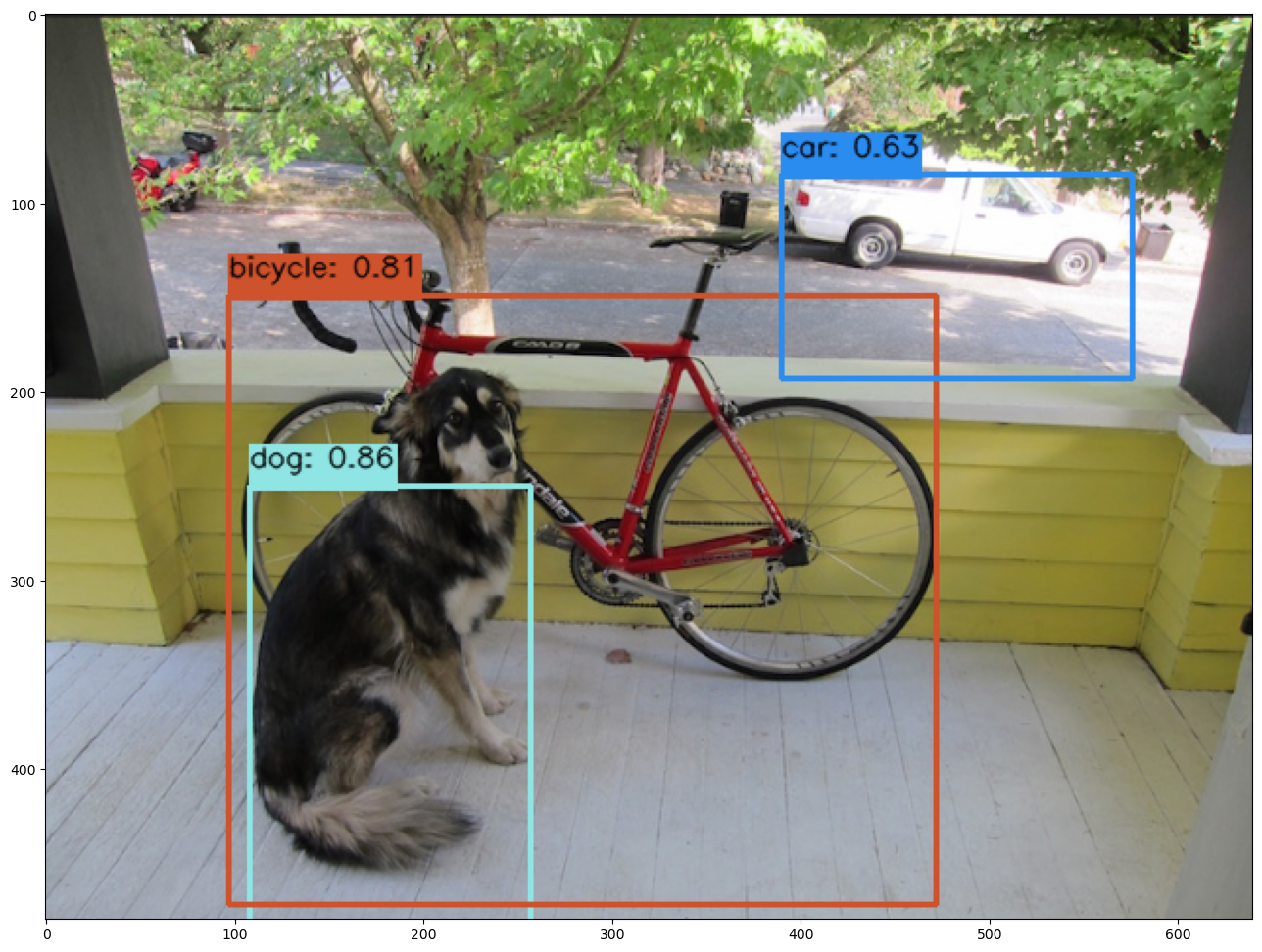
array([[[ 34, 34, 34],
[ 35, 35, 35],
[ 33, 33, 33],
...,
[ 33, 33, 33],
[ 33, 33, 33],
[ 35, 35, 35]],
[[ 41, 41, 39],
[ 42, 42, 40],
[ 42, 42, 40],
...,
[ 81, 91, 64],
[ 80, 92, 63],
[ 83, 90, 59]],
[[ 59, 61, 53],
[ 61, 62, 54],
[ 61, 62, 54],
...,
[193, 228, 136],
[195, 236, 136],
[203, 224, 122]],
...,
[[159, 167, 178],
[160, 166, 178],
[160, 165, 177],
...,
[126, 127, 121],
[126, 125, 120],
[127, 121, 117]],
[[160, 168, 179],
[157, 163, 175],
[154, 159, 171],
...,
[126, 127, 121],
[128, 126, 121],
[127, 119, 116]],
[[156, 164, 175],
[155, 162, 174],
[152, 158, 170],
...,
[127, 127, 121],
[130, 126, 122],
[128, 119, 116]]], dtype=uint8)
Inference Through Pipeline API
Another method of performing an inference using the pipeline’s deployment url.
Performing an inference through an API requires the following:
- The authentication token to authorize the connection to the pipeline.
- The pipeline’s inference URL.
- Inference data to sent to the pipeline - in JSON, DataFrame records format, or Apache Arrow.
Full details are available through the Wallaroo API Connection Guide on how retrieve an authorization token and perform inferences through the pipeline’s API.
For this demonstration we’ll submit the pandas record, request a pandas record as the return, and set the authorization header. The results will be stored in the file curl_response.df.
deploy_url = pipeline._deployment._url()
headers = wl.auth.auth_header()
headers['Content-Type']='application/json; format=pandas-records'
headers['Accept']='application/json; format=pandas-records'
!curl -X POST {deploy_url} \
-H "Authorization:{headers['Authorization']}" \
-H "Content-Type:application/json; format=pandas-records" \
-H "Accept:application/json; format=pandas-records" \
--data @./data/dogbike.df.json > curl_response.df
% Total % Received % Xferd Average Speed Time Time Time Current
Dload Upload Total Spent Left Speed
100 38.0M 100 22.9M 100 15.0M 4541k 2988k 0:00:05 0:00:05 --:--:-- 7920k
pipeline.undeploy()
| name | yolo8demonstration |
|---|---|
| created | 2023-10-11 15:06:07.064939+00:00 |
| last_updated | 2023-10-11 18:21:47.449547+00:00 |
| deployed | False |
| tags | |
| versions | 40c2402a-bb03-4cf4-b4be-dd009fc28a97, 283d1262-f1a8-49f3-b350-f83754272fac, 995df27c-33bb-48eb-9a6c-4eed1ca90a2d, af4af589-1805-4404-91f8-194308c166a0, e8e7f7bb-6502-487a-8afe-2bdc2b7566b1, 01e0ac28-5040-4ee5-90cf-069abb46d06b |
| steps | yolov8n |
| published | True |
Publish the Pipeline for Edge Deployment
It worked! For a demo, we’ll take working once as “tested”. So now that we’ve tested our pipeline, we are ready to publish it for edge deployment.
Publishing it means assembling all of the configuration files and model assets and pushing them to an Open Container Initiative (OCI) repository set in the Wallaroo instance as the Edge Registry service. DevOps engineers then retrieve that image and deploy it through Docker, Kubernetes, or similar deployments.
See Edge Deployment Registry Guide for details on adding an OCI Registry Service to Wallaroo as the Edge Deployment Registry.
This is done through the SDK command wallaroo.pipeline.publish(deployment_config) which has the following parameters and returns.
Publish a Pipeline Parameters
The publish method takes the following parameters. The containerized pipeline will be pushed to the Edge registry service with the model, pipeline configurations, and other artifacts needed to deploy the pipeline.
| Parameter | Type | Description |
|---|---|---|
deployment_config | wallaroo.deployment_config.DeploymentConfig (Optional) | Sets the pipeline deployment configuration. For example: For more information on pipeline deployment configuration, see the Wallaroo SDK Essentials Guide: Pipeline Deployment Configuration. |
Publish a Pipeline Returns
| Field | Type | Description |
|---|---|---|
| id | integer | Numerical Wallaroo id of the published pipeline. |
| pipeline version id | integer | Numerical Wallaroo id of the pipeline version published. |
| status | string | The status of the pipeline publication. Values include:
|
| Engine URL | string | The URL of the published pipeline engine in the edge registry. |
| Pipeline URL | string | The URL of the published pipeline in the edge registry. |
| Helm Chart URL | string | The URL of the helm chart for the published pipeline in the edge registry. |
| Helm Chart Reference | string | The help chart reference. |
| Helm Chart Version | string | The version of the Helm Chart of the published pipeline. This is also used as the Docker tag. |
| Engine Config | wallaroo.deployment_config.DeploymentConfig | The pipeline configuration included with the published pipeline. |
| Created At | DateTime | When the published pipeline was created. |
| Updated At | DateTime | When the published pipeline was updated. |
Publish Example
We will now publish the pipeline to our Edge Deployment Registry with the pipeline.publish(deployment_config) command. deployment_config is an optional field that specifies the pipeline deployment. This can be overridden by the DevOps engineer during deployment.
pub = pipeline.publish(deployment_config)
pub
Waiting for pipeline publish... It may take up to 600 sec.
Pipeline is Publishing...Published.
| ID | 14 |
| Pipeline Version | 4f05b506-2584-4eda-8c8d-54e6534b4bfb |
| Status | Published |
| Engine URL | ghcr.io/wallaroolabs/doc-samples/engines/proxy/wallaroo/ghcr.io/wallaroolabs/standalone-mini:v2023.3.0-3854 |
| Pipeline URL | ghcr.io/wallaroolabs/doc-samples/pipelines/yolo8demonstration:4f05b506-2584-4eda-8c8d-54e6534b4bfb |
| Helm Chart URL | ghcr.io/wallaroolabs/doc-samples/charts/yolo8demonstration |
| Helm Chart Reference | ghcr.io/wallaroolabs/doc-samples/charts@sha256:61e545e4d042bf6541bf5aba863bfb2ed090d2e00279f9fece05042a2b8d5ca3 |
| Helm Chart Version | 0.0.1-4f05b506-2584-4eda-8c8d-54e6534b4bfb |
| Engine Config | {'engine': {'resources': {'limits': {'cpu': 1.0, 'memory': '512Mi'}, 'requests': {'cpu': 1.0, 'memory': '512Mi'}}}, 'engineAux': {'images': {}}, 'enginelb': {'resources': {'limits': {'cpu': 1.0, 'memory': '512Mi'}, 'requests': {'cpu': 1.0, 'memory': '512Mi'}}}} |
| User Images | [] |
| Created By | john.hummel@wallaroo.ai |
| Created At | 2023-10-11 18:29:35.882859+00:00 |
| Updated At | 2023-10-11 18:29:35.882859+00:00 |
List Published Pipeline
The method wallaroo.client.list_pipelines() shows a list of all pipelines in the Wallaroo instance, and includes the published field that indicates whether the pipeline was published to the registry (True), or has not yet been published (False).
wl.list_pipelines()
| name | created | last_updated | deployed | tags | versions | steps | published |
|---|---|---|---|---|---|---|---|
| yolo8demonstration | 2023-11-Oct 15:06:07 | 2023-11-Oct 18:29:33 | False | 4f05b506-2584-4eda-8c8d-54e6534b4bfb, b7749a4f-1e62-47a0-8d4b-01c3dac414cb, 40c2402a-bb03-4cf4-b4be-dd009fc28a97, 283d1262-f1a8-49f3-b350-f83754272fac, 995df27c-33bb-48eb-9a6c-4eed1ca90a2d, af4af589-1805-4404-91f8-194308c166a0, e8e7f7bb-6502-487a-8afe-2bdc2b7566b1, 01e0ac28-5040-4ee5-90cf-069abb46d06b | yolov8n | True | |
| yolo8demonstration | 2023-11-Oct 14:37:32 | 2023-11-Oct 15:03:11 | False | b3bb9d2b-a41c-4ad4-9627-6e550ec70eea, 31eb1f8f-8c8e-4f4c-acf8-8930e95f81b0, 90d31341-fcae-4c6f-b03e-b506bf979c67, 2a3933c4-52db-40c6-b80f-9031664fd08a, 95bbabf1-1f15-4e4b-9e67-f7730c2b2cbd, 6c672144-ed4f-4505-97eb-a5b1763af847, 7149e0bc-089b-4d57-9a0b-5d4f4a9a4097, 329e394b-5105-4dc3-b0ff-5411623fc139, 7acaea4e-6ae3-426b-9f97-5e3dcc39c48e, a8b2c009-e7b5-4b96-81b9-40447797a05f, 09952a45-2401-4ebd-8e85-c678365b64a7, d870a558-10ef-448e-b00d-068c10c7e82b, fa531e16-1706-43c4-98d9-e0dd6355fe6f, 4c0b535e-b39b-40f4-82a7-34965b2f7c2a, 3507964d-382f-4e1c-84c7-64c5e27f819c, 9971f8dd-a17b-4d6a-ab72-d786d4990fab, b92a035f-903c-4039-8303-8ceb979a53c2 | yolov8n | True | |
| edge-cv-demo | 2023-10-Oct 16:52:02 | 2023-10-Oct 16:53:08 | False | 4f116503-6506-47d6-b427-1e7056a8c62e, a91a8b17-f587-439f-9001-292892e94336, 5320bc9c-e64f-4bc1-ac97-7d2b40eeb53e | resnet-50 | True | |
| edge04yolo8n | 2023-10-Oct 14:48:43 | 2023-10-Oct 16:35:13 | False | 9b40cc1b-af1c-4521-9354-4e33e4f9d9c5, b742ddbf-2c69-4c70-b59e-bb33a6f7979c, bab6e409-af82-4678-8ba7-0f0e49997529, 4812d72c-a0ca-4432-aa6d-8a12d9a7fd02 | yolov8n | False | |
| edge-pipeline-classification-cybersecurity | 2023-10-Oct 14:36:15 | 2023-10-Oct 14:37:08 | False | fe99cad9-dc32-4846-bcbc-27de68975784, b53618b7-191e-44cb-b38d-bbfd9ffc7748, e1a9f56c-17f5-45f8-86bf-69ebf6c446aa | aloha | True | |
| hf-summarizer | 2023-05-Oct 16:31:44 | 2023-05-Oct 20:24:57 | False | 6c591132-5ba7-413d-87a6-f4221ef972a6, 60bb46b0-52b8-464a-a379-299db4ea26c0, c4c1213a-6b6e-4a98-b397-c7903e8faae4, 25ef3557-d73b-4e8b-874e-1e126693eff8, cc4bd9e0-b661-48c9-a0a9-29dafddeedcb, d359aafc-843d-4e32-9439-e365b8095d65, 8bd92035-2894-4fe4-8112-f5f3512dc8ea | hf-summarizer | True | |
| houseprice-estimator | 2023-03-Oct 18:07:05 | 2023-03-Oct 18:10:31 | False | eac1e82a-e5c0-4f4b-a7fc-6583719f4a62, be1fc3f0-a769-4ce9-94e1-ba01898d91eb, 9007b5ba-d8a8-4cbe-aef7-2e9b24ee010a, d683431f-4074-4ba1-9d27-71361bd4ffd2, aaa216e0-94af-4173-b52a-b9d7c8118f17 | house-price-prime | True | |
| cv-mitochondria | 2023-28-Sep 20:25:17 | 2023-29-Sep 19:26:53 | False | 63f71352-93bc-4e4a-85f6-0a0bf603124c, d271be10-fadd-4408-97aa-c57e6ae4e35a, ac4bd826-f47f-48b7-8319-01fbc6622899, 4b6dab7d-b3ff-4f14-8425-7d9b6de76637, 66e72bc0-a3e3-4872-bc20-19b992c194b4, cf4bdfb4-1eec-46f8-9af4-b16dea894de6, 507cb1eb-8034-4b5b-bc96-2427730a6407, 50ed1d2f-6dba-411c-9579-1090791b33bd, 6208c9cf-fcd6-4b20-bbfc-f6ce714596e3 | mitochondria-detector | True | |
| retailimage | 2023-28-Sep 19:44:33 | 2023-28-Sep 19:54:59 | False | 26afe601-6515-48ca-9a37-d063ab1e1ea2, 1d806c89-ecc6-4207-b98f-c56eccd16c43, 11835eda-4e10-49c0-baab-63862c16d1ef, 57bf2bfb-009b-42b9-b926-742f8bbb8d3c, 891fe58d-902b-49bd-94d3-c2196a8efd3b, db0d489b-d8fa-41d3-b46f-a9623b28e336, f039eaf3-d0dd-4ab7-a767-852db5241ff0, 2f5cd92d-ecc8-4e75-aee5-1605c1f23f0e | v5s6 | False | |
| retailimage | 2023-28-Sep 18:55:14 | 2023-28-Sep 19:23:05 | False | d64dabed-7f7a-4f41-a307-e7995d7b8144, 8d257d18-2ca1-46b9-a40e-1f3d7f308dc1, e84586a7-05bb-4d67-a696-f04e80df8b58, 95c2157a-2722-4a5b-b564-d3a709c6238f, fa351ab0-fe77-4fc0-b521-ba15e92a91d7 | v5s6 | False | |
| cv-yolo | 2023-28-Sep 16:07:29 | 2023-28-Sep 18:47:35 | False | 5f889757-89c5-4475-a579-937639779ab3, f9981617-7734-4f2d-905a-62333c600fe7, b21ac721-49e3-402d-b6c0-af139d51299a, 3f277cc7-351d-4d10-bdb2-c770c0dc1ac2 | house-price-prime | False | |
| houseprice-estimator | 2023-27-Sep 16:51:15 | 2023-27-Sep 16:53:56 | False | 07cac6a2-140d-4a5e-b7ec-264f5fbf9dc3, bd389561-2c4f-492b-a82b-896cf76c2acf, 37bcce00-28d9-4d28-b637-33acf4021103, 146a3e4a-057b-4bd2-94f7-ebadc133df3d, 996a9877-142f-4934-aa4a-7696d3662297, a79802b5-42f4-4fb6-bd6b-3da560d39d73 | house-price-prime | False | |
| aloha-fraud-detector | 2023-27-Sep 16:29:55 | 2023-27-Sep 18:28:05 | False | e2a42011-d319-476f-bc32-9b6cccae4870, be15dcad-5a78-4493-b568-ee4502fa1791, b74a8b3a-8128-4356-a6ff-434c2b283cc8, 6d72feb7-76b5-4121-b401-9dfd4b978745, c22e3aa7-8efa-41c1-8844-cc4e7d1147c5, 739269a7-7890-4774-9597-fda5f80a3a6d, aa362e18-7f7e-4dc6-9069-3207e9d2f605, 79865932-5b89-4b2a-bfb1-cb9ebeb5125f, 4727b985-db36-44f7-a1a3-7f1886bbf894, 07cbfcae-1fa2-4746-b585-55349d230b45, 03824313-6bbb-4ccd-95ea-64340f789b9c, 9ce54998-a667-43b3-8198-b2d95e0d2879, 8a416842-5675-455a-b638-29fe7dbb5ba1 | aloha-prime | True | |
| cv-arm-edge | 2023-27-Sep 15:20:15 | 2023-27-Sep 15:20:15 | (unknown) | 86dd133a-c12f-478b-af9a-30a7e4850fc4 | True | ||
| cv-arm-edge | 2023-27-Sep 15:17:45 | 2023-27-Sep 15:17:45 | (unknown) | 97a92779-0a5d-4c2b-bcf1-7afd60ac83d5 | False |
List Publishes from a Pipeline
All publishes created from a pipeline are displayed with the wallaroo.pipeline.publishes method. The pipeline_version_id is used to know what version of the pipeline was used in that specific publish. This allows for pipelines to be updated over time, and newer versions to be sent and tracked to the Edge Deployment Registry service.
List Publishes Parameters
N/A
List Publishes Returns
A List of the following fields:
| Field | Type | Description |
|---|---|---|
| id | integer | Numerical Wallaroo id of the published pipeline. |
| pipeline_version_id | integer | Numerical Wallaroo id of the pipeline version published. |
| engine_url | string | The URL of the published pipeline engine in the edge registry. |
| pipeline_url | string | The URL of the published pipeline in the edge registry. |
| created_by | string | The email address of the user that published the pipeline. |
| Created At | DateTime | When the published pipeline was created. |
| Updated At | DateTime | When the published pipeline was updated. |
pipeline.publishes()
DevOps - Pipeline Edge Deployment
Once a pipeline is deployed to the Edge Registry service, it can be deployed in environments such as Docker, Kubernetes, or similar container running services by a DevOps engineer.
Docker Deployment
First, the DevOps engineer must authenticate to the same OCI Registry service used for the Wallaroo Edge Deployment registry.
For more details, check with the documentation on your artifact service. The following are provided for the three major cloud services:
- Set up authentication for Docker
- Authenticate with an Azure container registry
- Authenticating Amazon ECR Repositories for Docker CLI with Credential Helper
For the deployment, the engine URL is specified with the following environmental variables:
DEBUG(true|false): Whether to include debug output.OCI_REGISTRY: The URL of the registry service.CONFIG_CPUS: The number of CPUs to use.OCI_USERNAME: The edge registry username.OCI_PASSWORD: The edge registry password or token.PIPELINE_URL: The published pipeline URL.
Docker Deployment Example
Using our sample environment, here’s sample deployment using Docker with a computer vision ML model, the same used in the Wallaroo Use Case Tutorials Computer Vision: Retail tutorials.
For docker run commands, the persistent volume for storing session data is stored with -v ./data:/persist. Updated as required for your deployments.
docker run -p 8080:8080 \
-v ./data:/persist \
-e DEBUG=true -e OCI_REGISTRY={your registry server} \
-e CONFIG_CPUS=4 \
-e OCI_USERNAME=oauth2accesstoken \
-e OCI_PASSWORD={registry token here} \
-e PIPELINE_URL={your registry server}/pipelines/edge-cv-retail:bf70eaf7-8c11-4b46-b751-916a43b1a555 \
{your registry server}/engine:v2023.3.0-main-3707
Docker Compose Deployment
For users who prefer to use docker compose, the following sample compose.yaml file is used to launch the Wallaroo Edge pipeline. This is the same used in the Wallaroo Use Case Tutorials Computer Vision: Retail tutorials. The session and other data is stored with the volumes entry to add a persistent volume.
services:
engine:
image: {Your Engine URL}
ports:
- 8080:8080
volumes:
- ./data:/persist
environment:
PIPELINE_URL: {Your Pipeline URL}
OCI_REGISTRY: {Your Edge Registry URL}
OCI_USERNAME: {Your Registry Username}
OCI_PASSWORD: {Your Token or Password}
CONFIG_CPUS: 1
For example:
services:
engine:
image: sample-registry.com/engine:v2023.3.0-main-3707
ports:
- 8080:8080
environment:
PIPELINE_URL: sample-registry.com/pipelines/edge-cv-retail:bf70eaf7-8c11-4b46-b751-916a43b1a555
OCI_REGISTRY: sample-registry.com
OCI_USERNAME: _json_key_base64
OCI_PASSWORD: abc123
CONFIG_CPUS: 1
Docker Compose Deployment Example
The deployment and undeployment is then just a simple docker compose up and docker compose down. The following shows an example of deploying the Wallaroo edge pipeline using docker compose.
docker compose up
[+] Running 1/1
✔ Container cv_data-engine-1 Recreated 0.5s
Attaching to cv_data-engine-1
cv_data-engine-1 | Wallaroo Engine - Standalone mode
cv_data-engine-1 | Login Succeeded
cv_data-engine-1 | Fetching manifest and config for pipeline: sample-registry.com/pipelines/edge-cv-retail:bf70eaf7-8c11-4b46-b751-916a43b1a555
cv_data-engine-1 | Fetching model layers
cv_data-engine-1 | digest: sha256:c6c8869645962e7711132a7e17aced2ac0f60dcdc2c7faa79b2de73847a87984
cv_data-engine-1 | filename: c6c8869645962e7711132a7e17aced2ac0f60dcdc2c7faa79b2de73847a87984
cv_data-engine-1 | name: resnet-50
cv_data-engine-1 | type: model
cv_data-engine-1 | runtime: onnx
cv_data-engine-1 | version: 693e19b5-0dc7-4afb-9922-e3f7feefe66d
cv_data-engine-1 |
cv_data-engine-1 | Fetched
cv_data-engine-1 | Starting engine
cv_data-engine-1 | Looking for preexisting `yaml` files in //modelconfigs
cv_data-engine-1 | Looking for preexisting `yaml` files in //pipelines
Helm Deployment
Published pipelines can be deployed through the use of helm charts.
Helm deployments take up to two steps - the first step is in retrieving the required values.yaml and making updates to override.
- Pull the helm charts from the published pipeline. The two fields are the Helm Chart URL and the Helm Chart version to specify the OCI . This typically takes the format of:
helm pull oci://{published.helm_chart_url} --version {published.helm_chart_version}
- Extract the
tgzfile and copy thevalues.yamland copy the values used to edit engine allocations, etc. The following are required for the deployment to run:
ociRegistry:
registry: {your registry service}
username: {registry username here}
password: {registry token here}
Store this into another file, suc as local-values.yaml.
- Create the namespace to deploy the pipeline to. For example, the namespace
wallaroo-edge-pipelinewould be:
kubectl create -n wallaroo-edge-pipeline
Deploy the
helminstallation withhelm installthrough one of the following options:Specify the
tgzfile that was downloaded and the local values file. For example:helm install --namespace {namespace} --values {local values file} {helm install name} {tgz path}Specify the expended directory from the downloaded
tgzfile.helm install --namespace {namespace} --values {local values file} {helm install name} {helm directory path}Specify the Helm Pipeline Helm Chart and the Pipeline Helm Version.
helm install --namespace {namespace} --values {local values file} {helm install name} oci://{published.helm_chart_url} --version {published.helm_chart_version}
Once deployed, the DevOps engineer will have to forward the appropriate ports to the
svc/engine-svcservice in the specific pipeline. For example, usingkubectl port-forwardto the namespaceccfraudthat would be:kubectl port-forward svc/engine-svc -n ccfraud01 8080 --address 0.0.0.0`
The following code segment generates a docker run template based on the previously published pipeline.
docker_deploy = f'''
docker run -p 8080:8080 \\
-v ./data:/persist \\
-e OCI_REGISTRY=$REGISTRYURL \\
-e CONFIG_CPUS=4 \\
-e OCI_USERNAME=$REGISTRYUSERNAME \\
-e OCI_PASSWORD=$REGISTRYPASSWORD \\
-e PIPELINE_URL={pub.pipeline_url} \\
{pub.engine_url}
'''
print(docker_deploy)
docker run -p 8080:8080 \
-e OCI_REGISTRY=$REGISTRYURL \
-e CONFIG_CPUS=4 \
-e OCI_USERNAME=$REGISTRYUSERNAME \
-e OCI_PASSWORD=$REGISTRYPASSWORD \
-e PIPELINE_URL=ghcr.io/wallaroolabs/doc-samples/pipelines/yolo8demonstration:4f05b506-2584-4eda-8c8d-54e6534b4bfb \
ghcr.io/wallaroolabs/doc-samples/engines/proxy/wallaroo/ghcr.io/wallaroolabs/standalone-mini:v2023.3.0-3854
Edge Deployed Pipeline API Endpoints
Once deployed, we can check the pipelines and models available. We’ll use a curl command, but any HTTP based request will work the same way.
The endpoint /pipelines returns:
- id (String): The name of the pipeline.
- status (String): The status as either
Running, orErrorif there are any issues.
curl localhost:8080/pipelines
{"pipelines":[{"id":"yolo8demonstration","status":"Running"}]}
The following example uses the host localhost. Replace with your own host name of your Edge deployed pipeline.
!curl localhost:8080/pipelines
{"pipelines":[{"id":"yolo8demonstration","status":"Running"}]}
The endpoint /models returns a List of models with the following fields:
- name (String): The model name.
- sha (String): The sha hash value of the ML model.
- status (String): The status of either Running or Error if there are any issues.
- version (String): The model version. This matches the version designation used by Wallaroo to track model versions in UUID format.
{"models":[{"name":"yolov8n","sha":"3ed5cd199e0e6e419bd3d474cf74f2e378aacbf586e40f24d1f8c89c2c476a08","status":"Running","version":"7af40d06-d18f-4b3f-9dd3-0a15248f01c8"}]}
The following example uses the host localhost. Replace with your own host name of your Edge deployed pipeline.
!curl localhost:8080/models
{"models":[{"name":"yolov8n","sha":"3ed5cd199e0e6e419bd3d474cf74f2e378aacbf586e40f24d1f8c89c2c476a08","status":"Running","version":"7af40d06-d18f-4b3f-9dd3-0a15248f01c8"}]}
Edge Inference Endpoint
The inference endpoint takes the following pattern:
/pipelines/{pipeline-name}: Thepipeline-nameis the same as returned from the/pipelinesendpoint asid.
Wallaroo inference endpoint URLs accept the following data inputs through the Content-Type header:
Content-Type: application/vnd.apache.arrow.file: For Apache Arrow tables.Content-Type: application/json; format=pandas-records: For pandas DataFrame in record format.
Once deployed, we can perform an inference through the deployment URL.
The endpoint returns Content-Type: application/json; format=pandas-records by default with the following fields:
- check_failures (List[Integer]): Whether any validation checks were triggered. For more information, see Wallaroo SDK Essentials Guide: Pipeline Management: Anomaly Testing.
- elapsed (List[Integer]): A list of time in nanoseconds for:
- [0] The time to serialize the input.
- [1…n] How long each step took.
- model_name (String): The name of the model used.
- model_version (String): The version of the model in UUID format.
- original_data: The original input data. Returns
nullif the input may be too long for a proper return. - outputs (List): The outputs of the inference result separated by data type, where each data type includes:
- data: The returned values.
- dim (List[Integer]): The dimension shape returned.
- v (Integer): The vector shape of the data.
- pipeline_name (String): The name of the pipeline.
- shadow_data: Any shadow deployed data inferences in the same format as outputs.
- time (Integer): The time since UNIX epoch.
Once deployed, we can perform an inference through the deployment URL. We’ll assume we’re running the inference request through the localhost and submitting the local file ./data/dogbike.df.json. Note that our inference endpoint is pipelines/yolo8demonstration - the same as our pipeline name.
The following example demonstrates sending an inference request to the edge deployed pipeline and storing the results in a pandas DataFrame in record format. The results can then be exported to other processes to render the detected images or other use cases.
!curl -X POST localhost:8080/pipelines/yolo8demonstration \
-H "Content-Type: application/json; format=pandas-records" \
--data @./data/dogbike.df.json > edge-results.df.json
% Total % Received % Xferd Average Speed Time Time Time Current
Dload Upload Total Spent Left Speed
0 0 0 0 0 0 0 0 --:--:-- --:--:-- --:--:-- 0100 28.7M 100 13.6M 100 15.0M 14.2M 15.7M --:--:-- --:--:-- --:--:-- 30.3M
5.7 - Wallaroo Edge Computer Vision Observability
A demonstration on observability with computer vision deployed on edge devices.
This tutorial and the assets can be downloaded as part of the Wallaroo Tutorials repository.
Computer Vision for Object Detection in Retail
The following tutorial demonstrates using Wallaroo for observability of edge deployments of computer vision models.
Introduction
This tutorial focuses on the resnet50 computer vision model. By default, this provides the following outputs from receiving an image converted to tensor values:
boxes: The bounding boxes for detected objects.classes: The class of the detected object (bottle, coat, person, etc).confidences: The confidence the model has that the detected model is the class.
For this demonstration, the model is modified with Wallaroo Bring Your Own Predict (BYOP) to add two additional fields:
avg_px_intensity: the average pixel intensity checks the input to determine the average value of the Red/Green/Blue pixel values. This is used as a benchmark to determine if the two images are significantly different. For example, an all white photo would have anavg_px_intensityof1, while an all blank photo would have a value of0.avg_confidence: The average confidence of all detected objects.
This demonstration will use avg_confidence to demonstrate observability in our edge deployed computer vision model.
Prerequisites
- A Wallaroo Ops instance 2023.4 and above with [edge deployment enabled](Edge Deployment Registry Guide).
- An x64 edge device with Docker installed, recommended with at least 8 cores.
In order for the wallaroo tutorial notebooks to run properly, the videos directory must contain these models in the models directory.
To download the Wallaroo Computer Vision models, use the following link:
https://storage.googleapis.com/wallaroo-public-data/cv-demo-models/cv-retail-models.zip
Unzip the contents into the directory models.
The following models are required to run the tutorial:
onnx==1.12.0
onnxruntime==1.12.1
torchvision
torch
matplotlib==3.5.0
opencv-python
imutils
pytz
ipywidgets
To run this tutorial outside of a Wallaroo Ops center, the Wallaroo SDK is available and is installed via pip with:
pip install wallaroo==2023.4.1
References
Steps
Import Libraries
The following libraries are used to execute this tutorial. The utils.py provides additional helper methods for rendering the images into tensor fields and other useful tasks.
# preload needed libraries
import wallaroo
from wallaroo.object import EntityNotFoundError
from wallaroo.framework import Framework
from IPython.display import display
from IPython.display import Image
import pandas as pd
import json
import datetime
import time
import cv2
import matplotlib.pyplot as plt
import string
import random
import pyarrow as pa
import sys
import asyncio
import numpy as np
import utils
pd.set_option('display.max_colwidth', None)
import datetime
# api based inference request
import requests
Connect to the Wallaroo Instance
The first step is to connect to Wallaroo through the Wallaroo client. The Python library is included in the Wallaroo install and available through the Jupyter Hub interface provided with your Wallaroo environment.
This is accomplished using the wallaroo.Client() command, which provides a URL to grant the SDK permission to your specific Wallaroo environment. When displayed, enter the URL into a browser and confirm permissions. Store the connection into a variable that can be referenced later.
If logging into the Wallaroo instance through the internal JupyterHub service, use wl = wallaroo.Client(). For more information on Wallaroo Client settings, see the Client Connection guide.
The option request_timeout provides additional time for the Wallaroo model upload process to complete.
wl = wallaroo.Client(request_timeout=600)
Create Workspace
We will create a workspace to manage our pipeline and models. The following variables will set the name of our sample workspace then set it as the current workspace.
Workspace names must be unique. The following helper function will either create a new workspace, or retrieve an existing one with the same name. Verify that a pre-existing workspace has been shared with the targeted user.
Set the variables workspace_name to ensure a unique workspace name if required.
The workspace will then be set as the Current Workspace. Model uploads and
def get_workspace(name, client):
workspace = None
for ws in client.list_workspaces():
if ws.name() == name:
workspace= ws
if(workspace == None):
workspace = client.create_workspace(name)
return workspace
workspace_name = "cv-retail-edge-observability"
model_name = "resnet-with-intensity"
model_file_name = "./models/model-with-pixel-intensity.zip"
pipeline_name = "retail-inv-tracker-edge-obs"
workspace = get_workspace(workspace_name, wl)
wl.set_current_workspace(workspace)
{'name': 'cv-retail-edge-observability', 'id': 8, 'archived': False, 'created_by': 'cc3619bb-2cec-4a44-9333-55a0dc6b3997', 'created_at': '2024-01-10T17:37:38.659309+00:00', 'models': [], 'pipelines': []}
Upload Model
The model is uploaded as a BYOP model, where the model, Python script and other artifacts are included in a .zip file. This requires the input and output schemas for the model specified in Apache Arrow Schema format.
input_schema = pa.schema([
pa.field('tensor', pa.list_(
pa.list_(
pa.list_(
pa.float32(), # images are normalized
list_size=640
),
list_size=480
),
list_size=3
)),
])
output_schema = pa.schema([
pa.field('boxes', pa.list_(pa.list_(pa.float32(), list_size=4))),
pa.field('classes', pa.list_(pa.int64())),
pa.field('confidences', pa.list_(pa.float32())),
pa.field('avg_px_intensity', pa.list_(pa.float32())),
pa.field('avg_confidence', pa.list_(pa.float32())),
])
model = wl.upload_model(model_name,
model_file_name,
framework=Framework.CUSTOM,
input_schema=input_schema,
output_schema=output_schema)
Waiting for model loading - this will take up to 10.0min.
Model is pending loading to a container runtime......
Model is attempting loading to a container runtime.............successful
Ready
Deploy Pipeline
Next we configure the hardware we want to use for deployment. If we plan on eventually deploying to edge, this is a good way to simulate edge hardware conditions. The BYOP model is deployed as a Wallaroo Containerized Runtime, so the hardware allocation is performed through the sidekick options.
deployment_config = wallaroo.DeploymentConfigBuilder() \
.replica_count(1) \
.cpus(1) \
.memory("2Gi") \
.sidekick_cpus(model, 1) \
.sidekick_memory(model, '6Gi') \
.build()
We create the pipeline with the wallaroo.client.build_pipeline method, and assign our model as a model pipeline step. Once complete, we will deploy the pipeline to allocate resources from the Kuberntes cluster hosting the Wallaroo Ops to the pipeline.
pipeline = wl.build_pipeline(pipeline_name)
pipeline.clear()
pipeline.add_model_step(model)
pipeline.deploy(deployment_config = deployment_config)
| name | retail-inv-tracker-edge-obs |
|---|---|
| created | 2024-01-10 17:50:59.035145+00:00 |
| last_updated | 2024-01-10 17:50:59.700103+00:00 |
| deployed | True |
| arch | None |
| tags | |
| versions | d0c2ed1c-3691-49f1-8fc8-e6510e4c39f8, 773099d3-6d64-4a92-b5a7-f614a916965d |
| steps | resnet-with-intensity |
| published | False |
Monitoring for Model Drift
For this example, we want to track the average confidence of object predictions and get alerted if we see a drop in confidence.
We will convert a set of images to pandas DataFrames with the images converted to tensor values. The first set of images baseline_images as well formed images. The second set blurred_images are the same photos intentionally blurred for our observability demonstration.
baseline_images = [
"./data/images/input/example/dairy_bottles.png",
"./data/images/input/example/dairy_products.png",
"./data/images/input/example/product_cheeses.png"
]
blurred_images = [
"./data/images/input/example/blurred-dairy_bottles.png",
"./data/images/input/example/blurred-dairy_products.png",
"./data/images/input/example/blurred-product_cheeses.png"
]
baseline_images_list = utils.processImages(baseline_images)
blurred_images_list = utils.processImages(blurred_images)
The Wallaroo SDK is capable of using numpy arrays in a pandas DataFrame for inference requests. Our demonstration will focus on using API calls for inference requests, so we will flatten the numpy array and use that value for our inference inputs. The following examples show using a baseline and blurred image for inference requests and the sample outputs.
# baseline image
df_test = pd.DataFrame({'tensor': wallaroo.utils.flatten_np_array_columns(baseline_images_list[0], 'tensor')})
df_test
| tensor | |
|---|---|
| 0 | [0.9372549, 0.9529412, 0.9490196, 0.94509804, 0.94509804, 0.94509804, 0.94509804, 0.94509804, 0.94509804, 0.94509804, 0.94509804, 0.94509804, 0.94509804, 0.94509804, 0.94509804, 0.94509804, 0.94509804, 0.94509804, 0.9490196, 0.9490196, 0.9529412, 0.9529412, 0.9490196, 0.9607843, 0.96862745, 0.9647059, 0.96862745, 0.9647059, 0.95686275, 0.9607843, 0.9647059, 0.9647059, 0.9607843, 0.9647059, 0.972549, 0.95686275, 0.9607843, 0.91764706, 0.95686275, 0.91764706, 0.8784314, 0.89411765, 0.84313726, 0.8784314, 0.8627451, 0.8509804, 0.9254902, 0.84705883, 0.96862745, 0.89411765, 0.81960785, 0.8509804, 0.92941177, 0.8666667, 0.8784314, 0.8666667, 0.9647059, 0.9764706, 0.98039216, 0.9764706, 0.972549, 0.972549, 0.972549, 0.972549, 0.972549, 0.972549, 0.98039216, 0.89411765, 0.48235294, 0.4627451, 0.43137255, 0.27058825, 0.25882354, 0.29411766, 0.34509805, 0.36862746, 0.4117647, 0.45490196, 0.4862745, 0.5254902, 0.56078434, 0.6039216, 0.64705884, 0.6862745, 0.72156864, 0.74509805, 0.7490196, 0.7882353, 0.8666667, 0.98039216, 0.9882353, 0.96862745, 0.9647059, 0.96862745, 0.972549, 0.9647059, 0.9607843, 0.9607843, 0.9607843, 0.9607843, ...] |
result = pipeline.infer(df_test,
dataset=['time', 'out.avg_confidence','out.avg_px_intensity','out.boxes','out.classes','out.confidences','check_failures','metadata'])
result
| time | out.avg_confidence | out.avg_px_intensity | out.boxes | out.classes | out.confidences | metadata.partition | |
|---|---|---|---|---|---|---|---|
| 0 | 2024-01-10 17:53:50.655 | [0.35880384] | [0.425382] | [[2.1511102, 193.98323, 76.26535, 475.40292], [610.82245, 98.606316, 639.8868, 232.27054], [544.2867, 98.726524, 581.28845, 230.20497], [454.99344, 113.08567, 484.78464, 210.1282], [502.58884, 331.87665, 551.2269, 476.49182], [538.54254, 292.1205, 587.46545, 468.1288], [578.5417, 99.70756, 617.2247, 233.57082], [548.552, 191.84564, 577.30585, 238.47737], [459.83328, 344.29712, 505.42633, 456.7118], [483.47168, 110.56585, 514.0936, 205.00156], [262.1222, 190.36658, 323.4903, 405.20584], [511.6675, 104.53834, 547.01715, 228.23663], [75.39197, 205.62312, 168.49893, 453.44086], [362.50656, 173.16858, 398.66956, 371.8243], [490.42468, 337.627, 534.1234, 461.0242], [351.3856, 169.14897, 390.7583, 244.06992], [525.19824, 291.73895, 570.5553, 417.6439], [563.4224, 285.3889, 609.30853, 452.25943], [425.57935, 366.24915, 480.63535, 474.54], [154.538, 198.0377, 227.64284, 439.84412], [597.02893, 273.60458, 637.2067, 439.03214], [473.88763, 293.41992, 519.7537, 349.2304], [262.77597, 192.03581, 313.3096, 258.3466], [521.1493, 152.89026, 534.8596, 246.52365], [389.89633, 178.07867, 431.87555, 360.59323], [215.99901, 179.52965, 280.2847, 421.9092], [523.6454, 310.7387, 560.36487, 473.57968], [151.7131, 191.41077, 228.71013, 443.32187], [0.50784916, 14.856098, 504.5198, 405.7277], [443.83676, 340.1249, 532.83734, 475.77713], [472.37848, 329.13092, 494.03647, 352.5906], [572.41455, 286.26132, 601.8677, 384.5899], [532.7721, 189.89102, 551.9026, 241.76051], [564.0309, 105.75121, 597.0351, 225.32579], [551.25854, 287.16034, 590.9206, 405.71548], [70.46805, 0.39822236, 92.786545, 84.40113], [349.44534, 3.6184297, 392.61484, 98.43363], [64.40484, 215.14934, 104.09457, 436.50797], [615.1218, 269.46683, 633.30853, 306.03452], [238.31851, 0.73957217, 290.2898, 91.30623], [449.37347, 337.39554, 480.13208, 369.35126], [74.95623, 191.84235, 164.21284, 457.00143], [391.96646, 6.255016, 429.23056, 100.72327], [597.48663, 276.6981, 618.0615, 298.62778], [384.51172, 171.95828, 407.01276, 205.28722], [341.5734, 179.8058, 365.88345, 208.57889], [555.0278, 288.62695, 582.6162, 358.0912], [615.92035, 264.9265, 632.3316, 280.2552], [297.95154, 0.5227982, 347.18744, 95.13106], [311.64868, 203.67934, 369.6169, 392.58063], [163.10356, 0.0, 227.67468, 86.49685], [68.518974, 1.870926, 161.25877, 82.89816], [593.6093, 103.263596, 617.124, 200.96545], [263.3115, 200.12204, 275.699, 234.26517], [592.2285, 279.66064, 619.70496, 379.14764], [597.7549, 269.6543, 618.5473, 286.25214], [478.04306, 204.36165, 530.00745, 239.35196], [501.34528, 289.28003, 525.766, 333.00262], [462.4777, 336.92056, 491.32016, 358.18915], [254.40384, 203.89566, 273.66177, 237.13142], [307.96042, 154.70946, 440.4545, 386.88065], [195.53915, 187.13596, 367.6518, 404.91095], [77.52113, 2.9323518, 160.15236, 81.59642], [577.648, 283.4004, 601.4359, 307.41882], [516.63873, 129.74504, 540.40936, 242.17572], [543.2536, 253.38689, 631.3576, 466.62567], [271.1358, 45.97066, 640.0, 456.88235], [568.77203, 188.66449, 595.866, 235.05397], [400.997, 169.88531, 419.35645, 185.80077], [473.9581, 328.07736, 493.2316, 339.41437], [602.9851, 376.39505, 633.74243, 438.61758], [480.95963, 117.62996, 525.08826, 242.74872], [215.71178, 194.87447, 276.59906, 414.3832], [462.2966, 331.94638, 493.14175, 347.97647], [543.94977, 196.90623, 556.04315, 238.99141], [386.8205, 446.6134, 428.81064, 480.00003], [152.22516, 0.0, 226.98564, 85.44817], [616.91815, 246.15547, 630.8656, 273.48447], [576.33356, 100.67465, 601.9629, 183.61014], [260.99304, 202.73479, 319.40524, 304.172], [333.5814, 169.75925, 390.9659, 278.09406], [286.26767, 3.700516, 319.3962, 88.77158], [532.5545, 209.36183, 552.58417, 240.08965], [572.99915, 207.65208, 595.62415, 235.46635], [6.2744417, 0.5994095, 96.04993, 81.27411], [203.32298, 188.94266, 227.27435, 254.29417], [513.7689, 154.48575, 531.3786, 245.21616], [547.53815, 369.9145, 583.13916, 470.30206], [316.64532, 252.80664, 336.65454, 272.82834], [234.79965, 0.0003570557, 298.05707, 92.014496], [523.0663, 195.29694, 534.485, 242.23671], [467.7621, 202.35623, 536.2362, 245.53342], [146.07208, 0.9752747, 178.93895, 83.210175], [18.780663, 1.0261598, 249.98721, 88.49467], [600.9064, 270.41983, 625.3632, 297.94083], [556.40955, 287.84702, 580.2647, 322.64728], [80.6706, 161.22787, 638.6261, 480.00003], [455.98315, 334.6629, 480.16724, 349.97784], [613.9905, 267.98065, 635.95807, 375.1775], [345.75964, 2.459102, 395.91183, 99.68698]] | [44, 44, 44, 44, 44, 44, 44, 44, 44, 44, 44, 44, 44, 44, 44, 44, 44, 44, 44, 44, 44, 44, 44, 44, 44, 44, 44, 86, 82, 44, 44, 44, 44, 44, 44, 84, 84, 44, 44, 44, 44, 86, 84, 44, 44, 44, 44, 44, 84, 44, 44, 84, 44, 44, 44, 44, 51, 44, 44, 44, 44, 44, 44, 44, 44, 44, 82, 44, 44, 44, 44, 44, 86, 44, 44, 1, 84, 44, 44, 44, 44, 84, 47, 47, 84, 14, 44, 44, 53, 84, 47, 47, 44, 84, 44, 44, 82, 44, 44, 44] | [0.9965358, 0.9883404, 0.9700247, 0.9696426, 0.96478045, 0.96037567, 0.9542889, 0.9467539, 0.946524, 0.94484967, 0.93611854, 0.91653466, 0.9133634, 0.8874814, 0.84405905, 0.825526, 0.82326967, 0.81740034, 0.7956525, 0.78669065, 0.7731486, 0.75193685, 0.7360918, 0.7009186, 0.6932351, 0.65077204, 0.63243586, 0.57877576, 0.5023476, 0.50163734, 0.44628552, 0.42804396, 0.4253787, 0.39086252, 0.36836442, 0.3473236, 0.32950658, 0.3105372, 0.29076362, 0.28558296, 0.26680034, 0.26302803, 0.25444376, 0.24568668, 0.2353662, 0.23321979, 0.22612995, 0.22483191, 0.22332378, 0.21442991, 0.20122288, 0.19754867, 0.19439234, 0.19083925, 0.1871393, 0.17646024, 0.16628945, 0.16326219, 0.14825206, 0.13694529, 0.12920643, 0.12815322, 0.122357555, 0.121289656, 0.116281696, 0.11498632, 0.111848116, 0.11016138, 0.1095062, 0.1039151, 0.10385688, 0.097573474, 0.09632071, 0.09557622, 0.091599144, 0.09062039, 0.08262358, 0.08223499, 0.07993951, 0.07989185, 0.078758545, 0.078201495, 0.07737936, 0.07690251, 0.07593444, 0.07503418, 0.07482597, 0.068981, 0.06841128, 0.06764157, 0.065750405, 0.064908616, 0.061884128, 0.06010121, 0.0578873, 0.05717648, 0.056616478, 0.056017116, 0.05458274, 0.053669468] | engine-fc59fccbc-bs2sg |
# example of an inference from a bad photo
df_test = pd.DataFrame({'tensor': wallaroo.utils.flatten_np_array_columns(blurred_images_list[0], 'tensor')})
result = pipeline.infer(df_test, dataset=['time', 'out.avg_confidence','out.avg_px_intensity','out.boxes','out.classes','out.confidences','check_failures','metadata'])
result
| time | out.avg_confidence | out.avg_px_intensity | out.boxes | out.classes | out.confidences | metadata.partition | |
|---|---|---|---|---|---|---|---|
| 0 | 2024-01-10 17:53:59.016 | [0.29440108] | [0.42540666] | [[1.104647, 203.48311, 81.29011, 472.4321], [67.34002, 195.64558, 163.41652, 470.1668], [218.88916, 180.21216, 281.3725, 422.2332], [156.47955, 189.82559, 227.1866, 443.35718], [393.81195, 172.34473, 434.30322, 363.96057], [266.56137, 201.46182, 326.2503, 406.3162], [542.941, 99.440956, 588.42365, 229.33481], [426.12668, 260.50723, 638.6193, 476.10742], [511.26102, 106.84715, 546.8103, 243.0127], [0.0, 68.56848, 482.48538, 472.53766], [347.34027, 0.0, 401.10968, 97.51968], [289.03827, 0.32189485, 347.78888, 93.458755], [91.05826, 183.34473, 207.86084, 469.46518], [613.1202, 102.11072, 639.4794, 228.7474], [369.04257, 177.80518, 419.34775, 371.53873], [512.19727, 92.89032, 548.08636, 239.37686], [458.50125, 115.80958, 485.57538, 236.75961], [571.35834, 102.115395, 620.06, 230.47636], [481.23752, 105.288246, 516.5597, 246.37486], [74.288246, 0.4324219, 162.55719, 80.09118], [566.6188, 102.72982, 623.63257, 226.31448], [14.5338335, 0.0, 410.35077, 100.371155], [67.72321, 186.76591, 144.67079, 272.91965], [171.88432, 1.3620621, 220.8489, 82.6873], [455.16003, 109.83146, 486.36246, 243.25917], [320.3717, 211.61632, 373.62762, 397.29614], [476.53476, 105.55374, 517.4519, 240.22443], [530.3071, 97.575066, 617.83466, 235.27464], [146.26923, 184.24777, 186.76619, 459.51907], [610.5376, 99.28521, 638.6954, 235.62247], [316.39325, 194.10446, 375.8869, 401.48578], [540.51245, 105.909325, 584.589, 239.12834], [460.5496, 313.47333, 536.9969, 447.4658], [222.15643, 206.45018, 282.35947, 423.1165], [80.06503, 0.0, 157.40846, 79.61287], [396.70865, 235.83214, 638.7461, 473.58328], [494.6364, 115.012085, 520.81445, 241.98145], [432.90045, 145.19109, 464.7877, 264.47726], [200.3818, 181.47552, 232.85869, 429.13736], [50.631256, 161.2574, 321.71106, 465.66733], [545.57556, 106.189095, 593.3653, 227.64984], [338.0726, 1.0913361, 413.84973, 101.5233], [364.8136, 178.95511, 410.21368, 373.15686], [392.6712, 173.77844, 434.40182, 370.18982], [361.36926, 175.07799, 397.51382, 371.78812], [158.44263, 182.24762, 228.91519, 445.61328], [282.683, 0.0, 348.24307, 92.91383], [0.0, 194.40187, 640.0, 474.7329], [276.38458, 260.773, 326.8054, 407.18048], [528.4028, 105.582886, 561.3014, 239.953], [506.40353, 115.89468, 526.7106, 233.26082], [20.692535, 4.8851624, 441.1723, 215.57448], [193.52037, 188.48592, 329.2185, 428.5391], [1.6791562, 122.02866, 481.69287, 463.82855], [255.57025, 0.0, 396.8555, 100.11973], [457.83475, 91.354, 534.8592, 250.44174], [313.2646, 156.99405, 445.05853, 389.01157], [344.55948, 0.0, 370.23212, 94.05032], [24.93765, 11.427448, 439.70956, 184.92136], [433.3421, 132.6041, 471.16473, 259.3983]] | [44, 44, 44, 44, 44, 44, 44, 61, 90, 82, 44, 84, 44, 47, 44, 44, 90, 44, 44, 84, 47, 84, 44, 84, 44, 84, 90, 44, 44, 44, 44, 90, 61, 84, 44, 67, 90, 44, 44, 44, 47, 84, 84, 84, 44, 86, 44, 67, 84, 90, 90, 82, 44, 78, 84, 44, 44, 44, 78, 84] | [0.99679935, 0.9928388, 0.95979476, 0.94534546, 0.76680815, 0.7245405, 0.6529537, 0.6196737, 0.61694986, 0.6146526, 0.52818304, 0.51962215, 0.51650614, 0.50039023, 0.48194215, 0.48113948, 0.4220569, 0.35743266, 0.3185851, 0.31218198, 0.3114053, 0.29015902, 0.2836629, 0.24364658, 0.23470096, 0.23113059, 0.20228004, 0.19990075, 0.19283496, 0.18304716, 0.17492934, 0.16523221, 0.1606256, 0.15927774, 0.14796422, 0.1388699, 0.1340389, 0.13308196, 0.11703869, 0.10279331, 0.10200763, 0.0987304, 0.09823867, 0.09219642, 0.09162199, 0.088787705, 0.08765345, 0.080090344, 0.07868707, 0.07560313, 0.07533865, 0.07433937, 0.07159829, 0.069288105, 0.065867245, 0.06332389, 0.057103153, 0.05622299, 0.052092217, 0.05025773] | engine-fc59fccbc-bs2sg |
Inference Request via API
The following code performs the same inference request through the pipeline’s inference URL. This is used to demonstrate how the API inference result appears, which is used for the later examples.
headers = wl.auth.auth_header()
headers['Content-Type'] = 'application/json; format=pandas-records'
deploy_url = pipeline._deployment._url()
response = requests.post(
deploy_url,
headers=headers,
data=df_test.to_json(orient="records")
)
display(pd.DataFrame(response.json()))
| time | out | metadata | |
|---|---|---|---|
| 0 | 1704909276772 | {'avg_confidence': [0.29440108], 'avg_px_intensity': [0.42540666], 'boxes': [[1.104647, 203.48311, 81.29011, 472.4321], [67.34002, 195.64558, 163.41652, 470.1668], [218.88916, 180.21216, 281.3725, 422.2332], [156.47955, 189.82559, 227.1866, 443.35718], [393.81195, 172.34473, 434.30322, 363.96057], [266.56137, 201.46182, 326.2503, 406.3162], [542.941, 99.440956, 588.42365, 229.33481], [426.12668, 260.50723, 638.6193, 476.10742], [511.26102, 106.84715, 546.8103, 243.0127], [0.0, 68.56848, 482.48538, 472.53766], [347.34027, 0.0, 401.10968, 97.51968], [289.03827, 0.32189485, 347.78888, 93.458755], [91.05826, 183.34473, 207.86084, 469.46518], [613.1202, 102.11072, 639.4794, 228.7474], [369.04257, 177.80518, 419.34775, 371.53873], [512.19727, 92.89032, 548.08636, 239.37686], [458.50125, 115.80958, 485.57538, 236.75961], [571.35834, 102.115395, 620.06, 230.47636], [481.23752, 105.288246, 516.5597, 246.37486], [74.288246, 0.4324219, 162.55719, 80.09118], [566.6188, 102.72982, 623.63257, 226.31448], [14.5338335, 0.0, 410.35077, 100.371155], [67.72321, 186.76591, 144.67079, 272.91965], [171.88432, 1.3620621, 220.8489, 82.6873], [455.16003, 109.83146, 486.36246, 243.25917], [320.3717, 211.61632, 373.62762, 397.29614], [476.53476, 105.55374, 517.4519, 240.22443], [530.3071, 97.575066, 617.83466, 235.27464], [146.26923, 184.24777, 186.76619, 459.51907], [610.5376, 99.28521, 638.6954, 235.62247], [316.39325, 194.10446, 375.8869, 401.48578], [540.51245, 105.909325, 584.589, 239.12834], [460.5496, 313.47333, 536.9969, 447.4658], [222.15643, 206.45018, 282.35947, 423.1165], [80.06503, 0.0, 157.40846, 79.61287], [396.70865, 235.83214, 638.7461, 473.58328], [494.6364, 115.012085, 520.81445, 241.98145], [432.90045, 145.19109, 464.7877, 264.47726], [200.3818, 181.47552, 232.85869, 429.13736], [50.631256, 161.2574, 321.71106, 465.66733], [545.57556, 106.189095, 593.3653, 227.64984], [338.0726, 1.0913361, 413.84973, 101.5233], [364.8136, 178.95511, 410.21368, 373.15686], [392.6712, 173.77844, 434.40182, 370.18982], [361.36926, 175.07799, 397.51382, 371.78812], [158.44263, 182.24762, 228.91519, 445.61328], [282.683, 0.0, 348.24307, 92.91383], [0.0, 194.40187, 640.0, 474.7329], [276.38458, 260.773, 326.8054, 407.18048], [528.4028, 105.582886, 561.3014, 239.953], [506.40353, 115.89468, 526.7106, 233.26082], [20.692535, 4.8851624, 441.1723, 215.57448], [193.52037, 188.48592, 329.2185, 428.5391], [1.6791562, 122.02866, 481.69287, 463.82855], [255.57025, 0.0, 396.8555, 100.11973], [457.83475, 91.354, 534.8592, 250.44174], [313.2646, 156.99405, 445.05853, 389.01157], [344.55948, 0.0, 370.23212, 94.05032], [24.93765, 11.427448, 439.70956, 184.92136], [433.3421, 132.6041, 471.16473, 259.3983]], 'classes': [44, 44, 44, 44, 44, 44, 44, 61, 90, 82, 44, 84, 44, 47, 44, 44, 90, 44, 44, 84, 47, 84, 44, 84, 44, 84, 90, 44, 44, 44, 44, 90, 61, 84, 44, 67, 90, 44, 44, 44, 47, 84, 84, 84, 44, 86, 44, 67, 84, 90, 90, 82, 44, 78, 84, 44, 44, 44, 78, 84], 'confidences': [0.99679935, 0.9928388, 0.95979476, 0.94534546, 0.76680815, 0.7245405, 0.6529537, 0.6196737, 0.61694986, 0.6146526, 0.52818304, 0.51962215, 0.51650614, 0.50039023, 0.48194215, 0.48113948, 0.4220569, 0.35743266, 0.3185851, 0.31218198, 0.3114053, 0.29015902, 0.2836629, 0.24364658, 0.23470096, 0.23113059, 0.20228004, 0.19990075, 0.19283496, 0.18304716, 0.17492934, 0.16523221, 0.1606256, 0.15927774, 0.14796422, 0.1388699, 0.1340389, 0.13308196, 0.11703869, 0.10279331, 0.10200763, 0.0987304, 0.09823867, 0.09219642, 0.09162199, 0.088787705, 0.08765345, 0.080090344, 0.07868707, 0.07560313, 0.07533865, 0.07433937, 0.07159829, 0.069288105, 0.065867245, 0.06332389, 0.057103153, 0.05622299, 0.052092217, 0.05025773]} | {'last_model': '{"model_name":"resnet-with-intensity","model_sha":"6d58039b1a02c5cce85646292965d29056deabdfcc6b18c34adf566922c212b0"}', 'pipeline_version': '', 'elapsed': [146497846, 6506643289], 'dropped': [], 'partition': 'engine-fc59fccbc-bs2sg'} |
Store the Ops Pipeline Partition
Wallaroo pipeline logs include the metadata.partition field that indicates what instance of the pipeline performed the inference. This partition name updates each time a new pipeline version is created; modifying the pipeline steps and other actions changes the pipeline version.
ops_partition = result.loc[0, 'metadata.partition']
ops_partition
'engine-fc59fccbc-bs2sg'
API Inference Helper Functions
The following helper functions are set up to perform inferences through either the Wallaroo Ops pipeline, or an edge deployed version of the pipeline.
For this example, update the hostname testboy.local to the hostname of the deployed edge device.
import requests
def ops_pipeline_inference(df):
df_flattened = pd.DataFrame({'tensor': wallaroo.utils.flatten_np_array_columns(df, 'tensor')})
# api based inference request
headers = wl.auth.auth_header()
headers['Content-Type'] = 'application/json; format=pandas-records'
deploy_url = pipeline._deployment._url()
response = requests.post(
deploy_url,
headers=headers,
data=df_flattened.to_json(orient="records")
)
display(pd.DataFrame(response.json()).loc[:, ['time', 'metadata']])
def edge_pipeline_inference(df):
df_flattened = pd.DataFrame({'tensor': wallaroo.utils.flatten_np_array_columns(df, 'tensor')})
# api based inference request
# headers = wl.auth.auth_header()
headers = {
'Content-Type': 'application/json; format=pandas-records'
}
deploy_url = 'http://testboy.local:8080/pipelines/retail-inv-tracker-edge-obs'
response = requests.post(
deploy_url,
headers=headers,
data=df_flattened.to_json(orient="records")
)
display(pd.DataFrame(response.json()).loc[:, ['time', 'out', 'metadata']])
Edge Deployment
We can now deploy the pipeline to an edge device. This will require the following steps:
- Publish the pipeline: Publishes the pipeline to the OCI registry.
- Add Edge: Add the edge location to the pipeline publish.
- Deploy Edge: Deploy the edge device with the edge location settings.
pup = pipeline.publish()
Waiting for pipeline publish... It may take up to 600 sec.
Pipeline is Publishing......Published.
display(pup)
| ID | 5 |
| Pipeline Version | c2dd2c7d-618d-497f-8515-3aa1469d7985 |
| Status | Published |
| Engine URL | ghcr.io/wallaroolabs/doc-samples/engines/proxy/wallaroo/ghcr.io/wallaroolabs/standalone-mini:v2023.4.1-4351 |
| Pipeline URL | ghcr.io/wallaroolabs/doc-samples/pipelines/retail-inv-tracker-edge-obs:c2dd2c7d-618d-497f-8515-3aa1469d7985 |
| Helm Chart URL | oci://ghcr.io/wallaroolabs/doc-samples/charts/retail-inv-tracker-edge-obs |
| Helm Chart Reference | ghcr.io/wallaroolabs/doc-samples/charts@sha256:306df0921321c299d0b04c8e0499ab0678082a197da97676e280e5d752ab415b |
| Helm Chart Version | 0.0.1-c2dd2c7d-618d-497f-8515-3aa1469d7985 |
| Engine Config | {'engine': {'resources': {'limits': {'cpu': 4.0, 'memory': '3Gi'}, 'requests': {'cpu': 4.0, 'memory': '3Gi'}, 'arch': 'x86', 'gpu': False}}, 'engineAux': {}, 'enginelb': {'resources': {'limits': {'cpu': 1.0, 'memory': '512Mi'}, 'requests': {'cpu': 0.2, 'memory': '512Mi'}, 'arch': 'x86', 'gpu': False}}} |
| User Images | [] |
| Created By | john.hummel@wallaroo.ai |
| Created At | 2024-01-10 18:09:25.001491+00:00 |
| Updated At | 2024-01-10 18:09:25.001491+00:00 |
| Docker Run Variables | {} |
Add Edge
The edge location is added with the publish.add_edge(name) method. This returns the OCI registration information, and the EDGE_BUNDLE information. The EDGE_BUNDLE data is a base64 encoded set of parameters for the pipeline that the edge device is associated with.
Edge names must be unique. Update the edge name below if required.
edge_name = 'cv-observability-demo-sample'
edge_publish = pup.add_edge(edge_name)
display(edge_publish)
| ID | 5 |
| Pipeline Version | c2dd2c7d-618d-497f-8515-3aa1469d7985 |
| Status | Published |
| Engine URL | ghcr.io/wallaroolabs/doc-samples/engines/proxy/wallaroo/ghcr.io/wallaroolabs/standalone-mini:v2023.4.1-4351 |
| Pipeline URL | ghcr.io/wallaroolabs/doc-samples/pipelines/retail-inv-tracker-edge-obs:c2dd2c7d-618d-497f-8515-3aa1469d7985 |
| Helm Chart URL | oci://ghcr.io/wallaroolabs/doc-samples/charts/retail-inv-tracker-edge-obs |
| Helm Chart Reference | ghcr.io/wallaroolabs/doc-samples/charts@sha256:306df0921321c299d0b04c8e0499ab0678082a197da97676e280e5d752ab415b |
| Helm Chart Version | 0.0.1-c2dd2c7d-618d-497f-8515-3aa1469d7985 |
| Engine Config | {'engine': {'resources': {'limits': {'cpu': 4.0, 'memory': '3Gi'}, 'requests': {'cpu': 4.0, 'memory': '3Gi'}, 'arch': 'x86', 'gpu': False}}, 'engineAux': {}, 'enginelb': {'resources': {'limits': {'cpu': 1.0, 'memory': '512Mi'}, 'requests': {'cpu': 0.2, 'memory': '512Mi'}, 'arch': 'x86', 'gpu': False}}} |
| User Images | [] |
| Created By | john.hummel@wallaroo.ai |
| Created At | 2024-01-10 18:09:25.001491+00:00 |
| Updated At | 2024-01-10 18:09:25.001491+00:00 |
| Docker Run Variables | {'EDGE_BUNDLE': 'abcde'} |
DevOps Deployment
The edge deployment is performed with docker run, docker compose, or helm installations. The following command generates the docker run command, with the following values provided by the DevOps Engineer:
$REGISTRYURL$REGISTRYUSERNAME$REGISTRYPASSWORD
Before deploying, create the ./data directory that is used to store the authentication credentials.
# create docker run
docker_command = f'''
docker run -p 8080:8080 \\
-v ./data:/persist \\
-e DEBUG=true \\
-e OCI_REGISTRY=$REGISTRYURL \\
-e EDGE_BUNDLE={edge_publish.docker_run_variables['EDGE_BUNDLE']} \\
-e CONFIG_CPUS=6 \\
-e OCI_USERNAME=$REGISTRYUSERNAME \\
-e OCI_PASSWORD=$REGISTRYPASSWORD \\
-e PIPELINE_URL={edge_publish.pipeline_url} \\
{edge_publish.engine_url}
'''
print(docker_command)
docker run -p 8080:8080 \
-v ./data:/persist \
-e DEBUG=true \
-e OCI_REGISTRY=$REGISTRYURL \
-e EDGE_BUNDLE=ZXhwb3J0IEJVTkRMRV9WRVJTSU9OPTEKZXhwb3J0IEVER0VfTkFNRT1jdi1vYnNlcnZhYmlsaXR5LWRlbW8tc2FtcGxlCmV4cG9ydCBKT0lOX1RPS0VOPWQxN2E0NzJlLTYzNjQtNDcxMi05MWUyLWRhNzUzMjQ1MzNiYwpleHBvcnQgT1BTQ0VOVEVSX0hPU1Q9ZG9jLXRlc3QuZWRnZS53YWxsYXJvb2NvbW11bml0eS5uaW5qYQpleHBvcnQgUElQRUxJTkVfVVJMPWdoY3IuaW8vd2FsbGFyb29sYWJzL2RvYy1zYW1wbGVzL3BpcGVsaW5lcy9yZXRhaWwtaW52LXRyYWNrZXItZWRnZS1vYnM6YzJkZDJjN2QtNjE4ZC00OTdmLTg1MTUtM2FhMTQ2OWQ3OTg1CmV4cG9ydCBXT1JLU1BBQ0VfSUQ9OA== \
-e CONFIG_CPUS=6 \
-e OCI_USERNAME=$REGISTRYUSERNAME \
-e OCI_PASSWORD=$REGISTRYPASSWORD \
-e PIPELINE_URL=ghcr.io/wallaroolabs/doc-samples/pipelines/retail-inv-tracker-edge-obs:c2dd2c7d-618d-497f-8515-3aa1469d7985 \
ghcr.io/wallaroolabs/doc-samples/engines/proxy/wallaroo/ghcr.io/wallaroolabs/standalone-mini:v2023.4.1-4351
Verify Logs
Before we perform inferences on the edge deployment, we’ll collect the pipeline logs and display the current partitions. These should only include the Wallaroo Ops pipeline.
logs = pipeline.logs(dataset=['time', 'metadata'])
ops_locations = [pd.unique(logs['metadata.partition']).tolist()][0]
display(ops_locations)
ops_location = ops_locations[0]
Warning: The inference log is above the allowable limit and the following columns may have been suppressed for various rows in the logs: ['in.tensor']. To review the dropped columns for an individual inference’s suppressed data, include dataset=["metadata"] in the log request.
['engine-fc59fccbc-bs2sg']
Drift Detection Example
The following uses our baseline and blurred data to create observability values. We start with creating a set of baseline images inference results through our deployed Ops pipeline, storing the start and end dates.
baseline_start = datetime.datetime.now(datetime.timezone.utc)
for i in range(10):
for good_image in baseline_images_list:
ops_pipeline_inference(good_image)
time.sleep(10)
baseline_end = datetime.datetime.now(datetime.timezone.utc)
Build Assay with Baseline
We will use the baseline values to create our assay, specifying the start and end dates to use for the baseline values. From there we will run an interactive assay to view the current values against the baseline. Since they are just the baseline values, everything should be fine.
For our assay window, we will set the locations to both the Ops pipeline and the edge deployed pipeline. This gathers the pipeline log values from both partitions for the assay.
# create baseline from numpy
assay_name_from_dates = "average confidence drift detection example"
step_name = "resnet-with-intensity"
assay_builder_from_dates = wl.build_assay(assay_name_from_dates,
pipeline,
step_name,
iopath="output avg_confidence 0",
baseline_start=baseline_start,
baseline_end=baseline_end)
# assay from recent updates
assay_builder_from_dates = assay_builder_from_dates.add_run_until(baseline_end)
# View 1 minute intervals
# just ops
(assay_builder_from_dates
.window_builder()
.add_width(minutes=1)
.add_interval(minutes=1)
.add_start(baseline_start)
.add_location_filter([ops_partition, edge_name])
)
<wallaroo.assay_config.WindowBuilder at 0x14850dd00>
assay_config = assay_builder_from_dates.build()
assay_results = assay_config.interactive_run()
print(f"Generated {len(assay_results)} analyses")
assay_results.chart_scores()
Generated 6 analyses
Set Observability Data
The next set of inferences will send all blurred image data to the edge deployed pipeline, and all good to the Ops pipeline. By the end, we will be able to demonstrate viewing the assay results to show detecting the blurred images causing more and more scores outside of the baseline.
Every so often we will rerun the interactive assay to show the updated results.
assay_window_start = datetime.datetime.now(datetime.timezone.utc)
for i in range(1):
for bad_image in blurred_images_list:
edge_pipeline_inference(bad_image)
for i in range(9):
for good_image in baseline_images_list:
ops_pipeline_inference(good_image)
# assay window from dates
assay_window_end = datetime.datetime.now(datetime.timezone.utc)
assay_builder_from_dates = assay_builder_from_dates.add_run_until(assay_window_end)
# View 1 minute intervals
# just combined
(assay_builder_from_dates
.window_builder()
.add_width(minutes=6)
.add_interval(minutes=6)
.add_start(assay_window_start)
.add_location_filter([ops_partition, edge_name])
)
<wallaroo.assay_config.WindowBuilder at 0x14850dd00>
assay_config = assay_builder_from_dates.build()
assay_results = assay_config.interactive_run()
print(f"Generated {len(assay_results)} analyses")
assay_results.chart_scores()
Generated 1 analyses
for i in range(8):
for good_image in baseline_images_list:
ops_pipeline_inference(good_image)
for i in range(2):
for bad_image in blurred_images_list:
edge_pipeline_inference(bad_image)
for i in range(7):
print(i)
for good_image in baseline_images_list:
ops_pipeline_inference(good_image)
for i in range(3):
print(i)
for bad_image in blurred_images_list:
edge_pipeline_inference(bad_image)
for i in range(6):
print(i)
for good_image in baseline_images_list:
ops_pipeline_inference(good_image)
for i in range(4):
print(i)
for bad_image in blurred_images_list:
edge_pipeline_inference(bad_image)
# assay window from dates
assay_window_end = datetime.datetime.now(datetime.timezone.utc)
assay_builder_from_dates = assay_builder_from_dates.add_run_until(assay_window_end)
# View 1 minute intervals
# just combined
(assay_builder_from_dates
.window_builder()
.add_width(minutes=7)
.add_interval(minutes=7)
.add_start(assay_window_start)
.add_location_filter([ops_partition, edge_name])
)
<wallaroo.assay_config.WindowBuilder at 0x14850dd00>
assay_config = assay_builder_from_dates.build()
assay_results = assay_config.interactive_run()
print(f"Generated {len(assay_results)} analyses")
assay_results.chart_scores()
Generated 7 analyses
for i in range(5):
print(i)
for good_image in baseline_images_list:
ops_pipeline_inference(good_image)
for i in range(5):
print(i)
for bad_image in blurred_images_list:
edge_pipeline_inference(bad_image)
for i in range(4):
print(i)
for good_image in baseline_images_list:
ops_pipeline_inference(good_image)
for i in range(6):
print(i)
for bad_image in blurred_images_list:
edge_pipeline_inference(bad_image)
for i in range(3):
print(i)
for good_image in baseline_images_list:
ops_pipeline_inference(good_image)
for i in range(7):
print(i)
for bad_image in blurred_images_list:
edge_pipeline_inference(bad_image)
for i in range(2):
print(i)
for good_image in baseline_images_list:
ops_pipeline_inference(good_image)
for i in range(8):
print(i)
for bad_image in blurred_images_list:
edge_pipeline_inference(bad_image)
for i in range(1):
print(i)
for good_image in baseline_images_list:
ops_pipeline_inference(good_image)
for i in range(9):
print(i)
for bad_image in blurred_images_list:
edge_pipeline_inference(bad_image)
for i in range(10):
print(i)
for bad_image in blurred_images_list:
edge_pipeline_inference(bad_image)
# assay window from dates
assay_window_end = datetime.datetime.now(datetime.timezone.utc)
assay_builder_from_dates = assay_builder_from_dates.add_run_until(assay_window_end)
# just combined
(assay_builder_from_dates
.window_builder()
.add_width(minutes=6)
.add_interval(minutes=6)
.add_start(assay_window_start)
.add_location_filter([ops_partition, edge_name])
)
<wallaroo.assay_config.WindowBuilder at 0x14850dd00>
assay_config = assay_builder_from_dates.build()
assay_results = assay_config.interactive_run()
print(f"Generated {len(assay_results)} analyses")
assay_results.chart_scores()
Generated 16 analyses
If we isolate to just the Ops center pipeline, we see a different result.
# assay window from dates
assay_window_end = datetime.datetime.now(datetime.timezone.utc)
assay_builder_from_dates = assay_builder_from_dates.add_run_until(assay_window_end)
# just combined
(assay_builder_from_dates
.window_builder()
.add_width(minutes=6)
.add_interval(minutes=6)
.add_start(assay_window_start)
.add_location_filter([ops_partition])
)
<wallaroo.assay_config.WindowBuilder at 0x14850dd00>
assay_config = assay_builder_from_dates.build()
assay_results = assay_config.interactive_run()
print(f"Generated {len(assay_results)} analyses")
assay_results.chart_scores()
Generated 13 analyses
If we isolate to only the edge location, we see where the out of baseline scores are coming from.
# assay window from dates
assay_window_end = datetime.datetime.now(datetime.timezone.utc)
assay_builder_from_dates = assay_builder_from_dates.add_run_until(assay_window_end)
# just combined
(assay_builder_from_dates
.window_builder()
.add_width(minutes=6)
.add_interval(minutes=6)
.add_start(assay_window_start)
.add_location_filter([edge_name])
)
<wallaroo.assay_config.WindowBuilder at 0x14850dd00>
assay_config = assay_builder_from_dates.build()
assay_results = assay_config.interactive_run()
print(f"Generated {len(assay_results)} analyses")
assay_results.chart_scores()
Generated 12 analyses
With the demonstration complete, we can shut down the edge deployed pipeline and undeploy the pipeline in the Ops center.
pipeline.undeploy()
| name | retail-inv-tracker-edge-obs |
|---|---|
| created | 2024-01-10 17:50:59.035145+00:00 |
| last_updated | 2024-01-10 18:09:22.128239+00:00 |
| deployed | False |
| arch | None |
| tags | |
| versions | c2dd2c7d-618d-497f-8515-3aa1469d7985, bee8f4f6-b1d3-40e7-9fc5-221db3ff1b87, 79321f4e-ca2d-4be1-8590-8c3be5d8953c, 64c06b04-d8fb-4651-ae5e-886c12a30e94, d0c2ed1c-3691-49f1-8fc8-e6510e4c39f8, 773099d3-6d64-4a92-b5a7-f614a916965d |
| steps | resnet-with-intensity |
| published | True |
5.8 - Wallaroo Edge Arbitrary Python Deployment Demonstration
A demonstration on publishing an Arbitrary Python model for edge deployment via the Wallaroo SDK.
This tutorial can be downloaded as part of the Wallaroo Tutorials repository.
Arbitrary Python Tutorial Deploy Model in Wallaroo Upload and Deploy
This tutorial demonstrates how to use arbitrary python as a ML Model in Wallaroo and deploy the pipeline, then deploy that same pipeline to edge devices through an Open Container Initiative Registry, registered in the Wallaroo instance as the Edge Deployment Registry.
Tutorial Goals
- In Wallaroo Ops:
- Arbitrary Python Tutorial Deploy Model in Wallaroo Upload and Deploy: Deploys the
KMeansmodel in an arbitrary Python package in Wallaroo Ops, and perform sample inferences. The filemodels/model-auto-conversion-BYOP-vgg16-clustering.zipis provided so users can go right to testing deployment. - Publish pipeline to Open Container Initiative Registry, registered in the Wallaroo Ops instance as the Edge Deployment Registry.: This will containerize the pipeline and copy the engine, python steps, model, and deployment configuration to the registry service.
- Arbitrary Python Tutorial Deploy Model in Wallaroo Upload and Deploy: Deploys the
- In a remote aka edge device:
- Deploy the Pipeline to an Edge Device: The pipeline will be deployed to an Edge device as a remote Wallaroo Inference Server through Docker.
Arbitrary Python Script Requirements
The entry point of the arbitrary python model is any python script that must include the following.
class ImageClustering(Inference): The default inference class. This is used to perform the actual inferences. Wallaroo uses the_predictmethod to receive the inference data and call the appropriate functions for the inference.def __init__: Used to initialize this class and load in any other classes or other required settings.def expected_model_types: Used by Wallaroo to anticipate what model types are used by the script.def model(self, model): Defines the model used for the inference. Accepts the model instance used in the inference.self._raise_error_if_model_is_wrong_type(model): Returns the error if the wrong model type is used. This verifies that only the anticipated model type is used for the inference.self._model = model: Sets the submitted model as the model for this class, provided_raise_error_if_model_is_wrong_typeis not raised.
def _predict(self, input_data: InferenceData): This is the entry point for Wallaroo to perform the inference. This will receive the inference data, then perform whatever steps and return a dictionary of numpy arrays.
class ImageClusteringBuilder(InferenceBuilder): Loads the model and prepares it for inferencing.def inference(self) -> ImageClustering: Sets the inference class being used for the inferences.def create(self, config: CustomInferenceConfig) -> ImageClustering: Creates an inference subclass, assigning the model and any attributes required for it to function.
All other methods used for the functioning of these classes are optional, as long as they meet the requirements listed above.
References
Wallaroo SDK Essentials Guide: Model Uploads and Registrations: Arbitrary Python
Prerequisites
A deployed Wallaroo Ops instance.
A location with Docker or Kubernetes with
helmfor Wallaroo Inference server deployments.The following Python libraries installed:
Tutorial Steps
Import Libraries
The first step is to import the libraries we’ll be using. These are included by default in the Wallaroo instance’s JupyterHub service.
import numpy as np
import pandas as pd
import json
import pyarrow as pa
import wallaroo
from wallaroo.pipeline import Pipeline
from wallaroo.deployment_config import DeploymentConfigBuilder
from wallaroo.framework import Framework
from wallaroo.object import EntityNotFoundError
import requests
Open a Connection to Wallaroo
The next step is connect to Wallaroo through the Wallaroo client. The Python library is included in the Wallaroo install and available through the Jupyter Hub interface provided with your Wallaroo environment.
This is accomplished using the wallaroo.Client() command, which provides a URL to grant the SDK permission to your specific Wallaroo environment. When displayed, enter the URL into a browser and confirm permissions. Store the connection into a variable that can be referenced later.
If logging into the Wallaroo instance through the internal JupyterHub service, use wl = wallaroo.Client(). If logging in externally, update the wallarooPrefix and wallarooSuffix variables with the proper DNS information. For more information on Wallaroo DNS settings, see the Wallaroo DNS Integration Guide.
wl = wallaroo.Client()
Set Variables and Helper Functions
We’ll set the name of our workspace, pipeline, models and files. Workspace names must be unique across the Wallaroo workspace. For this, we’ll add in a randomly generated 4 characters to the workspace name to prevent collisions with other users’ workspaces. If running this tutorial, we recommend hard coding the workspace name so it will function in the same workspace each time it’s run.
We’ll set up some helper functions that will either use existing workspaces and pipelines, or create them if they do not already exist.
import string
import random
# make a random 4 character suffix to prevent overwriting other user's workspaces
suffix= ''.join(random.choice(string.ascii_lowercase) for i in range(4))
suffix='john'
workspace_name = f'vgg16-clustering-workspace{suffix}'
pipeline_name = f'vgg16-clustering-pipeline'
model_name = 'vgg16-clustering'
model_file_name = './models/model-auto-conversion-BYOP-vgg16-clustering.zip'
def get_workspace(name):
workspace = None
for ws in wl.list_workspaces():
if ws.name() == name:
workspace= ws
if(workspace == None):
workspace = wl.create_workspace(name)
return workspace
def get_pipeline(name):
try:
pipeline = wl.pipelines_by_name(name)[0]
except EntityNotFoundError:
pipeline = wl.build_pipeline(name)
return pipeline
Create Workspace and Pipeline
We will now create the Wallaroo workspace to store our model and set it as the current workspace. Future commands will default to this workspace for pipeline creation, model uploads, etc. We’ll create our Wallaroo pipeline that is used to deploy our arbitrary Python model.
workspace = get_workspace(workspace_name)
wl.set_current_workspace(workspace)
pipeline = get_pipeline(pipeline_name)
Upload Arbitrary Python Model
Arbitrary Python models are uploaded to Wallaroo through the Wallaroo Client upload_model method.
Upload Arbitrary Python Model Parameters
The following parameters are required for Arbitrary Python models. Note that while some fields are considered as optional for the upload_model method, they are required for proper uploading of a Arbitrary Python model to Wallaroo.
| Parameter | Type | Description |
|---|---|---|
name | string (Required) | The name of the model. Model names are unique per workspace. Models that are uploaded with the same name are assigned as a new version of the model. |
path | string (Required) | The path to the model file being uploaded. |
framework | string (Upload Method Optional, Arbitrary Python model Required) | Set as Framework.CUSTOM. |
input_schema | pyarrow.lib.Schema (Upload Method Optional, Arbitrary Python model Required) | The input schema in Apache Arrow schema format. |
output_schema | pyarrow.lib.Schema (Upload Method Optional, Arbitrary Python model Required) | The output schema in Apache Arrow schema format. |
convert_wait | bool (Upload Method Optional, Arbitrary Python model Optional) (Default: True) |
|
Once the upload process starts, the model is containerized by the Wallaroo instance. This process may take up to 10 minutes.
Upload Arbitrary Python Model Return
The following is returned with a successful model upload and conversion.
| Field | Type | Description |
|---|---|---|
name | string | The name of the model. |
version | string | The model version as a unique UUID. |
file_name | string | The file name of the model as stored in Wallaroo. |
image_path | string | The image used to deploy the model in the Wallaroo engine. |
last_update_time | DateTime | When the model was last updated. |
For our example, we’ll start with setting the input_schema and output_schema that is expected by our ImageClustering._predict() method.
input_schema = pa.schema([
pa.field('images', pa.list_(
pa.list_(
pa.list_(
pa.int64(),
list_size=3
),
list_size=32
),
list_size=32
)),
])
output_schema = pa.schema([
pa.field('predictions', pa.int64()),
])
Upload Model
Now we’ll upload our model. The framework is Framework.CUSTOM for arbitrary Python models, and we’ll specify the input and output schemas for the upload.
model = wl.upload_model(model_name,
model_file_name,
framework=Framework.CUSTOM,
input_schema=input_schema,
output_schema=output_schema,
convert_wait=True)
model
Waiting for model loading - this will take up to 10.0min.
Model is pending loading to a container runtime...
Model is attempting loading to a container runtime.....................successful
Ready
| Name | vgg16-clustering |
| Version | 220e1d9f-0f7f-4647-8aff-6968755b5f3c |
| File Name | model-auto-conversion-BYOP-vgg16-clustering.zip |
| SHA | 7bb3362b1768c92ea7e593451b2b8913d3b7616c19fd8d25b73fb6990f9283e0 |
| Status | ready |
| Image Path | proxy.replicated.com/proxy/wallaroo/ghcr.io/wallaroolabs/mlflow-deploy:v2023.3.0-3798 |
| Updated At | 2023-19-Sep 19:18:56 |
Deploy Pipeline
The model is uploaded and ready for use. We’ll add it as a step in our pipeline, then deploy the pipeline. For this example we’re allocated 0.25 cpu and 4 Gi RAM to the pipeline through the pipeline’s deployment configuration.
pipeline.add_model_step(model)
| name | vgg16-clustering-pipeline |
|---|---|
| created | 2023-09-08 14:52:44.325178+00:00 |
| last_updated | 2023-09-08 14:56:09.249050+00:00 |
| deployed | False |
| tags | |
| versions | 50d6586a-0661-4f26-802d-c71da2ceea2e, d94e44b3-7ff6-4138-8b76-be1795cb6690, 8d2a8143-2255-408a-bd09-e3008a5bde0b |
| steps | vgg16-clustering |
| published | True |
deployment_config = DeploymentConfigBuilder() \
.cpus(1).memory('4Gi') \
.build()
pipeline.deploy(deployment_config=deployment_config)
pipeline.status()
{'status': 'Running',
'details': [],
'engines': [{'ip': '10.244.3.202',
'name': 'engine-76955445fb-bbff5',
'status': 'Running',
'reason': None,
'details': [],
'pipeline_statuses': {'pipelines': [{'id': 'vgg16-clustering-pipeline',
'status': 'Running'}]},
'model_statuses': {'models': [{'name': 'vgg16-clustering',
'version': '220e1d9f-0f7f-4647-8aff-6968755b5f3c',
'sha': '7bb3362b1768c92ea7e593451b2b8913d3b7616c19fd8d25b73fb6990f9283e0',
'status': 'Running'}]}}],
'engine_lbs': [{'ip': '10.244.4.236',
'name': 'engine-lb-584f54c899-cfvmf',
'status': 'Running',
'reason': None,
'details': []}],
'sidekicks': [{'ip': '10.244.3.203',
'name': 'engine-sidekick-vgg16-clustering-53-86b66d46d8-r9qq8',
'status': 'Running',
'reason': None,
'details': [],
'statuses': '\n'}]}
Run inference
Everything is in place - we’ll now run a sample inference with some toy data. In this case we’re randomly generating some values in the data shape the model expects, then submitting an inference request through our deployed pipeline.
deploy_url = pipeline._deployment._url()
headers = wl.auth.auth_header()
headers['Content-Type']='application/json; format=pandas-records'
headers['Accept']='application/json; format=pandas-records'
dataFile = './data/vgg16_test.df.json'
# inference through Pipeline Deploy URL
!curl -X POST {deploy_url} \
-H "Authorization:{headers['Authorization']}" \
-H "Content-Type:{headers['Content-Type']}" \
-H "Accept:{headers['Accept']}" \
--data @{dataFile}
[{"time":1695151217023,"in":{"images":[23,109,44,60,212,137,45,255,159,203,92,99,75,244,173,169,213,186,247,81,161,135,206,44,150,191,1,73,60,210,61,198,189,3,27,29,225,138,32,184,1,88,137,36,207,149,212,226,114,173,4,68,226,177,254,75,105,51,29,168,119,230,221,128,1,135,104,246,46,164,69,120,21,98,143,173,113,167,100,71,128,119,162,98,191,108,102,103,180,246,155,13,9,214,67,7,81,189,166,182,5,229,242,143,42,237,179,142,116,51,0,205,150,204,43,173,219,249,105,105,234,196,132,45,195,248,208,135,154,254,5,244,48,169,227,9,164,72,92,36,203,162,165,155,64,77,242,110,14,44,238,197,203,159,190,205,9,6,247,34,58,38,171,237,228,15,244,79,147,97,81,199,251,244,89,156,154,96,125,45,91,26,147,40,186,91,252,213,113,13,168,130,61,217,10,252,115,167,163,66,246,98,24,120,46,255,249,56,37,65,222,206,185,39,54,154,26,123,93,95,38,34,197,24,149,212,120,170,87,11,1,29,84,244,101,117,51,53,196,8,201,127,232,117,128,63,138,60,59,65,25,153,160,52,21,251,186,63,143,36,196,128,136,206,31,249,122,70,167,245,78,144,245,0,19,186,116,222,120,28,237,6,102,158,203,113,89,224,161,51,114,26,172,231,70,213,42,217,101,79,246,79,177,137,195,222,25,213,162,87,185,109,225,137,97,149,195,31,57,135,127,76,163,246,180,106,93,29,182,189,244,251,2,227,118,72,183,129,203,161,105,124,156,212,30,167,250,225,3,164,70,41,212,171,60,26,5,6,98,218,120,113,11,231,0,167,136,34,142,59,166,198,118,130,15,169,158,235,117,0,70,246,131,85,171,206,220,202,153,45,252,136,123,210,163,177,60,118,124,138,53,255,126,26,173,121,45,115,103,202,108,176,47,93,85,159,133,145,11,190,73,191,106,89,46,63,164,142,5,26,150,140,167,62,128,71,170,2,145,173,113,18,125,70,15,179,121,165,176,120,84,249,1,104,15,75,99,15,249,114,8,103,18,191,30,108,243,145,26,4,173,231,254,120,220,8,8,110,244,71,91,154,85,251,101,90,68,52,12,209,8,15,84,103,136,32,189,187,34,58,220,168,188,51,134,16,172,107,243,162,181,29,91,109,56,4,177,179,55,147,29,139,161,7,181,161,24,211,247,102,117,213,222,71,26,23,196,111,164,200,97,60,163,229,9,38,44,9,214,36,7,149,112,21,84,223,41,133,75,35,189,144,67,43,199,38,4,168,70,219,73,195,115,95,80,120,128,247,115,46,184,4,211,115,49,99,147,145,10,10,168,32,101,116,181,128,56,17,133,185,13,39,109,230,239,65,142,235,6,74,13,55,208,239,104,171,117,40,59,182,150,184,97,4,197,206,227,24,188,246,108,37,68,221,217,69,142,113,220,147,51,47,146,194,127,67,99,145,176,86,129,54,237,143,86,209,116,209,235,24,59,134,69,67,95,130,227,150,93,187,230,119,85,132,50,41,203,148,182,221,186,113,214,105,38,154,134,177,117,228,144,233,76,61,223,6,142,187,129,56,208,152,86,206,28,180,172,66,40,102,162,107,219,34,87,241,165,73,160,175,158,33,67,34,155,250,173,231,250,18,227,67,251,21,208,116,198,135,143,133,99,176,227,106,62,145,161,152,39,105,56,185,111,234,225,28,188,142,251,164,205,68,249,235,54,246,63,11,124,158,58,31,189,137,49,229,59,68,143,85,114,79,9,131,16,113,114,91,93,248,20,225,159,94,237,130,117,129,79,50,176,104,76,27,254,148,155,41,143,148,117,159,44,57,15,252,120,183,245,104,247,130,3,72,69,195,41,24,180,73,243,148,16,241,8,102,115,223,161,138,102,9,1,15,97,206,71,238,164,174,11,30,184,216,62,255,118,7,97,185,59,96,72,26,130,127,104,143,211,67,191,81,99,164,231,67,142,84,140,96,19,98,155,143,72,178,101,181,131,113,16,239,117,111,207,91,162,145,68,52,163,146,216,212,29,146,46,206,116,235,12,80,75,156,236,11,146,235,10,195,150,91,107,47,194,237,198,157,166,29,194,202,13,95,151,232,20,180,10,65,224,84,127,218,60,153,74,44,180,217,203,159,220,250,36,137,212,242,47,239,188,44,195,131,233,233,55,146,7,95,105,12,50,246,130,146,112,205,36,18,92,209,85,210,94,181,73,4,212,233,205,89,249,239,50,254,92,39,73,69,251,255,100,15,99,147,226,59,2,100,214,219,43,107,100,99,60,210,178,78,131,208,144,28,213,49,180,59,86,214,20,10,45,22,45,39,18,61,47,207,101,174,161,58,126,212,109,87,199,92,134,100,73,139,137,71,46,20,177,28,86,172,221,79,121,147,252,219,215,139,213,197,197,9,171,160,202,3,55,134,151,116,16,79,229,18,182,134,197,219,169,53,230,36,65,109,254,84,163,100,81,31,130,63,188,15,126,129,99,100,134,43,23,92,48,100,102,126,215,144,48,157,31,125,232,183,192,174,51,98,231,165,73,81,104,91,164,3,75,108,170,138,115,210,155,183,142,200,176,223,138,120,104,239,85,62,147,53,50,130,25,9,118,64,21,90,134,33,5,143,240,203,38,229,23,116,120,240,119,237,123,58,111,34,9,156,181,118,194,212,155,35,242,72,13,57,22,63,179,154,129,168,79,197,200,186,58,67,91,187,91,66,72,47,189,214,253,230,167,90,0,70,190,149,19,64,94,195,6,230,110,177,190,13,173,91,82,142,172,205,7,56,249,77,243,141,189,12,88,65,251,175,4,191,203,110,102,39,95,173,207,167,209,26,255,22,131,163,239,215,200,137,190,226,209,185,236,104,242,255,64,1,200,119,42,59,65,206,57,107,21,90,20,87,145,158,221,62,124,81,214,129,138,72,104,174,177,210,246,254,242,58,119,73,53,142,91,173,40,56,155,5,90,51,55,163,60,187,152,13,85,50,82,223,51,184,92,175,31,239,238,72,43,243,134,248,77,247,220,35,136,147,228,79,141,21,162,18,186,213,74,13,133,63,113,167,97,156,68,200,61,35,22,78,138,123,184,232,139,194,59,252,94,161,34,60,74,136,116,182,7,7,146,182,222,0,153,51,207,146,198,83,44,82,238,38,204,65,240,200,200,245,205,209,124,64,241,21,50,97,12,151,139,115,242,44,205,26,44,96,153,183,60,195,78,216,155,147,137,71,99,193,91,76,42,206,166,86,77,38,25,79,35,216,85,92,218,148,255,76,150,65,139,109,69,53,4,245,169,169,34,240,228,54,135,126,174,178,61,190,165,118,16,195,71,89,251,247,77,115,150,151,72,18,0,204,198,80,253,15,56,227,9,142,246,142,164,237,202,5,153,231,92,131,11,125,100,174,162,194,238,110,143,127,198,55,3,210,24,54,33,210,239,63,184,170,45,202,39,172,68,231,93,76,233,73,83,178,249,43,78,19,93,195,144,96,152,31,34,25,71,154,143,119,253,113,98,130,97,161,173,173,152,17,77,130,118,21,163,189,59,135,68,59,173,208,79,47,145,46,136,255,198,243,57,88,222,3,52,250,84,126,176,67,239,1,43,87,156,93,166,98,24,141,220,145,54,214,201,138,68,69,150,167,14,205,4,194,13,66,174,128,109,235,203,139,135,85,0,105,249,100,205,89,250,207,204,129,16,194,9,134,72,5,184,246,122,139,98,50,149,152,174,50,97,114,231,100,16,74,31,73,248,11,30,150,233,170,160,170,74,207,46,99,183,247,222,103,107,186,226,174,36,63,17,234,107,148,6,35,104,193,136,88,51,204,222,142,109,57,4,6,108,180,125,219,113,53,228,149,168,142,198,4,206,195,183,231,94,78,87,184,178,227,106,112,70,136,51,68,50,238,130,231,236,117,154,241,13,16,217,125,110,147,188,31,184,8,60,30,147,233,202,244,192,46,2,25,155,11,169,32,217,130,112,137,128,114,5,148,73,47,97,199,157,226,210,211,73,223,242,19,72,237,184,238,185,79,167,47,163,98,115,190,28,209,221,173,243,172,197,45,28,39,81,76,34,216,200,28,76,167,79,241,53,227,208,11,16,194,21,244,165,210,168,168,104,219,235,199,143,152,193,226,232,209,57,82,103,135,24,252,15,215,80,136,190,147,29,107,57,226,213,56,170,202,97,22,185,34,186,89,152,234,87,52,223,194,88,90,104,82,18,167,55,254,249,222,195,130,109,54,162,5,45,7,233,46,150,166,201,221,135,209,162,182,91,107,42,196,40,192,84,248,191,84,166,176,6,212,149,138,170,59,90,68,200,245,59,243,164,1,210,83,177,182,120,18,200,157,226,81,241,124,151,79,126,216,153,137,20,241,182,249,231,241,81,6,226,129,24,53,81,100,238,162,31,235,67,132,106,57,163,28,178,143,62,9,182,154,5,243,83,170,19,126,140,36,216,245,22,188,91,243,127,117,39,167,133,134,186,253,247,46,198,135,232,92,251,200,9,247,126,223,142,190,206,111,9,96,73,149,129,32,99,20,61,67,182,238,234,9,203,57,228,144,138,133,137,94,214,175,226,112,48,69,130,37,78,142,124,25,79,72,30,94,251,84,93,34,32,156,139,174,6,37,133,179,112,128,130,46,13,121,148,33,121,62,30,48,114,56,132,146,180,92,140,3,82,104,138,232,20,128,81,118,182,174,113,30,106,224,107,146,38,218,236,6,42,187,228,253,18,137,32,243,129,30,78,5,190,16,84,75,232,116,193,87,206,187,185,28,234,218,59,93,173,99,228,108,44,150,185,238,86,78,162,254,133,98,112,202,205,96,145,169,5,227,231,160,140,84,69,38,95,146,238,245,96,237,204,210,45,186,200,184,32,68,224,76,65,205,146,18,74,134,42,226,171,138,62,205,104,200,202,192,26,37,30,210,157,202,21,72,138,198,107,81,177,243,33,226,91,82,210,52,110,124,38,229,54,247,157,238,14,244,149,85,22,168,163,98,165,31,181,174,170,34,50,235,120,88,24,100,214,153,64,154,98,139,10,74,33,93,68,203,254,53,221,201,147,36,180,157,77,52,102,239,32,62,243,50,28,222,25,16,93,185,92,194,10,192,130,126,165,193,71,108,234,210,111,151,54,91,8,150,95,253,199,138,76,98,22,211,217,120,190,198,74,9,221,135,69,240,56,246,227,158,89,114,212,154,188,190,119,144,71,137,1,186,217,56,29,108,63,208,104,79,28,208,164,37,126,170,50,52,48,154,135,57,4,204,61,95,230,149,147,26,88,80,95,194,37,195,250,1,116,121,174,53,101,197,89,95,23,143,27,181,188,133,247,36,106,237,55,194,135,39,243,119,139,190,128,143,255,51,60,54,255,71,87,16,146,11,106,87,167,78,63,217,68,128,156,66,94,118,158,140,9,247,161,197,229,5,89,41,35,188,132,225,34,32,228,149,210,244,154,218,0,215,192,4,206,1,169,113,208,90,36,238,137,104,61,10,196,109,33,53,46,84,114,195,225,52,235,205,193,157,21,38,111,94,26,243,113,44,41,67,42,195,221,189,72,58,201,222,182,223,128,124,158,28,35,212,76,237,202,6,252,240,235,23,56,123,155,62,71,198,52,114,70,218,100,141,5,187,0,251,121,117,17,19,158,29,209,76,160,155,182,61,142,108,178,238,151,24,49,89,170,196,137,177,191,107,25,70,66,244,243,100,31,88,225,244,5,244,193,166,123,115,174,38,122,239,169,146,229,228,41,241,12,89,235,196,187,21,87,199,234,165,125,102,136,76,38,208,10,234,171,80,126,152,252,68,36,3,12,108,112,236,159,10,148,8,173,212,129,110,173,136,187,236,60,61,209,131,251,218,20,216,116,23,43,195,193,156,183,37,11,1,11,223,241,26,13,169,23,66,139,208,62,76,149,84,133,217,119,254,247,187,217,76,252,82,94,82,20,220,170,177,245,1,93,50,173,110,150,17,16,52,79,16,54,102,1,184,138,50,100,92,84,39,213,66,203,255,114,143,65,149,244,19,175,223,248,46,191,149,45,159,161,239,59,146,4,56,57,199,160,234,230,2,26,98,234,190,143,30,4,206,160,150,142,5,238,131,198,113,107,41,242,240,96,44,199,149,0,57,55,142,87,248,190,109,252,107,114,244,185,5,42,234,144,193,20,19,78,237,191,132,189,205,242,245,225,31,130,247,31,222,155,24,81,66,64,86,17,241,161,209,237,128,251,66,2,80,241,148,40,133,246,28,215,7,79,112,200,252,109,73,251,157,210,59,90,213,40,32,110,65,0,90,96,124,255,244,174,20,252,58,81,233,61,213,222,191,216,156,238,18,204,76,212,238,74,222,92,231,251,14,234,16,244,180,15,42,160,245,37,142,242,34,16,203,21,233,205,188,2,217,7,237,111,16,135,232,210,223,3,143,57,88,241,14,47,187,219,197,51,211,29,145,32,85,184,210,137,155,235,47,138,6,23,156,238,168,216,61,217,48,11,96,227,213,5,235,222,228,196,23,1,124,51,105,60,115,216,8,175,156,178,75,216,234,9,40,154,230,128,88,58,130,197,254,122,8,82,254,255,250,243,225,232,77,48,17,228,59,0,140,36,216,158,100,160,246,53,3,87,222,231,112,121,227,138,108,9,119,235,203,78,123,191,250,126,2,107,17,34,229,181,201,206,213,106,166,154,173,175,233,191,95,43,204,177,239,21,74,79,144,150,208,65,188,24,185,98,77,25,126,93,177,69,255,172,166,193,102,139,6,241,95,250,173,9,60,95,27,190,158,170,248,16,104,23,250,154,153,111,159,184,17,93,100,113,136,248,246,203,50,210,21,136,114,39,137,120,71,9,130,195,13,165,11,236,142,142,114,99,168,195,57]},"out":{"predictions":1},"check_failures":[],"metadata":{"last_model":"{\"model_name\":\"vgg16-clustering\",\"model_sha\":\"7bb3362b1768c92ea7e593451b2b8913d3b7616c19fd8d25b73fb6990f9283e0\"}","pipeline_version":"","elapsed":[1638122,161056622],"dropped":[]}},{"time":1695151217023,"in":{"images":[23,109,44,60,212,137,45,255,159,203,92,99,75,244,173,169,213,186,247,81,161,135,206,44,150,191,1,73,60,210,61,198,189,3,27,29,225,138,32,184,1,88,137,36,207,149,212,226,114,173,4,68,226,177,254,75,105,51,29,168,119,230,221,128,1,135,104,246,46,164,69,120,21,98,143,173,113,167,100,71,128,119,162,98,191,108,102,103,180,246,155,13,9,214,67,7,81,189,166,182,5,229,242,143,42,237,179,142,116,51,0,205,150,204,43,173,219,249,105,105,234,196,132,45,195,248,208,135,154,254,5,244,48,169,227,9,164,72,92,36,203,162,165,155,64,77,242,110,14,44,238,197,203,159,190,205,9,6,247,34,58,38,171,237,228,15,244,79,147,97,81,199,251,244,89,156,154,96,125,45,91,26,147,40,186,91,252,213,113,13,168,130,61,217,10,252,115,167,163,66,246,98,24,120,46,255,249,56,37,65,222,206,185,39,54,154,26,123,93,95,38,34,197,24,149,212,120,170,87,11,1,29,84,244,101,117,51,53,196,8,201,127,232,117,128,63,138,60,59,65,25,153,160,52,21,251,186,63,143,36,196,128,136,206,31,249,122,70,167,245,78,144,245,0,19,186,116,222,120,28,237,6,102,158,203,113,89,224,161,51,114,26,172,231,70,213,42,217,101,79,246,79,177,137,195,222,25,213,162,87,185,109,225,137,97,149,195,31,57,135,127,76,163,246,180,106,93,29,182,189,244,251,2,227,118,72,183,129,203,161,105,124,156,212,30,167,250,225,3,164,70,41,212,171,60,26,5,6,98,218,120,113,11,231,0,167,136,34,142,59,166,198,118,130,15,169,158,235,117,0,70,246,131,85,171,206,220,202,153,45,252,136,123,210,163,177,60,118,124,138,53,255,126,26,173,121,45,115,103,202,108,176,47,93,85,159,133,145,11,190,73,191,106,89,46,63,164,142,5,26,150,140,167,62,128,71,170,2,145,173,113,18,125,70,15,179,121,165,176,120,84,249,1,104,15,75,99,15,249,114,8,103,18,191,30,108,243,145,26,4,173,231,254,120,220,8,8,110,244,71,91,154,85,251,101,90,68,52,12,209,8,15,84,103,136,32,189,187,34,58,220,168,188,51,134,16,172,107,243,162,181,29,91,109,56,4,177,179,55,147,29,139,161,7,181,161,24,211,247,102,117,213,222,71,26,23,196,111,164,200,97,60,163,229,9,38,44,9,214,36,7,149,112,21,84,223,41,133,75,35,189,144,67,43,199,38,4,168,70,219,73,195,115,95,80,120,128,247,115,46,184,4,211,115,49,99,147,145,10,10,168,32,101,116,181,128,56,17,133,185,13,39,109,230,239,65,142,235,6,74,13,55,208,239,104,171,117,40,59,182,150,184,97,4,197,206,227,24,188,246,108,37,68,221,217,69,142,113,220,147,51,47,146,194,127,67,99,145,176,86,129,54,237,143,86,209,116,209,235,24,59,134,69,67,95,130,227,150,93,187,230,119,85,132,50,41,203,148,182,221,186,113,214,105,38,154,134,177,117,228,144,233,76,61,223,6,142,187,129,56,208,152,86,206,28,180,172,66,40,102,162,107,219,34,87,241,165,73,160,175,158,33,67,34,155,250,173,231,250,18,227,67,251,21,208,116,198,135,143,133,99,176,227,106,62,145,161,152,39,105,56,185,111,234,225,28,188,142,251,164,205,68,249,235,54,246,63,11,124,158,58,31,189,137,49,229,59,68,143,85,114,79,9,131,16,113,114,91,93,248,20,225,159,94,237,130,117,129,79,50,176,104,76,27,254,148,155,41,143,148,117,159,44,57,15,252,120,183,245,104,247,130,3,72,69,195,41,24,180,73,243,148,16,241,8,102,115,223,161,138,102,9,1,15,97,206,71,238,164,174,11,30,184,216,62,255,118,7,97,185,59,96,72,26,130,127,104,143,211,67,191,81,99,164,231,67,142,84,140,96,19,98,155,143,72,178,101,181,131,113,16,239,117,111,207,91,162,145,68,52,163,146,216,212,29,146,46,206,116,235,12,80,75,156,236,11,146,235,10,195,150,91,107,47,194,237,198,157,166,29,194,202,13,95,151,232,20,180,10,65,224,84,127,218,60,153,74,44,180,217,203,159,220,250,36,137,212,242,47,239,188,44,195,131,233,233,55,146,7,95,105,12,50,246,130,146,112,205,36,18,92,209,85,210,94,181,73,4,212,233,205,89,249,239,50,254,92,39,73,69,251,255,100,15,99,147,226,59,2,100,214,219,43,107,100,99,60,210,178,78,131,208,144,28,213,49,180,59,86,214,20,10,45,22,45,39,18,61,47,207,101,174,161,58,126,212,109,87,199,92,134,100,73,139,137,71,46,20,177,28,86,172,221,79,121,147,252,219,215,139,213,197,197,9,171,160,202,3,55,134,151,116,16,79,229,18,182,134,197,219,169,53,230,36,65,109,254,84,163,100,81,31,130,63,188,15,126,129,99,100,134,43,23,92,48,100,102,126,215,144,48,157,31,125,232,183,192,174,51,98,231,165,73,81,104,91,164,3,75,108,170,138,115,210,155,183,142,200,176,223,138,120,104,239,85,62,147,53,50,130,25,9,118,64,21,90,134,33,5,143,240,203,38,229,23,116,120,240,119,237,123,58,111,34,9,156,181,118,194,212,155,35,242,72,13,57,22,63,179,154,129,168,79,197,200,186,58,67,91,187,91,66,72,47,189,214,253,230,167,90,0,70,190,149,19,64,94,195,6,230,110,177,190,13,173,91,82,142,172,205,7,56,249,77,243,141,189,12,88,65,251,175,4,191,203,110,102,39,95,173,207,167,209,26,255,22,131,163,239,215,200,137,190,226,209,185,236,104,242,255,64,1,200,119,42,59,65,206,57,107,21,90,20,87,145,158,221,62,124,81,214,129,138,72,104,174,177,210,246,254,242,58,119,73,53,142,91,173,40,56,155,5,90,51,55,163,60,187,152,13,85,50,82,223,51,184,92,175,31,239,238,72,43,243,134,248,77,247,220,35,136,147,228,79,141,21,162,18,186,213,74,13,133,63,113,167,97,156,68,200,61,35,22,78,138,123,184,232,139,194,59,252,94,161,34,60,74,136,116,182,7,7,146,182,222,0,153,51,207,146,198,83,44,82,238,38,204,65,240,200,200,245,205,209,124,64,241,21,50,97,12,151,139,115,242,44,205,26,44,96,153,183,60,195,78,216,155,147,137,71,99,193,91,76,42,206,166,86,77,38,25,79,35,216,85,92,218,148,255,76,150,65,139,109,69,53,4,245,169,169,34,240,228,54,135,126,174,178,61,190,165,118,16,195,71,89,251,247,77,115,150,151,72,18,0,204,198,80,253,15,56,227,9,142,246,142,164,237,202,5,153,231,92,131,11,125,100,174,162,194,238,110,143,127,198,55,3,210,24,54,33,210,239,63,184,170,45,202,39,172,68,231,93,76,233,73,83,178,249,43,78,19,93,195,144,96,152,31,34,25,71,154,143,119,253,113,98,130,97,161,173,173,152,17,77,130,118,21,163,189,59,135,68,59,173,208,79,47,145,46,136,255,198,243,57,88,222,3,52,250,84,126,176,67,239,1,43,87,156,93,166,98,24,141,220,145,54,214,201,138,68,69,150,167,14,205,4,194,13,66,174,128,109,235,203,139,135,85,0,105,249,100,205,89,250,207,204,129,16,194,9,134,72,5,184,246,122,139,98,50,149,152,174,50,97,114,231,100,16,74,31,73,248,11,30,150,233,170,160,170,74,207,46,99,183,247,222,103,107,186,226,174,36,63,17,234,107,148,6,35,104,193,136,88,51,204,222,142,109,57,4,6,108,180,125,219,113,53,228,149,168,142,198,4,206,195,183,231,94,78,87,184,178,227,106,112,70,136,51,68,50,238,130,231,236,117,154,241,13,16,217,125,110,147,188,31,184,8,60,30,147,233,202,244,192,46,2,25,155,11,169,32,217,130,112,137,128,114,5,148,73,47,97,199,157,226,210,211,73,223,242,19,72,237,184,238,185,79,167,47,163,98,115,190,28,209,221,173,243,172,197,45,28,39,81,76,34,216,200,28,76,167,79,241,53,227,208,11,16,194,21,244,165,210,168,168,104,219,235,199,143,152,193,226,232,209,57,82,103,135,24,252,15,215,80,136,190,147,29,107,57,226,213,56,170,202,97,22,185,34,186,89,152,234,87,52,223,194,88,90,104,82,18,167,55,254,249,222,195,130,109,54,162,5,45,7,233,46,150,166,201,221,135,209,162,182,91,107,42,196,40,192,84,248,191,84,166,176,6,212,149,138,170,59,90,68,200,245,59,243,164,1,210,83,177,182,120,18,200,157,226,81,241,124,151,79,126,216,153,137,20,241,182,249,231,241,81,6,226,129,24,53,81,100,238,162,31,235,67,132,106,57,163,28,178,143,62,9,182,154,5,243,83,170,19,126,140,36,216,245,22,188,91,243,127,117,39,167,133,134,186,253,247,46,198,135,232,92,251,200,9,247,126,223,142,190,206,111,9,96,73,149,129,32,99,20,61,67,182,238,234,9,203,57,228,144,138,133,137,94,214,175,226,112,48,69,130,37,78,142,124,25,79,72,30,94,251,84,93,34,32,156,139,174,6,37,133,179,112,128,130,46,13,121,148,33,121,62,30,48,114,56,132,146,180,92,140,3,82,104,138,232,20,128,81,118,182,174,113,30,106,224,107,146,38,218,236,6,42,187,228,253,18,137,32,243,129,30,78,5,190,16,84,75,232,116,193,87,206,187,185,28,234,218,59,93,173,99,228,108,44,150,185,238,86,78,162,254,133,98,112,202,205,96,145,169,5,227,231,160,140,84,69,38,95,146,238,245,96,237,204,210,45,186,200,184,32,68,224,76,65,205,146,18,74,134,42,226,171,138,62,205,104,200,202,192,26,37,30,210,157,202,21,72,138,198,107,81,177,243,33,226,91,82,210,52,110,124,38,229,54,247,157,238,14,244,149,85,22,168,163,98,165,31,181,174,170,34,50,235,120,88,24,100,214,153,64,154,98,139,10,74,33,93,68,203,254,53,221,201,147,36,180,157,77,52,102,239,32,62,243,50,28,222,25,16,93,185,92,194,10,192,130,126,165,193,71,108,234,210,111,151,54,91,8,150,95,253,199,138,76,98,22,211,217,120,190,198,74,9,221,135,69,240,56,246,227,158,89,114,212,154,188,190,119,144,71,137,1,186,217,56,29,108,63,208,104,79,28,208,164,37,126,170,50,52,48,154,135,57,4,204,61,95,230,149,147,26,88,80,95,194,37,195,250,1,116,121,174,53,101,197,89,95,23,143,27,181,188,133,247,36,106,237,55,194,135,39,243,119,139,190,128,143,255,51,60,54,255,71,87,16,146,11,106,87,167,78,63,217,68,128,156,66,94,118,158,140,9,247,161,197,229,5,89,41,35,188,132,225,34,32,228,149,210,244,154,218,0,215,192,4,206,1,169,113,208,90,36,238,137,104,61,10,196,109,33,53,46,84,114,195,225,52,235,205,193,157,21,38,111,94,26,243,113,44,41,67,42,195,221,189,72,58,201,222,182,223,128,124,158,28,35,212,76,237,202,6,252,240,235,23,56,123,155,62,71,198,52,114,70,218,100,141,5,187,0,251,121,117,17,19,158,29,209,76,160,155,182,61,142,108,178,238,151,24,49,89,170,196,137,177,191,107,25,70,66,244,243,100,31,88,225,244,5,244,193,166,123,115,174,38,122,239,169,146,229,228,41,241,12,89,235,196,187,21,87,199,234,165,125,102,136,76,38,208,10,234,171,80,126,152,252,68,36,3,12,108,112,236,159,10,148,8,173,212,129,110,173,136,187,236,60,61,209,131,251,218,20,216,116,23,43,195,193,156,183,37,11,1,11,223,241,26,13,169,23,66,139,208,62,76,149,84,133,217,119,254,247,187,217,76,252,82,94,82,20,220,170,177,245,1,93,50,173,110,150,17,16,52,79,16,54,102,1,184,138,50,100,92,84,39,213,66,203,255,114,143,65,149,244,19,175,223,248,46,191,149,45,159,161,239,59,146,4,56,57,199,160,234,230,2,26,98,234,190,143,30,4,206,160,150,142,5,238,131,198,113,107,41,242,240,96,44,199,149,0,57,55,142,87,248,190,109,252,107,114,244,185,5,42,234,144,193,20,19,78,237,191,132,189,205,242,245,225,31,130,247,31,222,155,24,81,66,64,86,17,241,161,209,237,128,251,66,2,80,241,148,40,133,246,28,215,7,79,112,200,252,109,73,251,157,210,59,90,213,40,32,110,65,0,90,96,124,255,244,174,20,252,58,81,233,61,213,222,191,216,156,238,18,204,76,212,238,74,222,92,231,251,14,234,16,244,180,15,42,160,245,37,142,242,34,16,203,21,233,205,188,2,217,7,237,111,16,135,232,210,223,3,143,57,88,241,14,47,187,219,197,51,211,29,145,32,85,184,210,137,155,235,47,138,6,23,156,238,168,216,61,217,48,11,96,227,213,5,235,222,228,196,23,1,124,51,105,60,115,216,8,175,156,178,75,216,234,9,40,154,230,128,88,58,130,197,254,122,8,82,254,255,250,243,225,232,77,48,17,228,59,0,140,36,216,158,100,160,246,53,3,87,222,231,112,121,227,138,108,9,119,235,203,78,123,191,250,126,2,107,17,34,229,181,201,206,213,106,166,154,173,175,233,191,95,43,204,177,239,21,74,79,144,150,208,65,188,24,185,98,77,25,126,93,177,69,255,172,166,193,102,139,6,241,95,250,173,9,60,95,27,190,158,170,248,16,104,23,250,154,153,111,159,184,17,93,100,113,136,248,246,203,50,210,21,136,114,39,137,120,71,9,130,195,13,165,11,236,142,142,114,99,168,195,57]},"out":{"predictions":1},"check_failures":[],"metadata":{"last_model":"{\"model_name\":\"vgg16-clustering\",\"model_sha\":\"7bb3362b1768c92ea7e593451b2b8913d3b7616c19fd8d25b73fb6990f9283e0\"}","pipeline_version":"","elapsed":[1638122,161056622],"dropped":[]}}]
Undeploy Pipelines
The inference is successful, so we will undeploy the pipeline and return the resources back to the cluster.
pipeline.undeploy()
| name | vgg16-clustering-pipeline |
|---|---|
| created | 2023-09-08 14:52:44.325178+00:00 |
| last_updated | 2023-09-19 19:19:03.122448+00:00 |
| deployed | False |
| tags | |
| versions | 7f6d902c-c264-401f-879c-c4a59997de70, 50d6586a-0661-4f26-802d-c71da2ceea2e, d94e44b3-7ff6-4138-8b76-be1795cb6690, 8d2a8143-2255-408a-bd09-e3008a5bde0b |
| steps | vgg16-clustering |
| published | True |
Publish the Pipeline for Edge Deployment
It worked! For a demo, we’ll take working once as “tested”. So now that we’ve tested our pipeline, we are ready to publish it for edge deployment.
Publishing it means assembling all of the configuration files and model assets and pushing them to an Open Container Initiative (OCI) repository set in the Wallaroo instance as the Edge Registry service. DevOps engineers then retrieve that image and deploy it through Docker, Kubernetes, or similar deployments.
See Edge Deployment Registry Guide for details on adding an OCI Registry Service to Wallaroo as the Edge Deployment Registry.
This is done through the SDK command wallaroo.pipeline.publish(deployment_config) which has the following parameters and returns.
Publish a Pipeline Parameters
The publish method takes the following parameters. The containerized pipeline will be pushed to the Edge registry service with the model, pipeline configurations, and other artifacts needed to deploy the pipeline.
| Parameter | Type | Description |
|---|---|---|
deployment_config | wallaroo.deployment_config.DeploymentConfig (Optional) | Sets the pipeline deployment configuration. For example: For more information on pipeline deployment configuration, see the Wallaroo SDK Essentials Guide: Pipeline Deployment Configuration. |
Publish a Pipeline Returns
| Field | Type | Description |
|---|---|---|
| id | integer | Numerical Wallaroo id of the published pipeline. |
| pipeline version id | integer | Numerical Wallaroo id of the pipeline version published. |
| status | string | The status of the pipeline publication. Values include:
|
| Engine URL | string | The URL of the published pipeline engine in the edge registry. |
| Pipeline URL | string | The URL of the published pipeline in the edge registry. |
| Helm Chart URL | string | The URL of the helm chart for the published pipeline in the edge registry. |
| Helm Chart Reference | string | The help chart reference. |
| Helm Chart Version | string | The version of the Helm Chart of the published pipeline. This is also used as the Docker tag. |
| Engine Config | wallaroo.deployment_config.DeploymentConfig | The pipeline configuration included with the published pipeline. |
| Created At | DateTime | When the published pipeline was created. |
| Updated At | DateTime | When the published pipeline was updated. |
Publish Example
We will now publish the pipeline to our Edge Deployment Registry with the pipeline.publish(deployment_config) command. deployment_config is an optional field that specifies the pipeline deployment. This can be overridden by the DevOps engineer during deployment.
pub = pipeline.publish(deployment_config)
pub
Waiting for pipeline publish... It may take up to 600 sec.
Pipeline is Publishing........Published.
| ID | 1 |
| Pipeline Version | 50d6586a-0661-4f26-802d-c71da2ceea2e |
| Status | Published |
| Engine URL | ghcr.io/wallaroolabs/doc-samples/engines/proxy/wallaroo/ghcr.io/wallaroolabs/standalone-mini:v2023.3.0-3798 |
| Pipeline URL | ghcr.io/wallaroolabs/doc-samples/pipelines/vgg16-clustering-pipeline:50d6586a-0661-4f26-802d-c71da2ceea2e |
| Helm Chart URL | ghcr.io/wallaroolabs/doc-samples/charts/vgg16-clustering-pipeline |
| Helm Chart Reference | ghcr.io/wallaroolabs/doc-samples/charts@sha256:95d3e467608bb389d00491cef157442ba757cb33d74f73ebffef6479241b1156 |
| Helm Chart Version | 0.0.1-50d6586a-0661-4f26-802d-c71da2ceea2e |
| Engine Config | {'engine': {'resources': {'limits': {'cpu': 1.0, 'memory': '512Mi'}, 'requests': {'cpu': 1.0, 'memory': '512Mi'}}}, 'engineAux': {'images': {}}, 'enginelb': {'resources': {'limits': {'cpu': 1.0, 'memory': '512Mi'}, 'requests': {'cpu': 1.0, 'memory': '512Mi'}}}} |
| User Images | [] |
| Created By | john.hummel@wallaroo.ai |
| Created At | 2023-09-08 14:56:09.365449+00:00 |
| Updated At | 2023-09-08 14:56:09.365449+00:00 |
List Published Pipeline
The method wallaroo.client.list_pipelines() shows a list of all pipelines in the Wallaroo instance, and includes the published field that indicates whether the pipeline was published to the registry (True), or has not yet been published (False).
wl.list_pipelines()
| name | created | last_updated | deployed | tags | versions | steps | published |
|---|---|---|---|---|---|---|---|
| vgg16-clustering-pipeline | 2023-08-Sep 14:52:44 | 2023-08-Sep 14:56:09 | False | 50d6586a-0661-4f26-802d-c71da2ceea2e, d94e44b3-7ff6-4138-8b76-be1795cb6690, 8d2a8143-2255-408a-bd09-e3008a5bde0b | vgg16-clustering | True |
List Publishes from a Pipeline
All publishes created from a pipeline are displayed with the wallaroo.pipeline.publishes method. The pipeline_version_id is used to know what version of the pipeline was used in that specific publish. This allows for pipelines to be updated over time, and newer versions to be sent and tracked to the Edge Deployment Registry service.
List Publishes Parameters
N/A
List Publishes Returns
A List of the following fields:
| Field | Type | Description |
|---|---|---|
| id | integer | Numerical Wallaroo id of the published pipeline. |
| pipeline_version_id | integer | Numerical Wallaroo id of the pipeline version published. |
| engine_url | string | The URL of the published pipeline engine in the edge registry. |
| pipeline_url | string | The URL of the published pipeline in the edge registry. |
| created_by | string | The email address of the user that published the pipeline. |
| Created At | DateTime | When the published pipeline was created. |
| Updated At | DateTime | When the published pipeline was updated. |
pipeline.publishes()
| id | pipeline_version_name | engine_url | pipeline_url | created_by | created_at | updated_at |
|---|---|---|---|---|---|---|
| 1 | 50d6586a-0661-4f26-802d-c71da2ceea2e | ghcr.io/wallaroolabs/doc-samples/engines/proxy/wallaroo/ghcr.io/wallaroolabs/standalone-mini:v2023.3.0-3798 | ghcr.io/wallaroolabs/doc-samples/pipelines/vgg16-clustering-pipeline:50d6586a-0661-4f26-802d-c71da2ceea2e | john.hummel@wallaroo.ai | 2023-08-Sep 14:56:09 | 2023-08-Sep 14:56:09 |
DevOps Deployment
We now have our pipeline published to our Edge Registry service. We can deploy this in a x86 environment running Docker that is logged into the same registry service that we deployed to.
For more details, check with the documentation on your artifact service. The following are provided for the three major cloud services:
- Set up authentication for Docker
- Authenticate with an Azure container registry
- Authenticating Amazon ECR Repositories for Docker CLI with Credential Helper
DevOps - Pipeline Edge Deployment
Once a pipeline is deployed to the Edge Registry service, it can be deployed in environments such as Docker, Kubernetes, or similar container running services by a DevOps engineer.
Docker Deployment
First, the DevOps engineer must authenticate to the same OCI Registry service used for the Wallaroo Edge Deployment registry.
For more details, check with the documentation on your artifact service. The following are provided for the three major cloud services:
- Set up authentication for Docker
- Authenticate with an Azure container registry
- Authenticating Amazon ECR Repositories for Docker CLI with Credential Helper
For the deployment, the engine URL is specified with the following environmental variables:
DEBUG(true|false): Whether to include debug output.OCI_REGISTRY: The URL of the registry service.CONFIG_CPUS: The number of CPUs to use.OCI_USERNAME: The edge registry username.OCI_PASSWORD: The edge registry password or token.PIPELINE_URL: The published pipeline URL.
Docker Deployment Example
Using our sample environment, here’s sample deployment using Docker with a computer vision ML model, the same used in the Wallaroo Use Case Tutorials Computer Vision: Retail tutorials.
For docker run commands, the persistent volume for storing session data is stored with -v ./data:/persist. Updated as required for your deployments.
docker run -p 8080:8080 \
-v ./data:/persist \
-e DEBUG=true -e OCI_REGISTRY={your registry server} \
-e CONFIG_CPUS=4 \
-e OCI_USERNAME=oauth2accesstoken \
-e OCI_PASSWORD={registry token here} \
-e PIPELINE_URL={your registry server}/pipelines/edge-cv-retail:bf70eaf7-8c11-4b46-b751-916a43b1a555 \
{your registry server}/engine:v2023.3.0-main-3707
Docker Compose Deployment
For users who prefer to use docker compose, the following sample compose.yaml file is used to launch the Wallaroo Edge pipeline. This is the same used in the Wallaroo Use Case Tutorials Computer Vision: Retail tutorials. The session and other data is stored with the volumes entry to add a persistent volume.
services:
engine:
image: {Your Engine URL}
ports:
- 8080:8080
volumes:
- ./data:/persist
environment:
PIPELINE_URL: {Your Pipeline URL}
OCI_REGISTRY: {Your Edge Registry URL}
OCI_USERNAME: {Your Registry Username}
OCI_PASSWORD: {Your Token or Password}
CONFIG_CPUS: 1
For example:
services:
engine:
image: sample-registry.com/engine:v2023.3.0-main-3707
ports:
- 8080:8080
environment:
PIPELINE_URL: sample-registry.com/pipelines/edge-cv-retail:bf70eaf7-8c11-4b46-b751-916a43b1a555
OCI_REGISTRY: sample-registry.com
OCI_USERNAME: _json_key_base64
OCI_PASSWORD: abc123
CONFIG_CPUS: 1
Docker Compose Deployment Example
The deployment and undeployment is then just a simple docker compose up and docker compose down. The following shows an example of deploying the Wallaroo edge pipeline using docker compose.
docker compose up
[+] Running 1/1
✔ Container cv_data-engine-1 Recreated 0.5s
Attaching to cv_data-engine-1
cv_data-engine-1 | Wallaroo Engine - Standalone mode
cv_data-engine-1 | Login Succeeded
cv_data-engine-1 | Fetching manifest and config for pipeline: sample-registry.com/pipelines/edge-cv-retail:bf70eaf7-8c11-4b46-b751-916a43b1a555
cv_data-engine-1 | Fetching model layers
cv_data-engine-1 | digest: sha256:c6c8869645962e7711132a7e17aced2ac0f60dcdc2c7faa79b2de73847a87984
cv_data-engine-1 | filename: c6c8869645962e7711132a7e17aced2ac0f60dcdc2c7faa79b2de73847a87984
cv_data-engine-1 | name: resnet-50
cv_data-engine-1 | type: model
cv_data-engine-1 | runtime: onnx
cv_data-engine-1 | version: 693e19b5-0dc7-4afb-9922-e3f7feefe66d
cv_data-engine-1 |
cv_data-engine-1 | Fetched
cv_data-engine-1 | Starting engine
cv_data-engine-1 | Looking for preexisting `yaml` files in //modelconfigs
cv_data-engine-1 | Looking for preexisting `yaml` files in //pipelines
Helm Deployment
Published pipelines can be deployed through the use of helm charts.
Helm deployments take up to two steps - the first step is in retrieving the required values.yaml and making updates to override.
- Pull the helm charts from the published pipeline. The two fields are the Helm Chart URL and the Helm Chart version to specify the OCI . This typically takes the format of:
helm pull oci://{published.helm_chart_url} --version {published.helm_chart_version}
- Extract the
tgzfile and copy thevalues.yamland copy the values used to edit engine allocations, etc. The following are required for the deployment to run:
ociRegistry:
registry: {your registry service}
username: {registry username here}
password: {registry token here}
Store this into another file, suc as local-values.yaml.
- Create the namespace to deploy the pipeline to. For example, the namespace
wallaroo-edge-pipelinewould be:
kubectl create -n wallaroo-edge-pipeline
Deploy the
helminstallation withhelm installthrough one of the following options:Specify the
tgzfile that was downloaded and the local values file. For example:helm install --namespace {namespace} --values {local values file} {helm install name} {tgz path}Specify the expended directory from the downloaded
tgzfile.helm install --namespace {namespace} --values {local values file} {helm install name} {helm directory path}Specify the Helm Pipeline Helm Chart and the Pipeline Helm Version.
helm install --namespace {namespace} --values {local values file} {helm install name} oci://{published.helm_chart_url} --version {published.helm_chart_version}
Once deployed, the DevOps engineer will have to forward the appropriate ports to the
svc/engine-svcservice in the specific pipeline. For example, usingkubectl port-forwardto the namespaceccfraudthat would be:kubectl port-forward svc/engine-svc -n ccfraud01 8080 --address 0.0.0.0`
The following code segment generates a docker compose template based on the previously published pipeline.
docker_compose = f'''
services:
engine:
image: {pub.engine_url}
ports:
- 8080:8080
volumes:
- ./data:/persist
environment:
PIPELINE_URL: {pub.pipeline_url}
OCI_USERNAME: YOUR USERNAME
OCI_PASSWORD: YOUR PASSWORD OR TOKEN
OCI_REGISTRY: {YOUR OCI EDGE REGISTRY}
CONFIG_CPUS: 1
'''
print(docker_compose)
services:
engine:
image: ghcr.io/wallaroolabs/doc-samples/engines/proxy/wallaroo/ghcr.io/wallaroolabs/standalone-mini:v2023.3.0-3798
ports:
- 8080:8080
environment:
PIPELINE_URL: ghcr.io/wallaroolabs/doc-samples/pipelines/vgg16-clustering-pipeline:50d6586a-0661-4f26-802d-c71da2ceea2e
OCI_USERNAME: YOUR USERNAME
OCI_PASSWORD: YOUR PASSWORD OR TOKEN
OCI_REGISTRY: ghcr.io
CONFIG_CPUS: 4
Edge Deployed Pipeline API Endpoints
Once deployed, we can check the pipelines and models available. We’ll use a curl command, but any HTTP based request will work the same way.
The endpoint /pipelines returns:
- id (String): The name of the pipeline.
- status (String): The status as either
Running, orErrorif there are any issues.
For this example, the deployment is made on a machine called testboy.local. Replace this URL with the URL of you edge deployment.
!curl testboy.local:8080/pipelines
{"pipelines":[{"id":"vgg16-clustering-pipeline","status":"Running"}]}
The endpoint /models returns a List of models with the following fields:
- name (String): The model name.
- sha (String): The sha hash value of the ML model.
- status (String): The status of either Running or Error if there are any issues.
- version (String): The model version. This matches the version designation used by Wallaroo to track model versions in UUID format.
!curl testboy.local:8080/models
{"models":[{"name":"vgg16-clustering","sha":"7bb3362b1768c92ea7e593451b2b8913d3b7616c19fd8d25b73fb6990f9283e0","status":"Running","version":"15f93d20-495d-4e73-bd76-b4ab614e796a"}]}
Edge Inference Endpoint
The inference endpoint takes the following pattern:
/pipelines/{pipeline-name}: Thepipeline-nameis the same as returned from the/pipelinesendpoint asid.
Wallaroo inference endpoint URLs accept the following data inputs through the Content-Type header:
Content-Type: application/vnd.apache.arrow.file: For Apache Arrow tables.Content-Type: application/json; format=pandas-records: For pandas DataFrame in record format.
Once deployed, we can perform an inference through the deployment URL.
The endpoint returns Content-Type: application/json; format=pandas-records by default with the following fields:
- check_failures (List[Integer]): Whether any validation checks were triggered. For more information, see Wallaroo SDK Essentials Guide: Pipeline Management: Anomaly Testing.
- elapsed (List[Integer]): A list of time in nanoseconds for:
- [0] The time to serialize the input.
- [1…n] How long each step took.
- model_name (String): The name of the model used.
- model_version (String): The version of the model in UUID format.
- original_data: The original input data. Returns
nullif the input may be too long for a proper return. - outputs (List): The outputs of the inference result separated by data type, where each data type includes:
- data: The returned values.
- dim (List[Integer]): The dimension shape returned.
- v (Integer): The vector shape of the data.
- pipeline_name (String): The name of the pipeline.
- shadow_data: Any shadow deployed data inferences in the same format as outputs.
- time (Integer): The time since UNIX epoch.
numpy = [np.random.randint(0, 256, (32, 32, 3), dtype=np.uint8)] * 2
input_data = {
"images": numpy,
}
dataframe = pd.DataFrame(input_data)
dataframe
# set the content type and accept headers
headers = {
'Content-Type': 'application/json; format=pandas-records'
}
data = dataframe.to_json(orient="records")
host = 'http://testboy.local:8080'
deployurl = f'{host}/pipelines/vgg16-clustering-pipeline'
response = requests.post(
deployurl,
headers=headers,
data=data,
verify=True
)
display(pd.DataFrame(response.json()))
| check_failures | elapsed | model_name | model_version | original_data | outputs | pipeline_name | shadow_data | time | |
|---|---|---|---|---|---|---|---|---|---|
| 0 | [] | [3814506, 41446817] | vgg16-clustering | 15f93d20-495d-4e73-bd76-b4ab614e796a | None | [{'Int64': {'data': [1, 1], 'dim': [2, 1], 'v'... | vgg16-clustering-pipeline | {} | 1694187135169 |
5.9 - Wallaroo Edge Observability with Classification Financial Models
A demonstration on publishing an a Classification Financial model with Edge Observability through Wallaroo.
The following tutorial is available on the Wallaroo Github Repository.
Classification Financial Services Edge Deployment Demonstration
This notebook will walk through building Wallaroo pipeline with a a Classification model deployed to detect the likelihood of credit card fraud, then publishing that pipeline to an Open Container Initiative (OCI) Registry where it can be deployed in other Docker and Kubernetes environments.
This demonstration will focus on deployment to the edge. For further examples of using Wallaroo with this computer vision models, see Wallaroo 101.
This demonstration performs the following:
- In Wallaroo Ops:
- Setting up a workspace, pipeline, and model for deriving the price of a house based on inputs.
- Creating an assay from a sample of inferences.
- Display the inference result and upload the assay to the Wallaroo instance where it can be referenced later.
- In a remote aka edge location:
- Deploying the Wallaroo pipeline as a Wallaroo Inference Server deployed on an edge device with observability features.
- In Wallaroo Ops:
- Observe the Wallaroo Ops and remote Wallaroo Inference Server inference results as part of the pipeline logs.
Prerequisites
- A deployed Wallaroo Ops instance.
- A location with Docker or Kubernetes with
helmfor Wallaroo Inference server deployments. - The following Python libraries installed:
References
Data Scientist Pipeline Publish Steps
Load Libraries
The first step is to import the libraries used in this notebook.
import wallaroo
from wallaroo.object import EntityNotFoundError
import pyarrow as pa
import pandas as pd
import requests
# used to display dataframe information without truncating
from IPython.display import display
pd.set_option('display.max_colwidth', None)
Connect to the Wallaroo Instance through the User Interface
The next step is to connect to Wallaroo through the Wallaroo client. The Python library is included in the Wallaroo install and available through the Jupyter Hub interface provided with your Wallaroo environment.
This is accomplished using the wallaroo.Client() command, which provides a URL to grant the SDK permission to your specific Wallaroo environment. When displayed, enter the URL into a browser and confirm permissions. Store the connection into a variable that can be referenced later.
If logging into the Wallaroo instance through the internal JupyterHub service, use wl = wallaroo.Client(). For more information on Wallaroo Client settings, see the Client Connection guide.
wl = wallaroo.Client()
Create a New Workspace
We’ll use the SDK below to create our workspace , assign as our current workspace, then display all of the workspaces we have at the moment. We’ll also set up variables for our models and pipelines down the road, so we have one spot to change names to whatever fits your organization’s standards best.
To allow this tutorial to be run by multiple users in the same Wallaroo instance, a random 4 character prefix will be added to the workspace, pipeline, and model. Feel free to set suffix='' if this is not required.
import string
import random
# make a random 4 character suffix to verify uniqueness in tutorials
random_suffix= ''.join(random.choice(string.ascii_lowercase) for i in range(4))
suffix='jch'
workspace_name = f'edge-observability-demo{suffix}'
pipeline_name = 'edge-observability-pipeline'
xgboost_model_name = 'ccfraud-xgboost'
xgboost_model_file_name = './models/xgboost_ccfraud.onnx'
def get_workspace(name):
workspace = None
for ws in wl.list_workspaces():
if ws.name() == name:
workspace= ws
if(workspace == None):
workspace = wl.create_workspace(name)
return workspace
def get_pipeline(name):
try:
pipeline = wl.pipelines_by_name(name)[0]
except EntityNotFoundError:
pipeline = wl.build_pipeline(name)
return pipeline
workspace = get_workspace(workspace_name)
wl.set_current_workspace(workspace)
{'name': 'edge-observability-demojch', 'id': 14, 'archived': False, 'created_by': 'b3deff28-04d0-41b8-a04f-b5cf610d6ce9', 'created_at': '2023-10-31T20:12:45.456363+00:00', 'models': [], 'pipelines': []}
Upload the Model
When a model is uploaded to a Wallaroo cluster, it is optimized and packaged to make it ready to run as part of a pipeline. In many times, the Wallaroo Server can natively run a model without any Python overhead. In other cases, such as a Python script, a custom Python environment will be automatically generated. This is comparable to the process of “containerizing” a model by adding a small HTTP server and other wrapping around it.
Our pretrained model is in ONNX format, which is specified in the framework parameter.
xgboost_edge_demo_model = wl.upload_model(
xgboost_model_name,
xgboost_model_file_name,
framework=wallaroo.framework.Framework.ONNX,
).configure(tensor_fields=["tensor"])
Reserve Pipeline Resources
Before deploying an inference engine we need to tell wallaroo what resources it will need.
To do this we will use the wallaroo DeploymentConfigBuilder() and fill in the options listed below to determine what the properties of our inference engine will be.
We will be testing this deployment for an edge scenario, so the resource specifications are kept small – what’s the minimum needed to meet the expected load on the planned hardware.
- cpus - 1 => allow the engine to use 4 CPU cores when running the neural net
- memory - 900Mi => each inference engine will have 2 GB of memory, which is plenty for processing a single image at a time.
- arch - we will specify the X86 architecture.
deploy_config = (wallaroo
.DeploymentConfigBuilder()
.replica_count(1)
.cpus(1)
.memory("900Mi")
.build()
)
Simulated Edge Deployment
We will now deploy our pipeline into the current Kubernetes environment using the specified resource constraints. This is a “simulated edge” deploy in that we try to mimic the edge hardware as closely as possible.
pipeline = get_pipeline(pipeline_name)
display(pipeline)
# clear the pipeline if previously run
pipeline.clear()
pipeline.add_model_step(xgboost_edge_demo_model)
pipeline.deploy(deployment_config = deploy_config)
| name | edge-observability-pipeline |
|---|---|
| created | 2023-10-31 20:12:45.895294+00:00 |
| last_updated | 2023-10-31 20:12:45.895294+00:00 |
| deployed | (none) |
| arch | None |
| tags | |
| versions | 5d440e01-f2db-440c-a4f9-cd28bb491b6c |
| steps | |
| published | False |
Waiting for deployment - this will take up to 45s ....... ok
| name | edge-observability-pipeline |
|---|---|
| created | 2023-10-31 20:12:45.895294+00:00 |
| last_updated | 2023-10-31 20:12:46.009712+00:00 |
| deployed | True |
| arch | None |
| tags | |
| versions | 2b335efd-5593-422c-9ee9-52542b59601a, 5d440e01-f2db-440c-a4f9-cd28bb491b6c |
| steps | ccfraud-xgboost |
| published | False |
Run Single Image Inference
A single image, encoded using the Apache Arrow format, is sent to the deployed pipeline. Arrow is used here because, as a binary protocol, there is far lower network and compute overhead than using JSON. The Wallaroo Server engine accepts both JSON, pandas DataFrame, and Apache Arrow formats.
The sample DataFrames and arrow tables are in the ./data directory. We’ll use the Apache Arrow table cc_data_10k.arrow.
Once complete, we’ll display how long the inference request took.
import datetime
import time
deploy_url = pipeline._deployment._url()
headers = wl.auth.auth_header()
headers['Content-Type']='application/vnd.apache.arrow.file'
# headers['Content-Type']='application/json; format=pandas-records'
headers['Accept']='application/json; format=pandas-records'
dataFile = './data/cc_data_1k.arrow'
local_inference_start = datetime.datetime.now()
!curl -X POST {deploy_url} \
-H "Authorization:{headers['Authorization']}" \
-H "Content-Type:{headers['Content-Type']}" \
-H "Accept:{headers['Accept']}" \
--data-binary @{dataFile} > curl_response_xgboost.df.json
% Total % Received % Xferd Average Speed Time Time Time Current
Dload Upload Total Spent Left Speed
100 799k 100 685k 100 114k 39.3M 6733k --:--:-- --:--:-- --:--:-- 45.9M
We will import the inference output, and isolate the metadata partition to store where the inference results are stored in the pipeline logs.
# display the first 20 results
df_results = pd.read_json('./curl_response_xgboost.df.json', orient="records")
# get just the partition
df_results['partition'] = df_results['metadata'].map(lambda x: x['partition'])
# display(df_results.head(20))
display(df_results.head(20).loc[:, ['time', 'out', 'partition']])
| time | out | partition | |
|---|---|---|---|
| 0 | 1698783174953 | {'variable': [1.0094898]} | engine-5d9b58dbd9-v5rvw |
| 1 | 1698783174953 | {'variable': [1.0094898]} | engine-5d9b58dbd9-v5rvw |
| 2 | 1698783174953 | {'variable': [1.0094898]} | engine-5d9b58dbd9-v5rvw |
| 3 | 1698783174953 | {'variable': [1.0094898]} | engine-5d9b58dbd9-v5rvw |
| 4 | 1698783174953 | {'variable': [-1.9073485999999998e-06]} | engine-5d9b58dbd9-v5rvw |
| 5 | 1698783174953 | {'variable': [-4.4882298e-05]} | engine-5d9b58dbd9-v5rvw |
| 6 | 1698783174953 | {'variable': [-9.36985e-05]} | engine-5d9b58dbd9-v5rvw |
| 7 | 1698783174953 | {'variable': [-8.3208084e-05]} | engine-5d9b58dbd9-v5rvw |
| 8 | 1698783174953 | {'variable': [-8.332728999999999e-05]} | engine-5d9b58dbd9-v5rvw |
| 9 | 1698783174953 | {'variable': [0.0004896521599999999]} | engine-5d9b58dbd9-v5rvw |
| 10 | 1698783174953 | {'variable': [0.0006609559]} | engine-5d9b58dbd9-v5rvw |
| 11 | 1698783174953 | {'variable': [7.57277e-05]} | engine-5d9b58dbd9-v5rvw |
| 12 | 1698783174953 | {'variable': [-0.000100553036]} | engine-5d9b58dbd9-v5rvw |
| 13 | 1698783174953 | {'variable': [-0.0005198717]} | engine-5d9b58dbd9-v5rvw |
| 14 | 1698783174953 | {'variable': [-3.695488e-06]} | engine-5d9b58dbd9-v5rvw |
| 15 | 1698783174953 | {'variable': [-0.00010883808]} | engine-5d9b58dbd9-v5rvw |
| 16 | 1698783174953 | {'variable': [-0.00017666817]} | engine-5d9b58dbd9-v5rvw |
| 17 | 1698783174953 | {'variable': [-2.8312206e-05]} | engine-5d9b58dbd9-v5rvw |
| 18 | 1698783174953 | {'variable': [2.1755695e-05]} | engine-5d9b58dbd9-v5rvw |
| 19 | 1698783174953 | {'variable': [-8.493661999999999e-05]} | engine-5d9b58dbd9-v5rvw |
Undeploy Pipeline
With our testing complete, we will undeploy the pipeline and return the resources back to the cluster.
pipeline.undeploy()
Waiting for undeployment - this will take up to 45s .................................... ok
| name | edge-observability-pipeline |
|---|---|
| created | 2023-10-31 20:12:45.895294+00:00 |
| last_updated | 2023-10-31 20:12:46.009712+00:00 |
| deployed | False |
| arch | None |
| tags | |
| versions | 2b335efd-5593-422c-9ee9-52542b59601a, 5d440e01-f2db-440c-a4f9-cd28bb491b6c |
| steps | ccfraud-xgboost |
| published | False |
Publish the Pipeline for Edge Deployment
It worked! For a demo, we’ll take working once as “tested”. So now that we’ve tested our pipeline, we are ready to publish it for edge deployment.
Publishing it means assembling all of the configuration files and model assets and pushing them to an Open Container Initiative (OCI) repository set in the Wallaroo instance as the Edge Registry service. DevOps engineers then retrieve that image and deploy it through Docker, Kubernetes, or similar deployments.
See Edge Deployment Registry Guide for details on adding an OCI Registry Service to Wallaroo as the Edge Deployment Registry.
This is done through the SDK command wallaroo.pipeline.publish(deployment_config) which has the following parameters and returns.
Publish a Pipeline Parameters
The publish method takes the following parameters. The containerized pipeline will be pushed to the Edge registry service with the model, pipeline configurations, and other artifacts needed to deploy the pipeline.
| Parameter | Type | Description |
|---|---|---|
deployment_config | wallaroo.deployment_config.DeploymentConfig (Optional) | Sets the pipeline deployment configuration. For example: For more information on pipeline deployment configuration, see the Wallaroo SDK Essentials Guide: Pipeline Deployment Configuration. |
Publish a Pipeline Returns
| Field | Type | Description |
|---|---|---|
| id | integer | Numerical Wallaroo id of the published pipeline. |
| pipeline version id | integer | Numerical Wallaroo id of the pipeline version published. |
| status | string | The status of the pipeline publication. Values include:
|
| Engine URL | string | The URL of the published pipeline engine in the edge registry. |
| Pipeline URL | string | The URL of the published pipeline in the edge registry. |
| Helm Chart URL | string | The URL of the helm chart for the published pipeline in the edge registry. |
| Helm Chart Reference | string | The help chart reference. |
| Helm Chart Version | string | The version of the Helm Chart of the published pipeline. This is also used as the Docker tag. |
| Engine Config | wallaroo.deployment_config.DeploymentConfig | The pipeline configuration included with the published pipeline. |
| Created At | DateTime | When the published pipeline was created. |
| Updated At | DateTime | When the published pipeline was updated. |
Publish Example
We will now publish the pipeline to our Edge Deployment Registry with the pipeline.publish(deployment_config) command. deployment_config is an optional field that specifies the pipeline deployment. This can be overridden by the DevOps engineer during deployment.
pub=pipeline.publish(deploy_config)
display(pub)
Waiting for pipeline publish... It may take up to 600 sec.
Pipeline is Publishing....Published.
| ID | 2 |
| Pipeline Version | 1a5a21e2-f0e8-4148-9ee2-23c877c0ac90 |
| Status | Published |
| Engine URL | us-central1-docker.pkg.dev/wallaroo-dev-253816/uat/engines/proxy/wallaroo/ghcr.io/wallaroolabs/standalone-mini:v2023.4.0-4092 |
| Pipeline URL | us-central1-docker.pkg.dev/wallaroo-dev-253816/uat/pipelines/edge-observability-pipeline:1a5a21e2-f0e8-4148-9ee2-23c877c0ac90 |
| Helm Chart URL | oci://us-central1-docker.pkg.dev/wallaroo-dev-253816/uat/charts/edge-observability-pipeline |
| Helm Chart Reference | us-central1-docker.pkg.dev/wallaroo-dev-253816/uat/charts@sha256:8bf628174b5ff87d913590d34a4c3d5eaa846b8b2a52bcf6a76295cd588cb6e8 |
| Helm Chart Version | 0.0.1-1a5a21e2-f0e8-4148-9ee2-23c877c0ac90 |
| Engine Config | {'engine': {'resources': {'limits': {'cpu': 1.0, 'memory': '512Mi'}, 'requests': {'cpu': 1.0, 'memory': '512Mi'}}}, 'engineAux': {'images': {}}, 'enginelb': {'resources': {'limits': {'cpu': 1.0, 'memory': '512Mi'}, 'requests': {'cpu': 1.0, 'memory': '512Mi'}}}} |
| User Images | [] |
| Created By | john.hummel@wallaroo.ai |
| Created At | 2023-10-31 20:13:32.751657+00:00 |
| Updated At | 2023-10-31 20:13:32.751657+00:00 |
| Docker Run Variables | {} |
List Published Pipelines
The method wallaroo.client.list_pipelines() shows a list of all pipelines in the Wallaroo instance, and includes the published field that indicates whether the pipeline was published to the registry (True), or has not yet been published (False).
wl.list_pipelines()
| name | created | last_updated | deployed | arch | tags | versions | steps | published |
|---|---|---|---|---|---|---|---|---|
| edge-observability-pipeline | 2023-31-Oct 20:12:45 | 2023-31-Oct 20:13:32 | False | None | 1a5a21e2-f0e8-4148-9ee2-23c877c0ac90, 2b335efd-5593-422c-9ee9-52542b59601a, 5d440e01-f2db-440c-a4f9-cd28bb491b6c | ccfraud-xgboost | True | |
| housepricesagapipeline | 2023-31-Oct 20:04:58 | 2023-31-Oct 20:13:02 | True | None | 0056edf3-730f-452d-a6ed-2dfa47ff5567, 8bc714ea-8257-4512-a102-402baf3143b3, 76006480-b145-4d6a-9e95-9b2e7a4f8d8e | housepricesagacontrol | True |
List Publishes from a Pipeline
All publishes created from a pipeline are displayed with the wallaroo.pipeline.publishes method. The pipeline_version_id is used to know what version of the pipeline was used in that specific publish. This allows for pipelines to be updated over time, and newer versions to be sent and tracked to the Edge Deployment Registry service.
List Publishes Parameters
N/A
List Publishes Returns
A List of the following fields:
| Field | Type | Description |
|---|---|---|
| id | integer | Numerical Wallaroo id of the published pipeline. |
| pipeline_version_id | integer | Numerical Wallaroo id of the pipeline version published. |
| engine_url | string | The URL of the published pipeline engine in the edge registry. |
| pipeline_url | string | The URL of the published pipeline in the edge registry. |
| created_by | string | The email address of the user that published the pipeline. |
| Created At | DateTime | When the published pipeline was created. |
| Updated At | DateTime | When the published pipeline was updated. |
pipeline.publishes()
| id | pipeline_version_name | engine_url | pipeline_url | created_by | created_at | updated_at |
|---|---|---|---|---|---|---|
| 2 | 1a5a21e2-f0e8-4148-9ee2-23c877c0ac90 | us-central1-docker.pkg.dev/wallaroo-dev-253816/uat/engines/proxy/wallaroo/ghcr.io/wallaroolabs/standalone-mini:v2023.4.0-4092 | us-central1-docker.pkg.dev/wallaroo-dev-253816/uat/pipelines/edge-observability-pipeline:1a5a21e2-f0e8-4148-9ee2-23c877c0ac90 | john.hummel@wallaroo.ai | 2023-31-Oct 20:13:32 | 2023-31-Oct 20:13:32 |
DevOps - Pipeline Edge Deployment
Once a pipeline is deployed to the Edge Registry service, it can be deployed in environments such as Docker, Kubernetes, or similar container running services by a DevOps engineer as a Wallaroo Server.
The following guides will demonstrate publishing a Wallaroo Pipeline as a Wallaroo Server.
Add Edge Location
Wallaroo Servers can optionally connect to the Wallaroo Ops instance and transmit their inference results. These are added to the pipeline logs for the published pipeline the Wallaroo Server is associated with.
Wallaroo Servers are added with the wallaroo.pipeline_publish.add_edge(name: string) method. The name is the unique primary key for each edge added to the pipeline publish and must be unique.
This returns a Publish Edge with the following fields:
| Field | Type | Description |
|---|---|---|
id | Integer | The integer ID of the pipeline publish. |
created_at | DateTime | The DateTime of the pipeline publish. |
docker_run_variables | String | The Docker variables in UUID format that include the following: The BUNDLE_VERSION, EDGE_NAME, JOIN_TOKEN_, OPSCENTER_HOST, PIPELINE_URL, and WORKSPACE_ID. |
engine_config | String | The Wallaroo wallaroo.deployment_config.DeploymentConfig for the pipeline. |
pipeline_version_id | Integer | The integer identifier of the pipeline version published. |
status | String | The status of the publish. Published is a successful publish. |
updated_at | DateTime | The DateTime when the pipeline publish was updated. |
user_images | List[String] | User images used in the pipeline publish. |
created_by | String | The UUID of the Wallaroo user that created the pipeline publish. |
engine_url | String | The URL for the published pipeline’s Wallaroo engine in the OCI registry. |
error | String | Any errors logged. |
helm | String | The helm chart, helm reference and helm version. |
pipeline_url | String | The URL for the published pipeline’s container in the OCI registry. |
pipeline_version_name | String | The UUID identifier of the pipeline version published. |
additional_properties | String | Any other identities. |
Two edge publishes will be created so we can demonstrate removing an edge shortly.
edge_01_name = f'edge-ccfraud-observability{random_suffix}'
edge01 = pub.add_edge(edge_01_name)
display(edge01)
edge_02_name = f'edge-ccfraud-observability-02{random_suffix}'
edge02 = pub.add_edge(edge_02_name)
display(edge02)
| ID | 2 |
| Pipeline Version | 1a5a21e2-f0e8-4148-9ee2-23c877c0ac90 |
| Status | Published |
| Engine URL | us-central1-docker.pkg.dev/wallaroo-dev-253816/uat/engines/proxy/wallaroo/ghcr.io/wallaroolabs/standalone-mini:v2023.4.0-4092 |
| Pipeline URL | us-central1-docker.pkg.dev/wallaroo-dev-253816/uat/pipelines/edge-observability-pipeline:1a5a21e2-f0e8-4148-9ee2-23c877c0ac90 |
| Helm Chart URL | oci://us-central1-docker.pkg.dev/wallaroo-dev-253816/uat/charts/edge-observability-pipeline |
| Helm Chart Reference | us-central1-docker.pkg.dev/wallaroo-dev-253816/uat/charts@sha256:8bf628174b5ff87d913590d34a4c3d5eaa846b8b2a52bcf6a76295cd588cb6e8 |
| Helm Chart Version | 0.0.1-1a5a21e2-f0e8-4148-9ee2-23c877c0ac90 |
| Engine Config | {'engine': {'resources': {'limits': {'cpu': 1.0, 'memory': '512Mi'}, 'requests': {'cpu': 1.0, 'memory': '512Mi'}}}, 'engineAux': {'images': {}}, 'enginelb': {'resources': {'limits': {'cpu': 1.0, 'memory': '512Mi'}, 'requests': {'cpu': 1.0, 'memory': '512Mi'}}}} |
| User Images | [] |
| Created By | john.hummel@wallaroo.ai |
| Created At | 2023-10-31 20:13:32.751657+00:00 |
| Updated At | 2023-10-31 20:13:32.751657+00:00 |
| Docker Run Variables | {'EDGE_BUNDLE': 'abcde'} |
| ID | 2 |
| Pipeline Version | 1a5a21e2-f0e8-4148-9ee2-23c877c0ac90 |
| Status | Published |
| Engine URL | us-central1-docker.pkg.dev/wallaroo-dev-253816/uat/engines/proxy/wallaroo/ghcr.io/wallaroolabs/standalone-mini:v2023.4.0-4092 |
| Pipeline URL | us-central1-docker.pkg.dev/wallaroo-dev-253816/uat/pipelines/edge-observability-pipeline:1a5a21e2-f0e8-4148-9ee2-23c877c0ac90 |
| Helm Chart URL | oci://us-central1-docker.pkg.dev/wallaroo-dev-253816/uat/charts/edge-observability-pipeline |
| Helm Chart Reference | us-central1-docker.pkg.dev/wallaroo-dev-253816/uat/charts@sha256:8bf628174b5ff87d913590d34a4c3d5eaa846b8b2a52bcf6a76295cd588cb6e8 |
| Helm Chart Version | 0.0.1-1a5a21e2-f0e8-4148-9ee2-23c877c0ac90 |
| Engine Config | {'engine': {'resources': {'limits': {'cpu': 1.0, 'memory': '512Mi'}, 'requests': {'cpu': 1.0, 'memory': '512Mi'}}}, 'engineAux': {'images': {}}, 'enginelb': {'resources': {'limits': {'cpu': 1.0, 'memory': '512Mi'}, 'requests': {'cpu': 1.0, 'memory': '512Mi'}}}} |
| User Images | [] |
| Created By | john.hummel@wallaroo.ai |
| Created At | 2023-10-31 20:13:32.751657+00:00 |
| Updated At | 2023-10-31 20:13:32.751657+00:00 |
| Docker Run Variables | {'EDGE_BUNDLE': 'abcde'} |
pipeline.list_edges()
| ID | Name | Tags | Pipeline Version | SPIFFE ID |
|---|---|---|---|---|
| 898bb58c-77c2-4164-b6cc-f004dc39e125 | edge-ccfraud-observabilityymgy | [] | 6 | wallaroo.ai/ns/deployments/edge/898bb58c-77c2-4164-b6cc-f004dc39e125 |
| 1f35731a-f4f6-4cd0-a23a-c4a326b73277 | edge-ccfraud-observability-02ymgy | [] | 6 | wallaroo.ai/ns/deployments/edge/1f35731a-f4f6-4cd0-a23a-c4a326b73277 |
Remove Edge Location
Wallaroo Servers are removed with the wallaroo.pipeline_publish.remove_edge(name: string) method.
This returns a Publish Edge with the following fields:
| Field | Type | Description |
|---|---|---|
id | Integer | The integer ID of the pipeline publish. |
created_at | DateTime | The DateTime of the pipeline publish. |
docker_run_variables | String | The Docker variables in UUID format that include the following: The BUNDLE_VERSION, EDGE_NAME, JOIN_TOKEN_, OPSCENTER_HOST, PIPELINE_URL, and WORKSPACE_ID. |
engine_config | String | The Wallaroo wallaroo.deployment_config.DeploymentConfig for the pipeline. |
pipeline_version_id | Integer | The integer identifier of the pipeline version published. |
status | String | The status of the publish. Published is a successful publish. |
updated_at | DateTime | The DateTime when the pipeline publish was updated. |
user_images | List[String] | User images used in the pipeline publish. |
created_by | String | The UUID of the Wallaroo user that created the pipeline publish. |
engine_url | String | The URL for the published pipeline’s Wallaroo engine in the OCI registry. |
error | String | Any errors logged. |
helm | String | The helm chart, helm reference and helm version. |
pipeline_url | String | The URL for the published pipeline’s container in the OCI registry. |
pipeline_version_name | String | The UUID identifier of the pipeline version published. |
additional_properties | String | Any other identities. |
Two edge publishes will be created so we can demonstrate removing an edge shortly.
sample = pub.remove_edge(edge_02_name)
display(sample)
None
pipeline.list_edges()
| ID | Name | Tags | Pipeline Version | SPIFFE ID |
|---|---|---|---|---|
| 898bb58c-77c2-4164-b6cc-f004dc39e125 | edge-ccfraud-observabilityymgy | [] | 6 | wallaroo.ai/ns/deployments/edge/898bb58c-77c2-4164-b6cc-f004dc39e125 |
Docker Deployment
First, the DevOps engineer must authenticate to the same OCI Registry service used for the Wallaroo Edge Deployment registry.
For more details, check with the documentation on your artifact service. The following are provided for the three major cloud services:
- Set up authentication for Docker
- Authenticate with an Azure container registry
- Authenticating Amazon ECR Repositories for Docker CLI with Credential Helper
For the deployment, the engine URL is specified with the following environmental variables:
DEBUG(true|false): Whether to include debug output.OCI_REGISTRY: The URL of the registry service.CONFIG_CPUS: The number of CPUs to use.OCI_USERNAME: The edge registry username.OCI_PASSWORD: The edge registry password or token.PIPELINE_URL: The published pipeline URL.
Docker Deployment Example
Using our sample environment, here’s sample deployment using Docker with a computer vision ML model, the same used in the Wallaroo Use Case Tutorials Computer Vision: Retail tutorials.
docker run -p 8080:8080 \
-e DEBUG=true \
-e OCI_REGISTRY={your registry server} \
-e EDGE_BUNDLE={Your edge bundle['EDGE_BUNDLE']}
-e CONFIG_CPUS=1 \
-e OCI_USERNAME=oauth2accesstoken \
-e OCI_PASSWORD={registry token here} \
-e PIPELINE_URL={your registry server}{Your Wallaroo Server pipeline} \
{your registry server}/{Your Wallaroo Server engine}
Docker Compose Deployment
For users who prefer to use docker compose, the following sample compose.yaml file is used to launch the Wallaroo Edge pipeline. This is the same used in the Wallaroo Use Case Tutorials Computer Vision: Retail tutorials.
services:
engine:
image: {Your Engine URL}
ports:
- 8080:8080
environment:
EDGE_BUNDLE: {Your Edge Bundle['EDGE_BUNDLE']}
PIPELINE_URL: {Your Pipeline URL}
OCI_REGISTRY: {Your Edge Registry URL}
OCI_USERNAME: {Your Registry Username}
OCI_PASSWORD: {Your Token or Password}
CONFIG_CPUS: 1
For example:
services:
engine:
image: sample-registry.com/engine:v2023.3.0-main-3707
ports:
- 8080:8080
environment:
PIPELINE_URL: sample-registry.com/pipelines/edge-cv-retail:bf70eaf7-8c11-4b46-b751-916a43b1a555
OCI_REGISTRY: sample-registry.com
OCI_USERNAME: _json_key_base64
OCI_PASSWORD: abc123
CONFIG_CPUS: 1
Docker Compose Deployment Example
The deployment and undeployment is then just a simple docker compose up and docker compose down. The following shows an example of deploying the Wallaroo edge pipeline using docker compose.
docker compose up
[+] Running 1/1
✔ Container cv_data-engine-1 Recreated 0.5s
Attaching to cv_data-engine-1
cv_data-engine-1 | Wallaroo Engine - Standalone mode
cv_data-engine-1 | Login Succeeded
cv_data-engine-1 | Fetching manifest and config for pipeline: sample-registry.com/pipelines/edge-cv-retail:bf70eaf7-8c11-4b46-b751-916a43b1a555
cv_data-engine-1 | Fetching model layers
cv_data-engine-1 | digest: sha256:c6c8869645962e7711132a7e17aced2ac0f60dcdc2c7faa79b2de73847a87984
cv_data-engine-1 | filename: c6c8869645962e7711132a7e17aced2ac0f60dcdc2c7faa79b2de73847a87984
cv_data-engine-1 | name: resnet-50
cv_data-engine-1 | type: model
cv_data-engine-1 | runtime: onnx
cv_data-engine-1 | version: 693e19b5-0dc7-4afb-9922-e3f7feefe66d
cv_data-engine-1 |
cv_data-engine-1 | Fetched
cv_data-engine-1 | Starting engine
cv_data-engine-1 | Looking for preexisting `yaml` files in //modelconfigs
cv_data-engine-1 | Looking for preexisting `yaml` files in //pipelines
Helm Deployment
Published pipelines can be deployed through the use of helm charts.
Helm deployments take up to two steps - the first step is in retrieving the required values.yaml and making updates to override.
- Pull the helm charts from the published pipeline. The two fields are the Helm Chart URL and the Helm Chart version to specify the OCI . This typically takes the format of:
helm pull oci://{published.helm_chart_url} --version {published.helm_chart_version}
- Extract the
tgzfile and copy thevalues.yamland copy the values used to edit engine allocations, etc. The following are required for the deployment to run:
ociRegistry:
registry: {your registry service}
username: {registry username here}
password: {registry token here}
Store this into another file, suc as local-values.yaml.
- Create the namespace to deploy the pipeline to. For example, the namespace
wallaroo-edge-pipelinewould be:
kubectl create -n wallaroo-edge-pipeline
Deploy the
helminstallation withhelm installthrough one of the following options:Specify the
tgzfile that was downloaded and the local values file. For example:helm install --namespace {namespace} --values {local values file} {helm install name} {tgz path}Specify the expended directory from the downloaded
tgzfile.helm install --namespace {namespace} --values {local values file} {helm install name} {helm directory path}Specify the Helm Pipeline Helm Chart and the Pipeline Helm Version.
helm install --namespace {namespace} --values {local values file} {helm install name} oci://{published.helm_chart_url} --version {published.helm_chart_version}
Once deployed, the DevOps engineer will have to forward the appropriate ports to the
svc/engine-svcservice in the specific pipeline. For example, usingkubectl port-forwardto the namespaceccfraudthat would be:kubectl port-forward svc/engine-svc -n ccfraud01 8080 --address 0.0.0.0`
The following code segment generates a docker run template based on the previously published pipeline. Replace the $REGISTRYURL, $REGISTRYUSERNAME and $REGISTRYPASSWORD with your OCI registry values.
docker_command = f'''
docker run -p 8080:8080 \\
-e DEBUG=true \\
-e OCI_REGISTRY=$REGISTRYURL \\
-e EDGE_BUNDLE={edge01.docker_run_variables['EDGE_BUNDLE']} \\
-e CONFIG_CPUS=1 \\
-e OCI_USERNAME=$REGISTRYUSERNAME \\
-e OCI_PASSWORD=$REGISTRYPASSWORD \\
-e PIPELINE_URL={edge01.pipeline_url} \\
{edge01.engine_url}
'''
print(docker_command)
Edge Deployed Pipeline API Endpoints
Once deployed, we can check the pipelines and models available. We’ll use a curl command, but any HTTP based request will work the same way.
The endpoint /pipelines returns:
- id (String): The name of the pipeline.
- status (String): The status as either
Running, orErrorif there are any issues.
For this example, the deployment is made on a machine called localhost. Replace this URL with the URL of you edge deployment.
!curl testboy.local:8080/pipelines
The endpoint /models returns a List of models with the following fields:
- name (String): The model name.
- sha (String): The sha hash value of the ML model.
- status (String): The status of either Running or Error if there are any issues.
- version (String): The model version. This matches the version designation used by Wallaroo to track model versions in UUID format.
!curl testboy.local:8080/models
Edge Inference Endpoint
The inference endpoint takes the following pattern:
/pipelines/{pipeline-name}: Thepipeline-nameis the same as returned from the/pipelinesendpoint asid.
Wallaroo inference endpoint URLs accept the following data inputs through the Content-Type header:
Content-Type: application/vnd.apache.arrow.file: For Apache Arrow tables.Content-Type: application/json; format=pandas-records: For pandas DataFrame in record format.
Once deployed, we can perform an inference through the deployment URL.
The endpoint returns Content-Type: application/json; format=pandas-records by default with the following fields:
- check_failures (List[Integer]): Whether any validation checks were triggered. For more information, see Wallaroo SDK Essentials Guide: Pipeline Management: Anomaly Testing.
- elapsed (List[Integer]): A list of time in nanoseconds for:
- [0] The time to serialize the input.
- [1…n] How long each step took.
- model_name (String): The name of the model used.
- model_version (String): The version of the model in UUID format.
- original_data: The original input data. Returns
nullif the input may be too long for a proper return. - outputs (List): The outputs of the inference result separated by data type, where each data type includes:
- data: The returned values.
- dim (List[Integer]): The dimension shape returned.
- v (Integer): The vector shape of the data.
- pipeline_name (String): The name of the pipeline.
- shadow_data: Any shadow deployed data inferences in the same format as outputs.
- time (Integer): The time since UNIX epoch.
!curl -X POST testboy.local:8080/pipelines/edge-observability-pipeline \
-H "Content-Type: application/vnd.apache.arrow.file" \
--data-binary @./data/cc_data_1k.arrow > curl_response_edge.df.json
# display the first 20 results
df_results = pd.read_json('./curl_response_edge.df.json', orient="records")
# display(df_results.head(20))
display(df_results.head(20).loc[:, ['time', 'out', 'metadata']])
pipeline.export_logs(
limit=30000,
directory='partition-edge-observability',
file_prefix='edge-logs',
dataset=['time', 'out', 'metadata']
)
# display the head 20 results
df_logs = pd.read_json('./partition-edge-observability/edge-logs-1.json', orient="records", lines=True)
# get just the partition
# df_results['partition'] = df_results['metadata'].map(lambda x: x['partition'])
# display(df_results.head(20))
display(df_logs.head(20).loc[:, ['time', 'out.variable', 'metadata.partition']])
display(pd.unique(df_logs['metadata.partition']))
5.10 - Wallaroo Edge Observability with Classification Financial Models through API
A demonstration on publishing an a Classification Financial model with Edge Observability through the Wallaroo MLOps API.
The following tutorial is available on the Wallaroo Github Repository.
Classification Financial Services Edge Deployment Demonstration via API
This notebook will walk through building Wallaroo pipeline with a a Classification model deployed to detect the likelihood of credit card fraud, then publishing that pipeline to an Open Container Initiative (OCI) Registry where it can be deployed in other Docker and Kubernetes environments. This example focuses on using the Wallaroo MLOps API to publish the pipeline and retrieve the relevant information.
This demonstration will focus on deployment to the edge. For further examples of using Wallaroo with this computer vision models, see Wallaroo 101.
For this demonstration, logging into the Wallaroo MLOps API will be done through the Wallaroo SDK. For more details on authenticating and connecting to the Wallaroo MLOps API, see the Wallaroo API Connection Guide.
This demonstration performs the following:
- In Wallaroo Ops:
- Setting up a workspace, pipeline, and model for deriving the price of a house based on inputs.
- Creating an assay from a sample of inferences.
- Display the inference result and upload the assay to the Wallaroo instance where it can be referenced later.
- In a remote aka edge location:
- Deploying the Wallaroo pipeline as a Wallaroo Inference Server deployed on an edge device with observability features.
- In Wallaroo Ops:
- Observe the Wallaroo Ops and remote Wallaroo Inference Server inference results as part of the pipeline logs.
Prerequisites
- A deployed Wallaroo Ops instance.
- A location with Docker or Kubernetes with
helmfor Wallaroo Inference server deployments. - The following Python libraries installed:
References
Data Scientist Pipeline Publish Steps
Load Libraries
The first step is to import the libraries used in this notebook.
import wallaroo
from wallaroo.object import EntityNotFoundError
import pyarrow as pa
import pandas as pd
import requests
# used to display dataframe information without truncating
from IPython.display import display
pd.set_option('display.max_colwidth', None)
Connect to the Wallaroo Instance through the User Interface
The next step is to connect to Wallaroo through the Wallaroo client. The Python library is included in the Wallaroo install and available through the Jupyter Hub interface provided with your Wallaroo environment.
This is accomplished using the wallaroo.Client() command, which provides a URL to grant the SDK permission to your specific Wallaroo environment. When displayed, enter the URL into a browser and confirm permissions. Store the connection into a variable that can be referenced later.
If logging into the Wallaroo instance through the internal JupyterHub service, use wl = wallaroo.Client(). For more information on Wallaroo Client settings, see the Client Connection guide.
wl = wallaroo.Client()
Create a New Workspace
We’ll use the SDK below to create our workspace , assign as our current workspace, then display all of the workspaces we have at the moment. We’ll also set up variables for our models and pipelines down the road, so we have one spot to change names to whatever fits your organization’s standards best.
To allow this tutorial to be run by multiple users in the same Wallaroo instance, a random 4 character prefix will be added to the workspace, pipeline, and model. Feel free to set suffix='' if this is not required.
import string
import random
# make a random 4 character suffix to verify uniqueness in tutorials
suffix_random= ''.join(random.choice(string.ascii_lowercase) for i in range(4))
suffix=''
workspace_name = f'edge-publish-api-demo{suffix}'
pipeline_name = 'edge-pipeline'
model_name = 'ccfraud'
model_file_name = './models/xgboost_ccfraud.onnx'
def get_workspace(name):
workspace = None
for ws in wl.list_workspaces():
if ws.name() == name:
workspace= ws
if(workspace == None):
workspace = wl.create_workspace(name)
return workspace
def get_pipeline(name):
try:
pipeline = wl.pipelines_by_name(name)[0]
except EntityNotFoundError:
pipeline = wl.build_pipeline(name)
return pipeline
workspace = get_workspace(workspace_name)
wl.set_current_workspace(workspace)
{'name': 'edge-publish-api-demo', 'id': 21, 'archived': False, 'created_by': 'b3deff28-04d0-41b8-a04f-b5cf610d6ce9', 'created_at': '2023-10-31T20:36:33.093439+00:00', 'models': [], 'pipelines': []}
Upload the Model
When a model is uploaded to a Wallaroo cluster, it is optimized and packaged to make it ready to run as part of a pipeline. In many times, the Wallaroo Server can natively run a model without any Python overhead. In other cases, such as a Python script, a custom Python environment will be automatically generated. This is comparable to the process of “containerizing” a model by adding a small HTTP server and other wrapping around it.
Our pretrained model is in ONNX format, which is specified in the framework parameter.
edge_demo_model = wl.upload_model(
model_name,
model_file_name,
framework=wallaroo.framework.Framework.ONNX,
).configure(tensor_fields=["tensor"])
Reserve Pipeline Resources
Before deploying an inference engine we need to tell wallaroo what resources it will need.
To do this we will use the wallaroo DeploymentConfigBuilder() and fill in the options listed below to determine what the properties of our inference engine will be.
We will be testing this deployment for an edge scenario, so the resource specifications are kept small – what’s the minimum needed to meet the expected load on the planned hardware.
- cpus - 0.5 => allow the engine to use 4 CPU cores when running the neural net
- memory - 900Mi => each inference engine will have 2 GB of memory, which is plenty for processing a single image at a time.
- arch - we will specify the X86 architecture.
deploy_config = (wallaroo
.DeploymentConfigBuilder()
.replica_count(1)
.cpus(1)
.memory("900Mi")
.build()
)
Simulated Edge Deployment
We will now deploy our pipeline into the current Kubernetes environment using the specified resource constraints. This is a “simulated edge” deploy in that we try to mimic the edge hardware as closely as possible.
pipeline = get_pipeline(pipeline_name)
display(pipeline)
pipeline.add_model_step(edge_demo_model)
pipeline.deploy(deployment_config = deploy_config)
| name | edge-pipeline |
|---|---|
| created | 2023-10-31 20:36:33.486078+00:00 |
| last_updated | 2023-10-31 20:36:33.486078+00:00 |
| deployed | (none) |
| arch | None |
| tags | |
| versions | a5752acc-9334-4cac-8b34-471979b55d61 |
| steps | |
| published | False |
Waiting for deployment - this will take up to 45s ............. ok
| name | edge-pipeline |
|---|---|
| created | 2023-10-31 20:36:33.486078+00:00 |
| last_updated | 2023-10-31 20:36:33.629569+00:00 |
| deployed | True |
| arch | None |
| tags | |
| versions | 932e9cd2-978e-40e6-ab84-2ed5e5d63408, a5752acc-9334-4cac-8b34-471979b55d61 |
| steps | ccfraud |
| published | False |
Run Sample Inference
A sample input will not be provided to test the inference.
The sample DataFrames and arrow tables are in the ./data directory. We’ll use the Apache Arrow table cc_data_1k.arrow with 1,000 records.
deploy_url = pipeline._deployment._url()
headers = wl.auth.auth_header()
headers['Content-Type']='application/vnd.apache.arrow.file'
# headers['Content-Type']='application/json; format=pandas-records'
headers['Accept']='application/json; format=pandas-records'
dataFile = './data/cc_data_1k.arrow'
!curl -X POST {deploy_url} \
-H "Authorization:{headers['Authorization']}" \
-H "Content-Type:{headers['Content-Type']}" \
-H "Accept:{headers['Accept']}" \
--data-binary @{dataFile} > curl_response.df.json
% Total % Received % Xferd Average Speed Time Time Time Current
Dload Upload Total Spent Left Speed
100 755k 100 641k 100 114k 44.7M 8176k --:--:-- --:--:-- --:--:-- 52.7M
# display the first 20 results
df_results = pd.read_json('./curl_response.df.json', orient="records")
# get just the partition
df_results['partition'] = df_results['metadata'].map(lambda x: x['partition'])
# display(df_results.head(20))
display(df_results.head(20).loc[:, ['time', 'out', 'partition']])
| time | out | partition | |
|---|---|---|---|
| 0 | 1698784607697 | {'variable': [1.0094898]} | engine-fc7d5c445-bw7hf |
| 1 | 1698784607697 | {'variable': [1.0094898]} | engine-fc7d5c445-bw7hf |
| 2 | 1698784607697 | {'variable': [1.0094898]} | engine-fc7d5c445-bw7hf |
| 3 | 1698784607697 | {'variable': [1.0094898]} | engine-fc7d5c445-bw7hf |
| 4 | 1698784607697 | {'variable': [-1.9073485999999998e-06]} | engine-fc7d5c445-bw7hf |
| 5 | 1698784607697 | {'variable': [-4.4882298e-05]} | engine-fc7d5c445-bw7hf |
| 6 | 1698784607697 | {'variable': [-9.36985e-05]} | engine-fc7d5c445-bw7hf |
| 7 | 1698784607697 | {'variable': [-8.3208084e-05]} | engine-fc7d5c445-bw7hf |
| 8 | 1698784607697 | {'variable': [-8.332728999999999e-05]} | engine-fc7d5c445-bw7hf |
| 9 | 1698784607697 | {'variable': [0.0004896521599999999]} | engine-fc7d5c445-bw7hf |
| 10 | 1698784607697 | {'variable': [0.0006609559]} | engine-fc7d5c445-bw7hf |
| 11 | 1698784607697 | {'variable': [7.57277e-05]} | engine-fc7d5c445-bw7hf |
| 12 | 1698784607697 | {'variable': [-0.000100553036]} | engine-fc7d5c445-bw7hf |
| 13 | 1698784607697 | {'variable': [-0.0005198717]} | engine-fc7d5c445-bw7hf |
| 14 | 1698784607697 | {'variable': [-3.695488e-06]} | engine-fc7d5c445-bw7hf |
| 15 | 1698784607697 | {'variable': [-0.00010883808]} | engine-fc7d5c445-bw7hf |
| 16 | 1698784607697 | {'variable': [-0.00017666817]} | engine-fc7d5c445-bw7hf |
| 17 | 1698784607697 | {'variable': [-2.8312206e-05]} | engine-fc7d5c445-bw7hf |
| 18 | 1698784607697 | {'variable': [2.1755695e-05]} | engine-fc7d5c445-bw7hf |
| 19 | 1698784607697 | {'variable': [-8.493661999999999e-05]} | engine-fc7d5c445-bw7hf |
Undeploy the Pipeline
With the testing complete, we can undeploy the pipeline. Note that deploying and undeploying a pipeline is not required for publishing a pipeline to the Edge Registry - this is done just for this demonstration.
pipeline.undeploy()
Waiting for undeployment - this will take up to 45s .................................... ok
| name | edge-pipeline |
|---|---|
| created | 2023-10-31 20:36:33.486078+00:00 |
| last_updated | 2023-10-31 20:36:33.629569+00:00 |
| deployed | False |
| arch | None |
| tags | |
| versions | 932e9cd2-978e-40e6-ab84-2ed5e5d63408, a5752acc-9334-4cac-8b34-471979b55d61 |
| steps | ccfraud |
| published | False |
Publish the Pipeline for Edge Deployment
It worked! For a demo, we’ll take working once as “tested”. So now that we’ve tested our pipeline, we are ready to publish it for edge deployment.
Publishing it means assembling all of the configuration files and model assets and pushing them to an Open Container Initiative (OCI) repository set in the Wallaroo instance as the Edge Registry service. DevOps engineers then retrieve that image and deploy it through Docker, Kubernetes, or similar deployments.
See Edge Deployment Registry Guide for details on adding an OCI Registry Service to Wallaroo as the Edge Deployment Registry.
This is done through the SDK command wallaroo.pipeline.publish(deployment_config) which has the following parameters and returns.
Publish a Pipeline Endpoint
Pipelines are published as images to the edge registry set in the Enable Wallaroo Edge Registry through the following endpoint.
- Endpoint:
/v1/api/pipelines/publish
- Parameters
- pipeline_id (Integer Required): The numerical id of the pipeline to publish to the edge registry.
- pipeline_version_id (Integer Required): The numerical id of the pipeline’s version to publish to the edge registry.
- model_config_ids (List Optional): The list of model config ids to include.
- Returns
- id (Integer): Numerical Wallaroo id of the published pipeline.
- pipeline_version_id (Integer): Numerical Wallaroo id of the pipeline version published.
- status: The status of the pipeline publish. Values include:
- PendingPublish: The pipeline publication is about to be uploaded or is in the process of being uploaded.
- Published: The pipeline is published and ready for use.
- created_at (String): When the published pipeline was created.
- updated_at (String): When the published pipeline was updated.
- created_by (String): The email address of the Wallaroo user that created the pipeline publish.
- pipeline_url (String): The URL of the published pipeline in the edge registry. May be
nulluntil the status isPublished) - engine_url (String): The URL of the published pipeline engine in the edge registry. May be
nulluntil the status isPublished. - helm (String): The helm chart, helm reference and helm version.
- engine_config (*
wallaroo.deployment_config.DeploymentConfig) | The pipeline configuration included with the published pipeline.
Publish Example
We will now publish the pipeline to our Edge Deployment Registry with the pipeline.publish(deployment_config) command. deployment_config is an optional field that specifies the pipeline deployment. This can be overridden by the DevOps engineer during deployment. For this demonstration, we will be retrieving the most recent pipeline version.
For this, we will require the pipeline version id, the workspace id, and the model config ids (which will be empty as not required).
# get the pipeline version
pipeline_version_id = pipeline.versions()[-1].id()
display(pipeline_version_id)
pipeline_id = pipeline.id()
display(pipeline_id)
headers = {
"Authorization": wl.auth._bearer_token_str(),
"Content-Type": "application/json",
}
url = f"{wl.api_endpoint}/v1/api/pipelines/publish"
response = requests.post(
url,
headers=headers,
json={"pipeline_id": 1,
"pipeline_version_id": pipeline_version_id,
"model_config_ids": [edge_demo_model.id()]
}
)
display(response.json())
7
7
{'id': 3,
'pipeline_version_id': 7,
'pipeline_version_name': 'a5752acc-9334-4cac-8b34-471979b55d61',
'status': 'PendingPublish',
'created_at': '2023-10-31T20:37:25.516351+00:00',
'updated_at': '2023-10-31T20:37:25.516351+00:00',
'created_by': 'b3deff28-04d0-41b8-a04f-b5cf610d6ce9',
'pipeline_url': None,
'engine_url': None,
'helm': None,
'engine_config': {'engine': {'resources': {'limits': {'cpu': 4.0,
'memory': '3Gi'},
'requests': {'cpu': 4.0, 'memory': '3Gi'}}},
'enginelb': {'resources': {'limits': {'cpu': 1.0, 'memory': '512Mi'},
'requests': {'cpu': 0.2, 'memory': '512Mi'}}},
'engineAux': {}},
'error': None,
'user_images': [],
'docker_run_variables': {}}
publish_id = response.json()['id']
display(publish_id)
3
Get Publish Status
The status of a created Wallaroo pipeline publish is available through the following endpoint.
- Endpoint:
/v1/api/pipelines/get_publish_status
- Parameters
- publish_id (Integer Required): The numerical id of the pipeline publish to retrieve.
- Returns
- id (Integer): Numerical Wallaroo id of the published pipeline.
- pipeline_version_id (Integer): Numerical Wallaroo id of the pipeline version published.
- status: The status of the pipeline publish. Values include:
- PendingPublish: The pipeline publication is about to be uploaded or is in the process of being uploaded.
- Published: The pipeline is published and ready for use.
- created_at (String): When the published pipeline was created.
- updated_at (String): When the published pipeline was updated.
- created_by (String): The email address of the Wallaroo user that created the pipeline publish.
- pipeline_url (String): The URL of the published pipeline in the edge registry. May be
nulluntil the status isPublished) - engine_url (String): The URL of the published pipeline engine in the edge registry. May be
nulluntil the status isPublished. - helm: The Helm chart information including the following fields:
- reference (String): The Helm reference.
- chart (String): The Helm chart URL.
- version (String): The Helm chart version.
- engine_config (*
wallaroo.deployment_config.DeploymentConfig) | The pipeline configuration included with the published pipeline.
Get Publish Status Example
The following example shows retrieving the status of a recently created pipeline publish. Once the published status is Published we know the pipeline is ready for deployment.
headers = {
"Authorization": wl.auth._bearer_token_str(),
"Content-Type": "application/json",
}
url = f"{wl.api_endpoint}/v1/api/pipelines/get_publish_status"
response = requests.post(
url,
headers=headers,
json={
"id": publish_id
},
)
display(response.json())
pub = response.json()
{'id': 3,
'pipeline_version_id': 7,
'pipeline_version_name': 'a5752acc-9334-4cac-8b34-471979b55d61',
'status': 'Publishing',
'created_at': '2023-10-31T20:37:25.516351+00:00',
'updated_at': '2023-10-31T20:37:25.516351+00:00',
'created_by': 'b3deff28-04d0-41b8-a04f-b5cf610d6ce9',
'pipeline_url': None,
'engine_url': None,
'helm': None,
'engine_config': {'engine': {'resources': {'limits': {'cpu': 4.0,
'memory': '3Gi'},
'requests': {'cpu': 4.0, 'memory': '3Gi'}}},
'enginelb': {'resources': {'limits': {'cpu': 1.0, 'memory': '512Mi'},
'requests': {'cpu': 0.2, 'memory': '512Mi'}}},
'engineAux': {}},
'error': None,
'user_images': [],
'docker_run_variables': {}}
List Publishes for a Pipeline
A list of publishes created for a specific pipeline is retrieved through the following endpoint.
- Endpoint:
/v1/api/pipelines/list_publishes_for_pipeline
- Parameters
- publish_id (Integer Required): The numerical id of the pipeline to retrieve all publishes for.
- Returns a List of pipeline publishes with the following fields:
- id (Integer): Numerical Wallaroo id of the published pipeline.
- pipeline_version_id (Integer): Numerical Wallaroo id of the pipeline version published.
- status: The status of the pipeline publish. Values include:
PendingPublish: The pipeline publication is about to be uploaded or is in the process of being uploaded.Published: The pipeline is published and ready for use.
- created_at (String): When the published pipeline was created.
- updated_at (String): When the published pipeline was updated.
- created_by (String): The email address of the Wallaroo user that created the pipeline publish.
- pipeline_url (String): The URL of the published pipeline in the edge registry. May be
nulluntil the status isPublished) - engine_url (String): The URL of the published pipeline engine in the edge registry. May be
nulluntil the status isPublished. - helm: The Helm chart information including the following fields:
- reference (String): The Helm reference.
- chart (String): The Helm chart URL.
- version (String): The Helm chart version.
- engine_config (*
wallaroo.deployment_config.DeploymentConfig) | The pipeline configuration included with the published pipeline.
List Publishes for a Pipeline Example
headers = {
"Authorization": wl.auth._bearer_token_str(),
"Content-Type": "application/json",
}
url = f"{wl.api_endpoint}/v1/api/pipelines/list_publishes_for_pipeline"
response = requests.post(
url,
headers=headers,
json={"pipeline_id": pipeline_id},
)
display(response.json())
{'publishes': [{'id': 3,
'pipeline_version_id': 7,
'pipeline_version_name': 'a5752acc-9334-4cac-8b34-471979b55d61',
'status': 'Publishing',
'created_at': '2023-10-31T20:37:25.516351+00:00',
'updated_at': '2023-10-31T20:37:25.516351+00:00',
'created_by': 'b3deff28-04d0-41b8-a04f-b5cf610d6ce9',
'pipeline_url': None,
'engine_url': None,
'helm': None,
'engine_config': {'engine': {'resources': {'limits': {'cpu': 4.0,
'memory': '3Gi'},
'requests': {'cpu': 4.0, 'memory': '3Gi'}}},
'enginelb': {'resources': {'limits': {'cpu': 1.0, 'memory': '512Mi'},
'requests': {'cpu': 0.2, 'memory': '512Mi'}}},
'engineAux': {}},
'error': None,
'user_images': [],
'docker_run_variables': {}}],
'edges': []}
DevOps Deployment
We now have our pipeline published to our Edge Registry service. We can deploy this in a x86 environment running Docker that is logged into the same registry service that we deployed to.
For more details, check with the documentation on your artifact service. The following are provided for the three major cloud services:
- Set up authentication for Docker
- Authenticate with an Azure container registry
- Authenticating Amazon ECR Repositories for Docker CLI with Credential Helper
Add Edge Location
Wallaroo Servers can optionally connect to the Wallaroo Ops instance and transmit their inference results. These are added to the pipeline logs for the published pipeline the Wallaroo Server is associated with.
Add Publish Edge
Edges are added to an existing pipeline publish with the following endpoint.
- Endpoint
/v1/api/pipelines/add_edge_to_publish
- Parameters
- name (String Required): The name of the edge. This must be a unique value across all edges in the Wallaroo instance.
- pipeline_publish_id (Integer Required): The numerical identifier of the pipeline publish to add this edge to.
- tags (List[String] Required): A list of optional tags.
- Returns
- id (Integer): The integer ID of the pipeline publish.
- created_at: (String): The DateTime of the pipeline publish.
- docker_run_variables (String) The Docker variables in base64 encoded format that include the following: The
BUNDLE_VERSION,EDGE_NAME,JOIN_TOKEN_,OPSCENTER_HOST,PIPELINE_URL, andWORKSPACE_ID. - engine_config (String): The Wallaroo
wallaroo.deployment_config.DeploymentConfigfor the pipeline. - pipeline_version_id (Integer): The integer identifier of the pipeline version published.
- status (String): The status of the publish.
Publishedis a successful publish. - updated_at (DateTime): The DateTime when the pipeline publish was updated.
- user_images (List[String]): User images used in the pipeline publish.
- created_by (String): The UUID of the Wallaroo user that created the pipeline publish.
- engine_url (String): The URL for the published pipeline’s Wallaroo engine in the OCI registry.
- error (String): Any errors logged.
- helm (String): The helm chart, helm reference and helm version.
- pipeline_url (String): The URL for the published pipeline’s container in the OCI registry.
- pipeline_version_name (String): The UUID identifier of the pipeline version published.
- additional_properties (String): Any additional properties.
headers = {
"Authorization": wl.auth._bearer_token_str(),
"Content-Type": "application/json",
}
edge_name = f"ccfraud-observability-api{suffix_random}"
url = f"{wl.api_endpoint}/v1/api/pipelines/add_edge_to_publish"
response = requests.post(
url,
headers=headers,
json={
"pipeline_publish_id": publish_id,
"name": edge_name,
"tags": []
}
)
display(response.json())
{'id': 3,
'pipeline_version_id': 7,
'pipeline_version_name': 'a5752acc-9334-4cac-8b34-471979b55d61',
'status': 'Published',
'created_at': '2023-10-31T20:37:25.516351+00:00',
'updated_at': '2023-10-31T20:37:25.516351+00:00',
'created_by': 'b3deff28-04d0-41b8-a04f-b5cf610d6ce9',
'pipeline_url': 'us-central1-docker.pkg.dev/wallaroo-dev-253816/uat/pipelines/edge-pipeline:a5752acc-9334-4cac-8b34-471979b55d61',
'engine_url': 'us-central1-docker.pkg.dev/wallaroo-dev-253816/uat/engines/proxy/wallaroo/ghcr.io/wallaroolabs/standalone-mini:v2023.4.0-4092',
'helm': {'reference': 'us-central1-docker.pkg.dev/wallaroo-dev-253816/uat/charts@sha256:4197aaf0beccfc7f935e93c60338aa043d84dddaf4deaeadb000a5cdb4c7ab33',
'chart': 'us-central1-docker.pkg.dev/wallaroo-dev-253816/uat/charts/edge-pipeline',
'version': '0.0.1-a5752acc-9334-4cac-8b34-471979b55d61',
'values': {'edgeBundle': 'ZXhwb3J0IEJVTkRMRV9WRVJTSU9OPTEKZXhwb3J0IEVER0VfTkFNRT1jY2ZyYXVkLW9ic2VydmFiaWxpdHktYXBpbnZ3aApleHBvcnQgSk9JTl9UT0tFTj1jMmFmNjgxNC0yZGI4LTRmNDgtOGJmMS03NzIwMTkxODhhMzEKZXhwb3J0IE9QU0NFTlRFUl9IT1NUPXByb2R1Y3QtdWF0LWVlLmVkZ2Uud2FsbGFyb29jb21tdW5pdHkubmluamEKZXhwb3J0IFBJUEVMSU5FX1VSTD11cy1jZW50cmFsMS1kb2NrZXIucGtnLmRldi93YWxsYXJvby1kZXYtMjUzODE2L3VhdC9waXBlbGluZXMvZWRnZS1waXBlbGluZTphNTc1MmFjYy05MzM0LTRjYWMtOGIzNC00NzE5NzliNTVkNjEKZXhwb3J0IFdPUktTUEFDRV9JRD0yMQ=='}},
'engine_config': {'engine': {'resources': {'limits': {'cpu': 4.0,
'memory': '3Gi'},
'requests': {'cpu': 4.0, 'memory': '3Gi'}}},
'enginelb': {'resources': {'limits': {'cpu': 1.0, 'memory': '512Mi'},
'requests': {'cpu': 0.2, 'memory': '512Mi'}}},
'engineAux': {}},
'error': None,
'user_images': [],
'docker_run_variables': {'EDGE_BUNDLE': 'abcde'}}
# used for deployment later
edge_location_publish=response.json()
Remove Edge from Publish
Edges are removed from an existing pipeline publish with the following endpoint.
- Endpoint
/v1/api/pipelines/remove_edge_from_publish
- Parameters
- name (String Required): The name of the edge. This must be a unique value across all edges in the Wallaroo instance.
- Returns
- null
# adding another edge to remove
headers = {
"Authorization": wl.auth._bearer_token_str(),
"Content-Type": "application/json",
}
edge_name2 = f"ccfraud-observability-api2{suffix_random}"
url = f"{wl.api_endpoint}/v1/api/pipelines/add_edge_to_publish"
response = requests.post(
url,
headers=headers,
json={
"pipeline_publish_id": publish_id,
"name": edge_name2,
"tags": []
}
)
display(response.json())
{'id': 3,
'pipeline_version_id': 7,
'pipeline_version_name': 'a5752acc-9334-4cac-8b34-471979b55d61',
'status': 'Published',
'created_at': '2023-10-31T20:37:25.516351+00:00',
'updated_at': '2023-10-31T20:37:25.516351+00:00',
'created_by': 'b3deff28-04d0-41b8-a04f-b5cf610d6ce9',
'pipeline_url': 'us-central1-docker.pkg.dev/wallaroo-dev-253816/uat/pipelines/edge-pipeline:a5752acc-9334-4cac-8b34-471979b55d61',
'engine_url': 'us-central1-docker.pkg.dev/wallaroo-dev-253816/uat/engines/proxy/wallaroo/ghcr.io/wallaroolabs/standalone-mini:v2023.4.0-4092',
'helm': {'reference': 'us-central1-docker.pkg.dev/wallaroo-dev-253816/uat/charts@sha256:4197aaf0beccfc7f935e93c60338aa043d84dddaf4deaeadb000a5cdb4c7ab33',
'chart': 'us-central1-docker.pkg.dev/wallaroo-dev-253816/uat/charts/edge-pipeline',
'version': '0.0.1-a5752acc-9334-4cac-8b34-471979b55d61',
'values': {'edgeBundle': 'ZXhwb3J0IEJVTkRMRV9WRVJTSU9OPTEKZXhwb3J0IEVER0VfTkFNRT1jY2ZyYXVkLW9ic2VydmFiaWxpdHktYXBpMm52d2gKZXhwb3J0IEpPSU5fVE9LRU49NDZhODVmZGYtMzYwZC00MjUxLTk2NTEtNTBkYmRiNDFkNTA1CmV4cG9ydCBPUFNDRU5URVJfSE9TVD1wcm9kdWN0LXVhdC1lZS5lZGdlLndhbGxhcm9vY29tbXVuaXR5Lm5pbmphCmV4cG9ydCBQSVBFTElORV9VUkw9dXMtY2VudHJhbDEtZG9ja2VyLnBrZy5kZXYvd2FsbGFyb28tZGV2LTI1MzgxNi91YXQvcGlwZWxpbmVzL2VkZ2UtcGlwZWxpbmU6YTU3NTJhY2MtOTMzNC00Y2FjLThiMzQtNDcxOTc5YjU1ZDYxCmV4cG9ydCBXT1JLU1BBQ0VfSUQ9MjE='}},
'engine_config': {'engine': {'resources': {'limits': {'cpu': 4.0,
'memory': '3Gi'},
'requests': {'cpu': 4.0, 'memory': '3Gi'}}},
'enginelb': {'resources': {'limits': {'cpu': 1.0, 'memory': '512Mi'},
'requests': {'cpu': 0.2, 'memory': '512Mi'}}},
'engineAux': {}},
'error': None,
'user_images': [],
'docker_run_variables': {'EDGE_BUNDLE': 'abcde'}}
edge_name2
'ccfraud-observability-api2nvwh'
# remove the edge
headers = {
"Authorization": wl.auth._bearer_token_str(),
"Content-Type": "application/json",
}
edge_name2 = f"ccfraud-observability-api2{suffix_random}"
url = f"{wl.api_endpoint}/v1/api/pipelines/remove_edge"
response = requests.post(
url,
headers=headers,
json={
"name": "ccfraud-observability-api2nvwh",
}
)
display(response)
<Response [200]>
DevOps - Pipeline Edge Deployment
Once a pipeline is deployed to the Edge Registry service, it can be deployed in environments such as Docker, Kubernetes, or similar container running services by a DevOps engineer.
Docker Deployment
First, the DevOps engineer must authenticate to the same OCI Registry service used for the Wallaroo Edge Deployment registry.
For more details, check with the documentation on your artifact service. The following are provided for the three major cloud services:
- Set up authentication for Docker
- Authenticate with an Azure container registry
- Authenticating Amazon ECR Repositories for Docker CLI with Credential Helper
For the deployment, the engine URL is specified with the following environmental variables:
DEBUG(true|false): Whether to include debug output.OCI_REGISTRY: The URL of the registry service.CONFIG_CPUS: The number of CPUs to use.OCI_USERNAME: The edge registry username.OCI_PASSWORD: The edge registry password or token.PIPELINE_URL: The published pipeline URL.
Docker Deployment Example
Using our sample environment, here’s sample deployment using Docker with a computer vision ML model, the same used in the Wallaroo Use Case Tutorials Computer Vision: Retail tutorials.
docker run -p 8080:8080 \
-e DEBUG=true -e OCI_REGISTRY={your registry server} \
-e CONFIG_CPUS=1 \
-e OCI_USERNAME=oauth2accesstoken \
-e OCI_PASSWORD={registry token here} \
-e PIPELINE_URL={your registry server}/pipelines/edge-cv-retail:bf70eaf7-8c11-4b46-b751-916a43b1a555 \
{your registry server}/engine:v2023.3.0-main-3707
Docker Compose Deployment
For users who prefer to use docker compose, the following sample compose.yaml file is used to launch the Wallaroo Edge pipeline. This is the same used in the Wallaroo Use Case Tutorials Computer Vision: Retail tutorials.
services:
engine:
image: {Your Engine URL}
ports:
- 8080:8080
environment:
PIPELINE_URL: {Your Pipeline URL}
OCI_REGISTRY: {Your Edge Registry URL}
OCI_USERNAME: {Your Registry Username}
OCI_PASSWORD: {Your Token or Password}
CONFIG_CPUS: 1
For example:
services:
engine:
image: sample-registry.com/engine:v2023.3.0-main-3707
ports:
- 8080:8080
environment:
PIPELINE_URL: sample-registry.com/pipelines/edge-cv-retail:bf70eaf7-8c11-4b46-b751-916a43b1a555
OCI_REGISTRY: sample-registry.com
OCI_USERNAME: _json_key_base64
OCI_PASSWORD: abc123
CONFIG_CPUS: 1
Docker Compose Deployment Example
The deployment and undeployment is then just a simple docker compose up and docker compose down. The following shows an example of deploying the Wallaroo edge pipeline using docker compose.
docker compose up
[+] Running 1/1
✔ Container cv_data-engine-1 Recreated 0.5s
Attaching to cv_data-engine-1
cv_data-engine-1 | Wallaroo Engine - Standalone mode
cv_data-engine-1 | Login Succeeded
cv_data-engine-1 | Fetching manifest and config for pipeline: sample-registry.com/pipelines/edge-cv-retail:bf70eaf7-8c11-4b46-b751-916a43b1a555
cv_data-engine-1 | Fetching model layers
cv_data-engine-1 | digest: sha256:c6c8869645962e7711132a7e17aced2ac0f60dcdc2c7faa79b2de73847a87984
cv_data-engine-1 | filename: c6c8869645962e7711132a7e17aced2ac0f60dcdc2c7faa79b2de73847a87984
cv_data-engine-1 | name: resnet-50
cv_data-engine-1 | type: model
cv_data-engine-1 | runtime: onnx
cv_data-engine-1 | version: 693e19b5-0dc7-4afb-9922-e3f7feefe66d
cv_data-engine-1 |
cv_data-engine-1 | Fetched
cv_data-engine-1 | Starting engine
cv_data-engine-1 | Looking for preexisting `yaml` files in //modelconfigs
cv_data-engine-1 | Looking for preexisting `yaml` files in //pipelines
Helm Deployment
Published pipelines can be deployed through the use of helm charts.
Helm deployments take up to two steps - the first step is in retrieving the required values.yaml and making updates to override.
- Pull the helm charts from the published pipeline. The two fields are the Helm Chart URL and the Helm Chart version to specify the OCI . This typically takes the format of:
helm pull oci://{published.helm_chart_url} --version {published.helm_chart_version}
- Extract the
tgzfile and copy thevalues.yamland copy the values used to edit engine allocations, etc. The following are required for the deployment to run:
ociRegistry:
registry: {your registry service}
username: {registry username here}
password: {registry token here}
Store this into another file, suc as local-values.yaml.
- Create the namespace to deploy the pipeline to. For example, the namespace
wallaroo-edge-pipelinewould be:
kubectl create -n wallaroo-edge-pipeline
Deploy the
helminstallation withhelm installthrough one of the following options:Specify the
tgzfile that was downloaded and the local values file. For example:helm install --namespace {namespace} --values {local values file} {helm install name} {tgz path}Specify the expended directory from the downloaded
tgzfile.helm install --namespace {namespace} --values {local values file} {helm install name} {helm directory path}Specify the Helm Pipeline Helm Chart and the Pipeline Helm Version.
helm install --namespace {namespace} --values {local values file} {helm install name} oci://{published.helm_chart_url} --version {published.helm_chart_version}
Once deployed, the DevOps engineer will have to forward the appropriate ports to the
svc/engine-svcservice in the specific pipeline. For example, usingkubectl port-forwardto the namespaceccfraudthat would be:kubectl port-forward svc/engine-svc -n ccfraud01 8080 --address 0.0.0.0`
The following generates a docker run command based on the added edge location example above. Replace $REGISTRYURL, $REGISTRYUSERNAME and $REGISTRYPASSWORD with the appropriate values.
docker_command = f'''
docker run -p 8080:8080 \\
-e DEBUG=true \\
-e OCI_REGISTRY=$REGISTRYURL \\
-e EDGE_BUNDLE={edge_location_publish['docker_run_variables']['EDGE_BUNDLE']} \\
-e CONFIG_CPUS=1 \\
-e OCI_USERNAME=$REGISTRYUSERNAME \\
-e OCI_PASSWORD=$REGISTRYPASSWORD \\
-e PIPELINE_URL={edge_location_publish['pipeline_url']} \\
{edge_location_publish['engine_url']}
'''
print(docker_command)
Edge Deployed Pipeline API Endpoints
Once deployed, we can check the pipelines and models available. We’ll use a curl command, but any HTTP based request will work the same way.
The endpoint /pipelines returns:
- id (String): The name of the pipeline.
- status (String): The status as either
Running, orErrorif there are any issues.
For this example, the deployment is made on a machine called testboy.local. Replace this URL with the URL of you edge deployment.
!curl testboy.local:8080/pipelines
The endpoint /models returns a List of models with the following fields:
- name (String): The model name.
- sha (String): The sha hash value of the ML model.
- status (String): The status of either Running or Error if there are any issues.
- version (String): The model version. This matches the version designation used by Wallaroo to track model versions in UUID format.
!curl testboy.local:8080/models
Edge Inference Endpoint
The inference endpoint takes the following pattern:
/pipelines/{pipeline-name}: Thepipeline-nameis the same as returned from the/pipelinesendpoint asid.
Wallaroo inference endpoint URLs accept the following data inputs through the Content-Type header:
Content-Type: application/vnd.apache.arrow.file: For Apache Arrow tables.Content-Type: application/json; format=pandas-records: For pandas DataFrame in record format.
Once deployed, we can perform an inference through the deployment URL.
The endpoint returns Content-Type: application/json; format=pandas-records by default with the following fields:
- check_failures (List[Integer]): Whether any validation checks were triggered. For more information, see Wallaroo SDK Essentials Guide: Pipeline Management: Anomaly Testing.
- elapsed (List[Integer]): A list of time in nanoseconds for:
- [0] The time to serialize the input.
- [1…n] How long each step took.
- model_name (String): The name of the model used.
- model_version (String): The version of the model in UUID format.
- original_data: The original input data. Returns
nullif the input may be too long for a proper return. - outputs (List): The outputs of the inference result separated by data type, where each data type includes:
- data: The returned values.
- dim (List[Integer]): The dimension shape returned.
- v (Integer): The vector shape of the data.
- pipeline_name (String): The name of the pipeline.
- shadow_data: Any shadow deployed data inferences in the same format as outputs.
- time (Integer): The time since UNIX epoch.
!curl -X POST testboy.local:8080/pipelines/edge-pipeline \
-H "Content-Type: application/vnd.apache.arrow.file" \
--data-binary @./data/cc_data_1k.arrow > curl_response_edge.df.json
# display the first 20 results
df_results = pd.read_json('./curl_response_edge.df.json', orient="records")
# display(df_results.head(20))
display(df_results.head(20).loc[:, ['time', 'out', 'metadata']])
pipeline.export_logs(
limit=30000,
directory='partition-edge-observability',
file_prefix='edge-logs-api',
dataset=['time', 'out', 'metadata']
)
# display the head 20 results
df_logs = pd.read_json('./partition-edge-observability/edge-logs-api-1.json', orient="records", lines=True)
# get just the partition
# df_results['partition'] = df_results['metadata'].map(lambda x: x['partition'])
# display(df_results.head(20))
display(df_logs.head(20).loc[:, ['time', 'out.variable', 'metadata.partition']])
display(pd.unique(df_logs['metadata.partition']))
5.11 - Wallaroo Edge Observability with Wallaroo Assays
A demonstration on deploying a Wallaroo Pipeline as a Wallaroo Server edge deployment, and using the inference data for assays.
This tutorial and the assets can be downloaded as part of the Wallaroo Tutorials repository.
Wallaroo Edge Observability with Assays Tutorial
This notebook is designed to demonstrate the Wallaroo Edge Observability with Wallaroo Assays. This notebook will walk through the process of:
- In Wallaroo Ops:
- Setting up a workspace, pipeline, and model for deriving the price of a house based on inputs.
- Creating an assay from a sample of inferences.
- Display the inference result and upload the assay to the Wallaroo instance where it can be referenced later.
- In a remote aka edge location:
- Deploying the Wallaroo pipeline as a Wallaroo Inference Server deployed on an edge device with observability features.
- In Wallaroo Ops:
- Updating the assay to use the edge location’s inferences for assays.
This tutorial provides the following:
- Models:
models/rf_model.onnx: The champion model that has been used in this environment for some time.models/xgb_model.onnxandmodels/gbr_model.onnx: Rival models that will be tested against the champion.
- Data:
data/xtest-1.df.jsonanddata/xtest-1k.df.json: DataFrame JSON inference inputs with 1 input and 1,000 inputs.data/xtest-1k.arrow: Apache Arrow inference inputs with 1 input and 1,000 inputs.
Prerequisites
- A deployed Wallaroo Ops instance.
- A location with Docker or Kubernetes with
helmfor Wallaroo Inference server deployments. - The following Python libraries installed:
References
# used for unique workspace names
import string
import random
suffix= ''.join(random.choice(string.ascii_lowercase) for i in range(4))
suffix='jch'
workspace_name = f'edge-observability-{suffix}'
main_pipeline_name = 'houseprice-estimation-edge'
model_name_control = 'housepricesagacontrol'
model_file_name_control = './models/rf_model.onnx'
# Set the name of the assay
edge_name=f"house-price-edge-{suffix}"
def get_workspace(name, client):
workspace = None
for ws in wl.list_workspaces():
if ws.name() == name:
workspace= ws
if(workspace == None):
workspace = wl.create_workspace(name)
return workspace
def get_pipeline(name, workspace):
pipelines = workspace.pipelines()
pipe_filter = filter(lambda x: x.name() == name, pipelines)
pipes = list(pipe_filter)
# we can't have a pipe in the workspace with the same name, so it's always the first
if pipes:
pipeline = pipes[0]
else:
pipeline = wl.build_pipeline(name)
return pipeline
Initial Steps
Import libraries
The first step is to import the libraries needed for this notebook.
import wallaroo
from wallaroo.object import EntityNotFoundError
from wallaroo.framework import Framework
from IPython.display import display
# used to display DataFrame information without truncating
from IPython.display import display
import pandas as pd
pd.set_option('display.max_colwidth', None)
import datetime
import time
Connect to the Wallaroo Instance
The first step is to connect to Wallaroo through the Wallaroo client. The Python library is included in the Wallaroo install and available through the Jupyter Hub interface provided with your Wallaroo environment.
This is accomplished using the wallaroo.Client() command, which provides a URL to grant the SDK permission to your specific Wallaroo environment. When displayed, enter the URL into a browser and confirm permissions. Store the connection into a variable that can be referenced later.
If logging into the Wallaroo instance through the internal JupyterHub service, use wl = wallaroo.Client(). For more information on Wallaroo Client settings, see the Client Connection guide.
# Login through local Wallaroo instance
wl = wallaroo.Client()
Create Workspace
We will create a workspace to manage our pipeline and models. The following variables will set the name of our sample workspace then set it as the current workspace.
Workspace, pipeline, and model names should be unique to each user, so we’ll add in a randomly generated suffix so multiple people can run this tutorial in a Wallaroo instance without effecting each other.
workspace = get_workspace(workspace_name, wl)
wl.set_current_workspace(workspace)
{'name': 'edge-observability-jch', 'id': 11, 'archived': False, 'created_by': '93dc3434-cf57-47b4-a3e4-b2168b1fd7e1', 'created_at': '2023-12-12T18:03:20.250521+00:00', 'models': [], 'pipelines': []}
Upload The Champion Model
For our example, we will upload the champion model that has been trained to derive house prices from a variety of inputs. The model file is rf_model.onnx, and is uploaded with the name housingcontrol.
housing_model_control = (wl.upload_model(model_name_control,
model_file_name_control,
framework=Framework.ONNX)
.configure(tensor_fields=["tensor"])
)
Standard Pipeline Steps
Build the Pipeline
This pipeline is made to be an example of an existing situation where a model is deployed and being used for inferences in a production environment. We’ll call it housepricepipeline, set housingcontrol as a pipeline step, then run a few sample inferences.
This pipeline will be a simple one - just a single pipeline step.
mainpipeline = get_pipeline(main_pipeline_name, workspace)
mainpipeline.clear()
mainpipeline.add_model_step(housing_model_control)
#minimum deployment config
deploy_config = wallaroo.DeploymentConfigBuilder().replica_count(1).cpus(0.5).memory("1Gi").build()
mainpipeline.deploy(deployment_config = deploy_config)
| name | houseprice-estimation-edge |
|---|---|
| created | 2023-12-12 18:03:28.275490+00:00 |
| last_updated | 2023-12-12 18:03:29.206241+00:00 |
| deployed | True |
| arch | None |
| tags | |
| versions | 66d73202-0c8c-4468-b589-67286a2f5dd6, be11e14c-1565-4d68-8bf5-f9eebd7cd458 |
| steps | housepricesagacontrol |
| published | False |
Testing
We’ll use two inferences as a quick sample test - one that has a house that should be determined around $700k, the other with a house determined to be around $1.5 million. We’ll also save the start and end periods for these events to for later log functionality.
normal_input = pd.DataFrame.from_records({"tensor": [[4.0, 2.5, 2900.0, 5505.0, 2.0, 0.0, 0.0, 3.0, 8.0, 2900.0, 0.0, 47.6063, -122.02, 2970.0, 5251.0, 12.0, 0.0, 0.0]]})
result = mainpipeline.infer(normal_input)
display(result)
| time | in.tensor | out.variable | check_failures | |
|---|---|---|---|---|
| 0 | 2023-12-12 18:03:46.251 | [4.0, 2.5, 2900.0, 5505.0, 2.0, 0.0, 0.0, 3.0, 8.0, 2900.0, 0.0, 47.6063, -122.02, 2970.0, 5251.0, 12.0, 0.0, 0.0] | [718013.7] | 0 |
large_house_input = pd.DataFrame.from_records({'tensor': [[4.0, 3.0, 3710.0, 20000.0, 2.0, 0.0, 2.0, 5.0, 10.0, 2760.0, 950.0, 47.6696, -122.261, 3970.0, 20000.0, 79.0, 0.0, 0.0]]})
large_house_result = mainpipeline.infer(large_house_input)
display(large_house_result)
| time | in.tensor | out.variable | check_failures | |
|---|---|---|---|---|
| 0 | 2023-12-12 18:03:46.644 | [4.0, 3.0, 3710.0, 20000.0, 2.0, 0.0, 2.0, 5.0, 10.0, 2760.0, 950.0, 47.6696, -122.261, 3970.0, 20000.0, 79.0, 0.0, 0.0] | [1514079.4] | 0 |
Assays
Wallaroo assays provide a method for detecting input or model drift. These can be triggered either when unexpected input is provided for the inference, or when the model needs to be retrained from changing environment conditions.
Wallaroo assays can track either an input field and its index, or an output field and its index. For full details, see the Wallaroo Assays Management Guide.
For this example, we will:
- Perform sample inferences based on lower priced houses.
- Create an assay with the baseline set off those lower priced houses.
- Generate inferences spread across all house values, plus specific set of high priced houses to trigger the assay alert.
- Run an interactive assay to show the detection of values outside the established baseline.
Assay Generation
To start the demonstration, we’ll create a baseline of values from houses with small estimated prices and set that as our baseline. Assays are typically run on a 24 hours interval based on a 24 hour window of data, but we’ll bypass that by setting our baseline time even shorter.
small_houses_inputs = pd.read_json('./data/smallinputs.df.json')
baseline_size = 500
# Where the baseline data will start
assay_baseline_start = datetime.datetime.now()
# These inputs will be random samples of small priced houses. Around 30,000 is a good number
small_houses = small_houses_inputs.sample(baseline_size, replace=True).reset_index(drop=True)
# Wait 30 seconds to set this data apart from the rest
time.sleep(30)
small_results = mainpipeline.infer(small_houses)
# Set the baseline end
assay_baseline_end = datetime.datetime.now()
display(small_results)
| time | in.tensor | out.variable | check_failures | |
|---|---|---|---|---|
| 0 | 2023-12-12 18:04:57.444 | [2.0, 1.0, 830.0, 26329.0, 1.0, 1.0, 3.0, 4.0, 6.0, 830.0, 0.0, 47.4011993408, -122.4250030518, 2030.0, 27338.0, 86.0, 0.0, 0.0] | [379398.28] | 0 |
| 1 | 2023-12-12 18:04:57.444 | [5.0, 1.75, 2660.0, 10637.0, 1.5, 0.0, 0.0, 5.0, 7.0, 1670.0, 990.0, 47.6944999695, -122.2919998169, 1570.0, 6825.0, 92.0, 0.0, 0.0] | [716776.56] | 0 |
| 2 | 2023-12-12 18:04:57.444 | [3.0, 1.75, 1630.0, 15600.0, 1.0, 0.0, 0.0, 3.0, 7.0, 1630.0, 0.0, 47.6800003052, -122.1650009155, 1830.0, 10850.0, 56.0, 0.0, 0.0] | [559631.06] | 0 |
| 3 | 2023-12-12 18:04:57.444 | [3.0, 1.0, 1980.0, 3243.0, 1.5, 0.0, 0.0, 3.0, 8.0, 1980.0, 0.0, 47.6428985596, -122.327003479, 1380.0, 1249.0, 102.0, 0.0, 0.0] | [577149.0] | 0 |
| 4 | 2023-12-12 18:04:57.444 | [4.0, 2.5, 2230.0, 4372.0, 2.0, 0.0, 0.0, 5.0, 8.0, 1540.0, 690.0, 47.6697998047, -122.3339996338, 2020.0, 4372.0, 79.0, 0.0, 0.0] | [682284.56] | 0 |
| ... | ... | ... | ... | ... |
| 495 | 2023-12-12 18:04:57.444 | [3.0, 2.75, 2050.0, 3320.0, 1.5, 0.0, 0.0, 4.0, 7.0, 1580.0, 470.0, 47.6719017029, -122.3010025024, 1760.0, 4150.0, 87.0, 0.0, 0.0] | [630865.5] | 0 |
| 496 | 2023-12-12 18:04:57.444 | [3.0, 2.5, 1520.0, 4170.0, 2.0, 0.0, 0.0, 3.0, 7.0, 1520.0, 0.0, 47.3842010498, -122.0400009155, 1560.0, 4237.0, 10.0, 0.0, 0.0] | [261886.94] | 0 |
| 497 | 2023-12-12 18:04:57.444 | [3.0, 1.75, 1460.0, 7800.0, 1.0, 0.0, 0.0, 2.0, 7.0, 1040.0, 420.0, 47.3035011292, -122.3820037842, 1310.0, 7865.0, 36.0, 0.0, 0.0] | [300480.3] | 0 |
| 498 | 2023-12-12 18:04:57.444 | [4.0, 1.75, 2320.0, 9240.0, 1.0, 0.0, 0.0, 3.0, 7.0, 1160.0, 1160.0, 47.4908981323, -122.2570037842, 2130.0, 7320.0, 55.0, 1.0, 55.0] | [404676.1] | 0 |
| 499 | 2023-12-12 18:04:57.444 | [5.0, 3.0, 2170.0, 2440.0, 1.5, 0.0, 0.0, 4.0, 8.0, 1450.0, 720.0, 47.6724014282, -122.3170013428, 2070.0, 4000.0, 103.0, 0.0, 0.0] | [675545.44] | 0 |
500 rows × 4 columns
Derive Numpy Values
For our assay, we will create it using the inference results and collect them into one numpy array.
# get the numpy values
# set the results to a non-array value
small_results_baseline_df = small_results.copy()
small_results_baseline_df['variable']=small_results['out.variable'].map(lambda x: x[0])
small_results_baseline_df
| time | in.tensor | out.variable | check_failures | variable | |
|---|---|---|---|---|---|
| 0 | 2023-12-12 18:04:57.444 | [2.0, 1.0, 830.0, 26329.0, 1.0, 1.0, 3.0, 4.0, 6.0, 830.0, 0.0, 47.4011993408, -122.4250030518, 2030.0, 27338.0, 86.0, 0.0, 0.0] | [379398.28] | 0 | 379398.28 |
| 1 | 2023-12-12 18:04:57.444 | [5.0, 1.75, 2660.0, 10637.0, 1.5, 0.0, 0.0, 5.0, 7.0, 1670.0, 990.0, 47.6944999695, -122.2919998169, 1570.0, 6825.0, 92.0, 0.0, 0.0] | [716776.56] | 0 | 716776.56 |
| 2 | 2023-12-12 18:04:57.444 | [3.0, 1.75, 1630.0, 15600.0, 1.0, 0.0, 0.0, 3.0, 7.0, 1630.0, 0.0, 47.6800003052, -122.1650009155, 1830.0, 10850.0, 56.0, 0.0, 0.0] | [559631.06] | 0 | 559631.06 |
| 3 | 2023-12-12 18:04:57.444 | [3.0, 1.0, 1980.0, 3243.0, 1.5, 0.0, 0.0, 3.0, 8.0, 1980.0, 0.0, 47.6428985596, -122.327003479, 1380.0, 1249.0, 102.0, 0.0, 0.0] | [577149.0] | 0 | 577149.00 |
| 4 | 2023-12-12 18:04:57.444 | [4.0, 2.5, 2230.0, 4372.0, 2.0, 0.0, 0.0, 5.0, 8.0, 1540.0, 690.0, 47.6697998047, -122.3339996338, 2020.0, 4372.0, 79.0, 0.0, 0.0] | [682284.56] | 0 | 682284.56 |
| ... | ... | ... | ... | ... | ... |
| 495 | 2023-12-12 18:04:57.444 | [3.0, 2.75, 2050.0, 3320.0, 1.5, 0.0, 0.0, 4.0, 7.0, 1580.0, 470.0, 47.6719017029, -122.3010025024, 1760.0, 4150.0, 87.0, 0.0, 0.0] | [630865.5] | 0 | 630865.50 |
| 496 | 2023-12-12 18:04:57.444 | [3.0, 2.5, 1520.0, 4170.0, 2.0, 0.0, 0.0, 3.0, 7.0, 1520.0, 0.0, 47.3842010498, -122.0400009155, 1560.0, 4237.0, 10.0, 0.0, 0.0] | [261886.94] | 0 | 261886.94 |
| 497 | 2023-12-12 18:04:57.444 | [3.0, 1.75, 1460.0, 7800.0, 1.0, 0.0, 0.0, 2.0, 7.0, 1040.0, 420.0, 47.3035011292, -122.3820037842, 1310.0, 7865.0, 36.0, 0.0, 0.0] | [300480.3] | 0 | 300480.30 |
| 498 | 2023-12-12 18:04:57.444 | [4.0, 1.75, 2320.0, 9240.0, 1.0, 0.0, 0.0, 3.0, 7.0, 1160.0, 1160.0, 47.4908981323, -122.2570037842, 2130.0, 7320.0, 55.0, 1.0, 55.0] | [404676.1] | 0 | 404676.10 |
| 499 | 2023-12-12 18:04:57.444 | [5.0, 3.0, 2170.0, 2440.0, 1.5, 0.0, 0.0, 4.0, 8.0, 1450.0, 720.0, 47.6724014282, -122.3170013428, 2070.0, 4000.0, 103.0, 0.0, 0.0] | [675545.44] | 0 | 675545.44 |
500 rows × 5 columns
# get the numpy values
small_results_baseline = small_results_baseline_df['variable'].to_numpy()
small_results_baseline
array([ 379398.28, 716776.56, 559631.06, 577149. , 682284.56,
950176.7 , 675545.44, 559631.06, 256630.36, 340764.53,
559631.06, 246088.6 , 241852.33, 1322835.6 , 317132.63,
435628.72, 519346.94, 252192.9 , 536371.2 , 559631.06,
575724.7 , 559452.94, 725572.56, 252192.9 , 274207.16,
703282.7 , 758714.3 , 827411.25, 736751.3 , 657905.75,
548006.06, 557391.25, 448180.78, 451058.3 , 381737.6 ,
502022.94, 411000.13, 488736.22, 716558.56, 430252.3 ,
450867.7 , 416774.6 , 559631.06, 682181.9 , 879092.9 ,
555231.94, 391459.97, 244380.27, 236238.67, 328513.6 ,
252539.6 , 879092.9 , 358668.2 , 291903.97, 365436.22,
320863.72, 713485.7 , 284336.47, 448627.8 , 439977.53,
758714.3 , 721518.44, 701940.7 , 879092.9 , 559631.06,
435628.72, 303002.25, 551223.44, 447162.84, 536371.2 ,
244380.27, 873848.44, 725572.56, 557391.25, 725184.1 ,
1077279.1 , 554921.94, 706407.4 , 673288.6 , 448627.8 ,
557391.25, 581002.94, 380009.28, 435628.72, 513264.66,
572709.94, 637377. , 448627.8 , 557391.25, 284336.47,
283759.94, 292859.44, 703282.7 , 258377. , 450867.7 ,
700294.25, 557391.25, 448627.8 , 380009.28, 287576.4 ,
701940.7 , 981676.7 , 557391.25, 341649.34, 450867.7 ,
1100884.3 , 365436.22, 448627.8 , 519346.94, 293808.03,
368504.3 , 437177.97, 423382.72, 448627.8 , 241330.17,
712309.9 , 244380.27, 236238.67, 987157.25, 713979. ,
288798.1 , 904378.7 , 400561.2 , 448627.8 , 904378.7 ,
424966.6 , 758714.3 , 450867.7 , 641162.2 , 473287.25,
557391.25, 278475.66, 559631.06, 736751.3 , 404676.1 ,
313096. , 447951.56, 275408.03, 431992.22, 450996.34,
718445.7 , 296411.7 , 450867.7 , 435628.72, 682284.56,
450867.7 , 1295531.8 , 757403.4 , 559631.06, 435628.72,
363491.63, 713358.8 , 404676.1 , 447162.84, 450867.7 ,
559631.06, 630865.5 , 597475.75, 999203.06, 236238.67,
544392.06, 365436.22, 559631.06, 437177.97, 1052897.9 ,
700294.25, 266405.63, 559452.94, 448627.8 , 268856.88,
448627.8 , 713979. , 435628.72, 391459.97, 276709.06,
765468.9 , 637377. , 846775.06, 536371.2 , 437177.97,
581002.94, 435628.72, 700271.56, 415964.3 , 513083.8 ,
431929.2 , 236238.67, 291857.06, 448627.8 , 457449.06,
442168.13, 236238.67, 711565.44, 291239.75, 725875.94,
831483.56, 448627.8 , 426066.38, 701940.7 , 829775.3 ,
431992.22, 308049.63, 553463.25, 300446.66, 291239.75,
553463.25, 439977.53, 873848.44, 713979. , 448627.8 ,
919031.5 , 1052897.9 , 765468.9 , 431992.22, 437177.97,
536371.2 , 379752.2 , 713485.7 , 446769. , 837085.5 ,
536371.2 , 837085.5 , 552992.06, 450867.7 , 642519.7 ,
381737.6 , 536371.2 , 713485.7 , 442168.13, 303002.25,
363491.63, 263051.63, 437177.97, 448627.8 , 846775.06,
553463.25, 523152.63, 379752.2 , 665791.5 , 475270.97,
758714.3 , 725184.1 , 448627.8 , 437177.97, 236238.67,
383833.88, 559631.06, 244351.92, 713485.7 , 450867.7 ,
416774.6 , 575285.1 , 630865.5 , 701940.7 , 290323.1 ,
284845.34, 554921.94, 581002.94, 519346.94, 340764.53,
338357.88, 340764.53, 421402.1 , 453195.8 , 999203.06,
448627.8 , 236238.67, 274207.16, 266405.63, 536371.2 ,
251194.58, 917346.2 , 349102.75, 947561.9 , 431992.22,
291239.75, 252192.9 , 448627.8 , 385561.78, 1122811.6 ,
317765.63, 725875.94, 784103.56, 422481.5 , 447951.56,
241657.14, 267013.97, 597475.75, 458858.44, 322015.03,
536371.2 , 725572.56, 448627.8 , 538436.75, 538436.75,
349102.75, 288798.1 , 448627.8 , 557391.25, 448627.8 ,
431992.22, 544392.06, 1160512.8 , 416774.6 , 300988.8 ,
310992.94, 555231.94, 421306.6 , 630865.5 , 278475.66,
656923.44, 921695.4 , 442168.13, 680620.7 , 236238.67,
324875.06, 628260.9 , 274207.16, 759983.6 , 252192.9 ,
290323.1 , 424966.6 , 450867.7 , 448627.8 , 450867.7 ,
400561.2 , 557391.25, 921695.4 , 303002.25, 274207.16,
450867.7 , 1100884.3 , 475270.97, 886958.6 , 573403.2 ,
557391.25, 873848.44, 379076.28, 464057.38, 261201.22,
246525.2 , 437177.97, 252539.6 , 1060847.5 , 532234.1 ,
947561.9 , 713485.7 , 424966.6 , 400561.2 , 1295531.8 ,
435628.72, 333878.22, 573403.2 , 517771.6 , 450996.34,
434534.22, 682284.56, 831483.56, 554921.94, 544392.06,
937359.6 , 1077279.1 , 332134.97, 391459.97, 718013.7 ,
448627.8 , 303002.25, 424966.6 , 348616.63, 758714.3 ,
532234.1 , 469038.13, 435628.72, 334257.7 , 309800.8 ,
274207.16, 516278.63, 559631.06, 276709.06, 718445.7 ,
437177.97, 437177.97, 675545.44, 559923.9 , 303002.25,
404551.03, 432908.6 , 687786.44, 292859.44, 411000.13,
252192.9 , 1108000. , 921695.4 , 1124493. , 542342. ,
293808.03, 448627.8 , 453195.8 , 383833.88, 630865.5 ,
380009.28, 340764.53, 758714.3 , 450867.7 , 435628.72,
276709.06, 421402.1 , 340764.53, 886958.6 , 447162.84,
475270.97, 442856.4 , 1082353.1 , 416774.6 , 785664.75,
383833.88, 403520.16, 404040.78, 921561.56, 437177.97,
482485.6 , 244380.27, 340764.53, 266405.63, 718588.94,
450867.7 , 332134.97, 563844.44, 701940.7 , 784103.56,
277145.63, 418823.38, 784103.56, 450996.34, 426066.38,
758714.3 , 1227073.8 , 332134.97, 290323.1 , 559631.06,
277145.63, 701940.7 , 291857.06, 404484.53, 418823.38,
236238.67, 380009.28, 342604.47, 542342. , 243585.28,
516278.63, 448627.8 , 594678.75, 431929.2 , 291239.75,
349102.75, 723934.9 , 559631.06, 517121.56, 423382.72,
296202.7 , 435628.72, 252192.9 , 1039781.2 , 450867.7 ,
303936.78, 393833.97, 403520.16, 276709.06, 284845.34,
320863.72, 308049.63, 267013.97, 701940.7 , 291239.75,
919031.5 , 461279.1 , 450867.7 , 557391.25, 726181.75,
700271.56, 400561.2 , 542342. , 788215.2 , 450996.34,
675545.44, 340764.53, 765468.9 , 536371.2 , 435628.72,
846775.06, 765468.9 , 641162.2 , 779810.06, 683845.75,
630865.5 , 261886.94, 300480.3 , 404676.1 , 675545.44])
Create Assay from Numpy Values
Assays are created with the wallaroo.client.build_assay method. We provide the following parameters:
- The unique name of the assay
- The pipeline
- The name of the model to track inference data from
- The model name
- The iopath (the fields output by the model to track)
- The baseline data - our derived numpy array.
assay_baseline_from_numpy_name = "assays from numpy for edge"
# assay builder by baseline
assay_builder_from_numpy = wl.build_assay(assay_name=assay_baseline_from_numpy_name,
pipeline=mainpipeline,
model_name=model_name_control,
iopath="output variable 0",
baseline_data = small_results_baseline)
We’ll display the histogram of the current baseline, which came directly from the previous inference results.
# assay_builder_from_numpy.window_builder().add_width(minutes=1)
# assay_builder_from_numpy.window_builder().add_start(assay_baseline_start)
<wallaroo.assay_config.WindowBuilder at 0x177b80c40>
# assay_config_from_numpy = assay_builder_from_numpy.build()
# assay_analysis_from_numpy = assay_config_from_numpy.interactive_run()
# get the histogram from the numpy baseline
assay_builder_from_numpy.baseline_histogram()
Assay Testing
Now we’ll perform some inferences with a spread of values, then a larger set with a set of larger house values to trigger our assay alert. We’ll use our assay created from the numpy baseline values to demonstrate.
Because our assay windows are 1 minutes, we’ll need to stagger our inference values to be set into the proper windows. This will take about 4 minutes.
# Get a spread of house values
# Set the start for our assay window period.
assay_window_start = datetime.datetime.now()
time.sleep(35)
regular_houses_inputs = pd.read_json('./data/xtest-1k.df.json', orient="records")
inference_size = 1000
regular_houses = regular_houses_inputs.sample(inference_size, replace=True).reset_index(drop=True)
# And a spread of large house values
time.sleep(65)
big_houses_inputs = pd.read_json('./data/biginputs.df.json', orient="records")
big_houses = big_houses_inputs.sample(inference_size, replace=True).reset_index(drop=True)
mainpipeline.infer(big_houses)
# End our assay window period
assay_window_end = datetime.datetime.now()
Assay Configuration
Because we are using a short amount of data, we’ll shorten the window and interval to just 1 minute each, and narrow the window to when we started our set of inferences to when we finish.
assay_builder_from_numpy.add_run_until(assay_window_end)
assay_builder_from_numpy.window_builder().add_width(minutes=1).add_interval(minutes=1).add_start(assay_window_start)
assay_config_from_dates = assay_builder_from_numpy.build()
assay_analysis_from_numpy = assay_config_from_numpy.interactive_run()
# Show how many assay windows were analyzed, then show the chart
print(f"Generated {len(assay_analysis_from_numpy)} analyses")
assay_analysis_from_numpy.chart_scores()
Generated 2 analyses
# Display the results as a DataFrame - we're mainly interested in the score and whether the
# alert threshold was triggered
display(assay_analysis_from_numpy.to_dataframe().loc[:, ["score", "start", "alert_threshold", "status"]])
| score | start | alert_threshold | status | |
|---|---|---|---|---|
| 0 | 0.002769 | 2023-12-12T18:04:26.569377+00:00 | 0.25 | Ok |
| 1 | 8.869974 | 2023-12-12T18:05:26.569377+00:00 | 0.25 | Alert |
Undeploy Main Pipeline
With the examples and tutorial complete, we will undeploy the main pipeline and return the resources back to the Wallaroo instance.
mainpipeline.undeploy()
| name | houseprice-estimation-edge |
|---|---|
| created | 2023-12-12 18:03:28.275490+00:00 |
| last_updated | 2023-12-12 18:03:29.206241+00:00 |
| deployed | False |
| arch | None |
| tags | |
| versions | 66d73202-0c8c-4468-b589-67286a2f5dd6, be11e14c-1565-4d68-8bf5-f9eebd7cd458 |
| steps | housepricesagacontrol |
| published | False |
Edge Deployment
We can now deploy the pipeline to an edge device. This will require the following steps:
- Publish the pipeline: Publishes the pipeline to the OCI registry.
- Add Edge: Add the edge location to the pipeline publish.
- Deploy Edge: Deploy the edge device with the edge location settings.
Publish Pipeline
Publishing the pipeline uses the pipeline publish() command, which returns the OCI registry information.
assay_pub = mainpipeline.publish()
Waiting for pipeline publish... It may take up to 600 sec.
Pipeline is Publishing....Published.
Add Edge
The edge location is added with the publish.add_edge(name) method. This returns the OCI registration information, and the EDGE_BUNDLE information. The EDGE_BUNDLE data is a base64 encoded set of parameters for the pipeline that the edge device is associated with.
display(edge_name)
edge_publish = assay_pub.add_edge(edge_name)
display(edge_publish)
'house-price-edge-jch'
| ID | 3 |
| Pipeline Version | 210d54bf-2788-4e61-be63-31a57738ce15 |
| Status | Published |
| Engine URL | ghcr.io/wallaroolabs/doc-samples/engines/proxy/wallaroo/ghcr.io/wallaroolabs/standalone-mini:v2023.4.0-4103 |
| Pipeline URL | ghcr.io/wallaroolabs/doc-samples/pipelines/houseprice-estimation-edge:210d54bf-2788-4e61-be63-31a57738ce15 |
| Helm Chart URL | oci://ghcr.io/wallaroolabs/doc-samples/charts/houseprice-estimation-edge |
| Helm Chart Reference | ghcr.io/wallaroolabs/doc-samples/charts@sha256:a075005a0aca85006392b49edcb0066f17261f32ace3796e87e2a753d78f42d3 |
| Helm Chart Version | 0.0.1-210d54bf-2788-4e61-be63-31a57738ce15 |
| Engine Config | {'engine': {'resources': {'limits': {'cpu': 4.0, 'memory': '3Gi'}, 'requests': {'cpu': 4.0, 'memory': '3Gi'}}}, 'engineAux': {}, 'enginelb': {'resources': {'limits': {'cpu': 1.0, 'memory': '512Mi'}, 'requests': {'cpu': 0.2, 'memory': '512Mi'}}}} |
| User Images | [] |
| Created By | john.hansarick@wallaroo.ai |
| Created At | 2023-12-12 18:16:53.829858+00:00 |
| Updated At | 2023-12-12 18:16:53.829858+00:00 |
| Docker Run Variables | {'EDGE_BUNDLE': 'abcde'} |
DevOps Deployment
The edge deployment is performed with docker run, docker compose, or helm installations. The following command generates the docker run command, with the following values provided by the DevOps Engineer:
$REGISTRYURL$REGISTRYUSERNAME$REGISTRYPASSWORD
Before deploying, create the ./data directory that is used to store the authentication credentials.
# create docker run
docker_command = f'''
docker run -p 8080:8080 \\
-v ./data:/persist \\
-e DEBUG=true \\
-e OCI_REGISTRY=$REGISTRYURL \\
-e EDGE_BUNDLE={edge_publish.docker_run_variables['EDGE_BUNDLE']} \\
-e CONFIG_CPUS=1 \\
-e OCI_USERNAME=$REGISTRYUSERNAME \\
-e OCI_PASSWORD=$REGISTRYPASSWORD \\
-e PIPELINE_URL={edge_publish.pipeline_url} \\
{edge_publish.engine_url}
'''
print(docker_command)
docker run -p 8080:8080 \
-v ./data:/persist \
-e DEBUG=true \
-e OCI_REGISTRY=$REGISTRYURL \
-e EDGE_BUNDLE=ZXhwb3J0IEJVTkRMRV9WRVJTSU9OPTEKZXhwb3J0IEVER0VfTkFNRT1ob3VzZS1wcmljZS1lZGdlLWpjaApleHBvcnQgSk9JTl9UT0tFTj05MzNjNDIyNy0wZWYxLTQxODQtYTkyZS1lMWFiYzNkM2Y0M2YKZXhwb3J0IE9QU0NFTlRFUl9IT1NUPWRvYy10ZXN0LmVkZ2Uud2FsbGFyb29jb21tdW5pdHkubmluamEKZXhwb3J0IFBJUEVMSU5FX1VSTD1naGNyLmlvL3dhbGxhcm9vbGFicy9kb2Mtc2FtcGxlcy9waXBlbGluZXMvaG91c2VwcmljZS1lc3RpbWF0aW9uLWVkZ2U6MjEwZDU0YmYtMjc4OC00ZTYxLWJlNjMtMzFhNTc3MzhjZTE1CmV4cG9ydCBXT1JLU1BBQ0VfSUQ9MTE= \
-e CONFIG_CPUS=1 \
-e OCI_USERNAME=$REGISTRYUSERNAME \
-e OCI_PASSWORD=$REGISTRYPASSWORD \
-e PIPELINE_URL=ghcr.io/wallaroolabs/doc-samples/pipelines/houseprice-estimation-edge:210d54bf-2788-4e61-be63-31a57738ce15 \
ghcr.io/wallaroolabs/doc-samples/engines/proxy/wallaroo/ghcr.io/wallaroolabs/standalone-mini:v2023.4.0-4103
Verify Logs
Before we perform inferences on the edge deployment, we’ll collect the pipeline logs and display the current partitions. These should only include the Wallaroo Ops pipeline.
logs = mainpipeline.logs(dataset=['time', 'out.variable', 'metadata'])
ops_locations = [pd.unique(logs['metadata.partition']).tolist()][0]
display(ops_locations)
ops_location = ops_locations[0]
Warning: There are more logs available. Please set a larger limit or request a file using export_logs.
['engine-6c9f97965b-pgjrw']
Edge Inferences
We will perform sample inference on our edge location, then verify that the inference results are added to our pipeline logs with the name of our edge location. For these example, the edge location is on the hostname testboy.local.
edge_datetime_start = datetime.datetime.now()
!curl testboy.local:8080/pipelines
{"pipelines":[{"id":"houseprice-estimation-edge","status":"Running"}]}
!curl -X POST testboy.local:8080/pipelines/{main_pipeline_name} \
-H "Content-Type: Content-Type: application/json; format=pandas-records" \
--data @./data/xtest-1k.df.json
[{"time":1702405553622,"in":{"tensor":[4.0,2.5,2900.0,5505.0,2.0,0.0,0.0,3.0,8.0,2900.0,0.0,47.6063,-122.02,2970.0,5251.0,12.0,0.0,0.0]},"out":{"variable":[718013.7]},"check_failures":[],"metadata":{"last_model":"{\"model_name\":\"housepricesagacontrol\",\"model_sha\":\"e22a0831aafd9917f3cc87a15ed267797f80e2afa12ad7d8810ca58f173b8cc6\"}","pipeline_version":"","elapsed":[5708247,1425087],"dropped":[],"partition":"house-price-edge-jch"}},{"time":1702405553622,"in":{"tensor":[2.0,2.5,2170.0,6361.0,1.0,0.0,2.0,3.0,8.0,2170.0,0.0,47.7109,-122.017,2310.0,7419.0,6.0,0.0,0.0]},"out":{"variable":[615094.56]},"check_failures":[],"metadata":{"last_model":"{\"model_name\":\"housepricesagacontrol\",\"model_sha\":\"e22a0831aafd9917f3cc87a15ed267797f80e2afa12ad7d8810ca58f173b8cc6\"}","pipeline_version":"","elapsed":[5708247,1425087],"dropped":[],"partition":"house-price-edge-jch"}},{"time":1702405553622,"in":{"tensor":[3.0,2.5,1300.0,812.0,2.0,0.0,0.0,3.0,8.0,880.0,420.0,47.5893,-122.317,1300.0,824.0,6.0,0.0,0.0]},"out":{"variable":[448627.7]},"check_failures":[],"metadata":{"last_model":"{\"model_name\":\"housepricesagacontrol\",\"model_sha\":\"e22a0831aafd9917f3cc87a15ed267797f80e2afa12ad7d8810ca58f173b8cc6\"}","pipeline_version":"","elapsed":[5708247,1425087],"dropped":[],"partition":"house-price-edge-jch"}},{"time":1702405553622,"in":{"tensor":[4.0,2.5,2500.0,8540.0,2.0,0.0,0.0,3.0,9.0,2500.0,0.0,47.5759,-121.994,2560.0,8475.0,24.0,0.0,0.0]},"out":{"variable":[758714.2]},"check_failures":[],"metadata":{"last_model":"{\"model_name\":\"housepricesagacontrol\",\"model_sha\":\"e22a0831aafd9917f3cc87a15ed267797f80e2afa12ad7d8810ca58f173b8cc6\"}","pipeline_version":"","elapsed":[5708247,1425087],"dropped":[],"partition":"house-price-edge-jch"}},{"time":1702405553622,"in":{"tensor":[3.0,1.75,2200.0,11520.0,1.0,0.0,0.0,4.0,7.0,2200.0,0.0,47.7659,-122.341,1690.0,8038.0,62.0,0.0,0.0]},"out":{"variable":[513264.63]},"check_failures":[],"metadata":{"last_model":"{\"model_name\":\"housepricesagacontrol\",\"model_sha\":\"e22a0831aafd9917f3cc87a15ed267797f80e2afa12ad7d8810ca58f173b8cc6\"}","pipeline_version":"","elapsed":[5708247,1425087],"dropped":[],"partition":"house-price-edge-jch"}},{"time":1702405553622,"in":{"tensor":[3.0,2.0,2140.0,4923.0,1.0,0.0,0.0,4.0,8.0,1070.0,1070.0,47.6902,-122.339,1470.0,4923.0,86.0,0.0,0.0]},"out":{"variable":[668287.94]},"check_failures":[],"metadata":{"last_model":"{\"model_name\":\"housepricesagacontrol\",\"model_sha\":\"e22a0831aafd9917f3cc87a15ed267797f80e2afa12ad7d8810ca58f173b8cc6\"}","pipeline_version":"","elapsed":[5708247,1425087],"dropped":[],"partition":"house-price-edge-jch"}},{"time":1702405553622,"in":{"tensor":[4.0,3.5,3590.0,5334.0,2.0,0.0,2.0,3.0,9.0,3140.0,450.0,47.6763,-122.267,2100.0,6250.0,9.0,0.0,0.0]},"out":{"variable":[1004846.6]},"check_failures":[],"metadata":{"last_model":"{\"model_name\":\"housepricesagacontrol\",\"model_sha\":\"e22a0831aafd9917f3cc87a15ed267797f80e2afa12ad7d8810ca58f173b8cc6\"}","pipeline_version":"","elapsed":[5708247,1425087],"dropped":[],"partition":"house-price-edge-jch"}},{"time":1702405553622,"in":{"tensor":[3.0,2.0,1280.0,960.0,2.0,0.0,0.0,3.0,9.0,1040.0,240.0,47.602,-122.311,1280.0,1173.0,0.0,0.0,0.0]},"out":{"variable":[684577.1]},"check_failures":[],"metadata":{"last_model":"{\"model_name\":\"housepricesagacontrol\",\"model_sha\":\"e22a0831aafd9917f3cc87a15ed267797f80e2afa12ad7d8810ca58f173b8cc6\"}","pipeline_version":"","elapsed":[5708247,1425087],"dropped":[],"partition":"house-price-edge-jch"}},{"time":1702405553622,"in":{"tensor":[4.0,2.5,2820.0,15000.0,2.0,0.0,0.0,4.0,9.0,2820.0,0.0,47.7255,-122.101,2440.0,15000.0,29.0,0.0,0.0]},"out":{"variable":[727898.1]},"check_failures":[],"metadata":{"last_model":"{\"model_name\":\"housepricesagacontrol\",\"model_sha\":\"e22a0831aafd9917f3cc87a15ed267797f80e2afa12ad7d8810ca58f173b8cc6\"}","pipeline_version":"","elapsed":[5708247,1425087],"dropped":[],"partition":"house-price-edge-jch"}},{"time":1702405553622,"in":{"tensor":[3.0,2.25,1790.0,11393.0,1.0,0.0,0.0,3.0,8.0,1790.0,0.0,47.6297,-122.099,2290.0,11894.0,36.0,0.0,0.0]},"out":{"variable":[559631.1]},"check_failures":[],"metadata":{"last_model":"{\"model_name\":\"housepricesagacontrol\",\"model_sha\":\"e22a0831aafd9917f3cc87a15ed267797f80e2afa12ad7d8810ca58f173b8cc6\"}","pipeline_version":"","elapsed":[5708247,1425087],"dropped":[],"partition":"house-price-edge-jch"}},{"time":1702405553622,"in":{"tensor":[3.0,1.5,1010.0,7683.0,1.5,0.0,0.0,5.0,7.0,1010.0,0.0,47.72,-122.318,1550.0,7271.0,61.0,0.0,0.0]},"out":{"variable":[340764.53]},"check_failures":[],"metadata":{"last_model":"{\"model_name\":\"housepricesagacontrol\",\"model_sha\":\"e22a0831aafd9917f3cc87a15ed267797f80e2afa12ad7d8810ca58f173b8cc6\"}","pipeline_version":"","elapsed":[5708247,1425087],"dropped":[],"partition":"house-price-edge-jch"}},{"time":1702405553622,"in":{"tensor":[3.0,2.0,1270.0,1323.0,3.0,0.0,0.0,3.0,8.0,1270.0,0.0,47.6934,-122.342,1330.0,1323.0,8.0,0.0,0.0]},"out":{"variable":[442168.06]},"check_failures":[],"metadata":{"last_model":"{\"model_name\":\"housepricesagacontrol\",\"model_sha\":\"e22a0831aafd9917f3cc87a15ed267797f80e2afa12ad7d8810ca58f173b8cc6\"}","pipeline_version":"","elapsed":[5708247,1425087],"dropped":[],"partition":"house-price-edge-jch"}},{"time":1702405553622,"in":{"tensor":[4.0,1.75,2070.0,9120.0,1.0,0.0,0.0,4.0,7.0,1250.0,820.0,47.6045,-122.123,1650.0,8400.0,57.0,0.0,0.0]},"out":{"variable":[630865.6]},"check_failures":[],"metadata":{"last_model":"{\"model_name\":\"housepricesagacontrol\",\"model_sha\":\"e22a0831aafd9917f3cc87a15ed267797f80e2afa12ad7d8810ca58f173b8cc6\"}","pipeline_version":"","elapsed":[5708247,1425087],"dropped":[],"partition":"house-price-edge-jch"}},{"time":1702405553622,"in":{"tensor":[4.0,1.0,1620.0,4080.0,1.5,0.0,0.0,3.0,7.0,1620.0,0.0,47.6696,-122.324,1760.0,4080.0,91.0,0.0,0.0]},"out":{"variable":[559631.1]},"check_failures":[],"metadata":{"last_model":"{\"model_name\":\"housepricesagacontrol\",\"model_sha\":\"e22a0831aafd9917f3cc87a15ed267797f80e2afa12ad7d8810ca58f173b8cc6\"}","pipeline_version":"","elapsed":[5708247,1425087],"dropped":[],"partition":"house-price-edge-jch"}},{"time":1702405553622,"in":{"tensor":[4.0,3.25,3990.0,9786.0,2.0,0.0,0.0,3.0,9.0,3990.0,0.0,47.6784,-122.026,3920.0,8200.0,10.0,0.0,0.0]},"out":{"variable":[909441.1]},"check_failures":[],"metadata":{"last_model":"{\"model_name\":\"housepricesagacontrol\",\"model_sha\":\"e22a0831aafd9917f3cc87a15ed267797f80e2afa12ad7d8810ca58f173b8cc6\"}","pipeline_version":"","elapsed":[5708247,1425087],"dropped":[],"partition":"house-price-edge-jch"}},{"time":1702405553622,"in":{"tensor":[4.0,2.0,1780.0,19843.0,1.0,0.0,0.0,3.0,7.0,1780.0,0.0,47.4414,-122.154,2210.0,13500.0,52.0,0.0,0.0]},"out":{"variable":[313096.0]},"check_failures":[],"metadata":{"last_model":"{\"model_name\":\"housepricesagacontrol\",\"model_sha\":\"e22a0831aafd9917f3cc87a15ed267797f80e2afa12ad7d8810ca58f173b8cc6\"}","pipeline_version":"","elapsed":[5708247,1425087],"dropped":[],"partition":"house-price-edge-jch"}},{"time":1702405553622,"in":{"tensor":[4.0,2.5,2130.0,6003.0,2.0,0.0,0.0,3.0,8.0,2130.0,0.0,47.4518,-122.12,1940.0,4529.0,11.0,0.0,0.0]},"out":{"variable":[404040.8]},"check_failures":[],"metadata":{"last_model":"{\"model_name\":\"housepricesagacontrol\",\"model_sha\":\"e22a0831aafd9917f3cc87a15ed267797f80e2afa12ad7d8810ca58f173b8cc6\"}","pipeline_version":"","elapsed":[5708247,1425087],"dropped":[],"partition":"house-price-edge-jch"}},{"time":1702405553622,"in":{"tensor":[3.0,1.75,1660.0,10440.0,1.0,0.0,0.0,3.0,7.0,1040.0,620.0,47.4448,-121.77,1240.0,10380.0,36.0,0.0,0.0]},"out":{"variable":[292859.5]},"check_failures":[],"metadata":{"last_model":"{\"model_name\":\"housepricesagacontrol\",\"model_sha\":\"e22a0831aafd9917f3cc87a15ed267797f80e2afa12ad7d8810ca58f173b8cc6\"}","pipeline_version":"","elapsed":[5708247,1425087],"dropped":[],"partition":"house-price-edge-jch"}},{"time":1702405553622,"in":{"tensor":[3.0,2.5,2110.0,4118.0,2.0,0.0,0.0,3.0,8.0,2110.0,0.0,47.3878,-122.153,2110.0,4044.0,25.0,0.0,0.0]},"out":{"variable":[338357.88]},"check_failures":[],"metadata":{"last_model":"{\"model_name\":\"housepricesagacontrol\",\"model_sha\":\"e22a0831aafd9917f3cc87a15ed267797f80e2afa12ad7d8810ca58f173b8cc6\"}","pipeline_version":"","elapsed":[5708247,1425087],"dropped":[],"partition":"house-price-edge-jch"}},{"time":1702405553622,"in":{"tensor":[4.0,2.25,2200.0,11250.0,1.5,0.0,0.0,5.0,7.0,1300.0,900.0,47.6845,-122.201,2320.0,10814.0,94.0,0.0,0.0]},"out":{"variable":[682284.5]},"check_failures":[],"metadata":{"last_model":"{\"model_name\":\"housepricesagacontrol\",\"model_sha\":\"e22a0831aafd9917f3cc87a15ed267797f80e2afa12ad7d8810ca58f173b8cc6\"}","pipeline_version":"","elapsed":[5708247,1425087],"dropped":[],"partition":"house-price-edge-jch"}},{"time":1702405553622,"in":{"tensor":[4.0,2.25,2020.0,10260.0,2.0,0.0,0.0,4.0,7.0,2020.0,0.0,47.6801,-122.114,2020.0,10311.0,31.0,0.0,0.0]},"out":{"variable":[583765.94]},"check_failures":[],"metadata":{"last_model":"{\"model_name\":\"housepricesagacontrol\",\"model_sha\":\"e22a0831aafd9917f3cc87a15ed267797f80e2afa12ad7d8810ca58f173b8cc6\"}","pipeline_version":"","elapsed":[5708247,1425087],"dropped":[],"partition":"house-price-edge-jch"}},{"time":1702405553622,"in":{"tensor":[2.0,2.0,1390.0,1302.0,2.0,0.0,0.0,3.0,7.0,1390.0,0.0,47.3089,-122.33,1390.0,1302.0,28.0,0.0,0.0]},"out":{"variable":[249227.78]},"check_failures":[],"metadata":{"last_model":"{\"model_name\":\"housepricesagacontrol\",\"model_sha\":\"e22a0831aafd9917f3cc87a15ed267797f80e2afa12ad7d8810ca58f173b8cc6\"}","pipeline_version":"","elapsed":[5708247,1425087],"dropped":[],"partition":"house-price-edge-jch"}},{"time":1702405553622,"in":{"tensor":[4.0,1.75,1400.0,7920.0,1.0,0.0,0.0,3.0,7.0,1400.0,0.0,47.4658,-122.184,1910.0,7700.0,52.0,0.0,0.0]},"out":{"variable":[267013.97]},"check_failures":[],"metadata":{"last_model":"{\"model_name\":\"housepricesagacontrol\",\"model_sha\":\"e22a0831aafd9917f3cc87a15ed267797f80e2afa12ad7d8810ca58f173b8cc6\"}","pipeline_version":"","elapsed":[5708247,1425087],"dropped":[],"partition":"house-price-edge-jch"}},{"time":1702405553622,"in":{"tensor":[2.0,2.5,1370.0,1140.0,2.0,0.0,0.0,3.0,8.0,1080.0,290.0,47.7055,-122.342,1340.0,1050.0,5.0,0.0,0.0]},"out":{"variable":[342604.44]},"check_failures":[],"metadata":{"last_model":"{\"model_name\":\"housepricesagacontrol\",\"model_sha\":\"e22a0831aafd9917f3cc87a15ed267797f80e2afa12ad7d8810ca58f173b8cc6\"}","pipeline_version":"","elapsed":[5708247,1425087],"dropped":[],"partition":"house-price-edge-jch"}},{"time":1702405553622,"in":{"tensor":[4.0,2.5,2390.0,6976.0,2.0,0.0,0.0,3.0,7.0,2390.0,0.0,47.4807,-122.182,2390.0,6346.0,11.0,0.0,0.0]},"out":{"variable":[410291.75]},"check_failures":[],"metadata":{"last_model":"{\"model_name\":\"housepricesagacontrol\",\"model_sha\":\"e22a0831aafd9917f3cc87a15ed267797f80e2afa12ad7d8810ca58f173b8cc6\"}","pipeline_version":"","elapsed":[5708247,1425087],"dropped":[],"partition":"house-price-edge-jch"}},{"time":1702405553622,"in":{"tensor":[5.0,3.0,2170.0,2440.0,1.5,0.0,0.0,4.0,8.0,1450.0,720.0,47.6724,-122.317,2070.0,4000.0,103.0,0.0,0.0]},"out":{"variable":[675545.4]},"check_failures":[],"metadata":{"last_model":"{\"model_name\":\"housepricesagacontrol\",\"model_sha\":\"e22a0831aafd9917f3cc87a15ed267797f80e2afa12ad7d8810ca58f173b8cc6\"}","pipeline_version":"","elapsed":[5708247,1425087],"dropped":[],"partition":"house-price-edge-jch"}},{"time":1702405553622,"in":{"tensor":[2.0,1.0,1370.0,9460.0,1.0,0.0,0.0,3.0,6.0,1370.0,0.0,47.6238,-122.191,1690.0,9930.0,65.0,0.0,0.0]},"out":{"variable":[449699.75]},"check_failures":[],"metadata":{"last_model":"{\"model_name\":\"housepricesagacontrol\",\"model_sha\":\"e22a0831aafd9917f3cc87a15ed267797f80e2afa12ad7d8810ca58f173b8cc6\"}","pipeline_version":"","elapsed":[5708247,1425087],"dropped":[],"partition":"house-price-edge-jch"}},{"time":1702405553622,"in":{"tensor":[4.0,2.5,2270.0,5000.0,2.0,0.0,0.0,3.0,9.0,2270.0,0.0,47.6916,-122.37,1210.0,5000.0,0.0,0.0,0.0]},"out":{"variable":[756046.0]},"check_failures":[],"metadata":{"last_model":"{\"model_name\":\"housepricesagacontrol\",\"model_sha\":\"e22a0831aafd9917f3cc87a15ed267797f80e2afa12ad7d8810ca58f173b8cc6\"}","pipeline_version":"","elapsed":[5708247,1425087],"dropped":[],"partition":"house-price-edge-jch"}},{"time":1702405553622,"in":{"tensor":[3.0,3.0,1330.0,1379.0,2.0,0.0,0.0,4.0,8.0,1120.0,210.0,47.6126,-122.313,1810.0,1770.0,9.0,0.0,0.0]},"out":{"variable":[450867.56]},"check_failures":[],"metadata":{"last_model":"{\"model_name\":\"housepricesagacontrol\",\"model_sha\":\"e22a0831aafd9917f3cc87a15ed267797f80e2afa12ad7d8810ca58f173b8cc6\"}","pipeline_version":"","elapsed":[5708247,1425087],"dropped":[],"partition":"house-price-edge-jch"}},{"time":1702405553622,"in":{"tensor":[5.0,1.75,2490.0,24969.0,1.0,0.0,2.0,4.0,8.0,1540.0,950.0,47.336,-122.35,2790.0,15600.0,55.0,0.0,0.0]},"out":{"variable":[392724.16]},"check_failures":[],"metadata":{"last_model":"{\"model_name\":\"housepricesagacontrol\",\"model_sha\":\"e22a0831aafd9917f3cc87a15ed267797f80e2afa12ad7d8810ca58f173b8cc6\"}","pipeline_version":"","elapsed":[5708247,1425087],"dropped":[],"partition":"house-price-edge-jch"}},{"time":1702405553622,"in":{"tensor":[4.0,3.0,3710.0,20000.0,2.0,0.0,2.0,5.0,10.0,2760.0,950.0,47.6696,-122.261,3970.0,20000.0,79.0,0.0,0.0]},"out":{"variable":[1514079.6]},"check_failures":[],"metadata":{"last_model":"{\"model_name\":\"housepricesagacontrol\",\"model_sha\":\"e22a0831aafd9917f3cc87a15ed267797f80e2afa12ad7d8810ca58f173b8cc6\"}","pipeline_version":"","elapsed":[5708247,1425087],"dropped":[],"partition":"house-price-edge-jch"}},{"time":1702405553622,"in":{"tensor":[3.0,2.25,2800.0,17300.0,1.0,0.0,0.0,4.0,8.0,1420.0,1380.0,47.5716,-122.128,2140.0,12650.0,44.0,0.0,0.0]},"out":{"variable":[706407.25]},"check_failures":[],"metadata":{"last_model":"{\"model_name\":\"housepricesagacontrol\",\"model_sha\":\"e22a0831aafd9917f3cc87a15ed267797f80e2afa12ad7d8810ca58f173b8cc6\"}","pipeline_version":"","elapsed":[5708247,1425087],"dropped":[],"partition":"house-price-edge-jch"}},{"time":1702405553622,"in":{"tensor":[3.0,1.75,1790.0,50529.0,1.0,0.0,0.0,5.0,7.0,1090.0,700.0,47.3511,-122.073,1940.0,50529.0,50.0,0.0,0.0]},"out":{"variable":[291904.0]},"check_failures":[],"metadata":{"last_model":"{\"model_name\":\"housepricesagacontrol\",\"model_sha\":\"e22a0831aafd9917f3cc87a15ed267797f80e2afa12ad7d8810ca58f173b8cc6\"}","pipeline_version":"","elapsed":[5708247,1425087],"dropped":[],"partition":"house-price-edge-jch"}},{"time":1702405553622,"in":{"tensor":[3.0,1.5,1340.0,11744.0,1.0,0.0,0.0,2.0,7.0,1340.0,0.0,47.4947,-122.36,2020.0,13673.0,64.0,0.0,0.0]},"out":{"variable":[259657.52]},"check_failures":[],"metadata":{"last_model":"{\"model_name\":\"housepricesagacontrol\",\"model_sha\":\"e22a0831aafd9917f3cc87a15ed267797f80e2afa12ad7d8810ca58f173b8cc6\"}","pipeline_version":"","elapsed":[5708247,1425087],"dropped":[],"partition":"house-price-edge-jch"}},{"time":1702405553622,"in":{"tensor":[3.0,2.5,2110.0,7434.0,2.0,0.0,0.0,4.0,7.0,2110.0,0.0,47.3935,-122.169,2100.0,7749.0,36.0,0.0,0.0]},"out":{"variable":[335398.94]},"check_failures":[],"metadata":{"last_model":"{\"model_name\":\"housepricesagacontrol\",\"model_sha\":\"e22a0831aafd9917f3cc87a15ed267797f80e2afa12ad7d8810ca58f173b8cc6\"}","pipeline_version":"","elapsed":[5708247,1425087],"dropped":[],"partition":"house-price-edge-jch"}},{"time":1702405553622,"in":{"tensor":[4.0,2.5,2440.0,3600.0,2.5,0.0,0.0,4.0,8.0,2440.0,0.0,47.6298,-122.362,2440.0,5440.0,112.0,0.0,0.0]},"out":{"variable":[713978.94]},"check_failures":[],"metadata":{"last_model":"{\"model_name\":\"housepricesagacontrol\",\"model_sha\":\"e22a0831aafd9917f3cc87a15ed267797f80e2afa12ad7d8810ca58f173b8cc6\"}","pipeline_version":"","elapsed":[5708247,1425087],"dropped":[],"partition":"house-price-edge-jch"}},{"time":1702405553622,"in":{"tensor":[4.0,2.75,2100.0,11894.0,1.0,0.0,0.0,4.0,8.0,1720.0,380.0,47.6006,-122.194,2390.0,9450.0,46.0,0.0,0.0]},"out":{"variable":[642519.75]},"check_failures":[],"metadata":{"last_model":"{\"model_name\":\"housepricesagacontrol\",\"model_sha\":\"e22a0831aafd9917f3cc87a15ed267797f80e2afa12ad7d8810ca58f173b8cc6\"}","pipeline_version":"","elapsed":[5708247,1425087],"dropped":[],"partition":"house-price-edge-jch"}},{"time":1702405553622,"in":{"tensor":[3.0,2.25,1280.0,959.0,3.0,0.0,0.0,3.0,8.0,1280.0,0.0,47.6914,-122.343,1130.0,1126.0,9.0,0.0,0.0]},"out":{"variable":[446768.88]},"check_failures":[],"metadata":{"last_model":"{\"model_name\":\"housepricesagacontrol\",\"model_sha\":\"e22a0831aafd9917f3cc87a15ed267797f80e2afa12ad7d8810ca58f173b8cc6\"}","pipeline_version":"","elapsed":[5708247,1425087],"dropped":[],"partition":"house-price-edge-jch"}},{"time":1702405553622,"in":{"tensor":[3.0,1.5,1740.0,9038.0,1.0,0.0,0.0,4.0,7.0,1740.0,0.0,47.5897,-122.136,1390.0,9770.0,59.0,0.0,0.0]},"out":{"variable":[557391.25]},"check_failures":[],"metadata":{"last_model":"{\"model_name\":\"housepricesagacontrol\",\"model_sha\":\"e22a0831aafd9917f3cc87a15ed267797f80e2afa12ad7d8810ca58f173b8cc6\"}","pipeline_version":"","elapsed":[5708247,1425087],"dropped":[],"partition":"house-price-edge-jch"}},{"time":1702405553622,"in":{"tensor":[2.0,2.5,1860.0,3504.0,2.0,0.0,0.0,3.0,7.0,1860.0,0.0,47.776,-122.239,1860.0,4246.0,14.0,0.0,0.0]},"out":{"variable":[438514.2]},"check_failures":[],"metadata":{"last_model":"{\"model_name\":\"housepricesagacontrol\",\"model_sha\":\"e22a0831aafd9917f3cc87a15ed267797f80e2afa12ad7d8810ca58f173b8cc6\"}","pipeline_version":"","elapsed":[5708247,1425087],"dropped":[],"partition":"house-price-edge-jch"}},{"time":1702405553622,"in":{"tensor":[4.0,4.5,5120.0,41327.0,2.0,0.0,0.0,3.0,10.0,3290.0,1830.0,47.7009,-122.059,3360.0,82764.0,6.0,0.0,0.0]},"out":{"variable":[1204324.9]},"check_failures":[],"metadata":{"last_model":"{\"model_name\":\"housepricesagacontrol\",\"model_sha\":\"e22a0831aafd9917f3cc87a15ed267797f80e2afa12ad7d8810ca58f173b8cc6\"}","pipeline_version":"","elapsed":[5708247,1425087],"dropped":[],"partition":"house-price-edge-jch"}},{"time":1702405553622,"in":{"tensor":[2.0,1.0,670.0,11505.0,1.0,0.0,0.0,3.0,5.0,670.0,0.0,47.499,-122.157,2180.0,11505.0,12.0,0.0,0.0]},"out":{"variable":[251194.61]},"check_failures":[],"metadata":{"last_model":"{\"model_name\":\"housepricesagacontrol\",\"model_sha\":\"e22a0831aafd9917f3cc87a15ed267797f80e2afa12ad7d8810ca58f173b8cc6\"}","pipeline_version":"","elapsed":[5708247,1425087],"dropped":[],"partition":"house-price-edge-jch"}},{"time":1702405553622,"in":{"tensor":[3.0,2.5,2370.0,4200.0,2.0,0.0,0.0,3.0,8.0,2370.0,0.0,47.3699,-122.019,2370.0,4370.0,1.0,0.0,0.0]},"out":{"variable":[349102.75]},"check_failures":[],"metadata":{"last_model":"{\"model_name\":\"housepricesagacontrol\",\"model_sha\":\"e22a0831aafd9917f3cc87a15ed267797f80e2afa12ad7d8810ca58f173b8cc6\"}","pipeline_version":"","elapsed":[5708247,1425087],"dropped":[],"partition":"house-price-edge-jch"}},{"time":1702405553622,"in":{"tensor":[5.0,2.75,2580.0,7865.0,1.0,0.0,0.0,4.0,8.0,1480.0,1100.0,47.6208,-122.139,2140.0,8400.0,51.0,0.0,0.0]},"out":{"variable":[701940.6]},"check_failures":[],"metadata":{"last_model":"{\"model_name\":\"housepricesagacontrol\",\"model_sha\":\"e22a0831aafd9917f3cc87a15ed267797f80e2afa12ad7d8810ca58f173b8cc6\"}","pipeline_version":"","elapsed":[5708247,1425087],"dropped":[],"partition":"house-price-edge-jch"}},{"time":1702405553622,"in":{"tensor":[3.0,2.25,998.0,904.0,2.0,0.0,0.0,3.0,7.0,798.0,200.0,47.6983,-122.367,998.0,1110.0,7.0,0.0,0.0]},"out":{"variable":[400561.06]},"check_failures":[],"metadata":{"last_model":"{\"model_name\":\"housepricesagacontrol\",\"model_sha\":\"e22a0831aafd9917f3cc87a15ed267797f80e2afa12ad7d8810ca58f173b8cc6\"}","pipeline_version":"","elapsed":[5708247,1425087],"dropped":[],"partition":"house-price-edge-jch"}},{"time":1702405553622,"in":{"tensor":[4.0,2.5,2930.0,7806.0,2.0,0.0,0.0,3.0,9.0,2930.0,0.0,47.6219,-122.024,2600.0,6051.0,9.0,0.0,0.0]},"out":{"variable":[779809.94]},"check_failures":[],"metadata":{"last_model":"{\"model_name\":\"housepricesagacontrol\",\"model_sha\":\"e22a0831aafd9917f3cc87a15ed267797f80e2afa12ad7d8810ca58f173b8cc6\"}","pipeline_version":"","elapsed":[5708247,1425087],"dropped":[],"partition":"house-price-edge-jch"}},{"time":1702405553622,"in":{"tensor":[3.0,1.75,1120.0,4000.0,1.0,0.0,0.0,4.0,7.0,870.0,250.0,47.6684,-122.368,1470.0,4000.0,98.0,0.0,0.0]},"out":{"variable":[448627.7]},"check_failures":[],"metadata":{"last_model":"{\"model_name\":\"housepricesagacontrol\",\"model_sha\":\"e22a0831aafd9917f3cc87a15ed267797f80e2afa12ad7d8810ca58f173b8cc6\"}","pipeline_version":"","elapsed":[5708247,1425087],"dropped":[],"partition":"house-price-edge-jch"}},{"time":1702405553622,"in":{"tensor":[4.0,1.0,2000.0,4800.0,2.0,0.0,0.0,4.0,7.0,2000.0,0.0,47.6583,-122.351,1260.0,1452.0,104.0,0.0,0.0]},"out":{"variable":[581002.94]},"check_failures":[],"metadata":{"last_model":"{\"model_name\":\"housepricesagacontrol\",\"model_sha\":\"e22a0831aafd9917f3cc87a15ed267797f80e2afa12ad7d8810ca58f173b8cc6\"}","pipeline_version":"","elapsed":[5708247,1425087],"dropped":[],"partition":"house-price-edge-jch"}},{"time":1702405553622,"in":{"tensor":[4.0,2.5,1520.0,3370.0,2.0,0.0,0.0,3.0,8.0,1520.0,0.0,47.5696,-122.004,1860.0,4486.0,21.0,0.0,0.0]},"out":{"variable":[535229.2]},"check_failures":[],"metadata":{"last_model":"{\"model_name\":\"housepricesagacontrol\",\"model_sha\":\"e22a0831aafd9917f3cc87a15ed267797f80e2afa12ad7d8810ca58f173b8cc6\"}","pipeline_version":"","elapsed":[5708247,1425087],"dropped":[],"partition":"house-price-edge-jch"}},{"time":1702405553622,"in":{"tensor":[4.0,2.5,2920.0,9904.0,2.0,0.0,0.0,4.0,9.0,2920.0,0.0,47.5759,-121.995,1810.0,5617.0,24.0,0.0,0.0]},"out":{"variable":[778197.5]},"check_failures":[],"metadata":{"last_model":"{\"model_name\":\"housepricesagacontrol\",\"model_sha\":\"e22a0831aafd9917f3cc87a15ed267797f80e2afa12ad7d8810ca58f173b8cc6\"}","pipeline_version":"","elapsed":[5708247,1425087],"dropped":[],"partition":"house-price-edge-jch"}},{"time":1702405553622,"in":{"tensor":[3.0,2.0,1850.0,8208.0,1.0,0.0,0.0,4.0,7.0,1180.0,670.0,47.3109,-122.362,1790.0,8174.0,44.0,0.0,0.0]},"out":{"variable":[291261.94]},"check_failures":[],"metadata":{"last_model":"{\"model_name\":\"housepricesagacontrol\",\"model_sha\":\"e22a0831aafd9917f3cc87a15ed267797f80e2afa12ad7d8810ca58f173b8cc6\"}","pipeline_version":"","elapsed":[5708247,1425087],"dropped":[],"partition":"house-price-edge-jch"}},{"time":1702405553622,"in":{"tensor":[4.0,2.5,3430.0,35120.0,2.0,0.0,0.0,3.0,10.0,3430.0,0.0,47.6484,-122.182,3920.0,35230.0,31.0,0.0,0.0]},"out":{"variable":[950176.56]},"check_failures":[],"metadata":{"last_model":"{\"model_name\":\"housepricesagacontrol\",\"model_sha\":\"e22a0831aafd9917f3cc87a15ed267797f80e2afa12ad7d8810ca58f173b8cc6\"}","pipeline_version":"","elapsed":[5708247,1425087],"dropped":[],"partition":"house-price-edge-jch"}},{"time":1702405553622,"in":{"tensor":[4.0,2.0,1530.0,6375.0,2.0,0.0,0.0,3.0,7.0,1530.0,0.0,47.4692,-122.162,1500.0,8712.0,72.0,1.0,41.0]},"out":{"variable":[289359.53]},"check_failures":[],"metadata":{"last_model":"{\"model_name\":\"housepricesagacontrol\",\"model_sha\":\"e22a0831aafd9917f3cc87a15ed267797f80e2afa12ad7d8810ca58f173b8cc6\"}","pipeline_version":"","elapsed":[5708247,1425087],"dropped":[],"partition":"house-price-edge-jch"}},{"time":1702405553622,"in":{"tensor":[3.0,2.25,1640.0,8400.0,1.0,0.0,0.0,3.0,8.0,1180.0,460.0,47.3733,-122.289,1600.0,8120.0,46.0,0.0,0.0]},"out":{"variable":[277145.72]},"check_failures":[],"metadata":{"last_model":"{\"model_name\":\"housepricesagacontrol\",\"model_sha\":\"e22a0831aafd9917f3cc87a15ed267797f80e2afa12ad7d8810ca58f173b8cc6\"}","pipeline_version":"","elapsed":[5708247,1425087],"dropped":[],"partition":"house-price-edge-jch"}},{"time":1702405553622,"in":{"tensor":[3.0,2.0,1540.0,8400.0,1.0,0.0,0.0,3.0,7.0,1180.0,360.0,47.6554,-122.129,1550.0,8760.0,46.0,0.0,0.0]},"out":{"variable":[552992.06]},"check_failures":[],"metadata":{"last_model":"{\"model_name\":\"housepricesagacontrol\",\"model_sha\":\"e22a0831aafd9917f3cc87a15ed267797f80e2afa12ad7d8810ca58f173b8cc6\"}","pipeline_version":"","elapsed":[5708247,1425087],"dropped":[],"partition":"house-price-edge-jch"}},{"time":1702405553622,"in":{"tensor":[4.0,2.5,1850.0,8310.0,1.0,0.0,0.0,3.0,7.0,1200.0,650.0,47.7717,-122.29,1840.0,10080.0,53.0,0.0,0.0]},"out":{"variable":[437753.3]},"check_failures":[],"metadata":{"last_model":"{\"model_name\":\"housepricesagacontrol\",\"model_sha\":\"e22a0831aafd9917f3cc87a15ed267797f80e2afa12ad7d8810ca58f173b8cc6\"}","pipeline_version":"","elapsed":[5708247,1425087],"dropped":[],"partition":"house-price-edge-jch"}},{"time":1702405553622,"in":{"tensor":[3.0,1.75,1530.0,7245.0,1.0,0.0,0.0,4.0,7.0,1530.0,0.0,47.731,-122.191,1530.0,7490.0,31.0,0.0,0.0]},"out":{"variable":[431929.03]},"check_failures":[],"metadata":{"last_model":"{\"model_name\":\"housepricesagacontrol\",\"model_sha\":\"e22a0831aafd9917f3cc87a15ed267797f80e2afa12ad7d8810ca58f173b8cc6\"}","pipeline_version":"","elapsed":[5708247,1425087],"dropped":[],"partition":"house-price-edge-jch"}},{"time":1702405553622,"in":{"tensor":[4.0,2.5,2610.0,5866.0,2.0,0.0,0.0,3.0,8.0,2610.0,0.0,47.3441,-122.04,2480.0,5188.0,9.0,0.0,0.0]},"out":{"variable":[358668.13]},"check_failures":[],"metadata":{"last_model":"{\"model_name\":\"housepricesagacontrol\",\"model_sha\":\"e22a0831aafd9917f3cc87a15ed267797f80e2afa12ad7d8810ca58f173b8cc6\"}","pipeline_version":"","elapsed":[5708247,1425087],"dropped":[],"partition":"house-price-edge-jch"}},{"time":1702405553622,"in":{"tensor":[4.0,2.5,1710.0,5000.0,1.0,0.0,0.0,3.0,8.0,1110.0,600.0,47.6772,-122.285,1750.0,5304.0,36.0,0.0,0.0]},"out":{"variable":[559631.1]},"check_failures":[],"metadata":{"last_model":"{\"model_name\":\"housepricesagacontrol\",\"model_sha\":\"e22a0831aafd9917f3cc87a15ed267797f80e2afa12ad7d8810ca58f173b8cc6\"}","pipeline_version":"","elapsed":[5708247,1425087],"dropped":[],"partition":"house-price-edge-jch"}},{"time":1702405553622,"in":{"tensor":[5.0,2.5,3470.0,12003.0,2.0,0.0,0.0,3.0,8.0,3470.0,0.0,47.624,-122.048,2220.0,12283.0,37.0,0.0,0.0]},"out":{"variable":[732736.0]},"check_failures":[],"metadata":{"last_model":"{\"model_name\":\"housepricesagacontrol\",\"model_sha\":\"e22a0831aafd9917f3cc87a15ed267797f80e2afa12ad7d8810ca58f173b8cc6\"}","pipeline_version":"","elapsed":[5708247,1425087],"dropped":[],"partition":"house-price-edge-jch"}},{"time":1702405553622,"in":{"tensor":[3.0,2.0,1020.0,1204.0,2.0,0.0,0.0,3.0,7.0,720.0,300.0,47.5445,-122.376,1360.0,1506.0,10.0,0.0,0.0]},"out":{"variable":[435628.56]},"check_failures":[],"metadata":{"last_model":"{\"model_name\":\"housepricesagacontrol\",\"model_sha\":\"e22a0831aafd9917f3cc87a15ed267797f80e2afa12ad7d8810ca58f173b8cc6\"}","pipeline_version":"","elapsed":[5708247,1425087],"dropped":[],"partition":"house-price-edge-jch"}},{"time":1702405553622,"in":{"tensor":[3.0,2.75,2870.0,6600.0,2.0,0.0,2.0,3.0,8.0,2870.0,0.0,47.5745,-122.113,2570.0,7925.0,30.0,0.0,0.0]},"out":{"variable":[710023.7]},"check_failures":[],"metadata":{"last_model":"{\"model_name\":\"housepricesagacontrol\",\"model_sha\":\"e22a0831aafd9917f3cc87a15ed267797f80e2afa12ad7d8810ca58f173b8cc6\"}","pipeline_version":"","elapsed":[5708247,1425087],"dropped":[],"partition":"house-price-edge-jch"}},{"time":1702405553622,"in":{"tensor":[2.0,2.0,1440.0,4666.0,1.0,0.0,0.0,3.0,8.0,1440.0,0.0,47.709,-122.019,1510.0,4595.0,5.0,0.0,0.0]},"out":{"variable":[359614.63]},"check_failures":[],"metadata":{"last_model":"{\"model_name\":\"housepricesagacontrol\",\"model_sha\":\"e22a0831aafd9917f3cc87a15ed267797f80e2afa12ad7d8810ca58f173b8cc6\"}","pipeline_version":"","elapsed":[5708247,1425087],"dropped":[],"partition":"house-price-edge-jch"}},{"time":1702405553622,"in":{"tensor":[4.0,3.0,4040.0,19700.0,2.0,0.0,0.0,3.0,11.0,4040.0,0.0,47.7205,-122.127,3930.0,21887.0,27.0,0.0,0.0]},"out":{"variable":[1028923.06]},"check_failures":[],"metadata":{"last_model":"{\"model_name\":\"housepricesagacontrol\",\"model_sha\":\"e22a0831aafd9917f3cc87a15ed267797f80e2afa12ad7d8810ca58f173b8cc6\"}","pipeline_version":"","elapsed":[5708247,1425087],"dropped":[],"partition":"house-price-edge-jch"}},{"time":1702405553622,"in":{"tensor":[6.0,4.5,3300.0,7480.0,2.0,0.0,0.0,3.0,8.0,3300.0,0.0,47.6796,-122.104,2470.0,7561.0,34.0,0.0,0.0]},"out":{"variable":[725572.5]},"check_failures":[],"metadata":{"last_model":"{\"model_name\":\"housepricesagacontrol\",\"model_sha\":\"e22a0831aafd9917f3cc87a15ed267797f80e2afa12ad7d8810ca58f173b8cc6\"}","pipeline_version":"","elapsed":[5708247,1425087],"dropped":[],"partition":"house-price-edge-jch"}},{"time":1702405553622,"in":{"tensor":[3.0,1.5,1670.0,3852.0,2.0,0.0,3.0,4.0,8.0,1670.0,0.0,47.6411,-122.371,2320.0,4572.0,87.0,0.0,0.0]},"out":{"variable":[559631.1]},"check_failures":[],"metadata":{"last_model":"{\"model_name\":\"housepricesagacontrol\",\"model_sha\":\"e22a0831aafd9917f3cc87a15ed267797f80e2afa12ad7d8810ca58f173b8cc6\"}","pipeline_version":"","elapsed":[5708247,1425087],"dropped":[],"partition":"house-price-edge-jch"}},{"time":1702405553622,"in":{"tensor":[4.0,2.5,1700.0,6031.0,2.0,0.0,0.0,3.0,8.0,1700.0,0.0,47.3582,-122.191,1930.0,6035.0,20.0,0.0,0.0]},"out":{"variable":[290323.1]},"check_failures":[],"metadata":{"last_model":"{\"model_name\":\"housepricesagacontrol\",\"model_sha\":\"e22a0831aafd9917f3cc87a15ed267797f80e2afa12ad7d8810ca58f173b8cc6\"}","pipeline_version":"","elapsed":[5708247,1425087],"dropped":[],"partition":"house-price-edge-jch"}},{"time":1702405553622,"in":{"tensor":[4.0,2.5,3220.0,7873.0,2.0,0.0,0.0,3.0,10.0,3220.0,0.0,47.5849,-122.03,2610.0,8023.0,21.0,0.0,0.0]},"out":{"variable":[886958.5]},"check_failures":[],"metadata":{"last_model":"{\"model_name\":\"housepricesagacontrol\",\"model_sha\":\"e22a0831aafd9917f3cc87a15ed267797f80e2afa12ad7d8810ca58f173b8cc6\"}","pipeline_version":"","elapsed":[5708247,1425087],"dropped":[],"partition":"house-price-edge-jch"}},{"time":1702405553622,"in":{"tensor":[5.0,3.25,3030.0,20446.0,2.0,0.0,2.0,3.0,9.0,2130.0,900.0,47.6133,-122.106,2890.0,20908.0,38.0,0.0,0.0]},"out":{"variable":[811666.5]},"check_failures":[],"metadata":{"last_model":"{\"model_name\":\"housepricesagacontrol\",\"model_sha\":\"e22a0831aafd9917f3cc87a15ed267797f80e2afa12ad7d8810ca58f173b8cc6\"}","pipeline_version":"","elapsed":[5708247,1425087],"dropped":[],"partition":"house-price-edge-jch"}},{"time":1702405553622,"in":{"tensor":[3.0,1.75,1050.0,9871.0,1.0,0.0,0.0,5.0,7.0,1050.0,0.0,47.3816,-122.087,1300.0,10794.0,46.0,0.0,0.0]},"out":{"variable":[236238.66]},"check_failures":[],"metadata":{"last_model":"{\"model_name\":\"housepricesagacontrol\",\"model_sha\":\"e22a0831aafd9917f3cc87a15ed267797f80e2afa12ad7d8810ca58f173b8cc6\"}","pipeline_version":"","elapsed":[5708247,1425087],"dropped":[],"partition":"house-price-edge-jch"}},{"time":1702405553622,"in":{"tensor":[3.0,1.5,2230.0,6000.0,1.0,0.0,1.0,3.0,8.0,1260.0,970.0,47.5373,-122.395,2120.0,7200.0,47.0,0.0,0.0]},"out":{"variable":[683845.6]},"check_failures":[],"metadata":{"last_model":"{\"model_name\":\"housepricesagacontrol\",\"model_sha\":\"e22a0831aafd9917f3cc87a15ed267797f80e2afa12ad7d8810ca58f173b8cc6\"}","pipeline_version":"","elapsed":[5708247,1425087],"dropped":[],"partition":"house-price-edge-jch"}},{"time":1702405553622,"in":{"tensor":[4.0,2.5,2710.0,6474.0,2.0,0.0,0.0,3.0,8.0,2710.0,0.0,47.5383,-121.878,2870.0,6968.0,11.0,0.0,0.0]},"out":{"variable":[717470.06]},"check_failures":[],"metadata":{"last_model":"{\"model_name\":\"housepricesagacontrol\",\"model_sha\":\"e22a0831aafd9917f3cc87a15ed267797f80e2afa12ad7d8810ca58f173b8cc6\"}","pipeline_version":"","elapsed":[5708247,1425087],"dropped":[],"partition":"house-price-edge-jch"}},{"time":1702405553622,"in":{"tensor":[4.0,2.5,3490.0,18521.0,2.0,0.0,0.0,4.0,9.0,3490.0,0.0,47.7406,-122.07,2850.0,18521.0,24.0,0.0,0.0]},"out":{"variable":[873314.94]},"check_failures":[],"metadata":{"last_model":"{\"model_name\":\"housepricesagacontrol\",\"model_sha\":\"e22a0831aafd9917f3cc87a15ed267797f80e2afa12ad7d8810ca58f173b8cc6\"}","pipeline_version":"","elapsed":[5708247,1425087],"dropped":[],"partition":"house-price-edge-jch"}},{"time":1702405553622,"in":{"tensor":[2.0,1.0,720.0,5820.0,1.0,0.0,1.0,5.0,6.0,720.0,0.0,47.7598,-122.255,952.0,5820.0,65.0,0.0,0.0]},"out":{"variable":[340764.53]},"check_failures":[],"metadata":{"last_model":"{\"model_name\":\"housepricesagacontrol\",\"model_sha\":\"e22a0831aafd9917f3cc87a15ed267797f80e2afa12ad7d8810ca58f173b8cc6\"}","pipeline_version":"","elapsed":[5708247,1425087],"dropped":[],"partition":"house-price-edge-jch"}},{"time":1702405553622,"in":{"tensor":[4.0,1.75,2100.0,11942.0,1.0,0.0,0.0,3.0,7.0,1030.0,1070.0,47.55,-122.356,1170.0,6986.0,50.0,0.0,0.0]},"out":{"variable":[642519.75]},"check_failures":[],"metadata":{"last_model":"{\"model_name\":\"housepricesagacontrol\",\"model_sha\":\"e22a0831aafd9917f3cc87a15ed267797f80e2afa12ad7d8810ca58f173b8cc6\"}","pipeline_version":"","elapsed":[5708247,1425087],"dropped":[],"partition":"house-price-edge-jch"}},{"time":1702405553622,"in":{"tensor":[5.0,3.5,3240.0,6919.0,2.0,0.0,0.0,3.0,8.0,2760.0,480.0,47.4779,-122.122,2970.0,5690.0,0.0,0.0,0.0]},"out":{"variable":[464811.22]},"check_failures":[],"metadata":{"last_model":"{\"model_name\":\"housepricesagacontrol\",\"model_sha\":\"e22a0831aafd9917f3cc87a15ed267797f80e2afa12ad7d8810ca58f173b8cc6\"}","pipeline_version":"","elapsed":[5708247,1425087],"dropped":[],"partition":"house-price-edge-jch"}},{"time":1702405553622,"in":{"tensor":[2.0,1.0,1410.0,5000.0,1.0,0.0,2.0,4.0,7.0,940.0,470.0,47.5531,-122.379,1450.0,5000.0,97.0,0.0,0.0]},"out":{"variable":[437929.72]},"check_failures":[],"metadata":{"last_model":"{\"model_name\":\"housepricesagacontrol\",\"model_sha\":\"e22a0831aafd9917f3cc87a15ed267797f80e2afa12ad7d8810ca58f173b8cc6\"}","pipeline_version":"","elapsed":[5708247,1425087],"dropped":[],"partition":"house-price-edge-jch"}},{"time":1702405553622,"in":{"tensor":[3.0,2.75,2300.0,5090.0,2.0,0.0,0.0,3.0,8.0,1700.0,600.0,47.545,-122.36,1530.0,9100.0,7.0,0.0,0.0]},"out":{"variable":[686890.9]},"check_failures":[],"metadata":{"last_model":"{\"model_name\":\"housepricesagacontrol\",\"model_sha\":\"e22a0831aafd9917f3cc87a15ed267797f80e2afa12ad7d8810ca58f173b8cc6\"}","pipeline_version":"","elapsed":[5708247,1425087],"dropped":[],"partition":"house-price-edge-jch"}},{"time":1702405553622,"in":{"tensor":[4.0,2.5,2410.0,7140.0,2.0,0.0,0.0,3.0,8.0,2410.0,0.0,47.6329,-122.021,2350.0,7140.0,21.0,0.0,0.0]},"out":{"variable":[701940.6]},"check_failures":[],"metadata":{"last_model":"{\"model_name\":\"housepricesagacontrol\",\"model_sha\":\"e22a0831aafd9917f3cc87a15ed267797f80e2afa12ad7d8810ca58f173b8cc6\"}","pipeline_version":"","elapsed":[5708247,1425087],"dropped":[],"partition":"house-price-edge-jch"}},{"time":1702405553622,"in":{"tensor":[4.0,1.75,1920.0,7455.0,1.0,0.0,0.0,4.0,7.0,960.0,960.0,47.7106,-122.286,1920.0,7455.0,75.0,1.0,25.0]},"out":{"variable":[447162.75]},"check_failures":[],"metadata":{"last_model":"{\"model_name\":\"housepricesagacontrol\",\"model_sha\":\"e22a0831aafd9917f3cc87a15ed267797f80e2afa12ad7d8810ca58f173b8cc6\"}","pipeline_version":"","elapsed":[5708247,1425087],"dropped":[],"partition":"house-price-edge-jch"}},{"time":1702405553622,"in":{"tensor":[4.0,1.75,1670.0,9886.0,1.0,0.0,0.0,5.0,7.0,1670.0,0.0,47.7249,-122.287,2590.0,9997.0,67.0,0.0,0.0]},"out":{"variable":[437177.88]},"check_failures":[],"metadata":{"last_model":"{\"model_name\":\"housepricesagacontrol\",\"model_sha\":\"e22a0831aafd9917f3cc87a15ed267797f80e2afa12ad7d8810ca58f173b8cc6\"}","pipeline_version":"","elapsed":[5708247,1425087],"dropped":[],"partition":"house-price-edge-jch"}},{"time":1702405553622,"in":{"tensor":[3.0,2.5,1880.0,5500.0,2.0,0.0,0.0,4.0,7.0,1880.0,0.0,47.657,-122.393,1230.0,5500.0,67.0,1.0,60.0]},"out":{"variable":[561604.7]},"check_failures":[],"metadata":{"last_model":"{\"model_name\":\"housepricesagacontrol\",\"model_sha\":\"e22a0831aafd9917f3cc87a15ed267797f80e2afa12ad7d8810ca58f173b8cc6\"}","pipeline_version":"","elapsed":[5708247,1425087],"dropped":[],"partition":"house-price-edge-jch"}},{"time":1702405553622,"in":{"tensor":[3.0,1.75,1270.0,10790.0,1.0,0.0,0.0,3.0,7.0,1270.0,0.0,47.6647,-122.177,1270.0,10790.0,58.0,0.0,0.0]},"out":{"variable":[448627.7]},"check_failures":[],"metadata":{"last_model":"{\"model_name\":\"housepricesagacontrol\",\"model_sha\":\"e22a0831aafd9917f3cc87a15ed267797f80e2afa12ad7d8810ca58f173b8cc6\"}","pipeline_version":"","elapsed":[5708247,1425087],"dropped":[],"partition":"house-price-edge-jch"}},{"time":1702405553622,"in":{"tensor":[3.0,1.75,1070.0,8100.0,1.0,0.0,0.0,4.0,6.0,1070.0,0.0,47.2853,-122.22,1260.0,8100.0,57.0,0.0,0.0]},"out":{"variable":[236238.66]},"check_failures":[],"metadata":{"last_model":"{\"model_name\":\"housepricesagacontrol\",\"model_sha\":\"e22a0831aafd9917f3cc87a15ed267797f80e2afa12ad7d8810ca58f173b8cc6\"}","pipeline_version":"","elapsed":[5708247,1425087],"dropped":[],"partition":"house-price-edge-jch"}},{"time":1702405553622,"in":{"tensor":[3.0,2.5,2480.0,4950.0,2.0,0.0,0.0,3.0,7.0,2480.0,0.0,47.4389,-122.116,2230.0,5298.0,11.0,0.0,0.0]},"out":{"variable":[397183.3]},"check_failures":[],"metadata":{"last_model":"{\"model_name\":\"housepricesagacontrol\",\"model_sha\":\"e22a0831aafd9917f3cc87a15ed267797f80e2afa12ad7d8810ca58f173b8cc6\"}","pipeline_version":"","elapsed":[5708247,1425087],"dropped":[],"partition":"house-price-edge-jch"}},{"time":1702405553622,"in":{"tensor":[3.0,1.0,1400.0,4914.0,1.5,0.0,0.0,3.0,7.0,1400.0,0.0,47.681,-122.364,1400.0,3744.0,85.0,0.0,0.0]},"out":{"variable":[448627.7]},"check_failures":[],"metadata":{"last_model":"{\"model_name\":\"housepricesagacontrol\",\"model_sha\":\"e22a0831aafd9917f3cc87a15ed267797f80e2afa12ad7d8810ca58f173b8cc6\"}","pipeline_version":"","elapsed":[5708247,1425087],"dropped":[],"partition":"house-price-edge-jch"}},{"time":1702405553622,"in":{"tensor":[4.0,2.5,3190.0,4980.0,2.0,0.0,0.0,3.0,9.0,3190.0,0.0,47.3657,-122.034,2830.0,6720.0,10.0,0.0,0.0]},"out":{"variable":[511200.13]},"check_failures":[],"metadata":{"last_model":"{\"model_name\":\"housepricesagacontrol\",\"model_sha\":\"e22a0831aafd9917f3cc87a15ed267797f80e2afa12ad7d8810ca58f173b8cc6\"}","pipeline_version":"","elapsed":[5708247,1425087],"dropped":[],"partition":"house-price-edge-jch"}},{"time":1702405553622,"in":{"tensor":[3.0,1.0,1700.0,4400.0,1.5,0.0,0.0,4.0,8.0,1700.0,0.0,47.612,-122.292,1610.0,4180.0,108.0,0.0,0.0]},"out":{"variable":[557391.25]},"check_failures":[],"metadata":{"last_model":"{\"model_name\":\"housepricesagacontrol\",\"model_sha\":\"e22a0831aafd9917f3cc87a15ed267797f80e2afa12ad7d8810ca58f173b8cc6\"}","pipeline_version":"","elapsed":[5708247,1425087],"dropped":[],"partition":"house-price-edge-jch"}},{"time":1702405553622,"in":{"tensor":[2.0,2.5,1620.0,14467.0,2.0,0.0,0.0,3.0,7.0,1620.0,0.0,47.6306,-122.035,1470.0,13615.0,33.0,0.0,0.0]},"out":{"variable":[557391.25]},"check_failures":[],"metadata":{"last_model":"{\"model_name\":\"housepricesagacontrol\",\"model_sha\":\"e22a0831aafd9917f3cc87a15ed267797f80e2afa12ad7d8810ca58f173b8cc6\"}","pipeline_version":"","elapsed":[5708247,1425087],"dropped":[],"partition":"house-price-edge-jch"}},{"time":1702405553622,"in":{"tensor":[3.0,2.5,2160.0,8809.0,1.0,0.0,0.0,3.0,9.0,1540.0,620.0,47.6994,-122.349,930.0,5420.0,0.0,0.0,0.0]},"out":{"variable":[726181.8]},"check_failures":[],"metadata":{"last_model":"{\"model_name\":\"housepricesagacontrol\",\"model_sha\":\"e22a0831aafd9917f3cc87a15ed267797f80e2afa12ad7d8810ca58f173b8cc6\"}","pipeline_version":"","elapsed":[5708247,1425087],"dropped":[],"partition":"house-price-edge-jch"}},{"time":1702405553622,"in":{"tensor":[2.0,1.0,1060.0,7868.0,1.0,0.0,0.0,3.0,7.0,1060.0,0.0,47.7414,-122.295,1530.0,10728.0,63.0,0.0,0.0]},"out":{"variable":[340764.53]},"check_failures":[],"metadata":{"last_model":"{\"model_name\":\"housepricesagacontrol\",\"model_sha\":\"e22a0831aafd9917f3cc87a15ed267797f80e2afa12ad7d8810ca58f173b8cc6\"}","pipeline_version":"","elapsed":[5708247,1425087],"dropped":[],"partition":"house-price-edge-jch"}},{"time":1702405553622,"in":{"tensor":[2.0,2.25,2320.0,18919.0,2.0,1.0,4.0,4.0,8.0,2320.0,0.0,47.3905,-122.462,1610.0,18919.0,39.0,0.0,0.0]},"out":{"variable":[491385.94]},"check_failures":[],"metadata":{"last_model":"{\"model_name\":\"housepricesagacontrol\",\"model_sha\":\"e22a0831aafd9917f3cc87a15ed267797f80e2afa12ad7d8810ca58f173b8cc6\"}","pipeline_version":"","elapsed":[5708247,1425087],"dropped":[],"partition":"house-price-edge-jch"}},{"time":1702405553622,"in":{"tensor":[6.0,3.75,3190.0,4700.0,2.0,0.0,0.0,3.0,8.0,3190.0,0.0,47.3724,-122.105,2680.0,5640.0,12.0,0.0,0.0]},"out":{"variable":[383833.94]},"check_failures":[],"metadata":{"last_model":"{\"model_name\":\"housepricesagacontrol\",\"model_sha\":\"e22a0831aafd9917f3cc87a15ed267797f80e2afa12ad7d8810ca58f173b8cc6\"}","pipeline_version":"","elapsed":[5708247,1425087],"dropped":[],"partition":"house-price-edge-jch"}},{"time":1702405553622,"in":{"tensor":[6.0,2.0,1900.0,8240.0,1.0,0.0,0.0,2.0,7.0,1200.0,700.0,47.7037,-122.296,1900.0,8240.0,51.0,0.0,0.0]},"out":{"variable":[458858.38]},"check_failures":[],"metadata":{"last_model":"{\"model_name\":\"housepricesagacontrol\",\"model_sha\":\"e22a0831aafd9917f3cc87a15ed267797f80e2afa12ad7d8810ca58f173b8cc6\"}","pipeline_version":"","elapsed":[5708247,1425087],"dropped":[],"partition":"house-price-edge-jch"}},{"time":1702405553622,"in":{"tensor":[4.0,3.25,3940.0,27591.0,2.0,0.0,3.0,3.0,9.0,3440.0,500.0,47.5157,-122.116,3420.0,29170.0,14.0,0.0,0.0]},"out":{"variable":[736751.25]},"check_failures":[],"metadata":{"last_model":"{\"model_name\":\"housepricesagacontrol\",\"model_sha\":\"e22a0831aafd9917f3cc87a15ed267797f80e2afa12ad7d8810ca58f173b8cc6\"}","pipeline_version":"","elapsed":[5708247,1425087],"dropped":[],"partition":"house-price-edge-jch"}},{"time":1702405553622,"in":{"tensor":[3.0,2.5,1340.0,3011.0,2.0,0.0,0.0,3.0,7.0,1340.0,0.0,47.3839,-122.038,1060.0,3232.0,19.0,0.0,0.0]},"out":{"variable":[244380.27]},"check_failures":[],"metadata":{"last_model":"{\"model_name\":\"housepricesagacontrol\",\"model_sha\":\"e22a0831aafd9917f3cc87a15ed267797f80e2afa12ad7d8810ca58f173b8cc6\"}","pipeline_version":"","elapsed":[5708247,1425087],"dropped":[],"partition":"house-price-edge-jch"}},{"time":1702405553622,"in":{"tensor":[4.0,2.0,2280.0,8339.0,1.0,0.0,0.0,4.0,7.0,1220.0,1060.0,47.6986,-122.297,1970.0,8340.0,61.0,0.0,0.0]},"out":{"variable":[665791.44]},"check_failures":[],"metadata":{"last_model":"{\"model_name\":\"housepricesagacontrol\",\"model_sha\":\"e22a0831aafd9917f3cc87a15ed267797f80e2afa12ad7d8810ca58f173b8cc6\"}","pipeline_version":"","elapsed":[5708247,1425087],"dropped":[],"partition":"house-price-edge-jch"}},{"time":1702405553622,"in":{"tensor":[3.0,2.25,2510.0,12013.0,2.0,0.0,0.0,3.0,8.0,2510.0,0.0,47.3473,-122.314,1870.0,8017.0,27.0,0.0,0.0]},"out":{"variable":[352864.06]},"check_failures":[],"metadata":{"last_model":"{\"model_name\":\"housepricesagacontrol\",\"model_sha\":\"e22a0831aafd9917f3cc87a15ed267797f80e2afa12ad7d8810ca58f173b8cc6\"}","pipeline_version":"","elapsed":[5708247,1425087],"dropped":[],"partition":"house-price-edge-jch"}},{"time":1702405553622,"in":{"tensor":[5.0,1.5,1750.0,12491.0,1.0,0.0,0.0,3.0,6.0,1390.0,360.0,47.6995,-122.174,1560.0,12473.0,54.0,0.0,0.0]},"out":{"variable":[467742.97]},"check_failures":[],"metadata":{"last_model":"{\"model_name\":\"housepricesagacontrol\",\"model_sha\":\"e22a0831aafd9917f3cc87a15ed267797f80e2afa12ad7d8810ca58f173b8cc6\"}","pipeline_version":"","elapsed":[5708247,1425087],"dropped":[],"partition":"house-price-edge-jch"}},{"time":1702405553622,"in":{"tensor":[3.0,1.0,1590.0,4600.0,1.5,0.0,0.0,4.0,7.0,1290.0,300.0,47.6807,-122.399,1770.0,4350.0,88.0,0.0,0.0]},"out":{"variable":[559631.1]},"check_failures":[],"metadata":{"last_model":"{\"model_name\":\"housepricesagacontrol\",\"model_sha\":\"e22a0831aafd9917f3cc87a15ed267797f80e2afa12ad7d8810ca58f173b8cc6\"}","pipeline_version":"","elapsed":[5708247,1425087],"dropped":[],"partition":"house-price-edge-jch"}},{"time":1702405553622,"in":{"tensor":[3.0,1.75,1740.0,3060.0,1.0,0.0,0.0,5.0,8.0,950.0,790.0,47.6816,-122.31,1800.0,3960.0,84.0,1.0,84.0]},"out":{"variable":[559631.1]},"check_failures":[],"metadata":{"last_model":"{\"model_name\":\"housepricesagacontrol\",\"model_sha\":\"e22a0831aafd9917f3cc87a15ed267797f80e2afa12ad7d8810ca58f173b8cc6\"}","pipeline_version":"","elapsed":[5708247,1425087],"dropped":[],"partition":"house-price-edge-jch"}},{"time":1702405553622,"in":{"tensor":[4.0,2.25,2570.0,11070.0,2.0,0.0,0.0,4.0,8.0,2570.0,0.0,47.4507,-122.152,2210.0,9600.0,49.0,0.0,0.0]},"out":{"variable":[427942.7]},"check_failures":[],"metadata":{"last_model":"{\"model_name\":\"housepricesagacontrol\",\"model_sha\":\"e22a0831aafd9917f3cc87a15ed267797f80e2afa12ad7d8810ca58f173b8cc6\"}","pipeline_version":"","elapsed":[5708247,1425087],"dropped":[],"partition":"house-price-edge-jch"}},{"time":1702405553622,"in":{"tensor":[4.0,2.25,2420.0,11120.0,1.0,0.0,2.0,4.0,8.0,1620.0,800.0,47.4954,-122.366,2210.0,8497.0,63.0,0.0,0.0]},"out":{"variable":[447951.6]},"check_failures":[],"metadata":{"last_model":"{\"model_name\":\"housepricesagacontrol\",\"model_sha\":\"e22a0831aafd9917f3cc87a15ed267797f80e2afa12ad7d8810ca58f173b8cc6\"}","pipeline_version":"","elapsed":[5708247,1425087],"dropped":[],"partition":"house-price-edge-jch"}},{"time":1702405553622,"in":{"tensor":[4.0,2.5,2632.0,4117.0,2.0,0.0,0.0,3.0,8.0,2632.0,0.0,47.3428,-122.278,2040.0,5195.0,1.0,0.0,0.0]},"out":{"variable":[368504.25]},"check_failures":[],"metadata":{"last_model":"{\"model_name\":\"housepricesagacontrol\",\"model_sha\":\"e22a0831aafd9917f3cc87a15ed267797f80e2afa12ad7d8810ca58f173b8cc6\"}","pipeline_version":"","elapsed":[5708247,1425087],"dropped":[],"partition":"house-price-edge-jch"}},{"time":1702405553622,"in":{"tensor":[3.0,1.0,1440.0,11330.0,1.0,0.0,0.0,3.0,7.0,1440.0,0.0,47.4742,-122.265,1580.0,10100.0,50.0,0.0,0.0]},"out":{"variable":[263051.63]},"check_failures":[],"metadata":{"last_model":"{\"model_name\":\"housepricesagacontrol\",\"model_sha\":\"e22a0831aafd9917f3cc87a15ed267797f80e2afa12ad7d8810ca58f173b8cc6\"}","pipeline_version":"","elapsed":[5708247,1425087],"dropped":[],"partition":"house-price-edge-jch"}},{"time":1702405553622,"in":{"tensor":[2.0,2.25,1630.0,1686.0,2.0,0.0,0.0,3.0,10.0,1330.0,300.0,47.6113,-122.314,1570.0,2580.0,0.0,0.0,0.0]},"out":{"variable":[917346.3]},"check_failures":[],"metadata":{"last_model":"{\"model_name\":\"housepricesagacontrol\",\"model_sha\":\"e22a0831aafd9917f3cc87a15ed267797f80e2afa12ad7d8810ca58f173b8cc6\"}","pipeline_version":"","elapsed":[5708247,1425087],"dropped":[],"partition":"house-price-edge-jch"}},{"time":1702405553622,"in":{"tensor":[5.0,2.5,2600.0,3839.0,2.0,0.0,0.0,3.0,7.0,2600.0,0.0,47.4324,-122.145,2180.0,4800.0,9.0,0.0,0.0]},"out":{"variable":[400676.47]},"check_failures":[],"metadata":{"last_model":"{\"model_name\":\"housepricesagacontrol\",\"model_sha\":\"e22a0831aafd9917f3cc87a15ed267797f80e2afa12ad7d8810ca58f173b8cc6\"}","pipeline_version":"","elapsed":[5708247,1425087],"dropped":[],"partition":"house-price-edge-jch"}},{"time":1702405553622,"in":{"tensor":[4.0,2.75,3160.0,8429.0,1.0,0.0,3.0,4.0,7.0,1620.0,1540.0,47.511,-122.251,1760.0,6780.0,33.0,0.0,0.0]},"out":{"variable":[480989.66]},"check_failures":[],"metadata":{"last_model":"{\"model_name\":\"housepricesagacontrol\",\"model_sha\":\"e22a0831aafd9917f3cc87a15ed267797f80e2afa12ad7d8810ca58f173b8cc6\"}","pipeline_version":"","elapsed":[5708247,1425087],"dropped":[],"partition":"house-price-edge-jch"}},{"time":1702405553622,"in":{"tensor":[3.0,2.25,1480.0,5400.0,2.0,0.0,0.0,4.0,8.0,1480.0,0.0,47.6095,-122.296,1280.0,3600.0,100.0,0.0,0.0]},"out":{"variable":[533935.94]},"check_failures":[],"metadata":{"last_model":"{\"model_name\":\"housepricesagacontrol\",\"model_sha\":\"e22a0831aafd9917f3cc87a15ed267797f80e2afa12ad7d8810ca58f173b8cc6\"}","pipeline_version":"","elapsed":[5708247,1425087],"dropped":[],"partition":"house-price-edge-jch"}},{"time":1702405553622,"in":{"tensor":[3.0,1.75,2040.0,12065.0,1.0,0.0,0.0,3.0,8.0,2040.0,0.0,47.3756,-122.044,2010.0,11717.0,27.0,0.0,0.0]},"out":{"variable":[328513.6]},"check_failures":[],"metadata":{"last_model":"{\"model_name\":\"housepricesagacontrol\",\"model_sha\":\"e22a0831aafd9917f3cc87a15ed267797f80e2afa12ad7d8810ca58f173b8cc6\"}","pipeline_version":"","elapsed":[5708247,1425087],"dropped":[],"partition":"house-price-edge-jch"}},{"time":1702405553622,"in":{"tensor":[4.0,2.5,3470.0,20445.0,2.0,0.0,0.0,4.0,10.0,3470.0,0.0,47.547,-122.219,3360.0,21950.0,51.0,0.0,0.0]},"out":{"variable":[1412215.4]},"check_failures":[],"metadata":{"last_model":"{\"model_name\":\"housepricesagacontrol\",\"model_sha\":\"e22a0831aafd9917f3cc87a15ed267797f80e2afa12ad7d8810ca58f173b8cc6\"}","pipeline_version":"","elapsed":[5708247,1425087],"dropped":[],"partition":"house-price-edge-jch"}},{"time":1702405553622,"in":{"tensor":[3.0,2.0,1400.0,6380.0,1.0,0.0,0.0,4.0,7.0,700.0,700.0,47.7015,-122.316,1690.0,5800.0,91.0,0.0,0.0]},"out":{"variable":[394707.13]},"check_failures":[],"metadata":{"last_model":"{\"model_name\":\"housepricesagacontrol\",\"model_sha\":\"e22a0831aafd9917f3cc87a15ed267797f80e2afa12ad7d8810ca58f173b8cc6\"}","pipeline_version":"","elapsed":[5708247,1425087],"dropped":[],"partition":"house-price-edge-jch"}},{"time":1702405553622,"in":{"tensor":[4.0,2.0,1610.0,8976.0,1.0,0.0,0.0,4.0,8.0,1610.0,0.0,47.6011,-122.192,1930.0,8976.0,48.0,0.0,0.0]},"out":{"variable":[559631.1]},"check_failures":[],"metadata":{"last_model":"{\"model_name\":\"housepricesagacontrol\",\"model_sha\":\"e22a0831aafd9917f3cc87a15ed267797f80e2afa12ad7d8810ca58f173b8cc6\"}","pipeline_version":"","elapsed":[5708247,1425087],"dropped":[],"partition":"house-price-edge-jch"}},{"time":1702405553622,"in":{"tensor":[3.0,2.5,1850.0,8770.0,2.0,0.0,0.0,3.0,8.0,1850.0,0.0,47.2091,-122.009,2350.0,8606.0,18.0,0.0,0.0]},"out":{"variable":[291857.1]},"check_failures":[],"metadata":{"last_model":"{\"model_name\":\"housepricesagacontrol\",\"model_sha\":\"e22a0831aafd9917f3cc87a15ed267797f80e2afa12ad7d8810ca58f173b8cc6\"}","pipeline_version":"","elapsed":[5708247,1425087],"dropped":[],"partition":"house-price-edge-jch"}},{"time":1702405553622,"in":{"tensor":[4.0,1.5,2170.0,9948.0,2.0,0.0,0.0,3.0,7.0,2170.0,0.0,47.4263,-122.331,1500.0,9750.0,62.0,0.0,0.0]},"out":{"variable":[371795.6]},"check_failures":[],"metadata":{"last_model":"{\"model_name\":\"housepricesagacontrol\",\"model_sha\":\"e22a0831aafd9917f3cc87a15ed267797f80e2afa12ad7d8810ca58f173b8cc6\"}","pipeline_version":"","elapsed":[5708247,1425087],"dropped":[],"partition":"house-price-edge-jch"}},{"time":1702405553622,"in":{"tensor":[5.0,2.25,1950.0,8086.0,1.0,0.0,0.0,3.0,7.0,1130.0,820.0,47.3179,-122.331,1670.0,8550.0,35.0,0.0,0.0]},"out":{"variable":[312429.8]},"check_failures":[],"metadata":{"last_model":"{\"model_name\":\"housepricesagacontrol\",\"model_sha\":\"e22a0831aafd9917f3cc87a15ed267797f80e2afa12ad7d8810ca58f173b8cc6\"}","pipeline_version":"","elapsed":[5708247,1425087],"dropped":[],"partition":"house-price-edge-jch"}},{"time":1702405553622,"in":{"tensor":[3.0,1.75,2080.0,87991.0,1.0,0.0,0.0,3.0,6.0,1040.0,1040.0,47.6724,-121.865,2080.0,84300.0,44.0,0.0,0.0]},"out":{"variable":[632114.7]},"check_failures":[],"metadata":{"last_model":"{\"model_name\":\"housepricesagacontrol\",\"model_sha\":\"e22a0831aafd9917f3cc87a15ed267797f80e2afa12ad7d8810ca58f173b8cc6\"}","pipeline_version":"","elapsed":[5708247,1425087],"dropped":[],"partition":"house-price-edge-jch"}},{"time":1702405553622,"in":{"tensor":[4.0,2.0,2580.0,4500.0,2.0,0.0,0.0,4.0,9.0,1850.0,730.0,47.6245,-122.316,2590.0,4100.0,110.0,0.0,0.0]},"out":{"variable":[964052.56]},"check_failures":[],"metadata":{"last_model":"{\"model_name\":\"housepricesagacontrol\",\"model_sha\":\"e22a0831aafd9917f3cc87a15ed267797f80e2afa12ad7d8810ca58f173b8cc6\"}","pipeline_version":"","elapsed":[5708247,1425087],"dropped":[],"partition":"house-price-edge-jch"}},{"time":1702405553622,"in":{"tensor":[4.0,2.0,2240.0,7725.0,1.0,0.0,0.0,5.0,7.0,1120.0,1120.0,47.5331,-122.365,1340.0,6300.0,58.0,0.0,0.0]},"out":{"variable":[423382.75]},"check_failures":[],"metadata":{"last_model":"{\"model_name\":\"housepricesagacontrol\",\"model_sha\":\"e22a0831aafd9917f3cc87a15ed267797f80e2afa12ad7d8810ca58f173b8cc6\"}","pipeline_version":"","elapsed":[5708247,1425087],"dropped":[],"partition":"house-price-edge-jch"}},{"time":1702405553622,"in":{"tensor":[2.0,1.0,800.0,1200.0,2.0,0.0,0.0,3.0,7.0,800.0,0.0,47.6969,-122.347,806.0,1200.0,15.0,0.0,0.0]},"out":{"variable":[404484.38]},"check_failures":[],"metadata":{"last_model":"{\"model_name\":\"housepricesagacontrol\",\"model_sha\":\"e22a0831aafd9917f3cc87a15ed267797f80e2afa12ad7d8810ca58f173b8cc6\"}","pipeline_version":"","elapsed":[5708247,1425087],"dropped":[],"partition":"house-price-edge-jch"}},{"time":1702405553622,"in":{"tensor":[3.0,1.0,1980.0,3243.0,1.5,0.0,0.0,3.0,8.0,1980.0,0.0,47.6429,-122.327,1380.0,1249.0,102.0,0.0,0.0]},"out":{"variable":[577149.0]},"check_failures":[],"metadata":{"last_model":"{\"model_name\":\"housepricesagacontrol\",\"model_sha\":\"e22a0831aafd9917f3cc87a15ed267797f80e2afa12ad7d8810ca58f173b8cc6\"}","pipeline_version":"","elapsed":[5708247,1425087],"dropped":[],"partition":"house-price-edge-jch"}},{"time":1702405553622,"in":{"tensor":[3.0,3.5,1280.0,1257.0,2.0,0.0,0.0,3.0,8.0,1040.0,240.0,47.6721,-122.374,1280.0,1249.0,14.0,0.0,0.0]},"out":{"variable":[448627.7]},"check_failures":[],"metadata":{"last_model":"{\"model_name\":\"housepricesagacontrol\",\"model_sha\":\"e22a0831aafd9917f3cc87a15ed267797f80e2afa12ad7d8810ca58f173b8cc6\"}","pipeline_version":"","elapsed":[5708247,1425087],"dropped":[],"partition":"house-price-edge-jch"}},{"time":1702405553622,"in":{"tensor":[3.0,1.75,2000.0,14733.0,1.0,0.0,0.0,4.0,8.0,2000.0,0.0,47.6001,-122.178,2620.0,14733.0,57.0,0.0,0.0]},"out":{"variable":[581002.94]},"check_failures":[],"metadata":{"last_model":"{\"model_name\":\"housepricesagacontrol\",\"model_sha\":\"e22a0831aafd9917f3cc87a15ed267797f80e2afa12ad7d8810ca58f173b8cc6\"}","pipeline_version":"","elapsed":[5708247,1425087],"dropped":[],"partition":"house-price-edge-jch"}},{"time":1702405553622,"in":{"tensor":[2.0,2.25,1350.0,1493.0,2.0,0.0,0.0,3.0,8.0,1050.0,300.0,47.5421,-122.388,1250.0,1202.0,7.0,0.0,0.0]},"out":{"variable":[435628.56]},"check_failures":[],"metadata":{"last_model":"{\"model_name\":\"housepricesagacontrol\",\"model_sha\":\"e22a0831aafd9917f3cc87a15ed267797f80e2afa12ad7d8810ca58f173b8cc6\"}","pipeline_version":"","elapsed":[5708247,1425087],"dropped":[],"partition":"house-price-edge-jch"}},{"time":1702405553622,"in":{"tensor":[4.0,1.5,1200.0,10890.0,1.0,0.0,0.0,5.0,7.0,1200.0,0.0,47.3423,-122.088,1250.0,10139.0,42.0,0.0,0.0]},"out":{"variable":[241330.19]},"check_failures":[],"metadata":{"last_model":"{\"model_name\":\"housepricesagacontrol\",\"model_sha\":\"e22a0831aafd9917f3cc87a15ed267797f80e2afa12ad7d8810ca58f173b8cc6\"}","pipeline_version":"","elapsed":[5708247,1425087],"dropped":[],"partition":"house-price-edge-jch"}},{"time":1702405553622,"in":{"tensor":[3.0,1.75,1850.0,7684.0,1.0,0.0,0.0,3.0,8.0,1320.0,530.0,47.2975,-122.37,1940.0,7630.0,35.0,0.0,0.0]},"out":{"variable":[291857.1]},"check_failures":[],"metadata":{"last_model":"{\"model_name\":\"housepricesagacontrol\",\"model_sha\":\"e22a0831aafd9917f3cc87a15ed267797f80e2afa12ad7d8810ca58f173b8cc6\"}","pipeline_version":"","elapsed":[5708247,1425087],"dropped":[],"partition":"house-price-edge-jch"}},{"time":1702405553622,"in":{"tensor":[2.0,1.5,1440.0,725.0,2.0,0.0,0.0,3.0,8.0,1100.0,340.0,47.5607,-122.378,1440.0,4255.0,3.0,0.0,0.0]},"out":{"variable":[447192.13]},"check_failures":[],"metadata":{"last_model":"{\"model_name\":\"housepricesagacontrol\",\"model_sha\":\"e22a0831aafd9917f3cc87a15ed267797f80e2afa12ad7d8810ca58f173b8cc6\"}","pipeline_version":"","elapsed":[5708247,1425087],"dropped":[],"partition":"house-price-edge-jch"}},{"time":1702405553622,"in":{"tensor":[3.0,1.0,1040.0,4240.0,1.0,0.0,0.0,4.0,7.0,860.0,180.0,47.6768,-122.367,1170.0,4240.0,90.0,0.0,0.0]},"out":{"variable":[448627.7]},"check_failures":[],"metadata":{"last_model":"{\"model_name\":\"housepricesagacontrol\",\"model_sha\":\"e22a0831aafd9917f3cc87a15ed267797f80e2afa12ad7d8810ca58f173b8cc6\"}","pipeline_version":"","elapsed":[5708247,1425087],"dropped":[],"partition":"house-price-edge-jch"}},{"time":1702405553622,"in":{"tensor":[2.0,1.5,1088.0,1360.0,2.0,0.0,0.0,3.0,7.0,1088.0,0.0,47.7094,-122.213,1098.0,1469.0,31.0,0.0,0.0]},"out":{"variable":[340764.53]},"check_failures":[],"metadata":{"last_model":"{\"model_name\":\"housepricesagacontrol\",\"model_sha\":\"e22a0831aafd9917f3cc87a15ed267797f80e2afa12ad7d8810ca58f173b8cc6\"}","pipeline_version":"","elapsed":[5708247,1425087],"dropped":[],"partition":"house-price-edge-jch"}},{"time":1702405553622,"in":{"tensor":[3.0,1.75,1260.0,15000.0,1.5,0.0,0.0,4.0,7.0,1260.0,0.0,47.2737,-122.153,2400.0,21715.0,32.0,0.0,0.0]},"out":{"variable":[254622.98]},"check_failures":[],"metadata":{"last_model":"{\"model_name\":\"housepricesagacontrol\",\"model_sha\":\"e22a0831aafd9917f3cc87a15ed267797f80e2afa12ad7d8810ca58f173b8cc6\"}","pipeline_version":"","elapsed":[5708247,1425087],"dropped":[],"partition":"house-price-edge-jch"}},{"time":1702405553622,"in":{"tensor":[4.0,2.75,2620.0,13777.0,1.5,0.0,2.0,4.0,9.0,1720.0,900.0,47.58,-122.285,3530.0,9287.0,88.0,0.0,0.0]},"out":{"variable":[1223838.8]},"check_failures":[],"metadata":{"last_model":"{\"model_name\":\"housepricesagacontrol\",\"model_sha\":\"e22a0831aafd9917f3cc87a15ed267797f80e2afa12ad7d8810ca58f173b8cc6\"}","pipeline_version":"","elapsed":[5708247,1425087],"dropped":[],"partition":"house-price-edge-jch"}},{"time":1702405553622,"in":{"tensor":[4.0,1.75,2260.0,41236.0,1.0,0.0,0.0,4.0,8.0,1690.0,570.0,47.5528,-122.034,3080.0,30240.0,53.0,0.0,0.0]},"out":{"variable":[695842.7]},"check_failures":[],"metadata":{"last_model":"{\"model_name\":\"housepricesagacontrol\",\"model_sha\":\"e22a0831aafd9917f3cc87a15ed267797f80e2afa12ad7d8810ca58f173b8cc6\"}","pipeline_version":"","elapsed":[5708247,1425087],"dropped":[],"partition":"house-price-edge-jch"}},{"time":1702405553622,"in":{"tensor":[3.0,2.0,1640.0,9234.0,1.0,0.0,0.0,5.0,7.0,1060.0,580.0,47.5162,-122.274,2230.0,10354.0,47.0,0.0,0.0]},"out":{"variable":[332134.94]},"check_failures":[],"metadata":{"last_model":"{\"model_name\":\"housepricesagacontrol\",\"model_sha\":\"e22a0831aafd9917f3cc87a15ed267797f80e2afa12ad7d8810ca58f173b8cc6\"}","pipeline_version":"","elapsed":[5708247,1425087],"dropped":[],"partition":"house-price-edge-jch"}},{"time":1702405553622,"in":{"tensor":[5.0,2.25,3320.0,13138.0,1.0,0.0,2.0,4.0,9.0,1900.0,1420.0,47.759,-122.269,2820.0,13138.0,51.0,0.0,0.0]},"out":{"variable":[1108000.1]},"check_failures":[],"metadata":{"last_model":"{\"model_name\":\"housepricesagacontrol\",\"model_sha\":\"e22a0831aafd9917f3cc87a15ed267797f80e2afa12ad7d8810ca58f173b8cc6\"}","pipeline_version":"","elapsed":[5708247,1425087],"dropped":[],"partition":"house-price-edge-jch"}},{"time":1702405553622,"in":{"tensor":[2.0,1.0,1320.0,1824.0,1.5,0.0,0.0,4.0,6.0,1320.0,0.0,47.585,-122.294,1320.0,4000.0,105.0,0.0,0.0]},"out":{"variable":[448627.7]},"check_failures":[],"metadata":{"last_model":"{\"model_name\":\"housepricesagacontrol\",\"model_sha\":\"e22a0831aafd9917f3cc87a15ed267797f80e2afa12ad7d8810ca58f173b8cc6\"}","pipeline_version":"","elapsed":[5708247,1425087],"dropped":[],"partition":"house-price-edge-jch"}},{"time":1702405553622,"in":{"tensor":[4.0,2.5,2250.0,10160.0,2.0,0.0,0.0,5.0,8.0,2250.0,0.0,47.5645,-122.219,2660.0,10125.0,48.0,0.0,0.0]},"out":{"variable":[684559.5]},"check_failures":[],"metadata":{"last_model":"{\"model_name\":\"housepricesagacontrol\",\"model_sha\":\"e22a0831aafd9917f3cc87a15ed267797f80e2afa12ad7d8810ca58f173b8cc6\"}","pipeline_version":"","elapsed":[5708247,1425087],"dropped":[],"partition":"house-price-edge-jch"}},{"time":1702405553622,"in":{"tensor":[3.0,2.5,1740.0,3690.0,2.0,0.0,0.0,3.0,8.0,1740.0,0.0,47.5345,-121.867,2100.0,4944.0,14.0,0.0,0.0]},"out":{"variable":[517771.6]},"check_failures":[],"metadata":{"last_model":"{\"model_name\":\"housepricesagacontrol\",\"model_sha\":\"e22a0831aafd9917f3cc87a15ed267797f80e2afa12ad7d8810ca58f173b8cc6\"}","pipeline_version":"","elapsed":[5708247,1425087],"dropped":[],"partition":"house-price-edge-jch"}},{"time":1702405553622,"in":{"tensor":[3.0,2.5,1730.0,4286.0,2.0,0.0,0.0,3.0,7.0,1730.0,0.0,47.432,-122.329,1780.0,4343.0,16.0,0.0,0.0]},"out":{"variable":[310164.06]},"check_failures":[],"metadata":{"last_model":"{\"model_name\":\"housepricesagacontrol\",\"model_sha\":\"e22a0831aafd9917f3cc87a15ed267797f80e2afa12ad7d8810ca58f173b8cc6\"}","pipeline_version":"","elapsed":[5708247,1425087],"dropped":[],"partition":"house-price-edge-jch"}},{"time":1702405553622,"in":{"tensor":[1.0,1.0,1020.0,3200.0,1.0,0.0,0.0,3.0,7.0,1020.0,0.0,47.6361,-122.343,1670.0,3480.0,87.0,0.0,0.0]},"out":{"variable":[449699.75]},"check_failures":[],"metadata":{"last_model":"{\"model_name\":\"housepricesagacontrol\",\"model_sha\":\"e22a0831aafd9917f3cc87a15ed267797f80e2afa12ad7d8810ca58f173b8cc6\"}","pipeline_version":"","elapsed":[5708247,1425087],"dropped":[],"partition":"house-price-edge-jch"}},{"time":1702405553622,"in":{"tensor":[3.0,2.5,1420.0,1438.0,2.0,0.0,0.0,3.0,9.0,1280.0,140.0,47.6265,-122.323,1490.0,1439.0,11.0,0.0,0.0]},"out":{"variable":[684577.1]},"check_failures":[],"metadata":{"last_model":"{\"model_name\":\"housepricesagacontrol\",\"model_sha\":\"e22a0831aafd9917f3cc87a15ed267797f80e2afa12ad7d8810ca58f173b8cc6\"}","pipeline_version":"","elapsed":[5708247,1425087],"dropped":[],"partition":"house-price-edge-jch"}},{"time":1702405553622,"in":{"tensor":[3.0,2.0,1180.0,1800.0,2.0,0.0,2.0,3.0,8.0,1180.0,0.0,47.6168,-122.301,1500.0,1948.0,21.0,0.0,0.0]},"out":{"variable":[448627.7]},"check_failures":[],"metadata":{"last_model":"{\"model_name\":\"housepricesagacontrol\",\"model_sha\":\"e22a0831aafd9917f3cc87a15ed267797f80e2afa12ad7d8810ca58f173b8cc6\"}","pipeline_version":"","elapsed":[5708247,1425087],"dropped":[],"partition":"house-price-edge-jch"}},{"time":1702405553622,"in":{"tensor":[4.0,2.5,2800.0,12831.0,2.0,0.0,0.0,3.0,8.0,2800.0,0.0,47.7392,-121.966,2810.0,10235.0,13.0,0.0,0.0]},"out":{"variable":[536371.2]},"check_failures":[],"metadata":{"last_model":"{\"model_name\":\"housepricesagacontrol\",\"model_sha\":\"e22a0831aafd9917f3cc87a15ed267797f80e2afa12ad7d8810ca58f173b8cc6\"}","pipeline_version":"","elapsed":[5708247,1425087],"dropped":[],"partition":"house-price-edge-jch"}},{"time":1702405553622,"in":{"tensor":[3.0,1.75,1320.0,9675.0,1.5,0.0,0.0,4.0,7.0,1320.0,0.0,47.5695,-121.902,1160.0,9675.0,44.0,0.0,0.0]},"out":{"variable":[438346.25]},"check_failures":[],"metadata":{"last_model":"{\"model_name\":\"housepricesagacontrol\",\"model_sha\":\"e22a0831aafd9917f3cc87a15ed267797f80e2afa12ad7d8810ca58f173b8cc6\"}","pipeline_version":"","elapsed":[5708247,1425087],"dropped":[],"partition":"house-price-edge-jch"}},{"time":1702405553622,"in":{"tensor":[3.0,1.75,1380.0,4590.0,1.0,0.0,0.0,2.0,7.0,930.0,450.0,47.6841,-122.293,1320.0,4692.0,64.0,0.0,0.0]},"out":{"variable":[448627.7]},"check_failures":[],"metadata":{"last_model":"{\"model_name\":\"housepricesagacontrol\",\"model_sha\":\"e22a0831aafd9917f3cc87a15ed267797f80e2afa12ad7d8810ca58f173b8cc6\"}","pipeline_version":"","elapsed":[5708247,1425087],"dropped":[],"partition":"house-price-edge-jch"}},{"time":1702405553622,"in":{"tensor":[3.0,1.0,1340.0,4000.0,1.5,0.0,0.0,4.0,7.0,1340.0,0.0,47.6652,-122.288,1510.0,4000.0,87.0,0.0,0.0]},"out":{"variable":[448627.7]},"check_failures":[],"metadata":{"last_model":"{\"model_name\":\"housepricesagacontrol\",\"model_sha\":\"e22a0831aafd9917f3cc87a15ed267797f80e2afa12ad7d8810ca58f173b8cc6\"}","pipeline_version":"","elapsed":[5708247,1425087],"dropped":[],"partition":"house-price-edge-jch"}},{"time":1702405553622,"in":{"tensor":[3.0,2.0,1580.0,14398.0,1.0,0.0,0.0,3.0,7.0,1080.0,500.0,47.6328,-122.174,1650.0,14407.0,34.0,0.0,0.0]},"out":{"variable":[558463.3]},"check_failures":[],"metadata":{"last_model":"{\"model_name\":\"housepricesagacontrol\",\"model_sha\":\"e22a0831aafd9917f3cc87a15ed267797f80e2afa12ad7d8810ca58f173b8cc6\"}","pipeline_version":"","elapsed":[5708247,1425087],"dropped":[],"partition":"house-price-edge-jch"}},{"time":1702405553622,"in":{"tensor":[2.0,1.0,920.0,43560.0,1.0,0.0,0.0,4.0,5.0,920.0,0.0,47.5245,-121.931,1530.0,11875.0,91.0,0.0,0.0]},"out":{"variable":[243300.83]},"check_failures":[],"metadata":{"last_model":"{\"model_name\":\"housepricesagacontrol\",\"model_sha\":\"e22a0831aafd9917f3cc87a15ed267797f80e2afa12ad7d8810ca58f173b8cc6\"}","pipeline_version":"","elapsed":[5708247,1425087],"dropped":[],"partition":"house-price-edge-jch"}},{"time":1702405553622,"in":{"tensor":[3.0,1.75,1720.0,37363.0,1.0,0.0,0.0,4.0,8.0,1350.0,370.0,47.6608,-122.035,2740.0,40635.0,41.0,0.0,0.0]},"out":{"variable":[559631.1]},"check_failures":[],"metadata":{"last_model":"{\"model_name\":\"housepricesagacontrol\",\"model_sha\":\"e22a0831aafd9917f3cc87a15ed267797f80e2afa12ad7d8810ca58f173b8cc6\"}","pipeline_version":"","elapsed":[5708247,1425087],"dropped":[],"partition":"house-price-edge-jch"}},{"time":1702405553622,"in":{"tensor":[4.0,3.0,2940.0,5763.0,1.0,0.0,0.0,5.0,8.0,1640.0,1300.0,47.5589,-122.295,2020.0,7320.0,59.0,0.0,0.0]},"out":{"variable":[727968.44]},"check_failures":[],"metadata":{"last_model":"{\"model_name\":\"housepricesagacontrol\",\"model_sha\":\"e22a0831aafd9917f3cc87a15ed267797f80e2afa12ad7d8810ca58f173b8cc6\"}","pipeline_version":"","elapsed":[5708247,1425087],"dropped":[],"partition":"house-price-edge-jch"}},{"time":1702405553622,"in":{"tensor":[4.0,1.5,1730.0,10396.0,1.0,0.0,0.0,3.0,7.0,1730.0,0.0,47.4497,-122.168,1510.0,10396.0,51.0,0.0,0.0]},"out":{"variable":[300988.88]},"check_failures":[],"metadata":{"last_model":"{\"model_name\":\"housepricesagacontrol\",\"model_sha\":\"e22a0831aafd9917f3cc87a15ed267797f80e2afa12ad7d8810ca58f173b8cc6\"}","pipeline_version":"","elapsed":[5708247,1425087],"dropped":[],"partition":"house-price-edge-jch"}},{"time":1702405553622,"in":{"tensor":[3.0,1.0,1320.0,11090.0,1.0,0.0,0.0,3.0,7.0,1320.0,0.0,47.7748,-122.304,1320.0,8319.0,59.0,0.0,0.0]},"out":{"variable":[341649.3]},"check_failures":[],"metadata":{"last_model":"{\"model_name\":\"housepricesagacontrol\",\"model_sha\":\"e22a0831aafd9917f3cc87a15ed267797f80e2afa12ad7d8810ca58f173b8cc6\"}","pipeline_version":"","elapsed":[5708247,1425087],"dropped":[],"partition":"house-price-edge-jch"}},{"time":1702405553622,"in":{"tensor":[3.0,2.5,2250.0,8076.0,2.0,0.0,0.0,3.0,8.0,2250.0,0.0,47.3667,-122.041,2180.0,7244.0,19.0,0.0,0.0]},"out":{"variable":[343304.66]},"check_failures":[],"metadata":{"last_model":"{\"model_name\":\"housepricesagacontrol\",\"model_sha\":\"e22a0831aafd9917f3cc87a15ed267797f80e2afa12ad7d8810ca58f173b8cc6\"}","pipeline_version":"","elapsed":[5708247,1425087],"dropped":[],"partition":"house-price-edge-jch"}},{"time":1702405553622,"in":{"tensor":[2.0,1.75,2260.0,280962.0,2.0,0.0,2.0,3.0,9.0,1890.0,370.0,47.6359,-121.94,2860.0,219542.0,9.0,0.0,0.0]},"out":{"variable":[735392.8]},"check_failures":[],"metadata":{"last_model":"{\"model_name\":\"housepricesagacontrol\",\"model_sha\":\"e22a0831aafd9917f3cc87a15ed267797f80e2afa12ad7d8810ca58f173b8cc6\"}","pipeline_version":"","elapsed":[5708247,1425087],"dropped":[],"partition":"house-price-edge-jch"}},{"time":1702405553622,"in":{"tensor":[4.0,2.25,2210.0,14073.0,1.0,0.0,0.0,3.0,8.0,1630.0,580.0,47.4774,-122.142,2340.0,11340.0,37.0,0.0,0.0]},"out":{"variable":[416774.66]},"check_failures":[],"metadata":{"last_model":"{\"model_name\":\"housepricesagacontrol\",\"model_sha\":\"e22a0831aafd9917f3cc87a15ed267797f80e2afa12ad7d8810ca58f173b8cc6\"}","pipeline_version":"","elapsed":[5708247,1425087],"dropped":[],"partition":"house-price-edge-jch"}},{"time":1702405553622,"in":{"tensor":[4.0,2.75,3800.0,9606.0,2.0,0.0,0.0,3.0,9.0,3800.0,0.0,47.7368,-122.208,3400.0,9677.0,6.0,0.0,0.0]},"out":{"variable":[1039781.1]},"check_failures":[],"metadata":{"last_model":"{\"model_name\":\"housepricesagacontrol\",\"model_sha\":\"e22a0831aafd9917f3cc87a15ed267797f80e2afa12ad7d8810ca58f173b8cc6\"}","pipeline_version":"","elapsed":[5708247,1425087],"dropped":[],"partition":"house-price-edge-jch"}},{"time":1702405553622,"in":{"tensor":[4.0,1.0,1200.0,43560.0,1.0,0.0,0.0,3.0,5.0,1200.0,0.0,47.3375,-122.123,1400.0,54450.0,46.0,0.0,0.0]},"out":{"variable":[242656.47]},"check_failures":[],"metadata":{"last_model":"{\"model_name\":\"housepricesagacontrol\",\"model_sha\":\"e22a0831aafd9917f3cc87a15ed267797f80e2afa12ad7d8810ca58f173b8cc6\"}","pipeline_version":"","elapsed":[5708247,1425087],"dropped":[],"partition":"house-price-edge-jch"}},{"time":1702405553622,"in":{"tensor":[3.0,2.0,1380.0,5198.0,1.0,0.0,0.0,4.0,7.0,1380.0,0.0,47.5514,-122.357,1320.0,6827.0,33.0,0.0,0.0]},"out":{"variable":[435628.56]},"check_failures":[],"metadata":{"last_model":"{\"model_name\":\"housepricesagacontrol\",\"model_sha\":\"e22a0831aafd9917f3cc87a15ed267797f80e2afa12ad7d8810ca58f173b8cc6\"}","pipeline_version":"","elapsed":[5708247,1425087],"dropped":[],"partition":"house-price-edge-jch"}},{"time":1702405553622,"in":{"tensor":[3.0,1.75,1480.0,8165.0,1.0,0.0,0.0,4.0,7.0,1480.0,0.0,47.3624,-122.079,1450.0,7939.0,30.0,0.0,0.0]},"out":{"variable":[256845.56]},"check_failures":[],"metadata":{"last_model":"{\"model_name\":\"housepricesagacontrol\",\"model_sha\":\"e22a0831aafd9917f3cc87a15ed267797f80e2afa12ad7d8810ca58f173b8cc6\"}","pipeline_version":"","elapsed":[5708247,1425087],"dropped":[],"partition":"house-price-edge-jch"}},{"time":1702405553622,"in":{"tensor":[3.0,2.25,1890.0,9646.0,1.0,0.0,0.0,3.0,8.0,1890.0,0.0,47.4838,-122.299,1580.0,9488.0,49.0,0.0,0.0]},"out":{"variable":[307947.7]},"check_failures":[],"metadata":{"last_model":"{\"model_name\":\"housepricesagacontrol\",\"model_sha\":\"e22a0831aafd9917f3cc87a15ed267797f80e2afa12ad7d8810ca58f173b8cc6\"}","pipeline_version":"","elapsed":[5708247,1425087],"dropped":[],"partition":"house-price-edge-jch"}},{"time":1702405553622,"in":{"tensor":[3.0,1.75,1260.0,11224.0,1.0,0.0,0.0,5.0,7.0,1260.0,0.0,47.7444,-122.321,1570.0,11052.0,67.0,0.0,0.0]},"out":{"variable":[340764.53]},"check_failures":[],"metadata":{"last_model":"{\"model_name\":\"housepricesagacontrol\",\"model_sha\":\"e22a0831aafd9917f3cc87a15ed267797f80e2afa12ad7d8810ca58f173b8cc6\"}","pipeline_version":"","elapsed":[5708247,1425087],"dropped":[],"partition":"house-price-edge-jch"}},{"time":1702405553622,"in":{"tensor":[5.0,3.5,4150.0,13232.0,2.0,0.0,0.0,3.0,11.0,4150.0,0.0,47.3417,-122.182,3840.0,15121.0,9.0,0.0,0.0]},"out":{"variable":[1042119.1]},"check_failures":[],"metadata":{"last_model":"{\"model_name\":\"housepricesagacontrol\",\"model_sha\":\"e22a0831aafd9917f3cc87a15ed267797f80e2afa12ad7d8810ca58f173b8cc6\"}","pipeline_version":"","elapsed":[5708247,1425087],"dropped":[],"partition":"house-price-edge-jch"}},{"time":1702405553622,"in":{"tensor":[5.0,3.0,3070.0,8474.0,2.0,0.0,0.0,3.0,9.0,3070.0,0.0,47.6852,-122.184,3070.0,8527.0,3.0,0.0,0.0]},"out":{"variable":[837085.44]},"check_failures":[],"metadata":{"last_model":"{\"model_name\":\"housepricesagacontrol\",\"model_sha\":\"e22a0831aafd9917f3cc87a15ed267797f80e2afa12ad7d8810ca58f173b8cc6\"}","pipeline_version":"","elapsed":[5708247,1425087],"dropped":[],"partition":"house-price-edge-jch"}},{"time":1702405553622,"in":{"tensor":[3.0,2.25,2160.0,9540.0,2.0,0.0,0.0,3.0,8.0,2160.0,0.0,47.7668,-122.243,1720.0,12593.0,36.0,0.0,0.0]},"out":{"variable":[513083.88]},"check_failures":[],"metadata":{"last_model":"{\"model_name\":\"housepricesagacontrol\",\"model_sha\":\"e22a0831aafd9917f3cc87a15ed267797f80e2afa12ad7d8810ca58f173b8cc6\"}","pipeline_version":"","elapsed":[5708247,1425087],"dropped":[],"partition":"house-price-edge-jch"}},{"time":1702405553622,"in":{"tensor":[3.0,1.75,1280.0,10716.0,1.0,0.0,0.0,4.0,7.0,1280.0,0.0,47.4755,-122.145,1440.0,9870.0,45.0,0.0,0.0]},"out":{"variable":[243585.28]},"check_failures":[],"metadata":{"last_model":"{\"model_name\":\"housepricesagacontrol\",\"model_sha\":\"e22a0831aafd9917f3cc87a15ed267797f80e2afa12ad7d8810ca58f173b8cc6\"}","pipeline_version":"","elapsed":[5708247,1425087],"dropped":[],"partition":"house-price-edge-jch"}},{"time":1702405553622,"in":{"tensor":[4.0,2.25,2190.0,3746.0,2.0,0.0,0.0,3.0,8.0,2190.0,0.0,47.3896,-122.034,2200.0,3591.0,9.0,0.0,0.0]},"out":{"variable":[341472.13]},"check_failures":[],"metadata":{"last_model":"{\"model_name\":\"housepricesagacontrol\",\"model_sha\":\"e22a0831aafd9917f3cc87a15ed267797f80e2afa12ad7d8810ca58f173b8cc6\"}","pipeline_version":"","elapsed":[5708247,1425087],"dropped":[],"partition":"house-price-edge-jch"}},{"time":1702405553622,"in":{"tensor":[1.0,1.0,930.0,7129.0,1.0,0.0,0.0,3.0,6.0,930.0,0.0,47.7234,-122.333,1300.0,8075.0,66.0,0.0,0.0]},"out":{"variable":[340764.53]},"check_failures":[],"metadata":{"last_model":"{\"model_name\":\"housepricesagacontrol\",\"model_sha\":\"e22a0831aafd9917f3cc87a15ed267797f80e2afa12ad7d8810ca58f173b8cc6\"}","pipeline_version":"","elapsed":[5708247,1425087],"dropped":[],"partition":"house-price-edge-jch"}},{"time":1702405553622,"in":{"tensor":[2.0,1.0,720.0,8040.0,1.0,0.0,0.0,3.0,6.0,720.0,0.0,47.4662,-122.359,2300.0,9500.0,71.0,0.0,0.0]},"out":{"variable":[251194.61]},"check_failures":[],"metadata":{"last_model":"{\"model_name\":\"housepricesagacontrol\",\"model_sha\":\"e22a0831aafd9917f3cc87a15ed267797f80e2afa12ad7d8810ca58f173b8cc6\"}","pipeline_version":"","elapsed":[5708247,1425087],"dropped":[],"partition":"house-price-edge-jch"}},{"time":1702405553622,"in":{"tensor":[3.0,1.0,1120.0,7250.0,1.0,0.0,0.0,4.0,7.0,1120.0,0.0,47.7143,-122.211,1340.0,7302.0,42.0,0.0,0.0]},"out":{"variable":[340764.53]},"check_failures":[],"metadata":{"last_model":"{\"model_name\":\"housepricesagacontrol\",\"model_sha\":\"e22a0831aafd9917f3cc87a15ed267797f80e2afa12ad7d8810ca58f173b8cc6\"}","pipeline_version":"","elapsed":[5708247,1425087],"dropped":[],"partition":"house-price-edge-jch"}},{"time":1702405553622,"in":{"tensor":[4.0,1.5,1760.0,6150.0,1.5,0.0,0.0,3.0,7.0,1760.0,0.0,47.3871,-122.224,1760.0,8276.0,63.0,0.0,0.0]},"out":{"variable":[289684.22]},"check_failures":[],"metadata":{"last_model":"{\"model_name\":\"housepricesagacontrol\",\"model_sha\":\"e22a0831aafd9917f3cc87a15ed267797f80e2afa12ad7d8810ca58f173b8cc6\"}","pipeline_version":"","elapsed":[5708247,1425087],"dropped":[],"partition":"house-price-edge-jch"}},{"time":1702405553622,"in":{"tensor":[4.0,2.25,1920.0,8259.0,2.0,0.0,0.0,4.0,8.0,1920.0,0.0,47.5616,-122.088,2030.0,8910.0,35.0,0.0,0.0]},"out":{"variable":[553463.4]},"check_failures":[],"metadata":{"last_model":"{\"model_name\":\"housepricesagacontrol\",\"model_sha\":\"e22a0831aafd9917f3cc87a15ed267797f80e2afa12ad7d8810ca58f173b8cc6\"}","pipeline_version":"","elapsed":[5708247,1425087],"dropped":[],"partition":"house-price-edge-jch"}},{"time":1702405553622,"in":{"tensor":[5.0,2.75,2590.0,6120.0,2.0,0.0,0.0,3.0,8.0,2590.0,0.0,47.6667,-122.327,1390.0,3060.0,105.0,0.0,0.0]},"out":{"variable":[715530.0]},"check_failures":[],"metadata":{"last_model":"{\"model_name\":\"housepricesagacontrol\",\"model_sha\":\"e22a0831aafd9917f3cc87a15ed267797f80e2afa12ad7d8810ca58f173b8cc6\"}","pipeline_version":"","elapsed":[5708247,1425087],"dropped":[],"partition":"house-price-edge-jch"}},{"time":1702405553622,"in":{"tensor":[2.0,2.5,1650.0,2710.0,2.0,0.0,2.0,3.0,8.0,1650.0,0.0,47.5173,-121.878,1760.0,2992.0,6.0,0.0,0.0]},"out":{"variable":[354512.44]},"check_failures":[],"metadata":{"last_model":"{\"model_name\":\"housepricesagacontrol\",\"model_sha\":\"e22a0831aafd9917f3cc87a15ed267797f80e2afa12ad7d8810ca58f173b8cc6\"}","pipeline_version":"","elapsed":[5708247,1425087],"dropped":[],"partition":"house-price-edge-jch"}},{"time":1702405553622,"in":{"tensor":[2.0,1.5,1280.0,8710.0,1.0,0.0,0.0,3.0,7.0,1280.0,0.0,47.4472,-122.16,1520.0,9375.0,47.0,0.0,0.0]},"out":{"variable":[245070.97]},"check_failures":[],"metadata":{"last_model":"{\"model_name\":\"housepricesagacontrol\",\"model_sha\":\"e22a0831aafd9917f3cc87a15ed267797f80e2afa12ad7d8810ca58f173b8cc6\"}","pipeline_version":"","elapsed":[5708247,1425087],"dropped":[],"partition":"house-price-edge-jch"}},{"time":1702405553622,"in":{"tensor":[3.0,1.0,1420.0,11040.0,1.0,0.0,0.0,4.0,7.0,1420.0,0.0,47.5969,-122.14,1530.0,8208.0,54.0,0.0,0.0]},"out":{"variable":[453195.78]},"check_failures":[],"metadata":{"last_model":"{\"model_name\":\"housepricesagacontrol\",\"model_sha\":\"e22a0831aafd9917f3cc87a15ed267797f80e2afa12ad7d8810ca58f173b8cc6\"}","pipeline_version":"","elapsed":[5708247,1425087],"dropped":[],"partition":"house-price-edge-jch"}},{"time":1702405553622,"in":{"tensor":[3.0,2.5,2330.0,33750.0,2.0,0.0,0.0,3.0,9.0,2330.0,0.0,47.4787,-121.723,2270.0,35000.0,32.0,1.0,18.0]},"out":{"variable":[521639.2]},"check_failures":[],"metadata":{"last_model":"{\"model_name\":\"housepricesagacontrol\",\"model_sha\":\"e22a0831aafd9917f3cc87a15ed267797f80e2afa12ad7d8810ca58f173b8cc6\"}","pipeline_version":"","elapsed":[5708247,1425087],"dropped":[],"partition":"house-price-edge-jch"}},{"time":1702405553622,"in":{"tensor":[3.0,1.75,1790.0,12000.0,1.0,0.0,0.0,3.0,7.0,1040.0,750.0,47.3945,-122.313,1840.0,12000.0,54.0,0.0,0.0]},"out":{"variable":[291872.63]},"check_failures":[],"metadata":{"last_model":"{\"model_name\":\"housepricesagacontrol\",\"model_sha\":\"e22a0831aafd9917f3cc87a15ed267797f80e2afa12ad7d8810ca58f173b8cc6\"}","pipeline_version":"","elapsed":[5708247,1425087],"dropped":[],"partition":"house-price-edge-jch"}},{"time":1702405553622,"in":{"tensor":[5.0,3.0,3520.0,36558.0,2.0,0.0,0.0,4.0,8.0,2100.0,1420.0,47.4658,-122.007,3000.0,36558.0,29.0,0.0,0.0]},"out":{"variable":[475971.53]},"check_failures":[],"metadata":{"last_model":"{\"model_name\":\"housepricesagacontrol\",\"model_sha\":\"e22a0831aafd9917f3cc87a15ed267797f80e2afa12ad7d8810ca58f173b8cc6\"}","pipeline_version":"","elapsed":[5708247,1425087],"dropped":[],"partition":"house-price-edge-jch"}},{"time":1702405553622,"in":{"tensor":[4.0,1.75,2090.0,7416.0,1.0,0.0,0.0,4.0,7.0,1050.0,1040.0,47.4107,-122.179,1710.0,7527.0,44.0,0.0,0.0]},"out":{"variable":[349619.6]},"check_failures":[],"metadata":{"last_model":"{\"model_name\":\"housepricesagacontrol\",\"model_sha\":\"e22a0831aafd9917f3cc87a15ed267797f80e2afa12ad7d8810ca58f173b8cc6\"}","pipeline_version":"","elapsed":[5708247,1425087],"dropped":[],"partition":"house-price-edge-jch"}},{"time":1702405553622,"in":{"tensor":[3.0,1.75,1760.0,6300.0,1.0,0.0,0.0,3.0,7.0,1060.0,700.0,47.5003,-122.26,1340.0,7300.0,52.0,0.0,0.0]},"out":{"variable":[300446.72]},"check_failures":[],"metadata":{"last_model":"{\"model_name\":\"housepricesagacontrol\",\"model_sha\":\"e22a0831aafd9917f3cc87a15ed267797f80e2afa12ad7d8810ca58f173b8cc6\"}","pipeline_version":"","elapsed":[5708247,1425087],"dropped":[],"partition":"house-price-edge-jch"}},{"time":1702405553622,"in":{"tensor":[4.0,2.75,1610.0,11201.0,1.0,0.0,0.0,5.0,7.0,1020.0,590.0,47.7024,-122.198,1610.0,9000.0,32.0,0.0,0.0]},"out":{"variable":[465401.9]},"check_failures":[],"metadata":{"last_model":"{\"model_name\":\"housepricesagacontrol\",\"model_sha\":\"e22a0831aafd9917f3cc87a15ed267797f80e2afa12ad7d8810ca58f173b8cc6\"}","pipeline_version":"","elapsed":[5708247,1425087],"dropped":[],"partition":"house-price-edge-jch"}},{"time":1702405553622,"in":{"tensor":[4.0,2.5,2630.0,48706.0,2.0,0.0,0.0,3.0,8.0,2630.0,0.0,47.775,-122.125,2680.0,48706.0,28.0,0.0,0.0]},"out":{"variable":[536371.2]},"check_failures":[],"metadata":{"last_model":"{\"model_name\":\"housepricesagacontrol\",\"model_sha\":\"e22a0831aafd9917f3cc87a15ed267797f80e2afa12ad7d8810ca58f173b8cc6\"}","pipeline_version":"","elapsed":[5708247,1425087],"dropped":[],"partition":"house-price-edge-jch"}},{"time":1702405553622,"in":{"tensor":[3.0,1.5,1570.0,10824.0,2.0,0.0,0.0,3.0,7.0,1570.0,0.0,47.54,-122.275,1530.0,8125.0,107.0,0.0,0.0]},"out":{"variable":[544392.1]},"check_failures":[],"metadata":{"last_model":"{\"model_name\":\"housepricesagacontrol\",\"model_sha\":\"e22a0831aafd9917f3cc87a15ed267797f80e2afa12ad7d8810ca58f173b8cc6\"}","pipeline_version":"","elapsed":[5708247,1425087],"dropped":[],"partition":"house-price-edge-jch"}},{"time":1702405553622,"in":{"tensor":[5.0,2.25,2910.0,9454.0,1.0,0.0,1.0,3.0,8.0,1910.0,1000.0,47.5871,-122.173,2400.0,10690.0,42.0,0.0,0.0]},"out":{"variable":[711565.44]},"check_failures":[],"metadata":{"last_model":"{\"model_name\":\"housepricesagacontrol\",\"model_sha\":\"e22a0831aafd9917f3cc87a15ed267797f80e2afa12ad7d8810ca58f173b8cc6\"}","pipeline_version":"","elapsed":[5708247,1425087],"dropped":[],"partition":"house-price-edge-jch"}},{"time":1702405553622,"in":{"tensor":[4.0,1.75,2120.0,7620.0,2.0,0.0,0.0,3.0,8.0,2120.0,0.0,47.457,-122.346,1820.0,7620.0,43.0,1.0,31.0]},"out":{"variable":[404040.8]},"check_failures":[],"metadata":{"last_model":"{\"model_name\":\"housepricesagacontrol\",\"model_sha\":\"e22a0831aafd9917f3cc87a15ed267797f80e2afa12ad7d8810ca58f173b8cc6\"}","pipeline_version":"","elapsed":[5708247,1425087],"dropped":[],"partition":"house-price-edge-jch"}},{"time":1702405553622,"in":{"tensor":[3.0,2.0,2320.0,9420.0,1.0,0.0,0.0,5.0,7.0,2320.0,0.0,47.5133,-122.196,2030.0,9420.0,62.0,0.0,0.0]},"out":{"variable":[413013.4]},"check_failures":[],"metadata":{"last_model":"{\"model_name\":\"housepricesagacontrol\",\"model_sha\":\"e22a0831aafd9917f3cc87a15ed267797f80e2afa12ad7d8810ca58f173b8cc6\"}","pipeline_version":"","elapsed":[5708247,1425087],"dropped":[],"partition":"house-price-edge-jch"}},{"time":1702405553622,"in":{"tensor":[3.0,1.5,1010.0,1546.0,2.0,0.0,0.0,3.0,8.0,1010.0,0.0,47.5998,-122.311,1010.0,1517.0,44.0,1.0,43.0]},"out":{"variable":[448627.7]},"check_failures":[],"metadata":{"last_model":"{\"model_name\":\"housepricesagacontrol\",\"model_sha\":\"e22a0831aafd9917f3cc87a15ed267797f80e2afa12ad7d8810ca58f173b8cc6\"}","pipeline_version":"","elapsed":[5708247,1425087],"dropped":[],"partition":"house-price-edge-jch"}},{"time":1702405553622,"in":{"tensor":[5.0,2.75,2730.0,5820.0,2.0,0.0,0.0,3.0,8.0,2730.0,0.0,47.4856,-122.154,2730.0,5700.0,0.0,0.0,0.0]},"out":{"variable":[457449.13]},"check_failures":[],"metadata":{"last_model":"{\"model_name\":\"housepricesagacontrol\",\"model_sha\":\"e22a0831aafd9917f3cc87a15ed267797f80e2afa12ad7d8810ca58f173b8cc6\"}","pipeline_version":"","elapsed":[5708247,1425087],"dropped":[],"partition":"house-price-edge-jch"}},{"time":1702405553622,"in":{"tensor":[2.0,1.0,870.0,7227.0,1.0,0.0,0.0,3.0,7.0,870.0,0.0,47.7288,-122.331,1250.0,7252.0,66.0,0.0,0.0]},"out":{"variable":[340764.53]},"check_failures":[],"metadata":{"last_model":"{\"model_name\":\"housepricesagacontrol\",\"model_sha\":\"e22a0831aafd9917f3cc87a15ed267797f80e2afa12ad7d8810ca58f173b8cc6\"}","pipeline_version":"","elapsed":[5708247,1425087],"dropped":[],"partition":"house-price-edge-jch"}},{"time":1702405553622,"in":{"tensor":[2.0,1.0,820.0,681.0,3.0,0.0,0.0,3.0,8.0,820.0,0.0,47.6619,-122.352,820.0,1156.0,8.0,0.0,0.0]},"out":{"variable":[448627.7]},"check_failures":[],"metadata":{"last_model":"{\"model_name\":\"housepricesagacontrol\",\"model_sha\":\"e22a0831aafd9917f3cc87a15ed267797f80e2afa12ad7d8810ca58f173b8cc6\"}","pipeline_version":"","elapsed":[5708247,1425087],"dropped":[],"partition":"house-price-edge-jch"}},{"time":1702405553622,"in":{"tensor":[4.0,2.75,2450.0,4187.0,2.0,0.0,2.0,3.0,8.0,2450.0,0.0,47.5471,-122.016,2320.0,4187.0,4.0,0.0,0.0]},"out":{"variable":[705013.4]},"check_failures":[],"metadata":{"last_model":"{\"model_name\":\"housepricesagacontrol\",\"model_sha\":\"e22a0831aafd9917f3cc87a15ed267797f80e2afa12ad7d8810ca58f173b8cc6\"}","pipeline_version":"","elapsed":[5708247,1425087],"dropped":[],"partition":"house-price-edge-jch"}},{"time":1702405553622,"in":{"tensor":[3.0,2.5,3380.0,7074.0,2.0,0.0,0.0,3.0,8.0,2200.0,1180.0,47.7462,-121.978,2060.0,6548.0,15.0,0.0,0.0]},"out":{"variable":[597475.75]},"check_failures":[],"metadata":{"last_model":"{\"model_name\":\"housepricesagacontrol\",\"model_sha\":\"e22a0831aafd9917f3cc87a15ed267797f80e2afa12ad7d8810ca58f173b8cc6\"}","pipeline_version":"","elapsed":[5708247,1425087],"dropped":[],"partition":"house-price-edge-jch"}},{"time":1702405553622,"in":{"tensor":[2.0,1.0,1050.0,6250.0,1.0,0.0,0.0,4.0,6.0,840.0,210.0,47.5024,-122.333,1310.0,12500.0,72.0,0.0,0.0]},"out":{"variable":[236238.66]},"check_failures":[],"metadata":{"last_model":"{\"model_name\":\"housepricesagacontrol\",\"model_sha\":\"e22a0831aafd9917f3cc87a15ed267797f80e2afa12ad7d8810ca58f173b8cc6\"}","pipeline_version":"","elapsed":[5708247,1425087],"dropped":[],"partition":"house-price-edge-jch"}},{"time":1702405553622,"in":{"tensor":[2.0,1.0,770.0,4800.0,1.0,0.0,0.0,3.0,7.0,770.0,0.0,47.527,-122.383,1390.0,4800.0,71.0,0.0,0.0]},"out":{"variable":[313906.47]},"check_failures":[],"metadata":{"last_model":"{\"model_name\":\"housepricesagacontrol\",\"model_sha\":\"e22a0831aafd9917f3cc87a15ed267797f80e2afa12ad7d8810ca58f173b8cc6\"}","pipeline_version":"","elapsed":[5708247,1425087],"dropped":[],"partition":"house-price-edge-jch"}},{"time":1702405553622,"in":{"tensor":[3.0,2.0,1600.0,7350.0,1.0,0.0,0.0,4.0,7.0,1600.0,0.0,47.6977,-122.126,1600.0,7200.0,35.0,0.0,0.0]},"out":{"variable":[469038.03]},"check_failures":[],"metadata":{"last_model":"{\"model_name\":\"housepricesagacontrol\",\"model_sha\":\"e22a0831aafd9917f3cc87a15ed267797f80e2afa12ad7d8810ca58f173b8cc6\"}","pipeline_version":"","elapsed":[5708247,1425087],"dropped":[],"partition":"house-price-edge-jch"}},{"time":1702405553622,"in":{"tensor":[3.0,1.75,1930.0,13350.0,1.0,0.0,0.0,3.0,8.0,1930.0,0.0,47.3317,-122.365,2270.0,13350.0,48.0,0.0,0.0]},"out":{"variable":[306159.4]},"check_failures":[],"metadata":{"last_model":"{\"model_name\":\"housepricesagacontrol\",\"model_sha\":\"e22a0831aafd9917f3cc87a15ed267797f80e2afa12ad7d8810ca58f173b8cc6\"}","pipeline_version":"","elapsed":[5708247,1425087],"dropped":[],"partition":"house-price-edge-jch"}},{"time":1702405553622,"in":{"tensor":[3.0,1.75,1330.0,13102.0,1.0,0.0,0.0,3.0,7.0,1330.0,0.0,47.3172,-122.322,1270.0,11475.0,46.0,0.0,0.0]},"out":{"variable":[244380.27]},"check_failures":[],"metadata":{"last_model":"{\"model_name\":\"housepricesagacontrol\",\"model_sha\":\"e22a0831aafd9917f3cc87a15ed267797f80e2afa12ad7d8810ca58f173b8cc6\"}","pipeline_version":"","elapsed":[5708247,1425087],"dropped":[],"partition":"house-price-edge-jch"}},{"time":1702405553622,"in":{"tensor":[4.0,2.75,2640.0,4000.0,2.0,0.0,0.0,5.0,8.0,1730.0,910.0,47.6727,-122.297,1530.0,3740.0,89.0,0.0,0.0]},"out":{"variable":[718445.6]},"check_failures":[],"metadata":{"last_model":"{\"model_name\":\"housepricesagacontrol\",\"model_sha\":\"e22a0831aafd9917f3cc87a15ed267797f80e2afa12ad7d8810ca58f173b8cc6\"}","pipeline_version":"","elapsed":[5708247,1425087],"dropped":[],"partition":"house-price-edge-jch"}},{"time":1702405553622,"in":{"tensor":[2.0,1.0,850.0,2340.0,1.0,0.0,0.0,3.0,7.0,850.0,0.0,47.6707,-122.328,1300.0,3000.0,92.0,0.0,0.0]},"out":{"variable":[448627.7]},"check_failures":[],"metadata":{"last_model":"{\"model_name\":\"housepricesagacontrol\",\"model_sha\":\"e22a0831aafd9917f3cc87a15ed267797f80e2afa12ad7d8810ca58f173b8cc6\"}","pipeline_version":"","elapsed":[5708247,1425087],"dropped":[],"partition":"house-price-edge-jch"}},{"time":1702405553622,"in":{"tensor":[3.0,2.25,2070.0,7995.0,1.0,0.0,0.0,3.0,7.0,1350.0,720.0,47.403,-122.175,1620.0,6799.0,28.0,0.0,0.0]},"out":{"variable":[349100.53]},"check_failures":[],"metadata":{"last_model":"{\"model_name\":\"housepricesagacontrol\",\"model_sha\":\"e22a0831aafd9917f3cc87a15ed267797f80e2afa12ad7d8810ca58f173b8cc6\"}","pipeline_version":"","elapsed":[5708247,1425087],"dropped":[],"partition":"house-price-edge-jch"}},{"time":1702405553622,"in":{"tensor":[3.0,2.5,1680.0,4226.0,2.0,0.0,0.0,3.0,8.0,1680.0,0.0,47.3684,-122.123,1800.0,5559.0,12.0,0.0,0.0]},"out":{"variable":[289727.94]},"check_failures":[],"metadata":{"last_model":"{\"model_name\":\"housepricesagacontrol\",\"model_sha\":\"e22a0831aafd9917f3cc87a15ed267797f80e2afa12ad7d8810ca58f173b8cc6\"}","pipeline_version":"","elapsed":[5708247,1425087],"dropped":[],"partition":"house-price-edge-jch"}},{"time":1702405553622,"in":{"tensor":[2.0,2.0,1350.0,2560.0,1.0,0.0,0.0,4.0,8.0,1350.0,0.0,47.6338,-122.106,1800.0,2560.0,41.0,0.0,0.0]},"out":{"variable":[450867.56]},"check_failures":[],"metadata":{"last_model":"{\"model_name\":\"housepricesagacontrol\",\"model_sha\":\"e22a0831aafd9917f3cc87a15ed267797f80e2afa12ad7d8810ca58f173b8cc6\"}","pipeline_version":"","elapsed":[5708247,1425087],"dropped":[],"partition":"house-price-edge-jch"}},{"time":1702405553622,"in":{"tensor":[4.0,2.75,3010.0,7215.0,2.0,0.0,0.0,3.0,9.0,3010.0,0.0,47.6952,-122.178,3010.0,7215.0,0.0,0.0,0.0]},"out":{"variable":[795841.06]},"check_failures":[],"metadata":{"last_model":"{\"model_name\":\"housepricesagacontrol\",\"model_sha\":\"e22a0831aafd9917f3cc87a15ed267797f80e2afa12ad7d8810ca58f173b8cc6\"}","pipeline_version":"","elapsed":[5708247,1425087],"dropped":[],"partition":"house-price-edge-jch"}},{"time":1702405553622,"in":{"tensor":[3.0,1.5,1260.0,10350.0,1.0,0.0,0.0,3.0,7.0,1260.0,0.0,47.6357,-122.123,1800.0,10350.0,55.0,0.0,0.0]},"out":{"variable":[450867.56]},"check_failures":[],"metadata":{"last_model":"{\"model_name\":\"housepricesagacontrol\",\"model_sha\":\"e22a0831aafd9917f3cc87a15ed267797f80e2afa12ad7d8810ca58f173b8cc6\"}","pipeline_version":"","elapsed":[5708247,1425087],"dropped":[],"partition":"house-price-edge-jch"}},{"time":1702405553622,"in":{"tensor":[2.0,1.75,1930.0,5570.0,1.0,0.0,0.0,3.0,8.0,1930.0,0.0,47.7173,-122.034,1810.0,5178.0,9.0,0.0,0.0]},"out":{"variable":[444885.5]},"check_failures":[],"metadata":{"last_model":"{\"model_name\":\"housepricesagacontrol\",\"model_sha\":\"e22a0831aafd9917f3cc87a15ed267797f80e2afa12ad7d8810ca58f173b8cc6\"}","pipeline_version":"","elapsed":[5708247,1425087],"dropped":[],"partition":"house-price-edge-jch"}},{"time":1702405553622,"in":{"tensor":[4.0,2.5,1850.0,7850.0,2.0,0.0,0.0,3.0,8.0,1850.0,0.0,47.6914,-122.103,1830.0,8140.0,29.0,0.0,0.0]},"out":{"variable":[550183.94]},"check_failures":[],"metadata":{"last_model":"{\"model_name\":\"housepricesagacontrol\",\"model_sha\":\"e22a0831aafd9917f3cc87a15ed267797f80e2afa12ad7d8810ca58f173b8cc6\"}","pipeline_version":"","elapsed":[5708247,1425087],"dropped":[],"partition":"house-price-edge-jch"}},{"time":1702405553622,"in":{"tensor":[4.0,1.5,1100.0,11824.0,1.0,0.0,0.0,4.0,7.0,1100.0,0.0,47.5704,-122.141,1380.0,11796.0,60.0,0.0,0.0]},"out":{"variable":[438346.25]},"check_failures":[],"metadata":{"last_model":"{\"model_name\":\"housepricesagacontrol\",\"model_sha\":\"e22a0831aafd9917f3cc87a15ed267797f80e2afa12ad7d8810ca58f173b8cc6\"}","pipeline_version":"","elapsed":[5708247,1425087],"dropped":[],"partition":"house-price-edge-jch"}},{"time":1702405553622,"in":{"tensor":[4.0,2.75,2910.0,6334.0,2.0,0.0,0.0,3.0,8.0,2910.0,0.0,47.4826,-121.771,2790.0,6352.0,1.0,0.0,0.0]},"out":{"variable":[463718.4]},"check_failures":[],"metadata":{"last_model":"{\"model_name\":\"housepricesagacontrol\",\"model_sha\":\"e22a0831aafd9917f3cc87a15ed267797f80e2afa12ad7d8810ca58f173b8cc6\"}","pipeline_version":"","elapsed":[5708247,1425087],"dropped":[],"partition":"house-price-edge-jch"}},{"time":1702405553622,"in":{"tensor":[3.0,2.25,2060.0,7080.0,2.0,0.0,0.0,3.0,9.0,1800.0,260.0,47.6455,-122.409,3070.0,7500.0,75.0,0.0,0.0]},"out":{"variable":[904204.2]},"check_failures":[],"metadata":{"last_model":"{\"model_name\":\"housepricesagacontrol\",\"model_sha\":\"e22a0831aafd9917f3cc87a15ed267797f80e2afa12ad7d8810ca58f173b8cc6\"}","pipeline_version":"","elapsed":[5708247,1425087],"dropped":[],"partition":"house-price-edge-jch"}},{"time":1702405553622,"in":{"tensor":[4.0,2.75,2700.0,37011.0,2.0,0.0,0.0,3.0,9.0,2700.0,0.0,47.3496,-122.088,2700.0,37457.0,30.0,0.0,0.0]},"out":{"variable":[490051.8]},"check_failures":[],"metadata":{"last_model":"{\"model_name\":\"housepricesagacontrol\",\"model_sha\":\"e22a0831aafd9917f3cc87a15ed267797f80e2afa12ad7d8810ca58f173b8cc6\"}","pipeline_version":"","elapsed":[5708247,1425087],"dropped":[],"partition":"house-price-edge-jch"}},{"time":1702405553622,"in":{"tensor":[4.0,2.0,1990.0,4740.0,1.0,0.0,0.0,3.0,7.0,1080.0,910.0,47.6112,-122.303,1560.0,2370.0,89.0,0.0,0.0]},"out":{"variable":[581002.94]},"check_failures":[],"metadata":{"last_model":"{\"model_name\":\"housepricesagacontrol\",\"model_sha\":\"e22a0831aafd9917f3cc87a15ed267797f80e2afa12ad7d8810ca58f173b8cc6\"}","pipeline_version":"","elapsed":[5708247,1425087],"dropped":[],"partition":"house-price-edge-jch"}},{"time":1702405553622,"in":{"tensor":[4.0,3.5,4300.0,70407.0,2.0,0.0,0.0,3.0,10.0,2710.0,1590.0,47.4472,-122.092,3520.0,26727.0,22.0,0.0,0.0]},"out":{"variable":[1115274.9]},"check_failures":[],"metadata":{"last_model":"{\"model_name\":\"housepricesagacontrol\",\"model_sha\":\"e22a0831aafd9917f3cc87a15ed267797f80e2afa12ad7d8810ca58f173b8cc6\"}","pipeline_version":"","elapsed":[5708247,1425087],"dropped":[],"partition":"house-price-edge-jch"}},{"time":1702405553622,"in":{"tensor":[3.0,2.0,1680.0,81893.0,1.0,0.0,0.0,3.0,7.0,1680.0,0.0,47.3248,-122.179,2480.0,38637.0,23.0,0.0,0.0]},"out":{"variable":[290987.34]},"check_failures":[],"metadata":{"last_model":"{\"model_name\":\"housepricesagacontrol\",\"model_sha\":\"e22a0831aafd9917f3cc87a15ed267797f80e2afa12ad7d8810ca58f173b8cc6\"}","pipeline_version":"","elapsed":[5708247,1425087],"dropped":[],"partition":"house-price-edge-jch"}},{"time":1702405553622,"in":{"tensor":[4.0,2.25,2040.0,12000.0,1.0,0.0,0.0,4.0,7.0,1300.0,740.0,47.7362,-122.241,1930.0,12000.0,52.0,0.0,0.0]},"out":{"variable":[477541.8]},"check_failures":[],"metadata":{"last_model":"{\"model_name\":\"housepricesagacontrol\",\"model_sha\":\"e22a0831aafd9917f3cc87a15ed267797f80e2afa12ad7d8810ca58f173b8cc6\"}","pipeline_version":"","elapsed":[5708247,1425087],"dropped":[],"partition":"house-price-edge-jch"}},{"time":1702405553622,"in":{"tensor":[4.0,1.75,2190.0,125452.0,1.0,0.0,2.0,3.0,9.0,2190.0,0.0,47.2703,-122.069,3000.0,125017.0,46.0,0.0,0.0]},"out":{"variable":[656707.06]},"check_failures":[],"metadata":{"last_model":"{\"model_name\":\"housepricesagacontrol\",\"model_sha\":\"e22a0831aafd9917f3cc87a15ed267797f80e2afa12ad7d8810ca58f173b8cc6\"}","pipeline_version":"","elapsed":[5708247,1425087],"dropped":[],"partition":"house-price-edge-jch"}},{"time":1702405553622,"in":{"tensor":[3.0,1.75,2220.0,11646.0,1.0,0.0,0.0,3.0,7.0,1270.0,950.0,47.7762,-122.27,1490.0,10003.0,64.0,0.0,0.0]},"out":{"variable":[513264.63]},"check_failures":[],"metadata":{"last_model":"{\"model_name\":\"housepricesagacontrol\",\"model_sha\":\"e22a0831aafd9917f3cc87a15ed267797f80e2afa12ad7d8810ca58f173b8cc6\"}","pipeline_version":"","elapsed":[5708247,1425087],"dropped":[],"partition":"house-price-edge-jch"}},{"time":1702405553622,"in":{"tensor":[3.0,2.5,1680.0,11193.0,2.0,0.0,0.0,3.0,8.0,1680.0,0.0,47.4482,-122.125,2080.0,8084.0,30.0,0.0,0.0]},"out":{"variable":[311515.1]},"check_failures":[],"metadata":{"last_model":"{\"model_name\":\"housepricesagacontrol\",\"model_sha\":\"e22a0831aafd9917f3cc87a15ed267797f80e2afa12ad7d8810ca58f173b8cc6\"}","pipeline_version":"","elapsed":[5708247,1425087],"dropped":[],"partition":"house-price-edge-jch"}},{"time":1702405553622,"in":{"tensor":[5.0,2.75,3460.0,7977.0,2.0,0.0,0.0,3.0,9.0,3460.0,0.0,47.5908,-122.062,3390.0,6630.0,3.0,0.0,0.0]},"out":{"variable":[879092.6]},"check_failures":[],"metadata":{"last_model":"{\"model_name\":\"housepricesagacontrol\",\"model_sha\":\"e22a0831aafd9917f3cc87a15ed267797f80e2afa12ad7d8810ca58f173b8cc6\"}","pipeline_version":"","elapsed":[5708247,1425087],"dropped":[],"partition":"house-price-edge-jch"}},{"time":1702405553622,"in":{"tensor":[4.0,2.5,2717.0,4513.0,2.0,0.0,0.0,3.0,8.0,2717.0,0.0,47.3373,-122.266,2550.0,4841.0,9.0,0.0,0.0]},"out":{"variable":[371040.2]},"check_failures":[],"metadata":{"last_model":"{\"model_name\":\"housepricesagacontrol\",\"model_sha\":\"e22a0831aafd9917f3cc87a15ed267797f80e2afa12ad7d8810ca58f173b8cc6\"}","pipeline_version":"","elapsed":[5708247,1425087],"dropped":[],"partition":"house-price-edge-jch"}},{"time":1702405553622,"in":{"tensor":[2.0,0.75,1020.0,1076.0,2.0,0.0,0.0,3.0,7.0,1020.0,0.0,47.5941,-122.299,1020.0,1357.0,6.0,0.0,0.0]},"out":{"variable":[448627.7]},"check_failures":[],"metadata":{"last_model":"{\"model_name\":\"housepricesagacontrol\",\"model_sha\":\"e22a0831aafd9917f3cc87a15ed267797f80e2afa12ad7d8810ca58f173b8cc6\"}","pipeline_version":"","elapsed":[5708247,1425087],"dropped":[],"partition":"house-price-edge-jch"}},{"time":1702405553622,"in":{"tensor":[3.0,2.25,1490.0,4522.0,2.0,0.0,0.0,3.0,7.0,1490.0,0.0,47.7611,-122.233,1580.0,4667.0,5.0,0.0,0.0]},"out":{"variable":[417980.06]},"check_failures":[],"metadata":{"last_model":"{\"model_name\":\"housepricesagacontrol\",\"model_sha\":\"e22a0831aafd9917f3cc87a15ed267797f80e2afa12ad7d8810ca58f173b8cc6\"}","pipeline_version":"","elapsed":[5708247,1425087],"dropped":[],"partition":"house-price-edge-jch"}},{"time":1702405553622,"in":{"tensor":[2.0,1.0,840.0,7020.0,1.5,0.0,0.0,4.0,7.0,840.0,0.0,47.5513,-122.394,1310.0,7072.0,72.0,0.0,0.0]},"out":{"variable":[435628.56]},"check_failures":[],"metadata":{"last_model":"{\"model_name\":\"housepricesagacontrol\",\"model_sha\":\"e22a0831aafd9917f3cc87a15ed267797f80e2afa12ad7d8810ca58f173b8cc6\"}","pipeline_version":"","elapsed":[5708247,1425087],"dropped":[],"partition":"house-price-edge-jch"}},{"time":1702405553622,"in":{"tensor":[4.0,1.5,1970.0,4590.0,2.5,0.0,0.0,3.0,7.0,1970.0,0.0,47.666,-122.332,1900.0,4590.0,105.0,0.0,0.0]},"out":{"variable":[572710.0]},"check_failures":[],"metadata":{"last_model":"{\"model_name\":\"housepricesagacontrol\",\"model_sha\":\"e22a0831aafd9917f3cc87a15ed267797f80e2afa12ad7d8810ca58f173b8cc6\"}","pipeline_version":"","elapsed":[5708247,1425087],"dropped":[],"partition":"house-price-edge-jch"}},{"time":1702405553622,"in":{"tensor":[2.0,1.0,820.0,3700.0,1.0,0.0,0.0,5.0,7.0,820.0,0.0,47.588,-122.251,1750.0,9000.0,46.0,0.0,0.0]},"out":{"variable":[450867.56]},"check_failures":[],"metadata":{"last_model":"{\"model_name\":\"housepricesagacontrol\",\"model_sha\":\"e22a0831aafd9917f3cc87a15ed267797f80e2afa12ad7d8810ca58f173b8cc6\"}","pipeline_version":"","elapsed":[5708247,1425087],"dropped":[],"partition":"house-price-edge-jch"}},{"time":1702405553622,"in":{"tensor":[4.0,2.5,2701.0,4500.0,2.0,0.0,0.0,3.0,9.0,2701.0,0.0,47.2586,-122.194,2570.0,4800.0,0.0,0.0,0.0]},"out":{"variable":[467855.44]},"check_failures":[],"metadata":{"last_model":"{\"model_name\":\"housepricesagacontrol\",\"model_sha\":\"e22a0831aafd9917f3cc87a15ed267797f80e2afa12ad7d8810ca58f173b8cc6\"}","pipeline_version":"","elapsed":[5708247,1425087],"dropped":[],"partition":"house-price-edge-jch"}},{"time":1702405553622,"in":{"tensor":[3.0,2.5,1340.0,8867.0,2.0,0.0,0.0,3.0,8.0,1340.0,0.0,47.724,-122.327,1630.0,7287.0,30.0,0.0,0.0]},"out":{"variable":[342604.44]},"check_failures":[],"metadata":{"last_model":"{\"model_name\":\"housepricesagacontrol\",\"model_sha\":\"e22a0831aafd9917f3cc87a15ed267797f80e2afa12ad7d8810ca58f173b8cc6\"}","pipeline_version":"","elapsed":[5708247,1425087],"dropped":[],"partition":"house-price-edge-jch"}},{"time":1702405553622,"in":{"tensor":[4.0,2.75,2420.0,10200.0,1.0,0.0,0.0,3.0,8.0,1220.0,1200.0,47.72,-122.236,2240.0,9750.0,53.0,0.0,0.0]},"out":{"variable":[538316.4]},"check_failures":[],"metadata":{"last_model":"{\"model_name\":\"housepricesagacontrol\",\"model_sha\":\"e22a0831aafd9917f3cc87a15ed267797f80e2afa12ad7d8810ca58f173b8cc6\"}","pipeline_version":"","elapsed":[5708247,1425087],"dropped":[],"partition":"house-price-edge-jch"}},{"time":1702405553622,"in":{"tensor":[2.0,1.0,1340.0,7788.0,1.0,0.0,2.0,3.0,7.0,1340.0,0.0,47.5094,-122.244,2550.0,7788.0,67.0,0.0,0.0]},"out":{"variable":[278475.63]},"check_failures":[],"metadata":{"last_model":"{\"model_name\":\"housepricesagacontrol\",\"model_sha\":\"e22a0831aafd9917f3cc87a15ed267797f80e2afa12ad7d8810ca58f173b8cc6\"}","pipeline_version":"","elapsed":[5708247,1425087],"dropped":[],"partition":"house-price-edge-jch"}},{"time":1702405553622,"in":{"tensor":[2.0,1.0,940.0,9839.0,1.0,0.0,0.0,3.0,6.0,940.0,0.0,47.5379,-122.386,1330.0,8740.0,104.0,0.0,0.0]},"out":{"variable":[435628.56]},"check_failures":[],"metadata":{"last_model":"{\"model_name\":\"housepricesagacontrol\",\"model_sha\":\"e22a0831aafd9917f3cc87a15ed267797f80e2afa12ad7d8810ca58f173b8cc6\"}","pipeline_version":"","elapsed":[5708247,1425087],"dropped":[],"partition":"house-price-edge-jch"}},{"time":1702405553622,"in":{"tensor":[3.0,4.0,2080.0,2250.0,3.0,0.0,4.0,3.0,8.0,2080.0,0.0,47.6598,-122.355,2080.0,2250.0,17.0,0.0,0.0]},"out":{"variable":[656923.5]},"check_failures":[],"metadata":{"last_model":"{\"model_name\":\"housepricesagacontrol\",\"model_sha\":\"e22a0831aafd9917f3cc87a15ed267797f80e2afa12ad7d8810ca58f173b8cc6\"}","pipeline_version":"","elapsed":[5708247,1425087],"dropped":[],"partition":"house-price-edge-jch"}},{"time":1702405553622,"in":{"tensor":[3.0,1.5,1810.0,8232.0,1.0,0.0,0.0,3.0,8.0,1810.0,0.0,47.3195,-122.273,2260.0,8491.0,27.0,0.0,0.0]},"out":{"variable":[291239.75]},"check_failures":[],"metadata":{"last_model":"{\"model_name\":\"housepricesagacontrol\",\"model_sha\":\"e22a0831aafd9917f3cc87a15ed267797f80e2afa12ad7d8810ca58f173b8cc6\"}","pipeline_version":"","elapsed":[5708247,1425087],"dropped":[],"partition":"house-price-edge-jch"}},{"time":1702405553622,"in":{"tensor":[3.0,1.0,1030.0,3000.0,1.0,0.0,0.0,3.0,7.0,830.0,200.0,47.6813,-122.317,1830.0,3000.0,90.0,0.0,0.0]},"out":{"variable":[450867.56]},"check_failures":[],"metadata":{"last_model":"{\"model_name\":\"housepricesagacontrol\",\"model_sha\":\"e22a0831aafd9917f3cc87a15ed267797f80e2afa12ad7d8810ca58f173b8cc6\"}","pipeline_version":"","elapsed":[5708247,1425087],"dropped":[],"partition":"house-price-edge-jch"}},{"time":1702405553622,"in":{"tensor":[2.0,1.5,1170.0,5248.0,1.0,0.0,0.0,5.0,6.0,1170.0,0.0,47.5318,-122.374,1170.0,5120.0,74.0,0.0,0.0]},"out":{"variable":[260266.5]},"check_failures":[],"metadata":{"last_model":"{\"model_name\":\"housepricesagacontrol\",\"model_sha\":\"e22a0831aafd9917f3cc87a15ed267797f80e2afa12ad7d8810ca58f173b8cc6\"}","pipeline_version":"","elapsed":[5708247,1425087],"dropped":[],"partition":"house-price-edge-jch"}},{"time":1702405553622,"in":{"tensor":[3.0,2.5,2830.0,3750.0,3.0,0.0,0.0,3.0,10.0,2830.0,0.0,47.6799,-122.385,1780.0,5000.0,0.0,0.0,0.0]},"out":{"variable":[937359.6]},"check_failures":[],"metadata":{"last_model":"{\"model_name\":\"housepricesagacontrol\",\"model_sha\":\"e22a0831aafd9917f3cc87a15ed267797f80e2afa12ad7d8810ca58f173b8cc6\"}","pipeline_version":"","elapsed":[5708247,1425087],"dropped":[],"partition":"house-price-edge-jch"}},{"time":1702405553622,"in":{"tensor":[4.0,2.25,3310.0,8540.0,1.0,0.0,4.0,4.0,9.0,1660.0,1650.0,47.5603,-122.158,3450.0,9566.0,41.0,0.0,0.0]},"out":{"variable":[921561.5]},"check_failures":[],"metadata":{"last_model":"{\"model_name\":\"housepricesagacontrol\",\"model_sha\":\"e22a0831aafd9917f3cc87a15ed267797f80e2afa12ad7d8810ca58f173b8cc6\"}","pipeline_version":"","elapsed":[5708247,1425087],"dropped":[],"partition":"house-price-edge-jch"}},{"time":1702405553622,"in":{"tensor":[1.0,2.0,3000.0,204732.0,2.5,0.0,2.0,3.0,8.0,3000.0,0.0,47.6331,-121.945,2330.0,213008.0,35.0,0.0,0.0]},"out":{"variable":[716558.5]},"check_failures":[],"metadata":{"last_model":"{\"model_name\":\"housepricesagacontrol\",\"model_sha\":\"e22a0831aafd9917f3cc87a15ed267797f80e2afa12ad7d8810ca58f173b8cc6\"}","pipeline_version":"","elapsed":[5708247,1425087],"dropped":[],"partition":"house-price-edge-jch"}},{"time":1702405553622,"in":{"tensor":[2.0,1.0,900.0,5000.0,1.0,0.0,0.0,3.0,7.0,900.0,0.0,47.6883,-122.395,1280.0,5000.0,70.0,0.0,0.0]},"out":{"variable":[448627.7]},"check_failures":[],"metadata":{"last_model":"{\"model_name\":\"housepricesagacontrol\",\"model_sha\":\"e22a0831aafd9917f3cc87a15ed267797f80e2afa12ad7d8810ca58f173b8cc6\"}","pipeline_version":"","elapsed":[5708247,1425087],"dropped":[],"partition":"house-price-edge-jch"}},{"time":1702405553622,"in":{"tensor":[4.0,2.25,2580.0,7344.0,2.0,0.0,0.0,3.0,8.0,2580.0,0.0,47.5647,-122.09,2390.0,7507.0,37.0,0.0,0.0]},"out":{"variable":[701940.6]},"check_failures":[],"metadata":{"last_model":"{\"model_name\":\"housepricesagacontrol\",\"model_sha\":\"e22a0831aafd9917f3cc87a15ed267797f80e2afa12ad7d8810ca58f173b8cc6\"}","pipeline_version":"","elapsed":[5708247,1425087],"dropped":[],"partition":"house-price-edge-jch"}},{"time":1702405553622,"in":{"tensor":[3.0,2.5,1990.0,4040.0,1.5,0.0,0.0,5.0,8.0,1390.0,600.0,47.6867,-122.354,1180.0,3030.0,88.0,0.0,0.0]},"out":{"variable":[581002.94]},"check_failures":[],"metadata":{"last_model":"{\"model_name\":\"housepricesagacontrol\",\"model_sha\":\"e22a0831aafd9917f3cc87a15ed267797f80e2afa12ad7d8810ca58f173b8cc6\"}","pipeline_version":"","elapsed":[5708247,1425087],"dropped":[],"partition":"house-price-edge-jch"}},{"time":1702405553622,"in":{"tensor":[3.0,2.5,1440.0,1102.0,3.0,0.0,0.0,3.0,8.0,1440.0,0.0,47.6995,-122.346,1440.0,1434.0,6.0,0.0,0.0]},"out":{"variable":[408956.34]},"check_failures":[],"metadata":{"last_model":"{\"model_name\":\"housepricesagacontrol\",\"model_sha\":\"e22a0831aafd9917f3cc87a15ed267797f80e2afa12ad7d8810ca58f173b8cc6\"}","pipeline_version":"","elapsed":[5708247,1425087],"dropped":[],"partition":"house-price-edge-jch"}},{"time":1702405553622,"in":{"tensor":[4.0,3.25,5010.0,49222.0,2.0,0.0,0.0,5.0,9.0,3710.0,1300.0,47.5489,-122.092,3140.0,54014.0,36.0,0.0,0.0]},"out":{"variable":[1092274.0]},"check_failures":[],"metadata":{"last_model":"{\"model_name\":\"housepricesagacontrol\",\"model_sha\":\"e22a0831aafd9917f3cc87a15ed267797f80e2afa12ad7d8810ca58f173b8cc6\"}","pipeline_version":"","elapsed":[5708247,1425087],"dropped":[],"partition":"house-price-edge-jch"}},{"time":1702405553622,"in":{"tensor":[4.0,1.5,1770.0,5750.0,2.0,0.0,0.0,3.0,7.0,1770.0,0.0,47.5621,-122.394,970.0,5750.0,67.0,0.0,0.0]},"out":{"variable":[544392.1]},"check_failures":[],"metadata":{"last_model":"{\"model_name\":\"housepricesagacontrol\",\"model_sha\":\"e22a0831aafd9917f3cc87a15ed267797f80e2afa12ad7d8810ca58f173b8cc6\"}","pipeline_version":"","elapsed":[5708247,1425087],"dropped":[],"partition":"house-price-edge-jch"}},{"time":1702405553622,"in":{"tensor":[4.0,2.25,1790.0,7203.0,1.0,0.0,0.0,4.0,7.0,1110.0,680.0,47.7709,-122.294,2270.0,9000.0,41.0,0.0,0.0]},"out":{"variable":[437177.88]},"check_failures":[],"metadata":{"last_model":"{\"model_name\":\"housepricesagacontrol\",\"model_sha\":\"e22a0831aafd9917f3cc87a15ed267797f80e2afa12ad7d8810ca58f173b8cc6\"}","pipeline_version":"","elapsed":[5708247,1425087],"dropped":[],"partition":"house-price-edge-jch"}},{"time":1702405553622,"in":{"tensor":[4.0,3.25,2470.0,4760.0,1.5,0.0,0.0,5.0,9.0,1890.0,580.0,47.6331,-122.31,2470.0,4760.0,108.0,0.0,0.0]},"out":{"variable":[957189.6]},"check_failures":[],"metadata":{"last_model":"{\"model_name\":\"housepricesagacontrol\",\"model_sha\":\"e22a0831aafd9917f3cc87a15ed267797f80e2afa12ad7d8810ca58f173b8cc6\"}","pipeline_version":"","elapsed":[5708247,1425087],"dropped":[],"partition":"house-price-edge-jch"}},{"time":1702405553622,"in":{"tensor":[3.0,1.75,2060.0,5721.0,1.0,0.0,2.0,3.0,9.0,1140.0,920.0,47.5268,-122.388,2060.0,8124.0,50.0,0.0,0.0]},"out":{"variable":[764936.7]},"check_failures":[],"metadata":{"last_model":"{\"model_name\":\"housepricesagacontrol\",\"model_sha\":\"e22a0831aafd9917f3cc87a15ed267797f80e2afa12ad7d8810ca58f173b8cc6\"}","pipeline_version":"","elapsed":[5708247,1425087],"dropped":[],"partition":"house-price-edge-jch"}},{"time":1702405553622,"in":{"tensor":[2.0,2.25,1240.0,720.0,2.0,0.0,0.0,3.0,7.0,1150.0,90.0,47.5322,-122.072,1260.0,810.0,7.0,0.0,0.0]},"out":{"variable":[258321.64]},"check_failures":[],"metadata":{"last_model":"{\"model_name\":\"housepricesagacontrol\",\"model_sha\":\"e22a0831aafd9917f3cc87a15ed267797f80e2afa12ad7d8810ca58f173b8cc6\"}","pipeline_version":"","elapsed":[5708247,1425087],"dropped":[],"partition":"house-price-edge-jch"}},{"time":1702405553622,"in":{"tensor":[5.0,4.0,4100.0,8120.0,2.0,0.0,0.0,3.0,9.0,4100.0,0.0,47.6917,-122.02,4100.0,7625.0,3.0,0.0,0.0]},"out":{"variable":[987974.8]},"check_failures":[],"metadata":{"last_model":"{\"model_name\":\"housepricesagacontrol\",\"model_sha\":\"e22a0831aafd9917f3cc87a15ed267797f80e2afa12ad7d8810ca58f173b8cc6\"}","pipeline_version":"","elapsed":[5708247,1425087],"dropped":[],"partition":"house-price-edge-jch"}},{"time":1702405553622,"in":{"tensor":[3.0,1.0,1680.0,7910.0,1.0,0.0,0.0,3.0,7.0,1680.0,0.0,47.5085,-122.385,1330.0,7910.0,66.0,0.0,0.0]},"out":{"variable":[323856.3]},"check_failures":[],"metadata":{"last_model":"{\"model_name\":\"housepricesagacontrol\",\"model_sha\":\"e22a0831aafd9917f3cc87a15ed267797f80e2afa12ad7d8810ca58f173b8cc6\"}","pipeline_version":"","elapsed":[5708247,1425087],"dropped":[],"partition":"house-price-edge-jch"}},{"time":1702405553622,"in":{"tensor":[3.0,1.0,1400.0,6600.0,1.0,0.0,0.0,3.0,6.0,1280.0,120.0,47.4845,-122.331,1730.0,6600.0,60.0,0.0,0.0]},"out":{"variable":[259955.61]},"check_failures":[],"metadata":{"last_model":"{\"model_name\":\"housepricesagacontrol\",\"model_sha\":\"e22a0831aafd9917f3cc87a15ed267797f80e2afa12ad7d8810ca58f173b8cc6\"}","pipeline_version":"","elapsed":[5708247,1425087],"dropped":[],"partition":"house-price-edge-jch"}},{"time":1702405553622,"in":{"tensor":[4.0,3.75,4410.0,8112.0,3.0,0.0,4.0,3.0,11.0,3570.0,840.0,47.5888,-122.392,2770.0,5750.0,12.0,0.0,0.0]},"out":{"variable":[1967344.1]},"check_failures":[],"metadata":{"last_model":"{\"model_name\":\"housepricesagacontrol\",\"model_sha\":\"e22a0831aafd9917f3cc87a15ed267797f80e2afa12ad7d8810ca58f173b8cc6\"}","pipeline_version":"","elapsed":[5708247,1425087],"dropped":[],"partition":"house-price-edge-jch"}},{"time":1702405553622,"in":{"tensor":[3.0,3.75,3710.0,34412.0,2.0,0.0,0.0,3.0,10.0,2910.0,800.0,47.5888,-122.04,2390.0,34412.0,36.0,0.0,0.0]},"out":{"variable":[924823.6]},"check_failures":[],"metadata":{"last_model":"{\"model_name\":\"housepricesagacontrol\",\"model_sha\":\"e22a0831aafd9917f3cc87a15ed267797f80e2afa12ad7d8810ca58f173b8cc6\"}","pipeline_version":"","elapsed":[5708247,1425087],"dropped":[],"partition":"house-price-edge-jch"}},{"time":1702405553622,"in":{"tensor":[4.0,2.5,3450.0,35100.0,2.0,0.0,0.0,3.0,10.0,3450.0,0.0,47.7302,-122.106,3110.0,35894.0,27.0,0.0,0.0]},"out":{"variable":[921695.2]},"check_failures":[],"metadata":{"last_model":"{\"model_name\":\"housepricesagacontrol\",\"model_sha\":\"e22a0831aafd9917f3cc87a15ed267797f80e2afa12ad7d8810ca58f173b8cc6\"}","pipeline_version":"","elapsed":[5708247,1425087],"dropped":[],"partition":"house-price-edge-jch"}},{"time":1702405553622,"in":{"tensor":[3.0,1.5,1810.0,5080.0,1.0,0.0,0.0,3.0,7.0,1030.0,780.0,47.6819,-122.287,1780.0,7620.0,57.0,0.0,0.0]},"out":{"variable":[559631.1]},"check_failures":[],"metadata":{"last_model":"{\"model_name\":\"housepricesagacontrol\",\"model_sha\":\"e22a0831aafd9917f3cc87a15ed267797f80e2afa12ad7d8810ca58f173b8cc6\"}","pipeline_version":"","elapsed":[5708247,1425087],"dropped":[],"partition":"house-price-edge-jch"}},{"time":1702405553622,"in":{"tensor":[3.0,2.75,1850.0,16960.0,1.0,0.0,2.0,4.0,8.0,1850.0,0.0,47.7128,-122.365,2470.0,13761.0,61.0,0.0,0.0]},"out":{"variable":[440821.3]},"check_failures":[],"metadata":{"last_model":"{\"model_name\":\"housepricesagacontrol\",\"model_sha\":\"e22a0831aafd9917f3cc87a15ed267797f80e2afa12ad7d8810ca58f173b8cc6\"}","pipeline_version":"","elapsed":[5708247,1425087],"dropped":[],"partition":"house-price-edge-jch"}},{"time":1702405553622,"in":{"tensor":[3.0,2.0,1570.0,6300.0,1.0,0.0,0.0,3.0,7.0,820.0,750.0,47.5565,-122.275,1510.0,4281.0,61.0,1.0,52.0]},"out":{"variable":[544392.1]},"check_failures":[],"metadata":{"last_model":"{\"model_name\":\"housepricesagacontrol\",\"model_sha\":\"e22a0831aafd9917f3cc87a15ed267797f80e2afa12ad7d8810ca58f173b8cc6\"}","pipeline_version":"","elapsed":[5708247,1425087],"dropped":[],"partition":"house-price-edge-jch"}},{"time":1702405553622,"in":{"tensor":[3.0,1.75,2140.0,13260.0,1.0,0.0,0.0,3.0,7.0,1240.0,900.0,47.5074,-122.353,1640.0,13260.0,66.0,0.0,0.0]},"out":{"variable":[388243.13]},"check_failures":[],"metadata":{"last_model":"{\"model_name\":\"housepricesagacontrol\",\"model_sha\":\"e22a0831aafd9917f3cc87a15ed267797f80e2afa12ad7d8810ca58f173b8cc6\"}","pipeline_version":"","elapsed":[5708247,1425087],"dropped":[],"partition":"house-price-edge-jch"}},{"time":1702405553622,"in":{"tensor":[4.0,3.0,4750.0,21701.0,1.5,0.0,0.0,5.0,11.0,4750.0,0.0,47.6454,-122.218,3120.0,18551.0,38.0,0.0,0.0]},"out":{"variable":[2002393.9]},"check_failures":[],"metadata":{"last_model":"{\"model_name\":\"housepricesagacontrol\",\"model_sha\":\"e22a0831aafd9917f3cc87a15ed267797f80e2afa12ad7d8810ca58f173b8cc6\"}","pipeline_version":"","elapsed":[5708247,1425087],"dropped":[],"partition":"house-price-edge-jch"}},{"time":1702405553622,"in":{"tensor":[3.0,2.5,1270.0,2509.0,2.0,0.0,0.0,3.0,8.0,1270.0,0.0,47.5357,-122.365,1420.0,2206.0,10.0,0.0,0.0]},"out":{"variable":[431992.1]},"check_failures":[],"metadata":{"last_model":"{\"model_name\":\"housepricesagacontrol\",\"model_sha\":\"e22a0831aafd9917f3cc87a15ed267797f80e2afa12ad7d8810ca58f173b8cc6\"}","pipeline_version":"","elapsed":[5708247,1425087],"dropped":[],"partition":"house-price-edge-jch"}},{"time":1702405553622,"in":{"tensor":[3.0,2.5,2030.0,4867.0,2.0,0.0,0.0,3.0,7.0,2030.0,0.0,47.3747,-122.128,2030.0,5000.0,12.0,0.0,0.0]},"out":{"variable":[327625.28]},"check_failures":[],"metadata":{"last_model":"{\"model_name\":\"housepricesagacontrol\",\"model_sha\":\"e22a0831aafd9917f3cc87a15ed267797f80e2afa12ad7d8810ca58f173b8cc6\"}","pipeline_version":"","elapsed":[5708247,1425087],"dropped":[],"partition":"house-price-edge-jch"}},{"time":1702405553622,"in":{"tensor":[3.0,2.5,1520.0,4170.0,2.0,0.0,0.0,3.0,7.0,1520.0,0.0,47.3842,-122.04,1560.0,4237.0,10.0,0.0,0.0]},"out":{"variable":[261886.9]},"check_failures":[],"metadata":{"last_model":"{\"model_name\":\"housepricesagacontrol\",\"model_sha\":\"e22a0831aafd9917f3cc87a15ed267797f80e2afa12ad7d8810ca58f173b8cc6\"}","pipeline_version":"","elapsed":[5708247,1425087],"dropped":[],"partition":"house-price-edge-jch"}},{"time":1702405553622,"in":{"tensor":[4.0,2.25,1570.0,499571.0,1.0,0.0,3.0,4.0,7.0,1570.0,0.0,47.1808,-122.023,1700.0,181708.0,42.0,0.0,0.0]},"out":{"variable":[303082.13]},"check_failures":[],"metadata":{"last_model":"{\"model_name\":\"housepricesagacontrol\",\"model_sha\":\"e22a0831aafd9917f3cc87a15ed267797f80e2afa12ad7d8810ca58f173b8cc6\"}","pipeline_version":"","elapsed":[5708247,1425087],"dropped":[],"partition":"house-price-edge-jch"}},{"time":1702405553622,"in":{"tensor":[5.0,3.25,2500.0,7620.0,1.0,0.0,3.0,3.0,7.0,1250.0,1250.0,47.5298,-122.344,2020.0,7620.0,53.0,0.0,0.0]},"out":{"variable":[474010.38]},"check_failures":[],"metadata":{"last_model":"{\"model_name\":\"housepricesagacontrol\",\"model_sha\":\"e22a0831aafd9917f3cc87a15ed267797f80e2afa12ad7d8810ca58f173b8cc6\"}","pipeline_version":"","elapsed":[5708247,1425087],"dropped":[],"partition":"house-price-edge-jch"}},{"time":1702405553622,"in":{"tensor":[5.0,2.25,3070.0,64033.0,1.0,0.0,0.0,3.0,9.0,2730.0,340.0,47.3238,-122.292,1560.0,28260.0,31.0,0.0,0.0]},"out":{"variable":[536388.3]},"check_failures":[],"metadata":{"last_model":"{\"model_name\":\"housepricesagacontrol\",\"model_sha\":\"e22a0831aafd9917f3cc87a15ed267797f80e2afa12ad7d8810ca58f173b8cc6\"}","pipeline_version":"","elapsed":[5708247,1425087],"dropped":[],"partition":"house-price-edge-jch"}},{"time":1702405553622,"in":{"tensor":[5.0,3.5,3060.0,8862.0,2.0,0.0,0.0,3.0,8.0,3060.0,0.0,47.5322,-122.185,2680.0,8398.0,26.0,0.0,0.0]},"out":{"variable":[481600.25]},"check_failures":[],"metadata":{"last_model":"{\"model_name\":\"housepricesagacontrol\",\"model_sha\":\"e22a0831aafd9917f3cc87a15ed267797f80e2afa12ad7d8810ca58f173b8cc6\"}","pipeline_version":"","elapsed":[5708247,1425087],"dropped":[],"partition":"house-price-edge-jch"}},{"time":1702405553622,"in":{"tensor":[4.0,1.5,1250.0,8400.0,1.0,0.0,0.0,3.0,7.0,960.0,290.0,47.7505,-122.315,1560.0,8400.0,64.0,0.0,0.0]},"out":{"variable":[340764.53]},"check_failures":[],"metadata":{"last_model":"{\"model_name\":\"housepricesagacontrol\",\"model_sha\":\"e22a0831aafd9917f3cc87a15ed267797f80e2afa12ad7d8810ca58f173b8cc6\"}","pipeline_version":"","elapsed":[5708247,1425087],"dropped":[],"partition":"house-price-edge-jch"}},{"time":1702405553622,"in":{"tensor":[3.0,2.0,1670.0,8800.0,1.0,0.0,0.0,4.0,7.0,1150.0,520.0,47.6096,-122.132,2020.0,8250.0,53.0,0.0,0.0]},"out":{"variable":[559631.1]},"check_failures":[],"metadata":{"last_model":"{\"model_name\":\"housepricesagacontrol\",\"model_sha\":\"e22a0831aafd9917f3cc87a15ed267797f80e2afa12ad7d8810ca58f173b8cc6\"}","pipeline_version":"","elapsed":[5708247,1425087],"dropped":[],"partition":"house-price-edge-jch"}},{"time":1702405553622,"in":{"tensor":[5.0,3.25,4115.0,7910.0,2.0,0.0,0.0,3.0,9.0,4115.0,0.0,47.6847,-122.016,3950.0,6765.0,0.0,0.0,0.0]},"out":{"variable":[988481.9]},"check_failures":[],"metadata":{"last_model":"{\"model_name\":\"housepricesagacontrol\",\"model_sha\":\"e22a0831aafd9917f3cc87a15ed267797f80e2afa12ad7d8810ca58f173b8cc6\"}","pipeline_version":"","elapsed":[5708247,1425087],"dropped":[],"partition":"house-price-edge-jch"}},{"time":1702405553622,"in":{"tensor":[4.0,3.0,2680.0,15438.0,2.0,0.0,2.0,3.0,8.0,2680.0,0.0,47.6109,-122.226,4480.0,14406.0,113.0,1.0,54.0]},"out":{"variable":[747075.75]},"check_failures":[],"metadata":{"last_model":"{\"model_name\":\"housepricesagacontrol\",\"model_sha\":\"e22a0831aafd9917f3cc87a15ed267797f80e2afa12ad7d8810ca58f173b8cc6\"}","pipeline_version":"","elapsed":[5708247,1425087],"dropped":[],"partition":"house-price-edge-jch"}},{"time":1702405553622,"in":{"tensor":[3.0,1.75,1150.0,6600.0,1.5,0.0,0.0,4.0,6.0,1150.0,0.0,47.6709,-122.185,1530.0,6600.0,44.0,0.0,0.0]},"out":{"variable":[448627.7]},"check_failures":[],"metadata":{"last_model":"{\"model_name\":\"housepricesagacontrol\",\"model_sha\":\"e22a0831aafd9917f3cc87a15ed267797f80e2afa12ad7d8810ca58f173b8cc6\"}","pipeline_version":"","elapsed":[5708247,1425087],"dropped":[],"partition":"house-price-edge-jch"}},{"time":1702405553622,"in":{"tensor":[3.0,1.75,1650.0,1180.0,3.0,0.0,0.0,3.0,8.0,1650.0,0.0,47.6636,-122.319,1720.0,1960.0,0.0,0.0,0.0]},"out":{"variable":[559631.1]},"check_failures":[],"metadata":{"last_model":"{\"model_name\":\"housepricesagacontrol\",\"model_sha\":\"e22a0831aafd9917f3cc87a15ed267797f80e2afa12ad7d8810ca58f173b8cc6\"}","pipeline_version":"","elapsed":[5708247,1425087],"dropped":[],"partition":"house-price-edge-jch"}},{"time":1702405553622,"in":{"tensor":[3.0,2.25,1850.0,2575.0,2.0,0.0,0.0,3.0,9.0,1850.0,0.0,47.5525,-122.273,1080.0,4120.0,1.0,0.0,0.0]},"out":{"variable":[723935.0]},"check_failures":[],"metadata":{"last_model":"{\"model_name\":\"housepricesagacontrol\",\"model_sha\":\"e22a0831aafd9917f3cc87a15ed267797f80e2afa12ad7d8810ca58f173b8cc6\"}","pipeline_version":"","elapsed":[5708247,1425087],"dropped":[],"partition":"house-price-edge-jch"}},{"time":1702405553622,"in":{"tensor":[4.0,2.0,1560.0,3840.0,1.0,0.0,0.0,4.0,6.0,960.0,600.0,47.6882,-122.365,1560.0,4800.0,90.0,0.0,0.0]},"out":{"variable":[557391.25]},"check_failures":[],"metadata":{"last_model":"{\"model_name\":\"housepricesagacontrol\",\"model_sha\":\"e22a0831aafd9917f3cc87a15ed267797f80e2afa12ad7d8810ca58f173b8cc6\"}","pipeline_version":"","elapsed":[5708247,1425087],"dropped":[],"partition":"house-price-edge-jch"}},{"time":1702405553622,"in":{"tensor":[5.0,3.25,5790.0,13726.0,2.0,0.0,3.0,3.0,10.0,4430.0,1360.0,47.5388,-122.114,5790.0,13726.0,0.0,0.0,0.0]},"out":{"variable":[1189654.5]},"check_failures":[],"metadata":{"last_model":"{\"model_name\":\"housepricesagacontrol\",\"model_sha\":\"e22a0831aafd9917f3cc87a15ed267797f80e2afa12ad7d8810ca58f173b8cc6\"}","pipeline_version":"","elapsed":[5708247,1425087],"dropped":[],"partition":"house-price-edge-jch"}},{"time":1702405553622,"in":{"tensor":[4.0,2.5,2070.0,2992.0,2.0,0.0,0.0,3.0,8.0,2070.0,0.0,47.4496,-122.12,1900.0,2957.0,13.0,0.0,0.0]},"out":{"variable":[400536.1]},"check_failures":[],"metadata":{"last_model":"{\"model_name\":\"housepricesagacontrol\",\"model_sha\":\"e22a0831aafd9917f3cc87a15ed267797f80e2afa12ad7d8810ca58f173b8cc6\"}","pipeline_version":"","elapsed":[5708247,1425087],"dropped":[],"partition":"house-price-edge-jch"}},{"time":1702405553622,"in":{"tensor":[3.0,1.0,980.0,6380.0,1.0,0.0,0.0,3.0,7.0,760.0,220.0,47.692,-122.308,1390.0,6380.0,73.0,0.0,0.0]},"out":{"variable":[444933.2]},"check_failures":[],"metadata":{"last_model":"{\"model_name\":\"housepricesagacontrol\",\"model_sha\":\"e22a0831aafd9917f3cc87a15ed267797f80e2afa12ad7d8810ca58f173b8cc6\"}","pipeline_version":"","elapsed":[5708247,1425087],"dropped":[],"partition":"house-price-edge-jch"}},{"time":1702405553622,"in":{"tensor":[5.0,1.75,2110.0,5000.0,1.5,0.0,0.0,4.0,7.0,1250.0,860.0,47.6745,-122.287,1720.0,5000.0,69.0,0.0,0.0]},"out":{"variable":[656396.2]},"check_failures":[],"metadata":{"last_model":"{\"model_name\":\"housepricesagacontrol\",\"model_sha\":\"e22a0831aafd9917f3cc87a15ed267797f80e2afa12ad7d8810ca58f173b8cc6\"}","pipeline_version":"","elapsed":[5708247,1425087],"dropped":[],"partition":"house-price-edge-jch"}},{"time":1702405553622,"in":{"tensor":[2.0,1.0,740.0,6250.0,1.0,0.0,0.0,3.0,6.0,740.0,0.0,47.506,-122.335,980.0,6957.0,72.0,0.0,0.0]},"out":{"variable":[236238.66]},"check_failures":[],"metadata":{"last_model":"{\"model_name\":\"housepricesagacontrol\",\"model_sha\":\"e22a0831aafd9917f3cc87a15ed267797f80e2afa12ad7d8810ca58f173b8cc6\"}","pipeline_version":"","elapsed":[5708247,1425087],"dropped":[],"partition":"house-price-edge-jch"}},{"time":1702405553622,"in":{"tensor":[3.0,1.0,1140.0,5258.0,1.5,0.0,0.0,3.0,6.0,1140.0,0.0,47.5122,-122.383,1140.0,5280.0,103.0,0.0,0.0]},"out":{"variable":[312719.84]},"check_failures":[],"metadata":{"last_model":"{\"model_name\":\"housepricesagacontrol\",\"model_sha\":\"e22a0831aafd9917f3cc87a15ed267797f80e2afa12ad7d8810ca58f173b8cc6\"}","pipeline_version":"","elapsed":[5708247,1425087],"dropped":[],"partition":"house-price-edge-jch"}},{"time":1702405553622,"in":{"tensor":[3.0,1.0,2298.0,10140.0,1.0,0.0,0.0,3.0,7.0,2298.0,0.0,47.6909,-122.083,2580.0,24724.0,46.0,0.0,0.0]},"out":{"variable":[683869.56]},"check_failures":[],"metadata":{"last_model":"{\"model_name\":\"housepricesagacontrol\",\"model_sha\":\"e22a0831aafd9917f3cc87a15ed267797f80e2afa12ad7d8810ca58f173b8cc6\"}","pipeline_version":"","elapsed":[5708247,1425087],"dropped":[],"partition":"house-price-edge-jch"}},{"time":1702405553622,"in":{"tensor":[3.0,1.0,890.0,9465.0,1.0,0.0,0.0,3.0,6.0,890.0,0.0,47.4388,-122.328,1590.0,9147.0,57.0,0.0,0.0]},"out":{"variable":[240212.23]},"check_failures":[],"metadata":{"last_model":"{\"model_name\":\"housepricesagacontrol\",\"model_sha\":\"e22a0831aafd9917f3cc87a15ed267797f80e2afa12ad7d8810ca58f173b8cc6\"}","pipeline_version":"","elapsed":[5708247,1425087],"dropped":[],"partition":"house-price-edge-jch"}},{"time":1702405553622,"in":{"tensor":[4.0,2.5,1950.0,5451.0,2.0,0.0,0.0,3.0,7.0,1950.0,0.0,47.4341,-122.144,2240.0,6221.0,10.0,0.0,0.0]},"out":{"variable":[350049.28]},"check_failures":[],"metadata":{"last_model":"{\"model_name\":\"housepricesagacontrol\",\"model_sha\":\"e22a0831aafd9917f3cc87a15ed267797f80e2afa12ad7d8810ca58f173b8cc6\"}","pipeline_version":"","elapsed":[5708247,1425087],"dropped":[],"partition":"house-price-edge-jch"}},{"time":1702405553622,"in":{"tensor":[2.0,1.0,830.0,26329.0,1.0,1.0,3.0,4.0,6.0,830.0,0.0,47.4012,-122.425,2030.0,27338.0,86.0,0.0,0.0]},"out":{"variable":[379398.38]},"check_failures":[],"metadata":{"last_model":"{\"model_name\":\"housepricesagacontrol\",\"model_sha\":\"e22a0831aafd9917f3cc87a15ed267797f80e2afa12ad7d8810ca58f173b8cc6\"}","pipeline_version":"","elapsed":[5708247,1425087],"dropped":[],"partition":"house-price-edge-jch"}},{"time":1702405553622,"in":{"tensor":[3.0,3.0,3570.0,6250.0,2.0,0.0,2.0,3.0,10.0,2710.0,860.0,47.5624,-122.399,2550.0,7596.0,30.0,0.0,0.0]},"out":{"variable":[1124493.1]},"check_failures":[],"metadata":{"last_model":"{\"model_name\":\"housepricesagacontrol\",\"model_sha\":\"e22a0831aafd9917f3cc87a15ed267797f80e2afa12ad7d8810ca58f173b8cc6\"}","pipeline_version":"","elapsed":[5708247,1425087],"dropped":[],"partition":"house-price-edge-jch"}},{"time":1702405553622,"in":{"tensor":[3.0,2.75,3170.0,34850.0,1.0,0.0,0.0,5.0,9.0,3170.0,0.0,47.6611,-122.169,3920.0,36740.0,58.0,0.0,0.0]},"out":{"variable":[1227073.8]},"check_failures":[],"metadata":{"last_model":"{\"model_name\":\"housepricesagacontrol\",\"model_sha\":\"e22a0831aafd9917f3cc87a15ed267797f80e2afa12ad7d8810ca58f173b8cc6\"}","pipeline_version":"","elapsed":[5708247,1425087],"dropped":[],"partition":"house-price-edge-jch"}},{"time":1702405553622,"in":{"tensor":[4.0,2.75,3260.0,19542.0,1.0,0.0,0.0,4.0,10.0,2170.0,1090.0,47.6245,-122.236,3480.0,19863.0,46.0,0.0,0.0]},"out":{"variable":[1364650.3]},"check_failures":[],"metadata":{"last_model":"{\"model_name\":\"housepricesagacontrol\",\"model_sha\":\"e22a0831aafd9917f3cc87a15ed267797f80e2afa12ad7d8810ca58f173b8cc6\"}","pipeline_version":"","elapsed":[5708247,1425087],"dropped":[],"partition":"house-price-edge-jch"}},{"time":1702405553622,"in":{"tensor":[2.0,1.75,1210.0,4141.0,1.0,0.0,0.0,4.0,7.0,910.0,300.0,47.686,-122.382,1310.0,4141.0,72.0,0.0,0.0]},"out":{"variable":[448627.7]},"check_failures":[],"metadata":{"last_model":"{\"model_name\":\"housepricesagacontrol\",\"model_sha\":\"e22a0831aafd9917f3cc87a15ed267797f80e2afa12ad7d8810ca58f173b8cc6\"}","pipeline_version":"","elapsed":[5708247,1425087],"dropped":[],"partition":"house-price-edge-jch"}},{"time":1702405553622,"in":{"tensor":[4.0,2.75,4020.0,18745.0,2.0,0.0,4.0,4.0,10.0,2830.0,1190.0,47.6042,-122.21,3150.0,20897.0,26.0,0.0,0.0]},"out":{"variable":[1322835.8]},"check_failures":[],"metadata":{"last_model":"{\"model_name\":\"housepricesagacontrol\",\"model_sha\":\"e22a0831aafd9917f3cc87a15ed267797f80e2afa12ad7d8810ca58f173b8cc6\"}","pipeline_version":"","elapsed":[5708247,1425087],"dropped":[],"partition":"house-price-edge-jch"}},{"time":1702405553622,"in":{"tensor":[3.0,1.75,1930.0,10183.0,1.0,0.0,0.0,4.0,8.0,1480.0,450.0,47.5624,-122.135,2320.0,10000.0,39.0,0.0,0.0]},"out":{"variable":[559453.0]},"check_failures":[],"metadata":{"last_model":"{\"model_name\":\"housepricesagacontrol\",\"model_sha\":\"e22a0831aafd9917f3cc87a15ed267797f80e2afa12ad7d8810ca58f173b8cc6\"}","pipeline_version":"","elapsed":[5708247,1425087],"dropped":[],"partition":"house-price-edge-jch"}},{"time":1702405553622,"in":{"tensor":[3.0,1.0,1240.0,5758.0,1.5,0.0,0.0,4.0,6.0,960.0,280.0,47.5675,-122.396,1460.0,5750.0,105.0,0.0,0.0]},"out":{"variable":[437002.72]},"check_failures":[],"metadata":{"last_model":"{\"model_name\":\"housepricesagacontrol\",\"model_sha\":\"e22a0831aafd9917f3cc87a15ed267797f80e2afa12ad7d8810ca58f173b8cc6\"}","pipeline_version":"","elapsed":[5708247,1425087],"dropped":[],"partition":"house-price-edge-jch"}},{"time":1702405553622,"in":{"tensor":[3.0,2.5,1730.0,4102.0,3.0,1.0,4.0,3.0,8.0,1730.0,0.0,47.645,-122.084,2340.0,16994.0,19.0,0.0,0.0]},"out":{"variable":[559631.1]},"check_failures":[],"metadata":{"last_model":"{\"model_name\":\"housepricesagacontrol\",\"model_sha\":\"e22a0831aafd9917f3cc87a15ed267797f80e2afa12ad7d8810ca58f173b8cc6\"}","pipeline_version":"","elapsed":[5708247,1425087],"dropped":[],"partition":"house-price-edge-jch"}},{"time":1702405553622,"in":{"tensor":[4.0,2.5,2160.0,10987.0,1.0,0.0,0.0,4.0,8.0,1440.0,720.0,47.6333,-122.034,1280.0,11617.0,34.0,1.0,22.0]},"out":{"variable":[673288.6]},"check_failures":[],"metadata":{"last_model":"{\"model_name\":\"housepricesagacontrol\",\"model_sha\":\"e22a0831aafd9917f3cc87a15ed267797f80e2afa12ad7d8810ca58f173b8cc6\"}","pipeline_version":"","elapsed":[5708247,1425087],"dropped":[],"partition":"house-price-edge-jch"}},{"time":1702405553622,"in":{"tensor":[3.0,1.5,1770.0,30689.0,1.0,0.0,4.0,3.0,9.0,1770.0,0.0,47.7648,-122.37,2650.0,30280.0,62.0,0.0,0.0]},"out":{"variable":[836230.3]},"check_failures":[],"metadata":{"last_model":"{\"model_name\":\"housepricesagacontrol\",\"model_sha\":\"e22a0831aafd9917f3cc87a15ed267797f80e2afa12ad7d8810ca58f173b8cc6\"}","pipeline_version":"","elapsed":[5708247,1425087],"dropped":[],"partition":"house-price-edge-jch"}},{"time":1702405553622,"in":{"tensor":[5.0,2.5,3001.0,5710.0,2.0,0.0,0.0,3.0,8.0,3001.0,0.0,47.3727,-122.177,2340.0,5980.0,8.0,0.0,0.0]},"out":{"variable":[379076.34]},"check_failures":[],"metadata":{"last_model":"{\"model_name\":\"housepricesagacontrol\",\"model_sha\":\"e22a0831aafd9917f3cc87a15ed267797f80e2afa12ad7d8810ca58f173b8cc6\"}","pipeline_version":"","elapsed":[5708247,1425087],"dropped":[],"partition":"house-price-edge-jch"}},{"time":1702405553622,"in":{"tensor":[2.0,1.0,962.0,1992.0,2.0,0.0,0.0,3.0,7.0,962.0,0.0,47.6911,-122.313,1130.0,1992.0,3.0,0.0,0.0]},"out":{"variable":[446768.88]},"check_failures":[],"metadata":{"last_model":"{\"model_name\":\"housepricesagacontrol\",\"model_sha\":\"e22a0831aafd9917f3cc87a15ed267797f80e2afa12ad7d8810ca58f173b8cc6\"}","pipeline_version":"","elapsed":[5708247,1425087],"dropped":[],"partition":"house-price-edge-jch"}},{"time":1702405553622,"in":{"tensor":[3.0,2.5,2350.0,5100.0,2.0,0.0,0.0,3.0,8.0,2350.0,0.0,47.3512,-122.008,2350.0,5363.0,11.0,0.0,0.0]},"out":{"variable":[349102.75]},"check_failures":[],"metadata":{"last_model":"{\"model_name\":\"housepricesagacontrol\",\"model_sha\":\"e22a0831aafd9917f3cc87a15ed267797f80e2afa12ad7d8810ca58f173b8cc6\"}","pipeline_version":"","elapsed":[5708247,1425087],"dropped":[],"partition":"house-price-edge-jch"}},{"time":1702405553622,"in":{"tensor":[3.0,1.75,1750.0,14400.0,1.0,0.0,0.0,4.0,7.0,1750.0,0.0,47.4535,-122.361,2030.0,14400.0,63.0,0.0,0.0]},"out":{"variable":[313096.0]},"check_failures":[],"metadata":{"last_model":"{\"model_name\":\"housepricesagacontrol\",\"model_sha\":\"e22a0831aafd9917f3cc87a15ed267797f80e2afa12ad7d8810ca58f173b8cc6\"}","pipeline_version":"","elapsed":[5708247,1425087],"dropped":[],"partition":"house-price-edge-jch"}},{"time":1702405553622,"in":{"tensor":[3.0,2.5,1620.0,1171.0,3.0,0.0,4.0,3.0,8.0,1470.0,150.0,47.6681,-122.355,1620.0,1505.0,6.0,0.0,0.0]},"out":{"variable":[557391.25]},"check_failures":[],"metadata":{"last_model":"{\"model_name\":\"housepricesagacontrol\",\"model_sha\":\"e22a0831aafd9917f3cc87a15ed267797f80e2afa12ad7d8810ca58f173b8cc6\"}","pipeline_version":"","elapsed":[5708247,1425087],"dropped":[],"partition":"house-price-edge-jch"}},{"time":1702405553622,"in":{"tensor":[2.0,1.0,1410.0,5101.0,1.5,0.0,0.0,3.0,8.0,1410.0,0.0,47.6872,-122.333,1410.0,4224.0,87.0,0.0,0.0]},"out":{"variable":[450928.88]},"check_failures":[],"metadata":{"last_model":"{\"model_name\":\"housepricesagacontrol\",\"model_sha\":\"e22a0831aafd9917f3cc87a15ed267797f80e2afa12ad7d8810ca58f173b8cc6\"}","pipeline_version":"","elapsed":[5708247,1425087],"dropped":[],"partition":"house-price-edge-jch"}},{"time":1702405553622,"in":{"tensor":[2.0,1.0,990.0,8140.0,1.0,0.0,0.0,1.0,6.0,990.0,0.0,47.5828,-122.382,2150.0,5000.0,105.0,0.0,0.0]},"out":{"variable":[450867.56]},"check_failures":[],"metadata":{"last_model":"{\"model_name\":\"housepricesagacontrol\",\"model_sha\":\"e22a0831aafd9917f3cc87a15ed267797f80e2afa12ad7d8810ca58f173b8cc6\"}","pipeline_version":"","elapsed":[5708247,1425087],"dropped":[],"partition":"house-price-edge-jch"}},{"time":1702405553622,"in":{"tensor":[3.0,2.5,2690.0,7000.0,2.0,0.0,0.0,5.0,7.0,1840.0,850.0,47.6784,-122.277,1800.0,6435.0,71.0,0.0,0.0]},"out":{"variable":[718445.6]},"check_failures":[],"metadata":{"last_model":"{\"model_name\":\"housepricesagacontrol\",\"model_sha\":\"e22a0831aafd9917f3cc87a15ed267797f80e2afa12ad7d8810ca58f173b8cc6\"}","pipeline_version":"","elapsed":[5708247,1425087],"dropped":[],"partition":"house-price-edge-jch"}},{"time":1702405553622,"in":{"tensor":[4.0,2.5,2240.0,4616.0,2.0,0.0,0.0,3.0,7.0,1840.0,400.0,47.5118,-122.194,2260.0,5200.0,14.0,0.0,0.0]},"out":{"variable":[407385.34]},"check_failures":[],"metadata":{"last_model":"{\"model_name\":\"housepricesagacontrol\",\"model_sha\":\"e22a0831aafd9917f3cc87a15ed267797f80e2afa12ad7d8810ca58f173b8cc6\"}","pipeline_version":"","elapsed":[5708247,1425087],"dropped":[],"partition":"house-price-edge-jch"}},{"time":1702405553622,"in":{"tensor":[2.0,1.0,810.0,4080.0,1.0,0.0,0.0,4.0,6.0,810.0,0.0,47.5337,-122.379,1400.0,4080.0,73.0,0.0,0.0]},"out":{"variable":[375011.88]},"check_failures":[],"metadata":{"last_model":"{\"model_name\":\"housepricesagacontrol\",\"model_sha\":\"e22a0831aafd9917f3cc87a15ed267797f80e2afa12ad7d8810ca58f173b8cc6\"}","pipeline_version":"","elapsed":[5708247,1425087],"dropped":[],"partition":"house-price-edge-jch"}},{"time":1702405553622,"in":{"tensor":[3.0,1.75,1240.0,10956.0,1.0,0.0,0.0,3.0,6.0,1240.0,0.0,47.3705,-122.15,1240.0,8137.0,27.0,0.0,0.0]},"out":{"variable":[243063.13]},"check_failures":[],"metadata":{"last_model":"{\"model_name\":\"housepricesagacontrol\",\"model_sha\":\"e22a0831aafd9917f3cc87a15ed267797f80e2afa12ad7d8810ca58f173b8cc6\"}","pipeline_version":"","elapsed":[5708247,1425087],"dropped":[],"partition":"house-price-edge-jch"}},{"time":1702405553622,"in":{"tensor":[4.0,2.5,2550.0,7555.0,2.0,0.0,0.0,3.0,8.0,2550.0,0.0,47.2614,-122.29,2550.0,6800.0,13.0,0.0,0.0]},"out":{"variable":[353912.0]},"check_failures":[],"metadata":{"last_model":"{\"model_name\":\"housepricesagacontrol\",\"model_sha\":\"e22a0831aafd9917f3cc87a15ed267797f80e2afa12ad7d8810ca58f173b8cc6\"}","pipeline_version":"","elapsed":[5708247,1425087],"dropped":[],"partition":"house-price-edge-jch"}},{"time":1702405553622,"in":{"tensor":[2.0,1.0,770.0,6731.0,1.0,0.0,0.0,4.0,6.0,770.0,0.0,47.7505,-122.312,1120.0,9212.0,72.0,0.0,0.0]},"out":{"variable":[340764.53]},"check_failures":[],"metadata":{"last_model":"{\"model_name\":\"housepricesagacontrol\",\"model_sha\":\"e22a0831aafd9917f3cc87a15ed267797f80e2afa12ad7d8810ca58f173b8cc6\"}","pipeline_version":"","elapsed":[5708247,1425087],"dropped":[],"partition":"house-price-edge-jch"}},{"time":1702405553622,"in":{"tensor":[4.0,3.5,3450.0,7832.0,2.0,0.0,0.0,3.0,10.0,3450.0,0.0,47.5637,-122.123,3220.0,8567.0,7.0,0.0,0.0]},"out":{"variable":[921695.2]},"check_failures":[],"metadata":{"last_model":"{\"model_name\":\"housepricesagacontrol\",\"model_sha\":\"e22a0831aafd9917f3cc87a15ed267797f80e2afa12ad7d8810ca58f173b8cc6\"}","pipeline_version":"","elapsed":[5708247,1425087],"dropped":[],"partition":"house-price-edge-jch"}},{"time":1702405553622,"in":{"tensor":[3.0,2.5,1660.0,2890.0,2.0,0.0,0.0,3.0,7.0,1660.0,0.0,47.5434,-122.293,1540.0,2890.0,14.0,0.0,0.0]},"out":{"variable":[544392.1]},"check_failures":[],"metadata":{"last_model":"{\"model_name\":\"housepricesagacontrol\",\"model_sha\":\"e22a0831aafd9917f3cc87a15ed267797f80e2afa12ad7d8810ca58f173b8cc6\"}","pipeline_version":"","elapsed":[5708247,1425087],"dropped":[],"partition":"house-price-edge-jch"}},{"time":1702405553622,"in":{"tensor":[4.0,2.0,1450.0,5456.0,1.0,0.0,0.0,5.0,7.0,1450.0,0.0,47.5442,-122.297,980.0,6100.0,63.0,0.0,0.0]},"out":{"variable":[451058.16]},"check_failures":[],"metadata":{"last_model":"{\"model_name\":\"housepricesagacontrol\",\"model_sha\":\"e22a0831aafd9917f3cc87a15ed267797f80e2afa12ad7d8810ca58f173b8cc6\"}","pipeline_version":"","elapsed":[5708247,1425087],"dropped":[],"partition":"house-price-edge-jch"}},{"time":1702405553622,"in":{"tensor":[2.0,1.0,1170.0,6543.0,1.0,0.0,0.0,3.0,7.0,1170.0,0.0,47.537,-122.385,1550.0,7225.0,101.0,0.0,0.0]},"out":{"variable":[434534.06]},"check_failures":[],"metadata":{"last_model":"{\"model_name\":\"housepricesagacontrol\",\"model_sha\":\"e22a0831aafd9917f3cc87a15ed267797f80e2afa12ad7d8810ca58f173b8cc6\"}","pipeline_version":"","elapsed":[5708247,1425087],"dropped":[],"partition":"house-price-edge-jch"}},{"time":1702405553622,"in":{"tensor":[4.0,2.5,2750.0,11830.0,2.0,0.0,0.0,3.0,9.0,2750.0,0.0,47.4698,-122.121,2310.0,11830.0,0.0,0.0,0.0]},"out":{"variable":[515844.28]},"check_failures":[],"metadata":{"last_model":"{\"model_name\":\"housepricesagacontrol\",\"model_sha\":\"e22a0831aafd9917f3cc87a15ed267797f80e2afa12ad7d8810ca58f173b8cc6\"}","pipeline_version":"","elapsed":[5708247,1425087],"dropped":[],"partition":"house-price-edge-jch"}},{"time":1702405553622,"in":{"tensor":[3.0,2.0,2060.0,2900.0,1.5,0.0,0.0,5.0,8.0,1330.0,730.0,47.5897,-122.292,1910.0,3900.0,84.0,0.0,0.0]},"out":{"variable":[630865.6]},"check_failures":[],"metadata":{"last_model":"{\"model_name\":\"housepricesagacontrol\",\"model_sha\":\"e22a0831aafd9917f3cc87a15ed267797f80e2afa12ad7d8810ca58f173b8cc6\"}","pipeline_version":"","elapsed":[5708247,1425087],"dropped":[],"partition":"house-price-edge-jch"}},{"time":1702405553622,"in":{"tensor":[3.0,1.75,2350.0,20820.0,1.0,0.0,0.0,4.0,8.0,1800.0,550.0,47.6095,-122.059,2040.0,10800.0,36.0,0.0,0.0]},"out":{"variable":[700294.1]},"check_failures":[],"metadata":{"last_model":"{\"model_name\":\"housepricesagacontrol\",\"model_sha\":\"e22a0831aafd9917f3cc87a15ed267797f80e2afa12ad7d8810ca58f173b8cc6\"}","pipeline_version":"","elapsed":[5708247,1425087],"dropped":[],"partition":"house-price-edge-jch"}},{"time":1702405553622,"in":{"tensor":[3.0,1.0,1160.0,3700.0,1.5,0.0,0.0,3.0,7.0,1160.0,0.0,47.5651,-122.359,1340.0,3750.0,105.0,0.0,0.0]},"out":{"variable":[435628.56]},"check_failures":[],"metadata":{"last_model":"{\"model_name\":\"housepricesagacontrol\",\"model_sha\":\"e22a0831aafd9917f3cc87a15ed267797f80e2afa12ad7d8810ca58f173b8cc6\"}","pipeline_version":"","elapsed":[5708247,1425087],"dropped":[],"partition":"house-price-edge-jch"}},{"time":1702405553622,"in":{"tensor":[3.0,2.0,2070.0,9600.0,1.0,0.0,1.0,3.0,7.0,1590.0,480.0,47.616,-122.239,3000.0,16215.0,68.0,0.0,0.0]},"out":{"variable":[636559.6]},"check_failures":[],"metadata":{"last_model":"{\"model_name\":\"housepricesagacontrol\",\"model_sha\":\"e22a0831aafd9917f3cc87a15ed267797f80e2afa12ad7d8810ca58f173b8cc6\"}","pipeline_version":"","elapsed":[5708247,1425087],"dropped":[],"partition":"house-price-edge-jch"}},{"time":1702405553622,"in":{"tensor":[4.0,2.5,2490.0,5812.0,2.0,0.0,0.0,3.0,8.0,2490.0,0.0,47.3875,-122.155,2690.0,6012.0,14.0,0.0,0.0]},"out":{"variable":[352272.5]},"check_failures":[],"metadata":{"last_model":"{\"model_name\":\"housepricesagacontrol\",\"model_sha\":\"e22a0831aafd9917f3cc87a15ed267797f80e2afa12ad7d8810ca58f173b8cc6\"}","pipeline_version":"","elapsed":[5708247,1425087],"dropped":[],"partition":"house-price-edge-jch"}},{"time":1702405553622,"in":{"tensor":[2.0,1.0,980.0,3800.0,1.0,0.0,0.0,3.0,7.0,980.0,0.0,47.6903,-122.34,1520.0,5010.0,89.0,0.0,0.0]},"out":{"variable":[448627.7]},"check_failures":[],"metadata":{"last_model":"{\"model_name\":\"housepricesagacontrol\",\"model_sha\":\"e22a0831aafd9917f3cc87a15ed267797f80e2afa12ad7d8810ca58f173b8cc6\"}","pipeline_version":"","elapsed":[5708247,1425087],"dropped":[],"partition":"house-price-edge-jch"}},{"time":1702405553622,"in":{"tensor":[2.0,1.0,1130.0,2640.0,1.0,0.0,0.0,4.0,8.0,1130.0,0.0,47.6438,-122.357,1680.0,3200.0,87.0,0.0,0.0]},"out":{"variable":[449699.75]},"check_failures":[],"metadata":{"last_model":"{\"model_name\":\"housepricesagacontrol\",\"model_sha\":\"e22a0831aafd9917f3cc87a15ed267797f80e2afa12ad7d8810ca58f173b8cc6\"}","pipeline_version":"","elapsed":[5708247,1425087],"dropped":[],"partition":"house-price-edge-jch"}},{"time":1702405553622,"in":{"tensor":[3.0,0.75,1240.0,4000.0,1.0,0.0,0.0,4.0,7.0,1240.0,0.0,47.6239,-122.297,1460.0,4000.0,47.0,0.0,0.0]},"out":{"variable":[448627.7]},"check_failures":[],"metadata":{"last_model":"{\"model_name\":\"housepricesagacontrol\",\"model_sha\":\"e22a0831aafd9917f3cc87a15ed267797f80e2afa12ad7d8810ca58f173b8cc6\"}","pipeline_version":"","elapsed":[5708247,1425087],"dropped":[],"partition":"house-price-edge-jch"}},{"time":1702405553622,"in":{"tensor":[3.0,2.5,1400.0,2036.0,2.0,0.0,0.0,3.0,7.0,1400.0,0.0,47.5516,-122.382,1500.0,2036.0,11.0,0.0,0.0]},"out":{"variable":[435628.56]},"check_failures":[],"metadata":{"last_model":"{\"model_name\":\"housepricesagacontrol\",\"model_sha\":\"e22a0831aafd9917f3cc87a15ed267797f80e2afa12ad7d8810ca58f173b8cc6\"}","pipeline_version":"","elapsed":[5708247,1425087],"dropped":[],"partition":"house-price-edge-jch"}},{"time":1702405553622,"in":{"tensor":[3.0,2.5,1530.0,8500.0,1.0,0.0,0.0,5.0,7.0,1030.0,500.0,47.3592,-122.046,1850.0,8140.0,19.0,0.0,0.0]},"out":{"variable":[281411.13]},"check_failures":[],"metadata":{"last_model":"{\"model_name\":\"housepricesagacontrol\",\"model_sha\":\"e22a0831aafd9917f3cc87a15ed267797f80e2afa12ad7d8810ca58f173b8cc6\"}","pipeline_version":"","elapsed":[5708247,1425087],"dropped":[],"partition":"house-price-edge-jch"}},{"time":1702405553622,"in":{"tensor":[3.0,2.5,1830.0,8133.0,1.0,0.0,0.0,3.0,8.0,1390.0,440.0,47.7478,-122.247,2310.0,11522.0,19.0,0.0,0.0]},"out":{"variable":[437177.88]},"check_failures":[],"metadata":{"last_model":"{\"model_name\":\"housepricesagacontrol\",\"model_sha\":\"e22a0831aafd9917f3cc87a15ed267797f80e2afa12ad7d8810ca58f173b8cc6\"}","pipeline_version":"","elapsed":[5708247,1425087],"dropped":[],"partition":"house-price-edge-jch"}},{"time":1702405553622,"in":{"tensor":[3.0,2.5,2570.0,10431.0,2.0,0.0,0.0,3.0,9.0,2570.0,0.0,47.4188,-122.213,2590.0,10078.0,25.0,0.0,0.0]},"out":{"variable":[482485.63]},"check_failures":[],"metadata":{"last_model":"{\"model_name\":\"housepricesagacontrol\",\"model_sha\":\"e22a0831aafd9917f3cc87a15ed267797f80e2afa12ad7d8810ca58f173b8cc6\"}","pipeline_version":"","elapsed":[5708247,1425087],"dropped":[],"partition":"house-price-edge-jch"}},{"time":1702405553622,"in":{"tensor":[3.0,1.75,1760.0,4125.0,1.5,0.0,3.0,4.0,7.0,1760.0,0.0,47.6748,-122.352,1760.0,4000.0,87.0,0.0,0.0]},"out":{"variable":[559631.1]},"check_failures":[],"metadata":{"last_model":"{\"model_name\":\"housepricesagacontrol\",\"model_sha\":\"e22a0831aafd9917f3cc87a15ed267797f80e2afa12ad7d8810ca58f173b8cc6\"}","pipeline_version":"","elapsed":[5708247,1425087],"dropped":[],"partition":"house-price-edge-jch"}},{"time":1702405553622,"in":{"tensor":[4.0,2.5,2990.0,5669.0,2.0,0.0,0.0,3.0,8.0,2990.0,0.0,47.6119,-122.011,3110.0,5058.0,11.0,0.0,0.0]},"out":{"variable":[728707.6]},"check_failures":[],"metadata":{"last_model":"{\"model_name\":\"housepricesagacontrol\",\"model_sha\":\"e22a0831aafd9917f3cc87a15ed267797f80e2afa12ad7d8810ca58f173b8cc6\"}","pipeline_version":"","elapsed":[5708247,1425087],"dropped":[],"partition":"house-price-edge-jch"}},{"time":1702405553622,"in":{"tensor":[3.0,3.0,2480.0,5500.0,2.0,0.0,3.0,3.0,10.0,1730.0,750.0,47.6466,-122.404,2950.0,5670.0,64.0,1.0,55.0]},"out":{"variable":[1100884.1]},"check_failures":[],"metadata":{"last_model":"{\"model_name\":\"housepricesagacontrol\",\"model_sha\":\"e22a0831aafd9917f3cc87a15ed267797f80e2afa12ad7d8810ca58f173b8cc6\"}","pipeline_version":"","elapsed":[5708247,1425087],"dropped":[],"partition":"house-price-edge-jch"}},{"time":1702405553622,"in":{"tensor":[3.0,1.5,1240.0,8410.0,1.0,0.0,0.0,5.0,6.0,1240.0,0.0,47.753,-122.328,1630.0,8410.0,67.0,0.0,0.0]},"out":{"variable":[340764.53]},"check_failures":[],"metadata":{"last_model":"{\"model_name\":\"housepricesagacontrol\",\"model_sha\":\"e22a0831aafd9917f3cc87a15ed267797f80e2afa12ad7d8810ca58f173b8cc6\"}","pipeline_version":"","elapsed":[5708247,1425087],"dropped":[],"partition":"house-price-edge-jch"}},{"time":1702405553622,"in":{"tensor":[5.0,2.5,2720.0,5000.0,1.5,0.0,0.0,4.0,7.0,1530.0,1190.0,47.6827,-122.376,1210.0,5000.0,75.0,0.0,0.0]},"out":{"variable":[718445.6]},"check_failures":[],"metadata":{"last_model":"{\"model_name\":\"housepricesagacontrol\",\"model_sha\":\"e22a0831aafd9917f3cc87a15ed267797f80e2afa12ad7d8810ca58f173b8cc6\"}","pipeline_version":"","elapsed":[5708247,1425087],"dropped":[],"partition":"house-price-edge-jch"}},{"time":1702405553622,"in":{"tensor":[4.0,2.5,3880.0,14550.0,2.0,0.0,0.0,3.0,10.0,3880.0,0.0,47.6378,-122.04,3240.0,14045.0,27.0,0.0,0.0]},"out":{"variable":[946325.5]},"check_failures":[],"metadata":{"last_model":"{\"model_name\":\"housepricesagacontrol\",\"model_sha\":\"e22a0831aafd9917f3cc87a15ed267797f80e2afa12ad7d8810ca58f173b8cc6\"}","pipeline_version":"","elapsed":[5708247,1425087],"dropped":[],"partition":"house-price-edge-jch"}},{"time":1702405553622,"in":{"tensor":[3.0,2.5,2460.0,38794.0,2.0,0.0,0.0,3.0,9.0,2460.0,0.0,47.7602,-122.022,2470.0,51400.0,16.0,0.0,0.0]},"out":{"variable":[721143.56]},"check_failures":[],"metadata":{"last_model":"{\"model_name\":\"housepricesagacontrol\",\"model_sha\":\"e22a0831aafd9917f3cc87a15ed267797f80e2afa12ad7d8810ca58f173b8cc6\"}","pipeline_version":"","elapsed":[5708247,1425087],"dropped":[],"partition":"house-price-edge-jch"}},{"time":1702405553622,"in":{"tensor":[2.0,1.0,920.0,4095.0,1.0,0.0,0.0,4.0,6.0,920.0,0.0,47.5484,-122.278,1460.0,4945.0,100.0,0.0,0.0]},"out":{"variable":[435628.56]},"check_failures":[],"metadata":{"last_model":"{\"model_name\":\"housepricesagacontrol\",\"model_sha\":\"e22a0831aafd9917f3cc87a15ed267797f80e2afa12ad7d8810ca58f173b8cc6\"}","pipeline_version":"","elapsed":[5708247,1425087],"dropped":[],"partition":"house-price-edge-jch"}},{"time":1702405553622,"in":{"tensor":[2.0,1.75,2330.0,7280.0,1.0,0.0,0.0,3.0,7.0,1450.0,880.0,47.4282,-122.28,1830.0,12178.0,33.0,0.0,0.0]},"out":{"variable":[392393.9]},"check_failures":[],"metadata":{"last_model":"{\"model_name\":\"housepricesagacontrol\",\"model_sha\":\"e22a0831aafd9917f3cc87a15ed267797f80e2afa12ad7d8810ca58f173b8cc6\"}","pipeline_version":"","elapsed":[5708247,1425087],"dropped":[],"partition":"house-price-edge-jch"}},{"time":1702405553622,"in":{"tensor":[4.0,2.0,1900.0,8160.0,1.0,0.0,0.0,3.0,7.0,1900.0,0.0,47.2114,-121.986,1280.0,6532.0,40.0,0.0,0.0]},"out":{"variable":[287576.44]},"check_failures":[],"metadata":{"last_model":"{\"model_name\":\"housepricesagacontrol\",\"model_sha\":\"e22a0831aafd9917f3cc87a15ed267797f80e2afa12ad7d8810ca58f173b8cc6\"}","pipeline_version":"","elapsed":[5708247,1425087],"dropped":[],"partition":"house-price-edge-jch"}},{"time":1702405553622,"in":{"tensor":[4.0,3.5,3820.0,17745.0,2.0,0.0,2.0,3.0,8.0,2440.0,1380.0,47.557,-122.295,2520.0,9640.0,59.0,0.0,0.0]},"out":{"variable":[785664.7]},"check_failures":[],"metadata":{"last_model":"{\"model_name\":\"housepricesagacontrol\",\"model_sha\":\"e22a0831aafd9917f3cc87a15ed267797f80e2afa12ad7d8810ca58f173b8cc6\"}","pipeline_version":"","elapsed":[5708247,1425087],"dropped":[],"partition":"house-price-edge-jch"}},{"time":1702405553622,"in":{"tensor":[5.0,3.0,2840.0,7199.0,1.0,0.0,0.0,3.0,7.0,1710.0,1130.0,47.5065,-122.275,2210.0,10800.0,11.0,0.0,0.0]},"out":{"variable":[432908.6]},"check_failures":[],"metadata":{"last_model":"{\"model_name\":\"housepricesagacontrol\",\"model_sha\":\"e22a0831aafd9917f3cc87a15ed267797f80e2afa12ad7d8810ca58f173b8cc6\"}","pipeline_version":"","elapsed":[5708247,1425087],"dropped":[],"partition":"house-price-edge-jch"}},{"time":1702405553622,"in":{"tensor":[3.0,1.75,1580.0,507038.0,1.0,0.0,2.0,4.0,7.0,1580.0,0.0,47.2303,-121.936,2040.0,210394.0,29.0,0.0,0.0]},"out":{"variable":[311536.88]},"check_failures":[],"metadata":{"last_model":"{\"model_name\":\"housepricesagacontrol\",\"model_sha\":\"e22a0831aafd9917f3cc87a15ed267797f80e2afa12ad7d8810ca58f173b8cc6\"}","pipeline_version":"","elapsed":[5708247,1425087],"dropped":[],"partition":"house-price-edge-jch"}},{"time":1702405553622,"in":{"tensor":[4.0,2.5,2650.0,18295.0,2.0,0.0,0.0,3.0,8.0,2650.0,0.0,47.6075,-122.154,2230.0,19856.0,28.0,0.0,0.0]},"out":{"variable":[706407.25]},"check_failures":[],"metadata":{"last_model":"{\"model_name\":\"housepricesagacontrol\",\"model_sha\":\"e22a0831aafd9917f3cc87a15ed267797f80e2afa12ad7d8810ca58f173b8cc6\"}","pipeline_version":"","elapsed":[5708247,1425087],"dropped":[],"partition":"house-price-edge-jch"}},{"time":1702405553622,"in":{"tensor":[3.0,2.0,1260.0,8092.0,1.0,0.0,0.0,3.0,7.0,1260.0,0.0,47.3635,-122.054,1950.0,8092.0,28.0,0.0,0.0]},"out":{"variable":[253958.77]},"check_failures":[],"metadata":{"last_model":"{\"model_name\":\"housepricesagacontrol\",\"model_sha\":\"e22a0831aafd9917f3cc87a15ed267797f80e2afa12ad7d8810ca58f173b8cc6\"}","pipeline_version":"","elapsed":[5708247,1425087],"dropped":[],"partition":"house-price-edge-jch"}},{"time":1702405553622,"in":{"tensor":[3.0,1.75,1960.0,8136.0,1.0,0.0,0.0,3.0,7.0,980.0,980.0,47.5208,-122.364,1070.0,7480.0,66.0,0.0,0.0]},"out":{"variable":[365436.22]},"check_failures":[],"metadata":{"last_model":"{\"model_name\":\"housepricesagacontrol\",\"model_sha\":\"e22a0831aafd9917f3cc87a15ed267797f80e2afa12ad7d8810ca58f173b8cc6\"}","pipeline_version":"","elapsed":[5708247,1425087],"dropped":[],"partition":"house-price-edge-jch"}},{"time":1702405553622,"in":{"tensor":[3.0,2.5,2210.0,7620.0,2.0,0.0,0.0,3.0,8.0,2210.0,0.0,47.6938,-122.13,1920.0,7440.0,20.0,0.0,0.0]},"out":{"variable":[677870.8]},"check_failures":[],"metadata":{"last_model":"{\"model_name\":\"housepricesagacontrol\",\"model_sha\":\"e22a0831aafd9917f3cc87a15ed267797f80e2afa12ad7d8810ca58f173b8cc6\"}","pipeline_version":"","elapsed":[5708247,1425087],"dropped":[],"partition":"house-price-edge-jch"}},{"time":1702405553622,"in":{"tensor":[5.0,3.25,3160.0,10587.0,1.0,0.0,0.0,5.0,7.0,2190.0,970.0,47.7238,-122.165,2200.0,7761.0,55.0,0.0,0.0]},"out":{"variable":[573403.06]},"check_failures":[],"metadata":{"last_model":"{\"model_name\":\"housepricesagacontrol\",\"model_sha\":\"e22a0831aafd9917f3cc87a15ed267797f80e2afa12ad7d8810ca58f173b8cc6\"}","pipeline_version":"","elapsed":[5708247,1425087],"dropped":[],"partition":"house-price-edge-jch"}},{"time":1702405553622,"in":{"tensor":[4.0,2.25,2280.0,7500.0,1.0,0.0,0.0,4.0,7.0,1140.0,1140.0,47.4182,-122.332,1660.0,8000.0,51.0,0.0,0.0]},"out":{"variable":[380461.7]},"check_failures":[],"metadata":{"last_model":"{\"model_name\":\"housepricesagacontrol\",\"model_sha\":\"e22a0831aafd9917f3cc87a15ed267797f80e2afa12ad7d8810ca58f173b8cc6\"}","pipeline_version":"","elapsed":[5708247,1425087],"dropped":[],"partition":"house-price-edge-jch"}},{"time":1702405553622,"in":{"tensor":[4.0,2.5,2870.0,6658.0,2.0,0.0,0.0,3.0,8.0,2870.0,0.0,47.5394,-121.878,2770.0,6658.0,11.0,0.0,0.0]},"out":{"variable":[713358.75]},"check_failures":[],"metadata":{"last_model":"{\"model_name\":\"housepricesagacontrol\",\"model_sha\":\"e22a0831aafd9917f3cc87a15ed267797f80e2afa12ad7d8810ca58f173b8cc6\"}","pipeline_version":"","elapsed":[5708247,1425087],"dropped":[],"partition":"house-price-edge-jch"}},{"time":1702405553622,"in":{"tensor":[4.0,3.0,2570.0,4000.0,2.0,0.0,0.0,3.0,8.0,1750.0,820.0,47.6743,-122.313,1970.0,4000.0,105.0,1.0,105.0]},"out":{"variable":[713978.94]},"check_failures":[],"metadata":{"last_model":"{\"model_name\":\"housepricesagacontrol\",\"model_sha\":\"e22a0831aafd9917f3cc87a15ed267797f80e2afa12ad7d8810ca58f173b8cc6\"}","pipeline_version":"","elapsed":[5708247,1425087],"dropped":[],"partition":"house-price-edge-jch"}},{"time":1702405553622,"in":{"tensor":[3.0,1.0,1220.0,3000.0,1.5,0.0,0.0,3.0,6.0,1220.0,0.0,47.6506,-122.346,1350.0,3000.0,114.0,0.0,0.0]},"out":{"variable":[448627.7]},"check_failures":[],"metadata":{"last_model":"{\"model_name\":\"housepricesagacontrol\",\"model_sha\":\"e22a0831aafd9917f3cc87a15ed267797f80e2afa12ad7d8810ca58f173b8cc6\"}","pipeline_version":"","elapsed":[5708247,1425087],"dropped":[],"partition":"house-price-edge-jch"}},{"time":1702405553622,"in":{"tensor":[3.0,1.5,1140.0,1069.0,3.0,0.0,0.0,3.0,8.0,1140.0,0.0,47.6907,-122.342,1230.0,1276.0,10.0,0.0,0.0]},"out":{"variable":[446768.88]},"check_failures":[],"metadata":{"last_model":"{\"model_name\":\"housepricesagacontrol\",\"model_sha\":\"e22a0831aafd9917f3cc87a15ed267797f80e2afa12ad7d8810ca58f173b8cc6\"}","pipeline_version":"","elapsed":[5708247,1425087],"dropped":[],"partition":"house-price-edge-jch"}},{"time":1702405553622,"in":{"tensor":[3.0,1.0,1700.0,6356.0,1.5,0.0,0.0,3.0,7.0,1700.0,0.0,47.5677,-122.281,2080.0,6000.0,107.0,0.0,0.0]},"out":{"variable":[548006.1]},"check_failures":[],"metadata":{"last_model":"{\"model_name\":\"housepricesagacontrol\",\"model_sha\":\"e22a0831aafd9917f3cc87a15ed267797f80e2afa12ad7d8810ca58f173b8cc6\"}","pipeline_version":"","elapsed":[5708247,1425087],"dropped":[],"partition":"house-price-edge-jch"}},{"time":1702405553622,"in":{"tensor":[3.0,1.5,1280.0,4366.0,2.0,0.0,0.0,4.0,6.0,1280.0,0.0,47.335,-122.215,1280.0,4366.0,29.0,0.0,0.0]},"out":{"variable":[243063.13]},"check_failures":[],"metadata":{"last_model":"{\"model_name\":\"housepricesagacontrol\",\"model_sha\":\"e22a0831aafd9917f3cc87a15ed267797f80e2afa12ad7d8810ca58f173b8cc6\"}","pipeline_version":"","elapsed":[5708247,1425087],"dropped":[],"partition":"house-price-edge-jch"}},{"time":1702405553622,"in":{"tensor":[2.0,2.75,1465.0,972.0,2.0,0.0,0.0,3.0,7.0,1050.0,415.0,47.621,-122.298,1480.0,1430.0,8.0,0.0,0.0]},"out":{"variable":[498579.4]},"check_failures":[],"metadata":{"last_model":"{\"model_name\":\"housepricesagacontrol\",\"model_sha\":\"e22a0831aafd9917f3cc87a15ed267797f80e2afa12ad7d8810ca58f173b8cc6\"}","pipeline_version":"","elapsed":[5708247,1425087],"dropped":[],"partition":"house-price-edge-jch"}},{"time":1702405553622,"in":{"tensor":[7.0,3.25,4340.0,8521.0,2.0,0.0,0.0,3.0,7.0,2550.0,1790.0,47.52,-122.338,1890.0,8951.0,28.0,0.0,0.0]},"out":{"variable":[474651.25]},"check_failures":[],"metadata":{"last_model":"{\"model_name\":\"housepricesagacontrol\",\"model_sha\":\"e22a0831aafd9917f3cc87a15ed267797f80e2afa12ad7d8810ca58f173b8cc6\"}","pipeline_version":"","elapsed":[5708247,1425087],"dropped":[],"partition":"house-price-edge-jch"}},{"time":1702405553622,"in":{"tensor":[4.0,2.75,2640.0,3750.0,2.0,0.0,0.0,5.0,7.0,1840.0,800.0,47.6783,-122.363,1690.0,5000.0,103.0,0.0,0.0]},"out":{"variable":[718445.6]},"check_failures":[],"metadata":{"last_model":"{\"model_name\":\"housepricesagacontrol\",\"model_sha\":\"e22a0831aafd9917f3cc87a15ed267797f80e2afa12ad7d8810ca58f173b8cc6\"}","pipeline_version":"","elapsed":[5708247,1425087],"dropped":[],"partition":"house-price-edge-jch"}},{"time":1702405553622,"in":{"tensor":[3.0,1.75,1397.0,18000.0,1.0,0.0,0.0,3.0,7.0,1397.0,0.0,47.3388,-122.166,1950.0,31294.0,49.0,1.0,49.0]},"out":{"variable":[261201.19]},"check_failures":[],"metadata":{"last_model":"{\"model_name\":\"housepricesagacontrol\",\"model_sha\":\"e22a0831aafd9917f3cc87a15ed267797f80e2afa12ad7d8810ca58f173b8cc6\"}","pipeline_version":"","elapsed":[5708247,1425087],"dropped":[],"partition":"house-price-edge-jch"}},{"time":1702405553622,"in":{"tensor":[3.0,2.0,1590.0,87120.0,1.0,0.0,3.0,3.0,8.0,1590.0,0.0,47.2241,-122.072,2780.0,183161.0,16.0,0.0,0.0]},"out":{"variable":[318011.44]},"check_failures":[],"metadata":{"last_model":"{\"model_name\":\"housepricesagacontrol\",\"model_sha\":\"e22a0831aafd9917f3cc87a15ed267797f80e2afa12ad7d8810ca58f173b8cc6\"}","pipeline_version":"","elapsed":[5708247,1425087],"dropped":[],"partition":"house-price-edge-jch"}},{"time":1702405553622,"in":{"tensor":[5.0,4.0,4660.0,9900.0,2.0,0.0,2.0,4.0,9.0,2600.0,2060.0,47.5135,-122.2,3380.0,9900.0,35.0,0.0,0.0]},"out":{"variable":[1058105.0]},"check_failures":[],"metadata":{"last_model":"{\"model_name\":\"housepricesagacontrol\",\"model_sha\":\"e22a0831aafd9917f3cc87a15ed267797f80e2afa12ad7d8810ca58f173b8cc6\"}","pipeline_version":"","elapsed":[5708247,1425087],"dropped":[],"partition":"house-price-edge-jch"}},{"time":1702405553622,"in":{"tensor":[2.0,2.25,1260.0,1312.0,3.0,0.0,0.0,3.0,8.0,1260.0,0.0,47.6538,-122.356,1300.0,1312.0,7.0,0.0,0.0]},"out":{"variable":[448627.7]},"check_failures":[],"metadata":{"last_model":"{\"model_name\":\"housepricesagacontrol\",\"model_sha\":\"e22a0831aafd9917f3cc87a15ed267797f80e2afa12ad7d8810ca58f173b8cc6\"}","pipeline_version":"","elapsed":[5708247,1425087],"dropped":[],"partition":"house-price-edge-jch"}},{"time":1702405553622,"in":{"tensor":[2.0,1.0,930.0,6098.0,1.0,0.0,0.0,4.0,6.0,930.0,0.0,47.5289,-122.03,1730.0,9000.0,95.0,0.0,0.0]},"out":{"variable":[246901.17]},"check_failures":[],"metadata":{"last_model":"{\"model_name\":\"housepricesagacontrol\",\"model_sha\":\"e22a0831aafd9917f3cc87a15ed267797f80e2afa12ad7d8810ca58f173b8cc6\"}","pipeline_version":"","elapsed":[5708247,1425087],"dropped":[],"partition":"house-price-edge-jch"}},{"time":1702405553622,"in":{"tensor":[1.0,1.0,1230.0,3774.0,1.0,0.0,0.0,4.0,6.0,830.0,400.0,47.6886,-122.354,1300.0,3774.0,90.0,0.0,0.0]},"out":{"variable":[448627.7]},"check_failures":[],"metadata":{"last_model":"{\"model_name\":\"housepricesagacontrol\",\"model_sha\":\"e22a0831aafd9917f3cc87a15ed267797f80e2afa12ad7d8810ca58f173b8cc6\"}","pipeline_version":"","elapsed":[5708247,1425087],"dropped":[],"partition":"house-price-edge-jch"}},{"time":1702405553622,"in":{"tensor":[3.0,2.25,1470.0,1703.0,2.0,0.0,0.0,3.0,8.0,1470.0,0.0,47.5478,-121.999,1380.0,1107.0,9.0,0.0,0.0]},"out":{"variable":[504122.38]},"check_failures":[],"metadata":{"last_model":"{\"model_name\":\"housepricesagacontrol\",\"model_sha\":\"e22a0831aafd9917f3cc87a15ed267797f80e2afa12ad7d8810ca58f173b8cc6\"}","pipeline_version":"","elapsed":[5708247,1425087],"dropped":[],"partition":"house-price-edge-jch"}},{"time":1702405553622,"in":{"tensor":[3.0,2.5,2120.0,5277.0,2.0,0.0,0.0,3.0,7.0,2120.0,0.0,47.6811,-122.034,2370.0,5257.0,10.0,0.0,0.0]},"out":{"variable":[657905.8]},"check_failures":[],"metadata":{"last_model":"{\"model_name\":\"housepricesagacontrol\",\"model_sha\":\"e22a0831aafd9917f3cc87a15ed267797f80e2afa12ad7d8810ca58f173b8cc6\"}","pipeline_version":"","elapsed":[5708247,1425087],"dropped":[],"partition":"house-price-edge-jch"}},{"time":1702405553622,"in":{"tensor":[3.0,2.5,1780.0,2778.0,2.0,0.0,0.0,3.0,8.0,1530.0,250.0,47.5487,-122.372,1380.0,1998.0,7.0,0.0,0.0]},"out":{"variable":[544392.1]},"check_failures":[],"metadata":{"last_model":"{\"model_name\":\"housepricesagacontrol\",\"model_sha\":\"e22a0831aafd9917f3cc87a15ed267797f80e2afa12ad7d8810ca58f173b8cc6\"}","pipeline_version":"","elapsed":[5708247,1425087],"dropped":[],"partition":"house-price-edge-jch"}},{"time":1702405553622,"in":{"tensor":[4.0,2.5,1860.0,3840.0,1.5,0.0,0.0,3.0,7.0,1170.0,690.0,47.6886,-122.359,1400.0,3840.0,87.0,1.0,86.0]},"out":{"variable":[560013.4]},"check_failures":[],"metadata":{"last_model":"{\"model_name\":\"housepricesagacontrol\",\"model_sha\":\"e22a0831aafd9917f3cc87a15ed267797f80e2afa12ad7d8810ca58f173b8cc6\"}","pipeline_version":"","elapsed":[5708247,1425087],"dropped":[],"partition":"house-price-edge-jch"}},{"time":1702405553622,"in":{"tensor":[4.0,2.75,1700.0,7495.0,1.0,0.0,0.0,4.0,7.0,1200.0,500.0,47.7589,-122.354,1650.0,7495.0,51.0,0.0,0.0]},"out":{"variable":[437177.88]},"check_failures":[],"metadata":{"last_model":"{\"model_name\":\"housepricesagacontrol\",\"model_sha\":\"e22a0831aafd9917f3cc87a15ed267797f80e2afa12ad7d8810ca58f173b8cc6\"}","pipeline_version":"","elapsed":[5708247,1425087],"dropped":[],"partition":"house-price-edge-jch"}},{"time":1702405553622,"in":{"tensor":[4.0,3.5,3770.0,8501.0,2.0,0.0,0.0,3.0,10.0,3770.0,0.0,47.6744,-122.196,1520.0,9660.0,6.0,0.0,0.0]},"out":{"variable":[1169643.0]},"check_failures":[],"metadata":{"last_model":"{\"model_name\":\"housepricesagacontrol\",\"model_sha\":\"e22a0831aafd9917f3cc87a15ed267797f80e2afa12ad7d8810ca58f173b8cc6\"}","pipeline_version":"","elapsed":[5708247,1425087],"dropped":[],"partition":"house-price-edge-jch"}},{"time":1702405553622,"in":{"tensor":[3.0,2.5,1740.0,30886.0,2.0,0.0,0.0,3.0,8.0,1740.0,0.0,47.46,-121.707,1740.0,39133.0,22.0,0.0,0.0]},"out":{"variable":[306037.66]},"check_failures":[],"metadata":{"last_model":"{\"model_name\":\"housepricesagacontrol\",\"model_sha\":\"e22a0831aafd9917f3cc87a15ed267797f80e2afa12ad7d8810ca58f173b8cc6\"}","pipeline_version":"","elapsed":[5708247,1425087],"dropped":[],"partition":"house-price-edge-jch"}},{"time":1702405553622,"in":{"tensor":[3.0,1.0,980.0,9135.0,1.0,0.0,0.0,3.0,7.0,980.0,0.0,47.3496,-122.289,1780.0,9135.0,59.0,0.0,0.0]},"out":{"variable":[247640.27]},"check_failures":[],"metadata":{"last_model":"{\"model_name\":\"housepricesagacontrol\",\"model_sha\":\"e22a0831aafd9917f3cc87a15ed267797f80e2afa12ad7d8810ca58f173b8cc6\"}","pipeline_version":"","elapsed":[5708247,1425087],"dropped":[],"partition":"house-price-edge-jch"}},{"time":1702405553622,"in":{"tensor":[3.0,2.5,1680.0,5000.0,2.0,0.0,0.0,3.0,8.0,1680.0,0.0,47.3196,-122.395,1720.0,5000.0,27.0,0.0,0.0]},"out":{"variable":[296411.75]},"check_failures":[],"metadata":{"last_model":"{\"model_name\":\"housepricesagacontrol\",\"model_sha\":\"e22a0831aafd9917f3cc87a15ed267797f80e2afa12ad7d8810ca58f173b8cc6\"}","pipeline_version":"","elapsed":[5708247,1425087],"dropped":[],"partition":"house-price-edge-jch"}},{"time":1702405553622,"in":{"tensor":[3.0,2.0,2330.0,4950.0,1.5,0.0,0.0,3.0,6.0,1430.0,900.0,47.5585,-122.29,1160.0,5115.0,114.0,0.0,0.0]},"out":{"variable":[689450.25]},"check_failures":[],"metadata":{"last_model":"{\"model_name\":\"housepricesagacontrol\",\"model_sha\":\"e22a0831aafd9917f3cc87a15ed267797f80e2afa12ad7d8810ca58f173b8cc6\"}","pipeline_version":"","elapsed":[5708247,1425087],"dropped":[],"partition":"house-price-edge-jch"}},{"time":1702405553622,"in":{"tensor":[3.0,1.75,1630.0,1526.0,3.0,0.0,0.0,3.0,8.0,1630.0,0.0,47.6536,-122.354,1570.0,1274.0,0.0,0.0,0.0]},"out":{"variable":[557391.25]},"check_failures":[],"metadata":{"last_model":"{\"model_name\":\"housepricesagacontrol\",\"model_sha\":\"e22a0831aafd9917f3cc87a15ed267797f80e2afa12ad7d8810ca58f173b8cc6\"}","pipeline_version":"","elapsed":[5708247,1425087],"dropped":[],"partition":"house-price-edge-jch"}},{"time":1702405553622,"in":{"tensor":[3.0,2.5,2040.0,3810.0,2.0,0.0,0.0,3.0,8.0,2040.0,0.0,47.3537,-122.0,2370.0,4590.0,9.0,0.0,0.0]},"out":{"variable":[328513.6]},"check_failures":[],"metadata":{"last_model":"{\"model_name\":\"housepricesagacontrol\",\"model_sha\":\"e22a0831aafd9917f3cc87a15ed267797f80e2afa12ad7d8810ca58f173b8cc6\"}","pipeline_version":"","elapsed":[5708247,1425087],"dropped":[],"partition":"house-price-edge-jch"}},{"time":1702405553622,"in":{"tensor":[5.0,2.0,2280.0,5750.0,1.0,0.0,0.0,4.0,8.0,1140.0,1140.0,47.5672,-122.39,1780.0,5750.0,64.0,0.0,0.0]},"out":{"variable":[682284.5]},"check_failures":[],"metadata":{"last_model":"{\"model_name\":\"housepricesagacontrol\",\"model_sha\":\"e22a0831aafd9917f3cc87a15ed267797f80e2afa12ad7d8810ca58f173b8cc6\"}","pipeline_version":"","elapsed":[5708247,1425087],"dropped":[],"partition":"house-price-edge-jch"}},{"time":1702405553622,"in":{"tensor":[3.0,1.75,1350.0,10125.0,1.0,0.0,0.0,3.0,8.0,1350.0,0.0,47.3334,-122.298,1520.0,9720.0,48.0,0.0,0.0]},"out":{"variable":[248495.05]},"check_failures":[],"metadata":{"last_model":"{\"model_name\":\"housepricesagacontrol\",\"model_sha\":\"e22a0831aafd9917f3cc87a15ed267797f80e2afa12ad7d8810ca58f173b8cc6\"}","pipeline_version":"","elapsed":[5708247,1425087],"dropped":[],"partition":"house-price-edge-jch"}},{"time":1702405553622,"in":{"tensor":[5.0,2.0,2050.0,10200.0,1.0,0.0,0.0,3.0,6.0,1430.0,620.0,47.4136,-122.333,1940.0,8625.0,58.0,0.0,0.0]},"out":{"variable":[355371.1]},"check_failures":[],"metadata":{"last_model":"{\"model_name\":\"housepricesagacontrol\",\"model_sha\":\"e22a0831aafd9917f3cc87a15ed267797f80e2afa12ad7d8810ca58f173b8cc6\"}","pipeline_version":"","elapsed":[5708247,1425087],"dropped":[],"partition":"house-price-edge-jch"}},{"time":1702405553622,"in":{"tensor":[3.0,1.75,1480.0,4800.0,2.0,0.0,0.0,4.0,7.0,1140.0,340.0,47.6567,-122.397,1810.0,4800.0,70.0,0.0,0.0]},"out":{"variable":[536175.75]},"check_failures":[],"metadata":{"last_model":"{\"model_name\":\"housepricesagacontrol\",\"model_sha\":\"e22a0831aafd9917f3cc87a15ed267797f80e2afa12ad7d8810ca58f173b8cc6\"}","pipeline_version":"","elapsed":[5708247,1425087],"dropped":[],"partition":"house-price-edge-jch"}},{"time":1702405553622,"in":{"tensor":[5.0,2.5,2990.0,15085.0,2.0,0.0,0.0,3.0,9.0,2990.0,0.0,47.746,-122.218,3150.0,13076.0,8.0,0.0,0.0]},"out":{"variable":[810731.1]},"check_failures":[],"metadata":{"last_model":"{\"model_name\":\"housepricesagacontrol\",\"model_sha\":\"e22a0831aafd9917f3cc87a15ed267797f80e2afa12ad7d8810ca58f173b8cc6\"}","pipeline_version":"","elapsed":[5708247,1425087],"dropped":[],"partition":"house-price-edge-jch"}},{"time":1702405553622,"in":{"tensor":[2.0,1.0,1450.0,4500.0,1.5,0.0,0.0,4.0,7.0,1450.0,0.0,47.6739,-122.396,1470.0,5000.0,93.0,0.0,0.0]},"out":{"variable":[464057.3]},"check_failures":[],"metadata":{"last_model":"{\"model_name\":\"housepricesagacontrol\",\"model_sha\":\"e22a0831aafd9917f3cc87a15ed267797f80e2afa12ad7d8810ca58f173b8cc6\"}","pipeline_version":"","elapsed":[5708247,1425087],"dropped":[],"partition":"house-price-edge-jch"}},{"time":1702405553622,"in":{"tensor":[3.0,1.5,1200.0,2002.0,2.0,0.0,0.0,3.0,8.0,1200.0,0.0,47.4659,-122.189,1270.0,1848.0,48.0,0.0,0.0]},"out":{"variable":[241852.31]},"check_failures":[],"metadata":{"last_model":"{\"model_name\":\"housepricesagacontrol\",\"model_sha\":\"e22a0831aafd9917f3cc87a15ed267797f80e2afa12ad7d8810ca58f173b8cc6\"}","pipeline_version":"","elapsed":[5708247,1425087],"dropped":[],"partition":"house-price-edge-jch"}},{"time":1702405553622,"in":{"tensor":[6.0,2.75,3500.0,5150.0,2.0,0.0,0.0,5.0,8.0,2430.0,1070.0,47.6842,-122.363,1430.0,3860.0,105.0,0.0,0.0]},"out":{"variable":[784103.5]},"check_failures":[],"metadata":{"last_model":"{\"model_name\":\"housepricesagacontrol\",\"model_sha\":\"e22a0831aafd9917f3cc87a15ed267797f80e2afa12ad7d8810ca58f173b8cc6\"}","pipeline_version":"","elapsed":[5708247,1425087],"dropped":[],"partition":"house-price-edge-jch"}},{"time":1702405553622,"in":{"tensor":[4.0,2.5,2190.0,4944.0,2.0,0.0,0.0,3.0,8.0,2190.0,0.0,47.5341,-121.866,2190.0,5108.0,16.0,0.0,0.0]},"out":{"variable":[598725.06]},"check_failures":[],"metadata":{"last_model":"{\"model_name\":\"housepricesagacontrol\",\"model_sha\":\"e22a0831aafd9917f3cc87a15ed267797f80e2afa12ad7d8810ca58f173b8cc6\"}","pipeline_version":"","elapsed":[5708247,1425087],"dropped":[],"partition":"house-price-edge-jch"}},{"time":1702405553622,"in":{"tensor":[3.0,2.5,2630.0,4611.0,2.0,0.0,0.0,3.0,8.0,2630.0,0.0,47.5322,-121.868,2220.0,5250.0,14.0,0.0,0.0]},"out":{"variable":[470087.56]},"check_failures":[],"metadata":{"last_model":"{\"model_name\":\"housepricesagacontrol\",\"model_sha\":\"e22a0831aafd9917f3cc87a15ed267797f80e2afa12ad7d8810ca58f173b8cc6\"}","pipeline_version":"","elapsed":[5708247,1425087],"dropped":[],"partition":"house-price-edge-jch"}},{"time":1702405553622,"in":{"tensor":[4.0,2.5,2550.0,5395.0,2.0,0.0,0.0,3.0,8.0,2550.0,0.0,47.5355,-121.874,2850.0,6109.0,14.0,0.0,0.0]},"out":{"variable":[699002.56]},"check_failures":[],"metadata":{"last_model":"{\"model_name\":\"housepricesagacontrol\",\"model_sha\":\"e22a0831aafd9917f3cc87a15ed267797f80e2afa12ad7d8810ca58f173b8cc6\"}","pipeline_version":"","elapsed":[5708247,1425087],"dropped":[],"partition":"house-price-edge-jch"}},{"time":1702405553622,"in":{"tensor":[6.0,3.75,2930.0,14980.0,2.0,0.0,3.0,3.0,9.0,2930.0,0.0,47.5441,-122.117,3210.0,10787.0,1.0,0.0,0.0]},"out":{"variable":[788215.1]},"check_failures":[],"metadata":{"last_model":"{\"model_name\":\"housepricesagacontrol\",\"model_sha\":\"e22a0831aafd9917f3cc87a15ed267797f80e2afa12ad7d8810ca58f173b8cc6\"}","pipeline_version":"","elapsed":[5708247,1425087],"dropped":[],"partition":"house-price-edge-jch"}},{"time":1702405553622,"in":{"tensor":[5.0,2.5,1630.0,20750.0,1.0,0.0,0.0,4.0,7.0,1100.0,530.0,47.3657,-122.113,1630.0,8640.0,40.0,0.0,0.0]},"out":{"variable":[278094.97]},"check_failures":[],"metadata":{"last_model":"{\"model_name\":\"housepricesagacontrol\",\"model_sha\":\"e22a0831aafd9917f3cc87a15ed267797f80e2afa12ad7d8810ca58f173b8cc6\"}","pipeline_version":"","elapsed":[5708247,1425087],"dropped":[],"partition":"house-price-edge-jch"}},{"time":1702405553622,"in":{"tensor":[5.0,1.75,2320.0,7700.0,1.0,0.0,0.0,5.0,7.0,1290.0,1030.0,47.3426,-122.285,1740.0,7210.0,52.0,0.0,0.0]},"out":{"variable":[347191.7]},"check_failures":[],"metadata":{"last_model":"{\"model_name\":\"housepricesagacontrol\",\"model_sha\":\"e22a0831aafd9917f3cc87a15ed267797f80e2afa12ad7d8810ca58f173b8cc6\"}","pipeline_version":"","elapsed":[5708247,1425087],"dropped":[],"partition":"house-price-edge-jch"}},{"time":1702405553622,"in":{"tensor":[2.0,2.5,1900.0,5065.0,2.0,0.0,0.0,3.0,8.0,1900.0,0.0,47.7175,-122.034,1350.0,4664.0,10.0,0.0,0.0]},"out":{"variable":[441512.63]},"check_failures":[],"metadata":{"last_model":"{\"model_name\":\"housepricesagacontrol\",\"model_sha\":\"e22a0831aafd9917f3cc87a15ed267797f80e2afa12ad7d8810ca58f173b8cc6\"}","pipeline_version":"","elapsed":[5708247,1425087],"dropped":[],"partition":"house-price-edge-jch"}},{"time":1702405553622,"in":{"tensor":[3.0,1.75,1020.0,7020.0,1.5,0.0,0.0,4.0,7.0,1020.0,0.0,47.7362,-122.314,1020.0,5871.0,61.0,0.0,0.0]},"out":{"variable":[340764.53]},"check_failures":[],"metadata":{"last_model":"{\"model_name\":\"housepricesagacontrol\",\"model_sha\":\"e22a0831aafd9917f3cc87a15ed267797f80e2afa12ad7d8810ca58f173b8cc6\"}","pipeline_version":"","elapsed":[5708247,1425087],"dropped":[],"partition":"house-price-edge-jch"}},{"time":1702405553622,"in":{"tensor":[3.0,1.5,1280.0,16738.0,1.5,0.0,0.0,4.0,5.0,1280.0,0.0,47.3895,-122.023,1590.0,16317.0,82.0,0.0,0.0]},"out":{"variable":[246525.2]},"check_failures":[],"metadata":{"last_model":"{\"model_name\":\"housepricesagacontrol\",\"model_sha\":\"e22a0831aafd9917f3cc87a15ed267797f80e2afa12ad7d8810ca58f173b8cc6\"}","pipeline_version":"","elapsed":[5708247,1425087],"dropped":[],"partition":"house-price-edge-jch"}},{"time":1702405553622,"in":{"tensor":[4.0,2.5,3500.0,7048.0,2.0,0.0,0.0,3.0,9.0,3500.0,0.0,47.6811,-122.025,3920.0,7864.0,9.0,0.0,0.0]},"out":{"variable":[879092.6]},"check_failures":[],"metadata":{"last_model":"{\"model_name\":\"housepricesagacontrol\",\"model_sha\":\"e22a0831aafd9917f3cc87a15ed267797f80e2afa12ad7d8810ca58f173b8cc6\"}","pipeline_version":"","elapsed":[5708247,1425087],"dropped":[],"partition":"house-price-edge-jch"}},{"time":1702405553622,"in":{"tensor":[3.0,2.25,1810.0,8158.0,1.0,0.0,0.0,3.0,8.0,1450.0,360.0,47.6258,-122.038,1740.0,9532.0,30.0,0.0,0.0]},"out":{"variable":[559631.1]},"check_failures":[],"metadata":{"last_model":"{\"model_name\":\"housepricesagacontrol\",\"model_sha\":\"e22a0831aafd9917f3cc87a15ed267797f80e2afa12ad7d8810ca58f173b8cc6\"}","pipeline_version":"","elapsed":[5708247,1425087],"dropped":[],"partition":"house-price-edge-jch"}},{"time":1702405553622,"in":{"tensor":[4.0,1.0,1220.0,5120.0,1.5,0.0,0.0,5.0,6.0,1220.0,0.0,47.205,-121.996,1540.0,7670.0,75.0,0.0,0.0]},"out":{"variable":[244351.94]},"check_failures":[],"metadata":{"last_model":"{\"model_name\":\"housepricesagacontrol\",\"model_sha\":\"e22a0831aafd9917f3cc87a15ed267797f80e2afa12ad7d8810ca58f173b8cc6\"}","pipeline_version":"","elapsed":[5708247,1425087],"dropped":[],"partition":"house-price-edge-jch"}},{"time":1702405553622,"in":{"tensor":[3.0,3.25,1720.0,1587.0,2.5,0.0,2.0,3.0,9.0,1410.0,310.0,47.6187,-122.299,1490.0,1620.0,11.0,0.0,0.0]},"out":{"variable":[725184.25]},"check_failures":[],"metadata":{"last_model":"{\"model_name\":\"housepricesagacontrol\",\"model_sha\":\"e22a0831aafd9917f3cc87a15ed267797f80e2afa12ad7d8810ca58f173b8cc6\"}","pipeline_version":"","elapsed":[5708247,1425087],"dropped":[],"partition":"house-price-edge-jch"}},{"time":1702405553622,"in":{"tensor":[3.0,2.0,1270.0,1333.0,3.0,0.0,0.0,3.0,8.0,1270.0,0.0,47.6933,-122.342,1330.0,1333.0,9.0,0.0,0.0]},"out":{"variable":[442168.06]},"check_failures":[],"metadata":{"last_model":"{\"model_name\":\"housepricesagacontrol\",\"model_sha\":\"e22a0831aafd9917f3cc87a15ed267797f80e2afa12ad7d8810ca58f173b8cc6\"}","pipeline_version":"","elapsed":[5708247,1425087],"dropped":[],"partition":"house-price-edge-jch"}},{"time":1702405553622,"in":{"tensor":[3.0,1.75,1250.0,3880.0,1.0,0.0,0.0,4.0,7.0,750.0,500.0,47.6869,-122.392,1240.0,3880.0,70.0,0.0,0.0]},"out":{"variable":[448627.7]},"check_failures":[],"metadata":{"last_model":"{\"model_name\":\"housepricesagacontrol\",\"model_sha\":\"e22a0831aafd9917f3cc87a15ed267797f80e2afa12ad7d8810ca58f173b8cc6\"}","pipeline_version":"","elapsed":[5708247,1425087],"dropped":[],"partition":"house-price-edge-jch"}},{"time":1702405553622,"in":{"tensor":[4.0,2.5,3710.0,7491.0,2.0,0.0,0.0,3.0,9.0,3710.0,0.0,47.5596,-122.016,3040.0,7491.0,12.0,0.0,0.0]},"out":{"variable":[879092.6]},"check_failures":[],"metadata":{"last_model":"{\"model_name\":\"housepricesagacontrol\",\"model_sha\":\"e22a0831aafd9917f3cc87a15ed267797f80e2afa12ad7d8810ca58f173b8cc6\"}","pipeline_version":"","elapsed":[5708247,1425087],"dropped":[],"partition":"house-price-edge-jch"}},{"time":1702405553622,"in":{"tensor":[3.0,1.5,1500.0,10227.0,1.0,0.0,0.0,4.0,7.0,1000.0,500.0,47.2043,-121.996,1490.0,7670.0,69.0,0.0,0.0]},"out":{"variable":[256845.56]},"check_failures":[],"metadata":{"last_model":"{\"model_name\":\"housepricesagacontrol\",\"model_sha\":\"e22a0831aafd9917f3cc87a15ed267797f80e2afa12ad7d8810ca58f173b8cc6\"}","pipeline_version":"","elapsed":[5708247,1425087],"dropped":[],"partition":"house-price-edge-jch"}},{"time":1702405553622,"in":{"tensor":[2.0,1.5,1160.0,1269.0,2.0,0.0,0.0,3.0,7.0,970.0,190.0,47.6608,-122.335,1700.0,3150.0,9.0,0.0,0.0]},"out":{"variable":[450867.56]},"check_failures":[],"metadata":{"last_model":"{\"model_name\":\"housepricesagacontrol\",\"model_sha\":\"e22a0831aafd9917f3cc87a15ed267797f80e2afa12ad7d8810ca58f173b8cc6\"}","pipeline_version":"","elapsed":[5708247,1425087],"dropped":[],"partition":"house-price-edge-jch"}},{"time":1702405553622,"in":{"tensor":[3.0,2.5,2000.0,7414.0,2.0,0.0,0.0,4.0,7.0,2000.0,0.0,47.3508,-122.057,2000.0,7414.0,21.0,0.0,0.0]},"out":{"variable":[320863.75]},"check_failures":[],"metadata":{"last_model":"{\"model_name\":\"housepricesagacontrol\",\"model_sha\":\"e22a0831aafd9917f3cc87a15ed267797f80e2afa12ad7d8810ca58f173b8cc6\"}","pipeline_version":"","elapsed":[5708247,1425087],"dropped":[],"partition":"house-price-edge-jch"}},{"time":1702405553622,"in":{"tensor":[3.0,1.75,1880.0,11700.0,1.0,0.0,0.0,4.0,7.0,1880.0,0.0,47.3213,-122.187,2230.0,35200.0,46.0,0.0,0.0]},"out":{"variable":[296253.94]},"check_failures":[],"metadata":{"last_model":"{\"model_name\":\"housepricesagacontrol\",\"model_sha\":\"e22a0831aafd9917f3cc87a15ed267797f80e2afa12ad7d8810ca58f173b8cc6\"}","pipeline_version":"","elapsed":[5708247,1425087],"dropped":[],"partition":"house-price-edge-jch"}},{"time":1702405553622,"in":{"tensor":[3.0,3.25,1710.0,2171.0,2.0,0.0,0.0,3.0,7.0,1400.0,310.0,47.5434,-122.368,1380.0,1300.0,0.0,0.0,0.0]},"out":{"variable":[544392.1]},"check_failures":[],"metadata":{"last_model":"{\"model_name\":\"housepricesagacontrol\",\"model_sha\":\"e22a0831aafd9917f3cc87a15ed267797f80e2afa12ad7d8810ca58f173b8cc6\"}","pipeline_version":"","elapsed":[5708247,1425087],"dropped":[],"partition":"house-price-edge-jch"}},{"time":1702405553622,"in":{"tensor":[3.0,1.5,2240.0,3800.0,2.0,0.0,0.0,3.0,8.0,1370.0,870.0,47.6887,-122.307,1690.0,4275.0,85.0,0.0,0.0]},"out":{"variable":[682284.5]},"check_failures":[],"metadata":{"last_model":"{\"model_name\":\"housepricesagacontrol\",\"model_sha\":\"e22a0831aafd9917f3cc87a15ed267797f80e2afa12ad7d8810ca58f173b8cc6\"}","pipeline_version":"","elapsed":[5708247,1425087],"dropped":[],"partition":"house-price-edge-jch"}},{"time":1702405553622,"in":{"tensor":[4.0,3.25,2720.0,4000.0,2.0,0.0,1.0,3.0,10.0,2070.0,650.0,47.5554,-122.267,1450.0,4000.0,0.0,0.0,0.0]},"out":{"variable":[941029.0]},"check_failures":[],"metadata":{"last_model":"{\"model_name\":\"housepricesagacontrol\",\"model_sha\":\"e22a0831aafd9917f3cc87a15ed267797f80e2afa12ad7d8810ca58f173b8cc6\"}","pipeline_version":"","elapsed":[5708247,1425087],"dropped":[],"partition":"house-price-edge-jch"}},{"time":1702405553622,"in":{"tensor":[3.0,2.25,2390.0,7875.0,1.0,0.0,1.0,3.0,10.0,1980.0,410.0,47.6515,-122.278,3720.0,9075.0,66.0,0.0,0.0]},"out":{"variable":[1364149.9]},"check_failures":[],"metadata":{"last_model":"{\"model_name\":\"housepricesagacontrol\",\"model_sha\":\"e22a0831aafd9917f3cc87a15ed267797f80e2afa12ad7d8810ca58f173b8cc6\"}","pipeline_version":"","elapsed":[5708247,1425087],"dropped":[],"partition":"house-price-edge-jch"}},{"time":1702405553622,"in":{"tensor":[3.0,2.75,2050.0,3320.0,1.5,0.0,0.0,4.0,7.0,1580.0,470.0,47.6719,-122.301,1760.0,4150.0,87.0,0.0,0.0]},"out":{"variable":[630865.6]},"check_failures":[],"metadata":{"last_model":"{\"model_name\":\"housepricesagacontrol\",\"model_sha\":\"e22a0831aafd9917f3cc87a15ed267797f80e2afa12ad7d8810ca58f173b8cc6\"}","pipeline_version":"","elapsed":[5708247,1425087],"dropped":[],"partition":"house-price-edge-jch"}},{"time":1702405553622,"in":{"tensor":[2.0,2.5,1100.0,1737.0,2.0,0.0,0.0,3.0,8.0,1100.0,0.0,47.4499,-122.189,1610.0,2563.0,8.0,0.0,0.0]},"out":{"variable":[241657.14]},"check_failures":[],"metadata":{"last_model":"{\"model_name\":\"housepricesagacontrol\",\"model_sha\":\"e22a0831aafd9917f3cc87a15ed267797f80e2afa12ad7d8810ca58f173b8cc6\"}","pipeline_version":"","elapsed":[5708247,1425087],"dropped":[],"partition":"house-price-edge-jch"}},{"time":1702405553622,"in":{"tensor":[1.0,0.75,770.0,4600.0,1.0,0.0,0.0,4.0,6.0,770.0,0.0,47.5565,-122.377,1550.0,4600.0,104.0,0.0,0.0]},"out":{"variable":[435628.56]},"check_failures":[],"metadata":{"last_model":"{\"model_name\":\"housepricesagacontrol\",\"model_sha\":\"e22a0831aafd9917f3cc87a15ed267797f80e2afa12ad7d8810ca58f173b8cc6\"}","pipeline_version":"","elapsed":[5708247,1425087],"dropped":[],"partition":"house-price-edge-jch"}},{"time":1702405553622,"in":{"tensor":[3.0,2.25,2920.0,6300.0,1.0,0.0,0.0,3.0,8.0,1710.0,1210.0,47.7065,-122.37,1940.0,6300.0,58.0,0.0,0.0]},"out":{"variable":[719351.6]},"check_failures":[],"metadata":{"last_model":"{\"model_name\":\"housepricesagacontrol\",\"model_sha\":\"e22a0831aafd9917f3cc87a15ed267797f80e2afa12ad7d8810ca58f173b8cc6\"}","pipeline_version":"","elapsed":[5708247,1425087],"dropped":[],"partition":"house-price-edge-jch"}},{"time":1702405553622,"in":{"tensor":[4.0,2.5,3340.0,34238.0,1.0,0.0,0.0,4.0,8.0,2060.0,1280.0,47.7654,-122.076,2400.0,36590.0,37.0,0.0,0.0]},"out":{"variable":[597475.75]},"check_failures":[],"metadata":{"last_model":"{\"model_name\":\"housepricesagacontrol\",\"model_sha\":\"e22a0831aafd9917f3cc87a15ed267797f80e2afa12ad7d8810ca58f173b8cc6\"}","pipeline_version":"","elapsed":[5708247,1425087],"dropped":[],"partition":"house-price-edge-jch"}},{"time":1702405553622,"in":{"tensor":[5.0,4.25,4110.0,42755.0,2.0,0.0,2.0,3.0,10.0,2970.0,1140.0,47.3375,-122.337,2730.0,12750.0,14.0,0.0,0.0]},"out":{"variable":[900814.5]},"check_failures":[],"metadata":{"last_model":"{\"model_name\":\"housepricesagacontrol\",\"model_sha\":\"e22a0831aafd9917f3cc87a15ed267797f80e2afa12ad7d8810ca58f173b8cc6\"}","pipeline_version":"","elapsed":[5708247,1425087],"dropped":[],"partition":"house-price-edge-jch"}},{"time":1702405553622,"in":{"tensor":[3.0,3.0,1560.0,1466.0,3.0,0.0,0.0,3.0,8.0,1560.0,0.0,47.6604,-122.352,1530.0,2975.0,8.0,0.0,0.0]},"out":{"variable":[557391.25]},"check_failures":[],"metadata":{"last_model":"{\"model_name\":\"housepricesagacontrol\",\"model_sha\":\"e22a0831aafd9917f3cc87a15ed267797f80e2afa12ad7d8810ca58f173b8cc6\"}","pipeline_version":"","elapsed":[5708247,1425087],"dropped":[],"partition":"house-price-edge-jch"}},{"time":1702405553622,"in":{"tensor":[3.0,2.25,1900.0,7225.0,1.0,0.0,0.0,3.0,8.0,1220.0,680.0,47.6394,-122.113,1900.0,7399.0,44.0,0.0,0.0]},"out":{"variable":[563844.5]},"check_failures":[],"metadata":{"last_model":"{\"model_name\":\"housepricesagacontrol\",\"model_sha\":\"e22a0831aafd9917f3cc87a15ed267797f80e2afa12ad7d8810ca58f173b8cc6\"}","pipeline_version":"","elapsed":[5708247,1425087],"dropped":[],"partition":"house-price-edge-jch"}},{"time":1702405553622,"in":{"tensor":[2.0,1.0,1480.0,6210.0,1.0,0.0,0.0,3.0,7.0,1080.0,400.0,47.774,-122.351,1290.0,7509.0,64.0,0.0,0.0]},"out":{"variable":[415964.2]},"check_failures":[],"metadata":{"last_model":"{\"model_name\":\"housepricesagacontrol\",\"model_sha\":\"e22a0831aafd9917f3cc87a15ed267797f80e2afa12ad7d8810ca58f173b8cc6\"}","pipeline_version":"","elapsed":[5708247,1425087],"dropped":[],"partition":"house-price-edge-jch"}},{"time":1702405553622,"in":{"tensor":[2.0,1.0,1070.0,5000.0,1.0,0.0,0.0,3.0,7.0,1070.0,0.0,47.6666,-122.331,1710.0,5000.0,91.0,0.0,0.0]},"out":{"variable":[450867.56]},"check_failures":[],"metadata":{"last_model":"{\"model_name\":\"housepricesagacontrol\",\"model_sha\":\"e22a0831aafd9917f3cc87a15ed267797f80e2afa12ad7d8810ca58f173b8cc6\"}","pipeline_version":"","elapsed":[5708247,1425087],"dropped":[],"partition":"house-price-edge-jch"}},{"time":1702405553622,"in":{"tensor":[3.0,2.0,2080.0,11375.0,1.0,0.0,0.0,3.0,8.0,2080.0,0.0,47.214,-121.993,1080.0,12899.0,12.0,0.0,0.0]},"out":{"variable":[337248.4]},"check_failures":[],"metadata":{"last_model":"{\"model_name\":\"housepricesagacontrol\",\"model_sha\":\"e22a0831aafd9917f3cc87a15ed267797f80e2afa12ad7d8810ca58f173b8cc6\"}","pipeline_version":"","elapsed":[5708247,1425087],"dropped":[],"partition":"house-price-edge-jch"}},{"time":1702405553622,"in":{"tensor":[2.0,1.5,1670.0,9880.0,1.0,0.0,0.0,4.0,7.0,1670.0,0.0,47.4864,-122.348,1670.0,9807.0,73.0,1.0,22.0]},"out":{"variable":[299854.8]},"check_failures":[],"metadata":{"last_model":"{\"model_name\":\"housepricesagacontrol\",\"model_sha\":\"e22a0831aafd9917f3cc87a15ed267797f80e2afa12ad7d8810ca58f173b8cc6\"}","pipeline_version":"","elapsed":[5708247,1425087],"dropped":[],"partition":"house-price-edge-jch"}},{"time":1702405553622,"in":{"tensor":[4.0,1.75,1920.0,7500.0,1.0,0.0,0.0,4.0,7.0,1920.0,0.0,47.4222,-122.318,1490.0,8000.0,52.0,0.0,0.0]},"out":{"variable":[303936.8]},"check_failures":[],"metadata":{"last_model":"{\"model_name\":\"housepricesagacontrol\",\"model_sha\":\"e22a0831aafd9917f3cc87a15ed267797f80e2afa12ad7d8810ca58f173b8cc6\"}","pipeline_version":"","elapsed":[5708247,1425087],"dropped":[],"partition":"house-price-edge-jch"}},{"time":1702405553622,"in":{"tensor":[3.0,2.25,2780.0,6000.0,1.0,0.0,3.0,4.0,9.0,1670.0,1110.0,47.6442,-122.406,2780.0,6000.0,66.0,0.0,0.0]},"out":{"variable":[998351.1]},"check_failures":[],"metadata":{"last_model":"{\"model_name\":\"housepricesagacontrol\",\"model_sha\":\"e22a0831aafd9917f3cc87a15ed267797f80e2afa12ad7d8810ca58f173b8cc6\"}","pipeline_version":"","elapsed":[5708247,1425087],"dropped":[],"partition":"house-price-edge-jch"}},{"time":1702405553622,"in":{"tensor":[4.0,2.5,2990.0,6037.0,2.0,0.0,0.0,3.0,9.0,2990.0,0.0,47.4766,-121.735,2990.0,5992.0,2.0,0.0,0.0]},"out":{"variable":[524275.44]},"check_failures":[],"metadata":{"last_model":"{\"model_name\":\"housepricesagacontrol\",\"model_sha\":\"e22a0831aafd9917f3cc87a15ed267797f80e2afa12ad7d8810ca58f173b8cc6\"}","pipeline_version":"","elapsed":[5708247,1425087],"dropped":[],"partition":"house-price-edge-jch"}},{"time":1702405553622,"in":{"tensor":[5.0,3.5,5430.0,10327.0,2.0,0.0,2.0,3.0,10.0,4010.0,1420.0,47.5476,-122.116,4340.0,10324.0,7.0,0.0,0.0]},"out":{"variable":[1207858.8]},"check_failures":[],"metadata":{"last_model":"{\"model_name\":\"housepricesagacontrol\",\"model_sha\":\"e22a0831aafd9917f3cc87a15ed267797f80e2afa12ad7d8810ca58f173b8cc6\"}","pipeline_version":"","elapsed":[5708247,1425087],"dropped":[],"partition":"house-price-edge-jch"}},{"time":1702405553622,"in":{"tensor":[3.0,2.5,1980.0,4500.0,2.0,0.0,0.0,3.0,7.0,1980.0,0.0,47.3671,-122.113,2200.0,4500.0,2.0,0.0,0.0]},"out":{"variable":[320395.44]},"check_failures":[],"metadata":{"last_model":"{\"model_name\":\"housepricesagacontrol\",\"model_sha\":\"e22a0831aafd9917f3cc87a15ed267797f80e2afa12ad7d8810ca58f173b8cc6\"}","pipeline_version":"","elapsed":[5708247,1425087],"dropped":[],"partition":"house-price-edge-jch"}},{"time":1702405553622,"in":{"tensor":[3.0,1.5,1240.0,12400.0,1.0,0.0,0.0,3.0,7.0,1240.0,0.0,47.607,-122.132,1640.0,9600.0,56.0,0.0,0.0]},"out":{"variable":[449699.75]},"check_failures":[],"metadata":{"last_model":"{\"model_name\":\"housepricesagacontrol\",\"model_sha\":\"e22a0831aafd9917f3cc87a15ed267797f80e2afa12ad7d8810ca58f173b8cc6\"}","pipeline_version":"","elapsed":[5708247,1425087],"dropped":[],"partition":"house-price-edge-jch"}},{"time":1702405553622,"in":{"tensor":[3.0,2.5,2360.0,4080.0,2.0,0.0,0.0,3.0,7.0,2360.0,0.0,47.6825,-122.038,2290.0,4080.0,11.0,0.0,0.0]},"out":{"variable":[701940.6]},"check_failures":[],"metadata":{"last_model":"{\"model_name\":\"housepricesagacontrol\",\"model_sha\":\"e22a0831aafd9917f3cc87a15ed267797f80e2afa12ad7d8810ca58f173b8cc6\"}","pipeline_version":"","elapsed":[5708247,1425087],"dropped":[],"partition":"house-price-edge-jch"}},{"time":1702405553622,"in":{"tensor":[5.0,2.5,3260.0,24300.0,1.5,0.0,1.0,4.0,8.0,2310.0,950.0,47.7587,-122.274,2390.0,32057.0,64.0,0.0,0.0]},"out":{"variable":[611431.06]},"check_failures":[],"metadata":{"last_model":"{\"model_name\":\"housepricesagacontrol\",\"model_sha\":\"e22a0831aafd9917f3cc87a15ed267797f80e2afa12ad7d8810ca58f173b8cc6\"}","pipeline_version":"","elapsed":[5708247,1425087],"dropped":[],"partition":"house-price-edge-jch"}},{"time":1702405553622,"in":{"tensor":[4.0,2.5,2280.0,27441.0,2.0,0.0,0.0,3.0,8.0,2280.0,0.0,47.7628,-122.123,2350.0,35020.0,18.0,0.0,0.0]},"out":{"variable":[519346.94]},"check_failures":[],"metadata":{"last_model":"{\"model_name\":\"housepricesagacontrol\",\"model_sha\":\"e22a0831aafd9917f3cc87a15ed267797f80e2afa12ad7d8810ca58f173b8cc6\"}","pipeline_version":"","elapsed":[5708247,1425087],"dropped":[],"partition":"house-price-edge-jch"}},{"time":1702405553622,"in":{"tensor":[3.0,1.0,1480.0,4200.0,1.5,0.0,0.0,3.0,7.0,1480.0,0.0,47.6147,-122.298,1460.0,3600.0,89.0,0.0,0.0]},"out":{"variable":[533935.94]},"check_failures":[],"metadata":{"last_model":"{\"model_name\":\"housepricesagacontrol\",\"model_sha\":\"e22a0831aafd9917f3cc87a15ed267797f80e2afa12ad7d8810ca58f173b8cc6\"}","pipeline_version":"","elapsed":[5708247,1425087],"dropped":[],"partition":"house-price-edge-jch"}},{"time":1702405553622,"in":{"tensor":[3.0,2.5,1710.0,1664.0,2.0,0.0,0.0,5.0,8.0,1300.0,410.0,47.6456,-122.383,1470.0,5400.0,11.0,0.0,0.0]},"out":{"variable":[557391.25]},"check_failures":[],"metadata":{"last_model":"{\"model_name\":\"housepricesagacontrol\",\"model_sha\":\"e22a0831aafd9917f3cc87a15ed267797f80e2afa12ad7d8810ca58f173b8cc6\"}","pipeline_version":"","elapsed":[5708247,1425087],"dropped":[],"partition":"house-price-edge-jch"}},{"time":1702405553622,"in":{"tensor":[3.0,3.5,2800.0,7694.0,1.0,0.0,0.0,3.0,9.0,2800.0,0.0,47.7095,-122.022,2420.0,7694.0,10.0,0.0,0.0]},"out":{"variable":[759983.5]},"check_failures":[],"metadata":{"last_model":"{\"model_name\":\"housepricesagacontrol\",\"model_sha\":\"e22a0831aafd9917f3cc87a15ed267797f80e2afa12ad7d8810ca58f173b8cc6\"}","pipeline_version":"","elapsed":[5708247,1425087],"dropped":[],"partition":"house-price-edge-jch"}},{"time":1702405553622,"in":{"tensor":[3.0,0.75,1080.0,5025.0,1.0,0.0,0.0,3.0,5.0,1080.0,0.0,47.4936,-122.335,1370.0,6000.0,66.0,0.0,0.0]},"out":{"variable":[236238.66]},"check_failures":[],"metadata":{"last_model":"{\"model_name\":\"housepricesagacontrol\",\"model_sha\":\"e22a0831aafd9917f3cc87a15ed267797f80e2afa12ad7d8810ca58f173b8cc6\"}","pipeline_version":"","elapsed":[5708247,1425087],"dropped":[],"partition":"house-price-edge-jch"}},{"time":1702405553622,"in":{"tensor":[4.0,2.75,2840.0,8800.0,2.0,0.0,0.0,3.0,9.0,2840.0,0.0,47.7029,-122.171,1840.0,7700.0,6.0,0.0,0.0]},"out":{"variable":[765468.75]},"check_failures":[],"metadata":{"last_model":"{\"model_name\":\"housepricesagacontrol\",\"model_sha\":\"e22a0831aafd9917f3cc87a15ed267797f80e2afa12ad7d8810ca58f173b8cc6\"}","pipeline_version":"","elapsed":[5708247,1425087],"dropped":[],"partition":"house-price-edge-jch"}},{"time":1702405553622,"in":{"tensor":[4.0,1.75,2000.0,8700.0,1.0,0.0,0.0,5.0,7.0,1010.0,990.0,47.374,-122.141,1490.0,7350.0,39.0,0.0,0.0]},"out":{"variable":[317551.3]},"check_failures":[],"metadata":{"last_model":"{\"model_name\":\"housepricesagacontrol\",\"model_sha\":\"e22a0831aafd9917f3cc87a15ed267797f80e2afa12ad7d8810ca58f173b8cc6\"}","pipeline_version":"","elapsed":[5708247,1425087],"dropped":[],"partition":"house-price-edge-jch"}},{"time":1702405553622,"in":{"tensor":[3.0,1.0,1410.0,7700.0,1.0,0.0,0.0,3.0,7.0,980.0,430.0,47.4577,-122.171,1510.0,7700.0,52.0,0.0,0.0]},"out":{"variable":[257630.27]},"check_failures":[],"metadata":{"last_model":"{\"model_name\":\"housepricesagacontrol\",\"model_sha\":\"e22a0831aafd9917f3cc87a15ed267797f80e2afa12ad7d8810ca58f173b8cc6\"}","pipeline_version":"","elapsed":[5708247,1425087],"dropped":[],"partition":"house-price-edge-jch"}},{"time":1702405553622,"in":{"tensor":[3.0,1.0,1000.0,4171.0,1.0,0.0,0.0,3.0,7.0,1000.0,0.0,47.6834,-122.097,1090.0,3479.0,29.0,0.0,0.0]},"out":{"variable":[448627.7]},"check_failures":[],"metadata":{"last_model":"{\"model_name\":\"housepricesagacontrol\",\"model_sha\":\"e22a0831aafd9917f3cc87a15ed267797f80e2afa12ad7d8810ca58f173b8cc6\"}","pipeline_version":"","elapsed":[5708247,1425087],"dropped":[],"partition":"house-price-edge-jch"}},{"time":1702405553622,"in":{"tensor":[2.0,1.0,1150.0,4000.0,1.0,0.0,0.0,3.0,7.0,1150.0,0.0,47.6575,-122.394,1150.0,4288.0,67.0,0.0,0.0]},"out":{"variable":[448627.7]},"check_failures":[],"metadata":{"last_model":"{\"model_name\":\"housepricesagacontrol\",\"model_sha\":\"e22a0831aafd9917f3cc87a15ed267797f80e2afa12ad7d8810ca58f173b8cc6\"}","pipeline_version":"","elapsed":[5708247,1425087],"dropped":[],"partition":"house-price-edge-jch"}},{"time":1702405553622,"in":{"tensor":[3.0,2.0,1050.0,18304.0,1.0,0.0,0.0,4.0,7.0,1050.0,0.0,47.3206,-122.269,1690.0,15675.0,61.0,0.0,0.0]},"out":{"variable":[241809.89]},"check_failures":[],"metadata":{"last_model":"{\"model_name\":\"housepricesagacontrol\",\"model_sha\":\"e22a0831aafd9917f3cc87a15ed267797f80e2afa12ad7d8810ca58f173b8cc6\"}","pipeline_version":"","elapsed":[5708247,1425087],"dropped":[],"partition":"house-price-edge-jch"}},{"time":1702405553622,"in":{"tensor":[4.0,2.25,2580.0,21115.0,2.0,0.0,0.0,4.0,9.0,2580.0,0.0,47.5566,-122.219,2690.0,10165.0,37.0,0.0,0.0]},"out":{"variable":[793214.3]},"check_failures":[],"metadata":{"last_model":"{\"model_name\":\"housepricesagacontrol\",\"model_sha\":\"e22a0831aafd9917f3cc87a15ed267797f80e2afa12ad7d8810ca58f173b8cc6\"}","pipeline_version":"","elapsed":[5708247,1425087],"dropped":[],"partition":"house-price-edge-jch"}},{"time":1702405553622,"in":{"tensor":[3.0,1.75,1750.0,5200.0,1.0,0.0,1.0,4.0,8.0,1750.0,0.0,47.6995,-122.383,2060.0,5200.0,58.0,0.0,0.0]},"out":{"variable":[467742.97]},"check_failures":[],"metadata":{"last_model":"{\"model_name\":\"housepricesagacontrol\",\"model_sha\":\"e22a0831aafd9917f3cc87a15ed267797f80e2afa12ad7d8810ca58f173b8cc6\"}","pipeline_version":"","elapsed":[5708247,1425087],"dropped":[],"partition":"house-price-edge-jch"}},{"time":1702405553622,"in":{"tensor":[5.0,3.0,3410.0,9600.0,1.0,0.0,0.0,4.0,8.0,1870.0,1540.0,47.6358,-122.103,2390.0,9679.0,46.0,0.0,0.0]},"out":{"variable":[732736.0]},"check_failures":[],"metadata":{"last_model":"{\"model_name\":\"housepricesagacontrol\",\"model_sha\":\"e22a0831aafd9917f3cc87a15ed267797f80e2afa12ad7d8810ca58f173b8cc6\"}","pipeline_version":"","elapsed":[5708247,1425087],"dropped":[],"partition":"house-price-edge-jch"}},{"time":1702405553622,"in":{"tensor":[2.0,2.5,1500.0,3608.0,2.0,0.0,0.0,3.0,8.0,1500.0,0.0,47.5472,-121.994,2080.0,2686.0,9.0,0.0,0.0]},"out":{"variable":[525737.75]},"check_failures":[],"metadata":{"last_model":"{\"model_name\":\"housepricesagacontrol\",\"model_sha\":\"e22a0831aafd9917f3cc87a15ed267797f80e2afa12ad7d8810ca58f173b8cc6\"}","pipeline_version":"","elapsed":[5708247,1425087],"dropped":[],"partition":"house-price-edge-jch"}},{"time":1702405553622,"in":{"tensor":[2.0,1.5,901.0,1245.0,3.0,0.0,0.0,3.0,7.0,901.0,0.0,47.6774,-122.325,1138.0,1137.0,13.0,0.0,0.0]},"out":{"variable":[448627.7]},"check_failures":[],"metadata":{"last_model":"{\"model_name\":\"housepricesagacontrol\",\"model_sha\":\"e22a0831aafd9917f3cc87a15ed267797f80e2afa12ad7d8810ca58f173b8cc6\"}","pipeline_version":"","elapsed":[5708247,1425087],"dropped":[],"partition":"house-price-edge-jch"}},{"time":1702405553622,"in":{"tensor":[5.0,2.75,2130.0,6222.0,1.0,0.0,0.0,3.0,7.0,1300.0,830.0,47.5272,-122.276,2130.0,6222.0,23.0,0.0,0.0]},"out":{"variable":[391460.0]},"check_failures":[],"metadata":{"last_model":"{\"model_name\":\"housepricesagacontrol\",\"model_sha\":\"e22a0831aafd9917f3cc87a15ed267797f80e2afa12ad7d8810ca58f173b8cc6\"}","pipeline_version":"","elapsed":[5708247,1425087],"dropped":[],"partition":"house-price-edge-jch"}},{"time":1702405553622,"in":{"tensor":[4.0,2.25,2640.0,8800.0,1.0,0.0,0.0,3.0,8.0,1620.0,1020.0,47.7552,-122.148,2500.0,11700.0,35.0,0.0,0.0]},"out":{"variable":[536371.2]},"check_failures":[],"metadata":{"last_model":"{\"model_name\":\"housepricesagacontrol\",\"model_sha\":\"e22a0831aafd9917f3cc87a15ed267797f80e2afa12ad7d8810ca58f173b8cc6\"}","pipeline_version":"","elapsed":[5708247,1425087],"dropped":[],"partition":"house-price-edge-jch"}},{"time":1702405553622,"in":{"tensor":[3.0,2.5,2100.0,2200.0,2.0,0.0,0.0,4.0,7.0,1500.0,600.0,47.614,-122.294,1750.0,4400.0,96.0,0.0,0.0]},"out":{"variable":[642519.75]},"check_failures":[],"metadata":{"last_model":"{\"model_name\":\"housepricesagacontrol\",\"model_sha\":\"e22a0831aafd9917f3cc87a15ed267797f80e2afa12ad7d8810ca58f173b8cc6\"}","pipeline_version":"","elapsed":[5708247,1425087],"dropped":[],"partition":"house-price-edge-jch"}},{"time":1702405553622,"in":{"tensor":[3.0,2.0,1080.0,9225.0,1.0,0.0,0.0,2.0,7.0,1080.0,0.0,47.4842,-122.346,1410.0,9840.0,59.0,0.0,0.0]},"out":{"variable":[236238.66]},"check_failures":[],"metadata":{"last_model":"{\"model_name\":\"housepricesagacontrol\",\"model_sha\":\"e22a0831aafd9917f3cc87a15ed267797f80e2afa12ad7d8810ca58f173b8cc6\"}","pipeline_version":"","elapsed":[5708247,1425087],"dropped":[],"partition":"house-price-edge-jch"}},{"time":1702405553622,"in":{"tensor":[4.0,2.25,2590.0,12600.0,2.0,0.0,0.0,3.0,9.0,2590.0,0.0,47.5566,-122.162,2620.0,11050.0,36.0,0.0,0.0]},"out":{"variable":[758714.2]},"check_failures":[],"metadata":{"last_model":"{\"model_name\":\"housepricesagacontrol\",\"model_sha\":\"e22a0831aafd9917f3cc87a15ed267797f80e2afa12ad7d8810ca58f173b8cc6\"}","pipeline_version":"","elapsed":[5708247,1425087],"dropped":[],"partition":"house-price-edge-jch"}},{"time":1702405553622,"in":{"tensor":[4.0,1.75,2180.0,7876.0,1.0,0.0,0.0,4.0,7.0,1290.0,890.0,47.5157,-122.191,1960.0,7225.0,38.0,0.0,0.0]},"out":{"variable":[395096.0]},"check_failures":[],"metadata":{"last_model":"{\"model_name\":\"housepricesagacontrol\",\"model_sha\":\"e22a0831aafd9917f3cc87a15ed267797f80e2afa12ad7d8810ca58f173b8cc6\"}","pipeline_version":"","elapsed":[5708247,1425087],"dropped":[],"partition":"house-price-edge-jch"}},{"time":1702405553622,"in":{"tensor":[2.0,1.0,810.0,5100.0,1.0,0.0,0.0,3.0,6.0,810.0,0.0,47.7317,-122.343,1500.0,5100.0,59.0,0.0,0.0]},"out":{"variable":[340764.53]},"check_failures":[],"metadata":{"last_model":"{\"model_name\":\"housepricesagacontrol\",\"model_sha\":\"e22a0831aafd9917f3cc87a15ed267797f80e2afa12ad7d8810ca58f173b8cc6\"}","pipeline_version":"","elapsed":[5708247,1425087],"dropped":[],"partition":"house-price-edge-jch"}},{"time":1702405553622,"in":{"tensor":[3.0,2.5,2430.0,88426.0,1.0,0.0,0.0,4.0,7.0,1570.0,860.0,47.4828,-121.718,1560.0,56827.0,29.0,0.0,0.0]},"out":{"variable":[418823.38]},"check_failures":[],"metadata":{"last_model":"{\"model_name\":\"housepricesagacontrol\",\"model_sha\":\"e22a0831aafd9917f3cc87a15ed267797f80e2afa12ad7d8810ca58f173b8cc6\"}","pipeline_version":"","elapsed":[5708247,1425087],"dropped":[],"partition":"house-price-edge-jch"}},{"time":1702405553622,"in":{"tensor":[5.0,4.0,4360.0,8030.0,2.0,0.0,0.0,3.0,10.0,4360.0,0.0,47.5923,-121.973,3570.0,6185.0,0.0,0.0,0.0]},"out":{"variable":[1160512.8]},"check_failures":[],"metadata":{"last_model":"{\"model_name\":\"housepricesagacontrol\",\"model_sha\":\"e22a0831aafd9917f3cc87a15ed267797f80e2afa12ad7d8810ca58f173b8cc6\"}","pipeline_version":"","elapsed":[5708247,1425087],"dropped":[],"partition":"house-price-edge-jch"}},{"time":1702405553622,"in":{"tensor":[3.0,3.5,3190.0,29982.0,1.0,0.0,3.0,4.0,8.0,2630.0,560.0,47.458,-122.368,2600.0,19878.0,74.0,0.0,0.0]},"out":{"variable":[509102.56]},"check_failures":[],"metadata":{"last_model":"{\"model_name\":\"housepricesagacontrol\",\"model_sha\":\"e22a0831aafd9917f3cc87a15ed267797f80e2afa12ad7d8810ca58f173b8cc6\"}","pipeline_version":"","elapsed":[5708247,1425087],"dropped":[],"partition":"house-price-edge-jch"}},{"time":1702405553622,"in":{"tensor":[3.0,2.75,2210.0,4000.0,2.0,0.0,0.0,3.0,8.0,2210.0,0.0,47.6954,-122.017,2230.0,4674.0,6.0,0.0,0.0]},"out":{"variable":[673519.5]},"check_failures":[],"metadata":{"last_model":"{\"model_name\":\"housepricesagacontrol\",\"model_sha\":\"e22a0831aafd9917f3cc87a15ed267797f80e2afa12ad7d8810ca58f173b8cc6\"}","pipeline_version":"","elapsed":[5708247,1425087],"dropped":[],"partition":"house-price-edge-jch"}},{"time":1702405553622,"in":{"tensor":[3.0,2.25,1453.0,2225.0,2.0,0.0,0.0,4.0,8.0,1453.0,0.0,47.5429,-122.188,1860.0,2526.0,29.0,0.0,0.0]},"out":{"variable":[453298.0]},"check_failures":[],"metadata":{"last_model":"{\"model_name\":\"housepricesagacontrol\",\"model_sha\":\"e22a0831aafd9917f3cc87a15ed267797f80e2afa12ad7d8810ca58f173b8cc6\"}","pipeline_version":"","elapsed":[5708247,1425087],"dropped":[],"partition":"house-price-edge-jch"}},{"time":1702405553622,"in":{"tensor":[3.0,2.5,1790.0,3962.0,2.0,0.0,0.0,3.0,8.0,1790.0,0.0,47.6894,-122.391,1340.0,3960.0,22.0,0.0,0.0]},"out":{"variable":[554922.0]},"check_failures":[],"metadata":{"last_model":"{\"model_name\":\"housepricesagacontrol\",\"model_sha\":\"e22a0831aafd9917f3cc87a15ed267797f80e2afa12ad7d8810ca58f173b8cc6\"}","pipeline_version":"","elapsed":[5708247,1425087],"dropped":[],"partition":"house-price-edge-jch"}},{"time":1702405553622,"in":{"tensor":[2.0,1.0,730.0,5040.0,1.0,0.0,0.0,3.0,6.0,730.0,0.0,47.5387,-122.374,790.0,5040.0,87.0,0.0,0.0]},"out":{"variable":[435628.56]},"check_failures":[],"metadata":{"last_model":"{\"model_name\":\"housepricesagacontrol\",\"model_sha\":\"e22a0831aafd9917f3cc87a15ed267797f80e2afa12ad7d8810ca58f173b8cc6\"}","pipeline_version":"","elapsed":[5708247,1425087],"dropped":[],"partition":"house-price-edge-jch"}},{"time":1702405553622,"in":{"tensor":[4.0,3.75,2690.0,4000.0,2.0,0.0,3.0,4.0,9.0,2120.0,570.0,47.6418,-122.372,2830.0,4000.0,105.0,1.0,80.0]},"out":{"variable":[999203.2]},"check_failures":[],"metadata":{"last_model":"{\"model_name\":\"housepricesagacontrol\",\"model_sha\":\"e22a0831aafd9917f3cc87a15ed267797f80e2afa12ad7d8810ca58f173b8cc6\"}","pipeline_version":"","elapsed":[5708247,1425087],"dropped":[],"partition":"house-price-edge-jch"}},{"time":1702405553622,"in":{"tensor":[3.0,1.0,1240.0,10800.0,1.0,0.0,0.0,5.0,7.0,1240.0,0.0,47.5233,-122.185,1810.0,10800.0,55.0,0.0,0.0]},"out":{"variable":[268856.88]},"check_failures":[],"metadata":{"last_model":"{\"model_name\":\"housepricesagacontrol\",\"model_sha\":\"e22a0831aafd9917f3cc87a15ed267797f80e2afa12ad7d8810ca58f173b8cc6\"}","pipeline_version":"","elapsed":[5708247,1425087],"dropped":[],"partition":"house-price-edge-jch"}},{"time":1702405553622,"in":{"tensor":[3.0,1.0,1300.0,8284.0,1.0,0.0,0.0,3.0,7.0,1300.0,0.0,47.3327,-122.306,1360.0,7848.0,46.0,0.0,0.0]},"out":{"variable":[243560.81]},"check_failures":[],"metadata":{"last_model":"{\"model_name\":\"housepricesagacontrol\",\"model_sha\":\"e22a0831aafd9917f3cc87a15ed267797f80e2afa12ad7d8810ca58f173b8cc6\"}","pipeline_version":"","elapsed":[5708247,1425087],"dropped":[],"partition":"house-price-edge-jch"}},{"time":1702405553622,"in":{"tensor":[3.0,2.0,1340.0,8505.0,1.0,0.0,0.0,3.0,6.0,1340.0,0.0,47.4727,-122.297,1370.0,9000.0,83.0,0.0,0.0]},"out":{"variable":[246026.86]},"check_failures":[],"metadata":{"last_model":"{\"model_name\":\"housepricesagacontrol\",\"model_sha\":\"e22a0831aafd9917f3cc87a15ed267797f80e2afa12ad7d8810ca58f173b8cc6\"}","pipeline_version":"","elapsed":[5708247,1425087],"dropped":[],"partition":"house-price-edge-jch"}},{"time":1702405553622,"in":{"tensor":[1.0,1.0,900.0,4368.0,1.0,0.0,0.0,5.0,6.0,900.0,0.0,47.2107,-121.99,1290.0,5000.0,100.0,1.0,35.0]},"out":{"variable":[236238.66]},"check_failures":[],"metadata":{"last_model":"{\"model_name\":\"housepricesagacontrol\",\"model_sha\":\"e22a0831aafd9917f3cc87a15ed267797f80e2afa12ad7d8810ca58f173b8cc6\"}","pipeline_version":"","elapsed":[5708247,1425087],"dropped":[],"partition":"house-price-edge-jch"}},{"time":1702405553622,"in":{"tensor":[4.0,1.75,2120.0,9706.0,1.0,0.0,0.0,3.0,7.0,1370.0,750.0,47.4939,-122.297,1730.0,11337.0,49.0,0.0,0.0]},"out":{"variable":[385561.78]},"check_failures":[],"metadata":{"last_model":"{\"model_name\":\"housepricesagacontrol\",\"model_sha\":\"e22a0831aafd9917f3cc87a15ed267797f80e2afa12ad7d8810ca58f173b8cc6\"}","pipeline_version":"","elapsed":[5708247,1425087],"dropped":[],"partition":"house-price-edge-jch"}},{"time":1702405553622,"in":{"tensor":[4.0,3.25,2500.0,5801.0,1.5,0.0,0.0,3.0,8.0,1960.0,540.0,47.632,-122.29,3670.0,7350.0,88.0,0.0,0.0]},"out":{"variable":[739536.3]},"check_failures":[],"metadata":{"last_model":"{\"model_name\":\"housepricesagacontrol\",\"model_sha\":\"e22a0831aafd9917f3cc87a15ed267797f80e2afa12ad7d8810ca58f173b8cc6\"}","pipeline_version":"","elapsed":[5708247,1425087],"dropped":[],"partition":"house-price-edge-jch"}},{"time":1702405553622,"in":{"tensor":[3.0,1.75,1670.0,5400.0,2.0,0.0,0.0,5.0,8.0,1670.0,0.0,47.635,-122.284,2100.0,5400.0,102.0,0.0,0.0]},"out":{"variable":[559631.1]},"check_failures":[],"metadata":{"last_model":"{\"model_name\":\"housepricesagacontrol\",\"model_sha\":\"e22a0831aafd9917f3cc87a15ed267797f80e2afa12ad7d8810ca58f173b8cc6\"}","pipeline_version":"","elapsed":[5708247,1425087],"dropped":[],"partition":"house-price-edge-jch"}},{"time":1702405553622,"in":{"tensor":[3.0,1.75,1200.0,9266.0,1.0,0.0,0.0,4.0,7.0,1200.0,0.0,47.314,-122.208,1200.0,9266.0,54.0,0.0,0.0]},"out":{"variable":[241330.19]},"check_failures":[],"metadata":{"last_model":"{\"model_name\":\"housepricesagacontrol\",\"model_sha\":\"e22a0831aafd9917f3cc87a15ed267797f80e2afa12ad7d8810ca58f173b8cc6\"}","pipeline_version":"","elapsed":[5708247,1425087],"dropped":[],"partition":"house-price-edge-jch"}},{"time":1702405553622,"in":{"tensor":[3.0,1.75,1330.0,36537.0,1.0,0.0,0.0,4.0,7.0,1330.0,0.0,47.3126,-122.129,1650.0,35100.0,26.0,0.0,0.0]},"out":{"variable":[249455.83]},"check_failures":[],"metadata":{"last_model":"{\"model_name\":\"housepricesagacontrol\",\"model_sha\":\"e22a0831aafd9917f3cc87a15ed267797f80e2afa12ad7d8810ca58f173b8cc6\"}","pipeline_version":"","elapsed":[5708247,1425087],"dropped":[],"partition":"house-price-edge-jch"}},{"time":1702405553622,"in":{"tensor":[5.0,2.5,2340.0,5670.0,2.0,0.0,0.0,3.0,7.0,2340.0,0.0,47.4913,-122.152,2190.0,4869.0,5.0,0.0,0.0]},"out":{"variable":[407019.03]},"check_failures":[],"metadata":{"last_model":"{\"model_name\":\"housepricesagacontrol\",\"model_sha\":\"e22a0831aafd9917f3cc87a15ed267797f80e2afa12ad7d8810ca58f173b8cc6\"}","pipeline_version":"","elapsed":[5708247,1425087],"dropped":[],"partition":"house-price-edge-jch"}},{"time":1702405553622,"in":{"tensor":[3.0,2.5,2160.0,4297.0,2.0,0.0,0.0,3.0,9.0,2160.0,0.0,47.5476,-122.012,2160.0,3968.0,15.0,0.0,0.0]},"out":{"variable":[723867.6]},"check_failures":[],"metadata":{"last_model":"{\"model_name\":\"housepricesagacontrol\",\"model_sha\":\"e22a0831aafd9917f3cc87a15ed267797f80e2afa12ad7d8810ca58f173b8cc6\"}","pipeline_version":"","elapsed":[5708247,1425087],"dropped":[],"partition":"house-price-edge-jch"}},{"time":1702405553622,"in":{"tensor":[2.0,1.0,1120.0,8661.0,1.0,0.0,0.0,3.0,7.0,1120.0,0.0,47.7034,-122.307,1470.0,7205.0,68.0,0.0,0.0]},"out":{"variable":[340764.53]},"check_failures":[],"metadata":{"last_model":"{\"model_name\":\"housepricesagacontrol\",\"model_sha\":\"e22a0831aafd9917f3cc87a15ed267797f80e2afa12ad7d8810ca58f173b8cc6\"}","pipeline_version":"","elapsed":[5708247,1425087],"dropped":[],"partition":"house-price-edge-jch"}},{"time":1702405553622,"in":{"tensor":[2.0,1.0,1350.0,8220.0,1.0,0.0,0.0,3.0,7.0,1060.0,290.0,47.7224,-122.358,1540.0,8280.0,66.0,0.0,0.0]},"out":{"variable":[342604.44]},"check_failures":[],"metadata":{"last_model":"{\"model_name\":\"housepricesagacontrol\",\"model_sha\":\"e22a0831aafd9917f3cc87a15ed267797f80e2afa12ad7d8810ca58f173b8cc6\"}","pipeline_version":"","elapsed":[5708247,1425087],"dropped":[],"partition":"house-price-edge-jch"}},{"time":1702405553622,"in":{"tensor":[4.0,2.5,2800.0,9538.0,2.0,0.0,0.0,3.0,8.0,2800.0,0.0,47.2675,-122.307,1970.0,7750.0,21.0,0.0,0.0]},"out":{"variable":[375104.94]},"check_failures":[],"metadata":{"last_model":"{\"model_name\":\"housepricesagacontrol\",\"model_sha\":\"e22a0831aafd9917f3cc87a15ed267797f80e2afa12ad7d8810ca58f173b8cc6\"}","pipeline_version":"","elapsed":[5708247,1425087],"dropped":[],"partition":"house-price-edge-jch"}},{"time":1702405553622,"in":{"tensor":[3.0,2.25,1260.0,1488.0,3.0,0.0,0.0,3.0,7.0,1260.0,0.0,47.7071,-122.336,1190.0,1095.0,5.0,0.0,0.0]},"out":{"variable":[340764.53]},"check_failures":[],"metadata":{"last_model":"{\"model_name\":\"housepricesagacontrol\",\"model_sha\":\"e22a0831aafd9917f3cc87a15ed267797f80e2afa12ad7d8810ca58f173b8cc6\"}","pipeline_version":"","elapsed":[5708247,1425087],"dropped":[],"partition":"house-price-edge-jch"}},{"time":1702405553622,"in":{"tensor":[4.0,2.25,1990.0,7712.0,1.0,0.0,0.0,3.0,8.0,1210.0,780.0,47.5688,-122.087,1720.0,7393.0,41.0,0.0,0.0]},"out":{"variable":[575724.75]},"check_failures":[],"metadata":{"last_model":"{\"model_name\":\"housepricesagacontrol\",\"model_sha\":\"e22a0831aafd9917f3cc87a15ed267797f80e2afa12ad7d8810ca58f173b8cc6\"}","pipeline_version":"","elapsed":[5708247,1425087],"dropped":[],"partition":"house-price-edge-jch"}},{"time":1702405553622,"in":{"tensor":[3.0,1.75,2330.0,16300.0,2.0,0.0,0.0,3.0,9.0,2330.0,0.0,47.7037,-122.24,2330.0,16300.0,51.0,0.0,0.0]},"out":{"variable":[920796.0]},"check_failures":[],"metadata":{"last_model":"{\"model_name\":\"housepricesagacontrol\",\"model_sha\":\"e22a0831aafd9917f3cc87a15ed267797f80e2afa12ad7d8810ca58f173b8cc6\"}","pipeline_version":"","elapsed":[5708247,1425087],"dropped":[],"partition":"house-price-edge-jch"}},{"time":1702405553622,"in":{"tensor":[9.0,3.0,3680.0,4400.0,2.0,0.0,0.0,3.0,7.0,2830.0,850.0,47.6374,-122.324,1960.0,2450.0,107.0,0.0,0.0]},"out":{"variable":[784103.5]},"check_failures":[],"metadata":{"last_model":"{\"model_name\":\"housepricesagacontrol\",\"model_sha\":\"e22a0831aafd9917f3cc87a15ed267797f80e2afa12ad7d8810ca58f173b8cc6\"}","pipeline_version":"","elapsed":[5708247,1425087],"dropped":[],"partition":"house-price-edge-jch"}},{"time":1702405553622,"in":{"tensor":[3.0,2.25,2340.0,6183.0,1.0,0.0,0.0,3.0,7.0,1210.0,1130.0,47.6979,-122.31,1970.0,6183.0,85.0,0.0,0.0]},"out":{"variable":[676904.8]},"check_failures":[],"metadata":{"last_model":"{\"model_name\":\"housepricesagacontrol\",\"model_sha\":\"e22a0831aafd9917f3cc87a15ed267797f80e2afa12ad7d8810ca58f173b8cc6\"}","pipeline_version":"","elapsed":[5708247,1425087],"dropped":[],"partition":"house-price-edge-jch"}},{"time":1702405553622,"in":{"tensor":[4.0,1.75,2140.0,159865.0,1.0,0.0,0.0,4.0,7.0,1140.0,1000.0,47.4235,-122.218,1830.0,15569.0,54.0,0.0,0.0]},"out":{"variable":[385957.0]},"check_failures":[],"metadata":{"last_model":"{\"model_name\":\"housepricesagacontrol\",\"model_sha\":\"e22a0831aafd9917f3cc87a15ed267797f80e2afa12ad7d8810ca58f173b8cc6\"}","pipeline_version":"","elapsed":[5708247,1425087],"dropped":[],"partition":"house-price-edge-jch"}},{"time":1702405553622,"in":{"tensor":[3.0,3.25,3080.0,12100.0,2.0,0.0,0.0,3.0,8.0,2080.0,1000.0,47.695,-122.399,2100.0,6581.0,30.0,0.0,0.0]},"out":{"variable":[756699.7]},"check_failures":[],"metadata":{"last_model":"{\"model_name\":\"housepricesagacontrol\",\"model_sha\":\"e22a0831aafd9917f3cc87a15ed267797f80e2afa12ad7d8810ca58f173b8cc6\"}","pipeline_version":"","elapsed":[5708247,1425087],"dropped":[],"partition":"house-price-edge-jch"}},{"time":1702405553622,"in":{"tensor":[4.0,2.5,3190.0,24170.0,2.0,0.0,0.0,3.0,10.0,3190.0,0.0,47.6209,-122.052,2110.0,26321.0,13.0,0.0,0.0]},"out":{"variable":[886958.5]},"check_failures":[],"metadata":{"last_model":"{\"model_name\":\"housepricesagacontrol\",\"model_sha\":\"e22a0831aafd9917f3cc87a15ed267797f80e2afa12ad7d8810ca58f173b8cc6\"}","pipeline_version":"","elapsed":[5708247,1425087],"dropped":[],"partition":"house-price-edge-jch"}},{"time":1702405553622,"in":{"tensor":[4.0,2.5,2570.0,7221.0,1.0,0.0,0.0,4.0,8.0,1570.0,1000.0,47.6921,-122.387,2440.0,7274.0,57.0,0.0,0.0]},"out":{"variable":[713978.94]},"check_failures":[],"metadata":{"last_model":"{\"model_name\":\"housepricesagacontrol\",\"model_sha\":\"e22a0831aafd9917f3cc87a15ed267797f80e2afa12ad7d8810ca58f173b8cc6\"}","pipeline_version":"","elapsed":[5708247,1425087],"dropped":[],"partition":"house-price-edge-jch"}},{"time":1702405553622,"in":{"tensor":[4.0,2.5,2830.0,5932.0,2.0,0.0,0.0,3.0,9.0,2830.0,0.0,47.6479,-122.408,2840.0,5593.0,0.0,0.0,0.0]},"out":{"variable":[800304.06]},"check_failures":[],"metadata":{"last_model":"{\"model_name\":\"housepricesagacontrol\",\"model_sha\":\"e22a0831aafd9917f3cc87a15ed267797f80e2afa12ad7d8810ca58f173b8cc6\"}","pipeline_version":"","elapsed":[5708247,1425087],"dropped":[],"partition":"house-price-edge-jch"}},{"time":1702405553622,"in":{"tensor":[3.0,1.75,1440.0,11787.0,1.0,0.0,0.0,3.0,8.0,1440.0,0.0,47.6276,-122.033,2190.0,11787.0,31.0,0.0,0.0]},"out":{"variable":[462431.13]},"check_failures":[],"metadata":{"last_model":"{\"model_name\":\"housepricesagacontrol\",\"model_sha\":\"e22a0831aafd9917f3cc87a15ed267797f80e2afa12ad7d8810ca58f173b8cc6\"}","pipeline_version":"","elapsed":[5708247,1425087],"dropped":[],"partition":"house-price-edge-jch"}},{"time":1702405553622,"in":{"tensor":[4.0,3.5,3740.0,41458.0,2.0,0.0,2.0,3.0,11.0,3740.0,0.0,47.7375,-122.139,3750.0,38325.0,14.0,0.0,0.0]},"out":{"variable":[957666.2]},"check_failures":[],"metadata":{"last_model":"{\"model_name\":\"housepricesagacontrol\",\"model_sha\":\"e22a0831aafd9917f3cc87a15ed267797f80e2afa12ad7d8810ca58f173b8cc6\"}","pipeline_version":"","elapsed":[5708247,1425087],"dropped":[],"partition":"house-price-edge-jch"}},{"time":1702405553622,"in":{"tensor":[3.0,2.5,1680.0,4584.0,2.0,0.0,0.0,3.0,7.0,1680.0,0.0,47.4794,-122.182,2160.0,4621.0,11.0,0.0,0.0]},"out":{"variable":[311515.1]},"check_failures":[],"metadata":{"last_model":"{\"model_name\":\"housepricesagacontrol\",\"model_sha\":\"e22a0831aafd9917f3cc87a15ed267797f80e2afa12ad7d8810ca58f173b8cc6\"}","pipeline_version":"","elapsed":[5708247,1425087],"dropped":[],"partition":"house-price-edge-jch"}},{"time":1702405553622,"in":{"tensor":[3.0,2.25,3230.0,17833.0,2.0,0.0,0.0,4.0,9.0,3230.0,0.0,47.5683,-122.188,3690.0,17162.0,41.0,0.0,0.0]},"out":{"variable":[937281.8]},"check_failures":[],"metadata":{"last_model":"{\"model_name\":\"housepricesagacontrol\",\"model_sha\":\"e22a0831aafd9917f3cc87a15ed267797f80e2afa12ad7d8810ca58f173b8cc6\"}","pipeline_version":"","elapsed":[5708247,1425087],"dropped":[],"partition":"house-price-edge-jch"}},{"time":1702405553622,"in":{"tensor":[3.0,2.5,1800.0,4357.0,2.0,0.0,0.0,3.0,8.0,1800.0,0.0,47.5337,-121.841,1800.0,3663.0,2.0,0.0,0.0]},"out":{"variable":[450996.3]},"check_failures":[],"metadata":{"last_model":"{\"model_name\":\"housepricesagacontrol\",\"model_sha\":\"e22a0831aafd9917f3cc87a15ed267797f80e2afa12ad7d8810ca58f173b8cc6\"}","pipeline_version":"","elapsed":[5708247,1425087],"dropped":[],"partition":"house-price-edge-jch"}},{"time":1702405553622,"in":{"tensor":[3.0,2.0,1460.0,11481.0,1.0,0.0,0.0,2.0,7.0,1170.0,290.0,47.4493,-121.777,1540.0,9680.0,19.0,0.0,0.0]},"out":{"variable":[266405.6]},"check_failures":[],"metadata":{"last_model":"{\"model_name\":\"housepricesagacontrol\",\"model_sha\":\"e22a0831aafd9917f3cc87a15ed267797f80e2afa12ad7d8810ca58f173b8cc6\"}","pipeline_version":"","elapsed":[5708247,1425087],"dropped":[],"partition":"house-price-edge-jch"}},{"time":1702405553622,"in":{"tensor":[4.0,2.75,3470.0,212639.0,2.0,0.0,0.0,3.0,7.0,2070.0,1400.0,47.7066,-121.968,2370.0,233917.0,21.0,0.0,0.0]},"out":{"variable":[727923.2]},"check_failures":[],"metadata":{"last_model":"{\"model_name\":\"housepricesagacontrol\",\"model_sha\":\"e22a0831aafd9917f3cc87a15ed267797f80e2afa12ad7d8810ca58f173b8cc6\"}","pipeline_version":"","elapsed":[5708247,1425087],"dropped":[],"partition":"house-price-edge-jch"}},{"time":1702405553622,"in":{"tensor":[3.0,2.5,3310.0,5300.0,2.0,0.0,2.0,3.0,8.0,2440.0,870.0,47.5178,-122.389,2140.0,7500.0,6.0,0.0,0.0]},"out":{"variable":[480151.44]},"check_failures":[],"metadata":{"last_model":"{\"model_name\":\"housepricesagacontrol\",\"model_sha\":\"e22a0831aafd9917f3cc87a15ed267797f80e2afa12ad7d8810ca58f173b8cc6\"}","pipeline_version":"","elapsed":[5708247,1425087],"dropped":[],"partition":"house-price-edge-jch"}},{"time":1702405553622,"in":{"tensor":[4.0,1.5,1770.0,6014.0,1.5,0.0,0.0,4.0,7.0,1240.0,530.0,47.5773,-122.393,1740.0,6014.0,68.0,0.0,0.0]},"out":{"variable":[559631.1]},"check_failures":[],"metadata":{"last_model":"{\"model_name\":\"housepricesagacontrol\",\"model_sha\":\"e22a0831aafd9917f3cc87a15ed267797f80e2afa12ad7d8810ca58f173b8cc6\"}","pipeline_version":"","elapsed":[5708247,1425087],"dropped":[],"partition":"house-price-edge-jch"}},{"time":1702405553622,"in":{"tensor":[3.0,2.0,1560.0,1020.0,3.0,0.0,0.0,3.0,8.0,1560.0,0.0,47.605,-122.304,1560.0,1728.0,0.0,0.0,0.0]},"out":{"variable":[557391.25]},"check_failures":[],"metadata":{"last_model":"{\"model_name\":\"housepricesagacontrol\",\"model_sha\":\"e22a0831aafd9917f3cc87a15ed267797f80e2afa12ad7d8810ca58f173b8cc6\"}","pipeline_version":"","elapsed":[5708247,1425087],"dropped":[],"partition":"house-price-edge-jch"}},{"time":1702405553622,"in":{"tensor":[3.0,2.0,1350.0,14200.0,1.0,0.0,0.0,3.0,7.0,1350.0,0.0,47.7315,-121.972,2100.0,15101.0,25.0,0.0,0.0]},"out":{"variable":[342604.44]},"check_failures":[],"metadata":{"last_model":"{\"model_name\":\"housepricesagacontrol\",\"model_sha\":\"e22a0831aafd9917f3cc87a15ed267797f80e2afa12ad7d8810ca58f173b8cc6\"}","pipeline_version":"","elapsed":[5708247,1425087],"dropped":[],"partition":"house-price-edge-jch"}},{"time":1702405553622,"in":{"tensor":[3.0,1.5,1840.0,5000.0,1.5,0.0,0.0,5.0,7.0,1340.0,500.0,47.6652,-122.362,1840.0,5000.0,99.0,0.0,0.0]},"out":{"variable":[559631.1]},"check_failures":[],"metadata":{"last_model":"{\"model_name\":\"housepricesagacontrol\",\"model_sha\":\"e22a0831aafd9917f3cc87a15ed267797f80e2afa12ad7d8810ca58f173b8cc6\"}","pipeline_version":"","elapsed":[5708247,1425087],"dropped":[],"partition":"house-price-edge-jch"}},{"time":1702405553622,"in":{"tensor":[3.0,1.75,2480.0,10804.0,1.0,0.0,0.0,3.0,8.0,1800.0,680.0,47.7721,-122.367,2480.0,10400.0,38.0,0.0,0.0]},"out":{"variable":[536371.2]},"check_failures":[],"metadata":{"last_model":"{\"model_name\":\"housepricesagacontrol\",\"model_sha\":\"e22a0831aafd9917f3cc87a15ed267797f80e2afa12ad7d8810ca58f173b8cc6\"}","pipeline_version":"","elapsed":[5708247,1425087],"dropped":[],"partition":"house-price-edge-jch"}},{"time":1702405553622,"in":{"tensor":[3.0,1.5,1030.0,8414.0,1.0,0.0,0.0,4.0,7.0,1030.0,0.0,47.7654,-122.297,1750.0,8414.0,47.0,0.0,0.0]},"out":{"variable":[340764.53]},"check_failures":[],"metadata":{"last_model":"{\"model_name\":\"housepricesagacontrol\",\"model_sha\":\"e22a0831aafd9917f3cc87a15ed267797f80e2afa12ad7d8810ca58f173b8cc6\"}","pipeline_version":"","elapsed":[5708247,1425087],"dropped":[],"partition":"house-price-edge-jch"}},{"time":1702405553622,"in":{"tensor":[4.0,2.75,2450.0,15002.0,1.0,0.0,0.0,5.0,9.0,2450.0,0.0,47.4268,-122.343,2650.0,15055.0,40.0,0.0,0.0]},"out":{"variable":[508746.75]},"check_failures":[],"metadata":{"last_model":"{\"model_name\":\"housepricesagacontrol\",\"model_sha\":\"e22a0831aafd9917f3cc87a15ed267797f80e2afa12ad7d8810ca58f173b8cc6\"}","pipeline_version":"","elapsed":[5708247,1425087],"dropped":[],"partition":"house-price-edge-jch"}},{"time":1702405553622,"in":{"tensor":[2.0,1.0,1010.0,4000.0,1.0,0.0,0.0,3.0,6.0,1010.0,0.0,47.5536,-122.267,1040.0,4000.0,103.0,0.0,0.0]},"out":{"variable":[435628.56]},"check_failures":[],"metadata":{"last_model":"{\"model_name\":\"housepricesagacontrol\",\"model_sha\":\"e22a0831aafd9917f3cc87a15ed267797f80e2afa12ad7d8810ca58f173b8cc6\"}","pipeline_version":"","elapsed":[5708247,1425087],"dropped":[],"partition":"house-price-edge-jch"}},{"time":1702405553622,"in":{"tensor":[3.0,2.5,1330.0,1200.0,3.0,0.0,0.0,3.0,7.0,1330.0,0.0,47.7034,-122.344,1330.0,1206.0,12.0,0.0,0.0]},"out":{"variable":[342604.44]},"check_failures":[],"metadata":{"last_model":"{\"model_name\":\"housepricesagacontrol\",\"model_sha\":\"e22a0831aafd9917f3cc87a15ed267797f80e2afa12ad7d8810ca58f173b8cc6\"}","pipeline_version":"","elapsed":[5708247,1425087],"dropped":[],"partition":"house-price-edge-jch"}},{"time":1702405553622,"in":{"tensor":[2.0,1.75,2770.0,19700.0,2.0,0.0,0.0,3.0,8.0,1780.0,990.0,47.7581,-122.365,2360.0,9700.0,31.0,0.0,0.0]},"out":{"variable":[536371.2]},"check_failures":[],"metadata":{"last_model":"{\"model_name\":\"housepricesagacontrol\",\"model_sha\":\"e22a0831aafd9917f3cc87a15ed267797f80e2afa12ad7d8810ca58f173b8cc6\"}","pipeline_version":"","elapsed":[5708247,1425087],"dropped":[],"partition":"house-price-edge-jch"}},{"time":1702405553622,"in":{"tensor":[3.0,1.75,1900.0,5520.0,1.0,0.0,0.0,3.0,7.0,1280.0,620.0,47.5549,-122.292,1330.0,5196.0,32.0,0.0,0.0]},"out":{"variable":[551223.5]},"check_failures":[],"metadata":{"last_model":"{\"model_name\":\"housepricesagacontrol\",\"model_sha\":\"e22a0831aafd9917f3cc87a15ed267797f80e2afa12ad7d8810ca58f173b8cc6\"}","pipeline_version":"","elapsed":[5708247,1425087],"dropped":[],"partition":"house-price-edge-jch"}},{"time":1702405553622,"in":{"tensor":[2.0,2.5,1470.0,2034.0,2.0,0.0,0.0,4.0,8.0,1470.0,0.0,47.6213,-122.153,1510.0,2055.0,29.0,0.0,0.0]},"out":{"variable":[517121.53]},"check_failures":[],"metadata":{"last_model":"{\"model_name\":\"housepricesagacontrol\",\"model_sha\":\"e22a0831aafd9917f3cc87a15ed267797f80e2afa12ad7d8810ca58f173b8cc6\"}","pipeline_version":"","elapsed":[5708247,1425087],"dropped":[],"partition":"house-price-edge-jch"}},{"time":1702405553622,"in":{"tensor":[4.0,3.5,2770.0,8763.0,2.0,0.0,0.0,3.0,8.0,2100.0,670.0,47.2625,-122.308,2030.0,7242.0,18.0,0.0,0.0]},"out":{"variable":[373955.94]},"check_failures":[],"metadata":{"last_model":"{\"model_name\":\"housepricesagacontrol\",\"model_sha\":\"e22a0831aafd9917f3cc87a15ed267797f80e2afa12ad7d8810ca58f173b8cc6\"}","pipeline_version":"","elapsed":[5708247,1425087],"dropped":[],"partition":"house-price-edge-jch"}},{"time":1702405553622,"in":{"tensor":[4.0,2.5,3550.0,35689.0,2.0,0.0,0.0,4.0,9.0,3550.0,0.0,47.7503,-122.074,3350.0,35711.0,23.0,0.0,0.0]},"out":{"variable":[873314.94]},"check_failures":[],"metadata":{"last_model":"{\"model_name\":\"housepricesagacontrol\",\"model_sha\":\"e22a0831aafd9917f3cc87a15ed267797f80e2afa12ad7d8810ca58f173b8cc6\"}","pipeline_version":"","elapsed":[5708247,1425087],"dropped":[],"partition":"house-price-edge-jch"}},{"time":1702405553622,"in":{"tensor":[4.0,2.5,2510.0,47044.0,2.0,0.0,0.0,3.0,9.0,2510.0,0.0,47.7699,-122.085,2600.0,42612.0,27.0,0.0,0.0]},"out":{"variable":[721143.56]},"check_failures":[],"metadata":{"last_model":"{\"model_name\":\"housepricesagacontrol\",\"model_sha\":\"e22a0831aafd9917f3cc87a15ed267797f80e2afa12ad7d8810ca58f173b8cc6\"}","pipeline_version":"","elapsed":[5708247,1425087],"dropped":[],"partition":"house-price-edge-jch"}},{"time":1702405553622,"in":{"tensor":[4.0,2.5,4090.0,11225.0,2.0,0.0,0.0,3.0,10.0,4090.0,0.0,47.581,-121.971,3510.0,8762.0,9.0,0.0,0.0]},"out":{"variable":[1048372.4]},"check_failures":[],"metadata":{"last_model":"{\"model_name\":\"housepricesagacontrol\",\"model_sha\":\"e22a0831aafd9917f3cc87a15ed267797f80e2afa12ad7d8810ca58f173b8cc6\"}","pipeline_version":"","elapsed":[5708247,1425087],"dropped":[],"partition":"house-price-edge-jch"}},{"time":1702405553622,"in":{"tensor":[2.0,1.0,720.0,5000.0,1.0,0.0,0.0,5.0,6.0,720.0,0.0,47.5195,-122.374,810.0,5000.0,63.0,0.0,0.0]},"out":{"variable":[244566.4]},"check_failures":[],"metadata":{"last_model":"{\"model_name\":\"housepricesagacontrol\",\"model_sha\":\"e22a0831aafd9917f3cc87a15ed267797f80e2afa12ad7d8810ca58f173b8cc6\"}","pipeline_version":"","elapsed":[5708247,1425087],"dropped":[],"partition":"house-price-edge-jch"}},{"time":1702405553622,"in":{"tensor":[4.0,2.75,2930.0,22000.0,1.0,0.0,3.0,4.0,9.0,1580.0,1350.0,47.3227,-122.384,2930.0,9758.0,36.0,0.0,0.0]},"out":{"variable":[518869.0]},"check_failures":[],"metadata":{"last_model":"{\"model_name\":\"housepricesagacontrol\",\"model_sha\":\"e22a0831aafd9917f3cc87a15ed267797f80e2afa12ad7d8810ca58f173b8cc6\"}","pipeline_version":"","elapsed":[5708247,1425087],"dropped":[],"partition":"house-price-edge-jch"}},{"time":1702405553622,"in":{"tensor":[2.0,1.0,850.0,5000.0,1.0,0.0,0.0,3.0,6.0,850.0,0.0,47.3817,-122.314,1160.0,5000.0,39.0,0.0,0.0]},"out":{"variable":[236238.66]},"check_failures":[],"metadata":{"last_model":"{\"model_name\":\"housepricesagacontrol\",\"model_sha\":\"e22a0831aafd9917f3cc87a15ed267797f80e2afa12ad7d8810ca58f173b8cc6\"}","pipeline_version":"","elapsed":[5708247,1425087],"dropped":[],"partition":"house-price-edge-jch"}},{"time":1702405553622,"in":{"tensor":[3.0,2.5,1570.0,1433.0,3.0,0.0,0.0,3.0,8.0,1570.0,0.0,47.6858,-122.336,1570.0,2652.0,4.0,0.0,0.0]},"out":{"variable":[557391.25]},"check_failures":[],"metadata":{"last_model":"{\"model_name\":\"housepricesagacontrol\",\"model_sha\":\"e22a0831aafd9917f3cc87a15ed267797f80e2afa12ad7d8810ca58f173b8cc6\"}","pipeline_version":"","elapsed":[5708247,1425087],"dropped":[],"partition":"house-price-edge-jch"}},{"time":1702405553622,"in":{"tensor":[3.0,2.5,2390.0,15669.0,2.0,0.0,0.0,3.0,9.0,2390.0,0.0,47.7446,-122.193,2640.0,12500.0,24.0,0.0,0.0]},"out":{"variable":[741973.7]},"check_failures":[],"metadata":{"last_model":"{\"model_name\":\"housepricesagacontrol\",\"model_sha\":\"e22a0831aafd9917f3cc87a15ed267797f80e2afa12ad7d8810ca58f173b8cc6\"}","pipeline_version":"","elapsed":[5708247,1425087],"dropped":[],"partition":"house-price-edge-jch"}},{"time":1702405553622,"in":{"tensor":[3.0,0.75,920.0,20412.0,1.0,1.0,2.0,5.0,6.0,920.0,0.0,47.4781,-122.49,1162.0,54705.0,64.0,0.0,0.0]},"out":{"variable":[338418.8]},"check_failures":[],"metadata":{"last_model":"{\"model_name\":\"housepricesagacontrol\",\"model_sha\":\"e22a0831aafd9917f3cc87a15ed267797f80e2afa12ad7d8810ca58f173b8cc6\"}","pipeline_version":"","elapsed":[5708247,1425087],"dropped":[],"partition":"house-price-edge-jch"}},{"time":1702405553622,"in":{"tensor":[4.0,2.5,2800.0,246114.0,2.0,0.0,0.0,3.0,9.0,2800.0,0.0,47.6586,-121.962,2750.0,60351.0,15.0,0.0,0.0]},"out":{"variable":[765468.75]},"check_failures":[],"metadata":{"last_model":"{\"model_name\":\"housepricesagacontrol\",\"model_sha\":\"e22a0831aafd9917f3cc87a15ed267797f80e2afa12ad7d8810ca58f173b8cc6\"}","pipeline_version":"","elapsed":[5708247,1425087],"dropped":[],"partition":"house-price-edge-jch"}},{"time":1702405553622,"in":{"tensor":[2.0,1.0,1120.0,9912.0,1.0,0.0,0.0,4.0,6.0,1120.0,0.0,47.3735,-122.43,1540.0,9750.0,34.0,0.0,0.0]},"out":{"variable":[309800.72]},"check_failures":[],"metadata":{"last_model":"{\"model_name\":\"housepricesagacontrol\",\"model_sha\":\"e22a0831aafd9917f3cc87a15ed267797f80e2afa12ad7d8810ca58f173b8cc6\"}","pipeline_version":"","elapsed":[5708247,1425087],"dropped":[],"partition":"house-price-edge-jch"}},{"time":1702405553622,"in":{"tensor":[3.0,3.5,2760.0,4500.0,2.0,0.0,0.0,3.0,9.0,2120.0,640.0,47.6529,-122.372,1950.0,6000.0,10.0,0.0,0.0]},"out":{"variable":[798189.0]},"check_failures":[],"metadata":{"last_model":"{\"model_name\":\"housepricesagacontrol\",\"model_sha\":\"e22a0831aafd9917f3cc87a15ed267797f80e2afa12ad7d8810ca58f173b8cc6\"}","pipeline_version":"","elapsed":[5708247,1425087],"dropped":[],"partition":"house-price-edge-jch"}},{"time":1702405553622,"in":{"tensor":[4.0,1.75,2710.0,11400.0,1.0,0.0,0.0,4.0,9.0,1430.0,1280.0,47.561,-122.153,2640.0,11000.0,38.0,0.0,0.0]},"out":{"variable":[772047.94]},"check_failures":[],"metadata":{"last_model":"{\"model_name\":\"housepricesagacontrol\",\"model_sha\":\"e22a0831aafd9917f3cc87a15ed267797f80e2afa12ad7d8810ca58f173b8cc6\"}","pipeline_version":"","elapsed":[5708247,1425087],"dropped":[],"partition":"house-price-edge-jch"}},{"time":1702405553622,"in":{"tensor":[3.0,2.5,1700.0,7496.0,2.0,0.0,0.0,3.0,8.0,1700.0,0.0,47.432,-122.189,2280.0,7496.0,20.0,0.0,0.0]},"out":{"variable":[310992.97]},"check_failures":[],"metadata":{"last_model":"{\"model_name\":\"housepricesagacontrol\",\"model_sha\":\"e22a0831aafd9917f3cc87a15ed267797f80e2afa12ad7d8810ca58f173b8cc6\"}","pipeline_version":"","elapsed":[5708247,1425087],"dropped":[],"partition":"house-price-edge-jch"}},{"time":1702405553622,"in":{"tensor":[4.0,3.5,3420.0,33106.0,2.0,0.0,0.0,3.0,9.0,3420.0,0.0,47.3554,-121.986,3420.0,36590.0,10.0,0.0,0.0]},"out":{"variable":[539867.06]},"check_failures":[],"metadata":{"last_model":"{\"model_name\":\"housepricesagacontrol\",\"model_sha\":\"e22a0831aafd9917f3cc87a15ed267797f80e2afa12ad7d8810ca58f173b8cc6\"}","pipeline_version":"","elapsed":[5708247,1425087],"dropped":[],"partition":"house-price-edge-jch"}},{"time":1702405553622,"in":{"tensor":[4.0,1.0,1060.0,5750.0,1.0,0.0,0.0,3.0,6.0,950.0,110.0,47.6562,-122.389,1790.0,5857.0,110.0,0.0,0.0]},"out":{"variable":[450867.56]},"check_failures":[],"metadata":{"last_model":"{\"model_name\":\"housepricesagacontrol\",\"model_sha\":\"e22a0831aafd9917f3cc87a15ed267797f80e2afa12ad7d8810ca58f173b8cc6\"}","pipeline_version":"","elapsed":[5708247,1425087],"dropped":[],"partition":"house-price-edge-jch"}},{"time":1702405553622,"in":{"tensor":[4.0,2.75,2720.0,54048.0,2.0,0.0,0.0,3.0,8.0,2720.0,0.0,47.7181,-122.089,2580.0,37721.0,30.0,0.0,0.0]},"out":{"variable":[546009.8]},"check_failures":[],"metadata":{"last_model":"{\"model_name\":\"housepricesagacontrol\",\"model_sha\":\"e22a0831aafd9917f3cc87a15ed267797f80e2afa12ad7d8810ca58f173b8cc6\"}","pipeline_version":"","elapsed":[5708247,1425087],"dropped":[],"partition":"house-price-edge-jch"}},{"time":1702405553622,"in":{"tensor":[4.0,2.5,2740.0,43101.0,2.0,0.0,0.0,3.0,9.0,2740.0,0.0,47.7649,-122.049,2740.0,33447.0,21.0,0.0,0.0]},"out":{"variable":[727898.1]},"check_failures":[],"metadata":{"last_model":"{\"model_name\":\"housepricesagacontrol\",\"model_sha\":\"e22a0831aafd9917f3cc87a15ed267797f80e2afa12ad7d8810ca58f173b8cc6\"}","pipeline_version":"","elapsed":[5708247,1425087],"dropped":[],"partition":"house-price-edge-jch"}},{"time":1702405553622,"in":{"tensor":[4.0,3.25,3320.0,8587.0,3.0,0.0,0.0,3.0,11.0,2950.0,370.0,47.691,-122.337,1860.0,5668.0,6.0,0.0,0.0]},"out":{"variable":[1130661.0]},"check_failures":[],"metadata":{"last_model":"{\"model_name\":\"housepricesagacontrol\",\"model_sha\":\"e22a0831aafd9917f3cc87a15ed267797f80e2afa12ad7d8810ca58f173b8cc6\"}","pipeline_version":"","elapsed":[5708247,1425087],"dropped":[],"partition":"house-price-edge-jch"}},{"time":1702405553622,"in":{"tensor":[4.0,2.5,3130.0,13202.0,2.0,0.0,0.0,3.0,10.0,3130.0,0.0,47.5878,-121.976,2840.0,10470.0,19.0,0.0,0.0]},"out":{"variable":[879083.4]},"check_failures":[],"metadata":{"last_model":"{\"model_name\":\"housepricesagacontrol\",\"model_sha\":\"e22a0831aafd9917f3cc87a15ed267797f80e2afa12ad7d8810ca58f173b8cc6\"}","pipeline_version":"","elapsed":[5708247,1425087],"dropped":[],"partition":"house-price-edge-jch"}},{"time":1702405553622,"in":{"tensor":[2.0,1.75,1370.0,5125.0,1.0,0.0,0.0,5.0,6.0,1370.0,0.0,47.6926,-122.346,1200.0,5100.0,70.0,0.0,0.0]},"out":{"variable":[444933.2]},"check_failures":[],"metadata":{"last_model":"{\"model_name\":\"housepricesagacontrol\",\"model_sha\":\"e22a0831aafd9917f3cc87a15ed267797f80e2afa12ad7d8810ca58f173b8cc6\"}","pipeline_version":"","elapsed":[5708247,1425087],"dropped":[],"partition":"house-price-edge-jch"}},{"time":1702405553622,"in":{"tensor":[4.0,2.5,2040.0,5508.0,2.0,0.0,0.0,4.0,8.0,2040.0,0.0,47.5719,-122.007,2130.0,5496.0,18.0,0.0,0.0]},"out":{"variable":[627853.44]},"check_failures":[],"metadata":{"last_model":"{\"model_name\":\"housepricesagacontrol\",\"model_sha\":\"e22a0831aafd9917f3cc87a15ed267797f80e2afa12ad7d8810ca58f173b8cc6\"}","pipeline_version":"","elapsed":[5708247,1425087],"dropped":[],"partition":"house-price-edge-jch"}},{"time":1702405553622,"in":{"tensor":[4.0,2.5,3140.0,12792.0,2.0,0.0,0.0,4.0,9.0,3140.0,0.0,47.3863,-122.156,2510.0,12792.0,37.0,0.0,0.0]},"out":{"variable":[513583.1]},"check_failures":[],"metadata":{"last_model":"{\"model_name\":\"housepricesagacontrol\",\"model_sha\":\"e22a0831aafd9917f3cc87a15ed267797f80e2afa12ad7d8810ca58f173b8cc6\"}","pipeline_version":"","elapsed":[5708247,1425087],"dropped":[],"partition":"house-price-edge-jch"}},{"time":1702405553622,"in":{"tensor":[4.0,1.0,1190.0,7620.0,1.5,0.0,0.0,3.0,6.0,1190.0,0.0,47.5281,-122.348,1060.0,7320.0,88.0,0.0,0.0]},"out":{"variable":[247792.72]},"check_failures":[],"metadata":{"last_model":"{\"model_name\":\"housepricesagacontrol\",\"model_sha\":\"e22a0831aafd9917f3cc87a15ed267797f80e2afa12ad7d8810ca58f173b8cc6\"}","pipeline_version":"","elapsed":[5708247,1425087],"dropped":[],"partition":"house-price-edge-jch"}},{"time":1702405553622,"in":{"tensor":[4.0,2.5,2927.0,12171.0,2.0,0.0,0.0,3.0,10.0,2927.0,0.0,47.5948,-121.983,2967.0,12166.0,17.0,0.0,0.0]},"out":{"variable":[829775.25]},"check_failures":[],"metadata":{"last_model":"{\"model_name\":\"housepricesagacontrol\",\"model_sha\":\"e22a0831aafd9917f3cc87a15ed267797f80e2afa12ad7d8810ca58f173b8cc6\"}","pipeline_version":"","elapsed":[5708247,1425087],"dropped":[],"partition":"house-price-edge-jch"}},{"time":1702405553622,"in":{"tensor":[5.0,3.75,4170.0,8142.0,2.0,0.0,2.0,3.0,10.0,4170.0,0.0,47.5354,-122.181,3030.0,7980.0,9.0,0.0,0.0]},"out":{"variable":[1098628.6]},"check_failures":[],"metadata":{"last_model":"{\"model_name\":\"housepricesagacontrol\",\"model_sha\":\"e22a0831aafd9917f3cc87a15ed267797f80e2afa12ad7d8810ca58f173b8cc6\"}","pipeline_version":"","elapsed":[5708247,1425087],"dropped":[],"partition":"house-price-edge-jch"}},{"time":1702405553622,"in":{"tensor":[3.0,2.5,2520.0,5000.0,3.0,0.0,0.0,3.0,9.0,2520.0,0.0,47.5664,-122.359,1130.0,5000.0,24.0,0.0,0.0]},"out":{"variable":[793214.3]},"check_failures":[],"metadata":{"last_model":"{\"model_name\":\"housepricesagacontrol\",\"model_sha\":\"e22a0831aafd9917f3cc87a15ed267797f80e2afa12ad7d8810ca58f173b8cc6\"}","pipeline_version":"","elapsed":[5708247,1425087],"dropped":[],"partition":"house-price-edge-jch"}},{"time":1702405553622,"in":{"tensor":[5.0,3.5,2738.0,6031.0,2.0,0.0,0.0,3.0,8.0,2738.0,0.0,47.2962,-122.35,2738.0,5201.0,0.0,0.0,0.0]},"out":{"variable":[371040.2]},"check_failures":[],"metadata":{"last_model":"{\"model_name\":\"housepricesagacontrol\",\"model_sha\":\"e22a0831aafd9917f3cc87a15ed267797f80e2afa12ad7d8810ca58f173b8cc6\"}","pipeline_version":"","elapsed":[5708247,1425087],"dropped":[],"partition":"house-price-edge-jch"}},{"time":1702405553622,"in":{"tensor":[3.0,2.0,1110.0,8724.0,1.0,0.0,0.0,4.0,7.0,1110.0,0.0,47.3056,-122.206,1390.0,7750.0,24.0,0.0,0.0]},"out":{"variable":[236238.66]},"check_failures":[],"metadata":{"last_model":"{\"model_name\":\"housepricesagacontrol\",\"model_sha\":\"e22a0831aafd9917f3cc87a15ed267797f80e2afa12ad7d8810ca58f173b8cc6\"}","pipeline_version":"","elapsed":[5708247,1425087],"dropped":[],"partition":"house-price-edge-jch"}},{"time":1702405553622,"in":{"tensor":[3.0,1.5,1180.0,1231.0,3.0,0.0,0.0,3.0,7.0,1180.0,0.0,47.6845,-122.315,1280.0,3360.0,7.0,0.0,0.0]},"out":{"variable":[448627.7]},"check_failures":[],"metadata":{"last_model":"{\"model_name\":\"housepricesagacontrol\",\"model_sha\":\"e22a0831aafd9917f3cc87a15ed267797f80e2afa12ad7d8810ca58f173b8cc6\"}","pipeline_version":"","elapsed":[5708247,1425087],"dropped":[],"partition":"house-price-edge-jch"}},{"time":1702405553622,"in":{"tensor":[3.0,1.0,910.0,6000.0,1.0,0.0,0.0,2.0,6.0,910.0,0.0,47.5065,-122.338,1090.0,6957.0,58.0,0.0,0.0]},"out":{"variable":[236238.66]},"check_failures":[],"metadata":{"last_model":"{\"model_name\":\"housepricesagacontrol\",\"model_sha\":\"e22a0831aafd9917f3cc87a15ed267797f80e2afa12ad7d8810ca58f173b8cc6\"}","pipeline_version":"","elapsed":[5708247,1425087],"dropped":[],"partition":"house-price-edge-jch"}},{"time":1702405553622,"in":{"tensor":[4.0,1.5,1540.0,7168.0,1.0,0.0,0.0,3.0,7.0,1160.0,380.0,47.455,-122.198,1540.0,7176.0,51.0,0.0,0.0]},"out":{"variable":[293808.06]},"check_failures":[],"metadata":{"last_model":"{\"model_name\":\"housepricesagacontrol\",\"model_sha\":\"e22a0831aafd9917f3cc87a15ed267797f80e2afa12ad7d8810ca58f173b8cc6\"}","pipeline_version":"","elapsed":[5708247,1425087],"dropped":[],"partition":"house-price-edge-jch"}},{"time":1702405553622,"in":{"tensor":[4.0,2.0,1570.0,9415.0,2.0,0.0,0.0,4.0,7.0,1570.0,0.0,47.3168,-122.174,1550.0,8978.0,30.0,0.0,0.0]},"out":{"variable":[276709.1]},"check_failures":[],"metadata":{"last_model":"{\"model_name\":\"housepricesagacontrol\",\"model_sha\":\"e22a0831aafd9917f3cc87a15ed267797f80e2afa12ad7d8810ca58f173b8cc6\"}","pipeline_version":"","elapsed":[5708247,1425087],"dropped":[],"partition":"house-price-edge-jch"}},{"time":1702405553622,"in":{"tensor":[4.0,2.5,2160.0,9682.0,2.0,0.0,0.0,3.0,8.0,2160.0,0.0,47.4106,-122.204,1770.0,9600.0,15.0,0.0,0.0]},"out":{"variable":[363491.66]},"check_failures":[],"metadata":{"last_model":"{\"model_name\":\"housepricesagacontrol\",\"model_sha\":\"e22a0831aafd9917f3cc87a15ed267797f80e2afa12ad7d8810ca58f173b8cc6\"}","pipeline_version":"","elapsed":[5708247,1425087],"dropped":[],"partition":"house-price-edge-jch"}},{"time":1702405553622,"in":{"tensor":[3.0,1.0,1190.0,9199.0,1.0,0.0,0.0,3.0,7.0,1190.0,0.0,47.4258,-122.322,1190.0,9364.0,59.0,0.0,0.0]},"out":{"variable":[241330.19]},"check_failures":[],"metadata":{"last_model":"{\"model_name\":\"housepricesagacontrol\",\"model_sha\":\"e22a0831aafd9917f3cc87a15ed267797f80e2afa12ad7d8810ca58f173b8cc6\"}","pipeline_version":"","elapsed":[5708247,1425087],"dropped":[],"partition":"house-price-edge-jch"}},{"time":1702405553622,"in":{"tensor":[4.0,4.25,3500.0,8750.0,1.0,0.0,4.0,5.0,9.0,2140.0,1360.0,47.7222,-122.367,3110.0,8750.0,63.0,0.0,0.0]},"out":{"variable":[1140733.8]},"check_failures":[],"metadata":{"last_model":"{\"model_name\":\"housepricesagacontrol\",\"model_sha\":\"e22a0831aafd9917f3cc87a15ed267797f80e2afa12ad7d8810ca58f173b8cc6\"}","pipeline_version":"","elapsed":[5708247,1425087],"dropped":[],"partition":"house-price-edge-jch"}},{"time":1702405553622,"in":{"tensor":[4.0,1.75,2230.0,9625.0,1.0,0.0,4.0,3.0,8.0,1180.0,1050.0,47.508,-122.244,2300.0,8211.0,59.0,0.0,0.0]},"out":{"variable":[473591.84]},"check_failures":[],"metadata":{"last_model":"{\"model_name\":\"housepricesagacontrol\",\"model_sha\":\"e22a0831aafd9917f3cc87a15ed267797f80e2afa12ad7d8810ca58f173b8cc6\"}","pipeline_version":"","elapsed":[5708247,1425087],"dropped":[],"partition":"house-price-edge-jch"}},{"time":1702405553622,"in":{"tensor":[4.0,2.5,2420.0,9147.0,2.0,0.0,0.0,3.0,10.0,2420.0,0.0,47.3221,-122.322,1400.0,7200.0,16.0,0.0,0.0]},"out":{"variable":[559139.4]},"check_failures":[],"metadata":{"last_model":"{\"model_name\":\"housepricesagacontrol\",\"model_sha\":\"e22a0831aafd9917f3cc87a15ed267797f80e2afa12ad7d8810ca58f173b8cc6\"}","pipeline_version":"","elapsed":[5708247,1425087],"dropped":[],"partition":"house-price-edge-jch"}},{"time":1702405553622,"in":{"tensor":[3.0,2.5,1750.0,7208.0,2.0,0.0,0.0,3.0,8.0,1750.0,0.0,47.4315,-122.192,2050.0,7524.0,20.0,0.0,0.0]},"out":{"variable":[311909.63]},"check_failures":[],"metadata":{"last_model":"{\"model_name\":\"housepricesagacontrol\",\"model_sha\":\"e22a0831aafd9917f3cc87a15ed267797f80e2afa12ad7d8810ca58f173b8cc6\"}","pipeline_version":"","elapsed":[5708247,1425087],"dropped":[],"partition":"house-price-edge-jch"}},{"time":1702405553622,"in":{"tensor":[5.0,1.75,2330.0,6450.0,1.0,0.0,1.0,3.0,8.0,1330.0,1000.0,47.4959,-122.367,2330.0,8258.0,57.0,0.0,0.0]},"out":{"variable":[448720.22]},"check_failures":[],"metadata":{"last_model":"{\"model_name\":\"housepricesagacontrol\",\"model_sha\":\"e22a0831aafd9917f3cc87a15ed267797f80e2afa12ad7d8810ca58f173b8cc6\"}","pipeline_version":"","elapsed":[5708247,1425087],"dropped":[],"partition":"house-price-edge-jch"}},{"time":1702405553622,"in":{"tensor":[4.0,3.5,4460.0,16271.0,2.0,0.0,2.0,3.0,11.0,4460.0,0.0,47.5862,-121.97,4540.0,17122.0,13.0,0.0,0.0]},"out":{"variable":[1208638.1]},"check_failures":[],"metadata":{"last_model":"{\"model_name\":\"housepricesagacontrol\",\"model_sha\":\"e22a0831aafd9917f3cc87a15ed267797f80e2afa12ad7d8810ca58f173b8cc6\"}","pipeline_version":"","elapsed":[5708247,1425087],"dropped":[],"partition":"house-price-edge-jch"}},{"time":1702405553622,"in":{"tensor":[3.0,2.75,3010.0,1842.0,2.0,0.0,0.0,3.0,9.0,3010.0,0.0,47.5836,-121.994,2950.0,4200.0,3.0,0.0,0.0]},"out":{"variable":[795841.06]},"check_failures":[],"metadata":{"last_model":"{\"model_name\":\"housepricesagacontrol\",\"model_sha\":\"e22a0831aafd9917f3cc87a15ed267797f80e2afa12ad7d8810ca58f173b8cc6\"}","pipeline_version":"","elapsed":[5708247,1425087],"dropped":[],"partition":"house-price-edge-jch"}},{"time":1702405553622,"in":{"tensor":[2.0,1.5,1780.0,4750.0,1.0,0.0,0.0,4.0,7.0,1080.0,700.0,47.6859,-122.395,1690.0,5962.0,67.0,0.0,0.0]},"out":{"variable":[558463.3]},"check_failures":[],"metadata":{"last_model":"{\"model_name\":\"housepricesagacontrol\",\"model_sha\":\"e22a0831aafd9917f3cc87a15ed267797f80e2afa12ad7d8810ca58f173b8cc6\"}","pipeline_version":"","elapsed":[5708247,1425087],"dropped":[],"partition":"house-price-edge-jch"}},{"time":1702405553622,"in":{"tensor":[3.0,2.5,1650.0,2201.0,3.0,0.0,0.0,3.0,8.0,1650.0,0.0,47.7108,-122.333,1650.0,1965.0,8.0,0.0,0.0]},"out":{"variable":[439977.38]},"check_failures":[],"metadata":{"last_model":"{\"model_name\":\"housepricesagacontrol\",\"model_sha\":\"e22a0831aafd9917f3cc87a15ed267797f80e2afa12ad7d8810ca58f173b8cc6\"}","pipeline_version":"","elapsed":[5708247,1425087],"dropped":[],"partition":"house-price-edge-jch"}},{"time":1702405553622,"in":{"tensor":[4.0,2.25,2370.0,11310.0,1.0,0.0,0.0,3.0,8.0,1550.0,820.0,47.7684,-122.289,1890.0,8621.0,47.0,0.0,0.0]},"out":{"variable":[536371.2]},"check_failures":[],"metadata":{"last_model":"{\"model_name\":\"housepricesagacontrol\",\"model_sha\":\"e22a0831aafd9917f3cc87a15ed267797f80e2afa12ad7d8810ca58f173b8cc6\"}","pipeline_version":"","elapsed":[5708247,1425087],"dropped":[],"partition":"house-price-edge-jch"}},{"time":1702405553622,"in":{"tensor":[3.0,3.0,1520.0,1884.0,3.0,0.0,0.0,3.0,8.0,1520.0,0.0,47.7176,-122.284,1360.0,1939.0,5.0,0.0,0.0]},"out":{"variable":[424966.44]},"check_failures":[],"metadata":{"last_model":"{\"model_name\":\"housepricesagacontrol\",\"model_sha\":\"e22a0831aafd9917f3cc87a15ed267797f80e2afa12ad7d8810ca58f173b8cc6\"}","pipeline_version":"","elapsed":[5708247,1425087],"dropped":[],"partition":"house-price-edge-jch"}},{"time":1702405553622,"in":{"tensor":[2.0,2.0,1300.0,4659.0,1.0,0.0,0.0,3.0,8.0,1300.0,0.0,47.7132,-122.033,1640.0,4780.0,9.0,0.0,0.0]},"out":{"variable":[340764.53]},"check_failures":[],"metadata":{"last_model":"{\"model_name\":\"housepricesagacontrol\",\"model_sha\":\"e22a0831aafd9917f3cc87a15ed267797f80e2afa12ad7d8810ca58f173b8cc6\"}","pipeline_version":"","elapsed":[5708247,1425087],"dropped":[],"partition":"house-price-edge-jch"}},{"time":1702405553622,"in":{"tensor":[3.0,2.5,2074.0,4900.0,2.0,0.0,0.0,3.0,8.0,2074.0,0.0,47.7327,-122.233,1840.0,7382.0,17.0,0.0,0.0]},"out":{"variable":[483519.2]},"check_failures":[],"metadata":{"last_model":"{\"model_name\":\"housepricesagacontrol\",\"model_sha\":\"e22a0831aafd9917f3cc87a15ed267797f80e2afa12ad7d8810ca58f173b8cc6\"}","pipeline_version":"","elapsed":[5708247,1425087],"dropped":[],"partition":"house-price-edge-jch"}},{"time":1702405553622,"in":{"tensor":[4.0,2.5,3200.0,6691.0,2.0,0.0,0.0,3.0,7.0,3200.0,0.0,47.367,-122.031,2610.0,6510.0,13.0,0.0,0.0]},"out":{"variable":[383833.94]},"check_failures":[],"metadata":{"last_model":"{\"model_name\":\"housepricesagacontrol\",\"model_sha\":\"e22a0831aafd9917f3cc87a15ed267797f80e2afa12ad7d8810ca58f173b8cc6\"}","pipeline_version":"","elapsed":[5708247,1425087],"dropped":[],"partition":"house-price-edge-jch"}},{"time":1702405553622,"in":{"tensor":[3.0,1.0,1060.0,12690.0,1.0,0.0,0.0,3.0,7.0,1060.0,0.0,47.6736,-122.167,1920.0,10200.0,45.0,0.0,0.0]},"out":{"variable":[450867.56]},"check_failures":[],"metadata":{"last_model":"{\"model_name\":\"housepricesagacontrol\",\"model_sha\":\"e22a0831aafd9917f3cc87a15ed267797f80e2afa12ad7d8810ca58f173b8cc6\"}","pipeline_version":"","elapsed":[5708247,1425087],"dropped":[],"partition":"house-price-edge-jch"}},{"time":1702405553622,"in":{"tensor":[2.0,1.75,1740.0,7290.0,1.0,0.0,0.0,3.0,8.0,1280.0,460.0,47.6461,-122.397,1820.0,6174.0,64.0,0.0,0.0]},"out":{"variable":[559631.1]},"check_failures":[],"metadata":{"last_model":"{\"model_name\":\"housepricesagacontrol\",\"model_sha\":\"e22a0831aafd9917f3cc87a15ed267797f80e2afa12ad7d8810ca58f173b8cc6\"}","pipeline_version":"","elapsed":[5708247,1425087],"dropped":[],"partition":"house-price-edge-jch"}},{"time":1702405553622,"in":{"tensor":[4.0,2.25,2490.0,8700.0,1.0,0.0,0.0,3.0,7.0,1890.0,600.0,47.7397,-122.324,1470.0,7975.0,39.0,0.0,0.0]},"out":{"variable":[530288.94]},"check_failures":[],"metadata":{"last_model":"{\"model_name\":\"housepricesagacontrol\",\"model_sha\":\"e22a0831aafd9917f3cc87a15ed267797f80e2afa12ad7d8810ca58f173b8cc6\"}","pipeline_version":"","elapsed":[5708247,1425087],"dropped":[],"partition":"house-price-edge-jch"}},{"time":1702405553622,"in":{"tensor":[3.0,1.75,1050.0,7854.0,1.0,0.0,0.0,4.0,7.0,1050.0,0.0,47.3011,-122.369,1360.0,7668.0,40.0,0.0,0.0]},"out":{"variable":[239734.06]},"check_failures":[],"metadata":{"last_model":"{\"model_name\":\"housepricesagacontrol\",\"model_sha\":\"e22a0831aafd9917f3cc87a15ed267797f80e2afa12ad7d8810ca58f173b8cc6\"}","pipeline_version":"","elapsed":[5708247,1425087],"dropped":[],"partition":"house-price-edge-jch"}},{"time":1702405553622,"in":{"tensor":[4.0,1.5,1800.0,6750.0,1.5,0.0,0.0,4.0,7.0,1800.0,0.0,47.6868,-122.285,1420.0,5900.0,64.0,0.0,0.0]},"out":{"variable":[557391.25]},"check_failures":[],"metadata":{"last_model":"{\"model_name\":\"housepricesagacontrol\",\"model_sha\":\"e22a0831aafd9917f3cc87a15ed267797f80e2afa12ad7d8810ca58f173b8cc6\"}","pipeline_version":"","elapsed":[5708247,1425087],"dropped":[],"partition":"house-price-edge-jch"}},{"time":1702405553622,"in":{"tensor":[4.0,2.5,2570.0,6466.0,2.0,0.0,0.0,3.0,9.0,2570.0,0.0,47.3324,-122.17,2520.0,6667.0,15.0,0.0,0.0]},"out":{"variable":[464060.25]},"check_failures":[],"metadata":{"last_model":"{\"model_name\":\"housepricesagacontrol\",\"model_sha\":\"e22a0831aafd9917f3cc87a15ed267797f80e2afa12ad7d8810ca58f173b8cc6\"}","pipeline_version":"","elapsed":[5708247,1425087],"dropped":[],"partition":"house-price-edge-jch"}},{"time":1702405553622,"in":{"tensor":[3.0,1.5,1590.0,21600.0,1.5,0.0,0.0,4.0,7.0,1590.0,0.0,47.2159,-121.966,1780.0,21600.0,44.0,0.0,0.0]},"out":{"variable":[283759.94]},"check_failures":[],"metadata":{"last_model":"{\"model_name\":\"housepricesagacontrol\",\"model_sha\":\"e22a0831aafd9917f3cc87a15ed267797f80e2afa12ad7d8810ca58f173b8cc6\"}","pipeline_version":"","elapsed":[5708247,1425087],"dropped":[],"partition":"house-price-edge-jch"}},{"time":1702405553622,"in":{"tensor":[2.0,1.5,1400.0,1650.0,3.0,0.0,0.0,3.0,7.0,1400.0,0.0,47.7222,-122.29,1430.0,1650.0,15.0,0.0,0.0]},"out":{"variable":[342604.44]},"check_failures":[],"metadata":{"last_model":"{\"model_name\":\"housepricesagacontrol\",\"model_sha\":\"e22a0831aafd9917f3cc87a15ed267797f80e2afa12ad7d8810ca58f173b8cc6\"}","pipeline_version":"","elapsed":[5708247,1425087],"dropped":[],"partition":"house-price-edge-jch"}},{"time":1702405553622,"in":{"tensor":[4.0,2.5,3010.0,7953.0,2.0,0.0,0.0,3.0,9.0,3010.0,0.0,47.522,-122.19,2670.0,6202.0,14.0,0.0,0.0]},"out":{"variable":[660749.5]},"check_failures":[],"metadata":{"last_model":"{\"model_name\":\"housepricesagacontrol\",\"model_sha\":\"e22a0831aafd9917f3cc87a15ed267797f80e2afa12ad7d8810ca58f173b8cc6\"}","pipeline_version":"","elapsed":[5708247,1425087],"dropped":[],"partition":"house-price-edge-jch"}},{"time":1702405553622,"in":{"tensor":[3.0,1.0,1280.0,9000.0,1.5,0.0,0.0,4.0,6.0,1280.0,0.0,47.4915,-122.338,1430.0,4500.0,60.0,0.0,0.0]},"out":{"variable":[243585.28]},"check_failures":[],"metadata":{"last_model":"{\"model_name\":\"housepricesagacontrol\",\"model_sha\":\"e22a0831aafd9917f3cc87a15ed267797f80e2afa12ad7d8810ca58f173b8cc6\"}","pipeline_version":"","elapsed":[5708247,1425087],"dropped":[],"partition":"house-price-edge-jch"}},{"time":1702405553622,"in":{"tensor":[3.0,2.0,1270.0,6760.0,1.0,0.0,0.0,5.0,7.0,1270.0,0.0,47.7381,-122.179,1550.0,5734.0,42.0,0.0,0.0]},"out":{"variable":[340764.53]},"check_failures":[],"metadata":{"last_model":"{\"model_name\":\"housepricesagacontrol\",\"model_sha\":\"e22a0831aafd9917f3cc87a15ed267797f80e2afa12ad7d8810ca58f173b8cc6\"}","pipeline_version":"","elapsed":[5708247,1425087],"dropped":[],"partition":"house-price-edge-jch"}},{"time":1702405553622,"in":{"tensor":[5.0,2.75,2160.0,7200.0,1.5,0.0,0.0,3.0,7.0,1220.0,940.0,47.5576,-122.273,1900.0,7200.0,59.0,0.0,0.0]},"out":{"variable":[673288.6]},"check_failures":[],"metadata":{"last_model":"{\"model_name\":\"housepricesagacontrol\",\"model_sha\":\"e22a0831aafd9917f3cc87a15ed267797f80e2afa12ad7d8810ca58f173b8cc6\"}","pipeline_version":"","elapsed":[5708247,1425087],"dropped":[],"partition":"house-price-edge-jch"}},{"time":1702405553622,"in":{"tensor":[4.0,3.5,4285.0,9567.0,2.0,0.0,1.0,5.0,10.0,3485.0,800.0,47.6434,-122.409,2960.0,6902.0,68.0,0.0,0.0]},"out":{"variable":[1886959.4]},"check_failures":[],"metadata":{"last_model":"{\"model_name\":\"housepricesagacontrol\",\"model_sha\":\"e22a0831aafd9917f3cc87a15ed267797f80e2afa12ad7d8810ca58f173b8cc6\"}","pipeline_version":"","elapsed":[5708247,1425087],"dropped":[],"partition":"house-price-edge-jch"}},{"time":1702405553622,"in":{"tensor":[5.0,2.75,2060.0,8906.0,1.0,0.0,0.0,4.0,7.0,1220.0,840.0,47.5358,-122.289,1840.0,8906.0,36.0,0.0,0.0]},"out":{"variable":[627884.3]},"check_failures":[],"metadata":{"last_model":"{\"model_name\":\"housepricesagacontrol\",\"model_sha\":\"e22a0831aafd9917f3cc87a15ed267797f80e2afa12ad7d8810ca58f173b8cc6\"}","pipeline_version":"","elapsed":[5708247,1425087],"dropped":[],"partition":"house-price-edge-jch"}},{"time":1702405553622,"in":{"tensor":[4.0,3.25,2670.0,5001.0,1.0,0.0,0.0,3.0,9.0,1640.0,1030.0,47.5666,-122.293,1610.0,5001.0,1.0,0.0,0.0]},"out":{"variable":[793214.3]},"check_failures":[],"metadata":{"last_model":"{\"model_name\":\"housepricesagacontrol\",\"model_sha\":\"e22a0831aafd9917f3cc87a15ed267797f80e2afa12ad7d8810ca58f173b8cc6\"}","pipeline_version":"","elapsed":[5708247,1425087],"dropped":[],"partition":"house-price-edge-jch"}},{"time":1702405553622,"in":{"tensor":[4.0,2.5,2380.0,13550.0,2.0,0.0,0.0,3.0,7.0,2380.0,0.0,47.4486,-122.288,1230.0,9450.0,15.0,0.0,0.0]},"out":{"variable":[397096.1]},"check_failures":[],"metadata":{"last_model":"{\"model_name\":\"housepricesagacontrol\",\"model_sha\":\"e22a0831aafd9917f3cc87a15ed267797f80e2afa12ad7d8810ca58f173b8cc6\"}","pipeline_version":"","elapsed":[5708247,1425087],"dropped":[],"partition":"house-price-edge-jch"}},{"time":1702405553622,"in":{"tensor":[5.0,2.75,3600.0,9437.0,2.0,0.0,0.0,3.0,9.0,3600.0,0.0,47.4822,-122.131,3550.0,9421.0,0.0,0.0,0.0]},"out":{"variable":[542342.0]},"check_failures":[],"metadata":{"last_model":"{\"model_name\":\"housepricesagacontrol\",\"model_sha\":\"e22a0831aafd9917f3cc87a15ed267797f80e2afa12ad7d8810ca58f173b8cc6\"}","pipeline_version":"","elapsed":[5708247,1425087],"dropped":[],"partition":"house-price-edge-jch"}},{"time":1702405553622,"in":{"tensor":[1.0,1.0,1090.0,32010.0,1.0,0.0,0.0,4.0,6.0,1090.0,0.0,47.6928,-121.87,1870.0,25346.0,56.0,0.0,0.0]},"out":{"variable":[444407.88]},"check_failures":[],"metadata":{"last_model":"{\"model_name\":\"housepricesagacontrol\",\"model_sha\":\"e22a0831aafd9917f3cc87a15ed267797f80e2afa12ad7d8810ca58f173b8cc6\"}","pipeline_version":"","elapsed":[5708247,1425087],"dropped":[],"partition":"house-price-edge-jch"}},{"time":1702405553622,"in":{"tensor":[4.0,2.0,1700.0,6375.0,1.0,0.0,0.0,4.0,7.0,850.0,850.0,47.6973,-122.295,1470.0,8360.0,65.0,0.0,0.0]},"out":{"variable":[469038.03]},"check_failures":[],"metadata":{"last_model":"{\"model_name\":\"housepricesagacontrol\",\"model_sha\":\"e22a0831aafd9917f3cc87a15ed267797f80e2afa12ad7d8810ca58f173b8cc6\"}","pipeline_version":"","elapsed":[5708247,1425087],"dropped":[],"partition":"house-price-edge-jch"}},{"time":1702405553622,"in":{"tensor":[5.0,2.0,2000.0,4211.0,1.5,0.0,2.0,4.0,7.0,1280.0,720.0,47.6283,-122.301,1680.0,4000.0,106.0,0.0,0.0]},"out":{"variable":[582564.1]},"check_failures":[],"metadata":{"last_model":"{\"model_name\":\"housepricesagacontrol\",\"model_sha\":\"e22a0831aafd9917f3cc87a15ed267797f80e2afa12ad7d8810ca58f173b8cc6\"}","pipeline_version":"","elapsed":[5708247,1425087],"dropped":[],"partition":"house-price-edge-jch"}},{"time":1702405553622,"in":{"tensor":[3.0,2.25,1780.0,9969.0,1.0,0.0,0.0,3.0,8.0,1450.0,330.0,47.7286,-122.168,1950.0,7974.0,29.0,0.0,0.0]},"out":{"variable":[437177.88]},"check_failures":[],"metadata":{"last_model":"{\"model_name\":\"housepricesagacontrol\",\"model_sha\":\"e22a0831aafd9917f3cc87a15ed267797f80e2afa12ad7d8810ca58f173b8cc6\"}","pipeline_version":"","elapsed":[5708247,1425087],"dropped":[],"partition":"house-price-edge-jch"}},{"time":1702405553622,"in":{"tensor":[3.0,1.75,2190.0,6450.0,1.0,0.0,0.0,3.0,8.0,1480.0,710.0,47.5284,-122.391,2190.0,6450.0,58.0,0.0,0.0]},"out":{"variable":[421402.2]},"check_failures":[],"metadata":{"last_model":"{\"model_name\":\"housepricesagacontrol\",\"model_sha\":\"e22a0831aafd9917f3cc87a15ed267797f80e2afa12ad7d8810ca58f173b8cc6\"}","pipeline_version":"","elapsed":[5708247,1425087],"dropped":[],"partition":"house-price-edge-jch"}},{"time":1702405553622,"in":{"tensor":[3.0,2.25,2220.0,10530.0,1.0,0.0,0.0,4.0,8.0,1700.0,520.0,47.6383,-122.098,2500.0,10014.0,41.0,0.0,0.0]},"out":{"variable":[680620.7]},"check_failures":[],"metadata":{"last_model":"{\"model_name\":\"housepricesagacontrol\",\"model_sha\":\"e22a0831aafd9917f3cc87a15ed267797f80e2afa12ad7d8810ca58f173b8cc6\"}","pipeline_version":"","elapsed":[5708247,1425087],"dropped":[],"partition":"house-price-edge-jch"}},{"time":1702405553622,"in":{"tensor":[2.0,1.5,1940.0,4400.0,1.0,0.0,0.0,3.0,7.0,970.0,970.0,47.6371,-122.279,1480.0,3080.0,92.0,0.0,0.0]},"out":{"variable":[567502.2]},"check_failures":[],"metadata":{"last_model":"{\"model_name\":\"housepricesagacontrol\",\"model_sha\":\"e22a0831aafd9917f3cc87a15ed267797f80e2afa12ad7d8810ca58f173b8cc6\"}","pipeline_version":"","elapsed":[5708247,1425087],"dropped":[],"partition":"house-price-edge-jch"}},{"time":1702405553622,"in":{"tensor":[3.0,1.5,2120.0,6290.0,1.0,0.0,0.0,4.0,8.0,1220.0,900.0,47.5658,-122.318,1620.0,5400.0,65.0,0.0,0.0]},"out":{"variable":[657905.8]},"check_failures":[],"metadata":{"last_model":"{\"model_name\":\"housepricesagacontrol\",\"model_sha\":\"e22a0831aafd9917f3cc87a15ed267797f80e2afa12ad7d8810ca58f173b8cc6\"}","pipeline_version":"","elapsed":[5708247,1425087],"dropped":[],"partition":"house-price-edge-jch"}},{"time":1702405553622,"in":{"tensor":[3.0,2.5,2242.0,4800.0,2.0,0.0,0.0,3.0,8.0,2242.0,0.0,47.2581,-122.2,2009.0,4800.0,2.0,0.0,0.0]},"out":{"variable":[343304.66]},"check_failures":[],"metadata":{"last_model":"{\"model_name\":\"housepricesagacontrol\",\"model_sha\":\"e22a0831aafd9917f3cc87a15ed267797f80e2afa12ad7d8810ca58f173b8cc6\"}","pipeline_version":"","elapsed":[5708247,1425087],"dropped":[],"partition":"house-price-edge-jch"}},{"time":1702405553622,"in":{"tensor":[2.0,1.0,770.0,5040.0,1.0,0.0,0.0,3.0,5.0,770.0,0.0,47.5964,-122.299,1330.0,2580.0,85.0,0.0,0.0]},"out":{"variable":[448627.7]},"check_failures":[],"metadata":{"last_model":"{\"model_name\":\"housepricesagacontrol\",\"model_sha\":\"e22a0831aafd9917f3cc87a15ed267797f80e2afa12ad7d8810ca58f173b8cc6\"}","pipeline_version":"","elapsed":[5708247,1425087],"dropped":[],"partition":"house-price-edge-jch"}},{"time":1702405553622,"in":{"tensor":[5.0,3.0,3320.0,5354.0,2.0,0.0,0.0,3.0,9.0,3320.0,0.0,47.6542,-122.331,2330.0,4040.0,11.0,0.0,0.0]},"out":{"variable":[974485.4]},"check_failures":[],"metadata":{"last_model":"{\"model_name\":\"housepricesagacontrol\",\"model_sha\":\"e22a0831aafd9917f3cc87a15ed267797f80e2afa12ad7d8810ca58f173b8cc6\"}","pipeline_version":"","elapsed":[5708247,1425087],"dropped":[],"partition":"house-price-edge-jch"}},{"time":1702405553622,"in":{"tensor":[3.0,1.0,840.0,9480.0,1.0,0.0,0.0,3.0,6.0,840.0,0.0,47.3277,-122.341,840.0,9420.0,55.0,0.0,0.0]},"out":{"variable":[236238.66]},"check_failures":[],"metadata":{"last_model":"{\"model_name\":\"housepricesagacontrol\",\"model_sha\":\"e22a0831aafd9917f3cc87a15ed267797f80e2afa12ad7d8810ca58f173b8cc6\"}","pipeline_version":"","elapsed":[5708247,1425087],"dropped":[],"partition":"house-price-edge-jch"}},{"time":1702405553622,"in":{"tensor":[4.0,2.0,2000.0,5000.0,1.5,0.0,0.0,5.0,7.0,2000.0,0.0,47.5787,-122.293,2200.0,5000.0,90.0,0.0,0.0]},"out":{"variable":[581002.94]},"check_failures":[],"metadata":{"last_model":"{\"model_name\":\"housepricesagacontrol\",\"model_sha\":\"e22a0831aafd9917f3cc87a15ed267797f80e2afa12ad7d8810ca58f173b8cc6\"}","pipeline_version":"","elapsed":[5708247,1425087],"dropped":[],"partition":"house-price-edge-jch"}},{"time":1702405553622,"in":{"tensor":[2.0,1.0,800.0,6016.0,1.0,0.0,0.0,3.0,6.0,800.0,0.0,47.6913,-122.369,1470.0,3734.0,72.0,0.0,0.0]},"out":{"variable":[446768.88]},"check_failures":[],"metadata":{"last_model":"{\"model_name\":\"housepricesagacontrol\",\"model_sha\":\"e22a0831aafd9917f3cc87a15ed267797f80e2afa12ad7d8810ca58f173b8cc6\"}","pipeline_version":"","elapsed":[5708247,1425087],"dropped":[],"partition":"house-price-edge-jch"}},{"time":1702405553622,"in":{"tensor":[3.0,2.25,2300.0,35287.0,2.0,0.0,0.0,3.0,8.0,2300.0,0.0,47.2477,-121.937,1760.0,47916.0,38.0,0.0,0.0]},"out":{"variable":[400628.5]},"check_failures":[],"metadata":{"last_model":"{\"model_name\":\"housepricesagacontrol\",\"model_sha\":\"e22a0831aafd9917f3cc87a15ed267797f80e2afa12ad7d8810ca58f173b8cc6\"}","pipeline_version":"","elapsed":[5708247,1425087],"dropped":[],"partition":"house-price-edge-jch"}},{"time":1702405553622,"in":{"tensor":[5.0,4.0,1680.0,7268.0,1.0,0.0,0.0,3.0,8.0,1370.0,310.0,47.5571,-122.356,2040.0,8259.0,7.0,0.0,0.0]},"out":{"variable":[546632.0]},"check_failures":[],"metadata":{"last_model":"{\"model_name\":\"housepricesagacontrol\",\"model_sha\":\"e22a0831aafd9917f3cc87a15ed267797f80e2afa12ad7d8810ca58f173b8cc6\"}","pipeline_version":"","elapsed":[5708247,1425087],"dropped":[],"partition":"house-price-edge-jch"}},{"time":1702405553622,"in":{"tensor":[3.0,1.5,1180.0,10277.0,1.0,0.0,0.0,3.0,6.0,1180.0,0.0,47.488,-121.787,1680.0,11104.0,31.0,0.0,0.0]},"out":{"variable":[246775.17]},"check_failures":[],"metadata":{"last_model":"{\"model_name\":\"housepricesagacontrol\",\"model_sha\":\"e22a0831aafd9917f3cc87a15ed267797f80e2afa12ad7d8810ca58f173b8cc6\"}","pipeline_version":"","elapsed":[5708247,1425087],"dropped":[],"partition":"house-price-edge-jch"}},{"time":1702405553622,"in":{"tensor":[4.0,1.0,1460.0,3840.0,1.5,0.0,0.0,3.0,8.0,1340.0,120.0,47.533,-122.347,990.0,4200.0,87.0,0.0,0.0]},"out":{"variable":[288798.13]},"check_failures":[],"metadata":{"last_model":"{\"model_name\":\"housepricesagacontrol\",\"model_sha\":\"e22a0831aafd9917f3cc87a15ed267797f80e2afa12ad7d8810ca58f173b8cc6\"}","pipeline_version":"","elapsed":[5708247,1425087],"dropped":[],"partition":"house-price-edge-jch"}},{"time":1702405553622,"in":{"tensor":[3.0,1.5,1540.0,3570.0,1.5,0.0,0.0,5.0,7.0,1490.0,50.0,47.6692,-122.325,1620.0,4080.0,84.0,0.0,0.0]},"out":{"variable":[552992.06]},"check_failures":[],"metadata":{"last_model":"{\"model_name\":\"housepricesagacontrol\",\"model_sha\":\"e22a0831aafd9917f3cc87a15ed267797f80e2afa12ad7d8810ca58f173b8cc6\"}","pipeline_version":"","elapsed":[5708247,1425087],"dropped":[],"partition":"house-price-edge-jch"}},{"time":1702405553622,"in":{"tensor":[2.0,1.0,870.0,4600.0,1.0,0.0,0.0,4.0,7.0,870.0,0.0,47.5274,-122.379,930.0,4600.0,72.0,0.0,0.0]},"out":{"variable":[313906.47]},"check_failures":[],"metadata":{"last_model":"{\"model_name\":\"housepricesagacontrol\",\"model_sha\":\"e22a0831aafd9917f3cc87a15ed267797f80e2afa12ad7d8810ca58f173b8cc6\"}","pipeline_version":"","elapsed":[5708247,1425087],"dropped":[],"partition":"house-price-edge-jch"}},{"time":1702405553622,"in":{"tensor":[2.0,2.0,2010.0,3797.0,1.5,0.0,0.0,3.0,7.0,1450.0,560.0,47.5596,-122.315,1660.0,4650.0,92.0,1.0,82.0]},"out":{"variable":[578362.9]},"check_failures":[],"metadata":{"last_model":"{\"model_name\":\"housepricesagacontrol\",\"model_sha\":\"e22a0831aafd9917f3cc87a15ed267797f80e2afa12ad7d8810ca58f173b8cc6\"}","pipeline_version":"","elapsed":[5708247,1425087],"dropped":[],"partition":"house-price-edge-jch"}},{"time":1702405553622,"in":{"tensor":[4.0,2.75,1790.0,47250.0,1.0,0.0,0.0,3.0,7.0,1220.0,570.0,47.5302,-121.746,1250.0,43791.0,27.0,0.0,0.0]},"out":{"variable":[323826.7]},"check_failures":[],"metadata":{"last_model":"{\"model_name\":\"housepricesagacontrol\",\"model_sha\":\"e22a0831aafd9917f3cc87a15ed267797f80e2afa12ad7d8810ca58f173b8cc6\"}","pipeline_version":"","elapsed":[5708247,1425087],"dropped":[],"partition":"house-price-edge-jch"}},{"time":1702405553622,"in":{"tensor":[4.0,2.5,2230.0,4372.0,2.0,0.0,0.0,5.0,8.0,1540.0,690.0,47.6698,-122.334,2020.0,4372.0,79.0,0.0,0.0]},"out":{"variable":[682284.5]},"check_failures":[],"metadata":{"last_model":"{\"model_name\":\"housepricesagacontrol\",\"model_sha\":\"e22a0831aafd9917f3cc87a15ed267797f80e2afa12ad7d8810ca58f173b8cc6\"}","pipeline_version":"","elapsed":[5708247,1425087],"dropped":[],"partition":"house-price-edge-jch"}},{"time":1702405553622,"in":{"tensor":[3.0,2.0,1310.0,9855.0,1.0,0.0,0.0,3.0,7.0,1310.0,0.0,47.7296,-122.241,1310.0,8370.0,52.0,0.0,0.0]},"out":{"variable":[340764.53]},"check_failures":[],"metadata":{"last_model":"{\"model_name\":\"housepricesagacontrol\",\"model_sha\":\"e22a0831aafd9917f3cc87a15ed267797f80e2afa12ad7d8810ca58f173b8cc6\"}","pipeline_version":"","elapsed":[5708247,1425087],"dropped":[],"partition":"house-price-edge-jch"}},{"time":1702405553622,"in":{"tensor":[4.0,3.0,2170.0,2500.0,2.0,0.0,0.0,3.0,8.0,1710.0,460.0,47.6742,-122.303,2170.0,4080.0,17.0,0.0,0.0]},"out":{"variable":[675545.4]},"check_failures":[],"metadata":{"last_model":"{\"model_name\":\"housepricesagacontrol\",\"model_sha\":\"e22a0831aafd9917f3cc87a15ed267797f80e2afa12ad7d8810ca58f173b8cc6\"}","pipeline_version":"","elapsed":[5708247,1425087],"dropped":[],"partition":"house-price-edge-jch"}},{"time":1702405553622,"in":{"tensor":[3.0,2.25,1180.0,14258.0,2.0,0.0,0.0,3.0,7.0,1180.0,0.0,47.7112,-122.238,1860.0,10390.0,27.0,0.0,0.0]},"out":{"variable":[340764.53]},"check_failures":[],"metadata":{"last_model":"{\"model_name\":\"housepricesagacontrol\",\"model_sha\":\"e22a0831aafd9917f3cc87a15ed267797f80e2afa12ad7d8810ca58f173b8cc6\"}","pipeline_version":"","elapsed":[5708247,1425087],"dropped":[],"partition":"house-price-edge-jch"}},{"time":1702405553622,"in":{"tensor":[3.0,2.0,1910.0,5040.0,1.5,0.0,0.0,3.0,8.0,1910.0,0.0,47.6312,-122.061,1980.0,4275.0,43.0,0.0,0.0]},"out":{"variable":[563844.5]},"check_failures":[],"metadata":{"last_model":"{\"model_name\":\"housepricesagacontrol\",\"model_sha\":\"e22a0831aafd9917f3cc87a15ed267797f80e2afa12ad7d8810ca58f173b8cc6\"}","pipeline_version":"","elapsed":[5708247,1425087],"dropped":[],"partition":"house-price-edge-jch"}},{"time":1702405553622,"in":{"tensor":[2.0,0.75,900.0,3527.0,1.0,0.0,0.0,3.0,6.0,900.0,0.0,47.5083,-122.336,1220.0,4080.0,76.0,0.0,0.0]},"out":{"variable":[236815.78]},"check_failures":[],"metadata":{"last_model":"{\"model_name\":\"housepricesagacontrol\",\"model_sha\":\"e22a0831aafd9917f3cc87a15ed267797f80e2afa12ad7d8810ca58f173b8cc6\"}","pipeline_version":"","elapsed":[5708247,1425087],"dropped":[],"partition":"house-price-edge-jch"}},{"time":1702405553622,"in":{"tensor":[4.0,2.25,2180.0,8000.0,1.0,0.0,0.0,4.0,9.0,1630.0,550.0,47.317,-122.378,2310.0,8000.0,39.0,0.0,0.0]},"out":{"variable":[444141.97]},"check_failures":[],"metadata":{"last_model":"{\"model_name\":\"housepricesagacontrol\",\"model_sha\":\"e22a0831aafd9917f3cc87a15ed267797f80e2afa12ad7d8810ca58f173b8cc6\"}","pipeline_version":"","elapsed":[5708247,1425087],"dropped":[],"partition":"house-price-edge-jch"}},{"time":1702405553622,"in":{"tensor":[3.0,2.75,1670.0,3330.0,1.5,0.0,0.0,4.0,7.0,1670.0,0.0,47.6551,-122.36,1370.0,5000.0,89.0,0.0,0.0]},"out":{"variable":[557391.25]},"check_failures":[],"metadata":{"last_model":"{\"model_name\":\"housepricesagacontrol\",\"model_sha\":\"e22a0831aafd9917f3cc87a15ed267797f80e2afa12ad7d8810ca58f173b8cc6\"}","pipeline_version":"","elapsed":[5708247,1425087],"dropped":[],"partition":"house-price-edge-jch"}},{"time":1702405553622,"in":{"tensor":[4.0,2.5,3250.0,8970.0,2.0,0.0,0.0,3.0,10.0,3250.0,0.0,47.5862,-122.037,3240.0,8449.0,20.0,0.0,0.0]},"out":{"variable":[886958.5]},"check_failures":[],"metadata":{"last_model":"{\"model_name\":\"housepricesagacontrol\",\"model_sha\":\"e22a0831aafd9917f3cc87a15ed267797f80e2afa12ad7d8810ca58f173b8cc6\"}","pipeline_version":"","elapsed":[5708247,1425087],"dropped":[],"partition":"house-price-edge-jch"}},{"time":1702405553622,"in":{"tensor":[3.0,2.0,1720.0,5525.0,1.0,0.0,2.0,5.0,7.0,960.0,760.0,47.559,-122.298,1760.0,5525.0,73.0,0.0,0.0]},"out":{"variable":[546632.0]},"check_failures":[],"metadata":{"last_model":"{\"model_name\":\"housepricesagacontrol\",\"model_sha\":\"e22a0831aafd9917f3cc87a15ed267797f80e2afa12ad7d8810ca58f173b8cc6\"}","pipeline_version":"","elapsed":[5708247,1425087],"dropped":[],"partition":"house-price-edge-jch"}},{"time":1702405553622,"in":{"tensor":[3.0,1.0,1060.0,10228.0,1.0,0.0,0.0,3.0,7.0,1060.0,0.0,47.7481,-122.3,1570.0,10228.0,66.0,0.0,0.0]},"out":{"variable":[340764.53]},"check_failures":[],"metadata":{"last_model":"{\"model_name\":\"housepricesagacontrol\",\"model_sha\":\"e22a0831aafd9917f3cc87a15ed267797f80e2afa12ad7d8810ca58f173b8cc6\"}","pipeline_version":"","elapsed":[5708247,1425087],"dropped":[],"partition":"house-price-edge-jch"}},{"time":1702405553622,"in":{"tensor":[4.0,2.5,2640.0,8625.0,2.0,0.0,0.0,3.0,8.0,2640.0,0.0,47.4598,-122.15,2240.0,8700.0,27.0,0.0,0.0]},"out":{"variable":[441465.78]},"check_failures":[],"metadata":{"last_model":"{\"model_name\":\"housepricesagacontrol\",\"model_sha\":\"e22a0831aafd9917f3cc87a15ed267797f80e2afa12ad7d8810ca58f173b8cc6\"}","pipeline_version":"","elapsed":[5708247,1425087],"dropped":[],"partition":"house-price-edge-jch"}},{"time":1702405553622,"in":{"tensor":[3.0,1.0,1440.0,27505.0,1.0,0.0,0.0,3.0,8.0,1440.0,0.0,47.7553,-122.37,2430.0,16400.0,64.0,0.0,0.0]},"out":{"variable":[359614.63]},"check_failures":[],"metadata":{"last_model":"{\"model_name\":\"housepricesagacontrol\",\"model_sha\":\"e22a0831aafd9917f3cc87a15ed267797f80e2afa12ad7d8810ca58f173b8cc6\"}","pipeline_version":"","elapsed":[5708247,1425087],"dropped":[],"partition":"house-price-edge-jch"}},{"time":1702405553622,"in":{"tensor":[4.0,3.0,3120.0,157875.0,2.0,0.0,0.0,4.0,8.0,3120.0,0.0,47.444,-122.187,1580.0,7050.0,38.0,0.0,0.0]},"out":{"variable":[448180.78]},"check_failures":[],"metadata":{"last_model":"{\"model_name\":\"housepricesagacontrol\",\"model_sha\":\"e22a0831aafd9917f3cc87a15ed267797f80e2afa12ad7d8810ca58f173b8cc6\"}","pipeline_version":"","elapsed":[5708247,1425087],"dropped":[],"partition":"house-price-edge-jch"}},{"time":1702405553622,"in":{"tensor":[3.0,2.5,1730.0,7442.0,2.0,0.0,0.0,3.0,7.0,1730.0,0.0,47.3507,-122.178,1630.0,6458.0,27.0,0.0,0.0]},"out":{"variable":[285253.16]},"check_failures":[],"metadata":{"last_model":"{\"model_name\":\"housepricesagacontrol\",\"model_sha\":\"e22a0831aafd9917f3cc87a15ed267797f80e2afa12ad7d8810ca58f173b8cc6\"}","pipeline_version":"","elapsed":[5708247,1425087],"dropped":[],"partition":"house-price-edge-jch"}},{"time":1702405553622,"in":{"tensor":[4.0,1.75,1540.0,7200.0,1.0,0.0,0.0,3.0,7.0,1260.0,280.0,47.3424,-122.308,1540.0,8416.0,48.0,0.0,0.0]},"out":{"variable":[275408.03]},"check_failures":[],"metadata":{"last_model":"{\"model_name\":\"housepricesagacontrol\",\"model_sha\":\"e22a0831aafd9917f3cc87a15ed267797f80e2afa12ad7d8810ca58f173b8cc6\"}","pipeline_version":"","elapsed":[5708247,1425087],"dropped":[],"partition":"house-price-edge-jch"}},{"time":1702405553622,"in":{"tensor":[3.0,1.0,1220.0,8040.0,1.5,0.0,0.0,3.0,7.0,1220.0,0.0,47.7133,-122.308,1360.0,8040.0,50.0,0.0,0.0]},"out":{"variable":[340764.53]},"check_failures":[],"metadata":{"last_model":"{\"model_name\":\"housepricesagacontrol\",\"model_sha\":\"e22a0831aafd9917f3cc87a15ed267797f80e2afa12ad7d8810ca58f173b8cc6\"}","pipeline_version":"","elapsed":[5708247,1425087],"dropped":[],"partition":"house-price-edge-jch"}},{"time":1702405553622,"in":{"tensor":[3.0,2.0,1460.0,9759.0,1.0,0.0,0.0,5.0,7.0,1460.0,0.0,47.6644,-122.144,1620.0,8421.0,42.0,0.0,0.0]},"out":{"variable":[498579.4]},"check_failures":[],"metadata":{"last_model":"{\"model_name\":\"housepricesagacontrol\",\"model_sha\":\"e22a0831aafd9917f3cc87a15ed267797f80e2afa12ad7d8810ca58f173b8cc6\"}","pipeline_version":"","elapsed":[5708247,1425087],"dropped":[],"partition":"house-price-edge-jch"}},{"time":1702405553622,"in":{"tensor":[2.0,1.0,1650.0,9780.0,1.0,0.0,0.0,3.0,7.0,950.0,700.0,47.6549,-122.394,1650.0,5458.0,72.0,0.0,0.0]},"out":{"variable":[558463.3]},"check_failures":[],"metadata":{"last_model":"{\"model_name\":\"housepricesagacontrol\",\"model_sha\":\"e22a0831aafd9917f3cc87a15ed267797f80e2afa12ad7d8810ca58f173b8cc6\"}","pipeline_version":"","elapsed":[5708247,1425087],"dropped":[],"partition":"house-price-edge-jch"}},{"time":1702405553622,"in":{"tensor":[3.0,1.75,1700.0,7532.0,1.0,0.0,0.0,3.0,7.0,1700.0,0.0,47.355,-122.176,1690.0,7405.0,27.0,0.0,0.0]},"out":{"variable":[284336.5]},"check_failures":[],"metadata":{"last_model":"{\"model_name\":\"housepricesagacontrol\",\"model_sha\":\"e22a0831aafd9917f3cc87a15ed267797f80e2afa12ad7d8810ca58f173b8cc6\"}","pipeline_version":"","elapsed":[5708247,1425087],"dropped":[],"partition":"house-price-edge-jch"}},{"time":1702405553622,"in":{"tensor":[3.0,2.25,2206.0,82031.0,1.0,0.0,2.0,3.0,6.0,866.0,1340.0,47.6302,-122.069,2590.0,53024.0,31.0,0.0,0.0]},"out":{"variable":[682181.8]},"check_failures":[],"metadata":{"last_model":"{\"model_name\":\"housepricesagacontrol\",\"model_sha\":\"e22a0831aafd9917f3cc87a15ed267797f80e2afa12ad7d8810ca58f173b8cc6\"}","pipeline_version":"","elapsed":[5708247,1425087],"dropped":[],"partition":"house-price-edge-jch"}},{"time":1702405553622,"in":{"tensor":[2.0,1.0,750.0,4000.0,1.0,0.0,0.0,4.0,6.0,750.0,0.0,47.5547,-122.272,1120.0,5038.0,89.0,0.0,0.0]},"out":{"variable":[435628.56]},"check_failures":[],"metadata":{"last_model":"{\"model_name\":\"housepricesagacontrol\",\"model_sha\":\"e22a0831aafd9917f3cc87a15ed267797f80e2afa12ad7d8810ca58f173b8cc6\"}","pipeline_version":"","elapsed":[5708247,1425087],"dropped":[],"partition":"house-price-edge-jch"}},{"time":1702405553622,"in":{"tensor":[3.0,1.0,1100.0,5400.0,1.5,0.0,0.0,3.0,7.0,1100.0,0.0,47.6604,-122.396,1770.0,4400.0,106.0,0.0,0.0]},"out":{"variable":[450867.56]},"check_failures":[],"metadata":{"last_model":"{\"model_name\":\"housepricesagacontrol\",\"model_sha\":\"e22a0831aafd9917f3cc87a15ed267797f80e2afa12ad7d8810ca58f173b8cc6\"}","pipeline_version":"","elapsed":[5708247,1425087],"dropped":[],"partition":"house-price-edge-jch"}},{"time":1702405553622,"in":{"tensor":[4.0,2.5,2340.0,8990.0,2.0,0.0,0.0,3.0,8.0,2340.0,0.0,47.3781,-122.03,2980.0,6718.0,11.0,0.0,0.0]},"out":{"variable":[349102.75]},"check_failures":[],"metadata":{"last_model":"{\"model_name\":\"housepricesagacontrol\",\"model_sha\":\"e22a0831aafd9917f3cc87a15ed267797f80e2afa12ad7d8810ca58f173b8cc6\"}","pipeline_version":"","elapsed":[5708247,1425087],"dropped":[],"partition":"house-price-edge-jch"}},{"time":1702405553622,"in":{"tensor":[4.0,2.5,2120.0,3220.0,2.0,0.0,0.0,3.0,9.0,2120.0,0.0,47.6662,-122.083,2120.0,3547.0,9.0,0.0,0.0]},"out":{"variable":[713948.4]},"check_failures":[],"metadata":{"last_model":"{\"model_name\":\"housepricesagacontrol\",\"model_sha\":\"e22a0831aafd9917f3cc87a15ed267797f80e2afa12ad7d8810ca58f173b8cc6\"}","pipeline_version":"","elapsed":[5708247,1425087],"dropped":[],"partition":"house-price-edge-jch"}},{"time":1702405553622,"in":{"tensor":[3.0,2.5,2520.0,53143.0,1.5,0.0,0.0,3.0,7.0,2520.0,0.0,47.743,-121.925,2020.0,56628.0,26.0,0.0,0.0]},"out":{"variable":[530288.94]},"check_failures":[],"metadata":{"last_model":"{\"model_name\":\"housepricesagacontrol\",\"model_sha\":\"e22a0831aafd9917f3cc87a15ed267797f80e2afa12ad7d8810ca58f173b8cc6\"}","pipeline_version":"","elapsed":[5708247,1425087],"dropped":[],"partition":"house-price-edge-jch"}},{"time":1702405553622,"in":{"tensor":[5.0,2.5,2960.0,8968.0,1.0,0.0,0.0,4.0,8.0,1640.0,1320.0,47.6233,-122.102,1890.0,9077.0,49.0,0.0,0.0]},"out":{"variable":[713485.7]},"check_failures":[],"metadata":{"last_model":"{\"model_name\":\"housepricesagacontrol\",\"model_sha\":\"e22a0831aafd9917f3cc87a15ed267797f80e2afa12ad7d8810ca58f173b8cc6\"}","pipeline_version":"","elapsed":[5708247,1425087],"dropped":[],"partition":"house-price-edge-jch"}},{"time":1702405553622,"in":{"tensor":[4.0,1.0,1510.0,7200.0,1.5,0.0,0.0,4.0,7.0,1510.0,0.0,47.761,-122.307,1950.0,10656.0,60.0,0.0,0.0]},"out":{"variable":[421306.5]},"check_failures":[],"metadata":{"last_model":"{\"model_name\":\"housepricesagacontrol\",\"model_sha\":\"e22a0831aafd9917f3cc87a15ed267797f80e2afa12ad7d8810ca58f173b8cc6\"}","pipeline_version":"","elapsed":[5708247,1425087],"dropped":[],"partition":"house-price-edge-jch"}},{"time":1702405553622,"in":{"tensor":[4.0,1.75,2350.0,18800.0,1.0,0.0,2.0,3.0,8.0,2350.0,0.0,47.5904,-122.177,3050.0,14640.0,55.0,0.0,0.0]},"out":{"variable":[718588.9]},"check_failures":[],"metadata":{"last_model":"{\"model_name\":\"housepricesagacontrol\",\"model_sha\":\"e22a0831aafd9917f3cc87a15ed267797f80e2afa12ad7d8810ca58f173b8cc6\"}","pipeline_version":"","elapsed":[5708247,1425087],"dropped":[],"partition":"house-price-edge-jch"}},{"time":1702405553622,"in":{"tensor":[4.0,2.5,1980.0,6566.0,2.0,0.0,0.0,3.0,8.0,1980.0,0.0,47.3809,-122.097,2590.0,6999.0,11.0,0.0,0.0]},"out":{"variable":[320395.44]},"check_failures":[],"metadata":{"last_model":"{\"model_name\":\"housepricesagacontrol\",\"model_sha\":\"e22a0831aafd9917f3cc87a15ed267797f80e2afa12ad7d8810ca58f173b8cc6\"}","pipeline_version":"","elapsed":[5708247,1425087],"dropped":[],"partition":"house-price-edge-jch"}},{"time":1702405553622,"in":{"tensor":[3.0,2.5,2170.0,3200.0,1.5,0.0,0.0,5.0,7.0,1280.0,890.0,47.6543,-122.347,1180.0,1224.0,91.0,0.0,0.0]},"out":{"variable":[675545.4]},"check_failures":[],"metadata":{"last_model":"{\"model_name\":\"housepricesagacontrol\",\"model_sha\":\"e22a0831aafd9917f3cc87a15ed267797f80e2afa12ad7d8810ca58f173b8cc6\"}","pipeline_version":"","elapsed":[5708247,1425087],"dropped":[],"partition":"house-price-edge-jch"}},{"time":1702405553622,"in":{"tensor":[3.0,3.5,3940.0,11632.0,2.0,0.0,0.0,3.0,10.0,3940.0,0.0,47.438,-122.344,2015.0,11632.0,0.0,0.0,0.0]},"out":{"variable":[655009.6]},"check_failures":[],"metadata":{"last_model":"{\"model_name\":\"housepricesagacontrol\",\"model_sha\":\"e22a0831aafd9917f3cc87a15ed267797f80e2afa12ad7d8810ca58f173b8cc6\"}","pipeline_version":"","elapsed":[5708247,1425087],"dropped":[],"partition":"house-price-edge-jch"}},{"time":1702405553622,"in":{"tensor":[3.0,2.5,1390.0,2815.0,2.0,0.0,0.0,3.0,8.0,1390.0,0.0,47.566,-122.366,1390.0,3700.0,16.0,0.0,0.0]},"out":{"variable":[435628.56]},"check_failures":[],"metadata":{"last_model":"{\"model_name\":\"housepricesagacontrol\",\"model_sha\":\"e22a0831aafd9917f3cc87a15ed267797f80e2afa12ad7d8810ca58f173b8cc6\"}","pipeline_version":"","elapsed":[5708247,1425087],"dropped":[],"partition":"house-price-edge-jch"}},{"time":1702405553622,"in":{"tensor":[3.0,2.0,1400.0,7384.0,1.0,0.0,0.0,3.0,7.0,1150.0,250.0,47.4655,-122.174,1820.0,7992.0,35.0,0.0,0.0]},"out":{"variable":[267013.97]},"check_failures":[],"metadata":{"last_model":"{\"model_name\":\"housepricesagacontrol\",\"model_sha\":\"e22a0831aafd9917f3cc87a15ed267797f80e2afa12ad7d8810ca58f173b8cc6\"}","pipeline_version":"","elapsed":[5708247,1425087],"dropped":[],"partition":"house-price-edge-jch"}},{"time":1702405553622,"in":{"tensor":[3.0,2.5,2780.0,32880.0,1.0,0.0,0.0,3.0,9.0,2780.0,0.0,47.4798,-121.727,2780.0,40091.0,21.0,0.0,0.0]},"out":{"variable":[533212.75]},"check_failures":[],"metadata":{"last_model":"{\"model_name\":\"housepricesagacontrol\",\"model_sha\":\"e22a0831aafd9917f3cc87a15ed267797f80e2afa12ad7d8810ca58f173b8cc6\"}","pipeline_version":"","elapsed":[5708247,1425087],"dropped":[],"partition":"house-price-edge-jch"}},{"time":1702405553622,"in":{"tensor":[3.0,2.5,1250.0,1150.0,2.0,0.0,0.0,3.0,8.0,1080.0,170.0,47.5582,-122.363,1250.0,1150.0,6.0,0.0,0.0]},"out":{"variable":[435628.56]},"check_failures":[],"metadata":{"last_model":"{\"model_name\":\"housepricesagacontrol\",\"model_sha\":\"e22a0831aafd9917f3cc87a15ed267797f80e2afa12ad7d8810ca58f173b8cc6\"}","pipeline_version":"","elapsed":[5708247,1425087],"dropped":[],"partition":"house-price-edge-jch"}},{"time":1702405553622,"in":{"tensor":[3.0,1.75,2360.0,8290.0,1.0,0.0,0.0,4.0,7.0,1180.0,1180.0,47.6738,-122.281,1880.0,7670.0,65.0,0.0,0.0]},"out":{"variable":[713978.94]},"check_failures":[],"metadata":{"last_model":"{\"model_name\":\"housepricesagacontrol\",\"model_sha\":\"e22a0831aafd9917f3cc87a15ed267797f80e2afa12ad7d8810ca58f173b8cc6\"}","pipeline_version":"","elapsed":[5708247,1425087],"dropped":[],"partition":"house-price-edge-jch"}},{"time":1702405553622,"in":{"tensor":[4.0,2.5,3070.0,6923.0,2.0,0.0,0.0,3.0,9.0,3070.0,0.0,47.669,-122.172,2190.0,9218.0,5.0,0.0,0.0]},"out":{"variable":[831483.5]},"check_failures":[],"metadata":{"last_model":"{\"model_name\":\"housepricesagacontrol\",\"model_sha\":\"e22a0831aafd9917f3cc87a15ed267797f80e2afa12ad7d8810ca58f173b8cc6\"}","pipeline_version":"","elapsed":[5708247,1425087],"dropped":[],"partition":"house-price-edge-jch"}},{"time":1702405553622,"in":{"tensor":[4.0,2.5,2370.0,10631.0,2.0,0.0,0.0,3.0,8.0,2370.0,0.0,47.3473,-122.302,2200.0,8297.0,15.0,0.0,0.0]},"out":{"variable":[349102.75]},"check_failures":[],"metadata":{"last_model":"{\"model_name\":\"housepricesagacontrol\",\"model_sha\":\"e22a0831aafd9917f3cc87a15ed267797f80e2afa12ad7d8810ca58f173b8cc6\"}","pipeline_version":"","elapsed":[5708247,1425087],"dropped":[],"partition":"house-price-edge-jch"}},{"time":1702405553622,"in":{"tensor":[3.0,1.0,1780.0,7800.0,1.0,0.0,0.0,3.0,7.0,1060.0,720.0,47.4932,-122.263,1450.0,7800.0,57.0,0.0,0.0]},"out":{"variable":[300446.72]},"check_failures":[],"metadata":{"last_model":"{\"model_name\":\"housepricesagacontrol\",\"model_sha\":\"e22a0831aafd9917f3cc87a15ed267797f80e2afa12ad7d8810ca58f173b8cc6\"}","pipeline_version":"","elapsed":[5708247,1425087],"dropped":[],"partition":"house-price-edge-jch"}},{"time":1702405553622,"in":{"tensor":[4.0,3.25,4240.0,25639.0,2.0,0.0,3.0,3.0,10.0,3550.0,690.0,47.3241,-122.378,3590.0,24967.0,25.0,0.0,0.0]},"out":{"variable":[1156651.3]},"check_failures":[],"metadata":{"last_model":"{\"model_name\":\"housepricesagacontrol\",\"model_sha\":\"e22a0831aafd9917f3cc87a15ed267797f80e2afa12ad7d8810ca58f173b8cc6\"}","pipeline_version":"","elapsed":[5708247,1425087],"dropped":[],"partition":"house-price-edge-jch"}},{"time":1702405553622,"in":{"tensor":[4.0,3.5,3440.0,9776.0,2.0,0.0,0.0,3.0,10.0,3440.0,0.0,47.5374,-122.216,2400.0,11000.0,9.0,0.0,0.0]},"out":{"variable":[1124493.1]},"check_failures":[],"metadata":{"last_model":"{\"model_name\":\"housepricesagacontrol\",\"model_sha\":\"e22a0831aafd9917f3cc87a15ed267797f80e2afa12ad7d8810ca58f173b8cc6\"}","pipeline_version":"","elapsed":[5708247,1425087],"dropped":[],"partition":"house-price-edge-jch"}},{"time":1702405553622,"in":{"tensor":[2.0,3.25,1400.0,1243.0,3.0,0.0,0.0,3.0,8.0,1400.0,0.0,47.6534,-122.353,1400.0,1335.0,14.0,0.0,0.0]},"out":{"variable":[448627.7]},"check_failures":[],"metadata":{"last_model":"{\"model_name\":\"housepricesagacontrol\",\"model_sha\":\"e22a0831aafd9917f3cc87a15ed267797f80e2afa12ad7d8810ca58f173b8cc6\"}","pipeline_version":"","elapsed":[5708247,1425087],"dropped":[],"partition":"house-price-edge-jch"}},{"time":1702405553622,"in":{"tensor":[4.0,2.75,2020.0,7070.0,1.0,0.0,0.0,5.0,7.0,1010.0,1010.0,47.5202,-122.378,1390.0,6000.0,56.0,0.0,0.0]},"out":{"variable":[379752.2]},"check_failures":[],"metadata":{"last_model":"{\"model_name\":\"housepricesagacontrol\",\"model_sha\":\"e22a0831aafd9917f3cc87a15ed267797f80e2afa12ad7d8810ca58f173b8cc6\"}","pipeline_version":"","elapsed":[5708247,1425087],"dropped":[],"partition":"house-price-edge-jch"}},{"time":1702405553622,"in":{"tensor":[3.0,1.5,2070.0,5386.0,1.0,0.0,0.0,4.0,7.0,1140.0,930.0,47.6896,-122.374,1770.0,5386.0,66.0,0.0,0.0]},"out":{"variable":[628260.94]},"check_failures":[],"metadata":{"last_model":"{\"model_name\":\"housepricesagacontrol\",\"model_sha\":\"e22a0831aafd9917f3cc87a15ed267797f80e2afa12ad7d8810ca58f173b8cc6\"}","pipeline_version":"","elapsed":[5708247,1425087],"dropped":[],"partition":"house-price-edge-jch"}},{"time":1702405553622,"in":{"tensor":[4.0,2.5,2570.0,7980.0,2.0,0.0,0.0,3.0,9.0,2570.0,0.0,47.6378,-122.065,2760.0,6866.0,16.0,0.0,0.0]},"out":{"variable":[758714.2]},"check_failures":[],"metadata":{"last_model":"{\"model_name\":\"housepricesagacontrol\",\"model_sha\":\"e22a0831aafd9917f3cc87a15ed267797f80e2afa12ad7d8810ca58f173b8cc6\"}","pipeline_version":"","elapsed":[5708247,1425087],"dropped":[],"partition":"house-price-edge-jch"}},{"time":1702405553622,"in":{"tensor":[2.0,1.0,1290.0,3140.0,2.0,0.0,0.0,3.0,7.0,1290.0,0.0,47.6971,-122.026,1290.0,2628.0,6.0,0.0,0.0]},"out":{"variable":[400561.06]},"check_failures":[],"metadata":{"last_model":"{\"model_name\":\"housepricesagacontrol\",\"model_sha\":\"e22a0831aafd9917f3cc87a15ed267797f80e2afa12ad7d8810ca58f173b8cc6\"}","pipeline_version":"","elapsed":[5708247,1425087],"dropped":[],"partition":"house-price-edge-jch"}},{"time":1702405553622,"in":{"tensor":[3.0,3.0,2230.0,12968.0,2.0,0.0,0.0,3.0,9.0,2230.0,0.0,47.6271,-122.197,2260.0,10160.0,25.0,0.0,0.0]},"out":{"variable":[757403.5]},"check_failures":[],"metadata":{"last_model":"{\"model_name\":\"housepricesagacontrol\",\"model_sha\":\"e22a0831aafd9917f3cc87a15ed267797f80e2afa12ad7d8810ca58f173b8cc6\"}","pipeline_version":"","elapsed":[5708247,1425087],"dropped":[],"partition":"house-price-edge-jch"}},{"time":1702405553622,"in":{"tensor":[3.0,1.5,1110.0,9762.0,1.0,0.0,0.0,4.0,7.0,1110.0,0.0,47.676,-122.15,1900.0,9720.0,51.0,0.0,0.0]},"out":{"variable":[450867.56]},"check_failures":[],"metadata":{"last_model":"{\"model_name\":\"housepricesagacontrol\",\"model_sha\":\"e22a0831aafd9917f3cc87a15ed267797f80e2afa12ad7d8810ca58f173b8cc6\"}","pipeline_version":"","elapsed":[5708247,1425087],"dropped":[],"partition":"house-price-edge-jch"}},{"time":1702405553622,"in":{"tensor":[3.0,1.5,1220.0,1086.0,3.0,0.0,0.0,3.0,8.0,1220.0,0.0,47.7049,-122.353,1220.0,1422.0,7.0,0.0,0.0]},"out":{"variable":[340764.53]},"check_failures":[],"metadata":{"last_model":"{\"model_name\":\"housepricesagacontrol\",\"model_sha\":\"e22a0831aafd9917f3cc87a15ed267797f80e2afa12ad7d8810ca58f173b8cc6\"}","pipeline_version":"","elapsed":[5708247,1425087],"dropped":[],"partition":"house-price-edge-jch"}},{"time":1702405553622,"in":{"tensor":[4.0,2.5,2160.0,3139.0,1.0,0.0,0.0,3.0,7.0,1080.0,1080.0,47.6662,-122.338,1650.0,3740.0,74.0,0.0,0.0]},"out":{"variable":[673288.6]},"check_failures":[],"metadata":{"last_model":"{\"model_name\":\"housepricesagacontrol\",\"model_sha\":\"e22a0831aafd9917f3cc87a15ed267797f80e2afa12ad7d8810ca58f173b8cc6\"}","pipeline_version":"","elapsed":[5708247,1425087],"dropped":[],"partition":"house-price-edge-jch"}},{"time":1702405553622,"in":{"tensor":[4.0,3.25,4700.0,38412.0,2.0,0.0,0.0,3.0,10.0,3420.0,1280.0,47.6445,-122.167,3640.0,35571.0,36.0,0.0,0.0]},"out":{"variable":[1164589.4]},"check_failures":[],"metadata":{"last_model":"{\"model_name\":\"housepricesagacontrol\",\"model_sha\":\"e22a0831aafd9917f3cc87a15ed267797f80e2afa12ad7d8810ca58f173b8cc6\"}","pipeline_version":"","elapsed":[5708247,1425087],"dropped":[],"partition":"house-price-edge-jch"}},{"time":1702405553622,"in":{"tensor":[3.0,2.5,1880.0,4499.0,2.0,0.0,0.0,3.0,8.0,1880.0,0.0,47.5664,-121.999,2130.0,5114.0,22.0,0.0,0.0]},"out":{"variable":[553463.4]},"check_failures":[],"metadata":{"last_model":"{\"model_name\":\"housepricesagacontrol\",\"model_sha\":\"e22a0831aafd9917f3cc87a15ed267797f80e2afa12ad7d8810ca58f173b8cc6\"}","pipeline_version":"","elapsed":[5708247,1425087],"dropped":[],"partition":"house-price-edge-jch"}},{"time":1702405553622,"in":{"tensor":[3.0,2.5,2160.0,15817.0,2.0,0.0,0.0,3.0,8.0,2160.0,0.0,47.4166,-122.183,1990.0,15817.0,16.0,0.0,0.0]},"out":{"variable":[404551.0]},"check_failures":[],"metadata":{"last_model":"{\"model_name\":\"housepricesagacontrol\",\"model_sha\":\"e22a0831aafd9917f3cc87a15ed267797f80e2afa12ad7d8810ca58f173b8cc6\"}","pipeline_version":"","elapsed":[5708247,1425087],"dropped":[],"partition":"house-price-edge-jch"}},{"time":1702405553622,"in":{"tensor":[3.0,2.75,2340.0,16500.0,1.0,0.0,0.0,4.0,8.0,1500.0,840.0,47.5952,-122.051,2210.0,15251.0,42.0,0.0,0.0]},"out":{"variable":[687786.44]},"check_failures":[],"metadata":{"last_model":"{\"model_name\":\"housepricesagacontrol\",\"model_sha\":\"e22a0831aafd9917f3cc87a15ed267797f80e2afa12ad7d8810ca58f173b8cc6\"}","pipeline_version":"","elapsed":[5708247,1425087],"dropped":[],"partition":"house-price-edge-jch"}},{"time":1702405553622,"in":{"tensor":[2.0,1.5,960.0,1829.0,2.0,0.0,0.0,3.0,7.0,960.0,0.0,47.6032,-122.308,1470.0,1829.0,10.0,0.0,0.0]},"out":{"variable":[448627.7]},"check_failures":[],"metadata":{"last_model":"{\"model_name\":\"housepricesagacontrol\",\"model_sha\":\"e22a0831aafd9917f3cc87a15ed267797f80e2afa12ad7d8810ca58f173b8cc6\"}","pipeline_version":"","elapsed":[5708247,1425087],"dropped":[],"partition":"house-price-edge-jch"}},{"time":1702405553622,"in":{"tensor":[3.0,2.5,1270.0,1062.0,2.0,0.0,0.0,3.0,8.0,1060.0,210.0,47.6568,-122.321,1260.0,1112.0,7.0,0.0,0.0]},"out":{"variable":[448627.7]},"check_failures":[],"metadata":{"last_model":"{\"model_name\":\"housepricesagacontrol\",\"model_sha\":\"e22a0831aafd9917f3cc87a15ed267797f80e2afa12ad7d8810ca58f173b8cc6\"}","pipeline_version":"","elapsed":[5708247,1425087],"dropped":[],"partition":"house-price-edge-jch"}},{"time":1702405553622,"in":{"tensor":[4.0,2.5,2560.0,5800.0,2.0,0.0,0.0,3.0,9.0,2560.0,0.0,47.3474,-122.025,3040.0,5800.0,10.0,0.0,0.0]},"out":{"variable":[464060.25]},"check_failures":[],"metadata":{"last_model":"{\"model_name\":\"housepricesagacontrol\",\"model_sha\":\"e22a0831aafd9917f3cc87a15ed267797f80e2afa12ad7d8810ca58f173b8cc6\"}","pipeline_version":"","elapsed":[5708247,1425087],"dropped":[],"partition":"house-price-edge-jch"}},{"time":1702405553622,"in":{"tensor":[3.0,1.0,1090.0,4000.0,1.5,0.0,0.0,4.0,7.0,1090.0,0.0,47.6846,-122.386,1520.0,4000.0,70.0,0.0,0.0]},"out":{"variable":[448627.7]},"check_failures":[],"metadata":{"last_model":"{\"model_name\":\"housepricesagacontrol\",\"model_sha\":\"e22a0831aafd9917f3cc87a15ed267797f80e2afa12ad7d8810ca58f173b8cc6\"}","pipeline_version":"","elapsed":[5708247,1425087],"dropped":[],"partition":"house-price-edge-jch"}},{"time":1702405553622,"in":{"tensor":[3.0,1.75,1610.0,14000.0,1.0,0.0,0.0,4.0,7.0,1050.0,560.0,47.3429,-122.036,1550.0,10080.0,38.0,0.0,0.0]},"out":{"variable":[276709.1]},"check_failures":[],"metadata":{"last_model":"{\"model_name\":\"housepricesagacontrol\",\"model_sha\":\"e22a0831aafd9917f3cc87a15ed267797f80e2afa12ad7d8810ca58f173b8cc6\"}","pipeline_version":"","elapsed":[5708247,1425087],"dropped":[],"partition":"house-price-edge-jch"}},{"time":1702405553622,"in":{"tensor":[3.0,2.5,1578.0,7340.0,2.0,0.0,0.0,3.0,7.0,1578.0,0.0,47.3771,-122.186,1850.0,7200.0,4.0,0.0,0.0]},"out":{"variable":[284081.56]},"check_failures":[],"metadata":{"last_model":"{\"model_name\":\"housepricesagacontrol\",\"model_sha\":\"e22a0831aafd9917f3cc87a15ed267797f80e2afa12ad7d8810ca58f173b8cc6\"}","pipeline_version":"","elapsed":[5708247,1425087],"dropped":[],"partition":"house-price-edge-jch"}},{"time":1702405553622,"in":{"tensor":[3.0,2.5,1370.0,22326.0,2.0,0.0,0.0,3.0,7.0,1370.0,0.0,47.4469,-121.775,1580.0,10920.0,21.0,0.0,0.0]},"out":{"variable":[252192.89]},"check_failures":[],"metadata":{"last_model":"{\"model_name\":\"housepricesagacontrol\",\"model_sha\":\"e22a0831aafd9917f3cc87a15ed267797f80e2afa12ad7d8810ca58f173b8cc6\"}","pipeline_version":"","elapsed":[5708247,1425087],"dropped":[],"partition":"house-price-edge-jch"}},{"time":1702405553622,"in":{"tensor":[4.0,1.5,1780.0,14810.0,1.0,0.0,0.0,4.0,8.0,1180.0,600.0,47.3581,-122.288,1450.0,6728.0,65.0,0.0,0.0]},"out":{"variable":[281823.16]},"check_failures":[],"metadata":{"last_model":"{\"model_name\":\"housepricesagacontrol\",\"model_sha\":\"e22a0831aafd9917f3cc87a15ed267797f80e2afa12ad7d8810ca58f173b8cc6\"}","pipeline_version":"","elapsed":[5708247,1425087],"dropped":[],"partition":"house-price-edge-jch"}},{"time":1702405553622,"in":{"tensor":[3.0,1.75,1630.0,15600.0,1.0,0.0,0.0,3.0,7.0,1630.0,0.0,47.68,-122.165,1830.0,10850.0,56.0,0.0,0.0]},"out":{"variable":[559631.1]},"check_failures":[],"metadata":{"last_model":"{\"model_name\":\"housepricesagacontrol\",\"model_sha\":\"e22a0831aafd9917f3cc87a15ed267797f80e2afa12ad7d8810ca58f173b8cc6\"}","pipeline_version":"","elapsed":[5708247,1425087],"dropped":[],"partition":"house-price-edge-jch"}},{"time":1702405553622,"in":{"tensor":[3.0,1.0,1100.0,17334.0,1.0,0.0,0.0,3.0,7.0,1100.0,0.0,47.3003,-122.27,1530.0,18694.0,36.0,0.0,0.0]},"out":{"variable":[238078.05]},"check_failures":[],"metadata":{"last_model":"{\"model_name\":\"housepricesagacontrol\",\"model_sha\":\"e22a0831aafd9917f3cc87a15ed267797f80e2afa12ad7d8810ca58f173b8cc6\"}","pipeline_version":"","elapsed":[5708247,1425087],"dropped":[],"partition":"house-price-edge-jch"}},{"time":1702405553622,"in":{"tensor":[2.0,1.0,950.0,11835.0,1.0,0.0,0.0,3.0,5.0,950.0,0.0,47.7494,-122.237,1690.0,12586.0,82.0,0.0,0.0]},"out":{"variable":[340764.53]},"check_failures":[],"metadata":{"last_model":"{\"model_name\":\"housepricesagacontrol\",\"model_sha\":\"e22a0831aafd9917f3cc87a15ed267797f80e2afa12ad7d8810ca58f173b8cc6\"}","pipeline_version":"","elapsed":[5708247,1425087],"dropped":[],"partition":"house-price-edge-jch"}},{"time":1702405553622,"in":{"tensor":[3.0,3.0,1390.0,1080.0,2.0,0.0,0.0,3.0,7.0,1140.0,250.0,47.5325,-122.282,1450.0,1461.0,9.0,0.0,0.0]},"out":{"variable":[271309.13]},"check_failures":[],"metadata":{"last_model":"{\"model_name\":\"housepricesagacontrol\",\"model_sha\":\"e22a0831aafd9917f3cc87a15ed267797f80e2afa12ad7d8810ca58f173b8cc6\"}","pipeline_version":"","elapsed":[5708247,1425087],"dropped":[],"partition":"house-price-edge-jch"}},{"time":1702405553622,"in":{"tensor":[3.0,1.75,2150.0,13789.0,1.0,0.0,0.0,4.0,8.0,1610.0,540.0,47.7591,-122.295,2150.0,15480.0,48.0,0.0,0.0]},"out":{"variable":[508926.25]},"check_failures":[],"metadata":{"last_model":"{\"model_name\":\"housepricesagacontrol\",\"model_sha\":\"e22a0831aafd9917f3cc87a15ed267797f80e2afa12ad7d8810ca58f173b8cc6\"}","pipeline_version":"","elapsed":[5708247,1425087],"dropped":[],"partition":"house-price-edge-jch"}},{"time":1702405553622,"in":{"tensor":[3.0,3.0,3920.0,13085.0,2.0,1.0,4.0,4.0,11.0,3920.0,0.0,47.5716,-122.204,3450.0,13287.0,18.0,0.0,0.0]},"out":{"variable":[1452224.5]},"check_failures":[],"metadata":{"last_model":"{\"model_name\":\"housepricesagacontrol\",\"model_sha\":\"e22a0831aafd9917f3cc87a15ed267797f80e2afa12ad7d8810ca58f173b8cc6\"}","pipeline_version":"","elapsed":[5708247,1425087],"dropped":[],"partition":"house-price-edge-jch"}},{"time":1702405553622,"in":{"tensor":[4.0,2.5,2720.0,8000.0,1.0,0.0,0.0,4.0,7.0,1360.0,1360.0,47.5237,-122.391,1790.0,8000.0,60.0,0.0,0.0]},"out":{"variable":[434958.8]},"check_failures":[],"metadata":{"last_model":"{\"model_name\":\"housepricesagacontrol\",\"model_sha\":\"e22a0831aafd9917f3cc87a15ed267797f80e2afa12ad7d8810ca58f173b8cc6\"}","pipeline_version":"","elapsed":[5708247,1425087],"dropped":[],"partition":"house-price-edge-jch"}},{"time":1702405553622,"in":{"tensor":[3.0,1.75,1200.0,9085.0,1.0,0.0,0.0,4.0,7.0,1200.0,0.0,47.2795,-122.353,1200.0,9085.0,46.0,0.0,0.0]},"out":{"variable":[241330.19]},"check_failures":[],"metadata":{"last_model":"{\"model_name\":\"housepricesagacontrol\",\"model_sha\":\"e22a0831aafd9917f3cc87a15ed267797f80e2afa12ad7d8810ca58f173b8cc6\"}","pipeline_version":"","elapsed":[5708247,1425087],"dropped":[],"partition":"house-price-edge-jch"}},{"time":1702405553622,"in":{"tensor":[1.0,1.0,1310.0,8667.0,1.5,0.0,0.0,1.0,6.0,1310.0,0.0,47.6059,-122.313,1130.0,4800.0,96.0,0.0,0.0]},"out":{"variable":[448627.7]},"check_failures":[],"metadata":{"last_model":"{\"model_name\":\"housepricesagacontrol\",\"model_sha\":\"e22a0831aafd9917f3cc87a15ed267797f80e2afa12ad7d8810ca58f173b8cc6\"}","pipeline_version":"","elapsed":[5708247,1425087],"dropped":[],"partition":"house-price-edge-jch"}},{"time":1702405553622,"in":{"tensor":[4.0,2.75,2400.0,3844.0,1.0,0.0,0.0,5.0,7.0,1200.0,1200.0,47.7027,-122.347,1100.0,3844.0,40.0,0.0,0.0]},"out":{"variable":[712309.8]},"check_failures":[],"metadata":{"last_model":"{\"model_name\":\"housepricesagacontrol\",\"model_sha\":\"e22a0831aafd9917f3cc87a15ed267797f80e2afa12ad7d8810ca58f173b8cc6\"}","pipeline_version":"","elapsed":[5708247,1425087],"dropped":[],"partition":"house-price-edge-jch"}},{"time":1702405553622,"in":{"tensor":[3.0,2.0,2160.0,15788.0,1.0,0.0,0.0,3.0,8.0,2160.0,0.0,47.6227,-122.207,2260.0,9787.0,63.0,0.0,0.0]},"out":{"variable":[673288.6]},"check_failures":[],"metadata":{"last_model":"{\"model_name\":\"housepricesagacontrol\",\"model_sha\":\"e22a0831aafd9917f3cc87a15ed267797f80e2afa12ad7d8810ca58f173b8cc6\"}","pipeline_version":"","elapsed":[5708247,1425087],"dropped":[],"partition":"house-price-edge-jch"}},{"time":1702405553622,"in":{"tensor":[4.0,2.75,2280.0,15347.0,1.0,0.0,0.0,5.0,7.0,2280.0,0.0,47.5218,-122.164,2280.0,15347.0,54.0,0.0,0.0]},"out":{"variable":[416617.4]},"check_failures":[],"metadata":{"last_model":"{\"model_name\":\"housepricesagacontrol\",\"model_sha\":\"e22a0831aafd9917f3cc87a15ed267797f80e2afa12ad7d8810ca58f173b8cc6\"}","pipeline_version":"","elapsed":[5708247,1425087],"dropped":[],"partition":"house-price-edge-jch"}},{"time":1702405553622,"in":{"tensor":[3.0,3.25,3230.0,7800.0,2.0,0.0,3.0,3.0,10.0,3230.0,0.0,47.6348,-122.403,3030.0,6600.0,9.0,0.0,0.0]},"out":{"variable":[1077279.3]},"check_failures":[],"metadata":{"last_model":"{\"model_name\":\"housepricesagacontrol\",\"model_sha\":\"e22a0831aafd9917f3cc87a15ed267797f80e2afa12ad7d8810ca58f173b8cc6\"}","pipeline_version":"","elapsed":[5708247,1425087],"dropped":[],"partition":"house-price-edge-jch"}},{"time":1702405553622,"in":{"tensor":[4.0,2.5,2210.0,8465.0,1.0,0.0,0.0,3.0,8.0,1490.0,720.0,47.2647,-122.221,2210.0,7917.0,24.0,0.0,0.0]},"out":{"variable":[338137.97]},"check_failures":[],"metadata":{"last_model":"{\"model_name\":\"housepricesagacontrol\",\"model_sha\":\"e22a0831aafd9917f3cc87a15ed267797f80e2afa12ad7d8810ca58f173b8cc6\"}","pipeline_version":"","elapsed":[5708247,1425087],"dropped":[],"partition":"house-price-edge-jch"}},{"time":1702405553622,"in":{"tensor":[4.0,2.25,2380.0,16236.0,1.0,0.0,0.0,3.0,7.0,1540.0,840.0,47.6126,-122.12,2230.0,8925.0,53.0,0.0,0.0]},"out":{"variable":[701940.6]},"check_failures":[],"metadata":{"last_model":"{\"model_name\":\"housepricesagacontrol\",\"model_sha\":\"e22a0831aafd9917f3cc87a15ed267797f80e2afa12ad7d8810ca58f173b8cc6\"}","pipeline_version":"","elapsed":[5708247,1425087],"dropped":[],"partition":"house-price-edge-jch"}},{"time":1702405553622,"in":{"tensor":[2.0,1.0,1080.0,4000.0,1.0,0.0,0.0,3.0,7.0,1080.0,0.0,47.6902,-122.387,1530.0,4240.0,75.0,0.0,0.0]},"out":{"variable":[448627.7]},"check_failures":[],"metadata":{"last_model":"{\"model_name\":\"housepricesagacontrol\",\"model_sha\":\"e22a0831aafd9917f3cc87a15ed267797f80e2afa12ad7d8810ca58f173b8cc6\"}","pipeline_version":"","elapsed":[5708247,1425087],"dropped":[],"partition":"house-price-edge-jch"}},{"time":1702405553622,"in":{"tensor":[3.0,2.5,2950.0,10254.0,2.0,0.0,0.0,3.0,9.0,2950.0,0.0,47.4888,-122.14,2800.0,9323.0,8.0,0.0,0.0]},"out":{"variable":[523152.7]},"check_failures":[],"metadata":{"last_model":"{\"model_name\":\"housepricesagacontrol\",\"model_sha\":\"e22a0831aafd9917f3cc87a15ed267797f80e2afa12ad7d8810ca58f173b8cc6\"}","pipeline_version":"","elapsed":[5708247,1425087],"dropped":[],"partition":"house-price-edge-jch"}},{"time":1702405553622,"in":{"tensor":[3.0,2.5,2100.0,5060.0,2.0,0.0,0.0,3.0,7.0,2100.0,0.0,47.563,-122.298,1520.0,2468.0,8.0,0.0,0.0]},"out":{"variable":[642519.75]},"check_failures":[],"metadata":{"last_model":"{\"model_name\":\"housepricesagacontrol\",\"model_sha\":\"e22a0831aafd9917f3cc87a15ed267797f80e2afa12ad7d8810ca58f173b8cc6\"}","pipeline_version":"","elapsed":[5708247,1425087],"dropped":[],"partition":"house-price-edge-jch"}},{"time":1702405553622,"in":{"tensor":[4.0,1.0,1540.0,115434.0,1.5,0.0,0.0,4.0,7.0,1540.0,0.0,47.4163,-122.22,2027.0,23522.0,91.0,0.0,0.0]},"out":{"variable":[301714.75]},"check_failures":[],"metadata":{"last_model":"{\"model_name\":\"housepricesagacontrol\",\"model_sha\":\"e22a0831aafd9917f3cc87a15ed267797f80e2afa12ad7d8810ca58f173b8cc6\"}","pipeline_version":"","elapsed":[5708247,1425087],"dropped":[],"partition":"house-price-edge-jch"}},{"time":1702405553622,"in":{"tensor":[3.0,2.0,940.0,5000.0,1.0,0.0,0.0,3.0,7.0,880.0,60.0,47.6771,-122.398,1420.0,5000.0,74.0,0.0,0.0]},"out":{"variable":[448627.7]},"check_failures":[],"metadata":{"last_model":"{\"model_name\":\"housepricesagacontrol\",\"model_sha\":\"e22a0831aafd9917f3cc87a15ed267797f80e2afa12ad7d8810ca58f173b8cc6\"}","pipeline_version":"","elapsed":[5708247,1425087],"dropped":[],"partition":"house-price-edge-jch"}},{"time":1702405553622,"in":{"tensor":[2.0,2.25,1620.0,1841.0,2.0,0.0,0.0,3.0,8.0,1540.0,80.0,47.5483,-122.004,1530.0,1831.0,10.0,0.0,0.0]},"out":{"variable":[544392.1]},"check_failures":[],"metadata":{"last_model":"{\"model_name\":\"housepricesagacontrol\",\"model_sha\":\"e22a0831aafd9917f3cc87a15ed267797f80e2afa12ad7d8810ca58f173b8cc6\"}","pipeline_version":"","elapsed":[5708247,1425087],"dropped":[],"partition":"house-price-edge-jch"}},{"time":1702405553622,"in":{"tensor":[4.0,3.5,3180.0,12528.0,2.0,0.0,1.0,4.0,9.0,2060.0,1120.0,47.7058,-122.379,2850.0,11410.0,36.0,0.0,0.0]},"out":{"variable":[944006.9]},"check_failures":[],"metadata":{"last_model":"{\"model_name\":\"housepricesagacontrol\",\"model_sha\":\"e22a0831aafd9917f3cc87a15ed267797f80e2afa12ad7d8810ca58f173b8cc6\"}","pipeline_version":"","elapsed":[5708247,1425087],"dropped":[],"partition":"house-price-edge-jch"}},{"time":1702405553622,"in":{"tensor":[4.0,1.5,1810.0,6583.0,1.0,0.0,0.0,3.0,7.0,1500.0,310.0,47.7273,-122.351,860.0,8670.0,47.0,0.0,0.0]},"out":{"variable":[437177.88]},"check_failures":[],"metadata":{"last_model":"{\"model_name\":\"housepricesagacontrol\",\"model_sha\":\"e22a0831aafd9917f3cc87a15ed267797f80e2afa12ad7d8810ca58f173b8cc6\"}","pipeline_version":"","elapsed":[5708247,1425087],"dropped":[],"partition":"house-price-edge-jch"}},{"time":1702405553622,"in":{"tensor":[5.0,3.0,3230.0,5167.0,1.5,0.0,0.0,4.0,8.0,2000.0,1230.0,47.7053,-122.34,1509.0,1626.0,106.0,0.0,0.0]},"out":{"variable":[756699.7]},"check_failures":[],"metadata":{"last_model":"{\"model_name\":\"housepricesagacontrol\",\"model_sha\":\"e22a0831aafd9917f3cc87a15ed267797f80e2afa12ad7d8810ca58f173b8cc6\"}","pipeline_version":"","elapsed":[5708247,1425087],"dropped":[],"partition":"house-price-edge-jch"}},{"time":1702405553622,"in":{"tensor":[3.0,1.75,1540.0,9154.0,1.0,0.0,0.0,3.0,8.0,1540.0,0.0,47.6207,-122.042,1990.0,10273.0,31.0,0.0,0.0]},"out":{"variable":[555231.94]},"check_failures":[],"metadata":{"last_model":"{\"model_name\":\"housepricesagacontrol\",\"model_sha\":\"e22a0831aafd9917f3cc87a15ed267797f80e2afa12ad7d8810ca58f173b8cc6\"}","pipeline_version":"","elapsed":[5708247,1425087],"dropped":[],"partition":"house-price-edge-jch"}},{"time":1702405553622,"in":{"tensor":[3.0,3.5,3080.0,6495.0,2.0,0.0,3.0,3.0,11.0,2530.0,550.0,47.6321,-122.393,4120.0,8620.0,18.0,1.0,10.0]},"out":{"variable":[1122811.6]},"check_failures":[],"metadata":{"last_model":"{\"model_name\":\"housepricesagacontrol\",\"model_sha\":\"e22a0831aafd9917f3cc87a15ed267797f80e2afa12ad7d8810ca58f173b8cc6\"}","pipeline_version":"","elapsed":[5708247,1425087],"dropped":[],"partition":"house-price-edge-jch"}},{"time":1702405553622,"in":{"tensor":[3.0,1.0,1420.0,7420.0,1.5,0.0,0.0,3.0,6.0,1420.0,0.0,47.4949,-122.239,1290.0,6600.0,70.0,0.0,0.0]},"out":{"variable":[256630.31]},"check_failures":[],"metadata":{"last_model":"{\"model_name\":\"housepricesagacontrol\",\"model_sha\":\"e22a0831aafd9917f3cc87a15ed267797f80e2afa12ad7d8810ca58f173b8cc6\"}","pipeline_version":"","elapsed":[5708247,1425087],"dropped":[],"partition":"house-price-edge-jch"}},{"time":1702405553622,"in":{"tensor":[3.0,1.0,1020.0,5410.0,1.0,0.0,0.0,4.0,7.0,880.0,140.0,47.6924,-122.31,1580.0,5376.0,86.0,0.0,0.0]},"out":{"variable":[444933.2]},"check_failures":[],"metadata":{"last_model":"{\"model_name\":\"housepricesagacontrol\",\"model_sha\":\"e22a0831aafd9917f3cc87a15ed267797f80e2afa12ad7d8810ca58f173b8cc6\"}","pipeline_version":"","elapsed":[5708247,1425087],"dropped":[],"partition":"house-price-edge-jch"}},{"time":1702405553622,"in":{"tensor":[3.0,2.5,2480.0,6112.0,2.0,0.0,0.0,3.0,7.0,2480.0,0.0,47.4387,-122.114,3220.0,6727.0,10.0,0.0,0.0]},"out":{"variable":[400456.03]},"check_failures":[],"metadata":{"last_model":"{\"model_name\":\"housepricesagacontrol\",\"model_sha\":\"e22a0831aafd9917f3cc87a15ed267797f80e2afa12ad7d8810ca58f173b8cc6\"}","pipeline_version":"","elapsed":[5708247,1425087],"dropped":[],"partition":"house-price-edge-jch"}},{"time":1702405553622,"in":{"tensor":[3.0,2.0,1770.0,7251.0,1.0,0.0,0.0,4.0,8.0,1770.0,0.0,47.4087,-122.17,2560.0,7210.0,24.0,0.0,0.0]},"out":{"variable":[294203.56]},"check_failures":[],"metadata":{"last_model":"{\"model_name\":\"housepricesagacontrol\",\"model_sha\":\"e22a0831aafd9917f3cc87a15ed267797f80e2afa12ad7d8810ca58f173b8cc6\"}","pipeline_version":"","elapsed":[5708247,1425087],"dropped":[],"partition":"house-price-edge-jch"}},{"time":1702405553622,"in":{"tensor":[2.0,1.0,820.0,5100.0,1.0,0.0,0.0,4.0,6.0,820.0,0.0,47.5175,-122.205,2270.0,5100.0,60.0,0.0,0.0]},"out":{"variable":[258377.03]},"check_failures":[],"metadata":{"last_model":"{\"model_name\":\"housepricesagacontrol\",\"model_sha\":\"e22a0831aafd9917f3cc87a15ed267797f80e2afa12ad7d8810ca58f173b8cc6\"}","pipeline_version":"","elapsed":[5708247,1425087],"dropped":[],"partition":"house-price-edge-jch"}},{"time":1702405553622,"in":{"tensor":[3.0,2.25,2420.0,7548.0,1.0,0.0,0.0,4.0,8.0,1370.0,1050.0,47.3112,-122.376,2150.0,8000.0,47.0,0.0,0.0]},"out":{"variable":[350835.88]},"check_failures":[],"metadata":{"last_model":"{\"model_name\":\"housepricesagacontrol\",\"model_sha\":\"e22a0831aafd9917f3cc87a15ed267797f80e2afa12ad7d8810ca58f173b8cc6\"}","pipeline_version":"","elapsed":[5708247,1425087],"dropped":[],"partition":"house-price-edge-jch"}},{"time":1702405553622,"in":{"tensor":[6.0,4.5,3500.0,8504.0,2.0,0.0,0.0,3.0,7.0,3500.0,0.0,47.7349,-122.295,1550.0,8460.0,35.0,0.0,0.0]},"out":{"variable":[637376.94]},"check_failures":[],"metadata":{"last_model":"{\"model_name\":\"housepricesagacontrol\",\"model_sha\":\"e22a0831aafd9917f3cc87a15ed267797f80e2afa12ad7d8810ca58f173b8cc6\"}","pipeline_version":"","elapsed":[5708247,1425087],"dropped":[],"partition":"house-price-edge-jch"}},{"time":1702405553622,"in":{"tensor":[4.0,2.5,2701.0,5821.0,2.0,0.0,0.0,3.0,7.0,2701.0,0.0,47.2873,-122.177,2566.0,5843.0,1.0,0.0,0.0]},"out":{"variable":[371040.2]},"check_failures":[],"metadata":{"last_model":"{\"model_name\":\"housepricesagacontrol\",\"model_sha\":\"e22a0831aafd9917f3cc87a15ed267797f80e2afa12ad7d8810ca58f173b8cc6\"}","pipeline_version":"","elapsed":[5708247,1425087],"dropped":[],"partition":"house-price-edge-jch"}},{"time":1702405553622,"in":{"tensor":[3.0,2.25,1620.0,997.0,2.5,0.0,0.0,3.0,8.0,1540.0,80.0,47.54,-122.026,1620.0,1068.0,4.0,0.0,0.0]},"out":{"variable":[544392.1]},"check_failures":[],"metadata":{"last_model":"{\"model_name\":\"housepricesagacontrol\",\"model_sha\":\"e22a0831aafd9917f3cc87a15ed267797f80e2afa12ad7d8810ca58f173b8cc6\"}","pipeline_version":"","elapsed":[5708247,1425087],"dropped":[],"partition":"house-price-edge-jch"}},{"time":1702405553622,"in":{"tensor":[4.0,3.25,2050.0,5000.0,2.0,0.0,0.0,4.0,8.0,1370.0,680.0,47.6235,-122.298,1720.0,5000.0,27.0,0.0,0.0]},"out":{"variable":[630865.6]},"check_failures":[],"metadata":{"last_model":"{\"model_name\":\"housepricesagacontrol\",\"model_sha\":\"e22a0831aafd9917f3cc87a15ed267797f80e2afa12ad7d8810ca58f173b8cc6\"}","pipeline_version":"","elapsed":[5708247,1425087],"dropped":[],"partition":"house-price-edge-jch"}},{"time":1702405553622,"in":{"tensor":[4.0,2.25,2400.0,7738.0,1.5,0.0,0.0,3.0,8.0,2400.0,0.0,47.4562,-122.33,2170.0,8452.0,50.0,0.0,0.0]},"out":{"variable":[424253.22]},"check_failures":[],"metadata":{"last_model":"{\"model_name\":\"housepricesagacontrol\",\"model_sha\":\"e22a0831aafd9917f3cc87a15ed267797f80e2afa12ad7d8810ca58f173b8cc6\"}","pipeline_version":"","elapsed":[5708247,1425087],"dropped":[],"partition":"house-price-edge-jch"}},{"time":1702405553622,"in":{"tensor":[2.0,1.0,710.0,4618.0,1.0,0.0,1.0,3.0,5.0,710.0,0.0,47.64,-122.394,1810.0,4988.0,90.0,0.0,0.0]},"out":{"variable":[450867.56]},"check_failures":[],"metadata":{"last_model":"{\"model_name\":\"housepricesagacontrol\",\"model_sha\":\"e22a0831aafd9917f3cc87a15ed267797f80e2afa12ad7d8810ca58f173b8cc6\"}","pipeline_version":"","elapsed":[5708247,1425087],"dropped":[],"partition":"house-price-edge-jch"}},{"time":1702405553622,"in":{"tensor":[3.0,1.75,1720.0,6000.0,1.0,0.0,2.0,3.0,7.0,1000.0,720.0,47.4999,-122.223,1690.0,6000.0,60.0,0.0,0.0]},"out":{"variable":[332793.6]},"check_failures":[],"metadata":{"last_model":"{\"model_name\":\"housepricesagacontrol\",\"model_sha\":\"e22a0831aafd9917f3cc87a15ed267797f80e2afa12ad7d8810ca58f173b8cc6\"}","pipeline_version":"","elapsed":[5708247,1425087],"dropped":[],"partition":"house-price-edge-jch"}},{"time":1702405553622,"in":{"tensor":[4.0,2.5,4200.0,35267.0,2.0,0.0,0.0,3.0,11.0,4200.0,0.0,47.7108,-122.071,3540.0,22234.0,24.0,0.0,0.0]},"out":{"variable":[1181336.1]},"check_failures":[],"metadata":{"last_model":"{\"model_name\":\"housepricesagacontrol\",\"model_sha\":\"e22a0831aafd9917f3cc87a15ed267797f80e2afa12ad7d8810ca58f173b8cc6\"}","pipeline_version":"","elapsed":[5708247,1425087],"dropped":[],"partition":"house-price-edge-jch"}},{"time":1702405553622,"in":{"tensor":[4.0,3.25,4160.0,47480.0,2.0,0.0,0.0,3.0,10.0,4160.0,0.0,47.7266,-122.115,3400.0,40428.0,19.0,0.0,0.0]},"out":{"variable":[1082353.1]},"check_failures":[],"metadata":{"last_model":"{\"model_name\":\"housepricesagacontrol\",\"model_sha\":\"e22a0831aafd9917f3cc87a15ed267797f80e2afa12ad7d8810ca58f173b8cc6\"}","pipeline_version":"","elapsed":[5708247,1425087],"dropped":[],"partition":"house-price-edge-jch"}},{"time":1702405553622,"in":{"tensor":[3.0,2.25,1500.0,7482.0,1.0,0.0,0.0,4.0,7.0,1210.0,290.0,47.4619,-122.187,1480.0,7308.0,46.0,0.0,0.0]},"out":{"variable":[265691.34]},"check_failures":[],"metadata":{"last_model":"{\"model_name\":\"housepricesagacontrol\",\"model_sha\":\"e22a0831aafd9917f3cc87a15ed267797f80e2afa12ad7d8810ca58f173b8cc6\"}","pipeline_version":"","elapsed":[5708247,1425087],"dropped":[],"partition":"house-price-edge-jch"}},{"time":1702405553622,"in":{"tensor":[3.0,1.5,1720.0,8100.0,2.0,0.0,0.0,3.0,8.0,1720.0,0.0,47.6746,-122.4,2210.0,8100.0,107.0,0.0,0.0]},"out":{"variable":[559631.1]},"check_failures":[],"metadata":{"last_model":"{\"model_name\":\"housepricesagacontrol\",\"model_sha\":\"e22a0831aafd9917f3cc87a15ed267797f80e2afa12ad7d8810ca58f173b8cc6\"}","pipeline_version":"","elapsed":[5708247,1425087],"dropped":[],"partition":"house-price-edge-jch"}},{"time":1702405553622,"in":{"tensor":[3.0,2.25,1590.0,11745.0,1.0,0.0,0.0,3.0,7.0,1090.0,500.0,47.3553,-122.28,1540.0,12530.0,36.0,0.0,0.0]},"out":{"variable":[276046.53]},"check_failures":[],"metadata":{"last_model":"{\"model_name\":\"housepricesagacontrol\",\"model_sha\":\"e22a0831aafd9917f3cc87a15ed267797f80e2afa12ad7d8810ca58f173b8cc6\"}","pipeline_version":"","elapsed":[5708247,1425087],"dropped":[],"partition":"house-price-edge-jch"}},{"time":1702405553622,"in":{"tensor":[3.0,2.5,2860.0,4500.0,2.0,0.0,2.0,3.0,8.0,1980.0,880.0,47.6463,-122.371,2310.0,4500.0,99.0,0.0,0.0]},"out":{"variable":[721518.4]},"check_failures":[],"metadata":{"last_model":"{\"model_name\":\"housepricesagacontrol\",\"model_sha\":\"e22a0831aafd9917f3cc87a15ed267797f80e2afa12ad7d8810ca58f173b8cc6\"}","pipeline_version":"","elapsed":[5708247,1425087],"dropped":[],"partition":"house-price-edge-jch"}},{"time":1702405553622,"in":{"tensor":[3.0,2.25,2120.0,6710.0,1.0,0.0,0.0,5.0,7.0,1420.0,700.0,47.7461,-122.324,1880.0,6960.0,55.0,0.0,0.0]},"out":{"variable":[494083.5]},"check_failures":[],"metadata":{"last_model":"{\"model_name\":\"housepricesagacontrol\",\"model_sha\":\"e22a0831aafd9917f3cc87a15ed267797f80e2afa12ad7d8810ca58f173b8cc6\"}","pipeline_version":"","elapsed":[5708247,1425087],"dropped":[],"partition":"house-price-edge-jch"}},{"time":1702405553622,"in":{"tensor":[3.0,2.5,2660.0,4975.0,2.0,0.0,0.0,3.0,8.0,2660.0,0.0,47.5487,-122.272,1840.0,6653.0,0.0,0.0,0.0]},"out":{"variable":[718445.6]},"check_failures":[],"metadata":{"last_model":"{\"model_name\":\"housepricesagacontrol\",\"model_sha\":\"e22a0831aafd9917f3cc87a15ed267797f80e2afa12ad7d8810ca58f173b8cc6\"}","pipeline_version":"","elapsed":[5708247,1425087],"dropped":[],"partition":"house-price-edge-jch"}},{"time":1702405553622,"in":{"tensor":[2.0,2.5,980.0,1020.0,3.0,0.0,0.0,3.0,8.0,980.0,0.0,47.6844,-122.387,980.0,1023.0,6.0,0.0,0.0]},"out":{"variable":[448627.7]},"check_failures":[],"metadata":{"last_model":"{\"model_name\":\"housepricesagacontrol\",\"model_sha\":\"e22a0831aafd9917f3cc87a15ed267797f80e2afa12ad7d8810ca58f173b8cc6\"}","pipeline_version":"","elapsed":[5708247,1425087],"dropped":[],"partition":"house-price-edge-jch"}},{"time":1702405553622,"in":{"tensor":[4.0,2.5,2040.0,5616.0,2.0,0.0,0.0,3.0,8.0,2040.0,0.0,47.7737,-122.238,2380.0,4737.0,2.0,0.0,0.0]},"out":{"variable":[481460.63]},"check_failures":[],"metadata":{"last_model":"{\"model_name\":\"housepricesagacontrol\",\"model_sha\":\"e22a0831aafd9917f3cc87a15ed267797f80e2afa12ad7d8810ca58f173b8cc6\"}","pipeline_version":"","elapsed":[5708247,1425087],"dropped":[],"partition":"house-price-edge-jch"}},{"time":1702405553622,"in":{"tensor":[3.0,1.75,1360.0,9603.0,1.0,0.0,0.0,3.0,7.0,1360.0,0.0,47.3959,-122.309,2240.0,10605.0,52.0,0.0,0.0]},"out":{"variable":[257407.33]},"check_failures":[],"metadata":{"last_model":"{\"model_name\":\"housepricesagacontrol\",\"model_sha\":\"e22a0831aafd9917f3cc87a15ed267797f80e2afa12ad7d8810ca58f173b8cc6\"}","pipeline_version":"","elapsed":[5708247,1425087],"dropped":[],"partition":"house-price-edge-jch"}},{"time":1702405553622,"in":{"tensor":[5.0,3.5,3450.0,28324.0,1.0,0.0,0.0,5.0,8.0,2350.0,1100.0,47.6991,-122.196,2640.0,14978.0,42.0,0.0,0.0]},"out":{"variable":[782434.4]},"check_failures":[],"metadata":{"last_model":"{\"model_name\":\"housepricesagacontrol\",\"model_sha\":\"e22a0831aafd9917f3cc87a15ed267797f80e2afa12ad7d8810ca58f173b8cc6\"}","pipeline_version":"","elapsed":[5708247,1425087],"dropped":[],"partition":"house-price-edge-jch"}},{"time":1702405553622,"in":{"tensor":[2.0,1.75,1810.0,4220.0,2.0,0.0,0.0,3.0,8.0,1810.0,0.0,47.7177,-122.034,1350.0,4479.0,10.0,0.0,0.0]},"out":{"variable":[437177.88]},"check_failures":[],"metadata":{"last_model":"{\"model_name\":\"housepricesagacontrol\",\"model_sha\":\"e22a0831aafd9917f3cc87a15ed267797f80e2afa12ad7d8810ca58f173b8cc6\"}","pipeline_version":"","elapsed":[5708247,1425087],"dropped":[],"partition":"house-price-edge-jch"}},{"time":1702405553622,"in":{"tensor":[4.0,4.5,5770.0,10050.0,1.0,0.0,3.0,5.0,9.0,3160.0,2610.0,47.677,-122.275,2950.0,6700.0,65.0,0.0,0.0]},"out":{"variable":[1689843.4]},"check_failures":[],"metadata":{"last_model":"{\"model_name\":\"housepricesagacontrol\",\"model_sha\":\"e22a0831aafd9917f3cc87a15ed267797f80e2afa12ad7d8810ca58f173b8cc6\"}","pipeline_version":"","elapsed":[5708247,1425087],"dropped":[],"partition":"house-price-edge-jch"}},{"time":1702405553622,"in":{"tensor":[4.0,1.5,1720.0,6417.0,1.0,0.0,0.0,3.0,7.0,1720.0,0.0,47.7268,-122.311,1430.0,6240.0,61.0,0.0,0.0]},"out":{"variable":[437177.88]},"check_failures":[],"metadata":{"last_model":"{\"model_name\":\"housepricesagacontrol\",\"model_sha\":\"e22a0831aafd9917f3cc87a15ed267797f80e2afa12ad7d8810ca58f173b8cc6\"}","pipeline_version":"","elapsed":[5708247,1425087],"dropped":[],"partition":"house-price-edge-jch"}},{"time":1702405553622,"in":{"tensor":[4.0,1.0,1470.0,18581.0,1.5,0.0,0.0,3.0,6.0,1470.0,0.0,47.4336,-122.197,1770.0,18581.0,90.0,0.0,0.0]},"out":{"variable":[275884.4]},"check_failures":[],"metadata":{"last_model":"{\"model_name\":\"housepricesagacontrol\",\"model_sha\":\"e22a0831aafd9917f3cc87a15ed267797f80e2afa12ad7d8810ca58f173b8cc6\"}","pipeline_version":"","elapsed":[5708247,1425087],"dropped":[],"partition":"house-price-edge-jch"}},{"time":1702405553622,"in":{"tensor":[3.0,1.75,2340.0,10495.0,1.0,0.0,0.0,4.0,8.0,2340.0,0.0,47.5386,-122.226,3120.0,11068.0,47.0,0.0,0.0]},"out":{"variable":[704672.25]},"check_failures":[],"metadata":{"last_model":"{\"model_name\":\"housepricesagacontrol\",\"model_sha\":\"e22a0831aafd9917f3cc87a15ed267797f80e2afa12ad7d8810ca58f173b8cc6\"}","pipeline_version":"","elapsed":[5708247,1425087],"dropped":[],"partition":"house-price-edge-jch"}},{"time":1702405553622,"in":{"tensor":[2.0,1.75,2080.0,8112.0,1.0,1.0,4.0,4.0,8.0,1040.0,1040.0,47.7134,-122.277,2030.0,8408.0,75.0,1.0,45.0]},"out":{"variable":[987157.4]},"check_failures":[],"metadata":{"last_model":"{\"model_name\":\"housepricesagacontrol\",\"model_sha\":\"e22a0831aafd9917f3cc87a15ed267797f80e2afa12ad7d8810ca58f173b8cc6\"}","pipeline_version":"","elapsed":[5708247,1425087],"dropped":[],"partition":"house-price-edge-jch"}},{"time":1702405553622,"in":{"tensor":[3.0,1.75,1360.0,16000.0,1.0,0.0,0.0,3.0,7.0,1360.0,0.0,47.7583,-122.306,1360.0,12939.0,36.0,0.0,0.0]},"out":{"variable":[342604.44]},"check_failures":[],"metadata":{"last_model":"{\"model_name\":\"housepricesagacontrol\",\"model_sha\":\"e22a0831aafd9917f3cc87a15ed267797f80e2afa12ad7d8810ca58f173b8cc6\"}","pipeline_version":"","elapsed":[5708247,1425087],"dropped":[],"partition":"house-price-edge-jch"}},{"time":1702405553622,"in":{"tensor":[2.0,1.5,1080.0,6760.0,1.0,0.0,2.0,3.0,6.0,1080.0,0.0,47.7008,-122.386,2080.0,5800.0,91.0,0.0,0.0]},"out":{"variable":[392867.25]},"check_failures":[],"metadata":{"last_model":"{\"model_name\":\"housepricesagacontrol\",\"model_sha\":\"e22a0831aafd9917f3cc87a15ed267797f80e2afa12ad7d8810ca58f173b8cc6\"}","pipeline_version":"","elapsed":[5708247,1425087],"dropped":[],"partition":"house-price-edge-jch"}},{"time":1702405553622,"in":{"tensor":[4.0,1.0,1750.0,68841.0,1.0,0.0,0.0,3.0,7.0,1750.0,0.0,47.4442,-122.081,1550.0,32799.0,72.0,0.0,0.0]},"out":{"variable":[303002.3]},"check_failures":[],"metadata":{"last_model":"{\"model_name\":\"housepricesagacontrol\",\"model_sha\":\"e22a0831aafd9917f3cc87a15ed267797f80e2afa12ad7d8810ca58f173b8cc6\"}","pipeline_version":"","elapsed":[5708247,1425087],"dropped":[],"partition":"house-price-edge-jch"}},{"time":1702405553622,"in":{"tensor":[1.0,1.0,670.0,5750.0,1.0,0.0,0.0,3.0,7.0,670.0,0.0,47.5624,-122.394,1170.0,5750.0,73.0,1.0,69.0]},"out":{"variable":[435628.56]},"check_failures":[],"metadata":{"last_model":"{\"model_name\":\"housepricesagacontrol\",\"model_sha\":\"e22a0831aafd9917f3cc87a15ed267797f80e2afa12ad7d8810ca58f173b8cc6\"}","pipeline_version":"","elapsed":[5708247,1425087],"dropped":[],"partition":"house-price-edge-jch"}},{"time":1702405553622,"in":{"tensor":[3.0,3.0,2990.0,9773.0,2.0,0.0,0.0,4.0,8.0,2990.0,0.0,47.6344,-122.174,2230.0,11553.0,42.0,0.0,0.0]},"out":{"variable":[713485.7]},"check_failures":[],"metadata":{"last_model":"{\"model_name\":\"housepricesagacontrol\",\"model_sha\":\"e22a0831aafd9917f3cc87a15ed267797f80e2afa12ad7d8810ca58f173b8cc6\"}","pipeline_version":"","elapsed":[5708247,1425087],"dropped":[],"partition":"house-price-edge-jch"}},{"time":1702405553622,"in":{"tensor":[3.0,2.0,1360.0,9688.0,1.0,0.0,0.0,4.0,7.0,1360.0,0.0,47.2574,-122.31,1390.0,9685.0,31.0,0.0,0.0]},"out":{"variable":[247009.34]},"check_failures":[],"metadata":{"last_model":"{\"model_name\":\"housepricesagacontrol\",\"model_sha\":\"e22a0831aafd9917f3cc87a15ed267797f80e2afa12ad7d8810ca58f173b8cc6\"}","pipeline_version":"","elapsed":[5708247,1425087],"dropped":[],"partition":"house-price-edge-jch"}},{"time":1702405553622,"in":{"tensor":[4.0,1.0,2500.0,35802.0,1.5,0.0,0.0,3.0,7.0,2500.0,0.0,47.6488,-122.153,2880.0,40510.0,59.0,0.0,0.0]},"out":{"variable":[713003.44]},"check_failures":[],"metadata":{"last_model":"{\"model_name\":\"housepricesagacontrol\",\"model_sha\":\"e22a0831aafd9917f3cc87a15ed267797f80e2afa12ad7d8810ca58f173b8cc6\"}","pipeline_version":"","elapsed":[5708247,1425087],"dropped":[],"partition":"house-price-edge-jch"}},{"time":1702405553622,"in":{"tensor":[3.0,1.75,2300.0,41900.0,1.0,0.0,0.0,4.0,8.0,1310.0,990.0,47.477,-122.292,1160.0,8547.0,76.0,0.0,0.0]},"out":{"variable":[430252.34]},"check_failures":[],"metadata":{"last_model":"{\"model_name\":\"housepricesagacontrol\",\"model_sha\":\"e22a0831aafd9917f3cc87a15ed267797f80e2afa12ad7d8810ca58f173b8cc6\"}","pipeline_version":"","elapsed":[5708247,1425087],"dropped":[],"partition":"house-price-edge-jch"}},{"time":1702405553622,"in":{"tensor":[3.0,2.5,5403.0,24069.0,2.0,1.0,4.0,4.0,12.0,5403.0,0.0,47.4169,-122.348,3980.0,104374.0,39.0,0.0,0.0]},"out":{"variable":[1946437.1]},"check_failures":[],"metadata":{"last_model":"{\"model_name\":\"housepricesagacontrol\",\"model_sha\":\"e22a0831aafd9917f3cc87a15ed267797f80e2afa12ad7d8810ca58f173b8cc6\"}","pipeline_version":"","elapsed":[5708247,1425087],"dropped":[],"partition":"house-price-edge-jch"}},{"time":1702405553622,"in":{"tensor":[3.0,1.0,1530.0,4944.0,1.0,0.0,0.0,3.0,7.0,1530.0,0.0,47.6857,-122.341,1500.0,4944.0,64.0,0.0,0.0]},"out":{"variable":[550275.25]},"check_failures":[],"metadata":{"last_model":"{\"model_name\":\"housepricesagacontrol\",\"model_sha\":\"e22a0831aafd9917f3cc87a15ed267797f80e2afa12ad7d8810ca58f173b8cc6\"}","pipeline_version":"","elapsed":[5708247,1425087],"dropped":[],"partition":"house-price-edge-jch"}},{"time":1702405553622,"in":{"tensor":[2.0,1.75,1120.0,758.0,2.0,0.0,0.0,3.0,7.0,1120.0,0.0,47.5325,-122.072,1150.0,758.0,2.0,0.0,0.0]},"out":{"variable":[247726.44]},"check_failures":[],"metadata":{"last_model":"{\"model_name\":\"housepricesagacontrol\",\"model_sha\":\"e22a0831aafd9917f3cc87a15ed267797f80e2afa12ad7d8810ca58f173b8cc6\"}","pipeline_version":"","elapsed":[5708247,1425087],"dropped":[],"partition":"house-price-edge-jch"}},{"time":1702405553622,"in":{"tensor":[4.0,2.5,2350.0,6958.0,2.0,0.0,0.0,3.0,9.0,2350.0,0.0,47.3321,-122.172,2480.0,6395.0,16.0,0.0,0.0]},"out":{"variable":[461279.13]},"check_failures":[],"metadata":{"last_model":"{\"model_name\":\"housepricesagacontrol\",\"model_sha\":\"e22a0831aafd9917f3cc87a15ed267797f80e2afa12ad7d8810ca58f173b8cc6\"}","pipeline_version":"","elapsed":[5708247,1425087],"dropped":[],"partition":"house-price-edge-jch"}},{"time":1702405553622,"in":{"tensor":[5.0,2.0,2300.0,7897.0,2.5,0.0,0.0,4.0,8.0,2300.0,0.0,47.7556,-122.356,2030.0,7902.0,59.0,0.0,0.0]},"out":{"variable":[523576.2]},"check_failures":[],"metadata":{"last_model":"{\"model_name\":\"housepricesagacontrol\",\"model_sha\":\"e22a0831aafd9917f3cc87a15ed267797f80e2afa12ad7d8810ca58f173b8cc6\"}","pipeline_version":"","elapsed":[5708247,1425087],"dropped":[],"partition":"house-price-edge-jch"}},{"time":1702405553622,"in":{"tensor":[4.0,2.5,2130.0,9100.0,1.0,0.0,0.0,3.0,8.0,1290.0,840.0,47.3815,-122.169,1770.0,7700.0,36.0,0.0,0.0]},"out":{"variable":[334257.66]},"check_failures":[],"metadata":{"last_model":"{\"model_name\":\"housepricesagacontrol\",\"model_sha\":\"e22a0831aafd9917f3cc87a15ed267797f80e2afa12ad7d8810ca58f173b8cc6\"}","pipeline_version":"","elapsed":[5708247,1425087],"dropped":[],"partition":"house-price-edge-jch"}},{"time":1702405553622,"in":{"tensor":[3.0,2.0,1560.0,7000.0,1.0,0.0,0.0,4.0,7.0,1560.0,0.0,47.3355,-122.284,1560.0,7200.0,46.0,0.0,0.0]},"out":{"variable":[276709.1]},"check_failures":[],"metadata":{"last_model":"{\"model_name\":\"housepricesagacontrol\",\"model_sha\":\"e22a0831aafd9917f3cc87a15ed267797f80e2afa12ad7d8810ca58f173b8cc6\"}","pipeline_version":"","elapsed":[5708247,1425087],"dropped":[],"partition":"house-price-edge-jch"}},{"time":1702405553622,"in":{"tensor":[5.0,2.5,2030.0,8400.0,1.0,0.0,0.0,3.0,7.0,1330.0,700.0,47.6713,-122.152,1920.0,8400.0,47.0,0.0,0.0]},"out":{"variable":[595497.4]},"check_failures":[],"metadata":{"last_model":"{\"model_name\":\"housepricesagacontrol\",\"model_sha\":\"e22a0831aafd9917f3cc87a15ed267797f80e2afa12ad7d8810ca58f173b8cc6\"}","pipeline_version":"","elapsed":[5708247,1425087],"dropped":[],"partition":"house-price-edge-jch"}},{"time":1702405553622,"in":{"tensor":[2.0,1.0,660.0,6509.0,1.0,0.0,0.0,4.0,5.0,660.0,0.0,47.4938,-122.171,970.0,5713.0,63.0,0.0,0.0]},"out":{"variable":[236238.66]},"check_failures":[],"metadata":{"last_model":"{\"model_name\":\"housepricesagacontrol\",\"model_sha\":\"e22a0831aafd9917f3cc87a15ed267797f80e2afa12ad7d8810ca58f173b8cc6\"}","pipeline_version":"","elapsed":[5708247,1425087],"dropped":[],"partition":"house-price-edge-jch"}},{"time":1702405553622,"in":{"tensor":[5.0,3.0,3420.0,18129.0,2.0,0.0,0.0,3.0,9.0,2540.0,880.0,47.5333,-122.217,3750.0,16316.0,62.0,1.0,53.0]},"out":{"variable":[1325960.9]},"check_failures":[],"metadata":{"last_model":"{\"model_name\":\"housepricesagacontrol\",\"model_sha\":\"e22a0831aafd9917f3cc87a15ed267797f80e2afa12ad7d8810ca58f173b8cc6\"}","pipeline_version":"","elapsed":[5708247,1425087],"dropped":[],"partition":"house-price-edge-jch"}},{"time":1702405553622,"in":{"tensor":[3.0,2.5,2460.0,4399.0,2.0,0.0,0.0,3.0,7.0,2460.0,0.0,47.5415,-121.884,2060.0,4399.0,7.0,0.0,0.0]},"out":{"variable":[701940.6]},"check_failures":[],"metadata":{"last_model":"{\"model_name\":\"housepricesagacontrol\",\"model_sha\":\"e22a0831aafd9917f3cc87a15ed267797f80e2afa12ad7d8810ca58f173b8cc6\"}","pipeline_version":"","elapsed":[5708247,1425087],"dropped":[],"partition":"house-price-edge-jch"}},{"time":1702405553622,"in":{"tensor":[3.0,3.25,4560.0,13363.0,1.0,0.0,4.0,3.0,11.0,2760.0,1800.0,47.6205,-122.214,4060.0,13362.0,20.0,0.0,0.0]},"out":{"variable":[2005883.4]},"check_failures":[],"metadata":{"last_model":"{\"model_name\":\"housepricesagacontrol\",\"model_sha\":\"e22a0831aafd9917f3cc87a15ed267797f80e2afa12ad7d8810ca58f173b8cc6\"}","pipeline_version":"","elapsed":[5708247,1425087],"dropped":[],"partition":"house-price-edge-jch"}},{"time":1702405553622,"in":{"tensor":[4.0,1.75,2670.0,189486.0,2.0,0.0,4.0,3.0,8.0,2670.0,0.0,47.2585,-122.061,2190.0,218610.0,42.0,0.0,0.0]},"out":{"variable":[495822.56]},"check_failures":[],"metadata":{"last_model":"{\"model_name\":\"housepricesagacontrol\",\"model_sha\":\"e22a0831aafd9917f3cc87a15ed267797f80e2afa12ad7d8810ca58f173b8cc6\"}","pipeline_version":"","elapsed":[5708247,1425087],"dropped":[],"partition":"house-price-edge-jch"}},{"time":1702405553622,"in":{"tensor":[3.0,1.75,1350.0,2325.0,3.0,0.0,0.0,3.0,7.0,1350.0,0.0,47.6965,-122.35,1520.0,1652.0,16.0,0.0,0.0]},"out":{"variable":[422481.38]},"check_failures":[],"metadata":{"last_model":"{\"model_name\":\"housepricesagacontrol\",\"model_sha\":\"e22a0831aafd9917f3cc87a15ed267797f80e2afa12ad7d8810ca58f173b8cc6\"}","pipeline_version":"","elapsed":[5708247,1425087],"dropped":[],"partition":"house-price-edge-jch"}},{"time":1702405553622,"in":{"tensor":[4.0,2.5,3670.0,54450.0,2.0,0.0,0.0,3.0,10.0,3670.0,0.0,47.6211,-122.016,2900.0,49658.0,15.0,0.0,0.0]},"out":{"variable":[921695.2]},"check_failures":[],"metadata":{"last_model":"{\"model_name\":\"housepricesagacontrol\",\"model_sha\":\"e22a0831aafd9917f3cc87a15ed267797f80e2afa12ad7d8810ca58f173b8cc6\"}","pipeline_version":"","elapsed":[5708247,1425087],"dropped":[],"partition":"house-price-edge-jch"}},{"time":1702405553622,"in":{"tensor":[5.0,3.5,4200.0,5400.0,2.0,0.0,0.0,3.0,9.0,3140.0,1060.0,47.7077,-122.12,3300.0,5564.0,2.0,0.0,0.0]},"out":{"variable":[1052897.8]},"check_failures":[],"metadata":{"last_model":"{\"model_name\":\"housepricesagacontrol\",\"model_sha\":\"e22a0831aafd9917f3cc87a15ed267797f80e2afa12ad7d8810ca58f173b8cc6\"}","pipeline_version":"","elapsed":[5708247,1425087],"dropped":[],"partition":"house-price-edge-jch"}},{"time":1702405553622,"in":{"tensor":[4.0,2.25,1810.0,9240.0,2.0,0.0,0.0,3.0,7.0,1810.0,0.0,47.4362,-122.187,1660.0,9240.0,54.0,0.0,0.0]},"out":{"variable":[303866.03]},"check_failures":[],"metadata":{"last_model":"{\"model_name\":\"housepricesagacontrol\",\"model_sha\":\"e22a0831aafd9917f3cc87a15ed267797f80e2afa12ad7d8810ca58f173b8cc6\"}","pipeline_version":"","elapsed":[5708247,1425087],"dropped":[],"partition":"house-price-edge-jch"}},{"time":1702405553622,"in":{"tensor":[2.0,1.0,700.0,5829.0,1.0,0.0,0.0,3.0,6.0,700.0,0.0,47.6958,-122.357,1160.0,6700.0,70.0,0.0,0.0]},"out":{"variable":[432971.75]},"check_failures":[],"metadata":{"last_model":"{\"model_name\":\"housepricesagacontrol\",\"model_sha\":\"e22a0831aafd9917f3cc87a15ed267797f80e2afa12ad7d8810ca58f173b8cc6\"}","pipeline_version":"","elapsed":[5708247,1425087],"dropped":[],"partition":"house-price-edge-jch"}},{"time":1702405553622,"in":{"tensor":[4.0,2.5,3220.0,38448.0,2.0,0.0,0.0,3.0,10.0,3220.0,0.0,47.6854,-122.053,3090.0,38448.0,21.0,0.0,0.0]},"out":{"variable":[886958.5]},"check_failures":[],"metadata":{"last_model":"{\"model_name\":\"housepricesagacontrol\",\"model_sha\":\"e22a0831aafd9917f3cc87a15ed267797f80e2afa12ad7d8810ca58f173b8cc6\"}","pipeline_version":"","elapsed":[5708247,1425087],"dropped":[],"partition":"house-price-edge-jch"}},{"time":1702405553622,"in":{"tensor":[4.0,2.0,1520.0,7983.0,1.0,0.0,0.0,5.0,7.0,1520.0,0.0,47.7357,-122.193,1520.0,7783.0,47.0,0.0,0.0]},"out":{"variable":[424966.44]},"check_failures":[],"metadata":{"last_model":"{\"model_name\":\"housepricesagacontrol\",\"model_sha\":\"e22a0831aafd9917f3cc87a15ed267797f80e2afa12ad7d8810ca58f173b8cc6\"}","pipeline_version":"","elapsed":[5708247,1425087],"dropped":[],"partition":"house-price-edge-jch"}},{"time":1702405553622,"in":{"tensor":[4.0,2.5,1910.0,5000.0,2.0,0.0,0.0,3.0,7.0,1910.0,0.0,47.3608,-122.036,2020.0,5000.0,9.0,0.0,0.0]},"out":{"variable":[296202.75]},"check_failures":[],"metadata":{"last_model":"{\"model_name\":\"housepricesagacontrol\",\"model_sha\":\"e22a0831aafd9917f3cc87a15ed267797f80e2afa12ad7d8810ca58f173b8cc6\"}","pipeline_version":"","elapsed":[5708247,1425087],"dropped":[],"partition":"house-price-edge-jch"}},{"time":1702405553622,"in":{"tensor":[3.0,2.5,2840.0,216493.0,2.0,0.0,0.0,3.0,9.0,2840.0,0.0,47.702,-121.892,2820.0,175111.0,23.0,0.0,0.0]},"out":{"variable":[765468.75]},"check_failures":[],"metadata":{"last_model":"{\"model_name\":\"housepricesagacontrol\",\"model_sha\":\"e22a0831aafd9917f3cc87a15ed267797f80e2afa12ad7d8810ca58f173b8cc6\"}","pipeline_version":"","elapsed":[5708247,1425087],"dropped":[],"partition":"house-price-edge-jch"}},{"time":1702405553622,"in":{"tensor":[5.0,2.75,3430.0,15119.0,2.0,0.0,0.0,3.0,10.0,3430.0,0.0,47.5678,-122.032,3430.0,12045.0,17.0,0.0,0.0]},"out":{"variable":[919031.3]},"check_failures":[],"metadata":{"last_model":"{\"model_name\":\"housepricesagacontrol\",\"model_sha\":\"e22a0831aafd9917f3cc87a15ed267797f80e2afa12ad7d8810ca58f173b8cc6\"}","pipeline_version":"","elapsed":[5708247,1425087],"dropped":[],"partition":"house-price-edge-jch"}},{"time":1702405553622,"in":{"tensor":[3.0,2.5,1760.0,5390.0,1.0,0.0,0.0,3.0,8.0,1760.0,0.0,47.3482,-122.042,2310.0,5117.0,0.0,0.0,0.0]},"out":{"variable":[291239.75]},"check_failures":[],"metadata":{"last_model":"{\"model_name\":\"housepricesagacontrol\",\"model_sha\":\"e22a0831aafd9917f3cc87a15ed267797f80e2afa12ad7d8810ca58f173b8cc6\"}","pipeline_version":"","elapsed":[5708247,1425087],"dropped":[],"partition":"house-price-edge-jch"}},{"time":1702405553622,"in":{"tensor":[2.0,2.25,1110.0,1290.0,3.0,0.0,0.0,3.0,8.0,1110.0,0.0,47.6968,-122.34,1360.0,1251.0,8.0,0.0,0.0]},"out":{"variable":[405552.56]},"check_failures":[],"metadata":{"last_model":"{\"model_name\":\"housepricesagacontrol\",\"model_sha\":\"e22a0831aafd9917f3cc87a15ed267797f80e2afa12ad7d8810ca58f173b8cc6\"}","pipeline_version":"","elapsed":[5708247,1425087],"dropped":[],"partition":"house-price-edge-jch"}},{"time":1702405553622,"in":{"tensor":[3.0,2.5,1350.0,941.0,3.0,0.0,0.0,3.0,9.0,1350.0,0.0,47.6265,-122.364,1640.0,1369.0,8.0,0.0,0.0]},"out":{"variable":[684577.1]},"check_failures":[],"metadata":{"last_model":"{\"model_name\":\"housepricesagacontrol\",\"model_sha\":\"e22a0831aafd9917f3cc87a15ed267797f80e2afa12ad7d8810ca58f173b8cc6\"}","pipeline_version":"","elapsed":[5708247,1425087],"dropped":[],"partition":"house-price-edge-jch"}},{"time":1702405553622,"in":{"tensor":[4.0,3.25,2980.0,7000.0,2.0,0.0,3.0,3.0,10.0,2140.0,840.0,47.5933,-122.292,2200.0,4800.0,114.0,1.0,114.0]},"out":{"variable":[1156206.5]},"check_failures":[],"metadata":{"last_model":"{\"model_name\":\"housepricesagacontrol\",\"model_sha\":\"e22a0831aafd9917f3cc87a15ed267797f80e2afa12ad7d8810ca58f173b8cc6\"}","pipeline_version":"","elapsed":[5708247,1425087],"dropped":[],"partition":"house-price-edge-jch"}},{"time":1702405553622,"in":{"tensor":[3.0,3.0,2260.0,1834.0,2.0,0.0,0.0,3.0,8.0,1660.0,600.0,47.6111,-122.308,2260.0,1834.0,12.0,0.0,0.0]},"out":{"variable":[682284.5]},"check_failures":[],"metadata":{"last_model":"{\"model_name\":\"housepricesagacontrol\",\"model_sha\":\"e22a0831aafd9917f3cc87a15ed267797f80e2afa12ad7d8810ca58f173b8cc6\"}","pipeline_version":"","elapsed":[5708247,1425087],"dropped":[],"partition":"house-price-edge-jch"}},{"time":1702405553622,"in":{"tensor":[5.0,3.25,3400.0,7452.0,2.0,0.0,0.0,3.0,10.0,3400.0,0.0,47.6141,-122.136,2650.0,8749.0,15.0,0.0,0.0]},"out":{"variable":[911794.4]},"check_failures":[],"metadata":{"last_model":"{\"model_name\":\"housepricesagacontrol\",\"model_sha\":\"e22a0831aafd9917f3cc87a15ed267797f80e2afa12ad7d8810ca58f173b8cc6\"}","pipeline_version":"","elapsed":[5708247,1425087],"dropped":[],"partition":"house-price-edge-jch"}},{"time":1702405553622,"in":{"tensor":[4.0,4.5,6380.0,88714.0,2.0,0.0,0.0,3.0,12.0,6380.0,0.0,47.5592,-122.015,3040.0,7113.0,8.0,0.0,0.0]},"out":{"variable":[1355747.1]},"check_failures":[],"metadata":{"last_model":"{\"model_name\":\"housepricesagacontrol\",\"model_sha\":\"e22a0831aafd9917f3cc87a15ed267797f80e2afa12ad7d8810ca58f173b8cc6\"}","pipeline_version":"","elapsed":[5708247,1425087],"dropped":[],"partition":"house-price-edge-jch"}},{"time":1702405553622,"in":{"tensor":[4.0,3.75,3180.0,9889.0,2.0,0.0,0.0,3.0,9.0,2500.0,680.0,47.6853,-122.204,2910.0,8558.0,2.0,0.0,0.0]},"out":{"variable":[946050.25]},"check_failures":[],"metadata":{"last_model":"{\"model_name\":\"housepricesagacontrol\",\"model_sha\":\"e22a0831aafd9917f3cc87a15ed267797f80e2afa12ad7d8810ca58f173b8cc6\"}","pipeline_version":"","elapsed":[5708247,1425087],"dropped":[],"partition":"house-price-edge-jch"}},{"time":1702405553622,"in":{"tensor":[4.0,3.0,3130.0,12381.0,2.0,0.0,0.0,3.0,9.0,3130.0,0.0,47.5599,-122.118,3250.0,10049.0,20.0,0.0,0.0]},"out":{"variable":[836480.94]},"check_failures":[],"metadata":{"last_model":"{\"model_name\":\"housepricesagacontrol\",\"model_sha\":\"e22a0831aafd9917f3cc87a15ed267797f80e2afa12ad7d8810ca58f173b8cc6\"}","pipeline_version":"","elapsed":[5708247,1425087],"dropped":[],"partition":"house-price-edge-jch"}},{"time":1702405553622,"in":{"tensor":[3.0,2.0,1470.0,7694.0,1.0,0.0,0.0,4.0,7.0,1470.0,0.0,47.3539,-122.054,1580.0,7480.0,23.0,0.0,0.0]},"out":{"variable":[259333.95]},"check_failures":[],"metadata":{"last_model":"{\"model_name\":\"housepricesagacontrol\",\"model_sha\":\"e22a0831aafd9917f3cc87a15ed267797f80e2afa12ad7d8810ca58f173b8cc6\"}","pipeline_version":"","elapsed":[5708247,1425087],"dropped":[],"partition":"house-price-edge-jch"}},{"time":1702405553622,"in":{"tensor":[5.0,3.25,2360.0,3873.0,2.0,0.0,0.0,3.0,8.0,1990.0,370.0,47.5635,-122.299,1720.0,3071.0,8.0,0.0,0.0]},"out":{"variable":[713978.94]},"check_failures":[],"metadata":{"last_model":"{\"model_name\":\"housepricesagacontrol\",\"model_sha\":\"e22a0831aafd9917f3cc87a15ed267797f80e2afa12ad7d8810ca58f173b8cc6\"}","pipeline_version":"","elapsed":[5708247,1425087],"dropped":[],"partition":"house-price-edge-jch"}},{"time":1702405553622,"in":{"tensor":[4.0,4.0,2790.0,16117.0,2.0,0.0,0.0,4.0,9.0,2790.0,0.0,47.6033,-122.155,2740.0,25369.0,15.0,0.0,0.0]},"out":{"variable":[765468.75]},"check_failures":[],"metadata":{"last_model":"{\"model_name\":\"housepricesagacontrol\",\"model_sha\":\"e22a0831aafd9917f3cc87a15ed267797f80e2afa12ad7d8810ca58f173b8cc6\"}","pipeline_version":"","elapsed":[5708247,1425087],"dropped":[],"partition":"house-price-edge-jch"}},{"time":1702405553622,"in":{"tensor":[4.0,2.5,2600.0,4506.0,2.0,0.0,0.0,3.0,9.0,2600.0,0.0,47.5146,-122.188,2470.0,6041.0,9.0,0.0,0.0]},"out":{"variable":[575285.2]},"check_failures":[],"metadata":{"last_model":"{\"model_name\":\"housepricesagacontrol\",\"model_sha\":\"e22a0831aafd9917f3cc87a15ed267797f80e2afa12ad7d8810ca58f173b8cc6\"}","pipeline_version":"","elapsed":[5708247,1425087],"dropped":[],"partition":"house-price-edge-jch"}},{"time":1702405553622,"in":{"tensor":[4.0,3.5,3270.0,15704.0,2.0,0.0,0.0,3.0,9.0,2110.0,1160.0,47.6256,-122.042,3020.0,8582.0,24.0,0.0,0.0]},"out":{"variable":[846775.0]},"check_failures":[],"metadata":{"last_model":"{\"model_name\":\"housepricesagacontrol\",\"model_sha\":\"e22a0831aafd9917f3cc87a15ed267797f80e2afa12ad7d8810ca58f173b8cc6\"}","pipeline_version":"","elapsed":[5708247,1425087],"dropped":[],"partition":"house-price-edge-jch"}},{"time":1702405553622,"in":{"tensor":[4.0,2.5,2810.0,6146.0,2.0,0.0,0.0,3.0,9.0,2810.0,0.0,47.4045,-122.208,2810.0,6180.0,16.0,0.0,0.0]},"out":{"variable":[488736.25]},"check_failures":[],"metadata":{"last_model":"{\"model_name\":\"housepricesagacontrol\",\"model_sha\":\"e22a0831aafd9917f3cc87a15ed267797f80e2afa12ad7d8810ca58f173b8cc6\"}","pipeline_version":"","elapsed":[5708247,1425087],"dropped":[],"partition":"house-price-edge-jch"}},{"time":1702405553622,"in":{"tensor":[3.0,1.0,1480.0,5600.0,1.0,0.0,0.0,4.0,6.0,940.0,540.0,47.5045,-122.27,1350.0,11100.0,67.0,0.0,0.0]},"out":{"variable":[267890.16]},"check_failures":[],"metadata":{"last_model":"{\"model_name\":\"housepricesagacontrol\",\"model_sha\":\"e22a0831aafd9917f3cc87a15ed267797f80e2afa12ad7d8810ca58f173b8cc6\"}","pipeline_version":"","elapsed":[5708247,1425087],"dropped":[],"partition":"house-price-edge-jch"}},{"time":1702405553622,"in":{"tensor":[4.0,1.75,2320.0,9240.0,1.0,0.0,0.0,3.0,7.0,1160.0,1160.0,47.4909,-122.257,2130.0,7320.0,55.0,1.0,55.0]},"out":{"variable":[404676.1]},"check_failures":[],"metadata":{"last_model":"{\"model_name\":\"housepricesagacontrol\",\"model_sha\":\"e22a0831aafd9917f3cc87a15ed267797f80e2afa12ad7d8810ca58f173b8cc6\"}","pipeline_version":"","elapsed":[5708247,1425087],"dropped":[],"partition":"house-price-edge-jch"}},{"time":1702405553622,"in":{"tensor":[4.0,1.75,1880.0,12150.0,1.0,0.0,0.0,3.0,7.0,1280.0,600.0,47.3272,-122.363,1980.0,9680.0,38.0,0.0,0.0]},"out":{"variable":[293560.13]},"check_failures":[],"metadata":{"last_model":"{\"model_name\":\"housepricesagacontrol\",\"model_sha\":\"e22a0831aafd9917f3cc87a15ed267797f80e2afa12ad7d8810ca58f173b8cc6\"}","pipeline_version":"","elapsed":[5708247,1425087],"dropped":[],"partition":"house-price-edge-jch"}},{"time":1702405553622,"in":{"tensor":[2.0,2.5,1785.0,779.0,2.0,0.0,0.0,3.0,7.0,1595.0,190.0,47.5959,-122.198,1780.0,794.0,39.0,0.0,0.0]},"out":{"variable":[559631.1]},"check_failures":[],"metadata":{"last_model":"{\"model_name\":\"housepricesagacontrol\",\"model_sha\":\"e22a0831aafd9917f3cc87a15ed267797f80e2afa12ad7d8810ca58f173b8cc6\"}","pipeline_version":"","elapsed":[5708247,1425087],"dropped":[],"partition":"house-price-edge-jch"}},{"time":1702405553622,"in":{"tensor":[4.0,2.5,2590.0,9530.0,1.0,0.0,0.0,4.0,8.0,1640.0,950.0,47.7752,-122.285,2710.0,10970.0,36.0,0.0,0.0]},"out":{"variable":[536371.2]},"check_failures":[],"metadata":{"last_model":"{\"model_name\":\"housepricesagacontrol\",\"model_sha\":\"e22a0831aafd9917f3cc87a15ed267797f80e2afa12ad7d8810ca58f173b8cc6\"}","pipeline_version":"","elapsed":[5708247,1425087],"dropped":[],"partition":"house-price-edge-jch"}},{"time":1702405553622,"in":{"tensor":[4.0,1.75,1910.0,8775.0,1.0,0.0,0.0,3.0,7.0,1210.0,700.0,47.7396,-122.247,2210.0,8778.0,59.0,0.0,0.0]},"out":{"variable":[438821.44]},"check_failures":[],"metadata":{"last_model":"{\"model_name\":\"housepricesagacontrol\",\"model_sha\":\"e22a0831aafd9917f3cc87a15ed267797f80e2afa12ad7d8810ca58f173b8cc6\"}","pipeline_version":"","elapsed":[5708247,1425087],"dropped":[],"partition":"house-price-edge-jch"}},{"time":1702405553622,"in":{"tensor":[5.0,2.5,1900.0,7843.0,2.0,0.0,0.0,5.0,7.0,1900.0,0.0,47.6273,-122.123,1900.0,7350.0,49.0,0.0,0.0]},"out":{"variable":[563844.5]},"check_failures":[],"metadata":{"last_model":"{\"model_name\":\"housepricesagacontrol\",\"model_sha\":\"e22a0831aafd9917f3cc87a15ed267797f80e2afa12ad7d8810ca58f173b8cc6\"}","pipeline_version":"","elapsed":[5708247,1425087],"dropped":[],"partition":"house-price-edge-jch"}},{"time":1702405553622,"in":{"tensor":[4.0,2.5,2440.0,5001.0,2.0,0.0,0.0,3.0,8.0,2440.0,0.0,47.5108,-122.193,2260.0,5001.0,9.0,0.0,0.0]},"out":{"variable":[444931.3]},"check_failures":[],"metadata":{"last_model":"{\"model_name\":\"housepricesagacontrol\",\"model_sha\":\"e22a0831aafd9917f3cc87a15ed267797f80e2afa12ad7d8810ca58f173b8cc6\"}","pipeline_version":"","elapsed":[5708247,1425087],"dropped":[],"partition":"house-price-edge-jch"}},{"time":1702405553622,"in":{"tensor":[3.0,1.0,1670.0,4005.0,1.5,0.0,0.0,4.0,7.0,1170.0,500.0,47.6878,-122.38,1240.0,4005.0,75.0,0.0,0.0]},"out":{"variable":[557391.25]},"check_failures":[],"metadata":{"last_model":"{\"model_name\":\"housepricesagacontrol\",\"model_sha\":\"e22a0831aafd9917f3cc87a15ed267797f80e2afa12ad7d8810ca58f173b8cc6\"}","pipeline_version":"","elapsed":[5708247,1425087],"dropped":[],"partition":"house-price-edge-jch"}},{"time":1702405553622,"in":{"tensor":[4.0,2.5,2810.0,6481.0,2.0,0.0,0.0,3.0,9.0,2810.0,0.0,47.333,-122.172,2660.0,6958.0,17.0,0.0,0.0]},"out":{"variable":[475271.03]},"check_failures":[],"metadata":{"last_model":"{\"model_name\":\"housepricesagacontrol\",\"model_sha\":\"e22a0831aafd9917f3cc87a15ed267797f80e2afa12ad7d8810ca58f173b8cc6\"}","pipeline_version":"","elapsed":[5708247,1425087],"dropped":[],"partition":"house-price-edge-jch"}},{"time":1702405553622,"in":{"tensor":[6.0,2.5,2590.0,10890.0,1.0,0.0,0.0,4.0,7.0,1340.0,1250.0,47.4126,-122.165,2474.0,10454.0,44.0,0.0,0.0]},"out":{"variable":[383253.88]},"check_failures":[],"metadata":{"last_model":"{\"model_name\":\"housepricesagacontrol\",\"model_sha\":\"e22a0831aafd9917f3cc87a15ed267797f80e2afa12ad7d8810ca58f173b8cc6\"}","pipeline_version":"","elapsed":[5708247,1425087],"dropped":[],"partition":"house-price-edge-jch"}},{"time":1702405553622,"in":{"tensor":[4.0,2.25,2200.0,6967.0,2.0,0.0,0.0,3.0,8.0,2200.0,0.0,47.7355,-122.202,1970.0,7439.0,29.0,0.0,0.0]},"out":{"variable":[519346.94]},"check_failures":[],"metadata":{"last_model":"{\"model_name\":\"housepricesagacontrol\",\"model_sha\":\"e22a0831aafd9917f3cc87a15ed267797f80e2afa12ad7d8810ca58f173b8cc6\"}","pipeline_version":"","elapsed":[5708247,1425087],"dropped":[],"partition":"house-price-edge-jch"}},{"time":1702405553622,"in":{"tensor":[3.0,2.5,1520.0,1304.0,2.0,0.0,0.0,3.0,8.0,1180.0,340.0,47.5446,-122.385,1270.0,1718.0,8.0,0.0,0.0]},"out":{"variable":[530271.7]},"check_failures":[],"metadata":{"last_model":"{\"model_name\":\"housepricesagacontrol\",\"model_sha\":\"e22a0831aafd9917f3cc87a15ed267797f80e2afa12ad7d8810ca58f173b8cc6\"}","pipeline_version":"","elapsed":[5708247,1425087],"dropped":[],"partition":"house-price-edge-jch"}},{"time":1702405553622,"in":{"tensor":[4.0,2.0,1580.0,9600.0,1.0,0.0,0.0,5.0,7.0,1050.0,530.0,47.4091,-122.313,1710.0,9600.0,49.0,0.0,0.0]},"out":{"variable":[281058.72]},"check_failures":[],"metadata":{"last_model":"{\"model_name\":\"housepricesagacontrol\",\"model_sha\":\"e22a0831aafd9917f3cc87a15ed267797f80e2afa12ad7d8810ca58f173b8cc6\"}","pipeline_version":"","elapsed":[5708247,1425087],"dropped":[],"partition":"house-price-edge-jch"}},{"time":1702405553622,"in":{"tensor":[2.0,1.0,1160.0,5000.0,1.0,0.0,0.0,4.0,8.0,1160.0,0.0,47.6865,-122.399,1750.0,5000.0,77.0,0.0,0.0]},"out":{"variable":[450867.56]},"check_failures":[],"metadata":{"last_model":"{\"model_name\":\"housepricesagacontrol\",\"model_sha\":\"e22a0831aafd9917f3cc87a15ed267797f80e2afa12ad7d8810ca58f173b8cc6\"}","pipeline_version":"","elapsed":[5708247,1425087],"dropped":[],"partition":"house-price-edge-jch"}},{"time":1702405553622,"in":{"tensor":[5.0,2.75,2770.0,6116.0,1.0,0.0,0.0,3.0,7.0,1490.0,1280.0,47.4847,-122.291,1920.0,6486.0,35.0,0.0,0.0]},"out":{"variable":[429876.34]},"check_failures":[],"metadata":{"last_model":"{\"model_name\":\"housepricesagacontrol\",\"model_sha\":\"e22a0831aafd9917f3cc87a15ed267797f80e2afa12ad7d8810ca58f173b8cc6\"}","pipeline_version":"","elapsed":[5708247,1425087],"dropped":[],"partition":"house-price-edge-jch"}},{"time":1702405553622,"in":{"tensor":[3.0,1.0,1260.0,7897.0,1.0,0.0,0.0,3.0,7.0,1260.0,0.0,47.1946,-122.003,1560.0,8285.0,35.0,0.0,0.0]},"out":{"variable":[246088.6]},"check_failures":[],"metadata":{"last_model":"{\"model_name\":\"housepricesagacontrol\",\"model_sha\":\"e22a0831aafd9917f3cc87a15ed267797f80e2afa12ad7d8810ca58f173b8cc6\"}","pipeline_version":"","elapsed":[5708247,1425087],"dropped":[],"partition":"house-price-edge-jch"}},{"time":1702405553622,"in":{"tensor":[3.0,1.75,1700.0,8481.0,2.0,0.0,0.0,3.0,7.0,1700.0,0.0,47.2623,-122.305,1830.0,6600.0,21.0,0.0,0.0]},"out":{"variable":[290323.1]},"check_failures":[],"metadata":{"last_model":"{\"model_name\":\"housepricesagacontrol\",\"model_sha\":\"e22a0831aafd9917f3cc87a15ed267797f80e2afa12ad7d8810ca58f173b8cc6\"}","pipeline_version":"","elapsed":[5708247,1425087],"dropped":[],"partition":"house-price-edge-jch"}},{"time":1702405553622,"in":{"tensor":[4.0,2.5,1890.0,6962.0,2.0,0.0,0.0,3.0,8.0,1890.0,0.0,47.3328,-122.187,2170.0,6803.0,17.0,0.0,0.0]},"out":{"variable":[293560.13]},"check_failures":[],"metadata":{"last_model":"{\"model_name\":\"housepricesagacontrol\",\"model_sha\":\"e22a0831aafd9917f3cc87a15ed267797f80e2afa12ad7d8810ca58f173b8cc6\"}","pipeline_version":"","elapsed":[5708247,1425087],"dropped":[],"partition":"house-price-edge-jch"}},{"time":1702405553622,"in":{"tensor":[4.0,2.5,2070.0,8685.0,2.0,0.0,0.0,3.0,7.0,2070.0,0.0,47.4697,-122.267,2170.0,9715.0,9.0,0.0,0.0]},"out":{"variable":[380009.28]},"check_failures":[],"metadata":{"last_model":"{\"model_name\":\"housepricesagacontrol\",\"model_sha\":\"e22a0831aafd9917f3cc87a15ed267797f80e2afa12ad7d8810ca58f173b8cc6\"}","pipeline_version":"","elapsed":[5708247,1425087],"dropped":[],"partition":"house-price-edge-jch"}},{"time":1702405553622,"in":{"tensor":[2.0,1.0,1010.0,6000.0,1.0,0.0,0.0,4.0,6.0,1010.0,0.0,47.771,-122.353,1610.0,7313.0,70.0,0.0,0.0]},"out":{"variable":[340764.53]},"check_failures":[],"metadata":{"last_model":"{\"model_name\":\"housepricesagacontrol\",\"model_sha\":\"e22a0831aafd9917f3cc87a15ed267797f80e2afa12ad7d8810ca58f173b8cc6\"}","pipeline_version":"","elapsed":[5708247,1425087],"dropped":[],"partition":"house-price-edge-jch"}},{"time":1702405553622,"in":{"tensor":[4.0,2.0,1540.0,5920.0,1.5,0.0,0.0,5.0,7.0,1540.0,0.0,47.7148,-122.301,1630.0,6216.0,79.0,0.0,0.0]},"out":{"variable":[433900.7]},"check_failures":[],"metadata":{"last_model":"{\"model_name\":\"housepricesagacontrol\",\"model_sha\":\"e22a0831aafd9917f3cc87a15ed267797f80e2afa12ad7d8810ca58f173b8cc6\"}","pipeline_version":"","elapsed":[5708247,1425087],"dropped":[],"partition":"house-price-edge-jch"}},{"time":1702405553622,"in":{"tensor":[3.0,2.5,1553.0,1991.0,3.0,0.0,0.0,3.0,8.0,1553.0,0.0,47.7049,-122.34,1509.0,2431.0,0.0,0.0,0.0]},"out":{"variable":[449229.88]},"check_failures":[],"metadata":{"last_model":"{\"model_name\":\"housepricesagacontrol\",\"model_sha\":\"e22a0831aafd9917f3cc87a15ed267797f80e2afa12ad7d8810ca58f173b8cc6\"}","pipeline_version":"","elapsed":[5708247,1425087],"dropped":[],"partition":"house-price-edge-jch"}},{"time":1702405553622,"in":{"tensor":[4.0,1.0,1820.0,5500.0,1.5,0.0,0.0,3.0,6.0,1820.0,0.0,47.5185,-122.363,1140.0,5500.0,68.0,0.0,0.0]},"out":{"variable":[322015.06]},"check_failures":[],"metadata":{"last_model":"{\"model_name\":\"housepricesagacontrol\",\"model_sha\":\"e22a0831aafd9917f3cc87a15ed267797f80e2afa12ad7d8810ca58f173b8cc6\"}","pipeline_version":"","elapsed":[5708247,1425087],"dropped":[],"partition":"house-price-edge-jch"}},{"time":1702405553622,"in":{"tensor":[3.0,1.5,1780.0,10196.0,1.0,0.0,0.0,4.0,7.0,1270.0,510.0,47.3375,-122.291,1320.0,7875.0,48.0,0.0,0.0]},"out":{"variable":[281823.16]},"check_failures":[],"metadata":{"last_model":"{\"model_name\":\"housepricesagacontrol\",\"model_sha\":\"e22a0831aafd9917f3cc87a15ed267797f80e2afa12ad7d8810ca58f173b8cc6\"}","pipeline_version":"","elapsed":[5708247,1425087],"dropped":[],"partition":"house-price-edge-jch"}},{"time":1702405553622,"in":{"tensor":[3.0,1.5,1760.0,4000.0,2.0,0.0,0.0,3.0,8.0,1760.0,0.0,47.6401,-122.32,1760.0,4000.0,92.0,0.0,0.0]},"out":{"variable":[559631.1]},"check_failures":[],"metadata":{"last_model":"{\"model_name\":\"housepricesagacontrol\",\"model_sha\":\"e22a0831aafd9917f3cc87a15ed267797f80e2afa12ad7d8810ca58f173b8cc6\"}","pipeline_version":"","elapsed":[5708247,1425087],"dropped":[],"partition":"house-price-edge-jch"}},{"time":1702405553622,"in":{"tensor":[3.0,1.75,1628.0,286355.0,1.0,0.0,0.0,3.0,7.0,1628.0,0.0,47.2558,-122.122,1490.0,216344.0,19.0,0.0,0.0]},"out":{"variable":[274207.16]},"check_failures":[],"metadata":{"last_model":"{\"model_name\":\"housepricesagacontrol\",\"model_sha\":\"e22a0831aafd9917f3cc87a15ed267797f80e2afa12ad7d8810ca58f173b8cc6\"}","pipeline_version":"","elapsed":[5708247,1425087],"dropped":[],"partition":"house-price-edge-jch"}},{"time":1702405553622,"in":{"tensor":[3.0,2.5,1300.0,1331.0,3.0,0.0,0.0,3.0,8.0,1300.0,0.0,47.6607,-122.352,1450.0,5270.0,8.0,0.0,0.0]},"out":{"variable":[448627.7]},"check_failures":[],"metadata":{"last_model":"{\"model_name\":\"housepricesagacontrol\",\"model_sha\":\"e22a0831aafd9917f3cc87a15ed267797f80e2afa12ad7d8810ca58f173b8cc6\"}","pipeline_version":"","elapsed":[5708247,1425087],"dropped":[],"partition":"house-price-edge-jch"}},{"time":1702405553622,"in":{"tensor":[3.0,1.75,2180.0,7700.0,1.0,0.0,0.0,3.0,8.0,1480.0,700.0,47.7594,-122.361,2180.0,7604.0,53.0,0.0,0.0]},"out":{"variable":[516278.66]},"check_failures":[],"metadata":{"last_model":"{\"model_name\":\"housepricesagacontrol\",\"model_sha\":\"e22a0831aafd9917f3cc87a15ed267797f80e2afa12ad7d8810ca58f173b8cc6\"}","pipeline_version":"","elapsed":[5708247,1425087],"dropped":[],"partition":"house-price-edge-jch"}},{"time":1702405553622,"in":{"tensor":[3.0,2.25,1500.0,1312.0,3.0,0.0,0.0,3.0,8.0,1500.0,0.0,47.6534,-122.346,1500.0,1282.0,7.0,0.0,0.0]},"out":{"variable":[536497.06]},"check_failures":[],"metadata":{"last_model":"{\"model_name\":\"housepricesagacontrol\",\"model_sha\":\"e22a0831aafd9917f3cc87a15ed267797f80e2afa12ad7d8810ca58f173b8cc6\"}","pipeline_version":"","elapsed":[5708247,1425087],"dropped":[],"partition":"house-price-edge-jch"}},{"time":1702405553622,"in":{"tensor":[3.0,3.25,1450.0,1468.0,2.0,0.0,0.0,3.0,8.0,1100.0,350.0,47.5664,-122.37,1450.0,1478.0,5.0,0.0,0.0]},"out":{"variable":[451058.16]},"check_failures":[],"metadata":{"last_model":"{\"model_name\":\"housepricesagacontrol\",\"model_sha\":\"e22a0831aafd9917f3cc87a15ed267797f80e2afa12ad7d8810ca58f173b8cc6\"}","pipeline_version":"","elapsed":[5708247,1425087],"dropped":[],"partition":"house-price-edge-jch"}},{"time":1702405553622,"in":{"tensor":[3.0,2.5,1400.0,4800.0,1.0,0.0,0.0,3.0,7.0,1200.0,200.0,47.6865,-122.379,1440.0,3840.0,93.0,0.0,0.0]},"out":{"variable":[448627.7]},"check_failures":[],"metadata":{"last_model":"{\"model_name\":\"housepricesagacontrol\",\"model_sha\":\"e22a0831aafd9917f3cc87a15ed267797f80e2afa12ad7d8810ca58f173b8cc6\"}","pipeline_version":"","elapsed":[5708247,1425087],"dropped":[],"partition":"house-price-edge-jch"}},{"time":1702405553622,"in":{"tensor":[4.0,2.5,2009.0,5000.0,2.0,0.0,0.0,3.0,8.0,2009.0,0.0,47.2577,-122.198,2009.0,5182.0,0.0,0.0,0.0]},"out":{"variable":[320863.75]},"check_failures":[],"metadata":{"last_model":"{\"model_name\":\"housepricesagacontrol\",\"model_sha\":\"e22a0831aafd9917f3cc87a15ed267797f80e2afa12ad7d8810ca58f173b8cc6\"}","pipeline_version":"","elapsed":[5708247,1425087],"dropped":[],"partition":"house-price-edge-jch"}},{"time":1702405553622,"in":{"tensor":[5.0,4.25,4860.0,9453.0,1.5,0.0,1.0,5.0,10.0,3100.0,1760.0,47.6196,-122.286,3150.0,8557.0,109.0,0.0,0.0]},"out":{"variable":[1910823.8]},"check_failures":[],"metadata":{"last_model":"{\"model_name\":\"housepricesagacontrol\",\"model_sha\":\"e22a0831aafd9917f3cc87a15ed267797f80e2afa12ad7d8810ca58f173b8cc6\"}","pipeline_version":"","elapsed":[5708247,1425087],"dropped":[],"partition":"house-price-edge-jch"}},{"time":1702405553622,"in":{"tensor":[3.0,2.0,1780.0,5720.0,1.0,0.0,0.0,5.0,7.0,980.0,800.0,47.6794,-122.351,1620.0,5050.0,89.0,0.0,0.0]},"out":{"variable":[557391.25]},"check_failures":[],"metadata":{"last_model":"{\"model_name\":\"housepricesagacontrol\",\"model_sha\":\"e22a0831aafd9917f3cc87a15ed267797f80e2afa12ad7d8810ca58f173b8cc6\"}","pipeline_version":"","elapsed":[5708247,1425087],"dropped":[],"partition":"house-price-edge-jch"}},{"time":1702405553622,"in":{"tensor":[5.0,1.75,2180.0,9178.0,1.0,0.0,0.0,3.0,7.0,1140.0,1040.0,47.4364,-122.28,2140.0,9261.0,51.0,0.0,0.0]},"out":{"variable":[382005.6]},"check_failures":[],"metadata":{"last_model":"{\"model_name\":\"housepricesagacontrol\",\"model_sha\":\"e22a0831aafd9917f3cc87a15ed267797f80e2afa12ad7d8810ca58f173b8cc6\"}","pipeline_version":"","elapsed":[5708247,1425087],"dropped":[],"partition":"house-price-edge-jch"}},{"time":1702405553622,"in":{"tensor":[5.0,2.75,2980.0,9838.0,1.0,0.0,0.0,3.0,7.0,1710.0,1270.0,47.3807,-122.222,2240.0,9838.0,47.0,0.0,0.0]},"out":{"variable":[379076.34]},"check_failures":[],"metadata":{"last_model":"{\"model_name\":\"housepricesagacontrol\",\"model_sha\":\"e22a0831aafd9917f3cc87a15ed267797f80e2afa12ad7d8810ca58f173b8cc6\"}","pipeline_version":"","elapsed":[5708247,1425087],"dropped":[],"partition":"house-price-edge-jch"}},{"time":1702405553622,"in":{"tensor":[3.0,1.75,1520.0,12282.0,1.0,0.0,0.0,3.0,8.0,1220.0,300.0,47.7516,-122.299,1860.0,13500.0,36.0,0.0,0.0]},"out":{"variable":[424966.44]},"check_failures":[],"metadata":{"last_model":"{\"model_name\":\"housepricesagacontrol\",\"model_sha\":\"e22a0831aafd9917f3cc87a15ed267797f80e2afa12ad7d8810ca58f173b8cc6\"}","pipeline_version":"","elapsed":[5708247,1425087],"dropped":[],"partition":"house-price-edge-jch"}},{"time":1702405553622,"in":{"tensor":[4.0,2.5,2630.0,5701.0,2.0,0.0,0.0,3.0,7.0,2630.0,0.0,47.375,-122.16,2770.0,5939.0,4.0,0.0,0.0]},"out":{"variable":[368504.25]},"check_failures":[],"metadata":{"last_model":"{\"model_name\":\"housepricesagacontrol\",\"model_sha\":\"e22a0831aafd9917f3cc87a15ed267797f80e2afa12ad7d8810ca58f173b8cc6\"}","pipeline_version":"","elapsed":[5708247,1425087],"dropped":[],"partition":"house-price-edge-jch"}},{"time":1702405553622,"in":{"tensor":[4.0,2.5,2270.0,11500.0,1.0,0.0,0.0,3.0,8.0,1540.0,730.0,47.7089,-122.241,2020.0,10918.0,47.0,0.0,0.0]},"out":{"variable":[625990.0]},"check_failures":[],"metadata":{"last_model":"{\"model_name\":\"housepricesagacontrol\",\"model_sha\":\"e22a0831aafd9917f3cc87a15ed267797f80e2afa12ad7d8810ca58f173b8cc6\"}","pipeline_version":"","elapsed":[5708247,1425087],"dropped":[],"partition":"house-price-edge-jch"}},{"time":1702405553622,"in":{"tensor":[5.0,2.5,2380.0,8204.0,1.0,0.0,0.0,3.0,8.0,1540.0,840.0,47.7,-122.287,2270.0,8204.0,58.0,0.0,0.0]},"out":{"variable":[712309.8]},"check_failures":[],"metadata":{"last_model":"{\"model_name\":\"housepricesagacontrol\",\"model_sha\":\"e22a0831aafd9917f3cc87a15ed267797f80e2afa12ad7d8810ca58f173b8cc6\"}","pipeline_version":"","elapsed":[5708247,1425087],"dropped":[],"partition":"house-price-edge-jch"}},{"time":1702405553622,"in":{"tensor":[3.0,2.5,1500.0,7420.0,1.0,0.0,0.0,3.0,7.0,1000.0,500.0,47.7236,-122.174,1840.0,7272.0,42.0,0.0,0.0]},"out":{"variable":[419677.06]},"check_failures":[],"metadata":{"last_model":"{\"model_name\":\"housepricesagacontrol\",\"model_sha\":\"e22a0831aafd9917f3cc87a15ed267797f80e2afa12ad7d8810ca58f173b8cc6\"}","pipeline_version":"","elapsed":[5708247,1425087],"dropped":[],"partition":"house-price-edge-jch"}},{"time":1702405553622,"in":{"tensor":[3.0,1.75,1620.0,12825.0,1.0,0.0,0.0,3.0,8.0,1340.0,280.0,47.3321,-122.323,2076.0,11200.0,53.0,0.0,0.0]},"out":{"variable":[284081.56]},"check_failures":[],"metadata":{"last_model":"{\"model_name\":\"housepricesagacontrol\",\"model_sha\":\"e22a0831aafd9917f3cc87a15ed267797f80e2afa12ad7d8810ca58f173b8cc6\"}","pipeline_version":"","elapsed":[5708247,1425087],"dropped":[],"partition":"house-price-edge-jch"}},{"time":1702405553622,"in":{"tensor":[3.0,1.5,1580.0,5000.0,1.0,0.0,0.0,3.0,8.0,1290.0,290.0,47.687,-122.386,1570.0,4500.0,75.0,0.0,0.0]},"out":{"variable":[557391.25]},"check_failures":[],"metadata":{"last_model":"{\"model_name\":\"housepricesagacontrol\",\"model_sha\":\"e22a0831aafd9917f3cc87a15ed267797f80e2afa12ad7d8810ca58f173b8cc6\"}","pipeline_version":"","elapsed":[5708247,1425087],"dropped":[],"partition":"house-price-edge-jch"}},{"time":1702405553622,"in":{"tensor":[3.0,1.5,1590.0,8911.0,1.0,0.0,0.0,3.0,7.0,1590.0,0.0,47.7394,-122.252,1590.0,9625.0,58.0,0.0,0.0]},"out":{"variable":[437177.88]},"check_failures":[],"metadata":{"last_model":"{\"model_name\":\"housepricesagacontrol\",\"model_sha\":\"e22a0831aafd9917f3cc87a15ed267797f80e2afa12ad7d8810ca58f173b8cc6\"}","pipeline_version":"","elapsed":[5708247,1425087],"dropped":[],"partition":"house-price-edge-jch"}},{"time":1702405553622,"in":{"tensor":[5.0,1.75,2660.0,10637.0,1.5,0.0,0.0,5.0,7.0,1670.0,990.0,47.6945,-122.292,1570.0,6825.0,92.0,0.0,0.0]},"out":{"variable":[716776.5]},"check_failures":[],"metadata":{"last_model":"{\"model_name\":\"housepricesagacontrol\",\"model_sha\":\"e22a0831aafd9917f3cc87a15ed267797f80e2afa12ad7d8810ca58f173b8cc6\"}","pipeline_version":"","elapsed":[5708247,1425087],"dropped":[],"partition":"house-price-edge-jch"}},{"time":1702405553622,"in":{"tensor":[3.0,1.5,1780.0,16000.0,1.0,0.0,0.0,2.0,7.0,1240.0,540.0,47.419,-122.322,1860.0,9775.0,54.0,0.0,0.0]},"out":{"variable":[308049.63]},"check_failures":[],"metadata":{"last_model":"{\"model_name\":\"housepricesagacontrol\",\"model_sha\":\"e22a0831aafd9917f3cc87a15ed267797f80e2afa12ad7d8810ca58f173b8cc6\"}","pipeline_version":"","elapsed":[5708247,1425087],"dropped":[],"partition":"house-price-edge-jch"}},{"time":1702405553622,"in":{"tensor":[3.0,2.75,2600.0,12860.0,1.0,0.0,0.0,3.0,7.0,1350.0,1250.0,47.695,-121.918,2260.0,12954.0,49.0,0.0,0.0]},"out":{"variable":[703282.56]},"check_failures":[],"metadata":{"last_model":"{\"model_name\":\"housepricesagacontrol\",\"model_sha\":\"e22a0831aafd9917f3cc87a15ed267797f80e2afa12ad7d8810ca58f173b8cc6\"}","pipeline_version":"","elapsed":[5708247,1425087],"dropped":[],"partition":"house-price-edge-jch"}},{"time":1702405553622,"in":{"tensor":[3.0,2.0,1460.0,2610.0,2.0,0.0,0.0,3.0,8.0,1460.0,0.0,47.6864,-122.345,1320.0,3000.0,27.0,0.0,0.0]},"out":{"variable":[498579.4]},"check_failures":[],"metadata":{"last_model":"{\"model_name\":\"housepricesagacontrol\",\"model_sha\":\"e22a0831aafd9917f3cc87a15ed267797f80e2afa12ad7d8810ca58f173b8cc6\"}","pipeline_version":"","elapsed":[5708247,1425087],"dropped":[],"partition":"house-price-edge-jch"}},{"time":1702405553622,"in":{"tensor":[4.0,2.5,2790.0,5450.0,2.0,0.0,0.0,3.0,10.0,1930.0,860.0,47.6453,-122.303,2320.0,5450.0,89.0,1.0,75.0]},"out":{"variable":[1097757.3]},"check_failures":[],"metadata":{"last_model":"{\"model_name\":\"housepricesagacontrol\",\"model_sha\":\"e22a0831aafd9917f3cc87a15ed267797f80e2afa12ad7d8810ca58f173b8cc6\"}","pipeline_version":"","elapsed":[5708247,1425087],"dropped":[],"partition":"house-price-edge-jch"}},{"time":1702405553622,"in":{"tensor":[3.0,2.25,2370.0,9619.0,1.0,0.0,0.0,4.0,8.0,1650.0,720.0,47.6366,-122.099,1960.0,9712.0,41.0,0.0,0.0]},"out":{"variable":[701940.6]},"check_failures":[],"metadata":{"last_model":"{\"model_name\":\"housepricesagacontrol\",\"model_sha\":\"e22a0831aafd9917f3cc87a15ed267797f80e2afa12ad7d8810ca58f173b8cc6\"}","pipeline_version":"","elapsed":[5708247,1425087],"dropped":[],"partition":"house-price-edge-jch"}},{"time":1702405553622,"in":{"tensor":[4.0,2.5,2340.0,8248.0,2.0,0.0,0.0,3.0,8.0,2340.0,0.0,47.6314,-122.03,2140.0,9963.0,25.0,0.0,0.0]},"out":{"variable":[687786.44]},"check_failures":[],"metadata":{"last_model":"{\"model_name\":\"housepricesagacontrol\",\"model_sha\":\"e22a0831aafd9917f3cc87a15ed267797f80e2afa12ad7d8810ca58f173b8cc6\"}","pipeline_version":"","elapsed":[5708247,1425087],"dropped":[],"partition":"house-price-edge-jch"}},{"time":1702405553622,"in":{"tensor":[3.0,2.25,3280.0,79279.0,1.0,0.0,0.0,3.0,10.0,3280.0,0.0,47.3207,-122.293,1860.0,24008.0,13.0,0.0,0.0]},"out":{"variable":[634865.75]},"check_failures":[],"metadata":{"last_model":"{\"model_name\":\"housepricesagacontrol\",\"model_sha\":\"e22a0831aafd9917f3cc87a15ed267797f80e2afa12ad7d8810ca58f173b8cc6\"}","pipeline_version":"","elapsed":[5708247,1425087],"dropped":[],"partition":"house-price-edge-jch"}},{"time":1702405553622,"in":{"tensor":[4.0,2.5,3260.0,5974.0,2.0,0.0,1.0,3.0,9.0,2820.0,440.0,47.6772,-122.267,2260.0,6780.0,8.0,0.0,0.0]},"out":{"variable":[947562.0]},"check_failures":[],"metadata":{"last_model":"{\"model_name\":\"housepricesagacontrol\",\"model_sha\":\"e22a0831aafd9917f3cc87a15ed267797f80e2afa12ad7d8810ca58f173b8cc6\"}","pipeline_version":"","elapsed":[5708247,1425087],"dropped":[],"partition":"house-price-edge-jch"}},{"time":1702405553622,"in":{"tensor":[4.0,1.75,2180.0,4431.0,1.5,0.0,0.0,3.0,8.0,2020.0,160.0,47.636,-122.302,1890.0,4400.0,103.0,0.0,0.0]},"out":{"variable":[675545.4]},"check_failures":[],"metadata":{"last_model":"{\"model_name\":\"housepricesagacontrol\",\"model_sha\":\"e22a0831aafd9917f3cc87a15ed267797f80e2afa12ad7d8810ca58f173b8cc6\"}","pipeline_version":"","elapsed":[5708247,1425087],"dropped":[],"partition":"house-price-edge-jch"}},{"time":1702405553622,"in":{"tensor":[3.0,3.0,2110.0,7794.0,1.0,0.0,0.0,3.0,6.0,2110.0,0.0,47.4005,-122.293,1330.0,10044.0,33.0,0.0,0.0]},"out":{"variable":[349668.47]},"check_failures":[],"metadata":{"last_model":"{\"model_name\":\"housepricesagacontrol\",\"model_sha\":\"e22a0831aafd9917f3cc87a15ed267797f80e2afa12ad7d8810ca58f173b8cc6\"}","pipeline_version":"","elapsed":[5708247,1425087],"dropped":[],"partition":"house-price-edge-jch"}},{"time":1702405553622,"in":{"tensor":[3.0,2.25,1960.0,1585.0,2.0,0.0,0.0,3.0,7.0,1750.0,210.0,47.5414,-122.288,1760.0,1958.0,11.0,0.0,0.0]},"out":{"variable":[559453.0]},"check_failures":[],"metadata":{"last_model":"{\"model_name\":\"housepricesagacontrol\",\"model_sha\":\"e22a0831aafd9917f3cc87a15ed267797f80e2afa12ad7d8810ca58f173b8cc6\"}","pipeline_version":"","elapsed":[5708247,1425087],"dropped":[],"partition":"house-price-edge-jch"}},{"time":1702405553622,"in":{"tensor":[4.0,2.25,3190.0,52953.0,2.0,0.0,0.0,4.0,10.0,3190.0,0.0,47.5933,-122.075,3190.0,51400.0,35.0,0.0,0.0]},"out":{"variable":[886958.5]},"check_failures":[],"metadata":{"last_model":"{\"model_name\":\"housepricesagacontrol\",\"model_sha\":\"e22a0831aafd9917f3cc87a15ed267797f80e2afa12ad7d8810ca58f173b8cc6\"}","pipeline_version":"","elapsed":[5708247,1425087],"dropped":[],"partition":"house-price-edge-jch"}},{"time":1702405553622,"in":{"tensor":[3.0,2.0,1740.0,18000.0,1.0,0.0,0.0,3.0,7.0,1230.0,510.0,47.7397,-122.242,1740.0,11250.0,25.0,0.0,0.0]},"out":{"variable":[437177.88]},"check_failures":[],"metadata":{"last_model":"{\"model_name\":\"housepricesagacontrol\",\"model_sha\":\"e22a0831aafd9917f3cc87a15ed267797f80e2afa12ad7d8810ca58f173b8cc6\"}","pipeline_version":"","elapsed":[5708247,1425087],"dropped":[],"partition":"house-price-edge-jch"}},{"time":1702405553622,"in":{"tensor":[3.0,1.5,2060.0,15050.0,1.5,0.0,0.0,4.0,7.0,2060.0,0.0,47.3321,-122.373,1900.0,15674.0,76.0,0.0,0.0]},"out":{"variable":[355736.1]},"check_failures":[],"metadata":{"last_model":"{\"model_name\":\"housepricesagacontrol\",\"model_sha\":\"e22a0831aafd9917f3cc87a15ed267797f80e2afa12ad7d8810ca58f173b8cc6\"}","pipeline_version":"","elapsed":[5708247,1425087],"dropped":[],"partition":"house-price-edge-jch"}},{"time":1702405553622,"in":{"tensor":[3.0,2.5,2590.0,7720.0,2.0,0.0,0.0,3.0,9.0,2590.0,0.0,47.659,-122.146,2600.0,9490.0,26.0,0.0,0.0]},"out":{"variable":[758714.2]},"check_failures":[],"metadata":{"last_model":"{\"model_name\":\"housepricesagacontrol\",\"model_sha\":\"e22a0831aafd9917f3cc87a15ed267797f80e2afa12ad7d8810ca58f173b8cc6\"}","pipeline_version":"","elapsed":[5708247,1425087],"dropped":[],"partition":"house-price-edge-jch"}},{"time":1702405553622,"in":{"tensor":[5.0,2.0,1900.0,6000.0,1.5,0.0,0.0,4.0,6.0,1900.0,0.0,47.6831,-122.186,2110.0,8400.0,95.0,0.0,0.0]},"out":{"variable":[563844.5]},"check_failures":[],"metadata":{"last_model":"{\"model_name\":\"housepricesagacontrol\",\"model_sha\":\"e22a0831aafd9917f3cc87a15ed267797f80e2afa12ad7d8810ca58f173b8cc6\"}","pipeline_version":"","elapsed":[5708247,1425087],"dropped":[],"partition":"house-price-edge-jch"}},{"time":1702405553622,"in":{"tensor":[3.0,2.5,2590.0,35640.0,1.0,0.0,0.0,3.0,9.0,2590.0,0.0,47.5516,-122.03,2590.0,31200.0,28.0,0.0,0.0]},"out":{"variable":[758714.2]},"check_failures":[],"metadata":{"last_model":"{\"model_name\":\"housepricesagacontrol\",\"model_sha\":\"e22a0831aafd9917f3cc87a15ed267797f80e2afa12ad7d8810ca58f173b8cc6\"}","pipeline_version":"","elapsed":[5708247,1425087],"dropped":[],"partition":"house-price-edge-jch"}},{"time":1702405553622,"in":{"tensor":[3.0,1.75,1820.0,78408.0,1.0,0.0,0.0,3.0,6.0,1220.0,600.0,47.3364,-122.128,1340.0,78408.0,65.0,0.0,0.0]},"out":{"variable":[281823.16]},"check_failures":[],"metadata":{"last_model":"{\"model_name\":\"housepricesagacontrol\",\"model_sha\":\"e22a0831aafd9917f3cc87a15ed267797f80e2afa12ad7d8810ca58f173b8cc6\"}","pipeline_version":"","elapsed":[5708247,1425087],"dropped":[],"partition":"house-price-edge-jch"}},{"time":1702405553622,"in":{"tensor":[2.0,1.75,2330.0,10143.0,1.0,0.0,2.0,4.0,7.0,1220.0,1110.0,47.4899,-122.359,2560.0,9750.0,61.0,0.0,0.0]},"out":{"variable":[422508.75]},"check_failures":[],"metadata":{"last_model":"{\"model_name\":\"housepricesagacontrol\",\"model_sha\":\"e22a0831aafd9917f3cc87a15ed267797f80e2afa12ad7d8810ca58f173b8cc6\"}","pipeline_version":"","elapsed":[5708247,1425087],"dropped":[],"partition":"house-price-edge-jch"}},{"time":1702405553622,"in":{"tensor":[4.0,1.5,3520.0,4933.0,1.5,0.0,0.0,4.0,8.0,2270.0,1250.0,47.5655,-122.315,1710.0,5400.0,86.0,0.0,0.0]},"out":{"variable":[784103.5]},"check_failures":[],"metadata":{"last_model":"{\"model_name\":\"housepricesagacontrol\",\"model_sha\":\"e22a0831aafd9917f3cc87a15ed267797f80e2afa12ad7d8810ca58f173b8cc6\"}","pipeline_version":"","elapsed":[5708247,1425087],"dropped":[],"partition":"house-price-edge-jch"}},{"time":1702405553622,"in":{"tensor":[3.0,1.0,1400.0,1581.0,1.5,0.0,0.0,5.0,8.0,1400.0,0.0,47.6221,-122.314,1860.0,3861.0,105.0,0.0,0.0]},"out":{"variable":[450867.56]},"check_failures":[],"metadata":{"last_model":"{\"model_name\":\"housepricesagacontrol\",\"model_sha\":\"e22a0831aafd9917f3cc87a15ed267797f80e2afa12ad7d8810ca58f173b8cc6\"}","pipeline_version":"","elapsed":[5708247,1425087],"dropped":[],"partition":"house-price-edge-jch"}},{"time":1702405553622,"in":{"tensor":[4.0,1.5,1940.0,6386.0,1.0,0.0,0.0,3.0,7.0,1140.0,800.0,47.5533,-122.285,1340.0,6165.0,60.0,0.0,0.0]},"out":{"variable":[558381.0]},"check_failures":[],"metadata":{"last_model":"{\"model_name\":\"housepricesagacontrol\",\"model_sha\":\"e22a0831aafd9917f3cc87a15ed267797f80e2afa12ad7d8810ca58f173b8cc6\"}","pipeline_version":"","elapsed":[5708247,1425087],"dropped":[],"partition":"house-price-edge-jch"}},{"time":1702405553622,"in":{"tensor":[4.0,2.5,3620.0,42580.0,2.0,0.0,0.0,3.0,10.0,3620.0,0.0,47.7204,-122.115,2950.0,33167.0,30.0,0.0,0.0]},"out":{"variable":[921695.2]},"check_failures":[],"metadata":{"last_model":"{\"model_name\":\"housepricesagacontrol\",\"model_sha\":\"e22a0831aafd9917f3cc87a15ed267797f80e2afa12ad7d8810ca58f173b8cc6\"}","pipeline_version":"","elapsed":[5708247,1425087],"dropped":[],"partition":"house-price-edge-jch"}},{"time":1702405553622,"in":{"tensor":[4.0,4.0,4620.0,130208.0,2.0,0.0,0.0,3.0,10.0,4620.0,0.0,47.5885,-121.939,4620.0,131007.0,1.0,0.0,0.0]},"out":{"variable":[1164589.4]},"check_failures":[],"metadata":{"last_model":"{\"model_name\":\"housepricesagacontrol\",\"model_sha\":\"e22a0831aafd9917f3cc87a15ed267797f80e2afa12ad7d8810ca58f173b8cc6\"}","pipeline_version":"","elapsed":[5708247,1425087],"dropped":[],"partition":"house-price-edge-jch"}},{"time":1702405553622,"in":{"tensor":[3.0,2.25,1560.0,35026.0,1.0,0.0,0.0,3.0,7.0,1290.0,270.0,47.3023,-122.069,1660.0,35160.0,30.0,0.0,0.0]},"out":{"variable":[278759.22]},"check_failures":[],"metadata":{"last_model":"{\"model_name\":\"housepricesagacontrol\",\"model_sha\":\"e22a0831aafd9917f3cc87a15ed267797f80e2afa12ad7d8810ca58f173b8cc6\"}","pipeline_version":"","elapsed":[5708247,1425087],"dropped":[],"partition":"house-price-edge-jch"}},{"time":1702405553622,"in":{"tensor":[4.0,2.5,2770.0,63118.0,2.0,0.0,0.0,3.0,9.0,2770.0,0.0,47.6622,-121.961,2770.0,44224.0,17.0,0.0,0.0]},"out":{"variable":[765468.75]},"check_failures":[],"metadata":{"last_model":"{\"model_name\":\"housepricesagacontrol\",\"model_sha\":\"e22a0831aafd9917f3cc87a15ed267797f80e2afa12ad7d8810ca58f173b8cc6\"}","pipeline_version":"","elapsed":[5708247,1425087],"dropped":[],"partition":"house-price-edge-jch"}},{"time":1702405553622,"in":{"tensor":[3.0,2.5,1660.0,10763.0,2.0,0.0,0.0,3.0,7.0,1660.0,0.0,47.3812,-122.029,2010.0,7983.0,20.0,0.0,0.0]},"out":{"variable":[284845.38]},"check_failures":[],"metadata":{"last_model":"{\"model_name\":\"housepricesagacontrol\",\"model_sha\":\"e22a0831aafd9917f3cc87a15ed267797f80e2afa12ad7d8810ca58f173b8cc6\"}","pipeline_version":"","elapsed":[5708247,1425087],"dropped":[],"partition":"house-price-edge-jch"}},{"time":1702405553622,"in":{"tensor":[2.0,1.0,1070.0,8130.0,1.0,0.0,0.0,3.0,7.0,1070.0,0.0,47.697,-122.37,1360.0,7653.0,73.0,0.0,0.0]},"out":{"variable":[403520.0]},"check_failures":[],"metadata":{"last_model":"{\"model_name\":\"housepricesagacontrol\",\"model_sha\":\"e22a0831aafd9917f3cc87a15ed267797f80e2afa12ad7d8810ca58f173b8cc6\"}","pipeline_version":"","elapsed":[5708247,1425087],"dropped":[],"partition":"house-price-edge-jch"}},{"time":1702405553622,"in":{"tensor":[3.0,2.5,2420.0,4750.0,2.0,0.0,0.0,3.0,8.0,2420.0,0.0,47.3663,-122.122,2690.0,4750.0,12.0,0.0,0.0]},"out":{"variable":[350835.88]},"check_failures":[],"metadata":{"last_model":"{\"model_name\":\"housepricesagacontrol\",\"model_sha\":\"e22a0831aafd9917f3cc87a15ed267797f80e2afa12ad7d8810ca58f173b8cc6\"}","pipeline_version":"","elapsed":[5708247,1425087],"dropped":[],"partition":"house-price-edge-jch"}},{"time":1702405553622,"in":{"tensor":[2.0,1.0,560.0,7560.0,1.0,0.0,0.0,3.0,6.0,560.0,0.0,47.5271,-122.375,990.0,7560.0,70.0,0.0,0.0]},"out":{"variable":[253679.61]},"check_failures":[],"metadata":{"last_model":"{\"model_name\":\"housepricesagacontrol\",\"model_sha\":\"e22a0831aafd9917f3cc87a15ed267797f80e2afa12ad7d8810ca58f173b8cc6\"}","pipeline_version":"","elapsed":[5708247,1425087],"dropped":[],"partition":"house-price-edge-jch"}},{"time":1702405553622,"in":{"tensor":[2.0,2.0,1651.0,18200.0,1.0,0.0,0.0,3.0,6.0,1651.0,0.0,47.4621,-122.461,1510.0,89595.0,68.0,0.0,0.0]},"out":{"variable":[316231.78]},"check_failures":[],"metadata":{"last_model":"{\"model_name\":\"housepricesagacontrol\",\"model_sha\":\"e22a0831aafd9917f3cc87a15ed267797f80e2afa12ad7d8810ca58f173b8cc6\"}","pipeline_version":"","elapsed":[5708247,1425087],"dropped":[],"partition":"house-price-edge-jch"}},{"time":1702405553622,"in":{"tensor":[3.0,1.0,1000.0,16376.0,1.0,0.0,0.0,3.0,7.0,1000.0,0.0,47.4825,-122.108,1420.0,16192.0,55.0,0.0,0.0]},"out":{"variable":[236238.66]},"check_failures":[],"metadata":{"last_model":"{\"model_name\":\"housepricesagacontrol\",\"model_sha\":\"e22a0831aafd9917f3cc87a15ed267797f80e2afa12ad7d8810ca58f173b8cc6\"}","pipeline_version":"","elapsed":[5708247,1425087],"dropped":[],"partition":"house-price-edge-jch"}},{"time":1702405553622,"in":{"tensor":[4.0,2.5,3340.0,10422.0,2.0,0.0,0.0,3.0,10.0,3340.0,0.0,47.6515,-122.197,1770.0,9490.0,18.0,0.0,0.0]},"out":{"variable":[1103101.4]},"check_failures":[],"metadata":{"last_model":"{\"model_name\":\"housepricesagacontrol\",\"model_sha\":\"e22a0831aafd9917f3cc87a15ed267797f80e2afa12ad7d8810ca58f173b8cc6\"}","pipeline_version":"","elapsed":[5708247,1425087],"dropped":[],"partition":"house-price-edge-jch"}},{"time":1702405553622,"in":{"tensor":[5.0,3.5,3760.0,10207.0,2.0,0.0,0.0,3.0,10.0,3150.0,610.0,47.5605,-122.225,3550.0,12118.0,46.0,0.0,0.0]},"out":{"variable":[1489624.4]},"check_failures":[],"metadata":{"last_model":"{\"model_name\":\"housepricesagacontrol\",\"model_sha\":\"e22a0831aafd9917f3cc87a15ed267797f80e2afa12ad7d8810ca58f173b8cc6\"}","pipeline_version":"","elapsed":[5708247,1425087],"dropped":[],"partition":"house-price-edge-jch"}},{"time":1702405553622,"in":{"tensor":[3.0,2.25,2020.0,3600.0,2.0,0.0,0.0,3.0,8.0,2020.0,0.0,47.6678,-122.165,2070.0,3699.0,16.0,0.0,0.0]},"out":{"variable":[583765.94]},"check_failures":[],"metadata":{"last_model":"{\"model_name\":\"housepricesagacontrol\",\"model_sha\":\"e22a0831aafd9917f3cc87a15ed267797f80e2afa12ad7d8810ca58f173b8cc6\"}","pipeline_version":"","elapsed":[5708247,1425087],"dropped":[],"partition":"house-price-edge-jch"}},{"time":1702405553622,"in":{"tensor":[4.0,1.75,1540.0,5120.0,1.0,0.0,0.0,5.0,6.0,770.0,770.0,47.5359,-122.372,1080.0,5120.0,71.0,0.0,0.0]},"out":{"variable":[538436.75]},"check_failures":[],"metadata":{"last_model":"{\"model_name\":\"housepricesagacontrol\",\"model_sha\":\"e22a0831aafd9917f3cc87a15ed267797f80e2afa12ad7d8810ca58f173b8cc6\"}","pipeline_version":"","elapsed":[5708247,1425087],"dropped":[],"partition":"house-price-edge-jch"}},{"time":1702405553622,"in":{"tensor":[4.0,2.75,2330.0,7642.0,1.0,0.0,0.0,3.0,8.0,1800.0,530.0,47.2946,-122.37,2320.0,7933.0,24.0,0.0,0.0]},"out":{"variable":[348323.88]},"check_failures":[],"metadata":{"last_model":"{\"model_name\":\"housepricesagacontrol\",\"model_sha\":\"e22a0831aafd9917f3cc87a15ed267797f80e2afa12ad7d8810ca58f173b8cc6\"}","pipeline_version":"","elapsed":[5708247,1425087],"dropped":[],"partition":"house-price-edge-jch"}},{"time":1702405553622,"in":{"tensor":[5.0,3.5,2700.0,11675.0,1.5,0.0,2.0,4.0,6.0,1950.0,750.0,47.7172,-122.349,2160.0,8114.0,66.0,0.0,0.0]},"out":{"variable":[559923.9]},"check_failures":[],"metadata":{"last_model":"{\"model_name\":\"housepricesagacontrol\",\"model_sha\":\"e22a0831aafd9917f3cc87a15ed267797f80e2afa12ad7d8810ca58f173b8cc6\"}","pipeline_version":"","elapsed":[5708247,1425087],"dropped":[],"partition":"house-price-edge-jch"}},{"time":1702405553622,"in":{"tensor":[2.0,1.0,700.0,8100.0,1.0,0.0,0.0,3.0,6.0,700.0,0.0,47.7492,-122.311,1230.0,8100.0,65.0,0.0,0.0]},"out":{"variable":[340764.53]},"check_failures":[],"metadata":{"last_model":"{\"model_name\":\"housepricesagacontrol\",\"model_sha\":\"e22a0831aafd9917f3cc87a15ed267797f80e2afa12ad7d8810ca58f173b8cc6\"}","pipeline_version":"","elapsed":[5708247,1425087],"dropped":[],"partition":"house-price-edge-jch"}},{"time":1702405553622,"in":{"tensor":[4.0,2.0,1890.0,4500.0,1.5,0.0,0.0,3.0,7.0,1490.0,400.0,47.6684,-122.356,1640.0,4010.0,108.0,1.0,86.0]},"out":{"variable":[562676.7]},"check_failures":[],"metadata":{"last_model":"{\"model_name\":\"housepricesagacontrol\",\"model_sha\":\"e22a0831aafd9917f3cc87a15ed267797f80e2afa12ad7d8810ca58f173b8cc6\"}","pipeline_version":"","elapsed":[5708247,1425087],"dropped":[],"partition":"house-price-edge-jch"}},{"time":1702405553622,"in":{"tensor":[2.0,2.25,1061.0,2884.0,2.0,0.0,0.0,3.0,7.0,1061.0,0.0,47.346,-122.218,1481.0,2887.0,2.0,0.0,0.0]},"out":{"variable":[236238.66]},"check_failures":[],"metadata":{"last_model":"{\"model_name\":\"housepricesagacontrol\",\"model_sha\":\"e22a0831aafd9917f3cc87a15ed267797f80e2afa12ad7d8810ca58f173b8cc6\"}","pipeline_version":"","elapsed":[5708247,1425087],"dropped":[],"partition":"house-price-edge-jch"}},{"time":1702405553622,"in":{"tensor":[4.0,2.25,2060.0,5649.0,1.0,0.0,0.0,5.0,8.0,1360.0,700.0,47.6496,-122.407,2060.0,5626.0,73.0,0.0,0.0]},"out":{"variable":[630865.6]},"check_failures":[],"metadata":{"last_model":"{\"model_name\":\"housepricesagacontrol\",\"model_sha\":\"e22a0831aafd9917f3cc87a15ed267797f80e2afa12ad7d8810ca58f173b8cc6\"}","pipeline_version":"","elapsed":[5708247,1425087],"dropped":[],"partition":"house-price-edge-jch"}},{"time":1702405553622,"in":{"tensor":[3.0,1.5,1390.0,10530.0,1.0,0.0,0.0,3.0,7.0,1390.0,0.0,47.7025,-122.196,1750.0,10530.0,54.0,0.0,0.0]},"out":{"variable":[376762.28]},"check_failures":[],"metadata":{"last_model":"{\"model_name\":\"housepricesagacontrol\",\"model_sha\":\"e22a0831aafd9917f3cc87a15ed267797f80e2afa12ad7d8810ca58f173b8cc6\"}","pipeline_version":"","elapsed":[5708247,1425087],"dropped":[],"partition":"house-price-edge-jch"}},{"time":1702405553622,"in":{"tensor":[3.0,2.5,1730.0,3600.0,2.0,0.0,0.0,3.0,8.0,1730.0,0.0,47.5014,-122.34,2030.0,3600.0,0.0,0.0,0.0]},"out":{"variable":[317132.63]},"check_failures":[],"metadata":{"last_model":"{\"model_name\":\"housepricesagacontrol\",\"model_sha\":\"e22a0831aafd9917f3cc87a15ed267797f80e2afa12ad7d8810ca58f173b8cc6\"}","pipeline_version":"","elapsed":[5708247,1425087],"dropped":[],"partition":"house-price-edge-jch"}},{"time":1702405553622,"in":{"tensor":[2.0,1.0,1550.0,7713.0,1.0,0.0,0.0,3.0,7.0,1550.0,0.0,47.7005,-122.358,1340.0,6350.0,84.0,1.0,49.0]},"out":{"variable":[465299.84]},"check_failures":[],"metadata":{"last_model":"{\"model_name\":\"housepricesagacontrol\",\"model_sha\":\"e22a0831aafd9917f3cc87a15ed267797f80e2afa12ad7d8810ca58f173b8cc6\"}","pipeline_version":"","elapsed":[5708247,1425087],"dropped":[],"partition":"house-price-edge-jch"}},{"time":1702405553622,"in":{"tensor":[3.0,1.5,1840.0,10125.0,1.0,0.0,0.0,4.0,8.0,1220.0,620.0,47.5607,-122.217,2320.0,10160.0,55.0,0.0,0.0]},"out":{"variable":[546632.0]},"check_failures":[],"metadata":{"last_model":"{\"model_name\":\"housepricesagacontrol\",\"model_sha\":\"e22a0831aafd9917f3cc87a15ed267797f80e2afa12ad7d8810ca58f173b8cc6\"}","pipeline_version":"","elapsed":[5708247,1425087],"dropped":[],"partition":"house-price-edge-jch"}},{"time":1702405553622,"in":{"tensor":[2.0,1.0,630.0,6000.0,1.0,0.0,0.0,3.0,6.0,630.0,0.0,47.4973,-122.221,1470.0,6840.0,71.0,1.0,62.0]},"out":{"variable":[236238.66]},"check_failures":[],"metadata":{"last_model":"{\"model_name\":\"housepricesagacontrol\",\"model_sha\":\"e22a0831aafd9917f3cc87a15ed267797f80e2afa12ad7d8810ca58f173b8cc6\"}","pipeline_version":"","elapsed":[5708247,1425087],"dropped":[],"partition":"house-price-edge-jch"}},{"time":1702405553622,"in":{"tensor":[4.0,2.5,1620.0,8125.0,2.0,0.0,0.0,4.0,7.0,1620.0,0.0,47.6255,-122.059,1480.0,8120.0,32.0,0.0,0.0]},"out":{"variable":[557391.25]},"check_failures":[],"metadata":{"last_model":"{\"model_name\":\"housepricesagacontrol\",\"model_sha\":\"e22a0831aafd9917f3cc87a15ed267797f80e2afa12ad7d8810ca58f173b8cc6\"}","pipeline_version":"","elapsed":[5708247,1425087],"dropped":[],"partition":"house-price-edge-jch"}},{"time":1702405553622,"in":{"tensor":[3.0,1.75,1760.0,12874.0,1.0,0.0,0.0,4.0,7.0,1230.0,530.0,47.5906,-122.167,1950.0,10240.0,47.0,0.0,0.0]},"out":{"variable":[559631.1]},"check_failures":[],"metadata":{"last_model":"{\"model_name\":\"housepricesagacontrol\",\"model_sha\":\"e22a0831aafd9917f3cc87a15ed267797f80e2afa12ad7d8810ca58f173b8cc6\"}","pipeline_version":"","elapsed":[5708247,1425087],"dropped":[],"partition":"house-price-edge-jch"}},{"time":1702405553622,"in":{"tensor":[3.0,2.25,1230.0,11601.0,1.0,0.0,0.0,4.0,7.0,910.0,320.0,47.1955,-121.991,1820.0,8465.0,23.0,0.0,0.0]},"out":{"variable":[253408.2]},"check_failures":[],"metadata":{"last_model":"{\"model_name\":\"housepricesagacontrol\",\"model_sha\":\"e22a0831aafd9917f3cc87a15ed267797f80e2afa12ad7d8810ca58f173b8cc6\"}","pipeline_version":"","elapsed":[5708247,1425087],"dropped":[],"partition":"house-price-edge-jch"}},{"time":1702405553622,"in":{"tensor":[3.0,1.75,1460.0,7800.0,1.0,0.0,0.0,2.0,7.0,1040.0,420.0,47.3035,-122.382,1310.0,7865.0,36.0,0.0,0.0]},"out":{"variable":[300480.25]},"check_failures":[],"metadata":{"last_model":"{\"model_name\":\"housepricesagacontrol\",\"model_sha\":\"e22a0831aafd9917f3cc87a15ed267797f80e2afa12ad7d8810ca58f173b8cc6\"}","pipeline_version":"","elapsed":[5708247,1425087],"dropped":[],"partition":"house-price-edge-jch"}},{"time":1702405553622,"in":{"tensor":[2.0,2.0,1494.0,19271.0,2.0,1.0,4.0,3.0,7.0,1494.0,0.0,47.4728,-122.497,1494.0,43583.0,71.0,1.0,54.0]},"out":{"variable":[359947.7]},"check_failures":[],"metadata":{"last_model":"{\"model_name\":\"housepricesagacontrol\",\"model_sha\":\"e22a0831aafd9917f3cc87a15ed267797f80e2afa12ad7d8810ca58f173b8cc6\"}","pipeline_version":"","elapsed":[5708247,1425087],"dropped":[],"partition":"house-price-edge-jch"}},{"time":1702405553622,"in":{"tensor":[4.0,2.75,3340.0,5677.0,2.0,0.0,0.0,3.0,9.0,3340.0,0.0,47.709,-122.118,3240.0,5643.0,4.0,0.0,0.0]},"out":{"variable":[857574.4]},"check_failures":[],"metadata":{"last_model":"{\"model_name\":\"housepricesagacontrol\",\"model_sha\":\"e22a0831aafd9917f3cc87a15ed267797f80e2afa12ad7d8810ca58f173b8cc6\"}","pipeline_version":"","elapsed":[5708247,1425087],"dropped":[],"partition":"house-price-edge-jch"}},{"time":1702405553622,"in":{"tensor":[4.0,2.5,2930.0,5973.0,2.0,0.0,0.0,3.0,10.0,2930.0,0.0,47.3846,-122.186,3038.0,7095.0,7.0,0.0,0.0]},"out":{"variable":[594678.75]},"check_failures":[],"metadata":{"last_model":"{\"model_name\":\"housepricesagacontrol\",\"model_sha\":\"e22a0831aafd9917f3cc87a15ed267797f80e2afa12ad7d8810ca58f173b8cc6\"}","pipeline_version":"","elapsed":[5708247,1425087],"dropped":[],"partition":"house-price-edge-jch"}},{"time":1702405553622,"in":{"tensor":[3.0,1.0,1310.0,18135.0,1.0,0.0,0.0,3.0,7.0,1310.0,0.0,47.6065,-122.113,2150.0,18135.0,67.0,0.0,0.0]},"out":{"variable":[450867.56]},"check_failures":[],"metadata":{"last_model":"{\"model_name\":\"housepricesagacontrol\",\"model_sha\":\"e22a0831aafd9917f3cc87a15ed267797f80e2afa12ad7d8810ca58f173b8cc6\"}","pipeline_version":"","elapsed":[5708247,1425087],"dropped":[],"partition":"house-price-edge-jch"}},{"time":1702405553622,"in":{"tensor":[2.0,1.75,1260.0,5300.0,1.0,0.0,0.0,4.0,7.0,840.0,420.0,47.6809,-122.348,1280.0,3000.0,64.0,0.0,0.0]},"out":{"variable":[448627.7]},"check_failures":[],"metadata":{"last_model":"{\"model_name\":\"housepricesagacontrol\",\"model_sha\":\"e22a0831aafd9917f3cc87a15ed267797f80e2afa12ad7d8810ca58f173b8cc6\"}","pipeline_version":"","elapsed":[5708247,1425087],"dropped":[],"partition":"house-price-edge-jch"}},{"time":1702405553622,"in":{"tensor":[3.0,1.0,1000.0,10560.0,1.0,0.0,0.0,3.0,7.0,1000.0,0.0,47.3217,-122.317,1190.0,9375.0,60.0,0.0,0.0]},"out":{"variable":[236238.66]},"check_failures":[],"metadata":{"last_model":"{\"model_name\":\"housepricesagacontrol\",\"model_sha\":\"e22a0831aafd9917f3cc87a15ed267797f80e2afa12ad7d8810ca58f173b8cc6\"}","pipeline_version":"","elapsed":[5708247,1425087],"dropped":[],"partition":"house-price-edge-jch"}},{"time":1702405553622,"in":{"tensor":[3.0,2.0,1790.0,6800.0,1.0,0.0,0.0,4.0,7.0,1240.0,550.0,47.728,-122.339,1470.0,6800.0,51.0,0.0,0.0]},"out":{"variable":[437177.88]},"check_failures":[],"metadata":{"last_model":"{\"model_name\":\"housepricesagacontrol\",\"model_sha\":\"e22a0831aafd9917f3cc87a15ed267797f80e2afa12ad7d8810ca58f173b8cc6\"}","pipeline_version":"","elapsed":[5708247,1425087],"dropped":[],"partition":"house-price-edge-jch"}},{"time":1702405553622,"in":{"tensor":[2.0,2.5,1830.0,1988.0,2.0,0.0,0.0,3.0,9.0,1530.0,300.0,47.5779,-122.409,1800.0,2467.0,3.0,0.0,0.0]},"out":{"variable":[725184.25]},"check_failures":[],"metadata":{"last_model":"{\"model_name\":\"housepricesagacontrol\",\"model_sha\":\"e22a0831aafd9917f3cc87a15ed267797f80e2afa12ad7d8810ca58f173b8cc6\"}","pipeline_version":"","elapsed":[5708247,1425087],"dropped":[],"partition":"house-price-edge-jch"}},{"time":1702405553622,"in":{"tensor":[4.0,2.5,2240.0,8664.0,1.0,0.0,0.0,5.0,8.0,1470.0,770.0,47.6621,-122.189,2210.0,8860.0,39.0,0.0,0.0]},"out":{"variable":[682284.5]},"check_failures":[],"metadata":{"last_model":"{\"model_name\":\"housepricesagacontrol\",\"model_sha\":\"e22a0831aafd9917f3cc87a15ed267797f80e2afa12ad7d8810ca58f173b8cc6\"}","pipeline_version":"","elapsed":[5708247,1425087],"dropped":[],"partition":"house-price-edge-jch"}},{"time":1702405553622,"in":{"tensor":[2.0,1.5,1320.0,10800.0,1.0,0.0,0.0,4.0,8.0,1320.0,0.0,47.7145,-122.367,2120.0,12040.0,67.0,0.0,0.0]},"out":{"variable":[341649.3]},"check_failures":[],"metadata":{"last_model":"{\"model_name\":\"housepricesagacontrol\",\"model_sha\":\"e22a0831aafd9917f3cc87a15ed267797f80e2afa12ad7d8810ca58f173b8cc6\"}","pipeline_version":"","elapsed":[5708247,1425087],"dropped":[],"partition":"house-price-edge-jch"}},{"time":1702405553622,"in":{"tensor":[3.0,1.0,1610.0,8500.0,1.5,0.0,0.0,3.0,7.0,1610.0,0.0,47.3717,-122.297,1070.0,8750.0,56.0,0.0,0.0]},"out":{"variable":[274207.16]},"check_failures":[],"metadata":{"last_model":"{\"model_name\":\"housepricesagacontrol\",\"model_sha\":\"e22a0831aafd9917f3cc87a15ed267797f80e2afa12ad7d8810ca58f173b8cc6\"}","pipeline_version":"","elapsed":[5708247,1425087],"dropped":[],"partition":"house-price-edge-jch"}},{"time":1702405553622,"in":{"tensor":[3.0,1.75,1390.0,13200.0,2.0,0.0,0.0,3.0,7.0,1390.0,0.0,47.4429,-121.771,1430.0,10725.0,35.0,0.0,0.0]},"out":{"variable":[252539.56]},"check_failures":[],"metadata":{"last_model":"{\"model_name\":\"housepricesagacontrol\",\"model_sha\":\"e22a0831aafd9917f3cc87a15ed267797f80e2afa12ad7d8810ca58f173b8cc6\"}","pipeline_version":"","elapsed":[5708247,1425087],"dropped":[],"partition":"house-price-edge-jch"}},{"time":1702405553622,"in":{"tensor":[3.0,1.0,1430.0,3455.0,1.0,0.0,0.0,3.0,7.0,980.0,450.0,47.6873,-122.336,1450.0,4599.0,67.0,0.0,0.0]},"out":{"variable":[453195.78]},"check_failures":[],"metadata":{"last_model":"{\"model_name\":\"housepricesagacontrol\",\"model_sha\":\"e22a0831aafd9917f3cc87a15ed267797f80e2afa12ad7d8810ca58f173b8cc6\"}","pipeline_version":"","elapsed":[5708247,1425087],"dropped":[],"partition":"house-price-edge-jch"}},{"time":1702405553622,"in":{"tensor":[4.0,2.25,2350.0,7210.0,1.5,0.0,0.0,4.0,7.0,2350.0,0.0,47.7407,-122.183,1930.0,7519.0,42.0,0.0,0.0]},"out":{"variable":[529302.44]},"check_failures":[],"metadata":{"last_model":"{\"model_name\":\"housepricesagacontrol\",\"model_sha\":\"e22a0831aafd9917f3cc87a15ed267797f80e2afa12ad7d8810ca58f173b8cc6\"}","pipeline_version":"","elapsed":[5708247,1425087],"dropped":[],"partition":"house-price-edge-jch"}},{"time":1702405553622,"in":{"tensor":[4.0,2.5,1750.0,6397.0,2.0,0.0,0.0,3.0,7.0,1750.0,0.0,47.3082,-122.358,1940.0,6502.0,27.0,0.0,0.0]},"out":{"variable":[291239.75]},"check_failures":[],"metadata":{"last_model":"{\"model_name\":\"housepricesagacontrol\",\"model_sha\":\"e22a0831aafd9917f3cc87a15ed267797f80e2afa12ad7d8810ca58f173b8cc6\"}","pipeline_version":"","elapsed":[5708247,1425087],"dropped":[],"partition":"house-price-edge-jch"}},{"time":1702405553622,"in":{"tensor":[3.0,2.5,1690.0,4500.0,1.5,0.0,1.0,4.0,8.0,1690.0,0.0,47.5841,-122.383,2140.0,7200.0,86.0,0.0,0.0]},"out":{"variable":[559631.1]},"check_failures":[],"metadata":{"last_model":"{\"model_name\":\"housepricesagacontrol\",\"model_sha\":\"e22a0831aafd9917f3cc87a15ed267797f80e2afa12ad7d8810ca58f173b8cc6\"}","pipeline_version":"","elapsed":[5708247,1425087],"dropped":[],"partition":"house-price-edge-jch"}},{"time":1702405553622,"in":{"tensor":[3.0,1.75,1260.0,8614.0,1.0,0.0,0.0,4.0,7.0,1260.0,0.0,47.3586,-122.056,1600.0,8614.0,29.0,0.0,0.0]},"out":{"variable":[246525.2]},"check_failures":[],"metadata":{"last_model":"{\"model_name\":\"housepricesagacontrol\",\"model_sha\":\"e22a0831aafd9917f3cc87a15ed267797f80e2afa12ad7d8810ca58f173b8cc6\"}","pipeline_version":"","elapsed":[5708247,1425087],"dropped":[],"partition":"house-price-edge-jch"}},{"time":1702405553622,"in":{"tensor":[3.0,2.5,1480.0,8381.0,1.0,0.0,0.0,4.0,7.0,1480.0,0.0,47.7078,-122.288,1710.0,8050.0,46.0,0.0,0.0]},"out":{"variable":[421153.03]},"check_failures":[],"metadata":{"last_model":"{\"model_name\":\"housepricesagacontrol\",\"model_sha\":\"e22a0831aafd9917f3cc87a15ed267797f80e2afa12ad7d8810ca58f173b8cc6\"}","pipeline_version":"","elapsed":[5708247,1425087],"dropped":[],"partition":"house-price-edge-jch"}},{"time":1702405553622,"in":{"tensor":[4.0,3.5,3660.0,4903.0,2.0,0.0,0.0,3.0,9.0,2760.0,900.0,47.7184,-122.156,3630.0,4992.0,0.0,0.0,0.0]},"out":{"variable":[873848.2]},"check_failures":[],"metadata":{"last_model":"{\"model_name\":\"housepricesagacontrol\",\"model_sha\":\"e22a0831aafd9917f3cc87a15ed267797f80e2afa12ad7d8810ca58f173b8cc6\"}","pipeline_version":"","elapsed":[5708247,1425087],"dropped":[],"partition":"house-price-edge-jch"}},{"time":1702405553622,"in":{"tensor":[4.0,2.0,2180.0,6000.0,1.5,0.0,0.0,3.0,8.0,2060.0,120.0,47.5958,-122.306,1370.0,4500.0,88.0,0.0,0.0]},"out":{"variable":[675545.4]},"check_failures":[],"metadata":{"last_model":"{\"model_name\":\"housepricesagacontrol\",\"model_sha\":\"e22a0831aafd9917f3cc87a15ed267797f80e2afa12ad7d8810ca58f173b8cc6\"}","pipeline_version":"","elapsed":[5708247,1425087],"dropped":[],"partition":"house-price-edge-jch"}},{"time":1702405553622,"in":{"tensor":[2.0,1.75,1670.0,6460.0,1.0,0.0,0.0,3.0,8.0,1670.0,0.0,47.7123,-122.027,2170.0,6254.0,10.0,0.0,0.0]},"out":{"variable":[437177.88]},"check_failures":[],"metadata":{"last_model":"{\"model_name\":\"housepricesagacontrol\",\"model_sha\":\"e22a0831aafd9917f3cc87a15ed267797f80e2afa12ad7d8810ca58f173b8cc6\"}","pipeline_version":"","elapsed":[5708247,1425087],"dropped":[],"partition":"house-price-edge-jch"}},{"time":1702405553622,"in":{"tensor":[3.0,1.0,970.0,7503.0,1.0,0.0,0.0,4.0,6.0,970.0,0.0,47.4688,-122.163,1230.0,9504.0,48.0,0.0,0.0]},"out":{"variable":[236238.66]},"check_failures":[],"metadata":{"last_model":"{\"model_name\":\"housepricesagacontrol\",\"model_sha\":\"e22a0831aafd9917f3cc87a15ed267797f80e2afa12ad7d8810ca58f173b8cc6\"}","pipeline_version":"","elapsed":[5708247,1425087],"dropped":[],"partition":"house-price-edge-jch"}},{"time":1702405553622,"in":{"tensor":[3.0,1.0,1780.0,6840.0,2.0,0.0,0.0,4.0,6.0,1780.0,0.0,47.727,-122.3,1410.0,7200.0,67.0,0.0,0.0]},"out":{"variable":[437177.88]},"check_failures":[],"metadata":{"last_model":"{\"model_name\":\"housepricesagacontrol\",\"model_sha\":\"e22a0831aafd9917f3cc87a15ed267797f80e2afa12ad7d8810ca58f173b8cc6\"}","pipeline_version":"","elapsed":[5708247,1425087],"dropped":[],"partition":"house-price-edge-jch"}},{"time":1702405553622,"in":{"tensor":[3.0,1.75,1720.0,4050.0,1.0,0.0,0.0,5.0,7.0,860.0,860.0,47.6782,-122.314,1720.0,4410.0,108.0,0.0,0.0]},"out":{"variable":[559631.1]},"check_failures":[],"metadata":{"last_model":"{\"model_name\":\"housepricesagacontrol\",\"model_sha\":\"e22a0831aafd9917f3cc87a15ed267797f80e2afa12ad7d8810ca58f173b8cc6\"}","pipeline_version":"","elapsed":[5708247,1425087],"dropped":[],"partition":"house-price-edge-jch"}},{"time":1702405553622,"in":{"tensor":[3.0,1.75,1680.0,8100.0,1.0,0.0,2.0,3.0,8.0,1680.0,0.0,47.7212,-122.364,1880.0,7750.0,65.0,0.0,0.0]},"out":{"variable":[437177.88]},"check_failures":[],"metadata":{"last_model":"{\"model_name\":\"housepricesagacontrol\",\"model_sha\":\"e22a0831aafd9917f3cc87a15ed267797f80e2afa12ad7d8810ca58f173b8cc6\"}","pipeline_version":"","elapsed":[5708247,1425087],"dropped":[],"partition":"house-price-edge-jch"}},{"time":1702405553622,"in":{"tensor":[3.0,2.5,2714.0,17936.0,2.0,0.0,0.0,3.0,9.0,2714.0,0.0,47.3185,-122.275,2590.0,18386.0,10.0,0.0,0.0]},"out":{"variable":[487028.0]},"check_failures":[],"metadata":{"last_model":"{\"model_name\":\"housepricesagacontrol\",\"model_sha\":\"e22a0831aafd9917f3cc87a15ed267797f80e2afa12ad7d8810ca58f173b8cc6\"}","pipeline_version":"","elapsed":[5708247,1425087],"dropped":[],"partition":"house-price-edge-jch"}},{"time":1702405553622,"in":{"tensor":[3.0,2.25,1700.0,1481.0,3.0,0.0,0.0,3.0,8.0,1700.0,0.0,47.6598,-122.349,1560.0,1350.0,12.0,0.0,0.0]},"out":{"variable":[557391.25]},"check_failures":[],"metadata":{"last_model":"{\"model_name\":\"housepricesagacontrol\",\"model_sha\":\"e22a0831aafd9917f3cc87a15ed267797f80e2afa12ad7d8810ca58f173b8cc6\"}","pipeline_version":"","elapsed":[5708247,1425087],"dropped":[],"partition":"house-price-edge-jch"}},{"time":1702405553622,"in":{"tensor":[4.0,2.0,1870.0,6000.0,1.5,0.0,0.0,3.0,7.0,1870.0,0.0,47.7155,-122.315,1520.0,7169.0,58.0,0.0,0.0]},"out":{"variable":[442856.3]},"check_failures":[],"metadata":{"last_model":"{\"model_name\":\"housepricesagacontrol\",\"model_sha\":\"e22a0831aafd9917f3cc87a15ed267797f80e2afa12ad7d8810ca58f173b8cc6\"}","pipeline_version":"","elapsed":[5708247,1425087],"dropped":[],"partition":"house-price-edge-jch"}},{"time":1702405553622,"in":{"tensor":[4.0,2.5,2030.0,5754.0,2.0,0.0,0.0,3.0,8.0,2030.0,0.0,47.3542,-122.137,2030.0,5784.0,14.0,0.0,0.0]},"out":{"variable":[327625.28]},"check_failures":[],"metadata":{"last_model":"{\"model_name\":\"housepricesagacontrol\",\"model_sha\":\"e22a0831aafd9917f3cc87a15ed267797f80e2afa12ad7d8810ca58f173b8cc6\"}","pipeline_version":"","elapsed":[5708247,1425087],"dropped":[],"partition":"house-price-edge-jch"}},{"time":1702405553622,"in":{"tensor":[4.0,2.5,2420.0,10603.0,1.0,0.0,0.0,5.0,7.0,1210.0,1210.0,47.7397,-122.259,1750.0,10800.0,56.0,0.0,0.0]},"out":{"variable":[530288.94]},"check_failures":[],"metadata":{"last_model":"{\"model_name\":\"housepricesagacontrol\",\"model_sha\":\"e22a0831aafd9917f3cc87a15ed267797f80e2afa12ad7d8810ca58f173b8cc6\"}","pipeline_version":"","elapsed":[5708247,1425087],"dropped":[],"partition":"house-price-edge-jch"}},{"time":1702405553622,"in":{"tensor":[3.0,2.0,1340.0,4320.0,1.0,0.0,0.0,3.0,5.0,920.0,420.0,47.299,-122.228,980.0,6480.0,102.0,1.0,81.0]},"out":{"variable":[244380.27]},"check_failures":[],"metadata":{"last_model":"{\"model_name\":\"housepricesagacontrol\",\"model_sha\":\"e22a0831aafd9917f3cc87a15ed267797f80e2afa12ad7d8810ca58f173b8cc6\"}","pipeline_version":"","elapsed":[5708247,1425087],"dropped":[],"partition":"house-price-edge-jch"}},{"time":1702405553622,"in":{"tensor":[3.0,2.5,2230.0,3939.0,2.0,0.0,0.0,3.0,8.0,2230.0,0.0,47.73,-122.335,2230.0,4200.0,1.0,0.0,0.0]},"out":{"variable":[519346.94]},"check_failures":[],"metadata":{"last_model":"{\"model_name\":\"housepricesagacontrol\",\"model_sha\":\"e22a0831aafd9917f3cc87a15ed267797f80e2afa12ad7d8810ca58f173b8cc6\"}","pipeline_version":"","elapsed":[5708247,1425087],"dropped":[],"partition":"house-price-edge-jch"}},{"time":1702405553622,"in":{"tensor":[4.0,1.5,1860.0,12197.0,1.0,0.0,0.0,3.0,7.0,1860.0,0.0,47.729,-122.235,1510.0,11761.0,50.0,0.0,0.0]},"out":{"variable":[438514.2]},"check_failures":[],"metadata":{"last_model":"{\"model_name\":\"housepricesagacontrol\",\"model_sha\":\"e22a0831aafd9917f3cc87a15ed267797f80e2afa12ad7d8810ca58f173b8cc6\"}","pipeline_version":"","elapsed":[5708247,1425087],"dropped":[],"partition":"house-price-edge-jch"}},{"time":1702405553622,"in":{"tensor":[3.0,2.75,1120.0,881.0,3.0,0.0,0.0,3.0,8.0,1120.0,0.0,47.6914,-122.343,1120.0,1087.0,15.0,0.0,0.0]},"out":{"variable":[446768.88]},"check_failures":[],"metadata":{"last_model":"{\"model_name\":\"housepricesagacontrol\",\"model_sha\":\"e22a0831aafd9917f3cc87a15ed267797f80e2afa12ad7d8810ca58f173b8cc6\"}","pipeline_version":"","elapsed":[5708247,1425087],"dropped":[],"partition":"house-price-edge-jch"}},{"time":1702405553622,"in":{"tensor":[4.0,1.75,2340.0,5940.0,1.0,0.0,0.0,3.0,8.0,1290.0,1050.0,47.6789,-122.281,1930.0,5940.0,61.0,0.0,0.0]},"out":{"variable":[689450.25]},"check_failures":[],"metadata":{"last_model":"{\"model_name\":\"housepricesagacontrol\",\"model_sha\":\"e22a0831aafd9917f3cc87a15ed267797f80e2afa12ad7d8810ca58f173b8cc6\"}","pipeline_version":"","elapsed":[5708247,1425087],"dropped":[],"partition":"house-price-edge-jch"}},{"time":1702405553622,"in":{"tensor":[3.0,2.25,1970.0,35100.0,2.0,0.0,0.0,4.0,9.0,1970.0,0.0,47.4635,-121.991,2340.0,35100.0,37.0,0.0,0.0]},"out":{"variable":[484757.22]},"check_failures":[],"metadata":{"last_model":"{\"model_name\":\"housepricesagacontrol\",\"model_sha\":\"e22a0831aafd9917f3cc87a15ed267797f80e2afa12ad7d8810ca58f173b8cc6\"}","pipeline_version":"","elapsed":[5708247,1425087],"dropped":[],"partition":"house-price-edge-jch"}},{"time":1702405553622,"in":{"tensor":[5.0,2.5,2620.0,8050.0,1.0,0.0,0.0,3.0,8.0,1520.0,1100.0,47.6919,-122.115,2030.0,7676.0,39.0,0.0,0.0]},"out":{"variable":[706407.25]},"check_failures":[],"metadata":{"last_model":"{\"model_name\":\"housepricesagacontrol\",\"model_sha\":\"e22a0831aafd9917f3cc87a15ed267797f80e2afa12ad7d8810ca58f173b8cc6\"}","pipeline_version":"","elapsed":[5708247,1425087],"dropped":[],"partition":"house-price-edge-jch"}},{"time":1702405553622,"in":{"tensor":[4.0,2.5,1960.0,7230.0,2.0,0.0,0.0,3.0,8.0,1960.0,0.0,47.2855,-122.36,1850.0,7208.0,12.0,0.0,0.0]},"out":{"variable":[317765.7]},"check_failures":[],"metadata":{"last_model":"{\"model_name\":\"housepricesagacontrol\",\"model_sha\":\"e22a0831aafd9917f3cc87a15ed267797f80e2afa12ad7d8810ca58f173b8cc6\"}","pipeline_version":"","elapsed":[5708247,1425087],"dropped":[],"partition":"house-price-edge-jch"}},{"time":1702405553622,"in":{"tensor":[3.0,2.25,1190.0,1022.0,3.0,0.0,0.0,3.0,8.0,1190.0,0.0,47.6972,-122.349,1210.0,1171.0,17.0,0.0,0.0]},"out":{"variable":[400561.06]},"check_failures":[],"metadata":{"last_model":"{\"model_name\":\"housepricesagacontrol\",\"model_sha\":\"e22a0831aafd9917f3cc87a15ed267797f80e2afa12ad7d8810ca58f173b8cc6\"}","pipeline_version":"","elapsed":[5708247,1425087],"dropped":[],"partition":"house-price-edge-jch"}},{"time":1702405553622,"in":{"tensor":[4.0,2.25,2130.0,11900.0,2.0,0.0,0.0,3.0,9.0,2130.0,0.0,47.6408,-122.058,2590.0,11900.0,38.0,0.0,0.0]},"out":{"variable":[730767.9]},"check_failures":[],"metadata":{"last_model":"{\"model_name\":\"housepricesagacontrol\",\"model_sha\":\"e22a0831aafd9917f3cc87a15ed267797f80e2afa12ad7d8810ca58f173b8cc6\"}","pipeline_version":"","elapsed":[5708247,1425087],"dropped":[],"partition":"house-price-edge-jch"}},{"time":1702405553622,"in":{"tensor":[4.0,1.75,2420.0,8400.0,1.0,0.0,0.0,5.0,7.0,1620.0,800.0,47.5017,-122.165,1660.0,8400.0,50.0,0.0,0.0]},"out":{"variable":[411000.16]},"check_failures":[],"metadata":{"last_model":"{\"model_name\":\"housepricesagacontrol\",\"model_sha\":\"e22a0831aafd9917f3cc87a15ed267797f80e2afa12ad7d8810ca58f173b8cc6\"}","pipeline_version":"","elapsed":[5708247,1425087],"dropped":[],"partition":"house-price-edge-jch"}},{"time":1702405553622,"in":{"tensor":[4.0,2.5,2230.0,8560.0,2.0,0.0,0.0,3.0,8.0,2230.0,0.0,47.4877,-122.143,2400.0,7756.0,12.0,0.0,0.0]},"out":{"variable":[429339.13]},"check_failures":[],"metadata":{"last_model":"{\"model_name\":\"housepricesagacontrol\",\"model_sha\":\"e22a0831aafd9917f3cc87a15ed267797f80e2afa12ad7d8810ca58f173b8cc6\"}","pipeline_version":"","elapsed":[5708247,1425087],"dropped":[],"partition":"house-price-edge-jch"}},{"time":1702405553622,"in":{"tensor":[3.0,3.5,1690.0,1765.0,2.0,0.0,0.0,3.0,8.0,1370.0,320.0,47.6536,-122.34,1690.0,1694.0,8.0,0.0,0.0]},"out":{"variable":[558463.3]},"check_failures":[],"metadata":{"last_model":"{\"model_name\":\"housepricesagacontrol\",\"model_sha\":\"e22a0831aafd9917f3cc87a15ed267797f80e2afa12ad7d8810ca58f173b8cc6\"}","pipeline_version":"","elapsed":[5708247,1425087],"dropped":[],"partition":"house-price-edge-jch"}},{"time":1702405553622,"in":{"tensor":[4.0,2.5,4060.0,8547.0,2.0,0.0,0.0,3.0,9.0,2790.0,1270.0,47.3694,-122.056,2810.0,8313.0,7.0,0.0,0.0]},"out":{"variable":[634262.5]},"check_failures":[],"metadata":{"last_model":"{\"model_name\":\"housepricesagacontrol\",\"model_sha\":\"e22a0831aafd9917f3cc87a15ed267797f80e2afa12ad7d8810ca58f173b8cc6\"}","pipeline_version":"","elapsed":[5708247,1425087],"dropped":[],"partition":"house-price-edge-jch"}},{"time":1702405553622,"in":{"tensor":[3.0,2.0,1620.0,8400.0,1.0,0.0,0.0,3.0,7.0,1180.0,440.0,47.6574,-122.128,2120.0,8424.0,46.0,0.0,0.0]},"out":{"variable":[559631.1]},"check_failures":[],"metadata":{"last_model":"{\"model_name\":\"housepricesagacontrol\",\"model_sha\":\"e22a0831aafd9917f3cc87a15ed267797f80e2afa12ad7d8810ca58f173b8cc6\"}","pipeline_version":"","elapsed":[5708247,1425087],"dropped":[],"partition":"house-price-edge-jch"}},{"time":1702405553622,"in":{"tensor":[4.0,2.25,2130.0,8499.0,1.0,0.0,0.0,4.0,7.0,1600.0,530.0,47.3657,-122.21,1890.0,11368.0,39.0,0.0,0.0]},"out":{"variable":[334257.66]},"check_failures":[],"metadata":{"last_model":"{\"model_name\":\"housepricesagacontrol\",\"model_sha\":\"e22a0831aafd9917f3cc87a15ed267797f80e2afa12ad7d8810ca58f173b8cc6\"}","pipeline_version":"","elapsed":[5708247,1425087],"dropped":[],"partition":"house-price-edge-jch"}},{"time":1702405553622,"in":{"tensor":[3.0,2.5,2100.0,4440.0,2.0,0.0,4.0,3.0,7.0,2100.0,0.0,47.5865,-122.397,2100.0,6000.0,70.0,0.0,0.0]},"out":{"variable":[672052.4]},"check_failures":[],"metadata":{"last_model":"{\"model_name\":\"housepricesagacontrol\",\"model_sha\":\"e22a0831aafd9917f3cc87a15ed267797f80e2afa12ad7d8810ca58f173b8cc6\"}","pipeline_version":"","elapsed":[5708247,1425087],"dropped":[],"partition":"house-price-edge-jch"}},{"time":1702405553622,"in":{"tensor":[5.0,1.0,1460.0,11726.0,1.5,0.0,0.0,3.0,6.0,1290.0,170.0,47.5039,-122.361,1460.0,10450.0,78.0,0.0,0.0]},"out":{"variable":[266253.56]},"check_failures":[],"metadata":{"last_model":"{\"model_name\":\"housepricesagacontrol\",\"model_sha\":\"e22a0831aafd9917f3cc87a15ed267797f80e2afa12ad7d8810ca58f173b8cc6\"}","pipeline_version":"","elapsed":[5708247,1425087],"dropped":[],"partition":"house-price-edge-jch"}},{"time":1702405553622,"in":{"tensor":[2.0,1.0,1210.0,8400.0,1.0,0.0,0.0,3.0,8.0,780.0,430.0,47.6503,-122.393,1860.0,6000.0,14.0,0.0,0.0]},"out":{"variable":[450867.56]},"check_failures":[],"metadata":{"last_model":"{\"model_name\":\"housepricesagacontrol\",\"model_sha\":\"e22a0831aafd9917f3cc87a15ed267797f80e2afa12ad7d8810ca58f173b8cc6\"}","pipeline_version":"","elapsed":[5708247,1425087],"dropped":[],"partition":"house-price-edge-jch"}},{"time":1702405553622,"in":{"tensor":[2.0,1.0,910.0,6490.0,1.0,0.0,0.0,3.0,7.0,910.0,0.0,47.6892,-122.306,1040.0,6490.0,72.0,0.0,0.0]},"out":{"variable":[448627.7]},"check_failures":[],"metadata":{"last_model":"{\"model_name\":\"housepricesagacontrol\",\"model_sha\":\"e22a0831aafd9917f3cc87a15ed267797f80e2afa12ad7d8810ca58f173b8cc6\"}","pipeline_version":"","elapsed":[5708247,1425087],"dropped":[],"partition":"house-price-edge-jch"}},{"time":1702405553622,"in":{"tensor":[4.0,2.5,2790.0,5423.0,2.0,0.0,0.0,3.0,9.0,2790.0,0.0,47.6085,-122.017,2450.0,6453.0,15.0,0.0,0.0]},"out":{"variable":[765468.75]},"check_failures":[],"metadata":{"last_model":"{\"model_name\":\"housepricesagacontrol\",\"model_sha\":\"e22a0831aafd9917f3cc87a15ed267797f80e2afa12ad7d8810ca58f173b8cc6\"}","pipeline_version":"","elapsed":[5708247,1425087],"dropped":[],"partition":"house-price-edge-jch"}},{"time":1702405553622,"in":{"tensor":[3.0,2.5,1810.0,1585.0,3.0,0.0,0.0,3.0,7.0,1810.0,0.0,47.6957,-122.376,1560.0,1586.0,1.0,0.0,0.0]},"out":{"variable":[502022.9]},"check_failures":[],"metadata":{"last_model":"{\"model_name\":\"housepricesagacontrol\",\"model_sha\":\"e22a0831aafd9917f3cc87a15ed267797f80e2afa12ad7d8810ca58f173b8cc6\"}","pipeline_version":"","elapsed":[5708247,1425087],"dropped":[],"partition":"house-price-edge-jch"}},{"time":1702405553622,"in":{"tensor":[3.0,3.5,1970.0,5079.0,2.0,0.0,0.0,3.0,8.0,1680.0,290.0,47.5816,-122.296,1940.0,6000.0,7.0,0.0,0.0]},"out":{"variable":[572710.0]},"check_failures":[],"metadata":{"last_model":"{\"model_name\":\"housepricesagacontrol\",\"model_sha\":\"e22a0831aafd9917f3cc87a15ed267797f80e2afa12ad7d8810ca58f173b8cc6\"}","pipeline_version":"","elapsed":[5708247,1425087],"dropped":[],"partition":"house-price-edge-jch"}},{"time":1702405553622,"in":{"tensor":[4.0,2.5,2641.0,8615.0,2.0,0.0,0.0,3.0,7.0,2641.0,0.0,47.4038,-122.213,2641.0,8091.0,16.0,0.0,0.0]},"out":{"variable":[384215.06]},"check_failures":[],"metadata":{"last_model":"{\"model_name\":\"housepricesagacontrol\",\"model_sha\":\"e22a0831aafd9917f3cc87a15ed267797f80e2afa12ad7d8810ca58f173b8cc6\"}","pipeline_version":"","elapsed":[5708247,1425087],"dropped":[],"partition":"house-price-edge-jch"}},{"time":1702405553622,"in":{"tensor":[3.0,1.0,1150.0,3000.0,1.0,0.0,0.0,5.0,6.0,1150.0,0.0,47.6867,-122.345,1460.0,3200.0,108.0,0.0,0.0]},"out":{"variable":[448627.7]},"check_failures":[],"metadata":{"last_model":"{\"model_name\":\"housepricesagacontrol\",\"model_sha\":\"e22a0831aafd9917f3cc87a15ed267797f80e2afa12ad7d8810ca58f173b8cc6\"}","pipeline_version":"","elapsed":[5708247,1425087],"dropped":[],"partition":"house-price-edge-jch"}},{"time":1702405553622,"in":{"tensor":[4.0,2.25,4470.0,60373.0,2.0,0.0,0.0,3.0,11.0,4470.0,0.0,47.7289,-122.127,3210.0,40450.0,26.0,0.0,0.0]},"out":{"variable":[1208638.1]},"check_failures":[],"metadata":{"last_model":"{\"model_name\":\"housepricesagacontrol\",\"model_sha\":\"e22a0831aafd9917f3cc87a15ed267797f80e2afa12ad7d8810ca58f173b8cc6\"}","pipeline_version":"","elapsed":[5708247,1425087],"dropped":[],"partition":"house-price-edge-jch"}},{"time":1702405553622,"in":{"tensor":[4.0,1.75,1720.0,8750.0,1.0,0.0,0.0,3.0,7.0,860.0,860.0,47.726,-122.21,1790.0,8750.0,43.0,0.0,0.0]},"out":{"variable":[437177.88]},"check_failures":[],"metadata":{"last_model":"{\"model_name\":\"housepricesagacontrol\",\"model_sha\":\"e22a0831aafd9917f3cc87a15ed267797f80e2afa12ad7d8810ca58f173b8cc6\"}","pipeline_version":"","elapsed":[5708247,1425087],"dropped":[],"partition":"house-price-edge-jch"}},{"time":1702405553622,"in":{"tensor":[3.0,2.5,2830.0,6000.0,1.0,0.0,3.0,3.0,9.0,1730.0,1100.0,47.5751,-122.378,2040.0,5300.0,60.0,0.0,0.0]},"out":{"variable":[981676.6]},"check_failures":[],"metadata":{"last_model":"{\"model_name\":\"housepricesagacontrol\",\"model_sha\":\"e22a0831aafd9917f3cc87a15ed267797f80e2afa12ad7d8810ca58f173b8cc6\"}","pipeline_version":"","elapsed":[5708247,1425087],"dropped":[],"partition":"house-price-edge-jch"}},{"time":1702405553622,"in":{"tensor":[2.0,1.5,1070.0,1236.0,2.0,0.0,0.0,3.0,8.0,1000.0,70.0,47.5619,-122.382,1170.0,1888.0,10.0,0.0,0.0]},"out":{"variable":[435628.56]},"check_failures":[],"metadata":{"last_model":"{\"model_name\":\"housepricesagacontrol\",\"model_sha\":\"e22a0831aafd9917f3cc87a15ed267797f80e2afa12ad7d8810ca58f173b8cc6\"}","pipeline_version":"","elapsed":[5708247,1425087],"dropped":[],"partition":"house-price-edge-jch"}},{"time":1702405553622,"in":{"tensor":[2.0,1.5,1090.0,1183.0,3.0,0.0,0.0,3.0,8.0,1090.0,0.0,47.6974,-122.349,1110.0,1384.0,6.0,0.0,0.0]},"out":{"variable":[400561.06]},"check_failures":[],"metadata":{"last_model":"{\"model_name\":\"housepricesagacontrol\",\"model_sha\":\"e22a0831aafd9917f3cc87a15ed267797f80e2afa12ad7d8810ca58f173b8cc6\"}","pipeline_version":"","elapsed":[5708247,1425087],"dropped":[],"partition":"house-price-edge-jch"}},{"time":1702405553622,"in":{"tensor":[4.0,3.25,3270.0,6027.0,2.0,0.0,0.0,3.0,10.0,3270.0,0.0,47.6346,-122.063,3270.0,6546.0,13.0,0.0,0.0]},"out":{"variable":[889377.4]},"check_failures":[],"metadata":{"last_model":"{\"model_name\":\"housepricesagacontrol\",\"model_sha\":\"e22a0831aafd9917f3cc87a15ed267797f80e2afa12ad7d8810ca58f173b8cc6\"}","pipeline_version":"","elapsed":[5708247,1425087],"dropped":[],"partition":"house-price-edge-jch"}},{"time":1702405553622,"in":{"tensor":[4.0,3.0,2410.0,8284.0,1.0,0.0,0.0,5.0,7.0,1210.0,1200.0,47.7202,-122.22,2050.0,7940.0,45.0,0.0,0.0]},"out":{"variable":[532234.1]},"check_failures":[],"metadata":{"last_model":"{\"model_name\":\"housepricesagacontrol\",\"model_sha\":\"e22a0831aafd9917f3cc87a15ed267797f80e2afa12ad7d8810ca58f173b8cc6\"}","pipeline_version":"","elapsed":[5708247,1425087],"dropped":[],"partition":"house-price-edge-jch"}},{"time":1702405553622,"in":{"tensor":[4.0,2.5,2490.0,12929.0,2.0,0.0,0.0,3.0,9.0,2490.0,0.0,47.6161,-122.021,2440.0,12929.0,31.0,0.0,0.0]},"out":{"variable":[758714.2]},"check_failures":[],"metadata":{"last_model":"{\"model_name\":\"housepricesagacontrol\",\"model_sha\":\"e22a0831aafd9917f3cc87a15ed267797f80e2afa12ad7d8810ca58f173b8cc6\"}","pipeline_version":"","elapsed":[5708247,1425087],"dropped":[],"partition":"house-price-edge-jch"}},{"time":1702405553622,"in":{"tensor":[3.0,1.75,2050.0,4080.0,2.0,0.0,0.0,3.0,8.0,2050.0,0.0,47.6698,-122.325,1890.0,4080.0,23.0,0.0,0.0]},"out":{"variable":[630865.6]},"check_failures":[],"metadata":{"last_model":"{\"model_name\":\"housepricesagacontrol\",\"model_sha\":\"e22a0831aafd9917f3cc87a15ed267797f80e2afa12ad7d8810ca58f173b8cc6\"}","pipeline_version":"","elapsed":[5708247,1425087],"dropped":[],"partition":"house-price-edge-jch"}},{"time":1702405553622,"in":{"tensor":[3.0,2.5,2540.0,5237.0,2.0,0.0,0.0,3.0,8.0,2540.0,0.0,47.5492,-122.276,1800.0,4097.0,3.0,0.0,0.0]},"out":{"variable":[713978.94]},"check_failures":[],"metadata":{"last_model":"{\"model_name\":\"housepricesagacontrol\",\"model_sha\":\"e22a0831aafd9917f3cc87a15ed267797f80e2afa12ad7d8810ca58f173b8cc6\"}","pipeline_version":"","elapsed":[5708247,1425087],"dropped":[],"partition":"house-price-edge-jch"}},{"time":1702405553622,"in":{"tensor":[3.0,1.75,1850.0,8667.0,1.0,0.0,0.0,4.0,7.0,880.0,970.0,47.7025,-122.198,1450.0,10530.0,32.0,0.0,0.0]},"out":{"variable":[467484.22]},"check_failures":[],"metadata":{"last_model":"{\"model_name\":\"housepricesagacontrol\",\"model_sha\":\"e22a0831aafd9917f3cc87a15ed267797f80e2afa12ad7d8810ca58f173b8cc6\"}","pipeline_version":"","elapsed":[5708247,1425087],"dropped":[],"partition":"house-price-edge-jch"}},{"time":1702405553622,"in":{"tensor":[3.0,2.25,2960.0,8330.0,1.0,0.0,3.0,4.0,10.0,2260.0,700.0,47.7035,-122.385,2960.0,8840.0,62.0,0.0,0.0]},"out":{"variable":[1178314.0]},"check_failures":[],"metadata":{"last_model":"{\"model_name\":\"housepricesagacontrol\",\"model_sha\":\"e22a0831aafd9917f3cc87a15ed267797f80e2afa12ad7d8810ca58f173b8cc6\"}","pipeline_version":"","elapsed":[5708247,1425087],"dropped":[],"partition":"house-price-edge-jch"}},{"time":1702405553622,"in":{"tensor":[4.0,1.75,1670.0,13125.0,1.0,0.0,0.0,5.0,8.0,1670.0,0.0,47.6315,-122.101,2360.0,12500.0,42.0,0.0,0.0]},"out":{"variable":[559631.1]},"check_failures":[],"metadata":{"last_model":"{\"model_name\":\"housepricesagacontrol\",\"model_sha\":\"e22a0831aafd9917f3cc87a15ed267797f80e2afa12ad7d8810ca58f173b8cc6\"}","pipeline_version":"","elapsed":[5708247,1425087],"dropped":[],"partition":"house-price-edge-jch"}},{"time":1702405553622,"in":{"tensor":[4.0,2.5,2240.0,5500.0,2.0,0.0,0.0,3.0,8.0,2240.0,0.0,47.496,-122.169,700.0,5500.0,1.0,0.0,0.0]},"out":{"variable":[426066.44]},"check_failures":[],"metadata":{"last_model":"{\"model_name\":\"housepricesagacontrol\",\"model_sha\":\"e22a0831aafd9917f3cc87a15ed267797f80e2afa12ad7d8810ca58f173b8cc6\"}","pipeline_version":"","elapsed":[5708247,1425087],"dropped":[],"partition":"house-price-edge-jch"}},{"time":1702405553622,"in":{"tensor":[3.0,2.25,1850.0,7151.0,2.0,0.0,0.0,3.0,7.0,1850.0,0.0,47.2843,-122.352,1710.0,6827.0,26.0,0.0,0.0]},"out":{"variable":[285870.5]},"check_failures":[],"metadata":{"last_model":"{\"model_name\":\"housepricesagacontrol\",\"model_sha\":\"e22a0831aafd9917f3cc87a15ed267797f80e2afa12ad7d8810ca58f173b8cc6\"}","pipeline_version":"","elapsed":[5708247,1425087],"dropped":[],"partition":"house-price-edge-jch"}},{"time":1702405553622,"in":{"tensor":[3.0,1.5,1330.0,9548.0,1.0,0.0,0.0,5.0,7.0,1330.0,0.0,47.3675,-122.11,1420.0,9548.0,47.0,0.0,0.0]},"out":{"variable":[244380.27]},"check_failures":[],"metadata":{"last_model":"{\"model_name\":\"housepricesagacontrol\",\"model_sha\":\"e22a0831aafd9917f3cc87a15ed267797f80e2afa12ad7d8810ca58f173b8cc6\"}","pipeline_version":"","elapsed":[5708247,1425087],"dropped":[],"partition":"house-price-edge-jch"}},{"time":1702405553622,"in":{"tensor":[2.0,1.0,870.0,3121.0,1.0,0.0,0.0,4.0,7.0,870.0,0.0,47.6659,-122.369,1570.0,1777.0,91.0,0.0,0.0]},"out":{"variable":[448627.7]},"check_failures":[],"metadata":{"last_model":"{\"model_name\":\"housepricesagacontrol\",\"model_sha\":\"e22a0831aafd9917f3cc87a15ed267797f80e2afa12ad7d8810ca58f173b8cc6\"}","pipeline_version":"","elapsed":[5708247,1425087],"dropped":[],"partition":"house-price-edge-jch"}},{"time":1702405553622,"in":{"tensor":[3.0,1.5,1430.0,9600.0,1.0,0.0,0.0,4.0,7.0,1430.0,0.0,47.4737,-122.15,1590.0,10240.0,48.0,0.0,0.0]},"out":{"variable":[260603.86]},"check_failures":[],"metadata":{"last_model":"{\"model_name\":\"housepricesagacontrol\",\"model_sha\":\"e22a0831aafd9917f3cc87a15ed267797f80e2afa12ad7d8810ca58f173b8cc6\"}","pipeline_version":"","elapsed":[5708247,1425087],"dropped":[],"partition":"house-price-edge-jch"}},{"time":1702405553622,"in":{"tensor":[4.0,3.25,5180.0,19850.0,2.0,0.0,3.0,3.0,12.0,3540.0,1640.0,47.562,-122.162,3160.0,9750.0,9.0,0.0,0.0]},"out":{"variable":[1295531.3]},"check_failures":[],"metadata":{"last_model":"{\"model_name\":\"housepricesagacontrol\",\"model_sha\":\"e22a0831aafd9917f3cc87a15ed267797f80e2afa12ad7d8810ca58f173b8cc6\"}","pipeline_version":"","elapsed":[5708247,1425087],"dropped":[],"partition":"house-price-edge-jch"}},{"time":1702405553622,"in":{"tensor":[3.0,2.75,2200.0,7000.0,1.0,0.0,0.0,4.0,7.0,1280.0,920.0,47.4574,-122.169,1670.0,7000.0,37.0,0.0,0.0]},"out":{"variable":[381737.6]},"check_failures":[],"metadata":{"last_model":"{\"model_name\":\"housepricesagacontrol\",\"model_sha\":\"e22a0831aafd9917f3cc87a15ed267797f80e2afa12ad7d8810ca58f173b8cc6\"}","pipeline_version":"","elapsed":[5708247,1425087],"dropped":[],"partition":"house-price-edge-jch"}},{"time":1702405553622,"in":{"tensor":[4.0,1.75,2430.0,7559.0,1.0,0.0,0.0,4.0,8.0,1580.0,850.0,47.7206,-122.11,1980.0,8750.0,34.0,0.0,0.0]},"out":{"variable":[538316.4]},"check_failures":[],"metadata":{"last_model":"{\"model_name\":\"housepricesagacontrol\",\"model_sha\":\"e22a0831aafd9917f3cc87a15ed267797f80e2afa12ad7d8810ca58f173b8cc6\"}","pipeline_version":"","elapsed":[5708247,1425087],"dropped":[],"partition":"house-price-edge-jch"}},{"time":1702405553622,"in":{"tensor":[5.0,1.75,2340.0,9148.0,2.0,0.0,0.0,3.0,7.0,2340.0,0.0,47.4232,-122.324,1390.0,10019.0,57.0,0.0,0.0]},"out":{"variable":[385982.16]},"check_failures":[],"metadata":{"last_model":"{\"model_name\":\"housepricesagacontrol\",\"model_sha\":\"e22a0831aafd9917f3cc87a15ed267797f80e2afa12ad7d8810ca58f173b8cc6\"}","pipeline_version":"","elapsed":[5708247,1425087],"dropped":[],"partition":"house-price-edge-jch"}},{"time":1702405553622,"in":{"tensor":[2.0,2.0,1870.0,4751.0,1.0,0.0,0.0,3.0,8.0,1870.0,0.0,47.7082,-122.015,2170.0,5580.0,8.0,0.0,0.0]},"out":{"variable":[451035.7]},"check_failures":[],"metadata":{"last_model":"{\"model_name\":\"housepricesagacontrol\",\"model_sha\":\"e22a0831aafd9917f3cc87a15ed267797f80e2afa12ad7d8810ca58f173b8cc6\"}","pipeline_version":"","elapsed":[5708247,1425087],"dropped":[],"partition":"house-price-edge-jch"}},{"time":1702405553622,"in":{"tensor":[3.0,2.5,2020.0,11935.0,1.0,0.0,0.0,4.0,9.0,2020.0,0.0,47.632,-122.092,2410.0,12350.0,38.0,0.0,0.0]},"out":{"variable":[716173.8]},"check_failures":[],"metadata":{"last_model":"{\"model_name\":\"housepricesagacontrol\",\"model_sha\":\"e22a0831aafd9917f3cc87a15ed267797f80e2afa12ad7d8810ca58f173b8cc6\"}","pipeline_version":"","elapsed":[5708247,1425087],"dropped":[],"partition":"house-price-edge-jch"}},{"time":1702405553622,"in":{"tensor":[3.0,1.0,1130.0,7920.0,1.0,0.0,0.0,3.0,7.0,1130.0,0.0,47.4852,-122.125,1390.0,8580.0,54.0,0.0,0.0]},"out":{"variable":[239033.16]},"check_failures":[],"metadata":{"last_model":"{\"model_name\":\"housepricesagacontrol\",\"model_sha\":\"e22a0831aafd9917f3cc87a15ed267797f80e2afa12ad7d8810ca58f173b8cc6\"}","pipeline_version":"","elapsed":[5708247,1425087],"dropped":[],"partition":"house-price-edge-jch"}},{"time":1702405553622,"in":{"tensor":[4.0,1.5,2190.0,13660.0,1.0,0.0,3.0,3.0,8.0,2190.0,0.0,47.7658,-122.37,2520.0,20500.0,62.0,0.0,0.0]},"out":{"variable":[522414.94]},"check_failures":[],"metadata":{"last_model":"{\"model_name\":\"housepricesagacontrol\",\"model_sha\":\"e22a0831aafd9917f3cc87a15ed267797f80e2afa12ad7d8810ca58f173b8cc6\"}","pipeline_version":"","elapsed":[5708247,1425087],"dropped":[],"partition":"house-price-edge-jch"}},{"time":1702405553622,"in":{"tensor":[4.0,2.5,2800.0,5900.0,1.0,0.0,0.0,3.0,8.0,1660.0,1140.0,47.6809,-122.286,2580.0,5900.0,51.0,0.0,0.0]},"out":{"variable":[718445.6]},"check_failures":[],"metadata":{"last_model":"{\"model_name\":\"housepricesagacontrol\",\"model_sha\":\"e22a0831aafd9917f3cc87a15ed267797f80e2afa12ad7d8810ca58f173b8cc6\"}","pipeline_version":"","elapsed":[5708247,1425087],"dropped":[],"partition":"house-price-edge-jch"}},{"time":1702405553622,"in":{"tensor":[2.0,1.0,650.0,5400.0,1.0,0.0,0.0,3.0,6.0,650.0,0.0,47.6185,-122.295,1310.0,4906.0,64.0,0.0,0.0]},"out":{"variable":[448627.7]},"check_failures":[],"metadata":{"last_model":"{\"model_name\":\"housepricesagacontrol\",\"model_sha\":\"e22a0831aafd9917f3cc87a15ed267797f80e2afa12ad7d8810ca58f173b8cc6\"}","pipeline_version":"","elapsed":[5708247,1425087],"dropped":[],"partition":"house-price-edge-jch"}},{"time":1702405553622,"in":{"tensor":[3.0,1.5,1120.0,6653.0,1.0,0.0,0.0,4.0,7.0,1120.0,0.0,47.7321,-122.334,1580.0,7355.0,78.0,0.0,0.0]},"out":{"variable":[340764.53]},"check_failures":[],"metadata":{"last_model":"{\"model_name\":\"housepricesagacontrol\",\"model_sha\":\"e22a0831aafd9917f3cc87a15ed267797f80e2afa12ad7d8810ca58f173b8cc6\"}","pipeline_version":"","elapsed":[5708247,1425087],"dropped":[],"partition":"house-price-edge-jch"}},{"time":1702405553622,"in":{"tensor":[3.0,1.75,1340.0,10276.0,1.0,0.0,0.0,4.0,7.0,1340.0,0.0,47.7207,-122.222,2950.0,7987.0,53.0,0.0,0.0]},"out":{"variable":[342604.44]},"check_failures":[],"metadata":{"last_model":"{\"model_name\":\"housepricesagacontrol\",\"model_sha\":\"e22a0831aafd9917f3cc87a15ed267797f80e2afa12ad7d8810ca58f173b8cc6\"}","pipeline_version":"","elapsed":[5708247,1425087],"dropped":[],"partition":"house-price-edge-jch"}},{"time":1702405553622,"in":{"tensor":[3.0,1.0,1580.0,8206.0,1.0,0.0,0.0,3.0,7.0,1100.0,480.0,47.3676,-122.312,1600.0,8196.0,52.0,0.0,0.0]},"out":{"variable":[277145.72]},"check_failures":[],"metadata":{"last_model":"{\"model_name\":\"housepricesagacontrol\",\"model_sha\":\"e22a0831aafd9917f3cc87a15ed267797f80e2afa12ad7d8810ca58f173b8cc6\"}","pipeline_version":"","elapsed":[5708247,1425087],"dropped":[],"partition":"house-price-edge-jch"}},{"time":1702405553622,"in":{"tensor":[6.0,2.5,3180.0,9375.0,1.0,0.0,0.0,4.0,8.0,1590.0,1590.0,47.5707,-122.129,2670.0,9625.0,47.0,0.0,0.0]},"out":{"variable":[725875.94]},"check_failures":[],"metadata":{"last_model":"{\"model_name\":\"housepricesagacontrol\",\"model_sha\":\"e22a0831aafd9917f3cc87a15ed267797f80e2afa12ad7d8810ca58f173b8cc6\"}","pipeline_version":"","elapsed":[5708247,1425087],"dropped":[],"partition":"house-price-edge-jch"}},{"time":1702405553622,"in":{"tensor":[4.0,2.5,2030.0,4997.0,2.0,0.0,0.0,3.0,8.0,2030.0,0.0,47.393,-122.184,2095.0,5500.0,10.0,0.0,0.0]},"out":{"variable":[332104.94]},"check_failures":[],"metadata":{"last_model":"{\"model_name\":\"housepricesagacontrol\",\"model_sha\":\"e22a0831aafd9917f3cc87a15ed267797f80e2afa12ad7d8810ca58f173b8cc6\"}","pipeline_version":"","elapsed":[5708247,1425087],"dropped":[],"partition":"house-price-edge-jch"}},{"time":1702405553622,"in":{"tensor":[3.0,1.0,1100.0,5132.0,1.0,0.0,0.0,3.0,6.0,840.0,260.0,47.7011,-122.336,1280.0,5132.0,66.0,0.0,0.0]},"out":{"variable":[392867.25]},"check_failures":[],"metadata":{"last_model":"{\"model_name\":\"housepricesagacontrol\",\"model_sha\":\"e22a0831aafd9917f3cc87a15ed267797f80e2afa12ad7d8810ca58f173b8cc6\"}","pipeline_version":"","elapsed":[5708247,1425087],"dropped":[],"partition":"house-price-edge-jch"}},{"time":1702405553622,"in":{"tensor":[2.0,1.0,970.0,2970.0,1.0,0.0,0.0,3.0,7.0,970.0,0.0,47.6233,-122.319,1670.0,3000.0,104.0,0.0,0.0]},"out":{"variable":[449699.75]},"check_failures":[],"metadata":{"last_model":"{\"model_name\":\"housepricesagacontrol\",\"model_sha\":\"e22a0831aafd9917f3cc87a15ed267797f80e2afa12ad7d8810ca58f173b8cc6\"}","pipeline_version":"","elapsed":[5708247,1425087],"dropped":[],"partition":"house-price-edge-jch"}},{"time":1702405553622,"in":{"tensor":[2.0,1.0,1190.0,11400.0,1.0,0.0,0.0,3.0,7.0,1190.0,0.0,47.5012,-122.265,1410.0,11400.0,63.0,0.0,0.0]},"out":{"variable":[242591.38]},"check_failures":[],"metadata":{"last_model":"{\"model_name\":\"housepricesagacontrol\",\"model_sha\":\"e22a0831aafd9917f3cc87a15ed267797f80e2afa12ad7d8810ca58f173b8cc6\"}","pipeline_version":"","elapsed":[5708247,1425087],"dropped":[],"partition":"house-price-edge-jch"}},{"time":1702405553622,"in":{"tensor":[4.0,2.25,1920.0,8910.0,1.0,0.0,0.0,4.0,8.0,1200.0,720.0,47.5897,-122.156,2250.0,8800.0,45.0,0.0,0.0]},"out":{"variable":[563844.5]},"check_failures":[],"metadata":{"last_model":"{\"model_name\":\"housepricesagacontrol\",\"model_sha\":\"e22a0831aafd9917f3cc87a15ed267797f80e2afa12ad7d8810ca58f173b8cc6\"}","pipeline_version":"","elapsed":[5708247,1425087],"dropped":[],"partition":"house-price-edge-jch"}},{"time":1702405553622,"in":{"tensor":[4.0,1.75,2250.0,13515.0,1.0,0.0,0.0,4.0,8.0,2150.0,100.0,47.3789,-122.229,2150.0,12508.0,74.0,0.0,0.0]},"out":{"variable":[348616.63]},"check_failures":[],"metadata":{"last_model":"{\"model_name\":\"housepricesagacontrol\",\"model_sha\":\"e22a0831aafd9917f3cc87a15ed267797f80e2afa12ad7d8810ca58f173b8cc6\"}","pipeline_version":"","elapsed":[5708247,1425087],"dropped":[],"partition":"house-price-edge-jch"}},{"time":1702405553622,"in":{"tensor":[3.0,1.0,1150.0,4800.0,1.5,0.0,0.0,4.0,6.0,1150.0,0.0,47.3101,-122.212,1310.0,9510.0,76.0,0.0,0.0]},"out":{"variable":[240834.94]},"check_failures":[],"metadata":{"last_model":"{\"model_name\":\"housepricesagacontrol\",\"model_sha\":\"e22a0831aafd9917f3cc87a15ed267797f80e2afa12ad7d8810ca58f173b8cc6\"}","pipeline_version":"","elapsed":[5708247,1425087],"dropped":[],"partition":"house-price-edge-jch"}},{"time":1702405553622,"in":{"tensor":[2.0,2.25,1660.0,2128.0,2.0,0.0,0.0,4.0,8.0,1660.0,0.0,47.7528,-122.252,1640.0,2128.0,41.0,0.0,0.0]},"out":{"variable":[437177.88]},"check_failures":[],"metadata":{"last_model":"{\"model_name\":\"housepricesagacontrol\",\"model_sha\":\"e22a0831aafd9917f3cc87a15ed267797f80e2afa12ad7d8810ca58f173b8cc6\"}","pipeline_version":"","elapsed":[5708247,1425087],"dropped":[],"partition":"house-price-edge-jch"}},{"time":1702405553622,"in":{"tensor":[4.0,3.75,3770.0,4000.0,2.5,0.0,0.0,5.0,9.0,2890.0,880.0,47.6157,-122.287,2800.0,5000.0,98.0,0.0,0.0]},"out":{"variable":[1182820.9]},"check_failures":[],"metadata":{"last_model":"{\"model_name\":\"housepricesagacontrol\",\"model_sha\":\"e22a0831aafd9917f3cc87a15ed267797f80e2afa12ad7d8810ca58f173b8cc6\"}","pipeline_version":"","elapsed":[5708247,1425087],"dropped":[],"partition":"house-price-edge-jch"}},{"time":1702405553622,"in":{"tensor":[2.0,1.0,1070.0,3000.0,1.0,0.0,0.0,4.0,7.0,870.0,200.0,47.6828,-122.353,1890.0,3300.0,89.0,0.0,0.0]},"out":{"variable":[450867.56]},"check_failures":[],"metadata":{"last_model":"{\"model_name\":\"housepricesagacontrol\",\"model_sha\":\"e22a0831aafd9917f3cc87a15ed267797f80e2afa12ad7d8810ca58f173b8cc6\"}","pipeline_version":"","elapsed":[5708247,1425087],"dropped":[],"partition":"house-price-edge-jch"}},{"time":1702405553622,"in":{"tensor":[3.0,2.75,3860.0,12786.0,2.0,0.0,0.0,4.0,10.0,3860.0,0.0,47.549,-122.141,2820.0,14636.0,30.0,0.0,0.0]},"out":{"variable":[946325.5]},"check_failures":[],"metadata":{"last_model":"{\"model_name\":\"housepricesagacontrol\",\"model_sha\":\"e22a0831aafd9917f3cc87a15ed267797f80e2afa12ad7d8810ca58f173b8cc6\"}","pipeline_version":"","elapsed":[5708247,1425087],"dropped":[],"partition":"house-price-edge-jch"}},{"time":1702405553622,"in":{"tensor":[4.0,2.5,2160.0,5298.0,2.5,0.0,0.0,4.0,9.0,2160.0,0.0,47.6106,-122.31,1720.0,2283.0,112.0,0.0,0.0]},"out":{"variable":[904378.75]},"check_failures":[],"metadata":{"last_model":"{\"model_name\":\"housepricesagacontrol\",\"model_sha\":\"e22a0831aafd9917f3cc87a15ed267797f80e2afa12ad7d8810ca58f173b8cc6\"}","pipeline_version":"","elapsed":[5708247,1425087],"dropped":[],"partition":"house-price-edge-jch"}},{"time":1702405553622,"in":{"tensor":[3.0,2.25,2120.0,9297.0,2.0,0.0,0.0,4.0,8.0,2120.0,0.0,47.5561,-122.154,2620.0,10352.0,33.0,0.0,0.0]},"out":{"variable":[657905.8]},"check_failures":[],"metadata":{"last_model":"{\"model_name\":\"housepricesagacontrol\",\"model_sha\":\"e22a0831aafd9917f3cc87a15ed267797f80e2afa12ad7d8810ca58f173b8cc6\"}","pipeline_version":"","elapsed":[5708247,1425087],"dropped":[],"partition":"house-price-edge-jch"}},{"time":1702405553622,"in":{"tensor":[2.0,1.0,780.0,6250.0,1.0,0.0,0.0,3.0,6.0,780.0,0.0,47.5099,-122.33,1280.0,7100.0,73.0,0.0,0.0]},"out":{"variable":[236815.78]},"check_failures":[],"metadata":{"last_model":"{\"model_name\":\"housepricesagacontrol\",\"model_sha\":\"e22a0831aafd9917f3cc87a15ed267797f80e2afa12ad7d8810ca58f173b8cc6\"}","pipeline_version":"","elapsed":[5708247,1425087],"dropped":[],"partition":"house-price-edge-jch"}},{"time":1702405553622,"in":{"tensor":[4.0,2.0,2160.0,4800.0,2.0,0.0,0.0,4.0,7.0,1290.0,870.0,47.4777,-122.212,1570.0,4800.0,86.0,0.0,0.0]},"out":{"variable":[384558.4]},"check_failures":[],"metadata":{"last_model":"{\"model_name\":\"housepricesagacontrol\",\"model_sha\":\"e22a0831aafd9917f3cc87a15ed267797f80e2afa12ad7d8810ca58f173b8cc6\"}","pipeline_version":"","elapsed":[5708247,1425087],"dropped":[],"partition":"house-price-edge-jch"}},{"time":1702405553622,"in":{"tensor":[1.0,1.0,620.0,8261.0,1.0,0.0,0.0,3.0,5.0,620.0,0.0,47.5138,-122.364,1180.0,8244.0,75.0,0.0,0.0]},"out":{"variable":[236815.78]},"check_failures":[],"metadata":{"last_model":"{\"model_name\":\"housepricesagacontrol\",\"model_sha\":\"e22a0831aafd9917f3cc87a15ed267797f80e2afa12ad7d8810ca58f173b8cc6\"}","pipeline_version":"","elapsed":[5708247,1425087],"dropped":[],"partition":"house-price-edge-jch"}},{"time":1702405553622,"in":{"tensor":[1.0,1.0,390.0,2000.0,1.0,0.0,0.0,4.0,6.0,390.0,0.0,47.6938,-122.347,1340.0,5100.0,95.0,0.0,0.0]},"out":{"variable":[442168.06]},"check_failures":[],"metadata":{"last_model":"{\"model_name\":\"housepricesagacontrol\",\"model_sha\":\"e22a0831aafd9917f3cc87a15ed267797f80e2afa12ad7d8810ca58f173b8cc6\"}","pipeline_version":"","elapsed":[5708247,1425087],"dropped":[],"partition":"house-price-edge-jch"}},{"time":1702405553622,"in":{"tensor":[3.0,1.0,1600.0,3200.0,1.5,0.0,0.0,3.0,7.0,1600.0,0.0,47.653,-122.331,1860.0,3420.0,105.0,0.0,0.0]},"out":{"variable":[559631.1]},"check_failures":[],"metadata":{"last_model":"{\"model_name\":\"housepricesagacontrol\",\"model_sha\":\"e22a0831aafd9917f3cc87a15ed267797f80e2afa12ad7d8810ca58f173b8cc6\"}","pipeline_version":"","elapsed":[5708247,1425087],"dropped":[],"partition":"house-price-edge-jch"}},{"time":1702405553622,"in":{"tensor":[2.0,1.0,980.0,5110.0,1.0,0.0,0.0,4.0,7.0,780.0,200.0,47.7002,-122.314,1430.0,5110.0,75.0,0.0,0.0]},"out":{"variable":[393833.94]},"check_failures":[],"metadata":{"last_model":"{\"model_name\":\"housepricesagacontrol\",\"model_sha\":\"e22a0831aafd9917f3cc87a15ed267797f80e2afa12ad7d8810ca58f173b8cc6\"}","pipeline_version":"","elapsed":[5708247,1425087],"dropped":[],"partition":"house-price-edge-jch"}},{"time":1702405553622,"in":{"tensor":[3.0,2.0,2100.0,31550.0,1.0,0.0,0.0,3.0,8.0,2100.0,0.0,47.6907,-121.917,1860.0,18452.0,4.0,0.0,0.0]},"out":{"variable":[641162.25]},"check_failures":[],"metadata":{"last_model":"{\"model_name\":\"housepricesagacontrol\",\"model_sha\":\"e22a0831aafd9917f3cc87a15ed267797f80e2afa12ad7d8810ca58f173b8cc6\"}","pipeline_version":"","elapsed":[5708247,1425087],"dropped":[],"partition":"house-price-edge-jch"}},{"time":1702405553622,"in":{"tensor":[3.0,2.25,1460.0,1353.0,2.0,0.0,0.0,3.0,8.0,1050.0,410.0,47.5774,-122.412,1690.0,3776.0,2.0,0.0,0.0]},"out":{"variable":[499651.47]},"check_failures":[],"metadata":{"last_model":"{\"model_name\":\"housepricesagacontrol\",\"model_sha\":\"e22a0831aafd9917f3cc87a15ed267797f80e2afa12ad7d8810ca58f173b8cc6\"}","pipeline_version":"","elapsed":[5708247,1425087],"dropped":[],"partition":"house-price-edge-jch"}},{"time":1702405553622,"in":{"tensor":[3.0,1.75,1360.0,18123.0,1.0,0.0,0.0,3.0,8.0,1360.0,0.0,47.4716,-121.756,1570.0,16817.0,31.0,0.0,0.0]},"out":{"variable":[252192.89]},"check_failures":[],"metadata":{"last_model":"{\"model_name\":\"housepricesagacontrol\",\"model_sha\":\"e22a0831aafd9917f3cc87a15ed267797f80e2afa12ad7d8810ca58f173b8cc6\"}","pipeline_version":"","elapsed":[5708247,1425087],"dropped":[],"partition":"house-price-edge-jch"}},{"time":1702405553622,"in":{"tensor":[3.0,2.25,2110.0,7350.0,1.0,0.0,0.0,3.0,8.0,1530.0,580.0,47.3088,-122.341,2640.0,7777.0,34.0,0.0,0.0]},"out":{"variable":[333878.22]},"check_failures":[],"metadata":{"last_model":"{\"model_name\":\"housepricesagacontrol\",\"model_sha\":\"e22a0831aafd9917f3cc87a15ed267797f80e2afa12ad7d8810ca58f173b8cc6\"}","pipeline_version":"","elapsed":[5708247,1425087],"dropped":[],"partition":"house-price-edge-jch"}},{"time":1702405553622,"in":{"tensor":[3.0,1.75,1700.0,5750.0,1.5,0.0,2.0,5.0,7.0,1450.0,250.0,47.5643,-122.38,1700.0,5750.0,89.0,0.0,0.0]},"out":{"variable":[546632.0]},"check_failures":[],"metadata":{"last_model":"{\"model_name\":\"housepricesagacontrol\",\"model_sha\":\"e22a0831aafd9917f3cc87a15ed267797f80e2afa12ad7d8810ca58f173b8cc6\"}","pipeline_version":"","elapsed":[5708247,1425087],"dropped":[],"partition":"house-price-edge-jch"}},{"time":1702405553622,"in":{"tensor":[4.0,2.5,1820.0,3899.0,2.0,0.0,0.0,3.0,7.0,1820.0,0.0,47.735,-121.985,1820.0,3899.0,16.0,0.0,0.0]},"out":{"variable":[437177.88]},"check_failures":[],"metadata":{"last_model":"{\"model_name\":\"housepricesagacontrol\",\"model_sha\":\"e22a0831aafd9917f3cc87a15ed267797f80e2afa12ad7d8810ca58f173b8cc6\"}","pipeline_version":"","elapsed":[5708247,1425087],"dropped":[],"partition":"house-price-edge-jch"}},{"time":1702405553622,"in":{"tensor":[4.0,2.5,1560.0,4350.0,2.0,0.0,0.0,3.0,7.0,1560.0,0.0,47.5025,-122.186,1560.0,4350.0,11.0,0.0,0.0]},"out":{"variable":[298900.9]},"check_failures":[],"metadata":{"last_model":"{\"model_name\":\"housepricesagacontrol\",\"model_sha\":\"e22a0831aafd9917f3cc87a15ed267797f80e2afa12ad7d8810ca58f173b8cc6\"}","pipeline_version":"","elapsed":[5708247,1425087],"dropped":[],"partition":"house-price-edge-jch"}},{"time":1702405553622,"in":{"tensor":[3.0,2.25,2510.0,6339.0,1.5,0.0,2.0,5.0,8.0,1810.0,700.0,47.6496,-122.391,1820.0,5741.0,82.0,0.0,0.0]},"out":{"variable":[717051.75]},"check_failures":[],"metadata":{"last_model":"{\"model_name\":\"housepricesagacontrol\",\"model_sha\":\"e22a0831aafd9917f3cc87a15ed267797f80e2afa12ad7d8810ca58f173b8cc6\"}","pipeline_version":"","elapsed":[5708247,1425087],"dropped":[],"partition":"house-price-edge-jch"}},{"time":1702405553622,"in":{"tensor":[2.0,1.0,1640.0,5200.0,1.0,0.0,0.0,4.0,7.0,1040.0,600.0,47.6426,-122.403,1780.0,5040.0,77.0,0.0,0.0]},"out":{"variable":[559631.1]},"check_failures":[],"metadata":{"last_model":"{\"model_name\":\"housepricesagacontrol\",\"model_sha\":\"e22a0831aafd9917f3cc87a15ed267797f80e2afa12ad7d8810ca58f173b8cc6\"}","pipeline_version":"","elapsed":[5708247,1425087],"dropped":[],"partition":"house-price-edge-jch"}},{"time":1702405553622,"in":{"tensor":[3.0,1.0,1580.0,7424.0,1.0,0.0,0.0,3.0,7.0,1010.0,570.0,47.4607,-122.171,1710.0,7772.0,52.0,0.0,0.0]},"out":{"variable":[296494.97]},"check_failures":[],"metadata":{"last_model":"{\"model_name\":\"housepricesagacontrol\",\"model_sha\":\"e22a0831aafd9917f3cc87a15ed267797f80e2afa12ad7d8810ca58f173b8cc6\"}","pipeline_version":"","elapsed":[5708247,1425087],"dropped":[],"partition":"house-price-edge-jch"}},{"time":1702405553622,"in":{"tensor":[3.0,1.0,1190.0,7500.0,1.0,0.0,0.0,5.0,7.0,1190.0,0.0,47.3248,-122.142,1200.0,9750.0,46.0,0.0,0.0]},"out":{"variable":[241330.19]},"check_failures":[],"metadata":{"last_model":"{\"model_name\":\"housepricesagacontrol\",\"model_sha\":\"e22a0831aafd9917f3cc87a15ed267797f80e2afa12ad7d8810ca58f173b8cc6\"}","pipeline_version":"","elapsed":[5708247,1425087],"dropped":[],"partition":"house-price-edge-jch"}},{"time":1702405553622,"in":{"tensor":[4.0,2.5,2160.0,7000.0,2.0,0.0,0.0,4.0,9.0,2160.0,0.0,47.5659,-122.013,2300.0,7440.0,25.0,0.0,0.0]},"out":{"variable":[723867.6]},"check_failures":[],"metadata":{"last_model":"{\"model_name\":\"housepricesagacontrol\",\"model_sha\":\"e22a0831aafd9917f3cc87a15ed267797f80e2afa12ad7d8810ca58f173b8cc6\"}","pipeline_version":"","elapsed":[5708247,1425087],"dropped":[],"partition":"house-price-edge-jch"}},{"time":1702405553622,"in":{"tensor":[3.0,1.5,2220.0,8994.0,1.0,0.0,0.0,4.0,8.0,1110.0,1110.0,47.5473,-122.172,2220.0,8994.0,52.0,0.0,0.0]},"out":{"variable":[680620.7]},"check_failures":[],"metadata":{"last_model":"{\"model_name\":\"housepricesagacontrol\",\"model_sha\":\"e22a0831aafd9917f3cc87a15ed267797f80e2afa12ad7d8810ca58f173b8cc6\"}","pipeline_version":"","elapsed":[5708247,1425087],"dropped":[],"partition":"house-price-edge-jch"}},{"time":1702405553622,"in":{"tensor":[6.0,4.0,5310.0,12741.0,2.0,0.0,2.0,3.0,10.0,3600.0,1710.0,47.5696,-122.213,4190.0,12632.0,48.0,0.0,0.0]},"out":{"variable":[2016006.1]},"check_failures":[],"metadata":{"last_model":"{\"model_name\":\"housepricesagacontrol\",\"model_sha\":\"e22a0831aafd9917f3cc87a15ed267797f80e2afa12ad7d8810ca58f173b8cc6\"}","pipeline_version":"","elapsed":[5708247,1425087],"dropped":[],"partition":"house-price-edge-jch"}},{"time":1702405553622,"in":{"tensor":[4.0,1.0,1330.0,2400.0,1.5,0.0,0.0,4.0,6.0,1330.0,0.0,47.65,-122.34,1330.0,4400.0,114.0,0.0,0.0]},"out":{"variable":[448627.7]},"check_failures":[],"metadata":{"last_model":"{\"model_name\":\"housepricesagacontrol\",\"model_sha\":\"e22a0831aafd9917f3cc87a15ed267797f80e2afa12ad7d8810ca58f173b8cc6\"}","pipeline_version":"","elapsed":[5708247,1425087],"dropped":[],"partition":"house-price-edge-jch"}},{"time":1702405553622,"in":{"tensor":[4.0,3.0,3750.0,11025.0,2.0,0.0,0.0,3.0,10.0,3750.0,0.0,47.6367,-122.059,2930.0,12835.0,38.0,0.0,0.0]},"out":{"variable":[950677.94]},"check_failures":[],"metadata":{"last_model":"{\"model_name\":\"housepricesagacontrol\",\"model_sha\":\"e22a0831aafd9917f3cc87a15ed267797f80e2afa12ad7d8810ca58f173b8cc6\"}","pipeline_version":"","elapsed":[5708247,1425087],"dropped":[],"partition":"house-price-edge-jch"}},{"time":1702405553622,"in":{"tensor":[4.0,2.5,2460.0,6454.0,2.0,0.0,0.0,3.0,7.0,2460.0,0.0,47.5381,-121.89,2320.0,4578.0,9.0,0.0,0.0]},"out":{"variable":[701940.6]},"check_failures":[],"metadata":{"last_model":"{\"model_name\":\"housepricesagacontrol\",\"model_sha\":\"e22a0831aafd9917f3cc87a15ed267797f80e2afa12ad7d8810ca58f173b8cc6\"}","pipeline_version":"","elapsed":[5708247,1425087],"dropped":[],"partition":"house-price-edge-jch"}},{"time":1702405553622,"in":{"tensor":[3.0,2.5,1600.0,2231.0,2.0,0.0,0.0,3.0,7.0,1600.0,0.0,47.3314,-122.29,1600.0,2962.0,11.0,0.0,0.0]},"out":{"variable":[277145.72]},"check_failures":[],"metadata":{"last_model":"{\"model_name\":\"housepricesagacontrol\",\"model_sha\":\"e22a0831aafd9917f3cc87a15ed267797f80e2afa12ad7d8810ca58f173b8cc6\"}","pipeline_version":"","elapsed":[5708247,1425087],"dropped":[],"partition":"house-price-edge-jch"}},{"time":1702405553622,"in":{"tensor":[3.0,2.5,2370.0,5353.0,2.0,0.0,0.0,3.0,8.0,2370.0,0.0,47.7333,-121.975,2130.0,6850.0,5.0,0.0,0.0]},"out":{"variable":[536371.2]},"check_failures":[],"metadata":{"last_model":"{\"model_name\":\"housepricesagacontrol\",\"model_sha\":\"e22a0831aafd9917f3cc87a15ed267797f80e2afa12ad7d8810ca58f173b8cc6\"}","pipeline_version":"","elapsed":[5708247,1425087],"dropped":[],"partition":"house-price-edge-jch"}},{"time":1702405553622,"in":{"tensor":[2.0,1.75,1740.0,4736.0,1.5,0.0,2.0,4.0,7.0,1040.0,700.0,47.5994,-122.287,2020.0,4215.0,107.0,0.0,0.0]},"out":{"variable":[559631.1]},"check_failures":[],"metadata":{"last_model":"{\"model_name\":\"housepricesagacontrol\",\"model_sha\":\"e22a0831aafd9917f3cc87a15ed267797f80e2afa12ad7d8810ca58f173b8cc6\"}","pipeline_version":"","elapsed":[5708247,1425087],"dropped":[],"partition":"house-price-edge-jch"}},{"time":1702405553622,"in":{"tensor":[3.0,1.75,1540.0,1044.0,3.0,0.0,0.0,3.0,8.0,1540.0,0.0,47.6765,-122.32,1580.0,3090.0,0.0,0.0,0.0]},"out":{"variable":[552992.06]},"check_failures":[],"metadata":{"last_model":"{\"model_name\":\"housepricesagacontrol\",\"model_sha\":\"e22a0831aafd9917f3cc87a15ed267797f80e2afa12ad7d8810ca58f173b8cc6\"}","pipeline_version":"","elapsed":[5708247,1425087],"dropped":[],"partition":"house-price-edge-jch"}},{"time":1702405553622,"in":{"tensor":[5.0,2.0,3540.0,9970.0,2.0,0.0,3.0,3.0,9.0,3540.0,0.0,47.7108,-122.277,2280.0,7195.0,44.0,0.0,0.0]},"out":{"variable":[1085835.8]},"check_failures":[],"metadata":{"last_model":"{\"model_name\":\"housepricesagacontrol\",\"model_sha\":\"e22a0831aafd9917f3cc87a15ed267797f80e2afa12ad7d8810ca58f173b8cc6\"}","pipeline_version":"","elapsed":[5708247,1425087],"dropped":[],"partition":"house-price-edge-jch"}},{"time":1702405553622,"in":{"tensor":[5.0,2.75,3230.0,13572.0,1.0,0.0,2.0,3.0,8.0,1880.0,1350.0,47.4393,-122.347,2910.0,15292.0,50.0,0.0,0.0]},"out":{"variable":[473287.38]},"check_failures":[],"metadata":{"last_model":"{\"model_name\":\"housepricesagacontrol\",\"model_sha\":\"e22a0831aafd9917f3cc87a15ed267797f80e2afa12ad7d8810ca58f173b8cc6\"}","pipeline_version":"","elapsed":[5708247,1425087],"dropped":[],"partition":"house-price-edge-jch"}},{"time":1702405553622,"in":{"tensor":[2.0,1.0,960.0,4920.0,1.0,0.0,0.0,3.0,6.0,960.0,0.0,47.6946,-122.362,1010.0,5040.0,72.0,0.0,0.0]},"out":{"variable":[441284.0]},"check_failures":[],"metadata":{"last_model":"{\"model_name\":\"housepricesagacontrol\",\"model_sha\":\"e22a0831aafd9917f3cc87a15ed267797f80e2afa12ad7d8810ca58f173b8cc6\"}","pipeline_version":"","elapsed":[5708247,1425087],"dropped":[],"partition":"house-price-edge-jch"}},{"time":1702405553622,"in":{"tensor":[4.0,1.75,2800.0,49149.0,1.0,0.0,0.0,4.0,7.0,1400.0,1400.0,47.4649,-122.034,2560.0,61419.0,36.0,0.0,0.0]},"out":{"variable":[439212.06]},"check_failures":[],"metadata":{"last_model":"{\"model_name\":\"housepricesagacontrol\",\"model_sha\":\"e22a0831aafd9917f3cc87a15ed267797f80e2afa12ad7d8810ca58f173b8cc6\"}","pipeline_version":"","elapsed":[5708247,1425087],"dropped":[],"partition":"house-price-edge-jch"}},{"time":1702405553622,"in":{"tensor":[4.0,2.25,2560.0,12100.0,1.0,0.0,0.0,4.0,8.0,1760.0,800.0,47.631,-122.108,2240.0,12100.0,38.0,0.0,0.0]},"out":{"variable":[701940.6]},"check_failures":[],"metadata":{"last_model":"{\"model_name\":\"housepricesagacontrol\",\"model_sha\":\"e22a0831aafd9917f3cc87a15ed267797f80e2afa12ad7d8810ca58f173b8cc6\"}","pipeline_version":"","elapsed":[5708247,1425087],"dropped":[],"partition":"house-price-edge-jch"}},{"time":1702405553622,"in":{"tensor":[4.0,2.5,2040.0,9225.0,1.0,0.0,0.0,5.0,8.0,1610.0,430.0,47.636,-122.097,1730.0,9225.0,46.0,0.0,0.0]},"out":{"variable":[627853.44]},"check_failures":[],"metadata":{"last_model":"{\"model_name\":\"housepricesagacontrol\",\"model_sha\":\"e22a0831aafd9917f3cc87a15ed267797f80e2afa12ad7d8810ca58f173b8cc6\"}","pipeline_version":"","elapsed":[5708247,1425087],"dropped":[],"partition":"house-price-edge-jch"}},{"time":1702405553622,"in":{"tensor":[4.0,2.75,2010.0,7000.0,2.0,0.0,0.0,5.0,8.0,2010.0,0.0,47.6607,-122.396,1420.0,4400.0,113.0,0.0,0.0]},"out":{"variable":[583765.94]},"check_failures":[],"metadata":{"last_model":"{\"model_name\":\"housepricesagacontrol\",\"model_sha\":\"e22a0831aafd9917f3cc87a15ed267797f80e2afa12ad7d8810ca58f173b8cc6\"}","pipeline_version":"","elapsed":[5708247,1425087],"dropped":[],"partition":"house-price-edge-jch"}},{"time":1702405553622,"in":{"tensor":[3.0,2.75,2890.0,12130.0,2.0,0.0,3.0,4.0,10.0,2830.0,60.0,47.6505,-122.203,2415.0,11538.0,27.0,0.0,0.0]},"out":{"variable":[987149.56]},"check_failures":[],"metadata":{"last_model":"{\"model_name\":\"housepricesagacontrol\",\"model_sha\":\"e22a0831aafd9917f3cc87a15ed267797f80e2afa12ad7d8810ca58f173b8cc6\"}","pipeline_version":"","elapsed":[5708247,1425087],"dropped":[],"partition":"house-price-edge-jch"}},{"time":1702405553622,"in":{"tensor":[2.0,1.0,1170.0,7142.0,1.0,0.0,0.0,3.0,7.0,1170.0,0.0,47.7497,-122.313,1170.0,7615.0,63.0,0.0,0.0]},"out":{"variable":[340764.53]},"check_failures":[],"metadata":{"last_model":"{\"model_name\":\"housepricesagacontrol\",\"model_sha\":\"e22a0831aafd9917f3cc87a15ed267797f80e2afa12ad7d8810ca58f173b8cc6\"}","pipeline_version":"","elapsed":[5708247,1425087],"dropped":[],"partition":"house-price-edge-jch"}},{"time":1702405553622,"in":{"tensor":[4.0,2.5,1980.0,5909.0,2.0,0.0,0.0,3.0,8.0,1980.0,0.0,47.3913,-122.185,2550.0,5487.0,11.0,0.0,0.0]},"out":{"variable":[324875.06]},"check_failures":[],"metadata":{"last_model":"{\"model_name\":\"housepricesagacontrol\",\"model_sha\":\"e22a0831aafd9917f3cc87a15ed267797f80e2afa12ad7d8810ca58f173b8cc6\"}","pipeline_version":"","elapsed":[5708247,1425087],"dropped":[],"partition":"house-price-edge-jch"}},{"time":1702405553622,"in":{"tensor":[3.0,1.75,1890.0,93218.0,1.0,0.0,0.0,4.0,7.0,1890.0,0.0,47.2568,-122.07,1690.0,172062.0,50.0,0.0,0.0]},"out":{"variable":[291799.88]},"check_failures":[],"metadata":{"last_model":"{\"model_name\":\"housepricesagacontrol\",\"model_sha\":\"e22a0831aafd9917f3cc87a15ed267797f80e2afa12ad7d8810ca58f173b8cc6\"}","pipeline_version":"","elapsed":[5708247,1425087],"dropped":[],"partition":"house-price-edge-jch"}},{"time":1702405553622,"in":{"tensor":[2.0,1.0,1430.0,3000.0,1.5,0.0,0.0,3.0,7.0,1300.0,130.0,47.6415,-122.303,1750.0,4000.0,85.0,0.0,0.0]},"out":{"variable":[455435.63]},"check_failures":[],"metadata":{"last_model":"{\"model_name\":\"housepricesagacontrol\",\"model_sha\":\"e22a0831aafd9917f3cc87a15ed267797f80e2afa12ad7d8810ca58f173b8cc6\"}","pipeline_version":"","elapsed":[5708247,1425087],"dropped":[],"partition":"house-price-edge-jch"}},{"time":1702405553622,"in":{"tensor":[4.0,2.5,2230.0,5650.0,2.0,0.0,0.0,3.0,7.0,2230.0,0.0,47.5073,-122.168,1590.0,7241.0,3.0,0.0,0.0]},"out":{"variable":[401263.84]},"check_failures":[],"metadata":{"last_model":"{\"model_name\":\"housepricesagacontrol\",\"model_sha\":\"e22a0831aafd9917f3cc87a15ed267797f80e2afa12ad7d8810ca58f173b8cc6\"}","pipeline_version":"","elapsed":[5708247,1425087],"dropped":[],"partition":"house-price-edge-jch"}},{"time":1702405553622,"in":{"tensor":[2.0,1.0,1380.0,4390.0,1.0,0.0,0.0,4.0,8.0,880.0,500.0,47.6947,-122.323,1390.0,5234.0,83.0,0.0,0.0]},"out":{"variable":[441284.0]},"check_failures":[],"metadata":{"last_model":"{\"model_name\":\"housepricesagacontrol\",\"model_sha\":\"e22a0831aafd9917f3cc87a15ed267797f80e2afa12ad7d8810ca58f173b8cc6\"}","pipeline_version":"","elapsed":[5708247,1425087],"dropped":[],"partition":"house-price-edge-jch"}},{"time":1702405553622,"in":{"tensor":[5.0,3.0,2230.0,6551.0,1.0,0.0,0.0,3.0,7.0,1330.0,900.0,47.487,-122.32,2230.0,9476.0,1.0,0.0,0.0]},"out":{"variable":[399760.3]},"check_failures":[],"metadata":{"last_model":"{\"model_name\":\"housepricesagacontrol\",\"model_sha\":\"e22a0831aafd9917f3cc87a15ed267797f80e2afa12ad7d8810ca58f173b8cc6\"}","pipeline_version":"","elapsed":[5708247,1425087],"dropped":[],"partition":"house-price-edge-jch"}},{"time":1702405553622,"in":{"tensor":[3.0,2.5,2010.0,2287.0,2.0,0.0,0.0,3.0,8.0,1390.0,620.0,47.5517,-121.998,1690.0,1662.0,0.0,0.0,0.0]},"out":{"variable":[578362.9]},"check_failures":[],"metadata":{"last_model":"{\"model_name\":\"housepricesagacontrol\",\"model_sha\":\"e22a0831aafd9917f3cc87a15ed267797f80e2afa12ad7d8810ca58f173b8cc6\"}","pipeline_version":"","elapsed":[5708247,1425087],"dropped":[],"partition":"house-price-edge-jch"}},{"time":1702405553622,"in":{"tensor":[4.0,2.75,2500.0,4950.0,2.0,0.0,0.0,3.0,8.0,2500.0,0.0,47.6964,-122.017,2500.0,4950.0,4.0,0.0,0.0]},"out":{"variable":[700271.5]},"check_failures":[],"metadata":{"last_model":"{\"model_name\":\"housepricesagacontrol\",\"model_sha\":\"e22a0831aafd9917f3cc87a15ed267797f80e2afa12ad7d8810ca58f173b8cc6\"}","pipeline_version":"","elapsed":[5708247,1425087],"dropped":[],"partition":"house-price-edge-jch"}},{"time":1702405553622,"in":{"tensor":[3.0,1.75,1600.0,9579.0,1.0,0.0,0.0,3.0,8.0,1180.0,420.0,47.7662,-122.159,1750.0,9829.0,38.0,0.0,0.0]},"out":{"variable":[437177.88]},"check_failures":[],"metadata":{"last_model":"{\"model_name\":\"housepricesagacontrol\",\"model_sha\":\"e22a0831aafd9917f3cc87a15ed267797f80e2afa12ad7d8810ca58f173b8cc6\"}","pipeline_version":"","elapsed":[5708247,1425087],"dropped":[],"partition":"house-price-edge-jch"}},{"time":1702405553622,"in":{"tensor":[2.0,1.0,870.0,8487.0,1.0,0.0,0.0,4.0,6.0,870.0,0.0,47.4955,-122.239,1350.0,6850.0,71.0,0.0,0.0]},"out":{"variable":[236238.66]},"check_failures":[],"metadata":{"last_model":"{\"model_name\":\"housepricesagacontrol\",\"model_sha\":\"e22a0831aafd9917f3cc87a15ed267797f80e2afa12ad7d8810ca58f173b8cc6\"}","pipeline_version":"","elapsed":[5708247,1425087],"dropped":[],"partition":"house-price-edge-jch"}},{"time":1702405553622,"in":{"tensor":[4.0,2.5,1690.0,7260.0,1.0,0.0,0.0,3.0,7.0,1080.0,610.0,47.3001,-122.368,1690.0,7700.0,36.0,0.0,0.0]},"out":{"variable":[284336.5]},"check_failures":[],"metadata":{"last_model":"{\"model_name\":\"housepricesagacontrol\",\"model_sha\":\"e22a0831aafd9917f3cc87a15ed267797f80e2afa12ad7d8810ca58f173b8cc6\"}","pipeline_version":"","elapsed":[5708247,1425087],"dropped":[],"partition":"house-price-edge-jch"}},{"time":1702405553622,"in":{"tensor":[3.0,2.5,2140.0,8925.0,2.0,0.0,0.0,3.0,8.0,2140.0,0.0,47.6314,-122.027,2310.0,8956.0,23.0,0.0,0.0]},"out":{"variable":[669645.44]},"check_failures":[],"metadata":{"last_model":"{\"model_name\":\"housepricesagacontrol\",\"model_sha\":\"e22a0831aafd9917f3cc87a15ed267797f80e2afa12ad7d8810ca58f173b8cc6\"}","pipeline_version":"","elapsed":[5708247,1425087],"dropped":[],"partition":"house-price-edge-jch"}},{"time":1702405553622,"in":{"tensor":[3.0,1.75,1300.0,10030.0,1.0,0.0,0.0,4.0,7.0,1300.0,0.0,47.7359,-122.192,1520.0,7713.0,48.0,0.0,0.0]},"out":{"variable":[340764.53]},"check_failures":[],"metadata":{"last_model":"{\"model_name\":\"housepricesagacontrol\",\"model_sha\":\"e22a0831aafd9917f3cc87a15ed267797f80e2afa12ad7d8810ca58f173b8cc6\"}","pipeline_version":"","elapsed":[5708247,1425087],"dropped":[],"partition":"house-price-edge-jch"}},{"time":1702405553622,"in":{"tensor":[3.0,2.5,2900.0,23550.0,1.0,0.0,0.0,3.0,10.0,1490.0,1410.0,47.5708,-122.153,2900.0,19604.0,27.0,0.0,0.0]},"out":{"variable":[827411.1]},"check_failures":[],"metadata":{"last_model":"{\"model_name\":\"housepricesagacontrol\",\"model_sha\":\"e22a0831aafd9917f3cc87a15ed267797f80e2afa12ad7d8810ca58f173b8cc6\"}","pipeline_version":"","elapsed":[5708247,1425087],"dropped":[],"partition":"house-price-edge-jch"}},{"time":1702405553622,"in":{"tensor":[4.0,1.75,2700.0,7875.0,1.5,0.0,0.0,4.0,8.0,2700.0,0.0,47.454,-122.144,2220.0,7875.0,46.0,0.0,0.0]},"out":{"variable":[441960.38]},"check_failures":[],"metadata":{"last_model":"{\"model_name\":\"housepricesagacontrol\",\"model_sha\":\"e22a0831aafd9917f3cc87a15ed267797f80e2afa12ad7d8810ca58f173b8cc6\"}","pipeline_version":"","elapsed":[5708247,1425087],"dropped":[],"partition":"house-price-edge-jch"}},{"time":1702405553622,"in":{"tensor":[4.0,3.25,2910.0,1880.0,2.0,0.0,3.0,5.0,9.0,1830.0,1080.0,47.616,-122.282,3100.0,8200.0,100.0,0.0,0.0]},"out":{"variable":[1060847.5]},"check_failures":[],"metadata":{"last_model":"{\"model_name\":\"housepricesagacontrol\",\"model_sha\":\"e22a0831aafd9917f3cc87a15ed267797f80e2afa12ad7d8810ca58f173b8cc6\"}","pipeline_version":"","elapsed":[5708247,1425087],"dropped":[],"partition":"house-price-edge-jch"}},{"time":1702405553622,"in":{"tensor":[3.0,1.75,2910.0,37461.0,1.0,0.0,0.0,4.0,7.0,1530.0,1380.0,47.7015,-122.164,2520.0,18295.0,47.0,0.0,0.0]},"out":{"variable":[706823.5]},"check_failures":[],"metadata":{"last_model":"{\"model_name\":\"housepricesagacontrol\",\"model_sha\":\"e22a0831aafd9917f3cc87a15ed267797f80e2afa12ad7d8810ca58f173b8cc6\"}","pipeline_version":"","elapsed":[5708247,1425087],"dropped":[],"partition":"house-price-edge-jch"}},{"time":1702405553622,"in":{"tensor":[3.0,2.0,2005.0,7000.0,1.0,0.0,0.0,3.0,7.0,1605.0,400.0,47.6039,-122.298,1750.0,4500.0,34.0,0.0,0.0]},"out":{"variable":[581002.94]},"check_failures":[],"metadata":{"last_model":"{\"model_name\":\"housepricesagacontrol\",\"model_sha\":\"e22a0831aafd9917f3cc87a15ed267797f80e2afa12ad7d8810ca58f173b8cc6\"}","pipeline_version":"","elapsed":[5708247,1425087],"dropped":[],"partition":"house-price-edge-jch"}}]
time.sleep(10)
edge_datetime_end = datetime.datetime.now()
logs = mainpipeline.logs(start_datetime = edge_datetime_start,
end_datetime = edge_datetime_end,
dataset=['time', 'out.variable', 'metadata'])
edge_locations = [pd.unique(logs['metadata.partition']).tolist()][0]
print(edge_locations)
Warning: Pipeline log size limit exceeded. Please request logs using export_logs
['house-price-edge-jch']
Edge Observability
We can now update our assay to include separate edge locations and display the results using the wallaroo.assay_config.AssayBuilder.window_builder.add_location_filter(). We’ll start by just including our Wallaroo Ops pipeline, with the dates limited to the start of of the Ops Pipeline inferences to include the edge inference results.
assay_builder_from_numpy.add_run_until(edge_datetime_end)
assay_builder_from_numpy.window_builder().add_width(minutes=1).add_interval(minutes=1).add_start(assay_window_start).add_location_filter([ops_location])
assay_config_from_numpy = assay_builder_from_numpy.build()
assay_analysis_from_numpy = assay_config_from_numpy.interactive_run()
# Show how many assay windows were analyzed, then show the chart
print(f"Generated {len(assay_analysis_from_numpy)} analyses")
assay_analysis_from_numpy.chart_scores()
Generated 1 analyses
Now we’ll update with for just the edge location.
assay_builder_from_numpy.add_run_until(edge_datetime_end)
(assay_builder_from_numpy
.window_builder()
.add_width(minutes=1)
.add_interval(minutes=1)
.add_start(assay_window_start)
.add_location_filter([edge_name]))
assay_config_from_numpy = assay_builder_from_numpy.build()
assay_analysis_from_numpy = assay_config_from_numpy.interactive_run()
# Show how many assay windows were analyzed, then show the chart
print(f"Generated {len(assay_analysis_from_numpy)} analyses")
assay_analysis_from_numpy.chart_scores()
Generated 1 analyses
And finally we will use both locations in a cumulative assay window.
assay_builder_from_numpy.add_run_until(edge_datetime_end)
(assay_builder_from_numpy
.window_builder()
.add_width(minutes=1)
.add_interval(minutes=1)
.add_start(assay_window_start)
.add_location_filter([ops_location, edge_name]))
assay_config_from_numpy = assay_builder_from_numpy.build()
assay_analysis_from_numpy = assay_config_from_numpy.interactive_run()
# Show how many assay windows were analyzed, then show the chart
print(f"Generated {len(assay_analysis_from_numpy)} analyses")
assay_analysis_from_numpy.chart_scores()
Generated 2 analyses
5.12 - Wallaroo Edge Deployment for U-Net Computer Vision for Brain Segmentation
A demonstration on publishing an a Computer Vision healthcare model through Wallaroo on edge devices.
This tutorial and the assets can be downloaded as part of the Wallaroo Tutorials repository.
U-Net for Brain Segmentation Deployment in Wallaroo
The following example uses the U-Net for brain segmentation model trained to detect lower-grade gliomas to demonstrate how to:
- Deploy the model into a Wallaroo Ops server.
- Perform a sample inferences via the Wallaroo SDK and the API calls.
- Publish the pipeline to an OCI (Open Container Initiative) registry service.
- Deploy the published pipeline to an edge device as a Wallaroo Inference Server, and perform the same inference calls.
Prerequisites
- A Wallaroo Community Edition or Enterprise Edition server with Edge Deployment enabled.
- For a free license of Wallaroo Community Edition, go to https://portal.wallaroo.community/.
- A x64 edge device capable of running Docker
References
- Edge Deployment Registry Guide
- Brain MRI segmentation: The original evaluation and training images. These can be used with this inference server.
Tutorial Steps
Import Libraries
The first step is to import the libraries we’ll be using. These are included by default in the Wallaroo instance’s JupyterHub service.
Verify that the following Python libraries are installed. The wallaroo library is included with the Wallaroo Ops JupyterHub instance.
pillowtorchvisionpandaspyarrowwallarooReferences
import wallaroo
from wallaroo.pipeline import Pipeline
from wallaroo.deployment_config import DeploymentConfigBuilder
from wallaroo.framework import Framework
# used to convert the Image into a numpy array
from PIL import Image
from torchvision import transforms
import pyarrow as pa
import numpy as np
import pandas as pd
import requests
# used to display dataframe information without truncating
from IPython.display import display
pd.set_option('display.max_colwidth', None)
Connect to the Wallaroo Instance
The first step is to connect to Wallaroo through the Wallaroo client. The Python library is included in the Wallaroo install and available through the Jupyter Hub interface provided with your Wallaroo environment.
This is accomplished using the wallaroo.Client() command, which provides a URL to grant the SDK permission to your specific Wallaroo environment. When displayed, enter the URL into a browser and confirm permissions. Store the connection into a variable that can be referenced later.
If logging into the Wallaroo instance through the internal JupyterHub service, use wl = wallaroo.Client(). For more information on Wallaroo Client settings, see the Client Connection guide.
The option request_timeout provides additional time for the Wallaroo model upload process to complete.
wl = wallaroo.Client()
Create Workspace
We will create a workspace to manage our pipeline and models. The following variables will set the name of our sample workspace then set it as the current workspace.
Workspace names must be unique. The following helper function will either create a new workspace, or retrieve an existing one with the same name. Verify that a pre-existing workspace has been shared with the targeted user.
Set the variables workspace_name to ensure a unique workspace name if required.
The workspace will then be set as the Current Workspace. Model uploads and pipeline creation through the SDK are set in the current workspace.
def get_workspace(name, client):
workspace = None
for ws in client.list_workspaces():
if ws.name() == name:
workspace= ws
if(workspace == None):
workspace = client.create_workspace(name)
return workspace
workspace_name = "unet-detection-run-anywhere-demonstration"
model_name = "pt-unet"
model_file_name = './models/unet.pt'
pipeline_name = "pt-unet"
workspace = get_workspace(workspace_name, wl)
wl.set_current_workspace(workspace)
{'name': 'unet-detection', 'id': 80, 'archived': False, 'created_by': '2ea98261-c84d-44b1-ac86-ff932e65b285', 'created_at': '2024-01-18T18:30:08.286449+00:00', 'models': [], 'pipelines': []}
Upload Model
The model is uploaded as a PyTorch model. This requires the input and output schemas for the model specified in Apache Arrow Schema format.
import pyarrow as pa
input_schema = pa.schema([
pa.field('input', pa.list_(
pa.list_(
pa.list_(
pa.float32(),
list_size=256
),
list_size=256
),
list_size=3
)),
])
output_schema = pa.schema([
pa.field('output', pa.list_(
pa.list_(
pa.list_(
pa.float32(),
list_size=256
),
list_size=256
),
list_size=1
)),
])
modelpath = 'models/unet.pt'
model = wl.upload_model(model_name,
model_file_name,
framework=Framework.PYTORCH,
input_schema=input_schema,
output_schema=output_schema)
model
Waiting for model loading - this will take up to 10.0min.
Model is pending loading to a native runtime......
Model is pending loading to a container runtime...
Model is attempting loading to a container runtime........................................................successful
Ready
| Name | pt-unet |
| Version | 5a0f70fc-e33b-487c-80c9-24e23e5621b5 |
| File Name | unet.pt |
| SHA | dfcd4b092e05564c36d28f1dfa7293f4233a384d81fe345c568b6bb68cafb0c8 |
| Status | ready |
| Image Path | proxy.replicated.com/proxy/wallaroo/ghcr.io/wallaroolabs/mlflow-deploy:v2023.4.0-4329 |
| Architecture | None |
| Updated At | 2024-18-Jan 18:37:44 |
model.config().runtime()
'flight'
Deploy Pipeline
We create the pipeline with the wallaroo.client.build_pipeline method, and assign our model as a model pipeline step. Once complete, we will deploy the pipeline to allocate resources from the Kuberntes cluster hosting the Wallaroo Ops to the pipeline.
pipeline = wl.build_pipeline(pipeline_name)
pipeline.add_model_step(model)
| name | pt-unet |
|---|---|
| created | 2024-01-18 18:38:16.925353+00:00 |
| last_updated | 2024-01-18 18:38:16.925353+00:00 |
| deployed | (none) |
| arch | None |
| tags | |
| versions | 4cbe7bae-2839-490f-b053-d164d2ec2fa4 |
| steps | |
| published | False |
Next we configure the hardware we want to use for deployment. If we plan on eventually deploying to edge, this is a good way to simulate edge hardware conditions.
The pipeline is then deployed with our deployment configuration, which allocates cluter resources to the pipeline.
deployment_config = DeploymentConfigBuilder() \
.cpus(0.25).memory('1Gi') \
.build()
pipeline.deploy(deployment_config=deployment_config)
pipeline.status()
{'status': 'Running',
'details': [],
'engines': [{'ip': '10.244.11.14',
'name': 'engine-5474f857f5-2hf6l',
'status': 'Running',
'reason': None,
'details': [],
'pipeline_statuses': {'pipelines': [{'id': 'pt-unet',
'status': 'Running'}]},
'model_statuses': {'models': [{'name': 'pt-unet',
'version': '5a0f70fc-e33b-487c-80c9-24e23e5621b5',
'sha': 'dfcd4b092e05564c36d28f1dfa7293f4233a384d81fe345c568b6bb68cafb0c8',
'status': 'Running'}]}}],
'engine_lbs': [{'ip': '10.244.14.40',
'name': 'engine-lb-584f54c899-rt426',
'status': 'Running',
'reason': None,
'details': []}],
'sidekicks': [{'ip': '10.244.11.13',
'name': 'engine-sidekick-pt-unet-33-7656bfd59c-l94l8',
'status': 'Running',
'reason': None,
'details': [],
'statuses': '\n'}]}
Test Inference
We will perform a test inference by converting the file TCGA_CS_4944.png into a numpy array, and setting that as a row in a DataFrame for our inference request.
input_image = Image.open("./data/TCGA_CS_4944.png")
display(input_image)
# preprocess
m, s = np.mean(input_image, axis=(0, 1)), np.std(input_image, axis=(0, 1))
preprocess = transforms.Compose([
transforms.ToTensor(),
transforms.Normalize(mean=m, std=s),
])
input_tensor = preprocess(input_image)
input_batch = input_tensor.unsqueeze(0)
nimage = input_batch.detach().numpy()
nimage.shape

(1, 3, 256, 256)
nimage = input_tensor.detach().numpy()
input_data = {
"input": [nimage]
}
dataframe = pd.DataFrame(input_data)
We can now perform an inference in two ways:
- Wallaroo SDK: The method
wallaroo.pipeline.inferaccepts a DataFrame or Apache Arrow table and returns an inference result. - Wallaroo Pipline Inference URL: Deployed pipelines provide an inference URL that accepts a DataFrame or Apache Arrow table through an API call.
For this demonstration and to save space in the notebook, only the first few elements are shown.
- References
# inference via the Wallaroo SDK
result = pipeline.infer(dataframe)
result['out.output'][0][0][0][0:5]
[1.471237e-05, 1.4594775e-05, 1.3948557e-05, 1.3920214e-05, 1.4539372e-05]
# inference via the Wallaroo Pipeline Inference URL
headers = wl.auth.auth_header()
headers['Content-Type'] = 'application/json; format=pandas-records'
deploy_url = pipeline._deployment._url()
response = requests.post(
deploy_url,
headers=headers,
data=dataframe.to_json(orient="records")
)
display(pd.DataFrame(response.json()).loc[0, 'out']['output'][0][0][0:5])
[1.471237e-05, 1.4594775e-05, 1.3948557e-05, 1.3920214e-05, 1.4539372e-05]
Undeploy the Pipeline
With the inference tests complete, we can undeploy the pipeline and return the resources back to the cluster.
pipeline.undeploy()
| name | pt-unet |
|---|---|
| created | 2024-01-18 18:38:16.925353+00:00 |
| last_updated | 2024-01-18 18:38:22.401026+00:00 |
| deployed | False |
| arch | None |
| tags | |
| versions | eb58f095-c1a1-4a92-af7b-7b8305a5dd65, 4cbe7bae-2839-490f-b053-d164d2ec2fa4 |
| steps | pt-unet |
| published | False |
Publish the Pipeline for Edge Deployment
It worked! For a demo, we’ll take working once as “tested”. So now that we’ve tested our pipeline, we are ready to publish it for edge deployment.
Publishing it means assembling all of the configuration files and model assets and pushing them to an Open Container Initiative (OCI) repository set in the Wallaroo instance as the Edge Registry service. DevOps engineers then retrieve that image and deploy it through Docker, Kubernetes, or similar deployments.
See Edge Deployment Registry Guide for details on adding an OCI Registry Service to Wallaroo as the Edge Deployment Registry.
This is done through the SDK command wallaroo.pipeline.publish(deployment_config) which has the following parameters and returns.
Publish a Pipeline Parameters
The publish method takes the following parameters. The containerized pipeline will be pushed to the Edge registry service with the model, pipeline configurations, and other artifacts needed to deploy the pipeline.
| Parameter | Type | Description |
|---|---|---|
deployment_config | wallaroo.deployment_config.DeploymentConfig (Optional) | Sets the pipeline deployment configuration. For example: For more information on pipeline deployment configuration, see the Wallaroo SDK Essentials Guide: Pipeline Deployment Configuration. |
Publish a Pipeline Returns
| Field | Type | Description |
|---|---|---|
| id | integer | Numerical Wallaroo id of the published pipeline. |
| pipeline version id | integer | Numerical Wallaroo id of the pipeline version published. |
| status | string | The status of the pipeline publication. Values include:
|
| Engine URL | string | The URL of the published pipeline engine in the edge registry. |
| Pipeline URL | string | The URL of the published pipeline in the edge registry. |
| Helm Chart URL | string | The URL of the helm chart for the published pipeline in the edge registry. |
| Helm Chart Reference | string | The help chart reference. |
| Helm Chart Version | string | The version of the Helm Chart of the published pipeline. This is also used as the Docker tag. |
| Engine Config | wallaroo.deployment_config.DeploymentConfig | The pipeline configuration included with the published pipeline. |
| Created At | DateTime | When the published pipeline was created. |
| Updated At | DateTime | When the published pipeline was updated. |
Publish Example
We will now publish the pipeline to our Edge Deployment Registry with the pipeline.publish(deployment_config) command.
# edge deployment
pub = pipeline.publish()
pub
Waiting for pipeline publish... It may take up to 600 sec.
Pipeline is Publishing..................................Published.
| ID | 15 |
| Pipeline Version | 309e703c-28e4-4603-9caf-1e488afc57ae |
| Status | Published |
| Engine URL | us-central1-docker.pkg.dev/wallaroo-dev-253816/uat/engines/proxy/wallaroo/ghcr.io/wallaroolabs/standalone-mini:v2023.4.0-4329 |
| Pipeline URL | us-central1-docker.pkg.dev/wallaroo-dev-253816/uat/pipelines/pt-unet:309e703c-28e4-4603-9caf-1e488afc57ae |
| Helm Chart URL | oci://us-central1-docker.pkg.dev/wallaroo-dev-253816/uat/charts/pt-unet |
| Helm Chart Reference | us-central1-docker.pkg.dev/wallaroo-dev-253816/uat/charts@sha256:e899a6968f68f0f24c07c85cd5ec9efea3e6a20891da5aeb2d243cb9a64bc9ac |
| Helm Chart Version | 0.0.1-309e703c-28e4-4603-9caf-1e488afc57ae |
| Engine Config | {'engine': {'resources': {'limits': {'cpu': 4.0, 'memory': '3Gi'}, 'requests': {'cpu': 4.0, 'memory': '3Gi'}, 'arch': 'x86', 'gpu': False}}, 'engineAux': {}, 'enginelb': {'resources': {'limits': {'cpu': 1.0, 'memory': '512Mi'}, 'requests': {'cpu': 0.2, 'memory': '512Mi'}, 'arch': 'x86', 'gpu': False}}} |
| User Images | [] |
| Created By | john.hummel@wallaroo.ai |
| Created At | 2024-01-18 18:39:59.294688+00:00 |
| Updated At | 2024-01-18 18:39:59.294688+00:00 |
| Docker Run Variables | {} |
DevOps - Pipeline Edge Deployment
Once a pipeline is deployed to the Edge Registry service, it can be deployed in environments such as Docker, Kubernetes, or similar container running services by a DevOps engineer.
Docker Deployment
First, the DevOps engineer must authenticate to the same OCI Registry service used for the Wallaroo Edge Deployment registry.
For more details, check with the documentation on your artifact service. The following are provided for the three major cloud services:
- Set up authentication for Docker
- Authenticate with an Azure container registry
- Authenticating Amazon ECR Repositories for Docker CLI with Credential Helper
For the deployment, the engine URL is specified with the following environmental variables:
DEBUG(true|false): Whether to include debug output.OCI_REGISTRY: The URL of the registry service.CONFIG_CPUS: The number of CPUs to use.OCI_USERNAME: The edge registry username.OCI_PASSWORD: The edge registry password or token.PIPELINE_URL: The published pipeline URL.
Docker Deployment Example
Using our sample environment, here’s sample deployment using Docker.
For docker run commands, the persistent volume for storing session data is stored with -v ./data:/persist. Updated as required for your deployments.
# create docker run
docker_command = f'''
docker run -p 8080:8080 \\
-v ./data:/persist \\
-e DEBUG=true \\
-e OCI_REGISTRY=$REGISTRYURL \\
-e CONFIG_CPUS=6 \\
-e OCI_USERNAME=$REGISTRYUSERNAME \\
-e OCI_PASSWORD=$REGISTRYPASSWORD \\
-e PIPELINE_URL={pub.pipeline_url} \\
{pub.engine_url}
'''
print(docker_command)
docker run -p 8080:8080 \
-v ./data:/persist \
-e DEBUG=true \
-e OCI_REGISTRY=$REGISTRYURL \
-e CONFIG_CPUS=6 \
-e OCI_USERNAME=$REGISTRYUSERNAME \
-e OCI_PASSWORD=$REGISTRYPASSWORD \
-e PIPELINE_URL=us-central1-docker.pkg.dev/wallaroo-dev-253816/uat/pipelines/pt-unet:309e703c-28e4-4603-9caf-1e488afc57ae \
us-central1-docker.pkg.dev/wallaroo-dev-253816/uat/engines/proxy/wallaroo/ghcr.io/wallaroolabs/standalone-mini:v2023.4.0-4329
Edge Deployed Pipeline API Endpoints
Once deployed, we can check the pipelines and models available. We’ll use a curl command, but any HTTP based request will work the same way.
The endpoint /pipelines returns:
- id (String): The name of the pipeline.
- status (String): The status as either
Running, orErrorif there are any issues.
For this example, the deployment is made on a machine called testboy.local. Replace this URL with the URL of your edge deployment.
deploy_url = 'http://testboy.local:8080/pipelines'
response = requests.get(
deploy_url
)
display(response.json())
{'pipelines': [{'id': 'pt-unet', 'status': 'Running'}]}
Edge Inference Endpoint
The inference endpoint takes the following pattern:
/pipelines/{pipeline-name}: Thepipeline-nameis the same as returned from the/pipelinesendpoint asid.
Wallaroo inference endpoint URLs accept the following data inputs through the Content-Type header:
Content-Type: application/vnd.apache.arrow.file: For Apache Arrow tables.Content-Type: application/json; format=pandas-records: For pandas DataFrame in record format.
Once deployed, we can perform an inference through the deployment URL.
The endpoint returns Content-Type: application/json; format=pandas-records by default with the following fields:
time (Integer): The time since UNIX epoch.
in: The original input data. Returns
nullif the input may be too long for a proper return.out (List): The outputs of the inference result separated by the model’s output fields.
check_failures (List[Integer]): Whether any validation checks were triggered. For more information, see Wallaroo SDK Essentials Guide: Pipeline Management: Anomaly Testing.
metadata (String): The metadata including the model name, etc.
For this example, we will use the same DataFrame with the image data and perform the same API inference request, this time through the edge device located at hostname testboy.local. Adjust the URL according to your edge deployment.
headers = {
'Content-Type': 'application/json; format=pandas-records'
}
#
deploy_url = 'http://testboy.local:8080/pipelines/pt-unet'
response = requests.post(
deploy_url,
headers=headers,
data=dataframe.to_json(orient="records")
)
display(pd.DataFrame(response.json()).loc[0, 'out']['output'][0][0][0:5])
[1.471237e-05, 1.45947615e-05, 1.3948585e-05, 1.3920239e-05, 1.453936e-05]
Undeploy Edge Pipeline
To undeploy the edge pipeline, either use Control-C from the terminal. Or, use:
docker ps
CONTAINER ID IMAGE COMMAND CREATED STATUS PORTS NAMES
df8dac1ba55c ghcr.io/wallaroolabs/standalone-mini:v2023.4.0-4329 "/usr/bin/tini -- /s…" 32 seconds ago Up 29 seconds 0.0.0.0:8080->8080/tcp, :::8080->8080/tcp great_swanson
Find the Docker container running. This example we can see the. wallaroolabs image running, and give it the kill command from the container id. When the image is no longer available with docker ps, the edge deployment of Wallaroo Inference Server has stopped.
docker stop df8dac1ba55c
docker ps
CONTAINER ID IMAGE COMMAND CREATED STATUS PORTS NAMES
6 - Wallaroo Features Tutorials
Tutorials on Wallaroo features.
The following tutorials are created to highlight specific features in Wallaroo.
6.1 - Hot Swap Models Tutorial
How to swap models in a pipeline step while the pipeline is deployed.
This tutorial and the assets can be downloaded as part of the Wallaroo Tutorials repository.
Model Hot Swap Tutorial
One of the biggest challenges facing organizations once they have a model trained is deploying the model: Getting all of the resources together, MLOps configured and systems prepared to allow inferences to run.
The next biggest challenge? Replacing the model while keeping the existing production systems running.
This tutorial demonstrates how Wallaroo model hot swap can update a pipeline step with a new model with one command. This lets organizations keep their production systems running while changing a ML model, with the change taking only milliseconds, and any inference requests in that time are processed after the hot swap is completed.
This example and sample data comes from the Machine Learning Group’s demonstration on Credit Card Fraud detection.
This tutorial provides the following:
- Models:
rf_model.onnx: The champion model that has been used in this environment for some time.xgb_model.onnxandgbr_model.onnx: Rival models that we will swap out from the champion model.
- Data:
- xtest-1.df.json and xtest-1k.df.json: DataFrame JSON inference inputs with 1 input and 1,000 inputs.
- xtest-1.arrow and xtest-1k.arrow: Apache Arrow inference inputs with 1 input and 1,000 inputs.
Reference
For more information about Wallaroo and related features, see the Wallaroo Documentation Site.
Prerequisites
- A deployed Wallaroo instance
- The following Python libraries installed:
Steps
The following steps demonstrate the following:
- Connect to a Wallaroo instance.
- Create a workspace and pipeline.
- Upload both models to the workspace.
- Deploy the pipe with the
rf_model.onnxmodel as a pipeline step. - Perform sample inferences.
- Hot swap and replace the existing model with the
xgb_model.onnxwhile keeping the pipeline deployed. - Conduct additional inferences to demonstrate the model hot swap was successful.
- Hot swap again with gbr_model.onnx, and perform more sample inferences.
- Undeploy the pipeline and return the resources back to the Wallaroo instance.
Load the Libraries
Load the Python libraries used to connect and interact with the Wallaroo instance.
import wallaroo
from wallaroo.object import EntityNotFoundError
# to display dataframe tables
from IPython.display import display
# used to display dataframe information without truncating
import pandas as pd
pd.set_option('display.max_colwidth', None)
import pyarrow as pa
Connect to the Wallaroo Instance
The first step is to connect to Wallaroo through the Wallaroo client. The Python library is included in the Wallaroo install and available through the Jupyter Hub interface provided with your Wallaroo environment.
This is accomplished using the wallaroo.Client() command, which provides a URL to grant the SDK permission to your specific Wallaroo environment. When displayed, enter the URL into a browser and confirm permissions. Store the connection into a variable that can be referenced later.
If logging into the Wallaroo instance through the internal JupyterHub service, use wl = wallaroo.Client(). For more information on Wallaroo Client settings, see the Client Connection guide.
# Login through local Wallaroo instance
wl = wallaroo.Client()
Set the Variables
The following variables are used in the later steps for creating the workspace, pipeline, and uploading the models. Modify them according to your organization’s requirements.
Just for the sake of this tutorial, we’ll use the SDK below to create our workspace , assign as our current workspace, then display all of the workspaces we have at the moment. We’ll also set up for our models and pipelines down the road, so we have one spot to change names to whatever fits your organization’s standards best.
To allow this tutorial to be run multiple times or by multiple users in the same Wallaroo instance, a random 4 character prefix will be added to the workspace, pipeline, and model.
import string
import random
# make a random 4 character prefix
prefix= ''.join(random.choice(string.ascii_lowercase) for i in range(4))
workspace_name = f'{prefix}hotswapworkspace'
pipeline_name = f'{prefix}hotswappipeline'
original_model_name = f'{prefix}housingmodelcontrol'
original_model_file_name = './models/rf_model.onnx'
replacement_model_name01 = f'{prefix}gbrhousingchallenger'
replacement_model_file_name01 = './models/gbr_model.onnx'
replacement_model_name02 = f'{prefix}xgbhousingchallenger'
replacement_model_file_name02 = './models/xgb_model.onnx'
def get_workspace(name):
workspace = None
for ws in wl.list_workspaces():
if ws.name() == name:
workspace= ws
if(workspace == None):
workspace = wl.create_workspace(name)
return workspace
def get_pipeline(name):
try:
pipeline = wl.pipelines_by_name(name)[0]
except EntityNotFoundError:
pipeline = wl.build_pipeline(name)
return pipeline
Create the Workspace
We will create a workspace based on the variable names set above, and set the new workspace as the current workspace. This workspace is where new pipelines will be created in and store uploaded models for this session.
Once set, the pipeline will be created.
workspace = get_workspace(workspace_name)
wl.set_current_workspace(workspace)
pipeline = get_pipeline(pipeline_name)
pipeline
| name | puaehotswappipeline |
|---|---|
| created | 2023-10-31 19:51:30.785109+00:00 |
| last_updated | 2023-10-31 19:51:30.785109+00:00 |
| deployed | (none) |
| arch | None |
| tags | |
| versions | 0f1ccb35-b6c4-4bf6-8467-2e1722c57eb8 |
| steps | |
| published | False |
Upload Models
We can now upload both of the models. In a later step, only one model will be added as a pipeline step, where the pipeline will submit inference requests to the pipeline.
original_model = (wl.upload_model(original_model_name ,
original_model_file_name,
framework=wallaroo.framework.Framework.ONNX)
.configure(tensor_fields=["tensor"])
)
replacement_model01 = (wl.upload_model(replacement_model_name01 ,
replacement_model_file_name01,
framework=wallaroo.framework.Framework.ONNX)
.configure(tensor_fields=["tensor"])
)
replacement_model02 = (wl.upload_model(replacement_model_name02 ,
replacement_model_file_name02,
framework=wallaroo.framework.Framework.ONNX)
.configure(tensor_fields=["tensor"])
)
wl.list_models()
| Name | # of Versions | Owner ID | Last Updated | Created At |
|---|---|---|---|---|
| puaexgbhousingchallenger | 1 | "" | 2023-10-31 19:51:36.363832+00:00 | 2023-10-31 19:51:36.363832+00:00 |
| puaegbrhousingchallenger | 1 | "" | 2023-10-31 19:51:34.715224+00:00 | 2023-10-31 19:51:34.715224+00:00 |
| puaehousingmodelcontrol | 1 | "" | 2023-10-31 19:51:33.070235+00:00 | 2023-10-31 19:51:33.070235+00:00 |
Add Model to Pipeline Step
With the models uploaded, we will add the original model as a pipeline step, then deploy the pipeline so it is available for performing inferences.
pipeline.add_model_step(original_model)
pipeline
| name | puaehotswappipeline |
|---|---|
| created | 2023-10-31 19:51:30.785109+00:00 |
| last_updated | 2023-10-31 19:51:30.785109+00:00 |
| deployed | (none) |
| arch | None |
| tags | |
| versions | 0f1ccb35-b6c4-4bf6-8467-2e1722c57eb8 |
| steps | |
| published | False |
pipeline.deploy()
| name | puaehotswappipeline |
|---|---|
| created | 2023-10-31 19:51:30.785109+00:00 |
| last_updated | 2023-10-31 19:51:39.783255+00:00 |
| deployed | True |
| arch | None |
| tags | |
| versions | b1e80203-be2b-4a78-9e24-3e56d5d10d21, 0f1ccb35-b6c4-4bf6-8467-2e1722c57eb8 |
| steps | puaehousingmodelcontrol |
| published | False |
pipeline.status()
{'status': 'Running',
'details': [],
'engines': [{'ip': '10.244.3.81',
'name': 'engine-696fcc57d7-7m9t7',
'status': 'Running',
'reason': None,
'details': [],
'pipeline_statuses': {'pipelines': [{'id': 'puaehotswappipeline',
'status': 'Running'}]},
'model_statuses': {'models': [{'name': 'puaehousingmodelcontrol',
'version': 'bc9e5117-5ab0-4da8-971c-06854137243f',
'sha': 'e22a0831aafd9917f3cc87a15ed267797f80e2afa12ad7d8810ca58f173b8cc6',
'status': 'Running'}]}}],
'engine_lbs': [{'ip': '10.244.4.102',
'name': 'engine-lb-584f54c899-c9z75',
'status': 'Running',
'reason': None,
'details': []}],
'sidekicks': []}
Verify the Model
The pipeline is deployed with our model. The following will verify that the model is operating correctly. The high_fraud.json file contains data that the model should process as a high likelihood of being a fraudulent transaction.
normal_input = pd.DataFrame.from_records({"tensor": [[4.0, 2.5, 2900.0, 5505.0, 2.0, 0.0, 0.0, 3.0, 8.0, 2900.0, 0.0, 47.6063, -122.02, 2970.0, 5251.0, 12.0, 0.0, 0.0]]})
result = pipeline.infer(normal_input)
display(result)
| time | in.tensor | out.variable | check_failures | |
|---|---|---|---|---|
| 0 | 2023-10-31 19:51:52.769 | [4.0, 2.5, 2900.0, 5505.0, 2.0, 0.0, 0.0, 3.0, 8.0, 2900.0, 0.0, 47.6063, -122.02, 2970.0, 5251.0, 12.0, 0.0, 0.0] | [718013.7] | 0 |
large_house_input = pd.DataFrame.from_records({'tensor': [[4.0, 3.0, 3710.0, 20000.0, 2.0, 0.0, 2.0, 5.0, 10.0, 2760.0, 950.0, 47.6696, -122.261, 3970.0, 20000.0, 79.0, 0.0, 0.0]]})
large_house_result = pipeline.infer(large_house_input)
display(large_house_result)
| time | in.tensor | out.variable | check_failures | |
|---|---|---|---|---|
| 0 | 2023-10-31 19:51:53.171 | [4.0, 3.0, 3710.0, 20000.0, 2.0, 0.0, 2.0, 5.0, 10.0, 2760.0, 950.0, 47.6696, -122.261, 3970.0, 20000.0, 79.0, 0.0, 0.0] | [1514079.4] | 0 |
Replace the Model
The pipeline is currently deployed and is able to handle inferences. The model will now be replaced without having to undeploy the pipeline. This is done using the pipeline method replace_with_model_step(index, model). Steps start at 0, so the method called below will replace step 0 in our pipeline with the replacement model.
As an exercise, this deployment can be performed while inferences are actively being submitted to the pipeline to show how quickly the swap takes place.
pipeline.replace_with_model_step(0, replacement_model01).deploy()
| name | puaehotswappipeline |
|---|---|
| created | 2023-10-31 19:51:30.785109+00:00 |
| last_updated | 2023-10-31 19:51:53.854214+00:00 |
| deployed | True |
| arch | None |
| tags | |
| versions | 90a41e8d-2b33-445c-a8af-411840377674, b1e80203-be2b-4a78-9e24-3e56d5d10d21, 0f1ccb35-b6c4-4bf6-8467-2e1722c57eb8 |
| steps | puaehousingmodelcontrol |
| published | False |
Verify the Swap
To verify the swap, we’ll submit the same inferences and display the result. Note that out.variable has a different output than with the original model.
normal_input = pd.DataFrame.from_records({"tensor": [[4.0, 2.5, 2900.0, 5505.0, 2.0, 0.0, 0.0, 3.0, 8.0, 2900.0, 0.0, 47.6063, -122.02, 2970.0, 5251.0, 12.0, 0.0, 0.0]]})
result02 = pipeline.infer(normal_input)
display(result02)
| time | in.tensor | out.variable | check_failures | |
|---|---|---|---|---|
| 0 | 2023-10-31 19:51:58.130 | [4.0, 2.5, 2900.0, 5505.0, 2.0, 0.0, 0.0, 3.0, 8.0, 2900.0, 0.0, 47.6063, -122.02, 2970.0, 5251.0, 12.0, 0.0, 0.0] | [704901.9] | 0 |
large_house_input = pd.DataFrame.from_records({'tensor': [[4.0, 3.0, 3710.0, 20000.0, 2.0, 0.0, 2.0, 5.0, 10.0, 2760.0, 950.0, 47.6696, -122.261, 3970.0, 20000.0, 79.0, 0.0, 0.0]]})
large_house_result02 = pipeline.infer(large_house_input)
display(large_house_result02)
| time | in.tensor | out.variable | check_failures | |
|---|---|---|---|---|
| 0 | 2023-10-31 19:51:58.541 | [4.0, 3.0, 3710.0, 20000.0, 2.0, 0.0, 2.0, 5.0, 10.0, 2760.0, 950.0, 47.6696, -122.261, 3970.0, 20000.0, 79.0, 0.0, 0.0] | [1981238.0] | 0 |
Replace the Model Again
Let’s do one more hot swap, this time with our replacement_model02, then get some test inferences.
pipeline.replace_with_model_step(0, replacement_model02).deploy()
| name | puaehotswappipeline |
|---|---|
| created | 2023-10-31 19:51:30.785109+00:00 |
| last_updated | 2023-10-31 19:51:59.247708+00:00 |
| deployed | True |
| arch | None |
| tags | |
| versions | ecf69506-b73a-455d-83de-b81a5c815b36, 90a41e8d-2b33-445c-a8af-411840377674, b1e80203-be2b-4a78-9e24-3e56d5d10d21, 0f1ccb35-b6c4-4bf6-8467-2e1722c57eb8 |
| steps | puaehousingmodelcontrol |
| published | False |
normal_input = pd.DataFrame.from_records({"tensor": [[4.0, 2.5, 2900.0, 5505.0, 2.0, 0.0, 0.0, 3.0, 8.0, 2900.0, 0.0, 47.6063, -122.02, 2970.0, 5251.0, 12.0, 0.0, 0.0]]})
result03 = pipeline.infer(normal_input)
display(result03)
| time | in.tensor | out.variable | check_failures | |
|---|---|---|---|---|
| 0 | 2023-10-31 19:52:03.710 | [4.0, 2.5, 2900.0, 5505.0, 2.0, 0.0, 0.0, 3.0, 8.0, 2900.0, 0.0, 47.6063, -122.02, 2970.0, 5251.0, 12.0, 0.0, 0.0] | [659806.0] | 0 |
large_house_input = pd.DataFrame.from_records({'tensor': [[4.0, 3.0, 3710.0, 20000.0, 2.0, 0.0, 2.0, 5.0, 10.0, 2760.0, 950.0, 47.6696, -122.261, 3970.0, 20000.0, 79.0, 0.0, 0.0]]})
large_house_result03 = pipeline.infer(large_house_input)
display(large_house_result03)
| time | in.tensor | out.variable | check_failures | |
|---|---|---|---|---|
| 0 | 2023-10-31 19:52:04.085 | [4.0, 3.0, 3710.0, 20000.0, 2.0, 0.0, 2.0, 5.0, 10.0, 2760.0, 950.0, 47.6696, -122.261, 3970.0, 20000.0, 79.0, 0.0, 0.0] | [2176827.0] | 0 |
Compare Outputs
We’ll display the outputs of our inferences through the different models for comparison.
display([original_model_name, result.loc[0, "out.variable"]])
display([replacement_model_name01, result02.loc[0, "out.variable"]])
display([replacement_model_name02, result03.loc[0, "out.variable"]])
['puaehousingmodelcontrol', [718013.7]]
[‘puaegbrhousingchallenger’, [704901.9]]
[‘puaexgbhousingchallenger’, [659806.0]]
display([original_model_name, large_house_result.loc[0, "out.variable"]])
display([replacement_model_name01, large_house_result02.loc[0, "out.variable"]])
display([replacement_model_name02, large_house_result03.loc[0, "out.variable"]])
['puaehousingmodelcontrol', [1514079.4]]
[‘puaegbrhousingchallenger’, [1981238.0]]
[‘puaexgbhousingchallenger’, [2176827.0]]
Undeploy the Pipeline
With the tutorial complete, the pipeline is undeployed to return the resources back to the Wallaroo instance.
pipeline.undeploy()
| name | puaehotswappipeline |
|---|---|
| created | 2023-10-31 19:51:30.785109+00:00 |
| last_updated | 2023-10-31 19:51:59.247708+00:00 |
| deployed | False |
| arch | None |
| tags | |
| versions | ecf69506-b73a-455d-83de-b81a5c815b36, 90a41e8d-2b33-445c-a8af-411840377674, b1e80203-be2b-4a78-9e24-3e56d5d10d21, 0f1ccb35-b6c4-4bf6-8467-2e1722c57eb8 |
| steps | puaehousingmodelcontrol |
| published | False |
6.2 - Inference URL Tutorials
How to use the Wallaroo SDK and the Wallaroo MLOps API to perform inferences.
Wallaroo provides multiple methods of performing inferences through a deployed pipeline.
6.2.1 - Wallaroo SDK Inferencing with Pipeline Inference URL Tutorial
How to use the Wallaroo SDK for inferences via the SDK and API with the Pipeline Inference URL.
This tutorial and the assets can be downloaded as part of the Wallaroo Tutorials repository.
Wallaroo SDK Inference Tutorial
Wallaroo provides the ability to perform inferences through deployed pipelines via the Wallaroo SDK and the Wallaroo MLOps API. This tutorial demonstrates performing inferences using the Wallaroo SDK.
This tutorial provides the following:
ccfraud.onnx: A pre-trained credit card fraud detection model.data/cc_data_1k.arrow,data/cc_data_10k.arrow: Sample testing data in Apache Arrow format with 1,000 and 10,000 records respectively.wallaroo-model-endpoints-sdk.py: A code-only version of this tutorial as a Python script.
This tutorial and sample data comes from the Machine Learning Group’s demonstration on Credit Card Fraud detection.
Prerequisites
The following is required for this tutorial:
- A deployed Wallaroo instance with Model Endpoints Enabled
- The following Python libraries:
Tutorial Goals
This demonstration provides a quick tutorial on performing inferences using the Wallaroo SDK using the Pipeline infer and infer_from_file methods. This following steps will be performed:
- Connect to a Wallaroo instance using environmental variables. This bypasses the browser link confirmation for a seamless login. For more information, see the Wallaroo SDK Essentials Guide: Client Connection.
- Create a workspace for our models and pipelines.
- Upload the
ccfraudmodel. - Create a pipeline and add the
ccfraudmodel as a pipeline step. - Run a sample inference through SDK Pipeline
infermethod. - Run a batch inference through SDK Pipeline
infer_from_filemethod. - Run a DataFrame and Arrow based inference through the pipeline Inference URL.
Open a Connection to Wallaroo
The first step is to connect to Wallaroo through the Wallaroo client. This example will store the user’s credentials into the file ./creds.json which contains the following:
{
"username": "{Connecting User's Username}",
"password": "{Connecting User's Password}",
"email": "{Connecting User's Email Address}"
}
Replace the username, password, and email fields with the user account connecting to the Wallaroo instance. This allows a seamless connection to the Wallaroo instance and bypasses the standard browser based confirmation link. For more information, see the Wallaroo SDK Essentials Guide: Client Connection.
If running this example within the internal Wallaroo JupyterHub service, use the wallaroo.Client(auth_type="user_password") method. If connecting externally via the Wallaroo SDK, use the following to specify the URL of the Wallaroo instance as defined in the Wallaroo DNS Integration Guide, replacing wallarooPrefix. and wallarooSuffix with your Wallaroo instance’s DNS prefix and suffix.
Note the . is part of the prefix. If there is no prefix, then wallarooPrefix = ""
import wallaroo
from wallaroo.object import EntityNotFoundError
import pandas as pd
import os
import pyarrow as pa
# used to display dataframe information without truncating
from IPython.display import display
pd.set_option('display.max_colwidth', None)
import requests
# Used to create unique workspace and pipeline names
import string
import random
# make a random 4 character suffix to prevent workspace and pipeline name clobbering
suffix= ''.join(random.choice(string.ascii_lowercase) for i in range(4))
# Retrieve the login credentials.
os.environ["WALLAROO_SDK_CREDENTIALS"] = './creds.json'
# Client connection from local Wallaroo instance
wl = wallaroo.Client(auth_type="user_password")
Create the Workspace
We will create a workspace to work in and call it the sdkinferenceexampleworkspace, then set it as current workspace environment. We’ll also create our pipeline in advance as sdkinferenceexamplepipeline.
The model to be uploaded and used for inference will be labeled as ccfraud.
workspace_name = f'sdkinferenceexampleworkspace{suffix}'
pipeline_name = f'sdkinferenceexamplepipeline{suffix}'
model_name = f'ccfraud{suffix}'
model_file_name = './ccfraud.onnx'
def get_workspace(name):
workspace = None
for ws in wl.list_workspaces():
if ws.name() == name:
workspace= ws
if(workspace == None):
workspace = wl.create_workspace(name)
return workspace
def get_pipeline(name):
try:
pipeline = wl.pipelines_by_name(name)[0]
except EntityNotFoundError:
pipeline = wl.build_pipeline(name)
return pipeline
workspace = get_workspace(workspace_name)
wl.set_current_workspace(workspace)
{'name': 'sdkinferenceexampleworkspacesrsw', 'id': 47, 'archived': False, 'created_by': 'fec5b97a-934b-487f-b95b-ade7f3b81f9c', 'created_at': '2023-05-19T15:14:02.432103+00:00', 'models': [], 'pipelines': []}
Build Pipeline
In a production environment, the pipeline would already be set up with the model and pipeline steps. We would then select it and use it to perform our inferences.
For this example we will create the pipeline and add the ccfraud model as a pipeline step and deploy it. Deploying a pipeline allocates resources from the Kubernetes cluster hosting the Wallaroo instance and prepares it for performing inferences.
If this process was already completed, it can be commented out and skipped for the next step Select Pipeline.
Then we will list the pipelines and select the one we will be using for the inference demonstrations.
# Create or select the current pipeline
ccfraudpipeline = get_pipeline(pipeline_name)
# Add ccfraud model as the pipeline step
ccfraud_model = (wl.upload_model(model_name,
model_file_name,
framework=wallaroo.framework.Framework.ONNX)
.configure(tensor_fields=["tensor"])
)
ccfraudpipeline.add_model_step(ccfraud_model).deploy()
| name | sdkinferenceexamplepipelinesrsw |
|---|---|
| created | 2023-05-19 15:14:03.916503+00:00 |
| last_updated | 2023-05-19 15:14:05.162541+00:00 |
| deployed | True |
| tags | |
| versions | 81840bdb-a1bc-48b9-8df0-4c7a196fa79a, 49cfc2cc-16fb-4dfa-8d1b-579fa86dab07 |
| steps | ccfraudsrsw |
Select Pipeline
This step assumes that the pipeline is prepared with ccfraud as the current step. The method pipelines_by_name(name) returns an array of pipelines with names matching the pipeline_name field. This example assumes only one pipeline is assigned the name sdkinferenceexamplepipeline.
# List the pipelines by name in the current workspace - just the first several to save space.
display(wl.list_pipelines()[:5])
# Set the `pipeline` variable to our sample pipeline.
pipeline = wl.pipelines_by_name(pipeline_name)[0]
display(pipeline)
[{'name': 'sdkinferenceexamplepipelinesrsw', 'create_time': datetime.datetime(2023, 5, 19, 15, 14, 3, 916503, tzinfo=tzutc()), 'definition': '[]'},
{'name': 'ccshadoweonn', 'create_time': datetime.datetime(2023, 5, 19, 15, 13, 48, 963815, tzinfo=tzutc()), 'definition': '[]'},
{'name': 'ccshadowgozg', 'create_time': datetime.datetime(2023, 5, 19, 15, 8, 23, 58929, tzinfo=tzutc()), 'definition': '[]'}]
| name | sdkinferenceexamplepipelinesrsw |
|---|---|
| created | 2023-05-19 15:14:03.916503+00:00 |
| last_updated | 2023-05-19 15:14:05.162541+00:00 |
| deployed | True |
| tags | |
| versions | 81840bdb-a1bc-48b9-8df0-4c7a196fa79a, 49cfc2cc-16fb-4dfa-8d1b-579fa86dab07 |
| steps | ccfraudsrsw |
Interferences via SDK
Once a pipeline has been deployed, an inference can be run. This will submit data to the pipeline, where it is processed through each of the pipeline’s steps with the output of the previous step providing the input for the next step. The final step will then output the result of all of the pipeline’s steps.
- Inputs are either sent one of the following:
- pandas.DataFrame. The return value will be a pandas.DataFrame.
- Apache Arrow. The return value will be an Apache Arrow table.
- Custom JSON. The return value will be a Wallaroo InferenceResult object.
Inferences are performed through the Wallaroo SDK via the Pipeline infer and infer_from_file methods.
infer Method
Now that the pipeline is deployed we’ll perform an inference using the Pipeline infer method, and submit a pandas DataFrame as our input data. This will return a pandas DataFrame as the inference output.
For more information, see the Wallaroo SDK Essentials Guide: Inferencing: Run Inference through Local Variable.
smoke_test = pd.DataFrame.from_records([
{
"tensor":[
1.0678324729,
0.2177810266,
-1.7115145262,
0.682285721,
1.0138553067,
-0.4335000013,
0.7395859437,
-0.2882839595,
-0.447262688,
0.5146124988,
0.3791316964,
0.5190619748,
-0.4904593222,
1.1656456469,
-0.9776307444,
-0.6322198963,
-0.6891477694,
0.1783317857,
0.1397992467,
-0.3554220649,
0.4394217877,
1.4588397512,
-0.3886829615,
0.4353492889,
1.7420053483,
-0.4434654615,
-0.1515747891,
-0.2668451725,
-1.4549617756
]
}
])
result = pipeline.infer(smoke_test)
display(result)
| time | in.tensor | out.dense_1 | check_failures | |
|---|---|---|---|---|
| 0 | 2023-05-19 15:14:22.066 | [1.0678324729, 0.2177810266, -1.7115145262, 0.682285721, 1.0138553067, -0.4335000013, 0.7395859437, -0.2882839595, -0.447262688, 0.5146124988, 0.3791316964, 0.5190619748, -0.4904593222, 1.1656456469, -0.9776307444, -0.6322198963, -0.6891477694, 0.1783317857, 0.1397992467, -0.3554220649, 0.4394217877, 1.4588397512, -0.3886829615, 0.4353492889, 1.7420053483, -0.4434654615, -0.1515747891, -0.2668451725, -1.4549617756] | [0.0014974177] | 0 |
infer_from_file Method
This example uses the Pipeline method infer_from_file to submit 10,000 records as a batch using an Apache Arrow table. The method will return an Apache Arrow table. For more information, see the Wallaroo SDK Essentials Guide: Inferencing: Run Inference From A File
The results will be converted into a pandas.DataFrame. The results will be filtered by transactions likely to be credit card fraud.
result = pipeline.infer_from_file('./data/cc_data_10k.arrow')
display(result)
pyarrow.Table
time: timestamp[ms]
in.tensor: list<item: float> not null
child 0, item: float
out.dense_1: list<inner: float not null> not null
child 0, inner: float not null
check_failures: int8
----
time: [[2023-05-19 15:14:22.851,2023-05-19 15:14:22.851,2023-05-19 15:14:22.851,2023-05-19 15:14:22.851,2023-05-19 15:14:22.851,...,2023-05-19 15:14:22.851,2023-05-19 15:14:22.851,2023-05-19 15:14:22.851,2023-05-19 15:14:22.851,2023-05-19 15:14:22.851]]
in.tensor: [[[-1.0603298,2.3544967,-3.5638788,5.138735,-1.2308457,...,0.038412016,1.0993439,1.2603409,-0.14662448,-1.4463212],[-1.0603298,2.3544967,-3.5638788,5.138735,-1.2308457,...,0.038412016,1.0993439,1.2603409,-0.14662448,-1.4463212],...,[-2.1694233,-3.1647356,1.2038506,-0.2649221,0.0899006,...,1.8174038,-0.19327773,0.94089776,0.825025,1.6242892],[-0.12405868,0.73698884,1.0311689,0.59917533,0.11831961,...,-0.36567155,-0.87004745,0.41288367,0.49470216,-0.6710689]]]
out.dense_1: [[[0.99300325],[0.99300325],...,[0.00024175644],[0.0010648072]]]
check_failures: [[0,0,0,0,0,...,0,0,0,0,0]]
# use pyarrow to convert results to a pandas DataFrame and display only the results with > 0.75
list = [0.75]
outputs = result.to_pandas()
# display(outputs)
filter = [elt[0] > 0.75 for elt in outputs['out.dense_1']]
outputs = outputs.loc[filter]
display(outputs)
| time | in.tensor | out.dense_1 | check_failures | |
|---|---|---|---|---|
| 0 | 2023-05-19 15:14:22.851 | [-1.0603298, 2.3544967, -3.5638788, 5.138735, -1.2308457, -0.76878244, -3.5881228, 1.8880838, -3.2789674, -3.9563255, 4.099344, -5.653918, -0.8775733, -9.131571, -0.6093538, -3.7480276, -5.0309124, -0.8748149, 1.9870535, 0.7005486, 0.9204423, -0.10414918, 0.32295644, -0.74181414, 0.038412016, 1.0993439, 1.2603409, -0.14662448, -1.4463212] | [0.99300325] | 0 |
| 1 | 2023-05-19 15:14:22.851 | [-1.0603298, 2.3544967, -3.5638788, 5.138735, -1.2308457, -0.76878244, -3.5881228, 1.8880838, -3.2789674, -3.9563255, 4.099344, -5.653918, -0.8775733, -9.131571, -0.6093538, -3.7480276, -5.0309124, -0.8748149, 1.9870535, 0.7005486, 0.9204423, -0.10414918, 0.32295644, -0.74181414, 0.038412016, 1.0993439, 1.2603409, -0.14662448, -1.4463212] | [0.99300325] | 0 |
| 2 | 2023-05-19 15:14:22.851 | [-1.0603298, 2.3544967, -3.5638788, 5.138735, -1.2308457, -0.76878244, -3.5881228, 1.8880838, -3.2789674, -3.9563255, 4.099344, -5.653918, -0.8775733, -9.131571, -0.6093538, -3.7480276, -5.0309124, -0.8748149, 1.9870535, 0.7005486, 0.9204423, -0.10414918, 0.32295644, -0.74181414, 0.038412016, 1.0993439, 1.2603409, -0.14662448, -1.4463212] | [0.99300325] | 0 |
| 3 | 2023-05-19 15:14:22.851 | [-1.0603298, 2.3544967, -3.5638788, 5.138735, -1.2308457, -0.76878244, -3.5881228, 1.8880838, -3.2789674, -3.9563255, 4.099344, -5.653918, -0.8775733, -9.131571, -0.6093538, -3.7480276, -5.0309124, -0.8748149, 1.9870535, 0.7005486, 0.9204423, -0.10414918, 0.32295644, -0.74181414, 0.038412016, 1.0993439, 1.2603409, -0.14662448, -1.4463212] | [0.99300325] | 0 |
| 161 | 2023-05-19 15:14:22.851 | [-9.716793, 9.174981, -14.450761, 8.653825, -11.039951, 0.6602411, -22.825525, -9.919395, -8.064324, -16.737926, 4.852197, -12.563343, -1.0762653, -7.524591, -3.2938414, -9.62102, -15.6501045, -7.089741, 1.7687134, 5.044906, -11.365625, 4.5987034, 4.4777045, 0.31702697, -2.2731977, 0.07944675, -10.052058, -2.024108, -1.0611985] | [1.0] | 0 |
| 941 | 2023-05-19 15:14:22.851 | [-0.50492376, 1.9348029, -3.4217603, 2.2165704, -0.6545315, -1.9004827, -1.6786858, 0.5380051, -2.7229102, -5.265194, 3.504164, -5.4661765, 0.68954825, -8.725291, 2.0267954, -5.4717045, -4.9123807, -1.6131229, 3.8021576, 1.3881834, 1.0676425, 0.28200775, -0.30759808, -0.48498034, 0.9507336, 1.5118006, 1.6385275, 1.072455, 0.7959132] | [0.9873102] | 0 |
| 1445 | 2023-05-19 15:14:22.851 | [-7.615594, 4.659706, -12.057331, 7.975307, -5.1068773, -1.6116138, -12.146941, -0.5952333, -6.4605103, -12.535655, 10.017626, -14.839381, 0.34900802, -14.953928, -0.3901092, -9.342014, -14.285043, -5.758632, 0.7512068, 1.4632998, -3.3777077, 0.9950705, -0.5855211, -1.6528498, 1.9089833, 1.6860862, 5.5044003, -3.703297, -1.4715525] | [1.0] | 0 |
| 2092 | 2023-05-19 15:14:22.851 | [-14.115489, 9.905631, -18.67885, 4.602589, -15.404288, -3.7169847, -15.887272, 15.616176, -3.2883947, -7.0224414, 4.086536, -5.7809114, 1.2251061, -5.4301147, -0.14021407, -6.0200763, -12.957546, -5.545689, 0.86074656, 2.2463796, 2.492611, -2.9649208, -2.265674, 0.27490455, 3.9263225, -0.43438172, 3.1642237, 1.2085277, 0.8223642] | [0.99999] | 0 |
| 2220 | 2023-05-19 15:14:22.851 | [-0.1098309, 2.5842443, -3.5887418, 4.63558, 1.1825614, -1.2139517, -0.7632139, 0.6071841, -3.7244265, -3.501917, 4.3637576, -4.612757, -0.44275254, -10.346612, 0.66243565, -0.33048683, 1.5961986, 2.5439718, 0.8787973, 0.7406088, 0.34268215, -0.68495077, -0.48357907, -1.9404846, -0.059520483, 1.1553137, 0.9918434, 0.7067319, -1.6016251] | [0.91080534] | 0 |
| 4135 | 2023-05-19 15:14:22.851 | [-0.547029, 2.2944348, -4.149202, 2.8648357, -0.31232587, -1.5427867, -2.1489344, 0.9471863, -2.663241, -4.2572775, 2.1116028, -6.2264414, -1.1307784, -6.9296007, 1.0049651, -5.876498, -5.6855297, -1.5800936, 3.567338, 0.5962099, 1.6361043, 1.8584082, -0.08202618, 0.46620172, -2.234368, -0.18116793, 1.744976, 2.1414309, -1.6081295] | [0.98877275] | 0 |
| 4236 | 2023-05-19 15:14:22.851 | [-3.135635, -1.483817, -3.0833669, 1.6626456, -0.59695035, -0.30199608, -3.316563, 1.869609, -1.8006078, -4.5662026, 2.8778172, -4.0887237, -0.43401834, -3.5816982, 0.45171788, -5.725131, -8.982029, -4.0279546, 0.89264476, 0.24721873, 1.8289508, 1.6895254, -2.5555577, -2.4714024, -0.4500012, 0.23333028, 2.2119386, -2.041805, 1.1568314] | [0.95601666] | 0 |
| 5658 | 2023-05-19 15:14:22.851 | [-5.4078765, 3.9039962, -8.98522, 5.128742, -7.373224, -2.946234, -11.033238, 5.914019, -5.669241, -12.041053, 6.950792, -12.488795, 1.2236942, -14.178565, 1.6514667, -12.47019, -22.350504, -8.928755, 4.54775, -0.11478994, 3.130207, -0.70128506, -0.40275285, 0.7511918, -0.1856308, 0.92282087, 0.146656, -1.3761806, 0.42997098] | [1.0] | 0 |
| 6768 | 2023-05-19 15:14:22.851 | [-16.900557, 11.7940855, -21.349983, 4.746453, -17.54182, -3.415758, -19.897173, 13.8569145, -3.570626, -7.388376, 3.0761156, -4.0583425, 1.2901028, -2.7997534, -0.4298746, -4.777225, -11.371295, -5.2725616, 0.0964799, 4.2148075, -0.8343371, -2.3663573, -1.6571938, 0.2110055, 4.438088, -0.49057993, 2.342008, 1.4479793, -1.4715525] | [0.9999745] | 0 |
| 6780 | 2023-05-19 15:14:22.851 | [-0.74893713, 1.3893062, -3.7477517, 2.4144504, -0.11061429, -1.0737498, -3.1504633, 1.2081385, -1.332872, -4.604276, 4.438548, -7.687688, 1.1683422, -5.3296027, -0.19838685, -5.294243, -5.4928794, -1.3254275, 4.387228, 0.68643385, 0.87228596, -0.1154091, -0.8364338, -0.61202216, 0.10518055, 2.2618086, 1.1435078, -0.32623357, -1.6081295] | [0.9852645] | 0 |
| 7133 | 2023-05-19 15:14:22.851 | [-7.5131927, 6.507386, -12.439463, 5.7453, -9.513038, -1.4236209, -17.402607, -3.0903268, -5.378041, -15.169325, 5.7585907, -13.448207, -0.45244268, -8.495097, -2.2323692, -11.429063, -19.578058, -8.367617, 1.8869618, 2.1813896, -4.799091, 2.4388566, 2.9503248, 0.6293566, -2.6906652, -2.1116931, -6.4196434, -1.4523355, -1.4715525] | [1.0] | 0 |
| 7566 | 2023-05-19 15:14:22.851 | [-2.1804514, 1.0243497, -4.3890443, 3.4924, -3.7609894, 0.023624033, -2.7677023, 1.1786921, -2.9450424, -6.8823, 6.1294384, -9.564066, -1.6273017, -10.940607, 0.3062539, -8.854589, -15.382658, -5.419305, 3.2210033, -0.7381137, 0.9632334, 0.6612066, 2.1337948, -0.90536207, 0.7498649, -0.019404415, 5.5950212, 0.26602694, 1.7534728] | [0.9999705] | 0 |
| 7911 | 2023-05-19 15:14:22.851 | [-1.594454, 1.8545462, -2.6311765, 2.759316, -2.6988854, -0.08155677, -3.8566258, -0.04912437, -1.9640644, -4.2058415, 3.391933, -6.471933, -0.9877536, -6.188904, 1.2249585, -8.652863, -11.170872, -6.134417, 2.5400054, -0.29327056, 3.591464, 0.3057127, -0.052313827, 0.06196331, -0.82863224, -0.2595842, 1.0207018, 0.019899422, 1.0935433] | [0.9980203] | 0 |
| 8921 | 2023-05-19 15:14:22.851 | [-0.21756083, 1.786712, -3.4240367, 2.7769134, -1.420116, -2.1018193, -3.4615245, 0.7367844, -2.3844852, -6.3140697, 4.382665, -8.348951, -1.6409378, -10.611383, 1.1813216, -6.251184, -10.577264, -3.5184007, 0.7997489, 0.97915924, 1.081642, -0.7852368, -0.4761941, -0.10635195, 2.066527, -0.4103488, 2.8288178, 1.9340333, -1.4715525] | [0.99950194] | 0 |
| 9244 | 2023-05-19 15:14:22.851 | [-3.314442, 2.4431305, -6.1724143, 3.6737356, -3.81542, -1.5950849, -4.8292923, 2.9850774, -4.22416, -7.5519834, 6.1932964, -8.59886, 0.25443414, -11.834097, -0.39583337, -6.015362, -13.532762, -4.226845, 1.1153877, 0.17989528, 1.3166595, -0.64433384, 0.2305495, -0.5776498, 0.7609739, 2.2197483, 4.01189, -1.2347667, 1.2847253] | [0.9999876] | 0 |
| 10176 | 2023-05-19 15:14:22.851 | [-5.0815525, 3.9294617, -8.4077635, 6.373701, -7.391173, -2.1574461, -10.345097, 5.5896044, -6.3736906, -11.330594, 6.618754, -12.93748, 1.1884484, -13.9628935, 1.0340953, -12.278127, -23.333889, -8.886669, 3.5720036, -0.3243157, 3.4229393, 0.493529, 0.08469851, 0.791218, 0.30968663, 0.6811129, 0.39306796, -1.5204874, 0.9061435] | [1.0] | 0 |
Inferences via HTTP POST
Each pipeline has its own Inference URL that allows HTTP/S POST submissions of inference requests. Full details are available from the Inferencing via the Wallaroo MLOps API.
This example will demonstrate performing inferences with a DataFrame input and an Apache Arrow input.
Request JWT Token
There are two ways to retrieve the JWT token used to authenticate to the Wallaroo MLOps API.
- Wallaroo SDK. This method requires a Wallaroo based user.
- API Clent Secret. This is the recommended method as it is user independent. It allows any valid user to make an inference request.
This tutorial will use the Wallaroo SDK method Wallaroo Client wl.auth.auth_header() method, extracting the Authentication header from the response.
Reference: MLOps API Retrieve Token Through Wallaroo SDK
headers = wl.auth.auth_header()
display(headers)
{'Authorization': 'Bearer eyJhbGciOiJSUzI1NiIsInR5cCIgOiAiSldUIiwia2lkIiA6ICJhSFpPS1RacGhxT1JQVkw4Y19JV25qUDNMU29iSnNZNXBtNE5EQTA1NVZNIn0.eyJleHAiOjE2ODQ1MDkzMDgsImlhdCI6MTY4NDUwOTI0OCwiYXV0aF90aW1lIjoxNjg0NTA4ODUwLCJqdGkiOiJkZmU3ZTIyMS02ODMyLTRiOGItYjJiMS1hYzFkYWY2YjVmMWYiLCJpc3MiOiJodHRwczovL3NwYXJrbHktYXBwbGUtMzAyNi5rZXljbG9hay53YWxsYXJvby5jb21tdW5pdHkvYXV0aC9yZWFsbXMvbWFzdGVyIiwiYXVkIjpbIm1hc3Rlci1yZWFsbSIsImFjY291bnQiXSwic3ViIjoiZmVjNWI5N2EtOTM0Yi00ODdmLWI5NWItYWRlN2YzYjgxZjljIiwidHlwIjoiQmVhcmVyIiwiYXpwIjoic2RrLWNsaWVudCIsInNlc3Npb25fc3RhdGUiOiI5ZTQ0YjNmNC0xYzg2LTRiZmQtOGE3My0yYjc0MjY5ZmNiNGMiLCJhY3IiOiIwIiwicmVhbG1fYWNjZXNzIjp7InJvbGVzIjpbImNyZWF0ZS1yZWFsbSIsImRlZmF1bHQtcm9sZXMtbWFzdGVyIiwib2ZmbGluZV9hY2Nlc3MiLCJhZG1pbiIsInVtYV9hdXRob3JpemF0aW9uIl19LCJyZXNvdXJjZV9hY2Nlc3MiOnsibWFzdGVyLXJlYWxtIjp7InJvbGVzIjpbInZpZXctaWRlbnRpdHktcHJvdmlkZXJzIiwidmlldy1yZWFsbSIsIm1hbmFnZS1pZGVudGl0eS1wcm92aWRlcnMiLCJpbXBlcnNvbmF0aW9uIiwiY3JlYXRlLWNsaWVudCIsIm1hbmFnZS11c2VycyIsInF1ZXJ5LXJlYWxtcyIsInZpZXctYXV0aG9yaXphdGlvbiIsInF1ZXJ5LWNsaWVudHMiLCJxdWVyeS11c2VycyIsIm1hbmFnZS1ldmVudHMiLCJtYW5hZ2UtcmVhbG0iLCJ2aWV3LWV2ZW50cyIsInZpZXctdXNlcnMiLCJ2aWV3LWNsaWVudHMiLCJtYW5hZ2UtYXV0aG9yaXphdGlvbiIsIm1hbmFnZS1jbGllbnRzIiwicXVlcnktZ3JvdXBzIl19LCJhY2NvdW50Ijp7InJvbGVzIjpbIm1hbmFnZS1hY2NvdW50IiwibWFuYWdlLWFjY291bnQtbGlua3MiLCJ2aWV3LXByb2ZpbGUiXX19LCJzY29wZSI6ImVtYWlsIHByb2ZpbGUiLCJzaWQiOiI5ZTQ0YjNmNC0xYzg2LTRiZmQtOGE3My0yYjc0MjY5ZmNiNGMiLCJlbWFpbF92ZXJpZmllZCI6dHJ1ZSwiaHR0cHM6Ly9oYXN1cmEuaW8vand0L2NsYWltcyI6eyJ4LWhhc3VyYS11c2VyLWlkIjoiZmVjNWI5N2EtOTM0Yi00ODdmLWI5NWItYWRlN2YzYjgxZjljIiwieC1oYXN1cmEtZGVmYXVsdC1yb2xlIjoidXNlciIsIngtaGFzdXJhLWFsbG93ZWQtcm9sZXMiOlsidXNlciJdLCJ4LWhhc3VyYS11c2VyLWdyb3VwcyI6Int9In0sInByZWZlcnJlZF91c2VybmFtZSI6ImpvaG4uaHVtbWVsQHdhbGxhcm9vLmFpIiwiZW1haWwiOiJqb2huLmh1bW1lbEB3YWxsYXJvby5haSJ9.YksrXBWIxMHz2Mh0dhM8GVvFUQJH5sCVTfA5qYiMIquME5vROVjqlm72k2FwdHQmRdwbwKGU1fGfuw6ijAfvVvd50lMdhYrT6TInhdaXX6UZ0pqsuuXyC1HxaTfC5JA7yOQo7SGQ3rjVvsSo_tHhf08HW6gmg2FO9Sdsbo3y2cPEqG7xR_vbB93s_lmQHjN6T8lAdq_io2jkDFUlKtAapAQ3Z5d68-Na5behVqtGeYRb6UKJTUoH-dso7zRwZ1RcqX5_3kT2xEL-dfkAndkvzRCfjOz-OJQEjo2j9iJFWpVaNjsUA45FCUhSNfuG1-zYtAOWcSmq8DyxAt6hY-fgaA'}
Retrieve the Pipeline Inference URL
The Pipeline Inference URL is retrieved via the Wallaroo SDK with the Pipeline ._deployment._url() method.
- IMPORTANT NOTE: The
_deployment._url()method will return an internal URL when using Python commands from within the Wallaroo instance - for example, the Wallaroo JupyterHub service. When connecting via an external connection,_deployment._url()returns an external URL.- External URL connections requires the authentication be included in the HTTP request, and Model Endpoints are enabled in the Wallaroo configuration options.
deploy_url = pipeline._deployment._url()
print(deploy_url)
https://sparkly-apple-3026.api.wallaroo.community/v1/api/pipelines/infer/sdkinferenceexamplepipelinesrsw-28/sdkinferenceexamplepipelinesrsw
HTTP Inference with DataFrame Input
The following example performs a HTTP Inference request with a DataFrame input. The request will be made with first a Python requests method, then using curl.
# get authorization header
headers = wl.auth.auth_header()
## Inference through external URL using dataframe
# retrieve the json data to submit
data = pd.DataFrame.from_records([
{
"tensor":[
1.0678324729,
0.2177810266,
-1.7115145262,
0.682285721,
1.0138553067,
-0.4335000013,
0.7395859437,
-0.2882839595,
-0.447262688,
0.5146124988,
0.3791316964,
0.5190619748,
-0.4904593222,
1.1656456469,
-0.9776307444,
-0.6322198963,
-0.6891477694,
0.1783317857,
0.1397992467,
-0.3554220649,
0.4394217877,
1.4588397512,
-0.3886829615,
0.4353492889,
1.7420053483,
-0.4434654615,
-0.1515747891,
-0.2668451725,
-1.4549617756
]
}
])
# set the content type for pandas records
headers['Content-Type']= 'application/json; format=pandas-records'
# set accept as pandas-records
headers['Accept']='application/json; format=pandas-records'
# submit the request via POST, import as pandas DataFrame
response = pd.DataFrame.from_records(
requests.post(
deploy_url,
data=data.to_json(orient="records"),
headers=headers)
.json()
)
display(response.loc[:,["time", "out"]])
| time | out | |
|---|---|---|
| 0 | 1684509263640 | {'dense_1': [0.0014974177]} |
!curl -X POST {deploy_url} -H "Authorization: {headers['Authorization']}" -H "Content-Type:{headers['Content-Type']}" -H "Accept:{headers['Accept']}" --data '{data.to_json(orient="records")}'
[{"time":1684509264292,"in":{"tensor":[1.0678324729,0.2177810266,-1.7115145262,0.682285721,1.0138553067,-0.4335000013,0.7395859437,-0.2882839595,-0.447262688,0.5146124988,0.3791316964,0.5190619748,-0.4904593222,1.1656456469,-0.9776307444,-0.6322198963,-0.6891477694,0.1783317857,0.1397992467,-0.3554220649,0.4394217877,1.4588397512,-0.3886829615,0.4353492889,1.7420053483,-0.4434654615,-0.1515747891,-0.2668451725,-1.4549617756]},"out":{"dense_1":[0.0014974177]},"check_failures":[],"metadata":{"last_model":"{\"model_name\":\"ccfraudsrsw\",\"model_sha\":\"bc85ce596945f876256f41515c7501c399fd97ebcb9ab3dd41bf03f8937b4507\"}","pipeline_version":"81840bdb-a1bc-48b9-8df0-4c7a196fa79a","elapsed":[62451,212744]}}]
HTTP Inference with Arrow Input
The following example performs a HTTP Inference request with an Apache Arrow input. The request will be made with first a Python requests method, then using curl.
Only the first 5 rows will be displayed for space purposes.
# get authorization header
headers = wl.auth.auth_header()
# Submit arrow file
dataFile="./data/cc_data_10k.arrow"
data = open(dataFile,'rb').read()
# set the content type for Arrow table
headers['Content-Type']= "application/vnd.apache.arrow.file"
# set accept as Apache Arrow
headers['Accept']="application/vnd.apache.arrow.file"
response = requests.post(
deploy_url,
headers=headers,
data=data,
verify=True
)
# Arrow table is retrieved
with pa.ipc.open_file(response.content) as reader:
arrow_table = reader.read_all()
# convert to Polars DataFrame and display the first 5 rows
display(arrow_table.to_pandas().head(5).loc[:,["time", "out"]])
| time | out | |
|---|---|---|
| 0 | 1684509265142 | {'dense_1': [0.99300325]} |
| 1 | 1684509265142 | {'dense_1': [0.99300325]} |
| 2 | 1684509265142 | {'dense_1': [0.99300325]} |
| 3 | 1684509265142 | {'dense_1': [0.99300325]} |
| 4 | 1684509265142 | {'dense_1': [0.0010916889]} |
!curl -X POST {deploy_url} -H "Authorization: {headers['Authorization']}" -H "Content-Type:{headers['Content-Type']}" -H "Accept:{headers['Accept']}" --data-binary @{dataFile} > curl_response.arrow
% Total % Received % Xferd Average Speed Time Time Time Current
Dload Upload Total Spent Left Speed
100 4200k 100 3037k 100 1162k 1980k 757k 0:00:01 0:00:01 --:--:-- 2766k
Undeploy Pipeline
When finished with our tests, we will undeploy the pipeline so we have the Kubernetes resources back for other tasks.
pipeline.undeploy()
| name | sdkinferenceexamplepipelinesrsw |
|---|---|
| created | 2023-05-19 15:14:03.916503+00:00 |
| last_updated | 2023-05-19 15:14:05.162541+00:00 |
| deployed | False |
| tags | |
| versions | 81840bdb-a1bc-48b9-8df0-4c7a196fa79a, 49cfc2cc-16fb-4dfa-8d1b-579fa86dab07 |
| steps | ccfraudsrsw |
6.2.2 - Wallaroo MLOps API Inferencing with Pipeline Inference URL Tutorial
How to use the Wallaroo MLOps API for inferences with the Pipeline Inference URL.
This tutorial and the assets can be downloaded as part of the Wallaroo Tutorials repository.
Wallaroo API Inference Tutorial
Wallaroo provides the ability to perform inferences through deployed pipelines via the Wallaroo SDK and the Wallaroo MLOps API. This tutorial demonstrates performing inferences using the Wallaroo MLOps API.
This tutorial provides the following:
ccfraud.onnx: A pre-trained credit card fraud detection model.data/cc_data_1k.arrow,data/cc_data_10k.arrow: Sample testing data in Apache Arrow format with 1,000 and 10,000 records respectively.wallaroo-model-endpoints-api.py: A code-only version of this tutorial as a Python script.
This tutorial and sample data comes from the Machine Learning Group’s demonstration on Credit Card Fraud detection.
Prerequisites
The following is required for this tutorial:
- A deployed Wallaroo instance with Model Endpoints Enabled
- The following Python libraries:
Tutorial Goals
This demonstration provides a quick tutorial on performing inferences using the Wallaroo MLOps API using a deployed pipeline’s Inference URL. This following steps will be performed:
- Connect to a Wallaroo instance using the Wallaroo SDK and environmental variables. This bypasses the browser link confirmation for a seamless login, and provides a simple method of retrieving the JWT token used for Wallaroo MLOps API calls. For more information, see the Wallaroo SDK Essentials Guide: Client Connection and the Wallaroo MLOps API Essentials Guide.
- Create a workspace for our models and pipelines.
- Upload the
ccfraudmodel. - Create a pipeline and add the
ccfraudmodel as a pipeline step. - Run sample inferences with pandas DataFrame inputs and Apache Arrow inputs.
Retrieve Token
There are two methods of retrieving the JWT token used to authenticate to the Wallaroo instance’s API service:
- Wallaroo SDK. This method requires a Wallaroo based user.
- API Client Secret. This is the recommended method as it is user independent. It allows any valid user to make an inference request.
This tutorial will use the Wallaroo SDK method for convenience with environmental variables for a seamless login without browser validation. For more information, see the Wallaroo SDK Essentials Guide: Client Connection.
API Request Methods
All Wallaroo API endpoints follow the format:
https://$URLPREFIX.api.$URLSUFFIX/v1/api$COMMAND
Where $COMMAND is the specific endpoint. For example, for the command to list of workspaces in the Wallaroo instance would use the above format based on these settings:
$URLPREFIX:smooth-moose-1617$URLSUFFIX:example.wallaroo.ai$COMMAND:/workspaces/list
This would create the following API endpoint:
https://smooth-moose-1617.api.example.wallaroo.ai/v1/api/workspaces/list
Connect to Wallaroo
For this example, a connection to the Wallaroo SDK is used. This will be used to retrieve the JWT token for the MLOps API calls.
This example will store the user’s credentials into the file ./creds.json which contains the following:
{
"username": "{Connecting User's Username}",
"password": "{Connecting User's Password}",
"email": "{Connecting User's Email Address}"
}
Replace the username, password, and email fields with the user account connecting to the Wallaroo instance. This allows a seamless connection to the Wallaroo instance and bypasses the standard browser based confirmation link. For more information, see the Wallaroo SDK Essentials Guide: Client Connection.
Update wallarooPrefix = "YOUR PREFIX." and wallarooSuffix = "YOUR SUFFIX" to match the Wallaroo instance used for this demonstration. Note the . is part of the prefix. If there is no prefix, then wallarooPrefix = ""
import wallaroo
from wallaroo.object import EntityNotFoundError
import pandas as pd
import os
import base64
import pyarrow as pa
import requests
from requests.auth import HTTPBasicAuth
# Used to create unique workspace and pipeline names
import string
import random
# make a random 4 character prefix
suffix= ''.join(random.choice(string.ascii_lowercase) for i in range(4))
display(suffix)
import json
# used to display dataframe information without truncating
from IPython.display import display
pd.set_option('display.max_colwidth', None)
'atwc'
# Retrieve the login credentials.
os.environ["WALLAROO_SDK_CREDENTIALS"] = './creds.json.example'
# wl = wallaroo.Client(auth_type="user_password")
# Client connection from local Wallaroo instance
wallarooPrefix = ""
wallarooSuffix = "autoscale-uat-ee.wallaroo.dev"
wl = wallaroo.Client(api_endpoint=f"https://{wallarooPrefix}api.{wallarooSuffix}",
auth_endpoint=f"https://{wallarooPrefix}keycloak.{wallarooSuffix}",
auth_type="user_password")
wallarooPrefix = "YOUR PREFIX."
wallarooPrefix = "YOUR SUFFIX"
wallarooPrefix = ""
wallarooSuffix = "autoscale-uat-ee.wallaroo.dev"
APIURL=f"https://{wallarooPrefix}api.{wallarooSuffix}"
APIURL
'https://api.autoscale-uat-ee.wallaroo.dev'
Retrieve the JWT Token
As mentioned earlier, there are multiple methods of authenticating to the Wallaroo instance for MLOps API calls. This tutorial will use the Wallaroo SDK method Wallaroo Client wl.auth.auth_header() method, extracting the token from the response.
Reference: MLOps API Retrieve Token Through Wallaroo SDK
# Retrieve the token
headers = wl.auth.auth_header()
display(headers)
{'Authorization': 'Bearer eyJhbGciOiJSUzI1NiIsInR5cCIgOiAiSldUIiwia2lkIiA6ICJEWkc4UE4tOHJ0TVdPdlVGc0V0RWpacXNqbkNjU0tJY3Zyak85X3FxcXc0In0.eyJleHAiOjE2ODg3NTE2NjQsImlhdCI6MTY4ODc1MTYwNCwianRpIjoiNGNmNmFjMzQtMTVjMy00MzU0LWI0ZTYtMGYxOWIzNjg3YmI2IiwiaXNzIjoiaHR0cHM6Ly9rZXljbG9hay5hdXRvc2NhbGUtdWF0LWVlLndhbGxhcm9vLmRldi9hdXRoL3JlYWxtcy9tYXN0ZXIiLCJhdWQiOlsibWFzdGVyLXJlYWxtIiwiYWNjb3VudCJdLCJzdWIiOiJkOWE3MmJkOS0yYTFjLTQ0ZGQtOTg5Zi0zYzdjMTUxMzA4ODUiLCJ0eXAiOiJCZWFyZXIiLCJhenAiOiJzZGstY2xpZW50Iiwic2Vzc2lvbl9zdGF0ZSI6Ijk0MjkxNTAwLWE5MDgtNGU2Ny1hMzBiLTA4MTczMzNlNzYwOCIsImFjciI6IjEiLCJyZWFsbV9hY2Nlc3MiOnsicm9sZXMiOlsiZGVmYXVsdC1yb2xlcy1tYXN0ZXIiLCJvZmZsaW5lX2FjY2VzcyIsInVtYV9hdXRob3JpemF0aW9uIl19LCJyZXNvdXJjZV9hY2Nlc3MiOnsibWFzdGVyLXJlYWxtIjp7InJvbGVzIjpbIm1hbmFnZS11c2VycyIsInZpZXctdXNlcnMiLCJxdWVyeS1ncm91cHMiLCJxdWVyeS11c2VycyJdfSwiYWNjb3VudCI6eyJyb2xlcyI6WyJtYW5hZ2UtYWNjb3VudCIsIm1hbmFnZS1hY2NvdW50LWxpbmtzIiwidmlldy1wcm9maWxlIl19fSwic2NvcGUiOiJwcm9maWxlIGVtYWlsIiwic2lkIjoiOTQyOTE1MDAtYTkwOC00ZTY3LWEzMGItMDgxNzMzM2U3NjA4IiwiZW1haWxfdmVyaWZpZWQiOmZhbHNlLCJodHRwczovL2hhc3VyYS5pby9qd3QvY2xhaW1zIjp7IngtaGFzdXJhLXVzZXItaWQiOiJkOWE3MmJkOS0yYTFjLTQ0ZGQtOTg5Zi0zYzdjMTUxMzA4ODUiLCJ4LWhhc3VyYS1kZWZhdWx0LXJvbGUiOiJ1c2VyIiwieC1oYXN1cmEtYWxsb3dlZC1yb2xlcyI6WyJ1c2VyIl0sIngtaGFzdXJhLXVzZXItZ3JvdXBzIjoie30ifSwibmFtZSI6IkpvaG4gSGFuc2FyaWNrIiwicHJlZmVycmVkX3VzZXJuYW1lIjoiam9obi5odW1tZWxAd2FsbGFyb28uYWkiLCJnaXZlbl9uYW1lIjoiSm9obiIsImZhbWlseV9uYW1lIjoiSGFuc2FyaWNrIiwiZW1haWwiOiJqb2huLmh1bW1lbEB3YWxsYXJvby5haSJ9.QE5WJ6NI5bQob0p2M7KsVXxrAiUUxnsIjZPuHIx7_6kTsDt4zarcCu2b5X6s6wg0EZQDX22oANWUAXnkWRTQd_E6zE7DkKF7H5kodtyu90ewiFM8ULx2iOWy2GkafQTdiuW90-BGDIjAcOiQtOkdHNaNHqJ9go2Lsom1t_b4-FOhh8bAGhMM3aDS0w-Y8dGKClxW_xFSTmOjNLaPxbFs5NCib-_QAsR_PiyfSFNJ_kjIV8f2mdzeyOauj0YOE-w5nXjhbrDvhS1kJ3n_8C2J2eOnEg85OGd3m6VKVzoR7oPzoZH15Jtl8shKTDS6BEUWpzZNfjYjwZdy1KTenCbzAQ'}
Create Workspace
In a production environment, the Wallaroo workspace that contains the pipeline and models would be created and deployed. We will quickly recreate those steps using the MLOps API. If the workspace and pipeline have already been created through the Wallaroo SDK Inference Tutorial, then we can skip directly to Deploy Pipeline.
Workspaces are created through the MLOps API with the /v1/api/workspaces/create command. This requires the workspace name be provided, and that the workspace not already exist in the Wallaroo instance.
Reference: MLOps API Create Workspace
# Retrieve the token
headers = wl.auth.auth_header()
# set Content-Type type
headers['Content-Type']='application/json'
# Create workspace
apiRequest = f"{APIURL}/v1/api/workspaces/create"
workspace_name = f"apiinferenceexampleworkspace{suffix}"
data = {
"workspace_name": workspace_name
}
response = requests.post(apiRequest, json=data, headers=headers, verify=True).json()
display(response)
# Stored for future examples
workspaceId = response['workspace_id']
{'workspace_id': 374}
Upload Model
The model is uploaded using the /v1/api/models/upload_and_convert command. This uploads a ML Model to a Wallaroo workspace via POST with Content-Type: multipart/form-data and takes the following parameters:
- Parameters
- name - (REQUIRED string): Name of the model
- visibility - (OPTIONAL string): The visibility of the model as either
publicorprivate. - workspace_id - (REQUIRED int): The numerical id of the workspace to upload the model to. Stored earlier as
workspaceId.
Directly after we will use the /models/list_versions to retrieve model details used for later steps.
Reference: Wallaroo MLOps API Essentials Guide: Model Management: Upload Model to Workspace
## upload model
# Retrieve the token
headers = wl.auth.auth_header()
apiRequest = f"{APIURL}/v1/api/models/upload_and_convert"
framework='onnx'
model_name = f"{suffix}ccfraud"
data = {
"name": model_name,
"visibility": "public",
"workspace_id": workspaceId,
"conversion": {
"framework": framework,
"python_version": "3.8",
"requirements": []
}
}
files = {
"metadata": (None, json.dumps(data), "application/json"),
'file': (model_name, open('./ccfraud.onnx', 'rb'), "application/octet-stream")
}
response = requests.post(apiRequest, files=files, headers=headers).json()
display(response)
modelId=response['insert_models']['returning'][0]['models'][0]['id']
{'insert_models': {'returning': [{'models': [{'id': 176}]}]}}
# Get the model details
# Retrieve the token
headers = wl.auth.auth_header()
# set Content-Type type
headers['Content-Type']='application/json'
apiRequest = f"{APIURL}/v1/api/models/get_by_id"
data = {
"id": modelId
}
response = requests.post(apiRequest, json=data, headers=headers, verify=True).json()
display(response)
{'msg': 'The provided model id was not found.', 'code': 400}
# Get the model details
# Retrieve the token
headers = wl.auth.auth_header()
# set Content-Type type
headers['Content-Type']='application/json'
apiRequest = f"{APIURL}/v1/api/models/list_versions"
data = {
"model_id": model_name,
"models_pk_id" : modelId
}
response = requests.post(apiRequest, json=data, headers=headers, verify=True).json()
display(response)
[{'sha': 'bc85ce596945f876256f41515c7501c399fd97ebcb9ab3dd41bf03f8937b4507',
'models_pk_id': 175,
'model_version': 'fa4c2f8c-769e-4ee1-9a91-fe029a4beffc',
'owner_id': '""',
'model_id': 'vsnaccfraud',
'id': 176,
'file_name': 'vsnaccfraud',
'image_path': 'proxy.replicated.com/proxy/wallaroo/ghcr.io/wallaroolabs/mlflow-deploy:v2023.3.0-main-3481',
'status': 'ready'},
{'sha': 'bc85ce596945f876256f41515c7501c399fd97ebcb9ab3dd41bf03f8937b4507',
'models_pk_id': 175,
'model_version': '701be439-8702-4896-88b5-644bb5cb4d61',
'owner_id': '""',
'model_id': 'vsnaccfraud',
'id': 175,
'file_name': 'vsnaccfraud',
'image_path': 'proxy.replicated.com/proxy/wallaroo/ghcr.io/wallaroolabs/mlflow-deploy:v2023.3.0-main-3481',
'status': 'ready'}]
model_version = response[0]['model_version']
display(model_version)
model_sha = response[0]['sha']
display(model_sha)
'fa4c2f8c-769e-4ee1-9a91-fe029a4beffc'
‘bc85ce596945f876256f41515c7501c399fd97ebcb9ab3dd41bf03f8937b4507’
Create Pipeline
Create Pipeline in a Workspace with the /v1/api/pipelines/create command. This creates a new pipeline in the specified workspace.
- Parameters
- pipeline_id - (REQUIRED string): Name of the new pipeline.
- workspace_id - (REQUIRED int): Numerical id of the workspace for the new pipeline. Stored earlier as
workspaceId. - definition - (REQUIRED string): Pipeline definitions, can be
{}for none.
For our example, we are setting the pipeline steps through the definition field. This will direct inference requests to the model before output.
Reference: Wallaroo MLOps API Essentials Guide: Pipeline Management: Create Pipeline in a Workspace
# Create pipeline
# Retrieve the token
headers = wl.auth.auth_header()
# set Content-Type type
headers['Content-Type']='application/json'
apiRequest = f"{APIURL}/v1/api/pipelines/create"
pipeline_name=f"{suffix}apiinferenceexamplepipeline"
data = {
"pipeline_id": pipeline_name,
"workspace_id": workspaceId,
"definition": {'steps': [{'ModelInference': {'models': [{'name': f'{model_name}', 'version': model_version, 'sha': model_sha}]}}]}
}
response = requests.post(apiRequest, json=data, headers=headers, verify=True).json()
pipeline_id = response['pipeline_pk_id']
pipeline_variant_id=response['pipeline_variant_pk_id']
pipeline_variant_version=['pipeline_variant_version']
Deploy Pipeline
With the pipeline created and the model uploaded into the workspace, the pipeline can be deployed. This will allocate resources from the Kubernetes cluster hosting the Wallaroo instance and prepare the pipeline to process inference requests.
Pipelines are deployed through the MLOps API command /v1/api/pipelines/deploy which takes the following parameters:
- Parameters
- deploy_id (REQUIRED string): The name for the pipeline deployment.
- engine_config (OPTIONAL string): Additional configuration options for the pipeline.
- pipeline_version_pk_id (REQUIRED int): Pipeline version id. Captured earlier as
pipeline_variant_id. - model_configs (OPTIONAL Array int): Ids of model configs to apply.
- model_ids (OPTIONAL Array int): Ids of models to apply to the pipeline. If passed in, model_configs will be created automatically.
- models (OPTIONAL Array models): If the model ids are not available as a pipeline step, the models’ data can be passed to it through this method. The options below are only required if
modelsare provided as a parameter.- name (REQUIRED string): Name of the uploaded model that is in the same workspace as the pipeline. Captured earlier as the
model_namevariable. - version (REQUIRED string): Version of the model to use.
- sha (REQUIRED string): SHA value of the model.
- name (REQUIRED string): Name of the uploaded model that is in the same workspace as the pipeline. Captured earlier as the
- pipeline_id (REQUIRED int): Numerical value of the pipeline to deploy.
- Returns
- id (int): The deployment id.
Reference: Wallaroo MLOps API Essentials Guide: Pipeline Management: Deploy a Pipeline
# Deploy Pipeline
# Retrieve the token
headers = wl.auth.auth_header()
# set Content-Type type
headers['Content-Type']='application/json'
apiRequest = f"{APIURL}/v1/api/pipelines/deploy"
exampleModelDeployId=pipeline_name
data = {
"deploy_id": exampleModelDeployId,
"pipeline_version_pk_id": pipeline_variant_id,
"model_ids": [
modelId
],
"pipeline_id": pipeline_id
}
response = requests.post(apiRequest, json=data, headers=headers, verify=True).json()
display(response)
exampleModelDeploymentId=response['id']
# wait 45 seconds for the pipeline to complete deployment
import time
time.sleep(45)
{'id': 260}
Get Deployment Status
This returns the deployment status - we’re waiting until the deployment has the status “Ready.”
- Parameters
- name - (REQUIRED string): The deployment in the format {deployment_name}-{deploymnent-id}.
Example: The deployed empty and model pipelines status will be displayed.
# Retrieve the token
headers = wl.auth.auth_header()
# set Content-Type type
headers['Content-Type']='application/json'
# Get model pipeline deployment
api_request = f"{APIURL}/v1/api/status/get_deployment"
data = {
"name": f"{pipeline_name}-{exampleModelDeploymentId}"
}
response = requests.post(api_request, json=data, headers=headers, verify=True).json()
response
{'status': 'Running',
'details': [],
'engines': [{'ip': '10.244.17.3',
'name': 'engine-f77b5c44b-4j2n5',
'status': 'Running',
'reason': None,
'details': [],
'pipeline_statuses': {'pipelines': [{'id': 'vsnaapiinferenceexamplepipeline',
'status': 'Running'}]},
'model_statuses': {'models': [{'name': 'vsnaccfraud',
'version': 'fa4c2f8c-769e-4ee1-9a91-fe029a4beffc',
'sha': 'bc85ce596945f876256f41515c7501c399fd97ebcb9ab3dd41bf03f8937b4507',
'status': 'Running'}]}}],
'engine_lbs': [{'ip': '10.244.17.4',
'name': 'engine-lb-584f54c899-q877m',
'status': 'Running',
'reason': None,
'details': []}],
'sidekicks': []}
Get External Inference URL
The API command /admin/get_pipeline_external_url retrieves the external inference URL for a specific pipeline in a workspace.
- Parameters
- workspace_id (REQUIRED integer): The workspace integer id.
- pipeline_name (REQUIRED string): The name of the pipeline.
In this example, a list of the workspaces will be retrieved. Based on the setup from the Internal Pipeline Deployment URL Tutorial, the workspace matching urlworkspace will have it’s workspace id stored and used for the /admin/get_pipeline_external_url request with the pipeline urlpipeline.
The External Inference URL will be stored as a variable for the next step.
Reference: Wallaroo MLOps API Essentials Guide: Pipeline Management: Get External Inference URL
# Retrieve the token
headers = wl.auth.auth_header()
# set Content-Type type
headers['Content-Type']='application/json'
## Retrieve the pipeline's External Inference URL
apiRequest = f"{APIURL}/v1/api/admin/get_pipeline_external_url"
data = {
"workspace_id": workspaceId,
"pipeline_name": pipeline_name
}
response = requests.post(apiRequest, json=data, headers=headers, verify=True).json()
deployurl = response['url']
deployurl
'https://api.autoscale-uat-ee.wallaroo.dev/v1/api/pipelines/infer/vsnaapiinferenceexamplepipeline-260/vsnaapiinferenceexamplepipeline'
Perform Inference Through External URL
The inference can now be performed through the External Inference URL. This URL will accept the same inference data file that is used with the Wallaroo SDK, or with an Internal Inference URL as used in the Internal Pipeline Inference URL Tutorial.
For this example, the externalUrl retrieved through the Get External Inference URL is used to submit a single inference request through the data file data-1.json.
Reference: Wallaroo MLOps API Essentials Guide: Pipeline Management: Perform Inference Through External URL
# Retrieve the token
headers = wl.auth.auth_header()
# set Content-Type type
headers['Content-Type']='application/json; format=pandas-records'
## Inference through external URL using dataframe
# retrieve the json data to submit
data = [
{
"tensor":[
1.0678324729,
0.2177810266,
-1.7115145262,
0.682285721,
1.0138553067,
-0.4335000013,
0.7395859437,
-0.2882839595,
-0.447262688,
0.5146124988,
0.3791316964,
0.5190619748,
-0.4904593222,
1.1656456469,
-0.9776307444,
-0.6322198963,
-0.6891477694,
0.1783317857,
0.1397992467,
-0.3554220649,
0.4394217877,
1.4588397512,
-0.3886829615,
0.4353492889,
1.7420053483,
-0.4434654615,
-0.1515747891,
-0.2668451725,
-1.4549617756
]
}
]
# submit the request via POST, import as pandas DataFrame
response = pd.DataFrame.from_records(
requests.post(
deployurl,
json=data,
headers=headers)
.json()
)
display(response.loc[:,["time", "out"]])
| time | out | |
|---|---|---|
| 0 | 1688750664105 | {'dense_1': [0.0014974177]} |
# Retrieve the token
headers = wl.auth.auth_header()
# set Content-Type type
headers['Content-Type']='application/vnd.apache.arrow.file'
# set accept as apache arrow table
headers['Accept']="application/vnd.apache.arrow.file"
# Submit arrow file
dataFile="./data/cc_data_10k.arrow"
data = open(dataFile,'rb').read()
response = requests.post(
deployurl,
headers=headers,
data=data,
verify=True
)
# Arrow table is retrieved
with pa.ipc.open_file(response.content) as reader:
arrow_table = reader.read_all()
# convert to Polars DataFrame and display the first 5 rows
display(arrow_table.to_pandas().head(5).loc[:,["time", "out"]])
| time | out | |
|---|---|---|
| 0 | 1688750664889 | {'dense_1': [0.99300325]} |
| 1 | 1688750664889 | {'dense_1': [0.99300325]} |
| 2 | 1688750664889 | {'dense_1': [0.99300325]} |
| 3 | 1688750664889 | {'dense_1': [0.99300325]} |
| 4 | 1688750664889 | {'dense_1': [0.0010916889]} |
Undeploy the Pipeline
With the tutorial complete, we’ll undeploy the pipeline with /v1/api/pipelines/undeploy and return the resources back to the Wallaroo instance.
Reference: Wallaroo MLOps API Essentials Guide: Pipeline Management: Undeploy a Pipeline
# Retrieve the token
headers = wl.auth.auth_header()
# set Content-Type type
headers['Content-Type']='application/json'
apiRequest = f"{APIURL}/v1/api/pipelines/undeploy"
data = {
"pipeline_id": pipeline_id,
"deployment_id":exampleModelDeploymentId
}
response = requests.post(apiRequest, json=data, headers=headers, verify=True).json()
display(response)
None
Wallaroo supports the ability to perform inferences through the SDK and through the API for each deployed pipeline. For more information on how to use Wallaroo, see the Wallaroo Documentation Site for full details.
6.3 - Large Language Model with GPU Pipeline Deployment in Wallaroo Demonstration
A demonstration on allocating GPU resources from a cluster for use by a large language model (LLM).
This tutorial and the assets can be downloaded as part of the Wallaroo Tutorials repository.
Large Language Model with GPU Pipeline Deployment in Wallaroo Demonstration
Wallaroo supports the use of GPUs for model deployment and inferences. This demonstration demonstrates using a Hugging Face Large Language Model (LLM) stored in a registry service that creates summaries of larger text strings.
Tutorial Goals
For this demonstration, a cluster with GPU resources will be hosting the Wallaroo instance.
- The containerized model
hf-bart-summarizer3will be registered to a Wallaroo workspace. - The model will be added as a step to a Wallaroo pipeline.
- When the pipeline is deployed, the deployment configuration will specify the allocation of a GPU to the pipeline.
- A sample inference summarizing a set of text is used as an inference input, and the sample results and time period displayed.
Prerequisites
The following is required for this tutorial:
- A Wallaroo Enterprise version 2023.2.1 or greater instance installed into a GPU enabled Kubernetes cluster as described in the Wallaroo Create GPU Nodepools Kubernetes Clusters guide.
- The Wallaroo SDK version 2023.2.1 or greater.
References
- Wallaroo SDK Essentials Guide: Pipeline Deployment Configuration
- Wallaroo SDK Reference wallaroo.deployment_config
Tutorial Steps
Import Libraries
The first step is to import the libraries we’ll be using. These are included by default in the Wallaroo instance’s JupyterHub service.
import json
import os
import pickle
import wallaroo
from wallaroo.pipeline import Pipeline
from wallaroo.deployment_config import DeploymentConfigBuilder
from wallaroo.framework import Framework
import pyarrow as pa
import numpy as np
import pandas as pd
from sklearn.datasets import load_iris
from sklearn.cluster import KMeans
Connect to the Wallaroo Instance through the User Interface
The next step is to connect to Wallaroo through the Wallaroo client. The Python library is included in the Wallaroo install and available through the Jupyter Hub interface provided with your Wallaroo environment.
This is accomplished using the wallaroo.Client() command, which provides a URL to grant the SDK permission to your specific Wallaroo environment. When displayed, enter the URL into a browser and confirm permissions. Store the connection into a variable that can be referenced later.
If logging into the Wallaroo instance through the internal JupyterHub service, use wl = wallaroo.Client(). For more information on Wallaroo Client settings, see the Client Connection guide.
wl = wallaroo.Client()
Register MLFlow Model in Wallaroo
MLFlow Containerized Model require the input and output schemas be defined in Apache Arrow format. Both the input and output schema is a string.
Once complete, the MLFlow containerized model is registered to the Wallaroo workspace.
input_schema = pa.schema([
pa.field('inputs', pa.string())
])
output_schema = pa.schema([
pa.field('summary_text', pa.string()),
])
model = wl.register_model_image(
name="hf-bart-summarizer3",
image=f"ghcr.io/wallaroolabs/doc-samples/gpu-hf-summ-official2:1.30"
).configure("mlflow", input_schema=input_schema, output_schema=output_schema)
model
| Name | hf-bart-summarizer3 |
| Version | d511a20c-9612-4112-9368-2d79ae764dec |
| File Name | none |
| SHA | 360dcd343a593e87639106757bad58a7d960899c915bbc9787e7601073bc1121 |
| Status | ready |
| Image Path | proxy.replicated.com/proxy/wallaroo/ghcr.io/wallaroolabs/gpu-hf-summ-official2:1.30 |
| Updated At | 2023-11-Jul 19:23:57 |
Pipeline Deployment With GPU
The registered model will be added to our sample pipeline as a pipeline step. When the pipeline is deployed, a specific resource configuration is applied that allocated a GPU to our MLFlow containerized model.
MLFlow models are run in the Containerized Runtime in the pipeline. As such, the DeploymentConfigBuilder method .sidekick_gpus(model: wallaroo.model.Model, core_count: int) is used to allocate 1 GPU to our model.
The pipeline is then deployed with our deployment configuration, and a GPU from the cluster is allocated for use by this model.
pipeline_name = f"test-gpu7"
pipeline = wl.build_pipeline(pipeline_name)
pipeline.add_model_step(model)
deployment_config = DeploymentConfigBuilder() \
.cpus(0.25).memory('1Gi').gpus(0) \
.sidekick_gpus(model, 1) \
.sidekick_env(model, {"GUNICORN_CMD_ARGS": "--timeout=180 --workers=1"}) \
.image("ghcr.io/wallaroolabs/doc-samples/gpu-hf-summ-official2:1.30") \
.build()
deployment_config
{'engine': {'cpu': 0.25,
'resources': {'limits': {'cpu': 0.25, 'memory': '1Gi', 'nvidia.com/gpu': 0},
'requests': {'cpu': 0.25, 'memory': '1Gi', 'nvidia.com/gpu': 0}},
'gpu': 0,
'image': 'proxy.replicated.com/proxy/wallaroo/ghcr.io/wallaroolabs/fitzroy-mini-cuda:v2023.3.0-josh-fitzroy-gpu-3374'},
'enginelb': {},
'engineAux': {'images': {'hf-bart-summarizer3-28': {'resources': {'limits': {'nvidia.com/gpu': 1},
'requests': {'nvidia.com/gpu': 1}},
'env': [{'name': 'GUNICORN_CMD_ARGS',
'value': '--timeout=180 --workers=1'}]}}},
'node_selector': {}}
pipeline.deploy(deployment_config=deployment_config)
pipeline.status()
Waiting for deployment - this will take up to 90s ................ ok
{‘status’: ‘Running’,
‘details’: [],
’engines’: [{‘ip’: ‘10.244.38.26’,
’name’: ’engine-7457c88db4-42ww6’,
‘status’: ‘Running’,
‘reason’: None,
‘details’: [],
‘pipeline_statuses’: {‘pipelines’: [{‘id’: ’test-gpu7’,
‘status’: ‘Running’}]},
‘model_statuses’: {‘models’: [{’name’: ‘hf-bart-summarizer3’,
‘version’: ‘d511a20c-9612-4112-9368-2d79ae764dec’,
‘sha’: ‘360dcd343a593e87639106757bad58a7d960899c915bbc9787e7601073bc1121’,
‘status’: ‘Running’}]}}],
’engine_lbs’: [{‘ip’: ‘10.244.0.113’,
’name’: ’engine-lb-584f54c899-ht5cd’,
‘status’: ‘Running’,
‘reason’: None,
‘details’: []}],
‘sidekicks’: [{‘ip’: ‘10.244.41.21’,
’name’: ’engine-sidekick-hf-bart-summarizer3-28-f5f8d6567-zzh62’,
‘status’: ‘Running’,
‘reason’: None,
‘details’: [],
‘statuses’: ‘\n’}]}
pipeline.status()
{'status': 'Running',
'details': [],
'engines': [{'ip': '10.244.38.26',
'name': 'engine-7457c88db4-42ww6',
'status': 'Running',
'reason': None,
'details': [],
'pipeline_statuses': {'pipelines': [{'id': 'test-gpu7',
'status': 'Running'}]},
'model_statuses': {'models': [{'name': 'hf-bart-summarizer3',
'version': 'd511a20c-9612-4112-9368-2d79ae764dec',
'sha': '360dcd343a593e87639106757bad58a7d960899c915bbc9787e7601073bc1121',
'status': 'Running'}]}}],
'engine_lbs': [{'ip': '10.244.0.113',
'name': 'engine-lb-584f54c899-ht5cd',
'status': 'Running',
'reason': None,
'details': []}],
'sidekicks': [{'ip': '10.244.41.21',
'name': 'engine-sidekick-hf-bart-summarizer3-28-f5f8d6567-zzh62',
'status': 'Running',
'reason': None,
'details': [],
'statuses': '\n'}]}
Sample Text Inference
A sample inference is performed 10 times using the definition of LinkedIn, and the time to completion displayed. In this case, the total time to create a summary of the text multiple times is around 2 seconds per inference request.
input_data = {
"inputs": ["LinkedIn (/lɪŋktˈɪn/) is a business and employment-focused social media platform that works through websites and mobile apps. It launched on May 5, 2003. It is now owned by Microsoft. The platform is primarily used for professional networking and career development, and allows jobseekers to post their CVs and employers to post jobs. From 2015 most of the company's revenue came from selling access to information about its members to recruiters and sales professionals. Since December 2016, it has been a wholly owned subsidiary of Microsoft. As of March 2023, LinkedIn has more than 900 million registered members from over 200 countries and territories. LinkedIn allows members (both workers and employers) to create profiles and connect with each other in an online social network which may represent real-world professional relationships. Members can invite anyone (whether an existing member or not) to become a connection. LinkedIn can also be used to organize offline events, join groups, write articles, publish job postings, post photos and videos, and more."]
}
dataframe = pd.DataFrame(input_data)
dataframe.to_json('test_data.json', orient='records')
dataframe
| inputs | |
|---|---|
| 0 | LinkedIn (/lɪŋktˈɪn/) is a business and employ... |
import time
start = time.time()
end = time.time()
end - start
2.765655517578125e-05
start = time.time()
elapsed_time = 0
for i in range(10):
s = time.time()
res = pipeline.infer_from_file('test_data.json', timeout=120)
print(res)
e = time.time()
el = e-s
print(el)
end = time.time()
elapsed_time += end - start
print('Execution time:', elapsed_time, 'seconds')
time in.inputs \
0 2023-07-11 19:27:50.806 LinkedIn (/lɪŋktˈɪn/) is a business and employ...
out.summary_text check_failures
0 LinkedIn is a business and employment-focused … 0
2.616016387939453
time in.inputs
0 2023-07-11 19:27:53.421 LinkedIn (/lɪŋktˈɪn/) is a business and employ…
out.summary_text check_failures
0 LinkedIn is a business and employment-focused … 0
2.478372097015381
time in.inputs
0 2023-07-11 19:27:55.901 LinkedIn (/lɪŋktˈɪn/) is a business and employ…
out.summary_text check_failures
0 LinkedIn is a business and employment-focused … 0
2.453855514526367
time in.inputs
0 2023-07-11 19:27:58.365 LinkedIn (/lɪŋktˈɪn/) is a business and employ…
out.summary_text check_failures
0 LinkedIn is a business and employment-focused … 0
2.4600493907928467
time in.inputs
0 2023-07-11 19:28:00.819 LinkedIn (/lɪŋktˈɪn/) is a business and employ…
out.summary_text check_failures
0 LinkedIn is a business and employment-focused … 0
2.461345672607422
time in.inputs
0 2023-07-11 19:28:03.273 LinkedIn (/lɪŋktˈɪn/) is a business and employ…
out.summary_text check_failures
0 LinkedIn is a business and employment-focused … 0
2.4581406116485596
time in.inputs
0 2023-07-11 19:28:05.732 LinkedIn (/lɪŋktˈɪn/) is a business and employ…
out.summary_text check_failures
0 LinkedIn is a business and employment-focused … 0
2.4555394649505615
time in.inputs
0 2023-07-11 19:28:08.192 LinkedIn (/lɪŋktˈɪn/) is a business and employ…
out.summary_text check_failures
0 LinkedIn is a business and employment-focused … 0
2.4681003093719482
time in.inputs
0 2023-07-11 19:28:10.657 LinkedIn (/lɪŋktˈɪn/) is a business and employ…
out.summary_text check_failures
0 LinkedIn is a business and employment-focused … 0
2.4639062881469727
time in.inputs
0 2023-07-11 19:28:13.120 LinkedIn (/lɪŋktˈɪn/) is a business and employ…
out.summary_text check_failures
0 LinkedIn is a business and employment-focused … 0
2.4664926528930664
Execution time: 24.782114267349243 seconds
elapsed_time / 10
2.4782114267349242
Undeploy the Pipeline
With the inferences completed, the pipeline is undeployed. This returns the resources back to the cluster for use by other pipeline.
pipeline.undeploy()
Waiting for undeployment - this will take up to 45s ..............
6.4 - Onnx Deployment with Multi Input-Output Tutorial
How to deploy an ONNX model with multiple inputs and outputs in Wallaroo.
This tutorial and the assets can be downloaded as part of the Wallaroo Tutorials repository.
ONNX Multiple Input Output Example
The following example demonstrates some of the data and input requirements when working with ONNX models in Wallaroo. This example will:
- Upload an ONNX model trained to accept multiple inputs and return multiple outputs.
- Deploy the model, and show how to format the data for inference requests through a Wallaroo pipeline.
For more information on using ONNX models with Wallaroo, see Wallaroo SDK Essentials Guide: Model Uploads and Registrations: ONNX.
Steps
Import Libraries
The first step is to import the libraries used for our demonstration - primarily the Wallaroo SDK, which is used to connect to the Wallaroo Ops instance, upload models, etc.
- References
import wallaroo
from wallaroo.deployment_config import DeploymentConfigBuilder
from wallaroo.framework import Framework
import pyarrow as pa
import numpy as np
import pandas as pd
Connect to the Wallaroo Instance
The next step is to connect to Wallaroo through the Wallaroo client. The Python library is included in the Wallaroo install and available through the Jupyter Hub interface provided with your Wallaroo environment.
This is accomplished using the wallaroo.Client() command, which provides a URL to grant the SDK permission to your specific Wallaroo environment. When displayed, enter the URL into a browser and confirm permissions. Store the connection into a variable that can be referenced later.
If logging into the Wallaroo instance through the internal JupyterHub service, use wl = wallaroo.Client(). For more information on Wallaroo Client settings, see the Client Connection guide.
# Login through local Wallaroo instance
wl = wallaroo.Client()
Create Workspace
We will create a workspace to manage our pipeline and models. The following variables will set the name of our sample workspace then set it as the current workspace. If this tutorial has been run before, the helper function get_workspace will either create or connect to an existing workspace.
Workspace names must be unique; verify that no other workspaces have the same name when running this tutorial. We then set the current workspace to our new workspace; all model uploads and other requests will use this
def get_workspace(workspace_name, wallaroo_client):
workspace = None
for ws in wallaroo_client.list_workspaces():
if ws.name() == workspace_name:
workspace= ws
if(workspace == None):
workspace = wallaroo_client.create_workspace(workspace_name)
return workspace
workspace_name = 'onnx-tutorial'
workspace = get_workspace(workspace_name, wl)
wl.set_current_workspace(workspace)
{'name': 'onnx-tutorial', 'id': 9, 'archived': False, 'created_by': '12ea09d1-0f49-405e-bed1-27eb6d10fde4', 'created_at': '2023-11-22T16:24:47.786643+00:00', 'models': [], 'pipelines': []}
Upload Model
The ONNX model ./models/multi_io.onnx will be uploaded with the wallaroo.client.upload_model method. This requires:
- The designated model name.
- The path for the file.
- The framework aka what kind of model it is based on the
wallaroo.framework.Frameworkoptions.
If we wanted to overwrite the name of the input fields, we could use the wallaroo.client.upload_model.configure(tensor_fields[field_names]) option. This ONNX model takes the inputs input_1 and input_2.
model = wl.upload_model('onnx-multi-io-model',
"./models/multi_io.onnx",
framework=Framework.ONNX)
model
| Name | onnx-multi-io-model |
| Version | 7adb9245-53c2-43b4-95df-2c907bb88161 |
| File Name | multi_io.onnx |
| SHA | bb3e51dfdaa6440359c2396033a84a4248656d0f81ba1f662751520b3f93de27 |
| Status | ready |
| Image Path | None |
| Architecture | None |
| Updated At | 2023-22-Nov 16:24:51 |
Create the Pipeline and Add Steps
A new pipeline ‘multi-io-example’ is created with the wallaroo.client.build_pipeline method that creates a new Wallaroo pipeline within our current workspace. We then add our onnx-multi-io-model as a pipeline step.
pipeline_name = 'multi-io-example'
pipeline = wl.build_pipeline(pipeline_name)
# in case this pipeline was run before
pipeline.clear()
pipeline.add_model_step(model)
| name | multi-io-example |
|---|---|
| created | 2023-11-22 16:24:53.843958+00:00 |
| last_updated | 2023-11-22 16:24:54.523098+00:00 |
| deployed | True |
| arch | None |
| tags | |
| versions | 73c1b57d-3227-471a-8e9b-4a8af62188dd, c8fb97d9-50cd-475d-8f36-1d2290e4c585 |
| steps | onnx-multi-io-model |
| published | False |
Deploy Pipeline
With the model set, deploy the pipeline with a deployment configuration. This sets the number of resources that the pipeline will be allocated from the Wallaroo Ops cluster and makes it available for inference requests.
- References
deployment_config = DeploymentConfigBuilder() \
.cpus(0.25).memory('1Gi') \
.build()
pipeline.deploy(deployment_config=deployment_config)
pipeline.status()
{'status': 'Running',
'details': [],
'engines': [{'ip': '10.244.3.143',
'name': 'engine-857444867-nldj5',
'status': 'Running',
'reason': None,
'details': [],
'pipeline_statuses': {'pipelines': [{'id': 'multi-io-example',
'status': 'Running'}]},
'model_statuses': {'models': [{'name': 'onnx-multi-io-model',
'version': '7adb9245-53c2-43b4-95df-2c907bb88161',
'sha': 'bb3e51dfdaa6440359c2396033a84a4248656d0f81ba1f662751520b3f93de27',
'status': 'Running'}]}}],
'engine_lbs': [{'ip': '10.244.4.155',
'name': 'engine-lb-584f54c899-h647p',
'status': 'Running',
'reason': None,
'details': []}],
'sidekicks': []}
Sample Inference
For our inference request, we will create a dummy DataFrame with the following fields:
- input_1: A list of randomly generated numbers.
- input_2: A list of randomly generated numbers.
10 rows will be created.
Inference requests for Wallaroo for ONNX models must meet the following criteria:
- Equal rows constraint: The number of input rows and output rows must match.
- All inputs are tensors: The inputs are tensor arrays with the same shape.
- Data Type Consistency: Data types within each tensor are of the same type.
Note that each input meets these requirements:
- Each input is one row, and will correspond to a single output row.
- Each input is a tensor. Field values are a list contained within their field.
- Each input is the same data type - for example, a list of floats.
For more details, see Wallaroo SDK Essentials Guide: Model Uploads and Registrations: ONNX.
np.random.seed(1)
mock_inference_data = [np.random.rand(10, 10), np.random.rand(10, 5)]
mock_dataframe = pd.DataFrame(
{
"input_1": mock_inference_data[0].tolist(),
"input_2": mock_inference_data[1].tolist(),
}
)
display(mock_dataframe)
| input_1 | input_2 | |
|---|---|---|
| 0 | [0.417022004702574, 0.7203244934421581, 0.0001... | [0.32664490177209615, 0.5270581022576093, 0.88... |
| 1 | [0.4191945144032948, 0.6852195003967595, 0.204... | [0.6233601157918027, 0.015821242846556283, 0.9... |
| 2 | [0.8007445686755367, 0.9682615757193975, 0.313... | [0.17234050834532855, 0.13713574962887776, 0.9... |
| 3 | [0.0983468338330501, 0.42110762500505217, 0.95... | [0.7554630526024664, 0.7538761884612464, 0.923... |
| 4 | [0.9888610889064947, 0.7481656543798394, 0.280... | [0.01988013383979559, 0.026210986877719278, 0.... |
| 5 | [0.019366957870297075, 0.678835532939891, 0.21... | [0.5388310643416528, 0.5528219786857659, 0.842... |
| 6 | [0.10233442882782584, 0.4140559878195683, 0.69... | [0.5857592714582879, 0.9695957483196745, 0.561... |
| 7 | [0.9034019152878835, 0.13747470414623753, 0.13... | [0.23297427384102043, 0.8071051956187791, 0.38... |
| 8 | [0.8833060912058098, 0.6236722070556089, 0.750... | [0.5562402339904189, 0.13645522566068502, 0.05... |
| 9 | [0.11474597295337519, 0.9494892587070712, 0.44... | [0.1074941291060929, 0.2257093386078547, 0.712... |
We now perform an inference with our sample inference request with the wallaroo.pipeline.infer method. The returning DataFrame displays the input variables as in.{variable_name}, and the output variables as out.{variable_name}. Each inference output row corresponds with an input row.
results = pipeline.infer(mock_dataframe)
results
| time | in.input_1 | in.input_2 | out.output_1 | out.output_2 | check_failures | |
|---|---|---|---|---|---|---|
| 0 | 2023-11-22 16:27:10.632 | [0.4170220047, 0.7203244934, 0.0001143748, 0.3... | [0.3266449018, 0.5270581023, 0.8859420993, 0.3... | [-0.16188532, -0.2735075, -0.10427341] | [-0.18745898, -0.035904408] | 0 |
| 1 | 2023-11-22 16:27:10.632 | [0.4191945144, 0.6852195004, 0.2044522497, 0.8... | [0.6233601158, 0.0158212428, 0.9294372337, 0.6... | [-0.16437894, -0.24449202, -0.10489924] | [-0.17241219, -0.09285815] | 0 |
| 2 | 2023-11-22 16:27:10.632 | [0.8007445687, 0.9682615757, 0.3134241782, 0.6... | [0.1723405083, 0.1371357496, 0.932595463, 0.69... | [-0.1431846, -0.33338487, -0.1858185] | [-0.25035447, -0.095617786] | 0 |
| 3 | 2023-11-22 16:27:10.632 | [0.0983468338, 0.421107625, 0.9578895302, 0.53... | [0.7554630526, 0.7538761885, 0.9230245355, 0.7... | [-0.21010575, -0.38097042, -0.26413786] | [-0.081432916, -0.12933002] | 0 |
| 4 | 2023-11-22 16:27:10.632 | [0.9888610889, 0.7481656544, 0.2804439921, 0.7... | [0.0198801338, 0.0262109869, 0.028306488, 0.24... | [-0.29807547, -0.362104, -0.04459526] | [-0.23403212, 0.019275911] | 0 |
| 5 | 2023-11-22 16:27:10.632 | [0.0193669579, 0.6788355329, 0.211628116, 0.26... | [0.5388310643, 0.5528219787, 0.8420308924, 0.1... | [-0.14283556, -0.29290834, -0.1613777] | [-0.20929304, -0.10064016] | 0 |
| 6 | 2023-11-22 16:27:10.632 | [0.1023344288, 0.4140559878, 0.6944001577, 0.4... | [0.5857592715, 0.9695957483, 0.5610302193, 0.0... | [-0.2372348, -0.29803842, -0.17791237] | [-0.20062584, -0.026013546] | 0 |
| 7 | 2023-11-22 16:27:10.632 | [0.9034019153, 0.1374747041, 0.1392763473, 0.8... | [0.2329742738, 0.8071051956, 0.3878606441, 0.8... | [-0.27525327, -0.46431914, -0.2719731] | [-0.17208403, -0.1618222] | 0 |
| 8 | 2023-11-22 16:27:10.632 | [0.8833060912, 0.6236722071, 0.750942434, 0.34... | [0.556240234, 0.1364552257, 0.0599176895, 0.12... | [-0.3599869, -0.37006766, 0.05214046] | [-0.26465484, 0.08243461] | 0 |
| 9 | 2023-11-22 16:27:10.632 | [0.114745973, 0.9494892587, 0.4499121335, 0.57... | [0.1074941291, 0.2257093386, 0.7129889804, 0.5... | [-0.20812269, -0.3822521, -0.14788152] | [-0.19157144, -0.12436578] | 0 |
Undeploy the Pipeline
With the tutorial complete, we will undeploy the pipeline and return the resources back to the cluster.
pipeline.undeploy()
6.5 - Wallaroo Assays Model Insights Tutorial
How to use Wallaroo Assays to monitor the environment and know when to retrain the model based on changes to data.
This tutorial and the assets can be downloaded as part of the Wallaroo Tutorials repository.
The Model Insights feature lets you monitor how the environment that your model operates within may be changing in ways that affect it’s predictions so that you can intervene (retrain) in an efficient and timely manner. Changes in the inputs, data drift, can occur due to errors in the data processing pipeline or due to changes in the environment such as user preference or behavior.
The validation framework performs per inference range checks with count frequency based thresholds for alerts and is ideal for catching many errors in input and output data.
In complement to the validation framework model insights focuses on the differences in the distributions of data in a time based window measured against a baseline for a given pipeline and can detect situations where values are still within the expected range but the distribution has shifted. For example, if your model predicts housing prices you might expect the predictions to be between \$200,000 and \$1,000,000 with a distribution centered around \$400,000. If your model suddenly starts predicting prices centered around \$250,000 or \$750,000 the predictions may still be within the expected range but the shift may signal something has changed that should be investigated.
Ideally we’d also monitor the quality of the predictions, concept drift. However this can be difficult as true labels are often not available or are severely delayed in practice. That is there may be a signficant lag between the time the prediction is made and the true (sale price) value is observed.
Consequently, model insights uses data drift detection techniques on both inputs and outputs to detect changes in the distributions of the data.
There are many useful statistical tests for calculating the difference between distributions; however, they typically require assumptions about the underlying distributions or confusing and expensive calculations. We’ve implemented a data drift framework that is easy to understand, fast to compute, runs in an automated fashion and is extensible to many specific use cases.
The methodology currently revolves around calculating the specific percentile-based bins of the baseline distribution and measuring how future distributions fall into these bins. This approach is both visually intuitive and supports an easy to calculate difference score between distributions. Users can tune the scoring mechanism to emphasize different regions of the distribution: for example, you may only care if there is a change in the top 20th percentile of the distribution, compared to the baseline.
You can specify the inputs or outputs that you want to monitor and the data to use for your baselines. You can also specify how often you want to monitor distributions and set parameters to define what constitutes a meaningful change in a distribution for your application.
Once you’ve set up a monitoring task, called an assay, comparisons against your baseline are then run automatically on a scheduled basis. You can be notified if the system notices any abnormally different behavior. The framework also allows you to quickly investigate the cause of any unexpected drifts in your predictions.
The rest of this notebook will shows how to create assays to monitor your pipelines.
NOTE: model insights operates over time and is difficult to demo in a notebook without pre-canned data. We assume you have an active pipeline that has been running and making predictions over time and show you the code you may use to analyze your pipeline.
Prerequisites
- A deployed Wallaroo instance
- The following Python libraries installed:
osdatetimejsonstringrandomnumpymatplotlibwallaroo: The Wallaroo SDK. Included with the Wallaroo JupyterHub service by default.pandas: Pandas, mainly used for Pandas DataFrame.pyarrow: PyArrow for Apache Arrow support.
Workflow
Model Insights has the capability to perform interactive assays so that you can explore the data from a pipeline and learn how the data is behaving. With this information and the knowledge of your particular business use case you can then choose appropriate thresholds for persistent automatic assays as desired.
To get started lets import some libraries we’ll need.
import datetime as dt
from datetime import datetime, timedelta, timezone, tzinfo
import wallaroo
from wallaroo.object import EntityNotFoundError
import wallaroo.assay
from wallaroo.assay_config import BinMode, Aggregation, Metric
import pandas as pd
import matplotlib.pyplot as plt
import matplotlib.patches as mpatches
import json
from IPython.display import display
# used to display dataframe information without truncating
from IPython.display import display
pd.set_option('display.max_colwidth', None)
plt.rcParams["figure.figsize"] = (12,6)
pd.options.display.float_format = '{:,.2f}'.format
# ignoring warnings for demonstration
import warnings
warnings.filterwarnings('ignore')
wallaroo.__version__
'2023.2.0rc3'
Connect to the Wallaroo Instance
The first step is to connect to Wallaroo through the Wallaroo client. The Python library is included in the Wallaroo install and available through the Jupyter Hub interface provided with your Wallaroo environment.
This is accomplished using the wallaroo.Client() command, which provides a URL to grant the SDK permission to your specific Wallaroo environment. When displayed, enter the URL into a browser and confirm permissions. Store the connection into a variable that can be referenced later.
If logging into the Wallaroo instance through the internal JupyterHub service, use wl = wallaroo.Client(). For more information on Wallaroo Client settings, see the Client Connection guide.
# Client connection from local Wallaroo instance
wl = wallaroo.Client()
Connect to Workspace and Pipeline
We will now connect to the existing workspace and pipeline. Update the variables below to match the ones used for past inferences.
workspace_name = 'housepricedrift'
pipeline_name = 'housepricepipe'
model_name = 'housepricemodel'
# Used to generate a unique assay name for each run
import string
import random
# make a random 4 character prefix
prefix= ''.join(random.choice(string.ascii_lowercase) for i in range(4))
assay_name = f"{prefix}example assay"
def get_workspace(name):
workspace = None
for ws in wl.list_workspaces():
if ws.name() == name:
workspace= ws
if(workspace == None):
workspace = wl.create_workspace(name)
return workspace
def get_pipeline(name):
try:
pipeline = wl.pipelines_by_name(name)[0]
except EntityNotFoundError:
pipeline = wl.build_pipeline(name)
return pipeline
workspace = get_workspace(workspace_name)
wl.set_current_workspace(workspace)
pipeline = get_pipeline(pipeline_name)
pipeline
| name | housepricepipe |
|---|---|
| created | 2023-05-17 20:41:50.504206+00:00 |
| last_updated | 2023-05-17 20:41:50.757679+00:00 |
| deployed | False |
| tags | |
| versions | 4d9dfb3b-c9ae-402a-96fc-20ae0a2b2279, fc68f5f2-7bbf-435e-b434-e0c89c28c6a9 |
| steps | housepricemodel |
We assume the pipeline has been running for a while and there is a period of time that is free of errors that we’d like to use as the baseline. Lets note the start and end times. For this example we have 30 days of data from Jan 2023 and well use Jan 1 data as our baseline.
import datetime
baseline_start = datetime.datetime.fromisoformat('2023-01-01T00:00:00+00:00')
baseline_end = datetime.datetime.fromisoformat('2023-01-02T00:00:00+00:00')
last_day = datetime.datetime.fromisoformat('2023-02-01T00:00:00+00:00')
Lets create an assay using that pipeline and the model in the pipeline. We also specify the start end end of the baseline.
It is highly recommended when creating assays to set the input/output path with the add_iopath method. This specifies:
- Whether to track the input or output variables of an inference.
- The name of the field to track.
- The index of the field.
In our example, that is output dense_2 0 for “track the outputs, by the field dense_2, and the index of dense_2 at 0.
assay_builder = wl.build_assay(assay_name=assay_name,
pipeline=pipeline,
model_name=model_name,
iopath="output dense_2 0",
baseline_start=baseline_start,
baseline_end=last_day)
We don’t know much about our baseline data yet so lets examine the data and create a couple of visual representations. First lets get some basic stats on the baseline data.
baseline_run = assay_builder.build().interactive_run()
baseline_run[0].baseline_stats()
| Baseline | |
|---|---|
| count | 182 |
| min | 12.00 |
| max | 14.97 |
| mean | 12.94 |
| median | 12.88 |
| std | 0.45 |
| start | 2023-01-01T00:00:00Z |
| end | 2023-01-02T00:00:00Z |
Another option is the baseline_dataframe method to retrieve the baseline data with each field as a DataFrame column. To cut down on space, we’ll display just the output_dense_2_0 column, which corresponds to the output output_dense 2 iopath set earlier.
assay_dataframe = assay_builder.baseline_dataframe()
display(assay_dataframe.loc[:, ["time", "metadata", "output_dense_2_0"]])
| time | metadata | output_dense_2_0 | |
|---|---|---|---|
| 0 | 1672531200000 | {'last_model': '{"model_name": "housepricemodel", "model_sha": "test_version"}', 'profile': '{"elapsed_ns": 243}'} | 12.53 |
| 1 | 1672531676753 | {'last_model': '{"model_name": "housepricemodel", "model_sha": "test_version"}', 'profile': '{"elapsed_ns": 216}'} | 13.36 |
| 2 | 1672532153506 | {'last_model': '{"model_name": "housepricemodel", "model_sha": "test_version"}', 'profile': '{"elapsed_ns": 128}'} | 12.80 |
| 3 | 1672532630259 | {'last_model': '{"model_name": "housepricemodel", "model_sha": "test_version"}', 'profile': '{"elapsed_ns": 333}'} | 12.79 |
| 4 | 1672533107013 | {'last_model': '{"model_name": "housepricemodel", "model_sha": "test_version"}', 'profile': '{"elapsed_ns": 53}'} | 13.16 |
| ... | ... | ... | ... |
| 177 | 1672615585332 | {'last_model': '{"model_name": "housepricemodel", "model_sha": "test_version"}', 'profile': '{"elapsed_ns": 228}'} | 12.37 |
| 178 | 1672616062086 | {'last_model': '{"model_name": "housepricemodel", "model_sha": "test_version"}', 'profile': '{"elapsed_ns": 195}'} | 12.96 |
| 179 | 1672616538839 | {'last_model': '{"model_name": "housepricemodel", "model_sha": "test_version"}', 'profile': '{"elapsed_ns": 113}'} | 12.37 |
| 180 | 1672617015592 | {'last_model': '{"model_name": "housepricemodel", "model_sha": "test_version"}', 'profile': '{"elapsed_ns": 94}'} | 12.61 |
| 181 | 1672617492346 | {'last_model': '{"model_name": "housepricemodel", "model_sha": "test_version"}', 'profile': '{"elapsed_ns": 211}'} | 12.47 |
182 rows × 3 columns
Now lets look at a histogram, kernel density estimate (KDE), and Emperical Cumulative Distribution (ecdf) charts of the baseline data. These will give us insite into the distributions of the predictions and features that the assay is configured for.
assay_builder.baseline_histogram()
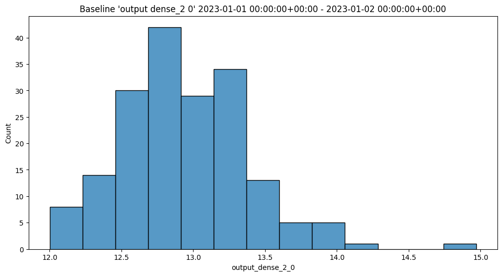
assay_builder.baseline_kde()
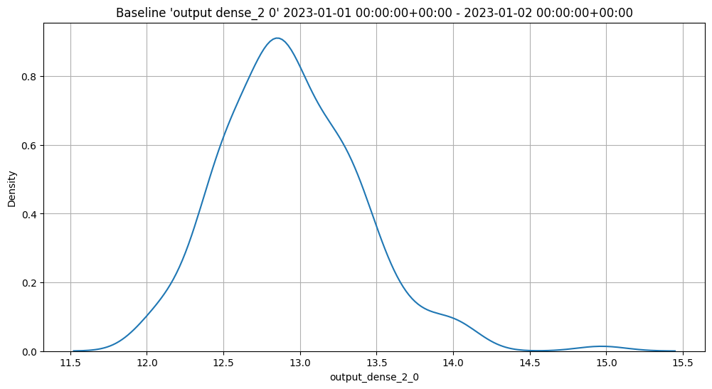
assay_builder.baseline_ecdf()
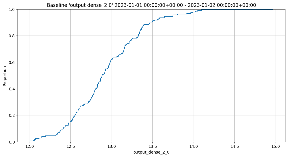
List Assays
Assays are listed through the Wallaroo Client list_assays method.
wl.list_assays()
| name | active | status | warning_threshold | alert_threshold | pipeline_name |
|---|---|---|---|---|---|
| api_assay | True | created | 0.0 | 0.1 | housepricepipe |
Interactive Baseline Runs
We can do an interactive run of just the baseline part to see how the baseline data will be put into bins. This assay uses quintiles so all 5 bins (not counting the outlier bins) have 20% of the predictions. We can see the bin boundaries along the x-axis.
baseline_run.chart()
baseline mean = 12.940910643273655
baseline median = 12.884286880493164
bin_mode = Quantile
aggregation = Density
metric = PSI
weighted = False
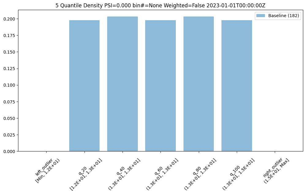
We can also get a dataframe with the bin/edge information.
baseline_run.baseline_bins()
| b_edges | b_edge_names | b_aggregated_values | b_aggregation | |
|---|---|---|---|---|
| 0 | 12.00 | left_outlier | 0.00 | Density |
| 1 | 12.55 | q_20 | 0.20 | Density |
| 2 | 12.81 | q_40 | 0.20 | Density |
| 3 | 12.98 | q_60 | 0.20 | Density |
| 4 | 13.33 | q_80 | 0.20 | Density |
| 5 | 14.97 | q_100 | 0.20 | Density |
| 6 | inf | right_outlier | 0.00 | Density |
The previous assay used quintiles so all of the bins had the same percentage/count of samples. To get bins that are divided equaly along the range of values we can use BinMode.EQUAL.
equal_bin_builder = wl.build_assay(assay_name, pipeline, model_name, baseline_start, baseline_end)
equal_bin_builder.summarizer_builder.add_bin_mode(BinMode.EQUAL)
equal_baseline = equal_bin_builder.build().interactive_baseline_run()
equal_baseline.chart()
baseline mean = 12.940910643273655
baseline median = 12.884286880493164
bin_mode = Equal
aggregation = Density
metric = PSI
weighted = False
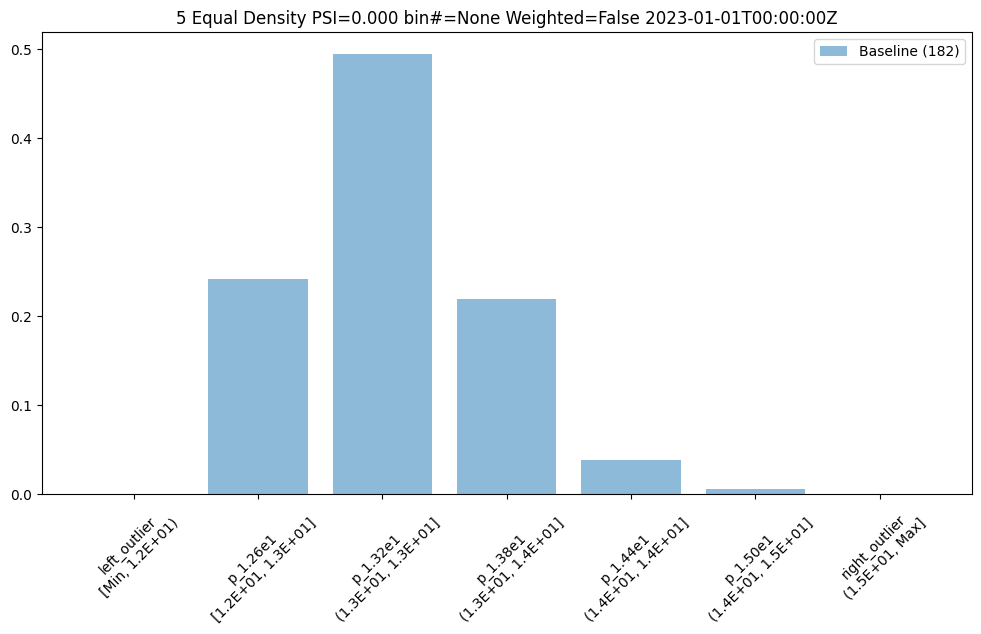
We now see very different bin edges and sample percentages per bin.
equal_baseline.baseline_bins()
| b_edges | b_edge_names | b_aggregated_values | b_aggregation | |
|---|---|---|---|---|
| 0 | 12.00 | left_outlier | 0.00 | Density |
| 1 | 12.60 | p_1.26e1 | 0.24 | Density |
| 2 | 13.19 | p_1.32e1 | 0.49 | Density |
| 3 | 13.78 | p_1.38e1 | 0.22 | Density |
| 4 | 14.38 | p_1.44e1 | 0.04 | Density |
| 5 | 14.97 | p_1.50e1 | 0.01 | Density |
| 6 | inf | right_outlier | 0.00 | Density |
Interactive Assay Runs
By default the assay builder creates an assay with some good starting parameters. In particular the assay is configured to run a new analysis for every 24 hours starting at the end of the baseline period. Additionally, it sets the number of bins to 5 so creates quintiles, and sets the target iopath to "outputs 0 0" which means we want to monitor the first column of the first output/prediction.
We can do an interactive run of just the baseline part to see how the baseline data will be put into bins. This assay uses quintiles so all 5 bins (not counting the outlier bins) have 20% of the predictions. We can see the bin boundaries along the x-axis.
We then run it with interactive_run and convert it to a dataframe for easy analysis with to_dataframe.
Now lets do an interactive run of the first assay as it is configured. Interactive runs don’t save the assay to the database (so they won’t be scheduled in the future) nor do they save the assay results. Instead the results are returned after a short while for further analysis.
assay_builder = wl.build_assay(assay_name, pipeline, model_name, baseline_start, baseline_end)
assay_config = assay_builder.add_run_until(last_day).build()
assay_results = assay_config.interactive_run()
assay_df = assay_results.to_dataframe()
assay_df.loc[:, ~assay_df.columns.isin(['assay_id', 'iopath', 'name', 'warning_threshold'])]
| score | start | min | max | mean | median | std | alert_threshold | status | |
|---|---|---|---|---|---|---|---|---|---|
| 0 | 0.00 | 2023-01-02T00:00:00+00:00 | 12.05 | 14.71 | 12.97 | 12.90 | 0.48 | 0.25 | Ok |
| 1 | 0.09 | 2023-01-03T00:00:00+00:00 | 12.04 | 14.65 | 12.96 | 12.93 | 0.41 | 0.25 | Ok |
| 2 | 0.04 | 2023-01-04T00:00:00+00:00 | 11.87 | 14.02 | 12.98 | 12.95 | 0.46 | 0.25 | Ok |
| 3 | 0.06 | 2023-01-05T00:00:00+00:00 | 11.92 | 14.46 | 12.93 | 12.87 | 0.46 | 0.25 | Ok |
| 4 | 0.02 | 2023-01-06T00:00:00+00:00 | 12.02 | 14.15 | 12.95 | 12.90 | 0.43 | 0.25 | Ok |
| 5 | 0.03 | 2023-01-07T00:00:00+00:00 | 12.18 | 14.58 | 12.96 | 12.93 | 0.44 | 0.25 | Ok |
| 6 | 0.02 | 2023-01-08T00:00:00+00:00 | 12.01 | 14.60 | 12.92 | 12.90 | 0.46 | 0.25 | Ok |
| 7 | 0.04 | 2023-01-09T00:00:00+00:00 | 12.01 | 14.40 | 13.00 | 12.97 | 0.45 | 0.25 | Ok |
| 8 | 0.06 | 2023-01-10T00:00:00+00:00 | 11.99 | 14.79 | 12.94 | 12.91 | 0.46 | 0.25 | Ok |
| 9 | 0.02 | 2023-01-11T00:00:00+00:00 | 11.90 | 14.66 | 12.91 | 12.88 | 0.45 | 0.25 | Ok |
| 10 | 0.02 | 2023-01-12T00:00:00+00:00 | 11.96 | 14.82 | 12.94 | 12.90 | 0.46 | 0.25 | Ok |
| 11 | 0.03 | 2023-01-13T00:00:00+00:00 | 12.07 | 14.61 | 12.96 | 12.93 | 0.47 | 0.25 | Ok |
| 12 | 0.15 | 2023-01-14T00:00:00+00:00 | 12.00 | 14.20 | 13.06 | 13.03 | 0.43 | 0.25 | Ok |
| 13 | 2.92 | 2023-01-15T00:00:00+00:00 | 12.74 | 15.62 | 14.00 | 14.01 | 0.57 | 0.25 | Alert |
| 14 | 7.89 | 2023-01-16T00:00:00+00:00 | 14.64 | 17.19 | 15.91 | 15.87 | 0.63 | 0.25 | Alert |
| 15 | 8.87 | 2023-01-17T00:00:00+00:00 | 16.60 | 19.23 | 17.94 | 17.94 | 0.63 | 0.25 | Alert |
| 16 | 8.87 | 2023-01-18T00:00:00+00:00 | 18.67 | 21.29 | 20.01 | 20.04 | 0.64 | 0.25 | Alert |
| 17 | 8.87 | 2023-01-19T00:00:00+00:00 | 20.72 | 23.57 | 22.17 | 22.18 | 0.65 | 0.25 | Alert |
| 18 | 8.87 | 2023-01-20T00:00:00+00:00 | 23.04 | 25.72 | 24.32 | 24.33 | 0.66 | 0.25 | Alert |
| 19 | 8.87 | 2023-01-21T00:00:00+00:00 | 25.06 | 27.67 | 26.48 | 26.49 | 0.63 | 0.25 | Alert |
| 20 | 8.87 | 2023-01-22T00:00:00+00:00 | 27.21 | 29.89 | 28.63 | 28.58 | 0.65 | 0.25 | Alert |
| 21 | 8.87 | 2023-01-23T00:00:00+00:00 | 29.36 | 32.18 | 30.82 | 30.80 | 0.67 | 0.25 | Alert |
| 22 | 8.87 | 2023-01-24T00:00:00+00:00 | 31.56 | 34.35 | 32.98 | 32.98 | 0.65 | 0.25 | Alert |
| 23 | 8.87 | 2023-01-25T00:00:00+00:00 | 33.68 | 36.44 | 35.14 | 35.14 | 0.66 | 0.25 | Alert |
| 24 | 8.87 | 2023-01-26T00:00:00+00:00 | 35.93 | 38.51 | 37.31 | 37.33 | 0.65 | 0.25 | Alert |
| 25 | 3.69 | 2023-01-27T00:00:00+00:00 | 12.06 | 39.91 | 29.29 | 38.65 | 12.66 | 0.25 | Alert |
| 26 | 0.05 | 2023-01-28T00:00:00+00:00 | 11.87 | 13.88 | 12.92 | 12.90 | 0.38 | 0.25 | Ok |
| 27 | 0.10 | 2023-01-29T00:00:00+00:00 | 12.02 | 14.36 | 12.98 | 12.96 | 0.38 | 0.25 | Ok |
| 28 | 0.11 | 2023-01-30T00:00:00+00:00 | 11.99 | 14.44 | 12.89 | 12.88 | 0.37 | 0.25 | Ok |
| 29 | 0.01 | 2023-01-31T00:00:00+00:00 | 12.00 | 14.64 | 12.92 | 12.89 | 0.40 | 0.25 | Ok |
Basic functionality for creating quick charts is included.
assay_results.chart_scores()
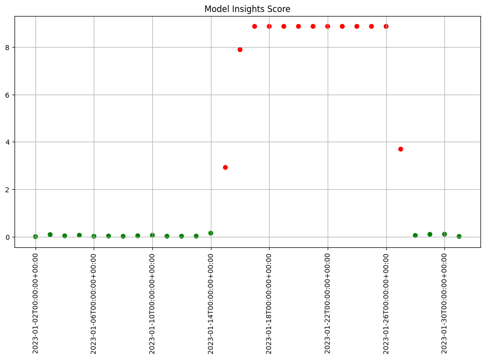
We see that the difference scores are low for a while and then jump up to indicate there is an issue. We can examine that particular window to help us decide if that threshold is set correctly or not.
We can generate a quick chart of the results. This chart shows the 5 quantile bins (quintiles) derived from the baseline data plus one for left outliers and one for right outliers. We also see that the data from the window falls within the baseline quintiles but in a different proportion and is skewing higher. Whether this is an issue or not is specific to your use case.
First lets examine a day that is only slightly different than the baseline. We see that we do see some values that fall outside of the range from the baseline values, the left and right outliers, and that the bin values are different but similar.
assay_results[0].chart()
baseline mean = 12.940910643273655
window mean = 12.969964654406132
baseline median = 12.884286880493164
window median = 12.899214744567873
bin_mode = Quantile
aggregation = Density
metric = PSI
weighted = False
score = 0.0029273068646199748
scores = [0.0, 0.000514261205558409, 0.0002139202456922972, 0.0012617897456473992, 0.0002139202456922972, 0.0007234154220295724, 0.0]
index = None

Other days, however are significantly different.
assay_results[12].chart()
baseline mean = 12.940910643273655
window mean = 13.06380216891949
baseline median = 12.884286880493164
window median = 13.027600288391112
bin_mode = Quantile
aggregation = Density
metric = PSI
weighted = False
score = 0.15060511096978788
scores = [4.6637149189075455e-05, 0.05969428191167242, 0.00806617426854112, 0.008316273402678306, 0.07090885609902021, 0.003572888138686759, 0.0]
index = None

assay_results[13].chart()
baseline mean = 12.940910643273655
window mean = 14.004728427908038
baseline median = 12.884286880493164
window median = 14.009637832641602
bin_mode = Quantile
aggregation = Density
metric = PSI
weighted = False
score = 2.9220486095961196
scores = [0.0, 0.7090936334784107, 0.7130482300184766, 0.33500731896676245, 0.12171058214520876, 0.9038825518183468, 0.1393062931689142]
index = None
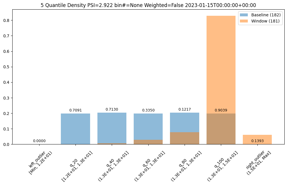
If we want to investigate further, we can run interactive assays on each of the inputs to see if any of them show anything abnormal. In this example we’ll provide the feature labels to create more understandable titles.
The current assay expects continuous data. Sometimes categorical data is encoded as 1 or 0 in a feature and sometimes in a limited number of values such as 1, 2, 3. If one value has high a percentage the analysis emits a warning so that we know the scores for that feature may not behave as we expect.
labels = ['bedrooms', 'bathrooms', 'lat', 'long', 'waterfront', 'sqft_living', 'sqft_lot', 'floors', 'view', 'condition', 'grade', 'sqft_above', 'sqft_basement', 'yr_built', 'yr_renovated', 'sqft_living15', 'sqft_lot15']
topic = wl.get_topic_name(pipeline.id())
all_inferences = wl.get_raw_pipeline_inference_logs(topic, baseline_start, last_day, model_name, limit=1_000_000)
assay_builder = wl.build_assay("Input Assay", pipeline, model_name, baseline_start, baseline_end).add_run_until(last_day)
assay_builder.window_builder().add_width(hours=4)
assay_config = assay_builder.build()
assay_results = assay_config.interactive_input_run(all_inferences, labels)
iadf = assay_results.to_dataframe()
display(iadf.loc[:, ~iadf.columns.isin(['assay_id', 'iopath', 'name', 'warning_threshold'])])
column distinct_vals label largest_pct
0 17 bedrooms 0.4244
1 44 bathrooms 0.2398
2 3281 lat 0.0014
3 959 long 0.0066
4 4 waterfront 0.9156 *** May not be continuous feature
5 3901 sqft_living 0.0032
6 3487 sqft_lot 0.0173
7 11 floors 0.4567
8 10 view 0.8337
9 9 condition 0.5915
10 19 grade 0.3943
11 745 sqft_above 0.0096
12 309 sqft_basement 0.5582
13 224 yr_built 0.0239
14 77 yr_renovated 0.8889
15 649 sqft_living15 0.0093
16 3280 sqft_lot15 0.0199
| score | start | min | max | mean | median | std | alert_threshold | status | |
|---|---|---|---|---|---|---|---|---|---|
| 0 | 0.19 | 2023-01-02T00:00:00+00:00 | -2.54 | 1.75 | 0.21 | 0.68 | 0.99 | 0.25 | Ok |
| 1 | 0.03 | 2023-01-02T04:00:00+00:00 | -1.47 | 2.82 | 0.21 | -0.40 | 0.95 | 0.25 | Ok |
| 2 | 0.09 | 2023-01-02T08:00:00+00:00 | -2.54 | 3.89 | -0.04 | -0.40 | 1.22 | 0.25 | Ok |
| 3 | 0.05 | 2023-01-02T12:00:00+00:00 | -1.47 | 2.82 | -0.12 | -0.40 | 0.94 | 0.25 | Ok |
| 4 | 0.08 | 2023-01-02T16:00:00+00:00 | -1.47 | 1.75 | -0.00 | -0.40 | 0.76 | 0.25 | Ok |
| ... | ... | ... | ... | ... | ... | ... | ... | ... | ... |
| 3055 | 0.08 | 2023-01-31T04:00:00+00:00 | -0.42 | 4.87 | 0.25 | -0.17 | 1.13 | 0.25 | Ok |
| 3056 | 0.58 | 2023-01-31T08:00:00+00:00 | -0.43 | 2.01 | -0.04 | -0.21 | 0.48 | 0.25 | Alert |
| 3057 | 0.13 | 2023-01-31T12:00:00+00:00 | -0.32 | 7.75 | 0.30 | -0.20 | 1.57 | 0.25 | Ok |
| 3058 | 0.26 | 2023-01-31T16:00:00+00:00 | -0.43 | 5.88 | 0.19 | -0.18 | 1.17 | 0.25 | Alert |
| 3059 | 0.84 | 2023-01-31T20:00:00+00:00 | -0.40 | 0.52 | -0.17 | -0.25 | 0.18 | 0.25 | Alert |
3060 rows × 9 columns
We can chart each of the iopaths and do a visual inspection. From the charts we see that if any of the input features had significant differences in the first two days which we can choose to inspect further. Here we choose to show 3 charts just to save space in this notebook.
assay_results.chart_iopaths(labels=labels, selected_labels=['bedrooms', 'lat', 'sqft_living'])
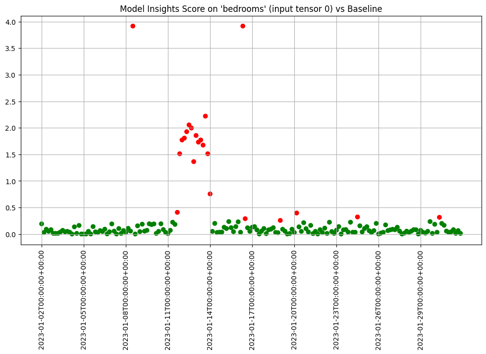
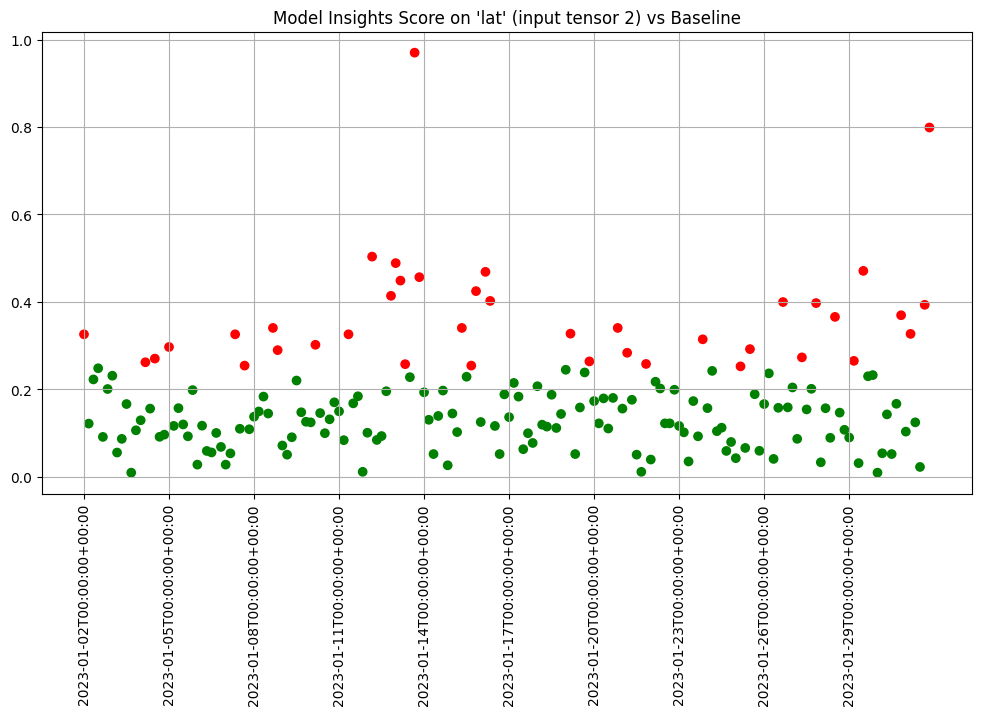
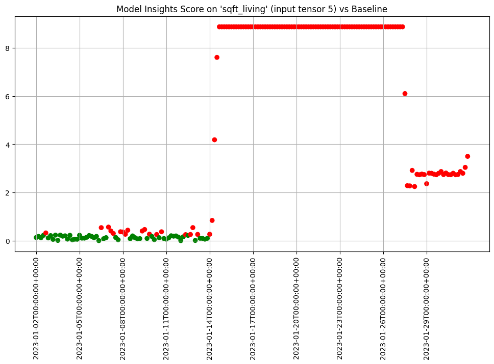
When we are comfortable with what alert threshold should be for our specific purposes we can create and save an assay that will be automatically run on a daily basis.
In this example we’re create an assay that runs everyday against the baseline and has an alert threshold of 0.5.
Once we upload it it will be saved and scheduled for future data as well as run against past data.
alert_threshold = 0.5
import string
import random
prefix= ''.join(random.choice(string.ascii_lowercase) for i in range(4))
assay_name = f"{prefix}example assay"
assay_builder = wl.build_assay(assay_name, pipeline, model_name, baseline_start, baseline_end).add_alert_threshold(alert_threshold)
assay_id = assay_builder.upload()
After a short while, we can get the assay results for further analysis.
When we get the assay results, we see that the assays analysis is similar to the interactive run we started with though the analysis for the third day does not exceed the new alert threshold we set. And since we called upload instead of interactive_run the assay was saved to the system and will continue to run automatically on schedule from now on.
Scheduling Assays
By default assays are scheduled to run every 24 hours starting immediately after the baseline period ends.
However, you can control the start time by setting start and the frequency by setting interval on the window.
So to recap:
- The window width is the size of the window. The default is 24 hours.
- The interval is how often the analysis is run, how far the window is slid into the future based on the last run. The default is the window width.
- The window start is when the analysis should start. The default is the end of the baseline period.
For example to run an analysis every 12 hours on the previous 24 hours of data you’d set the window width to 24 (the default) and the interval to 12.
assay_builder = wl.build_assay(assay_name, pipeline, model_name, baseline_start, baseline_end)
assay_builder = assay_builder.add_run_until(last_day)
assay_builder.window_builder().add_width(hours=24).add_interval(hours=12)
assay_config = assay_builder.build()
assay_results = assay_config.interactive_run()
print(f"Generated {len(assay_results)} analyses")
Generated 59 analyses
assay_results.chart_scores()
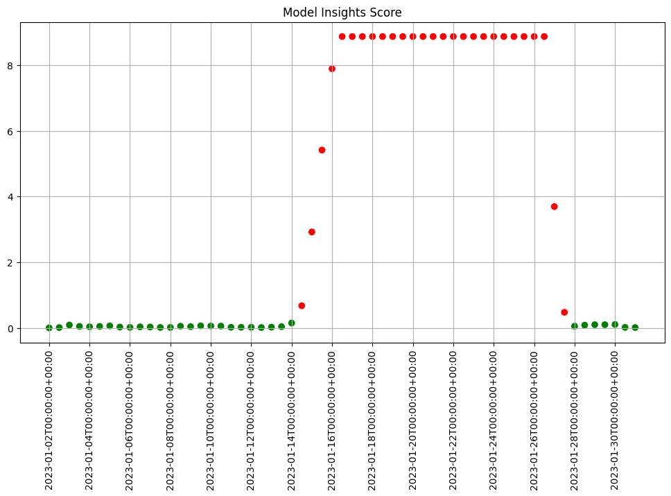
To start a weekly analysis of the previous week on a specific day, set the start date (taking care to specify the desired timezone), and the width and interval to 1 week and of course an analysis won’t be generated till a window is complete.
By default, assay start date is set to 24 hours from when the assay was created. For this example, we will set the assay.window_builder.add_start to set the assay window to start at the beginning of our data, and assay.add_run_until to set the time period to stop gathering data from.
report_start = datetime.datetime.fromisoformat('2022-01-03T00:00:00+00:00')
assay_builder = wl.build_assay(assay_name, pipeline, model_name, baseline_start, baseline_end)
assay_builder = assay_builder.add_run_until(last_day)
assay_builder.window_builder().add_width(weeks=1).add_interval(weeks=1).add_start(report_start)
assay_config = assay_builder.build()
assay_results = assay_config.interactive_run()
print(f"Generated {len(assay_results)} analyses")
Generated 5 analyses
assay_results.chart_scores()
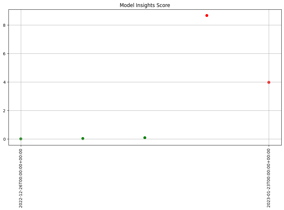
Advanced Configuration
The assay can be configured in a variety of ways to help customize it to your particular needs. Specifically you can:
- change the BinMode to evenly spaced, quantile or user provided
- change the number of bins to use
- provide weights to use when scoring the bins
- calculate the score using the sum of differences, maximum difference or population stability index
- change the value aggregation for the bins to density, cumulative or edges
Lets take a look at these in turn.
Default configuration
First lets look at the default configuration. This is a lot of information but much of it is useful to know where it is available.
We see that the assay is broken up into 4 sections. A top level meta data section, a section for the baseline specification, a section for the window specification and a section that specifies the summarization configuration.
In the meta section we see the name of the assay, that it runs on the first column of the first output "outputs 0 0" and that there is a default threshold of 0.25.
The summarizer section shows us the defaults of Quantile, Density and PSI on 5 bins.
The baseline section shows us that it is configured as a fixed baseline with the specified start and end date times.
And the window tells us what model in the pipeline we are analyzing and how often.
assay_builder = wl.build_assay(assay_name, pipeline, model_name, baseline_start, baseline_end).add_run_until(last_day)
print(assay_builder.build().to_json())
{
"name": "onmyexample assay",
"pipeline_id": 1,
"pipeline_name": "housepricepipe",
"active": true,
"status": "created",
"iopath": "output dense_2 0",
"baseline": {
"Fixed": {
"pipeline": "housepricepipe",
"model": "housepricemodel",
"start_at": "2023-01-01T00:00:00+00:00",
"end_at": "2023-01-02T00:00:00+00:00"
}
},
"window": {
"pipeline": "housepricepipe",
"model": "housepricemodel",
"width": "24 hours",
"start": null,
"interval": null
},
"summarizer": {
"type": "UnivariateContinuous",
"bin_mode": "Quantile",
"aggregation": "Density",
"metric": "PSI",
"num_bins": 5,
"bin_weights": null,
"bin_width": null,
"provided_edges": null,
"add_outlier_edges": true
},
"warning_threshold": null,
"alert_threshold": 0.25,
"run_until": "2023-02-01T00:00:00+00:00",
"workspace_id": 5
}
Defaults
We can run the assay interactively and review the first analysis. The method compare_basic_stats gives us a dataframe with basic stats for the baseline and window data.
assay_results = assay_builder.build().interactive_run()
ar = assay_results[0]
ar.compare_basic_stats()
| Baseline | Window | diff | pct_diff | |
|---|---|---|---|---|
| count | 182.00 | 181.00 | -1.00 | -0.55 |
| min | 12.00 | 12.05 | 0.04 | 0.36 |
| max | 14.97 | 14.71 | -0.26 | -1.71 |
| mean | 12.94 | 12.97 | 0.03 | 0.22 |
| median | 12.88 | 12.90 | 0.01 | 0.12 |
| std | 0.45 | 0.48 | 0.03 | 5.68 |
| start | 2023-01-01T00:00:00+00:00 | 2023-01-02T00:00:00+00:00 | NaN | NaN |
| end | 2023-01-02T00:00:00+00:00 | 2023-01-03T00:00:00+00:00 | NaN | NaN |
The method compare_bins gives us a dataframe with the bin information. Such as the number of bins, the right edges, suggested bin/edge names and the values for each bin in the baseline and the window.
assay_bins = ar.compare_bins()
display(assay_bins.loc[:, assay_bins.columns!='w_aggregation'])
| b_edges | b_edge_names | b_aggregated_values | b_aggregation | w_edges | w_edge_names | w_aggregated_values | diff_in_pcts | |
|---|---|---|---|---|---|---|---|---|
| 0 | 12.00 | left_outlier | 0.00 | Density | 12.00 | left_outlier | 0.00 | 0.00 |
| 1 | 12.55 | q_20 | 0.20 | Density | 12.55 | e_1.26e1 | 0.19 | -0.01 |
| 2 | 12.81 | q_40 | 0.20 | Density | 12.81 | e_1.28e1 | 0.21 | 0.01 |
| 3 | 12.98 | q_60 | 0.20 | Density | 12.98 | e_1.30e1 | 0.18 | -0.02 |
| 4 | 13.33 | q_80 | 0.20 | Density | 13.33 | e_1.33e1 | 0.21 | 0.01 |
| 5 | 14.97 | q_100 | 0.20 | Density | 14.97 | e_1.50e1 | 0.21 | 0.01 |
| 6 | NaN | right_outlier | 0.00 | Density | NaN | right_outlier | 0.00 | 0.00 |
We can also plot the chart to visualize the values of the bins.
ar.chart()
baseline mean = 12.940910643273655
window mean = 12.969964654406132
baseline median = 12.884286880493164
window median = 12.899214744567873
bin_mode = Quantile
aggregation = Density
metric = PSI
weighted = False
score = 0.0029273068646199748
scores = [0.0, 0.000514261205558409, 0.0002139202456922972, 0.0012617897456473992, 0.0002139202456922972, 0.0007234154220295724, 0.0]
index = None
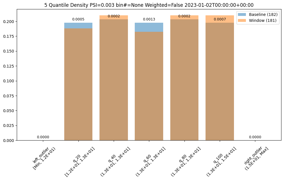
Binning Mode
We can change the bin mode algorithm to equal and see that the bins/edges are partitioned at different points and the bins have different values.
prefix= ''.join(random.choice(string.ascii_lowercase) for i in range(4))
assay_name = f"{prefix}example assay"
assay_builder = wl.build_assay(assay_name, pipeline, model_name, baseline_start, baseline_end).add_run_until(last_day)
assay_builder.summarizer_builder.add_bin_mode(BinMode.EQUAL)
assay_results = assay_builder.build().interactive_run()
assay_results_df = assay_results[0].compare_bins()
display(assay_results_df.loc[:, ~assay_results_df.columns.isin(['b_aggregation', 'w_aggregation'])])
assay_results[0].chart()
| b_edges | b_edge_names | b_aggregated_values | w_edges | w_edge_names | w_aggregated_values | diff_in_pcts | |
|---|---|---|---|---|---|---|---|
| 0 | 12.00 | left_outlier | 0.00 | 12.00 | left_outlier | 0.00 | 0.00 |
| 1 | 12.60 | p_1.26e1 | 0.24 | 12.60 | e_1.26e1 | 0.24 | 0.00 |
| 2 | 13.19 | p_1.32e1 | 0.49 | 13.19 | e_1.32e1 | 0.48 | -0.02 |
| 3 | 13.78 | p_1.38e1 | 0.22 | 13.78 | e_1.38e1 | 0.22 | -0.00 |
| 4 | 14.38 | p_1.44e1 | 0.04 | 14.38 | e_1.44e1 | 0.06 | 0.02 |
| 5 | 14.97 | p_1.50e1 | 0.01 | 14.97 | e_1.50e1 | 0.01 | 0.00 |
| 6 | NaN | right_outlier | 0.00 | NaN | right_outlier | 0.00 | 0.00 |
baseline mean = 12.940910643273655
window mean = 12.969964654406132
baseline median = 12.884286880493164
window median = 12.899214744567873
bin_mode = Equal
aggregation = Density
metric = PSI
weighted = False
score = 0.011074287819376092
scores = [0.0, 7.3591419975306595e-06, 0.000773779195360713, 8.538514991838585e-05, 0.010207597078872246, 1.6725322721660374e-07, 0.0]
index = None
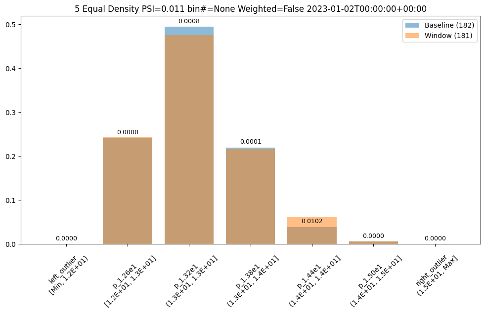
User Provided Bin Edges
The values in this dataset run from ~11.6 to ~15.81. And lets say we had a business reason to use specific bin edges. We can specify them with the BinMode.PROVIDED and specifying a list of floats with the right hand / upper edge of each bin and optionally the lower edge of the smallest bin. If the lowest edge is not specified the threshold for left outliers is taken from the smallest value in the baseline dataset.
edges = [11.0, 12.0, 13.0, 14.0, 15.0, 16.0]
assay_builder = wl.build_assay(assay_name, pipeline, model_name, baseline_start, baseline_end).add_run_until(last_day)
assay_builder.summarizer_builder.add_bin_mode(BinMode.PROVIDED, edges)
assay_results = assay_builder.build().interactive_run()
assay_results_df = assay_results[0].compare_bins()
display(assay_results_df.loc[:, ~assay_results_df.columns.isin(['b_aggregation', 'w_aggregation'])])
assay_results[0].chart()
| b_edges | b_edge_names | b_aggregated_values | w_edges | w_edge_names | w_aggregated_values | diff_in_pcts | |
|---|---|---|---|---|---|---|---|
| 0 | 11.00 | left_outlier | 0.00 | 11.00 | left_outlier | 0.00 | 0.00 |
| 1 | 12.00 | e_1.20e1 | 0.00 | 12.00 | e_1.20e1 | 0.00 | 0.00 |
| 2 | 13.00 | e_1.30e1 | 0.62 | 13.00 | e_1.30e1 | 0.59 | -0.03 |
| 3 | 14.00 | e_1.40e1 | 0.36 | 14.00 | e_1.40e1 | 0.35 | -0.00 |
| 4 | 15.00 | e_1.50e1 | 0.02 | 15.00 | e_1.50e1 | 0.06 | 0.03 |
| 5 | 16.00 | e_1.60e1 | 0.00 | 16.00 | e_1.60e1 | 0.00 | 0.00 |
| 6 | NaN | right_outlier | 0.00 | NaN | right_outlier | 0.00 | 0.00 |
baseline mean = 12.940910643273655
window mean = 12.969964654406132
baseline median = 12.884286880493164
window median = 12.899214744567873
bin_mode = Provided
aggregation = Density
metric = PSI
weighted = False
score = 0.0321620386600679
scores = [0.0, 0.0, 0.0014576920813015586, 3.549754401142936e-05, 0.030668849034754912, 0.0, 0.0]
index = None
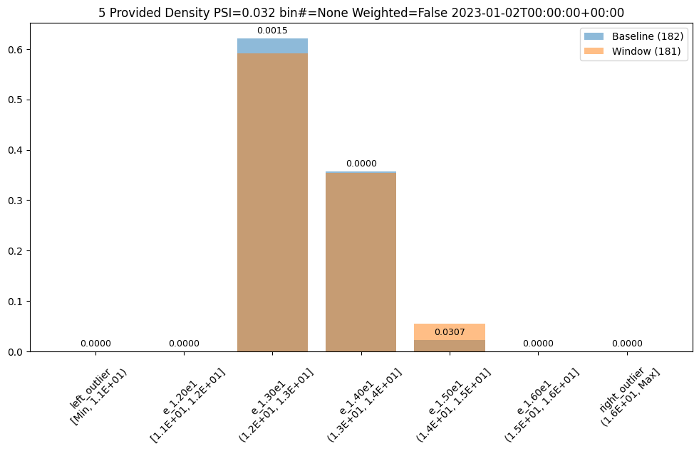
Number of Bins
We could also choose to a different number of bins, lets say 10, which can be evenly spaced or based on the quantiles (deciles).
assay_builder = wl.build_assay(assay_name, pipeline, model_name, baseline_start, baseline_end).add_run_until(last_day)
assay_builder.summarizer_builder.add_bin_mode(BinMode.QUANTILE).add_num_bins(10)
assay_results = assay_builder.build().interactive_run()
assay_results_df = assay_results[1].compare_bins()
display(assay_results_df.loc[:, ~assay_results_df.columns.isin(['b_aggregation', 'w_aggregation'])])
assay_results[1].chart()
| b_edges | b_edge_names | b_aggregated_values | w_edges | w_edge_names | w_aggregated_values | diff_in_pcts | |
|---|---|---|---|---|---|---|---|
| 0 | 12.00 | left_outlier | 0.00 | 12.00 | left_outlier | 0.00 | 0.00 |
| 1 | 12.41 | q_10 | 0.10 | 12.41 | e_1.24e1 | 0.09 | -0.00 |
| 2 | 12.55 | q_20 | 0.10 | 12.55 | e_1.26e1 | 0.04 | -0.05 |
| 3 | 12.72 | q_30 | 0.10 | 12.72 | e_1.27e1 | 0.14 | 0.03 |
| 4 | 12.81 | q_40 | 0.10 | 12.81 | e_1.28e1 | 0.05 | -0.05 |
| 5 | 12.88 | q_50 | 0.10 | 12.88 | e_1.29e1 | 0.12 | 0.02 |
| 6 | 12.98 | q_60 | 0.10 | 12.98 | e_1.30e1 | 0.09 | -0.01 |
| 7 | 13.15 | q_70 | 0.10 | 13.15 | e_1.32e1 | 0.18 | 0.08 |
| 8 | 13.33 | q_80 | 0.10 | 13.33 | e_1.33e1 | 0.14 | 0.03 |
| 9 | 13.47 | q_90 | 0.10 | 13.47 | e_1.35e1 | 0.07 | -0.03 |
| 10 | 14.97 | q_100 | 0.10 | 14.97 | e_1.50e1 | 0.08 | -0.02 |
| 11 | NaN | right_outlier | 0.00 | NaN | right_outlier | 0.00 | 0.00 |
baseline mean = 12.940910643273655
window mean = 12.956829186961135
baseline median = 12.884286880493164
window median = 12.929338455200195
bin_mode = Quantile
aggregation = Density
metric = PSI
weighted = False
score = 0.16591076620684958
scores = [0.0, 0.0002571306027792045, 0.044058279699182114, 0.009441459631493015, 0.03381618572319047, 0.0027335446937028877, 0.0011792419836838435, 0.051023062424253904, 0.009441459631493015, 0.008662563542113508, 0.0052978382749576496, 0.0]
index = None
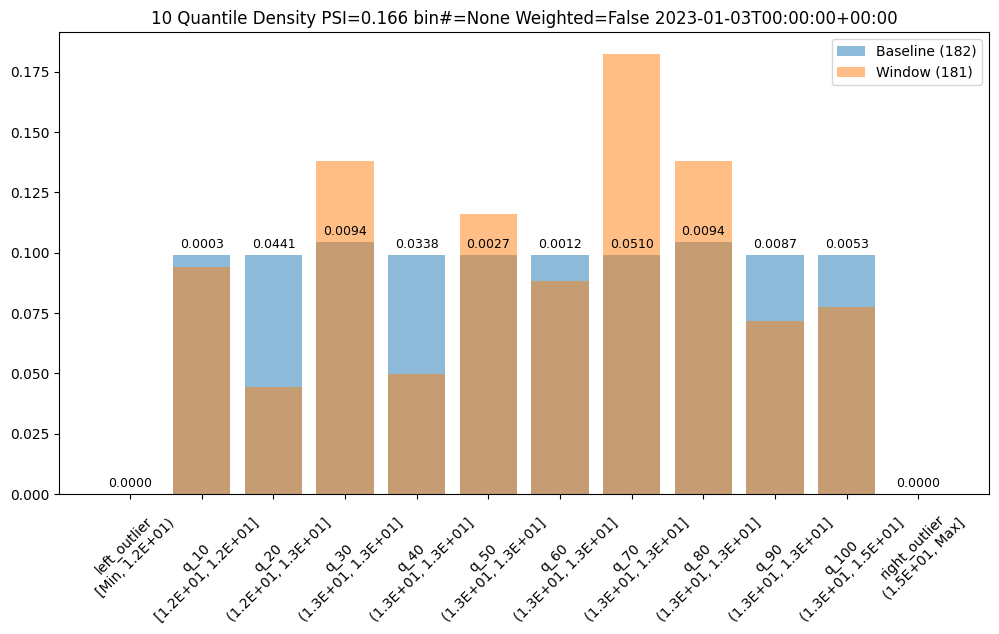
Bin Weights
Now lets say we only care about differences at the higher end of the range. We can use weights to specify that difference in the lower bins should not be counted in the score.
If we stick with 10 bins we can provide 10 a vector of 12 weights. One weight each for the original bins plus one at the front for the left outlier bin and one at the end for the right outlier bin.
Note we still show the values for the bins but the scores for the lower 5 and left outlier are 0 and only the right half is counted and reflected in the score.
weights = [0] * 6
weights.extend([1] * 6)
print("Using weights: ", weights)
assay_builder = wl.build_assay(assay_name, pipeline, model_name, baseline_start, baseline_end).add_run_until(last_day)
assay_builder.summarizer_builder.add_bin_mode(BinMode.QUANTILE).add_num_bins(10).add_bin_weights(weights)
assay_results = assay_builder.build().interactive_run()
assay_results_df = assay_results[1].compare_bins()
display(assay_results_df.loc[:, ~assay_results_df.columns.isin(['b_aggregation', 'w_aggregation'])])
assay_results[1].chart()
Using weights: [0, 0, 0, 0, 0, 0, 1, 1, 1, 1, 1, 1]
| b_edges | b_edge_names | b_aggregated_values | w_edges | w_edge_names | w_aggregated_values | diff_in_pcts | |
|---|---|---|---|---|---|---|---|
| 0 | 12.00 | left_outlier | 0.00 | 12.00 | left_outlier | 0.00 | 0.00 |
| 1 | 12.41 | q_10 | 0.10 | 12.41 | e_1.24e1 | 0.09 | -0.00 |
| 2 | 12.55 | q_20 | 0.10 | 12.55 | e_1.26e1 | 0.04 | -0.05 |
| 3 | 12.72 | q_30 | 0.10 | 12.72 | e_1.27e1 | 0.14 | 0.03 |
| 4 | 12.81 | q_40 | 0.10 | 12.81 | e_1.28e1 | 0.05 | -0.05 |
| 5 | 12.88 | q_50 | 0.10 | 12.88 | e_1.29e1 | 0.12 | 0.02 |
| 6 | 12.98 | q_60 | 0.10 | 12.98 | e_1.30e1 | 0.09 | -0.01 |
| 7 | 13.15 | q_70 | 0.10 | 13.15 | e_1.32e1 | 0.18 | 0.08 |
| 8 | 13.33 | q_80 | 0.10 | 13.33 | e_1.33e1 | 0.14 | 0.03 |
| 9 | 13.47 | q_90 | 0.10 | 13.47 | e_1.35e1 | 0.07 | -0.03 |
| 10 | 14.97 | q_100 | 0.10 | 14.97 | e_1.50e1 | 0.08 | -0.02 |
| 11 | NaN | right_outlier | 0.00 | NaN | right_outlier | 0.00 | 0.00 |
baseline mean = 12.940910643273655
window mean = 12.956829186961135
baseline median = 12.884286880493164
window median = 12.929338455200195
bin_mode = Quantile
aggregation = Density
metric = PSI
weighted = True
score = 0.012600694309416988
scores = [0.0, 0.0, 0.0, 0.0, 0.0, 0.0, 0.00019654033061397393, 0.00850384373737565, 0.0015735766052488358, 0.0014437605903522511, 0.000882973045826275, 0.0]
index = None

Metrics
The score is a distance or dis-similarity measure. The larger it is the less similar the two distributions are. We currently support
summing the differences of each individual bin, taking the maximum difference and a modified Population Stability Index (PSI).
The following three charts use each of the metrics. Note how the scores change. The best one will depend on your particular use case.
assay_builder = wl.build_assay(assay_name, pipeline, model_name, baseline_start, baseline_end).add_run_until(last_day)
assay_results = assay_builder.build().interactive_run()
assay_results[0].chart()
baseline mean = 12.940910643273655
window mean = 12.969964654406132
baseline median = 12.884286880493164
window median = 12.899214744567873
bin_mode = Quantile
aggregation = Density
metric = PSI
weighted = False
score = 0.0029273068646199748
scores = [0.0, 0.000514261205558409, 0.0002139202456922972, 0.0012617897456473992, 0.0002139202456922972, 0.0007234154220295724, 0.0]
index = None

assay_builder = wl.build_assay(assay_name, pipeline, model_name, baseline_start, baseline_end).add_run_until(last_day)
assay_builder.summarizer_builder.add_metric(Metric.SUMDIFF)
assay_results = assay_builder.build().interactive_run()
assay_results[0].chart()
baseline mean = 12.940910643273655
window mean = 12.969964654406132
baseline median = 12.884286880493164
window median = 12.899214744567873
bin_mode = Quantile
aggregation = Density
metric = SumDiff
weighted = False
score = 0.025438649748041997
scores = [0.0, 0.009956893934794486, 0.006648048084512165, 0.01548175581324751, 0.006648048084512165, 0.012142553579017668, 0.0]
index = None

assay_builder = wl.build_assay(assay_name, pipeline, model_name, baseline_start, baseline_end).add_run_until(last_day)
assay_builder.summarizer_builder.add_metric(Metric.MAXDIFF)
assay_results = assay_builder.build().interactive_run()
assay_results[0].chart()
baseline mean = 12.940910643273655
window mean = 12.969964654406132
baseline median = 12.884286880493164
window median = 12.899214744567873
bin_mode = Quantile
aggregation = Density
metric = MaxDiff
weighted = False
score = 0.01548175581324751
scores = [0.0, 0.009956893934794486, 0.006648048084512165, 0.01548175581324751, 0.006648048084512165, 0.012142553579017668, 0.0]
index = 3
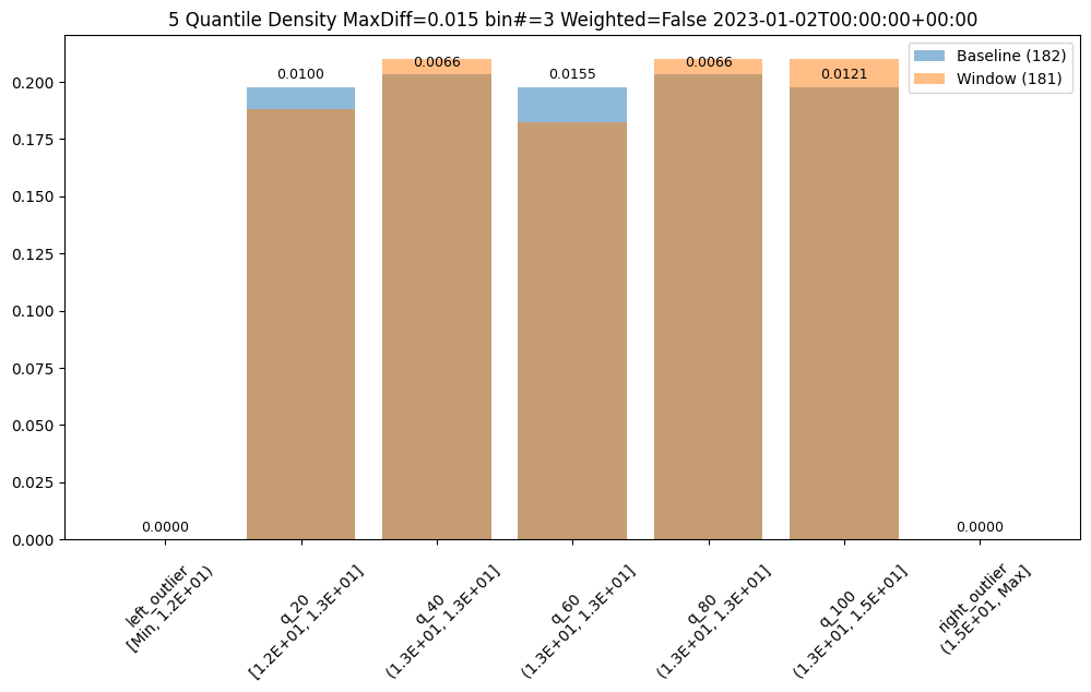
Aggregation Options
Also, bin aggregation can be done in histogram Aggregation.DENSITY style (the default) where we count the number/percentage of values that fall in each bin or Empirical Cumulative Density Function style Aggregation.CUMULATIVE where we keep a cumulative count of the values/percentages that fall in each bin.
assay_builder = wl.build_assay(assay_name, pipeline, model_name, baseline_start, baseline_end).add_run_until(last_day)
assay_builder.summarizer_builder.add_aggregation(Aggregation.DENSITY)
assay_results = assay_builder.build().interactive_run()
assay_results[0].chart()
baseline mean = 12.940910643273655
window mean = 12.969964654406132
baseline median = 12.884286880493164
window median = 12.899214744567873
bin_mode = Quantile
aggregation = Density
metric = PSI
weighted = False
score = 0.0029273068646199748
scores = [0.0, 0.000514261205558409, 0.0002139202456922972, 0.0012617897456473992, 0.0002139202456922972, 0.0007234154220295724, 0.0]
index = None

assay_builder = wl.build_assay(assay_name, pipeline, model_name, baseline_start, baseline_end).add_run_until(last_day)
assay_builder.summarizer_builder.add_aggregation(Aggregation.CUMULATIVE)
assay_results = assay_builder.build().interactive_run()
assay_results[0].chart()
baseline mean = 12.940910643273655
window mean = 12.969964654406132
baseline median = 12.884286880493164
window median = 12.899214744567873
bin_mode = Quantile
aggregation = Cumulative
metric = PSI
weighted = False
score = 0.04419889502762442
scores = [0.0, 0.009956893934794486, 0.0033088458502823492, 0.01879060166352986, 0.012142553579017725, 0.0, 0.0]
index = None
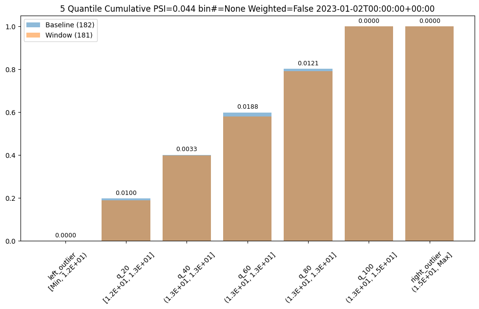
6.6 - Computer Vision Pipeline Logs MLOps API Tutorial
How to retrieve computer vision oriented pipeline logs through the Wallaroo MLOps API.
This tutorial and the assets can be downloaded as part of the Wallaroo Tutorials repository.
Pipeline API Log Tutorial
This tutorial demonstrates Wallaroo Pipeline MLOps API for pipeline log retrieval for Computer Vision based models.
This tutorial will demonstrate how to:
- Select or create a workspace, pipeline and upload the control model, and additional testing models.
- Add a pipeline step with the champion model, then deploy the pipeline and perform sample inferences for computer vision detection.
- Retrieve the logs via the Wallaroo MLOps API. These steps will be simplified to only show the API log retrieval method. See the Wallaroo Documentation site for full details.
- Use the pipeline logs to display metadata data.
- Undeploy the pipeline.
This tutorial provides the following:
- Models:
models/yolov8n.onnx: A pre-trained Yolov8n model.
- Data:
data/dogbike.png: A PNG image with a dog and bicycle.data/dogbike.df.json: A pandas Record format JSON file of the PNG image converted to numpy array values for inference requests.
Prerequisites
- A deployed Wallaroo instance
- The following Python libraries installed:
wallaroo: The Wallaroo SDK. Included with the Wallaroo JupyterHub service by default.
Initial Steps
Import libraries
The first step is to import the libraries needed for this notebook.
import wallaroo
from wallaroo.object import EntityNotFoundError
import pyarrow as pa
from IPython.display import display
# used to display DataFrame information without truncating
from IPython.display import display
import pandas as pd
pd.set_option('display.max_colwidth', None)
import datetime
import requests
Connect to the Wallaroo Instance
The first step is to connect to Wallaroo through the Wallaroo client. The Python library is included in the Wallaroo install and available through the Jupyter Hub interface provided with your Wallaroo environment.
This is accomplished using the wallaroo.Client() command, which provides a URL to grant the SDK permission to your specific Wallaroo environment. When displayed, enter the URL into a browser and confirm permissions. Store the connection into a variable that can be referenced later.
If logging into the Wallaroo instance through the internal JupyterHub service, use wl = wallaroo.Client(). If logging in externally, update the wallarooPrefix and wallarooSuffix variables with the proper DNS information. For more information on Wallaroo Client settings, see the Client Connection guide.
# Login through local Wallaroo instance
wl = wallaroo.Client()
Wallaroo MLOps API URL
API URL
The variable APIURL is used to specify the connection to the Wallaroo instance’s MLOps API URL, and is composed of the Wallaroo DNS prefix and suffix. For full details, see the Wallaroo API Connection Guide
.
For this demonstration, the following Wallaroo SDK methods are used to generate the API authentication Bearer token, and the MLOps API URL.
For full details on connecting to a Wallaroo instance via MLOps API calls, see the Wallaroo API Connection Guide.
These methods are:
wallaroo.client.auth_header(): Returns the authorization Bearer token for a user authenticated through the Wallaroo SDK.wallaroo.client.api_endpoint: Returns the Wallaroo instance’s api endpoint.
display(wl.auth.auth_header())
display(wl.api_endpoint)
{'Authorization': 'Bearer eyJhbGciOiJSUzI1NiIsInR5cCIgOiAiSldUIiwia2lkIiA6ICJzWThabWtGcm9VWDdDSzFiQjEyS1dwWGtaaUk2R01Gd1ZQUHduWmxxbkVRIn0.eyJleHAiOjE3MDMyNjYxOTIsImlhdCI6MTcwMzI2NjEzMiwiYXV0aF90aW1lIjoxNzAzMjY0OTgxLCJqdGkiOiI0NDdmNmU4YS02NTY0LTRhMDQtODBiYy03MDY1YjViMzM4NTQiLCJpc3MiOiJodHRwczovL2RvYy10ZXN0LmtleWNsb2FrLndhbGxhcm9vY29tbXVuaXR5Lm5pbmphL2F1dGgvcmVhbG1zL21hc3RlciIsImF1ZCI6WyJtYXN0ZXItcmVhbG0iLCJhY2NvdW50Il0sInN1YiI6ImNkOGZkMDYzLTYyZmItNDhkYy05NTg5LTFkZTFiMjlkOTZhNyIsInR5cCI6IkJlYXJlciIsImF6cCI6InNkay1jbGllbnQiLCJzZXNzaW9uX3N0YXRlIjoiMTIxNTg0M2UtMThhNy00NzgyLWE0YjgtODQ4YjIyYWQxYzdmIiwiYWNyIjoiMSIsInJlYWxtX2FjY2VzcyI6eyJyb2xlcyI6WyJkZWZhdWx0LXJvbGVzLW1hc3RlciIsIm9mZmxpbmVfYWNjZXNzIiwidW1hX2F1dGhvcml6YXRpb24iXX0sInJlc291cmNlX2FjY2VzcyI6eyJtYXN0ZXItcmVhbG0iOnsicm9sZXMiOlsibWFuYWdlLXVzZXJzIiwidmlldy11c2VycyIsInF1ZXJ5LWdyb3VwcyIsInF1ZXJ5LXVzZXJzIl19LCJhY2NvdW50Ijp7InJvbGVzIjpbIm1hbmFnZS1hY2NvdW50IiwibWFuYWdlLWFjY291bnQtbGlua3MiLCJ2aWV3LXByb2ZpbGUiXX19LCJzY29wZSI6InByb2ZpbGUgb3BlbmlkIGVtYWlsIiwic2lkIjoiMTIxNTg0M2UtMThhNy00NzgyLWE0YjgtODQ4YjIyYWQxYzdmIiwiZW1haWxfdmVyaWZpZWQiOmZhbHNlLCJodHRwczovL2hhc3VyYS5pby9qd3QvY2xhaW1zIjp7IngtaGFzdXJhLXVzZXItaWQiOiJjZDhmZDA2My02MmZiLTQ4ZGMtOTU4OS0xZGUxYjI5ZDk2YTciLCJ4LWhhc3VyYS1kZWZhdWx0LXJvbGUiOiJ1c2VyIiwieC1oYXN1cmEtYWxsb3dlZC1yb2xlcyI6WyJ1c2VyIl0sIngtaGFzdXJhLXVzZXItZ3JvdXBzIjoie30ifSwibmFtZSI6IkpvaG4gSGFuc2FyaWNrIiwicHJlZmVycmVkX3VzZXJuYW1lIjoiam9obi5odW1tZWxAd2FsbGFyb28uYWkiLCJnaXZlbl9uYW1lIjoiSm9obiIsImZhbWlseV9uYW1lIjoiSGFuc2FyaWNrIiwiZW1haWwiOiJqb2huLmh1bW1lbEB3YWxsYXJvby5haSJ9.W4rshsGTfdHrQnfP03zDcKUJSTEXVHb6HGmci5wDjCSUmqVibauaifoPl1b9mC9XR384-mt9CTEoA4k9JR9YntGzVgifQ2FgSvFtLHaTMMdl1BYulmJmnG_1jxheU7bc0XcgaBpTTQprkVn_UNvipIQuTxIwSsRyJzCmTXofQ8MQB5M1UVz2EQij-w9PzNWUbgDQ0K4IueYFK3idF3VWZCrO3ETEQV-xqySc-GoOmS8IQHWgNBb_WD11SjBYj1wrISYj3PgBAalyCc-hxZKDbdtuWGjjjeexqkGr_aTc4DfxQS3VUki4k9pCJEi5riLeOf0eJvRRYT69GrLrIe7IIA'}
Create Workspace
We will create a workspace to manage our pipeline and models. The following variables will set the name of our sample workspace then set it as the current workspace.
IMPORTANT NOTE: Workspace names must be unique across the Wallaroo instance. To verify unique names, the randomization code below is provided to allow the workspace name to be unique. If this is not required, set
suffixto''.References
import string
import random
# make a random 4 character suffix to prevent overwriting other user's workspaces
suffix= ''.join(random.choice(string.ascii_lowercase) for i in range(4))
suffix=''
workspace_name = f'log-api-cv-workspace{suffix}'
main_pipeline_name = 'log-api-cv'
model_name = 'yolov8n'
model_file_name = './models/yolov8n.onnx'
def get_workspace(name, client):
workspace = None
for ws in client.list_workspaces():
if ws.name() == name:
workspace= ws
if(workspace == None):
workspace = client.create_workspace(name)
return workspace
workspace = get_workspace(workspace_name, wl)
wl.set_current_workspace(workspace)
workspace_id = workspace.id()
Upload The Computer Vision Model
For our example, we will upload the Yolov8n model, and set the input field to images.
# Upload Retrained Yolo8 Model
yolov8_model = (wl.upload_model(model_name,
model_file_name,
framework=wallaroo.framework.Framework.ONNX)
.configure(tensor_fields=['images'],
batch_config="single"
)
)
Build the Pipeline
This pipeline is made to be an example of an existing situation where a model is deployed and being used for inferences in a production environment. We’ll call it housepricepipeline, set housingcontrol as a pipeline step, then run a few sample inferences.
mainpipeline = wl.build_pipeline(main_pipeline_name)
# in case this pipeline was run before
mainpipeline.undeploy()
mainpipeline.clear()
mainpipeline.add_model_step(yolov8_model).deploy()
| name | log-api-cv |
|---|---|
| created | 2023-12-22 17:10:06.563220+00:00 |
| last_updated | 2023-12-22 17:55:34.460452+00:00 |
| deployed | True |
| arch | None |
| tags | |
| versions | b1c6d8ea-0259-4a45-aca5-c065a2d59d2d, a8f0adef-5ab9-4695-95eb-e09c256b221c, d174e395-66b5-40bb-bec0-a689e597749f, 4db1d862-0c8d-4394-9009-8aee1324503c, ce598566-83f7-4983-a8e5-4fc779e2c008, b016fb58-d52e-46e1-afc4-31268f471077, 0bd75ecf-1923-42cf-b7e5-6593699465c0 |
| steps | api-sample-model |
| published | False |
Testing
We’ll pass in our DataFrame reference file as an inference request, noting the start and end times for our log retrieval.
dataframe_start = datetime.datetime.now(datetime.timezone.utc)
# run as inference api
# Retrieve the token
headers = wl.auth.auth_header()
# set Content-Type type
headers['Content-Type']='application/json; format=pandas-records'
## Inference through external URL using dataframe
df = pd.read_json('./data/dogbike.df.json')
data = df.to_dict(orient="records")
# submit the request via POST, import as pandas DataFrame
response = pd.DataFrame.from_records(
requests.post(
mainpipeline._deployment._url(),
json=data,
headers=headers)
.json()
)
# just to account for any local versus server time discrepancy
import time
time.sleep(20)
dataframe_end = datetime.datetime.now(datetime.timezone.utc)
# run additional inferences outside the time frame
for i in range(10):
# submit the request via POST, import as pandas DataFrame
response = pd.DataFrame.from_records(
requests.post(
mainpipeline._deployment._url(),
json=data,
headers=headers)
.json()
)
Get Pipeline Logs
Pipeline logs are retrieved through the Wallaroo MLOps API with the following request.
- REQUEST URL
v1/api/pipelines/get_logs
- Headers
- Accept:
application/json; format=pandas-records: For the logs returned as pandas DataFrameapplication/vnd.apache.arrow.file: for the logs returned as Apache Arrow
- Accept:
- PARAMETERS
- pipeline_name (String Required): The name of the pipeline.
- workspace_id (Integer Required): The numerical identifier of the workspace.
- cursor (String Optional): Cursor returned with a previous page of results from a pipeline log request, used to retrieve the next page of information.
- order (String Optional Default:
Desc): The order for log inserts returned. Valid values are:Asc: In chronological order of inserts.Desc: In reverse chronological order of inserts.
- page_size (Integer Optional Default:
1000.): Max records per page. - start_time (String Optional): The start time of the period to retrieve logs for in RFC 3339 format for DateTime. Must be combined with
end_time. - end_time (String Optional): The end time of the period to retrieve logs for in RFC 3339 format for DateTime. Must be combined with
start_time.
- RETURNS
- The logs are returned by default as
'application/json; format=pandas-records'format. To request the logs as Apache Arrow tables, set the submission headerAccepttoapplication/vnd.apache.arrow.file. - Headers:
- x-iteration-cursor: Used to retrieve the next page of results. This is not included if
x-iteration-statusisAll. - x-iteration-status: Informs whether there are more records available outside of this log request parameters.
- All: This page includes all logs available from this request. If
x-iteration-statusisAll, thenx-iteration-cursoris not provided. - SchemaChange: A change in the log schema caused by actions such as pipeline version, etc.
- RecordLimited: The number of records exceeded from the page size, more records can be requested as the next page. There may be more records available to retrieve OR the record limit was reached for this request even if no more records are available in next cursor request.
- ByteLimited: The number of records exceeded the pipeline log limit which is around 100K.
- All: This page includes all logs available from this request. If
- x-iteration-cursor: Used to retrieve the next page of results. This is not included if
- The logs are returned by default as
Get Pipeline Logs Example
For our example, we will retrieve the pipeline logs. FIrst by specifying the date and time, then we will request the logs and continue to show them as long as the cursor has another log to display. Because of the size of the input and outputs, most logs may be constrained by the x-iteration-status as ByteLimited.
# retrieve the authorization token
headers = wl.auth.auth_header()
url = f"{wl.api_endpoint}/v1/api/pipelines/get_logs"
# Standard log retrieval
data = {
'pipeline_name': main_pipeline_name,
'workspace_id': workspace_id,
'start_time': dataframe_start.isoformat(),
'end_time': dataframe_end.isoformat()
}
response = requests.post(url, headers=headers, json=data)
standard_logs = pd.DataFrame.from_records(response.json())
display(len(standard_logs))
display(standard_logs.loc[:, ["time", "out"]])
1
| time | out | |
|---|---|---|
| 0 | 1703267760538 | {'output0': [17.09787, 16.459343, 17.259743, 19.960602, 43.600235, 59.986958, 62.826073, 68.24793, 77.43261, 80.82158, 89.44183, 96.168915, 99.22421, 112.584045, 126.75803, 131.9707, 137.1645, 141.93822, 146.29594, 152.00876, 155.94037, 165.20976, 175.27249, 184.05307, 193.66891, 201.51189, 215.04979, 223.80424, 227.24472, 234.19638, 244.9743, 248.5781, 252.42526, 264.95795, 278.48563, 285.758, 293.1897, 300.48227, 305.47742, 314.46085, 319.89404, 324.83658, 335.99536, 345.1116, 350.31964, 352.41107, 365.44934, 381.30008, 391.52316, 399.29163, 405.78503, 411.33804, 415.93207, 421.6868, 431.67108, 439.9069, 447.71542, 459.38522, 474.13187, 479.32642, 484.49884, 493.5153, 501.29932, 507.7967, 514.26044, 523.1473, 531.3479, 542.5094, 555.619, 557.7229, 564.6408, 571.5525, 572.8373, 587.95703, 604.2997, 609.452, 616.31714, 623.5797, 624.13153, 634.47266, 16.970057, 16.788723, 17.441803, 17.900642, 36.188023, 57.277973, 61.664352, 62.556896, 63.43486, 79.50621, 83.844, 95.983765, 106.166, 115.368454, 123.09253, 124.5821, 128.65866, 139.16113, 142.02315, 143.69855, ...]} |
# retrieve the authorization token
headers = wl.auth.auth_header()
url = f"{wl.api_endpoint}/v1/api/pipelines/get_logs"
# datetime set back one day to get more values
data = {
'pipeline_name': main_pipeline_name,
'workspace_id': workspace_id
}
response = requests.post(url, headers=headers, json=data)
standard_logs = pd.DataFrame.from_records(response.json())
display(standard_logs.loc[:, ["time", "out"]])
cursor = response.headers['x-iteration-cursor']
# if there's another record, get the next one
while 'x-iteration-cursor' in response.headers:
# retrieve the authorization token
headers = wl.auth.auth_header()
url = f"{wl.api_endpoint}/v1/api/pipelines/get_logs"
# datetime set back one day to get more values
data = {
'pipeline_name': main_pipeline_name,
'workspace_id': workspace_id,
'cursor': response.headers['x-iteration-cursor']
}
response = requests.post(url, headers=headers, json=data)
# if there's no response, the logs are done
if response.json() != []:
standard_logs = pd.DataFrame.from_records(response.json())
display(standard_logs.head(5).loc[:, ["time", "out"]])
| time | out | |
|---|---|---|
| 0 | 1703267304746 | {'output0': [17.09787, 16.459343, 17.259743, 19.960602, 43.600235, 59.986958, 62.826073, 68.24793, 77.43261, 80.82158, 89.44183, 96.168915, 99.22421, 112.584045, 126.75803, 131.9707, 137.1645, 141.93822, 146.29594, 152.00876, 155.94037, 165.20976, 175.27249, 184.05307, 193.66891, 201.51189, 215.04979, 223.80424, 227.24472, 234.19638, 244.9743, 248.5781, 252.42526, 264.95795, 278.48563, 285.758, 293.1897, 300.48227, 305.47742, 314.46085, 319.89404, 324.83658, 335.99536, 345.1116, 350.31964, 352.41107, 365.44934, 381.30008, 391.52316, 399.29163, 405.78503, 411.33804, 415.93207, 421.6868, 431.67108, 439.9069, 447.71542, 459.38522, 474.13187, 479.32642, 484.49884, 493.5153, 501.29932, 507.7967, 514.26044, 523.1473, 531.3479, 542.5094, 555.619, 557.7229, 564.6408, 571.5525, 572.8373, 587.95703, 604.2997, 609.452, 616.31714, 623.5797, 624.13153, 634.47266, 16.970057, 16.788723, 17.441803, 17.900642, 36.188023, 57.277973, 61.664352, 62.556896, 63.43486, 79.50621, 83.844, 95.983765, 106.166, 115.368454, 123.09253, 124.5821, 128.65866, 139.16113, 142.02315, 143.69855, ...]} |
| 1 | 1703267414439 | {'output0': [17.09787, 16.459343, 17.259743, 19.960602, 43.600235, 59.986958, 62.826073, 68.24793, 77.43261, 80.82158, 89.44183, 96.168915, 99.22421, 112.584045, 126.75803, 131.9707, 137.1645, 141.93822, 146.29594, 152.00876, 155.94037, 165.20976, 175.27249, 184.05307, 193.66891, 201.51189, 215.04979, 223.80424, 227.24472, 234.19638, 244.9743, 248.5781, 252.42526, 264.95795, 278.48563, 285.758, 293.1897, 300.48227, 305.47742, 314.46085, 319.89404, 324.83658, 335.99536, 345.1116, 350.31964, 352.41107, 365.44934, 381.30008, 391.52316, 399.29163, 405.78503, 411.33804, 415.93207, 421.6868, 431.67108, 439.9069, 447.71542, 459.38522, 474.13187, 479.32642, 484.49884, 493.5153, 501.29932, 507.7967, 514.26044, 523.1473, 531.3479, 542.5094, 555.619, 557.7229, 564.6408, 571.5525, 572.8373, 587.95703, 604.2997, 609.452, 616.31714, 623.5797, 624.13153, 634.47266, 16.970057, 16.788723, 17.441803, 17.900642, 36.188023, 57.277973, 61.664352, 62.556896, 63.43486, 79.50621, 83.844, 95.983765, 106.166, 115.368454, 123.09253, 124.5821, 128.65866, 139.16113, 142.02315, 143.69855, ...]} |
| 2 | 1703267420527 | {'output0': [17.09787, 16.459343, 17.259743, 19.960602, 43.600235, 59.986958, 62.826073, 68.24793, 77.43261, 80.82158, 89.44183, 96.168915, 99.22421, 112.584045, 126.75803, 131.9707, 137.1645, 141.93822, 146.29594, 152.00876, 155.94037, 165.20976, 175.27249, 184.05307, 193.66891, 201.51189, 215.04979, 223.80424, 227.24472, 234.19638, 244.9743, 248.5781, 252.42526, 264.95795, 278.48563, 285.758, 293.1897, 300.48227, 305.47742, 314.46085, 319.89404, 324.83658, 335.99536, 345.1116, 350.31964, 352.41107, 365.44934, 381.30008, 391.52316, 399.29163, 405.78503, 411.33804, 415.93207, 421.6868, 431.67108, 439.9069, 447.71542, 459.38522, 474.13187, 479.32642, 484.49884, 493.5153, 501.29932, 507.7967, 514.26044, 523.1473, 531.3479, 542.5094, 555.619, 557.7229, 564.6408, 571.5525, 572.8373, 587.95703, 604.2997, 609.452, 616.31714, 623.5797, 624.13153, 634.47266, 16.970057, 16.788723, 17.441803, 17.900642, 36.188023, 57.277973, 61.664352, 62.556896, 63.43486, 79.50621, 83.844, 95.983765, 106.166, 115.368454, 123.09253, 124.5821, 128.65866, 139.16113, 142.02315, 143.69855, ...]} |
| 3 | 1703267426032 | {'output0': [17.09787, 16.459343, 17.259743, 19.960602, 43.600235, 59.986958, 62.826073, 68.24793, 77.43261, 80.82158, 89.44183, 96.168915, 99.22421, 112.584045, 126.75803, 131.9707, 137.1645, 141.93822, 146.29594, 152.00876, 155.94037, 165.20976, 175.27249, 184.05307, 193.66891, 201.51189, 215.04979, 223.80424, 227.24472, 234.19638, 244.9743, 248.5781, 252.42526, 264.95795, 278.48563, 285.758, 293.1897, 300.48227, 305.47742, 314.46085, 319.89404, 324.83658, 335.99536, 345.1116, 350.31964, 352.41107, 365.44934, 381.30008, 391.52316, 399.29163, 405.78503, 411.33804, 415.93207, 421.6868, 431.67108, 439.9069, 447.71542, 459.38522, 474.13187, 479.32642, 484.49884, 493.5153, 501.29932, 507.7967, 514.26044, 523.1473, 531.3479, 542.5094, 555.619, 557.7229, 564.6408, 571.5525, 572.8373, 587.95703, 604.2997, 609.452, 616.31714, 623.5797, 624.13153, 634.47266, 16.970057, 16.788723, 17.441803, 17.900642, 36.188023, 57.277973, 61.664352, 62.556896, 63.43486, 79.50621, 83.844, 95.983765, 106.166, 115.368454, 123.09253, 124.5821, 128.65866, 139.16113, 142.02315, 143.69855, ...]} |
| 4 | 1703267432037 | {'output0': [17.09787, 16.459343, 17.259743, 19.960602, 43.600235, 59.986958, 62.826073, 68.24793, 77.43261, 80.82158, 89.44183, 96.168915, 99.22421, 112.584045, 126.75803, 131.9707, 137.1645, 141.93822, 146.29594, 152.00876, 155.94037, 165.20976, 175.27249, 184.05307, 193.66891, 201.51189, 215.04979, 223.80424, 227.24472, 234.19638, 244.9743, 248.5781, 252.42526, 264.95795, 278.48563, 285.758, 293.1897, 300.48227, 305.47742, 314.46085, 319.89404, 324.83658, 335.99536, 345.1116, 350.31964, 352.41107, 365.44934, 381.30008, 391.52316, 399.29163, 405.78503, 411.33804, 415.93207, 421.6868, 431.67108, 439.9069, 447.71542, 459.38522, 474.13187, 479.32642, 484.49884, 493.5153, 501.29932, 507.7967, 514.26044, 523.1473, 531.3479, 542.5094, 555.619, 557.7229, 564.6408, 571.5525, 572.8373, 587.95703, 604.2997, 609.452, 616.31714, 623.5797, 624.13153, 634.47266, 16.970057, 16.788723, 17.441803, 17.900642, 36.188023, 57.277973, 61.664352, 62.556896, 63.43486, 79.50621, 83.844, 95.983765, 106.166, 115.368454, 123.09253, 124.5821, 128.65866, 139.16113, 142.02315, 143.69855, ...]} |
| 5 | 1703267437567 | {'output0': [17.09787, 16.459343, 17.259743, 19.960602, 43.600235, 59.986958, 62.826073, 68.24793, 77.43261, 80.82158, 89.44183, 96.168915, 99.22421, 112.584045, 126.75803, 131.9707, 137.1645, 141.93822, 146.29594, 152.00876, 155.94037, 165.20976, 175.27249, 184.05307, 193.66891, 201.51189, 215.04979, 223.80424, 227.24472, 234.19638, 244.9743, 248.5781, 252.42526, 264.95795, 278.48563, 285.758, 293.1897, 300.48227, 305.47742, 314.46085, 319.89404, 324.83658, 335.99536, 345.1116, 350.31964, 352.41107, 365.44934, 381.30008, 391.52316, 399.29163, 405.78503, 411.33804, 415.93207, 421.6868, 431.67108, 439.9069, 447.71542, 459.38522, 474.13187, 479.32642, 484.49884, 493.5153, 501.29932, 507.7967, 514.26044, 523.1473, 531.3479, 542.5094, 555.619, 557.7229, 564.6408, 571.5525, 572.8373, 587.95703, 604.2997, 609.452, 616.31714, 623.5797, 624.13153, 634.47266, 16.970057, 16.788723, 17.441803, 17.900642, 36.188023, 57.277973, 61.664352, 62.556896, 63.43486, 79.50621, 83.844, 95.983765, 106.166, 115.368454, 123.09253, 124.5821, 128.65866, 139.16113, 142.02315, 143.69855, ...]} |
| 6 | 1703267442644 | {'output0': [17.09787, 16.459343, 17.259743, 19.960602, 43.600235, 59.986958, 62.826073, 68.24793, 77.43261, 80.82158, 89.44183, 96.168915, 99.22421, 112.584045, 126.75803, 131.9707, 137.1645, 141.93822, 146.29594, 152.00876, 155.94037, 165.20976, 175.27249, 184.05307, 193.66891, 201.51189, 215.04979, 223.80424, 227.24472, 234.19638, 244.9743, 248.5781, 252.42526, 264.95795, 278.48563, 285.758, 293.1897, 300.48227, 305.47742, 314.46085, 319.89404, 324.83658, 335.99536, 345.1116, 350.31964, 352.41107, 365.44934, 381.30008, 391.52316, 399.29163, 405.78503, 411.33804, 415.93207, 421.6868, 431.67108, 439.9069, 447.71542, 459.38522, 474.13187, 479.32642, 484.49884, 493.5153, 501.29932, 507.7967, 514.26044, 523.1473, 531.3479, 542.5094, 555.619, 557.7229, 564.6408, 571.5525, 572.8373, 587.95703, 604.2997, 609.452, 616.31714, 623.5797, 624.13153, 634.47266, 16.970057, 16.788723, 17.441803, 17.900642, 36.188023, 57.277973, 61.664352, 62.556896, 63.43486, 79.50621, 83.844, 95.983765, 106.166, 115.368454, 123.09253, 124.5821, 128.65866, 139.16113, 142.02315, 143.69855, ...]} |
| 7 | 1703267449561 | {'output0': [17.09787, 16.459343, 17.259743, 19.960602, 43.600235, 59.986958, 62.826073, 68.24793, 77.43261, 80.82158, 89.44183, 96.168915, 99.22421, 112.584045, 126.75803, 131.9707, 137.1645, 141.93822, 146.29594, 152.00876, 155.94037, 165.20976, 175.27249, 184.05307, 193.66891, 201.51189, 215.04979, 223.80424, 227.24472, 234.19638, 244.9743, 248.5781, 252.42526, 264.95795, 278.48563, 285.758, 293.1897, 300.48227, 305.47742, 314.46085, 319.89404, 324.83658, 335.99536, 345.1116, 350.31964, 352.41107, 365.44934, 381.30008, 391.52316, 399.29163, 405.78503, 411.33804, 415.93207, 421.6868, 431.67108, 439.9069, 447.71542, 459.38522, 474.13187, 479.32642, 484.49884, 493.5153, 501.29932, 507.7967, 514.26044, 523.1473, 531.3479, 542.5094, 555.619, 557.7229, 564.6408, 571.5525, 572.8373, 587.95703, 604.2997, 609.452, 616.31714, 623.5797, 624.13153, 634.47266, 16.970057, 16.788723, 17.441803, 17.900642, 36.188023, 57.277973, 61.664352, 62.556896, 63.43486, 79.50621, 83.844, 95.983765, 106.166, 115.368454, 123.09253, 124.5821, 128.65866, 139.16113, 142.02315, 143.69855, ...]} |
| 8 | 1703267455734 | {'output0': [17.09787, 16.459343, 17.259743, 19.960602, 43.600235, 59.986958, 62.826073, 68.24793, 77.43261, 80.82158, 89.44183, 96.168915, 99.22421, 112.584045, 126.75803, 131.9707, 137.1645, 141.93822, 146.29594, 152.00876, 155.94037, 165.20976, 175.27249, 184.05307, 193.66891, 201.51189, 215.04979, 223.80424, 227.24472, 234.19638, 244.9743, 248.5781, 252.42526, 264.95795, 278.48563, 285.758, 293.1897, 300.48227, 305.47742, 314.46085, 319.89404, 324.83658, 335.99536, 345.1116, 350.31964, 352.41107, 365.44934, 381.30008, 391.52316, 399.29163, 405.78503, 411.33804, 415.93207, 421.6868, 431.67108, 439.9069, 447.71542, 459.38522, 474.13187, 479.32642, 484.49884, 493.5153, 501.29932, 507.7967, 514.26044, 523.1473, 531.3479, 542.5094, 555.619, 557.7229, 564.6408, 571.5525, 572.8373, 587.95703, 604.2997, 609.452, 616.31714, 623.5797, 624.13153, 634.47266, 16.970057, 16.788723, 17.441803, 17.900642, 36.188023, 57.277973, 61.664352, 62.556896, 63.43486, 79.50621, 83.844, 95.983765, 106.166, 115.368454, 123.09253, 124.5821, 128.65866, 139.16113, 142.02315, 143.69855, ...]} |
| 9 | 1703267462641 | {'output0': [17.09787, 16.459343, 17.259743, 19.960602, 43.600235, 59.986958, 62.826073, 68.24793, 77.43261, 80.82158, 89.44183, 96.168915, 99.22421, 112.584045, 126.75803, 131.9707, 137.1645, 141.93822, 146.29594, 152.00876, 155.94037, 165.20976, 175.27249, 184.05307, 193.66891, 201.51189, 215.04979, 223.80424, 227.24472, 234.19638, 244.9743, 248.5781, 252.42526, 264.95795, 278.48563, 285.758, 293.1897, 300.48227, 305.47742, 314.46085, 319.89404, 324.83658, 335.99536, 345.1116, 350.31964, 352.41107, 365.44934, 381.30008, 391.52316, 399.29163, 405.78503, 411.33804, 415.93207, 421.6868, 431.67108, 439.9069, 447.71542, 459.38522, 474.13187, 479.32642, 484.49884, 493.5153, 501.29932, 507.7967, 514.26044, 523.1473, 531.3479, 542.5094, 555.619, 557.7229, 564.6408, 571.5525, 572.8373, 587.95703, 604.2997, 609.452, 616.31714, 623.5797, 624.13153, 634.47266, 16.970057, 16.788723, 17.441803, 17.900642, 36.188023, 57.277973, 61.664352, 62.556896, 63.43486, 79.50621, 83.844, 95.983765, 106.166, 115.368454, 123.09253, 124.5821, 128.65866, 139.16113, 142.02315, 143.69855, ...]} |
| 10 | 1703267468362 | {'output0': [17.09787, 16.459343, 17.259743, 19.960602, 43.600235, 59.986958, 62.826073, 68.24793, 77.43261, 80.82158, 89.44183, 96.168915, 99.22421, 112.584045, 126.75803, 131.9707, 137.1645, 141.93822, 146.29594, 152.00876, 155.94037, 165.20976, 175.27249, 184.05307, 193.66891, 201.51189, 215.04979, 223.80424, 227.24472, 234.19638, 244.9743, 248.5781, 252.42526, 264.95795, 278.48563, 285.758, 293.1897, 300.48227, 305.47742, 314.46085, 319.89404, 324.83658, 335.99536, 345.1116, 350.31964, 352.41107, 365.44934, 381.30008, 391.52316, 399.29163, 405.78503, 411.33804, 415.93207, 421.6868, 431.67108, 439.9069, 447.71542, 459.38522, 474.13187, 479.32642, 484.49884, 493.5153, 501.29932, 507.7967, 514.26044, 523.1473, 531.3479, 542.5094, 555.619, 557.7229, 564.6408, 571.5525, 572.8373, 587.95703, 604.2997, 609.452, 616.31714, 623.5797, 624.13153, 634.47266, 16.970057, 16.788723, 17.441803, 17.900642, 36.188023, 57.277973, 61.664352, 62.556896, 63.43486, 79.50621, 83.844, 95.983765, 106.166, 115.368454, 123.09253, 124.5821, 128.65866, 139.16113, 142.02315, 143.69855, ...]} |
| time | out | |
|---|---|---|
| 0 | 1703267760538 | {'output0': [17.09787, 16.459343, 17.259743, 19.960602, 43.600235, 59.986958, 62.826073, 68.24793, 77.43261, 80.82158, 89.44183, 96.168915, 99.22421, 112.584045, 126.75803, 131.9707, 137.1645, 141.93822, 146.29594, 152.00876, 155.94037, 165.20976, 175.27249, 184.05307, 193.66891, 201.51189, 215.04979, 223.80424, 227.24472, 234.19638, 244.9743, 248.5781, 252.42526, 264.95795, 278.48563, 285.758, 293.1897, 300.48227, 305.47742, 314.46085, 319.89404, 324.83658, 335.99536, 345.1116, 350.31964, 352.41107, 365.44934, 381.30008, 391.52316, 399.29163, 405.78503, 411.33804, 415.93207, 421.6868, 431.67108, 439.9069, 447.71542, 459.38522, 474.13187, 479.32642, 484.49884, 493.5153, 501.29932, 507.7967, 514.26044, 523.1473, 531.3479, 542.5094, 555.619, 557.7229, 564.6408, 571.5525, 572.8373, 587.95703, 604.2997, 609.452, 616.31714, 623.5797, 624.13153, 634.47266, 16.970057, 16.788723, 17.441803, 17.900642, 36.188023, 57.277973, 61.664352, 62.556896, 63.43486, 79.50621, 83.844, 95.983765, 106.166, 115.368454, 123.09253, 124.5821, 128.65866, 139.16113, 142.02315, 143.69855, ...]} |
| 1 | 1703267788432 | {'output0': [17.09787, 16.459343, 17.259743, 19.960602, 43.600235, 59.986958, 62.826073, 68.24793, 77.43261, 80.82158, 89.44183, 96.168915, 99.22421, 112.584045, 126.75803, 131.9707, 137.1645, 141.93822, 146.29594, 152.00876, 155.94037, 165.20976, 175.27249, 184.05307, 193.66891, 201.51189, 215.04979, 223.80424, 227.24472, 234.19638, 244.9743, 248.5781, 252.42526, 264.95795, 278.48563, 285.758, 293.1897, 300.48227, 305.47742, 314.46085, 319.89404, 324.83658, 335.99536, 345.1116, 350.31964, 352.41107, 365.44934, 381.30008, 391.52316, 399.29163, 405.78503, 411.33804, 415.93207, 421.6868, 431.67108, 439.9069, 447.71542, 459.38522, 474.13187, 479.32642, 484.49884, 493.5153, 501.29932, 507.7967, 514.26044, 523.1473, 531.3479, 542.5094, 555.619, 557.7229, 564.6408, 571.5525, 572.8373, 587.95703, 604.2997, 609.452, 616.31714, 623.5797, 624.13153, 634.47266, 16.970057, 16.788723, 17.441803, 17.900642, 36.188023, 57.277973, 61.664352, 62.556896, 63.43486, 79.50621, 83.844, 95.983765, 106.166, 115.368454, 123.09253, 124.5821, 128.65866, 139.16113, 142.02315, 143.69855, ...]} |
| 2 | 1703267794241 | {'output0': [17.09787, 16.459343, 17.259743, 19.960602, 43.600235, 59.986958, 62.826073, 68.24793, 77.43261, 80.82158, 89.44183, 96.168915, 99.22421, 112.584045, 126.75803, 131.9707, 137.1645, 141.93822, 146.29594, 152.00876, 155.94037, 165.20976, 175.27249, 184.05307, 193.66891, 201.51189, 215.04979, 223.80424, 227.24472, 234.19638, 244.9743, 248.5781, 252.42526, 264.95795, 278.48563, 285.758, 293.1897, 300.48227, 305.47742, 314.46085, 319.89404, 324.83658, 335.99536, 345.1116, 350.31964, 352.41107, 365.44934, 381.30008, 391.52316, 399.29163, 405.78503, 411.33804, 415.93207, 421.6868, 431.67108, 439.9069, 447.71542, 459.38522, 474.13187, 479.32642, 484.49884, 493.5153, 501.29932, 507.7967, 514.26044, 523.1473, 531.3479, 542.5094, 555.619, 557.7229, 564.6408, 571.5525, 572.8373, 587.95703, 604.2997, 609.452, 616.31714, 623.5797, 624.13153, 634.47266, 16.970057, 16.788723, 17.441803, 17.900642, 36.188023, 57.277973, 61.664352, 62.556896, 63.43486, 79.50621, 83.844, 95.983765, 106.166, 115.368454, 123.09253, 124.5821, 128.65866, 139.16113, 142.02315, 143.69855, ...]} |
| 3 | 1703267802339 | {'output0': [17.09787, 16.459343, 17.259743, 19.960602, 43.600235, 59.986958, 62.826073, 68.24793, 77.43261, 80.82158, 89.44183, 96.168915, 99.22421, 112.584045, 126.75803, 131.9707, 137.1645, 141.93822, 146.29594, 152.00876, 155.94037, 165.20976, 175.27249, 184.05307, 193.66891, 201.51189, 215.04979, 223.80424, 227.24472, 234.19638, 244.9743, 248.5781, 252.42526, 264.95795, 278.48563, 285.758, 293.1897, 300.48227, 305.47742, 314.46085, 319.89404, 324.83658, 335.99536, 345.1116, 350.31964, 352.41107, 365.44934, 381.30008, 391.52316, 399.29163, 405.78503, 411.33804, 415.93207, 421.6868, 431.67108, 439.9069, 447.71542, 459.38522, 474.13187, 479.32642, 484.49884, 493.5153, 501.29932, 507.7967, 514.26044, 523.1473, 531.3479, 542.5094, 555.619, 557.7229, 564.6408, 571.5525, 572.8373, 587.95703, 604.2997, 609.452, 616.31714, 623.5797, 624.13153, 634.47266, 16.970057, 16.788723, 17.441803, 17.900642, 36.188023, 57.277973, 61.664352, 62.556896, 63.43486, 79.50621, 83.844, 95.983765, 106.166, 115.368454, 123.09253, 124.5821, 128.65866, 139.16113, 142.02315, 143.69855, ...]} |
| 4 | 1703267810346 | {'output0': [17.09787, 16.459343, 17.259743, 19.960602, 43.600235, 59.986958, 62.826073, 68.24793, 77.43261, 80.82158, 89.44183, 96.168915, 99.22421, 112.584045, 126.75803, 131.9707, 137.1645, 141.93822, 146.29594, 152.00876, 155.94037, 165.20976, 175.27249, 184.05307, 193.66891, 201.51189, 215.04979, 223.80424, 227.24472, 234.19638, 244.9743, 248.5781, 252.42526, 264.95795, 278.48563, 285.758, 293.1897, 300.48227, 305.47742, 314.46085, 319.89404, 324.83658, 335.99536, 345.1116, 350.31964, 352.41107, 365.44934, 381.30008, 391.52316, 399.29163, 405.78503, 411.33804, 415.93207, 421.6868, 431.67108, 439.9069, 447.71542, 459.38522, 474.13187, 479.32642, 484.49884, 493.5153, 501.29932, 507.7967, 514.26044, 523.1473, 531.3479, 542.5094, 555.619, 557.7229, 564.6408, 571.5525, 572.8373, 587.95703, 604.2997, 609.452, 616.31714, 623.5797, 624.13153, 634.47266, 16.970057, 16.788723, 17.441803, 17.900642, 36.188023, 57.277973, 61.664352, 62.556896, 63.43486, 79.50621, 83.844, 95.983765, 106.166, 115.368454, 123.09253, 124.5821, 128.65866, 139.16113, 142.02315, 143.69855, ...]} |
| time | out | |
|---|---|---|
| 0 | 1703266176951 | {'output0': [17.09787, 16.459343, 17.259743, 19.960602, 43.600235, 59.986958, 62.826073, 68.24793, 77.43261, 80.82158, 89.44183, 96.168915, 99.22421, 112.584045, 126.75803, 131.9707, 137.1645, 141.93822, 146.29594, 152.00876, 155.94037, 165.20976, 175.27249, 184.05307, 193.66891, 201.51189, 215.04979, 223.80424, 227.24472, 234.19638, 244.9743, 248.5781, 252.42526, 264.95795, 278.48563, 285.758, 293.1897, 300.48227, 305.47742, 314.46085, 319.89404, 324.83658, 335.99536, 345.1116, 350.31964, 352.41107, 365.44934, 381.30008, 391.52316, 399.29163, 405.78503, 411.33804, 415.93207, 421.6868, 431.67108, 439.9069, 447.71542, 459.38522, 474.13187, 479.32642, 484.49884, 493.5153, 501.29932, 507.7967, 514.26044, 523.1473, 531.3479, 542.5094, 555.619, 557.7229, 564.6408, 571.5525, 572.8373, 587.95703, 604.2997, 609.452, 616.31714, 623.5797, 624.13153, 634.47266, 16.970057, 16.788723, 17.441803, 17.900642, 36.188023, 57.277973, 61.664352, 62.556896, 63.43486, 79.50621, 83.844, 95.983765, 106.166, 115.368454, 123.09253, 124.5821, 128.65866, 139.16113, 142.02315, 143.69855, ...]} |
| 1 | 1703266192757 | {'output0': [17.09787, 16.459343, 17.259743, 19.960602, 43.600235, 59.986958, 62.826073, 68.24793, 77.43261, 80.82158, 89.44183, 96.168915, 99.22421, 112.584045, 126.75803, 131.9707, 137.1645, 141.93822, 146.29594, 152.00876, 155.94037, 165.20976, 175.27249, 184.05307, 193.66891, 201.51189, 215.04979, 223.80424, 227.24472, 234.19638, 244.9743, 248.5781, 252.42526, 264.95795, 278.48563, 285.758, 293.1897, 300.48227, 305.47742, 314.46085, 319.89404, 324.83658, 335.99536, 345.1116, 350.31964, 352.41107, 365.44934, 381.30008, 391.52316, 399.29163, 405.78503, 411.33804, 415.93207, 421.6868, 431.67108, 439.9069, 447.71542, 459.38522, 474.13187, 479.32642, 484.49884, 493.5153, 501.29932, 507.7967, 514.26044, 523.1473, 531.3479, 542.5094, 555.619, 557.7229, 564.6408, 571.5525, 572.8373, 587.95703, 604.2997, 609.452, 616.31714, 623.5797, 624.13153, 634.47266, 16.970057, 16.788723, 17.441803, 17.900642, 36.188023, 57.277973, 61.664352, 62.556896, 63.43486, 79.50621, 83.844, 95.983765, 106.166, 115.368454, 123.09253, 124.5821, 128.65866, 139.16113, 142.02315, 143.69855, ...]} |
| 2 | 1703266198591 | {'output0': [17.09787, 16.459343, 17.259743, 19.960602, 43.600235, 59.986958, 62.826073, 68.24793, 77.43261, 80.82158, 89.44183, 96.168915, 99.22421, 112.584045, 126.75803, 131.9707, 137.1645, 141.93822, 146.29594, 152.00876, 155.94037, 165.20976, 175.27249, 184.05307, 193.66891, 201.51189, 215.04979, 223.80424, 227.24472, 234.19638, 244.9743, 248.5781, 252.42526, 264.95795, 278.48563, 285.758, 293.1897, 300.48227, 305.47742, 314.46085, 319.89404, 324.83658, 335.99536, 345.1116, 350.31964, 352.41107, 365.44934, 381.30008, 391.52316, 399.29163, 405.78503, 411.33804, 415.93207, 421.6868, 431.67108, 439.9069, 447.71542, 459.38522, 474.13187, 479.32642, 484.49884, 493.5153, 501.29932, 507.7967, 514.26044, 523.1473, 531.3479, 542.5094, 555.619, 557.7229, 564.6408, 571.5525, 572.8373, 587.95703, 604.2997, 609.452, 616.31714, 623.5797, 624.13153, 634.47266, 16.970057, 16.788723, 17.441803, 17.900642, 36.188023, 57.277973, 61.664352, 62.556896, 63.43486, 79.50621, 83.844, 95.983765, 106.166, 115.368454, 123.09253, 124.5821, 128.65866, 139.16113, 142.02315, 143.69855, ...]} |
| 3 | 1703266205430 | {'output0': [17.09787, 16.459343, 17.259743, 19.960602, 43.600235, 59.986958, 62.826073, 68.24793, 77.43261, 80.82158, 89.44183, 96.168915, 99.22421, 112.584045, 126.75803, 131.9707, 137.1645, 141.93822, 146.29594, 152.00876, 155.94037, 165.20976, 175.27249, 184.05307, 193.66891, 201.51189, 215.04979, 223.80424, 227.24472, 234.19638, 244.9743, 248.5781, 252.42526, 264.95795, 278.48563, 285.758, 293.1897, 300.48227, 305.47742, 314.46085, 319.89404, 324.83658, 335.99536, 345.1116, 350.31964, 352.41107, 365.44934, 381.30008, 391.52316, 399.29163, 405.78503, 411.33804, 415.93207, 421.6868, 431.67108, 439.9069, 447.71542, 459.38522, 474.13187, 479.32642, 484.49884, 493.5153, 501.29932, 507.7967, 514.26044, 523.1473, 531.3479, 542.5094, 555.619, 557.7229, 564.6408, 571.5525, 572.8373, 587.95703, 604.2997, 609.452, 616.31714, 623.5797, 624.13153, 634.47266, 16.970057, 16.788723, 17.441803, 17.900642, 36.188023, 57.277973, 61.664352, 62.556896, 63.43486, 79.50621, 83.844, 95.983765, 106.166, 115.368454, 123.09253, 124.5821, 128.65866, 139.16113, 142.02315, 143.69855, ...]} |
| 4 | 1703266212538 | {'output0': [17.09787, 16.459343, 17.259743, 19.960602, 43.600235, 59.986958, 62.826073, 68.24793, 77.43261, 80.82158, 89.44183, 96.168915, 99.22421, 112.584045, 126.75803, 131.9707, 137.1645, 141.93822, 146.29594, 152.00876, 155.94037, 165.20976, 175.27249, 184.05307, 193.66891, 201.51189, 215.04979, 223.80424, 227.24472, 234.19638, 244.9743, 248.5781, 252.42526, 264.95795, 278.48563, 285.758, 293.1897, 300.48227, 305.47742, 314.46085, 319.89404, 324.83658, 335.99536, 345.1116, 350.31964, 352.41107, 365.44934, 381.30008, 391.52316, 399.29163, 405.78503, 411.33804, 415.93207, 421.6868, 431.67108, 439.9069, 447.71542, 459.38522, 474.13187, 479.32642, 484.49884, 493.5153, 501.29932, 507.7967, 514.26044, 523.1473, 531.3479, 542.5094, 555.619, 557.7229, 564.6408, 571.5525, 572.8373, 587.95703, 604.2997, 609.452, 616.31714, 623.5797, 624.13153, 634.47266, 16.970057, 16.788723, 17.441803, 17.900642, 36.188023, 57.277973, 61.664352, 62.556896, 63.43486, 79.50621, 83.844, 95.983765, 106.166, 115.368454, 123.09253, 124.5821, 128.65866, 139.16113, 142.02315, 143.69855, ...]} |
Undeploy Main Pipeline
With the examples and tutorial complete, we will undeploy the main pipeline and return the resources back to the Wallaroo instance.
mainpipeline.undeploy()
| name | log-api-cv |
|---|---|
| created | 2023-12-22 17:10:06.563220+00:00 |
| last_updated | 2023-12-22 17:55:34.460452+00:00 |
| deployed | False |
| arch | None |
| tags | |
| versions | b1c6d8ea-0259-4a45-aca5-c065a2d59d2d, a8f0adef-5ab9-4695-95eb-e09c256b221c, d174e395-66b5-40bb-bec0-a689e597749f, 4db1d862-0c8d-4394-9009-8aee1324503c, ce598566-83f7-4983-a8e5-4fc779e2c008, b016fb58-d52e-46e1-afc4-31268f471077, 0bd75ecf-1923-42cf-b7e5-6593699465c0 |
| steps | api-sample-model |
| published | False |
6.7 - Pipeline Logs MLOps API Tutorial
How to retrieve pipeline logs through the Wallaroo MLOps API.
This tutorial and the assets can be downloaded as part of the Wallaroo Tutorials repository.
Pipeline API Log Tutorial
This tutorial demonstrates Wallaroo Pipeline MLOps API for pipeline log retrieval.
This tutorial will demonstrate how to:
- Select or create a workspace, pipeline and upload the control model, and additional testing models.
- Add a pipeline step with the champion model, then deploy the pipeline and perform sample inferences.
- Retrieve the logs via the Wallaroo MLOps API. These steps will be simplified to only show the API log retrieval method. See the Wallaroo Documentation site for full details.
- Swap out the pipeline step with the champion model with a shadow deploy step that compares the champion model against two competitors.
- Perform sample inferences with a shadow deployed step, then display the log files through the MLOps API for a shadow deployed pipeline.
- Swap out the shadow deployed pipeline step with an A/B pipeline step.
- Perform sample inferences with a A/B pipeline step, then display the log files through the MLOps API for an A/B pipeline step.
- Undeploy the pipeline.
This tutorial provides the following:
- Models:
models/rf_model.onnx: The champion model that has been used in this environment for some time.models/xgb_model.onnxandmodels/gbr_model.onnx: Rival models that will be tested against the champion.
- Data:
data/xtest-1.df.jsonanddata/xtest-1k.df.json: DataFrame JSON inference inputs with 1 input and 1,000 inputs.data/xtest-1k.arrow: Apache Arrow inference inputs with 1 input and 1,000 inputs.
Prerequisites
- A deployed Wallaroo instance
- The following Python libraries installed:
Initial Steps
Import libraries
The first step is to import the libraries needed for this notebook.
import wallaroo
from wallaroo.object import EntityNotFoundError
import pyarrow as pa
from IPython.display import display
# used to display DataFrame information without truncating
from IPython.display import display
import pandas as pd
pd.set_option('display.max_colwidth', None)
import datetime
import requests
Connect to the Wallaroo Instance
The first step is to connect to Wallaroo through the Wallaroo client. The Python library is included in the Wallaroo install and available through the Jupyter Hub interface provided with your Wallaroo environment.
This is accomplished using the wallaroo.Client() command, which provides a URL to grant the SDK permission to your specific Wallaroo environment. When displayed, enter the URL into a browser and confirm permissions. Store the connection into a variable that can be referenced later.
If logging into the Wallaroo instance through the internal JupyterHub service, use wl = wallaroo.Client(). If logging in externally, update the wallarooPrefix and wallarooSuffix variables with the proper DNS information. For more information on Wallaroo Client settings, see the Client Connection guide.
# Login through local Wallaroo instance
wl = wallaroo.Client()
Wallaroo MLOps API URL
API URL
The variable APIURL is used to specify the connection to the Wallaroo instance’s MLOps API URL, and is composed of the Wallaroo DNS prefix and suffix. For full details, see the Wallaroo API Connection Guide
.
For our examples, we will use the Wallaroo SDK to retrieve the API endpoint via the wl.api_endpoint() method.
display(wl.api_endpoint)
'https://doc-test.api.wallarooexample.ai'
Create Workspace
We will create a workspace to manage our pipeline and models. The following variables will set the name of our sample workspace then set it as the current workspace.
workspace_name = 'logapiworkspace'
main_pipeline_name = 'logapipipeline'
model_name_control = 'logapicontrol'
model_file_name_control = './models/rf_model.onnx'
def get_workspace(name, client):
workspace = None
for ws in client.list_workspaces():
if ws.name() == name:
workspace= ws
if(workspace == None):
workspace = client.create_workspace(name)
return workspace
workspace = get_workspace(workspace_name, wl)
wl.set_current_workspace(workspace)
workspace_id = workspace.id()
Standard Pipeline
Upload The Champion Model
For our example, we will upload the champion model that has been trained to derive house prices from a variety of inputs. The model file is rf_model.onnx, and is uploaded with the name housingcontrol.
housing_model_control = (wl.upload_model(model_name_control,
model_file_name_control,
framework=wallaroo.framework.Framework.ONNX)
.configure(tensor_fields=["tensor"])
)
Build the Pipeline
This pipeline is made to be an example of an existing situation where a model is deployed and being used for inferences in a production environment. We’ll call it housepricepipeline, set housingcontrol as a pipeline step, then run a few sample inferences.
mainpipeline = wl.build_pipeline(main_pipeline_name)
mainpipeline.undeploy()
# in case this pipeline was run before
mainpipeline.clear()
mainpipeline.add_model_step(housing_model_control).deploy()
| name | logapipipeline |
|---|---|
| created | 2024-03-07 17:14:00.354660+00:00 |
| last_updated | 2024-03-07 17:14:01.362335+00:00 |
| deployed | True |
| arch | None |
| accel | None |
| tags | |
| versions | c6c4e074-9525-4c51-8496-d2ed4c0ec714, 9739a581-ea94-4ba6-bcef-169e076253d2 |
| steps | logapicontrol |
| published | False |
Testing
We’ll pass in two DataFrame formatted inference requests which are returned as a pandas DataFrame. Then roughly 1,000 inferences as a batch as an Apache Arrow table, which is returned as an arrow table, which we’ll convert into a pandas DataFrame to display the first 20 results.
dataframe_start = datetime.datetime.now(datetime.timezone.utc)
normal_input = pd.DataFrame.from_records({"tensor": [[4.0, 2.5, 2900.0, 5505.0, 2.0, 0.0, 0.0, 3.0, 8.0, 2900.0, 0.0, 47.6063, -122.02, 2970.0, 5251.0, 12.0, 0.0, 0.0]]})
result = mainpipeline.infer(normal_input)
display(result)
large_house_input = pd.DataFrame.from_records({'tensor': [[4.0, 3.0, 3710.0, 20000.0, 2.0, 0.0, 2.0, 5.0, 10.0, 2760.0, 950.0, 47.6696, -122.261, 3970.0, 20000.0, 79.0, 0.0, 0.0]]})
large_house_result = mainpipeline.infer(large_house_input)
display(large_house_result)
import time
time.sleep(10)
dataframe_end = datetime.datetime.now(datetime.timezone.utc)
# generating multiple log entries
batch_inferences = mainpipeline.infer_from_file('./data/xtest-1k.arrow')
batch_inferences = mainpipeline.infer_from_file('./data/xtest-1k.arrow')
batch_inferences = mainpipeline.infer_from_file('./data/xtest-1k.arrow')
large_inference_result = batch_inferences.to_pandas()
display(large_inference_result.head(20))
| time | in.tensor | out.variable | anomaly.count | |
|---|---|---|---|---|
| 0 | 2024-03-07 17:14:17.592 | [4.0, 2.5, 2900.0, 5505.0, 2.0, 0.0, 0.0, 3.0, 8.0, 2900.0, 0.0, 47.6063, -122.02, 2970.0, 5251.0, 12.0, 0.0, 0.0] | [718013.7] | 0 |
| time | in.tensor | out.variable | anomaly.count | |
|---|---|---|---|---|
| 0 | 2024-03-07 17:14:17.811 | [4.0, 3.0, 3710.0, 20000.0, 2.0, 0.0, 2.0, 5.0, 10.0, 2760.0, 950.0, 47.6696, -122.261, 3970.0, 20000.0, 79.0, 0.0, 0.0] | [1514079.4] | 0 |
| time | in.tensor | out.variable | anomaly.count | |
|---|---|---|---|---|
| 0 | 2024-03-07 17:14:28.829 | [4.0, 2.5, 2900.0, 5505.0, 2.0, 0.0, 0.0, 3.0, 8.0, 2900.0, 0.0, 47.6063, -122.02, 2970.0, 5251.0, 12.0, 0.0, 0.0] | [718013.75] | 0 |
| 1 | 2024-03-07 17:14:28.829 | [2.0, 2.5, 2170.0, 6361.0, 1.0, 0.0, 2.0, 3.0, 8.0, 2170.0, 0.0, 47.7109, -122.017, 2310.0, 7419.0, 6.0, 0.0, 0.0] | [615094.56] | 0 |
| 2 | 2024-03-07 17:14:28.829 | [3.0, 2.5, 1300.0, 812.0, 2.0, 0.0, 0.0, 3.0, 8.0, 880.0, 420.0, 47.5893, -122.317, 1300.0, 824.0, 6.0, 0.0, 0.0] | [448627.72] | 0 |
| 3 | 2024-03-07 17:14:28.829 | [4.0, 2.5, 2500.0, 8540.0, 2.0, 0.0, 0.0, 3.0, 9.0, 2500.0, 0.0, 47.5759, -121.994, 2560.0, 8475.0, 24.0, 0.0, 0.0] | [758714.2] | 0 |
| 4 | 2024-03-07 17:14:28.829 | [3.0, 1.75, 2200.0, 11520.0, 1.0, 0.0, 0.0, 4.0, 7.0, 2200.0, 0.0, 47.7659, -122.341, 1690.0, 8038.0, 62.0, 0.0, 0.0] | [513264.7] | 0 |
| 5 | 2024-03-07 17:14:28.829 | [3.0, 2.0, 2140.0, 4923.0, 1.0, 0.0, 0.0, 4.0, 8.0, 1070.0, 1070.0, 47.6902, -122.339, 1470.0, 4923.0, 86.0, 0.0, 0.0] | [668288.0] | 0 |
| 6 | 2024-03-07 17:14:28.829 | [4.0, 3.5, 3590.0, 5334.0, 2.0, 0.0, 2.0, 3.0, 9.0, 3140.0, 450.0, 47.6763, -122.267, 2100.0, 6250.0, 9.0, 0.0, 0.0] | [1004846.5] | 0 |
| 7 | 2024-03-07 17:14:28.829 | [3.0, 2.0, 1280.0, 960.0, 2.0, 0.0, 0.0, 3.0, 9.0, 1040.0, 240.0, 47.602, -122.311, 1280.0, 1173.0, 0.0, 0.0, 0.0] | [684577.2] | 0 |
| 8 | 2024-03-07 17:14:28.829 | [4.0, 2.5, 2820.0, 15000.0, 2.0, 0.0, 0.0, 4.0, 9.0, 2820.0, 0.0, 47.7255, -122.101, 2440.0, 15000.0, 29.0, 0.0, 0.0] | [727898.1] | 0 |
| 9 | 2024-03-07 17:14:28.829 | [3.0, 2.25, 1790.0, 11393.0, 1.0, 0.0, 0.0, 3.0, 8.0, 1790.0, 0.0, 47.6297, -122.099, 2290.0, 11894.0, 36.0, 0.0, 0.0] | [559631.1] | 0 |
| 10 | 2024-03-07 17:14:28.829 | [3.0, 1.5, 1010.0, 7683.0, 1.5, 0.0, 0.0, 5.0, 7.0, 1010.0, 0.0, 47.72, -122.318, 1550.0, 7271.0, 61.0, 0.0, 0.0] | [340764.53] | 0 |
| 11 | 2024-03-07 17:14:28.829 | [3.0, 2.0, 1270.0, 1323.0, 3.0, 0.0, 0.0, 3.0, 8.0, 1270.0, 0.0, 47.6934, -122.342, 1330.0, 1323.0, 8.0, 0.0, 0.0] | [442168.06] | 0 |
| 12 | 2024-03-07 17:14:28.829 | [4.0, 1.75, 2070.0, 9120.0, 1.0, 0.0, 0.0, 4.0, 7.0, 1250.0, 820.0, 47.6045, -122.123, 1650.0, 8400.0, 57.0, 0.0, 0.0] | [630865.6] | 0 |
| 13 | 2024-03-07 17:14:28.829 | [4.0, 1.0, 1620.0, 4080.0, 1.5, 0.0, 0.0, 3.0, 7.0, 1620.0, 0.0, 47.6696, -122.324, 1760.0, 4080.0, 91.0, 0.0, 0.0] | [559631.1] | 0 |
| 14 | 2024-03-07 17:14:28.829 | [4.0, 3.25, 3990.0, 9786.0, 2.0, 0.0, 0.0, 3.0, 9.0, 3990.0, 0.0, 47.6784, -122.026, 3920.0, 8200.0, 10.0, 0.0, 0.0] | [909441.1] | 0 |
| 15 | 2024-03-07 17:14:28.829 | [4.0, 2.0, 1780.0, 19843.0, 1.0, 0.0, 0.0, 3.0, 7.0, 1780.0, 0.0, 47.4414, -122.154, 2210.0, 13500.0, 52.0, 0.0, 0.0] | [313096.0] | 0 |
| 16 | 2024-03-07 17:14:28.829 | [4.0, 2.5, 2130.0, 6003.0, 2.0, 0.0, 0.0, 3.0, 8.0, 2130.0, 0.0, 47.4518, -122.12, 1940.0, 4529.0, 11.0, 0.0, 0.0] | [404040.8] | 0 |
| 17 | 2024-03-07 17:14:28.829 | [3.0, 1.75, 1660.0, 10440.0, 1.0, 0.0, 0.0, 3.0, 7.0, 1040.0, 620.0, 47.4448, -121.77, 1240.0, 10380.0, 36.0, 0.0, 0.0] | [292859.5] | 0 |
| 18 | 2024-03-07 17:14:28.829 | [3.0, 2.5, 2110.0, 4118.0, 2.0, 0.0, 0.0, 3.0, 8.0, 2110.0, 0.0, 47.3878, -122.153, 2110.0, 4044.0, 25.0, 0.0, 0.0] | [338357.88] | 0 |
| 19 | 2024-03-07 17:14:28.829 | [4.0, 2.25, 2200.0, 11250.0, 1.5, 0.0, 0.0, 5.0, 7.0, 1300.0, 900.0, 47.6845, -122.201, 2320.0, 10814.0, 94.0, 0.0, 0.0] | [682284.6] | 0 |
Standard Pipeline Logs
Pipeline logs are retrieved through the Wallaroo MLOps API with the following request.
- REQUEST URL
v1/api/pipelines/get_logs
- Headers
- Accept:
application/json; format=pandas-records: For the logs returned as pandas DataFrameapplication/vnd.apache.arrow.file: for the logs returned as Apache Arrow
- Accept:
- PARAMETERS
- pipeline_name (String Required): The name of the pipeline.
- workspace_id (Integer Required): The numerical identifier of the workspace.
- cursor (String Optional): Cursor returned with a previous page of results from a pipeline log request, used to retrieve the next page of information.
- order (String Optional Default:
Desc): The order for log inserts returned. Valid values are:Asc: In chronological order of inserts.Desc: In reverse chronological order of inserts.
- page_size (Integer Optional Default:
1000.): Max records per page. - start_time (String Optional): The start time of the period to retrieve logs for in RFC 3339 format for DateTime. Must be combined with
end_time. - end_time (String Optional): The end time of the period to retrieve logs for in RFC 3339 format for DateTime. Must be combined with
start_time.
- RETURNS
- The logs are returned by default as
'application/json; format=pandas-records'format. To request the logs as Apache Arrow tables, set the submission headerAccepttoapplication/vnd.apache.arrow.file. - Headers:
- x-iteration-cursor: Used to retrieve the next page of results. This is not included if
x-iteration-statusisAll. - x-iteration-status: Informs whether there are more records available outside of this log request parameters.
- All: This page includes all logs available from this request. If
x-iteration-statusisAll, thenx-iteration-cursoris not provided. - SchemaChange: A change in the log schema caused by actions such as pipeline version, etc.
- RecordLimited: The number of records exceeded from the page size, more records can be requested as the next page. There may be more records available to retrieve OR the record limit was reached for this request even if no more records are available in next cursor request.
- ByteLimited: The number of records exceeded the pipeline log limit which is around 100K.
- All: This page includes all logs available from this request. If
- x-iteration-cursor: Used to retrieve the next page of results. This is not included if
- The logs are returned by default as
# retrieve the authorization token
headers = wl.auth.auth_header()
url = f"{wl.api_endpoint}/v1/api/pipelines/get_logs"
# Standard log retrieval
data = {
'pipeline_name': main_pipeline_name,
'workspace_id': workspace_id
}
response = requests.post(url, headers=headers, json=data)
standard_logs = pd.DataFrame.from_records(response.json())
display(len(standard_logs))
display(standard_logs.head(5).loc[:, ["time", "in", "out"]])
cursor = response.headers['x-iteration-cursor']
2
| time | in | out | |
|---|---|---|---|
| 0 | 1709831657592 | {'tensor': [4.0, 2.5, 2900.0, 5505.0, 2.0, 0.0, 0.0, 3.0, 8.0, 2900.0, 0.0, 47.6063, -122.02, 2970.0, 5251.0, 12.0, 0.0, 0.0]} | {'variable': [718013.7]} |
| 1 | 1709831657811 | {'tensor': [4.0, 3.0, 3710.0, 20000.0, 2.0, 0.0, 2.0, 5.0, 10.0, 2760.0, 950.0, 47.6696, -122.261, 3970.0, 20000.0, 79.0, 0.0, 0.0]} | {'variable': [1514079.4]} |
# Get next page of results as an arrow table
# retrieve the authorization token
headers = wl.auth.auth_header()
headers['Accept']="application/vnd.apache.arrow.file"
url = f"{wl.api_endpoint}/v1/api/pipelines/get_logs"
# Standard log retrieval
data = {
'pipeline_name': main_pipeline_name,
'workspace_id': workspace_id,
'cursor': cursor
}
response = requests.post(url, headers=headers, json=data)
# Arrow table is retrieved
with pa.ipc.open_file(response.content) as reader:
arrow_table = reader.read_all()
# convert to Polars DataFrame and display the first 5 rows
display(arrow_table.to_pandas().head(5).loc[:,["time", "out"]])
| time | out | |
|---|---|---|
| 0 | 1709831668232 | {'variable': [718013.75]} |
| 1 | 1709831668232 | {'variable': [615094.56]} |
| 2 | 1709831668232 | {'variable': [448627.72]} |
| 3 | 1709831668232 | {'variable': [758714.2]} |
| 4 | 1709831668232 | {'variable': [513264.7]} |
# Retrieve logs from specific date/time to only get the two DataFrame input inferences in ascending format
# retrieve the authorization token
headers = wl.auth.auth_header()
url = f"{wl.api_endpoint}/v1/api/pipelines/get_logs"
# Standard log retrieval
data = {
'pipeline_name': main_pipeline_name,
'workspace_id': workspace_id,
'order': 'Asc',
'start_time': f'{dataframe_start.isoformat()}',
'end_time': f'{dataframe_end.isoformat()}'
}
response = requests.post(url, headers=headers, json=data)
standard_logs = pd.DataFrame.from_records(response.json())
display(standard_logs.head(5).loc[:, ["time", "in", "out"]])
display(response.headers)
| time | in | out | |
|---|---|---|---|
| 0 | 1709831657592 | {'tensor': [4.0, 2.5, 2900.0, 5505.0, 2.0, 0.0, 0.0, 3.0, 8.0, 2900.0, 0.0, 47.6063, -122.02, 2970.0, 5251.0, 12.0, 0.0, 0.0]} | {'variable': [718013.7]} |
| 1 | 1709831657811 | {'tensor': [4.0, 3.0, 3710.0, 20000.0, 2.0, 0.0, 2.0, 5.0, 10.0, 2760.0, 950.0, 47.6696, -122.261, 3970.0, 20000.0, 79.0, 0.0, 0.0]} | {'variable': [1514079.4]} |
{'content-type': 'application/json; format=pandas-records', 'x-iteration-status': 'All', 'content-length': '877', 'date': 'Thu, 07 Mar 2024 17:14:29 GMT', 'x-envoy-upstream-service-time': '4', 'server': 'envoy'}
Shadow Deploy Pipelines
Let’s assume that after analyzing the assay information we want to test two challenger models to our control. We do that with the Shadow Deploy pipeline step.
In Shadow Deploy, the pipeline step is added with the add_shadow_deploy method, with the champion model listed first, then an array of challenger models after. All inference data is fed to all models, with the champion results displayed in the out.variable column, and the shadow results in the format out_{model name}.variable. For example, since we named our challenger models housingchallenger01 and housingchallenger02, the columns out_housingchallenger01.variable and out_housingchallenger02.variable have the shadow deployed model results.
For this example, we will remove the previous pipeline step, then replace it with a shadow deploy step with rf_model.onnx as our champion, and models xgb_model.onnx and gbr_model.onnx as the challengers. We’ll deploy the pipeline and prepare it for sample inferences.
# Upload the challenger models
model_name_challenger01 = 'logcontrolchallenger01'
model_file_name_challenger01 = './models/xgb_model.onnx'
model_name_challenger02 = 'logcontrolchallenger02'
model_file_name_challenger02 = './models/gbr_model.onnx'
housing_model_challenger01 = (wl.upload_model(model_name_challenger01,
model_file_name_challenger01,
framework=wallaroo.framework.Framework.ONNX)
.configure(tensor_fields=["tensor"])
)
housing_model_challenger02 = (wl.upload_model(model_name_challenger02,
model_file_name_challenger02,
framework=wallaroo.framework.Framework.ONNX).configure(tensor_fields=["tensor"])
)
# Undeploy the pipeline
mainpipeline.undeploy()
mainpipeline.clear()
# Add the new shadow deploy step with our challenger models
mainpipeline.add_shadow_deploy(housing_model_control, [housing_model_challenger01, housing_model_challenger02])
# Deploy the pipeline with the new shadow step
mainpipeline.deploy()
| name | logapipipeline |
|---|---|
| created | 2024-03-07 17:14:00.354660+00:00 |
| last_updated | 2024-03-07 17:16:26.023654+00:00 |
| deployed | True |
| arch | None |
| accel | None |
| tags | |
| versions | 3690d26a-d9d8-4b48-b0a7-afcac1d7c6b9, c6c4e074-9525-4c51-8496-d2ed4c0ec714, 9739a581-ea94-4ba6-bcef-169e076253d2 |
| steps | logapicontrol |
| published | False |
Shadow Deploy Sample Inference
We’ll now use our same sample data for an inference to our shadow deployed pipeline, then display the first 20 results with just the comparative outputs.
shadow_date_start = datetime.datetime.now(datetime.timezone.utc)
shadow_result = mainpipeline.infer_from_file('./data/xtest-1k.arrow')
shadow_outputs = shadow_result.to_pandas()
display(shadow_outputs.loc[0:20,['out.variable','out_logcontrolchallenger01.variable','out_logcontrolchallenger02.variable']])
shadow_date_end = datetime.datetime.now(datetime.timezone.utc)
| out.variable | out_logcontrolchallenger01.variable | out_logcontrolchallenger02.variable | |
|---|---|---|---|
| 0 | [718013.75] | [659806.0] | [704901.9] |
| 1 | [615094.56] | [732883.5] | [695994.44] |
| 2 | [448627.72] | [419508.84] | [416164.8] |
| 3 | [758714.2] | [634028.8] | [655277.2] |
| 4 | [513264.7] | [427209.44] | [426854.66] |
| 5 | [668288.0] | [615501.9] | [632556.1] |
| 6 | [1004846.5] | [1139732.5] | [1100465.2] |
| 7 | [684577.2] | [498328.88] | [528278.06] |
| 8 | [727898.1] | [722664.4] | [659439.94] |
| 9 | [559631.1] | [525746.44] | [534331.44] |
| 10 | [340764.53] | [376337.1] | [377187.2] |
| 11 | [442168.06] | [382053.12] | [403964.3] |
| 12 | [630865.6] | [505608.97] | [528991.3] |
| 13 | [559631.1] | [603260.5] | [612201.75] |
| 14 | [909441.1] | [969585.4] | [893874.7] |
| 15 | [313096.0] | [313633.75] | [318054.94] |
| 16 | [404040.8] | [360413.56] | [357816.75] |
| 17 | [292859.5] | [316674.94] | [294034.7] |
| 18 | [338357.88] | [299907.44] | [323254.3] |
| 19 | [682284.6] | [811896.75] | [770916.7] |
| 20 | [583765.94] | [573618.5] | [549141.4] |
Shadow Deploy Logs
Pipelines with a shadow deployed step include the shadow inference result in the same format as the inference result: inference results from shadow deployed models are displayed as out_{model name}.{output variable}.
# Retrieve logs from specific date/time to only get the two DataFrame input inferences in ascending format
# retrieve the authorization token
headers = wl.auth.auth_header()
url = f"{wl.api_endpoint}/v1/api/pipelines/get_logs"
# Standard log retrieval
data = {
'pipeline_name': main_pipeline_name,
'workspace_id': workspace_id,
'order': 'Asc',
'start_time': f'{shadow_date_start.isoformat()}',
'end_time': f'{shadow_date_end.isoformat()}'
}
response = requests.post(url, headers=headers, json=data)
standard_logs = pd.DataFrame.from_records(response.json())
display(standard_logs.head(5).loc[:, ["time", "out", "out_logcontrolchallenger01", "out_logcontrolchallenger02"]])
| time | out | out_logcontrolchallenger01 | out_logcontrolchallenger02 | |
|---|---|---|---|---|
| 0 | 1709831801106 | {'variable': [718013.75]} | {'variable': [659806.0]} | {'variable': [704901.9]} |
| 1 | 1709831801106 | {'variable': [615094.56]} | {'variable': [732883.5]} | {'variable': [695994.44]} |
| 2 | 1709831801106 | {'variable': [448627.72]} | {'variable': [419508.84]} | {'variable': [416164.8]} |
| 3 | 1709831801106 | {'variable': [758714.2]} | {'variable': [634028.8]} | {'variable': [655277.2]} |
| 4 | 1709831801106 | {'variable': [513264.7]} | {'variable': [427209.44]} | {'variable': [426854.66]} |
A/B Testing Pipeline
A/B testing allows inference requests to be split between a control model and one or more challenger models. For full details, see the Pipeline Management Guide: A/B Testing.
When the inference results and log entries are displayed, they include the column out._model_split which displays:
| Field | Type | Description |
|---|---|---|
name | String | The model name used for the inference. |
version | String | The version of the model. |
sha | String | The sha hash of the model version. |
For this example, the shadow deployed step will be removed and replaced with an A/B Testing step with the ratio 1:1:1, so the control and each of the challenger models will be split randomly between inference requests. A set of sample inferences will be run, then the pipeline logs displayed.
pipeline = (wl.build_pipeline(“randomsplitpipeline-demo”)
.add_random_split([(2, control), (1, challenger)], “session_id”))
ab_date_start = datetime.datetime.now(datetime.timezone.utc)
mainpipeline.undeploy()
# remove the shadow deploy steps
mainpipeline.clear()
# Add the a/b test step to the pipeline
mainpipeline.add_random_split([(1, housing_model_control), (1, housing_model_challenger01), (1, housing_model_challenger02)], "session_id")
mainpipeline.deploy()
# Perform sample inferences of 20 rows and display the results
abtesting_inputs = pd.read_json('./data/xtest-1k.df.json')
for index, row in abtesting_inputs.sample(20).iterrows():
display(mainpipeline.infer(row.to_frame('tensor').reset_index()).loc[:,["out._model_split", "out.variable"]])
ab_date_end = datetime.datetime.now(datetime.timezone.utc)
| out._model_split | out.variable | |
|---|---|---|
| 0 | [{"name":"logcontrolchallenger01","version":"1ec4c975-95bf-4f83-8ef8-37c76fd2f861","sha":"31e92d6ccb27b041a324a7ac22cf95d9d6cc3aa7e8263a229f7c4aec4938657c"}] | [224316.13] |
| out._model_split | out.variable | |
|---|---|---|
| 0 | [{"name":"logapicontrol","version":"3a4d6449-64d8-482d-b497-a8c9d9092a8c","sha":"e22a0831aafd9917f3cc87a15ed267797f80e2afa12ad7d8810ca58f173b8cc6"}] | [241330.17] |
| out._model_split | out.variable | |
|---|---|---|
| 0 | [{"name":"logapicontrol","version":"3a4d6449-64d8-482d-b497-a8c9d9092a8c","sha":"e22a0831aafd9917f3cc87a15ed267797f80e2afa12ad7d8810ca58f173b8cc6"}] | [675545.44] |
| out._model_split | out.variable | |
|---|---|---|
| 0 | [{"name":"logcontrolchallenger01","version":"1ec4c975-95bf-4f83-8ef8-37c76fd2f861","sha":"31e92d6ccb27b041a324a7ac22cf95d9d6cc3aa7e8263a229f7c4aec4938657c"}] | [391424.6] |
| out._model_split | out.variable | |
|---|---|---|
| 0 | [{"name":"logcontrolchallenger01","version":"1ec4c975-95bf-4f83-8ef8-37c76fd2f861","sha":"31e92d6ccb27b041a324a7ac22cf95d9d6cc3aa7e8263a229f7c4aec4938657c"}] | [767853.5] |
| out._model_split | out.variable | |
|---|---|---|
| 0 | [{"name":"logcontrolchallenger02","version":"5a205da3-a31f-4758-9626-74da277f060e","sha":"ed6065a79d841f7e96307bb20d5ef22840f15da0b587efb51425c7ad60589d6a"}] | [327108.25] |
| out._model_split | out.variable | |
|---|---|---|
| 0 | [{"name":"logapicontrol","version":"3a4d6449-64d8-482d-b497-a8c9d9092a8c","sha":"e22a0831aafd9917f3cc87a15ed267797f80e2afa12ad7d8810ca58f173b8cc6"}] | [338138.0] |
| out._model_split | out.variable | |
|---|---|---|
| 0 | [{"name":"logcontrolchallenger01","version":"1ec4c975-95bf-4f83-8ef8-37c76fd2f861","sha":"31e92d6ccb27b041a324a7ac22cf95d9d6cc3aa7e8263a229f7c4aec4938657c"}] | [220148.0] |
| out._model_split | out.variable | |
|---|---|---|
| 0 | [{"name":"logapicontrol","version":"3a4d6449-64d8-482d-b497-a8c9d9092a8c","sha":"e22a0831aafd9917f3cc87a15ed267797f80e2afa12ad7d8810ca58f173b8cc6"}] | [291799.84] |
| out._model_split | out.variable | |
|---|---|---|
| 0 | [{"name":"logapicontrol","version":"3a4d6449-64d8-482d-b497-a8c9d9092a8c","sha":"e22a0831aafd9917f3cc87a15ed267797f80e2afa12ad7d8810ca58f173b8cc6"}] | [706407.4] |
| out._model_split | out.variable | |
|---|---|---|
| 0 | [{"name":"logcontrolchallenger02","version":"5a205da3-a31f-4758-9626-74da277f060e","sha":"ed6065a79d841f7e96307bb20d5ef22840f15da0b587efb51425c7ad60589d6a"}] | [231846.72] |
| out._model_split | out.variable | |
|---|---|---|
| 0 | [{"name":"logcontrolchallenger01","version":"1ec4c975-95bf-4f83-8ef8-37c76fd2f861","sha":"31e92d6ccb27b041a324a7ac22cf95d9d6cc3aa7e8263a229f7c4aec4938657c"}] | [428174.94] |
| out._model_split | out.variable | |
|---|---|---|
| 0 | [{"name":"logcontrolchallenger02","version":"5a205da3-a31f-4758-9626-74da277f060e","sha":"ed6065a79d841f7e96307bb20d5ef22840f15da0b587efb51425c7ad60589d6a"}] | [728114.44] |
| out._model_split | out.variable | |
|---|---|---|
| 0 | [{"name":"logcontrolchallenger02","version":"5a205da3-a31f-4758-9626-74da277f060e","sha":"ed6065a79d841f7e96307bb20d5ef22840f15da0b587efb51425c7ad60589d6a"}] | [416164.8] |
| out._model_split | out.variable | |
|---|---|---|
| 0 | [{"name":"logapicontrol","version":"3a4d6449-64d8-482d-b497-a8c9d9092a8c","sha":"e22a0831aafd9917f3cc87a15ed267797f80e2afa12ad7d8810ca58f173b8cc6"}] | [879092.9] |
| out._model_split | out.variable | |
|---|---|---|
| 0 | [{"name":"logapicontrol","version":"3a4d6449-64d8-482d-b497-a8c9d9092a8c","sha":"e22a0831aafd9917f3cc87a15ed267797f80e2afa12ad7d8810ca58f173b8cc6"}] | [441465.72] |
| out._model_split | out.variable | |
|---|---|---|
| 0 | [{"name":"logcontrolchallenger02","version":"5a205da3-a31f-4758-9626-74da277f060e","sha":"ed6065a79d841f7e96307bb20d5ef22840f15da0b587efb51425c7ad60589d6a"}] | [1532461.0] |
| out._model_split | out.variable | |
|---|---|---|
| 0 | [{"name":"logapicontrol","version":"3a4d6449-64d8-482d-b497-a8c9d9092a8c","sha":"e22a0831aafd9917f3cc87a15ed267797f80e2afa12ad7d8810ca58f173b8cc6"}] | [448627.8] |
| out._model_split | out.variable | |
|---|---|---|
| 0 | [{"name":"logapicontrol","version":"3a4d6449-64d8-482d-b497-a8c9d9092a8c","sha":"e22a0831aafd9917f3cc87a15ed267797f80e2afa12ad7d8810ca58f173b8cc6"}] | [713485.7] |
| out._model_split | out.variable | |
|---|---|---|
| 0 | [{"name":"logcontrolchallenger01","version":"1ec4c975-95bf-4f83-8ef8-37c76fd2f861","sha":"31e92d6ccb27b041a324a7ac22cf95d9d6cc3aa7e8263a229f7c4aec4938657c"}] | [1720818.0] |
Retrieve A/B Testing Log Files through API
The log files for A/B Testing pipeline inference results contain the model information with the model outputs in the out field.
# Retrieve logs from specific date/time to only get the two DataFrame input inferences in ascending format
# retrieve the authorization token
headers = wl.auth.auth_header()
url = f"{wl.api_endpoint}/v1/api/pipelines/get_logs"
# Standard log retrieval
data = {
'pipeline_name': main_pipeline_name,
'workspace_id': workspace_id,
'order': 'Asc',
'start_time': f'{ab_date_start.isoformat()}',
'end_time': f'{ab_date_end.isoformat()}'
}
response = requests.post(url, headers=headers, json=data)
standard_logs = pd.DataFrame.from_records(response.json())
display(standard_logs.head(5).loc[:, ["time", "out"]])
| time | out | |
|---|---|---|
| 0 | 1709831883585 | {'_model_split': ['{"name":"logcontrolchallenger01","version":"1ec4c975-95bf-4f83-8ef8-37c76fd2f861","sha":"31e92d6ccb27b041a324a7ac22cf95d9d6cc3aa7e8263a229f7c4aec4938657c"}'], 'variable': [224316.13]} |
| 1 | 1709831883828 | {'_model_split': ['{"name":"logapicontrol","version":"3a4d6449-64d8-482d-b497-a8c9d9092a8c","sha":"e22a0831aafd9917f3cc87a15ed267797f80e2afa12ad7d8810ca58f173b8cc6"}'], 'variable': [241330.17]} |
| 2 | 1709831884044 | {'_model_split': ['{"name":"logapicontrol","version":"3a4d6449-64d8-482d-b497-a8c9d9092a8c","sha":"e22a0831aafd9917f3cc87a15ed267797f80e2afa12ad7d8810ca58f173b8cc6"}'], 'variable': [675545.44]} |
| 3 | 1709831884273 | {'_model_split': ['{"name":"logcontrolchallenger01","version":"1ec4c975-95bf-4f83-8ef8-37c76fd2f861","sha":"31e92d6ccb27b041a324a7ac22cf95d9d6cc3aa7e8263a229f7c4aec4938657c"}'], 'variable': [391424.6]} |
| 4 | 1709831884465 | {'_model_split': ['{"name":"logcontrolchallenger01","version":"1ec4c975-95bf-4f83-8ef8-37c76fd2f861","sha":"31e92d6ccb27b041a324a7ac22cf95d9d6cc3aa7e8263a229f7c4aec4938657c"}'], 'variable': [767853.5]} |
Undeploy Main Pipeline
With the examples and tutorial complete, we will undeploy the main pipeline and return the resources back to the Wallaroo instance.
mainpipeline.undeploy()
| name | logapipipeline |
|---|---|
| created | 2024-03-07 17:14:00.354660+00:00 |
| last_updated | 2024-03-07 17:17:33.498224+00:00 |
| deployed | False |
| arch | None |
| accel | None |
| tags | |
| versions | 7fba4700-0076-48d8-924c-bbc18d030f47, 3690d26a-d9d8-4b48-b0a7-afcac1d7c6b9, c6c4e074-9525-4c51-8496-d2ed4c0ec714, 9739a581-ea94-4ba6-bcef-169e076253d2 |
| steps | logapicontrol |
| published | False |
6.8 - Pipeline Logs Tutorial
How to retrieve pipeline logs as DataFrame, Apache Arrow tables, and saved to files.
This tutorial and the assets can be downloaded as part of the Wallaroo Tutorials repository.
Pipeline Log Tutorial
This tutorial demonstrates Wallaroo Pipeline logs and
This tutorial will demonstrate how to:
- Select or create a workspace, pipeline and upload the control model, then additional models for A/B Testing and Shadow Deploy.
- Add a pipeline step with the champion model, then deploy the pipeline and perform sample inferences.
- Display the various log types for a standard deployed pipeline.
- Swap out the pipeline step with the champion model with a shadow deploy step that compares the champion model against two competitors.
- Perform sample inferences with a shadow deployed step, then display the log files for a shadow deployed pipeline.
- Swap out the shadow deployed pipeline step with an A/B pipeline step.
- Perform sample inferences with a A/B pipeline step, then display the log files for an A/B pipeline step.
- Undeploy the pipeline.
This tutorial provides the following:
- Models:
models/rf_model.onnx: The champion model that has been used in this environment for some time.models/xgb_model.onnxandmodels/gbr_model.onnx: Rival models that will be tested against the champion.
- Data:
data/xtest-1.df.jsonanddata/xtest-1k.df.json: DataFrame JSON inference inputs with 1 input and 1,000 inputs.data/xtest-1k.arrow: Apache Arrow inference inputs with 1 input and 1,000 inputs.
Prerequisites
- A deployed Wallaroo instance
- The following Python libraries installed:
Initial Steps
Import libraries
The first step is to import the libraries needed for this notebook.
import wallaroo
from wallaroo.object import EntityNotFoundError
import pyarrow as pa
from IPython.display import display
# used to display DataFrame information without truncating
from IPython.display import display
import pandas as pd
pd.set_option('display.max_colwidth', None)
import datetime
import os
Connect to the Wallaroo Instance
The first step is to connect to Wallaroo through the Wallaroo client. The Python library is included in the Wallaroo install and available through the Jupyter Hub interface provided with your Wallaroo environment.
This is accomplished using the wallaroo.Client() command, which provides a URL to grant the SDK permission to your specific Wallaroo environment. When displayed, enter the URL into a browser and confirm permissions. Store the connection into a variable that can be referenced later.
If logging into the Wallaroo instance through the internal JupyterHub service, use wl = wallaroo.Client(). For more information on Wallaroo Client settings, see the Client Connection guide.
# Login through local Wallaroo instance
wl = wallaroo.Client()
Create Workspace
We will create a workspace to manage our pipeline and models. The following variables will set the name of our sample workspace then set it as the current workspace.
workspace_name = 'logworkspace'
main_pipeline_name = 'logpipeline-test'
model_name_control = 'logcontrol'
model_file_name_control = './models/rf_model.onnx'
def get_workspace(name):
workspace = None
for ws in wl.list_workspaces():
if ws.name() == name:
workspace= ws
if(workspace == None):
workspace = wl.create_workspace(name)
return workspace
workspace = get_workspace(workspace_name)
wl.set_current_workspace(workspace)
{'name': 'logworkspace', 'id': 7, 'archived': False, 'created_by': '218d4494-6ef6-4781-be30-9cbea0aa1695', 'created_at': '2023-10-26T16:30:41.605212+00:00', 'models': [], 'pipelines': []}
Standard Pipeline
Upload The Champion Model
For our example, we will upload the champion model that has been trained to derive house prices from a variety of inputs. The model file is rf_model.onnx, and is uploaded with the name housingcontrol.
housing_model_control = (wl.upload_model(model_name_control,
model_file_name_control,
framework=wallaroo.framework.Framework.ONNX)
.configure(tensor_fields=["tensor"])
)
Build the Pipeline
This pipeline is made to be an example of an existing situation where a model is deployed and being used for inferences in a production environment. We’ll call it housepricepipeline, set housingcontrol as a pipeline step, then run a few sample inferences.
mainpipeline = wl.build_pipeline(main_pipeline_name)
mainpipeline.undeploy()
# in case this pipeline was run before
mainpipeline.clear()
mainpipeline.add_model_step(housing_model_control).deploy()
| name | logpipeline-test |
|---|---|
| created | 2023-10-26 16:50:50.930771+00:00 |
| last_updated | 2023-10-26 16:50:51.945682+00:00 |
| deployed | True |
| tags | |
| versions | 9aa799f3-bae4-49d5-93ec-82ae91a34ea0, 951f1a15-5aa3-478b-ac64-a1d11a070ab4 |
| steps | logcontrol |
| published | False |
Testing
We’ll use two inferences as a quick sample test - one that has a house that should be determined around $700k, the other with a house determined to be around $1.5 million. We’ll also save the start and end periods for these events to for later log functionality.
dataframe_start = datetime.datetime.now()
normal_input = pd.DataFrame.from_records({"tensor": [
[
4.0,
2.5,
2900.0,
5505.0,
2.0,
0.0,
0.0,
3.0,
8.0,
2900.0,
0.0,
47.6063,
-122.02,
2970.0,
5251.0,
12.0,
0.0,
0.0
]
]
}
)
result = mainpipeline.infer(normal_input)
display(result)
| time | in.tensor | out.variable | check_failures | |
|---|---|---|---|---|
| 0 | 2023-10-26 16:49:34.750 | [4.0, 2.5, 2900.0, 5505.0, 2.0, 0.0, 0.0, 3.0, 8.0, 2900.0, 0.0, 47.6063, -122.02, 2970.0, 5251.0, 12.0, 0.0, 0.0] | [718013.7] | 0 |
large_house_input = pd.DataFrame.from_records(
{
'tensor': [
[
4.0,
3.0,
3710.0,
20000.0,
2.0,
0.0,
2.0,
5.0,
10.0,
2760.0,
950.0,
47.6696,
-122.261,
3970.0,
20000.0,
79.0,
0.0,
0.0
]
]
}
)
large_house_result = mainpipeline.infer(large_house_input)
display(large_house_result)
import time
time.sleep(10)
dataframe_end = datetime.datetime.now()
| time | in.tensor | out.variable | check_failures | |
|---|---|---|---|---|
| 0 | 2023-10-26 16:49:35.392 | [4.0, 3.0, 3710.0, 20000.0, 2.0, 0.0, 2.0, 5.0, 10.0, 2760.0, 950.0, 47.6696, -122.261, 3970.0, 20000.0, 79.0, 0.0, 0.0] | [1514079.4] | 0 |
As one last sample, we’ll run through roughly 1,000 inferences at once and show a few of the results. For this example we’ll use an Apache Arrow table, which has a smaller file size compared to uploading a pandas DataFrame JSON file. The inference result is returned as an arrow table, which we’ll convert into a pandas DataFrame to display the first 20 results.
batch_inferences = mainpipeline.infer_from_file('./data/xtest-1k.arrow')
large_inference_result = batch_inferences.to_pandas()
display(large_inference_result.head(20))
| time | in.tensor | out.variable | check_failures | |
|---|---|---|---|---|
| 0 | 2023-10-26 16:51:09.710 | [4.0, 2.5, 2900.0, 5505.0, 2.0, 0.0, 0.0, 3.0, 8.0, 2900.0, 0.0, 47.6063, -122.02, 2970.0, 5251.0, 12.0, 0.0, 0.0] | [718013.75] | 0 |
| 1 | 2023-10-26 16:51:09.710 | [2.0, 2.5, 2170.0, 6361.0, 1.0, 0.0, 2.0, 3.0, 8.0, 2170.0, 0.0, 47.7109, -122.017, 2310.0, 7419.0, 6.0, 0.0, 0.0] | [615094.56] | 0 |
| 2 | 2023-10-26 16:51:09.710 | [3.0, 2.5, 1300.0, 812.0, 2.0, 0.0, 0.0, 3.0, 8.0, 880.0, 420.0, 47.5893, -122.317, 1300.0, 824.0, 6.0, 0.0, 0.0] | [448627.72] | 0 |
| 3 | 2023-10-26 16:51:09.710 | [4.0, 2.5, 2500.0, 8540.0, 2.0, 0.0, 0.0, 3.0, 9.0, 2500.0, 0.0, 47.5759, -121.994, 2560.0, 8475.0, 24.0, 0.0, 0.0] | [758714.2] | 0 |
| 4 | 2023-10-26 16:51:09.710 | [3.0, 1.75, 2200.0, 11520.0, 1.0, 0.0, 0.0, 4.0, 7.0, 2200.0, 0.0, 47.7659, -122.341, 1690.0, 8038.0, 62.0, 0.0, 0.0] | [513264.7] | 0 |
| 5 | 2023-10-26 16:51:09.710 | [3.0, 2.0, 2140.0, 4923.0, 1.0, 0.0, 0.0, 4.0, 8.0, 1070.0, 1070.0, 47.6902, -122.339, 1470.0, 4923.0, 86.0, 0.0, 0.0] | [668288.0] | 0 |
| 6 | 2023-10-26 16:51:09.710 | [4.0, 3.5, 3590.0, 5334.0, 2.0, 0.0, 2.0, 3.0, 9.0, 3140.0, 450.0, 47.6763, -122.267, 2100.0, 6250.0, 9.0, 0.0, 0.0] | [1004846.5] | 0 |
| 7 | 2023-10-26 16:51:09.710 | [3.0, 2.0, 1280.0, 960.0, 2.0, 0.0, 0.0, 3.0, 9.0, 1040.0, 240.0, 47.602, -122.311, 1280.0, 1173.0, 0.0, 0.0, 0.0] | [684577.2] | 0 |
| 8 | 2023-10-26 16:51:09.710 | [4.0, 2.5, 2820.0, 15000.0, 2.0, 0.0, 0.0, 4.0, 9.0, 2820.0, 0.0, 47.7255, -122.101, 2440.0, 15000.0, 29.0, 0.0, 0.0] | [727898.1] | 0 |
| 9 | 2023-10-26 16:51:09.710 | [3.0, 2.25, 1790.0, 11393.0, 1.0, 0.0, 0.0, 3.0, 8.0, 1790.0, 0.0, 47.6297, -122.099, 2290.0, 11894.0, 36.0, 0.0, 0.0] | [559631.1] | 0 |
| 10 | 2023-10-26 16:51:09.710 | [3.0, 1.5, 1010.0, 7683.0, 1.5, 0.0, 0.0, 5.0, 7.0, 1010.0, 0.0, 47.72, -122.318, 1550.0, 7271.0, 61.0, 0.0, 0.0] | [340764.53] | 0 |
| 11 | 2023-10-26 16:51:09.710 | [3.0, 2.0, 1270.0, 1323.0, 3.0, 0.0, 0.0, 3.0, 8.0, 1270.0, 0.0, 47.6934, -122.342, 1330.0, 1323.0, 8.0, 0.0, 0.0] | [442168.06] | 0 |
| 12 | 2023-10-26 16:51:09.710 | [4.0, 1.75, 2070.0, 9120.0, 1.0, 0.0, 0.0, 4.0, 7.0, 1250.0, 820.0, 47.6045, -122.123, 1650.0, 8400.0, 57.0, 0.0, 0.0] | [630865.6] | 0 |
| 13 | 2023-10-26 16:51:09.710 | [4.0, 1.0, 1620.0, 4080.0, 1.5, 0.0, 0.0, 3.0, 7.0, 1620.0, 0.0, 47.6696, -122.324, 1760.0, 4080.0, 91.0, 0.0, 0.0] | [559631.1] | 0 |
| 14 | 2023-10-26 16:51:09.710 | [4.0, 3.25, 3990.0, 9786.0, 2.0, 0.0, 0.0, 3.0, 9.0, 3990.0, 0.0, 47.6784, -122.026, 3920.0, 8200.0, 10.0, 0.0, 0.0] | [909441.1] | 0 |
| 15 | 2023-10-26 16:51:09.710 | [4.0, 2.0, 1780.0, 19843.0, 1.0, 0.0, 0.0, 3.0, 7.0, 1780.0, 0.0, 47.4414, -122.154, 2210.0, 13500.0, 52.0, 0.0, 0.0] | [313096.0] | 0 |
| 16 | 2023-10-26 16:51:09.710 | [4.0, 2.5, 2130.0, 6003.0, 2.0, 0.0, 0.0, 3.0, 8.0, 2130.0, 0.0, 47.4518, -122.12, 1940.0, 4529.0, 11.0, 0.0, 0.0] | [404040.8] | 0 |
| 17 | 2023-10-26 16:51:09.710 | [3.0, 1.75, 1660.0, 10440.0, 1.0, 0.0, 0.0, 3.0, 7.0, 1040.0, 620.0, 47.4448, -121.77, 1240.0, 10380.0, 36.0, 0.0, 0.0] | [292859.5] | 0 |
| 18 | 2023-10-26 16:51:09.710 | [3.0, 2.5, 2110.0, 4118.0, 2.0, 0.0, 0.0, 3.0, 8.0, 2110.0, 0.0, 47.3878, -122.153, 2110.0, 4044.0, 25.0, 0.0, 0.0] | [338357.88] | 0 |
| 19 | 2023-10-26 16:51:09.710 | [4.0, 2.25, 2200.0, 11250.0, 1.5, 0.0, 0.0, 5.0, 7.0, 1300.0, 900.0, 47.6845, -122.201, 2320.0, 10814.0, 94.0, 0.0, 0.0] | [682284.6] | 0 |
Standard Pipeline Logs
Pipeline logs with standard pipeline steps are retrieved either with:
- Pipeline
logswhich returns either a pandas DataFrame or Apache Arrow table. - Pipeline
export_logswhich saves the logs either a pandas DataFrame JSON file or Apache Arrow table.
For full details, see the Wallaroo Documentation Pipeline Log Management guide.
Pipeline Log Method
The Pipeline logs method includes the following parameters. For a complete list, see the Wallaroo SDK Essentials Guide: Pipeline Log Management.
| Parameter | Type | Description |
|---|---|---|
limit | Int (Optional) | Limits how many log records to display. Defaults to 100. If there are more pipeline logs than are being displayed, the Warning message Pipeline log record limit exceeded will be displayed. For example, if 100 log files were requested and there are a total of 1,000, the warning message will be displayed. |
start_datetime and end_datetime | DateTime (Optional) | Limits logs to all logs between the start and end DateTime parameters. Both parameters must be provided. Submitting a logs() request with only start_datetime or end_datetime will generate an exception.If start_datetime and end_datetime are provided as parameters, then the records are returned in chronological order, with the oldest record displayed first. |
dataset | List (OPTIONAL) | The datasets to be returned. The datasets available are:
metadata.elapsed: IMPORTANT NOTE: See Metadata Requests Restrictionsfor specifications on how this dataset can be used with other datasets.
|
arrow | Boolean (Optional) | Defaults to False. If arrow is set to True, then the logs are returned as an Apache Arrow table. If arrow=False, then the logs are returned as a pandas DataFrame. |
Pipeline Log Warnings
If the total number of logs the either the set limit or 10 MB in file size, the following warning is returned:
Warning: There are more logs available. Please set a larger limit or request a file using export_logs.
If the total number of logs requested either through the limit or through the start_datetime and end_datetime request is greater than 10 MB in size, the following error is displayed:
Warning: Pipeline log size limit exceeded. Only displaying 509 log messages. Please request a file using export_logs.
The following examples demonstrate displaying the logs, then displaying the logs between the control_model_start and control_model_end periods, then again retrieved as an Arrow table with the logs limited to only 5 entries.
# pipeline log retrieval - reverse chronological order
regular_logs = mainpipeline.logs()
display("Standard Logs")
display(len(regular_logs))
display(regular_logs)
# Display metadata
metadatalogs = mainpipeline.logs(dataset=["time", "out.variable", "metadata"])
display("Metadata Logs")
# Only showing the pipeline version for space reasons
display(metadatalogs.loc[:, ["time", "out.variable", "metadata.pipeline_version"]])
# Display logs restricted by date and limit
display("Logs restricted by date")
arrow_logs = mainpipeline.logs(start_datetime=dataframe_start, end_datetime=dataframe_end, limit=50)
display(len(arrow_logs))
display(arrow_logs)
# # pipeline log retrieval limited to arrow tables
display(mainpipeline.logs(arrow=True))
Warning: There are more logs available. Please set a larger limit or request a file using export_logs.
‘Standard Logs’
100
| time | in.tensor | out.variable | check_failures | |
|---|---|---|---|---|
| 0 | 2023-10-26 16:32:19.282 | [3.0, 2.0, 2005.0, 7000.0, 1.0, 0.0, 0.0, 3.0, 7.0, 1605.0, 400.0, 47.6039, -122.298, 1750.0, 4500.0, 34.0, 0.0, 0.0] | [581003.0] | 0 |
| 1 | 2023-10-26 16:32:19.282 | [3.0, 1.75, 2910.0, 37461.0, 1.0, 0.0, 0.0, 4.0, 7.0, 1530.0, 1380.0, 47.7015, -122.164, 2520.0, 18295.0, 47.0, 0.0, 0.0] | [706823.56] | 0 |
| 2 | 2023-10-26 16:32:19.282 | [4.0, 3.25, 2910.0, 1880.0, 2.0, 0.0, 3.0, 5.0, 9.0, 1830.0, 1080.0, 47.616, -122.282, 3100.0, 8200.0, 100.0, 0.0, 0.0] | [1060847.5] | 0 |
| 3 | 2023-10-26 16:32:19.282 | [4.0, 1.75, 2700.0, 7875.0, 1.5, 0.0, 0.0, 4.0, 8.0, 2700.0, 0.0, 47.454, -122.144, 2220.0, 7875.0, 46.0, 0.0, 0.0] | [441960.38] | 0 |
| 4 | 2023-10-26 16:32:19.282 | [3.0, 2.5, 2900.0, 23550.0, 1.0, 0.0, 0.0, 3.0, 10.0, 1490.0, 1410.0, 47.5708, -122.153, 2900.0, 19604.0, 27.0, 0.0, 0.0] | [827411.0] | 0 |
| ... | ... | ... | ... | ... |
| 95 | 2023-10-26 16:32:19.282 | [2.0, 1.5, 1070.0, 1236.0, 2.0, 0.0, 0.0, 3.0, 8.0, 1000.0, 70.0, 47.5619, -122.382, 1170.0, 1888.0, 10.0, 0.0, 0.0] | [435628.56] | 0 |
| 96 | 2023-10-26 16:32:19.282 | [3.0, 2.5, 2830.0, 6000.0, 1.0, 0.0, 3.0, 3.0, 9.0, 1730.0, 1100.0, 47.5751, -122.378, 2040.0, 5300.0, 60.0, 0.0, 0.0] | [981676.6] | 0 |
| 97 | 2023-10-26 16:32:19.282 | [4.0, 1.75, 1720.0, 8750.0, 1.0, 0.0, 0.0, 3.0, 7.0, 860.0, 860.0, 47.726, -122.21, 1790.0, 8750.0, 43.0, 0.0, 0.0] | [437177.84] | 0 |
| 98 | 2023-10-26 16:32:19.282 | [4.0, 2.25, 4470.0, 60373.0, 2.0, 0.0, 0.0, 3.0, 11.0, 4470.0, 0.0, 47.7289, -122.127, 3210.0, 40450.0, 26.0, 0.0, 0.0] | [1208638.0] | 0 |
| 99 | 2023-10-26 16:32:19.282 | [3.0, 1.0, 1150.0, 3000.0, 1.0, 0.0, 0.0, 5.0, 6.0, 1150.0, 0.0, 47.6867, -122.345, 1460.0, 3200.0, 108.0, 0.0, 0.0] | [448627.72] | 0 |
100 rows × 4 columns
Warning: There are more logs available. Please set a larger limit or request a file using export_logs.
‘Metadata Logs’
| time | out.variable | metadata.pipeline_version | |
|---|---|---|---|
| 0 | 2023-10-26 16:32:19.282 | [581003.0] | 23b11216-7b04-4e2e-862d-26308055f3cc |
| 1 | 2023-10-26 16:32:19.282 | [706823.56] | 23b11216-7b04-4e2e-862d-26308055f3cc |
| 2 | 2023-10-26 16:32:19.282 | [1060847.5] | 23b11216-7b04-4e2e-862d-26308055f3cc |
| 3 | 2023-10-26 16:32:19.282 | [441960.38] | 23b11216-7b04-4e2e-862d-26308055f3cc |
| 4 | 2023-10-26 16:32:19.282 | [827411.0] | 23b11216-7b04-4e2e-862d-26308055f3cc |
| ... | ... | ... | ... |
| 95 | 2023-10-26 16:32:19.282 | [435628.56] | 23b11216-7b04-4e2e-862d-26308055f3cc |
| 96 | 2023-10-26 16:32:19.282 | [981676.6] | 23b11216-7b04-4e2e-862d-26308055f3cc |
| 97 | 2023-10-26 16:32:19.282 | [437177.84] | 23b11216-7b04-4e2e-862d-26308055f3cc |
| 98 | 2023-10-26 16:32:19.282 | [1208638.0] | 23b11216-7b04-4e2e-862d-26308055f3cc |
| 99 | 2023-10-26 16:32:19.282 | [448627.72] | 23b11216-7b04-4e2e-862d-26308055f3cc |
100 rows × 3 columns
'Logs restricted by date'
2
| time | in.tensor | out.variable | check_failures | |
|---|---|---|---|---|
| 0 | 2023-10-26 16:30:58.396 | [4.0, 2.5, 2900.0, 5505.0, 2.0, 0.0, 0.0, 3.0, 8.0, 2900.0, 0.0, 47.6063, -122.02, 2970.0, 5251.0, 12.0, 0.0, 0.0] | [718013.7] | 0 |
| 1 | 2023-10-26 16:32:08.690 | [4.0, 3.0, 3710.0, 20000.0, 2.0, 0.0, 2.0, 5.0, 10.0, 2760.0, 950.0, 47.6696, -122.261, 3970.0, 20000.0, 79.0, 0.0, 0.0] | [1514079.4] | 0 |
Warning: There are more logs available. Please set a larger limit or request a file using export_logs.
pyarrow.Table
time: timestamp[ms]
in.tensor: list<item: float> not null
child 0, item: float
out.variable: list<inner: float not null> not null
child 0, inner: float not null
check_failures: int8
----
time: [[2023-10-26 16:32:19.282,2023-10-26 16:32:19.282,2023-10-26 16:32:19.282,2023-10-26 16:32:19.282,2023-10-26 16:32:19.282,...,2023-10-26 16:32:19.282,2023-10-26 16:32:19.282,2023-10-26 16:32:19.282,2023-10-26 16:32:19.282,2023-10-26 16:32:19.282]]
in.tensor: [[[3,2,2005,7000,1,...,1750,4500,34,0,0],[3,1.75,2910,37461,1,...,2520,18295,47,0,0],...,[4,2.25,4470,60373,2,...,3210,40450,26,0,0],[3,1,1150,3000,1,...,1460,3200,108,0,0]]]
out.variable: [[[581003],[706823.56],...,[1208638],[448627.72]]]
check_failures: [[0,0,0,0,0,...,0,0,0,0,0]]
result = mainpipeline.infer(normal_input, dataset=["*", "metadata.pipeline_version"])
display(result)
| time | in.tensor | out.variable | check_failures | metadata.pipeline_version | |
|---|---|---|---|---|---|
| 0 | 2023-10-26 16:47:45.922 | [4.0, 2.5, 2900.0, 5505.0, 2.0, 0.0, 0.0, 3.0, 8.0, 2900.0, 0.0, 47.6063, -122.02, 2970.0, 5251.0, 12.0, 0.0, 0.0] | [718013.7] | 0 | 23b11216-7b04-4e2e-862d-26308055f3cc |
The following displays the pipeline metadata logs.
Standard Pipeline Steps Log Requests
Effected pipeline steps:
add_model_stepreplace_with_model_step
For log file requests, the following metadata dataset requests for standard pipeline steps are available:
metadata
These must be paired with specific columns. * is not available when paired with metadata.
in: All input fields.out: All output fields.time: The DateTime the inference request was made.in.{input_fields}: Any input fields (tensor, etc.)out.{output_fields}: Any output fields (out.house_price,out.variable, etc.)check_failures: Any validation check failures.
The following requests the metadata, and displays the output variable and last model from the metadata.
# Display metadata
metadatalogs = mainpipeline.logs(dataset=["out","metadata"])
display("Metadata Logs")
display(metadatalogs.loc[:, ['out.variable', 'metadata.last_model']])
Warning: There are more logs available. Please set a larger limit or request a file using export_logs.
‘Metadata Logs’
| out.variable | metadata.last_model | |
|---|---|---|
| 0 | [581003.0] | {"model_name":"logcontrol","model_sha":"e22a0831aafd9917f3cc87a15ed267797f80e2afa12ad7d8810ca58f173b8cc6"} |
| 1 | [706823.56] | {"model_name":"logcontrol","model_sha":"e22a0831aafd9917f3cc87a15ed267797f80e2afa12ad7d8810ca58f173b8cc6"} |
| 2 | [1060847.5] | {"model_name":"logcontrol","model_sha":"e22a0831aafd9917f3cc87a15ed267797f80e2afa12ad7d8810ca58f173b8cc6"} |
| 3 | [441960.38] | {"model_name":"logcontrol","model_sha":"e22a0831aafd9917f3cc87a15ed267797f80e2afa12ad7d8810ca58f173b8cc6"} |
| 4 | [827411.0] | {"model_name":"logcontrol","model_sha":"e22a0831aafd9917f3cc87a15ed267797f80e2afa12ad7d8810ca58f173b8cc6"} |
| ... | ... | ... |
| 95 | [435628.56] | {"model_name":"logcontrol","model_sha":"e22a0831aafd9917f3cc87a15ed267797f80e2afa12ad7d8810ca58f173b8cc6"} |
| 96 | [981676.6] | {"model_name":"logcontrol","model_sha":"e22a0831aafd9917f3cc87a15ed267797f80e2afa12ad7d8810ca58f173b8cc6"} |
| 97 | [437177.84] | {"model_name":"logcontrol","model_sha":"e22a0831aafd9917f3cc87a15ed267797f80e2afa12ad7d8810ca58f173b8cc6"} |
| 98 | [1208638.0] | {"model_name":"logcontrol","model_sha":"e22a0831aafd9917f3cc87a15ed267797f80e2afa12ad7d8810ca58f173b8cc6"} |
| 99 | [448627.72] | {"model_name":"logcontrol","model_sha":"e22a0831aafd9917f3cc87a15ed267797f80e2afa12ad7d8810ca58f173b8cc6"} |
100 rows × 2 columns
Pipeline Limits
In a previous step we performed 10,000 inferences at once. If we attempt to pull them at once, we’ll likely run into the size limit for this pipeline and receive the following warning message indicating that the pipeline size limits were exceeded and we should use export_logs instead.
Warning: Pipeline log size limit exceeded. Only displaying 1000 log messages (of 10000 requested). Please request a file using export_logs.
logs = mainpipeline.logs(limit=10000)
display(logs)
Warning: Pipeline log size limit exceeded. Please request logs using export_logs
| time | in.tensor | out.variable | check_failures | |
|---|---|---|---|---|
| 0 | 2023-10-26 16:51:09.710 | [3.0, 2.0, 2005.0, 7000.0, 1.0, 0.0, 0.0, 3.0, 7.0, 1605.0, 400.0, 47.6039, -122.298, 1750.0, 4500.0, 34.0, 0.0, 0.0] | [581003.0] | 0 |
| 1 | 2023-10-26 16:51:09.710 | [3.0, 1.75, 2910.0, 37461.0, 1.0, 0.0, 0.0, 4.0, 7.0, 1530.0, 1380.0, 47.7015, -122.164, 2520.0, 18295.0, 47.0, 0.0, 0.0] | [706823.56] | 0 |
| 2 | 2023-10-26 16:51:09.710 | [4.0, 3.25, 2910.0, 1880.0, 2.0, 0.0, 3.0, 5.0, 9.0, 1830.0, 1080.0, 47.616, -122.282, 3100.0, 8200.0, 100.0, 0.0, 0.0] | [1060847.5] | 0 |
| 3 | 2023-10-26 16:51:09.710 | [4.0, 1.75, 2700.0, 7875.0, 1.5, 0.0, 0.0, 4.0, 8.0, 2700.0, 0.0, 47.454, -122.144, 2220.0, 7875.0, 46.0, 0.0, 0.0] | [441960.38] | 0 |
| 4 | 2023-10-26 16:51:09.710 | [3.0, 2.5, 2900.0, 23550.0, 1.0, 0.0, 0.0, 3.0, 10.0, 1490.0, 1410.0, 47.5708, -122.153, 2900.0, 19604.0, 27.0, 0.0, 0.0] | [827411.0] | 0 |
| ... | ... | ... | ... | ... |
| 661 | 2023-10-26 16:51:09.710 | [5.0, 3.25, 3160.0, 10587.0, 1.0, 0.0, 0.0, 5.0, 7.0, 2190.0, 970.0, 47.7238, -122.165, 2200.0, 7761.0, 55.0, 0.0, 0.0] | [573403.1] | 0 |
| 662 | 2023-10-26 16:51:09.710 | [3.0, 2.5, 2210.0, 7620.0, 2.0, 0.0, 0.0, 3.0, 8.0, 2210.0, 0.0, 47.6938, -122.13, 1920.0, 7440.0, 20.0, 0.0, 0.0] | [677870.9] | 0 |
| 663 | 2023-10-26 16:51:09.710 | [3.0, 1.75, 1960.0, 8136.0, 1.0, 0.0, 0.0, 3.0, 7.0, 980.0, 980.0, 47.5208, -122.364, 1070.0, 7480.0, 66.0, 0.0, 0.0] | [365436.25] | 0 |
| 664 | 2023-10-26 16:51:09.710 | [3.0, 2.0, 1260.0, 8092.0, 1.0, 0.0, 0.0, 3.0, 7.0, 1260.0, 0.0, 47.3635, -122.054, 1950.0, 8092.0, 28.0, 0.0, 0.0] | [253958.75] | 0 |
| 665 | 2023-10-26 16:51:09.710 | [4.0, 2.5, 2650.0, 18295.0, 2.0, 0.0, 0.0, 3.0, 8.0, 2650.0, 0.0, 47.6075, -122.154, 2230.0, 19856.0, 28.0, 0.0, 0.0] | [706407.4] | 0 |
666 rows × 4 columns
Pipeline export_logs Method
The Pipeline method export_logs returns the Pipeline records as either a DataFrame JSON file, or an Apache Arrow table file. For a complete list, see the Wallaroo SDK Essentials Guide: Pipeline Log Management.
The export_logs method takes the following parameters:
| Parameter | Type | Description |
|---|---|---|
directory | String (Optional) (Default: logs) | Logs are exported to a file from current working directory to directory. |
data_size_limit | String (Optional) ((Default: 100MB) | The maximum size for the exported data in bytes. Note that file size is approximate to the request; a request of 10MiB may return 10.3MB of data. The fields are in the format “{size as number} {unit value}”, and can include a space so “10 MiB” and “10MiB” are the same. The accepted unit values are:
|
file_prefix | String (Optional) (Default: The name of the pipeline) | The name of the exported files. By default, this will the name of the pipeline and is segmented by pipeline version between the limits or the start and end period. For example: ’logpipeline-1.json`, etc. |
limit | Int (Optional) | Limits how many log records to display. Defaults to 100. If there are more pipeline logs than are being displayed, the Warning message Pipeline log record limit exceeded will be displayed. For example, if 100 log files were requested and there are a total of 1,000, the warning message will be displayed. |
start and end | DateTime (Optional) | Limits logs to all logs between the start and end DateTime parameters. Both parameters must be provided. Submitting a logs() request with only start or end will generate an exception.If start and end are provided as parameters, then the records are returned in chronological order, with the oldest record displayed first. |
dataset | List (OPTIONAL) | The datasets to be returned. The datasets available are:
metadata.elapsed: IMPORTANT NOTE: See Metadata Requests Restrictionsfor specifications on how this dataset can be used with other datasets.
|
arrow | Boolean (Optional) | Defaults to False. If arrow is set to True, then the logs are returned as an Apache Arrow table. If arrow=False, then the logs are returned as JSON in pandas DataFrame format. |
The following examples demonstrate saving a DataFrame version of the mainpipeline logs, then an Arrow version.
# Save the DataFrame version of the log file
mainpipeline.export_logs()
display(os.listdir('./logs'))
mainpipeline.export_logs(arrow=True)
display(os.listdir('./logs'))
Warning: There are more logs available. Please set a larger limit to export more data.
[’logpipeline-1.json']
Warning: There are more logs available. Please set a larger limit to export more data.
[’logpipeline-1.arrow’, ’logpipeline-1.json’]
Shadow Deploy Pipelines
Let’s assume that after analyzing the assay information we want to test two challenger models to our control. We do that with the Shadow Deploy pipeline step.
In Shadow Deploy, the pipeline step is added with the add_shadow_deploy method, with the champion model listed first, then an array of challenger models after. All inference data is fed to all models, with the champion results displayed in the out.variable column, and the shadow results in the format out_{model name}.variable. For example, since we named our challenger models housingchallenger01 and housingchallenger02, the columns out_housingchallenger01.variable and out_housingchallenger02.variable have the shadow deployed model results.
For this example, we will remove the previous pipeline step, then replace it with a shadow deploy step with rf_model.onnx as our champion, and models xgb_model.onnx and gbr_model.onnx as the challengers. We’ll deploy the pipeline and prepare it for sample inferences.
# Upload the challenger models
model_name_challenger01 = 'logcontrolchallenger01'
model_file_name_challenger01 = './models/xgb_model.onnx'
model_name_challenger02 = 'logcontrolchallenger02'
model_file_name_challenger02 = './models/gbr_model.onnx'
housing_model_challenger01 = (wl.upload_model(model_name_challenger01,
model_file_name_challenger01,
framework=wallaroo.framework.Framework.ONNX)
.configure(tensor_fields=["tensor"])
)
housing_model_challenger02 = (wl.upload_model(model_name_challenger02,
model_file_name_challenger02,
framework=wallaroo.framework.Framework.ONNX)
.configure(tensor_fields=["tensor"])
)
# Undeploy the pipeline
mainpipeline.undeploy()
mainpipeline.clear()
# Add the new shadow deploy step with our challenger models
mainpipeline.add_shadow_deploy(housing_model_control, [housing_model_challenger01, housing_model_challenger02])
# Deploy the pipeline with the new shadow step
mainpipeline.deploy()
| name | logpipeline-test |
|---|---|
| created | 2023-10-26 16:50:50.930771+00:00 |
| last_updated | 2023-10-26 17:04:50.279469+00:00 |
| deployed | True |
| tags | |
| versions | b487e3d5-3cff-42de-b4d2-40eab6ad37c3, 9aa799f3-bae4-49d5-93ec-82ae91a34ea0, 951f1a15-5aa3-478b-ac64-a1d11a070ab4 |
| steps | logcontrol |
| published | False |
Shadow Deploy Sample Inference
We’ll now use our same sample data for an inference to our shadow deployed pipeline, then display the first 20 results with just the comparative outputs.
shadow_date_start = datetime.datetime.now()
shadow_result = mainpipeline.infer_from_file('./data/xtest-1k.arrow')
shadow_outputs = shadow_result.to_pandas()
display(shadow_outputs.loc[0:20,['out.variable','out_logcontrolchallenger01.variable','out_logcontrolchallenger02.variable']])
shadow_date_end = datetime.datetime.now()
| out.variable | out_logcontrolchallenger01.variable | out_logcontrolchallenger02.variable | |
|---|---|---|---|
| 0 | [718013.75] | [659806.0] | [704901.9] |
| 1 | [615094.56] | [732883.5] | [695994.44] |
| 2 | [448627.72] | [419508.84] | [416164.8] |
| 3 | [758714.2] | [634028.8] | [655277.2] |
| 4 | [513264.7] | [427209.44] | [426854.66] |
| 5 | [668288.0] | [615501.9] | [632556.1] |
| 6 | [1004846.5] | [1139732.5] | [1100465.2] |
| 7 | [684577.2] | [498328.88] | [528278.06] |
| 8 | [727898.1] | [722664.4] | [659439.94] |
| 9 | [559631.1] | [525746.44] | [534331.44] |
| 10 | [340764.53] | [376337.1] | [377187.2] |
| 11 | [442168.06] | [382053.12] | [403964.3] |
| 12 | [630865.6] | [505608.97] | [528991.3] |
| 13 | [559631.1] | [603260.5] | [612201.75] |
| 14 | [909441.1] | [969585.4] | [893874.7] |
| 15 | [313096.0] | [313633.75] | [318054.94] |
| 16 | [404040.8] | [360413.56] | [357816.75] |
| 17 | [292859.5] | [316674.94] | [294034.7] |
| 18 | [338357.88] | [299907.44] | [323254.3] |
| 19 | [682284.6] | [811896.75] | [770916.7] |
| 20 | [583765.94] | [573618.5] | [549141.4] |
Shadow Deploy Logs
Pipelines with a shadow deployed step include the shadow inference result in the same format as the inference result: inference results from shadow deployed models are displayed as out_{model name}.{output variable}.
# display logs with shadow deployed steps
display(mainpipeline.logs(start_datetime=shadow_date_start, end_datetime=shadow_date_end).loc[:, ["time", "out.variable", "out_logcontrolchallenger01.variable", "out_logcontrolchallenger02.variable"]])
Warning: Pipeline log size limit exceeded. Please request logs using export_logs
| time | out.variable | out_logcontrolchallenger01.variable | out_logcontrolchallenger02.variable | |
|---|---|---|---|---|
| 0 | 2023-10-26 17:05:08.349 | [718013.75] | [659806.0] | [704901.9] |
| 1 | 2023-10-26 17:05:08.349 | [615094.56] | [732883.5] | [695994.44] |
| 2 | 2023-10-26 17:05:08.349 | [448627.72] | [419508.84] | [416164.8] |
| 3 | 2023-10-26 17:05:08.349 | [758714.2] | [634028.8] | [655277.2] |
| 4 | 2023-10-26 17:05:08.349 | [513264.7] | [427209.44] | [426854.66] |
| ... | ... | ... | ... | ... |
| 663 | 2023-10-26 17:05:08.349 | [642519.75] | [390891.06] | [481425.8] |
| 664 | 2023-10-26 17:05:08.349 | [301714.75] | [406503.62] | [374509.53] |
| 665 | 2023-10-26 17:05:08.349 | [448627.72] | [473771.0] | [478128.03] |
| 666 | 2023-10-26 17:05:08.349 | [544392.1] | [428174.9] | [442408.25] |
| 667 | 2023-10-26 17:05:08.349 | [944006.75] | [902058.6] | [866622.25] |
668 rows × 4 columns
For log file requests, the following metadata dataset requests for testing pipeline steps are available:
metadata
These must be paired with specific columns. * is not available when paired with metadata.
in: All input fields.out: All output fields.time: The DateTime the inference request was made.in.{input_fields}: Any input fields (tensor, etc.).out.{output_fields}: Any output fields matching the specificoutput_field(out.house_price,out.variable, etc.).out_: All shadow deployed challenger steps Any output fields matching the specificoutput_field(out.house_price,out.variable, etc.).check_failures: Any validation check failures.
The following example retrieves the logs from a pipeline with shadow deployed models, and displays the specific shadow deployed model outputs and the metadata.elasped field.
# display logs with shadow deployed steps
display(mainpipeline.logs(start_datetime=shadow_date_start, end_datetime=shadow_date_end).loc[:, ["time",
"out.variable",
"out_logcontrolchallenger01.variable",
"out_logcontrolchallenger02.variable"
]
])
Warning: Pipeline log size limit exceeded. Please request logs using export_logs
| time | out.variable | out_logcontrolchallenger01.variable | out_logcontrolchallenger02.variable | |
|---|---|---|---|---|
| 0 | 2023-10-26 17:07:56.576 | [718013.75] | [659806.0] | [704901.9] |
| 1 | 2023-10-26 17:07:56.576 | [615094.56] | [732883.5] | [695994.44] |
| 2 | 2023-10-26 17:07:56.576 | [448627.72] | [419508.84] | [416164.8] |
| 3 | 2023-10-26 17:07:56.576 | [758714.2] | [634028.8] | [655277.2] |
| 4 | 2023-10-26 17:07:56.576 | [513264.7] | [427209.44] | [426854.66] |
| ... | ... | ... | ... | ... |
| 663 | 2023-10-26 17:07:56.576 | [642519.75] | [390891.06] | [481425.8] |
| 664 | 2023-10-26 17:07:56.576 | [301714.75] | [406503.62] | [374509.53] |
| 665 | 2023-10-26 17:07:56.576 | [448627.72] | [473771.0] | [478128.03] |
| 666 | 2023-10-26 17:07:56.576 | [544392.1] | [428174.9] | [442408.25] |
| 667 | 2023-10-26 17:07:56.576 | [944006.75] | [902058.6] | [866622.25] |
668 rows × 4 columns
metadatalogs = mainpipeline.logs(dataset=["time",
"out_logcontrolchallenger01.variable",
"out_logcontrolchallenger02.variable",
"metadata"
],
start_datetime=shadow_date_start,
end_datetime=shadow_date_end
)
display(metadatalogs.loc[:, ['out_logcontrolchallenger01.variable',
'out_logcontrolchallenger02.variable',
'metadata.elapsed'
]
])
Warning: Pipeline log size limit exceeded. Please request logs using export_logs
| out_logcontrolchallenger01.variable | out_logcontrolchallenger02.variable | metadata.elapsed | |
|---|---|---|---|
| 0 | [659806.0] | [704901.9] | [302804, 26900] |
| 1 | [732883.5] | [695994.44] | [302804, 26900] |
| 2 | [419508.84] | [416164.8] | [302804, 26900] |
| 3 | [634028.8] | [655277.2] | [302804, 26900] |
| 4 | [427209.44] | [426854.66] | [302804, 26900] |
| ... | ... | ... | ... |
| 663 | [390891.06] | [481425.8] | [302804, 26900] |
| 664 | [406503.62] | [374509.53] | [302804, 26900] |
| 665 | [473771.0] | [478128.03] | [302804, 26900] |
| 666 | [428174.9] | [442408.25] | [302804, 26900] |
| 667 | [902058.6] | [866622.25] | [302804, 26900] |
668 rows × 3 columns
The following demonstrates exporting the shadow deployed logs to the directory shadow.
# Save shadow deployed log files as pandas DataFrame
mainpipeline.export_logs(directory="shadow", file_prefix="shadowdeploylogs")
display(os.listdir('./shadow'))
Warning: There are more logs available. Please set a larger limit to export more data.
[‘shadowdeploylogs-1.json’]
A/B Testing Pipeline
A/B testing allows inference requests to be split between a control model and one or more challenger models. For full details, see the Pipeline Management Guide: A/B Testing.
When the inference results and log entries are displayed, they include the column out._model_split which displays:
| Field | Type | Description |
|---|---|---|
name | String | The model name used for the inference. |
version | String | The version of the model. |
sha | String | The sha hash of the model version. |
For this example, the shadow deployed step will be removed and replaced with an A/B Testing step with the ratio 1:1:1, so the control and each of the challenger models will be split randomly between inference requests. A set of sample inferences will be run, then the pipeline logs displayed.
pipeline = (wl.build_pipeline(“randomsplitpipeline-demo”)
.add_random_split([(2, control), (1, challenger)], “session_id”))
mainpipeline.undeploy()
# remove the shadow deploy steps
mainpipeline.clear()
# Add the a/b test step to the pipeline
mainpipeline.add_random_split([(1, housing_model_control), (1, housing_model_challenger01), (1, housing_model_challenger02)], "session_id")
mainpipeline.deploy()
# Perform sample inferences of 20 rows and display the results
ab_date_start = datetime.datetime.now()
abtesting_inputs = pd.read_json('./data/xtest-1k.df.json')
for index, row in abtesting_inputs.sample(20).iterrows():
display(mainpipeline.infer(row.to_frame('tensor').reset_index()).loc[:,["out._model_split", "out.variable"]])
ab_date_end = datetime.datetime.now()
| out._model_split | out.variable | |
|---|---|---|
| 0 | [{"name":"logcontrol","version":"096065f1-2d21-4c8b-b499-0c813bc09c04","sha":"e22a0831aafd9917f3cc87a15ed267797f80e2afa12ad7d8810ca58f173b8cc6"}] | [921695.4] |
| out._model_split | out.variable | |
|---|---|---|
| 0 | [{"name":"logcontrolchallenger01","version":"470363b5-6353-47ae-8c66-1631b783f562","sha":"31e92d6ccb27b041a324a7ac22cf95d9d6cc3aa7e8263a229f7c4aec4938657c"}] | [455095.16] |
| out._model_split | out.variable | |
|---|---|---|
| 0 | [{"name":"logcontrolchallenger01","version":"470363b5-6353-47ae-8c66-1631b783f562","sha":"31e92d6ccb27b041a324a7ac22cf95d9d6cc3aa7e8263a229f7c4aec4938657c"}] | [286100.3] |
| out._model_split | out.variable | |
|---|---|---|
| 0 | [{"name":"logcontrolchallenger02","version":"87a39cd8-1ff5-41a7-b66b-373d49fd2452","sha":"ed6065a79d841f7e96307bb20d5ef22840f15da0b587efb51425c7ad60589d6a"}] | [360863.16] |
| out._model_split | out.variable | |
|---|---|---|
| 0 | [{"name":"logcontrolchallenger02","version":"87a39cd8-1ff5-41a7-b66b-373d49fd2452","sha":"ed6065a79d841f7e96307bb20d5ef22840f15da0b587efb51425c7ad60589d6a"}] | [356897.44] |
| out._model_split | out.variable | |
|---|---|---|
| 0 | [{"name":"logcontrolchallenger02","version":"87a39cd8-1ff5-41a7-b66b-373d49fd2452","sha":"ed6065a79d841f7e96307bb20d5ef22840f15da0b587efb51425c7ad60589d6a"}] | [732620.3] |
| out._model_split | out.variable | |
|---|---|---|
| 0 | [{"name":"logcontrolchallenger01","version":"470363b5-6353-47ae-8c66-1631b783f562","sha":"31e92d6ccb27b041a324a7ac22cf95d9d6cc3aa7e8263a229f7c4aec4938657c"}] | [729163.06] |
| out._model_split | out.variable | |
|---|---|---|
| 0 | [{"name":"logcontrolchallenger02","version":"87a39cd8-1ff5-41a7-b66b-373d49fd2452","sha":"ed6065a79d841f7e96307bb20d5ef22840f15da0b587efb51425c7ad60589d6a"}] | [725518.4] |
| out._model_split | out.variable | |
|---|---|---|
| 0 | [{"name":"logcontrol","version":"096065f1-2d21-4c8b-b499-0c813bc09c04","sha":"e22a0831aafd9917f3cc87a15ed267797f80e2afa12ad7d8810ca58f173b8cc6"}] | [448627.8] |
| out._model_split | out.variable | |
|---|---|---|
| 0 | [{"name":"logcontrolchallenger01","version":"470363b5-6353-47ae-8c66-1631b783f562","sha":"31e92d6ccb27b041a324a7ac22cf95d9d6cc3aa7e8263a229f7c4aec4938657c"}] | [628291.1] |
| out._model_split | out.variable | |
|---|---|---|
| 0 | [{"name":"logcontrol","version":"096065f1-2d21-4c8b-b499-0c813bc09c04","sha":"e22a0831aafd9917f3cc87a15ed267797f80e2afa12ad7d8810ca58f173b8cc6"}] | [340764.53] |
| out._model_split | out.variable | |
|---|---|---|
| 0 | [{"name":"logcontrolchallenger01","version":"470363b5-6353-47ae-8c66-1631b783f562","sha":"31e92d6ccb27b041a324a7ac22cf95d9d6cc3aa7e8263a229f7c4aec4938657c"}] | [491306.7] |
| out._model_split | out.variable | |
|---|---|---|
| 0 | [{"name":"logcontrol","version":"096065f1-2d21-4c8b-b499-0c813bc09c04","sha":"e22a0831aafd9917f3cc87a15ed267797f80e2afa12ad7d8810ca58f173b8cc6"}] | [673288.6] |
| out._model_split | out.variable | |
|---|---|---|
| 0 | [{"name":"logcontrol","version":"096065f1-2d21-4c8b-b499-0c813bc09c04","sha":"e22a0831aafd9917f3cc87a15ed267797f80e2afa12ad7d8810ca58f173b8cc6"}] | [464811.13] |
| out._model_split | out.variable | |
|---|---|---|
| 0 | [{"name":"logcontrolchallenger02","version":"87a39cd8-1ff5-41a7-b66b-373d49fd2452","sha":"ed6065a79d841f7e96307bb20d5ef22840f15da0b587efb51425c7ad60589d6a"}] | [268304.4] |
| out._model_split | out.variable | |
|---|---|---|
| 0 | [{"name":"logcontrol","version":"096065f1-2d21-4c8b-b499-0c813bc09c04","sha":"e22a0831aafd9917f3cc87a15ed267797f80e2afa12ad7d8810ca58f173b8cc6"}] | [1182820.6] |
| out._model_split | out.variable | |
|---|---|---|
| 0 | [{"name":"logcontrolchallenger01","version":"470363b5-6353-47ae-8c66-1631b783f562","sha":"31e92d6ccb27b041a324a7ac22cf95d9d6cc3aa7e8263a229f7c4aec4938657c"}] | [271387.47] |
| out._model_split | out.variable | |
|---|---|---|
| 0 | [{"name":"logcontrol","version":"096065f1-2d21-4c8b-b499-0c813bc09c04","sha":"e22a0831aafd9917f3cc87a15ed267797f80e2afa12ad7d8810ca58f173b8cc6"}] | [637377.0] |
| out._model_split | out.variable | |
|---|---|---|
| 0 | [{"name":"logcontrol","version":"096065f1-2d21-4c8b-b499-0c813bc09c04","sha":"e22a0831aafd9917f3cc87a15ed267797f80e2afa12ad7d8810ca58f173b8cc6"}] | [403520.16] |
| out._model_split | out.variable | |
|---|---|---|
| 0 | [{"name":"logcontrolchallenger01","version":"470363b5-6353-47ae-8c66-1631b783f562","sha":"31e92d6ccb27b041a324a7ac22cf95d9d6cc3aa7e8263a229f7c4aec4938657c"}] | [1165000.1] |
## Get the logs with the a/b testing information
metadatalogs = mainpipeline.logs(dataset=["time",
"out",
"metadata"
]
)
display(metadatalogs.loc[:, ['out.variable', 'metadata.last_model']])
Warning: There are more logs available. Please set a larger limit or request a file using export_logs.
| out.variable | metadata.last_model | |
|---|---|---|
| 0 | [581003.0] | {"model_name":"logcontrol","model_sha":"e22a0831aafd9917f3cc87a15ed267797f80e2afa12ad7d8810ca58f173b8cc6"} |
| 1 | [706823.56] | {"model_name":"logcontrol","model_sha":"e22a0831aafd9917f3cc87a15ed267797f80e2afa12ad7d8810ca58f173b8cc6"} |
| 2 | [1060847.5] | {"model_name":"logcontrol","model_sha":"e22a0831aafd9917f3cc87a15ed267797f80e2afa12ad7d8810ca58f173b8cc6"} |
| 3 | [441960.38] | {"model_name":"logcontrol","model_sha":"e22a0831aafd9917f3cc87a15ed267797f80e2afa12ad7d8810ca58f173b8cc6"} |
| 4 | [827411.0] | {"model_name":"logcontrol","model_sha":"e22a0831aafd9917f3cc87a15ed267797f80e2afa12ad7d8810ca58f173b8cc6"} |
| ... | ... | ... |
| 95 | [435628.56] | {"model_name":"logcontrol","model_sha":"e22a0831aafd9917f3cc87a15ed267797f80e2afa12ad7d8810ca58f173b8cc6"} |
| 96 | [981676.6] | {"model_name":"logcontrol","model_sha":"e22a0831aafd9917f3cc87a15ed267797f80e2afa12ad7d8810ca58f173b8cc6"} |
| 97 | [437177.84] | {"model_name":"logcontrol","model_sha":"e22a0831aafd9917f3cc87a15ed267797f80e2afa12ad7d8810ca58f173b8cc6"} |
| 98 | [1208638.0] | {"model_name":"logcontrol","model_sha":"e22a0831aafd9917f3cc87a15ed267797f80e2afa12ad7d8810ca58f173b8cc6"} |
| 99 | [448627.72] | {"model_name":"logcontrol","model_sha":"e22a0831aafd9917f3cc87a15ed267797f80e2afa12ad7d8810ca58f173b8cc6"} |
100 rows × 2 columns
# Save a/b testing log files as DataFrame
mainpipeline.export_logs(directory="abtesting",
file_prefix="abtests",
start_datetime=ab_date_start,
end_datetime=ab_date_end)
display(os.listdir('./abtesting'))
['abtests-1.json']
The following exports the metadata with the log files.
# Save a/b testing log files as DataFrame
mainpipeline.export_logs(directory="abtesting-metadata",
file_prefix="abtests",
start_datetime=ab_date_start,
end_datetime=ab_date_end,
dataset=["time", "out", "metadata"])
display(os.listdir('./abtesting-metadata'))
['abtests-1.json']
Undeploy Main Pipeline
With the examples and tutorial complete, we will undeploy the main pipeline and return the resources back to the Wallaroo instance.
mainpipeline.undeploy()
| name | logpipeline-test |
|---|---|
| created | 2023-10-26 16:50:50.930771+00:00 |
| last_updated | 2023-10-26 17:46:09.340797+00:00 |
| deployed | False |
| tags | |
| versions | 7351b1ab-3038-48e6-81ef-0378a8afc36d, b487e3d5-3cff-42de-b4d2-40eab6ad37c3, 9aa799f3-bae4-49d5-93ec-82ae91a34ea0, 951f1a15-5aa3-478b-ac64-a1d11a070ab4 |
| steps | logcontrol |
| published | False |
6.9 - Statsmodel Forecast with Wallaroo Features
A life cycle with a Statsmodel forecast model from model creation to automation.
This tutorial series demonstrates how to use Wallaroo to create a Statsmodel forecasting model based on bike rentals. This tutorial series is broken down into the following:
- Create and Train the Model: This first notebook shows how the model is trained from existing data.
- Deploy and Sample Inference: With the model developed, we will deploy it into Wallaroo and perform a sample inference.
- Parallel Infer: A sample of multiple weeks of data will be retrieved and submitted as an asynchronous parallel inference. The results will be collected and uploaded to a sample database.
- External Connection: A sample data connection to Google BigQuery to retrieve input data and store the results in a table.
- ML Workload Orchestration: Take all of the previous steps and automate the request into a single Wallaroo ML Workload Orchestration.
6.9.1 - Statsmodel Forecast with Wallaroo Features: Deploy and Test Infer
Deploy the sample Statsmodel and perform sample inferences.
This tutorial and the assets can be downloaded as part of the Wallaroo Tutorials repository.
Statsmodel Forecast with Wallaroo Features: Deploy and Test Infer
This tutorial series demonstrates how to use Wallaroo to create a Statsmodel forecasting model based on bike rentals. This tutorial series is broken down into the following:
- Create and Train the Model: This first notebook shows how the model is trained from existing data.
- Deploy and Sample Inference: With the model developed, we will deploy it into Wallaroo and perform a sample inference.
- Parallel Infer: A sample of multiple weeks of data will be retrieved and submitted as an asynchronous parallel inference. The results will be collected and uploaded to a sample database.
- External Connection: A sample data connection to Google BigQuery to retrieve input data and store the results in a table.
- ML Workload Orchestration: Take all of the previous steps and automate the request into a single Wallaroo ML Workload Orchestration.
In the previous step “Statsmodel Forecast with Wallaroo Features: Model Creation”, the statsmodel was trained and saved to the Python file forecast.py. This file will now be uploaded to a Wallaroo instance as a Python model, then used for sample inferences.
Prerequisites
- A Wallaroo instance version 2023.2.1 or greater.
References
- Wallaroo SDK Essentials Guide: Model Uploads and Registrations: Python Models
- Wallaroo SDK Essentials Guide: Pipeline Management
- Wallaroo SDK Essentials: Inference Guide: Parallel Inferences
Tutorial Steps
Import Libraries
The first step is to import the libraries that we will need.
import json
import os
import datetime
import wallaroo
from wallaroo.object import EntityNotFoundError
from wallaroo.framework import Framework
# used to display dataframe information without truncating
from IPython.display import display
import pandas as pd
pd.set_option('display.max_colwidth', None)
wallaroo.__version__
'2023.2.1rc2'
Initialize connection
Start a connect to the Wallaroo instance and save the connection into the variable wl.
# Login through local Wallaroo instance
wl = wallaroo.Client()
Set Configurations
The following will set the workspace, model name, and pipeline that will be used for this example. If the workspace or pipeline already exist, then they will assigned for use in this example. If they do not exist, they will be created based on the names listed below.
Workspace names must be unique. To allow this tutorial to run in the same Wallaroo instance for multiple users, the suffix variable is generated from a random set of 4 ASCII characters. To use the same workspace each time, hard code suffix and verify the workspace name created is is unique across the Wallaroo instance.
# used for unique connection names
import string
import random
suffix= ''.join(random.choice(string.ascii_lowercase) for i in range(4))
workspace_name = f'multiple-replica-forecast-tutorial-{suffix}'
pipeline_name = 'bikedaypipe'
model_name = 'bikedaymodel'
Set the Workspace and Pipeline
The workspace will be either used or created if it does not exist, along with the pipeline.
def get_workspace(name):
workspace = None
for ws in wl.list_workspaces():
if ws.name() == name:
workspace= ws
if(workspace == None):
workspace = wl.create_workspace(name)
return workspace
def get_pipeline(name):
try:
pipeline = wl.pipelines_by_name(name)[0]
except EntityNotFoundError:
pipeline = wl.build_pipeline(name)
return pipeline
workspace = get_workspace(workspace_name)
wl.set_current_workspace(workspace)
pipeline = get_pipeline(pipeline_name)
Upload Model
The Python model created in “Forecast and Parallel Infer with Statsmodel: Model Creation” will now be uploaded. Note that the Framework and runtime are set to python.
model_file_name = 'forecast.py'
bike_day_model = wl.upload_model(model_name, model_file_name, Framework.PYTHON).configure(runtime="python")
Deploy the Pipeline
We will now add the uploaded model as a step for the pipeline, then deploy it. The pipeline configuration will allow for multiple replicas of the pipeline to be deployed and spooled up in the cluster. Each pipeline replica will use 0.25 cpu and 512 Gi RAM.
# Set the deployment to allow for additional engines to run
deploy_config = (wallaroo.DeploymentConfigBuilder()
.replica_count(1)
.replica_autoscale_min_max(minimum=2, maximum=5)
.cpus(0.25)
.memory("512Mi")
.build()
)
pipeline.add_model_step(bike_day_model).deploy(deployment_config = deploy_config)
| name | bikedaypipe |
|---|---|
| created | 2023-07-14 15:50:50.014326+00:00 |
| last_updated | 2023-07-14 15:50:52.029628+00:00 |
| deployed | True |
| tags | |
| versions | 7aae4653-9e9f-468c-b266-4433be652313, 48983f9b-7c43-41fe-9688-df72a6aa55e9 |
| steps | bikedaymodel |
Run Inference
Run a test inference to verify the pipeline is operational from the sample test data stored in ./data/testdata_dict.json.
inferencedata = json.load(open("./data/testdata_dict.json"))
results = pipeline.infer(inferencedata)
display(results)
[{'forecast': [1764, 1749, 1743, 1741, 1740, 1740, 1740]}]
Undeploy the Pipeline
Undeploy the pipeline and return the resources back to the Wallaroo instance.
pipeline.undeploy()
| name | bikedaypipe |
|---|---|
| created | 2023-07-14 15:50:50.014326+00:00 |
| last_updated | 2023-07-14 15:50:52.029628+00:00 |
| deployed | False |
| tags | |
| versions | 7aae4653-9e9f-468c-b266-4433be652313, 48983f9b-7c43-41fe-9688-df72a6aa55e9 |
| steps | bikedaymodel |
6.9.2 - Statsmodel Forecast with Wallaroo Features: Parallel Inference
Performing parallel inferences against the Statsmodel bike rentals model.
This tutorial and the assets can be downloaded as part of the Wallaroo Tutorials repository.
Statsmodel Forecast with Wallaroo Features: Parallel Inference
This tutorial series demonstrates how to use Wallaroo to create a Statsmodel forecasting model based on bike rentals. This tutorial series is broken down into the following:
- Create and Train the Model: This first notebook shows how the model is trained from existing data.
- Deploy and Sample Inference: With the model developed, we will deploy it into Wallaroo and perform a sample inference.
- Parallel Infer: A sample of multiple weeks of data will be retrieved and submitted as an asynchronous parallel inference. The results will be collected and uploaded to a sample database.
- External Connection: A sample data connection to Google BigQuery to retrieve input data and store the results in a table.
- ML Workload Orchestration: Take all of the previous steps and automate the request into a single Wallaroo ML Workload Orchestration.
This step will use the simulated database simdb to gather 4 weeks of inference data, then submit the inference request through the asynchronous Pipeline method parallel_infer. This receives a List of inference data, submits it to the Wallaroo pipeline, then receives the results as a separate list with each inference matched to the input submitted.
The results are then compared against the actual data to see if the model was accurate.
Prerequisites
- A Wallaroo instance version 2023.2.1 or greater.
References
- Wallaroo SDK Essentials Guide: Model Uploads and Registrations: Python Models
- Wallaroo SDK Essentials Guide: Pipeline Management
- Wallaroo SDK Essentials: Inference Guide: Parallel Inferences
Parallel Infer Steps
Import Libraries
The first step is to import the libraries that we will need.
import json
import os
import datetime
import wallaroo
from wallaroo.object import EntityNotFoundError
from wallaroo.framework import Framework
# used to display dataframe information without truncating
from IPython.display import display
import pandas as pd
import numpy as np
from resources import simdb
from resources import util
pd.set_option('display.max_colwidth', None)
display(wallaroo.__version__)
'2023.2.1rc2'
Initialize connection
Start a connect to the Wallaroo instance and save the connection into the variable wl.
# Login through local Wallaroo instance
wl = wallaroo.Client()
Set Configurations
The following will set the workspace, model name, and pipeline that will be used for this example. If the workspace or pipeline already exist, then they will assigned for use in this example. If they do not exist, they will be created based on the names listed below.
Workspace names must be unique. To allow this tutorial to run in the same Wallaroo instance for multiple users, the suffix variable is generated from a random set of 4 ASCII characters. To use the same workspace across the tutorial notebooks, hard code suffix and verify the workspace name created is is unique across the Wallaroo instance.
# used for unique connection names
import string
import random
suffix= ''.join(random.choice(string.ascii_lowercase) for i in range(4))
workspace_name = f'multiple-replica-forecast-tutorial-{suffix}'
pipeline_name = 'bikedaypipe'
model_name = 'bikedaymodel'
Set the Workspace and Pipeline
The workspace will be either used or created if it does not exist, along with the pipeline.
def get_workspace(name):
workspace = None
for ws in wl.list_workspaces():
if ws.name() == name:
workspace= ws
if(workspace == None):
workspace = wl.create_workspace(name)
return workspace
def get_pipeline(name):
try:
pipeline = wl.pipelines_by_name(name)[0]
except EntityNotFoundError:
pipeline = wl.build_pipeline(name)
return pipeline
workspace = get_workspace(workspace_name)
wl.set_current_workspace(workspace)
pipeline = get_pipeline(pipeline_name)
model_file_name = 'forecast.py'
bike_day_model = wl.upload_model(model_name, model_file_name, Framework.PYTHON).configure(runtime="python")
Upload Model
The Python model created in “Forecast and Parallel Infer with Statsmodel: Model Creation” will now be uploaded. Note that the Framework and runtime are set to python.
pipeline.add_model_step(bike_day_model)
| name | bikedaypipe |
|---|---|
| created | 2023-07-14 15:50:50.014326+00:00 |
| last_updated | 2023-07-14 15:50:52.029628+00:00 |
| deployed | False |
| tags | |
| versions | 7aae4653-9e9f-468c-b266-4433be652313, 48983f9b-7c43-41fe-9688-df72a6aa55e9 |
| steps | bikedaymodel |
Deploy the Pipeline
We will now add the uploaded model as a step for the pipeline, then deploy it. The pipeline configuration will allow for multiple replicas of the pipeline to be deployed and spooled up in the cluster. Each pipeline replica will use 0.25 cpu and 512 Gi RAM.
# Set the deployment to allow for additional engines to run
deploy_config = (wallaroo.DeploymentConfigBuilder()
.replica_count(1)
.replica_autoscale_min_max(minimum=2, maximum=5)
.cpus(0.25)
.memory("512Mi")
.build()
)
pipeline.deploy(deployment_config = deploy_config)
| name | bikedaypipe |
|---|---|
| created | 2023-07-14 15:53:07.284131+00:00 |
| last_updated | 2023-07-14 15:56:07.413409+00:00 |
| deployed | True |
| tags | |
| versions | 9c67dd93-014c-4cc9-9b44-549829e613ad, 258dafaf-c272-4bda-881b-5998a4a9be26 |
| steps | bikedaymodel |
Run Inference
For this example, we will forecast bike rentals by looking back one month from “today” which will be set as 2011-02-22. The data from 2011-01-23 to 2011-01-27 (the 5 days starting from one month back) are used to generate a forecast for what bike sales will be over the next week from “today”, which will be 2011-02-23 to 2011-03-01.
# retrieve forecast schedule
first_day, analysis_days = util.get_forecast_days()
print(f'Running analysis on {first_day}')
Running analysis on 2011-02-22
# connect to SQL data base
conn = simdb.get_db_connection()
print(f'Bike rentals table: {simdb.tablename}')
# create the query and retrieve data
query = util.mk_dt_range_query(tablename=simdb.tablename, forecast_day=first_day)
print(query)
data = pd.read_sql_query(query, conn)
data.head()
Bike rentals table: bikerentals
select cnt from bikerentals where date > DATE(DATE('2011-02-22'), '-1 month') AND date <= DATE('2011-02-22')
| cnt | |
|---|---|
| 0 | 986 |
| 1 | 1416 |
| 2 | 1985 |
| 3 | 506 |
| 4 | 431 |
pd.read_sql_query("select date, cnt from bikerentals where date > DATE(DATE('2011-02-22'), '-1 month') AND date <= DATE('2011-02-22') LIMIT 5", conn)
| date | cnt | |
|---|---|---|
| 0 | 2011-01-23 | 986 |
| 1 | 2011-01-24 | 1416 |
| 2 | 2011-01-25 | 1985 |
| 3 | 2011-01-26 | 506 |
| 4 | 2011-01-27 | 431 |
# send data to model for forecast
results = pipeline.infer(data.to_dict(orient='list'))[0]
results
{'forecast': [1462, 1483, 1497, 1507, 1513, 1518, 1521]}
# annotate with the appropriate dates (the next seven days)
resultframe = pd.DataFrame({
'date' : util.get_forecast_dates(first_day),
'forecast' : results['forecast']
})
# write the new data to the db table "bikeforecast"
resultframe.to_sql('bikeforecast', conn, index=False, if_exists='append')
# display the db table
query = "select date, forecast from bikeforecast"
pd.read_sql_query(query, conn)
| date | forecast | |
|---|---|---|
| 0 | 2011-02-23 | 1462 |
| 1 | 2011-02-24 | 1483 |
| 2 | 2011-02-25 | 1497 |
| 3 | 2011-02-26 | 1507 |
| 4 | 2011-02-27 | 1513 |
| 5 | 2011-02-28 | 1518 |
| 6 | 2011-03-01 | 1521 |
Four Weeks of Inference Data
Now we’ll go back staring at the “current data” of 2011-03-01, and fetch each week’s data across the month. This will be used to submit 5 inference requests through the Pipeline parallel_infer method.
The inference data is saved into the inference_data List - each element in the list will be a separate inference request.
# get our list of items to run through
inference_data = []
content_type = "application/json"
days = []
for day in analysis_days:
print(f"Current date: {day}")
days.append(day)
query = util.mk_dt_range_query(tablename=simdb.tablename, forecast_day=day)
print(query)
data = pd.read_sql_query(query, conn)
inference_data.append(data.to_dict(orient='list'))
Current date: 2011-03-01
select cnt from bikerentals where date > DATE(DATE('2011-03-01'), '-1 month') AND date <= DATE('2011-03-01')
Current date: 2011-03-08
select cnt from bikerentals where date > DATE(DATE('2011-03-08'), '-1 month') AND date <= DATE('2011-03-08')
Current date: 2011-03-15
select cnt from bikerentals where date > DATE(DATE('2011-03-15'), '-1 month') AND date <= DATE('2011-03-15')
Current date: 2011-03-22
select cnt from bikerentals where date > DATE(DATE('2011-03-22'), '-1 month') AND date <= DATE('2011-03-22')
Current date: 2011-03-29
select cnt from bikerentals where date > DATE(DATE('2011-03-29'), '-1 month') AND date <= DATE('2011-03-29')
Parallel Inference Request
The List inference_data will be submitted. Recall that the pipeline deployment can spool up to 5 replicas.
The pipeline parallel_infer(tensor_list, timeout, num_parallel, retries) asynchronous method performs an inference as defined by the pipeline steps and takes the following arguments:
- tensor_list (REQUIRED List): The data submitted to the pipeline for inference as a List of the supported data types:
- pandas.DataFrame: Data submitted as a pandas DataFrame are returned as a pandas DataFrame. For models that output one column based on the models outputs.
- Apache Arrow (Preferred): Data submitted as an Apache Arrow are returned as an Apache Arrow.
- timeout (OPTIONAL int): A timeout in seconds before the inference throws an exception. The default is 15 second per call to accommodate large, complex models. Note that for a batch inference, this is per list item - with 10 inference requests, each would have a default timeout of 15 seconds.
- num_parallel (OPTIONAL int): The number of parallel threads used for the submission. This should be no more than four times the number of pipeline replicas.
- retries (OPTIONAL int): The number of retries per inference request submitted.
parallel_infer is an asynchronous method that returns the Python callback list of tasks. Calling parallel_infer should be called with the await keyword to retrieve the callback results.
For more details, see the Wallaroo parallel inferences guide.
parallel_results = await pipeline.parallel_infer(tensor_list=inference_data, timeout=20, num_parallel=16, retries=2)
display(parallel_results)
[[{'forecast': [1764, 1749, 1743, 1741, 1740, 1740, 1740]}],
[{'forecast': [1735, 1858, 1755, 1841, 1770, 1829, 1780]}],
[{'forecast': [1878, 1851, 1858, 1856, 1857, 1856, 1856]}],
[{'forecast': [2363, 2316, 2277, 2243, 2215, 2192, 2172]}],
[{'forecast': [2225, 2133, 2113, 2109, 2108, 2108, 2108]}]]
Upload into DataBase
With our results, we’ll merge the results we have into the days we were looking to analyze. Then we can upload the results into the sample database and display the results.
# merge the days and the results
days_results = list(zip(days, parallel_results))
# upload to the database
for day_result in days_results:
resultframe = pd.DataFrame({
'date' : util.get_forecast_dates(day_result[0]),
'forecast' : day_result[1][0]['forecast']
})
resultframe.to_sql('bikeforecast', conn, index=False, if_exists='append')
On April 1st, we can compare March forecasts to actuals
query = f'''SELECT bikeforecast.date AS date, forecast, cnt AS actual
FROM bikeforecast LEFT JOIN bikerentals
ON bikeforecast.date = bikerentals.date
WHERE bikeforecast.date >= DATE('2011-03-01')
AND bikeforecast.date < DATE('2011-04-01')
ORDER BY 1'''
print(query)
comparison = pd.read_sql_query(query, conn)
comparison
SELECT bikeforecast.date AS date, forecast, cnt AS actual
FROM bikeforecast LEFT JOIN bikerentals
ON bikeforecast.date = bikerentals.date
WHERE bikeforecast.date >= DATE('2011-03-01')
AND bikeforecast.date < DATE('2011-04-01')
ORDER BY 1
| date | forecast | actual | |
|---|---|---|---|
| 0 | 2011-03-02 | 1764 | 2134 |
| 1 | 2011-03-03 | 1749 | 1685 |
| 2 | 2011-03-04 | 1743 | 1944 |
| 3 | 2011-03-05 | 1741 | 2077 |
| 4 | 2011-03-06 | 1740 | 605 |
| 5 | 2011-03-07 | 1740 | 1872 |
| 6 | 2011-03-08 | 1740 | 2133 |
| 7 | 2011-03-09 | 1735 | 1891 |
| 8 | 2011-03-10 | 1858 | 623 |
| 9 | 2011-03-11 | 1755 | 1977 |
| 10 | 2011-03-12 | 1841 | 2132 |
| 11 | 2011-03-13 | 1770 | 2417 |
| 12 | 2011-03-14 | 1829 | 2046 |
| 13 | 2011-03-15 | 1780 | 2056 |
| 14 | 2011-03-16 | 1878 | 2192 |
| 15 | 2011-03-17 | 1851 | 2744 |
| 16 | 2011-03-18 | 1858 | 3239 |
| 17 | 2011-03-19 | 1856 | 3117 |
| 18 | 2011-03-20 | 1857 | 2471 |
| 19 | 2011-03-21 | 1856 | 2077 |
| 20 | 2011-03-22 | 1856 | 2703 |
| 21 | 2011-03-23 | 2363 | 2121 |
| 22 | 2011-03-24 | 2316 | 1865 |
| 23 | 2011-03-25 | 2277 | 2210 |
| 24 | 2011-03-26 | 2243 | 2496 |
| 25 | 2011-03-27 | 2215 | 1693 |
| 26 | 2011-03-28 | 2192 | 2028 |
| 27 | 2011-03-29 | 2172 | 2425 |
| 28 | 2011-03-30 | 2225 | 1536 |
| 29 | 2011-03-31 | 2133 | 1685 |
Undeploy the Pipeline
Undeploy the pipeline and return the resources back to the Wallaroo instance.
conn.close()
pipeline.undeploy()
| name | bikedaypipe |
|---|---|
| created | 2023-07-14 15:53:07.284131+00:00 |
| last_updated | 2023-07-14 15:56:07.413409+00:00 |
| deployed | False |
| tags | |
| versions | 9c67dd93-014c-4cc9-9b44-549829e613ad, 258dafaf-c272-4bda-881b-5998a4a9be26 |
| steps | bikedaymodel |
6.9.3 - Statsmodel Forecast with Wallaroo Features: Data Connection
Using an external data connection for inference inputs and results with the bike rental prediction Statsmodel model.
This tutorial and the assets can be downloaded as part of the Wallaroo Tutorials repository.
Statsmodel Forecast with Wallaroo Features: Data Connection
This tutorial series demonstrates how to use Wallaroo to create a Statsmodel forecasting model based on bike rentals. This tutorial series is broken down into the following:
- Create and Train the Model: This first notebook shows how the model is trained from existing data.
- Deploy and Sample Inference: With the model developed, we will deploy it into Wallaroo and perform a sample inference.
- Parallel Infer: A sample of multiple weeks of data will be retrieved and submitted as an asynchronous parallel inference. The results will be collected and uploaded to a sample database.
- External Connection: A sample data connection to Google BigQuery to retrieve input data and store the results in a table.
- ML Workload Orchestration: Take all of the previous steps and automate the request into a single Wallaroo ML Workload Orchestration.
For this step, we will use a Google BigQuery dataset to retrieve the inference information, predict the next month of sales, then store those predictions into another table. This will use the Wallaroo Connection feature to create a Connection, assign it to our workspace, then perform our inferences by using the Connection details to connect to the BigQuery dataset and tables.
Prerequisites
- A Wallaroo instance version 2023.2.1 or greater.
- Install the libraries from
./resources/requirements.txtthat include the following:- google-cloud-bigquery==3.10.0
- google-auth==2.17.3
- db-dtypes==1.1.1
References
- Wallaroo SDK Essentials Guide: Model Uploads and Registrations: Python Models
- Wallaroo SDK Essentials Guide: Pipeline Management
- Wallaroo SDK Essentials: Inference Guide: Parallel Inferences
Statsmodel Forecast Connection Steps
Import Libraries
The first step is to import the libraries that we will need.
import json
import os
import datetime
import wallaroo
from wallaroo.object import EntityNotFoundError
from wallaroo.framework import Framework
# used to display dataframe information without truncating
from IPython.display import display
import pandas as pd
import numpy as np
from resources import simdb
from resources import util
pd.set_option('display.max_colwidth', None)
# for Big Query connections
from google.cloud import bigquery
from google.oauth2 import service_account
import db_dtypes
import time
display(wallaroo.__version__)
'2023.3.0+65834aca6'
Initialize connection
Start a connect to the Wallaroo instance and save the connection into the variable wl.
# Login through local Wallaroo instance
wl = wallaroo.Client()
Set Configurations
The following will set the workspace, model name, and pipeline that will be used for this example. If the workspace or pipeline already exist, then they will assigned for use in this example. If they do not exist, they will be created based on the names listed below.
Workspace names must be unique. To allow this tutorial to run in the same Wallaroo instance for multiple users, the suffix variable is generated from a random set of 4 ASCII characters. To use the same workspace across the tutorial notebooks, hard code suffix and verify the workspace name created is is unique across the Wallaroo instance.
# used for unique connection names
import string
import random
suffix= ''.join(random.choice(string.ascii_lowercase) for i in range(4))
workspace_name = f'multiple-replica-forecast-tutorial-{suffix}'
pipeline_name = 'bikedaypipe'
model_name = 'bikedaymodel'
Set the Workspace and Pipeline
The workspace will be either used or created if it does not exist, along with the pipeline.
def get_workspace(name):
workspace = None
for ws in wl.list_workspaces():
if ws.name() == name:
workspace= ws
if(workspace == None):
workspace = wl.create_workspace(name)
return workspace
def get_pipeline(name):
try:
pipeline = wl.pipelines_by_name(name)[0]
except EntityNotFoundError:
pipeline = wl.build_pipeline(name)
return pipeline
workspace = get_workspace(workspace_name)
wl.set_current_workspace(workspace)
pipeline = get_pipeline(pipeline_name)
Upload Model
The Python model created in “Forecast and Parallel Infer with Statsmodel: Model Creation” will now be uploaded. Note that the Framework and runtime are set to python.
model_file_name = 'forecast.py'
bike_day_model = wl.upload_model(model_name, model_file_name, Framework.PYTHON).configure(runtime="python")
pipeline.add_model_step(bike_day_model)
| name | bikedaypipe |
|---|---|
| created | 2023-06-28 20:11:58.734248+00:00 |
| last_updated | 2023-06-29 21:10:19.250680+00:00 |
| deployed | True |
| tags | |
| versions | 93b113a2-f31a-4e05-883e-66a3d1fa10fb, 7d687c43-a833-4585-b607-7085eff16e9d, 504bb140-d9e2-4964-8f82-27b1d234f7f2, db1a14ad-c40c-41ac-82db-0cdd372172f3, 01d60d1c-7834-4d1f-b9a8-8ad569e114b6, a165cbbb-84d9-42e7-99ec-aa8e244aeb55, 0fefef8b-105e-4a6e-9193-d2e6d61248a1 |
| steps | bikedaymodel |
Deploy the Pipeline
We will now add the uploaded model as a step for the pipeline, then deploy it. The pipeline configuration will allow for multiple replicas of the pipeline to be deployed and spooled up in the cluster. Each pipeline replica will use 0.25 cpu and 512 Gi RAM.
# Set the deployment to allow for additional engines to run
deploy_config = (wallaroo.DeploymentConfigBuilder()
.replica_count(4)
.cpus(0.25)
.memory("512Mi")
.build()
)
pipeline.deploy(deployment_config = deploy_config)
ok
| name | bikedaypipe |
|---|---|
| created | 2023-06-28 20:11:58.734248+00:00 |
| last_updated | 2023-06-29 21:12:00.676013+00:00 |
| deployed | True |
| tags | |
| versions | f5051ddf-1111-49e6-b914-f8d24f1f6a8a, 93b113a2-f31a-4e05-883e-66a3d1fa10fb, 7d687c43-a833-4585-b607-7085eff16e9d, 504bb140-d9e2-4964-8f82-27b1d234f7f2, db1a14ad-c40c-41ac-82db-0cdd372172f3, 01d60d1c-7834-4d1f-b9a8-8ad569e114b6, a165cbbb-84d9-42e7-99ec-aa8e244aeb55, 0fefef8b-105e-4a6e-9193-d2e6d61248a1 |
| steps | bikedaymodel |
Create the Connection
We have already demonstrated through the other notebooks in this series that we can use the statsmodel forecast model to perform an inference through a simulated database. Now we’ll create a Wallaroo connection that will store the credentials to a Google BigQuery database containining the information we’re looking for.
The details of the connection are stored in the file ./resources/bigquery_service_account_statsmodel.json that include the service account key file(SAK) information, as well as the dataset and table used. The details on how to generate the table and data for the sample bike_rentals table are stored in the file ./resources/create_bike_rentals.table, with the data used stored in ./resources/bike_rentals.csv.
Wallaroo connections are created through the Wallaroo Client create_connection(name, type, details) method. See the Wallaroo SDK Essentials Guide: Data Connections Management guide for full details.
With the credentials are three other important fields:
dataset: The BigQuery dataset from the project specified in the service account credentials file.input_table: The table used for inference inputs.output_table: The table used to store results.
We’ll add the helper method get_connection. If the connection already exists, then Wallaroo will return an error. If the connection with the same name already exists, it will retrieve it. Verify that the connection does not already exist in the Wallaroo instance for proper functioning of this tutorial.
forecast_connection_input_name = f'statsmodel-bike-rentals-{suffix}'
forecast_connection_input_type = "BIGQUERY"
forecast_connection_input_argument = json.load(open('./resources/bigquery_service_account_statsmodel.json'))
statsmodel_connection = wl.create_connection(forecast_connection_input_name,
forecast_connection_input_type,
forecast_connection_input_argument)
display(statsmodel_connection)
| Field | Value |
|---|---|
| Name | statsmodel-bike-rentals-jch |
| Connection Type | BIGQUERY |
| Details | ***** |
| Created At | 2023-06-29T19:55:17.866728+00:00 |
| Linked Workspaces | ['multiple-replica-forecast-tutorial-jch'] |
Add Connection to Workspace
We’ll now add the connection to our workspace so it can be retrieved by other workspace users. The method Workspace add_connection(connection_name) adds a Data Connection to a workspace.
workspace.add_connection(forecast_connection_input_name)
Retrieve Connection from Workspace
To simulate a data scientist’s procedural flow, we’ll now retrieve the connection from the workspace.
The method Workspace list_connections() displays a list of connections attached to the workspace. By default the details field is obfuscated. Specific connections are retrieved by specifying their position in the returned list.
forecast_connection = workspace.list_connections()[0]
display(forecast_connection)
| Field | Value |
|---|---|
| Name | statsmodel-bike-rentals-jch |
| Connection Type | BIGQUERY |
| Details | ***** |
| Created At | 2023-06-29T19:55:17.866728+00:00 |
| Linked Workspaces | ['multiple-replica-forecast-tutorial-jch'] |
Run Inference from BigQuery Table
We’ll now retrieve sample data through the Wallaroo connection, and perform a sample inference. The connection details are retrieved through the Connection details() method.
The process is:
- Create the BigQuery credentials.
- Connect to the BigQuery dataset.
- Retrieve the inference data.
bigquery_statsmodel_credentials = service_account.Credentials.from_service_account_info(
forecast_connection.details())
bigquery_statsmodel_client = bigquery.Client(
credentials=bigquery_statsmodel_credentials,
project=forecast_connection.details()['project_id']
)
inference_inputs = bigquery_statsmodel_client.query(
f"""
select dteday as date, cnt FROM {forecast_connection.details()['dataset']}.{forecast_connection.details()['input_table']}
where dteday > DATE_SUB(DATE('2011-02-22'),
INTERVAL 1 month) AND dteday <= DATE('2011-02-22')
ORDER BY dteday
LIMIT 5
"""
).to_dataframe().apply({"date":str, "cnt":int}).to_dict(orient='list')
# the original table sends back the date schema as a date, not text. We'll convert it here.
# inference_inputs = inference_inputs.apply({"date":str, "cnt":int})
display(inference_inputs)
{'date': ['2011-01-23',
'2011-01-24',
'2011-01-25',
'2011-01-26',
'2011-01-27'],
'cnt': [986, 1416, 1985, 506, 431]}
Perform Inference from BigQuery Connection Data
With the data retrieved, we’ll perform an inference through it and display the result.
results = pipeline.infer(inference_inputs)
results
[{'forecast': [1177, 1023, 1082, 1060, 1068, 1065, 1066]}]
Four Weeks of Inference Data
Now we’ll go back staring at the “current data” of the next month in 2011, and fetch the previous month to that date, then use that to predict what sales will be over the next 7 days.
The inference data is saved into the inference_data List - each element in the list will be a separate inference request.
# Start by getting the current month - we'll alway assume we're in 2011 to match the data store
month = datetime.datetime.now().month
month=5
start_date = f"{month+1}-1-2011"
display(start_date)
'6-1-2011'
def get_forecast_days(firstdate) :
days = [i*7 for i in [-1,0,1,2,3,4]]
deltadays = pd.to_timedelta(pd.Series(days), unit='D')
analysis_days = (pd.to_datetime(firstdate) + deltadays).dt.date
analysis_days = [str(day) for day in analysis_days]
analysis_days
seed_day = analysis_days.pop(0)
return analysis_days
forecast_dates = get_forecast_days(start_date)
display(forecast_dates)
['2011-06-01', '2011-06-08', '2011-06-15', '2011-06-22', '2011-06-29']
# get our list of items to run through
inference_data = []
days = []
# get the days from the start date to the end date
def get_forecast_dates(forecast_day: str, nforecast=7):
days = [i for i in range(nforecast)]
deltadays = pd.to_timedelta(pd.Series(days), unit='D')
last_day = pd.to_datetime(forecast_day)
dates = last_day + deltadays
datestr = dates.dt.date.astype(str)
return datestr
# used to generate our queries
def mk_dt_range_query(*, tablename: str, forecast_day: str) -> str:
assert isinstance(tablename, str)
assert isinstance(forecast_day, str)
query = f"""
select cnt from {tablename} where
dteday >= DATE_SUB(DATE('{forecast_day}'), INTERVAL 1 month)
AND dteday < DATE('{forecast_day}')
ORDER BY dteday
"""
return query
for day in forecast_dates:
print(f"Current date: {day}")
day_range=get_forecast_dates(day)
days.append({"date": day_range})
query = mk_dt_range_query(tablename=f"{forecast_connection.details()['dataset']}.{forecast_connection.details()['input_table']}", forecast_day=day)
print(query)
data = bigquery_statsmodel_client.query(query).to_dataframe().apply({"cnt":int}).to_dict(orient='list')
# add the date into the list
inference_data.append(data)
Current date: 2011-06-01
select cnt from release_testing_2023_2.bike_rentals where
dteday >= DATE_SUB(DATE('2011-06-01'), INTERVAL 1 month)
AND dteday < DATE('2011-06-01')
ORDER BY dteday
Current date: 2011-06-08
select cnt from release_testing_2023_2.bike_rentals where
dteday >= DATE_SUB(DATE('2011-06-08'), INTERVAL 1 month)
AND dteday < DATE('2011-06-08')
ORDER BY dteday
Current date: 2011-06-15
select cnt from release_testing_2023_2.bike_rentals where
dteday >= DATE_SUB(DATE('2011-06-15'), INTERVAL 1 month)
AND dteday < DATE('2011-06-15')
ORDER BY dteday
Current date: 2011-06-22
select cnt from release_testing_2023_2.bike_rentals where
dteday >= DATE_SUB(DATE('2011-06-22'), INTERVAL 1 month)
AND dteday < DATE('2011-06-22')
ORDER BY dteday
Current date: 2011-06-29
select cnt from release_testing_2023_2.bike_rentals where
dteday >= DATE_SUB(DATE('2011-06-29'), INTERVAL 1 month)
AND dteday < DATE('2011-06-29')
ORDER BY dteday
parallel_results = await pipeline.parallel_infer(tensor_list=inference_data, timeout=20, num_parallel=16, retries=2)
display(parallel_results)
[[{'forecast': [4373, 4385, 4379, 4382, 4380, 4381, 4380]}],
[{'forecast': [4666, 4582, 4560, 4555, 4553, 4553, 4552]}],
[{'forecast': [4683, 4634, 4625, 4623, 4622, 4622, 4622]}],
[{'forecast': [4732, 4637, 4648, 4646, 4647, 4647, 4647]}],
[{'forecast': [4692, 4698, 4699, 4699, 4699, 4699, 4699]}]]
days_results = list(zip(days, parallel_results))
# merge our parallel results into the predicted date sales
# results_table = pd.DataFrame(list(zip(days, parallel_results)),
# columns=["date", "forecast"])
results_table = pd.DataFrame(columns=["date", "forecast"])
# display(days_results)
for date in days_results:
# display(date)
new_days = date[0]['date'].tolist()
new_forecast = date[1][0]['forecast']
new_results = list(zip(new_days, new_forecast))
results_table = results_table.append(pd.DataFrame(list(zip(new_days, new_forecast)), columns=['date','forecast']))
Based on all of the predictions, here are the results for the next month.
results_table
| date | forecast | |
|---|---|---|
| 0 | 2011-06-01 | 4373 |
| 1 | 2011-06-02 | 4385 |
| 2 | 2011-06-03 | 4379 |
| 3 | 2011-06-04 | 4382 |
| 4 | 2011-06-05 | 4380 |
| 5 | 2011-06-06 | 4381 |
| 6 | 2011-06-07 | 4380 |
| 0 | 2011-06-08 | 4666 |
| 1 | 2011-06-09 | 4582 |
| 2 | 2011-06-10 | 4560 |
| 3 | 2011-06-11 | 4555 |
| 4 | 2011-06-12 | 4553 |
| 5 | 2011-06-13 | 4553 |
| 6 | 2011-06-14 | 4552 |
| 0 | 2011-06-15 | 4683 |
| 1 | 2011-06-16 | 4634 |
| 2 | 2011-06-17 | 4625 |
| 3 | 2011-06-18 | 4623 |
| 4 | 2011-06-19 | 4622 |
| 5 | 2011-06-20 | 4622 |
| 6 | 2011-06-21 | 4622 |
| 0 | 2011-06-22 | 4732 |
| 1 | 2011-06-23 | 4637 |
| 2 | 2011-06-24 | 4648 |
| 3 | 2011-06-25 | 4646 |
| 4 | 2011-06-26 | 4647 |
| 5 | 2011-06-27 | 4647 |
| 6 | 2011-06-28 | 4647 |
| 0 | 2011-06-29 | 4692 |
| 1 | 2011-06-30 | 4698 |
| 2 | 2011-07-01 | 4699 |
| 3 | 2011-07-02 | 4699 |
| 4 | 2011-07-03 | 4699 |
| 5 | 2011-07-04 | 4699 |
| 6 | 2011-07-05 | 4699 |
Upload into DataBase
With our results, we’ll upload the results into the table listed in our connection as the results_table. To save time, we’ll just upload the dataframe directly with the Google Query insert_rows_from_dataframe method.
output_table = bigquery_statsmodel_client.get_table(f"{forecast_connection.details()['dataset']}.{forecast_connection.details()['results_table']}")
bigquery_statsmodel_client.insert_rows_from_dataframe(
output_table,
dataframe=results_table
)
[[]]
We’ll grab the last 5 results from our results table to verify the data was inserted.
# Get the last insert to the output table to verify
# wait 10 seconds for the insert to finish
time.sleep(10)
task_inference_results = bigquery_statsmodel_client.query(
f"""
SELECT *
FROM {forecast_connection.details()['dataset']}.{forecast_connection.details()['results_table']}
ORDER BY date DESC
LIMIT 5
"""
).to_dataframe()
display(task_inference_results)
| date | forecast | |
|---|---|---|
| 0 | 2011-07-05 | 4699 |
| 1 | 2011-07-05 | 4699 |
| 2 | 2011-07-04 | 4699 |
| 3 | 2011-07-04 | 4699 |
| 4 | 2011-07-03 | 4699 |
Undeploy the Pipeline
Undeploy the pipeline and return the resources back to the Wallaroo instance.
pipeline.undeploy()
Waiting for undeployment - this will take up to 45s ..................................... ok
| name | bikedaypipe |
|---|---|
| created | 2023-06-28 20:11:58.734248+00:00 |
| last_updated | 2023-06-29 21:12:00.676013+00:00 |
| deployed | False |
| tags | |
| versions | f5051ddf-1111-49e6-b914-f8d24f1f6a8a, 93b113a2-f31a-4e05-883e-66a3d1fa10fb, 7d687c43-a833-4585-b607-7085eff16e9d, 504bb140-d9e2-4964-8f82-27b1d234f7f2, db1a14ad-c40c-41ac-82db-0cdd372172f3, 01d60d1c-7834-4d1f-b9a8-8ad569e114b6, a165cbbb-84d9-42e7-99ec-aa8e244aeb55, 0fefef8b-105e-4a6e-9193-d2e6d61248a1 |
| steps | bikedaymodel |
6.9.4 - Statsmodel Forecast with Wallaroo Features: ML Workload Orchestration
Automating the bike rental Statsmodel forecasting model.
This tutorial and the assets can be downloaded as part of the Wallaroo Tutorials repository.
Statsmodel Forecast with Wallaroo Features: ML Workload Orchestration
This tutorial series demonstrates how to use Wallaroo to create a Statsmodel forecasting model based on bike rentals. This tutorial series is broken down into the following:
- Create and Train the Model: This first notebook shows how the model is trained from existing data.
- Deploy and Sample Inference: With the model developed, we will deploy it into Wallaroo and perform a sample inference.
- Parallel Infer: A sample of multiple weeks of data will be retrieved and submitted as an asynchronous parallel inference. The results will be collected and uploaded to a sample database.
- External Connection: A sample data connection to Google BigQuery to retrieve input data and store the results in a table.
- ML Workload Orchestration: Take all of the previous steps and automate the request into a single Wallaroo ML Workload Orchestration.
This step will expand upon using the Connection and create a ML Workload Orchestration that automates requesting the inference data, submitting it in parallel, and storing the results into a database table.
Prerequisites
- A Wallaroo instance version 2023.2.1 or greater.
- Install the libraries from
./resources/requirements.txtthat include the following:- google-cloud-bigquery==3.10.0
- google-auth==2.17.3
- db-dtypes==1.1.1
References
- Wallaroo SDK Essentials Guide: Model Uploads and Registrations: Python Models
- Wallaroo SDK Essentials Guide: Pipeline Management
- Wallaroo SDK Essentials: Inference Guide: Parallel Inferences
Orchestrations, Taks, and Tasks Runs
We’ve details how Wallaroo Connections work. Now we’ll use Orchestrations, Tasks, and Task Runs.
| Item | Description |
|---|---|
| Orchestration | ML Workload orchestration allows data scientists and ML Engineers to automate and scale production ML workflows in Wallaroo to ensure a tight feedback loop and continuous tuning of models from training to production. Wallaroo platform users (data scientists or ML Engineers) have the ability to deploy, automate and scale recurring batch production ML workloads that can ingest data from predefined data sources to run inferences in Wallaroo, chain pipelines, and send inference results to predefined destinations to analyze model insights and assess business outcomes. |
| Task | An implementation of an Orchestration. Tasks can be either Run Once: They run once and upon completion, stop. Run Scheduled: The task runs whenever a specific cron like schedule is reached. Scheduled tasks will run until the kill command is issued. |
| Task Run | The execusion of a task. For Run Once tasks, there will be only one Run Task. A Run Scheduled tasks will have multiple tasks, one for every time the schedule parameter is met. Task Runs have their own log files that can be examined to track progress and results. |
Statsmodel Forecast Connection Steps
Import Libraries
The first step is to import the libraries that we will need.
import json
import os
import datetime
import wallaroo
from wallaroo.object import EntityNotFoundError
from wallaroo.framework import Framework
# used to display dataframe information without truncating
from IPython.display import display
import pandas as pd
import numpy as np
from resources import simdb
from resources import util
pd.set_option('display.max_colwidth', None)
# for Big Query connections
from google.cloud import bigquery
from google.oauth2 import service_account
import db_dtypes
import time
display(wallaroo.__version__)
'2023.3.0+785595cda'
Initialize connection
Start a connect to the Wallaroo instance and save the connection into the variable wl.
# Login through local Wallaroo instance
wl = wallaroo.Client()
Set Configurations
The following will set the workspace, model name, and pipeline that will be used for this example. If the workspace or pipeline already exist, then they will assigned for use in this example. If they do not exist, they will be created based on the names listed below.
Workspace names must be unique. To allow this tutorial to run in the same Wallaroo instance for multiple users, the suffix variable is generated from a random set of 4 ASCII characters. To use the same workspace across the tutorial notebooks, hard code suffix and verify the workspace name created is is unique across the Wallaroo instance.
# used for unique connection names
import string
import random
suffix= ''.join(random.choice(string.ascii_lowercase) for i in range(4))
workspace_name = f'multiple-replica-forecast-tutorial-{suffix}'
pipeline_name = 'bikedaypipe'
connection_name = f'statsmodel-bike-rentals-{suffix}'
Set the Workspace and Pipeline
The workspace will be either used or created if it does not exist, along with the pipeline.
def get_workspace(name):
workspace = None
for ws in wl.list_workspaces():
if ws.name() == name:
workspace= ws
if(workspace == None):
workspace = wl.create_workspace(name)
return workspace
def get_pipeline(name):
try:
pipeline = wl.pipelines_by_name(name)[0]
except EntityNotFoundError:
pipeline = wl.build_pipeline(name)
return pipeline
workspace = get_workspace(workspace_name)
wl.set_current_workspace(workspace)
pipeline = get_pipeline(pipeline_name)
Deploy Pipeline
The pipeline is already set witht the model. For our demo we’ll verify that it’s deployed.
# Set the deployment to allow for additional engines to run
deploy_config = (wallaroo.DeploymentConfigBuilder()
.replica_count(4)
.cpus(0.25)
.memory("512Mi")
.build()
)
pipeline.deploy(deployment_config = deploy_config)
Waiting for deployment - this will take up to 45s .................... ok
| name | bikedaypipe |
|---|---|
| created | 2023-06-30 15:42:56.781150+00:00 |
| last_updated | 2023-06-30 15:45:23.267621+00:00 |
| deployed | True |
| tags | |
| versions | 6552b04e-d074-4773-982b-a2885ce6f9bf, b884c20c-c491-46ec-b438-74384a963acc, 4e8d2a88-1a41-482c-831d-f057a48e18c1 |
| steps | bikedaymodel |
BigQuery Sample Orchestration
The orchestration that will automate this process is ./resources/forecast-bigquer-orchestration.zip. The files used are stored in the directory forecast-bigquery-orchestration, created with the command:
zip -r forecast-bigquery-connection.zip main.py requirements.txt.
This contains the following:
requirements.txt: The Python requirements file to specify the following libraries used:
google-cloud-bigquery==3.10.0
google-auth==2.17.3
db-dtypes==1.1.1
main.py: The entry file that takes the previous statsmodel BigQuery connection and statsmodel Forecast model and uses it to predict the next month’s sales based on the previous month’s performance. The details are listed below. Since we are using the asyncparallel_infer, we’ll use theasynciolibrary to run our samplemainmethod.
import json
import os
import datetime
import asyncio
import wallaroo
from wallaroo.object import EntityNotFoundError
from wallaroo.framework import Framework
import pandas as pd
import numpy as np
pd.set_option('display.max_colwidth', None)
# for Big Query connections
from google.cloud import bigquery
from google.oauth2 import service_account
import db_dtypes
import time
async def main():
wl = wallaroo.Client()
# get the arguments
arguments = wl.task_args()
if "workspace_name" in arguments:
workspace_name = arguments['workspace_name']
else:
workspace_name="multiple-replica-forecast-tutorial"
if "pipeline_name" in arguments:
pipeline_name = arguments['pipeline_name']
else:
pipeline_name="bikedaypipe"
if "bigquery_connection_input_name" in arguments:
bigquery_connection_name = arguments['bigquery_connection_input_name']
else:
bigquery_connection_name = "statsmodel-bike-rentals"
print(bigquery_connection_name)
def get_workspace(name):
workspace = None
for ws in wl.list_workspaces():
if ws.name() == name:
workspace= ws
return workspace
def get_pipeline(name):
try:
pipeline = wl.pipelines_by_name(name)[0]
except EntityNotFoundError:
print(f"Pipeline not found:{name}")
return pipeline
print(f"BigQuery Connection: {bigquery_connection_name}")
forecast_connection = wl.get_connection(bigquery_connection_name)
print(f"Workspace: {workspace_name}")
workspace = get_workspace(workspace_name)
wl.set_current_workspace(workspace)
print(workspace)
# the pipeline is assumed to be deployed
print(f"Pipeline: {pipeline_name}")
pipeline = get_pipeline(pipeline_name)
print(pipeline)
print("Getting date and input query.")
bigquery_statsmodel_credentials = service_account.Credentials.from_service_account_info(
forecast_connection.details())
bigquery_statsmodel_client = bigquery.Client(
credentials=bigquery_statsmodel_credentials,
project=forecast_connection.details()['project_id']
)
print("Get the current month and retrieve next month's forecasts")
month = datetime.datetime.now().month
start_date = f"{month+1}-1-2011"
print(f"Start date: {start_date}")
def get_forecast_days(firstdate) :
days = [i*7 for i in [-1,0,1,2,3,4]]
deltadays = pd.to_timedelta(pd.Series(days), unit='D')
analysis_days = (pd.to_datetime(firstdate) + deltadays).dt.date
analysis_days = [str(day) for day in analysis_days]
analysis_days
seed_day = analysis_days.pop(0)
return analysis_days
forecast_dates = get_forecast_days(start_date)
print(f"Forecast dates: {forecast_dates}")
# get our list of items to run through
inference_data = []
days = []
# get the days from the start date to the end date
def get_forecast_dates(forecast_day: str, nforecast=7):
days = [i for i in range(nforecast)]
deltadays = pd.to_timedelta(pd.Series(days), unit='D')
last_day = pd.to_datetime(forecast_day)
dates = last_day + deltadays
datestr = dates.dt.date.astype(str)
return datestr
# used to generate our queries
def mk_dt_range_query(*, tablename: str, forecast_day: str) -> str:
assert isinstance(tablename, str)
assert isinstance(forecast_day, str)
query = f"""
select cnt from {tablename} where
dteday >= DATE_SUB(DATE('{forecast_day}'), INTERVAL 1 month)
AND dteday < DATE('{forecast_day}')
ORDER BY dteday
"""
return query
for day in forecast_dates:
print(f"Current date: {day}")
day_range=get_forecast_dates(day)
days.append({"date": day_range})
query = mk_dt_range_query(tablename=f"{forecast_connection.details()['dataset']}.{forecast_connection.details()['input_table']}", forecast_day=day)
print(query)
data = bigquery_statsmodel_client.query(query).to_dataframe().apply({"cnt":int}).to_dict(orient='list')
# add the date into the list
inference_data.append(data)
print(inference_data)
parallel_results = await pipeline.parallel_infer(tensor_list=inference_data, timeout=20, num_parallel=16, retries=2)
days_results = list(zip(days, parallel_results))
print(days_results)
# merge our parallel results into the predicted date sales
results_table = pd.DataFrame(columns=["date", "forecast"])
# match the dates to predictions
# display(days_results)
for date in days_results:
# display(date)
new_days = date[0]['date'].tolist()
new_forecast = date[1][0]['forecast']
new_results = list(zip(new_days, new_forecast))
results_table = results_table.append(pd.DataFrame(list(zip(new_days, new_forecast)), columns=['date','forecast']))
print("Uploading results to results table.")
output_table = bigquery_statsmodel_client.get_table(f"{forecast_connection.details()['dataset']}.{forecast_connection.details()['results_table']}")
bigquery_statsmodel_client.insert_rows_from_dataframe(
output_table,
dataframe=results_table
)
asyncio.run(main())
This orchestration allows a user to specify the workspace, pipeline, and data connection. As long as they all match the previous conditions, then the orchestration will run successfully.
Upload the Orchestration
Orchestrations are uploaded with the Wallaroo client upload_orchestration(path) method with the following parameters.
| Parameter | Type | Description |
|---|---|---|
| path | string (Required) | The path to the ZIP file to be uploaded. |
Once uploaded, the deployment will be prepared and any requirements will be downloaded and installed.
For this example, the orchestration ./bigquery_remote_inference/bigquery_remote_inference.zip will be uploaded and saved to the variable orchestration. Then we will loop until the uploaded orchestration’s status displays ready.
orchestration = wl.upload_orchestration(name="statsmodel-orchestration", path="./resources/forecast-bigquery-orchestration.zip")
while orchestration.status() != 'ready':
print(orchestration.status())
time.sleep(5)
pending_packaging
pending_packaging
packaging
packaging
packaging
packaging
packaging
packaging
packaging
packaging
packaging
wl.list_orchestrations()
| id | name | status | filename | sha | created at | updated at |
|---|---|---|---|---|---|---|
| 8211497d-292a-4145-b28b-f6364e12544e | statsmodel-orchestration | packaging | forecast-bigquery-orchestration.zip | 44f591...1fa8d6 | 2023-30-Jun 15:45:48 | 2023-30-Jun 15:45:58 |
| f8f31494-41c4-4336-bfd6-5b3b1607dedc | statsmodel-orchestration | ready | forecast-bigquery-orchestration.zip | 27ad14...306ad1 | 2023-30-Jun 15:51:08 | 2023-30-Jun 15:51:57 |
| fd776f89-ea63-45e9-b8d6-a749074fd579 | statsmodel-orchestration | ready | forecast-bigquery-orchestration.zip | bd6a0e...3a6a09 | 2023-30-Jun 16:45:50 | 2023-30-Jun 16:46:39 |
| 8200995b-3e33-49f4-ac4f-98ea2b1330db | statsmodel-orchestration | ready | forecast-bigquery-orchestration.zip | 8d0c2f...a3c89f | 2023-30-Jun 15:54:14 | 2023-30-Jun 15:55:07 |
| 5449a104-abc5-423d-a973-31a3cfdf8b55 | statsmodel-orchestration | ready | forecast-bigquery-orchestration.zip | e00646...45d2a7 | 2023-30-Jun 16:12:39 | 2023-30-Jun 16:13:29 |
| 9fd1e58c-942d-495b-b3bd-d51f5c03b5ed | statsmodel-orchestration | ready | forecast-bigquery-orchestration.zip | bd6a0e...3a6a09 | 2023-30-Jun 16:48:53 | 2023-30-Jun 16:49:44 |
| 73f2e90a-13ab-4182-bde1-0fe55c4446cf | statsmodel-orchestration | ready | forecast-bigquery-orchestration.zip | f78c26...f494d9 | 2023-30-Jun 16:27:37 | 2023-30-Jun 16:28:31 |
| 64b085c7-5317-4152-81c3-c0c77b4f683b | statsmodel-orchestration | ready | forecast-bigquery-orchestration.zip | 37257f...4b4547 | 2023-30-Jun 16:39:49 | 2023-30-Jun 16:40:38 |
| 4a3a73ab-014c-4aa4-9896-44c313d80daa | statsmodel-orchestration | ready | forecast-bigquery-orchestration.zip | 23bf29...17b780 | 2023-30-Jun 16:52:45 | 2023-30-Jun 16:53:38 |
| b4ef4449-9afe-4fba-aaa0-b7fd49687443 | statsmodel-orchestration | ready | forecast-bigquery-orchestration.zip | d4f02b...0e6c5d | 2023-30-Jun 16:42:29 | 2023-30-Jun 16:43:26 |
Create the Task
The orchestration is now ready to be implemented as a Wallaroo Task. We’ll just run it once as an example. This specific Orchestration that creates the Task assumes that the pipeline is deployed, and accepts the arguments:
- workspace_name
- pipeline_name
- bigquery_connection_name
We’ll supply the workspaces, pipeline and connection created in previous steps and stored in the initial variables above. Verify these exist and match the existing workspace, pipeline and connection used in the previous notebooks in this series.
Tasks are generated and run once with the Orchestration run_once(name, json_args, timeout) method. Any arguments for the orchestration are passed in as a Dict. If there are no arguments, then an empty set {} is passed.
task = orchestration.run_once(name="statsmodel single run", json_args={"workspace_name":workspace_name, "pipeline_name": pipeline_name, "bigquery_connection_input_name":connection_name})
Monitor Run with Task Status
We’ll monitor the run first with it’s status.
For this example, the status of the previously created task will be generated, then looped until it has reached status started.
while task.status() != "started":
display(task.status())
time.sleep(5)
'pending'
‘pending’
display(connection_name)
'statsmodel-bike-rentals-jch'
List Tasks
We’ll use the Wallaroo client list_tasks method to view the tasks currently running.
wl.list_tasks()
| id | name | last run status | type | active | schedule | created at | updated at |
|---|---|---|---|---|---|---|---|
| c7279e5e-e162-42f8-90ce-b7c0c0bb30f8 | statsmodel single run | running | Temporary Run | True | - | 2023-30-Jun 16:53:41 | 2023-30-Jun 16:53:47 |
| a47dbca0-e568-44d3-9715-1fed0f17b9a7 | statsmodel single run | failure | Temporary Run | True | - | 2023-30-Jun 16:49:44 | 2023-30-Jun 16:49:54 |
| 15c80ad0-537f-4e6a-84c6-6c2f35b5f441 | statsmodel single run | failure | Temporary Run | True | - | 2023-30-Jun 16:46:41 | 2023-30-Jun 16:46:51 |
| d0935da6-480a-420d-a70c-570160b0b6b3 | statsmodel single run | failure | Temporary Run | True | - | 2023-30-Jun 16:44:50 | 2023-30-Jun 16:44:56 |
| e510e8c5-048b-43b1-9524-974934a9e4f5 | statsmodel single run | failure | Temporary Run | True | - | 2023-30-Jun 16:43:30 | 2023-30-Jun 16:43:35 |
| 0f62befb-c788-4779-bcfb-0595e3ca6f24 | statsmodel single run | failure | Temporary Run | True | - | 2023-30-Jun 16:40:39 | 2023-30-Jun 16:40:50 |
| f00c6a97-32f9-4124-bf86-34a0068c1314 | statsmodel single run | failure | Temporary Run | True | - | 2023-30-Jun 16:28:32 | 2023-30-Jun 16:28:38 |
| 10c8af33-8ff4-4aae-b08d-89665bcb0481 | statsmodel single run | failure | Temporary Run | True | - | 2023-30-Jun 16:13:30 | 2023-30-Jun 16:13:35 |
| 9ae4e6e6-3849-4039-acfe-6810699edef8 | statsmodel single run | failure | Temporary Run | True | - | 2023-30-Jun 16:00:05 | 2023-30-Jun 16:00:15 |
Display Task Run Results
The Task Run is the implementation of the task - the actual running of the script and it’s results. Tasks that are Run Once will only have one Task Run, while a Task set to Run Scheduled will have a Task Run for each time the task is executed. Each Task Run has its own set of logs and results that are monitoried through the Task Run logs() method.
We’ll wait 30 seconds, then retrieve the task run for our generated task, then start checking the logs for our task run. It may take longer than 30 seconds to launch the task, so be prepared to run the .logs() method again to view the logs.
#wait 30 seconds for the task to finish
time.sleep(30)
statsmodel_task_run = task.last_runs()[0]
statsmodel_task_run.logs()
2023-30-Jun 16:53:57 statsmodel-bike-rentals-jch
2023-30-Jun 16:53:57 BigQuery Connection: statsmodel-bike-rentals-jch
2023-30-Jun 16:53:57 Workspace: multiple-replica-forecast-tutorial-jch
2023-30-Jun 16:53:57 {'name': 'multiple-replica-forecast-tutorial-jch', 'id': 7, 'archived': False, 'created_by': '34b86cac-021e-4cf0-aa30-40da7db5a77f', 'created_at': '2023-06-30T15:42:56.551195+00:00', 'models': [{'name': 'bikedaymodel', 'versions': 1, 'owner_id': '""', 'last_update_time': datetime.datetime(2023, 6, 30, 15, 42, 56, 979723, tzinfo=tzutc()), 'created_at': datetime.datetime(2023, 6, 30, 15, 42, 56, 979723, tzinfo=tzutc())}], 'pipelines': [{'name': 'bikedaypipe', 'create_time': datetime.datetime(2023, 6, 30, 15, 42, 56, 781150, tzinfo=tzutc()), 'definition': '[]'}]}
2023-30-Jun 16:53:57 Pipeline: bikedaypipe
2023-30-Jun 16:53:57 {'name': 'bikedaypipe', 'create_time': datetime.datetime(2023, 6, 30, 15, 42, 56, 781150, tzinfo=tzutc()), 'definition': '[]'}
2023-30-Jun 16:53:57 Getting date and input query.
2023-30-Jun 16:53:57 Get the current month and retrieve next month's forecasts
2023-30-Jun 16:53:57 Start date: 7-1-2011
2023-30-Jun 16:53:57 Forecast dates: ['2011-07-01', '2011-07-08', '2011-07-15', '2011-07-22', '2011-07-29']
2023-30-Jun 16:53:57 Current date: 2011-07-01
2023-30-Jun 16:53:57
2023-30-Jun 16:53:57 select cnt from release_testing_2023_2.bike_rentals where
2023-30-Jun 16:53:57 dteday >= DATE_SUB(DATE('2011-07-01'), INTERVAL 1 month)
2023-30-Jun 16:53:57 AND dteday < DATE('2011-07-01')
2023-30-Jun 16:53:57 ORDER BY dteday
2023-30-Jun 16:53:57 Current date: 2011-07-08
2023-30-Jun 16:53:57
2023-30-Jun 16:53:57
2023-30-Jun 16:53:57 select cnt from release_testing_2023_2.bike_rentals where
2023-30-Jun 16:53:57 dteday >= DATE_SUB(DATE('2011-07-08'), INTERVAL 1 month)
2023-30-Jun 16:53:57 ORDER BY dteday
2023-30-Jun 16:53:57 AND dteday < DATE('2011-07-08')
2023-30-Jun 16:53:57
2023-30-Jun 16:53:57 Current date: 2011-07-15
2023-30-Jun 16:53:57
2023-30-Jun 16:53:57 select cnt from release_testing_2023_2.bike_rentals where
2023-30-Jun 16:53:57 dteday >= DATE_SUB(DATE('2011-07-15'), INTERVAL 1 month)
2023-30-Jun 16:53:57 ORDER BY dteday
2023-30-Jun 16:53:57 AND dteday < DATE('2011-07-15')
2023-30-Jun 16:53:57
2023-30-Jun 16:53:57 Current date: 2011-07-22
2023-30-Jun 16:53:57
2023-30-Jun 16:53:57 select cnt from release_testing_2023_2.bike_rentals where
2023-30-Jun 16:53:57 dteday >= DATE_SUB(DATE('2011-07-22'), INTERVAL 1 month)
2023-30-Jun 16:53:57 AND dteday < DATE('2011-07-22')
2023-30-Jun 16:53:57 ORDER BY dteday
2023-30-Jun 16:53:57
2023-30-Jun 16:53:57 Current date: 2011-07-29
2023-30-Jun 16:53:57 select cnt from release_testing_2023_2.bike_rentals where
2023-30-Jun 16:53:57
2023-30-Jun 16:53:57 dteday >= DATE_SUB(DATE('2011-07-29'), INTERVAL 1 month)
2023-30-Jun 16:53:57 ORDER BY dteday
2023-30-Jun 16:53:57 AND dteday < DATE('2011-07-29')
2023-30-Jun 16:53:57
2023-30-Jun 16:53:57 [({'date': 0 2011-07-01
2023-30-Jun 16:53:57 [{'cnt': [3974, 4968, 5312, 5342, 4906, 4548, 4833, 4401, 3915, 4586, 4966, 4460, 5020, 4891, 5180, 3767, 4844, 5119, 4744, 4010, 4835, 4507, 4790, 4991, 5202, 5305, 4708, 4648, 5225, 5515]}, {'cnt': [4401, 3915, 4586, 4966, 4460, 5020, 4891, 5180, 3767, 4844, 5119, 4744, 4010, 4835, 4507, 4790, 4991, 5202, 5305, 4708, 4648, 5225, 5515, 5362, 5119, 4649, 6043, 4665, 4629, 4592]}, {'cnt': [5180, 3767, 4844, 5119, 4744, 4010, 4835, 4507, 4790, 4991, 5202, 5305, 4708, 4648, 5225, 5515, 5362, 5119, 4649, 6043, 4665, 4629, 4592, 4040, 5336, 4881, 4086, 4258, 4342, 5084]}, {'cnt': [4507, 4790, 4991, 5202, 5305, 4708, 4648, 5225, 5515, 5362, 5119, 4649, 6043, 4665, 4629, 4592, 4040, 5336, 4881, 4086, 4258, 4342, 5084, 5538, 5923, 5302, 4458, 4541, 4332, 3784]}, {'cnt': [5225, 5515, 5362, 5119, 4649, 6043, 4665, 4629, 4592, 4040, 5336, 4881, 4086, 4258, 4342, 5084, 5538, 5923, 5302, 4458, 4541, 4332, 3784, 3387, 3285, 3606, 3840, 4590, 4656, 4390]}]
2023-30-Jun 16:53:57 1 2011-07-02
2023-30-Jun 16:53:57 2 2011-07-03
2023-30-Jun 16:53:57 3 2011-07-04
2023-30-Jun 16:53:57 4 2011-07-05
2023-30-Jun 16:53:57 5 2011-07-06
2023-30-Jun 16:53:57 6 2011-07-07
2023-30-Jun 16:53:57 dtype: object}, [{'forecast': [4894, 4767, 4786, 4783, 4783, 4783, 4783]}]), ({'date': 0 2011-07-08
2023-30-Jun 16:53:57 2 2011-07-10
2023-30-Jun 16:53:57 1 2011-07-09
2023-30-Jun 16:53:57 4 2011-07-12
2023-30-Jun 16:53:57 3 2011-07-11
2023-30-Jun 16:53:57 5 2011-07-13
2023-30-Jun 16:53:57 6 2011-07-14
2023-30-Jun 16:53:57 dtype: object}, [{'forecast': [4842, 4839, 4836, 4833, 4831, 4830, 4828]}]), ({'date': 0 2011-07-15
2023-30-Jun 16:53:57 1 2011-07-16
2023-30-Jun 16:53:57 2 2011-07-17
2023-30-Jun 16:53:57 3 2011-07-18
2023-30-Jun 16:53:57 4 2011-07-19
2023-30-Jun 16:53:57 5 2011-07-20
2023-30-Jun 16:53:57 6 2011-07-21
2023-30-Jun 16:53:57 dtype: object}, [{'forecast': [4895, 4759, 4873, 4777, 4858, 4789, 4848]}]), ({'date': 0 2011-07-22
2023-30-Jun 16:53:57 1 2011-07-23
2023-30-Jun 16:53:57 2 2011-07-24
2023-30-Jun 16:53:57 3 2011-07-25
2023-30-Jun 16:53:57 5 2011-07-27
2023-30-Jun 16:53:57 4 2011-07-26
2023-30-Jun 16:53:57 6 2011-07-28
2023-30-Jun 16:53:57 dtype: object}, [{'forecast': [4559, 4953, 4829, 4868, 4856, 4860, 4858]}]), ({'date': 0 2011-07-29
2023-30-Jun 16:53:57 1 2011-07-30
2023-30-Jun 16:53:57 3 2011-08-01
2023-30-Jun 16:53:57 2 2011-07-31
2023-30-Jun 16:53:57 5 2011-08-03
2023-30-Jun 16:53:57 4 2011-08-02
2023-30-Jun 16:53:57 6 2011-08-04
2023-30-Jun 16:53:57 dtype: object}, [{'forecast': [4490, 4549, 4586, 4610, 4624, 4634, 4640]}])]
2023-30-Jun 16:53:57 Uploading results to results table.Undeploy the Pipeline
Undeploy the pipeline and return the resources back to the Wallaroo instance.
pipeline.undeploy()
Waiting for undeployment - this will take up to 45s ..................................... ok
| name | bikedaypipe |
|---|---|
| created | 2023-06-30 15:42:56.781150+00:00 |
| last_updated | 2023-06-30 15:45:23.267621+00:00 |
| deployed | False |
| tags | |
| versions | 6552b04e-d074-4773-982b-a2885ce6f9bf, b884c20c-c491-46ec-b438-74384a963acc, 4e8d2a88-1a41-482c-831d-f057a48e18c1 |
| steps | bikedaymodel |
6.10 - Tags Tutorial
How to use create and manage Tags for Wallaroo models and pipelines.
This tutorial and the assets can be downloaded as part of the Wallaroo Tutorials repository.
Wallaroo SDK Tag Tutorial
The following tutorial demonstrates how to use Wallaroo Tags. Tags are applied to either model versions or pipelines. This allows organizations to track different versions of models, and search for what pipelines have been used for specific purposes such as testing versus production use.
The following will be demonstrated:
- List all tags in a Wallaroo instance.
- List all tags applied to a model.
- List all tags applied to a pipeline.
- Apply a tag to a model.
- Remove a tag from a model.
- Apply a tag to a pipeline.
- Remove a tag from a pipeline.
- Search for a model version by a tag.
- Search for a pipeline by a tag.
This demonstration provides the following through the Wallaroo Tutorials Github Repository:
models/ccfraud.onnx: a sample model used as part of the Wallaroo 101 Tutorials.
Prerequisites
- A deployed Wallaroo instance
- The following Python libraries installed:
osstringrandomwallaroo: The Wallaroo SDK. Included with the Wallaroo JupyterHub service by default.
Steps
The following steps are performed use to connect to a Wallaroo instance and demonstrate how to use tags with models and pipelines.
Load Libraries
The first step is to load the libraries used to connect and use a Wallaroo instance.
import wallaroo
from wallaroo.object import EntityNotFoundError
import pandas as pd
# used to display dataframe information without truncating
from IPython.display import display
pd.set_option('display.max_colwidth', None)
Connect to the Wallaroo Instance
The first step is to connect to Wallaroo through the Wallaroo client. The Python library is included in the Wallaroo install and available through the Jupyter Hub interface provided with your Wallaroo environment.
This is accomplished using the wallaroo.Client() command, which provides a URL to grant the SDK permission to your specific Wallaroo environment. When displayed, enter the URL into a browser and confirm permissions. Store the connection into a variable that can be referenced later.
If logging into the Wallaroo instance through the internal JupyterHub service, use wl = wallaroo.Client(). For more information on Wallaroo Client settings, see the Client Connection guide.
# Client connection from local Wallaroo instance
wl = wallaroo.Client()
Set Variables
The following variables are used to create or connect to existing workspace and pipeline. The model name and model file are set as well. Adjust as required for your organization’s needs.
The methods get_workspace and get_pipeline are used to either create a new workspace and pipeline based on the variables below, or connect to an existing workspace and pipeline with the same name. Once complete, the workspace will be set as the current workspace where pipelines and models are used.
To allow this tutorial to be run multiple times or by multiple users in the same Wallaroo instance, a random 4 character prefix will be added to the workspace, pipeline, and model.
import string
import random
# make a random 4 character prefix
prefix= ''.join(random.choice(string.ascii_lowercase) for i in range(4))
workspace_name = f'{prefix}tagtestworkspace'
pipeline_name = f'{prefix}tagtestpipeline'
model_name = f'{prefix}tagtestmodel'
model_file_name = './models/ccfraud.onnx'
def get_workspace(name):
workspace = None
for ws in wl.list_workspaces():
if ws.name() == name:
workspace= ws
if(workspace == None):
workspace = wl.create_workspace(name)
return workspace
def get_pipeline(name):
try:
pipeline = wl.pipelines_by_name(name)[0]
except EntityNotFoundError:
pipeline = wl.build_pipeline(name)
return pipeline
workspace = get_workspace(workspace_name)
wl.set_current_workspace(workspace)
{'name': 'rehqtagtestworkspace', 'id': 24, 'archived': False, 'created_by': '028c8b48-c39b-4578-9110-0b5bdd3824da', 'created_at': '2023-05-17T21:56:18.63721+00:00', 'models': [], 'pipelines': []}
Upload Model and Create Pipeline
The tagtest_model and tagtest_pipeline will be created (or connected if already existing) based on the variables set earlier.
tagtest_model = (wl.upload_model(model_name,
model_file_name,
framework=wallaroo.framework.Framework.ONNX)
.configure(tensor_fields=["tensor"])
)
tagtest_model
{'name': 'rehqtagtestmodel', 'version': '53febe9a-bb4b-4a01-a6a2-a17f943d6652', 'file_name': 'ccfraud.onnx', 'image_path': None, 'last_update_time': datetime.datetime(2023, 5, 17, 21, 56, 20, 208454, tzinfo=tzutc())}
tagtest_pipeline = get_pipeline(pipeline_name)
tagtest_pipeline
| name | rehqtagtestpipeline |
|---|---|
| created | 2023-05-17 21:56:21.405556+00:00 |
| last_updated | 2023-05-17 21:56:21.405556+00:00 |
| deployed | (none) |
| tags | |
| versions | e259f6db-8ce2-45f1-b2d7-a719fde3b18f |
| steps |
List Pipeline and Model Tags
This tutorial assumes that no tags are currently existing, but that can be verified through the Wallaroo client list_pipelines and list_models commands. For this demonstration, it is recommended to use unique tags to verify each example.
wl.list_pipelines()
| name | created | last_updated | deployed | tags | versions | steps |
|---|---|---|---|---|---|---|
| rehqtagtestpipeline | 2023-17-May 21:56:21 | 2023-17-May 21:56:21 | (unknown) | e259f6db-8ce2-45f1-b2d7-a719fde3b18f | ||
| osysapiinferenceexamplepipeline | 2023-17-May 21:54:56 | 2023-17-May 21:54:56 | False | 8f244f23-73f9-4af2-a95e-2a03214dca63 | osysccfraud | |
| fvqusdkinferenceexamplepipeline | 2023-17-May 21:53:14 | 2023-17-May 21:53:15 | False | a987e13f-ffbe-4826-a6f5-9fd8de9f47fa, 0966d243-ce76-4132-aa69-0d287ae9a572 | fvquccfraud | |
| gobtedgepipelineexample | 2023-17-May 21:50:13 | 2023-17-May 21:51:06 | False | dc0238e7-f3e3-4579-9a63-24902cb3e3bd, 5cf788a6-50ff-471f-a3ee-4bfdc24def34, 9efda57b-c18b-4ebb-9681-33647e7d7e66 | gobtalohamodel | |
| logpipeline | 2023-17-May 21:41:06 | 2023-17-May 21:46:51 | False | 66fb765b-d46c-4472-9976-dba2eac5b8ce, 328b2b59-7a57-403b-abd5-70708a67674e, 18eb212d-0af5-4c0b-8bdb-3abbc4907a3e, c39b5215-0535-4006-a26a-d78b1866435b | logcontrol | |
| btffhotswappipeline | 2023-17-May 21:37:16 | 2023-17-May 21:37:39 | False | 438796a3-e320-4a51-9e64-35eb32d57b49, 4fc11650-1003-43c2-bd3a-96b9cdacbb6d, e4b8d7ca-00fa-4e31-8671-3d0a3bf4c16e, 3c5f951b-e815-4bc7-93bf-84de3d46718d | btffhousingmodelcontrol | |
| qjjoccfraudpipeline | 2023-17-May 21:32:06 | 2023-17-May 21:32:08 | False | 89b634d6-f538-4ac6-98a2-fbb9883fdeb6, c0f8551d-cefe-49c8-8701-c2a307c0ad99 | qjjoccfraudmodel | |
| housing-pipe | 2023-17-May 21:26:56 | 2023-17-May 21:29:05 | False | 34e75a0c-01bd-4ca2-a6e8-ebdd25473aab, b7dbd380-e48c-487c-8f23-398a2ba558c3, 5ea6f182-5764-4377-9f83-d363e349ef32 | preprocess | |
| xgboost-regression-autoconvert-pipeline | 2023-17-May 21:21:56 | 2023-17-May 21:21:59 | False | f5337089-2756-469a-871a-1cb9e3416847, 324433ae-db9a-4d43-9563-ff76df59953d | xgb-regression-model | |
| xgboost-classification-autoconvert-pipeline | 2023-17-May 21:21:19 | 2023-17-May 21:21:22 | False | 5f7bb0cc-f60d-4cee-8425-c5e85331ae2f, bbe4dce4-f62a-4f4f-a45c-aebbfce23304 | xgb-class-model | |
| statsmodelpipeline | 2023-17-May 21:19:52 | 2023-17-May 21:19:55 | False | 4af264e3-f427-4b02-b5ad-4f6690b0ee06, 5456dd2a-3167-4b3c-ad3a-85544292a230 | bikedaymodel | |
| isoletpipeline | 2023-17-May 21:17:33 | 2023-17-May 21:17:44 | False | c129b33c-cefc-4873-ad2c-d186fe2b8228, 145b768e-79f2-44fd-ab6b-14d675501b83 | isolettest | |
| externalkerasautoconvertpipeline | 2023-17-May 21:13:27 | 2023-17-May 21:13:30 | False | 7be0dd01-ef82-4335-b60d-6f1cd5287e5b, 3948e0dc-d591-4ff5-a48f-b8d17195a806 | externalsimple-sentiment-model | |
| gcpsdkpipeline | 2023-17-May 21:03:44 | 2023-17-May 21:03:49 | False | 6398cafc-50c4-49e3-9499-6025b7808245, 7c043d3c-c894-4ae9-9ec1-c35518130b90 | gcpsdkmodel | |
| databricksazuresdkpipeline | 2023-17-May 21:02:55 | 2023-17-May 21:02:59 | False | f125dc67-f690-4011-986a-8f6a9a23c48a, 8c4a15b4-2ef0-4da1-8e2d-38088fde8c56 | ccfraudmodel | |
| azuremlsdkpipeline | 2023-17-May 21:01:46 | 2023-17-May 21:01:51 | False | 28a7a5aa-5359-4320-842b-bad84258f7e4, e011272d-c22c-4b2d-ab9f-b17c60099434 | azuremlsdkmodel | |
| copiedmodelpipeline | 2023-17-May 20:54:01 | 2023-17-May 20:54:01 | (unknown) | bcf5994f-1729-4036-a910-00b662946801 | ||
| pipelinemodels | 2023-17-May 20:52:06 | 2023-17-May 20:52:06 | False | 55f45c16-591e-4a16-8082-3ab6d843b484 | apimodel | |
| pipelinenomodel | 2023-17-May 20:52:04 | 2023-17-May 20:52:04 | (unknown) | a6dd2cee-58d6-4d24-9e25-f531dbbb95ad | ||
| sdkquickpipeline | 2023-17-May 20:43:38 | 2023-17-May 20:46:02 | False | 961c909d-f5ae-472a-b8ae-1e6a00fbc36e, bf7c2146-ed14-430b-bf96-1e8b1047eb2e, 2bd5c838-f7cc-4f48-91ea-28a9ce0f7ed8, d72c468a-a0e2-4189-aa7a-4e27127a2f2b | sdkquickmodel | |
| housepricepipe | 2023-17-May 20:41:50 | 2023-17-May 20:41:50 | False | 4d9dfb3b-c9ae-402a-96fc-20ae0a2b2279, fc68f5f2-7bbf-435e-b434-e0c89c28c6a9 | housepricemodel |
wl.list_models()
| Name | # of Versions | Owner ID | Last Updated | Created At |
|---|---|---|---|---|
| rehqtagtestmodel | 1 | "" | 2023-05-17 21:56:20.208454+00:00 | 2023-05-17 21:56:20.208454+00:00 |
Create Tag
Tags are created with the Wallaroo client command create_tag(String tagname). This creates the tag and makes it available for use.
The tag will be saved to the variable currentTag to be used in the rest of these examples.
# Now we create our tag
currentTag = wl.create_tag("My Great Tag")
List Tags
Tags are listed with the Wallaroo client command list_tags(), which shows all tags and what models and pipelines they have been assigned to. Note that if a tag has not been assigned, it will not be displayed.
# List all tags
wl.list_tags()
(no tags)
Assign Tag to a Model
Tags are assigned to a model through the Wallaroo Tag add_to_model(model_id) command, where model_id is the model’s numerical ID number. The tag is applied to the most current version of the model.
For this example, the currentTag will be applied to the tagtest_model. All tags will then be listed to show it has been assigned to this model.
# add tag to model
currentTag.add_to_model(tagtest_model.id())
{'model_id': 29, 'tag_id': 1}
# list all tags to verify
wl.list_tags()
| id | tag | models | pipelines |
|---|---|---|---|
| 1 | My Great Tag | [('rehqtagtestmodel', ['53febe9a-bb4b-4a01-a6a2-a17f943d6652'])] | [] |
Search Models by Tag
Model versions can be searched via tags using the Wallaroo Client method search_models(search_term), where search_term is a string value. All models versions containing the tag will be displayed. In this example, we will be using the text from our tag to list all models that have the text from currentTag in them.
# Search models by tag
wl.search_models('My Great Tag')
| name | version | file_name | image_path | last_update_time |
|---|---|---|---|---|
| rehqtagtestmodel | 53febe9a-bb4b-4a01-a6a2-a17f943d6652 | ccfraud.onnx | None | 2023-05-17 21:56:20.208454+00:00 |
Remove Tag from Model
Tags are removed from models using the Wallaroo Tag remove_from_model(model_id) command.
In this example, the currentTag will be removed from tagtest_model. A list of all tags will be shown with the list_tags command, followed by searching the models for the tag to verify it has been removed.
### remove tag from model
currentTag.remove_from_model(tagtest_model.id())
{'model_id': 29, 'tag_id': 1}
# list all tags to verify it has been removed from `tagtest_model`.
wl.list_tags()
(no tags)
# search models for currentTag to verify it has been removed from `tagtest_model`.
wl.search_models('My Great Tag')
(no model versions)
Add Tag to Pipeline
Tags are added to a pipeline through the Wallaroo Tag add_to_pipeline(pipeline_id) method, where pipeline_id is the pipeline’s integer id.
For this example, we will add currentTag to testtest_pipeline, then verify it has been added through the list_tags command and list_pipelines command.
# add this tag to the pipeline
currentTag.add_to_pipeline(tagtest_pipeline.id())
{'pipeline_pk_id': 45, 'tag_pk_id': 1}
# list tags to verify it was added to tagtest_pipeline
wl.list_tags()
| id | tag | models | pipelines |
|---|---|---|---|
| 1 | My Great Tag | [] | [('rehqtagtestpipeline', ['e259f6db-8ce2-45f1-b2d7-a719fde3b18f'])] |
# get all of the pipelines to show the tag was added to tagtest-pipeline
wl.list_pipelines()
| name | created | last_updated | deployed | tags | versions | steps |
|---|---|---|---|---|---|---|
| rehqtagtestpipeline | 2023-17-May 21:56:21 | 2023-17-May 21:56:21 | (unknown) | My Great Tag | e259f6db-8ce2-45f1-b2d7-a719fde3b18f | |
| osysapiinferenceexamplepipeline | 2023-17-May 21:54:56 | 2023-17-May 21:54:56 | False | 8f244f23-73f9-4af2-a95e-2a03214dca63 | osysccfraud | |
| fvqusdkinferenceexamplepipeline | 2023-17-May 21:53:14 | 2023-17-May 21:53:15 | False | a987e13f-ffbe-4826-a6f5-9fd8de9f47fa, 0966d243-ce76-4132-aa69-0d287ae9a572 | fvquccfraud | |
| gobtedgepipelineexample | 2023-17-May 21:50:13 | 2023-17-May 21:51:06 | False | dc0238e7-f3e3-4579-9a63-24902cb3e3bd, 5cf788a6-50ff-471f-a3ee-4bfdc24def34, 9efda57b-c18b-4ebb-9681-33647e7d7e66 | gobtalohamodel | |
| logpipeline | 2023-17-May 21:41:06 | 2023-17-May 21:46:51 | False | 66fb765b-d46c-4472-9976-dba2eac5b8ce, 328b2b59-7a57-403b-abd5-70708a67674e, 18eb212d-0af5-4c0b-8bdb-3abbc4907a3e, c39b5215-0535-4006-a26a-d78b1866435b | logcontrol | |
| btffhotswappipeline | 2023-17-May 21:37:16 | 2023-17-May 21:37:39 | False | 438796a3-e320-4a51-9e64-35eb32d57b49, 4fc11650-1003-43c2-bd3a-96b9cdacbb6d, e4b8d7ca-00fa-4e31-8671-3d0a3bf4c16e, 3c5f951b-e815-4bc7-93bf-84de3d46718d | btffhousingmodelcontrol | |
| qjjoccfraudpipeline | 2023-17-May 21:32:06 | 2023-17-May 21:32:08 | False | 89b634d6-f538-4ac6-98a2-fbb9883fdeb6, c0f8551d-cefe-49c8-8701-c2a307c0ad99 | qjjoccfraudmodel | |
| housing-pipe | 2023-17-May 21:26:56 | 2023-17-May 21:29:05 | False | 34e75a0c-01bd-4ca2-a6e8-ebdd25473aab, b7dbd380-e48c-487c-8f23-398a2ba558c3, 5ea6f182-5764-4377-9f83-d363e349ef32 | preprocess | |
| xgboost-regression-autoconvert-pipeline | 2023-17-May 21:21:56 | 2023-17-May 21:21:59 | False | f5337089-2756-469a-871a-1cb9e3416847, 324433ae-db9a-4d43-9563-ff76df59953d | xgb-regression-model | |
| xgboost-classification-autoconvert-pipeline | 2023-17-May 21:21:19 | 2023-17-May 21:21:22 | False | 5f7bb0cc-f60d-4cee-8425-c5e85331ae2f, bbe4dce4-f62a-4f4f-a45c-aebbfce23304 | xgb-class-model | |
| statsmodelpipeline | 2023-17-May 21:19:52 | 2023-17-May 21:19:55 | False | 4af264e3-f427-4b02-b5ad-4f6690b0ee06, 5456dd2a-3167-4b3c-ad3a-85544292a230 | bikedaymodel | |
| isoletpipeline | 2023-17-May 21:17:33 | 2023-17-May 21:17:44 | False | c129b33c-cefc-4873-ad2c-d186fe2b8228, 145b768e-79f2-44fd-ab6b-14d675501b83 | isolettest | |
| externalkerasautoconvertpipeline | 2023-17-May 21:13:27 | 2023-17-May 21:13:30 | False | 7be0dd01-ef82-4335-b60d-6f1cd5287e5b, 3948e0dc-d591-4ff5-a48f-b8d17195a806 | externalsimple-sentiment-model | |
| gcpsdkpipeline | 2023-17-May 21:03:44 | 2023-17-May 21:03:49 | False | 6398cafc-50c4-49e3-9499-6025b7808245, 7c043d3c-c894-4ae9-9ec1-c35518130b90 | gcpsdkmodel | |
| databricksazuresdkpipeline | 2023-17-May 21:02:55 | 2023-17-May 21:02:59 | False | f125dc67-f690-4011-986a-8f6a9a23c48a, 8c4a15b4-2ef0-4da1-8e2d-38088fde8c56 | ccfraudmodel | |
| azuremlsdkpipeline | 2023-17-May 21:01:46 | 2023-17-May 21:01:51 | False | 28a7a5aa-5359-4320-842b-bad84258f7e4, e011272d-c22c-4b2d-ab9f-b17c60099434 | azuremlsdkmodel | |
| copiedmodelpipeline | 2023-17-May 20:54:01 | 2023-17-May 20:54:01 | (unknown) | bcf5994f-1729-4036-a910-00b662946801 | ||
| pipelinemodels | 2023-17-May 20:52:06 | 2023-17-May 20:52:06 | False | 55f45c16-591e-4a16-8082-3ab6d843b484 | apimodel | |
| pipelinenomodel | 2023-17-May 20:52:04 | 2023-17-May 20:52:04 | (unknown) | a6dd2cee-58d6-4d24-9e25-f531dbbb95ad | ||
| sdkquickpipeline | 2023-17-May 20:43:38 | 2023-17-May 20:46:02 | False | 961c909d-f5ae-472a-b8ae-1e6a00fbc36e, bf7c2146-ed14-430b-bf96-1e8b1047eb2e, 2bd5c838-f7cc-4f48-91ea-28a9ce0f7ed8, d72c468a-a0e2-4189-aa7a-4e27127a2f2b | sdkquickmodel | |
| housepricepipe | 2023-17-May 20:41:50 | 2023-17-May 20:41:50 | False | 4d9dfb3b-c9ae-402a-96fc-20ae0a2b2279, fc68f5f2-7bbf-435e-b434-e0c89c28c6a9 | housepricemodel |
Search Pipelines by Tag
Pipelines can be searched through the Wallaroo Client search_pipelines(search_term) method, where search_term is a string value for tags assigned to the pipelines.
In this example, the text “My Great Tag” that corresponds to currentTag will be searched for and displayed.
wl.search_pipelines('My Great Tag')
| name | version | creation_time | last_updated_time | deployed | tags | steps |
|---|---|---|---|---|---|---|
| rehqtagtestpipeline | e259f6db-8ce2-45f1-b2d7-a719fde3b18f | 2023-17-May 21:56:21 | 2023-17-May 21:56:21 | (unknown) | My Great Tag |
Remove Tag from Pipeline
Tags are removed from a pipeline with the Wallaroo Tag remove_from_pipeline(pipeline_id) command, where pipeline_id is the integer value of the pipeline’s id.
For this example, currentTag will be removed from tagtest_pipeline. This will be verified through the list_tags and search_pipelines command.
## remove from pipeline
currentTag.remove_from_pipeline(tagtest_pipeline.id())
{'pipeline_pk_id': 45, 'tag_pk_id': 1}
wl.list_tags()
(no tags)
## Verify it was removed
wl.search_pipelines('My Great Tag')
(no pipelines)
7 - Model Validation and Testing in Wallaroo
Tutorials on using Wallaroo for model testing and validation.
The following tutorials demonstrate how to use Wallaroo to test and validation models in production against their target outcomes.
7.1 - A/B Testing Tutorial
How to use Wallaroo’s A/B Testing feature to evaluate competing ML models.
This tutorial and the assets can be downloaded as part of the Wallaroo Tutorials repository.
A/B Testing
A/B testing is a method that provides the ability to test out ML models for performance, accuracy or other useful benchmarks. A/B testing is contrasted with the Wallaroo Shadow Deployment feature. In both cases, two sets of models are added to a pipeline step:
- Control or Champion model: The model currently used for inferences.
- Challenger model(s): One or more models that are to be compared to the champion model.
The two feature are different in this way:
| Feature | Description |
|---|---|
| A/B Testing | A subset of inferences are submitted to either the champion ML model or a challenger ML model. |
| Shadow Deploy | All inferences are submitted to the champion model and one or more challenger models. |
So to repeat: A/B testing submits some of the inference requests to the champion model, some to the challenger model with one set of outputs, while shadow testing submits all of the inference requests to champion and shadow models, and has separate outputs.
This tutorial demonstrate how to conduct A/B testing in Wallaroo. For this example we will be using an open source model that uses an Aloha CNN LSTM model for classifying Domain names as being either legitimate or being used for nefarious purposes such as malware distribution.
For our example, we will perform the following:
- Create a workspace for our work.
- Upload the Aloha model and a challenger model.
- Create a pipeline that can ingest our submitted data with the champion model and the challenger model set into a A/B step.
- Run a series of sample inferences to display inferences that are run through the champion model versus the challenger model, then determine which is more efficient.
All sample data and models are available through the Wallaroo Quick Start Guide Samples repository.
Prerequisites
- A deployed Wallaroo instance
- The following Python libraries installed:
Steps
Import libraries
Here we will import the libraries needed for this notebook.
import wallaroo
from wallaroo.object import EntityNotFoundError
import os
import pandas as pd
import json
from IPython.display import display
# used to display dataframe information without truncating
from IPython.display import display
pd.set_option('display.max_colwidth', None)
wallaroo.__version__
'2023.2.0rc3'
Connect to the Wallaroo Instance
The first step is to connect to Wallaroo through the Wallaroo client. The Python library is included in the Wallaroo install and available through the Jupyter Hub interface provided with your Wallaroo environment.
This is accomplished using the wallaroo.Client() command, which provides a URL to grant the SDK permission to your specific Wallaroo environment. When displayed, enter the URL into a browser and confirm permissions. Store the connection into a variable that can be referenced later.
If logging into the Wallaroo instance through the internal JupyterHub service, use wl = wallaroo.Client(). For more information on Wallaroo Client settings, see the Client Connection guide.
# Login through local Wallaroo instance
wl = wallaroo.Client()
Create Workspace
We will create a workspace to manage our pipeline and models. The following variables will set the name of our sample workspace then set it as the current workspace for all other commands.
To allow this tutorial to be run multiple times or by multiple users in the same Wallaroo instance, a random 4 character prefix will be added to the workspace, pipeline, and model.
workspace_name = 'abhousetesting'
def get_workspace(name):
workspace = None
for ws in wl.list_workspaces():
if ws.name() == name:
workspace= ws
if(workspace == None):
workspace = wl.create_workspace(name)
return workspace
workspace = get_workspace(workspace_name)
wl.set_current_workspace(workspace)
{'name': 'abtesting', 'id': 33, 'archived': False, 'created_by': '028c8b48-c39b-4578-9110-0b5bdd3824da', 'created_at': '2023-05-18T13:55:21.887136+00:00', 'models': [], 'pipelines': []}
Set Up the Champion and Challenger Models
Now we upload the Champion and Challenger models to our workspace. We will use two models:
aloha-cnn-lstmmodel.aloha-cnn-lstm-new(a retrained version)
Set the Champion Model
We upload our champion model, labeled as control.
#control = wl.upload_model("aloha-control", 'models/aloha-cnn-lstm.zip').configure('tensorflow')
control = wl.upload_model("houseprice-control",'models/housing_control.zip', framework=wallaroo.framework.Framework.TENSORFLOW).configure('tensorflow')
Set the Challenger Model
Now we upload the Challenger model, labeled as challenger.
#challenger = wl.upload_model("aloha-challenger", 'models/aloha-cnn-lstm-new.zip').configure('tensorflow')
challenger = wl.upload_model("houseprice-challenger",'models/housing_challenger.zip', framework=wallaroo.framework.Framework.TENSORFLOW).configure('tensorflow')
Define The Pipeline
Here we will configure a pipeline with two models and set the control model with a random split chance of receiving 2/3 of the data. Because this is a random split, it is possible for one model or the other to receive more inferences than a strict 2:1 ratio, but the more inferences are run, the more likely it is for the proper ratio split.
pipeline = (wl.build_pipeline("randomsplitpipeline-demo")
.add_random_split([(2, control), (1, challenger)], "session_id"))
Deploy the pipeline
Now we deploy the pipeline so we can run our inference through it.
experiment_pipeline = pipeline.deploy()
experiment_pipeline.status()
{'status': 'Running',
'details': [],
'engines': [{'ip': '10.244.3.161',
'name': 'engine-66cbb56b67-4j46k',
'status': 'Running',
'reason': None,
'details': [],
'pipeline_statuses': {'pipelines': [{'id': 'randomsplitpipeline-demo',
'status': 'Running'}]},
'model_statuses': {'models': [{'name': 'aloha-control',
'version': '7e5d3218-f7ad-4f08-9984-e1a459f6bc1c',
'sha': 'fd998cd5e4964bbbb4f8d29d245a8ac67df81b62be767afbceb96a03d1a01520',
'status': 'Running'},
{'name': 'aloha-challenger',
'version': 'dcdd8ef9-e30a-4785-ac91-06bc396487ec',
'sha': '223d26869d24976942f53ccb40b432e8b7c39f9ffcf1f719f3929d7595bceaf3',
'status': 'Running'}]}}],
'engine_lbs': [{'ip': '10.244.4.194',
'name': 'engine-lb-584f54c899-ks6s8',
'status': 'Running',
'reason': None,
'details': []}],
'sidekicks': []}
Run a single inference
Now we have our deployment set up let’s run a single inference. In the results we will be able to see the inference results as well as which model the inference went to under model_id. We’ll run the inference request 5 times, with the odds are that the challenger model being run at least once.
# use dataframe JSON files
for x in range(5):
result = experiment_pipeline.infer_from_file("data/data-1.df.json")
value = result.loc[0]["out.dense_19"]
model = json.loads(result.loc[0]["out._model_split"][0])['name']
df = pd.DataFrame({'model': model, 'value': value})
display(df)
| out._model_split | out.dense_19 | |
|---|---|---|
| 0 | [{"name":"aloha-control","version":"7e5d3218-f7ad-4f08-9984-e1a459f6bc1c","sha":"fd998cd5e4964bbbb4f8d29d245a8ac67df81b62be767afbceb96a03d1a01520"}] | [0.997564] |
| out._model_split | out.dense_19 | |
|---|---|---|
| 0 | [{"name":"aloha-control","version":"7e5d3218-f7ad-4f08-9984-e1a459f6bc1c","sha":"fd998cd5e4964bbbb4f8d29d245a8ac67df81b62be767afbceb96a03d1a01520"}] | [0.997564] |
| out._model_split | out.dense_19 | |
|---|---|---|
| 0 | [{"name":"aloha-challenger","version":"dcdd8ef9-e30a-4785-ac91-06bc396487ec","sha":"223d26869d24976942f53ccb40b432e8b7c39f9ffcf1f719f3929d7595bceaf3"}] | [0.997564] |
| out._model_split | out.dense_19 | |
|---|---|---|
| 0 | [{"name":"aloha-control","version":"7e5d3218-f7ad-4f08-9984-e1a459f6bc1c","sha":"fd998cd5e4964bbbb4f8d29d245a8ac67df81b62be767afbceb96a03d1a01520"}] | [0.997564] |
| out._model_split | out.main | |
|---|---|---|
| 0 | [{"name":"aloha-challenger","version":"dcdd8ef9-e30a-4785-ac91-06bc396487ec","sha":"223d26869d24976942f53ccb40b432e8b7c39f9ffcf1f719f3929d7595bceaf3"}] | [0.997564] |
Run Inference Batch
We will submit 1000 rows of test data through the pipeline, then loop through the responses and display which model each inference was performed in. The results between the control and challenger should be approximately 2:1.
responses = []
test_data = pd.read_json('data/data-1k.df.json')
# For each row, submit that row as a separate dataframe
# Add the results to the responses array
for index, row in test_data.head(1000).iterrows():
responses.append(experiment_pipeline.infer(row.to_frame('text_input').reset_index()))
#now get our responses for each row
l = [json.loads(r.loc[0]["out._model_split"][0])["name"] for r in responses]
df = pd.DataFrame({'model': l})
display(df.model.value_counts())
aloha-control 666
aloha-challenger 334
Name: model, dtype: int64
Test Challenger
Now we have run a large amount of data we can compare the results.
For this experiment we are looking for a significant change in the fraction of inferences that predicted a probability of the seventh category being high than 0.5 so we can determine whether our challenger model is more “successful” than the champion model at identifying category 7.
control_count = 0
challenger_count = 0
control_success = 0
challenger_success = 0
for r in responses:
if json.loads(r.loc[0]["out._model_split"][0])["name"] == "aloha-control":
control_count += 1
if(r.loc[0]["out.main"][0] > .5):
control_success += 1
else:
challenger_count += 1
if(r.loc[0]["out.main"][0] > .5):
challenger_success += 1
print("control class 7 prediction rate: " + str(control_success/control_count))
print("challenger class 7 prediction rate: " + str(challenger_success/challenger_count))
control class 7 prediction rate: 0.972972972972973
challenger class 7 prediction rate: 0.9850299401197605
Logs
Logs can be viewed with the Pipeline method logs(). For this example, only the first 5 logs will be shown. For Arrow enabled environments, the model type can be found in the column out._model_split.
logs = experiment_pipeline.logs(limit=5)
display(logs.loc[:,['time', 'out._model_split', 'out.main']])
Warning: There are more logs available. Please set a larger limit or request a file using export_logs.
| time | out._model_split | out.dense_19 | |
|---|---|---|---|
| 0 | 2023-05-18 14:02:08.525 | [{"name":"aloha-challenger","version":"dcdd8ef9-e30a-4785-ac91-06bc396487ec","sha":"223d26869d24976942f53ccb40b432e8b7c39f9ffcf1f719f3929d7595bceaf3"}] | [0.99999803] |
| 1 | 2023-05-18 14:02:08.141 | [{"name":"aloha-control","version":"7e5d3218-f7ad-4f08-9984-e1a459f6bc1c","sha":"fd998cd5e4964bbbb4f8d29d245a8ac67df81b62be767afbceb96a03d1a01520"}] | [0.9998954] |
| 2 | 2023-05-18 14:02:07.758 | [{"name":"aloha-control","version":"7e5d3218-f7ad-4f08-9984-e1a459f6bc1c","sha":"fd998cd5e4964bbbb4f8d29d245a8ac67df81b62be767afbceb96a03d1a01520"}] | [0.66066873] |
| 3 | 2023-05-18 14:02:07.374 | [{"name":"aloha-control","version":"7e5d3218-f7ad-4f08-9984-e1a459f6bc1c","sha":"fd998cd5e4964bbbb4f8d29d245a8ac67df81b62be767afbceb96a03d1a01520"}] | [0.9999727] |
| 4 | 2023-05-18 14:02:07.021 | [{"name":"aloha-challenger","version":"dcdd8ef9-e30a-4785-ac91-06bc396487ec","sha":"223d26869d24976942f53ccb40b432e8b7c39f9ffcf1f719f3929d7595bceaf3"}] | [0.9999754] |
Undeploy Pipeline
With the testing complete, we undeploy the pipeline to return the resources back to the environment.
experiment_pipeline.undeploy()
| name | randomsplitpipeline-demo |
|---|---|
| created | 2023-05-18 13:55:25.914690+00:00 |
| last_updated | 2023-05-18 13:55:27.144796+00:00 |
| deployed | False |
| tags | |
| versions | 6350d3ee-8b11-4eac-a8f5-e32659ea0dd2, 170fb233-5b26-492a-ba86-e2ee72129d16 |
| steps | aloha-control |
7.2 - Anomaly Testing Tutorial
How to use Wallaroo’s pipeline validation feature to detect inference anomalies.
This tutorial and the assets can be downloaded as part of the Wallaroo Tutorials repository.
Anomaly Detection
Wallaroo provides multiple methods of analytical analysis to verify that the data received and generated during an inference is accurate. This tutorial will demonstrate how to use anomaly detection to track the outputs from a sample model to verify that the model is outputting acceptable results.
Anomaly detection allows organizations to set validation parameters in a pipeline. A validation is added to a pipeline to test data based on an expression, and flag any inferences where the validation failed inference result and the pipeline logs.
This tutorial will follow this process in setting up a validation to a pipeline and examining the results:
- Create a workspace and upload the sample model.
- Establish a pipeline and add the model as a step.
- Add a validation to the pipeline.
- Perform inferences and display anomalies through the
InferenceResultobject and the pipeline log files.
This tutorial provides the following:
- Housing model:
./models/housingprice.onnx- a pretrained model used to determine standard home prices. - Test Data:
./data- sample data.
Prerequisites
- A deployed Wallaroo instance
- The following Python libraries installed:
Steps
Import libraries
The first step is to import the libraries needed for this notebook.
import wallaroo
from wallaroo.object import EntityNotFoundError
import os
import json
from IPython.display import display
# used to display dataframe information without truncating
from IPython.display import display
import pandas as pd
pd.set_option('display.max_colwidth', None)
import datetime
Connect to the Wallaroo Instance
The first step is to connect to Wallaroo through the Wallaroo client. The Python library is included in the Wallaroo install and available through the Jupyter Hub interface provided with your Wallaroo environment.
This is accomplished using the wallaroo.Client() command, which provides a URL to grant the SDK permission to your specific Wallaroo environment. When displayed, enter the URL into a browser and confirm permissions. Store the connection into a variable that can be referenced later.
If logging into the Wallaroo instance through the internal JupyterHub service, use wl = wallaroo.Client(). For more information on Wallaroo Client settings, see the Client Connection guide.
# Login through local Wallaroo instance
wl = wallaroo.Client()
Create Workspace
We will create a workspace to manage our pipeline and models. The following variables will set the name of our sample workspace then set it as the current workspace.
workspace_name = 'anomalytesting'
pipeline_name = 'anomalytestexample'
model_name = 'anomaly-housing-model'
model_file_name = './models/house_price_keras.onnx'
def get_workspace(name):
workspace = None
for ws in wl.list_workspaces():
if ws.name() == name:
workspace= ws
if(workspace == None):
workspace = wl.create_workspace(name)
return workspace
workspace = get_workspace(workspace_name)
wl.set_current_workspace(workspace)
{'name': 'anomalytesting', 'id': 145, 'archived': False, 'created_by': '138bd7e6-4dc8-4dc1-a760-c9e721ef3c37', 'created_at': '2023-03-06T19:27:47.219395+00:00', 'models': [{'name': 'anomaly-housing-model', 'versions': 1, 'owner_id': '""', 'last_update_time': datetime.datetime(2023, 3, 13, 16, 39, 41, 683686, tzinfo=tzutc()), 'created_at': datetime.datetime(2023, 3, 13, 16, 39, 41, 683686, tzinfo=tzutc())}], 'pipelines': [{'name': 'anomalyhousing', 'create_time': datetime.datetime(2023, 3, 6, 19, 37, 23, 71334, tzinfo=tzutc()), 'definition': '[]'}]}
Upload The Model
The housing model will be uploaded for use in our pipeline.
housing_model = (wl.upload_model(model_name,
model_file_name,
framework=wallaroo.framework.Framework.ONNX)
.configure(tensor_fields=["tensor"])
)
Build the Pipeline and Validation
The pipeline anomaly-housing-pipeline will be created and the anomaly-housing-model added as a step. A validation will be created for outputs greater 100.0. This is interpreted as houses with a value greater than $350 thousand with the add_validation method. When houses greater than this value are detected, the InferenceObject will add it in the check_failures array with the message “price too high”.
Once complete, the pipeline will be deployed and ready for inferences.
p = wl.build_pipeline(pipeline_name)
p = p.add_model_step(housing_model)
p = p.add_validation('price too high', housing_model.outputs[0][0] < 35.0)
pipeline = p.deploy()
Testing
Two data points will be fed used for an inference.
The first, labeled response_normal, will not trigger an anomaly detection. The other, labeled response_trigger, will trigger the anomaly detection, which will be shown in the InferenceResult check_failures array.
Note that multiple validations can be created to allow for multiple anomalies detected.
if arrowEnabled is True:
normal_input = pd.DataFrame.from_records({"tensor": [
[
0.6752651953165153,
0.49993424710692347,
0.7386510547400537,
1.4527294113261855,
-0.08666382440547035,
-0.0713079330077084,
1.8870291307801872,
0.9294639723887077,
-0.305653139057544,
-0.6285378875598833,
0.29288456205300767,
1.181109967163617,
-0.65605032361317,
1.1203567680905366,
-0.20817781526102327,
0.9695503533113344,
2.823342771358126
]
]
})
else:
normal_input = {"tensor": [
[
0.6752651953165153,
0.49993424710692347,
0.7386510547400537,
1.4527294113261855,
-0.08666382440547035,
-0.0713079330077084,
1.8870291307801872,
0.9294639723887077,
-0.305653139057544,
-0.6285378875598833,
0.29288456205300767,
1.181109967163617,
-0.65605032361317,
1.1203567680905366,
-0.20817781526102327,
0.9695503533113344,
2.823342771358126
]
]
}
result = pipeline.infer(normal_input)
display(result)
| time | in.tensor | out.dense_2 | check_failures | |
|---|---|---|---|---|
| 0 | 2023-03-13 20:18:34.677 | [0.6752651953, 0.4999342471, 0.7386510547, 1.4527294113, -0.0866638244, -0.071307933, 1.8870291308, 0.9294639724, -0.3056531391, -0.6285378876, 0.2928845621, 1.1811099672, -0.6560503236, 1.1203567681, -0.2081778153, 0.9695503533, 2.8233427714] | [13.12781] | 0 |
if arrowEnabled is True:
trigger_input= pd.DataFrame.from_records({"tensor": [
[0.6752651953165153, -1.4463372267359147, 0.8592227450151407, -1.336883943861539, -0.08666382440547035, 372.11547809844996, -0.26674056237955046, 0.005746226275241667, 2.308796820400806, -0.6285378875598833, -0.5584151415472702, -0.08354305857288258, -0.65605032361317, -1.4648287573778653, -0.20817781526102327, 0.22552571571180896, -0.30338131340656516]
]
}
)
else:
trigger_input= {"tensor": [
[0.6752651953165153, -1.4463372267359147, 0.8592227450151407, -1.336883943861539, -0.08666382440547035, 372.11547809844996, -0.26674056237955046, 0.005746226275241667, 2.308796820400806, -0.6285378875598833, -0.5584151415472702, -0.08354305857288258, -0.65605032361317, -1.4648287573778653, -0.20817781526102327, 0.22552571571180896, -0.30338131340656516]
]
}
trigger_result = pipeline.infer(trigger_input)
display(trigger_result)
| time | in.tensor | out.dense_2 | check_failures | |
|---|---|---|---|---|
| 0 | 2023-03-13 18:53:50.585 | [0.6752651953, -1.4463372267, 0.859222745, -1.3368839439, -0.0866638244, 372.1154780984, -0.2667405624, 0.0057462263, 2.3087968204, -0.6285378876, -0.5584151415, -0.0835430586, -0.6560503236, -1.4648287574, -0.2081778153, 0.2255257157, -0.3033813134] | [39.575085] | 1 |
Multiple Tests
With the initial tests run, we can run the inferences against a larger set of data and identify anomalies that appear versus the expected results. These will be displayed into a graph so we can see where the anomalies occur. In this case with the house that came in at $350 million - outside of our validation range.
Note: Because this is splitting one batch inference into 500 separate inferences for this example, it may take longer to run.
Notice the one result that is outside the normal range - the one lonely result on the far right.
if arrowEnabled is True:
test_data = pd.read_json("./data/houseprice_inputs_500.json", orient="records")
responses_anomaly = pd.DataFrame()
# For the first 1000 rows, submit that row as a separate DataFrame
# Add the results to the responses_anomaly dataframe
for index, row in test_data.head(500).iterrows():
responses_anomaly = responses_anomaly.append(pipeline.infer(row.to_frame('tensor').reset_index()))
else:
test_data = json.load("./data/houseprice_inputs_500.json")
responses_anomaly =[]
for nth in range(500):
responses_anomaly.extend(pipeline.infer({ "tensor": [test_data['tensor'][0][nth]]}))
import pandas as pd
import matplotlib.pyplot as plt
%matplotlib inline
if arrowEnabled is True:
houseprices = pd.DataFrame({'sell_price': responses_anomaly['out.dense_2'].apply(lambda x: x[0])})
else:
houseprices = pd.DataFrame({'sell_price': [r.raw['outputs'][0]['Float']['data'][0] for r in responses_anomaly]})
houseprices.hist(column='sell_price', bins=75, grid=False, figsize=(12,8))
plt.axvline(x=40, color='gray', ls='--')
_ = plt.title('Distribution of predicted home sales price')
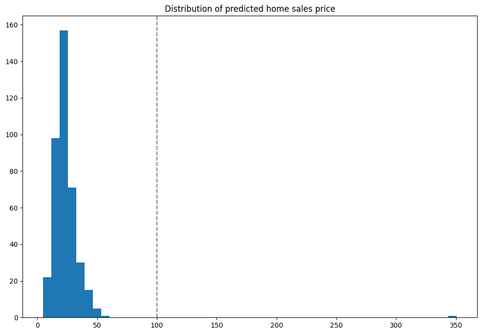
How To Check For Anomalies
There are two primary methods for detecting anomalies with Wallaroo:
- As demonstrated in the example above, from the
InferenceObjectcheck_failuresarray in the output of each inference to see if anything has happened. - The other method is to view pipeline’s logs and see what anomalies have been detected.
View Logs
Anomalies can be displayed through the pipeline logs() method.
For Arrow enabled Wallaroo instances, the logs are returned as a dataframe. Filtering by the column check_failures greater than 0 displays any inferences that had an anomaly triggered.
For Arrow disabled Wallaroo instances, the parameter valid=False will show any validations that were flagged as False - in this case, houses that were above 350 thousand in value.
if arrowEnabled is True:
logs = pipeline.logs()
logs = logs.loc[logs['check_failures'] > 0]
else:
logs = pipeline.logs(valid=False)
display(logs)
Warning: Pipeline log size limit exceeded. Please request logs using export_logs
| time | in.index | in.tensor | out.dense_2 | check_failures | |
|---|---|---|---|---|---|
| 32 | 2023-03-13 19:41:03.596 | tensor | [0.6752651953, -1.4463372267, 0.859222745, -1.3368839439, -0.0866638244, 372.1154780984, -0.2667405624, 0.0057462263, 2.3087968204, -0.6285378876, -0.5584151415, -0.0835430586, -0.6560503236, -1.4648287574, -0.2081778153, 0.2255257157, -0.3033813134] | [39.575085] | 1 |
Undeploy The Pipeline
With the example complete, we undeploy the pipeline to return the resources back to the Wallaroo instance.
pipeline.undeploy()
| name | anomalytestexample |
|---|---|
| created | 2023-03-13 20:18:16.622828+00:00 |
| last_updated | 2023-03-13 20:18:18.995804+00:00 |
| deployed | False |
| tags | |
| versions | dec18ab4-8b71-44c9-a507-c9763803153f, 64246a8b-61a8-4ead-94aa-00f4cf571f74 |
| steps | anomaly-housing-model |
7.3 - House Price Testing Life Cycle
A comprehensive tutorial on different testing and model comparison techniques for house price prediction.
This tutorial and the assets can be downloaded as part of the Wallaroo Tutorials repository.
House Price Testing Life Cycle Comprehensive Tutorial
This tutorial simulates using Wallaroo for testing a model for inference outliers, potential model drift, and methods to test competitive models against each other and deploy the final version to use. This demonstrates using assays to detect model or data drift, then Wallaroo Shadow Deploy to compare different models to determine which one is most fit for an organization’s needs. These features allow organizations to monitor model performance and accuracy then swap out models as needed.
- IMPORTANT NOTE: This tutorial assumes that the House Price Model Life Cycle Preparation notebook was run before this notebook, and that the workspace, pipeline and models used are the same. This is critical for the section on Assays below. If the preparation notebook has not been run, skip the Assays section as there will be no historical data for the assays to function on.
This tutorial will demonstrate how to:
- Select or create a workspace, pipeline and upload the champion model.
- Add a pipeline step with the champion model, then deploy the pipeline and perform sample inferences.
- Create an assay and set a baseline, then demonstrate inferences that trigger the assay alert threshold.
- Swap out the pipeline step with the champion model with a shadow deploy step that compares the champion model against two competitors.
- Evaluate the results of the champion versus competitor models.
- Change the pipeline step from a shadow deploy step to an A/B testing step, and show the different results.
- Change the A/B testing step back to standard pipeline step with the original control model, then demonstrate hot swapping the control model with a challenger model without undeploying the pipeline.
- Undeploy the pipeline.
This tutorial provides the following:
- Models:
models/rf_model.onnx: The champion model that has been used in this environment for some time.models/xgb_model.onnxandmodels/gbr_model.onnx: Rival models that will be tested against the champion.
- Data:
data/xtest-1.df.jsonanddata/xtest-1k.df.json: DataFrame JSON inference inputs with 1 input and 1,000 inputs.data/xtest-1k.arrow: Apache Arrow inference inputs with 1 input and 1,000 inputs.
Prerequisites
- A deployed Wallaroo instance
- The following Python libraries installed:
Initial Steps
Import libraries
The first step is to import the libraries needed for this notebook.
import wallaroo
from wallaroo.object import EntityNotFoundError
from wallaroo.framework import Framework
from IPython.display import display
# used to display DataFrame information without truncating
from IPython.display import display
import pandas as pd
pd.set_option('display.max_colwidth', None)
import datetime
import time
# used for unique connection names
import string
import random
suffix= ''.join(random.choice(string.ascii_lowercase) for i in range(4))
suffix='baselines'
import json
Connect to the Wallaroo Instance
The first step is to connect to Wallaroo through the Wallaroo client. The Python library is included in the Wallaroo install and available through the Jupyter Hub interface provided with your Wallaroo environment.
This is accomplished using the wallaroo.Client() command, which provides a URL to grant the SDK permission to your specific Wallaroo environment. When displayed, enter the URL into a browser and confirm permissions. Store the connection into a variable that can be referenced later.
If logging into the Wallaroo instance through the internal JupyterHub service, use wl = wallaroo.Client(). For more information on Wallaroo Client settings, see the Client Connection guide.
# Login through local Wallaroo instance
wl = wallaroo.Client()
Create Workspace
We will create a workspace to manage our pipeline and models. The following variables will set the name of our sample workspace then set it as the current workspace.
Workspace, pipeline, and model names should be unique to each user, so we’ll add in a randomly generated suffix so multiple people can run this tutorial in a Wallaroo instance without effecting each other.
workspace_name = f'housepricesagaworkspace{suffix}'
main_pipeline_name = f'housepricesagapipeline'
model_name_control = f'housepricesagacontrol'
model_file_name_control = './models/rf_model.onnx'
def get_workspace(name):
workspace = None
for ws in wl.list_workspaces():
if ws.name() == name:
workspace= ws
if(workspace == None):
workspace = wl.create_workspace(name)
return workspace
def get_pipeline(name, workspace):
pipelines = workspace.pipelines()
pipe_filter = filter(lambda x: x.name() == name, pipelines)
pipes = list(pipe_filter)
# we can't have a pipe in the workspace with the same name, so it's always the first
if pipes:
pipeline = pipes[0]
else:
pipeline = wl.build_pipeline(name)
return pipeline
workspace = get_workspace(workspace_name)
wl.set_current_workspace(workspace)
{'name': 'housepricesagaworkspacebaselines', 'id': 87, 'archived': False, 'created_by': 'd6a42dd8-1da9-4405-bb80-7c4b42e38b52', 'created_at': '2023-10-31T16:56:03.395454+00:00', 'models': [], 'pipelines': []}
Upload The Champion Model
For our example, we will upload the champion model that has been trained to derive house prices from a variety of inputs. The model file is rf_model.onnx, and is uploaded with the name housingcontrol.
housing_model_control = (wl.upload_model(model_name_control,
model_file_name_control,
framework=Framework.ONNX)
.configure(tensor_fields=["tensor"])
)
Standard Pipeline Steps
Build the Pipeline
This pipeline is made to be an example of an existing situation where a model is deployed and being used for inferences in a production environment. We’ll call it housepricepipeline, set housingcontrol as a pipeline step, then run a few sample inferences.
This pipeline will be a simple one - just a single pipeline step.
mainpipeline = get_pipeline(main_pipeline_name, workspace)
# clearing from previous runs and verifying it is undeployed
mainpipeline.clear()
mainpipeline.undeploy()
mainpipeline.add_model_step(housing_model_control)
#minimum deployment config
deploy_config = wallaroo.DeploymentConfigBuilder().replica_count(1).cpus(0.5).memory("1Gi").build()
mainpipeline.deploy(deployment_config = deploy_config)
Waiting for deployment - this will take up to 45s ............. ok
| name | housepricesagapipeline |
|---|---|
| created | 2023-10-31 16:56:07.345831+00:00 |
| last_updated | 2023-10-31 16:56:07.444932+00:00 |
| deployed | True |
| tags | |
| versions | 2ea0cc42-c955-4fc3-bac9-7a2c7c22ddc1, dca84ab2-274a-4391-95dd-a99bda7621e1 |
| steps | housepricesagacontrol |
| published | False |
Testing
We’ll use two inferences as a quick sample test - one that has a house that should be determined around $700k, the other with a house determined to be around $1.5 million. We’ll also save the start and end periods for these events to for later log functionality.
normal_input = pd.DataFrame.from_records({"tensor": [[4.0, 2.5, 2900.0, 5505.0, 2.0, 0.0, 0.0, 3.0, 8.0, 2900.0, 0.0, 47.6063, -122.02, 2970.0, 5251.0, 12.0, 0.0, 0.0]]})
result = mainpipeline.infer(normal_input)
display(result)
| time | in.tensor | out.variable | check_failures | |
|---|---|---|---|---|
| 0 | 2023-10-31 16:57:07.307 | [4.0, 2.5, 2900.0, 5505.0, 2.0, 0.0, 0.0, 3.0, 8.0, 2900.0, 0.0, 47.6063, -122.02, 2970.0, 5251.0, 12.0, 0.0, 0.0] | [718013.7] | 0 |
large_house_input = pd.DataFrame.from_records({'tensor': [[4.0, 3.0, 3710.0, 20000.0, 2.0, 0.0, 2.0, 5.0, 10.0, 2760.0, 950.0, 47.6696, -122.261, 3970.0, 20000.0, 79.0, 0.0, 0.0]]})
large_house_result = mainpipeline.infer(large_house_input)
display(large_house_result)
| time | in.tensor | out.variable | check_failures | |
|---|---|---|---|---|
| 0 | 2023-10-31 16:57:07.746 | [4.0, 3.0, 3710.0, 20000.0, 2.0, 0.0, 2.0, 5.0, 10.0, 2760.0, 950.0, 47.6696, -122.261, 3970.0, 20000.0, 79.0, 0.0, 0.0] | [1514079.4] | 0 |
As one last sample, we’ll run through roughly 1,000 inferences at once and show a few of the results. For this example we’ll use an Apache Arrow table, which has a smaller file size compared to uploading a pandas DataFrame JSON file. The inference result is returned as an arrow table, which we’ll convert into a pandas DataFrame to display the first 20 results.
time.sleep(5)
control_model_start = datetime.datetime.now()
batch_inferences = mainpipeline.infer_from_file('./data/xtest-1k.arrow')
large_inference_result = batch_inferences.to_pandas()
display(large_inference_result.head(20))
| time | in.tensor | out.variable | check_failures | |
|---|---|---|---|---|
| 0 | 2023-10-31 16:57:13.771 | [4.0, 2.5, 2900.0, 5505.0, 2.0, 0.0, 0.0, 3.0, 8.0, 2900.0, 0.0, 47.6063, -122.02, 2970.0, 5251.0, 12.0, 0.0, 0.0] | [718013.7] | 0 |
| 1 | 2023-10-31 16:57:13.771 | [2.0, 2.5, 2170.0, 6361.0, 1.0, 0.0, 2.0, 3.0, 8.0, 2170.0, 0.0, 47.7109, -122.017, 2310.0, 7419.0, 6.0, 0.0, 0.0] | [615094.6] | 0 |
| 2 | 2023-10-31 16:57:13.771 | [3.0, 2.5, 1300.0, 812.0, 2.0, 0.0, 0.0, 3.0, 8.0, 880.0, 420.0, 47.5893, -122.317, 1300.0, 824.0, 6.0, 0.0, 0.0] | [448627.8] | 0 |
| 3 | 2023-10-31 16:57:13.771 | [4.0, 2.5, 2500.0, 8540.0, 2.0, 0.0, 0.0, 3.0, 9.0, 2500.0, 0.0, 47.5759, -121.994, 2560.0, 8475.0, 24.0, 0.0, 0.0] | [758714.3] | 0 |
| 4 | 2023-10-31 16:57:13.771 | [3.0, 1.75, 2200.0, 11520.0, 1.0, 0.0, 0.0, 4.0, 7.0, 2200.0, 0.0, 47.7659, -122.341, 1690.0, 8038.0, 62.0, 0.0, 0.0] | [513264.66] | 0 |
| 5 | 2023-10-31 16:57:13.771 | [3.0, 2.0, 2140.0, 4923.0, 1.0, 0.0, 0.0, 4.0, 8.0, 1070.0, 1070.0, 47.6902, -122.339, 1470.0, 4923.0, 86.0, 0.0, 0.0] | [668287.94] | 0 |
| 6 | 2023-10-31 16:57:13.771 | [4.0, 3.5, 3590.0, 5334.0, 2.0, 0.0, 2.0, 3.0, 9.0, 3140.0, 450.0, 47.6763, -122.267, 2100.0, 6250.0, 9.0, 0.0, 0.0] | [1004846.56] | 0 |
| 7 | 2023-10-31 16:57:13.771 | [3.0, 2.0, 1280.0, 960.0, 2.0, 0.0, 0.0, 3.0, 9.0, 1040.0, 240.0, 47.602, -122.311, 1280.0, 1173.0, 0.0, 0.0, 0.0] | [684577.25] | 0 |
| 8 | 2023-10-31 16:57:13.771 | [4.0, 2.5, 2820.0, 15000.0, 2.0, 0.0, 0.0, 4.0, 9.0, 2820.0, 0.0, 47.7255, -122.101, 2440.0, 15000.0, 29.0, 0.0, 0.0] | [727898.25] | 0 |
| 9 | 2023-10-31 16:57:13.771 | [3.0, 2.25, 1790.0, 11393.0, 1.0, 0.0, 0.0, 3.0, 8.0, 1790.0, 0.0, 47.6297, -122.099, 2290.0, 11894.0, 36.0, 0.0, 0.0] | [559631.06] | 0 |
| 10 | 2023-10-31 16:57:13.771 | [3.0, 1.5, 1010.0, 7683.0, 1.5, 0.0, 0.0, 5.0, 7.0, 1010.0, 0.0, 47.72, -122.318, 1550.0, 7271.0, 61.0, 0.0, 0.0] | [340764.53] | 0 |
| 11 | 2023-10-31 16:57:13.771 | [3.0, 2.0, 1270.0, 1323.0, 3.0, 0.0, 0.0, 3.0, 8.0, 1270.0, 0.0, 47.6934, -122.342, 1330.0, 1323.0, 8.0, 0.0, 0.0] | [442168.12] | 0 |
| 12 | 2023-10-31 16:57:13.771 | [4.0, 1.75, 2070.0, 9120.0, 1.0, 0.0, 0.0, 4.0, 7.0, 1250.0, 820.0, 47.6045, -122.123, 1650.0, 8400.0, 57.0, 0.0, 0.0] | [630865.5] | 0 |
| 13 | 2023-10-31 16:57:13.771 | [4.0, 1.0, 1620.0, 4080.0, 1.5, 0.0, 0.0, 3.0, 7.0, 1620.0, 0.0, 47.6696, -122.324, 1760.0, 4080.0, 91.0, 0.0, 0.0] | [559631.06] | 0 |
| 14 | 2023-10-31 16:57:13.771 | [4.0, 3.25, 3990.0, 9786.0, 2.0, 0.0, 0.0, 3.0, 9.0, 3990.0, 0.0, 47.6784, -122.026, 3920.0, 8200.0, 10.0, 0.0, 0.0] | [909441.25] | 0 |
| 15 | 2023-10-31 16:57:13.771 | [4.0, 2.0, 1780.0, 19843.0, 1.0, 0.0, 0.0, 3.0, 7.0, 1780.0, 0.0, 47.4414, -122.154, 2210.0, 13500.0, 52.0, 0.0, 0.0] | [313096.0] | 0 |
| 16 | 2023-10-31 16:57:13.771 | [4.0, 2.5, 2130.0, 6003.0, 2.0, 0.0, 0.0, 3.0, 8.0, 2130.0, 0.0, 47.4518, -122.12, 1940.0, 4529.0, 11.0, 0.0, 0.0] | [404040.78] | 0 |
| 17 | 2023-10-31 16:57:13.771 | [3.0, 1.75, 1660.0, 10440.0, 1.0, 0.0, 0.0, 3.0, 7.0, 1040.0, 620.0, 47.4448, -121.77, 1240.0, 10380.0, 36.0, 0.0, 0.0] | [292859.44] | 0 |
| 18 | 2023-10-31 16:57:13.771 | [3.0, 2.5, 2110.0, 4118.0, 2.0, 0.0, 0.0, 3.0, 8.0, 2110.0, 0.0, 47.3878, -122.153, 2110.0, 4044.0, 25.0, 0.0, 0.0] | [338357.88] | 0 |
| 19 | 2023-10-31 16:57:13.771 | [4.0, 2.25, 2200.0, 11250.0, 1.5, 0.0, 0.0, 5.0, 7.0, 1300.0, 900.0, 47.6845, -122.201, 2320.0, 10814.0, 94.0, 0.0, 0.0] | [682284.56] | 0 |
Graph of Prices
Here’s a distribution plot of the inferences to view the values, with the X axis being the house price in millions, and the Y axis the number of houses fitting in a bin grouping. The majority of houses are in the $250,000 to $500,000 range, with some outliers in the far end.
import matplotlib.pyplot as plt
houseprices = pd.DataFrame({'sell_price': large_inference_result['out.variable'].apply(lambda x: x[0])})
houseprices.hist(column='sell_price', bins=75, grid=False, figsize=(12,8))
plt.axvline(x=0, color='gray', ls='--')
_ = plt.title('Distribution of predicted home sales price')
time.sleep(5)
control_model_end = datetime.datetime.now()
Pipeline Logs
Pipeline logs with standard pipeline steps are retrieved either with:
- Pipeline
logswhich returns either a pandas DataFrame or Apache Arrow table. - Pipeline
export_logswhich saves the logs either a pandas DataFrame JSON file or Apache Arrow table.
For full details, see the Wallaroo Documentation Pipeline Log Management guide.
Pipeline Log Methods
The Pipeline logs method accepts the following parameters.
| Parameter | Type | Description |
|---|---|---|
limit | Int (Optional) | Limits how many log records to display. Defaults to 100. If there are more pipeline logs than are being displayed, the Warning message Pipeline log record limit exceeded will be displayed. For example, if 100 log files were requested and there are a total of 1,000, the warning message will be displayed. |
start_datetimert and end_datetime | DateTime (Optional) | Limits logs to all logs between the start_datetime and end_datetime DateTime parameters. Both parameters must be provided. Submitting a logs() request with only start_datetime or end_datetime will generate an exception.If start_datetime and end_datetime are provided as parameters, then the records are returned in chronological order, with the oldest record displayed first. |
arrow | Boolean (Optional) | Defaults to False. If arrow is set to True, then the logs are returned as an Apache Arrow table. If arrow=False, then the logs are returned as a pandas DataFrame. |
The following examples demonstrate displaying the logs, then displaying the logs between the control_model_start and control_model_end periods, then again retrieved as an Arrow table.
# pipeline log retrieval - reverse chronological order
display(mainpipeline.logs())
# pipeline log retrieval between two dates - chronological order
display(mainpipeline.logs(start_datetime=control_model_start, end_datetime=control_model_end))
# pipeline log retrieval limited to the last 5 an an arrow table
display(mainpipeline.logs(arrow=True))
Warning: There are more logs available. Please set a larger limit or request a file using export_logs.
| time | in.tensor | out.variable | check_failures | |
|---|---|---|---|---|
| 0 | 2023-10-31 16:57:13.771 | [3.0, 2.0, 2005.0, 7000.0, 1.0, 0.0, 0.0, 3.0, 7.0, 1605.0, 400.0, 47.6039, -122.298, 1750.0, 4500.0, 34.0, 0.0, 0.0] | [581002.94] | 0 |
| 1 | 2023-10-31 16:57:13.771 | [3.0, 1.75, 2910.0, 37461.0, 1.0, 0.0, 0.0, 4.0, 7.0, 1530.0, 1380.0, 47.7015, -122.164, 2520.0, 18295.0, 47.0, 0.0, 0.0] | [706823.6] | 0 |
| 2 | 2023-10-31 16:57:13.771 | [4.0, 3.25, 2910.0, 1880.0, 2.0, 0.0, 3.0, 5.0, 9.0, 1830.0, 1080.0, 47.616, -122.282, 3100.0, 8200.0, 100.0, 0.0, 0.0] | [1060847.5] | 0 |
| 3 | 2023-10-31 16:57:13.771 | [4.0, 1.75, 2700.0, 7875.0, 1.5, 0.0, 0.0, 4.0, 8.0, 2700.0, 0.0, 47.454, -122.144, 2220.0, 7875.0, 46.0, 0.0, 0.0] | [441960.3] | 0 |
| 4 | 2023-10-31 16:57:13.771 | [3.0, 2.5, 2900.0, 23550.0, 1.0, 0.0, 0.0, 3.0, 10.0, 1490.0, 1410.0, 47.5708, -122.153, 2900.0, 19604.0, 27.0, 0.0, 0.0] | [827411.25] | 0 |
| ... | ... | ... | ... | ... |
| 95 | 2023-10-31 16:57:13.771 | [2.0, 1.5, 1070.0, 1236.0, 2.0, 0.0, 0.0, 3.0, 8.0, 1000.0, 70.0, 47.5619, -122.382, 1170.0, 1888.0, 10.0, 0.0, 0.0] | [435628.72] | 0 |
| 96 | 2023-10-31 16:57:13.771 | [3.0, 2.5, 2830.0, 6000.0, 1.0, 0.0, 3.0, 3.0, 9.0, 1730.0, 1100.0, 47.5751, -122.378, 2040.0, 5300.0, 60.0, 0.0, 0.0] | [981676.7] | 0 |
| 97 | 2023-10-31 16:57:13.771 | [4.0, 1.75, 1720.0, 8750.0, 1.0, 0.0, 0.0, 3.0, 7.0, 860.0, 860.0, 47.726, -122.21, 1790.0, 8750.0, 43.0, 0.0, 0.0] | [437177.97] | 0 |
| 98 | 2023-10-31 16:57:13.771 | [4.0, 2.25, 4470.0, 60373.0, 2.0, 0.0, 0.0, 3.0, 11.0, 4470.0, 0.0, 47.7289, -122.127, 3210.0, 40450.0, 26.0, 0.0, 0.0] | [1208638.1] | 0 |
| 99 | 2023-10-31 16:57:13.771 | [3.0, 1.0, 1150.0, 3000.0, 1.0, 0.0, 0.0, 5.0, 6.0, 1150.0, 0.0, 47.6867, -122.345, 1460.0, 3200.0, 108.0, 0.0, 0.0] | [448627.8] | 0 |
100 rows × 4 columns
Warning: Pipeline log size limit exceeded. Please request logs using export_logs
| time | in.tensor | out.variable | check_failures | |
|---|---|---|---|---|
| 0 | 2023-10-31 16:57:13.771 | [4.0, 2.5, 2900.0, 5505.0, 2.0, 0.0, 0.0, 3.0, 8.0, 2900.0, 0.0, 47.6063, -122.02, 2970.0, 5251.0, 12.0, 0.0, 0.0] | [718013.7] | 0 |
| 1 | 2023-10-31 16:57:13.771 | [2.0, 2.5, 2170.0, 6361.0, 1.0, 0.0, 2.0, 3.0, 8.0, 2170.0, 0.0, 47.7109, -122.017, 2310.0, 7419.0, 6.0, 0.0, 0.0] | [615094.6] | 0 |
| 2 | 2023-10-31 16:57:13.771 | [3.0, 2.5, 1300.0, 812.0, 2.0, 0.0, 0.0, 3.0, 8.0, 880.0, 420.0, 47.5893, -122.317, 1300.0, 824.0, 6.0, 0.0, 0.0] | [448627.8] | 0 |
| 3 | 2023-10-31 16:57:13.771 | [4.0, 2.5, 2500.0, 8540.0, 2.0, 0.0, 0.0, 3.0, 9.0, 2500.0, 0.0, 47.5759, -121.994, 2560.0, 8475.0, 24.0, 0.0, 0.0] | [758714.3] | 0 |
| 4 | 2023-10-31 16:57:13.771 | [3.0, 1.75, 2200.0, 11520.0, 1.0, 0.0, 0.0, 4.0, 7.0, 2200.0, 0.0, 47.7659, -122.341, 1690.0, 8038.0, 62.0, 0.0, 0.0] | [513264.66] | 0 |
| ... | ... | ... | ... | ... |
| 495 | 2023-10-31 16:57:13.771 | [4.0, 2.5, 3550.0, 35689.0, 2.0, 0.0, 0.0, 4.0, 9.0, 3550.0, 0.0, 47.7503, -122.074, 3350.0, 35711.0, 23.0, 0.0, 0.0] | [873315.2] | 0 |
| 496 | 2023-10-31 16:57:13.771 | [4.0, 2.5, 2510.0, 47044.0, 2.0, 0.0, 0.0, 3.0, 9.0, 2510.0, 0.0, 47.7699, -122.085, 2600.0, 42612.0, 27.0, 0.0, 0.0] | [721143.6] | 0 |
| 497 | 2023-10-31 16:57:13.771 | [4.0, 2.5, 4090.0, 11225.0, 2.0, 0.0, 0.0, 3.0, 10.0, 4090.0, 0.0, 47.581, -121.971, 3510.0, 8762.0, 9.0, 0.0, 0.0] | [1048372.44] | 0 |
| 498 | 2023-10-31 16:57:13.771 | [2.0, 1.0, 720.0, 5000.0, 1.0, 0.0, 0.0, 5.0, 6.0, 720.0, 0.0, 47.5195, -122.374, 810.0, 5000.0, 63.0, 0.0, 0.0] | [244566.39] | 0 |
| 499 | 2023-10-31 16:57:13.771 | [4.0, 2.75, 2930.0, 22000.0, 1.0, 0.0, 3.0, 4.0, 9.0, 1580.0, 1350.0, 47.3227, -122.384, 2930.0, 9758.0, 36.0, 0.0, 0.0] | [518869.03] | 0 |
500 rows × 4 columns
Warning: There are more logs available. Please set a larger limit or request a file using export_logs.
pyarrow.Table
time: timestamp[ms]
in.tensor: list<item: float> not null
child 0, item: float
out.variable: list<inner: float not null> not null
child 0, inner: float not null
check_failures: int8
----
time: [[2023-10-31 16:57:13.771,2023-10-31 16:57:13.771,2023-10-31 16:57:13.771,2023-10-31 16:57:13.771,2023-10-31 16:57:13.771,...,2023-10-31 16:57:13.771,2023-10-31 16:57:13.771,2023-10-31 16:57:13.771,2023-10-31 16:57:13.771,2023-10-31 16:57:13.771]]
in.tensor: [[[3,2,2005,7000,1,...,1750,4500,34,0,0],[3,1.75,2910,37461,1,...,2520,18295,47,0,0],...,[4,2.25,4470,60373,2,...,3210,40450,26,0,0],[3,1,1150,3000,1,...,1460,3200,108,0,0]]]
out.variable: [[[581002.94],[706823.6],...,[1208638.1],[448627.8]]]
check_failures: [[0,0,0,0,0,...,0,0,0,0,0]]
Anomaly Detection through Validations
Anomaly detection allows organizations to set validation parameters in a pipeline. A validation is added to a pipeline to test data based on an expression, and flag any inferences where the validation failed inference result and the pipeline logs.
Validations are added through the Pipeline add_validation(name, validation) command which uses the following parameters:
| Parameter | Type | Description |
|---|---|---|
| name | String (Required) | The name of the validation. |
| Validation | Expression (Required) | The validation test command in the format model_name.outputs][field][index] {Operation} {Value}. |
For this example, we want to detect the outputs of housing_model_control and validate that values are less than 1,500,000. Any outputs greater than that will trigger a check_failure which is shown in the output.
## Add the validation to the pipeline
mainpipeline = mainpipeline.add_validation('price too high', housing_model_control.outputs[0][0] < 1500000.0)
#minimum deployment config
deploy_config = wallaroo.DeploymentConfigBuilder().replica_count(1).cpus(0.5).memory("1Gi").build()
mainpipeline.deploy(deployment_config = deploy_config)
ok
| name | housepricesagapipeline |
|---|---|
| created | 2023-10-31 16:56:07.345831+00:00 |
| last_updated | 2023-10-31 16:57:24.026392+00:00 |
| deployed | True |
| tags | |
| versions | f7e0deaf-63a2-491a-8ff9-e8148d3cabcb, 2ea0cc42-c955-4fc3-bac9-7a2c7c22ddc1, dca84ab2-274a-4391-95dd-a99bda7621e1 |
| steps | housepricesagacontrol |
| published | False |
Validation Testing
Two validations will be tested:
- One that should return a house value lower than 1,500,000. The validation will pass so
check_failurewill be 0. - The other than should return a house value greater than 1,500,000. The validation will fail, so
check_failurewill be 1.
validation_start = datetime.datetime.now()
# Small value home
normal_input = pd.DataFrame.from_records({
"tensor": [[
3.0,
2.25,
1620.0,
997.0,
2.5,
0.0,
0.0,
3.0,
8.0,
1540.0,
80.0,
47.5400009155,
-122.0260009766,
1620.0,
1068.0,
4.0,
0.0,
0.0
]]
}
)
small_result = mainpipeline.infer(normal_input)
display(small_result.loc[:,["time", "out.variable", "check_failures"]])
| time | out.variable | check_failures | |
|---|---|---|---|
| 0 | 2023-10-31 16:57:26.205 | [544392.06] | 0 |
# Big value home
big_input = pd.DataFrame.from_records({
"tensor": [[
4.0,
4.5,
5770.0,
10050.0,
1.0,
0.0,
3.0,
5.0,
9.0,
3160.0,
2610.0,
47.6769981384,
-122.2750015259,
2950.0,
6700.0,
65.0,
0.0,
0.0
]]
}
)
big_result = mainpipeline.infer(big_input)
display(big_result.loc[:,["time", "out.variable", "check_failures"]])
| time | out.variable | check_failures | |
|---|---|---|---|
| 0 | 2023-10-31 16:57:27.138 | [1689843.1] | 1 |
Anomaly Results
We’ll run through our previous batch, this time showing only those results outside of the validation, and a graph showing where the anomalies are against the other results.
batch_inferences = mainpipeline.infer_from_file('./data/xtest-1k.arrow')
large_inference_result = batch_inferences.to_pandas()
# Display only the anomalous results
display(large_inference_result[large_inference_result["check_failures"] > 0].loc[:,["time", "out.variable", "check_failures"]])
| time | out.variable | check_failures | |
|---|---|---|---|
| 30 | 2023-10-31 16:57:28.974 | [1514079.4] | 1 |
| 248 | 2023-10-31 16:57:28.974 | [1967344.1] | 1 |
| 255 | 2023-10-31 16:57:28.974 | [2002393.6] | 1 |
| 556 | 2023-10-31 16:57:28.974 | [1886959.2] | 1 |
| 698 | 2023-10-31 16:57:28.974 | [1689843.1] | 1 |
| 711 | 2023-10-31 16:57:28.974 | [1946437.8] | 1 |
| 722 | 2023-10-31 16:57:28.974 | [2005883.1] | 1 |
| 782 | 2023-10-31 16:57:28.974 | [1910824.0] | 1 |
| 965 | 2023-10-31 16:57:28.974 | [2016006.1] | 1 |
import matplotlib.pyplot as plt
houseprices = pd.DataFrame({'sell_price': large_inference_result['out.variable'].apply(lambda x: x[0])})
houseprices.hist(column='sell_price', bins=75, grid=False, figsize=(12,8))
plt.axvline(x=1500000, color='red', ls='--')
_ = plt.title('Distribution of predicted home sales price')
Assays
Wallaroo assays provide a method for detecting input or model drift. These can be triggered either when unexpected input is provided for the inference, or when the model needs to be retrained from changing environment conditions.
Wallaroo assays can track either an input field and its index, or an output field and its index. For full details, see the Wallaroo Assays Management Guide.
For this example, we will:
- Perform sample inferences based on lower priced houses.
- Create an assay with the baseline set off those lower priced houses.
- Generate inferences spread across all house values, plus specific set of high priced houses to trigger the assay alert.
- Run an interactive assay to show the detection of values outside the established baseline.
Assay Generation
To start the demonstration, we’ll create a baseline of values from houses with small estimated prices and set that as our baseline. Assays are typically run on a 24 hours interval based on a 24 hour window of data, but we’ll bypass that by setting our baseline time even shorter.
small_houses_inputs = pd.read_json('./data/smallinputs.df.json')
baseline_size = 500
# Where the baseline data will start
baseline_start = datetime.datetime.now()
# These inputs will be random samples of small priced houses. Around 30,000 is a good number
small_houses = small_houses_inputs.sample(baseline_size, replace=True).reset_index(drop=True)
small_results = mainpipeline.infer(small_houses)
# Set the baseline end
baseline_end = datetime.datetime.now()
# turn the inference results into a numpy array for the baseline
# set the results to a non-array value
small_results_baseline_df = small_results.copy()
small_results_baseline_df['variable']=small_results['out.variable'].map(lambda x: x[0])
# get the numpy values
small_results_baseline = small_results_baseline_df['variable'].to_numpy()
assay_baseline_from_numpy_name = "house price saga assay from numpy"
# assay builder by baseline
assay_builder_from_numpy = wl.build_assay(assay_name=assay_baseline_from_numpy_name,
pipeline=mainpipeline,
model_name=model_name_control,
iopath="output variable 0",
baseline_data = small_results_baseline)
# set the width from the recent results
assay_builder_from_numpy.window_builder().add_width(minutes=1)
assay_config_from_numpy = assay_builder_from_numpy.build()
assay_analysis_from_numpy = assay_config_from_numpy.interactive_run()
# get the histogram from the numpy baseline
assay_builder_from_numpy.baseline_histogram()
# show the baseline stats
assay_analysis_from_numpy[0].baseline_stats()
| Baseline | |
|---|---|
| count | 500 |
| min | 236238.67 |
| max | 1489624.3 |
| mean | 513762.85694 |
| median | 448627.8 |
| std | 235726.284713 |
| start | None |
| end | None |
Now we’ll perform some inferences with a spread of values, then a larger set with a set of larger house values to trigger our assay alert.
Because our assay windows are 1 minutes, we’ll need to stagger our inference values to be set into the proper windows. This will take about 4 minutes.
By default, assay start date is set to 24 hours from when the assay was created. For this example, we will set the assay.window_builder.add_start to set the assay window to start at the beginning of our data, and assay.add_run_until to set the time period to stop gathering data from.
# Get a spread of house values
time.sleep(35)
# regular_houses_inputs = pd.read_json('./data/xtest-1k.df.json', orient="records")
inference_size = 1000
# regular_houses = regular_houses_inputs.sample(inference_size, replace=True).reset_index(drop=True)
# And a spread of large house values
big_houses_inputs = pd.read_json('./data/biginputs.df.json', orient="records")
big_houses = big_houses_inputs.sample(inference_size, replace=True).reset_index(drop=True)
# Set the start for our assay window period.
assay_window_start = datetime.datetime.now()
mainpipeline.infer(big_houses)
# End our assay window period
time.sleep(35)
assay_window_end = datetime.datetime.now()
assay_builder_from_numpy.add_run_until(assay_window_end)
assay_builder_from_numpy.window_builder().add_width(minutes=1).add_interval(minutes=1).add_start(assay_window_start)
assay_config_from_dates = assay_builder_from_numpy.build()
assay_analysis_from_numpy = assay_config_from_numpy.interactive_run()
# Show how many assay windows were analyzed, then show the chart
print(f"Generated {len(assay_analysis_from_numpy)} analyses")
assay_analysis_from_numpy.chart_scores()
Generated 5 analyses
# Display the results as a DataFrame - we're mainly interested in the score and whether the
# alert threshold was triggered
display(assay_analysis_from_numpy.to_dataframe().loc[:, ["score", "start", "alert_threshold", "status"]])
| score | start | alert_threshold | status | |
|---|---|---|---|---|
| 0 | 0.016079 | 2023-10-31T16:56:21.399000+00:00 | 0.25 | Ok |
| 1 | 0.006042 | 2023-10-31T16:57:21.399000+00:00 | 0.25 | Ok |
| 2 | 8.868832 | 2023-10-31T16:58:21.399000+00:00 | 0.25 | Alert |
| 3 | 8.868832 | 2023-10-31T16:59:21.399000+00:00 | 0.25 | Alert |
| 4 | 8.868832 | 2023-10-31T17:00:21.399000+00:00 | 0.25 | Alert |
assay_builder_from_numpy.upload()
18
The assay is now visible through the Wallaroo UI by selecting the workspace, then the pipeline, then Insights.
Shadow Deploy
Let’s assume that after analyzing the assay information we want to test two challenger models to our control. We do that with the Shadow Deploy pipeline step.
In Shadow Deploy, the pipeline step is added with the add_shadow_deploy method, with the champion model listed first, then an array of challenger models after. All inference data is fed to all models, with the champion results displayed in the out.variable column, and the shadow results in the format out_{model name}.variable. For example, since we named our challenger models housingchallenger01 and housingchallenger02, the columns out_housingchallenger01.variable and out_housingchallenger02.variable have the shadow deployed model results.
For this example, we will remove the previous pipeline step, then replace it with a shadow deploy step with rf_model.onnx as our champion, and models xgb_model.onnx and gbr_model.onnx as the challengers. We’ll deploy the pipeline and prepare it for sample inferences.
# Upload the challenger models
model_name_challenger01 = 'housingchallenger01'
model_file_name_challenger01 = './models/xgb_model.onnx'
model_name_challenger02 = 'housingchallenger02'
model_file_name_challenger02 = './models/gbr_model.onnx'
housing_model_challenger01 = (wl.upload_model(model_name_challenger01,
model_file_name_challenger01,
framework=Framework.ONNX)
.configure(tensor_fields=["tensor"])
)
housing_model_challenger02 = (wl.upload_model(model_name_challenger02,
model_file_name_challenger02,
framework=Framework.ONNX)
.configure(tensor_fields=["tensor"])
)
# Undeploy the pipeline
mainpipeline.undeploy()
mainpipeline.clear()
# Add the new shadow deploy step with our challenger models
mainpipeline.add_shadow_deploy(housing_model_control, [housing_model_challenger01, housing_model_challenger02])
# Deploy the pipeline with the new shadow step
#minimum deployment config
deploy_config = wallaroo.DeploymentConfigBuilder().replica_count(1).cpus(0.5).memory("1Gi").build()
mainpipeline.deploy(deployment_config = deploy_config)
Waiting for undeployment - this will take up to 45s ................................... ok
Waiting for deployment - this will take up to 45s ................................. ok
| name | housepricesagapipeline |
|---|---|
| created | 2023-10-31 16:56:07.345831+00:00 |
| last_updated | 2023-10-31 17:04:57.709641+00:00 |
| deployed | True |
| tags | |
| versions | 44d28e3e-094f-4507-8aa1-909c1f151dd5, b9f46ba3-3f14-4e5b-989e-e0b8d166392f, f7e0deaf-63a2-491a-8ff9-e8148d3cabcb, 2ea0cc42-c955-4fc3-bac9-7a2c7c22ddc1, dca84ab2-274a-4391-95dd-a99bda7621e1 |
| steps | housepricesagacontrol |
| published | False |
Shadow Deploy Sample Inference
We’ll now use our same sample data for an inference to our shadow deployed pipeline, then display the first 20 results with just the comparative outputs.
shadow_result = mainpipeline.infer_from_file('./data/xtest-1k.arrow')
shadow_outputs = shadow_result.to_pandas()
display(shadow_outputs.loc[0:20,['out.variable','out_housingchallenger01.variable','out_housingchallenger02.variable']])
| out.variable | out_housingchallenger01.variable | out_housingchallenger02.variable | |
|---|---|---|---|
| 0 | [718013.7] | [659806.0] | [704901.9] |
| 1 | [615094.6] | [732883.5] | [695994.44] |
| 2 | [448627.8] | [419508.84] | [416164.8] |
| 3 | [758714.3] | [634028.75] | [655277.2] |
| 4 | [513264.66] | [427209.47] | [426854.66] |
| 5 | [668287.94] | [615501.9] | [632556.06] |
| 6 | [1004846.56] | [1139732.4] | [1100465.2] |
| 7 | [684577.25] | [498328.88] | [528278.06] |
| 8 | [727898.25] | [722664.4] | [659439.94] |
| 9 | [559631.06] | [525746.44] | [534331.44] |
| 10 | [340764.53] | [376337.06] | [377187.2] |
| 11 | [442168.12] | [382053.12] | [403964.3] |
| 12 | [630865.5] | [505608.97] | [528991.3] |
| 13 | [559631.06] | [603260.5] | [612201.75] |
| 14 | [909441.25] | [969585.44] | [893874.7] |
| 15 | [313096.0] | [313633.7] | [318054.94] |
| 16 | [404040.78] | [360413.62] | [357816.7] |
| 17 | [292859.44] | [316674.88] | [294034.62] |
| 18 | [338357.88] | [299907.47] | [323254.28] |
| 19 | [682284.56] | [811896.75] | [770916.6] |
| 20 | [583765.94] | [573618.5] | [549141.4] |
A/B Testing
A/B Testing is another method of comparing and testing models. Like shadow deploy, multiple models are compared against the champion or control models. The difference is that instead of submitting the inference data to all models, then tracking the outputs of all of the models, the inference inputs are off of a ratio and other conditions.
For this example, we’ll be using a 1:1:1 ratio with a random split between the champion model and the two challenger models. Each time an inference request is made, there is a random equal chance of any one of them being selected.
When the inference results and log entries are displayed, they include the column out._model_split which displays:
| Field | Type | Description |
|---|---|---|
name | String | The model name used for the inference. |
version | String | The version of the model. |
sha | String | The sha hash of the model version. |
This is used to determine which model was used for the inference request.
# remove the shadow deploy steps
mainpipeline.clear()
# Add the a/b test step to the pipeline
mainpipeline.add_random_split([(1, housing_model_control), (1, housing_model_challenger01), (1, housing_model_challenger02)], "session_id")
mainpipeline.deploy()
# Perform sample inferences of 20 rows and display the results
ab_date_start = datetime.datetime.now()
abtesting_inputs = pd.read_json('./data/xtest-1k.df.json')
df = pd.DataFrame(columns=["model", "value"])
for index, row in abtesting_inputs.sample(20).iterrows():
result = mainpipeline.infer(row.to_frame('tensor').reset_index())
value = result.loc[0]["out.variable"]
model = json.loads(result.loc[0]["out._model_split"][0])['name']
df = df.append({'model': model, 'value': value}, ignore_index=True)
display(df)
ab_date_end = datetime.datetime.now()
ok
| model | value | |
|---|---|---|
| 0 | housingchallenger01 | [278554.44] |
| 1 | housingchallenger02 | [615955.3] |
| 2 | housepricesagacontrol | [1092273.9] |
| 3 | housepricesagacontrol | [683845.75] |
| 4 | housepricesagacontrol | [682284.56] |
| 5 | housepricesagacontrol | [247792.75] |
| 6 | housingchallenger02 | [315142.44] |
| 7 | housingchallenger02 | [530408.94] |
| 8 | housepricesagacontrol | [340764.53] |
| 9 | housepricesagacontrol | [421153.16] |
| 10 | housingchallenger01 | [395150.63] |
| 11 | housingchallenger02 | [544343.3] |
| 12 | housingchallenger01 | [395284.4] |
| 13 | housepricesagacontrol | [701940.7] |
| 14 | housepricesagacontrol | [448627.8] |
| 15 | housepricesagacontrol | [320863.72] |
| 16 | housingchallenger01 | [558485.3] |
| 17 | housingchallenger02 | [236329.28] |
| 18 | housepricesagacontrol | [559631.06] |
| 19 | housingchallenger01 | [281437.56] |
Model Swap
Now that we’ve completed our testing, we can swap our deployed model in the original housepricingpipeline with one we feel works better.
We’ll start by removing the A/B Testing pipeline step, then going back to the single pipeline step with the champion model and perform a test inference.
When going from a testing step such as A/B Testing or Shadow Deploy, it is best to undeploy the pipeline, change the steps, then deploy the pipeline. In a production environment, there should be two pipelines: One for production, the other for testing models. Since this example uses one pipeline for simplicity, we will undeploy our main pipeline and reset it back to a one-step pipeline with the current champion model as our pipeline step.
Once done, we’ll perform the hot swap with the model gbr_model.onnx, which was labeled housing_model_challenger02 in a previous step. We’ll do an inference with the same data as used with the challenger model. Note that previously, the inference through the original model returned [718013.7].
mainpipeline.undeploy()
# remove the shadow deploy steps
mainpipeline.clear()
mainpipeline.add_model_step(housing_model_control).deploy()
# Inference test
normal_input = pd.DataFrame.from_records({"tensor": [[4.0,
2.25,
2200.0,
11250.0,
1.5,
0.0,
0.0,
5.0,
7.0,
1300.0,
900.0,
47.6845,
-122.201,
2320.0,
10814.0,
94.0,
0.0,
0.0]]})
controlresult = mainpipeline.infer(normal_input)
display(controlresult)
ok
Waiting for deployment - this will take up to 45s ........ ok
| time | in.tensor | out.variable | check_failures | |
|---|---|---|---|---|
| 0 | 2023-10-31 17:08:19.579 | [4.0, 2.25, 2200.0, 11250.0, 1.5, 0.0, 0.0, 5.0, 7.0, 1300.0, 900.0, 47.6845, -122.201, 2320.0, 10814.0, 94.0, 0.0, 0.0] | [682284.56] | 0 |
Now we’ll “hot swap” the control model. We don’t have to deploy the pipeline - we can just swap the model out in that pipeline step and continue with only a millisecond or two lost while the swap was performed.
# Perform hot swap
mainpipeline.replace_with_model_step(0, housing_model_challenger02).deploy()
# wait a moment for the database to be updated. The swap is near instantaneous but database writes may take a moment
import time
time.sleep(15)
# inference after model swap
normal_input = pd.DataFrame.from_records({"tensor": [[4.0,
2.25,
2200.0,
11250.0,
1.5,
0.0,
0.0,
5.0,
7.0,
1300.0,
900.0,
47.6845,
-122.201,
2320.0,
10814.0,
94.0,
0.0,
0.0]]})
challengerresult = mainpipeline.infer(normal_input)
display(challengerresult)
ok
| time | in.tensor | out.variable | check_failures | |
|---|---|---|---|---|
| 0 | 2023-10-31 17:09:23.932 | [4.0, 2.25, 2200.0, 11250.0, 1.5, 0.0, 0.0, 5.0, 7.0, 1300.0, 900.0, 47.6845, -122.201, 2320.0, 10814.0, 94.0, 0.0, 0.0] | [770916.6] | 0 |
# Display the difference between the two
display(f'Original model output: {controlresult.loc[0]["out.variable"]}')
display(f'Hot swapped model output: {challengerresult.loc[0]["out.variable"]}')
'Original model output: [682284.56]'
‘Hot swapped model output: [770916.6]’
Undeploy Main Pipeline
With the examples and tutorial complete, we will undeploy the main pipeline and return the resources back to the Wallaroo instance.
mainpipeline.undeploy()
Waiting for undeployment - this will take up to 45s ...................................... ok
| name | housepricesagapipeline |
|---|---|
| created | 2023-10-31 16:56:07.345831+00:00 |
| last_updated | 2023-10-31 17:09:08.758964+00:00 |
| deployed | False |
| tags | |
| versions | 51034ba5-b58e-4475-908d-ec8fae069745, cd0f20e9-6923-4e6f-8114-1137676da5c5, 58274aab-0045-4557-a740-7d085af8574d, 4cf4f0dc-2c42-4f8b-975c-1f5c5d939a98, c5ae5a56-1c7f-4a94-9d4e-f08bf35e7f4f, f652a9d8-a4f6-428a-9b36-b29eec6b5198, 0e7d9d77-02d7-4c13-8062-9c77492145f8, 42b97784-fc16-43be-b89e-2d3dad20dd2b, 7d35285a-f8af-4bed-855b-60258c3435ee, 8b0dc4bb-3340-44f9-85d6-fbd091e19412, 06169fed-59e9-41f8-9dbd-0fc9f80ebb73, 44d28e3e-094f-4507-8aa1-909c1f151dd5, b9f46ba3-3f14-4e5b-989e-e0b8d166392f, f7e0deaf-63a2-491a-8ff9-e8148d3cabcb, 2ea0cc42-c955-4fc3-bac9-7a2c7c22ddc1, dca84ab2-274a-4391-95dd-a99bda7621e1 |
| steps | housepricesagacontrol |
| published | False |
7.4 - Shadow Deployment Tutorial
The Shadow Deployment Tutorial demonstrates how to use Wallaroo to deploy challenger models to test the performance against champion models.
This tutorial and the assets can be downloaded as part of the Wallaroo Tutorials repository.
Shadow Deployment Tutorial
Wallaroo provides a method of testing the same data against two different models or sets of models at the same time through shadow deployments otherwise known as parallel deployments. This allows data to be submitted to a pipeline with inferences running on two different sets of models. Typically this is performed on a model that is known to provide accurate results - the champion - and a model that is being tested to see if it provides more accurate or faster responses depending on the criteria known as the challengers. Multiple challengers can be tested against a single champion.
As described in the Wallaroo blog post The What, Why, and How of Model A/B Testing:
In data science, A/B tests can also be used to choose between two models in production, by measuring which model performs better in the real world. In this formulation, the control is often an existing model that is currently in production, sometimes called the champion. The treatment is a new model being considered to replace the old one. This new model is sometimes called the challenger….
Keep in mind that in machine learning, the terms experiments and trials also often refer to the process of finding a training configuration that works best for the problem at hand (this is sometimes called hyperparameter optimization).
When a shadow deployment is created, only the inference from the champion is returned in the InferenceResult Object data, while the result data for the shadow deployments is stored in the InferenceResult Object shadow_data.
The following tutorial will demonstrate how:
- Upload champion and challenger models into a Wallaroo instance.
- Create a shadow deployment in a Wallaroo pipeline.
- Perform an inference through a pipeline with a shadow deployment.
- View the
dataandshadow_dataresults from the InferenceResult Object. - View the pipeline logs and pipeline shadow logs.
This tutorial provides the following:
dev_smoke_test.json: Sample test data used for the inference testing.models/keras_ccfraud.onnx: The champion model.models/modelA.onnx: A challenger model.models/xgboost_ccfraud.onnx: A challenger model.
All models are similar to the ones used for the Wallaroo-101 example included in the Wallaroo Tutorials repository.
Prerequisites
- A deployed Wallaroo instance
- The following Python libraries installed:
Steps
Import libraries
The first step is to import the libraries required.
import wallaroo
from wallaroo.object import EntityNotFoundError
# used to display dataframe information without truncating
from IPython.display import display
import pandas as pd
pd.set_option('display.max_colwidth', None)
Connect to the Wallaroo Instance
The first step is to connect to Wallaroo through the Wallaroo client. The Python library is included in the Wallaroo install and available through the Jupyter Hub interface provided with your Wallaroo environment.
This is accomplished using the wallaroo.Client() command, which provides a URL to grant the SDK permission to your specific Wallaroo environment. When displayed, enter the URL into a browser and confirm permissions. Store the connection into a variable that can be referenced later.
If logging into the Wallaroo instance through the internal JupyterHub service, use wl = wallaroo.Client(). For more information on Wallaroo Client settings, see the Client Connection guide.
# Login through local Wallaroo instance
wl = wallaroo.Client()
Set Variables
The following variables are used to create or use existing workspaces, pipelines, and upload the models. Adjust them based on your Wallaroo instance and organization requirements.
import string
import random
suffix= ''.join(random.choice(string.ascii_lowercase) for i in range(4))
workspace_name = f'ccfraudcomparisondemo{suffix}'
pipeline_name = f'ccshadow{suffix}'
champion_model_name = f'ccfraud-lstm{suffix}'
champion_model_file = 'models/keras_ccfraud.onnx'
shadow_model_01_name = f'ccfraud-xgb{suffix}'
shadow_model_01_file = 'models/xgboost_ccfraud.onnx'
shadow_model_02_name = f'ccfraud-rf{suffix}'
shadow_model_02_file = 'models/modelA.onnx'
Workspace and Pipeline
The following creates or connects to an existing workspace based on the variable workspace_name, and creates or connects to a pipeline based on the variable pipeline_name.
def get_workspace(name):
workspace = None
for ws in wl.list_workspaces():
if ws.name() == name:
workspace= ws
if(workspace == None):
workspace = wl.create_workspace(name)
return workspace
def get_pipeline(name):
try:
pipeline = wl.pipelines_by_name(name)[0]
except EntityNotFoundError:
pipeline = wl.build_pipeline(name)
return pipeline
workspace = get_workspace(workspace_name)
wl.set_current_workspace(workspace)
pipeline = get_pipeline(pipeline_name)
pipeline
| name | ccshadowdmyb |
|---|---|
| created | 2023-10-19 18:50:52.588811+00:00 |
| last_updated | 2023-10-19 18:50:52.588811+00:00 |
| deployed | (none) |
| tags | |
| versions | 2d8f9f90-8ced-4e47-b5a6-e2512aeb9d17 |
| steps | |
| published | False |
Load the Models
The models will be uploaded into the current workspace based on the variable names set earlier and listed as the champion, model2 and model3.
champion = (wl.upload_model(champion_model_name,
champion_model_file,
framework=wallaroo.framework.Framework.ONNX)
.configure(tensor_fields=["tensor"])
)
model2 = (wl.upload_model(shadow_model_01_name,
shadow_model_01_file,
framework=wallaroo.framework.Framework.ONNX)
.configure(tensor_fields=["tensor"])
)
model3 = (wl.upload_model(shadow_model_02_name,
shadow_model_02_file,
framework=wallaroo.framework.Framework.ONNX)
.configure(tensor_fields=["tensor"])
)
Create Shadow Deployment
A shadow deployment is created using the add_shadow_deploy(champion, challengers[]) method where:
champion: The model that will be primarily used for inferences run through the pipeline. Inference results will be returned through the Inference Object’sdataelement.challengers[]: An array of models that will be used for inferences iteratively. Inference results will be returned through the Inference Object’sshadow_dataelement.
pipeline.add_shadow_deploy(champion, [model2, model3])
pipeline.deploy()
| name | ccshadowdmyb |
|---|---|
| created | 2023-10-19 18:50:52.588811+00:00 |
| last_updated | 2023-10-19 18:50:58.268275+00:00 |
| deployed | True |
| tags | |
| versions | 1ae1ebe1-f920-4590-a843-bf8429ece205, 2d8f9f90-8ced-4e47-b5a6-e2512aeb9d17 |
| steps | ccfraud-lstmdmyb |
| published | False |
Run Test Inference
Using the data from sample_data_file, a test inference will be made.
For Arrow enabled Wallaroo instances the model outputs are listed by column. The output data is set by the term out, followed by the name of the model. For the default model, this is out.dense_1, while the shadow deployed models are in the format out_{model name}.variable, where {model name} is the name of the shadow deployed model.
For Arrow disabled environments, the output is from the Wallaroo InferenceResult object.### Run Test Inference
Using the data from sample_data_file, a test inference will be made. As mentioned earlier, the inference results from the champion model will be available in the returned InferenceResult Object’s data element, while inference results from each of the challenger models will be in the returned InferenceResult Object’s shadow_data element.
sample_data_file = './smoke_test.df.json'
response = pipeline.infer_from_file(sample_data_file)
display(response)
| time | in.tensor | out.dense_1 | check_failures | out_ccfraud-rfdmyb.variable | out_ccfraud-xgbdmyb.variable | |
|---|---|---|---|---|---|---|
| 0 | 2023-10-19 18:51:10.396 | [1.0678324729, 0.2177810266, -1.7115145262, 0.682285721, 1.0138553067, -0.4335000013, 0.7395859437, -0.2882839595, -0.447262688, 0.5146124988, 0.3791316964, 0.5190619748, -0.4904593222, 1.1656456469, -0.9776307444, -0.6322198963, -0.6891477694, 0.1783317857, 0.1397992467, -0.3554220649, 0.4394217877, 1.4588397512, -0.3886829615, 0.4353492889, 1.7420053483, -0.4434654615, -0.1515747891, -0.2668451725, -1.4549617756] | [0.0014974177] | 0 | [1.0] | [0.0005066991] |
View Pipeline Logs
With the inferences complete, we can retrieve the log data from the pipeline with the pipeline logs method. Note that for each inference request, the logs return one entry per model. For this example, for one inference request three log entries will be created.
pipeline.logs()
| time | in.tensor | out.dense_1 | check_failures | out_ccfraud-rfdmyb.variable | out_ccfraud-xgbdmyb.variable | |
|---|---|---|---|---|---|---|
| 0 | 2023-10-19 18:51:10.396 | [1.0678324729, 0.2177810266, -1.7115145262, 0.682285721, 1.0138553067, -0.4335000013, 0.7395859437, -0.2882839595, -0.447262688, 0.5146124988, 0.3791316964, 0.5190619748, -0.4904593222, 1.1656456469, -0.9776307444, -0.6322198963, -0.6891477694, 0.1783317857, 0.1397992467, -0.3554220649, 0.4394217877, 1.4588397512, -0.3886829615, 0.4353492889, 1.7420053483, -0.4434654615, -0.1515747891, -0.2668451725, -1.4549617756] | [0.0014974177] | 0 | [1.0] | [0.0005066991] |
View Logs Per Model
Another way of displaying the logs would be to specify the model.
For Arrow enabled Wallaroo instances the model outputs are listed by column. The output data is set by the term out, followed by the name of the model. For the default model, this is out.dense_1, while the shadow deployed models are in the format out_{model name}.variable, where {model name} is the name of the shadow deployed model.
For arrow disabled Wallaroo instances, to view the inputs and results for the shadow deployed models, use the pipeline logs_shadow_deploy() method. The results will be grouped by the inputs.
logs = pipeline.logs()
display(logs)
| time | in.tensor | out.dense_1 | check_failures | out_ccfraud-rfdmyb.variable | out_ccfraud-xgbdmyb.variable | |
|---|---|---|---|---|---|---|
| 0 | 2023-10-19 18:51:10.396 | [1.0678324729, 0.2177810266, -1.7115145262, 0.682285721, 1.0138553067, -0.4335000013, 0.7395859437, -0.2882839595, -0.447262688, 0.5146124988, 0.3791316964, 0.5190619748, -0.4904593222, 1.1656456469, -0.9776307444, -0.6322198963, -0.6891477694, 0.1783317857, 0.1397992467, -0.3554220649, 0.4394217877, 1.4588397512, -0.3886829615, 0.4353492889, 1.7420053483, -0.4434654615, -0.1515747891, -0.2668451725, -1.4549617756] | [0.0014974177] | 0 | [1.0] | [0.0005066991] |
Undeploy the Pipeline
With the tutorial complete, we undeploy the pipeline and return the resources back to the system.
pipeline.undeploy()
| name | ccshadowdmyb |
|---|---|
| created | 2023-10-19 18:50:52.588811+00:00 |
| last_updated | 2023-10-19 18:50:58.268275+00:00 |
| deployed | False |
| tags | |
| versions | 1ae1ebe1-f920-4590-a843-bf8429ece205, 2d8f9f90-8ced-4e47-b5a6-e2512aeb9d17 |
| steps | ccfraud-lstmdmyb |
| published | False |
8 - Using Jupyter Notebooks in Production
How to go from Jupyter Notebooks to Production Systems
Using Jupyter Notebooks in Production
The following tutorials are available from the Wallaroo Tutorials Repository.
The following tutorials provide an example of an organization moving from experimentation to deployment in production using Jupyter Notebooks as the basis for code research and use. For this example, we can assume to main actors performing the following tasks.
| Number | Notebook Sample | Task | Actor | Description |
|---|---|---|---|---|
| 01 | 01_explore_and_train.ipynb | Data Exploration and Model Selection | Data Scientist | The data scientist evaluates the data and determines the best model to use to solve the proposed problems. |
| 02 | 02_automated_training_process.ipynd | Training Process Automation Setup | Data Scientist | The data scientist has selected the model and tested how to train it. In this phase, the data scientist tests automating the training process based on a data store. |
| 03 | 03_deploy_model.ipynb | Deploy the Model in Wallaroo | MLOps Engineer | The MLOps takes the trained model and deploys a Wallaroo pipeline with it to perform inferences on by feeding it data from a data store. |
| 04 | 04_regular_batch_inferences.ipynb | Regular Batch Inference | MLOps Engineer | With the pipeline deployed, regular inferences can be made and the results reported to a data store. |
Each Jupyter Notebook is arranged to demonstrate each step of the process.
Resources
The following resources are provided as part of this tutorial:
- data
data/seattle_housing_col_description.txt: Describes the columns used as part data analysis.data/seattle_housing.csv: Sample data of the Seattle, Washington housing market between 2014 and 2015.
- code
simdb.py: A simulated database to demonstrate sending and receiving queries.preprocess.pyandpostprocess.py: Processes the data into a format the model accepts, and formats the model outputs for database use.
- models
housing_model_xgb.onnx: Model created in Stage 2: Training Process Automation Setup../models/preprocess_byop.zip.: Formats the incoming data for the model../models/postprocess_byop.zip: Formats the outgoing data for the model.
8.1 - Data Exploration And Model Selection
The following tutorials are available from the Wallaroo Tutorials Repository.
Stage 1: Data Exploration And Model Selection
When starting a project, the data scientist focuses on exploration and experimentation, rather than turning the process into an immediate production system. This notebook presents a simplified view of this stage.
Resources
The following resources are used as part of this tutorial:
- data
data/seattle_housing_col_description.txt: Describes the columns used as part data analysis.data/seattle_housing.csv: Sample data of the Seattle, Washington housing market between 2014 and 2015.
- code
postprocess.py: Formats the data after inference by the model is complete.preprocess.py: Formats the incoming data for the model.simdb.py: A simulated database to demonstrate sending and receiving queries.wallaroo_client.py: Additional methods used with the Wallaroo instance to create workspaces, etc.
Steps
The following steps are part of this process:
- Retrieve Training Data: Connect to the data store and retrieve the training data.
- Data Transformations: Evaluate the data and train the model.
- Model Testing: Evaluate different models and determine which is best suited for the problem.
Import Libraries
First we’ll import the libraries we’ll be using to evaluate the data and test different models.
import numpy as np
import pandas as pd
import sklearn
import sklearn.ensemble
import xgboost as xgb
import seaborn
import matplotlib
import matplotlib.pyplot as plt
import simdb # module for the purpose of this demo to simulate pulling data from a database
matplotlib.rcParams["figure.figsize"] = (12,6)
# ignoring warnings for demonstration
import warnings
warnings.filterwarnings('ignore')
Retrieve Training Data
For training, we will use the data on all houses sold in this market with the last two years. As a reminder, this data pulled from a simulated database as an example of how to pull from an existing data store.
Only a few columns will be shown for display purposes.
conn = simdb.simulate_db_connection()
tablename = simdb.tablename
query = f"select * from {tablename} where date > DATE(DATE(), '-24 month') AND sale_price is not NULL"
print(query)
# read in the data
housing_data = pd.read_sql_query(query, conn)
conn.close()
housing_data.loc[:, ["id", "date", "list_price", "bedrooms", "bathrooms", "sqft_living", "sqft_lot"]]
select * from house_listings where date > DATE(DATE(), '-24 month') AND sale_price is not NULL
| id | date | list_price | bedrooms | bathrooms | sqft_living | sqft_lot | |
|---|---|---|---|---|---|---|---|
| 0 | 7129300520 | 2023-07-31 | 221900.0 | 3 | 1.00 | 1180 | 5650 |
| 1 | 6414100192 | 2023-09-26 | 538000.0 | 3 | 2.25 | 2570 | 7242 |
| 2 | 5631500400 | 2023-12-13 | 180000.0 | 2 | 1.00 | 770 | 10000 |
| 3 | 2487200875 | 2023-09-26 | 604000.0 | 4 | 3.00 | 1960 | 5000 |
| 4 | 1954400510 | 2023-12-06 | 510000.0 | 3 | 2.00 | 1680 | 8080 |
| ... | ... | ... | ... | ... | ... | ... | ... |
| 20518 | 263000018 | 2023-03-08 | 360000.0 | 3 | 2.50 | 1530 | 1131 |
| 20519 | 6600060120 | 2023-12-11 | 400000.0 | 4 | 2.50 | 2310 | 5813 |
| 20520 | 1523300141 | 2023-04-10 | 402101.0 | 2 | 0.75 | 1020 | 1350 |
| 20521 | 291310100 | 2023-11-03 | 400000.0 | 3 | 2.50 | 1600 | 2388 |
| 20522 | 1523300157 | 2023-08-02 | 325000.0 | 2 | 0.75 | 1020 | 1076 |
20523 rows × 7 columns
Data transformations
To improve relative error performance, we will predict on log10 of the sale price.
Predict on log10 price to try to improve relative error performance
housing_data['logprice'] = np.log10(housing_data.sale_price)
From the data, we will create the following features to evaluate:
house_age: How old the house is.renovated: Whether the house has been renovated or not.yrs_since_reno: If the house has been renovated, how long has it been.
import datetime
thisyear = datetime.datetime.now().year
housing_data['house_age'] = thisyear - housing_data['yr_built']
housing_data['renovated'] = np.where((housing_data['yr_renovated'] > 0), 1, 0)
housing_data['yrs_since_reno'] = np.where(housing_data['renovated'], housing_data['yr_renovated'] - housing_data['yr_built'], 0)
housing_data.loc[:, ['yr_built', 'yr_renovated', 'house_age', 'renovated', 'yrs_since_reno']]
| yr_built | yr_renovated | house_age | renovated | yrs_since_reno | |
|---|---|---|---|---|---|
| 0 | 1955 | 0 | 69 | 0 | 0 |
| 1 | 1951 | 1991 | 73 | 1 | 40 |
| 2 | 1933 | 0 | 91 | 0 | 0 |
| 3 | 1965 | 0 | 59 | 0 | 0 |
| 4 | 1987 | 0 | 37 | 0 | 0 |
| ... | ... | ... | ... | ... | ... |
| 20518 | 2009 | 0 | 15 | 0 | 0 |
| 20519 | 2014 | 0 | 10 | 0 | 0 |
| 20520 | 2009 | 0 | 15 | 0 | 0 |
| 20521 | 2004 | 0 | 20 | 0 | 0 |
| 20522 | 2008 | 0 | 16 | 0 | 0 |
20523 rows × 5 columns
Now we pick variables and split training data into training and holdout (test).
vars = ['bedrooms', 'bathrooms', 'sqft_living', 'sqft_lot', 'floors', 'waterfront', 'view',
'condition', 'grade', 'sqft_above', 'sqft_basement', 'lat', 'long', 'sqft_living15', 'sqft_lot15', 'house_age', 'renovated', 'yrs_since_reno']
outcome = 'logprice'
runif = np.random.default_rng(2206222).uniform(0, 1, housing_data.shape[0])
gp = np.where(runif < 0.2, 'test', 'training')
hd_train = housing_data.loc[gp=='training', :].reset_index(drop=True, inplace=False)
hd_test = housing_data.loc[gp=='test', :].reset_index(drop=True, inplace=False)
# split the training into training and val for xgboost
runif = np.random.default_rng(123).uniform(0, 1, hd_train.shape[0])
xgb_gp = np.where(runif < 0.2, 'val', 'train')
# for xgboost, further split into train and val
train_features = np.array(hd_train.loc[xgb_gp=='train', vars])
train_labels = np.array(hd_train.loc[xgb_gp=='train', outcome])
val_features = np.array(hd_train.loc[xgb_gp=='val', vars])
val_labels = np.array(hd_train.loc[xgb_gp=='val', outcome])
Postprocessing
Since we are fitting a model to predict log10 price, we need to convert predictions back into price units. We also want to round to the nearest dollar.
def postprocess(log10price):
return np.rint(np.power(10, log10price))
Model testing
For the purposes of this demo, let’s say that we require a mean absolute percent error (MAPE) of 15% or less, and the we want to try a few models to decide which model we want to use.
One could also hyperparameter tune at this stage; for brevity, we’ll omit that in this demo.
XGBoost
First we will test out using a XGBoost model.
xgb_model = xgb.XGBRegressor(
objective = 'reg:squarederror',
max_depth=5,
base_score = np.mean(hd_train[outcome])
)
xgb_model.fit(
train_features,
train_labels,
eval_set=[(train_features, train_labels), (val_features, val_labels)],
verbose=False,
early_stopping_rounds=35
)
XGBRegressor(base_score=5.666446833601829, booster=None, callbacks=None,
colsample_bylevel=None, colsample_bynode=None,
colsample_bytree=None, early_stopping_rounds=None,
enable_categorical=False, eval_metric=None, feature_types=None,
gamma=None, gpu_id=None, grow_policy=None, importance_type=None,
interaction_constraints=None, learning_rate=None, max_bin=None,
max_cat_threshold=None, max_cat_to_onehot=None,
max_delta_step=None, max_depth=5, max_leaves=None,
min_child_weight=None, missing=nan, monotone_constraints=None,
n_estimators=100, n_jobs=None, num_parallel_tree=None,
predictor=None, random_state=None, ...)In a Jupyter environment, please rerun this cell to show the HTML representation or trust the notebook.On GitHub, the HTML representation is unable to render, please try loading this page with nbviewer.org.
XGBRegressor(base_score=5.666446833601829, booster=None, callbacks=None,colsample_bylevel=None, colsample_bynode=None, colsample_bytree=None, early_stopping_rounds=None, enable_categorical=False, eval_metric=None, feature_types=None, gamma=None, gpu_id=None, grow_policy=None, importance_type=None, interaction_constraints=None, learning_rate=None, max_bin=None, max_cat_threshold=None, max_cat_to_onehot=None, max_delta_step=None, max_depth=5, max_leaves=None, min_child_weight=None, missing=nan, monotone_constraints=None, n_estimators=100, n_jobs=None, num_parallel_tree=None, predictor=None, random_state=None, ...)</pre>print(xgb_model.best_score) print(xgb_model.best_iteration) print(xgb_model.best_ntree_limit)0.07793614689092423 99 100XGBoost Evaluate on holdout
With the sample model created, we will test it against the holdout data. Note that we are calling the
postprocessfunction on the data.test_features = np.array(hd_test.loc[:, vars]) test_labels = np.array(hd_test.loc[:, outcome]) pframe = pd.DataFrame({ 'pred' : postprocess(xgb_model.predict(test_features)), 'actual' : postprocess(test_labels) }) ax = seaborn.scatterplot( data=pframe, x='pred', y='actual', alpha=0.2 ) matplotlib.pyplot.plot(pframe.pred, pframe.pred, color='DarkGreen') matplotlib.pyplot.title("test") plt.show()pframe['se'] = (pframe.pred - pframe.actual)**2 pframe['pct_err'] = 100*np.abs(pframe.pred - pframe.actual)/pframe.actual pframe.describe()

| pred | actual | se | pct_err | |
|---|---|---|---|---|
| count | 4.094000e+03 | 4.094000e+03 | 4.094000e+03 | 4094.000000 |
| mean | 5.340824e+05 | 5.396937e+05 | 1.657722e+10 | 12.857674 |
| std | 3.413714e+05 | 3.761666e+05 | 1.276017e+11 | 13.512028 |
| min | 1.216140e+05 | 8.200000e+04 | 1.000000e+00 | 0.000500 |
| 25% | 3.167628e+05 | 3.200000e+05 | 3.245312e+08 | 4.252492 |
| 50% | 4.568700e+05 | 4.500000e+05 | 1.602001e+09 | 9.101485 |
| 75% | 6.310372e+05 | 6.355250e+05 | 6.575385e+09 | 17.041227 |
| max | 5.126706e+06 | 7.700000e+06 | 6.637466e+12 | 252.097895 |
rmse = np.sqrt(np.mean(pframe.se))
mape = np.mean(pframe.pct_err)
print(f'rmse = {rmse}, mape = {mape}')
rmse = 128752.54982046234, mape = 12.857674005250548
Random Forest
The next model to test is Random Forest.
model_rf = sklearn.ensemble.RandomForestRegressor(n_estimators=100, max_depth=5, n_jobs=2, max_samples=0.8)
train_features = np.array(hd_train.loc[:, vars])
train_labels = np.array(hd_train.loc[:, outcome])
model_rf.fit(train_features, train_labels)
RandomForestRegressor(max_depth=5, max_samples=0.8, n_jobs=2)In a Jupyter environment, please rerun this cell to show the HTML representation or trust the notebook.
On GitHub, the HTML representation is unable to render, please try loading this page with nbviewer.org.
RandomForestRegressor(max_depth=5, max_samples=0.8, n_jobs=2)
Random Forest Evaluate on holdout
With the Random Forest sample model created, now we can test it against the holdout data.
pframe = pd.DataFrame({
'pred' : postprocess(model_rf.predict(test_features)),
'actual' : postprocess(test_labels)
})
ax = seaborn.scatterplot(
data=pframe,
x='pred',
y='actual',
alpha=0.2
)
matplotlib.pyplot.plot(pframe.pred, pframe.pred, color='DarkGreen')
matplotlib.pyplot.title("random forest")
plt.show()
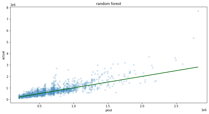
pframe['se'] = (pframe.pred - pframe.actual)**2
pframe['pct_err'] = 100*np.abs(pframe.pred - pframe.actual)/pframe.actual
pframe.describe()
| pred | actual | se | pct_err | |
|---|---|---|---|---|
| count | 4.094000e+03 | 4.094000e+03 | 4.094000e+03 | 4094.000000 |
| mean | 5.193927e+05 | 5.396937e+05 | 3.855718e+10 | 18.158892 |
| std | 2.787917e+05 | 3.761666e+05 | 4.146327e+11 | 17.546377 |
| min | 2.035980e+05 | 8.200000e+04 | 4.000000e+00 | 0.000354 |
| 25% | 3.296550e+05 | 3.200000e+05 | 6.581425e+08 | 6.114513 |
| 50% | 4.687280e+05 | 4.500000e+05 | 3.300043e+09 | 13.139936 |
| 75% | 5.871848e+05 | 6.355250e+05 | 1.384624e+10 | 24.662608 |
| max | 2.817928e+06 | 7.700000e+06 | 2.383463e+13 | 177.850488 |
rmse = np.sqrt(np.mean(pframe.se))
mape = np.mean(pframe.pct_err)
print(f'rmse = {rmse}, mape = {mape}')
rmse = 196359.8291940774, mape = 18.158891829018927
Final Decision
At this stage, we decide to go with the xgboost model, with the variables/settings above.
With this stage complete, we can move on to Stage 2: Training Process Automation Setup.
8.2 - From Jupyter to Production
How to go from Jupyter Notebooks to Production Systems
The following tutorials are available from the Wallaroo Tutorials Repository.
Stage 2: Training Process Automation Setup
Now that we have decided on the type and structure of the model from Stage 1: Data Exploration And Model Selection, this notebook modularizes the various steps of the process in a structure that is compatible with production and with Wallaroo.
We have pulled the preprocessing and postprocessing steps out of the training notebook into individual scripts that can also be used when the model is deployed.
Assuming no changes are made to the structure of the model, this notebook, or a script based on this notebook, can then be scheduled to run on a regular basis, to refresh the model with more recent training data. We’d expect to run this notebook in conjunction with the Stage 3 notebook, 03_deploy_model.ipynb. For clarity in this demo, we have split the training/upload task into two notebooks, 02_automated_training_process.ipynb and 03_deploy_model.ipynb.
Resources
The following resources are used as part of this tutorial:
- data
data/seattle_housing_col_description.txt: Describes the columns used as part data analysis.data/seattle_housing.csv: Sample data of the Seattle, Washington housing market between 2014 and 2015.
- code
postprocess.py: Formats the data after inference by the model is complete.preprocess.py: Formats the incoming data for the model.simdb.py: A simulated database to demonstrate sending and receiving queries.wallaroo_client.py: Additional methods used with the Wallaroo instance to create workspaces, etc.
Steps
The following steps are part of this process:
- Retrieve Training Data: Connect to the data store and retrieve the training data.
- Data Transformations: Evaluate the data and train the model.
- Generate and Test the Model: Create the model and verify it against the sample test data.
- Pickle The Model: Prepare the model to be uploaded to Wallaroo.
Retrieve Training Data
Note that this connection is simulated to demonstrate how data would be retrieved from an existing data store. For training, we will use the data on all houses sold in this market with the last two years.
import numpy as np
import pandas as pd
import sklearn
import xgboost as xgb
import seaborn
import matplotlib
import matplotlib.pyplot as plt
import pickle
import simdb # module for the purpose of this demo to simulate pulling data from a database
from preprocess import create_features # our custom preprocessing
from postprocess import postprocess # our custom postprocessing
matplotlib.rcParams["figure.figsize"] = (12,6)
# ignoring warnings for demonstration
import warnings
warnings.filterwarnings('ignore')
conn = simdb.simulate_db_connection()
tablename = simdb.tablename
query = f"select * from {tablename} where date > DATE(DATE(), '-24 month') AND sale_price is not NULL"
print(query)
# read in the data
housing_data = pd.read_sql_query(query, conn)
conn.close()
housing_data.loc[:, ["id", "date", "list_price", "bedrooms", "bathrooms", "sqft_living", "sqft_lot"]]
select * from house_listings where date > DATE(DATE(), '-24 month') AND sale_price is not NULL
| id | date | list_price | bedrooms | bathrooms | sqft_living | sqft_lot | |
|---|---|---|---|---|---|---|---|
| 0 | 7129300520 | 2023-07-31 | 221900.0 | 3 | 1.00 | 1180 | 5650 |
| 1 | 6414100192 | 2023-09-26 | 538000.0 | 3 | 2.25 | 2570 | 7242 |
| 2 | 5631500400 | 2023-12-13 | 180000.0 | 2 | 1.00 | 770 | 10000 |
| 3 | 2487200875 | 2023-09-26 | 604000.0 | 4 | 3.00 | 1960 | 5000 |
| 4 | 1954400510 | 2023-12-06 | 510000.0 | 3 | 2.00 | 1680 | 8080 |
| ... | ... | ... | ... | ... | ... | ... | ... |
| 20518 | 263000018 | 2023-03-08 | 360000.0 | 3 | 2.50 | 1530 | 1131 |
| 20519 | 6600060120 | 2023-12-11 | 400000.0 | 4 | 2.50 | 2310 | 5813 |
| 20520 | 1523300141 | 2023-04-10 | 402101.0 | 2 | 0.75 | 1020 | 1350 |
| 20521 | 291310100 | 2023-11-03 | 400000.0 | 3 | 2.50 | 1600 | 2388 |
| 20522 | 1523300157 | 2023-08-02 | 325000.0 | 2 | 0.75 | 1020 | 1076 |
20523 rows × 7 columns
Data transformations
To improve relative error performance, we will predict on log10 of the sale price.
Predict on log10 price to try to improve relative error performance
housing_data['logprice'] = np.log10(housing_data.list_price)
# split data into training and test
outcome = 'logprice'
runif = np.random.default_rng(2206222).uniform(0, 1, housing_data.shape[0])
gp = np.where(runif < 0.2, 'test', 'training')
hd_train = housing_data.loc[gp=='training', :].reset_index(drop=True, inplace=False)
hd_test = housing_data.loc[gp=='test', :].reset_index(drop=True, inplace=False)
# split the training into training and val for xgboost
runif = np.random.default_rng(123).uniform(0, 1, hd_train.shape[0])
xgb_gp = np.where(runif < 0.2, 'val', 'train')
# for xgboost
train_features = hd_train.loc[xgb_gp=='train', :].reset_index(drop=True, inplace=False)
train_features = np.array(create_features(train_features))
train_labels = np.array(hd_train.loc[xgb_gp=='train', outcome])
val_features = hd_train.loc[xgb_gp=='val', :].reset_index(drop=True, inplace=False)
val_features = np.array(create_features(val_features))
val_labels = np.array(hd_train.loc[xgb_gp=='val', outcome])
print(f'train_features: {train_features.shape}, train_labels: {len(train_labels)}')
print(f'val_features: {val_features.shape}, val_labels: {len(val_labels)}')
train_features: (13129, 18), train_labels: 13129
val_features: (3300, 18), val_labels: 3300
Generate and Test the Model
Based on the experimentation and testing performed in Stage 1: Data Exploration And Model Selection, XGBoost was selected as the ML model and the variables for training were selected. The model will be generated and tested against sample data.
xgb_model = xgb.XGBRegressor(
objective = 'reg:squarederror',
max_depth=5,
base_score = np.mean(hd_train[outcome])
)
xgb_model.fit(
train_features,
train_labels,
eval_set=[(train_features, train_labels), (val_features, val_labels)],
verbose=False,
early_stopping_rounds=35
)
XGBRegressor(base_score=5.666446833601829, booster=None, callbacks=None,
colsample_bylevel=None, colsample_bynode=None,
colsample_bytree=None, early_stopping_rounds=None,
enable_categorical=False, eval_metric=None, feature_types=None,
gamma=None, gpu_id=None, grow_policy=None, importance_type=None,
interaction_constraints=None, learning_rate=None, max_bin=None,
max_cat_threshold=None, max_cat_to_onehot=None,
max_delta_step=None, max_depth=5, max_leaves=None,
min_child_weight=None, missing=nan, monotone_constraints=None,
n_estimators=100, n_jobs=None, num_parallel_tree=None,
predictor=None, random_state=None, ...)In a Jupyter environment, please rerun this cell to show the HTML representation or trust the notebook.On GitHub, the HTML representation is unable to render, please try loading this page with nbviewer.org.
XGBRegressor(base_score=5.666446833601829, booster=None, callbacks=None,colsample_bylevel=None, colsample_bynode=None, colsample_bytree=None, early_stopping_rounds=None, enable_categorical=False, eval_metric=None, feature_types=None, gamma=None, gpu_id=None, grow_policy=None, importance_type=None, interaction_constraints=None, learning_rate=None, max_bin=None, max_cat_threshold=None, max_cat_to_onehot=None, max_delta_step=None, max_depth=5, max_leaves=None, min_child_weight=None, missing=nan, monotone_constraints=None, n_estimators=100, n_jobs=None, num_parallel_tree=None, predictor=None, random_state=None, ...)</pre>print(xgb_model.best_score) print(xgb_model.best_iteration) print(xgb_model.best_ntree_limit)0.07793614689092423 99 100test_features = np.array(create_features(hd_test.copy())) test_labels = np.array(hd_test.loc[:, outcome]) pframe = pd.DataFrame({ 'pred' : postprocess(xgb_model.predict(test_features)), 'actual' : postprocess(test_labels) }) ax = seaborn.scatterplot( data=pframe, x='pred', y='actual', alpha=0.2 ) matplotlib.pyplot.plot(pframe.pred, pframe.pred, color='DarkGreen') matplotlib.pyplot.title("test") plt.show()pframe['se'] = (pframe.pred - pframe.actual)**2 pframe['pct_err'] = 100*np.abs(pframe.pred - pframe.actual)/pframe.actual pframe.describe()
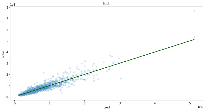
| pred | actual | se | pct_err | |
|---|---|---|---|---|
| count | 4.094000e+03 | 4.094000e+03 | 4.094000e+03 | 4094.000000 |
| mean | 5.340824e+05 | 5.396937e+05 | 1.657722e+10 | 12.857674 |
| std | 3.413714e+05 | 3.761666e+05 | 1.276017e+11 | 13.512028 |
| min | 1.216140e+05 | 8.200000e+04 | 1.000000e+00 | 0.000500 |
| 25% | 3.167628e+05 | 3.200000e+05 | 3.245312e+08 | 4.252492 |
| 50% | 4.568700e+05 | 4.500000e+05 | 1.602001e+09 | 9.101485 |
| 75% | 6.310372e+05 | 6.355250e+05 | 6.575385e+09 | 17.041227 |
| max | 5.126706e+06 | 7.700000e+06 | 6.637466e+12 | 252.097895 |
rmse = np.sqrt(np.mean(pframe.se))
mape = np.mean(pframe.pct_err)
print(f'rmse = {rmse}, mape = {mape}')
rmse = 128752.54982046234, mape = 12.857674005250548
Convert the Model to Onnx
This step converts the model to onnx for easy import into Wallaroo.
import onnx
from onnxmltools.convert import convert_xgboost
from skl2onnx.common.data_types import FloatTensorType, DoubleTensorType
import preprocess
# set the number of columns
ncols = len(preprocess._vars)
# derive the opset value
from onnx.defs import onnx_opset_version
from onnxconverter_common.onnx_ex import DEFAULT_OPSET_NUMBER
TARGET_OPSET = min(DEFAULT_OPSET_NUMBER, onnx_opset_version())
# Convert the model to onnx
onnx_model_converted = convert_xgboost(xgb_model, 'tree-based classifier',
[('input', FloatTensorType([None, ncols]))],
target_opset=TARGET_OPSET)
# Save the model
onnx.save_model(onnx_model_converted, "housing_model_xgb.onnx")
With the model trained and ready, we can now go to Stage 3: Deploy the Model in Wallaroo.
8.3 - Deploy the Model in Wallaroo
The following tutorials are available from the Wallaroo Tutorials Repository.
Stage 3: Deploy the Model in Wallaroo
In this stage, we upload the trained model and the processing steps to Wallaroo, then set up and deploy the inference pipeline.
Once deployed we can feed the newest batch of data to the pipeline, do the inferences and write the results to a results table.
For clarity in this demo, we have split the training/upload task into two notebooks:
02_automated_training_process.ipynb: Train and pickle ML model.03_deploy_model.ipynb: Upload the model to Wallaroo and deploy into a pipeline.
Assuming no changes are made to the structure of the model, these two notebooks, or a script based on them, can then be scheduled to run on a regular basis, to refresh the model with more recent training data and update the inference pipeline.
This notebook is expected to run within the Wallaroo instance’s Jupyter Hub service to provide access to all required Wallaroo libraries and functionality.
Resources
The following resources are used as part of this tutorial:
- data
data/seattle_housing_col_description.txt: Describes the columns used as part data analysis.data/seattle_housing.csv: Sample data of the Seattle, Washington housing market between 2014 and 2015.
- code
simdb.py: A simulated database to demonstrate sending and receiving queries.
- models
housing_model_xgb.onnx: Model created in Stage 2: Training Process Automation Setup../models/preprocess_byop.zip.: Formats the incoming data for the model../models/postprocess_byop.zip: Formats the outgoing data for the model.
Steps
The process of uploading the model to Wallaroo follows these steps:
- Connect to Wallaroo: Connect to the Wallaroo instance and set up the workspace.
- Upload The Model: Upload the model and autoconvert for use in the Wallaroo engine.
- Upload the Processing Modules: Upload the processing modules.
- Create and Deploy the Pipeline: Create the pipeline with the model and processing modules as steps, then deploy it.
- Test the Pipeline: Verify that the pipeline works with the sample data.
Connect to Wallaroo
First we import the required libraries to connect to the Wallaroo instance, then connect to the Wallaroo instance.
import json
import pickle
import pandas as pd
import numpy as np
import pyarrow as pa
import simdb # module for the purpose of this demo to simulate pulling data from a database
# from wallaroo.ModelConversion import ConvertXGBoostArgs, ModelConversionSource, ModelConversionInputType
import wallaroo
from wallaroo.object import EntityNotFoundError
# used to display dataframe information without truncating
from IPython.display import display
import pandas as pd
pd.set_option('display.max_colwidth', None)
import datetime
Connect to the Wallaroo Instance
The first step is to connect to Wallaroo through the Wallaroo client. The Python library is included in the Wallaroo install and available through the Jupyter Hub interface provided with your Wallaroo environment.
This is accomplished using the wallaroo.Client() command, which provides a URL to grant the SDK permission to your specific Wallaroo environment. When displayed, enter the URL into a browser and confirm permissions. Store the connection into a variable that can be referenced later.
If logging into the Wallaroo instance through the internal JupyterHub service, use wl = wallaroo.Client(). For more information on Wallaroo Client settings, see the Client Connection guide.
# Login through local Wallaroo instance
wl = wallaroo.Client()
def get_workspace(name):
workspace = None
for ws in wl.list_workspaces():
if ws.name() == name:
workspace= ws
if(workspace == None):
workspace = wl.create_workspace(name)
return workspace
def get_pipeline(name):
try:
pipeline = wl.pipelines_by_name(name)[0]
except EntityNotFoundError:
pipeline = wl.build_pipeline(name)
return pipeline
workspace_name = 'housepricing'
model_name = "housepricemodel"
model_file = "./housing_model_xgb.onnx"
pipeline_name = "housing-pipe"
The workspace housepricing will either be created or, if already existing, used and set to the current workspace.
new_workspace = get_workspace(workspace_name)
new_workspace
{'name': 'housepricing', 'id': 5, 'archived': False, 'created_by': '4a24979e-63e9-4f04-bab4-0cf828f15ae7', 'created_at': '2024-03-13T17:58:08.872971+00:00', 'models': [], 'pipelines': []}
_ = wl.set_current_workspace(new_workspace)
Upload The Model
With the connection set and workspace prepared, upload the model created in 02_automated_training_process.ipynb into the current workspace.
To ensure the model input contract matches the provided input, the configuration tensor_fields=["tensor"] is used so regardless of what the model input type is, Wallaroo will ensure inputs of type tensor are accepted.
hpmodel = (wl.upload_model(model_name,
model_file,
framework=wallaroo.framework.Framework.ONNX)
.configure(tensor_fields=["tensor"]
)
)
Upload the Processing Modules
Preprocess model:
input_schema = pa.schema([
pa.field('id', pa.int64()),
pa.field('date', pa.string()),
pa.field('list_price', pa.float64()),
pa.field('bedrooms', pa.int64()),
pa.field('bathrooms', pa.float64()),
pa.field('sqft_living', pa.int64()),
pa.field('sqft_lot', pa.int64()),
pa.field('floors', pa.float64()),
pa.field('waterfront', pa.int64()),
pa.field('view', pa.int64()),
pa.field('condition', pa.int64()),
pa.field('grade', pa.int64()),
pa.field('sqft_above', pa.int64()),
pa.field('sqft_basement', pa.int64()),
pa.field('yr_built', pa.int64()),
pa.field('yr_renovated', pa.int64()),
pa.field('zipcode', pa.int64()),
pa.field('lat', pa.float64()),
pa.field('long', pa.float64()),
pa.field('sqft_living15', pa.int64()),
pa.field('sqft_lot15', pa.int64()),
pa.field('sale_price', pa.float64())
])
output_schema = pa.schema([
pa.field('tensor', pa.list_(pa.float32(), list_size=18))
])
preprocess_model = wl.upload_model("preprocess-byop", "./models/preprocess_byop.zip", \
framework=wallaroo.framework.Framework.CUSTOM, \
input_schema=input_schema, output_schema=output_schema)
Waiting for model loading - this will take up to 10.0min.
Model is pending loading to a container runtime..
Model is attempting loading to a container runtime........successful
Ready
Postprocess model:
input_schema = pa.schema([
pa.field('variable', pa.list_(pa.float32()))
])
output_schema = pa.schema([
pa.field('variable', pa.list_(pa.float32()))
])
postprocess_model = wl.upload_model("postprocess-byop", "./models/postprocess_byop.zip", \
framework=wallaroo.framework.Framework.CUSTOM, \
input_schema=input_schema, output_schema=output_schema)
Waiting for model loading - this will take up to 10.0min.
Model is pending loading to a container runtime..
Model is attempting loading to a container runtime........successful
Ready
Create and Deploy the Pipeline
Create the pipeline with the preprocess module, housing model, and postprocess module as pipeline steps, then deploy the newpipeline.
pipeline = get_pipeline(pipeline_name)
# clear if the tutorial was run before
pipeline.clear()
pipeline.add_model_step(preprocess_model)
pipeline.add_model_step(hpmodel)
pipeline.add_model_step(postprocess_model)
deploy_config = wallaroo.DeploymentConfigBuilder().replica_count(1).cpus(0.5).memory("1Gi").build()
pipeline.deploy(deployment_config=deploy_config)
pipeline.status()
{'status': 'Running',
'details': [],
'engines': [{'ip': '10.28.0.131',
'name': 'engine-686c9db4fd-jhxf2',
'status': 'Running',
'reason': None,
'details': [],
'pipeline_statuses': {'pipelines': [{'id': 'housing-pipe',
'status': 'Running'}]},
'model_statuses': {'models': [{'name': 'postprocess-byop',
'version': 'a4f60a10-2097-4b89-ae9b-b97fc3343f12',
'sha': '7b95b800dd05b11b664ae269820da05de0ba6c99fc7ef270f3d645f330608a05',
'status': 'Running'},
{'name': 'preprocess-byop',
'version': '28e338eb-3dd6-40b8-a57e-f7405840d8c9',
'sha': '4e5a026b792ec84baf54b04ebf3a5d5cb24079629921efede64872cf6ccde5ca',
'status': 'Running'},
{'name': 'housepricemodel',
'version': 'a5198e1e-5a0e-42b3-86b5-4bcdfd330f2d',
'sha': 'd8b79e526eed180d39d4653b39bebd9d06e6ae7f68293b5745775a9093a3ae7d',
'status': 'Running'}]}}],
'engine_lbs': [{'ip': '10.28.0.130',
'name': 'engine-lb-d7cc8fc9c-r45rc',
'status': 'Running',
'reason': None,
'details': []}],
'sidekicks': [{'ip': '10.28.0.129',
'name': 'engine-sidekick-postprocess-byop-4-c987744bf-82kxx',
'status': 'Running',
'reason': None,
'details': [],
'statuses': '\n'},
{'ip': '10.28.2.104',
'name': 'engine-sidekick-preprocess-byop-3-ff88cfd96-gfmzr',
'status': 'Running',
'reason': None,
'details': [],
'statuses': '\n'}]}
Test the Pipeline
We will use a single query from the simulated housing_price table and infer. When successful, we will undeploy the pipeline to restore the resources back to the Kubernetes environment.
conn = simdb.simulate_db_connection()
# create the query
query = f"select * from {simdb.tablename} limit 1"
print(query)
# read in the data
singleton = pd.read_sql_query(query, conn)
conn.close()
display(singleton.loc[:, ["id", "date", "list_price", "bedrooms", "bathrooms", "sqft_living", "sqft_lot"]])
select * from house_listings limit 1
| id | date | list_price | bedrooms | bathrooms | sqft_living | sqft_lot | |
|---|---|---|---|---|---|---|---|
| 0 | 7129300520 | 2023-07-31 | 221900.0 | 3 | 1.0 | 1180 | 5650 |
result = pipeline.infer(singleton)
display(result.loc[:, ['time', 'out.variable']])
| time | out.variable | |
|---|---|---|
| 0 | 2024-03-13 18:28:37.873 | [224852.0] |
When finished, we undeploy the pipeline to return the resources back to the environment.
pipeline.undeploy()
Waiting for undeployment - this will take up to 45s ..................................... ok
| name | housing-pipe |
|---|---|
| created | 2024-03-13 18:19:37.008014+00:00 |
| last_updated | 2024-03-13 18:19:37.077324+00:00 |
| deployed | False |
| arch | None |
| tags | |
| versions | bc52c554-6b82-4e3c-a3d1-f6402ee388b0, 6348f7aa-89ba-4051-ad91-1398e5cdd519 |
| steps | preprocess-byop |
| published | False |
With this stage complete, we can proceed to Stage 4: Regular Batch Inference.
8.4 - Regular Batch Inference
The following tutorials are available from the Wallaroo Tutorials Repository.
Stage 4: Regular Batch Inference
In Stage 3: Deploy the Model in Wallaroo, the housing model created and tested in Stage 2: Training Process Automation Setup was uploaded to a Wallaroo instance and added to the pipeline housing-pipe in the workspace housepricing. This pipeline can be deployed at any point and time and used with new inferences.
For the purposes of this demo, let’s say that every month we find the newly entered and still-unsold houses and predict their sale price.
The predictions are entered into a staging table, for further inspection before being joined to the primary housing data table.
We show this as a notebook, but this can also be scripted and scheduled, using CRON or some other process.
Resources
The following resources are used as part of this tutorial:
- data
data/seattle_housing_col_description.txt: Describes the columns used as part data analysis.data/seattle_housing.csv: Sample data of the Seattle, Washington housing market between 2014 and 2015.
- code
simdb.py: A simulated database to demonstrate sending and receiving queries.
- models
housing_model_xgb.onnx: Model created in Stage 2: Training Process Automation Setup../models/preprocess_byop.zip.: Formats the incoming data for the model../models/postprocess_byop.zip: Formats the outgoing data for the model.
Steps
This process will use the following steps:
- Connect to Wallaroo: Connect to the Wallaroo instance and the
housepricingworkspace. - Deploy the Pipeline: Deploy the pipeline to prepare it to run inferences.
- Read In New House Listings: Read in the previous month’s house listings and submit them to the pipeline for inference.
- Send Predictions to Results Staging Table: Add the inference results to the results staging table.
Connect to Wallaroo
Connect to the Wallaroo instance and set the housepricing workspace as the current workspace.
import json
import pickle
import wallaroo
import pandas as pd
import numpy as np
import pyarrow as pa
import datetime
import simdb # module for the purpose of this demo to simulate pulling data from a database
from wallaroo_client import get_workspace
# used to display dataframe information without truncating
from IPython.display import display
pd.set_option('display.max_colwidth', None)
Connect to the Wallaroo Instance
The first step is to connect to Wallaroo through the Wallaroo client. The Python library is included in the Wallaroo install and available through the Jupyter Hub interface provided with your Wallaroo environment.
This is accomplished using the wallaroo.Client() command, which provides a URL to grant the SDK permission to your specific Wallaroo environment. When displayed, enter the URL into a browser and confirm permissions. Store the connection into a variable that can be referenced later.
If logging into the Wallaroo instance through the internal JupyterHub service, use wl = wallaroo.Client(). For more information on Wallaroo Client settings, see the Client Connection guide.
# Login through local Wallaroo instance
wl = wallaroo.Client()
def get_workspace(name, client):
workspace = None
for ws in client.list_workspaces():
if ws.name() == name:
workspace= ws
if(workspace == None):
workspace = client.create_workspace(name)
return workspace
workspace_name = 'housepricing'
model_name = "housepricemodel"
model_file = "./housing_model_xgb.onnx"
pipeline_name = "housing-pipe"
new_workspace = get_workspace(workspace_name, wl)
_ = wl.set_current_workspace(new_workspace)
Deploy the Pipeline
Deploy the housing-pipe workspace established in Stage 3: Deploy the Model in Wallaroo (03_deploy_model.ipynb).
pipeline = new_workspace.pipelines()[0]
pipeline
| name | housing-pipe |
|---|---|
| created | 2024-03-13 18:19:37.008014+00:00 |
| last_updated | 2024-03-13 18:19:37.077324+00:00 |
| deployed | False |
| arch | None |
| tags | |
| versions | bc52c554-6b82-4e3c-a3d1-f6402ee388b0, 6348f7aa-89ba-4051-ad91-1398e5cdd519 |
| steps | preprocess-byop |
| published | False |
deploy_config = wallaroo.DeploymentConfigBuilder().replica_count(1).cpus(0.5).memory("1Gi").build()
pipeline.deploy(deployment_config=deploy_config)
Waiting for deployment - this will take up to 45s ................. ok
| name | housing-pipe |
|---|---|
| created | 2024-03-13 18:19:37.008014+00:00 |
| last_updated | 2024-03-13 19:14:39.155596+00:00 |
| deployed | True |
| arch | None |
| tags | |
| versions | 0d8029ac-dcf0-4920-b74e-5ba0d31eab13, bc52c554-6b82-4e3c-a3d1-f6402ee388b0, 6348f7aa-89ba-4051-ad91-1398e5cdd519 |
| steps | preprocess-byop |
| published | False |
Read In New House Listings
From the data store, load the previous month’s house listing, prepare it as a DataFrame, then submit it for inferencing.
conn = simdb.simulate_db_connection()
# create the query
query = f"select * from {simdb.tablename} where date > DATE(DATE(), '-1 month') AND sale_price is NULL"
print(query)
# read in the data
# can't have null values - turn them into 0
newbatch = pd.read_sql_query(query, conn)
newbatch['sale_price'] = newbatch.sale_price.apply(lambda x: 0)
display(newbatch.shape)
display(newbatch.head(10).loc[:, ["id", "date", "list_price", "bedrooms", "bathrooms", "sqft_living", "sqft_lot"]])
select * from house_listings where date > DATE(DATE(), '-1 month') AND sale_price is NULL
(843, 22)
| id | date | list_price | bedrooms | bathrooms | sqft_living | sqft_lot | |
|---|---|---|---|---|---|---|---|
| 0 | 1695900060 | 2024-02-26 | 535000.0 | 4 | 1.00 | 1610 | 2982 |
| 1 | 1432900240 | 2024-02-23 | 205000.0 | 3 | 1.00 | 1610 | 8579 |
| 2 | 7960900060 | 2024-02-19 | 2900000.0 | 4 | 3.25 | 5050 | 20100 |
| 3 | 6378500125 | 2024-02-16 | 436000.0 | 2 | 1.00 | 1040 | 7538 |
| 4 | 2022069200 | 2024-02-20 | 455000.0 | 4 | 2.50 | 2210 | 49375 |
| 5 | 9412900055 | 2024-02-20 | 405000.0 | 3 | 1.75 | 2390 | 6000 |
| 6 | 7424700045 | 2024-02-28 | 2050000.0 | 5 | 3.00 | 3830 | 8480 |
| 7 | 3422059208 | 2024-02-26 | 390000.0 | 3 | 2.50 | 1930 | 64904 |
| 8 | 4268200055 | 2024-02-16 | 245000.0 | 3 | 1.75 | 1740 | 11547 |
| 9 | 2883200160 | 2024-02-14 | 595000.0 | 4 | 2.00 | 2020 | 2849 |
# query = {'query': newbatch.to_json()}
result = pipeline.infer(newbatch)
# display(result)
predicted_prices = pd.DataFrame(result['out.variable'].apply(lambda x: x[0])).rename(columns={'out.variable':'prediction'})
display(predicted_prices[0:5])
| prediction | |
|---|---|
| 0 | 500198.0 |
| 1 | 270739.0 |
| 2 | 3067264.0 |
| 3 | 378917.0 |
| 4 | 496464.0 |
Send Predictions to Results Staging Table
Take the predicted prices based on the inference results so they can be joined into the house_listings table.
Once complete, undeploy the pipeline to return the resources back to the Kubernetes environment.
result_table = pd.DataFrame({
'id': newbatch['id'],
'saleprice_estimate': predicted_prices['prediction']
})
display(result_table)
result_table.to_sql('results_table', conn, index=False, if_exists='append')
| id | saleprice_estimate | |
|---|---|---|
| 0 | 1695900060 | 500198.0 |
| 1 | 1432900240 | 270739.0 |
| 2 | 7960900060 | 3067264.0 |
| 3 | 6378500125 | 378917.0 |
| 4 | 2022069200 | 496464.0 |
| ... | ... | ... |
| 838 | 6140100028 | 365689.0 |
| 839 | 3304300300 | 577492.0 |
| 840 | 6453550090 | 882930.0 |
| 841 | 3345700207 | 537434.0 |
| 842 | 7853420110 | 634226.0 |
843 rows × 2 columns
# Display the top of the table for confirmation
pd.read_sql_query("select * from results_table limit 5", conn)
| id | saleprice_estimate | |
|---|---|---|
| 0 | 1695900060 | 500198.0 |
| 1 | 1432900240 | 270739.0 |
| 2 | 7960900060 | 3067264.0 |
| 3 | 6378500125 | 378917.0 |
| 4 | 2022069200 | 496464.0 |
conn.close()
pipeline.undeploy()
Waiting for undeployment - this will take up to 45s .................................... ok
| name | housing-pipe |
|---|---|
| created | 2024-03-13 18:19:37.008014+00:00 |
| last_updated | 2024-03-13 19:14:39.155596+00:00 |
| deployed | False |
| arch | None |
| tags | |
| versions | 0d8029ac-dcf0-4920-b74e-5ba0d31eab13, bc52c554-6b82-4e3c-a3d1-f6402ee388b0, 6348f7aa-89ba-4051-ad91-1398e5cdd519 |
| steps | preprocess-byop |
| published | False |
From here, organizations can automate this process. Other features could be used such as data analysis using Wallaroo assays, or other features such as shadow deployments to test champion and challenger models to find which models provide the best results.
9 - ML Workload Orchestration Tutorials
Tutorials on using the Wallaroo ML Workload Orchestration.
The following tutorials show how to use the Wallaroo ML Workload Orchestration feature with different data connections and situations.
9.1 - Wallaroo ML Workload Orchestration API Tutorial
A tutorial on using the ML Workload Orchestration with the Wallaroo MLOps API
This can be downloaded as part of the Wallaroo Tutorials repository.
Wallaroo Connection and ML Workload Orchestration API Tutorial
This tutorial provides a quick set of methods and examples regarding Wallaroo Connections and Wallaroo ML Workload Orchestration. For full details, see the Wallaroo Documentation site.
Wallaroo provides Data Connections and ML Workload Orchestrations to provide organizations with a method of creating and managing automated tasks that can either be run on demand or a regular schedule.
Definitions
- Orchestration: A set of instructions written as a python script with a requirements library. Orchestrations are uploaded to the Wallaroo instance as a .zip file.
- Task: An implementation of an orchestration. Tasks are run either once when requested, on a repeating schedule, or as a service.
- Connection: Definitions set by MLOps engineers that are used by other Wallaroo users for connection information to a data source. Usually paired with orchestrations.
Tutorial Goals
The tutorial will demonstrate the following:
- Create a workspace and pipeline with a sample model.
- Upload Wallaroo ML Workload Orchestration through the Wallaroo MLOps API.
- List available orchestrations through the Wallaroo MLOps API.
- Run the orchestration once as a Run Once Task through the Wallaroo MLOps API and verify that the information was saved the pipeline logs.
Prerequisites
- An installed Wallaroo instance.
- The following Python libraries installed. These are included by default in a Wallaroo instance’s JupyterHub service.
Initial Steps
For this tutorial, we’ll create a workspace, upload our sample model and deploy a pipeline. We’ll perform some quick sample inferences to verify that everything it working.
Load Libraries
Here we’ll import the various libraries we’ll use for the tutorial.
import wallaroo
from wallaroo.object import EntityNotFoundError, RequiredAttributeMissing
# to display dataframe tables
from IPython.display import display
# used to display dataframe information without truncating
import pandas as pd
pd.set_option('display.max_colwidth', None)
import pyarrow as pa
import time
import requests
# Used to create unique workspace and pipeline names
import string
import random
# make a random 4 character suffix
suffix= ''.join(random.choice(string.ascii_lowercase) for i in range(4))
display(suffix)
'gsze'
Connect to the Wallaroo Instance
The first step is to connect to Wallaroo through the Wallaroo client. The Python library is included in the Wallaroo install and available through the Jupyter Hub interface provided with your Wallaroo environment.
This is accomplished using the wallaroo.Client() command, which provides a URL to grant the SDK permission to your specific Wallaroo environment. When displayed, enter the URL into a browser and confirm permissions. Store the connection into a variable that can be referenced later.
If logging into the Wallaroo instance through the internal JupyterHub service, use wl = wallaroo.Client(). If logging in externally, update the wallarooPrefix and wallarooSuffix variables with the proper DNS information. For more information on Wallaroo Client settings, see the Client Connection guide.
# Login through local Wallaroo instance
wl = wallaroo.Client()
API URL
The variable APIURL is used to specify the connection to the Wallaroo instance’s MLOps API URL, and is composed of the Wallaroo DNS prefix and suffix. For full details, see the Wallaroo API Connection Guide
.
The variables wallarooPrefix and wallarooSuffix variables will be used to derive the API url. For example, if the Wallaroo Prefix is doc-test and the url is example.com, then the MLOps API URL would be doc-test.api.example.com/v1/api/{request}.
Note the . is part of the prefix. If there is no prefix, then wallarooPrefix = ""
Set the Wallaroo Prefix and Suffix in the code segment below based on your Wallaroo instance.
# Setting variables for later steps
wallarooPrefix = "YOUR PREFIX."
wallarooSuffix = "YOUR SUFFIX"
APIURL = f"https://{wallarooPrefix}api.{wallarooSuffix}"
workspace_name = f'apiorchestrationworkspace{suffix}'
pipeline_name = f'apipipeline{suffix}'
model_name = f'apiorchestrationmodel{suffix}'
model_file_name = './models/rf_model.onnx'
Helper Methods
The following helper methods are used to either create or get workspaces, pipelines, and connections.
# helper methods to retrieve workspaces and pipelines
def get_workspace(name):
workspace = None
for ws in wl.list_workspaces():
if ws.name() == name:
workspace= ws
if(workspace == None):
workspace = wl.create_workspace(name)
return workspace
def get_pipeline(name):
try:
pipeline = wl.pipelines_by_name(name)[0]
except EntityNotFoundError:
pipeline = wl.build_pipeline(name)
return pipeline
def get_connection(name, connection_type, connection_arguments):
try:
connection = wl.get_connection(name)
except RequiredAttributeMissing:
connection =wl.create_connection(name,
connection_type,
connection_arguments)
return connection
Create the Workspace and Pipeline
We’ll now create our workspace and pipeline for the tutorial. If this tutorial has been run previously, then this will retrieve the existing ones with the assumption they’re for us with this tutorial.
We’ll set the retrieved workspace as the current workspace in the SDK, so all commands will default to that workspace.
workspace = get_workspace(workspace_name)
wl.set_current_workspace(workspace)
workspace_id = workspace.id()
pipeline = get_pipeline(pipeline_name)
Upload the Model and Deploy Pipeline
We’ll upload our model into our sample workspace, then add it as a pipeline step before deploying the pipeline to it’s ready to accept inference requests.
# Upload the model
housing_model_control = (wl.upload_model(model_name,
model_file_name,
framework=wallaroo.framework.Framework.ONNX)
.configure(tensor_fields=["tensor"])
)
# Add the model as a pipeline step
pipeline.add_model_step(housing_model_control)
| name | apipipelinegsze |
|---|---|
| created | 2023-05-22 20:48:30.700499+00:00 |
| last_updated | 2023-05-22 20:48:30.700499+00:00 |
| deployed | (none) |
| tags | |
| versions | 101b252a-623c-4185-a24d-ec00593dda79 |
| steps |
#deploy the pipeline
pipeline.deploy()
Waiting for deployment - this will take up to 45s ......... ok
| name | apipipelinegsze |
|---|---|
| created | 2023-05-22 20:48:30.700499+00:00 |
| last_updated | 2023-05-22 20:48:31.357336+00:00 |
| deployed | True |
| tags | |
| versions | aac61b5a-e4f4-4ea3-9347-6482c330b5f5, 101b252a-623c-4185-a24d-ec00593dda79 |
| steps | apiorchestrationmodelgsze |
Wallaroo ML Workload Orchestration Example
With the pipeline deployed and our connections set, we will now generate our ML Workload Orchestration. See the Wallaroo ML Workload Orchestrations guide for full details.
Orchestrations are uploaded to the Wallaroo instance as a ZIP file with the following requirements:
| Parameter | Type | Description |
|---|---|---|
| User Code | (Required) Python script as .py files | If main.py exists, then that will be used as the task entrypoint. Otherwise, the first main.py found in any subdirectory will be used as the entrypoint. |
| Python Library Requirements | (Optional) requirements.txt file in the requirements file format. A standard Python requirements.txt for any dependencies to be provided in the task environment. The Wallaroo SDK will already be present and should not be included in the requirements.txt. Multiple requirements.txt files are not allowed. | |
| Other artifacts | Other artifacts such as files, data, or code to support the orchestration. |
For our example, our orchestration will:
- Use the
inference_results_connectionto open a HTTP Get connection to the inference data file and use it in an inference request in the deployed pipeline. - Submit the inference results to the location specified in the
external_inference_connection.
This sample script is stored in remote_inference/main.py with an empty requirements.txt file, and packaged into the orchestration as ./remote_inference/remote_inference.zip. We’ll display the steps in uploading the orchestration to the Wallaroo instance.
Note that the orchestration assumes the pipeline is already deployed.
API Upload the Orchestration
Orchestrations are uploaded via POST as a application/octet-stream with MLOps API route:
- REQUEST
- POST
/v1/api/orchestration/upload - Content-Type
multipart/form-data
- POST
- PARAMETERS
file: The file uploaded as Content-Type asapplication/octet-stream.metadata: Included as Content-Type asapplication/jsonwith:- workspace_id: The numerical id of the workspace to upload the orchestration to.
- name: The name of the orchestration.
- The metadata specifying the workspace id and Content-Type as
application/json.
Once uploaded, the deployment will be prepared and any requirements will be downloaded and installed.
# retrieve the authorization token
headers = wl.auth.auth_header()
url = f"{APIURL}/v1/api/orchestration/upload"
fp = open("./api_inference_orchestration.zip", "rb")
metadata = f'{{"workspace_id": {workspace_id},"name": "apiorchestrationsample"}}'
response = requests.post(
url,
headers=headers,
files=[
("file",
("api_inference_orchestration.zip", fp, "application/octet-stream")
),
("metadata",
("metadata", metadata, "application/json")
)
],
).json()
display(response)
orchestration_id = response['id']
{'id': 'b951f7b8-0690-4004-86bf-cc9802359313'}
API List Orchestrations
A list of orchestrations retrieved via POST MLOps API route:
- REQUEST
- POST
/v1/api/orchestration/list
- POST
- PARAMETERS
- workspace_id: The numerical identifier of the workspace associated with the orchestration.
# retrieve the authorization token
headers = wl.auth.auth_header()
url = f"{APIURL}/v1/api/orchestration/list"
data = {
'workspace_id': workspace_id
}
response=requests.post(url, headers=headers, json=data)
display(response.json())
[{'id': 'b951f7b8-0690-4004-86bf-cc9802359313',
'workspace_id': 8,
'sha': 'd3b93c9f280734106376e684792aa8b4285d527092fe87d89c74ec804f8e169e',
'name': 'apiorchestrationsample',
'file_name': 'api_inference_orchestration.zip',
'task_id': 'c9622cf8-cbe5-4e3c-b64c-dabd6c5b7fef',
'owner_id': 'a6857628-b0aa-451e-a0a0-bbc1d6eea6e0',
'status': 'pending_packaging',
'created_at': '2023-05-22T20:48:41.233482+00:00',
'updated_at': '2023-05-22T20:48:41.233482+00:00'}]
API Get Orchestration
A list of orchestrations retrieved via POST MLOps API route:
- REQUEST
- POST
/v1/api/orchestration/get_by_id
- POST
- PARAMETERS
- id: The UUID of the orchestration being retrieved.
- RETURNS
- id: The ID of the orchestration in UUID format.
- workspace_id: Numerical value of the workspace the orchestration was uploaded to.
- sha: The SHA hash value of the orchestration.
- file_name: The file name the orchestration was uploaded as.
- task_id: The task id in UUID format for unpacking and preparing the orchestration.
- owner_id: The Keycloak ID of the user that uploaded the orchestration.
- status: The status of the orchestration. Status values are:
packing: Preparing the orchestration to be used as a task.ready: The orchestration is ready to be deployed as a task.
# retrieve the authorization token
headers = wl.auth.auth_header()
url = f"{APIURL}/v1/api/orchestration/get_by_id"
data = {
'id': orchestration_id
}
# loop until status is ready
status = None
while status != 'ready':
response=requests.post(url, headers=headers, json=data).json()
display(response)
status = response['status']
time.sleep(10)
orchestration_sha = response['sha']
{'id': 'b951f7b8-0690-4004-86bf-cc9802359313',
'workspace_id': 8,
'sha': 'd3b93c9f280734106376e684792aa8b4285d527092fe87d89c74ec804f8e169e',
'file_name': 'api_inference_orchestration.zip',
'task_id': 'c9622cf8-cbe5-4e3c-b64c-dabd6c5b7fef',
'owner_id': 'a6857628-b0aa-451e-a0a0-bbc1d6eea6e0',
'status': 'packaging'}
{‘id’: ‘b951f7b8-0690-4004-86bf-cc9802359313’,
‘workspace_id’: 8,
‘sha’: ‘d3b93c9f280734106376e684792aa8b4285d527092fe87d89c74ec804f8e169e’,
‘file_name’: ‘api_inference_orchestration.zip’,
’task_id’: ‘c9622cf8-cbe5-4e3c-b64c-dabd6c5b7fef’,
‘owner_id’: ‘a6857628-b0aa-451e-a0a0-bbc1d6eea6e0’,
‘status’: ‘packaging’}
{‘id’: ‘b951f7b8-0690-4004-86bf-cc9802359313’,
‘workspace_id’: 8,
‘sha’: ‘d3b93c9f280734106376e684792aa8b4285d527092fe87d89c74ec804f8e169e’,
‘file_name’: ‘api_inference_orchestration.zip’,
’task_id’: ‘c9622cf8-cbe5-4e3c-b64c-dabd6c5b7fef’,
‘owner_id’: ‘a6857628-b0aa-451e-a0a0-bbc1d6eea6e0’,
‘status’: ‘ready’}
Task Management Tutorial
Once an Orchestration has the status ready, it can be run as a task. Tasks have three run options.
| Type | SDK Call | How triggered |
|---|---|---|
| Once | orchestration.run_once(name, json_args, timeout) | Task runs once and exits. |
| Scheduled | orchestration.run_scheduled(name, schedule, timeout, json_args) | User provides schedule. Task runs exits whenever schedule dictates. |
Run Task Once via API
We’ll do both a Run Once task and generate our Run Once Task from our orchestration. Orchestrations are started as a run once task with the following request:
- REQUEST
- POST
/v1/api/orchestration/task/run_once
- POST
- PARAMETERS
- name (String Required): The name to assign to the task.
- workspace_id (Integer Required): The numerical identifier of the workspace associated with the orchestration.
- orch_id(String Required): The orchestration ID represented by a UUID.
- json(Dict Required): The parameters to pass to the task.
Tasks are generated and run once with the Orchestration run_once method. Any arguments for the orchestration are passed in as a Dict. If there are no arguments, then an empty set {} is passed.
# retrieve the authorization token
headers = wl.auth.auth_header()
data = {
"name": "api run once task",
"workspace_id": workspace_id,
"orch_id": orchestration_id,
"json": {
"workspace_name": workspace_name,
"pipeline_name": pipeline_name
}
}
import datetime
task_start = datetime.datetime.now()
url=f"{APIURL}/v1/api/task/run_once"
response=requests.post(url, headers=headers, json=data).json()
display(response)
task_id = response['id']
{'id': 'c868aa44-f7fe-4e3d-b11d-e1e6af3ec150'}
Task Status via API
The list of tasks in the Wallaroo instance is retrieves through the Wallaroo MLOPs API request:
- REQUEST
- POST
/v1/api/task/get_by_id
- POST
- PARAMETERS
- task: The numerical identifier of the workspace associated with the orchestration.
- orch_id: The orchestration ID represented by a UUID.
- json: The parameters to pass to the task.
For this example, the status of the previously created task will be generated, then looped until it has reached status started.
# retrieve the authorization token
headers = wl.auth.auth_header()
url=f"{APIURL}/v1/api/task/get_by_id"
data = {
"id": task_id
}
status = None
while status != 'started':
response=requests.post(url, headers=headers, json=data).json()
display(response)
status = response['status']
time.sleep(10)
{'name': 'api run once task',
'id': 'c868aa44-f7fe-4e3d-b11d-e1e6af3ec150',
'image': 'proxy.replicated.com/proxy/wallaroo/ghcr.io/wallaroolabs/arbex-orch-deploy',
'image_tag': 'v2023.2.0-main-3271',
'bind_secrets': ['minio'],
'extra_env_vars': {'MINIO_URL': 'http://minio.wallaroo.svc.cluster.local:9000',
'ORCH_OWNER_ID': 'a6857628-b0aa-451e-a0a0-bbc1d6eea6e0',
'ORCH_SHA': 'd3b93c9f280734106376e684792aa8b4285d527092fe87d89c74ec804f8e169e',
'TASK_DEBUG': 'false',
'TASK_ID': 'c868aa44-f7fe-4e3d-b11d-e1e6af3ec150'},
'auth_init': True,
'workspace_id': 8,
'flavor': 'exec_orch_oneshot',
'reap_threshold_secs': 900,
'exec_type': 'job',
'status': 'pending',
'input_data': {'pipeline_name': 'apipipelinegsze',
'workspace_name': 'apiorchestrationworkspacegsze'},
'killed': False,
'created_at': '2023-05-22T21:08:31.099447+00:00',
'updated_at': '2023-05-22T21:08:31.105312+00:00',
'last_runs': []}
{’name’: ‘api run once task’,
‘id’: ‘c868aa44-f7fe-4e3d-b11d-e1e6af3ec150’,
‘image’: ‘proxy.replicated.com/proxy/wallaroo/ghcr.io/wallaroolabs/arbex-orch-deploy’,
‘image_tag’: ‘v2023.2.0-main-3271’,
‘bind_secrets’: [‘minio’],
’extra_env_vars’: {‘MINIO_URL’: ‘http://minio.wallaroo.svc.cluster.local:9000’,
‘ORCH_OWNER_ID’: ‘a6857628-b0aa-451e-a0a0-bbc1d6eea6e0’,
‘ORCH_SHA’: ‘d3b93c9f280734106376e684792aa8b4285d527092fe87d89c74ec804f8e169e’,
‘TASK_DEBUG’: ‘false’,
‘TASK_ID’: ‘c868aa44-f7fe-4e3d-b11d-e1e6af3ec150’},
‘auth_init’: True,
‘workspace_id’: 8,
‘flavor’: ’exec_orch_oneshot’,
‘reap_threshold_secs’: 900,
’exec_type’: ‘job’,
‘status’: ‘started’,
‘input_data’: {‘pipeline_name’: ‘apipipelinegsze’,
‘workspace_name’: ‘apiorchestrationworkspacegsze’},
‘killed’: False,
‘created_at’: ‘2023-05-22T21:08:31.099447+00:00’,
‘updated_at’: ‘2023-05-22T21:08:36.585775+00:00’,
’last_runs’: [{‘run_id’: ‘96a7f85f-e30c-40b5-9185-0dee5bd1a15e’,
‘status’: ‘running’,
‘created_at’: ‘2023-05-22T21:08:33.112805+00:00’,
‘updated_at’: ‘2023-05-22T21:08:33.112805+00:00’}]}
Task Results
We can view the inferences from our logs and verify that new entries were added from our task. In our case, we’ll assume the task once started takes about 1 minute to run (deploy the pipeline, run the inference, undeploy the pipeline). We’ll add in a wait of 1 minute, then display the logs during the time period the task was running.
time.sleep(30)
task_end = datetime.datetime.now()
display(task_end)
pipeline.logs(start_datetime = task_start, end_datetime = task_end)
datetime.datetime(2023, 5, 22, 21, 9, 32, 447321)
| time | in.tensor | out.variable | check_failures | |
|---|---|---|---|---|
| 0 | 2023-05-22 21:08:37.779 | [4.0, 2.5, 2900.0, 5505.0, 2.0, 0.0, 0.0, 3.0, 8.0, 2900.0, 0.0, 47.6063, -122.02, 2970.0, 5251.0, 12.0, 0.0, 0.0] | [718013.7] | 0 |
Get Tasks by Orchestration SHA
Tasks tied to the same orchestration are retrieved through the following request.
- REQUEST
- POST
/v1/api/task/get_tasks_by_orch_sha
- POST
- PARAMETERS
- sha: The orchestrations SHA hash.
- RETURNS
ids: List[string] List of tasks by UUID.
# retrieve the authorization token
headers = wl.auth.auth_header()
url=f"{APIURL}/v1/api/task/get_tasks_by_orch_sha"
data = {
"sha": orchestration_sha
}
response=requests.post(url, headers=headers, json=data).json()
display(response)
{'ids': ['2424a9a7-2331-42f6-bd84-90643386b130',
'c868aa44-f7fe-4e3d-b11d-e1e6af3ec150',
'a41fe4ae-b8a4-4e1f-a45a-114df64ae2bc']}
Task Last Runs History
The history of a task, which each deployment of the task is known as a task run is retrieved with the Task last_runs method that takes the following arguments. It returns the reverse chronological order of tasks runs listed by updated_at.
- REQUEST
- POST
/v1/api/task/list_task_runs
- POST
- PARAMETERS
- task_id: The numerical identifier of the task.
- status: Filters the task history by the
status. Ifall, returns all statuses. Status values are:running: The task has started.failure: The task failed.success: The task completed.
- limit: The number of tasks runs to display.
- RETURNS
- ids: List of task runs ids in UUID.
# retrieve the authorization token
headers = wl.auth.auth_header()
url=f"{APIURL}/v1/api/task/list_task_runs"
data = {
"task_id": task_id
}
response=requests.post(url, headers=headers, json=data).json()
task_run_id = response[0]['run_id']
display(response)
[{'task': 'c868aa44-f7fe-4e3d-b11d-e1e6af3ec150',
'run_id': '96a7f85f-e30c-40b5-9185-0dee5bd1a15e',
'status': 'success',
'created_at': '2023-05-22T21:08:33.112805+00:00',
'updated_at': '2023-05-22T21:08:33.112805+00:00'}]
Get Task Run Logs
Logs for a task run are retrieved through the following process.
- REQUEST
- POST
/v1/api/task/get_logs_for_run
- POST
- PARAMETERS
- id: The numerical identifier of the task run associated with the orchestration.
- lines: The number of log lines to retrieve starting from the end of the log.
- RETURNS
- logs: Array of log entries.
# retrieve the authorization token
headers = wl.auth.auth_header()
url=f"{APIURL}/v1/api/task/get_logs_for_run"
data = {
"id": task_run_id
}
response=requests.post(url, headers=headers, json=data).json()
display(response)
{'logs': ["2023-05-22T21:09:17.683428502Z stdout F {'pipeline_name': 'apipipelinegsze', 'workspace_name': 'apiorchestrationworkspacegsze'}",
'2023-05-22T21:09:17.683489102Z stdout F Getting the workspace apiorchestrationworkspacegsze',
'2023-05-22T21:09:17.683497403Z stdout F Getting the pipeline apipipelinegsze',
'2023-05-22T21:09:17.683504003Z stdout F Deploying the pipeline.',
'2023-05-22T21:09:17.683510203Z stdout F Performing sample inference.',
'2023-05-22T21:09:17.683516203Z stdout F time ... check_failures',
'2023-05-22T21:09:17.683521903Z stdout F 0 2023-05-22 21:08:37.779 ... 0',
'2023-05-22T21:09:17.683527803Z stdout F ',
'2023-05-22T21:09:17.683533603Z stdout F [1 rows x 4 columns]',
'2023-05-22T21:09:17.683540103Z stdout F Undeploying the pipeline']}
Run Task Scheduled via API
The other method of using tasks is as a scheduled run through the Orchestration run_scheduled(name, schedule, timeout, json_args). This sets up a task to run on an regular schedule as defined by the schedule parameter in the cron service format. For example:
schedule={'42 * * * *'}
Runs on the 42nd minute of every hour.
The following schedule runs every day at 12 noon from February 1 to February 15 2024 - and then ends.
schedule={'0 0 12 1-15 2 2024'}
The Run Scheduled Task request is available at the following address:
/v1/api/task/run_scheduled
And takes the following parameters.
- name (String Required): The name to assign to the task.
- orch_id (String Required): The UUID orchestration ID to create the task from.
- workspace_id (Integer Required): The numberical identifier for the workspace.
- schedule (String Required): The schedule as a single string in
cronformat. - timeout(Integer Optional): The timeout to complete the task in seconds.
- json (String Required): The arguments to pass to the task.
For our example, we will create a scheduled task to run every 5 minutes, display the inference results, then use the Orchestration kill task to keep the task from running any further.
It is recommended that orchestrations that have pipeline deploy or undeploy commands be spaced out no less than 5 minutes to prevent colliding with other tasks that use the same pipeline.
# retrieve the authorization token
headers = wl.auth.auth_header()
data = {
"name": "scheduled api task",
"workspace_id": workspace_id,
"orch_id": orchestration_id,
"schedule": "*/5 * * * *",
"json": {
"workspace_name": workspace_name,
"pipeline_name": pipeline_name
}
}
import datetime
task_start = datetime.datetime.now()
url=f"{APIURL}/v1/api/task/run_scheduled"
response=requests.post(url, headers=headers, json=data).json()
display(response)
scheduled_task_id = response['id']
{'id': '87c2c7c0-e17e-4c00-9407-bfc44d632910'}
# loop until the task is started
# retrieve the authorization token
headers = wl.auth.auth_header()
url=f"{APIURL}/v1/api/task/get_by_id"
data = {
"id": scheduled_task_id
}
status = None
while status != 'started':
response=requests.post(url, headers=headers, json=data).json()
display(response)
status = response['status']
time.sleep(10)
{'name': 'scheduled api task',
'id': '87c2c7c0-e17e-4c00-9407-bfc44d632910',
'image': 'proxy.replicated.com/proxy/wallaroo/ghcr.io/wallaroolabs/arbex-orch-deploy',
'image_tag': 'v2023.2.0-main-3271',
'bind_secrets': ['minio'],
'extra_env_vars': {'MINIO_URL': 'http://minio.wallaroo.svc.cluster.local:9000',
'ORCH_OWNER_ID': 'a6857628-b0aa-451e-a0a0-bbc1d6eea6e0',
'ORCH_SHA': 'd3b93c9f280734106376e684792aa8b4285d527092fe87d89c74ec804f8e169e',
'TASK_DEBUG': 'false',
'TASK_ID': '87c2c7c0-e17e-4c00-9407-bfc44d632910'},
'auth_init': True,
'workspace_id': 8,
'schedule': '*/5 * * * *',
'reap_threshold_secs': 900,
'status': 'started',
'input_data': {'pipeline_name': 'apipipelinegsze',
'workspace_name': 'apiorchestrationworkspacegsze'},
'killed': False,
'created_at': '2023-05-22T21:10:22.43957+00:00',
'updated_at': '2023-05-22T21:10:22.871615+00:00',
'last_runs': []}
# retrieve the authorization token
headers = wl.auth.auth_header()
url=f"{APIURL}/v1/api/task/list_task_runs"
data = {
"task_id": scheduled_task_id
}
# loop until we have a single run task
length = 0
while length == 0:
response=requests.post(url, headers=headers, json=data).json()
display(response)
length = len(response)
time.sleep(10)
task_run_id = response[0]['run_id']
[{'task': '87c2c7c0-e17e-4c00-9407-bfc44d632910',
'run_id': 'ad3d427a-3643-4f10-9b94-116688b32355',
'status': 'running',
'created_at': '2023-05-22T21:15:02.148274+00:00',
'updated_at': '2023-05-22T21:15:02.148274+00:00'}]
# retrieve the authorization token
headers = wl.auth.auth_header()
url=f"{APIURL}/v1/api/task/get_logs_for_run"
data = {
"id": task_run_id
}
# loop until we get a log
response=requests.post(url, headers=headers, json=data).json()
display(response)
{'logs': ["2023-05-22T21:15:55.548754679Z stdout F {'pipeline_name': 'apipipelinegsze', 'workspace_name': 'apiorchestrationworkspacegsze'}",
'2023-05-22T21:15:55.54880928Z stdout F Getting the workspace apiorchestrationworkspacegsze',
'2023-05-22T21:15:55.54881708Z stdout F Getting the pipeline apipipelinegsze',
'2023-05-22T21:15:55.54882328Z stdout F Deploying the pipeline.',
'2023-05-22T21:15:55.54883088Z stdout F Performing sample inference.',
'2023-05-22T21:15:55.54883628Z stdout F time ... check_failures',
'2023-05-22T21:15:55.54884248Z stdout F 0 2023-05-22 21:15:17.420 ... 0',
'2023-05-22T21:15:55.54884788Z stdout F ',
'2023-05-22T21:15:55.54885348Z stdout F [1 rows x 4 columns]',
'2023-05-22T21:15:55.54885938Z stdout F Undeploying the pipeline']}
Cleanup
With the tutorial complete, we can undeploy the pipeline and return the resources back to the Wallaroo instance.
Kill Task via API
Started tasks are killed through the following request:
/v1/api/task/kill
And takes the following parameters.
- orch_id (String Required): The UUID orchestration ID to create the task from.
# retrieve the authorization token
headers = wl.auth.auth_header()
url=f"{APIURL}/v1/api/task/kill"
data = {
"id": scheduled_task_id
}
response=requests.post(url, headers=headers, json=data).json()
display(response)
{'name': 'scheduled api task',
'id': '87c2c7c0-e17e-4c00-9407-bfc44d632910',
'image': 'proxy.replicated.com/proxy/wallaroo/ghcr.io/wallaroolabs/arbex-orch-deploy',
'image_tag': 'v2023.2.0-main-3271',
'bind_secrets': ['minio'],
'extra_env_vars': {'MINIO_URL': 'http://minio.wallaroo.svc.cluster.local:9000',
'ORCH_OWNER_ID': 'a6857628-b0aa-451e-a0a0-bbc1d6eea6e0',
'ORCH_SHA': 'd3b93c9f280734106376e684792aa8b4285d527092fe87d89c74ec804f8e169e',
'TASK_DEBUG': 'false',
'TASK_ID': '87c2c7c0-e17e-4c00-9407-bfc44d632910'},
'auth_init': True,
'workspace_id': 8,
'schedule': '*/5 * * * *',
'reap_threshold_secs': 900,
'status': 'pending_kill',
'input_data': {'pipeline_name': 'apipipelinegsze',
'workspace_name': 'apiorchestrationworkspacegsze'},
'killed': False,
'created_at': '2023-05-22T21:10:22.43957+00:00',
'updated_at': '2023-05-22T21:10:22.871615+00:00',
'last_runs': [{'run_id': 'ad3d427a-3643-4f10-9b94-116688b32355',
'status': 'success',
'created_at': '2023-05-22T21:15:02.148274+00:00',
'updated_at': '2023-05-22T21:15:02.148274+00:00'}]}
Close Resources
With the tutorial complete, we’ll verify the pipeline is closed so the resources are assigned back to the Wallaroo instance.
pipeline.undeploy()
ok
| name | apipipelinegsze |
|---|---|
| created | 2023-05-22 20:48:30.700499+00:00 |
| last_updated | 2023-05-22 20:48:31.357336+00:00 |
| deployed | False |
| tags | |
| versions | aac61b5a-e4f4-4ea3-9347-6482c330b5f5, 101b252a-623c-4185-a24d-ec00593dda79 |
| steps | apiorchestrationmodelgsze |
9.2 - Wallaroo Connection API with Google BigQuery Tutorial
A tutorial on using the Wallaroo MLOps API with Wallaroo Connections for Google BigQuery connections.
This can be downloaded as part of the Wallaroo Tutorials repository.
Wallaroo Connection and ML Workload Orchestration with BigQuery House Price Model Tutorial
This tutorial provides a quick set of methods and examples regarding Wallaroo Connections. For full details, see the Wallaroo Documentation site.
Wallaroo provides Data Connections to organizations with a method of creating and managing automated tasks that can either be run on demand or a regular schedule.
Definitions
- Orchestration: A set of instructions written as a python script with a requirements library. Orchestrations are uploaded to the Wallaroo instance as a .zip file.
- Task: An implementation of an orchestration. Tasks are run either once when requested, on a repeating schedule, or as a service.
- Connection: Definitions set by MLOps engineers that are used by other Wallaroo users for connection information to a data source. Usually paired with orchestrations.
This tutorial will focus on using Google BigQuery as the data source.
Tutorial Goals
The tutorial will demonstrate the following:
- Create a Wallaroo connection to retrieving information from a Google BigQuery source table.
- Create a Wallaroo connection to store inference results into a Google BigQuery destination table.
- Upload Wallaroo ML Workload Orchestration that supports BigQuery connections with the connection details.
- Run the orchestration once as a Run Once Task and verify that the inference request succeeded and the inference results were saved to the external data store.
- Schedule the orchestration as a Scheduled Task and verify that the inference request succeeded and the inference results were saved to the external data store.
Prerequisites
- An installed Wallaroo instance.
- The following Python libraries installed. These are included by default in a Wallaroo instance’s JupyterHub service.
- The following Python libraries. These are not included in a Wallaroo instance’s JupyterHub service.
google-cloud-bigquery: Specifically for its support for Google BigQuery.google-auth: Used to authenticate for bigquery.db-dtypes: Converts the BigQuery results to Apache Arrow table or pandas DataFrame.
Tutorial Resources
- Models:
models/rf_model.onnx: A model that predicts house price values.
- Data:
data/xtest-1.df.jsonanddata/xtest-1k.df.json: DataFrame JSON inference inputs with 1 input and 1,000 inputs.data/xtest-1k.arrow: Apache Arrow inference inputs with 1 input and 1,000 inputs.- Sample inference inputs in
CSVthat can be imported into Google BigQuery.data/xtest-1k.df.json: Random sample housing prices.data/smallinputs.df.json: Sample housing prices that return results lower than $1.5 million.data/biginputs.df.json: Sample housing prices that return results higher than $1.5 million.
- SQL queries to create the inputs/outputs tables with schema.
./resources/create_inputs_table.sql: Inputs table with schema../resources/create_outputs_table.sql: Outputs table with schema../resources/housrpricesga_inputs.avro: Avro container of inputs table.
Initial Steps
For this tutorial, we’ll create a workspace, upload our sample model and deploy a pipeline. We’ll perform some quick sample inferences to verify that everything it working.
Load Libraries
Here we’ll import the various libraries we’ll use for the tutorial.
import wallaroo
from wallaroo.object import EntityNotFoundError, RequiredAttributeMissing
# to display dataframe tables
from IPython.display import display
# used to display dataframe information without truncating
import pandas as pd
pd.set_option('display.max_colwidth', None)
import pyarrow as pa
import time
import json
# for Big Query connections
from google.cloud import bigquery
from google.oauth2 import service_account
import db_dtypes
import requests
# used for unique connection names
import string
import random
suffix= ''.join(random.choice(string.ascii_lowercase) for i in range(4))
wallaroo.__version__
'2023.2.0rc3'
Connect to the Wallaroo Instance
The first step is to connect to Wallaroo through the Wallaroo client. The Python library is included in the Wallaroo install and available through the Jupyter Hub interface provided with your Wallaroo environment.
This is accomplished using the wallaroo.Client() command, which provides a URL to grant the SDK permission to your specific Wallaroo environment. When displayed, enter the URL into a browser and confirm permissions. Store the connection into a variable that can be referenced later.
If logging into the Wallaroo instance through the internal JupyterHub service, use wl = wallaroo.Client(). If logging in externally, update the wallarooPrefix and wallarooSuffix variables with the proper DNS information. For more information on Wallaroo Client settings, see the Client Connection guide.
# Login through local Wallaroo instance
wl = wallaroo.Client()
API URL
The variable APIURL is used to specify the connection to the Wallaroo instance’s MLOps API URL, and is composed of the Wallaroo DNS prefix and suffix. For full details, see the Wallaroo API Connection Guide
.
The variables wallarooPrefix and wallarooSuffix variables will be used to derive the API url. For example, if the Wallaroo Prefix is doc-test. and the url is example.com, then the MLOps API URL would be doc-test.api.example.com/v1/api/{request}.
Note the . is part of the prefix. If there is no prefix, then wallarooPrefix = ""
Set the Wallaroo Prefix and Suffix in the code segment below based on your Wallaroo instance.
Variable Declaration
The following variables will be used for our big query testing.
We’ll use two connections:
- bigquery_input_connection: The connection that will draw inference input data from a BigQuery table.
- bigquery_output_connection: The connection that will upload inference results into a BigQuery table.
Not that for the connection arguments, we’ll retrieve the information from the files ./bigquery_service_account_input_key.json and ./bigquery_service_account_output_key.json that include the service account key file(SAK) information, as well as the dataset and table used.
| Field | Included in SAK |
|---|---|
| type | √ |
| project_id | √ |
| private_key_id | √ |
| private_key | √ |
| client_email | √ |
| auth_uri | √ |
| token_uri | √ |
| auth_provider_x509_cert_url | √ |
| client_x509_cert_url | √ |
| database | 🚫 |
| table | 🚫 |
# Setting variables for later steps
wallarooPrefix = "YOUR PREFIX."
wallarooSuffix = "YOUR SUFFIX"
APIURL = f"https://{wallarooPrefix}api.{wallarooSuffix}"
# Setting variables for later steps
workspace_name = 'bigqueryapiworkspace'
pipeline_name = 'bigqueryapipipeline'
model_name = 'bigqueryapimodel'
model_file_name = './models/rf_model.onnx'
bigquery_connection_input_name = f"bigqueryhouseapiinput{suffix}"
bigquery_connection_input_type = "BIGQUERY"
bigquery_connection_input_argument = json.load(open('./bigquery_service_account_input_key.json'))
bigquery_connection_output_name = f"bigqueryhouseapioutputs{suffix}"
bigquery_connection_output_type = "BIGQUERY"
bigquery_connection_output_argument = json.load(open('./bigquery_service_account_output_key.json'))
Helper Methods
The following helper methods are used to either create or get workspaces, pipelines, and connections.
# helper methods to retrieve workspaces and pipelines
def get_workspace(name):
workspace = None
for ws in wl.list_workspaces():
if ws.name() == name:
workspace= ws
if(workspace == None):
workspace = wl.create_workspace(name)
return workspace
def get_pipeline(name):
try:
pipeline = wl.pipelines_by_name(name)[0]
except EntityNotFoundError:
pipeline = wl.build_pipeline(name)
return pipeline
def get_connection(name, connection_type, connection_arguments):
try:
connection = wl.get_connection(name)
except RequiredAttributeMissing:
connection =wl.create_connection(name,
connection_type,
connection_arguments)
return connection
Create the Workspace and Pipeline
We’ll now create our workspace and pipeline for the tutorial. If this tutorial has been run previously, then this will retrieve the existing ones with the assumption they’re for us with this tutorial.
We’ll set the retrieved workspace as the current workspace in the SDK, so all commands will default to that workspace.
workspace = get_workspace(workspace_name)
wl.set_current_workspace(workspace)
workspace_id = workspace.id()
pipeline = get_pipeline(pipeline_name)
Upload the Model and Deploy Pipeline
We’ll upload our model into our sample workspace, then add it as a pipeline step before deploying the pipeline to it’s ready to accept inference requests.
# Upload the model
housing_model_control = (wl.upload_model(model_name,
model_file_name,
framework=wallaroo.framework.Framework.ONNX)
.configure(tensor_fields=["tensor"])
)
# Add the model as a pipeline step
pipeline.add_model_step(housing_model_control)
| name | bigqueryapipipeline |
|---|---|
| created | 2023-05-17 16:06:45.400005+00:00 |
| last_updated | 2023-05-17 16:06:48.150211+00:00 |
| deployed | True |
| tags | |
| versions | 5e78de4f-51f1-43ce-8c2c-d724a05f856a, d2f03a9c-dfbb-4a03-a014-e70aa80902e3 |
| steps | bigqueryapimodel |
#deploy the pipeline
pipeline.deploy()
| name | bigqueryapipipeline |
|---|---|
| created | 2023-05-17 16:06:45.400005+00:00 |
| last_updated | 2023-05-17 16:11:23.317215+00:00 |
| deployed | True |
| tags | |
| versions | 153a11e5-7968-450c-aef5-d1be17c6b173, 5e78de4f-51f1-43ce-8c2c-d724a05f856a, d2f03a9c-dfbb-4a03-a014-e70aa80902e3 |
| steps | bigqueryapimodel |
Connection Management via the Wallaroo MLOps API
The following steps will demonstration using the Wallaroo MLOps API to:
- Create the BigQuery connections
- Add the connections to the targeted workspace
- Use the connections for inference requests and uploading the results to a BigQuery dataset table.
Create Connections via API
We will create the data source connection via the Wallaroo api request:
/v1/api/connections/create
This takes the following parameters:
name (String Required): The name of the connection.
type (String Required): The user defined type of connection.
details (String Required): User defined configuration details for the data connection. These can be
{'username':'dataperson', 'password':'datapassword', 'port': 3339}, or{'token':'abcde123==', 'host':'example.com', 'port:1234'}, or other user defined combinations.IMPORTANT NOTE: Data connections names must be unique. Attempting to create a data connection with the same
nameas an existing data connection will result in an error.
# retrieve the authorization token
headers = wl.auth.auth_header()
url = f"{APIURL}/v1/api/connections/create"
# input connection
data = {
'name': bigquery_connection_input_name,
'type' : bigquery_connection_input_type,
'details': bigquery_connection_input_argument
}
response=requests.post(url, headers=headers, json=data).json()
display(response)
# saved for later steps
connection_input_id = response['id']
{'id': '839779d7-d4b3-4e1c-953a-2f5ef55f1bb2'}
# retrieve the authorization token
headers = wl.auth.auth_header()
url = f"{APIURL}/v1/api/connections/create"
# output connection
data = {
'name': bigquery_connection_output_name,
'type' : bigquery_connection_output_type,
'details': bigquery_connection_output_argument
}
response=requests.post(url, headers=headers, json=data).json()
display(response)
# saved for later steps
connection_output_id = response['id']
{'id': 'ef0c62e7-e59f-4c43-bdff-05ed0976cffa'}
Add Connections to Workspace via API
The connections will be added to the sample workspace with the MLOps API request:
/v1/api/connections/add_to_workspace
This takes the following parameters:
- workspace_id (String Required): The name of the connection.
- connection_id (String Required): The UUID connection ID
# retrieve the authorization token
headers = wl.auth.auth_header()
url = f"{APIURL}/v1/api/connections/add_to_workspace"
data = {
'workspace_id': workspace_id,
'connection_id': connection_input_id
}
response=requests.post(url, headers=headers, json=data)
display(response.json())
data = {
'workspace_id': workspace_id,
'connection_id': connection_output_id
}
response=requests.post(url, headers=headers, json=data)
display(response.json())
{'id': '3877da9d-e450-4b9a-85dd-7f68127b1313'}
{‘id’: ‘15f247ab-833f-468a-b7c5-9b50831052e6’}
Connect to Google BigQuery
With our connections set, we’ll now use them for an inference request through the following steps:
- Retrieve the input data from a BigQuery request from the input connection details.
- Perform the inference.
- Upload the inference results into another BigQuery table from the output connection details.
Create Google Credentials
From our BigQuery request, we’ll create the credentials for our BigQuery connection.
We will use the MLOps API call:
/v1/api/connections/get
to retrieve the connection. This request takes the following parameters:
- name (String Required): The name of the connection.
# get the connection input details
# retrieve the authorization token
headers = wl.auth.auth_header()
url = f"{APIURL}/v1/api/connections/get"
data = {
'name': bigquery_connection_input_name
}
connection_input_details=requests.post(url, headers=headers, json=data).json()['details']
# get the connection output details
# retrieve the authorization token
headers = wl.auth.auth_header()
url = f"{APIURL}/v1/api/connections/get"
data = {
'name': bigquery_connection_output_name
}
connection_output_details=requests.post(url, headers=headers, json=data).json()['details']
# Set the bigquery credentials
bigquery_input_credentials = service_account.Credentials.from_service_account_info(
connection_input_details)
bigquery_output_credentials = service_account.Credentials.from_service_account_info(
connection_output_details)
Connect to Google BigQuery
We can now generate a client from our connection details, specifying the project that was included in the big_query_connection details.
bigqueryinputclient = bigquery.Client(
credentials=bigquery_input_credentials,
project=connection_input_details['project_id']
)
bigqueryoutputclient = bigquery.Client(
credentials=bigquery_output_credentials,
project=connection_output_details['project_id']
)
Query Data
Now we’ll create our query and retrieve information from out dataset and table as defined in the file bigquery_service_account_key.json. The table is expected to be in the format of the file ./data/xtest-1k.df.json.
inference_dataframe_input = bigqueryinputclient.query(
f"""
SELECT tensor
FROM {connection_input_details['dataset']}.{connection_input_details['table']}"""
).to_dataframe()
inference_dataframe_input.head(5)
| tensor | |
|---|---|
| 0 | [4.0, 2.5, 2900.0, 5505.0, 2.0, 0.0, 0.0, 3.0, 8.0, 2900.0, 0.0, 47.6063, -122.02, 2970.0, 5251.0, 12.0, 0.0, 0.0] |
| 1 | [2.0, 2.5, 2170.0, 6361.0, 1.0, 0.0, 2.0, 3.0, 8.0, 2170.0, 0.0, 47.7109, -122.017, 2310.0, 7419.0, 6.0, 0.0, 0.0] |
| 2 | [3.0, 2.5, 1300.0, 812.0, 2.0, 0.0, 0.0, 3.0, 8.0, 880.0, 420.0, 47.5893, -122.317, 1300.0, 824.0, 6.0, 0.0, 0.0] |
| 3 | [4.0, 2.5, 2500.0, 8540.0, 2.0, 0.0, 0.0, 3.0, 9.0, 2500.0, 0.0, 47.5759, -121.994, 2560.0, 8475.0, 24.0, 0.0, 0.0] |
| 4 | [3.0, 1.75, 2200.0, 11520.0, 1.0, 0.0, 0.0, 4.0, 7.0, 2200.0, 0.0, 47.7659, -122.341, 1690.0, 8038.0, 62.0, 0.0, 0.0] |
Sample Inference
With our data retrieved, we’ll perform an inference and display the results.
result = pipeline.infer(inference_dataframe_input)
display(result.head(5))
| time | in.tensor | out.variable | check_failures | |
|---|---|---|---|---|
| 0 | 2023-05-17 16:12:53.970 | [4.0, 2.5, 2900.0, 5505.0, 2.0, 0.0, 0.0, 3.0, 8.0, 2900.0, 0.0, 47.6063, -122.02, 2970.0, 5251.0, 12.0, 0.0, 0.0] | [718013.75] | 0 |
| 1 | 2023-05-17 16:12:53.970 | [2.0, 2.5, 2170.0, 6361.0, 1.0, 0.0, 2.0, 3.0, 8.0, 2170.0, 0.0, 47.7109, -122.017, 2310.0, 7419.0, 6.0, 0.0, 0.0] | [615094.56] | 0 |
| 2 | 2023-05-17 16:12:53.970 | [3.0, 2.5, 1300.0, 812.0, 2.0, 0.0, 0.0, 3.0, 8.0, 880.0, 420.0, 47.5893, -122.317, 1300.0, 824.0, 6.0, 0.0, 0.0] | [448627.72] | 0 |
| 3 | 2023-05-17 16:12:53.970 | [4.0, 2.5, 2500.0, 8540.0, 2.0, 0.0, 0.0, 3.0, 9.0, 2500.0, 0.0, 47.5759, -121.994, 2560.0, 8475.0, 24.0, 0.0, 0.0] | [758714.2] | 0 |
| 4 | 2023-05-17 16:12:53.970 | [3.0, 1.75, 2200.0, 11520.0, 1.0, 0.0, 0.0, 4.0, 7.0, 2200.0, 0.0, 47.7659, -122.341, 1690.0, 8038.0, 62.0, 0.0, 0.0] | [513264.7] | 0 |
Upload the Results
With the query complete, we’ll upload the results back to the BigQuery dataset.
output_table = bigqueryoutputclient.get_table(f"{connection_output_details['dataset']}.{connection_output_details['table']}")
bigqueryoutputclient.insert_rows_from_dataframe(
output_table,
dataframe=result.rename(columns={"in.tensor":"in_tensor", "out.variable":"out_variable"})
)
[[], []]
Verify the Upload
We can verify the upload by requesting the last few rows of the output table.
task_inference_results = bigqueryoutputclient.query(
f"""
SELECT *
FROM {connection_output_details['dataset']}.{connection_output_details['table']}
ORDER BY time DESC
LIMIT 5
"""
).to_dataframe()
display(task_inference_results)
| time | in_tensor | out_variable | check_failures | |
|---|---|---|---|---|
| 0 | 2023-05-17 16:12:53.970 | [4.0, 2.5, 2500.0, 8540.0, 2.0, 0.0, 0.0, 3.0, 9.0, 2500.0, 0.0, 47.5759, -121.994, 2560.0, 8475.0, 24.0, 0.0, 0.0] | [758714.2] | 0 |
| 1 | 2023-05-17 16:12:53.970 | [4.0, 2.5, 2900.0, 5505.0, 2.0, 0.0, 0.0, 3.0, 8.0, 2900.0, 0.0, 47.6063, -122.02, 2970.0, 5251.0, 12.0, 0.0, 0.0] | [718013.75] | 0 |
| 2 | 2023-05-17 16:12:53.970 | [2.0, 2.5, 2170.0, 6361.0, 1.0, 0.0, 2.0, 3.0, 8.0, 2170.0, 0.0, 47.7109, -122.017, 2310.0, 7419.0, 6.0, 0.0, 0.0] | [615094.56] | 0 |
| 3 | 2023-05-17 16:12:53.970 | [3.0, 1.75, 2200.0, 11520.0, 1.0, 0.0, 0.0, 4.0, 7.0, 2200.0, 0.0, 47.7659, -122.341, 1690.0, 8038.0, 62.0, 0.0, 0.0] | [513264.7] | 0 |
| 4 | 2023-05-17 16:12:53.970 | [3.0, 2.5, 1300.0, 812.0, 2.0, 0.0, 0.0, 3.0, 8.0, 880.0, 420.0, 47.5893, -122.317, 1300.0, 824.0, 6.0, 0.0, 0.0] | [448627.72] | 0 |
Cleanup
With the tutorial complete, we can undeploy the pipeline and return the resources back to the Wallaroo instance.
pipeline.undeploy()
| name | bigqueryapipipeline |
|---|---|
| created | 2023-05-17 16:06:45.400005+00:00 |
| last_updated | 2023-05-17 16:11:23.317215+00:00 |
| deployed | False |
| tags | |
| versions | 153a11e5-7968-450c-aef5-d1be17c6b173, 5e78de4f-51f1-43ce-8c2c-d724a05f856a, d2f03a9c-dfbb-4a03-a014-e70aa80902e3 |
| steps | bigqueryapimodel |
9.3 - Wallaroo ML Workload Orchestration Simple Tutorial
A tutorial on using the ML Workload Orchestration for simple inference automation.
This can be downloaded as part of the Wallaroo Tutorials repository.
Wallaroo Connection and ML Workload Orchestration Simple Tutorial
This tutorial provides a quick set of methods and examples regarding Wallaroo Connections and Wallaroo ML Workload Orchestration. For full details, see the Wallaroo Documentation site.
Wallaroo provides Data Connections and ML Workload Orchestrations to provide organizations with a method of creating and managing automated tasks that can either be run on demand or a regular schedule.
Definitions
- Orchestration: A set of instructions written as a python script with a requirements library. Orchestrations are uploaded to the Wallaroo instance as a .zip file.
- Task: An implementation of an orchestration. Tasks are run either once when requested, on a repeating schedule, or as a service.
- Connection: Definitions set by MLOps engineers that are used by other Wallaroo users for connection information to a data source. Usually paired with orchestrations.
Tutorial Goals
The tutorial will demonstrate the following:
- Create a Wallaroo connection to retrieving information from an external source.
- Upload Wallaroo ML Workload Orchestration.
- Run the orchestration once as a Run Once Task and verify that the information was saved the pipeline logs.
- Schedule the orchestration as a Scheduled Task and verify that the information was saved to the pipeline logs.
Prerequisites
- An installed Wallaroo instance.
- The following Python libraries installed. These are included by default in a Wallaroo instance’s JupyterHub service.
Initial Steps
For this tutorial, we’ll create a workspace, upload our sample model and deploy a pipeline. We’ll perform some quick sample inferences to verify that everything it working.
Load Libraries
Here we’ll import the various libraries we’ll use for the tutorial.
import wallaroo
from wallaroo.object import EntityNotFoundError, RequiredAttributeMissing
# to display dataframe tables
from IPython.display import display
# used to display dataframe information without truncating
import pandas as pd
pd.set_option('display.max_colwidth', None)
import pyarrow as pa
import time
# Used to create unique workspace and pipeline names
import string
import random
# make a random 4 character suffix
suffix= ''.join(random.choice(string.ascii_lowercase) for i in range(4))
display(suffix)
'dtzw'
Connect to the Wallaroo Instance
The first step is to connect to Wallaroo through the Wallaroo client. The Python library is included in the Wallaroo install and available through the Jupyter Hub interface provided with your Wallaroo environment.
This is accomplished using the wallaroo.Client() command, which provides a URL to grant the SDK permission to your specific Wallaroo environment. When displayed, enter the URL into a browser and confirm permissions. Store the connection into a variable that can be referenced later.
If logging into the Wallaroo instance through the internal JupyterHub service, use wl = wallaroo.Client(). For more information on Wallaroo Client settings, see the Client Connection guide.
# Login through local Wallaroo instance
wl = wallaroo.Client()
# Setting variables for later steps
workspace_name = f'simpleorchestrationworkspace{suffix}'
pipeline_name = f'simpleorchestrationpipeline{suffix}'
model_name = f'simpleorchestrationmodel{suffix}'
model_file_name = './models/rf_model.onnx'
inference_connection_name = f'external_inference_connection{suffix}'
inference_connection_type = "HTTP"
inference_connection_argument = {'host':'https://github.com/WallarooLabs/Wallaroo_Tutorials/raw/main/wallaroo-testing-tutorials/houseprice-saga/data/xtest-1k.arrow'}
Helper Methods
The following helper methods are used to either create or get workspaces, pipelines, and connections.
# helper methods to retrieve workspaces and pipelines
def get_workspace(name):
workspace = None
for ws in wl.list_workspaces():
if ws.name() == name:
workspace= ws
if(workspace == None):
workspace = wl.create_workspace(name)
return workspace
def get_pipeline(name):
try:
pipeline = wl.pipelines_by_name(name)[0]
except EntityNotFoundError:
pipeline = wl.build_pipeline(name)
return pipeline
Create the Workspace and Pipeline
We’ll now create our workspace and pipeline for the tutorial. If this tutorial has been run previously, then this will retrieve the existing ones with the assumption they’re for us with this tutorial.
We’ll set the retrieved workspace as the current workspace in the SDK, so all commands will default to that workspace.
workspace = get_workspace(workspace_name)
wl.set_current_workspace(workspace)
pipeline = get_pipeline(pipeline_name)
Upload the Model and Deploy Pipeline
We’ll upload our model into our sample workspace, then add it as a pipeline step before deploying the pipeline to it’s ready to accept inference requests.
# Upload the model
housing_model_control = (wl.upload_model(model_name,
model_file_name,
framework=wallaroo.framework.Framework.ONNX)
.configure(tensor_fields=["tensor"])
)
# Add the model as a pipeline step
pipeline.add_model_step(housing_model_control)
| name | simpleorchestrationpipelinedtzw |
|---|---|
| created | 2023-05-23 15:26:00.268667+00:00 |
| last_updated | 2023-05-23 15:26:00.268667+00:00 |
| deployed | (none) |
| tags | |
| versions | 9a5afba3-c664-4d57-8c08-fc072d3f549c |
| steps |
#deploy the pipeline
pipeline.deploy()
Waiting for deployment - this will take up to 45s ....................... ok
| name | simpleorchestrationpipelinedtzw |
|---|---|
| created | 2023-05-23 15:26:00.268667+00:00 |
| last_updated | 2023-05-23 15:26:00.568944+00:00 |
| deployed | True |
| tags | |
| versions | 24f5d5e9-59fe-4440-9e08-78c0003226df, 9a5afba3-c664-4d57-8c08-fc072d3f549c |
| steps | simpleorchestrationmodeldtzw |
Create Connections
We will create the data source connection via the Wallaroo client command create_connection.
Connections are created with the Wallaroo client command create_connection with the following parameters.
| Parameter | Type | Description |
|---|---|---|
| name | string (Required) | The name of the connection. This must be unique - if submitting the name of an existing connection it will return an error. |
| type | string (Required) | The user defined type of connection. |
| details | Dict (Required) | User defined configuration details for the data connection. These can be {'username':'dataperson', 'password':'datapassword', 'port': 3339}, or {'token':'abcde123==', 'host':'example.com', 'port:1234'}, or other user defined combinations. |
- IMPORTANT NOTE: Data connections names must be unique. Attempting to create a data connection with the same
nameas an existing data connection will result in an error.
We’ll also create a data connection named inference_results_connection with our helper function get_connection that will either create or retrieve a connection if it already exists. From there we’ll create out connections:
houseprice_arrow_table: An Apache Arrow file stored on GitHub that will be used for our inference input.
wl.create_connection(inference_connection_name, inference_connection_type, inference_connection_argument)
| Field | Value |
|---|---|
| Name | external_inference_connectiondtzw |
| Connection Type | HTTP |
| Details | ***** |
| Created At | 2023-05-23T15:26:24.613152+00:00 |
| Linked Workspaces | [] |
Get Connection by Name
The Wallaroo client method get_connection(name) retrieves the connection that matches the name parameter. We’ll retrieve our connection and store it as inference_source_connection.
inference_source_connection = wl.get_connection(name=inference_connection_name)
display(inference_source_connection)
| Field | Value |
|---|---|
| Name | external_inference_connectiondtzw |
| Connection Type | HTTP |
| Details | ***** |
| Created At | 2023-05-23T15:26:24.613152+00:00 |
| Linked Workspaces | [] |
Add Connection to Workspace
The method Workspace add_connection(connection_name) adds a Data Connection to a workspace, and takes the following parameters.
| Parameter | Type | Description |
|---|---|---|
| name | string (Required) | The name of the Data Connection |
We’ll add both connections to our sample workspace, then list the connections available to the workspace to confirm.
workspace.add_connection(inference_connection_name)
workspace.list_connections()
| name | connection type | details | created at | linked workspaces |
|---|---|---|---|---|
| external_inference_connectiondtzw | HTTP | ***** | 2023-05-23T15:26:24.613152+00:00 | ['simpleorchestrationworkspacedtzw'] |
Wallaroo ML Workload Orchestration Example
With the pipeline deployed and our connections set, we will now generate our ML Workload Orchestration. See the Wallaroo ML Workload Orchestrations guide for full details.
Orchestrations are uploaded to the Wallaroo instance as a ZIP file with the following requirements:
| Parameter | Type | Description |
|---|---|---|
| User Code | (Required) Python script as .py files | If main.py exists, then that will be used as the task entrypoint. Otherwise, the first main.py found in any subdirectory will be used as the entrypoint. |
| Python Library Requirements | (Optional) requirements.txt file in the requirements file format. A standard Python requirements.txt for any dependencies to be provided in the task environment. The Wallaroo SDK will already be present and should not be included in the requirements.txt. Multiple requirements.txt files are not allowed. | |
| Other artifacts | Other artifacts such as files, data, or code to support the orchestration. |
For our example, our orchestration will:
- Use the
inference_results_connectionto open a HTTP Get connection to the inference data file and use it in an inference request in the deployed pipeline. - Submit the inference results to the location specified in the
external_inference_connection.
This sample script is stored in remote_inference/main.py with an empty requirements.txt file, and packaged into the orchestration as ./remote_inference/remote_inference.zip. We’ll display the steps in uploading the orchestration to the Wallaroo instance.
Note that the orchestration assumes the pipeline is already deployed.
Upload the Orchestration
Orchestrations are uploaded with the Wallaroo client upload_orchestration(path) method with the following parameters.
| Parameter | Type | Description |
|---|---|---|
| path | string (Required) | The path to the ZIP file to be uploaded. |
Once uploaded, the deployment will be prepared and any requirements will be downloaded and installed.
For this example, the orchestration ./remote_inference/remote_inference.zip will be uploaded and saved to the variable orchestration.
Orchestration Status
We will loop until the uploaded orchestration’s status displays ready.
orchestration = wl.upload_orchestration(path="./remote_inference/remote_inference.zip")
while orchestration.status() != 'ready':
print(orchestration.status())
time.sleep(5)
pending_packaging
pending_packaging
packaging
packaging
packaging
packaging
packaging
packaging
packaging
packaging
wl.list_orchestrations()
| id | name | status | filename | sha | created at | updated at |
|---|---|---|---|---|---|---|
| 701c991a-a716-4bca-aa69-afd957ff189e | None | ready | remote_inference.zip | b4593d...d5a86f | 2023-23-May 15:26:24 | 2023-23-May 15:27:13 |
Upload Orchestration via File Object
Another method to upload the orchestration is as a file object. For that, we will open the zip file as a binary, then upload it using the bytes_buffer parameter to specify the file object, and the file_name to give it a new name.
zipfile = open("./remote_inference/remote_inference.zip", "rb").read()
wl.upload_orchestration(bytes_buffer=zipfile, file_name="inferencetest.zip", name="uploadedbytesdemo")
| Field | Value |
|---|---|
| ID | 7683f0f9-13fa-4257-840a-8e1cf8b12089 |
| Name | uploadedbytesdemo |
| File Name | inferencetest.zip |
| SHA | b4593d6084e07e9ad1b57367258ca425d7f290540ab4378b8cba168b91d5a86f |
| Status | pending_packaging |
| Created At | 2023-23-May 15:27:15 |
| Updated At | 2023-23-May 15:27:15 |
wl.list_orchestrations()
| id | name | status | filename | sha | created at | updated at |
|---|---|---|---|---|---|---|
| 701c991a-a716-4bca-aa69-afd957ff189e | None | ready | remote_inference.zip | b4593d...d5a86f | 2023-23-May 15:26:24 | 2023-23-May 15:27:13 |
| 7683f0f9-13fa-4257-840a-8e1cf8b12089 | uploadedbytesdemo | pending_packaging | inferencetest.zip | b4593d...d5a86f | 2023-23-May 15:27:15 | 2023-23-May 15:27:15 |
Task Management Tutorial
Once an Orchestration has the status ready, it can be run as a task. Tasks have three run options.
| Type | SDK Call | How triggered |
|---|---|---|
| Once | orchestration.run_once(name, json_args, timeout) | Task runs once and exits. |
| Scheduled | orchestration.run_scheduled(name, schedule, timeout, json_args) | User provides schedule. Task runs exits whenever schedule dictates. |
Run Task Once
We’ll do both a Run Once task and generate our Run Once Task from our orchestration.
Tasks are generated and run once with the Orchestration run_once(name, json_args, timeout) method. Any arguments for the orchestration are passed in as a Dict. If there are no arguments, then an empty set {} is passed.
# Example: run once
import datetime
task_start = datetime.datetime.now()
task = orchestration.run_once(name="simpletaskdemo",
json_args={"workspace_name": workspace_name,
"pipeline_name": pipeline_name,
"connection_name": inference_connection_name
})
Task Status
The list of tasks in the Wallaroo instance is retrieves through the Wallaroo Client list_tasks() method. This returns an array list of the following.
| Parameter | Type | Description |
|---|---|---|
| id | string | The UUID identifier for the task. |
| last run status | string | The last reported status the task. Values are:
|
| type | string | The type of the task. Values are:
|
| created at | DateTime | The date and time the task was started. |
| updated at | DateTime | The date and time the task was updated. |
For this example, the status of the previously created task will be generated, then looped until it has reached status started.
while task.status() != "started":
display(task.status())
time.sleep(5)
'pending'
‘pending’
‘pending’
Task Results
We can view the inferences from our logs and verify that new entries were added from our task. We can do that with the task logs() method.
In our case, we’ll assume the task once started takes about 1 minute to run (deploy the pipeline, run the inference, undeploy the pipeline). We’ll add in a wait of 1 minute, then display the logs during the time period the task was running.
time.sleep(60)
task_end = datetime.datetime.now()
display(task_end)
pipeline.logs(start_datetime = task_start, end_datetime = task_end)
datetime.datetime(2023, 5, 23, 15, 28, 30, 718361)
Warning: Pipeline log size limit exceeded. Please request logs using export_logs
| time | in.tensor | out.variable | check_failures | |
|---|---|---|---|---|
| 0 | 2023-05-23 15:27:28.001 | [4.0, 2.5, 2900.0, 5505.0, 2.0, 0.0, 0.0, 3.0, 8.0, 2900.0, 0.0, 47.6063, -122.02, 2970.0, 5251.0, 12.0, 0.0, 0.0] | [718013.75] | 0 |
| 1 | 2023-05-23 15:27:28.001 | [2.0, 2.5, 2170.0, 6361.0, 1.0, 0.0, 2.0, 3.0, 8.0, 2170.0, 0.0, 47.7109, -122.017, 2310.0, 7419.0, 6.0, 0.0, 0.0] | [615094.56] | 0 |
| 2 | 2023-05-23 15:27:28.001 | [3.0, 2.5, 1300.0, 812.0, 2.0, 0.0, 0.0, 3.0, 8.0, 880.0, 420.0, 47.5893, -122.317, 1300.0, 824.0, 6.0, 0.0, 0.0] | [448627.72] | 0 |
| 3 | 2023-05-23 15:27:28.001 | [4.0, 2.5, 2500.0, 8540.0, 2.0, 0.0, 0.0, 3.0, 9.0, 2500.0, 0.0, 47.5759, -121.994, 2560.0, 8475.0, 24.0, 0.0, 0.0] | [758714.2] | 0 |
| 4 | 2023-05-23 15:27:28.001 | [3.0, 1.75, 2200.0, 11520.0, 1.0, 0.0, 0.0, 4.0, 7.0, 2200.0, 0.0, 47.7659, -122.341, 1690.0, 8038.0, 62.0, 0.0, 0.0] | [513264.7] | 0 |
| ... | ... | ... | ... | ... |
| 487 | 2023-05-23 15:27:28.001 | [3.0, 1.5, 1030.0, 8414.0, 1.0, 0.0, 0.0, 4.0, 7.0, 1030.0, 0.0, 47.7654, -122.297, 1750.0, 8414.0, 47.0, 0.0, 0.0] | [340764.53] | 0 |
| 488 | 2023-05-23 15:27:28.001 | [4.0, 2.75, 2450.0, 15002.0, 1.0, 0.0, 0.0, 5.0, 9.0, 2450.0, 0.0, 47.4268, -122.343, 2650.0, 15055.0, 40.0, 0.0, 0.0] | [508746.75] | 0 |
| 489 | 2023-05-23 15:27:28.001 | [2.0, 1.0, 1010.0, 4000.0, 1.0, 0.0, 0.0, 3.0, 6.0, 1010.0, 0.0, 47.5536, -122.267, 1040.0, 4000.0, 103.0, 0.0, 0.0] | [435628.56] | 0 |
| 490 | 2023-05-23 15:27:28.001 | [3.0, 2.5, 1330.0, 1200.0, 3.0, 0.0, 0.0, 3.0, 7.0, 1330.0, 0.0, 47.7034, -122.344, 1330.0, 1206.0, 12.0, 0.0, 0.0] | [342604.4] | 0 |
| 491 | 2023-05-23 15:27:28.001 | [2.0, 1.75, 2770.0, 19700.0, 2.0, 0.0, 0.0, 3.0, 8.0, 1780.0, 990.0, 47.7581, -122.365, 2360.0, 9700.0, 31.0, 0.0, 0.0] | [536371.25] | 0 |
492 rows × 4 columns
Scheduled Run Task Example
The other method of using tasks is as a scheduled run through the Orchestration run_scheduled(name, schedule, timeout, json_args). This sets up a task to run on an regular schedule as defined by the schedule parameter in the cron service format. For example:
schedule={'42 * * * *'}
Runs on the 42nd minute of every hour.
The following schedule runs every day at 12 noon from February 1 to February 15 2024 - and then ends.
schedule={'0 0 12 1-15 2 2024'}
For our example, we will create a scheduled task to run every 5 minutes, display the inference results, then use the Orchestration kill task to keep the task from running any further.
It is recommended that orchestrations that have pipeline deploy or undeploy commands be spaced out no less than 5 minutes to prevent colliding with other tasks that use the same pipeline.
scheduled_task_start = datetime.datetime.now()
scheduled_task = orchestration.run_scheduled(name="simple_inference_schedule",
schedule="*/5 * * * *",
timeout=120,
json_args={"workspace_name": workspace_name,
"pipeline_name": pipeline_name,
"connection_name": inference_connection_name
})
while scheduled_task.status() != "started":
display(scheduled_task.status())
time.sleep(5)
'pending'
#wait 420 seconds to give the scheduled event time to finish
time.sleep(420)
scheduled_task_end = datetime.datetime.now()
pipeline.logs(start_datetime = scheduled_task_start, end_datetime = scheduled_task_end)
Warning: Pipeline log size limit exceeded. Please request logs using export_logs
| time | in.tensor | out.variable | check_failures | |
|---|---|---|---|---|
| 0 | 2023-05-23 15:30:08.633 | [4.0, 2.5, 2900.0, 5505.0, 2.0, 0.0, 0.0, 3.0, 8.0, 2900.0, 0.0, 47.6063, -122.02, 2970.0, 5251.0, 12.0, 0.0, 0.0] | [718013.75] | 0 |
| 1 | 2023-05-23 15:30:08.633 | [2.0, 2.5, 2170.0, 6361.0, 1.0, 0.0, 2.0, 3.0, 8.0, 2170.0, 0.0, 47.7109, -122.017, 2310.0, 7419.0, 6.0, 0.0, 0.0] | [615094.56] | 0 |
| 2 | 2023-05-23 15:30:08.633 | [3.0, 2.5, 1300.0, 812.0, 2.0, 0.0, 0.0, 3.0, 8.0, 880.0, 420.0, 47.5893, -122.317, 1300.0, 824.0, 6.0, 0.0, 0.0] | [448627.72] | 0 |
| 3 | 2023-05-23 15:30:08.633 | [4.0, 2.5, 2500.0, 8540.0, 2.0, 0.0, 0.0, 3.0, 9.0, 2500.0, 0.0, 47.5759, -121.994, 2560.0, 8475.0, 24.0, 0.0, 0.0] | [758714.2] | 0 |
| 4 | 2023-05-23 15:30:08.633 | [3.0, 1.75, 2200.0, 11520.0, 1.0, 0.0, 0.0, 4.0, 7.0, 2200.0, 0.0, 47.7659, -122.341, 1690.0, 8038.0, 62.0, 0.0, 0.0] | [513264.7] | 0 |
| ... | ... | ... | ... | ... |
| 487 | 2023-05-23 15:30:08.633 | [3.0, 1.5, 1030.0, 8414.0, 1.0, 0.0, 0.0, 4.0, 7.0, 1030.0, 0.0, 47.7654, -122.297, 1750.0, 8414.0, 47.0, 0.0, 0.0] | [340764.53] | 0 |
| 488 | 2023-05-23 15:30:08.633 | [4.0, 2.75, 2450.0, 15002.0, 1.0, 0.0, 0.0, 5.0, 9.0, 2450.0, 0.0, 47.4268, -122.343, 2650.0, 15055.0, 40.0, 0.0, 0.0] | [508746.75] | 0 |
| 489 | 2023-05-23 15:30:08.633 | [2.0, 1.0, 1010.0, 4000.0, 1.0, 0.0, 0.0, 3.0, 6.0, 1010.0, 0.0, 47.5536, -122.267, 1040.0, 4000.0, 103.0, 0.0, 0.0] | [435628.56] | 0 |
| 490 | 2023-05-23 15:30:08.633 | [3.0, 2.5, 1330.0, 1200.0, 3.0, 0.0, 0.0, 3.0, 7.0, 1330.0, 0.0, 47.7034, -122.344, 1330.0, 1206.0, 12.0, 0.0, 0.0] | [342604.4] | 0 |
| 491 | 2023-05-23 15:30:08.633 | [2.0, 1.75, 2770.0, 19700.0, 2.0, 0.0, 0.0, 3.0, 8.0, 1780.0, 990.0, 47.7581, -122.365, 2360.0, 9700.0, 31.0, 0.0, 0.0] | [536371.25] | 0 |
492 rows × 4 columns
Kill Task
With our testing complete, we will kill the scheduled task so it will not run again. First we’ll show all the tasks to verify that our task is there, then issue it the kill command.
wl.list_tasks()
| id | name | last run status | type | active | schedule | created at | updated at |
|---|---|---|---|---|---|---|---|
| d0b6a83c-a3a1-41f0-98c9-92422d2544c4 | simple_inference_schedule | success | Scheduled Run | True | */5 * * * * | 2023-23-May 15:28:30 | 2023-23-May 15:28:31 |
| 74046e01-68ab-42a0-bcd2-3493cbc66576 | simpletaskdemo | success | Temporary Run | True | - | 2023-23-May 15:27:15 | 2023-23-May 15:27:26 |
scheduled_task.kill()
<ArbexStatus.PENDING_KILL: 'pending_kill'>
wl.list_tasks()
| id | name | last run status | type | active | schedule | created at | updated at |
|---|---|---|---|---|---|---|---|
| 74046e01-68ab-42a0-bcd2-3493cbc66576 | simpletaskdemo | success | Temporary Run | True | - | 2023-23-May 15:27:15 | 2023-23-May 15:27:26 |
Cleanup
With the tutorial complete, we can undeploy the pipeline and return the resources back to the Wallaroo instance.
pipeline.undeploy()
Waiting for undeployment - this will take up to 45s ..................................... ok
| name | simpleorchestrationpipelinedtzw |
|---|---|
| created | 2023-05-23 15:26:00.268667+00:00 |
| last_updated | 2023-05-23 15:26:00.568944+00:00 |
| deployed | False |
| tags | |
| versions | 24f5d5e9-59fe-4440-9e08-78c0003226df, 9a5afba3-c664-4d57-8c08-fc072d3f549c |
| steps | simpleorchestrationmodeldtzw |
9.4 - Wallaroo ML Workload Orchestration Google BigQuery with House Price Model Tutorial
A tutorial on using the ML Workload Orchestration with BigQuery and the house price model.
This can be downloaded as part of the Wallaroo Tutorials repository.
Wallaroo ML Workload Orchestration House Price Model Tutorial
This tutorial provides a quick set of methods and examples regarding Wallaroo Connections and Wallaroo ML Workload Orchestration. For full details, see the Wallaroo Documentation site.
Wallaroo provides Data Connections and ML Workload Orchestrations to provide organizations with a method of creating and managing automated tasks that can either be run on demand or a regular schedule.
Definitions
- Orchestration: A set of instructions written as a python script with a requirements library. Orchestrations are uploaded to the Wallaroo instance as a .zip file.
- Task: An implementation of an orchestration. Tasks are run either once when requested, on a repeating schedule, or as a service.
- Connection: Definitions set by MLOps engineers that are used by other Wallaroo users for connection information to a data source. Usually paired with orchestrations.
This tutorial will focus on using Google BigQuery as the data source.
Tutorial Goals
The tutorial will demonstrate the following:
- Create a Wallaroo connection to retrieving information from a Google BigQuery source table.
- Create a Wallaroo connection to store inference results into a Google BigQuery destination table.
- Upload Wallaroo ML Workload Orchestration that supports BigQuery connections with the connection details.
- Run the orchestration once as a Run Once Task and verify that the inference request succeeded and the inference results were saved to the external data store.
- Schedule the orchestration as a Scheduled Task and verify that the inference request succeeded and the inference results were saved to the external data store.
Prerequisites
- An installed Wallaroo instance.
- The following Python libraries installed. These are included by default in a Wallaroo instance’s JupyterHub service.
- The following Python libraries. These are not included in a Wallaroo instance’s JupyterHub service.
google-cloud-bigquery: Specifically for its support for Google BigQuery.google-auth: Used to authenticate for bigquery.db-dtypes: Converts the BigQuery results to Apache Arrow table or pandas DataFrame.
Tutorial Resources
- Models:
models/rf_model.onnx: A model that predicts house price values.
- Data:
data/xtest-1.df.jsonanddata/xtest-1k.df.json: DataFrame JSON inference inputs with 1 input and 1,000 inputs.data/xtest-1k.arrow: Apache Arrow inference inputs with 1 input and 1,000 inputs.- Sample inference inputs in
CSVthat can be imported into Google BigQuery.data/xtest-1k.df.json: Random sample housing prices.data/smallinputs.df.json: Sample housing prices that return results lower than $1.5 million.data/biginputs.df.json: Sample housing prices that return results higher than $1.5 million.
- SQL queries to create the inputs/outputs tables with schema.
./resources/create_inputs_table.sql: Inputs table with schema../resources/create_outputs_table.sql: Outputs table with schema../resources/housrpricesga_inputs.avro: Avro container of inputs table.
Initial Steps
For this tutorial, we’ll create a workspace, upload our sample model and deploy a pipeline. We’ll perform some quick sample inferences to verify that everything it working.
Load Libraries
Here we’ll import the various libraries we’ll use for the tutorial.
import wallaroo
from wallaroo.object import EntityNotFoundError, RequiredAttributeMissing
# to display dataframe tables
from IPython.display import display
# used to display dataframe information without truncating
import pandas as pd
pd.set_option('display.max_colwidth', None)
import pyarrow as pa
import time
import json
# for Big Query connections
from google.cloud import bigquery
from google.oauth2 import service_account
import db_dtypes
# used for unique connection names
import string
import random
suffix= ''.join(random.choice(string.ascii_lowercase) for i in range(4))
wallaroo.__version__
'2023.2.0+dfca0605e'
Connect to the Wallaroo Instance
The first step is to connect to Wallaroo through the Wallaroo client. The Python library is included in the Wallaroo install and available through the Jupyter Hub interface provided with your Wallaroo environment.
This is accomplished using the wallaroo.Client() command, which provides a URL to grant the SDK permission to your specific Wallaroo environment. When displayed, enter the URL into a browser and confirm permissions. Store the connection into a variable that can be referenced later.
If logging into the Wallaroo instance through the internal JupyterHub service, use wl = wallaroo.Client(). For more information on Wallaroo Client settings, see the Client Connection guide.
# Login through local Wallaroo instance
wl = wallaroo.Client()
Variable Declaration
The following variables will be used for our big query testing.
We’ll use two connections:
- bigquery_input_connection: The connection that will draw inference input data from a BigQuery table.
- bigquery_output_connection: The connection that will upload inference results into a BigQuery table.
Not that for the connection arguments, we’ll retrieve the information from the files ./bigquery_service_account_input_key.json and ./bigquery_service_account_output_key.json that include the service account key file(SAK) information, as well as the dataset and table used.
| Field | Included in SAK |
|---|---|
| type | √ |
| project_id | √ |
| private_key_id | √ |
| private_key | √ |
| client_email | √ |
| auth_uri | √ |
| token_uri | √ |
| auth_provider_x509_cert_url | √ |
| client_x509_cert_url | √ |
| database | 🚫 |
| table | 🚫 |
# Setting variables for later steps
workspace_name = f'bigqueryworkspace{suffix}'
pipeline_name = f'bigquerypipeline{suffix}'
model_name = f'bigquerymodel{suffix}'
model_file_name = './models/rf_model.onnx'
bigquery_connection_input_name = 'bigqueryhouseinputs{suffix}'
bigquery_connection_input_type = "BIGQUERY"
bigquery_connection_input_argument = json.load(open("./bigquery_service_account_input_key.json"))
bigquery_connection_output_name = 'bigqueryhouseoutputs{suffix}'
bigquery_connection_output_type = "BIGQUERY"
bigquery_connection_output_argument = json.load(open("./bigquery_service_account_output_key.json"))
Helper Methods
The following helper methods are used to either create or get workspaces, pipelines, and connections.
# helper methods to retrieve workspaces and pipelines
def get_workspace(name):
workspace = None
for ws in wl.list_workspaces():
if ws.name() == name:
workspace= ws
if(workspace == None):
workspace = wl.create_workspace(name)
return workspace
def get_pipeline(name):
try:
pipeline = wl.pipelines_by_name(name)[0]
except EntityNotFoundError:
pipeline = wl.build_pipeline(name)
return pipeline
Create the Workspace and Pipeline
We’ll now create our workspace and pipeline for the tutorial. If this tutorial has been run previously, then this will retrieve the existing ones with the assumption they’re for us with this tutorial.
We’ll set the retrieved workspace as the current workspace in the SDK, so all commands will default to that workspace.
workspace = get_workspace(workspace_name)
wl.set_current_workspace(workspace)
pipeline = get_pipeline(pipeline_name)
Upload the Model and Deploy Pipeline
We’ll upload our model into our sample workspace, then add it as a pipeline step before deploying the pipeline to it’s ready to accept inference requests.
# Upload the model
housing_model_control = (wl.upload_model(model_name,
model_file_name,
framework=wallaroo.framework.Framework.ONNX)
.configure(tensor_fields=["tensor"])
)
# Add the model as a pipeline step
pipeline.add_model_step(housing_model_control)
| name | bigquerypipelinechbp |
|---|---|
| created | 2023-05-23 15:17:30.123708+00:00 |
| last_updated | 2023-05-23 15:17:30.123708+00:00 |
| deployed | (none) |
| tags | |
| versions | fefa4278-04e0-4d1a-8d5b-9cc9c5275832 |
| steps |
#deploy the pipeline to set the pipeline steps
pipeline.deploy()
Waiting for deployment - this will take up to 45s ............ ok
| name | bigquerypipelinechbp |
|---|---|
| created | 2023-05-23 15:17:30.123708+00:00 |
| last_updated | 2023-05-23 15:17:30.428928+00:00 |
| deployed | True |
| tags | |
| versions | 3dd0653a-12b0-4298-b91b-1e0b712716c5, fefa4278-04e0-4d1a-8d5b-9cc9c5275832 |
| steps | bigquerymodelchbp |
Create Connections
We will create the data source connection via the Wallaroo client command create_connection.
Connections are created with the Wallaroo client command create_connection with the following parameters.
| Parameter | Type | Description |
|---|---|---|
| name | string (Required) | The name of the connection. This must be unique - if submitting the name of an existing connection it will return an error. |
| type | string (Required) | The user defined type of connection. |
| details | Dict (Required) | User defined configuration details for the data connection. These can be {'username':'dataperson', 'password':'datapassword', 'port': 3339}, or {'token':'abcde123==', 'host':'example.com', 'port:1234'}, or other user defined combinations. |
- IMPORTANT NOTE: Data connections names must be unique. Attempting to create a data connection with the same
nameas an existing data connection will result in an error.
connection_input = wl.create_connection(bigquery_connection_input_name, bigquery_connection_input_type, bigquery_connection_input_argument)
connection_output = wl.create_connection(bigquery_connection_output_name, bigquery_connection_output_type, bigquery_connection_output_argument)
wl.list_connections()
| name | connection type | details | created at | linked workspaces |
|---|---|---|---|---|
| bigqueryhouseinputs | BIGQUERY | ***** | 2023-05-23T14:35:26.896064+00:00 | ['bigqueryworkspace'] |
| bigqueryhouseoutputs | BIGQUERY | ***** | 2023-05-23T14:35:26.932685+00:00 | ['bigqueryworkspace'] |
| bigqueryhouseinputs-jcw | BIGQUERY | ***** | 2023-05-23T14:37:22.103147+00:00 | ['bigqueryworkspace-jcw'] |
| bigqueryhouseoutputs-jcw | BIGQUERY | ***** | 2023-05-23T14:37:22.141179+00:00 | ['bigqueryworkspace-jcw'] |
| bigqueryhouseinputs{suffix} | BIGQUERY | ***** | 2023-05-23T15:05:29.850628+00:00 | ['bigqueryworkspacekbcy'] |
| bigqueryhouseoutputs{suffix} | BIGQUERY | ***** | 2023-05-23T15:05:30.298941+00:00 | ['bigqueryworkspacekbcy'] |
| bigqueryforecastinputsrklr | BIGQUERY | ***** | 2023-05-23T15:05:58.206726+00:00 | ['bigquerystatsmodelworkspacerklr'] |
| bigqueryforecastoutputsrklr | BIGQUERY | ***** | 2023-05-23T15:05:58.673528+00:00 | ['bigquerystatsmodelworkspacerklr'] |
Get Connection by Name
The Wallaroo client method get_connection(name) retrieves the connection that matches the name parameter. We’ll retrieve our connection and store it as inference_source_connection.
big_query_input_connection = wl.get_connection(name=bigquery_connection_input_name)
big_query_output_connection = wl.get_connection(name=bigquery_connection_output_name)
display(big_query_input_connection)
display(big_query_output_connection)
| Field | Value |
|---|---|
| Name | bigqueryhouseinputs{suffix} |
| Connection Type | BIGQUERY |
| Details | ***** |
| Created At | 2023-05-23T15:05:29.850628+00:00 |
| Linked Workspaces | ['bigqueryworkspacekbcy'] |
| Field | Value |
|---|---|
| Name | bigqueryhouseoutputs{suffix} |
| Connection Type | BIGQUERY |
| Details | ***** |
| Created At | 2023-05-23T15:05:30.298941+00:00 |
| Linked Workspaces | ['bigqueryworkspacekbcy'] |
Add Connection to Workspace
The method Workspace add_connection(connection_name) adds a Data Connection to a workspace, and takes the following parameters.
| Parameter | Type | Description |
|---|---|---|
| name | string (Required) | The name of the Data Connection |
We’ll add both connections to our sample workspace, then list the connections available to the workspace to confirm.
workspace.add_connection(bigquery_connection_input_name)
workspace.add_connection(bigquery_connection_output_name)
workspace.list_connections()
| name | connection type | details | created at | linked workspaces |
|---|---|---|---|---|
| bigqueryhouseinputs{suffix} | BIGQUERY | ***** | 2023-05-23T15:05:29.850628+00:00 | ['bigqueryworkspacekbcy', 'bigqueryworkspacechbp'] |
| bigqueryhouseoutputs{suffix} | BIGQUERY | ***** | 2023-05-23T15:05:30.298941+00:00 | ['bigqueryworkspacekbcy', 'bigqueryworkspacechbp'] |
Big Query Connection Inference Example
We can test the BigQuery connection with a simple inference to our deployed pipeline. We’ll request the data, format the table into a pandas DataFrame, then submit it for an inference request.
Create Google Credentials
From our BigQuery request, we’ll create the credentials for our BigQuery connection.
bigquery_input_credentials = service_account.Credentials.from_service_account_info(
big_query_input_connection.details())
bigquery_output_credentials = service_account.Credentials.from_service_account_info(
big_query_output_connection.details())
Connect to Google BigQuery
We can now generate a client from our connection details, specifying the project that was included in the big_query_connection details.
bigqueryinputclient = bigquery.Client(
credentials=bigquery_input_credentials,
project=big_query_input_connection.details()['project_id']
)
bigqueryoutputclient = bigquery.Client(
credentials=bigquery_output_credentials,
project=big_query_output_connection.details()['project_id']
)
Query Data
Now we’ll create our query and retrieve information from out dataset and table as defined in the file bigquery_service_account_key.json. The table is expected to be in the format of the file ./data/xtest-1k.df.json.
inference_dataframe_input = bigqueryinputclient.query(
f"""
SELECT tensor
FROM {big_query_input_connection.details()['dataset']}.{big_query_input_connection.details()['table']}"""
).to_dataframe()
inference_dataframe_input.head(5)
| tensor | |
|---|---|
| 0 | [4.0, 2.5, 2900.0, 5505.0, 2.0, 0.0, 0.0, 3.0, 8.0, 2900.0, 0.0, 47.6063, -122.02, 2970.0, 5251.0, 12.0, 0.0, 0.0] |
| 1 | [2.0, 2.5, 2170.0, 6361.0, 1.0, 0.0, 2.0, 3.0, 8.0, 2170.0, 0.0, 47.7109, -122.017, 2310.0, 7419.0, 6.0, 0.0, 0.0] |
| 2 | [3.0, 2.5, 1300.0, 812.0, 2.0, 0.0, 0.0, 3.0, 8.0, 880.0, 420.0, 47.5893, -122.317, 1300.0, 824.0, 6.0, 0.0, 0.0] |
| 3 | [4.0, 2.5, 2500.0, 8540.0, 2.0, 0.0, 0.0, 3.0, 9.0, 2500.0, 0.0, 47.5759, -121.994, 2560.0, 8475.0, 24.0, 0.0, 0.0] |
| 4 | [3.0, 1.75, 2200.0, 11520.0, 1.0, 0.0, 0.0, 4.0, 7.0, 2200.0, 0.0, 47.7659, -122.341, 1690.0, 8038.0, 62.0, 0.0, 0.0] |
Sample Inference
With our data retrieved, we’ll perform an inference and display the results.
result = pipeline.infer(inference_dataframe_input)
display(result.head(5))
| time | in.tensor | out.variable | check_failures | |
|---|---|---|---|---|
| 0 | 2023-05-23 15:17:47.498 | [4.0, 2.5, 2900.0, 5505.0, 2.0, 0.0, 0.0, 3.0, 8.0, 2900.0, 0.0, 47.6063, -122.02, 2970.0, 5251.0, 12.0, 0.0, 0.0] | [718013.75] | 0 |
| 1 | 2023-05-23 15:17:47.498 | [2.0, 2.5, 2170.0, 6361.0, 1.0, 0.0, 2.0, 3.0, 8.0, 2170.0, 0.0, 47.7109, -122.017, 2310.0, 7419.0, 6.0, 0.0, 0.0] | [615094.56] | 0 |
| 2 | 2023-05-23 15:17:47.498 | [3.0, 2.5, 1300.0, 812.0, 2.0, 0.0, 0.0, 3.0, 8.0, 880.0, 420.0, 47.5893, -122.317, 1300.0, 824.0, 6.0, 0.0, 0.0] | [448627.72] | 0 |
| 3 | 2023-05-23 15:17:47.498 | [4.0, 2.5, 2500.0, 8540.0, 2.0, 0.0, 0.0, 3.0, 9.0, 2500.0, 0.0, 47.5759, -121.994, 2560.0, 8475.0, 24.0, 0.0, 0.0] | [758714.2] | 0 |
| 4 | 2023-05-23 15:17:47.498 | [3.0, 1.75, 2200.0, 11520.0, 1.0, 0.0, 0.0, 4.0, 7.0, 2200.0, 0.0, 47.7659, -122.341, 1690.0, 8038.0, 62.0, 0.0, 0.0] | [513264.7] | 0 |
Upload the Results
With the query complete, we’ll upload the results back to the BigQuery dataset.
output_table = bigqueryoutputclient.get_table(f"{big_query_output_connection.details()['dataset']}.{big_query_output_connection.details()['table']}")
bigqueryoutputclient.insert_rows_from_dataframe(
output_table,
dataframe=result.rename(columns={"in.tensor":"in_tensor", "out.variable":"out_variable"})
)
[[], []]
Wallaroo ML Workload Orchestration Example
With the pipeline deployed and our connections set, we will now generate our ML Workload Orchestration. See the Wallaroo ML Workload Orchestrations guide for full details.
Orchestrations are uploaded to the Wallaroo instance as a ZIP file with the following requirements:
| Parameter | Type | Description |
|---|---|---|
| User Code | (Required) Python script as .py files | If main.py exists, then that will be used as the task entrypoint. Otherwise, the first main.py found in any subdirectory will be used as the entrypoint. |
| Python Library Requirements | (Optional) requirements.txt file in the requirements file format. A standard Python requirements.txt for any dependencies to be provided in the task environment. The Wallaroo SDK will already be present and should not be included in the requirements.txt. Multiple requirements.txt files are not allowed. | |
| Other artifacts | Other artifacts such as files, data, or code to support the orchestration. |
For our example, our orchestration will:
- Use the
bigquery_remote_inferenceto open a connection to the input and output tables. - Deploy the pipeline.
- Perform an inference with the input data.
- Save the inference results to the output table.
- Undeploy the pipeline.
This sample script is stored in bigquery_remote_inference/main.py with an requirements.txt file having the specific libraries for the Google BigQuery connection., and packaged into the orchestration as ./bigquery_remote_inference/bigquery_remote_inference.zip. We’ll display the steps in uploading the orchestration to the Wallaroo instance.
Note that the orchestration assumes the pipeline is already deployed.
Upload the Orchestration
Orchestrations are uploaded with the Wallaroo client upload_orchestration(path) method with the following parameters.
| Parameter | Type | Description |
|---|---|---|
| path | string (Required) | The path to the ZIP file to be uploaded. |
Once uploaded, the deployment will be prepared and any requirements will be downloaded and installed.
For this example, the orchestration ./bigquery_remote_inference/bigquery_remote_inference.zip will be uploaded and saved to the variable orchestration. Then we will loop until the uploaded orchestration’s status displays ready.
orchestration = wl.upload_orchestration(path="./bigquery_remote_inference/bigquery_remote_inference.zip")
while orchestration.status() != 'ready':
print(orchestration.status())
time.sleep(5)
pending_packaging
pending_packaging
packaging
packaging
packaging
packaging
packaging
packaging
packaging
packaging
packaging
wl.list_orchestrations()
| id | name | status | filename | sha | created at | updated at |
|---|---|---|---|---|---|---|
| 78ea6222-c102-4eb1-9705-166233a12257 | None | ready | bigquery_remote_inference.zip | 582f33...a6957c | 2023-23-May 15:17:48 | 2023-23-May 15:18:39 |
Task Management Tutorial
Once an Orchestration has the status ready, it can be run as a task. Tasks have three run options.
| Type | SDK Call | How triggered |
|---|---|---|
| Once | orchestration.run_once(name, json_args, timeout) | Task runs once and exits. |
| Scheduled | orchestration.run_scheduled(name, schedule, timeout, json_args) | User provides schedule. Task runs exits whenever schedule dictates. |
Run Task Once
We’ll do both a Run Once task and generate our Run Once Task from our orchestration.
Tasks are generated and run once with the Orchestration run_once(name, json_args, timeout) method. Any arguments for the orchestration are passed in as a Dict. If there are no arguments, then an empty set {} is passed.
We’ll display the last 5 rows of our BigQuery output table, then start the task that will perform the same inference we did above.
task_inference_results = bigqueryoutputclient.query(
f"""
SELECT *
FROM {big_query_output_connection.details()['dataset']}.{big_query_output_connection.details()['table']}
ORDER BY time DESC
LIMIT 5
"""
).to_dataframe()
display(task_inference_results)
| time | in_tensor | out_variable | check_failures | |
|---|---|---|---|---|
| 0 | 2023-05-23 15:17:47.498 | [4.0, 2.5, 2500.0, 8540.0, 2.0, 0.0, 0.0, 3.0, 9.0, 2500.0, 0.0, 47.5759, -121.994, 2560.0, 8475.0, 24.0, 0.0, 0.0] | [758714.2] | 0 |
| 1 | 2023-05-23 15:17:47.498 | [4.0, 2.5, 2900.0, 5505.0, 2.0, 0.0, 0.0, 3.0, 8.0, 2900.0, 0.0, 47.6063, -122.02, 2970.0, 5251.0, 12.0, 0.0, 0.0] | [718013.75] | 0 |
| 2 | 2023-05-23 15:17:47.498 | [2.0, 2.5, 2170.0, 6361.0, 1.0, 0.0, 2.0, 3.0, 8.0, 2170.0, 0.0, 47.7109, -122.017, 2310.0, 7419.0, 6.0, 0.0, 0.0] | [615094.56] | 0 |
| 3 | 2023-05-23 15:17:47.498 | [3.0, 1.75, 2200.0, 11520.0, 1.0, 0.0, 0.0, 4.0, 7.0, 2200.0, 0.0, 47.7659, -122.341, 1690.0, 8038.0, 62.0, 0.0, 0.0] | [513264.7] | 0 |
| 4 | 2023-05-23 15:17:47.498 | [3.0, 2.5, 1300.0, 812.0, 2.0, 0.0, 0.0, 3.0, 8.0, 880.0, 420.0, 47.5893, -122.317, 1300.0, 824.0, 6.0, 0.0, 0.0] | [448627.72] | 0 |
# Example: run once
import datetime
task_start = datetime.datetime.now()
task = orchestration.run_once(name="big query single run", json_args={})
task
| Field | Value |
|---|---|
| ID | 59b20af0-4f2e-4371-9175-e0b69a94fb91 |
| Name | big query single run |
| Last Run Status | unknown |
| Type | Temporary Run |
| Active | True |
| Schedule | - |
| Created At | 2023-23-May 15:18:46 |
| Updated At | 2023-23-May 15:18:46 |
Task Status
The list of tasks in the Wallaroo instance is retrieves through the Wallaroo Client list_tasks() method. This returns an array list of the following.
| Parameter | Type | Description |
|---|---|---|
| id | string | The UUID identifier for the task. |
| last run status | string | The last reported status the task. Values are:
|
| type | string | The type of the task. Values are:
|
| schedule | string | The schedule for the task. If a run once task, the schedule will be -. |
| created at | DateTime | The date and time the task was started. |
| updated at | DateTime | The date and time the task was updated. |
For this example, the status of the previously created task will be generated, then looped until it has reached status started.
while task.status() != "started":
display(task.status())
time.sleep(5)
'pending'
‘pending’
wl.list_tasks()
| id | name | last run status | type | active | schedule | created at | updated at |
|---|---|---|---|---|---|---|---|
| 59b20af0-4f2e-4371-9175-e0b69a94fb91 | big query single run | failure | Temporary Run | True | - | 2023-23-May 15:18:46 | 2023-23-May 15:18:51 |
Task Results
We can view the inferences from our logs and verify that new entries were added from our task. We’ll query the last 5 rows of our inference output table after a wait of 60 seconds.
time.sleep(60)
task_inference_results = bigqueryoutputclient.query(
f"""
SELECT *
FROM {big_query_output_connection.details()['dataset']}.{big_query_output_connection.details()['table']}
ORDER BY time DESC LIMIT 5"""
).to_dataframe()
display(task_inference_results)
| time | in_tensor | out_variable | check_failures | |
|---|---|---|---|---|
| 0 | 2023-05-23 15:17:47.498 | [4.0, 2.5, 2500.0, 8540.0, 2.0, 0.0, 0.0, 3.0, 9.0, 2500.0, 0.0, 47.5759, -121.994, 2560.0, 8475.0, 24.0, 0.0, 0.0] | [758714.2] | 0 |
| 1 | 2023-05-23 15:17:47.498 | [4.0, 2.5, 2900.0, 5505.0, 2.0, 0.0, 0.0, 3.0, 8.0, 2900.0, 0.0, 47.6063, -122.02, 2970.0, 5251.0, 12.0, 0.0, 0.0] | [718013.75] | 0 |
| 2 | 2023-05-23 15:17:47.498 | [2.0, 2.5, 2170.0, 6361.0, 1.0, 0.0, 2.0, 3.0, 8.0, 2170.0, 0.0, 47.7109, -122.017, 2310.0, 7419.0, 6.0, 0.0, 0.0] | [615094.56] | 0 |
| 3 | 2023-05-23 15:17:47.498 | [3.0, 1.75, 2200.0, 11520.0, 1.0, 0.0, 0.0, 4.0, 7.0, 2200.0, 0.0, 47.7659, -122.341, 1690.0, 8038.0, 62.0, 0.0, 0.0] | [513264.7] | 0 |
| 4 | 2023-05-23 15:17:47.498 | [3.0, 2.5, 1300.0, 812.0, 2.0, 0.0, 0.0, 3.0, 8.0, 880.0, 420.0, 47.5893, -122.317, 1300.0, 824.0, 6.0, 0.0, 0.0] | [448627.72] | 0 |
Scheduled Run Task Example
The other method of using tasks is as a scheduled run through the Orchestration run_scheduled(name, schedule, timeout, json_args). This sets up a task to run on an regular schedule as defined by the schedule parameter in the cron service format. For example:
schedule={'42 * * * *'}
Runs on the 42nd minute of every hour.
The following schedule runs every day at 12 noon from February 1 to February 15 2024 - and then ends.
schedule={'0 0 12 1-15 2 2024'}
For our example, we will create a scheduled task to run every 5 minutes, display the inference results, then use the Orchestration kill task to keep the task from running any further.
It is recommended that orchestrations that have pipeline deploy or undeploy commands be spaced out no less than 5 minutes to prevent colliding with other tasks that use the same pipeline.
task_inference_results = bigqueryoutputclient.query(
f"""
SELECT *
FROM {big_query_output_connection.details()['dataset']}.{big_query_output_connection.details()['table']}
ORDER BY time DESC LIMIT 5"""
).to_dataframe()
display(task_inference_results.tail(5))
scheduled_task = orchestration.run_scheduled(name="simple_inference_schedule", schedule="*/5 * * * *", timeout=120, json_args={})
| time | in_tensor | out_variable | check_failures | |
|---|---|---|---|---|
| 0 | 2023-05-23 15:17:47.498 | [4.0, 2.5, 2500.0, 8540.0, 2.0, 0.0, 0.0, 3.0, 9.0, 2500.0, 0.0, 47.5759, -121.994, 2560.0, 8475.0, 24.0, 0.0, 0.0] | [758714.2] | 0 |
| 1 | 2023-05-23 15:17:47.498 | [4.0, 2.5, 2900.0, 5505.0, 2.0, 0.0, 0.0, 3.0, 8.0, 2900.0, 0.0, 47.6063, -122.02, 2970.0, 5251.0, 12.0, 0.0, 0.0] | [718013.75] | 0 |
| 2 | 2023-05-23 15:17:47.498 | [2.0, 2.5, 2170.0, 6361.0, 1.0, 0.0, 2.0, 3.0, 8.0, 2170.0, 0.0, 47.7109, -122.017, 2310.0, 7419.0, 6.0, 0.0, 0.0] | [615094.56] | 0 |
| 3 | 2023-05-23 15:17:47.498 | [3.0, 1.75, 2200.0, 11520.0, 1.0, 0.0, 0.0, 4.0, 7.0, 2200.0, 0.0, 47.7659, -122.341, 1690.0, 8038.0, 62.0, 0.0, 0.0] | [513264.7] | 0 |
| 4 | 2023-05-23 15:17:47.498 | [3.0, 2.5, 1300.0, 812.0, 2.0, 0.0, 0.0, 3.0, 8.0, 880.0, 420.0, 47.5893, -122.317, 1300.0, 824.0, 6.0, 0.0, 0.0] | [448627.72] | 0 |
while scheduled_task.status() != "started":
display(scheduled_task.status())
time.sleep(5)
'pending'
#wait 420 seconds to give the scheduled event time to finish
time.sleep(420)
task_inference_results = bigqueryoutputclient.query(
f"""
SELECT *
FROM {big_query_output_connection.details()['dataset']}.{big_query_output_connection.details()['table']}
ORDER BY time DESC LIMIT 5"""
).to_dataframe()
display(task_inference_results.tail(5))
| time | in_tensor | out_variable | check_failures | |
|---|---|---|---|---|
| 0 | 2023-05-23 15:17:47.498 | [4.0, 2.5, 2500.0, 8540.0, 2.0, 0.0, 0.0, 3.0, 9.0, 2500.0, 0.0, 47.5759, -121.994, 2560.0, 8475.0, 24.0, 0.0, 0.0] | [758714.2] | 0 |
| 1 | 2023-05-23 15:17:47.498 | [4.0, 2.5, 2900.0, 5505.0, 2.0, 0.0, 0.0, 3.0, 8.0, 2900.0, 0.0, 47.6063, -122.02, 2970.0, 5251.0, 12.0, 0.0, 0.0] | [718013.75] | 0 |
| 2 | 2023-05-23 15:17:47.498 | [2.0, 2.5, 2170.0, 6361.0, 1.0, 0.0, 2.0, 3.0, 8.0, 2170.0, 0.0, 47.7109, -122.017, 2310.0, 7419.0, 6.0, 0.0, 0.0] | [615094.56] | 0 |
| 3 | 2023-05-23 15:17:47.498 | [3.0, 1.75, 2200.0, 11520.0, 1.0, 0.0, 0.0, 4.0, 7.0, 2200.0, 0.0, 47.7659, -122.341, 1690.0, 8038.0, 62.0, 0.0, 0.0] | [513264.7] | 0 |
| 4 | 2023-05-23 15:17:47.498 | [3.0, 2.5, 1300.0, 812.0, 2.0, 0.0, 0.0, 3.0, 8.0, 880.0, 420.0, 47.5893, -122.317, 1300.0, 824.0, 6.0, 0.0, 0.0] | [448627.72] | 0 |
Kill Task
With our testing complete, we will kill the scheduled task so it will not run again. First we’ll show all the tasks to verify that our task is there, then issue it the kill command.
scheduled_task.kill()
<ArbexStatus.PENDING_KILL: 'pending_kill'>
Cleanup
With the tutorial complete, we can undeploy the pipeline and return the resources back to the Wallaroo instance.
pipeline.undeploy()
Waiting for undeployment - this will take up to 45s ..................................... ok
| name | bigquerypipelinechbp |
|---|---|
| created | 2023-05-23 15:17:30.123708+00:00 |
| last_updated | 2023-05-23 15:17:30.428928+00:00 |
| deployed | False |
| tags | |
| versions | 3dd0653a-12b0-4298-b91b-1e0b712716c5, fefa4278-04e0-4d1a-8d5b-9cc9c5275832 |
| steps | bigquerymodelchbp |
9.5 - Wallaroo ML Workload Orchestration Google BigQuery with Statsmodel Forecast Tutorial
A tutorial on using the ML Workload Orchestration with BigQuery and the Statsmodel Forecast.
This can be downloaded as part of the Wallaroo Tutorials repository.
Wallaroo ML Workload Orchestrations and BigQuery Connections with Statsmodel Tutorial
This tutorial provides a quick set of methods and examples regarding Wallaroo Connections and Wallaroo ML Workload Orchestration. For full details, see the Wallaroo Documentation site.
Wallaroo provides Data Connections and ML Workload Orchestrations to provide organizations with a method of creating and managing automated tasks that can either be run on demand or a regular schedule.
Definitions
- Orchestration: A set of instructions written as a python script with a requirements library. Orchestrations are uploaded to the Wallaroo instance as a .zip file.
- Task: An implementation of an orchestration. Tasks are run either once when requested, on a repeating schedule, or as a service.
- Connection: Definitions set by MLOps engineers that are used by other Wallaroo users for connection information to a data source. Usually paired with orchestrations.
This tutorial will focus on using Google BigQuery as the data source for supplying the inference data to perform inferences through a Statsmodel ML model.
Tutorial Goals
The tutorial will demonstrate the following:
- Create a Wallaroo connection to retrieving information from a Google BigQuery source table.
- Create a Wallaroo connection to store inference results into a Google BigQuery destination table.
- Upload Wallaroo ML Workload Orchestration that supports BigQuery connections with the connection details.
- Run the orchestration once as a Run Once Task and verify that the inference request succeeded and the inference results were saved to the external data store.
- Schedule the orchestration as a Scheduled Task and verify that the inference request succeeded and the inference results were saved to the external data store.
Prerequisites
- An installed Wallaroo instance.
- The following Python libraries installed. These are included by default in a Wallaroo instance’s JupyterHub service.
- The following Python libraries. These are not included in a Wallaroo instance’s JupyterHub service.
google-cloud-bigquery: Specifically for its support for Google BigQuery.google-auth: Used to authenticate for bigquery.db-dtypes: Converts the BigQuery results to Apache Arrow table or pandas DataFrame.
Tutorial Resources
- Models:
models/bike_day_model.pkl: The statsmodel model predicts how many bikes will be rented on each of the next 7 days, based on the previous 7 days’ bike rentals, temperature, and wind speed. This model only accepts shapes (7,4) - 7 rows (representing the last 7 days) and 4 columns (representing the fieldstemp,holiday,workingday,windspeed). Additional files to support this example are:infer.py: The inference script that is part of thestatsmodel.
- Data:
data/day.csv: Data used to train the samplestatsmodelexample.data/bike_day_eval.json: Data used for inferences. This will be transferred to a BigQuery table as shown in the demonstration.
- Resources:
resources/bigquery_service_account_input_key.json: Example service key to authenticate to a Google BigQuery project with the dataset and table used for the inference data.resources/bigquery_service_account_output_key.json: Example service key to authenticate to a Google BigQuery project with the dataset and table used for the inference result data.resources/statsmodel_forecast_inputs.sql: SQL script to create the inputs table schema, populated with the values from./data/day.csv.resources/statsmodel_forecast_outputs.sql: SQL script to create the outputs table schema.
Initial Steps
For this tutorial, we’ll create a workspace, upload our sample model and deploy a pipeline. We’ll perform some quick sample inferences to verify that everything it working.
Load Libraries
Here we’ll import the various libraries we’ll use for the tutorial.
import wallaroo
from wallaroo.object import EntityNotFoundError, RequiredAttributeMissing
# to display dataframe tables
from IPython.display import display
# used to display dataframe information without truncating
import pandas as pd
pd.set_option('display.max_colwidth', None)
import pyarrow as pa
import time
import json
# for Big Query connections
from google.cloud import bigquery
from google.oauth2 import service_account
import db_dtypes
import string
import random
suffix= ''.join(random.choice(string.ascii_lowercase) for i in range(4))
wallaroo.__version__
'2023.2.0+dfca0605e'
Connect to the Wallaroo Instance
The first step is to connect to Wallaroo through the Wallaroo client. The Python library is included in the Wallaroo install and available through the Jupyter Hub interface provided with your Wallaroo environment.
This is accomplished using the wallaroo.Client() command, which provides a URL to grant the SDK permission to your specific Wallaroo environment. When displayed, enter the URL into a browser and confirm permissions. Store the connection into a variable that can be referenced later.
If logging into the Wallaroo instance through the internal JupyterHub service, use wl = wallaroo.Client(). For more information on Wallaroo Client settings, see the Client Connection guide.
# Login through local Wallaroo instance
wl = wallaroo.Client()
Variable Declaration
The following variables will be used for our big query testing.
We’ll use two connections:
- bigquery_input_connection: The connection that will draw inference input data from a BigQuery table.
- bigquery_output_connection: The connection that will upload inference results into a BigQuery table.
Not that for the connection arguments, we’ll retrieve the information from the files ./bigquery_service_account_input_key.json and ./bigquery_service_account_output_key.json that include the service account key file(SAK) information, as well as the dataset and table used.
| Field | Included in SAK |
|---|---|
| type | √ |
| project_id | √ |
| private_key_id | √ |
| private_key | √ |
| client_email | √ |
| auth_uri | √ |
| token_uri | √ |
| auth_provider_x509_cert_url | √ |
| client_x509_cert_url | √ |
| database | 🚫 |
| table | 🚫 |
# Setting variables for later steps
workspace_name = f'bigquerystatsmodelworkspace{suffix}'
pipeline_name = f'bigquerystatsmodelpipeline{suffix}'
model_name = f'bigquerystatsmodelmodel{suffix}'
model_file_name = './models/bike_day_model.pkl'
bigquery_connection_input_name = f'bigqueryforecastinputs{suffix}'
bigquery_connection_input_type = "BIGQUERY"
bigquery_connection_input_argument = json.load(open('./resources/bigquery_service_account_input_key.json'))
bigquery_connection_output_name = f'bigqueryforecastoutputs{suffix}'
bigquery_connection_output_type = "BIGQUERY"
bigquery_connection_output_argument = json.load(open('./resources/bigquery_service_account_output_key.json'))
Helper Methods
The following helper methods are used to either create or get workspaces, pipelines, and connections.
# helper methods to retrieve workspaces and pipelines
def get_workspace(name):
workspace = None
for ws in wl.list_workspaces():
if ws.name() == name:
workspace= ws
if(workspace == None):
workspace = wl.create_workspace(name)
return workspace
def get_pipeline(name):
try:
pipeline = wl.pipelines_by_name(name)[0]
except EntityNotFoundError:
pipeline = wl.build_pipeline(name)
return pipeline
Create the Workspace and Pipeline
We’ll now create our workspace and pipeline for the tutorial. If this tutorial has been run previously, then this will retrieve the existing ones with the assumption they’re for us with this tutorial.
We’ll set the retrieved workspace as the current workspace in the SDK, so all commands will default to that workspace.
workspace = get_workspace(workspace_name)
wl.set_current_workspace(workspace)
pipeline = get_pipeline(pipeline_name)
Upload the Model and Deploy Pipeline
We’ll upload our model into our sample workspace, then add it as a pipeline step before deploying the pipeline to it’s ready to accept inference requests.
# Upload the model
bike_day_model = (wl.upload_model(model_name,
model_file_name,
framework=wallaroo.framework.Framework.ONNX)
.configure(runtime="python", tensor_fields=["tensor"])
)
# Add the model as a pipeline step
pipeline.add_model_step(bike_day_model)
| name | bigquerystatsmodelpipelinegztp |
|---|---|
| created | 2023-05-23 15:19:43.097185+00:00 |
| last_updated | 2023-05-23 15:19:43.097185+00:00 |
| deployed | (none) |
| tags | |
| versions | fa33af33-3cf3-43c9-8e2a-4f0b549d84bf |
| steps |
#deploy the pipeline
pipeline.deploy()
Waiting for deployment - this will take up to 45s ............. ok
| name | bigquerystatsmodelpipelinegztp |
|---|---|
| created | 2023-05-23 15:19:43.097185+00:00 |
| last_updated | 2023-05-23 15:19:43.390612+00:00 |
| deployed | True |
| tags | |
| versions | ee07358d-b6d5-46f3-a5bc-f98baae7ddca, fa33af33-3cf3-43c9-8e2a-4f0b549d84bf |
| steps | bigquerystatsmodelmodelgztp |
Sample Inferences
We’ll perform some quick sample inferences with the local file data to verity the pipeline deployed and is ready for inferences. Once done, we’ll undeploy the pipeline.
## perform inferences
results = pipeline.infer_from_file('./data/bike_day_eval.json', data_format="custom-json")
print(results)
[{'forecast': [1882.3784555157672, 2130.607915701861, 2340.84005381799, 2895.754978552066, 2163.657515565616, 1509.1792126509536, 2431.1838923957016]}]
Create Connections
We will create the data source connection via the Wallaroo client command create_connection.
Connections are created with the Wallaroo client command create_connection with the following parameters.
| Parameter | Type | Description |
|---|---|---|
| name | string (Required) | The name of the connection. This must be unique - if submitting the name of an existing connection it will return an error. |
| type | string (Required) | The user defined type of connection. |
| details | Dict (Required) | User defined configuration details for the data connection. These can be {'username':'dataperson', 'password':'datapassword', 'port': 3339}, or {'token':'abcde123==', 'host':'example.com', 'port:1234'}, or other user defined combinations. |
- IMPORTANT NOTE: Data connections names must be unique. Attempting to create a data connection with the same
nameas an existing data connection will result in an error.
See the statsmodel_forecast_inputs and statsmodel_forecast_outputs details listed above for the table schema used for our example.
connection_input = wl.create_connection(bigquery_connection_input_name, bigquery_connection_input_type, bigquery_connection_input_argument)
connection_output = wl.create_connection(bigquery_connection_output_name, bigquery_connection_output_type, bigquery_connection_output_argument)
display(connection_input)
display(connection_output)
| Field | Value |
|---|---|
| Name | bigqueryforecastinputsgztp |
| Connection Type | BIGQUERY |
| Details | ***** |
| Created At | 2023-05-23T15:19:58.159691+00:00 |
| Linked Workspaces | [] |
| Field | Value |
|---|---|
| Name | bigqueryforecastoutputsgztp |
| Connection Type | BIGQUERY |
| Details | ***** |
| Created At | 2023-05-23T15:19:58.195628+00:00 |
| Linked Workspaces | [] |
Get Connection by Name
The Wallaroo client method get_connection(name) retrieves the connection that matches the name parameter. We’ll retrieve our connection and store it as inference_source_connection.
big_query_input_connection = wl.get_connection(name=bigquery_connection_input_name)
big_query_output_connection = wl.get_connection(name=bigquery_connection_output_name)
display(big_query_input_connection)
display(big_query_output_connection)
| Field | Value |
|---|---|
| Name | bigqueryforecastinputsgztp |
| Connection Type | BIGQUERY |
| Details | ***** |
| Created At | 2023-05-23T15:19:58.159691+00:00 |
| Linked Workspaces | [] |
| Field | Value |
|---|---|
| Name | bigqueryforecastoutputsgztp |
| Connection Type | BIGQUERY |
| Details | ***** |
| Created At | 2023-05-23T15:19:58.195628+00:00 |
| Linked Workspaces | [] |
Add Connection to Workspace
The method Workspace add_connection(connection_name) adds a Data Connection to a workspace, and takes the following parameters.
| Parameter | Type | Description |
|---|---|---|
| name | string (Required) | The name of the Data Connection |
We’ll add both connections to our sample workspace, then list the connections available to the workspace to confirm.
workspace.add_connection(bigquery_connection_input_name)
workspace.add_connection(bigquery_connection_output_name)
workspace.list_connections()
| name | connection type | details | created at | linked workspaces |
|---|---|---|---|---|
| bigqueryforecastinputsgztp | BIGQUERY | ***** | 2023-05-23T15:19:58.159691+00:00 | ['bigquerystatsmodelworkspacegztp'] |
| bigqueryforecastoutputsgztp | BIGQUERY | ***** | 2023-05-23T15:19:58.195628+00:00 | ['bigquerystatsmodelworkspacegztp'] |
Big Query Connection Inference Example
We can test the BigQuery connection with a simple inference to our deployed pipeline. We’ll request the data, format the table into a pandas DataFrame, then submit it for an inference request.
Create Google Credentials
From our BigQuery request, we’ll create the credentials for our BigQuery connection.
bigquery_input_credentials = service_account.Credentials.from_service_account_info(
big_query_input_connection.details())
bigquery_output_credentials = service_account.Credentials.from_service_account_info(
big_query_output_connection.details())
Connect to Google BigQuery
We can now generate a client from our connection details, specifying the project that was included in the big_query_connection details.
bigqueryinputclient = bigquery.Client(
credentials=bigquery_input_credentials,
project=big_query_input_connection.details()['project_id']
)
bigqueryoutputclient = bigquery.Client(
credentials=bigquery_output_credentials,
project=big_query_output_connection.details()['project_id']
)
Query Data
Now we’ll create our query and retrieve information from out dataset and table as defined in the file bigquery_service_account_key.json.
We’ll grab the last 7 days of data - with every record assumed to be one day - and use that for our inference request.
inference_dataframe_input = bigqueryinputclient.query(
f"""
(select dteday, temp, holiday, workingday, windspeed
FROM {big_query_input_connection.details()['dataset']}.{big_query_input_connection.details()['table']}
ORDER BY dteday DESC LIMIT 7)
ORDER BY dteday
"""
).to_dataframe().drop(columns=['dteday'])
# convert to a dict, show the first 7 rows
display(inference_dataframe_input.to_dict())
{'temp': {0: 0.291304,
1: 0.243333,
2: 0.254167,
3: 0.253333,
4: 0.253333,
5: 0.255833,
6: 0.215833},
'holiday': {0: 1, 1: 0, 2: 0, 3: 0, 4: 0, 5: 0, 6: 0},
'workingday': {0: 0, 1: 1, 2: 1, 3: 1, 4: 0, 5: 0, 6: 1},
'windspeed': {0: 0.168726,
1: 0.316546,
2: 0.350133,
3: 0.155471,
4: 0.124383,
5: 0.350754,
6: 0.154846}}
Sample Inference
With our data retrieved, we’ll perform an inference and display the results.
#deploy the pipeline
pipeline.deploy()
ok
| name | bigquerystatsmodelpipelinegztp |
|---|---|
| created | 2023-05-23 15:19:43.097185+00:00 |
| last_updated | 2023-05-23 15:20:00.500498+00:00 |
| deployed | True |
| tags | |
| versions | f0c22a0a-7e6a-4d49-91ba-e93daf575e6b, ee07358d-b6d5-46f3-a5bc-f98baae7ddca, fa33af33-3cf3-43c9-8e2a-4f0b549d84bf |
| steps | bigquerystatsmodelmodelgztp |
results = pipeline.infer(inference_dataframe_input.to_dict())
display(results[0]['forecast'])
[1231.2556997246595,
1627.3643469089343,
1674.3769827243134,
1621.9273295873882,
1140.7465817903185,
1211.5223974364667,
1457.1896450382922]
Upload the Results
With the query complete, we’ll upload the results back to the BigQuery dataset.
output_table = bigqueryoutputclient.get_table(f"{big_query_output_connection.details()['dataset']}.{big_query_output_connection.details()['table']}")
job = bigqueryoutputclient.query(
f"""
INSERT {big_query_output_connection.details()['dataset']}.{big_query_output_connection.details()['table']}
VALUES
(current_timestamp(), "{results[0]['forecast']}")
"""
)
# Get the last insert to the output table to verify
# wait 10 seconds for the insert to finish
time.sleep(10)
task_inference_results = bigqueryoutputclient.query(
f"""
SELECT *
FROM {big_query_output_connection.details()['dataset']}.{big_query_output_connection.details()['table']}
ORDER BY date DESC
LIMIT 5
"""
).to_dataframe()
display(task_inference_results)
| date | forecast | |
|---|---|---|
| 0 | 2023-05-23 15:20:01.622083+00:00 | [1231.2556997246595, 1627.3643469089343, 1674.3769827243134, 1621.9273295873882, 1140.7465817903185, 1211.5223974364667, 1457.1896450382922] |
| 1 | 2023-05-23 15:06:06.678170+00:00 | [1231.2556997246595, 1627.3643469089343, 1674.3769827243134, 1621.9273295873882, 1140.7465817903185, 1211.5223974364667, 1457.1896450382922] |
| 2 | 2023-05-23 14:57:00.200596+00:00 | [1231.2556997246595, 1627.3643469089343, 1674.3769827243134, 1621.9273295873882, 1140.7465817903185, 1211.5223974364667, 1457.1896450382922] |
| 3 | 2023-05-19 22:39:01.932839+00:00 | [1231.2556997246595, 1627.3643469089343, 1674.3769827243134, 1621.9273295873882, 1140.7465817903185, 1211.5223974364667, 1457.1896450382922] |
| 4 | 2023-05-19 22:33:27.655703+00:00 | [1231.2556997246595, 1627.3643469089343, 1674.3769827243134, 1621.9273295873882, 1140.7465817903185, 1211.5223974364667, 1457.1896450382922] |
Wallaroo ML Workload Orchestration Example
With the pipeline deployed and our connections set, we will now generate our ML Workload Orchestration. See the Wallaroo ML Workload Orchestrations guide for full details.
Orchestrations are uploaded to the Wallaroo instance as a ZIP file with the following requirements:
| Parameter | Type | Description |
|---|---|---|
| User Code | (Required) Python script as .py files | If main.py exists, then that will be used as the task entrypoint. Otherwise, the first main.py found in any subdirectory will be used as the entrypoint. |
| Python Library Requirements | (Optional) requirements.txt file in the requirements file format. A standard Python requirements.txt for any dependencies to be provided in the task environment. The Wallaroo SDK will already be present and should not be included in the requirements.txt. Multiple requirements.txt files are not allowed. | |
| Other artifacts | Other artifacts such as files, data, or code to support the orchestration. |
For our example, our orchestration will:
- Use the
bigquery_remote_inferenceto open a connection to the input and output tables. - Deploy the pipeline.
- Perform an inference with the input data.
- Save the inference results to the output table.
- Undeploy the pipeline.
This sample script is stored in bigquery_statsmodel_remote_inference/main.py with an requirements.txt file having the specific libraries for the Google BigQuery connection., and packaged into the orchestration as ./bigquery_statsmodel_remote_inference/bigquery_statsmodel_remote_inference.zip. We’ll display the steps in uploading the orchestration to the Wallaroo instance.
Note that the orchestration assumes the pipeline is already deployed.
Upload the Orchestration
Orchestrations are uploaded with the Wallaroo client upload_orchestration(path) method with the following parameters.
| Parameter | Type | Description |
|---|---|---|
| path | string (Required) | The path to the ZIP file to be uploaded. |
Once uploaded, the deployment will be prepared and any requirements will be downloaded and installed.
For this example, the orchestration ./bigquery_remote_inference/bigquery_remote_inference.zip will be uploaded and saved to the variable orchestration. Then we will loop until the orchestration status is ready.
pipeline.deploy()
ok
| name | bigquerystatsmodelpipelinegztp |
|---|---|
| created | 2023-05-23 15:19:43.097185+00:00 |
| last_updated | 2023-05-23 15:20:13.581488+00:00 |
| deployed | True |
| tags | |
| versions | 2af13cbf-2dae-4dc9-85fa-ae06c04b6a54, f0c22a0a-7e6a-4d49-91ba-e93daf575e6b, ee07358d-b6d5-46f3-a5bc-f98baae7ddca, fa33af33-3cf3-43c9-8e2a-4f0b549d84bf |
| steps | bigquerystatsmodelmodelgztp |
orchestration = wl.upload_orchestration(path="./bigquery_remote_inference/bigquery_remote_inference.zip")
while orchestration.status() != 'ready':
print(orchestration.status())
time.sleep(5)
pending_packaging
pending_packaging
packaging
packaging
packaging
packaging
packaging
packaging
packaging
packaging
packaging
wl.list_orchestrations()
| id | name | status | filename | sha | created at | updated at |
|---|---|---|---|---|---|---|
| 2186543f-f7f6-46b2-8334-63d73ddb0204 | None | ready | bigquery_remote_inference.zip | 66945c...e28259 | 2023-23-May 15:20:13 | 2023-23-May 15:21:06 |
Task Management Tutorial
Once an Orchestration has the status ready, it can be run as a task. Tasks have three run options.
| Type | SDK Call | How triggered |
|---|---|---|
| Once | orchestration.run_once(name, json_args, timeout) | Task runs once and exits. |
| Scheduled | orchestration.run_scheduled(name, schedule, timeout, json_args) | User provides schedule. Task runs exits whenever schedule dictates. |
Run Task Once
We’ll do both a Run Once task and generate our Run Once Task from our orchestration.
Tasks are generated and run once with the Orchestration run_once(name, json_args, timeout) method. Any arguments for the orchestration are passed in as a Dict. If there are no arguments, then an empty set {} is passed.
We’ll display the last 5 rows of our BigQuery output table, then start the task that will perform the same inference we did above.
# Get the last insert to the output table to verify
task_inference_results = bigqueryoutputclient.query(
f"""
SELECT *
FROM {big_query_output_connection.details()['dataset']}.{big_query_output_connection.details()['table']}
ORDER BY date DESC
LIMIT 5
"""
).to_dataframe()
display(task_inference_results)
| date | forecast | |
|---|---|---|
| 0 | 2023-05-23 15:20:01.622083+00:00 | [1231.2556997246595, 1627.3643469089343, 1674.3769827243134, 1621.9273295873882, 1140.7465817903185, 1211.5223974364667, 1457.1896450382922] |
| 1 | 2023-05-23 15:06:06.678170+00:00 | [1231.2556997246595, 1627.3643469089343, 1674.3769827243134, 1621.9273295873882, 1140.7465817903185, 1211.5223974364667, 1457.1896450382922] |
| 2 | 2023-05-23 14:57:00.200596+00:00 | [1231.2556997246595, 1627.3643469089343, 1674.3769827243134, 1621.9273295873882, 1140.7465817903185, 1211.5223974364667, 1457.1896450382922] |
| 3 | 2023-05-19 22:39:01.932839+00:00 | [1231.2556997246595, 1627.3643469089343, 1674.3769827243134, 1621.9273295873882, 1140.7465817903185, 1211.5223974364667, 1457.1896450382922] |
| 4 | 2023-05-19 22:33:27.655703+00:00 | [1231.2556997246595, 1627.3643469089343, 1674.3769827243134, 1621.9273295873882, 1140.7465817903185, 1211.5223974364667, 1457.1896450382922] |
# Example: run once
task = orchestration.run_once(name="big query statsmodel run once", json_args={})
task
| Field | Value |
|---|---|
| ID | edf924ae-5a17-4596-adbe-b888b7102d33 |
| Name | big query statsmodel run once |
| Last Run Status | unknown |
| Type | Temporary Run |
| Active | True |
| Schedule | - |
| Created At | 2023-23-May 15:21:11 |
| Updated At | 2023-23-May 15:21:11 |
Task Status
The list of tasks in the Wallaroo instance is retrieves through the Wallaroo Client list_tasks() method. This returns an array list of the following.
| Parameter | Type | Description |
|---|---|---|
| id | string | The UUID identifier for the task. |
| last run status | string | The last reported status the task. Values are:
|
| type | string | The type of the task. Values are:
|
| created at | DateTime | The date and time the task was started. |
| updated at | DateTime | The date and time the task was updated. |
For this example, the status of the previously created task will be generated, then looped until it has reached status started.
while task.status() != "started":
display(task.status())
time.sleep(5)
'pending'
‘pending’
wl.list_tasks()
| id | name | last run status | type | active | schedule | created at | updated at |
|---|---|---|---|---|---|---|---|
| edf924ae-5a17-4596-adbe-b888b7102d33 | big query statsmodel run once | failure | Temporary Run | True | - | 2023-23-May 15:21:11 | 2023-23-May 15:21:16 |
Task Results
We can view the inferences from our logs and verify that new entries were added from our task. We’ll query the last 5 rows of our inference output table after a wait of 60 seconds.
time.sleep(30)
# Get the last insert to the output table to verify
task_inference_results = bigqueryoutputclient.query(
f"""
SELECT *
FROM {big_query_output_connection.details()['dataset']}.{big_query_output_connection.details()['table']}
ORDER BY date DESC
LIMIT 5
"""
).to_dataframe()
display(task_inference_results)
| date | forecast | |
|---|---|---|
| 0 | 2023-05-23 15:20:01.622083+00:00 | [1231.2556997246595, 1627.3643469089343, 1674.3769827243134, 1621.9273295873882, 1140.7465817903185, 1211.5223974364667, 1457.1896450382922] |
| 1 | 2023-05-23 15:06:06.678170+00:00 | [1231.2556997246595, 1627.3643469089343, 1674.3769827243134, 1621.9273295873882, 1140.7465817903185, 1211.5223974364667, 1457.1896450382922] |
| 2 | 2023-05-23 14:57:00.200596+00:00 | [1231.2556997246595, 1627.3643469089343, 1674.3769827243134, 1621.9273295873882, 1140.7465817903185, 1211.5223974364667, 1457.1896450382922] |
| 3 | 2023-05-19 22:39:01.932839+00:00 | [1231.2556997246595, 1627.3643469089343, 1674.3769827243134, 1621.9273295873882, 1140.7465817903185, 1211.5223974364667, 1457.1896450382922] |
| 4 | 2023-05-19 22:33:27.655703+00:00 | [1231.2556997246595, 1627.3643469089343, 1674.3769827243134, 1621.9273295873882, 1140.7465817903185, 1211.5223974364667, 1457.1896450382922] |
Scheduled Run Task Example
The other method of using tasks is as a scheduled run through the Orchestration run_scheduled(name, schedule, timeout, json_args). This sets up a task to run on an regular schedule as defined by the schedule parameter in the cron service format. For example:
schedule={'42 * * * *'}
Runs on the 42nd minute of every hour.
The following schedule runs every day at 12 noon from February 1 to February 15 2024 - and then ends.
schedule={'0 0 12 1-15 2 2024'}
For our example, we will create a scheduled task to run every 1 minute, display the inference results, then use the Orchestration kill task to keep the task from running any further.
task_inference_results = bigqueryoutputclient.query(
f"""
SELECT *
FROM {big_query_output_connection.details()['dataset']}.{big_query_output_connection.details()['table']}
ORDER BY date DESC
LIMIT 5
"""
).to_dataframe()
display(task_inference_results)
scheduled_task = orchestration.run_scheduled(name="simple_statsmodel_inference_schedule", schedule="*/1 * * * *", timeout=120, json_args={})
| date | forecast | |
|---|---|---|
| 0 | 2023-05-23 15:20:01.622083+00:00 | [1231.2556997246595, 1627.3643469089343, 1674.3769827243134, 1621.9273295873882, 1140.7465817903185, 1211.5223974364667, 1457.1896450382922] |
| 1 | 2023-05-23 15:06:06.678170+00:00 | [1231.2556997246595, 1627.3643469089343, 1674.3769827243134, 1621.9273295873882, 1140.7465817903185, 1211.5223974364667, 1457.1896450382922] |
| 2 | 2023-05-23 14:57:00.200596+00:00 | [1231.2556997246595, 1627.3643469089343, 1674.3769827243134, 1621.9273295873882, 1140.7465817903185, 1211.5223974364667, 1457.1896450382922] |
| 3 | 2023-05-19 22:39:01.932839+00:00 | [1231.2556997246595, 1627.3643469089343, 1674.3769827243134, 1621.9273295873882, 1140.7465817903185, 1211.5223974364667, 1457.1896450382922] |
| 4 | 2023-05-19 22:33:27.655703+00:00 | [1231.2556997246595, 1627.3643469089343, 1674.3769827243134, 1621.9273295873882, 1140.7465817903185, 1211.5223974364667, 1457.1896450382922] |
while scheduled_task.status() != "started":
display(scheduled_task.status())
time.sleep(5)
'pending'
#wait 120 seconds to give the scheduled event time to finish
time.sleep(60)
task_inference_results = bigqueryoutputclient.query(
f"""
SELECT *
FROM {big_query_output_connection.details()['dataset']}.{big_query_output_connection.details()['table']}
ORDER BY date DESC
LIMIT 5
"""
).to_dataframe()
display(task_inference_results)
| date | forecast | |
|---|---|---|
| 0 | 2023-05-23 15:20:01.622083+00:00 | [1231.2556997246595, 1627.3643469089343, 1674.3769827243134, 1621.9273295873882, 1140.7465817903185, 1211.5223974364667, 1457.1896450382922] |
| 1 | 2023-05-23 15:06:06.678170+00:00 | [1231.2556997246595, 1627.3643469089343, 1674.3769827243134, 1621.9273295873882, 1140.7465817903185, 1211.5223974364667, 1457.1896450382922] |
| 2 | 2023-05-23 14:57:00.200596+00:00 | [1231.2556997246595, 1627.3643469089343, 1674.3769827243134, 1621.9273295873882, 1140.7465817903185, 1211.5223974364667, 1457.1896450382922] |
| 3 | 2023-05-19 22:39:01.932839+00:00 | [1231.2556997246595, 1627.3643469089343, 1674.3769827243134, 1621.9273295873882, 1140.7465817903185, 1211.5223974364667, 1457.1896450382922] |
| 4 | 2023-05-19 22:33:27.655703+00:00 | [1231.2556997246595, 1627.3643469089343, 1674.3769827243134, 1621.9273295873882, 1140.7465817903185, 1211.5223974364667, 1457.1896450382922] |
Kill Task
With our testing complete, we will kill the scheduled task so it will not run again. First we’ll show all the tasks to verify that our task is there, then issue it the kill command.
scheduled_task.kill()
<ArbexStatus.PENDING_KILL: 'pending_kill'>
Running Task with Custom Parameters
Right now, our task assumes the workspace, pipeline, and connections all have the names we defined above. For this example, we’ll set up a new pipeline with the same pipeline step, but name it bigquerystatsmodelpipeline02.
When we create our task, we’ll add that pipeline name as an argument to our task. Within our orchestrations main.py there is a code block that takes in the task arguments, then sets the pipeline name:
arguments = wl.task_args()
if "pipeline_name" in arguments:
pipeline_name = arguments['pipeline_name']
else:
pipeline_name="bigquerystatsmodelpipeline"
We’ll pass along our new pipeline name as { "pipeline_name": "bigquerystatsmodelpipeline02" } and track the task progress as before.
newpipeline_name = 'bigquerystatsmodelpipeline02'
pipeline02 = get_pipeline(newpipeline_name)
# add the model as the pipeline step
pipeline02.add_model_step(bike_day_model)
| name | bigquerystatsmodelpipeline02 |
|---|---|
| created | 2023-05-23 15:23:02.136077+00:00 |
| last_updated | 2023-05-23 15:23:02.136077+00:00 |
| deployed | (none) |
| tags | |
| versions | b2c56497-7a50-434a-8973-6d91af80f143 |
| steps |
# required to set the pipeline steps
pipeline02.deploy()
Waiting for deployment - this will take up to 45s ........ ok
| name | bigquerystatsmodelpipeline02 |
|---|---|
| created | 2023-05-23 15:23:02.136077+00:00 |
| last_updated | 2023-05-23 15:24:48.381545+00:00 |
| deployed | True |
| tags | |
| versions | 9dc1f8c5-e9ab-48e7-9b54-290fed5bb28c, 1b44f058-9ab6-44dd-8de6-c52acfdf4fc5, b2c56497-7a50-434a-8973-6d91af80f143 |
| steps | bigquerystatsmodelmodelgztp |
# Get the last insert to the output table to verify
task_inference_results = bigqueryoutputclient.query(
f"""
SELECT *
FROM {big_query_output_connection.details()['dataset']}.{big_query_output_connection.details()['table']}
ORDER BY date DESC
LIMIT 5
"""
).to_dataframe()
display(task_inference_results)
# Generate the run once task with the new parameter
task = orchestration.run_once(name="parameter sample", json_args={ "pipeline_name": newpipeline_name })
display(task)
# wait for the task to run
while task.status() != "started":
display(task.status())
time.sleep(5)
| date | forecast | |
|---|---|---|
| 0 | 2023-05-23 15:20:01.622083+00:00 | [1231.2556997246595, 1627.3643469089343, 1674.3769827243134, 1621.9273295873882, 1140.7465817903185, 1211.5223974364667, 1457.1896450382922] |
| 1 | 2023-05-23 15:06:06.678170+00:00 | [1231.2556997246595, 1627.3643469089343, 1674.3769827243134, 1621.9273295873882, 1140.7465817903185, 1211.5223974364667, 1457.1896450382922] |
| 2 | 2023-05-23 14:57:00.200596+00:00 | [1231.2556997246595, 1627.3643469089343, 1674.3769827243134, 1621.9273295873882, 1140.7465817903185, 1211.5223974364667, 1457.1896450382922] |
| 3 | 2023-05-19 22:39:01.932839+00:00 | [1231.2556997246595, 1627.3643469089343, 1674.3769827243134, 1621.9273295873882, 1140.7465817903185, 1211.5223974364667, 1457.1896450382922] |
| 4 | 2023-05-19 22:33:27.655703+00:00 | [1231.2556997246595, 1627.3643469089343, 1674.3769827243134, 1621.9273295873882, 1140.7465817903185, 1211.5223974364667, 1457.1896450382922] |
| Field | Value |
|---|---|
| ID | 2fb3cba9-d515-44da-bd9e-59661b4372ef |
| Name | parameter sample |
| Last Run Status | unknown |
| Type | Temporary Run |
| Active | True |
| Schedule | - |
| Created At | 2023-23-May 15:24:59 |
| Updated At | 2023-23-May 15:24:59 |
'pending'
‘pending’
# wait 30 seconds then display the results
time.sleep(30)
task_inference_results = bigqueryoutputclient.query(
f"""
SELECT *
FROM {big_query_output_connection.details()['dataset']}.{big_query_output_connection.details()['table']}
ORDER BY date DESC
LIMIT 5
"""
).to_dataframe()
display(task_inference_results)
| date | forecast | |
|---|---|---|
| 0 | 2023-05-23 15:20:01.622083+00:00 | [1231.2556997246595, 1627.3643469089343, 1674.3769827243134, 1621.9273295873882, 1140.7465817903185, 1211.5223974364667, 1457.1896450382922] |
| 1 | 2023-05-23 15:06:06.678170+00:00 | [1231.2556997246595, 1627.3643469089343, 1674.3769827243134, 1621.9273295873882, 1140.7465817903185, 1211.5223974364667, 1457.1896450382922] |
| 2 | 2023-05-23 14:57:00.200596+00:00 | [1231.2556997246595, 1627.3643469089343, 1674.3769827243134, 1621.9273295873882, 1140.7465817903185, 1211.5223974364667, 1457.1896450382922] |
| 3 | 2023-05-19 22:39:01.932839+00:00 | [1231.2556997246595, 1627.3643469089343, 1674.3769827243134, 1621.9273295873882, 1140.7465817903185, 1211.5223974364667, 1457.1896450382922] |
| 4 | 2023-05-19 22:33:27.655703+00:00 | [1231.2556997246595, 1627.3643469089343, 1674.3769827243134, 1621.9273295873882, 1140.7465817903185, 1211.5223974364667, 1457.1896450382922] |
Conclusion
With that, our tutorial is over. Please feel free to use this tutorial code in your own Wallaroo related projects. Our last task will be to undeploy our pipelines to restore the resources back to the Wallaroo instance.
pipeline.undeploy()
pipeline02.undeploy()
ok
Waiting for undeployment - this will take up to 45s ..................................... ok
| name | bigquerystatsmodelpipeline02 |
|---|---|
| created | 2023-05-23 15:23:02.136077+00:00 |
| last_updated | 2023-05-23 15:24:48.381545+00:00 |
| deployed | False |
| tags | |
| versions | 9dc1f8c5-e9ab-48e7-9b54-290fed5bb28c, 1b44f058-9ab6-44dd-8de6-c52acfdf4fc5, b2c56497-7a50-434a-8973-6d91af80f143 |
| steps | bigquerystatsmodelmodelgztp |
9.6 - Wallaroo ML Workload Orchestration Comprehensive Tutorial
A tutorial on using the ML Workload Orchestration for more examples of Wallaroo connections and ML Workload Orchestrations.
This can be downloaded as part of the Wallaroo Tutorials repository.
ML Workload Orchestration Comprehensive Tutorial
This tutorial provides a complete set of methods and examples regarding Wallaroo Connections and Wallaroo ML Workload Orchestration.
Wallaroo provides data connections, orchestrations, and tasks to provide organizations with a method of creating and managing automated tasks that can either be run on demand, on a regular schedule, or as a service so they respond to requests.
| Object | Description |
|---|---|
| Orchestration | A set of instructions written as a python script with a requirements library. Orchestrations are uploaded to the Wallaroo instance |
| Task | An implementation of an orchestration. Tasks are run either once when requested, on a repeating schedule, or as a service. |
| Connection | Definitions set by MLOps engineers that are used by other Wallaroo users for connection information to a data source. Usually paired with orchestrations. |
A typical flow in the orchestration, task and connection life cycle is:
- (Optional) A connection is defined with information such as username, connection URL, tokens, etc.
- One or more connections are applied to a workspace for users to implement in their code or orchestrations.
- An orchestration is created to perform some set instructions. For example:
- Deploy a pipeline, request data from an external service, store the results in an external database, then undeploy the pipeline.
- Download a ML Model then replace a current pipeline step with the new version.
- Collect log files from a deployed pipeline once every hour and submit it to a Kafka or other service.
- A task is created that specifies the orchestration to perform and the schedule:
- Run once.
- Run on a schedule (based on
cronlike settings). - Run as a service to be run whenever requested.
- Once the use for a task is complete, it is killed and its schedule or service removed.
Tutorial Goals
The tutorial will demonstrate the following:
- Create a simple connection to retrieve an Apache Arrow table file from a GitHub registry.
- Create an orchestration that retrieves the Apache Arrow table file from the location defined by the connection, deploy a pipeline, perform an inference, then undeploys the pipeline.
- Implement the orchestration as a task that runs every minute.
- Display the logs from the pipeline after 5 minutes to verify the task is running.
Tutorial Required Libraries
The following libraries are required for this tutorial, and included by default in a Wallaroo instance’s JupyterHub service.
IMPORTANT NOTE: These libraries are already installed in the Wallaroo JupyterHub service. Do not uninstall and reinstall the Wallaroo SDK with the command below.
wallaroo: The Wallaroo SDK.
pandas: The pandas data analysis library.
pyarrow: The Apache Arrow Python library.
The specific versions used are set in the file ./resources/requirements.txt. Supported libraries are automatically installed with the pypi or conda commands. For example, from the root of this tutorials folder:
pip install -r ./resources/requirements.txt
Initialization
The first step is to connect to a Wallaroo instance. We’ll load the libraries and set our client connection settings
Workspace, Model and Pipeline Setup
For this tutorial, we’ll create a workspace, upload our sample model and deploy a pipeline. We’ll perform some quick sample inferences to verify that everything it working.
import wallaroo
from wallaroo.object import EntityNotFoundError
# to display dataframe tables
from IPython.display import display
# used to display dataframe information without truncating
import pandas as pd
pd.set_option('display.max_colwidth', None)
import pyarrow as pa
import requests
# Used to create unique workspace and pipeline names
import string
import random
# make a random 4 character suffix
suffix= ''.join(random.choice(string.ascii_lowercase) for i in range(4))
display(suffix)
'tgiq'
Connect to the Wallaroo Instance
The first step is to connect to Wallaroo through the Wallaroo client. The Python library is included in the Wallaroo install and available through the Jupyter Hub interface provided with your Wallaroo environment.
This is accomplished using the wallaroo.Client() command, which provides a URL to grant the SDK permission to your specific Wallaroo environment. When displayed, enter the URL into a browser and confirm permissions. Store the connection into a variable that can be referenced later.
If logging into the Wallaroo instance through the internal JupyterHub service, use wl = wallaroo.Client(). For more information on Wallaroo Client settings, see the Client Connection guide.
# Login through local Wallaroo instance
wl = wallaroo.Client()
# Setting variables for later steps
workspace_name = f'orchestrationworkspace{suffix}'
pipeline_name = f'orchestrationpipeline{suffix}'
model_name = f'orchestrationmodel{suffix}'
model_file_name = './models/rf_model.onnx'
connection_name = f'houseprice_arrow_table{suffix}'
Helper Methods
The following helper methods are used to either create or get workspaces and pipelines.
# helper methods to retrieve workspaces and pipelines
def get_workspace(name):
workspace = None
for ws in wl.list_workspaces():
if ws.name() == name:
workspace= ws
if(workspace == None):
workspace = wl.create_workspace(name)
return workspace
def get_pipeline(name):
try:
pipeline = wl.pipelines_by_name(name)[0]
except EntityNotFoundError:
pipeline = wl.build_pipeline(name)
return pipeline
Create the Workspace and Pipeline
We’ll now create our workspace and pipeline for the tutorial. If this tutorial has been run previously, then this will retrieve the existing ones with the assumption they’re for us with this tutorial.
We’ll set the retrieved workspace as the current workspace in the SDK, so all commands will default to that workspace.
workspace = get_workspace(workspace_name)
wl.set_current_workspace(workspace)
pipeline = get_pipeline(pipeline_name)
Upload the Model and Deploy Pipeline
We’ll upload our model into our sample workspace, then add it as a pipeline step before deploying the pipeline to it’s ready to accept inference requests.
# Upload the model
housing_model_control = (wl.upload_model(model_name,
model_file_name,
framework=wallaroo.framework.Framework.ONNX)
.configure(tensor_fields=["tensor"])
)
# Add the model as a pipeline step
pipeline.add_model_step(housing_model_control)
| name | orchestrationpipelinetgiq |
|---|---|
| created | 2023-05-22 19:54:06.933674+00:00 |
| last_updated | 2023-05-22 19:54:06.933674+00:00 |
| deployed | (none) |
| tags | |
| versions | ed5bf4b1-1d5d-4ff9-8a23-2c1e44a8e672 |
| steps |
#deploy the pipeline
pipeline.deploy()
Waiting for deployment - this will take up to 45s ........................ ok
| name | orchestrationpipelinetgiq |
|---|---|
| created | 2023-05-22 19:54:06.933674+00:00 |
| last_updated | 2023-05-22 19:54:08.008312+00:00 |
| deployed | True |
| tags | |
| versions | a7336408-20ef-4b65-8167-c2f80c968a21, ed5bf4b1-1d5d-4ff9-8a23-2c1e44a8e672 |
| steps | orchestrationmodeltgiq |
Sample Inferences
We’ll perform some quick sample inferences using an Apache Arrow table as the input. Once that’s finished, we’ll undeploy the pipeline and return the resources back to the Wallaroo instance.
# sample inferences
batch_inferences = pipeline.infer_from_file('./data/xtest-1k.arrow')
large_inference_result = batch_inferences.to_pandas()
display(large_inference_result.head(20))
| time | in.tensor | out.variable | check_failures | |
|---|---|---|---|---|
| 0 | 2023-05-22 19:54:33.671 | [4.0, 2.5, 2900.0, 5505.0, 2.0, 0.0, 0.0, 3.0, 8.0, 2900.0, 0.0, 47.6063, -122.02, 2970.0, 5251.0, 12.0, 0.0, 0.0] | [718013.75] | 0 |
| 1 | 2023-05-22 19:54:33.671 | [2.0, 2.5, 2170.0, 6361.0, 1.0, 0.0, 2.0, 3.0, 8.0, 2170.0, 0.0, 47.7109, -122.017, 2310.0, 7419.0, 6.0, 0.0, 0.0] | [615094.56] | 0 |
| 2 | 2023-05-22 19:54:33.671 | [3.0, 2.5, 1300.0, 812.0, 2.0, 0.0, 0.0, 3.0, 8.0, 880.0, 420.0, 47.5893, -122.317, 1300.0, 824.0, 6.0, 0.0, 0.0] | [448627.72] | 0 |
| 3 | 2023-05-22 19:54:33.671 | [4.0, 2.5, 2500.0, 8540.0, 2.0, 0.0, 0.0, 3.0, 9.0, 2500.0, 0.0, 47.5759, -121.994, 2560.0, 8475.0, 24.0, 0.0, 0.0] | [758714.2] | 0 |
| 4 | 2023-05-22 19:54:33.671 | [3.0, 1.75, 2200.0, 11520.0, 1.0, 0.0, 0.0, 4.0, 7.0, 2200.0, 0.0, 47.7659, -122.341, 1690.0, 8038.0, 62.0, 0.0, 0.0] | [513264.7] | 0 |
| 5 | 2023-05-22 19:54:33.671 | [3.0, 2.0, 2140.0, 4923.0, 1.0, 0.0, 0.0, 4.0, 8.0, 1070.0, 1070.0, 47.6902, -122.339, 1470.0, 4923.0, 86.0, 0.0, 0.0] | [668288.0] | 0 |
| 6 | 2023-05-22 19:54:33.671 | [4.0, 3.5, 3590.0, 5334.0, 2.0, 0.0, 2.0, 3.0, 9.0, 3140.0, 450.0, 47.6763, -122.267, 2100.0, 6250.0, 9.0, 0.0, 0.0] | [1004846.5] | 0 |
| 7 | 2023-05-22 19:54:33.671 | [3.0, 2.0, 1280.0, 960.0, 2.0, 0.0, 0.0, 3.0, 9.0, 1040.0, 240.0, 47.602, -122.311, 1280.0, 1173.0, 0.0, 0.0, 0.0] | [684577.2] | 0 |
| 8 | 2023-05-22 19:54:33.671 | [4.0, 2.5, 2820.0, 15000.0, 2.0, 0.0, 0.0, 4.0, 9.0, 2820.0, 0.0, 47.7255, -122.101, 2440.0, 15000.0, 29.0, 0.0, 0.0] | [727898.1] | 0 |
| 9 | 2023-05-22 19:54:33.671 | [3.0, 2.25, 1790.0, 11393.0, 1.0, 0.0, 0.0, 3.0, 8.0, 1790.0, 0.0, 47.6297, -122.099, 2290.0, 11894.0, 36.0, 0.0, 0.0] | [559631.1] | 0 |
| 10 | 2023-05-22 19:54:33.671 | [3.0, 1.5, 1010.0, 7683.0, 1.5, 0.0, 0.0, 5.0, 7.0, 1010.0, 0.0, 47.72, -122.318, 1550.0, 7271.0, 61.0, 0.0, 0.0] | [340764.53] | 0 |
| 11 | 2023-05-22 19:54:33.671 | [3.0, 2.0, 1270.0, 1323.0, 3.0, 0.0, 0.0, 3.0, 8.0, 1270.0, 0.0, 47.6934, -122.342, 1330.0, 1323.0, 8.0, 0.0, 0.0] | [442168.06] | 0 |
| 12 | 2023-05-22 19:54:33.671 | [4.0, 1.75, 2070.0, 9120.0, 1.0, 0.0, 0.0, 4.0, 7.0, 1250.0, 820.0, 47.6045, -122.123, 1650.0, 8400.0, 57.0, 0.0, 0.0] | [630865.6] | 0 |
| 13 | 2023-05-22 19:54:33.671 | [4.0, 1.0, 1620.0, 4080.0, 1.5, 0.0, 0.0, 3.0, 7.0, 1620.0, 0.0, 47.6696, -122.324, 1760.0, 4080.0, 91.0, 0.0, 0.0] | [559631.1] | 0 |
| 14 | 2023-05-22 19:54:33.671 | [4.0, 3.25, 3990.0, 9786.0, 2.0, 0.0, 0.0, 3.0, 9.0, 3990.0, 0.0, 47.6784, -122.026, 3920.0, 8200.0, 10.0, 0.0, 0.0] | [909441.1] | 0 |
| 15 | 2023-05-22 19:54:33.671 | [4.0, 2.0, 1780.0, 19843.0, 1.0, 0.0, 0.0, 3.0, 7.0, 1780.0, 0.0, 47.4414, -122.154, 2210.0, 13500.0, 52.0, 0.0, 0.0] | [313096.0] | 0 |
| 16 | 2023-05-22 19:54:33.671 | [4.0, 2.5, 2130.0, 6003.0, 2.0, 0.0, 0.0, 3.0, 8.0, 2130.0, 0.0, 47.4518, -122.12, 1940.0, 4529.0, 11.0, 0.0, 0.0] | [404040.8] | 0 |
| 17 | 2023-05-22 19:54:33.671 | [3.0, 1.75, 1660.0, 10440.0, 1.0, 0.0, 0.0, 3.0, 7.0, 1040.0, 620.0, 47.4448, -121.77, 1240.0, 10380.0, 36.0, 0.0, 0.0] | [292859.5] | 0 |
| 18 | 2023-05-22 19:54:33.671 | [3.0, 2.5, 2110.0, 4118.0, 2.0, 0.0, 0.0, 3.0, 8.0, 2110.0, 0.0, 47.3878, -122.153, 2110.0, 4044.0, 25.0, 0.0, 0.0] | [338357.88] | 0 |
| 19 | 2023-05-22 19:54:33.671 | [4.0, 2.25, 2200.0, 11250.0, 1.5, 0.0, 0.0, 5.0, 7.0, 1300.0, 900.0, 47.6845, -122.201, 2320.0, 10814.0, 94.0, 0.0, 0.0] | [682284.6] | 0 |
Create Wallaroo Connection
Connections are created at the Wallaroo instance level, typically by a MLOps or DevOps engineer, then applied to a workspace.
For this section:
- We will create a sample connection that just has a URL to the same Arrow table file we used in the previous step.
- We’ll apply the data connection to the workspace above.
- For a quick demonstration, we’ll use the connection to retrieve the Arrow table file and use it for a quick sample inference.
Create Connection
Connections are created with the Wallaroo client command create_connection with the following parameters.
| Parameter | Type | Description |
|---|---|---|
| name | string (Required) | The name of the connection. This must be unique - if submitting the name of an existing connection it will return an error. |
| type | string (Required) | The user defined type of connection. |
| details | Dict (Requires) | User defined configuration details for the data connection. These can be {'username':'dataperson', 'password':'datapassword', 'port': 3339}, or {'token':'abcde123==', 'host':'example.com', 'port:1234'}, or other user defined combinations. |
We’ll create the connection named houseprice_arrow_table, set it to the type HTTPFILE, and provide the details as 'host':'https://github.com/WallarooLabs/Wallaroo_Tutorials/raw/main/wallaroo-testing-tutorials/houseprice-saga/data/xtest-1k.arrow' - the location for our sample Arrow table inference input.
wl.create_connection(connection_name,
"HTTPFILE",
{'host':'https://github.com/WallarooLabs/Wallaroo_Tutorials/raw/main/wallaroo-testing-tutorials/houseprice-saga/data/xtest-1k.arrow'}
)
| Field | Value |
|---|---|
| Name | houseprice_arrow_tabletgiq |
| Connection Type | HTTPFILE |
| Details | ***** |
| Created At | 2023-05-22T19:54:33.723860+00:00 |
| Linked Workspaces | [] |
List Data Connections
The Wallaroo Client list_connections() method lists all connections for the Wallaroo instance.
wl.list_connections()
| name | connection type | details | created at | linked workspaces |
|---|---|---|---|---|
| houseprice_arrow_tabletgiq | HTTPFILE | ***** | 2023-05-22T19:54:33.723860+00:00 | [] |
Add Connection to Workspace
The method Workspace add_connection(connection_name) adds a Data Connection to a workspace, and takes the following parameters.
| Parameter | Type | Description |
|---|---|---|
| name | string (Required) | The name of the Data Connection |
We’ll add this connection to our sample workspace.
workspace.add_connection(connection_name)
Get Connection
Connections are retrieved by the Wallaroo Client get_connection(name) method.
connection = wl.get_connection(connection_name)
Connection Details
The Connection method details() retrieves a the connection details() as a dict.
display(connection.details())
{'host': 'https://github.com/WallarooLabs/Wallaroo_Tutorials/raw/main/wallaroo-testing-tutorials/houseprice-saga/data/xtest-1k.arrow'}
Using a Connection Example
For this example, the connection will be used to retrieve the Apache Arrow file referenced in the connection, and use that to turn it into an Apache Arrow table, then use that for a sample inference.
# Deploy the pipeline
pipeline.deploy()
# Retrieve the file
# set accept as apache arrow table
headers = {
'Accept': 'application/vnd.apache.arrow.file'
}
response = requests.get(
connection.details()['host'],
headers=headers
)
# Arrow table is retrieved
with pa.ipc.open_file(response.content) as reader:
arrow_table = reader.read_all()
results = pipeline.infer(arrow_table)
result_table = results.to_pandas()
display(result_table.head(20))
ok
| time | in.tensor | out.variable | check_failures | |
|---|---|---|---|---|
| 0 | 2023-05-22 19:54:34.320 | [4.0, 2.5, 2900.0, 5505.0, 2.0, 0.0, 0.0, 3.0, 8.0, 2900.0, 0.0, 47.6063, -122.02, 2970.0, 5251.0, 12.0, 0.0, 0.0] | [718013.75] | 0 |
| 1 | 2023-05-22 19:54:34.320 | [2.0, 2.5, 2170.0, 6361.0, 1.0, 0.0, 2.0, 3.0, 8.0, 2170.0, 0.0, 47.7109, -122.017, 2310.0, 7419.0, 6.0, 0.0, 0.0] | [615094.56] | 0 |
| 2 | 2023-05-22 19:54:34.320 | [3.0, 2.5, 1300.0, 812.0, 2.0, 0.0, 0.0, 3.0, 8.0, 880.0, 420.0, 47.5893, -122.317, 1300.0, 824.0, 6.0, 0.0, 0.0] | [448627.72] | 0 |
| 3 | 2023-05-22 19:54:34.320 | [4.0, 2.5, 2500.0, 8540.0, 2.0, 0.0, 0.0, 3.0, 9.0, 2500.0, 0.0, 47.5759, -121.994, 2560.0, 8475.0, 24.0, 0.0, 0.0] | [758714.2] | 0 |
| 4 | 2023-05-22 19:54:34.320 | [3.0, 1.75, 2200.0, 11520.0, 1.0, 0.0, 0.0, 4.0, 7.0, 2200.0, 0.0, 47.7659, -122.341, 1690.0, 8038.0, 62.0, 0.0, 0.0] | [513264.7] | 0 |
| 5 | 2023-05-22 19:54:34.320 | [3.0, 2.0, 2140.0, 4923.0, 1.0, 0.0, 0.0, 4.0, 8.0, 1070.0, 1070.0, 47.6902, -122.339, 1470.0, 4923.0, 86.0, 0.0, 0.0] | [668288.0] | 0 |
| 6 | 2023-05-22 19:54:34.320 | [4.0, 3.5, 3590.0, 5334.0, 2.0, 0.0, 2.0, 3.0, 9.0, 3140.0, 450.0, 47.6763, -122.267, 2100.0, 6250.0, 9.0, 0.0, 0.0] | [1004846.5] | 0 |
| 7 | 2023-05-22 19:54:34.320 | [3.0, 2.0, 1280.0, 960.0, 2.0, 0.0, 0.0, 3.0, 9.0, 1040.0, 240.0, 47.602, -122.311, 1280.0, 1173.0, 0.0, 0.0, 0.0] | [684577.2] | 0 |
| 8 | 2023-05-22 19:54:34.320 | [4.0, 2.5, 2820.0, 15000.0, 2.0, 0.0, 0.0, 4.0, 9.0, 2820.0, 0.0, 47.7255, -122.101, 2440.0, 15000.0, 29.0, 0.0, 0.0] | [727898.1] | 0 |
| 9 | 2023-05-22 19:54:34.320 | [3.0, 2.25, 1790.0, 11393.0, 1.0, 0.0, 0.0, 3.0, 8.0, 1790.0, 0.0, 47.6297, -122.099, 2290.0, 11894.0, 36.0, 0.0, 0.0] | [559631.1] | 0 |
| 10 | 2023-05-22 19:54:34.320 | [3.0, 1.5, 1010.0, 7683.0, 1.5, 0.0, 0.0, 5.0, 7.0, 1010.0, 0.0, 47.72, -122.318, 1550.0, 7271.0, 61.0, 0.0, 0.0] | [340764.53] | 0 |
| 11 | 2023-05-22 19:54:34.320 | [3.0, 2.0, 1270.0, 1323.0, 3.0, 0.0, 0.0, 3.0, 8.0, 1270.0, 0.0, 47.6934, -122.342, 1330.0, 1323.0, 8.0, 0.0, 0.0] | [442168.06] | 0 |
| 12 | 2023-05-22 19:54:34.320 | [4.0, 1.75, 2070.0, 9120.0, 1.0, 0.0, 0.0, 4.0, 7.0, 1250.0, 820.0, 47.6045, -122.123, 1650.0, 8400.0, 57.0, 0.0, 0.0] | [630865.6] | 0 |
| 13 | 2023-05-22 19:54:34.320 | [4.0, 1.0, 1620.0, 4080.0, 1.5, 0.0, 0.0, 3.0, 7.0, 1620.0, 0.0, 47.6696, -122.324, 1760.0, 4080.0, 91.0, 0.0, 0.0] | [559631.1] | 0 |
| 14 | 2023-05-22 19:54:34.320 | [4.0, 3.25, 3990.0, 9786.0, 2.0, 0.0, 0.0, 3.0, 9.0, 3990.0, 0.0, 47.6784, -122.026, 3920.0, 8200.0, 10.0, 0.0, 0.0] | [909441.1] | 0 |
| 15 | 2023-05-22 19:54:34.320 | [4.0, 2.0, 1780.0, 19843.0, 1.0, 0.0, 0.0, 3.0, 7.0, 1780.0, 0.0, 47.4414, -122.154, 2210.0, 13500.0, 52.0, 0.0, 0.0] | [313096.0] | 0 |
| 16 | 2023-05-22 19:54:34.320 | [4.0, 2.5, 2130.0, 6003.0, 2.0, 0.0, 0.0, 3.0, 8.0, 2130.0, 0.0, 47.4518, -122.12, 1940.0, 4529.0, 11.0, 0.0, 0.0] | [404040.8] | 0 |
| 17 | 2023-05-22 19:54:34.320 | [3.0, 1.75, 1660.0, 10440.0, 1.0, 0.0, 0.0, 3.0, 7.0, 1040.0, 620.0, 47.4448, -121.77, 1240.0, 10380.0, 36.0, 0.0, 0.0] | [292859.5] | 0 |
| 18 | 2023-05-22 19:54:34.320 | [3.0, 2.5, 2110.0, 4118.0, 2.0, 0.0, 0.0, 3.0, 8.0, 2110.0, 0.0, 47.3878, -122.153, 2110.0, 4044.0, 25.0, 0.0, 0.0] | [338357.88] | 0 |
| 19 | 2023-05-22 19:54:34.320 | [4.0, 2.25, 2200.0, 11250.0, 1.5, 0.0, 0.0, 5.0, 7.0, 1300.0, 900.0, 47.6845, -122.201, 2320.0, 10814.0, 94.0, 0.0, 0.0] | [682284.6] | 0 |
Remove Connection from Workspace
The Workspace method remove_connection(connection_name) removes the connection from the workspace, but does not delete the connection from the Wallaroo instance. This method takes the following parameters.
| Parameter | Type | Description |
|---|---|---|
| name | String (Required) | The name of the connection to be removed |
The previous connection will be removed from the workspace, then the workspace connections displayed to verify it has been removed.
workspace.remove_connection(connection_name)
display(workspace.list_connections())
(no connections)
Delete Connection
The Connection method delete_connection() removes the connection from the Wallaroo instance, and all attachments in workspaces they were connected to.
connection.delete_connection()
wl.list_connections()
(no connections)
Orchestration Tutorial
The next series of examples will build on what we just did. So far we have:
- Deployed a pipeline, performed sample inferences with a local Apache Arrow file, displayed the results, then undeployed the pipeline.
- Deployed a pipeline, use a Wallaroo connection details to retrieve a remote Apache Arrow file, performed inferences and displayed the results, then undeployed the pipeline.
For the orchestration tutorial, we’ll do the same thing only package it into a separate python script and upload it to the Wallaroo instance, then create a task from that orchestration and perform our sample inferences again.
Orchestration Requirements
Orchestrations are uploaded to the Wallaroo instance as a ZIP file with the following requirements:
- The ZIP file should not contain any directories - only files at the top level.
| Parameter | Type | Description |
|---|---|---|
| User Code | (Required) Python script as .py files | Python scripts for the orchestration to run. If the file main.py exists, that will be the entrypoint. Otherwise, if only one .py exists, then that will be the entrypoint. |
| Python Library Requirements | (Required) requirements.txt file in the requirements file format. This is in the root of the zip file, and there can only be one requirements.txt file for the orchestration. | |
| Other artifacts | Other artifacts such as files, data, or code to support the orchestration. |
Zip Instructions
In a terminal with the zip command, assemble artifacts as above and then create the archive. The zip command is included by default with the Wallaroo JupyterHub service.
zip commands take the following format, with {zipfilename}.zip as the zip file to save the artifacts to, and each file thereafter as the files to add to the archive.
zip {zipfilename}.zip file1, file2, file3....
For example, the following command will add the files main.py and requirements.txt into the file hello.zip.
$ zip hello.zip main.py requirements.txt
adding: main.py (deflated 47%)
adding: requirements.txt (deflated 52%)
Orchestration Recommendations
The following recommendations will make using Wallaroo orchestrations
- The version of Python used should match the same version as in the Wallaroo JupyterHub service.
- The same version of the Wallaroo SDK should match the server. For a 2023.2 Wallaroo instance, use the Wallaroo SDK version 2023.2.
- Specify the version of
pipdependencies. - The
wallaroo.Clientconstructorauth_typeargument is ignored. Usingwallaroo.Client()is sufficient. - The following methods will assist with orchestrations:
wallaroo.in_task(): ReturnsTrueif the code is running within an Orchestrator task.wallaroo.task_args(): Returns aDictof invocation-specific arguments passed to therun_calls.
- Use
printcommands so outputs are saved to the task’s log files.
Example requirements.txt file
dbt-bigquery==1.4.3
dbt-core==1.4.5
dbt-extractor==0.4.1
dbt-postgres==1.4.5
google-api-core==2.8.2
google-auth==2.11.0
google-auth-oauthlib==0.4.6
google-cloud-bigquery==3.3.2
google-cloud-bigquery-storage==2.15.0
google-cloud-core==2.3.2
google-cloud-storage==2.5.0
google-crc32c==1.5.0
google-pasta==0.2.0
google-resumable-media==2.3.3
googleapis-common-protos==1.56.4
Sample Orchestrator
The following orchestrator artifacts are in the directory ./remote_inference and includes the file main.py with the following code:
import wallaroo
from wallaroo.object import EntityNotFoundError
import pandas as pd
import pyarrow as pa
import requests
wl = wallaroo.Client()
# Setting variables for later steps
# get the arguments
arguments = wl.task_args()
if "workspace_name" in arguments:
workspace_name = arguments['workspace_name']
else:
workspace_name="orchestrationworkspace"
if "pipeline_name" in arguments:
pipeline_name = arguments['pipeline_name']
else:
pipeline_name="orchestrationpipeline"
if "connection_name" in arguments:
connection_name = arguments['connection_name']
else:
connection_name = "houseprice_arrow_table"
# helper methods to retrieve workspaces and pipelines
def get_workspace(name):
workspace = None
for ws in wl.list_workspaces():
if ws.name() == name:
workspace= ws
if(workspace == None):
workspace = wl.create_workspace(name)
return workspace
def get_pipeline(name):
try:
pipeline = wl.pipelines_by_name(name)[0]
except EntityNotFoundError:
pipeline = wl.build_pipeline(name)
return pipeline
print(f"Getting the workspace {workspace_name}")
workspace = get_workspace(workspace_name)
wl.set_current_workspace(workspace)
print(f"Getting the pipeline {pipeline_name}")
pipeline = get_pipeline(pipeline_name)
pipeline.deploy()
# Get the connection - assuming it will be the only one
inference_source_connection = wl.get_connection(name=connection_name)
print(f"Getting arrow table file")
# Retrieve the file
# set accept as apache arrow table
headers = {
'Accept': 'application/vnd.apache.arrow.file'
}
response = requests.get(
inference_source_connection.details()['host'],
headers=headers
)
# Arrow table is retrieved
with pa.ipc.open_file(response.content) as reader:
arrow_table = reader.read_all()
print("Inference time. Displaying results after.")
# Perform the inference
result = pipeline.infer(arrow_table)
print(result)
pipeline.undeploy()
This is saved to the file ./remote_inference/remote_inference.zip.
Preparing the Wallaroo Instance
To prepare the Wallaroo instance, we’ll once again create the Wallaroo connection houseprice_arrow_table and apply it to the workspace.
wl.create_connection(connection_name,
"HTTPFILE",
{'host':'https://github.com/WallarooLabs/Wallaroo_Tutorials/raw/main/wallaroo-testing-tutorials/houseprice-saga/data/xtest-1k.arrow'}
)
workspace.add_connection(connection_name)
Upload the Orchestration
Orchestrations are uploaded with the Wallaroo client upload_orchestration(path) method with the following parameters.
| Parameter | Type | Description |
|---|---|---|
| path | string (Required) | The path to the ZIP file to be uploaded. |
Once uploaded, the deployment will be prepared and any requirements will be downloaded and installed.
For this example, the orchestration ./remote_inference/remote_inference.zip will be uploaded and saved to the variable orchestration.
orchestration = wl.upload_orchestration(name="comprehensive sample", path="./remote_inference/remote_inference.zip")
Orchestration Status
The Orchestration method status() displays the current status of the uploaded orchestration.
| Status | Description |
|---|---|
| — | — |
pending_packaging | The orchestration is uploaded, but packaging hasn’t started yet. |
packaging | The orchestration is being packaged for use with the Wallaroo instance. |
ready | The orchestration is ready for use. |
For this example, the status of the orchestration will be displayed then looped until it has reached status ready.
import time
while orchestration.status() != 'ready':
print(orchestration.status())
time.sleep(5)
pending_packaging
pending_packaging
packaging
packaging
packaging
packaging
packaging
packaging
packaging
packaging
packaging
List Orchestrations
Orchestrations are listed with the Wallaroo Client list_orchestrations() which returns a list of available orchestrations.
wl.list_orchestrations()
| id | name | status | filename | sha | created at | updated at |
|---|---|---|---|---|---|---|
| 0f90e606-09f8-409b-a306-cb04ec4c011a | comprehensive sample | ready | remote_inference.zip | b88e93...2396fb | 2023-22-May 19:55:15 | 2023-22-May 19:56:09 |
Task Management Tutorial
Once an Orchestration has the status ready, it can be run as a task. Tasks have three run options.
| Type | SDK Call | How triggered | Purpose |
|---|---|---|---|
| Once | orchestration.run_once(name, json_args, timeout) | Task runs once and exits. | Single batch, experimentation |
| Scheduled | orchestration.run_scheduled() | User provides schedule. Task runs exits whenever schedule dictates. | Recurrent batch ETL. |
Task Run Once
Tasks are generated and run once with the Orchestration run_once(name, json_args, timeout) method. Any arguments for the orchestration are passed in as a Dict. If there are no arguments, then an empty set {} is passed.
For our example, we will pass the workspace, pipeline, and connection into our task.
# Example: run once
import datetime
task_start = datetime.datetime.now()
task = orchestration.run_once(name="house price run once 2", json_args={"workspace_name": workspace_name,
"pipeline_name":pipeline_name,
"connection_name": connection_name
}
)
task
| Field | Value |
|---|---|
| ID | f0e27d6a-6a98-4d26-b240-266f08560c48 |
| Name | house price run once 2 |
| Last Run Status | unknown |
| Type | Temporary Run |
| Active | True |
| Schedule | - |
| Created At | 2023-22-May 19:58:32 |
| Updated At | 2023-22-May 19:58:32 |
taskfail.last_runs()
| task id | pod id | status | created at | updated at |
|---|---|---|---|---|
| 5ee51c78-a1c6-41e4-86a6-77110ce26161 | 844902e0-5ff3-4c15-b497-e173aa3ce0d5 | running | 2023-22-May 20:15:08 | 2023-22-May 20:15:08 |
List Tasks
The list of tasks in the Wallaroo instance is retrieved through the Wallaroo Client list_tasks() method that accepts the following parameters.
| Parameter | Type | Description |
|---|---|---|
| killed | Boolean (Optional Default: False) | Returns tasks depending on whether they have been issued the kill command. False returns all tasks whether killed or not. True only returns killed tasks. |
This returns an array list of the following in reverse chronological order from updated at.
| Parameter | Type | Description |
|---|---|---|
| id | string | The UUID identifier for the task. |
| last run status | string | The last reported status the task. Values are:
|
| type | string | The type of the task. Values are:
|
| active | Boolean | True: The task is scheduled or running. False: The task has completed or has been issued the kill command. |
| schedule | string | The cron style schedule for the task. If the task is not a scheduled one, then the schedule will be -. |
| created at | DateTime | The date and time the task was started. |
| updated at | DateTime | The date and time the task was updated. |
wl.list_tasks()
| id | name | last run status | type | active | schedule | created at | updated at |
|---|---|---|---|---|---|---|---|
| f0e27d6a-6a98-4d26-b240-266f08560c48 | house price run once 2 | running | Temporary Run | True | - | 2023-22-May 19:58:32 | 2023-22-May 19:58:38 |
| 36509ef8-98da-42a0-913f-e6e929dedb15 | house price run once | success | Temporary Run | True | - | 2023-22-May 19:56:37 | 2023-22-May 19:56:48 |
Task Status
The status of the task is returned with the Task status() method that returned the tasks status. Tasks can have the following status.
pending: The task has not been started or is being prepared.started: The task has started to execute.
while task.status() != "started":
display(task.status())
time.sleep(5)
Task Last Runs History
The history of a task, which each deployment of the task is known as a task run is retrieved with the Task last_runs method that takes the following arguments.
| Parameter | Type | Description |
|---|---|---|
| status | String (Optional *Default: all) | Filters the task history by the status. If all, returns all statuses. Status values are:
|
| limit | Integer (Optional) | Limits the number of task runs returned. |
This returns the following in reverse chronological order by updated at.
| Parameter | Type | Description |
|---|---|---|
| task id | string | Task id in UUID format. |
| pod id | string | Pod id in UUID format. |
| status | string | Status of the task. Status values are:
|
| created at | DateTime | Date and time the task was created at. |
| updated at | DateTime | Date and time the task was updated. |
task.last_runs()
| task id | pod id | status | created at | updated at |
|---|---|---|---|---|
| f0e27d6a-6a98-4d26-b240-266f08560c48 | 7d9d73d5-df11-44ed-90c1-db0e64c7f9b8 | success | 2023-22-May 19:58:35 | 2023-22-May 19:58:35 |
Task Run Logs
The output of a task is displayed with the Task Run logs() method that takes the following parameters.
| Parameter | Type | Description |
|---|---|---|
| limit | Integer (Optional) | Limits the lines returned from the task run log. The limit parameter is based on the log tail - starting from the last line of the log file, then working up until the limit of lines is reached. This is useful for viewing final outputs, exceptions, etc. |
The Task Run logs() returns the log entries as a string list, with each entry as an item in the list.
- IMPORTANT NOTE: It may take around a minute for task run logs to be integrated into the Wallaroo log database.
# give time for the task to complete and the log files entered
time.sleep(60)
recent_run = task.last_runs()[0]
display(recent_run.logs())
2023-22-May 19:59:29 Getting the workspace orchestrationworkspacetgiq
2023-22-May 19:59:29 Getting the pipeline orchestrationpipelinetgiq
2023-22-May 19:59:29 Getting arrow table file
2023-22-May 19:59:29 Inference time. Displaying results after.
2023-22-May 19:59:29 pyarrow.Table
2023-22-May 19:59:29 time: timestamp[ms]
2023-22-May 19:59:29 in.tensor: list not null
2023-22-May 19:59:29 child 0, item: float
2023-22-May 19:59:29 out.variable: list not null
2023-22-May 19:59:29 check_failures: int8
2023-22-May 19:59:29 child 0, inner: float not null
2023-22-May 19:59:29 ----
2023-22-May 19:59:29 time: [[2023-05-22 19:58:49.767,2023-05-22 19:58:49.767,2023-05-22 19:58:49.767,2023-05-22 19:58:49.767,2023-05-22 19:58:49.767,...,2023-05-22 19:58:49.767,2023-05-22 19:58:49.767,2023-05-22 19:58:49.767,2023-05-22 19:58:49.767,2023-05-22 19:58:49.767]]
2023-22-May 19:59:29 in.tensor: [[[4,2.5,2900,5505,2,...,2970,5251,12,0,0],[2,2.5,2170,6361,1,...,2310,7419,6,0,0],...,[3,1.75,2910,37461,1,...,2520,18295,47,0,0],[3,2,2005,7000,1,...,1750,4500,34,0,0]]]
2023-22-May 19:59:29 check_failures: [[0,0,0,0,0,...,0,0,0,0,0]]
2023-22-May 19:59:29 out.variable: [[[718013.75],[615094.56],...,[706823.56],[581003]]] Failed Task Logs
We can create a task that fails and show it in the last_runs list, then retrieve the logs to display why it failed.
# Example: run once
import datetime
task_start = datetime.datetime.now()
taskfail = orchestration.run_once(name="house price run once 2", json_args={"workspace_name": "bob",
"pipeline_name":"does not exist",
"connection_name": connection_name
}
)
while taskfail.status() != "started":
display(taskfail.status())
time.sleep(5)
| Field | Value |
|---|---|
| ID | 54229bd2-c388-4196-9ce2-f76503a27f99 |
| Name | house price run once 2 |
| Last Run Status | unknown |
| Type | Temporary Run |
| Active | True |
| Schedule | - |
| Created At | 2023-22-May 20:17:16 |
| Updated At | 2023-22-May 20:17:16 |
# time.sleep(60)
taskfail.last_runs()
| task id | pod id | status | created at | updated at |
|---|---|---|---|---|
| 54229bd2-c388-4196-9ce2-f76503a27f99 | 79d7fe3e-ac8c-4f9c-8288-c9c207fb0a5e | failure | 2023-22-May 20:17:18 | 2023-22-May 20:17:18 |
# time.sleep(60)
taskfaillogs = taskfail.last_runs()[0].logs()
display(taskfaillogs)
2023-22-May 20:17:22 Getting the workspace bob
2023-22-May 20:17:22 File "/home/jovyan/main.py", line 43, in get_pipeline
2023-22-May 20:17:22 Traceback (most recent call last):
2023-22-May 20:17:22 Getting the pipeline does not exist
2023-22-May 20:17:22 pipeline = wl.pipelines_by_name(name)[0]
2023-22-May 20:17:22 File "/home/jovyan/venv/lib/python3.9/site-packages/wallaroo/client.py", line 1064, in pipelines_by_name
2023-22-May 20:17:22 raise EntityNotFoundError("Pipeline", {"pipeline_name": pipeline_name})
2023-22-May 20:17:22 wallaroo.object.EntityNotFoundError: Pipeline not found: {'pipeline_name': 'does not exist'}
2023-22-May 20:17:22
2023-22-May 20:17:22 During handling of the above exception, another exception occurred:
2023-22-May 20:17:22 Traceback (most recent call last):
2023-22-May 20:17:22
2023-22-May 20:17:22 File "/home/jovyan/main.py", line 54, in
2023-22-May 20:17:22 pipeline = get_pipeline(pipeline_name)
2023-22-May 20:17:22 pipeline = wl.build_pipeline(name)
2023-22-May 20:17:22 File "/home/jovyan/main.py", line 45, in get_pipeline
2023-22-May 20:17:22 File "/home/jovyan/venv/lib/python3.9/site-packages/wallaroo/client.py", line 1102, in build_pipeline
2023-22-May 20:17:22 require_dns_compliance(pipeline_name)
2023-22-May 20:17:22 File "/home/jovyan/venv/lib/python3.9/site-packages/wallaroo/checks.py", line 274, in require_dns_compliance
2023-22-May 20:17:22 wallaroo.object.InvalidNameError: Name 'does not exist is invalid: must be DNS-compatible (ASCII alpha-numeric plus dash (-))
2023-22-May 20:17:22 raise InvalidNameError( Task Results
We can view the inferences from our logs and verify that new entries were added from our task. In our case, we’ll assume the task once started takes about 1 minute to run (deploy the pipeline, run the inference, undeploy the pipeline). We’ll add in a wait of 1 minute, then display the logs during the time period the task was running.
task_end = datetime.datetime.now()
display(task_end)
pipeline.logs(start_datetime = task_start, end_datetime = task_end)
datetime.datetime(2023, 5, 22, 20, 1, 25, 418564)
Warning: Pipeline log size limit exceeded. Please request logs using export_logs
| time | in.tensor | out.variable | check_failures | |
|---|---|---|---|---|
| 0 | 2023-05-22 19:58:49.767 | [4.0, 2.5, 2900.0, 5505.0, 2.0, 0.0, 0.0, 3.0, 8.0, 2900.0, 0.0, 47.6063, -122.02, 2970.0, 5251.0, 12.0, 0.0, 0.0] | [718013.75] | 0 |
| 1 | 2023-05-22 19:58:49.767 | [2.0, 2.5, 2170.0, 6361.0, 1.0, 0.0, 2.0, 3.0, 8.0, 2170.0, 0.0, 47.7109, -122.017, 2310.0, 7419.0, 6.0, 0.0, 0.0] | [615094.56] | 0 |
| 2 | 2023-05-22 19:58:49.767 | [3.0, 2.5, 1300.0, 812.0, 2.0, 0.0, 0.0, 3.0, 8.0, 880.0, 420.0, 47.5893, -122.317, 1300.0, 824.0, 6.0, 0.0, 0.0] | [448627.72] | 0 |
| 3 | 2023-05-22 19:58:49.767 | [4.0, 2.5, 2500.0, 8540.0, 2.0, 0.0, 0.0, 3.0, 9.0, 2500.0, 0.0, 47.5759, -121.994, 2560.0, 8475.0, 24.0, 0.0, 0.0] | [758714.2] | 0 |
| 4 | 2023-05-22 19:58:49.767 | [3.0, 1.75, 2200.0, 11520.0, 1.0, 0.0, 0.0, 4.0, 7.0, 2200.0, 0.0, 47.7659, -122.341, 1690.0, 8038.0, 62.0, 0.0, 0.0] | [513264.7] | 0 |
| ... | ... | ... | ... | ... |
| 501 | 2023-05-22 19:58:49.767 | [3.0, 2.5, 1570.0, 1433.0, 3.0, 0.0, 0.0, 3.0, 8.0, 1570.0, 0.0, 47.6858, -122.336, 1570.0, 2652.0, 4.0, 0.0, 0.0] | [557391.25] | 0 |
| 502 | 2023-05-22 19:58:49.767 | [3.0, 2.5, 2390.0, 15669.0, 2.0, 0.0, 0.0, 3.0, 9.0, 2390.0, 0.0, 47.7446, -122.193, 2640.0, 12500.0, 24.0, 0.0, 0.0] | [741973.6] | 0 |
| 503 | 2023-05-22 19:58:49.767 | [3.0, 0.75, 920.0, 20412.0, 1.0, 1.0, 2.0, 5.0, 6.0, 920.0, 0.0, 47.4781, -122.49, 1162.0, 54705.0, 64.0, 0.0, 0.0] | [338418.8] | 0 |
| 504 | 2023-05-22 19:58:49.767 | [4.0, 2.5, 2800.0, 246114.0, 2.0, 0.0, 0.0, 3.0, 9.0, 2800.0, 0.0, 47.6586, -121.962, 2750.0, 60351.0, 15.0, 0.0, 0.0] | [765468.75] | 0 |
| 505 | 2023-05-22 19:58:49.767 | [2.0, 1.0, 1120.0, 9912.0, 1.0, 0.0, 0.0, 4.0, 6.0, 1120.0, 0.0, 47.3735, -122.43, 1540.0, 9750.0, 34.0, 0.0, 0.0] | [309800.75] | 0 |
506 rows × 4 columns
Scheduled Tasks
Scheduled tasks are run with the Orchestration run_scheduled method. We’ll set it up to run every 5 minutes, then check the results.
It is recommended that orchestrations that have pipeline deploy or undeploy commands be spaced out no less than 5 minutes to prevent colliding with other tasks that use the same pipeline.
task_start = datetime.datetime.now()
schedule = "*/5 * * * *"
task_scheduled = orchestration.run_scheduled(name="schedule example",
timeout=600,
schedule=schedule,
json_args={"workspace_name": workspace_name,
"pipeline_name": pipeline_name,
"connection_name": connection_name
})
while task_scheduled.status() != "started":
display(task_scheduled.status())
time.sleep(5)
task_scheduled
'pending'
| Field | Value |
|---|---|
| ID | 4af57c61-dfa9-43eb-944e-559135495df4 |
| Name | schedule example |
| Last Run Status | unknown |
| Type | Scheduled Run |
| Active | True |
| Schedule | */5 * * * * |
| Created At | 2023-22-May 20:08:25 |
| Updated At | 2023-22-May 20:08:25 |
time.sleep(420)
recent_run = task_scheduled.last_runs()[0]
display(recent_run.logs())
2023-22-May 20:11:02 Getting the workspace orchestrationworkspacetgiq
2023-22-May 20:11:02 Getting the pipeline orchestrationpipelinetgiq
2023-22-May 20:11:02 Inference time. Displaying results after.
2023-22-May 20:11:02 Getting arrow table file
2023-22-May 20:11:02 pyarrow.Table
2023-22-May 20:11:02 time: timestamp[ms]
2023-22-May 20:11:02 in.tensor: list not null
2023-22-May 20:11:02 child 0, item: float
2023-22-May 20:11:02 out.variable: list not null
2023-22-May 20:11:02 child 0, inner: float not null
2023-22-May 20:11:02 check_failures: int8
2023-22-May 20:11:02 ----
2023-22-May 20:11:02 time: [[2023-05-22 20:10:23.271,2023-05-22 20:10:23.271,2023-05-22 20:10:23.271,2023-05-22 20:10:23.271,2023-05-22 20:10:23.271,...,2023-05-22 20:10:23.271,2023-05-22 20:10:23.271,2023-05-22 20:10:23.271,2023-05-22 20:10:23.271,2023-05-22 20:10:23.271]]
2023-22-May 20:11:02 in.tensor: [[[4,2.5,2900,5505,2,...,2970,5251,12,0,0],[2,2.5,2170,6361,1,...,2310,7419,6,0,0],...,[3,1.75,2910,37461,1,...,2520,18295,47,0,0],[3,2,2005,7000,1,...,1750,4500,34,0,0]]]
2023-22-May 20:11:02 check_failures: [[0,0,0,0,0,...,0,0,0,0,0]]
2023-22-May 20:11:02 out.variable: [[[718013.75],[615094.56],...,[706823.56],[581003]]] Kill a Task
Killing a task removes the schedule or removes it from a service. Tasks are killed with the Task kill() method, and returns a message with the status of the kill procedure.
If necessary, all tasks can be killed through the following script.
- IMPORTANT NOTE: This command will kill all running tasks - scheduled or otherwise. Only use this if required.
# Kill all tasks
for t in wl.list_tasks(): t.kill()
When listed with Wallaroo client task_list(killed=True) , the field active displays tasks that are killed (False) or either completed running or still scheduled to run (True).
task_scheduled.kill()
<ArbexStatus.PENDING_KILL: 'pending_kill'>
wl.list_tasks(killed=True)
| id | name | last run status | type | active | schedule | created at | updated at |
|---|---|---|---|---|---|---|---|
| 4af57c61-dfa9-43eb-944e-559135495df4 | schedule example | success | Scheduled Run | False | */5 * * * * | 2023-22-May 20:08:25 | 2023-22-May 20:13:12 |
| dc185e24-cf89-4a97-b6f0-33fc3d67da72 | schedule example | unknown | Scheduled Run | False | */5 * * * * | 2023-22-May 20:05:47 | 2023-22-May 20:06:22 |
| f0e27d6a-6a98-4d26-b240-266f08560c48 | house price run once 2 | success | Temporary Run | True | - | 2023-22-May 19:58:32 | 2023-22-May 19:58:38 |
| 36509ef8-98da-42a0-913f-e6e929dedb15 | house price run once | success | Temporary Run | True | - | 2023-22-May 19:56:37 | 2023-22-May 19:56:48 |
Cleaning Up
With the tutorial complete we will undeploy the pipeline and ensure the resources are returned back to the Wallaroo instance.
pipeline.undeploy()
10 - Wallaroo Pipeline Architecture
Tutorials on working with different architectures for pipeline deployments.
The following tutorials are provided by Wallaroo to demonstrate how to deploy pipelines under different architectures.
10.1 - ARM BYOP (Bring Your Own Predict) VGG16 Demonstration
A demonstration of using Bring Your Own Predict (BYOP) deployed on ARM.
This tutorial can be downloaded as part of the Wallaroo Tutorials repository.
Arbitrary Python Tutorial Deploy Model in Wallaroo Upload and Deploy
This tutorial demonstrates how to use arbitrary python as a ML Model in Wallaroo. Arbitrary Python allows organizations to use Python scripts that require specific libraries and artifacts as models in the Wallaroo engine. This allows for highly flexible use of ML models with supporting scripts.
Arbitrary Python Script Requirements
The entry point of the arbitrary python aka BYOP (Bring Your Own Predict) model is any python script that must include the following.
class ImageClustering(Inference): The default inference class. This is used to perform the actual inferences. Wallaroo uses the_predictmethod to receive the inference data and call the appropriate functions for the inference.def __init__: Used to initialize this class and load in any other classes or other required settings.def expected_model_types: Used by Wallaroo to anticipate what model types are used by the script.def model(self, model): Defines the model used for the inference. Accepts the model instance used in the inference.self._raise_error_if_model_is_wrong_type(model): Returns the error if the wrong model type is used. This verifies that only the anticipated model type is used for the inference.self._model = model: Sets the submitted model as the model for this class, provided_raise_error_if_model_is_wrong_typeis not raised.
def _predict(self, input_data: InferenceData): This is the entry point for Wallaroo to perform the inference. This will receive the inference data, then perform whatever steps and return a dictionary of numpy arrays.
class ImageClusteringBuilder(InferenceBuilder): Loads the model and prepares it for inferencing.def inference(self) -> ImageClustering: Sets the inference class being used for the inferences.def create(self, config: CustomInferenceConfig) -> ImageClustering: Creates an inference subclass, assigning the model and any attributes required for it to function.
All other methods used for the functioning of these classes are optional, as long as they meet the requirements listed above.
Tutorial Prerequisites
- A Wallaroo version 2023.2.1 or above instance.
References
Tutorial Steps
Import Libraries
The first step is to import the libraries we’ll be using. These are included by default in the Wallaroo instance’s JupyterHub service.
import numpy as np
import pandas as pd
import json
import os
import pickle
import pyarrow as pa
import tensorflow as tf
import wallaroo
from wallaroo.object import EntityNotFoundError
from sklearn.cluster import KMeans
from tensorflow.keras.datasets import cifar10
from tensorflow.keras import Model
from tensorflow.keras.layers import Flatten
from wallaroo.pipeline import Pipeline
from wallaroo.deployment_config import DeploymentConfigBuilder
from wallaroo.framework import Framework
2023-09-18 14:57:12.681704: W tensorflow/stream_executor/platform/default/dso_loader.cc:64] Could not load dynamic library 'libcudart.so.11.0'; dlerror: libcudart.so.11.0: cannot open shared object file: No such file or directory
2023-09-18 14:57:12.681746: I tensorflow/stream_executor/cuda/cudart_stub.cc:29] Ignore above cudart dlerror if you do not have a GPU set up on your machine.
Open a Connection to Wallaroo
The next step is connect to Wallaroo through the Wallaroo client. The Python library is included in the Wallaroo install and available through the Jupyter Hub interface provided with your Wallaroo environment.
This is accomplished using the wallaroo.Client() command, which provides a URL to grant the SDK permission to your specific Wallaroo environment. When displayed, enter the URL into a browser and confirm permissions. Store the connection into a variable that can be referenced later.
If logging into the Wallaroo instance through the internal JupyterHub service, use wl = wallaroo.Client(). If logging in externally, update the wallarooPrefix and wallarooSuffix variables with the proper DNS information. For more information on Wallaroo DNS settings, see the Wallaroo DNS Integration Guide.
wl = wallaroo.Client()
Set Variables and Helper Functions
We’ll set the name of our workspace, pipeline, models and files. Workspace names must be unique across the Wallaroo workspace. For this, we’ll add in a randomly generated 4 characters to the workspace name to prevent collisions with other users’ workspaces. If running this tutorial, we recommend hard coding the workspace name so it will function in the same workspace each time it’s run.
We’ll set up some helper functions that will either use existing workspaces and pipelines, or create them if they do not already exist.
import string
import random
# make a random 4 character suffix to prevent overwriting other user's workspaces
suffix= ''.join(random.choice(string.ascii_lowercase) for i in range(4))
workspace_name = f'vgg16-clustering-workspace{suffix}'
pipeline_name = f'vgg16-clustering-pipeline'
model_name = 'arm-vgg16-clustering'
model_file_name = './models/model-auto-conversion-BYOP-vgg16-clustering_arm.zip'
def get_workspace(name):
workspace = None
for ws in wl.list_workspaces():
if ws.name() == name:
workspace= ws
if(workspace == None):
workspace = wl.create_workspace(name)
return workspace
def get_pipeline(name):
try:
pipeline = wl.pipelines_by_name(name)[0]
except EntityNotFoundError:
pipeline = wl.build_pipeline(name)
return pipeline
Create Workspace and Pipeline
We will now create the Wallaroo workspace to store our model and set it as the current workspace. Future commands will default to this workspace for pipeline creation, model uploads, etc. We’ll create our Wallaroo pipeline that is used to deploy our arbitrary Python model.
workspace = get_workspace(workspace_name)
wl.set_current_workspace(workspace)
pipeline = get_pipeline(pipeline_name)
Upload Arbitrary Python Model
Arbitrary Python models are uploaded to Wallaroo through the Wallaroo Client upload_model method.
Upload Arbitrary Python Model Parameters
The following parameters are required for Arbitrary Python models. Note that while some fields are considered as optional for the upload_model method, they are required for proper uploading of a Arbitrary Python model to Wallaroo.
| Parameter | Type | Description |
|---|---|---|
name | string (Required) | The name of the model. Model names are unique per workspace. Models that are uploaded with the same name are assigned as a new version of the model. |
path | string (Required) | The path to the model file being uploaded. |
framework | string (Upload Method Optional, Arbitrary Python model Required) | Set as Framework.CUSTOM. |
input_schema | pyarrow.lib.Schema (Upload Method Optional, Arbitrary Python model Required) | The input schema in Apache Arrow schema format. |
output_schema | pyarrow.lib.Schema (Upload Method Optional, Arbitrary Python model Required) | The output schema in Apache Arrow schema format. |
convert_wait | bool (Upload Method Optional, Arbitrary Python model Optional) (Default: True) |
|
Once the upload process starts, the model is containerized by the Wallaroo instance. This process may take up to 10 minutes.
Upload Arbitrary Python Model Return
The following is returned with a successful model upload and conversion.
| Field | Type | Description |
|---|---|---|
name | string | The name of the model. |
version | string | The model version as a unique UUID. |
file_name | string | The file name of the model as stored in Wallaroo. |
image_path | string | The image used to deploy the model in the Wallaroo engine. |
last_update_time | DateTime | When the model was last updated. |
For our example, we’ll start with setting the input_schema and output_schema that is expected by our ImageClustering._predict() method.
input_schema = pa.schema([
pa.field('images', pa.list_(
pa.list_(
pa.list_(
pa.int64(),
list_size=3
),
list_size=32
),
list_size=32
)),
])
output_schema = pa.schema([
pa.field('predictions', pa.int64()),
])
Upload Model
Now we’ll upload our model. The framework is Framework.CUSTOM for arbitrary Python models, and we’ll specify the input and output schemas for the upload.
An important note for the ARM version of the VGG16 model is verifying that the Python modules used will operate in an ARM environment. For example, the x86 model has the following as its requirements.txt:
tensorflow==2.8.0
scikit-learn==1.2.2
The ARM version replaces the tensorflow module with the tensorflow-aarch64 that runs in the ARM archtecture. Otherwise, the model and Python script is the same.
tensorflow-aarch64==2.8.4
scikit-learn==1.2.2
from wallaroo.engine_config import Architecture
model = wl.upload_model(model_name,
model_file_name,
framework=Framework.CUSTOM,
input_schema=input_schema,
output_schema=output_schema,
arch=Architecture.ARM,
convert_wait=True)
model
Waiting for model loading - this will take up to 10.0min.
Model is pending loading to a container runtime..
Model is attempting loading to a container runtime.......................successful
Ready
| Name | arm-vgg16-clustering |
| Version | 14f9929d-cb37-4e44-aacd-2120b349ef31 |
| File Name | model-auto-conversion-BYOP-vgg16-clustering_arm.zip |
| SHA | e53d1775766567eda5fd7ecb1618ea073fc18ffd6298c75da67be3b704029f15 |
| Status | ready |
| Image Path | proxy.replicated.com/proxy/wallaroo/ghcr.io/wallaroolabs/mlflow-deploy:v2023.4.0-main-3827 |
| Updated At | 2023-18-Sep 14:59:39 |
print(model)
{'name': 'arm-vgg16-clustering', 'version': '14f9929d-cb37-4e44-aacd-2120b349ef31', 'file_name': 'model-auto-conversion-BYOP-vgg16-clustering_arm.zip', 'image_path': 'proxy.replicated.com/proxy/wallaroo/ghcr.io/wallaroolabs/mlflow-deploy:v2023.4.0-main-3827', 'last_update_time': datetime.datetime(2023, 9, 18, 14, 59, 39, 729445, tzinfo=tzutc())}
Deploy Pipeline
The model is uploaded and ready for use. We’ll add it as a step in our pipeline, then deploy the pipeline. For this example we’re allocated 0.25 cpu and 4 Gi RAM to the pipeline through the pipeline’s deployment configuration.
pipeline.add_model_step(model)
| name | vgg16-clustering-pipeline |
|---|---|
| created | 2023-09-18 14:57:31.537378+00:00 |
| last_updated | 2023-09-18 14:57:31.537378+00:00 |
| deployed | (none) |
| tags | |
| versions | d42d5272-86dd-414b-8928-6dea07c866c1 |
| steps | |
| published | False |
deployment_config = DeploymentConfigBuilder() \
.cpus(1).memory('4Gi') \
.build()
pipeline.deploy(deployment_config=deployment_config)
pipeline.status()
Waiting for deployment - this will take up to 90s ........................ ok
{‘status’: ‘Running’,
‘details’: [],
’engines’: [{‘ip’: ‘10.244.2.13’,
’name’: ’engine-d665b9c7d-jhr7s’,
‘status’: ‘Running’,
‘reason’: None,
‘details’: [],
‘pipeline_statuses’: {‘pipelines’: [{‘id’: ‘vgg16-clustering-pipeline’,
‘status’: ‘Running’}]},
‘model_statuses’: {‘models’: [{’name’: ‘arm-vgg16-clustering’,
‘version’: ‘14f9929d-cb37-4e44-aacd-2120b349ef31’,
‘sha’: ’e53d1775766567eda5fd7ecb1618ea073fc18ffd6298c75da67be3b704029f15’,
‘status’: ‘Running’}]}}],
’engine_lbs’: [{‘ip’: ‘10.244.3.39’,
’name’: ’engine-lb-584f54c899-ksj6c’,
‘status’: ‘Running’,
‘reason’: None,
‘details’: []}],
‘sidekicks’: [{‘ip’: ‘10.244.0.40’,
’name’: ’engine-sidekick-arm-vgg16-clustering-2-6f5975c9f6-6dgct’,
‘status’: ‘Running’,
‘reason’: None,
‘details’: [],
‘statuses’: ‘\n’}]}
Run inference
Everything is in place - we’ll now run a sample inference with some toy data. In this case we’re randomly generating some values in the data shape the model expects, then submitting an inference request through our deployed pipeline.
input_data = {
"images": [np.random.randint(0, 256, (32, 32, 3), dtype=np.uint8)] * 2,
}
dataframe = pd.DataFrame(input_data)
dataframe
| images | |
|---|---|
| 0 | [[[142, 30, 10], [182, 46, 219], [233, 142, 22... |
| 1 | [[[142, 30, 10], [182, 46, 219], [233, 142, 22... |
pipeline.infer(dataframe, timeout=10000)
| time | in.images | out.predictions | check_failures | |
|---|---|---|---|---|
| 0 | 2023-09-18 15:00:07.019 | [142, 30, 10, 182, 46, 219, 233, 142, 223, 94,... | 1 | 0 |
| 1 | 2023-09-18 15:00:07.019 | [142, 30, 10, 182, 46, 219, 233, 142, 223, 94,... | 1 | 0 |
Undeploy Pipelines
The inference is successful, so we will undeploy the pipeline and return the resources back to the cluster.
pipeline.undeploy()
Waiting for undeployment - this will take up to 45s .................................... ok
| name | vgg16-clustering-pipeline |
|---|---|
| created | 2023-09-18 14:57:31.537378+00:00 |
| last_updated | 2023-09-18 14:59:40.816423+00:00 |
| deployed | False |
| tags | |
| versions | 65299c7d-79dd-477e-b54e-adb0239f60eb, d42d5272-86dd-414b-8928-6dea07c866c1 |
| steps | arm-vgg16-clustering |
| published | False |
10.2 - ARM Classification Cybersecurity Demonstration
A demonstration of a classification cybersecurity model deployed under standard and ARM pipeline deployment configurations.
This tutorial is available on the Wallaroo Tutorials repository.
Classification Cybersecurity with Arm Architecture
This tutorial demonstrates how to use the Wallaroo combined with ARM processors to perform inferences with pre-trained classification cybersecurity ML models. This demonstration assumes that:
- A Wallaroo version 2023.3 or above instance is installed.
- A nodepools with ARM architecture virtual machines are part of the Kubernetes cluster. For example, Azure supports Ampere® Altra® Arm-based processor included with the following virtual machines:
In this notebook we will walk through a simple pipeline deployment to inference on a model. For this example we will be using an open source model that uses an Aloha CNN LSTM model for classifying Domain names as being either legitimate or being used for nefarious purposes such as malware distribution.
Tutorial Goals
For our example, we will perform the following:
- Create a workspace for our work.
- Upload the Aloha model.
- Create a pipeline using the default architecture that can ingest our submitted data, submit it to the model, and export the results while tracking how long the inference took.
- Redeploy the same pipeline on the ARM architecture, then perform the same inference on the same data and model and track how long the inference took.
- Compare the inference timing through the default architecture versus the ARM architecture.
All sample data and models are available through the Wallaroo Quick Start Guide Samples repository.
Connect to the Wallaroo Instance
The first step is to connect to Wallaroo through the Wallaroo client. The Python library is included in the Wallaroo install and available through the Jupyter Hub interface provided with your Wallaroo environment.
This is accomplished using the wallaroo.Client() command, which provides a URL to grant the SDK permission to your specific Wallaroo environment. When displayed, enter the URL into a browser and confirm permissions. Store the connection into a variable that can be referenced later.
If logging into the Wallaroo instance through the internal JupyterHub service, use wl = wallaroo.Client(). If logging in externally, update the wallarooPrefix and wallarooSuffix variables with the proper DNS information. For more information on Wallaroo DNS settings, see the Wallaroo DNS Integration Guide.
import wallaroo
from wallaroo.object import EntityNotFoundError
from wallaroo.framework import Framework
# to display dataframe tables
from IPython.display import display
# used to display dataframe information without truncating
import pandas as pd
pd.set_option('display.max_colwidth', None)
import pyarrow as pa
import time
# Login through local Wallaroo instance
wl = wallaroo.Client()
Create Workspace
Now we’ll use the SDK below to create our workspace , assign as our current workspace, then display all of the workspaces we have at the moment. We’ll also set up for our models and pipelines down the road, so we have one spot to change names to whatever fits your organization’s standards best.
To allow this tutorial to be run multiple times or by multiple users in the same Wallaroo instance, a random 4 character prefix will be added to the workspace. Feel free to change this suffix variable to '' if not required.
When we create our new workspace, we’ll save it in the Python variable workspace so we can refer to it as needed.
For more information, see the Wallaroo SDK Essentials Guide: Workspace Management.
import string
import random
# make a random 4 character suffix to verify uniqueness in tutorials
suffix= ''.join(random.choice(string.ascii_lowercase) for i in range(4))
workspace_name = f'arm-classification-security{suffix}'
pipeline_name = 'alohapipeline'
model_name = 'alohamodel'
model_file_name = './models/alohacnnlstm.zip'
def get_workspace(name):
workspace = None
for ws in wl.list_workspaces():
if ws.name() == name:
workspace= ws
if(workspace == None):
workspace = wl.create_workspace(name)
return workspace
def get_pipeline(name):
try:
pipeline = wl.pipelines_by_name(name)[0]
except EntityNotFoundError:
pipeline = wl.build_pipeline(name)
return pipeline
workspace = get_workspace(workspace_name)
wl.set_current_workspace(workspace)
{'name': 'arm-classification-securityjohn', 'id': 24, 'archived': False, 'created_by': '0e5060a5-218c-47c1-9678-e83337494184', 'created_at': '2023-09-08T21:32:35.381464+00:00', 'models': [], 'pipelines': []}
We can verify the workspace is created the current default workspace with the get_current_workspace() command.
wl.get_current_workspace()
{'name': 'arm-classification-securityjohn', 'id': 24, 'archived': False, 'created_by': '0e5060a5-218c-47c1-9678-e83337494184', 'created_at': '2023-09-08T21:32:35.381464+00:00', 'models': [], 'pipelines': []}
Upload the Models
Now we will upload our models. Note that for this example we are applying the model from a .ZIP file. The Aloha model is a protobuf file that has been defined for evaluating web pages, and we will configure it to use data in the tensorflow format.
We will create two versions of the model: one that defaults to the x86 architecture, the other that will use the ARM architecture.
For more information, see the Wallaroo SDK Essentials Guide: Model Uploads and Registrations.
from wallaroo.engine_config import Architecture
x86_model = wl.upload_model(model_name,
model_file_name,
framework=Framework.TENSORFLOW).configure("tensorflow")
arm_model = wl.upload_model(model_name,
model_file_name,
framework=Framework.TENSORFLOW,
arch=Architecture.ARM).configure("tensorflow")
Deploy a model For x86
Now that we have a model that we want to use we will create a deployment for it. We will create a pipeline, then add the model to the pipeline as a pipeline step.
For more information, see the Wallaroo SDK Essentials Guide: Pipeline Management
aloha_pipeline = get_pipeline(pipeline_name)
aloha_pipeline
# clear the steps if used before
aloha_pipeline.clear()
aloha_pipeline.add_model_step(x86_model)
| name | alohapipeline |
|---|---|
| created | 2023-09-08 21:32:58.216028+00:00 |
| last_updated | 2023-09-08 21:32:58.216028+00:00 |
| deployed | (none) |
| tags | |
| versions | fcde3598-c68d-4310-aea6-b3e98d4a4fb7 |
| steps | |
| published | False |
Deploy Pipeline for x86
We will now deploy the pipeline. The x86 version of our model will be auto-applied in this pipeline configuration for x86 based architectures.
For more information, see the Wallaroo SDK Essentials Guide: Pipeline Deployment Configuration.
deployment_config = (wallaroo.deployment_config
.DeploymentConfigBuilder()
.cpus(4)
.memory('8Gi')
.build()
)
display(deployment_config)
aloha_pipeline.deploy(deployment_config=deployment_config)
{'engine': {'cpu': 4,
'resources': {'limits': {'cpu': 4, 'memory': '8Gi'},
'requests': {'cpu': 4, 'memory': '8Gi'}}},
'enginelb': {},
'engineAux': {'images': {}},
'node_selector': {}}
Waiting for deployment - this will take up to 45s …….. ok
| name | alohapipeline |
|---|---|
| created | 2023-09-08 21:32:58.216028+00:00 |
| last_updated | 2023-09-08 21:33:00.111664+00:00 |
| deployed | True |
| tags | |
| versions | 21218bd6-8ce8-4315-9683-b5a7542a0a94, fcde3598-c68d-4310-aea6-b3e98d4a4fb7 |
| steps | alohamodel |
| published | False |
We can verify that the pipeline is running and list what models are associated with it.
aloha_pipeline.status()
{'status': 'Running',
'details': [],
'engines': [{'ip': '10.244.3.42',
'name': 'engine-5bc7d8697f-6klln',
'status': 'Running',
'reason': None,
'details': [],
'pipeline_statuses': {'pipelines': [{'id': 'alohapipeline',
'status': 'Running'}]},
'model_statuses': {'models': [{'name': 'alohamodel',
'version': '49530373-9ecc-4fab-8d32-918caa240101',
'sha': 'd71d9ffc61aaac58c2b1ed70a2db13d1416fb9d3f5b891e5e4e2e97180fe22f8',
'status': 'Running'}]}}],
'engine_lbs': [{'ip': '10.244.3.41',
'name': 'engine-lb-584f54c899-k7h8s',
'status': 'Running',
'reason': None,
'details': []}],
'sidekicks': []}
Inference on Standard Architecture
We will now perform an inference on 25,000 records by specifying an Apache Arrow input file, and track the time it takes to perform the inference and display the first 5 results.
For more information, see the Wallaroo SDK Essentials Guide: Inference Management
startTime = time.time()
result = aloha_pipeline.infer_from_file('./data/data_25k.arrow')
endTime = time.time()
x86_time = endTime-startTime
display(result.to_pandas().loc[:, ["time","out.main"]])
| time | out.main | |
|---|---|---|
| 0 | 2023-09-08 21:33:08.904 | [0.997564] |
| 1 | 2023-09-08 21:33:08.904 | [0.99999994] |
| 2 | 2023-09-08 21:33:08.904 | [1.0] |
| 3 | 2023-09-08 21:33:08.904 | [0.9999997] |
| 4 | 2023-09-08 21:33:08.904 | [0.9999989] |
| ... | ... | ... |
| 24949 | 2023-09-08 21:33:08.904 | [0.9996881] |
| 24950 | 2023-09-08 21:33:08.904 | [0.99981505] |
| 24951 | 2023-09-08 21:33:08.904 | [0.9999919] |
| 24952 | 2023-09-08 21:33:08.904 | [1.0] |
| 24953 | 2023-09-08 21:33:08.904 | [0.99999803] |
24954 rows × 2 columns
Deploy with ARM
We have demonstrated performing our sample inference using a standard pipeline deployment. Now we will redeploy the same pipeline with the ARM architecture version of the model.
aloha_pipeline.undeploy()
# clear the steps if used before
aloha_pipeline.clear()
aloha_pipeline.add_model_step(arm_model)
aloha_pipeline.deploy(deployment_config = deployment_config)
ok
Waiting for deployment - this will take up to 45s .................................. ok
| name | alohapipeline |
|---|---|
| created | 2023-09-08 21:32:58.216028+00:00 |
| last_updated | 2023-09-08 21:35:11.663764+00:00 |
| deployed | True |
| tags | |
| versions | 9c61af33-2934-4552-bf45-42d03441a64b, 9c51cf24-9fcc-40c1-82ab-297972ce488d, 21218bd6-8ce8-4315-9683-b5a7542a0a94, fcde3598-c68d-4310-aea6-b3e98d4a4fb7 |
| steps | alohamodel |
| published | False |
Infer with ARM
We will now perform the same inference request, this time through the pipeline with the ARM architecture. The same data, the same model - just on ARM.
startTime = time.time()
result = aloha_pipeline.infer_from_file('./data/data_25k.arrow',timeout=2500)
endTime = time.time()
arm_time = endTime-startTime
display(result.to_pandas().loc[:, ["time","out.main"]])
| time | out.main | |
|---|---|---|
| 0 | 2023-09-08 21:36:22.500 | [0.997564] |
| 1 | 2023-09-08 21:36:22.500 | [0.99999994] |
| 2 | 2023-09-08 21:36:22.500 | [1.0] |
| 3 | 2023-09-08 21:36:22.500 | [0.9999997] |
| 4 | 2023-09-08 21:36:22.500 | [0.9999989] |
| ... | ... | ... |
| 24949 | 2023-09-08 21:36:22.500 | [0.9996881] |
| 24950 | 2023-09-08 21:36:22.500 | [0.99981505] |
| 24951 | 2023-09-08 21:36:22.500 | [0.9999919] |
| 24952 | 2023-09-08 21:36:22.500 | [1.0] |
| 24953 | 2023-09-08 21:36:22.500 | [0.99999803] |
24954 rows × 2 columns
Compare Standard against Arm
With the two inferences complete, we’ll compare the standard deployment architecture time against the ARM architecture.
display(f"Standard architecture: {x86_time}")
display(f"ARM architecture: {arm_time}")
'Standard architecture: 2.8868443965911865'
‘ARM architecture: 2.5103814601898193’
Undeploy Pipeline
When finished with our tests, we will undeploy the pipeline so we have the Kubernetes resources back for other tasks. Note that if the deployment variable is unchanged aloha_pipeline.deploy() will restart the inference engine in the same configuration as before.
aloha_pipeline.undeploy()
Waiting for undeployment - this will take up to 45s .................................... ok
| name | alohapipeline |
|---|---|
| created | 2023-09-08 21:32:58.216028+00:00 |
| last_updated | 2023-09-08 21:35:11.663764+00:00 |
| deployed | False |
| tags | |
| versions | 9c61af33-2934-4552-bf45-42d03441a64b, 9c51cf24-9fcc-40c1-82ab-297972ce488d, 21218bd6-8ce8-4315-9683-b5a7542a0a94, fcde3598-c68d-4310-aea6-b3e98d4a4fb7 |
| steps | alohamodel |
| published | False |
10.3 - ARM Financial Services Cybersecurity Demonstration
A demonstration of a classification financial services model deployed under standard and ARM pipeline deployment configurations.
This tutorial is available on the Wallaroo Tutorials repository.
Classification Financial Services with Arm Architecture
This tutorial demonstrates how to use the Wallaroo combined with ARM processors to perform inferences with pre-trained classification financial services ML models. This demonstration assumes that:
- A Wallaroo version 2023.3 or above instance is installed.
- A nodepools with ARM architecture virtual machines are part of the Kubernetes cluster. For example, Azure supports Ampere® Altra® Arm-based processor included with the following virtual machines:
In this notebook we will the example model and sample data from the Machine Learning Group’s demonstration on Credit Card Fraud detection.
Tutorial Goals
For our example, we will perform the following:
- Create a workspace for our work.
- Upload the CCFraud model.
- Create a pipeline using the default architecture that can ingest our submitted data, submit it to the model, and export the results while tracking how long the inference took.
- Redeploy the same pipeline on the ARM architecture, then perform the same inference on the same data and model and track how long the inference took.
- Compare the inference timing through the default architecture versus the ARM architecture.
import wallaroo
from wallaroo.object import EntityNotFoundError
import pyarrow as pa
from wallaroo.framework import Framework
# used to display dataframe information without truncating
from IPython.display import display
import pandas as pd
pd.set_option('display.max_colwidth', None)
import time
wallaroo.__version__
'2023.3.0+8a3f2fb38'
Connect to the Wallaroo Instance through the User Interface
The next step is to connect to Wallaroo through the Wallaroo client. The Python library is included in the Wallaroo install and available through the Jupyter Hub interface provided with your Wallaroo environment.
This is accomplished using the wallaroo.Client() command, which provides a URL to grant the SDK permission to your specific Wallaroo environment. When displayed, enter the URL into a browser and confirm permissions. Store the connection into a variable that can be referenced later.
If logging into the Wallaroo instance through the internal JupyterHub service, use wl = wallaroo.Client(). For more information on Wallaroo Client settings, see the Client Connection guide.
# Login through local Wallaroo instance
wl = wallaroo.Client()
Create Workspace
Now we’ll use the SDK below to create our workspace , assign as our current workspace, then display all of the workspaces we have at the moment. We’ll also set up for our models and pipelines down the road, so we have one spot to change names to whatever fits your organization’s standards best.
To allow this tutorial to be run multiple times or by multiple users in the same Wallaroo instance, a random 4 character prefix will be added to the workspace. Feel free to change this suffix variable to '' if not required.
When we create our new workspace, we’ll save it in the Python variable workspace so we can refer to it as needed.
For more information, see the Wallaroo SDK Essentials Guide: Workspace Management.
import string
import random
# make a random 4 character prefix
suffix= ''.join(random.choice(string.ascii_lowercase) for i in range(4))
suffix='john'
workspace_name = f'arm-classification-finserv{suffix}'
pipeline_name = 'arm-classification-example'
model_name = 'ccfraudmodel'
model_file_name = './models/ccfraud.onnx'
def get_workspace(name):
workspace = None
for ws in wl.list_workspaces():
if ws.name() == name:
workspace= ws
if(workspace == None):
workspace = wl.create_workspace(name)
return workspace
def get_pipeline(name):
try:
pipeline = wl.pipelines_by_name(name)[0]
except EntityNotFoundError:
pipeline = wl.build_pipeline(name)
return pipeline
workspace = get_workspace(workspace_name)
wl.set_current_workspace(workspace)
{'name': 'arm-classification-finservjohn', 'id': 25, 'archived': False, 'created_by': '0e5060a5-218c-47c1-9678-e83337494184', 'created_at': '2023-09-08T21:40:58.35659+00:00', 'models': [], 'pipelines': []}
Upload a model
Our workspace is created. Let’s upload our credit card fraud model to it. This is the file name ccfraud.onnx, and we’ll upload it as ccfraudmodel. The credit card fraud model is trained to detect credit card fraud based on a 0 to 1 model: The closer to 0 the less likely the transactions indicate fraud, while the closer to 1 the more likely the transactions indicate fraud.
We will create two versions of the model: one that defaults to the x86 architecture, the other that will use the ARM architecture.
For more information, see the Wallaroo SDK Essentials Guide: Model Uploads and Registrations.
from wallaroo.engine_config import Architecture
x86_ccfraud_model = (wl.upload_model(model_name,
model_file_name,
wallaroo.framework.Framework.ONNX)
.configure(tensor_fields=["tensor"])
)
arm_ccfraud_model = (wl.upload_model(model_name,
model_file_name,
wallaroo.framework.Framework.ONNX,
arch=Architecture.ARM)
.configure(tensor_fields=["tensor"])
)
We can verify that our model was uploaded by listing the models uploaded to our Wallaroo instance with the list_models() command. Note that since we uploaded this model before, we now have different versions of it we can use for our testing.
Create a Pipeline
With our model uploaded, time to create our pipeline and deploy it so it can accept data and process it through our ccfraudmodel. We’ll call our pipeline ccfraudpipeline.
- NOTE: Pipeline names must be unique. If two pipelines are assigned the same name, the new pipeline is created as a new version of the pipeline.
For more information, see the Wallaroo SDK Essentials Guide: Pipeline Management
pipeline = get_pipeline(pipeline_name)
Deploy Pipeline for x86 Architecture
Now our pipeline is set. Let’s add a single step to it - in this case, our x86_ccfraud_model that we uploaded to our workspace to use the default x86 architecture.
# clear the steps if used before
pipeline.undeploy()
pipeline.clear()
pipeline.add_model_step(x86_ccfraud_model)
Waiting for undeployment - this will take up to 45s ..................................... ok
| name | arm-classification-example |
|---|---|
| created | 2023-09-08 21:40:58.819251+00:00 |
| last_updated | 2023-09-08 21:45:48.571799+00:00 |
| deployed | False |
| tags | |
| versions | 7800fd1c-edc1-4177-99eb-29100c2908b9, 285566fa-5596-48c9-b2e8-81ede445bc80, 24fa4009-3ed7-4887-857d-9e2617433962, 6a2beaff-2bfd-41ab-abd6-b4ccfcab0f77, 7c2b0cce-82d7-4fb7-a052-50e2b13dea55 |
| steps | ccfraudmodel |
| published | False |
Deploy Pipeline
We will now deploy the pipeline.
For more information, see the Wallaroo SDK Essentials Guide: Pipeline Deployment Configuration.
Set Standard Pipeline Deployment Architecture
Now we can set our pipeline deployment architecture with the arch(wallaroo.engine_config.Architecture) parameter. By default, the deployment configuration architecture default to wallaroo.engine_config.Architecture.X86.
For this example, we will create a pipeline deployment and leave the arch out so it will default to X86.
This deployment will be applied to the pipeline deployment.
For more information, see the Wallaroo SDK Essentials Guide: Pipeline Deployment Configuration.
Deploy Pipeline
We will now deploy the pipeline.
For more information, see the Wallaroo SDK Essentials Guide: Pipeline Deployment Configuration.
deployment_config = (wallaroo.deployment_config
.DeploymentConfigBuilder()
.cpus(1)
.memory('1Gi')
.build()
)
deployment_config
{'engine': {'cpu': 1,
'resources': {'limits': {'cpu': 1, 'memory': '1Gi'},
'requests': {'cpu': 1, 'memory': '1Gi'}}},
'enginelb': {},
'engineAux': {'images': {}},
'node_selector': {}}
pipeline.deploy(deployment_config=deployment_config)
Waiting for deployment - this will take up to 45s ........ ok
| name | arm-classification-example |
|---|---|
| created | 2023-09-08 21:40:58.819251+00:00 |
| last_updated | 2023-09-08 21:47:16.136633+00:00 |
| deployed | True |
| tags | |
| versions | 1704c888-8b7a-4903-aaea-168194105baa, 7800fd1c-edc1-4177-99eb-29100c2908b9, 285566fa-5596-48c9-b2e8-81ede445bc80, 24fa4009-3ed7-4887-857d-9e2617433962, 6a2beaff-2bfd-41ab-abd6-b4ccfcab0f77, 7c2b0cce-82d7-4fb7-a052-50e2b13dea55 |
| steps | ccfraudmodel |
| published | False |
Inference on Standard Architecture
We will now perform an inference on 10,000 records by specifying an Apache Arrow input file, and track the time it takes to perform the inference and display the first 5 results.
For more information, see the Wallaroo SDK Essentials Guide: Inference Management
start_time = time.time()
result = pipeline.infer_from_file('./data/cc_data_10k.arrow')
end_time = time.time()
x86_time = end_time - start_time
outputs = result.to_pandas()
display(outputs.head(5))
| time | in.tensor | out.dense_1 | check_failures | |
|---|---|---|---|---|
| 0 | 2023-09-08 21:48:02.799 | [-1.0603298, 2.3544967, -3.5638788, 5.138735, -1.2308457, -0.76878244, -3.5881228, 1.8880838, -3.2789674, -3.9563255, 4.099344, -5.653918, -0.8775733, -9.131571, -0.6093538, -3.7480276, -5.0309124, -0.8748149, 1.9870535, 0.7005486, 0.9204423, -0.10414918, 0.32295644, -0.74181414, 0.038412016, 1.0993439, 1.2603409, -0.14662448, -1.4463212] | [0.99300325] | 0 |
| 1 | 2023-09-08 21:48:02.799 | [-1.0603298, 2.3544967, -3.5638788, 5.138735, -1.2308457, -0.76878244, -3.5881228, 1.8880838, -3.2789674, -3.9563255, 4.099344, -5.653918, -0.8775733, -9.131571, -0.6093538, -3.7480276, -5.0309124, -0.8748149, 1.9870535, 0.7005486, 0.9204423, -0.10414918, 0.32295644, -0.74181414, 0.038412016, 1.0993439, 1.2603409, -0.14662448, -1.4463212] | [0.99300325] | 0 |
| 2 | 2023-09-08 21:48:02.799 | [-1.0603298, 2.3544967, -3.5638788, 5.138735, -1.2308457, -0.76878244, -3.5881228, 1.8880838, -3.2789674, -3.9563255, 4.099344, -5.653918, -0.8775733, -9.131571, -0.6093538, -3.7480276, -5.0309124, -0.8748149, 1.9870535, 0.7005486, 0.9204423, -0.10414918, 0.32295644, -0.74181414, 0.038412016, 1.0993439, 1.2603409, -0.14662448, -1.4463212] | [0.99300325] | 0 |
| 3 | 2023-09-08 21:48:02.799 | [-1.0603298, 2.3544967, -3.5638788, 5.138735, -1.2308457, -0.76878244, -3.5881228, 1.8880838, -3.2789674, -3.9563255, 4.099344, -5.653918, -0.8775733, -9.131571, -0.6093538, -3.7480276, -5.0309124, -0.8748149, 1.9870535, 0.7005486, 0.9204423, -0.10414918, 0.32295644, -0.74181414, 0.038412016, 1.0993439, 1.2603409, -0.14662448, -1.4463212] | [0.99300325] | 0 |
| 4 | 2023-09-08 21:48:02.799 | [0.5817662, 0.09788155, 0.15468194, 0.4754102, -0.19788623, -0.45043448, 0.016654044, -0.025607055, 0.09205616, -0.27839172, 0.059329946, -0.019658541, -0.42250833, -0.12175389, 1.5473095, 0.23916228, 0.3553975, -0.76851654, -0.7000849, -0.11900433, -0.3450517, -1.1065114, 0.25234112, 0.020944182, 0.21992674, 0.25406894, -0.04502251, 0.10867739, 0.25471792] | [0.0010916889] | 0 |
x86_time
0.0525670051574707
Set Arm Pipeline Deployment Architecture
Now we can set our pipeline deployment architecture by specifying the ARM version of the model, then deploy our pipeline again.
pipeline.undeploy()
pipeline.clear()
# clear the steps if used before
pipeline.clear()
pipeline.add_model_step(arm_ccfraud_model)
pipeline.deploy(deployment_config=deployment_config)
Waiting for undeployment - this will take up to 45s ...................................... ok
Waiting for deployment - this will take up to 45s ........ ok
| name | arm-classification-example |
|---|---|
| created | 2023-09-08 21:40:58.819251+00:00 |
| last_updated | 2023-09-08 21:48:46.549206+00:00 |
| deployed | True |
| tags | |
| versions | 32315379-fae5-44bd-84e8-78a9d7f57b30, 1704c888-8b7a-4903-aaea-168194105baa, 7800fd1c-edc1-4177-99eb-29100c2908b9, 285566fa-5596-48c9-b2e8-81ede445bc80, 24fa4009-3ed7-4887-857d-9e2617433962, 6a2beaff-2bfd-41ab-abd6-b4ccfcab0f77, 7c2b0cce-82d7-4fb7-a052-50e2b13dea55 |
| steps | ccfraudmodel |
| published | False |
Inference with ARM
We’ll do the exact same inference with the exact same file and display the same results, storing how long it takes to perform the inference under the arm processors.
start_time = time.time()
result = pipeline.infer_from_file('./data/cc_data_10k.arrow')
end_time = time.time()
arm_time = end_time - start_time
outputs = result.to_pandas()
display(outputs.head(5))
| time | in.tensor | out.dense_1 | check_failures | |
|---|---|---|---|---|
| 0 | 2023-09-08 21:48:55.214 | [-1.0603298, 2.3544967, -3.5638788, 5.138735, -1.2308457, -0.76878244, -3.5881228, 1.8880838, -3.2789674, -3.9563255, 4.099344, -5.653918, -0.8775733, -9.131571, -0.6093538, -3.7480276, -5.0309124, -0.8748149, 1.9870535, 0.7005486, 0.9204423, -0.10414918, 0.32295644, -0.74181414, 0.038412016, 1.0993439, 1.2603409, -0.14662448, -1.4463212] | [0.99300325] | 0 |
| 1 | 2023-09-08 21:48:55.214 | [-1.0603298, 2.3544967, -3.5638788, 5.138735, -1.2308457, -0.76878244, -3.5881228, 1.8880838, -3.2789674, -3.9563255, 4.099344, -5.653918, -0.8775733, -9.131571, -0.6093538, -3.7480276, -5.0309124, -0.8748149, 1.9870535, 0.7005486, 0.9204423, -0.10414918, 0.32295644, -0.74181414, 0.038412016, 1.0993439, 1.2603409, -0.14662448, -1.4463212] | [0.99300325] | 0 |
| 2 | 2023-09-08 21:48:55.214 | [-1.0603298, 2.3544967, -3.5638788, 5.138735, -1.2308457, -0.76878244, -3.5881228, 1.8880838, -3.2789674, -3.9563255, 4.099344, -5.653918, -0.8775733, -9.131571, -0.6093538, -3.7480276, -5.0309124, -0.8748149, 1.9870535, 0.7005486, 0.9204423, -0.10414918, 0.32295644, -0.74181414, 0.038412016, 1.0993439, 1.2603409, -0.14662448, -1.4463212] | [0.99300325] | 0 |
| 3 | 2023-09-08 21:48:55.214 | [-1.0603298, 2.3544967, -3.5638788, 5.138735, -1.2308457, -0.76878244, -3.5881228, 1.8880838, -3.2789674, -3.9563255, 4.099344, -5.653918, -0.8775733, -9.131571, -0.6093538, -3.7480276, -5.0309124, -0.8748149, 1.9870535, 0.7005486, 0.9204423, -0.10414918, 0.32295644, -0.74181414, 0.038412016, 1.0993439, 1.2603409, -0.14662448, -1.4463212] | [0.99300325] | 0 |
| 4 | 2023-09-08 21:48:55.214 | [0.5817662, 0.09788155, 0.15468194, 0.4754102, -0.19788623, -0.45043448, 0.016654044, -0.025607055, 0.09205616, -0.27839172, 0.059329946, -0.019658541, -0.42250833, -0.12175389, 1.5473095, 0.23916228, 0.3553975, -0.76851654, -0.7000849, -0.11900433, -0.3450517, -1.1065114, 0.25234112, 0.020944182, 0.21992674, 0.25406894, -0.04502251, 0.10867739, 0.25471792] | [0.0010916889] | 0 |
Compare Differences
We will now compare the results on the standard architecture versus ARM. Typically, ARM delivers a 15% improvement on inference times while requireing less power and cost requirements.
display(f"Standard architecture: {x86_time}")
display(f"ARM architecture: {arm_time}")
'Standard architecture: 0.0525670051574707'
‘ARM architecture: 0.04808354377746582’
With our work in the pipeline done, we’ll undeploy it to get back our resources from the Kubernetes cluster. If we keep the same settings we can redeploy the pipeline with the same configuration in the future.
pipeline.undeploy()
Waiting for undeployment - this will take up to 45s .................................... ok
| name | arm-classification-example |
|---|---|
| created | 2023-09-08 21:40:58.819251+00:00 |
| last_updated | 2023-09-08 21:48:46.549206+00:00 |
| deployed | False |
| tags | |
| versions | 32315379-fae5-44bd-84e8-78a9d7f57b30, 1704c888-8b7a-4903-aaea-168194105baa, 7800fd1c-edc1-4177-99eb-29100c2908b9, 285566fa-5596-48c9-b2e8-81ede445bc80, 24fa4009-3ed7-4887-857d-9e2617433962, 6a2beaff-2bfd-41ab-abd6-b4ccfcab0f77, 7c2b0cce-82d7-4fb7-a052-50e2b13dea55 |
| steps | ccfraudmodel |
| published | False |
10.4 - ARM Computer Vision Retail Demonstration
A demonstration of a computer vision retail model deployed under standard and ARM pipeline deployment configurations.
This tutorial is available on the Wallaroo Tutorials repository.
This tutorial demonstrates how to use the Wallaroo combined with ARM processors to perform inferences with pre-trained computer vision ML models. This demonstration assumes that:
- A Wallaroo version 2023.3 or above instance is installed.
- A nodepools with ARM architecture virtual machines are part of the Kubernetes cluster. For example, Azure supports Ampere® Altra® Arm-based processor included with the following virtual machines:
Tutorial Goals
For our example, we will perform the following:
- Create a workspace for our work.
- Upload the the resnet computer vision model model.
- Create a pipeline using the default architecture that can ingest our submitted data, submit it to the model, and export the results while tracking how long the inference took.
- Redeploy the same pipeline on the ARM architecture, then perform the same inference on the same data and model and track how long the inference took.
- Compare the inference timing through the default architecture versus the ARM architecture.
Steps
Import Libraries
The first step will be to import our libraries.
import torch
import pickle
import wallaroo
from wallaroo.object import EntityNotFoundError
from wallaroo.framework import Framework
import numpy as np
import json
import requests
import time
import pandas as pd
# used to display dataframe information without truncating
from IPython.display import display
import pandas as pd
pd.set_option('display.max_colwidth', None)
# used for unique connection names
import string
import random
suffix= ''.join(random.choice(string.ascii_lowercase) for i in range(4))
/opt/conda/lib/python3.9/site-packages/tqdm/auto.py:22: TqdmWarning: IProgress not found. Please update jupyter and ipywidgets. See https://ipywidgets.readthedocs.io/en/stable/user_install.html
from .autonotebook import tqdm as notebook_tqdm
Connect to the Wallaroo Instance
The first step is to connect to Wallaroo through the Wallaroo client. The Python library is included in the Wallaroo install and available through the Jupyter Hub interface provided with your Wallaroo environment.
This is accomplished using the wallaroo.Client() command, which provides a URL to grant the SDK permission to your specific Wallaroo environment. When displayed, enter the URL into a browser and confirm permissions. Store the connection into a variable that can be referenced later.
If logging into the Wallaroo instance through the internal JupyterHub service, use wl = wallaroo.Client(). For more information on Wallaroo Client settings, see the Client Connection guide.
# Login through local service
wl = wallaroo.Client()
Set Variables
The following variables and methods are used later to create or connect to an existing workspace, pipeline, and model.
The suffix is used to ensure unique workspace names across the Wallaroo instance. Set this to ’’ if not required.
suffix=''
workspace_name = f'cv-arm-example{suffix}'
pipeline_name = 'cv-sample'
x86_resnet_model_name = 'x86-resnet50'
resnet_model_file_name = 'models/resnet50_v1.onnx'
arm_resnet_model_name = 'arm-resnet50'
resnet_model_file_name = 'models/resnet50_v1.onnx'
def get_workspace(name):
workspace = None
for ws in wl.list_workspaces():
if ws.name() == name:
workspace= ws
if(workspace == None):
workspace = wl.create_workspace(name)
return workspace
def get_pipeline(name):
try:
pipeline = wl.pipelines_by_name(name)[0]
except EntityNotFoundError:
pipeline = wl.build_pipeline(name)
return pipeline
Create Workspace
The workspace will be created or connected to, and set as the default workspace for this session. Once that is done, then all models and pipelines will be set in that workspace.
workspace = get_workspace(workspace_name)
wl.set_current_workspace(workspace)
wl.get_current_workspace()
{'name': 'cv-arm-example', 'id': 26, 'archived': False, 'created_by': '0e5060a5-218c-47c1-9678-e83337494184', 'created_at': '2023-09-08T21:54:56.56663+00:00', 'models': [{'name': 'x86-resnet50', 'versions': 1, 'owner_id': '""', 'last_update_time': datetime.datetime(2023, 9, 8, 21, 55, 1, 675188, tzinfo=tzutc()), 'created_at': datetime.datetime(2023, 9, 8, 21, 55, 1, 675188, tzinfo=tzutc())}, {'name': 'arm-resnet50', 'versions': 1, 'owner_id': '""', 'last_update_time': datetime.datetime(2023, 9, 8, 21, 55, 6, 69116, tzinfo=tzutc()), 'created_at': datetime.datetime(2023, 9, 8, 21, 55, 6, 69116, tzinfo=tzutc())}], 'pipelines': [{'name': 'cv-sample', 'create_time': datetime.datetime(2023, 9, 8, 21, 54, 57, 62345, tzinfo=tzutc()), 'definition': '[]'}]}
Create Pipeline and Upload Model
We will now create or connect to our pipeline, then create two versions of the model: one that defaults to the x86 architecture, the other that will use the ARM architecture.
pipeline = get_pipeline(pipeline_name)
from wallaroo.engine_config import Architecture
x86_resnet_model = wl.upload_model(x86_resnet_model_name,
resnet_model_file_name,
framework=Framework.ONNX)
arm_resnet_model = wl.upload_model(arm_resnet_model_name,
resnet_model_file_name,
framework=Framework.ONNX,
arch=Architecture.ARM)
Deploy Pipeline
With the model uploaded, we can add it is as a step in the pipeline, then deploy it.
For this deployment we will be using the default deployment which uses the x86 architecture.
Once deployed, resources from the Wallaroo instance will be reserved and the pipeline will be ready to use the model to perform inference requests.
deployment_config = (wallaroo.deployment_config
.DeploymentConfigBuilder()
.cpus(2)
.memory('2Gi')
.build()
)
# clear previous steps
pipeline.undeploy()
pipeline.clear()
pipeline.add_model_step(x86_resnet_model)
pipeline.deploy(deployment_config = deployment_config)
Waiting for deployment - this will take up to 45s .............. ok
| name | cv-sample |
|---|---|
| created | 2023-09-08 21:54:57.062345+00:00 |
| last_updated | 2023-09-08 21:55:33.858777+00:00 |
| deployed | True |
| tags | |
| versions | ccc676d6-019c-4f9a-8866-033950a5907b, 68297806-92bb-4dce-8c10-a1f1d278ab2a |
| steps | x86-resnet50 |
| published | False |
pipeline.status()
{'status': 'Running',
'details': [],
'engines': [{'ip': '10.244.3.60',
'name': 'engine-7645b79695-c78gv',
'status': 'Running',
'reason': None,
'details': [],
'pipeline_statuses': {'pipelines': [{'id': 'cv-sample',
'status': 'Running'}]},
'model_statuses': {'models': [{'name': 'x86-resnet50',
'version': '801b73a0-a6e3-45d7-b518-120c826fa718',
'sha': 'c6c8869645962e7711132a7e17aced2ac0f60dcdc2c7faa79b2de73847a87984',
'status': 'Running'}]}}],
'engine_lbs': [{'ip': '10.244.3.59',
'name': 'engine-lb-584f54c899-2w6j9',
'status': 'Running',
'reason': None,
'details': []}],
'sidekicks': []}
Run Inference
With that done, we can have the model detect the objects on the image by running an inference through the pipeline. For this example, we will use a prepared Apache Arrow table ./data/image_224x224.arrow
startTime = time.time()
# pass the table in
results = pipeline.infer_from_file('./data/image_224x224.arrow')
endTime = time.time()
x86_time = endTime-startTime
Deploy with ARM
We have demonstrated performing our sample inference using a standard pipeline deployment. Now we will redeploy the same pipeline with the ARM architecture version of the model.
# clear previous steps
pipeline.undeploy()
pipeline.clear()
pipeline.add_model_step(arm_resnet_model)
pipeline.deploy(deployment_config = deployment_config)
Waiting for undeployment - this will take up to 45s .................................... ok
Waiting for deployment - this will take up to 45s ............... ok
| name | cv-sample |
|---|---|
| created | 2023-09-08 21:54:57.062345+00:00 |
| last_updated | 2023-09-08 21:56:26.218871+00:00 |
| deployed | True |
| tags | |
| versions | 3aff896f-52cb-478b-9cd7-64c3212d768f, ccc676d6-019c-4f9a-8866-033950a5907b, 68297806-92bb-4dce-8c10-a1f1d278ab2a |
| steps | x86-resnet50 |
| published | False |
pipeline.status()
{'status': 'Running',
'details': [],
'engines': [{'ip': '10.244.3.61',
'name': 'engine-57548b6596-qx8k8',
'status': 'Running',
'reason': None,
'details': [],
'pipeline_statuses': {'pipelines': [{'id': 'cv-sample',
'status': 'Running'}]},
'model_statuses': {'models': [{'name': 'arm-resnet50',
'version': 'dec621e2-8b13-44cf-a330-4fdada1f518e',
'sha': 'c6c8869645962e7711132a7e17aced2ac0f60dcdc2c7faa79b2de73847a87984',
'status': 'Running'}]}}],
'engine_lbs': [{'ip': '10.244.3.62',
'name': 'engine-lb-584f54c899-56c8l',
'status': 'Running',
'reason': None,
'details': []}],
'sidekicks': []}
ARM Inference
We will now perform the same inference we did with the standard deployment architecture, only this time through the ARM virtual machines.
startTime = time.time()
# pass the table in
results = pipeline.infer_from_file('./data/image_224x224.arrow')
endTime = time.time()
arm_time = endTime-startTime
Compare Standard against Arm
With the two inferences complete, we’ll compare the standard deployment architecture against the ARM architecture.
display(f"Standard architecture: {x86_time}")
display(f"ARM architecture: {arm_time}")
'Standard architecture: 0.06283044815063477'
‘ARM architecture: 0.06364631652832031’
Undeploy the Pipeline
With the inference complete, we can undeploy the pipeline and return the resources back to the Wallaroo instance.
pipeline.undeploy()
Waiting for undeployment - this will take up to 45s ...................................... ok
| name | cv-sample |
|---|---|
| created | 2023-09-08 21:54:57.062345+00:00 |
| last_updated | 2023-09-08 21:56:26.218871+00:00 |
| deployed | False |
| tags | |
| versions | 3aff896f-52cb-478b-9cd7-64c3212d768f, ccc676d6-019c-4f9a-8866-033950a5907b, 68297806-92bb-4dce-8c10-a1f1d278ab2a |
| steps | x86-resnet50 |
| published | False |
10.5 - ARM Computer Vision Retail Yolov8 Demonstration
A demonstration of a computer vision Yolov8 model deployed under standard and ARM pipeline deployment configurations.
The following tutorial is available on the Wallaroo Github Repository.
Computer Vision Yolov8n ARM Deployment in Wallaroo
The Yolov8 computer vision model is used for fast recognition of objects in images. This tutorial demonstrates how to deploy a Yolov8n pre-trained model into a Wallaroo Ops server using the ARM architecture and perform inferences on it.
This demonstration assumes that:
- A Wallaroo version 2023.3 or above instance is installed.
- A nodepools with ARM architecture virtual machines are part of the Kubernetes cluster. For example, Azure supports Ampere® Altra® Arm-based processor included with the following virtual machines:
For this tutorial, the helper module CVDemoUtils and WallarooUtils are used to transform a sample image into a pandas DataFrame. This DataFrame is then submitted to the Yolov8n model deployed in Wallaroo.
This demonstration follows these steps:
- Upload the Yolo8 model to Wallaroo as two versions: one with the target deployment of x86, the other with the target deployment of ARM.
- Add the Yolo8 model as a Wallaroo pipeline step
- Deploy the Wallaroo pipeline and allocate cluster resources to the pipeline
- Perform sample inferences
- Undeploy and return the resources
References
- Wallaroo Workspaces: Workspaces are environments were users upload models, create pipelines and other artifacts. The workspace should be considered the fundamental area where work is done. Workspaces are shared with other users to give them access to the same models, pipelines, etc.
- Wallaroo Model Upload and Registration: ML Models are uploaded to Wallaroo through the SDK or the MLOps API to a workspace. ML models include default runtimes (ONNX, Python Step, and TensorFlow) that are run directly through the Wallaroo engine, and containerized runtimes (Hugging Face, PyTorch, etc) that are run through in a container through the Wallaroo engine.
- Wallaroo Pipelines: Pipelines are used to deploy models for inferencing. Each model is a pipeline step in a pipelines, where the inputs of the previous step are fed into the next. Pipeline steps can be ML models, Python scripts, or Arbitrary Python (these contain necessary models and artifacts for running a model).
Steps
Load Libraries
The first step is loading the required libraries including the Wallaroo Python module.
# Import Wallaroo Python SDK
import wallaroo
from wallaroo.object import EntityNotFoundError
from wallaroo.framework import Framework
from CVDemoUtils import CVDemo
from WallarooUtils import Util
cvDemo = CVDemo()
util = Util()
# used to display DataFrame information without truncating
from IPython.display import display
import pandas as pd
pd.set_option('display.max_colwidth', None)
Connect to the Wallaroo Instance through the User Interface
The next step is to connect to Wallaroo through the Wallaroo client. The Python library is included in the Wallaroo install and available through the Jupyter Hub interface provided with your Wallaroo environment.
This is accomplished using the wallaroo.Client() command, which provides a URL to grant the SDK permission to your specific Wallaroo environment. When displayed, enter the URL into a browser and confirm permissions. Store the connection into a variable that can be referenced later.
If logging into the Wallaroo instance through the internal JupyterHub service, use wl = wallaroo.Client(). For more information on Wallaroo Client settings, see the Client Connection guide.
wl = wallaroo.Client()
Create a New Workspace
We’ll use the SDK below to create our workspace , assign as our current workspace, then display all of the workspaces we have at the moment. We’ll also set up variables for our models and pipelines down the road, so we have one spot to change names to whatever fits your organization’s standards best.
To allow this tutorial to be run by multiple users in the same Wallaroo instance, a random 4 character prefix will be added to the workspace, pipeline, and model. Feel free to set suffix='' if this is not required.
# import string
# import random
# # make a random 4 character suffix to verify uniqueness in tutorials
# suffix= ''.join(random.choice(string.ascii_lowercase) for i in range(4))
suffix = ''
model_name = 'yolov8n'
model_filename = 'models/yolov8n.onnx'
pipeline_name = 'yolo8demonstration'
workspace_name = f'yolo8-arm-demonstration{suffix}'
def get_workspace(name):
workspace = None
for ws in wl.list_workspaces():
if ws.name() == name:
workspace= ws
if(workspace == None):
workspace = wl.create_workspace(name)
return workspace
Upload the Model
When a model is uploaded to a Wallaroo cluster, it is optimized and packaged to make it ready to run as part of a pipeline. In many times, the Wallaroo Server can natively run a model without any Python overhead. In other cases, such as a Python script, a custom Python environment will be automatically generated. This is comparable to the process of “containerizing” a model by adding a small HTTP server and other wrapping around it.
Our pretrained model is in ONNX format, which is specified in the framework parameter. For this model, the tensor fields are set to images to match the input parameters, and the batch configuration is set to single - only one record will be submitted at a time.
To specify the target deployment, the model’s arch is modified with the wallaroo.engine_config.Architecture settings. wallaroo.engine_config.Architecture.X86 is the default, and wallaroo.engine_config.Architecture.ARM is the other option.
from wallaroo.engine_config import Architecture
# Upload Retrained Yolo8 Model
yolov8_model_x86 = (wl.upload_model(model_name,
model_filename,
framework=Framework.ONNX
)
.configure(tensor_fields=['images'],
batch_config="single"
)
)
yolov8_model_arm = (wl.upload_model(model_name,
model_filename,
framework=Framework.ONNX,
arch=Architecture.ARM)
.configure(tensor_fields=['images'],
batch_config="single"
)
)
Pipeline Deployment Configuration
For our pipeline we set the deployment configuration to only use 1 cpu and 1 GiB of RAM. The target pipeline architecture deployment defaults to x86.
deployment_config = wallaroo.DeploymentConfigBuilder() \
.replica_count(1) \
.cpus(1) \
.memory("1Gi") \
.build()
Build and Deploy the Pipeline
Now we build our pipeline and set our Yolo8 model as a pipeline step, then deploy the pipeline using the deployment configuration above.
# build the pipeline and clear any steps
pipeline = wl.build_pipeline(pipeline_name) \
.clear() \
.add_model_step(yolov8_model_x86)
pipeline.deploy(deployment_config=deployment_config)
| name | yolo8demonstration |
|---|---|
| created | 2023-10-19 19:53:57.966934+00:00 |
| last_updated | 2023-10-19 19:56:45.013145+00:00 |
| deployed | True |
| tags | |
| versions | e4b1f01c-7460-4166-a137-323cecaf6cf8, ce85f4e1-04e1-4465-95f5-5e4d17dba021, e57864c1-9b28-4dc1-897c-475f3dcde8e6, a128227d-b376-4f03-a348-05db69e73b64, 61e0b0fb-7028-4587-b9e1-23432e5df9e0, 5c7d42f7-b287-45f5-b455-a1138207264f |
| steps | yolov8n |
| published | False |
Convert Image to DataFrame
The sample image dogbike.png was converted to a DataFrame using the cvDemo helper modules. The converted DataFrame is stored as ./data/dogbike.df.json to save time.
The code sample below demonstrates how to use this module to convert the sample image to a DataFrame.
# convert the image to a tensor
width, height = 640, 640
tensor1, resizedImage1 = cvDemo.loadImageAndResize('dogbike.png', width, height)
tensor1.flatten()
# add the tensor to a DataFrame and save the DataFrame in pandas record format
df = util.convert_data(tensor1,'images')
df.to_json("dogbike.df.json", orient = 'records')
# convert the image to a tensor
width, height = 640, 640
tensor1, resizedImage1 = cvDemo.loadImageAndResize('./data/dogbike.png', width, height)
tensor1.flatten()
# add the tensor to a DataFrame and save the DataFrame in pandas record format
df = util.convert_data(tensor1,'images')
df.to_json("dogbike.df.json", orient = 'records')
Inference Request
We submit the DataFrame to the pipeline using wallaroo.pipeline.infer_from_file, and store the results in the variable inf1.
inf1 = pipeline.infer_from_file('./data/dogbike.df.json')
Display Bounding Boxes
Using our helper method cvDemo we’ll identify the objects detected in the photo and their bounding boxes. Only objects with a confidence threshold of 50% or more are shown.
confidence_thres = 0.50
iou_thres = 0.25
cvDemo.drawYolo8Boxes(inf1, resizedImage1, width, height, confidence_thres, iou_thres, draw=True)
Score: 86.47% | Class: Dog | Bounding Box: [108, 250, 149, 356]
Score: 81.13% | Class: Bicycle | Bounding Box: [97, 149, 375, 323]
Score: 63.16% | Class: Car | Bounding Box: [390, 85, 186, 108]
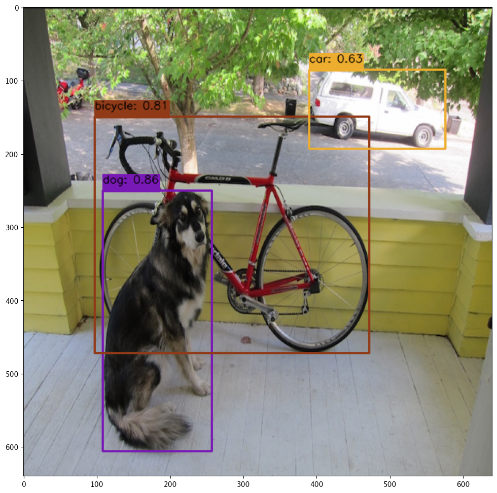
array([[[ 34, 34, 34],
[ 35, 35, 35],
[ 33, 33, 33],
...,
[ 33, 33, 33],
[ 33, 33, 33],
[ 35, 35, 35]],
[[ 33, 33, 33],
[ 34, 34, 34],
[ 34, 34, 34],
...,
[ 34, 34, 34],
[ 33, 33, 33],
[ 34, 34, 34]],
[[ 53, 54, 48],
[ 54, 55, 49],
[ 54, 55, 49],
...,
[153, 178, 111],
[151, 183, 108],
[159, 176, 99]],
...,
[[159, 167, 178],
[159, 165, 177],
[158, 163, 175],
...,
[126, 127, 121],
[127, 125, 120],
[128, 120, 117]],
[[160, 168, 179],
[156, 162, 174],
[152, 157, 169],
...,
[126, 127, 121],
[129, 127, 122],
[127, 118, 116]],
[[155, 163, 174],
[155, 162, 174],
[152, 158, 170],
...,
[127, 127, 121],
[130, 126, 122],
[128, 119, 116]]], dtype=uint8)
Redeploy as ARM
We will now undeploy the pipeline, then redeploy it with our Yolo model with the target deployment of ARM, and deploy the pipeline specifying it use the ARM architecture.
pipeline.undeploy()
# build the pipeline and clear any steps, then deploy as arm
pipeline = wl.build_pipeline(pipeline_name) \
.clear() \
.add_model_step(yolov8_model_arm)
deployment_config_arm = wallaroo.DeploymentConfigBuilder() \
.replica_count(1) \
.cpus(1) \
.memory("1Gi") \
.arch(Architecture.ARM) \
.build()
pipeline.deploy(deployment_config=deployment_config_arm)
| name | yolo8demonstration |
|---|---|
| created | 2023-10-19 19:53:57.966934+00:00 |
| last_updated | 2023-10-19 19:57:42.548101+00:00 |
| deployed | True |
| tags | |
| versions | 9ad91327-f671-4883-a00d-234f135b63b5, c13f317e-375a-4561-aa7e-e82226c4f794, e4b1f01c-7460-4166-a137-323cecaf6cf8, ce85f4e1-04e1-4465-95f5-5e4d17dba021, e57864c1-9b28-4dc1-897c-475f3dcde8e6, a128227d-b376-4f03-a348-05db69e73b64, 61e0b0fb-7028-4587-b9e1-23432e5df9e0, 5c7d42f7-b287-45f5-b455-a1138207264f |
| steps | yolov8n |
| published | False |
Image inference on ARM
We will perform the same inference with the same image and data input, only this time through the ARM architecture.
inf_arm = pipeline.infer_from_file('./data/dogbike.df.json')
cvDemo.drawYolo8Boxes(inf_arm, resizedImage1, width, height, confidence_thres, iou_thres, draw=True)
Score: 86.47% | Class: Dog | Bounding Box: [108, 250, 149, 356]
Score: 81.13% | Class: Bicycle | Bounding Box: [97, 149, 375, 323]
Score: 63.17% | Class: Car | Bounding Box: [390, 85, 186, 108]
array([[[ 34, 34, 34],
[ 35, 35, 35],
[ 33, 33, 33],
...,
[ 33, 33, 33],
[ 33, 33, 33],
[ 35, 35, 35]],
[[ 33, 33, 33],
[ 34, 34, 34],
[ 34, 34, 34],
...,
[ 34, 34, 34],
[ 33, 33, 33],
[ 34, 34, 34]],
[[ 53, 54, 48],
[ 54, 55, 49],
[ 54, 55, 49],
...,
[153, 178, 111],
[151, 183, 108],
[159, 176, 99]],
...,
[[159, 167, 178],
[159, 165, 177],
[158, 163, 175],
...,
[126, 127, 121],
[127, 125, 120],
[128, 120, 117]],
[[160, 168, 179],
[156, 162, 174],
[152, 157, 169],
...,
[126, 127, 121],
[129, 127, 122],
[127, 118, 116]],
[[155, 163, 174],
[155, 162, 174],
[152, 158, 170],
...,
[127, 127, 121],
[130, 126, 122],
[128, 119, 116]]], dtype=uint8)
Undeploy Pipeline
With the tutorial complete, we undeploy the pipeline and return the resources back to the cluster.
pipeline.undeploy()
| name | yolo8demonstration |
|---|---|
| created | 2023-10-19 19:53:57.966934+00:00 |
| last_updated | 2023-10-19 19:57:42.548101+00:00 |
| deployed | False |
| tags | |
| versions | 9ad91327-f671-4883-a00d-234f135b63b5, c13f317e-375a-4561-aa7e-e82226c4f794, e4b1f01c-7460-4166-a137-323cecaf6cf8, ce85f4e1-04e1-4465-95f5-5e4d17dba021, e57864c1-9b28-4dc1-897c-475f3dcde8e6, a128227d-b376-4f03-a348-05db69e73b64, 61e0b0fb-7028-4587-b9e1-23432e5df9e0, 5c7d42f7-b287-45f5-b455-a1138207264f |
| steps | yolov8n |
| published | False |
10.6 - ARM LLM Summarization Demonstration
A demonstration of a large language summarization model deployed under ARM pipeline deployment configurations.
This tutorial is available on the Wallaroo Tutorials repository.
This tutorial demonstrates how to use the Wallaroo combined with ARM processors to perform inferences with pre-trained computer vision ML models. This demonstration assumes that:
- A Wallaroo version 2023.3 or above instance is installed.
- A nodepools with ARM architecture virtual machines are part of the Kubernetes cluster. For example, Azure supports Ampere® Altra® Arm-based processor included with the following virtual machines:
- The model
hf-summarization-bart-large-samsun.zip(1.4 G) has been downloaded to the./modelsfolder.
Tutorial Goals
For our example, we will perform the following:
- Create a workspace for our work.
- Upload the the resnet computer vision model model.
- Create a pipeline using the default architecture that can ingest our submitted data, submit it to the model, and export the results while tracking how long the inference took.
- Redeploy the same pipeline on the ARM architecture, then perform the same inference on the same data and model and track how long the inference took.
- Compare the inference timing through the default architecture versus the ARM architecture.
Steps
Import Libraries
The first step will be to import our libraries.
import json
import os
import wallaroo
from wallaroo.pipeline import Pipeline
from wallaroo.deployment_config import DeploymentConfigBuilder
from wallaroo.framework import Framework
import pyarrow as pa
import numpy as np
import pandas as pd
Connect to the Wallaroo Instance
The first step is to connect to Wallaroo through the Wallaroo client. The Python library is included in the Wallaroo install and available through the Jupyter Hub interface provided with your Wallaroo environment.
This is accomplished using the wallaroo.Client() command, which provides a URL to grant the SDK permission to your specific Wallaroo environment. When displayed, enter the URL into a browser and confirm permissions. Store the connection into a variable that can be referenced later.
If logging into the Wallaroo instance through the internal JupyterHub service, use wl = wallaroo.Client(). For more information on Wallaroo Client settings, see the Client Connection guide.
wl = wallaroo.Client()
Configure PyArrow Schema
You can find more info on the available inputs under TextSummarizationInputs or under the official source code from 🤗 Hugging Face.
input_schema = pa.schema([
pa.field('inputs', pa.string()),
pa.field('return_text', pa.bool_()),
pa.field('return_tensors', pa.bool_()),
pa.field('clean_up_tokenization_spaces', pa.bool_()),
# pa.field('generate_kwargs', pa.map_(pa.string(), pa.null())), # dictionaries are not currently supported by the engine
])
output_schema = pa.schema([
pa.field('summary_text', pa.string()),
])
Upload Model
We will now create or connect to our pipeline and upload the model. We will set the architecture of the model to ARM for its deployment.
from wallaroo.engine_config import Architecture
model = wl.upload_model('hf-summarization-yns',
'hf-summarisation-bart-large-samsun.zip',
framework=Framework.HUGGING_FACE_SUMMARIZATION,
input_schema=input_schema,
output_schema=output_schema,
arch=Architecture.ARM)
model
Waiting for model loading - this will take up to 10.0min.
Model is pending loading to a container runtime..
Model is attempting loading to a container runtime.......................successful
Ready
| Name | hf-summarization-yns |
| Version | 2f708f1b-0ace-448b-b4ab-a337c962e6d9 |
| File Name | hf-summarisation-bart-large-samsun.zip |
| SHA | ee71d066a83708e7ca4a3c07caf33fdc528bb000039b6ca2ef77fa2428dc6268 |
| Status | ready |
| Image Path | proxy.replicated.com/proxy/wallaroo/ghcr.io/wallaroolabs/mlflow-deploy:v2023.3.0-3798 |
| Updated At | 2023-08-Sep 13:17:33 |
Deploy Pipeline
With the model uploaded, we can add it is as a step in the pipeline, then deploy it. The model has already been set as arm so the pipeline will use that architecture.
deployment_config = DeploymentConfigBuilder() \
.cpus(0.25).memory('1Gi') \
.sidekick_cpus(model, 4) \
.sidekick_memory(model, "8Gi") \
.build()
pipeline_name = "hf-summarization-pipeline-arm"
pipeline = wl.build_pipeline(pipeline_name)
pipeline.add_model_step(model)
pipeline.deploy(deployment_config=deployment_config)
pipeline.status()
Waiting for deployment - this will take up to 90s .................................. ok
{‘status’: ‘Running’,
‘details’: [],
’engines’: [{‘ip’: ‘10.244.2.53’,
’name’: ’engine-8494968846-jdj28’,
‘status’: ‘Running’,
‘reason’: None,
‘details’: [],
‘pipeline_statuses’: {‘pipelines’: [{‘id’: ‘hf-summarization-pipeline-arm’,
‘status’: ‘Running’}]},
‘model_statuses’: {‘models’: [{’name’: ‘hf-summarization-yns’,
‘version’: ‘2f708f1b-0ace-448b-b4ab-a337c962e6d9’,
‘sha’: ’ee71d066a83708e7ca4a3c07caf33fdc528bb000039b6ca2ef77fa2428dc6268’,
‘status’: ‘Running’}]}}],
’engine_lbs’: [{‘ip’: ‘10.244.3.34’,
’name’: ’engine-lb-584f54c899-2zkz6’,
‘status’: ‘Running’,
‘reason’: None,
‘details’: []}],
‘sidekicks’: [{‘ip’: ‘10.244.2.52’,
’name’: ’engine-sidekick-hf-summarization-yns-6-6555bb7d74-27ncn’,
‘status’: ‘Running’,
‘reason’: None,
‘details’: [],
‘statuses’: ‘\n’}]}
pipeline.status()
{'status': 'Running',
'details': [],
'engines': [{'ip': '10.244.2.53',
'name': 'engine-8494968846-jdj28',
'status': 'Running',
'reason': None,
'details': [],
'pipeline_statuses': {'pipelines': [{'id': 'hf-summarization-pipeline-arm',
'status': 'Running'}]},
'model_statuses': {'models': [{'name': 'hf-summarization-yns',
'version': '2f708f1b-0ace-448b-b4ab-a337c962e6d9',
'sha': 'ee71d066a83708e7ca4a3c07caf33fdc528bb000039b6ca2ef77fa2428dc6268',
'status': 'Running'}]}}],
'engine_lbs': [{'ip': '10.244.3.34',
'name': 'engine-lb-584f54c899-2zkz6',
'status': 'Running',
'reason': None,
'details': []}],
'sidekicks': [{'ip': '10.244.2.52',
'name': 'engine-sidekick-hf-summarization-yns-6-6555bb7d74-27ncn',
'status': 'Running',
'reason': None,
'details': [],
'statuses': '\n'}]}
Run inference
We can now run a sample inference using the wallaroo.pipeline.infer method and display the results.
input_data = {
"inputs": ["LinkedIn (/lɪŋktˈɪn/) is a business and employment-focused social media platform that works through websites and mobile apps. It launched on May 5, 2003. It is now owned by Microsoft. The platform is primarily used for professional networking and career development, and allows jobseekers to post their CVs and employers to post jobs. From 2015 most of the company's revenue came from selling access to information about its members to recruiters and sales professionals. Since December 2016, it has been a wholly owned subsidiary of Microsoft. As of March 2023, LinkedIn has more than 900 million registered members from over 200 countries and territories. LinkedIn allows members (both workers and employers) to create profiles and connect with each other in an online social network which may represent real-world professional relationships. Members can invite anyone (whether an existing member or not) to become a connection. LinkedIn can also be used to organize offline events, join groups, write articles, publish job postings, post photos and videos, and more"], # required
"return_text": [True], # optional: using the defaults, similar to not passing this parameter
"return_tensors": [False], # optional: using the defaults, similar to not passing this parameter
"clean_up_tokenization_spaces": [False], # optional: using the defaults, similar to not passing this parameter
}
dataframe = pd.DataFrame(input_data)
dataframe
| inputs | return_text | return_tensors | clean_up_tokenization_spaces | |
|---|---|---|---|---|
| 0 | LinkedIn (/lɪŋktˈɪn/) is a business and employ... | True | False | False |
# Adjust timeout as needed, started liberally with a 10 min timeout
out = pipeline.infer(dataframe, timeout=600)
out
| time | in.clean_up_tokenization_spaces | in.inputs | in.return_tensors | in.return_text | out.summary_text | check_failures | |
|---|---|---|---|---|---|---|---|
| 0 | 2023-09-08 13:18:58.557 | False | LinkedIn (/lɪŋktˈɪn/) is a business and employ... | False | True | LinkedIn is a business and employment-focused ... | 0 |
out["out.summary_text"][0]
'LinkedIn is a business and employment-focused social media platform that works through websites and mobile apps. It launched on May 5, 2003. LinkedIn allows members (both workers and employers) to create profiles and connect with each other in an online social network which may represent real-world professional relationships.'
Model Inferencing with Pipeline Deployment Endpoint
The other option is to use the pipeline’s inference endpoint.
pipeline.url()
'http://engine-lb.hf-summarization-pipeline-arm-3:29502/pipelines/hf-summarization-pipeline-arm'
!curl -X POST http://engine-lb.hf-summarization-pipeline-arm-3:29502/pipelines/hf-summarization-pipeline-arm \
-H "Content-Type: application/json; format=pandas-records" \
-d @./data/test_summarization.json
[{"time":1694179270999,"in":{"clean_up_tokenization_spaces":[false],"inputs":["LinkedIn (/lɪŋktˈɪn/) is a business and employment-focused social media platform that works through websites and mobile apps. It launched on May 5, 2003. It is now owned by Microsoft. The platform is primarily used for professional networking and career development, and allows jobseekers to post their CVs and employers to post jobs. From 2015 most of the company's revenue came from selling access to information about its members to recruiters and sales professionals. Since December 2016, it has been a wholly owned subsidiary of Microsoft. As of March 2023, LinkedIn has more than 900 million registered members from over 200 countries and territories. LinkedIn allows members (both workers and employers) to create profiles and connect with each other in an online social network which may represent real-world professional relationships. Members can invite anyone (whether an existing member or not) to become a connection. LinkedIn can also be used to organize offline events, join groups, write articles, publish job postings, post photos and videos, and more"],"return_tensors":[false],"return_text":[true]},"out":{"summary_text":"LinkedIn is a business and employment-focused social media platform that works through websites and mobile apps. It launched on May 5, 2003. LinkedIn allows members (both workers and employers) to create profiles and connect with each other in an online social network which may represent real-world professional relationships."},"check_failures":[],"metadata":{"last_model":"{\"model_name\":\"hf-summarization-yns\",\"model_sha\":\"ee71d066a83708e7ca4a3c07caf33fdc528bb000039b6ca2ef77fa2428dc6268\"}","pipeline_version":"4aeb608f-166b-4b59-bb10-c06f9e49df23","elapsed":[41800,4294967295],"dropped":[]}}]
Undeploy the Pipeline
With the demonstration complete, we can undeploy the pipeline and return the resources back to the Wallaroo instance.
pipeline.undeploy()
11 - Wallaroo Tools Tutorials
Tutorials on additional Wallaroo tools.
The following tutorials are provided by Wallaroo to demonstrate different tools and techniques for working with MLModels and data with Wallaroo.
11.1 - Wallaroo JSON Inference Data to DataFrame and Arrow Tutorials
How to convert from inference inputs using Wallaroo proprietary JSON to Pandas DataFrame and Apache Arrow
The following guide on using inference data inputs from Wallaroo proprietary JSON to either Pandas DataFrame or Apache Arrow downloaded as part of the Wallaroo Tutorials repository.
Introduction
The following guide is to help users transition from using Wallaroo Proprietary JSON to Pandas DataFrame and Apache Arrow. The latter two formats allow data scientists to work natively with DataFrames, and when ready convert those into Arrow table files which provides greater file size efficiency and overall speed.
Using Pandas DataFrames for inference inputs requires typecasting into the Wallaroo inference engine. For models that are sensitive to data types, Arrow is the preferred format.
This guide will demonstrate the following:
- Convert Wallaroo Proprietary JSON to Pandas DataFrame: Converting from Wallaroo Proprietary JSON to Pandas DataFrame used for inferences in the Wallaroo Engine.
- Convert Wallaroo JSON File to Pandas DataFrame: Converting from Wallaroo JSON files or DataFrame JSON files to Pandas DataFrame for Wallaroo Engine inferences.
- Convert Pandas DataFrame to Arrow Table: Converting from Pandas DataFrame to Apache Arrow used for inferences in the Wallaroo Engine.
- Read Arrow File to DataFrame: How to convert from an Arrow binary file to an Apache Arrow object or DataFrame object.
- Convert Flattened Arrow Table to Multi-Dimensional Pandas DataFrame: How to convert from a one dimensional arrow table to a Multi-Dimensional Pandas DataFrame.
Prerequisites
The demonstration code assumes a Wallaroo instance with Arrow support enabled and provides the following:
ccfraud.onnx: Sample trained ML Model trained to detect credit card fraud transactions.data/high_fraud.json: Sample inference input formatted in the Wallaroo proprietary JSON format.
The following demonstrates how to convert Wallaroo Proprietary JSON to Pandas DataFrame. This example data and models are taken from the Wallaroo 101, which uses the CCFraud model examples.
Initialization
Connect to the Wallaroo Instance
Connect to the Wallaroo Instance
The first step is to connect to Wallaroo through the Wallaroo client. The Python library is included in the Wallaroo install and available through the Jupyter Hub interface provided with your Wallaroo environment.
This is accomplished using the wallaroo.Client() command, which provides a URL to grant the SDK permission to your specific Wallaroo environment. When displayed, enter the URL into a browser and confirm permissions. Store the connection into a variable that can be referenced later.
If logging into the Wallaroo instance through the internal JupyterHub service, use wl = wallaroo.Client(). For more information on Wallaroo Client settings, see the Client Connection guide.
import wallaroo
from wallaroo.object import EntityNotFoundError
from IPython.display import display
# used to display dataframe information without truncating
from IPython.display import display
import pandas as pd
pd.set_option('display.max_colwidth', None)
# Login through local Wallaroo instance
wl = wallaroo.Client()
workspace_name = 'inferencedataexamplesworkspace'
pipeline_name = 'inferencedataexamplespipeline'
model_name = 'ccfraud'
model_file_name = './ccfraud.onnx'
def get_workspace(name):
workspace = None
for ws in wl.list_workspaces():
if ws.name() == name:
workspace= ws
if(workspace == None):
workspace = wl.create_workspace(name)
return workspace
def get_pipeline(name):
try:
pipeline = wl.pipelines_by_name(name)[0]
except EntityNotFoundError:
pipeline = wl.build_pipeline(name)
return pipeline
# Create the workspace
workspace = get_workspace(workspace_name)
wl.set_current_workspace(workspace)
# upload the model
model = wl.upload_model(model_name, model_file_name, framework=wallaroo.framework.Framework.ONNX).configure()
# Create the pipeline then deploy it
pipeline = get_pipeline(pipeline_name)
pipeline.add_model_step(model).deploy()
| name | inferencedataexamplespipeline |
|---|---|
| created | 2023-05-18 14:06:03.460084+00:00 |
| last_updated | 2023-05-18 14:06:04.140319+00:00 |
| deployed | True |
| tags | |
| versions | ad9c68c5-c692-486f-8796-a8e8561ea320, 65b69beb-a214-44ea-99fb-d60bca8d5804 |
| steps | ccfraud |
Convert Wallaroo Proprietary JSON to Pandas DataFrame
The following demonstrates how to convert Wallaroo Proprietary JSON to Pandas DataFrame.
Load Libraries
The following libraries are used as part of the conversion process.
import pandas as pd
import pyarrow as pa
import json
import datetime
import numpy as np
Load Wallaroo Data
The Wallaroo data will be saved to a variable. This sample input when run through the trained model as an inference returns a high probability of fraud.
# Start with the single example
high_fraud_data = {
"tensor": [
[1.0678324729342086,
18.155556397512136,
-1.658955105843852,
5.2111788045436445,
2.345247064454334,
10.467083577773014,
5.0925820522419745,
12.829515363712181,
4.953677046849403,
2.3934736228338225,
23.912131817957253,
1.7599568310350207,
0.8561037518143335,
1.1656456468728567,
0.5395988813934498,
0.7784221343010385,
6.75806107274245,
3.927411847659908,
12.462178276650056,
12.307538216518655,
13.787951906620115,
1.4588397511627804,
3.681834686805714,
1.7539143660379741,
8.484355003656184,
14.6454097666836,
26.852377436250144,
2.716529237720336,
3.061195706890285]
]
}
Convert to DataFrame
The Wallaroo proprietary JSON file will now be converted into Pandas DataFrame.
high_fraud_dataframe = pd.DataFrame.from_records(high_fraud_data)
display(high_fraud_dataframe)
| tensor | |
|---|---|
| 0 | [1.0678324729342086, 18.155556397512136, -1.658955105843852, 5.2111788045436445, 2.345247064454334, 10.467083577773014, 5.0925820522419745, 12.829515363712181, 4.953677046849403, 2.3934736228338225, 23.912131817957253, 1.7599568310350207, 0.8561037518143335, 1.1656456468728567, 0.5395988813934498, 0.7784221343010385, 6.75806107274245, 3.927411847659908, 12.462178276650056, 12.307538216518655, 13.787951906620115, 1.4588397511627804, 3.681834686805714, 1.7539143660379741, 8.484355003656184, 14.6454097666836, 26.852377436250144, 2.716529237720336, 3.061195706890285] |
DataFrame for Inferences
Once converted, the DataFrame version of the data can be used for inferences in an Arrow enabled Wallaroo instance.
# Use this dataframe to infer
result = pipeline.infer(high_fraud_dataframe)
display(result)
| time | in.tensor | out.dense_1 | check_failures | |
|---|---|---|---|---|
| 0 | 2023-05-18 14:06:20.449 | [1.0678324729, 18.1555563975, -1.6589551058, 5.2111788045, 2.3452470645, 10.4670835778, 5.0925820522, 12.8295153637, 4.9536770468, 2.3934736228, 23.912131818, 1.759956831, 0.8561037518, 1.1656456469, 0.5395988814, 0.7784221343, 6.7580610727, 3.9274118477, 12.4621782767, 12.3075382165, 13.7879519066, 1.4588397512, 3.6818346868, 1.753914366, 8.4843550037, 14.6454097667, 26.8523774363, 2.7165292377, 3.0611957069] | [0.981199] | 0 |
Pandas JSON to Pandas DataFrame
For JSON data that is in the Pandas DataFrame format, the data can be turned into a Pandas DataFrame object through the same method. Note that the original variable is JSON, which could have come from a file, to a DataFrame object.
high_fraud_dataframe_json = [
{
"tensor":[
1.0678324729,
18.1555563975,
-1.6589551058,
5.2111788045,
2.3452470645,
10.4670835778,
5.0925820522,
12.8295153637,
4.9536770468,
2.3934736228,
23.912131818,
1.759956831,
0.8561037518,
1.1656456469,
0.5395988814,
0.7784221343,
6.7580610727,
3.9274118477,
12.4621782767,
12.3075382165,
13.7879519066,
1.4588397512,
3.6818346868,
1.753914366,
8.4843550037,
14.6454097667,
26.8523774363,
2.7165292377,
3.0611957069
]
}
]
# Infer from the JSON
high_fraud_from_dataframe_json = pd.DataFrame.from_records(high_fraud_dataframe_json)
display(high_fraud_from_dataframe_json)
| tensor | |
|---|---|
| 0 | [1.0678324729, 18.1555563975, -1.6589551058, 5.2111788045, 2.3452470645, 10.4670835778, 5.0925820522, 12.8295153637, 4.9536770468, 2.3934736228, 23.912131818, 1.759956831, 0.8561037518, 1.1656456469, 0.5395988814, 0.7784221343, 6.7580610727, 3.9274118477, 12.4621782767, 12.3075382165, 13.7879519066, 1.4588397512, 3.6818346868, 1.753914366, 8.4843550037, 14.6454097667, 26.8523774363, 2.7165292377, 3.0611957069] |
# Use this dataframe to infer
results = pipeline.infer(high_fraud_from_dataframe_json)
display(results)
| time | in.tensor | out.dense_1 | check_failures | |
|---|---|---|---|---|
| 0 | 2023-05-18 14:06:20.877 | [1.0678324729, 18.1555563975, -1.6589551058, 5.2111788045, 2.3452470645, 10.4670835778, 5.0925820522, 12.8295153637, 4.9536770468, 2.3934736228, 23.912131818, 1.759956831, 0.8561037518, 1.1656456469, 0.5395988814, 0.7784221343, 6.7580610727, 3.9274118477, 12.4621782767, 12.3075382165, 13.7879519066, 1.4588397512, 3.6818346868, 1.753914366, 8.4843550037, 14.6454097667, 26.8523774363, 2.7165292377, 3.0611957069] | [0.981199] | 0 |
Convert Wallaroo JSON File to Pandas DataFrame
When working with files containing Wallaroo JSON data, these can be imported from their original JSON, then converted to a Pandas DataFrame object with the pandas method read_json.
high_fraud_filename = "./data/high_fraud.json"
high_fraud_data_from_file = pd.read_json(high_fraud_filename, orient="records")
display(high_fraud_data_from_file)
| tensor | |
|---|---|
| 0 | [1.067832472934208, 18.155556397512136, -1.658955105843852, 5.2111788045436445, 2.345247064454334, 10.467083577773014, 5.092582052241974, 12.829515363712181, 4.953677046849403, 2.393473622833822, 23.912131817957253, 1.7599568310350202, 0.8561037518143331, 1.165645646872856, 0.539598881393449, 0.778422134301038, 6.75806107274245, 3.927411847659908, 12.462178276650056, 12.307538216518655, 13.787951906620115, 1.45883975116278, 3.681834686805714, 1.7539143660379741, 8.484355003656184, 14.6454097666836, 26.852377436250144, 2.7165292377203363, 3.061195706890285] |
The data can be used in an inference either with the infer method on the DataFrame object, or directly from the file. Note that in either case, the returned object is a DataFrame.
# Use this dataframe to infer
result = pipeline.infer(high_fraud_data_from_file)
display(result)
| time | in.tensor | out.dense_1 | check_failures | |
|---|---|---|---|---|
| 0 | 2023-05-18 14:06:21.259 | [1.0678324729, 18.1555563975, -1.6589551058, 5.2111788045, 2.3452470645, 10.4670835778, 5.0925820522, 12.8295153637, 4.9536770468, 2.3934736228, 23.912131818, 1.759956831, 0.8561037518, 1.1656456469, 0.5395988814, 0.7784221343, 6.7580610727, 3.9274118477, 12.4621782767, 12.3075382165, 13.7879519066, 1.4588397512, 3.6818346868, 1.753914366, 8.4843550037, 14.6454097667, 26.8523774363, 2.7165292377, 3.0611957069] | [0.981199] | 0 |
# Infer from file - it is read as a Pandas DataFrame object from the DataFrame JSON
result = pipeline.infer_from_file(high_fraud_filename)
display(result)
| time | in.tensor | out.dense_1 | check_failures | |
|---|---|---|---|---|
| 0 | 2023-05-18 14:06:21.652 | [1.0678324729, 18.1555563975, -1.6589551058, 5.2111788045, 2.3452470645, 10.4670835778, 5.0925820522, 12.8295153637, 4.9536770468, 2.3934736228, 23.912131818, 1.759956831, 0.8561037518, 1.1656456469, 0.5395988814, 0.7784221343, 6.7580610727, 3.9274118477, 12.4621782767, 12.3075382165, 13.7879519066, 1.4588397512, 3.6818346868, 1.753914366, 8.4843550037, 14.6454097667, 26.8523774363, 2.7165292377, 3.0611957069] | [0.981199] | 0 |
Convert Pandas DataFrame to Arrow Table
The helper file convert_wallaroo_data.py is used to convert from Pandas DataFrame to an Arrow Table with the following caveats:
Arrow requires the user to specify the exact datatypes of the array elements before passing the data to the engine. If you are aware of what data type the model expects, create a dictionary with column names as key and data type as the value and pass it as a param in place of data_type_dict. If not, the convert_to_pa_dtype function will try and guess the equivalent pyarrow data type and use it (this may or may not work as intended).
import convert_wallaroo_data
data_type_dict = {"tensor": pa.float32()}
pa_table = convert_wallaroo_data.convert_pandas_to_arrow(high_fraud_dataframe, data_type_dict)
pa_table
pyarrow.Table
tensor: fixed_size_list<item: float>[29]
child 0, item: float
----
tensor: [[[1.0678325,18.155556,-1.6589551,5.211179,2.345247,...,8.484355,14.64541,26.852377,2.7165291,3.0611956]]]
An inference can be done using the arrow table. The following shows the code sample and result. Note that when submitting an Arrow table to infer, that the returned object is an Arrow table.
# use the arrow table for infer:
result = pipeline.infer(pa_table)
display(result)
pyarrow.Table
time: timestamp[ms]
in.tensor: list<item: float> not null
child 0, item: float
out.dense_1: list<inner: float not null> not null
child 0, inner: float not null
check_failures: int8
----
time: [[2023-05-18 14:06:22.107]]
in.tensor: [[[1.0678325,18.155556,-1.6589551,5.211179,2.345247,...,8.484355,14.64541,26.852377,2.7165291,3.0611956]]]
out.dense_1: [[[0.981199]]]
check_failures: [[0]]
Save Arrow Table to Arrow File
The converted Arrow table can be saved using the pyarrow library.
arrow_file_name = "./data/high_fraud.arrow"
with pa.OSFile(arrow_file_name, 'wb') as sink:
with pa.ipc.new_file(sink, pa_table.schema) as arrow_ipc:
arrow_ipc.write(pa_table)
arrow_ipc.close()
infer_from_file can be performed using the new arrow file. Note again that when submitting an inference with an Arrow object, the returning value is an Arrow object.
result = pipeline.infer_from_file(arrow_file_name)
display(result)
pyarrow.Table
time: timestamp[ms]
in.tensor: list<item: float> not null
child 0, item: float
out.dense_1: list<inner: float not null> not null
child 0, inner: float not null
check_failures: int8
----
time: [[2023-05-18 14:06:22.522]]
in.tensor: [[[1.0678325,18.155556,-1.6589551,5.211179,2.345247,...,8.484355,14.64541,26.852377,2.7165291,3.0611956]]]
out.dense_1: [[[0.981199]]]
check_failures: [[0]]
Read Arrow File to DataFrame
The data can go the opposite direction - reading from an Arrow binary file, and turning the data into either an Arrow table with the Arrow read_all method, or just the data into a DataFrame with the Arrow read_pandas method.
with pa.ipc.open_file(arrow_file_name) as source:
table = source.read_all() # to get pyarrow table
table_df = source.read_pandas() # to get pandas dataframe
display(table)
display(table_df)
pyarrow.Table
tensor: fixed_size_list<item: float>[29]
child 0, item: float
----
tensor: [[[1.0678325,18.155556,-1.6589551,5.211179,2.345247,...,8.484355,14.64541,26.852377,2.7165291,3.0611956]]]
| tensor | |
|---|---|
| 0 | [1.0678325, 18.155556, -1.6589551, 5.211179, 2.345247, 10.467084, 5.092582, 12.829515, 4.953677, 2.3934736, 23.912132, 1.7599568, 0.8561038, 1.1656456, 0.5395989, 0.7784221, 6.758061, 3.9274118, 12.462178, 12.307538, 13.787951, 1.4588398, 3.6818347, 1.7539144, 8.484355, 14.64541, 26.852377, 2.7165291, 3.0611956] |
Convert Arrow Infer to DataFrame
When an infer result is returned as an Arrow object, it can be converted to a DataFrame for easy viewing.
result = pipeline.infer_from_file(arrow_file_name)
display(result.to_pandas())
| time | in.tensor | out.dense_1 | check_failures | |
|---|---|---|---|---|
| 0 | 2023-05-18 14:06:22.910 | [1.0678325, 18.155556, -1.6589551, 5.211179, 2.345247, 10.467084, 5.092582, 12.829515, 4.953677, 2.3934736, 23.912132, 1.7599568, 0.8561038, 1.1656456, 0.5395989, 0.7784221, 6.758061, 3.9274118, 12.462178, 12.307538, 13.787951, 1.4588398, 3.6818347, 1.7539144, 8.484355, 14.64541, 26.852377, 2.7165291, 3.0611956] | [0.981199] | 0 |
Convert Flattened Arrow Table to Multi-Dimensional Pandas DataFrame
Some ML models use multi-dimensional DataFrames. Currently Wallaroo supports and outputs flattened tables for inferences.
For situations where the original data was in a multi-dimensional DataFrame, the following procedure will convert the flattened Arrow table back into a desired multi-dimensional pandas DataFrame.
Here is a sample infer result data in Arrow Table format.
time_array = pa.array([datetime.datetime(2023, 2 , 22, 22, 14)])
in_tensor_array = pa.array([[1.5997242884551583,-0.72885535293112,-0.8464381472712799,-0.48041787186839674,0.8211244519635765,0.999086254697715,-1.365979802921807,0.36611200379560294,1.27093766309002,0.4895466723195178]])
out_array = pa.array([[1.8749652,-0.94025564,-1.0790397,-0.72123086,0.90895796,1.092086,-1.2834015,0.340406,1.2441622,0.57471186]])
check_failures_array = pa.array([0])
names = ["time", "in.tensor", "out.reshape", "check_failures"]
flattened_2d_table = pa.Table.from_arrays([time_array, in_tensor_array, out_array, check_failures_array], names = names)
flattened_2d_table
pyarrow.Table
time: timestamp[us]
in.tensor: list<item: double>
child 0, item: double
out.reshape: list<item: double>
child 0, item: double
check_failures: int64
----
time: [[2023-02-22 22:14:00.000000]]
in.tensor: [[[1.5997242884551583,-0.72885535293112,-0.8464381472712799,-0.48041787186839674,0.8211244519635765,0.999086254697715,-1.365979802921807,0.36611200379560294,1.27093766309002,0.4895466723195178]]]
out.reshape: [[[1.8749652,-0.94025564,-1.0790397,-0.72123086,0.90895796,1.092086,-1.2834015,0.340406,1.2441622,0.57471186]]]
check_failures: [[0]]
flattened_2d_table["out.reshape"]
<pyarrow.lib.ChunkedArray object at 0x154467a40>
[
[
[
1.8749652,
-0.94025564,
-1.0790397,
-0.72123086,
0.90895796,
1.092086,
-1.2834015,
0.340406,
1.2441622,
0.57471186
]
]
]
Verify the Shape
Let’s suppose the shape of the output that natively comes out of the model is [2,5]. We can use that to make sure the shape is correct when translating from the 1 dimensional Arrow table.
tensor_type = {"shape": [2, 5]}
output_df = flattened_2d_table.to_pandas()['out.reshape']
# numpy array, shape [N, 2, 5]
# In this case N = 1
output_list = [elt.reshape(tensor_type['shape']) for elt in output_df]
output_tensor = np.stack(output_list)
output_tensor
array([[[ 1.8749652 , -0.94025564, -1.0790397 , -0.72123086,
0.90895796],
[ 1.092086 , -1.2834015 , 0.340406 , 1.2441622 ,
0.57471186]]])
output_2d_df = pd.DataFrame(output_tensor.tolist())
output_2d_df
| 0 | 1 | |
|---|---|---|
| 0 | [1.8749652, -0.94025564, -1.0790397, -0.72123086, 0.90895796] | [1.092086, -1.2834015, 0.340406, 1.2441622, 0.57471186] |
Undeploy Pipeline
The pipeline will now be undeployed to return the resources back to the Wallaroo instance.
pipeline.undeploy()
| name | inferencedataexamplespipeline |
|---|---|
| created | 2023-05-18 14:06:03.460084+00:00 |
| last_updated | 2023-05-18 14:06:04.140319+00:00 |
| deployed | False |
| tags | |
| versions | ad9c68c5-c692-486f-8796-a8e8561ea320, 65b69beb-a214-44ea-99fb-d60bca8d5804 |
| steps | ccfraud |